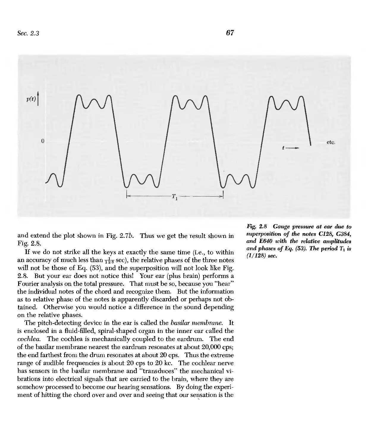
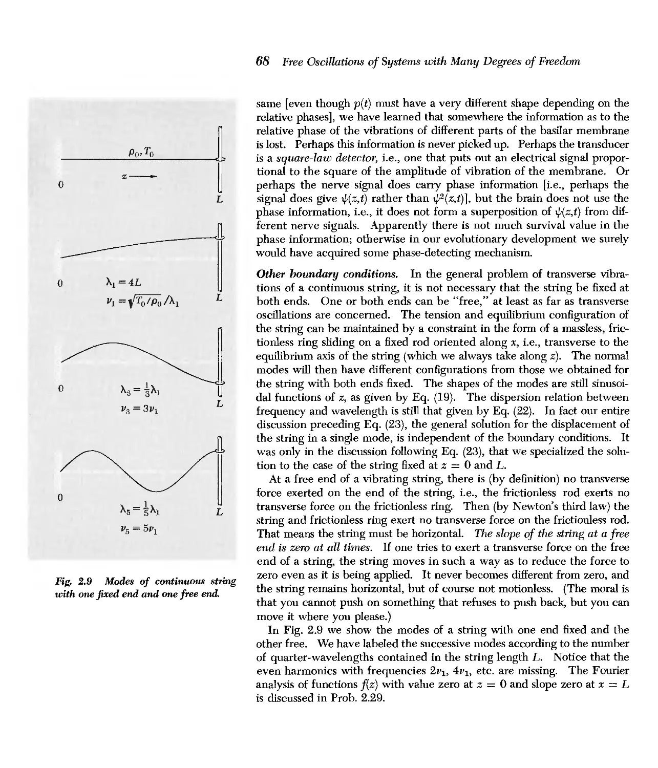
/


Автор: Frank S. Crawford Jr.
Теги: physics


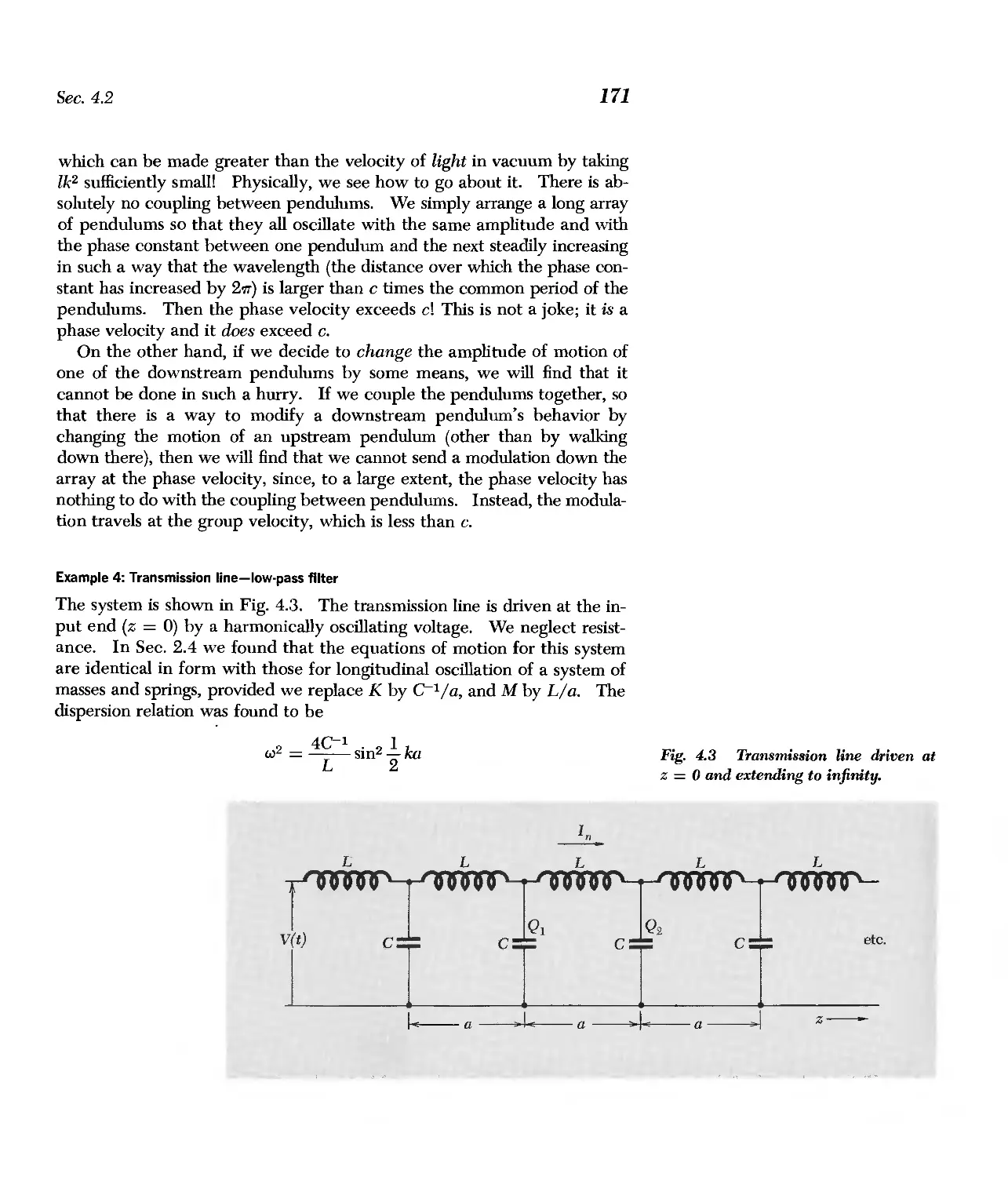
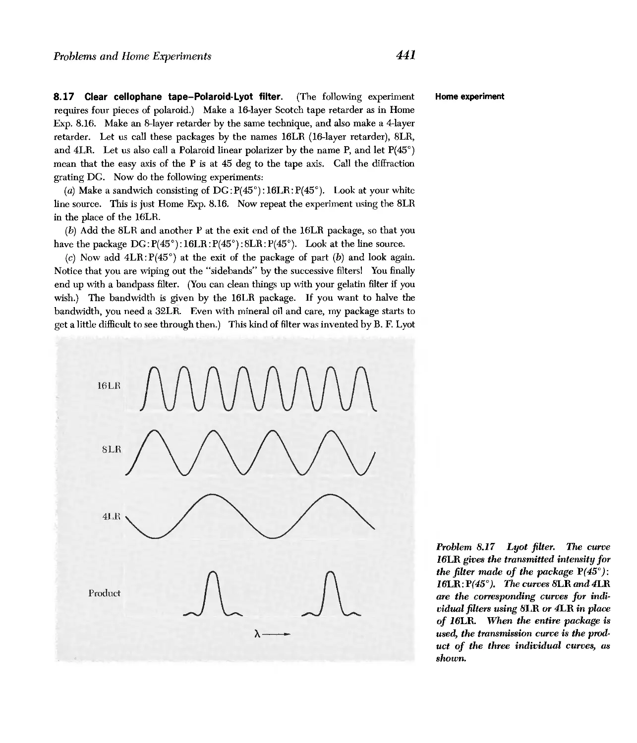
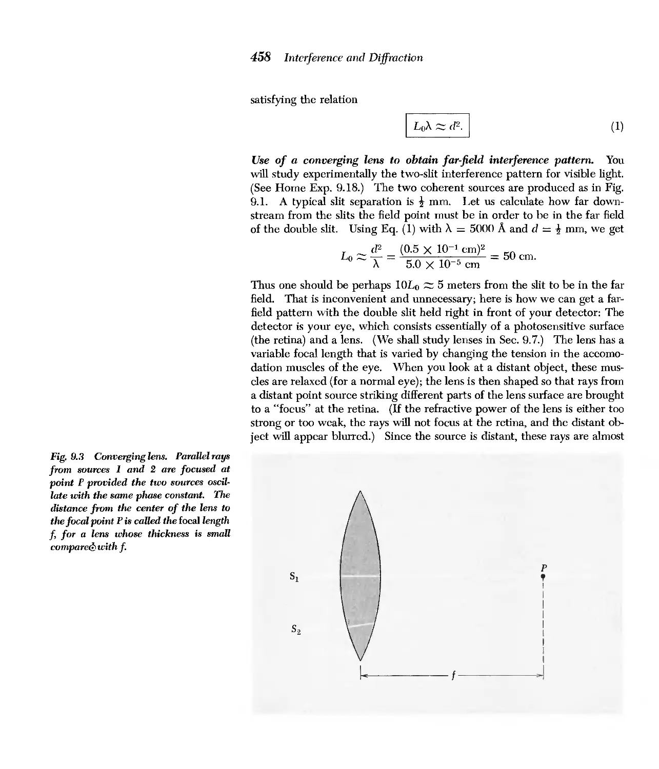
Текст
Speed of light in vacuum"
Fundamental charge
Planck's constant
"Reduced" Planck's constant
Electron rest mass
Proton rest mass
Gravitational constant
Acceleration of gravity at sea level
Bohr radius
Avogadro's number
Boltzmann's constant
Standard temperature
Standard pressure
Molar volume at S.T.P.
Thermal energy kT at S.T.P.
Density of air at S.T.P.
Speed of sound in air at S.T.P.
Sound impedance of air at S.T.P.
Standard sound intensity
Factor of ten in intensity
One fermi (F)
One angstrom unit (A)
One micron (/1)
One hertz (Hz)
Wavelength of one-electron-volt photon
One electron volt (ev)
One watt (W)
One coulomb (coul)
One volt (V)
One ohm (Q)
Thirty ohms
Impedance per square of vacuum for
electromagnetic waves
One farad (F)
One henry (H)
Useful Constants
c = 2.997925 X 10 10 cm/sec = 3 X 10 10 cm/sec
e = 4.8 X 10- 10 statcoulomb
= 1.6 X 10- 19 coulomb
h = 6.6 X 10- 27 erg-sec
Ii = h/2'lT = 1.0 X 10- 27 erg-sec
me = 0.9 X 10- 27 gm
mp = 1.7 X 10- 24 gm
G = 6.7 X 10- 8 CGS units
g::::: 980 cm/sec 2
ao = 0.5 X 10- 8 cm
No = 6.0 X 10 23 mole- 1
k = 1.4 X 10- 16 erg/ deg Kelvin
To = 273 deg Kelvin
po = 1 atm = 1.01 X 10 6 dyne/cm 2
V o = 22.4 X 10 3 cm 3 /mole
kTo = 3.8 X 10- 14 erg::::: -Iri ev
Po = 1.3 X 10- 3 gm/cm 3
Vo = 3.32 X 10 4 cm/sec
Zo = 42.8 (dyne/cm 2 )/(cm/sec)
10 = 1 /1watt/ cm 2
= 1 bel = 10 db
= 10- 13 cm
= 10- 8 cm
= 10- 4 cm
= 1 cycle per second (cps)
= 1.24 X 10- 4 cm ::::: 12345 A
= 1.6 X 10- 12 erg
= 1 joule/sec = 10 7 erg/sec
= 3 X 10 9 statcoul = c/lO statcoul"
= -rt-o- statvolt == 10 8 / c statvolt"
= 1/(9 X 1011) statohm = 10 9 /c 2 statohm"
= 1/ c statohm
= 4'lT / c statohm = 377 ohm
= 9 X 10¹¹ statfarad = c 2 /10 9 statfarad"
= 1/(9 X 1011) stathenry = 10 9 /c 2 stathenry"
. In converting from practica1 units to electrostatic units we have approximated the velocity of light as 3.00 X 10¹⁰ em/sec. Wherever a 3
appears, a more accurate conversion factor can be obtained by using the more accurate value of c. Similarly wherever 9 appears, it is more
accurately /2.998)2.
Recommended Unit Prefixes
Multiples and
Submultiples Prefixes Symbols
10 12 tera T
10 9 giga G
10 6 mega M
10 3 kilo k
10 2 hecto h
10 deka da
10- 1 deci d
10- 2 centi c
10- 3 milli m
10- 6 micro IL
10- 9 nano n
10- 12 pico p
Useful Identities
cos x + cos Y = [2 cos t(x - y)] cos t(x + y)
cos x - cos y = [-2 sin t(x - y)] sin t(x + y)
sin x + sin y = [2 cos t(x - y)] sin t(x + y)
sin x - sin Y = [2 sin t(x - y)] cos t(x + y)
cos (x + y) = cos x cos Y + sin x sin y
sin (x + y) = sin x cos y + sin y cos x
cos 2x = cos 2 X - sin 2 x
sin 2x = 2 sin x cos x
cos 2 X = t(1 + cos 2x)
sin 2 x = t(1 - cos 2x)
sinx=x-tx 3 + ...
cos x = 1 - tx2 + ...
(1 + x)n = 1 + nx + tn(n - 1)x 2 + .. .; x 2 < 1. . I N
sm2 Y
cos (it + cos (lit + y) + cos (0 1 + 2y) + . + cos [0 1 + (N - 1)y] = cos [0 1 + t(N - 1)y] . t
sm y
waves
mcgra\N-hill book company
s
berkeley physics course - volume 3
The preparation of this course teas supported hy a grant
from the National Science Foundation to Education De-
celopment Center
Frank S. Crawford, Jr.
Professor of Physics
University of California, Berkeley
COVER DESIGN
Photographic adaptation by Felix Cooper
from an original by John Severson
WAVES
Copyright @ 1965, 1966, 1968 by Education
Development Center, Inc. (successor by merger
to Educational Services Incorporated). All
Rights Reserved. Printed in the United States
of America. This book, or parts thereof, may
not be reproduced in any form without the
written permission of Education Development
Center, Inc., Newton, Massachusetts.
Library of Congress Catalog Card Number
64-66016
04860
34567890HDBP754321069
Preface to the Berkeley Physics Course
This is a two-year elementary college physics course for students majoring
in science and engineering. The intention of the writers has been to pre-
sent elementary physics as far as possible in the way in which it is used by
physicists working on the forefront of their field. We have sought to make
a course which would vigorously emphasize the foundations of physics.
Our specific objectives were to introduce coherently into an elementary
curriculum the ideas of special relativity, of quantum physics, and of sta-
tistical physics.
This course is intended for any student who has had a physics course in
high school. A mathematics course including the calculus should be taken
at the same time as this course.
There are several new college physics courses under development in the
United States at this time. The idea of making a new course has come to
many physicists, affected by the needs both of the advancement of science
and engineering and of the increasing emphasis on science in elementary
schools and in high schools. Our own course was conceived in a conversa-
tion between Philip Morrison of Cornell University and C. Kittel late in
1961. We were encouraged by John Mays and his colleagues of the
National Science Foundation and by Walter C. Michels, then the Chair-
man of the Commission on College Physics. An informal committee was
fonned to guide the course through the initial stages. The committee con-
sisted originally of Luis Alvarez, William B. Fretter, Charles Kittel, Walter
D. Knight, Philip Morrison, Edward M. Purcell, Malvin A. Rudennan, and
Jerrold R. Zacharias. The committee met first in May 1962, in Berkeley;
at that time it drew up a provisional outline of an entirely new physics
course. Because of heavy obligations of several of the original members,
the committee was partially reconstituted in January 1964, and now con-
sists of the undersigned. Contributions of others are acknowledged in the
prefaces to the individual volumes.
The provisional outline and its associated spirit were a powerful influence
on the course material finally produced. The outline covered in detail the
topics and attitudes which we believed should and could be taught to
beginning college students of science and engineering. It was never our
intention to develop a course limited to honors students or to students with
advanced standing. We have sought to present the principles of physics
from fresh and unified viewpoints, and parts of the course may therefore
seem almost as new to the instructor as to the students.
The five volumes of the course as planned will include:
1. Mechanics (Kittel, Knight, Rudennan) III. Waves (Crawford)
II. Electricity and Magnetism (Purcell) IV. Quantum Physics (Wichmann)
V. Statistical Physics (Reif)
The authors of each volume have been free to choose that style and method
of presentation which seemed to them appropriate to their subject.
A Further Note
June, 1968
Berkeley, California
vi Preface to the Berkeley Physics Course
The initial course activity led Alan M. Portis to devise a new elementary
physics laboratory, now known as the Berkeley Physics Laboratory.
Because the course emphasizes the principles of physics, some teachers
may feel that it does not deal sufficiently with experimental physics. The
laboratory is rich in important experiments, and is designed to balance the
course.
The financial support of the course development was provided by the
National Science Foundation, with considerable indirect support by the
University of California. The funds were administered by Educational
Services Incorporated, a nonprofit organization established to administer
curriculum improvement programs. We are particularly indebted to
Gilbert Oakley, James Aldrich, and William Jones, all of ESI, for their
sympathetic and vigorous support. ESI established in Berkeley an office
under the very competent direction of Mrs. Mary R. Maloney to assist the
development of the course and the laboratory. The University of Califor-
nia has no official connection with our program, but it has aided us in im-
portant ways. For this help we thank in particular two successive chair-
men of the Department of Physics, August C. Helmholz and Burton J.
Moyer; the faculty and nonacademic staff of the Department; Donald
Coney, and many others in the University. Abraham Olshen gave much
help with the early organizational problems.
January, 1965
Eugene D. Commins
Frank S. Crawford, Jr.
Walter D. Knight
Philip Morrison
Alan M. Portis
Edward M. Purcell
Frederick Reif
Malvin A. Ruderman
Eyvind H. Wichmann
Charles Kittel, Chairman
Volumes I, II, and V were published in final form in the period from Janu-
ary 1965 to June 1967. During the preparation of Volumes III and IV for
final publication some organizational changes occurred. Education Devel-
opment Center succeeded Educational Services Incorporated as the
administering organization. There were also some changes in the com-
mittee itself and some distribution of responsibilities. The committee is
particularly grateful to those of our colleagues who have tried this course
in the classroom and who, on the basis of their experience, have offered
criticism and suggestions for improvements.
As with the previously published volumes, your corrections and sugges-
tions will always be welcome.
Frank S. Crawford, Jr.
Charles Kittel
Walter D. Knight
Alan M. Portis
Frederick Reif
Malvin A. Ruderman
Eyvind H. Wichmann
A. Carl Helmholz } Ch .
Edward M. Purcell alrmen
Preface to Volume III
This volume is devoted to the study of waves. That is a broad subject.
Everyone knows many natural phenomena that involve waves-there are
water waves, sound waves, light waves, radio waves, seismic waves,
de Broglie waves, as well as other waves. Furthermore, perusal of the
shelves of any physics library reveals that the study of a single facet of wave
phenomena-for example, supersonic sound waves in water-may occupy
whole books or periodicals and may even absorb the complete attention of
individual scientists. Amazingly, a professional "specialist" in one of these
narrow fields of study can usually communicate fairly easily with other
supposedly narrow specialists in other supposedly unrelated fields. He has
first to learn their slang, their units (like what a parsec is), and what num-
bers are important. Indeed, when he experiences a change of interest, he
may become a "narrow specialist" in a new field surprisingly quickly. This
is possible because scientists share a common language due to the remark-
able fact that many entirely different and apparently unrelated physical
phenomena can be described in terms of a common set of concepts. Many
of these shared concepts are implicit in the word wave.
The principal objective of this book is to develop an understanding of
basic wave concepts and of their relations with one another. To that end
the book is organized in terms of these concepts rather than in terms of
such observable natural phenomena as sound, light, and so on.
A complementary goal is to acquire familiarity with many interesting and
important examples of waves, and thus to arrive at a concrete realization
of the wide applicability and generality of the concepts. After each new
concept is introduced, therefore, it is illustrated by immediate application
to many different physical systems: strings, slinkies, transmission lines, mail-
ing tubes, light beams, and so forth. This may be contrasted with the dif-
ferent approach of first developing the useful concepts using one simple
example (the stretched string) and then considering other interesting
physical systems.
By choosing illustrative examples having geometric "similitude" with one
another I hope to encourage the student to search for similarities and
analogies between different wave phenomena. I also hope to stimulate him
to develop the courage to use such analogies in "hazarding a guess" when
confronted with new phenomena. The use of analogy has well-known
dangers and pitfalls, but so does everything. (The guess that light waves
might be "just like" mechanical waves, in a sort of jelly-like "ether" was
very fruitful; it helped guide Maxwell in his attempts to guess his famous
equations. It yielded interesting predictions. When experiments-espe-
cially those of Michelson and Morley-indicated that this mechanical model
viii Preface to Volume III
could not be entirely correct, Einstein showed how to discard the moqel yet
keep Maxwell's equations. Einstein preferred to guess the equations
directly-what might be called "pure" guesswork. Nowadays, although
most physicists still use analogies and models to help them guess new equa-
tions, they usually publish only the equations.)
The home experiments form an important part of this volume. They can
provide pleasure-and insight-of a kind not to be acquired through the
ordinary lecture demonstrations and laboratory experiments, important as
these are. The home experiments are all of the "kitchen physics" type, re-
quiring little or no special equipment. (An optics kit is provided. Tuning
forks, slinkies, and mailing tubes are not provided, but they are cheap and
thus not "special.") These experiments really are meant to be done at
home, not at the lab. Many would be better termed demonstrations rather
than experiments.
Every major concept discussed in the text is demonstrated in at least one
home experiment. Besides illustrating concepts, the home experiments give
the student a chance to experience close personal "contact" with phe-
nomena. Because of the "home" aspect of the experiments, the contact is
intimate and leisurely. This is important. There is no lab partner who
may pick up the ball and run with it while you are still reading the rules of
the game (or sit on it when you want to pick it up); no instructor, explain-
ing the meaning of his demonstration, when what you really need is to per-
fonn your demonstration, with your own hands, at your own speed, and as
often as you wish.
A very valuable feature of the home experiment is that, upon discovering
at 10 P.M. that one has misunderstood an experiment done last week,
by 10: 15 P.M. one can have set it up once again and repeated it. This is
important. For one thing, in real experimental work no one ever "gets it
right" the first time. Afterthoughts are a secret of success. (There are
others.) Nothing is more frustrating or more inhibiting to learning than
inability to pursue an experimental afterthought because "the equipment is
tom down," or "it is after 5 P.M.," or some other stupid reason.
Finally, through the home experiments I hope to nurture what I may call
"an appreciation of phenomena." I would like to beguile the student into
creating with his own hands a scene that simultaneously surprises and
delights his eyes, his ears, and his brain. . .
Clear-colored stones
are vibrating in the brook-bed. . .
or the water is.
-SOSEKIt
f Reprinted from The Four Seasons (tr. Peter Beilenson), copyright @ 1958, by The Peter
Pauper Press, Mount Vernon, N.Y., and used by pennission of the publisher.
Acknowledgments
In its preliminary versions, Vol. III was used in several classes at Berkeley.
Valuable criticisms and comments on the preliminary editions came from
Berkeley students; from Berkeley professors L. Alvarez, S. Parker, A. Portis,
and especially from C. Kittel; from J. C. Thompson and his students at the
University of Texas; and from W. Walker and his students at the University
of California at Santa Barbara. Extremely useful specific criticism was pro-
vided by S. Pasternack's attentive reading of the preliminary edition.
Of particular help and influence were the detailed criticisms of W. Walker,
who read the almost-final version.
Luis Alvarez also contributed his first published experiment, "A Simpli-
fied Method for Determination of the Wavelength of Light," School Science
and Mathematics 32,89 (1932), which is the basis for Home Exp. 9.10.
I am especially grateful to Joseph Doyle, who read the entire final
manuscript. His considered criticisms and suggestions led to many impor-
tant changes. He also introduced me to the Japanese haiku that ends the
preface. He and another graduate student, Robert Fisher, contributed
many fine ideas for home experiments. My daughter Sarah (age 4t) and
son. Matthew (2t) not only contributed their slinkies but also demon-
strated that systems may have degrees of freedom nobody ever thought of.
My wife Bevalyn contributed her kitchen and very much more.
Publication of early preliminary versions was supervised by Mrs. Mary R.
Maloney. Mrs. Lila Lowell supervised the last preliminary edition and
typed most of the final manuscript. The illustrations owe their final form
to Felix Cooper.
I acknowledge gratefully the contributions others have made, but final
responsibility for the manuscript rests with me. I shall welcome any fur-
ther corrections, complaints, compliments, suggestions for revision, and
ideas for new home experiments, which may be sent to me at the Physics
Department, University of California, Berkeley, California, 94720. Any
home experiment used in the next edition will show the contributor's
name, even though it may first have been done by Lord Rayleigh or
somebody.
F. S. Crawford, Jr.
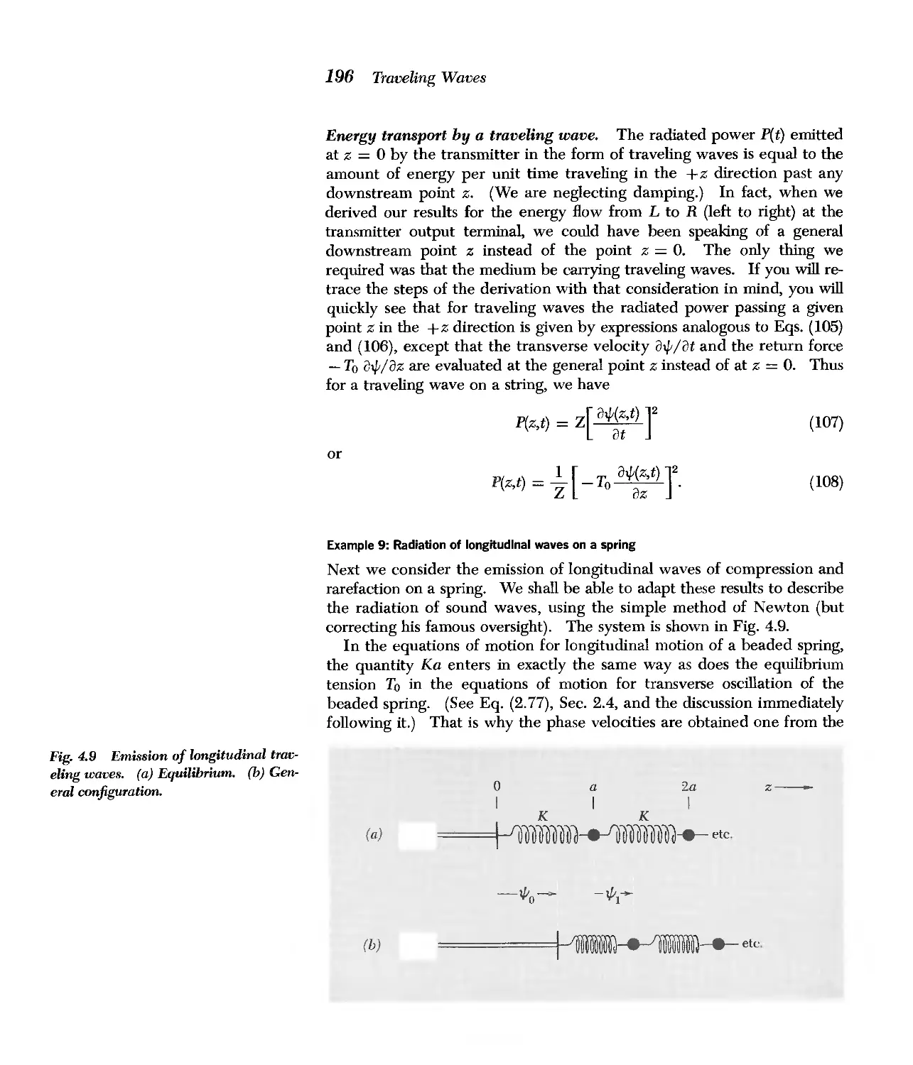
Traveling waves have great aesthetic appeal, and it would be tempting to begin with
them. In spite of their aesthetic and mathematical beauty, however, waves are physi-
cally rather complicated because they involve interactions between large numbers of
particles. Since I want to emphasize physical systems rather than mathematics, I
begin with the simplest physical system, rather than with the simplest wave.
Chapter 1 Free OsciUations of Simple Systems: We first review the free oscillations
of a one-dimensional harmonic oscillator, emphasizing the physical aspects of inertia
and return force, the physical meaning of w 2 , and the fact that for a real system the
oscillation amplitude must not be too large if we are to get simple harmonic motion.
Next, we consider free oscillations of two coupled oscillators and introduce the con-
cept of normal mode. We emphasize that the mode is like a single "extended" har-
monic oscillator, with all parts throbbing at the same frequency and all in phase, and
that, for a given mode, w 2 has the same physical meaning as it does for a one-dimen-
sional oscillator.
What to omit: Throughout the book, several physical systems recur repeatedly.
The teacher should not discuss all of them, nor the student study all of them. Exam-
ples 2 and 8 are longitudinal oscillations of mass and springs for one (Ex. 2) and two
(Ex. 8) degrees of freedom. In later chapters this system is extended to many degrees
of freedom, to continuous systems (rubber rope and slinky undergoing longitudinal os-
cillations) and is used as a model to assist comprehension of sound waves. A teacher
who wishes to omit sound may also wish to omit all longitudinal oscillations from the
beginning. Similarly, Examples 4 and 10 are LC circuits for one and two degrees of
freedom. In later chapters they are extended to LC networks and then to continuous
transmission lines. A teacher who wishes to omit the study of electromagnetic waves
in transmission lines, therefore, can omit all LC circuit examples from the very begin-
ning. (He can do this and still give a thorough discussion of electromagnetic waves,
starting in Chap. 7 with Maxwell's equations.) Do not omit transverse oscillations
(Examples 3 and 9).
Home experiments: We strongly advocate Home Exp. 1.24 (Sloshing mode in a
pan of water) and the related Prob. 1.25 (Seiches), to get the student started "doing it
himself." Home Exp. 1.8 (Coupled cans of soup) makes a good class demonstration.
Of course, you may already have available such a demonstration (coupled pendulums).
Nevertheless, I advocate slinky and soup cans for its crudity, even as a class demon-
stration, since it may encourage the student to get his own slinky and soup.
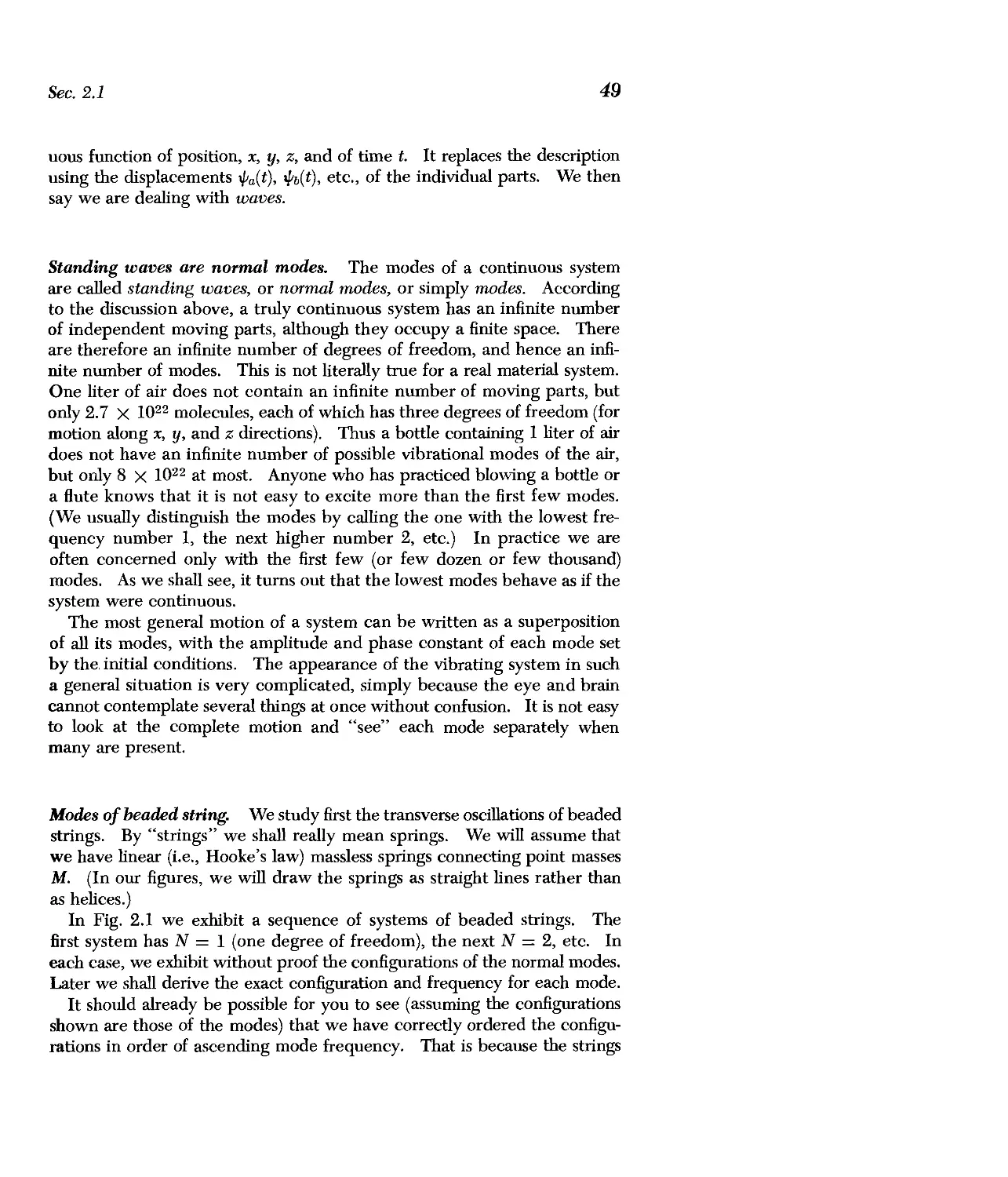
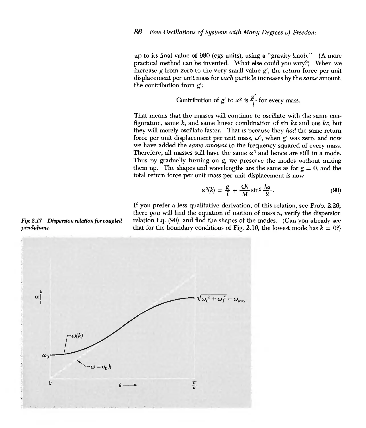
Chapter 2 Free Oscillations of Systems with Many Degrees of Freedom: We ex-
tend the number of degrees of freedom from two to a very large number and find the
transverse modes-the standing waves-of a continuous string. We define k and
introduce the concept of a dispersion relation, giving w as a function ofk. We use
the modes of the string to introduce Fourier analysis of periodic functions in Sec. 2.3.
The exact dispersion relation for beaded springs is given in Sec. 2.4.
Organization
of the Course
xii Teaching Notes
What to omit: Sec. 2.3 is optional-especially if the students already know some
Fourier analysis. Example 5 (Sec. 2.4) is a linear array of coupled pendulums, the
simplest system having a low-frequency cutoff. They are used later to help explain
the behavior of other systems that have a low-frequency cutoff. A teacher who does
not intend to discuss at a later time systems driven below cutoff (waveguide, iono-
sphere, total reflection of light in glass, barrier penetration of de Broglie waves, high-
pass filters, etc.) need not consider Example 5.
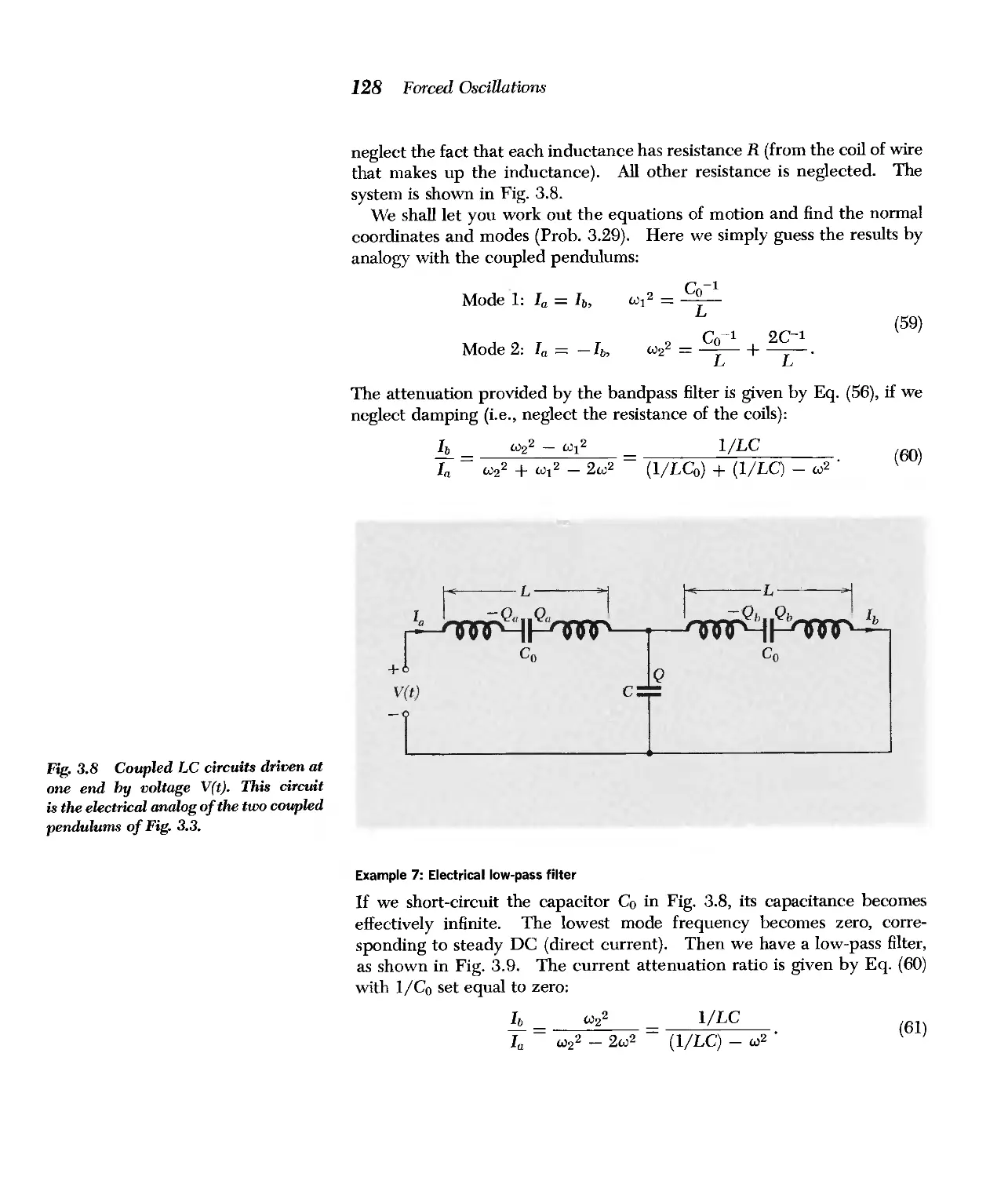
Chapter 3 F01'ced Oscillations: Chapters 1 and 2 started with free oscillations of a
harmonic oscillator and ended with free standing waves of closed systems. In Chaps.
3 and 4 we consider forced oscillations, first of closed sytems (Chap. 3) where we
find "resonances," and then in open systems (Chap. 4) where we find traveling waves.
In Sec. 3.2 we review the damped driven one-dimensional oscillator, considering its
transient behavior as well as its steady-state behavior. Then we go to two or more
degrees of freedom, and discover that there is a resonance corresponding to every
mode of free oscillation. We also consider closed systems driven below their lowest
(or above their highest) mode frequency and discover exponential waves and "filtering"
action.
What to omit: Transients (in Sec. 3.2) can be omitted. Some teachers may also
wish to omit everything about systems driven beyond cutoff.
Home experiments: Home Exps. 3.8 (Forced oscillations in a system of two coupled
cans of soup) and 3.16 (Mechanical bandpass filter) require phonograph turntables.
They make excellent class demonstrations, especially of exponential waves for systems
driven beyond cutoff.
Chapter 4 Traveling Waves: Here we introduce traveling waves resulting from
forced oscillations of an open system (contrasted with the standing waves resulting
from forced oscillations of a closed system that we found in Chap. 3). The remainder
of Chap. 4 is devoted to studying phase velocity (including dispersion) and impedance
in traveling waves. We contrast the two "traveling wave concepts," phase velocity
and impedance, with the "standing wave concepts," inertia and return force, and also
contrast the fundamental difference in phase relationships for standing versus traveling
waves.
Home experiments: We recommend Home Exp. 4.12 (Water prism). This is the
first optics kit experiment; it uses the purple filter (which passes red and blue but cuts
out green). We strongly recommend Home Exp. 4.18 (Measuring the solar constant
at the earth's surface) with your face as detector.
Chapter 5 Reflection: By the end of Chap. 4 we have at our disposal both stand-
ing and traveling waves (in one dimension). In Chap. 5 we consider general super-
positions of standing and traveling waves. In deriving reflection coefficients we make
a very "physical" use of the superposition principle, rather than emphasizing bound-
ary conditions. (Use of boundary conditions is emphasized in the problems.)
What to omit: There are many examples, involving sound, transmission lines, and
light. Don't do them all! Chapter 5 is essentially the "application" of what we have
acquired in Chaps. 1-4. Any or all of it can be omitted.
Home experiments: Everyone should do Home Exp. 5.3 (Transitory standing waves
on a slinky). Home Exps. 5.17 and 5.18 are especially interesting.
Teaching Notes xiii
Chapter 6 Modulations, Pulses, and Wave Packets: In Chaps. 1-5 we work mainly
with a single frequency w (except for Sec. 2.3,on Fourier analysis). In Chap. 6 we
consider superpositions, involving differeI).t freque,neies, to form pulses and wave
packets and to extend the concepts of Fourier analysis (developed in Chap. 2 for peri-
odic functions) so as to include nonperiodic functions.
What to omit: Most of the physics is in the first three sections. A teacher who
has omitted Fourier analysis in Sec. 2.3 will undoubtedly want to omit Sees. 6.4 and
6.5, where Fourier integrals are introduced and applied.
Home experiments: No one believes in group velocity until they have watched water
wave packets (see Home Exp. 6.11). Everyone should also do Home Exps. 6.12 and
6.13.
Problems: Frequency and phase modulation are discussed in problems rather than
in the text. So are such interesting recent developments as Mode-locking of a laser
(Prob. 6.23), Frequency multiplexing (Prob. 6.32), and Multiplex Interferometric
Fourier Spectroscopy (Prob. 6.33).
Chapter 7 Waves in Two and Three Dimensions: In Chaps. 1-6 the waves are all
one-dimensional. In Chap. 7 we go to three dimensions. The propagation vector k
is introduced. Electromagnetic waves are studied using Maxwell's equations as the
starting point. (In earlier chapters there are many examples of electromagnetic waves
in transmission lines, evolving from the LC-circuit example.) Water waves are also
studied.
What to omit: Sec. 7.3 (Water Waves) can be omitted, but we recommend the
home experiments on water waves whether or not Sec. 7.3 is studied. A teacher mainly
interested in optics could actually start his course at Sec. 7.4 (Electromagnetic Waves)
and continue on through Chaps. 7, 8, and 9.
Chapter 8 Polarization: This chapter is devoted to study of polarization of electro-
magnetic waves and of waves on slinkies, 'with emphasis on the physical relation be-
tween partial polarization and coherence.
Home experiments: Everyone should do at least Home Exps. 8.12, 8.14, 8.16, and
8.18 (Exp. 8.14 requiring slinky; the others, the optics kit).
Chapter 9 Interference and Diffraction: Here we consider superpositions of waves
that have traveled different paths from source to detector. We emphasize the physical
meaning of coherence. Geometrical optics is treated as a wave phenomenon-the
behavior of a diffraction-limited beam impinging on various reflecting and refracting
surfaces.
Home experiments: Everyone should do at least one each of the many home ex-
periments on interference, diffraction, coherence, and geometrical optics. We also
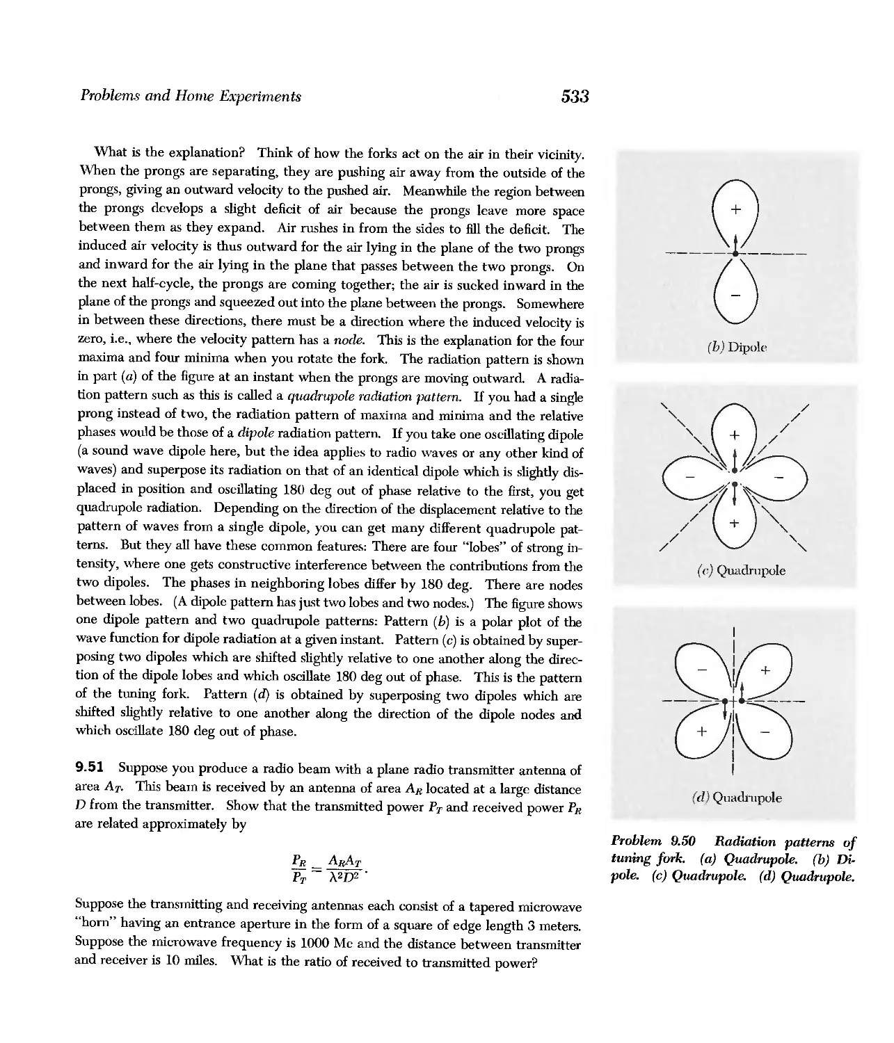
strongly recommend 9.50 (Quadrupole radiation from a tuning fork.)
Problems: Some topics are developed in the problems: Stellar interferometers, in-
cluding the recently developed "long-base-line interferometry" (Prob. 9.57); the
analogy between the phase-contrast microscope and the conversion of AM radio
waves to FM is discussed in Prob. 9.59.
Home Experiments
xiv Teaching Notes
GeneTal remarks: At least one home experiment should be assigned per week. For
your convenience we list here all experiments involving water waves, waves in
slinkies, and sound waves. We also later describe the optics kit.
Water waves: Discussed in Chap. 7; in addition they form a recurring theme devel-
oped in the following series of easy home experiments:
1.24 Sloshing modes in pan of water
1.25 Seiches
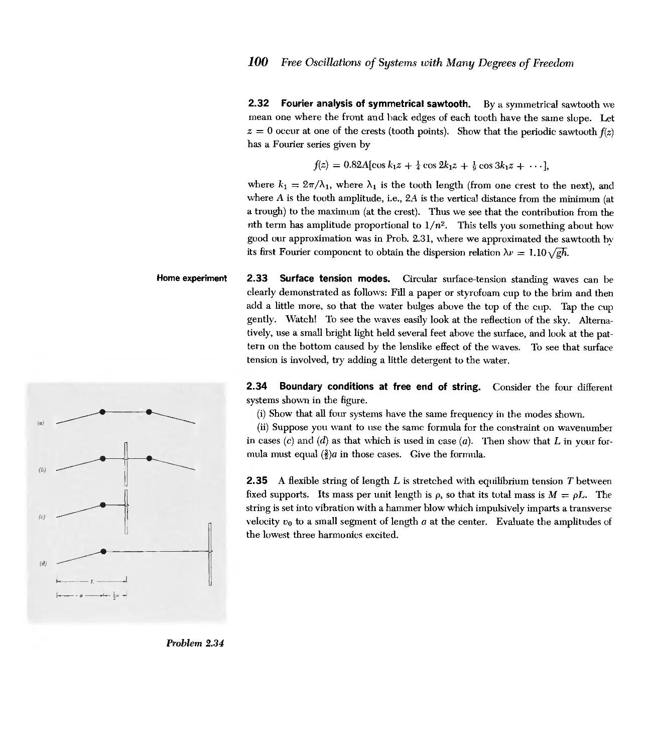
2.31 Sawtooth shallow-water standing waves
2.33 Surface tension modes
3.33 Sawtooth shallow-water standing waves
3.34 Rectangular two-dimensional standing surface waves on water
3.35 Standing waves in water
6.11 Water wave packets
6.12 Shallow-water wave packets-tidal waves
6.19 Phase and group velocities for deep-water waves
6.25 Resonance in tidal waves
7.11 Dispersion law for water waves
9.29 Diffraction of water waves.
Slinkies: Every student should have a Slinky (about $1 in any toy store). Four of
the following experiments require a record-player turntable and are therefore outside
the "kitchen physics" cost range. However, many students already have record
players. (The experiments involving record players make good lecture demonstrations.)
1.8 Coupled cans of soup
2.1 Slinky-dependence of frequency on length
2.2 Slinky as a continuous system
2.4 "Tone quality" of a slinky
3.7 Resonance in a damped slinky (turntable required)
3.8 Forced oscillations in a system of two coupled cans of soup (turntable required)
3.16 Mechanical bandpass filter (turntable required)
3.23 Exponential penetration into reactive region (turntable required)
4.4 Phase velocity for waves on a slinky
5.3 Transitory standing waves on a slinky
8.14 Slinky polarization
Sound: Many home experiments on sound involve use of two identical tuning forks,
preferably C523.3 or A440. The cheapest kind (about $1.25 each), which are
perfectly adequate, are available in music stores. Mailing tubes can be purchased for
about 25ft each in stationery or art-supply stores. The following home experiments
involve sound:
1.4 Measuring the frequency of vibrations
1.7 Coupled hacksaw blades
1.12 Beats from two tuning forks
1.13 Nonlinearities in your ear-combination tones
1.18 Beats between weakly coupled nonidentical guitar strings
2.4 "Tone quality" of a slinky
2.5 Piano as Fourier-analyzing machine-insensitivity of ear to phase
2.6 Piano harmonics-equal-temperament scale
3.27 Resonant frequency width of a mailing tube
Teaching Notes xv
4.6 Measuring the velocity of sound with wave packets
4.15 Whiskey-bottle resonator (Helmholtz resonator)
4.16 Sound velocity in air, helium, and natural gas
4.26 Sound impedance
5.15 Effective length of open-ended tube for standing waves
5.16 Resonance in cardboard tubes
5.17 Is your sound-detecting system (eardrum, nerves, brain) a phase-sensitive detector?
5.18 Measuring the relative phase at the two ends of an open tube
5.19 Overtones in tuning fork
5.31 Resonances in toy balloons
6.13 Musical trills and bandwidth
9.50 Radiation pattern of tuning fork-quadrupole radiation
Components: Four linear polarizers, a circular polarizer, a quarter-wave plate, a
half-wave plate, a diffraction grating, and four color filters (red, green, blue, and
purple). The components are described in the text (linear polarizer on p. 411; circu-
lar polarizer, p. 433; quarter- and half-wave retardation plates, p. 435; diffraction
grating, p. 496). Some experiments also require microscope slides, a showcase-lamp
line source, or a flashlight-bulb point source as described in Home Exp. 4.12, p. 217.
Aside from Exp. 4.12, all experiments requiring the optics kit are in Chaps. 8 and 9.
They are too numerous to list here.
The first experiment involving the complete optics kit should be identification of all
the components by the student. (Components are listed on the envelope container
glued to the inside back cover.) Label the components in some way for future refer-
ence. For example, use scissors to round off slightly the four corners of the circular
polarizer, and then scratch "IN" near one edge of the input face or stick a tiny piece
of tape on that face. Clip one corner of the one-quarter-wave retarder; clip two corners
of the two-quarter- (half-) wave retarder. Scratch a line along the axis of easy trans-
mission on the linear polarizers. (This axis is parallel to one of the edges of the polarizer.)
We should remark that the "quarter-wave plate" gives a spatial retardation of
1400 ::!: 200 A, nearly independent of wavelength (for visible light). Thus the wave-
length for which it is a quarter-wave retarder is 5600 ::!: 800 A. The ::!:200 A is
the manufacturer's tolerance. A manufactured batch that gives retardation 1400 A
is a quarter-wave retarder for green (5600 A), but it retards by less than one quarter-
wave for longer wavelengths (red) and more for shorter (blue). Another batch that
happens to give retardation 1400 + 200 = 1600 A is a quarter-wave retarder only for
red (6400 A). One that retards by 1400 -'-- 200 is a quarter-wave plate only for blue
(4800 A). Similar remarks apply to the circular polarizer, since it consists of a sand-
wich of quarter-wave plate and linear polarizer at 45 deg, and the quarter-wave plate
is a retarder of 1400 ::!: 200 A. Thus there may be slightly distracting color effects
when using white light. The student must be warned that in any experiment where
he is supposed to get "black," i.e., extinction, he will always have some "non-extin-
guished" light of the "wrong" color leaking through. For example, I was naive when
I wrote Home Exp. 8.12. You should perhaps strike out everything after the word
«band" in the sentences "Do you see the dark band at green? That is the color of
5600 A!"
Optics Kit
Home experiment
Use of Complex Numbers
xvi Teaching Notes
Complex numbers simplify algebra when sinusoidal oscillations or waves are to be
superposed. They may also obscure the physics. For that reason I have avoided
their use, especially in the first part of the book. All the trigonometric identities that
are needed will be found inside the front cover. In Chap. 6 I do make use of the complex
representation exp iwt, so as to use the well-known graphical or "phasor diagram"
method of superposing vibrations. In Chap. 8 (Polarization) I use complex quantities
extensively. In Chap. 9 (Interference and Diffraction) I do not make much use of com-
plex quantities, even though it would sometimes simplify the algebra. Many teachers
may wish to make much more extensive use of complex numbers than I do, especially
in Chap. 9. In the sections on Fourier series (Sec. 2.3) and Fourier integrals (Sees.
6.4 and 6.5), I make no use of complex quantities. (I especially wanted to avoid Fourier
integrals involving "negative frequencies"!)
A Note on the MKS System of Electrical Unitsf
t Reprinted from Berkeley Physics Course,
Vol. II, Electricity and Magnetism, by Ed-
ward M. Purcell, @ 1963, 1964, 1965 by
Education Development Center, Inc., suc-
cessor by merger to Educational Services
Incorporated.
Most textbooks in electrical engineering, and many elementary physics
texts, use a system of electrical units called the rationalized MKS system.
This system employs the MKS mechanical units based on the meter, the
kilogram, and the second. The MKS unit of force is the newton, defined
as the force which causes a I-kilogram mass to accelerate at a rate of
1 meter/sec 2 . Thus a newton is equivalent to exactly 10 5 dynes. The
corresponding unit of energy, the newton-meter, or ;oule, is equivalent to
10 7 ergs.
The electrical units in the MKS system include our familiar "practical"
units-coulomb, volt, ampere, and ohm-along with some new ones.
Someone noticed that it was possible to assimilate the long -used practical
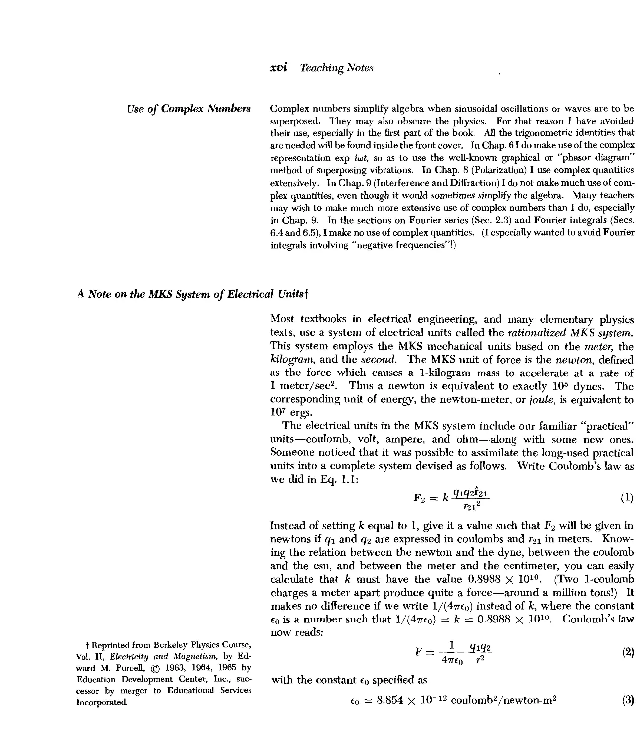
units into a complete system devised as follows. Write Coulomb's law as
we did in Eq. 1.1:
F 2 == k q1q2 f 21
r21 2
( 1)
Instead of setting k equal to 1, give it a value such that F 2 will be given in
newtons if q1 and q2 are expressed in coulombs and r21 in meters. Know-
ing the relation between the newton and the dyne, between the coulomb
and the esu, and between the meter and the centimeter, you can easily
calculate that k must have the value 0.8988 X 10 10 . (Two I-coulomb
charges a meter apart produce quite a force-around a million tons!) It
makes no difference if we write 1/(477£0) instead of k, where the constant
£0 is a number such that 1/(477£0) = k = 0.8988 X 10 10 . Coulomb's law
now reads:
F= q1q2
477£0 r 2
(2)
with the constant £0 specified as
£0 = 8.854 X 10- 12 coulomb 2 /newton-m 2
(3)
MKS System of Electrical Units xvii
Separating out a factor 1/477 was an arbitrary move, which will have the
effect of removing the 477 that would appear in many of the electrical
formulas, at the price of introducing it into some others, as here in
Coulomb's law. That is all that "rationalized" means. The constant £0
is called the dielectric constant (or "permittivity") of free space.
Electric potential is to be measured in volts, and electric field strength E
in volts/meter. The force on a charge q, in field E, is:
F (newtons) = qE (coulombs X volts/meter)
(4)
An ampere is 1 coulomb/sec, of course. The force per meter of length
on each of two parallel wires, r meters apart, carrying current I measured
in amperes, is:
f (newtons/meter) = ( ) 212 (amp2)
477 r (meters)
Recalling our CGS formula for the same situation,
f (d / ) 212 (esu/sec)2
ynes cm =-
rc 2 (cm 3 /sec 2 )
we compute that (/10/477) must have the value 10- 7 . Thus the constant /10,
called the permeability of free space, must be:
(5)
(6)
/10 = 477 X 10- 7 newtons/ amp 2 (exactly)
(7)
The magnetic field B is defined by writing the Lorentz force law as follows:
F (newtons) = qE + qv X B
(8)
where v is the velocity of a particle in meters/sec, q its charge in coulombs.
This requires a new unit for B. The unit is called a tesla, or a weber/m 2 .
One tesla is equivalent to precisely 10 4 gauss. In this system the auxiliary
field H is expressed in different units, and is related to B, in free space, in
this way:
B = /1oH (in free space)
The relation of H to the free current is
(9)
f H . ds = I free
(10)
I free being the free current, in amperes, enclosed by the loop around which
the line integral on the left is taken. Since ds is to be measured in meters,
the unit for H is called simply, ampere/meter.
Maxwell's equations for the fields in free space look like this, in the
rationalized MKS system:
div B = 0
aB
at
aE
curl B = /10£0 - + /1oJ
at
(11)
div E = p
curl E =
xviii MKS System of Electrical Units
If you will compare this with our Gaussian CGS version, in which c appears
out in the open, you will see that Eqs. 11 imply a wave velocity l/ yt:o!-to
(in meters/sec, of course). That is:
1
t:o!-to = 2
c
(12)
In our Gaussian CGS system the unit of charge, esu, was established by
Coulomb's law, with k _ 1. In this MKS system the coulomb is defined,
basically, not by Eq. 1 but by Eq. 5, that is, by the force between currents
rather than the force between charges. For in Eq. 5 we have !-to 47TX 10- 7 .
In other words, if a new experimental measurement of the speed of light
were to change the accepted value of c, we should have to revise the value
of the constant t:o, not that of !-to.
A partial list of the MKS units is given below, with their equivalents in
Gaussian CGS units.
Unit, in rationalized Equivalent, in
Quantity Symbol MKS system Gaussian CGS units
Distance s meter 10 2 em
Force F newton 10 5 dynes
Work energy W joule 10 7 ergs
Charge q coulomb 2.998 X 10 9 esu
Current I ampere 2.998 X 10 9 esu/ see
Electric potential cp volt (1/299.8) statvolts
Electric field E volts/meter (1/29980) statvolts/cm
Resistance R ohm 1.139 X 10- 12 see/em
Magnetic field B tesla 10 4 gauss
Magnetic flux II> weber 10 8 gauss-cm 2
Auxiliary field H H amperes/meter 4'17 X 10- 3 oersted
This MKS system is convenient in engineering. For a treatment of the
fundamental physics of fields and matter, it has one basic defect. Maxwell's
equations for the vacuum fields, in this system, are symmetrical in the
electric and magnetic field only if H, not B, appears in the role of the mag-
netic field. (Notice that Eqs. 11 above are not symmetrical, even in
the absence of J.) On the other hand, as we showed in Chapter 10, B,
not H, is the fundamental magnetic field inside matter. That is not a
matter of definition or of units, but a fact of nature, reflecting the absence
of magnetic charge. Thus the MKS system, as it has been constructed.
tends to obscure either the fundamental electromagnetic symmetry of the
vacuum, or the essential asymmetry of the sources. That was one of our
reasons for preferring the Gaussian CGS system in this book. The other
reason is that Gaussian CGS units, augmented by practical units on
occasion, are still the units used by most working physicists.
Contents
Preface to the Berkeley Physics Course v
A Further Note vi
Preface to Volume III vii
Acknowledgments ix
Teaching Notes xi
A Note on the MKS System of Electrical Units
xvi
Chapter 1 Free Oscillations of Simple Systems 1
1.1 Introduction 2
1.2 Free Oscillations of Systems with One Degree of Freedom 3
1.3 Linearity and the Superposition Principle 12
1.4 Free Oscillations of Systems with Two Degrees of Freedom 16
1.5 Beats 28
Problems and Home Experiments 36
Chapter 2 Free Oscillations of Systems with Many Degrees of
Freedom 47
2.1 Introduction 48
2.2 Transverse Modes of Continuous String 50
2.3 General Motion of Continuous String and Fourier Analysis 59
2.4 Modes of a Noncontinuous System with NDegrees of Freedom 72
Problems and Home Experiments 90
Chapter 3 Forced Oscillations 101
3.1 Introduction 102
3.2 Damped Driven One-dimensional Harmonic Oscillator 102
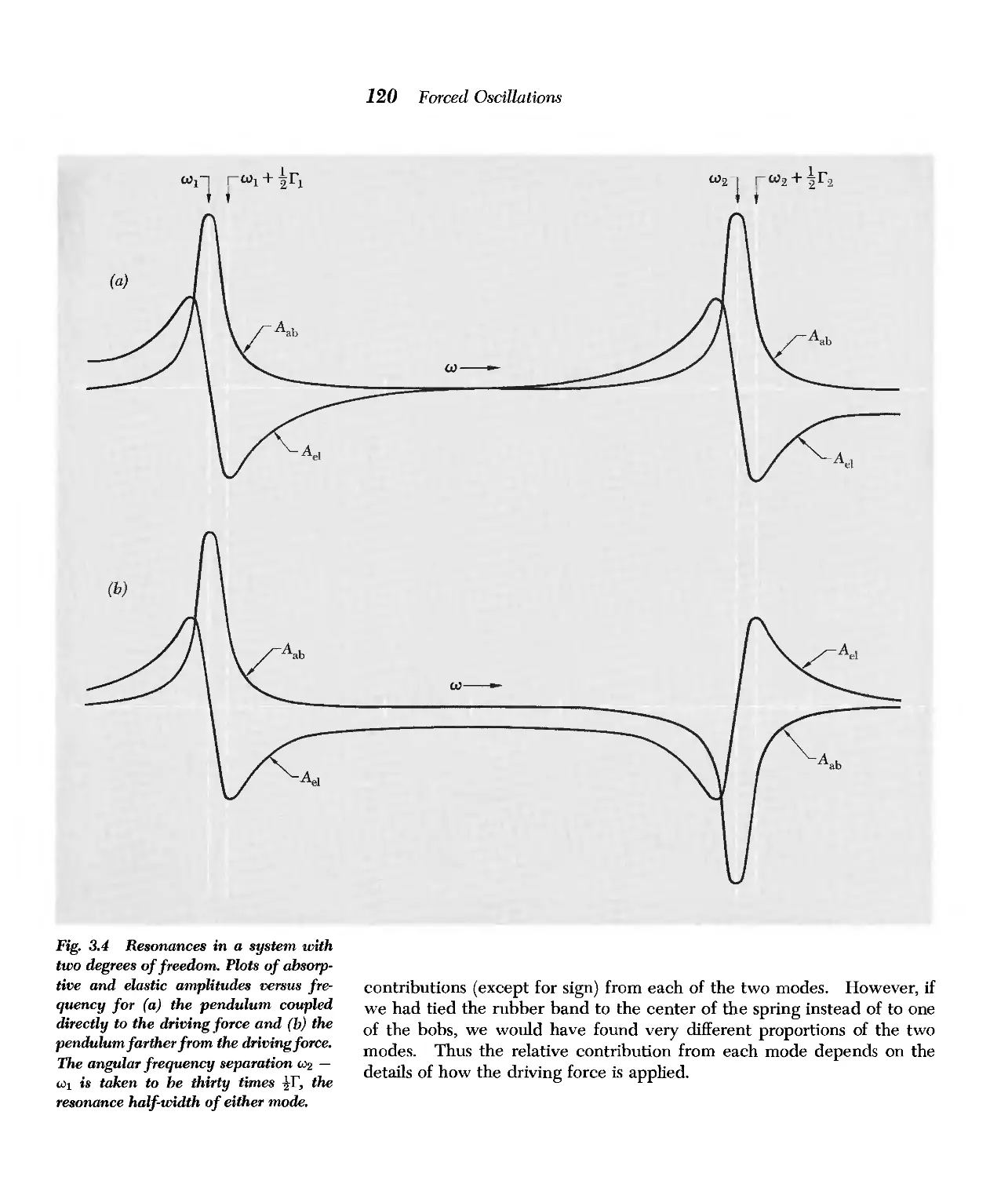
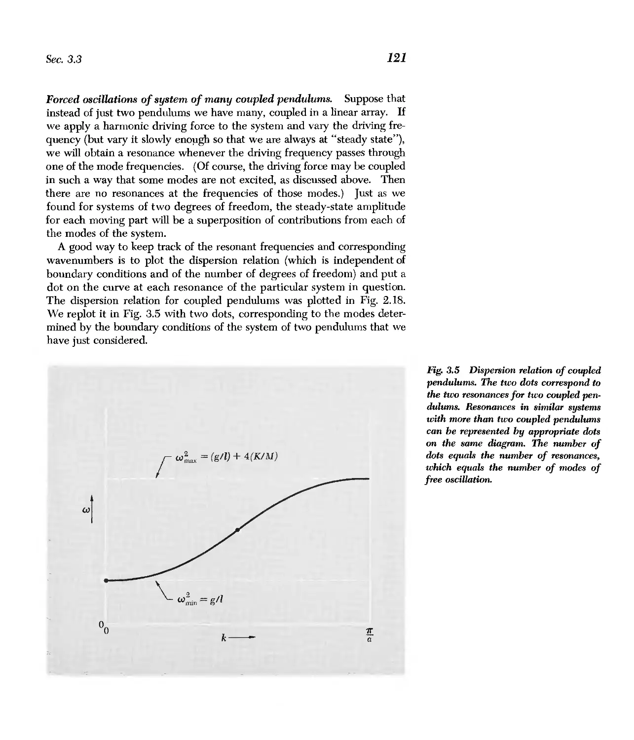
3.3 Resonances in System with Two Degrees of Freedom 116
3.4 Filters 122
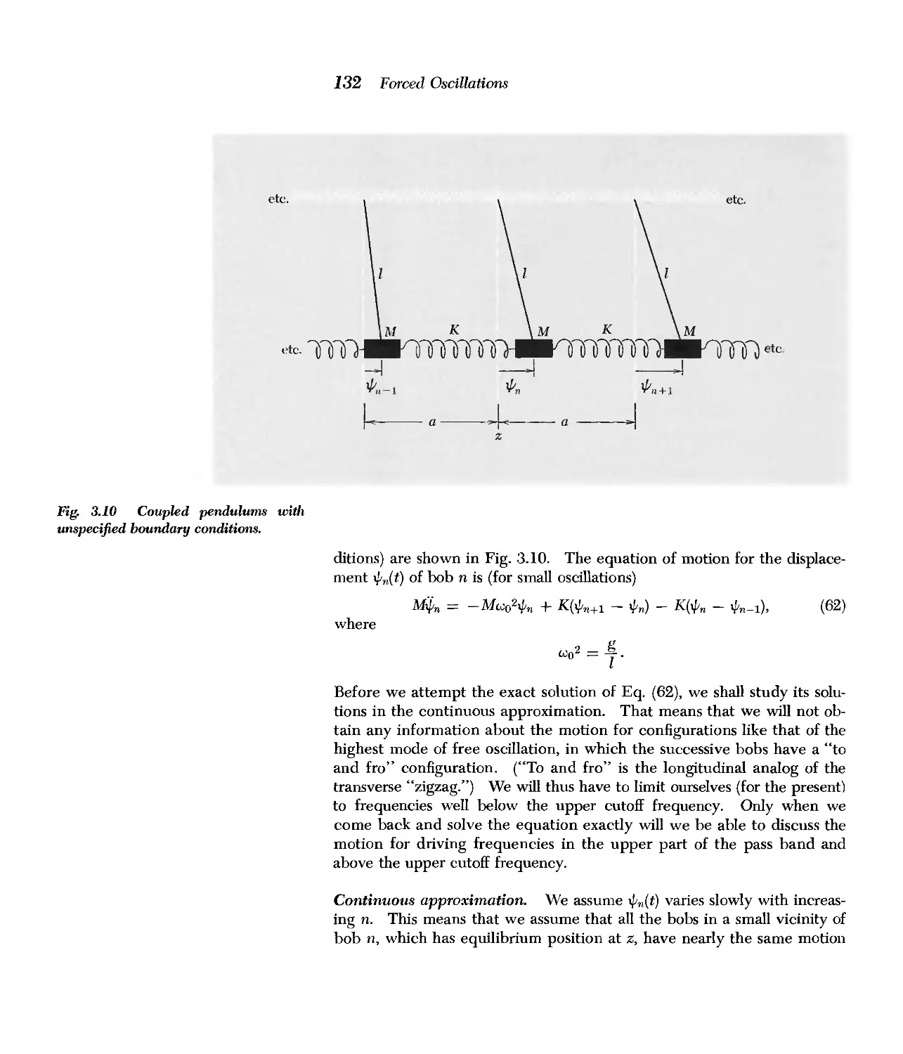
3.5 Forced Oscillations of Closed System with Many Degrees of
Freedom 130
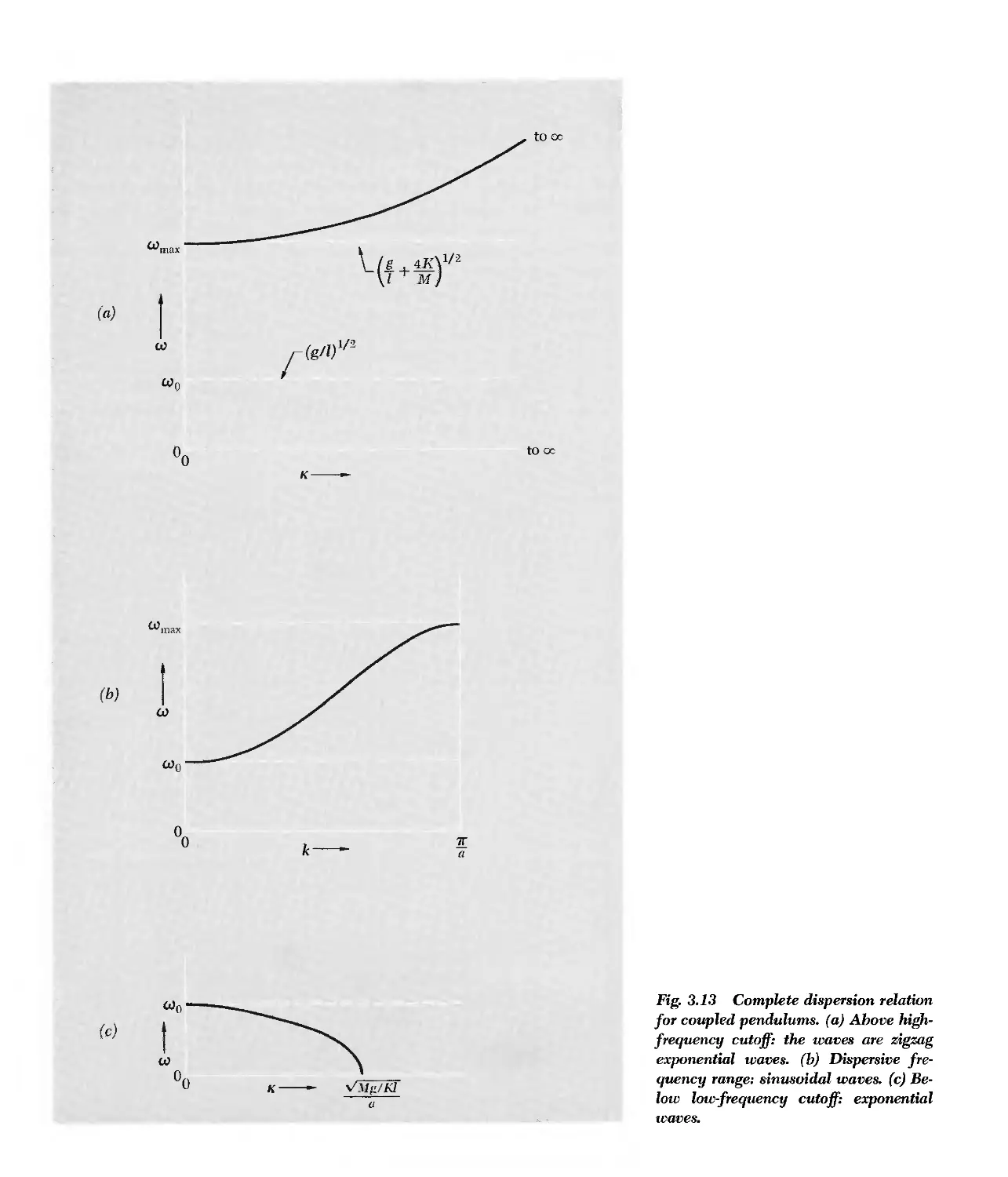
Problems and Home Experiments 146
Chapter 4 Traveling Waves 155
4.1 Introduction 156
4.2 Hannonic Traveling Waves in One Dimension and Phase
Velocity 157
4.3 Index of Refraction and Dispersion 176
4.4 Impedance and Energy Flux 191
Problems and Home Experiments 214
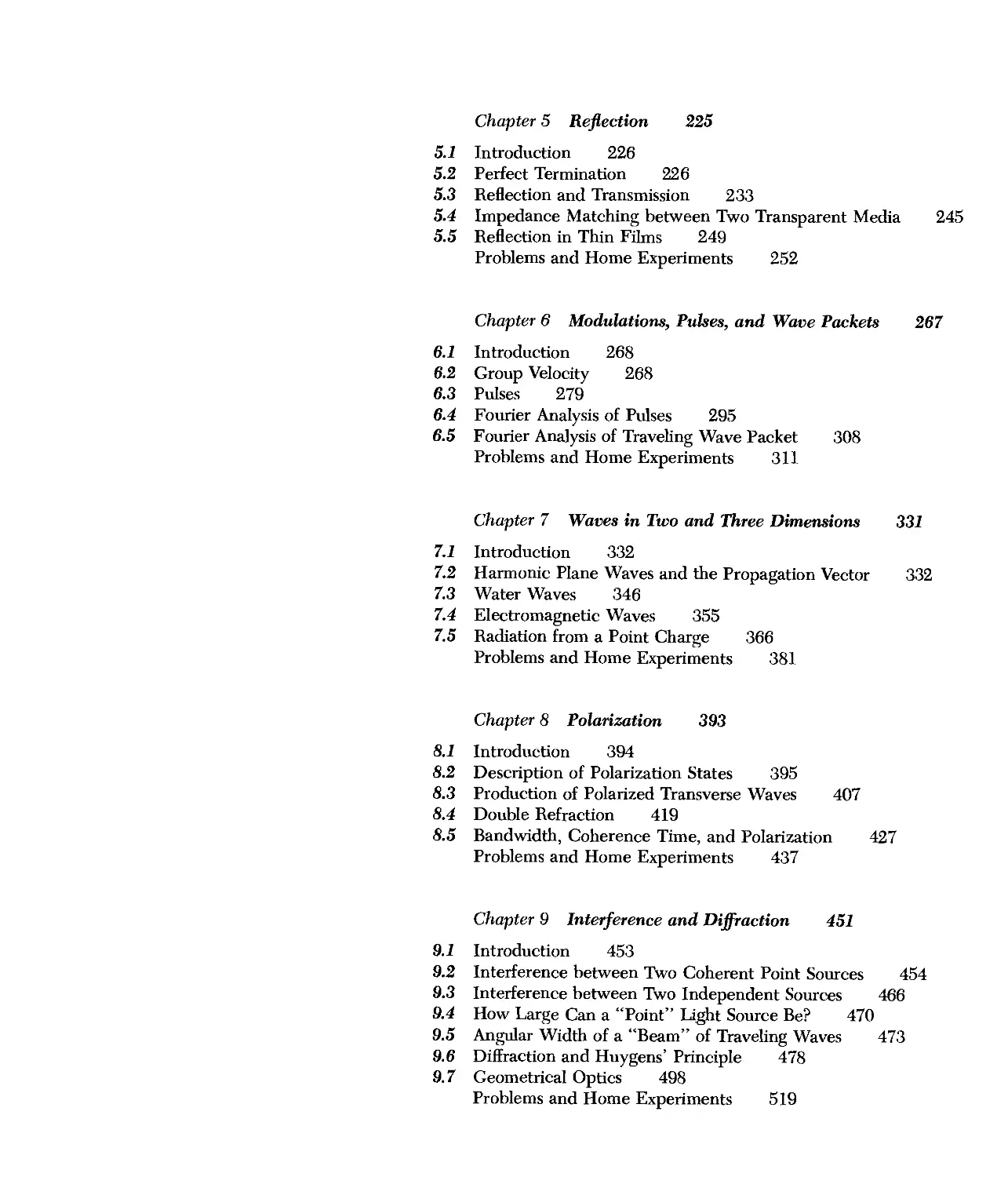
Chapter 5 Reflection 225
5.1 Introduction 226
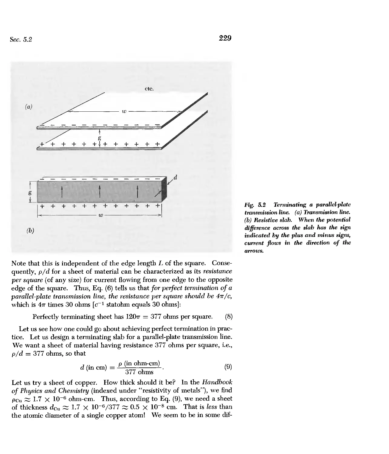
5.2 Perfect Termination 226
5.3 Reflection and Transmission 233
5.4 Impedance Matching between Two Transparent Media 245
5.5 Reflection in Thin Films 249
Problems and Home Experiments 252
Chapter 6 Modulations, Pulses, and Wave Packets 267
6.1 Introduction 268
6.2 Group Velocity 268
6.3 Pulses 279
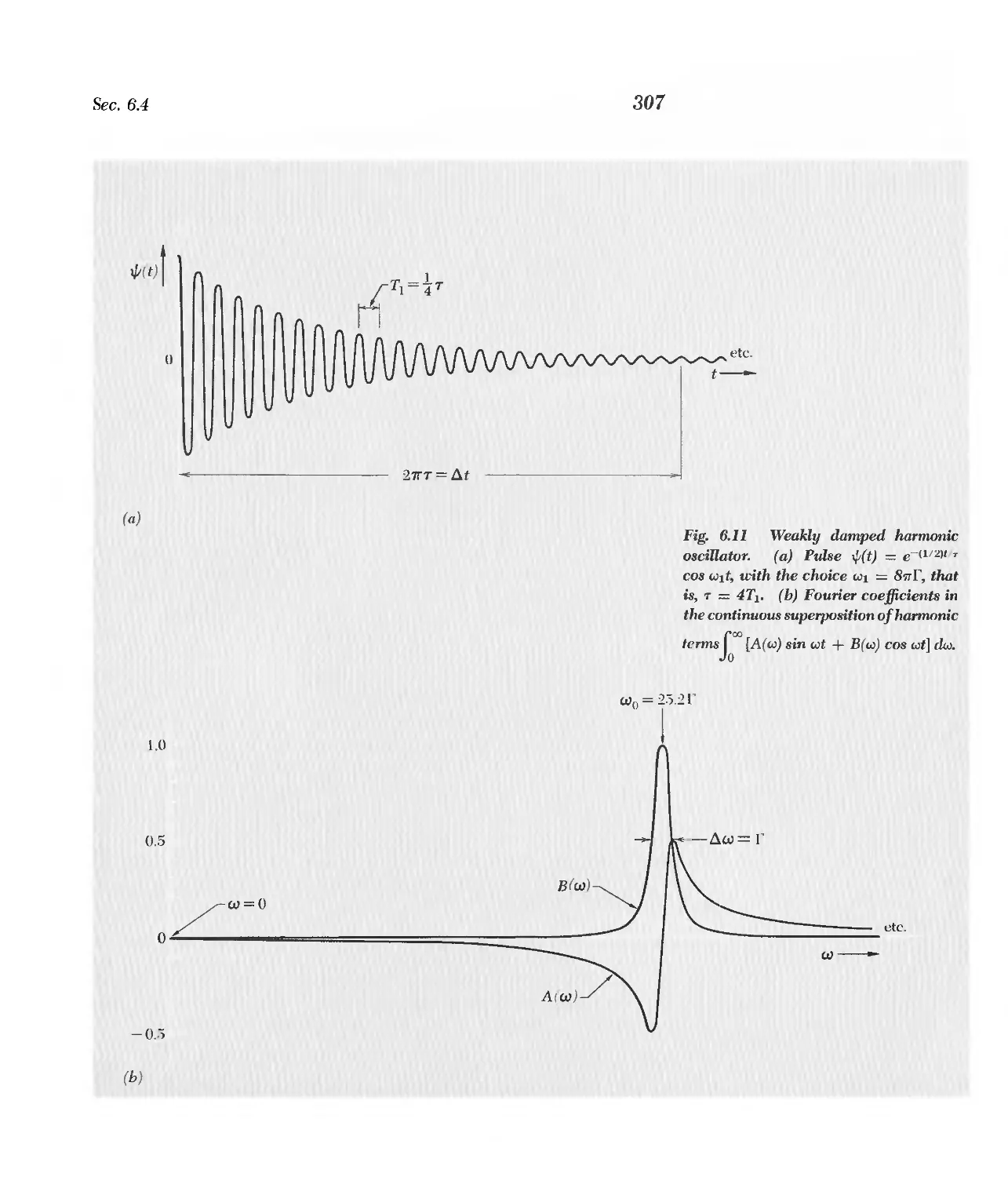
6.4 Fourier Analysis of Pulses 295
6.5 Fourier Analysis of Traveling Wave Packet 308
Problems and Home Experiments 311
Chapter 7 Waves in Two and Three Dimensions 331
7.1 Introduction 332
7.2 Harmonic Plane Waves and the Propagation Vector 332
7.3 Water Waves 346
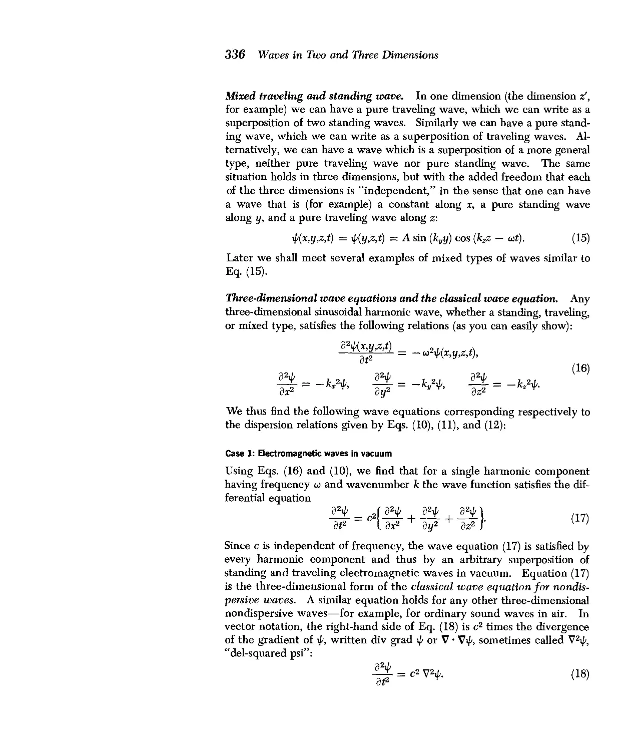
7.4 Electromagnetic Waves 355
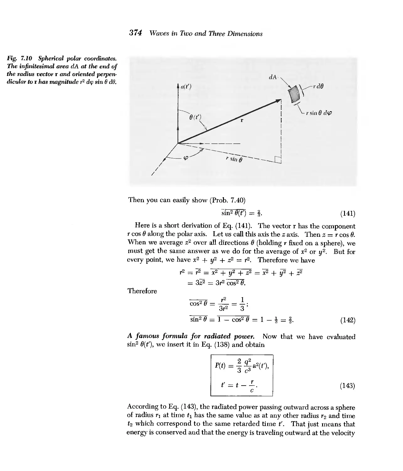
7.5 Radiation from a Point Charge 366
Problems and Home Experiments 381
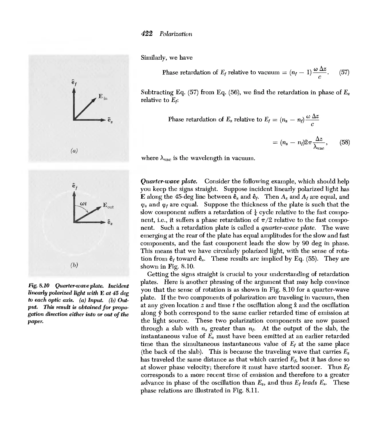
Chapter 8 Polarization 393
8.1 Introduction 394
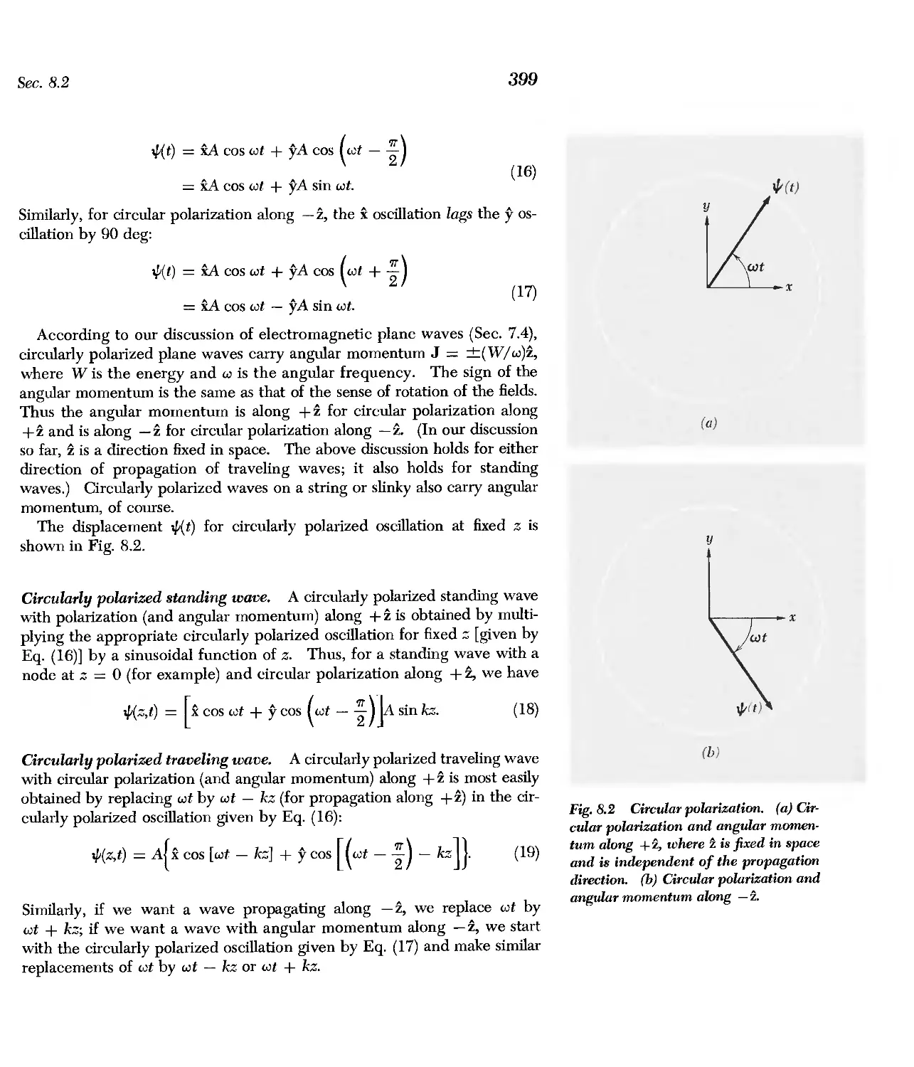
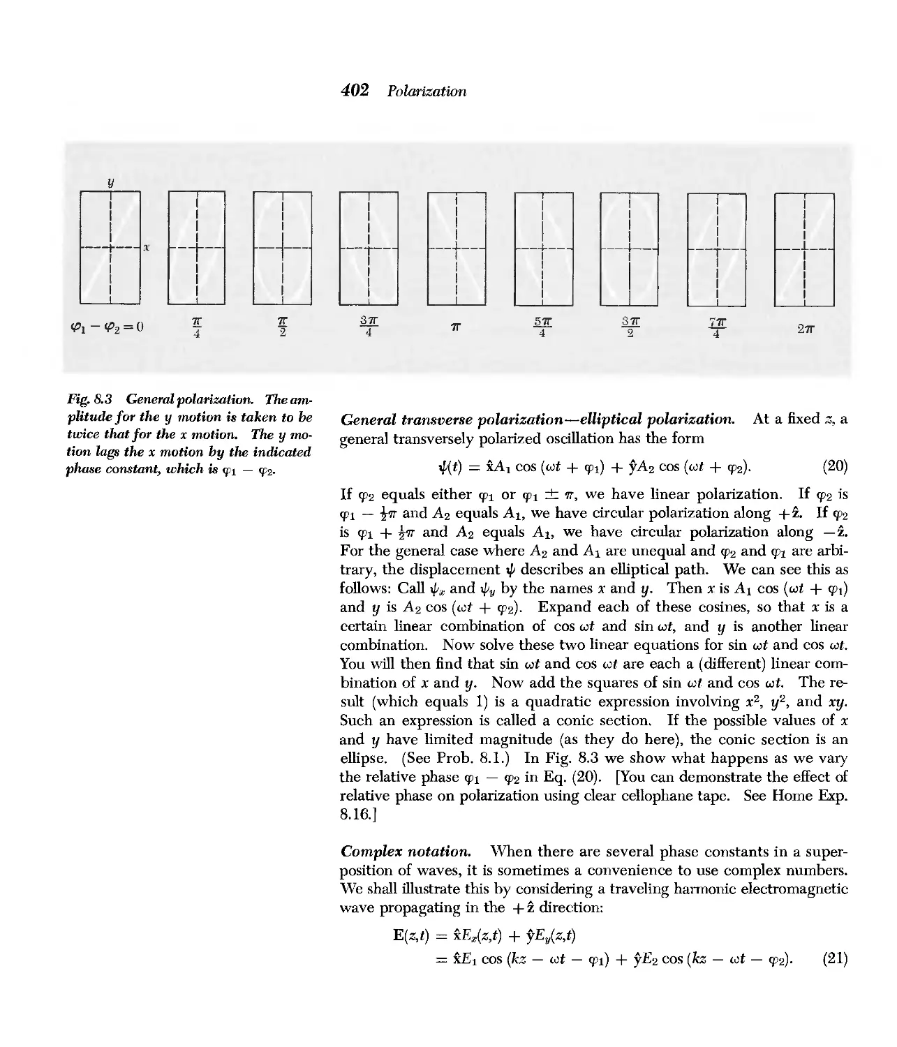
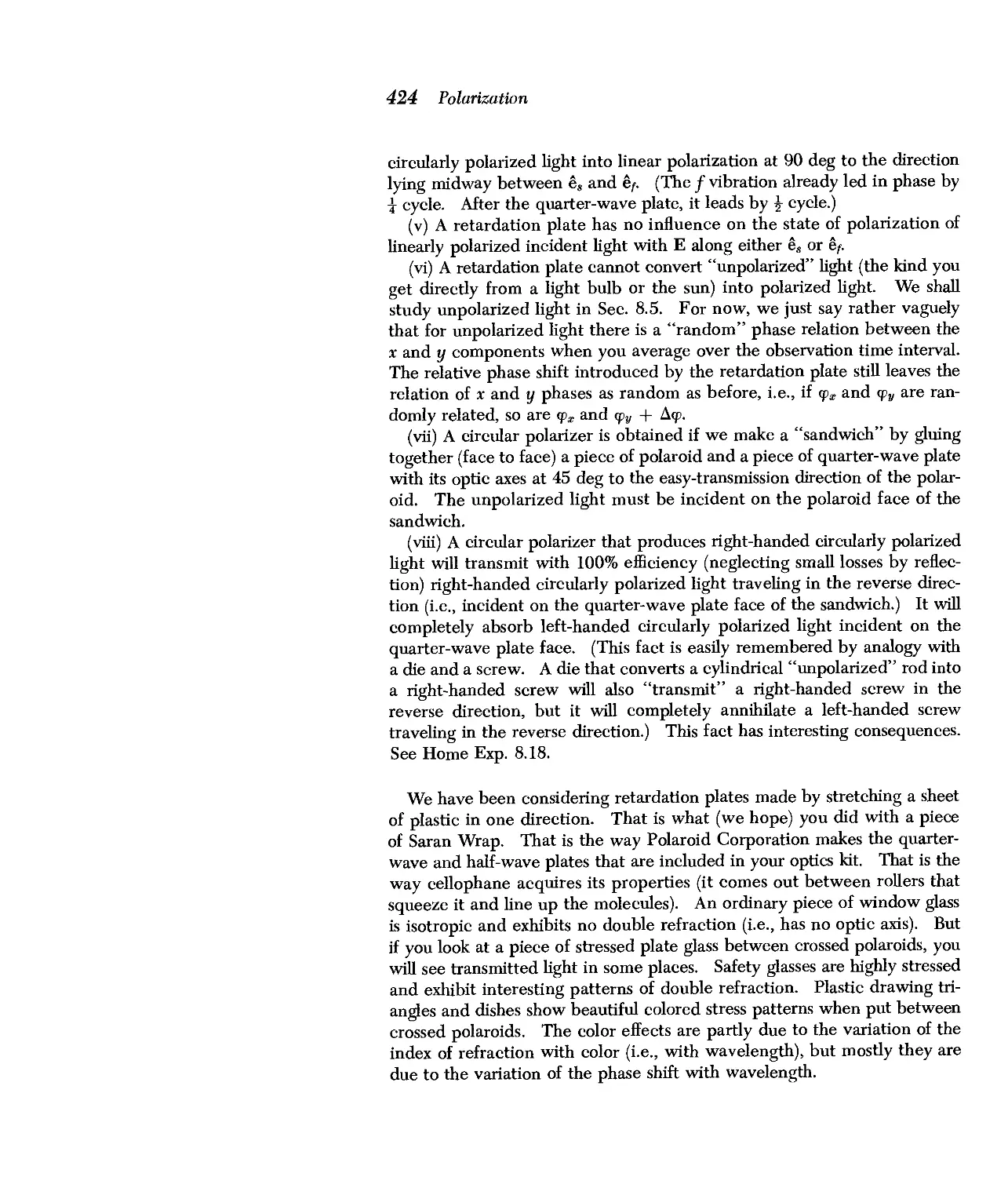
8.2 Description of Polarization States 395
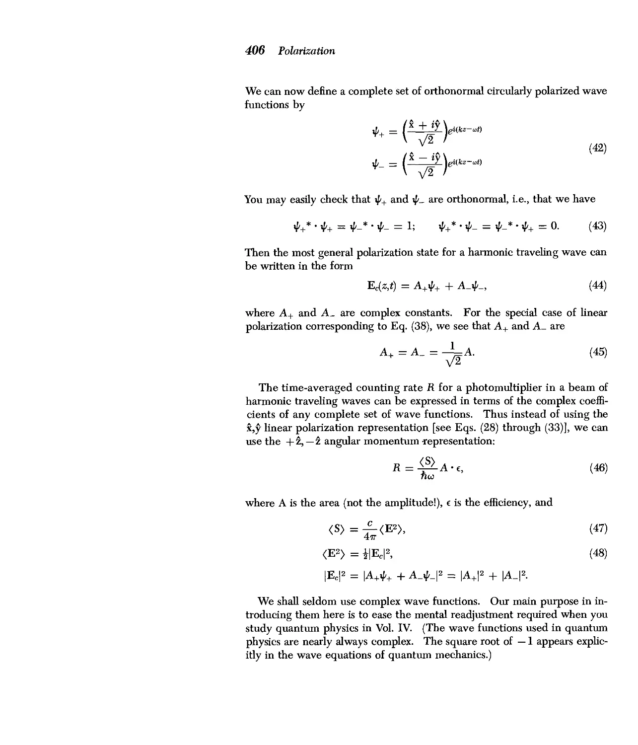
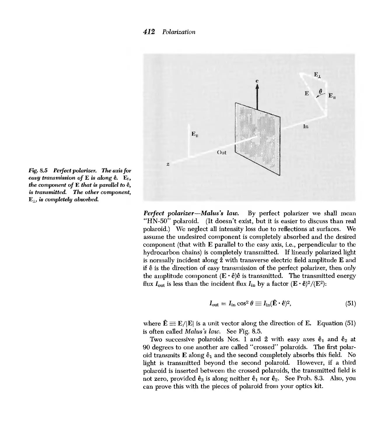
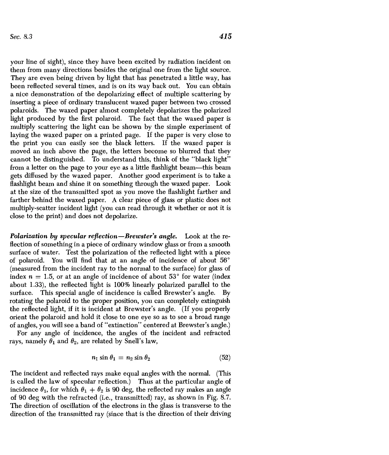
8.3 Production of Polarized Transverse Waves 407
8.4 Double Refraction 419
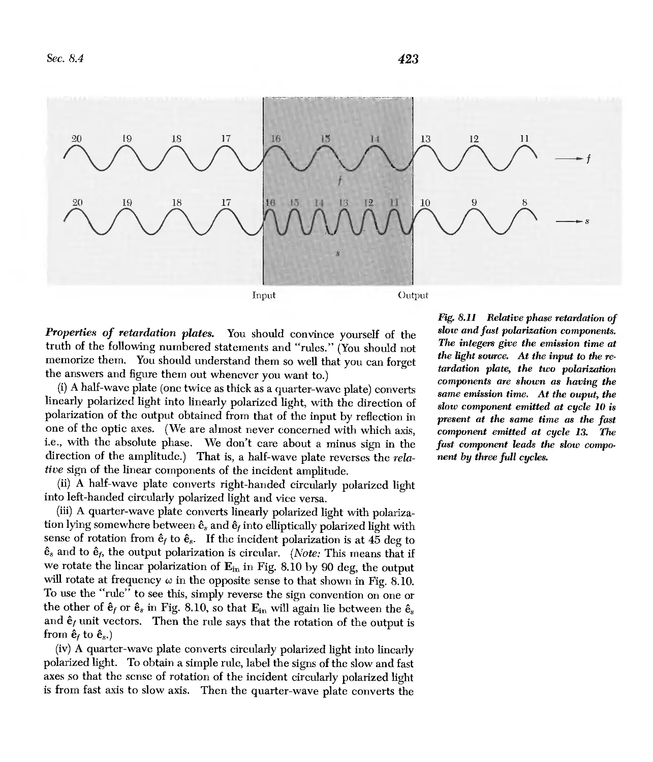
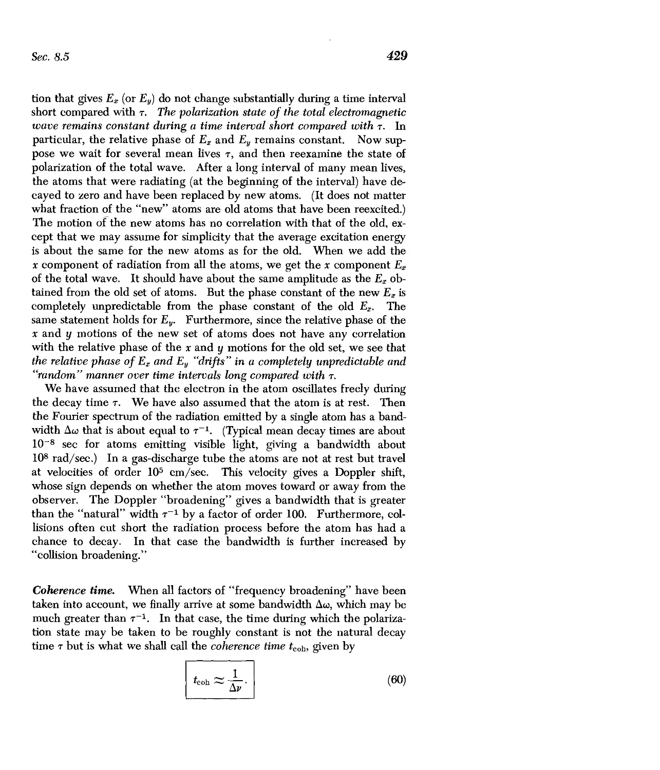
8.5 Bandwidth, Coherence Time, and Polarization 427
Problems and Home Experiments 437
Chapter 9 Interference and Diffraction 451
9.1 Introduction 453
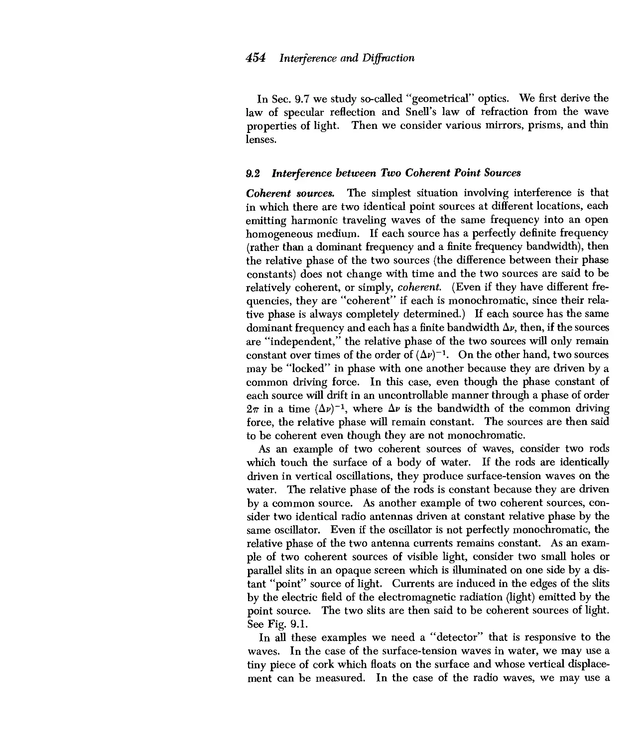
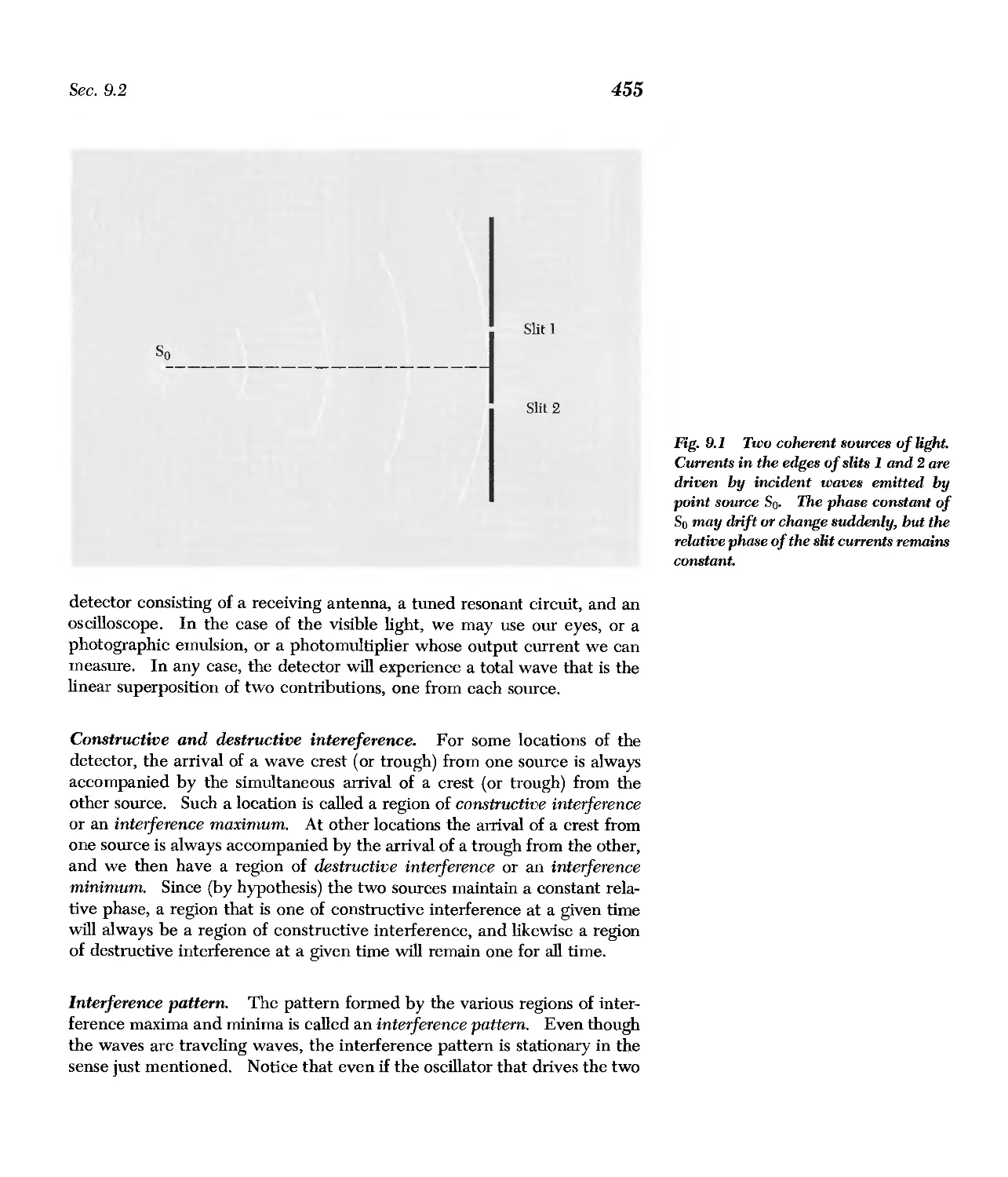
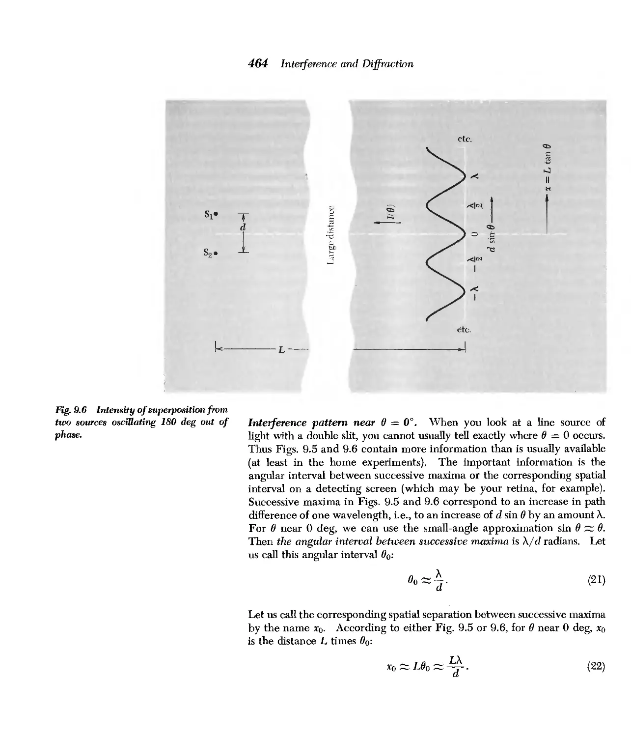
9.2 Interference between Two Coherent Point Sources 454
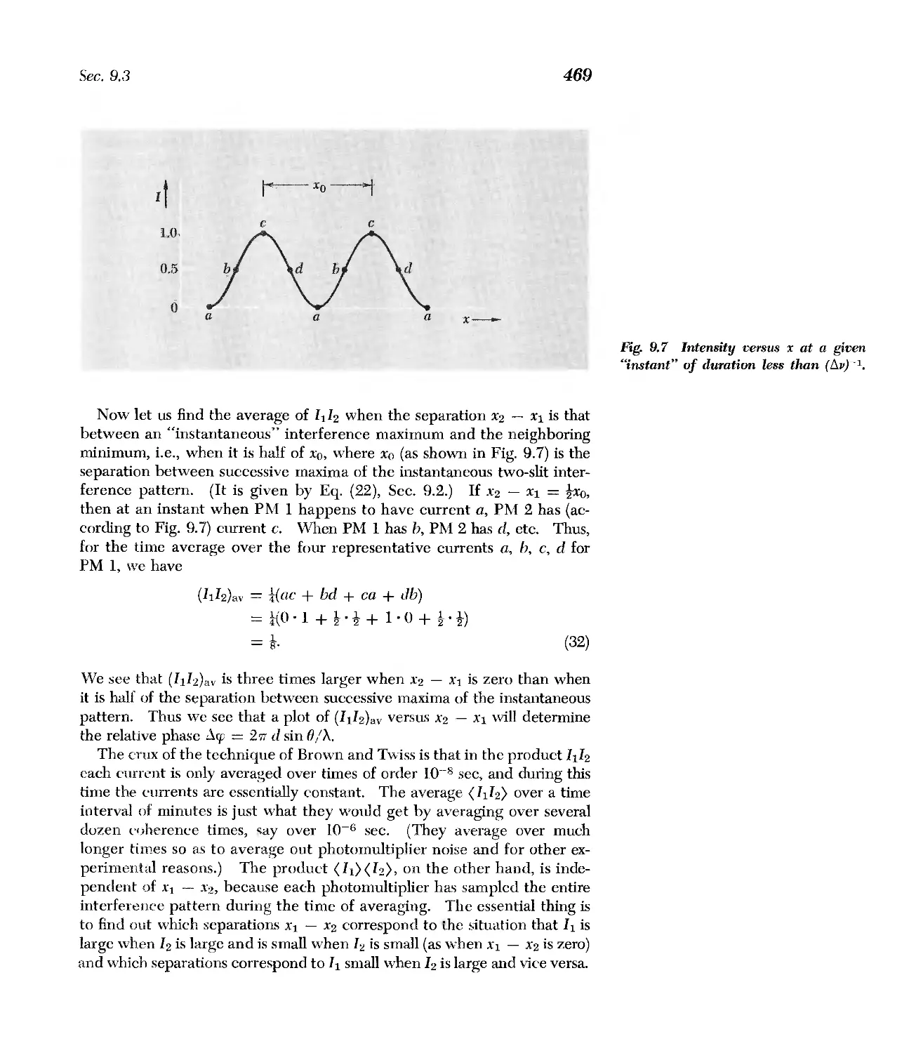
9.3 Interference between Two Independent Sources 466
9.4 How Large Can a "Point" Light Source Be? 470
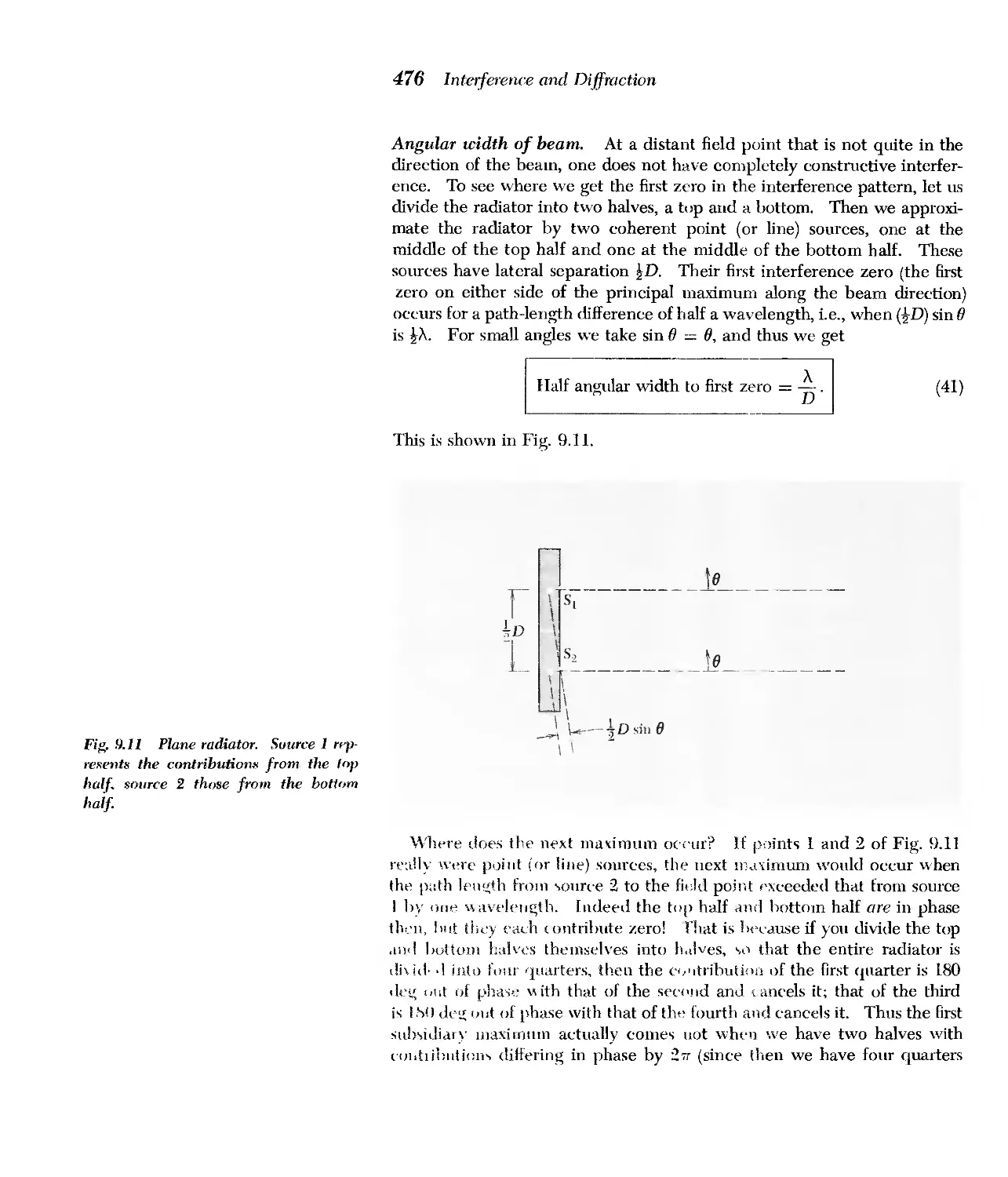
9.5 Angular Width of a "Beam" of Traveling Waves 473
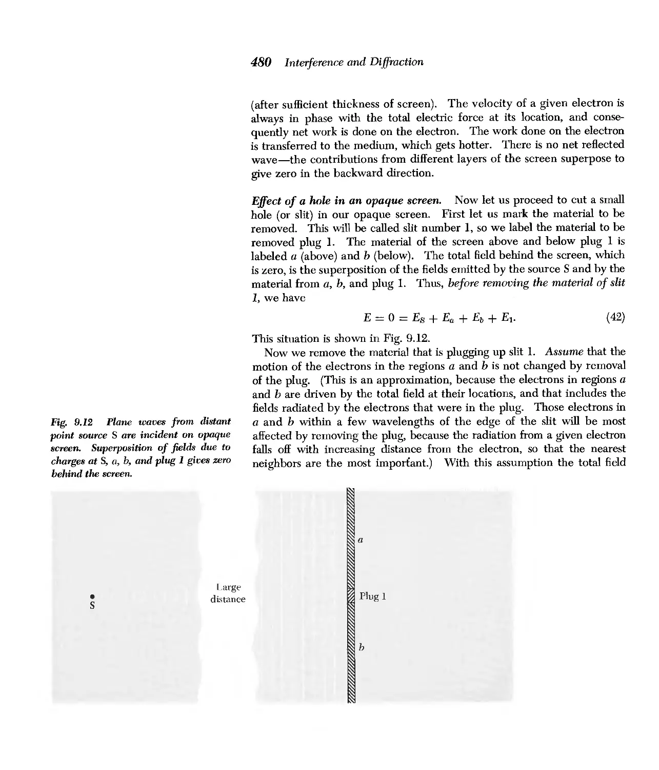
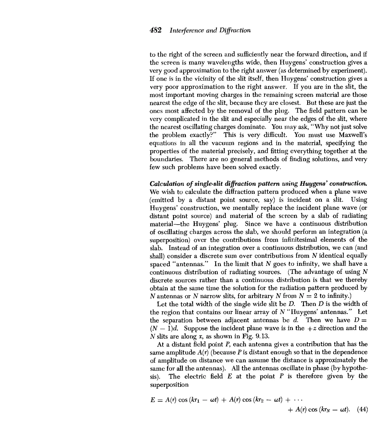
9.6 Diffraction and Huygens' Principle 478
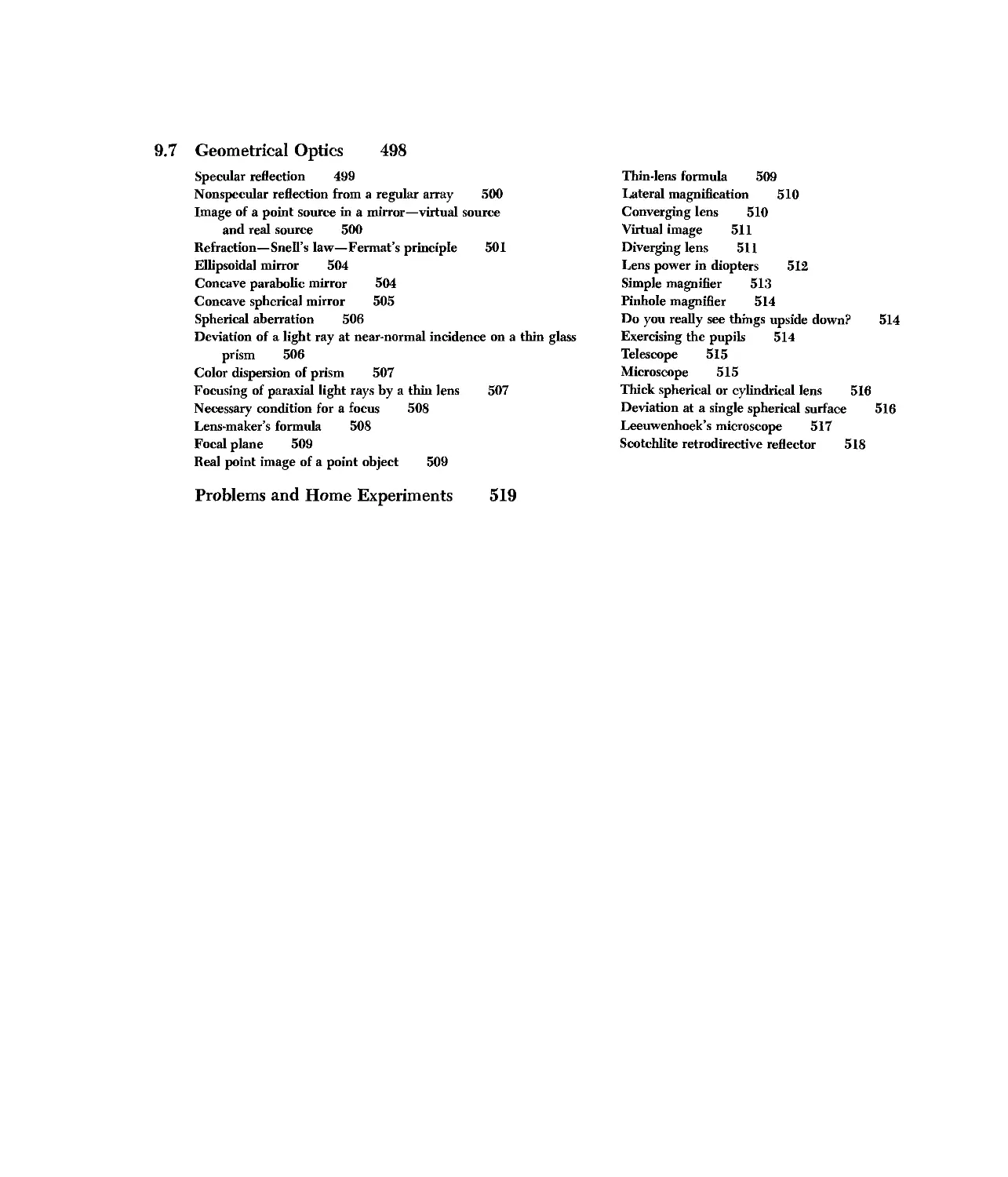
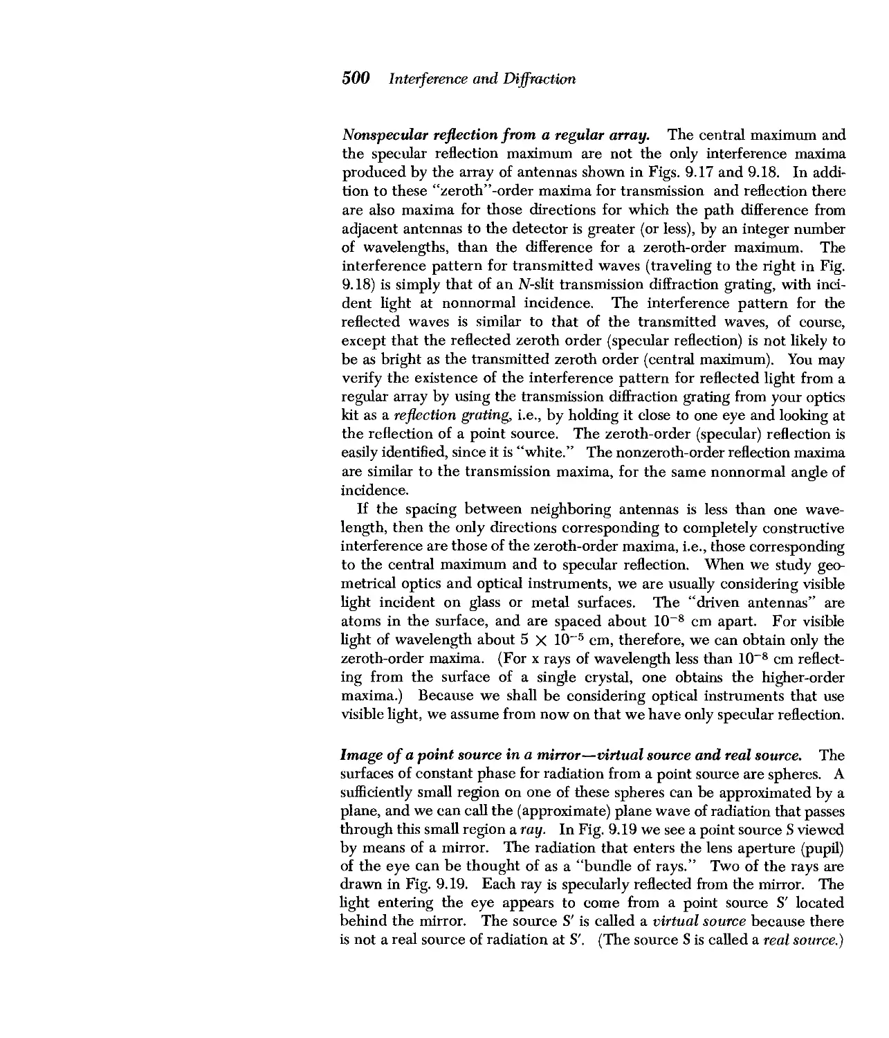
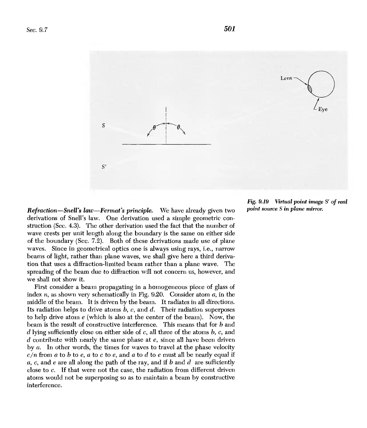
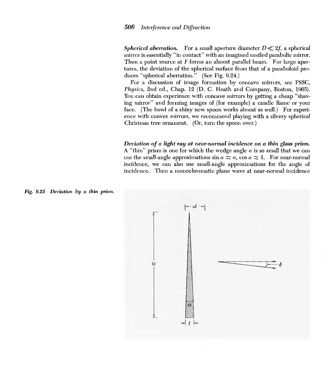
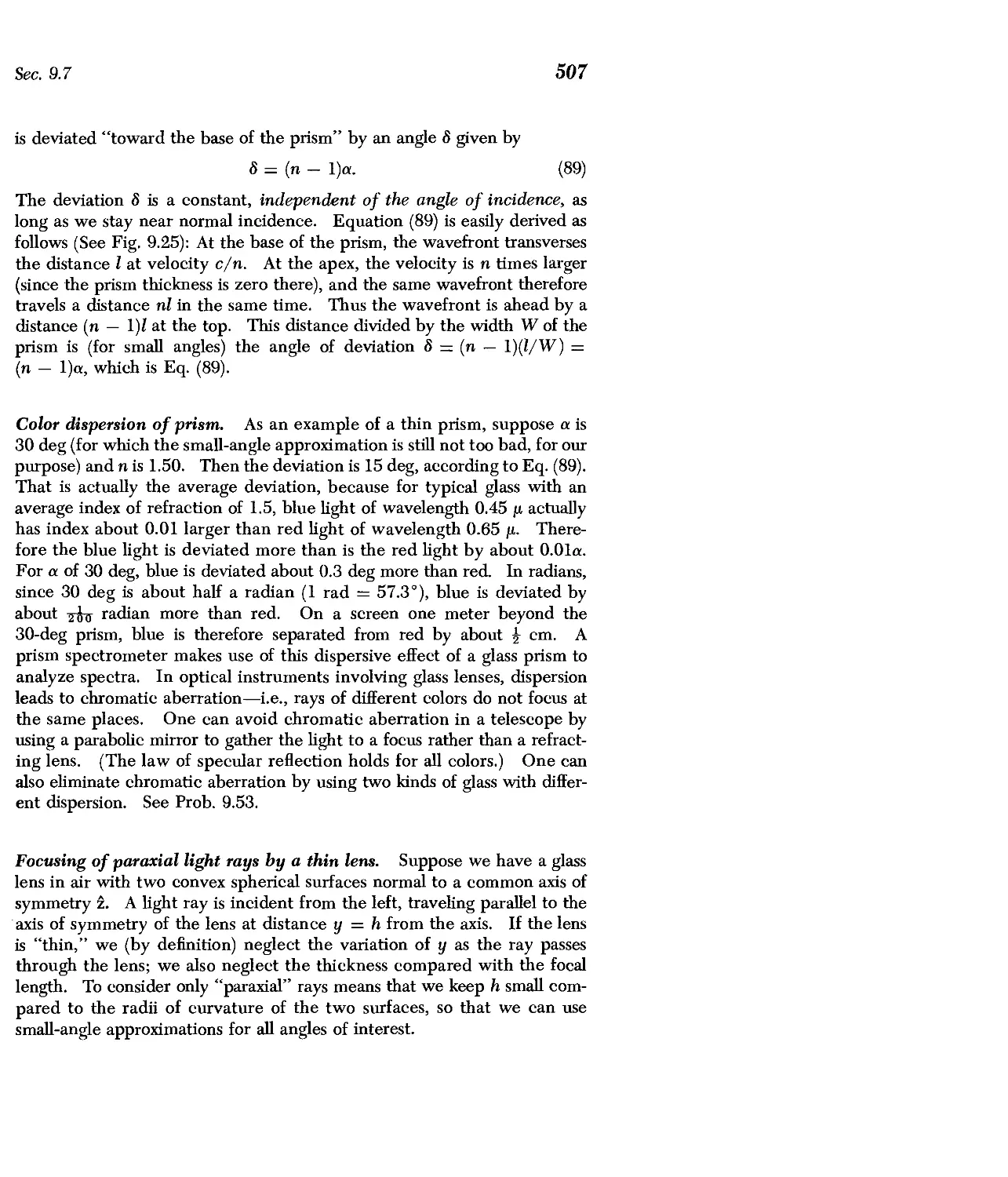
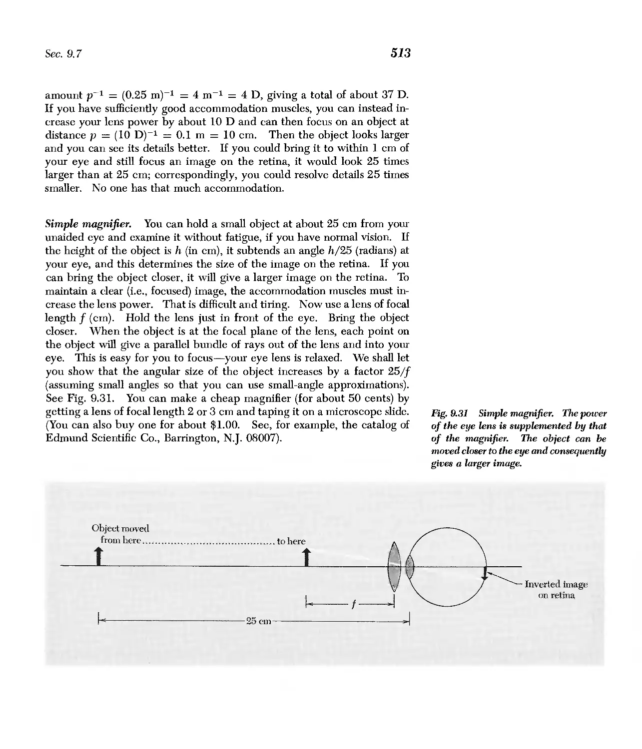
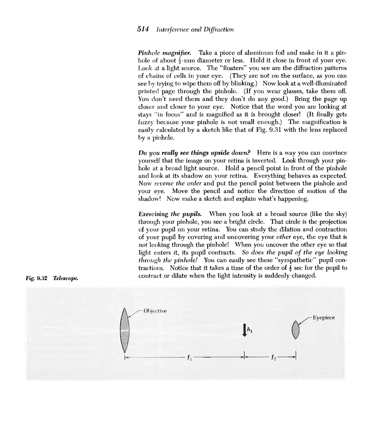
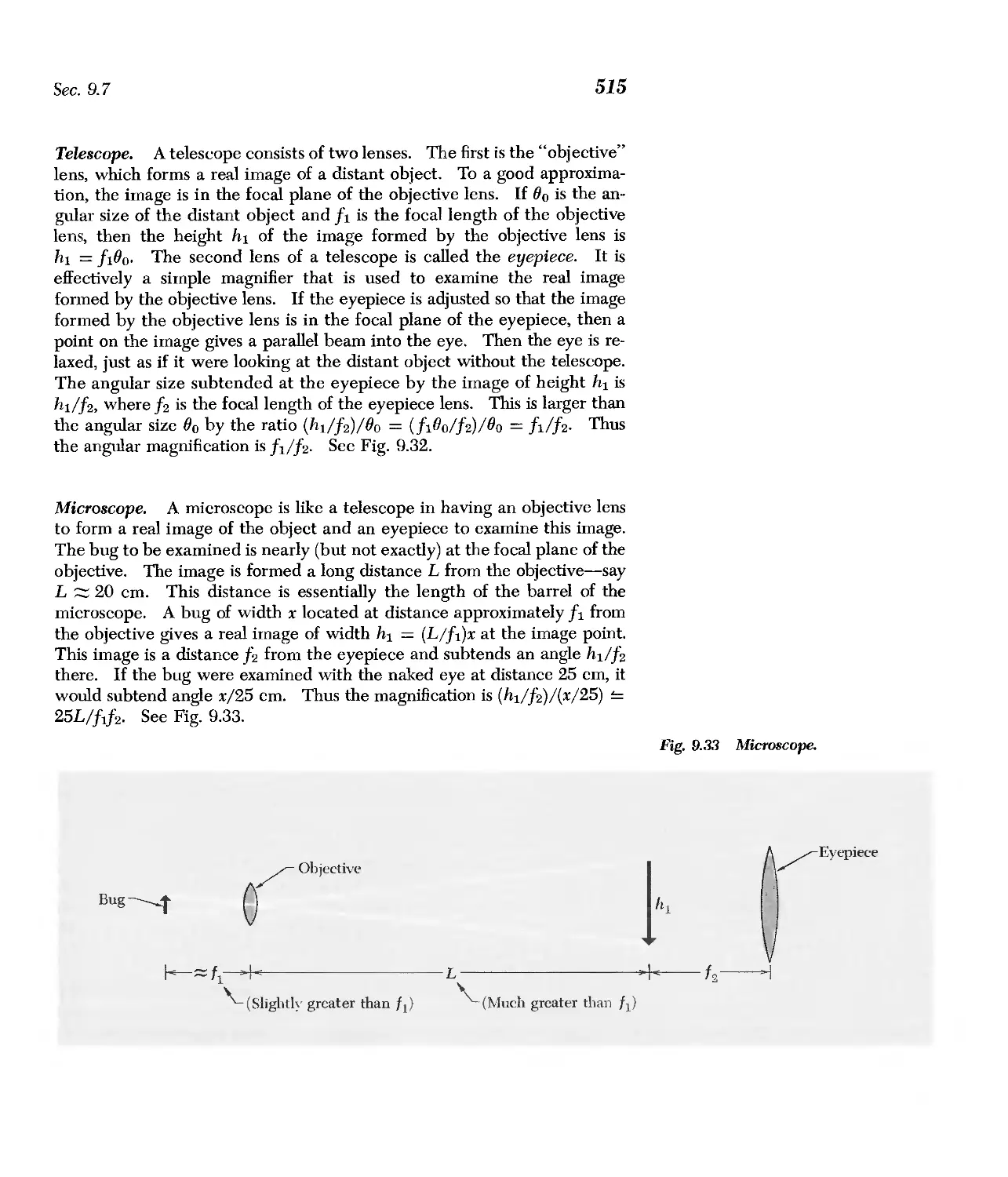
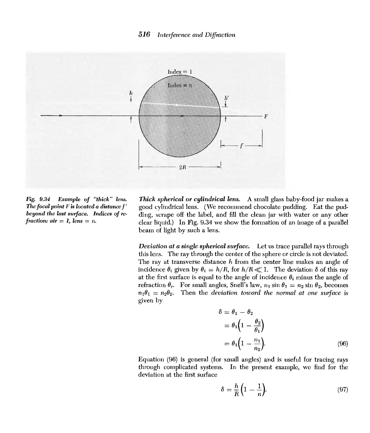
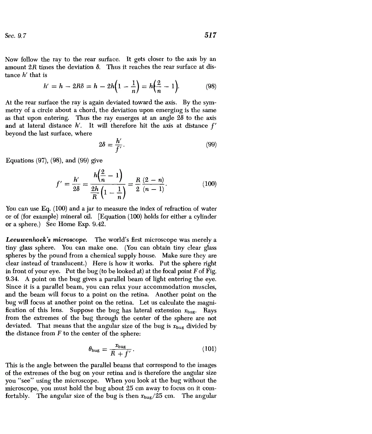
9.7 Geometrical Optics 498
Problems and Home Experiments 519
Supplementary Topics 545
1 "Microscopic" Examples of Weakly Coupled Identical
Oscillators 546
2 Dispersion Relation for de Broglie Waves 548
3 Penetration of a "Particle" into a "Classically Forbidden" Region of
Space 552
4 Phase and Croup Velocities for de Broglie Waves 555
5 Wave Equations for de Broglie Waves 556
6 Electromagnetic Radiation from a One-dimensional "Atom" 557
7 Time Coherence and Optical Beats 558
8 Why Is the Sky Bright? 559
9 Electromagnetic Waves in Material Media 563
Appendices 585
Supplementary Reading 591
Index 593
Optics Kit, Tables of Units, Values, and Useful Constants and
Identities Inside covers
Optical Spectra following page 528
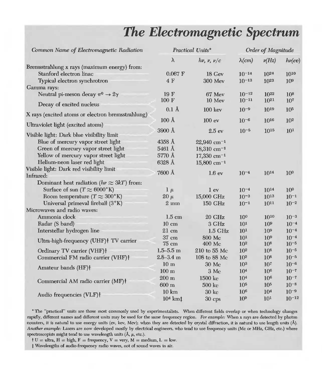
The Electromagnetic Spectrum
Comnwn Name of Electromagnetic Radiation Practical Units° Order of Magnitude
"A hv, v, vie "A(cm) v(Hz) hv( ev)
Bremsstrahlung x rays (maximum energy) from:
Stanford electron linac 0.067 F 18 Gev 10- 14 10 24 1010
Typical electron synchrotron 4F 300 Mev 10- 13 10 23 10 9
Gamma rays:
Neutral pi-meson decay wO 2y 19 F 67 Mev 10- 12 10 22 10 8
Decay of excited nucleus 100F 10 Mev 10- 11 10 21 10 7
0.1 A. 100 key 10- 9 10 19 1()5
X rays (excited atoms or electron bremsstrahlung) 100 A
100 ev 10- 6 10 16 10 2
Ultraviolet light (excited atoms) 3900 A
Visible light: Dark blue visibility limit 2.5 ev 10- 5 10 15 10 1
Blue of mercury vapor street light 4358 A 22,940 cm- 1
Green of mercury vapor street light 5461 A 18,310 cm- 1
Yellow of mercury vapor street light 5770 A 17,330 cm- 1
Helium-neon laser red light 6328 A 15,800 cm- 1
Visible light: Dark red visibility limit 7600 A 1.6 ev 10- 4 10 14 10°
Infrared:
Dominant heat radiation (hv;:::; 3kT) from:
Surface of sun (T;:::; 6000 0 K) 1fL 1 ev 10- 4 10 14 10°
Room temperature (T;:::; 300 0 K) 20 fL 15,000 GHz 10- 3 10 13 10- 1
Universal primeval fireball (3°K) 2mm 150 GHz 10- 1 1011 10- 2
Microwaves and radio waves:
Ammonia clock 1.5cm 20 GHz 10° 1010 10- 3
Radar (S band) lOcm 3GHz 10 1 10 9 10- 4
Interstellar hydrogen line 21cm 1.5 GHz 10 1 10 9 10- 4
Ultra-high-frequency (UHF)t TV carrier 37 cm 800 Mc 10 1 10 9 10- 4
75cm 400 Mc 10 2 10 8 10- 5
Ordinary TV carrier (VHF) t 1.5-5.5 m 210 to 55 Mc 10 2 10 8 10- 5
Commercial FM radio carrier (VHF) t 2.8-3.4 m 108 to 88 Mc 10 2 lOS 10- 5
Amateur bands (HF)t 10m 30Mc 10 3 10 7 10- 6
100m 3Mc 1()4 10 6 10- 7
Commercial AM radio carrier (MF)t 200m 1500 kc 10 4 10 6 10- 7
600m 500 kc 10 5 10 5 10- 8
Audio frequencies (VLF)t lOkm 30kc 10 6 10 4 10- 9
10 4 kmt 30 cps 10 9 10 1 10- 12
. The "practical" units are those most commonly used by experimentalists. When different fields overlap or when technology changes
rapidly, different names and different units may be used for the same frequency region. For example: When x rays are detected by photon
counters, it is natural to use energy units (ev, kev, Mev); when they are detected by crystal diffraction, it is natural to use length units (A).
Another example: Lasers are now developed mostly by electrical engineers, who tend to use frequency units (Mc or MHz, GHz, etc.) where
spectroscopists might tend to use wavelength units (A, p., etc.).
f U = ultra, H = high. F = frequency, V = very, M = medium, L = low.
* Wavelengths of audio-frequency radio waves, not of sound waves in air.
waves
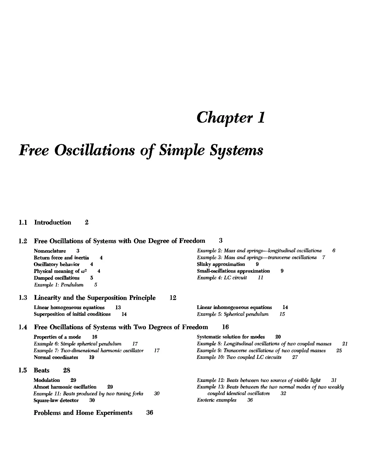
Chapter 1
Free Oscillations of Simple Systems
1.1 Introduction 2
1.2 Free Oscillations of Systems with One Degree of Freedom 3
Nomenclature 3 Example 2: Mass and springs-longitudinal oscillations 6
Return force and inertia 4 Example 3: Mass and springs-transverse oscillations 7
Oscillatory behavior 4 Slinky approximation 9
Physical meaning of ",2 4 Small-oscillations approximation 9
Damped oscillations 5 Example 4: LC circuit 11
Example 1: Pendulum 5
1.3 Linearity and the Superposition Principle
Linear homogeneous equations 13
Superposition of initial conditions 14
12
Linear inhomogeneous equations 14
Example 5: Spherical pendulum 15
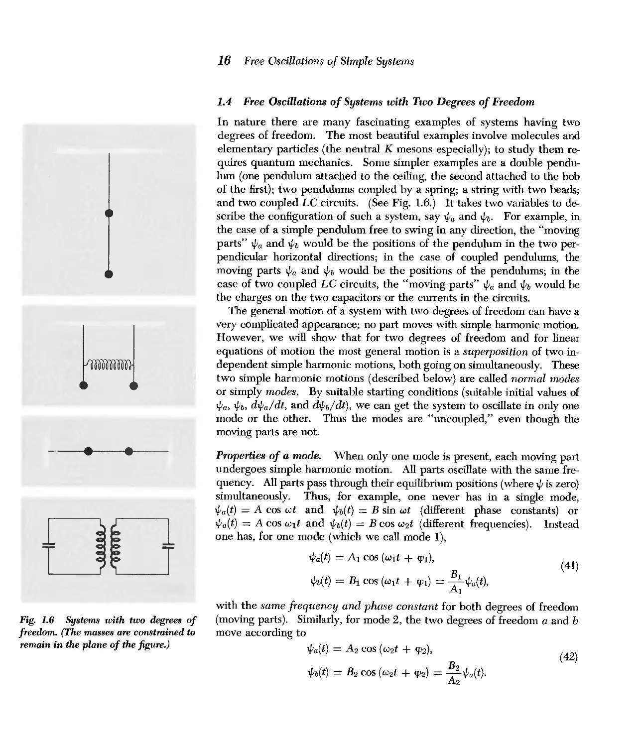
1.4
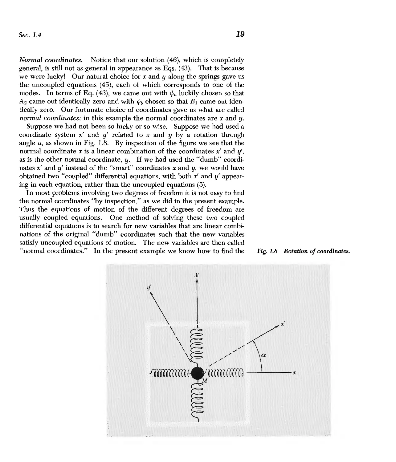
Free Oscillations of Systems with Two Degrees of Freedom 16
Properties of a mode 16 Systematic solution for modes 20
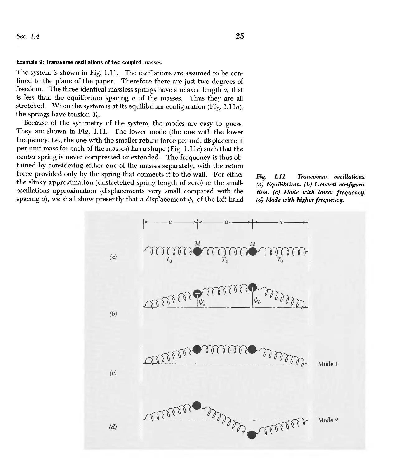
Example 6: Simple spherical pendulum 17 Example 8: Longitudinal oscillations of two coupled masses
Example 7: Two-dimensional harmonic oscillator 17 Example 9: Transverse oscillations of two coupled masses
Nonnal coordinates 19 Example 10: Two coupled LC circuits 27
21
25
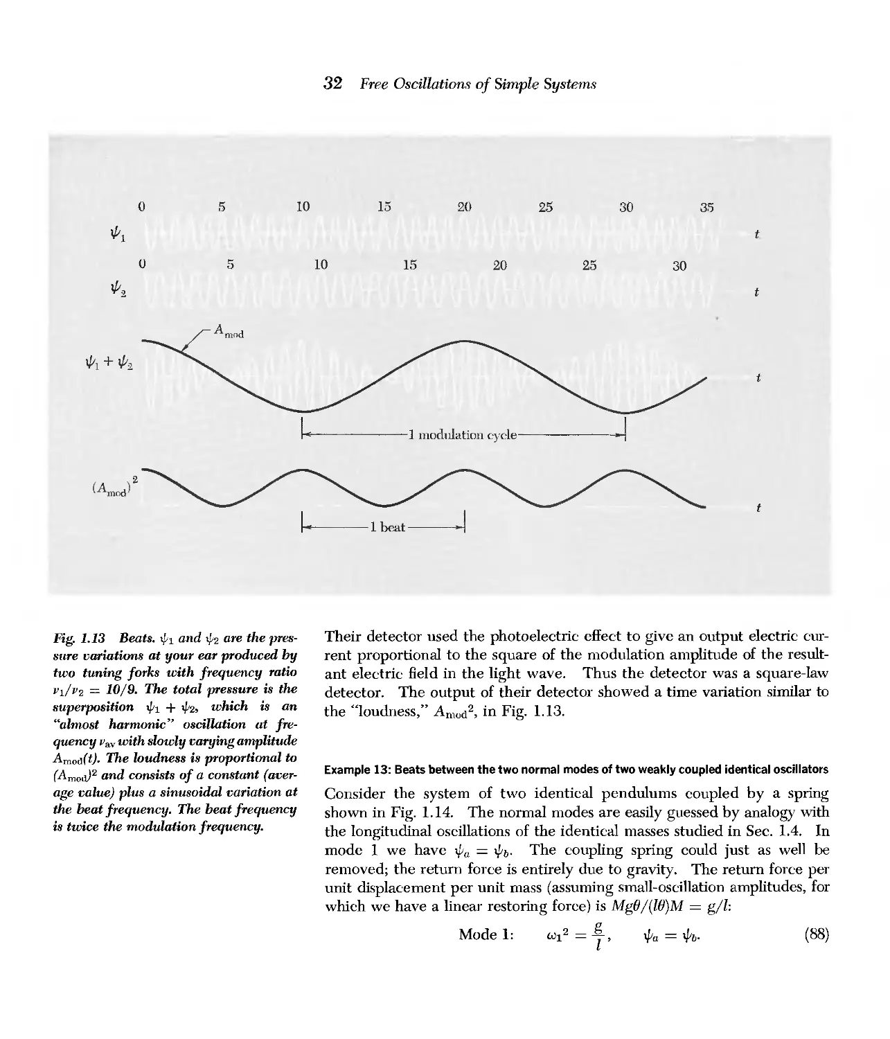
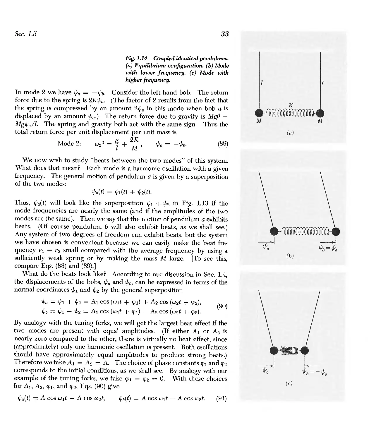
1.5 Beats 28
Modulation 29
Almost harmonic oscillation 29
Example 11: Beats produced by two tuning forks
Square-law detector 30
30
Example 12: Beats between two sources of visible light 31
Example 13: Beats between the two nonnal modes of two weakly
coupled identical oscillators 32
Esoteric examples 36
Problems and Home Experiments 36
Chapter 1
Free Oscillations of Simple Systems
1.1 Introduction
The world is full of things that move. Their motions can be broadly cate-
gorized into two classes, according to whether the thing that is moving
stays near one place or travels from one place to another. Examples of the
first class are an oscillating pendulum, a vibrating violin string, water slosh-
ing back and forth in a cup, electrons vibrating (or whatever they do)
in atoms, light bouncing back and forth between. the mirrors of a laser.
Parallel examples of traveling motion are a sliding hockey puck, a pulse
traveling down a long stretched rope plucked at one end, ocean waves roll-
ing toward the beach, the electron beam of a TV tube; a ray of light
emitted at a star and detected at your eye. Sometimes the same phenom-
enon exhibits one or the other class of motion (i.e., standing still on the
average, or traveling) depending on your point of view: the ocean waves
travel toward the beach, but the water (and the duck sitting on the surface)
goes up and down (and also forward and backward) without traveling.
The displacement pulse travels down the rope, but the material of the rope
vibrates without traveling.
We begin by studying things that stay in one vicinity and oscillate or vi-
brate about an average position. In Chaps. 1 and 2 we shall study many
examples of the motion of a closed system that has been given an initial
excitation (by some external disturbance) and is thereafter allowed to oscil-
late freely without further influence. Such oscillations are called free or
natural oscillations. In Chap. 1 study of these simple systems having one
or two moving parts will form the basis for our understanding of the free
oscillations of systems with many moving parts in Chap. 2. There we shall
find that the motion of a complicated system having many moving parts
may always be regarded as compounded from simpler motions, called
modes, all going on at once. No matter how complicated the system, we
shall find that each one of its modes has properties very similar to those of
a simple harmonic oscillator. Thus for motion of any system in a single
one of its modes, we shall find that each moving part experiences the same
return force per unit mass per unit displacement and that all moving parts
oscillate with the same time dependence cos (wt + cp), i.e., with the same
frequency wand the same phase constant cpo
Each of the systems that we shall study is described by some physical
quantity whose displacement from its equilibrium value varies with position
in the system and time. In the mechanical examples (involving moving
parts which are point masses subject to return forces), the physical quantity
is the displacement of the mass at the point x,y,z from its equilibrium posi-
Sec. 1.2
tion. The displacement is described by a vector lJ;(x,y,x,t). Sometimes we
call this vector function of x, y, z, t a wave function. (It is only a contin-
uous function of x, y, and z when we can use the continuous approxima-
tion, i.e., when near neighbors have essentially the same motion.) In some
of the electrical examples, the physical quantity may be the current in a
coil or the charge on a capacitor. In others, it may be the electric field
E(x,y,z,t) or the magnetic field B(x,y,z,t). In the latter cases, the waves are
called electromagnetic waves.
1.2 Free Oscillations of Systems with One Degree of Freedom
We shall begin with things that stay in one vicinity, oscillating or vibrating
about an average position. Such simple systems as a pendulum oscillating
in a plane, a mass on a spring, and an LC circuit, whose configuration at
any time can be completely specified by giving a single quantity, are said
to have one degree of freedom-loosely speaking, one moving part (see
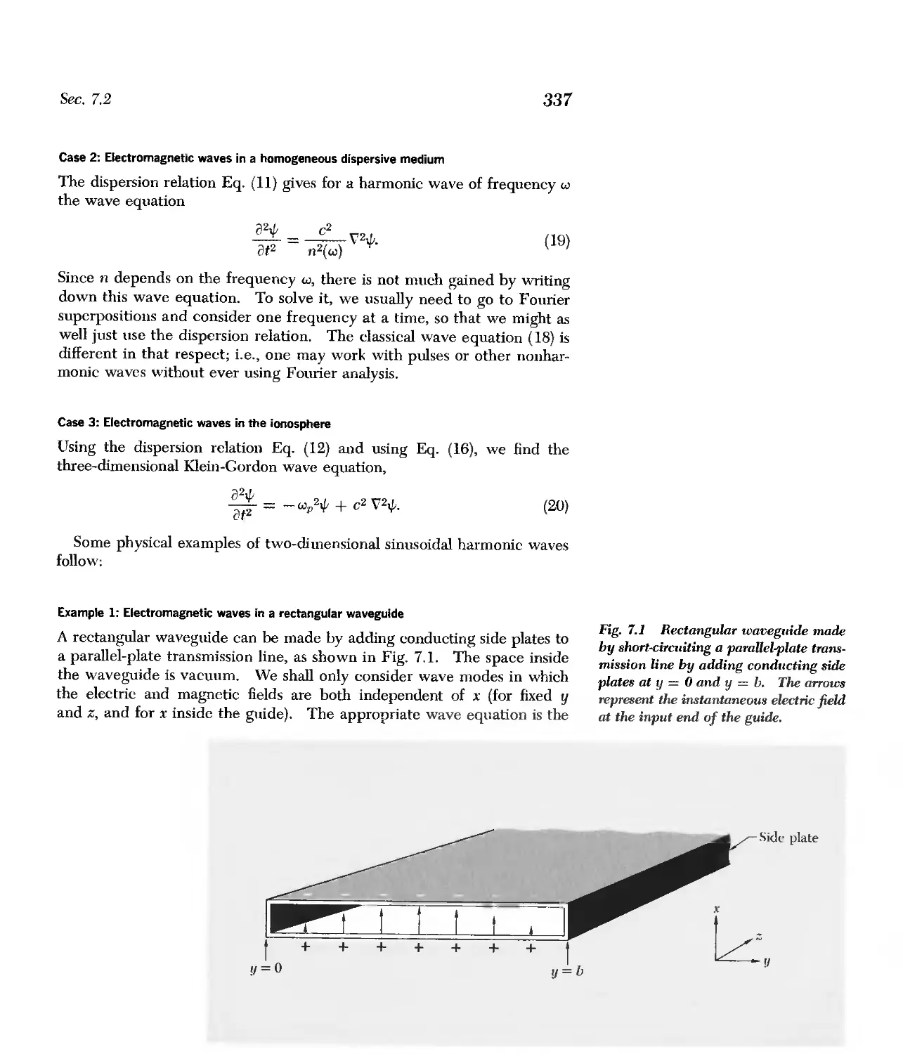
Fig. 1.1). For example, the swinging pendulum can be described by the
angle that the string makes with the vertical, and the LC circuit by the
charge on the capacitor. (A pendulum free to swing in any direction, like
a bob on a string, has not one but two degrees of freedom; it takes two co-
ordinates to specify the position of the bob. The pendulum on a grand-
father clock is constrained to swing in a plane, and thus has only one de-
gree of freedom.)
For all these systems with one degree of freedom, we shall find that the
displacement of the "moving part" from its equilibrium value has the
same simple time dependence (called harmonic oscillation),
1/;(t) = A cos (wt + rp).
For the oscillating mass, 1/; may represent the displacement of the mass from
its equilibrium position; for the oscillating LC circuit, it may represent the
current in the inductor or the charge on the capacitor. More precisely, we
shall find Eq. (1) gives the time dependence provided the moving part does
not move too far from its equilibrium position. [For large-angle swings of
a pendulum, Eq. (1) is a poor approximation to the motion; for large exten-
sions of a real spring, the return force is not proportional to the extension,
and the motion is not given by Eq. (1); a large enough charge on a capaci-
tor will cause it to "break down" by sparking between the plates, and the
charge will not satisfy Eq. (1).]
Nomenclature. We use the following nomenclature with Eq. (1): A is a
positive constant called the amplitude; w is the anglliarfreqllency, measured
in radians per second; v = w/2'lT is the frequency, measured in cycles per
3
(1)
, i
JUUUUOUUOOOOUd.
x
1
Q
c
-Q
L
Fig. 1.1 Systems with one degree of
freedom. (The pendulum is constrained
to swing in a plane.)
4 Free Oscillations of Simple Systems
second, or hertz (abbreviated cps, or Hz). The inverse of v is called the
period T, which is given in seconds per cycle:
1
T=-.
v
(2)
The phase constant cp corresponds to the choice of the zero of time. Often
we are not particularly interested in the value of the phase constant. In
these cases we can always "reset the clock," so that cp becomes zero, and
then we write 1f; = A cos wt or 1f; = A sin wt, instead of the more general
Eq. (1).
Return force and inertia. The oscillatory behavior represented by Eq. (1)
always results from the interplay of two intrinsic properties of the physical
system which have opposite tendencies: return force and inertia. The "re-
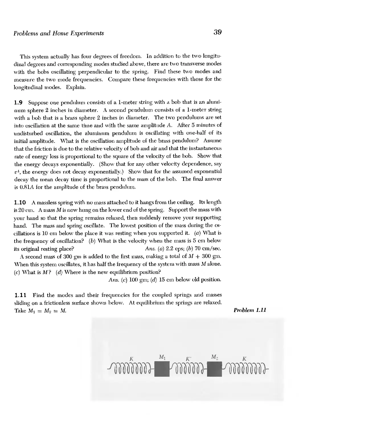
turn force" tries to return 1f; to zero by imparting a suitable "velocity"
d1f; / dt to the moving part. The greater 1f; is, the stronger the return force.
For the oscillating LC circuit, the return force is due to the repulsive force
between the electrons, which makes the electrons prefer not to crowd onto
one of the capacitor plates, but rather to distribute themselves equally on
each plate, giving zero charge. The second property, "inertia," "opposes"
any change in d1f;/dt. For the oscillating LC circuit, the inertia is due to
the inductance L, which opposes any change in the current d1f; / dt (letting
1f; stand for the charge on the capacitor).
Oscillatory behavior. If we start with 1f; positive and d1f;/dt zero, the re-
turn force gives an acceleration which induces a negative velocity. By the
time 1f; returns to zero, the negative velocity is maximum. The return force
is zero at 1f; = 0, but the negative velocity now induces a negative displace-
ment. Then the return force becomes positive, but it must now overcome
the inertia of the negative velocity. Finally, the velocity c#/dt is zero, but
by that time the displacement is large and negative, and the process reverses.
This cycle goes on and on: the return force tries to restore 1f; to zero; in so
doing, it induces a velocity; the inertia preserves the velocity and causes 1f;
to "overshoot." The system oscillates.
Physical meaning of ",2. The angular frequency of oscillation w is related
to the physical properties of the system in every case (as we shall show) by
the relation
w 2 = return force per unit displacement per unit mass. (3)
Sometimes, as in the case of the electrical examples (LC circuit), the "iner-
tial mass" may not actually be mass.
Sec. 1.2
Damped oscillations. If left undisturbed, an oscillating system will con-
tinue to oscillate forever in accordance with Eq. (1). However, in any real
physical situation, there are "frictional," or "resistive," processes which
"damp" the motion. Thus a more realistic description of an oscillating
system is given by a "damped oscillation." If the system is "excited" into
oscillation at t = 0 (by giving it a bump or closing a switch or something),
we find (see Vol. I, Chap. 7, page 209)
1f;(t) = Ae-t/2T cos (wt + cp), (4)
for t :> 0, with the understanding that 1/; is zero for t < O. For simplicity
we shall use Eq. (1) instead of the more realistic Eq. (4) in the examples
that follow. We are thus neglecting friction (or resistance in the case of
the LC circuit) by taking the decay time T to be infinite.
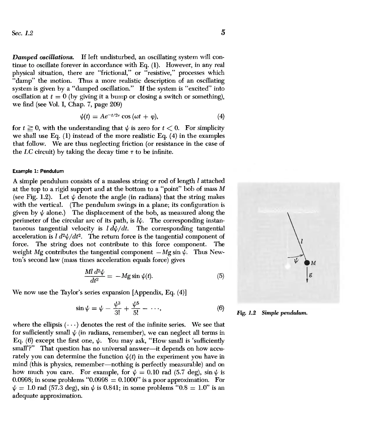
Example 1: Pendulum
A simple pendulum consists of a massless string or rod of length 1 attached
at the top to a rigid support and at the bottom to a "point" bob of mass M
(see Fig. 1.2). Let 1/; denote the angle (in radians) that the string makes
with the vertical. (The pendulum swings in a plane; its configuration is
given by 1/; alone.) The displacement of the bob, as measured along the
perimeter of the circular arc of its path, is l1/;. The corresponding instan-
taneous tangential velocity is 1 d1/; / dt. The corresponding tangential
acceleration is 1 d 2 1/;/dt 2 . The return force is the tangential component of
force. The string does not contribute to this force component. The
weight Mg contributes the tangential component -Mg sin 1/;. Thus New-
ton's second law (mass times acceleration equals force) gives
M d21/; = -Mgsin1/;(t).
t 2
We now use the Taylor's series expansion [Appendix, Eq. (4)]
. 1/;3 1/;5
sm 1/; = 1/; - 3f + 51 - ...,
where the ellipsis ( . . .) denotes the rest of the infinite series. We see that
for sufficiently small1/; (in radians, remember), we can neglect all terms in
Eq. (6) except the first one,1/;. You may ask, "How small is 'sufficiently
small'?" That question has no universal answer-it depends on how accu-
rately you can determine the function tJ;(t) in the experiment you have in
mind (this is physics, remember-nothing is perfectly measurable) and on
how much you care. For example, for 1/; = 0.10 rad (5.7 deg), sin 1/; is
0.0998; in some problems "0.0998 = 0.1000" is a poor approximation. For
1/; = 1.0 rad (57.3 deg), sin 1/; is 0.841; in some problems "0.8 = 1.0" is an
adequate approximation.
5
(5)
M
!g
(6)
Fig. 1.2 Simple pendulum.
r a o1
1))))])-
r ao 1
])))}
M
I
I
(a)
I, a . >1' a
AI
JUUUUUUi)1OUUUUUd-
I
(b)
2a-'>'
I" z > I ( "I
M
/011111111»1-
1- \ltj
z-
(c)
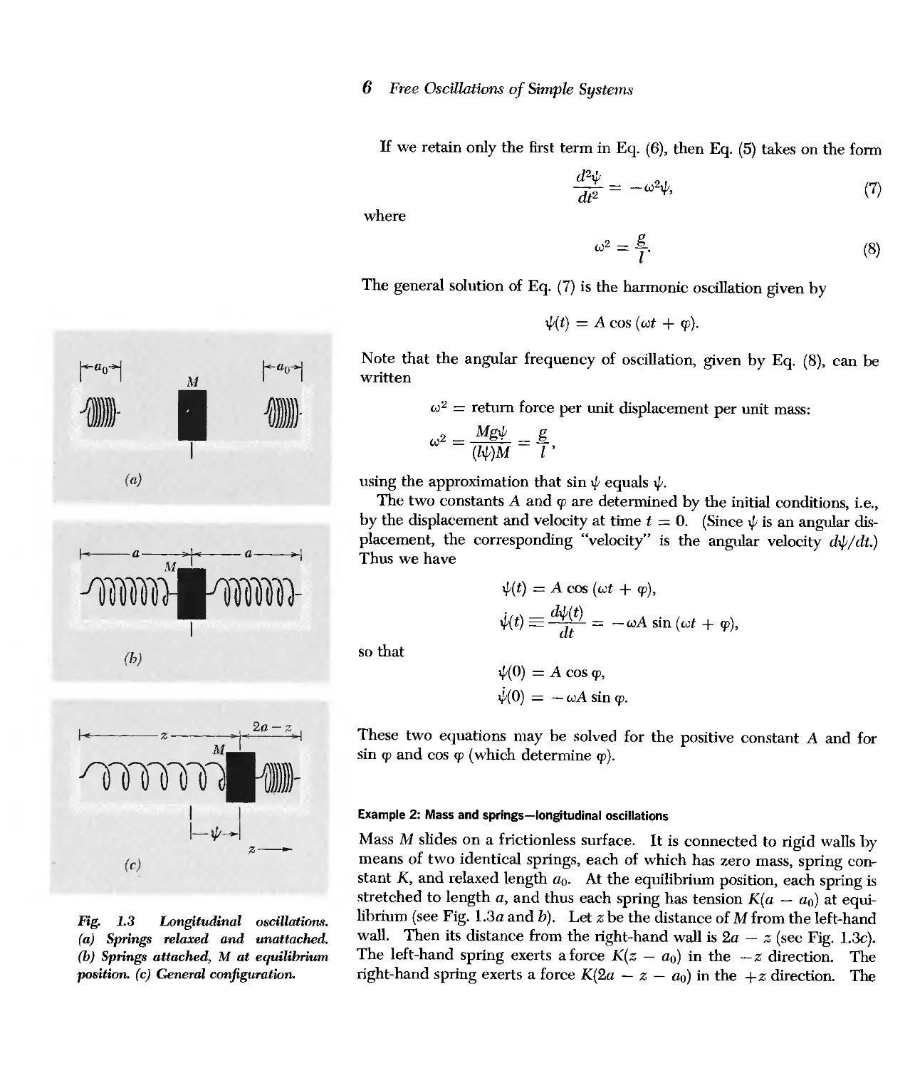
Fig. 1.3 Longitudinal oscillations.
(a) Springs relaxed and unattached.
(b) Springs attached, M at equilibrium
position. (c) General configuration.
6 Free Oscillations of Simple Systems
If we retain only the first term in Eq. (6), then Eq. (5) takes on the fonn
d 2 tJ;
dt 2 = - w 2 tJ;, (7)
where
w2 = if.
l
(8)
The general solution of Eq. (7) is the harmonic oscillation given by
tJ;(t) = A cos (wt + cp).
Note that the angular frequency of oscillation, given by Eq. (8), can be
written
w 2 = return force per unit displacement per unit mass:
2 _ MgtJ; _ g
w - (ltJ;)M - T'
using the approximation that sin tJ; equals tJ;.
The two constants A and cp are determined by the initial conditions, i.e.,
by the displacement and velocity at time t = O. (Since tJ; is an angular dis-
placement, the corresponding "velocity" is the angular velocity dtJ;/dt.)
Thus we have
tJ;(t) = A cos (wt + cp),
(t) _ d t) = -wA sin (wt + cp),
so that
tJ;(0) = A cos cp,
(O) = - wA sin cpo
These two equations may be solved for the positive constant A and for
sin cp and cos cp (which determine cp).
Example 2: Mass and springs-longitudinal oscillations
Mass M slides on a frictionless surface. It is connected to rigid walls by
means of two identical springs, each of which has zero mass, spring con-
stant K, and relaxed length ao. At the equilibrium position, each spring is
stretched to length a, and thus each spring has tension K(a - ao) at equi-
librium (see Fig. 1.3a and b). Let z be the distance of M from the left-hand
wall. Then its distance from the right-hand wall is 2a - z (see Fig. 1.3c).
The left-hand spring exerts a force K(z - ao) in the -z direction. The
right-hand spring exerts a force K(2a - z - ao) in the +z direction. The
Sec. 1.2
7
total force Fz in the +z direction is the superposition (sum) of these two
forces:
Fz = - K(z - ao) + K(2a - z - ao)
-2K(z - a).
Newton's second law then gives
Md 2 z
- = Fz = -2K(z - a).
dt 2
The displacement from equilibrium is z - a. We designate this by 1f;(t):
(9)
1f;(t) z(t) - a.
then
d 2 1f; d 2 z
dt 2 - dt 2 .
Now we can write Eq. (9) in the form
d 2 1f;
dt 2
-w 2 1f;,
(10)
with
2 2K
w =-.
M
(ll)
The general solution of Eq. (10) is again the harmonic oscillation
1f; = A cos (wt + cp). Note that Eq. (ll) has the form w 2 = force per unit
displacement per unit mass, since the return force is 2K1f; for a displace-
ment 1f;.
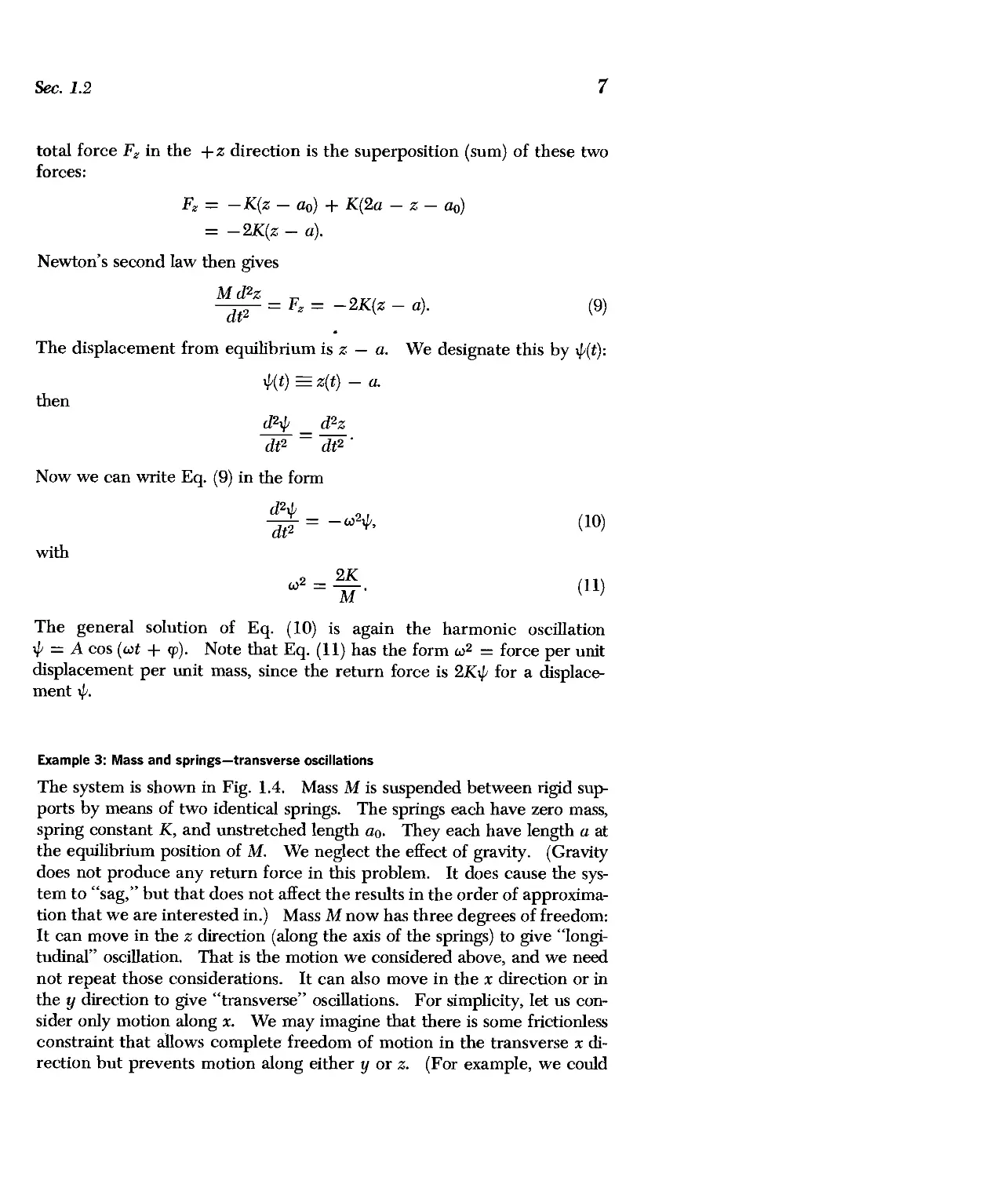
Example 3: Mass and springs-transverse oscillations
The system is shown in Fig. 1.4. Mass M is suspended between rigid sup-
ports by means of two identical springs. The springs each have zero mass,
spring constant K, and unstretched length ao. They each have length a at
the equilibrium position of M. We neglect the effect of gravity. (Gravity
does not produce any return force in this problem. It does cause the sys-
tem to "sag," but that does not affect the results in the order of approxima-
tion that we are interested in.) Mass M now has three degrees of freedom:
It can move in the z direction (along the axis of the springs) to give "longi-
tudinal" oscillation. That is the motion we considered above, and we need
not repeat those considerations. It can also move in the x direction or in
the y direction to give "transverse" oscillations. For simplicity, let us con-
sider only motion along x. We may imagine that there is some frictionless
constraint that allows complete freedom of motion in the transverse x di-
rection but prevents motion along either y or z. (For example, we could
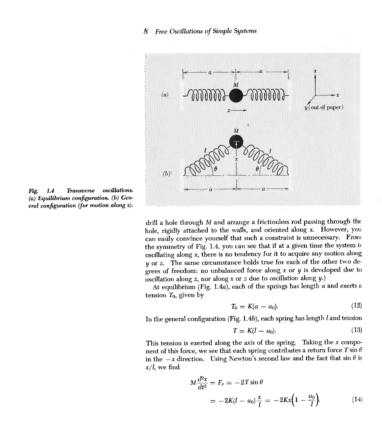
Fig. 1.4 Transverse oscillations.
(a) Equilibrium configuration. (b) Gen-
eral configuration (for motion along x).
8 Free Oscillation<; of Simple Systems
ia),
t[ a, :\1 c, ' a r
}.i
d]uooooo)-e11ooooo}-
}-,
Y,( outo{ pap!"!)
-------
'(b)f
M
J '
\) , , (/ "
-, - -
11 " :>,1"
<
a"
'" ? .....,
drill a hole through M and arrange a frictionless rod passing through the
hole, rigidly attached to the walls, and oriented along x. However, you
can easily convince yourself that such a constraint is unnecessary. From
the symmetry of Fig. 1.4, you can see that if at a given time the system is
oscillating along x, there is no tendency for it to acquire any motion along
y or z. The same circumstance holds true for each of the other two de-
grees of freedom: no unbalanced force along x or y is developed due to
oscillation along z, nor along x or ;:; due to oscillation along y.)
At equilibrium (Fig. 1.4a), each of the springs has length a and exerts a
tension To, given by
To = K(a - ao).
(12)
In the general configuration (Fig. lAb), each spring has length 1 and tension
T = K(l - ao).
(13)
This tension is exerted along the axis of the spring. Taking the x compo-
nent of this force, we see that each spring contributes a return force T sin B
in the -x direction. Using Newton's second law and the fact that sin B is
xll, we find
d 2 x .
M- d = Fa; = -2TsmB
t 2
= -2K(l - ao) = -2KX( 1 _ o ).
(14)
Sec. 1.2
9
Equation (14) is exact, under our assumptions (including the assumption,
expressed by Eq. (13), that the spring is a "linear" or "Hooke's law" spring).
Notice that the spring length 1 which appears on the right side of Eq. (14)
is a function of x. Therefore Eq. (14) is not exactly of the form that gives
rise to harmonic oscillations, because the return force on M is not exactly
linearly proportional to the displacement from equilibrium, x.
Slinky approximation. There are two interesting ways in which we can
obtain an approximate equation with a linear restoring force. The first way
we shall call the slinky approximation, in which we neglect ao/ a compared
to unity. Hence, since 1 is always greater than a, we neglect ao/l in Eq. (14).
[A slinky is a helical spring with relaxed length ao about 3 inches. It can
be stretched to a length a of about 15 feet without exceeding its elastic
limit. That would give ao/a < 1/60 in Eq. (14).] Using this approxima-
tion, we can write Eq. (14) in the form
d 2 x
dt 2
-w 2 x,
(15)
with
w 2 = 2K = 2To
M Ma
(for ao = 0).
(16)
This has the solution x = A cos (wt + cp), i.e., harmonic oscillation. Notice
that there is no restriction on the amplitude A. We can have "large" oscil-
lations and still have pedect linearity of the return force. Notice also that
the frequency for transverse oscillations, as given by Eq. (16), is the same
as that for longitudinal oscillations, as given by Eq. (11). That is not true
in general. It holds only in the slinky approximation, where we effectively
take ao = O.
Small-oscillations approximation. If ao cannot be neglected with respect
to a (as is the case, for example, with a rubber rope under the conditions
ordinarily met in lecture demonstrations), the slinky approximation does
not apply. Then Fx in Eq. (14) is not linear in x. However, we shall show
that if the displacements x are small compared with the length a, then 1
differs from a only by a quantity of order a(x/a)2. In the small-oscillations
approximation, we neglect the terms in Fx which are nonlinear in x/a. Let
us now do the algebra: We want to express 1 in Eq. (14) as 1 = a + some-
thing, where "something" vanishes when x = O. Since 1 is larger than a,
whether x is positive or negative, "something" must be an even function
of x. In fact we have from Fig. 1.4
l2 = a 2 + x 2
= a 2 (1 + E),
x 2
E ---;;z .
10 Free Oscillations of Simple Systems
Thus
1- = 1- (l + t:)-(1I2)
1 a
= [1 - G t:) + ( t: 2 ) - ...],
(17)
where we have used the Taylor's series expansion [Appendix Eq. (20)] for
(1 + x)n with n = -! and x = t:. Next we make the small-oscillations
approximation. We assume we have t: <:: 1 and discard the higher-order
terms in the infinite series of Eq. (17). (Eventually we shall drop every-
thing except the first term, l/a.) Thus we have
[ 1 - G t:)]
= [I- G:: )J
(18)
Inserting Eq. (18) into Eq. (14), we find
d 2 x = _ 2KX ( 1 _ ao )
dt 2 M 1
= - 2 X {I - [1 - G :: ) + ...]}
_ 2K (a _ ao)x + ao ( ) 3 + ....
Ma M a
(19)
Discarding the cubic and higher-order terms, we obtain
d 2 x 2K 2 Tox
- --(a - ao)x = --.
dt 2 Ma Ma
(20)
[In the second equality of Eq. (20), we used To as given by Eq. (12).]
Equation (20) is of the form
d 2 x
dt 2
-w 2 x,
with
2 _ 2To
w _-.
Ma
Therefore x( t) is given by the harmonic oscillation
x(t) = A cos (wt + cp).
Notice that w 2 given by Eq. (21) is the return force per unit displacement
per unit mass: for small oscillations, the return force is the tension To times
sin 0, which is x/a, times two (two springs). The displacement is x; the
(21)
Sec. 1.2
mass is M. Thus the return force per unit displacement per unit mass is
2 To(x/a)/xM.
Notice that the frequency for transverse oscillations is given by w 2 =
2To/Ma for both the case of the slinky approximation (ao = 0) and the
small-oscillations approximation (x/a < 1), as we see by comparing Eqs.
(16) and (21). In the slinky approximation, the longitudinal oscillation also
has this same frequency, as we see from Eqs. (ll) and (16). If the slinky
approximation does not hold (i.e., if ao/ a cannot be neglected), then the
longitudinal oscillations and (small) transverse oscillations do not have the
same frequency, as we see from Eqs. (ll), (12), and (21). In this case,
( 2 ) _ 2Ka
W long - -,
Ma
(22)
( 2 ) _ 2To
W tr - -,
Ma
Thus for small oscillations of a rubber rope (where ao/a cannot be neglected),
the longitudinal oscillations are more rapid than the transverse oscillations:
To = K(a - ao).
(23)
Wiong 1
- [ ao ] 1I2.
I--
a
Example 4: LC circuit
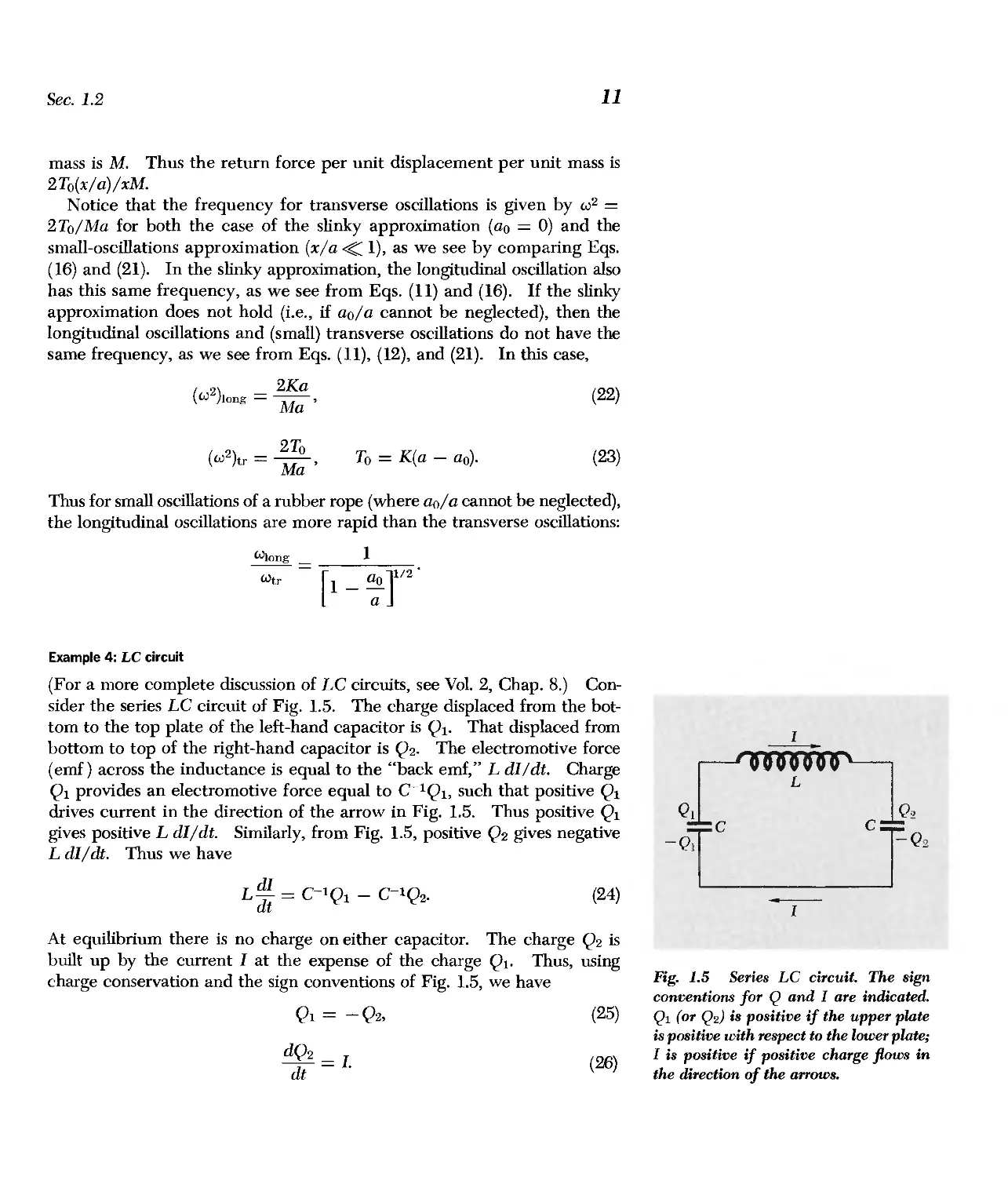
(For a more complete discussion of LC circuits, see Vol. 2, Chap. 8.) Con-
sider the series LC circuit of Fig. 1.5. The charge displaced from the bot-
tom to the top plate of the left-hand capacitor is Ql. That displaced from
bottom to top of the right-hand capacitor is Q2. The electromotive force
(emf) across the inductance is equal to the "back emf," L dIl dt. Charge
Ql provides an electromotive force equal to C lQl, such that positive Ql
drives current in the direction of the arrow in Fig. 1.5. Thus positive Ql
gives positive L dI/dt. Similarly, from Fig. 1.5, positive Q2 gives negative
L dI/ dt. Thus we have
dI _ _
L- = C lQl - C lQ2.
dt
(24)
At equilibrium there is no charge on either capacitor. The charge Q2 is
built up by the current I at the expense of the charge Ql. Thus, using
charge conservation and the sign conventions of Fig. 1.5, we have
Ql = -Q2,
dQ2 = 1.
dt
(25)
(26)
11
I
L
QI Q2
- QT C C Y Q '
-
I
Fig. 1.5 Series LC circuit. The sign
conventions for Q and I are indicated.
Q1 (or Q2) is positive if the upper plate
is positive with respect to the lower plate;
I is positive if positive charge flows in
the direction of the arrows.
12 Free Oscillations of Simple Systems
Because of Eqs. (25) and (26), there is only one degree of freedom. We
can describe the instantaneous configuration of the system by giving Ql, or
Q2, or I. The current I will be most convenient in our later work (when
we go to systems having more than one degree of freedom), and we shall
use it here. We first use Eq. (25) to eliminate Ql from Eq. (24); then we
differentiate with respect to t and use Eq. (26) to eliminate Q2:
L dI C-I Q C-I Q 2C-I Q
dt = 1 - 2 = - 2;
L d 2 1 = -2C-l dQ2 = -2C-II.
dt 2 dt
Thus the current I(t) obeys the equation
d 2 1 = _w 2 [
dt 2 '
with
2C-l
w 2 --
- L '
(27)
and I(t) undergoes harmonic oscillation:
I(t) = A cos (wt + cp).
We can think of Eq. (27) as an illustration of the fact that w 2 is always
the "return force" per unit "displacement" per unit "inertia." We can
take the "return force" to be the electromotive force 2C-IQ, where Q is
the "charge displacement" Q2. We then take the self-inductance L to be
the "charge inertia." Then the return force per unit displacement per unit
inertia is (2C-IQ)/QL.
You may have noticed a mathematical parallelism between Examples 2,
3, and 4. We purposely gave these examples the same spatial symmetry
("inertia" in the center, "driving forces" located symmetrically on either
side) so as to produce the parallelism. Such parallelisms are often useful as
mnemonic devices.
1.3 Linearity and the Superposition Principle
In Sec. 1.2 we solved for the oscillations of the pendulum and of the mass
and springs only for the cases where we could assume the return force to
be proportional to -I/;, with (for example) no dependence on 1/;2, 1/;3, etc.
A differential equation that contains no higher than the first power of t/;, of
dt/;/dt, of d 2 1/;/dt 2 , etc., is said to be linear in I/; and its time derivatives. If,
in addition, no terms independent of I/; occur, the equation is said to be
homogeneous as well. If any higher powers of I/; or its derivatives occur in
the equation, the equation is said to be nonlinear. For example, Eq. (5) is
Sec. 1.3
13
nonlinear, as we can see from the expansion of sin 1/; given by Eq. (6). Only
when we neglect the higher powers of 1/; do we obtain a linear equation.
Nonlinear equations are generally difficult to solve. (The nonlinear pen-
dulum equation is solved exactly in Volume I, pp. 225 ff.) Fortunately,
there are many interesting physical situations for which linear equations
give a very good approximation. We shall deal almost entirely with linear
equations.
Linear homogeneous equations. Linear homogeneous differential equa-
tions have the following very interesting and important property: The sum
of any two solutions is itself a solution. Nonlinear equations do not have
that property. The sum of two solutions of a nonlinear equation is not it-
self a solution of the equation.
We shall prove these statements for both cases (linear and nonlinear) at
once. Suppose that we have found the differential equation of motion of
a system with one degree of freedom to be of the form
d 2 1/;( t)
= - C1/; + a1/;2 + {31/;3 + y1/ft + . . .,
(28)
as we found, for example, for the pendulum [Eqs. (5) and (6)] or for the
transverse oscillations of a mass suspended by springs [Eq. (19)]. If the
constants a, {3, y, etc. are all zero or can be taken to be zero as a sufficiently
good approximation, then Eq. (28) is linear and homogeneous. Otherwise,
it is nonlinear. Now suppose that 1/;l(t) is a solution of Eq. (28) and that
1/;2(t) is a different solution. For example, 1/;1 may be the solution corre-
sponding to a particular initial displacement and initial velocity of a pendu-
lum bob, and 1/;2 may correspond to different initial displacement and ve-
locity. By hypothesis 1/;1 and 1/;2 each satisfy Eq. (28). Thus we have
d 2 1/;1
----;Ii2 = - C1/;l + a1/;1 2 + {31/;1 3 + y1/;1 4 +
(29)
and
d 2 1/;2
dt 2 = -C1/;2 + a1/;2 2 + {31/;2 3 + y1/;2 4 + ....
(30)
The question of interest to us is whether or not the superposition of 1/;1 and
1/;2, defined as the sum 1/;(t) = 1/;l(t) + 1/;2(t), satisfies the same equation of
motion, Eq. (28). Do we have
d2(1/; t; 1/;2) = -c(1/;1 + 1/;2) + a(1/;l + 1/;2)2 + {3(1/;1 + 1/;2)3 + ...? (31)
The question (31) has the answer "yes" if and only if the constants a, {3,
etc. are zero. That is easily shown as follows. Add Eqs. (29) and (30).
14 Free Oscillations of Simple Systems
The sum gives Eq. (31) if and only if all the following conditions are
satisfied:
d 2 1/;1 cJ21/;2 cJ2( 1/;1 + 1/;2)
dt 2 + dt 2 = dt 2 '
- C1/;1 - C1/;2 = - C(1/;1 + 1/;2),
a1/;1 2 + a1/;22 = a(1/;1 + 1/;2)2,
/31/;1 3 + /31/;2 3 = /3(1/;1 + 1/;2)3, etc.
(32)
(33)
(34)
(35)
Equations (32) and (33) are both true. Equations (34) and (35) are not true
unless a and /3 are zero. Thus we see that the superposition of two solu-
tions is itself a solution if and only if the equation is linear.
The property that a superposition of solutions is itself a solution is unique
to homogeneous linear equations. Oscillations that obey such equations are
said to obey the superposition principle. We shall not study any other kind.
Superposition of initial conditions. As an example of the applications of
the concept of superposition, consider the motion of a simple pendulum
under small oscillations. Suppose that one has found a solution 1/;1 corre-
sponding to a certain set of initial conditions (displacement and velocity)
and another solution 1/;2 corresponding to a different set of initial conditions.
Now suppose we prescribe a third set of initial conditions as follows: We
superpose the initial conditions corresponding to 1/;1 and 1/;2. That means
that we give the bob an initial displacement that is the algebraic sum of the
initial displacement corresponding tO'the motion 1/;1(t) and that correspond-
ing to 1/;2(t), and we give the bob an initial velocity that is the algebraic sum
of the two initial velocities corresponding to 1/;1 and 1/;2. Then there is no
need to do any more work to find the new motion, described by 1/;3(t). The
solution 1/;3 is just the superposition 1/;1 + 1/;2. We let you finish the proof.
This result holds only if the pendulum oscillations are sufficiently small so
that we can neglect the nonlinear terms in the return force.
Linear inhomogeneous equations. Linear inhomogeneous equations (i.e.,
equations containing terms independent of 1/;) also give rise to a superposi-
tion principle, though of a slightly different sort. There are many physical
situations analogous to a driven harmonic oscillator, which satisfies the
equation
M ;t(t) = _ C1/;(t) + F(t),
(36)
where F(t) is an "external" driving force that is independent of 1/;(t). The
corresponding superposition principle is as follows: Suppose a driving force
F 1 (t) produces an oscillation 1/;1(t) (when F 1 is the only driving force), and
suppose another driving force F2(t) produces an oscillation \f-'2(t) [when F2(t)
Sec. 1.3
15
is present by itself]. Then, if both driving forces are present simultaneously
[so that the total driving force is the superposition FI(t) + F 2 (t)], the corre-
sponding oscillation [i.e., corresponding solution of Eq. (36)] is given by the
superposition 1f;(t) = 1f;1(t) + 1f;2(t). We leave it to you to show that this is
true for the linear inhomogeneous Eq. (36) and not true for an equation
nonlinear in 1f;(t). (See Prob. 1.16.)
The systems we dealt with in Sec. 1.2 and our illustrations of the super-
position principle in this section have all been systems of one degree of
freedom. However, the superposition principle is applicable to systems of
any number of degrees of freedom (when the equations are linear), and we
shall be using it very often, usually without mentioning its name.
Example 5: Spherical pendulum
To illustrate the application of the superposition principle when we have
two degrees of freedom, we consider the motion of a pendulum consisting
of a bob of mass M on a string of length 1. The pendulum is free to swing
in any direction and is called a spherical pendulum. At equilibrium the
string is vertical, along z, and the bob is at x = y = O. For displacements
x and y that are sufficiently small, you can easily show that x(t) and y(t)
satisfy the differential equations
d 2 x Mg
M dt 2 = - TX
M d 2 y _ _ Mg
dt 2 - 1 y.
(37)
(38)
These two equations are "uncoupled," by which we mean that the x com-
ponent of force depends only on x, not on y, and vice versa. Thus Eq. (37)
does not contain y, and similarly Eq. (38) does not contain x. Equations
(37) and (38) can be solved independently to give
x(t) = Al cas (wt + <PI) (39)
y(t) = A 2 cos (wt + <P2), (40)
with
w2 = .Ii,
1
where the constants AI, A 2 , <PI, and <P2 are determined by the initial con-
ditions of displacement and velocity in the x and y directions. The com-
plete motion can now be thought of as a superposition of the motion h(t)
and the motion yy(t), where x and yare unit vectors. The power of the
superposition principle lies in the fact that we can solve for the x and y
motions separately and then merely superpose the two motions to get the
complete motion involving both degrees of freedom.
11 1
. .
00
Fig. 1.6 Systems with two degrees of
freedom. (The masses are constrained to
remain in the plane of the figure.)
16 Free Oscillations of Simple Systems
1.4 Free Oscillations of Systems with Two Degrees of Freedom
In nature there are many fascinating examples of systems having two
degrees of freedom. The most beautiful examples involve molecules and
elementary particles (the neutral K mesons especially); to study them re-
quires quantum mechanics. Some simpler examples are a double pendu-
lum (one pendulum attached to the ceiling, the second attached to the bob
of the first); two pendulums coupled by a spring; a string with two beads;
and two coupled LC circuits. (See Fig. 1.6.) It takes two variables to de-
scribe the configuration of such a system, say tfa and tfb' For example, in
the case of a simple pendulum free to swing in any direction, the "moving
parts" tfa and tfb would be the positions of the pendulum in the two per-
pendicular horizontal directions; in the case of coupled pendulums, the
moving parts tfa and tfb would be the positions of the pendulums; in the
case of two coupled LC circuits, the "moving parts" tfa and tfb would be
the charges on the two capacitors or the currents in the circuits.
The general motion of a system with two degrees of freedom can have a
very complicated appearance; no part moves with simple harmonic motion.
However, we will show that for two degrees of freedom and for linear
equations of motion the most general motion is a superposition of two in-
dependent simple harmonic motions, both going on simultaneously. These
two simple harmonic motions (described below) are called normal modes
or simply modes. By suitable starting conditions (suitable initial values of
tfa, tfb, dtfa/ dt , and dtfb/dt), we can get the system to oscillate in only one
mode or the other. Thus the modes are "uncoupled," even though the
moving parts are not.
Properties of a mode. When only one mode is present, each moving part
undergoes simple harmonic motion. All parts oscillate with the same fre-
quency. All parts pass through their equilibrium positions (where tf is zero)
simultaneously. Thus, for example, one never has in a single mode,
tfa(t) = A cos wt and tfb(t) = B sin wt (different phase constants) or
tfa(t) = A cos wIt and tfb(t) = B cos W2t (different frequencies). Instead
one has, for one mode (which we call mode 1),
tfa(t) = Al cas (WIt + <PI),
BI
tfb(t) = BI cos (WIt + <PI) = -tfa(t),
A]
with the same frequency and phase constant for both degrees of freedom
(moving parts). Similarly, for mode 2, the two degrees of freedom a and b
move according to
tfa(t) = A 2 COS (W2t + <P2),
) B2
tfb(t = B 2 cos (W2 t + <P2) = -tfa(t).
A 2
(41)
(42)
Sec. 1.4
17
Each mode has its own characteristic frequency: Wl for mode 1, Wz for
mode 2. In each mode the system also has a characteristic "configuration"
or "shape," given by the ratio of the amplitudes of motion of the moving
parts: AdBl for mode 1 and Az/Bz for mode 2. Note that in a mode the
ratio 1/;a(t)/I/Jb(t) is constant, independent of time. It is given by the appro-
priate ratio AdBl or Az/Bz, which can be either positive or negative.
The most general motion of the system is (as we will show) simply a
superposition with both modes oscillating at once:
1/;a(t) = Al cos (Wlt + <Pl) + Az COS (wzt + <pz),
1/;b(t) = Bl cos (Wlt + <Pl) + Bz cos (Wzt + <PZ).
(43)
Let us consider some specific examples.
Example 6: Simple spherical pendulum
This example is almost too simple, for it does not reveal the full richness of
complexity of the general motion that corresponds to Eqs. (43) because the
two modes, corresponding respectively to oscillation in the x and in the y
direction, have the same frequency, given by w Z = g/l. Rather than the
superpositions of Eq. (43), corresponding to two different frequencies, we
have the simpler results obtained in Eqs. (39) and (40)
x(t) - 1/;a(t) = Al cos (Wlt + <Pl),
y(t) 1/;b(t) = Bz cos (wzt + <pz),
Wl = W,
(44)
Wz = Wl = W,
where we have forced Eqs. (44) to appear to resemble Eqs. (43). For the
two modes to have the same frequency is unusual; the two modes are then
said to be "degenerate."
Example 7: Two-dimensional harmonic oscillator
In Fig. 1.7 we show a mass M that is free to move in the xy plane. It is
coupled to the walls by two unstretched massless springs of spring constant
Kl oriented along x and by two unstretched massless springs of spring con-
stant Kz oriented along y. In the small-oscillations approximation, where
we neglect xZ/a z , yZ/a z , and xy/a z , we shall show that the x component
of return force is due entirely to the two springs Kl' Similarly, the y com-
ponent of return force is entirely due to the springs Kz. You can prove
this by writing out the exact Fx and F y and then discarding nonlinear
terms. Here is an easier way to See it: Start at the equilibrium position of
Fig. 1. 7 a. Mentally make a small displacement x of M in the + x direc-
tion. The return force at this stage in the argument is given by inspection
of Fig. 1.7:
Fx = -2K l x,
Fy = O.
18 Free Oscillations of Simple Systems
fY
f o r=
o r=?
o ('?
00 r=" K .
I .fNmi1VU'ij uu"i ij)uuu}----<;
r @
L K'
a a
(a)
Fig. 1. 7 Two-dimensional harmonic
oscillator. (a) Equilibrium. (b) General
configuration.
I-X)
K2
Kl K
roU\rQuuu1jJQU ,::IY
f':::::.
0:::::,
K2
(h)
Next make a second small displacement y (starting at the terminus of the
first displacement), this time in the + y direction. The question of inter-
est is whether Fx changes. The K I springs get longer by a small amount
proportional to y2. We neglect that. The K 2 springs change their length
by an amount proportional to y (one gets shorter, the other longer), but
the projection of their force on the x direction is proportional also to x.
We neglect the product yx. Thus Fx is unchanged. A similar argument
applies to Fy. Thus we obtain the two linear equations
d 2 x
M- = -2K I x
dt 2 '
which have the solutions
and
d 2 y
M dt 2 = -2K 2 y,
(45)
2 _ 2K I
WI - '
x = A] cos (WIt + CjJ]),
(46)
y = B 2 cos (W2t + CP2),
W2 2 = 2K 2
M
We see that the x motion and y motion are uncoupled, and that each is a
harmonic oscillation with its own frequency. Thus the x motion corre-
sponds to one normal mode of oscillation, the y motion to the other. The
x mode has amplitude Al and phase constant CPI that depend only on the
initial values x(O) and x(O), i.e., the x displacement and velocity at time
t = O. Similarly the y mode has amplitude B 2 and phase constant CP2 that
depend only on the initial values y(O) and y(O).
Sec. 1.4
Normal coordinates. Notice that our solution (46), which is completely
general, is still not as general in appearance as Eqs. (43). That is because
we were lucky! Our natural choice for x and y along the springs gave us
the uncoupled equations (45), each of which corresponds to one of the
modes. In terms of Eq. (43), we came out with 1fa luckily chosen so that
A 2 came out identically zero and with 1fb chosen so that Bl came out iden-
tically zero. Our fortunate choice of coordinates gave us what are called
normal coordinates; in this example the normal coordinates are x and y.
Suppose we had not been so lucky or so wise. Suppose we had used a
coordinate system x' and y' related to x and y by a rotation through
angle lX, as shown in Fig. 1.8. By inspection of the figure we see that the
normal coordinate x is a linear combination of the coordinates x' and y',
as is the other normal coordinate, y. If we had used the "dumb" coordi-
nates x' and y' instead of the "smart" coordinates x and y, we would have
obtained two "coupled" differential equations, with both x' and y' appear-
ing in each equation, rather than the uncoupled equations (5).
In most problems involving two degrees of freedom it is not easy to find
the normal coordinates "by inspection," as we did in the present example.
Thus the equations of motion of the different degrees of freedom are
usually coupled equations. One method of solving these two coupled
differential equations is to search for new variables that are linear combi-
nations of the original "dumb" coordinates such that the new variables
satisfy uncoupled equations of motion. The new variables are then called
"normal coordinates." In the present example we know how to find the
y
y
\
\ t<
\
\ /
\ r-=:" //
\ //
JUJOOOUJuum 10;OGGOUG1
19
Fig. 1.8 Rotation of coordinates.
X'
x
20 Free Oscillations of Simple Systems
normal coordinates, given the "dumb" coordinates x' and y'. Simply rotate
the coordinate system so as to obtain x and y, each of which is a linear
combination of x' and y'. In a more general problem, we would have to
uSe a more general linear transformation of coordinates than can be
obtained by a simple rotation. That would be the case if, for example, the
pairs of springs in Fig. 1. 7 were not orthogonal.
Systematic solution for modes. Without considering any specific physical
system, we assume that we have found two coupled first-order linear
homogeneous equations in the "dumb" coordinates x and y:
d 2 x
dt 2
d 2 y _
dt 2 -a21 x - a22Y.
-anx - a12Y
(47)
(48)
Now we simply assume that we have oscillation in a single normal mode.
That means we assume that both degrees of freedom, namely x and y, os-
cillate with harmonic motion with the same frequency and same phase
constant. Thus we assume we have
x = A cos (wt + cp),
y = B cos (wt + cp),
(49)
with w unknown and B/A unknown at this stage. Then we have
d 2 x
- = -w 2 x
dt 2 '
d 2
dt = -w 2 y.
(50)
Substituting Eq. (50) into Eqs. (47) and (48) and rearranging, we obtain
two homogeneous linear equations in x and y:
(au - w 2 )x + a12Y = 0,
a21X + (a22 - w 2 )y = O.
Equations (51) and (52) each give the ratio y/x:
(51)
(52)
1L _ w 2 - au
x a12
1L _ a21
x w 2 - a22 .
(53)
(54)
For consistency, we need to have Eqs. (53) and (54) give the same result.
Thus we need the condition
w 2 - au
a12
a2l
w 2 - a22 '
i.e.,
(an - w 2 )(a22 - w 2 ) - a21a12 = O.
(55)
Sec. 1.4
21
Another way to write Eq. (55) is to say that the determinant of coefficients
of the linear homogeneous equations (51) and (52) must vanish:
I au - w 2
a2I
aI2 I
2 (au - w 2 )(a22 - w 2 ) - a2I a 12 = O.
a22 - W
(56)
Equation (55) or (56) is a quadratic equation in the variable w 2 . It has
two solutions, which we call WI 2 and W2 2 . Thus we have found that if we
assume we have oscillation in a single mode, there are exactly two ways
that that assumption can be realized. Frequency WI is the frequency of
mode 1; W2 is that of mode 2. The shape or configuration of x and y in
mode 1 is obtained by substituting w 2 = WI 2 back into either one of
Eqs. (53) and (54). [They are equivalent, because of Eq. (56).] Thus
( Y ) _ ( B ) _ B I _ WI 2 - au (57a)
mode 1 - if mode 1 - Al - aI2
Similarly,
( Y ) _ ( B ) _ B 2 _
mode 2 - if mode 2 - A 2 -
W2 2 - aU
aI2
(57b)
Once we have found the mode frequencies WI and W2 and the amplitude
ratios Bd Al and B2f A 2 , we can write down the most general superposition
of the two modes as follows:
x(t) = XI(t) + X2(t) = Al cos (WIt + <PI) + A 2 cos (W2t + <P2), (58)
B I B 2
y(t) = _ A Al cos (WIt + <PI) + -A 2 cos (W2 t + <P2)
1 A 2
= B I cos (WIt + <PI) + B 2 cos (W2t + <P2). (59)
Notice that, whereas we chose AI, <PI. A 2 , and <P2 with complete freedom
in Eq. (58), we had no freedom at all left when we came to write the con-
stants in Eq. (59), because <PI and <P2 were already fixed and because we
had to satisfy Eqs. (57).
The most general solution of Eqs. (47) and (48) consists of a superposi-
tion of any two independent solutions which satisfies the four initial condi-
tions given by x(O), i(O), y(O), and y(O). A superposition of the two normal
modes, with the four constants AI, <PI, A 2 , and <P2 determined by the four
initial conditions, is such a solution. Thus the general solution can be
(although it need not be) written as a superposition of the modes.
Example 8: Longitudinal oscillations of two coupled masses
The system is shown in Fig. 1.9. The two masses M slide on a frictionless
table. The three springs are massless and identical, each with spring con-
stant K. We will let the reader do the systematic solution (Prob. 1.23), but
here let us try to guess the normal modes. We know there must be two
Fig. 1.9 Longitudinal oscillations.
(a) Equilibrium. (b) General configura-
tion.
22 Free Oscillations of Simple Systems
(a)
? I a "'/" a "I
-40UoutO"Ji)I.oolfjuounl uuo UIUUI
I )
I I
I I
I a I b
roollTUlllpd uOOI ml lID)}-
I I
j ¥tbj
I'
a
(b)
modes, since there are two degrees of freedom. In a mode, each moving
part (each mass) oscillates with harmonic motion. This means that each
moving part oscillates with the same frequency, and thus the return force
per unit displacement per unit mass is the same for both masses. (We
learned in Sec. 1.2 that w 2 is the return force per unit displacement per
unit mass. That holds for each moving part, whether it is a single isolated
system with one degree of freedom or is part of a larger system. The
only requirement is that the motion be harmonic motion with a single
frequency.)
In the present example the masses are equal. We need therefore only
search for configurations that have the same return force per unit displace-
ment for both masses. Let us guess that the displacements may be the
same, and see if that works: Suppose we start at the equilibrium position
and then displace both masses by the same amount to the right. Is the re-
turn force the same on each mass? Notice that the central spring has the
same length as it had at equilibrium, so that it exerts no force on either
mass. The left-hand mass is pulled to the left because the left-hand spring
is extended. The right-hand mass is pushed to the left with the same force,
because the right-hand spring is compressed by the same amount. We
have therefore discovered one mode!
Mode 1:
1fa( t) = 1fb( t),
K
W1 2 = -.
M
(60)
The frequency W1 2 = KIM in Eq. (60) follows from the fact that each mass
oscillates just as it would if the central spring were removed.
Sec. 1.4
Now let us try to guess the second mode. From the symmetry, we guess
that if a and b move oppositely we may have a mode. If a moves a distance
\fla to the right and b moves an equal distance to the left, each has the same
return force. Thus the second mode has \flb = - \fla. The frequency W2
can be found by considering a single mass and finding its return force per
unit displacement per unit mass. Consider the left-hand mass a. It is
pulled to the left by the left-hand spring with a force Fz = - K\fla. It is
pushed to the left by the middle spring with a force Fz = - 2K\fla. (The
factor of two occurs because the central spring is compressed by an amount
2\fla.) Thus the net force for a displacement \fla is -3K\fla, and the return
force per unit displacement per unit mass is 3K/M:
Mode 2:
3K
W2 2 = -.
M
(61)
\fla = -\flb,
The modes are shown in Fig. 1.10.
I a M IbM
(a) -'l1111111l11.uuUUUiUUUd.UOUUOUOd- Mode 1
1Pa a
I a b I
(b) .rooolll1101cl.]))}))) 110o11111d- Mode 2
U LJ
11 -1Pa
\Ve shall solve this problem once more, using the method of searching
for normal coordinates, i.e., "smart" coordinates. The "smart" coordinates
are always a linear combination of ordinary "dumb" coordinates, such that
:nstead of two coupled linear equations, one obtains two uncoupled equa-
:ions. From Fig. 1.9b, we easily see that the equations of motion for a
;eneral configuration are
M d 2 \fla = - K\fla + K(\flb - \fla),
dt 2
(62)
M d 2 \flb = - K(\flb - \fla) - K\flb.
dt 2
(63)
23
Fig. 1.10 Normal modes of longitudinal
oscillation. (a) Mode with lower fre-
quency. (b) Mode with higher frequency.
24 Free Oscillations of Simple Systems
By inspection of these equations of motion, we see that alternately adding
and subtracting these equations will produce the desired uncoupled equa-
tions. Adding Eqs. (62) and (63), we obtain
d 2
M dt 2 (1/;a + 1/;b) = -K(1/;a + 1/;b).
(64)
Subtracting Eq. (63) from Eq. (62), we obtain
M d 2 (\fla - tJ;b) - -3K ( 'r, _.r, )
dt 2 - 'ra 'rb .
(65)
Equations (64) and (65) are uncoupled equations in the variables 1/;a + %
and 1/;a - 1/;b. They have the solutions
\fla + 1/;b - 1/;I(t) = Al cos (WIt + <PI),
K
WI 2 =-,
M
3K
W2 2 = -,
M
(66)
\fla - \flb \fl2(t) = A 2 cos (W2 t + <P2),
(67)
where Al and <PI are the amplitude and phase constant of mode 1 and
where A2 and <P2 are the amplitude and phase constant of mode 2. We see
that 1/;I(t) corresponds to the motion of the center of mass, since t(1/;a + 1/;b)
is the position of the center of mass. (We could have divided Eq. (64) by 2
and defined 1/;1 to be the position of the center of mass. The proportion-
ality factor of t is not of much interest.) We see that 1/;2 is the compression
of the central spring, or (what amounts to the same thing) it is the relative
displacement of the two masses. If we had been smart enough, we might
have chosen 1/;1 and 1/;2 to start with, since the motion of the center of mass
and the "internal motion" (relative motion of the two particles) are physi-
cally interesting variables. In many cases it is not so easy to find a simple
physical meaning for the normal coordinates. Thus we shall usually stick
with our original "dumb" coordinates even after finding the modes, simply
because we understand them best.
In the present problem we have found the normal coordinates 1/;1 and 1/;2.
Let us go back to our more familiar coordinates 1/;a and 1/;b. Solving Eqs.
(66) and (67), we find
21/;a = Al cos (WIt + <PI) + A 2 cos (W2 t + <P2)
21/;b = Al cos (WIt + <PI) - A 2 cas (W2 t + <P2)'
(68)
(69)
Notice that if we have a motion that is purely mode 1, then A 2 is zero, and,
according to Eqs. (68) and (69), we have 1/;b = 1/;a. Similarly, in mode 2 we
have Al = 0 and 1/;b = -1/;a. That is what we found before [in Eqs. (60)
and (61)].
Sec. 1.4
25
Example 9: Transverse oscillations of two coupled masses
The system is shown in Fig. 1.11. The oscillations are assumed to be con-
fined to the plane of the paper. Therefore there are just two degrees of
freedom. The three identical massless springs have a relaxed length aD that
is less than the equilibrium spacing a of the masses. Thus they are all
stretched. When the system is at its equilibrium configuration (Fig. 1.11a),
the springs have tension To.
Because of the symmetry of the system, the modes are easy to guess.
They are shown in Fig. 1.11. The lower mode (the one with the lower
frequency, i.e., the one with the smaller return force per unit displacement
per unit mass for each of the masses) has a shape (Fig. 1.11c) such that the
center spring is never compressed or extended. The frequency is thus ob-
tained by considering either one of the masses separately, with the return
force provided only by the spring that connects it to the wall. For either
the slinky approximation (unstretched spring length of zero) or the small-
oscillations approximation (displacements very small compared with the
spacing a), we shall show presently that a displacement \fla of the left-hand
Fig. 1.11 Transverse oscillations.
(a) Equilibrium. (b) General configura-
tion. (c) Mode with lower frequency.
(d) Mode with higher frequency.
IE
a
"1<
a
) IE
a
I
(a)
AI M
.rolllllllerullllllfver01111111-
To To To
ouuuuul o
41 ') 1 1 ____l !Oo
(b)
\f erullo Ollle-roOOOOO
.ill---- ------- -D+ Model
(c)
)
..Q1- --- & dd \\'\\\\\'iT
Mode 2
(d)
26 Free Oscillations of Simple Systems
mass causes the left-hand spring to exert a return force of To(1/;a/a). Hence,
in this mode the return force per unit displacement per unit mass, W1 2 , is
given by
Mode 1:
To
W1 2 = -,
Ma
1/;b
1/;a
+1.
(70)
We see this as follows. First consider the slinky approximation (Sec. 1.2).
In this approximation, the tension T is larger than To by the factor l/a,
where 1 is the spring length and a is the length at equilibrium (Fig. LIla).
The spring exerts a transverse return force equal to the tension T times the
sine of the angle between the spring and the equilibrium axis of the springs,
i.e., the return force is T(1/;a/l). But T = To (l/a). Thus the return force is
To(1/;a/a), and this gives Eq. (70). Next consider the small-oscillations ap-
proximation (Sec. 1.2). In that approximation, the increase in length of
the spring is neglected, because it differs from the equilibrium length a only
by a quantity of order a(1/;a/a)2, and therefore the increase in tension also
is neglected. The tension is thus To when the displacement is 1/;a. The
return force is equal to the tension To times the sine of the angle between
the spring and the equilibrium axis. This angle may be taken to be a
"small" angle, since the oscillations are small. Then the angle (in radians)
and its sine are equal, and both are equal to 1/;a/ a. Thus the return force
is To(1/;a/a). This gives Eq. (70).
Similarly, we can obtain the frequency for mode 2 (Fig. 1.Ild) as follows:
Consider the left-hand mass. The left-hand spring contributes a return
force per unit displacement per unit mass of To/Ma, as we have just seen
in considering mode 1. In mode 2 the center spring is "helping" the left-
hand spring, and in fact it is providing twice as great a return force as is
the left-hand spring. This is easily seen in the small-oscillations approxi-
mation: The spring tension is To for both springs, but the center spring
makes twice as large an angle with the axis as does the end spring, so that
it gives twice as large a transverse force component. The total return
force per unit displacement per unit mass, W2 2 , is thus given by
Mode 2:
2 To 2To 3 T o
W2 =-+-=-,
Ma Ma Ma
= -1.
1/;a
(71)
Notice that in the slinky approximation, where the relation To =
K(a - ao) becomes To = Ka, the frequencies of the modes of transverse
oscillation [Eqs. (70) and (71)] are the same as those for longitudinal oscil-
lation [Eqs. (60) and (61)]. Thus we have a form of degeneracy. This
degeneracy does not occur for the small-oscillation approximation, where
ao is not negligible compared with a.
If the modes had not been so easy to guess, we would have written down
the equations of motion of the two masses a and b and then proceeded with
the equations, rather than with a mental picture of the physical system it-
self. We shall let you do that (Prob. 1.20).
Sec. 1.4
Example 10: Two coupled LC circuits
Consider the system shown in Fig. 1.12. Let us find the equations of
"motion" -motion of the charges in this case. The electromotive force
(emf) across the left-hand inductance is L dlaldt. A positive charge Ql on
the left-hand capacitor gives an emf C-IQl that tends to increase Ia (with
our sign conventions). A positive charge Q2 on the middle capacitor gives
an emf C-IQ2 that tends to decrease Ia. Thus we have for the complete
contribution to L dIal dt
L dla = C-IQl _ C-IQ2.
dt
(72)
Similarly,
L dh = C-IQ2 _ C-IQ3.
dt
(73)
As in Sec. 1.2, we will express the configuration of the system in terms of
currents rather than charges. To do this, we differentiate Eqs. (72) and
(73) with respect to time and use conservation of charge. Differentiating
gives
L d2Ia = C-l dQl _ C-l dQ2
dt 2 dt dt '
L d2Ib = C-l dQ2 _ C-l dQ3 .
dt 2 dt dt
(74)
(75)
Charge conservation gives
dQl _ _ I
dt - a,
dQ2
----;It = Ia - I b ,
dQ3 = lb.
dt
(76)
Substituting Eqs. (76) into Eqs. (74) and (75), we obtain the coupled equa-
tions of motion
L d2Ia = -C-Il a + C-l(Ib - Ia)
dt 2
L ;;b = - C-l(I b - Ia) - C-Il b .
(77)
(78)
27
Fig. 1.12 Two coupled LC circuits.
General configuration of charges and
currents. The arrows give sign conven-
tions for positive currents.
la
Ib
Ql
C T Q ,
L
L
Q2
C T Q ,
Q'3
C T Q ,
28 Free Oscillations of Simple Systems
Now that we have the two equations of motion we want to find the two
normal modes. These can be found by searching for normal coordinates,
by guessing, or by the systematic method (see Prob. 1.21). One finds
Mode 1:
Ia = h,
C-l
W1 2 = -.
L
3C-l
W2 2 = -.
L
(79)
Mode 2:
Ia = -I b ,
Notice that in mode 1 the center capacitor never acquires any charge, and
it could be removed without affecting the motion of the charges. Also, in
mode 1 the charges Ql and Q3 are always equal in magnitude and opposite
in sign. In mode 2 the charges Ql and Q3 are always equal in both
magnitude and sign, and Q2 has twice that magnitude, but opposite sign.
We purposely chose the three examples (8-10) of longitudinal oscillations
(Fig. 1.9), transverse oscillations (Fig. 1.11), and coupled LC circuits (Fig.
1.12) to have the same spatial symmetry and to give equations of motion
and normal modes with the same mathematical form. We also chose these
examples to be the natural extensions (to two degrees of freedom) of the
similar systems with one degree of freedom that we considered in Examples
2-4 in Sec. 1.2, as shown in Figs. 1.3, 1.4, and 1.5. In Chap. 2 we shall
extend these same three examples to an arbitrarily large number of degrees
of freedom.
1.5 Beats
There are many physical phenomena where the motion of a given moving
part is a superposition of two harmonic oscillations having different angular
frequencies WI and W2. For example, the two harmonic oscillations may
correspond to the two normal modes of a system having two degrees of
freedom. As a contrasting example, the two harmonic oscillations may be
due to driving forces produced by two independently oscillating uncoupled
systems. This sort of situation is illustrated by two tuning forks of differ-
ent frequencies. Each produces its own "note" by causing harmonically
oscillating pressure variations at the fork, which radiate through the air as
sound waves. The motion induced in your eardrum is a superposition of
two harmonic oscillations.
In all these examples, the mathematics is the same. For simplicity we
assume that the two harmonic oscillations have the same amplitude. We
also assume that the two oscillations have the same phase constant, which
we take to be zero. Then we write the superposition 1/; of the two harmonic
oscillations tfl and 1/;2:
1/;1 = A cos WIt,1/;2 = A cos W2t,
1/; = 1/;1 + 1/;2 = A cos WIt + A cos W2 t .
(80)
(81)
Sec. 1.5
29-
Modulation. We shall now recast Eq. (81) into an interesting form. We
define an "average" angular frequency Way and a "modulation" angular
frequency Wmod:
Way - t( WI + W2),
The sum and difference of these give
Wmod - t( WI - W2).
(82)
WI = Way + Wmod,
W2 = Way - Wmod.
(83)
Then we may write Eq. (81) in terms of Way and Wmod:
1f; = A cos WIt + A cos W2t
= A cos (wavt + Wmodt) + A cos (wavt - Wmodt)
= [2A cos Wmodt] COS wavt,
i.e.,
1f; = Amod(t) cos wavt,
(84)
where
Amod(t) = 2A cos Wmodt.
(85)
We can think of Eqs. (84) and (85) as representing an oscillation at angular
frequency Way, with an amplitude Amod that is not constant but rather varies
with time according to Eq. (85). Equations (84) and (85) are exact. How-
ever, it is most useful to write the superposition, Eq. (81), in the form of
Eqs. (84) and (85) when WI and W2 are of comparable magnitude. Then
the modulation frequency is small in magnitude compared with the average
frequency:
WI;::::: W2;
Wmod < Way.
In that case, the modulation amplitude, Amod(t), varies only slightly during
several of the so-called "fast" oscillations of cos wavt, and therefore Eq. (84) I
corresponds to "almost harmonic" oscillation at frequency Way. Of course,
if Amod is exactly constant, Eq. (84) represents exact harmonic oscillation
at angular frequency Way. Then Way = WI = W2, since Amod is only con-
stant if Wmod is zero. If WI and W2 differ only slightly, the superposition of
the two (exactly harmonic) oscillations WI and W2 is called an "almost har-
monic" or "almost monochromatic" oscillation of frequency Way with a
slowly varying amplitude.
Almost harmonic oscillation. This is our first example of a very impor-
tant and very general result that we will encounter many times: A linear
superposition of two or more exactly harmonic oscillations having different
frequencies (and different amplitudes and phase constants), with all the
frequencies lying in a relatively narrow range or "band" of frequencies,
gives a resultant oscillation that is "almost" a harmonic oscillation, with a
frequency Way that lies somewhere in the band of the "component" oscil-
lations that make up the superposition. The resultant motion is not
30 Free Oscillations of Simple Systems
exactly a harmonic oscillation because the amplitude and phase constant
are not exactly constant, but only "almost constant." Their variation is
negligible during one cycle of oscillation at the average "fast" frequency
Way, provided that the frequency range or "bandwidth" of the component
harmonic oscillations is small compared with Way. (We shall prove these
remarks in Chap. 6.)
Some physical examples of beats follow:
Example 11: Beats produced by two tuning forks
When a sound wave reaches your ear, it produces a variation in air pres-
sure at the eardrum. Let 1f1 and tf2 represent the respective contributions
to the gauge pressure produced outside your eardrum by two tuning forks,
numbered 1 and 2. (The gauge pressure is just the pressure on the outer
surface of your eardrum minus the pressure on the inner surface; the pres-
sure on the inner surface is normal atmospheric pressure. This pressure
difference provides the driving force to drive the eardrum.)
If both forks are struck equally hard at the same time and are held at
the same distance from the eardrum, the amplitudes and phase constants
for the gauge pressures 1f1 and tf2 are the same, and thus Eq. (80) correctly
represents the two pressure contributions. The total pressure (which gives
the total force on the drum) is the superposition 1f = 1f1 + 1f2 of the con-
tributions from the two forks. It is given either by Eq. (81) or by Eqs. (84)
and (85). If the frequencies of the two forks, VI and V2, differ by more
than about 6% of their average value, then your ear and brain ordinarily
prefer Eq. (81). That is, you "hear" the total sound as two separate notes
with slightly different pitches. For example, if V2 is t times VI, you hear
two notes with an interval of a "major third." If V2 is 1.06v1, you hear V2
as a note "one half-tone higher" in pitch than VI. However, if VI and V2
differ by less than about 10 cps, your ear (plus brain) no longer easily
recognizes them as different notes. (A musician's trained ear may do
much better.) Then a superposition of the two is not heard as a "chord"
made up of the two notes VI and V2, but rather as a single pitch of
frequency V av with a slowly varying amplitude A mod , just as given by Eqs.
(84) and (85).
Square-law detector. The modulation amplitude Amod oscillates at the
modulation angular frequency Wmod. Whenever Wmodt has increased by an
amount 2'IT (radians of phase), the amplitude Amod has gone through one
complete cycle of oscillation (i.e., the "slow" oscillation at the modulation
frequency) and has returned to its original value. At two times during one
cycle, Amod is zero. At those times, the ear doesn't hear anything-there
is no sound. In between the silences, you hear a sound at the average
pitch. Since cos Wmodt goes from zero to + 1, to zero, to -1, to zero, to
Sec. 1.5
31
+ 1, etc., we see that Amod has opposite signs at successive loud times.
Nevertheless, your ear does not recognize "two kinds" of loud times, as
you will discover if you perform the experiment with tuning forks. Thus
your ear (plus brain) does not distinguish positive from negative values of
Amod' It only distinguishes whether the magnitude of Amod is large
("loud") or small ("soft"), that is, whether the square of Amod is large or
small. For that reason, your ear (plus brain) is sometimes said to be a
square-law detector. Since Amod 2 has two maxima for every modulation
cycle (during which Wmodt increases by 271"), the repetition rate for the se-
quence "loud, soft, loud, soft, loud, soft, . . ." is twice the modulation fre-
quency. This repetition rate of large values of Amod 2 is called the beat
frequency:
eat = 2W mo d = W1 - W2.
(86)
We can see this algebraically as follows:
A mod ( t) = 2A cos Wmodt.
[A mod (t)]2 = 4A 2 cos 2 Wmod t ;
but
cos 2 (j = t[cos 2 (j + sin 2 (j + cos 2 (j - sin 2 (j] = -HI + cos 2(j].
Thus
[Amod(t)]2 = 2A2[1 + cos 2Wmodt],
i.e.,
(Amod)2 = 2A2[1 + COS Wbeatt].
(87)
Thus Amod 2 oscillates about its average value at twice the modulation fre-
quency, i.e., at the beat frequency, W1 - W2.
The superposition of two harmonic oscillations with nearly equal fre-
quencies to produce beats is illustrated in Fig. 1.13.
Example 12: Beats between two sources of visible light
In 1955, Forrester, Gudmundsen, and Johnson performed a beautiful ex-
periment showing beats between two independent sources of visible light
with nearly the same frequency. t The light sources were gas discharge
tubes containing freely decaying mercury atoms with an average frequency
of V av = 5.49 X 10¹⁴ cps, corresponding to the bright "green line" of mer-
cury. The atoms were placed in a magnetic field. This caused the green
radiation to "split" into two neighboring frequencies, with the frequency
difference proportional to the magnetic field. The beat frequency was
V1 - V2 :::::: 10 10 cps. This is a typical "radar" or "microwave" frequency.
t A. T. Forrester, R. A. Gudmundsen, and P. O. Johnson, "Photoelectric mixing of incoherent
light," Phys. Rev. 99, 1691 (1955).
o
5
1/1 1
u
5
1/1 2
32 Free Oscillations of Simple Systems
10
15
25
20
30
35
t
10
15
20
25
30
1/1 1 + 1/1 2
t
1.
1 modulation cycle
.1
2
(A mod )
Fig. 1.13 Beats. ,/;1 and 1/;2 are the pres-
sure variations at your ear produced by
two tuning forks with frequency ratio
/J11/J2 = 10/9. The total pressure is the
superposition 1/;1 + 1/;2. which is an
"almost harmonic" oscillation at fre-
quency /J av with slowly varying amplitude
Amod(t). The loudness is proportional to
(Amo.J2 and consists of a constant (aver-
age value) plus a sinusoidal variation at
the beat frequency. The beat frequency
is twice the modulation frequency.
I
.1
1 beat
Their detector used the photoelectric effect to give an output electric cur-
rent proportional to the square of the modulation amplitude of the result-
ant electric field in the light wave. Thus the detector was a square-law
detector. The output of their detector showed a time variation similar to
the "loudness," Amod 2 , in Fig. 1.13.
Example 13: Beats between the two normal modes of two weakly coupled identical oscillators
Consider the system of two identical pendulums coupled by a spring
shown in Fig. 1.14. The normal modes are easily guessed by analogy with
the longitudinal oscillations of the identical masses studied in Sec. 1.4. In
mode 1 we have 1/;a = 1/;b. The coupling spring could just as well be
removed; the return force is entirely due to gravity. The return force per
unit displacement per unit mass (assuming small-oscillation amplitudes, for
which we have a linear restoring force) is Mg8/(W)M = g/l:
Mode 1: W1 2 = 7 , 1/;a = 1/;b. (88)
Sec. 1.5
33
Fig. 1.14 Coupled identical pendulums.
(a) Equilibrium configuration. (b) Mode
with lower frequency. (c) Mode with
higher frequency.
In mode 2 we have 1/;a = -1/;b. Consider the left-hand bob. The return
force due to the spring is 2K1/;a. (The factor of 2 results from the fact that
the spring is compressed by an amount 21/;a in this mode when bob a is
displaced by an amount t/;a.) The return force due to gravity is Mg() =
Mg1/;a/1. The spring and gravity both act with the same sign. Thus the
total return force per unit displacement per unit mass is
Mode 2: W2 2 = 7 + 2: ' 1/;a = -1/;b. (89)
We now wish to study "beats between the two modes" of this system.
%at does that mean? Each mode is a harmonic oscillation with a given
frequency. The general motion of pendulum a is given by a superposition
of the two modes:
1/;a(t) = 1/;1(t) + 1/;2 (t).
Thus, 1/;a( t) will look like the superposition 1/;1 + 1/;2 in Fig. 1.13 if the
mode frequencies are nearly the same (and if the amplitudes of the two
modes are the same). Then we say that the motion of pendulum a exhibits
beats. (Of course pendulum b will also exhibit beats, as we shall see.)
Any system of two degrees of freedom can exhibit beats, but the system
we have chosen is convenient because we can easily make the beat fre-
quency VI - V2 small compared with the average frequency by using a
sufficiently weak spring or by making the mass M large. [To see this,
compare Eqs. (88) and (89).]
%at do the beats look like? According to our discussion in Sec. 1.4,
the displacements of the bobs, 1/;a and 1/;b, can be expressed in tenns of the
normal coordinates 1/;1 and 1/;2 by the general superposition
1/;a = 1/;1 + 1/;2 = Al cos (WIt + <PI) + A 2 cos (W2t + <P2),
1/;b = 1/;1 - 1/;2 = Al cos (WIt + <PI) - A 2 cos (W2 t + <P2).
(90)
By analogy with the tuning forks, we will get the largest beat effect if the
two modes are present with equal amplitudes. (If either Al or A 2 is
nearly zero compared to the other, there is virtually no beat effect, since
(approximately) only one harmonic oscillation is present. Both oscillations
should have approximately equal amplitudes to produce strong beats.)
Therefore we take Al = A 2 = A. The choice of phase constants <PI and <P2
corresponds to the initial conditions, as we shall see. By analogy with our
example of the tuning forks, we take <PI = <P2 = O. With these choices
for AI. A 2 , <PI. and <P2, Eqs. (90) give
1/;a(t) = A cos wIt + A cos W2t, 1/;b(t) = A cos wIt - A cos W2t. (91)
l
K
OOVVOOUOVVVUVJ
AI M
00)))))))))))))
L
a lh = 1/Ia
(c)
T
((I)
VUOUOVVOUUOUUJ
--1
1/I b = 1/Ia
(b)
34 Free Oscillations of Simple Systems
The velocities of the bobs are given by
. d. I ,
1/;a(t) It = - wlA sin WIt - wv\ sin W2 t ,
b(t) dt b = -wiA sin WIt + W2A sin w2t.
(92)
In order to see how to excite the two modes in just such a way as to get
oscillations corresponding to Eq. (91), let us consider the initial conditions
at time t = O. According to Eqs. (91) and (92), the initial displacements
and velocities of the bobs are given by
1/;a(O) = 2A,
\h(O) = 0;
a(O) = 0,
b(O) = O.
Therefore we hold bob a at displacement 2A, bob b at zero, and release
both bobs from rest at the same time, which we call t = O.
After that we just watch. (You should do this experiment YolU"self.
You need two cans of soup, a slinky, and some string. See Home Experi-
ment 1.8.) A fascinating process unfolds. Gradually the oscillation ampli-
tude of pendulum a decreases and that of pendulum b increases, until
eventually pendulum a is resting and pendulum b is oscillating with the
amplitude and energy that pendulum a started out with. (We are neglect-
ing frictional forces.) The vibration energy is transferred completely from
one pendulum to the other. By the symmetry of the system we see that
the process continues. The vibration energy slowly Hows back and forth
between a and b. One complete round trip for the energy from a to b
and back to a is a beat. The beat period is the time for the round trip and
is the inverse of the beat frequency.
All of this is predicted by Eqs. (91) and (92). Using WI = Way + Wmod
and W2 = Way - Wmod in Eqs. (91), we get the "almost harmonic" oscillations
1/;a(t) = A cos (w av + Wmod)t + A cos (w av - Wmod)t
= (2A cos Wmodt) COS wavt
Amod(t) cos wavt (93)
and
1/;b(t) = A cos (w av + Wmod)t - A cos (w av - Wmod)t
= (2A sin WnlOdt) sin wavt
Bmod(t) sin wavt. (94)
Let us find an expression for the energy (kinetic plus potential) of each
pendulum. We think of the oscillation amplitude Amod(t) as essentially
constant over one cycle of the "fast" oscillation, and we also neglect the
energy that is transferred between the weak coupling spring and the pen-
dulum. (If the spring is very weak, it never has a significant amount of
stored energy.) Thus during one fast oscillation cycle we think of pendu-
lum a as a harmonic oscillator of frequency Way with constant amplitude,
Sec. 1.5
35
Amod' The energy is then easily seen to be given by twice the average
value of the kinetic energy (averaged over one "fast" cycle). This gives
Ea = tMwav2Amod2 = 2MA 2 w av 2 cos 2 Wmodt.
(95)
Similarly,
Eb = tMwav2Bmod2 = 2MA 2 w av 2 sin 2 Wmodt.
(96)
The total energy of both pendulums is constant, as we see by adding
Eqs. (95) and (96):
Ea + Eb = (2MA 2 w av 2 ) = E.
The energy difference between the two pendulums is
Ea - Eb = E(cos 2 Wmodt - sin 2 Wmodt)
= E cas 2Wmodt = E cas (WI - W2)t. (98)
(97)
Combining Eqs. (97) and (98) gives
Ea = tE[l + cos (WI - W2)t],
Eb = tE[l - cas (WI - W2)t].
(99a)
(99b)
Fig. 1.15 Energy transfer between two
weakly coupled identical pendulums.
Energy flows back and forth from a to b
at the frequency IV1 - v21, the beat fre-
quency of the two modes.
Equations (99) show that the total energy E is constant and that it flows
back and forth between the two pendulums at the beat frequency. In
Fig. 1.15 we plot tfa(t), tfb( t), Ea, and Eb.
1/-'a
t
1/-'11
t
I
1 beat
I
t
Home experiment
36 Free Oscillations of Simple Systems
Esoteric examples
In the study of microscopic systems-molecules, elementary partic1es-
one encounters several beautiful examples of systems that are mathemati-
cally analogous to our mechanical example of two identical weakly coupled
pendulums. One needs quantum mechanics to understand these systems.
The "stuff' that "flows" back and forth between the two degrees of free-
dom, in analogy to the energy transfer between two weakly coupled pen-
dulums, is not energy but probability. Then energy is "quantized" -it
cannot "subdivide" to flow. Either one "moving part" or the other has
all the energy. What "flows" is the probability to have the excitation
energy. Two examples, the ammonia molecule (which is the "clockworks"
of the ammonia clock) and the neutral K mesons, are discussed in Supple-
mentary Topic 1.
Problems and Home Experiments
1.1 Find the two mode frequencies in cps (cycles per second) for the LC network
shown in Fig. 1.12, with L = 10 H (henrys) and C = 6 p.F (microfarads). Also, sketch
the current configuration for each mode. Ans. PI :::::; 20 cps, 1'2 :::::; 35 cps.
1.2 If you set a small block of wood (or something) on a record player turntable and
look at it from the side as the turntable goes around, using only one eye so as to get
rid of your depth perception, the apparent motion (i.e., motion projected perpendicular
to your line of sight) is harmonic, i.e., of the form x = Xo cos wt. (a) Prove the fore-
going statement. (b) Make a simple pendulum by suspending a small weight (like a
nut or bolt) from a string hung over the back of a chair. Adjust the length of string
until you can get your pendulum to swing in synchronization with the projected mo-
tion of the block on the turntable when the record player is set at 45 rpm. This gives
you a nice demonstration of the fact that the projection of a uniform circular motion
is a harmonic oscillation. It is also a nice way to measure g. If g has the standard
"textbook value" of 980 cm/sec 2 , show that 1 :::::; 45 em for I' = 45 rpm. That should
be easy to remember!
1.3 TV set as a stroboscope. The light emitted by a TV set makes a good stro-
boscope. A given point on the screen is actually dark most of the time; it is lit a small
fraction of the time at a regular repetition rate. (You can see this by waving your
finger rapidly in front of the screen.) Let us call the regular repetition rate PTV' The
object of this experiment is to measure PTV' We will tell you that it is either 30 or
60 cps. (For the frequency to be accurately at its proper value, the set should be
tuned to a station and locked in on a stable picture-not one that is flickering or
drifting. )
(a) As a very crude measurement, wave your finger in steady oscillation in front of
the screen at a rhythm of about 4 cps, for example. Your finger will block the light
from the screen wherever it happens to be when the screen flashes on. Measure the
amplitude of your finger's oscillation. Measure the separation between successive
Problems and Home Experiments
finger shadows at the point of maximum velocity. Assume the motion is sinusoidal.
Calculate the maximum velocity of the finger, given the amplitude and frequency.
Putting all of this together will give you VTV'
(b) Using a newspaper or something, mask off all of the TV except a horizontal
strip a few inches wide. Sit with your back to the TV and look at it in a nand mirror.
Shake the mirror, rotating it about a horizontal axis. What do you conclude? Now
mask off all except a vertical strip. Shake 'the mirror about a vertical axis. What do
you conclude? (One conclusion should be that the TV will be a better stroboscope if
you mask all but a horizontal strip.) Now remove the mask. Shake the mirror about
a horizontal axis and look at the "many TV tubes." Can you notice that the reflected
TV's seen in the oscillating mirror have only half as many horizontal lines per unit
vertical distance as does the stationary tube seen when you don't shake the mirror?
(c) Here is an accurate way to measure VTV using a record player turntable. Make
a stroboscopic disk by drawing a circle on a piece of white paper with the edge of a
protractor. Make pencil marks at angular intervals which will produce stroboscopic
superposition of successive marks; mark t of the circle for strobing at 120 cps, t for
60 cps, and t for 30 cps. Punch a hole in the center and put it on the turntable like
a record. Then illuminate it with the TV and see which sector of the circle has the
appearance of the original pencil marks. (If you want a very accurate turntable strobe
disk, you can get one at a high fidelity phonograph shop or from Audiotex Co., Los
Angeles 18, Calif., or Rockford, Ill., Catalogue No. 30-228, list price 55 cents.)
1.4 Measuring the frequency of vibrations. (a) Piano strings. Now that you
know VTV (Home Exp. 1.3), use the TV set to measure the frequency of vibration of
piano strings. Illuminate the lowest two octaves of strings with the TV (at night with
other lights out). Hold down the damper pedal and strum all of these strings with
your hand near the middle of the strings. (If you use the piano hammers, as in play-
ing, the vibration amplitudes are too small.) You can quickly see which string "stands
still." Note the exact string; then strum the string one octave down. If you were
correct, the lower string should appear to stand still but to be "double." (Why?) You
have now found the piano string (and corresponding note on the keyboard) that has
the frequency VTV' You can obtain the frequency of each successive octave of that
note by multiplying by two. Look up the answer in the Handbook of Chemistry and
Physics (indexed under "musical scales") to see if your piano is in tune. (The equal-
temperament scale with A440 is the standard tuning.)
(b) Guitar strings. An analogous experiment can be done with a guitar. Suppose
the lowest string, the E string, is in tune. Strobe it with the TV. It does not stand
still. Loosen it. After you have gone down an interval of about a fourth, i.e., to the
B below that E, it will stand still. Go down another octave to see whether the string
"doubles." (At this lowest note the string is very loose, but it still works fairly well
for strobing.) Finally, use your results to tell us the pitch of the low E string on a
guitar. Is it E82 or E164?
(c) Hacksaw blade. Another nice experiment is to strobe a vibrating hacksaw blade
with the TV. Clamp the blade to a table with a C clamp. Vary the length of the
blade to vary the pitch.
37
Home experiment
Home experiment
Home experiment
38 Free Oscillations of Simple Systems
1.5 Consider the energy transfer between two weakly coupled identical oscillators
(Sec. 1.5). At t = 0, when oscillator a has all the oscillation energy and b has none,
it is easy to see which is the "driven" oscillator (it is b) and which the "driving force"
(it is a). Now consider the time t = tTbeat. a quarter of a beat cycle after t = O. At
that time pendulum a has lost half its energy, and b has gained that energy; the pen-
dulums have the same oscillation amplitude. How do they "know" which one is the
driven and which the driver? How do they know which way the energy should flow?
To put it differently, suppose you are allowed to look at the system and follow it through
one oscillation (a fast oscillation of frequency about WI or (2) at a time when both
have the same energy. How can you predict whether the energy partition will
(a) stay the same; (b) change so as to increase the energy of b; (c) change the other
way? Try not to use the formulas; that is too easy. Look at the system itself-what
pulls on what, when, etc. (Hint: The phase relationships are crucial.)
1.6 Devise a damping mechanism ("friction") that will damp only mode 1 of the
coupled pendulums of Fig. 1.14. Devise another that will damp only mode 2. Notice
that friction at the supports (hinges) damps both modes. So does air resistance.
These will not work. See Supplementary Topic 1.
1.7 Coupled hacksaw blades. Clamp two hacksaw blades (about 25 cents apiece
at a hardware store) to a table with C clamps, leaving about four inches free to vibrate.
One way to adjust them to the same frequency is to shorten the protruding part of
one blade until it vibrates at a recognizable pitch and then tune the other to sound
the same pitch. Another way is to "strobe" each of them, using the light from a TV
tube as a convenient stroboscope. (See Home Exp. 1.3.) When the two blades are
in reasonably close tune, couple them with a rubber band. Strum one of them and
watch the beats between the modes. Vary the coupling by moving the rubber band
in or out along the blades. If the two blades are not in tune, do you get beats?
Here are some other examples of coupled identical oscillators that give nice beats:
(i) two identical magnets hung so they can swing on a piece of iron-the magnets are
coupled by their fields; (ii) two clotheslines or strings tied to the same flexible post at
one end and tied independently at the other ends; (ill) two strings on a guitar tuned
to the same pitch.
1.8 Coupled cans of soup. One of the standard sizes for a can of soup has an
outer diameter of about 2-a- in. and fits perfectly into the end of a slinky. (A slinky is
available in any toy store for about $1.) Get a slinky and two cans of soup. Use the
cans for pendulum bobs, suspended by strings about 50 em long tied and taped to the
cans. Couple the bobs with the slinky (tape helps). Measure the frequencies of the
two longitudinal modes and the frequency for energy transfer. (Start with one pen-
dulum at its equilibrium position and the other displaced.) Does your experiment
show this frequency to be the beat frequency P1 - P2? From the frequency of the
lowest mode, the beat frequency, and the number of turns of the slinky that you are
using, calculate the inverse spring constant per turn of the slinky K-1/a.
Problem.s and Home ExpeTiments
39
This system actually has four degrees of freedom. In addition to the two longihl-
dinal degrees and corresponding modes studied above, there are two transverse modes
with the bobs oscillating perpendicular to the spring. Find these two modes and
measure the two mode frequencies. Compare these frequencies with those for the
longitudinal modes. Explain.
1.9 Suppose one pendulum consists of a I-meter string \vith a bob that is an alumi-
mUll sphere 2 inches in diameter. A second pendulum consists of a I-meter string
with a bob that is a brass sphere 2 inches in diameter. The two pendulums are set
into oscillation at the same time and with the same amplihlde A. After 5 minutes of
undisturbed oscillation, the aluminum pendulum is oscillating with one-half of its
initial amplitude. That is the oscillation amplitude of the brass pendulum? Assume
that the friction is due to the relative velocity of bob and air and that the instantaneous
rate of energy loss is proportional to the square of the velocity of the bob. Show that
the energy decays exponentially. (Show that for any other velocity dependence, say
t,\ the energy does not decay exponentially.) Show that for the assumed exponential
decay the mean decay time is proportional to the mass of the Lob. The final answer
is 0.81A for the amplitude of the brass pendulum.
1.10 A massless spring with no mass attached to it hangs from the ceiling. Its length
is 20 cm. A mass M is now hung on the lower end of the spring. Support the mass with
your hand so that the spring remains relaxed, then suddenly remove your supporting
hand. The mass and spring oscillate. The lowest position of the mass during the os-
cillations is 10 cm below the place it was resting when you supported it. (a) That is
the frequency of oscillation? (b) What is the velocity when the mass is 5 cm below
its original resting place? Ans. (a) 2.2 cps; (b) 70 em/sec.
A second mass of 300 gm is added to the first mass, making a total of .\1 + 300 gm.
\Vhen this system oscillates, it has half the frequency of the system with mass .\1 alone.
(c) That is M? (cI) Where is the new equilibrium position?
Ans. (c) 100 gm; (cI) 15 em below old position.
1.11 Find the modes and their frequencies for the coupled springs and mas es
sliding on a frictionless surface shown below. At equilibrium the springs are relaxed.
Take .\1 1 = 111 2 = .\1.
Problem 1.11
K M) K' Mo K
JUooououul-.ouuuuul-.uuUUUUUUd-
Home experiment
Home experiment
40 Free Oscillations of Simple Systems
1.12 Beats from two tuning forks. Use two forks, each having the same nominal
frequency. C523.3 and A440 forks are available in many music stores for about $1.
[Forks for C517 and A435 (International pitch) are available for about 85 cents each
from Central Scientific Co., Irving Park Road, Chicago, Ill., 60613, Cenco Nos. 8455-1
and 2.]
Strike one fork against the other at equal distances from the ends of the prongs.
Hold both forks near one ear and make fine adjustments in the positions of the forks
until you hear beats. "Load" one prong of one fork by wrapping it with a rubber
band. Vary the beat frequency by pushing the rubber band nearer to or farther from
the end of the prong.
Some ordinary dinner forks make good tuning forks, as do some carving forks (if
the handle does not damp the vibrations). You should be able to find two forks that
give nearly the same pitch and give beats. Some wine glasses also give clear tones
(they usually vibrate in several modes at once). In listening for beats between bells
(or brandy snifters or pot lids), you will hear beats coming from a single bell! When
this happens, it is because the bell has two modes that are closely spaced in frequency.
When you hit it on one edge, you excite both modes.
1.13 Nonlinearities in your ear-combination tones. For this experiment you
need one A440 and one C523 tuning fork. (Other combinations also work well.)
You also need a quiet environment. Strike the forks together. Bring C523 up to your
ear, then A440 (at the san1e time removing C523); then, keeping A440 at your ear, bring
back C523. But this time don't focus your attention on either the A440 or C523.
Listen for a note about a major third below the A440. (The technique of listening to
first the C, then the A, then both, is to help get your attention to progress downward
in pitch with successive configurations.) After some trying, you may hear the F below
A440 when the A and C are both present. (Many people don't hear it. Most violin
players hear it immediately. If you don't know what to listen for, try the notes on a
piano to find out.) Altogether one has a pleasant F-major triad, i.e., F, A, C. To prove
that the phenomenon happens in your eardrum (or perhaps your basilar membrane)
and not in your brain (i.e., to prove that it is not heard merely because your brain just
likes to hear major triads and makes up the missing part, the F), put one fork at one
ear and the other fork at the other ear. (This also helps to convince you that you
really hear the F.) If the phenomenon were "psychological," in that the brain liked
to fill in the chord, it could still do so. Does it (experimentally)?
Here is at least part of the explanation: Let p(t) be the gauge pressure just outside
your eardrum. Let q(t) be the response of the eardrum (i.e., its displacement), or
perhaps q(t) should be the response of the basilar membrane in the inner ear-we are
not sure. At any rate, we are searching for an explanation of a response that does not
satisfy the superposition principle. Thus, when frequency "1 (A440) and "2 (C523)
are superposed at the ear, the response includes not only "1 and "2, but also a third
frequency, "3 (;::::F349). That suggests a nonlinearity. (We already know that linear
responses obey the superposition principle, and we shall see it again below.) Let us
assume that q(t) is a nonlinear function of p(t):
Problems and Home Experiments
41
q(t) = ap(t) + {3p2(t) + yp3(t).
Now let p(t) be a superposition of two different harmonic oscillations (produced by
the two tuning forks). For simplicity, let us take the amplitudes equal and the phase
constants zero. Also, let us use units in which each amplitude is unity, so that we
don't have so much to write. Thus we take
p(t) = cos W1t + cos w2t.
The response q(t) of the eardrum (or basilar membrane?) is then given by
q(t) = a[cos W1t + cos W2t] + {3[cos W1t + cos W2t]2 + y[cos W1t + cos W2tP.
H {3 and y are zero, then q(t) is said to be linear in its response. (It responds like a
perfectly linear Hooke's law spring to an impressed force.) In that case, q(t) is just a
superposition of harmonic oscillations at frequencies W1 and W2. (Then you don't hear
the F!) The term with {3 is a quadratic nonlinearity; the term with y is a cubic
nonlinearity.
We want to express q(t) as a superposition of harmonic oscillations. We need some
trigonometric identities; we shall derive them now. Let f(x) - cos x. We already
know the identity cos (x + y) + cos (x - y) = 2 cos x cos y, i.e.,
f(x)f(y) = H(x + y) + U(x - y).
We use this result to derive the identity (needed for the cubic nonlinearity)
[f(x)f(y)]f(z) = [H(x + y) + H(x - y)]f(z)
= U(x + y)f(z) + Y(x - y)f(z)
= tf(x + y + z) + tf(x + y - z) + tf(x - y + z) + tf(x - y - z).
Now let us find the quadratic response term. Letting (h - W1t, (J2 = w2t, we have
(for the quadratic nonlinearity)
(cos W1t + COS W2t)2 - [f((J1) + f((J2)]2
= [f((J1)f((J1)] + [2f((J1)f((J2)] + [f((J2)f((J2)]
= [U((J1 + (Jl) + H((J1 - (J1)] + [f((J1 + (J2) + f((J1 - (J2)]
+ [H((J2 + (J2) + H((J2 - (J2)]'
Thus the quadratic response term includes frequencies 2W1, 0, W1 + W2, W1 - W2, and
2W2. These are called combination tones or combination frequencies.
The cubic nonlinear response term has
(cos W1t + COS W2t)3 = [f(Ol) + f((J2)P
= f3((Jl) + 3j2((J1)f((J2) + 3f((Jl)j2((J2) + f3((J2)'
Using the identity for f(x)f(y)f(z), we see that the term f3((Jl) is a superposition of har-
monic oscillations of frequencies 3Wl and W1; the term f 2 ((Jl)f((J2) is a superposition of
frequencies 2W1 + W2, 2W1 - W2, and W2; f((J1)f2((J2) is a superposition of 2W2 + Wl,
2W2 - W1, and W1; f3((J2) is a superposition of 3W2 and W2' Thus the cubic response
Optical harmonics
42 Free Oscillations of Simple Systems
term is a superposition of harmonic oscillations with combination tones 3W1, W1,
2W1 :i:: W2, 2W2 :i:: W1, W2, and 3W2.
Back to the tuning fork experiment! A little arithmetic shows that our F does not
result from a quadratic nonlinearity. In fact, it is given by the cubic contribution
2W1 - W2:
1'1 = A440
1'2 = C523
21'1 - 1'2 = 880 - 523 = 357.
According to the handbook, F is 349 and F is 370. Thus 21'1 - 1'2 is a rather
"sharp" F; it is /r of the way from F to F . (It also sounds a bit sharp.) (If you use
tuning forks tuned to the scientific or "just" scale, then you get an exact F. It also
sounds exact.)
Now comes the interesting part. Is the cubic nonlinearity in the eardrum? Or is
it perhaps in the resonating basilar membrane? I believe it is not in the drum, for
the following reasons: when I move the two forks away from my ear, so that the per-
ceived intensity from each one decreases, I still hear the nonlinear term. If it were
due to nonlinear response in my eardrum, it should falloff in loudness much faster
with distance than the 1'1 and 1'2 terms, but it doesn't. Also, the nonlinear contribu-
tion 21'2 - 1'1 = 1046 - 440 = 606 ;:::; halfway between D and D should be present,
but I don't hear it. None of this proves that the basilar membrane is responsible, but
just that the drum does not seem to be responsible. Does this leave only the basilar
membrane or its nerve endings? I don't know the answer. (I discovered the effect
accidentally while inventing home experiments. Perhaps it is well known and under-
stood already.)
It is possible to produce optical harmonics (and sum and difference frequencies, i.e.,
combination frequencies) by making use of the small nonlinear contribution to the
dielectric constant of a transparent substance. The cover of the magazine Scientific
American for July 1963 has a beautiful photograph showing a beam of red light of
wavelength 6940 angstrom units (1 angstrom = 10- 8 em) incident on a crystal.
Emerging from the opposite side of the crystal is a beam of blue light of wavelength
3470 angstroms. Halving the wavelength is equivalent to doubling the frequency.
Therefore the nonlinearity must be a quadratic one. See also "The Interaction of
Light with Light," by J. A. Giordmaine, Scientific American (April 1964).
1.14 Superposition of initial conditions gives superposition of corresponding
motions. Suppose a and b are two coupled oscillators. Consider three different
initial conditions:
(i) a and b are released from rest with amplitudes 1 and -1, respectively;
(ii) they are released from rest with amplitudes 1 and 1;
(iii) they are released from rest with amplitudes 2 and 0, respectively. Thus the
initial conditions for case (iii) are a superposition of those for cases (i) and (ii).
Show that the motion in case (iii) is a superposition of the motions for cases (i)
and (ii).
Problems and Home Experiments
1.15 Prove the general case corresponding to the example of Prob. 1.14. (Include
the velocities as well as the displacements in the initial conditions.)
1.16 Prove the superposition principle for inhomogeneous linear equations of
motion given after Eq. (36). Prove that it does not apply to nonlinear inhomogeneous
equations.
1.17 Write down the three equations for a system of three degrees of freedom
analogous to the general equations (47) and (48). Show that if one assumes a mode,
one gets a determinantal equation analogous to Eq. (56), except that it is a three-by-
three determinant. Show that this gives a cubic equation in the variable w 2 . Since
a cubic has three solutions, there are three modes. Generalize to N degrees of free-
dom. This constitutes a proof that N modes exist for a system of N degrees of free-
dom. They must exist, because here you have a prescription for finding them.
1.18 Beats between weakly coupled nonidentical guitar strings. Borrow a
guitar. Tune the two lowest strings to the same frequency. Pluck one string and
watch the other closely. (They should be tuned as exactly as possible to the same fre-
quency. The most exact tuning is in fact obtained by maximizing the beats that you
see.) Now pluck the other and watch. Is the energy transferred completely from
one string to the other during the beating process? Can you get the energy to trans-
fer completely by improving the tuning? Describe what you observe. What is the
explanation? See Prob. 1.19.
1.19 Nonidentical coupled pendulums. Consider two pendulums, a and b, with
the same string length 1, but with different bob masses, Ma and Mb. They are
coupled by a spring of spring constant K which is attached to the bobs. Show that
the equations of motion (for small oscillations) are
d 2 1/Ja g
Ma----;Ji2 = -M aT 1/Ja + K(1/Jb -1/Ja),
d 2 1/Jb g
Mb----;Ji2 = -M bT 1/Jb - K(1/Jb -1/Ja).
Solve these two equations for the two modes by the method of searching for normal
coordinates. Show that 1/J1 (Ma1/Ja + M b 1/Jb)/(M a + M b ) and 1/J2 = 1/Ja - 1/Jb are nor-
mal coordinates. Find the frequencies and configurations of the modes. What is the
physical significance of 1/J1? Of 1/J2? Find a superposition of the two modes which
corresponds to the initial conditions at time t = 0 that both pendulums have zero
velocity, that bob a have amplitude A, and that bob b have amplitude zero. Let E
be the total energy of bob a at t = O. Find an expression for Ea(t) and for Eb(t).
Assume weak coupling. Does the energy of bob a transfer completely to bob b dur-
ing a beat? Is it perhaps the case that if the pendulum which initially has all the en-
ergy is the heavy one, the energy is not completely transferred, but if it is the light
one, the energy is completely transferred?
43
Home experiment
44 Free Oscillations of Simple Systems
Am.
,..2_ g
1 -I'
W2 2 = Ji + K ( + ) .
1 Ma Mb
A( Ma Mb )
1f;a = M cos W1t + M cos W2t ,
% = A Ma (cas W1t - cos W2t),
M
where M = Ma + Mb'
Mer defining Wmod = (W2 - (1) and Way = t(W2 + (1), one finds
1f;a = (A cos Wmoot) cas wavt + (A Ma Mb sin Wmodt) sin wav t ,
1f;b = (2A sin Wmodt) sin wavt.
The energy of each pendulum is easily found in the weak-coupling approximation,
where we neglect the time variation of the sine or cosine of Wmodt during one cycle
of the fast oscillation at frequency Way, because we assume Wmod Way' We also ne-
glect the energy stored in the spring at any instant. Then you should find
Eb = E( 2 Mb )[1 - COS (W2 - (1)t]
Ea = E[ Ma 2 + M b .2 + 2 Mb cas (W2 - (1)t ].
Thus the energy of pendulum a (the one with all the energy at time zero) varies
sinusoidally at the beat frequency, oscillating between a maximum value of E and a
minimum value of [(Ma - M b )/M]2E.
The energy of pendulum b oscillates at the beat frequency between a minimum
value of zero and a maximum value of (4MaMb/M2)E. The total energy Ea + Eb is
constant (since we neglect damping). Now look at Home Exp. 1.18. Also, give a
qualitative explanation of why the energy transfer does not continue to completion,
so to speak, when the masses are unequal. [Hint: Consider the two extreme cases
(i) Ma is huge compared with Mb and (ii) Ma is tiny compared with Mb.]
1.20 Transverse oscillations of two coupled masses. Using either the slinky
approximation or the small-oscillations approximation, find the two coupled equations
of motion for the transverse displacements 1f;a and 1f;b of Fig. 1.11. (a) Use the sys-
tematic method to find the frequencies and amplitude ratios for the two normal
modes. (b) Find linear combinations of 1f;a and 1f;b that give uncoupled equations; i.e.,
find the normal coordinates, and find the frequencies and amplitude ratios for the
two modes. Am. See Eqs. (70) and (71).
1.21 Oscillations of two coupled LC circuits. Find the two normal modes of
oscillation of the coupled LC circuits shown in Fig. 1.12, with equations of motion
given by Eqs. (77) and (78). (a) Use the systematic method. (b) Use the method of
finding normal coordinates. Am. See Eq. (79).
Problems and Home Experiments
1.22 A heavy object placed on a rubber pad that is to be used as a shock absorber
compresses the pad by 1 em. If the object is given a vertical tap, it will oscillate.
(The oscillations will be damped; we neglect the damping.) Estimate the oscillation
frequency. (Hint: Assume the pad acts like a Hooke's law spring.) Am. About 5 cps.
1.23 Longitudinal oscillations of two coupled masses. The system is shown in
Fig. 1.9. The equations of motion are given by Eqs. (62) and (63). Use the systema-
tic method given in Eqs. (47) through (59) to find the modes. You should not simply
plug into these equations, however, you should go through the analogous steps "with-
out looking." Ans. See Eqs. (60) and (61).
1.24 Sloshing mode in a pan of water. The lowest mode of oscillation in a closed
body of liquid can be called the "sloshing" mode. It is easily excited, as anyone knows
who has ever tried to carry a pan of water without sloshing.
Partly fill a rectanglar pan with water. Push the pan a little. It sloshes. A better
method is to lay the pan on a flat horizontal surface, fill it to the brim, and then over-
fill it so that water bulges above the level of the brim. Gently nudge the pan. After
higher modes have damped out, you will be left with the sloshing mode, which will
then oscillate with very little damping. (It is a gravitational mode, even though you
are using surface tension to hold the water "above the walls"; this is done so as to
minimize damping.) The water surface remains practically flat. (It is flat after the
higher modes have damped out.) Assume it is flat throughout the motion-horizontal
when it passes through the equilibrium position, and tilted at the extremes of its os-
cillation. Let x be along the horizontal oscillation direction and let y be vertical up-
ward. Let i and ij be the horizontal and vertical coordinates of the center of gravity
of the water. Let:to and ijo be the equilibrium values of i and ij. Find a formula for
y - ijo as a function of i - io. (A convenient parameter to work with is the water
level at one end of the pan, relative to its equilibrium level.) The potential energy
increase of the body of water is mg(ij - ijo). You will find that ij - ijo is proportional
to (i - iO)2. Thus the center of gravity has a potential energy like that of a harmonic
oscillator. Use Newton's second law as if the entire mass m were at the center of
gravity. Find a formula for the frequency.
Ans. w 2 = 3gh o /L2, where ho is the equilibrium depth of water, g = 980 cm/sec 2 ,
and L is half the length of the pan along the direction of wave motion, i.e., along x.
Tryout this formula on your experiment with the pan of water, i.e., measure w, ho,
and L, and see how they agree with the formula. Now see Prob. 1.25.
1.25 Seiches. According to an encyclopedia the average depth of Lake Geneva is
about 150 meters. The length is about 60 kilometers (including the narrower western
end). If we approximate the lake by a rectangular pan, we can use the formula for
w 2 obtained in Home Exp. 1.24. What does it predict, under those assumptions, for
the period of the seiches (sloshing modes) that go in the long direction of the lake?
(The observed period is of the order of an hour.) The seiches are probably excited
45
Home experiment
46 Free Oscillations of Simple Systems
by sudden differences in atmospheric pressure at one part of the lake relative to that
at another. The observed amplitudes are up to five feet.
In June 1954, a seiche of amplitude about ten feet that occurred in Lake Michigan
swept away a number of people fishing from piers.
According to Time (Nov. 17, 1967), shock waves from the great Alaskan earthquake
of Good Friday 1964 produced seiches in rivers, lakes, and harbors along the Gulf Coast
of the United States and caused water to slosh over the top of a swimming pool in an
Atlantic City hotel in New Jersey.
Chapter 2
Free Oscillations of Systems with Many Degrees
of Freedom
2.1 Introduction 48
Standing waves are nonnal modes 49
Modes of beaded string 49
2.2 Transverse Modes of Continuous String
Longitudinal and transverse vibration 51
Linear polarization 51
Classical wave equation 54
Standing waves 54
Wave velocity 56
Boundary conditions 56
50
Harmonic frequency ratios 57
Wavenumber 58
Dispersion relation 58
Dispersion law for real piano string
Nondispersive and dispersive waves
59
59
2.3 General Motion of Continuous String and Fourier Analysis 59
Motion of string fixed at both ends 60 Other boundary conditions 68
Fourier series for function with zeros at both ends 60 Dependence of tone quality on method of excitation 69
Fourier analysis of a periodic function of z 61 Modes of homogeneous string fonn complete set of functions 69
Finding Fourier coefficients 62 Inhomogeneous string 69
Fourier coefficients 63 Sinusoidal shape of standing wave is characteristic of homogeneous
Square wave 64 system 70
Fourier analysis of a periodic function of time 66 Modes of inhomogeneous string fonn complete set of functions 70
Sound of a piano chord 66 Eigenfunctions 71
2.4 Modes of a Noncontinuous System with N Degrees of Freedom 72
E:ro.mple 1: Transverse oscillations of beaded string 72 Lumped parameters and distn'buted parameters 80
Equation of motion 74 E:ro.mple 3: Slinky 81
Normal modes 74 E:ro.mple 4: LC network 82
Exact dispersion relation for beaded string 75 The meaning of ka 83
Boundary conditions 76 Other fonus of dispersion relation 84
Continuous or long wavelength limit 77 E:ro.mple 5: Coupled pendulums 84
Dispersion relation for real piano string 78 E:ro.mple 6: Plasma oscillations 87
E:ro.mple 2: Longitudinal oscillations of a system of springs and Esoteric examples 89
masses 79
Problems and Home Experiments 90
Chapter 2
Free Oscillations of Systems with Many Degrees
of Freedom
2.1 Introduction
In Chap. 1 we studied oscillations of systems having one or two degrees of
freedom. In this chapter we shall study systems having N degrees of free-
dom, where N can range up to some very large number, which we shall
loosely call "infimty."
For a system with N degrees of freedom, there are always exactly N
modes (see Prob. 1.17). Each mode has its own frequency wand its own
"shape" given by the amplitude ratios A : B : C: D :. . . etc., corresponding to
the degrees of freedom a, b, c, d, . . . , etc. In each mode, all moving parts
go through their equilibrium positions simultaneously; that is, every degree
of freedom oscillates in that mode with the same phase constant. Thus
there is a single phase constant for the entire mode, which is determined by
the initial conditions. Since each degree of freedom oscillates in a given
mode with the same frequency w, each moving part experiences the same
return force per unit displacement per unit mass, given by w 2 .
As an example, suppose we have a system with four degrees of freedom
a, b, c, d. Then there are four modes. Suppose that in mode 1 the am-
plitude ratios are
A:B:C:D = 1:0: -2:7.
Then the motions of a, b, c, and d (if mode 1 is the only excited mode) are
given by
1/;a = Al cos (WIt + <PI),
1/;b = 0,
1/;c = -21/;a,
1/;d = 71/;a,
where Al and <PI depend on the initial conditions.
If a system contains a very large number of moving parts, and if these
parts are distributed within a limited region of space, the average distance
between neighboring moving parts becomes very small. As an approxima-
tion, one may wish to think of the number of parts as becoming infinite and
the distance between neighboring parts as going to zero. One then says
that the system behaves as if it were "continuous." Implicit in this point
of view is the assumption that the motion of near neighbors is nearly the
same. This assumption allows us to describe the vector displacement of
all the moving parts in a small neighborhood of a point x, y, z, with a single
vector quantity 1/;(x,y,z,t). Then the "displacement" 1/;(x,y,z,t) is a contin-
Sec. 2.1
49
uous function of position, x, y, z, and of time t. It replaces the description
using the displacements 1fa(t), 'h(t), etc., of the individual parts. We then
say we are dealing with waves.
Standing waves are normal modes. The modes of a continuous system
are called standing waves, or normal modes, or simply modes. According
to the discussion above, a truly continuous system has an infinite number
of independent moving parts, although they occupy a finite space. There
are therefore an infinite number of degrees of freedom, and hence an infi-
nite number of modes. This is not literally true for a real material system.
One liter of air does not contain an infinite number of moving parts, but
only 2.7 X 10 22 molecules, each of which has three degrees of freedom (for
motion along x, y, and z directions). Thus a bottle containing 1 liter of air
does not have an infinite number of possible vibrational modes of the air,
but only 8 X 10 22 at most. Anyone who has practiced blowing a bottle or
a flute knows that it is not easy to excite more than the first few modes.
(We usually distinguish the modes by calling the one with the lowest fre-
quency number 1, the next higher number 2, etc.) In practice we are
often concerned only with the first few (or few dozen or few thousand)
modes. As we shall see, it turns out that the lowest modes behave as if the
system were continuous.
The most general motion of a system can be written as a superposition
of all its modes, with the amplitude and phase constant of each mode set
by the. initial conditions. The appearance of the vibrating system in such
a general situation is very complicated, simply because the eye and brain
cannot contemplate several things at once without confusion. It is not easy
to look at the complete motion and "see" each mode separately when
many are present.
Modes of beaded string. We study first the transverse oscillations of beaded
strings. By "strings" we shall really mean springs. We will assume that
we have linear (i.e., Hooke's law) massless springs connecting point masses
M. (In our figures, we will draw the springs as straight lines rather than
as helices.)
In Fig. 2.1 we exhibit a sequence of systems of beaded strings. The
first system has N = 1 (one degree of freedom), the next N = 2, etc. In
each case, we exhibit without proof the configurations of the normal modes.
Later we shall derive the exact configuration and frequency for each mode.
It should already be possible for you to see (assuming the configurations
shown are those of the modes) that we have correctly ordered the configu-
rations in order of ascending mode frequency. That is because the strings
50 Free Oscillations of Systems with Many Degrees of Freedom
Mode
N 1 2 3 4 N
1
2
3
4 . . . .
etc.
N
N '\/' etc. wg
Fig. 2.1 Transverse vibrational modes
of a beaded string. A string with N
beads has N modes. In mode m the
string crosses the equilibrium axis
m - 1 times and has m half-wavelengths.
The highest frequency mode is the "zig-
zag" configuration shown.
make increasingly large angles with the equilibrium axis as we increase the
mode number (taking the displacement of a given bead to be the same).
Consequently the return force per unit displacement per unit mass for a
given bead in a given system increases when we go from one configuration
to the next, and therefore so does the mode frequency.
Another thing that is apparent is that our sequence of assumed mode
shapes always gives exactly N configurations: the first mode always has
zero "nodes" (places where the string crosses the axis, excluding the end
points), the second has one node, etc. The highest mode always has the
largest possible number of nodes, namely N - 1, which is achieved by "zig-
zagging" up and down, i.e., crossing the axis once between each two suc-
cessive masses.
2.2 Transverse Modes of Continuous String
We now consider the case where N is huge, say N = 1,000,000 or so.
Then for the lowest modes (say the first few thousand), there are a very
large number of beads between each node. Thus the displacement varies
Sec. 2.2
51
slowly from one bead to the next. [We shall not consider here the highest
modes, since they approach the "zigzag limit," where a description using a
continuous function t/;(x,y,z,t) is not possible.] Therefore, in accordance
with the remarks above, we shall not describe the instantaneous configura-
tion by the list of displacements t/;a(t), th,(t), t/;c(t), t/;d(t), etc., of each bead.
Instead we consider all the particles with equilibrium positions in the
neighborhood of the point x,y,z (a neighborhood being an infinitesimal cube,
if you wish, with edges of length .:lx, .:ly, and .:lz) as having the same instan-
taneous vector displacement t/;(x,y,z,t):
t/;(x,y,z,t) = X1f.x(x,y,z,t) + Y1fy(x,y,z,t) + zo/z(x,y,z,t), (1)
where X, y, and z are unit vectors and 1f.x, o/y, and O/Z are the components
of the vector displacement t/;. It is important to realize that x,y,z label the
equilibrium position of the particles in that neighborhood. Thus x,y,z are
not functions of time.
Longitudinal and transverse vibration. Equation (1) is of a much more
general form than we need in order to study the vibrations of a string. Sup-
pose that at equilibrium the string is stretched along the z axis. Then the
coordinate z is sufficient to label the equilibrium position of each bead (to
an accuracy .:lz) and Eq. (1) can be written in the simpler form
t/;(z,t) = X1f.x(z,t) + Y1fy(z,t) + Z1fz(z,t).
(2)
Vibrations along the z direction are called longitudinal vibrations. Vibra-
tions along the x and y directions are called transverse vibrations. At
present we wish to consider only the transverse vibrations of the string.
Therefore we assume 1fz is zero:
1/-{z,t) = xo/.x(z,t) + Y1fy(z,t).
(3)
Linear polarization. As a further simplification, we assume that the vibra-
tions are entirely along x (i.e., 1fy 0). The vibrations are then said to be
linearly polarized along X. (In Chap. 8 we shall study general states of
polarization.) Now we can drop the unit vector x and the subscript on o/.x
from the notation:
1f(z,t) = instantaneous transverse displacement of
particles having equilibrium position z.
(4)
Now consider a very small segment of the continuous string. At equi-
librium, the segment occupies a small interval of length .:lz centered at z.
The mass .:lM of the segment divided by the length .:lz is defined as the
mass density Po, measured in units of mass per unit length:
b.M = Po .:lz.
(5)
Fig. 2.2 Transverse oscillations of a
continuous string. At bottom is the equi-
librium position of an infinitesimal seg-
ment along the z axis. Above is a general
position and configuration of the same
segment.
52 Free Oscillations of Systems with Many Degrees of Freedom
The mass density is assumed to be uniform along the string. The string
tension at equilibrium, denoted by To, is also assumed to be unifonn.
For a general (nonequilibrium) situation, the segment has a transverse
displacement \f;(z,t), averaged over the segment. (See Fig. 2.2.) The seg-
ment is no longer exactly straight; it has (generally) a slight curvature.
This is indicated in Fig. 2.2 by the fact that (h and ()2 are not equal. The
tension in the segment is no longer To, since the segment is longer than its
equilibrium length Llz. Let us find the net force Fa; on the segment at the
instant shown. At its left end, the segment is pulled downward with a
force Tl sin ()l. At its right end, it is pulled upward with a force T 2 sin ()2.
Thus the net force upward is
Fa;(t) = T 2 sin ()2 - Tl sin ()l.
We want to express Fa;(t) in terms of \f;(z,t) and its space derivative
o\f;(z,t) = slope of string at position z at time t.
oz
(6)
(7)
t 8 2
1/-'(Z, t)
x
To
To
z
I.--- Z----J
Zl Z2
Sec. 2.2
53
According to Fig. 2.2, the string slope at Zl is tan (h, and the slope at Z2 is
tan ()2. Also, T 1 cos ()1 is the horizontal component of the string tension at
Zl, and T 2 cos ()2 is the horizontal component at Z2. Now, we want even-
tually to obtain a linear differential equation of motion. To this end, we
shall assume that we can use either the slinky approximation or the small-
oscillations approximation. In the slinky approximation, T is larger than
To by a factor l/cos (), because the segment is longer than Llz by a factor
l/cos (). Therefore T cos () ::::: To. In the small-oscillations approximation,
we neglect the increase in length of the segment, and we also approximate
cos () by 1. Thus we have T cos () ::::: To in that case also. Then Eq. (6) gives
Fx(t) ::::: T 2 sin ()2 - T 1 sin ()1
::::: T 2 cos ()2 tan ()2 - T 1 COS ()1 tan ()1
::::: To tan ()2 - To tan ()1
::::: ( G ) _ To ( G ) .
GZ 2 GZ 1
Now consider the function f(z) defined by
f( ) - G (z,t)
z - ,
GZ
where we have suppressed the variable t in writing f(z) because we intend
to hold t constant. We expand f(z) in a Taylor's series around Zl and then
set z ::::: Z2. [See Appendix Eq. (3)]:
f(Z2) ::::: f(Zl) + (Z2 - zl{ l + (Z2 - Zl? ( )1 + ..., (10)
(8)
(9)
where Z2 - Zl ::::: Llz, according to Fig. 2.2. We now go to the limit in
which Llz is small enough so that we can neglect quadratic and higher terms
in Eq. (10). Then we write
f(Z2) - f(Zl) ::::: 1lz ( !!:L ) ::::: Ilz ( G (Z,t) )
dz 1 dz GZ
::::: Llz ( G (Z,t) )
GZ GZ
::::: Llz G2 ,t) .
GZ
Notice that in arriving at Eq. (11) we dropped the subscript 1. That is be-
cause it does not matter where in the interval Llz we evaluate the z deriva-
tive, since we are neglecting higher derivatives in the Taylor's series, Eq.
(10). Notice also that we must write the space derivative as a partial de-
rivative once we use the notation (z,t).
(11)
54 Free Oscillations of Systems with Many Degrees of Freedom
We can now use Eqs. (9) and (11) in Eq. (8) to obtain for the net force
on the segment the result
Fe(t) = To Ll z o21j;(Z,t) . (12)
OZ2
We now use Newton's second law. The force Fx, as given by Eq. (12),
equals the mass LlM of the segment times the acceleration of the segment.
The velocity and acceleration of the segment with equilibrium position z
are expressed in terms of Ij;(z,t) and its derivatives as follows:
Ij;(z,t) = displacement
olj;(z,t) = velocity
ot
o 21j;(Z,t) = acceleration.
ot 2
(13)
Thus Newton's law [with LlM = Po Llz] gives
o21j; o21j;
Po Llz = Fx = To ilz- 2 '
ot oz
i.e.,
o21j;(Z,t) _ To o21j;(Z,t)
ot 2 Po OZ2
(14)
Classical wave equation. Equation (14) is a very famous second-order
linear partial differential equation. It is called the classical wave equation.
We will encounter it often and will eventually know many of the proper-
ties of its solutions and the physical situations where it occurs. (Of course
the positive constant To/po is special to the string. In other physical
applications, some other positive constant appears in its place in the wave
equation. )
Standing waves. We are trying to find the normal modes-the standing
waves-of a continuous string. Therefore we assume that we have a
mode. We assume that all parts of the string oscillate in harmonic motion
at the same angular frequency wand with the same phase constant cpo
Thus Ij;(z,t), which is the displacement of string particles with equilibrium
position z, should have the same time dependence, cos (wt + cp) for all
particles, i.e., for all z. As usual, the phase constant cp corresponds to the
"turn-on time" of the mode. The "shape" of a mode made up of discrete
degrees of freedom labeled a, b, c, etc., is given by the relative vibration
amplitudes, A, B, C, etc. In the present case of a continuous string, where
the (infinitely many) degrees of freedom are labeled by the parameter z,
Sec. 2.2
55
the amplitude of vibration of the degrees of freedom at z (i.e., in a small
neighborhood of z) can be written as a continuous function of z denoted
by A(z). The shape of A(z) as a function of z depends on the mode; that
is, each mode has a different A(z). Thus we can write down the general
expression for a standing wave:
1f;(z,t) = A(z) cos (wt + cp).
The acceleration corresponding to Eq. (15) is
(15)
o21f;
- = -w 2 1f; = -w 2 A(z) cos (wt + cp)
ot 2
The second partial derivative of Eq. (15) with respect to z is
(16)
o21f; _ o2[A(z) cos (wt + cp)]
OZ2 OZ2
d2A(z)
= cos (wt + cp) ,
(17)
where we have an ordinary derivative with respect to z rather than a par-
tial derivative because A(z) has no time dependence. Inserting Eqs. (16)
and (17) into Eq. (14) and canceling the common factor cos (wt + cp), we
obtain
d 2 A(z) = _w 2 A(z). (18)
dz 2 To
Equation (18) governs the shape of the mode. Since each mode has a dif-
ferent angular frequency w, and since w 2 appears in Eq. (18), we see that
different modes have different shapes, as expected.
Equation (18) is of the form of the differential equation for hannonic os-
cillation, but for oscillation in space rather than in time. The general
form of a harmonic oscillation in space can be written
A(z) = A sin (2...,. ) + B cos (277 ) ,
(19)
where the constant A represents the distance over which one complete
oscillation occurs. Thus it is called the wavelength. It is the parameter
for oscillations in space analogous to the period T for oscillations in time.
The wavelength A is measured in units of centimeters per cycle (i.e., per
cycle of spatial oscillation along z), or simply in centimeters.
To see how to adapt this solution to Eq. (18), differentiate Eq. (19) twice:
d 2 A(z) = _ ( 277 ) 2A ( )
dz2 A z .
(20)
56 Free Oscillations of Systems with Many Degrees of Freedom
Then comparing Eqs. (18) and (20), we see that we need to have
( 2'17 ) 2 = W2 ( ) = (2'17v)2 , (21)
A To To
i.e.,
jp; 0
AV = - - Vo = constant.
Po
(22)
Wave velocity. Equation (22) gives the relation between wavelength and
frequency for transverse standing waves on a continuous homogeneous
string. The constant (To/ PO)1I2 has the dimensions of velocity, since AV
has dimensions length/time. The velocity Vo (To/ po)1/2 is called the
"phase velocity for traveling waves," for this system. (We will study
traveling waves in Chap. 4.) In our present study of standing waves, the
concept of phase velocity is not needed, because standing waves do not
"go anywhere." They "stand and wave" like a big "distributed" harmonic
oscillator. Hereafter in this chapter we shall avoid calling (TO/PO)1I2 a
velocity, because we want your mental picture to be that of standing
waves.
The general solution for the displacement 1f;(z,t) of the string in a single
mode (standing wave) is obtained by combining Eqs. (15) and (19):
1f;(z,t) = cos (wt + <p)[A sin (2'17Z/A) + B cos (2'17Z/A)]. (23)
Boundary conditions. Equation (23) is slightly too general. It does not
manifest the important boundary conditions. Our vibrating string is fixed
at both ends, but we have not yet incorporated that bit of information into
the solution. We do so as follows. Suppose the string has total length L.
Let us choose the origin of coordinates so that the left-hand end of the
string is at Z = O. The right-hand end is then at z = L. Consider z = O.
The string is fixed there, so 1f;(O,t) must be zero for all t. This condition re-
quires that B = 0, since, for all times t,
1f;(O,t) = cos (wt + <p)[0 + B] = O.
(24)
Thus we have
1f;(z,t) = A cos (wt + <p) sin 2 z .
The other boundary condition is that the string be fixed at z = L, so 1f;(L,t)
must be zero for all t. We certainly do not want to choose A = 0 in
Eq. (25), since that corresponds to the uninteresting situation of a string
(25)
Sec. 2.2
permanently at rest. The only way we can satisfy the boundary condition
at L is to have
. 27TL 0
SIll ---y::- = .
(26)
The only wavelengths A that can satisfy this boundary condition are those
for which the number of half-wavelengths, L, is an integer. Thus the
acceptable wavelengths must satisfy one of the following possibilities:
27TL 2 3 4 -
---y::- == 7T, 7T, 7T, 7T, V7T, . . . .
(27)
(Why did we exclude the case 27TL/A = O?) This sequence of possible
ways to satisfy the boundary conditions corresponds to all the possible
modes of the string. We number the modes according to the sequence,
beginning with the first term in the sequence as number 1. Then accord-
ing to Eq. (27), we have the wavelengths of the modes given by
Al = 2L,
A4 = tAl.
(28)
A2 = tAl,
A3 = tAl,
Harmonic frequency ratios. The corresponding frequencies of the modes
are found by using Eq. (22):
'Co
VI =-,
Al
V4 = 4VI,
(29)
V2 = 2VI,
1'3 = 3vl,
The frequencies 2VI, 3vl, etc., are called the second, third, etc., hannonics
of the fundamental frequency VI. The fact that the mode frequencies V2,
1'3, etc., consist of a sequence of harmonics of the lowest mode frequency
VI is a result of our assumption that the string is perfectly uniform and
flexible. Most real physical systems have mode frequencies that do not
follow this harmonic sequence of frequency ratios. For example, the
mode frequencies for a string of nonuniform mass density do not form a
sequence of harmonics of the fundamental. Instead one might have, for
example, V2 = 2.78vl, V3 = 4.62vl, etc. For a real piano or violin string,
the mode requencies follow approximately, but not exactly, the harmonic
sequence. That is because they are not perfectly flexible. (For a qualita-
tive argument that shows how these "harmonic" frequency ratios are due
to the uniformity of the string, see Frob. 2.7.)
The modes of the string are shown in Fig. 2.3. The equilibrium con-
figuration would correspond to the missing first term, 27TL/A = 0, in the
sequence given by Eq. (27). The corresponding frequency is zero. There
is no motion, and the equilibrium state is not called a mode.
57
PO' To
z-
o
L
o
L
Al = 2L
VI = V T u I Po /AI
o
1
A 2 = 2A1 = L
11 2 = 211 1
o L
] 2
A3 = 3A1 = 3 L
II) = 3111
" _1" _l L
"4 - 4'1\1 - 2'
114 = 4v l
etc.
Fig. 2.3 Modes of continuous homo-
geneous string with fixed ends.
58 Free Oscillations of Systems with Many Degrees of Freedom
Wavenumber. The inverse of the wavelength A is called the wave-
number (J. Its units are cycles per centimeter or, more often, "inverse
centimeters." It is the parameter for oscillations in space analogous to the
frequency v for oscillations in time.
1
(J = X" = wavenumber (cycles per cm).
The wavenumber times 2'IT is called the angular wavenumber k. Its units
are radians of phase per centimeter. It is the quantity for oscillations in
space analogous to the angular frequency w for oscillations in time.
(30)
k = 2; = angular wavenumber (radians per cm). (31)
We can illustrate the use of these quantities by writing the same standing
wave in several equivalent fonns:
tf;(z,t) = A sin 2'IT sin 2'IT == A sin 2'ITvt sin 2'IT(Jz == A sin wt sin kz. (32)
As another illustration, we can describe the sequence of normal modes
given by Eqs. (27), (28), and (29) as follows:
klL = 'IT rad,
k 2 L = 2'IT rad,
k3L == 3'IT rad,
etc. (33)
etc. (34)
(JIL = t cycle,
(J2L = 1 cycle,
(J3L == ! cycle,
Dispersion relation. Equation (22) gives the relation between frequency
and wavelength for the normal modes of the unifonn flexible string:
v== . == '(J)
or (multiplying by 2'IT)
w== 0 k.
V--;;
(35)
Equation (35) gives the relation between frequency and wavenumber for
the normal modes of the string. (Note that we dropped the adjective
"angular" from the designations "angular frequency" and "angular wave-
number." This is common practice, but the symbols and the units always
remove any ambiguity.) Such a relation, giving w as a function of k, is
called a dispersion relation. It is a convenient way of characterizing the
wave behavior of a system.
Sec. 2.3
Dispersion law for real piano string. The dispersion relation given by
Eq. (35) is extremely simple, but we shall find more complicated ones
later. For a more complicated dispersion relation, the quantity AV = w/k
is not constant, i.e., it is not independent of wavelength. For example, it
turns out that the dispersion law for a real piano string is given approxi-
mately by
w 2 = To + exk2
k 2 Po
where ex is a small positive constant that would be zero if the string were
perfectly flexible. [In that case Eq. (36) reduces to Eq. (35).] The modes
of a real piano string have the same spatial dependence as those of a per-
fectly flexible string, i.e., Al = 2L, A2 = tAl, A3 = tAl, etc., because the
boundary conditions are the same. But the mode frequencies do not
satisfy the "harmonic" sequence V2 = 2VI, V3 = 3vl, etc., because the dis-
persion relation Eq. (36) does not give that sequence. The harmonic se-
quence is obtained only in the idealized limit where ex is zero, i.e., where
we have AV = constant. For a real piano string the frequencies of the
higher modes are slightly "sharper" (i.e., have slightly higher frequencies)
than the frequencies given by the harmonic sequence.
(36)
Nondispersive and dispersive waves. Waves satisfying the simple disper-
sion relation w/k = constant are called "nondispersive waves." en w/k
depends on the wavelength (and hence on the frequency), the waves are
called "dispersive." For dispersive waves, it is customary to make a plot
of w versus k. In the present example of the flexible string this plot is just
a straight line passing through the point w = k = 0 and having slope
(To/ PO)L 2, as shown in Fig. 2.4.
2.3 General Motion of Continuous String and Fourier Analysis
The most general state of motion of the continuous string (with both ends
fixed and for transverse vibrations along x) is given by a superposition of
all the modes, numbered 1,2, 3, . . . , with amplitudes AI, A 2 , A 3 , . . . , and
phase constants <PI, <P2, <P3, . . . :
1f;(z,t) = Al sin klz cos (WIt + <PI) + A 2 sin k 2 z cos (W2t + <P2) + ..., (37)
where k n are chosen as described in the preceding section to satisfy the
boundary conditions at z = 0 and z = L, and where W n are related to k n
by the dispersion relation w(k). The amplitudes An and phase constants
<pn, which complete the description of the motion for all positions z and
times t, are determined by specifying the initial conditions, namely, the
instantaneous displacement 1f;(;:;,t) and the corresponding instantaneous
velocity v(z,t) = a1f;(z,t)/at for each point z at t = O.
59
etc.
wt
etc.
etc.
k--
Fig. 2.4 Dispersion relation for con-
tinuous, homogeneous, flexible string.
60 Free Oscillations of Systems with Many Degrees of Freedom
Motion of string fixed at both ends. Suppose that for t < 0 we constrain
the string to follow a prescribed shape f(z) by means of some sort of tem-
plate. Then, at t = 0, we let the string go by suddenly removing the tem-
plate. Thus at t = 0 each part of the string has its displacement lj;(z,O)
equal to f(z) and has velocity v(z,O) equal to zero. Now, the nth tenn in
the velocity [which is the time derivative of Eq. (37)] is proportional to
sin (wnt + CPn), which reduces to sin cpn at t = O. Thus we can make
v(z,O) = 0 for all z simply by setting each phase constant cpn equal either
to zero or to 7T. However, the phase constant CPl = 7T (for example) is just
equivalent to a minus sign affixed to AI. Therefore we can satisfy these
initial conditions if we set all the phase constants to zero but allow the am-
plitudes AI, A 2 , etc., to be either positive or negative. Thus we have, for
v(z,O) = 0,
Ij;(z,t) = Al sin k 1 z cos WIt + A 2 sin k 2 z cos W2t +
and, at t = 0,
(38)
lj;(z,O) = f(z) = Al sin k 1 z + A 2 sin k 2 z + (39)
As we shall see below, Eq. (39) determines the amplitudes AI, A 2 , . . . .
Fourier series for function with zeros at both ends. Now, the function
f(z) can be a very general function of z. The only condition we specified
was that it was to constrain the string. Therefore, virtually all we require
of f(z) is that we have f(z) = 0 at z = 0 and z = L. We also require that
f(z) not be "jagged" on a "small" scale, since our wave function Ij;(z,t) is
supposed to be a slowly varying function of z. Therefore, f(z) must be reason-
ably smooth in order for us to be able to use it to constrain the string and
still have the string obey the differential equation that we obtained in the
"continuous" approximation. Thus we have found that any reasonable
function f(z) that vanishes at z = 0 and L can be expanded in a series of
the fonn of Eq. (39), i.e., as a sum of sinusoidal oscillations. Equation (39)
is called a Fourier series or Fourier expansion. It is a special example of a
Fourier series in that it applies only to functions f(z) that vanish at z = 0
and L. However, a much broader class of functions can be expressed in
appropriate Fourier expansions. We shall now find this broader class of
functions.
Our function f(z) was used to constrain the string, and therefore it was
defined only between z = 0 and L. However, the functions sin k 1 z,
sin 2k 1 z, sin 3k 1 z, etc., that make up the infinite series of Eq. (39) are de-
fined for all z from - 00 to + 00. Also, we notice that sin k 1 z is periodic
in z with period AI. This means it satisfies the periodicity condition, namely,
that for any given z, it must have the same value at z + Al as it does at z.
(The period Al is 2L in our example.) We notice that the function sin 2k 1 z
is also periodic in z with period AI. (Of course it goes through two cycles
in distance AI; it is thus periodic with period tAl. as well as periodic with
Sec. 2.3
fez)
o
L
z-
61
etc
etc.
0 z- L 2L 3L
1 , Al ' I
I Al .1
I Al I
period A1.) In fact, all the sinusoidal functions in the expansion, Eq. (39),
are periodic in z with period AI. Therefore, the expansion itself is periodic
with period AI. Thus we can broaden the class of functions which have a
Fourier expansion of the form of Eq. (39): all periodic functions F(z) with
period Al that vanish at ;:; = 0 and at z = tAl can be expanded in a
Fourier series of the form of Eq. (39). Given a function f(z) defined only
between ;:; = 0 and L and vanishing at those points, we can construct a
periodic function F(z) which will have the same Fourier expansion as f(z)
by the following procedure: Between z = 0 and L, we let F(z) coincide with
f(;:;). Between Land 2L, we construct F(z) by making an "inverted mirror
image" of f(z) in a "mirror" located at z = L. Now that we have defined
F(z) between z = 0 and 2L, we simply repeat it in successive intervals of
length 2L to define F(z) for all z. The construction is shown in Fig. 2.5.
Fourier analysis of a periodic function of z. We now broaden the class
of functions for which we can write Fourier expansions once more, as fol-
lows: Equation (39) corresponds only to functions that are periodic with
period A1 and that vanish at z = 0 and tAl, However, the condition that
the function vanish at z = 0 and tAl was the result of our particular choice
of boundary conditions, namely that the string have both ends fixed. With-
out those particular boundary conditions, we would have obtained solutions
for the string vibrations which included not only the terms in sin mk 1 z but
also terms in cos mk 1 z. These functions are also periodic in z with period AI,
Fig. 2.5 Construction of a periodic
function F(z) with period h1 = 2L from
a function f(z) that vanishes at z = 0
and L. Note that F(z) satisfies the pe-
riodicity condition.
62 Free Oscillations of Systems with Many Degrees of Freedom
but they do not vanish at z = 0 and tAl, (They correspond to string vibra-
tions with a free end or ends.) By including them in the series, we finally
arrive at a very general class of functions for which we can write Fourier
series: all (reasonable) periodic functions F(z) with period AI, i.e., functions
such that F(z + AI) = F(z) for all z, can be expanded in a Fourier series of
the fonn
[ . 277 277 ]
F(z) = L.. An Sill n-::;::-z + Bn cos n z
n=O 1 Al
A . 277 277
= Bo + L.. n Sill n-::;::-z + L.. Bn cos n-::;::-z
n= 1 1 n= 1 1
OQ 00
= Bo + 2: An sin nk 1 z + 2: Bn cos nk 1 z. (40)
n=l n=l
Finding Fourier coefficients. The process of finding the amplitudes or
Fourier coefficients Bo, An, and Bn (for all n) for a given periodic function
F(z) is called Fourier analysis. We shall now show you how to find these
coefficients.
First we find Bo as follows: We integrate both sides of Eq. (40) over any
complete period of F(z); i.e., we integrate from z = Zl to z = Z2, where Zl
is any value of z and where Z2 = Zl + AI. The function F(z) is assumed to
be known; therefore its integral from Zl to Z2, which is the integral of the
left side of Eq. (40), can be found. Now consider the integral of the right
side of Eq. (40). There are an infinite number of terms and therefore an
infinite number of integrals to consider. The first term is Bo; it produces
the integral
i Z2
Bo dz = BO(Z2 - Zl) = BoA1'
z,
(41)
All the other terms give zero when integrated over one period. That is
because sin nk 1 z and cos nk 1 z are as often negative as positive in any com-
plete period, and therefore they integrate to zero:
i Z2
sin nk 1 z dz = 0;
z,
i Z2
cos nk 1 z dz = O.
z,
Thus we have found Bo. It is given by
i Z2
BOAI = F(z) dz.
z,
(42)
Next we show you how to find Am, where m is any particular value of n
in Eq. (40) from 1 to infinity. The trick is to multiply both sides of Eq. (40)
by sin mk1z and integrate both sides over one complete period of F(z). The
integral of the left-hand side can be evaluated since F(z) is known. Now
consider the integral of the right-hand side. The first tenn is the integral
of Bo times sin mk 1 z; that integrates to zero because it includes m complete
Sec. 2.3
63
periods of sin mk 1 z. That leaves us with the integrals of sin nk 1 z sin mk 1 z
and of cos nk 1 z sin mk}z for n = 1, 2, . . .. Consider the particular term
that has n = m. The square of sin mk 1 z averages to t over one period of
F(z) of length A} (which is m complete periods of the function sin mk 1 z).
This gives a contribution tArnAl to the integral of the right side of Eq. (40).
All other terms contribute zero. We see that as follows: Consider for ex-
ample the integrand sin nk}z sin mk}z, for m not equal to n. This can be
written in the form
sin nk 1 z sin mk 1 z = t cos (n - m)k}z - t cos (n + m)klz. (43)
Since n - m and n + m are integers, each of the two terms on the right
side of Eq. (43) is as often positive as negative in any complete period of
F(z) of length AI. Therefore both terms integrate to zero (except for the
case n = m which we have already considered). Similarly, the tenns of the
fonn cos nk 1 z sin mk 1 z integrate to zero because of the identity
cos nk}z sin mk}z = t sin (m + n)k}z + t sin (m - n)klz.
Thus we find that
1 i Z2
-AmA} = sin mk}z F(z) dz.
2 Z,
(44)
Similarly, we can find the coefficients Bm by multiplying both sides of
Eq. (40) by cos mk}z and integrating over one period of length AI. The only
nonzero contribution to the integral of the right side comes from the term
with coefficient Bm. Thus we find that
1 i Z2
- BmA} = cos mk}z F(z) dz.
2 Z,
(45)
Fourier coefficients. Our results are given by Eqs. (40), (42), (44), and (45),
which we collect in one place for convenience of future reference:
OQ OQ
F(z) = Bo + 2: Am sin mk 1 z + 2: Bm cos mk}z,
m=l m=l
Bo = ,I i Z1 + A1 F(z) dz,
I\} Z,
2 i Z1 + A1
Am = '\ F(z) sin mk}z dz,
1\1 Z,
2 i Z1 + A1
Bm = '\ F(z) cos mk 1 z dz,
1\1 Z,
(46)
where ZI is any value of z. Equations (46) tell us how to Fourier-analyze
F(z), any periodic function of z having period A}.
Fig. 2.6 Square wave f(z). Periodic
square wave F(z).
64 Free Oscillations of Systems with Many Degrees of Freedom
Square wave. Here is an illustrative example, the Fourier analysis of a
"square wave." Let f(z) be zero at the points z = 0 and z = L, but let it
equal + 1 for 0 < Z < L. (This function has a discontinuity at z = 0 and
another at;:, = L, so that it does not satisfy the assumption in our discussion
above that it be "smooth" everywhere. Therefore we cannot reasonably
expect the Fourier series to give a perfect representation of a square wave.
It turns out that there is a sharp "overshoot spike" at;:, = 0 and at z = L
for every partial sum of the series. As more and more terms are added,
the spike gets sharper, but its height does not go to zero.)
The periodic function F(z) that we construct according to the prescrip-
tion of Fig. 2.5 is given as follows: F(z) = 0 for;:, = 0; + 1 for 0 < z < L;
o for z = L; -1 for L < z < 2L; etc.; as shown in Fig. 2.6.
1 f(z)
o. .
0 L z-
etc. +1 F(z)
+1 etc.
. O. .0 .
-1 -1
U L 2L z-
I . Al I
Using Eqs. (46), one can easily obtain the results (Prob. 2.11) Eo = 0;
Em = 0 for all m; Am = 0 for m = 2,4,6,8. . . (even integers); Am =4/111>'
for m = 1,3,5, 7, . . . (odd integers). Thus F(z) is given by
x
00
F(z) = Eo + L Em cos mk1z + 2.: Am sin mk 1 ;:.
m=I m=l
= : {sin k1z + sin 3k I ;::; + sin 5k 1 z + ...}
7TZ 37TZ 57TZ
= 1.273 sin - + 0.424 sin - + 0.255 sin _ +
L L L
(47'
Sec. 2.3
(a)
1.0
rf(Z)
1.0
(b)
z ----
L
In Fig. 2.7 are shown the square wave f(z), the first three contributing
terms given by Eq. (47), and the superposition of these first three ternlS.
Suppose that instead of trying to force a slinky into the configuration of
the sharp-cornered function f(;:;) which we have been considering, we con-
strain it at time zero to follow exactly the function
( ) 1 273 . 'iT;:' 0 424 . 3'iTZ 0 255 . 5'iTZ
gz =. sm-+. sm-+. sm- L '
L L
(48)
This corresponds to the first three terms of Eq. (47) and is plotted in Fig.
2.7b. Now we let the slinky go at t = O. What is 1/;(z,t)? Does the shape
remain constant as t increases? (See Prob. 2.16.)
65
Fig. 2.7 Fourier analysis of square
wave f(z). (a) Square wave f(z) and the
first three contributions to its Fourier
decomposition. The labels 1, 3, and 5
refer to the normal modes 1, 3, 5.
(b) Square wave f(z) and the supe1posi-
tion /1+3+5 of its first three Fourier
components.
66 Free Oscillations of Systems with Many Degrees of Freedom
Fourier analysis of a periodic function of time. Suppose we are given a
function F( t) that is defined for all t and that is periodic in t with period h
F(t + T 1 ) = F(t) for any t. (49)
We assume that F(t) can be expanded in the Fourier series
with
OQ OQ
F(t) = Bo + 2: An sin nWlt + 2: Bn cos nWlt,
n=l n=l
(50)
2'17
Wl = 27TVl = -.
Tl
(51)
The Fourier coefficients can be obtained directly from our results for the
Fourier analysis of a spatially periodic function F(z), which we studied
above. The mathematical analysis cannot distinguish the variable () = Wlt
from the variable () = k1z. Thus we obtain the results for the coefficients
in Eqs. (50) directly from Eqs. (46):
Bo = 1- fft+T, F(t) dt,
Tl Jt,
2 i t,+T, ) d
Bn = - T F(t cos nWlt t,
1 t,
2 i t,+T,
An = - T F(t) sin nWlt dt,
1 t,
(52)
where the time h is any convenient time.
Sound of a piano chord. We shall illustrate this with a superposition of
known ingredients, rather than by a Fourier analysis of a known function
F(t). Suppose you have a piano that is tuned to the "scientific scale."
(See Home Exp. 2.6 if you want to know more about musical scales.) Let
Vl = 128 cps. That is the note C one octave (i.e., a factor of 2 in frequency)
below middle C. Now let V3 = 3Vl = 384 cps. That is the G above mid-
dle C. Let V5 = 5Vl = 640 cps. That is the E above the G above middle
C. Now strike all three notes at the same time. One hears a nice "open"
chord. If you strike them at exactly the same time, and if you adjust your
striking force so that the gauge pressure of air produced at your ear by the
C128 string is (in appropriate units) 1.273 sin 27Tvlt, pressure by the G384
string is 0.424 sin 27Tv3t, and pressure by the E640 string is 0.255 sin 27TV5t,
then the total air pressure p( t) at your ear is the superposition
p(t) = 1.273 sin 2'ITVlt + 0.424 sin 27Tv3t + 0.255 sin 2'ITV5t. (53)
But Eq. (53) is very similar to Eq. (48), which is plotted in Fig. 2.7b. All
we have to do to obtain a plot of p(t) is to change variables from k1z to Wlt
Sec. 2.3
p(t) t
o
67
1<
TI
,.1
and extend the plot shown in Fig. 2.7b. Thus we get the result shown in
Fig. 2.8.
If we do not strike all the keys at exactly the same time (i.e., to within
an accuracy of much less than 1 8 sec), the relative phases of the three notes
will not be those of Eq. (53), and the superposition will not look like Fig.
2.8. But your ear does not notice this! Your ear (plus brain) performs a
Fourier analysis on the total pressure. That must be so, because you "hear"
the individual notes of the chord and recognize them. But the information
as to relative phase of the notes is apparently discarded or perhaps not ob-
tained. Otherwise you would notice a difference in the sound depending
on the relative phases.
The pitch-detecting device in the ear is called the basilar membrane. It
is enclosed in a fluid-filled, spiral-shaped organ in the inner ear called the
cochlea. The cochlea is mechanically coupled to the eardrum. The end
of the basilar membrane nearest the eardrum resonates at about 20,000 cps;
the end farthest from the drum resonates at about 20 cps. Thus the extreme
range of audible frequencies is about 20 cps to 20 kc. The cochlear nerve
has sensors in the basilar membrane and "trans duces" the mechanical vi-
brations into electrical signals that are carried to the brain, where they are
somehow processed to become our hearing sensations. By doing the experi-
ment of hitting the chord over and over and seeing that our se sation is the
etc.
t-
Fig. 2.8 Gauge pressure at ear due to
superposition of the notes C128, G384,
and E640 with the relative amplitudes
and phases of Eq. (53). The period T 1 is
(1/128) sec.
Po' To
z-
o
o
Al = 4L
VI = fTOIPO /XI
o
As = AI
V s = 3VI
o
A5 = Al
v 5 = 5v I
Fig. 2.9 Modes of continuous string
with one fixed end and one free end.
68 Free Oscillations of Systems with Many Degrees of Freedom
II
L
same [even though p(t) must have a very different shape depending on the
relative phases], we have learned that somewhere the information as to the
relative phase of the vibrations of different parts of the basilar membrane
is lost. Perhaps this information is never picked up. Perhaps the transducer
is a square-law detector, i.e., one that puts out an electrical signal propor-
tional to the square of the amplitude of vibration of the membrane. Or
perhaps the nerve signal does carry phase information [i.e., perhaps the
signal does give 1f;(z,t) rather than 1f;2(Z,t)], but the brain does not use the
phase information, i.e., it does not form a superposition of 1f;(z,t) from dif-
ferent nerve signals. Apparently there is not much survival value in the
phase information; otherwise in our evolutionary development we surely
would have acquired some phase-detecting mechanism.
Other boundary conditions. In the general problem of transverse vibra-
tions of a continuous string, it is not necessary that the string be fixed at
both ends. One or both ends can be "free," at least as far as transverse
oscillations are concerned. The tension and equilibrium configuration of
the string can be maintained by a constraint in the form of a massless, fric-
tionless ring sliding on a fixed rod oriented along x, i.e., transverse to the
equilibrium axis of the string (which we always take along z). The normal
modes will then have different configurations from those we obtained for
the string with both ends fixed. The shapes of the modes are still sinusoi-
dal functions of z, as given by Eq. (19). The dispersion relation between
frequency and wavelength is still that given by Eq. (22). In fact our entire
discussion preceding Eq. (23), the general solution for the displacement of
the string in a single mode, is independent of the boundary conditions. It
was only in the discussion following Eq. (23), that we specialized the solu-
tion to the case of the string fixed at z = 0 and L.
At a free end of a vibrating string, there is (by definition) no transverse
force exerted on the end of the string, i.e., the frictionless rod exerts no
transverse force on the frictionless ring. Then (by Newton's third law) the
string and frictionless ring exert no transverse force on the frictionless rod.
That means the string must be horizontal. The slope of the string at a free
end is zero at all times. If one tries to exert a transverse force on the free
end of a string, the string moves in such a way as to reduce the force to
zero even as it is being applied. It never becomes different from zero, and
the string remains horizontal, but of course not motionless. (The moral is
that you cannot push on something that refuses to push back, but you can
move it where you please.)
In Fig. 2.9 we show the modes of a string with one end fixed and the
other free. We have labeled the successive modes according to the number
of quarter-wavelengths contained in the string length L. Notice that the
even harmonics with frequencies 2Vl, 4Vl, etc. are missing. The Fourier
analysis of functions f(z) with value zero at z = 0 and slope zero at x = L
is discussed in Prob. 2.29.
n
L
L
Sec. 2.3
69
Dependence of tone quality on method of excitation. When a piano string
is struck by its hammer, the fundamental (VI), the second harmonic or oc-
tave (2Vl), the octave plus a fifth (3111), the second octave (4Vl), the second
octave plus a major third (5Vl), and the second octave plus a fifth (6Vl) are
all excited to some extent, as are higher harmonics of the fundamental tone
VI. The amount and phase of each Fourier component (each harmonic)
depend on the initial configuration and velocity of all parts of the string at
the instant just after it has been struck by the hammer. These depend to
a great extent on the location of the hammer, i.e., on its distance from the
end of the string. No mode that has a node (a permanently motionless
point) at the striking point will be excited by the hammer blow, since the
hammer imparts an initial velocity to the part of the string it hits. For ex-
ample, if the string is plucked at its center, the modes with a node at the
center are not excited. Inspection of Fig. 2.3 shows that in that case all the
even harmonics are missing. Thus if we pluck the string for C128 in the
middle, we expect it to vibrate in a superposition of C128, G384, E640,
etc. The "tone quality" is then appreciably different from that produced
when the string is struck near one end and vibrates in a superposition of
C128, C256, G384, C512, E640, G768, etc.
Modes of homogeneous string form complete set of functions. Starting
with a string fixed at both ends, we discovered that any reasonable function
f(z) that is defined between z = 0 and z = L and that is zero at z = 0 and
L can be expanded in the Fourier series
OQ
j(z) = 2: An sin nklz;
n=l
klL = 7T.
(54)
For that reason, the functions sin nklz, with n = 1, 2, 3, . . . , are said to
be a complete set of functions [with respect to functions j(z) that vanish at
z = 0 and L]. A complete set of functions is defined as a set such that any
(reasonable) function j(z) can be written as a superposition of functions
from the set by choosing suitable constant coefficients.
Inhomogeneous string. Besides the sinusoidal functions that constitute a
Fourier series, are there other complete sets? Yes, infinitely many sets!
We can see this as follows. Suppose that the string is not homogeneous,
i.e., that either its mass density or its tension (or both) is a continuous
function of position z. (An example of a "string" with varying density and
tension is provided by a vertically hanging slinky with fixed top and bot-
tom ends. The tension at the bottom is less than that at the top by the
weight Mg, where M is the total mass of the slinky.) Then the equation of
motion of a small segment of string does not again lead to the classical
70 Free Oscillations of Systems with Many Degrees of Freedom
wave equation, which is
021f;(Z,t) To o 21f;(Z,t)
ot 2 Po OZ2
Instead, if we have equilibrium tension To(z) and density po(z), we easily
find (Prob. 2.10) that we have
o21f;(Z,t) = [ To(z) o1f;(z,t) ] , (55)
ot 2 po(z) OZ oz
which reduces to the classical wave equation only if To(z) and po(z) are
constants, independent of z. In a normal mode of this inhomogeneous
string, just as in a mode of the homogeneous string, every part of the
string vibrates in harmonic motion with the same frequency and phase
constant:
Thus
1f;(z,t) = A(z) cos (wt + cp).
o21f;
ot 2 = -w 2 A(z) cos (wt + cp),
o1f; dA ( z )
- = cos (wt + cp)-.
OZ dz
(56)
(57)
(58)
Substituting these in Eq. (55) and canceling the common factor cos (wt + cp)
yields the equation for the shape of the mode:
1 d [ dA(z) ]
- - To(z)- = -w 2 A(z).
po(z) dz dz
(59)
Sinusoidal shape of standing waves is characteristic of homogeneous
systems. The shape of the mode is given by A(z), which is obtained by
solving the differential equation Eq. (59) with the appropriate boundary
conditions that A(z) = 0 at z = 0 and L. The function A(z) is not sinus-
oidal in shape unless To and Po are constants. Thus sinusoidal oscillations
in space are only characteristic of the shapes of the normal modes of a
homogeneous system.
Modes of inhomogeneous string form complete set of functions. We
shall tell you without proof the characteristics of the normal modes for an
inhomogeneous string with ends fixed at z = 0 and L. The lowest mode
corresponds to a solution of Eq. (59), AI(z), which is zero only at z = 0
and L. (That is like one half-wavelength of a "distorted sine wave,"
which has no nodes between 0 and L.) This mode has frequency WI.
The next mode has one node between z = 0 and L and thus resembles one
full wavelength of a distorted sine wave. It has characteristic frequency
W2. The mth mode has m - 1 nodes between z = 0 and L and resembles
m half-wavelengths of a distorted sine wave. There are an infinite number
Sec. 2.3
71
of modes (for a continuous string). The functions A 1 (z), A 2 (z), A 3 (z), . . . ,
which give the space dependence of the modes, form a complete set with
respect to any reasonable function f(z) that vanishes at z = 0 and L. A
reasonable function f(z) is defined to be one which the string or slinky can
follow without violating any of our assumptions. In that case we can
make a template that has the shape f(z), fit the inhomogeneous string to
the template, and let it go from rest at t = O. The string will vibrate in
an infinite superposition of its modes:
OQ
tf;(z,t) = cmAm(z) cos wmt
m=l
(60)
Then at t = 0 we have
Cf)
tf;(z,O) = f(z) = cmAm(z).
m=l
(61)
Equation (61) shows that f(z) (subject to our assumptions) can be expanded
in the set of functions Am(z). Thus Am(z) form a complete set of functions.
This argument is exactly analogous to the one that convinced us that the
sinusoidal functions of a Fourier series form a complete set with respect to
functions f(z) that vanish at z = 0 and L.
Eigenfunctions. There are an infinite number of different ways that we
can construct a string with nonuniform mass density and tension. There-
fore, there are an infinite number of different complete sets Am(z). Sinus-
oidal functions of z are thus not the only complete set of functions for ex-
panding functions f(z). But they are a very important set, because they
are very simple and easy to understand. Furthermore, they give the shapes
of the modes whenever we have a system that is spatially homogeneous.
When that is not the case, the sinusoidal functions are not very useful.
Instead one tries to find and use the appropriate functions Am(z) that cor-
respond to the normal modes of the system. These functions Am(z), or,
more generally, Am(x,y,z) for a three-dimensional system, are called eigen-
functions. They give the space dependence of the normal modes.
For every position x, y, z, the time dependence of a mode is always
given by cos (wt + cp). Thus a mode is essentially nothing but the simul-
taneous small oscillation (small enough to give linear equations) of all the
moving parts, all parts oscillating with the same frequency and same phase
constant. When the entire system is in a single mode, it pulsates and
throbs like one big oscillator. Each mode has its own "shape," i.e., its own
eigenfunction. The relation between mode frequency and shape is called
the dispersion relation, w(k), when the shapes of the eigenfunctions are
sinusoidal. When they are not sinusoidal, there is, of course, no such
thing as wavelength or wavenumber k. Then the relation between mode
frequency and shape is not usually called by the name "dispersion relation."
72 Free Oscillations of Systems with Many Degrees of Freedom
We will not study inhomogeneous systems further. When you study
quantum physics, you will study the eigenfunctions (shapes) of de Broglie
standing waves in systems with nonconstant potential energy. These are
analogous to the standing waves of an inhomogeneous string. See Supple-
mentary Topic 2.
2.4 Modes of a Noncontinuous System with N Degrees of Freedom
In Sec. 2.2 we considered a continuous string, which is a system with
infinitely many degrees of freedom. No real mechanical system has an in-
finite number of degrees of freedom, and we are interested in real systems.
In this section we will find the exact solution for the modes of a uniform
beaded string having N beads and with fixed ends. In the limit that we
take the number of beads N to be infinite (and maintain the finite length L),
we shall find the standing waves that we studied in Sec. 2.2. Our purpose
is not merely that, however. Rather, we shall find that, in going to the
limit of a continuous string, we discarded some extremely interesting
behavior of the system. Remember that in order to use the smooth func-
tion 1f;(z,t) to describe the displacement when N is huge but not infinite,
we have to prohibit ourselves from considering the highest modes, i.e., the
modes m = N, N - 1, N - 2, etc. We must confine ourselves to values
of m much less than N. That is because mode N has the zigzag configura-
tion shown in Fig. 2.1, and thus neighboring beads do not have nearly the
same displacement.
The most interesting new result we shall obtain in this section is that the
dispersion law which we obtained for the continuous string, namely
"w equals a constant times k," does not generally hold. This relationship
between frequency and wavelength, which implies that the frequency
doubles when the wavelength is halved (i.e., which gives the harmonic fre-
quency ratios), is an approximation that holds for the flexible string only in
the continuous limit. The fact that it does not hold for a "lumpy" (but
otherwise uniform) string provides an example of an interesting physical
phenomenon called dispersion. A medium that satisfies the simple disper-
sion relation above, "w equals constant times k," is called nondispersive
(for the appropriate waves). If any other dispersion relation holds, the
medium is called dispersive. Now consider the example:
Example 1: Transverse oscillations of beaded string
The system is shown in Fig. 2.10. There are N beads. The string is fixed
at z = 0 and L. The beads are located at z = a, 2a, . . . , Na. The total
length L is (N + l)a. The beads each have mass M. The string (or
spring) segments are identical. They are massless and are perfect Hooke's
law springs. The equilibrium tension is To. If the springs (strings) satisfy
the slinky approximation (tension proportional to length), the oscillations
Sec. 2.4
To M To M
I a 2a
z=o
M To M To
etc. .
I
(N - l)a Na I
L=(N+l)a
may have arbitrarily large amplitude and still give us linear equations of
motion. If the springs are not slinkies, we shall confine ourselves to small-
amplitude oscillations, so as to get linear equations.
Now we consider the general configuration shown in Fig. 2.11. [It is
not completely general, in that we are now considering only transverse os-
cillations along x. Later we shall consider the longitudinal oscillations
along z. The general motion is of course a superposition of longitudinal
oscillations along z and transverse oscillations along x and y.] The displace-
ment of bead n upward (in the figure) from its equilibrium position is
1fn(t), with n = 1, 2, 3, . . . , N - 1, N. We focus our attention on an ar-
bitrary bead n and its neighbors n - 1 (to the left) and n + 1 (to the right).
etc.
M
etc.
1/In -1 1/1" 1/1"+1
etc. I 1 I etc.
(n -l)a na (n+ l)a z-
73
Fig.2.10 Equilibrium configuration of
beaded string.
Fig. 2.11 General configuration of
beaded string for transverse oscillations
along x.
74 Free Oscillations of Systems with Many Degrees of Freedom
Equation of motion. We want the equation of motion for bead n. We
have already solved a problem very similar to this one (in Sec. 1.2, for one
degree of freedom, and in Sec. 1.4 for two degrees of freedom). There-
fore, we leave it to you to show that, for either the slinky approximation
or the small-oscillations approximation, Newton's law applied to the motion
of bead n gives
M d 2 1/;n(t) = To [ 1/;n+i(t) - 1/;n(t) ] _ To [ 1/;n(t) - 1/;n-i(t) ]
dt2 0 a 0 a .
(62)
Equation (62) is perfectly general; it holds for an arbitrary motion of the
freely oscillating system, i.e., for an arbitrary superposition of the N differ-
ent modes.
Normal modes. We want to find the frequencies and configurations of the
individual modes. Therefore, we assume that we have a single mode of
frequency w. Each bead oscillates harmonically with the same frequency w
and with the same phase constant cpo The shape of the mode is given by
the ratios of amplitudes of the beads. We let An designate the vibration
amplitude for bead n in the mode we are considering. Thus we have, in
a single mode,
1/;l(t) = Ai cos (wt + cp); 1/;2(t) = A 2 cos (wt + cp); . . . ;
1/;n-i(t) = An-i cos (wt + cp); tfn(t) = An cos (wt + cp);
1/;n+i(t) = A n + i cos (wt + cp); . . . . (63)
Because of Eq. (63), we have
d21 (t) = -w21/;n(t) = -w2An cos (wt + cp).
(64)
Now use Eq. (64) on the left side of Eq. (62), and Eqs. (63) on the right
side. Then cancel the common time-dependent factor cos (wt + cp). This
gives
-Mw2An = To (An+i - 2An + An-i);
a
i.e.,
An+i + An-i = An(2 - : w 2 ).
Equation (65) looks fonnidable. It gives the shape of the mode with
angular frequency w. Let us solve it by bold guesswork. We are guided
in our guessing by our previous solution for the modes of a continuous
(65)
Sec. 2.4
75
string with fixed ends at z = 0 and L. In that problem we found the
shape of the modes to be given by
A(z) = A sin 2 z = A sin kz. (66)
Our solution for An must of course reduce to Eq. (66) in the limit of infi-
nitely many beads (the continuous limit). Let us try a solution obtained
by simply setting z = na in Eq. (66):
A A .27ma A ' k
n = SIn ---x-- = sIn 00.
(67)
Then
An+I = A sin k(n + l)a = A sin (koo + ka)
= A(sin kna cos ka + cos koo sin ka).
An-l = A sin k(n - l)a = A sin (koo - ka)
= A(sin kna cos ka - cos kna sin ka).
A n + I + An-l = 2A sin kna cos ka = 2An cos ka (68)
Inserting Eq. (68) into Eq. (65), we obtain
2An cos ka = An(2 - : W 2 ). (69)
Exact dispersion relation for beaded string. Equation (69) is supposed to
hold for every bead n, whether or not An happens to be zero for that par-
ticular bead n in a particular mode. Therefore, we can take n to corre-
spond to a bead that is not at a node, i.e., one for which An is not zero.
Then we cancel An and obtain the condition that our guess for a solution
must meet to be an actual solution:
Ma
2 cos ka = 2 - _w 2 ,
To
i.e.,
2To
w 2 = Ma (1 - cos ka)
2To [ ( ka . ka )]
= Ma 1 - COS 2 2 - sm 2 2 '
w 2 = 4To sin 2 ka = 4To sin 2 'lTa .
Ma 2 Ma A
(70)
Equation (70), which relates frequency to wavelength (or wavenumber) for
a mode with angular frequency w, is the dispersion relation for the beaded
sbing.
M
.
T O \ rai
. ..
z
o
Al = 2L
WI:::;:: .,JTo/AIa . 2 sin
1
A 2 :::;:: "2A1 :::;:: L
V 2 :::;:: 1. 932v l
"\ _I" _2 L
1\3 - 3" 1\1 - S
V 3 :::;:: 2. 733v 1
A4:::;:: -tAl =!L
v 4 :::;:: 3.346v 1
A5= Al= L
v 5 = 3.732v 1
Fig. 2.12 Modes of a string with five
beads.
L
76 Free Oscillations of Systems with Many Degrees of Freedom
Boundary conditions. We have not yet specified the boundary conditions
completely. When we wrote Eq. (67) instead of the more general expression
An = A sin kna + B cos kna, (71)
we had already satisfied the boundary condition at z = 0, namely that the
string displacement be zero there for any mode. Setting;::; = na = 0 in
Eq. (71) and demanding Ao = 0 gives B = O. We must still satisfy the
boundary condition at z = L, namely that the string displacement be zero
there also. The wall at z = L corresponds to the "fixed bead N + 1:'
Thus we need AN+l = 0:
AN+l = A sin k(N + l)a = A sin kL = O. (72)
There are N possible solutions for Eq. (72). Each solution corresponds to
a single mode m, with m = 1, 2, . . . , N. We number the modes so that
m = 1 has the longest wavelength. Thus we have
klL = 7T, k 2 L = 27T,
kmL = m7T,
kNL = N7T. (73)
The reason that there are only N solutions [the modes specified by Eq. (73)]
is that the last term in the sequence of Eq. (73) corresponds to a completely
zigzag configuration: starting at ;:; = 0, the first string segment "zigs" up
to the first bead, the second string "zags" down to bead 2, . . . , string N + 1
zags (or zigs) from bead N to the wall. Equation (72) does have the further
solutions kN+IL = (N + 1)7T, kN+2L = (N + 2)7T, etc., but to do all the zig-
zagging such solutions imply, takes more string segments than we have.
The equation for the shape of the modes, Eq. (65), was obtained without
consideration of boundary conditions. (Figure 2.11 contains no boundary
conditions.) The most general solution of this equation is given by Eq. (71),
with B/ A and k determined by the boundary conditions. If you substitute
Eq. (71) into Eq. (65), you find the dispersion relation Eq. (70), indepen-
dent of the boundary conditions, i.e., independent of the values of A, B,
and k, as you can easily show (Prob. 2.19). For our particular boundary
conditions (string fixed at z = 0 and L), we obtain the mode configurations
of Eq. (72) with k m given by Eq. (73). Then the frequencies W m are given
by Eq. (70).
Notice that the mode configurations of Eq. (73) are exactly the same as
those that we obtained for the continuous string, the only difference being
that for the continuous string we had N = 00 and thus no highest mode.
Also, for the beaded string, the string segments are straight and do not fol-
low the smooth sinusoidal function Am that passes through the beads.
We illustrate the modes by showing the case N = 5 in Fig. 2.12. In Fig.
2.13 we plot the dispersion relation given by Eq. (70):
o . ka
w(k) =2 -sm-.
Ma 2
(74)
Sec. 2.4
wt
{!ii oa k
w= -
M '\...
-w = 2 fi7J
ma " M:i
5
k-
1[
a
The five labeled points give k and w for the five modes of the string of five
beads with both ends fixed. If there were a different number of beads or
different boundary conditions (for example we could have a free end at
z = L), the points representing the modes would lie at different places on
the same curve w(k). Thus Fig. 2.13 holds for every beaded string.
Continuous or long wavelength limit. In the continuous approximation,
we assume an infinite number of beads in the region between z = 0 and
z = L. Thus the bead separation a goes to zero. It is interesting to look
at the properties of our exact dispersion relation, Eq. (74), for bead separa-
tions a that are "very small" but not exactly zero, in order to see that the
dispersion relation approaches that of the continuous string. We have to
know what we mean by "small", i.e., small with respect to what? The
continuous approximation is a good one when bead spacing a is small com-
pared with the wavelength A:
a A;
ka = 2'IT 1.
We now use the Taylor's series expansion [Appendix Eq. (4)],
sinx=x-tx 3 +
77
Fig. 2.13 Dispersion relation for the
beaded string. The five labeled points
correspond to the five modes of a string
of five beads with both ends fixed.
Different boundary conditions or a dif-
ferent number of beads would give dif-
ferent points on the same diagram.
78 Free Oscillations of Systems with Many Degrees of Freedom
We insert this series with x equal to tka into Eq. (74):
jl£[ 1 1 ]
w(k) = 2 - ka - - (ka)3 + ...
Ma 2 48
[ 1 ]
= vi M k 1 - 24 (ka)2 ... ,
i.e.
w(k) jr;; k.
Equation (75) is the "nondispersive" dispersion law that we obtained for
the continuous string in Sec. 2.3, with M/ a = Po.
(75)
Dispersion relation for real piano string. We have discovered that the
modes of a noncontinuous string do not satisfy the nondispersive wave dis-
persion relation of Eq. (75). Therefore, we expect that the overtones of a
piano string, for example, the string with fundamental tone C128, are not
given exactly by the octave C256, twelfth G384, double octave C512, etc.
That is correct; they are not. According to Eq. (74) or, more easily, its
plot in Fig. 2.13, an increase in k does not produce a proportional increase
in frequency, but rather slightly less. Therefore, you might expect the
overtones of the piano string to be slightly "flat" with respect to the pre-
dictions of the continuous-string theory, i.e., you might expect the second
harmonic to have V2 < 256, the third to have V3 < 384, etc. That is
incorrect! The overtones of a piano string are not flat; they are sharp with
respect to the simple "harmonic-overtone" prediction of Eq. (75)! That is
because, although the model of a perfectly continuous and perfectly flex-
ible string is not a perfect description of a piano string, neither is the
beaded-string model. In fact the beaded-string model is worse than the
continuous-string model, since it gives to the result of the latter a "correc-
tion" with the wrong sign! The trouble with the continuous-string model
for a piano string is not that it needs some beads, but rather that a real
piano string is not perfectly flexible. When you bend it, it wants to
straighten out again, even if there is no tension helping to pull it straight.
Consequently, the return force on a small curved segment of string (i.e.,
the force that tends to straighten the string out-it is straight at equilibrium)
is slightly greater than that predicted by the "completely flexible" model.
The mode frequency is of course given by w 2 = return force per unit dis-
placement per unit mass. The higher modes have shorter wavelengths, so
they are bent more. The stiffness is thus more important for the higher
modes than for the lower, and hence the frequency increases faster than
expected from the flexible-string model.
There is an interesting "fine point" to this explanation. The return
force due to the tension and that due to the stiffness both increase with k.
Sec. 2.4
Therefore, if the stiffness is to play a relatively larger role at higher values
of k than at its lower values, the return force due to stiffness must increase
with k at a rate greater than the return force due to tension. The return
force due to tension is proportional to k 2 . That due to stiffness turns out
to be proportional to k 4 . Thus the dispersion relation for a real piano
string is given by
To
w 2 :::::: _k 2 + ak4,
Po
where a is a positive constant that is due to the stiffness. If the stiffness
term were also proportional to k 2 , we would still get the "non dispersive"
dispersion relation, Eq. (75), with To/po merely replaced by (To/po) + a.
Then the frequency ratios would still be the "harmonic" ones V2 = 2Vl,
V3 = 3Vl, etc. Now we shall consider more examples:
(76)
Example 2: Longitudinal oscillations of a system of springs and masses
This is an important example because it will later provide us with a very
simple model to help us understand sound waves. (Sound waves consist
of longitudinal vibrations; i.e., the vibrations are perpendicular to the
"wavefronts". )
We have already studied the cases N = 1 and 2 in Secs. 1.2 and 1.4,
respectively. We now consider the general case of N masses coupled by
springs as shown in Fig. 2.14.
79
Fig. 2.14 Longitudinal oscillations of
N masses and N + 1 springs. (a) Equi-
librium configuration. (b) General con-
figuration.
n=l 2 N-l N
M MAiM
(a) fQoooooolro'dwooooooooo'derDOQ' etc. JOdtVOoooooooo'd-wDlfOooOOOOd-
KKK K
ollll11-e--ruuuuuuuuud-e-'1))}]]})}
,.!
1/IN-l
z=O
2a
(N - l)a
a
z=O
a
2a
(N - l)a
(b)
JOolllllll1-eJUuUUUUUUUd-eJO
T
Na.
(N +1)a=L
Na
-----J
1/I N
80 Free Oscillations of Systems with Many Degrees of Freedom
The equation of motion of bead n is very easily derived. (If you have
difficulty, review the derivation for N = 2 in Sec. 1.4.) One finds
d 2 1fn
M di2 = K(1fn+l - 1fn) - K(1fn - 1fn-l). (77)
The mathematical form of Eq. (77) is the same as that of the equation of
motion for transverse displacements, Eq. (62), except for the replacement
of constant Tol a by the spring constant K. Therefore, all of our former
mathematical steps can be repeated. Thus we get the dispersion relation-
ship [obtained by replacing Tola by K in Eq. (74)]
w(k) = 2 yKIM sin = 2 yKIM sin 7T: .
(78)
In the mode with wavenumber k, the motion of mass n is given by
1fn(t) = A sin nka cos [w(k)t + <p],
with the N different possibilities for k given by
k1L = 7T, k 2 L = 27T,
(79)
kNL = N7T.
(80)
The dispersion relation plotted in Fig. 2.13 need only be suitably relabeled
to represent Eq. (78).
Lumped parameters and distributed parameters. When we considered
the transverse vibrations of a beaded string, we went to the continuous limit
by letting the bead spacing a go to zero (keeping L constant). Once one
has gone to sufficiently small a/A, so that the continuous approximation is
a good one, then one can use a different physical model of the system. In-
stead of letting the spacing a continue to go to zero while maintaining the
mental picture of massless springs alternating with point masses, we can
distribute the mass uniformly along the spring. Then there are no longer
lumped masses and massless springs (lumped spring constants). Instead
there is just one long spring with the mass distributed along it. A good
example is provided by a slinky. For the "repeat length" a we can now
take the length along z of a single turn of the helical spring. The meanings
of the parameters M and K become respectively the mass of one turn (of
the helix) and the spring constant of one turn. If one has a total of N turns
(N is not the number of degrees of freedom, now), then the total mass is
NM. The total spring constant (i.e., the spring constant of the complete
spring of length L = Na) is KIN. (That is because two identical springs
hooked in series make one longer spring with half the spring constant of
the two component springs.)
Instead of retaining the repeat length a (of one turn of the helix), we can
eliminate it completely from the notation (in the continuous approxima-
Sec. 2.4
81
tion) by replacing M/ a by the mass per unit length (linear mass density)
Po = M/ a. Similarly, one can eliminate K, the spring constant of one turn,
replacing it by a quantity that is characteristic of the material of the spring
and. its construction. That quantity is the inverse spring constant per unit
length, K-1/ a . That is easily seen as follows. For a spring of total length
L = Na, the spring constant K L is N times smaller than K:
1 a
K L = - K = - K.
N L
(81)
Thus we have K L . L = Ka, which is independent of L; i.e., Ka is a property
of the "springiness" of the material and is independent of the length of the
spring. Since we like to deal with quantities that have dimensions of
"something per unit length," we write the relation
K L . L = Ka
in the form
K-1 K L -1
=
a L
(82)
Now we can express the result by saying that the inverse spring constant
per unit length is a property of the spring which is independent of its length.
Example 3: Slinky
A slinky is a helical spring having N 100 turns, with each turn about
7 cm in diameter. The unstretched length is about 6 cm. %en stretched
to a length L of about a meter, it satisfies the slinky approximation very
well. A convenient "repeat length" a is given by the length per turn,
a = L/N. Then K is the spring constant for one turn, and K-1/ a is inde-
pendent of the length L. (The mass is of course distributed, not lumped
at intervals of length a.) The dispersion relation for longitudinal oscilla-
tions is obtained by going to the continuous limit, starting with Eq. (78):
w(k) = 2 sin ka
VM 2
= 2 AT - ( k; Y + ...J
j Ka 2 k
M
= V (M7d) k.
(83)
82 Free Oscillations of Systems with Many Degrees of Freedom
The dispersion relation for transverse oscillations is [see Eq. (75)]
w(k) j :;a k
j :;a k, (84)
since To = Ka in the slinky approximation. Thus the slinky has the same
dispersion relation for longitudinal and for transverse oscillations. There-
fore, if the boundary conditions are the same (for example, both ends
rigidly fixed for vibrations along x, y, or z), the modes for x, y, and z vibra-
tions have the same sequence of wavelengths and frequencies. You can
easily verify for yourself that the longitudinal and transverse modes have
the same frequencies. We strongly recommend that you now perform
some of the Home Experiments involving slinkies. There is no better way
to understand waves than to make your own. Get a slinky. (Made by
James Industries, Inc., Hollidaysburg, Pa.; available in any toy store for
about $1.)
Example 4: LC network
Consider the sequence of coupled inductances and capacitances shown in
Fig. 2.15. From Fig. 2.15b (and our discussion involving the same net-
work for the case N = 2, in Sec. 1.4), we easily find that the equation for
the electromotive force across the nth inductance is given by
L dIn = _ C-IQ' + C-IQ.
dt
Then
L d2In = -C-I dQ' C-I dQ .
dt 2 dt + dt
U sing conservation of charge to eliminate dQ' I dt and dQ I dt, we get
d 2 1
L dt 2n = - C-I[I n - In+l] + C-I[In_1 - In] (85)
= C-I[I n + 1 - In] - C-I[In - In-I]'
Equation (85) has the same mathematical form as Eq. (77), the equation
of motion governing the longitudinal oscillations of a sequence of masses
and springs. Therefore, without yet worrying about the boundary condi-
tions, we can write down the dispersion relation and the general solution
for the currents in the inductances. The dispersion relation is obtained by
replacing KIM by C-I/L in Eq. (78):
h- - I k
w(k) = 2 -sin--..!!:.
L 2
(86)
Sec. 2.4
L
L
83
C 1
(a) _
L L
nnToo no }
N-l N
c L ek c T c T
1"-1 I" 1"+1
- - -
OOOO }: 00000 ]; 0000
L L L
Q Q'
C YQ C j Q
2
a
I
2a
etc.
(b)
The general solution of Eq. (85) for a single mode, without regard to
boundary conditions, is
In(t) = [A sin nka + B cos nka] cos [w(k)t + <p], (87)
where the constants A and B and the sequence of values of k corresponding
to modes depend on the boundary conditions at the ends of the system.
The meaning of ka. You may have noticed that the equation governing
the behavior of the LC circuit, Eq. (85), does not contain the distance a.
We labeled such a distance in Fig. 2.15, but there was no need to do so,
since a circuit diagram is not a spatial diagram, and the behavior of the
circuit does not depend on its spatial configuration. What then do we
mean by ka in the dispersion relation, Eq. (86), and in the general solution
for the currents, Eq. (87)? When the length along z really has an impor-
tant physical significance, as in the oscillating string, then we know that k
means the increase per unit length along z of the phase of the function
A sin kz + B cos kz which gives the shape of the mode. When we have
lumped parameters, as in the beaded string, we write z = na, where
n = 1, 2, . . . is the bead index. Then, the quantity ka appearing in the
I
(N - 1 )a
I
Na
z-
etc.
Fig. 2.15 Network of coupled induct-
ances and capacitances. (a) The lumped
parameters. (b) General current and
charge configuration at nth inductance.
84 Free Oscillations of Systems with Many Degrees of Freedom
shape function A sin nka + B cos nka is the product of radians of phase
(of the shape function) per unit distance times the distance between
lumped masses. Thus ka is the number of radians of phase increase from
the lumped mass n to the succeeding lumped mass n + 1. In the case of
the system of lumped inductances and capacitances, the quantity ka is
similarly the increase in phase of the "shape" function A sin nka + B sin nka
when we go from one lumped inductance to the next. We do not really
need to specify the distance a by which the inductances are separated.
We could merely replace ka by some symbol, say 0, where 0 would then
denote the increase of phase when n is increased by 1 in the shape func-
tion A sin nO + B cos nO. That notation is too abstract for us and aban-
dons the mathematical similarity to the mechanical examples, so we shall
retain the idea that the lumped inductances are separated by distance a.
Other forms of dispersion relation. You may have noticed that every
lumped-parameter system we have considered so far in this section has an
exact dispersion relation of the form
w(k) = W max sin k; ,
as plotted in Fig. 2.13, with W max a constant depending on the physical
system. That is only because of our choice of systems. In every case we
considered, we chose a system in which the return force on a given mass
(or inductance) is entirely the result of the coupling of that mass to neigh-
boring masses and is proportional to the relative displacement of that mass
and its neighbors. Such systems are numerous, but there are many other
interesting and important forms of dispersion relations. For example,
there are systems having the property that the return force on a given
moving part has the following two independent contributions. One is due
to the force arising from coupling with similar neighboring moving parts.
If this were the only contribution, the dispersion relation would take the
form of Eq. (88). The other is due to its coupling to some "external" force.
This external contribution depends only on the displacement of the mov-
ing part from its equilibrium position and not on the displacements of the
neighboring parts. If it were the only contribution, then the moving parts
would be uncoupled, and their displacements would be the normal coor-
dinates of the entire system. This kind of system is illustrated by the
following example.
(88)
Example 5: Coupled pendulums
The system is shown in Fig. 2.16. Each mass has a return force made up
of two contributions. The "external" contribution is that due to gravity.
It is proportional to the displacement of the mass from its equilibrium
position and is independent of the displacement of its neighbors. The
Sec. 2.4
85
M
n=1
K
fOouuoo1
M
2
2a
K
fO etc. OOd
M
N-l
(N -1)a
K
fOOOOUOd
M
N
(a)
z=a
Na
n-l
n
n+l
etc.
etc.
(b)
etc. 0-011
-!
1/-'11-1
iOllllll
-..J
1/-'n
---J
1/-'''+1
second independent force contribution is due to the coupling of a given
mass to its neighbors by means of the springs. This contribution depends
on the displacement of the neighboring masses.
Let us try to guess the dispersion relation. If we had only the coupling
between masses, i.e., if g were zero, then we would have the dispersion re-
lation for longitudinal oscillations of coupled masses. Thus the return
force per unit displacement per unit mass, w 2 , would be given by Eq. (78):
Fig.2.16 Coupled pendulums. (a) Equi-
librium. (b) General configuration.
2 4 K . 2 ka
w = - sin -
M 2 '
if g = O.
(89)
Now suppose that (with g = 0) we have oscillation in a single mode, with
a definite shape determined by the definite value of k, which is set by the
boundary conditions. Imagine that we can gradually increase g from zero
86 Free Oscillations of Systems with Many Degrees of Freedom
up to its final value of 980 (cgs units), using a "gravity knob." (A more
practical method can be invented. What else could you vary?) When we
increase g from zero to the very small value g', the return force per unit
displacement per unit mass for each particle increases by the same amount,
the contrihution from g':
,
Contribution of g' to w 2 is 1 for every mass.
That means that the masses will continue to oscillate with the same con-
figuration, same k, and same linear combination of sin kz and cos k::., but
they will merely oscillate faster. That is because they had the same return
force per unit displacement per unit mass, w 2 , when g' was zero, and now
we have added the same amount to the frequency squared of every mass.
Therefore, all masses still have the same w 2 and hence are still in a mode.
Thus by gradually turning on g, we preserve the modes without mixing
them up. The shapes and wavelengths are the same as for g = 0, and the
total return force per unit mass per unit displacement is now
p 4K. ka
w 2 (k) = 1 + M sm2T'
(90)
Fig. 2.17 Dispersion relation for coupled
pendulums.
If you prefer a less qualitative derivation, of this relation, see Prob. 2.26;
there you will find the equation of motion of mass n, verify the dispersion
relation Eq. (90), and find the shapes of the modes. (Can you already see
that for the boundary conditions of Fig. 2.16, the lowest mode has k = O?)
wt
r wlkJ
-V W V 2 + W 1 2 = W max
w{)
w=vok
o
k-
.!!:
a
Sec. 2.4
87
Later we shall encounter more examples of dispersion laws of the form
of Eq. (90), which we can write in the general fonn
w 2 (k) = wo 2 + W1 2 sin2 ka . (91)
2
In the continuous limit, where we have ka <:: 1, this relation becomes
w 2 (k) = wo 2 + vo 2 k 2 ,
(92)
where vo 2 is the constant w1 2 a 2 /4.
We shall encounter dispersion laws of the form of Eq. (92) when we
study electromagnetic radiation in a waveguide and electromagnetic waves
in the earth's ionosphere. (That is also the form of dispersion law for rela-
tivistic de Broglie waves in the quantum description of particles.) We
plot Eq. (91) in Fig. 2.17.
Example 6: Plasma oscillations
This is an interesting example of a system with a dispersion relation like
that of coupled pendulums. In Chap. 4 we shall derive the dispersion re-
lation for electromagnetic waves in the earth's ionosphere. It turns out to
have the form of Eq. (92):
w 2 (k) = w p 2 + c 2 k 2 ,
(93)
where c is the velocity of light and where W p , called the "plasma oscilla-
tion frequency," is given by
2 47TNe 2
W p = m
(94)
Here N is the number density of electrons (in electrons per cm 3 ), e is the
charge on the electron, and m is the electron mass. From Fig. 2.17 we
see that the mode of lowest possible frequency for a system with a disper-
sion relation like Eq. (91) or (92) is a mode with k = 0, i.e., with infinite
wavelength. That just means all the pendulums oscillate with the same
phase constant and same amplitude. The pendulum frequency is then
given by w 2 = g/l. The frequency of that lowest mode in the present ex-
ample is the plasma oscillation frequency W p , as we see by setting k = 0 in
Eq. (93). We shall now consider that mode and derive Eq. (94) as its
frequency.
A neutral plasma consists of a gas of neutral molecules with some of the
molecules ionized. Every singly ionized molecule consists of one positive
ion which has set free one (negative) electron. The earth's ionosphere is a
layer of air (actually several layers with somewhat differing properties) that
contains many ionized air molecules (N 2 and O 2 molecules). The ioniza-
tion of an air molecule usually occurs by means of absorption of an ultra-
violet-light quantum emitted by the sun. The ion and free-electron
Fig. 2.18 Oscillations in a confined
plasma.
-Q
E
Q
x-
88 Free Oscillations of Systems with Many Degrees of Freedom
density is greatest at about 200 to 400 km above the earth's surface.
Higher than that, the electron (and ion) density decreases because the
density of neutral air molecules available to be ionized decreases. Lower
than that, the electron density decreases because the ultraviolet radiation
has already been mostly absorbed. (We would soon die of sunburn with-
out the protective air layer above us.)
Since the plasma is neutral (on the average), it does not act as a source
of electrostatic field. However, one region of the plasma may have at any
one instant a slight excess of charge, with a corresponding deficit in some
other neighboring region. This creates an electric field in the plasma.
Under the influence of the electric field, the ions are accelerated in one di-
rection (i.e., along the field), and the electrons in the other. The charges
move in directions that tend to cancel those charge excesses and deficits
which created the electric field. Thus we have a "return force." By the
time the charge excess has been canceled to zero and the corresponding
electric field reduced to zero, the ions and electrons have acquired velocities.
Their inertia causes them to "overshoot," and we get a new charge excess
and deficit with opposite sign from the original one. We have here the
typical situation that sustains oscillations, once they are excited.
If we are interested only in the net motion of charge back and forth
from one region to another, we can forget about the positive ions and con-
sider the entire motion of charge to be due to the motion of the electrons.
This is because the acceleration of an electron is larger than that of a
singly charged ion by the ratio of their respective masses (about 3 X 1()4),
since the electric force is the same on each.
Let us study a simplified situation where the plasma is contained between
confining walls. We neglect motion of the ions compared with that of the
electrons. At any instant there may be an excess of charge Q on one wall
and a corresponding deficit on the other wall. This produces a spatially
uniform electric field in the plasma (Vol. II, Sec. 3.5) given by
Q
Em = -4'77-
A'
(95
where A is the area of the wall, and where the minus sign signifies that E:
tends to return Q to zero. There is no other source of electric field.
(The plasma between the walls is neutral, because every electron that
moves to the right out of a given region is replaced by another moving in
from the left.) A single electron has mass m and charge q. Newton's
second law gives
md 2 x
= qEx
(96
Sec. 2.4
89
for every electron in the plasma. (We are neglecting other forces on the
electrons which arise from collisions among the electrons and ions; these
forces average to zero and give no net motion of charge.) Now suppose
that there are N free electrons per cubic centimeter and that each electron
is displaced from its average (equilibrium) position by a distance x. Then
the net charge deposited on one wall (and removed from the other) is
given by
Q = NqAx.
(97)
Differentiating Eq. (97) twice with respect to time and inserting Eqs. (96)
and (95) yields
d 2 Q 4'1TNq2
dt 2 = - m Q.
(98)
This has the solution
Q = Qo cos (wt + cp),
with
4'1TNe 2
w 2 = w p 2 .
m
(99)
The quantity w p is called the plasma oscillation frequency.
The free-electron density N in the earth's ionosphere varies with height
and with time. The recombination of ions and electrons to form neutral
molecules continues after sunset, but the forming of new ions ceases. The
electron density therefore decreases at night. Typical daytime plasma
oscillation frequencies v p ( = w p /2'1T) are
v p = 10 to 30 Mc (megacycles per second),
(100)
which corresponds to N 10 6 to 10 7 free electrons per cm 3 .
Esoteric examples
If one combines De Broglie's hypothesis, which says that a particle of
momentum p has a wave number k given by p = hk, with the "Bohr fre-
quency condition," which says that a particle of energy E has a wave fre-
quency W given by E = hw, one can then find a dispersion relation
between wand k for particles, given the relation between E and p. Ex-
amples are given in Supplementary Topic 2.
Home experiment
Home experiment
90 Free Oscillations of Systems with Many Degrees of Freedom
Problems and Home Experiments
2.1 Slinky-dependence of frequency on length. Hold the first turn of your
slinky in your left hand and the last turn in your right, with your hands about 3 ft
apart. Measure the frequency for vertical transverse oscillations. (Don't worry
about the sag.) Next stretch the slinky out as far as you can reach. Measure the fre-
quency. Now fasten each end to something so that the total length is 8 or 10 feet.
Measure the frequency. Explain your result. Use your frequency measurement to
determine the inverse spring constant per turn. Suppose that No is the total number
of turns of the slinky. Hold or fasten the slinky so that only N turns are free. Before
doing the experiment, predict the frequency dependence on NINo. Then do the
experiment.
2.2 Slinky as a continuous system. Fasten each end to something fixed. (Tape,
string, "eyes" (as in hook and eye), and C clamps may possibly be useful.) A con-
venient length is about 8 or 10 ft. Don't worry about the sag. Excite the lowest
transverse mode in each transverse direction. Measure the frequencies for both modes.
Also excite the lowest longitudinal mode and measure its frequency. (There are two
good ways to excite a desired mode. One is to constrain the slinky in an appropriate
way and then let it go; the other is to hold it near one end and gently shake it at the
right frequency until it builds up a decent amplitude, then let go. Use both methods.)
Next learn how to excite the second mode, in which the length L is two half-
wavelengths. Do this for all three directions, x, y, and z. Measure the frequencies.
With some practice you should also be able to excite the third modes.
Now excite the lowest vertical mode and the second longitudinal mode simultane-
ously. (This can easily be done by a suitable initial constraint.) Look at the system
and measure the beat frequency between the longitudinal (second) mode and twice
the lowest vertical mode. This is easy once you get the idea and practice for a few
minutes. This is a good way to see by inspection that one has an accurate factor of
two in frequency in going from the "fundamental" to the "first octave." Similarly
you can easily excite the lowest vertical mode and the second horizontal mode
simultaneously.
2.3 Null measurements. Read Home Exp. 2.2 (though you need not perform it
to work this problem). Suppose you measure slinky frequencies by counting oscilla-
tions for about ten seconds and then dividing the number of complete cycles by the
time. Suppose that you read the watch to an accuracy of ::!::: 1 see and that you can
estimate a "complete" oscillation to an accuracy of about ::!:::t cycle. The frequency
1'1 of the lowest mode is about 1 cps. The frequency 1'2 of the second mode is about
2 cps.
(a) Roughly, what is the fractional (or percent) accuracy that your measurement
would give for P1? For P2? (We want an answer like "1'1 = 1.0::!::: 0.1, 1'2 = 2.0 ::!:::0.2,"
or whatever it is.)
Problems and Home Experiments
(b) Next, suppose you were to excite both modes simultaneously and measure the
beat frequency between 2P1 and P2, as described in Home Exp. 2.2. This could be
done by watching for beats for about 10 see, i.e., about ten cycles of Pl' Suppose that
you could detect, to an accuracy of t beat, no beat between 2P1 and P2 in that time.
Thus your experimental result would be P2 - 2P1 = O. What is the experimental ac-
curacy? (We want an answer like "P2 - 2P1 = 0 ::t: 0.10P1", or whatever it is.) What
is the accuracy of an estimate of the quantity P2 - 2P1 (expressed in the same way)
obtained by combining the results of your independent measurements of P1 and P2
from part (a)? Can you see an experimental advantage in the method of counting
beats? Explain why you would do much better with that method. Try to generalize
this into a statement on"how to make a measurement, if possible."
2.4 "Tone quality" of a slinky. The tone quality of a musical instrument depends
on what harmonics are excited. [For example, the even harmonics are missing (or
nearly so) from a clarinet; only P1, 3P1, 5P1, etc., are present.] Locate the center of
your slinky (suspended as in Home Exp. 2.2). Excite the slinky by giving it a sudden
push at the center with your hand. Try different degrees of abruptness. You should
soon be able to see that the even harmonics are always missing and the more impul-
sive your excitation, the larger the number of (odd) modes you excite. Can you devise
a way to excite only the even modes?
Try plucking a guitar or piano string at different places-in the middle or near one
end-and see if you can hear a difference in "tone quality."
2.5 Piano as Fourier-analyzing machine-insensitivity of ear to phase. Find a
piano. Hold down the damper pedal. Shout "hey" into the region of the strings and
sounding board. Listen. Shout "ooh." Try all vowels. The piano strings are pick-
ing up (in somewhat distorted form) and then preserving the Fourier analysis of your
voice! Notice that the recognizable vowel sound persists for several seconds. What
does that tell you about the importance to your ear and brain of the relative phases
of the Fourier components that make up the sound?
2.6 Piano harmonics-equal-temperament scale. Look in the Handbook of
Chemistry and Physics under "musical scales" for convenient tables of pitches for the
three common scales:
American Standard pitch (A440) equal-temperament chromatic scale
International pitch (A435) equal-temperament chromatic scale
Scientific or Just scale (based on C256, which gives A426.67)
First we shall explain the scientific scale. Let 256 cps equal one unit of frequency,
" = 1. The harmonics of this fundamental note are then P = 2, 3, 4, etc.; the sub-
harmonics are defined to be , t, t, etc. Middle C on the piano is C256 (if the piano
is tuned that way). It is called C 4 . (The subscript refers to the octave. The subscript
increases by one at each higher octave of C.) Suppose that piano strings perfectly
91
Home experiment
Home experiment
Home experiment
92 Free Oscillations of Systems with Many Degrees of Freedom
obeyed the "continuous, perfectly flexible string" dispersion law. Then the mode fre-
quencies of a given 'string would consist of the harmonic sequence Vh 2Vl, 3vl, etc.
The names and frequencies of the first 16 harmonics of string C 4 . and also its first
two subharmonics would be as follows (we underline C 4 and its octaves):
Name: F 3 C 3 C 4 C 5 G 5 C6 E6 G 6 Bb6 C 7 D7 E7 Fjh G 7 G 7 Bb7 B7 Cs
v: t i 1 g 3 .1 5 6 7 8 9 10 11 12 13 14 15 16
An octave is always higher by a factor of two in frequency (compare G 6 and G 7 ).
Now let us construct a scale within the single octave between C 4 and.C 5 by dividing
or multiplying the harmonics and subharmonics of C 4 by appropriate powers of 2.
We then get the Scientific or Just diatonic scale in C major (diatonic means we have
only the "white notes," none of the "black notes" on the piano keyboard):
Name:
v:
C
1
D
!
E
i
F
t
G
t
A
i
B
¥
C
2
(We sneaked in the A. It is iF.) The note C is called the tonic in this scale.
The smallest musical interval in this diatonic scale is called a minor second. The
frequency ratio for a minor second is F /E = C/B = H = 1.067. The next larger
ratio is called a major second. There are two kinds of major seconds: D/C = G/F =
B/A =! = 1.125; E/D = A/G = = 1.111. There are also two kinds of the next
larger ratio, the minor third: F /D = it = 1.185; G/E = C/ A = ! = 1.200. There
is only one kind of major third: E/C = A/F = B/G = t = 1.250. Now comes the
difficulty, musically. Suppose that, in the course of composing for a piano tuned to
this scale, you suddenly decide that you want to change to a new "key signature,"
that is, to a diatonic scale with a different note as tonic. For example, you might want
to change from C major to D major. You want the same kind of scale, i.e., the same
frequency ratios as before. Thus you want the first major second in the new scale,
E/D, to be a "D/C type of major second" with ratio 1.125. Unfortunately you can't
use the E that you already have, because that gives E/D = 1.111. So you need a new
string, E', with E' /C = (1.125)(D/C) = 1.265, whereas E/C = 1.250. The next note
after E' also demands a new string, called F . We make it in the ratio F#/D = E/C,
so that F = m(!) = 1.407. (This is a "black key" on the piano.) Notice that the
piano has now acquired a new kind of minor second: F#/F = 1.0555. As you com-
plete the scale, you must add more and more keys. Then, if you want to play in still
other keys, the situation just gets worse and worse. (Try completing the D scale.
You have to add the "black key" C to get the note corresponding to B on the C scale.
But what other "primed" strings do you need?
The equal-temperament scale gets around all this by making all notes equally spaced
on a logarithmic scale. The octave is divided into 12 minor seconds ("half tones"),
each of which has the frequency ratio 21/12 = 1.059. Then all major seconds have
the ratio 2 2 / 12 = 1.122; all minor thirds have 2 3 / 12 , etc. None of the intervals are
"just" except the octaves, but all intervals are close to the just values in diatonic scales
based on any note as tonic.
Problems and Home Experiments
93
Try the following experiments:
(i) Steadily hold down the key for, say, Bb6, so as to lift its damper without sound-
ing the note. Now strike a lower note sharply, hold it for a few seconds, and release
the lower key so as to damp the lower note. If you now hear the Bb6 string sound-
ing, it must have been excited by one of the harmonics present in the mode pattern
of the lower vibrating string. Try various lower strings. The note an octave down
should WOl"k. SO should the 12th down, Eb, since Bb is its third harmonic. So should
the C string for which Bb6 is the 7th harmonic, provided that that harmonic is present
in the vibrating string C. Another way to work this experiment is to hit the same
lower note, say C 4 , while silently holding down different higher notes to see if they
are excited. When you have found a note that is excited, try the neighboring note one
minor second away. Is it excited?
(ii) This time hold the key of a low note down silently and strike a higher note
sharply. If the higher note is one of the overtones of the lower string, you will excite
that overtone in the lower string without exciting the lowest mode (the fundamental)
of the lower string. Thus you get to hear what the harmonics of the lower string
sound like when they are not masked by the loud fundamental.
(ill) Use the method of (ii) to learn what the first 6 or 7 harmonics of C 4 (or a lower C)
sound like. Then learn how to hear a particular harmonic in the tone pattern when
the lower key is struck in the nomal manner. For example, to learn how to hear the
7th harmonic, Bb6, when C 4 is struck, hold down C 4 silently and hit Bb6 sharply.
That tells you what Bb6 sounds like when it is the 7th harmonic of C 4 . Then, while
your memory is fresh, hit string C 4 and concentrate on picking Bb6 out of the sound
(dominated by the fundamental of C 4 ). Note that the frequency of this note when it
occurs as the 7th harmonic of C 4 , i.e., on the C 4 strin will not be exactly the same
as the frequency of the fundamental note of the Bb6 string. It will be close enough
so that it can be excited, probably, but as soon as the Bb6 string is damped and the
C 4 string has had a few seconds to forget how it was excited, it will oscillate at its
own (7th harmonic) frequency, not the exciting frequency. Thus it sounds slightly
different from the exciting note. (Of course if the piano is out of tune, it may sound
very different.) Because of this small frequency difference, you can hear beats as
follows:
(iv) Hold down C 4 silently. Hit C5 sharply. This excites the second mode of the
C 4 string. Now, before this dies away, damp the C 5 string and then hit C 5 again,
gently, trying to match its loudness to what is left of the second harmonic of C 4 .
Listen for beats. (This works better on some pianos than on others. It should be
done in an otherwise quiet room.)
(v) The lowest two notes on the piano are A 0 27.5 and Ajt 0 29.1. Their beat fre-
quency is thus 1.6 cps, which is easily detectable. Hit both notes together, gently.
Once you think you hear beats, let one key up, but not the other. Do the beats go
away? (Is the piano in tune?)
94 Free Oscillations of Systems with Many Degrees of Freedom
2.7 Why an ideal continuous string gives exactly "harmonic" frequency ratios
but a beaded string does not. Consider a beaded string of very many beads (say
100) with both ends fixed. We will think of this string as being essentially continuous.
Suppose it is oscillating in its lowest mode; then the length L is one half-wavelength
of a sine wave. Now consider the second mode: The length L is two half-wavelengths,
so the first half of L is one half-wavelength. Now compare the 50 beads in the first
half of the string when it is in its second mode, with the entire 100 beads when the
string is in its lowest mode. In each case the beads follow a curve that is one half-
wavelength of a sine wave. Compare bead 1 (in mode 2) with the average of beads
1 and 2 (in mode 1); compare bead 2 (in mode 2) with beads 3 and 4 (mode 1), etc.
Thus, in mode 2, bead 17 has the same amplitude as the average of beads 33 and 34
in mode 1 (if the sine waves have the same amplitude). But in mode 2 the string at
bead 17 makes twice as great an angle to the equilibrium axis as does the string at
beads 33 and 34 in mode 1 (using the small-angle approximation). Thus the return
force per unit displacement on bead 17 is twice that on the two beads 33 and 34. Also,
the mass of bead 17 is only half that of the two beads 33 and 34. Thus the return force
per unit displacement per unit mass is four times greateT for bead 17 in mode two
than it is for the combination of beads 33 and 34 in rrwde one. Thus we find, in the
"nearly continuous" approximation (implied by our "large number" of beads),
W2 = 2W1.
This argument does not work if the number of beads becomes small. Explain why
not. Then you can see why you get the "harmonic" ratios V2 = 2V1, V3 = 3vl, etc.
in the continuous limit, but not when there are only a few beads, as shown for exam-
ple in Fig. 2.12.
2.8 How many years does it take to double your money if you invest it at 5.9% in-
terest (per year, compounded annually)? [Hint: Consider the equal-tempered scale
(Home Exp. 2.6).]
2.9 Complete the "just" diatonic scale for D major which we started in Home Exp.
2.6. We found there that we had to add a new E string, which we called E'. We
needed our first "black note," Fjt. We will also need another black note, Cjt. What
about G, F, A, and B? Can we use the ones we have, or do we need G', F', A', and B'?
2.10 Derive Eq. (55), the wave equation for a nonuniform string.
2.11 Obtain the result Eq. (47) for the Fourier coefficients of F(z) plotted in Fig. 2.6.
2.12 Find the mode configurations and frequencies for the first three modes of trans-
verse vibration of a continuous string with tension To, mass density Po, and length L,
given the boundary conditions that both ends are free. (They slide on frictionless
rods that pass through massless rings at each end of the string.) Show that the lowest
mode has the peculiar property of having infinite wavelength and zero frequency. In
this mode, the string translates with uniform velocity. (That includes the possibility
of its remaining at rest with arbitrary displacement.)
Problems and Home Experiments
95
2.13 Find the three mode configurations and frequencies for transverse vibrations
of a uniformly beaded string having three beads and four string segments, given the
boundary conditions that both ends are free. (The end string segments have massless
rings at their ends and slide on frictionless rods.) Compare the lowest mode with that
in Prob. 2.12.
2.14 Consider an LC network of three inductances and four capacitances, arranged
as in Fig. 2.15 for N = 3, except that the outeT two capacitors are short-circuited.
Find the three modes-current configurations and frequencies. Compare the physi-
cal significance of the "peculiar" lowest mode in this problem with that in Prob. 2.13.
Compare the boundary conditions with those in Prob. 2.13.
2.15 Consider the piano string which sounds middle C, C256 (Scientific scale).
The density of the steel of the string is about 9 gm/cm 3 . (This is not the linear mass
density Po. Why not?) Suppose the string diameter is mm and its length is 100 em.
What is its tension in dynes, in kg-wt, and in pounds? 980 dynes = 1 gm-wt; 354
gm-wt = lib.) Am. To :::::; 47 kg-wt :::::; 104 lb.
2.16 Find 1fi(z,t) for a slinky constrained at t = 0 to follow the function g(z) given
by Eq. (48). Plot 1fi(z,to), where WI to = 'TT/3. Compare the shape of 1fi(z,to) with that
of 1fi(z,O), which is shown in Fig. 2.7.
2.17 Compare the tension in a steel gtritar string with that in a catgut string of the
same length, diameter, and pitch (of lowest mode). The density of steel is about
9 gm/cm 3 ; the density of catgut is not much more than 1 gm/cm 3 . Are the string
diameters actually the same for steel-string gtritars as for catgut-string gtritars? Look
at guitars and find out. Once you have looked and estimated the ratio of diameters,
recalculate the ratio of tensions in the two cases.
2.18 Derive the classical wave equation [Eq. (14)] in the following way: Start with
the exact Eq. (62). Now go to the continuous approximation. Replace subscript n
by location z, taking into account the bead separation is length a. Use the Taylor's
series expansions of the right side of Eq. (62). Include one more term than is neces-
sary to obtain the classical wave equation. Give a criterion for neglecting this and
higher-order terms.
2.19 Show that by taking Eq. (71) as the solution to the equation of motion for
transverse vibrations of the beaded string, Eq. (65), one gets the dispersion relation
Eq. (70). Show that this fact is independent of the choices for the constants A, B, and
k, which depend only on initial conditions and boundary conditions.
2.20 Use Eqs. (73) and (70) to obtain the frequency ratios shown in Fig. 2.12 for
N= 5.
96 Free Oscillations of Systems with Many Degrees of Freedom
2.21 Find the mode configurations and frequencies for transverse oscillations of a
beaded string of 5 beads with one end fixed and one free. Plot the five corresponding
points on the dispersion relation w(k) as in Fig. 2.13.
2.22 By inspection of Fig. 2.13 and a sketch of the system, show an easy way to add
6 more points to Fig. 2.13, so that it gives the modes for a beaded string of 11 beads
with both ends fixed.
2.23 Show that Eqs. (73) and (74) give the same answers for the frequencies for
N = 1 and N = 2 as those we obtained in Sec. 1.2 and Sec. 1.4.
2.24 Sketch the configurations of the five modes of a 5-beaded string corresponding
to Eqs. (78) to (80).
2.25 Plot the dispersion relation for the system shown in Fig. 2.15.
2.26 Show that, for the system of coupled pendulums shown in Fig. 2.16, the equa-
tion of motion for the nth pendulum bob is given (for small oscillations) by
d21[;n = _ Jr 1[;n + uK ( 1[;n+1 - 1[;n ) _ aK ( 1[;n - 1[;n-1 )
dt 2 1 M a M a
Show that the general solution for a mode, without regard to boundary conditions, is
1[;n(t) = cos (wt + cp)[A sin nka + B cos nka].
Show that the dispersion relation is
2 g 4K' 2 ka
w =-+-sm-
1 M 2
Show that, for the boundary conditions shown in Fig. 2.16 (i.e., no springs coupling
the end bobs to the wall), the above solution reduces to
1[;n(t) = cos (wt + cp)B cos nka,
with the nth bob located at z = (n - t)a. Show that the lowest mode has k = O.
Sketch its configuration. What would be the behavior of the system in this configu-
ration if the gravitational constant were gradually reduced to zero? Sketch the con-
figurations for N = 3 and give the frequencies for the three modes.
2.27 Find the system of coupled capacitances and inductances which is "analogous"
to the system of coupled pendulums of Fig. 2.16, in the sense that the equation of
motion for the nth inductance has the same form as the equation of motion for the
nth pendulum bob, which you found in Prob. 2.26. Find the dispersion relation.
2.28 Go to the continuous limit in the coupled-pendulum problem (Prob. 2.26).
Show that the equation of motion becomes a wave equation of the form
0 2 1[; =
ot 2
0 2 1[;
-w0 2 1[; + v0 2 -.
OZ2
Problems and Home Experiments
97
2.29 Prove each of the following numbered statements using two methods: (a) the
"physical" method that makes use of the normal modes of a continuous string with
appropriate boundary conditions, and (b) the method of Fourier analysis of a periodic
function of z.
(i) Any (reasonable) function f(z) defined between z = 0 and z = L and having
value zero at z = 0 and slope zero at z = L can be expanded in a Fourier series of
the form
j(z) = 2: An sin nk1z;
n
n = 1, 3, 5, 7, . . . ;
k 1 L = i.
(Note: In using the method of Fourier analysis you must first construct a periodic
function from j(z) so that you can use the formulas of Fourier analysis.)
(ii) Any (reasonable) function j(z) defined between z = 0 and z = L and having
zero slope at z = 0 and zero slope at z = L can be expanded in a Fourier series of
the form
j(z) = Bo + 2: Bn cos nk1z;
n
n = 1,2,3,4,...;
klL = 'TT.
(ill) Any (reasonable) function j(z) defined between z = 0 and z = L and having
slope zero at z = 0 and value zero at z = L can be expanded in a Fourier series of
the form
j(z) = 2: Bn cos nk1z;
n
n = 1, 3, 5, 7, . . . ;
k 1 L = .
2
2.30 Fourier analysis of a periodically repeated square pulse. When you clap
your hands periodically, the resulting air pressure at your ear can be approximated by
a periodically repeated square pulse. Let F(t) represent the gauge pressure at your
ear. Take F(t) to be + 1 unit for the short time interval M, and zero before and after
that interval. This "square pulse" of unit height and width M [on a plot of F(t) ver-
sus t] is repeated periodically at time intervals of length TI' The short interval M
gives the duration of each clapping sound. The period T 1 is the time between suc-
cessive claps. The frequency V1 = T 1 -1 is the clapping frequency. You are to Fourier-
analyze F(t).
(a) Show that you can choose the time origin so that only cosines of nW1t appear,
i.e., so that
00
F(t) = Bo + 2: Bn cos ru.J1t.
n=l
(b) Show that Bo = M/Th which is just the fractional "on" time. Show that
Bn = sin (n'TTV1 M),
n'TT
for n = 1, 2, . . . .
(c) Show that for M <: T 1 the "fundamental" tone V1 and the low harmonics 2V1,
3Vh 4vl, etc. all have essentially the same value for their Fourier amplitudes Bn.
98 Free Oscillations of Systems with Many Degrees of Freedom
(d) Sketch Bn versus nV1, going up to sufficiently high n so that Bn has gone through
zero two or three times.
(e) Show from part (d) that the "most important" frequencies (i.e., those with rela-
tively large values for Bn) go from the fundamental, V1, to a frequency of the order of
1/ t. Thus we may call 1/ t by the name Vmax. Actually, of course, there is no
maximum frequency since the Fourier series extends to n = 00. However, the most
important frequencies lie between zero and V max . The "frequency band" of domi-
nant frequencies has "bandwidth" equal to about V max = 1/ M. The important fre-
quencies are thus
1
v = 0, V1, 2V1, 3 V 1, 4 V 1, . . . V max = t
The bandwidth of dominant frequencies can be given the name v. Then your
result can be written
V M::::; 1.
This is a very important relation. It holds not only for our assumed F(t), a repeated
"square" pulse of width t, but for any pulse shape that can be characterized as
being zero most of the time and nonzero for a time of duration about t. If (as in
our example) the pulse is repeated at intervals Tl, then the dominant frequencies are
zero, v!, 2V1, 3V1, etc. up to about 1/ M. If the pulse is not repeated but only occurs
once, then it turns out (as we shall show in Chap. 6) that the "Fourier spectrum" of
important frequencies still occupies the frequency band extending from zero to about
1/ t, but it is a continuous spectrum, including all frequencies in the band rather than
just the fundamental, Vl, and its harmonics.
The present problem can help you to understand the frequency spectrum of the
electromagnetic radiation called synchrotron radiation which is emitted by a relativis-
tic electron undergoing uniform circular motion. It can be shown (Chap. 7) that a
. nonrelativistic electron undergoing uniform circular motion at frequency V1 emits
electromagnetic radiation having the single frequency V1. That is because the elec-
tric field in the radiation for nonrelativistic electron velocities is just proportional to
the component of acceleration of the charge perpendicular to the line of sight from
the charge to the observer. For circular motion this projected acceleration is simple
harmonic motion. Therefore for a nonrelativistic electron the radiated field is pro-
portional to the cosine (or sine) of W1t. For a relativistic electron, the radiated field
does not have the time dependence cos W1t. Instead the radiation intensity is very
strongly concentrated in direction, along the instantaneous direction of the velocity
of the charge. When the electron is headed directly toward the observer, it is emit-
ting radiation that will later be detected by the observer. At other times, the radia-
tion it is emitting will not reach the observer. Thus the electric field measured by
the observer is strong for a short time interval M once every period T 1 , and nearly
zero at other times. Thus the frequency spectrum observed consists of V1 = I/T1
and its harmonics 2V1, 3Vb etc., up to a maximum (important) frequency of about
1/ M. Show that the time interval M is given roughly by t/T1 ::::; M /2'TT, where M
is the "angular full-width" of the radiation pattern.
Problems and Home Experiments
99
2.31 Sawtooth shallow-water standing waves. Shallow-water waves are waves
in which the amplitude of motion of the water at the bottom of the pan, lake, or
ocean is comparable in magnitude with that at the surface. The sloshing mode
(Home Exp. 1.24) is a shallow-water wave. Show this experimentally by stirring
some coffee grounds into the water so that some grounds are near the bottom.
Excite the sloshing mode (the one where the surface remains essentially flat) and look
at the motion of coffee grounds at the bottom and at the surface near the center of
the pan. Look also near the end walls.
Now €onsider the following idealized sawtooth shallow-water standing wave.
Suppose you have two independent pans of the same shape with water of the same
equilibrium depth, h, undergoing oscillation in the sloshing mode. The pans are
adjacent so that, if there were no partition, the two would form one long pan along
the horizontal oscillation direction. Suppose the phases of the oscillations are such
that water in one pan always moves horizontally opposite to that in the other, caus-
ing the water to pile up to its maximum height in both pans at the same time at the
walls separating the two. Now imagine that you remove the walls separating the two
pans. The water at the boundary surface had no horizontal motion when the walls
were in place. It still has none because of the symmetry of the motion of the two
bodies of water (now joined to form one long body). The motion should continue
unchanged! We can continue joining pans if we wish. We have here a standing
wave with a sawtooth shape. Let us approximate that shape by a sine wave. Then
we see that one pan length equals one half-wavelength. (Note: If you Fourier-
analyze this periodic function of z, the first and most dominant term in the Fourier
expansion will be the one that we are using to approximate the sawtooth.) Use that
approximation in the formula that gives the frequency of the sloshing mode (see
Home Exp. 1.24). Show that one thus obtains
2V3
hV = - ViJi = 1.10 ViJi.
'TT
We see that these waves are nondispeTsive. (Note: It turns out that the exact disper-
sion relation for sinusoidal shallow-water waves is hV = ViJI. Our sawtooth approxi-
mation gives a propagation velocity 10% too high.)
For deep-water waves (waves where the equilibrium water depth is large compared
with the wavelength), the wave amplitude falls off exponentially with depth below
the surface, with a decrease in amplitude by a factor of e = 2.718 . . . for every in-
crease in depth by an amount X = h/2'TT, where X (pronounced "lambda bar") is
called the reduced wavelength. To a crude approximation we can say that a deep-
water wave is something like a shallow-water wave from the surface down to an
effective depth h = X, since in that region the amplitude is relatively large and
roughly constant, whereas for depths much greater than X the amplitude is very
small. Thus we guess that the dispersion relation for deep-water waves may be ob-
tained from that for shallow-water waves by replacing the equilibrium depth h for
shallow-water waves by the mean amplitude attenuation length X for deep-water
waves. That conjecture turns out to be correct, as we shall show in Chap. 7. Thus
the dispersion law for deep-water waves is given by hV = ViJC
Home experiment
(oj --------------- ------------
IbJ
leJ
IdJ
I--L---1
i---- a ---I-- fl -
Problem 2.34
100 Free Oscillations of Systems with Many Degrees of Freedom
2.32 Fourier analysis of symmetrical sawtooth. By a symmetrical sawtooth we
mean one where the front and back edges of each tooth have the same slope. Let
z = 0 occur at one of the crests (tooth points). Show that the periodic sawtooth j(z)
has a Fourier series given by
j(z) = 0.82A[cos k 1 z + t cos 2k 1 z + t cos 3k 1 z + ...],
where k 1 = 2'TT/h1' where h1 is the tooth length (from one crest to the next), and
where A is the tooth amplitude, i.e., 2A is the vertica] distance from the minimum (at
a trough) to the maximum (at the crest). Thus we see that the contribution from the
nth term has amplitude proportional to l/n 2 . This tells you something about how
good our approximation was in Prob. 2.31, where we approximated the sawtooth by
its first Fourier component to obtain the dispersion relation hV = 1.10ygn.
2.33 Surface tension modes. Circular surface-tension standing waves can be
clearly demonstrated as follows: Fill a paper or styrofoam cup to the brim and then
add a little more, so that the water bulges above the top of the cup. Tap the cup
gently. Watch! To see the waves easiJy look at the reflection of the sky. Alterna-
tively, use a small bright light held several feet above the surface, and look at the pat-
tern on the bottom caused by the lenslike effect of the waves. To see that surface
tension is involved, try adding a JiU]e detergent to the water.
2.34 Boundary conditions at free end of string. Consider the four different
systems shown in the figure.
(i) Show that all four systems have the same frequency in the modes shown.
(ii) Suppose you want to use the same formula for the constraint on wavenumber
in cases (c) and (d) as that which is used in case (a). Then show that L in your for-
mula must equal (t)a in those cases. Give the formula.
2.35 A flexible string of length L is stretched with equilibrium tension T between
fixed supports. Its mass per unit length is p, so that its total mass is M = pL. The
string is set into vibration with a hammer blow which impulsively imparts a transverse
velocity Vo to a small segment of length a at the center. Evaluate the amplitudes of
the lowest three harmonics excited.
Forced Oscillations
3.1 Introduction 102
3.2
Damped Driven One-dimensional Harmonic Oscillator
Transient decay of free oscillations 103
Steady-state oscillation under hannonic driving force
Absorptive and elastic amplitudes 105
Resonance 107
Example 1: Decay time of a mailing tube
Frequency dependence of elastic amplitude
Other resonance curves 110
104
108
109
3.3
Resonances in System with Two Degrees of Freedom
Example 2: Forced osciUations of two coupled
pendulums 117
Each mode acts like driven oscillator 119
3.4 Filters 122
Example 3: Two coupled pendulums as a nwchanical
filter 122
High-frequency cutoff 123
Low-frequency cutoff 124
Nomenclature 125
Chapter 3
102
Transient forced oscillations 112
Initially undisturbed oscillator 112
Case 1: Driving frequency equals natural oscillation
frequency 112
Case 2: Zero damping and interminable beats 113
Case 3: Transient beats 114
Qualitative derivation of resonance shape 115
116
Each part moves as a superposition of driven modes
Forced oscillations of system of many coupled
pendulums 121
Example 4: Mechanical bandpass filter 125
Example 5: Mechanicallow.pass filter 126
Example 6: Electrical bandpass filter 127
Example 7: Electricallow-pass filter 128
Example 8: Low-pass filter for a DC power supply 129
3.5 Forced Oscillations of Closed System with Many Degrees of Freedom 130
Neglect of damping 130 Dispersive or reactive medium 138
Relative phases of moving parts 131 Example 10: The ionosphere 138
Example 9: Coupled pendulums 131 Wave penetration into a reactive region 139
Continuous approximation 132 Resonance 142
Klein-Gordon wave equation 133 Bound modes 142
Sinusoidal waves for 6) above low-frequency cutoff 134 Exact solution for forced oscillations of coupled
Exponential waves for 6) below low-frequency cutoff 134 pendulums 142
Coupled pendulums as high-pass filter 135 Dispersive frequency range 143
Nomenclature for exponential waves 136 Lower reactive range 143
Dispersion relations 137 Upper reactive range 144
Problems and Home Experiments 146
119
Chapter 3
Forced Oscillations
3.1 Introduction
In Chaps. 1 and 2 we studied the free oscillations of various systems. In
the present chapter we shall study forced oscillations of these systems.
This means that we shall investigate the behavior of the systems when a
given external time-dependent force is applied to the system in some way.
With no loss of generality, we shall specialize to harmonically oscillating
driving forces and investigate the response of the system as a function of
frequency.
In Sec. 3.2 we shall review the free oscillations of a damped one-
dimensional oscillator. Then we shall look at the transient response when
the damped oscillator starts at rest and is driven by a harmonically oscil-
lating force. We shall find the interesting phenomenon of "transient
beats" between the driving force and the free oscillation "transient."
Then we shall study the steady-state oscillations which remain after the
transients have decayed to zero. We shall examine the resonant response
of the driven oscillator as we slowly vary the driving frequency. In Sec. 3.3
we shall study a system with two degrees of freedom and shall find that
each of the modes of free oscillation contributes to the driven motion of a
given moving part. In fact, we shall derive the very simple result that the
motion of a given moving part is a superposition of independent contribu-
tions, one from each mode. In Sec. 3.4 we shall discover the remarkable
behavior of a system of several degrees of freedom which is driven at a
frequency above or below its lowest mode frequency. In Sec. 3.5 we shall
study the behavior of a driven system of many coupled pendulums. We
will thus be led to the discovery of exponential waves.
All of the phenomena discussed in this chapter can be studied experi-
mentally in simple home experiments with coupled pendulums, using a
slinky for coupling spring, standard sized (lot oz) cans of soup (which fit
nicely inside the slinky) for bobs, and a phonograph turntable for a driving
force.
3.2 Damped Driven One-dimensional Harmonic Oscillator
This section is partly a review of Vol. 1, Chap. 7, where you studied the
free oscillations and the steady-state forced oscillations of a damped oscil-
lator. We will also consider the "transient response" of the oscillator sub-
ject to a hannonic driving force when the oscillator is initially at rest at its
equilibrium position.
Consider a point mass M oscillating in the x direction. Its displacement
from equilibrium is x( t). The mass M experiences a return force - Mwo2x( t)
due to a spring of spring constant K = Mwo2. If there were no other
Sec. 3.2
103
force, the mass would therefore undergo harmonic oscillation with angular
frequency Woo The mass also experiences a frictional drag force -Mrx(t),
where f is a constant that we can call the damping constant per unit mass,
or simply the damping constant. Finally, the mass is subject to an exter-
nal force F(t). Newton's second law then gives for the equation of motion
of M the inhomogeneous second-order linear differential equation
Mx(t) = -Mwo2x(t) - Mfx(t) + F(t).
(1)
First we consider the special case where there is no external force.
Transient decay of free oscillations. The equation of motion, Eq. (1),
becomes
x(t) + rx(t) + wo 2 x(t) = O.
We try a solution Xl( t) of the form
XI(t) = e-(l/2)t/r cos (WIt + ())
(2)
(3)
where 7, WI, and () are unknown. By direct substitution, we find that
Eq. (3) gives a solution to Eq. (2) for any value of the phase constant (),
provided that we choose
1
7 =-
f
(4)
and
WI 2 = wo 2 - tf 2 .
(5)
The most general solution of Eq. (2) is a superposition of two linearly inde-
pendent solutions with two "arbitrary" constants that may be chosen to fit
the initial displacement and velocity XI(O) and XI(O). Two independent
solutions can be obtained by setting () equal (for example) to zero or -two
Thus the general solution can be written in the form
XI(t) = e-(l/2)rt(A I sin WIt + BI cos WIt). (6)
The constants Al and BI are easily seen to be given by BI = XI(O) and by
wlAI = XI(O) + tfXI(O). Then Eq. (6) gives
{ [ . 1 ] sin WIt }
XI(t) = e-(l/2)rt XI(O) cos WIt + XI(O) + 2" fXI(O) WI
(7)
When t f is small compared with wo, the oscillation is said to be weakly
damped. When tf equals wo, the motion is called critically damped. In
that case Eq. (5) gives that WI is zero. In the solution Eq. (7) we then re-
place cos WIt by 1 and (ljWI) sin WIt by t, since the limit as WI goes to zero of
(ljwI) sin wIt is just t.
When tf is greater than wo, the oscillator is said to be overdamped. In
that case, Eq. (5) gives WI 2 as negative. This means that WI is given by
104 Forced Oscillations
W1 = + ilw11, IW11 = v iP - w0 2 , (8)
where i is the square root of - 1. The solution Eq. (7) is still valid and can
be written in the form (Prob. 3.25)
X1(t) = e-(1/2)rt {x 1 (0) cosh IW11t + [x 1 (0) + rX 1 (0)] si wI111It } (9)
We shall only be concerned with the case where tr is less than wo, in
which case the oscillator is said to be underdamped. That includes the
case of weak damping, where we have tr <:: woo In the case of weak
damping, we may consider the exponential factor e-(l/2)rt to be essentially
constant during anyone cycle of oscillation. Then the velocity is given to
a sufficiently good approximation by taking the time derivative of Eq. (6)
with e-(l/2)rt regarded as a constant. It is then easily shown that the en-
ergy (kinetic plus potential) is 'essentially constant during anyone cycle
but decays exponentially over a time interval that includes many cycles:
E(t) = tMx12(t) + tMw02X12(t)
= Eoe- rt = Eoe- tlr ,
(10)
where
Eo = tM(W1 2 + (0 2 )(tA 1 2 + tB 1 2).
(11)
We now turn to the case of an underdamped oscillator subject to an ex-
ternal force F( t) that is not zero.
Steady-state oscillation under harmonic driving force. A very large class
of functions F( t) can be written as a Fourier expansion over various fre-
quencies w:
F(t) = 2: f(w) cos [wt + <p(w)].
(12)
w
For example, as we saw in Sec. 2.3, any (reasonable) periodic function F(t)
can be expanded in this way. In addition, many nonperiodic functions
can also be expanded in Fourier series or Fourier integrals, as we shall see
in Chap. 6. Consider a single Fourier component of such a force:
F(t) = Fo cos wt,
(13)
where we have chosen the zero of time so as to set the phase constant to
zero. Once we know how to find x(t) for a harmonic driving force like
that of Eq. (13), we can find x(t) for a superposition like that of Eq. (12).
That is because, according to our discussion in Sec. 1.3, the inhomogene-
ous linear equation satisfies a superposition principle such that the solution
corresponding to a superposition of different external forces is just the
superposition of the individual solutions. Therefore we need consider only
the inhomogeneous equation with an external force of a single harmonic
component:
Mx(t) + Mrx(t) + Mw02x(t) = Fo cos wt.
(14)
Sec. 3.2
105
We want to find the steady-state solution of Eq. (14). The steady-state
solution gives the motion of the oscillator after the harmonic driving force
has been applied for a time that is very long compared with the decay
time T. Then the "transient oscillations," which describe the behavior of
the oscillator during the first few mean decay times after the initial driving
force is applied, have decayed away to zero. The oscillator then under-
goes harmonic oscillations at the driving frequency w. There are no
adjustable or "arbitrary" constants. The oscillation amplitude is propor-
tional to the amplitude Fo of the driving force. The phase constant has a
definite relationship to the phase constant of the driving force.
Absorptive and elastic amplitudes. Rather than describe the oscillation
in terms of its amplitude and phase constant, we can describe it in terms
of two amplitudes A and B that give the oscillation component A sin wt
that is 90 degrees out of phase with the driving force Fo cos wt, and the
oscillation component B cos wt that is in phase with the driving force.
Thus the steady-state solution xs(t) can be written as
xs(t) = A sin wt + B cos wt, (15)
with suitable choices for A and B. By direct substitution you may verify
that xs(t) satisfies Eq. (14) if and only if A and B are given by
Fo fw _
A = M [(wo 2 _ w 2 )2 + f2w 2 ] = A ab , (16)
Fo (wo 2 - w 2 ) _
B = M [(wo 2 _ w 2 )2 + f 2 w 2 ] = Ael' (17)
The constant Aab is called the absorptive amplitude. The constant Ael is
called the elastic amplitude. (Sometimes the elastic amplitude is called
instead, the "dispersive" amplitude.) These names are chosen because the
time-averaged input power absorption is entirely due to the term Aab sin wt.
The term Ael cos wt contributes to the instantaneous power absorption P(t),
but averages to zero over one cycle of steady-state oscillation. These re-
sults follow from the fact that the instantaneous power P( t) is the force
Fo cos wt times the velocity x(t). The instantaneous velocity has a con-
tribution that is in phase with the force and a contribution that is 90 degrees
out of phase with the force. Only that velocity contribution which is in
phase with the force contributes to the time-averaged power, P. This "in
phase" velocity is contributed by the "out of phase" displacement,
Aab sin wt. We see these relations algebraically as follows:
F(t) = Fo cos wt,
xs(t) = Aab sin wt + Ael cos wt,
xs( t) = WAab cos wt - WAel sin wt.
Then the steady-state instantaneous input power is given by
P(t) = F(t)xs(t) = Fo cos wt[WAab cos wt - WAel sin wt]. (18)
106 Forced Oscillations
Denoting the time average over one cycle by brackets ( ), we find
P = FowAab( cos 2 wt) - FowAel( cos wt sin wt).
But
1 i to+T 1
(cos 2 wt) - cos 2 wtdt =-,
T to 2
where T is the oscillation period. Similarly
(cos wt sin wt) = t( sin 2wt) = O.
Thus we obtain the time-averaged steady-state input power,
P = tFowAab.
(19)
(20)
(21)
In Eq. (21) we have verified that the time-averaged input power is propor-
tional to the amplitude Aab of that part of the steady-state displacement xs(t)
which is 90 deg out of phase with the driving force. This result is inde-
pendent of the phase convention whereby we chose the force to be pro-
portional to cos wt, rather than to the more general expression cas (wt + cp).
At steady state the time-averaged power must equal the time average of
the power dissipated by friction. The instantaneous frictional force is
- Mfx(t). The instantaneous frictional power is the frictional force times
the velocity. You can easily show that the time-averaged power loss to
friction is given by
P ir = Mr(xs2)
= tMfw 2 [Aab 2 + AeI 2 J,
(22)
and can show that this is in fact equal to the time-averaged input power
P given by Eq. (21). (See Prob. 3.6.)
At steady state the energy stored in the oscillator is not perfectly constant,
because the instantaneous power input F(t)xs(t) given by Eq. (18) does not
equal the instantaneous frictional power loss, Mrxs2(t). It is only when
we average over one cycle that the power input and power loss due to
friction are equal. We are interested in the time average of the stored
energy. You can easily show that for steady-state oscillation the time-
averaged stored energy E is given by
E = tM(x s 2 ) + tMwo2(xs2)
= tM(w 2 + w02)(tAab2 + -MeI 2 ). (23)
(See Prob. 3.10.) Notice that the term with w 2 is the time-averaged kinetic
energy and that that with wo 2 is the time-averaged potential energy. These
are equal only if we have w = woo (Recall that for a weakly damped free
oscillator the time-averaged kinetic and potential energies are equal.) That
fact can be understood qualitatively as follows: If w is large compared with
wo, the velocity of M gets reversed before it has a chance to acquire a
large displacement and hence before it can acquire a large potential energy
stored in the spring. On the other hand, if w is small compared with wo,
Sec. 3.2
107
the velocity never gets very large, and then the time-averaged potential
energy dominates.
Notice that for w = Wo the stored energy E given by Eq. (23) is equal to
the product of the steady-state power dissipation [given by Eq. (22)] times
the decay time 'T for free oscillation. This is qualitatively understandable:
If we turned off the driving force, friction would cause the oscillator energy
to "decay" exponentially with a mean decay time 'T, as shown by Eq. (10).
When we drive the oscillator at its natural frequency, which is essentially
Wo for weak damping, the oscillation amplitude continues to build up until,
at steady state, the power input is matched by the power loss due to fric-
tion. Since friction dissipates most of the energy in a time 'T, the steady-
state stored energy is equal to that which has been supplied "recently" by
the driving force, i.e., within a time 'T. Thus we expect that at equilibrium
the stored energy will be approximately equal to the input power times 'T,
which is equal to the frictional power times 'T. We have seen that that is
indeed the case, for w = woo (For w not equal to Wo, the relationship be-
tween input power and stored energy is less easily guessed.)
Resonance. Next we shall consider the variation in response of the oscil-
lator when we slowly vary the driving frequency, always maintaining an
essentially constant frequency during any time interval of duration equal to
many mean decay times 'T, so that we are always essentially at steady state.
The time-averaged input power P is given by [Eqs. (21) and (16)]
f 2 w 2
P = Po 2 ' (24)
(wo 2 - w 2 )2 + f2w
where Po is the value of P "at resonance," i.e., at w = woo The maximum
value of P occurs at resonance. The "half-power points" are defined as
those values of w for which P is half of its maximum value. You may show
that the half-power points are given by (Prob. 3.11)
w 2 = wo 2 + fw,
(25)
which is equivalent to
w = y wo2 + tf 2 + tf.
(26)
[Notice that Eq. (25) is two separate quadratic equations in w. Each of
these quadratics has one positive and one negative solution. The two pos-
itive solutions give Eq. (26).] The frequency interval between the two
half-power points is called the full-frequency width at half-maximum power,
or simply the resonance full width, written (LlW)fwhm or simply Llw. Ac-
cording to Eq. (26),
(LlW)fwhm = f. (27)
Now, we have already found [Eq. (4)] that the free oscillations have a mean
decay lifetime 'T given by 'T = l/f. Thus we have found a very important
108 Forced Oscillations
relation between the resonance full-width for forced oscillations and the
mean decay time for free oscillations:
I ( W)res'Tfree = 1.1 (28)
In words, the frequency width of the resonance curve for driven oscillations
equals the inverse decay lifetime for free oscillations. This is a result of
great generality. It holds not only for a system of one degree of freedom,
but also for systems of many degrees of freedom, as we shall later show.
In those cases it turns out that the resonances occur at the frequencies of
the normal modes for undamped free oscillation, just as they do for the one-
dimensional oscillator. (The resonance frequency Wo is only equal to the
oscillation frequency WI for free oscillation provided that the damping con-
stant r is zero. In the damped free oscillations the frequency is "pulled"
from Wo to WI, because of the damping factor e-(I/2)ft. In the forced oscil-
lations the amplitude is constant and the resonant frequency is what the
free oscillation frequency would be if there were no damping.) When there
are several degrees of freedom the resonant width and free-decay time for
each mode satisfy Eq. (28), provided the resonances are sufficiently well
separated in frequency so that they do not "overlap."
Equation (28) has very important consequences for experiment. Often
it is easier experimentally to observe the resonant response of a system
than it is to observe its free decay. In that case, one can obtain the mean
decay time for free oscillation by studying instead the resonant response so
as to obtain w. The decay time is then obtained from Eq. (28).
Example 1: Decay time of a mailing tube
Here is an illustrative application of Eq. (28) to a system having many de-
grees of freedom. Take a cardboard mailing tube. Excite it suddenly and
then let it decay freely. To do this merely tap the tube on your head. The
tap excites mainly the lowest mode, in which the tube length is one half-
wavelength. The system oscillates. It radiates sound energy out the ends
of the tube and also loses some sound energy by "friction" of the air rub-
bing against the rough walls of the tube (i.e., sound energy gets converted
into "heat"). Thus we have damped oscillations. The question is, what is
the mean decay time? Your ear easily recognizes that there is a dominant
frequency, the same dominant frequency you hear when you blow steadily
across the end of the tube. However the decay time is too rapid to meas-
ure with the unaided ear. You have two choices. You can get a micro-
phone, audio amplifier, and oscilloscope; trigger the oscilloscope sweep at
the same time that you excite the oscillations; and put the amplifier output
on the vertical plates. (This is done most easily with a good oscilloscope
that has an "internal trigger," so that the beginning of the output of the
amplifier can be used to trigger the sweep.) Photograph the oscilloscope
trace and measure 'T directly-or alternatively, indirectly as follows: Get an
Sec. 3.2
109
audio signal generator. Let it drive a small loudspeaker at the entrance to
the tube. This drives the tube in steady-state oscillations at the signal fre-
quency. Pick up the tube's output radiation at the other end with your
microphone, measure the wave amplitude on the oscilloscope. Now vary
the driving frequency. [Experimentally, it may be easier to hold the driving
frequency constant and vary the length of the tube with a trombone. Plot
the square of the amplitude versus inverse tube length (why inverse?).]
Find the half-output power points. This gives Llw. Then use Eq. (28) to
find T.
Without this equipment, you can still do fairly well. Use one tuning fork
and five or six tubes that are identical except for their lengths. Move the
tuning fork quickly along the row of tubes and try to decide on the "full
width at half-maximum power output." You might be able to devise a way
to recognize a factor of two in intensity at a given pitch. In any case, you
can estimate Llw (and hence the decay time) to within a factor of two. I
found typical decay times for mailing tubes are 20 to 50 millisec. (See
Home Exp. 3.27.)
Frequency dependence of elastic amplitude. The term Ael cos wt in the
steady-state oscillation xs(t) is the part of xs(t) which is in phase with the
driving force Fo cos wt. As discussed earlier, this "elastic" term makes no
contribution to the time-averaged energy absorption. Furthermore, at res-
onance (i.e., at w = wo), Ael is zero. Does that mean that Ael is unimpor-
tant? No. Indeed, at driving frequencies that are far from resonance, tire
elastic term is the dominant one. We see that as follows: The elastic am-
plitude is given by [Eq. (17)]
Fo (wo 2 - w 2 )
Ael=- .
M (wo 2 - w 2 )2 + f2w 2
The ratio of elastic to absorptive amplitudes is given by [See Eqs. (16) and
(17)]
(29)
Ael
Aab
wo 2 - w 2
fw
(30)
For w less than wo, Ael/ Aab is positive and can be made as large as you
please by choosing w sufficiently small. For w greater than wo, Ael/ Aab is
negative and can be made as large in magnitude as you please, by choosing
w sufficiently large. For either of these cases we have fw <:: Jwo2 - w 2 J,
and may neglect the contribution Aab sin wt to xs( t) provided we are willing
to neglect the very small time-averaged power. (When we are far from
resonance, the power absorption is very small compared with that at reso-
nance.) Thus, far from resonance, the steady-state solution is given by
Ael cos wt, with Ael given by neglecting the term f2w 2 in the denominator
of Eq. (29):
( ) _ A - Fo cos wt
Xs t _ el cos wt _
M( wo 2 - w 2 )
(31)
Fig. 3.1 Resonance in driven oscillator.
When the oscillator is subject to the
external force Fo cos wt, the steady-
state oscillation is x.(t} = Aab sin wt +
Ael cos wt.
110 Forced Oscillations
Q)
-.:1
t
-I'
Fur
_______________ Mw()
Aab
w-
Ael
-0.5
w -lr
o 2
1
Wu + ZT
W()
Notice that the damping constant r has completely disappeared from the
result, Eq. (31). In fact it is easy to see that Eq. (31) gives the exact steady-
state solution to the equation of motion, Eq. (14), if we set r = 0 in that
equation (Prob. 3.13).
In Fig. 3.1 we plot the absorptive and elastic amplitudes in the vicinity
of the resonance.
Other "resonance curves." The behavior of the forced harmonic oscilla-
tor is described by several different quantities, all of which exhibit similar
(but not identical) "resonance shapes" when plotted against frequenc -.
These quantities are the absorptive amplitude A ab , the squared magnitude
of the amplitude, IAI2 Ael 2 + Aab 2 , the input power P (which also equals
the dissipated power), and the stored energy E. In this paragraph we will
Sec. 3.2
111
write them all down for the sake of comparison. From Eqs. (16), (17), (22),
and (23), we have
f 2 wow
Aab(W) = Aab(WO) (2 2)2 f2 2 ' (32)
Wo -w + W
f2w02
IA(w)12 = IA(wo)J2 (w0 2 _ w 2 )2 + f2w 2 ' (33)
f2w 2
p(w) = P(wo) (w0 2 _ w 2 )2 + f 2 w 2 ' (34)
E(w) = E(wo) tf2(w 2 + w0 2 ) (35)
(w0 2 - w 2 )2 + f2w 2
All of these quantities have in common the "resonance denominator" D,
gi ven by
D (w0 2 - w 2 )2 + f2w 2 = (wo - w)2(wo + w)2 + f2w 2 .
Near resonance (i.e., near w = wo), the rapid variation of D with w is almost
entirely due to the factor (wo - w)2 in the first term. The occurrence of w
elsewhere in D and in the numerators of the four quantities above contri-
butes only much slower variation. Now, the absorptive amplitude and the
other quantities given above are relatively important only "near" resonance.
(We can very loosely define "near" as meaning, say, within the range
Wo - lOf < w < Wo + lOf.) In the near-resonance region and for weak
damping, i.e., f Wo, it is a v ry good approximation to set w equal to Wo
everywhere in D except in the sensitive factor (wo - W)2 of the first term.
Then D becomes
D;:::::: (wo - w)2(wo + wO)2 + f2w02 = 4w02[(wo - w)2 + (tf)2].
To the same approximation we can set w = Wo in the numerators of all four
resonant quantities. Then all four quantities have the same shape, which
we can denote by R for resonance:
aD2
(wo - w)2 + (tf)2
[We chose the proportionality constant such that R(wo) = 1.] Notice that
R(w) is an even function of Wo - w, i.e., it is symmetric about the resonance
frequency. It is easy to see that the full width at half-maximum of R(w) is
f, just as is the case for the exact expression for full width at half-maximum
power.
In optics, the frequency dependence exhibited by R(w) is usually called
the "Lorentz line shape." In nuclear physics, R(w) is called the "Breit-
Wigner resonance curve," with Wo and w replaced by Eo = hwo and w by
E = hw. The exact resonance curves are always more complicated than
R(w), both in optics and in nuclear physics, just as they are for the harmonic
oscillator.
112 Forced Oscillations
Transient forced oscillations. We wish to find the solution of Eq. (14),
the differential equation of a harmonically driven damped harmonic oscil-
lator, for given arbitrary initial conditions x(O) and x(O). For that we need
the general solution. The general solution is given by a superposition of
the steady-state solution xs(t) and the general solution XI(t) of the homoge-
neous equation of motion (the equation for free oscillations):
x(t) = xs(t) + XI(t)
= Aab sin wt + Ael cos wt + e-(l/2)rt[A I sin WIt + BI cos WIt], (37)
where Al and BI are arbitrary constants that can be chosen so as to satisfy
the initial conditions of displacement and velocity. We can see that Eq.
(37) is the general solution as follows: First, it satisfies the given second-
order differential equation. Second, it can be made to match arbitrary ini-
tial conditions x(O) and x(O) b suitable choices for Al and BI' That is all
that is required for it to be a unique solution, according to the theory of
differential equations.
Initially undisturbed oscillators. Let us specialize our general solution to
the interesting situation where at t = 0 the oscillator is practically at rest
at its equilibrium position. We choose BI = -A eb since that will give the
initial condition that x(O) = O. Now let us choose Al as simply as we can,
yet provide that the initial velocity X(O) is essentially zero. We are only
interested in weak damping; therefore we take e-(l/2)rt to be essentially
constant during any given cycle. With that approximation you can show
x(O) ;::::; WAab + wiA I . Since we are interested in driving frequencies not
too far from resonance we simply take Al = -Aab. Then
x(O) ;::::; (w - wI)A ab ,
(38)
which is zero for W = WI or for Aab = 0 (which implies r = 0). With these
choices we have x(O) = 0 and x(O) ;::::; O. Then Eq. (37) becomes
x(t) = Aab[sin wt - e-(1/2)rt sin WIt] + Ael[COS wt - e-(I/2)rt cos WIt]. (39)
Some interesting special cases follow.
Case 1: Driving frequency equals natural oscillation frequency
Setting w = WI in Eq. (39) we obtain
x(t) = [1 - e-(l/2)rt][A ab sin wt + Ael cos wt] = [1 - e-(l/2)rt]x s (t), (40)
where xs( t) is the steady-state solution. Thus when the driving frequency
is exactly equal to the natural oscillation frequency WI the steady-state
solution is "present from the beginning." Its oscillation amplitude builds
up smoothly from zero to its final steady-state value.
Sec. 3.2
113
Case 2: Zero damping and interminable beats
Setting r = 0 gives Aab = 0 and
Fo/M
Ael = .
w0 2 - w 2
Then Eq. (39) gives
( ) _ Fo [cos wt - cos wot]
xt _- .
M w0 2 - w 2
Equation (41) is similar to the superposition of two harmonic oscillations,
encountered when we studied the phenomenon of beats between two tun-
ing forks in Sec. 1.5. We recall that we can write x(t) either as a linear
superposition of two exactly harmonic oscillations, as in Eq. (41), or, alter-
natively, as an "almost harmonic" oscillation at the "fast" average frequency
Way = t(wo + w) with a "slowly varying" amplitude that oscillates har-
monically at the "slow" modulation frequency Wmod = !{wo - w). The
latter procedure gives (Prob. 3.22)
(41)
x( t) = A mod ( t) sin wavt,
(42)
where
A ( t ) _ Fo 2 sin t(wo - w)t
mod - M ( 2 2 ) .
Wo - W
(43)
Thus the oscillation amplitude oscillates forever at the modulation fre-
quency t( Wo - w). The stored energy oscillates about its average value,
going from zero to its maximum value Eo according to the relation
E(t) = Eo sin 2 t(wo - w)t
= tEo[l - cos (wo - w)t].
(44)
Thus the energy oscillates forever at the beat frequency between the driv-
ing frequency and the natural oscillation frequency.
In order to observe almost-interminable beats you may hang a can of
soup or something on a string of length about 45 em. Couple this pendu-
lum by means of several feet of rubber bands to a record player turning at
45 rpm.
For the special case w = wo, Eq. (43) implies that the amplitude of the
fast oscillations increases linearly with time, forever, corresponding to an
infinite beat period:
[ 1 Fot ] .
x(t) = - - SIll wot.
2 Mwo
(45)
After an infinite time the amplitude is infinite.
114 Forced Oscillations
Case 3: Transient beats
Fig. 3.2 Transient beats. (We chose the
beat period equal to the decay time 1'.)
The stored energy E(t) rises from ZeTO,
undergoes damped oscillations at the
beat frequency between the driving force
and the natural oscillations, and even-
tually settles at the steady-state value E.
For weak damping and for w near WI. it is not difficult (but it is tedious) to
show that the stored energy is given approximately by (Prob. 3.24)
E(t) = E[l + e- rt - 2e-(1/2)rt cos (w - WI)t], (46)
where E is the steady-state energy. (If we take W = WI. we obtain Case 1
above. If we take r = 0, we obtain Case 2 above.) Thus we see that if
we start at t = 0 with no energy in the oscillator, the energy E( t) does not
build up smoothly to its steady-state value unless the driving frequency W
is exactly equal to the free-oscillation frequency WI. Instead, the energy
undergoes oscillations at the beat frequency W - WI. These beats are
caused by the fact that the oscillator "likes" to oscillate at its natural fre-
quency WI. whereas it is being pushed at frequency w. Therefore the
driving force is sometimes pushing with a relative phase which helps build
up the oscillation amplitude, but it is sometimes (one-half of a beat period
later) pushing with the opposite phase, thus diminishing the oscillations.
If there were no damping, these beats would go on and on forever as in
Case 2. However, because of the damping, the oscillator gradually adjusts
its phase with respect to that of the driving force. After a sufficiently long
1
etc
4
3
....,
f.;:f 2
o
1
2
3
4
5
t/7-
Sec. 3.2
115
time, the oscillator settles into a steady state of vibration with no beats,
oscillating exactly at the driving frequency w, with the relative phase be-
tween the oscillator and the driving force stabilized so that the amount of
energy delivered to the oscillator in each push (each cycle) of the driving
force is exactly equal to the energy lost by the oscillator in one cycle due
to the frictional drag. Then the oscillator energy remains constant, and
the relative phase of the oscillator and driving force remains constant.
The transient buildup of energy is shown in Fig. 3.2.
Qualitative derivation of resonance shape. Let us use the insight gained
from studying the transient response of the oscillator in order to guess the
ratio of the steady-state oscillation amplitude exactly at resonance to that
at other frequencies. Let us start with the oscillator at rest and drive it
exactly at its resonance frequency. If there were no damping, the oscilla-
tion amplitude would build up linearly with time forever [see Eq. (45)].
Actually it starts to build up linearly with time because at first, when the
average speed is small, the damping is negligible. However, because of
the damping, it eventually levels off to a value equal to that amplitude
which it can "acquire" in a time of order 'T. Due to the damping it can
only retain the motion it has acquired "recently," i.e., within a time of
order 'T. We can guess this amplitude by thinking of the maximum force
Fo as pushing for a time 'T so as to impart a maximum momentum Fo'T to
the mass. But the maximum momentum of the oscillating mass is M times
the maximum velocity, which is woA(wo). Thus Fo'T ;:::::; MwoA(wo) and we
have
Fo'T
A(wo) :::::;-,
Mwo
as our guess for the steady-state amplitude at w = woo
Now let us drive the oscillator at a frequency w that differs greatly from
the resonance frequency woo If there were no damping, the amplitude
would oscillate forever at the modulation frequency t( Wo - w), and the os-
cillator energy would oscillate at the beat frequency, Wo - w. We now
"turn on" the damping. The energy loss to damping goes as the square of
the velocity. Therefore, at those times when the energy is maximum, the
damping is greatest. At those times when it is zero, there is no damping.
The damping thus tends to "cut off the hilltops" in a plot of energy versus
time. (The damping also tends to "fill the valleys.") Eventually the beats
are damped out. We can guess that the amplitude damps to about one-
half of the maximum value it reaches at first, when the beats are present.
We therefore replace sint(wo - w)t in Eq. (43) by t. Thus for w far from
Wo we get from Eq. (43)
(47)
A(w) :::::; Fo 1
M wo 2 - w 2
(48)
116 Forced Oscillations
Putting it differently, we can guess that A(w) corresponds to the maximum
momentum that can be delivered by the maximum force Fo pushing for a
certain fraction f of one beat period. This mOmentum is M times the am-
plitude A(w) times the average angular frequency t(wo + w). The beat
period T beat is equal to 2'IT/(wo - w). Thus we can guess
Fof2'IT ::::; MA(w) (wo _ w).
(wo - w) 2
This gives Eq. (48) if we are smart enough to guess f = 1/4'17. (I wasn't.)
We know from our exact solution that exactly at resonance the oscilla-
tion amplitude is A ab ( wo), since Ael is zero at resonance. Indeed, our
guessed amplitude A(wo) is equal to Aab(wo) as you can verify by compar-
ing Eqs. (47) and (16). We know that far from resonance the exact solu-
tion gives that the oscillation amplitude is essentially Ae1(w). Our guessed
amplitude A(w) for w far from Wo is indeed equal to Ael(W) far from reso-
nance, as you can verify by comparing Eqs. (48) and (17).
3.3 Resonances in System with Two Degrees of Freedom
In Chap. 1 we found that each mode of a freely oscillating system with
more than one degree of freedom behaves very much like a simple harmonic
oscillator. The main difference is that the system occupies a finite region
of space, and thus the "harmonic oscillator" is spread throughout the region
occupied by the system, rather than being confined to a point mass. Thus
each mode has a characteristic "shape," a concept not needed for a one-
dimensional oscillator.
In Chap. 1 we neglected damping in studying the modes of freely oscil-
lating systems. When damping is taken into account, one finds (as we shall
see) that each mode is similar to a damped one-dimensional oscillator. Thus
each mode has its own characteristic damping mechanism and damping
constant r, and each therefore has its own characteristic decay time T. For
some systems, the damping mechanisms may be associated with the indi-
vidual "moving parts," and then all modes may have roughly the same
damping constants and decay times. An example is that of a system of two
identical pendulums coupled by a spring in which the damping is provided
by something rubbing either on each of the two supporting strings or on
each bob. Since both bobs move equally in each mode, the two modes have
the same decay times. For other systems, the damping mechanisms are
associated with the modes. For example, the spring that couples two pen-
dulums may have some stretchy tape stuck on it, so that it experiences a
frictional damping when it is extended or compressed. If that is essen-
tially the only damping mechanism, then mode 2 (the mode in which the
spring is stretched and compressed) has a much larger damping constant
Sec. 3.3
117
than mode 1, i.e., r 2 r 1, and thus mode 2 has a much shorter decay time
than mode 1: 'T2 <::'T1.
When one drives a system having several modes, one finds a resonance
whenever the driving frequency is near a mode frequency. It turns out that
the absorptive and elastic amplitudes for a given moving part are simply
superpositions of the amplitude contributions arising from each resonance
(each mode of the undriven system). Each of these contributions has a
form similar to that which we found in Sec. 3.2 for a system with a single
degree of freedom.
If we (slowly) vary the driving frequency and plot the rate of energy ab-
sorption by a given moving part as a function of the driving frequency w,
we find a resonance each time w passes through the neighborhood of a mode
frequency. (We shall use "resonance frequency" and "mode frequency"
as interchangeable expressions, even though the one refers to forced oscilla-
tions and the other to free oscillations.) Each resonance exhibits a fre-
quency full width given by [see Eq. (28)]
1
Llw = r = -,
'T
where Llw is the full width at half-maximum power absorption, and where
rand 'T are the damping constant and decay time for free oscillations of
that particular mode. This relation holds if the damping is sufficiently
weak and if the individual resonances are separated by frequency intervals
large compared to their half-widths. In that case we have at most one mode
contributing to the absorptive amplitude at any given point on the frequency
plot. On the other hand, it turns out that we cannot ordinarily neglect any
of the elastic contributions. (See Prob. 3.20.)
Example 2: Forced oscillations of two coupled pendulums
The system is shown in Fig. 3.3, and is also described in Home Exp. 3.8
(where the pendulum bobs are cans of soup, the spring is a slinky, the driv-
ing force is provided by a phonograph turntable coupled to the system by
ten feet or so of rubber bands, and damping is provided by having the
strings rub on something). For simplicity, we assume that each pendulum
has the same damping constant, r. The equations of motion are easily
seen to be
.. Mg .
Mo/a = - TtPa - K(o/a - o/b) - Mfo/a + Fo cos wt, (49)
.. Mg .
Mo/b = - To/b + K(o/a - o/b) - Mfo/b. (50)
(a)
(b)
Fig. 3.3 Forced oscillations of coupled
pendulums. (a) Equilibrium. (b) General
configuration.
118 Forced Oscillations
1
b
M
---.j
t/;b(t)
K
iUoooooool
II
b
-
M
K
iUoooooool
t/;a( t)
F(t)
d
We have already studied the free oscillations of this system in the absence
of damping. Thus we know that if Fo and r are both zero, the modes are
gi ven by
Mode 1: 1/;a = 1/;b,
W 2_
1 - 1 '
I
1/;1 = "2(1/;a + 1/;b),
(51
Mode 2: 1/;a = -1/;b,
W 2 2 = + 2K
1 M'
1
1/;2 = "2(1/;a - %),
(52
where the superpositions 1/;1 and 1/;2 are the normal coordinates.
Sec. 3.3
119
Each mode acts like driven oscillator. Let us transfonn to the normal
coordinates 1/;1 and 1/;2. If we add Eqs. (49) and (50), we get
.. Mg . 1
M1/;l = - 11/;1 - Mr1/;l + "2Fo cos wt. (53)
Subtracting Eq. (50) from Eq. (49) gives
M 2 = - M [ 7 + ]1/;2 - Mr 2 + Fo cos wt.
(54)
Notice that Eqs. (53) and (54) are uncoupled. By comparison with Eq. (1),
we see that Eqs. (53) and (54) are each of the form appropriate to a driven,
damped harmonic oscillator. Thus the nonnal coordinate 1/;1 behaves like
a simple harmonic oscillator with mass M, spring constant MW12, damping
constant r, and driving force !Fo cos wt. The normal coordinate 1/;2 behaves
similarly, with mass M, spring constant MW22, damping constant r, and
driving force !Fo cos wt. The two oscillations are independent, so we can
write down the steady-state solutions for 1/;1 and for 1/;2 separately. Each
mode acts like a one-dimensional forced oscillator. Therefore each mode
has its own absorptive amplitude and its own elastic amplitude, with reso-
nant frequency corresponding to the mode frequency just as for a one-
dimensional oscillator.
Each parl moves as a superposition of driven modes. Now let us consider
the motion of the two moving parts a and b. According to Eqs. (51) and
(52) we have
1/;a = 1/;1 + 1/;2,
1/;b = 1/;1 - 1/;2.
(55)
According to Eq. (55), the absorptive amplitude of part a is just the sum of
the absorptive amplitudes contributed by the two modes. The absorptive
amplitude of part b is the difference of the absorptive amplitudes of the
two modes. Similarly the elastic amplitude of part a is the sum of the elas-
tic amplitudes of the two modes, and that of part b is their difference.
When the driving frequency is equal to one of the mode frequencies then
the motion of a and b is essentially what it would be in that mode (for free
oscillations) .
In Fig. 3.4 we plot the absorptive and elastic amplitudes for 1/;a and 1/;b'
In this example we found the general result that the steady-state ampli-
tude for each moving part can be written as a superposition of contributions
from each resonance, i.e., from each mode of the freely oscillating system.
Each contribution to the superposition has the form appropriate to the
driven oscillator corresponding to that mode. The contribution from each
mode depends on how the driving force is coupled to the system. For the
configuration of Fig. 3.3, we found that each moving part receives equal
120 Forced Oscillations
1
W1l WI + "2 r l
WZl
1
,WZ + "2 r z
t
W-
Ael
W---
Fig. 3.4 Resonances in a system with
two degrees of freedom. Plots of absorp-
tive and elastic amplitudes versus fre-
quency for (a) the pendulum coupled
directly to the driving force and (b) the
pendulum farther from the drivingforce.
The angular frequency separation W2 -
W1 is taken to be thirty times r, the
resonance half-width of either mode.
contributions (except for sign) from each of the two modes. However, if
we had tied the rubber band to the center of the spring instead of to one
of the bobs, we would have found very different proportions of the two
modes. Thus the relative contribution from each mode depends on the
details of how the driving force is applied.
Sec. 3.3
121
Forced oscillations of system of many coupled pendulums. Suppose that
instead of just two pendulums we have many, coupled in a linear array. If
we apply a harmonic driving force to the system and vary the driving fre-
quency (but vary it slowly eno gh so that we are always at "steady state"),
we will obtain a resonance whenever the driving frequency passes through
one of the mode frequencies. (Of course, the driving force may be coupled
in such a way that some modes are not excited, as discussed above. Then
there are no resonances at the frequencies of those modes.) Just as we
found for systems of two degrees of freedom, the steady-state amplitude
for each moving part will be a superposition of contributions from each of
the modes of the system.
A good way to keep track of the resonant frequencies and corresponding
wave numbers is to plot the dispersion relation (which is independent of
boundary conditions and of the number of degrees of freedom) and put a
dot on the curve at each resonance of the particular system in question.
The dispersion relation for coupled pendulums was plotted in Fig. 2.18.
We replot it in Fig. 3.5 with two dots, corresponding to the modes deter-
mined by the boundary conditions of the system of two pendulums that we
have just considered.
r w = (g/l) + 4(K/M)
w1
'- 2 _
W mil1 - g/l
00
k-
11:.
a
Fig. 3.5 Dispersion relation of coupled
pendulums. The two dots correspond to
the two resonances for two coupled pen-
dulums. Resonances in similar systems
with more than two coupled pendulums
can be represented by appropriate dots
on the same diagram. The number of
dots equals the number of resonances,
which equals the number of modes of
free oscillation.
122 Forced Oscillations
3.4 Filters
When we drive a system at some frequency w, the steady-state motion of
each moving part is a superposition of contributions from all the resonances.
In particular, the return force per unit displacement per unit mass, w 2 ,
which is the same for all moving parts in the steady state, is provided by a
superposition of the configurations corresponding to the various modes.
Consider qualitatively what happens as we vary w 2 . Suppose first that w lies
somewhere between the minimum and maximum mode frequencies, but
that it does not lie near any particular resonance. Then the amplitude of
a given moving part is essentially just the elastic contributions from all
the modes. Different modes contribute with different signs, depending on
what moving part we are considering. [See Eqs. (55), and compare the
contributions of mode 2 to 1/;a and to 1/;b'] As we increase w 2 , we may ap-
proach a resonance frequency. When we pass from below the resonance
to above it, the sign of the elastic contribution from that mode reverses.
As we continue to increase the frequency, various moving parts increase or
decrease their amplitudes in some more or less complicated way, as we pass
one mode frequency after another. Finally, we pass the highest mode fre-
quency. After that, there are no more sign changes in the contributions;
i.e., the sign of each contribution to the elastic amplitude of a given moving
part keeps the same sign as we increase the frequency beyond the highest
resonance. Therefore the moving parts maintain more or less the shape of
the highest mode (but not exactly, of course). Something very interesting
happens. If the system is a linear array and we drive it from one end at a
frequency above the highest mode frequency, the moving part nearest the
driven end has the largest amplitude, its neighbor has a smaller amplitude,
the third moving part has amplitude smaller still, etc. The amplitude is
attenuated with increasing distance from the input end of the system. The
system is then called a filter.
Example 3: Two coupled pendulums as a mechanical filter
Consider, for example, the two coupled pendulums of Fig. 3.3. Suppose
we drive the input end (pendulum a) at a frequency higher than the mode
frequency W2. Now, pendulum a is coupled directly to the driving force.
Therefore, in the steady state the return force on pendulum a is provided
in part by the driving force. That is not the case for pendulum b. Its re-
turn force is provided only by the spring and gravity, just as is the case for
free oscillations. Now, in a mode of free oscillation the largest return force
per unit displacement that the spring (and gravity) can provide is that cor-
responding to the highest mode configuration, where the bobs move oppo-
sitely to one another. But that is now insufficient to equal w 2 if the config-
uration is precisely that of the highest mode, where the magnitude IBI of
the oscillation of pendulum b is the same as the magnitude IAI of the oscil-
lation of pendulum a. The only way that pendulum b can have the same
Sec. 3.4
123
return force per unit mass per unit displacement as pendulum a is for b to
have smaller displacement: IBI < IAI. The higher w goes above W2, the
smaller must be the corresponding displacement of pendulum b relative to
that of a. To put it differently, b cannot keep up with a unless it travels
less.
If we have three or more coupled pendulums in a linear array instead of
two, and if we drive them at one end at a frequency exceeding the highest
mode frequency, an analogous situation occurs. The configuration in the
steady state resembles that of the highest mode; i.e., each bob moves with
a phase opposite to that of its neighbor on either side. This provides the
greatest possible return force per unit mass per unit displacement for each
bob. But that is still insufficient to equal w 2 unless each successive bob has
a smaller displacement than that of the next bob nearer to the input end (the
driven end). Thus the amplitude of motion of successive bobs decreases
as one progresses farther from the driven end of the system.
High-frequency cutoff. Thus we have an example of a mechanical filter.
If you push on the input end with a force Fo cos wt, the amplitude of
motion at the output end (the end farthest from the driving force) is much
smaller than that at the input end, provided that w is much greater than
the highest mode frequency of the system. The configuration of the sys-
tem is like that of the highest mode, except for the progressive decrease of
amplitude as one travels farther from the driven end. The highest mode
frequency (for free oscillation) is called a cutoff frequency (for forced oscil-
lation). A driving force at one end with frequency above the cutoff fre-
quency gives motion that is not "passed" through the filter-it is "cut off."
We say that the system is being "driven above cutoff." In Fig. 3.6 we show
a system of three coupled pendulums driven above cutoff. (This situation
can easily be set up with one slinky and three cans of soup. See Home
Exp. 3.16.)
rouuuuuuuuu..... ] I
c b a
Fig. 3.6 Mechanical filter. The driving
frequency exceeds the highest mode fre-
quency. The configuration is such that
the relative phases of the bobs are the
same as those in the highest mode. The
"output" amplitude (that of bob c) is
less than the "input" amplitude (that of
bob a).
F(t)
Fig. 3.7 Mechanical filter. The driving
frequency is less than the lowest mode
frequency. The configuration is such that
the relative phases are the same as those
of the lowest mode. The output ampli-
tude (that of bob c) is less than thdnput
amplitude (that of bob a).
124 Forced Oscillations
F(O
o 100'0101111)0
c: d ,,' U
iOl)]:U11)0 '
:a
Lowjrequency cutoff. Now let us consider what happens if we drive the
system at a frequency less than the lowest natural frequency (i.e., the low-
est mode frequency for free oscillations). We shall show that if the driving
frequency is much less than the lowest natural frequency, then the output
amplitude (i.e., the amplitude of the bob farthest from the driving force) is
much less than the input amplitude (the amplitude of the driven bob).
Thus the lowest mode frequency is also a cutoff frequency.
Consider our system of two coupled pendulums (Fig. 3.3). The lowest
mode corresponds to a configuration in which all the pendulums oscillate
in phase with one another and with the same amplitude. The springs are
not stretched or compressed; the return force is due to gravity alone. Thus
the frequency is WI = @. Now suppose we drive the system at a fre-
quency W that is less than WI. Then in the steady state the return force
per unit displacement per unit mass, w 2 , must be less than g/l for every
bob. The bob at the input end has part of its return force provided by the
direct coupling to the driving force. The second bob has to get along with
only the force provided by gravity and by the spring. The only way its
return force per unit displacement per unit mass can be reduced below g/l
is for the spring to contribute a force with opposite sign to that provided
by gravity. It is easy to see that the displacement of bob b must therefore
be less than that of bob a, but in the same direction. (Then the spring is
stretched.) Thus the relative phases are the same as those of the lowest
mode, but the relative amplitudes are not. (Bob b has smaller amplitude
than bob a.)
The same result holds if we have three or more coupled pendulums
driven below the lowest mode frequency. The relative phases are the same
Sec. 3.4
125
as those of the lowest mode, but the amplitudes decrease progressively as
we get farther and farther from the input end. This situation is shown in
Fig. 3.7. The easiest way to understand Fig. 3.7 is to think of the driving
frequency as being zero. Then you have just a steady force, the pendu-
lums are motionless, and your intuition immediately tells you that the pen-
dulum configuration does indeed resemble Fig. 3.7.
Nomenclature. The band of frequencies between the low- and high-cutoff
frequencies is called the pass band of the filter. For driving frequencies
lying in the pass band, the amplitude at the output end is comparable with
that at the input end. For driving frequencies lying outside the pass band,
the output amplitude is less than the input amplitude. The system is there-
fore called a bandpass filter. If the low-frequency cutoff frequency is zero
(i.e., if the lowest mode has frequency zero), the system is called a low-pass
filter. For example, if in the system of coupled pendulums we allow the
length of the pendulum strings to become infinite, then the strings are
always vertical and never give any return force. (The strings are then
equivalent to supporting the bobs on a "frictionless table.") Then the
lowest mode frequency is zero (corresponding to translational motion). If
we drive the system at one end, we have a low-pass filter which passes fre-
quencies from zero to the high-frequency cutoff.
If the lowest mode frequency is greater than zero but the highest mode
frequency is "infinite," the system is called a high-pass filter. For example,
if we let KIM go to infinity in the system of coupled pendulums, we get a
high-pass filter. The springs are then so stiff (or the masses so small) that
the springs can always provide sufficient return force per unit mass per unit
displacement without requiring successively decreasing amplitudes, no
matter how high the driving frequency.
A system of two or three (or more) slinky-coupled soup-can pendulums
driven at one end by a record player can nicely demonstrate the properties
of a bandpass filter. (See Home Exp. 3.16.)
Example 4: Mechanical bandpass filter
Two coupled pendulums driven at one end as in Fig. 3.3 form a simple
mechanical bandpass filter. We will let you show (Problem 3.28) that the
ratio of output amplitude to input amplitude (neglecting damping) is
given by
1fb _ W2 2 - WI 2
1fa - W2 2 + WI 2 - 2w 2 '
(56)
with
WI2 = li,
1
g K
W2 2 = - + 2 -.
1 M
(57)
126 Forced Oscillations
Notice that when W is equal to either of the resonance values WI or W2 the
amplitude ratio is the same as it would be in the corresponding mode:
\h/1/;a is + 1 for W = WI and is -1 for W = W2. As W is decreased below
the lowest mode frequency, WI. the amplitude ratio remains positive as it
decreases from + 1, its value at W = WI. to (W2 2 - WI 2 )/( W2 2 + WI 2 ), its
value at W = O. Thus oscillations with driving frequencies well below the
low-frequency cutoff are strongly attenuated in passing through the ffiter,
provided the frequency range of the pass band is small compared with the
average frequency in the pass band. As W is increased above the highest
mode frequency, W2, the amplitude ratio remains negative. It decreases
in magnitude with increasing wand becomes - (W2 2 - wl 2 )/2w 2 for suffi-
ciently high frequencies. Thus driving frequencies well above the high-
frequency cutoff are strongly attenuated.
Example 5: Mechanical low-pass filter
Suppose we start with the two coupled pendulums of Fig. 3.3. Now in-
crease the height of the string support and lengthen the strings (so the bobs
remain where they were). When the strings become "infinitely long,"
they remain vertical under any finite displacements of the bobs. There-
fore gravity exerts no return force, and the strings act merely as a support,
equivalent to a frictionless table. Then the lowest mode frequency,
WI 2 = gll, goes to zero. Thus we have a low-pass filter, which passes fre-
quencies between zero and the high-frequency cutoff, W2 2 = 2KIM.
(That is also the result for two spring-coupled masses resting on a friction-
less table and driven at one end by a harmonic driving force.) The ampli-
tude attenuation ratio 1/;bl1/;a is given by Eq. (56) with WI set equal to zero:
_ W2 2 _ KIM
1/;a - W2 2 - 2w 2 - (KIM) - w 2 .
We see that the attenuation ratio is + 1 at zero frequency. It is infinite
(meaning that 1/;a is zero) at w 2 = tW22. It is -1 at the high-frequency
cutoff. It becomes very small (and negative) for very high frequencies.
Here is an application of Eq. (58). Suppose we have a delicate piece of
apparatus that will not work if it is subject to horizontal jiggling; however,
vertical jiggling does no harm. Therefore we mount it on a Hat plate
which rests on a Hat, frictionless, horizontal table (the frictionless support
being provided by a thin film of air, perhaps). In order to keep the plate
from drifting off the table, we must provide some horizontal support.
Suppose the walls, Hoor, and ceiling are all vibrating with frequency com-
ponents of 20 cps or more, the worst offender being at 20 cps. Suppose
that if the plate is fastened to the walls through rigid supports, the vibra-
tion is 100 times greater (in amplitude) than we can tolerate. Suppose the
\lpparatus plus plate weighs 10 Kg. What should we do? Let us couple
(58)
Sec. 3.4
127
the apparatus and its plate to the walls through a low-pass filter, consisting
of a spring in the x direction and another spring in the y direction. Each
spring has spring constant K (to be determined). The x and y degrees of
freedom are independent, so we need only consider the x motion. We
designate the wall at the connection of the spring as "moving part a" and
the apparatus as "moving part b." Now, in obtaining Eq. (58) we consid-
ered two masses coupled by a spring, with mass a driven by a force
Fo cos wt. But of course mass b doesn't know what is pushing on mass a;
it only knows that it is coupled to a moving part through a spring K and
that at steady state there is a certain relation between its motion and that
of a, the relation being given by Eq. (58). Therefore we can use Eq. (58)
even when mass a is replaced by a jiggling wall, with 1fa giving the motion
of the end of the spring attached to the wall. We want 1fb/1fa to be less
than 10- 2 for frequencies 20 cps or higher:
1fa = 1 - = -100
% K/M '
i.e.,
K w 2
M - 101 '
A .
For a fixed wall, the natural oscillation angular frequency of the apparatus
and plate is V K/ M . We see that if we want to attenuate frequencies v
and above by at least a factor f = 10- 2 , then the spring constant K must
be weak enough so that the natural oscillation frequency of the apparatus
is less than fl/2 v . In our example, the natural frequency must be less than
t8- = 2 cps.
Here is another example. Suppose you are uncomfortable sitting on the
floor because the floor is vibrating vertically at 20 cps. (Perhaps it is the
floor of an airplane or something.) You therefore sit on a cushion. The
cushion attenuates the vertical jiggling amplitude by a factor of 100.
(You are comfortable.) How far does the top of the cushion sink down
when you sit on it? (Prob. 3.12.)
Example 6: Electrical bandpass filter
Let us find an electrical analog for the mechanical example of the two
coupled pendulums of Fig. 3.3. For each mass M we substitute an induc-
tance L. For the coupling spring of spring constant K we substitute a
capacitor with inverse capacitance C-l. Now, the gravitational return
force on each pendulum depends on the displacement of that pendulum
but not on its coupling to the other pendulum. Similarly we want to pro-
vide an emf to drive each inductance independently of its coupling to the
other. We do this by breaking the inductance into two halves and insert-
ing a capacitor Co in series in the middle of the inductance. Finally, we
Fig. 3.8 Coupled LC circuits driven at
one end by voltage V(t). This circuit
is the electrical analog of the two coupled
pendulums of Fig. 3.3.
128 Forced Oscillations
neglect the fact that each inductance has resistance R (from the coil of wire
that makes up the inductance). All other resistance is neglected. The
system is shown in Fig. 3.8.
We shall let you work out the equations of motion and find the normal
coordinates and modes (Prob. 3.29). Here we simply guess the results by
analogy with the coupled pendulums:
Mode 1: Ia = h,
C -1
W1 2 =
L
Co -1 2C-1
W2 2 =-+-.
L L
(59)
Mode 2: Ia = -h,
The attenuation provided by the bandpass filter is given by Eq. (56), if we
neglect damping (i.e., neglect the resistance of the coils):
h W2 2 - W1 2 11LC
Ia - W2 2 + W1 2 - 2w 2 - (l/LC o ) + (l/Le) - w 2 .
(60)
-
(" rooi Qo
Co
+
V(t)
I I
!
Co
Q
C
Example 7: Electrical low-pass filter
If we short-circuit the capacitor Co in Fig. 3.8, its capacitance becomes
effectively infinite. The lowest mode frequency becomes zero, corre-
sponding to steady DC (direct current). Then we have a low-pass filter,
as shown in Fig. 3.9. The current attenuation ratio is given by Eq. (60)
with 11C o set equal to zero:
Ib
Ia
W2 2
W2 2 - 2w 2
11LC
(l/Le) - w 2 .
(61)
Sec. 3.4
129
la
o ..
L L
'ooooL'OOOT'
T C
o
Ib
. 0
Input
Output
o
Example 8: Low-pass filter for a DC power supply
This is a very practical application of Eq. (61). In a typical direct-current
(DC) power supply, one starts with alternating current (AC) from a wall
receptacle that furnishes power at a frequency of 60 cps and at an rms
(root-mean-square) voltage of about 110 volts. This voltage is applied to
the input winding of a transformer. The output winding of the transformer
may have more turns than the input winding (step-up transformer) or less
turns (step-down transformer), depending on what DC voltage we even-
tually want to obtain. The output winding is connected across a diode,
which passes current in only one direction. That would give "half-wave
rectified" DC current. In practice two diodes are used with a center-tapped
output winding to obtain "full-wave rectification." This current is used to
charge up a capacitor, which then acts as a source of steady voltage. The
charge (and hence the voltage) on the capacitor is not exactly constant,
however. To a good approximation it is given by a constant plus a small
"ripple" oscillating at a frequency of 120 cps (for hill-wave rectification).
(Question: Why does the ripple frequency equal twice the AC frequency
that we started with?) If this charged capacitor is used as a source of
DC voltage to power radio or phonograph tubes, the output of the radio
will include an annoying 120 cps "hum." (To hear this hum, listen to a
radio just after it is turned on, before the tubes warm up. Of course, a
battery-operated radio doesn't have this hum. Alternatively, find an elec-
tric clock or a "high-intensity lamp" that uses 12-volt auto headlight bulbs.
Both of these have inductive windings, and you can hear the hum due to
the mechanical stress in the windings. Why is this hum at 120 cps instead
of at 60 cps?)
To get rid of the 120 cps hum, we connect the capacitor across the in-
put terminals of the low-pass filter of Fig. 3.9, and use the output of the
filter as a source of DC voltage. Values used for Land C in a typical filter
Fig. 3.9 Low-pass electrical filter.
130 Forced Oscillations
are (see any handbook for radio amateurs) L = 1Oh, C = 6pf. Then the
high-frequency cutoff is given by
1 II 1 j 2
V2 = 277 Y LC = 6.28 10 X 6 X 10- 6 = 29.1 cps.
The attenuation factor for the 120-cps component of the current is given
by Eq. (61):
Ib
Ia
V2 2
V2 2 - 2v 2
(29.1)2
(29.1)2 - 2(120)2
- 0.030.
Thus the ripple component is reduced by a factor of about 30. The DC
component is not affected by the filter.
3.5 Forced Oscillations of Closed System with Many Degrees of Freedom
In this section we will study the behavior of a system of coupled identical
pendulums experiencing steady-state oscillations under the influence of a
driving force of arbitrary frequency w. At first we will not specify the
boundary conditions; neither will we specify which one or ones of the
moving parts are directly coupled to the driving force. (The latter speci-
fications can be thought of as being part of the boundary conditions.) We
shall look only at the equation of motion of a pendulum bob that does not
happen to be coupled directly to any driving force. By doing this, we shall
be able to find the general solution for the motion of the bob with unspec-
ified boundary conditions. Of course, in any specific situation it is neces-
sary to specify conditions of the system completely-whether the ends are
fixed or free (or neither), where the forces are applied, etc.
Neglect of damping. We shall omit damping terms from the equations of
motion. Will that limit the generality of our results? Yes, but not very
seriously. Recall that in Sec. 3.3 we found that, as long as w is not near
any resonance (any mode frequency for free oscillations of the system), the
displacement of each moving part is a superposition of only the elastic
contributions, one from each mode. The absorptive amplitudes do not
contribute. That is because the absorptive amplitude falls off much more
rapidly as the frequency changes than does the elastic amplitude. As long
as w is at least 5 or 10 half-widths away from any resonance frequency, we
can neglect the absorptive terms. That is equivalent to setting r = 0 in
the results. We shall instead set r = 0 in the equations of motion, but we
shall nevertheless assume that there is some damping, so that the system
reaches a steady state of oscillation at the driving frequency w. We know
that if there actually were no damping, then the system would not reach
Sec. 3.5
131
any steady state but would continue forever to experience "interminable
beats." We are assuming that there is damping, but we shall avoid describ-
ing the behavior when w is near a resonance. (We already know what
that behavior is from the results of Sec. 3.3.)
Relative phases of moving parls. An important consequence of our
neglecting the absorptive amplitudes contributed by the different modes is
that every mode gives a contribution (to the displacement of a given mov-
ing part) that is either in phase or 180 deg out of phase with the driving
force Fo cos (wt + <po). That is because the elastic amplitude is a positive
or negative constant times cos (wt + <po), as we showed in Sec. 3.3. An-
other way to obtain that result without looking back at Sec. 3.3 is as fol-
lows: Assume that there is no damping, but that nevertheless you have
somehow gotten the system into a steady state of oscillation at the driving
frequency w. Since there is no damping, there is no energy dissipation.
Therefore the driving force must not be doing any work, positive or nega-
tive, on any moving part. (Otherwise the driving force would perform
some net work in each oscillation cycle.) That implies that the displace-
ment of every moving part is either in phase or 180 deg out of phase with
the driving force; i.e., we have purely elastic amplitudes.
We thus have the important result that at steady state (and for w not
near a resonance) every moving part has the same phase constant, and this
phase constant is the same as that of the driving force. (We let the ampli-
tude of each moving part be either positive or negative, so that we do not
have to talk about 180-deg phase constants.) We also have the result that
the return force per unit displacement per unit mass, w 2 , is the same for all
moving parts, since each moving part is oscillating at the same frequency.
(Notice that these are just the conditions that also hold for a single normal
mode of a freely oscillating undamped system!)
We are now ready to consider a specific system.
Example 9: Coupled pendulums
By now, it will not surprise you to learn that, by merely changing names
(for example, changing "string length" to "capacitance" and "mass" to
"inductance") and drawing new sketches, one can obtain the results for
very many different physical systems from the final results for the coupled
pendulums, without repeating the mathematical details. (We did this
often in Chap. 2.) For now, we shall pretend we are interested only in
coupled pendulums.
Three of the identical coupled pendulums in a linear array (with the total
number of pendulums left unspecified and with unspecified boundary con-
132 Forced Oscillations
etc. etc.
etc. (foll
--1
1/111.-1
K
1011111'1
-----I
1/;11.+1
I <
a
I<
a
I
z
Fig. 3.10 Coupled pendulums with
unspecified boundary conditions.
ditions) are shown in Fig. 3.10. The equation of motion for the displace-
ment tfn(t) of bob n is (for small oscillations)
M;j;n = - MW o 2 tfn + K(tfn+l - tfn) - K(tfn - tfn-l), (62)
where
Wo2 = Ji.
1
Before we attempt the exact solution of Eq. (62), we shall study its solu-
tions in the continuous approximation. That means that we will not ob-
tain any information about the motion for configurations like that of the
highest mode of free oscillation, in which the successive bobs have a "to
and fro" configuration. ("To and fro" is the longitudinal analog of the
transverse "zigzag.") We will thus have to limit ourselves (for the present)
to frequencies well below the upper cutoff frequency. Only when we
come back and solve the equation exactly will we be able to discuss the
motion for driving frequencies in the upper part of the pass band and
above the upper cutoff frequency.
Continuous approximation. We assume tfn(t) varies slowly with increas-
ing n. This means that we assume that all the bobs in a small vicinity of
bob 11, which has equilibrium position at z, have nearly the same motion
Sec. 3.5
133
as bob n, so that the motion of a bob at z can be described by a continu-
ous function Ij;(z,t). We expand the appropriate terms in Eq. (62) in a
Taylor's series:
Ij;n(t) = Ij;(z,t),
olj;(z t) 1 o21j;(Z t)
Ij;n+l(t) = Ij;(z + a, t) = 1f;(z,t) + a ' + -a 2 2' +...,
oz 2 OZ
Ij;n-l(t) = Ij;(z - a, t) = Ij;(z,t) - a olj;(z,t) + 2 1 a2 o21j;( ,t) +
oz oz
Thus
olj; 1 o21j;
tfn+t -Ij;n = aaz + 2 a2 OZ2 +
olj; 1 o21j;
Ij;n - Ij;n-l = a - - - a 2 - +
oz 2 OZ2
Then inserting these expressions (and also n(t) = o21j;(Z,t)/ot 2 ) into Eq. (62),
we get
o 21j;(Z,t)
ot 2
-wo 2 1j;(z,t) + K;:/ o2 ,t) .
(63)
Klein-Gordon wave equation. Equation (63) is a famous wave equation.
It is not the classical wave equation, except when Wo is zero. It is sometimes
called the "Klein-Gordon wave equation." (It holds for the de Broglie
waves of relativistic free particles. See Supplementary Topic 2.)
We assume that all moving parts are in steady-state oscillation at the
driving frequency w, with no work being done by the driving force, and
therefore with all moving parts having the same phase constant. Then
Ij;(z,t) = cos (wt + <p)A(z),
o21j;
_ 2 = _W 2 COS (wt + <p)A(z),
ot
021j; d 2 A(z)
= COS(wt + <P)- d 2 .
OZ Z
(64)
(65)
(66)
Inserting Eqs. (64), (65), and (66) in Eq. (63) and canceling the common
factor cos (wt + <p), we get the differential equation for the spatial config-
uration of the pendulums when they are driven at steady state at fre-
quency w:
d 2 A(z) M
- = - (wo 2 - w 2 )A(z).
dz 2 Ka 2
(67)
134 Forced Oscillations
The solutions of Eq. (67) have very different dependence on z for the
two cases w 2 > w0 2 and w 2 < w0 2 . When w 2 is greater than w0 2 , we obtain
sinusoidal waves of the type studied earlier (Sec. 2.2) for the continuous
string:
",2 > "'02: Sinusoidal waves. For w 2 > w0 2 , Eq. (67) has the fonn
d 2 A(z) = -k2 A( )
dz 2 z,
where k 2 is the positive constant
k2 = (w 2 - W02) . (69)
Ka 2
(68)
Equation (69) is the dispersion relation for waves in the system with
w 2 > w0 2 . The general solution of Eq. (68) is
A(z) = A sin kz + B cos kz, (70)
where A and B are constants determined by the boundary conditions. De-
pending on the boundary conditions, there will be certain wavelengths (and
corresponding driving frequencies) that correspond to a "resonance." The
resonance frequencies are the same as the frequencies of the normal modes
(standing waves) of the freely oscillating system.
Now we come to something new and important:
w 2 < "'02: Exponential waves. If w 2 is less than w0 2 , we define the posi-
tive constant I( (kappa) as the positive square root of the positive quantity
M
1(2 = (w0 2 - w 2 )-.
Ka 2
(71)
(Do not confuse kappa with the similar-appearing capital K.) Equation (71)
is the dispersion relation for the case w 2 < w0 2 . Then Eq. (67) has the form
d 2 A(z) _ 2 A( )
- I( Z.
dz 2
The presence of a plus sign on the right-hand side of Eq. (72) gives its
solutions a completely different shape from that of the sinusoidal solutions
of the similar-appearing Eq. (68). Because of the minus sign in Eq. (68),
its solution, the sinusoidal function A(z) given by Eq. (70), is always bend-
ing toward the z axis. Therefore it always eventually crosses the z axis.
After it crosses, it bends back and eventually crosses it again, etc., thus
giving oscillations in space. By contrast, the plus sign on the right-hand
side of Eq. (72) means that its solution A(z) always bends away from the z
axis. Therefore if A(z) happens to have positive value and positive slope (or
negative value and slope), it will never return to the z axis. If it has posi-
(72)
Sec. 3.5
135
tive value and negative slope, it will approach the z axis more and more
slowly with increasing z. If it does eventually cross the z axis with nega-
tive slope (which it may, but need not), it will continue on to more and
more negative values of A(z) with increasing z and will never again cross
the z axis.
The general solution of Eq. (72) is a superposition of two exponential
functions:
A(z) = Ae- KZ + Be hz .
(73)
To see that this A(z) is a solution, differentiate it:
dA ( z )
- - - KAe- KZ + KBe+KZ
dz - ,
d 2 A ( z )
- = (-K)2Ae- KZ + (K)2Be hz = K 2 A(z),
dz 2
so that Eq. (73) satisfies Eq. (72). The constants A and B are determined
by the boundary conditions. Thus for w 2 < wo 2 , the general solution
1f;(z,t), is
1f;(z,t) = (Ae- KZ + Be hz ) cos (wt + cp).
(74)
Coupled pendulums as high-pass filter. Equation (74) gives the general
fonn of an exponential wave. The frequency wo 2 = g/l acts as a low-
frequency cutoff frequency. This was to be expected, since we found that
same value for the low-frequency cutoff for the simple system of two coupled
pendulums. At that lowest mode frequency, all the pendulums are swing-
ing in phase with one another, with return force proVided only by gravity.
The springs are not stretched or compressed. The wavelength is "infinite",
i.e., k is zero. If the system is driven below cutoff, it cannot sustain sinus-
oidal space dependence for the relative amplitudes of the oscillating bobs.
Instead, the relative amplitudes of the bobs depend exponentially on the
distance, as given by Eq. (74). Thus the system acts like a high-pass filter.
(Actually it is a bandpass filter, but we are only treating the system in the
continuous approximation, and we must avoid considering the response of
the system near the highest modes with their "zigzag" configuration.)
Suppose that the system is driven at z = 0 and extends from z = 0 to
z = L, at which point the last spring is tied to a rigid wall. It should be
intuitively evident that if we drive the system below cutoff, the amplitude
A(z) must decrease with increasing distance z from the driven end. If the
system is very long, i.e., if L is large, the amplitude must become very small
by the time we reach the wall at z = L. In the limit that L is "infinite,"
the amplitude must be zero at z = L. That implies that the contribution
Be+ KZ in Eq. (74) must vanish, i.e., that B must be zero. That guess is cor-
rect. (See Prob. 3.30.)
F
o
136 Forced Oscillations
fOoooo'd UOOOd iOOOOOd rooooo
fOVoao") uoUVl oluo}
z
L
A(z)
o
Fig.3.11 Coupled pendulums driven at
left end at a frequency below the cutoff
frequency WOo (a) Instantaneous configu-
ration of system. (b) Plot of A(z}.
L
z
In Fig. 3.11 we show an example of this situation. Notice that for the
example shown in Fig. 3.11, it makes very little difference whether or not
we actually tie down the end at z = L. If we have KL 1, the oscillation
amplitude is essentially zero before we reach;;; = L. Thus we can experi-
mentally simulate an "infinite" length with a finite length L that is large
compared with I/K. (See Home Exp. 3.16.)
Nomenclature for exponential waves. The constant K (kappa) is called the
amplitude attenuation constant or simply the attenuation constant. It,
units are fractional amplitude attenuation-per unit length or simply atten-
uation per unit length. These units are arrived at by considering an am-
Sec. 3.5
137
plitude A(z) produced by a driving force at the left end of a long system,
i.e., long enough so that we have only the decreasing exponential:
1f;(z,t) = A(z) cos wt, (75)
with
A(z) = Ae- KZ .
(76)
The fractional amplitude attenuation per unit length of the amplitude A(z)
is defined as
- dA(z) = fractional amplitude attenuation per unit length (77)
A(z) dz
This is equal to K in the case that A(z) is given by Eq. (76). On the other
hand, when A(z) is given by A(z) = B exp ( + KZ), the amplitude is attenuated
when z decreases rather than when it increases. However, that causes no
confusion, and we can continue to call K the attenuation constant. When
we have the general solution A exp ( - KZ) + B exp ( + KZ), we still retain
the same name for K, even though A(z) may be increasing for some ranges
of z and decreasing for others. We simply say that A(z) is a superposition
of two terms, one of which is attenuated with increasing z, the other of
which is attenuated with decreasing z.
The inverse of K is a length, '8, which is the distance over which the am-
plitude e- KZ = e- zl8 is attenuated by a factor of e = 2.718. . .. It is called
the amplitude attenuation length, or the e-fold attenuation length, or simply
the attenuation length:
1.. = 8 = attenuation length. (78)
K
There is something of a parallel between the attenuation constant K for
exponential attenuated waves and the wavenumber k for sinusoidal waves:
K is the fractional attenuation per unit distance; k is the number of radians
per unit distance. Similarly, the attenuation length 8 and the wavelength
A are somewhat analogous: 8 is the distance for attenuation by a factor e- 1 ;
A is the distance for increase in phase by an amount 277.
Dispersion relations. For w above the low-cutoff frequency wo, we have
smusoidal waves. The frequency and wavenumber are related by Eq. (69),
which we rewrite:
( Ka 2 )
w 2 = wo 2 + M k 2 .
(79)
For w below the low-cutoff frequency wo, there are no sinusoidal waves.
(They are "cut off.") Instead, we have exponential waves. The frequency
wand attenuation constant K are related by Eq. (71), which we rewrite:
( Ka 2 )
w 2 = wo 2 - M K 2 .
(80)
138 Forced Oscillations
Equations (79) and (80) constitute the complete dispersion relation for the
system (in the continuous approximation).
For the frequency range in which the forced oscillations are sinusoidal
waves, the dispersion relation Eq. (79) for forced oscillations is identical
with that which we found for the modes of free oscillation. [See Sec. 2.4,
Eqs. (2.90), (2.91), and (2.92).] That is no accident. In both derivations,
we found the equation of motion of bead n and then inserted the assump-
tion that all the moving parts moved in harmonic oscillation with the same
frequency W (a mode frequency in one case, the steady-state oscillation fre-
quency in the other) and the same phase constant. The dispersion relation
followed from these assumptions. That is generally the case: the dispersion
relation for forced sinusoidal oscillations is the same as that for free
oscillations.
Dispersive or reactive medium. In the example we are considering, the
"medium" in which the waves occur consists of the system of coupled pen-
dulums. A medium which can support sinusoidal waves is said to be a dis-
persive medium. That just means that W is not below the cutoff frequency
Woo A medium which cannot support sinusoidal waves but which instead
gives exponential waves (without energy dissipation) is called a reactive
medium. The same medium can of course be reactive at some frequencies
and dispersive at others, as is the case for our coupled pendulums.
Example 10: The ionosphere
The earth's ionosphere is an example of a medium (for electromagnetic
waves) that is dispersive for frequencies above a cutoff frequency (called
the plasma oscillation frequency v p ) and reactive for frequencies below that
cutoff. The dispersion relation for driven oscillations in the earth's iono-
sphere is very similar to that for the coupled pendulums. It turns out that
it is given by
W 2 = wp2 + c 2 k 2 ,
W>W p ,
(81)
and
W 2 = wp2 _ C 2 ,,2,
W<W p .
The plasma oscillation frequency is the frequency of the lowest mode of
vibration of the "free" electrons, which we derived in Eq. (2.99), Sec. 2.4.
Typical daytime plasma oscillation frequencies V p (= w p /2'IT) are 10 to 30 Mc.
If the ionosphere is driven "at one end" by a radio station emitting typical
AM broadcast frequencies, say v = 1000 Kc, it behaves as a reactive me-
dium, since v V p . The waves are exponentially attenuated, just as is the
case for our coupled pendulums in Fig. 3.11. No work is done on the ion-
osphere in this process, since (it turns out) the velocity of every electron is
Sec. 3.5
139
+ 90 0 out of phase with the electric field in its neighborhood. Now, in the
case of the driven pendulums of Fig. 3.11, the average energy output of
the driving force is zero (neglecting the damping). Energy that is instan-
taneously given to the pendulums is returned to the driving force later in
the cycle. In the case of the three-dimensiona1 problem of the radio sta-
tion and the ionosphere, that is not the case: The radio station gets back
very little of the energy it broadcasts. The ionosphere absorbs no energy,
but the waves are reflected back to earth over a broad region, not just back
to the transmitter. This total reflection from the "underside" of the iono-
sphere provides a technique used to broadcast to distant receivers that are
"out of sight" around the curve of the earth's surface: One simply bounces
the signals off the ionosphere. This works whenever w is below the cutoff
frequency W p '
Typica1 FM radio and TV broadcasting frequencies are around 100 Mc.
This frequency is greater than the cutoff frequency of 10 to 30 Mc of the
ionosphere. Therefore the ionosphere behaves like a dispersive medium at
FM and TV frequencies. That means it is "transparent." There is no ex-
ponentia1 attenuation of the waves; they are sinusoida1 instead. Thus there
is no tota1 reflection of the electromagnetic waves back to the earth, and
one cannot use the ionosphere as an aid to transmitting signa1s in the way
that one can at AM frequencies. Thus transmission is restricted to "line
of sight."
The ionosphere is a1so a dispersive medium for electromagnetic waves of
frequency v ;::::: 10 15 cps, the order of magnitude of frequency of visible
light. We know that the ionosphere is not reactive at 10 15 cps, because
otherwise we would not see the stars or the sun. [However, our vision
evolved to see whatever frequencies got through and lit things up, so we
might see ultraviolet stars instead.] In a later chapter we shall derive the
dispersion relation of the ionosphere, Eq. (81).
Wave penetration into a reactive region. When the ionosphere is driven
by a radio station at a frequency below cutoff, the radio waves are totally
reflected back to earth. But this does not happen all at one place, so to
speak. Let us consider an ana1ogous problem for coupled pendulums
(which have the same form of dispersion relation as the ionosphere) in the
continuous approximation. Suppose the first bob, at z = 0, is driven by
whatever force is necessary to produce the motion 'h(t) = Ao cos wt. In
the region between z = 0 and z = L, we have a number of coupled pen-
dulums, each with a length it such that
wo 2 = .If. < w2.
1 1
(82)
Thus this region (we will call it region 1) is dispersive. (The driving force
is the "radio station." The region from z = 0 to z = L is "ordinary air,"
Fig. 3.12 Coupled pendulums with
sudden change in w 0 2 at z = L. (a) The
system. The pendulum at z = 0 is cou-
pled to an external driving force. (b) Plot
of W 0 2 VerSu.9 z. For driving frequencies
w between V g/h and V g/12 , region 1
(from;:; = 0 to L) is dispersive, and
region 2 (from z = L to CIJ) is reactive.
(c) Plot of amplitude A(z) versus z for
driving frequency w near the lowest
resonance frequency of the system.
(a)
-
F 0
(b)
(c) t
A(z)
II
z-
° t
w-
o
gill
00
"1 tftJl tt 1 JJ1L
L
r gl12
etc.
L
etc.
z-
o
L
z-
Sec. 3.5
141
not "plasma.") At z = L, the pendulum strings suddenly became shorter,
each having a length 1 2 such that
wo 2 = f > w 2 .
(83)
Thus this region (called region 2) is reactive. (Region 2 is the "plasma.")
This region extends to z = 00. The system is shown in Fig. 3.12.
Let us find 1/;(z,t), given that at z = 0 it is equal to Ao cos wt. For any z
we will have
1/;(z,t) = A(z) cos wt,
(84)
where A(z) is to be determined. In region 2, the reactive region between
z = L and infinity, A(z) must be given by
A 2 (z) = Ce-K(z-L), (85)
with C an unknown constant and with" given by
,,2 - ( _ w2 )
- Ka 2 1 2 '
(86)
assuming w 2 is less than the cutoff g112' In the dispersive region between
z = 0 and z = L, A(z) is given by
Al(z) = A sin k(z - L) + B cos k(z - L), (87)
with A and B unknown constants and with k given by
k 2 = ( w2 _ ) ,
Ka 2 11
(88)
assuming w 2 is greater than gill' We now impose the boundary conditions:
At z = L the functions Al(z) and A 2 (z) must join smootWy, i.e., their values
and slopes must be equal at z = L. Equating their values at z = L gives
B = G. Equating their slopes at z = L gives kA = - "G. Thus we have
in region 1
Al(z) = C [ k" sin k(z - L) + cos k(z - L)]. (89)
The boundary condition at z = 0 is that Al(z) = Ao at z = O. Then Eq.
(89) gives
C = Ao
sin kL + cos kL
The complete solution is given by Eqs. (84), (85), (89), and (90) plus the
dispersion relations Eqs. (86) and (88).
(90)
142 Forced Oscillations
Resonance. The denominator of Eq. (90) goes to zero for certain values
of kL, giving "infinite" amplitude C. (When damping is not neglected,
we do not get any infinite amplitudes.) These values of kL determine the
resonant frequencies for the system. To find the resonant frequencies, one
must use the dispersion relations, as well as Eq. (90). (See Prob. 3.31.)
The amplitude A(z) for w near the lowest resonance is plotted in Fig. 3.12,
with C taken to be large but not infinite.
Bound modes. We see from Fig. 3.12c that a reactive region that extends
a long distance (to If = 00 in our example) acts something like a "gradual
wall." The bob at z = L is not held fixed, as at a wall; nevertheless the
bob motion is negligible beyond a few attenuation distances {) past z = L.
This suggests that if we enclose a dispersive region by surrounding it with
an infinitely thick reactive region on either side, we can have modes (of
free oscillation) of the pendulums in the dispersive region, somewhat as if
they were contained between two walls. That conjecture is correct. The
modes are called bound modes. They occur approximately at the resonant
frequencies of the system of Fig. 3.12.
One interesting feature of the bound modes is that there are only a
limited number of bound modes for a given system, even if there are an
"infinite" number of pendulums in the dispersive region. That is because
the frequency increases as we progress from one bound mode to the next
higher one, until finally we reach a bound mode for which the frequency is
greater than yg/12 ' For w 2 > g/12 the outer regions are dispersive, and
they no longer serve to "contain" oscillations in the central region.
In quantum physics, one finds that the de Broglie waves of electrons in
atoms behave like bound modes of coupled pendulums. The modes of
oscillation of the electrons are called bound states. An example of a quan-
tum system with bound states is given in Supplementary Topic 3.
Exact solution for the forced oscillations of a system of coupled pendu-
lums. We have been examining the properties of forced oscillations of
coupled pendulums in the continuous approximation. Now let us find the
exact solution of the equation of motion of a pendulum in the linear array,
Eq. (62), which we recopy here:
.. K
1/;n = -wo 2 1/;n + M (1/;n+l - 21/;n + 1/;n-l). (91)
We assume that all moving parts oscillate in harmonic motion with the
same frequency and phase constant:
1/;n = An cos wt.
(92)
Sec. 3.5
143
Inserting Eq. (92) into Eq. (91) and canceling the factor cos wt, we get
2 A _ 2 A 2K A 2K ( An+I + An-I )
-w n - -wo n - - n + - ,
M M 2
i.e.,
w 2 = Wo 2 + 2K ( 1 _ t(A n + I + An-I) ) .
M An
(93)
Dispersive frequency range. (This is the "pass band," in ffiter terminol-
ogy.) In the dispersive region, the oscillations are sinusoidal in space.
Thus, let us assume a solution of the fonn
An = A sin kna + B cos kna.
(94)
Then
An+I = A sin (kna + ka) + B cos (kna + ka),
An-I = A sin (kna - ka) + B cos (kna - ka).
Thus
A n + I + An-I = 2A sin kna cos ka + 2B cos kna cos ka
= 2 cos ka(A sin kna + B cos kna) = 2 cos kaAn
Insertion of this result into Eq. (93) gives
2K
w 2 = wo 2 + M (1 - cos ka),
(95)
(96)
(97)
i.e.,
2 4K. ka
w = wo 2 + -sln 2 -.
M 2
(98)
Equation (98) is the dispersion law for the dispersive frequency range. It
gives frequencies from w 2 = wo 2 to w 2 = wo 2 + 4KjM, corresponding to
values of ka from ka = 0 to ka = 'IT. Equation (98) is exactly the same
dispersion law as that which we obtained for freely oscillating coupled pen-
dulums in Eq. (2.90), Sec. 2.4.
Lower reactive range. Using our experience with the continuous approxi-
mation, let us guess that the general solution for frequencies below the low-
frequency cutoff Wo has the form of an exponential wave:
An = Ae- Knu + Be+ KnU .
(99)
(100)
Then
A n + I + An-I = (e KU + e-Ku)An.
Then Eq. (93) gives the dispersion law
w 2 = wo 2 + [1 - (e KU + e- KU ) l
(101)
144 Forced Oscillations
Equation (101) can be put into forms that resemble Eqs. (97) and (98).
Using the definitions of the hyperbolic sine and hyperbolic cosine [Appen-
dix Eqs. (11) and (12)], we find
2K
w 2 = wo 2 + -(1 - cosh Ka)
M
(102)
or
w 2 = wo2 _ 4K sinh21. Ka.
M 2
(103)
At w = wo, the dispersive solution Eq. (98) gives k = 0, and the reactive
solution Eq. (103) gives K = O. These are both "Hat waves," and thus
they agree.
Upper reactive range. This range consists of all frequencies above the
high-frequency cutoff W max , where w max 2 = wo 2 + 4KjM. For this range,
we are guided by our study of filters of two degrees of freedom. There
we found that oscillations driven at a frequency above the high-frequency
cutoff have a zigzag shape, like that of the highest mode, but that they also
have an attenuation of amplitude with increasing distance from the input
end. (See Fig. 3.6.) Let us make the guess that the shape of An is given
by the exponential zigzag wave
An = (-l)n(Ae- K1Ia + Be hna ).
(104)
Then we get (by the same steps that gave Eq. (100), except for the minus
signs)
A n + 1 + An-l = -An(e Ka + e- Ka ).
Then Eq. (93) gives the dispersion law
w 2 = wo 2 + {I + (e Ka + e- Ka )}
2K
= wo 2 + M {I + cosh Ka}
4K 1
= wo 2 + - cosh 2 - Ka.
M 2
(105)
(106)
At K = 0, w 2 is wo 2 + 4KjM = w max 2 . Thus exactly at the high-frequency
cutoff W max we have no attenuation.
In Fig. 3.13 we plot the exact dispersion law for all frequencies as given
by Eqs. (98), (103), and (106).
UJ rnax
L(f + ffY /2
(a)
W
r(g/lyl/2
Wo
00
1(-
W max
(b)
W
Wo
00
k-
1!:
a
Wo
(c)
W
00
1(-
V5fiiKf
a
to cc
to cc
I
Fig. 3.13 Complete dispersion relation
for coupled pendulums. (a) Above high-
frequency cutoff: the waves are zigzag
exponential waves. (b) Dispcrsive fre-
quency range: sinusoidal waves. (c) Be-
low lowjrequency cutoff: exponential
waves.
Home experiment
Home experiment
146 Forced Oscillations
Problems and Home Experiments
3.1 See Eq. (10) and fill in the algebraic steps omitted in obtaining the result
E = Eoe- tlT .
3.2 Show by direct substitution that X1(t) as given by Eq. (3) is a solution of the
damped harmonic oscillator equation of motion, Eq. (2).
3.3 Show that if X1(t) is a solution of Eq. (1) for a driving force F 1 (t), and if X2(t) is
a solution for a different driving force F 2 (t), then the force F(t) = F 1 (t) + F 2 (t) gives
the solution x(t) = X1(t) + X2(t), provided that the initial conditions x(0) and x(O) for
the superposition are also the corresponding sums of the initial conditions, i.e., pro-
vided x(O) = X1(0) + X2(0) and x(O) = X1(0) + X2(0).
3.4 Show by substitution that Eqs. (15), (16), and (17), give a solution to Eq. (14).
3.5 Transient beats. For this and some later experiments you will need a phono-
graph record turntable. In the present experiment, you are to drive a pendulum by
means of the turntable. For a pendulum bob you can use a can of soup or some-
thing. A convenient turntable speed is 45 rpm. (What is the corresponding length
of the pendulum string?) Tape a light cardboard box to the turntable and tape a
pencil upright to the box. Slip a loop of string over the pencil. To the loop fasten
one end of a 6- to 8-ft length of tied-together rubber bands, and fasten the other end
to the string of the pendulum. Measure the frequency of the pendulum for free os-
cillations (an ordinary watch with a second hand is all you need). Measure the beat
frequency when the pendulum is driven. Try different string lengths. Add some
damping by placing a book or board or something for the pendulum string to rub
against. (A slot is best, i.e., a board or book on either side.) The reason for having
such a long coupling rubber band is to make it a sufficiently weak spring. Also, it is
best to couple the rubber band near enough to the top of the pendulum string so that
the amplitude of motion of the string at that point is considerably less than the ampli-
tude of motion of the pencil (on the turntable), even for large pendulum amplitude.
This ensures a driving force independent of the pendulum amplitude.
3.6 Verify Eq. (22) for the power loss due to friction. Verify that it is eqnal to the
input power as given by Eq. (21).
3.7 Resonance in a damped slinky. Stretch the slinky out to 8 ft or so and sup-
port it at both ends. One end should be clamped in such a way that the slinky can
be easily released and reclamped with a different number of turns between the
clamps. Drive the slinky with the phonograph turntable of Home Exp. 3.5, using a
long coupling rubber band. Use the 45-rpm speed. Measure the free-oscillation fre-
quency of the slinky. (Units of rpm are most convenient.) This frequency can be
varied by changing the number of helical turns between the fixed supports. (See
Problems and Home Experiments
147
Home Exp. 2.1.) Measure tM mean decay time 1'. Increase the damping by adding
a long strip of tape (the stretchy kind) along the slinky, so as to get a convenient
damping time (say 10 to 20 sec). Plot a resonance curve, i.e., plot IAI2 versus wo,
with w fixed at 45 rpm. Notice the phase relations and make sure you understand
them. One way to measure IAI is to use a light that casts sharp shadows (clear bulb
instead of frosted bulb, i.e., a point source). Measure the positions on the wall or
floor of the shadow of a piece of tape on the slinky. Calculate the expected full width
at half-maximum, measured in slinky turns, while you are doing the experiment.
(You may decide to shorten the damping time if you find it will give an inconveniently
narrow resonance or too long a time for transient beats to die.)
Possible sources of trouble: If the rubber band ever relaxes completely and then
"snaps" taut, the Fourier analysis of the force exerted by the rubber band will con-
tain harmonics of 45 rpm as well as 45 rpm itself. These will excite harmonics of the
slinky. It is an interesting trouble at least. AnotheT: Twang the rubber band and
watch it oscillate. Make sure that its oscillations are quite fast compared with one or
two times 45 rpm; otherwise crazy things happen. You may find other problems.
See if you can see the disappearance of the elastic amplitude and appearance of the
absorptive amplitude when you are exactly at resonance, i.e., look at the relative
phase of phonograph (pencil) and slinky. What do you get for the product of the
resonant full width times the mean decay time? Does your result agree (within ex-
perimental errors) with Eq. (28)?
3.8 Forced oscillations in a system of two coupled cans of soup. The setup is
shown in Fig. 3.3 and the theory is given in Sees. 3.3 and 3.4. The strings should be
attached to sticks on which the strings can be rolled up or let down to vary the fre-
quencies. Clamp the sticks to a bookcase or table or something. The string lengths
should be variable over a range of 30 to 70 em. As you vary the string lengths, you
vary both W1 2 and W2 2 in such a way that their difference remains constant. Thus
varying the string while holding the driving frequency constant is almost equivalent
to varying the driving frequency while holding W1 2 and W2 2 constant. For given
string lengths, measure the frequencies of the two modes (with the phonograph un-
coupled). Then drive the system at 45 rpm. Drive the longitudinal oscillations
(mainly) by aligning the coupling &rection to be along the slinky. The longitudinal
and transverse modes have the same sets of frequencies, as you can easily determine.
This can lead to distracting, though interesting, effects-especially near a resonance.
There are five interesting frequencies to hit, namely the two resonance frequencies
and the regions far below, halfway between, and far above the resonances. Look at
the filter characteristics above and below cutoff. Study the phase relationships-just
look, and see if you understand. Transient beats can last a very long time if no damping
is provided. It is best to damp the strings by having them rub on something. It is
probably too time consuming to trace out the resonant curves. Don't bother. (You
did that once, we hope, in Home Exp. 3.7.) Instead, measure the damping times of
the two modes and calculate the expected resonant full widths, r, using W1' = 1.
Home experiment
Home experiment
148 Forced Oscillations
How close is your situation to that described in Fig. 3.4? Do the mechanical filter
equations of Sec. 3.4 work?
An alternative way to vary the relative frequencies is, of course, to use the other
turntable settings of 78, 33, and 16 rpm. Unfortunately these do not provide a con-
tinuous variable.
3.9 A jackhammer pounds the pavement at about 20 cps. The handle pounds the
operator's hands at the same frequency. Design a low-pass filter for incorporation
into the handle to reduce the vibration amplitude in the handle by a factor of 10.
One way (called "brute force") is simply to increase the mass of the body of the tool
(the part the hammer blade recoils against) by a factor of 10. Since the tool already
weighs about 50 Ibs, however, try an arrangement of springs and masses.
3.10 Verify that the time-averaged stored energy E for steady-state oscillation is
given by Eq. (23).
3.11 Verify that the half-power points for the steady-state resonance curve are
given by Eqs. (25) and (26).
3.12 Mechanical filter. (See Sec. 3.4.) A piece of delicate apparatus sits on a
floor which has a vertical vibration of about 20 cps. You wish to attenuate this
jiggling by a factor of 100, so you set the apparatus on a cushion. About how far
down should the top of the cushion sink when the apparatus is placed on it? (Hint:
See the example following Eq. (58), Sec. 3.4. Also, approximate the cushion by a per-
fect Hooke's law spring.) Am. About 6 em.
3.13 Show that Eq. (31) gives the exact steady-state solution to the driven oscillator
equation (14), for the case where the damping constant r is zero.
3.14 Show that if the pendulums of Fig. 3.10 are coupled by slinkies, they have the
same equations of motion for transverse horizontal oscillation as they do for the longi-
tudinal motion shown.
3.15 Sketch a system of inductances and capacitances that has equations of motion
similar in form to Eq. (62), and derive their equations of motion.
3.16 Mechanical bandpass filter. With only two coupled pendulums, one cannot
see the exponential character of the filtering behavior-any curve can be passed
through two points. Put a third can of soup inside your slinky, halfway between the
other two cans, and suspend it so as to have a system like that in Fig. 3.6 and 3.7.
Drive the system above cutoff and below cutoff with the phonograph. Measure the
ratios .f;aNb and .f;bNc. Are they eqnal? Should they be?
Problems and Home Experiments
149
3.17 Assume the ionosphere starts suddenly at a boundary, at which the cutoff fre-
quency V p suddenly increases from zero to 20 Me. Find the amplitude attenuation
distance {j for AM radio waves of frequency 1000 Kc.
Ans. About 2.5 meters, independent of frequency, as long as the frequency is far
below cutoff.
3.18 Using the coupled pendulums as a guide, write down the complete dispersion
relation for the analogous system of coupled inductances and capacitances. We want
the dispersion law in the pass band and in the two cutoff regions of frequency.
3.19 Show that, if we use the weak-damping approximation and if we stay reasona-
bly near a resonance, the absorptive and elastic amplitudes can be written (with a
suitable choice of units) in the form
A -
ab- x2 + 1 '
A-
el- x2 + 1 '
where x = (w - wo)/ -r.
3.20 Suppose we have a system with two resonances at frequencies W1 and W2
which make equal contributions to the elastic amplitude of some moving part. For w
far from both W1 and W2, we can write (in some units or other)
Ael = 1 +
W1 2 - w 2
1
W2 2 - W2 '
Show that, if w differs from W1 and W2 by much more than their difference W2 - W1,
then Ael is (to a good approximation) just twice as large as either of the two contribu-
tions. That is, show that
Ael = ( 2 2 2 ) {1 + £2 + ...},
Way - W
where
2_1 ( 2 2 )
Way -"2 W1 + W2 ,
1 (W1 2 - (2 2 )
£ --
- 2 W av 2 - w 2 .
3.21 Start with the exact dispersion law for the coupled pendulums given by Eqs.
(98), (103), and (106). Assume you have a/h <.. 1 and a/ {j <.. 1. Then the continu-
ous approximation should be a good one. (Why?) Expand the dispersion formulas
in a Taylor's series and keep only the first significant terms. Compare your result
with that obtained in Sec. 3.5 in the continuous approximation.
3.22 Interminable transient beats. (See Sec. 3.2.) Verify the "amplitude-modu-
lated almost harmonic-oscillation" form of the oscillator displacement for transient
oscillation with zero damping, i.e., verify Eq. (43). Show that for zero damping and
for driving frequency exactly at resonance the modulated amplitude builds up linearly
with time [Eq. (45)].
Home experiment
Home experiment
150 Forced Oscillations
3.23 Exponential penetration into reactive region. Set up a system of soup cans
and slinky as in Fig. 3.12. Couple your phonograph drive system to one end of the
dispersive region. Design the lengths so that 78 rpm is above the upper cutoff fre-
quency, 45 rpm is in the pass band, and 33 rpm (and 16 rpm) are below cutoff. If
you can design a quick and easy way to change all the string lengths at once by the
same amount, you can vary w0 2 (and hence all the resonance frequencies) continuously,
keeping the driving frequency constant, and look for resonances.
3.24 Transient beats. Verify Eq. (46), which gives the time dependence of the
stored energy in a driven oscillator that starts with zero energy at time zero. Assume
weak damping. Assume the driving frequency is near (but not exactly equal) to W1.
Thus take wi W1 = 1, where appropriate. (It is not appropriate to take w = W1 in
an expression like cos wt - cos W1t, because whatever small difference there is between
w and W1 eventually leads to a large effect, i.e., to a large relative shift in phase.)
3.25 Show that the result for the "overdamped" oscillator given by Eq. (9) follows
from Eqs. (7) and (8). (Hint: First verify the identities cos ix = cosh x, sin ix =
i sinh x; then use them.)
3.26 Critical damping. Starting with the equation for the underdamped free oscil-
lations, Eq. (7), show that for critical damping the solution becomes
X1(t) = e-(1I2)ft{X1(0) + [X1(0) + tfX1(0)]t}.
Show that this same result is obtained if you start instead with the equation for over-
damped oscillations, Eq. (9).
3.27 Resonant frequency width of a mailing tube. Read the paragraphs follow-
ing Eq. (28). In the lowest normal mode of sound waves in a mailing tube open at
both ends, the tube length is essentially one half-wavelength. (There is a small "end
correction," so that the tube length is actually about one tube diameter less than a
half-wavelength.) The velocity of sound is about 330 m/sec. If your tuning fork is
C523 cps, the mailing tube will resonate loudest if its length is about 32 em.
(a) Verify that statement. The resonant frequency Po of a tube of length L is thus
given by
523 Wo
Po = (LILo) = 2'1T '
with Lo about 32 em. (Lo will not be exactly 32 em, because of the end effect men-
tioned above.)
(b) Verify that formula. Now cut 5 or 6 mailing tubes with values of L judiciously
chosen so as to "cover" the peak of the resonance curve and the two half-power
points on either side of the peak. The sound intensity I is expected to have a "reso-
nant shape" given by
I _ (tf)2
- (wo - w)2 + (tf)2 '
Problems and Home Experiments
151
where we have normalized I to equal 1.0 at w = woo In your experiment the driving
frequency P is that of the tuning fork and is therefore constant. The resonant fre-
quency Po is varied by changing the tube length. You are to find the tube length Lo
for resonance, including the end correction (this is most easily done by ear, tapping
the tube on your head and comparing the pitch with that of the tuning fork), and you
are to find the two tube lengths that correspond to the half-power points. Thus you
are to find the full-width f. That will give you, indirectly, the decay time for free
oscillation. Your main experimental problem is to devise a reasonably simple method
of estimating a decrease in sound intensity by a factor of two.
3.28 Two coupled pendulums as a mechanical bandpass filter. Consider the
system shown in Fig. 3.3 and described in Sec. 3.3. Neglect damping. Show that
Fo { II }
1[;a ;:::; 2M cos wt 2 2 + 2 2 '
WI - W W2 - W
Fo { II }
1[;b ;:::; 2M cos wt 2 2 - 2 2 '
W1-W W2-W
and
1[;b _ W2 2 - W1 2
1[;a - W2 2 + W1 2 - 2w 2 '
where W1 is; the lower of the two mode frequencies, W2 is the higher, and w is the
driving frequency.
3.29 Electrical bandpass filter. Consider the filter shown in Fig. 3.8. Find the
differential equation for la and for h. Show that the normal coordinates are la + h
and la - h, and that the modes are given by Eqs. (59).
3.30 Coupled pendulums. Consider a linear array of coupled pendulums driven
below cutoff at z = 0 and attached to a rigid wall at z = L, as shown in Fig. 3.1l.
Show that if 1[;(z,t) equals Ao cos wt at z = 0, then 1[;(z,t) = A(z) cos wt, where
[e-KZ _ e-KLe-K(L-z)]
A(z) = Ao 1 -2KL .
-e
Notice that for L 00 this becomes simply Aoe- Kz .
3.31 Resonance in a system of coupled pendulums. Read the discussion follow-
ing Eq. (90). Find the resonant values of w 2 as follows. (a) Show that at resonance
one has
kcotkL = -K.
That shows that resonant values of (J = kL must lie in quadrant 2 (90 deg to 180 deg),
quadrant 4 (270 deg to 360 deg), quadrant 6, quadrant 8, etc. (b) Let Ka 2 /M[} equal
"one unit" of return force per unit displacement per unit mass, i.e., of w 2 . Let g/h =
W1 2 , g/ = W2 2 . Then show that the resonance values of w 2 are obtained by plotting
152 Forced Oscillations
versus 8 the two functions
w 2 = W1 2 + 8 2
w 2 = W2 2 - 8 2 cot 2 8.
The resonances are given by half of the points of intersection of the two curves. Why
only half? (Note: w 2 , W1 2 , and W2 2 are dimensionless in the above equations; i.e., they
are given in units Ka 2 / MD.) Make a sketch showing a typical plot that gives the
resonance frequencies. What happens at very high frequency?
3.32 Total reflection of visible light from a silvered mirror. Assume that the
"valence" electron of a silver atom becomes a "free" electron in solid silver. Look
up (in Handbook of Physics and Chemistry) the valence of silver, its atomic weight,
and its mass density. Thus find the number density N of free electrons per unit
volume in solid silver. Assume that the dispersion relation for light in silver has the
same form as for light (or other electromagnetic waves) in the ionosphere, i.e., assume
W 2 = w p 2 + c 2 k 2 ,
w 2 = w p 2 _ C 2 K 2 ,
if w 2 w p 2 ,
if w 2 wp2,
where wp2 = 47TNe 2 /m, and e and m are the charge and mass of the electron.
(a) Calculate the cutoff frequency P p for solid silver. Show that for visible light the
frequency P of the light is below cutoff. Therefore we expect that a sufficiently thick
layer of silver will give total reflection for normally incident visible light. That is
what gives the "silvery" appearance of a silvered mirror.
(b) Calculate the mean attenuation distance {j for red light of vacuum wavelength
0.65 X 10- 4 em and for blue light of vacuum wavelength 0.45 X 10- 4 em. A "half-
silvered" mirror is a slab of glass with a silver layer which is somewhat thinner than
an attenuation distance, so that about half of the light gets through (i.e., the reflection
is not total). Suppose you look at a "white" light bulb through a piece of half-silvered
mirror. (The "white" light actually contains all visible colors.) Would you expect
the transmitted light to look white? Have a bluish tinge? Have a reddish tinge?
What about the reflected light?
(c) How thick must the silver layer be in order to reduce the intensity (which is
proportional to the square of the amplitude) of blue light at the back side of the layer
by a factor of lOO? Such a mirror should reflect 99% of the incident light. (Actually
the reflectivity is more like 95%, for visible light. We have neglected energy loss due
to the resistivity of the silver. Also, the surface may tarnish, acquiring a layer of silver
oxide with properties quite different from those of metallic silver.)
(d) For what frequencies should the silver layer become transparent? (Give the
vacuum wavelength also. This is called "ultraviolet" light.)
Problems and Home Experiments
153
3.33 Sawtooth shallow-water standing waves. These are described in Prob. 2.31.
We wish now to learn how to excite the lowest sawtooth modes in a pan of water.
The lowest sawtooth mode is the sloshing mode; there is only one-half a "tooth."
The surface is flat. The pan length is one half-wavelength. The next sawtooth mode
would have one complete tooth, i.e., the pan length would be one wavelength (of the
lowest Fourier component of the sawtooth). This mode is not excited if you excite
the oscillations by pushing the pan back and forth. Explain why it is not excited.
The next mode has It teeth, i.e., three flat regions. The pan length is thus three half-
wavelengths. You can excite this mode. Use trial and error, gently shaking the pan.
When you think you have it, release the pan and let it oscillate freely. Mter some
practice, you can recognize the mode and can excite it. Here is a more systematic
method: Borrow a metronome, or make one by hanging a weight on a string (a pen-
dulum) with the bob hitting a piece of paper or something to make a noise. For a
given metronome setting, gently shake the pan at the metronome tempo and wait for
a steady state. Vary the metronome tempo to search for resonance. When you are
near the resonance, watch the transient beats! They are not only beautiful; they also
tell you about how far you are from resonance. Calculate the expected resonance
frequency, using v = vgn. Do this while you are doing the experiment, so as to
zero in rapidly on the resonance (i.e., so you don't search in the wrong ballpark).
When you hit the resonance, let go of the pan and let it oscillate freely; time the free
oscillations.
H you use a sufficiently lightweight pan so that the mass is mostly due to the water
and not to the pan, and if you have a total mass that is big enough to give a signifi-
cant reactive push on your hands, you can zero in on the resonance by a combination
of feeling in your hands and watching. Then you don't need a metronome.
You may see cusplike "points" if you excite sawtooth waves in both horizontal
directions. When these break and toss water into the air, you can be sure that no
linear wave theory could ever explain them!
3.34 Rectangular two-dimensional standing surface waves on water. Obtain an
icebox dish of rectangular shape (not one of stiff Lucite but the more pliable polyeth-
ylene kind). Fill it to the brim with water, and then overfill it so that the water sur-
face bulges over the top. (This reduces the damping by the sides.) Tap gently and
see the grid of freely oscillating standing waves. Obtain a toy gyroscope (at any toy
store, or, e.g., See the catalog of Edmund Scientific Co., Barrington, New Jersey
08007). Hold the spinning gyroscope against the side of the dish (or, for example,
couple through an inverted pie pan on which both are set). You can watch the wave-
length of the forced oscillations (the standing waves) gradually lengthen as the gyro
slows down. You will probably also notice the effect of passing through resonance.
Home experiment
Home experiment
Home experiment
154 Forced Oscillations
3.35 Standing waves in water. (a) Dip a vibrating tuning fork in water and look
at the waves, especially between the prongs.
(b) Hold a vibrating tuning fork flat on a water surface (like two parallel floating
logs) and look between the prongs. (Some of the modes of the fork are rapidly
damped. There is one which persists for several seconds.) Try illuminating with a
small light source at various angles (parallel and perpendicular to the prongs) to see
the amazing amount of structure.
3.36 Harmonics and subharmonics. Given a harmonic oscillator with natural
oscillation frequency Po = 10 cps and a very long decay time. If this oscillator is
driven with a harmonically oscillating force at frequency 10 cps, it will acquire a large
amplitude, i.e., it will "resonate" at the driving frequency. No other harmonically
oscillating driving force will produce a large amplitude (a resonance).
(a) Justify the preceding statement. Next, suppose the oscillator is subject to a
force that is a periodically repeated square pulse of duration 0.01 see, repeated once
per second.
(b) Describe qualitatively the Fourier analysis of the repeated square pulse.
(c) Will the harmonic oscillator "resonate" (acquire a large amplitude) under the
influence of that driving force?
(d) Suppose the driving force is the same square pulse (of width 0.01 see) but re-
peated twice per second. Will the oscillator resonate? Answer the same question
for repetition rates of 3/sec, 4/sec, 5/sec, 6/sec, 7/sec, 8/sec and 9/sec.
(e) Now we come to something new. What if we drive the same oscillator with
the same square pulse at a repetition rate 20/sec? Will the oscillator resonate? Note
that the oscillator frequency is in this case a sub harmonic of the fundamental repeti-
tion rate of the driving square pulse.
(f) Similarly consider driving forces consisting of repeated square pulses at 3, 4,
etc., times the oscillator frequency. Does the oscillator resonate? Explain.
(g) Now we come again to something different. Suppose that the driving force is
only coupled to the oscillator when the oscillator displacement from equilibrium is
positive. For example, that is the case when you push a child on a swing. You only
push when her displacement puts her within reach of your arms (the driving force).
Reconsider the question of whether you can excite subharmonics in this case of
"asymmetric coupling." Suppose the "swing" oscillates at 1 cps. If you push (blindly,
whether or not the swing is there) at 2 cps, will the swing resonate? What if you
push at 3 cps? at 3.5 cps? Explain. Now explain how it is that a high-frequency
driving force from (for example) an airplane engine can excite a resonance at a much
lower frequency that is a subharmonic of the driving frequency, i.e., is t, t, etc., of
the driving frequency. Would you expect the excitation of subharmonics to be com-
mon in systems that can shake and rattle? Explain.
Traveling Waves
4.1 Introduction 156
Open systems 156
Amplitude relations 156
P erelations 157
Chapter 4
4.2 Harmonic Traveling Waves in One Dimension and Phase Velocity 157
P e velocity 157 Example 2: Longitudinal waves on a beaded string 164
Do traveling waves have the same dispersion relation as P e velocity of sound-Newton's model 165
standing waves? 160 Correcting Newton's mistake 167
Dispersion law for linear array of coupled pendulums 161 Example 3: Electromagnetic waves in the earth's ionosphere
Sinusoidal traveling wave 161 and phnse velocities that exceed c 169
Exponential waves in an open system 162 Example 4: Transmission line-Iow-pass filter 171
Exponential zigzag waves 162 Can the p e velocity of this low-pass transmission line
Dispersive and nondispersive sinusoidal waves 163 exceed c? 172
Reactive exponential waves 163 P e velocity of straight and parallel transmission lines 173
Example 1: Transverse waves on a beaded string 163 Example 5: Parallel-plate transmission line 173
4.3 Index of Refraction and Dispersion 176
Table 4.1: Indices of refraction of common materials 177
Variation of index of refraction with color-dispersion 178
Refraction and Snell's law 178
Dispersion of glass 180
Table 4.2: Dispersion of index of refraction of gla8s 180
Why does the index of refraction vary with frequency? 180
Example 6: Simple model of "gla8s molecule" 181
4.4 Impedance and Energy Flux 191
Example 8: Transverse traveling waves on continuous string 192
Characteristic impedance 193
Transmitter output power 194
Energy transport by a traveling wave 196
Example 9: Radiation of longitudinal waves on a spring 196
Example 10: Sound waves 197
Standard sound intensities 199
Nomenclature-decIDel 199
Application: RMS gauge pressure for painful sound intensity 199
Application: Amplitude for painfully loud sound 200
Application: Amplitude for barely audible sound 200
Application: Audio output from typical hi-fi speaker 201
Application: Sum of two nearly painful sounds 201
Problems and Home Experiments 214
Phase velocities which are greater than c 183
Exponential waves-reactive frequency range 184
Example 7: Dispersion of the ionosphere 184
Qualitative explanation for low-frequency cutoff 186
Qualitative discussion of index of refraction in dispersive
frequency range 188
Nomenclature: Why do we always consider E and neglect B?
191
Example 11: 1Taveling waves on low-pass transmission line 201
Example 12: Parallel-plate transmission line 203
Plane electromagnetic waves in transparent media 205
Plane electromagnetic waves in unbounded vacuum 205
Application: Finding the solar constant 207
Measurement of energy flux of electromagnetic radiation 208
Standard intensities for visible Hght-candlepower 210
Surface brightness 210
Why the moon doesn't look brighter when it's closer 211
Illurnination-foot-candle 213
Table 4.3: Surface brightness 213
Application: Comparing 40-watt bulb and the moon 213
Application: Satellite moon mirror 213
Chapter 4
Traveling Waves
4.1 Introduction
The systems we considered in Chaps. 1, 2, and 3 were closed systems, i.e.,
systems enclosed by definite boundaries, so that all the energy remains
within the confines of the system. We found that the free oscillations of a
closed system can be described in tenns of a superposition of standing
waves, i.e., modes, and that the steady-state forced oscillations can be de-
scribed in terms of a superposition of standing-wave contributions arising
from the modes. The character of the modes present is determined by the
boundary conditions.
Open systems. In Chap. 4, we shall consider forced oscillations of open
systems, i.e., systems which have no outer boundary. For example, if a
man playing a trumpet is suspended by a long rope from the gondola of a
balloon high above the earth, the air acts like an open system or open me-
dium for sound waves, at least to an extent that enables us to neglect
echoes, reflections from the earth back to the trumpeter. If the same trum-
peter plays instead in a closed room having hardwood floor, walls, and
ceiling, the effect will be quite different. In that case, the air in the room
acts like a closed system and will resonate at its mode frequencies, if suit-
ably driven. However, if the walls of the room are covered by pedectly
sound-absorbing material, so that no waves are ever reflected back to the
transmitter (the trumpet), then the room behaves as if it were a completely
open system with no outer boundaries. Thus it is not necessary that the
medium actually extend to infinity for it to be an open system.
The waves produced by a driving force that is coupled to an open me-
dium are called traveling waves-they travel away from the disturbance
that created them. Traveling waves have the important property that they
transport energy and momentum. Thus if you drop a rock into a quiet
pond, the expanding circular waves that propagate outward from the splash
may later impart kinetic energy to a distant floating bug or may increase
the gravitational potential energy of a twig lying half in and half out of
the water on a sandy beach by washing it up onto the beach.
If a driving force (coupled to the open medium) oscillates with harmonic
motion, the traveling waves it produces are called harmonic traveling
waves. At steady state, all moving parts of the system oscillate with har-
monic motion at the driving frequency.
Amplitude relations. If the waves are spreading out in two or three
dimensions, the amplitude of the motion is smaller the farther the moving
part is from the source of the waves (assuming the source is small). On
the other hand, if the medium is one-dimensional (as, for example, a
Sec. 4.2
157
stretched string driven at one end and extending to infinity or terminating
in a wave-absorbing device), then the amplitude of harmonic motion of the
moving parts does not decrease with distance from the source (assuming
the medium is homogeneous). That is the case not only for one-dimensional
waves (as on a string), but also two-dimensional "straight waves" (ocean
swells from a distant storm) and three-dimensional "plane waves" (radio
waves from a distant star).
Phase relations. The relative phase between two different moving parts
in an open medium carrying a harmonic traveling wave is very different
from that for a standing wave in a closed system. In the case of a stand-
ing wave, which may be either a normal mode of free oscillation of a
closed system or a forced oscillation of a closed system, all the moving
parts oscillate in phase with one another (except for possible minus signs).
In a traveling wave, that is not the case. Instead, if moving part b is far-
ther from the driving force than moving part a, then b goes through the
same motion as a but at a later time, because of the time that the wave
takes to travel from a to b. Thus b has a phase constant which differs from
that of a by an amount equal to the frequency times the time delay.
4.2 Harmonic Traveling Waves in One Dimension and Phase Velocity
Suppose we have a one-dimensional system consisting of a continuous,
homogeneous string stretching from z = 0 to infinity. The string is attached
at z = 0 to the ouput terminal of some device ("transmitter") that can
shake the string and thus "radiate" traveling waves along the string. Sup-
pose that the displacement D(t) of the output terminal is given by the har-
monic oscillation
D(t) = A cos wt. (1)
We wish to find the displacement 1f;(z,t) of a moving part located at posi-
tion z, where z is anywhere between z = 0 and infinity. We can easily
find 1f;(z,t) at z = O. Since the string is tied directly to the output terminal
of the transmitter, the displacement of the string at z = 0 is equal to D(t):
1f;(O,t) = D(t) = A cos wt.
(2)
Phase velocity. Now, from our common experience of watching traveling
water waves, we know that they travel with constant velocity as long as
the properties of the medium (water depth, for example) remain constant.
When the waves are harmonic traveling waves, this velocity is called the
phase velocity vcp' We also recognize that the motion of a moving part at
position z at time t is the same as that of the moving part at z = 0 at the
earlier time -r, where t' is earlier than t by the time that the wave takes to
158 Traveling Waves
travel the distance z at velocity vip:
t'=t- .
vip
(3)
Thus we have the form of a traveling sinusoidal wave,
1/;(z,t) = 1/;(O,t')
= A cas wt'
= A cas w(t - :J
= A cas (wt - :: ).
Notice that at fixed z, 1/;(z,t) is a harmonic oscillation in time. Notice also
that at fixed t, 1/;(z,t) is a sinusoidal oscillation in space. Of course, both of
these statements also hold for a sinusoidal standing wave, which can have
the form, for example,
(4)
1/;(z,t) = B cas wt cas (a - kz),
(5)
where a is a constant. For fixed time, the space dependence of the travel-
ing wave given by Eq. (4) has the same form as that of the standing wave
of Eq. (5). Thus, if we write the traveling wave in the form
1/;(z,t) = A cas (wt - kz),
(6)
then we can use the same concept of wavenumber k (and wavelength A)
for a sinusoidal traveling wave at fixed time as we have been using for a
standing wave. By comparison of Eqs. (4) and (6), we see that for a sinus-
oidal traveling wave at a fixed time the rate of increase of phase angle per
unit length, k, is given by
k w
=-,
vip
(7)
i.e., the phase velocity is given by
I Vip = , I
(8a)
or, since w = 2'11'V and k = 2'11'/A,
I Vip = AV,
(8b)
or, since v = liT,
Iv.=H
(8e)
Sec. 4.2
t=O
t -L
-8
T
t = -8
t = :3T
8
t - ,IT
-8
5T
t=8
t= 6T
8
t = 7T
8
t= T
z=O
[< A
z-
etc.
etc.
A
-.t
t
etc.
159
Fig. 4.1 Driving force at z = 0 de-
scribes harmonic motion of period T.
Sinusoidal traveling wave propagates in
+ z direction. The wavelength is h.
The phase velocity is AjT = w/k = hV.
Every point on the string undergoes the
same harmonic motion as that at z = 0,
but at a later time.
160 Traveling Waves
The phase velocity of a sinusoidal traveling wave is an extremely impor-
tant quantity. We give the various forms of Eqs. (8) and urge you to learn
each of them forward, upside down, and backward. In Fig. 4.1 we show
a sinusoidal traveling wave.
Equations (8) are so important that we now give an alternative deriva-
tion. We define the phase function cp(z,t) of a sinusoidal traveling wave
propagating in the +z direction to be the argument of the wave function
cos (wt - kz):
cp(z,t) = wt - kz.
(9)
[We have suppressed a possible phase constant in Eq. (9).] At a given z,
the phase increases linearly with time in the term wt. At a given time t,
the phase decreases linearly with z in the term - kz. Going to greater z
decreases the phase because it corresponds to waves emitted at earner
times. (Our sign convention for positive phase is not universal; some
people prefer to call kz - wt the phase.) If we wish to follow a given
wave crest [maximum of cos cp(z,t)] or trough [minimum of cos cp(z,t)] while
the wave propagates, we must keep looking at different z as t changes, in
order to keep the phase cp(z,t) constant. Thus by taking the total differen-
tial of cp(z,t) and setting the result equal to zero, we can find the relation
between z and t for a point of constant phase. The total differential of
cp(z,t) is given by
dcp = ( ) dt + ( : ) dz = w dt - k dz, (10)
which is zero provided dt and dz are related by
_ ( dZ ) w
Vcp = dt [dcp=O] = k'
(11)
which is Eq. (8a).
Do traveling waves have the same dispersion relation as standing waves?
In Chap. 2 we found that the dispersion relation giving w as a function of k
(or k as a function of w) for freely oscillating standing waves in a given
medium does not depend on the boundary conditions, although the par-
ticular values of k do. In Chap. 3 we found that the standing waves that
result from forced oscillations of a closed system satisfy the very same dis-
persion law as freely oscillating standing waves, with particular values of k
that depend on boundary conditions. (We also discovered a new kind of
wave, the exponential wave, for a system driven above or below its maxi-
mum and minimum mode frequencies.) In our present study of traveling
waves in open systems, there are no boundary conditions other than that
at the end coupled to the transmitter. We expect that the dispersion rela-
Sec. 4.2
161
lion will (as before) be independent of boundary conditions. However,
there is one thing about traveling waves that is quite different from stand-
ing waves due either to free or to forced oscillations of a closed system,
and that is the relative phase of different moving parts. In the case of both
the free and the forced oscillations (with damping neglected), all moving
parts have the same phase. That is not so for traveling waves. Might not
that affect the dispersion relation? No, as we shall now demonstrate.
Dispersion law for linear array of coupled pendulums. Let us consider
a specific example, but one that will be sufficiently general to convince us
that, indeed, all dispersion relations have the same form for traveling
waves as for standing waves. Now, in introducing the concept of a travel-
ing wave, we used the continuous string as a simple example. But of
course we can have traveling waves in lumped parameter systems as well
as in continuous systems, just as is the case for standing waves. Therefore,
in order to obtain a very general result, we consider that wonderfully rich
system, the coupled pendulums. We shall find the exact dispersion law
for an infinite linear array of coupled pendulums which is driven at z = O.
We ask you to look at Fig. 3.10, Sec. 3.5, which shows a general configura-
tion of three successive coupled pendulums, and to convince yourself that
the exact equation of motion of bob n is as given in Eq. (3.62), Sec. 3.5,
which we recopy here:
.. g K K
tfn = - T 1/;n + M (1/;n+l - 1/;n) - M (1/;n - 1/;n-l)' (12)
Since all moving parts should oscillate with harmonic motion for steady-
state traveling waves, as well as for steady-state forced oscillations of a
closed system, we know that, whatever the phase constant for 1/;n may be,
we must have
{;n = - w 2 1/;n.
(13)
Inserting Eq. (13) into Eq. (12), collecting terms, and dividing by 1/;n(t),
we find
2 g 2K K (1/;n+l + 1/;n-l)
w =-+--- .
1 M M 1/;n
(14)
Sinusoidal traveling wave. Now we assume that we have a sinusoidal
traveling wave of the form
1/;n = A cos (wt + cp - kz),
z = na;
then, as you can easily show,
1/;n+1 + 1/;n-l = 21/;n cos ka.
162 Traveling Waves
Thus Eq. (14) becomes
g 2K
w 2 = T + M (1 - cos ka),
(15)
i.e.,
w 2 = .£ + 4K sin2 tka.
I M
(16)
This is the very same dispersion law that we found in Sec. 3.5, Eqs. (3.91)
through (3.98), for forced oscillations. We see that the frequency range for
sinusoidal waves is the same for traveling as for standing waves; it extends
from Wmin to W max , where
W .2 -.£= w0 2
mm - I - ,
2_g 4K
W max -T+ M '
(17)
Exponential waves in an open system. For driving frequencies below the
low-frequency cutoff wo, we may guess that the dispersion law for a driven
open system will again be the same as that for a closed one. This is cor-
rect. Thus for an open system of coupled pendulums extending from
z = 0 to + 00 and driven at z = 0 at frequency W < wo, we have
1/1(z,t) = Ae- KZ cos wt, z = na,
w 2 = w02 _ 4K sinh2 -.l,m.
M 2
(18)
(19)
Exponential zigzag waves. Similarly, for a driving frequency above the
upper cutoff frequency, we obtain the exponential zigzag waves
Ij;(z,t) = A( _1)ne- Kz cos wt, z = na,
4K 1
w 2 = w0 2 + - cosh 2 - /Ca.
M 2
(20)
(21)
Thus an exponential wave in a driven open system differs froin 'that of the
general case of the driven closed system only in that we must discard the
solution e hz that goes to infinity at z = + 00. Notice that in an exponen-
tial wave all moving parts oscillate with the same phase constant [see Eqs.
(18) and (20)]; thus there is no such thing as a phase velocity, because there
is no waveform that propagates without change of shape, nor even a wave-
form that propagates with change of shape but with recognizable wave
crests and troughs.
Thus we have demonstrated with the example of the coupled pendulums
that for a given medium the dispersion law, which relates wand k, is the
same for traveling waves as it is for standing waves due to free oscillations
or to steady-state forced oscillations of a closed system.
Sec. 4.2 163
Dispersive and nondispersive sinusoidal waves. When the dispersion
law has the simple form
v(k) = w k) = constant, independent of k,
(22)
the waves are said to be nondispersive; otherwise they are called dispersive.
(The use of the symbol k implies in either case that they are sinusoidal.)
A dispersive wave that is a superposition of traveling waves with different
wave numbers will change its shape as the superposition progresses in space,
because different wavelength components travel at different speeds. The
different frequency components of the superposition thus become "dis-
persed." Dispersive waves are sinusoidal waves for which the phase ve-
locity Vcp = w /k varies with wavelength.
Reactive exponential waves. When the driving frequency w is not in the
"pass band" between the low-frequency cutoff (which may be at zero fre-
quency, in some examples) and the high-frequency cutoff (which may be
at infinite frequency, in some examples), then, as we have seen, the waves
are exponential (not sinusoidal) in their space dependence. This kind of
exponential wave is sometimes said to be "reactive," whereas a sinusoidal
wave is said to be "dispersive." Sometimes one speaks of a "dispersive
medium" or a "reactive medium." Of course the same medium can be
dispersive in one frequency range (the pass band) and reactive in another
range (outside the pass band).
In the following examples we deal with phase velocities of dispersive
waves.
Example 1: Transverse waves on a beaded string
The dispersion relationt for transverse waves on a beaded string with equi-
librium tension To, bead mass M, and bead spacing a is [see Eq. (2.70),
Sec. 2.4]
w2 = 4To sin 2 .lka
Ma 2'
O < k < '11' .
- - a
(23)
Therefore the phase velocity for transverse traveling waves is given by
2 _ w 2 _ 4To sin 2 tka
Vcp - k2 - Ma k2
(24)
for 0 < ka '11'. For frequencies above the high-frequency cutoff, which
is Wo = y 4To/Ma, the waves are zigzag exponential waves, and there is no
t A very fine experimental demonstration of this dispersion relation, Eq. (23), is given by J. M.
Fowler, J. T. Brooks, and E. D. Lambe, "One-dimensional Wave Demonstration," Am. J. Phys.
35, 1065 (1967).
164 Traveling Waves
such thing as a phase velocity. For frequencies between zero and wo, the
waves are dispersive waves, since the phase velocity is not a constant but
depends on k. In the long-wavelength (or small bead spacing) limit, where
we have a/A < 1, the phase velocity becomes essentially independent of
wavelength, so that the waves become nondispersive. We can see that by
expanding sin tka in a Taylor's series:
jToa sin (tka)
vip = M (- ka)
jToa (tka) - t(- ka)3 +
M (tka)
= jr;; [ 1 - 2 (ka)2 + ...J.
(25)
Then, defining Po as the average mass per unit length at equilibrium, i.e.,
po MI a, we have for the continuous string that
vip = /Ii .
,;-,;;
(26)
Thus the phase velocity for transverse traveling waves on a continuous
string is a constant, independent of frequency. Equation (26) is identical
with the result for w Ik that we obtained in Chap. 2 for the dispersion law
of standing waves on the continuous string [Eq. (2.22), Sec. 2.2].
Example 2: Longitudinal waves on a beaded spring
The dispersion law can be obtained from that for the transverse waves by
simply replacing the tension To by the spring constant K times the bead
spacing a [see Eq. (2.78), Sec. 2.4]. In the continuous limit, we obtain
[substituting Ka for To in Eq. (26)]
vip = = jK: ,
(27)
where we wrote Ka = KLL to remind you that if you add springs in series
to make a long spring of total length L, the total spring constant K L is just
aiL times the spring constant K of one spring segment of length a. Ac-
cording to Eq. (27), longitudinal waves on a continuous spring are nondis-
persive. In Fig. 4.2 we show a traveling "wave packet," consisting of one
"compression" and one "rarefaction," traveling on a spring.
Sec. 4.2
165
t=o==[JOoooooooooooooooooooo etc.
t = 1 .
001 11'0000'000'0000000000- etc.
c
t=2 =O) o111Oooooo'OOOOOOO de.
1- c--1
r
t=3=DO'O'Ooo 'l11oooooooo'Oo de.
I" r " c-1
t=4 =DOooooo'Ooo oloooooo0 ete.
I r :>1" c
t=5 =rroOOOO'OOOO'Ooob rooloo etc.
I. r :>L c
Phase velocity of sound-Newton's model. Newton was the first to de-
rive an expression predicting the velocity of sound waves in air. Newton's
formula gives the wrong answer; it predicts a velocity of about 280 m/sec,
whereas the observed velocity is 332 m/sec [at STP (standard temperature
and pressure), i.e., at 1 atmosphere pressure and at a temperature of O°C].
His derivation is very simple, and the reason it gives the wrong answer is
quite interesting. Here is his derivation.
If air is confined in a closed container, it exerts an outward pressure on
the walls of the container. Thus the air acts like a compressed spring
which would like to extend itself. Suppose that the container is a long
cylinder with one end closed by a wall and the other closed by a massless
movable piston. Then the air is like a compressed spring extending along
Fig. 4.2 Longitudinal traveling wave,
consisting of a single compression c and
a single rarefaction r, propagating on a
spring. The sixth helical turn has a
marker on it so you can follow its motion.
166 Traveling Waves
the cylinder and trying to push the piston out of the cylinder with a force
of magnitude F. At equilibrium, an external force of magnitude F on the
piston counterbalances the force of the air.
For a spring of relaxed length L 1 , compressed length L (with L < L 1 )
and spring constant KL, F is given by
F = KL(LI - L).
If the spring length L is changed, the change in F is obtained by differen-
tiating this expression to obtain
dF = -K L dL.
Similarly, the air exerts a force on the piston given by
F=pA,
where p is the pressure and A is the cross-sectional area of the cylinder.
If the piston is displaced a small amount from its equilibrium position, SO
that the length L of the cylinder changes by (say) dL, then the volume
changes by A dL == dV. Thus F changes by
dF == A dp == A ( dp ) A dL, (29)
dV 0
(28)
where the subscript zero means that dp/dV is evaluated at the equilibrium
volume. By comparison of Eqs. (28) and (29), we see that the "equivalent
spring constant" of the air in the tube is given by
K L == -A2( ; t
Suppose we have a compressed spring of spring constant KL held at
equilibrium with length Lo and linear mass density Po (linear). Then the
phase velocity for longitudinal waves is given by [see Eq. (27)]
v2 = KLLO ( 31 )
Po (linear)
In adapting Eq. (31) for sound, we use Eq. (30) for K L . We also have that
ALo == Yo, the equilibrium volume, and that the linear mass density is
given by
(30)
po(linear) 1.0 = po(volume) ALo,
(32)
where Po (volume) is the volume mass density at equilibrium. Inserting
Eqs. (30) and (32) into Eq. (31) and dropping the qualifier "volume" from
the volume mass density at equilibrium, Po, we get for the velocity of sound
v 2 == -
Vo(dp/dV)o
Po
(33)
Sec. 4.2
167
We must still find dp/dV, the rate of change of pressure with volume.
Here Newton used Boyle's law, which says that at constant temperature
the product of pressure times volume is constant:
pV = poV o ,
poV o
p=-,
V
(34)
where po is the equilibrium pressure. Differentiating gives
dp _ poV o
dV -V2'
Le., at equilibrium, with V = Yo, we have
V o (: )o = -po.
Thus Eq. (33) becomes Newton's result
VNewton = .
yip;
(35)
(36)
For air at STP, we have
po = 1 atm = 1.01 X 10 6 dyne/cm 2
29 gm /mole
Po = = 1.29 X 10- 3 gm/cm 3 .
22.4 liter/mole
Thus Newton finds for the velocity of sound
1.01 X 1 1 0 0 6 3 = 2.80 X 10 4 cm/sec = 280 meter/sec.
1.29 X -
(37)
VNewton =
The experimental velocity (which you should memorize) is, for air at STP,
v = 332 meter / sec
= 745 miles/hr
= 1 mile/4.8 sec. (39)
[You are perhaps familiar with the common method of estimating the dis-
tance to a lightning Hash by counting the number of seconds between the
Hash and the thunder. Then "one mile equals five seconds," approxi-
mately. Similarly, you can measure the velocity of sound using a stopwatch
and a fire.cracker (set off by a helper).]
Correcting Newton's mistake. Now comes the interesting question: How
could Newton come so close to the right answer (which shows that some-
thing is right with his derivation) and yet miss it by 15% (which shows
something is wrong with his derivation)? The trouble came from assum-
ing Boyle's law, which holds only at constant temperature. The tempera-
168 Traveling Waves
ture in a sound wave does not remain constant. The air located (at a given
instant) in a region of compression has had work done on it. It is slightly
hotter than its equilibrium temperature. The neighboring regions one
half-wavelength away are regions of rarefaction. They have cooled slightly
in expanding. (Energy is conserved; the excess energy at a compression .
equals the energy deficit at a rarefaction.) Because of the increase in tem-
perature in a compression, the pressure in the compression is larger than
predicted by Boyle's law, and the pressure in a rarefaction is less than that
predicted. This effect produces a larger return force than expected and
hence a larger phase velocity.
It turns out that instead of Boyle's law (which holds at constant temper-
ature) we should use the adiabatic gas law, which gives the relation
between p and V when no heat is allowed to How. (There is not sufficient
time for heat to How from the compressions to the rarefactions so as to
equalize the temperature. Before that can happen, a half-cycle has elapsed.
and a former region of compression has become a region of rarefaction.
Thus the result is the same as if there were "walls" preventing the heat
from Howing from one region to another.) This relation can be shown to
be given by
pVy :;:: poVoy,
p :;:: po VoyV-y,
(40)
where y is a constant called "the ratio of specific heat at constant pressure
to specific heat at constant volume" and has the numerical value
y :;:: 1.40 for air at STP.
Differentiating Eq. (40) and th n setting V :;:: V o gives
dp _ _ yp Yo yV-y-l
dV - 0 0 ,
VO( : )o :;:: -ypo.
Inserting this into Eq. (33) gives the correct result for the velocity of sound:
Vsound :;:: j ypo
. Po
y1.40 VNewton :;:: 332 meter/sec.
(41)
Let us examine why the heat does not have time to How from a com-
pression to a rarefaction and thus to equalize the temperature. In order
for the heat How to keep the temperature everywhere constant, the heat
would have to How a distance of one half-wavelength (from a compression
to a rarefaction) in a time which is short compared with one-half of a
period of oscillation (after half a period, the compressions and rarefactions
Sec. 4.2
169
will have exchanged places). Thus for the heat How to be fast enough, one
would need
t;\
v(heat How) t T = Vsound'
It turns out that the heat How is mostly due to conduction, Le., due to the
transfer of translational kinetic energy from one air molecule to another
via collisions. For an air molecule of mass M in air at absolute tempera-
ture T, the rms thermal velocity (translational velocity due to heat energy)
in a given direction z turns out to be
- < 2 ) 1/2 - /J?r (42b)
V rffiS - VI!' - V - M '
where k is a constant called Boltzmann's constant. The velocity of sound
can be also expressed in tenus of T and M. It is given by
Vsound = jr o = jr': . (42c)
Thus, aside from the constant yy, the velocity of sound equals the nus
thermal velocity of a molecule along z. Thus if the molecules traveled in
straight lines for distances of order t;\ before making collisions, they would
"just make it" in time to transfer heat. They would not on the average
satisfy Eq. (42a), but some of the exceptionally fast ones would. There
could thus be a significant amount of heat transfer in one half-period.
But instead of traveling in straight lines for distances of order t;\, the
molecules zigzag their way in a random fashion, only going distances be-
tween collisions of the order of 10- 5 cm (for air at STP). As long as the
wavelength is long compared with 10- 5 cm, the adiabatic law is therefore
a very good approximation. (The shortest wavelength for audible sound
waves corresponds to p;:::::: 20,000 cps, so;\ = vip;:::::: 3.32 X 10 4 /2 X 10 4 =
1.6 cm.)
( 42a)
Example 3: Electromagnetic waves in the earth's ionosphere
and phase velocities that exceed c
The dispersion relation for electromagnetic waves in the ionosphere turns
out to be (approximately)
W 2 = w p 2 + c 2 k 2 ,
(43)
where c is the velocity of light and W p = 27TV p is the angular frequency of
natural oscillations of the electrons of plasma. For driving frequencies W
above the cutoff frequency W p , the ionosphere is a dispersive medium, and
thus the electromagnetic waves are sinusoidal. That is the case for typical
FM or TV frequencies of 100 Mc or so. The phase velocity for a travel-
170 Traveling Waves
ing wave of frequency w is given by
2 2
2 _ _ 2 W p
vip - k 2 - c + k 2 .
But this velocity exceeds c, the vacuum velocity of light (and of all other
electromagnetic waves, including the lOO-Mc TV waves we are now
considering) .
Indeed, the phase velocity does exceed c, but that does not mean that it
is in conflict with the theory of relativity. Remember that a phase
velocity vip merely gives the phase relation between the steady-state har-
monic oscillation of a moving part (an electron in the ionosphere) at
position Zl and that of another moving part at position Z2. In a steady
state of harmonic oscillation, there is no telling which oscillation at Z2 is the
"result" of a particular oscillation at Zl. None is. The whole system is in
a steady state, which has been attained after a long time in which the
transients were dying out. We will find out (in Chap. 6) that if you modu-
late the wave by varying its amplitude, thereby sending information (e.g.,
a TV show) via the electromagnetic waves, then the modulations do not
propagate at the phase velocity. They propagate at a different velocity,
called the group velocity. The group velocity is always less than c, the
velocity of light in vacuum.
Let us try to understand how we can obtain a phase velocity greater
than c. Notice that the source of the "trouble" (if you are troubled) is in
the constant w p 2 that appears in the dispersion relation. If w p 2 were zero,
the phase velocity would equal c and thus would not exceed c. This con-
stant is the return force on an electron per unit displacement per unit mass
which leads to the free oscillations of the electrons in the plasma:
(44)
2 47TNe 2
W p =
M
(45)
As such, it is analogous to the gravitational contribution to the return force
of coupled pendulums. The coupled pendulums have the dispersion
relation (in the long-wavelength approximation)
g Ka2
w 2 = T + M k2 , (46)
which is of the same general form as that for the ionosphere, Eq. (43).
Now suppose that we cut all the springs that couple the linear array of
pendulums, Le., we let K = O. (We cannot so easily imagine how to set
c = 0 in Eq. (43). In that respect the coupled pendulums are more con-
venient.) Then the dispersion relation for the array of pendulums gives
the phase velocity
2_ w 2 _ g
vip - k2 - Ik2 '
(47)
Sec. 4.2
171
which can be made greater than the velocity of light in vacuum by taking
lk 2 sufficiently small! Physically, we see how to go about it. There is ab-
solutely no coupling between pendulums. We simply arrange a long array
of pendulums so that they all oscillate with the same amplitude and with
the phase constant between one pendulum and the next steadily increasing
in such a way that the wavelength (the distance over which the phase con-
stant has increased by 2'17) is larger than c times the common period of the
pendulums. Then the phase velocity exceeds c! This is not a joke; it is a
phase velocity and it does exceed c.
On the other hand, if we decide to change the amplitude of motion of
one of the downstream pendulums by some means, we will find that it
cannot be done in such a hurry. If we couple the pendulums together, so
that there is a way to modify a downstream pendulum's behavior by
changing the motion of an upstream pendulum (other than by walking
down there), then we will find that we cannot send a modulation down the
array at the phase velocity, since, to a large extent, the phase velocity has
nothing to do with the coupling between pendulums. Instead, the modula-
tion travels at the group velocity, which is less than c.
Example 4: Transmission line-low-pass filter
The system is shown in Fig. 4.3. The transmission line is driven at the in-
put end (z = 0) by a harmonically oscillating voltage. We neglect resist-
ance. In Sec. 2.4 we found that the equations of motion for this system
are identical in form with those for longitudinal oscillation of a system of
masses and springs, provided we replace K by C-lja, and M by Lja. The
dispersion relation was found to be
4C-l 1
w 2 = -sin 2 -ka
L 2
Fig. 4.3 Transmission line driven at
z = 0 and extending to infinity.
L L L L L
r 00000 1 0000 1 00001 ooO I 00000 '--
T C T ci' cf C T .
a
k--a
I"
a
,,1<
z-
172 Traveling Waves
in the dispersive frequency range (the pass band) from zero to Wo =
2 yC-l/L. In the low-frequency limit (k;::::: 0) or continuous limit (a;::::: 0),
we can replace sin tka by tka. Then the phase velocity is given by
w 2 1
v./ = 12 = (C/a)(L/a) ,
where Cia is the shunt capacitance per unit length and L/a is the series
inductance per unit length. Thus for a continuous transmission line (any
pair of parallel conductors) in vacuum, the phase velocity is the inverse of
the square root of the capacitance per unit length times the indue--tance per
unit length and is a constant, independent of frequency. Thus the waves
of voltage and current are nondispersive waves.
(48)
Can the phase velocity of this low-pass transmission line exceed cP . We
know from Example 3 (of the ionosphere) that it is possible to have a phase
velocity which exceeds c without violating relativity. But, at least in that
example, we could have any phase velocity we pleased for a good reason:
there was a low cutoff frequency W p . We saw that we could even make a
system of coupled pendulums with phase velocity exceeding c. But in the
present low-pass ffiter, there is no corresponding cutoff frequency. That
is, there is no "return force" on the currents in the inductances except that
which is provided by coupling to the adjacent capacitors. Therefore we
should not expect to be able to find a phase velocity that exceeds c. Now
consider Eq. (48). Let us try to make the phase velocity as large as we
possibly can. That means we want the series inductance per unit length
and the shunt capacitance per unit length to be as small as possible. By
inspection of Fig. 4.3, we see that we can make the inductance per unit
length a minimum by replacing each lumped inductance by a straight wire.
We can minimize the shunt capacitance by simply removing all the lumped
capacitances. You might at first suppose that now both Cia and L/a
would be zero, so that Eq. (48) would give infinity for Vq>' That is wrong.
We must not forget that two straight wires (one carrying the current out,
the other carrying it back) have a nonzero self-inductance per unit length.
They also have a nonzero shunt capacitance per unit length. In fact, you
can show (perhaps after some reviewing of Vol. II) that the shunt capaci-
tance per unit length and the series inductance per unit length for two
infinitely long, straight, parallel wires are given by (Prob. 4.8)
C 1
41n (D ;- r )
a
(esu),
(49)
L = In ( D + r )
a c 2 r
(esu),
(50)
Sec. 4.2
173
where r is the radius of each wire and D is the distance between the wires
(from the closest surface of one wire to the closest surface of the other).
Taking the product of Eqs. (49) and (50), we obtain the remarkable result
C L 1
-;; -;; - c 2 .
(51)
Thus, by Eq. (48), the phase velocity for traveling waves of current (or
voltage) on a transmission line consisting of ttpo strpight parallel wires is c,
the velocity of light in vacuum. .
Phase velocity of straight and parallel transmission lines. Suppose now
that we construct other transmission lines by building them up of "pairs of
parallel wires," one carrying a current down the line, the other carrying it
back. We shall call these straight and parallel transmission lines. It should
not surprise you to learn that in these cases again, although C/a and L/a
depend strongly on the geometry of the arrangement, their product is
always l/c 2 , as in Eq. (51). That can be understood by thinking of what
happens if you suddenly change the voltage across the transmission line at
one end. Each "pair of wires" carries a voltage pulse at velocity c. The
pulse from one pair of wires cannot disturb that on any other pair of wires,
because the waves are moving as fast as they can-nothing can pass them
to disturb them.
Example 5: Parallel-plate transmission line
The system consists of two parallel conducting plates of width w in the y
direction, separated at their inner surfaces by a gap g in the x direction,
and carrying current in the z direction, as shown in Fig. 4.4. We wish to
calculate the capacitance and the inductance per unit length along z. For
that purpose, we can take the potential V(t) between the plates at z = 0 to
be constant. Then we have steady current. (We can assume that the two
plates are joined at z = 00 so as to ensure that current going out has a
return path. Alternatively, we could simply assume the two plates extend
to infinity and never join-the results are the same.)
Let us take the bottom plate positive and the top plate negative. Then
the electric field is in the +x direction (see Fig. 4.4). Assume w is large
compared with g, so that there is no "edge effect." Let Q be the charge dis-
placement on an area of the plates (indicated in Fig. 4.4) of width walong
y and of length a along z. (The length a is arbitrary, but it helps in the
derivation if we include it explicitly.) Let C be the capacitance of this area
Fig. 4.4 Parallel-plate transmission line.
The driving force (not shown) provides
a potential difference V(t) between the
plates at ;::; = 0 and furnishes a current
l(t) which (at any instant) is going out in
the + z direction onto one plate and re-
turning in the - z direction on the other.
The dimension a is an arbitrary length
along the z direction, taken to be small
compared with the wavelength of the
traveling waves.
174 Traveling Waves
a
x
y
w
of the plates. Then we have the relations (see Vol. II, Sec. 3.5, if you need
review)
Q = Cv,
V = gEx,
_ 4'17Q
E$_-,
wa
(52)
(53)
(54)
where Eqs. (52) and (53) hold in either esu or in MKS units, and where
Eq. (54) is 4'17 times the charge per unit area and gives the electric field in
esu (statvolts per cm). Solving these three equations for C, we find the
capacitance per unit length to be
C w
a 4'17g
(55)
Now let us find the inductance per unit length, L/ a. The bottom plate
is connected to the positive terminal of the power supply, the top plate to
the negative terminal. Therefore a positive current I flows in the +;::
direction on the bottom plate and in the -;:: direction on the top plate.
Using your right hand and Fig. 4.4, you can convince yourself that the
magnetic field between the plates is in the + y direction. The magnetic
field is zero in the region outside the plates, as you can easily convince your-
self. Let L be the self-inductance of the part of the plates indicated in
Fig. 4.4. The magnetic flux <I> through the area ga is given by
<I> = Byga.
(56\
Sec. 4.2
175
The magnetic field By is given by
wB y = 47TI
c
(57)
(See Vol. II, Sec. 6.6; the "sheet current density" defined there is the same
as our Ilw.) The self-inductance L is defined by [see Vol. II, Sec. 7.8,
Eqs. (7.53) and (7.54)]
L dI _ 1- dq, .
dt-c dt'
i.e., for steady current I,
LI = Lq,.
c
(58)
Solving Eqs. (56), (57), and (58) for L, we find the self-inductance per unit
length to be
L _ 47Tg
a - c 2 w'
(59)
Perhaps you are worried about the fact that we have calculated the self-
inductance using a steady current, whereas you know that the Maxwell
equation which gave us Eq. (57) for steady current is (Vol. II, Sec. 7.13)
v X B = 47T J + 1- aE .
c c at
Thus we have neglected the contribution from the "displacement current"
term, (l/c) aE/at. It turns out (Prob. 4.10) that this omission is justifiable
provided that the thickness do of each plate satisfies
(60)
do A.
(61)
We shall assume that this condition holds.
The phase velocity vip for traveling waves is given by [using Eqs. (48),
(55), and (59)]
Vip =
1
= c.
y (Lla)(Cla)
(62)
Thus we have found that the phase velocity equals c for two quite different
examples of straight and parallel transmission lines. It should be plausible
that this is a general result: the phase velocity for any transmission line
consisting of two isolated, identical, straight, parallel conductors in
vacuum is c.
176 Traveling Waves
4.3 Index of Refraction and Dispersion
If all the space between the plates of a parallel-plate transmission line is
filled with a dielectric material having dielectric constant i, the capacitance
is thereby increased by a factor i (See Vol. II, Sec. 9.9). (That is also the
case for the parallel-wire transmission line, except that in that case we must
fill all space with the dielectric. For a parallel-plate capacitance, the elec-
tric field outside of the region between the plates is zero, and it doesn't
matter whether or not there is dielectric material there.) Similarly, if the
material inserted has magnetic permeability fL, then the self-inductance is
increased by a factor fL. [We shall only be considering materials like glass,
water, air, or similar materials, for which the magnetic permeability is
essentially unity. Therefore, there is no need for you to review at this time
the physics of magnetic materials (Vol. II, Chap. 10). We shall carry the
constant fL with us in what follows but shall always set it equal to unity
when we consider an actual example.] Therefore, the phase velocity of
traveling waves of current and voltage propagating along a parallel-plate
transmission line (or any other straight and parallel transmission line), with
all the space fillied with a material of dielectric constant i and of magnetic
permeability fL, is given by
vip = f!i]i = _ vlp(vacuum),
yLC vfLE
i.e.,
1 0 .= I
(63)
Equation (63), which we have obtained for the special case of traveling
waves of current and voltage on a transmission line, is actually a very
general result. It holds for any kind of electromagnetic wave propagating
through matter. Thus, for example, Eq. (63) holds for visible light propa-
gating through a piece of glass or other dielectric material.
Let us make the generality of Eq. (63) plausible. We have seen that it
holds for current and voltage waves propagating on a transmission line.
Now, the space between the plates of the line is filled with electric and
magnetic fields. (The electric field corresponds to the voltage across the
plates; the magnetic field corresponds to the current along the plates.)
Thus the electric and magnetic field patterns must propagate with the same
velocity as the current and voltage waves. (The field patterns are them-
selves waves, of course-they vary in space and time, and that character-
istic is what constitutes a wave.) When the space is vacuum, the velocity is c.
But we know that c is the velocity of all electromagnetic waves in vacuum,
whether or not they happen to be between the plates of a transmission line.
When the space is filled with a material of constants i and fL, the velocity
of the electric and magnetic field waves (accompanying the voltage and
Sec. 4.3
177
current waves) is c/ W. It seems plausible that that is the velocity of all
electromagnetic waves in such material, whatever their source, Le., whether
they are the electromagnetic waves accompanying voltage and current
waves on the plates of a transmission line or are, for example, eledromag-
netic waves produced by a distant light bulb or a radio antenna or a star.
One of the things that we have tried to drive home in Chaps. 1-3 is that
the dispersion relation is independent of the boundary conditions. It
depends only on the inherent properties of the waves and the medium.
Electromagnetic waves can be produced by means of voltages applied at
the end of a transmission line or by means of a transmitter or antenna,
without benefit of a transmission line. These merely represent different
boundary conditions, Le., different ways to drive the system. (The system
is the medium, consisting of the material with constants t: and /1.) The dis-
persion law, Eq. (63), is independent of these conditions. We have not
proved it, but we hope we have made it plausible. (We shall prove it in
Chap. 7.)
Equation (63) holds for all electromagnetic radiation and in particular
for light. (We will study electromagnetic radiation in more detail in Chap.
7.) The factor V/if., called the index of refraction, is designated by n. You
should learn all the following ways to express the effect of the index of
refraction. It helps to keep things straight if you remember the example
of glass, which has an index of refraction for visible light of about 1.5.
Then, in all the following expressions, you should form a mental image of
what quantities get bigger and what quantities get smaller in glass as com-
pared with vacuum:
n == .£ == V/if.,
Vip
1 c 1
"A == - - == -"A(vacuum),
n v n
(64)
(65)
w
k == n- == nk(vacuum).
c
(66)
Of course the frequency of the driving force is not affected by the medium,
and c means the velocity of light in vacuum. Therefore if you want to
designate the wavelength in vacuum, you can just call it c/v, instead of, for
example, "A(vacuum). Similarly k(vacuum) == w/c. In glass, the wave-
length of visible light is only about i as large as its value in vacuum. The
number of waves per centimeter, (J == 1/"A, is larger by a factor of 1.5 in
glass than in vacuum.
Table 4.1 gives values of the index of refraction of common materials for
yellow sodium light of wavelength "A == 5893 A (1 A == 1 Angstrom unit ==
10- 8 cm). You should memorize the approximate values n == t for glass
and plastics, n == t for water, and n == 1 + 0.3 X 10- 3 == 1 + 0.3 mil for air.
Table 4.1 Indices of refraction of
common materials
Material
Air (STP)
Water (20°C)
Zinc crown glass
Heavy lead glass
lucite
Transparent Scotch tape
Index, 5893 A
1.0002926
1.33
1.52
1.90
1.50
1.50
(a)
(b)
Fig.4.5 Dispersion. Sunlight (a) is in-
cident on an opaque screen having a slit
(b) perpendicular to the paper. The
beam of white light formed by the slit
passes first through a filter (c), which
transmits light of only one colar, and
then through a glass prism (d), which
bends the light by an amount that de-
pends on the color. Blue is bent more
than red. With no filter, all the colors
are present, spread out in the same order
as that seen in the rainbow.
178
Traveling Waves
Blue
(c)
Red
Green
(d)
Variation of index of refraction with color-dispersion. A prism (which
is a wedge-shaped piece of glass or other transparent material) bends a beam
of incident light by an amount that depends on the color, i.e., on the wave-
length of the light. The different colors in a parallel beam of "white" light
are bent through different angles an are thus "dispersed"; i.e., they emerge
from the prism at different angles and give a rainbowlike colored pattern
on a screen situated behind the prism. This is shown in Fig. 4.5.
Refraction and Snell's law. A beam of light of a given color is bent or
refracted whenever it encounters a surface where the phase velocity takes
on a new value, i.e., where the index of refraction n changes. The amount
of refraction depends on the ratio nl/n2 of the index of refraction in medium
1 (from which the beam is incident) to that in medium 2 (into which it
passes). It also depends on the angle of incidence, which is defiined as the
angle that the incident light beam makes with the normal to the surface.
The angle of refraction is defined as the angle that the refracted beam
makes with the normal to the surface. (We shall always take the angle of
incidence and angle of refraction to be positive angles between 00 and 90 0 . \
These definitions are illustrated in Fig. 4.6.
We can easily derive the relation between ndnz, (h, and ()z as follows.
The "wave crests" of the light beam, or "wavefronts," as they are called in
the three-dimensional wave we have here, are perpendicular to the direc-
tion of travel of the light beam. When a given wavefront reaches the
boundary where the index increases (as in going from air to glass), one end
of the wavefront reaches the boundary before the other end. Thus the
phase velocity decreases at one end before it does at the other. Therefore
Sec. 4.3
179
I
---'
/8 1 I
I
1
I
I
I
I
I
1
I
,I
I .
iof'
I
I
I
I
I
/ 8 1 1
I
I
1 1 I
1
I
I
I'
I:
I'
I
J.!'
I
I
I '.
. .
'I
Ii
n 1
n;2
1 2
Fig. 4.7 Refraction. If TI2 is greater
than nh the end of the wavefront to the
right (looking along the beam's direction
of travel) travels a distance 1 2 , which is
less than the distance i 1 traveled by the
left end. Therefore the beam bends to-
ward the normal, as shown.
the angle of the wavefront changes, somewhat as the angle of a row of
marchers changes if one end of the row slows down while the other does
not. The geometrical relations are shown in Fig. 4.7.
Consider the two right triangles having the common hypotenuse x in
Fig. 4.7. From the figure, we see that
it = x sin (h, 1 2 = x sin {)2. (67)
Fig. 4.6 Nomenclature. For a light
beam traveling in the direction indicated
by the arrows, (}1 is called the angle of
incidence, and (}2 is called the angle of
refraction.
Let t be the time it takes for the traveling wave to progress a distance it in
medium 1 or a distance 1 2 in medium 2. Then
ct
1 1 =-,
nl
ct
1 2 =-.
n2
(68)
Thus
ct = nl11 = n212.
Then, using Eq. (67), we get
I nl sin ()1 = n2 sin ()2.1
(69)
Equation (69) is called Snell's law of refraction.
n1
u'!,
180 Traveling Waves
Dispersion of glass. We now see that the dispersion of the prism results
from the fact that the index of refraction is greater for blue than for red
light. Here are some values for zinc crown glass taken from the Handbook
of Physics and Chemistry. The wavelengths are given in units of angstroms
(10- 8 em) and microns (10- 4 em). The frequencies (v = ciA) are given in
units of 10 14 Hz (1 hertz = 1 cycle per second).
Table 4.2 can be summarized crudely by saying that the index of refrac-
tion of glass is about 1.5 over the entire visible range of frequencies and
that the dispersion, Le., the rate of change of n with A, gives an increase in
the index n of about six mils (i.e., about 0.006) for every 1OoO-A decrease
in wavelength.
You can study the dispersion of water with a simple prism made from
two microscope slides (plus putty and tape) and your purple ffiter, which
absorbs green but passes red and blue. (See Home Exp. 4.12.)
Table 4.2 Dispersion of index of refraction of glass
Color name h(A) h(p.) V(I014 Hz) n
Near ultraviolet 3610 0.361 8.31 1.539
Dark blue 4340 0.434 6.92 1.528
Blue-green 4860 0.486 6.18 1.523
Yellow 5890 0.589 5.10 1.517
Red 6560 0.656 4.57 1.514
Very dark red 7680 0.768 3.91 1.511
Infrared 12,000 1.20 2.50 1.505
Far infrared 20,000 2.00 1.50 1.497
Why does the index of refraction vary with frequency? Let us go back
to our transmission line. The phase velocity is
1
v<p = y(Cla)(Lla) '
Qualitatively, the phase velocity is slower if we increase C, because then
the "return force," the electromotive force C-1Q, is smaller for a given
charge Q. The phase velocity is smaller also if we increase L, because then
the "inertia" is larger.
Let us consider materials where the magnetic permeability fJ. is 1.0.
(For glass, fJ. only differs from unity in about the fifth decimal place.) Thus
we merely need to understand how
_ c _ c
v<p - - - -
y!f n
(70)
depends on frequency.
Sec. 4.3
181
We learned in Vol. II, Sec. 9.9, that in a capacitor filled with dielectric
and having an electric field EQ(t) due to the charge Q on the plates, the
local space-averaged field E(t) in the dielectric is given by the superposition
of EQ(t) and the field -4'ITP(t) resulting from the induced electric polari-
zation:
E(t) = EQ(t) - 4'ITP(t),
where P(t) is the induced dipole moment per unit volume:
P(t) = Nqx(t)x.
(71)
(72)
Here N is the number density of polarizable charges (number per unit
volume), q is the charge on each polarizable charge, x(t) is the displacement
of the charge from its equilibrium position, and x is a unit vector. Let us
take EQ, P, and E to be along x and drop the vector symbols. Since the
capacitance C is defined by C = Q/V, where V is the potential difference
between the plates, we see that, upon insertion of the dielectric, the reduc-
tion of electric field due to induced polarization (with a proportional de-
crease in V) gives an increase in C. The factor by which C increases is
called the dielectric constant, £. Thus according to Eqs. (71) and (72)
£ = EQ = 1 4'ITP(t) = 1 4'ITNqx(t) .
E + E(t) + E(t)
(73)
Example 6: Simple model of "glass molecule"
Despite the simplicity of the model we shall now make, it will manifest
essentially all the successful features of any classical (Le., pre-quantum-
mechanical) models describing the microscopic interaction of light with
matter. Nor are these negligible successes; classical mechanics predicts
many of the observed features of these phenomena, as we shall see. The
reason is that a quantum-mechanical description supersedes but does not
necessarily contradict the classical description; it includes the classical
description as a limiting case, applicable under conditions which are pres-
ent in a wide range of ordinary phenomena.
We assume that a "glass molecule" consists of a massive motionless
nucleus to which is attached a charge q having a relatively small mass M.
The charge is attached by means of a spring of spring constant Mw02. The
motion of the charge is damped with damping constant r. The equation
of motion of q is thus given by
Mx = -Mw02x - Mfx + qE(t). (74)
Now we suppose that the external field EQ(t) is harmonically varying at an-
gular frequency w. Then P(t) and E(t) will also vary at frequency w.
Thus we can take the field at a given "average" molecule to be
E(t) = Eo cos wt.
(75)
182 Traveling Waves
But then Eq. (74) is just the harmonically driven oscillator that we consid-
ered in Sec. 3.2, with Fo = qEo. The solution x(t) for steady-state oscilla-
tions is given by
x(t) = Ael '-'Os wt + Aab sin wt,
(76)
where Ael and Aab are the elastic and absorptive amplitudes. Now, in the
case of a "colorless" transparent substance like clear glass or water, there
are no important resonances of the glass molecules in the visible frequency
range. (That is why it is transparent and "colorless.") In the case of sub-
stances like colored glass or the gelatin filters in your optics kit, there are
resonances in the visible range. In fact, it is the absorption of radiation
energy due to the term Aab sin wt at these resonances that subtracts part
of the color spectrum from incident white light and leaves the transmitted
color that you see. (You should now look at a "white" source, such as an
incandescent lamp, using your diffraction grating and filters.) We do not
wish to consider the behavior of colored filters at frequencies near absorb-
ing resonances. Therefore we shall neglect the term Aab sin wt in Eq. (76).
We know from Chap. 3 that that is a good approximation as long as we
are not near a resonance. The general case (including absorption) is dis-
cussed in Supplementary Topic 9.
The index of refraction is thus given by
X ( t ) Ael
n 2 = t: = 1 + 47TNq- = 1 + 47TNq-.
E(t) Eo
(77)
Assuming that we are far from resonance, i.e., taking r = 0 in Eq. (74),
we have [see Eq. (3.17), Sec. 3.2],
Fo 1
Ael=-
M w0 2 - w 2
_ qEo
M
1
w0 2 - w 2 .
Thus we obtain
c 2 k2 = n2 = t: = 1 + 47TNq2 1
w 2 M w0 2 - w 2 .
(78)
To adapt this result, based on a simple model with a single resonance, to
a real piece of glass, we should sum the contributions to n 2 - 1 from all
the important resonances. In that case, w0 2 in Eq. (78) can be taken to
mean a rough "average" resonance frequency. (See Prob. 3.20.) For N
we should take the number of glass molecules per cubic centimeter times
the average number of contributing resonances per molecule. The num-
ber of electrons that make substantial contributions is about equal to the
number of "outer shell" or "valence" electrons.
When w is in the range of frequencies of visible light, the most impor-
tant resonances in glass turn out to be at "ultraviolet" frequencies, corre-
Sec. 4.3
183
sponding to wavelengths A = cjv of order 1000 A (Le., 10- 5 cm) or less.
Wavelengths of visible light are about 5 times greater than that; frequen-
cies w of visible light are correspondingly about 5 times smaller than the
average resonance frequency woo Then n 2 - 1 is positive, according to
Eq. (78). That agrees with experiment, for visible light in glass. Notice
also that as w increases (always remaining less than wo), the denominator
wo 2 - w 2 in Eq. (78) becomes smaller, whence n 2 - 1 becomes larger.
Thus blue light (higher frequency) has a larger index than red light. That
agrees with the experimental result that a prism bends blue more than it
does red.
Phase velocities which are greater than c. When the driving frequency w
of the electromagnetic radiation (the light) is less than the resonance fre-
quency wo, we obtain the results given above, namely that the phase
velocity is less than c, that the wavelength is less than the wavelength in
vacuum, and that increasing frequency leads to increasing index of refrac-
tion. That is called "normal" dispersion. When the driving frequency is
greater than the resonance frequency, as is the case for "extreme ultraviolet"
light in glass, then we have from Eq. (78) that n 2 - 1 is negative; Le., n 2
is less than 1. If n 2 lies between zero and 1, we again have what is called
normal dispersion. But in that case the phase velocity is greater than c,
the wavelength is greater than the wavelength in vacuum, and increasing
the frequency again leads to increasing index of refraction. (When the
frequency finally becomes very large, n finally increases to 1, and the light
behaves as in vacuum.) In the frequency range Wo - tr < w < Wo + tr
it turns out that the index of refraction decreases with increasing w. That
is called "anomalous" dispersion.
The physical origin of phase velocities that are greater than c lies
in the crucial phase relation existing between the driving force qE(t)
and the oscillation x(t) of the driven charge q. We know that if the driv-
ing frequency is below the resonance frequency, then x(t) can "follow" the
force qE(t). Then the charges are displaced in the same direction as the
force and build up a field that tends to cancel the original field. (This
holds for q either positive or negative.) This reduced field gives a reduced
return force and hence a reduced phase velocity. On the other hand,
when the charge is driven above its resonance frequency, it "cannot keep
up," and the displacement x(t) is always in the opposite direction from the
instantaneous force qE(t). Thus, for example, when you push an other-
wise free ball back and forth from one hand to the other, you exert the
maximum force to the left when the ball is in contact with your right hand
and at its farthest distance to the right. The displacement at a given time
is mostly due to the force exerted one half-cycle earlier. The field due to
the relative displacement of the charges thus tends to increase the original
field. That gives an increased return force and hence a phase velocity
greater than that in vacuum.
184 Traveling Waves
We can conclude that there is nothing more mysterious about a phase
velocity's being greater than c than there is about a ball's being at the
right in spite of the fact that it is being pushed to the left.
Exponential waves-reactive frequency range. When the driving fre-
quency w exceeds the resonance frequency wo, then n 2 is less than 1,
according to Eq. (78). As long as n 2 lies between zero and 1, we have
sinusoidal waves, Le., k 2 comes out to be a positive number. That will
certainly be the case for sufficiently large w (always assuming w > wo),
since, for huge w, n 2 is only slightly less than 1. But between w = Wo plus
several f [so that we can use the approximate form for Ael that gave
Eq. (78)J and w = 00, there is a region where Eq. (78) gives n 2 to be nega-
tive. That will be the case in the frequency range such that
47TNq2 > 2 2
W - W o
M '
(79)
where we assume w 2 - wo 2 > fwo, to ensure that we are safely above the
resonance and can use the approximate expression for Ael' When Eq. (79)
holds, then Eq. (78) gives that n 2 is negative, Le., that k 2 is negative.
That merely means that the differential equation for the spatial depend-
ence of the waves is not
o21f;(Z,t) = _k2.I, ( Z t )
OZ2 or , ,
k 2 > 0,
(80a)
corresponding to sinusoidal waves, but is instead
o21f;(Z,t) _ 2.1, ( t)
2 - +,. or z, ,
OZ
,.2> 0,
(80b)
corresponding to exponential waves. That is a situation we have encoun-
tered before, for example with a system of coupled pendulums. When the
dispersion relation for k 2 in terms of w 2 gives a negative value for k 2 , we
merely change the name from k 2 to _,.2 and recognize that the waves are
exponential rather than sinusoidal.
We shall give a qualitative derivation of the condition for exponential
waves, Eq. (79), after we have considered the special case where Wo is zero.
That special case gives the dispersion law for the ionosphere, as we shall
now show:
Example 7: Dispersion of the ionosphere
In Sec. 2.4 (Example 6), we gave a simple model of the plasma of the
earth's ionosphere and derived the frequency w p of free vibrations in what
could be called the "sloshing mode" of the ionosphere (the mode with in-
finite wavelength, similar to the sloshing mode in a pan of water, where
Sec. 4.3
185
the water surface remains Hat as the water sloshes). In that model, we ne-
glect the motion of the positive ions and also neglect any damping of the
motion of the "free" electrons. (There actually is damping due to the col-
lisions of electrons with ions, with a consequent transfer of energy from
the oscillation to random "thermal" energy.) The equation of motion of a
single electron of charge q and mass M is then
Mx = qE(t),
(81)
where E(t) is the electric field at the position of the electron. For free 08-
ciUations, E( t) is entirely due to the polarization per unit volume:
E(t) = -4'1TP(t) = -4'1TNqx(t).
Thus for free oscillations Eqs. (81) and (82) give
x = _ 4'1TNq2 X -wp2x.
M
(82)
(83)
Thus we have repeated (in briefer form) the earlier derivation of the equa-
tion of motion for oscillations at the plasma frequency w p ' Now suppose
that the plasma is driven at one end by a radio or TV transmitter. (Assume
that the geometry is of the straight and parallel kind, as in a parallel-plate
transmission line, so that our problem is as simple as possible.) Then E( t) is
the superposition [analogous to Eq. (71)]
E(t) = En, - 4'1Tp(t),
(84)
where Etr (subscript means transmitter) is the field that would be present
if there were no free electrons contributing. The equation of motion of
the electron is similar to that of the electron in the "glass molecule," pro-
vided we set both the "spring constant," K = Mwo2, and the damping
constant r to zero [see Eq. (74)]. Thus the free electron has "zero reso-
nance frequency," Wo = O. The result for the index of refraction, i.e., for
the dispersion relation, is therefore obtained by merely setting Wo = 0 in
Eq. (78):
c 2 k 2 W 2
- - n 2 - t: - 1 _ -L
w 2 - -- w 2 '
(85)
with
2 4'1TNe 2
W p = M
Multiplying Eq. (85) through by w 2 puts it in the form we gave earlier:
W 2 = w p 2 + c 2 k 2 ,
W 2 > w p 2 .
(86)
For the reactive frequency region, we have exponential waves:
W2 = w p 2 - C 2 ,,2,
W 2 < w p 2 .
(87)
186 Traveling Waves
It is only fair to mention that our model of the ionosphere is not exact.
Some of our physical assumptions break down at various frequencies for
various interesting reasons, and the exact dispersion relation is actually
considerably more complicated than that indicated by Eqs. (86) and (87).
For example, at sufficiently low frequencies, an electron makes several col-
lisions with ions per oscillation cycle, on the average. The damping force
is then dominant; we neglected damping in our model. Also, at certain
frequencies there are resonances other than that which occurs at the
plasma oscillation frequency W p . For example, the plasma oscillations of
the slower and heavier positive ions become important for low frequencies.
(Their plasma oscillation frequency is about 100 kc.) Similarly, the "cycl
tron frequency" We which corresponds to circular motion of the electrons
in the earth's magnetic field (about t gauss) is important. For an interest-
ing discussion of experimental results, see "Ionosphere Explorer I Satellite:
First Observations from the Fixed-Frequency Topside Sounder," by
W. Calvert, R. Knecht, and T. Van Zandt, Science 146, 391 (Oct. 16, 1964).
Qualitative explanation for low-frequency cutoff. We know for any sys-
tem (for example, for a system of coupled pendulums) that the frequency
of the lowest possible mode for free oscillations is also the lowest possible
frequency for sinusoidal waves under a harmonic driving force. Thus the
lowest mode frequency is a low-frequency cutoff, for forced oscillations.
For driving frequencies below the cutoff frequency, the waves are expo-
nential rather than sinusoidal.
Exactly at the cutoff frequency the wavelength for sinusoidal waves is
infinitely long, as is the attenuation distance for exponential waves. (For
coupled pendulums, the pendulums all swing in phase.) Thus if we wish
to look for a low-frequency cutoff in any dispersion law, we merely set
k = 0 in the dispersion relation. The frequency obtained from the disper-
sion law with k = 0 is then the cutoff frequency, which we can call W c . o ..
In our example of the index of refraction, we have [see Eq. (78)]
c 2 k 2 4'1TN q 2 1
n 2 = - = 1 +
w 2 M wo 2 - w 2 .
Setting k = 0 gives the low-frequency cutoff frequency:
W 2 2 4'1TN q 2
C.o. = Wo + M
(88)
Now, as always, w2 is the return force per unit mass per unit displacement.
According to our discussion (above) of the ionosphere, this return force
(per unit mass per unit displacement) for free oscillations of the electrons
in the ionosphere is w p 2 = 4 '1TNe 2 1M. This is the lowest nonnal mode of
oscillation for the electrons and has infinite wavelength, Le., all electrons
oscillate in phase. It is clear that if we now add to each oscillating charge
Sec. 4.3
187
a binding force by means of a spring of spring constant Mwo2, then we are
merely adding a return force (per unit mass per unit displacement) wo 2 to
each charge. The charges can still oscillate all in phase, so that k is still
zero, and the system is still in its lowest mode of free oscillation. Thus we
see that the right-hand side of Eq. (88) gives the return force per unit mass
per unit displacement for the lowest mode of free oscillation. It is there-
fore a low-frequency cutoff. Thus we find Eq. (88), as well as the inequality
Eq. (79), both of which hold for the "reactive" frequency range where the
waves are exponential.
Here is another more physical explanation for the existence of the low-
frequency cutoff in the dispersion law for the index of refraction. For
simplicity, we set Wo = O. Then our "model" is the ionosphere. The
question is, why is there a low-frequency cutoff, Eq. (89)?
W 2 _ 47TNq2
c.o. - M
(89)
First we point out that in many respects the ionosphere (or our model of
it) is something like an ordinary metallic conductor. In each case there
are "free" electrons which carry current if an electric field is maintained
in the medium. Now, a metallic conductor in a "static" electric field (one
where the charges are at rest and the fields are all constant in time) has
zero electric field inside the conductor. The reason the field is zero is not
that the metal has somehow "blocked" the external driving field or gob-
bled it up. The external field is in fact still there, inside the metal. But it
i'i "canceled" by superposition with another field, the field produced by
the charges that have been driven to the surface of the metal. If the driv-
ing field is suddenly turned on from zero, the electrons in the metal require
some time to move because they have inertia, and the field inside is at first
not zero, but rather just that due to the external driving field. After the
charges move and come into equilibrium, they produce a field which,
superposed with the driving field, gives a resultant of zero. (If that is not
the case, then they are not yet in equilibrium. They keep moving until it
i'i the case.) Let us call the time it takes for equilibrium the "mean relaxa-
tion time," designated by 7'. If the driving field is reversed in a time short
compared with 7', then the How of charge will not have time to set up a
canceling field before it has to start Howing back in the other direction.
Thus the cutoff frequency will be of order 7'-1. For incident electromag-
netic radiation with frequency high compared with the cutoff frequency 7'-1,
the electrons will not have time to move so as to cancel the field to zero.
The medium will therefore be "transparent" for frequencies above cutoff.
At "infinite" frequency, the electrons will not have time to move at all, and
the radiation will go through as if in vacuum. If the system is driven at
one end at frequencies below the cutoff frequency ".-1, it will act like a
high-pass filter driven below cutoff. The field at points very close to the
188 Traveling Waves
driven end will essentially equal the driving field. At points farther down-
stream, the motion of the electrons has time to cancel the incident field.
and we get progressively greater cancellation-exponential attenuation-
with increasing distance.
Let us estimate the relaxation time T. Suppose the field Eo is turned on
at time zero. It produces an acceleration given by force/M == qEo/M.
During a time t, if this acceleration remained constant, the electrons
would travel a distance tat 2 , where a is the acceleration. Dropping the
factor of t for our crude estimate, we get a displacement x in time t given by
x;::::: q O t 2 . (90)
Suppose the motion of the charges is limited by the "surfaces" of the
plasma (the ionosphere) or of the metal. The total charge added to one
surface and subtracted from the other is
Q = NqxA,
(91)
where N is the number density, A is a cross-sectional area, and x is the dis-
placement. The charges Q on one surface and - Q on the other produce
a uniform field E given by
Q qE t 2
E == 4'17 if == 4'ITNqx ;::::: 4'ITNq +. (92)
If the time t is long enough so that E (the canceling field) can build up so
as to equal Eo (the driving field), then we shall have reached equilibrium.
Therefore the relaxation time T is obtained by setting E ;::::: Eo and t ;::::: T in
Eq. (92):
4'ITN q 2
W 2 - -2 -
c.o.-' -
which agrees with the exact result, Eq. (89).
Qualitative discussion of index of refraction in dispersive frequency range.
An isolated charged particle oscillating in vacuum emits electromagnetic
waves that travel in vacuum at the velocity of light. Therefore when an
incident light wave drives a single charged particle in steady-state oscilla-
tion, the oscillating charge emits radiation that travels in vacuum at veloc-
ity c. The fields radiated by the oscillating charge superpose with the inci-
dent field to give a resultant field. When there are many charges, as in a
piece of glass (or in the ionosphere), each charge is driven by the local
electric field in the vicinity of the charge. This field is in turn the result of
a superposition of the field that would be present if there were no charges
(the "incident field") plus the fields radiated by all the oscillating charges.
See; 4.3
189
Each oscillating charge (in a piece of glass, for example) radiates waves
that travel with the velocity of light in vacuum, c, even though the waves are
"going through glass." How is it possible for a superposition of waves
all having the same velocity c, same frequency v, and hence same wave-
length c/v, to give a resultant that has a wavelength A that is not c/v and a
phase velocity that is different from c? The clue is in that word "phase."
Everything depends on the relative phase between the field radiated by a
single oscillating charge and the field that is driving it. If the field radiated
by the driven charge were exactly in phase with the driving radiation, then
at some downstream observation point it would increase the total field (by
so called "constructive intederence"), but it would not produce any shift
in phase of the total field and therefore would not affect the phase velocity.
Similarly, if the radiated field were 180 deg out of phase with the driving
field, the superposition of radiated and driving fields would give a resultant
less than the incident field (by "destructive intederence"), but it would not
shift the phase. In order for the radiation from the charges to shift the
phase of the resultant, it must include a contribution that is either + 90 deg
or - 90 deg out of phase with the driving field. The phase constant of the
resultant is mostly determined by the driving field (because the driving
field is larger than the infinitesimal contribution from the single charge that
we are considering), but the phase constant is slightly "pulled" by the con-
bibution from the oscillating charge.
Thus, for example, suppose that at a fixed downstream point from the
driven charge the field due to the incident radiation is Eo cos wt. That is
the electric field at the observation point when there is no glass present.
It is due to the oscillating electrons in some distant light bulb, for example.
When the glass is inserted between the distant light bulb and the observer,
the field contributed by the oscillating light-bulb electrons is still given by
Eo cos wt and still tr:wels (through the glass and all) with velocity c. Now
suppose that a small contribution from some of the oscillating glass molecules
is given by the field 8 sin wt, where 8 is very small and is (for example)
positive. This radiation also travels through the rest of the glass at veloc-
ity c, but it has, by hypothesis, a 90-deg phase shift relative to the driving
radiation. The superposition gives the resultant oscillating field at the
observation point:
E(t) = Eo cos wt + 8 sin wt.
For 8 Eo, this is equivalent to
E(t) = Eo cos (wt - 8),
8 :0 1,
as you can easily see (use cos 8 ;::::: 1 and sin 8 ;::::: 8). Thus we see that at a
downstream point the resultant E( t) has a phase shift 8 when the glass is
present. The observer at the downstream point has to "wait longer" for
190 Traveling Waves
the phase of E(t) to acquire a given value, i.e., he has to wait for wt - {) to
reach the value that wt would reach if there were no glass. He therefore
says that the phase velocity is less than c. Note that if the contribution of
the glass were proportional to cos wt, then there would be no phase shift,
since then the resultant would be
E(t) = (Eo + 8) cos wt,
and the phase velocity would still be the vacuum value, c. Instead, experi-
ment shows that the phase velocity of the resultant is different from c, in
spite of the fact that every contribution to the superposition travels at ve-
locity c. That means the radiation from glass molecules that arrives at a
given time t must be + 90 deg out of phase with the radiation from the
light bulb that arrives at the same time.
The only thing that remains is to show that an infinitesimal contribution
from radiating glass molecules is indeed + 90 deg out of phase with the
driving field. We do that as follows. Suppose the incident field is Eo cos wt.
Then the oscillating charge has displacement x(t) = Ael cos wt, for w not
near a resonance. In Chap. 7 we shall learn that the radiation from an
oscillating charge is proportional to the "retarded acceleration." That
means that the radiated field a distance z downstream is proportional to the
acceleration of the charge at the earlier time t - (z/ c) when the radiation
was being emitted. For harmonic motion the acceleration is - w 2 times
the displacement. Thus we arrive at the horrible result that the radiation
contributed by each of the oscillating charges is proportional to cos wt,
whereas we have decided that it must be proportional to sin wt if we are to
get a phase velocity different from c! The explanation is this: Suppose we
have a "plane wave" of radiation propagating in the z direction. Then at
a given instant we should consider not only the contribution from the one
molecule directly upstream from the observation point but all the contri-
butions from a thin slab of the glass perpendicular to the direction of
propagation of the wave. As we have just seen, the molecule closest to the
observation point contributes an infinitesimal contribution that is in phase
with the driving field (neglecting plus or minus signs), but other molecules
in the slab are farther away. Their contributions take longer to arrive
(always traveling at velocity c). When we integrate over an infinitely wide
slab, it turns out (as we shall show in Chap. 7) that the net contribution
from the slab has a phase that is 90 deg behind that from the closest mole-
cule. In other words, the average molecule in the slab is effectively one
quarter-wavelength farther from the observation point than is the closest
molecule. Thus we have found the source of the 90-deg phase shift, and
we can see how it is that many waves, all traveling at velocity c, can super-
pose to give a resultant with phase velocity not c. The question of whether
the phase velocity is greater than or less than c hinges only on whether the
driven oscillations are in phase or are 180 deg out of phase with the driving
Sec. 4.4
191
radiation. That in turn depends, as we have seen, on whether the driving
frequency is below or above the resonance frequency. Since all the mole-
cules are at steady state, there is no need to "worry" about the fact that
the phase velocity can exceed e.
Nomenclature: Why do we always consider E and neglect B? We don't
always, but we often do. Part of the reason we usually express the effect
of electromagnetic waves in terms of E and suppress B from the formulas
is the following: When electromagnetic waves interact with a charged par-
ticle of charge q and velocity v, the force on the particle is given by the
Lorentz force (Vol. II, Sec. 5.2)
v
F = qE + q c X B.
In an electromagnetic traveling wave in vacuum, it turns out that E and B
have the same instantaneous magnitude. Therefore, the magnitude of the
force contributed by B is smaller than that contributed by E by a factor of
order Ivjel. Now, it turns out that when E and B are due to ordinary light
sources or even due to a powerful laser, the fields E and B are sufficiently
weak so that the maximum velocity Ivl attained in the steady-state motion
of driven electrons in a piece of ordinary materials is tiny compared with
c. Thus, there are a large number of physical situations where we can
neglect the force due to B. That is why we emphasize E.
Sometimes, however, the effects of B can dominate, small as they are
according to the above discussion. And, of course, if E and B are not due
to radiation (traveling waves) but are (for example) static fields due to inde-
pendent charges and currents, then Band E are not constrained to have
the same magnitude. For example, we could then have lEI = 0 and
IBI = 100 kilogauss.
4.4 Impedance and Energy Flux
In studying modes and standing waves, we found that a continuous medium
can be characterized by two parameters, one denoting a "return force," the
other "inertia." For a continuous string, the equilibrium tension To gives
the return force, and the mass density po gives the inertia. For the low-
pass transmission line, the corresponding parameters are (Cja)-l, the in-
verse of the shunt capacitance per unit length, and Lj a, the inductance per
unit length. For longitudinal waves on a spring, the return force parame-
ter is Ka, and the inertial parameter is Mja = po. For sound waves, the
"springiness" is given by ypo, the inertia by the volume mass density Po.
In all cases, the standing wave modes behave in a way that is analogous to
a simple harmonic oscillator. (For coupled pendulums or a band-pass
transmission line, we need another parameter, the low-frequency cutoff.)
192 Traveling Waves
Traveling waves behave very differently from standing waves; they
transport energy and momentum. The phase relations are different from
those for standing waves. An extended system carrying traveling waves
does not behave like "one big harmonic oscillator," as it does when it car-
ries standing waves. Thus the harmonic oscillator parameters, return force
and inertia, are not the best physical parameters to describe a medium car-
rying traveling waves. One quantity that does characterize a medium
carrying traveling waves is the phase velocity vcp' For transverse waves on
a string, this is given by
Vcp = !":!Ji ,
y-';;
which is just a certain combination of the return force and inertia param-
eters To and Po. An independent combination of To and Po is given by
(93)
z = VpoTo .
(94)
This quantity is called the characteristic impedance, or simply impedance,
for transverse waves on a continuous string. As we shall show, the impe-
dance determines the rate at which energy is radiated onto the string by a
given driving force. Thus it turns out that the phase velocity and the im-
pedance are the two natural parameters to describe traveling waves in a
given medium.
Example 8: Transverse traveling waves on continuous string
Suppose we have a continuous string stretching from left to right, with the
left end at z = 0 driven transversely by a harmonically oscillating force.
The system is shown in Fig. 4.8. Let us designate the connection by which
the driving force is imparted to the string-the "transmitter output termi-
nal" -by the letter L (for left), and let us designate the string immediately
in contact with the terminal by the letter R (for right). At equilibrium
(Fig. 4.8a), we have no transverse component of force on L. The force
along z is the equilibrium tension To. For the general configuration of
Fig. 4.8b, the string tension is T. The transverse component of force ex-
erted by the string on the transmitter output terminal, Fx(R on L), is
given by
Fx(R on L) = T sin ()
(T ()) sin ()
= cos -
cos ()
= To tan ()
at/;
= To-.
az
(95)
Sec. 4.4
193
-
x
of To
z= z-
r . etc.
Po
(a)
t
t/; (0, t)
+
etc.
(h)
The result (95) holds exactly for an ideal slinky, which has T = To/cas B.
It also holds for any spring for small angles B.
Characteristic impedance. Now let us assume that the transmitter is
driving a completely open medium (the string) at steady state, so that it is
emitting traveling waves in the +z direction. Then IJ;(z,t) has the form
IJ;(z,t) = A cas (wt - kz).
(96)
Differentiation gives
alJ; = kA sin (wt - kz),
az
alJ; = -wA sin (wt - kz).
at
(97)
(98)
Fig. 4.8 Emission of transverse travel-
ing waves. (a) Equilibrium. (b) Gen-
eral configuration.
194 Traveling Waves
Comparing Eqs. (97) and (98) and using vq> = w/k, we see that for a travel-
ing wave traveling in the + z direction
alf; _ alf;
az Vip at
Inserting Eq. (99) into Eq. (95), we obtain (for traveling waves)
F.x(R on L) = _ To alf; .
vip at
Now, alf;/at is just the transverse velocity of the string at the point where
it is attached to the transinitter output terminal. The quantity To/vip is a
constant. Thus we have found that when the transmitter emits traveling
waves the "reaction force" exerted by the medium (the string R) on the
transmitter output terminal L is a damping force or drag force. That is,
when the transmitter emits traveling waves in the direction L to R, the
string opposes the motion with a force negatively proportional to the ve-
locity that is imposed on it. The proportionality constant is called the
characteristic impedance, Z:
(99)
(100)
alf;
FAR on L) = -Z-,
at
(101)
where
Z = To . (102)
vip
For the transverse traveling waves on a continuous string we have
vip = f!Q units of em/sec. (103)
y
Then
To _
Z = - = V ToPo
vip
units of dyne/(cm/sec).
(104)
Transmitter output power. The most characteristic thing about a damping
force is that it "dissipates" or "absorbs" energy. In the present example,
it is best to say that the string absorbs energy in the fonn of "radiation" by
the transmitter output. The energy lost by the transmitter has not been
dissipated, in the sense that it has not been "degraded" into "heat." In-
stead it has been radiated onto the string, which can transport it to a dis-
tant "receiver," where it can be completely recovered (as we shall learn
later). The radiated output power is given by the product of the transverse
force exerted by the transmitter on the string at z = 0 times the transverse
velocity of the string at z = O. Using the fact that F.x(L on R) is the nega-
tive of F.x(R on L) (which is Newton's third law) and using Eq. (101), we find
Sec. 4.4
195
the instantaneous output power P(t) to be given (in units of erg/sec) by
P(t) = Fx(L on R) 01/; (general)
ot
P(t) = ( z 01/; ) 01/; = Z ( 01/; ) 2 (traveling wave).
ot ot at
(105)
The first equality in Eq. (105) is general. The second is not; it holds only
for traveling waves.
In Eq. (105) we have expressed the output power in terms of the wave
quantity 01/; lot, which corresponds to the instantaneous transverse velocity
of the string (at z = 0) in units of cm/sec. Another equally interesting and
important wave quantity is the transverse force Fx(R on L) given (in units
of dynes) by Eq. (95). The transmitter output power can be expressed in
terms of this quantity by means of Eqs. (95) and (99):
P(t) = Fx(L on R) 01/;
ot
= [ -To 01/; ] 01/;
oz ot
P(t) = [ - To o1/; ][ _v 01/; ]
oz cp oz
= [ -To 01/; ] 2
To OZ
= [ _ To 01/; ] 2.
Z OZ
(general)
(general)
(traveling wave)
( 106)
The first and second equalities in Eq. (106) are general; the third is not; it
holds only for traveling waves.
We take the trouble to express P(t) in the different but equivalent ways
of Eqs. (105) and (106) because we shall always find that there are two
physically interesting wave quantities and in some systems we may wish to
use one, while in other systems we may wish to use the other. For exam-
ple, in the case of sound waves we shall find that the gauge pressure plays
a role analogous to that of the transverse return force - To o1/;/oz for the
string and that the longitudinal air velocity in the sound wave plays a role
analogous to the transverse string velocity o1/;/ot. Similarly, in the case of
electromagnetic radiation we shall find that the transverse magnetic field By
plays a role analogous to that of the transverse string velocity o1/;/ot, while
the transverse electric field Ex plays a role analogous to that of the return
force - To o1/;/oz for the string.
Fig. 4.9 Emission of longitudinal trav-
eling waves. (a) Equilibrium. (b) Gen-
eral configuration.
196 Traveling Waves
Energy transport by a traveling wave. The radiated power P( t) emitted
at z = 0 by the transmitter in the form of traveling waves is equal to the
amount of energy per unit time traveling in the +z direction past any
downstream point z. (We are neglecting damping.) In fact, when we
derived our results for the energy flow from L to R (left to right) at the
transmitter output terminal, we could have been speaking of a general
downstream point z instead of the point z = O. The only thing we
required was that the medium be carrying traveling waves. If you will re-
trace the steps of the derivation with that consideration in mind, you will
quickly see that for traveling waves the radiated power passing a given
point z in the + z direction is given by expressions analogous to Eqs. (105)
and (106), except that the transverse velocity o1f;/ot and the return force
- To o1f;/oz are evaluated at the general point z instead of at z = O. Thus
for a traveling wave on a string, we have
P(z,t) = z[ o1f; :,t) r
( 107)
or
P(z,t) = 1... [ -To o1f;(z,t) ] 2.
Z oz
(108)
Example 9: Radiation of longitudinal waves on a spring
Next we consider the emission of longitudinal waves of compression and
rarefaction on a spring. We shall be able to adapt these results to describe
the radiation of sound waves, using the simple method of Newton (but
correcting his famous oversight). The system is shown in Fig. 4.9.
In the equations of motion for longitudinal motion of a beaded spring,
the quantity Ka enters in exactly the same way as does the equilibrium
tension To in the equations of motion for transverse oscillation of the
beaded spring. (See Eq. (2.77), Sec. 2.4, and the discussion immediately
following it.) That is why the phase velocities are obtained one from the
(a)
o a 2a
I I
K K
O VVVVVO}.JUvvovvov1-e-- etc
z-
-1/10-
- 1/;1--
(b)
l-1ij 1OOijuu},, .ijou}-.- etc
Sec. 4.4
197
other by interchanging To and Ka [see Eq. (27), Sec. 4.2]. Similarly, we
can find the characteristic impedance and the energy flux relations for
longitudinal waves on a continuous spring by simply substituting Ka for To
in our results obtained for transverse oscillation. Thus, from Eqs. (103),
(104), (107), and (108) we obtain for longitudinal waves the results
V'P = jKa ,
Po
and the power flow in a traveling wave (in erg/see),
z = v'Kapo ,
(109)
P(z,t) = Z [ o1f;(z,t) ] 2 = [ _ Ka o1f;(z,t) ] 2.
at Z oz
(110)
The quantity 1f;(z,t) is the displacement from its equilibrium position of
that part of the spring having equilibrium position z; it is positive if the
displacement is in the + z direction. The corresponding velocity is
a1f;(z,t)/ot. The quantity - Ka o1f;(z,t)/oz turns out to be the force in the
+z direction exerted on that part of the spring with equilibrium position
to the right of point z by that having equilibrium position to the left of
point z, after the equilibrium value of that force, Fo, has been subtracted
out (Prob. 4.29):
o1f;(z,t)
Fz(L on R) = Fo - Ka .
oz
The force Fo in Eq. (111) is due to the stretching or compression of the
springs in their equilibrium configuration. It makes no contribution to any
waves. That is why it is only the excess above Fo, namely -Ka o1f;/oz,
that appears in the second equality of Eq. (1l0).
(111)
Example 10: Sound waves
We will use Newton's model for sound waves as discussed in Sec. 4.2.
The system is shown in Fig. 4.10.
-
o
(a) 0 ]
z-
etc.
t/;(O,t)
.
(b) D
W 1?{ :', '" ".
,... ," \-,)". , . .,
".;.-:- .0......: ':
etc.
Fig. 4.10 Emission of longitudinal
sound waves. (a) Equilibrium. (b) Gen-
eral configuration.
198 Traveling Waves
Now, in Sec. 4.2 we found the phase velocity of sound by making use of
Newton's analogy of sound waves with longitudinal waves on a continuous
spring. We ended up by replacing the equilibrium linear mass density for
the spring with the equilibrium volume mass density for the air and by re-
placing Ka for the spring by the equilibrium pressure po for air times the
famous factor y. We can therefore easily guess the impedence and energy
relations for sound waves. We simply replace Ka by YPo in the relations
for longitudinal waves on a spring. Thus for sound waves we obtain [from
Eqs. (109) and (1l0)] the results
Vcp = j ypo , Z == VYPOPO , (1l2)
Po
and the intensity of the energy How in a traveling sound wave, in
erg/cm 2 see,
I ( z t ) == Z [ ot/;(z,t) ] 2 = [ _ ot/;(z,t) ] 2.
, at Z ypo oz
(113)
The quantity t/;(z,t) is the displacement of a bit of air along the z direction
from its equilibrium position, which is z. The quantity ot/;(z,t)/ot is the
corresponding velocity. The quantity - ypo ot/;(z,t)/oz is equal to the
force per unit area in the + z direction exerted on the air to the right of z
by that to the left of z (remember z is the equilibrium position, not the in-
stantaneous position, of the air), after the equilibrium value of that force,
per unit area, po, has been subtracted out:
Fz(L on R) o1/;(z,t)
A = po - ypo oz .
(114)
This follows from Eq. (1l1) for longitudinal waves on a spring, with the
substitution of po for Fo and of ypo for Ka. The equilibrium pressure po
does not contribute any waves. We shall dignify -ypo ot/;/oz by the
name gauge pressure, pg:
ot/;(z,t)
pg = - ypo .
oz
(115)
For air at STP, we have po = 1 atm == 1.01 X 10 6 dyne/cm 2 and
po = 1.29 X 10- 3 gm/cm 3 . Thus Eqs. (1l2) give
Vcp == 3.32 X 10 4 em/see,
(1l6)
Z = 42.8 (dyne/ cm 2 ) .
(em/see)
( 117)
Sec. 4.4
199
Standard sound intensities. The intensity of a traveling sound wave is
defined as the energy propagating through a unit area per unit time. A
commonly used standard of sound intensity is given by
Standard intensity = 10 = l/Lw/cm 2 = 10 erg/cm 2 see, (118)
where we used the facts that l/Lw = 10- 6 watt and that 1 watt = 10 7 erg/
sec. A person speaking in an average conversational tone emits about 100
erg/see of sound energy. The mouth aperture is about 10 cm 2 when
speaking. Therefore if you speak into one end of a mailing tube, so that
all the sound energy goes in the z direction (down the tube), the sound in-
tensity is about (100 erg/sec)/10 cm 2 = 10. Thus you can get a feeling for
the magnitude of 10 by having someone talk to you through a (short) mail-
ing tube. (A long tube attenuates the sound by friction on the rough card-
board walls and by radiation out the sides of the tube.) If the person
shouts as loud as he can into the mailing tube, the intensity is about 10010.
For intensities of 100 to 1000 times 10, the listener feels pain.
The intensity of the faintest sound that can be heard depends on its fre-
quency. At about A440 (Le., 440 Hz or 440 cps), the average person's
threshold of audibility is about 10- 1 °1 0 . Thus the human ear has the huge
dynamic range of a factor of 10 12 in intensity (from 10010 to 10- 1 °1 0 ).
Nomenclature-decibel. Whenever the sound intensity increases by a
factor of 10, it is said to have increased by 1 bel. Thus the dynamic range
of the ear is about 12 bels. Whenever the intensity increases by a factor
of 10°.1, it has increased by 0.1 bel or 1 decibel. Thus
1 db = 1 decibel = factor of 100.1 = factor of 1.26 in intensity;
1 bel = 10 db = factor of 10 in intensity.
(119)
A person with normal hearing can barely detect an increase of loudness of
about 1 db.
The following applications involve calculations of sound impedance
and flux.
Application: RMS gauge pressure for painful sound intensity
For painful sound intensity, what is the root-mean-square gauge pressure
(in atmospheres)? We want the answer in atmospheres because we are
interested in the question of whether the pain has the same cause as that
which you feel if you swim down 15 ft or so beneath the surface of water
(without pumping air into your inner ear by swallowing). We know that
200 Traveling Waves
33 feet of water gives 1 atmosphere of pressure, so at a 15-ft depth the
gauge pressure is about t atmosphere of pressure. Is this the gauge pres-
sure that a painful sound wave has?
Solution: Take I = 10001 0 as the painful intensity. Then according to
Eq. (113), we have
(pi)1I2 = (ZI)1I2
= (1000 ZIO)1I2
= [(1000)(42.8)(10)]112 = 650 dyne/cm 2 .
This is tiny compared with 1 atm = 1.01 X 10 6 dyne/cm 2 . Thus we have
the interesting result that the pain is not due simply to the time-averaged
pressure's being too high, because 600 dyne/cm 2 is 6 X 10- 4 atm, which
is like swimming under only t cm of water.
Application: Amplitude for painfully loud sound
What is the amplitude A of the excursions of the air molecules for a pain-
fully loud sound? Take 1f;(z,t) = A cos (wt - kz). Then aNat, squared and
averaged over one cycle at fixed z, equals tw 2 A2. Then using Eq. (113)
and assuming the frequency is 440 cps we find
A = (2I/Z)1I2
W
_ (2' 1000. 10/42.8)112
- (6.28)(440)
= 2.5 X 10- 2 cm = t mm.
Application: Amplitude for barely audible sound
What is the amplitude of the air excursions for barely audible sound?
Suppose the intensity is 10- 10 1 0 . The amplitude is proportional to the
square root of 1. Thus for frequency A449, the result is the square root of
10- 13 times the result found in the application above, where we took
I = 100010. Thus
A = 10- 6 . 5 (2.5 X 10- 2 )
_ 2.5 X 10- 8 10 - 8
- v'IO cm.
This is about the diameter of an average atom. Thus your ear is so acutely
sensitive that it is capable of detecting motions of the eardrum equaling
about one atomic diameter!
Sec. 4.4
201
Application: Audio output from typical hi-fi speaker
What is the approximate audio (sound) output (in watts) that you would
expect to find from a typical hi-fi speaker? Assume that an average hi-fi
enthusiast wishes to fill a long room that has reflecting side walls but a
sound-absorbing rear wall with painfully loud traveling waves of intensity
10010. Suppose the room has cross-sectional area 10 ft X 10 ft ;::::: 10 5 cm 2 .
At the end where the speaker is radiating, the enthusiast can let the speaker
drive the entire wall as a sounding board, or he can use the first part of the
room to provide a gradually tapered "horn" so as to "match impedances"
between the speaker and the room. (Impedance matching will be discussed
in Chap. 5.) In any case, the audio output is given by
P = I. (area) = (100)1 0 . 10 5 = 10 7 fLw.
= 10 watts.
Thus 10 watts of audio output is common in hi-fi sets.
Application: Sum of two nearly painful sounds
Suppose a person can barely stand the pain of intensity 1001 0 at A440, but
he cannot bear the pain: of 20010' at that same frequency. Suppose that
this is also true for C512-he can stand 1001 0 but cannot stand 2001 0 .
What happens if both notes are sounded at once, each with intensity
100I o ? The total intensity is now 2001 0 . Can he stand it? I don't know.
(I have a guess.) .
We hope we have convinced you that you are now equipped to answer
some interesting questions about sound. We have not yet discussed stand-
ing waves of sound, but they behave just like standing longitudinal waves
on a slinky. Therefore you should have no difficulty in understanding the
home experiments on sound if you look at them now.
Example 11: Traveling waves on low-pass transmission line
The system for this important example is shown in Fig. 4.11. The driving
forceis the voltage V(t) applied at z = O. We shall only consider the long-
wavelength limit (i.e.; the continuous limit)', where V(z,t) and I(z,t) are con-
tinuous functions of z. If the transmission line is infinitely long (or is ter-
minated in perfectly absorbing material), we have an open system carrying
traveling waves o£ voltage V(z,t) and current I(z,t). If the driving voltage
V( t) at the input end has the fonn
V(t) = V o cos wt, (120)
Fig. 4.11 Emission of traveling waves
on a transmission line.
202 Traveling Waves
r-- a --j
II 1 2
etc.
Vet)
I
etc.
z-
ZI
then the voltage wave V(z,t) must equal V o cos wt at z = 0, and hence it is
given by
V(z,t) = V o cos (wt - kz). (121)
We wish to find the relation between V(z,t) and l(z,t). It will turn out that
(for a traveling wave) they are proportional to one another (and not, for
example, + 90 deg out of phase). We shall anticipate that result by writing
I(z,t) = 10 cas (wt - kz) + J o sin (wt - kz) (122)
where, as we shall find, the constant J o has value zero.
Consider the first capacitor in Fig. 4.11. It has charge Ql(t), which cor-
responds to the potential difference V 1 (t), where
Ql(t) = CV 1 (t) = CV(Zl,t).
( 123)
Then
c 0 V(z},t) = dQl
at dt
= II - 1 2
= -(12 - 11)
_ _ OI(ZI,t)
- a ,
oz
where in the last equality we used the continuous approximation. Thus
3V(zl,t) = _ ( P- ) -1 OI(Zl,t) .
ot a oz (124)
Inserting Eqs. (121) and (122) into Eq. (124), we see that the constant J o
in Eq. (122) must indeed be zero. The remaining terms give
-wV o sin (Wt - kz) = - ( rlIok sin (wt - kz),
Sec. 4.4
203
Le.,
Yo - (Cla)-l L
o -- 0,
Vip
(125)
whence
(Cla)-l _
V(z,t) = I(z,t) = ZI(z,t),
Vip
(126)
by definition of Z. Thus the phase velocity [from Sec. 4.2, Eq. (48)] and
characteristic impedance are given (in the long-wavelength or continuous
or "distributed-parameter" limit) by
Vip =
(Cia) 1
(Lla) ,
Z = (C:;-l = j( ) ( rl.
(127)
(128)
The instantaneous power output of the transmitter at z = 0 is given by
P(t) = V(t)I(t) = V(O,t)I(O,t) = ZJ2(O,t).
Alternatively, P(t) is given by
V2(0,t)
P(t) = V(O,t)I(O,t) == Z .
(129)
(130)
Notice that we could have obtained Z by merely substituting C-l for K
and L for M in the results for longitudinal oscillations of masses on springs.
Because of the importance of this example, we went through the details
instead.
Example 12: Parallel-plate transmission line
This important example will lead us to results of great generality. Accord-
ing to Eqs. (55) and (59), Sec. 4.2, the capacitance per unit length and
inductance per unit length for the parallel-plate transmission line (with
vacuum between the plates) are
C w
-;; - 477g '
L 4g
-;; = wc 2 '
(131)
where w is the width and g is the gap distance. Thus the characteristic
impedance is [see Eq. (128)]
Z = jLI a = 477 If.. (132)
Cia c w
(Here the units of Z are statvolts/statamps, i.e., statohms.) The radiated
power P(t) is given by Eq. (130) to be
P(t) = 1. V2(0,t) = ..£ V2(0,t). (133)
Z 477 g
204 Traveling Waves
Let us express the radiated power in terms of the only nonzero electric
field component E:c, which is defined at every point between the plates,
rather than in terms of the potential difference V(O,t), which is the integral
of the (uniform) electric field across the gap g:
V(O,t) = gEx(O,t).
(134)
Then Eq. (133) becomes
e
P(t) = -(wg)E:c 2 (O,t).
4'IT
( 135)
Notice that wg is the cross-sectional area of the end of the transmission
line. If we divide the radiated power by wg, we have the radiated inten-
sity (in erg/cm 2 see). We don't want to designate this intensity by the
symbol I, because the letter I is reserved at the moment for current. Instead,
we shall use the symbol commonly used for electromagnetic waves, S.
From our experience with strings and with sound waves, we know that we
can write the intensity in the wave by simply replacing z = 0 with a gen-
eral position z. Thus for a traveling plane wave of electromagnetic radia-
tion propagating in the +z direction in a parallel-plate transmission line,
the energy per square centimeter per unit time passing a point z is given
by the intensity
S(z,t) = ...E... E:c 2 (z,t).
4'IT
( 136)
Let us now find the ratio of the only nonzero magnetic field component
By(z,t) to the electric field component E:c(z,t). We can find that ratio be-
cause we have found that the ratio of V(z,t) to E(z,t) is the constant Z, and
because we know how to relate V to E:c and I to By. Thus we have
i.e.,
V= ZI
_ 4'IT g
gE:c - --1.
e w
( 137)
But according to Eq. (57), Sec. 4.2, we have
4'IT
wB y = -I.
e
(138)
By comparison of Eqs. (137) and (138), we find that, for a traveling plane
wave of electromagnetic radiation propagating in the +z direction in a
parallel-plate transmission line, the electric and magnetic fields at every z
and t are perpendicular to one another and to the direction of propagation,
are equal in magnitude, and have algebraic signs such that the cross prod-
uct E X B is in the direction of propagation. More briefly,
I E:c(z,t) = By(z,t). I
(139)
Sec. 4.4
205
Plane electromagnetic waves in transparent media. Suppose the trans-
mission line is filled with material having dielectric constant f and magnetic
permeability fL. The applied potential is V(t). Then we can write the
radiated power
V2
P(t) = Z'
where
v = gEx,
and
Z = jL/a == 5 Z
Cia y 7 vacuum,
i.e.,
Z = fji 4...,. .
y7 c w
(140)
These three equations give the intensity S = P / gw:
S(z,t) == f{ ..£.-.- E x 2(Z,t).
Y p: 4...,.
(141)
Let us also find the ratio of By to Ex. For a given current I, the magnetic
field is larger by a factor fL than it would be without the transparent mate-
rial present. Thus
wBy = fL 4...,. 1.
c
But
V= ZI,
i.e.,
A 4...,. g
gEx= ---I.
f c w
Comparison of these expressions for Ex and By gives
By _
Ex = V ffL .
Thus
I By = WEx = nEx.1
(142)
Plane electromagnetic waves in unbounded vacuum. The results given
for vacuum by Eqs. (136) and (139),
S(z,t) = 4 c ...,. E x 2(Z,t),
By(z,t) = Ex(z,t),
(143)
were derived for the electromagnetic waves (waves of electric and mag-
netic field variation) that result from current and potential waves on a
206 Traveling Waves
straight and parallel transmission line. Now, not only is a parallel-plate
transmission line straight and parallel, but it is also uniform (assuming
there are no edge effects). The electric and magnetic fields Ex(z,t) and
By(z,t) are also uniform: as long as one stays between the plates and as long
as the width w is so great that edge effects are negligible, Ex has the same
value for all positions x and y (for a fixed position z and time t); By is sirni-
larly independent of x and y. Such waves are called plane waves. Any
plane perpendicular to the z axis (the propagation axis of the waves) is a
plane of constant phase, Le., a plane of constant value of wt - kz. These
planes are called wave fronts.
Now, there is more than one way to obtain traveling electromagnetic
plane waves. One way is the way we have just studied, using a parallel-
plate transmission line. Another way to obtain traveling waves that are
approximately plane waves is to go very far from a "point source" of elec-
tromagnetic radiation, such as a candle, or a street light, or a star. (In a
later chapter we shall find how small the source must be before it is a suffi-
ciently good approximation to call it a "point.") In this situation, all the
radiation in the neighborhood of the observer is traveling in essentially the
same direction, as long as one does not take too large a neighborhood
transverse to the (approximate) propagation direction. (We shall learn
later how large the "neighborhood" can be. It depends on the type of ex-
periment you have in mind, as usual.) It turns out (as should by now seem
plausible to you, and as we shall prove using Maxwell's equations in a later
chapter) that the results in Eq. (143) are "local" properties of electromag-
netic plane waves and do not depend on the boundary conditions, Le.,
upon the current and charge configurations that radiated the waves. Of
course, the fact that E happens to be along x depends on the boundary
conditions we specified by our arrangement of the parallel-plate trans-
mission line. Therefore we should express these very important and gen-
eral results in a more general way than Eq. (143). We shall do so now:
A traveling electromagnetic plane wave traveling in the +z direction in
vacuum has the following properties (not all of which are independent):
1. E(z,t) and B(z,t) are perpendicular to z and to each other.
2. The magnitude of E(z,t) equals the magnitude of B(z,t).
3. The directions of E(z,t) and B(z,t) are such that E(z,t) X B(z,t)
is along + z.
4. The first three properties imply that B(z,t) = z X E(z,t), which
is equivalent to the relations By(z,t) = Ex(z,t) and
Bx(z,t) = - Ey(z,t).
5. The phase velocity is c, independent of frequency; i.e., electro-
magnetic waves in vacuum are nondispersive.
6. The instantaneous intensity (in units of erg/cm 2 sec) is given by
S(z,t) = 4 C 7T E2(Z,t) = 4: [Ex2(Z,t) + Ey2(Z,t)].
(144)
Sec. 4.4
207
Some commonly used synoJlyms for this quantity are intensity, flux, and
energy flux:.
The above relationships are very important and, as far as is known, com-
pletely general. They hold for all frequencies, from (say) v = 1 cycle per
100,000 years (corresponding to a wavelength of 100,000 light-years, about
the diameter of our galaxy) to frequencies of (say) v ;::::; 3 X 10 25 Hz, cor-
responding to a wavelength c/v of 10- 15 cm or a "photon energy" hvof
about 100 BeV (billion electron volts). (You must get used to the fact that
different units are used in different frequency ranges.)
Application: Finding the solar constant
This is a numerical example illustrating the energy flux:. (It is a combina-
tion home experiment and calculation. We hope you will do the experiment.)
Problem: Determine the root-mean-square electric field in traveling
waves of ordinary sunlight at the earth's surface.
Solution: (Since this is a real experiment, we shall make various approxi-
mations and assumptions as we go along. The answer will therefore be
full of qualifications, as are most experimental results.) Get a 200- or
300-watt incandescent light bulb having a clear glass envelope (Le., not
frosted glass) and a filament an inch or less in length. Turn it on. Close
your eyes. Bring the glowing bulb up near your face. Use your eyes as a
detector with closed eyelids as a filter. Your eyelids detect some of the
invisible infrared-they feel warm. Your eyes, covered by the eyelid
ffiters, see a "redness," due to light that penetrates the filter. Now turn
off the light and go outside (assuming it is a sunny day). "Look" with
closed eyes at the sun. Get the feel of the warmth on your eyelids and the
"redness" as "seen" through your eyelids. Go back to the electric light.
Measure the distance R from the eyelids to the ffiament for which the in-
tensity, as judged by your detectors, is the same as that from the sun.
The experiment is over and the rest is mostly arithmetic. Use the rated
power P of the bulb and the distance R to calculate the flux: at your eye-
lids, assuming the filament radiates equally strongly in all directions. Then
the answer (in mixed units) is that the time-averaged intensity at your lids is
(S(z,t) S = 4:R2 '
Then that is also the time-averaged intensity of sunlight at your lids, at
least in the range of colors that you can detect (including some infrared
detected by your lids). Assuming that the "spectra" of colors from the
light bulb and the sun are not too different, we can assume that the total
flux: from the sun, including the ultraviolet which we are presumably not
detecting by this technique, is given by Eq. (145). S is called the "solar
constant" and is indexed in the Handbook of Physics and Chemistry.
There, you will find that S equals 1.94 "small calories" per square centi-
(145)
Home experiment
208 Traveling Waves
meter per minute. To convert the units, we use the fact that 1 small
calorie = 4.18 joule and that 1 joule/see = 1 watt. According to the
Handbook, the solar constant at the top of the earth'8 atmosphere is
S = (1.94)(4.18) joule = 135 milliwatt/cm2.
60 see
Assuming the Handbook value, Eq. (146), what is the rms electric field
in volts/em?
(146)
c
S = 0.135 X 10 7 erg/cm 2 see = _(E2),
4'IT
(E2) = (12.57)(0.135 X 10⁷) = 5.6 10- 4
3 X 10¹⁰ X,
E rffiS = (E2) 1/2 = 2.4 X 10- 2 esu = 2.4 X 10- 2 statvolt/ em.
But
1 statvolt = 300 volt
thus
Erms = 7.2 volt/em.
(147)
Notice that, since all our formulas are in esu and CGS units, one should con-
vert to CGS and esu, work out the answer, and then convert to whatever
units suit you.
Measurement of energy flux of electromagnetic radiation. In the example
just given, your eyes and eyelids were used to determine the solar constant
at the earth's surface. Your eyes and the heat sensors in your lids are typi-
cal of many radiation detectors, in that they are square-law detectors-they
respond to the incident intensity but are insensitive to phase infonnation.
(That is also the case for sound detection by your ears.) Then the appro-
priate quantity to describe the incident flux is not the instantaneous value
of S(z,t), but rather its time-averaged value, averaged over one oscillation
cycle,
S = (S(z,t) = (E2(Z,t).
4w
(For a plane wave, this time-averaged intensity is independent of position z.)
A typical square-law detector consists of a band-pass ffiter (used to pass
radiation of the desired frequency and exclude other "background" radia-
tion) followed by a "sensitive element" that absorbs all the incident flux
without loss (by reflection) and gives an "output signal" proportional to (or
at least dependent upon) the amount of absorbed energy. One broad class
of such detectors uses a senstitive calorimeter as the energy-absorbing
sensitive element. The amount of energy absorbed per unit time is deter-
mined by measuring the rate of increase of temperature in some absorbing
(148)
Sec. 4.4
209
material or by measuring the equilibrium excess of the temperature of the
sensitive element over that of a standard environment (which may be
something very reproducible and very cold, like liquid helium), with the
equilibrium maintained by a constant heat leak between the sensitive ele-
ment and the environment. Such a detector might have a self-contained
calibration device, where one would (for example) temporarily exclude the
external radiation and instead turn on a current through a standard resistor
contained in the sensitive element. The power dissipated by the resistor
is easily measured by measuring the current and potential drop and must
equal the absorbed power from radiation which gives the same tempera-
ture excess. There are many ingenious refinements of this method.
Another class of detectors consists of photon counters. A photomulti-
plier tube is a photon counter. Whenever the "photocathode" of a photo-
multiplier absorbs a photon, one "photoelectron" is produced. This
photoelectron is then accelerated through a potential of about 100 volts to
a "multiplying dynode," where one photoelectron produces 3 or 4 second-
ary electrons. These are accelerated to a second dynode, where each pro-
duces 3 or 4 more elctrons, etc. Finally, after perhaps 10 such stages of
amplification, Le.,after 10 dynodes, one has about (3.5)10 electrons from
each incident photon, which are then collected on a "collector plate" or
"anode." They are passed through a resistor, giving a pulse of voltage.
The pulses are recorded and can be counted. Each pulse corresponds to
the absorption of exactly one photon having electromagnetic energy hv,
where v is the oscillation frequency; and h is Planck's constant. For a
given frequency v, the photomultiplier's detection efficiency e(v) can be
determined by using some standard source of radiation. Then the average
counting rate R (in counts per second), averaged over some time interval
to, is given by the observed number of counts N divided by the time to:
R = N-x. VN ,
to
where the "standard deviation" of the number of counts, a conventional
estimate of the statistical uncertainty in the measurement, is taken to be
the square root of the number of counts. The measured quantity R is
used to determine the energy flux in erg/cm 2 sec by the relation
(149)
R = (:v }1e(v) = ;v 4 C 7T (E2(z,t)Ae(v),
(150)
where A is the area of the photocathode (in units of cm 2 ), S is the time-
averaged intensity, Le., energy flux (in erg/cm 2 sec), S/hv is the time-
averaged photon flux in photons/cm 2 sec, and e(v) is the detection efficiency.
The detection efficiency is the probability that a photon incident on the
photocathode will be absorbed, producing a photoelectron. Typical detec-
tion efficiencies for photomultipliers range between 1 and 20%.
210 Traveling Waves
An example of a detector that is not a square-law detector consists of a
receiving antenna, a tuned resonant circuit driven by the voltage induced
in the antenna (by the traveling waves from a distant transmitter), an ampli-
fier, and an oscilloscope. The oscilloscope signal shows the instantaneous
phase of the incident radiation as well as its intensity; i.e., it gives a signal
proportional to the instantaneous electric field at the antenna, rather than
the time-averaged square of the electric field. It is possible to measure the
phase in an electromagnetic wave with unlimited accuracy only if you
have such a huge number of photons present that you cannot distinguish
the individual photon counts. Then you can "sample" the electric field as
a function of time by absorbing a large number of photons during each
"instant." It is not possible to determine the phase constant cp of a single
photon in a light wave described by Ell' = A cos (wt - kz + cp).
Standard intensities for visible light-candlepower. The Bureau of
Standards keeps something called a "standard candle." Its brightness is
about that of an ordinary candle. A standard candle, by definition, has a
total output power emitted in all directions of about 20.3 milliwatts of visi-
ble light (taken to be at a frequency at the peak of visibility, about 5560 A):
1 cd = 1 candle 20 milliwatts of visible light. (151)
Surface brightness. Each part of the radiating surface of a candle flame
radiates light in all directions. When you look at a candle flame, it looks
uniformly bright over its surface. It also looks just as "bright" when you
are near it as when you are far from it. That is also true for the moon or
a piece of white paper. It is approximately true for the surface of a frosted
incandescent light bulb. The surface brightness is defined as the outgoing
energy (of visible light) per unit area of surface per unit time. It can be
measured in watts of visible light per unit area or in candles per unit area.
An ordinary candle flame has a total surface area of about 2 cm 2 and a
total output of about one candle. Thus the surface brightness of a candle
is given by
Surface brightness of candle 2 1 cd2 = 0.5 cd/cm 2 . (152)
cm
An ordinary 40-watt, 1I5-volt, incandescent "Mazda" lamp with a tung-
sten filament has an absolute luminous efficiency of about 1.8% (according
to the Handbook of Physics and Chemistry, under "photometric quantities";
for comparison, a lOO-watt lamp has about 2.5% efficiency). That means
that about 1.8% of the 40 watts dissipated as "J2R loss" in the filament
emerges as visible radiation. Most of the rest goes into invisible radiation.
(A small amount is also lost by conduction to the base of the bulb through
the input leads to the filament. Some of the infrared is absorbed in the
glass envelope, as is shown by the fact that the glass envelope gets very
Sec. 4.4
211
hot-even a clear glass envelope that is almost perfectly transparent to
visible radiation.)
Let us estimate the sudace brightness of a 40-watt bulb. (We can com-
pare our result with that listed in the Handbook, 2.5 cd/cm 2 .) My bulb
has a diameter of about 6 cm. If I turn on the lamp and look at it, I see
that, unlike the moon, it is not uniformly bright over the projected area.
It is almost uniformly bright near the center but suffers a sudden decrease
in brightness at a radius corresponding to a "full width at half-maximum
brightness" of diameter about 2 cm; i.e., it has the appearance of a nearly
uniformly bright projected surface of a sphere of 2-cm diameter. There-
fore we shall approximate the light by a uniformly bright sphere of diame-
ter 2 cm. The surface brightness of this "effective" sphere is the visible
power divided by the sudace area. The area is 4'ITr 2 = 4'IT = 12.6 cm 2 .
The visible power is 40 watts times the efficiency, 0.0176. Expressing the
answer in candles per square centimeter, cd/cm 2 , where 1 cd/cm 2 is
20 mw/cm 2 , we find
Sudace brightness of 40-watt bulb = (4 )(0.0176) = 2.8 cd/cm 2 .
(12.6 (20 X 10- 3 )
(153)
The value given in the Handbook is 2.5 cd/cm 2 .
The "frosting" of an ordinary frosted light bulb (the kind considered
above) consists of a roughening of the inner sudace. Another common
type of bulb is labeled "soft white." Unlike an ordinary frosted bulb, a
"soft white" bulb gives an almost uniformly bright projection. It looks like
the moon, but brighter.
Why the moon doesn't look brighter when it's closer. Let us see why the
apparent surface brightness of something that emits light in all directions,
like a piece of white paper (or the moon, or sun, or blue sky) does not de-
pend on how far you are from the surface. Suppose you are looking at a
wall that is completely covered with incandescent light bulbs having "soft
white" envelopes. Let D be the surface density of bulbs, measured in
bulbs per unit area of wall. By definition, the surface brightness of the
wall is the same as that of a single bulb. Now, the visual sensation of
brightness depends on the amount of light energy entering the eye (from
the source) within a "standard cone" with its apex at the eye and with a
certain angular aperture. Thus you "look at" only a small part of a bright
surface at anyone time, and your brightness sensation depends on the en-
ergy entering your eye from the part of the sudace intercepted by the
standard cone. Suppose the distance from your eye to the wall is R, and
suppose that you "look at" an area LlA on the wall. The solid angle M
subtended at your eye by the area M is defined as
M
Llg = -, (154)
R2
212 Traveling Waves
where the area M is taken as the projected area perpendicular to your line
of sight, and where M is assumed to be small, so that any lateral dimen-
sion of the region LlA is very small compared with R. A given constant
solid angle LlQ corresponds to a cone of given apex angle. The brightness
sensation is proportional to the energy entering your eye from some small
constant solid angle (i.e., a given cone) subtended at your eye by a part of
the surface. The number N of light bulbs within the constant cone of solid
angle LlQ is the bulb density D times the area M:
N = DM = DLlQ.R2.
(155)
Now suppose you move farther from the wall of light bulbs. Since D and
LlQ are constant, the number N of light bulbs you look at goes up in pro-
portion to R2. However, the intensity contributed to your sensation of
brightness from a single light bulb falls off as 1/R2, because the power P
of each bulb (in erg/sec) is distributed unifonnly over an area 477R2.
These two tendencies "cancel" one another. The number N of contribut-
ing bulbs times 1/R2 is constant. Thus the light intensity S (in erg/cm 2 sec)
coming to your eye from a cone of fixed solid angle LlQ is constant:
NP LlQ
S (at eye) = 4 R 2 = D-P.
77 477
( 156)
Thus the wall of light bulbs looks equally "bright" whether you are near it
or far from it, as does a piece of white paper.
In the above discussion we assumed that your line of sight was perpen-
dicular to the wall of light bulbs. Suppose instead that the wall of bulbs is
tilted at some fairly large angle to your line of sight. You might then
argue that, since more bulbs are intercepted by the cone of constant solid
angle, the surface should look brighter if it is tilted. However, that is not
the case. The light bulbs are three-dimensional objects-spheres. When
you look at the tilted wall, the bulbs partially obscure one another. If you
take two shining frosted (soft white) bulbs and partially (or wholly) obscure
one by the other, there is no light contribution from the obscured bulb.
The projected area of "overlap" is no brighter than the projection of a
single bulb.
When a sheet of white paper, or a surface sprinkled with salt, or sugar,
or the surface of the moon is lit by illumination from the room or the sun,
the material is illuminated to some considerable depth. Light emerging
from the surface has been scattered many times. The net effect is a sur-
face which reemits light something like a multilayered wall of soft-white
frosted light bulbs. In order to see that much of the emerging light comes
from a considerable depth, you can lay one sheet of white tissue on top of
a dark surface. Then add a second sheet, a third, etc. The tissue gets more
and more "white" as more layers are added.
Sec. 4.4
213
nlumination-foot-candle. The total light intensity (in erg/cm 2 sec) re-
ceived at a given location is sometimes called the illumination. The illumi-
nation is proportional to the surface brightness of the source and to the
total solid angle subtended at that location by the source. For example, if
the moon were twice as large in diameter, its surface brightness would be
unchanged (since that is due to its illumination by the sun). However, it
would subtend four times the (former) solid angle, and the light flux S at
the earth would be four times as great. The illumination provided by a
standard candle at a distance of one foot is called a foot-candle. It is easy
to show from Eq. (151) that
1 foot-candle;::::: l.8/Lw/cm 2 (of visible light). (157)
According to Table 4.3, which gives some typical values of surface
brightness for various interesting surfaces, a candle is about as bright as the
sky. This means that if you hold a candle and look at it with the sky as
a background, the candle flame should be difficult to see. Of course the
color makes a difference; the candle is yellow, the sky is blue.
Application: Comparing 40-watt bulb and the moon
This is a numerical example: How far away should a 40-watt frosted bulb
of "effective" diameter 2 cm be to provide the same illumination as the
full moon? According to Table 4.3, the bulb has 10 times the surface
brightness of the full moon. To provide the same illumination, it should
therefore subtend 10 the solid angle subtended by the moon, i.e., it should
subtend II VIO = (1/3.2) times the ordinary angular diameter of the moon.
The angular diameter of the moon is about t cm at an arm's length of 50
cm, which is Th radian. Therefore, we want the bulb to subtend an
angular diameter of :do radian. Thus (ato) = 2 cmlR; R = 2(320) =
640 cm = 6.4 meters. Of course 6.4 meters must be the distance for "full
moonlight" for any 40-watt bulb, whether frosted or not. An unfrosted
bulb will look brighter but will provide the same illumination.
Application: Satellite moon mirror
Suppose that farmers in Kansas and part of Nebraska living in a circular
farm region with a diameter of 330 kilometers (the east-west length of
Kansas) would like to plow their fields at night by the light of the full moon
at all times during the month. The Department of Agriculture comes up
with the solution: an earth satellite made of an inflated plastic bag with the
shape of a circular disk and with a highly reflective surface. If the farmers
wanted light equivalent to full sunlight, the smallest satellite mirror to do
the job would be a plane mirror having the size of the farm area in Kansas
and Nebraska. That would be impossible with present satellite technology.
Table 4.3 Surface brightness
Surface brightness,
candle/cm 2
Surface
Candle
40-watt frosted bulb
Clear sky
Moon
Sun
40-watt clear bulb
(at filament)
0.5
2.5
0.4
0.25
160,000
200
SOURCE: Handbook of Chemistry and Physics,
48th ed. (The Chemical Rubber Co., Cleve-
land, ann. pub.), indexed under "photometric
quantities. "
214 Traveling Waves
But these farmers only want full moonlight. According to Table 4.3, the
moon is 640,000 times less bright than the sun. It subtends about the same
solid angle as the sun. Thus the farmers want 64 X 10 4 times less inten-
sity than the sun gives. Therefore the satellite mirror can have an area
64 X 10 4 times smaller than the farm region and still intercept enough sun-
light to satisfy the farmers. (Instead of being a plane mirror, the mirror
should be slightly diverging so as to spread the sunlight over the farm
region.) Thus the diameter of the mirror can be 8 X 10 2 times smaller
than the diameter of the region. The mirror diameter required is thus 330
km/800= 410 meters. That is feasible!
Problems and Home Experiments
4.1 The end of a string at z = 0 is driven harmonically at frequency 10 cps and with
amplitude 1 em. The far end of the string is infinitely far away (or else the string is
"terminated" so that there are no reflections). The phase velocity is 5 meter/sec.
Describe (precisely) the motion of a point on the string located 325 em downstream
from the driving terminal. What is the motion of a second point located 350 em
downstream?
4.2 The phase velocity v'I' was introduced in describing traveling waves. It satisfies
V'I' = hP. We also know what h and P mean for standing waves; therefore we can find
V'I' by studying standing waves instead of traveling waves.
(a) Given a piano string of length 1 meter and with frequency A440 (440 cps) for
its lowest mode, find the phase velocity.
(b) Show that, for a violin or piano string fixed at both ends, the period T of the
lowest mode is given by the "down and back" time required for a pulse to travel from
one end of the string to the other and then back to the first end, traveling always at
the phase velocity. What are the periods of the higher modes?
(c) Explain the result of part (b) by thinking of a blow from the piano hammer near
one end of the string as generating a "wave packet" or "pulse" which propagates
back and forth at the phase velocity. Think of the Fourier analysis of the time de-
pendence for the motion of any fixed point on the string. You need only the kind of
Fourier analysis studied in Chap. 2.
(rf) Consider a string fixed at z = 0 and free at z = L. Show that the period of the
lowest mode equals the time it takes a pulse to go down and back and down and back,
i.e., down and back twice at the phase velocity. Can you explain in a simple way why
this result is so different from that in part (b)? Why does the pulse have to make
two trips?
4.3 Assume that the piano string studied in part (a) of Prob. 4.2 has diameter 1 mm
and is made of steel having volume density 7.9 gm/cm 3 . Find the tension in dynes
and in pounds. (980 dyne = 1 gm-wt; 1 kgm weighs 2.2 lb.) Am. about 1100 lb.
Problems and Home Experiments
215
4.4 Phase velocity for waves on a slinky. (a) Measure the phase velocity by the
method described in Prob. 4.2, i.e., using standing waves.
(b) Calculation: Show "theoretically" that the phase velocity of a slinky (consisting
of a fixed number of turns, i.e., a fixed amount of actual material) is proportional to
the length of the slinky. Thus if you double the length by stretching it out farther,
the phase velocity increases by a factor of 2.
(c) Verify this experimentally, using standing waves as in part (a).
(d) Send a short "pulse" or "wave packet" along the slinky. At the same time,
release the entire slinky from rest in a configuration that will give oscillation in the
lowest transverse mode. Is the "down and back" time for the pulse equal to the
period for the lowest mode?
4.5 Damping in rubber bands. Make a "rubber rope" two or three feet long by
tying together some rubber bands cut open to form a single strand. Try to verify that
the phase velocity for longitudinal waves is greater (if it is) than that for transverse
waves. You will find the longitudinal modes are highly damped. Hold one of the
bands against your moistened lips. Suddenly stretch it. Wait. Suddenly relax it.
What, if anything, do the results of this experiment tell you about damping? Why
are the longitudinal modes damped so much more than the transverse ones? To put
it differently, how can you get decent transverse oscillations with such great damping?
4.6 Measuring the velocity of sound with wave packets. Here are two methods:
(a) Have a helper set off a flrecracker a half-mile or so away. Start a stopwatch
when you see the flash of light from the explosion. Stop it when you hear the sound.
Pace off the distance. Perform the experiment at two different distances differing by
a factor of order 2. Plot time delay versus distance for these two points. Does a plot
of a straight line passing through the two points intersect the origin? If it doesn't,
why doesn't it? If it does not, can you nevertheless determine the velocity? How?
(b) Find a school yard or playground with a broad flat space terminated at one side
by a building, so that you get a clear echo when you clap your hands while standing
50 yards or so from the wall. The "down and back" time is then of order two-
or three-tenths of a second. This is difficult to measure accurately, even with a stop-
watch. Here is a method that requires only an ordinary watch (with a second hand).
Lay the watch on the ground where you can watch it while you clap. Start clapping
rhythmically, slowly at first. Listen both to your clap and the echo. Increase the
tempo until the echoes come exactly on the "off beat." This can turn out to be an easy
tempo like twice per second. Maintain this tempo for 10 seconds or so, looking at
your watch and simultaneously counting the claps. (It may take a few minutes prac-
tice.) Pace off the distance to the flat wall that is doing the echoing. The rest is
arithmetic.
Home experiment
Home experiment
Home experiment
216 Traveling Waves
4.7 Coaxial transmission line. Show that the capacitance per unit length, Cia,
for a coaxial transmission line with inner conductor of radius r1 and outer conductor
of radius r2 and with vacuum between the inner and outer cylindrical conductors is
given (in esu, i.e., em of capacitance per em of length along the axis) by
_ 1
a - 2ln (r2/r1) .
Show that the self-inductance per unit length, L/a, is given (in esu) by
!:: = -.!ln .
a c 2 r1
To obtain Cia, use Q = CVand Gauss's law (Vol. II, Sec. 3.5). To obtain L/a, use
L = (l/c)<I>/I, where <I> is the magnetic flux produced by a current I [Vol. II, Sec. 7.8,
Eqs. (7.53) and 7.54)].
4.8 Parallel-wire transmission line. First work Prob. 4.7, in which you can make
use of the symmetry. This problem lacks that symmetry but can be easily worked by
using the superposition principle: Calculate the contribution from the field of a single
wire; then multiply by 2. Show that Cia and L/a are given by
C 1
=
a 41n [(r + D)/r] ,
b=.1.-ln r+D ,
a c 2 r
where r is the radius of either wire and r + D is the distance from the axis of one wire
to the surface of the other. Note that the calculation is very similar to that for Prob.
4.7, except that one finds an interesting factor of 2. Explain this factor.
4.9 Show (for example, by a simple argument based on symmetry) that the electric
and magnetic fields are zero outside the outer conductor of a coaxial transmission line
and inside the inner conductor. Show that the electric and magnetic fields are zero
outside of the region between the plates of a parallel-plate transmission line.
4.10 Show that the self-inductance of a parallel-plate transmission line is given by
Eq. (59), Sec. 4.2, for alternating current as well as for steady current, as long as the
wavelength is long compared with the plate thickness do. See the discussion in Sec.
4.2, including Eq. (60). Use Eq. (60) as your starting point.
4.11 According to Table 9.1, Vol. II, Sec. 9.1, the dielectric constant of air at STP
is 1.00059. (Assume its magnetic permeability is unity.) Thus acc ording to Eq. (63),
Sec. 4.3, the index of refraction of air at STP should be y 1.ooo59 = 1.00029. That
agrees very well with the experimental value given in Table 4.1, Sec. 4.3. On the
other hand, the dielectric constant of water is 80. Its index of refraction is not
..;so ;::::: 9 but is instead about 1.33. Why is there this huge discrepancy?
Problems and Home Experiments
217
4.12 Water prism-dispersion of water. Make a water prism as follows. Tape
two microscope slides together to form a V-shaped "trough." Seal the ends of the
trough with putty or clay or tape or something. Fill the trough with water. (Now
fix the leaks!) Hold the prism up close to your eye and look at things through it.
The colored edges you see on white objects are called "chromatic aberrations" when
they are found in a lens-where they are undesirable. Now look at a point or line
source of white light. (The best point source of light for this and other home experi-
ments is made from a simple flashlight. Remove the glass "lens." Cover the alumi-
num reflector with a piece of black (or dark) cloth with a hole through which you can
push the light bulb. Of course, this cannot be done with a "sealed-beam" flashlight.
The best line source of light is a simple 25- or 40-watt "showcase lamp" with a clear
glass envelope and a straight filament about 3 inches long, available for about 50 cents
wherever light bulbs are sold.) Now put the purple filter from your optics kit between
your eye and the light source. (Don't get the filter wet. It is gelatin and willdisolvel)
You will see two "virtual sources," one red, the other blue. (In order to understand
the filter, look at the white light source with the filter both in and out, but using your
diffraction grating instead of the prism. You can see that green is absorbed, while
red and blue are transmitted.) Assume that the blue passed by the filter has wave-
length averaging about 4500 A and that the red has wavelength averaging 6500 A.
(After we have studied diffraction gratings, you will be asked to measure these wave-
lengths more accurately.) Measure the angular separation at your eye between the
red and blue virtual sources of light. An easy method is to put a piece of paper with
marked lines next to the light source. Walk toward the source. The angular separa-
tion of the lines changes and you can make the marked lines "coincide" with the two
virtual sources. Then you can decide how many centimeters apart the colored virtual
sources are. The angular separtion is that distance divided by the distance from
your eye to the source. Tilt the prism to see whether the angular separation of the
virtnal sources depends sensitively on the angle of incidence of the beam on the first
slide. Derive a formula for the bending of the light beam as a function of the prism
angle and the index of refraction. (Hint: Normal incidence on the first slide is easiest
for the derivation. Therefore do the experiment that way, or at least see if it matters.)
Measure the prism angle. Do the parallel-sided microscope slides contribute to the
angular separation or bending? How can you find out experimentally? Finally, de-
termine a value for the rate of change of the index of refraction of water per thousand
angstrom units. How does it compare with glass? (See Table 4.2, Sec. 4.3.) (It is
conceivable that, although water has smaller index, it might have greater dispersion
than glass. Is that the case?) For a pleasant surprise, repeat the experiment using
heavy mineral oil. Try other clear liquids.
4.13 An infinite string with linear mass density 0.1 gm/cm and tension 100 Ib
(lib = 354 gm-wt; 1 gm-wt = 980 dyne) is driven at z = 0 in harmonic motion of
amplitude 1 em and frequency 100 cps. What is the time-averaged energy flux in
watts?
Am. About 40 watts. (Your answer should be slightly more accurate than this; i.e.,
is it 35 watts? 44 watts?)
Home experiment
Home experiment
Problem 4.15
218 Traveling Waves
4.14 One of the best wave demonstrators is a torsional wave machine. It consists
of a long "backbone" along;:; with transverse "ribs" spaced about a = 1 em apart.
The backbone is a steel wire of square cross section with transverse dimensions about
2 mm by 2 mm. Each rib is an iron rod about 0.5 em in diameter and 30 cm in length,
fastened at its middle to the steel backbone. Let K denote the angular spring con-
stant of the wire. That is, the return torque is K times the angle of twist (in radians).
Let I denote the moment of inertia of 1 rod.
(a) Derive a formula for the wave velocity and the impedance for torsional waves
(waves of twist of the wire). Define the impedance Z by "torque = Z times angular
velocity." Assume the wavelength is long compared with the rib spacing a.
(b) Show that the exact dispersion law is given w 2 = 4W12 sin 2 (tka), and find an
expression for W1.
(c) So far, we have neglected any return force due to gravity. Suppose now that
when all the rods oscillate together (so that the wire backbone is never twisted, they
oscillate with angular frequency Wo about their horizontal equilibrium position. What
is the dispersion law? For the answer and some experimental results, see B. A. Burgel,
Am. ]. Phys. 35, 913 (1967).
4.15 Whiskey-bottle resonator (Helmholtz resonator). If you blow across the
mouth of a jug or bottle, you get a tone because you have excited the lowest mode.
If you try to estimate what frequency to expect, assuming that the bottle acts like a
uniform tube closed at one end so that the length from bottom to top is th, you will
get a surprise. The tone is much lower than you guessed. Here is Helmholtz's ap-
proximate derivation. It gives fairly good results. (Using an empty Jim Beam bottle,
I predicted 110 cps and found 130 cps, according to my piano.) Assume that the air
in the large volume V o acts like a spring. It is attached to a mass which is the air in
the neck of the bottle. This mass is poal, where 1 is the length of the neck, a is its
area, and Po is the density of the air. Helmholtz's approximation is to assume that all
the motion is in the neck and that all the return force comes from pressure changes
in V o .
/i '
t :
!;+
1
p
,
/ ------ -----
/
/
//
V o
,1,/
Problems and Home Experiments
219
(a) Show that if x is the outward displacement of fluid along the neck, and if all the
return force F", is due to the pressure differential p - po, where p is the pressure in
V o and po is the equilibrium pressure, then
_ ypoa 2X
F",=
V o
where y is the "ratio of specific heats," equal to about 1.4 for air.
(b) Show that this gives the single mode an angular frequency w given by
w 2 = V2
Vol'
where v is the velocity of sound. In using this result, one must replace 1 by the "ef-
fective" length of the neck, which is the actual length plus about 0.6 of a neck radius
at each end. If the actnal neck length is zero, the formula still works fairly well (the
length 1 then being completely due to "end corrections"). That case corresponds to
something like one of the rectangular cans that paint thinner comes in.
If you blow very hard across the mouth of your bottle, you can excite the higher
modes. Once you have heard them by blowing loudly, you can usually hear their
faint presence even when you are blowing softly so as to excite mainly the lowest
mode. There is no easy "one-dimensional" way to calculate the expected higher
resonance frequencies. You will find that two bottles with different shapes have quite
different frequency ratios for their first and second or third modes, even though you
can calculate the lowest mode frequencies for each one fairly well using Helmholtz's
approxinlation.
4.16 Sound velocity in air, helium, and natural gas. Get an ordinary whistle.
Blow it and remember the pitch. Now connect the whistle to a helium bottle (avail-
able in any laboratory or physics department) and blow the whistle using helium.
What is the pitch now? Measure experimentally the pitch ratio for helium as com-
pared to air. The easiest method is to recognize the pitches and then use a table of
frequencies versus pitch (found in the Handbook of Physics and Chemistry, or see
Home Exp. 2.6). Show that the theoretically expected pitch ratio is about 3 to 1.
Experimentally you may only get about 2.5. Why is that? Can you improve the ex-
periment? How does the sound wavelength in the whistle compare in the two cases
of helium and air? Instead of helium or air, use natural gas, connecting the whistle
through a hose to the gas outlet for a gas stove or Bunsen burner. What is the pitch
ratio? What can you learn about the molecular properties of the gas by measuring
the pitch ratio for the gas and air?
4.17 Find the rms (root-mean-square) electric field (averaged over all frequencies)
at a point in space 1 meter from a 40-watt light bulb.
Home experiment
Home experiment
220 Traveling Waves
4.18 Measuring the solar constant at the earth's surface. This experiment is
described in Example 17, Sec. 4.4. Do the experiment, and give the result in watt/
cm 2 . You might try using several layers of glass, or perhaps just the glass of a win-
dow, to reduce the infrared "heat" detected by your eyelids from the light bulb,
under the assumption that the earth's atmosphere has already done that for the sun-
light to a great extent. Then, by limiting oneself to visible light (as seen through
closed eyelids), perhaps one can come close to the solar constant outside the earth's
atmosphere. The temperature of the tungsten filament is less than that of the sun,
and the wavelength spectrum depends on color. Find a graph of emitted energy
versus wavelength for the sun's surface temperature, which is about SOOooK, and one
for the tungsten's temperature, which is about 3000°K. By roughly estimating the
fraction of the total flux which is visible for each of these, see if you are underestimat-
ing or overestimating the sun's total flux (including the invisible) by comparing it with
the light bulb only for visible frequencies.
4.19 Photomultiplier counting rate. Suppose you have a photomultiplier with the
following properties: photocathode area = 1 cm 2 ; photocathode efficiency = 5%,
averaged over the visible spectrum. Suppose you have a candle that emits 1 candle-
power of visible light. How far must the candle be placed from the photomultiplier
for the ouput counting rate to be as low as 10 counts per second? (We want it low
so we can hear the individual counts.) Alternatively, if the candle is at 1 meter, how
large a pinhole in a lighttight shield over the photomultiplier will give the same result?
Units: a photon having 1 electron volt of energy has wavelength about 12,345 A.
(The last two digits are wrong; however, this is an easy and famous mnemonic.) Thus,
if it has 2 eV, it has 6170 A. Take all the photons at green, i.e., 5500 A. Also,
1 eV = 1.6 X 10- 12 erg.
4.20 Candlelight and romance. If a candle had the same intrinsic brightness as
the moon, it would provide the same illumination as the moon when placed at a dis-
tance at which it subtended the same solid angle at your eye as the moon does. Ac-
cording to Table 4.3, Sec. 4.4, a candle has twice the brightness of the moon. Assume
that full moonlight provides "perfect illumination for romance." Measure the
approximate horizontally projected area of a candle flame. Calculate how far away
the candle should be to provide "perfect illumination" as defined above.
4.21 Moonlight. According to the example following Table 4.3, Sec. 4.4, a 4O-watt
bulb of effective diameter 2 em provides the same illumination as the moon when the
bulb is placed at a distance of 6.4 meters. That calculation started with the surface
brightness, as given in Table 4.3, and the effective diameter, as previously calculated.
Of course, a 40-watt bulb with a clear glass envelope will provide the same illumina-
tion. (The brightness of the tungsten filament is much greater than that of the frosted
surface, but the total power output is the same.) Use these facts to calculate the illu-
Problems and Home Experiments
221
mination provided by full moonlight in units of microwatts of visible light per square
centimeter of illuminated surface. (Take into account the efficiency of the light bulb.)
Ans. Between 0.1 and 0.2 p.w /cm 2 . (Your answer should be to 2 significant figures;
e.g., 0.13, or 0.18, or whatever it is.)
4.22 Sunlight. The sun subtends about the same solid angle as the moon. (If you
are going to check that statement by holding a ruler at arm's length, be sure to use
an adequate filter. Almost-crossed polaroids from your optics kit will work.) Use
Table 4.3, Sec. 4.4, and the results of Prob. 4.21 to find the illumination provided by
the sun. Am. About 90 mw/cm 2 of visible light.
4.23 Luminous efficiency of the sun. Assume that all the visible light of the sun
penetrates the earth's atmosphere with negligible attenuation. Use the results of
Prob. 4.22 and the Handbook value of the solar constant outside the earth's atmos-
phere to calculate the luminous efficiency of the sun. How does it compare with that
of light bulbs? (A 5000-watt 115-volt bulb has 4.7% efficiency, according to the
Handbook. )
4.24 Measuring the candlepower and luminous efficiency of a light bulb. For
this experiment you need an incandescent lamp (either clear or frosted glass enve-
lope), a candle, two slabs of paraffin wax ("household wax" used to seal glasses of
jellies, jams, and preserves), and a piece of aluminum foil. The candle is your stand-
ard. We assume that your candle is close to a standard candle and thus emits
1 candlepower, about 20 milliwatts of visible radiation. The lamp is the unknown.
Its total power is known (marked on the bulb). Measure its visible output by com-
paring it with the candle as follows. Sandwich the aluminum foil between the two
slabs of paraffin. Hold the paraffin sandwich near the candle; notice the brightness
of the paraffin slab nearer the candle and the darkness of the slab farther from the
candle. Hold it near the lamp. Now (at night, with only the candle and lamp on)
hold the paraffin detector between the lamp and the candle with one slab facing each
light source. Vary the location until the two slabs appear equally bright. Measure
the distances. The rest is arithmetic. (Use the inverse-square law.) Give the visible
output of the lamp in candlepower and in visible watts, assuming your candle is
"standard." Give the efficiency of the bulb.
With a slightly more sophisticated arrangement, you should be able to measure the
illumination of the sun in visible watts/cm 2 or (taking 1 cd/cm 2 = 20 mw/cm 2 ) in
candles per square em. You may have a problem with background light coming from
neither the sun nor from your standard light bulb. It helps to have a strong light
bulb, perhaps 200 watts. Perhaps you need a mailing tube collimator, or a cardboard
carton with suitable holes, or a dark cloth somewhere. Calibrate the light bulb in
candles as described above. Find the distance of the bulb from the paraffin that gives
equal illumination to that of the sun. From the geometry, you can calculate the flux
from the bulb in cd/cm 2 and thus calculate the illumination of the sun in cd/cm 2 .
Home experiment
Home experiment
Home experiment
222 Traveling Waves
4.25 Frosted light bulbs. Get an ordinary frosted bulb (of any wattage) and also
a "soft white" bulb of the same wattage and bulb diameter. Turn them on and look.
Notice the "bright core" of projected light for the frosted bulb. The soft white bulb
is much more uniform. The frosted bulb therefore has a smaller "effective" surface
than the soft white bulb. Since their power is the same, they presumably have the
same total light output. The frosted bulb must therefore be brighter over the smaller
surface of its bright core. Look at the central region of each lit bulb through a hole
between your curled fingers, with your hand held at constant distance from your eye
so that a constant solid angle is admitted. Which bulb is brighter (at the center)?
Measure the diameter of the projected area of the bright core of the frosted bulb by
holding a ruler against it. (You may need to reduce the brightness by looking through
partially crossed polaroids from your optics kit.) Calculate a predicted ratio of sur-
face brightnesses for the two bulbs, taking as a model an "effective sphere" for the
frosted bulb with diameter equal to the diameter of the projected bright core. Now
measure the ratio of surface brightnesses as follows. Put each bulb behind a card-
board carton (or something) with a hole in the cardboard that reveals only the central
region of each bulb. Make the two holes the same size. Locate the bulbs so that
they are several feet apart and shining at each other through the holes. Use the
paraffin-sandwich technique described in Home Exp. 4.24 to measure the ratio of sur-
face brightnesses of the central regions of the two bulbs. How does your result com-
pare with your calculation based on the "effective sphere" model?
Finally, break the bulbs to see how their frostings differ. (Wrap a bulb in a towel
before breaking it!) If this seems too wasteful of bulbs and money, you may take our
word for it that the ordinary frosted bulbs we have broken open are slightly rough on
the inner surface, which could be achieved by etching with acid or by sandblasting.
The soft-white bulbs are coated with white powder (undoubtedly magnesium oxide).
The powder wipes off at the touch of a finger, leaving a clear envelope. If you do
break the bulb, save the largest hemispherical piece. It makes a very good "plano-
convex" lens when partially filled with liquid. (To get a large piece, break the bulb
by tapping at the neck.) You can use it to measure the indexes of refraction of water
and mineral oil.
4.26 Sound impedance. Sing a steady note into a cardboard mailing tube, with
the tube held tight against your mouth so no air leaks around the edges. Vary the
pitch to find the resonances. (They are not exactly where the free modes are that
you hear when you tap the tube on your head. Your mouth and throat change the
effective length at that end.) Sing a steady note not at a resonance. Suddenly
remove the tube while continuing to sing. The change of impedance should be
noticeable. Now sing at a resonance. Notice the markedly different feeling in your
throat. The load is not a purely resistive load at resonance but rather is largely reac-
tive. Now find a large jar or vase or bucket. (A large glass vase or large styrofoam
or plastic jar or bucket will work very well.) Find a strong resonance by searching
with your singing voice. Sing as loudly as you can at the resonance, with your
mouth and throat closely coupled to the resonating system. If there were no radia-
Problems and Home Experiments
223
tion loss or other resistive loss, the load on your singing apparatus would be a purely
reactive load. That is, as much energy would flow back into your throat on anyone
cycle as left it (during another part of the cycle). As it is, the feeling in your throat
is remarkably different from that when you sing into an open medium. You will find
that you have difficulty in controlling the pitch. The pitch "wobbles" because you
are used to a resistive load and are experiencing a reactive one.
4.27 Suppose two traveling waves on an elastic string with To = 1 dyne,
p = 1 gm/cm, and w = 10 3 rad/sec are given by
1/;1 = A cos (wt - kz + 'IT),
1/;2 = A cos (wt - kz + i)'
Find the time-averaged intensity of the superposition of '1'1 and '1'2.
4.28 Three plane electromagnetic waves, given by
Eh; = Eo cos (kz - wt - lh) = B 111 ,
E 2z = Eo cos (kz - wt - 8 2 ) = Ih ll ,
and
E 3z = Eo cos (kz - wt - 8 3 ) = B 311 ,
travel over the same space. What are the maximum and minimum amplitudes and
energy fluxes that can be produced by adjusting the values of the constants 81. 8 2 ,
and 8 3 ?
4.29 "Gauge pressure" for longitudinal waves on a spring. Derive Eq. (111),
Sec. 4.4, which is
Fz(L on R) = Fo _ Ka o1/;(z,t) .
oz
Start with a lumped-parameter beaded spring. At equilibrium each spring is com-
pressed so that it exerts a force Fo- The spring constant is K. The bead separation
is a. Find the force on a given bead exerted in the +z direction by the spring just
to the left of that bead. Go to the continuous limit, and thus derive the desired re-
lation. Note that in the continuous limit the product Ka is a property of the continu-
ous spring and is independent of the length a.
4.30 Rubber ropes and slinkies. For an ordinary rubber rope (or for the kind of
spring that closes doors) the unstretched length is not negligible compared with the
stretched length. Show that therefore the phase velocity is slower for transverse
waves than for longitudinal waves. Show, for example, that if the stretched length is
t times the unstretched length, the longitudinal waves travel at twice the speed of the
transverse waves. For a slinky, the unstretched length is about 3 in. and the stretched
length can be 15 It or so. What is the ratio of velocities in that case?
224 Traveling Waves
4.31 Are sound waves perfectly nondispersive? We found in Sec. 4.2 that the
phase velocity of sound is constant, independent of frequency. The dispersion law
that gave that result was
w2 = ypo k 2 ,
Po
which is similar to the dispersion law for longitudinal oscillations on a continuous spring,
w 2 = Kk 2 .
M
For a lumped-parameter beaded spring, the dispersion law is
2 _ K sin 2 tka
w - M (ta)2 '
which leads to a high-frequency cutoff. By analogy and by physical reasoning, guess
a value for a high-frequency cutoff for sound in air at STP (standard temperature and
pressure). Would you expect ultrasonic waves of frequency P ;::::: 100 Me to travel at
ordinary sound velocity? Ans. You expect a high-frequency cutoff Po ;::::: 10 10 Hz.
Reflection
5.1 Introduction 226
5.2 Perfect Termination 226
ExamplE 1: Continuous string 226
Impedance matching 227
Distributed load 228
ExamplE 2: ParallEl-plate transmission line
Resistance per square 228
228
5.3 Reflection and Transmission 233
Continuous string 233
How mismatched load impedance generates reflection 233
Reflection coefficient 234
Return force and displacement reflect with opposite signs 235
Reflection at boundary between dispersive media 235
Transmission at boundary between dispersive media 236
Boundary conditions and continuity 236
AmpHtude transmission coefficient 236
Case 1: Perfect impedance matching 237
Case 2: Infinite drag 237
Case 3: Zero drag 238
General fonn of a sinusoidal wave 238
5.4
Impedance Matching between Two Transparent Media
Nonreflecting layer 245
Small-reflection approximation 246
Solution for nonreflecting layer 247
ExamplE 9: Optical impedance matching 247
5.5 Reflection in Thin Films 249
Interference fringes 249
Example 12: Why the first fringe is white
The prettiest fringe 250
250
Problems and Home Experiments 252
Chapter 5
Spacecloth 230
Straight and parallel waves 230
Tenninating a plane wave in free space
Other methods of perfect termination
231
232
ExamplE 3: Reflection of sound waves 240
Closed end 240
Open end 240
Effective length of open-ended tube 241
ExamplE 4: Reflections in transmission lines 242
ExamplE 5: Short-circuited end-zero impedance
ExamplE 6: Open-circuited end-infinite impedance
Parallel-plate transmission line 243
Reflection coefficients for the fields 243
Example 7: Reflection in transmission line having
discontinuity in . 244
ExamplE 8: Reflection of visible light 244
245
Tapered section 248
Example 10: Exponential horn 249
ExamplE 11: Tapered index of refraction
249
Expression for fringe intensity 250
One plus one equals four? 251
ExamplE 13: Fabry-Perot fringes in a microscope slide
242
243
251
Chapter 5
Reflection
5.1 Introduction
In this chapter we shall apply the concept of impedance to find what hap-
pens when a traveling wave encounters a discontinuity in the medium. In
Sec. 5.2 we consider a lumped resistive load that "matches" the character-
istic impedance of the wave medium. This leads us to discover how to
make "spacec1oth" that can terminate electromagnetic waves without
reflection. In Sec. 5.3 we consider reflections induced by "mismatched"
impedances. By generalizing the results obtained for a transmission line,
we learn how light waves are reflected at a discontinuity in index of refrac-
tion. Through studying multiple reflections in Sec. 5.5 we learn how to
use a pane of glass to tell us something about the mean decay lifetime of
excited neon atoms.
5.2 Perfect termination
If a transmitter is coupled to a completely open medium and drives the
medium at a frequency in its dispersive range, the transmitter emits travel-
ing waves. The transmitter output terminal experiences a purely resistive
drag force proportional to the characteristic impedance. The characteristic
impedance depends on the medium and also on the geometrical configura-
tion of the waves. (For example, a parallel-plate transmission line has a
different impedance from that of a parallel-wire transmission line.)
As far as the transmitter is concerned, it cannot tell whether it is actually
radiating traveling waves into an open medium or merely driving a lumped
resistive load. If you were to disconnect the antenna of your local radio
station and replace it by an equivalent resistor, the oscillator could not tell
the difference. (This is slightly oversimplified, in that a radio antenna also
has inductance and capacitance. Thus to "fool" the driving oscillator
completely, you should replace the antenna with a suitable LRC circuit.
The resistance R in this circuit is the "radiation resistance," and that is the
characteristic impedance we are talking about.) Let us begin with a sim-
pler example than a radio antenna.
Example 1: Continuous string
If you were to replace the string (which is being shaken by the oscillating
output terminal of the transmitter) with a suitable "dash pot," the transmit-
ter would experience the same drag force as it does when it is emitting trav-
eling waves into an infinite string. Bya dashpot we mean a device (which
we shall call R for "right") with the following property: If its input terminal
is forced to undergo a velocity u( t), the dash pot responds to the driving
Sec. 5.2
227
force (which we shall call L for "left") by reacting with an opposing force
proportional to the velocity.
F(R on L) = - ZRU(t),
(1)
where ZR is a positive constant called the impedance of the dashpot. The
impedance of a dashpot is said to be "purely resistive," because F(R on L) is
proportional to the velocity. (A device involving either inertial mass or a
spring would react with a force proportional respectively to the accelera-
tion or to the displacement. In either case such a device would offer a
"reactive" rather than a resistive load.) Now, when the transmitter is
emitting traveling waves into an open system with characteristic impedance
Z, the output terminal of the transmitter experiences a drag force
F(R on L) = -Z ( a1/; ) ,
at z=o
where a1/; lot is the velocity of the string at z = 0 and hence also of the
output terminal. Thus, we see that if ZR equals Z then the transmitter expe-
riences the same "purely resistive" reaction when it drives the input terminal
of the dashpot as when it drives an infinitely long string. One characteris-
tic of a traveling wave is that every downstream point in the medium has
the same "experience" as the output terminal of the transmitter, but at a
later time. Thus, for any downstream point z of a system carrying travel-
ing waves, the point L just to the left of z cannot tell whether the point R
just to the right of z is actually the first point of a continuation of the string
to infinity or is merely the input terminal of a dashpot having impedance
ZR = Z.
(2)
Impedance matching. This shows us that the way to obtain perfect ter-
mination of a continuous string, so that there are no reflections of transverse
traveling waves incident on the termination, is to attach it to a resistive
load consisting of a perfect dashpot having impedance
ZR = Z = yTOpo . (3)
When Eq. (3) is satisfied, we say that the load impedance "matches" the
characteristic impedance of the string. An example of perfect termination
is shown in Fig. 5.1.
Fig. 5.1 The source cannot tell the
length of the string, if the string is per-
fectly terminated. As far as the source
can tell, it may be connected to an infi-
nitely long string, or it may be connected
directly to the input terminal of the dash-
pot. Here it is shown connected to a
finite string that is perfectly terminated.
z=O
r
z=L
?
- Source
_ Perfect
dashpot
1"-
?
f
y
y
1
228 Reflection
Distributed load. A dashpot is a "lumped" resistive load, i.e., it occupies
a region small compared with one wavelength. A way to achieve effective
perfect termination without the stringent design requirement needed to
satisfy the impedance-matching condition [Eq. (3)] is to use a very long
"distributed" load that provides a small drag force, starting at the point
z = L where you wish to begin absorbing the wave energy. This drag
force is then applied continuously and uniformly along the string at all z
greater than L. If the drag force absorbs only a small fraction of the
energy of the wave in a distance of one wavelength, then it turns out that
it will not introduce a significant reflection, and will gradually absorb all
the energy of the wave.
Example 2: Parallel-plate transmission line
This example will lead to a very general result. The input end of the line
is shown in Fig. 5.2, along with a slab of resistive material that could be
used either to replace the transmission line as the load on the transmitter
or to terminate the transmission line without reflection. For the direction
of current indicated, the resistance of the slab is the resistivity p times the
length divided by the pross-sectional area (Vol. II, Sec, 4.7):
R = P' (length) = Pg . (4)
(area) dw
But the characteristic impedance Z of a parallel-plate transmission line is
[see Eq. (4.132), Sec. 4.4]
Z = 477 JI..
c w
(5)
If R is to be a perfect tennination, we need R = Z. By equating Eqs. (4)
and (5), we find
.E.. 477
d c
(6)
where p is in esu (statohm-cm) and d is in cm. The ratio pld is in statohm.
Resistance per square. This slab can be characterized in a useful way
which is independent of the thickness d as follows. Let us cut a square of
length L and width L from this sheet of material of thickness d. Apply a
voltage V between two opposite ends of the square. This gives a current
flowing parallel to the surface of the sheet. The resistance of the square is
equal to the resistivity times the length along the current (i.e., L) divided
by the area perpendicular to the current (i.e., La). Thus, the resistance of
the square is
R = pL = .E..
Ld d'
(7)
Sec. 5.2
229
etc.
(a)
/
/
: : : : : :i:
+ + + +
w
t, " /d
g i /
L
I + + + + + + + + + + :1
w
(b)
Note that this is independent of the edge length L of the square. Conse-
quently, p / d for a sheet of material can be characterized as its resistance
per square (of any size) for current flowing from one edge to the opposite
edge of the square. Thus, Eq. (6) tells us that for perfect termination of a
parallel-plate transmission line, the resistance per square should be 47T / c,
which is 47T times 30 ohms [c- 1 stat ohm equals 30 ohms]:
Perfectly terminating sheet has I207T = 377 ohms per square. (8)
Let us see how one could go about achieving perfect termination in prac-
tice. Let us design a terminating slab for a parallel-plate transmission line.
We want a sheet of material having resistance 377 ohms per square, i.e.,
p/d = 377 ohms, so that
d ( . ) _ p (in ohm-em)
III em - 377 ohms .
Let us try a sheet of copper. How thick should it be? In the Handbook
of Physics and Chemistry (indexed under "resistivity of metals"), we find
pCu::::::: 1.7 X 10- 6 ohm-em. Thus, according to Eq. (9), we need a sheet
of thickness d cu ::::::: 1.7 X 10- 6 /377::::::: 0.5 X 10- 8 em. That is less than
the atomic diameter of a single copper atom! We seem to be in some dif-
Fig. 5.2 Terminating a parallel-plate
transmission line. (a) Transmission line.
(b) Resistive slab. When the potential
difference across the slab has the sign
indicated by the plus and minus signs,
current flows in the direction of the
arrows.
(9)
230 Reflection
ficulty. Back to the Handbook! Finally we discover carbon. It has resis-
tivity about 3500 X 10- 6 ohm-cm, which gives d ;::::: 3500 X 10- 6 /377;:::::
10- 5 cm. That is a feasible thickness, and it works! We can start with
(say) a piece of canvas having sufficiently high resistivity so that its resist-
ance per square is very large compared with 377 ohms. Now we mix up a
thin "paint" of soot (carbon powder) suspended in water or some other
liquid carrier. We spray paint on the canvas until the resistance is 377
ohms per square, as determined by an ohmmeter.
Spacecloth. In microwave jargon, a piece of material having resistance
377 ohms per square is called spacecloth. An incident traveling plane wave
of electromagnetic radiation in a plane L just to the left of position z cannot
tell whether the plane R just to the right of z is actually the beginning of
an infinite continuation of the parallel-plate transmission line to the right
of R or is merely a sheet of spacecloth.
Straight and parallel waves. The traveling waves in a coaxial transmis-
sion line or a parallel-wire transmission line are not plane waves, because
by definition a plane wave is composed of electric and magnetic fields
whose values at a given instant t do not depend on x and y, but only on z
(the propagation direction). They are instead members of a more general
class, that of straight and parallel waves, which includes plane waves.
Straight and parallel waves are those in which the fields E and B may de-
pend on x and y, but in which the x and y dependence does not vary with z,
the propagation direction. Thus, the waves in straight and parallel trans-
mission lines (i.e., those that can be constructed from pairs of identical,
straight, parallel wires) are straight and parallel waves.
A sheet of spacec10th provides perfect termination for any straight
and parallel transmission line, and it does so for the following reason:
It turns out that, in any neighborhood of a given point which is
sufficiently small in the transverse direction, an incident straight and paral-
lel traveling wave cannot be distinguished from a plane wave. That is,
over a region of sufficiently small dimensions Llx and Lly transverse to the
propagation direction z, the fields E(x,y,z,t) and B(x,y,z,t) may be regarded
as constants, independent of x and y. Furthennore, it can be shown (using
Maxwell's equations for a general demonstration) that, at a given x and y,
straight and parallel waves satisfy relations analogous to those given for
plane waves in transparent media, Sec. 4.4. Thus, for straight and parallel
traveling waves at fixed x and y, E(x,y,z,t) and B(x,y,z,t) are perpendicular
to each other and to z, have equal magnitudes, and have signs such that
E X B is along +z; i.e., B = z X E. Furthermore, the "local" energy flux
(in the neighborhood Llx Lly) is given by an expression analogous to that
which holds for plane waves. Thus, for straight and parallel traveling
waves in vacuum, we have
Sec. 5.2
231
S(x,y,z,t) = 4 C 7T E2(x,y,z,t),
(10)
where S is the intensity in erg/cm 2 sec. Since this relation between the
energy flux and the fields is locally the same as for plane waves, the "[2R
losses" from the currents induced in space cloth by straight and parallel
waves will exactly balance the incident energy flux, just as for plane waves.
Therefore, the spacecloth in any given neighborhood Llx Lly will absorb in-
cident straight and parallel radiation without reflection, as long as the cloth
has resistance 377 ohms per square.
Terminating a plane wave in free space. After the discussion above you
might guess that a sheet of spacecloth provides perfect termination not
only for plane waves in a parallel-plate transmission line but also for plane
waves in free space. This is a reasonable guess, but it is wrong. A plane
wave incident on a sheet of spacecloth feels an impedance that is just half
of the perfect termination value of 377 ohms per square!
We can easily understand that factor of one-half by considering the
parallel-plate transmission line. If we have a parallel-plate transmission
tine extending from z = - 00 to + 00, we can terminate a wave incident
from the left by connecting a sheet of spacecloth across the face of the line
at z = 0 provided we also disconnect the rest of the line extending from
z = 0 to + 00. If we fail to disconnect the line to the right of z = 0, then
the voltage in the incident wave at z = 0 is applied across two equal im-
pedances that are conneded in parallel-one being the spacecloth, the
other being the infinite continuation of the line. Thus the wave feels an
effective impedance that is the impedance of two equal resistances in
parallel, i.e., half of the impedance of either resistance. This is also what
happens when a plane wave in empty space is incident on a sheet of
spacecloth. The voltage being applied across the sheet of spacecloth at
any instant is also being applied across the infinite continuation of empty
space to the right of the spacecloth. The resultant impedance is just half
that of the spacecloth or of the empty space. The wave is not completely
absorbed; it is partly refleded, partly absorbed, and partly transmitted.
How can one "disconnect" the empty space to the right of a sheet of
spacecloth? In the case of the transmission line it is easy. You can cut
through the transmission line with a saw. The sawcut provides an infinite
impedance that disconnects the transmission line to the right of the cut.
The incident wave is then applied across the spacecloth in parallel with
an infinite impedance. The resultant impedance is that of the space-
cloth. Now, in the case of empty space, there is no way to make
a "sawcut" to provide infinite impedance. Nevertheless there is an ingeni-
ous trick whereby one IJl<1Y effectively "disconnect" the space to the right
. of z =0, for i1 harmonic wave with a single definite wilv lengtJ1. . The
trick works for empty space and also for the transmission line. Consider
232 Reflection
the transmission line: Instead of trying to "disconnect" with a sawcut at
z = 0, the trick is to "short-circuit" by means of a sheet of perfect con-
ductor having zero resistivity. The short-circuit is located not at z = 0
but at z = -tA. The voltage is then always zero at z = tA. To the left of
the short-circuit the voltage has the form of a standing wave. (The space-
cloth has not yet been inserted.) The current also has the form of a stand-
ing wave. It turns out that the places where the current is zero are one
quarter-wavelength from the places where the voltage is zero. Thus the
current is always zero at z = O. This is like having infinite impedance due
to a sawcut at z = O. (Infinite impedance means the current is zero.)
Thus the transmission line is effectively "disconnected" at z = 0 by a
short-circuit at z = tA.
The same trick works for empty space. A plane wave is pedectly ter-
minated by a sheet of spacecloth at z = 0 followed by a sheet of perfect
conductor (a "mirror") at z = tA. All of the wave energy is dissipated in
the spacec1oth.
In the case of waves on a string, our "pedect dashpot" had its input
connected to the string. Its other moving part (which moves relative to
the input to provide the frictional damping) was anchored firmly to a rigid
support. This is like its being connected to another string of infinite mass
density extending from z = 0 to + 00. Such a string would have infinite
impedance. This is analogous to the sawcut in the transmission line and
is why the dashpot provided perfect termination. If, instead, the other
moving part of the dashpot were connected to a string of impedance Z2
extending from z = 0 to + 00, then the incident wave at z = 0 would feel
an impedance that turns out to be equivalent to the impedance of the
dashpot connected in parallel with the impedance Z2 of the continuation
of the string. Just as for the transmission line and for empty space, we
can have perfect termination for waves on a string, provided the second
connection of the dashpot is made either to solid support or.to a quarter-
wavelength string segment that is connected to a frictionles's ring sliding
on a rod, so as to give zero impedance at the rod and infinite impedance
at the dashpot. This ensures that the dashpot output connection will not
move. See Prob. 5.32.
Other methods of perfect termination. It is not always easy to make
"perfect spacec1oth." If you are satisfied to absorb the radiation with a
distributed load that takes up a lot of space, you can do so with negligible
reflection without having to satisfy the impedance-matching requirement of
the lumped-parameter perfect termination, i.e., spacec1oth. For example,
if, you want to absorb a flashlight beam with a negligible reflection, you can
let the beam enter a hole in the side of a large lighttight cardboard box.
Line the box with black (i.e., absorbing) material and provide some bafHes
so that the light has to bounce several times to get back out. If you look
Sec. 5.3
233
at such a hole in broad daylight, it looks much blacker than an ordinary
black object like candle soot. Such a "black sudace" is indistinguishable
from pedect spacecloth, because essentially none of the radiation that
enters the hole gets back out; it is as if the transparent medium (air)
extended to infinity.
5.3 Reflection and Transmission
Continuous string. Suppose we have a semi-infinite string with charac-
teristic impedance Zl extending from z = - 00 to z = O. At z = 0 it is
attached to a load consisting of the input terminal of a dashpot having an
impedance Z2 which is not equal to Zl. At z = - 00 there is a transmitter
emitting traveling waves in the +z direction. Thus there is an incident
traveling wave given by
1finc(Z,t) = A cos (wt - kz). (ll)
At z = 0 the incident wave is given by [setting z = 0 in Eq. (11)]
1finc(O,t) = A cos wt. (12)
How mismatched load impedance generates reflection. Let us call the last
point on the string L (for "left") and the input terminal to the dashpot R
(for "right"). If the dash pot had impedance Zl, it would "match" the
impedance of the string and terminate the incident wave without reflection.
In this case, the "terminating force" exerted by the dashpot on the string,
Fterm, would be given by
D (R on L ) - Z a1finc(O,t)
rterm - - 1 at .
(13)
The actual force F(R on L) may be regarded as a superposition of this ter-
minating force plus a force excess, Fexc, above (or below) that which is
responsible for absorbing the incident wave. This excess force generates a
traveling wave ,traveling in the -z direction, just as if R were the output
terminal of a"transmitter. This wave is the reflected wave 1fref(Z,t). At
z =" 0 it satisfies the relation that always holds when a traveling wave is
emitted, namely that the iliiVing force is the impedance times the velocity:
" z a1fref(O,t) - F (R L)
1 - exc on ,
at
(14)
where Fexc(R on L) is the force exerted as if by a transmitter. The total
force F(R on L) is the superposition of the terminating force and the force
excess, each acting "independently":
F(R on L) = Fterm(R on L) + Fexc(R on L).
(15)
234 Reflection
Combining Eqs. (13), (14), and (15) we get
F(R on L) = - Z1 alfinc(O,t) + Z1 alfref(O,t) .
at at
(16)
Now, the total force F(R on L) is provided by the drag force of the dash-
pot, given by - Z2 times the velocity of point L. This velocity is the
superposition of contributions from the incident and reflected waves:
alf(O,t) alfinc(O,t) alfref(O,t)
at = at + at .
Thus, F(R on L), the drag exerted by the dashpot, is given by
F(R on L) = _ Z2 alf(O,t)
at
- _ z alfinc(O,t)
- 2 at
(17)
_ Z2 alfref(O,t) .
at
(18)
Equating the right-hand sides of Eqs. (16) and (18), we find (at z = 0)
_ Z1 alfinc + Z1 alfref = _ Z2 alfinc _ Z2 alfref
at at at at '
i.e.,
alfref(O,t) = [ Z1 - Z2 ] alfinc(O,t) .
at Z1 + Z2 at
Reflection coefficient. Then we have (by integrating both sides of Eq. (19)
and assuming there is no integration constant)
(19)
Ifref(O,t) = R 12 Ifinc(0,t) = R 12 A cos wt,
(20)
where the quantity R 12 , called the reflection coefficient for the displacement
If, is given by
R Z1 - Z2
12 =
Z1 + Z2
(21)
Since the reflected wave is a sinusoidal wave traveling in the - z direction,
its form for z < 0 is obtained from its fonn at z = 0 by replacing the vari-
ables z = O,t by z,t + z/vrp, where vrp is the magnitude of the phase veloc-
ity. Thus
Ifref(Z,t) = R 12 A cos [ w(t + :J ] = R 12 A cos (wt + kz). (22)
The total displacement If(Z,t) is given by the superposition
If(Z,t) = lfinc(Z,t) + Ifref(Z,t),
,j.e.,
If(Z,t) = A cos (wt - kz) + R 12 A cos (wt + kz). (23)
Sec. 5.3
235
Return force and displacement reflect with opposite signs. The physically
interesting wave quantities for transverse waves on a string are not only the
displacement, 1/;(z,t), but also the transverse velocity, a1/;(z,t)jat, and the
transverse projection of the tension, - T o a1/;(z,t)jaz, which gives the return
force exerted by the string to the left of z on that to the right of z. We see
from Eqs. (19) and (20) that the velocity wave a1/;(z,t)jat has the same re-
flection coefficient as the displacement wave 1/;(z,t). However, the "return-
force" wave - T o a1/;(z,t)jaz has a reflection coefficient that is the same in
magnitude but has the opposite sign to the reflection coefficient for a1/;jat.
Thus we have
1/;inc = A cos (wt - kz),
1/;ref = R 12 A cos (wt + kz);
a1/;ref = RId -wA sin (wt + kz)];
at
(24)
a1/;inc = _ wA sin (wt - kz),
at
(25)
a1f;nc = kA sin (wt - kz),
az
a1/;ref = -R 12 [kA sin (wt + kz)].
az
(26)
We see from Eqs. (25) that at z = 0 the part of the velocity contributed
by the reflected wave is R 12 times that contributed by the incident wave.
We see from Eqs. (26) that at z = 0 the part of the return force contributed
by the reflected wave is - R I2 times that contributed by the incident
wave. Thus, we can summarize Eqs. (24), (25), and (26) by defining
reflection coefficients for 1/;, aNat, and a1/;jaz:
Zl - Z2
R", = R a",/at = R 12 = (27)
Zl + Z2 '
R a1/;jaz = -R 12 .
Notice that R 12 must lie between -1 and + 1.
(28)
Reflection at boundary between dispersive media. Suppose that the
string with impedance ZI extending from z = - 00 to z = 0 is joined
there to a string with impedance Z2 which extends from z = 0 to + 00.
The point L just to the left of z = 0 cannot tell whether the point R just
to the right of z = 0 is the beginning of an infinite string of impedance Z2
or is merely the input tenninal of a dashpot of impedance Z2. Therefore,
the reflection coefficients of Eqs. (27) and (28) again give us the reflected
wave in medium 1. Notice that R 21 = - R 1 2. Therefore the sign of the
reflection coefficient is reversed if the properties of the two media are
interchanged. For example: R", is negative for a wave incident from a
light string to a heavy string (taking the tension to be the same in each
string); R", is positive for a wave incident from a heavy string to a light string.
236 Reflection
Transmission at boundary between dispersive media. The point at
z = 0 undergoes oscillations under the combined driving force of the inci-
dent and reflected waves in medium 1. It then acts as a source of travel-
ing waves going in the + z direction in medium 2. We wish to find the
transmitted waves of displacement 1/;2, transverse velocity a1/;2/at, and
return force - T 2 a1/;2/aZ, where subscript 2 designates the transmitted
wave in medium 2. We shall make use of the boundary conditions.
Boundary conditions and continuity. These boundary conditions are
that 1/;(z,t) is the same just a little to the left of the boundary as it is a little
to the right, Le., the displacement 1/;(z,t) is continuous. Therefore, the
velocity a\f;(z,t)/at is continuous. Also, the return force - To a1/;(z,t)/az is
continuous. The boundary conditions of continuity for the displacement
and velocity of a point on the string are obvious and need no comment.
The boundary condition on return force is not so obvious. (For example,
you might have thought that the slope a1/;(z,t)/az, rather than the tension
times the slope, would be continuous. However, if the tension changes at
the boundary, the string will exhibit a "kink" at the boundary. The slope
will not be continuous, but the tension times the slope will be.) To see
that the return force is continuous, imagine that there is an infinitesimal
element of mass at z = O. This mass has transverse force - T 1 a\f;t!az
exerted on it by the string on its left. It has transverse force + T 2 a1/;21az
exerted on it by the string to its right. The superposition of these two
forces gives the mass of the infinitesimal element times its acceleration.
But its mass is zero. Therefore the superposition gives zero:
- T 1 a1/;1 + T 2 a1/;2 = 0 at z = 0,
az az
which says that To a1/;/az is continuous. (Note: We are using To to denote
the equilibrium string tension in general, and using T 1 and T 2 to denote the
equilibrium string tension in medium 1 and medium 2.)
Amplitude transmission coefficient. Let cp(z,t) represent anyone of the
three wave quantities, displacement, velocity, or return force. In medium 1
the wave function CP1(Z,t) is the superposition
CP1(Z,t) = CPo cos (wt - k 1 z) + Rcpo cos (wt + k 1 z), (29)
where according to Eqs. (27) and (28) the reflection coefficient R is equal
to R 12 (Z1 - Z2)/(Z1 + Z2) if cp(z,t) represents either the displacement
or velocity and is equal to - R 1 2 if cp(z,t) represents the return force. In
medium 2 this same wave quantity is a traveling wave going only in the
+z direction. (That is because, by hypothesis, the only external driving
force is located at z = - 00. It produces the incident wave. The discon-
Sec. 5.3
237
tinuity produces reflected and transmitted waves. However there is
nothing to produce a wave traveling in the -z direction in medium 2.)
Thus we can write down the form of CP2(Z,t) and at the same time define
the amplitude transmission coefficient T:
CP2(Z,t) = Tcpo cos (wt - k 2 z).
(30)
The condition that cp(z,t) be continuous at the boundary at z = 0 gives
CP2(0,t) = CPI(O,t),
i.e.,
Tcpo cos wt = cpo(l + R) cas wt,
i.e.,
I T = 1 + R, I
(31)
where R is R I2 fort/; and at/;jat, and is -R 12 for the return force, - T at/;jaz.
(Note: We use capital T for both string tension and transmission coefficient.
In examples other than the string this will not cause any confusion.)
Notice that since R must lie between -1 and + 1, T must lie between
zero and + 2. Thus the transmission coefficient is always positive.
Here are some interesting limiting cases:
Case 1: Perfect impedance matching
If Z2 = ZI there is no reflected wave; i.e., R I2 is zero. The transmission
coefficient is unity. Notice that the condition Z2 = ZI does not neces-
sarily imply that the two media are identical. If the string density and
tension both change at a junction in such a way that their product remains
constant, then the impedances ZI = yTIPI and Z2 = yT 2 P2 are the same.
However, the phase velocities VI = yTt! PI and V2 = yT2I P2 will not
then be the same in the two media.
Case 2: Infinite drag
If Z2jZI is "infinite," R I2 is -1. Then the point z = 0 remains fixed.
The displacement and velocity have reflection coefficients -1, so that the
incident and reflected waves at z = 0 superpose to give zero displacement
and velocity. An incident wave that is a positive displacement ("up")
pulse becomes a negative ("down") pulse upon reflection. The transverse
force has reflection coefficient + 1, so that the force exerted on the string
at z = 0 is the same direction as for pedect termination (i.e., down) but is
twice as great as that necessary to produce pedect termination. The
excess force is thus downward, and it generates a reflected wave with
negative amplitude and equal magnitude to that of the incident wave.
v
-
1j;
238 Reflection
z=o
I
1j;
v
-
al/i LJ' 01/1
at at
al/i rl:u al/i
az oz
(a) (b)
Fig. 5.3 Reflection of an incident pulse
at a fixed end of the string: (a) before
reflection; (b) after reflection. (The
string is joined at z = 0 to a string with
infinite mass density.) The small verti-
cal arrows on the three points indicate
the instantaneous velocity of the string
at those points. (The center point rep-
resents a zero-length arrow.)
Case 3: Zero drag
If Z2lZ1 is zero, the end of the string at ;:s = 0 is a free end. Then the
slope of the string remains zero there. Thus, the reflection coefficient for
the return force is -1. An incident wave that is a positive return-force
pulse becomes a negative pulse upon reflection. The reflection coefficients
for the displacement and velocity are + 1, and the string has twice the
velocity at z = 0 that it would have if there were perfect impedance
matching. An incident wave that is a positive displacement pulse is still a
positive pulse after reflection. The limiting cases in which Z2IZl is infinite
and zero are illustrated in Figs. 5.3 and 5.4.
General form of a sinusoidal wave. When we have an incident and a
reflected wave in medium 1 we have
1f;(z,t) = A cos (wt - kz) + RA cos (wt + kz),
(32)
where R is the reflection coefficient and lies between - 1 and + 1. When
R is zero, we have perfect termination. Then 1f;(z,t) is a "pure" traveling
wave, i.e., a wave traveling in only the +z direction. When R is -1,
1f;(z,t) is a "pure" standing wave, i.e., a wave with permanent nodes
(zeros). There is a node at z = O. Whel R is + 1, 1f;(z,t) is again a pure
Sec. 5.3
239
tJ;
etc.
z=O
I
tJ;
a1Jl LJ' a1Jl
7ft 7ft
iJ1JI flu a1Jl
a;:; a;:;
(a)
standing wave, with a permanent antinode (maximum magnitude) at z = 0,
i.e., with a permanent node one quarter-wavelength from z = O. \Vhen R
is neither zero nor -+- 1, 1f;(z,t) is neither a pure standing wave nor a pure
traveling wave; it is a more general sinusoidal wave. The most general
sinusoidal wave (for given frequency w) can be written either as a super-
position of standing waves or as a superposition of traveling waves (or as
some combination of both). Thus any sinusoidal wave 1f;(z,t) can be
written in the form
1f;(z,t) = A cos (wt + a) sin kz + B cos (wt + {3) cos kz, (33)
which is a superposition of two standing waves with nodes displaced by
one quarter-wavelength and with different amplitudes and phase constants.
Alternatively, the same wave 1f;(z,t) can be written in the form
1f;(z,t) = C cos (wt - kz + y) + D cos (wt + kz + 8), (34)
which is a superposition of two tra'Celing waves traveling in opposite direc-
tions and having different amplitudes and phase constants. For example,
the wave given by Eq. (32) is written as a superposition of traveling waves;
it can just as well be written as a superposition of standing waves. We
shall let you do thai. (Problem 5.20).
Some physical examples of reflection follow.
/\
z=O
I
etc.
(b)
Fig. 5.4 Reflection of a pulse from a
free end: (a) before reflection; (b) after
reflection. (The string is joined at z = 0
to a string with negligible mass density.)
240 Reflection
Example 3: Reflection of sound waves
The equations of motion for sound waves are similar to those for longitudi-
nal waves on a spring. These are in turn similar to those for transverse
waves on a continuous string. Without repeating the work, we can take
over the results for the reflection and transmission coefficients obtained for
the string. The air velocity is given by elf;jet. The gauge pressure
- ypo elf; jez is analogous to the return force - To elf; jez for the string.
Closed end. At a closed end of a tube, the average velocity of air mole-
cules along z (along the tube) is permanently zero. (For every molecule
moving to the right along + z toward the wall, there is another that has re-
cently bounced off the wall and is moving to the left.) Thus the wave of
the velocity elf;jet must have reflection coefficient -1 at a closed end, so
that the superposition of the incident and reflected velocity waves gives
zero. The other physically interesting wave is the gauge pressure "retum-
force" wave, -ypo elf;jez. According to the mathematics we have just
been through for the string, the gauge pressure wave must have a reflec-
tion coefficient equal in magnitude but opposite in sign to that of the
velocity wave. Therefore, the gauge pressure must reflect with coefficient
+ 1 at a closed end. The gauge pressure, therefore, has the same sign at a
closed end as for a perfectly terminated sound wave but has twice the
magnitude. On a "microscopic" level, we can see why the pressure at a
closed end is double what it would be if the tube were continued there:
Pressure is force per unit area. Force is momentum transfer per unit time.
A molecule that bounces elastically from a wall reverses its z component
of momentum. (If the wall is rough, this statement does not hold for each
molecular collision, but it holds on the average; that is all we require.)
Thus it transfers twice the momentum it would deliver if it were absorbed
without bouncing or if it simply continued down the tube.
Open end. At an open end of a tube, we have an experimental problem:
We don't want to let the air escape into vacuum. Let us ask what hap-
pens if we let the tube terminate by opening into a large room full of air
at the same pressure po as the air in the tube (as it does in your home ex-
periments with mailing tubes). At the open end of the tube, air can rush
in and out freely. Thus the velocity wave is not constrained to be zero
there (as it is at a closed end). At locations in the room that are sufficiently
far from the open end of the tube, the pressure p is pennanently equal to
the equilibrium pressure po. Right at the end of the tube, the pressure is
not exactly equal to po, because the pressure waves emerging from the tube
are still felt at the entrance to the tube. As soon as a region of compres-
sion (for example) reaches the open end of the tube, the air has a chance
to spread out sideways, whereas inside the tube the air motion in the
sound wave is purely along z. Thus the compression is "relieved" rapidly
Sec. 5.3
241
with increasing distance from the end of the tube, until at a certain dis-
tance into the room (which turns out to be of the order of a tube radius)
the pressure is essentially equal to po. Thus, at an open end of a tube that
ends in a large room, the gauge pressure is (approximately) permanently
zero at a location just outside the tube. Let us call that (approximate) lo-
cation the "effective" open end of the tube. Since the gauge pressure is
permanently zero there, the reflection coefficient for gauge pressure must
be - 1 at an open end. The reflection coefficient for velocity is therefore
+ 1. The impedance Z2 offered by the room is effectively zero. (The fact
that the air flows freely sideways is what gives zero impedance. Our for-
mula Z = V ypopo for impedance cannot be used for the impedance offered
by the room, because that formula is based on the assumption of strictly
longitudinal motion.)
Here is a "microscopic" picture of what happens at an effective open
end. Consider what happens when a compression reaches an open end.
Before the compression reaches the open end, it is propagating by pushing
on downstream air and transferring longitudinal momentum to it and by
being pushed on the upstream side and receiving momentum. Suddenly
the compression reaches an open end. There is no longer any impedance
on the downstream side. The air rushes out into the room without having
to transfer momentum downstream. This "excessive" outflow of air
creates a deficit of pressure at the open end (a rarefaction). Air on the up-
stream side of this rarefaction now experiences less impedance than "usual"
and rushes in to fill the rarefaction. This moves the rarefaction farther up-
stream. Molecules farther upstream rush in, etc. We notice that a com-
pression traveling in the +z direction has produced a rarefaction traveling
in the -z direction. A velocity wave consisting of a pulse of positive z
component of velocity and traveling in the +z direction has produced a
velocity wave traveling in the -z direction and consisting of a z compo-
nent of same sign (the molecules always rush in the +z direction to fill the
rarefaction). Thus we see that the reflection coefficient for the velocity
wave is positive at an open end and that that for a pressure wave is negative.
Effective length of open-ended tube. The effective distance beyond an
open end of the tube at which the gauge pressure is zero can be defined
experimentally as follows. Consider a mailing tube open at both ends.
The lowest mode of free oscillation is one in which the effective length of
the tube is one half-wavelength. (At a given instant when the air is rush-
ing to the right at the right end of the tube, it is rushing to the left at the
left end. At the middle of the tube, there is a permanent zero of air
velocity, Le., a node of the velocity standing wave. There is also an anti-
node of the pressure standing wave there.) To find the effective length of
the tube, tap it on something to hear the pitch. (The lowest mode is the
most easily excited, and that is what you will hear.) Determine the pitch
242 Reflection
somehow. Calculate the half-wavelength of sound at that pitch (frequency).
It will be slightly longer than the tube and can be considered the effective
length of the tube. An easier method is to,use a standard driving frequency,
i.e., use a tuning fork. Then vary the length of the tube by gradually cut-
ting off pieces of a tube that is too long or by sliding a "trombone" exten-
sion of the tube so as to vary the length. Tune for resonance. Notice that
when you have achieved resonance (Le., a maximum in the loudness of the
radiation escaping from the tube when driven by the fork), the pitch you
hear for free oscillations excited by tapping the tube is the same as the
driving frequency of the fork. At "off-resonance" lengths, the natural fre-
quency is not the same as the tuning-fork frequency. (What frequency do
you hear when you drive the "off-resonance" tube with the fork, the natu-
ral oscillation frequency or the frequency of the fork? See the home
experiments. )
Example 4: Reflections in transmission lines
A driving voltage V(t) from a transmitter at the left end L of an infinite
transmission line of impedance Zl produces (in the continuous approxima-
tion) a traveling current wave I(z,t) such that, at the transmitter (at z = 0),
we have
V o cos wt = V(t) = Zd(O,t).
The current and voltage traveling waves are given by
(35)
V(z,t) = V o cos (wt - k1z),
I = 10 cos (wt - k1z),
Vo = ZlIo. (36)
At a boundary where the characteristic impedance changes suddenly
from Zl to Z2, a reflected wave and a transmitted wave are generated.
There is no need to repeat the steps that we used for the string. The re-
flection and transmission coefficients have forms analogous to those that
hold for waves on a string and sound waves. Before writing down these
formulas, let us consider the physical situation in the limiting cases of zero
impedance Z2 (Example 5) and infinite impedance Z2 (Example 6) at the
end of the line.
Example 5: Short-circuited end-zero impedance
If the right end of the line is short-circuited by being connected across a
resistor having negligible resistance, the voltage across that end is perma-
nently zero. The voltage reflection coefficient at a shorted end is there-
fore -1. The current, on the other hand, has reflection coefficient + 1
and has twice the value (at the end of the line) that it would have if the
line were perfectly terminated. A wavefront of positive voltage propagat-
ing in the +z direction is reflected as a wavefront of negative voltage. A
positive current wave is reflected as a positive current wave.
Sec. 5.3
243
Example 6: Open-circuited end-infinite impedance
If the right-hand end is cOQnected across an infinite resistance (or left
"open" with no resistor at all), no current can flow across from one con-
ductor to the other. Thus, the current is permanently zero at an open-
circuited end, and the current reflection coefficient must be - 1. The
voltage reflection coefficient is then + 1.
From the above physical considerations we can deduce that the reflec-
tion coefficients for potential V and current I are given by
Z2 - Zl _
Rv = Z Z = -R 12 , R 1 = -Rv. (37)
2 + 1
As a check we notice that for Z2 = 0 (shorted end) Eq. (37) gives Rv = -1
as it should; for Z2 = 00 (open end), R 1 = -1.
Parallel.plate transmission line.
[Eq. (4.140), Sec. 4.4]
The impedance (in statohm) is given by
Z = Ii 4'IT .
V c w
(38)
Thus, if (for example) the gap g is doubled in going from line 1 to line 2,
the impedance is then doubled.
Reflection coefficients for the fields. Instead of considering the potential
and the current, we can focus our attention on the electric field E:e and the
magnetic field By. In a given transmission line, the electric field is propor-
tional to V and the magnetic field is proportional to 1. Thus, we have
gE:e= V
4'IT
wB y = - Ip,. (39)
c
Since a reflected wave in line 1 is in the same transmission line as the incident
wave, Le., with same gap g, width w, and permeability p" we see that the
reflection coefficient for E:e is the same as that for V and that the reflection
coefficient for By is the same as that for 1. (To convince yourself that there
is no "extra" minus sign relating the reflected current wave and the
reflected magnetic field wave, make a sketch and use your right hand.)
On the other hand, we see that the transmission coefficient for gE:e is the
same as that for V. Similarly, the transmission coefficient for wBy/ p, is
equal to that for 1. We shall consider only the reflection coefficients.
Then we have
. Z2 - Zl
Electnc field: R E = Z .
2 + Zl
(40)
The magnetic field By has a reflection coefficient equal in magnitude and
opposite in sign to that of the electric field E:e.
In Example 7 we consider an important special case.
244 Reflection
Example 7: Reflection in transmission line having discontinuity in £
We assume that the cross-sectional geometry (i.e., width wand gap g) does
not change at the boundary and that the magnetic penneability fL does not
change. (Many important media like glass, water, air, and the ionosphere
have fL := 1 to a high degree of accuracy.) Then, according to Eq. (38),
the only quantity in the impedance Z that changes at the boundary is the
dielectric constant f. Then Z is proportional to 1/0, which is equal to
l/n, where n = Vi- is the index of refraction (for fL = 1). Thus we find
(after substituting ZI = l/nl and Z2 = l/n2 in Eq. (40) and multiplying
by ni n2 to clear fractions)
RE = ni - n2 .
ni + n2
(41)
Now we shall generalize the application of this result. Let the gaps of
the transmission lines go to infinity and let the widths increase proportion-
ally. The reflection coefficients for the local fields cannot depend on the
boundary conditions. Therefore, Eq. (41) should hold even if the incident
wave is emitted by a distant street light or a distant TV antenna. The co-
efficients given by Eq. (41) hold for any straight and parallel electromag-
netic waves normally incident on a surface where the dielectric constant
changes suddenly (within less than a wavelength).
We can immediately apply this result to the interesting case of visible
light:
Example 8: Reflection of visible light
The reflection coefficient given by Eq. (41) holds for any electromagnetic
plane wave reflecting at normal incidence at a boundary between two trans-
parent media (if both have fL = 1). Thus, taking the index of refraction of
air to be 1.00 and the index of refraction of glass to be 1.50 for visible
light, we have, in going from air to glass,
R E = 1 - n = 1 - 1.5
1 + n 1 + 1.5
1
-5"'
(42)
Thus, the electric field reverses sign and is reduced in magnitude by a fac-
tor of 5. (In going from glass to air, the reflection coefficient has the
opposite sign and is thus +t.) The reflected energy flux is proportional to
the square of the electric field. Therefore the fraction of light intensity
reflected at a single air-glass surface is n; Le., 4 percent of the incident
light intensity is reflected at normal incidence. See Home Exp. 5.1.
Sec. 5.4
245
5.4 Impedance Matching between Two Transparent Media
Suppose that we wish to transmit traveling waves from one medium into
another medium without generating a reflected wave. For example, we
may wish to transfer sound energy from the air in a loudspeaker to the air
of the room without generating reflections. (The reflections are undesir-
able because they make the effective load impedance felt by the driving
mechanism a partly reactive load, with an impedance that varies with fre-
quency, perhaps giving undesired resonances at some frequencies.) As
another example, we may wish to transfer traveling waves of visible light
from air into a glass lens or slab without generating a reflection. (The re-
flection may be undesirable both because of the loss of light intensity from
the beam and also because we don't want reflected light to get into some
other part of the apparatus.) In still another example, we may wish to
devise a method by which two skindivers, equipped with underwater
breathing apparatus, can talk with one another while under water. Each
diver can talk out loud into a face mask (one that covers the mouth as well
as eyes and nose), but very little of the sound wave is transmitted through
the glass of the face mask into the water because T 12 , the transmission
coefficient, is very small. That is because the sound impedance of water
differs greatly from that of air.
Solving the problem of transferring traveling waves from one medium to
another without reflection is called impedance matching. We shall discuss
two methods: one involves a "nonreflecting layer," the other involves
"tapering." (It turns out that neither of these methods provides a solution
to the communication problem of the skin divers. That solution was
achieved by converting the audio frequencies of the voice to supersonic
frequencies before attempting to radiate them into the water; it is easier to
match impedances at these frequencies. Each skin diver is equipped with
a supersonic transmitter and receiver and a frequency converter.)
Nonrefkcting layer. Suppose medium 1 extends from z = - 00 to z = O.
An impedance-matching device (medium 2) extends from z = 0 to z = L.
Medium 3 extends from z = L to z = + 00. We wish to match impedances
between media 1 and 3 for waves of angular frequency w. That is, we
want no reflected wave when a wave is incident from medium 1 traveling
in the +z direction. Now, there is no way that we can "turn off" the
reflection generated at a discontinuity in impedance. The ingenious
impedance-matching trick consists in making use of the fact that we can
generate two reflected waves, one due to a discontinuity at z = 0 and the
other due to a discontinuity at z = L. If we are clever, we can arrange
things so that the superposition of these two waves gives a total reflected
wave in medium 1 with zero amplitude.
Let us ffil the region from z = 0 to L with a dispersive medium having
characteristic impedance Z2. It seems reasonable that, if we solve the
etc
L
k 1
k 2 '
z =0
z=L
Fig. 5.5 Incident wave and first two
reflected waves. The rays are drawn at
nonnormal incidence to prevent overlap
on the sketch.
246 Reflection
impedance-matching problem, we will find that Z2 lies between Zl and Z3.
Let us assume that is the case. According to our formula for reflection
coefficients, we have
R Zl - Z2
12 =
Zl+ Z 2
1 - (Z2/ Z 1) , R 23 = Z2 - Z3 = 1 - (Z3/ Z 2) . (43)
1 + (Z2/Z1) Z2 + Z3 1 + (Z3/Z2)
Therefore, (assuming Zl < Z2 < Z3) the two reflection coefficients R 12 and
R 23 have the same sign. At first that sounds discouraging, because we want
the two reflected waves to cancel one another to zero; but we have not yet
taken into account the fact that the two reflected waves are generated at
two different places, namely z = 0 and z = L. Let us now follow a given
incident wave crest: At z = 0 the incident wave is partially reflected (with
coefficient R 12) and partially transmitted, with a transmission coefficient T 12
that is always positive. The transmitted wave propagates to z = L, where
it is partially reflected with coefficient R 23 and partially transmitted. The
reflected wave travels back to z = 0, where it is partially transmitted with
coefficient T 21 . Thus, it emerges into medium 1 at z = 0, traveling in the
-z direction, with amplitude given by the amplitude of the incident wave
times T12R23 T 21 , and with a phase constant that differs from that of the
wave reflected at the first surface because of the time delay taken to go
"down and back" a total distance of 2L in medium 2. Thus, we have in
medium 1
¥-'ine = A cos (wt - k 1 z), (44)
¥-,(ref at z = 0) = R 12 A cos (wt + k1z), (45)
¥-,(ref at z = L) = T12R23T21A cos (wt + k 1 :::. - 2k 2 L), (46)
where -2k 2 L is the phase (in radians) corresponding to propagating down
and back a distance of 2L with angular wavenumber k 2 . (The minus sign
is due to the fact that we have a phase lag, Le., a delay.) The incident
wave and the two reflected waves given by Eqs. (45) and (46) are indicated
in Fig. 5.5.
Small-reflection approximation. Aside from the two reflected waves
shown, there are an infinite number of additional reflected waves, indicated
by the ray labeled "etc." in Fig. 5.5. Now, in all our applications, Zl, Z2,
and Z3 do not differ by very much, and therefore the reflection coefficients
are small compared with unity. In that case it turns out that the first two
reflected waves (Le., those shown) dominate, and we can, as a good approxi-
mation, neglect the additional contributions due to multiple internal reflec-
tion. For example, the next reflected ray to be added to the two shown is
smaller in amplitude by a factor R 21 R 23 than the second reflected ray. We
Sec. 5.4
247
can neglect this factor compared with unity if, for example, R 21 and R 23
are of order 0.1. To the same degree of approximation, we can replace
T 12 T 21 by unity in Eq. (46):
T 12 T 21 = (1 + R 12 )(1 - R 12 ) = 1 - R 12 2 ;::::: 1. (47)
Thus in this small-reflection approximation the total reflected wave is the
sum of the two contributions from Z = 0 and z = L given by [using Eq. (47)
in Eq. (46)]
t¥ref ;::::: R 12 A cos (wt + k1z) + R 2 aA cos (wt + k1z - 2k 2 L), (48)
where the quantity 2k 2 L gives the "down and back" phase shift.
Solution for nonreflecting layer. The solution to the impedance-matching
problem is now at hand: First, choose Z2 so that R 12 = R 23 , i.e., so that
[according to Eq. (43)]
Zl Z2
Z2 Z3 '
Then Eq. (48) becomes
t¥ref ;::::: Rl [cos (wt + k1z) + cos (wt + k1z - 2k 2 L)]. (50)
Z2 = yZ 1 Z3 .
(49)
Now choose the length L so that the two contributions to this superposition
cancel one another to zero, i.e., so that we have "completely destructive
interference." That will be the case if 2k 2 L is 7T, i.e., if the down and back
distance, 2L, is one half-wavelength in medium 2. The total reflected wave
is zero if Z2 is the geometric mean of Zl and Z3 and if the thickness L of
the nonreflective layer is one quarter-wavelength of the wave in the layer.
Example 9: Optical impedance matching
When a beam of visible light passes through a slab of glass, it passes
through two surfaces. At each surface, the intensity suffers a reflection
given by the square of the amplitude reflection coefficient (since the inten-
sity is proportional to the time-averaged square of the electric field). Thus,
according to Eq. (42), Sec. 5.3, there is a loss of (!)2 = ls = 4% in in-
tensity at each surface. For transmission through the two surfaces of a slab
of glass, there is thus an 8% loss. (We are neglecting "interference" due
to superposition of waves reflected from the two surfaces. For ordinary
"white" light, these interference effects are zero when we average over a
wide band of colors. However, see Home Exp. 5.10.) This loss is intoler-
able in an optical instrument having many glass-air interfaces. Conse-
quently, it is common practice to "coat" the lenses with a nonreflecting
layer. According to our results of Eq. (49), the impedance of the coating
248 Reflection
should be the geometric mean of the impedance of air and glass. Thus,
the index of refraction of the coating should be the square root of 1 times
n, i.e., it should, for glass, have index y1.50 ;::::: 1.22. It should also be 1- A 2
thick, where A2 is the wavelength of light in the coating. For light of
vacuum wavelength 5500A, the wavelength in the coating is 5500/1.22 =
4500 A. Thus, the thickness of the coating should be 4500 A/4 =
1120 A = 1.12 X 10- 5 cm. This can be accomplished by putting the piece
of glass to be coated, say a lens, in a vacuum chamber containing a small
crucible in which the coating material is heated until it evaporates. Mole-
cules from the evaporated material fly in straight lines in all directions and
evenly coat the lens on the side facing the crucible.
Here is an interesting question: Suppose the glass lens has been coated
with a nonreflecting coating that is tA2 in thickness for green light of
vacuum wavelength 5500 A. Then there is zero reflection of green light.
What is the reflected intensity for other colors? See Prob. 5.21.
Tapered section. One possibly troublesome feature of the quarter-
wavelength nonreflecting layer is that it only works well at certain frequen-
cies. If we have enough space available, we can do much better than that.
Suppose L is long compared with any of the wavelengths that we would
like to transmit without reflection. Let the impedance change gradually
over the distance L. In any given quarter-wavelength, the impedance
changes very little. For simplicity let us think of the impedance as increas-
ing by a series of tiny discrete steps, a new step being taken whenever the
distance z increases by tA for a wavelength somewhere among those we
are interested in transmitting. We will get rid of all reflected waves if the
amplitude reflected from one tiny step at position z is canceled by that from
the next tiny step, which is at a position downstream a distance Llz = tA.
(We are neglecting multiple reflections.) Now, the reflection from a tiny
step where the impedance goes from Zl to Z2 = Zl + LlZ is given by the
infinitesimal reflection coefficient LlR, where
LlR = Zl - Z2 ;::::: -LlZ ;::::: -1 [ dZ(Z) ] ( !A ) . (51)
Zl + Z2 2Z 2Z dz 4
If the reflection from one little step is to be canceled by that from the next
step, one quarter-wavelength downstream, LlR must be a constant, indepen-
dent of z. Call this constant by the name a. Then setting till = a in Eq.
(51) gives
dZ _ 8a dz
Z A'
(52)
Sec. 5.5
249
Example 10: Exponential horn
If we take A to be constant, independent of z, as for example for sound
waves in air in a tube whose impedance is changing because the diameter
is changing, then integration of Eq. (52) gives an exponential dependence
of the impedance Z on distance, as you can easily show.
An impedance-matching exponential horn is commonly used in high
fidelity audio loudspeakers so that a vibrating speaker piston of area Al can
transfer sound energy to the room without reflection. Then the impedance
offered to the mechanism that drives Al can be chosen to suit the proper-
ties of that mechanism. If Al were instead the area of a cylindrical tube
which was driven by the speaker's driving mechanism at one end, and if
the tube, without any flaring, suddenly ended in the room, then the tube
would resonate at every wavelength for which the open end and the driven
end were velocity antinodes. That would mess up the music.
Example 11: Tapered index of refraction
Similarly, optical impedance matching by the method of tapering the index
of refraction can be accomplished by coating the optical element in ques-
tion with successive thin layers of a variable mixture of substances having
index varying from ni to n2. Thus, the index can be made to change
gradually from ni to n2. This is a better method than a single nonreflec-
tive coating but technically more demanding. In this case the desired z
dependence is not exponential. What is it? (Prob. 5.22.)
5.5 Reflection in thin films
Interference fringes. Any box of a dozen microscope slides will usually
furnish several examples of two slides stuck closely together and exhibiting
beautifully colored "interference fringes." Similarly, a drop of light
machine oil placed on a surface of hot water will spread out and, when thin
enough, exhibit the same sort of colored interference fringes. These
fringes are due to interference between light reflected from both the front
and the back surfaces of the thin mm. Suppose, for example, that we have
a thin mm of air between two microscope slides. Where the glass surfaces
touch, the mm of air has zero thickness, and there is, of course, no reflec-
tion. That can be "accounted for" by noticing that, since R 2I = - R 12 ,
the reflection from the first surface has opposite sign to that from the sec-
ond, and, since there is no phase shift introduced by a "down and back"
distance of zero, the two contributions cancel one another to zero. (If
they did not, we would have a paradox and the whole theory of optics would
collapse!) If the spacing now is increased from zero to tA, then the "down
and back" distance is A. The relative phase of the two contributions is thus
increased by 277, and again one has zero net reflection. Halfway between
these successive zeros of reflectivity the reflection is maximum. Thus for a
given color the reflection maxima occur when the thickness is tA, lA, A, . . . .
Home experiment
250 Reflection
Example 12: Why the first fringe is white
Take two clean microscope slides. By a simultaneous combination of
pressing the slides together and sliding them over one another, you can get
the slides stuck together in intimate contact. (Don't press too hard-glass
breaks!) Hold the pair of slides so that you can see the reflection of a
broad source of light like the sky or an incandescent bulb with frosted glass
envelope. Put a dark cloth or something beneath the slides, so as to reduce
the background light. You should now see concentric "contours" consist-
ing of colored fringes. The center of the pattern is "black." This is the
region between zero thickness and the first maximum of reflected light.
The first "fringe" (maximum of reflected skylight or bulblight) is essentially
"white" in color. Let us see why this is so. Green is at the center of the
visible spectrum and corresponds to "A ;:::::; 5500 A = 5.5 X 10- 5 cm. The
thickness of the air film between the slides is thus about t(5.5) X 10- 5 =
1.37 X 10- 5 cm at the center of the first fringe of green. Blue has "A ;:::::;
4.5 X 10- 5 cm; therefore this same thickness corresponds to a wavelength
fraction (1.37/4.5)"A = 0.30"A for blue. Similarly, for red ("A ;:::::; 6.5 X 10- 5 )
this thickness is a fraction (1.37/6.5)"A = 0.21A. Thus, blue and red are
also at nearly their maximum reflectivity (corresponding to t"A) in the first
fringe of green. That is why the first fringe is white.
The preUiest fringe. Successive fringes show more and more color. The
most nearly monochromatic fringe should be the one where the thickness
is some odd number N of quarter-wavelengths for green (t, t . . . , N/4)
and where blue is about N + 1 quarter-wavelengths and red is about N - 1
quarter-wavelengths. Then blue and red are at reflection minima, and the
fringe should be as green as possible. Thus the number N for the prettiest
fringe is a constant of nature which we should perhaps know. (See Prob.
5.23.)
Expression for fringe intensity. We can obtain an expression for the
intensity of a given color reflected from a film of air between two slabs of
glass (or for a thin piece of glass in air) by suitable adaptation of our pre-
vious results for reflection from two discontinuities separating media 1, 2,
and 3. In the present example, medium 3 is the same kind of medium as
medium 1. Thus R 23 = R 21 = - R 12 . Then you can show that the frac-
tional reflected time-averaged intensity is given by (Prob. 5.24)
I ref = R 12 2 sin 2 k 2 L.
10
For glass to air or air to glass, we have R 12 2 = 0.04. Thus we have
I ref ;:::::; 0.16 sin 2 k 2 L, (54)
10
(53)
Sec. 5.5
251
which is zero for L = 0 and for L = tA2 and reaches its first maximum at
L = tA2. Notice that the maximum fractional intensity reflected from the
film is 0.16; that is four times the fractional intensity that is reflected from
a single air-glass interface.
One plus one equals four? How can we add the intensity from one sur-
face to an equal intensity from the other and get a total of four times the
intensity? The same way we can add them and get zero: (1 + 1)2 = 4;
(1 - 1)2 = O. First superpose the waves, then square and time-average to
get the intensity.
Notice that if you look for colored fringes from the air film between two
microscope slides the colored maxima have fractional intensity 0.16. The
fractional intensity of the background light from the outer surface of the
top slide is 0.04; that from the bottom is 0.04. [The interference from the
top and bottom surfaces of the two slides is not noticed because it is of
such high order (i.e., the interference is at such a large number of quarter-
wavelengths) that the colors overlap completely.] Thus, the colored fringes
are twice as intense as the background light and are easy to see (especially
if you put dark cloth under the slide so that there is no additional
background. )
Example 13: Fabry-Perot fringes in a microscope slide
If you use a sufficiently monochromatic light source, you can easily see in-
terference fringes due to superposition of the amplitudes of light reflected
from the two surfaces of an ordinary microscope slide or a pane of window
glass. A complete description of these fringes requires calculation of the
reflection coefficient for nonnormal incidence as well as for normal inci-
dence. That is easily done, but we shall not do it here. We shall only
consider here the central fringe, i.e., the one corresponding to normal inci-
dence, and ask the question, "How monochromatic must the light source
be?" The answer can be obtained from Eq. (53). Suppose L = 1 mm =
0.1 cm. If a single wavenumber k 2 is present, then this central fringe is a
maximum or a minimum depending on whether sin 2 k 2 L is 1.0 or 0.0. If
a band of wave numbers D.k 2 is present, then if the band is too broad, some
wave numbers will correspond to a maximum and some to a minimum, and
the fringe will be "washed out." How narrow must the band be in order
to get a good visible central fringe? (We can assume the fringes for non-
normal incidence will also be easily visible if the central fringe is.) Suc-
cessive maxima of Eq. (54) are separated by an increase in k 2 L of 'IT. As a
crude criterion, we can say that if (D.k2)L is less than 'IT, we should get good
fringes. You may then show that the required bandwidth is (Prob. 5.25)
D.(A-l) ;::::: 3.3 cm-I,
(55)
Home experiment
252 Reflection
i.e.,
D.v = c D.(A -1) ;:::; 1011 Hz;
i.e., if we take A ;:::; 5.5 X 10- 5 cm (green light),
D.A ;:::: 1.0 A.
Thus the bandwidth of the light is required to be less than 3.3 inverse cen-
timeters (these are the units commonly used in spectroscopy). As we shall
learn m Chap. 6, the bandwidth D.v ;:::; 10 9 Hz is approximately the "nat-
ural line width" for a freely decaying atom. It is hard to do better than
that (except with a laser). Thus, to see intederence fringes in a window
pane, we can use a good light source of freely decaying atoms. A neon
lamp works beautifully. (See Home Exp. 5.10.) So does a burning wad of
toilet paper! (See Home Exp. 9.27.)
Problems and Home Experiments
5.1 Reflection from glass. A flat slab of glass reflects about 8% of incident light
intensity for normal incidence, 4% in intensity being reflected from each surface. An
ordinary silvered mirror reflects more than 90% of the visible light. Take a mirror
and a single clean piece of glass (a microscope slide, for example). Compare the re-
flection from the mirror and from the slide with the two held close together so you
can see both reflections at once. Look at the reflection of a broad light source like
an incandescent bulb, or a piece of white paper, or a patch of sky. Compare the re-
flectivity of the slide and that of the mirror at near-normal incidence. Now do the
same at near-grazing incidence. At near-grazing incidence, the source, mirror reflec-
tion, and slide reflection should be nearly indistingtrishable; i.e., you get nearly 100%
reflection at near-grazing incidence. At near-normal incidence, the glass should be
noticeably dimmer than the mirror.
Next take four clean microscope slides. Lay them on top of one another in a series
of "steps," with the first slide giving a "floor," the second slide giving the first "step,"
and the remaining two slides giving a second "step" of double height. Thus, you can
compare at the same time reflection at near-normal incidence from one slide, two
slides, and four slides. Look at a broad source (the sky) reflected at near-normal inci-
dence. Neglecting the complications of internal reflections, you should transmit
about 0.92 through each slide. Thus, four slides should transmit (0.92)4 = 0.72 and
reflect 1 - (0.92)4 :::::; 0.28.
Now make a pile of about a dozen clean slides; they should reflect 1 - (0.92)12 = 0.64.
Compare with the mirror. Suppose the formula keeps working (and the slides are
clean). How many slides will equal one good mirror if the mirror reflects 93% of the
intensity? Try it-compare the stack of slides with the mirror at near-normal inci-
dence. Also look directly at the source through the stack to see the transmitted light.
(It takes about 32 slides, according to the formula. Needless to say, they should be
free of fingerprints.) (Microscope slides cost about 35 cents per dozen. Three dozen
slides is a good investment for home experiments.)
Problems and Home Experiments
253
5.2 Interference in thin films. (See Sec. 5.5.) Fill a pan with hot water. Put
one drop of light penetrating oil on the water and watch the oil spread. (Use a light
oil; salad oil, for example, is too heavy-it does not spread.) Look at the sky (or an-
other broad source of light) reflected in the oil film as the film spreads out. (A black
cloth or paper on the bottom of the pan helps by giving a dark background and elimi-
nating undesired reflections from the bottom of the pan.) Notice that no colored
fringes appear until the film has spread to 10 em by 10 em or so. Why is that?
Watch the colored fringes as the film continues to spread. When it gets thin enough,
you will get no more fringes; it will be "black" where the oil is thinnest. That is the
region where the film is less than a quarter-wavelength thick. Use this fact to esti-
mate crudely the wavelength of visible light. Take the "black" region to be (for a
crude estimate) about an eighth of a wavelength thick; estimate the area of the film,
and use that and the original size of the drop to find the film thickness, which then
gives the wavelength.
5.3 Transitory standing waves on a slinky. Attach one end of a slinky to a tele-
phone pole or something. Hold the other end. Stretch the slinky out to 30 ft or so.
Shake the end of the slinky about 3 or 4 times as rapidly as you can. A "wave packet"
is thus propagated down the slinky. After you have sufficiently enjoyed following
packets back and forth, try something new: This time, keep your attention fixed on a
region near the fixed end of the slinky. As the packet comes in, reflects, and returns,
you should see transitory standing waves during the time interval in which the inci-
dent and reflected wave packets overlap. (It may help to fix both ends of the slinky
so that you can watch the process at close range at your end of the slinky.) That
should help to convince you that a standing wave can always be regarded as the
superposition of two traveling waves traveling in opposite directions.
5.4 Multiple internal reflection in a microscope slide. Make a sketch showing a
ray coming in from the left and hitting a slab of glass tilted at some angle. Show the
first transmitted ray, the second (i.e., that transmitted after two internal reflections),
the third, . . ., Now look at a point or line source through a microscope slide. Hold
the slide close to your eye. Starting at normal incidence, gradually tilt the slide.
Look for the "virtual sources" due to multiple reflections. (The effect is greater near
grazing incidence.) Look also for the light that emerges, not by transmission out of
the surface of the slide, but from the end. This is the "internally trapped" light,
which finally escapes when it reaches the end surface at near-normal incidence rather
than at the near-grazing incidence at which it encounters the sides of the slide.
5.5 Reflections in transmission lines. Suppose a coaxial transmission line having
50 ohms characteristic impedance is joined to one having 100 ohms characteristic
impedance.
(a) A voltage pulse of + 10 volts (maximum value) is incident from the 50 g line to
the 100 g line. What is the ''height'' (in volts, including the sign) of the reflected
pulse? Of the transmitted pulse?
(b) A + 10-volt pulse is incident from the 100 g to the 50 g line. What are the
reflected and transmitted pulse heights?
Home experiment
Home experiment
Home experiment
Home experiment
254 Reflection
5.6 Irreversible impedance matching. Consider the transmission lines of Prob. 5.5.
(a) How can you insert an ordinary resistor so that an incident pulse traveling from
the 50 Q to the 100 Q line is transmitted without generating any reflected pulse? We
want to know how many ohms the resistance has, and we want a schematic sketch
showing the center conductor and outer conductor of each of the lines at the place
where they join and showing the resistor connected. (Do not worry about "distribut-
ing" the resistor. If the wavelengths are long compared with the diameter of the
cable, there is no need to distribute the resistance.)
(b) What is the size of the transmitted pulse? (Suppose a + lO-volt pulse is incident.)
(c) Now suppose a + lO-volt pulse is sent down this line in the "wrong" direction,
i.e., from the 100 Q line to the 50 Q line. What happens? Find the reflected and
transmitted pulse heights.
(d) Next consider the problem of transmitting a pulse from the 100 Q line to the
50 Q line without generating any reflection. What should be the resistance value and
how should it be connected at the place where the lines are joined? What is the
pulse height transmitted if + 10 volts is incident? What happens now when a + 10-
volt pulse is incident from the 50 Q to the 100 Q line, i.e., in the "wrong" direction?
5.7 Light of wavelength h = 5000 A is incident normally on a series of two trans-
parent plastic disks separated by a distance large compared with the wavelength. If
the index of refraction of the disks is n = 1.5, what fraction of the light is transmitted?
Neglect absorption, internal multiple reflections, and interference effects.
Am. It/10 = 0.85.
5.8 Compare the amplitude and intensity reflection coefficients for light normally
incident on a smooth water surface (index n = 1.33) for the two cases of incidence
from air to water and from water to air.
5.9 Reflections in a thin film of air. Suppose you have two optically flat slabs of
glass touching at one edge and spaced apart by a sheet of paper at the other edge,
which is a distance L from the edge where they touch. Assume the paper has the
thickness of one page of this book. (How can you measure that without a microme-
ter?) Suppose you want successive fringes of green light to be separated by 1 mm so
that you can see them easily. How long must the length L of the "wedge" of air be?
5.10 Fabry-Perot fringes in a window pane. For this experiment you need a
broad, almost monochromatic source of light. The best cheap source I know of is a
General Electric lamp NE-40 (available, for example, at Brill Electronics, 610 E. 10th St.,
Oakland, Calif. 94604; list price $2.56). This provides a circular disk of glowing neon
of diameter about 2.5 em. It screws directly into a standard 60-cps 115-volt lamp
socket. (Any neon lamp will work almost as well; for example a "circuit continuity
tester" is available in most hardware stores for about $1.00.) Turn on the lamp and
look at it with the diffraction grating (hold the grating up close to your eye). You can
see (in the first-order spectrum, which occurs about 15 or 20 deg to the side of the
central orange light) at least three clearly defined virtual sources. The brightest three
Problems and Home Experiments
2$5
are a yellow, an orange, and a red. (Actually there are about a dozen bright "lines"
in the yellow, orange, and red.) The fact that the virtual light sources are clearly de-
flned and not smeared out in angle shows that each individual color is a monochro-
matic light source (to the limits of your resolution). Each corresponds to a different
atomic transition of excited neon atoms. Here is the experiment: Get an ordinary
piece of glass. A microscope slide or a piece of window glass or the window pane in
your room will do. Holding the neon lamp close to your nose, sight over the top of
the lamp and look at the reflection of the lamp in the piece of glass. If you see two
reflections, get another piece of glass. (Window panes become wedges after many
years of,slow viscous flow of the glass.) Look for "fringes," Le., "contour lines" of
alternating bright and dark regions in the image of the lamp. After a minute of
searching? you will see them. Once you find them, they are easy to see." (The glass
should be roughly two feet from you.) They are due to interference between th front
and back surfaces of the glass. To prove that, stick a piece of transparel).t tape on
. one surface and hold the glass first with this surface nearer you and then with it far-
ther from you. Look for fringes in the image when the tape is in the region of the
reflected image. The sticky side of the tape is "optically rough," i.e., there are
irregularities smaller than a wavelength of light and finer on a transverse scale than
the fringe spacing. In some tiny regions, the light goes from glass to tape without re-
flection (the index of the tape is nearly that of the glass) and does not reflect until it
reaches the smooth outer surface of tape. In other tiny regions, the sticky surface
does not touch the glass, and the reflection occurs at the glass-to-air surface (the air
between the glass and the sticky side of the tape). You can now use the viewing of
fringes as a way to find out if a slab of plastic or glass or cellophane is "optically
smooth" on a transverse scale of the order of the fringe width. Scotch brand trans-
parent tape is not; glass is. Try the pieces of polaroid and the quarter-wave and half-
wave plates from your optics kit: Are they smooth to less than a wavelength? Try
your red gelatin filter. Is it optically smooth? (You may have trouble finding a good
flat spot to get a decent reflected image.)
An ordinary fluorescent lamp also works, although not as well as a neon lamp; it is
perhaps more readily available. (The famous "green line of mercury" is the almost
monochromatic light that gives the fringes.)
Here is an experiment that works with the neon lamp (I couldn't make it work with a
fluorescent lamp). Look at the neon fringes from a piece of polaroid. Use a piece
of polaroid in front of your eyes (or polaroid sunglasses). Try both orientations of the
target polaroid. Now turn the polaroid over and repeat the experiment. Thus, there
are four orientations: polaroid axes parallel and perpendicular and polaroid flipped
over. Notice the size of the fringes. (Wider fringes mean a thinner film.) Polaroid
consists of a sandwich of three layers, with two outer clear layers (the "bread") and
the central layer of absorbing "ham." Here is the question: Is the "ham" optically
smooth on both sides?
Here is another interesting experiment (or demonstration) with the neon Fabry-
Perot fringes. At night, with no other illumination, illuminate your face with the
neon lamp. Look at your image in a piece of glass held a foot or two away. Your
face is now a "broad source of monochromatic light." Look for concentric circular
Home experiment
256 Reflection
fringes centered on the image of each eye. (The fringes are only circles if the glass
is reasonably flat.) The effect is eerie.
5.11 Neon stroboscope. H you have the bulb NE-4O described in Home Exp. 5.10,
you can do other interesting things with it. With the lamp a foot from your eye,
look in a direction such that your line of sight makes about a 45-deg angle with the
line from your eye to the bulb. Notice the flicker! Now look at the bulb directly.
The flicker disappears! Apparently, evolution has developed our peripheral vision so
that it is sensitive to very rapid changes of light intensity. This seems wise. (You
may also try this with a TV picture. Compare looking directly at it to looking
peripherally.) Each plate of the NE-40 turns on and off at 60 cps. But they are
180 deg out of phase! When one is bright, the other is dark. Thus, you can use this
bulb as a 60- or 120-cps stroboscope, depending on how you use it to illuminate an
object. You can prove that the two plates are out of phase. Screw the bulb into a
lamp that is not too heavy, so that you can easily shake it. Turn the lamp so that the
two plates are seen edgewise. Now shake the lamp sideways vigorously at about
4 cycles per second (faster if you can) with as large an amplitude as possible (say 10
or 20 em). Look at the orange streaks made by the plates. Do they occur together,
or do they alternate? You can also use this shaking technique, plus an ordinary
watch, to estimate the frequency. Assume the motion is sinusoidal. Measure the fre-
quency and amplitude necessary to make the two red streaks look like an "alternating
square wave." Since you know the light frequency must be related to 60 cps as some
multiple that is an integer, you can easily determine the strobe frequency by this
crude measurement.
Note: Rather than shake the lamp, it is easier to look at the reflection of the lamp
in a mirror and shake the mirror. You can easily get a nice "alternating square
wave" this way with the neon lamp. The same technique can be applied to examin-
ing the time structure of the illumination of the TV tube. Mask the TV so as to
allow only a vertical strip to be seen. Shake the mirror about a vertical axis. The
"sawtooth" that you will see will show you that some part of the TV tube is giving
off light at any instant. Therefore, to have a good TV stroboscope, you should use a
horizontal slit.
5.12 Continuity of a wave at a boundary. For light (or other electromagnetic
radiation) incident from medium 1 to medium 2, we found that, provided the mag-
netic permeability of the medium is unity (or does not change at the discontinuity)
and provided the "geometry" is constant (parallel-plate transmission line of constant
cross-sectional shape or slab of material in free space), then the reflection and trans-
mission coefficients for the electric field Ell and magnetic field By are given by
k 1 - k 2
R E = k k '
1 + 2
2k 1
T E = 1 + R E =
k 1 + k 2 '
k 2 - k 1
R B =
k 2 + k 1 '
2k 2
T B = 1 + R B = ,
k 2 + k 1
Problems and Home Experiments
257
where k = nw/c and n is the index of refraction. Show that the reflection and trans-
lnission coefficients for E", imply that E", and aE",/az are both continuous at the dis-
continuity, i.e., that they have the same instantaneous values on either side of the dis-
continuity. (By the field on the left side (medium 1) we mean, of course, the sUPeT-
position of the incident and reflected waves.) Similarly, show that the reflection and
transmission coefficients for the magnetic fleld By imply that By is continuous at the
boundary but that aBy/az is not continuous. Show that aBy/az increases by a factor
(k2/k1)2 = (n2ln1)2 in crossing from medium 1 to medium 2. It is important to
notice that we mean the total field, not just the part traveling in a particular direction.
5.13 Show that for waves on a string the boundary condition that is analogous to
constant magnetic permeability (across a discontinuity) for light is that the mass den-
sity of the string be constant. Show that an increase in dielectric constant for light
in crossing the boundary is analogous to a decrease in string tension. Show that the
transverse string velocity behaves like the magnetic field in a light wave, in the sense
that it is continuous but that its z derivative increases by a factor (k2lk 1 )2 in going
from medium 1 to 2. Show that the transverse tension - T o a1[;/az behaves like the
electric field, in that both it and its z derivative are continuous at the boundary. (In
all cases, we are referring to the total field, not to components traveling in a particu-
lar direction.)
5.14 Suppose you have a coaxial cable with vacuum between the conductors and
having (for example) 50 ohms characteristic impedance. Now suppose one end of
this cable is pressed against a piece of spacecloth having resistance 377 ohms per
square. The inner and outer conductors of the cable are thus connected by the
spacecloth. At the other end of this cable, measure the DC resistance between the
inner and outer conductors, using an ordinary ohmmeter. Neglect the resistance of the
conductors themselves (the piece of cable is as short as you please). The resistance is
entirely due to the terminating spacecloth. What will the ohmmeter read? (a) Guess.
(b) Prove it.
5.15 Effective length of open-ended tube for standing waves. Use a cardboard
tube from a roll of paper towels or wax paper (or a mailing tube). Use a C523.3 tun-
ing fork as a pitch standard. Tap the open-ended tube against your head and listen.
Cut off some of the tube (if necessary) so that the pitch is slightly sharp (higher pitch
than 523.3 cps). Then insert a slightly smaller tube in the end to act as a tuning-
element "trombone." (For example, using the cardboard tube from a roll of toilet
paper, first cut along the length of the tube and then cut off some material so as to
make a smaller tube. Next seal the crack along the seam with tape so that the
smaller inner tube has no air outlets along its sides.) The mode you hear is the low-
est mode of an open-ended tube. The tube contains one half-wavelength of the
oscillation. Sound velocity is 332 meters/sec. Therefore, you "expect" the tube
length to be
L = ! = ! 3.32 X 10⁴ 3 1 7
2 p 2 523.3 = . em.
Home experiment
Home experiment
Home experiment
258 Reflection
Instead you will find that the actual length Lo is less than 31.7 em by about 0.6 of a
tube diameter. This can be interpreted as an "end effect" of about 0.6 of a tube
radius at each end: To check that this is an end effect and not just' a wrong value for
the velocity of sound, try fat tubes and skinny tubes.
5.16 Resonance in cardboard tubes. Take the tube from Home Exp. 5.15. Hold
the vibrating tuning fork near one end of the tube. If the tube's "trombone" exten-
sion is tuned for 523.3 Hz (cps), you will hear a nice loud sound. If not, vary the ex-
tension and tune for a resonance. Question: When the tube's natural vibration pitch
differs from that of the tuning fork, what pitch do you hear when you drive the tube
with the fork? (First, guess the answer from your knowledge of driven oscillators;
then try it.)
Here is a way to get a nice sharp resonance. Hold the tube vertically and dip the
lower end into a sufficiently deep container of water. Hold the vibrating tuning fork
at the open end. Raise and lower the tube and fork to tune for resonance. The tube
plus one end correction should be h/4.
Here is another good resonance. Fill a pop bottle about two-thirds full, so that
when you blow across it you get something a little higher than C523.3. Put a straw
in the bottle. Hold the vibrating fork at the mouth of the bottle. Tune for resonance
by sucking water out with the straw.
You can search for resonances in mailing tubes, jars, rooms, and tunnels by singing
a slow ascending "siren." You will both hear and "feel" the strong resonances. The
change of impedance may actually "turn you off" or cause you to slide to a neighbor-
ing pitch.
5.17 Is your sound-detecting system (eardrum, nerves, brain) a phase-sensitive
detector? Let us find out! Some people have said that for high-frequency sound
you detect the direction by noticing a time delay between a crest at one ear and a
crest at the other; i.e., you detect a phase shift for the vibration of one eardrum rela-
tive to that of the other. The question of whether this is true boils down to this: Can
you tell the difference between "both drums in, both drums out, both drums in, both
drums out, . . ." and "left drum in while right drum out, left drum out while right drum
in, . . . etc,"
First let us consider an open-ended mailing tube (tuned to C523 to get nice loud
sounds). The tube is h/2 in length. This means that when air is rushing to the right
at the right-hand end, it is simultaneously rushing to the left at the left-hand end; i.e.,
the velocities at the two ends are 180 deg out of phase when the tube is resonating.
To put it differently, the air is rushing out of both ends at the same time and into
both ends at the same time. Now strike two C523 tuning forks on each other at eqnal
distances from the ends of the prongs and put one fork at each end of the tube, so as
to get beats. At a maximum in intensity, each fork is helping the air go where it
wants to go to resonate; i.e., at the instant when the fork at one end is pushing air
into the tube, the fork at the other end is also pushing air into the tube. Half of a
Problems and Home Experiments
259
fast cycle (at 523 Hz) later, each fork is sucking air out of its end of the tube. Half
of a beat cycle later, we have a minimum in intensity of the sound coming out of the
tube. (The minimum is zero if you struck the forks at eqnal distances from the ends.)
This is because one fork is pushing air in at one end while the other is sucking it out
at the other, which is the opposite of what is desired to sustain the resonance. It de-
stroys the resonance. To put it differently, motion induced by the two forks is com-
posed of two resonance vibrations superposed 180 deg out of phase, giving zero.
The point of all this is that the tube can tell whether the forks are vibrating "both
in, both out. . ." or instead "one in, the other out; one out, the other in; . . . etc." In
one case you are at a beat maximum, in the other at a minimum. The question about
your hearing apparatus is this: If you hold one fork at one ear and the other at the
other ear, will you hear beats? Or anything having the mathematical structure of
beats? For example, perhaps your system will tell you, "It's coming from the left
side of the room; it's coming from the right side of the room; etc.," as you go through
what would correspond to beat maxima and minima. That is, if the people who say
that sound direction is determined by phase differences are right, the brain might say
that if one drum is ahead of the other in phase by say 90 deg, then the sound is com-
ing from the direction of the ear drum that leads by 90 deg. This direction would
reverse at the beat frequency. To answer the question, do the experiment.
Another way to phrase the question (with the cardboard tube as an example) is
this: Do you have a hole in your head?
5.18 Measuring the relative phase at the two ends of an open tube. Suppose
someone has taken a long hoselike tube, coiled it up in a box, and let one open end
stick out one side of the box and the other out the other. You are not allowed to see
how much of the tube is coiled inside the box. By adding a small tuning trombone
to a protruding end, you find that you get a resonance at 523.3 cps from your tuning
fork. That means that the total length is either h, or h, or th, or . . .. How can you
find out whether the tube is an odd or even number of half-wavelengths? Hold two
vibrating forks at one end of the tube and listen to the beats. Get the rhythm in your
head so that if you remove one fork momentarily and then replace it (without
disturbing the continued vibrations of both forks), you can tell that the beat maximum
comes "on the beat" (in musical jargon) just where it should be. Practice several times
so that you can skip a beat, count beats in your head, and come back in step when
you replace the fork. (You can adjust the rubber-band loading to get a convenient
beat frequency. If you find all this difficult, you can use a metronome.) Now! This
time, instead of replacing the (momentarily) removed fork at the same end of the
tube, carry it to the other end. Again listen for the beats. (Both forks have continued
vibrating all this time.) Do they come back "on the beat," or do they come back "on
the off-beat"? Depending on the experimental result, you should be able to decide
whether the tube is an odd or even number of half-wavelengths. Predict the answer;
then try the experiment with your half-wavelength tube. (Make another tube one
wavelength long to get the opposite result.)
Home experiment
Home experiment
260 Reflection
5.19 Overtones in tuning fork. Does your C523.3 tuning fork emit nothing but a
523-cps sound? Strike the fork against something hard. You should hear a faint high
tone in addition to the strong 523-cps tone. The high tone dies away in two or three
seconds. It is a higher mode of the fork and is strongly damped because it involves
greater bending of the prongs. What about the note an octave higher, CI046? This
is difficult to listen for because of the presence of the fundamental, C523. To search
for it, use a resonating tube. Tune a tube to C1046 by tapping it on your head and
listening for the octave above C523. (Or simply cut it by "theory," subtracting 0.6
of a radius R for each end from hj2 to get the length.) Hold the C523 fork at the
end of the CI046 tube and listen. (Use a tube tuned at C523 as a control. Move
the fork back and forth between the C523 and CI046 tubes.)
5.20 General sinusoidal wave. Write the traveling wave 1[;(z,t) = A cos (wt - kz)
as a superposition of two standing waves. Write the standing wave 1[;(z,t) = A cos wt
cos kz as a superposition of two traveling waves traveling in opposite directions.
Consider the following superposition of traveling waves:
1[;(z,t) = A cos (wt - kz) + RA cos (wt + kz).
Show that this sinusoidal wave can be written as a superposition of standing waves
given by
1[;(z,t) = A(1 + R) cos wt cos kz + A(1 - R) sin wt sin kz.
Thus the same wave can be thought of as a superposition either of standing waves or
of traveling waves.
5.21 Nonreflecting coating. A glass lens has been coated with a nonreflecting
coating that is one quarter-wavelength in thickness in the coating for light of vacuum
wavelength hO. The index of refraction of the coating is yn; that of the glass is n.
Take the index of refraction to be constant, independent of frequency, over the visible
frequency spectrum. Let l ref denote the time-averaged reflected intensity and 10 the
incident intensity, for light at normal incidence. Show that the fractional reflected
intensity has the following dependence on the wavelength of the incident light:
l ref = 4 [ 1 - y'n ] 2 sin2.!. 'TT ( Xo _ 1 ) ,
10 1 + y'n 2 h
where h is the vacuum wavelength of the incident light. Take n = 1.5 for glass.
Suppose hO = 5500 A (green light). Then l ref is zero for green. What is lretl10 for
blue light of vacuum wavelength 4500 A? What is it for red light of vacuum wave-
length 6500 A?
Ans. The red reflected fractional intensity is about 2 X 10- 3 ; the blue reflected in-
tensity is about twice that for red. (Your answers should contain two significant
figures. )
Problems and Home Experiments
261
5.22 Impedance matching by "tapered" index of refraction. Suppose you want
to match optical impedances between a region of index n1 and a region of index TI2,
and you want to expend a total distance L in the impedance-matching transition
region. What is the optimum z dependence of the index n between the two regions?
Is it exponential? Why not?
Ans. The wavelength h = (c/v)/n should vary linearly with z, i.e., if the transition
region extends from z = 0 to z = L, we want h(z) = h1 + (z/L)(h2 - h1).
5.23 The prettiest white-light fringe. Look at the concentric interference fringes
of two microscope slides pressed together. The center of the pattern is black (i.e.,
shows no reflected sky). The first fringe is white. Then the fringes get colorful.
Mter a dozen fringes, they get all mixed up and overlapping and are again white.
Which fringe (roughly) is the most monochromatic looking? To be more precise:
define the "prettiest" fringe to be one that is "not red and not blue," where red has
wavelength 0.65 p. (p. designates micron; one micron = 10- 6 meter), blue has wave-
length 0.45 p., and "not present" means that, for the prettiest fringe, both red and
blue give zero by destructive interference. Give the, prettiest fringe number to the
nearest integer, the wavelength for which the interference in this fringe is completely
constructive, and the approximate color.
5.24 Interference in thin films. Show that for monochromatic light at normal in-
cidence the reflected intensity from a layer of air of thickness L between two glass
microscope slides is given in the small-reflection approximation by
l f 4R122 sin2 k2f-,.
(Neglect the interference effects from the two outer surfaces of the two slides. Those
fringes would be washed out by the spread in colors of any but very monochromatic
light, as discussed under Home Exp. 5.10, "Fabry-Perot fringes in a window pane.")
5.25 Fabry-Perot fringes in a I-mm glass slide. Derive the result that, for light
to produce Fabry-Perot interference fringes in a glass slide 1 mm thick, the "line
width" (i.e., bandwidth) of the light must be less than about 3 inverse centimeters in
order for the fringes not to be washed out.
5.26 Multiple reflection. In the following derivations you are to use complex
numbers. Suppose lfiinc is the real part of Aei(",t-kz), where A is real. Thus lfiinc =
A cas (wt - kz). At z = 0 the impedance suffers a sudden change from Zl to Z2. At
z = L the impedance changes again from Z2 to Z3. Let R 12 = (Zl - Z2)/(Zl + Z2) =
-R 2h R 23 = (Z2 - Z3)/(Z2 + Z3). Assume that in medium 1 there is a reflected
wave that is the real part of RAei(",t+kZ), where R is complex, and may be written
R = IRle- i8 .
262 Reflection
(a) Show that if we neglect all contributions except the reflection from z = 0 and
the first reflection from z = L, we obtain
R = R 12 + T12R23T21e-2ik"L,
where T 12 = 1 + R 12 and T 21 = 1 + R 21 = 1 - R 12 .
(b) Show by explicit summation of the infinite series corresponding to an infinite
number of multiple reflections that the exact solution for R is
_ (1 - R122)R23e-2ik"L
R - R 12 + 1 R R -n L '
- 23 2le '2
where the first term, R 12 , is due to the reflection at the first discontinuity at z = 0,
and the rest is due to one or more reflections at z = L. Show that in the small-
reflection approximation this result reduces to that of part (a). Show that the exact
result can be written in the form
R = R 12 + R 23 e- 2i k"L
1 + R12R23e-2ik"L .
Show that this exact expression for R vanishes for the same combinations of R 23 /R 12
and k 2 L as does the approximate expression for R obtained in the "small-reflection
approximation" used in Sec. 5.5. Thus the approximate expression gives the zeroes
correctly, but is inexact as to the intensity at the maxima.
5.27 Boundary-condition method for reflection and transmission coefficients.
The physical situation is exactly as in Prob. 5.26. The method of solution will be
completely different. Instead of sununing an infinite series of multiply-reflected rays
we take the following approach: Each "ray" of the superposition of multiply-reflected
rays is continuous. Therefore the superposition itself is continuous. That is the basis
of the method. Thus we do not bother with summing over multiple reflections. In-
stead we write 1[;(z,t) in the three regions: 1 (z < 0), 2 (z = 0 to L), and 3 (z > L)
as the real part of
1[;l(Z,t) = ei(wt-k,z) + Rei(wt+k,z),
1[;2(Z,t) = Fei(wt-k"z) + Bei(wt+k"z),
and
1[;3(Z,t) = Tei[wt- k 3(Z-L)],
where R (reflected), F (forward), B (backward), and T (transmitted) are unknown
complex numbers to be determined. (For simplicity we have taken the amplitude of
the incident wave to be unity.) Notice that the term with complex amplitude Fis the
superposition of all of the multiply-reflected rays between z == 0 and L that are going
in the forward direction at time t. Similarly the term with complex amplitude B is
the superposition of all the backward-going rays. At the two discontinuities, z = 0
and z = L, you are to apply the boundary conditions of continuity. Assume 1[;(z,t) is
continuous, and assume a1[;(z,t)/az is continuous. (This means that the string tension
Problems and Home Experiments
263
is constant, if we have a string; or that the equilibrium pressure po times the factor y
is constant, for sound waves; or that the magnetic permeability p. is constant, for elec-
tromagnetic waves.) These two boundary conditions at each of the two places give
four linear equations in the four complex numbers T, F, B, and R. That is sufficient
to determine T, F, B, and R uniquely. Justify that statement. Find T, F, B, and R.
Show that your result for R is identical with that obtained by the method of multiple
reflection, in Prob. 5.26.
5.28 Transmission resonance. (a) Show that for reflection due to two disconti-
nuities (Prob. 5.26 and 5.27) the fractional time-averaged energy flux that is not
reflected (and hence by energy conservation must be transmitted) is given by
1 - R 12 2 - R 23 2 + R 1 2 2 R 23 2
1 - IRJ2 = 1 + 2R 12 R23 cos 2k 2 L + R 12 2R 23 2 .
(b) Show that if medium 3 has the same impedance as medium 1 this becomes
(1 - R122)2
1 - IRI2 = 1 _ 2R 12 2 cos 2k 2 L + R 12 4 .
(c) Show that at certain values of k 2 L the fractional time-averaged energy flux not re-
flected is unity, i.e., for those values, all the energy is transmitted and none reflected.
Call anyone of these "resonance values" of k 2 by the name ko. Show that the reso-
nance values are given by koL = 'TT, 2'TT, 3'TT, etc.
(d) Show that for k 2 sufficiently near a resonance value ko the transmitted (time-
averaged) energy flux is given by
1 _ IRI2 :::::: (1 - R122)2 .
(1 - R122)2 + R 12 2[2L(k 2 - ko)]2
Show that this form is that of a "Breit-Wigner resonance shape," as discussed in
Sec. 3.2, and has a full width at half-maximum transmitted intensity k2, given by
( ) L _ (1 - R122)
2 - IRd '
provided that IRd is not too much less than unity. (Show that for IR121 < 1, the
Breit- Wigner approximation is useless, because it does not hold except very near ko,
i.e., it doesn't hold out even to the "half-maximum transmitted power" points. In
that case one should use the exact result.) Show that for IR121 :::::: 1, when the Breit-
Wigner shape holds for many resonance widths away from ko, the resonance full
width is given by
(Mc 2 )L.:::::; 2(1 - IR 12 1).
Problem 5.29
264 Reflection
5.29 Suppose that instead of tying the semi-infinite string directly to the output of
the driving mechanism. it is coupled to the transmitter through a spring as follows:
i1/-'(O.t)
Ir
f?
c
n- D(t!
11- Driving rod
String
Z-
The string tension is T, the mass density of the string is p, and the spring constant is
K. The length of the spring is such that, if the displacement of the driving rod D( t)
is zero and the spring is relaxed, then >/;(O,t) is zero. The motion of the rod is given
by D(t) = A cos wt. Assume there is a traveling wave of the form >/;(;:;,t) =
B cos (wt - kz + Ip). The problem is to figure out what the "boundary condition" is
at Z = 0 and then to apply it to find B/ A and Ip. (Hint: The algebra is easier if you
use complex numbers.)
Ans. tan Ip = - W(Tp)l '2/K, B/ A = [1 + (w 2 Tp/K2)]-n = cos Ip. Notice that for
K huge we get >/;(O,t) = D(t), as we should expect. Why?
5.30 Suppose that a point a on a string at Zo. = 10 em oscillates in harmonic motion
at frequency 10 cps with amplitude 1 em. Its phase is such that at t = 0 the point
on the string is passing through its equilibrium position with upward velocity (positive
displacement is upward).
(a) What is the magnitude and direction of the velocity of point a at t = 0.05 sec?
Suppose the string parameters (mass per unit length and tension) are such that the
wave velocity is 100 cmjsec.
(b) What is the wavelength of a traveling wave? What is the wavelength of a
standing wave?
(c) Another point b at Zb = 15 em oscillates with the same amplitude as that at
Zo. = 10 em, but with a relative phase of 180 deg with respect to the oscillation at ;;".
Can you tell whether we have here a pure traveling wave, a pure standing wave, or a
combination?
(d) A third point c at 12.5 em also oscillates with the same amplitude as that at Zo.
but 180 deg out of phase with point a. Point b oscillates as given above. Now tell
us whether the wave is a traveling or a standing wave (or a combination).
Problems and Home Experiments
265
5.31 Resonances in toy baUoons. Get a helium-filled balloon. Hold it near your
ear and tap it. Sing into the side of it and search for resonant pitches. Blow up
another balloon with air to the same diameter as the helium balloon. Tap it. Esti-
mate the ratio of frequencies of the lowest modes (the ones you hear when you tap)
of the helium and air balloons. What frequency ratio would you predict: Compare
the strength (loudness) of the resonances you get singing into the side of a helium bal-
loon with those you get from the air balloon. Why is there such a difference?
5.32 Termination of waves on a string. (a) Suppose you have a massless dashpot
having two moving parts 1 and 2 that can move relative to one another along the x
direction, which is transverse to the string direction z. Friction is provided by a fluid
that retards the relative motion of the two moving parts. The friction is such that
the force needed to maintain relative velocity Xl - X2 between the two moving parts
is Zd(X1 - X2), where Zd is the impedance of the dashpot. The input (part 1) is con-
nected to the end of a string of impedance Zl stretching from z = - 00 to z = O.
The output (part 2) is connected to a string of impedance Z2 that extends to z = + 00.
Show that a wave incident from the left experiences an impedance at z = 0 which is
the same as that it would experience if connected to a "load" consisting of a string
stretching from z = 0 to + 00 and having impedance ZL given by
Z _ Zd Z 2
L - Zd + Z2 '
that is,
111
---+-
ZL - Zd Z2 .
Thus it is as if the dash pot and string 2 were impedances connected "in parallel" and
driven by the incident wave.
(b) Show that if string Z2 extends only to z = th2, where h2 is the wavelength in
medium 2 (assuming we have a harmonic wave with a single frequency), and there is
terminated by a dash pot of zero impedance (frictionless), the wave incident at z = 0
is perfectly terminated. Show that the output connection of the dashpot at z = 0
cannot tell whether it is connected to a string of infinite impedance or is instead con-
nected to a quarter-wavelength string that is "short-circuited" by a frictionless dash-
pot at ;:; = th2' In either case the output connection remains at rest.
5.33 Acoustical properties of rooms. The acoustical properties of a room are
determined mainly by the "reverberation time" as a function of frequency. Suppose
the room is driven at steady state at a given frequency. Then the driving force (which
may be an electrically driven organ pipe) is suddenly turned off. The stored sound
energy will decay approximately exponentially with mean lifetime l' given by
1 1 dElost
l' = Estored .
At least that is the way a one-dimensional harmonic oscillator behaves, and we can
assume that the room behaves that way also. Let PE denote the sound energy density,
and V denote the volume of the room. What is the stored energy? For a plane
Home experiment
Table 5.1 Absorption coefficients, at,
fOT P = 512 cps
Open window
Carpet rugs
Linoleum
Hair felt, 1 in. thick
Audience, per person (taking each
person to have effective floor
area 1 m2)
Wood
Plaster
Glass
1.00
0.20
0.12
0.78
0.44
0.061
0.033
0.027
SOURCE: Wallace C. Sabine, Collected Papers
on Acoustics, pp. 223£. (Dover Publications,
New York, 1964). A classic work.
266 Reflection
traveling wave, the energy flux (in ergjcm Z see) is the energy density times the veloc-
ity of sound, v = 332 m/sec. The sound waves in the room are not traveling waves,
but they can be thought of as a superposition of traveling waves traveling :in an direc-
tions. Approximately one-sixth of the energy can be thought of as traveling in each
of the six directions, Le., along the plus and minus x, y, and z axes.
Energy flux traveling in the + x direction and encountering an open window travels
out the window and is lost. An open window is said to have an absorption coefficient
a = 1.0. The walls (and ceiling and floor) have a total area A that can be thought of
as a sum of areas Ah A 2 , etc., with absorption coefficients al, az, etc. Derive the fol-
lowing approximate expression for the mean decay time T:
l' k(Aioi) ;::::; BV
v
where the sum covers all the surfaces of the room. See the accompanying table of
absorption (:oefficients (Table 5.1).
In 1895 Wallace Sab:ine was asked to "do something" about the terrible acoustical
properties of the lecture room in Harvard's new Fogg Art Museum, which had just
been completed. \\le now ask you to estimate how bad it was (Le., the duration of
the residual sound), given the following information (from W. C. Sabine, Collected
Papers on Acoustics, p. 30, Dover, 1964): V = 2740 m 3 ; shape approximately a cube;
plaster walls and ceiling, wood floor. Also take the "audible time duration" to be
about four times 1'. Sabine's experiments used human listeners as detectors. His
experimental result for the audible time duration was 5.61 see (which he reduced to
0.75 see by adding various absorbing materials).
Chapter 6
Modulations, Pulses, and Wave Packets
6.1 Introduction 268
6.2 Group Velocity 268
Modulations carry signals 269
Superposition of two harmonic oscillations to give amplitnde-
modulated oscillation 269
Superposition of two sinusoidal traveling waves to give amplitnde-
modulated traveling wave 270
Modulation velocity 271
Group velocity 272
Example 1: AM radio waves 274
6.3 Pulses 279
Rotating-vector diagram 280
Constructing a pulse 282
Time duration of pulse 282
Bandwidth-time interval product 283
Pounding the piano 284
Harmonic oscillation of limited duration 284
Example 6: Television bandwidth 285
Example 7: Broadcasting with visible light 286
6.4 Fourier Analysis of Pulses 295
Pulse of limited duration 295
Going &om Fourier sum to Fourier integral 297
Fourier integral 299
Application: Square frequency spectrum 299
Application: Square pulse in time 300
Use of piano to Fourier-analyze a handclap 301
6.5 Fourier Analysis of Traveling Wave Packet 308
Traveling waves in homogeneous dispersive medium
Nondispersive waves (special case) 308
308
Problems and Home Experiments 311
Sidehands 275
Bandwidth 275
The "music" travels at the group velocity 275
Example 2: Electromagnetic radiation in vacuum 276
Example 3: Other nondispersive waves 276
Example 4: Electromagnetic waves in the ionosphere 277
Example 5: Surface waves on water 277
Table 6.1: Deep-water waves 279
Exact solution for the pulse 1[I(t) produced hy a "square"
frequency spectrum 286
Fourier integral 289
Fourier &equency spectrum 290
Traveling wave packet 292
Product of length times the wavenumber handwidth 292
Spread of wave packet with time 293
Wave packets in water 293
Delta function of time 303
Application: Damped harmonic oscillator-naturallinewidth 303
Comparison of &00 decay with forced oscillation 304
Lorentz line shape-relation to resonance curve 305
Measurement of natural &equency and frequency width 306
Nondispersive waves and classical wave equation 309
Waves that preserve their shape satisfy classical wave equation
310
Chapter 6
Modulations, Pulses, and Wave Packets
6.1 Introduction
Up until now we have mainly studied waves and oscillations having a har-
monic time dependence of cos (wt + cp) with a single frequency w present.
An exception was our study of beats in Sec. 1.5. There we learned that
the superposition of two harmonic oscillations with nearly, but not quite,
the same frequency leads to the very interesting phenomenon of beats.
Chapter 6 is an extension of our study of beats. We shall study beats in
space as well as in time, and beats resulting from the superposition of
many frequency components as well as from just two components. We
shall also study how the beats (or more generally "modulations," for more
than two frequency components) propagate as traveling waves. It turns
out that the modulations, called wave groups or wave packets, carry
energy as they propagate and travel at the group velocity.
The best way for you to obtain personal experience with wave packets
is to pitch pebbles into ponds and watch the expanding circular wave
packets. (Dropping water droplets into dishes also works very well.) It is
obvious that these expanding circular wave packets carry energy-they
can set a distant cork to bobbing when the wave packet arrives. If you
look closely, you will see that the little wavelets that make up the wave
packet do not maintain constant positions relative to the packet. For
water wave packets with wavelet wavelengths of more than a few centi-
meters, the wavelets travel almost twice as fast as the packet. They are
"born" at the rear of the packet, travel to the front, and dwindle away.
The wavelets travel at the phase velocity. The wave packet as a whole
travels at the group velocity.
We urge the reader to fill a bowl or tub with water and make some
wave packets. (At first, you may not be able to see the relative motion of
wavelets and wave packet. This is most easily seen by throwing pebbles
or water drops in a large pond where you can follow the wave progress for
a number of seconds. There is too little time in a small bowl.)
6.2 Group Velocity
We encountered several examples in Chap. 4 which showed that the phase
velocity of a sinusoidal traveling wave is not necessarily the velocity at
which energy or information is transported. F or example, we found that
the phase velocity of light in the ionosphere is greater than c. If signals
could be propagated at a speed greater than c, the theory of relativity
would be wrong.
Sec. 6.2
269
Modulations carry signals. A signal cannot be sent with a harmonic
traveling wave involving only a single frequency. That is because a har-
monic traveling wave goes on and on forever, each cycle like the preced-
ing cycle. It conveys no information except that it is there, so to speak.
If you want to send a message, you must modulate the wave, which means
to change something about it in a way that can be decoded at a distant
«receiver." You may change the amplitude; that is called amplitude
modulation. For example, you may modulate the amplitude so as to send
a series of dots and dashes in Morse code, each pattern of dots and dashes
representing a letter of the alphabet. Alternatively, you may vary the fre-
quency or the phase constant in some way that can be decoded; those
ways are called frequency modulation and phase modulation, respectively.
In any of these cases, the driving force is not given by a simple harmonic
force.
In order to discover how signals propagate, we must study the traveling
waves emitted into an open medium by a transmitter at z = 0 whose dis-
placement D(t) does not have the simple harmonic time dependence
D(t) = A cos wt, but rather a more complicated dependence, D(t) = f(t).
It turns out that a wide class of functions f(t) can be expressed as linear
superpositions (sums) of harmonic functions of the formA(w) cos [wt + <p(w)],
where the amplitude A(w) and the phase constant <p(w) are different for
each frequency w present and are determined by the function f( t) that is
to be expressed as a superposition. We will later study how to determine
the amplitudes A(w) and phase constants <p(w) by the methods of Fourier
analysis. For the present, let us consider a superposition containing only
two terms. That will be sufficient to give us some very interesting results,
which will eventually lead us to an understanding of how a pulse or wave
group propagates in a dispersive medium (one where the phase velocity
depends on wavelength).
Superposition of two harmonic oscillations to give amplitude-modulated
oscillation. Let us assume that a transmitter at z = 0 drives a string
stretching from z = 0 to + 00. The transmitter oscillates in a superposi-
tion of two harmonic motions with angular frequencies WI and W2. We
shall not miss any interesting results if we let the amplitudes and phase
constants of the two contributions be the same. Therefore we assume
that for the displacement of the oscillating output terminal of the transmitter
we have
D(t) = A cos WIt + A cos W2t.
(1)
From our previous study of beats [see Sec. 1.5, Eqs. (1.80) through (1.85)],
we know that the superposition given by Eq. (1) can be written in the form
270 Modulations, Pulses, and Wave Packets
of an amplitude-modulated oocillation,
D(t) = Amod(t) cos wavt,
Amod(t) = 2A cos Wmod t ,
(2)
(3)
where
with
Wmod = t( WI - Wz),
Way = t( WI + wz).
(4)
If WI and Wz are of comparable magnitude, the modulation frequency Wmod
is small compared with the average frequency Way. Then the form of
Eq. (2) can be thought of as an almost harmonic oscillation at frequency
Way with an amplitude that is almost, but not quite, constant; it is hannoni-
cally amplitude-modulated at the relatively slow modulation frequency Wmod'
We have in Eqs. (2) and (3) the simplest possible amplitude-modulated
oscillation, in that it involves only a single modulation frequency Wmod' A
more general amplitude-modulated oscillation would have the form of
Eq. (2) but with Amod(t) given by a superposition of many different tenns
similar in form to Eq. (3), each term having its own modulation frequency
and its own amplitude and phase constant. For example, in AM radio Pav
would be the "carrier frequency" of perhaps 1000 kc (kilocycles per
second). The modulation frequencies would be audible frequencies in the
range from 20 cps to 20 kc.
Superposition of two sinusoidal traveling waves to give amplitude-
modulated traveling wave. Let us examine the traveling waves radiated
by a transmitter whose output terminal oscillates with the time dependence
given by Eqs. (1) or (2). The medium is coupled to the transmitter in such
a way that, at z = 0, 1f;(z,t) is given by
1f;(O,t) = D(t) = A cos WIt + A cos wzt. (5)
Because the waves satisfy the superposition principle, the two contributions
to the transmitter displacement given by the linear superposition Eq. (5)
will give two "independent" traveling waves. Thus the traveling wave
1/;(z,t) will be the superposition of the two sinusoidal traveling waves 1f;1(Z,t)
and 1f;z(z,t) that would be present if one or the other of the transmitter os-
cillations A cos WIt or A cos wzt were present by itself. We know that
1f;1(Z,t) is obtained from 1f;1(O,t) by replacing WIt by WIt - kIz. This just
expresses the fact that the phase velocity is Wt/kl' Similarly, 1f;z(z,t) is ob-
tained by replacing wzt by wzt - kzz. Thus the traveling wave 1f;(z,t) is
given by making both of those replacements in Eq. (5):
1f;(z,t) = A cos (WIt - kIz) + A cos (wzt - kzz). (6)
Of course, we can make these same substitutions of WIt - kIz for WIt and
wzt - kzz for wzt in Eqs. (2), (3), and (4) to find the form of the traveling
Sec. 6.2
271
wave analogous to the amplitude-modulated almost harmonic oscillation
given by Eqs. (2), (3), and (4). In this way we obtain the amplitude-
modulated, almost sinusoidal traveling wave
Ij;(z,t) = Amod(z,t) cos (wavt - kavz),
where (as you can easily show)
Amod(z,t) = 2A cas (Wmodt - kmodz),
(7)
(8)
with
Wmod = t( WI - Wz),
k mod = kl - k z ),
Way = t( WI + WZ),
kav = t(k i + k z ).
Notice that wavt - kavz is obtained where we had wavt by replacing WIt
with WIt - kIz and by replacing wzt with wzt - kzz. Similarly, Wmodt - kmodz
is obtained where we had Wmodt by making these same replacements.
(9)
(10)
Modulation velocity. Now we ask the very interesting question: at what
velocity do the modulations propagate? Suppose that Wmod is small com-
pared with Way. Then the transmitter output at z = 0 has the form of
amplitude-modulated oscillations (shown in Fig. 1.13, Sec. 1.5). The ques-
tion is at what velocity a given modulation wave crest [i.e., a place where
Amod(z,t) = + 1] propagates. The answer is given by inspection of Eq. (8);
we see that to follow a given constant value (such as a crest) of the modu-
lation amplitude Amod(z,t), we need to maintain a constant value for its
argument wmodt - kmodz. Thus when t increases by dt, z must increase by
dz in such a way that the increment of Wmodt - kmodz, namely wmoddt -
kmoddz, remains zero:
wmoddt - kmoddz = O.
(11)
To satisfy this condition, we must travel at the modulation velocity,
dz Wmod
-=Vmod=-=
dt k mod
WI - Wz
k i - k z
(12)
Now, wand k are related by a dispersion relation:
W = w(k).
(13)
This dispersion relation gives WI, once k i is specified, and it gives Wz, once
k z is specified:
WI = w(k l ),
Wz = w(k z ).
(14)
272 Modulations, Pulses, and Wave Packets
Therefore the modulation velocity given by Eq. (12) can be expressed (by
using a Taylor's series expansion of w(k) at k = kav)
W(kl) - w(k 2 ) dw
Vrnod = k 1 _ k 2 = dk + ..., (15)
where the derivatives of the function w(k) are evaluated at the average
wavenumber kayo
Group velocity. In most of the interesting applications of Eq. (12), WI
and W2 differ by only a small fraction of their average value. Then we can
neglect all terms except the first one in Eq. (15). The quantity dw/dk,
evaluated at a suitable average value of k, is called the group velocity:
G I . ty - dw
roup ve OCI = v g = dk '
(16)
Thus we see that a "signal" consisting of a wave crest of the modulation
amplitude propagates, not at the average phase velocity Vav = way/kay, but
at the group velocity V g = dw / dk.
In Fig. 6.1 we show the propagation of the traveling wave 1f;(z,t) given
by Eq. (7) or Eq. (6), with the specifications that the average frequency be
8 times the modulation frequency and that the group elocity dw/dk
(evaluated at the average frequency) be equal to half of the phase velocity
way/kayo
Here is a briefer derivation of the modulation velocity. The difference
in phase between waves 1 and 2 of the superposition Eq. (6) is given by
CPl(Z,t) - CP2(Z,t) == (WIt - k 1 z + CPl) - (W2 t - k 2 z + CP2)
= (WI - (2)t - (k 1 - k 2 )z + (CPl - CP2).
Now, at certain values of the phase difference CPl(z,t) - CP2(Z,t), the two
components are in phase, producing constructive interference and a maxi-
mum of the magnitude of the modulation amplitude. At other values of
the phase difference CPl(Z,t) - CP2(Z,t), they are out of phase, producing de-
structive interference and zeros of the modulation amplitude. Thus, in
order to travel at the speed of a modulation, we should travel at the speed
that corresponds to maintaining constant phase difference CPl(Z,t) - CP2(Z,t).
Therefore we take the total differential of the above expression and set it
equal to zero:
(WI - (2)dt - (kl - k 2 )dz = O.
The modulation velocity is dz/dt; that gives Eq. (12).
Sec. 6.2
273
t==O
(6z)t;-J
Tav
t==T
t == Tav
Fig. 6.1 Group velocity. The
arrows follow the beats, which
travel at the group velocity V Y .
The white circles follow individual
wave crests, which travel at the
average phase velocity Vav.
274 Modulations, Pulses, and Wave Packets
Example 1: AM radio waves
Our simple example consisted of a traveling wave that can be regarded
either as an almost harmonic amplitude-modulated traveling wave, with
slowly varying amplitude Amod(z,t) and with fast harmonic frequency Way,
or as a superposition of two exactly harmonic traveling waves with two dif-
ferent fast hannonic frequencies WI and W2. The modulation amplitude
Amod(z,t) was of course "almost constant" only on a time scale of durations
of the order of one period of the fast oscillations at angular frequency Way.
Actually Amod(z,t) varied sinusoidally in time (at a given z) at the modula-
tion frequency Wmod, and sinusoidally in space (at fixed time) with the
modulation wavenumber k mod ' In our example, we started with a super-
position of two exactly harmonic traveling waves and found it was equiva-
lent to an amplitude-modulated traveling wave having a single modulation
frequency Wmod' We could just as well have started with the amplitude-
modulated oscillation given by Eq. (2) and discovered that it consists of a
superposition of two exactly harmonic oscillations. In describing the out-
put of an amplitude-modulated (AM) radio transmitter, we must take into
account not just one modulation frequency but a whole range of modula-
tion frequencies. The current in the antenna is driven by a voltage con-
sisting of an almost harmonic oscillation at an average frequency Way, which
is called the carrier frequency. (In commercial AM radio, each station is
assigned a single carrier frequency lying somewhere in the range between
about 500 and 1600 kc.) The driving voltage applied to the transmitter
antenna does not have constant amplitude. It has a modulated amplitude
that can be expressed as the Fourier series
Amod(t) = Ao + 2: A(Wmod) cos [Wmod t + <p(Wmod)], (17)
""mod
where Amod(t) - Ao is arranged to be proportional to the gauge pressure
in a given sound wave, which is the information to be transmitted. (A
microphone converts the instantaneous gauge pressure in the air into an
electrical voltage.) The constant Ao in the amplitude of the driving voltage
gives a contribution that is present whether or not anyone is talking or
singing into the microphone. The remaining terms are due to the sound
waves picked up by the microphone. The modulation frequencies in Eq.
(17) are thus the frequencies of the sound waves. They lie in the audible
range from 20 to 20,000 cps and are called "audio" frequencies. The
audio frequencies are small compared with the carrier frequency. The
driving voltage V( t) is given by an almost hannonic oscillation at frequency
Way:
V(t) = Amod(t) cos wavt
= Ao cos wavt + 2: A(Wmod) cos [Wmod t + <p(Wmod)] cos wavt. (18)
""mod
Sec. 6.2
275
This expression may be written as a superposition of exactly harmonic
oscillations,
V( t) = Ao cos wavt
+ i-A(Wrnod) cos [(way + Wrnod)t + <P(Wrnod)]
+ tA(Wrnod) cos [(Way - Wrnod)t - <p(Wrnod)]. (19)
Sidebands. The amplitude-modulated voltage V(t) is thus a superposition
of harmonic oscillations consisting of a single term with frequency Way,
called the carrier oscillation, a sum of many harmonic oscillations with fre-
quencies Way + Wrnod, called the upper sideband, and a sum of many har-
monic oscillations with frequencies Way - Wrnod, called the lower sideband.
In order to radiate traveling waves that carry all the information in sounds
in the audio frequency range from zero to 20 kc, the voltage V(t) must
consist of a superposition of harmonic components with angular frequen-
cies W in a frequency range from the lowest frequency of the lower side-
band to the highest frequency of the upper sideband. Thus the radiated
frequencies occupy the frequency band
Way - Wrnod(max) < W < Way + Wrnod(max),
V av - VrnOd(max) < V < Vav + Vrnod(max).
(20)
(21)
i.e.,
Bandwidth. The maximum frequency minus the minimum frequency is
called the bandwidth:
Bandwidth D.v = v(max) - v(min) = 2V rno d(max). (22)
Thus to transmit the carrier and two sidebands due to amplitude modula-
tions occupying the complete audible frequency range requires a bandwidth
of twice 20 kc or 40 kc. (Actually, commercial AM radio stations are only
allowed to broadcast a bandwidth of 10 kc. Thus they can only carry
audible information in the range zero to 5 kc. This is completely adequate
for ordinary speech and fairly adequate for music; the highest note on the
piano has frequency about 4.2 kc.)
The "music" travels at the group velocity. The driving force V(t) given
by Eqs. (18) or (19) leads to radiation of electromagnetic traveling waves.
These waves may be regarded as a superposition of harmonic components
occupying a certain frequency band D.w centered at Way. Alternatively,
they may be regarded as a single almost harmonic traveling wave having a
"fast" oscillation frequency Way equal to the carrier frequency and having
an "almost constant," slowly varying amplitude Arnod(z,t), consisting of a
superposition of terms like that in Eq. (8). (In that example, where there
are only two harmonic components, the upper sideband consists of the
276 Modulations, Pulses, and Wave Packets
single frequency WI = Way + Wmod; the lower sideband consists of the
single frequency W2 = Way - Wmod') The modulations propagate through
the medium (air, ionosphere, . . .) at the modulation velocity. In the case
of an AM radio station with (for example) a carrier frequency of 1000 kc
and a bandwidth of 10 kc, the frequency band extends from 995 kc to
1005 kc. Since the bandwidth is small compared with the average fre-
quency, we expect that the neglected higher terms in the Taylor's series
expansion [Eq. (15)] are indeed negligible, and the group velocity as given
by Eq. (16) is completely adequate to describe the propagation of the
modulations.
Frequency modulation, phase modulation, and related topics are discussed
in Probs. 6.27 to 6.32. (There is another important modulation technique,
called pulse-code modulation. t)
Now we shall consider some physical examples of group velocities. In
the cases that involve electromagnetic traveling waves, we shall not limit
ourselves to frequencies of AM radio (v - 10 3 cps) but shall also include
visible light (v - 10 15 cps), microwaves (- 10 10 cps), and other frequencies.
Example 2: Electromagnetic radiation in vacuum
The dispersion relation is given by
W = ck.
The phase and group velocities are given by
(23)
W
Vcp = k = c,
dw
V g = - = c.
dk
(24)
Thus the phase and group velocities are both equal to c for light (or other
electromagnetic radiation) in vacuum. Modulations propagate at velocity c.
Example 3: Other nondispersive waves
Light waves in vacuum are nondispersive; i.e., the phase velocity does not
depend on frequency (or on wavenumber). Whenever that is the case, the
group velocity equals the phase velocity, since in general we have
W = vcpk,
_ dw _ dvcp
v g - dk - Vcp + k dk .
(25)
(26)
Thus the group and phase velocities are equal if dvcp/ dk is zero. Other
examples of nondispersive waves are audible sound waves, where we have
t J. S. Mayo, "Pulse-Code Modulation," Scientific American, p. 102 (March 1968).
Sec. 6.2
277
w = jrpo k,
Po
(27)
and transverse waves on a continuous string, where we have
w= m k .
VPo
(28)
Example 4: Electromagnetic waves in the ionosphere
The dispersion relation for sinusoidal waves is
w 2 = wp2 + c 2 k 2 (29)
for frequencies exceeding the cutoff frequency, V p Z 20 Mc. Differentiat-
ing Eq. (29) with respect to k gives
dw
2w dk = 2c 2 k, (30)
i.e.,
( )( ) = V Vg = c 2 .
(31)
Thus the phase velocity and group velocity ar e given by
v = j C 2 + Wp2 > C
k 2 = ,
V g = c (:J < c.
We see that although the phase velocity always exceeds c, the group veloc-
ity is always less than c. Thus a signal cannot be transmitted at a velocity
greater than c.
(32)
Example 5: Surface waves on water
At equilibrium, the surface of a body of water is Hat and horizontal. When
a wave is present, there are two kinds of restoring forces that tend to Hat-
ten the wave crests and restore equilibrium: one is gravity, the other is sur-
face tension. For wavelengths of more than a few centimeters, gravity
dominates. For millimeter wavelengths, surface tension dominates.
Because of the great incompressibility of water, the excess of water that
appears in a wave crest must How in from the neighboring trough regions.
Individual water drops in a water wave therefore undergo a motion that is
a combination of longitudinal motion (forward and backward) and trans-
verse (up and down) motion. If the wavelength is small compared to the
278 Modulations, Pulses, and Wave Packets
equilibrium depth of water, we have what are called deep-water waves.
Then the individual water droplets in a traveling wave move in circles. A
floating duck or a droplet at the surface) undergoes a uniform circular
motion with radius equal to the amplitude of the harmonic wave and with
period equal to that of the wave. On the crest of a traveling wave, the
duck has its maximum forward velocity; in a trough, it has its greatest
backward velocity. Water droplets below the surface travel in smaller cir-
cles; it turns out that the radius of gyration decreases exponentially with
depth. The motion is negligibly small a few wavelengths below the
surface. (These properties of water waves are derived in Sec. 7.3.)
The dispersion relation for deep-water waves is given approximately by
T
w 2 = gk + - k 3 ,
P
(33)
where p ;::::: 1.0 gm/cm 3 and T;::::: 72 dyne/em (surface tension) for water;
g = 980 cm/sec 2 .
We shall let you show that when g and (T/p)k2 are equal so that gravity
and surface tension make equal contributions to the return force per unit
displacement per unit mass (Le., to w 2 ), then the phase and group velocities
are equal. You can show that this occurs at a wavelength A = 1. 70 em.
The phase and group velocities are then both 23 em/sec. For wavelengths
much less than 1. 7 em, surface tension dominates; then the group velocity
is 1.5 times the phase velocity. For wavelengths much greater than 1. 7 em,
gravity dominates; then the group velocity is half the phase velocity. (See
Prob. 6.19.)
In Table 6.1 we give wave parameters for wavelengths ranging from 1
mm (such as can be excited by a tuning fork driving a styrofoam cup full
of water) up to 64 meters (very long ocean waves).
Application
Here is an example that makes use of Table 6.1. Suppose you are having
a picnic at the beach. Someone wonders about the wavelength of waves
in the open ocean twenty or thirty miles out from the coast. You tell them
to wait a minute you'll tell them the wavelength. You take out your watch
and time the waves breaking on your beach. You find an average of 12
waves per minute, i.e., one per five seconds: v = 0.2 cps. The weather
has been constant for several days, so you can assume that the waves are
at steady state (aside from local winds that do not affect the big ocean
swells). The frequency is thus 0.2 cps at sea, as well as at your beach.
(Of course the wavelength is different, because the waves breaking on your
beach are not deep-water waves. The wavelength depends on the water
depth at your local beach. The steady-state driving frequency does not.)
Sec. 6.3 279
Table 6.1 Deep-wateT waves
h, P, v"' v g ,
em cps em/see em/see v"
0.10 675 67.5 101.4 1.50
0.25 172 43.0 63.7 1.48
0.50 62.5 31.2 44.4 1.42
1.0 24.7 24.7 30.7 1.24
1.7 13.6 23.1 23.1 1.00
2 11.6 23.2 21.4 0.92
4 6.80 27.2 17.8 0.65
8 4.52 36.2 19.6 0.54
16 3.14 50.3 25.8 0.51
32 2.22 71 35.8 0.50
100 1.25 125 62.5 0.50
200 0.884 177 88.5 0.50
400 0.625 250 125 0.50
800 0.442 354 177 0.50
1600 0.313 500 250 0.50
3200 0.221 708 354 0.50
6400 0.156 1000 500 0.50
According to the table, the wavelength of the waves in the open ocean
should be about 40 meters.
How far have the wave crests now breaking on your beach traveled in
the last hour? If most of the time was spent traveling in deep water, then
according to Table 6.1 the phase velocity has been about 8 meters/see, i.e.,
about 29,000 meters per hour. Thus the waves have traveled about 30 kilo-
meters (20 miles) in the last hour, and since the weather has been constant
for many hours you should feel confident that your estimate of wavelength
in the open ocean is a good one.
If you are not at the beach but are at a seismograph within ten or twenty
miles of the beach, you can answer the same question.
6.3 Pulses
We wish to consider a situation where a transmitter at z = 0 describes a
motion which is a superposition of many hannonic oscillations, all with
equal amplitudes and with closely neighboring frequencies lying in a nar-
row band between the lowest, "-'1, and the highest, "-'2. We have already
considered the situation where there are only two frequencies. In that case
we get modulations which propagate with the group velocity.
280 Modulations, Pulses, and Wave Packets
T=O T= Ts T = 2Ts etc.
(a) , C, @ (@) 0
(w-ws)Ts=O
(b)
,
OJ
@
(w - ws)T s = 7T'/8
(c)
,
c;
(Q
\w - ws)T s = - 7T'/8
Fig. 6.2 Stroboscopic snapshots of ro-
tating complex vector e iwt . The spirals
are to help you keep track of the number
of rotations of the vector. The time in-
terval between snapshots is Ts = 2'IT / W s .
Rotating-vector diagram. In preparation for the more complicated case
involving many harmonic components with slightly differing frequencies,
let us reexamine the case of just two frequencies using the technique of
the rotating-vector diagram. (See Vol. I, p. 125.) The hannonic oscillation
1/;(t) = A cos wt (34)
is the rea] part of the complex harmonic oscillation
Sec. 6.3
281
2
2 ,- 2
I/; '" 1/-' I/;ll__ I_I_L__
, 2 ----L
------ ......
) 1 \ 2 \
./ 1 '-- 1
1
t= 0 t = (lJ4)Tb t = (1f2)T b t = T"
I/; = 2A 1/;=0 1/-'=-2A
1f;c(t) = Ae iwt , (35)
where the subscript c stands for complex. A graphical representation of
1f;c(t) is given by a vector of length A in the complex plane rotating coun-
terclockwise at angular frequency w. [The projection of this rotating vec-
tor on the horizontal axis (i.e., the real axis) gives the harmonic motion Eq.
(34).] Instead of visualizing this rotating vector throughout one cycle, we
shall imagine that we take "stroboscopic snapshots." Then, if the strobo-
scope has the same frequency as the rotating vector, the vector will appear
to stand still, i.e., every snapshot will catch the vector in the same position.
(See Fig. 6.2a.) If the angular frequency w of the rotating vector is slightly
greater than that of the stroboscope, W 8 , the vector will appear to rotate
slowly forward (counterclockwise) at the difference angular frequency
W - W 8 (see Fig. 6.2b); if, instead, W - W 8 is negative, the vector will ap-
pear to rotate slowly in the "retrograde" (clockwise) direction (see Fig.
6.2c). The subscript s stands for stroboscope.
Now let us consider a superposition of two harmonic waves having the
same amplitude but slightly different frequencies,
1f;(t) = A cos wIt + A cos W2t.
(36)
We "strobe" (take stroboscopic snapshots of) the rotating vectors Ae iw1t and
Ae iw2 t at the frequency
W 8 = Way = t(WI + W2).
(37)
Thus (taking W2 - WI to be positive) W2 - Way is positive and WI - Way is
negative. Recall that 1f;(t) may be written [as in Eq. (2), Sec. 6.2] as the
product of a slowly varying amplitude A(t) times a fast oscillation of fre-
quency Way' Our strobe frequency of Way will cause the fast oscillation to
"stand still," and only A(t) will change between snapshots. Thus we obtain
the snapshots shown in Fig. 6.3.
Fig. 6.3 Beats in the superposition
1jJ(t) = Aei"'lt + Aei"'zt. The stroboscopic
snapshots are taken with w. = Way and
altogether cover exactly one beat of pe-
riod Tb. [In this example the beat fre-
quency is t the average frequency; that
is, W2 - W1 = tw av ']
282 Modulations, Pulses, and Wave Packets
Constructing a pulse. Now let us consider the situation where 1f;(t) is a
superposition of very many oscillations, all of equal amplitude A, phase
constant zero, and distributed uniformly in the frequency band between
WI and W2. The oscillations thus occupy a bandwidth Llw = W2 - WI. The
corresponding stroboscopic vector diagram is shown in Fig. 6.4.
At t = 0 the total amplitude A( t) of the superposition \f; is NA. At a
time t slightly before 2'17/ Llw, which is the period for a beat between the
extreme frequencies W2 and WI, the total amplitude A( t) is zero, since the
component contributions are uniformly distributed in phase. (When N
00, this first zero occurs at exactly t = 2'17/ Llw.) For a long time after t =
2'17 / Llw, the vector contributions will still be widely distributed in phase,
although not quite uniformly, so that the total amplitude A(t) remains
small for a long time. The vectors all reach the same phase again (and A(t)
returns to its original value of NA) only when the beats between contribu-
tions neighboring in frequency again reach their maxima. Since neighbor-
ing contributions have frequency separations Llw/(N - 1), the period for
beats between neighboring frequencies is (N - 1) times the beat period
corresponding to the frequency separation Llw. Thus if N 00, the total
amplitude A(t) remains small "forever," never returning to its original
value. We then have what is called a pulse, i.e., a function of time that is
significantly different from zero only during a limited time interval.
Time duration of pulse. Let us denote the duration of the pulse, Le., the
time interval during which 1f;(t) is "substantial," by the symbol Llt. That
interval is given approximately by the time interval from t = 0, when all
the frequency components between WI and W2 are in phase, to time tl, when
all the frequency components are distributed uniformly in phase over a
total phase interval of 2'17 radians:
M ;::::: tt, (38)
where
(W2 - WI)tl = 2'17.
(39)
Thus the bandwidth Llw = W2 = WI and the time interval M satisfy the
relation
Llw M ;::::: 2'17,
(40)
i.e.,
I Llv M ;::::: 1. I
(41)
Equation (41) is a specific example of a very general (and very important)
mathematical relationship between the time duration M of a pulse 1f;(t) and
the bandwidth Llv of the frequency spectrum of harmonic components
Sec. 6.3
283
2
2 2
" T (
J ./ '-- \
1 I
1
t"" 0
1/-'=NA
which superpose to form the pulse. This relation is of broad applicability
in all of physics, wherever there are phenomena with the form of a pulse
in time or some other variable. The general relationship is independent of
the detailed specific shape of 1f;(t), as long as 1f;(t) has the characteristic that
defines a pulse, namely that 1f;(t) be substantially different from zero only
during a single limited time interval of duration D.t.
Bandwidth-time interval product. The general relationship that holds be-
tween the frequency bandwidth D.v and the time duration D.t describing a
pulse is given by
1 8 ,8,> 1. 1
(42)
The inequality sign in Eq. (42) results from the fact that if we superpose a
number of harmonic oscillations occupying a frequency band D.v, we only
get a pulse of duration as short as D.t ::::: 1/ D.v if we choose the relative phase
constants appropriately. In the example of Fig. 6.4, all the harmonic com-
ponents have the same phase constant. If their phase constants were not
all equal, then there would be no time when all components were exactly
in phase (as they are at t = 0 in the example), Le., no time when the
superposition 1f;( t) would be as large as possible. Then the time interval
during which 1f;(t) is substantially nonzero (i.e., not too much smaller than
its maximum value) would have to be chosen as a much broader interval.
In the limit that the phases are chosen completely randomly, the duration
D.t becomes arbitrarily large. In that extreme limit there is no recogniz-
able pulse.
2
1
t = 27r
I1w
1J;=-A
I1w
/ W av + N - 1
----W av
'- . I1w
Way - N - I
Fig. 6.4 Stroboscopic snapshots of N
oscillations (N = 9 here) distributed
uniformly within the frequency interval
w = W2 - W1' The strobe frequency is
w av . The oscillation having W = W av
appears to "stand sti". "
284 Modulations, Pulses, and Wave Packets
Pounding the piano. Suppose that you devise a method to strike al] the
keys on a piano at once. The bandwidth of the resulting sound is about
4000 cps (the range of the piano). Thus if all the strings were excited
exactly in phase at t = 0, you would thereby make a sound that would be
very loud for a time b..t given by b..t ;:::::: 4 (lo 0 ;:::::: 0.2 millisec and would be
relatively weak after that. If your method of striking all the keys at once
merely makes use of your arms or a long board or something, then it is
impossible for you to excite every string at the same instant to within a
small fraction of its period, i.e., a small fraction of about 10- 3 sec. Instead,
the phase constants are more likely to be essentially random. The sound
then does not have the character of a pulse but just sounds like a steady
noise.
Fig. 6.5 Harmonic oscillation of limited
duration.
Harmonic oscillation of limited duration. Here is another illustration of
Eq. (41). Suppose an oscillator is turned OIl., builds up rapidly (in a few
cycles) to constant amplitude A, oscillates for about n cycles according to
the harmonic oscillation A cos wot, is then turned off, and dies out in a few
cycles, as shown in Fig. 6.5. Since the oscillation does not continue forever,
it is not a pure harmonic oscillation of frequency woo Certainly the (an-
gular) frequency w = Wo dominates, but, according to what we have said,
it cannot be the only frequency w present. There must be a band of frequen-
cies centered at w ;:::::: woo Here is a very simple way to estimate (crudely)
the bandwidth b..w. Using the definition of frequency as cycles per second,
we simply count the total number of cycles in the time interval b..t during
which the oscillator is turned on and divide by b..t. Thus, counting n cycles,
1/-'(t)
I
l:1t
I
r-- Tn--j
t-
1 2 3 4
CYdeS counted
n-l
n
Sec. 6.3
285
we find
v (dominant) = :t '
(43)
which is bound to be about equal to Vo = To -1, according to Fig. 6.5. How-
ever, we see by inspection of Fig. 6.5 that it is not possible to specify n
exactly. There is an uncertainty of order + t cycle at each end of the
pulse, where we have to decide "Shall we count one more, or is it dead?"
You may remark, "It doesn't matter very much, especially if n is large-
the error is small compared with n." Yes, but it is exactly that error that
we are concerned with. According to Eq. (43), an uncertainty bandwidth
Lln of width approximately 1 in the number of cycles n leads to a fractional
frequency bandwidth Llvlv given by
Llv _ Lln _ 1- (44)
v
n
n
Taking the product of Eqs. (43) and (44) gives Llv z II M.
Example 6: Television bandwidth
The picture on the TV screen consists of a rectangular grid pattern of
black and white spots. A given spot is "white" if the phosphorescent TV
screen was recently (within z--;O sec) struck by the electron beam at that
spot. The spot separation is about 1 mm. A typical screen 50 cm X 50 cm
thus has 500 lines with 500 spots per line, or 25 X 10 4 spots. Each spot
is renewed every -.Jo sec. (Every other horizontal line is skipped during a
given traversal of the electron beam over the screen. The skipped lines
are renewed on the next traversal. Thus a given region of the screen that
includes many horizontal lines has a flicker rate of 60 cps. That is the
"TV strobe" rate.) Thus the rate at which the instructions "turn off, turn
on, . . ." must be sent to the electron beam is about 30 X 25 X 10 4 or
8 X 10 6 times per second. The transmitted and received antenna voltages
must therefore have about 10 7 little voltage on-off bumps per second.
Each bump can last no longer than Llt - 10- 7 sec, to prevent overlap.
Therefore the required bandwidth is Llv Z II Llt z 10 7 cps = 10 Me. The
carrier wave frequencies used for TV range from about 55 to 210 Mc.
According to our discussion of AM radio, you might think that the 10 Mc
would be spread over an upper and lower sideband of "modulation fre-
quencies." Actually, by an ingenious technique the carrier wave and one
of the sidebands are "suppressed." They are illtered out and never
applied to the transmitting antenna. (But they are regenerated in the re-
ceiver from the information contained in the single sideband that is sent.)
This technique, called single sideband transmission, halves the bandwidth
requirement to about 5 Mc. Thus between 55 and 210 Mc there is an
amount of "frequency space" available for about 30 TV stations, each
using about 5 Mc bandwidth. If there were many more stations than that,
it would not be possible to tune so as to get a single station.
286 Modulations, Pulses, and Wave Packets
Example 7: Broadcasting with visible light
A laser is a device that holds promise of eventually providing as much con-
trol over electromagnetic radiation at frequencies of visible light as one has
now at radio and microwave frequencies. Many individuals are hard at
work developing techniques to modulate the light output in a manner
analogous to the way a radio or TV transmitter modulates its carrier wave.
Assume that suitable modulation techniques will be developed over most
of the visible frequency range. Then we can consider how many TV
channels can be accommodated within the "frequency space" consisting
of the visible frequency range of light. The light is to be used as the car-
rier wave. The required bandwidth is 10 Mc per channel. Visible light
has wavelengths from about 6500 A (red) to 4500 A (blue), i.e., frequencies
from v = ciA = 3 X 10 10 /6.5 X 10- 5 ;:::::: 4.6 X 10 14 Hz = 4.6 X 10 8 Mc
to v = 3 X 10 10 /4.5 X 10- 5 ;:::::: 6.6 X 10 14 Hz = 6.6 X 10 8 Mc. Thus
the total frequency band that might be available is 4.6 to 6.6 X 10 8 Mc,
i.e., a bandwidth of 2 X 10 8 Mc. That would allow 2 X 10 7 non-overlapping
TV channels, each having 10 Mc bandwidth. (We could perhaps demand
that at least one in a million of these channels be allocated to educa-
tional TV.)
Exact solution for the pulse t/;(t) produced by a "square" frequency spec-
trum. Now we shall find an explicit expression for the pulse t/;(t) formed
by superposing N different harmonic components having equal ampli-
tudes A, equal phase constants (zero), and frequencies distributed uni-
formly between the lowest frequency, WI. and the highest frequency, W2.
This is the superposition that is illustrated in the "stroboscopic snapshots"
of Fig. 6.4. It is given by
t/;(t) = A cos WIt + A cos (WI + 8w)t + A cos (WI + 28w)t
+ ... + A cos W2t, (45)
where 8w is the frequency spacing between neighboring contributions, i.e.,
8w _ W2 - WI = Llw .
N-l N-l
(46)
Equation (45) expresses t/;( t) as a linear superposition over many exactly
harmonic components. We wish now to find an alternative expression for
lJ;(t) in the form of an almost harmonic oscillation with a single "fast" os-
cillation frequency, Way, given by
Way = t(Wl + W2), (47)
and having an amplitude A(t) that is "almost constant" on the time scale
of the fast oscillations. That is, from our experience with a superposition
of just two harmonic oscillations (Sec. 5.2), we hope to find an expression
Sec. 6.3
287
of the form
1f;(t) = A(t) cos wayt.
(48)
We shall indeed find such an expression. It will turn out that if the band-
width Llw is small compared with Way, then A(t) is slowly varying on the
time scale of the fast oscillations. (However, our answer will be exact
regardless of this condition.) Then we shall have written 1f;(t) as an
amplitude-modulated almost harmonic oscillation. We shall find that 1f;(t)
has the fonn of a pulse, as we have already shown qualitatively in the dis-
cussion following Fig. 6.4. From the exact expression, we will be able to
see just what we mean by the statement that the bandwidth-time duration
product is approximately unity.
In order to simplify the algebra, we shall use complex numbers. The
superposition Eq. (45) is the constant A times the real part of the complex
function f(t), where
f(t) = eiw,t + ei(wIHw)t + e i (Wl+28w)t + ... + ei(w,Hw)t (49)
eiw,tS,
where [letting a = e i 8wt and using Llw = (N - 1) 8w] the sum S is the geo-
metric series
S = 1 + a + a 2 + ... + aN-I.
Then
as = a + a 2 + ... + a N - I + aN,
(a - l)S = aN - 1,
S= a N -l
a-I
e iN 8wt - 1
e i 8wt - 1
_ e(l/2)(iN 8wt) . [ e(l/2)(iN 8wt} _ e-(l/2)(iN 8wt) ]
- e(l/2)(i 8wt) e(l/2)(i 8wt) _ e-(l/2)(i 8wt)
= e(l/2)i(N-I) 8wt sin tN 8wt
sin t 8wt
= e(l/2)(i /lwt) sin tN 8wt .
sin t 8wt
Thus
f( t) = eiwltS = ei[w, +(l/2)/lw]t si tN 8wt
sm t 8wt
= eiwavt sin tN 8wt .
sin t 8wt
Finally, 1f;(t) is the constant A times the real part of f(t):
sintN 8wt
1f;( t) = A cos wayt . I 8 '
sm"2 wt
288 Modulations, Pulses, and Wave Packets
i.e.,
1f;(t) = A(t) cos wavt,
(50)
where
A(t) = A sin tN 8wt .
sin t 8wt
Equation (51) is exact. Let us check to see whether it reduces to the
familiar form for beats when there are only two terms present: Setting
N = 2 in Eq. (51) and using the identity sin 2x = 2 sin x cos x, with
x = i- 8wt, we obtain
(51)
N=2:
1f;(t) = [2A cos i- 8wt] cos wavt
= 2A COS t(Wl - W2)t cos wavt.
This is the same expression we found for beats in Sec. 1.5.
A more convenient form for Eq. (51) is obtained by eliminating the con-
stant A in favor of A(O), the value of A(t) at time t = O. Inspection of
Eq. (51) shows us that we must exercise care in evaluating A(t) at t = 0,
because both the numerator and denominator of Eq. (51) vanish there.
That problem is easily resolved by expanding the numerator and denomi-
nator in a Taylor's series at t = O. Letting 0 t 8wt, we have
sin NO NO - t( NO)3 + ...
sin 0 0 - t0 3 + ...
(52)
For sufficiently small 0, we can neglect all terms except the first term in
the numerator and the first term in the denominator. Thus we find
lim { si NO } = N.
0->0 SIn 0
(53)
Then Eq. (51) gives
A(O) = NA,
A = A(O) ,
N
(54)
i.e.,
A(t) = A(O) sin tN 8wt .
N sin t 8wt
(55)
Now let us go to the interesting limit where N is huge. When N gets
large enough, the frequency spacing 8w between neighboring harmonic
components will become small enough so that it cannot be resolved by
whatever experimental apparatus we have in mind. (This is physics, not
mathematics; we must always have some apparatus in mind, eventually.)
Then we can think of the frequency components as being essentially con-
tinuously distributed. Such a sufficiently large N is given the nickname
"infinity." For huge N we can neglect the difference between Nand
Sec. 6.3
289
N - 1. Then
N = huge:
N l>w ;::::: (N - 1) l>w = .:lw.
(56)
Thus we let N go to "infinity" and l>w go to "zero." Their product is al-
ways the bandwidth .:lw. In the denominator term sin t l>wt in Eq. (55),
we assume that l>w goes to zero but that t does not go to infinity (the ex-
periment must end sometime). Then we can neglect all but the first tenn
in the Taylor's series for sin t l>wt. Thus we obtain
A(t) = A(O) sin tN l>wt
N sin t l>wt
= A(O) sin t .:lwt ,
N . i- l>wt
= A ( O ) sin t .:lwt
t.:lwt '
(57)
and
1/;(t) = A(t) cos wavt.
(58)
Now let us go back to the expression for 1/;(t) as a superposition, Eq. (45),
and express it in an appropriate way to correspond to the limit l>w O.
We can use Eqs. (54) and (56) to write
A = A(O) = A(O) l>w. (59)
N .:lw
Then the superposition Eq. (45) can be expressed as
1/;(t) = ) [l>w cos WIt + l>w cos (WI + l>w)t + ... + l>w cos wzt]. (60)
But, in the limit l>w 0, the expression in brackets is just the integral of
cos wt times dw (we replace letter l> by letter d), integrated from w = WI to
Wz. Thus Eq. (60) becomes
A ( O) i W2
1/;(t) = - cos wt dw.
.:lw Wi
(61)
Fourier integral. Equation (61) is an example of a continuous harmonic
superposition or Fourier integral. It turns out that any (reasonable) non-
periodic function 1/;(t) can be expressed as a continuous Fourier superposi-
tion of the general form
1/;(t) = fo oo A(w) sin wt dw + fo oo B(w) cos wt dw. (62)
The continuous functions A(w) and B(w) are called Fourier coefficients of
1/;( t) by analogy with the same name given to the constants in a Fourier
series consisting of discrete frequencies.
290 Modulations, Pul es, and Wave Packets
By comparison of Eq. (61) and (62), we see that the function 1/;(t) given
by Eqs. (57) and (58) has Fourier coefficients
A(w) = 0 for all w,
B(w) = 0 for w not between W1 and W2,
B(w) - _ A(O) f b d
or w etween W1 an W2'
Ilw
(63)
Fourier frequency spectrum. A plot of the Fourier coefficients versus w is
called the frequency spectrum of the continuous Fourier superposition.
The spectrum given by Eq. (63) is as simple as a spectrum can be. It is
"flat" [Le., B(w) is constant] over a certain limited frequency band of width
Ilw, and it is zero elsewhere. Such a spectrum is sometimes called a
"square" spectrum because of the appearance of its plot. [In general, we
have to give two plots, one of A(w) and one of B(w).]
In Fig. 6.6 we plot the pulse 1/;(t) and its Fourier coefficient B( w). Notice
that A(t) has its first zero (for positive t) at a time t1 which satisfies t1 =
2'lr/ Ilw. That is how long it takes for all the frequency components to be-
come uniformly distributed in relative phase over an interval of 2'lr radians,
as we had already concluded from the "stroboscopic snapshots" of Fig. 6.4.
For the time duration M during which the amplitude A(t) of 1/;(t) is relatively
large, we could take the interval between the two zeros of A( t) at t = - h
and t = + h. However, that is too large. It is more reasonable to take
Ilt to be that interval outside of which 1/;(t) "never recovers" (its lost ampli-
tude). A convenient definition of the full width Ilt (for this particular
pulse) is to take half of the time interval between the two zeros at t = + t1.
Thus we can define the duration of this pulse to be
2'lr
Ilt = t1 = -,
Ilw
Illl M = 1.
(64)
Equation (64) has an "equals" sign rather than an "approximately equals"
sign because we have defined precisely what we mean by the duration Ilt
for this pulse. According to our definition, A( t) at the ends of the interval
Ilt is given by
A ( ) = A(O) sin ('lr /2) = A(O).
2 'lr/2 'lr
Thus at the beginning and end of the interval M the amplitude A(t) is down
by a factor 2/'lr from its maximum value.
An "almost harmonic oscillator" with displacement 1/;(t) = A(t) cos wavt
has stored energy proportional to A2( t). Thus the energy is maximum at
the center of the pulse (at t = 0) and is down to a fraction (2/'lr)2 = 0.406
(65)
1/!(t) t
ilt 1
(a)
B(W)t
t""O
/A(t)
r-
21T'
l tI = ilw
I
I
I
t-
Fig.6.6 Fourier analysis of a nonperi-
odic function. (a) Pulse 1fi(t) C01'l'espond-
ing to Eqs. (57) and (58). (b) Continu-
ous frequency spectrum of Fourier
coefficients given by Eq. (63). (Because
1fi(t) is an even function of t, the FourieT
coefficient A(w) is zero for all w; it is not
plotted.)
WI W z
AiO) + .
w ---- .---------
o
(b)
w
W av
w-
292 Modulations, Pulses, and Wave Packets
at the beginning and end of the interval M. Thus our definition of the
duration I::1t corresponds to the interval during which the oscillator has 40
per cent or more of its maximum stored energy.
In Sec. 6.4 we shall study further examples of pulses and their corre-
sponding continuous Fourier superpositions.
Traveling wave packet. Suppose a transmitter at z = 0 describes a motion
in the form of a pulse similar to that of Fig. 6.6. Since the transmitter ra-
diates waves into the medium for a time of limited duration and since the
waves propagate away from the transmitter, they will form a pulse of waves
with a limited extent in space. Such a pulse is called a wave packet or
wave group. The wave packet propagates with the group velocity. Be-
cause k and ware related through the dispersion relation k(w), the existence
of a band I::1w of frequencies emitted by the transmitter implies a correspond-
ing band I::1k of wavenumbers (and corresponding wavelengths) in the wave
packet. Related to the dominant frequency Wo there will be a dominant
wavenumber ko = k(wo) [i.e., ko is obtained by substituting w = Wo in the
functional relation k(w)]. The band I::1k is centered at ko and is obtained by
differentiating the dispersion relation and setting w = wo:
I::1k = ( dk ) I::1w = I::1w , (66)
dw 0 V g
where we used V g = (dw/dk)o. [The subscript zero means that the deriva-
tive is evaluated at the center of the band. Also, we neglect higher terms
in the Taylor's series expansion of the dispersion relation, for which Eq.
(66) may be considered the first term.]
Product of length times the wavenumber bandwidth. A packet of length
I::1z traveling at group velocity V g passes a given fixed point z in a time in-
tervall::1t given by
I::1z ;::::: v g I::1t.
Taking the product of Eqs. ( 66) and (67), we o btain
Il::1k I::1z ;::::: I::1w I::1t. I
(67)
(68)
Thus since I::1w I::1t > 2'17 we have I::1k I::1z > 2'17, i.e., using the wavenumber
a k/2'17 = A-1, we have
1 1::1 a I::1z S 1. I
(69)
This relation is completely analogous to the general relation 1::1111::1t:s 1, but
it applies to a pulse in space instead of time.
Sec. 6.3
293
Another simple way to derive Eq. (69) is to consider the "uncertainty
bandwidth" in the number of cycles contained in Llz. Thus a (in cycles
per unit length) is given by
_ cycles :!: t
a_ Llz '
(70)
so that the wavenumber bandwidth Lla is approximately II Llz. This deri-
vation is the analog in space of the derivation of Llv Llt :::::: 1 that we gave
following Eq. (44).
Spread of wave packet with time; Finally we should point out that the
length Llz of a packet does not remain constant as the packet propagates in
a dispersive me-num; the packet spreads as it progresses. That is because
. the group velocity V g = dwldk depends on k (or w). Therefore the band
Llk contains a band of group velocities Llv g , given approximately by.
Llv g = ( t Ilk = ( t Ilk.
A group which starts out at t = 0 with width (Llz)o will have at time t a
width (Llz)t given approximately by
(71)
(Llz)t :::::: (Llz)o + (Llvg)t.
(72)
The time Llt that the packet takes to pass a fixed z will increase accordingly.
[Equation (68) holds at all times and, of course, Llw and Llk are constant.]
Because of this spreading of the packet, the relations Lla Llz :::::: 1 and
Llv Llt :::::: 1 cannot hold except at t = O. In order to have a transmitter
output that satisfies Llv Llt :::::: 1 we must take all harmonic components to
be in the correct phase at t = O. However, once we let the group propa-
gate a sufficient distance in the medium, we cannot have the entire band
Llk in phase at a downstream point, because some parts of the group arrive
early and some late due to the variation in group velocity. Thus the phases
of different frequency components of the wave are different from one an-
other at a downstream point, unlike the situation at t = O. Then we get
Lla /).z :::::: Llv Llt > 1.
Of course, if the medium is "nondispersive," then the packet does not
spread and the relation Lla Llz :::::: Llv Llt :::::: 1 will be preserved.
Wave packets in water. You can make a nice expanding circular wave
packet by tossing a pebble in a pond. With some practice you can follow
a packet with your eyes and watch individual wavelets grow at the back,
pass through the packet, and "disappear" at the front. (The phase velocity
is greater than the group velocity for water wavelengths greater than 1.7
em, as is usually the case for waves from a moderate-sized pebble. A pic-
Fig. 6.7 Wave packet with phase veloc-
ity twice the group velocity. The arrow
travels at the phase velocity, following a
point of constant phase for the domi-
nant wavelength. The cross travels at
the group velocity with the packet as a
whole.
294 Modulations, Pulses, and Wave Packets
I
!!J.z
.1
Sec. 6.4
295
ture of a wave group with phase velocity twice the group velocity is shown
in Fig. 6.7.) I strongly urge the student to study water wave packets in
sink, bathtub, and pond. Because they move rather rapidly (see Table 5.1,
Sec. 5.2), it takes some practice but the effort is amply repaid. (See the
Home Experiments.)
6.4 Fourier Analysis of Pulses
In Sec. 6.3 we encountered our first example of a function of time 1/;(t) ex-
panded in a continuous Fourier superposition (Fourier integral). In this
section we shall show you how to find the continuous frequency spectrum
of any (reasonable) pulse and shall give several examples that have general
interest in many branches of physics.
Pulse of limited duration. Suppose 1/;( t) has the form of a pulse of limited
duration, as shown in Fig. 6.8. We assume that 1/;(t) is zero at a sufficiently
early time to (and all earlier times). Likewise we assume that 1/;(t) is zero
at a sufficiently late time to + T 1 (and all later times). Thus we assume
there is some finite time interval T 1 within which the oscillations of 1/;(t)
occur, as shown in Fig. 6.8. The time interval of duration T 1 is arbitrary,
except that 1/;(t) must be zero for all times outside of the interval. Even-
tually we shall let T 1 be huge (but not infinite). (Then llT1 _ "1 will be-
come our "unit of frequency," a unit which can be chosen as small as we
wish. )
In Sec. 2.3 we learned how to Fourier-analyze a periodic function F(t)
defined for all t and having period T 1 , so that F(t + T 1 ) = F(t). We also
learned how to Fourier-analyze a function defined only in a limited inter-
Mt)1
0
to to+ Tl
t-
1< Tl "I
Fig. 6.8 A pulse >J;(t). For times earlier
than to or later than to + Th the func-
tion \f;(t) is zero.
296 Modulations, Pulses, and Wave Packets
t
F(t)
etc. etc.
t-
I < TI > ! < TI .1
Fig. 6.9 Periodic function F(t) with
period T 1 constructed by "repeating" the
pulse \f;(t) in successive time intervals of
duration T 1 .
val of t. We Fourier-analyzed it by constructing a periodic function
defined for all t and coinciding with the function of interest in the interval
where that function is defined. Then we were able to use the formulas
derived for periodic functions. That is the procedure we shall now follow.
We construct a periodic function F(t) with period T 1 , where TI is the time
interval shown in Fig. 6.8, by making F(t) simply a "repetition" of the
pulse t/;(t) in each similar interval of duration TI' This is shown in Fig. 6.9.
The Fourier series for the periodic function F(t) is given in Eqs. (2.49)
through (2.52), Sec. 2.3. We recopy here those results we need:
x x,
F(t) = Eo + L An sin nWlt + En cos nWlt, (73)
n=l n=l
with
2'17
WI = 2'17Pl = -.
Tl
(74)
Then
Eo = 1- fto+T 1 F(t) dt,
Tl Jt o
(75)
2 i to + T1 F( ) d
En = - t cos nWlt t,
T 1 to
(76)
2 i to + Tl 1 ) . d
An = - F t SIll nw1t t,
Tl t"
(77)
where
n = 1, 2, 3, . . . .
We will now adapt Eqs. (73) through (77) to our present problem, which is
to express the pulse t/;(t) as a superposition of harmonic oscillations.
Sec. 6.4
297
First we note that the constant term Bo given in Eq. (73) must be absent
(i.e., Bo is zero). That is because we assumed 1/;(t) to be zero for sufficiently
early and sufficiently late times. There is no "constant displacement," or
constant voltage, or whatever it is, included in our 1/;(t). (That does not
mean that we cannot tell you (for example) the DC voltage on the vertical
oscilloscope plates, if you are interested. It just means we are not inter-
ested. The great power of the superposition principle is that it allows us
to discard "uninteresting" parts of any superposition with the argument
"we understand that already; we can always add it on later.")
Going from Fourier sum to Fourier integral. Next consider the first few
terms in the remaining infinite sums in Eq. (73). These terms give the
contributions Al sin Wlt + Bl cos wlt, Az sin 2Wlt + Bz cos 2Wlt, etc. These
first few terms are negligibly small. That is obvious from our sketch of Fig.
6.8. We see that there is no component of 1/;(t) varying as slowly as an os-
cillation with period Tl' The artificially constructed function F(t) indeed
has a frequency component with period Tl' But since Tl is arbitrary (ex-
cept for the properties we have specified), we can double it, i.e., replace it
by a new Tl twice as large. Then double that, etc., etc. We see that since
Tl can be made as large as we please, the angular frequency Wl = 2'17 ITl
can correspondingly be made as small as we please. Thus the artificially
introduced constants Al and B 1 , although not strictly zero, are (like Bo)
strictly uninteresting. The constants Az and Bz are essentiatly zero (for Tl
large enough). In fact, we can take Tl so large that all the first few con-
stants An and Bn are negligible, where "first few" can mean, for example,
the first ten thousand or so. Now let us consider some n so large that An
and Bn are not completely negligible. Consider two successive terms in
Eq. (73), designated by nand n + 1:
F(t) = ... + An sin nWlt + A n + 1 sin (nwl + Wl)t + .... (78)
If Tl is sufficiently large, we can assume that Wl is so small and n so large
(the first few n having been passed-they had negligible coefficients) that
A n + 1 differs only infinitesimally from An. Then we may regard nWl as the
continuous variable wand An as a continuous function of w:
W = nWl.
(79)
Let l)w be the increment of W when n increases by l)n in going from n to
n + l)n:
l)w = Wl l)n,
l)n = l)w .
Wl
(80)
Now let l)n be sufficiently small so that all the coefficients An in the band
from n to n + l)n are essentially equal to one another. We may then
group together all the terms in Eq. (78) that correspond to the band l)n,
298 Modulations, Pulses, and Wave Packets
taking them all to have the same frequency w (the average value of w in the
band l>w). Since all the terms are equal (in a band), and since there are l>n
terms, we may write the infinite series Eq. (78) in the form [using Eqs.
(79) and (80)]
F(t) =
+ l>n An sin nWlt + '"
=
An. t
+ uW - sm w + .,.
Wl
+ l>wA(w) sin wt + ..,
= f: A( w) sin wt dw + ....
(81)
To reach the last equation, we merely recognized that the Sum over suc-
cessive bands of width l>w can be written as an integral, with l>w replaced
by the more comon symbol dw. The ellipsis ( . . . ) represents the remain-
ing terms in Eq. (73), which originate in the sum Bn cos nWlt. This stun
also becomes an integral. Thus we obtain the complete expression
F(t) = fo"" A(w) sin wt dw + fo"" B(w) cos wt dw,
(82)
A(w) = A(nWl) = An ,
Wl
B(w) = B(nwl) = B n .
Wl
(83)
Notice that we have let the continuous variable w start at zero. We can
do that because we know An and Bn are zero near n = 0, so that A(w) and
B( w) must be zero near w = O.
According to Eqs. (83) and (77), A(w) is given by
A( 2 i to + T1 ( ) .
w) = - T Ft smwtdt,
wl 1 to
i.e., since wlTl = 217,
1 f ""
A(w) = -;; _",,1/;(t) sinwtdt,
where we used the fact that the integral of the artificially constructed peri-
odic function F(t) over one of its periods equals the integral of the nonperi-
odic pulse 1/;( t) over all time.
Sec. 6.4
299
Fourier integral. Finally we can discard the periodic function F(t) given
in Eq. (82) and write the Fourier integral,
1/;( t) = fo oo A( w) sin wt dw + fo oo B( w) cos wt dw,
1 f oo
A( w) = -; _ 00 1/;(t) sin wt dt,
1 f oo
B(w) = -; _oo1/;(t) cos wt dt.
(84)
(85)
(86)
We can now apply these formulas to interesting examples.
Application: Square frequency spectrum
Suppose that A(w) is zero for all w, and suppose that B(w) is a constant for
values of w in the interval from Wl to Wz and is zero for all other w. Let
us choose the constant value of B in this interval so that the "area" of a
plot of B(w) versus w is unity; i.e.,
1
B(w) = .:lw
B(w) = 0
for Wl < W < Wz = Wl + .:lw;
(87)
elsewhere.
(Notice that since B(w) has been chosen to have dimensions of inverse fre-
quency, 1/;(t) should turn out to be dimensionless.) Here is the solution for
1/;(t):
1/;(t) = fo oo A(w) sin wt dw + fo oo B(w) cos wt dw
O i W2 1 d 1 sin wt I w=w,
= + -coswt W=-'-
w, .:lw .:lw t w=w,
1/;(t) = sin wzt - sin Wl t = sin wzt - sin Wl t . (88)
.:lwt (wz - Wl)t
The numerator of Eq. (88) is a superposition of a type we have encountered
before, which gives modulations at the modulation frequency t( Wz - Wl)'
The denominator contains a factor t that makes 1/;( t) largest at t = O.
Let us write Eq. (88) as an almost harmonic oscillation with average fre-
quency Wo and with a slowly varying amplitude:
Wo = t(wz + Wl), t.:lw = t(wz - Wl); (89)
Wz = Wo + t .:lw, Wl = Wo - t .:lw.
.1, ( ) _ sin (wo + t .:lw)t - sin (wo - t .:lw)t _ [ sin t .:l wt ] (90)
'I' t - A - A cos wot.
wt wt
300 Modulations, Pulses, and Wave Packets
Thus 1/;(t) is a fast oscillation with slowly varying amplitude A(t):
1/;(t) = A(t) cos wot,
A(t) = sin t Ilwt . (91)
tllwt
The result, Eq. (91), is identical with that which we obtained in Sec. 6.3,
where we studied a superposition of N harmonic oscillations having N dif-
ferent discrete frequencies distributed uniformly between Wl and Wz.
When we took the limit N 00, we obtained Eq. (91). [See Eqs. (57)
and (58), Sec. 6.3.] The pulse 1/;(t) and its Fourier coefficient B(w) are
plotted in Fig. 6.6.
Application: Square pulse in time
Suppose that 1/;(t) is zero for all time except for an interval of duration Ilt
centered at to and extending between tl and tz. In that interval 1/;( t) is
constant; we set the constant so that the integral of 1/;(t) over the interval
Ilt is unity:
1
1/;(t) = Tt'
h <: t <: tz = tl + Ilt.
(92)
Let us find the Fourier coefficients A(w) and B(w).
Notice that if to is zero, then 1/;(t) is an even function of t, and thus A(w)
must be zero (because sin wt is an odd function). For an arbitrary to, we
need both A(w) and B(w), i.e., we have both the odd function sin wt and
the even function cos wt. By a trick we can save half the work. Let us
simply replace t by t - to in our general results. Then, since 1/;(t) is an
even function of t - to, we have
1/;(t) = fo oo B(w) cos w(t - to) dw,
(93)
with
1 f oo
B( w) = -;;; _ 00 1/;(t) cos w( t - to) dt.
(94)
We shalIlet you perform an easy integration to find (Prob. 6.20)
B(w) = ..!. sin t Lltw .
7T t Iltw
(95)
The square pulse of Eq. (92) and its Fourier coefficient B(w) are plotted in
Fig. 6.10. Notice that if we define Ilw to be the interval from the mini-
mum frequency, which is zero, to the first zero of the Fourier coefficient
B(w), then we have
Ilw Ilt = 27T,
Illl Ilt = 1.
(96)
Sec. 6.4
301
f 1/; (t)
' JU
to
t-
(a)
l
1T'
B(w) f
21T'
/W=t;t
o
(b)
Use of piano to Fourier-analyze a handclap. Here is an application of
the Fourier spectrum plotted in Fig. 6.10. Suppose that you would like
to know the approximate duration of the loud sound that you hear when
you clap your hands. Suppose that you don't happen to have a micro-
phone, audio amplifier, and oscilloscope, but you do have a piano. Hold
down the damper pedal so that all the strings can vibrate, hold your hands
near the sounding board, and clap. The piano Fourier-analyzes the clap
and preserves the analysis on the vibrating strings. If you can estimate
Fig. 6.10 Square pulse \f;(t) and its
Fourier coefficient B(w).
302 Modulations, Pulses, and Wave Packets
the highest pitch at which the sound intensity from the strings is large,
then that frequency must be rougWy v ;:::::; 1/ D.t. This physical example
gives us some additional insight into the meaning of Fourier analysis, as
follows:
To a certain approximation, all the strings are pushed in the same direc-
tion by an air pressure wave of duration D.t. They start to oscitlate at
their natural frequency in a beginning transient oscillation. Those strings
with frequency small compared with 1/ D.t do not get through an appre-
ciable fraction of one natural oscillation cycle before the force ends.
These strings are accelerated for the entire interval D.t. The string whose
period is exactly D.t is accelerated by the pressure wave for the first half-
cycle of duration t D.t and is decelerated on the next half-cycle. It ends
up decelerated as much as accelerated, and thus it does not vibrate at all
after the force ceases. Thus the strings with natural frequencies from
zero to a value somewhat less than 1/ D.t are excited with positive ampli-
tude. The string with frequency 1/ M has zero amplitude: that frequency
is also the first zero of the Fourier coefficient B(w) given by Eq. (95).
Strings with frequency between 1/ D.t and 2/ D.t make between. one and
two complete cycles during M. The first cycle is wasted, in the sense that
no net impulse is picked up from the pressure pulse. The string with fre-
quency 2/ D.t goes through two complete cycles and picks up no impulse.
Thus B( w) has its second zero at frequency 2/ D.t. The string with frequency
1.5/ D.t does fairly well; the first cycle is wasted, but the force pushes in
the same direction for the first half of the second cycle. Then the force
ends. This string gets "1 value" out of the pulse, in the sense tI1at it goes
through three half-cycles of its natural oscillation, two of which get can-
celing contributions. By contrast, a string with frequency t( 1/ D.t) goes
through one half-cycle during D.t and should have three times the final vi-
bration amplitude of the string that has v = (%)(1/ D.t). Indeed, we see
from Eq. (95) that B(w) is three times larger in magnitude for w D.t = 'IT
than for w D.t = 3'lT.
This example shows how a piano or other similar apparatus can be used
as a Fourier-analyzing device. (We have neglected the fact that the
coupling from !ilie air to the strings may not be uniformly good.) Notice
that it would be very difficult to extract the phase information from the
piano Fourier-analyzer. But your ear is not interested in phase. That is a
common situation: often we are not interested in knowing A(w) and B(w)
separately. It is then enough to know the Fourier intensity, I(w), which
can be defined by
I(w) = A2(W) + B2(W).
(97)
Sec. 6.4
303
Delta function of time. If the duration of the square pulse I::1t is much
shorter than the period of that oscillation with the highest frequency we
can detect (Le., the shortest period), then the Fourier coefficient B( w) is
constant over the entire detected frequency spectrum. That is obvious
from Fig. 6.10. If we let I::1t go to zero, then the first zero of B( w) moves
to + 00, and any finite frequency has B(w) = 1/'17, independent of fre-
quency. The pulse defined in Eq. (92) is called a delta function of time,
when I::1t is sufficiently small. For example, since the highest note on the
piano has JI ;:::::; 5000 cps, any short sound that is shorter than a millisec or
so should excite all the strings about equally well. The piano analyzer
would not distinguish such a sound from another sound ten times larger in
amplitude and ten times shorter in duration; the strings would have the
same final motion in either case.
Application: Damped harmonic oscillator-naturallinewidth
We want to find the frequency spectrum, "line shape," of visible light
emitted by an atom that has a mean decay lifetime 'T ;:::::; 10- 8 sec. If we
want only the bandwidth, we can quit now: the bandwidth 1::1" must be of
order 10 8 cps, since the duration of the pulse is about 10- 8 sec. We want
to do better than that, however. We want to find the detailed shape of
the spectrum, assuming the decay has the time dependence of a damped
harmonic oscillator. Therefore we assume that t/;(t) is zero for all time less
than t = 0, that at t = 0 it is suddenly given an excitation, and that it
thereafter describes the damped harmonic oscillation
t/;(t) = e-(1/2)rt cos Wlt. (98)
(We take the amplitude constant to be unity in order to save writing in
what follows.) The damping constant is the inverse of the mean decay
lifetime:
1
f=-.
'T
(99)
The spring constant is related to the mass M and the undamped natural
frequency Wo by [see Eq. (3.5), Sec. 3.2]
K = Mwo 2 .
(100)
The almost harmonic damped oscillation frequency Wl is related to Wo
and f by
W1 2 = wo 2 - tf 2 .
Let us expand Eq. (98) in a continuous Fourier superposition:
(101)
t/;(t) = fo"" A(w) sin wt dw + L"" B(w) cos wt dw.
(102)
304 Modulations, Pulses, and Wave Packets
Then
2'1TA(w) = 2 f oo 1/;(t) sin wt dt = [00 e-(l/2) rt 2 cos Wlt sin wt dt
-00 Jo
= fo oo e-(l/2)rt[sin (w + Wl)t + sin (w - Wl)t] dt, (103)
2'1TB(w) = 2 f oo 1/;(t) cos wt dt = [00 e-(l/2) rt 2 cos wlt cos wt dt
- 00 Jo
= faoo e-(l/2)rt[cos (w + Wl)t + cos (w - Wl)t] dt. (104)
Any table of definite integrals gives
[00 e- ax sin bx dx = b ,
Jo b 2 + a 2
l oo a
e-a:c cos bx dx = b .
o 2 + a 2
Thus Eqs. (103) and (104) give
_ (w + Wl) (w - Wl)
2'1TA(w) - (w + Wl)2 + (t f )2 + ( )2 (tf) '
W - Wl + 2
2'1TB(w) = tf + i-f
(w + wl)2 + (tf)2 (w - Wl)2 + (tf)2
We can make use of Eq. (101) to eliminate W1 2 in favor of w0 2 .
some algebra we get
2'1TA(w) = 2w(w 2 - w0 2 ) + Wf2 ,
(w0 2 - W 2 )2 + Pw 2
f( w 2 + w0 2 )
2'1TB(w) =
(w0 2 - W 2 )2 + f 2 w 2 '
I(w) - [2'1TA(w)J2 + [2'1TB(w)J2 = 4w 2 + f2
(w0 2 - W 2 )2 + Pw 2 .
( 105)
( 106)
(107)
After
(108)
(109)
(110)
Comparison of free decay with forced osciUation. It is interesting to
compare these Fourier components of the freely decaying damped har-
monic oscillator with amplitudes and intensities obtained when the same
system undergoes steady-state forced oscillations at frequency w. We
recopy here the results of Eqs. (3.17) and (3.32) through (3.35), Sec. 3.2:
Fo (w0 2 - w 2 )
Ael(W) = M (w02 _ W 2 )2 + Pw 2 ' (111)
A _ Fo fw
ab(W) - M (w02 _ W2)2 + Pw2 '
(112)
Sec. 6.4
305
JAI2 [Aei(W)]2 + [Aab(W)]2 = F, M o : (2 2 2 rz 2 ' (113)
Wo -w + w
1 F02 rw 2
p(w)=-- ,
2 M (wo 2 - w 2 )2 + rzw 2
(114)
1 D 0 2 (W 2 + W0 2 )
E( w) = -
2 M (wo 2 - W 2 )2 + rzw 2 .
(115)
We see that the Fourier amplitude B(w) for free decay is proportional to
the stored energy E(w) for forced oscillation. We see that A(w) for free
decay has one contribution proportional to wA ei ( w) for forced oscillation
and another contribution proportional to Aab(W). For reasonably weak
damping, the contribution proportional to Aab is negligible except when w
is very near the resonance frequency wo; thus A(w) is essentially propor-
tional to WAei(W). The Fourier intensity I(w) has one contribution propor-
tional to the power absorption P( w) for forced oscillation and another con-
tribution that is negligible for reasonably weak damping, Le., for rz <: w 2 .
Thus I(w) for free decay is essentially proportional to the power P(w) for
forced oscillation.
Lorentz line shape-relation to resonance curve. For weak damping and
for w not too far from Wo, the Fourier amplitude B(w) and the Fourier in-
tensity I(w) are each proportional to the "Lorentz line-shape curve," L(w),
given by
L w _ (i-r)2
( ) - (wo - W)2 + (i-r)2
( 116)
The damping constant r, which is equal to the full frequency width at half-
maximum of the Lorentz line-shape curve, is called the linewidth .:lw of the
frequency spectrum of the Fourier superposition that describes the free
decay:
(.:lW)r.d. = r.
(117)
The Lorentz line shape, Eq. (116), has exactly the same form as the Breit-
Wigner resonance response curve R(w) which gives (for weak damping) the
frequency dependence of Aab(W), IAI2, E(w), and P(w) for forced oscillations
[Eq. (3.36), Sec. 3.2]:
( -r)2
R(w) = (wo _ W)2 + (tf)2
(118)
306 Modulations, Pulses, and Wave Packets
The full resonance width at half-maximum is given by
(.:lW)res = r.
(119)
Thus we have the remarkable result that for a weakly damped harmonic
oscillator the Fourier spectrum for free decay has the same frequency de-
pendence as does the resonance response for driven oscillations. We may
summarize by writing the equalities
1
(.:lW)r.d. = (.:lw)res = -.
'Tr.d.
(120)
Measurement of natural frequency and frequency width. The close rela-
tionship between the Fourier components for free decay and the resonance
response for steady-state forced oscillations has important experimental
consequences. Suppose we want to study (a) the lowest mode of a piano
string and (b) the first excited state of an atom. Here are three methods
that we may use:
1. Time dependence of free oscillation. Excite the system suddenly at
t = 0, using either a hammer or a collision with another atom. Then take
high-speed photographs of the motion of the damped decaying oscillator,
and plot the displacement versus time. This can be done for the piano
string. It cannot be done for the atom, even in principle, as you will learn
in Vol. IV (Quantum Physics).
2. Resonant response to forced oscillation. Drive the system at steady
state with a harmonic force Fo cos wt. Vary the driving frequency. Meas-
ure the absorbed power P(w) as a function of frequency. This can be done
with the piano string. It can also be done with some excited states of
atoms by driving them with steady-state electromagnetic radiation and ob-
serving the absorbed power P as a function of w to obtain Wo and r.
3. Fourier analysis of emission spectrum. Excite the system suddenly.
Fourier-analyze the radiation that it emits. This can be done with the
piano string. It can also be done with some excited states of atoms by
looking at the frequency spectrum of the emitted light. The easiest thing
to measure is the emitted intensity of radiation as a function of frequency.
That is proportional in turn to the Fourier intensity I(w). Determination
of I(w) gives the mode frequency Wo and width r.
In Fig. 6.11 we plot a damped harmonic oscillation and the Fourier co-
efficients A(w) and B(w). In order to obtain as an exact equality the rela-
tion .:lw.:lt = 2'17 for the bandwidth-time interval product, we can define
the time duration .:It to be 2'17 times the mean decay time 'T. Then Eq. (120)
gives .:lw .:It = 2'17.
Sec. 6.4
1j;(t) t
II
(a)
1.0
0.5
/W=O
o
-0..)
(b)
1
[Tl =4 T
II
27rT = I::1t
W o = :2:).:2 r
I
307
etc.
t--
Fig. 6.II Weakly damped harmonic
oscillator. (a) Pulse \f;(t) = e-(1I2)1 T
cos W1t, with the choice W1 = 8wr, that
is, l' = 4T 1 . (b) Fourier coefficients in
the continuous superposition oflwrnwnic
tl'rmsLoo [A(w) sin wt + B(w) cos wt] dw.
-I::1W=r
etc.
W-
308 Modulations, Pulses, and Wave Packets
6.5 Fourier Analysis of a Traveling Wave Packet
Suppose a transmitter at z = 0 drives a continuous homogeneous one-
dimensional open system in such a way that the wave function t/;(z,t) of the
traveling waves has time dependence at z = 0 given by a known function
of time f( t):
t/;(O,t) = f(t).
(121)
Any reasonable function f( t) can be expanded in a superposition of harmonic
oscillations. If f( t) is not a periodic function of time, the superposition is
continuous (in frequency) and is given by the Fourier integral
fit) = fo""[A(w) sin wt + B(w) cos wt] dw.
(122)
Traveling waves in homogeneous dispersive medium. Each harmonic
component of the superposition Eq. (122) gives rise to its own harmonic
traveling wave, with its angular wavenumber k given by the dispersion
relation.
k = k(w).
(123)
Each frequency component of the harmonic traveling wave travels at its
own phase velocity
w
vcp = k(w) '
The total traveling wave t/;(z,t) is just the superposition of all these harmonic
traveling waves. That means that we obtain t/;(z,t) from t/;(O,t) by replacing
wt by wt - kz = wt - k(w)z in each of the harmonic terms in the super-
position given by Eq. (122):
(124)
t/;(O,t) = 1:0 [A(w) sin wt + B(w) cos wt] dw, (125)
t/;(z,t) = 1:0 {A(w) sin [wt - k(w)z] + B(w) cos [wt - k(w)z]} dw. (126)
For the general case of dispersive waves, the phase velocity Vcp depends
on the frequency w. Therefore the shape of t/;(z,t) for fixed t does not re-
main constant with time.
Nondispersive waves (special case). For the special case in which the
phase velocity Vcp does not depend on frequency, the wave function t/;(z,t)
has the same shape for every fixed time t. We can derive that result from
the general expression Eq. (126) as follows: Let v be the phase velocity
common to all the harmonic waves:
w
v = k(w) ;
i.e., k(w) = w .
v
( 127)
Sec. 6.5
309
Then Eq. (126) becomes
i oo z z
1/;(z,t) = [A(w) sin w(t - -) + B(w) cos w(t - -)] dw.
o v v
(128)
But v is constant (by hypothesis), independent of frequency w. We see
that each of the terms of the superposition Eq. (128) is obtained from the
superposition Eq. (125) representing 1/;(O,t) by simply replacing tin 1/;(O,t)
by t - (zlv). Thus we have, for nondispersive waves,
1/;(z,t) = 1/;(0,t'),
t' t - .
v
(129)
Notice that for nondispersive waves we need never have written down a
Fourier superposition unless we wished to. Since we are given 1/;(O,t), we
could obtain 1/;(z,t) immediately from Eq. (129) without the necessity for
the intermediate steps of Fourier analysis. Equation (129) says that a trav-
eling wave in a nondispersive medium travels without changing its shape.
That is, the displacement (or electric field, or whatever it is) at the down-
stream point z has the same value at time t as the displacement at z = 0 at
the earlier time t - (zlv).
Here is an example of a nondispersive wave in which we make no use of
Fourier analysis or of harmonic functions. Suppose that we have nondis-
persive waves (for example, audible sound waves or light in vacuum).
Suppose that at z = 0 the displacement satisfies
1/;(O,t) = Ae-(lIZ)t 2 !T 2 . (130)
Equation (140) is a Gaussian-shaped pulse. It is maximum at t = 0 and
becomes very small for times much earlier than t = 0 or much later than
t = 0 (in units of '1'). We can Fourier-analyze Eq. (140), but we do not
need to, since the medium is by hypothesis nondispersive. We can imme-
diately write down the form of the traveling wave:
1/;(z,t) = 1/;(0,t') = Ae-(lIZ)(t')2!T 2
= Ae-(lIZr 2 )[t-(zlv)]2.
(131)
Nondispersive waves and classical wave equation. Every harmonic trav-
eling wave of the form
1/;(z,t) = A cos [wt - k( w)z] (132)
satisfies (as you can easily show) the differential equation
oZ1/;(z,t) = W Z oZ1/;(z,t) = v Z(w) oZ1/;(z,t) .
ot Z k Z ozz cp ozz
(133)
For the special case in which the waves are nondispersive, we have Vcp = v,
a constant velocity independent of w. In that case, every term in a super-
310 Modulations, Pulses, and Wave Packets
position of traveling harmonic waves [like Eq. (128)] satisfies the same dif-
ferential equation, namely
OZt/;(z,t) _ Z ozt/;(z,t)
ot Z - v ozz '
(134)
where t/;(z,t) is supposed to represent anyone of the harmonic traveling
waves in the superposition. But since each term satisfies Eq. (134), so does
the entire superposition; Le., the total wave function t/;(z,t) satisfies Eq. (134).
This partial differential equation is called the classical wave equation for
nondispersive waves, or simply the classical wave equation.
Waves that preserve their shape satisfy classical wave equation. We
made use of the harmonic traveling waves of Eq. (132) in obtaining Eq.
(134). That was not necessary. Any traveling wave which preserves its
shape as it travels must satisfy Eq. (134). Thus suppose we are given
t/;(O,t) = f(t), and we are given that the wa<ve travels without change of
shape, Le.,
t/;(z,t) = f(t'),
t' t- .
v
( 135)
You can easily see that t/;(z,t) as given by Eq. (135) satisfies the classical
wave equation. (Prob. 6.26.) Similarly, any nondispersive traveling wave
traveling in the -z direction also satisfies the classical wave equation, as
you can see by replacing v by - v in your derivation. Also, any superpo-
sition of nondispersive traveling waves traveling in both directions satisfies
the classical wave equation, since all the terms in the superposition satisfy it.
A harmonic standing wave of the form
t/;(z,t) = A cos k(z - zo) cos w(t - to)
satisfies Eq. (133), as you can easily show. If the medium is nondispersive,
then all harmonic standing waves satisfy the classical wave equation, Eq.
(134). This follows from Eq. (135) with Vcp = v for all frequencies. (For
a standing wave, Vcp means wjk, even though the concept of phase velocity
is not a natural one to use in describing standing waves.) It also follows
from the fact that a standing wave can be regarded as a superposition of
traveling waves traveling in opposite directions. In fact, our first encoun-
ter with the classical wave equation was in studying standing waves on a
continuous string in Sec. 2.2.
Problems and Home Experiments
311
Problems and Home Experiments
6.1 Show that the sum of two traveling harmonic waves A 1 cos (wt - kz + Ip1) and
A 2 cos (wt - kz + Ip2) traveling in the +z direction and having the same frequency
w is itself a harmonic traveling wave of the same kind. That is, the sum can be writ-
ten in the form A cos (wt - kz + Ip). Find out how A and Ip are related to Al, A 2 ,
IpI, and Ip2. (Hint: The use of complex numbers or a rotating vector diagram helps
immensely.)
6.2 Consider electromagnetic' radiation in a medium with dielectric constant £(w).
Suppose the magnetic permeability p. is 1. Then n(w) = [£(w)]1I2. According to the
theory of relativity, no signal can propagate faster than c = 3.0 X 10 10 em/sec.
What limitation does that put on the possible variation of £(w) with w? [Assume £(w)
is positive for all w.] Ans. w(dn/dw) + (n - 1) O.
6.3 Measure the approximate bandwidth broadcast band received in your AM radio
by twisting the tuning dial and seeing what the extremes are for receiving a given
station. (The highest reading on the AM dial is usually 130. This means 1300kc.)
How does your result compare with the result that one needs /I 40 kc to cover
both sidebands for very high fidelity sound reproduction?
6.4 Tubas can play very low, for example C 1 at 32.7 cps (the lowest C on the piano,
called C 1 ). Flutes can play very high, their highest note normally being C 7 at 2093
cps (one octave below the highest note on the piano). Each note on the equal-
tempered scale differs from its neighbor by a factor of about 1.06. Flutes can play
very fast; tubas don't go so fast. Is that the fault of the tuba player? Or the tuba?
Could the tuba be redesigned so that tuba players could playas fast as flutists? What
would you calculate as reasonable top speed for tubists playing scales near C32.7?
For flutists playing near C2093? First you have to decide on a reasonable musical
criterion, then do physics. Ans. 2 notes/see for tuba; 120 per see for flute (wow!).
6.5 A man brought his AM radio into a repair shop and complained that the tuning
wasn't fine enough. He wanted a given station to be very sharply defined on the dial.
So they fixed it according to his desires. Then he brought it back again. What was
his complaint this time?
6.6 (a) One way to measure the velocity of sound in air is to clap your hands and
determine the time delay between the clap and an echo from a known reflector. An-
other way is to measure the length of a mailing tube that resonates at a known fre-
quency (and correct for end effects). Do these methods determine phase velocity?
Group velocity?
(b) One way to measure the velocity of light is to send a chopped light beam
through the air from Mt. Wilson to Mt. Palomar, reflect it from a mirror, and time
the round trip. Another way is to find the length of a resonant cavity oscillating in a
known mode at a known frequency. Do these methods determine phase velocity?
Group velocity?
Home experiment
312 Modulations, Pulses, and Wave Packets
6.7 Show that for light of index n(h),
_ _ -.!.h dn(h)
V g - v", c dA'
where h is the vacuum wavelength of the light.
6.8 The velocity of light in vacuum is quoted in tables as c = 2.997925 X 10 10
cmj sec. It is pretty well known. Suppose you measured the velocity of light by re-
flecting a chopped light beam between Mt. Wilson and Mt. Palomar and timing the
round trip. Suppose that at first you neglect to take into account the fact that the
path is in air rather than vacuum. Estimate the correction that must be added to or
subtracted from your measured value to obtain the velocity in vacuum, assuming that
the light travels at the phase velocity in air. Repeat your estimate of the correction,
assuming that the light travels at the group velocity in air. (For the index of refrac-
tion of air, use n = 1 + 0.3 X 10- 3 .) In order to estimate the correction using the
group velocity, use the result of Prob. 6.7. Also, assume that an air molecule is indis-
tinguishable from a glass molecule. Therefore, if there were as many air molecules
per unit volume in air at STP as there are glass molecules in glass, you could obtain
dnjdh directly from Table 4.2, Sec. 4.3. But there aren't. For air, N:::::; 2.7 X 10 19
moleculesjcm 3 . For glass, N:::::; 2.6 X 10 22 moleculesjcm 3 . Find dnjdh for air (for
average visible light), using Table 4.2 and a suitable correction for number density.
Finally, does it matter which correction you use (assuming you are aiming for the kind
of accuracy quoted above)? Which correction should you use?
6.9
by
Show that for a damped harmonic oscillator the decay lifetime l' is given
1 1 dElos t
l' Estored .
6.10 Suppose you tap a mailing tube on your head. You hear the pitch of the low-
est mode for a short time. Assume the oscillation is damped harmonic motion. Thus
there is a certain decay time 1'. Now suppose you double the length of the tube; the
lowest mode frequency is halved. But suppose you somehow excite the tube so it
vibrates at the original frequency (which is now the second mode of the longer tube).
The excitation is sudden, and the air then oscillates freely and undergoes damped
oscillations.
(a) Assume that all the energy loss is due to radiation out the ends of the tube.
Compare the new decay time with the old one.
(b) Assume that the tube diameter is so small that the energy loss at the ends of
the tube is negligible compared with frictional loss along the walls of the tube and ra-
diation out the sides of the tube. Compare the new and old decay times again.
(c) Suppose you measure the resonant full widths of the new and old tubes by driv-
ing each of them with the same tuning fork (oscillating at the lowest mode frequency
of the original short tube) and varying the length of the tube with a paper "trombone."
Compare the "length full width" L for the two cases mentioned above. Be careful
-relate L to the frequency full width. Make use of the results of Prob. 6.9.
Problems and Home Experiments
313
6.11 Water wave packets. The best way to understand the difference between
phase and group velocities is to make water wave packets. To make expanding cir-
cular wave packets having dominant wavelength 3 or 4 em or longer, throw a big
rock in a pond or pool. To make straight waves (the two-dimensional analog of three-
dimensional plane waves) with wavelengths of several centimeters, float a stick across
the end of a bathtub or a large pan of water. Give the stick about two swift vertical
pushes with your hand. After some practice, you should see that for these packets
the phase velocity is greater than the group velocity. (See Table 6.1, Sec. 6.2.) You
will see little wavelets grow from zero at the rear end of the packet, travel through
the packet, and disappear at the front. (It takes practice; the waves travel rather fast.)
Another good method is to put a board at the end of a bathtub and tap the board.
To make millimeter-wavelength waves (surface tension waves), use an eyedropper
full of water. Squeeze out one drop and let it fall on your pan or tub of water.
First let the drop fall from a height of only a few millimeters. This gives dominant
wavelengths of only a few millimeters. To see that these waves really are due to sur-
face tension, add some soap to the water and repeat the experiment. You should
notice a decrease in the group velocity when you add the soap. (To see that the longer
wavelength waves are not due to surface tension, you can repeat the experiment at
long wavelengths.) To lengthen the dominant wavelength of the group, let the water
drop fall from a greater height.
Here is a way to see (without doing a difficult measurement) that millimeter waves
have a faster group velocity than waves of a centimeter or so. Generate a packet that
has both millimeter and centimeter waves by dropping a water drop from a height of
a foot or so into a circular pan filled to the brim. (A coffee can works very well.)
Drop the drop near the center of the circular pan. Notice that after reflection from
the rim the group comes to a focus at a point that is conjugate to the point where the
drop hit. (By two conjugate points we mean points located on a line through the center
of the circle and lying at eqnal distances on either side of the center.) When the
packet is passing through the conjugate focus, there is a transitory standing wave there
(similar to the transitory standing wave you get when you shake a wave packet onto
a slinky tied to a wall). This enables you to judge the average arrival time of the
packet. Look to see if there is a difference in arrival times for short-wavelength con-
tributions to the packet as compared with longer wavelength contributions. It is dif-
ficult to measure, but you can see the effect fairly easily.
An experiment I have not yet tried is to find a smooth running stream with flow veloc-
ity roughly equal to the group velocity for reasonable wavelengths. One should be
able to make wave packets that travel upstream at about the flow velocity, so that the
packet remains nearly at rest in your reference frame (assuming you are wading, not
floating with the current). Surely that would be a most pleasant way to study wave
packets.
6.12 Shallow-water wave packets-tidal waves. In Prob. 2.31 you derived the
dispersion law for sawtooth shallow-water standing waves, obtaining the result v", ;:::;
1.1 ygh. For sinusoidal shallow-water waves the result turns out to be v", == Vifi.
Thus shallow-water waves are nondispersive. (The phase velocity does not depend
Home experiment
Home experiment
314 Modulations, Pulses, and Wave Packets
on the wavelength.) Instead of standing waves we now consider shallow-water trav-
eling wave packets. Since the waves are nondispersive, a single "solitary wave" or
"tidal wave" will propagate without changing its shape (approximately). Such waves,
called tsunami, can be excited by undersea earthquakes in the ocean. The average
water depth in the deep ocean is about 5 kilometers: h = 5 X 10 5 em. Tidal waves
of horizontal length much longer than 5 km are therefore "shallow-water" waves.
Tsunami waves propagate in the deep o cean at a velocity
v = ViJi = V (980)5 X 10 5 = 2.2 X 1()4 = 220 meter/see
= 495 milesjhour,
which is somewhat slower than a typical jet airplane. How long does it take such a
tidal wave to propagate from Alaska to Hawaii?
In 1883 the volcano Krakatoa blew up, creating the world's biggest explosion.
(Krakatoa is located in Sunda Strait, between Sumatra and Java. An account of the
explosion can be found in any encyclopedia.) Huge tidal waves and atmospheric
waves were created. Recently it has been discovered that there are air traveling
waves with velocity about 220 m/sec. (Recall that ordinary sound velocity at O°C
is 332 m/sec. On the average the air is colder than that, so the velocity is less than
that.) The existence of these air waves probably explains how the tidal water waves
from Krakatoa appeared on the far sides of land masses that should have blocked the
water waves. Apparently the tidal waves "jumped over" the land masses by coupling
to the air waves having the same velocity (and same excitation time). See the article
by F. Press and D. Harkrider, "Air-Sea Waves from the Explosion of Krakatoa,"
Science 154, 1325 (Dec. 9, 1966).
In the experiment make your own shallow-water tidal waves as follows: Take a
square pan a foot or two long. Fill it with water to a depth of about t or 1 em. Give
the pan a quick nudge (or lift one end and drop it suddenly). You will create two
traveling wave packets, one at the near end and one at the far end, traveling in op-
posite directions. Follow the bigger of the packets. Measure the velocity by timing
the wave for as many pan lengths as you can (probably about four). A stopwatch
helps. Alternatively, you can count out loud as the packet hits the walls, memorize
the "musical tempo," and finally measure the tempo with an ordinary watch. How
well do your results agree with v = y'gTi? As the depth of the water increases, you
will finally get to the point where the waves are not shallow-water waves. Then the
dispersion relation gradually goes over to the deep-water gravitational-wave dispersion
relation w 2 = gk, i.e.,
v", = hV = /iJ\ .
y2;
(We shall derive this relation in Chap. 7.) Thus the wave packet will spread out and
not maintain its shape. For sufficiently shallow water (less than 1 em, roughly), the
shape is maintained fairly well for several feet.
Finally, make a traveling tidal wave in your bathtub by suddenly pushing the entire
end of the tub water with a board. Measure the down and back time and thus meas-
ure the velocity. Is it ygh? Notice the breakers!
Problems and Home Experiments
315
6.13 Musical trills and bandwidth. This experiment requires a piano. Trill two
adjacent notes (a halftone apart). First pick two notes near the top of the keyboard.
Trill slowly, then as fast as you can. Estimate the trill frequency. Can you still easily
make out the two notes of the trill? Now trill two adjacent notes near the bottom of
the keyboard, first very slowly, then gradually more rapidly. Is there a speed at which
the two notes blend into a messy, indistingtrishable mixture? Estimate the frequency
where things get messy. Then do arithmetic and decide how good your ear and
brain are at recognizing two separate maxima in the Fourier analysis, even when the
frequency widths of the peaks (at half-maximum intensity) are not small compared to
the frequency spacing between the maxima.
6.14 Group velocity at cutoff. Show that for a system of coupled pendulums the
group velocity is zero at both the lower and upper cutoff frequencies (minimum and
maximum frequencies for sinusoidal waves). What is the phase velocity at these two
frequencies? Make a sketch of the dispersion relation, i.e., a plot of w versus k. Show
how one can read at a glance the group and phase velocities from such a diagram.
6.15 Fourier analysis of exponential function. Consider a function f(t) that is
zero for negative t and equals exp (-t/21') for t O. Find its Fourier coefficients
A(w) and B(w) in the continuous superposition
f(t) = fooo[A(w) sin wt + B(w) cos wt] dw.
6.16 Truncated sine wave with one oscillation. Suppose fit) is zero except in the
interval from t = t1 to t = t2 of duration t = t2 - t1 and centered at to = t(t1 + t2)'
Suppose that in this interval f(t) makes exactly one sinusoidal oscillation at angular
frequency wo, starting and ending with value zero at hand t2 (i.e., M = To = 2'1T / wo).
Find the Fourier coefficients A(w) and B(w) in the continuous superposition
fit) = Loo[A(w) sin w(t - to) + B(w) cos w(t - to)] dw.
Make a rough plot of the Fourier coefficients versus wand a sketch of f(t).
6.17 Beaded string. Derive an expression for the group velocity of traveling
waves on a beaded string. Plot (roughly) the dispersion relation for the beaded string
from k = 0 to the maximum value. Plot (roughly) the group velocity versus k and
the phase velocity versus k from k = 0 to kmax'
6.18 Phase and group velocities for light in glass. Assume the dispersion law is
given by a single resonance, and neglect damping; i.e., assume
c2k2 = W 2 ( 1 + wl ) ,
w0 2 - w 2
2 _ 4'1TNe 2
W p - ----:;:n-'
where N is the number of resonating electrons per unit volume.
Home experiment
316 Modulations, Pulses, and Wave Packets
(a) Sketch the square of the index of refraction, n 2 , versus w, for 0 w < 00. The
important features are the value a nd slope a t w = 0, at w slightly less than Wo and
slightly greater than wo, at w = y w02 + w p 2 , and at infinity. How do you interpret
the region where n 2 is negative? The region near wo?
(b) Derive the following formula for the square of the group velocity:
2
1 + W p
( V ) 2 W02 _ w 2
; = [ W 2W02 ] 2
1 + p
(w02 _ ( 2 )2
Sketch (v g / C)2 versus w. Show that (v g / c)2 is always less than unity, as required by
the theory of relativity. Show that Vg 2 is negative in the same frequency region
where n 2 is negative. For what frequency is the group velocity greatest? What is
the group velocity at that frequency?
6.19 Phase and group velocities for deep.water waves. The dispersion law is
w 2 =gk+ Tk3 ,
p
where g = 980, T = 72, and p = 1.0 (all in CGS units). Derive formulas for the
group velocity and for the phase velocity. Show that the group velocity equals the
phase velocity when gk and Tk 3 / p are equal and that this occurs for wavelength
1.7 em and velocity 23.1 em/sec. Show that for surface-tension waves, i.e., waves
with wavelength very short compared with 1. 7 em, the group velocity is 1.5 times the
phase velocity. Show that for gravity waves, i.e., waves with wavelength long com-
pared with 1.7 em, the group velocity is half the phase velocity. Extend Table 6.1,
Sec. 6.2 to include wavelength 128 meters and 256 meters. Give the wave velocities
in km/hr as well as em/sec. (To observe frequencies as low as four or five per min-
ute, go to a beach on a sheltered ocean bay on a day when there is no strong offshore
wind. Then the only waves are those coming from far out at sea.)
6.20 Fourier analysis of a single square pulse in time. Consider a square pulse
tJ;(t) which is zero for all t not in the interval t 1 to t2. Within that interval, tJ;(t) has
the constant value 1/ t, where t = t2 - 11. Let to be the time at the center of the
interval. Show that tJ;(t) can be Fourier-analyzed as follows:
tJ;(t) = Loo A(w) sin w(t - to) dw + Loo B(w) cos w(t - to) dw,
with the solution
A(w) = 0,
B(w) = 1:. sin t tw .
'IT t tw
Sketch B(w) versus w. In the limit where t goes to zero, tJ;(t) is called"a "delta func-
tion" of time, written p(t - to). What is B(w) for this delta function of time?
Problems and Home Experiments
317
6.21 Fourier analysis of a truncated harmonic oscillation. Suppose tJ;(t) is zero
outside of the interval from h to t2, which has duration t2 - t1 = t and central
value t(t1 + t2) = to. Suppose tJ;(t) is equal to cos wo(t - to) within that interval.
(a) Show that tJ;(t) can be Fourier-analyzed as follows:
tJ;(t) = foooB(w) cos w(t - to),
'1TB(w) = sin [(wo + w)t M] + sin [(wo - w)t M]
Wo + w Wo - w
(b) Show that if M is much shorter than the period of any frequency that we can
measure or are interested in, then '1TB(w) has the constant value t.
(c) Show that if t contains many oscillations, i.e., if Wo t > 1, then, for w suffi-
ciently near wo, B(w) is given essentially by the second term only:
B( ) sin [(wo - w)t t]
'IT w -..,; ,
Wo - w
Iwo - wl< Iwo + wi.
(fl) Sketch tJ;(t) and B(w) for part (c).
This problem can help us to understand collision broackning of spectral lines. An
undisturbed atom emitting almost monochromatic visible light has a mean decay time
of about 10- 8 see, and thus the Fourier spectrum of its radiation has a bandwidth II
of about 10 8 cps. If the atoms are in a gas-discharge-tube light source, then it turns
out that the bandwidth of the emitted light (called "line width" in optics) is about
10 9 cps, rather than 10 8 cps. Part of the reason for this "line broadening" is the fact
that the atoms do not radiate in a free and undisturbed manner; they collick. A col-
lision results in a sudden change in amplitude or phase constant or both. That is
similar to the situation illustrated by the truncated harmonic oscillator. A given
atom may spend most of its time "unexcited." Occasionally it is excited into an os-
cillatory motion of the optical (valence) electrons (we are speaking classically; a more
accurate picture requires quantum mechanics). The atom begins to oscillate as a
damped harmonic oscillation with decay time of order 10- 8 sec. However, within a
time t of about 10- 9 see (in a typical gas-tube light source), it has a collision that
truncates the oscillation in some random way. If one adds the light from many such
sources, the bandwidth II will be given by II (II t) 10 9 cps.
6.22 Fourier analysis of almost periodically repeated square pulse. A single
square pulse of duration t in time gives a continuous frequency spectrum that has
its most important contributions between zero and llmax = II, with II 11M. (See
Prob. 6.20.) A periodically repeated square pulse of duration M, repeated at time
intervals T 1 (with T 1 > M), gives a discrete frequency spectrum consisting of
harmonics (integral multiples) of III = IIT 1 , with the most important contributions
extending from zero to IImax = II, with II II t. (See Prob. 2.30). Now consider
an "almost periodic" repeated square pulse of duration M, repeated at time intervals
T 1 , for a total time T 1ong , where the time 'liong is long compared to the period T 1 . If
1iong were infinite, we would have an exactly periodically repeated square wave, as
318 Modulations, Pulses, and Wave Packets
described above. In that case each of the discrete harmonics would be "infinitely
narrow. "
(a) Show that for a finite value of T!ong the Fourier analysis of this almost periodi-
cally repeated square pulse consists of a superposition of almost discrete harmonics of
the fundamental frequency III = I/T 1 , each harmonic being actually a continuum of
frequencies extending over a narrow frequency band of width l>II ::::::: 1/1iong. The
most important harmonics lie between zero and llmax ::::::: 1/ t. You need not perform
any integrations. Use qualitative arguments.
(b) Sketch qnalitatively the shapes of lJ;(t) and of the Fourier coefficients A(w) or
B(w) that you would expect, without worrying about the distinction between A(w)
and B(w).
6.23 Mode-locking of a laser to achieve narrow pulses of visible light. (First
work Prob. 6.22.) A laser consists (crudely speaking) of a region of length L with
mirrors at each end to reflect light back and forth. Under proper conditions, when
the space is filled with suitable excited atoms, the radiation from each atom stimu-
lates other excited atoms to radiate with phase relations that give constructive inter-
ference among all the radiating atoms, for radiation along the length of the laser
(back and forth between the mirrors). Then all the atoms oscillate in phase, and the
system of atoms plus radiation oscillates in a normal mode. The frequencies of the
possible normal modes of free oscillation are harmonics of a fundamental frequency
"l. The period T 1 = 1/111 is just the "down and back" time required for light to
propagate down and back between the mirrors. Thus T 1 = 2L/(c/n), where n is the
index of refraction. Then III = I/T 1 , and the possible modes have frequencies
II = mill, where m = 1,2,3, etc. Now, if there were no mirrors, the excited atoms
would independently radiate their usual light. For a helium-neon gas laser, this is
the red neon light of wavelength 6328 A. The damping time l' for a single atom in
that case would be about 10- 9 see, giving a frequency bandwidth II of about 10 9 cps.
When, instead, one has a normal mode of the entire system (of atoms plus radiation),
the damping time for the mode of the entire system is very much longer than the
free-decay time l' for a single atom. The damping of the mode is caused by leakage
of light out through the end mirrors, imperfectly parallel light "walking" sideways off
the mirrors, and other factors. The damping time 1iOng can be hundreds or thousands
of times the free-decay time. This means that each mode has a frequency width
811 ::::::: 1/1iong which is hundreds or thousands of times narrower than the natural line-
width II. The naturallinewidth II does play an important role, however. Since it
takes initially freely decaying atoms to get the whole system excited into a mode, the
only modes appreciably excited are those for which the mode frequency mill lies
somewhere in the band II of the freely decaying atoms. For visible light and with a
length L on the order of 1 meter, it is easy to see that the harmonic number m is a
very large integer.
(a) What is the order of magnitude of the mode integer m?
(b) Sketch the shape of the frequency spectrum of the important modes of a laser.
In other words, put into graphical form what has been said so far. Label the frequency
Problems and Home Experiments
319
separation "1 between "adjacent" mode frequencies, the frequency width 8" of each
mode, and the frequency width " of the most easily excited modes.
Now we continue: When any complicated system is given some excitation and
then allowed to oscillate, it oscillates in some more or less complicated superposition
of its normal modes. If it is excited in a rather "brutal" fashion, there may be many
modes present, with no particularly simple phase relationship between the different
modes. We could call such a superposition an "incoherent" superposition of modes.
That is what you get ordinarily if you excite a laser in such a way that several of its
modes are excited. For example, it is not hard to excite a laser in such a way that
practically all the modes in the band " are excited. The phase relation between the
different modes is "random," in the following sense: If you look at the system at one
time and determine the relative phases of the modes, and then look at a later time,
much later than the decay time 1iong, the relative phases among the modes will be
unpredictably different. That is because during a time of order 1iong the energy has
all leaked out of a given mode and has meanwhile been replenished by newly excited
atoms. The mode is thus effectively "turned on again" about once every interval1iOng.
The "turn-on time" is random. Therefore the phase has changed unpredictably in a
time of order 1iong. Now, the frequency spectrum of the important modes that you
sketched in part (b) is quite similar to the frequency spectrum of the Fourier analysis
of an almost periodically repeated square pulse, as given in Prob. 6.22. There is one
extremely important difference, however. In the Fourier analysis of the almost
periodic square wave, there is a very definite and completely specified phase relation-
ship between each of the frequency components that make up the superposition.
This is not the case for an incoherent mixture of laser modes.
(c) Show that a superposition of an incoherent mixture of laser modes, each of
bandwidth 8" ;:::; IITlong and occupying a total frequency region of width '" gives a
time dependence tJ;(t) that is an almost periodic function of t with period T 1 . Show
that this almost periodic function will only maintain a recognizable similarity to itself
during successive periods T 1 contained in time intervals of order 1iong. Show that,
although it may happen by chance that during a given time interval of order 1iong the
almost periodic function tJ;(t) happens to look like a periodically repeated square wave
of duration t;:::; 1/ ", this would only happen by rare accident. Ordinarily we
would expect tJ;(t) to be significantly different from zero during the entire period Tl.
Thus we would have M';?> II ". Now we are ready to understand the effect of the
beautiful invention of mode-locking. Suppose that we can somehow get all the im-
portant laser modes "locked" in phase with one another; never mind how, yet.
Then we may expect that this coherent superposition of modes, all with the same
phase constant, will give an almost periodic function tJ;(t) consisting of repeated
pulses of duration M ;:::; 1/ ", repeated at intervals T 1 , with a pulse shape that remains
roughly constant over times of order 1iong. That expectation has been realized ex-
perimentally. Here is the ingenious mode-locking trick: Turn on the laser. Some
mode near the center of the band " will ordinarily be the first to start oscillating.
Call this mode "0. Now arrange it so that (for example) the transparency of the me-
dium, (or of the mirrors, or of some object through which the light must pass) is varied
320 Modulations, Pulses, and Wave Packets
or nwdulated sinusoidally about some average value, the modulation frequency being
chosen to equal the fundamental frequency "1 = I/T1 that corresponds to the "down
and back" time, T 1 . Then the first mode to oscillate will have an amplitude that is
not constant but is modulated at the modulation frequency "1:
1/;1st mode = [Ao + Amod cos W1t] cos wot,
where the modulated amplitude is Ao + Amod cos W1t. This "almost harmonic" oscil-
lation can be written as a superposition of exactly harmonic oscillations at frequen-
cies wo, Wo + W1, and Wo - W1:
1/;1st mode = Ao cos wot + tA mod COS (wo + (1)t + tA mod COS (wo - (1)t.
The terms in cos (wo + (1)t and cos (wo - (1)t now act as driving forces. They help
turn on the modes Wo + W1 and Wo - W1. Thus these modes are not turned on
randomly but are driven into oscillation. They therefore have a definite phase rela-
tion (that given above) to the central mode woo Once the modes Wo + W1 and
Wo - W1 are turned on, their amplitude is modulated by the same physical effect that
is modulating Wo, and with the same phase. Therefore these modes in turn contain
components which act as driving forces to turn on their neighbors (one of which is
already on, the other is not). In this way the modes Wo + 2W1 and Wo - 2W1 are
turned on. As modes with frequencies farther and farther from Wo are turned on,
they start up with definite phase relationships. That is how it works.
For a gas laser, the natural decay time Tis of order 10- 9 see; therefore the natural
linewidth " is of order 10 9 Hz. Hence one can generate pulses of width t :::: 10- 9 see
by mode-locking a gas laser. For a solid laser, for example one made of a polished
ruby, the natural damping time for individual atoms is of order 10- 11 see or 10- 12 sec.
(The atomic oscillations are rapidly damped because of collisions with neighboring
atoms in the solid.) Therefore the bandwidth of radiation from atoms emitting red
ruby light is about 10 12 sec- 1 ", This is also the bandwidth of the easily excited laser
modes. Using a solid laser, therefore, one can generate ultrashort light pulses of du-
ration t :::: 1/ " :::: 10- 11 or 10- 12 sec. Of course this is merely the duration of the
light pulse from a single atom decaying in the solid, according to classical mechanics.
Then why should we be so enthusiastic about the result? For one thing, a single
atom doesn't give much light, whereas we have here a huge number of atoms all
emitting at once so as to get an extremely powerful light pulse of short duration.
Even more important than this is the fact that according to quantum mechanics (and
experiment) a single atom does not emit light in a continuous stream as described by
our classical model. Instead the light "photon" comes out in a discrete "bundle."
For a single atom there is no way of telling exactly when this bundle of energy is go-
ing to be emitted. Only the probability versus time is known. Thus one cannot
actually obtain synchronized short light pulses using single atoms.
These ultrashort light pulses can be used for many interesting experiments. See
A. de Maria, D. Stetser, and W. Glenn, Jr., "Ultrashort Light Pulses," Science 156,
1557 (June 23, 1967).
Problems and Home Experiments
321
6.24 Frequency delta function. In Sec. 6.4 we considered the superposition
tJ;(t) = fooo B(w) cos wt dw
of a "square" frequency spectrum given by setting B(w) = 1/ w for w in the interval
from W1 to W2 = W1 + w and setting B(w) = 0 elsewhere. We found that super-
position to be
[ sin t wt ]
tJ;(t) = t wt cos wot,
where Wo is the frequency at the center of the band w. Let t max be a time longer
than the duration of whatever experiment you have in mind. Show that if w is suf-
ficiently small so that wtmax 1, then, as far as you can tell (in your experiment of
duration t max ), tJ;(t) is an exactly harmonic oscillation of constant amplitude and phase
constant. The Fourier coefficient B(w) is then called a "delta function of frequency."
A delta function of frequency has the properties that it is zero everywhere except in
a tiny region, w, and that its integral over all w gives unity. Show that B(w) given
above has these properties in the limit w l/t max and hence is an example of a
delta function of frequency.
6.25 Resonance in tidal waves. Take the ocean to have uniform depth of 5 km.
(That is about the average depth.) Show that a tidal wave generated by (for exam-
ple) an earthquake travels at about 220 m/sec. Suppose there were no continents.
Suppose that the water were confined in "canals" running along lines of constant lati-
tude, so that the water could not move north and south but only east and west. At
what latitude would a traveling tidal wave (generated by an earthquake) take 25 hours
to encircle the globe? Call this latitude eo. (At the equator, eo is zero. At the
poles, it is 90 deg.)
The sun and moon provide gravitational driving forces that drive the tides. Con-
sider the moon. (The sun provides half as large a driving force as does the moon.)
A moon "day" (the time between successive transits of the moon) lasts about 25 hours.
It turns out that if the earth did not turn on its axis the tidal bulges of high water due
to the moon would be directly under the moon and also at the diametrically opposite
point. At new moon and at full moon, the sun and moon cooperate to give very
high tides. Therefore at these times of the month you would expect high water to
occur exactly at noon and midnight, with low water at sunrise and sunset (according
to the "static model" of a nonrotating earth). At least that is what you would expect
out on an island in the ocean. (In a harbor you must wait for the water to flow in
and out.) Now consider the "canal model," and a rotating earth. At new moon and
full moon, when would you expect high water to occur in the canal at the equator?
When would you expect it to occur for a canal at greater latitude than eo? (Hint:
Consider a driven oscillator.)
For further reading on tidal waves, seiches in Lake Geneva, the possible evolution
of the Earth-Moon system, and other fascinating subjects, see that popular classic The
322 Modulations, Pulses, and Wave Packets
Tides, by George H. Darwin (Charles Darwin's son), written in 1898, available from
W. H. Freeman and Company, San Francisco (1962), paperback $2.75. Fourier
analysis was just starting to be used in those days, and Darwin describes some simple,
ingenious Fourier-analyzing machines, among other things.
6.26 Nondispersive waves. Show that any differentiable function f(t') of t' =
t - (z/v) satisfies the classical wave equation, i.e., show
(j2f(t') _ 2 (j2f(t')
-v (jZ2 .
Show also that any differentiable function g(t") of t" = t + (z/v) satisfies the classical
wave equation. Make up an example of a function f(t') and show explicitly that it
satisfies the classical wave equation.
6.27 Amplitude modulation and nonlinearity. (a) One way to produce an ampli-
tude-modulated carrier wave is to pass a current I = 10 cos wot oscillating at the car-
rier frequency Wo through a resistance R which is not constant but has a component
that varies at the modulation frequency Wmod, that is, R = Ro(1 + am cos Wmodt). (In
a "carbon-granule" microphone the resistance is modulated by the motion of a dia-
phragm, which compresses the carbon granules that provide the resistance.) The
voltage V = 1R across the resistor is an amplitude-modulated carrier wave. Find the
expression for V in terms of a superposition of carrier (frequency wo), upper sideband
(frequency Wo + Wmod), and lower sideband (frequency Wo - Wmod).
(b) Alternatively, suppose we happen to start with two voltages, one oscillating at
the carrier frequency, the other at the modulation frequency. The problem is this:
How can you physically combine these two voltages, V o = Ao cos wot, and
V m = Am cos Wmodt in such a way as to produce an amplitude-modulated carrier
wave? First, suppose you merely superpose the two voltages, i.e., you put them both
on the broadcasting antenna. Will this work?
(c) Next, suppose that the voltages in part (b), after being superposed, are then
applied to the input of a voltage amplifier. (For example they may be applied
between control grid and cathode of a radio tube.) Suppose that the amplifier is a
linear amplifier, i.e., its output (for example the plate-to-cathode voltage of the tube)
is proportional to the input. Will this work?
(d) Finally, suppose that the amplifier output has both a linear and a quadratic
component, as follows:
V out = AlVin + A 2 (V in )2.
Let V in = V o + V m as defined in part (b). Show that because of the nonlinear quad-
ratic term A 2 (V in )2 the amplifier output includes, among other things, an amplitude-
modulated carrier wave, with modulation amplitude proportional to Am.
(e) The amplitude-modulated carrier wave in (cI) contributes Fourier components
with frequencies wo, Wo + Wmod, and Wo - Wmod' What other frequency components
are there in V out ? Make a diagram showing a complete frequency spectrum of the
Problems and Home Experiments
323
amplifier output. Describe how you could get rid of these other (undesired) compo-
nents, using bandpass filters. Suppose that Wmod is small compared with Woo How
selective do the filters have to be?
6.28 Amplitude demodulation and nonlinearity. Suppose that your receiving
antenna picks up an amplitude-modulated carrier wave with voltage given by
V = V o (cos wot)(1 + am cos Wmodt).
How can you recover the modulation voltage, Urn COS Wmodt? Assume that you have
at your disposal whatever bandpass filters you wish, and that you also have at your
disposal a nonlinear amplifier of the type described in Prob. 6.27 such that
V out = A 1 "'in + A 2 (V in )2.
(Hint: Express the amplitude-modulated carrier wave as a superposition, pass it
through the nonlinear amplifier, and then filter it.)
6.29 Frequency modulation (FM). A frequency-modulated voltage can be written
in the form (for example)
V = V o cos [wo(1 + am cos Wmodt)t] = V o cos wt,
with
W = Wo + WoUrn COS Wmodt.
One way of producing a frequency-modulated carrier wave to transmit music is by
use of a "capacitative microphone." The sound waves move a diaphragm which
moves one plate of a capacitor. The capacitor then has capacitance (for example)
C = C o (1 + em cos Wmodt).
Suppose this capacitance is part of an LC circuit with natural oscillation frequency
W = yl/LG. The voltage across the capacitor is, for example, V = V o cos wt. Show
that for C m small in magnitude compared with unity, one obtains a frequency-modulated
voltage with amplitude am proportional to Cm. Find the proportionality constant
between C m and am.
6.30 Phase modulation (PM). A phase-modulated voltage can have the form (for
example)
V = V o cos (wot + am sin Wmodt) = V o cos (wot + Ip),
with
Ip = am sin Wmodt.
The "instantaneous frequency" is obtained by differentiating the quantity in paren-
theses with respect to time:
dip
W = Wo + (jj = Wo + Urn Wmod COS Wmodt.
324 Modulations, Pulses, and Wave Packets
By comparison with Prob. 6.29 we see that phase modulation and frequency modulation
are closely related. (Sometimes both are loosely called FM.)
(a) Show that the phase-modulated voltage can be written as a superposition of
harmonic oscillations having frequencies wo, wo::!:: Wmod, Wo ::!:: 2W mo d, Wo ::!:: 3W mo d, etc.
[Hint: First expand cos (wot + Ip). Next expand sin Ip and cos Ip in their infinite
Taylor's series. Then use the trigonometric relations developed in Prob. 1.13.]
(b) Show that if the modulation amplitude am is small compared with unity we can
reasonably neglect all terms in the superposition except those with frequencies Wo and
Wo ::!:: Wmod. Thus we see that for small phase-modulation amplitude we have just the
carrier and essentially only one upper and one lower sideband. Hence for small am
the required bandwidth is the same as for AM (amplitude-modulated) transmission.
For large am the required bandwidth is larger because of the additional sidebands at
Wo ::!:: 2W mo d, etc.
(c) Compare the relative phase of carrier and two neighboring sidebands in PM
(phase modulation) with those of the carrier and two sidebands for AM found in
Prob. 6.27. The phase relations are (as you will find) different. That is one way to
distinguish PM and also FM) from AM.
(cI) Suppose you wish to convert an AM voltage to a PM voltage. You are given
whatever bandpass filters you wish, and also are given a circuit that will perform a
desired arbitrary phase shift. After you have tried to invent a method, turn to Prob.
9.58 where you will be led by the hand. [This problem is given in Chap. 9 because
there is a very beautiful analogy with the phase-contrast microscope (Prob. 9.59).]
6.31 Single sideband transmission. If information to be transmitted occupies a
band of modulation frequencies from wmod(min) to Wmod(max) then the AM or FM
broadcast band extends from Wo - wmod(max) to Wo + Wmod(maX), where Wo is the
carrier frequency. The bandwidth is thus 2W mo d(max). Bandwidth is precious,
because each station in a region must occupy a different band to prevent mutual
overlap and interference of the signals.
(a) Suppose you are broadcasting AM radio waves, and you use a bandpass filter to
separate out the carrier and upper sideband, discarding the lower sideband. You
broadcast just the carrier and upper sideband. Invent a way to re-create the lower
sideband in the receiver by putting the received signal (carrier and upper sideband)
through a nonlinear amplifier of the type described in Probs. 6.27 and 6.28. Discuss
the necessary amplitude and phase relations so that you will end up with a signal pro-
portional to the original AM signal.
(b) You can decrease the transmitted bandwidth even further if you suppress not
only the lower sideband but also the carrier. Suppose you transmit only the upper
sideband. Suppose that the receiver has its own "local oscillator" that puts out a
signal V = A cos woft, where wo' is as close as possible to being equal to Woo (It will
never be exactly equal to wo, because of unavoidable drifts due to various causes.)
Invent a method by which you can combine the signal from the local oscillator with
that received from the transmitter (the upper sideband) so as to re-create the lower
sideband. Use nonlinear amplifiers, filters, phase shifters-whatever you need.
Problems and Home Experiments
325
(c) Suppose that the carrier frequency is Wo = 100 Me (1 Me is 10 6 cps) and that
the local oscillator frequency wo' used for single sideband transmission (with carrier
also suppressed) exceeds Wo by (for example) 30 cps. That is an error of only one part
in three million. Suppose that the music consists of a flute playing the note A440 (at
440 cps). What note will come out of your loudspeaker after you have finally recreated
the sidebands and demodulated? That result will tell you why at present (1968)
single sideband transmission includes the carrier as well as one sideband, for commer-
cial TV. For voice communication the carrier can be suppressed, since nobody cares
if your voice pitch is not precisely reproduced.
6.32 Frequency multiplexing. It often happens that we want to transmit two or
more completely independent "channels" of information using the same carrier fre-
quency woo These channels may carry information in the form of bands of modula-
tion frequencies w mo d(I), w mo d(2), etc., for channels 1, 2, etc. If the modulation
frequency bands do not overlap, one can simply modulate the carrier with all the
modulation channels at once. For example you could superpose the carrier and the
modulation voltages from all the channels at the input to a nonlinear amplifier, just as
you did with a single modulation voltage (single channel) in Prob. 6.27. The amplifier
output would then consist (among other things) of an amplitude-modulated carrier
that is equivalent to a superposition containing frequencies wo, wo::!: w mo d(I),
Wo ::!: w mo d(2), etc.
(a) Justify the preceding statement.
In the receiver you would demodulate, for example as in Prob. 6.28, in order to
recover the modulation bands w mo d(I), w mo d(2), etc. These bands could then be sepa-
rated by bandpass filters, provided that the modulation frequency bands do not over-
lap. Finally we would have separate output information for channels 1, 2, etc., with
no "crosstalk" or "overlap," i.e., without the channell output giving us false signals
derived from channel 2, etc.
Since in most cases of interest, the modulation frequencies carried by the separate
charmels ccupy overlapping freq ency bands, t., above method will no.t w rk. or
example, m FM stereo broadcastmg there are two channels, one of which IS to glVe
(eventually) a loudspeaker output derived entirely from one input microphone (near
"the woodwinds"), the other of which is to give an output from the other input
microphone (near "the brass instruments"). The modulation frequencies for the two
channels are those of the music, and they overlap.
As another example, in long distance telephone transmission using a single wire, or
a single carrier frequency for radio transmission, the various channels consist of vari-
ous simultaneous telephone conversations. The modulation frequencies are those of
the human voice. Similarly in "telemetering" the readings of instruments in an earth
satellite back to the ground station, each instrument has a separate channel. The
modulation frequencies depend on how the instrument is designed. (For example, a
thermometer may consist of a capacitor whose capacitance changes with temperature.
This capacitance may then determine the frequency Wmod in an LC circuit in an oscil-
lator.) The modulation frequencies may largely overlap.
326 Modulations, Pulses, and Wave Packets
What is needed, then, is a means to "label" each channel, so that the channels can
be kept separate. One method would be to use a different carrier frequency for each
channel. That is what one does with separate radio or TV stations. But there is a
much more convenient method, called frequency multiplexing. In frequency multi-
plexing each channel is "labeled" with its own "subcarrier" frequency, as follows:
Call the subcarrier frequencies WI, W2, etc., for channels 1, 2, etc. (The subcarrier
frequencies are large compared with the modulation frequencies. The main carrier
frequency Wo in turn is large compared with any of the subcarriers.) Subcarrier W1
is amplitude modulated (or frequency modulated) at modulation frequency w m od(l)
by channel 1. This gives a channel 1 amplitude-modulated output that consists of a
superposition with frequencies W1, W1 + w mo d(I), and W1 - w mo d(I). Similarly chan-
nel 2 has an output with frequencies W2, W2 + w mo d(2), and W2 - w mo d(2). The sub-
carrier frequencies W1 and W2 are chosen to be sufficiently far apart so that there is
no overlap in the two bands that surround the two carriers, i.e., taking W1 less than
W2, the highest fequency in the upper sideband W1 + w mo d(l) is less than the smallest
frequency in the lower sideband W2 - w mo d(2). For example, for FM stereo broad-
casting, typical subcarrier frequencies are "1 = 20 kc, "2 = 40 kc. If the modulation
frequencies (the music) extend from zero to 10 kc, then channell will include a
band from 10 to 30 kc and channel 2 a band from 30 to 50 kc. So far we seem to
have two carriers (for two channels). But we have not yet gotten to the output
antenna! We now superpose the outputs of all the channels and regard this multi-
channel multiband superposition as one big band of modulation frequencies, extending
from the lower end of the lower sideband of channel 1 to the upper end of the upper
sideband of the highest channel. We use this complete band to modulate the main
carrier wo, by (for example) superposing this multichannel band on the carrier voltage
and applying the resultant to the input of a nonlinear amplifier, as in Prob. 6.27.
(b) If you use the nonlinear amplifier of Prob. 6.27, what will the amplifier output
consist of? Rather than use formulas you can make a qualitative sketch of intensity
versus frequency. Show the frequency bands near Wo (the main carrier) that you will
apply to the transmitting antenna. Show also the other frequencies coming out of
the amplifier that you will filter out and discard.
(c) At the receiver you can "demultiplex" as follows: Apply the signal consisting of
the carrier Wo and its multiband upper and lower sidebands to the input of a nonlinear
amplifiet, as in Prob. 6.28. The amplifier output will include among other things, the
subcarrier W1 and its sidebands W1 ::t: w mo d(I), and similarly for the other channels.
Justify that statement. The various subcarriers and their sidebands are nonoverlapping
and can now be separated by bandpass filters. Each channel then provides its own
output, with no "crosstalk."
6.33 Multiplex Interferometric Fourier Spectroscopy (MIFS). In 1967 the tech-
nique of infrared astronomy was revolutionized by a new technique called Multiplex
Interferometric Fourier Spectroscopy, or MIFS for short. The new technique pro-
vides a factor of 100 improvement in frequency resolution over old techniques, and a
factor of 60,000 decrease in the time spent collecting light in order to determine a fre-
Problems and Home Experiments
327
quency spectrum. The MIFS technique is an ingenious application of the concept of
frequency multiplexing discussed in Prob. 6.32.
The frequency spectrum of a star emitting visible light can be obtained with a dif-
fraction grating followed at a suitable distance downstream by a photographic emul-
sion. The entire spectrum is obtained at once because different wavelengths are dif-
fracted in different directions and hence to different parts of the film. The blackness
of the film at a given diffraction angle gives the intensity of that wavelength component.
For infrared light (i.e., wavelengths of order 10- 4 em) there is no photographic film
that is adequate. The diffraction grating still works and can be used. In place of the
film one can use a photomultiplier tube with a movable slit. The slit location gives
the diffraction angle and hence gives the wavelength. The photomultiplier current
gives the intensity. If you want narrow resolution (in frequency or wavelength), you
must use a narrow slit, so as to have narrow angular resolution. If you want a com-
plete frequency spectrum, you must count for sufficient time at one slit location to
measure the intensity at the corresponding wavelength, then move the slit by one slit
width and count for sufficient time at the new position, etc. To obtain a complete
spectrum in frequency range "1 to "2 with every part of the range measured with
bandwidth '" it takes ("2 - "1)/ " separate intensity measurements. For a range of
wavelengths from 1 to 3 microns (1 micron = 10- 4 em), we have a range of wave-
numbers from 1 to t times 10 4 cm- 1 (inverse centimeters), that is, h1- 1 - h2- 1 =
i X 1()4 cm- 1 . For a typical good resolving power of (h-1) = (,,/c) ;:::; 0.1 em-I,
we would need about i X 10 5 ;:::; 60,000 separate measurements to cover the complete
spectrum. Since each measurement may occupy one night, that would take us several
hundred years!
Of course, if you had 60,000 photomultipliers you could measure the entire spec-
trum at once, but that is obviously impractical. If one photomultiplier extended over
the entire diffraction pattern from the diffraction grating, you would measure all wave-
lengths at once. The photomultiplier output would be proportional to the total inten-
sity averaged over the entire spectrum, however, and you could never tell what part
came from what wavelength. It would be like having all the telephone conversations
from San Francisco to New York coming over one line without any way of separating
them. The problem of sending separate telephone conversations over one line has
been solved by "labeling" each conversation with its own "subcarrier," and then
"multiplexing" all the subcarriers together, as discussed in Prob. 6.32. If only there
were a way to label each separate infrared wavelength somehow with a "subcarrier"
frequency so as to identify the wavelength! Then all the infrared light could be
focused at the same time onto one photomultiplier. The photomultiplier output could
be Fourier-analyzed so as to resolve it into separate sub carrier bands. The intensity
for each subcarrier would then give the intensity for the corresponding infrared
wavelength.
(a) Invent a way of labeling each wavelength with a subcarrier by using a mechan-
ical "chopper," consisting of a rotating wheel with holes or slits that pass light inci-
dent on a slit and block it otherwise. Your main problem is to devise a way to make
the chopping frequency depend on the infrared wavelength.
Problem 6.33
328 Modulations, Pulses, and Wave Packets
A
L
o
s
I
I
L
o
M2
J>
//
//
//
//
//
//
//
q
<=>L
DPM
The elegant method used in the MIFS technique is as follows. No diffraction grat-
ing or mechanical chopper is used. Instead a Michelson interferometer with one
movable mirror is used. (This type of interferometer, used in the Michelson-Morley
experiment, is shown in the accompanying sketch above.) Light from the star
is incident in (for example) the x direction on a half-silvered mirror "beam
splitter" oriented at 45 deg to the incident beam. The beam splitter reflects half of
the light in the y direction and transmits half in the x direction. Mirrors then redirect
the two beams back to the beam splitter, which reflects half of the recombined light
in the - y direction to a photomultiplier. (The other half is transmitted in the =x
direction back toward the star and is lost.) For a given wavelength h the photomul-
tiplier current is a maximum or a minimum depending on whether the two recombined
beams are in phase or 180 deg out of phase. This in turn depends on whether their
path lengths (from beam splitter to mirror to beam splitter to photomultiplier) differ
by an even number of half-wavelengths (to give zero relative phase) or an odd num-
ber of half-wavelengths (to give 180 deg relative phase).
(b) Now suppose that one of the mirrors is moved at a perfectly well-known uni-
form velocity v. Show that infrared light of frequency P gives a photomultiplier output
having a time dependence which includes a component that oscillates harmonically as
cos Wmodt with modulation frequency Pmod = 2(v/c)p. Alternatively, show that if the
position @f the mirror is varied in some arbitrary way (as far as time dependence is
concerned) and the photomultiplier output is measured as a function of x, then the
Problems and Home Experiments
329
photomultiplier output has an x dependence which includes a component that varies
as cos kmodx, with modulation wavenumber given by k mod = 4'1T/h. If there are many
wavelengths present, then the photomultiplier output is a superposition consisting of
a constant (the average over the whole spectrum) plus one Fourier component for each
modulation wavenumber k mod ' Thus if we Fourier-analyze the output, the intensity
at each modulation wavenumber kmoiI gives us the corresponding intensity at the in-
frared wavelength h. The important thing is that while the data (a recording of
photomultiplier output versus x) is being taken, all infrared wavelengths are being
measured at once. Each wavelength is "labeled" by the modulation frequency (or
wavenumber) that it produces in the photomultiplier output. Thus the modulation
frequency acts like a "sub carrier" in enabling the various simultaneously recorded
wavelengths to be separated by Fourier analysis of the photomultiplier output.
This technique may offer the best method of detecting life on Mars without going
there. Analysis of the infrared spectrum of the atmosphere of Mars would indicate its
composition and a search could be made for components that are the result of life
processes. The MIFS technique is so sensitive that, with telescopes now being
planned, not only the major components but also trace components of gases down to
perhaps one part in 10 9 may be determined. These prospects, as well as a more
detailed description of MIFS, are given in five related articles in the British magazine
Science Journal for April, 1967: "Detecting Planetary Life from Earth," by J. Love-
lock, D. Hitchcock, P. Fellgett, J. and P. Connes, L. Kaplan, and J. Ring, p. 56, and
in The Physics Teacher for April, 1968: "Remote Sensing of Planetary Atmospheroo
by Fourier Spectroscopy," by Reinhard Beer, p. 151.
Chapter 7
Waves in Two and Three Dimensions
7.1 Introduction 332
7.2 Harmonic Plane Waves and the Propagation Vector
Propagation vector 333
Why not a wavelength vector? 334
Plane of constant phase 334
Phase velocity 335
Three-dimensional dispersion relations 335
Case 1: Electromagnetic waves in vacuum 335
Case 2: Electromagnetic waves in a dispersive medium 335
Case 3: Electromagnetic waves in the ionosphere 335
Standing waves 335
Mixed traveling and standing wave 336
Three-dimensional wave equations and the classical
wave equation 336
Case 1: Electromagnetic waves in vacuum 336
7.3 Water Waves 346
Straight waves 347
Properties of ideal water 348
Standing water waves 349
Boundary conditions at the walls 350
Relation between horizontal and vertical motions
Boundary condition at the bottom 350
350
7.4 Electromagnetic Waves 355
Maxwell's equations for vacuum 355
Classical wave equation for electromagnetic waves in
vacuum 355
Electromagnetic plane waves in vacuum
Electromagnetic plane waves are transverse
Coupling of Ex and By 357
Linear and eIliptical polarization
Traveling harmonic wave 358
Standing harmonic wave 359
356
356
358
7.5 Radiation from a Point Charge 366
Maxwell's equations with source tenns 366
Gauss's law and conservation of Hux of E 367
Motion of the charge 367
Radiation field 370
Generalization to arbitrary (nonrelativistic) motion of
point charge 371
Avoiding "overlap" 372
Once E is known, so is B 372
Energy radiated by a point charge 372
Total instantaneous power radiated in all directions 373
Problems and Home Experiments 381
332
Case 2: Electromagnetic waves in a homogeneous
dispersive medium 337
Case 3: Electromagnetic waves in the ionosphere 337
Example 1: Electromagnetic waves in a rectangular waveguide 337
Low-frequency cutoff frequency 338
Physical origin of waveguide cutoff frequency 339
Crisscross traveling waves 340
Phase velocity, group velocity, and c. 340
Example 2: Reflection and tra118mission of light from glass to air 342
Critical angle for total internal reHection 343
Snell's law 344
Total internal reHection 344
Barrier penetration of light 345
Deep-water waves 351
Shallow-water waves 351
Dispersion relation for gravitational water waves
Surface tension waves 354
Traveling water waves 354
352
Energy Hux in a plane wave 359
Poynting vector 360
Energy density and Hux in traveling wave 361
Energy density and Hux in standing wave 361
Flux of linear momentum in traveling plane wave-radiation
pressure 362
Angular momentum in traveling plane wave 364
Electromagnetic waves in a homogeneous medium 366
A famous formula for radiated power 374
Radiation and "near-zone" fields 375
Definition of solid angle 375
Power radiated into a differential solid angle dr! 376
Electric dipole radiation 376
Naturallinewidth for atom emitting light 377
Why is the sky blue? 378
Blue-sky law 379
Integrated cross section for scattering 379
Classical Thomson scattering cross section 380
Chapter 7
Waves in Two and Three Dimensions
7.1 1ntroduction
Practically all the waves that we have considered so far have been "one-
dimensional." That is, they have been waves propagating along a straight
line, which we usually call the z axis. In Sec. 7.2 we shall introduce three-
dimensional waves by a rotation of the coordinate system used to describe
a one-dimensional plane traveling wave. We thus obtain the three-dimen-
sional form of plane harmonic traveling waves.
We shall see that there is something more to having extra dimensions
than is implied by a mere change of variables. One has qualitatively new
features because the extra dimensions give extra degrees of freedom. For
example, in three dimensions and in vacuum one can have an electromag-
netic wave that is a pure traveling wave in one direction, a pure standing
wave in another, and an exponential wave in still another direction! In
one dimension it is not possible to have exponential electromagnetic waves
in vacuum, because the dispersion relation w 2 = c 2 k 2 cannot become
w 2 = - C 2 K 2 for some frequency ranges. In order to have exponential
waves in one dimension, one needs a cutoff frequency, i.e., one needs a
dispersion relation like that of the ionosphere, w 2 = wo 2 + c 2 k 2 , which can
become w 2 = wo 2 - C 2 K 2 for sufficiently low frequency. In three dimen-
sions we shall find that k is the magnitude of a vector, called the propaga-
tion vector. Thus the dispersion relation for electromagnetic waves in
vacuum becomes w 2 = c 2 (k x 2 + ki + k z 2 ). Under certain circumstances
one can have one or two of the components k x 2 , etc., replaced by -Kx 2 ,
etc., and still have the return force per unit displacement per unit inertia,
w 2 , be positive, as it must be. We shall examine electromagnetic waves in
waveguides and total reflection of light as examples. In Sec. 7.3 we shall
study water waves (for ideal water) and find their space dependence and
dispersion law. (There are several home experiments by which you can
easily verify the dispersion law for water waves.) Section 7.4 is devoted to
demonstrating through Maxwell's equations those things we learned in
Chap. 4 when we studied waves in parallel-plate transmission lines. In
Sec. 7.5 we shall derive the radiation from an oscillating point charge. We
use it to find the "naturallinewidth" of visible light and the reason why
the sky is blue.
7.2 Harmonic Plane Waves and the Propagation Vector
Suppose we have a harmonic traveling plane wave propagating in a homo-
geneous dispersive medium in the direction of the unit vector z', along the
+ z axis. Suppose that at the plane z = 0 the wave function has the time
Sec. 7.2
333
dependence
1/;(z',t) = A cos wt.
(1)
Then at the plane given by a fixed value of z' the wave function is given by
1/;(z',t) = A cos (wt - kz').
(2)
We wish to express this wave function in terms of a general Cartesian co-
ordinate system x, y, z, instead of by the coordinate z' along the propaga-
tion direction. Let the origin of the x, y, z system be in the plane z' = O.
Let r = xX + yy + zz denote a point in space as measured from the origin
of the x, y, z system. The plane z' = constant is described in the x, y, z
system by the plane z' = r . Z' = constant. Thus the quantity kz' in Eq.
(2) can be written
kz' = k(z' . r) = (H') . r - k . r.
(3)
Propagation vector. The quantity kz' is called the propagation vector k:
k kz'. (4)
The magnitude of k is k; the direction of k is z', along the wave propaga-
tion direction. Equation (3) becomes
kz' = k . r = k:cx + kyy + kzz.
(5)
The physical meaning of the wavenumber k is the number of radians of
phase per unit displacement along the propagation direction z', so that kz'
is the phase accumulated in distance z'. (We are temporarily reversing our
usual sign convention for phase; we usually think of phase as increasing
positively when wt increases for fixed z'.) The meaning of k:c is the number
of radians of phase per unit displacement along the +x axis, i.e., along X,
with similar meanings for ky and k z . For example, suppose x makes an
angle () with z'. Suppose that the wavelength is A. Then if one advances
along the direction Z' by a distance A (at fixed time), the phase increases
by 2'17. If instead one advances along x, one must travel a distance A/cas ()
before z' increases by one wavelength. Then the phase has increased by
2'17 in a distance along x that is larger than A by a factor (cos ())-1, i.e., the
increase in phase per unit distance along x is smaller than k by a factor
cos (). That is the way a vector is supposed to behave: if you take a pro-
jection k . x = k:c of the vector along some direction X, you get a number
less than the magnitude of the vector by a factor equal to the cosine of the
appropriate angle. This condition ensures that the sum of the squares of
the components equals the square of the magnitude. Thus we see that k:c
has the right relation to k to be the x component of a vector k whose mag-
nitude is k.
334 Waves in Two and Three Dimensions
"Why not a wavelength vector? That last sentence sounds so obvious as
not to be worth stating. Here is a counter example to show that it is worth
checking such an obvious requirement. Consider the following plausible
(but wrong) argument: The phase velocity of a traveling wave is given by
Vep == AV. When we want to describe a wave propagating in the direction
Z' in three dimensions, it is supposedly a good idea to define a "wavelength
vector" A as follows:
vep = AVz' == (Az')v = AV?
The wavelength A is defined as the distance between wave crests, for dis-
placement along z', and is naturally the magnitude of the "vector" A.
Similarly Ax is the distance between wave crests for displacement along x.
But notice the following horrible property of Ax: it is longer than A! Thus
if i is perpendicular to z', the quantity Ax is infinite, whereas it would be
zero if it were the x component of an ordinary vector directed along z',
The conclusion is that there is no such vector A that can be defined in any
sensible fashion, since nothing should be called a vector that has "compo-
nents" larger than the magnitude of the vector.
Plane of constant phase. The traveling wave given by Eq. (2) can now
be written in the equivalent forms
1/;(x,y,z,t) = A cos (wt - kz')
== A cos (wt - kxx - kyy - kzz)
== A cos (wt - k . r).
(6)
The argument of the sinusoidal wave function is called the phase cp(x,y,z,t):
cp(x,y,z,t) :::: wt - kz'
== wt - kxx - kyy - kzz.
== wt - k . r.
(7)
At fixed time t, the places with equal cp define a plane called a wavefront:
dcp == w dt - k . dr
== 0 - k . dr at fixed time
== 0 only if dr is perpendicular to k.
(8)
Then at fixed t the phase will have the same value at all places reached by
adding up vectors dr that are perpendicular to the propagation direction k,
i.e., dcp == 0 in going from one such place to another, which means going
about in a plane. That is why such a wave is called a plane wave.
Sec. 7.2 335
Phase velocity. The phase velocity is equal to dz' / dt for fixed cp:
d<p = w dt - k dz' = 0,
dz' w
Vcp = dt = k'
(9)
Three-dimensional dispersion relations. Here are the three-dimensional
forms of some of the dispersion relations you have become familiar with:
Case 1: Electromagnetic waves in vacuum
w 2 = c 2 k 2 = c 2 (k:c 2 + kl + k z 2 ).
(10)
Case 2: Electromagnetic waves in a dispersive medium
w 2 = k 2 = (k 2 + k 2 + k 2)
n 2 n2:c y z.
(11)
Case 3: Electromagnetic waves in the ionosphere
w 2 = w p 2 + c 2 k 2 = W p 2 + c 2 (k:c 2 + kl + k z 2 ). (12)
The dispersion relations are always independent of the boundary condi-
tions. The boundary conditions are of course the determining factor in
deciding whether one has (for example) standing waves, or traveling
waves, or (as we shall see) a mixed type.
Standing waves. Two traveling plane waves traveling in opposite direc-
tions and having the same amplitude (and frequency) may be superposed
to form a standing plane wave of the form
t/;(x,y,z,t) = A cos (wt + cp) cos (k. r + 0').
(13)
Writing out k . r = k:J;x + kyy + kzz and using trigonometric identities we
may write this standing wave as a superposition of terms each of which
has the general form
t/;(x,y,z,t) = A cos (wt + cp) cos (k:cx + 0'1) cos (kyy + 0'2) cos (kzz + 0'3). (14)
When we express a harmonic wave in terms of standing waves of the form
of Eq. (14) we can define k:c, ky, and k z to be positive quantities. The
physical reason is that in a standing wave the waves are not propagating
in a .definite direction, as they are in a traveling wave, but are "going in
both directions at once." Algebraically we see that if (for example) k:c in
Eq. (14) is negative we can replace k:c by -k:c and replace 0'1 by -0'1
without affecting t/;(x,y,z,t). Thus we can let all three of k:c, k y , and k z be
positive and make compensating changes (if necessary) in the phase con-
stants 0'1, 0'2, and 0'3.
336 Waves in Two and Three Dimensions
Mixed traveling and standing wave. In one dimension (the dimension z,
for example) we can have a pure traveling wave, which we can write as a
superposition of two standing waves. Similarly we can have a pure stand-
ing wave, which we can write as a superposition of traveling waves. Al-
ternatively, we can have a wave which is a superposition of a more general
type, neither pure traveling wave nor pure standing wave. The same
situation holds in three dimensions, but with the added freedom that each
of the three dimensions is "independent," in the sense that one can have
a wave that is (for example) a constant along x, a pure standing wave
along y, and a pure traveling wave along z:
1/;(x,y,z,t) = 1/;(y,z,t) = A sin (kyy) cos (k"z - wt). (15)
Later we shall meet several examples of mixed types of waves similar to
Eq. (15).
Three-dimensional wave equations and the classical wave equation. Any
three-dimensional sinusoidal harmonic wave, whether a standing, traveling,
or mixed type, satisfies the following relations (as you can easily show):
021/; = _ km 2 . I ,
ox 2 'j',
o21/;(X,y,z,t) _ _ 2.1, ( t)
ot 2 - W 'j' x,y,z, ,
o21/; = _ k 2.1, o21/; = _ k 2.1,.
oy2 y 'j', OZ2 " 'j'
(16)
We thus find the following wave equations corresponding respectively to
the dispersion relations given by Eqs. (10), (ll), and (12):
Case 1: Electromagnetic waves in vacuum
Using Eqs. (16) and (10), we find that for a single harmonic component
having frequency wand wavenumber k the wave function satisfies the dif-
ferential equation
o21/; = c 2 { o21/; + o21/; + o21/; } .
ot 2 ox 2 oy2 OZ2
Since c is independent of frequency, the wave equation (17) is satisfied by
every harmonic component and thus by an arbitrary superposition of
standing and traveling electromagnetic waves in vacuum. Equation (17)
is the three-dimensional form of the classical wave equation for nondis-
persive waves. A similar equation holds for any other three-dimensional
nondispersive waves-for example, for ordinary sound waves in air. In
vector notation, the right-hand side of Eq. (18) is c 2 times the divergence
of the gradient of 1/;, written div grad 1/; or V . V1/;, sometimes called ,\721/;,
"del-squared psi":
(17)
o21/; = c2 V 2 1/;.
ot 2
(18)
Sec. 7.2
337
Case 2: Electromagnetic waves in a homogeneous dispersive medium
The dispersion relation Eq. (ll) gives for a harmonic wave of frequency w
the wave equation
a 2 1/; = V 2 1/;.
at 2 n 2 (w)
Since 11 depends on the frequency w, there is not much gained by writing
down this wave equation. To solve it, we usually need to go to Fourier
superpositions and consider one frequency at a time, so that we might as
well just use the dispersion relation. The classical wave equation (18) is
different in that respect; Le., one may work with pulses or other llo11har-
monic waves without ever using Fourier analysis.
(19)
Case 3: Electromagnetic waves in the ionosphere
Using the dispersion relation Eq. (12) and using Eq. (16), we find the
three-dimensional Klein-Gordon wave equation,
a 2 1/;
- = -w p 2 1/; + c 2 V21/;.
ct 2
(20)
Some physical examples of two-dimensional sinusoidal harmonic waves
follow:
Example 1: Electromagnetic waves in a rectangular waveguide
A rectangular waveguide can be made by adding conducting side plates to
a parallel-plate transmission line, as shown in Fig. 7.1. The space inside
the waveguide is vacuum. We shall only consider wave modes in which
the electric and magnetic fields are both independent of x (for fixed y
and z, and for x inside the guide). The appropriate wave equation is the
Fig. 7.1 Rectangular waveguide made
by short-circuiting a parallel-plare trans-
mission line by adding conducting side
plates at y = 0 and y = b. The arrows
represent the instantaneous electric field
at the input end of the guide.
+
+
+
+
+
,
+
Sid!.' plate
+
x
L:,
338 Waves in Two and Three Dimensions
two-dimensional version of the classical wave equation, Eq. (17). Letting
tf; stand for the electric field Ex, we have
a 2 tf; a 2 tf; a 2 tf;
_=C 2 _+C 2 _.
at 2 ay2 az 2
We choose a definite frequency w, so that Eq. (21) becomes
a 2 tf; a 2 tf;
-w 2 tf; = c 2 - + c 2 -.
ay2 az 2
The conducting sideplates force the electric field Ex to be zero at y = 0
and y = b. Therefore tf;(y,z,t) must be a standing wave with respect to
the y direction with permanent nodes at y = 0 and b. We assume there
is a driving voltage at z = O. Therefore electromagnetic waves propagate
in the +z direction down the guide. The waves must therefore be travel-
ing waves with respect to the z direction. Equation (22) is satisfied by
the mixed standing and traveling wave
(21)
(22)
tf;(y,z,t) = A sin kyy cos (kzz - wt),
provided we have the dispersion relation
w 2 = c 2 kl + c 2 k z 2 .
By our choice of sin kyy, we satisfied the condition Ex = 0
However, we also need sin kyy to be zero at y = b:
lcyb = 'IT, 2'lT, . . . , m'lT, . . . .
(23)
(24)
at y = O.
(25)
These waves are called TE modes (transverse electric field modes). It is
not necessary for us to study the magnetic field separately, since it is de-
termined by the electric field.
Lowjrequency cutoff frequency. Let us consider the lowest mode, Le.,
that having m = 1 in Eq. (25). That is the mode sketched in Fig. 7.1,
since the figure shows one half-wavelength from y = 0 to b. Inserting
Eq. (25) into Eq. (24) for m = 1, we obtain
C 2 'lT 2
w 2 = - + c 2 k z 2 .
b 2
Thus the dispersion relation between wand k z (for this mode with kyb = 'IT)
is similar in appearance to the dispersion relation for plane waves traveling
in the z direction in the ionosphere, namely
(26)
w 2 = wl + c 2 k 2 ,
(27)
'or to the dispersion relation for coupled pendulums (in the long-wavelength
limit), namely
g Ka2
w 2 = - + - k 2 .
1 M
(28)
Sec. 7.2
339
Therefore we expect that the quantity c 2 'IT21b 2 acts as (the square of) a
low-cutoff frequency and that for driving frequency w below this cutoff,
the dispersion relation Eq. (26) goes over to the dispersion relation
C 2 'IT2
W 2 - - _ C 2 K 2
- b 2 z.
(29)
That surmise is correct. For frequency w < 'ITclb, the wave equation Eq.
(21) has the solution
1/;(y,z,t) = A sin kyy cos wt e- KzZ
provided that w, k y , and Kz are related by
(30)
w 2 = c2kl - C 2 Kz2,
(31)
that Eq. (25) is sati fied, and that w 2 is less than c 2 'IT21b 2 (taking m = 1), so
that Eq. (29) is satisfied with Kz2 positive. (Note that we could have
included a term with exp ( + KzZ) in Eq. (30). However the boundary con-
dition that the waveguide extend to Z = + 00 requires zero for the coeffi-
cient of such a term.)
Physical origin of waveguide cutoff frequency. Let us think of the fre-
quency as fixed and the width b as variable. According to Eq. (26), if b is
infinitely large, the dispersion relation is that for electromagnetic plane
waxes in vacuum propagating along the z direction; the waves think they
are in a parallel-plate transmission line. For finite b, k y (which is 'IT Ib) is
not zero. Thus if we want to think of the wave function as a superposition
of plane traveling waves (which we are always free to do-even when we
have a pure standing wave), we see that a decrease of b from infinity to
something finite changes the wave from a pure traveling wave traveling
along + z to a superposition with a nonzero component of propagation
vector along y. Actually, we must have traveling waves going simultane-
ously in the + y and - y directions and superposing, to give a standing
wave along y. The components of k along plus and minus yare necessary
to satisfy the boundary condition introduced by the conducting side plates.
The magnitude of k is always given by the vacuum dispersion relation,
w 2
k 2 = - = k z 2 + kl.
c 2
(32)
Therefore the increase of the y components from zero to something finite
necessarily leads to a decrease in the z component of k. Thus as b decreases
further, the y components increase further, and the z component decreases
further. At any fixed b, the wave function can be thought of as superposi-
tion of plane waves crisscrossing down the guide and superposing so as to
satisfy the boundary condition at the side plates. (More physically, we can
say that the currents generated in a side plate by an incident "crissing"
340 Waves in Two and Three Dimensions
plane wave generate a specularly reflected wave that "crosses" back in the
opposite y direction.) With this picture, we see that when b gets suffi-
ciently small the z component of k will be zero. Then the wave is bounc-
ing back and forth between the side plates, and there is no flow of waves
down the tube. This says that the cutoff period Tc.o. must be the time for
a plane wave to travel from one side of the guide to the other and back in
vacuum at velocity c:
2b
Tc.o. =-.
c
Then
2'17 2'17 C'17
W c . o . = 2'17Pc.o. = --r:- = 2b / c = b'
c.o.
(33)
By comparison of Eqs. (33) and (26), we see that Eq. (33) does in fact give
the cutoff frequency.
For a frequency below cutoff, the wave amplitude decreases exponentially
with increasing z, even though the waves are in vacuum. The physical
reason for the decrease in the electric field is this: With the conducting side
plates in place, the charges on the top and bottom plates can run around
through the side plates and neutralize one another. In the region at z = 0,
the driving source of voltage furnishes new charge and maintains the elec-
tric field. Farther downstream, the driving force has less influence, and
when the frequency is too slow, the charges have time to neutralize one
another.
Crisscross traveling waves. The mixed standing wave and traveling wave
of Eq. (23) is equivalent to a superposition of traveling plane waves criss-
crossing down the guide. You can see that algebraically by showing (Prob.
7.1) the identity
t/; = A sin kyy cos (kzz - wt)
= tA sin (k 1 . r - wt) - tA sin (k 2 . r - wt), (34)
where
k 1 = zk z + yky, k 2 = zk z - yky.
The crisscrossing lies in the fact that k 1 and k 2 have opposite y components.
Phase velocity, group velocity, and c. The crisscross-traveling-wave pic-
ture gives a very simple way to see the relations between the phase and
group velocities. Consider just one of the two traveling waves superposed
in Eq. (34), as shown in Fig. 7.2. Consider a little bit of wavefront (called
a "ray" in optics) that travels diagonally across the guide a distance ct in
time t, as shown by the labeled "k 1 ray" in Fig. 7.2. We are interested in
the phase velocity and the group velocity in the z direction. (We know
that there is a traveling wave only in that direction. The k 2 partner to the
2 3il
iii -....
y==o
k. ra,:
1 . ......
I.
.\;f"
f
t
J
jb
I
r
I
o .r
/ \Va,-efront
-z
ct
y==b
8
L
I
r;'gt
v t
31
k 1 wave shown cancels the y part of the traveling wave k 1 but has the same
z part.) While the ray travels a distance ct, the intersection of the wave-
front with any fixed value of y (for example y = b) travels the distance
labeled vlpt in the figure. That gives the phase velocity along ;:;, that is, the
velocity at which a wave crest travels along z. Notice that when the angle
() (as labeled in Fig. 7.2) becomes 90 deg, the phase velocity goes to infinity.
In general, we see from the figure that we have
. _ c
Vip - cas () .
The group velocity is the velocity at which energy travels in the z direc-
tion. If we "chopped" the wave, a pulse would propagate at the group
velocity. The ray labeled k 1 would carry a pulse at velocity c diagonally
down the guide. The k 2 wave would give a pulse that cancels the y part
of the k 1 wave. Both k 1 and k 2 pulses travel a distance vgt along z in the
time t corresponding to the labeled distance in Fig. 7.2. We see that we
have
(35)
V g = c cos ().
(36)
We could now verify that Vcp and V g as given by Eqs. (35) and (36) are cor-
rect by using the dispersion relation. Instead, we shall turn the problem
around and derive the dispersion relation, given Eqs. (35) and (36):
w c
Vcp = k z = cos () ,
dw
v g = dk z = c cos ().
Fig. 7.2 One of the crisscross waves in
a waveguide.
,.......--Glass
Fig. 7.3 Retrodirective prism used to
deflect light through 180 deg without
loss of intensity.
Air
342 Waves in Two and Three Dimensions
Then
_wdw_ 2
vcpv g - k z dk z - C ,
(37)
i.e.,
d(w 2 ) _ 2
d(ki) - C ,
i.e.,
d( w 2 ) = c 2 d(k z 2 ).
Integration gives
w 2 = c 2 k z 2 + constant.
(38)
The constant can be determined by setting k z = 0, so that w = W c . o ., and
requiring that the "over and back" time Tc.o. be 2bjc. Thus we get the
dispersion law Eq. (26). The higher modes are obtained by letting the
cutoff frequency be a harmonic of the lowest possible cutoff frequency.
That gives the more general case [Eqs. (24) and (25)]
c 2 7T 2 m 2
w 2 = c 2 k z 2 +
(39)
b 2
Example 2: Reflection and transmission of light incident from glass to air
This is another two-dimensional wave example. Suppose we have a lot of
glass from z = - 00 to z = O. At the plane z = 0 the glass ends; the
vacuum begins and extends to z = + 00. You might think that the vacuum
would always act as a dispersive medium, as it does for plane waves. But,
as you have seen in Example 1 (the rectangular waveguide), when we do
not have plane waves (Le., when Ex varies along the y axis as well as along
z, the axis of propagation), the waveguide becomes reactive under certain
conditions (width too narrow, or what amounts to the same thing, frequency
too low), even though it still has nothing in it but vacuum. Something
similar happens for light incident from glass to air, if the angle of incidence
becomes too large-i.e., as the light gets too near to grazing incidence.
This is of great practical importance in the design of many optical instru-
ments that make use of total internal reflection in order to get 100 percent
reflection. An example is shown in Fig. 7.3.
Now let us see how it works. The light waves satisfy the wave equation
in each medium, glass and vacuum. (We are considering a single frequency
w.) The boundary between the glass and vacuum is at z = O. The prop-
agation vector k 1 of the incident wave has a component k z along z and a
component ky along y. Thus we have a two-dimensional problem (some-
what as we did for the waveguide in the TE mode). The geometry is
shown in Fig. 7.4.
Sec. 7.2
343
In glass, the magnitude k 1 of the propagation vector k 1 is equal to the
product of the index of refraction n times the vacuum magnitude wlc of
the propagation vector. The magnitude k 2 of k 2 is just wlc:
W
k 2 =-,
C
k 1 = n w .
c
(40)
The dispersion relation in medium 2 (the vacuum to the right of z = 0) is
thus
w 2
2 = k 2 2 = k 2 i + k2z 2 .
c
(41)
Next, we claim that k 2y must equal k 1y . This is because the meaning of
k 1y is 2'1T times the number of wave crests per unit length along y in
medium 1. Similarly, k 2y is 2'1T times the number of wave crests per unit
length along y in medium 2. But as you travel along the y axis at z = 0,
the number of crests that you pass just inside the glass must be the same
as the number just outside the glass in the vacuum. You cannot "lose" any
crests per unit length along y in going from the glass to the vacuum. Thus
k 2y = k 1y
= k 1 sin (it
= n w sin (it,
c
(42)
where the second equality in Eq. (42) is obvious from Fig. 7.4 and the third
equality uses Eq. (40). Inserting Eq. (42) into Eq. (41) gives
w 2 n 2 w 2 .
- = - sm 2 (it + k 2 2
c 2 c 2 z ,
(43)
Le., we have the dispersion relation
w 2
k 2z 2 = 2 (1 - n 2 sin 2 (it).
c
(44)
Critical angle for total internal reflection. As we increase the angle of
incidence (it, the z component of the propagation vector k 2 becomes smaller
and smaller. Finally we reach an angle of incidence for which k 2z is zero
(we are assuming n is greater than unity, as for example for visible light in
glass or water). That gives us the cutoff angle, otherwise called the critical
angle of incidence for total internal reflection or simply the critical angle
(}crit. According to Eq. (44), the critical angl e is given by
I n sin (}crit = 1. I (45)
y
k 2
6 2
z
" 81
k
. Class
n
Air
1.0
Fig. 7.4 Reflection and transmission of
ray incident from glass to vacuum.
344 Waves in Two and Three Dimensions
(For glass of index n = 1.52 this gives ()erit = 41.2 0 .) At the critical angle
of incidence, the beam emerging in vacuum is tangential to the surface of
the glass.
Snell's law. For angles ()l between zero and ()erit. the beam is partly
reflected and partly refracted into the vacuum. Then there exists an angle
()z as drawn in Fig. 7.4, and the relation k zy = k 1y is equivalent to Snell's
law (derived by a different method in Sec. 4.3):
k zy = k z sin ()z = nz w sin ()z,
c
k 1y = k 1 sin ()l = nl w sin ()l;
c
then k zy = k 1y gives
I nl sin ()l = nz sin ()2. I
(46)
Total internal reflection. For angles of incidence greater than the critical
angle, the dispersion relation is obtained from Eq. (44) by replacing k zz z
with - Kz z z - K Z :
w Z
K Z = - [n Z sin Z ()l - 1],
C Z
(47)
with
n sin ()l > 1.
Then the wave function (electric field or magnetic field) is given in medium
2 (vacuum) by a wave that is a traveling wave along y, but an exponential
wave along z:
t/;(y,z,t) = A cos (wt - kyy)e-"Z,
(48)
where K is given by Eq. (47) and k y is k 1 sin ()l = n(w/c) sin ()l. The time-
averaged energy density is proportional to the time-averaged square of
t/;( y,z,t), that is,
Energy density ex e-z"z.
(49)
As an application of Eq. (47), consider the retrodirective prism shown in
Fig. 7.3. The light is incident internally from glass to air at angle of inci-
dence ()l = 45 0 . This angle exceeds the crictical angle ()erit = 41.2 0 (for
glass of index n = 1.52). Therefore the ray is totally reflected. The mean
exponential decay distance (of the fields penetrating into the vacuum) is
Sec. 7.2
345
given (for (h = 450) by
l) = K- 1 =.£ [n 2 sin 2 (h - 1]-112
W
_ /\ [ ( 1.52)2 ] -112 _
- - - 1 _ 0.4/\
2'17 2
Thus at a distance of several wavelengths into the "forbidden" region (the
vacuum) the fields are negligible.
A beautiful demonstration of total internal reflection is provided when
you swim with a faceplate (so your eyes can see well under water). With
your eyes several inches under the water surface look ahead at the "under-
side" of the surface. It looks "shiny," somewhat tike liquid mercury. That
is because your line of sight exceeds the critical angle. Then the surface
acts like a perfect mirror for light reflected into your eyes.
A more convenient way to observe total internal reflection from the
underside of a water surface is to look up at the underside of the surface
while looking through the flat vertical side of a transparent glass or plastic
container.
Bamer penetration of light. If the vacuum does not extend to infinity
but is terminated by another slab of glass, then we should include a second
term in Eq. (48) with a positive exponential, exp (+KZ). Then one has a
typical barrier-penetration problem.
A beautiful and ingenious experiment which verifies the exponential
attenuation of the energy density has been performed by D. D. Coon, a
graduate student (as of spring 1965) at Princeton. t Although his experi-
ment is inherently quantum-mechanical, it verifies this result of classical
optics. This is but one of many results of classical optics which are retained
in quantum mechanics. (Classical optics is what we have been studying
whenever we dealt with electromagnetic waves of those wavelengths which
we call "light," instead of, say, "microwaves.") Coon set two prisms with
a variable air gap so that light (from the green line of mercury) was inci-
dent through one prism on the gap at an angle beyond the critical angle.
The light energy transmitted through the air gap into the second prism is
proportional to the energy density at the surface of the second prism.
Now, quantum mechanics tells us that light of frequency w comes in indi-
visible units called photons, each with energy exactly ftw. Thus for a given
w the energy density is proportional to the number of photons. Coon
measured the energy density by counting transmitted photons as a function
of the air gap and verified the predicted exponential dependence given by
t D. D. Coon, Am. J. Phys. 34, 240 (1966).
346 Waves in Two and Three Dimensions
Eq. (49). His experiment was the first to verify it at wavelengths of less
than 1 cm and the first to verify it at any wavelength by detecting individ-
ual photons.
A qualitative demonstration of barrier penetration and of the rapid
decrease of the fields in a light wave with distance from the glass into the
"forbidden" vacuum (or air) region is easily performed with a glass prism
or cube. While looking at a spot on the surface that is totally reflecting
along your line of sight, touch that spot lightly with one finger, from the
far side of the surface. The finger is then invisible. It lies in the "forbid-
den" region. Now press the finger tightly against the surface. Then you
will see your "fingerprint." The ridges of the whorls on your finger make
intimate contact with the totally reflecting glass surface and spoil the total
reflection. The valleys of the whorls do not quite touch the glass and thus
do not spoil the total reflection. They look like silvery whorls separating
the ridges. The depth of these valleys must be several wavelengths, i.e.,
several times the mean penetration depth l> = k- 1 . If the valleys were
shallower than l>, the fields would pentrate the "barrier" between the glass
and skin to a significant extent, and would then interact with the skin so as
to spoil the total reflection.
The above demonstration of barrier penetration may be performed using,
in place of the glass prism or cube, a transparent rectangular container filled
with water.
7.3 Water Waves
Water waves are easily observed. Since your early childhood you have
seen them in bathtub, lake, and sea. Undoubtedly you have experienced
great aesthetic pleasure in watching them in all their beauty and complexity.
Now we wish to enjoy the intellectual pleasure of understanding them.
That understanding requires simplicity. We will therefore neglect some
properties of real water. For example, we will neglect visco city, which is
the result of internal friction. (Professor Richard P. Feynman gives such
idealized water the wonderful name "dry water.") We will also confine
ourselves to gentle waves of small amplitude. No breakers for us!
In spite of our simplifications we will learn the geometrical structure and
the dispersion relation w(k) for gentle water waves. You can verify all the
results by easy home experiments using a shoe box or fish tank. (See Home
Exp. 7.11.)
At equilibrium (i.e., when there are no waves) the surface of a body of
water is flat and horizontal. When a wave is present there are two restor-
ing forces that tend to flatten the wave crests: gravity and surface tension.
Because of the great incompressibility of water, the excess of water that
appears in a wave crest must flow in from the neighboring trough regions.
Sec. 7.3
347
Individual water drops in a water wave therefore undergo a motion which
is some combination of longitudinal motion (along the wave propagation
direction and transverse (up and down) motion.
If the equilibrium water depth is small compared to the wavelength (of
harmonic waves) the waves are called shallow-water waves, or tidal waves.
It turns out that these waves have a propagation velocity that is independ-
ent of wavelength but depends on the depth.
If the wavelength is small compared to the equilibrium water depth we
have what are called deep-water waves. The individual water droplets in
a traveling harmonic deep-water wave do not have any average transla-
tion. They move in circles! For example, a floating cork (or a water
droplet at the surface) undergoes a uniform circular motion with radius
equal to the amplitude of the harmonic wave, and period equal to that of
the wave. In a trough the cork has its maximum backward velocity; on a
crest it has an equally large velocity forward (with respect to the direction
of wave propagation). Water droplets below the surface travel in smaller
circles; the circular radius decreases exponentially with increasing depth,
and is negligibly small a few wavelengths below the surface.
Straight waves. Let us consider water waves having a single wavelength A
and having long straight parallel crests and troughs. Such waves are
called straight waves. They are the two-dimensional analog of three-
dimensional plane waves.
Suppose we have an infinite lake of uniform equilibrium depth h. When
there are no waves, the surface of the water is a plane, which we call the
plane y = O. Positive y is measured vertically upward. We shall take the
wave propagation direction to be along the horizontal direction x. Thus
the wave crests and troughs are along lines perpendicular to x.
Let x and y designate the equilibrium position of a given drop of water.
(No matter where this drop goes in a wave motion, its equilibrium position
is still x,y. The equilibrium position labels a given drop and does not tell
us where the drop is when there is a wave present.) The variable x goes
from x = - 00 to + 00. The variable y goes from y = - h (the bottom
of the lake) to y = 0 (the surface of the lake).
When a wave is present, a given drop undergoes a motion that combines
up-and-down motion (along y) and forward-and-backward motion (along x).
Let tf;(x,y,t) denote the instantaneous vector displacement from its equi-
librium position of the water drop with equilibrium position x,y. The dis-
placement vector in a straight water wave has only an x component and
a y component:
tf;(x,y,t) = xtf;x(x,y,t) + y"/;Y(X,y,t).
(50)
348 Waves in Two and Three Dimensions
The instantaneous velocity v of the water droplet with equilibrium coor-
dinates x,y is the partial derivative of 1/; with respect to t:
( ) _ a1/;(x,y,t) _ A a1/;x A a1/;y
vx,y,t _ _x-+y-.
at at at
(51)
Properties of ideal water. In the following paragraphs we shall examine
some of the properties of ideal water.
1. Conservation of mass. When you studied electric currents (Vol. II,
Sec. 4.2), you found that the conservation of electric charge is expressed
by the equation of continuity:
v . (pv) =
ap
at
(52)
Equation (52) merely says that the reason the charge density p in an in-
finitesimal volume changes with time is that a current pv flows out the sur-
face of the volume. In the present case we let p designate the water's
mass density; then Eq. (52) expresses conservation of mass. Now, to a
good approximation, water is incompressible. Therefore the mass density p
is a constant, independent of time and position, and hence, the right side
of Eq. (52) is zero. We can also factor p from the left side of Eq. (52) and
discard it. Then we use Eq. (51) to express v:
ap
o = - - = V' (pv) = pV' v,
at
i.e.,
o = V' v = V' ( a1/; ) = (V'1/;)
at at '
i.e.,
V'1/; = constant.
(53)
2. Absence of bubbles. The constant in Eq. (53) can only be zero.
Otherwise, according to Gauss's theorem, the surface integral of 1/; over the
surface of a little sphere would not be zero, which could only mean that
we have bubbles. We assume there are no bubbles. Thus we have found
that conserved, incompressible, bubbleless water satisfies
V'1/; = a1/;x(x,y,t) + a1/;y(x,y,t) = o.
ax ay
3. Absence of whirlpools. In a whirlpool, the line integral of the
velocity v around a circular path enclosing the vortex is not zero. On an
infinitesimal scale, the presence of little vortices or whirlpools would imply
(by Stokes' law) that the curl of v is not zero. (See Vol. II, Sees. 2.15
through 2.18 for a review of the meaning of the curl of a vector.) We as-
(54)
Sec. 7.3
349
Sume there are no vortices. Thus we assume
at[;
O=VXv=VX-
at
a
= - (V X t[;),
at
i.e.,
V X I/; = Z ( I/;y - I/;,, ) = o.
ax ay
(55)
Standing water waves. We want to use our intuition to help us find the
form of water waves without too much algebra. You should get a rectan-
gular aquarium or container of some sort. (An ordinary cardboard carton
lined with a plastic bag of the sort used to line garbage cans will work
fairly well. Any cardboard carton will work for about ten minutes before
falling apart. If it is painted on the inside, it will last indefinitely.) Fill it
with 6 or 8 inches of water. Shake it gently along x and try to find
sinusoidal-appearing modes. You will find that the lowest mode looks
something like Fig. 7.5.
If you stir some coffee grounds into the water, you can see the motion
of the water. You will notice that all the coffee grounds are motionless at
the same time, and that the x and y displacements are zero at the same
time. That is what we expect for a normal mode, i.e., for a standing
wave: all degrees of freedom ("moving parts") oscillate in phase. There-
fore we can assume that for sufficiently small oscillations the time depend-
ence of both 1/;" and I/;y is given by a harmonic oscillation with the same
Fig. 7.5 Lowest sinusoidal mode in a
rectangular fish tank.
y
Fish tan;
y=O
x
y=-h
x=-i L
x=O
x=lL
2
350 Waves in Two and Three Dimensions
phase constant, i.e., that the time dependence is given by a common factor
cos wt.
N ext let us assume that the x dependence of the vertical displacement
I/;y is that of a sinusoidal standing wave. If the mode looks like that shown
in Fig. 7.5, then I/;y has a node at x = O. Therefore I/;y contains the factor
sin kx (rather than cos kx). We can thus write
I/;y(x,y,t) = cos wt sin kx f(y),
where f(y) is an as-yet-unknown function of y.
(56)
Boundary conditions at the walls. What is the x dependence of 1/;11'? At
the ends of the tank, a water droplet can only go up and down. It cannot
leave the wall. Thus the places where I/;y has its maxima (at the walls) are
places where I/;:c has nodes. Thus we must have cas kx for I/;:c where we
had sin kx for I/;y:
I/;:c(x,y,t) = cos wt cos kx g(y),
where g(y) is an as-yet-unknown function of y.
(57)
Relation between horizontal and vertical motions. Now let us make use
of the facts that the div and curl of I/; are zero. Then you can easily show
that Eqs. (56) and (57) give
V'I/; = 0:
-kg(y) + df(y) = 0;
dy
dg(y) _ kf(y) = O.
dy
(58)
v xl/;= 0:
(59)
We can eliminate g(y) from Eqs. (58) and (59) by differentiating Eq. (58)
with respect to y and then using (59) to eliminate dg/dy. That gives
= k 2 f, (60)
which has the general solution
f(y) = Ae ky + Be-ky.
Then we obtain g(y) from Eq. (58):
g(y) = Ae ky - Be- ky .
(61)
(62)
Boundary condition at the bottom. Finally we put in the boundary con-
dition that at the bottom of the lake there is no vertical motion of water
droplets-they cannot leave the bottom. The condition I/;y = 0 at y = - h
is equivalent to f(y) = 0 at y = - h. Then Eq. (61) gives B = _Ae- 2kh .
Sec. 7.3
351
Our final result for a standing sinusoidal water wave in a lake of equi-
librium depth h is then .
tPy = A cos wt sin kx(e ky - e-2khe-ky),
tP:c = A cos wt cos kx(e ky + e-2khe-ky).
(63)
(64)
Equations (63) and (64) give the instantaneous displacement of a water
droplet with equilibrium position x, y. As you can easily show from these
equations, the motion of a given droplet (or coffee ground) in a standing
water wave consists of harmonic oscillation along a straight line in the
xy plane. That can also be seen by watching the coffee grounds in your
tank.
Deep-water waves. If the depth h is huge compared with the wavelength,
then the factor e- 2kh is essentially zero, and we can neglect the second
terms in the y dependences f(y) and g(y). In that case Eqs. (63) and (64)
become
tPy = A cos wt sin kx e kY ,
tP:c = A cos wt cos kx e ky .
(65)
(66)
We see that the waves are sinusoidal in the x direction and exponential in
the y direction. The amplitude attenuation length l) is Ilk, which equals
A;2'lr. The quantity A;2'lr, which is called the reduced wavelength, is
designated by the symbol X (pronounced "lambda bar"). Thus we have
for deep-water waves
f(y) = e ky = e- k1Y1 = e-1Y1/f-;
(67)
the amplitude attenuation length for deep-water waves equals the reduced
wavelength. Therefore the oscillation amplitude of a water drop whose
equilibrium position is one wavelength beneath the surface is less than that
of a drop at the surface by a factor of e- 2 '7T ;:::: 1/500. We see that the
equilibrium water depth need only be of order one wavelength for the
wave motion at the bottom to be essentially negligible and thus for the
"deep-water wave" approximation to be an excellent one.
Shallow-water waves. By a shallow-water wave we mean one, for which
the equilibrium depth h is small compared to the attenuation depth X. In
that case, we can approximate the y dependence of tP:c and tPy by retaining
only the first interesting terms in the Taylor's series expansion of f(y) and
g(y). Thus we can easily show that, for h <. X, Eqs. (63) and (64) become
tPy = 2A cos wt sin kx[k(y + h)], (68)
tP:c = 2A cos wt cos kx. (69)
352 Waves in Two and Three Dimensions
We see that for a shallow-water wave the horizontal motion 1/;", is inde-
pendent of the equilibrium vertical position y of the water drop. The ver-
tical motion 1/;y varies linearly with the depth of the droplet, being zero at
the bottom and maximum at the surface. At the surface the maximum
vertical motion is less than the maximum horizontal motion by a factor
h/X < 1.
In our "idealized water" model we have neglected friction of the water
rubbing on the rough bottom. For deep-water waves this omission is not
important. For shallow-water waves the friction is important, as you can
easily see if you excite shallow-water standing waves in a rectangular pan
(as in Home Exp. 7.11). You will notice that the coffee grounds get swept
away from the regions of maximum horizontal velocity and collect at the
regions where the horizontal velocity is always zero, Le., at the maxima for
vertical motion. Another approximation was in our neglect of the "inter-
nal" friction in the liquid, the viscosity. If you wish to see the effect of
viscosity, try repeating any of the home experiments using mineral oil in-
stead of water.
Dispersion relation for gravitational water waves. We have learned the
geometrical structure of (ideal) water waves, but we still know nothing
about the relation between the "shape" (the wavelength and depth) and
the frequency. This is because we have not said anything about the
return forces that act on the water in the waves. (Recall that the return
force per unit displacement per unit mass is w 2 . This is a very general re-
sult and holds for harmonic water waves as well as for any other harmonic
waves.)
In studying modes in Chap. 1 we learned that, since in a mode all mov-
ing parts have the same value of w 2 , we can find the relation between the
mode frequency and mode shape by considering the motion of a single
degree of freedom of one moving part, once the shape of the mode is
known. In the present problem that shape is given by Eqs. (63) and (64).
Therefore we need consider only the x (or y) motion of a single drop of
water. We choose to consider the x motion of an infinitesimal volume of
water that lies very near the surface.
Consider a tiny volume which at equilibrium extends a small distance
Llx along the propagation direction x, a distance L along the "uninterest-
ing" direction z, and a small vertical distance Lly. The dimensions Llx and
Lly are both supposed to be tiny compared with the wavelength. The re-
turn force along x on this volume is equal to the area L Lly of the side of
this volume times the difference between the pressures on the two faces
located (at equilibrium) at x and x + Llx. This pressure difference is given
by pg (mass density times gravitational acceleration) times the difference
in water height at the two faces, Le., the difference in 1/;y at the two faces,
Sec. 7.3
y
}-,
z
353
-------- 1
I. ___'t'y<x+th)-l/Iy(X)
--------------
p(x)
--------7
L
P( '+ .'cL____1
as shown in Fig. 7.6. This difference in 1/;y is in turn given essentially by
the x derivative of 1/;y times the equilibrium separation !:::.X between the two
faces. Thus we find
Fx = -L !:::.y[p(x + !:::.x) - p(x)]
-L !:::.ypg[1/;y(x + !:::.x) - 1/;y(x)]
_ L !:::.y !:::.xpg o1/;y
ax
= - (!:::.M)g [ o1/;y ]
ax y=O
(70)
where!:::.M pL !:::.y !:::.x is the mass of the water in the volume element.
This force produces an acceleration along x. The acceleration along x is
021/;x/ot2, which is equal to -w 2 1/;x, since we have harmonic motion. Thus
Newton's second law for the acceleration of the mass tiM is
F = ( !:::. M) 021/;x
x ot 2 '
which gives [using Eq. (70) for Fx]
(!:::.M)g [ o1/;y ] = (!:::.M)w 2 [1/;x]y=o.
ax y=o
(71)
Fig. 7.6 Gravitational return force
along x on a volume element of water.
The shaded volume experiences a force
that is proportional to the pressure dif-
ference p(x + x) - p(x}. This pres-
sure difference is proportional to the
difference in water height tf;y{x + x} -
tf;Y{x}.
354 Waves in Two and Three Dimensions
Now use tPy and tP:c as given by Eqs. (63) and (64). Then Eq. (71) gives
(1 - e- Zkh )
w Z = gk .
(1 + e- 2kh )
(72)
Equation (72) is the desired dispersion relation. In the interesting limiting
cases of deep- and shallow-water gravity waves the dispersion relation and
corresponding phase velocities are easily obtained from Eq. (72); they are
Deep water: w 2 = gk, vip = -vgx, (73)
Shallow water: w 2 = gk(h/X), vip = -ygh. (74)
Thus shallow-water gravity waves are nondispersive. Deep-water gravity
waves are dispersive: the phase velocity doubles when the wavelength
quadruples.
Surface tension waves. In deriving the dispersion law Eq. (72) we
neglected the return force contributed by surface tension. For a given
volume element of displaced water the surface tension's contribution to the
return fQrce is proportional to T (surface tension constant) times the curva-
ture of the surface. The curvature is proportional to k 2 . Thus the sur-
face tension contribution is proportional to Tk 2 . The gravitational con-
tribution is proportional to the weight Mg, i.e., to pg. Thus we might guess
that the relative contribution to w 2 of surface tension and gravity is pro-
portional to the dimensionless ratio Tk 2 / pg. That guess is correct. (See
Prob. 7.33.)
Traveling water waves. We shall let you show (Prob. 7.31) that the form
of traveling water waves is
tPy = A cos (wt - kx)(e kY - e-2khe-ky), (75)
tP:c = A sin (wt - kx)(e kY + e-2khe-kY). (76)
From Eqs. (75) and (76) you can easily show that for deep-water traveling
waves a given water droplet travels in a circle in the xyplane, traveling
forward when on a crest and backward when in a trough. For a general
water depth h, the water droplet travels in an ellipse. This elliptical motion
is similar to the circular motion found in a deep-water traveling wave
except that the circle is "squashed flat" between the top surface and the
bottom of the pan (or lake or ocean). At least that is the case if the fric-
tion at the bottom is negligible. If it is not negligible, then the water
travels relatively easily forward (on the crests) but rubs on the bottom when
trying to go backward in the troughs. The result is that water is carried
forward more on the crests than backward in the troughs, and there is a
net translation of water. When that is the case, the waves are near to (or
Sec. 7.4
355
are) "breaking." Thus the breakers at the beach carry water with them.
(The return Bow is the "undertow.") A skin diver swimming at what he
regards as a safe distance offshore from a rocky beach (onto which he
would not like to be translated) may be in trouble (at least I was) when a
wave of exceptionally long wavelength comes in.
7.4 Electromagnetic Waves
In this section we shall use Maxwell's equations to give general proofs of
several things that we already know from having studied parallel-plate
transmission lines. We will thus "strengthen our foundations" as well as
prepare for a better understanding of electromagnetic waves in three-
dimensional space.
Maxwell's equations for vacuum. These are given by (see Vol. II, p. 264)
aE = c V X B (77a)
at
aB
-= -cVxE
at
(77b)
V.E = 0
V.B = O.
(77c)
(77d)
Classical wave equation for electromagnetic waves in vacuum. We shall
find a partial differential equation for E by eliminating B from Eqs. (77a)
through (77 d). We start by differentiating Eq. (77 a) with respect to t.
Then we use Eq. (77b):
aE
-=cVXB,
at
a 2 E = c1-(V X B)
at 2 at
= c V X aB
at
= c V X (-c V X E)
= - c 2 V X (V X E).
(77e)
356 Waves in Two and Three Dimensions
It can be shown [Appendix, Eq. (39)] that for any vector C
V X (V X C) = V(V' C) - (V. V)C.
(78)
Subsituting E for C in Eq. (78) and using the fact that V' E = 0 [Eq. (77 c)],
we obtain from Eq. (77e)
a 2 E(x,y,z,t) _ 2 t'7 2 E( t)
2 - C v x,y,z,.
at
(79a)
This vector equation consists of three separate partial differential equations:
a 2 E IC = c2 V2E IC ; a 2 Ey = c2 V2E . a 2 E z = c 2 V2Ez. ( 79b )
a& a a&
Thus E IC , Ey, and Ez each satisfy the classical wave equation for nondisper-
sive waves [see Eq. (18), Sec. 7.2]. Similarly, one can eliminate E from
Maxwell's equations and obtain the classical wave equation for the three
components of B (Prob. 7.12).
Electromagnetic plane waves in vacuum. An electromagnetic plane wave
consists of space- and time-dependent electric and magnetic fields E(x,y,z,t)
and B(x,y,z,t) having the following properties:
1. There is a unique propagation direction, which we take to be along z. (The
waves can be any combination of traveling or standing waves.)
2. None of the components of E or B depends on either of the transverse
coordinates x and y.
Thus we have
E = xEIC(z,t) + yEy(z,t) + zEz(z,t)
B = xBIC(z,t) + yBy(z,t) + zBz(z,t).
(80)
(81)
Of course the fact that we have plane waves [waves of the form of Eqs.
(80) and (81)] has something to do with where the waves came from, how
they were produced, etc. We are not interested in the sources now. We
just assume that the waves came from somewhere and have the form of
Eqs. (80) and (81).
Electromagnetic plane waves are transverse. Now let us apply Maxwell's
equations to Eqs. (80) and (81). First we use Gauss's law, which says that
div E is 4wp. In vacuum, p is zero. Also, since there are no x or y depen-
dences of any of the components, the partial derivatives with respect to x
and y give zero. Thus we have
V' E = aEz(z,t) = 0,
az
(82)
Sec. 7.4
357
which says that Ez is independent of z. That Ez is also independent of t
can be seen by considering Maxwell's "displacement current" equation,
oE
- = c V X B.
at
Take the z component of Eq. (83). The right-hand side involves oBy/ox
and aBm/oy, both of which are zero. Thus oEz/ot is zero. We conclude
that Ez is a constant. For simplicity, we take the constant to be zero. (We
are not thereby losing generality. We are merely using the superposition
principle to "turn off" any constant field that we already understand. We
can always add it back if occasion calls for it.)
Similarly, the fact that we have V. B = 0 tells us that Bz(z,t) has no z
dependence. That it also has no time dependence is seen by considering
the z component of Faraday's law,
oB
- = -c V X E, (84)
at
(83)
which gives oBz/ot to be zero. Thus, although there may be some steady
magnetic fields due to big steady currents somewhere, they have no space
or time dependence and are not of present interest to us. We therefore
take Bz to be zero (again using the superposition principle).
So far, we have concluded that (aside from nonwavelike constant fields)
electromagnetic plane waves are transverse waves. That is, the electric
and magnetic fields are perpendicular to the direction of propagation z.
Coupling of Em and By. We are left with Em, Ey, Bm, and By, and the
as-yet-unused x and y components of Eqs. (83) and (84). The x component
of Eq. (83) and the y component of Eq. (84) give
1 oEm _ oBy 1 oBy _
---at - -az' -Z---at
oEm
oz
(85)
Similarly the y component of Eq. (83) and the x component of Eq. (84) give
1 oEy _ oBm 1 oBm _ oEy ( 86 )
-Z---at - az' -Z---at az
According to Eqs. (85), Em and By are not independent. They are
"coupled" by two first-order linear partial differential equations, Eqs. (85).
Thus if, for example, Em is constant in both space and time, then so is By.
On the other hand, if Em is completely known as a function of both z and
t, then, as we shall show, By is also completely determined (aside from con-
stant fields in which we are not interested). Similarly, according to Eqs.
(86), Ey and Bm are coupled. If Ey is known, then Bm is determined: if Ey
is zero, Bm is zero (or constant).
358 Waves in Two and Three Dimensions
Linear and elliptical polarization. The fields Em and Ey are not coupled
by Maxwell's equations (for the plane waves we are considering). They
are "independent." That means that it is possible to produce (by a suitable
radiating source) electromagnetic plane waves with Em different from zero
but with Ey equal to zero for all z and t. In that case, the waves are said
to be linearly polarized along x. The electric field Em and magnetic field
By are then the only nonzero (or rather nonconstant) fields. Similarly we
can have electromagnetic waves that are linearly polarized along y, where
Ey and Bm are the only nonzero fields. We can also have any combination
of Em and Ey with (in the case of a single frequency) an arbitrary relative
phase between Em and Ey. Then we have a general state of polarization,
called elliptical polarization. We will study polarization in Chap. 8.
You may have noticed that Eqs. (86) relate Ey and minus Bm in the same
way that Eqs. (85) relate Em and By. The minus sign may be puzzling at
first. However, as you can easily show, if you had linearly polarized waves
with Em and By both positive (at a given instant) and if you rotated the co-
ordinate axes by 90 deg so as to put the new y axis along the electric field,
then the new x axis would be along the negative of the magnetic field.
(Prob. 7.34). Therefore Eqs. (86) are physically equivalent to Eqs. (85).
That means that we shall not be missing anything if we confine ourselves
to studying the consequences of Eqs. (85).
From now on we shall assume that we have only the single linear polar-
ization state corresponding to nonzero Em and By, Le., corresponding to
Eqs. (85). It will be simplest if we consider first a pure harmonic traveling
wave propagating in the + z direction. Then we will immediately see how
to get the equivalent result for a pure harmonic wave propagating in the
- z direction. A superposition of these with arbitrary amplitudes and
phase constants is then the most general solution for a given frequency and
includes pure standing waves as a special case.
Traveling harmonic wave. Assume that Em is given by
Em = A cos (wt - kz).
Then Eqs. (85) and the relation w = ck give
(87)
aB y _
az
aB y _
at
_ aE m = w A sin (wt _ kz) = aE m ,
c at c az
aE m kA . ( kz) aEm
- c- = - c SIn wt - = -.
az at
(88)
(89)
According to Eqs. (88) and (89) the variation of By with respect to z and t
is the same as that of Em. Thus we see that in a traveling harmonic plane
wave propagating in the +z direction By and Em are equal, aside from
uninteresting additive constants, which we "superpose to zero,"
Sec. 7.4
359
If we consider a harmonic traveling wave propagating in the -z direc-
tion, we find that By is the negative of Em, as you can easily see by replac-
ing k with - k in the above equations. Both directions of propagation are
included in the summarizing statements
[ IE(z,t) [ = IB(z,t)[,
Traveling wave: E . B = 0,
:It X B = v.
(90)
Standing harmonic wave. Assume that Em is given by
E:c(z,t) = A cos wt cos kz.
Then we shall let you show (Prob. 7.36)
By(z,t) = A sin wt sin kz = Em(z - tA, t - t 1).
(91)
(92)
We see from Eqs. (91) and (92) that in an electromagnetic standing plane
wave in vacuum E and B are perpendicular to one another and to z, have
the same amplitude, and are 90 deg out of phase both in space and in time.
(This behavior is similar to that of the pressure and velocity in a standing
sound wave or that of the tranverse tension and velocity in a standing wave
on a string.)
Energy flux in a plane wave. The energy density of electromagnetic
fields in vacuum is given by
Energy density = 1- (E2 + B2).
8'1T
(93)
(This expression is given for static fields in Vol. II, pp. 102 and 256, and
can be shown to hold generally.) We are interested in the energy in any
linear combination of traveling and standing plane waves. In particular,
we are interested in the Bow of energy. Let us therefore obtain an expres-
sion for the energy in an infinitesimal volume element having area A per-
pendicular to the z axis and infinitesimal thickness .:lz along the z axis.
(We shall then examine the rate of change of this energy with time.) The
energy W(z,t) in this volume element is the energy density times the
volume A .:lz:
W(z,t) = A8 (Em 2 + Bi).
(94)
Differentiating the energy W(z,t) with respect to t gives
a W(z,t) = A .:lz ( E oEm B aB y ) .
at 4'1T m at + y at
(95)
360 Waves in Two and Three Dimensions
Now use Maxwell's equations, Eqs. (85), to eliminate aE:c/ot and oBy/ot:
oW(z,t) _ AC.:lz ( E oBy B oE:c )
at 4'17:C oz + y oz
_ Ac.:lz o(E:cBy)
4'17 oz
_ Ac .:lz [ (E:cBy)z+b.Z - (E:cBy)z ] . (96)
4'17 .:lz
The last step corresponds, in the limit of infinitesimal .:lz, to the definition
of the partial derivative of E:cBy with respect to z (at fixed time); i.e., we
evaluate the quantity E:cBy at positions z and z + .:lz, subtract one result
from the other, divide by .:lz, and take the limit as .:lz goes to zero. Thus
we have found that the rate of change of energy in the volume A .:lz is
given by
oW(z,t) = E:c(z,t)By(z,t) - 4 c E:c(z + .:lz, t)By(z + .:lz, t)
A at 4'17 '17
= Sz(z,t) - Sz(z + .:lz, t), (97)
where
Sz(z,t) _ E:c(z,t)By(z,t)
4'17
c
= -(E X B)z.
4'17
Thus the rate of change of energy in the volume element A .:lz is the value
of a quantity ASz(z,t) evaluated at z, the left edge of the interval, minus
the value of this same quantity at z + .:lz, the right edge of the interval.
The quantity Sz(z,t) must therefore be the instantaneous rate of flow of
energy per unit area in the +z direction at point z. The increase of energy
in the volume element (if there is an increase) results from the difference
of the inflow (from the left) minus the outflow (to the right). The z com-
ponent Sz(z,t) of the flux vector S is defined as the rate of energy flow in
the +z direction per unit area (in erg/cm 2 sec) at z,t. (Of course, that is
the only direction of energy flux in our problem, since we chose z for the
propagation direction.)
(98)
Poynting vector. The general form of the flux vector is
I S = 1; E X B, I
(99)
which is independent of the choice of coordinates. The flux vector S is
also called the Poynting vector.
Sec. 7.4
361
Energy density and flux in traveling wave. For a linearly polarized wave
traveling in the +z direction, we can take E = xEm and B = yBy, with
By = Em for every z,t. Thus (with Eo in statvolt/cm)
Em = Eo cos (wt - kz),
By = Eo cos (wt - kz),
(100)
Energy density = _ 8 1 (Em2 + Bl) = E02 cos 2 (wt - kz), (101)
'IT 4'lT
Energy flux
= Sz = 5-EmBy = ...£E02 cos 2 (wt - kz).
4'lT 4'lT
(102)
Notice that the energy flux Sz (in erg/cm 2 sec) for a traveling wave is
simply the energy density (in erg/cm 3 ) times the velocity of light (in
cm/sec).
The time-averaged energy flux (at fixed z) equals the space-averaged
energy flux (at fixed t). Both are independent of z and t and are obtained
from Eq. (102) by replacing cos 2 (wt - kz) by its average value of t.
Energy density and flux in standing wave. For a standing wave we have
Em = Eo cos wt cos kz,
By = Eo sin wt sin kz.
(103)
The electric energy density and magnetic energy density have their maxima
at times separated by i period and at positions separated by i wavelength.
We shall let you show (Prob. 7.36) that in any regipn of length p, the total
energy is constant. The energy in the electric field oscillates harmonically
about its average value at a frequency 2w, between the limiting values of
zero and twice the average value. So does the energy in the magnetic field.
Thus the energy oscillates back and forth from being purely electric, with
maximum energy density at one place, to being purely magnetic, with
maximum energy density at another place p, away. This is somewhat like
the behavior of a harmonic oscillator: The total energy of the oscillator is
constant but oscillates back and forth between being purely potential energy
with the mass at one place and being purely kinetic energy with the mass
at another place. The potential and kinetic energies each oscillate har-
monically about their average values at frequency 2w, where the factor of
two arises from the fact that the potential energy is large and positive
twice per oscillation cycle (as is the kinetic energy). The electric field Em
in a standing wave is somewhat analogous to the displacement from equi-
librium of the mass of a harmonic oscillator, while the magnetic field By is
somewhat analogous to the velocity of the mass.
362 Waves in Two and Three Dimensions
Flux of linear momentum in traveling plane wave-radiation pressure.
If a beam of electromagnetic radiation is absorbed without reflection (by a
perfect termination, for example), thereby giving an amount of energy W
to the absorber, it also gives momentum (along the propagation direction)
to the absorber, as we shall show. The amount of momentum turns out to
be Wlc. If the beam is reflected through 180 deg by a mirror (without
any absorption), then it gives twice this amount of momentum to the
mirror; i.e., if an amount of energy W is reflected without absorption, then
the mirror acquires momentum 2 WI c along the propagation direction.
Thus the radiation pushes on things that absorb it or reflect it. This push
is called radiation pressure. Every amount of energy W in a traveling
electromagnetic plane wave has an amount of momentum P given by
I p= I
(104)
where z is along the direction of propagation.
A simple derivation of Eq. (104) is obtained by using the idea that light
in a traveling wave is bundled into packages called photons. A photon is
like a "particle" having zero rest mass. A relativistic particle with rest
mass M and momentum P has energy W given by
W = [(CP)2 + (MC 2 )2J1/2. (105)
If M is zero, we get Eq. (104).
The above derivation is short, and perhaps misleading. The fact that
electromagnetic radiation turns out to be "quantized," in the sense that it
can only deliver energy in quantized "bits" of magnitude ftw, really has
nothing to do with radiation pressure, i.e., has nothing to do with Eq. (104).
Therefore we should be able to give a purely classical derivation of Eq. (104)
without using the idea of photons or "particles," and we shall now do that.
(You will study the quantum aspects of light in Vol. IV.)
Consider a particle of charge q acted on by a traveling plane wave.
Take the charge q to be positive, and suppose the particle is released from
rest at t = o. The force F on the particle is given by the Lorentz force,
F = qE + q X B.
c
(106)
At first (during the first few oscillations, for example), the magnitude of the
velocity v is small. Therefore the motion of the charge is mainly due to E.
Thus v is along E and reverses direction at the same rate that E reverses
direction. But B reverses whenever E reverses. Thus v X B always has
the same sign. The force on q due to B is therefore always in the propa-
gation direction, the direction of E X B. Thus the charge q undergoes a
Sec. 7.4
363
motion that is a superposition of a transverse oscillation at the frequency
of the fields plus a slowly increasing velocity along the propagation direc-
tion. We shall now show that the time-averaged rate at which the charge
acquires momentum along z is 1/ c times the time-averaged rate at which
the charge absorbs energy from the traveling wave. (The charge does not
keep the energy that it absorbs. If it is a charge in a piece of perfectly
terminating spacecloth, then it is continually transferring energy to the
material through the resistive drag acting on the charge. If it is a charge
in free space, then it turns out to be continually radiating energy in all
directions. The amount of energy radiated in the direction of the incident
traveling wave is negligible, so that a negligible amount of the absorbed
energy is returned to the traveling wave.)
Here is the derivation. Our "standard traveling wave" has E = xEx,
B = yBy, and By = Ex. The velocity v of the charged particle is given by
v = xx + yy + zz. Inserting these values into Eq. (106) and using
i X Y = z, y X Y = 0, and z X y = - x, we get
F A E q . B A q . B A
= xq x + -x yZ - -z yX.
C C
( 107)
Now we take the time average of Eq. (107) over one cycle. The first term,
iqEx, averages to zero. So does the last term, containing zBy. That is be-
cause we can assume that the increment of velocity along z during one
cycle is negligible, i.e., w can take the slowly increasing velocity z to be
constant during one cycle. The field By then averages to zero over the
cycle. The remaining term !I xByz does not average to zero, because the
c
transverse velocity x is oscillating at the same rate as By. Thus we have
(recalling that force is time rate of change of momentum) for the time
average (denoted by brackets ( »)
(F) = <:) = z (xB y ). (108)
Now let us consider the rate at which work is done on the charge by the
traveling wave. The instantaneous rate of doing work on q is given by
dW ( v )
- = V" F = V" qE + q- X B
dt c
=qv"E+O
= qxEx.
Averaging over one cycle gives
<dd ) = q(xE x ).
(109)
E
B
q
Fig. 7. 7 Circularly polarized light drives
charge q in circular path. z is out of
the paper.
364 Waves in Two and Three Dimensions
By comparing Eqs. (108) and (109), and using the fact that By = Ex (for a
traveling wave), we see that
< ) = z (d:) . (110)
Thus, during a time interval in which the electron removes energy W from
the traveling wave, it also removes momentum z(Wjc) from the wave. It
is not possible to remove the energy W without removing the momentum
z(Wjc). This is the same as saying that the radiation has momentum
given by Eq. (104). Radiation pressure from the Still is discussed in Probs.
7.13, 7.14, and 7.15.
Angular momentum in traveling plane wave. We shall show that a trav-
eling plane wave can transfer not only energy and linear momentum to the
charge q, but also angular momentum. In order to do this, it has to dIive
the charge in a circular motion. Obviously, this will not happen in the case
of the "linearly polarized" field that we have been considering. It does
happen if the fields are "circularly polarized." Let us consider a traveling
wave propagating in the + z direction with an electric field E that has
constant magnitude and rotates (at fixed z) with angular velocity w about
the z axis, the sense of rotation being along +z as given by a right-hand
rule for rotation. Thus Ex and Ey are harmonic functions of time (at fixed
z), and Ex leads Ey by 90 deg in phase. The magnetic field B is given (as
always for a traveling wave) by B = z X E. Since the electIic field drives
the charge q (and the magnetic field bends it), we can assume that at steady
state, q is traveling in a circle at angular velocity w with the same sense of
rotation as the fields. (The charge q is also slowly dIifting in the +z
direction because of the radiation pressure exerted on it by the traveling
wave. This we can neglect.) Thus the configurations of the fields and of
the position r and velocity v of the charge are as shown in Fig. 7.7. Notice
that wr has the same magnitude as v and that the relative directions of wr
and v are as indicated.
The torque T on the charge q is equal to r X F. Thus (multiplying by
w) we see that
WT = wr X F
= wr X qE + wr X !L (v X B).
c
(111)
We average this torque over one cycle. From Fig. 7.7 we see that v X B
is along Z, and thus r X (v X B) is along -v. Since each component of v
averages to zero over one cycle, we see that the magnetic field makes no
net contribution to the time-averaged torque. From Fig. 7.7 we also see
Sec. 7.4
365
that wr X E is along z and has the same algebraic magnitude as V' E.
Therefore it is given by
wrxE=zv'E.
(112)
Thus the time-averaged torque on q given by Eq. (111) is
dJ > z Z dW >
("/') = - = -(qv' E) = - - ,
dt w w dt
( 113)
where we used the facts that the torque is the time rate of change of angular
momentum J and that qv . E is the rate of doing work on q. According to
Eq. (113), a charge q that absorbs an amount of energy W from a circularly
polarized traveling plane wave in which the sense of rotation is along +z
also absorbs an angular momentum J given by
J =z W .
w
A better way to express this result is to use the unit vector w for the rota-
tion direction, which can be along either + z or - z. Thus the result is that
a circularly polarized plane traveling wave carries angular momentum
I J= : ' I
(114)
where w is either along, or opposite to, the propagation direction.
As we shall learn in Chap. 8, a linearly polarized traveling plane wave of
amplitude A can be regarded as a superposition of two circularly polarized
traveling plane waves, each having amplitude tA, but with opposite senses
of rotation. Thus it carries no angular momentum.
As you will study in Vol. IV, electromagnetic plane traveling waves only
transfer energy in "quantized" bits of energy .:l W = 1tw. According to Eq.
(114) such a wave must transfer a correspondingly quantized amount of
angular momentum.:lJ = 1tw when it is absorbed (or emitted). It is impor-
tant to realize that Eq. (114) only holds for plane traveling waves. Thus it
holds at sufficiently large distance from a radiating "point source."
It turns out that if you send "right-handed" circularly polarized light
through a transparent "half-wave retardation plate," you will reverse the
handedness. That gives a recoil torque to the plate, since the plate must
provide (by recoil) twice the angular momentum given by Eq. (114). This
is discussed in Prob. 8.19.
366 Waves in Two and Three Dimensions
Electromagnetic waves in a homogeneous medium. We have used Max-
well's equations to study electromagnetic plane waves in vacuum. In Sup-
plementary Topic 9 we use Maxwell's equations to study electromagnetic
waves in a homogeneous medium that is not vacuum. We then obtain the
result
w 2
k 2 = -EJ.L,
C 2
(115)
where E is the dielectric constant and J.L is the magnetic permeability. This
result is the same as that we obtained in Sec. 4.3 by considering electro-
magnetic waves in a parallel-plate transmission line [Eq. (4.66)].
7.5 Radiation from a Point Charge
In this section we shall find the electric and magnetic fields in the out-
going spherical traveling waves emitted by an oscillating point charge.
The results will help us to understand the properties of electromagnetic
radiation emitted by atoms, radio stations, and stars, and will also tell us
why the sky is blue.
Maxwell's equations with source terms. We must use Maxwell's complete
equations, including the "source terms" that give the contributions of
charges and currents:
v . E = 4'1Tp
V X E = _ 1. aB
c at
V'B = 0
V X B = 1. aE + 4'1T J.
c at c
We have already made use of all four of these equations for vacuum (where
p and J are zero). We thus found (in Sec. 7.4) that E and B obey the clas-
sical wave equation for nondispersive waves that propagate with velocity c.
Futhermore, we have already found the relations between E and B at large
distances from the source, because we can assume that in regions sufficiently
far from the source the waves are indistinguishable from plane waves (if
we do not try to correlate the fields at one place with those at another too
far away). It only remains to make use of the source terms in Maxwell's
equations to find how the radiated waves depend on the motion of the
source. Now, there are two "sources" in Maxwell's equations. One is the
charge density p; the other is the current density J. These two sources
(116)
( 117)
( 118)
(119)
Sec. 7.5
367
are not independent; they are related by conservation of charge:
+ V' J = o.
at
[You can easily verify Eq. (120) by using Eqs. (116) and (119) and the fact
that V' V X V = O. See Vol. II, Eq. (4.9).] Therefore we shall not need
to use J explicitly, because we shall automatically impose charge conserva-
tion as we follow the motion of the point charge q. Thus the current will
be implicitly present but need not concern us. We can concentrate on the
effect of the charge as given by Eq. (116).
(120)
Gauss's law and conservation of flux of E. Equation (116) is equivalent
to Gauss's law. (See Vol. II, Secs. 1.10 and 2.10.) For a motionless point
charge, Gauss's law [or Eq. (116)] gives the familiar inverse-square field
(Vol. II, Sec. 1.11),
A
r
E=q-,
r 2
( 121)
where r = IT is the vector displacement of a given observation point from
the charge q. For a moving charge, we can make use of the concept of
lines of force and the conservation of flux of E (which is equivalent to
charge conservation). [See Vol. II, Secs. 5.3 and 5.4.]
Motion of the charge. We shall now use Gauss's law to find the radiation
field emitted by a point charge that undergoes the following motion: The
positive charge q is at rest at the origin of an inertial frame from time
t = - 00 until t = O. At t = 0, it accelerates in the + x direction with a
constant acceleration, a, for a short time I::1t. After that, it coasts at con-
stant velocity v = a I::1t. Before t = 0, the electric field is given every-
where in the inertial frame by Eq. (121); the magnetic field is zero. The
lines of force of E are directed away from the position of q during all that
time. The sudden acceleration at t = 0 creates "kinks" in the lines of
force of E and creates lines of B. These propagate outward from the
source at the velocity c. (We used all of MaxweU's equations in that sen-
tence!) We are only going to find the fields at a large distance; therefore
we need only find E. (Our results for plane waves will then give B.)
Consider a time t that is large compared with I::1t. At positions whose
distance r from the origin are greater than ct, the "news" of the accelera-
tion has not yet arrived (Le., the kink has not arrived). At positions with r
less than ct - I::1t, the kink has already passed by, and the electric field is
that due to a charge moving at steady velocity v. 'This field has a direc-
tion that points away from the "present position" of the charge q. The
electric field at a fixed observation point located at a distance r' from the
368 Waves in Two and Three Dimensions
instantaneous position of a charge q moving with uniform velocity v is
derived in Vol. II, Sec. 5.6. The direction of this field at the observation
point is along the line from the instantaneous position of the charge to the
observation point. The magnitude of this electric field is given by
q 1 - {32
E=- ,
1'2 (1 - {32 sin 2 ())3/2
( 122)
where {3 = v I c and () is the angle between the direction of the velocity v
and the direction from the instantaneous position of q to the fixed observa-
tion point. We shall only be concerned with situations where v is tiny
compared with c. (That is the case for the emission of visible light by
atoms, where it turns out that vie is of order n-,..) Then as a very good
approximation we can set {3 = 0 in Eq. (122). t
Thus we have the simple result that, for a charge moving with uniform
velocity v <: c, the electric field at a distant observation point is
A,
E' r
= q-;;2'
( 123)
where r' = rr' is the vector displacement from the instantaneous position
of q to the fixed observation point.
We are interested in the electric field in the kink that propagates out-
ward with the speed of light. We can find that field by using Gauss's law
at a given instant to "join" the field just ahead of the kink [given by Eq.
(121)] to that just behind the kink [given by Eq. (123)] in such a way that
the flux of E (surface integral of E) is conserved. (See Vol. II, Sec. 5.7.)
We now consider a time t that is large compared with the time duration
I::1t of the acceleration. Then we can neglect the distance ta( I::1t)2 that the
charge traveled in time I::1t compared with the much larger distance vt that
it has traveled at constant velocity. We consider an observation point
whose vector displacement r from the origin makes an angle e with the
velocity v. The time t is chosen so that the kink is starting to sweep past
the observation point at time t. Thus r = ct. Now consider r' at the rear
of the kink. Since v <: c, the charge has traveled a distance vt that is very
small compared to r = ct. Therefore the direction of r' is essentially
parallel to the direction r. The distance l' is therefore given essentially by
r' = r - vt cos () = r( 1 - cos ()) ;::::: r, since <: 1. (124)
The geometry is shown in Fig. 7.8.
t The general case for arbitrary v (v c) is given by J. R. Tessman and J. T. Finnell, Jr., Am.
J. Phys. 35, 523 (1967).
Sec. 7.5
x
vt
\
\c t
\1.
\
\
)
8 /
/
/Vllt
369
Line of for(;e
Very
V1.\
large
distance
9//
1 \,
/'\J
,1J
/'
Let E 1. and Ell denote the magnitudes of the components of E that are
respectively perpendicular to and parallel to the propagation direction r,
where E is the electric field in the space occupied by the kink. Conserva-
tion of electric flux implies continuity of the lines of force. Therefore the
ratio of the transverse (perpendicular) component E-1- to the longitudinal
(parallel) component Ell is obtained by simple inspection of Fig. 7.8. The
right triangle whose hypotenuse is the line of force of E in the kink and
whose sides are E -1- and Ell is similar to the right triangle with sides of
length V-1-t and c 11t. Thus by inspection of Fig. 7.8 we see that
E-1- V-1-t
& - c b.t '
( 125)
r
\
\
,
,
''v a
t>\
G
/
Fig. 7.8 Radiation from an accelerated
point charge. The kink in the line of
force of E propagates at the velocity c.
The figure is drawn for the case t > t
and v (= a M) c. The components
of v perpendicular to and parallel to the
direction r from q to the observation
point are labeled v 1- and VII, respectively.
etc.
Fig. 7.9 Electric field E in the kink.
The dotted lines show an imagined sur-
face usedfor application of Gauss's law.
370 Waves in Two and Three Dimensions
or, since v 1- is a 1- 6.t and t is r Ie,
r
E1- _ (a1- 6.t)(rlc)
Ell c 6.t
( 126)
r
= a1- -,
c 2
where a 1- is the magnitude of the transverse component of the acceleration a.
We stiH need to know Ell, the longitudinal component of E inside the
kink. We find it by applying Gauss's law to the little pillbox-shaped vol-
ume shown in Fig. 7.9. There is no charge inside the "pillbox," so the
electric flux entering it must be the same as that leaving it. We chose the
pillbox in such a way that the entering flux is Ell times the area of the en-
trance surface of the pillbox and the flux that leaves is the radial field Er
just ahead of the kink times an equal area. We conclude from Fig. 7.9
that Ell and Er are equal. But Er is given by the inverse-square field,
Eq. (121). Thus we have
E - E -q
II - r--.
r 2
(127)
[If this pillbox argument is used at the rear of the kink, one obtains the re-
sult that Ell must equal E; as given by Eq. (123). But E; is equal to Er be-
cause r and r are essentially equal, according to Eq. (124). Thus we
obtain Eq. (127). Equation (125) may also be obtained by a pillbox argu-
ment. Our simpler method, "inspection" of the direction of E in the kink,
is equivalent to the pillbox argument, as you can easily show (Prob. 7.16).]
Radiation field. Combining Eqs. (126) and (127), we find for the magni-
tude of the transverse field in the kink
( r ) r q qa1-
E1- = a1- 2 Ell = a.L22= '
c c r rc
(128)
We now include the direction of E1- by noticing from Fig. 7.8 that E1- at
point r at time t is along the negative of the direction of a1- at the earlier t',
where t f = t - (rlc). We also dignify E1- by a name, the radiation field
E rad :
_ qa1-(t')
Erad(r,t) - - 2 '
rc
t'=t-.!.....
c
(129)
Note that since the radial component of E in the kink is the same as the
radial field ahead of and behind the kink, it carries no "news;" it is not
"radiation;" it is not part of a traveling wave. A detector that could only
detect radial electric field would not notice the kink at all. That is why
we only include the transverse field in the kink under the name "radiation
Sec. 7.5
371
field." This result is to be expected from our results for plane waves in
Sec. 7.4, where we learned that the longitudinal components of E and B
are constant in space and time for a plane wave and are therefore not to
be called part of the wave. (In the present example of radiation from a
point charge, the fields at a distant point r are expected to be similar to
those for a plane wave over a limited region transverse to r.) We shall
boldly assume that we can take over other results for traveling plane
waves, namely that Band E are perpendicular to one another and to the
propagation direction r and that the magnitudes of Band E are equal at
every instant and place.
Generalization to arbitrary (nonrelativistic) point charge. Suppose we
have a point charge q that is undergoing some complicated three-dimensional
motion. We shall call this an "arbitrary" motion, but it must always
satisfy our assumption v < c. Furthermore we assume for simplicity that q
remains in the neighborhood of the origin of coordinates. Thus q may be
one of the electrons in a distant radio antenna or in a distant atom. What
we mean by "neighborhood" and "distant" is that the vector displacement
r' from the instantaneous position of q to the fixed observation point can
be taken as nearly constant in direction and length. Thus a "distant"
atom may be 10- 5 cm away from the observation point, since the "neigh-
borhood" occupied by an atom is only about 10- 8 cm in radius. For a
radio antenna of 10-meter length to be just as "distant," it should be about
10,000 meters away.
What is the form of the radiation field due to this "arbitrarily" moving
charge at a distant observation point? Equation (129) was derived for an
especially simple motion, consisting of a constant acceleration for a short
time I::1t followed by motion at constant velocity. We have discovered that
the resulting radiation field at the observation point at time t is entirely due
to the transverse acceleration a-L(t') at the earlier "retarded time"
t' = t - (rlc). Now, for an arbitrary motion in which a(t') is a continually
(but continuously) varying quantity, we can regard a(t') as constant in
magnitude and direction for a sufficiently short time intervall::1t'. There-
fore the acceleration a( t') produces during 1::1t' a radiation field at the dis-
tant observation point that is given by Eq. (129) and that sweeps past the
observation point in a time intervall::1t. Now we come to a complication.
The retarded time t' at which the acceleration occurs is given by
r
t'=t--. (130)
c
The radiation emitted by q during time intervall::1t' sweeps past the obser-
vation point in a time intervall::1t given by
I::1t = 1::1(t' + ) = 1::1t' + 1::1: '
(131)
372 Waves in Two and Three Dimensions
where I::1r is the change of the distance between the charge q and the ob-
servation point during the intervall::1t!. We see that in generall::1t does not
equall::1t'. Therefore, at a given instant t at the observation point, there is
an "overlap" between contributions to the radiation field emitted at differ-
ent retarded times t'.
Avoiding "overlap." We do not wish to study this general case. We
notice that I::1r is equal to the longitudinal component of the velocity times
1::1t!. Therefore, for V < c, we can to a good approximation neglect I::1r in
Eq. (131):
I::1t = 1::1t' + (I::1r)
c
= 1::1t' + (VII 1::1t')
c
:::::; 1::1t'
for < l.
c
(132)
Thus for V < c there is negligible overlap between I::1t and 1::1t'. Then there
is a one-to-one correspondence between the radiation detected at time t
and the transverse acceleration at a single retarded time t'. In that case,
the radiation field Erad(r,t) is given by Eq. (129) for all t.
Once E is known, so is B. From now on we assume that Eq. (129) holds
for a distant observation point, with r essentially constant. We also assume
that Brad is given by the relationship that holds for a plane wave. Thus
(dropping the subscript "rad" from the radiation fields) we have
B(r,t) = r X E(r,t).
(133)
Energy radiated by a point charge. For a distant observation point, the
energy flux vector S(r,t) is given by
S(r,t) = :w E X B
= :w [E(r,t)]2r
= [ - qa1-(t') ] 2 r
4w rc 2
q2 r
= 3 [a1-(t')]2- 4 2'
C wr
(134)
Sec. 7.5
373
where the units of S are erg/cm 2 sec. The energy flux in erg/see passing
through the infinitesimal area dA located at the observation point r (and
oriented perpendicular to r) is given by the magnitude of the flux vector S
times the area dA. Let us call this energy flux dP (P is for power in erg/see;
the letter d indicates that we are considering the infinitesimal power pass-
ing through dA):
dP(r,t) = IS(r,t) I dA
2 dA
= !L a l..2(t')-.
c3 4'17r 2
(135)
Let O(t') be the angle that the instantaneous retarded acceleration a(t')
makes with the constant direction r from the neighborhood of q to the ob-
servation point. Then, according to Fig. 7.8, we see
a l.. 2( t') = a 2 ( t') sin 2 O( t').
Then Eq. (135) can be written
2 dA
dP(r,t) = !L 3 a2(t') sin 2 O(t') - .
c 4'1T1'2
(136)
(137)
Total instantaneous power radiated in all directions. Let us hold both t'
and r fixed and integrate dP over all directions r (i.e., over the surface of a
sphere of radius r). If it were not for the factor sin 2 O(t'), we could per-
form the integration trivially by simply replacing the infinitesimal area dA
by the total area of the sphere 4'17r 2 . As it is, we must include the varia-
tion of sin 2 O(t') as we integrate over different infinitesimal areas dA at dif-
ferent observation points distributed over the sphere. Thus we can write
2
P( t) = !L a 2 ( t') sin 2 O( t'),
c3
r
t' = t - -,
c
(138)
where
sin 2 O(t') _ f sin 2 O(t') dA .
4'17r 2
(139)
In order to evaluate this integral, one can use spherical polar coordinates
as shown in Fig. 7.10. The infinitesimal area dA is the area of a tiny rec-
tangle having edge lengths r dO and r sin 0 dcp. Thus
dA _ (r dO) ( r sin 0 dcp) = dO sin 0 dcp.
r 2 r 2
(140)
Fig. 7.10 Spherical polar coordinates.
The infinitesimal area dA at the end of
the radius vector r and oriented perpen-
dicular to r has magnitude r 2 dip sin e dB.
374 Waves in Two and Three Dimensions
art')
dA "-
Dy-rdO
A
\ rsin 0 dip
/
/
/
I
I
I
I
I
I
- ---- I
---__ I
Ip /' Si;;e----__-d
Then you can easily show (Pro b. 7.40)
sin 2 ()( t') = t.
(141 )
Here is a short derivation of Eq. (141). The vector r has the component
r cos () along the polar axis. Let us call this axis the z axis. Then z = r cos ().
When we average Z2 over all directions () (holding r fixed on a sphere), we
must get the same answer as we do for the average of x 2 or y2. But for
every point, we have x 2 + y2 + Z2 = r 2 . Therefore we have
r 2 = 12 = x 2 + y2 + Z2 = x 2 + y2 + Z2
= 3 Z2 = 3r 2 cos 2 ().
Therefore
- r 2 1
cos 2 () = - = -'
3r 2 3 '
sin 2 () = ] - cos 2 () = 1 - t = t.
(142)
A famous formula for radiated power. Now that we have evaluated
sin 2 ()( t'), we insert it in Eq. (138) and obtain
P(t) = : a 2 (t'),
t'=t-!....
c
(143)
According to Eq. (143), the radiated power passing outward across a sphere
of radius r] at time tl has the same value as at any other radius r2 and time
t2 which correspond to the same retarded time t'. That just means that
energy is conserved and that the energy is traveling outward at the velocity
Sec. 7.5
375
of light. Notice that this result depends on the fact that the radiation field
varies as the inverse first power of r. Therefore the outgoing energy flux
ISI in ergjcm 2 sec falls off as the inverse square of r. The energy is dis-
tributed over a sphere of area proportional to r 2 . These two factors,
T- 2 times r 2 , nullify one another, so that the total outgoing energy per unit
time is constant on a sphere whose radius is expanding at the velocity of
light.
Radiation and "near-zone" fields. It turns out that the exact solution for
the time-dependent electric and magnetic fields produced by a moving
charge contains fields that vary in proportion to r- 2 and to r- 3 , as well as
the "radiation" fields that vary in proportion to r- 1 . At sufficiently small
distances, these time-dependent inverse-square and inverse-cube fields
dominate. They are sometimes called "near-zone" fields. If one is in the
"near zone" of a radio antenna or an atom, these fields are important. At
sufficiently great distances r, they become negligible compared to the inverse-
first-power field, i.e., the radiation field. Thus, for example, they do not
contribute any net outgoing energy flux at large distances. In the near
zone they do contribute to the energy flux vector S(r,t). Their contribu-
tions give an energy flux that travels outward part of the time and inward
part of the time, somewhat as in a standing wave. Thus an oscillating
point charge does not produce a "pure" outgoing spherical traveling wave,
but rather a combination of both traveling and standing waves, with the
standing waves dominant at small distances and the traveling waves domi-
nant at large distances. A distant detector is only influenced by the trav-
eling waves. A close detector is influenced by both the standing and
traveling waves.
Definition of solid angle. Let dA be an infinitesimal area located at the
observation point r and oriented perpendicular to r. The differential solid
angle dQ, subtended by dA at the origin is defined by
dQ, = dA , (144)
r 2
in dimensionless units called steradians, abbreviated ster. Now consider a
sphere of radius r with center at the origin. The surface area of this sphere
is composed of many infinitesimal areas dA, each of which is oriented per-
pendicular to the radius vector connecting it to the origin. Therefore a
differential element of solid angle can be assigned to each infinitesimal area.
The total solid angle subtended by the sphere is obtained by adding up all
the infinitesimal solid angles and is thus given by the total area of the
sphere divided by r 2 :
f f dA 417r 2
Q, = dQ, = - = - = 417 ster.
r 2 r 2
(145)
376 Waves in Two and Three Dimensions
Here is another derivation of Eq. (145). According to Eq. (140), the dif-
ferential solid angle dQ, is given in spherical polar coordinates by
dQ, = dcp sin (J dfJ,
with dcp and dfJ positive, or by
dQ, = dcp d( cos (J),
(146)
(147)
with dcp and d(cos (J) positive. The variable cp goes from zero to 217. The
variable (J goes from 0 to 17. The variable cos (J goes from -1 to + l.
The total solid angle subtended by any closed surface surrounding the
origin is
f f21T f +l
Q, = dQ, = Jo d<p -1 d(cos (J) = (217)' 2 = 4'1T ster.
(148)
Power radiated into a differential solid angle d!!, We can use the defini-
tion of solid angle to write Eq. (137) in the simpler form
q2 dn
dP(r,t) = _ 3 a2(t') sin 2 (J(t')-. (149)
c 417
Electric dipole radiation. If the motion of q is a harmonic motion along
a fixed direction X, the resulting radiation is called electric dipole radiation.
Then we have
x( t') = Xo cos wt'
a(t') = xx(t') = -w 2 h(t').
( 150)
The power radiated into a solid angle dQ, and averaged over one cycle of
oscillation is
2 dQ,
dP(r) = !L(a 2 (t') sin 2 (J-
c 3 417
2 dn
= 9-w 4 (x 2 (t') sin 2 (J-.
c 3 417
(151 )
The total time-averaged power radiated in all directions is obtained by
integrating over the total solid angle. Then we simply replace dQ, by
Q, = 417 and sin 2 (J by its average value of i in Eq. (151):
2 2
P = - !L w 4 (X2(t').
3 c 3
( 152)
Sec. 7.5
377
Naturallinewidth for atom emitting light. We can use Eq. (152) to obtain
a simple classical estimate of the lifetime for free decay of an excited atom
emitting electric dipole radiation. Remarkably enough, the result will turn
out to agree with the experimentally observed values, even though we shall
use no explicit quantum theory.
We consider a simple classical model of an atom. The atom consists of
an "electron" with charge q = - e and mass m which is bound to a heavy
"nucleus" by a spring with spring constant mw02. If the atom is given an
excitation energy Eo at time zero, it oscillates with weakly damped harmonic
motion at frequency woo (We neglect the slight change of the frequency
Wo caused by the damping; Le., we do not bother to use W1 2 = w0 2 - tf 2
instead of w0 2 .) The energy of the atom is given by
E( t) = Eoe- th .
( 153)
The inverse mean life, 1/1', is equal to the fractional decrease of energy
per unit time:
[ - ; ] = .
( 154)
The energy E(t) is given by
E(t) = fmw02X2(t) + fmx 2 (t).
(155)
We can neglect the change of E(t) during one cycle and replace the instan-
taneous quantities on the right-hand side of Eq. (155) by the time-averaged
values:
E(t) = fmw02(X2(t)) + fm(x 2 (t)
= fmw02(X2) + fm w 0 2 (X2),
Le.,
E(t) = mw02(X2).
(156)
We now assume that the damping is entirely due to the loss of energy by
radiation of electromagnetic radiation. The radiation is electric dipole
radiation, with the radiated power given by Eq. (152):
dE 2e 2
- - = p = - -w0 4 (X2).
dt 3 c 3
(157)
Combining Eqs. (154), (156), and (157), we obtain the naturallinewidth
for an atom emitting light,
_ 1 _ P _ 2 e 2 w0 2
.:lw - - ---
-T-E-3c 3 m'
( 158)
378 Waves in Two and Three Dimensions
where we have used the fact that for a damped oscillator the full frequency
width at half maximum power (in the Fourier spectrum of the radiation)
equals the inverse of the mean lifetime. Equation (158) applies to any
damped electric dipole radiation for which the damping is entirely due to
radiation. For an atom emitting visible light, we can take Ao = 5000 A =
5 X 10- 5 cm, Po = ciAo = 3 X 10 10 15 X 10- 5 = 6 X 10 14 Hz. For e and
m we take the electron charge e = 4.8 X 10- 10 esu and mass m =
0.91 X 10- 27 cm. Thus we get
3 c 3 m
'T = ---
2 e 2 w0 2
( 3 ) (3 X 10¹⁰)3 (0.91 X 10- 27 )
= "2 (4.8 X 10⁻¹⁰)2 (2'17)2(6 X 10¹⁴)2 ;::: 4.5 X 10- 8 sec.
It is important to remember 'T - 10- 8 sec for freely-decaying atoms emit-
ting visible light.
Here is a question to which we can apply our results for dipole radiation:
( 159)
Why is the sky blue? We shall look at the frequency dependence of the
scattering of sunlight into our eyes by a single atom of air. We shall find
that blue is scattered more strongly than red. That is why the sky is blue.
(Sunsets are red because the blue has largely been removed, leaving red.)
You may demonstrate this color effect for yourself very easily as follows:
Get a glass bowl or jar of water and a flasWight. Add a few drops of milk
to the water and stir it up. Shine the flashlight beam through the water in
such a way that you can either look at the light beam from the side by vir-
tue of the scattering from suspended milk molecules or instead look straight
through the water at the flashlight bulb. Notice the blue tinge to the scat-
tered light (that's the blue sky). Notice the reddish tinge to the directly
observed flashlight bulb (that's the sunset). Keep adding milk gradually, a
few drops at a time, to simulate the effect of gradually increasing smog.
Consider an electron in a "classical milk molecule" driven at steady state
by the electric field of the traveling electromagnetic wave produced by the
flasWight. If the flashlight beam is directed along z, the electric field in the
traveling wave has only x and y components. Let us consider only the x
component of the electric field in the flasWight beam. (The y component
gives similar results.) Furthermore, let us consider a single color, i.e., a
single Fourier component of the "white" light (which consists of frequen-
cies covering the visible range, as well as others that we do not detect with
our eyes). Then the electric field Ex(t) at the location of the milk molecule
is given by
Ex = Eo cos wt.
( 160)
Suppose an "electron" of the milk molecule is bound to the milk nucleus
Sec. 7.5
379
with spring constant mwo2. Let us neglect damping (Le., assume the driv-
ing frequency w is not near the resonant frequency wo). Then the equa-
tion of motion of the electron is
mx = -mwo2x + qEx. (161)
At steady state, x(t) is a harmonic oscillation at frequency w. Therefore
x(t) is - w 2 x(t). Then Eq. (161) gives
-mw 2 x(t) = -mwo2x(t) + qEx
x( t) = qEx( t) (162)
m( w o 2 - w 2 )
The harmonic oscillation x(t) emits dipole radiation. The total radiated
power is given by Eq. (152):
2 e 2
p = - -W 4 (X 2 )
3 c 3
_ ! e 2 4 [ -e ] 2 2
- 3 c3 w m(wo 2 _ w 2 ) (Ex (t).
( 163)
Now, in studying the index of refraction of a classical glass molecule (Sec.
4.3), we found that the effective angular frequency Wo is large compared
with w for frequencies w corresponding to visible light. Therefore we can
take wo w in Eq. (163). Thus we see that the scattered power is propor-
tional to the fourth power of the driving frequency w, Le., to the inverse
fourth power of the driving wavelength:
P ex w 4 ex 1-
;.\4'
(164)
Blue-sky law. Equation (164) is called "Lord Rayleigh's blue-sky law."
The wavelength ratio of red light of wavelength 6500 A to blue light of
wavelength 4500 A is -H = 1.44. The fourth power of 1.44 is 4.3. Thus,
according to Eq. (164), blue light is scattered about 4 times as effectively
as red light. That is why the sky is blue. Why is it so bright? See Sup-
plementary Topic 8.
Integrated cross section for scattering. Suppose you had a billiard ball of
radius R sitting in a broad uniform beam of steel BB's traveling in the z
direction with velocity v. Those BB's that hit the ball are elastically scat-
tered out of the beam. The energy that they carry is removed from the
beam and directed in other directions. The total number of BB's scattered
per unit time is the product of the incident number flux. in BB's per square
centimeter per second, times the integrated cross section (J = WR2 of the
ball:
Scattered BB's per second = (J X (incident BB flux). (165)
380 Waves in Two and Three Dimensions
Since the BB's are assumed to be scattered elastically, each scattered BB
has the same energy as an incident BB. Thus we can multiply both sides
of Eq. (165) by the energy of one BE. Then Eq. (165) becomes
Scattered energy per second = a X (incident energy flux). (166)
We can now define by a suitable interpretation of Eq. (166) the integrated
cross section for elastic scattering of light by a classical milk molecule: The
"scattered" energy per unit time is defined as the radiated power P of the
driven electron, and the incident energy flux is the electromagnetic energy
flux Sz. Thus, by analogy with Eq. (166), we define age by
P = a se . ....£ (E I1 ,z(t).
4'17
By comparison of Eqs. (167) and (163), we obtain
4'17 P 8 ( e2 ) 2 W4
age = (EI1,2) = 3" '17 mc2 (w0 2 _ W 2 )2 ' (168)
Thus our result Eq. (164), which says that for Wo w the scattered intensity
is proportional to w4, is expressed more precisely by Eq. (168), which gives
the frequency dependence of the integrated cross section for elastic scatter-
ing of light by an atom (for this classical model). The quantity e 2 /mc 2 has
the dimensions of length. (It must have, since a has dimensions of length
squared and the frequency dependence of a occurs in a dimensionless ratio.)
It is called for historical reasons the classical radius of the electron, ro, or
the Lorentz radius of the electron:
(167)
e 2
ro - - =
mc 2
(4.8 X 10- 10 )2 _ -13
(0.91 X 10⁻²⁷)(3 X 10¹⁰)2 - 2.82 X 10 cm. (169)
Classical Thomson scattering cross section. If the electron is bound to
the nucleus with a spring of spring constant zero, it is not bound at all; it
is free. If the spring constant is zero, Wo is zero. Thus the elastic scatter-
ing cross section for scattering of light by a free electron, otherwise called
the classical Thomson scattering cross section, is obtained by setting
Wo = 0 in Eq. (168):
aThomson = i'17r02 = i(3.14)(2.82 X 10- 13 )2 = 0.67 X 10- 24 cm 2 . (170)
Now, a cross section of 10- 24 cm 2 may not seem large to you, but in some
branches of physics (namely nuclear physics) and at a certain time in his-
tory it seemed as big as the side of a barn. Therefore it is called a barn:
1 barn = 10- 24 cm 2 .
(171)
(Nuclear cross sections are ordinarily given in millibarns, abbreviated mb.)
Thus the Thomson cross section given by Eq. (170) is easily remembered:
the Thomson cross section is very big; it is two-thirds of a barn.
Problems and Home Experiments
381
Problems and Home Experiments
7.1 Show that the identity given in Eq. (34), Sec. 7.2, holds. This identity is the
basis of the "crisscross traveling wave" description of waves in a wavegtride. It is an
illustration of the fact that three-dimensional traveling harmonic waves form a "com-
plete set" of functions for describing three-dimensional waves. Of course three-
dimensional standing waves also form a complete set.
7.2 (a) Show that for glass of index 1.52 the critical angle for internal reflection is
about 41.2 deg.
(b) What is the critical angle for water of index 1.33? Will a water prism in the
shape of an isosceles right triangle (as shown in Fig. 7.3) give retrodirection of light
without any loss (by refraction into air). First assume that the water extends right up
to the air. Then worry about the glass microscope slides that form the sides of your
water prism.
7.3 Retrodirective water prism. Make a water prism from two microscope slides
and some putty or tape. Check the results of Prob. 7.2b by shining a flashlight beam
down onto the surface of the water.
7.4 Show that the retrodirective glass prism shown in Fig. 7.3 works at other angles
of incidence than the normal incidence shown, in the sense that it directs the light
back in the opposite direction from the incident direction.
7.5 Calculate the mean penetration distance (the mean amplitude attenuation dis-
tance K- 1 = 8) for visible light of wavelength 5500 A retrodirected by the glass prism
of Fig. 7.3. (We mean the distance normal to the rear glass-to-air surface.) Assume
the incident light beam is at normal incidence as shown in the figure. Take the index
of refraction to be 1.52. Ans. 8 = 2.2 X 10- 5 em.
7.6 Light in vacuum. For light (or microwaves) in a waveguide we found that, if
the frequency is below cutoff, the z direction (along the guide) is "reactive." The
other two directions were not reactive. Is it possible in principle by some ingenious
method to construct a "generalized wavegtride" in which the waves will be reactive
in all three directions x, y, and z?
7.7 Fiber optics. It is possible to "pipe" light around in wavegtrides made of glass
fibers. The light stays in the glass because it makes glancing collisions at the glass-to-
air surface and is thus incident at angles greater than the critical angle. However, if
the fiber is too small in diameter, the fiber becomes a wavegtride in which the frequency
of the light is below cutoff. Assume the fibers have a square cross section (like a rec-
tangular wavegtride). Estimate the minimum edge length for a fiber if the fiber is to
be dispersive, i.e., if it is to carry traveling visible light waves.
Ans. Edge> 1. 7 X 10- 5 em for h = 5000 A.
Home experiment
Home experiment
Home experiment
382 Waves in Two and Three Dimensions
7.8 Critical angle for reflection from the ionosphere. Replace the glass to the
left of z = 0 in Fig. 7.4 by vacuum. Replace the air to the right of z = 0 by a plasma-
the ionosphere, idealized so as to have a sharp boundary (and a uniform composition).
Show that for every angle of incidence (h there is a cutoff frequency W e . o . which de-
pends on (h and that at normal incidence this cutoff frequency is the plasma oscilla-
tion frequency W p ' Show that for every frequency W above the plasma oscillation fre-
quency W p there is a critical angle for total reflection such that for angles of incidence
greater than the critical angle the wave is exponential in the ionosphere. As an
example, take the plasma oscillation frequency to be V p = 25 MHz (megahertz) and
find the critical angle for microwaves of frequency v = 100 MHz.
Ans. For fixed (h, W e . o . = wp/cos (J1. For fixed frequency W above W p , cos (Jerit =
wp/w.
7.9 Fish's view of the world above the water. For this experiment you need a
quiet pond somewhere or a home with a swimming pool. Otherwise (in a public
pool), you must be the first one in the pool, so that the water surface is still smooth.
Use a face plate (a skindiver's glass viewing mask). Swim down, turn on your back
and look up. As a problem, predict (now) what you will see.
7.10 Phase velocity of water waves versus water depth. Suppose you have a
rectangular aquarium (or a cardboard carton painted on the inside, or something) of
length 25 em along x. You fill it to equilibrium height and excite the lowest sinusoi-
dal mode (shown in Fig. 7.5).
(a) What is the phase velocity (in cm/sec) for deep-water waves? (Remember that
you can define the phase velocity even though the waves are standing waves.)
(b) Make a plot of phase velocity (in em/see) versus water depth, h (in em), for this
mode and this aquarium, using the exact dispersion relation (for small-amplitude
waves) given by Eq. (72), Sec. 7.3. On the plot show the "deep-water limit." Also
plot the expression for the shallow-water phase velocity on the same plot, plotting it
as if it held for all h independent of wavelength. Your exact plot should thus show
the "transition" between shallow- and deep-water phase velocities.
7.11 Dispersion law for water waves. Get a rectangular tank measuring about a
foot along x. (Anything from t ft to 2 ft will do.) It should be at least i as deep as
it is long (so that you can reach the deep-water limit). The best tank is an aquarium.
(They cost about $5 in a typical pet shop.) The cheapest tank is a cardboard carton
(for example a shoe box, hat box, or grocery carton). If you spray water-sealing paint
on the inside of the carton, it will last longer, and you will not get so wet. Damping
caused by the flexing of the cardboard reduces the lifetimes of the modes and makes
the cardboard less desirable than a glass (or stiff plastic) tank. Also it is nice to be
able to see in through the sides of a glass tank. But cardboard is adequate.
(a) Lowest mode. This is shown in Fig. 7.5. Calculate h for your tank for this
mode. Calculate 8 for your tank for this mode. Plot the theoretical expression for
the phase velocity v'" = hV for your tank for this mode as a function of water depth h,
Problems and Home Experiments
383
as discussed in Problem 7.10. (Use the "exact" dispersion relation of Eq. (72),
Sec. 7.3.) Now fill the tank to some arbitrary height h. Stir in some coffee grounds
so that you can see the motion throughout the water. Excite the lowest mode by
gently pushing the tank back and forth. When you see that you have it, let go.
Measure the frequency. (An ordinary watch is adequate.) Calculate your experi-
mental result for v", and put an experimental point on your graph of the theoretical
expression for the phase velocity. Repeat the experiment for different values of h.
You should have at least one "shallow-water" experimental point, at least one "deep-
water" point, and at least one point in the transition region h ;:::: 8.
(b) Next highest mode. If you have a cardboard tank, you can excite the mode
where the center of the tank at x = 0 (in Fig. 7.5) is at an antinode in t/Jv and the
tank length is one wavelength. How can you excite that mode? If your tank is rigid,
you cannot excite that mode (at least not easily). Why not? In that case the next
easily excited mode has L equal to three half-wavelengths and has a node in t/Jv at
x = 0 (Fig. 7.5). Calculate 8 for this tank and this mode. Calculate the expected
frequency. Now try shaking the tank at that frequency to excite the mode. Meas-
ure the frequency of the free oscillations in this mode, once you have learned how to
excite it.
(c) Transient beats. You need a metronome for this experiment. Borrow one, or
make one by hanging a can of soup or something by a string of variable length, with
a piece of paper for the bob to hit to make a noise. With the metronome ticking,
shake the tank gently and uniformly at the metronome tempo. Vary the length of
the string (or the metronome frequency) in small steps so as to sweep through the
resonance frequency for the second mode described in part (b) above. You should
notice transient beats at the beat frequency between the driving force and the natu-
ral oscillation frequency. It will be obvious when you reach the resonance frequency.
(You will also notice in these experiments many things that are not accounted for by
the "small-oscillations" theory!) It may be possible for you to estimate the width w
of the resonance. (I have not tried that.) In any case, calculate the width of the
resonance by measuring (crudely) the mean decay time for the mode and then using
the famous relation between bandwidth and decay time for a damped mode /I t ;:::: 1.
7.12 Obtain the classical wave equation for B, as suggested following Eq. (79b),
See.. 7.4.
7.13 Radiation pressure of the sun. Given that the solar constant (outside the
earth's atmosphere) is 1.94 small calories per square centimeter per minute (which is
1.35 X 10 6 erg/cm 2 see), calculate in dyne/cm 2 the radiation pressure on the earth
(at normal incidence) under the two assumptions (a) and (b). Then compare the
result to atmospheric pressure of air at sea level.
(a) The earth is "black" and absorbs all the light.
(b) The earth is a perfect mirror and reflects all the light.
Ans. (a) About 5 X 10- 11 atmosphere (1 atm ;:::: 10 6 dyne/cm 2 ).
384 Waves in Two and Three Dimensions
7.14 Radiation pressure. (First work Problem 7.13.) The radiation pressure of
the sun on the earth gives an effective repulsive force between the sun and the earth.
(a) Show that this effective repulsive force satisfies the inverse-square law. Thus, if
the earth were twice as far away, the net force On the earth would be four times
smaller, as would the gravitational force.
(b) Review Kepler's law. Show that it can be written (for circular orbits) in the
form w 2 R3 = MG, where w is the angular frequency of a planet going around the sun,
R is the distance from the sun to the planet, M is the mass of the sun, and G is the
gravitational constant.
(c) Show that for a spherical "black" object having mass density p and radius rand
traveling in a circular equilibrium orbit about the sun, Kepler's law must be "corrected"
to read w 2 R3 = MG - (P/4'lTc)(3/4pr), where Pis the total electromagnetic output
power of the sun.
(d) Given the solar constant (Prob. 7.13) and given that the sun is 93 million miles
from earth, calculate P in erg/sec.
(e) Suppose you have a "dust particle" in a circular orbit about the sun. Take the
mass density to be the same as that of water (1.0 gm/cm 3 ). For what particle
radius r does the outward radiation pressure equal the inward gravitational attraction?
What happens to such dust particles (and smaller ones)?
(f) Suppose you have a "comet" consisting of small particles of dust or ice or
something, all having the same mass density and same radius. Will such a "comet"
change its "shape" as it passes the sun? (We are no longer talking about circular or-
bits; we are talking about elliptical orbits. But you should still be able to guess the
answer.)
(g) It is said that the long tail of a comet (extending away from the sun) is due to
radiation pressure. Suppose you have a comet (a cloud of dust particles) in a circular
equilibrium orbit. The comet has an angular frequency common to all of the parti-
cles. But the particles do not all have the same equilibrium radius; the comet
extends from R 1 to R 2 , where R 1 is closest to the sun and R 2 is farthest from the sun.
Suppose you can measure R 1 and R 2 (merely by looking at the extended size of the
comet with a telescope). Show how you can use that information and other easily
obtained information to discover the distribution (or limits of the distribution) of
radius sizes r, assuming all the particles are "black" and have the density of water.
Of course all of this does not prove that radiation pressure is more important than,
for example, the "solar wind" of protons emitted by the sun in determining the out-
ward pressure on dust particles and comet tails.
7.15 Sailing by sunlight. Suppose you would like to design a solar sail that can
"hover" in space, the gravitational pull of the sun exactly canceled by the radiation
pressure. Suppose the sail consists of aluminized plastic. Take the mass density of
the sail as 2.0. (Aluminum has density 2.7 gm/cm 3 ; plastic has density about 1.)
Suppose there is no "pay load," so that the sail need support only its own weight.
Suppose the sunlight is completely reflected. Show that for the sail to hover at rest
Problems and Home Experiments
385
(in the inertial frame) its thickness d must be given by
d- 2P/4'1TC
P - MG '
where the symbols are as defined in Problem 7.14. Show (from Prob. 7.13) that
P = 3.8 X 10 33 erg/sec. Show (using Kepler's law for the earth, with R = 149 million
kilometers and p = once per year) that MG = 1.3 X 10 26 cm 3 /sec 2 . Show that for
P = 2 the thickness d required is about 10- 4 em (unless I made a mistake). This is
1 micron and is thinner by a factor of 10 or 100 than we would like. We would also
like to support a pay load. It looks as though we need some orbital motion to keep
from falling into the sun. Show that the result of this problem gives the size of a
"shiny cubical dust particle" of density 2.0 that will hover about the sun, if it is ori-
ented with one face toward the sun.
7.16 Radiation from a point charge. Use a "pillbox integration" to obtain Eq.
(125), Sec. 7.5, which says EdEll = v t/c M. See the discussion following Eq. (127),
Sec. 7.5.
7.17 Electric dipole radiation from a "dipole doublet" radio antenna. Consider
the radio transmitter and antenna shown in the diagram. The current I is assumed to
be uniform over the entire length 1 of the antenna. The leads from the oscillator to
the antenna are very close together or are twisted around one another. Therefore
the net current in the outgoing and incoming leads is effectively zero, and the leads
do not radiate appreciably compared with the antenna. The little balls on the ends
of the antenna are capacitors to collect the charge accumulated from the current 1.
These balls are not necessary-charge accumulates at the ends of the conductors and
tends to make the current not perfectly uniform, but we can neglect that. The an-
tenna length 1 is very small compared with the wavelength h of the electromagnetic
radiation.
(a) Show that at a distant observation point r the radiated electric field E is given by
_ li (t')
Erad(r,t) - - ,
rc
t' = t - ,
C
where I is a vector whose direction and magnitude are those of the current in the an-
tenna, and I -L is the projection of I transverse to the line of sight r from the antenna
to the distant observation point. [Hint: You can derive this formula by inventing an
"equivalent point charge q moving with equivalent velocity v(t')" that will give
results indistinguishable from those of I.]
(b) Show that for wavenumber k the characteristic impedance Z experienced by the
oscillator (i.e., the resistive load it thinks it is hooked up to) is given by
Z = (kl)2. 20 ohms,
where, we recall, c- 1 statohrn = 30 ohm.
(},cillator
and
power supply
'1
1
'J
Problem 7.17
Home experiment
386 Waves in Two and Three Dimensions
7.18 Scattering of light by milk molecules. Fill a glass jar with water. Shine a
flashlight beam from the side into the water. Look at light scattered through an angle
of about 90 deg, and also look through the water at the flashlight bulb. Add a few
drops of milk to the water and stir it up. Keep looking and adding more milk.
Notice the blue tinge to the scattered light and the yellowish or reddish tinge to the
remaining transmitted light. Explain. Notice that when you get enough (or too
much) milk in the water the scattered light no longer looks bluish. It looks whitish,
like fog or smog. The "sunset" keeps getting more and more red, however. Explain.
Finally, it gets so thick that you cannot see the flashlight bulb at all, and the scattered
light is white. You also cannot "see" the flashlight "beam" in the liquid. The "air"
has become a "white cloud." Explain. Look at the scattered light with your polar-
oid. (We will explain that in Chap 8!)
7.19 Radiation by a thin sheet of charge. Suppose the xy plane at z == 0 is filled
with a very thin sheet of positive charge of uniform charge density o. All the charges
oscillate along the x direction with the same amplitude and frequency.
(a) Show by Gauss's law that, for z positive, Ez(z,t) == 2770, whether or not the
charges are all oscillating or are all at rest. (This is like a stretched spring in the
slinky approximation, where the z component of tension is constant, independent of
the motion).
(b) Show by drawing a sketch of a line of force that the radiation field is given by
E,,(z,t) _ _ x(t')
Ez(z,t) - c
where x(t') is the velocity of anyone of the charges at the retarded time t' =: t - (z/c).
Thus the radiation field at positive z is
_ x(t')
Ex(z,t) _ -2770-.
C
(Instead of a sketch you may wish to use a Gaussian pillbox argument.) Notice the
peculiar fact that, in contrast to the case of radiation from a single point charge,
where it is the (retarded) acceleration that is proportional to the radiation field, here
it is the earlier (retarded) velocity that is proportional to the radiation field. Can you
give a qualitative explanation for "what has happened?" (Hint: Consider the con-
tributions from various point charges distributed over the plane.)
7.20 Radiation by a thin sheet of charge. Derive the result of Prob. 7.19 by
adding up (integrating) all the point charge contributions from the plane. In order to
get your integral to converge, assume that the sheet is not exactly of zero thickness
but has thickness d (where d is very small compared with the wavelength h). Assume
that the sheet absorbs or scatters radiation (as it must) and that the mean amplitude
attenuation constant is K. Show that this gives an exponential attenuation factor (e.aJ.)
e.aJ. == e- aT ,
a= Kd
- ,
Problems and Home Experiments
387
where k is the wavenumber and r is the distance from the point charge contribution
to the observation point located a perpendicular distance z from the sheet. Define
Ip = kr - kz. Notice that Ip = 0 for the point charge at x = y = z = 0, that is, the
point charge closest to the observation point at x = y = 0, z = z. Show that if x(t')
is given by the real part of
x(t') = Xo&",t',
then the contribution to E" from an annular ring in the plane with radius p and radial
thickness dp can be juggled until it has the form
dE" = 2wkx o &(",t-kz)e- i 'Pe-/J'P dip,
where
R = _ Kd
fJ-k-kz'
and where the fact that the projection of the acceleration perpendicular to the line of
sight must be used has been neglected. (This is based on the assumption that, since
this projection factor is 1 for small Ip, we can assume that it is slowly decreasing with
increasing Ip and can be lumped into our "experimental" attenuation factor, e-/J'P.
All of this is possible because of the amazing fact that when we are done we can take
{3 = 0 and find an answer that is independent of {3. The factor e-/J'P is called a con-
vergence factor. It is necessary in order to get an answer, but it doesn't matter what
value you use for {3 as long as {3 is small in magnitude compared with unity.) Next
show that E" is the real part of the integral of dE" from Ip = 0 to Ip = 00. Show that
fo OO e-i'Pe-/J'P dip = i {3 ;::::; -i
for
{3<1.
Finally, take the real part and show that you get the same result as in Prob. 7.19.
Thus you can now explain the physical origin of the "effective 9O-deg phase shift"
that makes the total field 90 deg retarded in phase compared with the contribution
from the nearest charge, the one at x = y = z = O. The "average" charge is effec-
tively one quarteT-wavelength fartheT away than the nearest charge.
7.21 Approximate expression for index of refraction. Consider a plane wave
incident on a thin sheet of charge. The charges are in a thin plane, the xy plane at
z = O. The thickness of the plane is z. The number density of charges is N (in units
of particles per cm 3 ). Each charge has the same charge q, and mass m, and each is
bound by a spring of spring constant mw02. Assume that each charge experiences
forces due to its spring and due to the incident driving plane wave. Neglect the con-
tribution from the other charges (i.e., neglect the polarization contribution to the
field). Take the incident electric field (at z = 0) to be the real part of Eo&",t. Find
the radiated field in the forward direction. Superpose that with the incident field.
Show that the total field is then given at z = 0 (for these approximations) by the real
part of
E - E i",t { 1 _ iw2wNq2 z }
tot - oe mc( w02 _ (2) .
388 Waves in Two and Three Dimensions
Show that if you think of the slab of charge as a slab with thickness and index of
refraction n, then insertion of the slab gives a phase shift corresponding to a time
delay to, Le., instead of Eoei",t at the rear of the slab (at z = 0), one has a field
Eoei",(t-to), where
wto = T2'IT(n - 1) = k z(n - 1).
Show that for wto < 1 this gives
n _ 1 = 2'ITNq2
m(w02 - ( 2 )
Show that this is what one finds (approximately for n near unity, in the more exact
result derived in Sec. 4.3.
7.22 Angular momentum of circularly polarized plane traveling wave. Derive
simply the famous result J = W/w as follows: Assume the plane wave is produced by
a sheet of charge with all the charges going in similar circles. Each charge is constrained
to move in a circle of fixed radius r by a frictionless tube. The charges slow down as
they lose energy. Thus their angular velocity w decreases, their energy decreases, and
their angular momentum decreases, all because of the loss to radiation. (They always
have L' < c, however.) Show that the loss of angular momentum of the charges
moving in circles is w- 1 times the loss of energy. Q.E.D.
7.23 'What are the time-averaged energy flux, energy density; and Jinear momentum
per unit volume in a uniform monochromatic light beam of intensity 1000 watts/cm 2 ?
7.24 An electron oscillates harmonically with an amplitude of 10- 8 em and a fre-
quency of 10 14 Hz; what is the total average power radiated?
Am. Approximately t X 10- 10 erg/sec.
7.25 How can an object absorb light energy without absorbing linear momentum?
How can it absorb linear momentum with negligible absorption of energy? How
can it absorb angular momentum with negligible absorption of energy?
7.26 Suppose you had a superconducting oscillator and antenna emitting microwave
radiation of wavelength 100 em. At t = 0 you remove the source of power that
replenishes the energy lost by radiation. There is no ordinary resistance anywhere in
the circuit. Find the mean decay time of the damped harmonic oscillations of the
electrons in the antenna. Use the results of Prob. 7.17.
Ans. Let L be the inductance in the oscillating LC circuit that gives the oscillation
frequency. Let 1 be the length of the antenna (l<h). Then
l_ £. w2
1'-3Lc 3 '
Problems and Home Experiments
389
This can be compared with the expression for the inverse decay lifetime for a single
charge e having mass m:
1 2 e 2 w 2
-:;:--3 mc 3 '
7.27 A radio station 10 miles away radiates 50 watts of vertically polarized radio
waves. What is the maximum instantaneous voltage driving the electrons in your
receiving antenna if the antenna is 20 em long and is oriented vertically? Neglect all
reflections of the waves from the ground, buildings, etc.
7.28 Smith-Purcell light source. A narrow beam of electrons of kinetic energy
300 kev travels at grazing incidence parallel to the surface of a metallic diffraction
grating that has scratches separated by d = 1.67 microns. The beam travels perpen-
dicular to the scratches. The "mirror-image" induced charge that travels with a given
electron suffers a sudden deflection whenever it encounters a scratch, since the
induced charge must follow the surface. Thus a "radiation kink" is propagated out
from each scratch when the electron passes it. Suppose the observer is at angle (J to
the electron beam, where (J = 0 is along the beam.
(a) Show that the observer receives radiation pulses with period T between
pulses, where T = (d/v) - (d cos (J)/c; Show that the wavelength is then equal to
d(f3-1 - cos (J).
(b) Would you expect this to be the only wavelength observed at a given (J?
(Think about the Fourier analysis of the time dependence of the radiation impulses
that arrive at time intervals T.)
(c) Put in numbers for 300 kev electrons observed at (J = 15°. What colors would
you expect to see?
(cI) Would you expect the light to be polarized?
Now read about the lovely experiment of S. J. Smith and E. M. Purcell (author of
Vol. II), Phys. Rev. 92, 1069 (1953).
7.29 Form of standing water waves. In the text we used an intuitive argument
to show that if the vertical displacement in a standing wave has x dependence sin kx
then the horizontal displacement must have the dependence cos kx.
(a) Obtain this same result algebraically. Assume
1/1y = cos wt sin kx fly),
1/1" = cos wt[cos kx g(y) + sin kx h(y)].
Then show that h(y) must be zero.
(b) Show that the results obtained for the motion of a water droplet in a standing
wave correspond to harmonic oscillation back and forth along a straight line.
7.30 Suppose that at the surface of the ocean there are traveling waves with lO-ft
amplitude and wavelength 30 ft. If you were a fish (or a Scuba diver), how far
beneath the surface should you swim if you wished the amplitude of your motion to
be t foot? Am. About 15 ft.
390 Waves in Two and Three Dimensions
7.31 Form of traveling water waves. Assume that lJ1y has the form
lJ1y = A cos (wt - kx)f(y) ,
where f(y) is an unknown function of y. Now assume that water is conserved, is
incompressible, and has no bubbles to show that lJ1y and IJ1x are given by Eqs. (75) and
(76), Sec. 7.3.
7.32 The dispersion law for water waves, Eq. (72), Sec. 7.3, was derived when we
were considering standing waves. What is the dispersion law for traveling waves?
7.33 Dispersion law for surface-tension waves. The surface of the water acts like
a stretched membrane. At equilibrium the tension along x is the surface tension con-
stant, T = 72 dyne/em, times the length L along the "uninteresting" z direction. If
the surface has a convex curvature, the surface tension contributes a downward pres-
sure. Show that for a sinusoidal wave the downward pressure is given by
p = Tk21J1y.
Show that the gravitational weight of the water gives a pressure that is a constant (the
value at equilibrium) plus a contribution
p = p{;l/;y.
Show that the contribution to the return force per unit mass per unit displacement,
w 2 , due to surface tension can be obtained from the result for the gravitational return
force by replacing pg by Tk2. Thus show that the complete dispersion law is given by
w2 = ( k + l. k 3 )( 1 - e- 2kh ] .
g p 1 + e- 2kh
7.34 Plane electromagnetic waves. Show that, for electromagnetic plane waves
in vacuum, those Maxwell's equations that give the relation between Ey and Bx are
"equivalent" to the Maxwell equations relating Ex and By, in the sense that one set of
equations can be obtained from the other merely by rotating the coordinate system
by 90 deg about the z axis (which is the propagation axis). Make a sketch showing
the orientations of E, B, and the x and y axes.
7.35 Standing electromagnetic waves in vacuum. Show that if Ex(z,t) is the
standing wave Ex = A cos wt cos kz, then By(z,t) is the standing wave A sin wt sin kz'
7.36 Energy relations in electromagnetic standing waves. Assume a standing
wave of the form given in Prob. 7.35. Find the electric and magnetic energy densities
and the P<;>ynting vector as functions of space and time. Consider a region of length
th extending from a node in Ex to an antinode in Ex. Sketch a plot of Ex and By ver-
sus z over that region at the times t = 0, T18, and T14. Sketch a plot of the electric
energy density, the magnetic energy density, and the total energy density over that
region for the same times. Give the direction and magnitude of the Poynting vector
Sz for those same times.
Problems and Home Experiments
391
7.37 First-order coupled linear differential equations for waves on a string.
Consider a continuous homogeneous string of linear mass density Po and equilibrium
tension To. As you know, such a string can carry nondispersive waves with velocity
v = yTol po . Define the wave quantities F 1 (z,t) and F 2 (z,t) as follows:
To at/1x
F!(z,t) = - - --::;-,
v uz
( ) _ at/1x
F 2 z,t = P0at'
Thus F 1 is I/v times the transverse return force exerted on the portion of the string
to the right of z by that to the left of z, and F 2 is the transverse momentum per unit
length. Show that F 1 and F 2 satisfy the first-order coupled equations
1 aF 1 _ aF 2
-:;--at- -az-'
1 aF 2
v at
aF!
= -az-'
Show that one of these equations is "trivial," Le., is essentially an identity. Show that
the other is equivalent to Newton's second law. Notice that these equations are simi-
lar in form to Maxwell's two equations relating Ex and By, with Ex analogous to F 1
and By to F 2 . Similarly, one of the two Maxwell equations can be regarded as a
"trivial identity," if one knows the special theory of relativity.
7.38 Find suitable wave quantities F 1 (z,t) and F 2 (z,t) for longitudinal waves on a
beaded string such that F 1 and F 2 satisfy first-order coupled equations of the same
form as those in Prob. 7.37. Do the same for sound waves. Do the same for electro-
magnetic waves in a transmission line. (In this last case, the coupled equations are not
merely "similar in form" to Maxwell's equations; they are Maxwell's equations,
expressed in terms of current and voltage instead of the fields Ex and By.)
7.39 Show by direct integration that the average value of sin 2 (J, averaged over all
directions, is i, where (J is the angle between a given direction and a fixed axis, the
"polar" axis, and where each infinitesimal solid angle carries a "weight" (in the aver-
aging) proportional to the solid angle. Use spherical polar coordinates in performing
the integration.
7.40 Mirages on the highway. Driving on a hot summer day you will often see
far ahead what appear to be pools of water reflecting the sky or the headlights of an
approaching car. As you draw nearer, the reflections suddenly disappear when the
angle of reflection (measured from the highway surface) becomes greater than a cer-
tain critical angle. These reflections or "mirages" are due t" total internal reflectian
of light incident from cooler air (the denser medium) to hotter air near the hot pave-
ment. The hotter air is less dense and has smaller index. (Recall that n 2 - 1 is pro-
portional to the air density.) Suppose the air near the pavement is hotter by an
amount T than that several inches above the pavement. Assume as an approxima-
tion that the temperature change is sudden. Take the cool air temperature to be
T = 300 0 K (degrees Kelvin), and the temperature increment AT to be 10°C near the
pavement. The index of refraction n of the air is about 1.0003. Let Ip be the angle
of incidence of a ray at the critical angle for total internal reflection, with Ip measured
392 Waves in Two and Three Dimensions
from the pavement, that is, Ip is 90° minus the angle of incidence as measured from
the normal to the pavement. Assuming n - 1 1, derive the formula Ip;:::
[2(n - 1) T /T]1I2 for Ip 1. If your eyes are 4 ft above the pavement, how far
ahead of you will you see the near edge of the apparent "pool of water"?
Am. About 1000 ft.
7.41 Waveguide. A rectangular waveguide has internal transverse dimensions of
5 X 10 em.
(a) What is the frequency in megacycles per see of the lowest frequency electro-
magnetic wave that will pass down the gtride without being attenuated?
(b) Show by a sketch the direction and variation with position of the electric field
for this wave.
(c) Find the phase and group velocity (expressed as a multiple of c) for a wave with
frequency equal to i of the lowest frequency that is passed without attenuation.
(d) Find the mean attenuation length for a wave with frequency! of the lowest
frequency not attenuated.
7.42 Reflection coefficient for electric field. Given the analogy that inductance
per unit length in a transmission line is equivalent to mass per unit length for a
stretched string, and inverse capacitance per unit length is like string tension, and
given that C = {C var and L = p.4ac, and that the phase velocity is c for vacuum.
(a) Show by analogy with the string that the index of refraction n is ({p.)112 and that
the characteristic impedance Z is (p./{)1I2 times its value for vacuum in the transmis-
sion line. Then show that the reflection coefficient for the electric field is R =
[1 - (n/p.)]![1 + (n/p.)] in going from vacuum to the medium. This is also the reflec-
tion coefficient for the electric field for plane waves normally incident from vacuum
to a surface where the medium begins.
(b) We shall now give (or ask you to give) a more rigorous derivation of the reflec-
tion coefficient, using Maxwell's equations. Show by using Maxwell's equations and
a suitable line integration that the tangential electric field is continuous at the bound-
ary, provided iJB/iJt is not infinite at the boundary. (It isn't.) Thus, assuming the
incident electromagnetic wave is linearly polarized with electric field along x, show
EX(inc) + Ex(ref) = Ex(tr).
(c) Use Maxwell's equations for a medium as given in Supplementary Topic 9.
Consider the field B - 47TM. This field is equal to B/p., by definition of p., and is
also called H. Show that the tangential component of H is continuous, provided
that the partial time derivative of E + 47TP is not infinite. (It isn't.) Then show that
for a wave incident from vacuum BY(inc) + By(ref) = (1/p.)By(tr). Now use the fact that
in the medium By is n times Ex, and use the relation between By and Ex in the inci-
dent and reflected waves to obtain the reflection coefficient R = Ex(ref/Ex(inC)' Show
that R = [1 - (n/p.)]![1 + (n/p.)].
Polarization
8.1 Introduction 394
8.2 Description of Polarization States 395
Polarization of transverse waves 395
Effective point charge 396
Linear polarization 397
Linearly polarized standing wave 398
Linearly polarized traveling wave 398
Circular polarization 398
Circularly polarized standing wave 399
Circularly polarized traveling wave 399
Handedness conventions for circularly polarized
traveling waves 400
8.3 Production of Polarized Transverse Waves 407
407
408
Polarization by selective emission
Polarization by selective absorption
Skein of wires 408
Polaroid 410
Perfect polarizer-Malus's law
Polarization by single scattering
412
413
8.4 Double Refraction 419
Cellophane 420
Slow and fast axes of retardation plate 421
Relative phase retardation 421
Quarter-wave plate 422
Properties of retardation plates 423
8.5 Bandwidth, Coherence Time, and Polarization
Classical atom emitting polarized radiation 427
Duration of polarization state 428
Coherence time 429
Unpolarized radiation defined 430
Measurement of polarization 431
Measurement time 431
Problems and Home Experiments 437
Chapter 8
Properties of transverse polarization states 401
General transverse polarization-elliptical polarization 402
Complex notation 402
Complex wave functions and complex amplitudes 403
Orthononnal wave functions 403
Time-averaged energy Hux in complex notation 404
Other complete representations of polarized light 404
Circular polarization representation 405
Depolarization by multiple scattering 414
Polarization by specular reHection-Brewster's angle 415
Phase relations for specularly reHected light 417
futensity relations for specularly reHected light 418
Brewster window for a laser 418
Polarization of the rainbow 419
Table 8.1: Some uniaxial crystals 425
Optical activity 425
Pasteur's first great discovery 426
Metallic reHection 426
427
Measurement for four constants 432
Circular polarizer 433
Quarter-wave plate and half-wave plate
Unpolarized light 435
Partial polarization 436
435
Chapter 8
Polarization
8.1 Introduction
We learned in Chap. 7 that the electric and magnetic fields in electromag-
netic plane waves are transverse to the direction of propagation z. There
are two transverse directions, x and y, and the fields with one orientation
with respect to x and yare independent of those with an orientation differ-
ing by 90 deg. One may therefore have various amounts (amplitudes) of
the fields in each of the two transverse directions and various possible rela-
tive phases. A specific relation of the amplitudes and phases of the two
independent transverse fields is called a state of polarization.
When electromagnetic waves impinge on (and interact with) maUer, it
often happens that different polarization states of the incident radiation do
not interact with the material in the same way. For example, we might
find a material in which charged particles are free to move along x but
cannot move at all along y. In that case, Ex can do work on the charged
particles, but Ey cannot. Then the electromagnetic wave energy associated
with Ex may be reduced by being converted into charged-particle kinetic
energy and thence by particle-particle collisions into heat energy, whereas
the amplitude of Ey is not affected. Or instead it may only happen that
the phase of Ex is shifted relative to that of Ey, without any diminution of
energy (Le., without decrease in the amplitude of Ex). In all such cases of
asymmetrical interactions, the polarization state of the electromagnetic
radiation is modified or changed by the interaction. This fact has many
important consequences. By studying the effect of well-understood mate-
rials on an incident beam of unknown polarization state, the polarization
state can be determined. Conversely, by measuring the modification of a
known polarization state by a material, one can learn something about the
material. For example, the direction of magnetic field in "our" spiral arm
of our galaxy is now being mapped out by measuring the polarization
direction of radio waves from extragalactic sources as a function of the
direction of the source and of the wavelength of the radiation [G. L. Berge
and G. A. Seielstad, Scientific American p. 46, (June 1965).
It is important to recognize that the concept of polarization applies only
to waves that have at least two independent "polarization directions."
Consider, for example, a sound wave propagating in air along Z. Once one
knows the frequency, amplitude, and phase constant of such a wave, there
is nothing left to specify. We know that the displacements of the air in a
sound wave are along the propagation direction-the waves are longitudinal
waves. However, we do not ordinarily say that these waves are "longitu-
dinally polarized"; that would be poor terminology. We reserve the term
polarization state to describe waves for which there are at least two alter-
native polarization directions. In the cases of sound waves in a solid or of
Sec. 8.2
395
waves on a slinky, there are three possible polarization states-one longitu-
dinal and two transverse polarization directions are available. In such a
case, one can have longitudinally polarized waves or two different trans-
versely polarized waves (or a general superposition of all three polarizations).
8.2 Description of Polarization States
All the waves that we study consist of some physical quantity whose dis-
placement from its equilibrium value varies with position and time. The
displacement can be described by a vector t[;(x,y,z,t). We usually study
plane waves for which t[; has the form t[;(z,t), where z is measured along the
propagation direction. (Here we include both standing waves and travel-
ing waves.) The quantities at[;(z,t)/at and at[;(z,t)/az are often the quanti-
ties with the most interesting physical properties. We have seen this to be
the case for waves on a string and for sound waves, where in each case
t[;(z,t) designates the displacement of the particles of the medium away
from their equilibrium positions.
For plane waves propagating along Z, we can write the displacement as
t[;(z,t) = xt[;:c(z,t) + Ny(z,t) + zt[;z(z,t).
(1)
In the case of transverse waves on a string, t[; has only x and y components.
Such waves are said to have transverse polarization. (Actually, one can also
have longitudinal waves on a string consisting of variations of the tension
and of the longitudinal velocity of the particles of the string.) For sound
waves in air, the displacement t[; is along the propagation direction z.
These are called longitudinal waves but are not usually termed longitudi-
nally polarized. (Actually, it is possible to have transverse sound waves in
a tube. These transverse waves can be thought of as longitudinal waves
that do not head down the tube but rather bounce from one side of the
tube to the other. The net propagation direction is down the tube, but the
air oscillations have transverse components as well as longitudinal compo-
nents.) In the case of electromagnetic plane waves, the displacement t[; is
transverse to Z, as we saw in Sec. 7.5. We found there that E and Bare
always transverse to z for plane waves in vacuum. (It is possible to have
longitudinal components of E and B if, for example, the waves are enclosed
in a waveguide or cavity.)
Polarization of transverse waves. From now on we shall only consider
transverse waves of the form
l/A.,z,t) = xt[;:c(z,t) + yt[;y(z,t).
(2)
We shall have two physical examples in mind in the discussion that follows:
one is transverse waves on a stretched string or slinky; the other is electro-
396 Polarization
magnetic plane waves in vacuum. For waves on a string, tf;(z,t) will denote
the instantaneous transverse displacement of the string from its equi-
librium position. The other physically interesting quantities are the trans-
verse velocity atf;/at and the transverse force - To atf;/az exerted by the
string to the left of a position z on that to the right of z. These are known
if tf;(z,t) is known. For electromagnetic plane waves, tf;(z,t) will denote the
transverse electric field E(z,t). The other physically interesting quantity is
the transverse magnetic field B(z,t), which is known if E(z,t) is known.
For example, we can always resolve a general E(z,t) into a superposition of
traveling waves traveling in both +z and -z directions. Letting E+
denote the part of E contributed by waves traveling in the +z direction
and E- the part contributed by waves traveling in the - z direction, we
can write
E(z,t) = E+(z,t) + E-(z,t).
(3)
Then from our study of traveling waves (Sec. 7.4) we know that the mag-
netic field B+ corresponding to E+ is equal to z X E+, and that the mag-
netic field B- corresponding to E- is equal to - z X E-. Thus the magnetic
field corresponding to the superposition Eq. (3) is
B(z,t) = z X [E+(z,t) - E-(z,t)].
(4)
We shall not make explicit use of Eq. (4). We only wished to show you
(or remind you) that B is known "automatically" (in the sense that Max-
well's equations are" automatic") once E is known (assuming we know that
we have plane waves in vacuum).
Effective point charge. Another physical picture which is very helpful in
the case of electromagnetic plane waves is that obtained if we think of the
plane waves as having been emitted by a harmonically oscillating point
charge at the origin of coordinates, which is assumed to be far enough
away so that the radiated waves are plane waves to a sufficiently good
approximation. If the instantaneous transverse displacement of the charge q
is denoted by
tf;(t) = x.x(t) + yy(t) = x.xo cos (wt + <Pl) + yyo cos (wt + <P2), (5)
then we know from our discussion of the radiation from a point charge
(Sec. 7.5) that the electric field E(z,t) is given by
E(z,t) = _ qa1-(t')
rc 2
_ q t')
zc 2 .
Sec. 8.2
397
Thus, since = - w 2 tf;, we have
E( ) _ qw 2 tf;( t')
z,t -
zc 2
qW 2 tf;(t - )
zc 2
(6)
Thus, when we are considering traveling plane electromagnetic waves, we
may think of tf;(z,t) as denoting the electric field E(z,t); alternatively, we
may think of it as denoting (aside from a known proportionality constant
qw 2 / zc 2 ) the displacement of a positive charge q at the earlier retarded
time t' = t - z/c. Even if E(z,t) is not really produced by a single charge q,
we can "invent" the charge q, defining it by Eq. (6). (Lacking any explicit
knowledge of the source of radiation, we cannot tell that the radiation is
not produced by the effective point charge q.)
Linear polarization. In the case of transverse waves (electromagnetic
plane waves and transverse waves on a string), if the displacement is an
oscillation back and forth along a fixed line transverse to :2, the waves are
said to be linearly polarized. There are two independent transverse direc-
tions. These may be taken to be x and y. Let us consider a fixed value
of z. Then we need not specify whether we are dealing with standing
waves or traveling waves or both; i.e., we need not specify the phase rela-
tions between oscillations at different values of z, since we are now con-
sidering only a single value of z. Then the oscillations corresponding to a
linearly polarized plane wave can have one or the other of the forms
tf;(t) = XAl cos wt,
tf;(t) = yA 2 cos wt,
(7)
(8)
where we have suppressed z from the notation and set the phase constant
to zero. More generally, we can have a linearly polarized oscillation along
a line that is neither x nor y. Such an oscillation can always be written as
a superposition of the two independent linearly polarized oscillations given
by Eqs. (7) and (8), where the x and y components of the superposition
have the same phase constant (or else phase constants that differ by 'IT):
tf;(t) = XAl cos wt + yA 2 cos wt,
(9)
i.e.,
tf;(t) = (XA 1 + yA 2 ) cos wt.
(10)
The vector XAl + yA 2 has magnitude and direction that are independent
of time. Therefore tf;(t) as given by Eq. (10) consists of an oscillation along
a fixed line. The amplitude A of t he oscillatio n is given by
A = y' A12 + A 2 2. (11)
y
A 2
Fig.8.1 Linear polarization. The dis-
placement tJt(t) for fixed z, given by Eqs.
(9) and (10), oscillates harmonically
along the line indicated by the double-
headed arrow.
398 Polarization
The direction of tf;(t) is (for linear polarization) always either along +e or
(half a cycle later) along - e, where e is the unit vector
A A 1 A A 2 A (12)
e = AX + A Y '
We can see that e is a unit vector:
x
e . e = (AIX + A 2 y)2
A2
_ A12x' x + A22y' Y + 2AIA2X' Y
A2
_ A12 + A 2 2 _
_ -1.
A2
The displacement tf;(t) for a linearly polarized wave (at fixed z) is shown in
Fig. 8.1.
(13)
Linearly polarized standing wave. Suppose we wish to describe a linearly
polarized "pure" standing wave having a node in tf; at (for example) z = O.
Then we simply multiply the linearly polarized displacement for fixed z
[given by Eq. (10)] by sin b:
tf;(z,t) = (Xih + yA 2 ) sin k::; cos wt. (14)
Linearly polarized traveling wave. In order to describe a traveling wave
propagating (for example) in the +z direction, we simply replace wt by
wt - k::; in the linearly polarized displacement for fixed z:
tf;(z,t) = (Xih + yA 2 ) cos (wt - k::;).
(15)
Circular polarization. If the displacement in a transverse wave is a mo-
tion in a circle, the waves are said to be circularly polarized. We consider
at first, a fixed value of z. We do not (yet) specify whether the waves are
propagating along +z or along -z (or even whether they are traveling
waves). If the thumb of your right hand points along +z when the
fingers curl in the direction of rotation, then the oscillation is said to be
circularly polarized along +z. (Similarly, we use the right-hand rule to
define circular polarization along - z.) An oscillation circularly polarized
along + z can be expressed as a superposition of a linearly polarized oscil-
lation along x and a linearly polarized oscillation along y with the same
amplitude as the oscillation along x. Taking the x,y,::; axes to be (as usual)
a right-handed set of axes, so that x X y = Z, we see that, for circular
polarization along + z, the x oscillation leads the y oscillation by 90 deg:
Sec. 8.2
399
1/;(t) = XA cos wt + yA cos (wt - )
(16)
= XA cos wt + yA sin wt.
Similarly, for circular polarization along -z, the x oscillation lags the yos-
cillation by 90 deg:
1/;(t) = XA cos wt + yA cos (wt + )
(17)
= XA cos wt - yA sin wt.
According to our discussion of electromagnetic plane waves (Sec. 7.4),
circularly polarized plane waves carry angular momentum J = + (Wjw)z,
where W is the energy and w is the angular frequency. The sign of the
angular momentum is the same as that of the sense of rotation of the fields.
Thus the angular momentum is along + z for circular polarization along
+ z and is along - z for circular polarization along - z. (In our discussion
so far, z is a direction fixed in space. The above discussion holds for either
direction of propagation of traveling waves; it also holds for standing
waves.) Circularly polarized waves on a string or slinky also carry angular
momentum, of course.
The displacement 1/;( t) for circularly polarized oscillation at fixed z is
shown in Fig. 8.2.
Circularly polarized standing wave. A circularly polarized standing wave
with polarization (and angular momentum) along +z is obtained by multi-
plying the appropriate circularly polarized oscillation for fixed [given by
Eq. (16)] by a sinusoidal function of z. Thus, for a standing wave with a
node at z = 0 (for example) and circular polarization along + z, we have
1/;(z,t) = [x cos wt + Y cos (wt - )]A sin kz. (18)
Circularly polarized traveling wave. A circularly polarized traveling wave
with circular polarization (and angular momentum) along +z is most easily
obtained by replacing wt by wt - kz (for propagation along +z) in the cir-
cularly polarized oscillation given by Eq. (16):
1/;(z,t) = A{ x cos [wt - k ] + Y cos [( wt - ) - kz]}. (19)
Similarly, if we want a wave propagating along -z, we replace wt by
wt + k ; if we want a wave with angular momentum along - Z, we start
with the circularly polarized oscillation given by Eq. (17) and make similar
replacements of wt by wt - kz or wt + kz.
L{:J
(a)
y
x
(b)
Fig.8.2 Circular polarization. (a) Cir-
cular polarization and angular momen-
tum along + z, where z is fixed in space
and is independent of the propagation
direction. (b) Circular polarization and
angular momentum along - z.
400 Polarization
Handedness conventions for circularly polarized traveling waves. Sup-
pose we have a circularly polarized traveling wave propagating in the +z
direction. Suppose its angular momentum is also in the + z direction, and
therefore the sense of rotation of the fields (for electromagnetic waves) or
of the displacements (for waves on a slinky) is along +z as given by a
right-hand rule. It is natural to call such a polarization "right-handed";
we shall call that convention the angular-momentum convention. Accord-
ing to the angular-momentum convention, a circularly polarized traveling
wave is called right-handed if its angular momentum is along the propaga-
tion direction and is called left-handed if the angular momentum is oppo-
site to the propagation direction. That convention is, however, opposite
to the convention that is customarily used in optics. For example, it is
opposite to the convention used to label the circular polarizer in your
optics kit as "left-handed." The optics convention can be called the
"screw-shape convention" or simply the screwy convention. Its justifica-
tion can be obtained by considering the emission of a circularly polarized
traveling wave on a slinky that you shake. Suppose you shake one end of
a slinky in a rapid circular motion that is clockwise as seen from your
viewpoint. A circularly polarized wave packet travels down the slinky
away from you. Its sense of rotation is clockwise; the angular momentum
is along the propagation direction. The wave is right-handed by the
angular-momentum convention. Now "stop the motion" with a mental
snapshot, and look at the instantaneous shape of the slinky. Is it a right-
handed screw or a left-handed screw? The optics convention is to let the
handedness of the screw be used to name the handedness of the polariza-
tion. Unfortunately the handedness is that of a left-handed screw! (To
see that, think of the motion of your hand and the slinky as the wave is be-
ing emitted. Picture the present slinky configuration near to your hand.
The slinky slightly downstream from your hand has a present angular
position corresponding to the angular position of your hand at a slightly
earlier time-it lags the present position of your hand. The slinky even
farther downstream lags even more, since its wave was emitted even earlier.
As you progress farther downstream at fixed time, you are tracing out a
left-handed screw.) Thus the screwy convention assigns labels with oppo-
site handedness to those assigned in the angular-momentum convention.
The angular-momentum convention is easier on the brain. The optics
\
convention is most easily remembered by remembering that it is screwy.
It is instructive to have a tapgible experience of different transverse
polarizations by playing with a slinky. To obtain standing waves, tie one
end to a telephone pole and shake the other. To simulate a "free" end, tie
one end of the slinky to about 30 feet of string, and tie the other end of
the string to the pole. Linearly or circularly polarized standing waves are
easy to generate. Traveling harmonic waves are difficult to generate, be-
cause it is not easy to terminate a slinky with an impedance-matching
resistive load. [I suspect that the combination of a long string (to "free"
Sec. 8.2
401
the end) with suitable styrofoam ("massless") pistons or paddles stirring
buckets of water can be made to work.] However, one can easily send a
pulse or wave packet down the slinky and follow it as it reflects at fixed or
free ends.
Properties of transverse polarization states. By playing with a slinky or
by studying the above equations, you can verify the following properties
of transverse polarization states (which hold for electromagnetic plane
waves as well):
1. In a linearly polarized wave, the displacement at fixed z goes through zero
twice per cycle.
In a standing wave, all points go through zero simultaneously.
In a traveling wave, all points undergo the same motion as all others, but with
a phase shift corresponding to the propagation time of the wave between the
points.
2. In a circularly polarized standing or traveling wave, the displacement at
fixed z has constant magnitude.
If the slinky is carrying a circularly polarized traveling wave, a snapshot at a
fixed time t would show the slinky to be in the shape of a corkscrew.
If instead it carries a circularly polarized standing wave, the slinky always lies
completely in a plane. The single snapshot could not distinguish this shape
from either that of a linearly polarized standing wave or that of a linearly
polarized traveling wave. (A second snapshot taken slightly later, combined
with the first snapshot, would tell us which of these three possibilities held.)
3. The reflection at a termination of a traveling slinky wave packet with circular
polarization along +z (a direction fixed in space) gives a reflected wave with
circular polarization along the same direction. This is true for reflection from
either fixed or free ends (or any other kind of load). Thus the sense of the ro-
tation with respect to the fixed direction z is preserved under reflection. This
follows directly from conservation of angular momentum. A fixed or free end
of a slinky cannot exert any torque, and therefore the angular momentum
with respect to the fixed +z axis is preserved under reflection. Of course, the
handedness is reversed because the propagation direction is reversed upon re-
flection. Electromagnetic radiation has the same behavior as the slinky. By
this we mean that the sense of rotation with respect to a fixed direction z of
circularly polarized light or microwaves or any other electromagnetic radiation
is not changed by a reflection through 180 deg, but the handedness, i.e., the
sense of rotation with respect to the propagation direction, is reversed. The
fact that the handedness of light is reversed under reflection is not new to you.
You know that if you look at your right hand in a mirror it looks like a left
hand. That may not seem to be obviously related to the preservation (under
reflection from a mirror) of the sense of rotation of circularly polarized light
with respect to a fixed direction z, but in fact it is related. Both can be thought
of as being the result of conservation of momentum transverse to z in the
interaction of the wave with the reflecting medium, i.e., the wall in the case
of the slinky or the electrons of the mirror in the case of electromagnetic
radiation. (However, see Home Exp. 8.27.)
402 Polarization
y
I I i i I I I I J
I I I I I I I I I
I I I I t I t I I
I I I I t 1 I I
---1--- :t --r-- ---1--- --,-- -- -- --+-- ----t-- I __.L_
I I I I --T-- I
I I I I I I I I I
I I I I
I I I I t I I I
I t ! I ! I I I
<PI - <Pz = 0 7I 7r 37r 7r 57r 37r 77r
4 '2 4 4 2""" T 27r
Fig. 8.3 General polarization. The am-
plitude for the y motion is taken to be
twice that for the x motion. The y mo-
tion lags the x motion by the indicated
phase constant, which is Ipi - Ip2.
General transverse polarization-elliptical polarization. At a fixed z, a
general transversely polarized oscillation has the form
1/;(t) = XAl cos (wt + <pI) + yA2 cos (wt + <P2). (20)
If <P2 equals either <PI or <PI + 'IT, we have linear polarization. If <P2 is
<PI - t'lT and A 2 equals AI, we have circular polarization along +z. If <P2
is <PI + 'lT and A 2 equals AI, we have circular polarization along -z.
For the general case where A 2 and Al are unequal and <P2 and <PI are arbi-
trary, the displacement t/; describes an elliptical path. We can see this as
follows: Call t/;x and t/;y by the names x and y. Then x is Al COS (wt + <PI)
and y is A 2 COS (wt + <P2). Expand each of these cosines, so that x is a
certain linear combination of cos wt and sin wt, and y is another linear
combination. Now solve these two linear equations for sin wt and cos wt.
You will then find that sin wt and cos wt are each a (different) linear com-
bination of x and y. Now add the squares of sin wt and cos wt. The re-
sult (which equals 1) is a quadratic expression involving x 2 , y2, and xy.
Such an expression is called a conic section. If the possible values of x
and y have limited magnitude (as they do here), the conic section is an
ellipse. (See Prob. 8.1.) In Fig. 8.3 we show what happens as we vary
the relative phase <PI - <P2 in Eq. (20). [You can demonstrate the effect of
relative phase on polarization using clear cellophane tape. See Home Exp.
8.16.]
Complex notation. When there are several phase constants in a super-
position of waves, it is sometimes a convenience to use complex numbers.
We shall illustrate this by considering a traveling harmonic electromagnetic
wave propagating in the + z direction:
E(z,t) = xEx(z,t) + yEy(z,t)
= XE1 cos (kz - wt - <PI) + yE2 cos (kz - wt - <P2)' (21)
Sec. 8.2
403
The electric field given by Eq. (21) is easily seen to be the real part of the
following complex wave function:
Ec(z,t) = e i (kz-wt)(XE 1 e- i <pl + yE2e- i 'P2). (22)
The fact that exp i(kz - wt) can be factored out of the complete expres-
sion for Ec is sometimes a help in evaluating expressions involving super-
positions of several different waves. We should always return to the real
electric fields E before applying any results to a physical situation. (There
is no y=I in Maxwell's equations; there is no such thing as an electric
field having strength y=I volt/em.)
Complex wave functions and complex amplitudes. The complex quan-
tity Ec, whose real part is the electric field E, can be thought of as a
superposition,
Ec(z,t) = A1 h(z,t) + A2 h(z,t),
(23)
where
h(z,t) = xei(kz-wt),
h(z,t) = yei(kz-wt),
A 1 = E 1 e- i <pl, A 2 = E 2 e- i <p2.
(24)
(25)
Orthonormal wave functions. The wave functions t[;1 and t[;2 constitute a
complete set of orthonormal wave functions. The adjective "complete"
means that any harmonic traveling wave can be expanded in a super-
position of t[;1 and t[;2 with suitable complex constant coefficients A 1 and
A 2 . The adjective "orthonormal" means that one has
t[;1 * . t[;1 = t[;2* . t[;2 = 1,
t[;1 * . t[;2 = t[;2 * . t[;1 = 0,
(26)
where the asterisk indicates complex conjugation (i.e., replacing of i by -i).
Thus we have
t[;1 * . t[;1 = [xe-i(kz-wt)] . [xei(kz-wt)] = x' x = 1.
t[;1 * . t[;2 = [xe-i(kz-wt)] . [yei(kz-wt)] = x' y = o.
Because of the orthonormality conditions, Eqs. (26), the absolute magnitude
squared of the complex vector Ec has a very simple expression:
IEcl2 (Ec *) . (Ec)
= (A 1 *t[;1* + A 2 *t[;2*)' (A 1 t[;1 + A 2 t[;2)
= IAl12 + IA212
= E 1 2 + E 2 2.
(27)
404 Polarization
Time-averaged energy flux in complex notation. The counting rate of a
photomultiplier detector in a beam of traveling electromagnetic waves is
proportional to the time-averaged energy flux of the beam. More precisely,
for angular frequency w a detector with area A and photocathode conver-
sion efficiency f will have an average counting rate R (in units of counts
per second) given by
R == . A . f,
(28)
where the time-averaged energy flux (in erg/cm 2 sec) is
c
(8) ==_(E2),
4'77
(29)
and
(E2) == «(XE IC + yEy)2)
== (EIC 2 ) + (El)
= tE 1 2 + tE 2 2.
(30)
The factors of t in the last line of Eq. (30) result from the time average
over the square of the harmonic oscillations given by Eq. (21).
By comparison of Eqs. (27) and (30) we see that if we wish to work with
the complex quantity Ec whose real part is the electric field E, we can ob-
tain the correct expression for the time-averaged energy flux if we use half
the absolute magnitude squared of Ec in place of the time-averaged square
of E:
E == Re Ec real part of Ec,
(E2) = t[EcI 2 ,
(31)
(32)
where
(E2) = (EIC 2 ) + Ey2),
IEcl2 = IEICC12 + IEyc1 2 .
(33)
Other complete representations of polarized light. The most general
polarization state can be represented as a superposition of waves with linear
polarization along x and along y. Of course there are an infinite number
of directions (fixed in the inertial frame) that we could have chosen for x.
Thus there are an infinite number of linear polarization representations
that can be used. In complex notation, we can say (very fancily) that
there are an infinite number of complete sets of orthonormal wave functions
t[;1 and t[;2 that can be used to form the basis for a superposition (with
complex coefficients) that gives Ec. For example, suppose that the unit
vectors th and e2 are obtained from our original x and y by rotating x and
y through an angle cp (in the direction of rotation from x to y). Then you
can easily show that
Sec. 8.2
405
el = x COs cp + Y sin cp, Cz = -x sin cp + Y cos cp. (34)
The complete set of orthonormal wave functions corresponding to the
linear polarization representation with linear polarization along Cl and Cz is
given by
t[;l = el ei(kz-"Jt),
t[;z = czei(kz-wt).
(35)
You can easily check to see that t[;l and t[;z satisfy the orthonormality con-
ditions, Eqs. (26).
Circular polarization representation. A general polarization state of a
harmonic traveling wave can also be represented as a superposition of
right-handed and left-handed circularly polarized components with suitable
amplitudes and phase constants. For example, a wave linearly polarized
along x can be written in either of the equivalent forms
E = XA cos (kz - wt)
(36)
or
E = { x cos [wt - kz] + Y cos [ (wt - ) - kz ]}
+ { i cos [wt - kz] + Y cos [ ( wt + ) - kz]}. (37)
(The terms in y have equal amplitudes and 180-deg phase difference; they
add up to zero.) The representation of E given by Eq. (36) is a linear
polarization representation with amplitude A. The representation of E
given by Eq. (37) is a superposition of circularly polarized components
having angular momentum along + z and - z and each having amplitude
tA. The complex expressions analogous to Eqs. (36) and (37) are as follows:
Ec = Axei(kz-wt)
(38)
and
Ec = tA [xei(kz-wt) + yei{kz-[wt-<?T/Z)]}]
+ tA [xei(kz-wt) + yei{kz-[wt+<?T/Z)]}] (39)
Now we use the facts
ei('1T/2) = cos!!.. + i sin!!.. = i
2 2'
(40)
e- i ('1T/Z) = cos!!.. - i sin!!.. = - i
2 2
to write Eq. (39) in the briefer form
Ec = tA[(i + iy)ei(kz-wt)] + tA[(x - iy)ei(kZ-wt)]. (41)
406 Polarization
We can now define a complete set of orthonormal circularly polarized wave
functions by
tfI+ = ( * -:;;Y )ei(kZ-wt>
tfI- = ( * y )ei(kZ-wt>
(42)
You may easily check that tfI+ and tfI- are orthonormal, i.e., that we have
tfI+ * . tfI+ = tfI- * . tfI- = 1;
tfI+ * . tfI- = tfI- * . tfI+ = o.
(43)
Then the most general polarization state for a harmonic traveling wave can
be written in the form
Ec(z,t) = A+tfI+ + A-tfl-,
(44)
where A+ and A_ are complex constants. For the special case of linear
polarization corresponding to Eq. (38), we see that A+ and A_ are
1
A+ = A_ = yl2 A.
(45)
The time-averaged counting rate R for a photomultiplier in a beam of
harmonic traveling waves can be expressed in terms of the complex coeffi-
cients of any complete set of wave functions. Thus instead of using the
x,y linear polarization representation [see Eqs. (28) through (33)], we can
use the + z, - z angular momentum -representation:
R = (5) A. €,
hw
(46)
where A is the area (not the amplitude!), € is the efficiency, and
(5) = -.£..(E2),
4'17
(E2) = -lEcI2,
IEcl2 = IA+tfI+ + A_tfl_12 = IA+12 + IA_12.
(47)
(48)
We shall seldom use complex wave functions. Our main purpose in in-
troducing them here is to ease the mental readjustment required when you
study quantum physics in Vol. IV. (The wave functions used in quantum
physics are nearly always complex. The square root of -1 appears explic-
itly in the wave equations of quantum mechanics.)
Sec. 8.3
407
8.3 Production of Polarized Transverse Waves
In this section we shall examine several methods for producing a desired
polarization state. Control of polarization is easiest when you control the
radiation process, shaking a slinky or broadcasting electromagnetic waves
from an antenna of your own design. However, it may happen that you
have no control over the radiation process. In that case, whether you start
with light from an electric bulb or the sun, the problem is to select some-
how a desired polarization state from the existing complicated superposi-
tion of different states. Perhaps the undesired polarization components
can be absorbed by a sheet of polaroid. Or perhaps you can arrange to
reflect light with negligible reflection of the undesired polarization compo-
nents and then look only at the reflected radiation. This kind of selective
reflection is what makes the blue sky polarized and what makes light
reflected from water or glass or concrete or a knee polarized.
Polarization by selective emission. When you shake a slinky, you control
the polarization state of the waves by controlling the direction of the shak-
ing. Similarly, the radio waves or microwaves emitted by an antenna have
polarization which depends on the motion of the electrons in the antenna.
If the antenna is a straight piece of wire normal to z, the electrons oscillat-
ing along the wire shake the electric lines of force in that direction, and the
electromagnetic waves propagated along z are linearly polarized with the
electric field parallel to the antenna. Those radiated in other propagation
directions are linearly polarized along the direction of the projection of the
antenna perpendicular to the propagation direction. If there is one straight
antenna along x and another along y, and if they are driven by equal cur-
rents which have the same phase, the radiation propagated along + z, will
be linearly polarized along the 45-deg direction between x and y. If the x
current is equal in amplitude to the y current but leads it by 90 deg in
phase, the electromagnetic radiation radiated along either the + z or - z
axes will be circularly polarized with angular momentum along + z. The
radiation emitted along +z will be right-handed (by the angular momen-
tum convention); that radiated along - z will left-handed. The radiation
is indistinguishable (at a sufficiently large distance) from that which would
be produced by a single oscillating "equivalent point charge" q describing
a circular motion
tf; = A[x cos wt + y sin wt], (49)
where the amplitude A (and the phase constant) of the circular motion of
q are related to the radiated circularly polarized electric field by Eq. (6),
Sec. 8.2. The polarization of the radiation emitted in any direction from
this system of two antennas is just what one would get from the motion of
408 Polarization
the equivalent point charge as given by Eq. (49). From a general observa-
tion point, the projected circular motion of the equivalent charge looks like
(and is) an elliptical motion. Thus the polarization for a general emission
direction is elliptical. For example, for emission in a direction perpendicu-
lar to z, the polarization is linear (a special case of a "degenerate ellipse").
All these results follow directly from our discussion of the radiation point
charge (Sec. 7.5) with only two provisos: (i) we must be sufficiently far from
the antenna so that we can neglect the "near-zone" fields, and (ii) the an-
tenna must be short compared with a wavelength, so that it takes only one
equivalent charge to represent the motion of all the electrons in the antenna.
(For an antenna that is several wavelengths long electrons in different parts
of the antenna contribute with different phases; then it takes more than one
equivalent charge and we have what is called "multipole" radiation, as
contrasted with the "dipole" radiation obtained from a single harmonically
oscillating charge.)
Polarization by selective absorption. If you start with a general state of
polarization, one way to produce a given polarization is to get rid of the
undesired components of the waves by arranging to have them do work on
some "moving parts," while the desired component does not. As an exam-
ple, consider standing waves on a slinky. Suppose z is horizontal (along
the slinky), y is vertical, and x is horizontal. A vertical massless (styrofoam)
push rod is attached to a massless piston that stirs the water in a bucket.
The piston will be driven by the y component of vibrations. If we start
out with a standing wave that includes both x and y vibrations in equal
amounts, the y vibrations will soon be damped out as their energy is con-
verted into heat in the water bucket (provided we do not keep regenerat-
ing them by shaking).
Skein of wires. In the case of microwaves, we can accomplish selective
absorption by means of a skein of parallel conducting wires stretched along
y, as shown in Fig. 8.4. Suppose that the electric field in the incident elec-
tromagnetic radiation (microwave radiation) has both x and y components.
We may consider the effect of the wires on these two components sepa-
rately. First consider the y component, along the wires. The electric
field of the incident radiation drives the electrons along the wire. The wire
(if it is made of copper or silver or any good metallic conductor) acts as a
resistive load. The conduction electrons reach terminal velocity in a time
which is short compared with the period of the microwaves (which we may
take as having a frequency of 1000 Mc, for example). The electric field
does work on the electrons; they transfer some of their energy to the cop-
per lattice through collisions. They also radiate. It turns out that their
radiation in the forward direction interferes destructively with the incident
radiation and cancels it essentially to zero. In the backward direction, the
Sec. 8.3
409
I
I
I
. I
. I
I
.J-
/
:1
x
tLl l
radiation due to motion of the electrons driven along y gives a reflected
wave. (Actually, only a small part of the energy of the incident radiation
with E along y is turned into heat in the wires. Most is reflected back in
the - z direction.) Thus the skein of wires eliminates the y component.
Now consider what happens along x. The electrons are not free to
move along X, because they cannot leave the wire. Instead of reaching a
steady terminal velocity (as they do for motion along y), the electrons soon
build up a surface charge along the + x and - x edges of the wire. When
the field due to the surface charge is sufficient to cancel the incident field
(inside the wire), the electrons stop moving. This happens in a time which
is short compared with the microwave period. Thus the electrons are
always in a sort of static equilibrium (or nearly so) with no velocity or ac-
celeration. They do not absorb energy, nor do they radiate. Conse-
quently the x component of the radiation is unaffected.
It may have occurred to you that surface charge will also build up on
the + y ends of the wires. However, the resulting field from these end
charges (which tends to cancel the incident field along y inside the wires)
Fig. 8.4 Skein of wires absorbs those
microwaves with E along y.
410 Polarization
can be made as small as we wish in the region of interest (near the center
of the skein) by making the wires sufficiently long in the y direction.
For visible light with A - 5 X 10- 5 cm, it is not easy to make parallel
conducting "wires" spaced at less than A. Nevertheless, it has been done!t
Polaroid. In 1938 Edwin H. Land invented Polaroid, which behaves
somewhat like a wire grid. In the manufacturing process, a sheet of
plastic consisting of long hydrocarbon chains is greatly stretched in one
direction. This lines up the molecules. Next, the sheet is dipped in a
solution containing iodine. The iodine attaches to the long hydrocarbon
chains and provides conduction electrons that can move along the chains
but not perpendicular to them. One thus has effective "wires" along the
hydrocarbon chains. The electric field component along the wires is ab-
sorbed; that perpendicular to the wires is transmitted with very little
attenuation. [A simple analogy of a rope and a picket fence is sometimes
used as a reminder of the action of a skein of wires on incident electro-
magnetic waves. The rope passes between the slats of the fence. Waves
are absorbed if the transverse velocity of the rope is transverse to the di-
rection of the slats. The transverse velocity for waves on a rope is analo-
gous to the magnetic field in an electromagnetic wave. Thus the mnemonic
is that magnetic field transverse to the wires is absorbed; i.e., the electric
field parallel to the wires is absorbed. It is not a very good mnemonic, be-
cause one must remember that it is the transverse velocity (rather than the
transverse component of tension) that makes the rope hit the slats, and one
must also remember that the analog of rope velocity is magnetic field
rather than electric field (which is analogous to transverse tension). The
mnemonic requires remembering more things than the simple correct
explanation. ]
A sheet of polaroid thus has an axis (lying in the sheet) called the axis of
easy transmission. If E is along this axis, the light is transmitted with very
little absorption. If E is perpendicular to the easy-transmission axis, the
light is almost completely absorbed. The easy-transmission axis is perpen-
dicular to the direction of stretching of the plastic, i.e., it is perpendicular
to the "wires."
When you look at a white sheet of paper through a piece of polaroid,
the paper looks gray. That is because half the light coming from the
paper is absorbed by the polaroid, so the paper naturally looks darker. On
the other hand, a piece of clear cellophane (or other clear plastic) trans-
mits almost all the light incident on it.
t G. R. Bird and M. Parrish, Jr., J. Opt. Soc. Am. SO, 886 (1960), evaporated gold at a glancing
angle onto a plastic diffraction grating having 50,000 parallel scratches per inch. The gold
deposited on the downstream sides of the scratches to fonn parallel conducting "wires."
Sec. 8.3
411
Your optics kit has five gray-colored pieces of plastic. Take them out
and look at them. One of them is a piece of circular polarizer (to be dis-
cussed later). The other four are pieces of Polaroid HN-32 linear polarizer,
otherwise called simply polaroids (to be discussed now). The circular
polarizer can be identified as follows: Put a dime or penny (or any shiny
piece of metal) on a table. Lay one of the gray pieces of plastic on top of
the dime. Look at the dime through the plastic. Now flip the plastic over
and look again. Does the dime look the same? If so, it is not the circular
polarizer. (The fascinating asymmetry exhibited by the circular polarizer
will be discussed later.) Look at an incandescent light through the two
pieces of polaroid, with the polaroids superposed face to face and held
close in front of your eye. Rotate one polaroid relative to the other.
When the light is essentially extinguished, the polaroids are said to be
"crossed." Their easy-transmission axes are then at 90 deg to one another.
When the easy axes are parallel, most of the light that gets through the
first polaroid also gets through the second. Ideally, one would get the fol-
lowing results: The light from the light bulb is "unpolarized" -that means
that there is just as much intensity with linear polarization along a trans-
verse direction x as there is along the perpendicular transverse direction y
(where x is any transverse direction-any x and y form a complete repre-
sentation for description of polarized light). If the first polaroid had a
perfect impedance-matching nonreflective coating on both surfaces, and if
all the hydrocarbon chains were perfectly parallel, and if the thickness
were sufficient to completely absorb the undesired polarization compo-
nent, then 50% of the intensity from the light bulb would be transmitted.
However, there are no nonreflective coatings on polaroids. Therefore
about 4% in intensity is lost at each surface. [The index of refraction of
the plastic is about the same as that of glass, i.e., about 1.5. Therefore the
reflected intensity is [(n - 1)/(n + 1)]2 ;::::;: 0.04 from each surface. We
can neglect interference effects between the two surfaces when we aver-
age over a reasonable band of colors. Thus there is a total loss of 8%.] If
the hydrocarbon chains were perfectly aligned, there would be no further
loss. Such Polaroid would be labeled HN-46, meaning that 46% of the in-
cident unpolarized light is transmitted. Your polaroid is labeled HN-32,
which means that about 32% of the intensity of the original 100% is trans-
mitted through the first polaroid. That means that about 64% of the
desired component of the unpolarized incident light is transmitted. (Less
than 10- 4 of the intensity of the other component is transmitted over most
of the color spectrum.) If the second polaroid is parallel to the first, it will
transmit about 64% of the intensity incident on it, since all the light has
the correct polarization direction to be transmitted. Thus the intensity
passed by two parallel HN-32 linear polarizers is about
lout = I in X 0.32 X 0.64 = 0.21 Iin, (50)
if I in is the intensity of incident unpolarized light.
Fig. 8.5 Perfect polarizer. The axis for
easy transmission of E is along e. E",
the component of E that is parallel to e,
is transmitted. The other component,
E 1-, is completely absorbed.
412 Polarization
E.l
e
E
8
rEI!
Ell
I
I III',' ,
: :11 'II!::!IIIIII III II
.illlllllllllllllll'll II!i:
,I,! !
In
Out
z
Perfect polarizer-Malus's law. By perfect polarizer we shall mean
"HN-50" polaroid. (It doesn't exist, but it is easier to discuss than real
polaroid.) We neglect all intensity loss due to reflections at surfaces. We
assume the undesired component is completely absorbed and the desired
component (that with E parallel to the easy axis, Le., perpendicular to the
hydrocarbon chains) is completely transmitted. If linearly polarized light
is normally incident along z with transverse electric field amplitude E and
if e is the direction of easy transmission of the perfect polarizer, then only
the amplitude component (E . e)e is transmitted. The transmitted energy
flux lout is less than the incident flux I in by a factor (E' e)2/(E2):
lout = I in cos 2 () _ IinCE . e)2,
(51)
where it E/IEI is a unit vector along the direction of E. Equation (51)
is often called Malus's law. See Fig. 8.5.
Two successive polaroids Nos. 1 and 2 with easy axes e1 and e2 at
90 degrees to one another are called "crossed" polaroids. The first polar-
oid transmits E along e1 and the second completely absorbs this field. No
light is transmitted beyond the second polaroid. However, if a third
polaroid is inserted between the crossed polaroids, the transmitted field is
not zero, provided e3 is along neither e1 nor C2. See Prob. 8.3. Also, you
can prove this with the pieces of polaroid from your optics kit.
Sec. 8.3
413
Polarization by single scattering. On a sunny day look at the blue sky
through a piece of polaroid held close to one eye so that you can see a
large area of sky. Rotate the polaroid and watch for a minimum that looks
like a dark swath across the sky. The light coming from that part of the
sky is strongly polarized. Measure (roughly) the angle between the line
connecting your head and the sun and the line connecting your head and
the region of greatest polarization of the blue sky. (You will find it is
about 90°.) Measure the direction of polarization. (You can find the axis
of easy transmission of a polaroid by looking at a source having known
polarization. For example, look at light reflected from a window or from
a wooden or plastic floor. As we will show later in this section, the
reflected light is polarized parallel to the flat surface, say the floor.)
The explanation for the polarization of the blue sky is as follows: Let z
be the direction of propagation of light from the sun to a given air mole-
cule (see Fig. 8.6). The electric field in the sunlight is tmpolarized. (You
may verify this by cutting a small hole in a piece of cardboard, holding the
cardhoard so that the sunlight makes a bright spot on the floor where it
comes through the hole, covering the hole with a piece of polaroid, rotat-
ing the polaroid, and looking for a variation in the intensity of the spot on
x
Incident light
!I
I "'bmting electmn
{
Osc
r
Ohserver
Fig. 8.6 Polarization by single scatter-
ing. The y axis is chosen to lie in the
plane of z and r. The observer sees the
full projected motion of the electron
along X, but he sees a projected ampli-
tude along y that is only a fraction
cos (Jse of the actual y motion. At
(Jse == 90°. the scattered radiation is
100% polarized along x.
;::
414 Polarization
the floor. Don't look at the sun!) The electrons in an air molecule act
somewhat like oscillators driven by the incident light. They therefore
oscillate in a superposition of motions along x and y (the directions trans-
verse to z). The oscillating electrons radiate in all directions, but they do
not radiate equally well in all directions. From our previous discussion in
Sec. 7.5, we know that the amplitude and polarization direction of the
electric field radiated by a single oscillating point charge are proportional
to the "projected" amplitude of motion of the oscillating charge as seen by
an observer who looks toward the radiating oscillating charge. By the
projected amplitude of motion we mean the amplitude of that vector com-
ponent of the electron's motion which is perpendicular to the propagation
direction r from the oscillating charge to the observer. If r is along y, then
the observer sees only the x component of the electron's motion. He
therefore observes radiation which is 100% linearly polarized along i.
The intensity is only half what it would be if he were looking back along
the z axis and could see both the x and y motions of the electron. [In our
example it is difficult to look back directly along z because then we are
blinded by the sun. But you can look at various angles and see that, if
you look near the sun, the sky appears unpolarized. That is also the case
if you look at light that required large scattering angles (as near 180 deg
as you can manage) to get to your eye.] This polarization process is illus-
trated in Fig. 8.6.
Bees don't need polaroids to detect the polarization of the blue sky;
they use it to navigate. t Some people (but not I) can also detect the po-
larization without polaroid; they see "Haidinger's brush."t
Depolarization by multiple scattering. The bluish reflected light by
which we see a searchlight beam "from the side" as it penetrates ordinary
(i.e., smoggy) air is polarized by the same mechanism as is the blue sky.
If the air is foggy, the searchlight beam appears white instead of bluish;
then the light is not polarized. Neither is sunlight polarized when it is re-
flected from white clouds, from sugar, or from a piece of white paper. Al-
though a single scatter at just the right angle can give strongly polarized
scattered light, this does not mean that many scatters are even better! If
you reflect light at the correct angle from a piece of glass, you get 100%
linearly polarized light. (This is discussed in the next paragraph.) But if
you grind up the glass into a powder, the light that comes to your eye
from a given part of the surface will have suffered many reflections and
will have penetrated to considerable depth into the ground class. As a re-
sult you are looking at electrons vibrating in all directions (transverse to
t Karl von Frisch, Bees, Their Vision, Chemical Sense, and Language (Cornell University
Press, Ithaca, N.Y., 1950).
t M. Minnaert, Light and Colour (Dover Publications, Inc., New York, 1954). This is a won-
derful book full of "outdoor home experiments."
Sec. 8.3
415
your line of sight), since they have been excited by radiation incident on
them from many directions besides the original one from the light source.
They are even being driven by light that has penetrated a little way, has
been reflected several times, and is on its way back out. You can obtain
a nice demonstration of the depolarizing effect of multiple scattering by
inserting a piece of ordinary translucent waxed paper between two crossed
polaroids. The waxed paper almost completely depolarizes the polarized
light produced by the first polaroid. The fact that the waxed paper is
multiply scattering the light can be shown by the simple experiment of
laying the waxed paper on a printed page. If the paper is very close to
the print you can easily see the black letters. If the waxed paper is
moved an inch above the page, the letters become so blurred that they
cannot be distinguished. To understand this, think of the "black light"
from a letter on the page to your eye as a little flasWight beam-this beam
gets diffused by the waxed paper. Another good experiment is to take a
flasWight beam and shine it on something through the waxed paper. Look
at the size of the transmitted spot as you move the flashlight farther and
farther behind the waxed paper. A clear piece of glass or plastic does not
multiply-scatter incident light (you can read through it whether or not it is
close to the print) and does not depolarize.
Polarization by specular reflection-Brewster's angle. Look at the re-
flection of something in a piece of ordinary window glass or from a smooth
surface of water. Test the polarization of the reflected light with a piece
of polaroid. You will find that at an angle of incidence of about 56°
(measured from the incident ray to the normal to the surface) for glass of
index n = 1.5, or at an angle of incidence of about 53° for water (index
about 1.33), the reflected light is 100% linearly polarized parallel to the
surface. This special angle of incidence is called Brewster's angle. By
rotating the polaroid to the proper position, you can completely extinguish
the reflected light, if it is incident at Brewster's angle. (If you properly
orient the polaroid and hold it close to one eye so as to see a broad range
of angles, you will see a band of "extinction" centered at Brewster's angle.)
For any angle of incidence, the angles of the incident and refracted
rays, namely (h and ()2, are related by Snell's law,
nl sin ()1 = n2 sin ()2
(52)
The incident and reflected rays make equal angles with the normal. (This
is called the law of specular reflection.) Thus at the particular angle of
incidence ()1, for which ()1 + ()2 is 90 deg, the reflected ray makes an angle
of 90 deg with the refracted (Le., transmitted) ray, as shown in Fig. 8.7.
The direction of oscillation of the electrons in the glass is transverse to the
direction of the transmitted ray (since that is the direction of their driving
Fig. 8.7 Brewster's angle. The angles
are drawn correctly for glass (n = 1.5).
The reflected light is 100% polarized
perpendicular to the plane of incidence,
i.e., the plane of the incident ray and
the normal. (The circled dot indicates
electric field polarization into or om of
the paper.)
416 Polarization
Air
'(;lass
f Elecbic field components
in incident ray
I
I
I
I
I
I
..-!----
/01 : 0 1 ""
I
I
I
I > gO'
I
I
I
I
I 0 ./
t-2
I
I
I
t
I
I
I
I
f} = n2
V'
Reflected ray
'- Electric field
1 = III
> Electric ficldcomponcnts
in trans} nitted ray
force). For any angle of incidence, the component of electron motion
perpendicular to the plane of incidence (perpendicular to the plane of the
paper in Fig. 8.7) is completely "visible" to an observer looking at the re-
flected light (the light radiated by the driven electrons in the glass), since
this component of the motion is perpendicular to the direction of propa-
gation from electron to observer (i.e., the direction of the reflected ray).
However, the component of electron motion that lies in the plane of inci-
dence is not perpendicular to the direction of the reflected ray. Only the
component of motion projected perpendicular to the reflected ray contrib-
utes to the reflected radiation. At Brewster's angle of incidence, the com-
ponent of the motion of the electrons in the plane of incidence is exactly
along the line from the electron to the observer and contributes no reflected
light. Thus the reflected light is completely polarized perpendicular to
the plane of incidence. From Fig. 8.7 we see that this condition corre-
sponds to ()l + ()2 equal to 90 deg. Therefore Eq. (4) gives [using nl = 1,
n2 = n, and sin ()2 equal to sin (90 0 - ()l), which is cos ()l]
tan ()l = n, ()l = Brewster's angle. (53)
Sec. 8.3
t
Incident
electric fields
I
1
I
I
I
I
I
I
I
I
1
]
I
I
I'"'
I
I
I
, hIC . . ident
electric
fields
Reflected electric
fields along negative
uf projected driving
fields
Air
...
Phase relations for specularly reflected light. The phase relations be-
tween the incident, transmitted, and reflected light are interesting. They
are shown in Fig. 8.8. These phase relations can be understood as follows.
The transmitted wave always has the same phase as the incident wave.
We can understand that by analogy with reflected and transmitted waves
on a string. The incident wave furnishes the driving force and produces a
transmitted wave with positive transmission coefficient, because the driv-
ing force provided by the incident wave is similar to the driving force that
originally produced the incident wave. (For a more quantitative discussion
of reflection and transmission at normal incidence, see Sec. 5.3.) The
transmitted wave is due mainly to the original light source, hut partly al'io
to the radiation from the driven electrons in the glass. The reflected wave
is due entirely to the radiation from the driven electrons. We know that
at normal incidence the reflection coefficient for the electric field (going
from air to glass) is negative (see Sec. 5.3). We also know that the reflected
electric field must be made up of a superposition of contributions propor-
tional to the projected motion of the electrons as seen by an observer look-
ing at the reflected light. The motion of the electrons is proportional to
417
I
I
I
1
1
I
I
I
I
I
I
I
I
I
,I!
Reflected electric
fields along negative
of projected driving fields
Fig. 8.8 Phase relations in light re-
flected from glass. (a) (J1 less than
Brewster's angle. (b) (J1 greater than
Brewster's angle. (A dot means E is out
of the paper, a cross means E is into the
paper, and an arrow in the plane of the
paper indicates E along the arrow.)
418 Polarization
the transmitted electric field. Therefore all the phase relations at normal
incidence come out correctly if we say that for light incident from air to glass
the observer looking at the reflected light sees an amplitude that is the nega-
tive of the protected amplitude of the transmitted field, as protected perpen-
dicular to the observer's line of sight. This statement holds not only for
normal incidence but for all angles of incidence. It correctly gives Brewster's
angle, and it gives the phase relationships for all other angles of incidence
as well. (It gives the intensity only approximately.) You can easily verify
the phase relations in Fig. 8.8 using two pieces of polaroid and one micro-
scope slide. (See Home Exp. 8.26.)
Intensity relations for specularly reflected light. We shall not derive these
relationships. t Using polaroids and a microscope slide, you can easily
verify that the linear polarization component perpendicular to the plane of
incidence is reflected with gradually increasing fractional intensity as the
angle of incidence is increased from 0 deg (normal incidence) to 90 deg
(grazing incidence). At normal incidence, about 4% of the intensity is
reflected from a single surface; about twice that is reflected from a micro-
scope slide having two surfaces. At grazing incidence, essentially 100% of
the light is reflected. For the component polarized in the plane of inci-
dence, the intensity reflected from the two surfaces of the slide decreases
from about 8% at normal incidence to zero at Brewster's angle (56 deg)
and then gradually increases to essentially 100% at grazing incidence. See
Home Exp. 8.26.
Brewster window for a laser. One interesting application of Brewster's
angle is in the design of a glass window having 100% transmission, called a
Brewster window. Suppose you have an apparatus in which it is necessary
or convenient to send a light beam through a glass window. At normal
incidence only about 92% of the incident intensity is transmitted through a
glass window. (About 4% is lost at each surface.) This may be tolerable
in some situations, but not in a gas laser with mirrors outside the windows,
where one wants perhaps 100 traversals of the window; that is because 0.92
to the 100th power is only about 0.0003. An ingenious solution is to tilt
the window so that the light beam is incident at Brewster's angle of inci-
dence. The polarization component perpendicular to the plane of incidence
is partially reflected and partially transmitted. Mter a large number of
transmissions through the window, it has been almost completely removed
from the beam by reflection. On the other hand, the polarization compo-
nent polarized parallel to the plane of incidence is completely transmitted-
the reflection coefficient is zero at Brewster's angle. Thus even after many
t A beautiful derivation of these relations, called Fresnel's formulas, is given by R. Feynman,
The Feynman Lectures on Physics, vol. I, chap. 33 (Addison Wesley, Reading, Mass., 1963).
Sec. 8.4
419
E
'"
'''l
100%
traversals of the window this component has suffered negligible loss. The
net result is that half the light is almost completely discarded, half is almost
completely retained, and the light emitted by the laser is 100% linearly
polarized. The inexpensive gas lasers that can be found around any physics
department usually have Brewster windows. Find such a laser. Test the
polarization of the output with a piece of polaroid. Turn it off and take off
the lid to see the Brewster windows. (Some lasers don't use Brewster win-
dows-their output is not linearly polarized.) The operation of a Brewster
window is illustrated in Fig. 8.9.
Polarization of the rainbow. Even more spectacular than the polariza-
tion of the blue sky is the polarization of the rainbow. It is an interesting
exercise to try to predict whether the polarization is radial or tangential
(with respect to the bow). If you cannot wait for rain in order to verify
your prediction, get a garden hose and wait for sun (or use a source of light
at night). For an explanation of how a rainbow works, see M. Minnaert,
Light and Colour (Dover Publications Inc., New York, 1954).
8.4 Double Refraction
In Sec. 8.3 we learned how to change the state of polarization of a beam
of electromagnetic waves by means of selective absorption or reflection
(selective in the sense that one polarization component is absorbed or
reflected more than the other). In this section we shall learn to change the
state of polarization by changing the relative phase of the two components.
Fig. 8.9 Brewster window. The figure
is drawn for n = 1.5.
420 Polarization
Cellophane. Take two pieces of polaroid and cross them so that no light
gets through. Now slip an ordinary piece of cellophane (from a candy
wrapper or bread wrapper or something-almost any kind of clear plastic
will do) between the crossed polaroids. Now light gets through! Since the
cellophane is perfectly transparent, with none of the "dark" appearance of
polaroid, we know that the cellophane cannot be absorbing light. The
only way it can change the polarization of the light is to change the rela-
tive phases of different polarization components. (Then there will be no
loss of intensity, as you can easily show.)
Now rotate the piece of cellophane between the polaroids, keeping the
polaroids crossed. You should find two angles at 90° from one another (in
180° of rotation) where the cellophane has its greatest effect and two
angles at 90° from one another where the cellophane has no effect. Thus
cellophane has two special directions, oriented at 90° to one another and
lying in the plane of the cellophane, which are related to the property of
introducing relative phase shifts in different polarization components of
light.
Just to show that not all transparent plastic has this peculiar property,
find a piece of household plastic wrap (such as Saran Wrap) or a piece of
the stretchy polyethylene used by dry cleaners to protect clothes. Try this
between crossed polaroids. You will find that it has little effect. Not much
light gets through. (There will be some effect, but it will be small com-
pared with that of the cellophane.) Since (or if) you have now found a
piece of plastic that has no "optic axes," i.e., no special directions in the
plane of the sheet, try to create a special direction. Take a piece of this
stretchy plastic (like Saran Wrap) and stretch it. Lay the plastic between
the crossed polaroids with the stretch direction at 45° to the axes of the
crossed polaroids. You should now get a huge effect.
Here is the explanation for the behavior of stretched Saran Wrap. Be-
fore the stretching, the long organic molecules of the plastic were coiled in
a spaghettilike mess going in all directions. However, the molecules tend
to get straightened out and aligned by the stretching. The electrons in a
single, long chainlike organic molecule have different "effective spring COn-
stants" for vibrations along the hydrocarbon chain as compared with vibra-
tions in the two directions perpendicular to it. Therefore the polarizability
of the molecule is different for displacements along and perpendicular to
the hydrocarbon chain. After the stretching operation, the direction of the
long dimension of the molecules tends to lie along the stretching direction.
One of the directions perpendicular to the stretching direction can be taken
to lie in the plane of the sheet of plastic. (The other is perpendicular to
the sheet and does not concern us.) The electric susceptibility (induced
polarization per unit volume and per unit incident electric field) for elec-
tric fields along the stretch direction will thus be different from that for
Sec. 8.4
421
fields perpendicular to the stretch direction. Thus the dielectric constant
is different for these two directions, and thus the index of refraction is dif-
ferent for these two directions.
Slow and fast axes of retardation plate. These two directions, the stretch
direction and the direction perpendicular to it (and lying in the plane of
the sheet), are called the optic axes. The optic axis yielding the larger of
the two indices of refraction (for E directed along it) is called the slow axis.
(Larger index of refraction means slower phase velocity.) The other optic
axis is called the fast axis. We will call the two corresponding indices of
refraction nf and ns (f stands for fast, s for slow), with ns > nf. A sheet
of cellophane or plastic or other material having these properties is called a
retardation plate.
Now let us examine the effect of a retardation plate on an incident trav-
eling electromagnetic plane wave. First let us resolve the incident electric
field into orthogonal components along the slow axis e s x and the fast
axis ef - y. Suppose that there is vacuum for z < 0, and the retardation
plate begins at z = 0 and extends to z = .:lz, after which we again have
vacuum. Suppose that the oscillations of the electric field of the incident
wave at z = 0 are given by the real part of the complex quantity
Ec(O,t) = eiwt[XAsei'P8 + yA,ei'l'r].
(54)
The amplitudes As and Af and phase constants CPs and CPf are those we get
when we resolve the incident electric field into linearly polarized compo-
nents along x and y. (Since these amplitudes and phase constants are
arbitrary, Eq. (54) represents a general polarization.) Now consider the
transmitted wave inside the retardation plate, between z = 0 and.:lz. We
neglect any loss due to reflection at the first surface and then merely
replace wt by wt - kz in Eq. (54). But we must remember that k is not
the same for E along C s as it is for E along cf' Thus, recalling that k is
proportional to the index of refraction and is given by nw/c, we have inside
the retardation plate
Ec(z,t) = eiwt[XAsei'Pse-in8WZ/C + yAfei'Pre-inrwz/c]. (55)
Relative phase retardation. By the time the wave has reached the exit of
the plate at z = .:lz, each component has suffered a phase retardation rela-
tive to the phase it would have had if the plate had been vacuum (with
n = 1). For the s component, this is given by (ns - l)w.:lz/c:
Phase retardation of Es relative to vacuum = (ns _ 1) w .:lz . (56)
c
ef
t J'E'"_
IL. e s
(a)
e f
L, _ E ,
IL. e s
(b)
Fig. 8.10 Quarter-wave plate. Incident
linearly polarized light with E at 45 deg
to each optic axis. (a) Input. (b) Out-
put. This result is obtained for propa-
gation direction either into or out of the
paper.
422 Polarization
Similarly, we have
Phase retardation of Ef relative to vacuum = (nf - 1) w Llz . (57)
c
Subtracting Eq. (57) from Eq. (56), we find the retardation in phase of Es
relative to E f :
Phase retardation of Es relative to Ef = (ns _ nf) w Llz
c
Llz
= (ns - nf)27T ,
I\vac
(58)
where Avac is the wavelength in vacuum.
Quarter-wave plate. Consider the following example, which should help
you keep the signs straight. Suppose incident linearly polarized light has
E along the 45-deg line between e s and cf. Then As and A f are equal, and
cps and CPf are equal. Suppose the thickness of the plate is such that the
slow component suffers a retardation of t cycle relative to the fast compo-
nent, Le., it suffers a phase retardation of 7T /2 relative to the fast compo-
nent. Such a retardation plate is called a quarter-wave plate. The wave
emerging at the rear of the plate has equal amplitudes for the slow and fast
components, and the fast component leads the slow by 90 deg in phase.
This means that we have circularly polarized light, with the sense of rota-
tion from ef toward e R . These results are implied by Eq. (55). They are
shown in Fig. 8.10.
Getting the signs straight is crucial to your understanding of retardation
plates. Here is another phrasing of the argument that may help convince
you that the sense of rotation is as shown in Fig. 8.10 for a quarter-wave
plate. If the two components of polarization are traveling in vacuum, then
at any given location z and time t the oscillation along x and the oscillation
along y both correspond to the same earlier retarded time of emission at
the light source. These two polarization components are now passed
through a slab with ns greater than nf. At the output of the slab, the
instantaneous value of Es must have been emitted at an earlier retarded
time than the simultaneous instantaneous value of Ef at the same place
(the back of the slab). This is because the traveling wave that carries Es
has traveled the same distance as that which carried Ef, but it has done so
at slower phase velocity; therefore it must have started sooner. Thus E f
corresponds to a more recent time of emission and therefore to a greater
advance in phase of the oscillation than Es, and thus Ef leads Es. These
phase relations are illustrated in Fig. 8.11.
Sec. 8.4
423
20 19 18 17 13 l2 11
, I
, --f
, , ... ...
:) 9 8
...
\ -8
\,
Input
Output
Properties of retardation plates. You should convince yourself of the
truth of the following numbered statements and "rules." (You should not
memorize them. You should understand them so well that you can forget
the answers and figure them out whenever you want to.)
(i) A half-wave plate (one twice as thick as a quarter-wave plate) converts
linearly polarized light into linearly polarized light, with the direction of
polarization of the output obtained from that of the input by reflection in
one of the optic axes. (We are almost never concerned with which axis,
Le., with the absolute phase. We don't care about a minus sign in the
direction of the amplitude.) That is, a half-wave plate reverses the rela-
tive sign of the linear components of the incident amplitude.
(ii) A half-wave plate converts right-handed circularly polarized light
into left-handed circularly polarized light and vice versa.
(iii) A quarter-wave plate converts linearly polarized light with polariza-
tion lying somewhere between C s and cf into elliptically polarized light with
sense of rotation from Cf to e s . If the incident polarization is at 45 deg to
C s and to cf, the output polarization is circular. (Note: This means that if
we rotate the linear polarization of E in in Fig. 8.10 by 90 deg, the output
will rotate at frequency w in the opposite sense to that shown in Fig. 8.10.
To use the "rule" to see this, simply reverse the sign convention on one or
the other of ef or e s in Fig. 8.10, so that E;n will again lie between the C s
and ef unit vectors. Then the rule says that the rotation of the output is
from ef to e s .)
(iv) A quarter-wave plate converts circularly polarized light into linearly
polarized light. To obtain a simple rule, label the signs of the slow and fast
axes so that the sense of rotation of the incident circularly polarized light
is from fast axis to slow axis. Then the quarter-wave plate converts the
Fig. 8.11 Relative phase retardation of
slow and fast polarization components.
The integers give the emission time at
the light source. At the input to the re-
tardation plate, the two polarization
components are shown as having the
same emission time. At the ouput, the
slow component emitted at cycle 10 is
present at the same time as the fast
component emitted at cycle 13. The
fast component leads the slow compo-
nent by three full cycles.
424 Polarization
circularly polarized light into linear polarization at 90 deg to the direction
lying midway between e 8 and ef. (The f vibration already led in phase by
t cycle. Mter the quarter-wave plate, it leads by cycle.)
(v) A retardation plate has no influence on the state of polarization of
linearly polarized incident light with E along either e 8 or ef.
(vi) A retardation plate cannot convert "unpolarized" light (the kind you
get directly from a light bulb or the sun) into polarized light. We shall
study unpolarized light in Sec. 8.5. For now, we just say rather vaguely
that for unpolarized light there is a "random" phase relation between the
x and y components when you average over the observation time interval.
The relative phase shift introduced by the retardation plate still leaves the
relation of x and y phases as random as before, i.e., if epIC and epy are ran-
domly related, so are epIC and epy + Ilep.
(vii) A circular polarizer is obtained if we make a "sandwich" by gluing
together (face to face) a piece of polaroid and a piece of quarter-wave plate
with its optic axes at 45 deg to the easy-transmission direction of the polar-
oid. The unpolarized light must be incident on the polaroid face of the
sandwich.
(viii) A circular polarizer that produces right-handed circularly polarized
light will transmit with 100% efficiency (neglecting small losses by reflec-
tion) right-handed circularly polarized light traveling in the reverse direc-
tion (i.e., incident on the quarter-wave plate face of the sandwich.) It will
completely absorb left-handed circularly polarized light incident on the
quarter-wave plate face. (This fact is easily remembered by analogy with
a die and a screw. A die that converts a cylindrical "unpolarized" rod into
a right-handed screw will also "transmit" a right-handed screw in the
reverse direction, but it will completely annihilate a left-handed screw
traveling in the reverse direction.) This fact has interesting consequences.
See Home Exp. 8.18.
We have been considering retardation plates made by stretching a sheet
of plastic in one direction. That is what (we hope) you did with a piece
of Saran Wrap. That is the way Polaroid Corporation makes the quarter-
wave and half-wave plates that are included in your optics kit. That is the
way cellophane acquires its properties (it comes out between rollers that
squeeze it and line up the molecules). An ordinary piece of window glass
is isotropic and exhibits no double refraction (i.e., has nO optic axis). But
if you look at a piece of stressed plate glass between crossed polaroids, you
will see transmitted light in some places. Safety glasses are highly stressed
and exhibit interesting patterns of double refraction. Plastic drawing tri-
angles and dishes show beautiful colored stress patterns when put between
crossed polaroids. The color effects are partly due to the variation of the
index of refraction with color (i.e., with wavelength), but mostly they are
due to the variation of the phase shift with wavelength.
Sec. 8.4
425
Most crystalline materials exhibit double refraction. If (like the stretched
plastic) they have only one direction of anisotropy, they are called uniaxial.
The direction along the axis of anisotropy is called the "extraordinary"
direction. The other two directions perpendicular to the anisotropy axis
are called "ordinary" directions. The corresponding indices of refraction
are called ne and no (e for extraordinary and 0 for ordinary) for electric field
along the e and 0 directions. The anisotropy axis can be either a fast axis
or a slow axis, depending on the crystal structure. Table 8.1 shows some
examples, with indices of refraction for light of wavelength 5890 A (yellow
light emitted by excited sodium atoms).
Optical activity. Here is an interesting home experiment. Fill a glass-
bottomed jar or glass (not a plastic one) with about two inches of Karo
corn syrup (obtained at any grocery store). Put a light source under the
jar, a piece of polaroid under the jar, and one above it. Now look through
the syrup. You will see beautiful color effects. Now investigate quantita-
tively: Use the red or green gelatin filter in your optics kit in order to work
with a reasonably small band of wavelengths. (You may look at a light
bulb using your Edmund diffraction grating from the optics kit with the
filter either in or out to see what sort of band of colors you are using.)
Vary the depth of the syrup. You should find that the linearly polarized
light remains linearly polarized, but the direction of polarization is rotated
by about 30° clockwise (as you face the light) per inch of syrup. This
phenomenon is called optical activity.
Here is the explanation. The linearly polarized light produced by the
first polaroid is a superposition of equal amounts of right- and left-handed
circularly polarized light (see Fig. 8.12):
Ec = Eoxe iwt = Eo [xeiwt + yei[wt-(1:2)'iT]] + Eo [xeiwt + yei[wt+(1'2)'iT]] (59)
2 2
1
{'i.EO
\ ' rEo
f
/
Table 8.1 Some uniaxial crystals
Material ne no e axis
Quartz 1.553 1. 544 Slow
Calcite 1.486 1.658 Fast
Ice 1.307 1.306 Slow
Home experiment
Fig. 8.12 Linearly polarized oscillation
of amplitude Eo is a superposition of
left- and right-handed circularly polar-
ized oscillations each having amplitude
tEo. The direction of the linearly po-
larized superposition depends on the
relative phases of the circular com-
ponents.
426 Polarization
The sugar molecules have a helical structure. All sugar molecules made
from corn have the same handedness. A helix has the same handedness
whether viewed from one end or the other. Therefore a solution of ran-
domly oriented sugar molecules has a net handedness like that of the indi-
vidual molecules. Because of the helical structure of the molecules, the
sugar solution has different indices of refraction for traveling waves with
right-handed and with left-handed circular polarization. As the linearly
polarized wave progresses through the sugar solution, one of the circularly
polarized components gets ahead of the other in phase. A little thought
and a sketch should convince you that the direction of rotation of the
linear polarization is the same as the direction of rotation of the fast cir-
cular component (the fast one being the one with the smaller index of
refraction). Here is food for thought: What happens if we send light
through a sugar solution, reflect it from a mirror, and send it back through
the solution in the opposite direction? Does the rotation get doubled?
Or is it returned to zero?
Pasteur's first great discovery. Louis Pasteur's first great discovery was
that racemic acid, an optically inactive form of tartaric acid, is an equal
mixture of left-handed and right-handed tartaric acid. He succeeded in
recognizing under a microscope the right-handed and left-handed crystals
in the racemic mixture, and he separated the crystals into two piles using a
fine tweezer. When dissolved in water, one pile rotated the plane of
polarized light in the same direction as does natural tartaric acid produced
by grapes. The other pile rotated the polarization by an equal amount in
the opposite direction. That kind of tartaric acid had never been seen in
the world before! t
The observed single-handedness of helical organic molecules made by
present-day living organisms is undoubtedly a fundamental clue for the
umaveling of the history of the evolution of life on our planet. All present
DNA molecules (the stuff of life) are right-handed helixes! Why? Because
of original chance? Did the oceans once contain equal amounts of right-
handed and left-handed primitive DNA? Did the right-handed DNA learn
how to eat up the left-handed kind? Nobody knows, yet.t
Metallic reflection. After observing the strong polarization (which is
100% at Brewster's angle) obtained by specular reflection from a dielectric
material like glass or water, one finds it something of a shock when looking
for polarization upon reflection from ordinary aluminized or silvered mir-
t For an account of this and other great experiments of Pasteur, see Rene Dubos, Pasteur and
Modern Science (Anchor Books, Doubleday & Company, Inc., Garden City, N.Y., 1960).
t For a beautiful account of the role of handedness in living organisms and in the weak decay
interactions of elementary particles, see Martin Gardner, The Ambidextrous Universe (Basic
Books, Inc., Publishers, New York, 1964).
Sec. 8.5
427
rors (or any other such silvery-looking substances, as automobile chrome
trim or a table knife) to discover essentially zero polarization. That is be-
cause a silvery-looking metal reflects both polarizations almost completely.
That is why it is silvery looking; it would be darker if it were polarizing
by reflecting less light of one polarization than another. (To see this, place
a silvery mirror beside a piece of glass and look at both near Brewster's
angle for the glass. Put something dark under the glass.)
The fact that a shiny piece of metal does not produce polarized light from
unpolarized light should not lead us too hastily to believe that it has no
effect on polarized light. After all, a piece of cellophane does not produce
polarized light from unpolarized incident light, but it can change the polar-
ization state of incident polarized light. That is exactly what a piece of
shiny metal does. You can verify this in an easy home experiment by
which you convert linearly polarized light into circularly polarized light by
metallic reflection. See Home Exp. 8.28.
8.5 Bandwidth, Coherence Time, and Polarization
In this section we shall discuss the polarization of light emitted by atoms.
We shall use a classical picture of an electron bound to a heavy nucleus.
In this picture, the electron oscillates and emits classical electromagnetic
waves, just as if the atom were a little radio antenna. This classical pic-
ture omits the "graininess" of the emission of light, i.e., it omits the fact
that light is emitted and absorbed in "lumps" called photons. Aside from
that, the classical picture gives many of the same results as does sophisti-
cated quantum theory. The main difference is that in the classical theory
we think of electromagnetic waves as carrying a continuous energy flux,
whereas in quantum theory we learn that the energy flux is not continuous.
However, Maxwell's equations (the equations of classical electromagnetic
theory) do give the right predictions for the average energy flux. Classi-
cally we think of the electric and magnetic fields of the electromagnetic
radiation as being quite "tangible," with their squares giving the "actual"
energy density in the wave. Quantum theory reinterprets the classical
energy density as being the average number of photons times the energy
of one photon. (When the average number of photons in a given volume
is less than unity, it is called the probability of finding one photon.) You
will study quantum theory in Volume IV. We only give you these remarks
so as to assure you that the results we shall obtain with a classical picture
still hold in quantum theory, after suitable reinterpretation of energy flux
as probability flux times photon energy.
Classical atom emitting polarized radiation. Let us consider a single
classical atom situated at x = y = z = O. The electron may be oscillating
in a superposition of motions along X, y, and z. The observer of the emitted
light is situated somewhere far away on the positive z axis. Only the x
428 Polarization
and y components of the electron's motion contribute to the electromag-
netic waves observed (the light).
Suppose that at t = 0 the electron is excited into vibration, perhaps by
a collision. After t = 0 the electron vibrates freely at a natural frequency
Woo The polarization state of the emitted radiation depends on the ampli-
tudes of the x and y components of the motion and on the relative phase
of the x and y motions. The electron does not vibrate forever. It loses
energy by radiation, with a mean decay time 'T (the time for the energy to
decrease by a factor e, also called mean life). After several mean lives,
the electron has lost most of its energy, and its subsequent radiation is
negligible. During the time (of order 'T) that it radiates, its x and y mo-
tions retain constant relative phase. (They both oscillate with the same
frequency, and we assume the atom is undisturbed during this interval.)
Therefore the polarization of the emitted radiation is constant during this
time interval.
At a later time the atom may suffer a second collision, again exciting the
electron into a motion that is a superposition of oscillations along X, y, and
z, all with the same natural frequency wo, and with amplitudes and phase
constants that depend on the circumstances of the collision. If the atom
is in a gas and is being bombarded uniformly from all sides, we may
assume that there is practically no correlation between the x and y ampli-
tudes and phases in successive excitations. Therefore the polarization
state of the radiation emitted during the second time interval (of order 'T)
following the second excitation bears no relation to that emitted following
the first excitation.
Duration of polarization state. Now suppose that instead of one atom
we have many atoms excited at anyone instant. They are all located in
a small region near x = y = z = 0, and the observer out on the z axis sees
an electromagnetic wave that is a superposition of the waves emitted by
the individual atoms. Let us call by the name "instant" a time interval
which is short compared with the mean decay time 'T but which neverthe-
less contains many oscillations at frequency woo Suppose the observer
describes the radiation in terms of the amplitudes for Em and for Ey and
the relative phase between Em and Ey. At any "instant," Em is a superposi-
tion of contributions from all the atoms radiating at that instant. The
same is true of Ey. All atoms oscillate with the same dominant frequency
wo, but with different amplitudes and phase constants. Therefore the
superposition Em has dominant frequency Wo and has amplitude and phase
constant that depend on the amplitudes and phase constants of all the con-
tributing atoms. (The same statement holds for Ey.) During any time in-
terval that is short compared with 'T, all the atoms that are vibrating lose
only a small fraction of their energy, and they maintain the same phase
constants. Therefore the amplitude and phase constant of the superposi-
Sec. 8.5
429
tion that gives Em (or Ey) do not change substantially during a time interval
short compared with 'T. The polarization state of the total electromagnetic
wave remains constant during a time interval short compared with 'T. In
particular, the relative phase of Em and Ey remains constant. Now sup-
pose we wait for several mean lives 'T, and then reexamine the state of
polarization of the total wave. After a long interval of many mean lives,
the atoms that were radiating (at the beginning of the interval) have de-
cayed to zero and have been replaced by new atoms. (It does not matter
what fraction of the "new" atoms are old atoms that have been reexcited.)
The motion of the new atoms has no correlation with that of the old, ex-
cept that we may assume for simplicity that the average excitation energy
is about the same for the new atoms as for the old. When we add the
x component of radiation from all the atoms, we get the x component Em
of the total wave. It should have about the same amplitude as the Em ob-
tained from the old set of atoms. But the phase constant of the new Em is
completely unpredictable from the phase constant of the old Em. The
same statement holds for Ey. Furthermore, since the relative phase of the
x and y motions of the new set of atoms does not have any correlation
with the relative phase of the x and y motions for the old set, we see that
the relative phase of Em and Ey "drifts" in a completely unpredictable and
"random" manner over time intervals long compared with 'T.
We have assumed that the electron in the atom oscillates freely during
the decay time 'T. We have also assumed that the atom is at rest. Then
the Fourier spectrum of the radiation emitted by a single atom has a band-
width Llw that is about equal to 'T- 1 . (Typical mean decay times are about
10- 8 see for atoms emitting visible light, giving a bandwidth about
10 8 rad/sec.) In a gas-discharge tube the atoms are not at rest but travel
at velocities of order 10 5 em/sec. This velocity gives a Doppler shift,
whose sign depends on whether the atom moves toward or away from the
observer. The Doppler "broadening" gives a bandwidth that is greater
than the "natural" width 'T- 1 by a factor of order 100. Furthermore, col-
lisions often cut short the radiation process before the atom has had a
chance to decay. In that case the bandwidth is further increased by
"collision broadening."
Coherence time. When all factors of "frequency broadening" have been
taken into account, we finally arrive at some bandwidth Llw, which may be
much greater than 'T- 1 . In that case, the time during which the polariza-
tion state may be taken to be roughly constant is not the natural decay
time 'T but is what we shall call the coherence time tcoh, given by
t _ 1
coh - Llv .
(60)
430 Polarization
We can understand Eq. (60) as follows. The state of polarization remains
essentially unchanged as long as the relative phase of Em and Ey drifts by
an amount that is small compared with 2'17. Therefore the coherence time
tcoh is given approximately by the time that it takes the maximum and
minimum frequencies of the band to get out of phase by 2'17:
.:lwtcoh :::::: 2'17,
(61)
which is the same as Eq. (60).
The fact that there is a finite bandwidth .:lw does not necessarily mean
that the polarization will change after a time interval of order (.:lV)-l. For
example, there may be a piece of polaroid between the radiating atoms
and the observer. In that case, the x and y components of the radiation
seen by the observer maintain a constant phase relation, although the
bandwidth is still .:lv. That is because the x and y components are no
longer "independent." The polaroid has, so to speak, "examined" the x
and y components of the incident radiation and at any instant has "selected
for transmission" only those parts of the incident x and y components
which superposed with the proper phase relation to drive the electrons in
the polaroid along the easy direction, transverse to the "wires." Those
parts of the incident x and y radiation which had a relative phase that
drove electrons "along the wires" were absorbed.
Here is another example. Suppose we have two identical gas-discharge
light sources giving light of the same dominant frequency wo, same band-
width, and same average intensity. With a suitable slab of glass or a "half-
silvered" mirror, we can make an arrangement such that the two sources
appear to the observer to be superposed on top of one another (i.e., their
images are superposed). Light from each source ends up going in the +z
direction to the observer. Now we put a piece of polaroid over each source,
so that one source gives radiation linearly polarized along x, and the other
gives radiation linearly polarized along y (after both light beams are finally
going in the +z direction). If the observer makes a measurement of polari-
zation during a time interval short compared with the coherence time (.:lV)-l,
he will find some definite polarization state. If he waits for a time interval
long compared with (.:lv)-l and makes another measurement of polariza-
tion, he will find a polarization state that is completely uncorrelated with
the previous measurement. As a matter of fact, the observer will find it
essentially impossible to distinguish this radiation from that which he
would get by removing one of the sources and at the same time removing
the piece of polaroid from the remaining source.
Unpolarized radiation defined. We are now prepared to say what is
meant by "unpolarized" light. Unpolarized light is light whose two
polarization components (x and y, or right- and left-handed) are emitted
"independently" (i.e., are not locked in phase, as by a piece of polaroid)
Sec. 8.5
431
and whose amplitudes and relative phase for the two polarization compo-
nents have been measured by a technique that averages over a time inter-
val long compared with the coherence time (.:lV)-l. There is no such
thing as "intrinsically" unpolarized light. All you have to do to change
"unpolarized" light into "completely polarized" light is to invent a tech-
nique that allows you to measure the polarization before the phases have
a chance to drift.
Measurement of polarization. A quantitative description of the "amount
of polarization," which means the amount of correlation between phases
and amplitudes that is maintained during the measurement interval, can
be given as follows: Suppose we represent the instantaneous state of
polarization by E 1 , E 2 , <J!l, and <J!2 in the linear polarization representation,
where E is the real part of
Ec = ei(w o t-k o Z)(xE 1 e i 'P1 + yE2e i 'Pz).
(62)
We could write this as a continuous Fourier superposition of exactly har-
monic waves occupying a small band of frequencies; but we can equally
well think of Eq. (62) as an almost harmonic wave with dominant frequency
Wo and with amplitudes and phase constants Eb E 2 , <J!1, and <J!2 that are
not quite constant in time but vary slowly (in some unpredictable manner).
Now let us see how to express E 1 , E 2 , <J!1, and <J!2 in terms of measure-
ments of intensity only. (We use the word intensity as a synonym for en-
ergy flux.) That is the kind of measurement that is easiest to make. We
imagine that we have polaroids and quarter-wave plates and also a photo-
multiplier with which we can measure the photon flux (number of photons
per unit area per unit time) for any experimental setup. The average
photon flux is proportional to the average classical energy flux. The aver-
age classical energy flux is proportional to the average over one cycle of
the square of the electric field. We assume we have a photomultiplier
with a photocathode of known area and with known detection efficiency
and that we can therefore determine the time-averaged square of the elec-
tric field in the light beam incident on the photocathode.
Measurement time. Let T be the total time duration of all the measure-
ments about to be described; we shall call it the measurement time. It is
the time during which we shall determine all of the interesting constants
E 1 , E 2 , <J!b and <J!2. We want to complete the measurement before the
state of polarization has a chance to change. Therefore we assume that
the measurement time T is small compared with the coherence time .:lv- 1 .
Our description will seem to be that of a rather leisurely experiment that
takes "all day"; that is not necessarily the case. We should (by the exer-
cise of sufficient ingenuity) be able to arrange things so that we measure
everything simultaneously. In that case, the basic limitation on the meas-
432 Polarization
urement time T should be the instrumental resolving time. If the instru-
ment is a typical photomultiplier, the resolution time is about 10- 9 sec.
Therefore we should be able to measure the "instantaneous" polarization
state for radiation with coherence time longer than 10- 9 see, say 10- 8 sec.
Measurements for four constants. We must leave something for the ex-
perimenter to do. Therefore we shall not specify exactly how he is to
accomplish the measurements (now to be described) in a time T of order
10- 8 sec. Here then is a (leisurely) procedure for finding the four con-
stants that describe the light beam, given that we already know its frequency
and direction. We assume that we have in addition to the calibrated
photomultiplier a perfect polaroid (or a calibrated one) and a quarter-
wave plate. The procedure is as follows:
1. Put the polaroid in front of the photomultiplier. Choose arbitrary
transverse axes x and y. Rotate the axis of easy transmission to x. Meas-
ure the time-averaged photon counting rate. The result gives
(E:c 2 ) = E12.
(63)
2. Rotate the polaroid to y and measure the counting rate. This gives
(El) = E22. (64)
3. Rotate the polaroid to the 45-deg direction between x and y. Call
this direction e. Then we have that the unit vector e is given by
A_ X+y
c- .
V2
(65)
The electric field component transmitted by the polaroid is the dot prod-
uct of e with the incident field E. Using the complex Ec, we have from
Eqs. (65) and (62)
e . E ( z t ) = ei(wot-koz) ( El ei'Pl + E2 ei'P2 ) .
c, V2 V2
(66)
The transmitted photon flux now gives us a measurement of
«(e' E)2) = t[tE 1 2 + tE 2 2 + E 1 E 2 cos (<pi - <P2)]' (67)
Since we have already determined E 1 2 and E 2 2 (El and E 2 are positive real
numbers) from Eqs. (63) and (64), we see that Eq. (67) gives us cos (<Pi - <P2).
We still need sin (<pi - <P2) to pin down the relative phase. (We are not
usually interested in the absolute phases.) To get it we use the quarter-
wave plate:
4. Leave the polaroid along e at 45 deg to x and y. Then Eq. (66) gives
the transmitted field. Now insert a quarter-wave plate ahead of the
polaroid with its slow axis along x or y. For definiteness, suppose the slow
Sec. 8.5
433
axis is along y. Then Ec as given by Eq. (62) has <J!2 replaced by <J!2 - tw.
(Also, both <J!1 and <J!2 have acquired an uninteresting constant, which we
drop.) Consequently, e . Ec as given by Eq. (66) has <J!2 replaced by <J!2 - tw.
Now measure the photon flux behind the system of quarter-wave plate
plus polaroid. The flux is given by an expression like Eq. (67) with <J!2 re-
placed by <J!2 - tw. Thus we determine
«(e' E)2) = .HtE 1 2 + tE 2 2 - E 1 E 2 sin (<J!1 - <J!2)]' (68)
Thus we have completely determined E 1 , E 2 , and <J!1 - <J!2 by measure-
ments represented by Eqs. (63), (64), (67), and (68). These are the results
one gets if the measurement time T is short compared with the coherence
time.
As we mentioned earlier, if the light beam is put through a polarizer
(such as a piece of polaroid or a circular polarizer) before it reaches the
detecting equipment, then the polarization coherence time is not so short
as ilp-1. Instead, the polarization coherence time is infinite (at least if no
one removes the piece of polaroid). Then you can make the leisurely
measurements implied by the above description; you can also use your eye
instead of a photomultiplier. You should practice using your optics kit to
determine the polarization state of a light source of unknown polarization.
If the source is linearly polarized or circularly polarized or elliptically
polarized and has coherence' time longer than the few minutes it takes you
to make the measurement, then you can completely determine the polari-
zation state using your eye, a polaroid, and a quarter-wave plate. (You
can also make use of the circular polarizer and half-wave plate.)
Our description of a general measurement of polarization was more gen-
eral than is necessary in many practical cases. For example, if the light
turns out to be linearly polarized along a certain transverse direction, then
it is silly to use general Cartesian directions x and y. As soon as you find
that the light is linearly polarized, you will naturally mentally orient x
along the polarization direction. In that case, the relative phase <J!1 - <J!2
is irrelevant, since the amplitude along y is zero. Similarly, if you find for
example that the light is circularly polarized and is right-handed, then it is
silly to use the linear polarization representation (used in the general
description above) to describe the light.
Circular polarizer. The circular polarizer in your optics kit is a sandwich
consisting of a piece of linear polarizer glued to a quarter-wave plate.
The easy axis of the polaroid is at 45 deg to the optic axes of the quarter-
wave plate. The "input" end is the linear-polarizer face of the sandwich.
The ouput end is the quarter-wave face. If you shine unpolarized light
from a light bulb at the input end, you get out left-handed light (by the
screwy optics convention). Thus the polarizer has absorbed all of the light
434 Polarization
except that which corresponds to motion of electrons in circles that would
look counterclnckwise to you (if you could see them) as you look at the
light bulb. If you add your half-wave plate behind the output end, you
will convert this left-handed (screw) light into right-handed light. If
instead you let the left-handed light reflect at near-normal incidence from
a mirror, you will convert it to right-handed light.
You can use your circular polarizer "run backward" as an analyzer. It
then "passes" light with the same handedness that it produces (when run
"forward"); it absorbs light with the opposite handedness. We can under-
stand this as follows. The phase retardation of the slow linear polariza-
tion component relative to the fast linear component is independent of the
direction of traversal of the quarter-wave plate. When the circular polar-
izer is run forward, the linear polarizer followed by the quarter-wave plate
produce circular polarization with E rotating from f toward s. If this
light is reflected from a mirror, it continues to rotate in the same direction
with respect to an axis fixed in space (by angular momentum conservation).
As it passes back through the quarter-wave plate, the phase retardation
proceeds as before and thus gives an additional 90 deg of phase lag by the
time the light again reaches the linear polarizer traveling in the reverse
direction. That means the light is linearly polarized at 90 deg to its
original direction along the easy axis of the linear polarizer, because one
linear component has suffered a sign reversal relative to the other. The
light is therefore absorbed. That explains why a mirror or shiny piece of
metal looks "black" (actually it is dark blue) when you lay your circular
polarizer on it with input end upward. The mirror reverses the handed-
ness. Similarly, any right-handed (screw) light is absorbed by your polar-
izer [which produces left-handed (screw) light] when it is incident on the
output face. On the other hand, if left-handed (screw) light is incident on
the output face of your left-handed polarizer, the linear component along
the axis of the quarter-wave plate leads the f component. The quarter-
wave plate reduces this lead from 90 deg to zero. Thus, when the light
reaches the linear polarizer, the sand f linear components are in phase,
and the light is completely transmitted through the linear polarizer. It
emerges linearly polarized and with all of its intensity (neglecting the
losses that we usually neglect).
Here is an example: Suppose you look at a light source through a polar-
oid; rotating the polaroid about the line of sight produces no variation in
intensity. Then suppose you look at it through your left-handed polarizer
(run backward); the intensity is unchanged. (What can you conclude at
this stage?) Then you put your half-wave plate between the source and
your left-handed polarizer and repeat the last measurement; the light is
completely absorbed. Conclusion: It is left-handed circularly polarized
light.
Sec. 8.5
435
Quarter.wave plate and half-wave plate. Take one of the two pieces of
clear plastic from your optics kit. Hold it face to face with a piece of
polaroid, with its edge at 45 deg to the edge of the polaroid. Look through
both pieces at a light bulb or the sky, with the polaroid toward the source.
Place a second polaroid on the other side of the clear plastic. Rotate the
second polaroid. Now repeat the experiment with the other piece of
plastic. Which one is the quarter-wave plate and which is the half-wave
plate? Repeat the experiment with the edge of the clear plastic parallel to
the edge of the polaroids.
The label on the sheet of quarter-wave retardation plate from which
your piece was cut does not say "quarter-wave retarder"; instead it says
"retardation value is 140 + 20 mIL." A mIL is a millimicron = 10- 3 . 10- 6
meter = 10- 7 cm = 10 A. Thus the retardation is 1400 A. That is one
quarter-wavelength if the wavelength is 4 X 1400 A = 5600 A (which is
green). It is some other fraction of a wavelength if the wavelength is
other than 5600 A. Let us try to understand what the label means. The
relative phase retardation Il<p between sand f components traversing a
retardation plate of thickness Ilz and with indices ns and nf is
ilz
Il<p = 2'1T(ns - nf) -.
A
(69)
For a quarter-wave plate, the phase retardation corresponds to t cycle,
i.e., to t'1T radians. Thus a quarter-wave plate must have
(ns - nf) /).z = tA.
(70)
The labeling indicates that (ns - nf) Ilz is tAD, where AD is 5600 A. That
is the "spatial retardation," independent of A (over most of the visible
range). This just means that to a good approximation ns - nf is inde-
pendent of wavelength. For an arbitrary (visible) wavelength, we thus have
11 - 5600 A ( 71 )
<P-2 A .
Similarly your half-wave plate has retardation value 280 + 20 mIL.
Unpolarized light. If you use your optics kit to determine the polariza-
tion of light from a light bulb, you will find that the linear polarizer gives
no variation in intensity for any angle about the line of sight; neither is
there any variation in intensity when a quarter-wave plate is inserted be-
tween the source and the polarizer. In terms of the x,y linear polarization
representation of Eqs. (63), (64), (67), and (68), these facts imply (we use
a "bar" over the measured quantities to remind us that the measurements
436 Polarization
take place during the "measurement time" T)
tE 1 2 = tE 2 2
= M tE12 + tE 2 2 + E 1 E 2 cos (<p1 - <P2 )]
= M tE 1 2 + tE 2 2 - E 1 E 2 sin (<p1 - <P2)].
(72)
In other words, for any choice of axes. x-and y, the time average of E:c 2
equals the time average of El, and the time average of cos (<p1 - <P2) and
of sin (<p1 - <P2) is zero. Now of course there is no angle <P1 - <P2 with
the property that both its sign and cosine are zero! The essential thing
about Eq. (72) is the bar, which indicates the time average over time
interval T. The reason the relative phase has zero for its time-averaged
cosine and for its time-averaged sine is that the relative phase has been
wandering at random for the long time T during which we made the
measurement. It has taken on all values between - 'IT and + 'IT (relative
phase is only defined over an interval of 2'lT). Both the sine and cosine
have been as often positive as negative and have averaged to zero.
If we could complete the measurement in less than 10- 10 sec (for a
typical Doppler-broadened gas-discharge source), we would get a very
different result. We would find the light is completely polarized at any
"instant," where an instant includes many oscillations but is small com-
pared with the inverse bandwidth (the coherence time).
One can simulate unpolarized light with a slinky. Shake it one way for
a while, then shake it another way for a while. Make a time exposure
photograph over a time T. If T is short compared with the time of
unchanged shaking, the photograph will indicate complete polarization. If
T is long, then anyone examining the picture will say "The slinky is unpo-
larized" -that just means T was too long.
Partial polarization. If T is neither short nor long compared with the
coherence time, the radiation is called partially polarized. In that case,
there is some distinguishable difference b etween the re sults of the four in -
tensity measurements that give E:c 2 , El , cos (<p1 - <P2), and sin (<p1 - <P2).
There are many different ways one can express the fact that the polariza-
tion has been "washed out" over the measurement time T. For example,
one can define a "fractional polarization P" by
p2 [sin (<P1 - <P2)]2 + [cos (<P1 - <P2)]2,
(73)
where sin (<p1 - <P2) and cos (<p1 - <P2) are defined by the intensity meas-
urements that give the results of Eqs. (63), (64), (67), and (68). If Tis
small compared with the coherence time, then P is 1. If T is large com-
pared with the coherence time, then P is zero. For intermediate T, Plies
between 0 and 1. Of course, P is not the whole story; the whole story re-
quires all four measurements.
Problems and Home Experiments
437
Problems and Home Experiments
8.1 Carry out explicitly the steps outlined following Eq. (20), Sec. 8.2, to show that
Eq. (20) represents a displacement I[i(t) that follows an elliptical path.
8.2 Unpolarized light from a mercury discharge tube is passed through your green
gelatin filter, which isolates the green line. Slits and lenses form a parallel beam
propagating in the +z direction. The beam is well defined at z = O. At z = 100
there is a photomultiplier counting photons from the beam. The average counting
rate is 64 counts per minute: R = 64.
(a) We insert a quarter-wave plate with fast axis along x at z = 10. What is R now?
(Neglect small losses due to reflections, etc.)
(b) We insert a linear polarizer with easy transmission axis along (x + y)/V2 at
z = 20. Now what is R? (Note: As we keep inserting things in this problem, we
leave all the old stuff in place. The z locations are just to help keep the order straight.)
(c) We add a half-wave plate with fast axis along x at z = 30. What is R?
(cI) Now we add a linear polarizer with easy axis along x at z = 40. What is R?
(e) A left-handed circular polarizer is now added at z = 50. What is the maximum
counting rate possible (with the polarizer run in the forward direction)? What is the
minimum possible rate?
(f) With the left-handed polarizer of part (e) set for maximum counting rate, we
insert a half-wave plate with fast axis along (x + Y)/V2 at z = 60, followed by a
linear polarizer at z = 70 with easy transmission axis along y. What is R?
8.3 Circularly polarized light of intensity 10 (intensity means energy flux per unit
area per unit time; this is proportional to a photomultiplier's output current, for light
at a given frequency) is incident on a single polaroid. Show that the output intensity
(intensity of the light emerging from the rear of the polaroid) is -Ho.
8.4 Linearly polarized light with polarization direction at angle e from x is incident
on a polaroid with easy axis along x. The first polaroid is followed by a second polar-
oid with its easy axis along the direction of polarization of the original incident light.
Show that if the input intensity is 1 0 , the output intensity is 10 cos 4 e.
8.5 Circularly polarized light of intensity 10 is incident on a sandwich of three polar-
oids. The first and third polaroids are crossed, i.e., their easy axes are at 90 deg to
one another. The middle polaroid makes an angle e with the axis of the first polaroid.
Show that the output intensity is Yo cos 2 e sin 2 e.
8.6 A very large number N + 1 of polaroids are arranged in a sandwich. The angle
of the easy axis of each polaroid is a constant angle a greater than that of its imme-
diate predecessor in the sandwich. Thus the last polaroid is at an angle e = Na
from the first. Neglecting any losses due to reflection at the many surfaces, and sup-
posing that linearly polarized light of intensity 10 is incident on the first polaroid with
its polarization along the easy axis of the first polaroid, find the output intensity. Take
Home experiment
Home experiment
438 Polarization
N to be very large and retain only the first interesting terms in an appropriate power
series (Taylor's expansion). Ans. 1= 1 0 (1 _ + higher-order terms).
That means that even if (J is 90 deg, so that the first and last polaroids are crossed,
the output intensity is equal to the input intensity if we have enough intermediate
polaroids. We can "gently" rotate the plane of polarization and lose nothing! Thus
if we cemented a large number of polaroids together (using clear cement with the
same index as the polaroids, so as to minimize reflections), we would have something
like a gigantic sugar molecule, which rotates the plane of polarization without absorb-
ing any energy.
Another way to get "macroscopic optical activity" is to twist pieces of tinfoil into
corkscrews (all with the same handedness), embed them in styrofoam (a good approxi-
mation to a massless, rigid, electron-free supporting medium), and send linearly polar-
ized microwaves through the stuff. The plane of polarization of the microwaves will
be rotated.
8.7 Suppose you have linearly polarized incident light with polarization along x.
You desire linearly polarized light with polarization at 30 deg to X, i.e., along
e = x cos 30° + y sin 30° .
How can you obtain this transmitted field (a) at the cost of some loss of intensity; (b)
without loss of intensity and without using any polaroids?
8.8 What is the transmitted intensity for unpolarized light of intensity 10 incident
on crossed polaroids with a half-wave plate between them, (a) when the retardation
plate's optic axis (say the slow axis) is parallel to the easy axis of one of the polaroids;
(b) when the wave plate's optic axis is at 45 deg to one of the easy axes?
8.9 Answer the same questions as in Prob. 8.8, but use a quarter-wave plate.
8.10 Test various sheets of plastic (drawing instruments, cellophane, Scotch-brand
cellophane tape, etc.) for double refraction by rotating them between crossed polar-
oids' How can you tell if you are lucky enough to find a quarter-wave plate or half-
wave plate? Try the experiment of stretching Saran Wrap to make it doubly
refracting.
8.11 Saran Wrap quarter-wave plate. Get a roll of Saran Wrap or Handi- Wrap
(clear stretchy plastic used to wrap sandwiches) at a grocery store. About six or
seven parallel layers make a very good quarter-wave plate. (A quarter-wave plate of
the same size-about 1 foot square-can be obtained from Polaroid Corporation,
Cambridge, Mass. 02141, for about $13.) It can be "tuned" for different colors by
adding or subtracting one layer. For example, if seven layers is a perfect quarter-
wave plate for 5600 A (green), then eight layers should be perfect for wavelength
(-9-)(5600) = 6400 A (red). To get rid of some of the wrinkles, you can tape the stuff
on the side of a cardboard carton with a hole cut in the cardboard.
Problems and Home Experiments
439
8.12 Color dependence of retardation plates. A "half-wave plate" is truly a half-
wave plate only at a particular wavelength. The half-wave plate in your optics kit is
a half-wave plate for 5600 A. Get a bright white line source. (Any incandescent
bulb with a clear glass envelope will do, for example, a 150-watt bulb with a straight
filament that is a helix about an inch long and 1 mm in diameter.) Look at the white
source with your diffraction grating. (Spread the colors out perpendicular to the line
source to get the best resolution.) Now take two parallel polaroids. Put the half-
wave plate between the polaroids at 45 deg. Then the color for which the half-wave
plate is a half-wave plate will have its linear polarization flipped by 90 deg and will
be absorbed. Look through the sandwich using your diffraction grating. (Hold every-
thing close to one eye.) Do you see the dark band at green? That is the color
of 5600 At (Note: Rotate the last polaroid slightly to tune for the maximum black-
ness in the absorption band.)
8.13 Saran Wrap half.wave plate. Make a half-wave plate by the method
described in Home Exp. 8.11. It should take about 12 to 15 layers (if your Saran
Wrap is like my Handi-Wrap). Perhaps you can use the method of Home Exp. 8.12
to "tune" the plate, adding layers until the absorption band is at 5600 A (as determined
by comparison with the half-wave plate in your kit). That will tell you fairly accu-
rately the value of (ns - nr) for one layer.
8.14 Slinky polarization. Find a slinky and a partner. You and your partner hold
opposite ends of the slinky.
(a) Let each shake the slinky in a clockwise circular rotation (from his own point of
view). If this doesn't convince you that linear polarization is a superposition of
opposite circular polarizations, nothing else will.
(b) With each person using a book as a straightedge to guide his hand, let one
partner shake linear polarization at 45 deg to the horizontal, and let the other shake
linear polarization at 90 deg to the first. (The 45 deg angle is so as to prevent gravity
from giving a big asymmetry.) One counts out loud, "1, 2, 3, 4, 1,2,3, 4, . . ." four
beats to a cycle, or perhaps four to a half-cycle), with "one" coming at a reproducible
phase of the motion of his hand. The other shakes in phase, or 180 deg out of phase,
or 90 deg out of phase. It takes some concentration not to be distracted by what
you see.
(c) With the far end fixed to something (your partner can now go home), shake out
a circularly polarized wave packet of one or two turns. Verify that it conserves
angular momentum upon reflection. Verify that if the angular momentum is along
the propagation direction, the shape is that of a left-handed screw, and that the hand-
edness reverses upon reflection.
8.15 Clear cellophane tape half.wave plate. Stick one layer of clear cellophane
tape on a microscope slide (the slide is for mechanical support). Test it for being a
half-wave plate by the method of Home Exp. 8.12. Estimate (ns - nr) z.
Home experiment
Home experiment
Home experiment
Home experiment
Home experiment
440 Polarization
8.16 General polarization with clear cellophane tape. Stick 16 layers of clear
cellophane Scotch tape on a microscope slide. There will probably be bubbles and it
will then be difficult to see through. Here is an improved technique: Lay a clean
microscope slide on a table. Put a "bead" of oil (Three-in-One oil or mineral oil or
something) on the center of the slide. Take a piece of tape as long as the slide plus
about two or three inches extra at each end. Stick the tape on the slide, making a
good optical contact by spreading the oil. Stick the tape to the table as you do SQ.
Put a bead of oil in the center region of the tape. Now add another layer of tape.
(The tape will stick to itself out near the ends where there is no oil.) Oil, tape, oil,
tape, . . .. On the 16th tape layer, put one more bead of oil, then a final microscope
slide. Add more tape to hold the slide-but don't obscure the clear sensitive region.
Now you have a package with flat outer glass surfaces and with 16 layers of tape. It
should be reasonably clear and easy to see through.
Here is the experiment: Tape a polaroid to one face of the package with the polar-
oid axis at 45 deg to the tape axis. Tape the diffraction grating on also. Hold this
package so as to look at your bright white line source. With your other hand, hold a
linear polarizer (polaroid) at the exit end of the package and parallel to the first
polaroid.
(a) Notice the several black bands! Those black bands all have linear polarization
that is absorbed by the linear polarizer. They are separated in relative phase (of
linear polarization components along the fast and slow Scotch tape axes) by 2'IT. The
"bright" region between two successive dark bands has relative phase that varies
from zero to 2'IT and thus sweeps through all the varieties of polarization shown in
Fig. 8.3, Sec. 8.2.
(b) Rotate the rear "analyzing" polaroid by 90 deg. The black regions become
bright and the bright become black I Why?
(c) Replace the polaroid by your circular polarizer run backward as an analyzer,
Le., with the output end toward the source. (When you lay it on a dime and the dime
turns dark blue, then the input end is upward.)
(cI) Put both the linear and circular polarizers in place, splitting the field of view
between the two. They should be parallel to the first polarizer (45 deg to the slide).
Move the package so that you see through first the circular, then the linear analyzer.
The bands move a quarter of the distance between black bands (Le., 'IT/2 radians of
phase). Now rotate the linear polarizer and repeat. The direction of displacement
of the bands from the circular to the linear should reverse. By such methods, you
should be able to convince yourself that the polarization varies from (for example)
linear upper right to right-handed circular to linear upper left to left-handed circular
to linear upper right as you go through 2'IT. Make a sketch of polarization versus color
(wavelength), indicating linear polarization by double-headed arrows and circular
polarization by "circular arrows."
Problems and Home Experiments
441
8.17 Clear cellophane tape-Polaroid-Lyot filter. (The following experiment
requires four pieces of polaroid.) Make a 16-1ayer Scotch tape retarder as in Home
Exp. 8.16. Make an 8-1ayer retarder by the same technique, and also make a 4-1ayer
retarder. Let us call these packages by the names 16LR (16-1ayer retarder), 8LR,
and 4LR. Let us also call a Polaroid linear polarizer by the name P, and let P(45°)
mean that the easy axis of the P is at 45 deg to the tape axis. Call the diffraction
grating DC. Now do the following experiments:
(a) Make a sandwich consisting of DG:P(45°): 16LR: P(45°). Look at your white
line source. This is just Home Exp. 8.16. Now repeat the experiment using the 8LR
in the place of the 16LR.
(b) Add the 8LR and another P at the exit end of the 16LR package, so that you
have the package DG: P(45°): 16LR:P(45°) :8LR:P(45°). Look at the line source.
(c) Now add 4LR:P(45°) at the exit of the package of part (b) and look again.
Notice that you are wiping out the "sidebands" by the successive filters! You finally
end up with a bandpass filter. (You can clean things up with your gelatin filter if you
wish.) The bandwidth is given by the 16LR package. If you want to halve the
bandwidth, you need a 32LR. Even with mineral oil and care, my package starts to
get a little difficult to see through then.) This kind of filter was invented by B. F. Lyot
16LR
8LR
4LR
Product
JlJl
x ----
Home experiment
Problem 8.17 Lyot filter. The curve
16LR gives the transmitted intensity for
the filter made of the package P(45°):
16LR: P(45 ° ). The curves 8LR and 4LR
are the corresponding curves for indi-
vidual filters using 8LR or 4LR in place
of 16LR. When the entire package is
used, the transmission curve is the prod-
uct of the three individual curves, as
shown.
Home experiment
442 Polarization
in 1932. Astronomers use a Lyot filter made with quartz retardation plates instead
of Scotch-tape retardation plates. They typically achieve a bandwidth 1 A, centered
on (for example) the Ha spectral line of the Balmer series of hydrogen, with wave-
length 6563 A. It is used to photograph the sun. The total transmitted filtered
intensity is the product of the intensity transmission curves for the individual 16LR,
8LR, and 4LR filters. (The order does not matter. You can run the filter forward or
backward.) This is shown in the figure.
Question: Tell us why it is that the total transmitted intensity is obtained by taking
the product of the intensity transmission curves for the individual filters. Why not
(for example) add the three amplitudes lor the three filters (when only one is present),
then square, then time average?
8.18 Circular polarizer. (a) Lay your circular polarizer on a piece of aluminum
foil (available in any grocery store) or on an ordinary mirror or shiny knife. Turn it
so that the foil looks "black" (or dark blue). Flip it over and look. (Do the same
with a piece of polaroid.) Flip it back to "black" position. Now lift the polarizer
slightly off the metal, so that light can get to the metal without going through the
polarizer. Look at the "shadow" or "image" of the polarizer as you slowly lift it off
the metal and put it back. Explain what you see.
(b) Take the aluminum foil and make a V-shaped crease in it. Use illumination
such that most of the light comes from a definite direction (a lamp or a window).
Put the circular polarizer on the foil, partly covering the crease and partly covering
the uncreased foil. Notice that the crease now looks bright, while the rest of the foil
is still dark. Explain! (Hint: When you look at your right hand in a single mirror, it
looks like a left hand. What does it look like in a "double mirror" made by joining
two mirrors at right angles to form a trough-shaped mirror?
(c) Now take the foil and crinkle it all up in a mess to make a "rough" surface. Lay
the circular polarizer on it. Look closely. Explain the statement, "It is depolarized
on a large scale but is completely polarized on a small scale." Explain the statement,
"That is somewhat analogous to the depolarization of light on a large time scale and
the complete polarization of light on a sufficiently small time scale."
(cI) Lay the polarizer on a piece of ordinary white paper. Can you tell the circular
polarizer from a piece of polaroid in this way? Explain.
(e) Lay the circular polarizer on the smooth metal surface again. Insert your half-
wave plate between the polarizer and the metal. First predict what you will see,
then do the experiment. Repeat, using your quarter-wave retarder. (Note: Every
color is retarded by a different amount, as you have learned. The effects can be
somewhat enhanced by using your green gelatin filter. That is not really necessary,
as long as you understand that "black" is an approxinlate description.)
8.19 Angular momentum of light. Suppose right-handed circularly polarized
light (by the angular momentum convention) is incident on an absorbing slab. The
slab is suspended by a vertical thread. The light is directed upward and hits the
underside of the slab.
Problems and Home Experiments
443
(a) If the circularly polarized light beam has 1 watt of visible light of average wave-
length 5500 A and if all of this light is absorbed by the slab, what is the torque exerted
on the slab? (Give the answer in dyne-em.) Remember that torque is rate of change
of angular momentum, and that the slab is of course absorbing the angular momen-
tum of the radiation.
(b) Suppose that instead of an absorbing slab you use an ordinary silvered mirror
surface, so that the light is reflected back at 180 deg to its original direction. What
is the torque now?
(0) Suppose that the slab is a transparent half-wave plate. The light goes through
the plate and doesn't hit anything else. What is the torque? (Neglect reflections at
the surfaces of the slab.)
(d) Suppose the slab is a transparent half-wave plate with the top surface silvered
so that the light goes through the half-wave plate, reflects from the mirror, and
returns through the plate. What is the torque?
(e) The slab is a transparent half-wave plate. Above the slab is a fixed quarter-wave
plate (i.e., not attached to the slab) silvered on the top surface so as to reflect light
back through the slab. What is the torque exerted on the slab?
(f) How can you get the biggest torque?
(g) Suppose that the thread on which the slab is suspended, together with the slab,
has a natural period for torsional oscillations of 10 min. How would you design an
experiment so as to "magnify" the effect of the torque, so that you can finally get a
decent measurement? (We want only the ingenious idea, not engineering details.)
Now read how the experiment was actually done by R. A. Beth, Physical Review 50,
115 (1936).
8.20 Polarization by scattering. (a) Put a few drops of milk in a glass jar of
water. Shine a flashlight beam through the liquid. Look at the bluish-tinged light
scattered from the "milk molecules." Test the polarization with your linear polarizer.
Do this for 90-deg scattering (scattering through an angle of deviation of 90 deg) and
for scattering at small angles (near 0 deg) and large angles (near 180 deg). (Note: you
should put a small piece of tape or something on your linear polarizer to label the easy
transmission axis. This axis is found by looking at the specularly reflected light from
glass, or a wood or plastic floor, or any painted surface, at angle of incidence near 45
deg (that is close enough to Brewster's angle).
(b) Linearly polarize the flashlight beam (collimated with a piece of cardboard so
the beam is smaller than the polaroid) and look at the scattered light from different
directions in the plane at 90 deg to the beam (or rotate the polaroid at the flashlight).
(c) Study Fig. 8.6 and its caption. Define the fractional polarization P by
1( ) - l(y)
P=
1( ) + l(y) ,
where 1( ) is the intensity of scattered light polarized along and l(y) is the intensity
of scattered light polarized along the projection of y seen by the observer. Show that
Home experiment
Home experiment
Home experiment
Home experiment
Home experiment
444 Polarization
the dependence of P on the scattering angle Osc of Fig. 8.6 is given by
1 - cos 2 Osc
P= .
1 + cos 2 Osc
Notice that P is zero at scattering of 0 or 180 deg and is 1 at 90 deg.
(cI) Add a little milk; the beam gets whitish. Look at the polarization at 90 deg,
where it is maximum. Add more milk. Explain what is happening. Would you ex-
pect sunlight scattered from a white cloud to be polarized? Try the experiment and
see.
8.21 Polarization of the rainbow. Is it polarized? You can use the fine spray
from a garden hose instead of rain.
8.22 Moonlight and earthlight. When the moon appears half-full, the illuminated
portion is scattering sunlight through about 90 deg to your eye. We know that for
90 deg scattering the blue sky is almost completely linearly polarized. Do you pre-
dict that half-moon-light is polarized? Do the experiment. Now think about how
the earth looks from the moon at "half-earth." Is the earthlight polarized? (You can
look for twenty-four hours while the earth turns.)
Ans. Sometimes; it depends on the time and the weather. Why?
8.23 Suppose that a beam of linearly polarized light is incident on a half-wave plate
which is rotating about the beam axis with angular velocity woo Show that the out-
put light is linearly polarized, with the polarization direction rotating at 2wo.
8.24 Look at a light bulb through a piece of polaroid. Is the light polarized? Now
insert a piece of cellophane (or your quarter- or half-wave plate) between the light
bulb and the polaroid. Now is the light polarized? Reflect the light from a silvery
metal, like a table knife. Is the reflected light polarized?
8.25 Measuring the index of refraction by finding Brewster's angle. You need
a light bulb (perhaps covered with a piece of cardboard with a hole to get a reasonably
small source), a piece of glass, a table, a cardboard box or something to give a meas-
urable location for your eye, and a single piece of polaroid. Lay the piece of glass
flat on the table and look at the reflection of the bulb. (You will see two reflections,
one from the front and one from the rear surface. If you wish to, you can eliminate
the one from the rear surface by spraying the rear surface of the glass with black
paint.) Vary the angles until the polaroid reveals that the reflected light is completely
polarized. Measure the appropriate distances and obtain the index of refraction by
the formula for Brewster's angle, tan OB = n. With this crude setup, you cannot
measure to better than a few degrees, so that you probably cannot distingtrish Brew-
ster's angle for glass from that for a smooth surface of water.
Problems and Home Experiments
445
8.26 Phase relations in specular reflection of light from glass. We are trying
to verify the relationships shown in .Fig. 8.8. The experimental setup is as in Home
Exp. 8.25, except that between the piece of glass lying on the table and the light we
place a piece of polaroid with easy axis rotated at 45 deg to the horizontal. (Sugges-
tion: For a convenient mounting, put a little nonhardening putty or glazing compound
on a microscope slide and stick the corner of the polaroid into the putty. The micro-
scope slide can be the glass surface used for reflecting the light.)
Suppose that when your eye is at the microscope slide and you are looking back at
the light bulb through the first polaroid, the easy direction of the polaroid is "upper
right to lower left." Keep analyzing the polarization of the reflected light as you vary
the angle of incidence by changing the position of the slide or light bulb. You will
find that near normal incidence the polarization of the reflected light is along "upper
left to lower right." As you move the slide and approach Brewster's angle, the polar-
ization remains linear, but it rotates toward the horizontal. It becomes horizontal at
Brewster's angle and then continues to rotate in the same direction as you go beyond
Brewster's angle toward grazing incidence; i.e., it becomes "lower left to upper right."
Thus in going from normal to grazing incidence, the polarization rotates by 90 deg,
as predicted by Fig. 8.8. (At normal incidence, both components are equally well
reflected, as they must be since they don't know which is which, so to speak. There-
fore the polarization is at 45 deg. At grazing incidence, both components are almost
completely reflected, so that they are equally well reflected. Therefore the polariza-
tion is at 45 deg.) It is interesting to notice that the polarization remains linear
through all of this experiment. This means that there are no phase shifts other than
o or 180 deg introduced between those components in the plane of incidence and
those perpendicular to it. Thus the incident waves always experience a purely resis-
tive load when they reflect. That is what we expect for reflection from a transparent
medium.
8.27 Conservation of angular momentum. Reflection at normal incidence
changes right-handed circularly polarized light into left-handed light. (When you look
at your right hand in a mirror, it looks like a left hand.) What about grazing incidence?
Is the handedness the same after reflection, or is it reversed? Predict the answer
using Fig. 8.8.
(a) Now do the experiment. (Use your quarter-wave plate and one polarizer taped
together to make a circular polarizer. Use your circular polarizer run backward as
an anlyzer. Make sure you know the handedness of the circular polarizer you make
relative to that in the kit.) What does your hand look like at grazing incidence?
What does the following "philosophical" statement mean: "You must be skeptical
about using intensity measurements to make predictions that involve signs, i.e.,
phases?" What has this statement to do with the way your hand looks in a mirror?
(b) Do a similar experiment with linear polarization. With one polaroid, make
"upper right" linearly polarized light. Look at its reflection at grazing incidence. Is
the reflected light "upper right" or "lower right?" If you look at the image of a
pencil held so it is aligned along "upper right," what does its image look like, "upper
right" or "lower right?" What is the relevance of the "philosophical" statement above?
Home experiment
Home experiment
Home experiment
446 Polarization
8.28 Phase changes in metallic reflection. The experimental setup is like that
for Home Exp. 8.26. But instead of a piece of glass, use any shiny flat piece of metal,
for example the stainless steel blade of a table or kitchen knife, or any chromium or
silver-plated object. (Do not use an ordinary mirror, Le., a rear-surfaced piece of
glass; it won't work.) You will need two polaroids and one quarter-wave plate.
First verify that II (parallel) or ..l (perpendicular) linearly polarized light (Le., respec-
tively parallel or perpendicular to the plane of incidence) retains its polarization upon
reflection. (That is analogous to the action of a retardation plate on linearly polar-
ized light that is polarized parallel or perpendicular to the optic axis; nothing happens
to the polarization.) Next linearly polarize the incident light at 45 deg to the plane
of incidence. Set the angle of incidence so that if the light bulb is 1 ft above the
table, the knife is about 3 ft from the light bulb. Now analyze the reflected light,
using your polaroid and quarter-wave plate (or using your circular polarizer run
backward as an analyzer, with or without a half-wave plate). You will find that the
polarization is elliptical. By varying the angle of incidence, you can find a spot
where the polarization of the reflected light is almost perfectly circular. If you now
tilt the polarizing polaroid by five or ten degrees away from 45 deg, tilting the easy
axis toward the vertical so as to increase the II component slightly, you can get com-
pletely circularly polarized reflected light. (This slight tilt is necessary to compensate
for the fact that the II component is not as completely reflected as is the ..l component.)
Rotating the polarizing polaroid from an "upper right" to an "upper left" direction
of the easy transmission axis reverses the handedness of the reflected light.
Here is a qualitative explanation of the phenomenon. The metal is a reactive
medium. Both polarization components of the incident light are almost totally
reflected. There is a phase shift corresponding to the time required for the fields to
penetrate into the reactive medium for about one exponential attenuation distance
(on the average) and then to turn around and come back out. The II and ..l polari-
zation components do not have the same phase shift for the following reason. The
..l component is parallel to the surface; the electrons are free to move parallel to the
surface and move so as to cancel the incident radiation. The time delay and phase
shift is due to the inertia of the electrons. The..l component therefore has a certain
phase retardation, due to this time delay. Now consider the II component. At near-
normal incidence, the II component is nearly parallel to the surface and therefore be-
haves like the ..l component. The phase retardation is therefore the same as for the
..l component. Both components receive a minus sign upon reflection, in addition
to the phase shift due to penetration. Therefore the incident polarization "upper
right" (as seen looking back at the light bulb from the metallic reflector) becomes
"upper left" after reflection. But now suppose we are not near normal incidence.
Then the II component of electric field is not parallel to the surface. We can resolve
it into a component parallel to the surface and a component perpendicular to the sur-
face. That component parallel to the surface continues to behave in the usual way
and undergoes a phase retardation as before. But the component perpendicular to
the surface behaves in a completely different manner; charges are not free to move
perpendicular to the surface. The surface acquires a surface charge, and the charges
Problems and Home Experiments
447
come to rest very rapidly. The time delay due to the inertia of the electrons moving
parallel to the surface is not present for the motion perpendicular to the surface, be-
cause the motion is so tiny. Therefore this part of the II component reflects with
negligible time delay.
In order to complete the explanation, we must be able to calculate the phase
retardation of each component and to see how it depends on the angle of incidence.
That is difficult.
8.29 Optical activity. Suppose you send linearly polarized light through a length L
of Kaxo com syrup and find that, for L = 5 em, red light is rotated by 45 deg. Now
reflect the light that has passed through the syrup from a mirror and send it back
through the syrup, so that the total length is 10 em. (If you do the experiment, make
the angle of reflection not quite 180 deg; then look at the "image light bulb" through
both the "real syrup" and the "image syrup." As a control experiment, you can look
through the "image syrup" alone by moving your head.) Question: After the two
traversals, is the linear polarization at 0 or 90 deg to the original direction?
8.30 Finding the fast axis of your quarter-wave plate. Given that your circular
polarizer makes left-handed light (by the screwy optics convention-or right-handed
light by the angular momentum convention). Find the fast axis of your quarter-wave
plate. (Once you find it, put a notch or tape or something on it.)
8.31 Effective spring constants for Saran Wrap molecules. Stretch a piece of
Saran Wrap and lay it behind a polaroid at 45 deg to the easy axis of the polaroid.
Don't stretch too hard-we don't want to go beyond a relative phase shift of 'IT/2.
Now determine the handedness of the elliptically polarized light. You can do this
with your circular polarizer and half-wave plate. Once you know the handedness,
you know whether the axis of stretch is the slow or fast axis. Now assume that the
stretching has lined up the molecules with their long dimension along the stretching
direction. You now can figure out whether the index of refraction is larger or smaller
along the long direction of the molecule. Large index of refraction means large
dielectric constant, which means large molecular polarizability, which means weak
effective spring constant (as long as the frequency of the light is less than the effective
natural vibration frequency of the electrons in the molecule. That is the case for vis-
ible light in glass. We can assume it is also the case here.) Thus if (for example) the
stretch axis turns out to be the slow axis, it means that the effective spring constant
for vibration along the molecule is less than for vibration perpendicular to it. What
is the experimental result?
8.32 Iceland spar (calcite crystal). Get a nice big (an inch or so thick) crystal of
Iceland spar. (See any mineral or lapidary store, for example Frazier's Mineral &
Lapidary, 1724 University Ave., Berkeley, Calif.; or see Central Scientific Co., 1700
W. Irving Park Rd., Chicago, Ill., 60613, Catalogue item 87595, $0.65.) Put a black
pencil dot on a piece of paper, set the crystal on the paper, and look at the dot
Home experiment
Home experiment
Home experiment
448 Polarization
through the crystal; you will see two dots. Now look at these two dots with a linear
polarizer. They are each 100% polarized! Rotate the crystal about a vertical axis as
you look at the dots. One rotates, and the other doesn't! The extraordinary dot has
its E vector along the optic axis. It is the one that moves.. Now use your two eyes
and your depth perception to decide which of the two dots is closer to you. Con-
vince yourself with a slab of glass or with a sketch (or a slab of water, such as a fish
aquarium) that things look closer when seen through material with index n bigger
than 1. Is it the extraordinary or the ordinary dot that is closer and hence has the
larger index? Does your experimental result agree with the indices in Table 8.1, Sec.
8A? Show by using a pencil as a marker in space and looking down at normal incidence
that the ordinary dot has no lateral displacement. Thus the ray which enters normal
to the surface, continues normal to the surface, and emerges normal to the surface is
the ordinary ray. The extraordinary ray does not travel normal to the surface! Show
by a time-reversibility argument that an extraordinary ray that leaves the real dot and
is normally incident on the surface must leave the exit surface at normal incidence,
even if it travels obliquely inside the crystal. (The top and bottom surfaces are paral-
lel for any orientation of the crystal on the piece of paper.) Does the extraordinary
ray bend in an attempt to become more parallel to the optic axis, or instead does it
try to become more perpendicular? (Think of the indices of refraction.) The physi-
cal explanation of the deflection of the extraordinary ray is as follows: Resolve E of
the incident extraordinary ray into a component along the optic axis and a component
perpendicular. The indices are different for E along these two directions, so the polar-
izability is different. Thus the amplitude of oscillation of the driven electrons is dif-
ferent, so they do not radiate the same amount (or one component of motion does
not radiate the same as the other). When you superpose the radiation fields due to
these two components of electron motion, they give a wave traveling in a "skewed"
direction. All you have to do now is get straight on which way the ray is skewed.
Does the result agree with your experimental observation?
8.33 Navigation by the Vikings. At high latitudes (say above the Arctic Circle)
the magnetic compass is unreliable. The sun is also difficult to use for navigation; it
may be below the horizon even at noon. Airline navigators then sometimes use a
"twilight compass" that locates the sun's position below the horizon by means of the
variation with direction of the polarization of the blue sky. The compass contains a
piece of polaroid. Some natural crystals have properties similar to polaroid-one such
substance is tourmaline; another is cordierite. When linearly polarized light is viewed
through a cordierite crystal, the crystal is clear (with a yellowish tinge) when the polar-
ization is along the axis of easy transmission, and the crystal is dark blue when the
polarization is 90 deg to this axis. Such substances are called "dichroic."
The Viking sailors of the ninth century navigated their ships without benefit of either
magnetic compass or polaroid. At night they used the stars. In the day they used
the sun, when it was not obscured by clouds. According to ancient Scandinavian
sagas, the Viking navigators could always locate the sun, even when it was behind the
clouds, by using magical "sun stones." It was long a mystery what these "sun stones"
were. The mystery has probably been solved by a Danish archeologist, who knew
Problems and Home Experiments
449
about the Vikings, and a ten-year-old boy, who knew about the twilight compass (his
father is chief navigator of the Scandinavian Airlines System). Archeologist Thorkild
Ramskou had written in an archeology journal, ". . . but there seems to be a possibil-
ity that it was an instrument which in clouded weather could show where the sun
was." The boy read this; to him it sounded like a twilight compass. The boy's father,
Jorgen Jensen, passed on this observation to Ramskou. Ramskou and the jeweler of
Denmark's royal court collected and tested various dichroic crystals found in Scandi-
navia. The best "sun stone" turned out to be cordierite. Ramskou found that he
could locate the sun to ::t:2t deg and track it until it was 7 deg below the horizon.
Here is the question: According to the account in Time magazine, July 14, 1967,
p. 58, the ancient Scandinavian sagas said that the sun could always be located by
the magical "sun stones" no matter what the weather. Do you believe that? Explain.
8.34 Polarization "projection operator." If a piece of linear polaroid with easy
axis along x is placed in a beam of light containing a mixture of all sorts of polariza-
tion, the polaroid absorbs all light that does not have linear polarization along x. It
has an "output" at the rear of the polarizer consisting of light linearly polarized along
x. We shall call this piece of polaroid a "projection operator." It "projects out" the
x polarization without loss (neglecting small reflections) and delivers it at its output
end. Note that this "x projection operator" can be run either forward or backward;
i.e., either face of the polaroid may be used as the input end. Now consider a piece
of circular polarizer consisting of a piece of linear polarizer (input end) glued to a
quarter-wave plate with optic axis at 45 deg to the easy axis of the polaroid. This
polarizer puts out (for example) right-handed light. But it absorbs half of any right-
handed light incident. If it is run backward, it passes incident right-handed light and
absorbs left-handed light. But when it thus passes right-handed light incident on the
quarter-wave-plate face, it delivers it out the polaroid face as linearly polarized light.
Therefore it is not what we are calling a polarization projection operator. Here is the
problem: Invent circular polarization projection operators, one for left-handed and
one for right-handed light. The right-handed projection operator should transmit
incident right-handed light with no loss (neglecting small reflections) and should
deliver it as right-handed light. It should absorb left-handed light. Question: Is your
circular polarization projection operator reversible? Can you use either face for the
input end?
8.35 Glare elimination. Suppose you wish to shine your flashlight through a glass
window to illuminate something on the far side of the window. How can you get rid
of the bothersome glare from light specularly reflected from the glass? Suppose
instead that you are trying to look at something through rain, at night, using a flash-
light beam for illumination. Will the trick used for eliminating window glare get rid
of the light reflected from the raindrops? Suppose that instead of visible light you
are using 100cm microwaves emitted and received by the same antenna system, i.e.,
radar. How can you arrange the phase relations in two antennas oriented along x
and y so as to eliminate glare from raimwops?
Home experiment
Home experiment
450 Polarization
8.36 Colors in clear plastics. Find a piece of clear plastic with a glossy finish on
both sides,-for example, a plastic icebox dish or other container. Look at specular
reflection of the sky at angle of incidence 45 deg or so. Do you see colors? (Put
dark cloth or paper underneath to reduce background.) To enhance the effect, hold
a piece of polaroid in front of your eye. Explain the origin of the colors.
Chapter 9
Interference and Diffraction
9.1 Introduction 453
9.2 Interference between Two Coherent Point Sources 454
Coherent sources 454
Constructive and destructive interference 455
Interference pattern 455
Near field and far field 456
"Boundary" between near and far 457
Use of a converging lens to obtain far-field interference
pattern 458
Far.field interference pattern 459
Principal maximum 460
Relative phase due to path difference 461
"Average" traveling wave
Photon flux 462
Two-slit interference pattern 462
Sources oscillating in phase 463
Sources oscillating out of phase
Interference pattern near (I = 0°
Energy conservation 465
One plus one equals four 465
One plus one equals zero 466
461
463
464
9.3 Interference between Two Independent Sources 466
Independent sources and coherence time 466
"Incoherence" and interference 467
Brown and Twiss experiment 468
9.4 How Large Can a "Point" Light Source Be? 470
Classical point source 470
Simple extended source 471
Coherence condition 472
9.5 Angular Width of a "Beam" of Traveling Waves
Angular width of a beam is diffraction limited 473
A beam is an interference maximum 475
9.6 Diffraction and Huygens' Principle 478
Difference between interference and diffraction 478
How an opaque screen works 478
Shiny and black opaque screens 479
Effect of a hole in an opaque screen 480
Huygens' principle 481
Calculation of single-slit diffraction pattern using Huygens'
construction 482
Single-slit diffraction pattern 485
Angular width of a diffraction-limited beam 487
Angular resolution of the human eye 487
Rayleigh's criterion 488
Nomenclature: Fraunhofer and Fresnel diffraction 488
473
Angular width of beam 476
Application: Laser beam versus flashlight beam
477
Fourier analysis of the transverse space dependence of a coherent
source 489
Important results of Fourier analysis 490
Diffraction pattern for two wide slits 491
Diffraction pattern for many identical parallel wide slits 492
Multiple-slit interference pattern 493
Principal maxima, central maximum, white light source 493
Angular width of a principal maximum 495
Transmission-type diffraction grating 496
Diffraction by an opaque obstacle 496
How far downstream does a shadow extend? 497
9.7 Geometrical Optics 498
Specular reHection 499
Nonspecular reHection from a regular array 500
Image of a point source in a mirror-virtual source
and real source 500
Refraction-Snell's law-Fennat's principle 501
Ellipsoidal mirror 504
Concave parabolic mirror 504
Concave spherical mirror 505
Spherical aberration 506
Deviation of a light ray at near-normal incidence on a thin glass
prism 506
Color dispersion of prism 507
Focusing of paraxial light rays by a thin lens 507
Necessary condition for a focus 508
Lens-maker's fonnula 508
Focal plane 509
Real point image of a point object 509
Problems and Home Experiments 519
Thin-lens fonnula 509
Lateral magnification 510
Converging lens 510
Virtual image 511
Diverging lens 511
Lens power in diopters 512
Simple magnifier 513
Pinhole magnifier 514
Do you really see things upside down? 514
Exercising the pupils 514
Telescope 515
Microscope 515
Thick spherical or cylindrical lens 516
Deviation at a single spherical surface 516
Leeuwenhoek's microscope 517
Scotchlite retrodirective reHector 518
Chapter 9
Interference and Diffraction
9.1 Introduction
Most of our studies so far have been essentially one-dimensional, in the
sense that there was only one path by which a wave emitted at one place
could go to another place. Now we shall consider situations where there
are different possible paths from an emitter to a detector. These lead to
what are called interference or diffraction phenomena, resulting from con-
structive and destructive superposition of waves that have different phase
shifts, depending on the path taken.
In Sec. 9.2 we consider the superposition at a detector of the waves
emitted by two point sources having the same frequency and a constant
phase relation. Examples are water waves emitted by two screwheads
jiggling the surface of a pan of water or light emitted by the currents in
the edges of two slits which are illuminated by a line or point source
(Home Exp. 9.18) or sound waves emitted by two loudspeakers driven by
the same audio oscillator.
In Sec. 9.3 we consider interference between two "independent" sources,
i.e., sources whose phases are not constrained to maintain a definite rela-
tion. We find that the interference pattern remains constant only for time
intervals of order (.:lv)-l, where .:lv is the frequency bandwidth of the
sources. Nevertheless, by a sufficiently fast measurement one can deter-
mine the interference pattern.
In Sec. 9.4 we find how large a source can be and still behave like a
point source, when the source consists of independently radiating parts
and when the detector averages over long time intervals [Le., long com-
pared with (.:lV)-l]. The result can be verified in an easy home experiment
(Home Exp. 9.20). Another home experiment (Home Exp. 9.21) demon-
strates the coherence of a Lloyd's mirror.
In Sec. 9.5 we give a crude derivation of the result that a beam of spa-
tial width D has an angular divergence ("width") of order M:::::: AID
about the dominant direction of travel. This fact is mathematically related
(by the theory of Fourier analysis) to the fact that a pulse of time width .:It
has a frequency width of order (.:It)-l.
In Sec. 9.6 we use Huygens' construction to find the interference pat-
terns of single and multiple slits. The emphasis is on optical and electro-
magnetic phenomena. There are several home experiments involving
diffraction gratings and various diffraction patterns. For these experiments
we strongly advise the student to get a "display lamp" -a light bulb with
a clear glass envelope and a single straight filament about 3 inches long
(about 40 cents in most grocery or hardware stores). Most of the experi-
ments use one of these as a line source.
454 Interference and Diffraction
In Sec. 9.7 we study so-called "geometrical" optics. We first derive the
law of specular reflection and Snell's law of refraction from the wave
properties of light. Then we consider various mirrors, prisms, and thin
lenses.
9.2 Interference between Two Coherent Point Sources
Coherent sources. The simplest situation involving interference is that
in which there are two identical point sources at different locations, each
emitting harmonic traveling waves of the same frequency into an open
homogeneous medium. If each source has a perfectly definite frequency
(rather than a dominant frequency and a finite frequency bandwidth), then
the relative phase of the two sources (the difference between their phase
constants) does not change with time and the two sources are said to be
relatively coherent, or simply, coherent. (Even if they have different fre-
quencies, they are "coherent" if each is monochromatic, since their rela-
tive phase is always completely determined.) If each source has the same
dominant frequency and each has a finite bandwidth /).v, then, if the sources
are "independent," the relative phase of the two sources will only remain
constant over times of the order of (/).V)-l. On the other hand, two sources
may be "locked" in phase with one another because they are driven by a
common driving force. In this case, even though the phase constant of
each source will drift in an uncontrollable manner through a phase of order
2'17 in a time (/).v)-l, where /).v is the bandwidth of the common driving
force, the relative phase will remain constant. The sources are then said
to be coherent even though they are not monochromatic.
As an example of two coherent sources of waves, consider two rods
which touch the surface of a body of water. If the rods are identically
driven in vertical oscillations, they produce surface-tension waves on the
water. The relative phase of the rods is constant because they are driven
by a common source. As another example of two coherent sources, con-
sider two identical radio antennas driven at constant relative phase by the
same oscillator. Even if the oscillator is not perfectly monochromatic, the
relative phase of the two antenna currents remains constant. As an exam-
ple of two coherent sources of visible light, consider two small holes or
parallel slits in an opaque screen which is illuminated on one side by a dis-
tant "point" source of light. Currents are induced in the edges of the slits
by the electric field of the electromagnetic radiation (light) emitted by the
point source. The two slits are then said to be coherent sources of light.
See Fig. 9.1.
In all these examples we need a "detector" that is responsive to the
waves. In the case of the surface-tension waves in water, we may use a
tiny piece of cork which floats on the surface and whose vertical displace-
ment can be measured. In the case of the radio waves, we may use a
Sec. 9.2
455
J
--------------------1
I
Slit 1
Slit 2
detector consisting of a receiving antenna, a tuned resonant circuit, and an
oscilloscope. In the case of the visible light, we may use our eyes, or a
photographic emulsion, or a photomultiplier whose output current we can
measure. In any case, the detector will experience a total wave that is the
linear superposition of two contributions, one from each source.
Constructive and destructive intereference. For some locations of the
detector, the arrival of a wave crest (or trough) from one source is always
accompanied by the simultaneous arrival of a crest (or trough) from the
other source. Such a location is called a region of constructive interference
or an interference maximum. At other locations the arrival of a crest from
one source is always accompanied by the arrival of a trough from the other,
and we then have a region of destructive interference or an interference
minimum. Since (by hypothesis) the two sources maintain a constant rela-
tive phase, a region that is one of constructive interference at a given time
will always be a region of constructive interference, and likewise a region
of destructive interference at a given time will remain one for all time.
Interference pattern. The pattern formed by the various regions of inter-
ference maxima and minima is called an interference pattern. Even though
the waves are traveling waves, the interference pattern is stationary in the
sense just mentioned. Notice that even if the oscillator that drives the two
Fig. 9.1 Two coherent sources of light.
Currents in the edges of slits 1 and 2 are
driven by incident waves emitted by
point source So. The phase constant of
So may drift or change suddenly, but the
relative phase of the slit currents remains
constant.
456 Interference and Diffraction
antennas is turned off and then on again with a new phase constant, the
relative phase of the antenna currents remains unchanged. Similarly, if
the point source driving the two slits is turned off and on, the slit currents
maintain constant relative phase. Therefore the interference pattern is
unchanged. On the other hand, if the point source is moved so as to change
the distance to one slit by a different amount from the distance to the other
slit, the relative phase of the induced currents will change, and the locations
of interference maxima and minima will change, Le., the interference pat-
tern will change. Similarly if we insert a delay cable between the radio
oscillator and one of the antennas so as to change the relative phase of the
antenna currents, that will change the interference pattern in that case.
Near field and far field. In most of the cases that we shall consider, the
detector is at a distance from the two sources which is large compared with
the separation of the sources. One then says that the detector is in the far
field of the sources. We usually consider the far field because we can make
simplifying geometrical approximations. As far as the effect of distance on
wave amplitude is concerned, we can then say that the two identical sources
are essentially at the same distance from the detector. In this case, each
source will contribute a traveling wave having essentially the same ampli-
tude as that contributed by the other (provided the sources are identical).
At a given position of the detector (often called the field point P), the
time dependence of the total wave function is therefore given by super-
position of two harmonic oscillations having the same frequency and ampli-
tude but having (generally) different phase constants. The two phase con-
stants (at a given field point) depend on the phase constants of the two
oscillating sources and on the number of wavelengths between each source
and the field point. If the distance from the field point P to one source
equals that to the other source or if they differ by a whole number of
wavelengths, and if the sources oscillate in phase, then P is at an interfer-
ence maximum and the amplitude of its harmonic oscillation is twice the
amplitude it would have if either source were present alone. (If the
sources oscillate 180 0 out of phase, P is at an interference node and has
zero amplitude.) If the distance from the field point P to one source
exceeds that to the other by t;.\ (plus any whole number of wavelengths)
and if the sources oscillate in phase, then P is at an interference node and
has zero amplitude. The approximation consists in taking the amplitudes
of the individual contributions from the two sources to be exactly equal, in
spite of the facts that they are in general at slightly different distances from
the field point and that the amplitudes fall off with distance. Thus the
amplitude at an interference minimum is generally not exactly zero.
A second important simplification that can be used in the far field is the
approximation that the direction from source 1 to the field point P is
parallel to the dire('tion from source 2 to P. We shall utilize this approxi-
Sec. 9.2
457
Source 1
LlP
.p
dl
L 2P
Source 2
mation when we cakulate (below) the interference pattern from two point
sources. We now give an approximate criterion that is helpful in deciding
in a given case whether use of the far-field approximation is justified. We
consider a field point P at which the direction from source 1 to P is per-
pendicular to the line joining source 1 and source 2. (See Fig. 9.2.) The
far-field approximation is justified provided we can take the direction from
source 2 to P to be parallel to that from 1 to P. In this case one can assume
that the relative phase of the two wave contributions at P is essentially the
same as the relative phase of the two sources (for the geometry of Fig. 9.2).
This approximation breaks down badly if the distance L 2P from source 2 to
P exceeds the distance L 1P by one half-wavelength (or more), since then
the two wave contributions at P differ in phase by 180 deg (or more) when
the two sources are in phase.
"Boundary" between near and far. Let uS define a crude sort of "bound-
ary distance" Lo between sources and field point, such that when LIP and
L 2P are very large compared with Lv, the far-field approximation is a good
one. Thus Lo is a rough boundary between the far-field and the near-field
regions. The natural choice for the boundary distance Lo is a distance LlP
at which L 2P exceeds LIP by exactly one half-wavelength. We obtain an
approximate expression for this approximate boundary as follows: Accord-
ing to Fig. 9.2, we have (exactly)
L 2p 2 = L1f;2 + d 2 ,
Le.,
L2f;2 - LIP2 =(L 2P - LIP)(L2P + LIP) = d 2 .
But, for the case of interest, L 2P and LIP are nearly equal to one another
and both are essentially equal to Lo, since L 2P exceeds LIP by t;.\:
d 2 = (L 2P - LIP)(L2P + LIP) ;:::::; (t;.\)(L o + Lo).
Thus for a rough criterion we can say that far-field approximations are
justified for field points P much farther from the sources than a distance Lo
Fig. 9.2 Far field. The detector at P is
in the far field of the two sources pro-
dded Lzp exceeds L 1P by much less than
one tcavelength, for the configuration
shown.
Fig. 9.3 Converging lens. Parallel rays
from sources 1 and 2 are focused at
point P provided the two sources oscil-
late with the same phase constant. The
distance from the center of the lens to
the focal point P is called the focal length
f, for a lens whose thickness is small
compareG with f.
458 Intclferencc and Diffraction
satisfying the relation
I LoA;:::; d 2 . I
(1)
Use of a converging lens to obtain far-field interference pattern. You
will study experimentally the two-slit interference pattern for visible light.
(See Home Exp. 9.18.) The two coherent sources are produced as in Fig.
9.1. A typical slit separation is i- mm. Let us calculate how far down-
stream from the slits the field point must be in order to be in the far field
of the double slit. Using Eq. (1) with A = 5000 A and d = ! mm, we get
L - d 2 = (0.5 X 10-] cm)2 = 50 m.
o - A 5.0 X 10⁻⁵ cm C
Thus one should be perhaps lOLo ;:::; 5 meters from the slit to be in the far
field. That is inconvenient and unnecessary; here is how we can get a far-
field pattern with the double slit held right in front of your detector: The
detector is your eye, which consists essentially of a photosensitive surface
(the retina) and a lens. (We shall study lenses in Sec. 9.7.) The lens has a
variable focal length that is varied by changing the tension in the accomo-
dation muscles of the eye. When you look at a distant object, these mus-
cles are relaxed (for a normal eye); the lens is then shaped so that rays from
a distant point source striking different parts of the lens surface are brought
to a "focus" at the retina. (If the refractive power of the lens is either too
strong or too weak, the rays will not focus at the retina, and the distant ob-
ject will appear blurred.) Since the source is distant, these rays are almost
Sl
p
,
I
I
I
I
I
I
I
I
I
I
52
I"
f
Sec. 9.2
459
parallel. But this same lens (with accommodation muscles relaxed) will
focus any parallel rays on the retina, whether or not they arise from a "dis-
tant point source." The focusing action of the lens is shown in Fig. 9.3.
It turns out (as we shall show in Sec. 9.7) that although the actual distance
from source 1 to P (in Fig. 9.3) is less than that from source 2 to P, the
number of wavelengths is the same. That is possible because the path from
S1 to P has a larger amount of path length in the lens, where the wave-
length is shorter than in air. The point P is "effectively" infinitely far away,
in the sense that the parallel rays shown leaving sources 1 and 2 reach the
detection point P after traversing the same number of wavelengths. Thus
the point P is at an interference maximum (assuming sources 1 and 2 oscil-
late in phase) just as it would be if the entire region had constant index of
refraction and P were infinitely far to the right.
From now on we shall assume that P is in the far field of sources 1 and
2, either because P is actually very far from the sources or because we are
using a lens and P is "effectively" very far from the sources.
Far-field interference pattern. In Fig. 9.4 we show two point sources
emitting electromagnetic waves that are detected at a distant field point P.
We are only going to look at the interference pattern in the plane contain-
ing the two sources and the field point P. Our results will also apply to
two "line" sources (consisting of slits, in the case of light), or to two
radio antennas, or to surface waves in water.
Fig. 9.4 Two point sources emitting
waves which are detected at a distant
field point P.
T
d
1
51
s
p
Lu'g..
di\talll'e
LtanOzLO
..--dsinO
---
1<
L-
",I
460 Interference and Diffraction
Principal maximum. When the distances rl and r2 from sources 1 and 2 to
the field point P are large compared with the separation d, then the two
rays along the lines of sight from the two sources to point P are nearly par-
allel, both being at essentially the same angle () to the z axis as shown in the
figure. In that case, the path difference r2 - rl is essentially equal to
d sin (). Therefore, if the two sources oscillate in phase, P lies in a region
of constructive interference when d sin () = 0, + A, + 2A, etc. The inter-
ference maximum at () = 0 is called the principal or zeroth-order maximum.
The first maximum on either side, where d sin () is + A, is called the first-
order maximum, etc. The regions of destructive interference, where the
total wave is always zero, are called nodes. They occur at angles where
the path difference d sin () is + A, + A, etc.
We now derive an expression for the total electric field at P under the
assumption that both sources undergo the same harmonic "motion," except
that they may have different phase constants. We shall use a mental pic-
ture for the sources of two oscillating point charges. We consider a single
polarization component, which we can take to be one or the other of the
two independent directions transverse to the line of sight from the sources
to P. We need not specify the polarization, because the results obtained
hold independently for either (or any other) polarization; for example, left-
handed or right-handed circular polarization). However, for concreteness
we consider the linear polarization component along y, where y is perpen-
dicular to the plane of Fig. 9.4. Then the motions of the point charges 1
and 2 have y components
Yl(t) = yo cos (wt + <PI),
Y2( t) = yo cos (wt + <P2)'
The field point P is located at the angle () given by Fig. 9.4 and at a distance
r, where we take r to be the average of rl and r2 (i.e., we put the origin of
coordinates halfway between the two sources). The radiation field El(t) at
field point P due to the earlier retarded motion Yl(tl) is given by
(2)
El(t) = _ qih(tl)
rlc 2
_ w 2 qyo cos (wtl + <p1)
rl c2
(3)
The radiation field E2(t) due to Y2(tZ) is given by an analogous expression.
In the far-field approximation, we take rl and r2 both essentially equal to
the average distance r:
r th + T2),
El(t) = A(r) cos (wtl + <PI),
E 2 ( t) = A( r) cos (wtz + <P2),
A( ) = w 2 qyo
r - 2'
rc
(4)
(5)
(6)
Sec. 9.2
461
The emission times tl and t2 of the radiation detected at the later time t
are given by
wtl = w(t - ) = wt - kr1
Wt2 = w( t - ) = wt - kr2.
(7)
Relative phase due to path difference. Because of the fact that the path
difference 1'2 - r1 depends on the angle e, the relative phase of the two
waves at P depends on e. It is just this variation of the relative phase with
angle that gives rise to the interference pattern. This relati£e phase due
to path difference is important, so we give it a name, ,1<p:
il<p = wtl - Wt2
= k(r2 - r1)
= k(d sin e)
2 d sin e
= 'IT-y::-,
(8)
where d sin e is the path difference as indicated in Fig. 9.4. All the various
lines of Eq. (8) are equivalent mathematically, but they correspond to dif-
ferent mental pictures, each of which should be learned independently.
Thus, in the first line, we think about different emission times; in the last
line, we think about the fact that the phase difference is 2'lT times the num-
ber of wavelengths of path difference; in the second and third lines, we
think about the number of radians of phase per unit distance (the wave
number k) times the path difference. In addition to L1<p as given by Eq.
(8), there is of course the phase difference <p1 - <P2 of the oscillations of the
two sources.
The total field E at P is the superposition of E 1 and E 2 :
E(r,e,t) = E 1 + E 2
= A(r) cos (wtl + <P1) + A(r) cos (Wt2 + <P2)
= A(r) cos (wt + <p1 - kr1) + A(r) cos (wt + <P2 - kr 2 ). (9)
"Average" traveling wave. Rather than express E as a superposition of
two outgoing spherical traveling waves from sources 1 and 2, we can
express it as a single "average" outgoing spherical traveling wave with an
amplitude that is modulated as a function of the propagation direction e
and with a phase constant that is the average of the phase constants <p1 and
<P2 of the two sources. To show this, we use the trigonometric identities
cos a + cos b = cos [ (a + b) + (a - b)] + cos [ (a + b) - (a - b)]
= 2 cos!(a + b) cos Ha - b),
462 Interference and Diffraction
with
a = wt + CPl - krl,
b = wt + CP2 - kr2.
Then
!(a + b) = wt + !(CPl + CP2) - k. -!(rl + r2)
= wt + CPay - kr,
-!(a - b) = !(cpl - CP2) - !k(rl - r2)
= !( CPl - CP2) + ! .:lcp.
(10)
(11)
Then Eq. (9) becomes
E(r,O,t) = {2A(r) cos [t(CPl - CP2) + ! .:lcpD cos (wt + cpay - kr)
= A(r,O) cos (wt + cpay - kr),
with amplitude A(r,O) given by
A(r,O) = 2A(r) cos [-!{CPl - CP2) + ! .:lcp],
A k( dsinO
u.cp = r2 - rl) = 2'17 A
(12)
(13)
Photon flux. The photon flux at the field point P is proportional to the
time-averaged energy flux (5). If we have only the single polarization
component along y that we have been considering, the energy flux is given
by
(5) = -.£ (E2), (14)
4'17
with
E = yE(r,O,t). (15)
Then
(E2) = ([A(r,O) cos (wt + CPay - kr)p)
= !A2(r,O), (16)
with
A2(r,O) = {2A(r) cos [!(CPl - CP2) + ! .:lcp]}Z. (17)
Two-slit interference pattern. Let us hold r fixed and look at the variation
of the- photon flux with angle O. According to Eqs. (14) through (17), we
have [calling the photon flux 1(0)]
1(0) = Imax cos 2 [-!{CPl - cp2) + t .:lcp]. (18)
According to Eq. (18), the intensity varies as the squared cosine of half
the relative phase, where the relative phase is partly that of the oscillating
sources and partly that due to the dependence of the path difference on
angle.
Sec. 9.2
463
St-
T
d
1
.
.....
-
etc.
Q:)
c:
('j
+-
.< ..;:j
II
H
-<IC'I f 1
Q:)
0
'"
"tj
-<IC'I
I
.<
J
etc.
,.!
52-
'"
I <'
0<
L-
Sources oscillating in phase. If CPl and CP2 are equal, the angular depend-
ence of the two-slit (or two-point-source) pattern is
1(6) = Irnax cos 2 cP
2 [ d sin 6 ]
= Irnax cos 'IT A .
Fig. 9.5 Intensity of superposition from
two sources oscillating in phase. The
separation d is large compared with h.
(19)
In Fig. 9.5 we plot this angular distribution in the region near 6 = 0 under
the assumption that the sources are separated by many wavelengths (d::> A),
so that 1(6) goes through many maxima and minima while 6 is still rather
small. This enables us to make a diagram in which we show several
maxima and minima in the same small region (near 6 = 0).
Sources oscillating out of phase. If CPl and CP2 differ in phase by -I- 'lT,
then half their phase difference is + t'lT, so that Eq. (18) gives
1(6) = Irnax sin 2 i- L1cp
I . 2 'lTd sin 6
= rnax SIn A .
(20)
In Fig. 9.6 we plot Eq. (20) near 6 = 0 for the case where d is many
wavelengths, so that several maxima of 1(6) occur near 6 = O.
52-
Fig. 9.6 Intensity of superposition from
two sources osciUating 180 deg out of
phase.
464 Interference and Diffraction
etc.
51-
.
--0
q;-
.:::;-
-
-<
....:J
"
H
<:b
::::> t:
";;
1
T
d
1
"tj
-<
I
etc.
I.,
L-
) I
Interference pattern near 0 = 0 0 . When you look at a line source of
light with a double slit, you cannot usually tell exactly where 0 = 0 occurs.
Thus Figs. 9.5 and 9.6 contain more information than is usually available
(at least in the home experiments). The important information is the
angular interval between successive maxima or the corresponding spatial
interval on a detecting screen (which may be your retina, for example).
Successive maxima in Figs. 9.5 and 9.6 correspond to an increase in path
difference of one wavelength, Le., to an increase of d sin 0 by an amount A.
For 0 near 0 deg, we can use the small-angle approximation sin 0 ;::::; O.
Then the angular interval between Stlccessive maxima is Aid radians. Let
uS call this angular interval 0 0 :
O _ A
0- d .
(21)
Let us call the corresponding spatial separation between successive maxima
by the name Xo. According to either Fig. 9.5 or 9.6, for 0 near 0 deg, Xo
is the distance L times 0 0 :
- LO - LA
Xo- o-d.
(22)
Sec. 9.2 465
Energy conservation. If source 2 is turned off, the electric field at P is
given by source 1 only:
E = E 1 = A(r) cos (wt + CP1 - kr 1 ).
The photon flux is then proportional to
(E12) = A2(r)(cos 2 (wt + CP1 - kr1)
= i-A2(r),
(23)
(24)
which is independent of (). Similarly, if only source 2 is turned on, the
photon flux is proportional to
(E22) = M2(r). (25)
When both sources are turned on, the photon flux is proportional (with the
same proportionality constant as above) to
(E2) = «(E1 + E2)2)
= tA2(r,())
= i-' {2A(r) cos [i-(CP1 - CP2) + t.:lcp]}2
= A2(r) . 2 cos 2 [t( CP1 - CP2) + t.:lcp].
Using Eqs. (24) and (25), we write this in the form
(E2) = [(E 1 2) + (E 2 2)] 2 cos 2 [t(CP1 - CP2) + i- .:lcp], (26)
with
.:lcp = 2'17 d sin () /A.
(27)
Thus the energy flux when both sources are turned on is the product of
the angular modulation factor 2 cos 2 [t( CP1 - CP2) + t .:lcp] times the sum of
the fluxes that would be produced by each source acting by itself. If
there are many maxima and minima between () = 0 0 and () = 360 0 , the
angular modulation factor will be zero as often as it is 2.0 and will have an
average value of unity. In order to produce many maxima and minima,
the two sources must be many wavelengths apart. Thus we see that the
total energy emitted (in the plane of the figures we have shown) is just the
sum of what the sources would give individually, provided the two sources
are many wavelengths apart. That seems reasonable.
One plus one equals four. However, consider the case where the two
sources are very close together. Let them be at a separation d that is very
much less than one wavelength. If the sources are in phase, Eqs. (26) and
(27) give
(E2) ;:::;2[(E 1 2) + (E 2 2)].
(28)
Thus, instead of having an amount of energy that is the sum of what the
two sources give individually, we get twice that amount. This may seem
strange. Doesn't it violate energy conservation? No. The implication is
466 Interference and Diffraction
that each source emits twice as much energy when the other source is sit-
ting on top of it (and oscillating in phase) as it does when oscillating by it-
self. How can that be? We have prescribed the motion of each source
by Eqs. (2), independent of the separation d. The energy output doubles
not because the motion of either source changes but because the impedance
experienced by each source has doubled! Why is that? It is because the
resistive drag force exerted on the electrons in one antenna by the radi-
ated field (taking the two radio antennas as an example) is due not just to
the field being emitted by that antenna; it is that force plus the force due
to the field being emitted by the other antenna. Since the currents are in
phase (by hypothesis) and since the antennas are in very close proximity,
the net drag force exerted on the electrons in one antenna is twice what it
would be if the other antenna were not present. The power supply must
therefore push twice as hard to maintain the prescribed velocity, and thus
we get twice the work done by the power supply. Since this holds for
each antenna, we have accounted for the twofold increase in total energy
emission.
One plus one equals zero. If the sources oscillate 180 deg out of phase
and if you then superpose ,one antenna almost on top of the other, you get
almost zero for the total wave amplitude. In the limit that the antennas
are on top of one another, the output is zero, according to Eq. (20). The
power supply does no work, and no energy is radiated. The field emitted
by one antenna pushes on the electrons in the other antenna in such a way
as to help the oscillator. In the limit of zero separation of the antennas,
the electrons in the two antennas drive one another with no help from the
oscillator. We then have a "closed" system with energy going out of one
antenna into the other and back again. The antennas are then just part of
the resonant circuit of the oscillator, and the power supply need only re-
plenish the losses due to the resistance of the antennas. The radiation
resistance-the characteristic impedance-has gone to zero.
9.3 Interference between Two Independent Sources
Independent sources and coherence time. Suppose that each of two
sources has dominant angular frequency Wo and bandwidth Llw. Suppose
further that the sources are independent. That is, they are not driven by
a common driving force. Then there is nothing that keeps them exactly
in phase. In the case of two radio antennas, that would mean that each
antenna is driven by a separate oscillator and power supply. In the case
of sources of visible light, it means we have two independent sources with
different atoms contributing to each source. For example, we may have a
mercury vapor lamp consisting of a gas discharge in a glass tube surrounded
Sec. 9.3
467
by an opaque jacket which is pierced by two pin holes or slits. Each pin-
hole is illuminated by different atoms of the gas. Alternatively, we may
have two pinholes or slits in an opaque piece of material set in front of an
ordinary light bulb. (In order to have a reasonably small band of frequen-
cies, we could put a red gelatin filter over the slits.)
We shall suppose that the frequency bandwidth I::1v is small compared
with the dominant frequency vo. Then there are many oscillations at fre-
quency Vo during a time interval of length (I::1v)-1. The time interval
(I::1V)-1 is the coherence time, tcoh; it is the time interval required for fre-
quency components at extremes of the frequency band to get out of phase
by about 2'17. Thus if tcoh is defined by
I::1w tcoh ;:::: 2'17,
(29)
we see that tcoh is 2'17/l::1w, i.e., tcoh is (I::1v)-1. For time intervals smaller
than (I::1v)-l, we can think of the relative phase of the two sources as
remaining essentially constant. (There can be many oscillations in such a
time interval, because we assume vO(l::1v)-1 is large.)
"Incoherence" and interference. Let us consider only the situation in
which the separation d between the two sources is large compared with
the wavelength A. Then the interference pattern looks like Fig. 9.5 at
times when the relative phase of the two sources happens to be zero. It
looks like Fig. 9.6 at times when the relative phase happens to be 180 deg.
For relative phases between 0 and 180 deg, the interference pattern lies
between those shown in Figs. 9.5 and 9.6.
If the detector is one which requires a long time to detect the intensity
at a given position, such as the eye (which has a resolution time of about
n sec), then the plot of time-averaged intensity versus () will show no
() dependence, because during a time long compared with (I::1V)-1 the inter-
ference pattern will have taken on all appearances between the extremes
given by Figs. 9.5 and 9.6, and every value of d sin () will have experienced
the same time-averaged intensity. One then says that the two point
sources are "incoherent." The time-averaged energy flux (the photon flux)
is then just the sum of the fluxes one would get for either source by itself.
The interference pattern is "washed out" because of the long time average
during the measuring process. This fact is expressed algebraically by
noting that Eq. (26), Sec. 9.2, gives (E2) ;:::: (E 1 2) + (E22), independent
of (), provided that the relative phase <P1 - <P2 takes on all possible values
with roughly equal amounts of time spent in each small interval of relative
phase between zero and 2'17. That follows from
(cos 2 [i-(<P1 - <P2) + t 1::1<p]) = t,
(30)
for fixed 1::1<p and for <P1 - <P2 uniformly distributed from zero to 2'17.
468 Interference and Diffraction
It is clear that there are no "intrinsically" incoherent sources. "Inco-
herence" is merely the result of a measurement process which throws
away information that is available in the interference pattern if one has
the technique to look at times comparable to or shorter than (Ll1')-l. For
visible light, the coherence times are of order 10- 9 to 10- 8 sec (for a
source consisting of independently radiating atoms in a gas-discharge tube),
so that it takes some experimental ingenuity to measure the interference
pattern before it changes. Nevertheless, it has been done in a very beauti-
ful experiment by R. Brown and R. Twiss. t
Brown and Twiss experiment. The method by which Brown and Twiss
effectively "read" the interference pattern in a time less than 10 8 sec is
as follows: One uses two photomultipliers at different values of x (as de-
fined in Figs. 9.5 and 9.6) and with a variable separation Xl - X2. The
output current of one photomultiplier, 11, is multiplied by that of the other,
1 2 , in a fast circuit which can follow current fluctuations that occur in
times of order 10- 8 sec. (In other words, the fast circuitry has 100-l\k
bandwidth.) The product 1 1 1 2 is determined "instantaneously," Le., in a
time interval at the 10- 8 sec level, but then the average of this product,
(1 1 1 2 ), is taken over a long time interval of many minutes. The separation
Xl - X2 of the two photomultipliers is varied, and the time average of the
product of currents is taken at each separation. Finally, one plots the
time-averaged product versus Xl - X2. Now, the instantaneous current in
each photomultiplier is proportional to the flux of light energy, Le., to I(())
at that photomultiplier. First let us consider the case where the separa-
tion Xl - X2 is zero, so that each photomultiplier is subject to the same
instantaneous light flux. Let us perform a very crude average of the
product of the two currents. Let us say that I(()) only takes on the four
values indicated by a, h, c, and d in Fig. 9.7. Let us call the correspond-
ing currents by the names a, b, c, and d and give them units in which we
shall have a = 0, b = t, c = 1, and d = t. For one-fourth of the "instants"
(of duration about 10- 8 sec), PM 1 (photomultiplier 1) has current 11 cor-
responding approximately to a. At the same times, 1 2 is also equal to a,
since PM 2 is at the same place as PM 1. One-fourth of the time, each
has current corresponding to b, one-fourth of the time to c, and one-fourth
of the time to d as the interference pattern shifts. Thus the time average
of the product of the two currents for X2 = Xl is given (in our crude
approximation) by
(I 1 1 2 )av = t(aa + bb + cc + dd)
= t(0. 0 + t . t + 1. 1 + t. t) = i. (31)
t R. Hanbury Brown and R. O. Twiss, "The Question of Correlation between Photons in Co-
herent light Rays," Nature 178, 1447 (1956). For a more recent experiment using lasers, see
R. PHeegor and L. Mandel, "Interference of Independent Photon Beams," Phys. Rer. 159, 1084
(1967).
Sec. 9.3
469
It
xo ------1
LO,
c
c
0.5
o
a
x-
a
a
Now let us find the average of 1112 when the separation X2 - Xl is that
between an "instantaneous" interference maximum and the neighboring
minimum, Le., when it is half of Xo, where Xo (as shown in Fig. 9.7) is the
separation between successive maxima of the instantaneous two-slit inter-
ference pattern. (It is given by Eq. (22), Sec. 9.2.) If X2 - Xl = b:o,
then at an instant when PM 1 happens to have current a, PM 2 has (ac-
cording to Fig. 9.7) current c. When Pt-.-1 1 has b, PM 2 has d, etc. Thus,
for the time average over the four representative currents a, b, c, d for
PM 1, we have
(hI 2 )av = t(ac + bd + ca + db)
= HO. 1 + .. t + 1 .0 + . t)
_ 1
- S.
(32)
We see that (IIIz)av is three times larger when X2 - Xl is zero than when
it is half of the separation between successive maxima of the instantaneous
pattern. Thus we see that a plot of (IlI2)av versus X2 - Xl will determine
the relative phase j,qJ = 2'17 d sin () /A.
The crux of the technique of Brown and Twiss is that in the product hI2
each current is only averaged over times of order 10-- 8 sec, and during this
time the currents are essentially constant. The average (I 1 1 2 ) over a time
interval of minutes is just what they would get by averaging over several
dozen coherence times, "ay over 10- 6 sec. (They average over much
longer times so as to average out photomultiplier noise and for other ex-
perimental reasons.) The product (11)(12), on the other hand, is inde-
pendent of Xl - X2, because each photomultiplier has samplcd the entire
interference pattern during the time of averaging. The essential thing is
to find out which separations Xl - X2 correspond to the situation that II is
large when 1 2 is large and is small when 1 2 is small (as when Xl - X2 is zero)
and which separations correspond to 11 small when 1 2 is large and vice versa.
Fig. 9.7 Intensity versus x at a given
"instant" of duration less than ( p)-l.
(a)
I
I
I
S2
S1
I
I S,
S2
(b)
Fig.9.8 (a) Sources 1 and 2 are driven
by a single point source and maintain
constant relative phase. They are co-
herent. (b) Sources 1 and 2 are driven
by different sets of independently radi-
ating atoms. For measurement times
long compared with (:lp)-l, they are
incoherent.
470 Interference and Diffraction
In terms of photons, one finds that the probability for detecting a pho-
ton in photomultiplier 2 is larger than average when photomultiplier 1 has
"recently" (within 10- 8 sec) detected a photon, provided one has Xl = X2;
it is smaller than average if one has Xl - X2 = xo. To put it very crudely
and "semiclassically," if one has (for example) a wave that corresponds in
intensity to about 100 photons interfering with another wave that also cor-
responds to about 1 00 photons, then if the wavetrains happen to overlap
in space, their superposition ean give a total intensity that corresponds to
400 photons (completely constructive interference) or to zero intensity
(completely destructive interference). This is experimentally distinguishable
(by the technique of Brown and Twiss) from a situation where the wave-
trains never overlap and where one therefore always has approximately
100 + 100 ::: 200 photons. It is obvious from this way of expressing it
that the experiment is helped by having an intense light source (to increase
the chance of an overlap between the wavetrains of two photons) and by
having photons with narrow bandwidths [because the length of the wave-
train is essentially c times the mean decay time 'T (that is, c/ Ll1'), and a long
wavetrain means a higher chance for overlap].
9.4 How Large Can a "Point" Light Source Be?
In Fig. 9.1 we showed how one can obtain two coherent sources of light
(two sources whose relative phase remains constant) by irradiating two
slits in an opaque screen with radiation from a "point" source of light. On
the other hand, if the source is so broad that one slit is illuminated mostly
by one set of atoms and the other by another independent set, then the
two slits are completely incoherent, i.e., their phases are uncorrelated [for
measurement times that are long compared with (Ll1')-l]. These two
extremes are illustrated in Fig. 9.8.
Classical point source. The closest we can get to having a point source
is to have a single atom. According to the classical picture, this atom
emits electromagnetic waves in all directions and drives the slit currents
in Fig. 9.8a with equal phase. (The quantum theory gives effectively the
same result.) A practical source of light will have a huge number of
radiating atoms. If they were all sitting at exactly the same point, we
would have a point source. (It would be even more like a classical point
source than is a single real atom.) But in any practical source the atoms
are in a region of finite dimensions. How large can a light source be and
still be an "effective" point source (meaning that the slit currents in the
double slit irradiated by the "point" source maintain constant relative
phase)?
Sec. 9.1 471
I Slit 1
,rSb T
dI r Sc
D
i"-- s 1
I a
I
I
I Slit 2
I 'I
I. L
Simple extended source. Let us consider a very simple source that is not
a point source. It consists of three independent point sources a, b, and c,
each with the same dominant frequency, bandwidth, and average inten-
sity, arrayed as shown in Fig. 9.9. Suppose \ve start out with only point
source a turned on. Then slits 1 and 2 are driven at constant relative
phase (which happens to be zero for our figure) and are coherent over any
time interval. Next turn on both sources a and c. Source c is a light
source with the same frequency and bandwidth as source a but not cor-
related in phase with source a. Thus c and a do not maintain constant
relative phase over times long compared with pv) -1. Nevertheless, the
relative phase of slits 1 and 2 remains zero for all time, because source c
drives the slit currents with zero relative phase just as does source a. The
slit currents may be regarded as a superposition of the currents induced by
the two sources, and if each source contribution gives zero relative phase
between the slit currents, so does the superposition. Thus we conclude
that we can extend the point source along the line connecting a and c
without spoiling the coherence of slits 1 and 2.
Now consider the situation where both sources a and h are turned on
\ with c turnell off). Sources a and b are independent sources having the
same dominant frequency and bandwidth and the same average intensity.
During any time interval short compared with ( ptl, the amplitude and
phase constant of each source remain constant. Suppose that for a given
instant [an instant means a time interval short compared with the coher-
ence timc ( V)-l but long enough to have at least one complete fast oscil-
lation, so that we can tell what the amplitudes and phases are] it so happens
that the amplitude of b is very small compared with that of a. Then to a
good approximation the two slits are irradiated only by a, and the slit cur-
rents therefore have zero relative phase. Now let us wait a time long
comparell with the coherence time of sources a and b and look again.
Fig. 9.9 Coherence. Slits 1 and 2 are
driven by the three independent sources
a, b, and c. Must the three sources be
coalesced to a single point for slits 1 and
2 to be coherent?
472 Interference and Diffraction
Suppose that this time it so happens that the amplitudes of the oscillations
of a and b are practically equal. In this case, the screen with the slits is
irradiated by the two-source interference pattern that we have seen in
Figs. 9.5, 9.6, and 9.7. The locations of the maxima and minima depend
on the relative phase of sources a and b. The question of interest is
whether or not the two slits 1 and 2 are still driven with zero relative
phase. We know that the amplitude of the interference pattern changes
sign when we go from one interference maximum to the next. [According
to Eq. (13), Sec. 9.2, the amplitude A( r,O) is proportional to the cosine of
!( <Pl - <P2) + 'lTd sin 0 lA. It thus changes sign when d sin 0 increases
by an amount A, as between successive interference maxima.] We see that
both slits are driven at zero relative phase most of the time only if they
are separated by much less than the separation Xo between successive
interference maxima of the two-source interference pattern. (Even when
the slits are closely spaced, it may happen that a zero of the two-source
pattern irradiating them falls between the two slits, in which case they are
driven 180 deg out of phase. However, this happens a smaller and smaller
fraction of the time as the slits get closer together.) Thus we need
D<xo,
(33)
where Xo is the spatial separation between successive maxima and is given
according to Eq. (22), Sec. 9.2, by
A
Xo = L d . (34)
Coherence condition. The" extended source" consisting of points a, b,
and c therefore acts like an effective point source provided that it satisfies
the coherence condition,
D< A , (35)
i.e.,
d< r; , (36)
i.e.,
L df , (37)
where one or the other of these forms may be most appropriate depending
on what parameters are experimentally variable. [You can verify Eq. (37)
in an easy home experiment (see Home Exp. 9.20). In that experiment L
is the variable.] The easiest way to remember the coherence condition is
in the fonn
I dD < LA, I
(38)
Sec. 9.5
473
which says that the product of the two transverse widths d and D must be
small compared with the product of the two longitudinal lengths Land A.
If the source consists of a huge number of points between a and b, so
that the source has width d, Eq. (38) applies to the entire source if it applies
to the extreme points a and b (Le., point sources closer together than d are
coherent if those d apart are). Similarly, when we (later) consider several
or many slits in a screen instead of just two, the coherence condition Eq.
(38) can be applied to the entire array of slits with D taken as the separa-
tion of the outermost slits.
9.5 Angular Width of a "Beam" of Traveling Waves
A "beam" of traveling waves is a pattern of waves traveling in a given
direction and having a finite lateral width. A flashlight beam of visible
light and a radar beam of microwaves can each be made by putting a
small source of electromagnetic radiation at the focal point of a parabolic
reflector. The small source drives the electrons in the metallic surface of
the reflector with just the proper phase relations so that the reflected radia-
tion from all points of the surface interferes constructively along the direc-
tion of the beam. Another way to get a light beam is to reflect light from
a small or distant source (the sun, for example) off a small plane mirror.
Alternatively, we can use a hole in an opaque screen instead of a mirror.
If the source is sufficiently far away and sufficiently small, the radiation
incident on the mirror (or hole) can be approximated as a plane wave-Le.,
one with all the radiation traveling in exactly the same direction. Then the
mirror reflects "part of the plane wave." Similarly in the case of the small
source at the focus of a parabolic mirror, if the source is sufficiently small
and the mirror is a perfect paraboloid, the beam is (to a certain approxima-
tion) like a "segment of a plane wave," consisting of radiation all traveling
in the same direction. All these considerations hold equally well for sound
waves or water waves.
Angular width of a beam is diffraction limited. Now comes the interest-
ing and very important question: Can one, by very careful design, make a
beam of waves that is just like a "cross-sectional segment" of a plane wave,
in the sense that all the waves are traveling in exactly the same direction,
so that one has a perfectly parallel beam that will continue forever with
the same width? No. No matter how small the point source at the focus of
a perfect parabola, the radiation in the beam will not be perfectly parallel.
If the "dominant" direction is along z and the spatial width of the beam
(at a given value of z, say at the reflector) is D, then there will be an angu-
lar distribution of propagation directions with a "full width at half maxi-
mum intensity" of about AID. (We will show this below.) Similarly if we
have a perfectly plane wave from a distant point source falling on a hole
474 Illtelferellce and Diflraction
(-
(a)
etc. I
D 1
t
w
L 1
etc. L
(b)
1 etc.
,
etc.
(c)
(ef)
Fig. 9.10 Diffraction. Beam of width
1) ha. llllf!:ular tddth :::::h/D and spreads
by an amount n' ::::. 1.)"','D in trat'eling
a distance L (a) Beam made by point
source and parabolic mirror. (b) Beam
made by plane tL"Uve incident on hole in
opaque screen. (c) Beam made bt) plane
u'al'e incident on plane mirTOr. (d)
Beam emitted by plane radiator with all
parts osdllating in phase.
Sec. 9.5
475
of width D (or a mirror of width D), the angular width of the transmitted
beam is about AID. The angular width can only be zero if D is infinite
(or if A is zero). The angular width of the beam is said to be diffraction
limited. In Fig. 9.10 we show some examples of beams. Note that if the
original width of the beam is D, and if every attempt is made to make the
beam as perfectly parallel as possible, the width Wafter the beam has trav-
eled a large distance L is approximately the original width D plus L times
the angular full width A.jD. For large enough L, we can neglect the origi-
nal width D. Thus we have
Beam width:
IM- A I
- D'
_ A
W_L D .
(39)
Angular full width:
(40)
Everyone of the four sketches in Fig. 9.10 can be taken to represent
either water waves, sound waves, or electromagnetic waves (visible light of
wavelength 5 X 10- 5 em, for example, or microwaves of wavelength 10
cm, for another example).
A beam is an interference maximum. Here is a crude derivation of Eq.
(39). (In Sec. 9.6 we shall give an exact derivation.) The result is inde-
pendent of the kind of waves and is independent of how the waves are
produced. We might as well take the simplest source, which is probably
a plane radiator as shown in Fig. 9.1Od. For sound waves, this can be an
oscillating piston in free air. For electromagnetic waves, it can be an oscil-
lating sheet of charge of finite extent, for example a plane antenna array.
In any case, the entire radiator is coherent. That is, all the "moving parts"
move in phase with one another. (If that is not the case, the angular
spread will be larger than that given by Eq. (39). In the limit of an inco-
herent radiator, there is no beam at all.) In the dominant direction of the
beam, a field point sufficiently far from the radiator is essentially equidis-
tant from all parts of the radiator. Therefore waves from all parts of the
radiator add with the same relative phase and we have a constructive inter-
ference maximum. That is what defines the dominant direction of the
beam. (If one varies the relative phase over the surface of the radiator,
one can "steer" the beam in a direction that is not normal to the surface
of the radiator. That is exactly what happens in Fig. 9.1Oc, where different
parts of the mirror tilted at 45 deg to the incident plane wave are driven
with different phase by the incident wave, so that the region of maximmn
constructive interference-the direction of the reflected beam-is not
normal to the mirror but instead satisfies the law of "specular reflection.")
Fig. 9.1I Plane radiator. 5IJurce 1 rFp-
resents the contributions from the fop
half. source 2 those from the bottom
half.
476 Intelference and Diffraction
Angular width of beam. At a distant field point that is not quite in the
direction of the beam, one does not have completely constmctive interfer-
ence. To see where we get the first zero in the interference pattern, let us
divide the radiator into two halves, a top and a bottom. Then we approxi-
mate the radiator by two coherent point (or line) sources, one at the
middle of the top half and one at the middle of the bottom half. These
sources have lateral separation tD. Their first interference zero (the first
zero on either side of the principal maximum along the beam direction)
occurs for a path-length difference of half a wavelength, i.e., when ( D) sin (J
is po,. For small angles we take sin (J = (J, an d thus we get
IIa1f an u1", width to fi", ,",0 = 1. -_ 1 (41)
D
This is shown in Fig. 9.11.
n to
-r- I t ------------ ------
I \ 51
D U \
-, \ S, to
L \ \ _______L
\ \ I.
k---") D Sill 0
\ \ -
\\'lwre does the next m,nimum O(Tur? If pDint<; I and 2 of Fig. 9011
redly were p'Jiut (or line) sources, the next In,nimum would occur when
the p::th JCI1'!;th from "OUfce 2 to the fiLl,l point exceeded that from source
I hy Olle '.\,wdc!J£;th. fndeed the top half and hottom half are in phase
th,:n, IUlt tb,-,y each ,ontrihllte zero! rlmt is IWt'd.use if you lIivide the top
,IiV! hottom halves themselves into h,tlves, ',0 that the entire radiator is
did d.. 1 into foar 'puuters, then the (",'1tribution of the first (fllarter is 180
de\.; (d,1 of pha,' \\ ith that of the s('('(lud and u,ncels it; that of the third
is 1:-'0 dc 01.t of phase with that of t}w fourtn and cancels it. Thus the first
snb"iL!i,uy maximnm actually comes \lot wnen we have two halves with
cObb ihlltio!h diH:ering in phase by 7T (since then we have four quarters
Sec. 9.5
477
with contributions differing in phase between successive quarters by 7/')
but rather when we have three thirds of the radiator with adjacent thirds
differing in phase by 7/' from one another. Two of the thirds eaneeJ one
another, but the third third remains. Thus the amplitude for the first sub-
sidiary maximum is smaller than that of the principal maximum by at least
a factor of t (it is actually maller by more than that because of phase dif-
ferences within the one-third contribution that is left). \Ve see that the
subsidiary maxima have small amplitude compared with the ef'ntral maxi-
mum that gives the "beam" direction. \"'hen we stndy the exact pattern,
we will find that the half angular "idth to the first zero is equal to the fun
angular width at about half maxinmm intensity, which h 110\\ \\ (' have de-
fined the angular width of the heam in Eq. (39). Thus we have derived
Eq. (39), roughly. (The exad result i<, given in Fig. 9.14, See:. n.R)
Application: Laser beam versus flashlight beam
Suppose you have a diffnlction-linlited laser beam of diameter n :::c 2 nun,
with wavelength 6000 A. How much does the beam diameter imrca e in
a distance of 50 ft? The angular spread of the beam is
fJ.() - - 6 X 10- 5 cm - 3 10--4 I
- D - 0.2 - X ral' .
The angular spread times the distance L = 50 ft :::::- 1500 em gives a spatial
spread of W:::::- (1500)(3 X ]()-4) ::: 0.5 cm = 5 mm. (This ('an he nicely
demonstrated in the classroom with a laser.) If you have a "penlight" type
of flashlight with a beam of diameter 2 mm at the flashlight formed by a
"point" filament at the foem of a lens, how small would the filament have
to be for the flashlight beam to be diffraction-limited? If the filament is
not a point, then different parts of the filament give "independent" beams.
The angular spread due to the finite size of the filament turns out to be
approximately the width of the filament divided by the focal length r
Llx
fJ.() :::::- 7 .
If we want to obtain a diffraction-limited (rather than filament-size-limited)
flashlight beam that starts at a 2-mm width, then we want Llf} due to the
filament to be less than the diffraction width, which is about 3 X 10- 4 rad
according to our calculation above. For a typical penlight, the filament is
about 0.5 cm from the lens; i.e., f :::::- 0.5 cm. Thus the filament must have
transverse dimension Llx given by
Llx < f fJ.() :::::- (0.5)(3 X 10- 4 ) :::::- 1.5 X 10- 4 CIllo
Such a small filament is hard to make.
478 Interference and Diffraction
9.6 Diffraction and Huygens' Principle
Difference between interference and diffraction. In Sec. 9.5 we discussed
the angular width of a diffraction-limited beam. We gave a crude deriva-
tion of the diffraction pattern produced when an infinite plane wave strikes
an aperture in an opaque screen (Fig. lOb) or a mirror (Fig. lOc) or is
emitted by a plane radiator (Fig. lOd). In previous sections we discussed
the interference pattern produced by two point or line sources. What is
the difference between an interference pattern and a diffraction pattern?
None, really. For historical reasons, the amplitude or intensity pattern
produced by superposing contributions from a finite number of discrete
coherent sources is usually called an interference pattern. The amplitude
or intensity pattern produced by superposing the contributions from a
"continuous" distribution of coherent sources is usually called a diffraction
pattern. Thus one speaks of the interference pattern from two narrow slits,
or the diffraction pattern from one wide slit, or the combined interference
and diffraction pattern from two wide slits.
In Sec. 9.5 we assumed that the diffraction-limited beam produced when
a plane wave is incident on an aperture in a screen (Fig. lOb) is equivalent
to that produced by a plane radiator having the size of the aperture, with
all parts of the radiator oscillating in phase and with the same amplitude
(Fig. lOd). In the present section we shall seek to justify that assumed
equivalence. In so doing, we shall find that the equivalence is not exact;
it is a useful approximation that greatly simplifies the calculation of diffrac-
tion patterns. It only works if the aperture width is large compared with
the wavelength. In that case, it works very well for calculating the radia-
tion emitted at not too large angles from the beam direction and thus for
calculating the intensity and amplitude sufficiently far downstream from
the aperture or equivalent radiator. It is not of any use if you wish to
know the fields inside the aperture itself. The calculation technique that
makes use of this assumed equivalence is called Huygens' construction.
We shall use it to calculate the diffraction pattern produced when a plane
wave (produced, for example, by a distant point source) strikes a hole in
an opaque screen.
How an opaque screen works. All electromagnetic radiation has its ulti-
mate origin in oscillating charged particles. The total electric (and mag-
netic) field at any given point is a superposition of the waves produced by
all the sources, i.e., all the oscillating charges. In the present problem, one
of the sources is the distant point source that produces the plane wave in-
cident on the screen. We shall call this the source S. Behind the opaque
screen the total wave amplitude is zero (by hypothesis-that is what we
mean by an opaque screen). This total wave is a superposition of the wave
from S and the waves emitted by oscillating electrons in the material of the
screen. That is, the screen doesn't just gobble up the incident wave from
Sec. 9.6
479
S. Its electrons are driven by the incident radiation (and also by the radia-
tion emitted by the other electrons of the screen), and the superposition of
all of the waves, i.e., from S and from all the electrons, gives zero behind
the screen. If this seems strange to you, recall how it comes about that a
static electric field is zero inside a good metallic conductor. The conduc-
tor doesn't eat up the external driving field. That field is still there inside
the conductor, but charges move in the conductor (before static equilibrium
is established) and come to rest on the surfaces until finally the superposi-
tion of the fields from the surface charges and the incident field gives zero
total field inside the conductor. All electromagnetic fields come from
charged particles, and such a "zero" field as that behind an opaque screen
is the result of a superposition.
If you have a mental picture of the electric lines of force of a charged
particle as being like a little stream of bullets sent out at the velocity of
light from the point charge, you will get into trouble. Little buJlets do not
obey the superposition principle. They do not pass through one another
without disturbance. Two bullets cannot superpose to give zero bullets.
With this misleading mental picture, you will probably think of the effect
of a metallic conductor on an electrostatic field as one of "stopping the
bullets," like a sort of armor. That is also the way in which you might
incorrectly think of a screen which is opaque to incident light, as a sort of
armor that stops the light and eats it up, turning it into heat (if the screen
is black) or bouncing the bullets back (if the screen is a shiny metal foil).
This is a bad picture. If you have it, you will not be the first-but it is
wrong. Get rid of it.
Shiny and black opaque screens. There are two extremes in the varieties
of opaque screen. At one extreme we can have a shiny opaque screen
(such as an opaque piece of aluminum foil). The electrons in the metal
are driven by the local electric field; consequently they emit electromag-
netic waves. In the forward direction (the direction of the incident radia-
tion), it turns out that the superposition of the incident wave and that from
the electrons gives zero. In the backward direction, it gives a reflected
wave. Far from any resonance, the motion of a given electron is entirely
due to the elastic amplitude, and thus the velocity is 90 deg out of phase
with the total electric field at its location; therefore no work is done on the
electron during any complete cycle. (The electron "redirects" the radia-
tion energy without permanently absorbing any energy.)
At the other extreme, we can have a black opaque screen (such as black
cardboard or a microscope slide painted with a layer of "aquadag" -soot
suspended in water). Again the eleetrons are driven by the incident radia-
tion. They also suffer a resistive drag from the medium and are always at
terminal velocity. Their radiation in the forward direction is 180 deg out
of phase with the incident radiation and superposes with it to give zero
Fig. 9.12 Plane waves from distant
point source S are incident on opaque
screen. Superposition of fields due to
charges at S, a, b, and plug 1 gives zero
behind the screen.
.
S
Large
distance
480 Interference and Diffraction
(after sufficient thickness of screen). The velocity of a given electron is
always in phase with the total electric force at its location, and conse-
quently net work is done on the electron. The work done on the electron
is transferred to the medium, which gets hotter. There is no net reflected
wave-the contributions from different layers of the screen superpose to
give zero in the backward direction.
Effect of a hole in an opaque screen. Now let us proceed to cut a small
hole (or slit) in our opaque screen. First let us mark the material to be
removed. This will be called slit number 1, so we label the material to be
removed plug 1. The material of the screen above and below plug 1 is
labeled a (above) and b (below). The total field behind the screen, which
is zero, is the superposition of the fields emitted by the source S and by the
material from a, b, and plug 1. Thus, before removing the material of slit
1, we have
E = 0 = Es + Ea + Eb + E 1 .
(42)
This situation is shown in Fig. 9.12.
Now we remove the material that is plugging up slit 1. Assume that the
motion of the electrons in the regions a and b is not changed by removal
of the plug. (This is an approximation, because the electrons in regions a
and b are driven by the total field at their locations, and that includes the
fields radiated by the electrons that were in the plug. Those electrons in
a and b within a few wavelengths of the edge of the slit will be most
affected by removing the plug, because the radiation from a given electron
falls off with increasing distance from the electron, so that the nearest
neighbors are the most important.) With this assumption the total field
a
Plug 1
b
Sec. 9.6
481
behind the screen is no longer the superposition given by Eq. (42), which
adds to zero. Instead it is that superposition minus the contribution from
plug 1:
E = Es + Ea + Eb
= (Es + Ea + Eb + E 1 ) - E 1
;:::::;0 - E 1
;:::::; -E 1 .
(43)
We see that the remaining field, which is a superposition of contributions
from the source S and the remaining material of the screen, a and b, is just
the same (except for a minus sign) as that which was being emitted by the
plug when it was in place. Thus we can find the field behind the screen
by imagining that we substitute for the source and the screen with slit the
simpler system consisting of just the plug by itself, with no source S and no
remaining screen, and with the electrons in the plug all oscillating with the
same phase and amplitude, as they actually were doing when the plug was
in place. This gives us an easy way to calculate the interference patterns
due to slits in an opaque screen. It is easy because we make no attempt
to know the variation of amplitude and phase constant of the oscillating
electrons in the plug as functions of position along the beam direction.
(The screen has a finite thickness, of course.) If we knew that, we could
say something about the "backward" radiation from the plug; i.e., we could
distinguish between a shiny and a black opaque screen. Instead we just
assume the field E 1 produced by the plug is due to an infinitesimally thin
layer of oscillating charges, all oscillating in phase and with the same
amplitude.
Huygens' principle. This calculation device is called Huygens' principle.
It can be used with any number of slits and also with a single broad slit.
Its basis is in Eqs. (42) and (43). Notice that the mentally substituted thin
"radiating plug" gives the correct interference pattern only behind the
screen. A real "radiating plug," i.e., a "sheet" antenna, radiates in all
directions. A real opaque screen with a hole in it has much or little back-
ward (reflected) radiation, depending on whether it is shiny or black. The
Huygens' plug cannot be used to calculate the field to the left of the screen
(taking the incident radiation to be coming from the left, as in the figure),
because we neglected the phase and amplitude variation that occur between
the front and back surfaces of the plug. That variation depends on whether
the screen is shiny or black.
Another thing to notice is that in writing Eq. (43) we assumed Ea and
Eb were the same with the plug in place as without it. This is only approxi-
mately true, as mentioned above. If one has, for example, a single wide
slit and uses Huygens' construction to calculate the fields to the right of the
screen and in the slit itself, one finds the following: If one is sufficiently far
482 Interference and Diffraction
to the right of the screen and sufficiently near the forward direction, and if
the screen is many wavelengths wide, then Huygens' construction gives a
very good approximation to the right answer (as determined by experiment).
If one is in the vicinity of the slit itself, then Huygens' construction gives a
very poor approximation to the right answer. If you are in the slit, the
most important moving charges in the remaining screen material are those
nearest the edge of the slit, because they are closest. But these are just the
ones most affected by the removal of the plug. The field pattern can be
very complicated in the slit and especially near the edges of the slit, where
the nearest oscillating charges dominate. You may ask, "Why not just solve
the problem exactly?" This is very difficult. You must use Maxwell's
equations in all the vacuum regions and in the material, specifying the
properties of the material precisely, and fitting everything together at the
boundaries. There are no general methods of finding solutions, and very
few such problems have been solved exactly.
Calculation of single-slit diffraction pattern using Huygens' construction.
We wish to calculate the diffraction pattern produced when a plane wave
(emitted by a distant point source, say) is incident on a slit. Using
Huygens' construction, we mentally replace the incident plane wave (or
distant point source) and material of the sereen by a slab of radiating
material-the Huygens' plug. Since We have a continuous distribution
of oscillating charges across the slab, we should perform an integration (a
superposition) over the contributions from infinitesimal elements of the
slab. Instead of an integration over a continuous distribution, we can (and
shall) consider a discrete sum over contributions from N identical equally
spaced "antennas." In the limit that N goes to infinity, we shall have a
continuous distribution of radiating sources. (The advantage of using N
discrete sources rather than a continuous distribution is that we thereby
obtain at the same time the solution for the radiation pattern produced by
N antennas or N narrow slits, for arbitrary N from N = 2 to infinity.)
Let the total width of the single wide slit be D. Then D is the width of
the region that contains our linear array of N "Huygens' antennas." Let
the separation between adjacent antennas be d. Then we have D =
(N - l)d. Suppose the incident plane wave is in the +z direction and the
N slits are along x, as shown in Fig. 9.13.
At a distant field point P, each antenna gives a contribution that has the
same amplitude A( r) (because P is distant enough so that in the dependence
of amplitude on distance we can assume the distance is approximately the
same for all the antennas). All the antennas oscillate in phase (by hypothe-
sis). The electric field E at the point P is therefore given by the
superposition
E = A(r) cos (krl - wt) + A(r) cos (kr2 - wt) +
+ A(r) cos (krN - wt). (44)
Sec. 9.6
T
D
1
l
d
T
Slits
1
I
\
2 I
I
I
3 I
etc. -\--------- ---
I
I
I
I
I
\ \
Nil I
\I I
II I
-....\1 DsinO
II I
II I
--\ \--- d sin 0
II
\I
Large
distance
or lens
\Ve wish to reexpress this superposition of N outgoing traveling waves by a
single outgoing traveling wave propagating from the average position of
the array and having an amplitude that is modulated as a function of emis-
sion angle. (That is what we did when we considered the interference
pattern of two point sources in Sec. 9.2. For N = 2 our present derivation
should reproduce those results.) We can simplify the algebra by using
complex numbers. The field E is the real part of the complex quantity Ec,
where
Ec = A(r)e -iwt( eikr, + eikr2 + ... + eikr }
But according to Fig. 9.13,
1'2 = 1'1 + d sin e,
1'3 = 1'1 + 2d sin e,
("1 = r1 + (N - 1) d sin e. (46)
Thus Eq. (45) becomes
Ec = A(r)e-iwteikrl( 1 + e ik (r2- r ,) + e ik (r3- r ,) + ...) (47)
= A(r)e-iwteikrIS,
483
(45)
___________J
Fig. 9.13 N antennas, or N narrow slits,
with charges all oscillating in phase.
484 Interference and Diffraction
where
s =- 1 + e ik (r2- r ,) + e ik (r3-1",) + ...
= 1 + a + a 2 + ... + a N -' 1,
(48)
with
a eik(rz-r,) = e'ik(d sin 8) = ei ;).'1',
(49)
where
.lm = kd sin 0 = 2'17 d sin 0
't' A '
(50)
is the relative phase of the waves (at P) from neighboring antennas. The
geometric series S given by Eq. (48) satisfies the relation
as - S = aN - 1,
S= (lN-1
a-I
eiN;).q- - 1
ei;).<p - 1
e i (l/2)N;).<p [eUI '2)N;).q; _ e-i(1I2)N;).q;]
e i (l/2) ;).'1' [e i (1/2);).q- _ e-i(1/2);).q-]
= e i (l 2)(N-1);).q, sin tN Llcp .
sin t Llcp
(51)
Then Eq. (47) becomes
Ec = A(r)e-iwteik[r, +(1 2)(N-1) d sin 8] sin tN Llcp
sin t flcp
sin l.N Llm
= A(r)e-iwteikr . 2 't' ,
SIn t flcp
(52)
where the quantity
r r1 + t{N - 1) d sin 0
= r1 + tDsin 0
(53)
gives the distance from P to the center of the array. Taking the real part
of Eq. (52), we obtain for the field at P
[ A ( r) sin l..N .lm ]
E(r,O,t) = ' . 2 't' cas (kr - wt).
SIn t Llcp
A(r,O) cas (k1' - wt).
(54)
Let us check that Eq. (54) gives the same result for N = 2 as our earlier
results, Eqs. (12) and (13), Sec. 9.2, using the identity sin 2x = 2 sin x cas x
with x = t Llcp:
Sec. 9.6
485
E( 0 ) - A( ) 2 sin -! .:l<p cos -! .:l<p (k _ )
r, ,t - r . l A cos r wt
sm:r u.<p
= [2A cos t .:l<p] cos (kr - wt),
which agrees with the earlier results.
Single-sUt diffraction pattern. We let N go to infinity. We hold D con-
stant. The spacing d goes to zero. The relative phase shift C!.<p between
the waves contributed by adjacent antennas goes to zero. The total phase
shift IP between the contributions of the first and Nth antennas at P is ex-
actly (N - 1) .:l<p. This is approximately N .:l<p for N huge:
IP = (N - 1) .:l<p = kD sin O.
IP ;:::: N .:l<p, N> l.
Thus the modulated amplitude in Eq. (54) becomes
A(r,O) = A(r) sin tN .:l<p ;::::; A(r) sin tIP .
sint.:l<p sin [t(IPjN)]
In the limit that N is sufficiently large, we can neglect all except the first
term of the Taylor's series for sin It(IPjN)1 in Eq. (57):
. lIP_lIP
sm"2 N -"2 N ' (58)
sin tIP
A(r,O) = NA(r) . (59)
(55)
(56)
(57)
We can make one further simplification. As N goes to infinity, we must
let A(r) go to zero in such a way that NA(r) is constant, because we want
the same contribution for a given infinitesimal element dx of the continu-
ous array no matter how many antennas it contains. (Remember, we are
using the antennas in a Huygens' construction.) We can eliminate specific
reference to Nand A(r) in Eq. (59) by noticing that as 0 goes to zero, IP
goes to zero, and the ratio sin tIP /tIP goes to unity:
sin x x-ix 3 +". 1
= 1 - - x 2 +
x x 6
= 1 for x = O.
Thus A(r,O) equals NA(r) times unity, according to Eq. (59). Finally we
have
[ sin tIP ]
E(r,O,t) = A(r,O) tIP cos (kr - wt),
(60)
with
IP = 2'17 D sin 0 .
A
(61)
486 Interference and Diffraction
A(O)
-3A
-2A
D sin 0-
-A
A
2A
3A
o
1(0)
(b)
-3A
-2A
Fig. 9.14 Single-slit diffraction pattern.
(a) Amplitude. (b) Intensity. The angu-
lar band :18 extending from -tVD to
+tVD corresponds approximately (for
small angles) to the '1ull width at half
intensity. " The intensity is down by a
factor (2/'lT)2 = 0.41, rather than 0.5.
-A
A
3A
DsinO-
2A
o
The time-averaged energy flux has angular dependence (for fixed r)
sin 2 cI>
I(r,O) = Imax ( cI»2 ' (62)
as is easily seen from Eq. (60). The amplitude and intensity patterns of
Eqs. (60) and (62) are plotted in Fig. 9.14.
Sec. 9.6
487
Angular width of a diffraction-limited beam. We have now justified the
result given in Sec. 9.5 that a "beam" of width D has an angular full width
/).() approximately equal to AjD. The precise shapes of the amplitude and
intensity versus () are given by Fig. 9.14. The main feature of the inten-
sity plot is that the intensity is large only in an angular band roughly
between () = -p\/D and () = +tAjD:
A
M = D ' (63)
The simplest way to see a single-slit diffraction pattern is as follows:
Tear off two little pieces of paper, each with a straight edge. Hold one
piece in each hand with the straight edges parallel to form a slit of variable
width. Look at a line source or a point source through the slit, holding the
slit parallel to the line source. Hold the slit close in front of your eye with
one hand steadied by the other. Vary the slit width from "zero" to "infin-
ity," where "zero" is zero and "infinity" is about 1 mm. A better single
slit is obtained by looking between the tines of an ordinary dinner fork.
Hold the fork close in front of one eye. The tine spacing is too wide, so
you must rotate the fork until the projected slit width becomes sufficiently
small. You can then vary the projected slit width and see how the pattern
changes. With a very quick (and crude) measurement, you can (crudely)
verify Eq. (63). See Home Exp. 9.17.
Angular resolution of the human eye. Take a millimeter scale or make
marks on a piece of paper (or look at some newsprint) and find the distance
at which the lines become blurred together and are thus unresolved (or at
which you cannot read the print). Typically you will find 1 mm can be
barely resolved at 2 meters and not at all at 4 meters. Thus, for the human
eye at the center of the field of view (i.e., looking directly at the lines) we
find an angular resolution limit /).() ;:::::; 1 mm/2m = 1/2000. Now look in
the mirror and measure the diameter D of your pupil, using a ruler held
near the eye. Typically D;:::::; 2 mm. The diffraction limit of angular
resolution for your eye is given by the angular size of the image spot on
your retina from an incident plane wave emitted by a distant point source.
The angular full width M of the image of a distant point is thus
A () (diffr . I " ) A 5.5 X 10- 5 cm 1
L1 action Imlt ;:::::; D ;:::::; 0.2 cm ;:::::; 4000 .
Thus the brain (or mine anyway) likes to have the points separated by
an angular separation of about twice the diffraction width before it sees
them as resolved.
In order to verify that the (rough) agreement between eye resolution
and diffraction width is not accidental, repeat the above experiment look-
ing through a pinhole in a piece of paper (or opaque tape or foil or some-
thing). The pinhole should have diameter about 1 mm (assuming your
488 Interference and Diffraction
pupil is about 2 mm). Does your angular resolution get worse? By a fac-
tor of 2?
Rayleigh's criterion. If two points have angular separation of one diffrac-
tion width AID, then according to Fig. 9.14b the maximum of intensity
from one point will fall on the first minimum of the intensity pattern of
the other point. In that case the two points are said to be iust resolved
according to Rayleigh's criterion.
The actual lateral width on your retina of the image of a distant point is
given approximately by the focal length of the eye's lens times the angular
width of the image. The focal length f is the inner diameter of the eye,
about 3 cm (when a distant object is viewed). Thus the lateral width of
the image spot for a distant point is roughly f(AlD) = 3 X 5 X 10- 5 /0.2 = 8
microns. The fact that you do about as well as the diffraction limit implies
that the photoreceptors at the center of the retina (these are the ones called
cones) are separated by no more than about 8 microns.
An astronaut orbiting at an elevation of about 150 miles once said that
he could see the individual houses in the villages as they passed beneath
him. Do you believe him?
Nomenclature: Fraunhofer diffraction and Fresnel diffraction. In our
consideration of the diffraction pattern produced by a single slit or aper-
ture we assumed we had an incident plane wave (from a distant point
source S). We also assumed that we detected the radiation emitted from
the slit at a given angle. This means we considered a superposition of
waves traveling parallel to one another to the detection point P, and that
either P is very far from the slit or that we use a lens (for example the lens
of your eye) to focus the waves at P (for example on your retina). Diffrac-
tion observed under these two conditions-incident plane wave and
diffracted wave emitted in a given direction-is called Fraunhofer diffrac-
tion. If no lenses are used, the point source S and detector P must each be
in the "far zone" of the slit. To determine whether S (for example) is in
the far zone, imagine that we pass a plane through the slit so that the plane
is oriented perpendicular to the line of sight from S to the center of the slit.
Consider the solid cone of all the straight lines from S that pass through all
parts of the area of the slit. If these lines all intersect the plane described
above at "practically the same" distance from S, then S is in the far zone
of the slit. "Practically the same" distance means to within much less than
one half-wavelength. In that case the radiation from S will be practically
indistinguishable from a plane wave. An analogous criterion holds for the
detection point P.
It is not difficult to show that for a slit of width D a point at distance L
is in the far zone, provided
LA > ( D cos ())2,
Sec. 9.6
489
where i-D cos () is the projected half-width of the slit, as projected perpen-
dicular to the line of sight from the slit to the point. If one or the other of
these two conditions is not satisfied, i.e., if either the point source S or the
detection point P is not in the far zone of the slit, then we have what is
called Fresnel diffraction (which we shall not discuss in detail).
Fourier analysis of the transverse space dependence of a coherent source.
The result Eq. (63) can be put in a different interesting form. Let us think
of a single frequency component of the traveling wave. We may take this
component to be exactly monochromatic. Then the bandwidth .:lw is zero.
What about the propagation vector? The square of the propagation vec-
tor, k 2 , is equal to w 2 jc 2 (for light in vacuum). Therefore k 2 must have a
perfectly definite value if w 2 does. But that does not mean that each com-
ponent of k must have a definite value! Now, k 2 is the sum of the squares
of its components:
k 2 = k:c 2 + kl + k z 2 , (64)
where k:c gives the number of radians of phase per unit distance along X,
k y gives radians of phase per unit distance along y, and k z gives radians of
phase per unit distance along z. If the beam were a true plane wave trav-
eling along + z instead of a diffraction-limited beam, then k:c and k y would
be zero. For a Fourier component of the diffraction-limited beam that is
traveling with a propagation vector in the xz plane and making a small
angle () with the z axis, we have ky = 0, k:c = k sin (), and k z = k cos ().
For small angles (), we can approximate sin () by () and cos () by 1. Then
we have for the x component
k:c ;:::::; k().
(65)
But we have already seen that the beam has an angular spread about the
dominant direction z given by
A () -l..
L.l -D'
(66)
Thus the spread in k:c is given by [combining Eqs. (65) and (66)]
.:lk:c ;:::::; k .:l() ;:::::; k l.. = 2'17 ,
D D
or, writing .:lx for the full width D of the beam in the x direction, we have
/.:lk:c.:lx 2'17./
(67)
(The inequality reminds us that the diffraction limit is only attained if the
sources are coherent and all in phase.)
490 Interference and Diffraction
In fact we can be much more explicit. According to our Huygens' con-
struction, we have a radiating slab consisting of sources distributed uni-
formly along x from (say) x = -tD to x = +tD. All sources have the
same strength and phase constant. A plot of source strength f(x) versus x
from x = - 00 to + 00 gives zero except in the region of width D centered
at the origin. Thus it is a "square wave" in x. We should be able to
Fourier-analyze it in terms of a superposition of sinusoidal space-dependent
functions sin kxx and cos k",x, just as we have Fourier-analyzed a square pulse
in time in terms of sin wt and cos wt. Now, in Eq. (6.95), Sec. 6.4, we found
that the Fourier transform of a square pulse in time f(t) with height 11M
and width Llt is given by
B(w) = sin tw Llt . (68)
'IT tw Llt
By analogy, a square pulse f(x) in x of width D and height liD should have
the Fourier transform
B ( k ) = ! sin tkxD
x 'IT tkxD .
(69)
But
kxD = kD sin () = el>.
(70)
Therefore
B(k x ) = sin tel> . (71)
'IT tel>
By comparison of Eqs. (71) and (60), we see that the amplitude of the field
detected at angle () (which is given by k x ) is (aside from proportionality
constants) the Fourier transform of the source strength at the slit (the
square wave). At the slit, the oscillation amplitude is f(x) cos wt, where
f(x) is the source strength (here a constant over the aperture of the slit).
At distance r and direction (), the traveling wave is obtained by replacing
cos wt by cos (wt - kr) and replacing f(x) by its Fourier transform B(k x ).
The other transverse dimension of the beam, y, satisfies a relation like Eq.
(67), but with x replaced by y.
Important results of Fourier analysis. Recalling our previous results for
Fourier analysis in terms of the longitudinal component of the wave vector,
k z , and for Fourier analysis in terms of the frequency, we can summarize
all the results of Fourier analysis:
Llkx Llx > 2'lT
Llky Lly > 2'lT
Llk z Llz > 2'lT
Llw M > 2'lT. (72)
Fourier analysis furnishes a powerful technique for calculating diffraction
patterns. However, we shall not pursue that topic here (see Prob. 9.59).
Sec. 9.6
491
Diffraction pattern for two wide slits. Make a double slit. (One good
method is to tape a piece of household aluminum foil on a microscope slide
so that it is stretched flat and tight against the slide. Cut a slit in the foil
with a razor blade guided by a straight edge of another slide. The second
slit should be as close to the first as you can make it without ruining the
first slit-a spacing of less than mm is easily achieved.) Look at your
line source both with and without the red gelatin filter with the slit held
close in front of one eye. The narrowly spaced "interference fringes"
correspond to the double-slit interference pattern. Thus they have angular
separation Ajd radians (using the small-angle approximation that sin 0
equals 0). On the same slide make a single slit of the same width as those
in the double slit (Le., use the same razor blade and same type of stroke, or
simply make one of the two slits of the double slit longer than the other).
Compare the single- and double-slit patterns. Notice that the double-slit
pattern is modulated by the single-slit pattern. (See Fig. 9.15.) In fact it
is usually rather difficult to see any of the double-slit pattern except within
the central maximum of the single-slit modulation. (If you use the red fil-
ter and have a good double slit, you may succeed.)
Here is the explanation for the appearance of the pattern. Each slit
gives an electric field at the detector (your retina) that has a certain ampli-
tude and a certain phase constant. The phase constant of the contribu-
tion from one entire slit is the same as that from the differential contribu-
tion (tl:1e "antenna") at the center of the slit. That follows from the fact
that the wave has the factor cos (kr - wt), where r is the distance from the
center of the slit to the detector. [See Eqs. (60) and (53), Sec. 9.6.] The
amplitude is proportional to sin cI> HcI>, where cI> is the difference in phase
of the contributions from opposite edges of the slit. When there are two
I r
l'
I
I
0-
91.
-D
Fig. 9.15 Double-slit pattern. The slit
separation d is four times the width D
of each slit in this example. The expres-
sions for the angular separation, h/ d,
and for the fuU width between modula-
tion zeroes, 2h/D, me the small-angle
approximation, sin 8 = 8.
492 Interference and Diffraction
such slits separated by distance d, each slit gives a contribution which, as
far as phase is concerned, is the same as that which one would get from a
narrow slit located at the center of the actual slit. As far as amplitude is
concerned, there is the factor sin tel> ;tel>. Thus the pattern is just the
two-slit pattern found previously, except that the constant amplitude A(r)
contributed by each slit is now replaced by a constant times sin tel> !tel>.
In other words, the double-slit pattern that one would get from two infi
nitely narrow slits is modulated by being multiplied by sin tel>;tel>. Com-
bining our previous results for the two-slit pattern [Eq. (13), Sec. 9.2] with
the modulation factor, we find that if the two slits are excited with the
same phase the radiation pattern is given by
E(O,t) = A(O) cos (kr - wt),
A(O) = A(O) . [ Si :el> ] cos .:lcp,
. DsinO
el> = kD SIn 0 = 217 A '
A kd ' 0 2 dsinO
u.cp = SIn =17 A '
where D is the slit width of each slit, d is the slit separation (center to
center), and r is the distance from the observation point P to a point mid-
way between the centers of the two slits. If D goes to zero, then the cen-
tral maximum "covers the entire field of view," and we get the result of
Sec. 9.2 for two narrow slits.
The intensity pattern 1(0) is proportional to the time average of the
square of the electric field; Le., according to Eqs. (73) and (74),
1(0) = 1(0) [ Si :el> r (cos 2 .:lcp). (77)
(73)
(74)
(75)
(76)
The factor cos 2 t .:lcp gives the rapid angular variation characteristic of the
two-slit pattern, with maxima separated in angle by Ald. The factor
(sin tel> ;tel» 2 gives the single-slit modulation, with angular full width at
approximately half intensity of AID, or angular full width between zeros
on either side of the central maximum of 2AjD. By counting the number
of "two-slit" fringes in the central maximum of the "single-slit modulation,"
you can estimate the ratio diD for your double slit. The intensity pattern
corresponding to Eq. (77) is plotted in Fig. 9.15.
Diffraction pattern for many identical parallel wide slits. From our dis-
cussion of the case of two wide slits, it should be apparent that the pattern
for many identical wide slits is easily obtained by first assuming the slits
are narrow and then multiplying the result by the single-slit amplitude
modulation factonin tel> Itel>.
Sec. 9.6
493
Multiple-slit interference pattern. Let us consider how the interference
pattern for the N antennas of Fig. 9.13 depends on N. (We may just as
well be considering N narrow slits as N antennas.) The amplitude for N
narrow slits is given by Eq. (54), which we recopy:
E(r,O,t) = A(r,O) cos (kr -'- wt),
A(r,O) = A(r) Si t LlLlf{J ,
sm 2 f{J
A 2 d sin 0
1J.f{J= 'IT
I\.
(78)
(79)
(80)
Principal maxima, central maximum, white light source. The angles for
which the denominator (and numerator) of Eq. (79) goes to zero are
given by t Llf{J = 0, + 'IT, + 2'lT, etc. These are the angles for which the
path length increment d sin 0 is zero, + 1\., etc., corresponding to com-
pletely constructive interference between all N antennas. These are
called principal maxima:
dsinO = 0, + 1\., + 21\.,..., ml\.,
m = 0, + 1, + 2,....
(81)
The maximum at 0 = 0 is called the central maximum or zeroth-order
maximum. Those with m = + 1 are called first-order maxima, etc. The
central maximum differs from all other principal maxima in one important
respect, which is that all slits give contributions that are in phase inde-
pendent of wavelength. Thus for a white source the central maximum is
white. For all other principal maxima except the central one, the angle of
the maximum depends on the wavelength, Le., on the color.
At a principal maximum, the amplitude of the superposition is just N
times the amplitude contributed by each slit. That is physically obvious.
It also follows from Eq. (79): For the central maximum, we have Llf{J = O.
Then we use (taking t Llf{J = x)
sin Nx _ Nx - i(Nx)3 + '" = N [1 - t(NX)2 + ...]
sin x x - lx3 + .,. [1 - b;2 + ...]
= N for x ---.,> O. (82)
For the first-order maximum with m = + 1, we can similarly show that
the limit as x goes to 'IT of sin Nx/sin x is + N. To do that, we expand in
terms of the small angle E: by which x differs from 'IT:
x = 'IT - E:
sin Nx = sin (N'lT - NE:) = ( _l)N+1 sin NE: .
sin x sin('lT - E:) sinE:
(83)
As E: goes to zero, we get the limit of the ratio to be ( -1 )N+l N = + N.
Fig. 9.16 Multiple-slit interference pat-
tern. Two principal maxima are shOtDn.
The angles are assumed to be small, so
that sin 8 = 8. For large N, each prin-
cipal maximum has the shape of the
single-slit diffraction pattern shown in
Fig. 9.I4b.
494 Interference and Diffraction
N=2
A
d
+
k.- i..--I
2d
+
0-
A
d
N=3
+
k- 3 -1
0-
1< A 'I
d
N=4
+
k-- -J 0-
4d
etc.
1< A > I
d
N large
+
-!!. 0-
Nd - D
SEc.9.6
495
Angular width of a principal maximum. As N increases, the angular
widths of the principal maxima decrease. The angular half-width from a
principal maximum to the first zero on one side or the other of the maxi-
mum is given by inspection of Eq. (79). At a principal maximum, both
the numerator and denominator are zero. When the argument tN L1cp of
the sinusoidal function in the numerator of Eq. (79) increases by 'IT, the
numerator is again zero. (The denominator is not then zero.) Thus the
phase increment L1cp increases by 2'lT IN in going from a principal maxi-
mum to the first adjacent zero of amplitude. That means the path length
increment d sin () increases by A/N in going from a principal maximum to
the first adjacent zero of amplitude. Now, the path length increment be-
tween two successive principal maxima is A. Thus we see that the ampli-
tude falls from maximum to zero in an interval in sin () that is N times
narrower than the interval Aldin sin () between successive principal
maxima.
For large N, or for N even (whether it is large or small), it is easy to see
why the first zero (next to a principal maximum) occurs when the path-
length increment d sin () is AI N. Suppose there are 6 antennas. The first
zero occurs when the first three can be paired off with the last three in
"canceling" pairs, with 1 canceled by 4, 2 by 5, and 3 by 6. The cancel-
lation occurs when antennas 1 and 4 have tA path difference (and similarly
for the other pairs). Then 1 and 2 have path difference Aj6, which is AjN.
When N is odd, this argument cannot be used because the antennas can-
not be so paired off. In this case the easiest way to obtain this result
"visually" rather than algebraically is to make a vector diagram in the
complex plane of the contributing amplitudes. Then it is easy to see that
the N complex amplitudes join to make a closed polygon, so as to give zero
total amplitude, when L1cp is 2'lTIN. (Prob.9.52.) In Fig. 9.16 we show
how the interference pattern depends on N when the slit separation d is
held fixed.
You can demonstrate the narrowing of the principal maxima when N in-
creases from 2 to 3 as follows: With a razor blade make a triple slit in
aluminum foil taped to a slide. Make two of the slits longer than the third,
so that you can go from a double slit to a triple slit by a slight shift of the
slide in front of one eye. After a half dozen tries, you may succeed (I did)
in getting three decent slits having about the same separations, with d less
than t mm. (After each try, hold the array up to a light to inspect it. An
ordinary cheap magnifying glass having magnification of 2 X or 3 X is
helpful.) When you look at your line source with a double slit, the bright
fringes look slightly broader than the "black" regions that separate the
fringes. When you shift to the triple slit, the bright regions look narrower
than the intervening black regions. Of course, if you do not have fairly
evenly spaced and uniform slits, you will get patterns we have not discussed.
496 Interference and Diffraction
Transmission-type diffraction grating. Instead of N antennas or N slits
in an opaque screen, we may have N parallel scratches on a piece of
smooth glass or plastic of width D. If there were no scratches, the light
would give a diffraction pattern corresponding to a single wide slit of
width D. The scratches act like "antennas." They give an "N-scratch"
interference pattern which is what we just obtained for N slits, with one
exception. At the central maximum (at 0°), we get contributions not only
from the scratches but also from all the transparent material between the
scratches. Therefore we expect the central maximum to be considerably
brighter than the other principal maxima.
A line source of monochromatic light seen through a diffraction grating
has at each principal maximum an intensity profile (plot of intensity versus
angle) like that of the single-slit pattern of Fig. 9.14b.
The diffraction grating in your optics kit has this same design-it has
13,400 scratches per inch, which gives d = 1.90 X 10- 4 cm., i.e., 1.9 mi-
crons. For green light with wavelength about 5500 A, that is, 0.55 microns,
how many principal maxima do you expect to find? According to Eq. (81),
the principal maxima occur at values of sin () of 0, Aid, etc. Of course
sin () cannot be greater than 1. For our grating we have d :::::: 3.5;,\ when
;.\ = 0.55 p,. Therefore if sin () = m;.\1 d, we can have m = 0, + 1, + 2,
and + 3, but not + 4. Now look at a light bulb with your grating. The
"straight ahead" bulb is the central maximum. All colors overlap at () = O.
The streaks of colors at the side are light-bulb images of various colors at
angles corresponding to d sin () = ;.\ for first order, 2;.\ for second order, etc.
Do you see all three orders? (If you see four, somebody is wrong.) If you
want to see the colors of an incandescent bulb as they really are, you
should not use a large light bulb, because its size causes overlap of the
various "colored light bulbs." Either put a narrow vertical slit over your
light bulb (and hold the grating so it spreads the colors out horizontally)
or, better, get a "display bulb" at any hardware or grocery store. (They
have a clear glass envelope and a straight filament about three inches long,
and they cost about 40 cents.)
You can measure d for your grating very easily, given that (for example)
green light has wavelength 5500 A. Just look at a light bulb and measure
the angle in radians (or its sine or tangent) from the central maximum to
"green," using your hand and arm or a ruler held at arm's length with the
grating held close in front of one eye. Then use Eq. (81). Do you get
d :::::: 3.5;'\? For further exploration of the properties of your grating, see
the home experiments.
Diffraction by an opaque obstacle. In Fig:9.12 we showed a point source S
and an opaque screen consisting of parts a, b, and 1. The (zero) field be-
hind the screen was regarded as the superposition Es + Ea + Eb + E 1 = O.
When plug 1 was removed, the field Es + Ea + Eb was taken to be the
Sec. 9.6
497
same as it was before removing the plug, Le., to be equal to - E 1 (before
the plug was removed). This gave the method of Huygens' construction
for finding the diffraction pattern from the screen with plug 1 removed,
Le., from a screen with an aperture having the shape of the plug. Now
we wish to consider what happens if we leave the plug in place and remove
the rest of the screen. This will give the diffraction pattern of an opaque
obstacle.
Before removing anything, we have Es + Ea + Eb + E 1 = O. Now re-
move a and b and assume that the motions of the electrons in plug 1 (the
opaque obstacle) are unchanged. (That is an approximation, since these
electrons are driven by radiation from the electrons in a and b as well as
by radiation from S.) The field behind the plug is then Es + E 1 . In the
region close behind the plug ("close" will be defined presently), the field
should be essentially what it was when the entire screen was present,
because the regions a and b were even then rather far away (compared to
plug 1) and gave contributions small compared with Es + E 1 . Therefore
the region close behind the plug should have essentially zero electric field.
This is the "shadow" of the plug. It is caused by the fact that at a point
close behind the screen the field (which is zero) is essentially due only to S
and to the nearby charges, which in this case are those in plug 1. Thus
close behind the screen the field E 1 superposes with Es to give zero.
Hence plug 1 is emitting a "part of a plane wave" in the same direction as
the incident plane wave from the distant source S, with amplitude equal
to that of the plane wave from S, and with a phase constant 180 deg out
of phase with the plane wave so as to cancel it to zero in the superposition
Es + E 1 . This is the way the shadow is produced. The opaque obstacle
does not "eat up" the incident light; it radiates a beam of "negative-
amplitude light" (i.e., negative with respect to the incident light) in the
forward direction that combines with the incident wave to give zero close
behind the obstacle.
How far downstream does a shadow extend? Now, the plug does not
emit a true plane wave of "negative-amplitude" light, because it has a finite
width (or diameter) D. Instead it emits a "beam," with the direction of
the beam the same as that of the plane wave Es, but with a diffraction-
limited angular spread in its direction with angular full width M ;::::; AID.
By the time this beam has traveled a distance L from the screen (the
plug), it has spread out in its lateral dimension by an amount W given
roughly by W;::::; L!:J.() ;::::; L(AlD). As the beam spreads out, its amplitude
naturally decreases. (Each point charge in the plug gives a contribution
that falls off as the inverse distance. Also, suppose the plug were radiating
by itself; as its radiated energy spread over a larger area, its amplitude at
anyone point would have to decrease.) Only when its electric field am-
plitude is equal in magnitude (and opposite in sign) to that of the plane
498 Interference and Diffraction
wave Es can it cancel Es to zero. Thus the shadow eventually disappears
after a sufficient distance "downstream." Crudely speaking, we can say
that the "negative-amplitude" light emitted by the driven plug is signifi-
cantly weakened when the diffraction spreading of the beam has doubled
its width. That gives us a crude "boundary distance" £0, at which D ;:::::; Woo
But since W o ;:::::; Lo(A;D), we have
I LoA;:::::; D2.1
(84)
Thus, for L Lo, we expect to have a nice black shadow behind the
obstacle, except near the edges (where the assumption that E 1 is unchanged
when a and b are removed, breaks down badly). For L':::Jp Lo, we expect
that it will be difficult to detect the effect of the obstacle at all, since its
electric field contribution is then small compared with that of the plane
wave Es. In order to detect it easily, you can make use of the directional
information; you can use a lens. The plane wave Es will focus to a small
spot in the focal plane, the spot size being given by fA; ens, where D lens
is the lens diameter and f the focal length. The negative-amplitude light
from the obstacle gives an image of width fA/D. If D lens is much larger
than the obstacle size D, then the bright spot due to the plane wave
obscures only a small region at the center of the image.
You may study the diffraction patterns of obstacles using a flashlight for
a point source (with lens removed and reflector covered up) and pins and
hairs for obstacles. One of the amazing results is the "bright spot" you
see at the center of the shadow when you are at distances L Lo. See
Home Exp. 9.34.
Equation (84) can be tested with waves other than light waves. You can
test it by putting an obstacle in the path of a beam of traveling water
waves in a ripple tank or bathtub. The "shadow" is well defined for
L Lo and gone for L Lo. See Home Exp. 9.29.
9.7 Geometrical Optics
The name "geometrical optics" refers to the study of how light beams
behave in optical instruments (which consist of various reflecting and re-
fracting surfaces) in the approximation that one considers only the domi-
nant directions of the beams and does not worry about the spreading of
the beams due to diffraction. (The name "physical optics" is sometimes
used to describe studies which take into account the wave nature of light.
and which therefore include interference and diffraction.) The basic
"laws" of geometrical optics are the law of specular reflection and Snell's
law of refraction. Of course both of these laws are actually due to the
wave nature of light; each results from a particular constructive interference.
Sec. 9.7
499
Specular reflection. Whenever a plane wave is incident on a smooth flat
material surface, specular reflection occurs; that is, (a) there is a reflected
ray that lies in the plane of incidence (the plane containing the incident
ray and the normal to the surface), and (b) the angle of reflection equals
the angle of incidence (both angles are measured from the normal).
Specular reflection is due to constructive interference. The electrons in
the materia] are driven by the incident wave. They reradiate. The
reflected ray for specular reflection is the direction of a constructive inter-
ference maximum.
We can most easily understand this by considering our familiar linear
antenna array. We let the antenna currents be driven by the electric field
of an incident plane wave at nonnormal incidence, as shown in Fig. 9.17.
Now let us examine the distant radiation field due to the antenna cur-
rents alone. First consider the central interference maximum. It is easy
to see that this occurs in the drection of propagation of the incident beam;
antenna 1 is excited ahead of antenna 2 (in phase) and therefore radiates
ahead of no. 2 by the same amount. At a distant point P the radiation
from antennas 1 through N will be exactly in phase if the antenna-radiation
propagation direction is the same as the incident propagation direction; a
certain crest of the wave from antenna 1 has to travel farther than a crest
from antenna N, but it started earlier by just the right amount.
It is obvious from the symmetry of the antenna array that the antennas
excited as in Fig. 9.17 will form not only the central interference maximum
"to the right" (in the figure) but also a corresponding maximum "to the
left." This "image" maximum is the specularly reflected radiation. We
see from Fig. 9.18 that the angle of reflection equals the angle of incidence.
Specular reflection from any smooth plane surface is due to constructive
interference occurring in a manner completely analogous to that for the
closely spaced antennas.
speCUlar !
reflection
\ Central
\ l11:Lximum
_______ ___________1 _______
'- Normal to plane
of antennas
Antenna N
--8\- -
,...'1 '0
i'> te "\ - -- ---
:(\\).\
j'.:(\te'f\
Fig. 9.17 Antenna array driven by
plane wave at nonnormal incidence.
The dotted line is the normal to the
plane of the antennas. The arrows give
the direction of propagation. The angle
of incidence is 8.
Fig. 9.18 Directions of interference
maxima of antennas driven with phase
relations of Fig. 9.17.
500 Inteiference and Diffraction
Nonspecular reflection from a regular a"ay. The central maximum and
the specular reflection maximum are not the only interference maxima
produced by the array of antennas shown in Figs. 9.17 and 9.18. In addi-
tion to these "zeroth" -order maxima for transmission and reflection there
are also maxima for those directions for which the path difference from
adjacent antennas to the detector is greater (or less), by an integer number
of wavelengths, than the difference for a zeroth-order maximum. The
interference pattern for transmitted waves (traveling to the right in Fig.
9.18) is simply that of an N-slit transmission diffraction grating, with inci-
dent light at nonnormal incidence. The interference pattern for the
reflected waves is similar to that of the transmitted waves, of course,
except that the reflected zeroth order (specular reflection) is not likely to
be as bright as the transmitted zeroth order (central maximum). You may
verify the existence of the interference pattern for reflected light from a
regular array by using the transmission diffraction grating from your optics
kit as a reflection grating, i.e., by holding it close to one eye and looking at
the reflection of a point source. The zeroth-order (specular) reflection is
easily identified, since it is "white." The nonzeroth-order reflection maxima
are similar to the transmission maxima, for the same nonnormal angle of
incidence.
If the spacing between neighboring antennas is less than one wave-
length, then the only directions corresponding to completely constructive
interference are those of the zeroth-order maxima, i.e., those corresponding
to the central maximum and to specular reflection. When we study geo-
metrical optics and optical instruments, we are usually considering visible
light incident on glass or metal surfaces. The" driven antennas" are
atoms in the surface, and are spaced about 10- 8 cm apart. For visible
light of wavelength about 5 X 10- 5 cm, therefore, we can obtain only the
zeroth-order maxima. (For x rays of wavelength less than 10- 8 cm reflect-
ing from the surface of a single crystal, one obtains the higher-order
maxima.) Because we shall be considering optical instruments that use
visible light, we assume from now on that we have only specular reflection.
Image of a point source in a mi"or-virtual source and real source. The
surfaces of constant phase for radiation from a point source are spheres. A
sufficiently small region on one of these spheres can be approximated by a
plane, and we can call the (approximate) plane wave of radiation that passes
through this small region a ray. In Fig. 9.19 we see a point source S viewed
by means of a mirror. The radiation that enters the lens aperture (pupil)
of the eye can be thought of as a "bundle of rays." Two of the rays are
drawn in Fig. 9.19. Each ray is specularly reflected from the mirror. The
light entering the eye appears to come from a point source S' located
behind the mirror. The source S' is called a virtual source because there
is not a real source of radiation at S'. (The source S is called a real source.)
Sec. 9.7
501
s
;0 I 0,\
!
S'
Refraction-Snell's law-Fermat's principle. We have already given two
derivations of Snell's law. One derivation used a simple geometric con-
struction (Sec. 4.3). The other derivation used the fact that the number of
wave crests per unit length along the boundary is the same on either side
of the boundary (Sec. 7.2). Both of these derivations made use of plane
waves. Since in geometrical optics one is always using rays, Le., narrow
beams of light, rather than plane waves, we shall give here a third deriva-
tion that uses a diffraction-limited beam rather than a plane wave. The
spreading of the beam due to diffraction will not concern us, however, and
we shall not show it.
First consider a beam propagating in a homogeneous piece of glass of
index n, as shown very schematically in Fig. 9.20. Consider atom a, in the
middle of the beam. It is driven by the beam. It radiates in all directions.
Its radiation helps to drive atoms b, c, and d. Their radiation superposes
to help drive atom e (which is also at the center of the beam). Now, the
beam is the result of constructive interference. This means that for band
d lying sufficiently close on either side of c, all three of the atoms b, c, and
d contribute with nearly the same phase at e, since all have been driven
by a. In other words, the times for waves to travel at the phase velocity
cln from a to b to e, a to c to e, and a to d to e must all be nearly equal if
a, c, and e are all along the path of the ray, and if band d are sufficiently
close to c. If that were not the case, the radiation from different driven
atoms would not be superposing so as to maintain a beam by constructive
interference.
Le '
!Eye
Fig. 9.19 Virtual point image S' of real
point source S in plane mirror.
502 Interference and Diffraction
a
.
a
T
j
I
I
J O /'
r- 1
yll
I
I
I
I
I
I
1 1
Xl
p
Xz nl
I 'n2'
r
I
I
I
I.
Iz ..k 8 -"-I
- !Y2
I
I
I'
I,
I
.
e
.
e
Fig. 9.20 Light beam propagating in
glass. The arrows are along the propa-
gation direction and give the width of
the beam. The points a, b, c, d, and e
are glass atoms.
Fig. 9.21 Refraction. The optical path
length n1h + n 2 12 varies, depending on
the location of the point P. The actual
path of the light ray that travels from a
to e is found by varying the position of P
so as to minimize the optical path length,
according to Ferrnat's principle. In that
case aPe is along the interference maxi-
mum, and is analogous to ace in Fig.
9.20.
Now, it is obvious from Fig. 9.20 that if a, c, and e are along the ray,
then the neighboring paths abe and ade are slightly longer than the path
ace. What we mean by saying that they are nearly equal to ace is that if
(for example) b has a small transverse displacement x from c, then the path
abe exceeds ace by a quantity that is proportional to the square of the small
quantity x, rather than proportional to the first power of x. Thus, in a
Taylor's series expansion of the path length versus the parameter x, the first
derivative vanishes (that term in the series is what gives a contribution
linear in x).
Actually it is not path length but propagation time that matters. Thus
we have the principle that a light beam propagates along a path such that
the derivative of the propagation time with respect to x is zero, where x is
Sec. 9.7
503
a parameter that is zero for the path of the beam (like ace ) and not zero
for a neighboring path (like abe or ade ). This condition says that the prop-
agation time along the beam is an extremum. This is called Fermat's Prin-
ciple of Least Time, or simply Fermat's principle.
We shall now use Fermat's principle to derive Snell's law. In Fig. 9.21
we show atom a in medium 1 and atom e in medium 2 (They are analogous
to atoms a and e in Fig. 9.20). The point of intersection of the beam with
the interface, labeled P, is variable. The path aPe has a segment aP that
takes propagation time tl = ltnd c and a segment Pe that takes propagation
time t2 = 12n2/ c. The distances ctl and ct2 are called the optical path
lengths nlh and n212. The total optical path (o.p.) is a minimum if the
total elapsed time is minimum. Thus we want to find the point P for which
o.p. nlh + n212 = minimum. (85)
From Fig. 9.21 we have
o.p. = nl( y1 2 + X1 2 )l!2 + n2(Y2 2 + X2 2 )1/2. (86)
Now let P move an infinitesimal distance away from its (as yet unknown)
position which minimizes o.p. Let d(o.p.) be the change in o.p. due to
this displacement. To find d(o.p.), we differentiate Eq. (86). The only
variables are Xl and X2, since P remains on the interface. The sum of Xl
and X2 is of course constant (since atoms a and e are fixed), so that the
increment dX2 is the negative of the increment dXl when P is displaced.
Thus we have
d(o.p.) = nl dl l + n2 d1 2
= nl d(Y1 2 + X1 2 )1/2 + n2 d( y2 2 + X2 2 )l!2
nlXl dXl n2X2 dX2
+
( y1 2 + X1 2 )1/2 ( y2 2 + X2 2 )1/2
nlXI d n2X2 ( d )
=- Xl+- - Xl.
1 1 1 2
(87)
In writing Eq. (87), we have neglected the higher-order terms involving
dX12, dX13, etc. Now we assume P is such that aPe is along the beam; then
the first-order variation of o.p. with Xl is zero, according to Fermat's prin-
ciple. Then Eq. (87) gives
[ nlXl n2X2 ]
d(o.p.) = 0 = T - T dXl,
Le.,
Xl X2
n l 1; = n 2 T;'
i.e.,
nl sin (h = n2 sin ()2,
(88)
which is Snell's law.
Now we shall consider some basic optical components.
504 Inte1ference and Diffraction
Ellipsoidal mirror. In Fig. 9.22 we see a hollow ellipsoid of revolution
with a specularly reflecting inner surface and with a point source of light
located at F, one of the two principal foci. From the definition of an
ellipse, the distances from F to the other focus F ' are the same for all
paths (except for the direct path not involving a reflection). Therefore the
focus F I is a region of complete constructive interference for radiation
emitted by electrons in the surface that are driven by radiation from F.
We say that the source at F is imaged at the point F'.
The image at F I is not a point; the phase of the resultant field at a point
near F ' is within about + '1T of the phase at F ' provided the point lies
within a sphere with radius about ;,\/4 centered at F'. Therefore that is
roughly the size of the image at F'.
Fig. 9.22 Ellipsoidal mirror.
Concave parabolic mirror. Imagine that the focal point F and the focal
length f of the ellipsoid in Fig. 9.22 are held fixed, but that the focal point F '
is moved to the right; the ellipse is "stretched." If F ' is moved infinitely
F!
F' - ........
I
I
I
I
I
I
I I
f---- f
I
I
Ie
2a
Sec. 9.7
r-! ---- ·
2f i
LJ-
I
I
I
k-f-J
Fig. 9.23 Concave parabolic mirror.
far to the right, the ellipsoid degenerates into a paraboloid. Rays emitted
from F then form a parallel beam (because they still focus at F', infinitely
far away). This is shown in Fig. 9.23.
If the parabolic mirror aperture has a diameter D, then a point source
at F does not form a perfectly parallel beam. The angular width of the
interference maximum is 11() ;:::; A/D. If D is "infinite," we get a perfect
plane wave from the point source.
Conversely, an incident plane wave (perfectly well defined in angle)
focuses to an image at F that is not a point unless D is infinite. The image
has a width I1x ;:::; f M ;:::; fA/D.
Concave spherical mirror. A sphere is said to be "nestled" at the apex of
a paraboloid if it is tangent to the paraboloid there and has the same
radius as the radius of curvature of the paraboloid there. It is not difficult
to show that the radius of such a nestled sphere is 2f. See Fig. 9.24.
505
I
,F
1
I
I
I
I
1
1
I
\. I
'i
I I',
I I,
f--!
I
I
I
I, R
-
_____ Sphere
a'
a
,C
I
I
1
1
I
1
I
I
1
1
1
1
I
I
I
I
I
I
",I
Fig. 9.24 Concave spherical mirror ("in
contact" with an imagined nestled para-
bolic mirror). The sphere's center is at
C; its radius is 2f Ray a reflected from
the sphere is not parallel to the axis;
ray a' reflected from the paraboloid is.
This illustrates spherical aberration.
Fig. 9.25 Deviation by a thin prism.
506 IntC1ference and Diffraction
Spherical aberration. For a small aperture diameter D 2f, a spherical
mirror is essentially "in contact" with an imagined nestled parabolic mirror.
Then a point source at F forms an almost parallel beam. For large aper-
tures, the deviation of the spherical surface from that of a paraboloid pro-
duces "spherical aberration." (See Fig. 9.24.)
For a discussion of image formation by concave mirrors, see PSSC,
Physics, 2nd ed., Chap. 12 (D. C. Heath and Company, Boston, 1965).
You can obtain experience with concave mirrors by getting a cheap "shav-
ing mirror" and forming images of (for example) a candle flame or your
face. (The bowl of a shiny new spoon works almost as well.) For experi-
ence with convex mirrors, we recommend playing with a silvery spherical
Christmas tree ornament. (Or, turn the spoon over.)
Deviation of a light ray at near-normal incidence on a thin glass prism.
A "thin" prism is one for which the wedge angle IX is so small that we can
use the small-angle approximations sin IX ::::: IX, cos IX :::: 1. For near-normal
incidence, we can also use small-angle approximations for the angle of
incidence. Then a monochromatic plane wave at near-normal incidence
r-nl---j
w
--T
-----c:::::- 0
(X,
-Ill--
Sec. 9.7
507
is deviated "toward the base of the prism" by an angle l) given by
l) = (n - l)a.
(89)
The deviation l) is a constant, independent of the angle of incidence, as
long as we stay near normal incidence. Equation (89) is easily derived as
follows (See Fig. 9.25): At the base of the prism, the wavefront transverses
the distance I at velocity cln. At the apex, the velocity is n times larger
(since the prism thickness is zero there), and the same wavefront therefore
travels a distance nl in the same time. Thus the wavefront is ahead by a
distance (n - 1)1 at the top. This distance divided by the width Wof the
prism is (for small angles) the angle of deviation l) = (n - l)(IIW) =
(n - l)a, which is Eq. (89).
Color dispersion of prism. As an example of a thin prism, suppose a is
30 deg (for which the small-angle approximation is still not too bad, for our
purpose) and n is 1.50. Then the deviation is 15 deg, according to Eq. (89).
That is actually the average deviation, because for typical glass with an
average index of refraction of 1.5, blue light of wavelength 0.45 p, actually
has index about 0.01 larger than red light of wavelength 0.65 p,. There-
fore the blue light is deviated more than is the red light by about O.Ola.
For a of 30 deg, blue is deviated about 0.3 deg more than red. In radians,
since 30 deg is about half a radian (1 rad = 57.3°), blue is deviated by
about radian more than red. On a screen one meter beyond the
30-deg prism, blue is therefore separated from red by about cm. A
prism spectrometer makes use of this dispersive effect of a glass prism to
analyze spectra. In optical instruments involving glass lenses, dispersion
leads to chromatic aberration-i.e., rays of different colors do not focus at
the same places. One can avoid chromatic aberration in a telescope by
using a parabolic mirror to gather the light to a focus rather than a refract-
ing lens. (The law of specular reflection holds for all colors.) One can
also eliminate chromatic aberration by using two kinds of glass with differ-
ent dispersion. See Prob. 9.53.
Focusing of paraxial light rays by a thin lens. Suppose we have a glass
lens in air with two convex spherical surfaces normal to a common axis of
symmetry z. A light ray is incident from the left, traveling parallel to the
. axis of symmetry of the lens at distance y = h from the axis. If the lens
is "thin," we (by definition) neglect the variation of y as the ray passes
through the lens; we also neglect the thickness compared with the focal
length. To consider only "paraxial" rays means that we keep h small com-
pared to the radii of curvature of the two surfaces, so that we can use
small-angle approximations for all angles of interest.
508 Interference and Diffraction
R I
R2.
Ra ---1 h
AXIS
-------- -------
F
z
f
, I
"--- n
Fig. 9.26 Thin lens. Incident ray
paraUel to the axis.
Let us find the focal point F where a ray which is incident parallel to
the symmetry axis crosses the symmetry axis after deviation by the lens, as
shown in Fig. 9.26. We see that if the incident ray is focussed at F it must
have been deviated by the small angle
h
l) = r
(90)
Necessary condition for a focus. Thus we see that the necessary condi-
tion for the existence of a comnwn focal point for all parallel paraxial inci-
dent rays is that the deviation be linearly propoltional to the displacement h
of the ray from the axis. Thus if Eq. (90) is satisfied for all h (but always
assuming small-angle deviations), then all parallel rays will be focused at
the same distance f behind the lens. This condition holds for any similar
focusing problem, for example for the focusing of a beam of charged parti-
cles by a magnetic lens.
It remains to be seen whether a thin lens with spherical surfaces satis-
fies Eq. (90) with f independent of h. This is seen as follows: As far as the
ray in Fig. 9.26 is concerned, it could just as well have been deviated by
an equivalent thin prism. The first surface is at angle h/Rl to the vertical
(where the ray strikes it). The second surface is at an angle h/R2 to the
vertical in the opposite sense. The equivalent prism angle 0' is therefore
hR 1 -1 + hRz-l. The deviation l) by the equivalent thin prism is (n - 1)0',
so that we have
B = (n - l)h(R 1 -l + R 2 -1).
(91)
T-,ens-maker's formula. We see that Eq. (91) satisfies the condition for a
focus, namely that B be proportional to h; the focal length f is given by
[see Eq. (90)]
1- = (n - 1) ( + ) .
f Rl R 2
Equation (92) is called the lens-maker's formula.
(92)
Sec. 9.7
509
----
_---------- to
o
---
I <
t-
Focal plane. Now consider a bundle of parallel rays which are not paral-
lel to the symmetry axis but rather make angle () with the axb. The
deviation of a thin prism is independent of the angle of incidence (for small
angles). Therefore a ray that strikes the lens at distance h from its center
is deviated by lJ = hlf, independent of the angle vf incidencc. That
means that any parallel bundle focuses at a point in a plane, uIJed the
focal plane, a distance f hehind the lens, and the lateral displacement in
the plane of the point is f() from the axis, as shown in Fig. 9.27.
Real point image of a point object. We have found the point image of a
parallel beam, i.e., a beam from an object point (source) infinitel ' far to
the left. Let us now consider an object point 0 at distance p to the left of
our converging lens and find its image I at distance q to the right. We let
o be on the symmetry axis; then I will be on the axis. Now consider Fig.
9.28. It is obvious from the figure that if we start with a vector pointing
from 0 in the + z direction and then perform the rotations + ()1, --- lJ, and
+ ()2, we are back to the + z axis:
()1 - lJ + ()2 = O.
(93)
Thin-lens formula. But
h
()1 = -,
p
h
()2 = -,
q
h
and lJ = r
(The deviation is always hlf, independent of angle of incidence.) TIlere-
fore Eq. (93) gives
= + ,
f p q
I + =7 i
Equation (94) is called the thin-lens fonHula.
Le.,
(94)
z
___ Focal plane
Fig. 9.27 Focal plane.
o
Lv
8 1
Fig. 9.28 Real point image of a point
ob;ect.
>I
510 Interference and Diffraction
o
I
8 2
z
q
Lateral magnification. The angles of deviation of rays by a thin lens are
unchanged if the lens is given a slight rotation about an axis through its
center perpendicular to the plane of Fig. 9.28. Thus the fay from the ob-
ject point through the center of the lens is still undeviated, and the ray
striking the lens at distance h from the center is deviated by hlf. There-
fore the object and image points in Fig. 9.28 are unchanged if the lens is
given a slight rotation about its center. (On the other hand, if the lens is
given a slight translation perpendicular to its axis, then the image point
will be translated. The new location is obtained by the observation that
the ray through the center of the lens is undeviated.) Instead of making a
slight rotation of the lens about its center, suppose we hold the lens fixed
and give the object point a slight upward translation perpendicular to the
axis of the lens. The entire ray diagram can then be rotated about the
center of the lens (because the deviations are independent of the angle of
incidence, for near-normal incidence). Thus we see that if the object
point is translated up an amount y, then the image point will be translated
down an amount that is greater than y by the ratio of the "lever arms" q
and p. One expresses this by saying that the lateral magnification is -qlp:
Lateral magnification = _!I. (95)
P
The minus sign tells us that if the object point goes up the image point
goes down. If the object is not a single point but an extended object, like
a little arrow with head and tail, we see that the image is inverted.
Converging lens. The lens shown in Fig. 9.28 is a converging lens. The
image of an object that is at a distance greater than the focal length f from
a converging thin lens is a real inverted image. The adjective "real"
means that there really is light at the image. By contrast, an image in an
ordinary plane mirror is "virtual" -there is no light behind the mirror
surface.
Sec. 9.7
511
Virtual image. If the object point in Fig. 9.28 is at distance f to the left
of the thin converging lens shown, then the deviation hlf of rays at dis-
tance h from the lens center is just such as to form a parallel beam to the
right of the lens. If the object point is closer than f, then the deviation
hlf is insufficient to direct the ray back toward the axis. Therefore the
ray never crosses the axis again. Thus there is no real image. This ray
seems to come from a "virtual" point to the left of the lens. One a:'s that
there is a drtual image. See Fig. 9.29. It is easy to show (we hal1let
you do it) that the location of the virtual image is still given by the thin-
lens formula, Eq. (94), provided we interpret a negative value of (I to
mean a distance measured to the left of the lens.
Diverging lens. If a lens is thinner at the center than at the edges. it is a
diverging lens (assuming it is a glass lens in air). If we think of tht: lens as
consisting of thin prisms (as we did for the converging lens), then the apex
of each prism is closer to the axis than the base is. Rays are deflected
away from the lens axis (rather than toward it as in a converging lens). A
parallel beam incident from the left gives a diverging beam that diverges
from a virtual focus to the left of the lens, as shown in Fig. 9.30. It is
I
F
o
I ·
I <
f
P=j
Ray
Axis
F
\
I"
I
It!
Fig. 9.29 Virtual point image of point
object. The object distance p is less
than the focal length f
\0
z
,0
Fig. 9.30 Diverging lens.
512 Interference and Diffraction
easy to show (we shall let you do it) that all the formulas obtained for thin
converging lenses can be used for thin diverging lenses if we give suitable
interpretation to the meaning of negative quantities. Thus if we say that
a diverging lens has a negative focal length, f = -I f I, we can use the
thin-lens formula to relate object and image distances. For example, Fig.
9.30 corresponds to p = + 00, q = -If I, andf = -Ifi in the formula
p-l + q-l = f-l.
Lens power in diopters. The inverse focal length in units of inverse
meters is called the lens power in diopters. Thus a converging lens of
focal length 50 cm has power +2 diopters (+2 D). A diverging lens of
focal length - 50 cm has power - 2 D. The inverse focal length (the
power) has the nice feature that it is linear in the following sense: If one
thin lens is followed immediately by another, the total power of the two
thin lenses in contact is the sum of their individual powers. That is easily
seen as follows. The first lens deviates a ray toward the axis by an angle
hlft, where fl is positive for a converging lens and negative for a diverg-
ing lens. If the second lens is located at the exit end of the first lens, then
the ray does not have a chance to change its transverse distance h from the
common axis of the two lenses. Therefore it is incident on the second lens
at the same distance h as it was on the first lens. Therefore the deviation
produced by the second lens is hl/2. The total deviation produced by the
two lenses is hlft + hl/2. That is the deviation that would be produced
by an equivalent single lens of focal length f such that Ilf = 11ft + 1//2.
Thus the total power, or total equivalent inverse focal length, is the sum
of the individual powers. Of course if there is a space between the two
lenses, then the ray does not strike the second lens at the same distance h
from the axis as it did the first. The powers of lenses in series therefore
add linearly only if we can neglect the separation between the lenses.
If you wear glasses, you should take them off and measure (roughly) the
power of each lens in both the horizontal and vertical planes. Use a dis-
tant point source (or the sun). If the lens is a positive lens you can form
an image of the source on a wall or piece of paper. Are the focal lengths
of each lens the same in both planes? (If they are different the lens is said
to be "astigmatic," and you are said to have astigmatism in the eye that
differs from the norm.)
The distance q from the eye lens to the retina is about 3 em. In inverse
meters (m- 1 ) this gives q-l = (0.03 m)-1 = 33 m-l, that is, q-l is about
33 inverse meters. An eye focused on a very distant object at distance
p = 00 has lens power f- 1 given by f- 1 = p-l + q-l = 0 + 33 m- 1 =
33 D. To focus on an object at distance p = 25 em from your eye the ac-
commodation muscles of the eye must increase the lens power by an
Sec. 9.7
513
amount p-l = (0.25 m)-l = 4 m- 1 = 4 D, giving a total of about 37 D.
If you have sufficiently good accommodation muscles, you can instead in-
crease your lens power by about 10 D and can then focus on an object at
distance p = (10 D)-l = 0.1 m = 10 cm. Then the object looks larger
and you can see its details better. If you could bring it to within] cm of
your eye and still focus an image on the retina, it would look 25 times
larger than at 25 cm; correspondingly, you could resolve details 25 times
smaller. No one has that much accommodation.
Simple magnifier. You can hold a small object at about 25 cm from your
unaided eye and examine it without fatigue, if you have normal vision. If
the height of the object is h (in cm), it subtends an angle h/25 (radians) at
your eye, and this determines the size of the image on the retina. If you
can bring the object closer, it will give a larger image on the retina. To
maintain a clear (Le., focused) image, the accommodation muscles must in-
crease the lens power. That is difficult and tiring. Now use a lens of focal
length f (cm). Hold the lens just in front of the eye. Bring the object
closer. When the object is at the focal plane of the lens, each point on
the object will give a parallel bundle of rays out of the lens and into your
eye. This is easy for you to focus-your eye lens is relaxed. We shall let
you show that the angular size of the object increases by a factor 25/f
(assuming small angles so that you can use small-angle approximations).
See Fig. 9.31. You can make a cheap magnifier (for about 50 cents) by
getting a lens of focal length 2 or 3 cm and taping it on a microscope slide.
(You can also buy one for about $1.00. See, for example, the catalog of
Edmund Scientific Co., Barrington, N.J. 08007).
Fig. 9.31 Simple magnifier. The power
of the eye lens is supplemented by that
of the magnifier. The object can be
moved closer to the eye and consequently
gives a larger image.
Object moved
from here........ .......... ...... ......... "'H'B." to here
I. f
I.
25cm
I
Fig. 9.32 Telescope.
514 Intcrferrnce and Diffraction
Pinhole magnifier. Take a piece of aluminum foil and make in it a pin-
hole of about t-mm diameter or less. Hold it close in front of your eye.
Look at a light source. The "floaters" you see are the diffraction patterns
of chains of veIls in your eye. (They are not on the surface, as you can
see by trying to wipe them off by blinking.) Now look at a well-illuminated
printed page through the pinhole. (If you wear glasses, take them off.
You don't need them and they don't do any good.) Bring the page up
closer and closer to your eye. Notice that the word you are looking at
stays '"in focus" and is magnified as it is brought closer! (It finally gets
fuzzy because your pinhole is not small enough.) The magnification is
easily calculated by a sketch like that of Fig. 9.31 with the lens replaced
by a pinhole.
Do you really see things upside down? Here is a way you can convince
yourself that the image on your retina is inverted. Look through your pin-
hole at a broad light source. Hold a pencil point in front of the pinhole
and look at its shadow on your retina. Everything behaves as expected.
Now reverse the order and put the pencil point between the pinhole and
your eye. Move the pencil and notice the direction of motion of the
shadow! Now make a sketch and explain what's happening.
Exercising the pupils. When you look at a broad source (like the sky)
through your pinhole, you see a bright circle. That circle is the projection
of your pupil on your retina. You can study the dilation and contraction
of your pupil by covering and uncovering your other eye, the eye that is
not looking through the pinhole! When you uncover the other eye so that
light enters it, its pupil contracts. So does the pupil of the eye looking
through the pinhole! You can easily see these "sympathetic" pupil con-
tractions. Notice that it takes a time of the order of ! sec for the pupil to
contrae:t or dilate when the light intensity is suddenly changed.
/Ohjective
/ Eyepiece
o
Ih 1
f------
f 1
.1.
f2
Sec. 9.7
Telescope. A telescope consists of two lenses. The first is the "objective"
lens, which forms a real image of a distant object. To a good approxima-
tion, the image is in the focal plane of the objective lens. If ()o is the an-
gular size of the distant object and ft is the focal length of the objective
lens, then the height h l of the image formed by the objective lens is
h l = !t()o. The second lens of a telescope is called the eyepiece. It is
effectively a simple magnifier that is used to examine the real image
formed by the objective lens. If the eyepiece is adjusted so that the image
formed by the objective lens is in the focal plane of the eyepiece, then a
point on the image gives a parallel beam into the eye. Then the eye is re-
laxed, just as if it were looking at the distant object without the telescope.
The angular size subtended at the eyepiece by the image of height h l is
hdh, where h is the focal length of the eyepiece lens. This is larger than
the angular size ()o by the ratio (hdh)/()o = (ft()o/h)/()o = it/h. Thus
the angular magnification is idh See Fig. 9.32.
Microscope. A microscope is like a telescope in having an objective lens
to form a real image of the object and an eyepiece to examine this image.
The bug to be examined is nearly (but not exactly) at the focal plane of the
objective. The image is formed a long distance L from the objective-say
L ;::::; 20 em. This distance is essentially the length of the barrel of the
microscope. A bug of width x located at distance approximately ft from
the objective gives a real image of width h l = (L/ft)x at the image point.
This image is a distance h from the eyepiece and subtends an angle hl/h
there. If the bug were examined with the naked eye at distance 25 cm, it
would subtend angle x/25 cm. Thus the magnification is (h l /h)/(x/25) ::
25L/fth See Fig. 9.33.
Bug -----t
/Ohjective
a
l---:::::f 1 "I
'-(Slightly greater than f 1 )
L >1<
'-(Much greater than f 1 )
515
1"
Fig.9.33 Microscope.
f2
Fig. 9.34 Example of "thick" lens.
The focal point F is located a distance f'
beyond the last surface. Indices of re-
fraction: air = I, lens = n.
516 Interference and Diffraction
Index = 1
F
t---f'
L, 2R
,,!
Thick spherical or cylindrical lens. A small glass baby-food jar makes a
good cylindrical lens. (We recommend chocolate pudding. Eat the pud-
ding, scrape off the label, and fill the clean jar with water or any other
clear liquid.) In Fig. 9.34 we show the formation of an image of a parallel
beam of light by such a lens.
Deviation at a single spherical surface. Let us trace parallel rays through
this lens. The ray through the center of the sphere or circle is not deviated.
The ray at transverse distance h from the center line makes an angle of
incidence ()i given by ()i = hi R, for hlR <: 1. The deviation {J of this ray
at the first surface is equal to the angle of incidence ()i minus the angle of
refraction ()r- For small angles, Snell's law, n1 sin ()] = n2 sin ()2, becomes
nl()l = 112()2. Then the deviation toward the normal at one surface is
given by
{J = ()1 - ()2
= ()1(1 - ;: )
= ()1( 1 - ).
Equation (96) is general (for small angles) and is useful for tracing rays
through complicated systems. In the present example, we find for the
deviation at the first surface
(96)
{J = (1 - ).
(97)
Sec. 9.7
517
Now follow the ray to the rear surface. It gets closer to the axis by an
amount 2R times the deviation l>. Thus it reaches the rear surface at dis-
tance h' that is
h' = h - 2RB = h - 2h( 1 - ;) = h( - 1). (98)
At the rear surface the ray is again deviated toward the axis. By the sym-
metry of a circle about a chord, the deviation upon emerging is the same
as that upon entering. Thus the ray emerges at an angle 2l> to the axis
and at lateral distance h'. It will therefore hit the axis at distance f'
beyond the last surface, where
h'
2l>= f"
Equations (97), (98), and (99) give
(99)
h ( - 1 )
h' n
f' = 2l> = (1 _ )
R (2 - n)
2 (n - 1)
(100)
You can use Eq. (100) and a jar to measure the index of refraction of water
or of (for example) mineral oil. [Equation (100) holds for either a cylinder
or a sphere.) See Home Exp. 9.42.
Leeuwenhoek's microscope. The world's first microscope was merely a
tiny glass sphere. You can make one. (You can obtain tiny clear glass
spheres by the pound from a chemical supply house. Make sure they are
clear instead of translucent.) Here is how it works. Put the sphere right
in front of your eye. Put the bug (to be looked at) at the focal point F of Fig.
9.34. A point on the bug gives a parallel beam of light entering the eye.
Since it is a parallel beam, you can relax your accommodation muscles,
and the beam will focus to a point on the retina. Another point on the
bug will focus at another point on the retina. Let us calculate the magni-
fication of this lens. Suppose the bug has lateral extension Xbug. Rays
from the extremes of the bug through the center of the sphere are not
deviated. That means that the angular size of the bug is Xbug divided by
the distance from F to the center of the sphere:
()bug = RX gf' (101)
This is the angle between the parallel beams that correspond to the images
of the extremes of the bug on your retina and is therefore the angular size
you "see" using the microscope. When you look at the bug without the
microscope, you must hold the bug about 25 em away to focus on it com-
fortably. The angular size of the bug is then xbug/25 em. The angular
Fig. 9.35 Retrodirection of light by an
ideal Scotchlite reflector having index
n = 2.
518 Interference and Diffraction
magnification M is therefore
M= 25
R+f'
25
R[ 1 + e = )]
= 50;m (1 _ ).
(102)
Thus, for example, if R = 1 mm and n = (glass), we get M = 167.
Scotchlite retrodirective reflector. If n = 2, then according to Eq. (98) a
paraxial ray entering at transverse distance h strikes the rear surface of the
sphere of Fig. 9.32 at distance h' = O. Thus a parallel beam is focused
exactly at the rear surface. The beam is partly reflected and partly trans-
mitted there. The reflected part is eventually directed back at 180 deg to
the original direction, as is seen by inspection of Fig. 9.35. The transmitted
light at the rear surface can be largely reflected back into the glass by
covering the rear surface with a silvery reflector.
A reflecting material called Scotchlite, which uses this principle, can be
obtained at any hardware store. It is used for bright road signs, among
other things. Examine it with a magnifying glass. You will see that it
consists of many tiny glass spheres embedded on a sticky silvery surface
and then painted with clear red shellac (for red Scotchlite) or something
else for other effects. It turns out that the largest index that one can
easily get with glass is about n = 1.9. This is close enough to 2 so that it
works fairly well.
The "next generation" of the world's largest liquid hydrogen bubble
chambers, now (1968) being designed, will (at least some of them will) use
Scotchlite on the bottom of the chamber to retrodirect light rays toward
their source. You can easily measure the retrodirective properties of
Scotchlite. See Home Exp. 9.35.
Heflector
Problems and Home Experiments
519
Problems and Home Experiments
9.1 Near field and far field. How far away should you be from a double slit of
slit spacing 0.1 mm irradiated with visible light in order to use the far-field approxi-
mation without making use of a lens? How far should you be from two microwave
antennas having spacing 10 em and emitting 3-cm microwaves to use the far-field
approximation?
9.2 A double slit of slit separation 0.5 mm is illuminated by a parallel beam from a
helium-neon laser that emits monochromatic light of wavelength 6328 A. Five
meters beyond the slits is a screen. What is the separation of the interference fringes
on the screen?
9.3 What is the "mean length" of the classical wavetrain (wave packet) correspond-
ing to the light emitted by an atom with mean decay time 10- 8 see? In an ordinary
gas-discharge source the atoms do not decay freely but rather have an effective
coherence time::::: 10- 9 see due to Doppler broadening and collision broadening.
What is the length of the corresponding classical wavetrain?
9.4 If a "line" source of visible light is not really a line but has width 1 mm, how
far must it be from a double slit which it illuminates in order for the two slits to be
reasonably coherent? Assume the slit separation is t mm.
9.5 How far away is an automobile when you can barely resolve the two headlights
with your eye?
9.6 Venus has a diameter of about 8000 miles. When it is visible as a "morning
star" (or "evening star"), it is about as far away as the sun, Le., about 93 million
miles. It looks "larger than a point" to the unaided eye. Are you seeing the true
size of Venus?
9.7 Resolution of the eye. Take two light bulbs of the same power (say 150 watt),
one with a clear glass envelope and reasonably small filament (:::::1 in. by t in.), the
other with a frosted bulb::::: 3 in. in diameter. Find out by experiment how far away
you must walk before the two lights have the same apparent size. (It will be a block
or two.) At this same large distance, compare the apparent sizes of two frosted bulbs
having the same actual size but differing in power by a factor of two or three. How
do you explain the result? Why does Venus look larger than a point? (See Prob. 9.6.)
Home experiment
Home experiment
Home experiment
Home experiment
Home experiment
520 Interference and Diffraction
9.8 Diffraction grating moire pattern. You need a white line source and two
identical gratings. [The best line source (which you will need for many of these ex-
periments) is a "display lamp." For example, one of about 40 watts with a 3-in. long
straight filament in a clear glass envelope is available for about 40 cents in grocery
and hardware stores. Your optics kit has only one grating. More gratings are availa-
ble for about 25 cents each (or about 10 cents each in boxes of 100) from, e.g., Edmund
Scientific Company, Barrington, N.J. 08007.] With the line source oriented vertically,
look through one grating (hold it up close to one eye) and orient the grating so that
the colors are spread out horizontally. Now superpose the second grating on the first.
Carefully rotate it so as to superpose exactly the first-order images from the two grat-
ings. With care, you will succeed (in a minute) in obtaining "black stripes" across
the colored first-order image. Here is part of the explanation. The line spacing on
the grating is d. Suppose the space between the planes of the two gratings is s.
Think of them as two picket fences superposed with a slight space between them or
as two identical screens parallel to one another. At some angles, the grating scratches
will lie one behind the other. At other angles, the scratches of one grating will lie (in
projection) halfway between the scratches of the other. At these angles, the effective
number of scratches per unit length (i.e., d- 1 ) is doubled. Now comes the physics:
Why do you get the black stripes? Do they correspond to angles where the effective
number of lines is "single" or "double"? Given the number of lines per em, d-!, for
each grating, how can you determine the spacing s? Given s, how can you deter-
mine d?
9.9 Silk-stocking diffraction pattern. You need a sheer silk (or nylon) stocking
and a point source of white light. Although a reasonably distant street light will per-
haps do for the point source, the best point source for this and other experiments is
made from a 6-volt flashlight, for example a "camper" flashlight, with a bulb that has
a filament about t mm long. To get a good point source, remove the glass lens and
cover the parabolic reflector with a piece of dark cloth or paper (with a hole cut for
the bulb). Or simply look at the bulb from the side, out of the beam from the reflector.
(Note: A "sealed beam" flashlight will not work!)
Look through the stocking at the point source. From the pattern you see, you
could determine the average thread spacing and the number of sets of threads at
different angles. Fold over many layers and look at the source again. The pattern
of concentric circles you see is similar to an x-ray "powder diffraction pattern."
9.10 Long-playing diffraction grating. Look at a white point source reflected at
near-glancing incidence on a 33-rpm record. The record grooves make a good reflec-
tion grating. Measure crudely the wavelength of red and of green light using the
record. Describe your method. How can you easily determine the location of the
zeroth-order "specular" maximum?
9.11 Which side has the scratches? One side of the plastic of your diffraction
grating is smooth; the other side has the scratches. You can find out which side has
the scratches by looking through it at a white source after rubbing one side of the
grating with an oily finger; then clean it and try the other side. What is the explanation?
Problems and Home Experiments
521
9.12 Consider nestled spherical and parabolic mirrors as shown in Fig. 9.24. Take
the +z direction to the right (along the axis of symmetry) and x transverse to z; take
x = z = 0 at the apex of the mirrors.
(a) Show that the parabolic surface is given by
x 2
Z = 4J'
(b) Show that the spherical surface is given (for x f) by
x 2 xi
Z = 4f + 64[3 +
(c) Compare a spherical mirror with aperture of diameter D and with focallengthf
to a parabolic mirror with the same D and f. For the spherical mirror, consider the
angular deviation 8(J of the "worst" rays (near the rim of the aperture) due to spheri-
cal aberration. (8e is the deviation from the z direction for rays from a point source).
Show that 8e is less than the diffraction angular width e ;:::; hiD provided that
D 4 f( ) 1/4
< 4f .
Thus (for example) for visible light and for focal length f;:::; 50 in., a spherical mirror
is about as good as a parabolic mirror provided the mirror diameter D is less than
3.5in.
9.13 A plane slab of glass of thickness t and index n is inserted between an observer's
eye and a point source. Show that the point source appears to be displaced to a
point closer to the observer by approximately [(n - 1)/n]t. Use small-angle
approximations.
9.14 A "corner reflector" consists of three plane mirrors joined so as to form an in-
side corner of a rectangular box. Show that a light beam that strikes a corner reflector
is directed back at 180 deg to its original direction, independent of the angle of inci-
dence, as long as it hits all three surfaces.
9.15 Show that a plane wave normally incident on one face of a wedge-shaped
prism of angle A is deviated by an amout e dev , where
n sin A = sin (A + e dev )'
9.16 A diffraction-limited laser beam of diameter 1 em is pointed at the moon.
What is the diameter of the area illuminated on the moon? (The moon is 240,000 mi
away.) Take the light wavelength to be 6328 A. Neglect scattering in the earth's
atmosphere.
Home experiment
Home experiment
Home experiment
Home experiment
522 Interference and Diffraction
9.17 Single-slit diffraction pattern. Tape a piece of aluminum foil by its edges to
a microscope slide. (The most convenient tape is Scotch translucent "magic mend-
ing tape.") Cut a single slit with a razor blade or sharp knife. Hold the slit close in
front of one eye and look at a white line source. Estimate the angular full width of
the central maximum by (for example) making marks on a piece of paper that is be-
hind the line source to give a scale. Estimate the ratio of the wavelength of red light
to that of green light, where these colors are given by your gelatin filters. Using the
red filter, estimate the width of the razor cut, i.e., the width of your slit, using the
measured angular width of the diffraction pattern and assuming h 6500 A. If you
have a magnifying glass, you can lay your slit on a millimeter scale and estimate the
slit width directly. How do the two results for the width compare?
9.18 Double-slit diffraction and interference pattern. Make two parallel slits
separated by t mm or less, using the technique of Home Exp. 9.17. Make one slit
about t em longer than the other, so that you can go quickly from the double-slit pat-
tern to the single-slit pattern by displacing the slits slightly. You can thus see what
part of the double-slit pattern is the "single-slit modulation," due to the nonzero
width of the single slit. To see the effect of variable slit spacing d easily, cut one slit
at a slight angle to the other, so that they cross in a "vee" shape. You should make
many slits (it takes 10 see to make one pair of slits-the tenth time you do it); some
will be better than others. (Hold the slit up to a light and examine it to see why it is
a bad one, if it is.)
9.19 Three-slit pattern. Try this only after you have made a number of good
double slits by the technique of Home Exps. 9.17 and 9.18. Cut a third slit parallel
to the first two slits. Make the third slit not as long as the first two, so that you can
quickly go from two to three slits by a slight translation. The important thing to try
to see is the narrowing of the intensity maxima when the third slit is added. [You
can get a very beautiful set of single, double, triple, and quadruple slits, along with
slits of variable width and an array of up to 80 slits, all mounted on a single conveni-
ent slide called the Cornell Slitfilm Demonstrator, which is obtainable from The
National Press, 850 Hansen Way, Palo Alto, Calif. List price is $1.50.]
9.20 Coherence-size of a "point" source or line source. Use a single slit of
known (estimated) width. Place the red gelatin filter over the source. Stand far
enough from the source so that you obtain a sharp single-slit pattern. Now move
closer to the source. Find the distance L at which the single-slit pattern "washes out."
[It washes out at a distance at which different parts of the filament of the flashlight
bulb (if that is your point source) become independent light sources and thus are in-
coherent for the resolution time of your eye, as discussed in Sec. 9.4.] Use your esti-
mates of the sizes of the source and the slit and your measurement of the distance L
at which the pattern washes out to estimate the wavelength of the light, using the re-
lation derived in Sec. 9.4, d(source) D(slit) ;:::: Lh.
Problems - and Home Experiments
523
9.21 Coherence-Lloyd's mirror, the "guaranteed coherent double slit." If
you hold an ordinary double slit in front of one eye and look at a broad source like
the sky or a frosted light bulb, you will see no interference pattern. Why is that?
We shall now design a double slit that will give a two-slit interference pattern even
when you look at a frosted light bulb. First make a single slit by the technique of
Home Exp. 9.17. Now take a second microscope slide and place it edgewise to the
first slide (the one with the slit) and parallel to the slit, so that the mirror image of the
slit in the second slide is parallel to the first slit. Stick the second slide to the first
with a big glob of putty or modeling clay (nondrying putty, e.g., Nu-Glaze glazing
compound works well), so that you can easily wiggle the second slide to adjust it, but
it will stay in place when you don't push on it. Adjust the mirror (the second slide)
so as to get as narrow a separation between the slit and its "image slit" as you can
manage-say t mm. Do this by holding the assembly a foot or so from your head,
so that you can easily focus your eyes on the "double" slit while you hold it in front
of a bright background and adjust the mirror. When you have a good double slit,
bring the assembly up close to one eye and focus the eye at a large distance (i.e., on
the light source). Look for three or four "black streaks" parallel to the "coherent
double slit." These are interference zeros due to destructive interference between
the light coming from the real slit and that coming from the image slit. The image
slit is of course always completely coherent with the real slit. (Why?) Because of
the phase reversal in reflection, the slit currents and the "image slit currents" are
180 deg out of phase. Therefore the fringe at the plane of the mirror is "black"-an
interference zero. Here is a question, to be answered both by experiment and by
"theory"; Are the "bright" lines between the "black" lines exactly as bright as the
bright background that one sees with just the single slit? Brighter? Dimmer?
9.22 Paper-clip Lloyd's mirror. (See Home Exp. 9.21.) A paper clip illuminated
by a light bulb gives a shiny narrow line source. Hold the clip against (and parallel
to) the edge of a microscope slide used as a mirror. When you get a decent looking
"coherent double slit" of separation less than t mm, bring it up close to one eye and
look for the dark interference bands discussed in Home Exp. 9.21. It takes a little
more practice than the method of Home Exp. 9.21. The light must be at nearly
grazing incidence on the mirror. Also the illumination should be arranged so that
the light source doesn't blind you.
. 9.23 Two-dimensional diffraction patterns. (a) Look at a distant streetlight
through a piece of ordinary window screen. Turn the screen sideways so that the
projected wire separation is as small as you please. Problem: How far away must a
streetlight of 20-cm diameter (frosted bulb) be in order to give coherent illumination
over two neighboring wires of the screen?
(b) Look at a streetlight or your flashlight point source through various kinds of
cloth-a silk handkerchief, nylon panties, an umbrella, etc.
Home experiment
Home experiment
Home experiment
Home experiment
Home experiment
524 Interference and Diffraction
(c) Look at a point source through two diffraction gratings of the type that you have
in your kit. Rotate one grating so that its lines are perpendicular to those of the first.
Notice that one gets some (rather faint) bright spots at 45 deg to the two sets of lines.
These spots are something new, not obtained by superposing intensities from the two
gratings. Of course they must be due to superposition of amplitudes from the two
sets of lines. Make a sketch and explain the origin of these "extra spots." The dif-
fraction pattern produced by two crossed gratings is similar to the pattern produced
by diffraction from a single crystal. You may have seen the movie made for Education
Development Center (EDC, formerly ESI) by L. Germer, showing diffraction of a
monoenergetic electron beam reflected from the surface of a single crystal. (The
technique is easier for reflected than for transmitted waves, if one wants to look at a
single crystal. Similarly, you can get reflection gratings from Edmund Scientific Co.
They are like your transmission grating, except that the surface is lightly silvered to
enhance reflection.)
9.24 Diffraction grating-gelatin filter passbands. Use your diffraction grating
as follows to measure the wavelengths of the red and green passed by your filters.
Put a line (or point) source right next to a wall or door. Make a mark on the wall
about a foot to the side of the source. Look at the source through the grating, hold-
ing the filter over your grating (or put the filter over the source-but don't melt it!)
Move closer and farther from the source until the color of interest appears to be
superposed with your mark on the wall. Measure the appropriate distances and cal-
culate h. Thus calibrate the wavelengths transmitted by your red, green, and purple
filters. Memorize the results. (Then you can use your filters and the grating to find
the wavelengths of other colors when you wish to, without repeating the geometric
measurement of this experiment.)
9.25 Spectral lines. Pour some table salt on a wet knife or spoon (one that you
don't mind ruining). Set the knife in the flame of a gas stove. Look at the yellow
flame through your diffraction grating (this is easiest at night in a darkened room).
Notice that the first-order (and higher-order) images of the yellow sodium flame are
as sharp and clear as the zeroth-order "direct" image. That is because the yellow
light is a "spectral line" having narrow bandwidth. (Actually the yellow light from
sodium is a "doublet" of two lines with wavelengths 5890 and 5896 A.) Now look at
a candle. In zeroth order, it does not look terribly different from the sodium flame;
they are both yellow. But in the first-order diffraction image, the candle is very
much spread out in color, whereas the sodium remains sharp. The "yellow" of the
candle, which is due to hot particles of carbon, has a wavelength spectrum extending
over (and beyond) the entire visible range.
Here are other convenient sources of sharp spectral lines; look at them through your
grating:
Mercury vapOT: Fluorescent lamps, mercury-vapor street lights, sunlamps. (A sun-
lamp is convenient in that it screws directly into an ordinary nO-volt AC socket. It
is probably the cheapest source of mercury-vapor spectral lines; the cost is about $10.)
Problems an.d Home Experiments
525
Neon: Many advertising signs. Neon has a profusion of lines; you see "many
signs." A cheap broad monochromatic source is a G.E. bulb NE-34 which screws
directly into a 1l0-volt AC socket (the cost is about $1.60). Others are a "circuit
continuity tester," which plugs into any wall receptacle and which costs about $1 (at
a hardware store), and a neon "night light."
Strontium: Strontium cWoride salt (available at a chemical supply house for about
25 cents/oz); dissolve a little in a few drops of water and put it in the gas flame on
your ruined spoon. The wavelength of the red line is a famous length standard.
Copper: Copper sulfate; availability and technique as for strontium chloride. It
gives a beautiful green color.
Hydrocarbon: Look at your gas flame in the first-order spectrum. There are a
sharp, clear blue image and a sharp, clear green image. The "blue" color of the flame
is therefore due to one or more almost monochromatic spectral lines.
9.26 Monochromatic toilet paper. Burn a piece of toilet paper and look at it
through your diffraction grating (held, as always, close in front of one eye). Notice
the beautifully clear "first-order flame." This shows that the soft yellow light is al-
most monochromatic, with very little "white light" color spectrum due to hot carbon.
The yellow that you see is the by now familiar (we hope) sodium doublet of wave-
lengths 5890 and 5896 A.
Now that you recognize "sodium yellow," light an ordinary paper match and look
at it with your grating. Most of the light is "hot carbon yellow," which is not really
yellow but a complete "white" color spectrum. But look closely! In the yellow part
of the hot carbon spectrum, down low next to the cardboard, where the flame is
"blue" looking-below the blindingly bright hot carbon spectrum-do you see a
crisp, clear little monochromatic match flame? If you don't, try again! Now burn
other things and look. You may well conclude that everything is made of salt or is at
least contaminated by it.
9.27 Fabry-Perot sodium fringes. The world's cheapest broad, almost monochro-
matic light source is obtained by burning a wad of toilet paper. You can use this source
to see Fabry-Perot fringes. Burn the paper. (The room should be dark-perhaps
also you should have some water handy!) Look through the flame at the image of
'the flame at near-normal incidence in a piece of glass-a microscope slide or picture-
frame glass. You will see finger-print-like fringes. If the glass is optically flat, the
fringes will be circles centered on your eyeballs; in any case, you can see them easily.
If you have a gas stove or bunsen burner, you can get a brighter monochromatic
sodium source by sprinkling salt on a wet knife and immersing it in the flame. Then
you can see the Fabry-Perot fringes even in the daytime. For a nice, steady, broad
monochromatic source with which to look at the fringes, use the G.E. neon bulb NE-34.
Home experiment
Home experiment
Home experiment
526 Interference and Diffraction
9.28 Mailing-tube spectrometer-Fraunhofer lines. Use a mailing tube It to
2 ft long. Mount your diffraction grating on one end. Mount a single slit on the
other end. The slit is best made with two single-edged razor blades. Glue or tape
one blade permanently in place; stick the other on with nonhardening putty (glazing
compound, obtainable in any hardware store), so that you can easily adjust it (narrower
for better resolution, wider for more light). Look at the spectra mentioned in Home
Exp. 9.25.
Problem: Should you be able to resolve the sodium doublet (wavelengths 5890 and
5896 A) with this spectrometer?
Ans. No-the line separation given by this grating is just about eqnal to the image
width due to diffraction in the pupil of your eye.
Can you resolve it by using a longer mailing tube?
Ans. No. There are two ways to improve the resolution. One is to get a grating
with smaller line spacing d. The other is to increase the number of lines that are
used, i.e., to increase the width D of grating used. With the design above, D is the
width of your pupil, about 2 mm. If you add a telescope with an objective lens of
diameter 2 em, and if all the rays that enter the objective lens get through the pupil
of your eye, then with the diffraction grating at the objective lens, your angular
resolution, hiD, is improved tenfold.
With this simple spectrometer you can see the Fraunhofer lines in the spectrum of
the sun. Go outside on a sunny day. Lay a pile of half a dozen sheets of white
paper on the ground (more than one so that it is as "white as possible"). Look at the
sunlit paper with your spectrometer. Use a coat or blanket to cover your head to
keep out stray light; otherwise you will have difficulty seeing the first-order spectrum.
Also, use the edge of the tube to "hide" the blindingly bright zeroth-order light. Ad-
just the slit to about t mm. Look for three or four or five dark lines crossing the con-
tinuous spectrum of the sun. If you don't see anything, keep trying-adjust the slit
width for comfortable intensity. Another technique is to cover the slit with several
layers of waxed paper, use a very narrow slit, and look at the sky near the sun, vary-
ing the intensity by how close you come to pointing the spectrometer at the sun.
The dark Fraunhofer lines you see are absorption lines. Atoms in the relatively
cool outer gas mantle of the sun are driven by the continuous spectrum emitted by
the hot sun. Those frequencies that correspond to natural resonances of the atoms
excite the atoms. This takes energy out of the continuous spectrum at the resonant
frequency. The outer gas is actually opaque at those frequencies, so that the spec-
trum has corresponding "black lines" at colors where the sunlight has been completely
absorbed. The easiest lines to see are some closely spaced lines in the yellow-green
due to iron, calcium, and magnesium; the H line in the blue-green due to hydrogen;
and several closely spaced lines in the blue due to hydrocarbons-similar to the
emission lines you see with a gas flame. The sodium D line is also present, but hard
to see (for me at least). To see where to look for it, look at the sodium emission line
by throwing salt on a gas flame. That is the color that is "missing" in the Fraunhofer
spectrum. (See the color plate following p. 528.)
Problems and Home Experiments
527
9.29 Diffraction of water waves. Illuminate a bathtub from above with an
incandescent lamp that has a small filament in a clear envelope, so as to get sharp
shadows. Generate traveling waves that are "straight waves" -the two-dimensional
analog of plane waves-by jiggling a floating stick or board placed across the end of
the tub. Float a coffee cup as an opaque obstacle. Estimate the distance downstream
at which the "shadow" of the cup is "healed." Suppose that you didn't know the
diameter of the cup. Determine this diameter (approximately) experimentally by
multiplying the "healing length," Lo, by the wavelength of the water waves, h, and
taking the square root. (We assume you know where that formula comes from. See
Sec. 9.6.) This is one way of finding the diameter of nuclei-by measuring their dif-
fraction "cross section." (Note: It is rather difficult to measure the wavelength of the
water waves with the crude technique we suggest. It is easier to shake the stick at a
reproducible tempo (as fast as you can) and then measure the frequency. The wave-
length can then be obtained from the dispersion relation for water waves, as tabulated
in Sec. 4.2.) How does your cross-section measurement of the cup diameter compare
with a direct measurement of it?
9.30 How wide is a "plane wave" from a distant point source? We have often
said that the traveling wave from a distant point source is "like" a plane wave over a
"limited region" transverse to the line of sight from the point source to the field point.
How limited is the region? Suppose the source is at distance L and we wish to con-
sider a circular plane region of radius R transverse to the line of sight from the source.
How large can R be so that the phase at the center of the circle and that at the edge
of the circle differ by less than Ip radians?
Ans. The phase at the center of the circle is ahead of that at the edge (the center is
closer to the source) by an amount Ip = 'lTR2/Lh. Thus the phase is "the same"
over the entire plane of the circle to the extent that the area of the circle is small
compared with Lh.
9.31 The world's largest parabolic radio antenna at present, at the National Radio
Astronomy Observatory, Green Bank, West Virginia, is a paraboloid dish 300 ft in
diameter. What is its angular resolution in radians and in minutes of arc (the units
used by astronomers) for the famous 21-cm radiation of hydrogen?
Ans. A point source will look like a volley ball at a distance of 300 ft.
9.32 Telescope "exit pupil." Suppose you have a simple telescope consisting of
an objective lens and an eyepiece. The angular magnification is f1l/2, where /1 and
f2 are the focal lengths of the objective and eyepiece lenses, respectively. Show that
, not all of the rays from a distant object which strike a very large diameter objective
lens get into your eye and that in fact the "useful diameter" of the objective lens is
about f1l/2 times the diameter of your eye pupil. Thus, in an eight-power telescope,
if the exit beam is a parallel beam of width 4 mm (twice as wide as the pupil of your
eye, so that your eye need not be perfectly lined up and also so that off-axis points in
the field of view deliver all their light), the objective lens should be 32 mm in
diameter. A larger diameter is a waste of objective lens.
Home experiment
Home experiment
Home experiment
528 Interference and Diffraction
9.33 Eye-pupil size and mental activity. If someone shows you a picture of a
good-looking individual of the opposite sex, your eye-pupil diameter may increase by
as much as 30%, according to Eckhard H. Hess, Scientific American p. 46 (April, 1965).
This large a change is very easy to detect in your own pupil by using a pinhole in a
piece of aluminum foil that covers one eye, with a bright source illuminating the pin-
hole, as discussed in Sec. 9.7. Perhaps by just thinking, you can vary your pupil size,
depending on what you think about. Have someone read to you. (Concentrate on
listening, not on the pupil size.)
9.34 Diffraction by an opaque obstacle. This experiment works well with a white
point source consisting of a 6-volt "camper" flashlight with lens removed and reflector
covered by dark cloth. (The filament size is about t mm.) The source should be at
least three meters from the obstacle, so that you get a decent "coherent plane wave"
over an obstacle the size of a pin. The detecting "screen" is a microscope slide on
which is stuck a layer of Scotch translucent magic mending tape. Make the shadow
of the object fall on the screen with the screen held a foot in front of your face (or
whatever distance you find comfortable for looking at the screen). Your eye should
be almost in line with the light source and the image on the screen so as to take
advantage of the large intensity scattered at small angles (about the forward direction)
from the translucent screen. Aside from looking at the beautiful fringes, one purpose
of the experiment is to explore (crudely) the concept of the "length of the shadow,"
Lo, given by LOh ::::; D2, where D is the width of the obstacle. Among other things,
look at a pin (if the pin width is t mm, then Lo ::::; 50 em for visible light) and a
human hair (yours). [Mine has width about irr mm. This gives Lo ::::; t em.]
First consider the pin. Place the screen 5 or 6 meters downstream from the pin.
The diffraction image should then be large enough so that you do not need a magni-
fying glass. It may help to jiggle the screen slightly, so as to wash out the effect of
the irregularities of the magic mending tape. Notice the famous bright spot at the
center of the "shadow" of the pinhead and the bright line at the center of the pin
shaft. Is the bright spot or line brighter or dimmer than the bright screen itself (at a
point well outside the image)? Next examine the image of the pin with the screen at
a distance of only 5 em downstream from the pin. (You will need a magnifying glass,
unless you have very good eyes.) Notice that the shadow is a nice solid black, with
no bright spot in the center. That is because you are much closer than Lo. At the
edges it shows fringes, as is expected from our discussion in Sec. 9.6.
Next consider the human hair. Put the screen immediately behind the hair (i.e.,
about 1 mm downstream). Look at the shadow with a magnifying glass. It should
be nice and black, since L is small compared with Lo. Now go to a distance of a few
centimeters. You should see nice fringes. Go to 5 or 6 meters downstream. This is
several hundred times Lo. According to our discussion, the shadow should be practi-
cally "healed" and the image of the hair very difficult to see against the background
of light from the source. Your eyes are very sensitive detectors of constrast, and you
will see something. Look at other things, knife-edges, holes in aluminum foil, etc.
Problems and Home Experiments
529
9.35 Scotch lite. You can get a piece of red Scotchlite adhesive tape in a hardware
store. It is used for decorating, safety reflectors, bubble chambers, etc. Look at it
with a magnifying glass. Tape a piece on a wall and shine a flashlight beam on it,
with the flashlight held right in front of your nose so you see the light that is retro-
directed through 180 deg. Now gradually move the flashlight out to the side while
still shining the beam on the tape. That way you can estimate the angular width of
the retrodirected beam. Why do you expect some angular width; i.e., why doesn't it
give perfect retrodirection?
9.36 Coherence and polarization. Light is emitted from an unpolarized point
source. First it passes through a linear polarizer with easy transmission axis at 45
deg to the x and y axes. Then it is incident on a double slit. Each slit is covered by
a linear polarizer, one slit having the polarization axis along X, the other having it
along y.
(a) Suppose you look at the interference pattern with the unaided eye. Do you
expect to have the usnal two-slit interference pattern? What do you expect?
(b) Next suppose you look at the interference pattern while holding a polaroid
linear polarizer in front of one eye. What do you expect to see? What happens as
you rotate the polaroid in front of your eye?
(c) Now suppose you look at the pattern through a circular polarizer run backward
as an analyzer. What pattern do you expect to see?
There are many nice variations you can make on this problem: (i) Put a right-
handed circular polarizer over one slit and a left-handed circular polarizer over the
other and repeat the above observations. (ii) Add a quarter- or half-wave plate just
behind the slits, etc.
9.37 Double-slit interferometer. Suppose you cover one of two slits with a micro-
scope slide and the other with nothing. If the slide has thickness 1 mm, show that
monochromatic light of wavelength 5000 A gets a retardation in one slit of about
1000 wavelengths relative to the other. If the double-slit pattern is not to wash out,
the light must be fairly monochromatic. How narrow a band of wavelengths (in ang-
stroms) is required so that the relative phase shift of the two slits varies by less than
180 deg from one edge of the wavelength band to the other? How could you use
this fact to measure the bandwidth of a spectral line? (What would you measure and
plot versus what, and how would you obtain the bandwidth from the plot?)
9.38 Pinhole magnifier. Derive a formula for the magnification of a pinhole mag-
nifier. Check the formula as follows: Make two marks 2 em apart on one piece of
paper; make two marks 2 mm apart on another. Put the pinhole over one eye and
nothing over the other. Both pieces of paper should be illuminated from behind (at
least, that is easiest to look at). With both eyes open, look with one eye through the
pinhole at the 2 mm marks and with your other eye look at the 2 em marks. Bring
the 2 mm marks closer until you superpose the two sets of marks with your two eyes.
Measure appropriate distances.
Home experiment
Home experiment
Home experiment
Home experiment
Home experiment
530 Interference and Diffraction
9.39 Floaters in the eye. Use a pinhole in a piece of aluminum foil illuminated
by a broad source to study the floaters. When you are looking at one, try to wipe it
off by blinking. Can it be wiped? "Roll" your eyes once or twice and then watch
the floaters swirl! Now try to find if they are nearer to the pupil or to the retina: vary
the distance of the pinhole from your eye. The size of the circle of light changes.
(Make a sketch to aid in explaining why.) Any object at the same location as the
pupil would change apparent size by the same ratio as does the projection of the pupil.
(Why?) Anything at the retina (or near it) would not change apparent size at all.
(Why?) What do the floaters do? Are they closer to the retina or to the pupil?
Now try to estimate their length and diameter. To estimate the diameter, compare
them with a human hair (yours) held in front of your pupil between the pinhole and
the pupil. For this purpose, you need a very small pinhole, smaller than you can
easily make with a pin. Crinkle up a piece of aluminum foil, then smooth it. Look
for an accidental small pinhole. (You can tell if it is small-less light intensity gets
through.) Now look at a hair. You should see its shadow and see nice diffraction
fringes at its edge. Compare its size with that of a floater. Are they finer than a
hair? (Note: A human hair has a diameter about irr mm, i.e., 50 p. (micron). A typi-
cal red blood cell has a diameter of 5 or 6 p..)
9.40 Marbles. Get some clear glass marbles at a toy store. One of these can be
used as a Leeuwenhoek magnifying glass. Put a point light source a meter or so away
and focus it to a "point" with a marble. How far beyond the marble is the focal point?
What is the index of refraction of the glass? (To put it differently, does the location
of the focal point agree with the result derived in Sec. 9.7 if you take n = 1.5?)
Look at something small. Measure the magnification using the technique of Home
Exp. 9.38.
9.41 Planoconvex lens. A planoconvex lens is flat on one side and has a spherical
(or cylindrical) surface on the other. Derive a formula for the location of the focal
point for light incident on the plane side of the lens.
9.42 Measuring index of refraction of liquids. Use an empty glass jar, for exam-
ple a baby-food jar. (You can also use a clear glass envelope from a broken light bulb.)
With the jar full of clear liquid, upright, and illuminated from the side, one has a
thick cylindrical lens as discussed in Sec. 9.7. With the jar lying on its side and half
filled, it is a planoconvex lens, the flat side being the surface of the liquid. illuminate
it from above with a point or line source. Measure the location of the focal point.
Use the appropriate formula to find the index of refraction. Try water, alcohol,
mineral oil.
9.43 Satellite cameras. According to the newspapers, we now have a satellite
carrying a camera that can resolve objects a foot in diameter. What must be the
diameter of the lens if the satellite is at a height of 150 miles?
Problems and Home Experiments
531
9.44 Inside-out lens. A baby-food jar full of air and immersed in water is a
diverging lens. Use a fish tank with glass sides, or use an ordinary pan with a mirror
to change a vertically downward flashlight beam into a horizontal beam. Put a little
milk in the water so you can see the beam. A good pencil-sized beam is obtained
from a flashlight covered by an opaque piece of cardboard with an off-center hole.
(The flashlight bulb is usually irregular at the tip. Also, you don't want the direct
light from the bulb, which falls off as the inverse square of distance, but the parallel
beam from the parabolic reflector.) You can study lenses of air and mineral oil and
glass using a suspension of milk in water to see the beam.
9.45 Color mixing. Your eye and brain do not Fourier-analyze light (the way your
ear Fourier-analyzes sound). It takes some practice, but you can recognize the dif-
ference between a color due to monochromatic light and a color due to a mixture of
wavelengths. Psychologically, "white" is a "color." However, your diffraction grat-
ing tells you it is the whole visible spectrum of wavelengths.
(a) Look at things through your purple filter, which passes red and blue but absorbs
green.
(b) Look at two separated white light sources-line sources or incandescent bulbs-
through your diffraction grating. Vary your distance from the two sources until the
left-hand first-order spectrum of the right-hand bulb can be superposed with the
right-hand first-order spectrum of the left-hand bulb. Then you can superpose any
two wavelengths and see what "psychological" cQlor results. In order to be super-
posing two "pure" wavelengths, you should use two line sources (i.e., display lamps).
One gets beautiful colors. Try it! (Joseph Doyle suggested this experiment.)
9.46 A point object is 2 meters from a positive lens of power 1 diopter. Where is
the image? (The object is on the lens axis.)
9.47 A thin lens used as a magnifying glass has magnification 5. A second thin lens
has magnification 7. When both lenses are used (one lens immediately following the
other), what is the magnification of the magnifier? Is it 35? 12? 2?
9.48 Longitudinal magnification. Show that if a point object on the axis of a thin
positive lens is moved a distance dp along the axis, then the image moves in the same
direction by an amount dq, where dq has magnitude q2/p2 times dp.
9.49 Depth of focus. A point object at distance p is focused to a point image on
a camera film located at distance q behind a thin lens of diameter D. Another point
. object at distance p + p will not be in focus on the film. It will pass through its
focus before (or after) reaching the film and will give a "circle of confusion" on the
film.
(a) Show that the diameter d of the circle of confusion on the film of an out-of-focus
point is given by d ;:::: D(q/p2) p. Thus for a given "tolerable" circle of confusion,
i.e., a given value of d, and for given q and p, the "depth of focus" p is inversely
Home experiment
Home experiment
',,> 0/'
" rl <\> /
,\:J /
" /
" ! /
, /
" /
" /,
" /
,"(' /
'/
)<
/
L/
/
Prongs' //
/
-0/
\ '/
'')/
/
-.
(a) Qiu drupqle
Home experiment
-
T
f
"
"-
"
'" Air velocity
"(
" ,,
'<0
"
532 Inteiference and Diffraction
proportional to the lens diameter D. Small D gives large depth of focus. The focal
length divided by the diameter is called the "f-number." Thus large f-number means
small diameter of the aperture "stop" on the lens and gives large depth of focus. For
D equal to zero, we have a "pinhole camera"; then this formula would say that the
depth of focus is infinite. You verify that to some extent when you use your pinhole
magnifier and find that everything stays "in focus" from p ;:::: 1 cm to infinity, without
your having to try to focus with your accommodation muscles.
(b) If D gets too small, we cannot neglect diffraction. Show that diffraction gives a
circle of confusion d ;:::: qh/ D. Now suppose that you are not limited by the photo-
graphic film's "grain density" or anything else about the film. Also, suppose you are
not limited by intensity (which might require large D). Define d 2 av as the sum of the
squares of the two contributions to d, one from depth of focus and one from diffrac-
tion. Minimize d 2 av as a function of the lens diameter D, holding everything else
constant. Show that, for given h, p, and p, the least fuzzy image is obtained with D
for which D2 = hp2 / p.
(c) Forget about diffraction. Suppose you are photographing two people at once;
one is 15 ft away, the other is 25 ft away. The lens focal length is 10 cm. You want
the circle of confusion on both people to be less than 1 mm in diameter "in the object
space," i.e., 1 mm "on the person." Find the required f-number. (Use rough
approximations; for example, take p;:::: 20 ft as an average.)
(d:) Does diffraction make the image noticeably worse in the geometry of part (c)?
Am. f-number;:::: 50. Diffraction contributes about as much as depth of focus to
the fuzziness.
9.50 Radiation pattern of tuning fork-quadrupole radiation. Hold a single vi-
brating tuning fork near your ear. Twirl it about its long axis (the axis of the handle)
and listen to the maxima and minima of intensity. Hold the fork at one end of a tube
that has been tuned for resonance with the fork. Slowly rotate the fork about its long
axis. In 360 deg of rotation, you should find four angles of zero intensity and four
angles of maximum intensity. Hold the fork so that you are at a zero of intensity.
Without disturbing the relative position of the fork and tube, insert a piece of card-
board that closes half the end of the tube, giving one prong of the fork an open path
down the tube but shielding the other. What happens? Why? Now strike two forks
against one another, hold one at each end of the tube, and listen for the beats. When
you have established the rhythm, twist one fork by 90 deg about its long axis, so that
you go from one angle of maximum intensity to the next. The beats do not continue
"on the beat." Just after the twisting, there are two beats when there should have
been one, and then the beats continue on the offbeats of the original rhythm. Unless
you have a good ear for keeping a steady beat, you may have trouble proving to yourself
that the new beats are on the offbeats of the old, but you should have no difficulty in
hearing the "extra" beat that comes when you rotate the fork. (It helps if you count
"I and 2 and 3 and. . .," with the numbers on beat maxima and the "ands" on zeroes;
then don't let your counting be influenced by what you hear when you twist the fork.)
Problems and Home Experiments
What is the explanation? Think of how the forks act on the air in their vicinity.
When the prongs are separating, they are pushing air away from the outside of the
prongs, giving an outward velocity to the pushed air. Meanwhile the region between
the prongs develops a slight deficit of air because the prongs leave more space
between them as they expand. Air rushes in from the sides to fill the deficit. The
induced air velocity is thus outward for the air lying in the plane of the two prongs
and inward for the air lying in the plane that passes between the two prongs. On
the next half-cycle, the prongs are coming together; the air is sucked inward in the
plane of the prongs and squeezed out into the plane between the prongs. Somewhere
in between these directions, there must be a direction where the induced velocity is
zero, i.e., where the velocity pattern has a node. This is the explanation for the four
maxima and four minima when you rotate the fork. The radiation pattern is shown
in part (a) of the figure at an instant when the prongs are moving outward A radia-
tion pattern such as this is called a quadrupole radiation pattern. If you had a single
prong instead of two, the radiation pattern of maxima and minima and the relative
phases would be those of a dipole radiation pattern. If you take one oscillating dipole
(a sound wave dipole here, but the idea applies to radio waves or any other kind of
waves) and superpose its radiation on that of an identical dipole which is slightly dis-
placed in position and oscillating 180 deg out of phase relative to the first, you get
quadrupole radiation. Depending on the direction of the displacement relative to the
pattern of waves from a single dipole, you can get many different quadrupole pat-
terns. But they all have these common features: There are four "lobes" of strong in-
tensity, where one gets constructive interference between the contributions from the
two dipoles. The phases in neighboring lobes differ by 180 deg. There are nodes
between lobes. (A dipole pattern has just two lobes and two nodes.) The figure shows
one dipole pattern and two quadrupole patterns: Pattern (b) is a polar plot of the
wave function for dipole radiation at a given instant. Pattern (c) is obtained by super-
posing two dipoles which are shifted slightly relative to one another along the direc-
tion of the dipole lobes and which oscillate 180 deg out of phase. This is the pattern
of the tuning fork. Pattern (cI) is obtained by superposing two dipoles which are
shifted slightly relative to one another along the direction of the dipole nodes and
which oscillate 180 deg out of phase.
9.51 Suppose you produce a radio beam with a plane radio transmitter antenna of
area AT. This beam is received by an antenna of area A R located at a large distance
D from the transmitter. Show that the transmitted power P T and received power P R
are related approximately by
P R AI0T
P T - h 2 D2 .
Suppose the transmitting and receiving antennas each consist of a tapered microwave
«horn" having an entrance aperture in the form of a square of edge length 3 meters.
Suppose the microwave frequency is 1000 Mc and the distance between transmitter
and receiver is 10 miles. What is the ratio of received to transmitted power?
533
0)
-----1:-----
o
(b) Dipole
'" //
"" + /
/ "
// . + ""
/ "
/ "
(c) Quadrupole
I
C)
----,+L----
GiG
I
(d) Quadrupole
Problem 9.50 Radiation patterns of
tuning fork. (a) Quadrupole. (b) Di.
pole. (c) Quadrupole. (d) Quadrupole.
Home experiment
Home experiment
534 Interference and Diffraction
9.52 Interference pattern of N identical slits. The amplitude is given by Eq.
(54), Sec. 9.6. Make a graphical representation of the sum of the corresponding com-
plex amplitudes for an "arbitrary" value of Ip (the relative phase between contribu-
tions of neighboring slits). Make the graphical representation for the first zero
adjoining a principal maximum; thus derive graphically the fact that Ip = 2'lT/N for
this zero. Show from the graphical representation that the phase constant for the
superposition is the average of the phase constants of the first and last contributions.
9.53 Chromatic aberration correction. By using two different kinds of glass in a
"compound" lens, you can get rid of some of the chromatic aberration. Rather than a
lens, consider a thin prism. Design a thin compound prism from simple wedges with
angles £Xl and £X2 that will give a certain desired deviation (Jo at wavelength ho = 5500 A
and will have zero rate of change of deviation with wavelength, given that the two
types of glass have indices n1(h) and n2(h), where the functions n1(h) and n2(h) are
known. dn! dn2
Ans. £Xl di: = £X2 dA .
Now express the deviation (J of the prism for wavelength h in terms of a Taylor's
series in the quantity h - hO. Carry the series only through (h - ho)2. How could
you further reduce the chromatic aberration (given whatever you need)?
9.54 Seeing underwater. Look at things underwater using a skin diver's face mask.
Derive the fact that things appear to be about three-fourths as far away as they really
are. An especially vivid demonstration is to look at someone in a swimlning pool
whose head is above water and whose body is below the surface. Immerse the lower
half of your face mask in the water so that water level is at your eye level. Then you
can look at the person's head by looking through the air above the water and can by
a flick of your eyes look at the person's body through the water.
9.55 Underwater glasses. When you put your face under water and try looking
without a face mask, everything looks blurred, because the change of index of refrac-
tion in going from water to eye is not very great. As a simplification, assume there is
no change in index. Also assume your eye lens has very little effect, as if all the
focusing were done at the first air-to-eye interface. (This is a crude approximation.
Actnally, you can see underwater to same extent.) Assume the focal length of that
first surface is 3 em, and that a parallel beam of light in air is brought to a focus at
the retina. When you look underwater, you lose that focusing action. Design glasses
that can be worn underwater so as to enable you to see clearly. Use glass with index
of refraction 1.5. Show that if the focal length when used underwater is 3 em, then
the focal length when used in air is about 1 em. If one of these glass lenses is used
as an ordinary magnifying glass what is its magnification? Suppose you use an ordi-
nary glass marble for the lens. You want to form an image (of a parallel beam in
water) 3 em behind the rear surface of the marble. What should be the diameter of
the marble?
Ans. about 1.7 em. Now get a clear glass marble and try it. (Hold the marble up
close to one eye.)
Problems and Home Experiments
535
9.56 Interference in scattered light. Here is a very simple way to get beautiful
colored interference fringes. Rub a little ordinary talcum powder over an ordinary
mirror. (You can also use flour, or dust, or you can simply breathe on the mirror so
as to give condensed water vapor.) Stand back several feet from the mirror. Shine
a small "penlight" flashlight in the mirror and look at the reflection of the light bulb.
(Or USe any flashlight, covering most of the reflector with your hand so as to have a
source smaller than 1 em or so; or use a candle at night.) Notice the fringes! Try
different positions of the light source, moving the source closer to the mirror than
your eyes and farther away. The fringes are produced by interference between the
following two kinds of rays: The first type is a ray that passes through a grain of tal-
cum powder, scatters, is specularly reflected from the mirror toward your eye, and is
not scattered on the way back through the powder. The second kind is a ray that
passes through the powder without being scattered, reflects specularly from the mir-
ror, and is scattered toward your eye from the same grain of powder. The powder
grains are transparent. (They look white for the same reason that ground glass looks
white.) The scattering is very nearly in the forward direction for either of the rays.
Thus each of the two interfering rays goes through about the same thickness of trans-
parent material in a given grain. Derive the observed result that the central fringe,
meaning the one that apparently passes through the image of the point source, is
always an interference maximum. For white light it is white. The fringes become
colored only beyond a distance of several fringes on either side of this central fringe.
The geometrical appearance of the fringes is not easily calculated. See A. J. de Witte,
"Interference in Scattered Light," Am. Jour. Phys. 35,301 (April, 1967).
9.57 Stellar interferometers. (a) A double slit followed by a lens and a photo-
graphic film can give angular resolution 8(J ;::; V d, where h is the wavelength of light
and d is the slit separation. Thus one can detect the structure of astronomical objects
emitting visible light provided they subtend an angle Vd or more. Justify the pre-
ceding remark.
(b) When d gets to be about 30 em or so, then the occurrence of turbulent "bub-
bles" of air in the earth's atmosphere having different index of refraction from that of
surrounding air are sufficient to give relative phase shifts of order 'IT for two air paths
from the astronomical object to the two slits. (The air paths are then about 1 ft apart
all the way through the atmosphere.) Show that the resulting limit on angular resolu-
tion is about 2 microradians for visible light at the earth's surface.
(c) Now let us replace the two optical slits by two radio antennas detecting waves
of wavelength 30 em. In place of the lens, which was used to bring to one place the
light waves from the two slits in order to form an interfering superposition, let us
, either use coaxial cables or else rebroadcast (or redirect) the signal from each antenna
through the air to a central receiving station. This station takes the place of the
photographic emulsion. Show that in order to get the same resolution as for visible
light with slit separation 30 em, the radio antennas must have separation of about
180 km.
(d) Now, the size of the turbulent air bubbles is a few feet. Once the air paths are
separated by many feet, the random phase shifts accumulated for the two paths in
Home experiment
536 Interference and Diffraction
passing through the atmosphere are essentially independent of the path separation.
For a first guess, therefore, you might suppose that the effect of the atmosphere on
the two radio antennas separated by about 180 km would be about the same as that
of the two slits for visible light separated by a few feet, and thus one might guess
that atmospheric variation of index of refraction would wash out the angular resolu-
tion of the two radio antennas. It is indeed true that the index of refraction of air for
the radio waves is not too different from that of the light. However, the correspond-
ing relative phase shift for the 30-cm waves is many thousands of times smaller than
for the light waves. Why is that the case?
(e) The radio interferometer does not suffer from atmospheric variation in index of
refraction, and we can increase the separation between the antennas to much rrwre
than 180 Km, thus getting better resolution than with the interferometer that uses
visible light. (Of course, the astronomical object must be emitting 30-cm waves as
well as visible waves, if we are to detect it by both methods.) We can therefore con-
template a radio interferometer with, for example, one antenna in New York and one
in California, giving a base line (separation of the antennas) of about 3000 km and a
corresponding angular resolution 10- 7 rad. Unfortunately there is a new problem,
which is the variable phase shift of the radio waves sent by cable (due to temperature
variations) or by broadcast from the two antennas to the central station at which the
signals are to be superposed to give interference. The amount of air over our heads
is equivalent to a uniform layer about 8 km thick with the same density as at sea level.
The amount of air between New York or California and some central station in the
Midwest is several hundred times more than that, and it won't work. What should
we do? Here is an ingenious solution by N. Broten, et al., "Long Base-line Interfer-
ometry Using Atomic Clocks and Tape Recorders," Science 156, 1592'Hime 23, 1967):
At each station there is an atomic clock, for example a hydrogen maser oscillator run-
ning at 1000 MHz (which is 10 9 cps). Such a clock may have a stability of 1 part in
10 1 4, which means that it drifts randomly in phase by only one cycle out of 10 14
cycles. Show that such a clock is stable (drifts by less than one cycle) for a time of
order 1 day.
(f) Suppose we wish to measure a star's radio waves at a central frequency
/10 = 1000 MHz (corresponding to 30-cm radio waves) with a bandwidth /I = 1 MHz.
The local oscillator at each station is then run at /10 = 1000 MHz. At each station
the local oscillator signal is superposed with the signal from the antenna. If the local
oscillator provides a current cos wot, and if the anteuna provides a current A cos (wt + Ip),
then the superposition of the two currents, squared and averaged over one fast cycle
(at 1000 MHz), gives power P = J2R with time dependence
P = 1 + A2 + 2A cos [(wo - w)t - Ip],
times some constant. Justify that formula.
(g) If /lot is known to better than 1 cycle for t = 1 day, then P is known to better
than 1 cycle at the slower "beat" frequency /10 - /I for t = 1 day. The oscillator fre-
quency /10 is set at the center of the desired band. Then the average of /10 - /I through
the band of signals detected is zero. The bandwidth /I is about 1 MHz. This sig-
Problems and Home Experiments
537
nal, P, with frequencies extending from zero up to about 1 MHz, is recorded on a
tape recorder at each station. (Video tape recorders used in TV have sufficient band-
width for this.) After each station has recorded for some time (of less than a day),
the two tape recorders may be carried, by airplane for example, from the two
antennas to the office of the physicist. The two tape recorders are then synchronized
and played back together so as to superpose their signals. In order for the phase in-
formation not to be lost, it is necessary that neither tape recorder lose one cycle, or
get out of step with the other by one cycle (one cycle at the oscillation frequency of
the signal P on each recorder). This signal has frequency components from zero to
about 1 MHz, since that is the original bandwidth. Therefore the two tapes must be
synchronized to an accuracy better than 1 microsecond. Also, when the tapes were
being made at their respective antennas, they had to have time markers put on them,
so that the physicist would know at what times the incoming signals were simultane-
ous. The time markers on the magnetic tape must be accurate to better than 1 micro-
second. The synchronization and time-marking of ordinary video tape recorders
used in television to better than I-p.sec accuracy is easy standard practice! Thus one
may contemplate a stellar interferometer consisting of a radio antenna in New York,
mixed with a local hydrogen maser signal and recorded on magnetic tape, and a simi-
lar station in California. The interferometer sweeps across the sky as the earth turns.
The phase "constant" Ip in each antenna current is just the quantity kr, where r is
essentially the distance from the antenna to the star. Thus antenna 1 in New York
has current A 1 cos (wt + kr1) due to a given star, and antenna 2 in California has cur-
rent A 2 cos (wt + kr2) due to the same star, for the same frequency component wof
the signal. Assume for simplicity that the antennas are identical in construction and
that the received amplitudes are equal: A 1 = A 2 = A. Show that, when the tape-
recorder output currents P 1 and P 2 are superposed, the resultant current P 1 + P 2 is
proportional to 1 + A2 + 2A cos t(wo - w)t cos tk(r1 - r2)' Now take this current
and square and average over one cycle of "0 - II. Show that the resulting time-
averaged power is proportional to (1 + A2)2 + A2[1 + cos k(r1 - r2)]. The term
cos k( r1 - r2) goes through one cycle every time California gets 15 em closer to a
point star while New York gets 15 em farther from it (assuming h is 30 em). If there
is a second star (or some internal structure), it will be resolved provided its value of
k(r1 - r2) differs from that of the first star by, for example, 'IT, i.e., provided its angu-
lar separation from the first star is of order hid.
(h) There are other technical problems that we have not mentioned. For example,
since there are many radio stars, we want each telescope to point only at the same
small region of sky, so that there is only one star to worry about. How can we arrange
that? (Assume each telescope has a diameter of 50 meters.)
(i) Here is another problem. We want to be able to recognize the "central" fringe
in the interference pattern, so that we know the exact direction to the star. (Hint:
When you look at a point source with a double slit and (for example) green light, it is
not easy to pick out the central interference fringe. That is also true if you use red
light. However, if you use white light, which includes both red and green, it is easy
to pick out the central fringe.) Why is that? Show how you could use, at each an-
538 Interference and Diffraction
tenna, two detected frequency bands (this is like using red and green light), mixing
each with the same local oscillator signal, correlating the corresponding magnetic
tapes for each frequency band separately, and finally mixing the resultant tape output
signals from the two frequency bands.
The kind of radio-star interferometer just discussed may someday be used to give
very precise measurements of the fluctuations in the rotational period of the earth.
See T. Gold, Science 157,302 (July 21, 1967), and G. J. F. MacDonald, Science 157,
304 (July 21, 1967).
9.58 Converting amplitude modulation to phase modulation in FM radio broad-
casting. (This problem is closely coupled to Prob. 9.59.)
(a) An amplitude-modulated voltage has the form
V(t) = V o [1 + a(t)] cos wot,
where Wo is the carrier frequency and a(t) is the fractional amplitude modulation. A
phase-modulated voltage has the form
V(t) = V o cos [wot + Ip(t)],
where Ip(t) is the modulated (i.e., time-dependent) phase "constant." Show that the
instantaneous angular frequency in this phase-modulated wave is given by w(t) = Wo +
dlp(t)/dt. Thus we could call this a frequency-modulated (FM) voltage rather than a
phase-modulated voltage.
(b) The fractional amplitude modulation a(t), or the modulated phase Ip(t), contains
the information that is to be transmitted, for example, music. Let us Fourier-analyze
the music and consider a single Fourier frequency component of frequency w m ,
where subscript m stands for "modulation." Then we replace a(t) by am cos wmt.
(We should also consider a term involving sin wmt, but we won't.) The amplitude-
modulated voltage becomes
V(t) = V o [1 + am cos wmt] cos wot = V o cos wot + Voa m cos wmt cos wot.
This amplitude-modulated voltage is equivalent to a superposition of purely harmonic
oscillations at the carrier frequency wo, the upper sideband frequency Wo + w m , and
the lower sideband frequency Wo - w m . Justify the preceding remark by writing V(t)
explicitly as that superposition.
In AM radio these frequencies are broadcast and are picked up by your radio
antenna. Lightning and electric shavers also broadcast in the same frequency range
and contribute to the amplitude modulation by suddenly increasing or decreasing the
amplitude at a given frequency. This gives "static" and messes up the music. If we
convert the amplitude-modulated voltage to a phase-modulated voltage, this static
can be largely eliminated, because the lightning makes the mistake of changing the
amplitude, and the FM receiver knows that that can't be part of the music, since the
music has been broadcast at constant amplitude. The FM receiver can therefore
arrange to filter out the sudden changes in amplitude, i.e., the static.
Here is how the AM voltage is converted to an FM (phase-modulated) voltage: The
AM voltage is applied at the input of a bandpass filter which passes a narrow band
Problems and Home Experiments
539
that inc!udes the carrier Wo but excludes the two sidebands wo:!:: w m . Once the
carrier has been thus isolated from the two sidebands, it is given a quarter-cycle time
delay (or advance) at the carrier frequency, i.e., it is shifted in phase by 90 deg.
Then it is superposed once more with the two sidebands, which have been preserved
without change. (We can also amplify or reduce the amplitude of the carrier voltage
if we wish to, but we shall omit that.) Thus we can, for example, replace cos wot by
sin wpt in the carrier voltage V o cos wot. Mter phase-shifting and recombining, we
obtain
V'(t) = V o sin wot + VoUrn cas wmt cas wot.
Now let us give the name Ip(t) to am cos wmt, which is also our original a(t) for a given
modulation frequency. For simplicity, let us assume that the magnitude of a(t), i.e.,
of Ip(t), is small compared with unity. Then cos Ip(t) 1, sin Ip(t) Ip(t).
(c) Show that the above voltage can be written in the form
V'(t) = V o sin [wot + Ip(t)],
Ip( t) = Urn cos wmt.
Thus we have found the trick for converting AM to FM (or vice versa): phase-shift
the carrier wave by :!::90 deg relative to the two sidebands. That beautiful invention
of E. H. Armstrong in 1936 made commercial FM radio possible.
(cI) Show that another way to convert AM to FM (or vice versa) is to shift either
sideband by 180 deg, leaving the carrier and the other sideband unchanged.
9.59 Converting phase-modulated light to amplitude-modulated light in a phase-
contrast microscope. (a) First consider an ordinary microscope. We are not pri-
marily interested in the magnification now, so we let the magnification be unity, as
follows. We put a glass microscope slide at z = 0, with the slide lying in the xy plane.
We put a simple lens at z = 2f, where f is the focal length of the lens. We put a
screen or photographic plate at z = 4f. Then the microscope slide is imaged at the
screen, and the magnification is unity. Justify the preceding statement.
(b) Now we put an amoeba in a drop of water on the microscope slide and form its
image on the screen. Unfortunately we cannot see the amoeba because it is trans-
parent, with an index of refraction not very different from that of the water in which
it is immersed. So we stain the amoeba with a dye. Now we can see it, but the dye
killed it, and we wished to study its life processes.
The role of the dye was to modulate the amplitude of the light emerging at the +z
end of the amoeba, i.e., modulating it relative to the amplitude of the light that
comes through the microscope slide where there is no amoeba. When there is no dye,
the mplitude at the + z end of the amoeba, at a given transverse position x, is the
same as it would be if there were no amoeba. However the phase is different, be-
cause the light has passed through different amounts of amoeba depending on x, and
the index of refraction of the amoeba is different from that of water. Thus suppose
that the microscope slide is illuminated with a plane wave of monochromatic light
traveling in the + z direction, the light having been emitted by a point source S lo-
cated at the focal point of a lens which then forms a parallel beam. (See the figure.)
540 Interference and Diffraction
x
L, I
I
I
I
I
I
I
S I
I
I
I
I
I 1 I
f f
z=o z = 2f z=3f z=4f
Problem 9.59 Phase-contrast micro-
scope. In this example we have chosen
the magnification to be unity. The object
plane is at z = O. The image plane is
at ;;; = 4f. The focal plane of the ob-
jective lem is at z = 3f.
Suppose that at z = 0, just downstream from the amoeba, the electric field when
there is no amoeba is given for all x by
E(x,z,t) = Eo sin wt.
When the amoeba is present, there is a phase shift Ip(x) that depends on x. In that
case the electric field in the light at z = 0 is given by
E(x,z,t) = Eo sin [wt + Ip(x)].
Thus the unstained amoeba produces phase-modulated light. The lens at z = 2f
forms an image of the amoeba on the screen at z = 4f. The electric field at the
screen is given by the same expression as at z = 0 (neglecting small losses, and not
worrying about the inverting of the image, Le., the replacing of x by -x). The time-
averaged square of the electric field is then tEo2, independent of x, and thus we can-
not see an image. Justify both parts of the preceding statement.
(c) The stain modulates the amplitude Eo but kills the amoeba. Instead we wish to
convert the phase-modulated light into amplitude-modulated light. How can we do
it? Let us be guided by analogy with the conversion of an AM voltage to an FM voltage
as discussed in Prob. 9.58. We want to work that problem backward, so to speak,
and convert FM light to AM light. (However, one should notice the peculiarity that
we are working here with a phase modulation in space, Ip(x), rather than in time, Ip(t).
Let us not worry about that yet!) Looking at the end of Prob. 9.58, we see that we
finished up with a phase modulation Ip( t) = am cos wmt because we started with an
Problems and Home Experiments
541
amplitude modulation a(t) = am cos wmt. We are now starting with a phase modula-
tion Ip(x). Let us assume the magnitude of Ip(x) is small compared with 1 radian for
all x, Le., the amoeba has index of refraction nearly equal to that of water. Show that
the phase-modulated light at z = 0 or at z = 4f can be written in the form (for Ip «( 1)
E(x,z,t) = Eo sin wt + Eolp(x) cos wt.
Now let us Fourier-analyze the x dependence Ip(x) and consider a single Fourier com-
ponent of wayenumber k m . Thus we let Ip(x) = am cos kmx. Then the phase-
modulated light at z = 0 or at z = 4f is given by
E(x,z,t) = Eo sin wt + EoUm cos kmx cos wt.
This is still the phase-modulated light we started from and still gives an "invisible"
image at z = 4f Now we look once more at Prob. 9.58. By analogy, let us call the
contribution Eo sin wt by the name "carrier light wave." Then we see that if we can
shift the phase of the carrier light wave by 90 deg relative to the modulated light (the
light with amplitude am), we will have produced AM light. Without worrying yet
about how in the world it can be done, let us simply replace sin wt by cos wt in the
carrier light in the above expression. Then we have for the light at the screen at
z = 4f
E'(x,z,t) = Eo cos wt + EoUm cos kmx cos wt
= Eo[1 + am cas kmx] cos wt
= Eo[1 + a(x)] cos wt.
This amplitude-modulated light gives intensity proportional to the time-averaged
square of the electric field, i.e., to tE02[1 + a(x)]2, which depends on x and thus
shows us how the amoeba's thickness and internal index of refraction depends on x.
Thus we can see the amoeba.
(d) There is only one "minor" problem left: How can we isolate the carrier light
wave from the rest of the light, shift its phase by 90 deg relative to the rest of the light
wave, and then recombine it (superpose it) with the rest of the wave at the screen-
all this to be accomplished between z = 0 and z = 4f? In the case of the conver-
sion of AM voltage to FM voltage, the trick was to use a frequency bandpass filter to
separate the carrier frequency w = Wo from the sidebands w = Wo ::t:w m . Therefore
by analogy we must search for a wavenumber bandpass filter to separate the carrier
wavenumber k" = ko = 0 from the sidebands k" = ko ::t: k m . This last statement is
made more understandable if we write the phase-modulated electric field at z = 0 in
the form
E(x,z,t) = Eo sin [wt - kox] + tEoUm cos [wt - (ko + km)x]
+ tEoUm cos [wt - (ko - km)x],
where ko = 0 and where we have written the standing wave cos kmx cos wt as a
superposition of two traveling waves with k" = +k m and with k" = - k m . Justify
this last formula. Thus we see that the phase-modulated oscillation at z = 0 produces
three traveling waves. The carrier wave has k" = 0; the modulations give one wave
542 Interference and Diffraction
with k" = + k m and one with k" = - km- All three traveling waves have essentially
the same value for k z , this value being essentially wlc, because we are assuming that
k" is small compared with k z , i.e., that the wave s all travel in essentially the z direc-
tion, and therefore that the magnitude w/ c = V k z 2 + k,,2 of the propagation vector
is essentially equal to k z for all three waves. (We are omitting k y from this discussion.)
(e) In the figure we show a glass microscope slide plus the k m Fourier component
of the x dependence of the thickness of the amoeba. The carrier wave is produced
by the point source S. Its otitermost rays are drawn with solid lines. The upper
sideband with k" = + k m is drawn with dotted lines. (The lower sideband with
k" = -km is not shown.) The lens focuses these three traveling waves, each of
which is almost a plane wave, to separate almost-point images in the focal plane of
the lens, located at z = 3f. The rays continue on to the screen at z = 4f, where they
again overlap. Notice that at the focal plane of the lens (at z = 3f) the three waves
are completely separated in space. That is where we can work on the carrier wjth-
out disturbing the sidebands! Thus we have a spatial filter to isolate a given k",
analogy with the time filter (Fourier-analyzing circuit) used to isolate a given w,
Now that we have the carrier wave isolated spatially from the sidebands at z = 3f, it
should be easy to shift its phase by 90 deg without disturbing the sidebands. Invent
a way to shift the phase of the carrier wave by 90 deg relative to the sidebands. The
beautiful invention of the phase-contrast microscope was made by F. Zemicke in 1934.
We can describe the procedure we have just been through in a more abstract (and
hence more general) way as follows: At z = 0 we were given the functional x depend-
ence of the amplitude and phase constant of an oscillation A(x) cos [wt + Ip(x)]. [In
the present example there was not amplitude modulation at z = 0, that is, A(x) was
constant. In other examples involving diffraction patterns, we have had Ip(x) constant
instead.] We Fourier-analyzed the x dependence to find standing waves at z = O.
These acted as sources of traveling waves with known values of k" and k z . We then
used a lens to convert a dependence on k" (at z = 0) to a dependence on x (at the
focal plane of the lens, a distance f beyond the lens), with different k" focused at dif-
ferent x. The x dependence at this focal plane is thus equivalent to the k" depend-
ence, with a one-to-one correspondence between k" and x. Thus the x dependence
at this focal plane is eqnal to a constant times the Fourier transform of the x depend-
ence at the object plane at z = O. There is no other value of z for which that is true.
When the waves finally reach the screen (the image plane), they have again the same
x dependence as at the object plane (neglecting the replacement of x by -x, and
neglecting the fact that the magnification may be different from unity). Thus, in go-
ing from the object plane to the focal plane behind the lens and then to the screen,
the x dependence has gone from the x dependence at the object plane to the k"
dependence at the object plane and then to the x dependence at the object plane. In
going from the k" dependence at the object plane to the x dependence at the object
plane, we are going through the inverse Fourier transform. Thus we may say that in
the phase-contrast microscope we start with a given x dependence, Fourier-transform
it, work on it (shift the phase of part of the Fourier transform, perhaps amplify or
Problems and Home Experiments
543
attenuate its amplitude also), and then perform the inverse Fourier transform. (If we
leave the Fourier transform intact, i.e., put no phase shifter at the focal plane, then
the final result is the same as the original x dependence.) Many remarkable effects
can he achieved in this way, in what is sometimes called "Fourier-transform spectros-
copy" or "focal-plane spectroscopy."
(f) Describe the conversion of AM voltage to FM voltage in the same general
terms we have just used to describe the phase-contrast microscope.
(g) In our discussion we did not take into account the total width (in the x direc-
tion) of the amoeba, and of the carrier wave. Assume the carrier wave beam width
is Wand that the amoeba has total width w. What is the effect of these widths on
the x variation of intensity in the focal plane at z = 3/, i.e., how are our former results
modified, if at all?
(h) Suppose that instead of shifting the phase of the carrier wave by 90 deg at the
focal plane we completely remove the carrier by an opaque obstruction in the focal
plane. What will be the x dependence of the intensity of the image in that case?
9.60 Two thin lenses in series. Given two thin lenses of power /1-1 and h- 1
arranged in series along a common axis, with separation s between the two lenses.
Take both lenses to be positive lenses. (The results will hold in general, with suitable
interpretations of signs.) Consider a ray parallel to the axis, at distance h from the
axis, and incident on the first lens. Say the ray is incident from the left, and the
lenses are in order 1, 2 from the left. The first lens deflects the ray toward the axis.
Assume the ray hits the second lens before crossing the axis. Find the focal point F
where the ray crosses the axis after leaving the second lens. Show that the location
of F is independent of h (for small-angle approximations). Now define the location P
(which stands for "principal plane") as follows: Extrapolate the incident ray forward
(to the right) and the emergent ray (the one that goes through F) backward until they
cross. They cross at the principal plane P. Let x be the distance of F to the right of
the second lens. Let y be the distance of P to the left of the second lens. Then
x + y is the distance of the focal plane F to the right of the principal plane P. This
distance is called the focal length / of the combination of the two lenses, considered
as though it were a single thin lens located at the principal plane P. Find x, y, and /
in terms of /1, /2, and 8. Once you have found / and P for rays going from left to
right, do the same for rays traveling from right to left. Are the focal lengths the
same? Are the principal planes at the same place?
Ans. For rays incident from the left,
/-1 = /1-1 + h- 1 - 8/1-1/2-1;
x = (1 - 8/1-1)/;
y = s/1-1f
544 Interference and Diffraction
9.61 Two lenses having/! = +20 em andf2 = +30 em are placed 10 cm apart.
If an object 5 cm high is located 30 em in front of the first lens, find (a) the location,
(b) the orientation, and (c) the size of the final image. By the ray-tracing technique
locate the position of the image on a diagram.
9.62 A distant green object is to be pictured with a pinhole camera in which the
distance from pinhole to film is D. What should be the approximate diameter of the
pinhole if the picture is to be of maximum sharpness?
Supplementary Topics
1 "Microscopic" Examples of Weakly Coupled Identical Oscillators 546
Ammonia molecule 546
Neutral K mesons 547
2 Dispersion Relation for de Broglie Waves 548
Electrons in a box 549
Standing wave shapes like those of a violin string 549
Standing wave frequencies unlike those of a violin string
Inhomogeneous medium 551
551
3 Penetration of a "Particle" into a "Classically Forbidden" Region of Space 552
Analogy with coupled pendulums 553
4 Phase and Group Velocities for de Broglie Waves 555
5 Wave Equations for de Broglie Waves 556
6 Electromagnetic Radiation from a One-dimensional "Atom" 557
Why the radiation frequency is the beat frequency 558
7 Time Coherence and Optical Beats 558
8 Why Is the Sky Bright? 559
9 Electromagnetic Waves in Material Media 563
Maxwell's equations 563
Linear isotropic medium 563
Definitions of X, Xm, £, and p. for static fields 564
Susceptibilities for time-dependent fields 565
Simple model of linear isotropic medium 565
Use of complex quantities in Maxwell's equations 567
Complex susceptibility 568
Complex dielectric constant 569
Complex dielectric constant for the simple model of linear
isotropic medium 569
Maxwell's equations for linear isotropic medium 570
Maxwell's equations for neutral homogeneous linear isotropic
medium 570
Wave equation 571
Complex index of refraction 572
Plane-wave solutions 572
Plane waves propagating along z 573
Relation between E and B for plane wave 573
Numerical example of complex index of refraction 574
ReHection and transmission of plane waves 574
Boundary conditions at z = 0 574
Example: Simple model of dispersion relation of
conductor 576
"Purely resistive" frequency range 576
Case 1: "Dilute resistive medium" 578
Case 2: "Dense resistive medium" 579
Purely elastic frequency range 580
Case 1: Dispersive frequency range 581
Case 2: Reactive frequency range 581
Summary of properties of conductors 582
Application: Solid silver 583
Application: Graphite 583
Supplementary Topics
1 "Microscopic" Examples of Weakly Coupled ldentical Oscillators
First, read Sec. 1.5 on weakly coupled identical pendulums including the
last paragraph, Esoteric Examples, which introduces this topic.
Here are Some examples of weakly coupled oscillators taken from atomic
physics and elementary-particle physics. In each case there are "two
identical degrees of freedom" which are "weakly coupled," so that there
are two "normal modes" with frequencies Wl and W2. However, we are
not dealing here with macroscopic mechanical systems. Newton's laws do
not suffice. The understanding of these "microscopic" systems requires
quantum mechanics. Nevertheless, in the behavior of the microscopic
systems we shall describe there is a great mathematical similarity to the
behavior of two weakly coupled pendulums. The physical interpretation
is very different, however. For the coupled pendulums, the square of the
amplitude if a pendulum is proportional to the energy (kinetic plus poten-
tial) of that pendulum. The energy "flows" back and forth from one
pendulum to the other at the beat frequency. For a system described by
quantum mechanics, the square of the amplitude for a particular degree of
freedom (actually the absolute square-the amplitudes are always complex
quantities in quantum mechanics) gives the probability that that degree of
freedom is "excited" (I.e., has all the energy). This probability "flows"
back and forth from one degree of freedom to the other at the beat fre-
quency, Pl - P2. The energy itself is "quantized"; it cannot subdivide to
"flow." In the case of the pendulums, the total energy of both pendulums
is constant. The corresponding fact in the microscopic systems is that the
total probability that either one or the other degree of freedom be excited
is constant. (This total probability is unity, as long as the system does not
somehow lose the excitation energy.) The following two examples are
famous; you will encounter them again when you study quantum mechanics.
Ammonia molecule. The ammonia molecule, NHa, is composed of one
nitrogen and three hydrogen atoms. (See Vol. II, page 316.) The three
H atoms form an equilateral triangle. Call the plane of this triangle the
Ha plane. The N atom has two possible positions where it may vibrate,
corresponding to the two pendulums a and b. One (position a) is on one
side of the Ha plane; the other (position b) is on the other side. The
N atom cannot easily get from a to b, or vice versa, because there is a
potential-energy "hill" or barrier between a and b. In classical mechanics
(I.e., according to Newtonian mechanics, without quantum mechanics), a
and b are positions of stable equilibrium, and an N atom vibrating at a can
never get over to b. (In the pendulum analogy, this corresponds to remov-
ing the coupling spring. Then if pendulum a is vibrating and b is at rest:.
ST 1
547
that condition will be preserved forever, neglecting friction.) However,
quantum mechanics introduces a "coupling" between a and b, in that it
allows "potential-barrier penetration." Suppose the molecule starts at
time t = 0 in the quantum-mechanical state for which N is definitely at a.
Then the initial probabilities are given by l¥'al 2 = 1, l¥'bl 2 = 0 (i.e., unit
probability for N to be vibrating at position a; zero probability for it to be
at position b). However, one finds that this condition is not maintained.
In fact, one finds (by solving the Schrodinger equation) that for this start-
ing condition the probability of finding N at a, namely l¥'al 2 , and that to
find it at b, namelyl¥'bI 2 , are given by
l¥'al 2 = -HI + cos (W1 - W2)t], (la)
l¥'bl 2 = -HI - cos (W1 - W2)t], (lb)
where W1 and W2 are the frequencies of the nonnal modes. Equations (1)
are remarkably similar to Equations (1.99), Sec. 1.5. The total probability
that N be at either one place or the other is of course unity, as we find by
adding Eqs. (la) and (lb).
Just as with coupled pendulums, an ammonia molecule can be "started
up" so that it is in one normal mode (or the other). It turns out that if the
molecule is in the mode with slightly higher frequency (can this mode 2;
W2 > W1), then it is unstable. It tends to emit electromagnetic radiation
and change from mode 2, called "the excited state," into mode 1, called
"the ground state." This radiation can be detected. Its frequency is the
beat frequency, "2 - "1. which has the value
"beat = "2 - "1 ;:::; 2 X 10 10 cps.
This corresponds to a wavelength (A = C/"beat) of about 1.5 cm, which is
in the typical "radar" or "mi rowave" range. If one sends a microwave
beam of frequency 2 X 10 10 cps through ammonia gas, some of the micro-
wave photons induce transitions from the ground state (mode 1) to the ex-
cited state (mode 2). Thus energy is exchanged between the microwave
beam and the gas by exciting the molecules. Similarly, an excited mole-
cule may "decay" to its ground state, thus adding one photon to the
microwave beam. ,This energy exchange between the microwave beam
and the ammonia gas provides the basis for the" ammonia clock." Absorp-
tion of energy from the microwave beam "winds up" the clock. The
"probability flow" from state a to b and back at the beat frequency pro-
vides the "escapement mechanism" of the clock. The ammonia clock and
its descendants provide the world's most accurate measurements of time.
Neutral K mesons. Another fascinating system with a behavior analogous
to that of weakly coupled pendulums is that of the neutral K mesons,
which are called "strange particles." They are very strange and are not
yet understood completely. This system has two degrees of freedom,
548 SupplemewyTopi'Cs
called the KO meson and the ](0 meson, analogous to the two pendulums.
They are "coupled" because either of them can interact with two pi mesons
(among other things) via a "weak interaction." The pi mesons (or pions,
for short) are analogous to the spring. There are therefore two normal
modes, which are called the K 1 0 meson and the K 2 0 meson. Unlike the
modes we have previously discussed, one of these modes (the K 1 0 mode) is
strongly damped. The other is weakly damped. (Systems with damping
are discussed in Chap. 3.) If the system starts out at t = 0 with unit
probability of being in the K 1 0 mode, that probability decreases exponen-
tially with time and is given by e- tIT1 . A similar (but much smaller) damp-
ing occurs for the K 2 mode. The "loss of probability" corresponding to
the damping is the result of radioactive decay of the modes into other par-
ticles. For example, K 1 0 decays mostly into two pions, and '1'1 is the mean
decay time for K 1 °.
If the system started at t = 0 with unit probability of being in the KO
state (call that state a), and if there were no damping, then the probability
at a later time of the system's being in that same state (KO) would be given
by Eq. (la). The corresponding probability of finding the system in state b
(1(0) would be given by Eq. (lb). Because of the damping, these formulas
must be modified to
1¥,(KO)12 = .He- tIT1 + e- t1T2 + 2e-(1I2)(tI T l+tlT2) cos (WI - W2)t], (2a)
1¥'(1(0)12 = .He- tIT1 + e- tlr2 - 2e-(1I2)(tI T 1 +t 1r 2) cos (WI - W2)t]. (2b)
Note that when '1'1 = '1'2 = 00 (no damping), Eqs. (2) are identical with
Eqs. (1).
It is an interesting exercise to devise a damping mechanism that will
damp only mode 1 and another that will damp only mode 2 for the weakly
coupled pendulums. Then the equations for the energy in the pendulums
will be like Eqs. (2) instead of Eqs. (1).
2 Dispersion Relation for de Broglie Waves
A de Broglie wave to describe a single particle of definite energy has the
form
¥,(z,t) = A f(z) e- iwt .
(1)
The probability of finding the particle in an interval dz at position z is
I¥,(z,t) 1 2 dz, which is independent of t. If the potential energy of the par-
ticle is constant, we have a "homogeneous medium," and j(z) is then a
sinusoidal function of kz:
1/;(z,t) = [A sin kz + B cos kz] e- iwt .
(2)
The dispersion relation for a particle in a region of constant potential
energy V is obtained by substituting E = hw and p = hk (the Bohr frequency
ST2
549
condition and the de Broglie wavenumber relation) into the classical ex-
pression for the energy. For example, for nonrelativistic electrons of
mass m, the classical relation between the energy E, momentum p, and
potential V is given by
2
E = L + V, (3)
2m
which gives the dispersion relation for the de Broglie waves as
h 2 k 2
hw = 2m + V. (4)
Electrons in a box. As an example, take the electron to be confined to a
one-dimensional "box" extending from z = 0 to z = L. Inside the box,
we take V = VI (a constant). For z less than 0 or greater than L, we take
V(z) to be + 00. Thus the electron is confined to the box. If this "bound
electron" behaved like a classical particle, it could have any kinetic energy,
given by
p2
- = E - VI.
2m
But a real electron is not a classical particle. The possible bound states of
a real electron in the above "infinite potential well" are just the normal
modes of the de Broglie waves of the electron; Le., they are standing waves
with frequency and wavelength related by Eq. (4).
(5)
Standing wave shapes like those of a violin string. What is the sequence
of wave numbers k for the standing waves? The probability of finding the
electron outside of the interval 0 < Z < L is zero. Thus 1¥,(z,t)12 is zero
just outside the well. But ¥,(z,t) is a continuous function of z. Thus ¥' must
be zero at z = 0 and L. (These are the same boundary conditions as those
one has for a homogeneous violin string fixed at z = 0 and L. The stand-
ing de Broglie waves therefore have exactly the same sequence of config-
urations as those of an ideal violin string.) Thus the boundary condition at
z = 0 requires that B = 0 in Eq. (2), giving
¥,(z,t) = e-iwtA sin kz. (6)
The boundary condition at z = L requires that sin kL = O. Thus the pos-
sible standing waves are given by L = one half-wavelength, two half-
wavelengths, etc.:
klL = 'IT,
k 2 L = 2'lT,
... ,
knL = n'lT,
(7)
If the electron is in a single mode, the probability per unit length (so that
we can drop the interval dz) of finding the particle at position z at time t is
1¥,(z,t)12 = le-iwtA sin kzl 2 = IAI2 sin 2 kz. (8)
550 Supplemetary Topics
E 2
(a)
El
VI
o
cc
To cc
o
z-
L
f 1 (z)
(b)
0 0 L
z-
fiz)
(c)
0
z-
Fig. ST.l Electron hound in an infinite
potential weU. (a) Plot of V(z), with
added horizontal lines E 1 and E 2 show-
ing the energies of the first and second
modes (the ground state and first excited
state). The kinetic energy En - V 1 is
proportional to n 2 , so we have shown
E 2 - V 1 to he four times E 1 - V 1 .
(h) Spatial dependence of ground-state
wave function. (c) Spatial dependence
of wave function of first excited state.
ST2
551
This probability is independent of time, and the electron is said to be in a
"stationary state." The probability that the electron is somewhere between
Z == 0 and L is unity. This gives the "normalization condition" on IAI2:
1 = S: 11/;1 2 dz = IAI2 SOL sin 2 kz dz = 1-IAI2L,
which determines IAI. Thus if
A = IAle ia = A e ia ,
(9)
then
1/;(z,t) = A e-i(wt-a) sin kz,
where a is an undetermined phase constant.
The frequencies of the standing waves are given by the dispersion rela-
tion, Eq. (4):
(10)
hk n 2
wn=wo+-,
2m
Thus the electron energy E is given by
_ h 2 kn 2 _ h2(n'lT/L)2
En - VI + _ 2 - VI + ,
m 2m
_ VI
wo=--.,;.
(11)
for n = 1,2,3, . . .. (12)
Standing wave frequencies unlike those of a violin string. Thus, although
the shapes of the standing waves are like those of a violin string, the fre-
quencies are not "harmonics" of the lowest mode frequency, as they are
for a violin string. This is because the dispersion relation for de Broglie
waves is very different from the dispersion relation for violin-string waves.
In Fig. ST.l we plot the lowest mode (called the "ground state") and
the second mode (called the "first excited state").
Inhomogeneous medium. If the potential function V(z) is not a constant,
independent of z, then the shapes of the de Broglie standing waves that
correspond to the modes (states with definite wave frequencies, i.e., definite
particle energies) are not sinusoidal in space. Thus there is no "dispersion
relation" giving w as a function of k, because the space dependence is not
that of Eq. (2), and there is no single wavenumber k corresponding to fre-
quency w. Instead one must solve the Schrodinger differential wave equa-
tion to obtain f(z). This is somewhat analogous to the case of the contin-
uous string discussed in Sec. 2.3. There we found that the modes are
sinusoidal in their space dependence only if the medium is homogeneous.
For an inhomogeneous string, the space dependence of the standing waves
is obtained by solving the differential equation [Eq. (2.59), Sec. 2.3; we take
the tension To(z) = To = constant, the mass density Po(z) not constant]
552 Supplementary Topics
d 2 f(z) = _ W 2 pO(Z) f( )
dz2 To Z .
Similarly, for an inhomogeneous potential V(z), the space dependence of
the de Broglie standing waves is obtained by solving the Schr6dinger equa-
tion, which is in this case
(13)
d: ) = ': [V(z) - hw] f(z). (14)
3 Penetration of a "Particle" into a
"Classically Forbidden" Region of Space
The kinetic plus potential energy of a classical particle can be written
(nonrelativistically) as
2
E = L + V, (1)
2m
where p2/2m is the kinetic energy and V is the potential energy. Suppose
that V is Vi between z = 0 and z = L and is V 2 (V 2 > Vi) from z = L to
+ 00 and from z = 0 to - 00. Suppose that the classical particle is "bound"
in the "potential well," described in Supplementary Topic 2. That is the
case if the energy E of the particle lies somewhere between Vi and V 2 ;
then, if the classical particle somehow finds itself in the region between
z = 0 and L, it can never get out. It bounces back and forth between the
walls with momentum pz = + y 2m(E - Vi), reversing the sign of pz
whenever it hits a wall. It cannot enter the regions where the potential is
V 2 , because in those regions the kinetic energy would be negative:
2
L = E - V = E - V 2 = - (V 2 - E),
2m
for E < V 2 .
(2)
Of course, it makes no sense for a classical particle to have negative kinetic
energy .
Real particles are not classical particles. They have wave properties as
well as "particle" properties. The de Broglie relations p = hk and E = Ii.w
give the dispersion relation
Jik2
W = wo(z) + -,
2m
for w > Wo,
(3)
with
_ V(z)
wo(z) =T'
ST3
553
Analogy with coupled pendulums. One can compare this with the dis-
persion relation for coupled pendulums (in the continuous approximation-
see Sec. 3.5)
K 2 a 2
w 2 = wo 2 (z) + - k 2 ,
M
for w 2 > wo 2 ,
(4)
with
wo 2 (z) 7 .
(5)
For the coupled pendulums, when w is less than wo, the waves are not
sinusoidal; they are exponential waves. The medium is said to be reactive.
The dispersion relation becomes
K 2 a 2
w 2 = W o 2 - - K 2
M '
w 2 < wo 2 ,
(6)
where K is the attenuation constant and {) = IlK is the attenuation length.
Similarly for de Broglie waves, when w is less than wo, the dispersion rela-
tion becomes
ftK 2
W = wo(z) - 2m '
w<wo.
(7)
Thus the kinetic energy, E - V, is given in our example by
ft 2 k I 2
E -VI =-, O < z < L
2m
(8)
and
ft2K22
E - V2 = - 2m '
other places.
(9)
Hence, for positive kinetic energy of the particle, the corresponding
de Broglie waves are sinusoidal (for a homogeneous medium) with wave-
number k l , while for negative kinetic energy of the particle, the de Broglie
waves are exponential waves with attenuation constant K2. The wave
functions of the possible states of an electron bound in this "finite potential
well" are very similar in shape to the "bound modes" of coupled pendu-
lums described in Sec. 3.5. Thus the ground state wave function f(z) is
sinusoidal in the "positive kinetic energy" region (the dispersive region),
with wavenumber such that kL is slightly less than '!T. At z = 0 and at
z = L, this sinusoidal wave function joins smoothly to an exponential func-
tion which attenuates to zero at infinite distance from the dispersive region.
(The two lowest stationary states are shown in Fig. ST.2.)
Fig. ST.2 Electron bound in a finite
potential weU. (a) Plot of V(z), with
added horizontal lines E 1 and E 2 shott'-
ing energies of ground state and first
excited state. (b) Space dependence of
ground state. (c) Space dependence of
first excited state.
554 Supplementary Topics
etc.
v.
2
(a)
ft(z)
(b)
f2(z)
(c)
etc.
E 2
E 1
v
o
o
L
z
o
o
L
z-
z--
ST4
555
From the graph we see that the probability of finding the particle in the
''''classically forbidden" regions is not zero. For z less than zero, the proba-
bility is proportional to lexp [-K2( -Z)]12; for z greater than L it is propor-
tional to lexp [-K2(Z - L)]12.
Notice that if V 2 goes to + 00, then according to Eq. (9), K2 becomes
infinite and the attenuation distance /)2 goes to zero. This is the situation
discussed in Supplementary Topic 2. For that case, we were able to write
down immediately the wavenumbers of the allowed modes and then to
obtain the corresponding energies from the dispersion relation. In the
present example of a finite potential well, it takes more work to find the
allowed values of k (inside the well) and K (outside the well).
4 Phase and Group Velocities for de Broglie Waves
For a nonrelativistic electron of energy E in a constant potential V, the dis-
persion relation is (see Supplementary Topic 2)
hk 2 V
w=-+-.
2m h
(1)
The phase velocity is
( k ) w hk V
Vcp = k = 2m + hk .
The velocity of the classical particle is plm, that is, hklm. Thus Eq. (2)
reads
(2)
vcp(k) = 2 1 v (particle) + ( V. I ) ,
p partic e
which is a peculiar relationship. Luckily, vcp(k) is not directly observable.
The velocity of a quantum-mechanical particle is instead that of a "wave
packet" made up of several neighboring values of k, not just one value.
The velocity of propagation of a wave packet is given by the group veloc-
ity v g . Thus, using Eq. (1), we find
(3)
V g = ( dw ) = ( hk ) ,
dko mo
where the subscript zero means one is to evaluate the derivative at.the
value ofk at the center of the band D.k that forms the packet. Thus we
see that V g = v (particle) if we take the particle momentum to be (hk)o,
corresponding to the center of the packet.
For a relativistic free particle, the relation between energy, momentum,
and rest mass m is given by
(4)
E2 = (mc2)2 + (cp)2,
(5)
556 Supplementary Topics
which gives the dispersion relation (using E = hw and p = hk, which are
relativistically correct)
h 2 w 2 = (mc 2 )2 + (hck)2. (6)
The phase velocity Vcp = w/k has the value Vcp = w/k = E/p, which is
c 2 /v (particle) and is thus greater than c. The group velocity is
_ dw _ c 2 k _ c 2 p _ .
v g - - - - - - - v (partIcle). (7)
dk w E
The relation between the phase velocity, group velocity, and velocity of
light is the same as that for radio waves in the ionosphere, namely vcpv g = c 2 .
That is because the dispersion relations are similar.
5 Wave Equations for de Broglie Waves
A harmonic de Broglie wave (i.e., a stationary state) in a region of constant
potential has the form
1/;(z,t) = e-iwt(Aeik + Be-ik ). (1)
Thus
o1/;(z,t) _ _' .1, ( t) .
- twor z, ,
at
a 21/;(Z,t) = _ W2.I, ( Z t ) .
ot 2 or , ,
(2)
(3)
o1/;(z,t) = e-iwt(ikAeik _ ikBe-ik );
OZ
(4)
o21/;(Z,t) = _ k2.I, ( Z t )
OZ2 or , .
(5)
For nonrelativistic particles, the dispersion relation is given by (see Supple-
mentary Topic 2)
h 2 k 2
hw=-+V.
2m
(6)
Multiplying Eq. (2) by ih and using Eqs. (5) and (6), we obtain
iho1/;(z,t) = _ h 2 a 21/;(Z,t) V.I, ( Z t ) .
at 2m OZ2 + or ,
(7)
Equation (7) was derived using harmonic waves for a uniform potential,
which gives a space dependence that is sinusoidal in kz, There is no rea-
son why one should demand that Eq. (7) hold when one has V = V(z), i.e.,
when V is a function of position, but one can hope. That is what
Schrodinger did. He guessed that perhaps Eq. (7) would hold even for a
V(z) which is not constant. Equation (7), with V = V(z), is called the
Schrodinger equation (more precisely, the one-dimensional, time-dependent
Schrodinger equation). It works, for atomic physics.
ST6
557
When we cannot neglect relativistic effects, we cannot use Eq. (6), nor
q. (7). For free relativistic particles, the relativistic dispersion relation is
h 2 w 2 = h 2 c 2 k 2 + (mc 2 )2.
(8)
Multiplying Eq. (8) by -h- 2 t/;(z,t) and using Eqs. (3) and (5), we obtain
02t/;(Z,t) = c 2 02t/;(Z,t) _ (mc 2 ) t/;(z t). (9)
ot 2 OZ2 h 2 '
Equation (9) is called the Klein-Gordon equation. Notice that if we set
m = 0 we get the classical wave equation for nondispersive waves of
velocity c. This corresponds to the fact that a photon has zero rest mass.
6 Electromagnetic Radiation from a One-dimensional "Atom"
First, review Supplementary Topic 2. Consider the stationary states for an
electron bound in a one-dimensional potential well with infinite "sides"
located at z = - L/2 and + L/2. Suppose now that this bound electron
happens to be in a superposition of the ground state and the first excited
state:
t/;(z,t) = t/;1(Z,t) + t/;2(Z,t), (1)
t/;1(Z,t) = AIe-i"'lt cos kIz. klL = '7T; (2)
t/;2(Z,t) = A 2 e-iU1:!t sin k 2 z, k 2 L = 2'7T. (3)
The probability (per unit length) of finding the electron at position z at
time t is given by
1t/;(z,t)12 = IAIe-i"'lt cos k 1 z + A 2 e- iW2t sin k 2 z1 2
= AI2 cos 2 kIz + A 2 2 sin 2 k 2 z
+ 2AIA2 cas kIz sin k 2 z cos (W2 - WI)t (4)
We see that the probability has a term which oscillates hannonically at the
beat frequency between the two de Broglie frequencies WI and W2. In fact,
it is not difficult to perform the following integrations and obtain z, the
space-averaged value of z:
f L/2 1t/;12 dz = (A12 + A22) L ,
-L 2
f L/2 I I d 16V
zt/; 2 z = _ 9 2 AIA2 COS (W2 - WI)t,
-L/2 '7T
- _ fzlt/;12 dz _ 32L AIA2
z - flt/;12 dz - 9'7T2 AI2 + A 2 2 cos (W2 - WI)t,
i.e.,
- AIA2
Z = (O.36L) 2 COS (W2 - WI)t.
Al + A 2 2
(5)
558 Supplementary Topics
Why the radiation frequency is the beat frequency. If the electron has a
charge q = - e, it will radiate electromagnetic radiation of the frequency
at which it oscillates. We see from Eq. (5) that the average position of the
charge oscillates at the beat frequency W2 - WI. Therefore the radiation
frequency is the beat frequency between the two stationary states involved
in the "transition":
Wrad = W2 - WI'
(6)
7 Time Coherence and Optical Beats
One can obtain interference between waves of different frequency. That
holds for optical phenomena as well as other phenomena. Suppose we
have two light waves 1 and 2 producing electric fields E 1 and E 2 , both
polarized (let us say) along x. (Thus we can drop vector signs.) The total
field at fixed z is the superposition of E 1 and E 2 . Using a complex field
Ec(t), we have
Ec(t) = Eleiwltei'Pl + E 2 e i "'2 t e i 'P2.
(1)
The energy flux, which can be measured by a photomultiplier (whose out-
put current is proportional to the incident energy flux), is proportional to
the average of E2(t) over one period T of the "fast" oscillations at the
average frequency:
(E2(1') = tIEc(t)12
= t{E12 + E 2 2 + 2E 1 E 2 cos [(WI - W2)t + (<PI - <p2)]). (2)
Thus one may hope to measure a photomultiplier current that varies at the
relatively slow beat frequency WI - W2' What are the requirements on the
bandwidths? Remember that our simple point of view is to think of the
amplitudes and phase constants as slowly varying in an unpredictable man-
ner, with (for example) <PI drifting randomly by an amount of order 2'17 in
a coherence time interval which is the inverse of the bandwidth of
oscillation 1:
tl(coh) ;:::; (.:lVl)-I.
t 2 (coh) ;:::; (.:lV2)-1.
(3)
(4)
It is clear that if we are to observe beats, the individual components must
keep their phases roughly constant for the duration of a beat period. Thus,
to observe beats, we require that both coherence times be long compared
with the beat period, i.e., that both bandwidths be small compared with
the beat frequency:
.:lVl < IVI - V2!
.:lV2 < IVI - v21
(for observable beats).
(5)
ST8
559
In addition, you need to be able to detect variations in the photomulti-
plier current at the beat frequency. It also helps to be ingenious. The
experiment has been done, and it is a beauty. t
8 Why Is the Sky Bright?
We learned why the sky is blue when we considered in Sec. 7.5 the color
dependence of the scattering of light from individual air molecules. Here
is an argument that seems to show that the sky should be invisible: Con-
sider a given monochromatic component of sunlight. The electric field
drives a given air molecule. Each oscillating electron of the air molecule
radiates waves in all directions, some of which travel to the eye of a given
observer. But for a given molecule (call it 1) there is another (No.2) that
is one half-wavelength farther from the observer. If both molecules are
driven with same amplitude and phase constant, their waves should super-
pose to give zero at the position of the observer. For scattering near 90
deg, we can obviously satisfy these phase and amplitude conditions, pro-
vided the number of air molecules per unit volume is large enough so that
there is nearly always a molecule "No.2" for every molecule "No. 1." (For
scattering near zero deg, molecules that are a half-wavelength farther from
the observer are excited half a period earlier; therefore they do not give
destructive interference.) For air at STP, the number density is about
3 X 10 19 cm- 3 . Therefore a cube of edge length 5 X 10- 5 cm (the wave-
length of blue light) contains about 4 X 10 6 molecules, Le., about 100 mole-
cules along each edge of a cube with edge length equal to one wavelength.
That would seem to be more than sufficient to give almost completely
destructive interference, even when we take into account the fact that the
air density falls off exponentially with height above the surface of the earth.
Therefore we arrive at the prediction that the part of the sky which corre-
sponds to scattering through about 90 deg should be "black" rather than
bright blue!
That prediction obviously completely contradicts experience. In fact,
the intensity observed is very nearly that which would be predicted on the
basis of the scattering from individual air molecules, taking into account
the number density of molecules and adding the intensities contributed by
independent molecules. For some reason, the predicted destructive inter-
ference does not occur. Why?
Here is another related fact: If instead of air we use glass or clean water,
the predicted destructive interference for 90-deg scattering does indeed
occur. That is why a flashlight beam proceeds through clean water with
negligible loss of intensity (except for the spreading of the beam due to
t A. T. Forrester, R. A. Gudmundsen, and P. O. Johnson, "Photoelectric Mixing of Incoherent
Light," Phys. Rev. 99, 169 (1955).
560 Supplementary Topics
diffraction). Now, the amount of air above the surface of the earth is
equivalent in weight and (approximately) in number of molecules to about
33 ft of water. Nevertheless the amount of 90-deg scattering experienced
by a flashlight beam in traversing 33 ft of clean water is very small com-
pared with that experienced by sunlight in traversing the atmosphere. In
the case of water, one adds the amplitudes for 90-deg scattering, and one
gets the expected destructive interference. In the case of air, it is the in-
tensities which seem to add. Why?
The answer lies in the uniformity of the spacing of the water molecules
as compared with that of the air molecules. (It has nothing to do with the
difference between an air molecule and a water molecule: water vapor
behaves like gaseous air; liquid air behaves like liquid water.) The water
molecules are "in contact" and have very uniform spacing. There is al-
ways "guaranteed" to be a molecule "No.2" to cancel the contribution of
a given molecule "No.1" (in the superposition of their radiation fields at
the position of the observer). In the case of air, it is only on the average
that there is a molecule "No.2" for every molecule "No.1"; sometimes
there is, and sometimes there isn't. The fluctuations (in uniformity of
number density of air molecules) destroy the coherence. The "expected"
destructive interference of amplitudes for 90-deg scattering does not occur.
Instead (as is always the case for incoherent sources) the total intensity is
the sum of the intensities from the contributing sources.
Here is a simplified derivation: Consider a tiny region in space, called
region 1. Now pick another region (called No.2) of the same size, situ-
ated at the same distance from the sun, and situated one half-wavelength
farther from the observer than region 1. (We are considering a monochro-
matic component of the sunlight.) Suppose each of these two regions is
tiny compared with a wavelength. Then all the molecules in region 1 are
driven in phase. Each contributes a field E 1 at the observer's position. If
there are nl molecules in region 1 at a given time, then the field at the ob-
server due to these molecules is niEI. Similarly, the field due to region 2
is n2E2. The total field due to these two regions is the superposition
E = nlEI + n2E2. Because of the fact that the two regions are driven in
phase and are half a wavelength apart along the direction from the observer,
we have that E 2 is -E1. Thus at a given instant we have
E = nlEI + n2E2 = (nl - n2)E 1 .
( 1)
The field E 1 is the field radiated by one driven air molecule. For this field,
we can write (dropping the vector notation, because we are not interested
in the polarization)
E 1 = Al cos (wt + cp).
(2)
ST 8 561
Therefore the field contributed by the two regions 1 and 2 is given by
E = A cos (wt + cp), (3)
where
A = (n1 - n2)A 1 .
(4)
What is the average or "expected" value of the amplitude A? Sometimes
n1 is larger than n2; sometimes it is smaller. On the average n1 and n2 are
equal; therefore on the average A is zero. If n1 and n2 remained fixed at
their average values, E would always be zero, and we would get no scat-
tering at 90 deg. But this is not the case, as we shall see.
Now let us look at the intensity of scattered radiation. The intensity is
proportional to the square of the radiated electric field. Let us average
over one period of oscillation. (The period is about 10- 15 sec; n1 and n2
do not change during that short time interval.) Then the scattered inten-
sity is proportional to the square of the amplitude A. Aside from uninter-
esting constants, we have that
Intensity = A2 = (n1 - n2)2A 1 2.
(5)
Now we consider the effect of the fluctuations in n1 - n2. If we aver-
age over a long enough time interval, so that our regions 1 and 2 have had
time to "sample" the constantly varying number density, we see that the
time-averaged intensity from the two regions is just the average of
(n1 - n2)2 times the intensity we would get from a single molecule that
remained in region 1. Using the letter I for the time-averaged intensity
from the two regions, we have
I = (n1 - n2)21 1 , (6)
where 1 1 is the intensity from a single molecule (that remains in region 1),
and where the bar denotes the time averaging. Now, the average value
of n1, ih, equals the average value of n2, ih. Therefore we can write
(n1 - n2)2 = [(n1 - ih) - (n2 - ih)]2
= (n1 - ih)2 + (n2 - ih)2 - 2(n1 - ih)(n2 - n2)' (7)
Taking the average , we find
(n1 - n2)2 = ( n1 - n1)2 + (n2 - n2)2
- 2(n1 - n1)(n2 - n2). (8)
So far, everything we have written applies both to air and water. Now we
come to the crucial difference. For air, the two regions 1 and 2 are com-
pletely "independent," in the sense that the fluctuations in n1 are (at a
given instant) independent of those in n2. That is because there is no direct
influence of molecules in region 1 upon those in region 2. (For water, that
is not the case. All the molecules are touching. If you want to push a
molecule into one side of region 1, you have to make room for it by push-
562 Supplementary Topics
ing one out the other side. You will even be pushing molecules through
region 2 when you do.) Therefore for air the average of the product of
(n1 - ih) and (n2 - ih) is just the product of the two independent average
values:
(n1 - ih)(n2 - ih) = (n1 -tit) . (n2 - n2) = (n1 - n1) . (n2 - n2) = O. (9)
(The crucial step was in recognizing that for air the fluctuation in n1 is
independent of that in n2') Next we evaluate the mean square fluctuations
of n1 and n2 about their average values. In the case of the air, there is
"plenty of space" in region 1 (or region 2); there is no crowding of mole-
cules. The fact that there may happen to be an excess of molecules in
region 1 at a given instant has no influence on whether an additional mole-
cule can get in. In that case, it turns out (as you will learn in Vol. V) that
the number of molecules in region 1 (or region 2) obeys a probability dis-
tribution function (called "the Poisson distribution") for which the mean
square deviation of n1 from its average value is equal to the average value
itself:
(n1 - n1)2 = n1, (n2 - n2)2 = n2. (10)
This relationship holds for the air molecules. However, it does not hold
for the water molecules, because the presence of a small excess strongly
inhibits the entrance of any additional molecules. Instead, we have for
water
(11)
(n1 - n1)2 ::rf1,
(n2 - n2)2 < n2'
The time-averaged inte nsity from the two regions is thus given for air by
I = (n1 - n2)2 I 1
= (n1 - n1)2h + (n2 - n2)2I 1 + 0
= n1h + n2 I 1
= n1 I 1 + n2 1 2.
(12)
This intensity is just the sum of the intensities contributed by the air mole-
cules in region 1 plus those contributed by the molecules in region 2. For
water, we have instead
(13)
I == (n1 - n2)2lt <n1I1 + n2h
If n1 and n2 were always exactly equal, we would have "perfectly rigid and
unifonn water" which would give zero intensity.
By a very simple and ingenious experiment, R. W. Wood has demon-
strated that the intensity of light scattered from air at 90 deg is proportional
to the number of contributing molecules, as predicted by Eq. (12). You
can easily repeat his experiment. See for example the description in
M. Minnaert, Light and Colour, paragraphs 172 and 174 (Dover Publica-
tions, Inc., New York, 1954).
ST9
563
9 Electromagnetic Waves in Material Media
Our discussion will be more general than that in the main text. We shall
not avoid discussing the absorptive part of the dielectric comtant npr shall
we avoid the use of complex numbers.
Maxwell's equations. We start by writing Maxwell's equations in their
most general form (in esu): .
V.B = 0
V' E = 4'17Ptot = 4'17Pfree - 4'17 V . P
V X B = 4'17 J tot + 1. aE
c c at
4'17 ( 4'17 ap ) 1 aE
= -J free + 4'17 V X M + - - + --
c c at c at
V X E = _ 1. aB .
c at
(1)
(2)
(3)
(4)
[For Eq. (1), see Vol. II, p. 360, Eq. (10.1); for Eq. (2), see Vol. II, p. 332,
Eq. (9.57); for Eq. (3), see Vol. II, p. 343, Eq. (9.79), which holds when M
is zero, and p. 390, Eq. (10.50), which holds when ap jot and aEjat are
zero; for Eq. (4), see Vol. II, p. 243, Eq. (10.30).]
An alternative way to write Eqs. (1) through (4) is as follows:
V . B = 0 (5)
V' {E + 4'17P} = 4'17Pfree (6)
V X {B - 4'17M} = 1.. {E + 4'17P} + 4'17 J free (7)
c at c
V X E = _1.. aB . (8)
c at
The combination E + 4'17P is called D. The combination B - 4'17M is
called H:
E + 4'17P D,
B - 4'17M H.
(9)
We shall avoid using the symbols D and H, however.
Linear isotropic medium. The force on a point charge q located at a
given point x, y, z, at a given time t is given by
F = qE + q(vjc) X B,
(10)
where E and B are the instantaneous local fields. In discussing "continu-
ous" media we use the average force per unit charge, averaged over a small
volume element, to define the space-averaged values of E and B. We
consider these fields to act on an "average" charge, whose charge and
564 Supplementary Topics
velocity are averages over the volume element, and correspond to the
charge and current densities in the volume element.
The forces on the charges and currents in the medium are due to the
fields E and B in the medium. These forces modify the charge and cur-
rent distributions and contribute to P and M. The medium is said to be
isotropic if the polarization P is along + E and the magnetization M is
along + B. This also implies that P is zero when E is zero and M is zero
when B is zero. It also implies that (for example) PIC depends only on EIC
and not on Ey or Ez. (In some crystals, if you push on the electrons of the
atoms with a force proportional to E, their displacement, which is the
source of P, is not along E because the constraint forces of the crystal
make it easier for the electrons to move in some directions than in others.)
Thus for an isotropic medium we have, for example,
PIC = XEIC + aEIC2 + f3E1C 3 + .... (11)
For sufficiently weak fields the quadratic and higher terms in Eq. (11) are
negligible. This is the case for ordinary intensities of electromagnetic fields
in ordinary matter. (For sufficiently strong fields such as can be produced
with a pulsed ruby laser the nonlinear contributions to P can be detected
and studied.) A medium is said to be linear if we can neglect the terms
a E 1C 2 , f3 E IC 3 , etc., in Eq. (11). We see that "linearity" is a property not just
of the medium but also of the intensity of the fields present.
Definitions of x, Xm, €, and p, for static fields. For a linear isotropic
medium the electric susceptibility X and magnetic susceptibility Xm are
defined for time-independent fields as follows;
Pix,y,z) = X(x,y,z)EIC(x,y,z)
MIC(x,y,z) = Xm BIC(x,y,z).
p,
The dielectric constant € and magnetic permeability p, are defined by
EIC + 4wPIC = €EIC
1
BIC - 4wMIC = - BIC'
P,
(12)
(13)
(14)
(15)
Combining these definitions we have
1 + 4wX = €
1 - 4w Xm = .
p, p,
[For Eq. (14), see Vol. II, p. 323, Eq. (9.38). To get Eq. (15), see Vol. II,
p. 393, Eq. (10.55) for the equation M = XmH, and p. 390, Eq. (10.52) for
the definition H B - 4w M. The further definition H = B / p, gives
Eq. (15).]
(16)
(17)
ST9
565
Susceptibilities for time-dependent fields. We wish to extend these linear
relations so that they hold for time-dependent fields in a linear isotropic
medium. We might hope that once we had measured (for example) X for
static electric fields, we could simply generalize Eq. (12) so as to write
PIC(x,y,z,t) = xEIC(x,y,z,t), where X is the value obtained from the static
measurements. That hope is forlorn, as we shall see. In general it is
necessary'to Fourier-analyze the fields into various'frequency components.
The electric and magnetic susceptibilities depend on frequency. Thus
there is no "overall" X that can be factored from a sum of contributions
to P from different frequencies.
Once we have found that the susceptibilities depend on frequency, we
might expect that we could generalize Eq. (12) by writing
PIC(x,y,z,wt) = X(x,y,z,w)EIC(x,y,z,wt), (18)
with a similar expression for MIC. However, we shall find that even Eq. (18)
is an oversimplification, because it implies that PIC is proportional to EIC at
every instant, Le., that PIC is in phase (except for a possible minus sign)
with EIC. More generally, we must include the possibility of a component
of PIC that is in quadrature with EIC (Le., is + 90 deg out of phase with E IC ).
We shall find that the part of PIC which is in phase with EIC does not lead to
absorption of electromagnetic energy by the medium. We shall therefore
call the in-phase part of PIC the "elastic" or "dispersive" part. The part of
PIC that is in quadrature with EIC gives energy absorption and will be called
the "absorptive" part of PIC' We can write PIC(x,y,z,wt) as the sum of an
elastic and an absorptive part. For a linear isotropic medium the elastic
part is proportional to EIC(x,y,z,wt) with a proportionality constant Xe!(x,y,z,w).
The absorptive part can be taken to be proportional to EIC(x,y,z,wt - t'1T),
with a proportionality constant Xab(X,y,z,w):
PIC(x,y,z,wt) = xeI(x,y,z,w)EIC(x,y,z,wt) + Xab(X,y,z,w)EIC(x,y,z,wt - t;r). (19)
Let us consider a given location and drop x, y, z from the notation.
Suppose that at that location we have
EIC(wt) = Eo cos (wt - cp).
Then Eq. (19) gives
PIC(wt) = XelEIC(wt) + XabEIC(wt - !'1T),
(20)
(21)
Le.,
P:c(wt) = XelEO cos (wt - cp) + XabEO sin (wt - cp). (22)
Simple model of linear isotropic medium. Assume that in a small neigh-
borhood of a given fixed location the medium consists of N neutral "atoms"
per unit volume. Each atom consists of a particle (an "electron") having
mass M, charge q (with q algebraic, i.e., unspecified as to sign) bound by a
spring of spring constant Mw02 to a much heavier "nucleus" having a
566 Supplementary Topics
charge equal in magnitude and opposite in sign to q. (We also include the
case where Wo is zero. In that case we have a neutral "plasma.") We ne-
glect the comparatively tiny motion of the nucleus and hence neglect its
contribution to P. The atom has no magnetic moment, and no magnetic
moment is induced by magnetic fields. Thus the magnetization is zero.
We neglect the fluctuations and irregularities in the motion of individual
particles and assume that every particle acts like a fictitious "average"
particle. It is assumed that the particle M is acted on by the spring, by
the electric field Em(wt) at its location, and by a "damping force" which
takes into account the loss of energy from the particle to its neighbors by
collisions (or by radiation). We neglect the force q(vjc) X B on the par-
ticle M compared with the force qE. This is because we assume there are
no static magnetic fields present, and because we assume v j c is always
tiny. (This is the case even for the intense electric fields produced by a
pulsed ruby laser.) Therefore for the .x component of the motion of q we
have
Mx = -Mw0 2 x - Mrx + qEm,
(23)
(24)
with
Em(wt) = Eo cos (wt - cp).
The damping force - Mrx represents transfer of energy from the oscil-
lating charge to the medium. This energy is no longer in either the elec-
tromagnetic field components of frequency w nor is it in the oscillation
energy of M at frequency w, but is instead in the form of translational and
rotational energy of the atoms, and also of "random" vibrations at other
frequencies. It is called heat.
In writing Eq. (24) we are assuming that the amplitude Eo and phase
constant cp depend only on the equilibrium position of the charge q and
not on the instantaneous displacement x(t) of q from its equilibrium posi-
tion. We are therefore assuming that the amplitude of vibration of q is
very small compared with the wavelength of the electromagnetic waves
that give the space and time dependence of Em. Otherwise we would
have to include an x dependence in Eo and cp.
We shall assume that the "local field" Em which appears in Eq. (23) for
the motion of our "average" charge q is the same as the space-averaged
field Em which appears in Eq. (21). This is nearly the case for a gas and
for certain crystals. (In many crystals the electric field felt by a given
charge is dominated by a close neighbor. In general the average local field
is not the same as the space-averaged field.)
According to Sec. 3.2, the steady-state solution of Eq. (23) has the form
x(t) = Ael cos (wt - cp) + Aab sin (wt - cp),
where Ael cos (wt - cp) is the elastic component of the displacement x, Le.,
the part in phase with the driving force, and Aab sin (wt - cp) is the
ST 9
567
absorptive part of the displacement, i.e., the part in quadrature with the
driving force. The elastic and absorptive amplitudes are given by
Ael = qEo (WO Z - W Z ) (25)
M (WO Z - WZ)Z + rzw z
Aab = qEo rw . (26)
M (WO Z - WZ)Z + rzw z
The polarization Px is the number density N times the dipole moment qx
corresponding to the displacement x of q from its equilibrium position.
Thus we have
Px(t) = Nqx(t)
(27)
i.e.,
Px(t) = NqAel cos (wt - cp) + NqAab sin (wt - cp), (28)
i.e.,
NqAel NqAab ( l
Px(wt) = Ex(wt) + Ex wt - 2'17).
By comparison of Eq. (29) with Eq. (21) we find
NqAel NqZ (WO Z - W Z )
Xel=-=-
Eo M (WO Z - WZ)Z + rzw z
_ NqAab _ NqZ rw
Xab---- .
Eo M (WO Z - WZ)Z + rzw z
(29)
(30)
(31)
Use of complex quantities in Maxwell's equations. Maxwell's equations
do not contain the square root of -1. Neither do any observable quanti-
ties such as E or B or P or M. However, we can greatly simplify the alge-
bra used to describe electromagnetic waves in media where there is absorp-
tion by making use of complex numbers.
When absorption can be neglected, Eq. (21) reduces to the simpler form
Px(wt) = X(w)Ex(wt), where X(w) is Xel. This is the form of Eq. (18), which
in turn is similar to the linear relation that holds for static fields, Eq. (12).
In that case the definitions of dielectric constant and magnetic permeability
given by Eqs. (12) through (17) can be used for time-dependent fields.
When absorption cannot be neglected, Eq. (18) must be replaced by the
more complicated expression given by Eq. (21). That is because we must
include the "in quadrature" as well as the "in phase" components of P (and
similarly of M) when we cannot neglect absorption. In that case we have
to keep track separately of E(wt), E(wt - t'17), B(wt), B(wt - '17), and the
corresponding polarizations and magnetizations that are in phase or in
quadrature with E( wt) and B( wt).
A very neat way to accomplish this "bookkeeping" is to make use of
complex quantities which we call E, B, P, and M, with the understanding
that the actual physical fields are the real parts of these "complex fields."
568 Supplementary Topics
The time dependence of each of the complex fields is taken to be of the
form exp ( -iwt), where the minus sign is the convention used in optics.
[In electrical engineering the usual convention is exp (+iwt). In quantum
mechanics the convention is always exp (-iwt).] Thus we introduce the
complex quantity EIC (at a given location) given by
EIC(wt) = Eoeicpe-iwt = Eo cos (wt - cp) - iEo sin (wt - cp). (32)
The physical field corresponding to the complex field EIC is the real part of
E IC , and is thus equal to Eo cos (wt - cp) according to Eq. (32).
The simplification that comes from using complex time dependence
exp ( - iwt) is the result of the fact that a 90-deg phase shift is merely
equivalent to multiplying by i:
e-i[wt-(l/2)'1T] = e i (l/2)'1Te- iwt = ie- iwt .
Thus
EJ...wt - t'1T) = iEIC(wt).
(33)
Complex susceptibility. Whether or not we are using complex fields, the
physical polarization is related to the physical electric field by the linear
relation (for a linear isotropic medium)
PIC(wt) = XelEIC(wt) + XabEIC(wt - t'1T), (34)
where all quantities are real and hence physical. We now make use of
complex EJ...wt) given by Eq. (32) and reinterpret (34) with PIC and EIC com-
plex (Xel and Xab are still real):
PIC(wt) = XelEIC(wt) + XabEIC(wt - t'1T)
= XelEJ...wt) + iXabEIC(wt)
i.e.,
PIC(wt) = X(w)EIC(wt),
(35)
where
X(w) = Xel + iXab. (36)
The physical polarization along x is the real part of the complex quantity
PIC given by Eq. (35). It involves both the real part Xel and the imaginary
part Xab of the complex susceptibility Xel + iXab. (Of course, Xe! and Xab
are both real quantities.) For example [taking cp = 0 in Eq. (32)] we have
EIC = Eoe- iwt = Eo cos wt - iEo sin wt (37)
PIC = XEIC = (Xel + iXab)(Eo cos wt - iEo sin wt)
= XelEO cos wt + XabEO sin wt + i' (imaginary part). (38)
The real part of PIC as given by Eq. (38), the real part of EIC as given by
Eq. (37), and the real quantities Xel and Xab satisfy Eq. (34), which holds
for the physical (hence real) fields.
ST 9
569
Complex dielectric constant. Because we have introduced complex fields
Ex and Px we have obtained the very simple expression Px = XEx given by
Eq. (35), in place of the more complicated expression, Eq. (34). The price
has been that we now have complex susceptibility X(w), given by Eq. (36).
Because Eq. (35) is similar in form to Eq. (12) (which holds for static fields),
we can extend the definitions given in Eqs. (12) through (17) so that they
hold for time-dependent fields. This means that when we cannot neglect
absorption we must use complex dielectric constant and complex magnetic
permeability if we want Eqs. (12) through (17) to hold. Then according
to Eqs. (16) and (36) we have
f = 1 + 4'1TX = 1 + 4'1TXel + i4'1TXab.
(39)
Thus
f = Re € + i 1m €,
where
Re f = 1 + 4'1TXel
(40)
(41)
1m € = 4'1TXab.
For w = 0 all quantities reduce to their static values.
Complex dielectric constant for the simple model of linear isotropic
medium. For our simple model we have M = O. Hence Xm = 0 and
p, = 1 according to Eqs. (13), (15), and (17). The electric susceptibility has
real (i.e., elastic) and imaginary (i.e., absorptive) parts given by Eqs. (30)
and (31). Thus Eq. (39) gives
€ = 1 + 4'1TN q 2 . (W0 2 -W 2 ) + i 4 '1T N q 2 . fw (42)
M (w0 2 - w 2 )2 + f 2 w 2 M (w0 2 - W 2 )2 + f 2 w 2 .
We may remark that once we have decided to use complex numbers the
solution of the equation of motion of q, Eq. (23), becomes quite simple:
x + fx + w0 2 x = !L Ex = !L Eoe- iwt ,
M M
(43)
with Eo complex. Now let x = xo exp (-iwt). Then x = -iwx and
x = -w 2 x. Substitution in Eq. (43) gives
(_w 2 - iwf + w0 2 )x = Ex,
i.e.,
x(wt) = M q . (2 \ . f Ex(wt).
Wo - w - tw
(44)
570 Supplementary Topics
Then the complex susceptibility is given by
PIC Nqx Nq2 1
X( w) = EIC = E;; = M . (wo 2 - w 2 ) - iwf
The complex dielectric constant € is given by
4'lTNq2 1
€ = 1 + 4'lTX = 1 + - M . (2 2) . f ' (46)
Wo - w - tw
(45)
You can easily check that Eqs. (46) and (42) are equivalent, by multiplying
numerator and denominator of € - 1 [in Eq. (46)] by (wo 2 - w 2 ) + iwf,
so as to be able to write € as the sum Re € + i 1m €. Sometimes it is more
convenient to leave € in the form of Eq. (46).
Maxwell's equations for linear isotropic medium. We start with the gen-
eral Maxwell's equations given by Eqs. (5) through (8). We then assume
the linear relations between PIC and EIC and between MIC and EIC given by
Eqs. (12) through (17). These relations hold with real quantities only if we
take w = O. They hold for arbitrary frequency w only if we take all quan-
tities to be complex, as we have seen. We thus obtain Maxwell's equations
that relate the complex fields Band E (whose real parts are the physical
fields):
V.B = 0
V. (€E) = 4'lTPfree
V ( B / ) -1. a(€E) 4'lT J
X P, - c at + c free
V X E = _ 1.. aB .
c at
For the general case of frequency-dependent € and p, these equations all
refer to a given frequency w. Since the physical Pfree and J free may each
have parts proportional to both cos wt and sin wt, they will generally be the
real parts of complex quantities that appear in the above equations. Of
course in the special case of a medium where € and p, do not depend on
frequency, all quantities are real.
(47)
(48)
(49)
(50)
Maxwell's equations for neutral homogeneous linear isotropic medium.
In Eqs. (48) and (49) the dielectric constant and magnetic permeability are
complex functions of frequency wand also functions of x, y, z, since we
have not assumed that all places in the medium have the same properties.
For example, in our simple model we can take the number density to be a
function of position, N = N(x,y,z). We now consider the especially simple
and important case where the medium is homogeneous, which means that
p, and € do not depend on x, y, and z. With these assumptions € and p, are
ST9
571
constants in Eqs. (48) and (49). We also assume that the medium is neutral,
by which we mean that pfree and J free are both zero. (Our simple model
consists of a neutral gas or amorphous solid or plasma.) Then Maxwell's
equations (47) through (50) become
V.B = 0 (51)
V' E = 0 (52)
V X B = p'E aE (53)
c at
V X E = _1.. aB . (54)
c at
Notice that if we set p, = 1 and E = 1 we obtain Maxwell's equations for
vacuum. For the cases we are interested in, p, and E are in general com-
plex, so that E and B are complex. For example, for our simple model,
p, = 1 and E is complex. Then both E and B are complex, and the physi-
cal fields are their real parts.
Wave equation. Equations (51) through (54) are first-order linear differ-
ential equations. Equations (53) and (54) are "coupled" equations, relat-
ing B and E. We can obtain second-order uncoupled equations as follows.
Take the curl of Eq. (53) and then use Eq. (54):
f1.€ a p'E a 2 B
V X (V X B) = -;- ai(V X E) = - c 2 at 2 . (55)
Similarly take the curl of Eq. (54) and then use Eq. (53):
1 a f1.€ a 2 E
V X (V X E) = - -;- ai(V X B) = - c 2 at 2 . (56)
Now apply the vector identity [Appendix Eq. (39)]
V X (V xC) V(V' C) - V2C (57)
to the left side of Eq. (55) and likewise to Eq. (56) and use the fact that
V . E and V . B are both zero. That gives
V2B _ p'E a 2 B = 0 V2E _ p'E a 2 E = o. (58)
c 2 at 2 ' c 2 at 2
Equations (58) actually consist of six separate equations each of the form
t'7 2 . 1 , ( ) _ p'E a 21/;(X,y,z,t) _ 0
v 'I' x,y,z,t c 2 at 2 -,
(59)
where 1/;(x,y,z,t) stands for anyone of the six quantities Em, Ey, Ez, Bm, By,
and Bz.
572 Supplementary Topics
For the special case that f and p, are real and positive and independent
of frequency, Eq. (59) is the classical wave equation for nondispersive
waves. That is the case for vacuum, where we have p, = f = 1. We are
interested in the general case of a homogeneous neutral isotropic linear
medium where f and p, are complex and depend on frequency. In that
case we take E and B as complex quantities with time dependence
exp (-iwt). Thus for all six quantities represented by 1/;(x,y,z,t) we have
1/;(x,y,z,t) = cp(x,y,z)e- iwt
(j21/; = -w 2 1/;.
(jt 2
Substituting Eq. (61) into Eq. (59) and canceling exp (-iwt) gives the dif-
ferential equation satisfied by the space dependence cp(x,y,z):
(60)
(61)
V2cp(X,y,Z) + k2cp(X,y,z) = 0,
where we define the complex constant k 2 by
(62)
w 2
k 2 = p,f-.
c 2
(63)
Complex index of refraction. We further define the complex constant n 2 ,
called the square of the complex index of refraction, by
n 2 = p,f.
(64)
Thus
w 2 w 2
k 2 = n 2 - = p,f-.
c 2 c 2
(65)
Notice that since f and p, are complex, so is k 2 and so is n 2 . We can take
the square root of k 2 or of n 2 . The square root of a complex number is a
complex number. Thus we have a complex k and a complex index of
refraction.
Plane-wave solutions. The general solution of Eq. (62) can be written as
a superposition of terms of the form
cp(x,y,z) = eik-r = exp i(k.,x + k ll y + k"z),
(66)
where
w 2 w 2
k x 2 + ki + k,,2 = k 2 = n 2 - = p,f-.
c 2 c 2
(67)
Then the general solution of Eq. (59) can be written as a superposition of
plane traveling waves of the form
1/;(x,y,z,t) = e-i(wt-kor),
(68)
with k 2 complex.
ST9
573
Plane waves propagating along z. As a special case we consider the case
where only k z differs from zero. Then the general solution has a plane
wave propagating along + z and one propagating along - z:
1/;(z,t) = [A +e+ ikz + A - e-ikz]e-i",t, (69)
where + k and - k are the two square roots of k 2 , and A + and A - are
complex constants. Since we want exp [i(kz - wt)] to represent a wave
propagating in the + z direction, we let k be that square root of k 2 that has
a positive real part, provided k has a real part. If k is a pure imaginary,
we call k that square root of k 2 that equals +ilkl.
Relation between E and B for plane wave. Equation (69) must hold for
anyone of the six quantities Ex, Ey, Ez, Bx, By, Bz, since all these quanti-
ties satisfy the wave equation Eq. (59). In obtaining that second-order
wave equation we have discarded some of the information contained in the
Maxwell's first-order equations. We shall now go back to Maxwell's equa-
tions and incorporate all the information. From V. B = 0 and V. E = 0
we conclude that Bz and Ez are constant (for k along the z axis). Since we
are not considering the special case of zero frequency, that constant is
zero. We thus have only Ex, Ey, Bx, and By to consider. For simplicity
we consider only linear polarization with Ex different from zero and Ey
equal to zero. Then according to Eq. (69) we have
Ex(z,t) = (E+e ikz + E-e-ikz)e-i",t, (70)
where E+ and E- are complex constants. From Maxwell's equations (53)
and (54) we then find that Bx is zero and that By and Ex are related by
aB y _ _ ME aE x
az - c at
aB y _ aE x
at - -caz'
(71)
Using the fact that By has a form given by Eq. (69) and using Eqs. (71),
we find
By(z,t) = n(E+e ikz - E-e-ikZ)e- M . (72)
Thus if we are given Ex [see Eq. (70)], then By is completely determined
[by Eq. (72)]. Similar results are obtained if we consider E y to be nonzero.
The general results are that for components propagating in the + direc-
tion, Band E are related by
B+ = + X (nE+),
B- = - X (nE-),
(73)
where the superscripts refer to propagation along + or - . In all these
relations nand k are generally complex.
574 Supplementary Topics
Numerical example of complex index of refraction. Suppose we have a
medium with J1. = 1.0 and € = 1 + i 0, at a given frequency w. Then
n 2 = 1 + iy'3 = 2 exp (i!'17). (74)
n = y'2 exp i'::' = y'2 ( 0 + i ) = 1.225 + 0.707i
6 2 2
k = n w = 1.225 w + 0.707i .
c c c
Suppose the wave is linearly polarized along x and is propagating in the
+ z direction. Then E- = O. We take E+ = Eo, where Eo is real. Then
E:c = Eoei(kz-wt) = Eoe-O.707(w!c)zeiw[(1.225z!c)-t]
By = nE:c = y/2E:c exp (i ; ).
In this example the wave is propagating in the +z direction. Its wave-
length (distance over which phase increases by 2'17 at fixed t) is (1.225t 1
times its vacuum wavelength. The wave amplitude decreases exponen-
tially with distance. The magnetic field is y'2 times larger in magnitude
than the electric field, and lags it by 60 deg in phase angle.
Reflection and transmission of plane waves. Suppose media 1 and 2 are
different homogeneous media having the plane z = 0 as an interface.
Medium 1 occupies all space with negative z, medium 2 occupies all space
with positive z. A plane wave is generated by a source at z = - 00.
This gives an incident wave traveling in the + z direction in medium 1.
The discontinuity generates a reflected and a transmitted wave. For sim-
plicity we consider only normal incidence. Let the incident wave be
linearly polarized along x and have complex amplitude unity for E:c. Let
R12 and T 12 be the complex amplitudes of the reflected and transmitted E:c.
Thus we have
E:c(I) = 1 . ei(k,z-wt) + R1 2 e- i (k,,,+wt)
E:c(2) = T 12 e i (k 2 z-wt),
(75)
(76)
where E:c(I) is the total (i.e., incident plus reflected) field E:c in medium 1,
E:c(2) is the total (i.e., transmitted) field E:c in medium 2, and R12 and T 12
are unknown complex constants to be determined.
We can use Eq. (72) to find By in both media, once E:c is known:
By(l) = nlei(k,"-wt) - n 1 R 12 e- i (k,z-wt),
By(2) = n2 T 12 ei(k 2 ,,-wt).
(77)
(78)
Boundary conditions at z = O. Since we have a discontinuity at z = 0,
we should not use Maxwell's equations for a homogeneous medium when
we consider the region immediately bordering the plane z = O. Instead
ST9
575
we use Maxwell's Eqs. (47) through (50) for a linear isotropic medium.
We assume both media are neutral and that there are no surface charges
or currents on the plane of discontinuity. The two Maxwell equations of
interest are those involving the curl:
v X (B/p.) = a(€E) = -i W €E
c at c
1 aB . w
V X E = - -- = t-B
c at c
(79)
(80)
where E = xEm and B = yBy for our problem. According to Stokes'
theorem, any vector C satisfies
f(V XC)' dA = f C . dl, (81)
where dA is an element of surface area and dl is a line element along the
contour that encloses the area. We apply Eq. (81) to C - y(Bylp.) using a
contour that goes out along the + y direction on one side of the plane
z = 0 and returns along the - y direction on the other side of the plane,
with tiny separation /).z between these two legs of the contour. As /).z goes
to zero, the area enclosed by the contour goes to zero. Hence the surface
integral on the left side of Eq. (81) goes to zero, provided V X C is not in-
finite. (It isn't.) Therefore the contour integral on the right side of
Eq. (81) is zero. Therefore the component of C tangential to the bound-
ary is the same on each side of the boundary. Thus we find that the tan-
gential component of B/p. is the same on either side of the boundary; it is
"continuous" at z = O. Similarly the tangential component of E is con-
tinuous at z = O.
Continuity of Em at z = 0 gives [using Eqs. (75) and (76)]
1 + R 12 = T 12 . (82)
Continuity of Hy = Bylp. at z = 0 gives [using Eqs. (77) and (78)]
n1 (1 _ R12) = n2 T 12 .
P.1 P.2
Defining the characteristic impedance (aside from a proportionality con-
stant) as
(83)
p. p.
Z= = yq; = V
and solving Eqs. (82) and (83) we obtain
(84)
R _ Z2- Z 1
12 - Z Z '
2 + 1
T12 = 1 + R 12 .
(85)
576 Supplementary Topics
For the special case where the magnetic permeability p, is unity we have
Z = n- 1 . Then Eq. (85) becomes
R n1 - n2
12 = ,
n1 + n2
For the special case where medium 1 is vacuum with n1 = 1 and medium 2
is a medium with complex index n = nR + in], Eq. (86) gives
R12 = 1 - n = (1 - nR) - in] - IR I ex i . ( 8 7)
1 + n (1 + nR) + in] p cp
The amplitude of the reflected wave is IRI times that of the incident
wave. The time dependence exp ( - iwt) of the incident wave becomes
exp ( -iwt + icp) for the reflected wave, so that cp is the phase lag intro-
duced by the reflection. The fractional intensity is IR12I2, where accord-
ing to Eq. (87)
T 12 = 1 + R 12 .
(86)
IR 1 2 _ (1 - nR)2 + n?
12 - .
(1 + nR)2 + n?
(88)
Example: Simple model of dispersion relation of conductor
We assume we can apply our simple model. We take the spring constant
Mwo2 to be zero. That means that the "average charges" obey the equa-
tion of motion
.. r . q E
X+ X=- m'
M
(89)
We first consider a steady electric field turned on suddenly at t = O. The
velocity x builds up exponentially with time until it reaches "terminal
velocity" given by setting x = 0 in Eq. (89). For a "DC" (constant) field
Em turned on at t = 0 the solution of Eq. (89) is
. _ qEm ( 1 _ -rt ) . _ qEm
x - rM e, x - rM
when t>r- 1 .
(90)
Thus r, which has dimensions of frequency, gives the "rate of reaching
terminal velocity." Putting it differently, r- 1 is the mean relaxation time
of "transient" currents when the electric field is suddenly changed to a new
constant value.
"Purely resistive" frequency range. For "small" w (meaning for w small
compared to f), the charges will always be at essentially the terminal veloc-
ity appropriate to the instantaneous field Em. In that case the phase rela-
tion between x and Em is practically the same as for zero frequency (i.e.,
ST9
577
for DC). The medi'um is then said to be purely resistive. Then Eq. (90)
gives
x(t) = qE",(t) ,
fM
w f.
(91)
The current density J", is then proportional to E",. (This is called Ohm's
law.) The "purely resistive" conductivity (JDC is related to f as follows:
J", = Nqx = Nq ( ) _ (JDcE""
(92)
i.e.,
N2
(JDC = f '
w f.
(93)
For the general case of arbitrary frequency the velocity x will have not
only a component in phase with E"" as for the DC case, but will also have
a component in quadrature with E",. Then we use complex quantities, all
having time dependence exp (-iwt). The steady-state solution of Eq. (89)
is easily obtained. [Set Wo = 0 in Eq. (44).] The complex conductivity
a( w) is then given by
J", = Nqx = Nq( -iwx) = -iwP", = -iwXE", - (J(w)E",. (94)
Thus
a(w) = -iwX = -iW(Xel + iXab) = WXab - iWXel. (95)
We see that if a(w) is real, x is in phase with E"" and (J is proportional to
the absorptive electric susceptibility.
Rather than separate X( w) or a( w) into their real and imaginary parts, it
is less cumbersome to write them with complex denominator as in Eq. (45).
Thus we have [setting Wo = 0 in Eq. (45)]
Nq2 1
X(w) = - M ' 2 . f (96)
- w - fW
Nq2 iw
a(w) = -iwX(w) = - M ' 2 . .
w + fwf
(97)
In the limit w f we can neglect w 2 compared with wf, so that in the
purely resistive or DC limit we have
_ . Nq2 1
X(w) - f M wf '
w f
(98)
and
Nq2
a(w) = Mf = a(O) = aDC,
w f.
(99)
578 Supplementary Topics
We see that for the purely resistive frequency range 0 <: W < f, the con-
ductivity a(w) is real and is equal to its DC (zero frequency) value a(O).
The velocity x is then in phase with Em.
The complex electric susceptibility x( w) is pure imaginary for w < f,
according to Eq. (98). The complex square of the index of refraction, n 2 ,
is then given for w < f by
47TNq2 1 w 2
n 2 = 1 + 47TX = 1 + i- - = 1 + i----E-, (100)
M wf wf
where
W 2 = 47TNq2
P - M
(101)
There are two limiting cases of a "purely resistive medium" with quali-
tatively different physical characteristics.
Case 1: "Dilute resistive medium"
That means w, f, and W p satisfy the relations
wp<f,
w 2
f <w<f.
(102)
Then according to Eq. (100) we have
[ w 2 ] 1/2 1 w 2
n = 1 + i----E- -- 1 + -i----E-
wf -- 2 wf'
with neglect of higher-order terms. Then
w w . 1 wl w 27Ti
k = n- = - + t- - = - + -aDO,
c c 2 cf c c
(103)
(104)
where we used Eqs. (101) and (93) in the last equality. The real part of k
is equal to wlc, just as in vacuum. The imaginary part is much smaller
than the real part. The imaginary part of k gives an exponential attenua-
tion of a traveling plane wave. The mean attenuation length is large
compared with one wavelength. The intensity of the plane wave is pro-
portional to the absolute square of the complex amplitude. Therefore it is
exponentially attenuated with distance by a factor exp ( - 2kIZ), where k[
is the imaginary part of k. The distance d (2k[)-1 in which the intensity
is attenuated by a factor e- 1 is given by Eq. (104):
1 47T . PDO 47T
d 2k[ = aDO, l.e., d = . (105)
The "resistance per square" of a square slab of dilute resistive medium
having slab thickness d and edge lengths L is the DC resistivity divided by d.
ST9
579
That equals 4'1Tlc = 377 ohms per square, according to Eq. (105). You
may recall that 377 ohms per square is the characteristic impedance for
"perfect termination" -of an electromagnetic plane wave. (See Chap. 5.)
Of course the wave is not absorbed in just one exponential decay length d
of the intensity. However practically none is reflected, and it is all even-
tually absorbed.
More precisely, since the real part of n is essentially unity and the imag-
inary part is small compared with unity, the fractional reflected intensity
for a plane wave normally incident from vacuum is given by
IRI2 = (nR - 1)2 + n? ;:::::; 0 + n? n? <:1. (106)
(nR + 1)2 + n? 2 2 + n? 4
Using Eqs. (103) and (105) this becomes
IRI2;:::::; 1 ( ; r = ( ;d f <:1, (107)
where X clw is the "reduced" wavelength in vacuum.
Case 2: "Dense resistive medium"
That means we have the relations
w<:r. w<:w P ' wr<:wl. (108)
Then n 2 is essentially pure imaginary, according to Eq. (100). When we
take the square root of n 2 , we use the fact that the square root of i is
[exp (ii-'1T)]1/2 = exp (i-t'1T), which is 2-(112)(1 + i). That gives
n = [ i Wp2 ] 1/2 = ( wl ) 112(1 + i) = Inl (1 + i) (109)
wr 2wr
Then
k = n = A ( ;;; )112(1 + i)
A ( 2'1T;DC Y/2(1 + i). (110)
Then the real and imaginary parts of k are equal. Each is large compared
to the vacuum value of k (that is, wi c). The mean penetration distance
for the amplitude, k I -l, is small compared with the vacuum wavelength.
It then turns out that a plane wave incident from vacuum to a dense
resistive medium is reflected with practically no absorption. That is be-
cause the penetration distance is so small that relatively few charges feel
any electric field. Those which do feel it are at terminal velocity, in phase
with Em, and hence are absorbing energy. However they are so few that
the wave "escapes" with little loss of intensity.
580 Supplementary Topics
More precisely, the fractional reflected intensity is given by
IRI2 = (nR - 1)2 + n]2 ;::::: Inj2 - 2nR =
(nR + 1)2 + n]2 Inl 2 + 2nR
;::::: 1 _ 2 V2 = 1 _ 2 V2 ( wr ) 1/2
Inl w p 2
Thus IRI2;::::: 1 since wr wp2.
The e-fold attenuation length for the intensity, d = (2k[)-1, is given by
d = X j wr X.
2wl
InJ2 - V2lnj
I n l 2 + V2l n l
(Ill)
Although this d is small compared with the wavelength, it is greater by a
factor (Xj2d) than the thickness that gives 377 ohms per square for DC.
Therefore the impedance is small compared with that which gives perfect
termination. This is why the sign of Ez reverses upon reflection.
We see that there is a great qualitative difference between a dilute and
a dense resistive medium. A dilute resistive medium is essentially "black."
It is almost completely absorbing. By contrast, a dense resistive medium
acts like a "lumped" impedance that is very small. It gives almost com-
plete reflection.
Finally, we must remember that our descriptive phrases are merely
names for the conditions expressed by the inequalities (102) and (108).
These names omit the important fact that a given conductor has different
properties, depending on the frequency. For example, according to Eq.
(108), any conductor acts like a dense resistive medium if w is sufficiently
small. On the other hand, a conductor cannot be a "dilute" resistive
medium at any frequency unless it has r W p ' If that condition is satis-
fied, it is a dilute resistive medium only in the frequency range given by
Eq. (102).
Purely elastic frequency range. The equation of motion for a single
average charge is given by Eq. (89). For complex time dependence
exp ( - iwt) this equation can be written
.. r . q E
-twX + x = - z.
M
(112)
The purely resistive frequency range just considered was that for which
we could neglect w compared with r. The purely elastic range is that for
which w is very large compared with r. Thus for a purely elastic frequency
range we have
. iq E
x=- z,
wM
w r.
(113)
ST9
581
Then the velocity is in quadrature with the force and no net work is done
on the charge in one cycle. There is no absorption. The complex con-
ductivity is a pure imaginary given by [using Eq. (113)]
. T 2
J - T . - . LYq E = ( )E
:£ - LYqx - t wM :£ - a w :£,
i.e.,
a(w) = i Nq2 ,
wM
[See also Eq. (97), with neglect of wr compared with w 2 .]
The square of the complex index of refraction, n 2 , is given by
w r.
(114)
4'lTNl q 2 W 2
n 2 = 1 + 4'lTX = 1 - = 1 _ ---1!........,
Mw 2 w 2
w r.
(115)
There are two qualitatively different purely elastic frequency ranges.
Case 1: Dispersive frequency range
That means we have
r wp < w.
Then according to Eq. (115) we have
o < n 2 < 1,
(116)
O < n < 1.
(117)
(118)
i.e.,
Thus for a conductor in its dispersive frequency range the index n is real
and lies between 0 and 1. The medium is transparent. There is no
absorption. The phase velocity is greater than c. The fractional reflected
intensity is (n - 1)2/(n + 1)2.
Case 2: Reactive frequency range
That means
r w < w p .
( 119)
Then Eq. (115) gives
W 2
- ;2 n 2 < O.
(120)
Thus n 2 is negative and n is a pure imaginary:
[ W 2 ] 112
n = ilnl = i :2 - 1 ,
582 Supplementary Topics
and
k = n W = i W Inl = ilkl.
c c
A plane wave in a reactive medium has the form
Ex = [A+e- 1k1z + A-e+lklz]e-iwt.
If the medium extends to z = + 00 then A-is zero. Thus a plane wave
incident from vacuum to such a medium must be totally reflected without
absorption. More precisely, the fractional reflected intensity is given by
IRI2 = (nR - 1)2 + n? ;:::::; 1 + n? = l.
(nR + 1)2 + n? 1 + n?
In the main text we avoided discussion of complex index of refraction
and complex wave number k by avoiding discussion of absorptive media.
For the reactive frequency range we used the symbol K in place of what
we are now calling the magnitude of complex k, Ikl, for the reactive range.
For the dispersive range we used k, which corresponds to our present
complex k when it is real.
Summary of properties of conductors. We can now summarize the prop-
erties of any conductor (to the extent that our simple model works):
(i) For sufficiently low frequency any conductor is a dense resistive
medium. It then gives practically complete reflection with very little
absorption.
(ii) For sufficiently high frequency any conductor is a dispersive medium.
It is then transparent.
Conductors can be roughly divided into three classes, according to the
relative magnitude of the rate of reaching terminal velocity, r, and the
plasma oscillation frequency, Wp'
(i) A conductor with r Wp has a frequency range for which it is a
dilute resistive medium. In that range it can absorb a wave without
reflection. Such a conductor has no purely reactive frequency range.
Thus such a conductor cannot give total reflection at any frequency.
(ii) A conductor with r <: W p has a frequency range for which it is a
purely reactive medium. In that range it can give total reflection without
absorption. It has no frequency range for which it is a dilute resistive
medium. It can therefore never absorb a plane wave without reflection.
(iii) A conductor with r ;:::::; W p has no frequency range for which it is a
dilute resistive medium, nor does it have a range for which it is a purely
reactive medium. Of course, it still has the general property that for
sufficiently low W it is a dense resistive medium and for sufficiently high W
it is transparent.
ST 9
583
Application: Solid silver
Assume solid silver can be approximated by our simple model. The
movable charges are the "conduction electrons," which are supplied by
the "valence electrons" of silver atoms. The valence is unity. The atomic
weight is 107.9 gm/mole. The mass density is 10.5 gm/cm 3 . Avogadro's
number is 6 X 10 23 per mole. Then N is (6 X 10 2 1')(10.5)/(1O7.9) =
5.8 X 10 22 . Assuming M and q are the mass and charge of a free electron
we find
j 47TNe 2
Wp = = 1.36 X 10 16 rad/sec.
The resistivity PDC is 1.59 X 10- 6 ohm cm. But 30 ohms is c- 1 statohm,
with c = 3 X 10 10 cm/ sec. Thus the resistivity is 1.81 X 10- 18 statohm cm.
Then the rate of reaching terminal velocity, r, is given by
Ne 2 w 2
r = - = PDC = 2.7 X 10 13 sec- 1 .
MaDc 47T
We see that, for solid silver, r<w p . For w<2.7 X 10 13 rad/sec silver
is a dense resistive medium, according to the model. (This is the case for
microwaves, for example.) For w 2.7 X 10 13 rad/sec it is purely elastic.
For the purely elastic range having w < 1.36 X 10 16 rad/sec it is purely
reactive. (That range includes visible light.) For the purely elastic range
having w > 1.36 X 10 16 rad/sec it is transparent. (That is the far ultra-
violet and x-ray region.) Of course, real silver does not follow this model
exactly. (For one thing, we have neglected contributions from the "bound"
electrons. )
Application: Graphite
We assume the valence is 4, density is 2.0, atomic weight is 12. Then the
simple model gives
w p = 0.36 X 10 17 rad/sec.
The resistivity PDC is 1.57 X 10- 15 statohm em. This gives
r = 1.6 X 10 17 sec- 1 .
For w < 1.6 X 10 17 rad/sec graphite is purely resistive, according to the
model. For w < 8 X 10 15 rad/sec it is a dense resistive medium. For
8 X 10 15 < w < 1.6 X 10 17 it is a dilute resistive medium. Since that
range only covers a factor of 20 in frequency, both inequalities cannot be
well satisfied, so graphite is not very dilute at any frequency, and hence is
not "completel," black" at any frequency. Graphite has no reactive fre-
quency range. For w 1.6 X 10 17 it is transparent, according to the
model.
584 Supplementary Topics
Let us predict the reflectivity IRI2 for visible light on idealized
graphite. For green light of vacuum wavelength 5500 A we have
W = 2(3.14)(3 X 10 10 )/(5.5 X 10- 5 ) = 3.42 X 10 15 rad/sec. This is not
in the "dense resistive medium" frequency range, given by w < 8 X 10 15 .
Thus we do not expect nearly 100% reflectivity. Neither do we expect
very small reflectivity. We have
n 2 = f = fR + ifr,
w 2 ( W0 2 - w 2 ) W 2
fR = 1 + p = 1 - p
(W0 2 - W 2 )2 + f 2 w 2 w 2 + f2
= 1 _ (36)2 = 0.951
(3.42)2 + (160)2
f[ = w p 2 fw = w p 2 (f/w)
(w0 2 - w 2 )2 + f 2 w 2 w 2 + f2
= 160 (36)2 _ 2 6
3.42 (3.42)2 + (160)2 - .3
n 2 = 0.951 + 2.36i = 2.55 exp icp,
where
cp = tan-1 2.36 ;:::; 68 deg.
0.951
Then
n = yl2.55 exp(iiw) = 1.60 (cos 34° + isin34°) = 1.33 + iO.90.
Then
IRI2 = (nR - 1)2 + n? = (.33)2 + (.90)2 = 0.15.
(nR + 1)2 + n? (2.33)2 + (.90)2
Thus according to the model a sheet of polished graphite reflects about
15% of the intensity of normally incident visible green light.
Appendix
A.I Taylor's Series 586
A.2 Commonly Used Series 586
sin x and cos x 586
Exponential eaz 586
sinh x and cosh x 586
Relationships involving the exponential 587
tan x 587
Binomial series (1 + x)n 588
A.3 Superposition of Harmonic Functions 588
AA Vector Identities 589
586 Appendix
A.I Taylor's Series
We assume that f(x) can be written as an infinite series of the form
f(x) = Co + Cl(X - xo) + C2(X - XO)2 + C3(X - XO)3 + '.., (1)
where the c's are constants. Then f(x) is said to be expressed as "an ex-
pansion at point xo." To find Co, we set x = Xo; then all terms on the
right-hand side vanish except the first. Thus Co = f(xo). To find Cl, we
differentiate Eq. (1) once with respect to x and then set x = Xo. All terms
vanish except the Cl term; thus we find Cl = (df/dx)o, where the subscript
zero means that df/dx is evaluated at x = Xo. Similarly,
(dmf/dxm)o = m! Cm, (2)
and Eq. (1) becomes
( df ) (x - Xo)2 ( d2f )
f(x) = f(Xo) + (x - xo) dx 0 + 2! dx 2 0
(x - xo)3 ( d3f )
+ 3! dx 3 0 +
(3)
A.2 Commonly Used Series
sin x and cos x. We use d(sinx)/dx = cosx, d(cosx)/dx = -sin x,
cos (0) = 1, sin (0) = 0, and Xo = 0 in Eq. (3) to obtain
. x 3 x 5
SlllX=X--+-- ...
3! 5! '
x 2 x4
cos X = 1 - - + - -
2! 4!
(4)
(5)
Exponential ea:J:. We use d(ea:C)/dx = aea:c, eO = 1, and Xo = 0 in Eq. (3)
to obtain
22 33 4..A
a:C- 1+ + ax + ax + a;,v +
e_ ax---
2! 3! 4!
(6)
sinh x and cosh x. These functions may be defined by d(sinh x)/dx =
cosh x, d(cosh x)/dx = sinh x, sinh (0) = 0, cosh (0) = 1, and Eq. (3) with
Xo = 0 to give
. x 3 x 5
SInh x = x + - + - + ...
3! 5! '
x 2 x 4
cosh x = 1 + _ 2 1 + - +
. 41
(7)
(8)
A.2
587
Relationships involving the exponential. If we set a = + 1 in Eq. (6)
and compare with Eqs. (7) and (8), and if we then do the same for a = -1,
we find
eX = cosh x + sinh x,
e- X = cosh x - sinh x,
(9)
(10)
which may be solved to obtain
eX + e- X
cosh x = 2 '
(11)
sinh x = eX - e- X .
2
If we set a = +i _ + y=T in Eq. (6), we obtain
. . x 2 ix 3 x4 ix 5 x6
e'X = 1 + IX - - - - + - + - - - +
2! 31 4! 5! 6!
(12)
(13)
Similarly, if we set a = -i in Eq. (6), we obtain
_' . x 2 ix3 x4 ix 5 x6
e 'x = 1 - IX - - + - + - - - - _ +
2! 3! 4! 5! 6!
(14)
By adding or subtracting Eqs. (13) and (14) and comparing the results with
Eqs. (4) and (5), we obtain
e ix + e- ix
2
= cos X,
(15)
e ix _ e- ix
= sin x,
2i
(16)
which may be solved to give
e ix = cas X + i sin x,
e- ix = cas X - i sin x.
(17)
(18)
tan x. We use tan X sin x/cos x, d(sin x)/dx = cos x, and d(cos x)/dx =
-sin X to obtain d(tan x)/dx = (cos X)-2, d 2 (tan x)/dx 2 = 2 sin X (cos X)-3,
d 3 (tan x)/dx 3 = 2(cos X)-2 - 6 sin 2 X (cos X)-4, etc. Then we use Xo = 0
in Eq. (3) to obtain
x3 2x 5
tan x = x + - + - +
3 15
(19)
588 Appendix
Binomial series (1 + x)n. We use d( 1 + x)n j dx = n( 1 + x)n-l,
d2(1 + x)njdx2 = n(n - 1)(1 + x)n-2, d 3 (1 + x)njdx 3 = n(n - l)(n - 2)
(1 + x)n-3, etc., and Eq. (3) with Xo = 0 to obtain
(1 ) - 1 n(n - 1)x 2 n(n - l)(n - 2)x 3 (20)
+ x n _ + nx + , + , + ....
2. 3.
Equation (20) holds for any n, positive or negative, and for any x, positive
or negative, as long as x satisfies the relation x 2 < 1.
A.3 Superposition of Harmonic Functions
The following superpositions of N harmonic functions are encountered in
wave phenomena:
u(t) = cos WIt + COS (WI + a)t + cos (WI + 2a)t
+ '" + cos [WI + (N -l)a]t; (21)
u(z) = cos kz + cos (kz + /3) + cos (kz + 2/3)
+ '" + cas (kz + (N - l)m. (22)
These are both of the form
u = COS ()I + cos (()I + y) + cos (()I + 2y)
+ '" + cos [()I + (N - 1)y]. (23)
We wish to find a convenient expression for Eq. (23). We note that u can
be written as the real part of v, where
v = e i81 + ei( 8 1+Y) + ei( 9 1+ 2 y) + '" + e i [81+(N-I)y] = ei91S, (24)
where S is a geometric series of N terms, given by
S = 1 + a + a 2 + a 3 + '" + aN-I, with a = e iy . (25)
Multiply S by a. Then subtract S from as, term by term, to get
as - S = aN - 1, (26)
i.e.,
S = aN - 1 = e iNy - 1 _ e<1I2)iNy (e(1I2)iNy _ e-(1I2)iNy)
a-I &y - 1 e(1I2)iy (e(1I2)iy _ e-(1I2)iy)
== e<1I2)i(N-I)y sin i-Ny , (27)
sinh
where we used Appendix Eq. (16) in the last step. Inserting Eq. (27) into
Eq. (24) gives
v = ei[81 +(1I2)(N-I)y] sin !Ny .
sinh
(28)
A.4
589
Taking the real part, we obtain the desired result,
sin i-Ny
u = cos [lit + (N - 1)y] . i- .
sm y
(29)
The result, Eq. (29), can be put in another useful form. In Eq. (23) lh is
the argument of the first term, and the argument of the last term, which
we shall call 8 2 , is given by
8 2 - 8l + (N - l)y.
The average of the first and last arguments 8l and 8 2 is then
8av - i-(8l + ( 2 ) = ¥Jl + i- 8 l + i-(N - 1)y.
(30)
(31)
Thus the first factor in Eq. (29) is just cos 8 av . Using this and the fact that
y is (82 - 8 l )/(N - 1) [according to Eq. (30)], we write Eq. (29) in the fonn
u = cos 8av sin [i-N(82 - 8 l )/(N - 1)] . (32)
sin [i-(8 2 - 8 l )/(N - 1)]
Equation (29) emphasizes the increment y between the arguments of suc-
cessive terms in the sum, Eq. (23). Equation (32) is equivalent to Eq. (29)
but emphasizes the first and last contributions, 8l and 8 2 , and their average.
Note that cos 8av is a harmonic oscillation of the same form as each of the
terms in the superposition, Eq. (23); but instead of amplitude unity, it has
amplitude A(8l,82,N) given by the expression
A(8 l ,8 2 ,N) = sin [i-N(82 - Ol)/(N - 1)] .
sin [t(8 2 - 8 l )/(N - 1)]
The most compact expression of our result is then
u = A(8l,82,N) cos Oav. (34)
The case N = 2 corresponds for oscillations in time [Eq. (21)] to the phe-
nomenon of "beats" and for oscillations in space [Eq. (22)] to the two-slit
interference pattern. For oscillations in time, larger N gives "modulations,"
which produce a "pulse" behavior in u(t) in the limit as N 00. For oscil-
lations in space, larger N gives the multiple-slit interference pattern, and
the limit N 00 gives the single-slit diffraction pattern due to a single slit
that is many wavelengths wide.
(33)
A.4 Vector Identities
We shall use A, B, and C to stand for scalar functions of x, y, and z, that
is, A(x,y,z), B(x,y,z), and C(x,y,z). Similarly A, B, and C stand for vector
functions of x, y, and z. Thus A means XA",(x,y,z) + yA lI (x,y,z) + ZAz(x,y,z),
where X, y, and z are unit vectors. We want to learn how to work with
the object V (pronounced "del") that is both a vector and a "take the
590 Appendix
derivative" operator. The trick is to write equations involving del so as to
satisfy both its vector aspects and its "take the derivative" aspects. For
example, in
V(AB) = (VA)B + A(VB) = EVA + AVB,
(35)
the first equality comes from the rille for differentiation of a product: first
B is held constant, then A. The second equality gets rid of the parentheses,
because, by convention, del differentiates only what is to the right of it.
We can temporarily symbolize this by writing del as Va when it is to oper-
ate only on A (or A) and Vb when it is to operate on B (or B). In that way
we take care of the product differentiation rule by adding subscripts. Then
we move the operators and vectors around so that quantities not to be dif-
ferentiated are "safely" on the left side of del, making sure that we satisfy
the vector rules as we do so. Finally we erase the subscripts a and b. Thus
V(AB) = Va(AB) + Vb(AB) = EVaA + AVbB = EVA + AVB. (36)
Similarly
V X (AB) = Va X (AB) + Vb X (AB) = EVa X A - A X VbB
= EV X A - A X VB. (37)
After some practice, you don't need to write the intermediate steps.
Now we wish to find an identity for V X (V X q. We assume you
know the identity
A X (B X q = B(A' q - C(A' B) ("back minus cab" rule) (38a)
= B(A' q - (A. B)C. (38b)
We can use this rille, substituting del for A and del for B. We must be
carefill to keep both dels on the left side of C, because both dels are sup-
posed to differentiate C. Thus we cannot use Eq. (38a); we must use Eq.
(38b). Then we get
V X (V X q ::;: V(V. q - (V. V)C.
In terms of x, y, and z components, Eq. (39) means
[V X (V X q],. = o(V. q - V 2 C,.,
ax
with similar expressions for y and z, where
V2 L+L+L.
ox 2 oy2 oZ2
(39)
(40)
(41)
Supplementary Reading
General References
(The parenthetical cross reference at the end of an entry refers to a chapter or problem in
Vol. III of the Berkeley Physics Series.)
American Institute of Physics, Selected Reprints, Polarized Light (American Institute of Physics,
New York, 1963). Reprints of 18 articles chosen for their interest and importance.
American Institute of Physics, Selected Reprints, Quantum and Statistical Aspects of Light
(American Institute of Physics, New York, 1963). Includes the Brown and Twiss experiment
mentioned in the text.
Arthur H. Benade, Horns, Strings and Harmony (Anchor Books, Science Study Series S 11,
Doubleday & Company, Inc., Garden City, N.Y., 1960). A delightful book by a flute-playing
physicist.
George H. Darwin, The Tides, and Kindred Phenomena in the Solar System (W. H. Freeman &
Company, San Francisco, 1962). This popular classic, written in 1898, has fascinating de-
scriptions of seiches in Lake Geneva, tidal "bores," the past and future history of the earth and
moon as deciphered from the tides, etc.
Donald G. Fink and David M. Lutyens, The Physics of Television (Anchor Books, Science Study
Series S 8, Doubleday & Company, Inc., Garden City, N.Y., 1960).
Winston Kock, Sound Waves and Light Waves (Anchor Books, Science Study Series S 40,
Doubleday & Company, Inc., Garden City, N.Y., 1965).
E. H. Land, "Some Aspects of the Development of Sheet Polarizers," J. Opt. Soc. Am. 41,957
(1951).
, M. Minnaert, Light and Colour in the Open Air (Dover Publications, Inc., New York, 1954). A
classic full of "outdoor home experiments." (A general reference, but see also Chap. 8
and Supplementary Topic 8.)
Physical Science Study Committee, Physics, 2nd ed. (D. C. Heath & Company, Boston, Mass.,
1965).
John R. Pierce, Electrons and Waves (Anchor Books, Science Study Series S 38, Doubleday &
Company, Inc., Garden City, N.Y., 1964). A fine introduction to electronics and communica-
tion by a physicist who has made notable contributions to both of these arts.
William A. Shurcliff and Stanley S. Ballard, Polarized Light (Momentum Book 7, D. Van
Nostrand Company, Inc., Princeton, N.J., 1964). Fascinating and dramatic examples of the
production and use of polarized light in many branches of physics.
Ivan Simon, Infrared Radiation (Momentum Book 12, D. Van Nostrand Company, Inc., Princeton,
N.J., 1966).
Alex G. Smith and Thomas D. Carr, Radio Exploration of the Planetary System (Momentum
Book 2, D. Van Nostrand Company, Inc., Princeton, N.J., 1964).
Elizabeth A. Wood, Crystals and Light, An Introduction to Optical Crystallography (Momen-
tum Book 5, D. Van Nostrand Company, Inc., Princeton, N.J., 1964). Paperback; this
is a beautiful little book describing the study of crystals, use of polarization microscopes, etc.
The piece of Polaroid pasted inside the book for home experiments actually started me on my
binge of inventing home experiments for Vol. III of the Berkeley Physics Series.
592 Supplementary Reading
Specific References
Reinhard Beer, "Remote Sensing of Planetary Atmospheres by Fourier Spectroscopy," The
Physics Teacher, p. 151 (April 1968). (See Prob. 6.33.)
G. L. Berge and G. A. Seielstad, "The Magnetic Field of the Galaxy," Scientific American, p. 46
(June 1965). (See Chap. 8.)
G. R. Bird and M. Parrish, Jr., J. Opt. Soc. Am. 50,886 (1960). Evaporation of gold onto a plas-
tic diffraction grating. (See Chap. 8.)
N. Broten, et al., "Long Base-line Interferometry Using Atomic Clocks and Tape Recorders,"
Science 156, 1592 (June 23, 1967). (See Prob. 9.57.)
R. Hanbury Brown and R. O. Twiss, "The Question of Correlation between Photons in Coherent
Light Rays," Nature 178, 1447 (1956). (See Chap. 9.)
B. A. Burgel, "Dispersion, Reflection, and Eigenfrequencies on the Wave Machine," Am. J. Phys.
35, 913 (1967). (See Prob. 4.14.)
W. Calvert, R. Knecht, and T. Van Zandt, "Ionosphere Explorer I Satellite: First Observations
from the Fixed-Frequency Topside Sounder," Science 146,391 (Oct. 16, 1964). (See Chap. 4.)
D. D. Coon, Am. J. Phys. 34, 240 (1966). (See Chap. 7.)
A. de Maria, D. Stetser, and W. Glenn, Jr., "Ultrashort Light Pulses," Science 156, 1557 (June
23, 1967). (See Prob. 6.23.)
A. J. de Witte, "Interference in Scattered Light," Am. J. Phys. 35,301 (April 1967). (See Prob.
9.56.)
Rene Dubos, Pasteur and Modern Science (Anchor Books, Doubleday & Company, Inc.,
Garden City, N.Y., 1960). (See Chap. 8.)
R. Feynman, The Feynman Lectures on Physics, vol. I, chap. 33 (Addison Wesley, Reading,
Mass., 1963). (See Chap. 8.)
A. T. Forrester, R. A. Gudmundsen, and P. O. Johnson, "Photoelectric Mixing of Incoherent
Light," Phys. Rev. 99, 1691 (1955). (See Chap. 1 and Supplementary Topic 7.)
J. M. Fowler, J. T. Brooks, and E. D. Lambe, "One-dimensional Wave Demonstration," Am. J.
Phys. 35, 1065 (1967). (See Chap. 4.)
Martin Gardner, The Ambidextrous Universe (Basic Books, Inc., Publishers, New York, 1964.)
An account of handedness in living organisms and in the weak decay interactions of elemen-
tary particles. (See Chap. 8.)
J. A. Giordmaine, "The Interaction of Light with Light," Scientific American, p. 38 (April 1964).
(See Prob. 1.13.)
T. Gold, "Radio Method for the Precise Measurement of the Rotation Period of the Earth,"
Science 157, 302 (July 21, 1967). (See Prob. 9.57.)
Eckhard H. Hess, "Attitude and Pupil Size," Scientific American, p. 46 (April 1965). (See
Prob. 9.33.)
J. Lovelock, D. Hitchcock, P. Fellgett, J. and P. Connes, L. Kaplan, and J. Ring, "Detecting
Planetary Life from Earth," Science Journal, p. 56 (April 1967). (See Prob. 6.33.)
G. J. F. MacDonald, "Implications for Geophysics of the Precise Measurement of the Earth's
Rotation," Science 157,304 (July 21, 1967). (See Prob. 9.57.)
J. S. Mayo, "Pulse-Code Modulation," Scientific American, p. 102 (March 1968). (Sec. 6.2.)
R. pfleegor and L. Mandel, "Interference of Independent Photon Beams," Phys. Rev. 159,
1084 (1967). (See Chap. 9.)
F. Press and D. Harkrider, "Air-Sea Waves from the Explosion of Krakatoa," Science 154, 1325
(Dec. 9, 1966). (See Prob. 6.12.)
S. J. Smith and E. M. Purcell, "Visible Light from Localized Surface Charges Moving across a
Grating," Phys. Rev. 92, 1069 (1953). (See Prob. 7.28.)
J. R. Tessman and J. T. Finnell, Jr., Am. J. Phys. 35,523 (1967). (See Chap. 7.)
Karl von Frisch, Bees, Their Vision, Chemical Sense, and Language (Cornell University Press,
Ithaca, N.Y., 1950). (See Chap. 8.)
Index
Reference to a specific problem is indicated by p and the number in
parentheses following the page citation.
Aberration, chromatic, 507
spherical, 506
Absolute luminous efficiency, 210
Absorptive amplitude, 105, 117, 119, 182
Acoustics of rooms, 265
Adiabatic gas law, 168
Almost harmonic oscillation, 29, 270,286
and interminable beats, 113
Almost sinusoidal traveling wave, 271,275
Almost spherical wave, 461
AM radio, 274
Ammonia clock, 546
Ammonia molecule, 546
Alllplitude,absorptive, 105, 117, 119, 182
of barely audible sound, 200
elastic, 105, 109, 117, 119, 182
of harmonic oscillation, 3
modulation (AM), 29, 269, 322
of painfully loud sound, 200
of standing wave, 55
of traveling wave, 156
Angle, of incidence, 178
phase (see Phase constant)
of refraction, 178
Angular frequency (w), 3
cutoff values, 123-125
definition, 3
physical meaning for system with one
degree of freedom, 4
for a mode, 22
for a piano strin 78
Angular momentuln, 364-366, 442, 445
convention, 400
Angular resolution, criterion of Rayleigh,
488
of eye, 487
Angular wavenumber (k), 58
Angular width, of beam, 473-477, 487
of principal maximum, 495
of single-slit pattern, 487
Anomalous dispersion, 183
Attenuation of amplitude with distance
in filter, 122, 136
Attenuation constant (K), 136
Attenuation length (8), 137
Audio frequency, 67,274
Axis, easy transmission, 410
optic, 420-425
Bandpass filter, 125, 135
Bandwidth, 30
of AM radio waves, 275
and coherence, 429-430, 454
of repeated square pulse, 98
of TV, 285
Bandwidth-time interval product, 283
Barn (10- 24 cm 2 ), 380
Barrier penetration of light, 345
Basilar membrane, nonlinearities in, 42
phase insensitivity of, 67
Beaded string, dispersion relation for, 75
longitudinal traveling waves on, 164
transverse modes of, 49, 72
transverse traveling waves on, 163
"Beam" of traveling waves, 473-477
Beats, 28, 281
interminable, 113
between light sources, 31
between nonidentical coupled oscilla-
tors, 43
transient, 114, 146, 149 (p3.22), 150
between two normal modes, 32
between two tuning forks, 30, 40
Blue sky, brightness of, 559
polarization of, 413
Blue-sky law of Rayleigh, 378
Bound modes, of coupled pendulums,
142, 553
Boundary conditions, and allowed wave-
lengths, 57
for beaded string, 76
at a discontinuity, 236,256,262,574
for fixed end of string, 56
for free end of string, 68, 94 (p2.12), 100
at "infinity," 135, 151 (p3.30)
Boyle's law, 167
Brewster angle, 415, 444
Brewster window, 418
Brown and Twiss experiment, 468
Candlepower, 210, 220, 221
Capacitance per unit length, of parallel-
plate transmission line, 174
of parallel-wire transmission line, 172
Carrier &equency, 274
Cellophane, 420
half-wave plate, 439
thick retardation plate, 440
594 Index
Characteristic impedance (see Impedance)
Chromatic aberration, 507
Circular polarization, 398
handedness conventions for, 401
representation, 405
Circular polarizer, 433-434, 442
Classical wave equation, 54, 95 (p2.18),
309
in three dimensions, 336, 355
Cochlea, 67
Coherence and blue sky, 560
Coherence condition, 472
Coherence time, 429-430
and independent sources, 466
and optical beats, 558
Coherent source, 454
Combination tones, from aural non-
linearity, 40
from optical nonlinearity, 42
Complete set of functions, 69
modes of homogeneous string, 69
modes of inhomogeneous string, 69, 70
for polarization states, 403-404
Complex dielectric constant, 569
Complex index of refraction, 572-574
Complex wave functions, and energy flux,
404
and Maxwell's equations, 567-574
and polarization, 402-406
Continuity, 236
equation of, 348, 367
of return force, 236
of velocity, 236
Continuous limit, 77, 80
for coupled pendulums, 132
for longitudinal oscillations, 81
Continuous string, and Fourier analysis,
59
transverse modes of, 50
transverse traveling waves on, 163, 192
Continuous system, 48
and waves, 49
Converging lens, 458, 510
Coupled equations, 19, 20, 23, 357, 391
Coupled pendulums, 32
complete dispersion law of, 145, 161
dispersion relation for, 86, 137
exact solution for forced oscillations, 142
Coupled pendulums, forced oscillations
of many, 121, 131, 142
forced oscillations of two, 117
as high-pass filter, 135
as mechanical filter, 122, 125, 151
modes of two, 84, 118
soup-can, 147
system of, 84, 96 (p2.26)
wave equation for, 96 (p2.28), 133
Coupling of E and B, 357, 396
Crisscross traveling waves, 340
Critical angle, 343, 382
Critical damping, 103, 150
Cross section, 379
Thomson, 380
Cutoff, group velocity at, 315
high-frequency, 123
low-frequency, 124, 135, 137
of dispersive medium, 186
of ionosphere, 87,139,185
of wavegtride, 338-340
Damped oscillator, 102
transient decay of free oscillations of,
103
Damping, constant, 103, 11 7
critical, 103, 150
force on radiating transmitter, 194, 227
of modes, 38 (p1.6)
of oscillations, 5, 103
overdamped, 103
underdamped,l04
weak, 103
Dashpot, 226, 232, 265
De Broglie waves, 548-557
Decay time, of damped harmonic oscilla-
tion, 5, 103
of mailing tube, 108
Decibel (db), 199
Deep-water wave, dispersion law for, 99
shape of, 351
Degeneracy, 17,26
Degrees of freedom, one degree, 3
two degrees, 16, 116
Delta function, of frequency, 321
of time, 303
Depolarization, 414
Depth of focus, 531
Determinant of coefficients of ordinary
linear homogeneous equation, 21
Deviation, by prism, 521
at spherical surface, 516
by thin prism, 506
Dielectric constant (€), 176, 181, 564-570
Diffraction, Fraunhofer, 488
Fresnel, 488
by opaque obstacle, 496
using Huygens' construction, 481
versus interference, 478
Diffraction grating, 496
Diffraction-limited beam, 473-477, 487
Diffraction pattern, of many slits, 492
of single slit, 482-487
of two slits, 491-492
Diopter, 512
Dipole moment per unit volume (P), 181,
185
Dipole radiatioll,_376, 385
Dispersion, 59, 72, 163, 176-191
anomalous, 183
of glass, 180
normal, 183
by prism, 178, 507
Dispersion relation w(k), 58, 71
and boundary conditions, 177
of conductor, 576
of coupled pendulums, 145, 161
for de Broglie waves, 548
of ionosphere, 138, 184
for LC network, 82
for longitudinal oscillations, of beaded
string, 80
of slinky, 82
for real piano string, 59, 72
for system of coupled pendulums, 86,
121, 137
in three dimensions, 335
for transverse oscillations, of beaded
string, 75
of continuous string, 58
of traveling wave, 160
for water waves, 99, 352-354
Dispersive frequency range for coupled
pendulums, 143
Dispersive wave, 59
medium, 72, 337
medium versus reactive medium, 138
and nondispersive wave, 59, 163
Display lamp, 453
Distributed load, 228
Distributed parameters, and lumped
parameters, 80
of slinky, 81
Diverging lens, 511
Dominant (or average) frequency, 29,108
Doppler broadening, 429
Double refraction, 419-426
by cellophane, 420
Driven oscillations (see Forced oscilla-
tions)
Ear, basilar membrane of, 42
phase insensitivity of, 67, 91
Effective point charge, 396
Eigenfunctions, 71
of de Broglie waves, 72
of inhomogeneous string, 71
Elastic amplitude, 105, 109, 117, 119, 182
Electric dipole radiation, 376, 385
Electric susceptibility (X), 564-570
Electromagnetic waves, plane, 355-366
radiated by point charge, 366-380
Elliptical polarization, 358, 402
Energy, density, 359
dissipation by friction, 106
radiated by point charge, 372-374
radiated by transmitter, 194
radiated by two coherent charges,
465-466
stored in forced oscillator, 106
transfer between identical coupled
pendulums, 34, 38 (p1.5)
transport by traveling wave, in electro-
magnetic plane wave, 205-207,
359-361
in sound wave, 197-201
on string, 196
on transmission line, 201-204
of weakly damped oscillator, 104
Equal-temperament scale, 91-93
Equation of continuity, 348
Exit pupil, 527
Exponential function, 135
Exponential horn, 249
Exponential wave, 134-135, 138, 184, 186
penetration of, 139, 150, 187, 344
zigzag, 144
Extended source, 471
Eye, angular resolution of, 487
contractions of pupil, 514
floaters in, 514, 530
image on retina, 514
Eyepiece, 515
Fabry-Perot fringes, 251, 254, 525
Far field, 456-459
Fast axis, 421
Fermat's principle, 501-503
Fiber optics, 381
Filters, 122-130
electrical, 12 7-130
band-pass, 127
for DC power supply, 129
low-pass, 128
mechanical, 122-127, 148
band-pass, 125
high-pass, 125, 127
low-pass, 125, 126
pass-band, 125
Focal plane, 509
Focal point, 508
Focus, condition for, 508
Foot-candle, 213
Forced (or driven) oscillations, of damped
oscillator, 102
at steady state, 104-111
transient, 112-115
of many coupled pendulums, 121, 130
exact solution for, 142
of two coupled pendulums, 117
of undamped oscillator, 14, 113
Fourier analysis, 59
of almost periodic square wave, 317
and boundary conditions, 97 (p2.29)
of coherent source, 489-490
and continuous string, 59
of damped oscillator, 303
of delta function, 303
Index 595
Fourier analysis, by ear, 66
of periodic function F( t), 66
of periodic function F(z), 61
of periodically repeated square pulse,
97 (p2.30)
by piano, 91
of pulses, 295-307
of sawtooth, 100 (p2.32)
of single square wave, 300, 316
of square wave f(z), 64
of wave packet, 308-310
Fourier coefficients for periodic function,
63, 66
Fourier integral, 289, 299
Fraunhofer diffraction, 488
Fraunhofer lines, 526
Free oscillations, 3
of electrons in ionosphere, 185
longitudinal, of masses and springs, 6
of systems, with many degrees of free-
dom, 48
with one degree of freedom, 3
with two degrees of freedom, 16
transverse, of masses and springs, 7
Frequency (v), 3
angular (w), 3
band, 29
bandwidth, 30, 98
dominant (or average), 29, 108
fundamental, 57, 78
harmonics, 57, 59
of a mode, 16, 57, 71
multiplexing, 325-326
range of audible sounds, 67
of resonance or mode, 117
of TV "stroboscope, " 36 (p1.3)
width of resonance, 107, 108
of mailing tube, 150
Frequency modulation (FM), 323, 538
Fresnel diffraction, 488
Gauge pressure, 30, 67, 223
for painfully loud sound, 199
in sound wave, 198,240
Gauss's law, 367
Geometrical optics, 498-518
laws of, 498
596 Index
Glare, elimination of, 449
Glass, dispersion of, 180
index of refraction of, 177
molecule, simple model of, 181
total internal reflection in, 342-345
Gravitational water wave, dispersion rela-
tion for, 352-354
Group velocity, 268-278
of de Broglie waves, 555
of waveguide, 340-342
Half-power points, 107, 109
Half-wave plate, 435
Harmonic frequency sequence, 57, 59
qualitative explanation of, 94
used to define scientific scale, 91
Harmonic oscillation, 3, 6
almost harmonic, 29
two-dimensional, 17
uniform circular motion, 36 (p1.2)
Harmonic traveling wave, 156
Hertz (Hz), 4
High-frequency cutoff, 123
High-pass filter, 125, 135
Homogeneity of strin and sinusoidal
functions, 69
Homogeneous equation, 13
differential, 13
of freely decaying damped oscillator,
103
ordinary, 20
Huygens' construction, 478-482
antennas, 482
Iceland spar, 447
illumination, 213
Impedance (Z), 191-213
of dashpot, 227
for longitudinal waves on sprin 196-
197
of low-pass transmission line, 203
matching, 227, 245, 254
of neighboring antennas, 466
of parallel-plate transmission line, 203
and phase velocity, 192
for sound waves, 198
for transverse waves on string, 192-194
Incoherence, 467
Independent sources, 466
Index of refraction (n), 176-191
approxinlate derivation for, 387
of common materials, 177
complex, 572
frequency dependence of, 180-182
qualitative discussion of, 188
Inductance per unit length, of parallel-
plate transmission line, 175
of parallel-wire transmission line, 172
Infrared light, 207
Inhomogeneous differential equation, 14
of forced harmonic oscillator, 104
superposition principle for, 14
Inhomogeneous strin modes of, 70
and nonsinusoidal modes, 69
and SchrOdinger equation, 551
wave equations for, 70
Initial conditions, 6
of continuous string, 59
of coupled pendulums, 34
superposition of, 14, 42
Interference, constructive and des truc-
tive,455
in thin films, 249, 253
versus diffraction, 478
between waves of different frequency,
558
Interference fringes, 249-252
Fabry-Perot, 251
Interference pattern, 455
of "beam," 475
of many narrow slits, 493-495
of two coherent sources, 459-464
of two independent sources, 466-470
Interminable beats, 113
Ionosphere, 87
amplitude attenuation length, 147
(p3.17)
cutoff frequency, 139
dispersion of, 184
driven below cutoff, 138
group velocity, 277
inexactness of model, 186
phase velocity, 169
plasma oscillation frequency of (w p ),
87-89, 184
K mesons, 547
Kappa (K), 134, 184
Klein-Gordon wave equation, 133, 337,
557
exponential-wave solutions of, 134
sinusoidal-wave solutions of, 134
laser, 286, 318, 418, 477
LC circuit(s), 11
network, 82
dispersion relation for, 82
general solution for, 83
meaning of ka for, 83
two coupled, 27
Leeuwenhoek microscope, 517
Lens, converging, 458, 510
diverging, 511
eyepiece, 515
objective, 515
power, 512
thick, 516
Lens-maker's formula, 508
Light, standard intensities, 210-213
Limit, continuous, 77
long wavelength, 77
Line shape, 111
Line source, 453
Linear homogeneous differential equation,
13
superposition principle for, 13
Linear inhomogeneous differential equa-
tion, 14
Linear isotropic medium, 563
Linear momentum in plane wave, 362
Linear polarization, 51, 358, 397
Linewidth, 377
Uoyd's mirror, 523
Long wavelength limit, 77
Longitudinal oscillation, of continuous
string, 51
of mass and springs, 6
of system of springs and masses, 79
in traveling sound wave, 197-201
in traveling waves on beaded spring,
196
of two coupled masses, 21
Lorentz electron radius, 380
Lorentz line shape, Ill, 305
Low-frequency cutoff, 124
for light in dispersive medium, 186
for system of coupled pendulums, 135-
137
Low-pass filter, 125, 126
Luminous efficiency, 210, 221
Lumped parameters and distributed
parameters, 80
Lyot filter, 441
Magnetic permeability (p.), 176, 564-570
Magnetic susceptibility (Xm), 564-570
Magnification, angular, of Leeuwenhoek
microscope, 517
of microscope, 515
of simple magnifier, 513
of telescope, 515
lateral, 510
longitudinal, 531
Magnifier, pinhole, 514
simple, 513
Mailing tube, decay time of, 108
Malus's law, 412
Maxwell's equations, general, 366, 563
for linear isotropic medium, 570
for vacuum, 355
Measurement time, 431
Mechanical filter, 122-127, 148
Metallic reflection, 426, 446
Microscope, 515
of Leeuwenhoek, 517
Mirages, 391
Mirror, ellipsoidal, 504
parabolic, 504
plane, 500
spherical, 505
Modes, 16
of beaded string, 49, 74
bound, of coupled pendulums, 142
characteristic configuration of, 17
characteristic frequency of, 16, 20, 57
of continuous system, 49
general solution, 21, 43 (pl.I7)
of inhomogeneous string, 70
for N degrees of freedom, 43, 48, 72
Modes, of noncontinuous system, 72
normal coordinates for, 19
properties of, 16
systematic solution for, 20
transverse electric field, 338
of two coupled pendulums, 84, 118
Modulation, 29, 269
amplitude (A mod ), 29, 269, 322
frequency (Wmod), 29, 271
velocity, 271
wavenumber, 271
Moon, brightness of, 211, 213, 220
Multiple reflection, 261
Multiple-slit interference pattern, 493-495
Multiplex Interferometric Fourier Spec-
troscopy (MIFS), 326-329
Multiplexing, 325, 326
Musical scale, eqnal-temperament, 91-93
in tervals, 92
scientific ("just"), 91-93
Naturallinewidth,377
Near field, 456-459
"Near" zone of oscillating charge, 375
Newton's mistake, 167
Node, 50
of mode of inhomogeneous string, 70
Nondispersive wave, 59
electromagnetic, 276
general, 308-310
medium, 72
in shallow water, 99, 354
Nonlinearity, 13
and demodulation, 323
in ear, 40 (p1.l3)
and modulation, 322
Nonperiodic function (see Pulse)
Nonreflecting layer, 245-247, 260
Normal coordinates, 19
for longitudinal oscillations, 23
Normal dispersion, 183
Normal mode (see Modes)
Null measurements, 90
Number density (N) of electrons, in
earth's ionosphere, 87-89
in solid silver, 152
Index 597
Objective lens, 515
Opaque screen, 478
hole in, 480
Open systems, 156
Optic axes, 420-421
ordinary and extraordinary, 425
slow and fast, 421
Optical activity, 425-426
Optical beats, 558
Optics kit, 411, 433, 435, 438, 447
diffraction grating from, 496
Orthonormal wave function, 403
Oscillation, harmonic, 3, 6
almost harmonic, 29, 113, 270, 286
two-dimensional, 17
uniform circular motion, 36
Oscillatory behavior, 4
Overtone, 59, 78
of real piano string, 93
of tuning fork, 260
Parallel-plate transmission line, 173-175
energy flux, 204
impedance, 203
phase velocity, 173-175
Paraxial ray, 507
Pass band, 125
Path difference, 461
Pendulum, coupled (see Coupled
pendulums)
simple, 5, 36 (p1.2)
spherical, 15, 17
Penetration of wave into reactive region,
139, 150, 552
Perfect termination, 226
of flashlight beam, 232
of plane wave, 231
of string, 226,237
of transmission line, 228-230
Period, 4
of harmonic oscillator (1), 4
of periodic function of distance (Xl)' 61
Periodic function of distance (z), 60
construction of, 61
Permeability (see Magnetic permeability)
598 Index
Phase constant, 4
insensitivity, of ear, 67, 91, 258
of square-law detector, 30, 32, 68
of a mode, 16, 71
relative, and index of refraction,
188-190
of moving parts in forced oscillation,
131
in standing wave, 54, 259
in traveling wave, 157
Phase-contrast microscope, 539
Phase function [Ip (z,t)), 160,334
Phase modulation, 323, 538
Phase velocity, of de Broglie waves, 555
of electromagnetic waves in the
ionosphere, 169
greater than c, 169-172, 183
of harmonic traveling wave, 157-160
and impedance, 192
of low-pass transmission line, 171-173
of parallel-plate transmission line, 175
of plane wave, 335
of sound, 165-169
of straight and parallel transmission
line, 175
of wavegtride, 340-342
for waves on continuous string, 56
Photomultiplier, 209, 220
Photon counter, 209
Photon flux, 209, 427, 462
Piano, dispersion relation for, 59, 78
equal-temperament scale, 91-93
as Fourier-analyzing machine, 91, 301
frequency measurement of, 37 (pIA)
overtones, 93
sound of chord, 66
Pinhole magnifier, 514
Plane waves, 205-207, 332-337, 356-366
Plasma oscillations, 87
dispersion relation, 87, 184-186
oscillation frequency, 87, 88, 185
Point source, 470
Poisson distribution, 562
Polar coordinates, spherical, 373-374
Polarization, circular (see Circular
polarization)
of earthlight, 444
electric, per unit volume (P), 181, 185
Polarization, linear (see Linear
polarization)
measurement of, 431-433
of moonlight, 444
partial, 436
of rainbow, 419
by single scattering, 413, 443
of slinky, 436, 439
by specular reflection, 415
of transverse waves, 396
production of, 407-418
properties of, 401-406
Polaroid, 410-412
"crossed," 412, 420
Power, dissipated by friction, 106
instantaneous input, of forced
oscillator, 105
radiated onto string, 195
time-averaged input, of forced
oscillator, 106
transport by traveling wave, on low-
pass transmission line, 201-203
on parallel-plate transmission line,
203
on spring, 197
on string, 196
Poynting vector, 360
Pressure, gauge (see Gauge pressure)
Principal maximum, 460, 493
Prism, deviation by, 506
and dispersion, 178, 507
retrodirective, 344
Projection operator, 449
Propagation vector (k), 333
Pulse, 279-306
construction of, 282
time duration of, 282
Quadrature, 565
Quadrupole radiation, 532
Quarter-wave plate, 422, 435, 438
Radiation, electric dipole, 376
from one-dimensional "atom," 557
from point charge, 366-380
by sheet of charge, 386
of waves onto a string, 194
Radiation detectors, 208
Radiation pressure, 362, 384
Ray, 500
paraxial, 507
Rayleigh's criterion, 488
Reactive medium, 138-142, 163, 184
frequency ranges for coupled
pendulums, 143-146
Real image, 509
Real source, 500
Rectangular wavegtride, 337-342
Reflection, 226-266
of light from glass, 244, 252,
392
of sound waves, 240-242
in thin films, 249
in transmission line, 242-244
Reflection coefficient, 234
at fixed end, 237
at free end, 238
Reflection grating, 500
Refraction, 178-179, 501
double (see Double refraction)
Refractive index (see Index of refraction)
Resistance per square, 228-230, 257
Resistivity, 228
Resonance, contributions to steady-state
motion, 119
of forced oscillator, 107
frequency width ( w), 107
relation to decay time (1'), 108
in mailing tubes, 258
in system of coupled pendulums, 142,
151
in systems with two degrees of
freedom, 116
in toy balloon, 265
transmission, 263
Resonance curves, 110
Resonance denominator, 111
Resonance shapes, 110, 115-116
Retardation plates, 421-425
properties of, 423, 435, 439
Retarded time (t'), 371
Retrodirection of light, by comer
reflector, 521 (p9.14)
by prism, 342, 344
by Scotchlite, 518
Return force, and inertia, 4, 191
per unit mass per unit displacement
(w 2 ), 4, 22, 50, 122, 131,332,352
Right-handed circular polarization, 400
Right-handed DNA, 426
Right-handed sugar, 426
Rubber rope, 223
Saran Wrap, 420, 438, 439, 447
Sawtooth, shallow-water standing wave,
99, 153
Scales, musical, eqnal-temperament,
91-93
scientific ("just"), 91-93
Scattering, cross section, 379-380
by milk, 386
Schrodinger wave equation, 552, 556
Scotchlite, 518
Screwy optics convention, 400
Seiches, in Lake Geneva, 45 (p 1.25)
in pan of water, 45 (p1.24)
Series, commonly used, 586-589
Shadow, 497
length of, 498
Shallow-water wave, sawtooth, 99, 153
shape of, 351
Sidebands, 275, 324
Simple magnifier, 513
Sinusoidal space dependence of wave
and homogeneity, 69, 70
for w 2 > w0 2 , 134, 137
Skein of wires, 408
Slinky, 9, 81
as a continuous system, 90
dependence of frequency in length, 90
phase velocity, 215,223
polarization of, 400, 408, 436, 439
resonance in, 146
soup-can pendulums coupled by, 125
"time quality," 91
Slinky approxinlation, 9, 26, 53, 72
Sloshing mode, of ionosphere, 184
of Lake Geneva, 45 (pl.25)
of pan of water, 45 (p1.24), 153
Slow axis, 421
Small-angle approximation, 506
Small-oscillations approxinlation, 9, 26,
53,73
Small-reflection approximation, 246
Smith-Purcell light source, 389
Snell's law, 178-180,344,501-503
Solar constant, 207,220
Solid angle, 211, 375
Sound, barely audible, 200
dispersion of, 224
intensity standard (10), 199
painful, 199
reflection of, 240
Sound impedance, 197-198,222
Sound velocity, 165-169,215 (p4.6), 219
Space cloth, 230
Specific heat ratio, 168, 198
Spectral lines, 524
Spectroscopy (MIFS), 326-329
Spectrum, Fourier, 290
Specular reflection, of beam of waves,
499
phase relations for, 417, 445
Spherical aberration, 506
Spherical polar coordinates, 373-374
Spring constant (k), 6
of springs in series, 80, 81
Square-law detector, 30
the ear, 30, 68
of light, 208
photoelectric effect, 32
Square wave, Fourier analysis of, 64, 300
repeated periodically, 97 (p2.30)
Standard light intensities, 210-213
Standard sound intensities, 199
Standing waves, 49
of continuous string, 54
sinusoidal, and homogeneity, 69
i:1 three dimensions, 335
on water surface, 153, 154, 349
Steady-state oscillation under harmonic
driving force, 104-105
Stellar interferometers, 535
Steradian (ster), 375
Straight waves, 347
Stroboscope, 36, 256, 280
Subharmonic, 91 (p2.6)
and asymmetric coupling, 154
Sugar, optical activity of, 425-426
Index 599
Sunlight, 207, 221
Superposition, of driven modes, 119
of initial condition, 14, 42 (p1.l4)
of standing waves, 239
of traveling waves, 239, 253 (p5.3)
of two independent motions, 15, 16
of two modes, 17
Superposition principle, for homogeneous
differential equation, 13
for inhomogeneous differential
equation, 14, 104
and linearity, 12, 13
Surface brightness, 210
table of, 213
Surface tension waves, 354, 390
Synchrotron radiation, bandwidth of,
98 (p2.30)
Tapered section, 248, 249
TE modes, 338
Telescope, 515
Terminating force, 233
Thin lens, 507
formula, 509
Thin prism, 506
Thomson scattering, 380
Tidal waves, 313, 321
Tone, fundamental, 57, 78
Tone quality, of piano string, 69
of slinky, 91
Torsional wave, 218
Total reflection, of light, in glass,
342-345
from silvered mirror, 152
of radio waves from the ionosphere,
139
Transient beats, 114, 146, 149, 150
Transient forced oscillations, 112-115
Transient free oscillations, 103
Transmission coefficient, 236-237
Transmission grating, 496
Transmission line, low-pass, 171
parallel-plate, 173-175
parallel-wire, 172-173
straight and parallel, 173
Transmission resonance, 263
600 Index
Transverse oscillation, of beaded string,
72-74
ofcontinuousstrin 50,51
of mass and springs, 7
of two coupled masses, 25
Traveling wave, 155
dispersion relation of, 160
exponential, 162
exponential zigzag, 162
harmonic, 156
longitudinal, on beaded spring, 164,
196-197
on low-pass transmission line, 201-203
on parallel-plate transmission line, 203
sinusoidal, 161
transverse, on beaded string, 163
on continuous string, 192
Tsunami, 314
TV as stroboscope, 36 (p1.3)
TV bandwidth, 285
TV carrier frequencies, 285
Ultraviolet light, 182, inside back cover
(table)
Uniaxial material, 425
table of, 425
Unpolarized light, 430-431, 435
Vector diagram, 280
Vector identities, 589-590
Velocity, group (see Group velocity)
phase (see Phase velocity)
Vikings, navigation by, 448
Virtual image, 511
Virtual source, 500
Water, ideal, properties of, 348-349
Water prism, 217
Water waves, 277-279, 346-354
standing, 349-351
traveling, 354
velocities of (table), 279
Wave, and continuous system, 49
dispersive, 59
exponential, 134, 135
mixed type, 336
nondispersive, 59
sinusoidal, 134, 238
standing, in three dimensions, 335
(See also Standing waves)
straight, 347
straight and parallel, 230
torsional, 218 (p4.14)
traveling (see Traveling wave)
Wave equation, classical (see Classical
wave equation)
Klein-Gordon (see Klein-Gordon wave
equation)
Wave packet, 292-294
Wave penetration into reactive region,
139
Wave velocity for continuous string, 56
Wavegtride,337-342
phase and group velocities, 340-342
Wavelength, 55
allowed by boundary conditions, 57
defined, 55
inverse, 58
Wavenumber (X- 1 - 0),58
angular (k), 58, 333
bandwidth, 292
Weakly coupled oscillators, 32, 546
Whiskey-bottle resonator, 218
White light, 178, 250
and principal maximum, 493
Wood, R. W., 562
Zigzag, exponential standing wave, 144
exponential traveling wave, 162
mode of beaded string, 50, 51, 72, 76