F# U."> ATI • S F
A
U S I N G C + + P S E U D O C O D E
SECOND EDITION
s
t'
V
T
1
I
■i
c
*
.ti.
a
RICHARD NEAPOLITAN • KU^IARSS NAIMIPOUR

niiHMiTiiiHt u iumihk

{OUNDATION! Of flKOftlMt
UilHC (++ PUUDOCOtH
SECOND EDITION
Richard E. Neapolitan
Kumarss Naimipour
Northeastern Illinois University
Jones and Bartlett Publishers
Sudbury, Massachusetts
Boston London Singapore

Editorial, Sales, and Customer Service Offices
Jones and Bartlett Publishers
40 Tall Pine Drive
Sudbury, MA 01776
(508) 443-5000
info@jbpub.com
http://www.jbpub.com
Jones and Bartlett Publishers International
Barb House, Barb Mews
London W6 7PA
UK
Copyright © 1998, 1997, by Jones and Bartlett Publishers, Inc., 1996 by D. C. Heath and
Company.
All rights reserved. No part of this publication may be reproduced or transmitted in any
form or by any means, electronic or mechanical, including photocopy, recording, or any
information storage or retrieval system, without written permission from the publisher.
Library of Congress Cataloging-in-Publication Data
Neapolitan, Richard E.
Foundations of algorithms : with C++ pseudocode / Richard E. Neapolitan, Kumarss
Naimipour. —2nd ed.
p. cm.
Includes index.
ISBN 0-7637-0620-5
1. Algorithms. 2. Constructive mathematics. 3. Computational complexity.
I. Naimipour, Kumarss. II. Title.
QA9.58.N43 1997 97-28337
005.1—dc21 CIP
Printed in the United States of America
00 99 98 97 10 9 8 7 6 5 4 3 2 1

In memory of my mother,
whose kindness made growing up tolerable
Rich Neapolitan
To my family,
for their endurance and support
Kumars s Naimipour

Preface to the Second Edition
Other than correcting errors found in the first edition, the purpose of this
second edition is to present algorithms using a C++ like pseudocode. Even though by
the time we wrote this text, C and C++ had become the dominant programming
languages, we chose a Pascal-like pseudocode because that language was
designed specifically to be a teaching language for algorithms. We felt that
students would more readily understand algorithms shown in the English-like
notation of Pascal rather than the sometimes cryptic notation of C++. However, when
students, who had seen only C or C++ in their earlier courses, arrived in our
algorithms course, we realized that this is not the case. We learned that these students
'thought' in the C++ language when developing algorithms, and therefore they
communicated most easily using that language. We found, for example, that it is
most natural for students, versed only in C++, to interpret "&&" to mean "and."
Indeed, we noticed that students (and then ourselves) began showing algorithms
on the board using pseudocode that looked more like C++ than Pascal. The
Pascal-like pseudocode in the text had become a burden rather than an asset. We
therefore made the change to C++ in accordance with our primary objective to
present analysis of algorithms as accessibly as possible.
As in the first edition, we still use pseudocode and not actual C++ code. The
presentation of complex algorithms using all the details of any programming
language would only cloud the students' understanding of the algorithms.
Furthermore, the pseudocode should be understandable to someone versed in any
high-level language, which means it should avoid details specific to any one
language as much as possible. Significant deviations from C++ are discussed on
pages 4-7 of the text.
We thank Cella Neapolitan for providing the photo of the chess board that
appears on the cover of this edition. We also thank all those professors who
pointed out errors in the first edition and who had kind words regarding our text.
Again, please address and further comments/corrections to Rich Neapolitan,
reneapol @ gamut, neiu.edu.
R.N.
K.N.

This text is about designing algorithms, complexity analysis of algorithms, and
computational complexity (analysis of problems). It does not cover other types of
analyses, such as analysis of correctness. Our motivation for writing this book was
our inability to find a text that rigorously discusses complexity analysis of
algorithms, yet is accessible to computer science students at mainstream universities
such as Northeastern Illinois University. The majority of Northeastern's students
have not studied calculus, which means that they are not comfortable with abstract
mathematics and mathematical notation. The existing texts that we know of use
notation that is fine for a mathematically sophisticated student, but is a bit terse
for our student body.
To make our text more accessible, we do the following:
1. assume that the student's mathematics background includes only college
algebra and discrete structures;
2. use more English description than is ordinarily used to explain mathematical
concepts;
3. give more detail in formal proofs than is usually done;
4. provide many examples.
Because the vast majority of complexity analysis requires only a knowledge of
finite mathematics, in most of our discussions we are able to assume only a
background in college algebra and discrete structures. That is, for the most part, we do
not find it necessary to rely on any concepts learned only in a calculus course.
Often students without a calculus background are not yet comfortable with
mathematical notation. Therefore, wherever possible, we introduce mathematical
concepts (such as "big O") using more English description and less notation than is
ordinarily used. It is no mean task finding the right mix of these two—a certain
amount of notation is necessary to make a presentation lucid, whereas too much
vexes many students. Judging from students' responses, we have found a good mix.
This is not to say that we cheat on mathematical rigor. We provide formal
proofs for all our results. However, we give more detail in the presentation of these
proofs than is usually done, and we provide a great number of examples. By
seeing concrete cases, students can often more easily grasp a theoretical concept.
Therefore, if students who do not have strong mathematical backgrounds are
willing to put forth sufficient effort, they should be able to follow the mathematical
arguments and thereby gain a deeper grasp of the subject matter. Furthermore, we
do include material that requires knowledge of calculus (such as the use of limits
to determine order and proofs of some theorems). However, students do not need
to master this material to understand the rest of the text. Material that requires
calculus is marked with a @ symbol in the table of contents and in the margin of the
text; material that is inherently more difficult than most of the text but that
requires no extra mathematical background is marked with a ^ symbol.

Preface
Prerequisites
As mentioned previously, we assume that the student's background in
mathematics includes only finite mathematics. The actual mathematics that is required is
reviewed in Appendix A. For computer science background, we assume that the
student has taken a data structures course. Therefore, material that typically
appears in a data structures text is not presented here.
Chapter Contents
For the most part, we have organized this text by technique used to solve
problems, rather than by application area. We feel that this organization makes the field
of algorithm design and analysis appear more coherent. Furthermore, students can
more readily establish a repertoire of techniques that they can investigate as
possible ways to solve a new problem. The chapter contents are as follows:
• Chapter 1 is an introduction to the design and analysis of algorithms. It
includes both an intuitive and formal introduction to the concept of order.
• Chapter 2 covers the divide-and-conquer approach to designing algorithms.
• Chapter 3 presents the dynamic programming design method. We discuss
when dynamic programming should be used instead of divide-and-conquer.
• Chapter 4 discusses the greedy approach and ends with a comparison of the
dynamic programming and greedy approaches to solving optimization
problems.
• Chapters 5 and 6 cover backtracking and branch-and-bound algorithms
respectively.
• In Chapter 7 we switch from analyzing algorithms to computational
complexity, which is the analysis of problems. We introduce computational
complexity by analyzing the Sorting Problem. We chose that problem because of
its importance, because there are such a large variety of sorting algorithms,
and, most significantly, because there are sorting algorithms that perform
about as well as the lower bound for the Sorting Problem (as far as algorithms
that sort only by comparisons of keys). After comparing sorting algorithms, we
analyze the problem of sorting by comparisons of keys. The chapter ends with
Radix Sort, which is a sorting algorithm that does not sort by comparing keys.
• In Chapter 8 we further illustrate computational complexity by analyzing
the Searching Problem. We analyze both the problem of searching for a key
in a list and the Selection Problem, which is the problem of finding the kth-
smallest key in a list.
• Chapter 9 is devoted to intractability and the theory of NP To keep our text
accessible yet rigorous, we give a more complete discussion of this material
than is usually given in an algorithms text. We start out by explicitly drawing
the distinction between problems for which polynomial-time algorithms have

Preface
ix
been found, problems that have been proven to be intractable, and problems
that have not been proven to be intractable but for which polynomial-time
algorithms have never been found. We then discuss the sets P and NP, NP-
complete problems, complementary problems, MP-hard problems, NP-easy
problems, and MP-equivalent problems. We have found that students are often
left confused if they do not explicitly see the relationships among these sets.
We end the chapter with a discussion of approximation algorithms.
• Chapter 10 includes a brief introduction to parallel architectures and parallel
algorithms.
• Appendix A reviews the mathematics that is necessary for understanding the
text. Appendix ft covers techniques for solving recurrences. The results in
Appendix B are used in our analyses of divide-and-conquer algorithms in
Chapter 2. Appendix C presents a disjoint set data structure that is needed to
implement two algorithms in Chapter 4.
Pedagogy
To motivate the student, we begin each chapter with a story that relates to the
material in the chapter. In addition, we use many examples and end the chapters
with ample exercises, which are grouped by section. Following the section
exercises are supplementary exercises that are often more challenging.
To show that there is more than one way to attack a problem, we solve some
problems using more than one technique. For example, we solve the Traveling
Salesperson Problem using dynamic programming, branch-and-bound, and an
approximation algorithm. We solve the 0-1 Knapsack Problem using dynamic
programming, backtracking, and branch-and-bound. To further integrate the
material, we present a theme that spans several chapters, concerning a salesperson
named Nancy who is looking for an optimal tour for her sales route.
Course Outlines
We have used the manuscript several times in a one-semester algorithms course
that meets three hours per week. The prerequisites include courses in college
algebra, discrete structures, and data structures. In an ideal situation, the students
remember the material in the mathematics prerequisites sufficiently well for them
to be able to review Appendixes A and B on their own. However, we have found
it necessary to review most of the material in these appendixes. Given this need,
we cover the material in the following order:
Appendix A: All
Chapter 1: All
Appendix B: All
Chapter 2: Sections 2.1-2.5, 2.8
Chapter 3: Sections 3.1-3.4, 3.6

X
Preface
Chapter 4: Sections 4.1, 4.2, 4.4
Chapter 5: Sections 5.1, 5.2, 5.4, 5.6, 5.7
Chapter 6: Sections 6.1, 6.2
Chapter 7: Sections 7.1-7.5, 7.7, 7.8.1, 7.8.2, 7.9
Chapter 8: Sections 8.1.1, 8.5.1, 8.5.2
Chapter 9: Brief introduction to the concepts.
Chapters 2-6 contain several sections each solving a problem using the
design method presented in the chapter. We cover the ones of most interest to us,
but you are free to choose any of the sections.
If your students are able to review the appendixes on their own, you should
be able to cover all of Chapter 9. Although you still may not be able to cover any
of Chapter 10, this material is quite accessible once students have studied the first
nine chapters. Interested students should be able to read it independently.
Acknowledgments
We would like to thank all those individuals who have read this manuscript and
provided many useful suggestions. In particular, we thank our colleagues William
Bultman, Jack Hade, Mary and Jim Kenevan, Stuart Kurtz, Don La Budde, and
Miguel Vian, all of whom quite readily and thoroughly reviewed whatever was
asked of them. We further thank D. C. Heath's reviewers, who made this a far
better text through their insightful critiques. Many of them certainly did a much more
thorough job than we would have expected. They include David D. Berry, Xavier
University; David W Boyd, Valdosta State University; Vladimir Drobot, San Jose
State University; Dan Hirschberg, University of California at Irvine; Raghu
Karinthi, West Virginia University; C. Donald La Budde, Northeastern Illinois
University; Y. Daniel Liang, Indiana Purdue University at Fort Wayne; David
Magagnosc, Drexel University; Robert J. McGlinn, Southern Illinois University
at Carbondale; Laurie C. Murphy, University of Mississippi; Paul D. Phillips,
Mount Mercy College; H. Norton Riley, California State Polytechnic University,
Pomona; Majid Sarrafzadeh, Northwestern University; Cliff Shaffer, Virginia
Polytechnical Institute and State University; Nancy Van Cleave, Texas Tech
University; and William L. Ziegler, State University of New York, Binghamton.
Errors
There are sure to be some errors in the first edition of an endeavor of this
magnitude. If you find any errors or have any suggestions for improvements, we would
certainly like to hear from you. Please send your comments to Rich Neapolitan,
Computer Science Department, Northeastern Illinois University, 5500 N. St.
Louis, Chicago, Illinois 60625. E-mail:reneapol@ gamut.neiu.edu. Thanks.
R.N.
K. N.

Contents
Chapter I Algorithms: Efficiency, Analysis, and Order I
1.1 Algorithms 2
1.2 The Importance of Developing Efficient Algorithms 9
1.2.1 Sequential Search Versus Binary Search 9
1.2.2 The Fibonacci Sequence 12
1.3 Analysis of Algorithms 17
1.3.1 Time Complexity Analysis 17
1.3.2 Applying the Theory 24
1.3.3 Analysis of Correctness 25
1.4 Order 25
1.4.1 An Intuitive Introduction to Order 26
1.4.2 A Rigorous Introduction to Order 28
<0> 1.4.3 Using a Limit to Determine Order 39
1.5 Outline of This Book 41
Chapter 2 Divide-and-Conquer 46
2.1 Binary Search 47
2.2 Mergesort 52
2.3 The Divide-and-Conquer Approach 59
2.4 Quicksort (Partition Exchange Sort) 59
2.5 Strassen's Matrix Multiplication Algorithm 66
2.6 Arithmetic with Large Integers 71
2.6.1 Representation of Large Integers: Addition and Other Linear-Time
Operations 71
2.6.2 Multiplication of Large Integers 72
2.7 Determining Thresholds 78
2.8 When Not to Use Divide-and-Conquer 82
Chapter 3 Dynamic Programming 89
3.1 The Binomial Coefficient 90
3.2 Floyd's Algorithm for Shortest Paths 94
3.3 Dynamic Programming and Optimization Problems 103
3.4 Chained Matrix Multiplication 105
XI

Contents
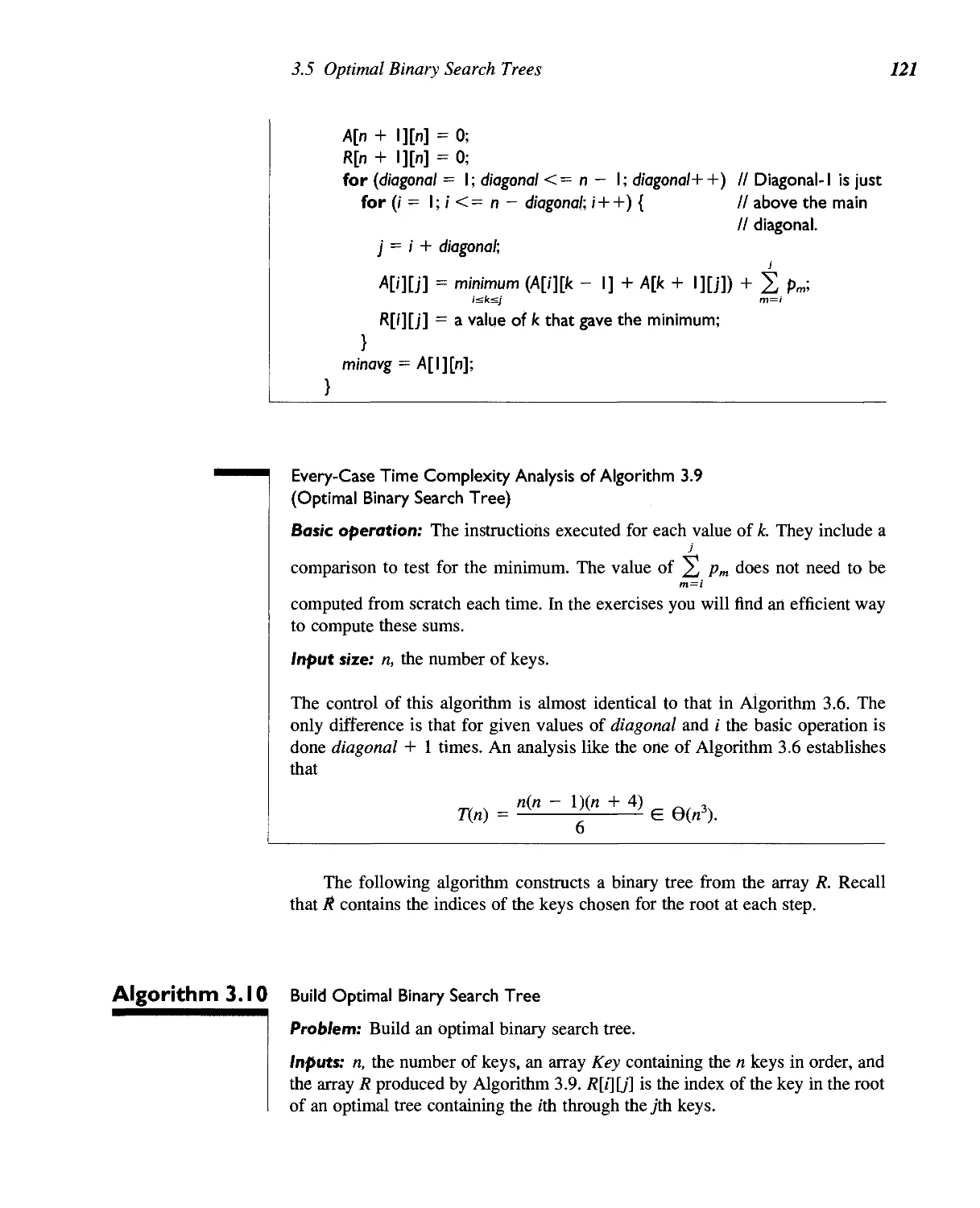
3.5 Optimal Binary Search Trees 113
3.6 The Traveling Salesperson Problem 123
Chapter 4 The Greedy Approach 134
4.1 Minimum Spanning Trees 138
4.1.1 Prim's Algorithm 141
4.1.2 Kruskal's Algorithm 147
4.1.3 Comparing Prim's Algorithm with Kruskal's Algorithm 152
4.1.4 Final Discussion 152
4.2 Dijkstra's Algorithm for Single-Source Shortest Paths 153
4.3 Scheduling 156
4.3.1 Minimizing Total Time in the System 156
4.3.2 Scheduling with Deadlines 159
4.4 The Greedy Approach Versus Dynamic Programming:
The Knapsack Problem 165
4.4.1 A Greedy Approach to the 0-1 Knapsack Problem 166
4.4.2 A Greedy Approach to the Fractional Knapsack Problem 168
4.4.3 A Dynamic Programming Approach to the 0-1
Knapsack Problem 168
4.4.4 A Refinement of the Dynamic Programming Algorithm for the 0-1
Knapsack Problem 169
Chapter 5 Backtracking 176
5.1 The Backtracking Technique 177
5.2 The rc-Queens Problem 185
5.3 Using a Monte Carlo Algorithm to Estimate the Efficiency of a Backtracking
Algorithm 190
5.4 The Sum-of-Subsets Problem 194
5.5 Graph Coloring 199
5.6 The Hamiltonian Circuits Problem 204
5.7 The 0-1 Knapsack Problem 207
5.7.1 A Backtracking Algorithm for the 0-1 Knapsack Problem 207
5.7.2 Comparing the Dynamic Programming Algorithm and the Backtracking
Algorithm for the 0-1 Knapsack Problem 217

Contents
xm
Chapter 6 Branch-and-Bound 222
6.1 Illustrating Branch-and-Bound with the 0-1 Knapsack Problem 224
6.1.1 Breadth-First Search with Branch-and-Bound Pruning 225
6.1.2 Best-First Search with Branch-and-Bound Pruning 230
6.2 The Traveling Salesperson Problem 236
0) 6.3 Abductive Inference (Diagnosis) 245
Chapter 7 Introduction to Computational Complexity:
The Sorting Problem 257
7.1 Computational Complexity 258
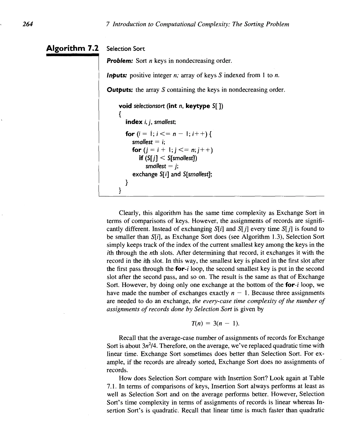
7.2 Insertion Sort and Selection Sort 260
7.3 Lower Bounds for Algorithms That Remove at Most One Inversion per
Comparison 265
7.4 Mergesort Revisited 267
7.5 Quicksort Revisited 273
7.6 Heapsort 275
7.6.1 Heaps and Basic Heap Routines 275
7.6.2 An Implementation of Heapsort 279
7.7 Comparison of Mergesort, Quicksort, and Heapsort 286
7.8 Lower Bounds for Sorting Only by Comparisons of Keys 287
7.8.1 Decision Trees for Sorting Algorithms 287
7.8.2 Lower Bounds for Worst-Case Behavior 290
7.8.3 Lower Bounds for Average-Case Behavior 292
7.9 Sorting by Distribution (Radix Sort) 296
Chapter 8 More Computational Complexity:
The Searching Problem 307
8.1 Lower Bounds for Searching Only by Comparisons of Keys 308
8.1.1 Lower Bounds for Worst-Case Behavior 311
8.1.2 Lower Bounds for Average-Case Behavior 312
8.2 Interpolation Search 318
8.3 Searching in Trees 321
8.3.1 Binary Search Trees 321
8.3.2 B-Trees 325
8.4
Hashing 326

Contents
.5 The Selection Problem: Introduction to Adversary Arguments 332
8.5.1 Finding the Largest Key 332
8.5.2 Finding Both the Smallest and Largest Keys 333
8.5.3 Finding the Second-Largest Key 340
8.5.4 Finding the A:th-Smallest Key 345
8.5.5 A Probabilistic Algorithm for the Selection Problem 354
Chapter 9 Computational Complexity and Intractability:
An Introduction to the Theory of NP 363
9.1 Intractability 364
9.2 Input Size Revisited 366
9.3 The Three General Categories of Problems 370
9.3.1 Problems for Which Polynomial-Time Algorithms Have
Been Found 370
9.3.2 Problems That Have Been Proven to Be Intractable 370
9.3.3 Problems That Have Not Been Proven to Be Intractable but for Which
Polynomial-Time Algorithms Have Never Been Found 371
9.4 The Theory of NP 372
9.4.1 The Sets P and NP 31A
9.4.2 MP-Complete Problems 379
9.4.3 yVP-Hard, MP-Easy, and MP-Equivalent Problems 388
9.5 Handling MP-Hard Problems 392
9.5.1 An Approximation Algorithm for the Traveling
Salesperson Problem 393
9.5.2 An Approximation Algorithm for the Bin Packing Problem 398
Chapter 10 Introduction to Parallel Algorithms 405
10.1 Parallel Architectures 408
10.1.1 Control Mechanism 408
10.1.2 Address-Space Organization 410
10.1.3 Interconnection Networks 411
10.2 The PRAM Model 415
10.2.1 Designing Algorithms for the CREW PRAM Model 418
10.2.2 Designing Algorithms for the CRCW PRAM Model 426
Appendix A Review of Necessary Mathematics 431
A.l Notation 431
A.2 Functions 433

Contents
A.3 Mathematical Induction 434
A.4 Theorems and Lemmas 440
A.5 Logarithms 441
A.5.1 Definition and Properties of Logarithms
A.5.2 The Natural Logarithm 443
A.6 Sets 445
A.7 Permutations and Combinations 447
A.8 Probability 450
A.8.1 Randomness 455
A.8.2 The Expected Value 458
442
Appendix B Solving Recurrence Equations: With Applications to
Analysis of Recursive Algorithms 465
B.l
B.2
B.3
B.4
B.5
Solving Recurrences Using Induction 465
Solving Recurrences Using the Characteristic Equation 469
B.2.1 Homogeneous Linear Recurrences 469
B.2.2 Nonhomogeneous Linear Recurrences 477
B.2.3 Change of Variables (Domain Transformations) 483
Solving Recurrences by Substitution 486
Extending Results for n a Power of a Positive Constant b to n in General
Proofs of Theorems 494
Appendix C Data Structures for Disjoint Sets 502
References 513
Index 517

Chapter 1
Algorithms: Efficiency,
Analysis, and Order
T
JL his text is about techniques for solving problems using a computer. By
"technique," we do not mean a programming style or a programming language
but rather the approach or methodology used to solve a problem. For example,
suppose Barney Beagle wants to find the name "Collie, Colleen" in the phone
book. One approach is to check each name in sequence, starting with the first
name, until "Collie, Colleen" is located. No one, however, searches for a
name this way. Instead, Barney takes advantage of the fact that the names in
the phone book are sorted and opens the book to where he thinks the C's are
located. If he goes too far into the book, he thumbs back a little. He continues
thumbing back and forth until he locates the page containing "Collie,
Colleen." You may recognize this second approach as a modified binary search
and the first approach as a sequential search. We discuss these searches further
1

1 Algorithms: Efficiency, Analysis, and Order
in Section 1.2. The point here is that we have two distinct approaches to
solving the problem, and the approaches have nothing to do with a programming
language or style. A computer program is simply one way to implement these
approaches.
Chapters 2 through 6 discuss various problem-solving techniques and
apply those techniques to a variety of problems. Applying a technique to a
problem results in a step-by-step procedure for solving the problem. This step-by-
step procedure is called an algorithm for the problem. The purpose of studying
these techniques and their applications is so that, when confronted with a new
problem, you have a repertoire of techniques to consider as possible ways to
solve the problem. We will often see that a given problem can be solved using
several techniques but that one technique results in a much faster algorithm
than the others. Certainly a modified binary search is faster than a sequential
search when it comes to finding a name in a phone book. Therefore, we will be
concerned not only with determining whether a problem can be solved using a
given technique but also with analyzing how efficient the resulting algorithm is
in terms of time and storage. When the algorithm is implemented on a
computer, time means CPU cycles and storage means memory. You may wonder
why efficiency should be a concern, because computers keep getting faster and
memory keeps getting cheaper. In this chapter we discuss some fundamental
concepts necessary to the material in the rest of the text. Along the way, we
show why efficiency always remains a consideration, regardless of how fast
computers get and how cheap memory becomes.
/./ ALGORITHMS
So far we have mentioned the words "problem," "solution," and "algorithm."
Most of us have a fairly good idea of what these words mean. However, to lay a
sound foundation, let's define these terms concretely.
A computer program is composed of individual modules, understandable by
a computer, that solve specific tasks (such as sorting). Our concern in this text is
not the design of entire programs, but rather the design of the individual modules
that accomplish the specific tasks. These specific tasks are called problems.
Explicitly, we say that a problem is a question to which we seek an answer.
Examples of problems follow.
Example 1.1 The following is an example of a problem:
Sort the list S of n numbers in nondecreasing order. The answer is the numbers in
sorted sequence.
By a list we mean a collection of items arranged in a particular sequence.
For example,
S = [10, 7, 11, 5, 13, 8]

1.1 Algorithms
3
is a list of six numbers in which the first number is 10, the second is 7, and so
on. We say "nondecreasing order" in Example 1.1 instead of increasing order
to allow for the possibility that the same number may appear more than once in
the list.
Example 1.2 The following is an example of a problem:
Determine whether the number x is in the list S of n numbers. The answer is yes if x
is in S and no if it is not.
A problem may contain variables that are not assigned specific values in the
statement of the problem. These variables are called parameters to the problem.
In Example 1.1 there are two parameters: S (the list) and n (the number of items
in S). In Example 1.2 there are three parameters: S, n, and the number x. It is not
necessary in these two examples to make n one of the parameters because its
value is uniquely determined by S. However, making n a parameter facilitates
our descriptions of problems.
Because a problem contains parameters, it represents a class of problems,
one for each assignment of values to the parameters. Each specific assignment of
values to the parameters is called an instance of the problem. A solution to an
instance of a problem is the answer to the question asked by the problem in that
instance.
Example 1.3 An instance of the problem in Example 1.1 is
S = [10, 7, 11, 5, 13, 8] and n = 6.
The solution to this instance is [5, 7, 8, 10, 11, 13].
Example 1.4 An instance of the problem in Example 1.2 is
S = [10, 7, 11, 5, 13, 8], n = 6, and x = 5.
The solution to this instance is, "yes, x is in S."
We can find the solution to the instance in Example 1.3 by inspecting S and
allowing the mind to produce the sorted sequence by cognitive steps that cannot
be specifically described. This can be done because S is so small that at a
conscious level, the mind seems to scan S rapidly and produce the solution almost
immediately (and therefore one cannot describe the steps the mind follows to
obtain the solution). However, if the instance had a value of 1000 for n, the mind
would not be able to use this method, and it certainly would not be possible to
convert such a method of sorting numbers to a computer program. To produce

1 Algorithms: Efficiency, Analysis, and Order
eventually a computer program that can solve all instances of a problem, we must
specify a general step-by-step procedure for producing the solution to each
instance. This step-by-step procedure is called an algorithm. We say that the
algorithm solves the problem.
Example 1.5 An algorithm for the problem in Example 1.2 is as follows. Starting with the first
item in 5, compare x with each item in S in sequence until x is found or until S
is exhausted. If x is found, answer yes; if x is not found, answer no.
We can communicate any algorithm in the English language as we did in
Example 1.5. However, there are two drawbacks to writing algorithms in this
manner. First, it is difficult to write a complex algorithm this way, and even if
we did, a person would have a difficult time understanding the algorithm. Second,
it is not clear how to create a computer language description of an algorithm from
an English language description of it.
Because C++ is the language with which students are currently most
familiar, we use a C+ + like pseudocode to communicate algorithms. Anyone with
programming experience in an Algol-like imperative language such as C, Pascal,
or Java should have no difficulty with the pseudocode. We illustrate the
pseudocode with an algorithm that solves a generalization of the problem in Example
1.2. For simplicity, Examples 1.1 and 1.2 were stated for numbers. However, in
general we want to search and sort items that come from any ordered set. Often
each item uniquely identifies a record, and therefore we commonly call the items
keys. For example, a record may consist of personal information about an
individual and have the person's social security number as its key. We write searching
and sorting algorithms using the defined data type keytype for the items. It means
the items are from any ordered set.
The following algorithm represents the list S by an array and, instead of
merely returning yes or no, returns x's location in the array if x is in S and returns
0 otherwise. This particular searching algorithm does not require that the items
come from an ordered set, but we still use our standard data type.
Algorithm I.I Sequential Search
Problem: Is the key x in the array S of n keys?
Inputs (parameters): positive integer n, array of keys S indexed from 1 to n, and
a key x.
Outputs: location, the location of x in S (0 if x is not in S).
void seqsearch (int n,
const keytype S[ ],
keytype x,
index& location)

1.1 Algorithms
{
location = I;
while (location<=n && S[location] != x)
location + +;
if (location> n)
location = 0;
}
The pseudocode is similar, but not identical, to C+ + . A notable exception
is our use of arrays. C++ only allows arrays to be indexed by integers starting
at 0. Often we can explain algorithms more clearly using arrays indexed by other
integer ranges, and sometimes we can explain them best using indices which are
not integers at all. So we allow arbitrary sets to index our arrays. We always
specify the ranges of indices in the Inputs and Outputs specifications for the
algorithm. For example, in Algorithm 1.1 we specified that S is indexed from 1
to n. Since we are used to counting the items in a list starting with one, this is a
good index range to use for a list. Of course, this particular algorithm can be
implemented directly in C+ + by declaring
keytype S[n + I];
and simply not using the S[0] slot. Hereafter we will not discuss the
implementation of algorithms in any particular programming language. Our purpose is only
to present algorithms clearly so they can be readily understood and analyzed.
There are two other significant deviations from C++ regarding arrays. First,
we allow variable length two-dimensional arrays as parameters to routines. See
for example Algorithm 1.4 on page 9. Second, we declare local variable-length
arrays. For example, if n is a parameter to procedure example, and we need a
local array indexed from 2 to n, we declare
void example (int n)
{
keytype S[2..n];
}
The notation S[2..n], which means an array S indexed from 2 to n, is strictly
pseudocode; that is, it is not part of the C+ + language.
Whenever we can demonstrate steps more succinctly and clearly using
mathematical expressions or English-like descriptions than we could using actual
C++ instructions, we do so. For example, suppose some instructions are to be
executed only if a variable x is between the values low and high. We write

1 Algorithms: Efficiency, Analysis, and Order
if (low < x < high) { if (/ow < = x && x < = high){
rather than
} }
Suppose we wanted the variable x to take the value of variable y and y to
take the value of x. We write
temp = x;
exchange x and y; rather than x = y;
y = temp;
Besides the data type keytype, we often use the following, which also are
not predefined C+ + data types:
Data Type
index
number
bool
Meaning
An integer variable used as an index.
A variable that could be defined as integral (int) or real (float).
A variable that can take the values "true" or "false".
We use the data type number when it is not important to the algorithm whether
the numbers can take any real values or are restricted to the integers.
Sometimes we use the following nonstandard control structure:
repeat (n times) {
}
This means repeat the code n times. In C+ + it would be necessary to introduce
an extraneous control variable and write a for loop. We only use a for loop when
we actually need to refer to the control variable within the loop.
When the name of an algorithm seems appropriate for a value it returns, we
write the algorithm as a function. Otherwise, we write the algorithm as a
procedure (void function in C++) and use reference parameters (that is, parameters
that are passed by address) to return values. If the parameter is not an array, it is
declared with an ampersand (&) at the end of the data type name. For our purposes
this means that the parameter contains a value returned by the algorithm. Because
arrays are automatically passed by reference in C + + and the ampersand is not
used in C+ + when passing arrays, we do not use the ampersand to indicate that
an array contains values returned by the algorithm. Instead, since the reversed

1.1 Algorithms 7
word const is used in C + + to prevent modification of a passed array, we use
const to indicate that the array does not contain values returned by the algorithm.
In general, we avoid features peculiar to C++ so that the pseudocode is
accessible to someone who knows only another high-level language. However,
we do write instructions like /+ + which means increment /by 1.
If you do not know C+ + , you may find the notation used for logical
operators and certain relational operators unfamiliar. This notation is as follows:
Operator
and
or
not
C++ symbol
&&
II
j
Comparison
x = y
x + y
(jc<y)
jSy
C++ code
(*==y)
(x != y)
(x <= y)
(x >= y)
More example algorithms follow. The first shows the use of a function. While
procedures have the keyword void before the routine's name, functions have the
data type returned by the function before the routine's name. The value is returned
in the function via the return statement.
Algorithm 1.2 Add Array Members
Problem: Add all the numbers in the array S of n numbers.
Inputs: positive integer n, array of numbers S indexed from 1 to n.
Outputs: sum, the sum of the numbers in S.
number sum (int n, const number S[ ])
{
index i;
number result;
result = 0;
for (/ = I; /<= n;i++)
result = result + S[/];
return result;
}
We discuss many sorting algorithms in this text. A simple one follows.
Algorithm 1.3 Exchange Sort
Problem: Sort n keys in nondecreasing order.
Inputs: positive integer n, array of keys S indexed from 1 to n.

1 Algorithms: Efficiency, Analysis, and Order
Outputs: the array S containing the keys in nondecreasing order.
void exchangesort (int n, keytype S[])
{
index i, j;
for(/ = l;i <= n - 1;/ + +)
for(j= i + l;j< = n;j + +)
if(S[j]<S[/])
exchange S[/] and S[j];
}
The instruction
exchange S[i] and S[j]
means that S[i] is to take the value of S[j] and S[j] is to take the value of S[i].
This command looks nothing like a C++ instruction; whenever we can state
something more simply by not using the details of C+ + instructions we do so.
Exchange Sort works by comparing the number in the rth slot with the numbers
in the (i + l)st through nth slots. Whenever a number in a given slot is found to
be smaller than the one in the fth slot, the two numbers are exchanged. In this
way, the smallest number ends up in the first slot after the first pass through for
i loop, the second-smallest number ends up in the second slot after the second
pass, and so on.
The next algorithm does matrix multiplication. Recall that if we have two
2X2 matrices,
A =
an a12
_a2\ a22_
and
B =
t>2l
b12
b22.
their product C = A X B is given by
Cy = anbv + ai2b2j-
For example,
"2X5 + 3X6 2X7 + 3X
4X5+1X6 4X7+1X
[2 3]
L4 1J
X
[5 7]
|_6 8J
—
28 38
26 36
In general, if we have two n X n matrices A and B, their product C is given by
Cij = 2 aikbkJ for 1 < i, j < n.
k=\

1.2 The Importance of Developing Efficient Algorithms
9
Directly from this definition, we obtain the following algorithm for matrix
multiplication.
Algorithm 1.4 Matrix Multiplication
Problem: Determine the product of two n X n matrices.
Inputs: a positive integer n, two-dimensional arrays of numbers A and B, each
of which has both its rows and columns indexed from 1 to n.
Outputs: a two-dimensional array of numbers C, which has both its rows and
columns indexed from 1 to n, containing the product of A and B.
void matrixmult (int n,
const number A[ ][ ],
const number B[][],
number C[][])
{
index i, j, k;
for (/' = !;;'< = n;/++)
for(j'= l;j< =n;j++){
C[i][j] = 0;
for (k = l;k<= n;k++)
C['][i] = C[i][j] + A[i][k] * B[k][j];
}
}
THE IMPORTANCE OF DEVELOPING
1.2 EFFICIENT ALGORITHMS
Previously we mentioned that, regardless of how fast computers become or how
cheap memory gets, efficiency will always remain an important consideration.
Next we show why this is so by comparing two algorithms for the same problem.
1.2.1 Sequential Search Versus Binary Search
Earlier we mentioned that the approach used to find a name in the phone book is
a modified binary search, and is usually much faster than a sequential search.
Next we compare algorithms for the two approaches to show how much faster
the binary search is.
We have already written an algorithm that does a sequential search—namely,
Algorithm 1.1. An algorithm for doing a binary search of an array that is sorted
in nondecreasing order is similar to thumbing back and forth in a phone book.
That is, given that we are searching for x, the algorithm first compares x with the

10 1 Algorithms: Efficiency, Analysis, and Order
middle item of the array. If they are equal, the algorithm is done. If x is smaller
than the middle item, then x must be in the first half of the array (if it is present
at all), and the algorithm repeats the searching procedure on the first half of the
array. (That is, x is compared with the middle item of the first half of the array.
If they are equal, the algorithm is done, etc.) If x is larger than the middle item
of the array, the search is repeated on the second half of the array. This procedure
is repeated until x is found or it is determined that x is not in the array. An
algorithm for this method follows.
Algorithm 1.5 Binary Search
Problem: Determine whether x is in the sorted array S of n keys.
Inputs: positive integer n, sorted (nondecreasing order) array of keys S indexed
from 1 to n, a key x.
Outputs: location, the location of x in S (0 if x is not in S).
void binsearch (int n,
const keytype S[ ],
keytype x,
index& location)
{
index low, high, mid;
low = I; high = n;
location = 0;
while (low < = high && location = = 0) {
mid = L(/ow + high)!2J;
if (x==S[m/d])
location = mid;
else if (x < S[mid])
high = mid - I;
else
low = mid + I;
}
}
Let's compare the work done by Sequential Search and Binary Search. For
focus we will determine the number of comparisons done by each algorithm. If
the array S contains 32 items and x is not in the array, Algorithm 1.1 (Sequential
Search) compares x with all 32 items before determining that x is not in the array.

1.2 The Importance of Developing Efficient Algorithms
11
In general, Sequential Search does n comparisons to determine that x is not in an
array of size n. It should be clear that this is the most comparisons Sequential
Search ever makes when searching an array of size n. That is, if x is in the array,
the number of comparisons is no greater than n.
Next consider Algorithm 1.5 (Binary Search). There are two comparisons of
x with S[mid] in each pass through the while loop (except when x is found). In
an efficient assembler language implementation of the algorithm, x would be
compared with S[mid] only once in each pass, the result of that comparison would
set the condition code, and the appropriate branch would take place based on the
value of the condition code. This means that there would be only one comparison
of x with S[mid] in each pass through the while loop. We will assume the
algorithm is implemented in this manner. With this assumption, Figure 1.1 shows
that the algorithm does six comparisons when x is larger than all the items in an
array of size 32. Notice that 6 = lg 32 + 1. By "lg" we mean log2. The log2 is
encountered so often in analysis of algorithms that we reserve the special symbol
lg for it. You should convince yourself that this is the most comparisons Binary
Search ever does. That is, if x is in the array, or if x is smaller than all the array
items, or if x is between two array items, the number of comparisons is no greater
than when x is larger than all the array items.
Suppose we double the size of the array so that it contains 64 items. Binary
Search does only one comparison more because the first comparison cuts the
array in half, resulting in a subarray of size 32 that is searched. Therefore, when
x is larger than all the items in an array of size 64, Binary Search does seven
comparisons. Notice that 7 = lg 64 + 1. In general, each time we double the size
of the array we add only one comparison. Therefore, if n is a power of 2 and x
is larger than all the items in an array of size n, the number of comparisons done
by Binary Search is lg n + 1.
Table 1.1 compares the number of comparisons done by Sequential Search
and Binary Search for various values of n, when x is larger than all the items in
the array. When the array contains around 4 billion items (about the number of
people in the world), Binary Search does only 33 comparisons whereas Sequential
Search compares x with all 4 billion items. Even if the computer was capable of
completing one pass through the while loop in a nanosecond (one billionth of a
second), Sequential Search would take 4 seconds to determine that x is not in the
S[\] S[I6] S[24] S[28] S[30] S[3I] S[32]
1st 2nd 3rd 4th 5th 6th
Figure I.I The array items that Binary Search compares with x when x is larger than all
the items in an array of size 32. The items are numbered according to the order in
which they are compared.

12 1 Algorithms: Efficiency, Analysis, and Order
Table 1.1 The number of comparisons done by Sequential Search
and Binary Search when x is larger than all the array items
Number of Comparisons Number of Comparisons
Array Size by Sequential Search by Binary Search
128 128 8
1,024 1,024 11
1,048,576 1,048,576 21
4,294,967,296 4,294,967,296 33
array, whereas Binary Search would make that determination almost
instantaneously. This difference would be significant in an on-line application or if we
needed to search for many items.
For convenience, we considered only arrays whose sizes were powers of 2
in the previous discussion of Binary Search. In Chapter 2 we will return to Binary
Search, because it is an example of the divide-and-conquer approach, which is
the focus of that chapter. At that time we will consider arrays whose sizes can be
any positive integer.
As impressive as the searching example is, it is not absolutely compelling
because Sequential Search still gets the job done in an amount of time tolerable
to a human life span. Next we will look at an inferior algorithm that does not get
the job done in a tolerable amount of time.
1.2.2 The Fibonacci Sequence
The algorithms discussed here compute the nth term of the Fibonacci Sequence,
which is defined recursively as follows:
/o = 0
/i = 1
/„ = fn-l + fn~2 for« S 2
Computing the first few terms, we have
h = /i + So = 1 + 0 = 1
h = h + /i = 1 + 1 = 2
U = h + h = 2 + 1 = 3
fs = J4 + h = 3 + 2 = 5, etc.
There are various applications of the Fibonacci Sequence in computer science
and mathematics. Because the Fibonacci Sequence is defined recursively, we
obtain the following recursive algorithm from the definition.

7.2 The Importance of Developing Efficient Algorithms 13
Algorithm 1.6 nth Fibonacci Term (Recursive)
Problem: Determine the nth term in the Fibonacci Sequence.
Inputs: a nonnegative integer n.
Outputs: fib, the nth term of the Fibonacci Sequence.
int fib (int n)
{
if(n<= I)
return n;
else
return fib(n - I) + fib(n - 2);
}
By ' 'nonnegative integer'' we mean an integer that is greater than or equal
to 0, whereas by "positive integer" we mean an integer that is strictly greater
than 0. We specify the input to the algorithm in this manner to make it clear what
values the input can take. However, for the sake of avoiding clutter, we declare
n simply as an integer in the expression of the algorithm. We will follow this
convention throughout the text.
Although the algorithm was easy to create and is understandable, it is
extremely inefficient. Figure 1.2 shows the recursion tree corresponding to the
algorithm when computing fib(5). The children of a node in the tree contain the
recursive calls made by the call at the node. For example, to obtain fib(5) at the
top level we medfib(4) andfib(3), then to obtain fib(3) we medfib(2) andfib(l),
etc. As the tree shows, the function is inefficient because values are computed
over and over again. For example, fib{2) is computed three times.
How inefficient is this algorithm? The tree in Figure 1.2 shows that the
algorithm computes the following numbers of terms to determine fib(n) for 0 <
n <6:
Number of Terms
n Computed
0 1
1 1
2 3
3 5
4 9
5 15
6 25
The first six values can be obtained by counting the nodes in the subtree rooted
at fib(n) for 1 < n < 5, whereas the number of terms fox fib{6) is the sum of the

14 1 Algorithms: Efficiency, Analysis, and Order
Figure 1.2 The recursion tree corresponding to Algorithm 1.6 when computing the
fifth Fibonacci term.
nodes in the trees rooted atfib(5) andfib(4) plus the one node at the root. These
numbers do not suggest a simple expression like the one obtained for Binary
Search. Notice, however, that in the case of the first seven values, the number of
terms in the tree more than doubles every time n increases by 2. For example,
there are nine terms in the tree when n = 4 and 25 terms when n = 6. Let's call
T(n) the number of terms in the recursion tree for n. If the number of terms more
than doubled every time n increased by 2, we would have the following for n a
positive power of 2:
T(n) > 2 X T(n - 2)
> 2 X 2 X T(n - 4)
> 2 X 2 X 2 X T(n - 6)
>2x2x2x---X2 X T(0)
v
nil terms
Because jf(0) = 1, this would mean T(n) > 2"n. We use induction to show that
this is true for n > 2 even if n is not a power of 2. The inequality does not hold
for n = 1 because T{\) = 1, which is less than 21/2. Induction is reviewed in
Section A.3 in Appendix A.

1.2 The Importance of Developing Efficient Algorithms
15
Theorem 1.I If T(n) is the number of terms in the recursion tree corresponding
to Algorithm 1.6, then, for n s 2,
T{ri) > 2"n.
Proof: The proof is by induction on n.
Induction base: We need two base cases because the induction step assumes the
results of two previous cases. For n = 2 and n = 3, the recursion in Figure 1.2
shows that
71(2) = 3 > 2 = 22/2
7X3) = 5 > 2.83 « 23/2
Induction hypothesis: One way to make the induction hypothesis is to assume
that the statement is true for all m < n. Then, in the induction step, show that
this implies that the statement must be true for n. This technique is used in this
proof. Suppose for all m such that 2 < m < n
T(m) > 2mn.
Induction step: We must show that T(n) > 2"n. The value of T(n) is the sum of
T(n — 1) and T(n — 2) plus the one node at the root. Therefore,
7X«) = 7X« - 1) + 7X« - 2) + 1
> 2("-1)/2 + 2("-2)/2 + 1 {by induction hypothesis}
-> y(n-1)l1 , y(n-1)l1 _ 2 X 2("/2)_1 = 2"/2
We established that the number of terms computed by Algorithm 1.6 to
determine the «th Fibonacci term is greater than 2"/2. We will return to this result
to show how inefficient the algorithm is. But first let's develop an efficient
algorithm for computing the «th Fibonacci term. Recall that the problem with the
recursive algorithm is that the same value is computed over and over. As Figure
1.2 shows, fib(2) is computed three times in determining^fc(5). If when computing
a value, we save it in an array, then whenever we need it later we do not need to
recompute it. The following iterative algorithm uses this strategy.
Algorithm 1.7 nth Fibonacci Term (Iterative)
Problem: Determine the «th term in the Fibonacci Sequence.
Inputs: a nonnegative integer n.
Outputs: fib2, the «th term in the Fibonacci Sequence.
int fib! (int n)
{
index i;
int f [0..n];

1 Algorithms: Efficiency, Analysis, and Order
f [0] = 0;
if (n > 0) {
f[i] = i;
for (/' = 2;/<= n;/++)
m = W- i] + f['"-2];
}
return f[n];
}
Algorithm 1.7 can be written without using the array / because only the two
most recent terms are needed in each iteration of the loop. However, it is more
clearly illustrated using the array.
To determine fib2(n), the previous algorithm computes every one of the first
n + 1 terms just once. So it computes n + 1 terms to determine the nth Fibonacci
term. Recall that Algorithm 1.6 computes more than 2"n terms to determine the
nth Fibonacci term. Table 1.2 compares these expressions for various values of
n. The execution times are based on the simplifying assumption that one term
can be computed in 10~9 second. The table shows the time it would take
Algorithm 1.7 to compute the nth term on a hypothetical computer that could compute
each term in a nanosecond, and it shows a lower bound on the time it would take
to execute Algorithm 1.7. By the time n is 80, Algorithm 1.6 takes at least 18
minutes. When n is 120, it takes more than 36 years, an amount of time intolerable
to a human life span. Even if we could build a computer one billion times as fast,
Algorithm 1.6 would take over 40,000 years to compute the 200th term. This
result can be obtained by dividing the time for the 200th term by one billion. We
see that regardless of how fast computers become, Algorithm 1.6 will still take
Table 1.2
n
40
60
80
100
120
160
200
A comparison
n + 1
41
61
81
101
121
161
201
of Algorithms 1.6 and 1.7
2*1/2
1,048,576
1.1 X 109
1.1 X 1012
1.1 X 1015
1.2 X 1018
1.2 X 1024
1.3 X 1030
Execution Time
Using Algorithm 1.7
41 ns*
61 ns
81 ns
101 ns
121 ns
161 ns
201 ns
Lower Bound on
Execution Time
Using Algorithm 1.6
1048 (is?
1 s
18 min
13 days
36 years
3.8 X 107 years
4 X 1013 years
*1 ns = 10 9 second.
+ 1 fis = 10~6 second.

1.3 Analysis of Algorithms
17
an intolerable amount of time unless n is small. On the other hand, Algorithm
1.7 computes the nth Fibonacci term almost instantaneously. This comparison
shows why the efficiency of an algorithm remains an important consideration
regardless of how fast computers become.
Algorithm 1.6 is a divide-and-conquer algorithm. Recall that the divide-and-
conquer approach produced a very efficient algorithm (Algorithm 1.5: Binary
Search) for the problem of searching a sorted array. As shown in Chapter 2, the
divide-and-conquer approach leads to very efficient algorithms for some
problems, but very inefficient algorithms for other problems. Our efficient algorithm
for computing the nth Fibonacci term (Algorithm 1.7) is an example of the
dynamic programming approach, which is the focus of Chapter 3. We see that
choosing the best approach can be essential.
We showed that Algorithm 1.6 computes at least an exponentially large
number of terms, but could it be even worse? The answer is no. Using the techniques
in Appendix B, it is possible to obtain an exact formula for the number of terms,
and the formula is exponential in n. See Examples B.5 and B.9 in Appendix B
for further discussion of the Fibonacci Sequence.
1.3 ANALYSIS OF ALGORITHMS
To determine how efficiently an algorithm solves a problem, we need to analyze
the algorithm. We introduced efficiency analysis of algorithms when we
compared the algorithms in the preceding section. However, we did those analyses
rather informally. We will now discuss terminology used in analyzing algorithms
and the standard methods for doing analyses. We will adhere to these standards
in the remainder of the text.
1.3.1 Time Complexity Analysis
When analyzing the efficiency of an algorithm in terms of time, we do not
determine the actual number of CPU cycles, because this depends on the particular
computer on which the algorithm is run. Furthermore, we do not even want to
count every instruction executed, because the number of instructions depends on
the programming language used to implement the algorithm and the way the
programmer writes the program. Rather, we want a measure that is independent
of the computer, the programming language, the programmer, and all the complex
details of the algorithm such as incrementing of loop indices, setting of pointers,
etc. We learned that Algorithm 1.5 is much more efficient than Algorithm 1.1 by
comparing the numbers of comparisons done by the two algorithms for various
values of n, where n is the number of items in the array. This is a standard
technique for analyzing algorithms. In general, the running time of an algorithm
increases with the size of the input, and the total running time is roughly
proportional to how many times some basic operation (such as a comparison
instruction) is done. We therefore analyze the algorithm's efficiency by determining the

1 Algorithms: Efficiency, Analysis, and Order
number of times some basic operation is done as a function of the size of the
input.
For many algorithms it is easy to find a reasonable measure of the size of
the input, which we call the input size. For example, consider Algorithms 1.1
(Sequential Search), 1.2 (Add Array Members), 1.3 (Exchange Sort), and 1.5
(Binary Search). In all these algorithms, n, the number of items in the array, is a
simple measure of the size of the input. Therefore, we can call n the input size.
In Algorithm 1.4 (Matrix Multiplication), n, the number of rows and columns, is
a simple measure of the size of the input. Therefore, we can again call n the input
size. In some algorithms, it is more appropriate to measure the size of the input
using two numbers. For example, when the input to an algorithm is a graph, we
often measure the size of the input in terms of both the number of vertices and
the number of edges. Therefore, we say that the input size consists of both
parameters.
Sometimes we must be cautious about calling a parameter the input size. For
example, in Algorithms 1.6 (nth Fibonacci Term, Recursive) and 1.7 (nth
Fibonacci Term, Iterative), you may think that n should be called the input size.
However, n is the input; it is not the size of the input. For this algorithm, a reasonable
measure of the size of the input is the number of symbols used to encode n. If
we use binary representation, the input size will be the number of bits it takes to
encode n, which is Ug n\ + 1. For example,
n = 13 = 11012
4 bits
Therefore, the size of the input n = 13 is 4. We gained insight into the relative
efficiency of the two algorithms by determining the number of terms each
computes as a function of n, but still n does not measure the size of the input. These
considerations will be important in Chapter 9, where we will discuss the input
size in more detail. Until then it will usually suffice to use a simple measure, such
as the number of items in an array, as the input size.
After determining the input size, we pick some instruction or group of
instructions such that the total work done by the algorithm is roughly proportional
to the number of times this instruction or group of instructions is done. We call
this instruction or group of instructions the basic operation in the algorithm. For
example, x is compared with an item S in each pass through the loops in
Algorithms 1.1 and 1.5. Therefore, the compare instruction is a good candidate for the
basic operation in each of these algorithms. By determining how many times
Algorithms 1.1 and 1.5 do this basic operation for each value of n, we gained
insight into the relative efficiencies of the two algorithms.
In general, a time complexity analysis of an algorithm is the determination
of how many times the basic operation is done for each value of the input size.
Although we do not want to consider the details of how an algorithm is
implemented, we will ordinarily assume that the basic operation is implemented as

1.3 Analysis of Algorithms
19
efficiently as possible. For example, we assume that Algorithm 1.5 is implemented
such that the comparison is done just once. In this way, we analyze the most
efficient implementation of the basic operation.
There is no hard-and-fast rule for choosing the basic operation. It is largely
a matter of judgment and experience. As already mentioned, we ordinarily do not
include the instructions that compose the control structure. For example, in
Algorithm 1.1 we do not include the instructions that increment and compare the
index in order to control the passes through the while loop. Sometimes it suffices
simply to consider one pass through a loop as one execution of the basic operation.
At the other extreme, for a very detailed analysis, one could consider the execution
of each machine instruction as doing the basic operation once. As mentioned
earlier, because we want our analyses to remain independent of the computer, we
will never do that in this text.
At times we may want to consider two different basic operations. For
example, in an algorithm that sorts by comparing keys, we often want to consider
the comparison instruction and the assignment instruction each individually as
the basic operation. By this we do not mean that these two instructions together
compose the basic operation, but rather that we have two distinct basic operations,
one being the comparison instruction and the other being the assignment
instruction. We do this because ordinarily a sorting algorithm does not do the same
number of comparisons as it does assignments. Therefore, we can gain more
insight into the efficiency of the algorithm by determining how many times each
is done.
Recall that a time complexity analysis of an algorithm determines how many
times the basic operation is done for each value of the input size. In some cases
the number of times it is done depends not only on the input size, but also on the
input's values. This is the case in Algorithm 1.1 (Sequential Search). For example,
if x is the first item in the array, the basic operation is done once, whereas if x is
not in the array, it is done n times. In other cases, such as Algorithm 1.2 (Add
Array Members), the basic operation is always done the same number of times
for every instance of size n. When this is the case, T(n) is defined as the number
of times the algorithm does the basic operation for an instance of size n. T(ri) is
called the every-case time complexity of the algorithm, and the determination of
T(n) is called an every-case time complexity analysis. Examples of every-case
time complexity analyses follow.
Every-Case Time Complexity Analysis of Algorithm 1.2 (Add Array Members)
Other than control instructions, the only instruction in the loop is the one that
adds an item in the array to sum. Therefore, we will call that instruction the basic
operation.
Basic operation: the addition of an item in the array to sum.
Input size: n, the number of items in the array.

1 Algorithms: Efficiency, Analysis, and Order
Regardless of the values of the numbers in the array, there are n passes through
the for loop. Therefore, the basic operation is always done n times and
T(n) = n.
Every-Case Time Complexity Analysis of Algorithm 1.3 (Exchange Sort)
As mentioned previously, in the case of an algorithm that sorts by comparing
keys, we can consider the comparison instruction or the assignment instruction
as the basic operation. We will analyze the number of comparisons here.
Basic operation: the comparison of S[j] with S[i].
Input size: n, the number of items to be sorted.
We must determine how many passes there are through the for/ loop. For a given
n there are always n — 1 passes through the for i loop. In the first pass through
the for i loop, there are n — 1 passes through the for / loop, in the second pass
there are n — 2 passes through the for/ loop, in the third pass there are n — 3
passes through the for / loop, ..., and in the last pass there is one pass through
the for / loop. Therefore, the total number of passes through the for / loop is
given by
T(n) = (n - 1) + (« - 2) + (« - 3) + • • • + 1 = (" ~ 1)W .
The last equality is derived in Example A.l in Appendix A.
Every-Case Time Complexity Analysis of Algorithm 1.4 (Matrix Multiplication)
The only instruction in the innermost for loop is the one that does a multiplication
and an addition. It is not hard to see that the algorithm can be implemented in
such a way that fewer additions are done than multiplications. Therefore, we will
consider only the multiplication instruction to be the basic operation.
Basic operation: multiplication instruction in the innermost for loop.
Input size: n, the number of rows and columns.
There are always n passes through the for i loop, in each pass there are always
n passes through the for/ loop, and in each pass through the for/ loop there are
always n passes through the for k loop. Because the basic operation is inside the
for k loop,
T(n) = n X n X n = n3.
As discussed previously, the basic operation in Algorithm 1.1 is not done the
same number of times for all instances of size n. So this algorithm does not have
an every-case time complexity. This is true for many algorithms. However, this

1.3 Analysis of Algorithms
21
does not mean that we cannot analyze such algorithms, because there are three
other analysis techniques that can be tried. The first is to consider the maximum
number of times the basic operation is done. For a given algorithm, W(n) is
defined as the maximum number of times the algorithm will ever do its basic
operation for an input size of n. So W(n) is called the worse-case time complexity
of the algorithm, and the determination of W(n) is called a worst-case time
complexity analysis. If T(n) exists, then clearly W(n) = T(n). The following is an
analysis of W(n) in a case where T(n) does not exist.
Worst-Case Time Complexity Analysis of Algorithm I. I (Sequential Search)
Basic operation: the comparison of an item in the array with x.
Input size: n, the number of items in the array.
The basic operation is done at most n times, which is the case if x is the last item
in the array or if x is not in the array. Therefore,
W(n) = n.
Although the worst-case analysis informs us of the absolute maximum
amount of time consumed, in some cases we may be more interested in knowing
how the algorithm performs on the average. For a given algorithm, A(n) is defined
as the average (expected value) of the number of times the algorithm does the
basic operation for an input size of n. (See Section A.8.2 in Appendix A for a
discussion of average.) A(n) is called the average-case time complexity of the
algorithm, and the determination of A(n) is called an average-case time
complexity analysis. As is the case for W(n), if T(n) exists, then A(n) = T(n).
To compute A(n), we need to assign probabilities to all possible inputs of
size n. It is important to assign probabilities based on all available information.
For example, our next analysis will be an average-case analysis of Algorithm 1.1.
We will assume that if x is in the array, it is equally likely to be in any of the
array slots. If we know only that x may be somewhere in the array, our information
gives us no reason to prefer one array slot over another. Therefore, it is reasonable
to assign equal probabilities to all array slots. This means that we are determining
the average search time when we search for all items the same number of times.
If we have information indicating that the inputs will not arrive according to this
distribution, we should not use this distribution in our analysis. For example, if
the array contains first names and we are searching for names that have been
chosen at random from all people in the United States, an array slot containing
the common name "John" will probably be searched more often than one
containing the uncommon name "Felix" (see Section A.8.1 in Appendix A for a
discussion of randomness). We should not ignore this information and assume
that all slots are equally likely.
As the following analysis illustrates, it is usually harder to analyze the
average case than it is to analyze the worst case.

1 Algorithms: Efficiency, Analysis, and Order
Average-Case Time Complexity Analysis of Algorithm I. I (Sequential Search)
Basic operation: the comparison of an item in the array with x.
Input size: n, the number of items in the array.
We first analyze the case where it is known that x is in S, where the items in S
are all distinct, and where we have no reason to believe that x is more likely to
be in one array slot than it is to be in another. Based on this information, for
1 < k ^ n, the probability that x is in the Mi array slot is \ln. If x is in the Mi
array slot, the number of times the basic operation is done to locate x (and,
therefore, to exit the loop) is k. This means that the average time complexity is
given by
" / l\ 1 " 1
A{n) =2*X-=-x2> = -x
k=x \ n) n k=\ n
«(«+!) n + 1
The third step in this quadruple equality is derived in Example A. 1 of Appendix
A. As we would expect, on the average, about half the array is searched.
Next we analyze the case where x may not be in the array. To analyze this
case we must assign some probability p to the event that x is in the array. If x is
in the array, we will again assume that it is equally likely to be in any of the slots
from 1 to n. The probability that x is in the Mi slot is then pin, and the probability
that it is not in the array is 1 — p. Recall that there are k passes through the loop
if x is found in the Mi slot, and n passes through the loop if x is not in the array.
The average time complexity is therefore given by
Mn) = 2 (* X^j + "(1 ~ P)
p ^ n(n + 1) / p\ p
^-X—r— + ^l-p)=„ll--l+-.
n
The last step in this triple equality is derived with algebraic manipulations. If
p = 1, A(n) = (n + l)/2, as before, whereas if p = 1/2, A(n) = 3«/4 + 1/4. This
means that about 3/4 of the array is searched on the average.
Before proceeding, we offer a word of caution about the average. Although
an average is often referred to as a typical occurrence, one must be careful in
interpreting the average in this manner. For example, a meteorologist may say
that a typical January 25 in Chicago has a high of 22 °F because 22 °F has been
the average high for that date over the past 80 years. The paper may run an article
saying that the typical family in Evanston, Illinois, earns $50,000 annually
because that is the average income. An average can be called "typical" only if the
actual cases do not deviate much from the average (that is, only if the standard
deviation is small). This may be the case for the high temperature on January 25.
However, Evanston is a community with wealthy areas and fairly poor areas. It

1.3 Analysis of Algorithms
23
is more typical for a family to make either $20,000 annually or $100,000 annually
than to make $50,000. Recall in the previous analysis that A(n) is (n + l)/2 when
it is known that x is in the array. This is not the typical search time, because all
search times between 1 and n are equally typical. Such considerations are
important in algorithms that deal with response time. For example, consider a system
that monitors a nuclear power plant. If even a single instance has a bad response
time, the results could be catastrophic. It is therefore important to know whether
the average response time is 3 seconds because all response times are around 3
seconds or because most are 1 second and some are 60 seconds.
A final type of time complexity analysis is the determination of the smallest
number of times the basic operation is done. For a given algorithm, B(n) is defined
as the minimum number of times the algorithm will ever do its basic operation
for an input size of n. So B(n) is called the best-case time complexity of the
algorithm, and the determination of B(n) is called a best-case time complexity
analysis. As is the case for W(n) and A(n), if T(n) exists, then B(n) = T(n). Let's
determine B{n) for Algorithm 1.1.
Best-Case Time Complexity Analysis of Algorithm I. I (Sequential Search)
Basic operation: the comparison of an item in the array with x.
Input size: n, the number of items in the array.
Because n > 1, there must be at least one pass through the loop. If x = S[l],
there will be one pass through the loop regardless of the size of n. Therefore,
B(n) = 1.
For algorithms that do not have every-case time complexities, we do worst-
case and average-case analyses much more often than best-case analyses. An
average-case analysis is valuable because it tells us how much time the algorithm
would take when used many times on many different inputs. This would be useful,
for example, in the case of a sorting algorithm that was used repeatedly to sort
all possible inputs. Often, a relatively slow sort can occasionally be tolerated if,
on the average, the sorting time is good. In Section 2.4 we will see an algorithm,
named Quicksort, that does exactly this. It is one of the most popular sorting
algorithms. As noted previously, an average-case analysis would not suffice in a
system that monitored a nuclear power plant. In this case, a worst-case analysis
would be more useful because it would give us an upper bound on the time taken
by the algorithm. For both the applications just discussed, a best-case analysis
would be of little value.
We have only discussed analysis of the time complexity of an algorithm. All
these same considerations also pertain to analysis of memory complexity, which
is an analysis of how efficient the algorithm is in terms of memory. Although
most of the analyses in this text are time complexity analyses, we will occasionally
find it useful to do a memory complexity analysis.

1 Algorithms: Efficiency, Analysis, and Order
In general, a complexity function can be any function from the nonnegative
integers to the nonnegative reals. When not referring to the time complexity or
memory complexity for some particular algorithm, we will usually use standard
function notation, such as f(n) and g{n), to represent complexity functions.
Example 1.6 The functions
/(«) = «
/(«) = n2
f(n) = lg n
f(n) = 3n2 + An
are all examples of complexity functions because they all map the nonnegative
integers to the nonnegative reals.
1.3.2 Applying the Theory
When applying the theory of algorithm analysis, one must sometimes be aware
of the time it takes to execute the basic operation, the overhead instructions, and
the control instructions on the actual computer on which the algorithm is
implemented. By "overhead instructions" we mean instructions such as initialization
instructions before a loop. The number of times these instructions execute does
not increase with input size. By "control instructions" we mean instructions such
as incrementing an index to control a loop. The number of times these instructions
execute increases with input size. The basic operation, overhead instructions, and
control instructions are all properties of an algorithm and the implementation of
the algorithm. They are not properties of a problem. This means that they are
usually different for two different algorithms for the same problem.
Suppose we have two algorithms for the same problem with the following
every-case time complexities: n for the first algorithm and n2 for the second
algorithm. The first algorithm appears more efficient. Suppose, however, a given
computer takes 1000 times as long to process the basic operation once in the first
algorithm as it takes to process the basic operation once in the second algorithm.
By "process" we mean that we are including the time it takes to execute the
control instructions. Therefore, if t is the time required to process the basic
operation once in the second algorithm, lOOOr is the time required to process the
basic operation once in the first algorithm. For simplicity, let's assume that the
time it takes to execute the overhead instructions is negligible in both algorithms.
This means the times it takes the computer to process an instance of size n are
n X lOOOr for the first algorithm and n2 X t for the second algorithm. We
must solve the following inequality to determine when the first algorithm is
more efficient:
n2 X t > n X lOOOr.

1.4 Order
25
Dividing both sides by nt yields
n > 1000.
If the application never had an input size larger than 1000, the second
algorithm should be implemented. Before proceeding, we should point out that it
is not always so easy to determine precisely when one algorithm is faster than
another. Sometimes we must use approximation techniques to analyze the
inequalities obtained by comparing two algorithms.
Recall that we are assuming that the time it takes to process the overhead
instructions is negligible. If this were not the case, these instructions would also
have to be considered to determine when the first algorithm would be more
efficient.
1.3.3 Analysis of Correctness
In this text, "analysis of an algorithm" means an efficiency analysis in terms of
either time or memory. There are other types of analyses. For example, we can
analyze the correctness of an algorithm by developing a proof that the algorithm
actually does what it is supposed to do. Although we will often informally show
that our algorithms are correct and will sometimes prove that they are, you should
see Dijkstra (1976), Gries (1981), or Kingston (1990) for a comprehensive
treatment of correctness.
1.4 ORDER
We just illustrated that an algorithm with a time complexity of n is more efficient
than one with a time complexity of n2 for sufficiently large values of n, regardless
of how long it takes to process the basic operations in the two algorithms. Suppose
now that we have two algorithms for the same problem, and that their every-case
time complexities are lOOn for the first algorithm and 0.0In2 for the second
algorithm. Using an argument such as the one just given, we can show that the
first algorithm will eventually be more efficient than the second one. For example,
if it takes the same amount of time to process the basic operations in both
algorithms and the overhead is about the same, the first algorithm will be more
efficient if
O.Oln2 > lOOn.
Dividing both sides by O.Oln yields
n > 10,000.
If it takes longer to process the basic operation in the first algorithm than in the
second, then there is simply some larger value of n at which the first algorithm
becomes more efficient.

1 Algorithms: Efficiency, Analysis, and Order
Algorithms with time complexities such as n and lOOn are called linear-time
algorithms because their time complexities are linear in the input size n, whereas
algorithms with time complexities such as n2 and 0.0In2 are called quadratic-
time algorithms because their time complexities are quadratic in the input size n.
There is a fundamental principle here. That is, any linear-time algorithm is
eventually more efficient than any quadratic-time algorithm. In the theoretical analysis
of an algorithm, we are interested in eventual behavior. Next we will show how
algorithms can be grouped according to their eventual behavior. In this way we
can readily determine whether one algorithm's eventual behavior is better than
another's.
1.4.1 An Intuitive Introduction to Order
Functions such as 5n2 and 5n2 + 100 are called pure quadratic functions because
they contain no linear term, whereas a function such as O.ln2 + n + 100 is called
a complete quadratic function because it contains a linear term. Table 1.3 shows
that eventually the quadratic term dominates this function. That is, the values of
the other terms eventually become insignificant compared with the value of the
quadratic term. Therefore, although the function is not a pure quadratic function,
we can classify it with pure quadratic functions. This means that if some algorithm
has this time complexity, we can call the algorithm a quadratic-time algorithm.
Intuitively, it seems that we should always be able to throw away low-order terms
when classifying complexity functions. For example, it seems that we should be
able to classify O.ln3 + 10n2 + 5n + 25 with pure cubic functions. We will soon
establish rigorously that we can do this. First let's impart an intuitive feel for how
complexity functions are classified.
The set of all complexity functions that can be classified with pure quadratic
functions is called 6(n2), where 0 is the Greek capital letter' 'theta." If a function
is a member of the set 0(n2), we say that the function is order of n2. For example,
because we can throw away low-order terms,
g(n) = 5n2 + lOOn + 20 G 9(n2),
which means that g(n) is order of n2. As a more concrete example, recall from
Section 1.3.1 that the time complexity for Algorithm 1.3 (Exchange Sort) is given
by T(ri) = n(n — l)/2. Because
n(n — 1) _ n2 n
2 ~ ~2 2'
throwing away the lower-order term n/2 shows that T(n) G 0(n2).
When an algorithm's time complexity is in 0(n2), the algorithm is called a
quadratic-time algorithm or a Q(n2) algorithm. We also say that the algorithm is
0(/r2). Exchange Sort is a quadratic-time algorithm.

1.4 Order
27
Table 1.3 The quadratic term eventually
n O.ln2
10 10
20 40
50 250
100 1,000
1000 100,000
dominates
O.ln2
+ n + 100
120
160
400
1,200
101,100
Similarly, the set of complexity functions that can be classified with pure
cubic functions is called 9(n3), and functions in that set are said to be order of
n3, and so on. We will call these sets complexity categories. The following are
some of the most common complexity categories.
9(lgn) 9(n) 9(n lg n) 9(n2) 9(n3) 9(2")
In this ordering, if f(n) is in a category to the left of the category containing g(n),
then f(n) eventually lies beneath g(n) on a graph. Figure 1.3 plots the simplest
members of these categories: n, lg n, n lg n, etc. Table 1.4 shows the execution
times of algorithms whose time complexities are given by these functions. The
simplifying assumption is that it takes 1 nanosecond (10~9 second) to process the
basic operation for each algorithm. The table shows a possibly surprising result.
One might expect that as long as an algorithm is not an exponential-time
algorithm, it will be adequate. However, even the quadratic-time algorithm takes 31.7
years to process an instance with an input size of 1 billion. On the other hand,
the 9(n lg n) algorithm takes only 29.9 seconds to process such an instance.
Ordinarily an algorithm has to be 9(n lg n) or better for us to assume that it can
process extremely large instances in tolerable amounts of time. This is not to say
that algorithms whose time complexities are in the higher-order categories are
not useful. Algorithms with quadratic, cubic, and even higher-order time
complexities can often handle the actual instances that arise in many applications.
Before ending this discussion, we stress that there is more information in
knowing a time complexity exactly than in simply knowing its order. For
example, recall the hypothetical algorithms, discussed earlier, that have time
complexities of lOOn and 0.0In2. If it takes the same amount of time to process the
basic operations and execute the overhead instructions in both algorithms, then
the quadratic-time algorithm is more efficient for instances smaller than 10,000.
If the application never requires instances larger than this, the quadratic-time
algorithm should be implemented. If we knew only that the time complexities
were in O(n) and Q(n2), respectively, we would not know this. The coefficients
in this example are extreme, and in practice they are often less extreme.
Furthermore, there are times when it is quite difficult to determine the time complexities
exactly. Therefore, we are sometimes content to determine only the order.

28 1 Algorithms: Efficiency, Analysis, and Order
Figure 1.3 Growth rates of some common complexity functions.
131,072
65,536
32,768
16,384
8,192
4,096
2,048
1,024
512
256
128
64
32
16
8
4
2
1
0 1 2 4 8 16 32 64 128 256 512 1,024 2,048
1.4.2 A Rigorous Introduction to Order
The previous discussion imparted an intuitive feel for order (©). Here we develop
theory that enables us to define order rigorously. We accomplish this by
presenting two other fundamental concepts. The first is "big O."
Definition For a given complexity function f(n), 0(f(n)) is the set of complexity functions
g(n) for which there exists some positive real constant c and some nonnegative
integer N such that for all n > N
g{n) < c X f(n).

1.4 Order
29
Table 1.4 Execution times for a
n
10
20
30
40
50
102
103
104
105
106
107
108
10"
f(n) = \gn
0.003 /us*
0.004 /j,s
0.005 /lis
0.005 /lis
0.006 /lis
0.007 /lis
0.010 /lis
0.013 /lis
0.017 /lis
0.020 /lis
0.023 /lis
0.027 /lis
0.030 /lis
f(n) = n
0.01 /LIS
0.02 /lis
0.03 /lis
0.04 /lis
0.05 /lis
0.10 /LIS
1.00 /lis
10 /LIS
0.10 ms
1 ms
0.01 s
0.10 s
1 s
lgorithms with the
f(n) = n\gn
0.033 /lis
0.086 /lis
0.147 /lis
0.213 /lis
0.282 /lis
0.664 /lis
9.966 /lis
130/lis
1.67 ms
19.93 ms
0.23 s
2.66 s
29.90 s
given time complexities
f(n) = n2
0.1 /LIS
0.4/lis
0.9/lis
1.6 /as
2.5 /lis
10 /LIS
1 ms
100 ms
10 s
16.7 min
1.16 days
115.7 days
31.7 years
f(n) = n>
1 /LIS
8 /lis
27 /lis
64 /lis
125 /lis
1 ms
1 s
16.7 min
11.6 days
31.7 years
31,709 years
3.17 X 107 years
f(n) = T
1 /LIS
1 ms+
1 s
18.3 min
13 days
4 X 1013 years
*1 /us = 10 6 second.
+ 1 ms = 10~3 second.
If g(n) G 0(f(n)), we say that gin) is big O of fin). Figure 1.4(a) illustrates
"big 0." Although gin) starts out above c/(n) in that figure, eventually it falls
beneath cf(n) and stays there. Figure 1.5 shows a concrete example. Although
n2 + 10» is initially above 2n2 in that figure, for n ^ 10
We can therefore take c
that
n2 + lOn < 2n2.
2 and N = 10 in the definition of' 'big C' to conclude
n2 + lOn G 0{n2),
N
(a) g(«)eO (/(«))
Figure 1.4 Illustrating "big 0," CI, and ®.
gin)
cfin)
(b)g(n) eft (/(«))
(c) g(») e 9 (/(»))

30 I Algorithms: Efficiency, Analysis, and Order
Figure 1.5 The function n2 + I On eventually stays beneath the function 2n2.
400
350
300
250
200
150
100
50
1 2 3 4 5 6 7 8 9 10 11 12 13 14 15
If, for example, g(n) is in 0(n2), then eventually g{n) lies beneath some pure
quadratic function en2 on a graph. This means that if g{n) is the time complexity
for some algorithm, eventually the running time of the algorithm will be at least
as fast as quadratic. For the purposes of analysis, we can say that eventually g{n)
is at least as good as a pure quadratic function. ' 'Big O'' (and other concepts that
will be introduced soon) are said to describe the asymptotic behavior of a function
because they are concerned only with eventual behavior. We say that ' 'big O''
puts an asymptotic upper bound on a function.
The following examples illustrate how to show "big O."
Example 1.7 We show that 5n2 G 0(n2). Because, for n > 0,
5n2 < 5n2,
we can take c = 5 and N = 0 to obtain our desired result.
Example 1.8 Recall that the time complexity of Algorithm 1.3 (Exchange Sort) is given by
n{n - 1)
T{n) = —r-.
Because, for n > 0,
n(n — 1) n(n) 1 ,
^ = - n ,
2 2 2
we can take c = 1/2 and N = 0 to conclude that T{n) G 0(n2).

1.4 Order
31
A difficulty students often have with "big O" is that they erroneously think
there is some unique c and unique N that must be found to show that one function
is "big O" of another. This is not the case at all. Recall that Figure 1.5 illustrates
that n2 + lOn G 0(n2) using c = 2 and N = 10. Alternatively, we could show
it as follows.
Example 1.9 We show that n2 + lOn G 0(n2). Because, for n ^ 1,
n2 + lOn < n2 + 10n2 = lln2,
we can take c = 11 and N = I to obtain our result.
In general, one can show "big O" using whatever manipulations seem most
straightforward.
Example 1.10 We show that n2 G 0(n2 + lOn). Because, for n ^ 0,
n2 < 1 X {n2 + lOn),
we can take c = 1 and N = 0 to obtain our result.
The purpose of this last example is to show that the function inside "big O"
does not have to be one of the simple functions plotted in Figure 1.3. It can be
any complexity function. Ordinarily, however, we take it to be a simple function
like those plotted in Figure 1.3.
Example 1.11 We show that n G 0(n2). Because, for n > 1,
n < 1 X n2,
we can take c = 1 and N = 1 to obtain our result.
This last example makes a crucial point about "big O." A complexity
function need not have a quadratic term to be in 0(n2). It need only eventually lie
beneath some pure quadratic function on a graph. Therefore, any logarithmic or
linear complexity function is in 0{n2). Similarly, any logarithmic, linear, or
quadratic complexity function is in 0(n3), and so on. Figure 1.6(a) shows some
exemplary members of 0(n2).
Just as "big O" puts an asymptotic upper bound on a complexity
function, the following concept puts an asymptotic lower bound on a complexity
function.

1 Algorithms: Efficiency, Analysis, and Order
Figure 1.6 The sets 0(n2), fi(n2), and ®(n2). Some exemplary members are shown.
e(«2)
(a) 0(«2) (b) £l(n2) (c) 9(«2) = 0(n2) n Q(«2)
Definition For a given complexity function /(n), !!(/(«)) is the set of complexity functions
g(n) for which there exists some positive real constant c and some nonnegative
integer N such that, for all n ^ N,
g{n) > c X /(«).
The symbol il is the Greek capital letter "omega." If g{n) G il(f(n)), we
say that g{n) is omega of /(n). Figure 1.4(b) illustrates il. Some examples follow.
Example 1.12 We show that 5n2 G H(n2). Because, for n > 0,
5n2 > 1 X n2,
we can take c = 1 and N = Oto obtain our result.
Example 1.13 We show that n2 + lOn G £l(n2). Because, for n > 0,
n2 + lOn > n2,
we can take c = 1 and N = Oto obtain our result.
Example 1.14 Consider again the time complexity of Algorithm 1.3 (Exchange Sort). We show
I that
n(n — 1) ^ ,
T(n) = 2 G H(n2).
For n > 2,
n
n - 1 > -.
2

1.4 Order
33
Therefore, for n > 2,
n(n — 1) n n 1 ,
— > - X - = - n2,
2 2 2 4
which means we can take c = 1/4 and N = 2to obtain our result.
As is the case for "big 0" there are no unique constants c and N for which
the conditions in the definition of Cl hold. We can choose whichever ones make
our manipulations easiest.
If a function is in £l(n2), then eventually the function lies above some pure
quadratic function on a graph. For the purposes of analysis, this means that
eventually it is at least as bad as a pure quadratic function. However, as the following
example illustrates, the function need not be a quadratic function.
Example 1.15 We show that n3 G Cl(n2). Because, if n > 1,
n3 > 1 X n2,
we can take c = 1 and N = 1 to obtain our result.
Figure 1.6(b) shows some exemplary members of Ci{n2).
If a function is in both 0(n2) and il(n2), we can conclude that eventually the
function lies beneath some pure quadratic function on a graph and eventually it
lies above some pure quadratic function on a graph. That is, eventually it is at
least as good as some pure quadratic function and eventually it is at least as bad
as some pure quadratic function. We can therefore conclude that its growth is
similar to that of a pure quadratic function. This is precisely the result we want
for our rigorous notion of order. We have the following definition.
Definition For a given complexity function f(n),
9(/(n)) = 0(f(n)) n ft(/(n)).
This means that 0(/(n)) is the set of complexity functions g(n) for which there
exists some positive real constants c and d and some nonnegative integer N such
that, for all n > N,
c X /(n) <= g(n) <rfX /(«).
If g(n) G 0(/(n)), we say that g(n) is order of f(n).
Example 1.16 Consider once more the time complexity of Algorithm 1.3. Examples 1.8 and
1.14 together establish that
T{n) = — is in both 0(n2) and il(n2).

34 1 Algorithms: Efficiency, Analysis, and Order
This means that
T(n) G 0(n2) D il(n2) = 9(n2).
Figure 1.6(c) depicts that Q(n2) is the intersection of 0(n2) and il(n2),
whereas Figure 1.4(c) illustrates 0. Notice in Figure 1.6(c) that the function
5n + 7 is not in £l(n2), and the function 4n3 + 3n2 is not in 0(n2). Therefore,
neither of these functions is in Q(n2). Although intuitively this seems correct, we
have not yet proven it. The following example shows how such a proof proceeds.
Example 1.17 We show that n is not in il(n2) using proof by contradiction. In this type of proof
we assume something is true—in this case, that n G £l(n2)—and then we do
manipulations that lead to a result that is not true. That is, the result contradicts
something known to be true. We then conclude that what we assumed in the first
place cannot be true.
Assuming that n G £l(n2) means we are assuming that there exists some
positive constant c and some nonnegative integer N such that, for n > N,
n ^ en2.
If we divide both sides of this inequality by en, we have, for n > N,
1
- > n.
c
However, for any n > 1/c, this inequality cannot hold, which means that it cannot
hold for all n ^ N. This contradiction proves that n is not in il(n2).
We have one more definition concerning order that expresses relationships
such as the one between the function n and the function n2.
Definition For a given complexity function f(n), o(f(n)) is the set of all complexity functions
g{n) satisfying the following: For every positive real constant c there exists a
nonnegative integer N such that, for all n ^ N,
g(n) < c X f(n).
If g(n) G <?(/(«)), we say that g(n) is small o of f(n). Recall that "big 0"
means there must be some real positive constant c for which the bound holds.
This definition says that the bound must hold for every real positive constant c.
Because the bound holds for every positive c, it holds for arbitrarily small c. For
example, if g{n) G <?(/(«)), there is an N such that, for n > N,
g(n) < 0.00001 X f(n).
We see that g{n) becomes insignificant relative to /(n) as n becomes large. For
the purposes of analysis, if g(n) is in <?(/(«)), then g{n) is eventually much better
than functions such as f(n). The following examples illustrate this.

1.4 Order
35
Example 1.18 We show that
n G o(n2).
Let c > 0 be given. We need to find an N such that, for n ^ N,
n £ en2.
If we divide both sides of this inequality by en, we get
1
- < n.
c
Therefore, it suffices to choose any N > 1/c.
Notice that the value of N depends on the constant c. For example, if c =
0.00001, we must take N equal to at least 100,000. That is, for n > 100,000,
n < O.OOOOln2.
Example 1.19 We show that n is not in o(5n). We will use proof by contradiction to show this.
Let c = |. If n G o(5n), then there must exist some N such that, for n ^ N,
1 c 5
6 6
This contradiction proves that n is not in o(5n).
The following theorem relates "small <?" to our other asymptotic notation.
Theorem 1.2 If g{n) G o(/(n)), then
g{n) G 0(/(n)) - il(f(n)).
That is, g(n) is in 0(f(n)) but is not in fi(/(n)).
Proof: Because g(n) G <?(/(«)), for every positive real constant c there exists an
N such that, for all n ^ N,
g(n) < c X /(n),
which means that the bound certainly holds for some c. Therefore,
g(n) E 0(f(n)).
We will show that g(n) is not in 0(/(n)) using proof by contradiction. If g(n) G
n(/(n)), then there exists some real constant c > 0 and some N, such that, for
all n > N„
g(n) a c X /(«).

1 Algorithms: Efficiency, Analysis, and Order
But, because g(ri) G <?(/(«)), there exists some N2 such that, for all n ^ N2,
g(n) £ ^ X f(n).
Both inequalities would have to hold for all n greater than both Nt and N2. This
contradiction proves that g{n) cannot be in H(/(n)).
You may think that <?(/(«)) and 0(f(n)) — £l(f(n)) must be the same set.
This is not true. There are unusual functions that are in 0{f{n)) — £l(f(n)) but
that are not in <?(/(«)). The following example illustrates this.
1.20 Consider the function
[n if n is even
g(n) = \
[1 if n is odd
It is left as an exercise to show that
g{n) G 0(n) - Ci{n) but that g(n) is not in o(n).
Example 1.20 of course is quite contrived. When complexity functions
represent the time complexities of actual algorithms, ordinarily the functions in
0(f(n)) - Cl(f(n)) are the same ones that are in <?(/(«)).
Let's discuss 0 further. In the exercises we establish that
g(n) G 0(/(n)) if and only if /(n) G 0(g(n)).
For example,
n2 + lOn G 0(n2) and n2 G 0(n2 + lOn).
This means that 0 separates complexity functions into disjoint sets. We will call
these sets complexity categories. Any function from a given category can
represent the category. For convenience, we ordinarily represent a category by its
simplest member. The previous complexity category is represented by 0(n2).
The time complexities of some algorithms do not increase with n. For
example, recall that the best-case time complexity B(n) for Algorithm 1.1 is 1 for
every value of n. The complexity category containing such functions can be
represented by any constant, and for simplicity we represent it by 0(1).
The following are some important properties of order that make it easy to
determine the orders of many complexity functions. They are stated without proof.
The proofs of some will be derived in the exercises, whereas the proofs of others
follow from results obtained in the next subsection. The second result we have
already discussed. It is included here for completeness.

1.4 Order
Properties of Order:
1. g(n) G 0(f(n)) if and only if f(n) G H(g(n)).
2. g(n)G9(/(n)) if and only if f(n) G 9(g(n)).
3. If ft > 1 and a > 1, then
loga n e 0(logfc n).
This implies that all logarithmic complexity functions are in the same complexity
category. We will represent this category by 0(lg n).
4. If b > a > 0, then
a" G o(bn).
This implies that all exponential complexity functions are not in the same
complexity category.
5. For all a > 0
a" G o(n\).
This implies that n! is worse than any exponential complexity function.
6. Consider the following ordering of complexity categories:
6(lg n) 6(n) 6(n lg n) 9(n2) 6(n'') 6(rt*) 6(o") 0(b") 9(n!),
where k> j > 2 and b > a > 1. If a complexity function g(n) is in a category
that is to the left of the category containing f(n), then
g(n) G o(/(n)).
7. If c > 0, d > 0, g(n) G <9(/(n)), and A(n) G 6(/(n)), then
c X g(n) + c( X A(n) G 6(/(n)).
Property 3 states that all logarithmic complexity functions are in the same
complexity category. For example,
e(log4 n) = 6(lg n).
This means that the relationship between log4 n and lg n is the same as the one
between In2 + 5n and n2.
Property 6 states that any logarithmic function is eventually better than any
polynomial, any polynomial is eventually better than any exponential function, and
any exponential function is eventually better than the factorial function. For
example,
lg n G o(n), n10 G o(2"), and 2" G o(nl).

1 Algorithms: Efficiency, Analysis, and Order
Properties 6 and 7 can be used repeatedly. For example, we can show that 5n +
3 1gn+ 10nlgn + In2 G 0(n2), as follows. Repeatedly applying Properties 6
and 7, we have
In2 G 9(n2),
which means
10 n lg n + In2 G 9(n2),
which means
3 lg n + 10 n lg n + In2 G 9(n2),
which means
5n + 3 lg n + 10 n lg n + In2 G 9(n2).
In practice, we do not repeatedly appeal to the properties, but rather we
simply realize that we can throw out low-order terms.
If we can obtain the exact time complexity of an algorithm, we can determine
its order simply by throwing out low-order terms. When this is not possible, we
can appeal back to the definitions of "big O" and il to determine order. For
example, suppose for some algorithm we are unable to determine T(n) [or W(n),
A{n), or B(n)] exactly. If we can show that
T{n) G 0(f(n)) and T{n) G 0(/(n))
by appealing directly to the definitions, we can conclude that T(ri) G 9(/(n)).
Sometimes it is fairly easy to show that T(n) G 0(f(n)) but difficult to
determine whether T(n) is in H(/(n)). In such cases we may be content to show
only that T(n) G 0(f(n)), because this implies that T{n) is at least as good as
functions such as /(«). Similarly, we may be content to learn only that T{n) G
^(/("))> because this implies that T{n) is at least as bad as functions such as f(ri).
Before closing, we mention that many authors say
f(n) = 9(n2) instead of f(n) G 9(n2).
Both mean the same thing—namely, that f(n) is a member of the set 9(n2).
Similarly, it is common to write
f(n) = 0(n2) instead of /(n) G 0{n2).
You are referred to Knuth (1976) for an account of the history of "order"
and to Brassard (1985) for a discussion of the definitions of order given here. Our
definitions of "big O," Q,, and 9 are for the most part standard. There are,
however, other definitions of "small o. It is not standard to call the sets 9(n),

1.4 Order
39
0(n2), etc., "complexity categories." Some authors call them "complexity
classes," although this term is used more often to refer to the sets of problems
discussed in Chapter 9. Other authors do not give them any particular name at
all.
1.4.3 Using a Limit to Determine Order
We now show how order can sometimes be determined using a limit. This
material is included for those familiar with limits and derivatives. Knowledge of this
material is not required elsewhere in the text.
Theorem 1.3 We have the following:
,. g(n)
lim —— = ■
c implies g(n) G 0(/(n)) if c > 0
0 implies g(n) G o(f(n))
oo implies /(n) G o(g(ri))
Proof: The proof is left as an exercise.
Example 1.24 Theorem 1.3 implies that
because
- G o(n3)
r "2/2 r l n
lim —r- = lim — = 0.
Using Theorem 1.3 in Example 1.24 is not very exciting because the result
could have easily been established directly. The following examples are more
interesting.
Example 1.25 Theorem 1.3 implies that, for b > a > 0,
a" G o(b")
because
iz ai = lz{i) = °-
The limit is 0 because 0 < alb < 1.
This is Property 4 in the Properties of Order (near the end of Section 1.4.2).

1 Algorithms: Efficiency, Analysis, and Order
1.26
Theorem 1.3 implies that, for a > 0,
a" e o(n\).
If a < 1, the result is trivial. Suppose that a > 1. If n is so large that
n
2
>a\
then
a" a"
,—■
1 4 4 <■
n\ a a ■ ■ ■ a
[n/2] times
l^
a" AY"
(a4)"'2 a2n \a) '
Because a > 1, this implies that
■ a" n
lim — = 0.
n-oo n!
This is Property 5 in the Properties of Order.
The following theorem, whose proof can be found in most calculus texts,
enhances the usefulness of Theorem 1.3.
Theorem 1.4 L'Hdpital's Rule If f(x) and g{x) are both differentiable with
derivatives fix) and g'ix), respectively, and if
lim f(x) = lim g(x) = °°,
then
,. fix) .. fix)
lim = lim ——
*-oo g(x) ^oo g (X)
whenever the limit on the right exists.
Theorem 1.4 holds for functions of real valuables, whereas our complexity
functions are functions of integer variables. However, most of our complexity
functions (for example, lg n, n, etc.) are also functions of real variables.
Furthermore, if a function f(x) is a function of a real variable x, then
lim f{n) = lim fix),
where n is an integer, whenever the limit on the right exists. Therefore, we can
apply Theorem 1.4 to complexity analysis, as the following examples illustrate.

1.5 Outline of This Book 41
Example 1.27 Theorems 1.3 and 1.4 imply that
lg n G o(n)
because
,. lgx d(lgx)/dx l/(xln2)
lim — = lim — = lim = 0.
X-.00 x x^,„ dx/dx i--,oo 1
Example 1.28 Theorems 1.3 and 1.4 imply that, for b > 1 and a > 1,
loga n G e(logi n)
because
loga x ^(loga x)/dx l/(x In a) In ft
lim = lim = =
x-oo logi x x^m d(\ogb x)ldx l/(x In b) In a
This is Property 3 in the Properties of Order.
1.5 OUTLINE OF THIS BOOK
We are now ready to develop and analyze sophisticated algorithms. For the most
part, our organization is by technique rather than by application area. As noted
earlier, the purpose of this organization is to establish a repertoire of techniques
that can be investigated as possible ways to approach a new problem. Chapter 2
discusses a technique called "divide-and-conquer." Chapter 3 covers dynamic
programming. Chapter 4 addresses "the greedy approach." In Chapter 5, the
backtracking technique is presented. Chapter 6 discusses a technique related to
backtracking called "branch-and-bound." In Chapters 7 and 8, we switch from
developing and analyzing algorithms to analyzing problems themselves. Such an
analysis, which is called a computational complexity analysis, involves
determining a lower bound for the time complexities of all algorithms for a given
problem. Chapter 7 analyzes the Sorting Problem, and Chapter 8 analyzes the
Searching Problem. Chapter 9 is devoted to a special class of problems. That class
contains problems for which no one has ever developed an algorithm whose time
complexity is better than exponential in the worst case. Yet no one has ever proven
that such an algorithm is not possible. It turns out that there are thousands of such
problems and that they are all closely related. The study of these problems has
become a relatively new and exciting area of computer science. All of the
algorithms discussed in the first nine chapters are developed for a computer containing
a single processor that executes a single sequence of instructions. Owing to the
drastic reduction in the price of computer hardware, there has been a recent
increase in the development of parallel computers. Such computers have more than
one processor, and all the processors can execute instructions simultaneously (in

42
1 Algorithms: Efficiency, Analysis, and Order
parallel). Algorithms written for such computers are called "parallel algorithms."
Chapter 10 is an introduction to such algorithms.
Exercises
Section I.I
1. Write an algorithm that finds the largest number in a list (an array) of n
numbers.
2. Write an algorithm that finds the m smallest numbers in a list of n numbers.
3. Write an algorithm that prints out all the subsets of three elements of a set
of n elements. The elements of this set are stored in a list that is the input to
the algorithm.
4. Write an Insertion Sort algorithm that uses Binary Search to find the position
where the next insertion should take place.
5. Write an algorithm that finds the greatest common divisor of two integers.
6. Write an algorithm that finds both the smallest and largest numbers in a list
of n numbers. Try to find a method that does at most about 1.5n comparisons
of array items.
7. Write an algorithm that determines whether or not an almost complete binary
tree is a heap.
Section 1.2
8. Under what circumstances, when a searching operation is needed, would
Sequential Search (Algorithm 1.1) not be appropriate?
9. Give a practical example in which you would not use Exchange Sort
(Algorithm 1.3) to do a sorting task.
Sect/on 1.3
10. Define basic operations for your algorithms in Exercises 1-7, and study the
performance of these algorithms. If a given algorithm has an every-case
time complexity, determine it. Otherwise, determine the worst-case time
complexity.
11. Determine the worst-case, average-case, and best-case time complexities for
the basic Insertion Sort and for the version given in Exercise 4, which uses
Binary Search.
12. Write a linear-time algorithm that sorts n distinct integers ranging from 1 to
500, inclusive. (Hint: Use a 500-element array.)
13. Algorithm A performs 10n2 basic operations, and algorithm B performs
300 In n basic operations. For what value of n does algorithm B start to show
its better performance?

Exercises
43
14. There are two algorithms called Algl and Alg2 for a problem of size n. Algl
runs in n2 microseconds and Alg2 runs in lOOn log n microseconds. Algl
can be implemented using 4 hours of programmer time and needs 2 minutes
of CPU time. On the other hand, Alg2 requires 15 hours of programmer time
and 6 minutes of CPU time. If programmers are paid 20 dollars per hour and
CPU time costs 50 dollars per minute, how many times must a problem
instance of size 500 be solved using Alg2 in order to justify its development
cost?
Section 1.4
15. Show directly that f(n) = n2 + 3n3 G 9(n3). That is, use the definitions of
O and Cl to show that /(n) is in both 0(n3) and 0(n3).
16. Using the definitions of O and fl, show that
6n2 + 20n G 0(n3) but 6n2 + 20n £ il(n3).
17. Using the Properties of Order in Section 1.4.2, show that
5n5 + 4n4 + 6n3 + 2n2 + n + 1 G 9(n5).
18. Let p{n) = aknk + ak-^nk~] + • • • a,n + a0, where ak > 0. Using the
Properties of Order in Section 1.4.2, show that p(n) G 9(n*).
19. Group the following functions by complexity category.
n In n (lg nf 5n2 + In n5'2
n\ 2"! 4" nn n" + In n
5lg" lg(n!) (lg n)\ Vn e" 8n + 12 10" + n20
20. Establish properties 1,2,6, and 7 of the Properties of Order in Section 1.4.2.
21. Discuss the reflexive, symmetric, and transitive properties for asymptotic
comparisons (O, il, O, o).
22. Suppose you have a computer that requires 1 minute to solve problem
instances of size n = 1000. What instance sizes can be run in 1 minute if you
buy a new computer that runs 1000 times faster than the old one, assuming
the following time complexities T(n) for our algorithm?
(a) T(n) G 6(n)
(b) T(n) G 9(n3)
(c) T(n) G 9(10")
23. Derive the proof of Theorem 1.3.
24. Show the correctness of the following statements.
(a) lg n G 0{n)
(b) n G 0(n lg n)
(c) n lg n G 0(n2)
(d) 2" G n(5ln")
(e) lg3 n G o(n05)

1 Algorithms: Efficiency, Analysis, and Order
Additional Exercises
25. Presently we can solve problem instances of size 100 in 1 minute using
algorithm A, which is a 0(2") algorithm. On the other hand, we will soon
have to solve problem instances twice this large in 1 minute. Do you think
it would help to buy a faster (and more expensive) computer?
26. What is the time complexity T(n) of the nested loops below? For simplicity,
you may assume that n is a power of 2. That is, n = 2k for some positive
integer k.
for(i = l;/<= n;/++){
j = n;
while 0 >= I) {
< body of the while loop> // Needs 0(1).
J = Lj/2i
}
}
27. Give an algorithm for the following problem, and determine its time
complexity. Given a list of n distinct positive integers, partition the list into two
sublists, each of size nil, such that the difference between the sums of the
integers in the two sublists is maximized. You may assume that n is a multiple
of 2.
28. What is the time complexity T(n) of the nested loops below? For simplicity,
you may assume that n is a power of 2. That is, n = 2k for some positive
integer k.
i = n;
while (/>= l){
j = /;
while (j <= n) {
< body of the inner while loop> // Needs 0( I).
j = 2 * j;
}
i = L-/2J;
}
29. Give a 0(n lg n) algorithm that computes the remainder when x" is divided
by p. For simplicity, you may assume that n is a power of 2. That is, n = 2k
for some positive integer k.

Exercises
45
30. Explain in English what functions are in the following sets,
(a) nom (b) O(now) (c) 0(0(n°w))
31. Show that the function /(n) = | n2 sin n | is in neither 0(n) nor Cl(n).
32. Justify the correctness of the following statements assuming that /(n) and
g(n) are asymptotically positive functions.
(a) f(n) + g(n) €E 0(max(/(«), g(n))
(b) /2(n) G H(/(n))
(c) /(n) + o(/(n)) G 0(/(n)), where o(/(n)) means any function g(n) G
o(/(n))
33. Give an algorithm for the following problem. Given a list of n distinct
positive integers, partition the list into two sublists, each of size n/2, such that
the difference between the sums of the integers in the two sublists is
minimized. Determine the time complexity of your algorithm. You may assume
that n is a multiple of 2.
34. Algorithm 1.7 (nth Fibonacci Term, Iterative) is clearly linear in n, but is it
a linear-time algorithm? In Section 1.3.1 we denned the input size as the size
of the input. In the case of the nth Fibonacci term, n is the input, and the
number of bits it takes to encode n could be used as the input size. Using
this measure the size of 64 is lg 64 = 6, and the size of 1024 is lg 1024 =
10. Show that Algorithm 1.7 is exponential-time in terms of its input size.
Show further that any algorithm for computing the nth Fibonacci term must
be an exponential-time algorithm because the size of the output is exponential
in the input size. See Section 9.2 for a related discussion of the input size.
35. Determine the time complexity of Algorithm 1.6 (nth Fibonacci Term,
Recursive) in terms of its input size (See Exercise 34).
36. Can you verify the correctness of your algorithms for Exercises 1 to 7?

Chapter 2
Divide-and-Conquer
\_S ur first approach to designing algorithms, divide-and-conquer, is patterned
after the brilliant strategy employed by the French emperor Napoleon in the
Battle of Austerlitz on December 2, 1805. A combined army of Austrians and
Russians outnumbered Napoleon's army by about 15,000 soldiers. The Austro-
Russian army launched a massive attack against the French right flank.
Anticipating their attack, Napoleon drove against their center and split their forces in
two. Because the two smaller armies were individually no match for Napoleon,
they each suffered heavy losses and were compelled to retreat. By dividing the
large army into two smaller armies and individually conquering these two
smaller armies, Napoleon was able to conquer the large army.
The divide-and-conquer approach employs this same strategy on an
instance of a problem. That is, it divides an instance of a problem into two or
more smaller instances. The smaller instances are usually instances of the
original problem. If solutions to the smaller instances can be obtained readily, the
46

2.1 Binary Search
47
solution to the original instance can be obtained by combining these solutions.
If the smaller instances are still too large to be solved readily, they can be
divided into still smaller instances. This process of dividing the instances
continues until they are so small that a solution is readily obtainable.
The divide-and-conquer approach is a top-down approach. That is, the
solution to a top-level instance of a problem is obtained by going down and
obtaining solutions to smaller instances. The reader may recognize this as the
method used by recursive routines. Recall that when writing recursion one
thinks at the problem-solving level, and lets the system handle the details of
obtaining the solution (by means of stack manipulations). When developing a
divide-and-conquer algorithm, we usually think at this level and write it as a
recursive routine. After this, we can sometimes create a more efficient iterative
version of the algorithm.
We now introduce the divide-and-conquer approach with examples,
starting with Binary Search.
2.1 BINARY SEARCH
We showed an iterative version of Binary Search (Algorithm 1.5) in Section 1.2.
Here we present a recursive version because recursion illustrates the top-down
approach used by divide-and-conquer. Stated in divide-and-conquer terminology,
Binary Search locates a key jc in a sorted (nondecreasing order) array by first
comparing x with the middle item of the array. If they are equal, the algorithm is
done. If not, the array is divided into two subarrays, one containing all the items
to the left of the middle item and the other containing all the items to the right.
If x is smaller than the middle item, this procedure is then applied to the left
subarray. Otherwise, it is applied to the right subarray. That is, x is compared
with the middle item of the appropriate subarray. If they are equal, the algorithm
is done. If not, the subarray is divided in two. This procedure is repeated until x
is found or it is determined that x is not in the array.
The steps of Binary Search can be summarized as follows.
If x equals the middle item, quit. Otherwise,
1. Divide the array into two subarrays about half as large. If x is smaller than
the middle item, choose the left subarray. If x is larger than the middle item,
choose the right subarray.
2. Conquer (solve) the subarray by determining whether x is in that subarray.
Unless the subarray is sufficiently small, use recursion to do this.
3. Obtain the solution to the array from the solution to the subarray.
Binary Search is the simplest kind of divide-and-conquer algorithm because
the instance is broken down into only one smaller instance and so there is no
combination of outputs. The solution to the original instance is simply the solution
to the smaller instance. The following example illustrates Binary Search.

2 Divide-and-Conquer
Example 2.I Suppose x = 18 and we have the following array:
10 12 13 14 18 20 25 27 30 35 40 45 47.
T
Middle item
1. Divide the array: Because x < 25, we need to search
10 12 13 14 18 20.
2. Conquer the subarray by determining whether x is in the subarray. (This is
accomplished by recursively dividing the subarray):
Yes, x is in the subarray.
3. Obtain the solution to the array from the solution to the subarray:
Yes, x is in the array.
In Step 2 we simply assumed that the solution to the subarray was available.
We did not discuss all the details involved in obtaining the solution because we
wanted to show the solution at a problem-solving level. When developing a
recursive algorithm for a problem, we need to
• Develop a way to obtain the solution to an instance from the solution to one
or more smaller instances.
• Determine the terminal condition(s) that the smaller instance(s) is (are)
approaching.
• Determine the solution in the case of the terminal condition(s).
We need not be concerned with the details of how the solution is obtained
(in the case of a computer, by means of stack manipulations). Indeed, worrying
about these details can sometimes hinder one's development of a complex
recursive algorithm. For the sake of concreteness, Figure 2.1 shows the steps done by
a human when searching with Binary Search.
A recursive version of Binary Search now follows.
Algorithm 2.1 Binary Search (Recursive)
Problem: Determine whether x is in the sorted array S of size n.
Inputs: positive integer n, sorted (nondecreasing order) array of keys S indexed
from 1 to n, a key x.
Outputs: location, the location of x in S (0 if x is not in S).
index location (index low, index high)
{
index mid;

2.1 Binary Search
if (low > high)
return 0;
else {
mid = L(/ow + high)/!},
if(x== S[mid])
return mid;
else if (x < S[mid])
return location(low, mid
else
return location(mid + 1
}
}
- i);
high);
Notice that n, S, and x are not parameters to function location. Because they
remain unchanged in each recursive call, there is no need to make them
parameters. In this text only the variables, whose values can change in the recursive
10 12 13 14 18 20 25 27 30 35 40 45 47
Choose left subarray
because x < 25.
Compare x with 25
10 12 13 14 18 20
r~
Compare x with 13
Choose right subarray
because x> 13.
14 18 20
Compare x with 18
Determine that x is present
because x= 18.
Figure 2.1 The steps done by a human when searching with Binary Search.
(Note:x= 18.)

2 Divide-and-Conquer
calls, are made parameters to recursive routines. There are two reasons for doing
this. First, it makes the expression of recursive routines less cluttered. Second, in
an actual implementation of a recursive routine, a new copy of any variable passed
to the routine is made in each recursive call. If a variable's value does not change,
the copy is unnecessary. This waste could be costly if the variable is an array.
One way to circumvent this would be to pass the variable by address. Indeed, if
the implementation language is C++, an array is automatically passed by
address, and using the reserved word copst guarantees the array cannot be modified.
However, including all of this in our pseudocode expression of recursive
algorithms again serves to clutter them and possibly diminish their clarity.
Each of the recursive algorithms could be implemented in a number of ways,
depending on the language used for the implementation. For example, one
possible way to implement them in C++ would be pass all the parameters to the
recursive routine; another would be to use classes; and yet another would be to
globally define the parameters that do not change in the recursive calls. We will
illustrate how to implement the last one since this is the alternative consistent
with our expression of the algorithms. If we did define S and x globally and n
was the number of items in S, our top-level call to function location in Algorithm
2.1 would be as follows:
locationout = location( I, n);
Because the recursive version of Binary Search employs tail-recursion (that
is, no operations are done after the recursive call), it is straightforward to produce
an iterative version, as was done in Section 1.2. As previously discussed, we have
written a recursive version because recursion clearly illustrates the divide-and-
conquer process of dividing an instance into smaller instances. However, it is
advantageous in languages such as C++ to replace tail-recursion by iteration.
Most importantly, a substantial amount of memory can be saved by eliminating
the stack developed in the recursive calls. Recall that when a routine calls another
routine it is necessary to save the first routine's pending results by pushing them
onto the stack of activation records. If the second routine calls another routine,
the second routine's pending results must also be pushed onto the stack, and so
on. When control is returned to a calling routine, its activation record is popped
from the stack and the computation of the pending results is completed. In the
case of a recursive routine, the number of activation records pushed onto the stack
is determined by the depth reached in the recursive calls. For Binary Search, the
stack reaches a depth that in the worst case is about lg n + 1.
Another reason for replacing tail-recursion by iteration is that the iterative
algorithm will execute faster (but only by a constant multiplicative factor) than
the recursive version because no stack needs to be maintained. Because most
modern LISP dialects compile tail-recursion to iterative code, there is no reason
to replace tail-recursion by iteration in these dialects.

2.1 Binary Search
51
Binary Search does not have an every-case time complexity. We will do a
worst-case analysis. We already did this informally in Section 1.2. Here we do
the analysis more rigorously. Although the analysis refers to Algorithm 2.1, it
pertains to Algorithm 1.5 as well. If you are not familiar with techniques for
solving recurrence equations, you should study Appendix B before proceeding.
Worst-Case Time Complexity Analysis of Algorithm 2.1
(Binary Search, Recursive)
In an algorithm that searches an array, the most costly operation is usually the
comparison of the search item with an array item. Thus, we have the following:
Basic operation: the comparison of x with S[mid].
Input size: n, the number of items in the array.
We first analyze the case where n is a power of 2. There are two comparisons of
x with S[mid] in any call to function location in which x does not equal S[mid].
However, as discussed in our informal analysis of Binary Search in Section 1.2,
we can assume that there is only one comparison, because this would be the case
in an efficient assembler language implementation. Recall from Section 1.3 that
we ordinarily assume that the basic operation is implemented as efficiently as
possible.
As discussed in Section 1.2, one way the worst case can occur is when x is
larger than all array items. If n is a power of 2 and x is larger than all the array
items, each recursive call reduces the instance to one exactly half as big. For
example, if n = 16, then mid = L(l + 16)/2j = 8. Because x is larger than all
the array items, the top eight items are the input to the first recursive call.
Similarly, the top four items are the input to the second recursive call, and so on. We
have the following recurrence:
W(n) = W\£\ + 1
Comparisons in Comparison at
recursive call top level
If n = 1 and x is larger than the single array item, there is a comparison of x with
that item followed by a recursive call with low > high. At this point the terminal
condition is true, which means that there are no more comparisons. Therefore,
W(l) is 1. We have established the recurrence
W(n) = w(^\ + 1 for n > 1, n a power of 2
W(l) = 1

52
2 Divide-and-Conquer
This recurrence is solved in Example B.l in Appendix B. The solution is
W(n) = lg n + 1.
If n is not restricted to be a power of 2, then
W(n) = Llg n] + 1 G 9(lg n),
where LyJ means the greatest integer less than or equal to y. We show how to
establish this result in the exercises.
2.2 MERGESORT
A process related to sorting is merging. By two-way merging we mean combining
two sorted arrays into one sorted array. By repeatedly applying the merging
procedure, we can sort an array. For example, to sort an array of 16 items, we can
divide it into two subarrays, each of size 8, sort the two subarrays, and then merge
them to produce the sorted array. In the same way, each subarray of size 8 can
be divided into two subarrays of size 4, and these subarrays can be sorted and
merged. Eventually the size of the subarrays will become 1, and an array of size
1 is trivially sorted. This procedure is called "Mergesort." Given an array with
n items (for simplicity, let n be a power of 2), Mergesort involves the following
steps:
1. Divide the array into two subarrays each with n/2 items.
2. Conquer (solve) each subarray by sorting it. Unless the array is sufficiently
small, use recursion to do this.
3. Combine the solutions to the subarrays by merging them into a single sorted
array.
The following example illustrates these steps.
Example 2.2 Suppose the array contains these numbers in sequence:
27 10 12 20 25 13 15 22.
1. Divide the array:
27 10 12 20 and 25 13 15 22.
2. Sort each subarray:
10 12 20 27 and 13 15 22 25.
3. Merge the subarrays:
10 12 13 15 20 22 25 27.

2.2 Mergesort
53
Figure 2.2 The steps done by a human when sorting with Mergesort.
27 10 12 20 25 13 15 22
Divide
27 10 12 20
Divide
27 10
12 20
1 Divide
'Divide!
27 10 12 20
10 27
12 20
Merge
10 12 20 27
25 13 15 22
Divide
25 13
15 22
/ Divide \ /Divide
25 13 15 22
Merge/ 1 Merge/ \ Merge/ \ Merge/
13 25
15 22
Merge
13 15 22 25
Merge
10 12 13 15 20 22 25 27
In Step 2 we think at the problem-solving level and assume that the solutions
to the subarrays are available. To make matters more concrete, Figure 2.2
illustrates the steps done by a human when sorting with Mergesort. The terminal
condition is when an array of size 1 is reached; at that time, the merging begins.
To implement Mergesort, we need an algorithm that merges two sorted
arrays. First we give the algorithm for Mergesort.
Algorithm 2.2 Mergesort
Problem: Sort n keys in nondecreasing sequence.
Inputs: positive integer n, array of keys S indexed from 1 to n.

2 Divide-and-Conquer
Outputs: the array S containing the
void mergesort (int n, keytype
{
const int h = \_nll], m = n
keytype L/[l..h],V[l..m];
if(n> l){
copy S[l] through S[h] to
keys in nondecreasing order.
S[])
-h;
L/[l] through U[h];
copy S[h + 1] through S[n] to V[l] through V[m];
mergesort(h, U);
mergesort(m, V);
merge(h, m, U, V, S);
}
}
Before we can analyze Mergesort, we must write and analyze an algorithm
that merges two sorted arrays.
Algorithm 2.3
Merge
Problem: Merge two sorted arrays into one sorted array.
Inputs: positive integers h and m, array of sorted keys U indexed from 1 to h,
array of sorted keys V indexed from 1 to m.
Outputs: an array S indexed from 1 to h + m containing the keys in U and V
in a single sorted array.
void merge (int h, int m, const keytype U[ ],
const keytype V[],
keytype S[])
{
index /, j, k;
/= \;j= l;k= I;
while (/ <= h &&j <= m) {
if Mi] < V[j]){
S[k] = U[i];
}
else {
S[k] = V[j];
}

2.2 Mergesort
k++;
}
if (/ > h)
copy V[j] through V[m] to S[k] through S[h + m];
else
copy U[i] through U[h] to S[k] through S[h + m];
}
Table 2.1 illustrates how procedure merge works when merging two arrays
of size 4.
Worst-Case Time Complexity Analysis of Algorithm 2.3 (Merge)
As mentioned in Section 1.3, in the case of algorithms that sort by comparing
keys, the comparison instruction and the assignment instruction can each be
considered the basic operation. Here we will consider the comparison instruction.
When we discuss Mergesort further in Chapter 7, we will consider the number
of assignments. In this algorithm, the number of comparisons depends on both h
and m. We therefore have the following:
Basic operation: the comparison of U[i] with V[j].
Input size: h and m, the number of items in each of the two input arrays.
The worst case occurs when the loop is exited, because one of the indices—say,
i—has reached its exit point h whereas the other index j has reached m — 1, 1
less than its exit point. For example, this can occur when the first m — 1 items
in V are placed first in S, followed by all h items in U, at which time the loop is
exited because i equals h. Therefore,
W(h, m) = h + m - 1.
Table 2.1 An example of merging two arrays U and V into one array S*
k U V S (Result)
10
10
10
10
10
10
10
10
12
12
12
12
12
12
12
12
20
20
20
20
20
20
20
20
27
27
27
27
27
27
27
27
13
13
13
13
13
13
13
13
15
15
15
15
15
15
15
15
22
22
22
22
22
22
22
22
25
25
25
25
25
25
25
25
10
10
10
10
10
10
10
10
12
12
12
12
12
12
12
13
13
13
13
13
13
15
15
15
15
15
20
20 22
20 22 25
20 22 25 27 «- Final values
*The items compared are in boldface.

2 Divide-and-Conquer
We can now analyze Mergesort.
Worst-Case Time Complexity Complexity Analysis of Algorithm 2.2
(Mergesort)
The basic operation is the comparison that takes place in merge. Because the
number of comparisons increases with h and m, and h and m increase with n, we
have the following:
Basic operation: the comparison that takes place in merge.
Input size: n, the number of items in the array 5.
The total number of comparisons is the sum of the number of comparisons in the
recursive call to mergesort with U as the input, the number of comparisons in the
recursive call to mergesort with V as the input, and the number of comparisons
in the top-level call to merge. Therefore,
W(n) = W(h) + W(m) + h + m - 1.
Time to sort U Time to sort V Time to merge
We first analyze the case where n is a power of 2. In this case,
h = U/2J = -^
n n
m = n — h = n
2 2
n n
h + m = —I— = n.
2 2
Our expression for W(n) becomes
W{n) = W\^\ + wW + n - 1
= 2w(§) + » - 1.
When the input size is 1, the terminal condition is met and no merging is done.
Therefore, W(l) is 0. We have established the recurrence
W(n) = 2wi ^ J + n - 1 for n > 1, n a power of 2
W(l) = 0

2.2 Mergesort
This recurrence is solved in Example B.19 in Appendix B. The solution is
W(n) = n lg n - (n - 1) G Q(n lg n).
For n not a power of 2, we will establish in the exercises that
n
L2J
\ /
+ W\
J \
n
—
2
W{n) = W^-jj + Wy - J + n - 1,
where pyl and LyJ are the smallest integer > y and the largest integer < y,
respectively. It is hard to analyze this case exactly because of floors and ceilings.
However, using an induction argument like the one in Example B.25 in
Appendix B, it can be shown that W(n) is nondecreasing. Therefore, Theorem B.4 in
that appendix implies that
W(n) £ 9(n lg n).
An in-place sort is a sorting algorithm that does not use any extra space
beyond that needed to store the input. Algorithm 2.2 is not an in-place sort because
it uses the arrays U and V besides the input array 5. If U and V are variable
parameters (pass by address) in merge, a second copy of these arrays will not be
created when merge is called. However, new arrays U and V will still be created
each time mergesort is called. At the top level, the sum of the numbers of items
in these two arrays is n. In the top-level recursive call, the sum of the numbers
of items in the two arrays is about n/2, in the recursive call at the next level the
silm of the numbers of items in the two arrays is about n/4, and in general the
sum of the numbers of items in the two arrays at each recursion level is about
one-half of the sum at the previous level. Therefore, the total number of extra
array items created is about n(l + 1/2 + 1/4 + • • ■) = 2n.
Algorithm 2.2 clearly illustrates the process of dividing an instance of a
problem into smaller instances because two new arrays (smaller instances) are
actually created from the input array (original instance). Therefore, this was a
good way to introduce Mergesort and illustrate the divide-and-conquer approach.
However, it is possible to reduce the amount of extra space to only one array
containing n items. This is accomplished by doing much of the manipulation on
the input array 5. The following method for doing this is similar to the method
used in Algorithm 2.1 (Binary Search, Recursive).
Mergesort 2
Problem: Sort n keys in nondecreasing sequence.
Inputs; positive Integer n, array of keys S indexed from 1 to n.
Outputs: the array 5 containing the keys in nondecreasing order.
void mergesort! (index low, index high)
{
index micl;

2 Divide-and-Conquer
if (low < high) {
mid = l(low + high)/!},
mergesort2(low, mid);
mergesort2(mid + I, high);
merge2(low, mid, high);
}
}
Following our convention of making only variables, whose values can change
in recursive calls, parameters to recursive routines, n and 5 are not parameters to
procedure mergesort2. If the algorithm were implemented by defining 5 globally
and n was the number of items in 5, the top-level call to mergesort2 would be as
follows:
mergesort2( I ,n);
The merging procedure that works with mergesort2 follows.
Algorithm 2.5 Merge 2
Problem: Merge the two sorted subarrays of 5 created in Mergesort 2.
Inputs: Indices low, mid, and high, and the subarray of 5 indexed from low to
high. The keys in array slots from low to mid are already sorted in nondecreasing
order, as are the keys in array slots from mid + 1 to high.
Outputs: the subarray of 5 indexed from low to high containing the keys in
nondecreasing order.
void merge2 (index low, index mid, index high)
{
index i, j, k;
keytype U[low..high]; IIA local array needed for the merging
/' = low, j = mid + I; k — low,
while (/ < mid && j < high) {
if(S[i]<S[j]){
U[k] = S[/];
}
else {
U[k] = SM;
i++;
}

2.4 Quicksort (Partition Exchange Sort)
k++;
}
if (/ > mid)
move S[j] through S[high] to U[k] through U[high];
else
move S[i] through S[mid] to U[k] through U[high];
move U[low] through U[high] to S[low] through S[high];
}
THE DIVIDE-AND-CONQUER
2.3 APPROACH
Having studied two divide-and-conquer algorithms in detail, you should now
better understand the following general description of this approach.
The divide-and-conquer design strategy involves the following steps:
1. Divide an instance of a problem into one or more smaller instances.
2. Conquer (solve) each of the smaller instances. Unless a smaller instance is
sufficiently small, use recursion to do this.
3. If necessary, combine the solutions to the smaller instances to obtain the
solution to the original instance.
The reason we say "if necessary" in Step 3 is that in algorithms such as Binary
Search (Algorithm 2.1) the instance is reduced to just one smaller instance. So
there is no need to combine solutions.
More examples of the divide-and-conquer approach follow. In these
examples we will not explicitly mention the steps previously outlined. It should be
clear that we are following them.
QUICKSORT (PARTITION
2.4 EXCHANGE SORT)
Next we look at a sorting algorithm, called "Quicksort," that was developed by
Hoare (1962). Quicksort is similar to Mergesort in that the sort is accomplished
by dividing the array into two partitions and then sorting each partition
recursively. In Quicksort, however, the array is partitioned by placing all items smaller
than some pivot item before that item and all items larger than or equal to the
pivot item after it. The pivot item can be any item, and for convenience we will
simply make it the first one. The following example illustrates how Quicksort
works.

2 Divide-and-Conquer
Example 2.3
Suppose the array contains these numbers in s(
Pivot item
4
15 22 13 27 12
jquence:
10 20 25
1. Partition the array so that all items smaller than the pivot item are to the left
of it and all items larger are to the right:
Pivot item
1
10 13 12 15 22
All smaller
2. Sort the subarrays:
Pivot item
4
10 12 13 15 20
Sorted
27 20 25
All larger
22 25 27
Sorted
After the partitioning, the order of the items in the subarrays is unspecified
and is a result of how the partitioning is implemented. We have ordered them
according to how the partitioning routine, that will be presented shortly, would
place them. The important thing is that all items smaller than the pivot item are
to the left of it, and all items larger are to the right of it. Quicksort is then called
10
10
15 22 13 27 12 10 20 25
10 13 12
13 12
15
15
20
22 27 20 25
t
22
22
25 27
Figure 2.3 The steps done by a human when sorting with Quicksort. The subarrays are
enclosed in rectangles whereas the pivot points are free.

2.4 Quicksort (Partition Exchange Sort)
61
recursively to sort each of the two subarrays. They are partitioned, and this
procedure is continued until an array with one item is reached. Such an array is
trivially sorted. Example 2.3 shows the solution at the problem-solving level.
Figure 2.3 illustrates the steps done by a human when sorting with Quicksort.
The algorithm follows.
Algorithm 2.6 Quicksort
Problem: Sort n keys in nondecreasing order.
Inputs: positive integer n, array of keys 5 indexed from 1 to n.
Outputs: the array 5 containing the keys in nondecreasing order.
void quicksort (index low, index high)
{
index pivotpoint;
if (high > low) {
partition(low, high, pivotpoint);
quicksort(low, pivotpoint - I);
quicksort(pivotpoint + I, high);
}
}
Following our usual convention, n and 5 are not parameters to procedure
quicksort. If the algorithm were implemented by denning 5 globally and n was
the number of items in 5, the top-level call to quicksort would be as follows:
quicksort( I ,n);
The partitioning of the array is done by procedure partition. Next we show
an algorithm for this procedure.
Algorithm 2.7 Partition
Problem: Partition the array 5 for Quicksort.
Inputs: two indices, low and high, and the subarray of S indexed from low to
high.
Outputs: pivotpoint, the pivot point for the subarray indexed from low to high.
void partition (index low, index high,
index& pivotpoint)

2 Divide-and-Conquer
}
index i, j;
keytype pivotitem;
pivotitem = S[low\;
j = low,
for (/' = low + I; / <= high; /' + +)
if (S[/] < pivotitem) {
exchange S[i] and S[j];
}
pivotpoint = /;
exchange S[low] and S[/)/Votpo/nt];
// Choose first item for pivotitem.
II Put pivotitem at pivotpoint.
Procedure partition works by checking each item in the array in sequence.
Whenever an item is found to be less than the pivot item, it is moved to the left
side of the array. Table 2.2 shows how partition would proceed on the array in
Example 2.3.
Table 2.2
i j
— —
2 1
3 2
4 2
5 3
6 4
7 4
8 4
— 4
An example of procedu
S[l]
15
15
15
15
15
15
15
15
m
S[2]
22
22
22
H
13
13
13
13
13
re partition*
S[3]
13
13
13
|22|
22
|12|
12
12
12
S[4]
27
27
27
27
27
27
m
10
m
S[5]
12
12
12
12
12
m
22
22
22
S[6]
10
10
10
10
10
10
m
27
27
S[7]
20
20
20
20
20
20
20
20
20
S[8]
25
25
25
25
25
25
25
25
25
<—Initial values
<—Final values
*Items compared are in boldface. Items just exchanged appear in squares.
Next we analyze Partition and Quicksort.
Every-Case Time Complexity Analysis of Algorithm 2.7 (Partition)
Basic operation: the comparison of S[i] with pivotitem.
Input size: n = high — low + 1, the number of items in the subarray.
Because every item except the first is compared,
T(n) = n - 1.

2.4 Quicksort (Partition Exchange Sort)
We are using n here to represent the size of the subarray, not the size of the array
5. It represents the size of 5 only when partition is called at the top level.
Quicksort does not have an every-case complexity. We will do worst-case
and average-case analyses.
Worst-Case Time Complexity Analysis of Algorithm 2.6 (Quicksort)
Basic operation: the comparison of S[i] with pivotitem in partition.
Input size: n, the number of items in the array 5.
Oddly enough, it turns out that the worse case occurs if the array is already sorted
in nondecreasing order. The reason for this should become clear. If the array is
already sorted in nondecreasing order, no items are less than the first item in the
array, which is the pivot item. Therefore, when partition is called at the top level,
no items are placed to the left of the pivot item, and the value of pivotpoint
assigned by partition is 1. Similarly, in each recursive call pivotpoint receives the
value of low. Therefore, the array is repeatedly partitioned into an empty subarray
on the left and a subarray with one less item on the right. For the class of instances
that are already sorted in nondecreasing order, we have
T(n) = J(0) + T(n - 1) + n - 1
Time to sort Time to sort Time to
left subarray right subarray partition
We are using the notation T(n) because we are presently determining the every-
case complexity for the class of instances that are already sorted in nondecreasing
order. Because T(0) = 0, we have the recurrence
T(n) = T(n - 1) + n - 1 for n > 0
r(0) = 0
This recurrence is solved in Example B.16 in Appendix B. The solution is
n(n — 1)
7X»)=-^—•
We have established that the worst case is at least n(n - l)/2. Although
intuitively it may now seem that this is as bad as things can get, we still need to
show this. We will accomplish this by using induction to show that, for all n,
Win) S .
2

2 Divide-and-Conquer
Induction base: For n = 0
0(0 - 1)
W(0) = 0^ 2 •
Induction hypothesis: Assume that, for 0 < k < n,
Induction step: We need to show that
n(n - 1)
W(n) < -*— '-.
2
For a given n there is some instance with size n for which the processing time is
W(n). Let/? be the value of pivotpoint returned by partition at the top level when
this instance is processed. Because the time to process the instances of size p — 1
and n - p can be no more than W(p — 1) and W(n - p), respectively, we have
W(n) < W(p - 1) + W(n - p) + n - 1
„ (p - l)(p - 2) , (n - p){n -p-\) ,
— ^ •" ~ ^ 1- n - 1.
2 2
The last inequality is by the induction hypothesis. Algebraic manipulations can
show that for 1 < p s n this last expression is
n(n — 1)
-c —i
2
This completes the induction proof.
We have shown that the worst-case time complexity is given by
W(n) = "-^ E e<rf).
The worst case occurs when the array is already sorted because we always
choose the first item fpr the pivot item. Therefore, if we have reason to believe
that the array is close to being sorted, this is not a good choice for the pivot item.
When we discuss Quicksort further in Chapter 7, we will investigate other
methods for choosing the pivot item. If we use these methods, the worst case does not
occur when the array is already sorted. But the worst-case time complexity is still
n(n - l)/2.
In the worst case, Algorithm 2.6 is no faster than Exchange Sort (Algorithm
1.3). Why then js this sort called Quicksort? As we shall see, it is in its average-
case behavior that Quicksort earns its name.

2.4 Quicksort (Partition Exchange Sort) 65
Average-Case Time Complexity Analysis of Algorithm 2.6 (Quicksort)
Basic operation: the comparison of S[i] with pivotitem in partition.
Input size: n, the number of items in the array 5.
We will assume that we have no reason to believe that the numbers in the array
are in any particular order, and therefore that the value of pivotpoint returned by
partition is equally likely to be any of the numbers from 1 through n. If there
was reason to believe a different distribution, this analysis would not be
applicable. The average obtained is, therefore, the average sorting time when every
possible ordering is sorted the same number of times. In this case, the average-
case time complexity is given by the following recurrence:
1(»)
we
n
P=\
Probability
pivotpoint is p
4
= 2 - \Mp - 1) + A(n
P=\ n
•f
Average time to
sort subarrays wher
pivotpoint is p
show that
[A(p - 1) + A(n ~p)] = 2
~P)] +
1
n
2 Mp
n - 1
Time to
partition
- 1).
(2.1)
Plugging this equality into Equality 2.1 yields
2 "
A(n) = - 2 MP - 1) + n - 1.
n p=i
Multiplying by n we have
n
nA(ri) = 2 ^ A(p - 1) + n(n - 1). (2.2)
P=\
Applying Equality 2.2 to n - 1 gives
n-\
(n - \)A(n -l) = 2^A(p-l) + (n- \){n - 2). (2.3)
P=i
Subtracting Equality 2.3 from Equality 2.2 yields
nA(n) - (n - \)A(n - 1) = 2A(n - 1) + 2(n - 1),
which simplifies to
A(n) _ A(n - 1) 2(n - 1)
n + 1 n n(n + 1)

2 Divide-and-Conquer
If we let
A(ri)
an = ,
n + 1
we have the recurrence
, 2(n - 1) r
<z„ = a„-i H for n > 0
«(« + 1)
a0 = 0.
Like the recurrence in Example B.22 in Appendix B, the approximate solution to
this recurrence is given by
an = 2 In n,
which implies that
A(n) « (n + 1)2 In n = (n + l)2(ln 2)(lg n)
= 1.38(« + 1) lg n G Q(n lg «)•
Quicksort's average-case time complexity is of the same order as Mergesort's
time complexity. Mergesort and Quicksort are compared further in Chapter 7 and
in Knuth (1973).
STRASSEN'S MATRIX
2.5 MULTIPLICATION ALGORITHM
Recall that Algorithm 1.4 (Matrix Multiplication) multiplied two matrices strictly
according to the definition of matrix multiplication. We showed that the time
complexity of its number of multiplications is given by T(n) = n3, where n is the
number of rows and columns in the matrices. We can also analyze the number
of additions. As you will show in the exercises, after the algorithm is modified
slightly, the time complexity of the number of additions is given by T(n) =
n3 - n2. Because both these time complexities are in 6(n3), the algorithm can
become impractical fairly quickly. In 1969, Strassen published an algorithm
whose time complexity is better than cubic in terms of both multiplications and
additions/subtractions. The following example illustrates his method.
Example 2.4 Suppose we want the product C of two 2X2 matrices, A and B. That is,
Cn c12l = Tan ai2l r&n &i2~|
Si\ cii\ \_ai\ a?i\ L*2i &22J

2.5 Strassen's Matrix Multiplication Algorithm
Strassen determined that, if we let
mx = (an + a22){bu
m2 = (a21 + a22)b „
m3 = au{bl2 - b22)
m4 = a22(b2i ~ bn)
m5 = (an + a12)b22
m6 = {a2l - an)(bn
m7 = (a 12 - a22)(b2i
the product C is given by
C =
mx + m4 — m5 + m7
m2 + m4 m^
+ b22)
+ bl2)
+ b22),
m3 + m5 "I
+ m3 — m2 + m6]
In the exercises, you will show that this is correct.
To multiply two 2X2 matrices, Strassen's Method requires seven
multiplications and 18 additions/subtractions, whereas the straightforward method
requires eight multiplications and four additions/subtractions. We have saved
ourselves one multiplication at the expense of doing 14 additional additions or
subtractions. This is not very impressive, and indeed it is not in the case of 2 X 2
matrices that Strassen's Method is of value. Because the commutativity of
multiplication is not used in Strassen's formulas, those formulas pertain to larger
matrices that are each divided into four submatrices. First we divide the matrices
A and B, as illustrated in Figure 2.4. Assuming that n is a power of 2, the matrix
An, for example, is meant to represent the following submatrix of A:
Au =
#11 a12 ' ' ' al.nf2
a21 a22 ■ • • a2n/2
an/2,l - ' ' 0.nn.nn
Using Strassen's Method, first we compute
Mi = (A,, + A22)(5n + B22),
t
nil
\
~«/2»
cn : c12
C21 ! C22
1
—
r
An
A21
1
An
A22
J
X
r
Sll
B2\
1
Bn
B22
J
Figure 2.4 The partitioning into submatrices in Strassen's Algorithm.

2 Divide-and-Conquer
where our operations are now matrix addition and multiplication. In the same
way, we compute M2 through M7. Next we compute
Cn = Mi + M4 - M5 + M7
and C12, C2l, and C22- Finally, the product C of A and B is obtained by combining
the four submatrices Cy. The following example illustrates these steps.
5 Suppose that
1 2
5 6
9 1
4 5
3 4"
7 8
2 3
6 7_
# =
8 9 12
3 4 5 6
7 8 9 1
2 3 4 5
Figure 2.5 illustrates the partitioning in Strassen's Method. The computations
proceed as follows:
Af, = (A„ + A22) X (5n + B22)
(
"1 2"
.5 6.
3 5"
LI 13.
+
X
"2 3"
.6 7.
"17
. 7
)
10
9.
<
"8 9"
.3 4.
+
"9 l"
4 5
When the matrices are sufficiently small, we multiply in the standard way. In this
example, we do this when n = 2. Therefore,
M, =
3 5
11 13
X
17 10
7 9
3X17+5X7 3X10+5X9
11 X 17 + 13 X 7 11 X 10 + 13 X 9
86 75
278 227
After this, M2 through M7 are computed in the same way, and then the values of
Cn, C12, C2i, and C22 are computed. They are combined to yield C.
~-2^
'21
-12
'22
=
1 2
5 6
9 1
4 5
3 4
7 8
2 3
6 7
X
8 9 : 1 2
3 4 15 6
7 8 '; 9 1
2 3 14 5
Figure 2.5 The partitioning in Strassen's Algorithm with n = 4 and values given to the
matrices.
Next we present an algorithm for Strassen's Method when n is a power of 2.

2.5 Strassen's Matrix Multiplication Algorithm
69
Algorithm 2.8 Strassen
Problem: Determine the product of two n X n matrices where n is a power of 2.
Inputs: an integer n that is a power of 2, and two n X n matrices A and B.
Outputs: the product C of A and B.
void strassen (int n
n X n_matrixA,
n X n_matrix B,
n X n_matrix& C)
{
if (n <= threshold)
compute C = ^XB using the standard algorithm;
else {
partition A into four submatrices A,,, A,2, A2I, A22;
partition B into four submatrices BM, B!2, B2h B22;
compute C = A X B using Strassen's Method;
// example recursive call; strassen(n/2, AM + A22, BM + B^, M,)
}
}
The value of threshold is the point where we feel it is more efficient to use
the standard algorithm than it would be to call procedure strassen recursively. In
Section 2.7 we discuss a method for determining thresholds.
Every-Case Time Complexity Analysis of Number of Multiplications
in Algorithm 2.8 (Strassen)
Basic operation: one elementary multiplication.
Input size: n, the number of rows and columns in the matrices.
For simplicity, we analyze the case where we keep dividing until we have two
1 X 1 matrices, at which point we simply multiply the numbers in each matrix.
The actual threshold value used does not affect the order. When n = 1, exactly
one multiplication is done. When we have two n X n matrices with n > 1, the
algorithm is called exactly seven times with an {nil) X {nil) matrix passed each
time, and no multiplications are done at the top level. We have established the
recurrence
T{n) = ITy ^ I for n > 1, n a power of 2
7X1) = 1

2 Divide-and-Conquer
This recurrence is solved in Example B.2 in Appendix B. The solution is
T(n) = nlg7 « n2"81 G 6(n2"81).
Every-Case Time Complexity Analysis of Number of Additions/Subtractions
in Algorithm 2.8 (Strassen)
Basic operation: one elementary addition or subtraction.
Input size: n, the number of rows and columns in the matrices.
Again we assume that we keep dividing until we have two 1X1 matrices. When
n = 1, no additions/subtractions are done. When we have two n X n matrices
with n > 1, the algorithm is called exactly seven times with an (n/2) X (n/2)
matrix passed in each time, and 18 matrix additions/subtractions are done on
(n/2) X (n/2) matrices. When two (n/2) X (n/2) matrices are added or subtracted,
(n/2)2 additions or subtractions are done on the items in the matrices. We have
established the recurrence
T(n) = 1t( 1 ] + 18( ^) for n > 1, n a power of 2
T(l) = 0
This recurrence is solved in Example B.20 in Appendix B. The solution is
T(n) = 6nlgl - 6n2 « 6n281 - 6n2 G 6(n2"81).
When n is not a power of 2, we must modify the previous algorithm. One
simple modification is to add sufficient numbers of columns and rows of O's to
the original matrices to make the dimension a power of 2. Alternatively, in the
recursive calls we could add just one extra row and one extra column of O's
whenever the number of rows and columns is odd. Strassen (1969) suggested the
following, more complex modification. We embed the matrices in larger ones
with 2km rows and columns, where k = Llg n — 4j and m = [ril2k\ + 1. We use
Strassen's Method up to a threshold value of m, and use the standard algorithm
after reaching the threshold. It can be shown that the total number of arithmetic
operations (multiplications, additions, and subtractions) is less than 4.7n281.
Table 2.3 compares the time complexities of the standard algorithm and
Strassen's Algorithm for n a power of 2. Ignoring for the moment the overhead
involved in the recursive calls, Strassen's Algorithm is always more efficient in
terms of multiplications, and for large values of n, Strassen's Algorithm is more
efficient in terms of additions/subtractions. In Section 2.7 we will discuss an
analysis technique that accounts for the time taken by the recursive calls.
Shmuel Winograd developed a variant of Strassen's Algorithm that requires

2.6 Arithmetic With Large Integers
71
Table 2.3 A comparison
Multiplications
Additions/Subtractions
of two algorithms that
Standard Algorithm
«3
3 2
n — n
multiply n X n matrices
Strassen's Algorithm
,,2.81
6n281 - 6n2
only 15 additions/subtractions. It appears in Brassard and Bratley (1988). For this
algorithm, the time complexity of the additions/subtractions is given by
T(n) = 5n2-81 - 5n2.
Coppersmith and Winograd (1987) developed a matrix multiplication
algorithm whose time complexity for the number of multiplications is in 0(n23s).
However, the constant is so large that Strassen's Algorithm is usually more
efficient.
It is possible to prove that matrix multiplication requires an algorithm whose
time complexity is at least quadratic. Whether matrix multiplications can be done
in quadratic time remains an open question, because no one has ever created a
quadratic-time algorithm for matrix multiplication, and no one has proven that it
is not possible to create such an algorithm.
One last point is that other matrix operations such as inverting a matrix and
finding the determinant of a matrix are directly related to matrix multiplication.
Therefore, we can readily create algorithms for these operations that are as
efficient as Strassen's Algorithm for matrix multiplication.
ARITHMETIC WITH LARGE
2.6 INTEGERS
Suppose that we need to do arithmetic operations on integers whose size exceeds
the computer's hardware capability of representing integers. If we need to
maintain all the significant digits in our results, switching to a floating point
representation would be of no value. In such cases our only alternative is to use software
to represent and manipulate the integers. We can accomplish this with the help
of the divide-and-conquer approach. Our discussion focuses on integers
represented in base 10. However, the methods developed can readily be modified for
use in other bases.
2.6.1 Representation of Large Integers:
Addition and Other Linear-Time Operations
A straightforward way to represent a large integer is to use an array of integers,
where each array slot stores one digit. For example, the integer 543,127 can be
represented in the array S as follows:

72
2 Divide-and-Conquer
5 4 3 1 2 7
sl_6j sLsJ sl_4j 5L3J 5L2J sLiJ"
To represent both positive and negative integers we need only reserve the high-
order array slot for the sign. We could use 0 in that slot to represent a positive
integer and 1 to represent a negative integer. We will assume this representation
and use the defined data type large_integer to mean an array big enough to
represent the integers in the application of interest.
It is not difficult to write linear-time algorithms for addition and subtraction,
where n is the number of digits in the large integers. The basic operation consists
of the manipulation of one decimal digit. In the exercises you are asked to write
and analyze these algorithms. Furthermore, linear-time algorithms can readily be
written that do the operation
u X 10m u divide 10m u rem 10m,
where u represents a large integer, m is a nonnegative integer, divide returns the
quotient in integer division, and rem returns the remainder. This, too, is done in
the exercises.
2.6.2 Multiplication of Large Integers
A simple quadratic-time algorithm for multiplying large integers is one that
mimics the standard way learned in grammar school. We will develop one that is
better than quadratic time. Our algorithm is based on Using divide-and-conquer
to split an n-digit integer into two integers of approximately nil digits. Following
are two examples of such splits,
567,832 = 567 X 103 + 832
6 digits 3 digits 3 digits
9,423,723 = 9423 X 103 + 723
7 digits 4 digits 3 digits
In general, if n is the number of digits in the integer u, we will split the integer
into two integers, one with \nl2~\ and the other with Ln/2_|, as follows:
u x X 10m + y
n digits \nll\ digits Vnll\ digits

2.6 Arithmetic With Large Integers
73
With this representation, the exponent m of 10 is given by
n
If we have two n-digit integers
u = x X 10m + y
v = w X 10m + z,
their product is given by
uv = (x X 10m + y)(w X 10m + z)
= xw X 102m + (xz + wy) X 10m + yz.
We can multiply u and u by doing four multiplications on integers with about
half as many digits and performing linear-time operations. The following example
illustrates this method.
Example 2.6 Consider the following:
567,832 X 9,423,723 = (567 X 103 + 832)(9423 X 103 + 723)
= 567 X 9423 X 106 + (567 X 723 + 9423 X 832)
X 103 + 832 X 723
Recursively, these smaller integers can then be multiplied by dividing them into
yet smaller integers. This division process is continued until a threshold value is
reached, at which time the multiplication can be done in the standard way.
Although we illustrate the method using integers with about the same number
of digits, it is still applicable when this is not the case. We simply use m =
to split both of them, where n is the number of digits in the larger integer. The
algorithm now follows. We keep dividing until one of the integers is 0 or we
reach some threshold value for the larger integer, at which time the multiplication
is done using the hardware of the computer (that is, in the usual way).
Algorithm 2.9 Large Integer Multiplication
Problem: Multiply two large integers, u and v.
Inputs: large integers u and v.
Outputs: prod, the product of u and v.
Iarge_integer prod (large_integer u, large_integer v)
{
large_integer x, y, w, z;
int n, m;

2 Divide-and-Conquer
n = max/mum(number of digits in u, number of digits in v)
if(u==0 || v==0)
return 0;
else if (n <= threshold)
return u X v obtained in the usual way;
else {
m = Ln/2_|;
x = u divide I0m; y = u rem I0m;
w = v divide 10m; z = v rem 10m;
return prod(x,w) X I02m + (prod(x,z) + prod(w,y)) X I0m + prod(y,z);
}
}
Notice that n is an implicit input to the algorithm because it is the number
of digits in the larger of the two integers. Remember that divide, rem, and X
represent linear-time functions that we need to write.
Worst-Case Time Complexity Analysis of Algorithm 2.9
(Large Integer Multiplication)
We analyze how long it takes to multiply two n-digit integers.
Basic operation: The manipulation of one decimal digit in a large integer when
adding, subtracting, or doing divide 10m, rem 10m, or X 10m. Each of these latter
three calls results in the basic operation being done m times.
Input size: n, the number of digits in each of the two integers.
The worst case is when both integers have no digits equal to 0, because the
recursion only ends when threshold is passed. We will analyze this case.
Suppose n is a power of 2. Then x, y, w, and z all have exactly nil digits,
which means that the input size to each of the four recursive calls to prod is nil.
Because m = nil, the linear-time operations of addition, subtraction, divide 10m,
rem 10m, and X 10m all have linear time complexities in terms of n. The
maximum input size to these linear-time operations is not the same for all of them,
and so the determination of the exact time complexity is not straightforward. It
is much simpler to group all the linear-time operations in the one term en, where
c is a positive constant. Our recurrence is then
W(n) - AW\ - J + en for n > s, n a power of 2
W(s) = 0.

2.6 Arithmetic With Large Integers
75
The actual value s at which we no longer divide the instance is less than or equal
to threshold and is a power of 2, because all the inputs in this case are powers
of 2.
For n not restricted to being a power of 2, it is possible to establish a
recurrence like the previous one but involving floors and ceilings. Using an induction
argument like the one in Example B.25 in Appendix B, we can show that W(n)
is eventually nondecreasing. Therefore, Theorem B.6 in Appendix B implies that
W(n) G 6(nlg4) = 6(n2).
Our algorithm for multiplying large integers is still quadratic. The problem
is that the algorithm does four multiplications on integers with half as many digits
as the original integers. If we can reduce the numbers of these multiplications,
we can obtain an algorithm that is better than quadratic. We do this in the
following way. Recall that function prod must determine
xw, xz + yw, and yz, (2.4)
and we accomplished this by calling function prod recursively four times to
compute
xw, xz, yw, and yz.
If instead we set
r = (x + y)(w + z) = xw + (xz + yw) + yz,
then
xz + yw = r — xw — yz.
This means we can get the three values in Expression 2.4 by determining the
following three values:
r = (x + y)(w + z), xw, and yz.
To get these three values we need to do only three multiplications, while doing
some additional linear-time additions and subtractions. The algorithm that follows
implements this method.
Algorithm 2.10 Large Integer Multiplication 2
Problem: Multiply two large integers, u and v.
Inputs: large integers u and v.
Outputs: prod.2, the product of u and v.
Iarge_integer prod! (Iarge_integer u, large_integer v)
{
large_integer x, y, w, z, r, p, q;
int n, m;

2 Divide-and-Conquer
n = max/mum(number of d
if(u== 0 || v==0)
return 0;
else if (n < = threshold)
return u X v obtained i
else {
m = Ln/2j;
x = u divide 10m; y = u
gits i
i the
rem
w = v divide 10m; z = v rem
r = prod2(x + y, w + z);
p = prod2(x, w);
q = prod2(y, z);
return/} X I02m + (r -
}
}
P~
n u, number of d
usual
I0m;
I0m;
q)X
way;
Iff" + q;
gits in v);
Worse-Case Time Complexity Analysis of Algorithm 2.10
(Large Integer Multiplications 2)
We analyze how long it takes to multiply two n-digit integers.
Basic operation: The manipulation of one decimal digit in a large integer when
adding, subtracting, or doing divide 10m, rem 10"\ or X 10m. Each of these latter
three calls results in the basic operation being done m times.
Input size: n, the number of digits in each of the two integers.
The worst case happens when both integers have no digits equal to 0, because in
this case the recursion ends only when the threshold is passed. We analyze this
case.
If n is a power of 2, then x, y, w, and z all have n/2 digits. Therefore, as
Table 2.4 illustrates,
n
2
n
2
<
<
digits
digits
in x
in w
+
+
y
z
<
<
n
2
n
2
+
+
1.
1.
This means we have the following input sizes for the given function calls:
Input Size
n n
prod2(x+y,w+z) — ^ input size < - + 1
n
prod2(x,w) -
prod2(y,z) -

2.6 Arithmetic With Large Integers 77
Table 2.4 Examples
n x
4 10
4 99
8 1000
8 9999
of the number of digits in x
Y
10
99
1000
9999
x + y
20
198
2,000
19,998
+
y in Algorithm 2.10
Number of Digits
in x + y
»-s
3 = = +,
«-i
»-§♦'
Because m = nil, the linear-time operations of addition, subtraction, divide 10m,
rem 10m, and X 10m all have linear-time complexities in terms of n. Therefore,
W(n) satisfies
3w( ^ I + en < W(n) < 3Wl - + 1 ] + en for n > s, n a power of 2
W(s) = 0
where s is less than or equal to threshold and is a power of 2, because all the
inputs in this case are powers of 2. For n not restricted to being a power of 2, it
is possible to establish a recurrence like the previous one but involving floors and
ceilings. Using an induction argument like the one in Example B.25 in Appendix
B, we can show that W(n) is eventually nondecreasing. Therefore, owing to the
left inequality in this recurrence and Theorem B.6, we have
W(n) G a(nlog23).
Next we show that
W(n) G 0(n10^3).
To that end, let
W'(n) = W(n + 2).
Using the right inequality in the recurrence, we have
W'(n) = W(n + 2) < 3W(^4— + 1) + c[n + 2]
< 3wl^ + 2j + en + 2c
~ 3W'\^) + cn + 2c-

78 2 Divide-and-Conquer
Because W(n) is nondecreasing, so is W'(n). Therefore, owing to Theorem B.6
in Appendix B,
W'(n) G <9(nlog23),
and so
W(n) = W'(n - 2) G 0(r^0^3).
Combining our two results, we have
W(n) G 6(n,og23) = 6(n'-58).
Using Fast Fourier Transforms, Borodin and Munro (1975) developed a
0(n(lg n)2) algorithm for multiplying large integers. The survey article (Brassard,
Monet and Zuffelatto, 1986) concerns very large integer multiplication.
It is possible to write algorithms for other operations on large integers, such
as division and square root, whose time complexities are of the same order as
that of the algorithm for multiplication.
2.7 DETERMINING THRESHOLDS
As discussed in Section 2.1, recursion requires a fair amount of overhead in terms
of computer time. If, for example, we are sorting only eight keys, is it really worth
this overhead just so we can use a 0(n lg n) algorithm instead of a Q(n2)
algorithm? Or perhaps, for such a small n, would Exchange Sort (Algorithm 1.3) be
faster than our recursive Mergesort? We develop a method that determines for
what values of n it is at least as fast to call an alternative algorithm as it is to
divide the instance further. These values depend on the divide-and-conquer
algorithm, the alternative algorithm, and the computer on which they are
implemented. Ideally we would like to find an optimal threshold value of n. This would
be an instance size such that for any smaller instance it would be at least as fast
to call the other algorithm as it would be to divide the instance further, and for
any larger instance size it would be faster to divide the instance again. However,
as we shall see, an optimal threshold value does not always exist. Even if our
analysis does not yield an optimal threshold value, we can use the results of the
analysis to pick a threshold value. We then modify the divide-and-conquer
algorithm so that the instance is no longer divided once n reaches that threshold
value; instead, the alternative algorithm is called. We have already seen the use
of thresholds in Algorithms 2.8, 2.9, and 2.10.
To determine a threshold, we must consider the computer on which the
algorithm is implemented. This technique is illustrated using Mergesort and
Exchange Sort. We use Mergesort's worst-case time complexity in this analysis. So
we are actually trying to optimize the worse-case behavior. When analyzing

2.7 Determining Thresholds
79
Mergesort, we determined that the worst case is given by the following
recurrence:
W(n) = W\
n
L2J
^ „/
+ m
J \
n
—
2
+ n
1.
Let's assume that we are implementing Mergesort 2 (Algorithm 2.4). Suppose
that on the computer of interest the time Mergesort 2 takes to divide and
recombine an instance of size n is 32n fis, where /as stands for microseconds. The time
to divide and recombine the instance includes the time to compute the value of
mid, the time to do the stack operations for the two recursive calls, and the time
to merge the two subarrays. Because there are several components to the division
and recombination time, it is unlikely that the total time would simply be a
constant times n. However, assume that this is the case to keep things as simple as
possible. Because the term n — 1 in the recurrence for W(n) is the recombination
time, it is included in the time 32n fis. Therefore, for this computer, we have
W(n) = W\
n
—
L2J
\ /
+ m
) \
n
2
+ 32n fis
for Mergesort 2. Because only a terminal condition check is done when the input
size is 1, we assume that W(l) is essentially 0. For simplicity, we initially limit
our discussion to n being a power of 2. In this case we have the following
recurrence:
W{n) = 2W(n/2) + 32n fis for n > 1, n a power of 2
WW = 0 fis
The techniques in Appendix B can be used to solve this recurrence. The solution
is
W(n) = 32 nign fis.
Suppose on this same computer Exchange Sort takes exactly
n(n - 1)
fis
to sort an instance of size n. Sometimes students erroneously believe that the
optimal point where Mergesort 2 should call Exchange Sort can now be found
by solving the inequality
n(n — 1)
fis < 32nlgn fis.
The solution is
n < 257.

80 2 Divide-and-Conquer
Students sometimes believe that it is optimal to call Exchange Sort when n < 257
and Mergesort2 otherwise. This analysis is only approximate because we base it
on n being a power of 2. But more importantly it is incorrect, because it only
tells us that if we use Mergesort 2 and keep dividing until n = 1, then Exchange
Sort is better for n < 257. We want to use Mergesort 2 and keep dividing until
it is better to call Exchange Sort rather than divide the instance further. This is
not the same as dividing until n = 1, and therefore the point where we call
Exchange Sort should be less than 257. That this value should be less than 257
is a bit hard to grasp in the abstract. The following concrete example, which
determines the point at which it is more efficient to call Exchange Sort rather
than dividing the instance further, should make the matter clear. From now on,
we no longer limit our considerations to n being a power of 2.
Example 2.7 We determine the optimal threshold for Algorithm 2.4 (Mergesort 2) when calling
Algorithm 1.3 (Exchange Sort). Suppose we modify Mergesort 2 so that
Exchange Sort is called when n ^ t for some threshold t. Assuming the hypothetical
computer just discussed, for this versioq of Mergesort 2
W(n) =
n(n
k
-
2
n
_2_
I)
— flS
M
n
2
for n < t
+ 32n fis for n > t
(2.5)
We want to determine the optimal value of t. That value is the value for which
the top and bottom expressions in Equality 2.5 are equal, because this is the point
where calling Exchange Sort is as efficient as dividing the instance further.
Therefore, to determine the optimal value of t, we must solve
W\ -
t
_2_
\ /
M
- -
2
+ 32r =
tit - 1)
(2.6)
Because U/2J and \tli\ are both less than or equal to t, the execution time is
given by the top expression in Equality 2.5 if the instance has either of these
input sizes. Therefore,
W\
bnXltnl - i)
and
W\
U/2\Un\ - i)
Substituting these equalities into Equation 2.6 yields
L?/2j(U/2j - i) , U/2\Un\ - i)
+ 32/ =
/(/ - 1)
(2.7)
In general, in an equation with floors and ceilings, we can obtain a different
solution when we insert an odd value for / than when we insert an even value for
/. This is the reason there is not always an optimal threshold value. Such a case
is investigated next. In this case, however, if we insert an even value for /, which

2.7 Determining Thresholds
81
is accomplished by setting \_t/2] and [t/2~] both equal to t/2, and solve Equation
2.7, we obtain
t = 128.
If we insert an odd value for t, which is accomplished by setting \j/2\ equal to
(t - l)/2 and [t/2~] equal to (t + l)/2, and solve Equation 2.7, we obtain
t = 128.008.
Therefore, we have an optimal threshold value of 128.
Next we give an example where there is no optimal threshold value.
Example 2.8 Suppose for a given divide-and-conquer algorithm running on a particular
computer we determine that
T(n) = 37*1
+ 16n /as,
where 16n /as is the time needed to divide and recombine an instance of size n.
Suppose on the same computer a certain iterative algorithm takes n2 /is to process
an instance of size n. To determine the value t at which we should call the iterative
algorithm, we need to solve
37"|
+ 16f = t2.
Because [t/2] < t, the iterative algorithm is called when the input has this size,
which means that
r "i2
t
Therefore, we need to solve
+ 16f = t2
If we substitute an even value for t (by setting [t/2] = t/2) and solve, we get
t = 64.
If we substitute an odd value for t (by setting [t/2] = (t + l)/2) and solve, we
get
t = 70.04.
Because the two values of t are not equal, there is no optimal threshold value.
This means that if the size of an instance is an even integer between 64 and 70,
it is more efficient to divide the instance one more time, whereas if the size is an

82 2 Divide-and-Conquer
Table 2.5 Various instance
illustrating that the threshold
sizes
is 64
for n even and 70 for n odd in Example 2.8
n n2
62 3844
63 3969
64 4096
65 4225
68 4624
69 4761
70 4900
71 5041
3
n
2
2
+ \6n
3875
4080
4096
4307
4556
4779
4795
5024
odd integer between 64 and 70, it is more efficient to call the iterative algorithm.
When the size is less than 64, it is always more efficient to call the iterative
algorithm. When the size is greater than 70, it is always more efficient to divide
the instance again. Table 2.5 illustrates that this is so.
WHEN NOT TO USE
2.8 DIVIDE-AND-CONQUER
If possible, we should avoid divide-and-conquer in the following two cases:
1. An instance of size n is divided into two or more instances each almost of
size n.
2. An instance of size n is divided into almost n instances of size n/c, where c
is a constant.
The first partitioning leads to an exponential-time algorithm, where the second
leads to a Q(nle") algorithm. Neither of these is acceptable for large values of n.
Intuitively we can see why such partitionings lead to poor performance. For
example, the first case would be like Napoleon dividing an opposing army of 30,000
soldiers into two armies of 29,999 soldiers (if this were somehow possible).
Rather than dividing his enemy, he has almost doubled their number! If Napoleon
did this, he would have met his Waterloo much sooner.
As you should now verify, Algorithm 1.6 (nth Fibonacci Term, Recursive)
is a divide-and-conquer algorithm that divides the instance that computes the nth
term into two instances that compute respectively the (n — l)st term and the
(n — 2)nd term. Although n is not the input size in that algorithm, the situation
is the same as that just described concerning input size. That is, the number of

Exercises
83
terms computed by Algorithm 1.6 is exponential in n, whereas the number of
terms computed by Algorithm 1.7 (nth Fibonacci Term, Iterative) is linear in n.
Sometimes, on the other hand, a problem requires exponentiality, and in such
a case there is no reason to avoid the simple divide-and-conquer solution.
Consider the Towers of Hanoi Problem, which is presented in Exercise 17. Briefly,
the problem involves moving n disks from one peg to another given certain
restrictions on how they may be moved. In the exercises you will show that the
sequence of moves, obtained from the standard divide-and-conquer algorithm for
the problem, is exponential in terms of n and that it is the most efficient sequence
of moves given the problem's restrictions. Therefore, the problem requires an
exponentially large number of moves in terms of n.
Exercises
Section 2.1
1. Use Binary Search (Algorithm 2.1) to search for the integer 120 in the
following list (array) of integers. Show the actions step by step.
12 34 37 45 57 82 99 120 134
2. Suppose that, even unrealistically, we are to search a list of 700 million items
using Binary Search (Algorithm 2.1). What is the maximum number of
comparisons that this algorithm must perform before finding a given item or
concluding that it is not in the list?
3. Let us assume that we always perform a successful search. That is, in
Algorithm 2.1 the item x can always be found in the list S. Improve Algorithm
2.1 by removing all unnecessary operations.
4. Show that the worst-case time complexity for Binary Search (Algorithm 2.1)
is given by
W(n) = Llg nJ + 1
when n is not restricted to being a power of 2. Hint: First show that the
recurrence equation for W(n) is given by
for n > 1
W(n) = 1 + W[
W(l) = 1
To do this, consider even and odd values of n separately. Then use induction
to solve the recurrence equation.
5. Suppose that, in Algorithm 2.1 (line 4), the splitting function is changed to
mid = low;. Explain the new search strategy. Analyze the performance of this
strategy and show the results using order notation.
6. Write an algorithm that searches a sorted list of n items by dividing it into

84
2 Divide-and-Conquer
three sublists of almost n/3 items. This algorithm finds the sublist that might
contain the given item, and divides it into three smaller sublists of almost
equal size. The algorithm repeats this process until it finds the item or
concludes that the item is not in the list. Analyze your algorithm, and give the
results using order notation.
Use the divide-and-conquer approach to write an algorithm that finds the
largest item in a list of n items. Analyze your algorithm, and show the results
in order notation.
Section 2.2
8. Use Mergesort (Algorithms 2.2 and 2.4) to sort the following list. Show the
actions step by step.
123 34 189 56 150 12 9 240
9. Give the tree of recursive calls in Exercise 8.
10. Write for the following problem a recursive algorithm whose worst-case time
complexity is not worse than 0(n lg n). Given a list of n distinct positive
integers, partition the list into two sublists, each of size n/2, such that the
difference between the sums of the integers in the two sublists is maximized.
You may assume that n is a multiple of 2.
11. Write a nonrecursive algorithm for Mergesort (Algorithms 2.2 and 2.4).
12. Show that the recurrence equation for the worst-case time complexity for
Mergesort (Algorithms 2.2 and 2.4) is given by
n
_2_
\ /
+ w[
) \
n
2
W(n) = W{ 2 ) + W\ 2 I +n~ 1
when n is not restricted to being a power of 2.
13. Write an algorithm that sorts a list of n items by dividing it into three sublists
or almost n/3 items, sorting each sublist recursively and merging the three
sorted sublists. Analyze your algorithm, and give the results using order
notation.
Section 2.3
14. Given the recurrence relation
T(n) = lA ^ 1 + 10n for n > 1
7X1) = 1
find 7X625).
15. Consider procedure solve(PJ,0) given below. This algorithm solves problem
P by finding the output (solution) O corresponding to any input /.

Exercises
85
procedure solve(P,l,0)
begin
if s/ze(/) = I then
find solution 0 directly
else
partition / into 5 inputs /,, l2,13,1\, '5, where
size(/j):= s/ze(/)/3 for j = 1 5;
forj:= I to 5 do
solveiP^Oj)
end;
combine 0,, 02, 03, 04, 0S to get 0 for P with input /
end
end;
Assume g(n) basic operations for partitioning and combining and no basic
operations for an instance of size 1.
(a) Write a recurrence equation T(n) for the number of basic operations
needed to solve P when the input size is n.
(b) What is the solution to this recurrence equation if g(n) e O(n) (proof
not required)?
(c) Assuming that g(n) = n2, solve the recurrence equation exactly for n =
27.
(d) Find the general solution for n a power of 3.
16. Suppose that, in a divide-and-conquer algorithm, we always divide an
instance of size n of a problem into 10 subinstances of size n/3, and the dividing
and combining steps take a time in 0(n2). Write a recurrence equation for
the running time T(n), and solve the equation for T(n).
17. Write a divide-and-conquer algorithm for the Towers of Hanoi Problem. The
Towers of Hanoi Problem consists of three pegs and n disks of different
sizes. The object is to move the disks that are stacked, in decreasing order
of their size, on one of the three pegs to a new peg using the third one as a
temporary peg. The problem should be solved according to the following
rules: (1) when a disk is moved, it must be placed on one of the three pegs;
(2) only one disk may be moved at a time, and it must be the top disk on
one of the pegs; and (3) a larger disk may never be placed on top of a smaller
disk.
(a) Show for your algorithm that S(n) = 2" - 1. [Here S(n) denotes the
number of steps (moves), given an input of n disks.]
(b) Prove that any other algorithm takes at least as many moves as given in
part (a).
18. When a divide-and-conquer algorithm divides an instance of size n of a
problem into subinstances each of size nlc, the recurrence relation is typically
given by / v
T(n) = aTl - j + g(n) for n > 1
7U) = d

2 Divide-and-Conquer
where g(n) is the cost of the dividing and combining processes, and d is a
constant. Let n = c*.
(a) Show that
k
T(ck) = dXak + J,[ak~JX g(cJ)]
7=1
(b) Solve the recurrence relation given that g(n) G O(n).
Section 2.4
19. Use Quicksort (Algorithm 2.6) to sort the following list. Show the actions
step by step.
123 34 189 56 150 12 9 240
20. Give the tree of recursive calls in Exercise 19.
21. Verify the following identity
n n
X [A(p - 1) + A(n - p)] = 2 X MP ~ 1).
p=\ P=\
This result is used in the discussion of the average-case time complexity
analysis of Algorithm 2.6 (Quicksort).
22. Show that if
W(n) ^ (P ~ DC/* - 2) + («-pX«-p-l)t
then
n(n - 1)
W(n) < -1——- for 1 < p < n.
This result is used in the discussion of the worst-case time complexity
analysis of Algorithm 2.6 (Quicksort).
23. Write a nonrecursive algorithm for Quicksort (Algorithm 2.6). Analyze your
algorithm, and give the results using order notation.
24. Assuming that Quicksort uses the first item in the list as the pivot item:
(a) Give a list of n items (for example, an array of 10 integers) representing
the worst-case scenario.
(b) Give a list of n items (for example, an array of 10 integers) representing
the best-case scenario.

Exercises
87
Section 2.5
25. Show that the number of additions performed by Algorithm 1.4 (Matrix
Multiplication) can be reduced to n3 — n2 after a slight modification of this
algorithm.
26. In Example 2.4, we gave Strassen's product of two 2X2 matrices. Verify
the correctness of this product.
27. How many multiplications would be performed in finding the product of two
64 X 64 matrices using the standard algorithm?
28. How many multiplications would be performed in finding the product of two
64 X 64 matrices using Strassen's Method (Algorithm 2.8)?
29. Write a recurrence equation for the modified Strassen's Algorithm developed
by Shmuel Winograd that uses 15 additions/subtractions instead of 18. Solve
the recurrence equation, and verify your answer using the time complexity
shown at the end of Section 2.5.
Section 2.6
30. Use Algorithm 2.10 (Large Integer Multiplication 2) to find the product of
1253 and 23,103.
31. How many multiplications are needed to find the product of the two integers
in Exercise 30?
32. Write algorithms that perform the operations
u X 10m; u divide 10m; u rem 10m,
where u represents a large integer, m is a nonnegative integer, divide returns
the quotient in integer division, and rem returns the remainder. Analyze
your algorithms, and show that these operations can be done in linear time.
33. Modify Algorithm 2.9 (Large Integer Multiplication) so that it divides each
n-digit integer into
(a) three smaller integers of n/3 digits (you may assume that n = 3*).
(b) four smaller integers of n/4 digits (you may assume that n = 4k).
Analyze your algorithms, and show their time complexities in order notation.
Section 2.7
34. Implement both Exchange Sort and Quicksort algorithms on your computer
to sort a list of n elements. Find the lower bound for n that justifies application
of the Quicksort algorithm with its overhead.
35. Implement both the standard algorithm and Strassen's Algorithm on your
computer to multiply two nX n matrices (n = 2*). Find the lower bound for
n that justifies application of Strassen's Algorithm with its overhead.

2 Divide-and-Conquer
36. Suppose that on a particular computer it takes 12n2 fis to decompose and
recombine an instance of size n in the case of Algorithm 2.8 (Strassen). Note
that this time includes the time it takes to do all the additions and subtractions.
If it takes n3 fjs to multiply two n X n matrices using the standard algorithm,
determine thresholds at which we should call the standard algorithm instead
of dividing the instance further. Is there a unique optimal threshold?
Section 2.8
37. Use the divide-and-conquer approach to write a recursive algorithm that
computes n\. Define the input size (see Exercise 34 in Chapter 1), and answer
the following questions. Does your function have an exponential time
complexity? Does this violate the statement of case 1 given in Section 2.8?
38. Suppose that, in a divide-and-conquer algorithm, we always divide an
instance of size n of a problem into n subinstances of size n/3, and the dividing
and combining steps take linear time. Write a recurrence equation for the
running time T(n), and solve this recurrence equation for T(ri), Show your
solution in order notation.
Additional Exercises
39. Write an efficient algorithm that searches for a value in an n X m table (two-
dimensional array). This table is sorted along the rows and columns—that
is,
Table[i]]j] < Table[i]]j + 1]
Table[i]\j] < Table[i + 1][/]
40. Suppose that there are n = 2k teams in an elimination tournament, where
there are nil games in the first round, with the nil = 2*_1 winners playing
in the second round, and so on.
(a) Develop a recurrence equation for the number of rounds in the
tournament.
(b) How many rounds are there in the tournament when there are 64 teams?
(c) Solve the recurrence equation of part (a).
41. Write a recursive O(nlgn) algorithm whose parameters are three integers x,
n, and p, and which computes the remainder when x" is divided by p. For
simplicity, you may assume that n is a power of 2—that is, that n = 2k for
some positive integer k.
42. Use the divide-and-conquer approach to write a recursive algorithm that finds
the maximum sum in any contiguous sublist of a given list of n real values.
Analyze your algorithm, and show the results in order notation.

Chapter 3
Dynamic Programming
M. V ecall that the number of terms computed by the divide-and-conquer
algorithm for determining the nth Fibonacci term (Algorithm 1.6) is exponential in
n. The reason is that the divide-and-conquer approach solves an instance of a
problem by dividing it into smaller instances and then blindly solving these
smaller instances. As discussed in Chapter 2, this is a top-down approach. It
works in problems such as Mergesort, where the smaller instances are
unrelated. They are unrelated because each consists of an array of keys that must be
sorted independently. However, in problems such as the nth Fibonacci term, the
smaller instances are related. For example, as shown in Section 1.2, to compute
the fifth Fibonacci term we need to compute the fourth and third Fibonacci
terms. However, the determinations of the fourth and third Fibonacci terms are
related in that they both require the second Fibonacci term. Because the divide-
and-conquer algorithm makes these two determinations independently, it ends
up computing the second Fibonacci term more than once. In problems where
the smaller instances are related, a divide-and-conquer algorithm often ends up
89

3 Dynamic Programming
repeatedly solving common instances, and the result is a very inefficient
algorithm.
Dynamic programming, the technique discussed in this chapter, takes the
opposite approach. Dynamic programming is similar to divide-and-conquer in
that an instance of a problem is divided into smaller instances. However, in this
approach we solve small instances first, store the results, and later, whenever
we need a result, look it up instead of recomputing it. The term "dynamic
programming" comes from control theory, and in this sense "programming"
means the use of an array (table) in which a solution is constructed. As
mentioned in Chapter 1, our efficient algorithm (Algorithm 1.7) for computing the
nth Fibonacci term is an example of dynamic programming. Recall that this
algorithm determines the nth Fibonacci term by constructing in sequence the first
n + 1 terms in an array / indexed from 0 to n. In a dynamic programming
algorithm, we construct a solution from the bottom up in an array (or sequence
of arrays). Dynamic programming is therefore a bottom-up approach.
Sometimes, as is the case for Algorithm 1.7, after developing the algorithm using an
array (or sequence of arrays), we are able to revise the algorithm so that much
of the originally allocated space is not needed.
The steps in the development of a dynamic programming algorithm are as
follows:
1. Establish a recursive property that gives the solution to an instance of the
problem.
2. Solve an instance of the problem in a bottom-up fashion by solving smaller
instances first.
To illustrate these steps, we present another simple example of dynamic
programming in Section 3.1. The remaining sections present more advanced
applications of dynamic programming.
3.1 THE BINOMIAL COEFFICIENT
The binomial coefficient, which is discussed in Section A.7 in Appendix A, is
given by
" ' '" for 0 s k < n.
k) k\(n - k)\
For values of n and k that are not small, we cannot compute the binomial
coefficient directly from this definition because n! is very large even for moderate
values of n. In the exercises we establish that
n- 1\ + In- 1, 0<k<n
k- \) \ k ) (3.1)
1 k = 0 or k = n

3.1 The Binomial Coefficient
91
We can eliminate the need to compute n\ or k\ by using this recursive property.
This suggests the following divide-and-conquer algorithm.
Algorithm 3.1
Binomial Coefficient Using Divide-and-Conquer
Problem; Compute the binomial coefficient.
Inputs: nonnegative integers n and k, where k s n.
Outputs: bin, the binomial coefficient'
int bin (int n, int k)
{
if(k = = 0 || n ==k)
return I;
else
return bin(n - I, k - I) + bin(n - I, k);
}
Like Algorithm 1.6 (nth Fibonacci Term, Recursive), this algorithm is very
inefficient. In the exercises you will establish that the algorithm computes
1
terms to determine ( I. The problem is that the same instances are solved in
each recursive call. For example, bin(n — 1, fc — 1) and bin(n — 1, k) both need
the result of bin(n — 2, k — 1), and this instance is solved separately in each
recursive call. As mentioned in Section 2.8, the divide-and-conquer approach is
always inefficient when an instance is divided into two smaller instances that are
almost as large as the original instance.
A more efficient algorithm is developed next using dynamic programming.
A recursive property has already been established in Equality 3.1. We will use
that property to construct our solution in an array B, where B[i][/] will contain
The steps for constructing a dynamic programming algorithm for this
problem are as follows:
1. Establish a recursive property. This has already been done in Equality 3.1.
Written in terms of B, it is
B[i\\J\ =
B[i~ 1][/- 1] + B[i- 1][/] 0<j<i
1 y = 0 or j
Solve an instance of the problem in a bottom-up fashion by computing the
rows in B in sequence starting with the first row.

92
3 Dynamic Programming
Step 2 is illustrated in Figure 3.1 (you may recognize the array in that figure
as Pascal's Triangle). Each successive row is computed from the row preceding
it using the recursive property established in Step 1. The final value computed,
B[n][&], is I I. Example 3.1 illustrates these steps. Notice in the example that
we compute only the first two columns. The reason is that k = 2 in the example,
and in general we need to compute the values in each row only up to the kth
column. Example 3.1 computes B[0][0] because the binomial coefficient is
defined for n = k = 0. Therefore, an algorithm would perform this step even though
the value is not needed in the computation of other binomial coefficients.
Example 3. / Compute B[4] [2] =
Compute row 0: {This is done only to mimic the algorithm exactly.}
{The value B[0][0] is not needed in a later computation.}
B[0][0] = 1
Compute row 1:
B[1][0] = 1
B[l][l] = 1
Compute row 2:
B[2][0] = 1
B[2][l] = B[1][0] + B[l][l] = 1 + 1=2
B[2][2] = 1
Compute row 3:
B[3][0] = 1
B[3][l] = B[2][0] + B[2][l] =1+2 = 3
5[3][2] = 5[2][1] + 5[2][2] = 2+1=3
Compute row 4:
B[4][0] = 1
5[4][1] = 5[3][0] + 5[3][1] =1 + 3=4
5[4][2] = 5[3][1] + 5[3][2] = 3 + 3=6
Example 3.1 computes increasingly larger values of the binomial coefficient
in sequence. At each iteration, the values needed for that iteration have already
been computed and saved. This procedure is fundamental to the dynamic
programming approach. The following algorithm implements this approach in
computing the binomial coefficient.

3.1 The Binomial Coefficient
Figure 3.1 The array B used to compute the binomial coefficient.
0 12 3 4 j k
0
1
2
3
4
1
1
1
1
1
1
2
3
4
1
3 1
6 4
1
B[i-\][j-\]B[i-\][j]
I +
1 *>B[i]W\
Algorithm 3.2 Binomial Coefficient Using Dynamic Programming
Problem: Compute the binomial coefficient.
Inputs: nonnegative integers n and k, where & < n.
Outputs: bin2, the binomial coefficient
int bin! (int n, int k)
{
index i, j;
int B[0„n][0..k];
for (i = 0;/ <= n;/ + +)
for (j = 0; j <= min/mum(i, k); j++)
&[>][}]= i;
else
B['][j] = B[i - l][j- l] + B[i- l][j];
return 8[n][k];

3 Dynamic Programming
The parameters n and k are not the size of the input to this algorithm. Rather
they are the input, and the input size is the number of symbols it takes to encode
them. We discussed a similar situation in Section 1.3 regarding algorithms that
compute the nth Fibonacci term. However, we can still gain insight into the
efficiency of the algorithm by determining how much work it does as a function
of n and k. For given n and k, let's compute the number of passes through the
for-y loop. The following table shows the number of passes for each value of i:
i
Number of passes
0
1
1
2
2
3
3
4
k
k+ 1
k + 1
k+ 1
n
■ k+ 1
The total number of passes is therefore given by
n — k + 1 times
1 + 2 + 3 + 4 + • • • + k + (k + 1) + (k + 1) • • • + (k + 1).
Applying the result in Example A.l in Appendix A, we find that this expression
equals
+ (n - k + l)(k + 1) = G 0(nk).
By using dynamic programming instead of divide-and-conquer, we have
developed a much more efficient algorithm. As mentioned earlier, dynamic
programming is similar to divide-and-conquer in that we find a recursive property
that divides an instance into smaller instances. The difference is that in dynamic
programming we use the recursive property to iteratively solve the instances in
sequence, starting with the smallest instance, instead of blindly using recursion.
In this way we solve each smaller instance just once. Dynamic programming is
a good technique to try when divide-and-conquer leads to an inefficient algorithm.
The most straightforward way to present Algorithm 3.2 was to create the
entire two-dimensional array B. However, once a row is computed, we no longer
need the values in the row that precedes it. Therefore, the algorithm can be written
using only a one-dimensional array indexed from 0 to k. This modification is
investigated in the exercises. Another improvement to the algorithm would be to
take advantage of the fact that I , I = I _ ,
FLOYD'S ALGORITHM
3.2 FOR SHORTEST PATHS
A common problem encountered by air travelers is the determination of the
shortest way to fly from one city to another when a direct flight does not exist. Next

3.2 Floyd's Algorithm for Shortest Paths
95
we develop an algorithm that solves this and similar problems. First, let's
informally review some graph theory. Figure 3.2 shows a weighted, directed graph.
Recall that in a pictorial representation of a graph the circles represent vertices,
and a line from one circle to another represents an edge (also called an arc). If
each edge has a direction associated with it, the graph is called a directed graph
or digraph. When drawing an edge in such a graph, we use an arrow to show the
direction. In a digraph there can be two edges between two vertices, one going
in each direction. For example, in Figure 3.2 there is an edge from vllov2 and
an edge from v2 to iv If the edges have values associated with them, the values
are called weights and the graph is called a weighted graph. We assume here that
these weights are nonnegative. Although the values are ordinarily called weights,
in many applications they represent distances. Therefore, we talk of a path from
one vertex to another. In a directed graph, a path is a sequence of vertices such
that there is an edge from each vertex to its successor. For example, in Figure
3.2 the sequence [vlt u4, v3] is a path because there is an edge from vx to u4 and
an edge from v4 to v3. The sequence [v3, u4, ut] is not a path because there is no
edge from u4 to Vi. A path from a vertex to itself is called a cycle. The path
[vly u4, v5, v{\ in Figure 3.2 is a cycle. If a graph contains a cycle, it is cyclic;
otherwise it is acyclic. A path is called simple if it never passes through the same
vertex twice. The path [vu v2, v3] in Figure 3.2 is simple, but the path [vlt v4,
^5. i>i> v2] is not simple. Notice that a simple path never contains a subpath that
is a cycle. The length of a path in a weighted graph is the sum of the weights on
the path; in an unweighted graph it is simply the number of edges in the path.
A problem that has many applications is finding the shortest paths from each
vertex to all other vertices. Clearly, a shortest path must be a simple path. In
Figure 3.2 there are three simple paths from vx to v3—namely, [vly v2, v3], [vu v4,
v3], and [vu v2, v4, v3]. Because
length[vi, v2, v3] = 1 + 3 = 4
length[vu v4, v3] = 1 + 2 = 3
length[Vi, v2, v4, v3] = 1 + 2 + 2 = 5,
[vi, u4, v3] is the shortest path from Vi to v3. As mentioned previously, one
common application of shortest paths is determining the shortest routes between
cities.
Figure 3.2 A weighted, directed graph.

3 Dynamic Programming
The Shortest Paths Problem is an optimization problem. There can be more
than one candidate solution to an instance of an optimization problem. Each
candidate solution has a value associated with it, and a solution to the instance is
any candidate solution that has an optimal value. Depending on the problem, the
optimal value is either the minimum or the maximum. In the case Of the Shortest
Paths Problem, a candidate solution is a path from one vertex to another, the value
is the length of the path, and the optimal value is the minimum of these lengths.
Because there can be more than one shortest path from one vertex to another,
our problem is to find any one of the shortest paths. An obvious algorithm for
this problem would be to determine, for each vertex, the lengths of all the paths
from that vertex to each other vertex, and compute the minimum of these lengths.
However, this algorithm is worse than exponential-time. For example, suppose
there is an edge from every vertex to every other vertex. Then a subset of all the
paths from one vertex to another vertex is the set of all those paths that start at
the first vertex, end at the other vertex, and pass through all the other vertices.
Because the second vertex on such a path can be any of n — 2 vertices, the third
vertex on such a path can be any of n — 3 vertices and the second-to-last
vertex on such a path can be only one vertex, the total number of paths from one
vertex to another vertex that pass through all the other vertices is
(n - 2)(n - 3) • • • 1 = (n - 2)!,
which is worse than exponential. We encounter this same situation in many
optimization problems. That is, the obvious algorithm that considers all possibilities
is exponential-time or worse. Our goal is to find a more efficient algorithm.
Using dynamic programming, we create a cubic-time algorithm for the
Shortest Paths Problem. First we develop an algorithm that determines only the lengths
of the shortest paths. After that we modify it to produce shortest paths as well.
We represent a weighted graph containing n vertices by an array W where
W[i][j] =
weight on edge if there is an edge from vt to Vj
00 if there is no edge from vt to Vj
0 if i = j
Because vertex vs is said to be adjacent to V; if there is an edge from vt to Vj, this
array is called the adjacency matrix representation of the graph. The graph in
Figure 3.2 is represented in this manner in Figure 3.3. The array D in Figure 3.3
contains the lengths of the shortest paths in the graph. For example, £>[3][5] is 7
because 7 is the length of a shortest path from v3 to v5. If we can develop a way
to calculate the values in D from those in W, we will have an algorithm for the
Shortest Paths Problem. We accomplish this by creating a sequence of n + 1
arrays Dik\ where 0<t</i and where
D(k)[i][j] = length of a shortest path from u, to Vj using only
vertices in the set [vu v2,. ■ ■, vk] as intermediate vertices

3.2 Floyd's Algorithm for Shortest Paths
97
Figure 3.3 W represents the graph in Figure 3.2 and 0 contains the lengths of the
shortest paths. Our algorithm for the Shortest Paths problem computes the values in D
from those in W.
1
2
3
4
5
1
0
9
oo
oo
3
2
1
0
OO
oo
oo
3
oo
3
0
2
oo
4
1
2
4
0
OO
5
5
OO
oo
3
0
1
2
3
4
5
1
0
8
10
6
3
2
1
0
11
7
4
3
3
3
0
2
6
4
1
2
4
0
4
5
4
5
7
3
0
w
Before showing why this enables us to compute D from W, let's illustrate the
meaning of the items in these arrays.
Example 3.2 We will calculate some exemplary values of D(k)[i][j] for the graph in Figure 3.2.
D(0)[2][5] = length[v2, v5] = oo.
D(1)[2][5] = minimum(length[v2, v5], length[v2, vu v5])
= minimum(°°, 14) = 14.
£>(2)[2][5] = £>(1)[2][5] = 14. {For any graph these are equal because a}
{shortest path starting at v2 cannot}
{pass through v2.}
£>(3)[2][5] = £>(2)[2][5] = 14. {For this graph these are equal because}
{including v3 yields no new paths}
{from v2 to vs.}
D(4)[2][5] = minimum(length[v2, vu vs], length[v2, u4, vs],
length[v2, Vi, u4, vs], length[v2, v3, u4, vs])
= minimum(l4, 5, 13, 10) = 5.
£>(5)[2][5] = £>(4)[2][5] = 5. {For any graph these are equal because a}
{shortest path ending at v5 cannot}
{pass through vs.}
The last value computed, £>(5)[2][5], is the length of a shortest path from v2
to vs that is allowed to pass through any of the other vertices. This means that it
is the length of a shortest path.
Because D(n)[i'][/'] is the length of a shortest path from vt to Vj that is allowed
to pass through any of the other vertices, it is the length of a shortest path from
vt to Vj. Because D(0)[i][j] is the length of a shortest path that is not allowed to

3 Dynamic Programming
pass through any odier vertices, it is die weight on die edge from v; to Vj. We
have established diat
D(0) = W and D(n) = D.
Therefore, to determine D from W we need only find a way to obtain D(n) from
D(0). The steps for using dynamic programming to accomplish diis are as follows:
1. Establish a recursive property (process) widi which we can compute Dw
from D(k~l).
2. Solve an instance of die problem in a bottom-up fashion by repeating die
process (established in Step 1) for k = 1 to n. This creates die sequence
Di0\ Dm, Di2\ ,.,, D(n\
f f (3.2)
W D
We accomplish Step 1 by considering two cases:
Case 1. At least one shortest padi from u, to Vj, using only vertices in [vu v2,. ..,
vk] as intermediate vertices, does not use yt Then
Dik)[i][j] = Ep-»[i\\j\- (3.3)
An example of this case in Figure 3.2 is diat
D(5)[l][3] = D(4)[l][3] = 3,
because when we include vertex v5, die shortest padi from vx to v3 is still
[Vi, V4, V3].
Case 2. All shortest padis from v, to vp using only vertices in [vu v2, ■ ■ ■, vk]
as intermediate vertices, do use v^ In diis case any shortest padi appears as in
Figure 3.4. Because vk cannot be an intermediate vertex on die subpadi from vt
to vk, diat subpadi uses only vertices in {vit v2, ■ ■ ■, vk-.x} as intermediates. This
implies diat die subpadi's lengdi must be equal to D^k~l)[i][k] for die following
reasons: First, die subpadi's lengdi cannot be shorter because D(k~l)[i][k] is die
lengdi of a shortest padi from v^ to vk using only vertices in {vly v2, ■ ■ ■, vk-\}
Figure 3.4 The shortest path uses vk.
A shortest path from v(- to v- using only vertices in {Vj, v2 vk)
/■ * N
^ „ y ^ „ '
v -v-
A shortest path from v(- to vk using A shortest path from vk to v- using
only vertices in {v1; v2, ..., vkl) only vertices in {vj, v2, ■ ■., vkl]

3.2 Floyd's Algorithm for Shortest Paths 99
as intermediates. Second, the subpath' s length cannot be longer because if it were,
we could replace it in Figure 3.4 by a shortest path, which contradicts the fact
that the entire path in Figure 3.4 is a shortest path. Similarly, the length of the
subpath from vk to v, in Figure 3.4 must be equal to Dik~l)[k][j]. Therefore, in
the second case
Dit>im = D*-»[i][jt] + D^mui 0.4)
An example of the second case in Figure 3.2 is that
D(2)[5][3] = 7=4 + 3= £>(1)[5][2] + D(1)[2][3].
Because we must have either Case 1 or Case 2, the value of D(k)[i][j] is the
minimum of the values on the right in Equalities 3.3 and 3.4. This means that we
can determine Dw from D(*_1) as follows:
Dw[i\U] = minimum(D(k'l)[q\J], D(t_1)[i'][A:] + D(t_1)[A:][/])
Case 1 Case 2
We have accomplished Step 1 in the development of a dynamic programming
algorithm. To accomplish Step 2, we use the recursive property in Step 1 to create
the sequence of arrays shown in Expression 3.2. Let's do an example showing
how each of these arrays is computed from the previous one.
Example 3.3 Given the graph in Figure 3.2, which is represented by the adjacency matrix W
in Figure 3.3, some sample computations are as follows (recall that £>(0) = W):
D(1)[2][4] = minimum(Di0)[2][4], D(0)[2][l] + D(0)[l][4])
= minimum(2, 9 + 1) = 2
D(1)[5][2] = minimum(Dm[5][2], D(0)[5][l] + D(0)[l][2])
= minimum(°°, 3 + 1) = 4
D(1)[5][4] = minimum(D(0)[5][4], D(0)[5][l] + D(0)[l][4])
= minimum(°°, 3 + 1) = 4
Once the whole array Dm is computed, the array D(2) is computed. A sample
computation is
D(2)[5][4] = minimum(Dm[5][4], D(1)[5][2] + D(1)[2][4])
= minimum(4, 4 + 2) = 4
After computing all of D<2), we continue in sequence until D<5) is computed.
This final array is D, the lengths of shortest paths. It appears on the right in
Figure 3.3.
Next we present the algorithm developed by Floyd (1962) and known as
"Floyd's Algorithm." Following the algorithm, we explain why it uses only one
array D besides the input array W.

3 Dynamic Programming
Algorithm 3.3 Floyd's Algonthm for Shortest Paths
Problem: Compute the shortest paths from each vertex in a weighted graph to
each of the other vertices. The weights are nonnegative numbers.
Inputs: A weighted, directed graph and n, the number of vertices in the graph.
The graph is represented by a two-dimensional array W, which has both its rows
and columns indexed from 1 to n, where W[i][/] is the weight on the edge from
the j'th vertex to they'th vertex.
Outputs: A two-dimensional array D, which has both its rows and columns
indexed from 1 to n, where D[i][/] is the length of a shortest path from the j'th
vertex to they'th vertex.
void floyd (int n
const number W[ ][ ],
number D[][])
{
index i, j, k;
D = W;
for(k = l;k<= n;k++)
for (/' = !;/'<= n;/'++)
for(j= \;j<= n;j + +)
D[i][j] = minimum(D[i][j], D[i][k] + D[k][j]);
}
We can perform our calculations using only one array D because the values
in the kth row and the kth column are not changed during the kth iteration of the
loop. That is, in the Ath iteration the algorithm assigns
D[i][k] = minimum(D[i][k], D[i][jfc] + D[k][k\),
which clearly equals D[i][fc], and
D[k][f] = minimum(D[k]\J], D[k][k] + D[k][f]),
which clearly equals D[k]\j].
During the kth iteration, D[i][/] is computed from only its own value and
values in the kth row and the kth column. Because these values have maintained
their values from the (k — l)st iteration, they are the values we want. As
mentioned before, sometimes after developing a dynamic programming algorithm, it
is possible to revise the algorithm to make it more efficient in terms of space.
Next we analyze Floyd's Algorithm.

3.2 Floyd's Algorithm for Shortest Paths
101
Every-Case Time Complexity Analysis of Algorithm 3.3
(Floyd's Algorithm for Shortest Paths)
Basic operation: The instructions in the for-y loop.
Input size: n, the number of vertices in the graph.
We have a loop within a loop within a loop, with n passes through each loop. So
T(n) = nXnXn = n3G Q(n3).
The following modification to Algorithm 3.3 produces shortest paths.
Algorithm 3.4 Floyd's Algorithm for Shortest Paths 2
Problem: Same as in Algorithm 3.3, except shortest paths are also created.
Additional outputs: an array P, which has both its rows and columns indexed
from 1 to n, where
p\m =
' highest index of an intermediate vertex on the shortest path
from v, to Vj if at least one intermediate vertex exists.
0 if no intermediate vertex exists.
void floyd2 (int n,
const number W[ ][ ],
number D[][],
index P[][])
{
index /, j, k;
for(/ = 1;/ <= n;/ + +)
for(j= l;j<=n;j + +)
P[i][j] = 0;
D = W;
for(k = \;k<= n;k++)
for(/ = 1;/ <= n;/ + +)
for(j= \;j<= n;j + +)
if (D[i][k] + D[k][j]<D[i][j]){
P[/][j] = k;
D[i)[j] = D[/][k] + D[k][j];
}

102
3 Dynamic Programming
Figure 3.5 shows the array P that is created when the algorithm is applied to
the graph in Figure 3.2.
The following algorithm produces a shortest path from vertex vq to vr using
the array P.
Algorithm 3.5 Print Shortest Path
Problem: Print the intermediate vertices on a shortest path from one vertex to
another vertex in a weighted graph.
Inputs: the array P produced by Algorithm 3.4, and two indices, q and r, of
vertices in the graph that is the input to Algorithm 3.4.
mu\ =
highest index of an intermediate vertex on the shortest path
from vt to Vj if at least one intermediate vertex exists.
0 if no intermediate vertex exists.
Outputs: the intermediate vertices on a shortest path from vq to vr.
void path (index q, r)
{
if(P[q][r]!=0){
path(q, P[q][r]);
cout « " v" « P[q][r\,
path(P[q][r], r);
}
}
1
2
3
4
5
1
0
5
5
5
0
2
0
0
5
5
1
3
4
0
0
0
4
4
0
0
0
0
1
5
4
4
4
0
0
Figure 3.5 The array P produced when Algorithm 3.4 is applied to the graph in
Figure 3.2.

3.3 Dynamic Programming and Optimization Problems
Recall the convention established in Chapter 2 of making only variables,
whose values can change in the recursive calls, inputs to recursive routines.
Therefore, the array P is not an input to path. If the algorithm were implemented by
defining P globally, and we wanted a shortest path from vq to vr, the top-level
call to path would be as follows:
path(q,r);
Given the value of P in Figure 3.5, if the values of q and r were 5 and 3
respectively, the output would be
vl v4.
These are the intermediate vertices on a shortest path from v5 to v3.
In the exercises we establish that W(n) G 0(n) for Algorithm 3.5.
DYNAMIC PROGRAMMING
3.3 AND OPTIMIZATION PROBLEMS
Recall that Algorithm 3.4 not only determines the lengths of the shortest paths
but also constructs shortest paths. The construction of the optimal solution is a
third step in the development of a dynamic programming algorithm for an
optimization problem. This means that the steps in the development of such an
algorithm are as follows:
1. Establish a recursive property that gives the optimal solution to an instance
of the problem.
2. Compute the value of an optimal solution in a bottom-up fashion.
3. Construct an optimal solution in a bottom-up fashion.
Steps 2 and 3 are ordinarily accomplished at about the same point in the algorithm.
Because Algorithm 3.2 is not an optimization problem, there is no third step.
Although it may seem that any optimization problem can be solved using
dynamic programming, this is not the case. The principle of optimality must apply
in the problem. That principle can be stated as follows:
Definition The principle of optimality is said to apply in a problem if an optimal solution
to an instance of a problem always contains optimal solutions to all subinstances.
The principle of optimality is difficult to state, and can be better understood
by looking at an example. In the case of the Shortest Paths Problem we showed
that if vk is a vertex on an optimal path from y, to Vj, then the subpaths from y,
to vk and from vk to Vj must also be optimal. Therefore, the optimal solution to
the instance contains optimal solutions to all subinstances, and the principle of
optimality applies.
If the principle of optimality applies in a given problem, we can develop a

104
3 Dynamic Programming
recursive property that gives an optimal solution to an instance in terms of optimal
solutions to subinstances. The important but subtle reason we can then use
dynamic programming to construct an optimal solution to an instance is that the
optimal solutions to the subinstances can be any optimal solutions. For example,
in the case of the Shortest Paths Problem, if the subpaths are any shortest paths,
the combined path will be optimal. We can therefore use the recursive property
to construct optimal solutions to increasingly large instances from the bottom up.
Each solution along the way will always be optimal.
Although the principle of optimality may appear obvious, in practice it is
necessary to show that the principle applies before assuming that an optimal
solution can be obtained using dynamic programming. The following example
shows that it does not apply in every optimization problem.
Example 3.4 Consider the Longest Paths Problem of finding the longest simple paths from
each vertex to all other vertices. We restrict the Longest Paths Problem to simple
paths because with a cycle we could always create an arbitrarily long path by
repeatedly passing through the cycle. In Figure 3.6 the optimal (longest) simple
path from y, to vA is [i/,, v3, v2, v4]. However, the subpath [vu v3] is not an
optimal (longest) path from vl to v3 because
lengih[vu v3] = 1 and length[vu v2, v3] = 4.
Therefore, the principle of optimality does not apply. The reason for this is that
the optimal paths from y, to v3 and from v3 to v4 cannot be strung together to
give an optimal path from vt to v4. Doing this would create a cycle rather than
an optimal path.
The remainder of this chapter is concerned with optimization problems.
When developing the algorithms, we will not explicitly mention the steps outlined
earlier. It should be clear that they are being followed.

3.4 Chained Matrix Multiplication
105
3.4 CHAINED MATRIX MULTIPLICATION
Suppose we want to multiply a 2 X 3 matrix times a 3 X 4 matrix as follows:
"7 8 9 1"
2 3 4 5
6 7 8 9
1 2 3
4 5 6
X
29
74
35
89
41
104
38
83
The resultant matrix is a 2 X 4 matrix. If we use the standard method of
multiplying matrices (that is, the one obtained from the definition of matrix
multiplication), it takes three elementary multiplications to compute each item in the
product. For example, the first item in the first column is given by
1X7 + 2X2 + 3X6.
3 multiplications
Because there are 2 X 4 = 8 entries in the product, the total number of elementary
multiplications is
2 X 4 X 3 = 24.
In general, to multiply an i X j matrix times ay X k matrix, using the standard
method, it is necessary to do
i X j X k elementary multiplications.
Consider the multiplication of the following four matrices:
A X B X C X D
20 x 2 2 x 30 30 x 12 12 x 8
The dimension of each matrix appears under the matrix. Matrix multiplication is
an associative operation meaning the order in which we multiply does not matter.
For example, A(B(CD)) and (AB)(CD) both give the same answer. There are five
different orders in which we can multiply four matrices, each possibly resulting
in a different number of elementary multiplications. In the case of the previous
matrices, we have the following number of elementary multiplications for each
order.
A(B(CD)) 30X12X8+ 2x30X8+ 20X2X8= 3,680
(AB)(CD) 20 X 2 X 30 + 30 X 12 X 8 + 20 X 30 X 8 = 8,880
A((BC)D) 2X30X12+ 2X12X8+ 20x2X8= 1,232
((AB)C)D 20 X 2 X 30 + 20 X 30 X 12 + 20 X 12 X 8 = 10,320
(A(BC))D 2 X 30 X 12 + 20 X 2 X 12 + 20 X 12 X 8 = 3,120
The third order is the optimal order for multiplying the four matrices.
Our goal is to develop an algorithm that determines the optimal order for
multiplying n matrices. The optimal order depends only on the dimensions of the

106
3 Dynamic Programming
matrices. Therefore, besides n, these dimensions would be the only input to the
algorithm. The brute-force algorithm is to consider all possible orders and take
the minimum as we just did. We will show that this algorithm is at least
exponential-time. To this end, let tn be the number of different orders in which we
can multiply n matrices: A,, A2,..., A„. A subset of all the orders is the set of
orders for which A, is the last matrix multiplied. As illustrated below, the number
of different orders in this subset is f„_i, because it is the number of different
orders with which we can multiply A2 through An.
Ai(A2A3 • • • A„)
v
f„_! different orders
A second subset of all the orders is the set of orders for which A„ is the last
matrix multiplied. Clearly, the number of different orders in this subset is also
t„-i. Therefore,
tn £=*„_,+ f„_, = 2f„_,.
Because there is only one way to multiply two matrices, t2 — 1. Using the
techniques in Appendix B, we can solve this recurrence to show that
tn > 2n~2.
It is not hard to see that the principle of optimality applies in this problem.
That is, the optimal order for multiplying n matrices includes the optimal order
for multiplying any subset of the n matrices. For example, if the optimal order
for multiplying six particular matrices is
AM(A2A3)A4)A5)A6),
then
(A2A3)A4
must be the optimal order for multiplying matrices A2 through A4. This means
we can use dynamic programming to construct a solution.
Because we are multiplying the (k - l)st matrix At_, times the kth matrix
Ah the number of columns in Ak^l must equal the number of rows in Ak. For
example, in the product discussed earlier, the first matrix has three columns and
the second has three rows. If we let d0 be the number of rows in A] and dk be
the number of columns in Ak for 1 < k < n, the dimension of Ak is dk-, X dk.
This is illustrated in Figure 3.7.
As in the previous section, we will use a sequence of arrays to construct our
solution. For 1 < i < _/ < n, let
MflL/] = minimum number of multiplications needed to multiply A,
through Aj if i < j
mm = o.

3.4 Chained Matrix Multiplication 107
Figure 3.7 The number of columns in Ak_, is the same as the number of rows in Ak.
t
Before discussing how we will use these arrays, let's illustrate the meanings
of the items in them.
Suppose we have the following six matrices:
A, X A2 X A3 X A4 X A5 X A6
5X2 2X3 3X4 4X6 6X7 7X8
d0 di di d2 d2 d^ rf3 d4 d4 d5 d5 d6
To multiply AA, As, and A6, we have the following two orders and numbers of
elementary multiplications:
(A4AS)A6 Number of multiplications = d3 X dA X ds + d3 X ds X d6
= 4X6X7 + 4X7X8 = 392
A4(A5A6) Number of multiplications = d4 X d5 X d6 + d3 X d4 X d6
= 6X7X8 + 4X6X8 = 528
Therefore,
M[4][6] = minimum(392, 528) = 392.
The optimal order for multiplying six matrices must have one of these
factorizations:
1. A1(A2A3A4ASA6)
2. (A,A2)(A3A4A5A6)
3. (A,A2A3)(A4A5A6)
4. (A,A2A3A4)(A5A6)
5. (A1A2A3A4AS)A6
where inside each parentheses the products are obtained according to the optimal
order for the matrices inside the parentheses. Of these factorizations, the one that
yields the minimum number of multiplications must be the optimal one. The
number of multiplications for the Ath factorization is the minimum number needed
ak-i *■
H-l
uk-l

3 Dynamic Programming
Figure 3.8 The array A1 developed in Example 3.6. M[l][4], which is circled, is
computed from the pairs of entries indicated.
Diagonal 1 Diagonal 2 Diagonal 3 Diagonal 4 Diagonal 5
30
64
132
k
k
0
k
24
0
72
J
72
f
0
J
226
156
198
168
348 < Final
answer
268
366
392
336
to obtain each factor plus the number needed to multiply the two factors. This
means that it equals
M[l][k] + M[k + 1][6] + d0dkd6.
We have established that
M[l][6] = minimum(M[l][k] + M[k + 1][6] + d0dkd6).
lsksS
There is nothing in the preceding argument that restricts the first matrix to being
A, or the last matrix to being A6. For example, we could have obtained a similar
result for multiplying A2 through A6. Therefore, we can generalize this result to
obtain the following recursive property when multiplying n matrices. For 1 < «' <
M[i\\j] = minimum(M[i][k] + M[k + l]\J] + d^xdkd^) if i < j
tafcy-i (3.5)
mm = o.

3.4 Chained Matrix Multiplication
109
A divide-and-conquer algorithm based on this property is exponential-time.
We develop a more efficient algorithm using dynamic programming to compute
the values of A/[«'][/] in steps. A grid similar to Pascal's triangle is used (see
Section 3.1). The calculations, which are a little more complex than those in
Section 3.1, are based on the following property of Equality 3.5: M[i][j] is
calculated from all entries on the same row as Af[«'][/'] but to the left of it along with
all entries in the same column as M[i][j] but beneath it. Using this property, we
can compute the entries in M as follows: first we set all those entries in the main
diagonal to 0; next we compute all those entries in the diagonal just above it,
which we call diagonal 1; next we compute all those entries in diagonal 2; and
so on. We continue in this manner until we compute the only entry in diagonal
5, which is our final answer, Af[l][6]. This procedure is illustrated in Figure 3.8
for the matrices in Example 3.5. The following example shows the calculations.
Example 3.6 Suppose we have the six matrices in Example 3.5. The steps in the dynamic
programming algorithm follow. The results appear in Figure 3.8.
Compute diagonal 0:
M[i][i\ = 0 for 1 < i < 6.
Compute diagonal 1:
M[l][2] = minimum(M[l][k] + M[k + 1][2] + d0dkd2)
lsksl
= M[l][l] + M[2][2] + d0d,d2
= 0 + 0 + 5X2X3 = 30
The values of M[2][3], M[3][4], M[4][5], and M[5][6] are computed in the same
way. They appear in Figure 3.8.
Compute diagonal 2:
M[l][3] = minimum(M[l][k] + M[k + 1][3] + d0dkd3)
= minimum(M[l][l] + Af[2][3] + d0did3,
M[l][2] + M[3][3] + d0d2d3)
= minimum(0 +24+ 5X2X4, 30+ 0 + 5X3X4) = 64
The values of Af[2][4], Af[3][5], and Af[4][6] are computed in the same way and
are shown in Figure 3.8.
Compute diagonal 3:
M[l][4] = minimum(M[l][k] + M[k + 1][4] + d0dkd4)
lsyb=3

3 Dynamic Programming
= minimum(M[l][l] + M[2][4] + d0dxdA,
M[l][2] + M[3][4] + d0d2dA,
M[l][3] + M[4][4] + rf0^4)
= minimum^ + 72 + 5 X 2 X 6, 30 + 72 + 5 X 3 X 6,
64 + 0 + 5 X 4 X 6) = 132
The values of Af[2][5] and Af[3][6] are computed in the same manner and are
shown in Figure 3.8.
Compute diagonal 4:
The entries in diagonal 4 are computed in the same manner and are shown in
Figure 3.8.
Compute diagonal 5:
Finally, the entry in diagonal 5 is computed in the same manner. This entry is
the solution to our instance; it is the minimum number of elementary
multiplications, and its value is given by
M[l][6] = 348.
The algorithm that follows implements this method. The dimensions of the
n matrices—namely, the values of d0 through d„—are the only inputs to the
algorithm. Matrices themselves are not inputs because the values in the matrices
are irrelevant to the problem. The array P produced by the algorithm can be used
to print the optimal order. We discuss this after analyzing Algorithm 3.6.
Algorithm 3.6 Minimum Multiplications
Problem: Determining the minimum number of elementary multiplications
needed to multiply n matrices and an order that produces that minimum number.
Inputs: the number of matrices n, and an array of integers d, indexed from 0 to
n, where d[i — 1] X d[i] is the dimension of the j'th matrix.
Outputs: minmult, the minimum number of elementary multiplications needed
to multiply the n matrices; a two-dimensional array P from which the optimal
order can be obtained. P has its rows indexed from 1 to n — 1 and its columns
indexed from 1 to n. P[i\\j] is the point where matrices i through j are split in an
optimal order for multiplying the matrices.
int minmult (int n,
const int d[ ],
index P[][])
{
index /, j, k, diagonal;
intM[l..n][l..n];

3.4 Chained Matrix Multiplication
for(/ = l;/<= n;/ + +)
mm = o;
for (diagonal = I; diagonal <= n — I; diagonal+ +) II Diagonal-1 is just
for (/ = I; / <= n — diagonal; /++) { // above the main
j = / + diagonal; II diagonal.
M[i][j] = minimum (M[i][k] + M[k + \][j] + d[t - \]*d[k]*d[j]);
isksy-l
P[i][}] = a value of k that gave the minimum;
}
return M[l][n];
}
Next we analyze Algorithm 3.6.
Every-Case Time Complexity Analysis of Algorithm 3.6
(Minimum Multiplications)
Basic operation: We can consider the instructions executed for each value of k
to be the basic operation. Included is a comparison to test for the minimum.
Input size: n, the number of matrices to be multiplied.
We have a loop within a loop within a loop. Becausey = i + diagonal, for given
values of diagonal and i, the number of passes through the k loop is
j — 1 — i + 1 = i + diagonal — 1 — i + 1 = diagonal.
For a given value of diagonal, the number of passes through the for-i loop is
n — diagonal. Because diagonal goes from 1 to n — 1, the total number of times
the basic operation is done equals
n-l
2 [(n ~ diagonal) X diagonal],
diagonal^ 1
In the exercises we establish that this expression equals
n{n ~ 1)(" + 1} 6 9(«3).
6
Next we show how an optimal order can be obtained from the array P. The
values of that array, when the algorithm is applied to the dimensions in Example
3.5, are shown in Figure 3.9. The fact that, for example, P[2][5] = 4 means that
the optimal order for multiplying matrices A2 through A5 has the factorization
(A2A3A4)AS,

112
3 Dynamic Programming
Figure &9 The array P produced when Algorithm 3.6 is applied to the dimensions in
Example 3.5.
1
2
3
4
5
1
2
1
3
1
2
4
1
3
3
5
1
4
4
4
6
1
5
5
5
5
where inside the parentheses the matrices are multiplied according to the optimal
order. That is, P[2][5], which is 4, is the point where the matrices should be split
to obtain the factors. We can produce an optimal order by visiting -P[l][n] first
to determine the top-level factorization. Because n = 6 and P[l, 6] = 1, the top-
level factorization in the optimal order is
AI(A2A3A4A5A6).
Next we determine the factorization in the optimal order for multiplying A2
through A6 by visiting P[2][6]. Because the value of P[2][6] is 5, that
factorization is
(A2A3A4AS)A6.
We now know that the factorization in the optimal order is
A1((A2A3A4AS)A6),
where the factorization for multiplying A2 through A5 must still be determined.
Next we look up P[2][5] and continue in this manner until all the factorizations
are determined. The answer is
A,((((A2A3)A4)A5)A6).
The following algorithm implements the method just described.
Algorithm 3.7 Print Optimal Order
Problem: Print the optimal order for multiplying n matrices.
Inputs: positive integer n, and the array P produced by Algorithm 3.6. P[i\[j] is
the point where matrices i through j are split in an optimal order for multiplying
those matrices.
Outputs: the optimal order for multiplying the matrices.

3.5 Optimal Binary Search Trees
void order (index /, index j)
{
if (;==,)
cout « "A" « »;
else {
k = P[i][j];
cout « "(";
order(i, k);
order(k + I, j);
cout << ")";
}
}
Following our usual convention for recursive routines, P and n are not inputs
to order, but are inputs to the algorithm. If the algorithm were implemented by
defining P and n globally, the top-level call to order would be as follows:
order(\, n);
When the dimensions are those in Example 3.5, the algorithm prints the following:
(A1((((A2A3)A4)A5)A6)).
There are parentheses around the entire expression because the algorithm puts
parentheses around every compound term. In the exercises we establish for
Algorithm 3.7 that
T(n) G 0(n).
Our 0(n3) algorithm for chained matrix multiplication is from Godbole
(1973). Yao (1982) developed methods for speeding up certain dynamic
programming solutions. Using those methods, it is possible to create a 0(n2)
algorithm for chained matrix multiplication. Hu and Shing (1982, 1984) describe a
0(n lg n) algorithm for chained matrix multiplication.
3.5 OPTIMAL BINARY SEARCH TREES
Next we obtain an algorithm for determining the optimal way of organizing a set
of items in a binary search tree. Before discussing what kind of organization is
considered optimal, let's review such trees. For any node in a binary tree, the
subtree whose root is the left child of the node is called the left subtree of the
node. The left subtree of the root of the tree is called the left subtree of the tree.
The right subtree is defined analogously.

3 Dynamic Programming
A binary search tree is a binary tree of items (ordinarily called keys), that come
from an ordered set, such that
1. Each node contains one key.
2. The keys in the left subtree of a given node are less than or equal to the key
in that node.
3. The keys in the right subtree of a given node are greater than or equal to the
key in that node.
Figure 3.10 shows two binary search trees, each with the same keys. In the
tree on the left, look at the right subtree of the node containing "Ralph." That
subtree contains "Tom," "Ursula," and "Wally," and these names are all
greater than "Ralph" according to an alphabetic ordering. Although in general
a key can occur more than once in a binary search tree, for simplicity we assume
that the keys are distinct.
The depth of a node in a tree is the number of edges in the unique path from
the root to the node. This is also called the level of the node in the tree. Usually
we say that a node has a depth and that the node is at a level. For example, in
the tree on the left in Figure 3.10, the node containing "Ursula" has a depth of
2. Alternatively, we could say that the node is at level 2. The root has a depth of
0 and is at level 0. The depth of a tree is the maximum depth of all nodes in the
tree. The tree on the left in Figure 3.10 has a depth of 3, whereas the tree on the
right has a depth of 2. A binary tree is called balanced if the depth of the two
subtrees of every node never differ by more than 1. The tree on the left in Figure
3.10 is not balanced because the left subtree of the root has a depth of 0, and the
right subtree has a depth of 2. The tree on the right in Figure 3.10 is balanced.
Ralph
Devia ( Ursula
Carmen) I Isabelle ( Tom ( Wally
Figure 3.10 Two binary search trees.

3.5 Optimal Binary Search Trees
115
Ordinarily, a binary search tree contains records that are retrieved according
to the values of the keys. Our goal is to organize the keys in a binary search tree
so that the average time it takes to locate a key is minimized (see Section A.8.2
for a discussion of the average). A tree that is organized in this fashion is called
optimal. It is not hard to see that, if all keys have the same probability of being
the search key, the tree on the right in Figure 3.10 is optimal. We are concerned
with the case where the keys do not have the same probability. An example of
this case would be a search of one of the trees in Figure 3.10 for a name picked
at random from people in the United States. Because ' 'Tom'' is a more common
name than "Ursula," we would assign a greater probability to "Tom." (See
Section A.8.1 in Appendix A for a discussion of randomness.)
We will discuss the case where it is known that the search key is in the tree.
A generalization to the case where it may not be in the tree is investigated in the
exercises. To minimize the average search time, we need to know the time
complexity of locating a key. Therefore, before proceeding, let's write and analyze
an algorithm that searches for a key in a binary search tree. The algorithm uses
the following data types:
struct nodetype
{
keytype key,
nodetype* left;
nodetype9" right;
};
typedef nodetype4' nodepointer;
This declaration means that a node_pointer variable is a pointer to a nodetype
record. That is, its value is the memory address of such a record.
Algorithm 3.8 Search Binary Tree
Problem: Determine the node containing a key in a binary search tree. It is
assumed that the key is in the tree.
Inputs: a pointer tree to a binary search tree and a key keyin.
Outputs: a pointer p to the node containing the key.
void search (node_pointer tree,
keytype keyin,
node_pointer& p)
{
bool found;

116
3 Dynamic Programming
p = tree;
found = false;
while (! found)
if (p-> key = = keyin)
found = true;
else if (keyin < p-> key);
p = p-> left; II Advance to left child.
else
p = p-> right; II Advance to right child.
}
The number of comparisons done by procedure search to locate a key is
called the search time. Our goal is to determine a tree for which the average
search time is minimal. As discussed in Section 1.2, we assume that comparisons
are implemented efficiently. With this assumption, only one comparison is done
in each iteration of the while loop in the previous algorithm. Therefore, the search
time for a given key is
depth(key) + 1,
where depth(key) is the depth of the node containing the key. For example,
because the depth of the node containing "Ursula" is 2 in the left tree in Figure
3.10, the search time for "Ursula" is
depth(\Jvsa\di) +1=2+1=3.
Let Key i, Key2,..., Key„ be the n keys in order, and let/?, be the probability
that Keyt is the search key. If c, is the number of comparisons needed to find Keyt
in a given tree, the average search time for that tree is
n
2 ctPi-
This is the value we want to minimize.
Example 3.7 Figure 3.11 shows the five different trees when n = 3. The actual values of the
keys are not important. The only requirement is that they be ordered. If
Pi = 0.7 p2 = 0.2, and p3 = 0.1,
the average search times for the trees in Figure 3.11 are:
1. 3(0.7) + 2(0.2) + 1(0.1) = 2.6
2. 2(0.7) + 3(0.2) + 1(0.1) = 2.1
3. 2(0.7) + 1(0.2) + 2(0.1) = 1.8

3.5 Optimal Binary Search Trees
117
4. 1(0.7) + 3(0.2) + 2(0.1) = 1.5
5. 1(0.7) + 2(0.2) + 3(0.1) = 1.4
The fifth tree is optimal.
Figure 3.11 The possible binary search trees when there are three keys.
In general, we cannot find an optimal binary search tree by considering all
binary search trees, because the number of such trees is at least exponential in n.
We prove this by showing that if we just consider all binary search trees with a
depth of n — 1, we have an exponential number of trees. In a binary search tree
with a depth of n — 1, the single node at each of the n — 1 levels beyond the
root can be either to the left or to the right of its parent, which means there are
two possibilities at each of those levels. This means that the number of different
binary search trees with a depth of n — 1 is 2"_1.
Dynamic programming will be used to develop a more efficient algorithm.
To that end, suppose that keys Keyt through Keyj are arranged in a tree that
minimizes
j

3 Dynamic Programming
where cm is the number of comparisons needed to locate Keym in the tree. We
will call such a tree optimal for those keys and denote the optimal value by A[i] [/'].
Because it takes one comparison to locate a key in a tree containing one key,
A[i\[i\ = pt.
Example 3.8 Suppose we have three keys and the probabilities in Example 3.7. That is,
Pi = 0.7, p2 = 0.2, and p3 = 0.1.
To determine A[2][3] we must consider the two trees in Figure 3.12. For those
two trees we have the following:
1. \{p2) + 2(/>3) = 1(0.2) + 2(0.1) = 0.4
2. 2(p2) + l(p3) = 2(0.2) + 1(0.1) = 0.5
The first tree is optimal, and
A[2][3] = 0.4.
1 2
Figure 3.12 The binary search trees composed of Key2 and Key3.
Notice that the optimal tree obtained in Example 3.8 is the right subtree of
the root of the optimal tree obtained in Example 3.7. Even if this tree was not
the exact same one as that right subtree, the average time spent searching in it
would have to be the same. Otherwise, we could substitute it for that subtree,
resulting in a tree with a smaller average search time. In general, any subtree of
an optimal tree must be optimal for the keys in that subtree. Therefore, the
principle of optimality applies.
Next, let tree 1 be an optimal tree given the restriction that Keyx is at the
root, tree 2 be an optimal tree given the restriction that Key2 is at the root,
tree n be an optimal tree given the restriction that Keyn is at the root. For 1 ^ k
< n, the subtrees of tree k must be optimal, and therefore the average search
times in these subtrees are as depicted in Figure 3.13. This figure also shows that
for each m + k it takes exactly one more comparison (the one at the root) to
locate Keym in tree k than it does to locate that key in the subtree that contains

3.5 Optimal Binary Search Trees
119
Figure 3.13 Optimal binary search tree given that Keyk is at the root.
For each key, there is one
additional comparison at
the root.
Average search time
in this subtree
isA[!P-l]
Average search time
in this subtree
is A[k+I] [n]
it. This one comparison adds 1 X pm to the average search time for Keym in tree
k. We've established that the average search time for tree k is given by
A[l][k - 1] +Pi + ••• + pk-K + pk + A[k + l][n] +pk+1 + •■■ + p„,
Average time Additional time Average time Average time Additional time
in left comparing at root searching in right comparing at root
subtree for root subtree
which equals
A[l][k - 1] + A[k + l][n] + 2 Pn
Because one of the k trees must be optimal, the average search time for the optimal
tree is given by
n
A[l][n] = minimum{A[\][k - 1] + A[k + !][«]) + 2 Pm,
where A[1][0] and A[n + l][n] are defined to be 0. Although the sum of the
probabilities in this last expression is clearly 1, we have written it as a sum because
we now wish to generalize the result. To that end, there is nothing in the previous
discussion that requires that the keys be Key i through Keyn. That is, in general,
the discussion pertains to Keyt through Key} where i < j. We have therefore
derived the following:

120
3 Dynamic Programming
A[i\U] — minimum(A[i][k — 1] + A[k + 1 ][/']) + 2 Pm l <j
i^k^j m=i
A[i\[i\ = Pi (3.6)
A[i][i - 1] and A[j + l][j] are defined to be 0.
Using Equality 3.6, we can write an algorithm that determines an optimal
binary search tree. Because A [/][/] is computed from entries in the ith row but to
the left of A[i][/] and from entries in they'th column but beneath A[i'][/'], we
proceed by cornputing in sequence the values on each diagonal (as was done in
Algorithm 3.6). Because the steps in the algorithm are so similar to those in
Algorithm 3.6, we do not include an example illustrating these steps. Rather, we
simply give the algorithm, followed by a comprehensive example showing the
results of applying the algorithm. The array R produced by the algorithm contains
the indices of the keys chosen for the root at each step. For example, /f[l][2] is
the index of the key in the root of an optimal tree containing the first two keys,
and #[2] [4] is the index of the key in the root of an optimal tree containing the
second, third, and fourth keys. After analyzing the algorithm, we will discuss how
to build an optimal tree from R.
Algorithm 3.9 Optimal Binary Search Tree
Problem: Determine an optimal binary search tree for a set of keys, each with a
given probability of being the search key.
Inputs: n, the number of keys, and an array of real numbers p indexed from 1
to h, where p[i] is the probability of searching for the ith key.
Outputs: a variable minavg, whose value is the average search time for an
optimal binary search tree; and a two-dimensional array R from which an optimal
tree can be constructed. R has its rows indexed from 1 to n + 1 and its columns
indexed from 0 to n. R[i][j] is the index of the key in the root of an optimal tree
containing the ith through the 7th keys.
void optsearchtree (int n,
const float p[ ],
float& minavg,
index R[][])
{
index /, j, k, diagonal;
float >\[l..n + l][0..n];
for(/= l;/<= n;/++){
A[i][i - I] = 0;
*[/][/] = PM
R[i][i] = i;
R[i][i- l] = 0;
}

3.5 Optimal Binary Search Trees
121
A[n + l][n] = 0;
R[n + \][n] = 0;
for (diagonal = I; diagonal <= n — I; diagonals- +) II Diagonal-1 is just
for (/ = I; / <= n — diagonal; / + +) { // above the main
// diagonal.
j = i + diagonal;
A[i][j] = minimum {A[i][k - \] + A[k + l][J]) + t Pm;
R[f][j] = a value of k that gave the minimum;
}
minavg = A[\][n];
}
Every-Case Time Complexity Analysis of Algorithm 3.9
(Optimal Binary Search Tree)
Basic operation: The instructions executed for each value of k. They include a
j
comparison to test for the minimum. The value of 2 Pm does not need to be
m=i
computed from scratch each time. In the exercises you will find an efficient way
to compute these sums.
Input size: n, the number of keys.
The control of this algorithm is almost identical to that in Algorithm 3.6. The
only difference is that for given values of diagonal and ;' the basic operation is
done diagonal + 1 times. An analysis like the orte of Algorithm 3.6 establishes
that
n(n - l)(n + 4)
T(n) = E 6(«J)-
o
The following algorithm constructs a binary tree from the array R. Recall
that R contains the indices of the keys chosen for the root at each step.
Algorithm 3.10 Build Optimal Binary Search Tree
Problem: Build an optimal binary search tree.
Inputs: n, the number of keys, an array Key containing the n keys in order, and
the array R produced by Algorithm 3.9. /?[/][/] is the index of the key in the root
of an optimal tree containing the ith through the/th keys.

3 Dynamic Programming
Outputs: a pointer tree to an optimal binary search tree containing the n keys.
node_pointer tree (index /, j)
{
index k;
node_pointer p;
k = R[i][j];
if (k == 0)
return NULL;
else {
p = new nodetype;
p-> key = Key[k];
p-> left = tree(i, k - I);
p-> right = tree{k + I, j);
return p;
}
}
The instruction p = new nodetype gets a new node and puts its address in
p. Following our convention for recursive algorithms, the parameters n, Key, and
R are not inputs to function tree. If the algorithm were implemented by defining
n, Key, and R globally, a pointer root to the root of an optimal binary search tree
is obtained by calling tree as follows:
root = tree( I, n);
We did not illustrate the steps in Algorithm 3.9 because it is similar to
Algorithm 3.6 (Minimum Multiplications). Likewise, we will not illustrate the steps
in Algorithm 3.10 because this algorithm is similar to Algorithm 3.7 (Print
Optimal Order). Rather, we provide one comprehensive example showing the results
of applying both Algorithms 3.9 and 3.10.
Suppose we have the following values of the array Key:
Don
Isabelle
Ralph
Wally
Key[l] Key[2] Key[i] Key[A]
and
3 3 _ 1 _ 1
Pi- 8 P2--% P3-3 />4-g.
The arrays A and R produced by Algorithm 3.9 are shown in Figure 3.14, and
the tree created by Algorithm 3.10 is shown in Figure 3.15. The minimal average
search time is 7/4.

3.6 The Traveling Salesperson Problem
1
2
3
4
5
0 12 3
0 2 9 11
8 8 8
o 1 i
» k
0
A
4
I >
1 2
1 3
1 '
0 5
0 1 2
0 1 1
0 2
0
R
3
2
2
3
0
Figure 3.14 The arrays A and R, produced when Algorithm 3.9
instance in Example 3.9.
4
2
2
3
4
0
is applied to the
Notice that ^?[1][2] could be 1 or 2. The reason is that either of these indices
could be the index of the root in an optimal tree containing only the first two
keys. Therefore, both these indices give the minimum value of A[l][2] in
Algorithm 3.9, which means that either could be chosen for /?[1][2].
Figure 3.15 The tree proc
instance in Example 3.9.
I Isabelle)
( Don ) ( Ralph
uced when Algorithms 3.9 and 3.10
Wally J
ire applied to the
The previous algorithm for determining an optimal binary search tree is from
Gilbert and Moore (1959). A 0(«2) algorithm can be obtained using the dynamic
programming speed-up method in Yao (1982).
THE TRAVELING
3.6 SALESPERSON PROBLEM
Suppose a salesperson is planning a sales trip that includes 20 cities. Each city is
connected to some of the other cities by a road. To minimize travel time, we want
to determine a shortest route that starts at the salesperson's home city, visits each

124
3 Dynamic Programming
Figure 3.16 The optimal
tour is [vh v3, v4, v2, v{\.
to determine a shortest route that starts at the salesperson's home city, visits each
of the cities once, and ends up at the home city. This problem of determining a
shortest route is called the Traveling Salesperson Problem.
An instance of this problem can be represented by a weighted graph, where
each vertex represents a city. As in Section 3.2, we generalize the problem to
include the case where the weight (distance) going in one direction can be
different than the weight going in another direction. Again we assume that the
weights are nonnegative numbers. Figures 3.2 and 3.16 show such weighted
graphs. A tour (also called a Hamiltonian Circuit) in a directed graph is a path
from a vertex to itself that passes through each of the other vertices exactly once.
An optimal tour in a weighted, directed graph is such a path of minimum length.
The Traveling Salesperson Problem is to find an optimal tour in a weighted,
directed graph when at least one tour exists. Because the starting vertex is
irrelevant to the length of an optimal tour, we will consider v j to be the starting
vertex. The following are the three tours and lengths for the graph in Figure 3.16:
length[vu v2, v3, u4, yx] = 22
length[vu v3, v2, vA, Vi] = 26
length[Vi, v3, v4, v2, v,] = 21
The last tour is optimal. We solved this instance by simply considering all possible
tours. In general, there can be an edge from every vertex to every other vertex.
If we consider all possible tours, the second vertex on the tour can be any of
Ti—1 vertices, the third vertex on the tour can be any of n — 2 vertices,...,
the nth vertex on the tour can be only one vertex. Therefore, the total number of
tours is
(n - l)(n - 2) • • • 1 = (n - 1)!,
which is worse than exponential.
Can dynamic programming be applied to this problem? Notice that if vk is
the first vertex after u,onan optimal tour, the subpath of that tour from vk to vl
must be a shortest path from vk to v, that passes through each of the other vertices
exactly once. This means that the principle of optimality applies, and we can use
dynamic programming. To that end, we represent the graph by an adjacency
matrix W, as was done in Section 3.2. Figure 3.17 shows the adjacency matrix
representation of the graph in Figure 3.16. Let
Figure 3.17 The
adjacency matrix
representation W of the graph in
Figure 3.16.
1
2
3
4
1
0
1
oo
6
2
2
0
7
3
3
9
6
0
OO
4
OO
4
8
0

3.6 The Traveling Salesperson Problem
V = set of all the vertices
A = a subset of V
T>[Vi][A] = length of a shortest path from i>, to v^ passing
through each vertex in A exactly once.
Example 3.10 For the graph in Figure 3.16,
V = [vu v2, v3, v4}.
Notice that [vuv2, v3, i>4} uses curly braces to represent a set, whereas [vu v2,
v3, i>4] uses square brackets to represent a path. If A = [v3], then
D[i;2][A] = length[v2, v3, v{]
= 00.
If A = [v3, v4], then
D[f2][A] = minimum(length[v2, v3, f4, v{], length[v2, v4, v3, vJ)
= minimum(20, <=o) = 20.
Because V — [vh Vj] contains all the vertices except vx and Vj and the
principle of optimality applies, we have
Length of an optimal tour = minimum(W[l][j] + D[Vj][V - [v{, Vj}]),
2s/'£n
and, in general for ;' + 1 and ;' not in A,
D[Vi][A] = minimum(W[i][j] + D[Vj][A - {Vj}]) if A * 0
VJ^A (3.7)
D[v,][0] = W[i][l].
We can create a dynamic programming algorithm for the Traveling
Salesperson Problem using Equality 3.7. But first, let's illustrate how the algorithm
would proceed.
Example 3.11 Determine an optimal tour for the graph represented in Figure 3.17.
First consider the empty set:
D[v2][0] = 1
D[v3][0] = oo
D[v4][0] = 6

126
3 Dynamic Programming
Next consider all sets containing one element:
D[v3][{v2}] = minimum(W[3][j] + D[Vj][{v2} - {Vj}])
= W[3][2] + D[v2][0] = 7+1=8
Similarly,
D[v4][[v2}] = 3 + 1=4
D[v2][{v3}] = 6 + co = co
ONKD3I] = 00 + co = co
D[v2][{v4}] = 4 + 6 = 10
OMK}] = 8 + 6 = 14
Next consider all sets containing two elements:
D[v4][{v2, v3}] => minimum(W[4M + D[Vj][{v2, v3] - {Vj}])
VjE[V2,V3)
= minimum(W[4][2] + D[v2][{v3}], W[4][3] + D[v3][{v2}])
= minimum{3 + co, 00 + 8) = 00
Similarly,
D[v3][{v2, v4}] = minimumO + 10, 8 + 4) = 12
D[v2][{v3, t>4}] = minimum(6 + 14, 4 + 00) = 20
Finally, compute the length of an optimal tour:
D[vi][{v2, v3, v4}] = minimum(W[l]\J] + D[uy][{y2, v3, vA] - {«,■}])
VjE[v2,v3,v4)
= mimm«m(lV[l][2] + D[y2][{u3, u4}],
W[l][3] + D[w3][{i;2, w4}],
Ml][4] + D[v4][{v2, v3}])
= minimum(2 + 20, 9 + 12, 00 + 00) = 21.
The dynamic programming algorithm for the Traveling Salesperson Problem
follows.
Algorithm 3.1 I The Dynamic Programming Algorithm
""""""""^^^^^H for the Traveling Salesperson Problem
Problem: Determine an optimal tour in a weighted, directed graph. The weights
are nonnegative numbers.
Inputs: a weighted, directed graph, and «, the number of vertices in the graph.
The graph is represented by a two-dimensional array W, which has both its rows
and columns indexed from 1 to n, where W[i][y] is the weight on the edge from
ith vertex to they'th vertex.

3.6 The Traveling Salesperson Problem 127
Outputs: a variable minlength, whose value is the length of an optimal tour, and
a two-dimensional array P from which an optimal tour can be constructed. P has
its rows indexed from 1 to n and its columns indexed by all subsets of V - {Vi}.
P[i][A] is the index of the first vertex after v,• on a shortest path from vt to vx that
passes through all the vertices in A exactly once.
void travel (int n,
const number W[][],
index P[][],
number& minlength)
{
index /, j, k;
number D[I..n][subset of V - {v,}];
for(; = 2;/<= n;i++)
D[i][0] = W[i][\];
for(k = \;k< = n - 2;k++)
for (all subsets A C V — {v,} containing k vertices)
for (/' such that / + I and v, is not in A) {
D[i][A] = minimum (W[i][j] + D[Vj][A - fy}]);
vjeA
P[i][A] = value of j that gave the minimum;
}
D[I][V - {v,}] = minimum {W[\][j] + D[vJ[V - {v,}]);
2s/Sn
P[I][V — {vi}] = value of j that gave the minimum;
minlength = D[\][V - {v,}];
}
The sets A and V and their members v,• are not defined as variables in the
algorithm because they would not be defined in an implementation of the
algorithm. However, expressing the algorithm without referring to them gets us too
involved in the implementation and hinders the clarity of the algorithm. Before
showing how an optimal tour can be obtained from the array P, we analyze the
algorithm. First we need a theorem:
Theorem 3. / For all n > 1
Proof: It is left as an exercise to show that

128
3 Dynamic Programming
Therefore,
I, ii) -1, {i ~,'
"2 ("i1
«2
n-l
The last equality is obtained by applying the result found in Example A. 10 in
Appendix A.
The analysis of Algorithm 3.11 follows.
Every-Case Time and Space Complexity Analysis of Algorithm 3.11
(The Dynamic Programming Algorithm for the Traveling Salesperson Problem)
Basic operation: The time in both the first and last loops is insignificant
compared to the time in the middle loop, because the middle loop contains various
levels of nesting. Therefore, we will consider the instructions executed for each
value of Vj to be the basic operation. They include an addition instruction.
Input size: n, the number of vertices in the graph.
For each set A containing k vertices, we must consider n — 1 — k vertices, and
for each of these vertices the basic operation is done k times. Because the number
of subsets A of V — {i^} containing k vertices is equal to I , I, the total
number of times the basic operation is done is given by
Tin) = E (n - 1 - k)k(n ~ M. (3.8)
It is not hard to show that
Substituting this equality into Equality 3.8, we have
T(n) = («-!) £ *(" k A
Finally, applying Theorem 3.1, we have
Tin) = in - 1)(« - 2)2"-3 E 0(«22").
Because the memory used in this algorithm is also large, we will analyze the
memory complexity, which we call M(«). The memory used to store the arrays
^[WilW] and /'[UilW] is clearly the dominant amount of memory. So we will

3.6 The Traveling Salesperson Problem
129
determine how large these arrays must be. Because V — {i>i} contains n — 1
vertices, we can apply the result in Example A. 10 in Appendix A to conclude
that it has 2"_1 subsets A. The first index of the arrays D and P ranges in value
between 1 and n. Therefore,
M{n) = 2 X «2"_1 = nT E 0(«2").
At this point you may be wondering what we have gained, because our new
algorithm is still 0(n22"). The following example shows that even an algorithm
with this time complexity can sometimes be useful.
Example 3.12 Ralph and Nancy are both competing for the same sales position. The boss tells
them on Friday that, starting on Monday, whoever can cover the entire 20-city
territory faster will get the position. The territory includes the home office, and
they must return to the home office when they are done. There is a road from
every city to every other city. Ralph figures he has the whole weekend to
determine his route; so he simply runs the brute-force algorithm that considers all
(20 — 1)! tours on his computer. Nancy recalls the dynamic programming
algorithm from her algorithms course. Figuring she should take every advantage she
can, she runs that algorithm on her computer. Assuming that the time to process
the basic instruction in Nancy's algorithm is 1 microsecond, and that it takes 1
microsecond for Ralph's algorithm to compute the length of each tour, the time
taken by each algorithm is given about by the following:
Brute-force algorithm: 19! /i,s = 3857 years
Dynamic programming algorithm: (20 - 1)(20 - 2)220-3 /i,s = 45 seconds.
We see that even a 6(n22") algorithm can be useful when the alternative is a
factorial-time algorithm. The memory used by the dynamic programming
algorithm in this example is
20 X 220 = 20,971,520 array slots.
Although this is quite large, it is feasible by today's standards.
Using the 6(n22") algorithm to find the optimal tour is practical only because
n is small. If, for example, there were 60 cities, that algorithm, too, would take
many years.
Let's discuss how to retrieve an optimal tour from the array P. We don't give
the algorithm; rather, we simply illustrate how it would proceed. The members
of the array P needed to determine an optimal tour for the graph represented in
Figure 3.16 are:
P[\, [v2, v3, v4}] P[3, [v2, v4}] P[4, [v2]]
3
4
2

3 Dynamic Programming
We obtain an optimal tour as follows:
Index of first node = P [l][{u2> V3, ^4}] = 3
I
Index of second node = P [3][{u2, v4}] = 4
I
Index of third node = P [4][{u2}] = 2
The optimal tour is, therefore,
[Vi, V3, VA, V2, Vi\.
No one has ever found an algorithm for the Traveling Salesperson Problem
whose worst-case time complexity is better than exponential. Yet no one has ever
proved that such an algorithm is not possible. This problem is one of a large class
of closely related problems that share this property and are the focus of
Chapter 9.
Exercises
Section 3.1
1. Establish Equality 3.1 given in this section.
2. Use induction on n to show that the divide-and-conquer algorithm for the
Binomial Coefficient Problem (Algorithm 3.1), based on Equality 3.1, com-
(n\ (n\
putes 21 I - 1 terms to determine 1,1.
3. Implement both Algorithms for the Binomial Coefficient Problem
(Algorithms 3.1 and 3.2) on your system, and study their performances using
different problem instances.
4. Modify Algorithm 3.2 (Binomial Coefficient Using Dynamic Programming)
so that it uses only a one-dimensional array indexed from 0 to k.
Section 3.2
5. Use Floyd's Algorithm for the Shortest Paths Problem 2 (Algorithm 3.4) to
construct the matrix D, which contains the lengths of the shortest paths, and
the matrix P, which contains the highest indices of the intermediate vertices
on the shortest paths, for the following graph. Show the actions step by step.

Exercises
131
6. Use the Print Shortest Path algorithm (Algorithm 3.5) to find the shortest
path from vertex v7 to vertex v3, in the graph of Exercise 5, using the matrix
P found in that exercise. Show the actions step by step.
7. Analyze the Print Shortest Path algorithm (Algorithm 3.5), and show that it
has a linear time complexity.
8. Implement Floyd's Algorithm for the Shortest Paths Problem 2 (Algorithm
3.4) on your system, and study its performance using different graphs.
9. Can Floyd's Algorithm for the Shortest Paths Problem 2 (Algorithm 3.4) be
modified to give just the shortest path from a given vertex to another specified
vertex in a graph? Justify your answer.
10. Can Floyd's Algorithm for the Shortest Paths Problem 2 (Algorithm 3.4) be
used to find the shortest paths in a graph with some negative weights? Justify
your answer.
Section 3.3
11. Find an optimization problem in which the principle of optimality does not
apply, and therefore the optimal solution cannot be obtained using dynamic
programming. Justify your answer.
Section 3.4
12. Find the optimal order, and its cost, for evaluating the product Al XA2X
A3 X AA X As, where
Al is (10 X 4)
A2 is (4 X 5)
A3 is (5 X 20)
A4 is (20 X 2)
A5 is (2 X 50).

3 Dynamic Programming
13. Implement the Minimum Multiplications algorithm (Algorithm 3.6) and the
Print Optimal Order algorithm (Algorithm 3.7) on your system, and study
their performances using different problem instances.
14. Show that a divide-and-conquer algorithm based on Equality 3.5 has an
exponential time complexity.
15. Establish the equality
"v u a- n v a- n »(» ~ !)(» + 1)
2j [(n — diagonal) X diagonal] = .
diagonal— 1 "
This is used in the every-case time complexity analysis of Algorithm 3.6.
16. Show that to fully parenthesize an expression having n matrices we need
n — 1 pairs of parentheses.
17. Analyze Algorithm 3.7, and show that it has a linear time complexity.
18. Write an efficient algorithm that will find an optimal order for multiplying n
matrices Ax X A2 X • • • X An where the dimension of each matrix is 1 X 1,
1 X d, d X 1, or d X d for some positive integer d. Analyze your algorithm,
and show the results using order notation.
Sect/on 3.5
19. How many different binary search trees can be constructed using six distinct
keys?
20. Create the optimal binary search tree for the following items, where the
probability occurrence of each word is given in parentheses: CASE (.05),
ELSE (.15), END (.05), IF (.35), OF (.05), THEN (.35).
j
21. Find an efficient way to compute 2 Pm> which is used in the Optimal Binary
m=i
Search Tree algorithm (Algorithm 3.9).
22. Implement the Optimal Binary Search Tree algorithm (Algorithm 3.9) and
the Build Optimal Binary Search Tree algorithm (Algorithm 3.10) on your
system, and study their performances using different problem instances.
23. Analyze Algorithm 3.10, and show its time complexity using order notation.
24. Generalize the Optimal Binary Search Tree algorithm (Algorithm 3.9) to the
case where the search key may not be in the tree. That is, you should let qh
where i = 0, 1, 2,. . ., n, be the probability that a missing search key can
be situated between Keyt and Keyi + l. Analyze your generalized algorithm,
and show the results using order notation.
25. Show that a divide-and-conquer algorithm based on Equality 3.6 has an
exponential time complexity.

Exercises
133
Section 3.6
26. Find an optimal circuit for the weighted, direct graph represented by the
following matrix W. Show the actions step by step.
W
27. Write a more detailed version of the dynamic programming algorithm for
the Traveling Salesperson Problem (Algorithm 3.11).
28. Implement your detailed version of Algorithm 3.11 from Exercise 27 on your
system, and study its performance using several problem instances.
0
3
4
6
10
8
0
11
6
6
13
7
0
7
2
18
8
10
0
1
20
10
7
11
0
Additional Exercises
29. Like algorithms for computing the nth Fibonacci term (see Exercise 34 in
Chapter 1) the input size in Algorithm 3.2 (Binomial Coefficient Using
Dynamic Programming) is the number of symbols it takes to encode the numbers
n and k. Analyze the algorithm in terms of its input size.
30. Determine the number of possible orders for multiplying n matrices A,,
A2,.. ., A„.
31. Show that the number of binary search trees with n keys is given by the
formula
1
(n+ 1)
32. Can you develop a quadratic-time algorithm for the Optimal Binary Search
Tree Problem (Algorithm 3.9)?
33. Use the dynamic programming approach to write an algorithm to find the
maximum sum in any contiguous sublist of a given list of n real values.
Analyze your algorithm, and show the results using order notation.
34. Let us consider two sequences of characters 5, and S2. For example, we
could have S, = A$CMA*MN and S2 = AXMC4ANB. Assuming that a
subsequence of a sequence can be constructed by deleting any number of
characters from any positions, use the dynamic programming approach to
create an algorithm that finds the longest common subsequence of 5, and S2.
This algorithm returns the maximum-length common subsequence of each
sequence.

Chapter 4
The Greedy Approach
r
\^y harles Dickens' classic character Ebenezer Scrooge may well be the most
greedy person ever, fictional or real. Recall that Scrooge never considered the
past or future. Each day his only drive was to greedily grab as much gold as he
could. After the Ghost of Christmas Past reminded him of the past and the
Ghost of Christmas Future warned him of the future, he changed his greedy
ways.
A greedy algorithm proceeds in the same way as Scrooge did. That is, it
grabs data items in sequence, each time taking the one that is deemed "best"
according to some criterion, without regard for the choices it has made before
or will make in the future. One should not get the impression that there is
something wrong with greedy algorithms because of the negative connotations
of Scrooge and the word "greedy." They often lead to very efficient and
simple solutions.
Like dynamic programming, greedy algorithms are often used to solve
optimization problems. However, the greedy approach is more straightforward. In
134

The Greedy Approach
135
dynamic programming, a recursive property is used to divide an instance into
smaller instances. In the greedy approach, there is no division into smaller
instances. A greedy algorithm arrives at a solution by making a sequence of
choices, each of which simply looks the best at the moment. That is, each
choice is locally optimal. The hope is that a globally optimal solution will be
obtained, but this is not always the case. For a given algorithm, we must
determine whether the solution is always optimal.
A simple example illustrates the greedy approach. Joe the sales clerk often
encounters the problem of giving change for a purchase. Customers usually
don't want to receive a lot of coins. For example, most customers would be
aggravated if he gave them 87 pennies when the change was $0.87. Therefore,
his goal is not only to give the correct change, but to do so with as few coins
as possible. A solution to an instance of Joe's change problem is a set of coins
that adds up to the amount he owes the customer, and an optimal solution is
such a set of minimum size. A greedy approach to the problem could proceed
as follows. Initially there are no coins in the change. Joe starts by looking
for the largest coin (in value) he can find. That is, his criterion for deciding
which coin is best (locally optimal) is the value of the coin. This is called the
selection procedure in a greedy algorithm. Next he sees if adding this coin
to the change would make the total value of the change exceed the amount
owed. This is called the feasibility check in a greedy algorithm. If adding the
coin would not make the change exceed the amount owed, he adds the coin
to the change. Next he checks to see if the value of the change is now equal
to the amount owed. This is the solution check in a greedy algorithm. If
they are not equal, he gets another coin using his selection procedure, and
repeats the process. He does this until the value of the change equals the
amount owed or he runs out of coins. In the latter case, he is not able to
return the exact amount owed. The following is a high-level algorithm for
this procedure.
While (there are more coins and the instance is not solved) {
Grab the largest remaining coin; // selection procedure
If (adding the coin makes the change exceed the // feasibility check
amount owed)
reject the coin;
else
add the coin to the change;
If (the total value of the change equals the // solution check
the amount owed)
the instance is solved;
}

136
4 The Greedy Approach
Figure 4.1 A greedy algorithm for giving change.
Coins:
Amount owed: 36 cents
Step
Total Change
1. Grab quarter
2. Grab first dime
3. Reject second dime
4. Reject nickel
5. Grab penny

The Greedy Approach
137
In the feasibility check, when we determine that adding a coin would make
the change exceed the amount owed, we learn that the set obtained by adding
that coin cannot be completed to give a solution to the instance. Therefore, that
set is unfeasible and is rejected. An example application of this algorithm
appears in Figure 4.1. Again, the algorithm is called "greedy" because the
selection procedure simply consists of greedily grabbing the next-largest coin
without considering the potential drawbacks of making such a choice. There is no
opportunity to reconsider a choice. Once a coin is accepted, it is permanently
included in the solution; once a coin is rejected, it is permanently excluded
from the solution. This procedure is very simple, but does it result in an
optimal solution? That is, in the change problem, when a solution is possible,
does the solution provided by the algorithm contain the minimum number of
coins necessary to give the correct change? If the coins consist of U.S. coins
(penny, nickel, dime, quarter, half dollar) and if there is at least one type of
each coin available, the greedy algorithm always returns an optimal solution
when a solution exists. This js proven in the exercises. There are cases other
than those involving standard U.S. coins for which the greedy algorithm
produces optimal solutions. Some of these also are investigated in the exercises.
Notice here that if we include a 12-cent coin with the U.S. coins, the greedy
algorithm does not always give an optimal solution. Figure 4.2 illustrates
this. In that figure, the greedy solution contains five coins, whereas the optimal
solution, which consists of the dime, nickel, and penny, contains only three
coins.
As the Change Problem shows, a greedy algorithm does not guarantee an
optimal solution. We must always determine whether this is the case for a
particular greedy algorithm. Sections 4.1, 4.2, and 4.3 discuss problems for which
the greedy approach always yields an optimal solution. Section 4.4 investigates
a problem in which it does not. In that section, we compare the greedy
approach with dynamic programming to illuminate when each approach might be
applicable.
We close here with a general outline of the greedy approach. A greedy
algorithm starts with an empty set and adds items to the set in sequence until the
set represents a solution to an instance of a problem. Each iteration consists of
the following components:
• A selection procedure chooses the next item to add to the set. The selection
is performed according to a greedy criterion that satisfies some locally
optimal consideration at the time.
• A feasibility check determines if the new set is feasible by checking whether
it is possible to complete this set in such a way as to give a solution to the
instance,
• A solution check determines whether the new set constitutes a solution to
the instance.

4 The Greedy Approach
Figure 4.2 The greedy algorithm is not optimal if a 12-cent coin is included.
Amount owed: 16 cents
Step Total Change
4.1 MINIMUM SPANNING TREES
Suppose an urban planner wants to connect certain cities with roads so that it is
possible for someone to drive from any city to any other city. If there are
budgetary restrictions, the planner may want to do this with the minimum amount of
road. We will develop an algorithm that solves this and similar problems. First,
let's informally review more graph theory. Figure 4.3(a) shows a connected,
weighted, undirected graph G. We assume here that the weights are nonnegative
numbers. The graph is undirected because the edges do not have direction. This
is represented pictorially by an absence of arrows on the edges. Because the edges

4.1 Minimum Spanning Trees
139
Figure 4.3 A weighted graph and three subgraphs.
(a) A connected, weighted, (b) If (v4, v5) were removed from this subgraph,
undirected graph G. the graph would remain connected.
(c) A spanning tree for G. (d) A minimum spanning tree for G.
do not have direction, we say an edge is between two vertices. A path in an
undirected graph is a sequence of vertices such that there is an edge between each
vertex and its successor. Because the edges have no direction, there is a path from
vertex u to vertex v if and only if there is a path from v to u. Therefore, for
undirected graphs we simply say that there is a path between two vertices. An
undirected graph is called connected if there is a path between every pair of
vertices. All the graphs in Figure 4.3 are connected. If we removed the edge
between v2 and v4 from the graph in Figure 4.3(b), it would no longer be
connected.
In an undirected graph, as in a directed graph, a path from a vertex to itself
is called a cycle, and a graph with no cycles is called acyclic. The graphs in

140
4 The Greedy Approach
Figure 4.3(c) and (d) are acyclic, whereas the ones in Figure 4.3(a) and (b) are
not. A tree, as it is defined here, is an acyclic, connected, undirected graph.
Equivalently, a tree can be defined as an undirected graph in which there is exactly
one path between every pair of vertices. The graphs in Figure 4.3(c) and (d) are
trees. With this definition, no vertex is singled out as the root, and a rooted tree
is defined as a tree with one vertex designated as the root. Therefore, a rooted
tree is what is often called a tree (as was done in Section 3.5).
Consider the problem of removing edges from a connected, weighted,
undirected graph G to form a subgraph such that all the vertices remain connected
and the sum of the weights on the remaining edges is as small as possible. Such
a problem has numerous applications. As mentioned earlier, in road construction
we may want to connect a set of cities with a minimum amount of road. Similarly,
in telecommunications we may want to use a minimal length of cable, and in
plumbing we may want to use a minimal amount of pipe. A subgraph with
minimum weight must be a tree, because if a subgraph were not a tree, it would
contain a cycle, and we could remove any edge on the cycle, resulting in a
connected graph with a smaller weight. To illustrate this, look at Figure 4.3. The
subgraph in Figure 4.3(b) of the graph in Figure 4.3(a) cannot have minimum
weight because if we remove any edge on the cycle [v3, v4, v5, v3], the subgraph
remains connected. For example, we could remove the edge connecting v4 and
i>5, resulting in a connected graph with a smaller weight.
A spanning tree for G is a connected subgraph that contains all the vertices
in G and is a tree. The trees in Figure 4.3(c) and (d) are spanning trees for G. A
connected subgraph of minimum weight must be a spanning tree, but not every
spanning tree has minimum weight. For example, the spanning tree in Figure
4.3(c) does not have minimum weight, because the spanning tree in Figure 4.3(d)
has a lesser weight. An algorithm for our problem must obtain a spanning tree
of minimum weight. Such a tree is called a minimum spanning tree. The tree
in Figure 4.3(d) is a minimum spanning tree for G. A graph can have more than
one minimum spanning tree. There is another one for G, which you may wish to
find.
To find a minimum spanning tree by the brute-force method of considering
all spanning trees is worse than exponential in the worst case. We will solve the
problem more efficiently using the greedy approach. First we need the formal
definition of an undirected graph.
Definition An undirected graph G consists of a finite set V whose members are called the
vertices of G, together with a set E of pairs of vertices in V. These pairs are called
the edges of G. We denote G by
G = (V, E).
We will denote members of V by i>, and the edge between i>, and Vj by
(Vi, Vj).

4.1 Minimum Spanning Trees
141
Example 4.1 For the graph in Figure 4.3(a),
V = {u„ v2, v3, v4, v5)
E = {(vi, v2), (vu v3), (v2, v3), (v2, v4), (v3, v4),
(v3, v5), (v4, v5)}
The order in which we list the vertices to denote an edge is irrelevant in an
undirected graph. For example, (vu v2) denotes the same edge as (v2, Vi). We
have listed the vertex with the lower index first.
A spanning tree T for G has the same vertices V as G, but the set of edges
of T is a subset F of E. We will denote a spanning tree by T = (V, F). Our
problem is to find a subset F of E such that T — (V, F) is a minimum spanning
tree for G. A high-level greedy algorithm for the problem could proceed as
follows:
F=0;
while (the instance is not solved) {
select an edge according to some locally
optimal consideration;
// Initialize set of
// edges to empty.
// selection procedure
if (adding the edge to F does not create a cycle) // feasibility check
add it;
if (T = (V,F) is a spanning tree)
the instance is solved;
// solution check
This algorithm simply says ' 'select an edge according to some locally optimal
consideration." There is no unique locally optimal property for a given problem.
We will investigate two different greedy algorithms for this problem, Prim's
Algorithm and Kruskal's Algorithm. Each uses a different locally optimal
property. Recall that there is no guarantee that a given greedy algorithm always yields
an optimal solution. It is necessary to prove whether or not this is the case. We
will prove that both Prim's and Kruskal's Algorithms always produce minimum
spanning trees.
4.1.1 Prim's Algorithm
Prim's Algorithm starts with an empty subset of edges F and a subset of vertices
Y initialized to contain an arbitrary vertex. We will initialize Y to {ui}. A vertex

Figure 4.4 A weighted graph (in upper left corner) and the steps in Prim's Algorithm
for that graph. The vertices in V and the edges in F are shaded at each step.
Determine a minimum
spanning tree. 1. Vertex Vj is selected first.
2. Vertex v2 is selected because 3. Vertex v3 is selected because
it is nearest to (vj). it is nearest to {v1(v2}.
4. Vertex v5 is selected because 5. Vertex v4 is selected,
it is nearest to {v1; v2, v3}.
142

4.1 Minimum Spanning Trees
nearest to Y is a vertex in V — Y that is connected to a vertex in Y by an edge of
minimum weight. (Recall from Chapter 3 that weight and distance terminology
are used interchangeably for weighted graphs.) In Figure 4.3(a), v2 is nearest to
Y when Y = {i^}. The vertex that is nearest to Y is added to Y and the edge
is added to F. Ties are broken arbitrarily. In this case, v2 is added to Y, and (vlt v2)
is added to F. This process of adding nearest vertices is repeated until Y = V.
The following is a high-level algorithm for this procedure:
F=0;
Y = {v,};
while (the instance is not solved) {
select a vertex in V — Y that is
nearest to Y;
add the vertex to Y;
add the edge to F;
if(y—V)
the instance is solved;
// Initialize set of edges to empty.
// Initialize set of vertices to
// contain only the first one.
// selection procedure and
// feasibility check
// solution check
The selection procedure and feasibility check are done together because
taking the new vertex from V — Y guarantees that a cycle is not created. Figure 4.4
illustrates Prim's Algorithm. At each step in that figure, Y contains the shaded
vertices and F contains the shaded edges.
The high-level algorithm works fine for a human creating a minimum
spanning tree for a small graph from a picture of the graph. The human merely finds
the vertex nearest to Y by inspection. However, for the purposes of writing an
algorithm that can be implemented in a computer language, we need to describe
a step-by-step procedure. To this end, we represent a weighted graph by its
adjacency matrix. That is, we represent it by an n X n array W of numbers where
W[i]\J] =
weight on edge
00
0
if there is an edge between i>, and Vj
if there is no edge between vt and Vj
if i = j
The graph in Figure 4.3(a) is represented in this manner in Figure 4.5. We
maintain two arrays, nearest and distance, where, for i — 2,..., n,
nearest[i] = index of the vertex in Y nearest to i>,
distance[i] = weight on edge between i>, and the vertex indexed
by nearest[i]

144 4 The Greedy Approach
Figure 4.5 The array representation W of the graph in Figure 4.3(a).
1
0
1
3
oo
oo
2
1
0
3
6
OO
3
3
3
0
4
2
4
OO
6
4
0
5
5
OO
OO
2
5
0
Because at the start Y — {i>i}, nearest[i] is initialized to 1 and distance[i] is
initialized to the weight on the edge between vx and vL. As vertices are added to
Y, these two arrays are undated to reference the new vertex in Y nearest to each
vertex outside of Y. To determine which vertex to add to Y, in each iteration we
compute the index for which distance[i] is the smallest. We call this index vnear.
The vertex indexed by vnear is added to Y by setting distance[vnear] to — 1. The
following algorithm implements this procedure.
Algorithm 4.1 Prim's Algorithm
Problem: Determine a minimum spanning tree.
Inputs: integer n > 2, and a connected, weighted, undirected graph containing
n vertices. The graph is represented by a two-dimensional array W, which has
both its rows and columns indexed from 1 to n, where W[i][/] is the weight on
the edge between the rth vertex and the j'th vertex.
Outputs: set of edges F in a minimum spanning tree for the graph.
void prim (int n,
const number W[][],
set of edges& F)
{
index /', vnear,
number mm;
edge e;
index nearest[2..n];
number distance[2..n];
F=0;
for(i = 2;/<= n;/'++){
nearest[i] = I;
distance^] = W[l][/];
}
// For all vertices, initialize V|
// to be the nearest vertex in
// V and initialize the distance
// from V to be the weight
// on the edge to vt.

4.1 Minimum Spanning Trees
145
repeat (n — 1 times) {
min = oo;
for(/ = 2;/< = n;/'++)
if (0 < distance[i] < min) {
min = distance[i];
vnear = /;
}
e = edge connecting vertices indexed
by vnear and nearest[vnear\,
add e to F;
dhtance[vnear] = — 1;
for(/ = 2;/< = n;/ + +)
if (W[/][vneor] < d/stonce[/']) {
d/'stonce[i] = W[/'][vneor];
nearest[i] - vnear,
}
}
}
// Add all n — 1 vertices to V.
// Check each vertex for
// being nearest to V.
// Add vertex indexed by
// vnear to V.
// For each vertex not in Y,
II update its distance from V.
Every-Case Time Complexity Analysis of Algorithm 4.1 (Prim's Algorithm)
Basic operation: There are two loops, each with n — \ iterations, inside the
repeat loop. Executing the instructions inside each of them can be considered
to be doing the basic operation once.
Input size: n, the number of vertices.
Because the repeat loop has n — 1 iterations, the time complexity is given by
T(n) = 2(n - l)(n - 1) E 6(n2)
Clearly, Prim's Algorithm produces a spanning tree. However, is it
necessarily minimal? Because at each step we select the vertex nearest to Y, intuitively
it seems that the tree should be minimal. However, we need to prove whether or
not this is the case. Although greedy algorithms are often easier to develop than
dynamic programming algorithms, usually it is more difficult to determine
whether or not a greedy algorithm always produces an optimal solution. Recall
that for a dynamic programming algorithm we need only show that the principle
of optimality applies. For a greedy algorithm we usually need a formal proof.
Next we give such a proof for Prim's Algorithm.
Let an undirected graph G = (V, E) be given. A subset F of E is called
promising if edges can be added to it so as to form a minimum spanning tree.
The subset ((«,, v2), (ui, v3)} in Figure 4.3(a) is promising, and the subset
((i>2, u4)} is not promising.

4 The Greedy Approach
Lemma 4.1 Let G = (V, E) be a connected, weighted, undirected graph, let F
be a promising subset of £, and let Y be the set of vertices connected by the edges
in F. If e is an edge of minimum weight that connects a vertex in Y to a vertex
in V — Y, then FU (e} is promising.
Proof: Because F is promising, there must be some set of edges F' such that
F QF'
and (V, F') is a minimum spanning tree. If e e F', then
F U [e] QF',
which means FU {e} is promising and we're done. Otherwise, because (V, F')
is a spanning tree, F' U {e} must contain exactly one cycle and e must be in the
cycle. Figure 4.6 illustrates this. The cycle is [u1; i>2, f4, u3]. As can be seen in
Figure 4.6, there must be another edge e' €E F' in the cycle that also connects a
vertex in Y to one in V — Y. If we remove e' from F' U (e}, the cycle disappears,
which means that we have a spanning tree. Because e is an edge of minimum
weight that connects a vertex in Y to one in V — Y, the weight of e must be less
than or equal to the weight of e' (in fact, they must be equal). So
F' U [e] - [e'\
is a minimum spanning tree. Now
Figure 4.6 A graph illustrating the proof in Lemma 4.1. The edges in F' are shaded.

4.1 Minimum Spanning Trees
147
FU(«)CF'U [e] - {<>'},
because e' cannot be in F (recall that edges in F connect only vertices in Y).
Therefore, F U {e} is promising, which completes the proof.
Theorem 4.1 Prim's Algorithm always produces a minimum spanning tree.
Proof: We use induction to show that the set F is promising after each iteration
of the repeat loop.
Induction base: Clearly the empty set 0 is promising.
Induction hypothesis: Assume that, after a given iteration of the repeat loop,
the set of edges so far selected—namely, F—is promising.
Induction step: We need to show that the set F U {e} is promising, where e is
the edge selected in the next iteration. Because the edge e selected in the next
iteration is an edge of minimum weight that connects a vertex in Y to one in
V — Y, F U (e} is promising, by Lemma 4.1. This completes the induction proof.
By the induction proof, the final set of edges is promising. Because this set
consists of the edges in a spanning tree, that tree must be a minimum spanning tree.
4.1.2 Kruskal's Algorithm
Kruskal's Algorithm for the Minimum Spanning Tree Problem starts by creating
disjoint subsets of V, one for each vertex and containing only that vertex. It then
inspects the edges according to nondecreasing weight (ties are broken arbitrarily).
If an edge connects two vertices in disjoint subsets, the edge is added and the
subsets are merged into one set. This process is repeated until all the subsets are
merged into one set. The following is a high-level algorithm for this procedure.
F = 0; // Initialize set of
// edges to empty,
create disjoint subsets of V, one for each
vertex and containing only that vertex;
sort the edges in £ in nondecreasing order;
while (the instance is not solved) {
select next edge;
if (the edge connects two vertices in
disjoint subsets) {
merge the subsets;
add the edge to F;
}
if (all the subsets are merged) // solution check
the instance is solved;
}
// selection procedure
// feasiblity check

148
4 The Greedy Approach
Figure 4.7 A weighted graph (in upper left corner) and the steps in Kruskal's Algorithm
for that graph.
Determine a minimum
spanning tree.
1. Edges are sorted by weight.
(vp v2) 1
(v3>v5) 2
(vp v3) 3
(v2,v3) 3
(v3,v4) 4
(v4,v5) 5
(v2. v4) 6
2. Disjoint sets are created.
vi ) ( v2
0
V4
v5
3. Edge (Vj, v2) is selected.
v2
v3
0
4. Edge (v3, v5) is selected.
1
vi
v2
v4
5. Edge (vp v3) is selected.
1
v2
v4
6. Edge (v2, v3) is rejected.
1
vi
v3
v5
v2
V4
7. Edge (v3, v4) is selected.
1

4.1 Minimum Spanning Trees
149
Figure 4.7 illustrates Kruskal's Algorithm.
To write a formal version of Kruskal's Algorithm, we need a disjoint set
abstract data type. Such a data type is implemented in Appendix C. Because that
implementation is for disjoint subsets of indices, we need only refer to the vertices
by index to use the implementation. The disjoint set abstract data type consists
of data types index and set_pointer, and routines initial, find, merge, and equal,
such that if we declare
index /';
set_pointer p, q;
then
• initial(n) initializes n disjoint subsets, each of which contains exactly one of
the indices between 1 and n.
• p = fmd(i) makes p point to the set containing index i;
• merge(p,q) merges the two sets, to which p and q point, into the set.
• equal(p,q) returns true if p and q both point to the same set.
The algorithm follows.
Algorithm 4.2 Kruskal's Algorithm
Problem Determine a minimum spanning tree.
Inputs: integer n > 2, positive integer m, and a connected, weighted, undirected
graph containing n vertices and m edges. The graph is represented by a set E that
contains the edges in the graph along with their weights.
Outputs: F, a set of edges in a minimum spanning tree.
void kruskal (int n, int m,
set_of_edges £,
set_of edges& F)
{
index /', j;
set_pointer p, q;
edge e;

150
4 The Greedy Approach
Sort the m edges in £ by weight in nondecreasing order;
F=0;
initial(n); II Initialize n disjoint subsets.
while (number of edges in F is less than n — I) {
e = edge with least weight not yet considered;
i,j = indices of vertices connected by e;
P = /»«*(');
q = fmd(j);
if (! equal(p, q)) {
mergeip, q);
add e to F;
}
}
}
The while loop is exited when there are n — 1 edges in F, because there are
n — 1 edges in a spanning tree.
Worst-Case Time-Complexity Analysis of Algorithm 4.2 (Kruskal's Algorithm)
Basic operation: a comparison instruction.
Input size: n, the number of vertices, and m, the number of edges.
There are three considerations in this algorithm:
1. The time to sort the edges. We obtained a sorting algorithm in Chapter 2
(Mergesort) that is worst-case Q(m lg m). In Chapter 7 we will show, for
algorithms that sort by comparison of keys, that it is not possible to improve
on this performance. Therefore, the time complexity for sorting the edges is
given by
W(m) E Q(m lg m).
2. The time in the while loop. The time it takes to manipulate the disjoint sets
is dominant in this loop (because everything else is constant). In the worst
case, every edge is considered before the while loop is exited, which means
there are m passes through the loop. Using the implementation called Disjoint
Set Data Structure II in Appendix C, the time complexity for m passes
through a loop that contains a constant number of calls to routines find, equal,
and merge is given by
W(m) E Q(m lg m),
where the basic operation is a comparison instruction.

4.1 Minimum Spanning Trees
151
3. The time to initialize n disjoint sets. Using the disjoint set data structure
implementation mentioned previously, the time complexity for the
initialization is given by
T(n) E 0(n).
Because m s n — 1, the sorting and the manipulations of the disjoint
sets dominate the initialization time, which means that
W(m, ri) E Q(m lg m).
It may appear that the worst case has no dependence on n. However, in
the worst case every vertex can be connected to every other vertex, which
would mean that
n(n ~ 1) 2
m = E 9(nz).
Therefore, we can also write the worst case as follows:
W(m, ri) E 9(n2 lg n2) = 9(^2 lg ri) = Qin2 lg ri).
It is useful to use both expressions for the worst case when comparing Krus-
kal's Algorithm with Prim's Algorithm.
We need the following lemma to prove that Kruskal's Algorithm always
produces an optimal solution.
Lemma 4.2 Let G = (V, E) be a connected, weighted, undirected graph, let F
be a promising subset of E, and let e be an edge of minimum weight in E — F
such that F U {e} has no cycles. Then F U [e] is promising.
Proof: The proof is similar to the proof of Lemma 4.1. Because F is promising,
there must be some set of edges F' such that
F QF'
and (V, F') is a minimum spanning tree. If e E F', then
F U [e] <ZF',
which means that F U [e) is promising and we're done. Otherwise, because
(V, F') is a spanning tree, F' U [e) must contain exactly one cycle and e
must be in the cycle. Because FU(c) contains no cycles, there must be some
edge e' E F' that is in the cycle and that is not in F. That is, e' E E — F. The
set/7 U {e'\ has no cycles because it is a subset of F'. Therefore, the weight of
e is no greater than the weight of e'. (Recall that we assumed e is an edge of
minimum weight in E — F such that F U {e} has no cycles.) If we remove e'
from F' U [e], the cycle in this set disappears, which means we have a spanning
tree. Indeed

752
4 The Greedy Approach
F'U{e)-{e')
is a minimum spanning tree because, as we have shown, the weight of e is no
greater than the weight of e'. Because e' is not in F,
FUWCF'U [e] - (e'}-
Therefore, F U \e) is promising, which completes the proof.
Theorem 4.2 Kruskal's Algorithm always produces a minimum spanning tree.
Proof: The proof is by induction, starting with the empty set of edges. You are
asked to apply Lemma 4.2 to complete the proof in the exercises.
4.1.3 Comparing Prim's Algorithm with Kruskal's Algorithm
We obtained the following time complexities:
Prim's Algorithm: T(n) E Q{r?)
Kruskal's Algorithm: W(m, ri) E Q(m lg m) and W(m, ri) E Q{if lg ri)
We also showed that in a connected graph
n(n - 1)
n — 1 S m < .
2
For a graph whose number of edges m is near the low end of these limits (the
graph is very sparse), Kruskal's Algorithm is Q(n lg ri), which means that
Kruskal's Algorithm should be faster. However, for a graph whose number of edges
is near the high end (the graph is highly connected), Kruskal's Algorithm is
0(n2 lg ri), which means that Prim's Algorithm should be faster.
4.1.4 Final Discussion
As mentioned before, the time complexity of an algorithm sometimes depends
on the data structure used to implement it. Using heaps, Johnson (1977) created
a Q(m lg ri) implementation of Prim's Algorithm. For a sparse graph, this is
Q(n lg ri), which is an improvement over our implementation. But for a dense
graph it is Q(n2 lg ri), which is slower than our implementation. Using the
Fibonacci Heap, Fredman and Tarjan (1987) developed the fastest implementation
of Prim's Algorithm. Their implementation is Q(m + n lg ri). For a sparse graph,
this is Q(n lg ri), and for a dense graph it is 9(n2).
Prim's Algorithm originally appeared in Jarnik (1930) and was published by
its namesake in Prim (1957). Kruskal's Algorithm is from Kruskal (1956). The
history of the Minimum Spanning Tree Problem is discussed in Graham and Hell
(1985). Other algorithms for the problem can be found in Yao (1975) and Tarjan
(1983).

4.2 Dijkstra 's Algorithm for Single-Source Shortest Paths
DIJKSTRA'S ALGORITHM FOR
4.2 SINGLE-SOURCE SHORTEST PATHS
In Section 3.2, we developed a 0(n3) algorithm for determining the shortest paths
from each vertex to all other vertices in a weighted, directed graph. If we wanted
to know only the shortest paths from one particular vertex to all the others, that
algorithm would be overkill. Next we will use the greedy approach to develop a
Q(n2) algorithm for this problem (called the Single-Source Shortest Paths
Problem). This algorithm is due to Dijkstra (1959). We present the algorithm,
assuming that there is a path from the vertex of interest to each of the other vertices. It
is a simple modification to handle the case where this is not so.
This algorithm is similar to Prim's Algorithm for the Minimum Spanning
Tree Problem. We initialize a set Y to contain only the vertex whose shortest
paths are to be determined. For focus, we say that the vertex is u,. We initialize
a set F of edges to being empty. First we choose a vertex v that is nearest to i>,,
add it to Y, and add the edge <u,, v> to F. (By <u,, v> we mean the directed
edge from u, to v.) That edge is clearly a shortest path from v\ to v. Next we
check the paths from v\ to the vertices in V — Y that allow only vertices in Y as
intermediate vertices. A shortest of these paths is a shortest path (this needs to be
proven). The vertex at the end of such a path is added to Y, and the edge (on the
path) that touches that vertex is added to F. This procedure is continued until Y
equals V, the set of all vertices. At this point, F contains the edges in shortest
paths. The following is a high-level algorithm for this approach.
Y = {v,};
F=0;
while (the instance is not solved) {
select a vertex v from V — Y, that has a // selection procedure
shortest path from vh using only vertices // and feasibility check
in V as intermediates;
add the new vertex v to V;
add the edge (on the shortest path) that touches v to F;
it(Y==V)
the instance is solved; // solution check
}
Figure 4.8 illustrates Dijkstra's Algorithm. As was the case for Prim's
Algorithm, the high-level algorithm works only for a human solving an instance by
inspection on a small graph. Next we give a detailed algorithm. For this algorithm,
the weighted graph is represented by a two-dimensional array exactly as was done
in Section 3.2. This algorithm is very similar to Algorithm 4.1 (Prim). The dif-

154
4 The Greedy Approach
Figure 4.8 A weighted, directed graph (in upper left corner) and the steps in Dijkstra's
Algorithm for that graph. The vertices in Y and the edges in F are shaded at each step.
Compute shortest paths from v,. 1. Vertex v5 is selected because it is 2. Vertex v4 is selected because it
nearest to vl. has the shortest path from v.
using only vertices in {v,}
as intermediates.
3. Vertex v3 is selected because it 4. The shortest path from v, to v2
has the shortest path from v. is [vj, v., v., v,].
using only vertices in {v., v,}
as intermediates.
ference is that instead of the arrays nearest and distance, we have arrays touch
and length, where for i = 2,..., n,
touch[i] = index of vertex v in Y such that the edge <v, v,> is the
last edge on the current shortest path from v1 to
vt using only vertices in Y as intermediates.
length[i] - length of the current shortest path from v1 to i>, using only
vertices in Y as intermediates.
The algorithm follows.

4.2 Dijkstra's Algorithm for Single-Source Shortest Paths 155
Algorithm 4.3 Dijkstra's Algorithm
Problem: Determine the shortest paths from Uj to all other vertices in a weighted,
directed graph.
Inputs: integer n s 2, and a connected, weighted, directed graph containing n
vertices. The graph is represented by a two-dimensional array W, which has both
its rows and columns indexed from 1 to n, where W[i][y] is the weight on the
edge from the iih vertex to the yth vertex.
Outputs: set of edges F containing edges in shortest paths.
void dijkstra (int n,
const number W[][],
set_of_edges& F)
{
index /, vnear,
edge e;
index touch[2..n];
number length[2..n];
F = 0;
for (i = 2;/ <= n;/ + +){
touch[i] = I;
length[i] = W[l][/];
}
repeat (n - I times) {
mm = oo;
for (/ = 2;/ <= n;/ + +)
if (0 < length[i] < mm) {
mm = length[i];
vnear = i;
// For all vertices, initialize v,
// to be the last vertex on the
// current shortest path from
// V|, and initialize length of
// that path to be the weight
// on the edge from v,.
// Add all n - I vertices to V.
// Check each vertex for
// having shortest path.
}
e = edge from vertex indexed by touch[vnear]
to vertex indexed by vnear,
add e to F;
for (/' = 2;/<= n;/++)
if (length[vnear] + W[vneor][/] < /ength[/]) {
/ength[i] = length[vnear] + W[vneor][/];
touch[i] = vnear, II For each vertex not in V,
} // update its shortest path.
Iength[vnear] = — I; // Add vertex indexed by vnear
// to Y.

156
4 The Greedy Approach
Because we are assuming that there is a path from v1 to every other vertex,
the variable vnear has a new value in each iteration of the repeat loop. If this
were not the case, the algorithm, as written, would end up adding the last edge
over and over until n — 1 iterations of the repeat loop were completed.
Algorithm 4.3 determines only the edges in the shortest paths. It does not
produce the lengths of those paths. These lengths could be obtained from the
edges. Alternatively, a simple modification of the algorithm would enable it to
compute the lengths and store them in an array as well.
The control in Algorithm 4.3 is identical to that in Algorithm 4.1. Therefore,
from the analysis of that Algorithm 4.1, we know for Algorithm 4.3 that
T(n) = 2(« - l)2 G G(n2).
Although we do not do it here, it is possible to prove that Algorithm 4.3
always produces shortest paths. The proof uses an induction argument similar to
the one used to prove that Prim's Algorithm (Algorithm 4.1) always produces a
minimum spanning tree.
As is the case for Prim's Algorithm, Dijkstra's Algorithm can be
implemented using a heap or a Fibonacci Heap. The heap implementation is Q(m lg «),
and the Fibonacci Heap implementation is Q(m + n lg «), where m is the number
of edges. See Fredman and Tarjan (1987) for this latter implementation.
4.3 SCHEDULING
Suppose a hair stylist has several customers waiting for different treatments (e.g.,
simple cut, cut with shampoo, permanent, hair coloring). The treatments don't all
take the same amount of time, but the stylist knows how long each takes. A
reasonable goal would be to schedule the customers in such a way as to minimize
the total time they spend both waiting and being served (getting treated). Such a
schedule is considered optimal. The time spent both waiting and being served is
called the time in the system. The problem of minimizing the total time in the
system has many applications. For example, we may want to schedule users'
access to a disk drive to minimize the total time they spend waiting and being
served.
Another scheduling problem is when each job (customer) takes the same
amount of time to complete, but has a deadline by which it must start to yield a
profit associated with the job. The goal is to schedule the jobs to maximize the
total profit. We will consider scheduling with deadlines after discussing the
simpler scheduling problem of minimizing the total time in the system.
4.3.1 Minimizing Total Time in the System
A simple solution to minimizing the total time in the system is to consider all
possible schedules and take the minimum. This is illustrated in the following
example.

4.3 Scheduling
157
Example 4.2 Suppose there are three jobs and the service times for these jobs are
tl = 5, t2 = 10, and t3 = 4.
The actual time units are not relevant to the problem. If we schedule them in the
order 1, 2, 3, the times spent in the system for the three jobs are as follows:
Job Time in the System
1 5 (service time)
2 5 (wait for job 1) + 10 (service time)
3 5 (wait for job 1) + 10 (wait for job 2) + 4 (service time)
The total time in the system for this schedule is
5 + (5 + 10) + (5 + 10 + 4) = 39.
Time for Time for Time for
job 1 job 2 job 3
This same method of computation yields the following list of all possible
schedules and total times in the system:
Schedule
[1,2,3]
[1,3,2]
[2, 1, 3]
[2, 3, 1]
[3, 1, 2]
[3, 2, 1]
Schedule [3, 1
Total Time in the System
5 + (5 + 10) + (5 + 10 + 4) =
5 + (5 + 4) + (5 + 4 + 10) =
10 + (10 + 5) + (10 + 5 + 4) =
10 + (10 + 4) + (10 + 4 + 5) =
4 + (4 + 5) + (4 + 5 + 10) =
4 + (4 + 10) + (4 + 10 + 5) =
2] is optimal with a total time of 32.
= 39
= 33
= 44
= 43
= 32
= 37
Clearly, an algorithm that considers all possible schedules is factorial-time.
Notice in the previous example that an optimal schedule occurs when the job
with the smallest service time (job 3, with a service time of 4) is scheduled first,
followed by the job with the second-smallest service time (job 1, with a service
time of 5), followed finally by the job with the largest service time (job 2, with
a service time of 10). Intuitively, it seems that such a schedule would be optimal
because it gets the shortest jobs out of the way first. A high-level greedy algorithm
for this approach is as follows:

158
4 The Greedy Approach
sort the jobs by service time in nondecreasing order;
while (the instance is not solved) {
schedule the next job; // selection procedure and
// feasibility check
if (there are no more jobs) // solution check
the instance is solved;
}
We wrote this algorithm in the general form of the greedy approach to show
that it is indeed a greedy algorithm. However, clearly all the algorithm does is
sort the jobs according to service time. Its time complexity is therefore given by
W(n) G G(n lg n).
Although intuitively it seems that the schedule created by this algorithm is
optimal, this needs to be proved. The following theorem proves the stronger result
that this schedule is the only optimal one.
Theorem 4.3 The only schedule that minimizes the total time in the system is
one that schedules jobs in nondecreasing order by service time.
Proof: For 1 < i < n - 1, let t-, be the service time for the fth job scheduled in
some particular optimal schedule (one that minimizes the total time in the system).
We need to show that the schedule has the jobs scheduled in nondecreasing order
by service time. We show this using proof by contradiction. If they are not
scheduled in nondecreasing order, then for at least one i where lsi<B-l,
tt > ti+1.
We can rearrange our original schedule by interchanging the ith and (i + l)st
jobs. By doing this, we have taken f, units off the time the (i + l)st job (in the
original schedule) spends in the system. The reason is that it no longer waits while
the /th job (in the original schedule) is being served. Similarly, we have added
ti+1 units to the time the ith job (in the original schedule) spends in the system.
Clearly, we have not changed the time that any other job spends in the system.
Therefore, if T is the total time in the system in our original schedule and 7" is
the total time in the rearranged schedule,
r = t + ti+l - t,.
Because tt > ti+1,
V < T,
which contradicts the optimality of our original schedule.

4.3 Scheduling
159
It is straightforward to generalize our algorithm to handle the Multiple-Server
Scheduling Problem. Suppose there are m servers. Order those servers in an
arbitrary manner. Order the jobs again by service time in nondecreasing order. Let
the first server serve the first job, the second server the second job,..., and the
m\h server the mth job. The first server will finish first because that server serves
the job with the shortest service time. Therefore, the first server serves the
(m + 1 )st job. Similarly, the second server serves the (m + 2)nd job, and so on.
The scheme is as follows:
Server 1 serves jobs 1, (1 + m), (1 + 2m), (1 + 3m),...
Server 2 serves jobs 2, (2 + m), (2 + 2m), (2 + 3m),...
Server i serves jobs i, (i + m), (i + 2m), (i + 3m),...
Server m serves jobs m, (m + m), (m + 2m), (m + 3m),....
Clearly, the jobs end up being processed in the following order:
1, 2,. . ., m, 1 + m, 2 + m,. .. , m + m, 1 + 2m,....
That is, the jobs are processed in nondecreasing order by service time.
4.3.2 Scheduling with Deadlines
In this scheduling problem, each job takes one unit of time to finish and has a
deadline and a profit. If the job starts before or at its deadline, the profit is
obtained. The goal is to schedule the jobs so as to maximize the total profit. Not all
jobs have to be scheduled. We need not consider any schedule that has a job
scheduled after its deadline because that schedule has the same profit as one that
doesn't schedule the job at all. We call such a schedule impossible. The following
example illustrates this problem.
Example 4.3 Suppose we have the following jobs, deadlines, and profits:
Job Deadline Profit
1 2 30
2 1 35
3 2 25
4 1 40
When we say that job 1 has a deadline of 2, we mean that job 1 can start at time
1 or time 2. There is no time 0. Because job 2 has a deadline of 1, that job can
start only at time 1. The possible schedules and total profits are as follows:

160
4 The Greedy Approach
Schedule
[1,3]
[2,1]
[2,3]
[3,1]
[4,1]
[4,3]
Total profit
30 + 25 = 55
35 + 30 = 65
35 + 25 = 60
25 + 30 = 55
40 + 30 = 70
40 + 25 = 65
Impossible schedules have not been listed. For example, schedule [1, 2] is not
possible, and is therefore not listed, because job 1 would start first at time 1, take
one unit of time to finish, causing job 2 to start at time 2. However, the deadline
for job 2 is time 1. Schedule [1, 3], for example, is possible because job 1 is
started before its deadline, and job 3 is started at its deadline. We see that schedule
[4, 1] is optimal with a total profit of 70.
To consider all schedules, as is done in Example 4.3, takes factorial time.
Notice in the example that the job with the greatest profit (job 4) is included in
the optimal schedule, but the job with the second-greatest profit (job 2) is not.
Because both jobs have deadlines equal to 1, both cannot be scheduled. Of course,
the one with the greatest profit is the one scheduled. The other job scheduled is
job 1, because its profit is bigger than that of job 3. This suggests that a reasonable
greedy approach to solving the problem would be to first sort the jobs in nonin-
creasing order by profit. Next inspect each job in sequence and add it to the
schedule if it is possible. Before we can create even a high-level algorithm for
this approach, we need some definitions. A sequence is called & feasible
sequence if all the jobs in the sequence start by their deadlines. For example, [4,1]
is a feasible sequence in Example 4.3, but [1, 4] is not a feasible sequence. A
set of jobs is called a feasible set if there exists at least one feasible sequence
for the jobs in the set. In Example 4.3, {1,4} is a feasible set because the
scheduling sequence [4, 1] is feasible, whereas {2, 4} is not a feasible set because no
scheduling sequence allows both jobs to start by their deadlines. Our goal is to
find a feasible sequence with maximum total profit. We call such a sequence an
optimal sequence and the set of jobs in the sequence an optimal set of jobs. We
can now present a high-level greedy algorithm for the Scheduling with Deadlines
Problem.
sort the jobs in nonincreasing order by profit;
S = 0;
whi|e (the instance is not solved) {
select next job; //selection procedure
if (S is feasible with this job added) //feasbility check
add this job to S;

4.3 Scheduling
161
if (there are no more jobs) // solution check
the instance is solved;
}
The following example illustrates this algorithm.
Example 4.4 Suppose we have the following jobs, deadlines, and profits:
Job Deadline Profit
1 3 40
2 1 35
3 1 30
4 3 25
5 1 20
6 3 15
7 2 10
We have already sorted the jobs before labeling them. The previous greedy
algorithm does the following:
1. S is set to 0.
2. S is set to {1} because the sequence [1] is feasible.
3. S is set to {1, 2} because the sequence [2, 1] is feasible.
4. {1, 2, 3} is rejected because there is no feasible sequence for this set.
5. S is set to {1, 2, 4} because the sequence [2, 1, 4] is feasible.
6. {1, 2, 4, 5} is rejected because there is no feasible sequence for this set.
7. {1, 2, 4, 6} is rejected because there is no feasible sequence for this set.
8. {1, 2, 4, 7} is rejected because there is no feasible sequence for this set.
The final value of S is {1, 2, 4}, and a feasible sequence for this set is [2, 1,4].
Because jobs 1 and 4 both have deadlines of 3, we could use the feasible sequence
[2, 4, 1] instead.
Before proving that this algorithm always produces an optimal sequence,
let's write a formal version of it. To do this, we need an efficient way to determine
whether a set is feasible. To consider all possible sequences is not acceptable
because it would take factorial time to do this. The following lemma enables us
to check efficiently whether or not a set is feasible.
Lemma 4.3 Let S be a set of jobs. Then S is feasible if and only if the sequence
obtained by ordering the jobs in S according to nondecreasing deadlines is
feasible.

162
4 The Greedy Approach
Proof: Suppose S is feasible. Then there exists at least one feasible sequence for
the jobs in S. In this sequence, suppose that job x is scheduled before job y, and
job y has a smaller (earlier) deadline than job x. If we interchange these two jobs
in the sequence, job y will still start by its deadline because it will have started
even earlier, and because the deadline for job x is larger than the deadline for job
y and the new time slot given to job x was adequate for job y, job x will also start
by its deadline. Therefore, the new sequence will still be feasible. We can prove
that the ordered sequence is feasible by repeatedly using this fact while we do an
Exchange Sort (Algorithm 1.3) on the original feasible sequence. In the other
direction, of course, S is feasible if the ordered sequence is feasible.
Example 4.5 Suppose we have the jobs in Example 4.4. To determine whether {1, 2, 4, 7} is
feasible, Lemma 4.3 says we need only check the feasibility of the sequence
[2, 7, 1, 4].
t t t t
12 3 3
The deadline of each job has been listed under the job. Because job 4 is not
scheduled by its deadline, the sequence is not feasible. By Lemma 4.3, the set is
not feasible.
The algorithm follows. It is assumed that the jobs have already been sorted
by profit in nonincreasing order, before being passed to the algorithm. Because
the profits are needed only to sort the jobs, they are not listed as parameters of
the algorithm.
Algorithm 4.4 Scheduling with Deadlines
Problem: Determine the schedule with maximum total profit given that each job
has a profit that will be obtained only if the job is scheduled by its deadline.
Inputs: n, the number of jobs, and array of integers deadline, indexed from 1 to
n, where deadline[i\ is the deadline for the /th job. The array has been sorted in
nonincreasing order according to the profits associated with the jobs.
Outputs: an optimal sequence / for the jobs.
void schedule (int n,
const int deadl'me[ ],
sequence_of_integer& j)
{
index /;
sequence_of_integer K;

4.3 Scheduling
163
for (i = 2;/ <= n;i++){
K = J with /' added according to nondecreasing values of deadline[i];
if (K is feasible)
}
}
Before analyzing this algorithm, let's apply it.
Example 4.6 Suppose we have the jobs in Example 4.4. Recall that they had the following
deadlines:
Job Deadline
1 3
2 1
3 1
4 3
5 1
6 3
7 2
Algorithm 4.4 does the following:
1. /is set to [1].
2. K is set to [2, 1] and is determined to be feasible.
/ is set to [2, 1] because K is feasible.
3. K is set to [2, 3, 1] and is rejected because it is not feasible.
4. K is set to [2, 1, 4] and is determined to be feasible.
/ is set to [2, 1, 4] because K is feasible.
5. K is set to [2, 5, 1,4] and is rejected because it is not feasible.
6. K is set to [2, 1, 6, 4] and is rejected because it is not feasible.
7. Kis set to [2, 7, 1, 4] and is rejected because it is not feasible.
The final value of / is [2, 1,4].
Worst-Case Time Complexity Analysis of Algorithm 4.4
(Scheduling With Deadlines)
Basic operation: We need to do comparisons to sort the jobs, we need to do
more comparisons when we set K equal to / with job / added, and we need to do

4 The Greedy Approach
more comparisons to check if K is feasible. Therefore, a comparison instruction
is the basic operation.
Input size: n, the number of jobs.
It takes a time of 0(« lg n) to sort the jobs before passing them to the procedure.
In each iteration of the for-/ loop, we need to do at most i — 1 comparisons to
add the /th job to K, and at most i comparisons to check if K is feasible. Therefore,
the worst case is
n
2 [(/ - 1) + /] = n2 - 1 G Q(n2).
The first equality is obtained in Example A.l in Appendix A. Because this time
dominates the sorting time,
W(n) G Q(n2).
Finally, we prove that the algorithm always gives an optimal solution.
Theorem 4.4 Algorithm 4.4 always produces an optimal set of jobs.
Proof: The proof is by induction on the number of jobs n.
Induction base: Clearly, the theorem holds if there is one job.
Induction hypothesis: Suppose the set of jobs our algorithm obtains from the first
n jobs is optimal for the first n jobs.
Induction step: We need to show that the set of jobs our algorithm obtains from
the first n + 1 jobs is optimal for the first n + 1 jobs. To that end, let A be the
set of jobs our algorithm obtains from the first n + 1 jobs and let B be an optimal
set of jobs obtained from the first n + 1 jobs.
There are two cases:
Case 1 B does not include job (n + 1).
In this case B is a set of jobs obtained from the first n jobs. However, by the
induction hypothesis, A includes an optimal set of jobs obtained from the first n
jobs. Therefore, the total profit of the jobs in B can be no greater than the total
profit of the jobs in A, and A must be optimal.
Case 2 B includes job (n + 1).
Suppose A includes job (n + 1). Then
B = B' U {job (n + 1)} and A = A' U {job (n + 1)},
where B' is a set obtained from the first n jobs and A' is the set our algorithm
obtains from the first n jobs. By the induction hypothesis, A' is optimal for the
first n jobs. Therefore,
profit (B) = profit (B') + profit (n + 1)
< profit (A') + profit («+!)= profit (A),

4.4 The Greedy Approach Versus Dynamic Programming
165
where profit (n + 1) is the profit of job (n + 1) and profit (A) is the total profit
of the jobs in A. Since B is optimal for the first n + 1 jobs, we can conclude that
A is also.
Suppose A does not include job (n + 1). Consider the time slot occupied by
job (n + 1) in B. If that slot was available when our algorithm considered job
(n + 1), it would schedule that job. Therefore, that time slot must be given to
some job in A, which we will call job ('. Because the jobs are sorted by profit in
nonincreasing order, job /'s profit is at least as great as job (n + l)'s profit.
If job / is not in B, we can replace job (n + 1) with job / in B. The result is
a set of jobs that has a total profit at least as great as the total profit of the jobs
in B. However, this set is obtained from the first n jobs. Therefore, by the
induction hypothesis, its total profit can be no greater than the total profit of the jobs
in A, which means that A is optimal.
If job / is in B, then whatever time slot it occupies in B must be occupied by
some job in A, which we will call job j. [Otherwise, our algorithm could have
put job / in that slot and scheduled job (n + 1).] As Figure 4.9 illustrates, in B
we can replace job (n + 1) by job / and job i by job j. Because job j's profit is
at least as great as job (n + l)'s profit, the result is again a set of jobs that has a
total profit at least as great as the total profit of the jobs in B. We then proceed
as before to conclude that A is optimal.
Figure 4.9 If in 8 we replace job (n + I) by job i and job i by job j, the total profit will
be at least as great as it was before.
The schedule A produced ... ...
by Algorithm 4.4: J*i Job^ ■ ■ ■
An optimal schedule B job („ + j} job ■
containing job (n + 1): -—
Using Disjoint Set Data Structure III, which is presented in Appendix C, it
is possible to create a 0(« lg m) version of procedure schedule (in Algorithm
4.4), where m is the minimum of n and the largest of the deadlines for the n jobs.
Because the time to sort is still in 0(« lg n), the entire algorithm is 0(« lg n).
This modification will be discussed in the exercises.
THE GREEDY APPROACH VERSUS
DYNAMIC PROGRAMMING:
4.4 THE KNAPSACK PROBLEM
The greedy approach and dynamic programming are two ways to solve
optimization problems. Often a problem can be solved using either approach. For
example, the Single-Source Shortest Paths Problem is solved using dynamic pro-

4 The Greedy Approach
gramming in Algorithm 3.3 and is solved using the greedy approach in Algorithm
4.3. However, the dynamic programming algorithm is overkill in that it produces
the shortest paths from all sources. There is no way to modify the algorithm to
produce more efficiently only shortest paths from a single source because the
entire array D is needed regardless. Therefore, the dynamic programming
approach yields a 0(n3) algorithm for the problem, whereas the greedy approach
yields a 0(n2) algorithm. Often when the greedy approach solves a problem, the
result is a simpler, more efficient algorithm.
On the other hand, it is usually more difficult to determine whether a greedy
algorithm always produces an optimal solution. As the Change Problem shows,
not all greedy algorithms do. A proof is needed to show that a particular greedy
algorithm always produces an optimal solution, whereas a counterexample is
needed to show that it does not. Recall that in the case of dynamic programming
we need only determine whether the principle of optimality applies.
To illuminate further the differences between the two approaches, we will
present two very similar problems, the 0-1 Knapsack Problem and the Fractional
Knapsack Problem. We will develop a greedy algorithm that successfully solves
the Fractional Knapsack Problem but fails in the case of the 0-1 Knapsack
Problem. Then we will successfully solve the 0-1 Knapsack Problem using dynamic
programming.
4.4.1 A Greedy Approach to the 0-1 Knapsack Problem
An example of this problem concerns a thief breaking into a jewelry store carrying
a knapsack. The knapsack will break if the total weight of the items stolen exceeds
some maximum weight W. Each item has a value and a weight. The thief's
dilemma is to maximize the total value of the items while not making the total
weight exceed W. This problem is called the 0-1 Knapsack Problem. It can be
formalized as follows.
Suppose there are n items. Let
S = {item,, item2, ■. ., item„ }
w, = weight of iterrtj
Pi = profit of itentj
W = maximum weight the knapsack can hold,
where vv„ ph and W are positive integers. Determine a subset A of S such that
2 Pi is maximized subject to 2 wi — W.
itentj&A item^A
The brute-force solution is to consider all subsets of the n items; discard
those subsets whose total weight exceeds W; and, of those remaining, take one
with maximum total profit. Example A. 10 in Appendix A shows that there are
2" subsets of a set containing n items. Therefore, the brute-force algorithm is
exponential-time.
An obvious greedy strategy is to steal the items with the largest profit first.

4.4 The Greedy Approach Versus Dynamic Programming
167
That is, steal them in nonincreasing order according to profit. This strategy,
however, would not work very well if the most profitable item had a large weight in
comparison with its profit. For example, suppose we had three items, the first
weighing 25 pounds and having a profit of $10, and the second and third each
weighing 10 pounds and having a profit of $9. If the capacity W of the knapsack
was 30 pounds, this greedy strategy would yield only a profit of $10, whereas
the optimal solution is $18.
Another obvious greedy strategy is to steal the lightest items first. This
strategy fails badly when the light items have small profits compared with their
weights.
To avoid the pitfalls of the previous two greedy algorithms, a more
sophisticated greedy strategy is to steal the items with the largest profit per unit weight
first. That is, we order the items in nonincreasing order according to profit per
unit weight, and select them in sequence. An item is put in the knapsack if its
weight does not bring the total weight above W. This approach is illustrated in
Figure 4.10. In that figure, the weight and profit for each item are listed by the
item, and the value of W, which is 30, is listed in the knapsack. We have the
following profits per unit weight:
$50 „,
itemx: — =■ $10
$60 ^
item-,: = $6
10
$140 „,
item-,.: = $7
20
Ordering them by profit per unit weight yields
itemu item3, item2.
As can be seen in the figure, this greedy approach chooses itemx and item3,
resulting in a total profit of $190, whereas the optimal solution is to choose item2
and item3, resulting in a total profit of $200. The problem is that after iteml and
$140
$50
$60
;r " -
1
Item 1
Item 2
20 tb
301b
Max.
51b
Wasted
"1*frl""W
30*
$140
$50
HI* J
$140
$60
Greedy
solution
Optimal
solution
Item 3 Knapsack
Figure 4.10 A greedy solution and an optimal solution to the 0-1 Knapsack Problem.

168
4 The Greedy Approach
item3 are chosen, there are 5 pounds of capacity left, but it is wasted because
item2 weighs 10 pounds. Even this more sophisticated greedy algorithm does not
solve the 0-1 Knapsack Problem.
4.4.2 A Greedy Approach to the
Fractional Knapsack Problem
In the Fractional Knapsack Problem, the thief does not have to steal all of an
item, but rather can take any fraction of the item. We can think of the items in
the 0-1 Knapsack Problem as being gold or silver ingots and the items in the
Fractional Knapsack Problem as being bags of gold or silver dust. Suppose we
have the items in Figure 4.10. If our greedy strategy is again to choose the items
with the largest profit per unit weight first, all of tern, and item3 will be taken
as before. However, we can use the 5 pounds of remaining capacity to take 5/10
of item2- Our total profit is
$50 + $140 + — ($60) = $220.
Our greedy algorithm never wastes any capacity in the Fractional Knapsack
Problem as it does in the 0-1 Knapsack Problem. As a result, it always yields an
optimal solution. You are asked to prove this in the exercises.
4.4.3 A Dynamic Programming Approach
to the 0-1 Knapsack Problem
If we can show that the principle of optimality applies, we can solve the 0-1
Knapsack Problem using dynamic programming. To that end, let A be an optimal
subset of the n items. There are two cases: either A contains item„ or it does not.
If A does not contain itemm A is equal to an optimal subset of the first n — 1
items. If A does contain itemn, the total profit of the items in A is equal to/?„ plus
the optimal profit obtained when the items can be chosen from the first n — 1
items under the restriction that the total weight cannot exceed W — w„. Therefore,
the principle of optimality applies.
The result just obtained can be generalized as follows. If for i > 0 and
w > 0 we let P[/][w] be the optimal profit obtained when choosing items only
from the first i items under the restriction that the total weight cannot exceed w,
maximum(P[i — l][w], pt + P[i — l][w — w,]) if w, ^ w
P[i - l][w] if w, > w
The maximum profit is equal to P[n][lV]. We can determine this value using a
two-dimensional array P, whose rows are indexed from 0 to n and whose columns
are indexed from 0 to W. We compute the values in the rows of the array in
sequence using the previous expression for />[j][w]. The values of P[0][w] and

4.4 The Greedy Approach Versus Dynamic Programming 169
P[i][0] are set to 0. You are asked to actually write the algorithm in the exercises.
It is straightforward that the number of array entries computed is
riW G Q(nW).
4.4.4 A Refinement of the Dynamic Programming
Algorithm for the 0-1 Knapsack Problem
The fact that the previous expression for the number of array entries computed
is linear in n can mislead one into thinking that the algorithm is efficient for all
instances containing n items. This is not the case. The other term in that expression
is W, and there is no relationship between n and W. Therefore, for a given n, we
can create instances with arbitrarily large running times by taking arbitrarily large
values of W. For example, the number of entries computed is in 0(n X n!) if W
equals n\. If n = 20 and W = 20!, the algorithm will take thousands of years to
run on a modern-day computer. When W is extremely large in comparison with
n, this algorithm is worse than the brute-force algorithm that simply considers all
subsets.
The algorithm can be improved so that the worst-case number of entries
computed is in 0(2"). With this improvement, it never performs worse than the
brute-force algorithm and often performs much better. The improvement is based
on the fact that it is not necessary to determine the entries in the ith row for every
w between 1 and W. Rather, in the nth row we need only determine P[n][lV].
Therefore, the only entries needed in the (n — l)st row are the ones needed to
compute P[n][lV]. Because
Dr ir„/i \maximum(P[n - 1][W\, P« + P\n - l][W - w„]) if w„ < W
P[n][W] = <
[P[n - l][W] if w„ > W,
the only entries needed in the (n — l)st row are
P[n ~ l][W] and P[n - l][W - w„].
We continue to work backward from n to determine which entries are needed.
That is, after we determine which entries are needed in the fth row, we determine
which entries are needed in the (i — l)st row using the fact that
P[/][w] is computed from P[i - l][w] and P[i - l][w - w,].
We stop when n = 1 or w ^ 0. After determining the entries needed, we do the
computations starting with the first row. The following example illustrates this
method.
Example 4.7 Suppose we have the items in Figure 4.10 and W = 30. First we determine which
entries are needed in each row.
Determine entries needed in row 3:
We need
P[3][W] = P[3][30].

170
4 The Greedy Approach
Determine entries needed in row 2:
To compute P[3][30], we need
P[3 - 1][30] = P[2][30] and P[3 - 1][30
Determine entries needed in row 1:
To compute P[2][30], we need
P[2 - 1][30] = P[l][30] and P[2 - 1][30
To compute P[2][10], we need
P[2 - 1][10] = P[l][lO] and P[2 - 1][10
Next we do the computations.
Compute row 1:
f mwcimum(P[0][w], $50 + P[0][w - 5])
P[l][w] = <
\P[0][w]
_ f $50 if Wl = 5 < w
[$0 if Wi = 5 > w.
Therefore,
P[l][0] = $0
P[l][l0] = $50
P[l][20] = $50
P[l][30] = $50
Compute row 2:
- imaximum(p\-1^10^ $60 + ^*[i][0])
1/*[1][10]
= $60
- f'«a««««(',[l][30], $60 + P[l][20])
l/*[l][30]
= $60 + $50 = $110
Compute row 3:
- f'«a««««(',[2][30], $140 + P[2][10])
LP[2][30]
= $140 + $60 = $200
- w3] = P[2][10].
- w2] = P[l][20].
- w2] = P[1][0].
if Wi = 5 ^ w
if Wi = 5 > w
if w2 = 10 < 10
if w2 = 10 > 10
if w2 = 10 < 30
if w2 = 10 > 30
if w3 = 20 < 30
if w3 = 20 > 30
This version of the algorithm computes only seven entries, whereas the
original version would have computed (3)(30) = 90 entries.
Let's determine how efficient this version is in the worst case. Notice that

4.4 The Greedy Approach Versus Dynamic Programming
171
we compute at most 2' entries in the (n — Oth row. Therefore, at most the total
number of entries computed is
1 + 2 + 22 + • • ■ + 2"-1 = 2" - 1.
This equality is obtained in Example A.3 in Appendix A. It is left as an exercise
to show that the following is an instance for which about 2" entries are computed
(the profits can have any values):
Wi = T~x for 1 < i < n and W = 2" - 2.
Combining these two results, we can conclude that the worst-case number of
entries computed is in
6(2").
The previous bound is in terms of only n. Let's also obtain a bound in terms
of n and W combined. We know that the number of entries computed is in 0(nW),
but perhaps this version avoids ever reaching this bound. This is not the case. In
the exercises you will show that ifn=W+l and w,- = 1 for all i, then the total
number of entries computed is about
ij-o-hj. j. n(-n + *> (W + l)(n + 1)
1 +2 + 3 + ---+n = = .
2 2
The first equality is obtained in Example A.l in Appendix A, and the second
derives from the fact that n = W + 1 in this instance. Therefore, this bound is
reached for arbitrarily large values of n and W
Q(nW).
Combining our two results, the worst-case number of entries computed is in
0(minimum(2", nW)).
We do not need to create the entire array to implement the algorithm. Instead,
we can store just the entries that are needed. The entire array exists only implicitly.
If the algorithm is implemented in this manner, the worst-case memory usage has
these same bounds.
We could write a divide-and-conquer algorithm using the expression for
P[j][w] that was used to develop the dynamic programming algorithm. For this
algorithm the worst-case number of entries computed is also in 0(2"). The main
advantage of the dynamic programming algorithm is the additional bound in terms
of nW. The divide-and-conquer algorithm does not have this bound. Indeed, this
bound is obtained because of the fundamental difference between dynamic
programming and divide-and-conquer. That is, dynamic programming does not
process the same instance more than once. The bound in terms of nW is very
significant when W is not large in comparison with n.
As is the case for the Traveling Salesperson Problem, no one has ever found
an algorithm for the 0-1 Knapsack Problem whose worst-case time complexity is
better than exponential, yet no one has proven that such an algorithm is not
possible. Such problems are the focus of Chapter 9.

172
4 The Greedy Approach
Exercises
Section 4.1
1. Show that the greedy approach always finds an optimal solution for the
Change Problem when the coins are in the denominations D°, D\ D2,...,
D' for some integers i > 0 and D > 0.
2. Use Prim's Algorithm (Algorithm 4.1) to find a minimum spanning tree for
the following graph. Show the actions step by step.
18
59
17
v8
32
-o
10
45
25
28
12
3. Draw a graph that has more than one minimum spanning tree.
4. Implement Prim's Algorithm (Algorithm 4.1) on your system, and study its
performance using different graphs.
5. Modify Prim's Algorithm (Algorithm 4.1) to check if an undirected, weighted
graph is connected. Analyze your algorithm, and show the results using order
notation.
6. Use Kruskal's Algorithm (Algorithm 4.2) to find a minimum spanning tree
for the graph in Exercise 2. Show the actions step by step.
7. Implement Kruskal's Algorithm (Algorithm 4.2) on your system, and study
its performance using different graphs.
8. Do you think it is possible for a minimum spanning tree to have a cycle?
Justify your answer.
9. Assume that in a network of computers any two computers can be linked.
Given a cost estimate for each possible link, should Algorithm 4.1 (Prim's
Algorithm) or Algorithm 4.2 (Kruskal's Algorithm) be used? Justify your
answer.
10. Apply Lemma 4.2 to complete the proof of Theorem 4.2.

Exercises
173
Section 4.2
11. Use Dijkstra's Algorithm (Algorithm 4.3) to find the shortest paths from the
vertex v4 to all the other vertices of the graph in Exercise 2. Show the actions
step by step. Assume that each undirected edge represents two directed edges
with the same weight.
12. Implement Dijkstra's Algorithm (Algorithm 4.3) on your system, and study
its performance using different graphs.
13. Modify Dijkstra's Algorithm (Algorithm 4.3) so that it computes the lengths
of the shortest paths. Analyze the modified algorithm, and show the results
using order notation.
14. Modify Dijkstra's Algorithm (Algorithm 4.3) so that it checks if a directed
graph has a cycle. Analyze your algorithm, and show the results using order
notation.
15. Can Dijkstra's Algorithm (Algorithm 4.3) be used to find the shortest paths
in a graph with some negative weights? Justify your answer.
16. Use induction to prove the correctness of Dijkstra's Algorithm (Algorithm
4.3).
Sect/on 4.3
17. Consider the following jobs and service times. Use the algorithm in Section
4.3.1 to minimize the total amount of time spent in the system.
Job Service Time
1 7
2 3
3 10
4 5
18. Implement the algorithm in Section 4.3.1 on your system, and run it on the
instance in Exercise 17.
19. Write an algorithm for the generalization of the Single-Server Scheduling
Problem to the Multiple-Server Scheduling Problem in Section 4.3.1.
Analyze your algorithm, and show the results using order notation.
20. Consider the following jobs, deadlines, and profits. Use the Scheduling with
Deadlines Algorithm (Algorithm 4.4) to maximize the total profit.
Job
1
2
3
4
5
6
7
Deadline
2
4
3
2
3
1
1
Profit
40
15
60
20
10
45
55

174
4 The Greedy Approach
21. Consider procedure schedule in the Scheduling with Deadlines Algorithm
(Algorithm 4.4). Let d be the maximum of the deadlines for n jobs. Modify
the procedure so that it adds a job as late as possible to the schedule being
built, but no later than its deadline. Do this by initializing d + 1 disjoint sets,
containing the integers 0, 1,..., d. Let small(S) be the smallest member of
set S. When a job is scheduled, find the set S containing the minimum of its
deadline and n. If small(S) = 0, reject the job. Otherwise, schedule it at time
small(S), and merge S with the set containing small(S) — 1. Assuming we
use Disjoint Set Data Structure III in Appendix C, show that this version is
6{n lg m), where m is the minimum of d and n.
22. Implement the algorithm developed in Exercise 21.
23. Suppose we minimize the average time to store n files of lengths lu l2,...,
/„ on a tape. If the probability of requesting file k is given by pk, the expected
access time to load these n files in the order ku k2,..., k„ is given by the
formula
« /
-* average ^ ^ ' \Pkf / ' *kJ'
f=l i'=l
The constant C represents parameters such as the speed of the drive and the
recording density.
(a) In what order should a greedy approach store these files to guarantee
minimum average access time?
(b) Write the algorithm that stores the files, analyze your algorithm, and show
the results using order notation.
Section 4.4
24. Write the dynamic programming algorithm for the 0-1 Knapsack Problem.
25. Use a greedy approach to construct an optimal binary search tree by
considering the most probable key, Keyk, for the root, and constructing the left and
right subtrees for Keyx, Key2, ■ ■ ■, Keyk-X and Keyk + l, Keyk+2, ■ ■ •, Key„
recursively in the same way.
(a) Assuming the keys are already sorted, what is the worst-case time
complexity of this approach? Justify your answer.
(b) Use an example to show that this greedy approach does not always find
an optimal binary search tree.
26. Suppose we assign n persons to n jobs. Let C*, be the cost of assigning the
rth person to the y'th job. Use a greedy approach to write an algorithm that
finds an assignment that minimizes the total cost of assigning all n persons
to all n jobs. Analyze your algorithm, and show the results using order
notation.
27. Use the dynamic programming approach to write an algorithm for the
problem of Exercise 26. Analyze your algorithm, and show the results using order
notation.

Exercises
175
28. Use a greedy approach to write an algorithm that minimizes the number of
record moves in the problem of merging n files. Use a two-way merge pattern
(two files are merged during each merge step.) Analyze your algorithm, and
show the results using order notation.
29. Use the dynamic programming approach to write an algorithm for Exercise
28. Analyze your algorithm, and show the results using order notation.
30. Prove that the greedy approach to the Fractional Knapsack Problem yields
an optimal solution.
31. Show that the worst-case number of entries computed by the refined dynamic
programming algorithm for the 0-1 Knapsack Problem is in ft(2"). Do
this by considering the instance where W = 2" — 2 and w, = 2'-1 for
1 == i == n.
32. Show that in the refined dynamic programming algorithm for the 0-1
Knapsack Problem, the total number of entries computed is about (W + 1) X
(n + l)/2, when n = W + 1 and w, = 1 for all i.
Additional Exercises
33. Show with a counterexample that the greedy approach does not always yield
an optimal solution for the Change Problem when the coins are U.S. coins
and we do not have at least one of each type of coin.
34. Prove that a complete graph (a graph in which there is an edge between every
pair of vertices) has n"~2 spanning trees. Here n is the number of vertices in
the graph.
35. Use a greedy approach to write an algorithm for the Traveling Salesperson
Problem. Show that your algorithm does not always find a minimum-length
tour.
36. Prove that the algorithm for the Multiple-Server Scheduling Problem of
Exercise 19 always finds an optimal schedule.

Chapter 5
j
A. f you were trying to find your way through the well-known maze of hedges
by Hampton Court Palace in England, you would have no choice but to follow
a hopeless path until you reached a dead end. When that happened, you'd go
back to a fork and pursue another path. Anyone who has ever tried solving a
maze puzzle has experienced the frustration of hitting dead ends. Think how
much easier it would be if there were a sign, positioned a short way down a
path, that told you that the path led to nothing but dead ends. If the sign were
positioned near the beginning of the path, the time savings could be enormous,
because all forks after that sign would be eliminated from consideration. This
means that not one but many dead ends would be avoided. There are no such
signs in the famous maze of hedges or in most maze puzzles. However, as we
shall see, they do exist in backtracking algorithms.
Backtracking is very useful for problems such a the 0-1 Knapsack
Problem. Although in Section 4.4.3 we found a dynamic programming algorithm for
this problem that is efficient if the capacity W of the knapsack is not large, the
176

5.7 The Backtracking Technique 177
algorithm is still exponential-time in the worst case. The 0-1 Knapsack Problem
is in the class of problems discussed in Chapter 9. No one has ever found
algorithms for any of those problems whose worst-case time complexities are better
than exponential, but no one has ever proved that such algorithms are not
possible. One way to try to handle the 0-1 Knapsack Problem would be to actually
generate all the subsets, but this would be like following every path in a maze
until a dead end is reached. Recall from Section 4.4.1 that there are 2" subsets,
which means that this brute-force method is feasible only for small values of n.
However, if while generating the subsets we can find signs that tell us that
many of them need not be generated, we can often avoid much unnecessary
labor. This is exactly what a backtracking algorithm does. Backtracking
algorithms for problems such as the 0-1 Knapsack Problem are still exponential-
time (or even worse) in the worst case. They are useful because they are
efficient for many large instances, not because they are efficient for all large
instances. We return to the 0-1 Knapsack Problem in Section 5.7. Before that,
we introduce backtracking with a simple example in Section 5.1, and solve
several other problems in the other sections.
5.1 THE BACKTRACKING TECHNIQUE
Backtracking is Used to solve problems in which a sequence of objects is chosen
from a specified set so that the sequence satisfies some criterion. The classic
example of backtracking is the n-Queens Problem. The goal in this problem is to
position n queens on an n X n chessboard so that no two queens threaten each
other. That is, no two queens may be in the same row, column, or diagonal. The
sequence in this problem is the n positions where the queens are placed, the set
for each choice is the n2 possible positions on the chessboard, and the criterion
is that no two queens can threaten each other. The n-Queens Problem is a
generalization of its instance when n = 8, which is the instance using a standard
chessboard. For the sake of brevity, we will illustrate backtracking using the
instance when n = 4.
Backtracking is a modified depth-first search of a tree (here "tree" means a
rooted tree). So let's review the depth-first search before proceeding. Although
the depth-first search is defined for graphs in general, we will discuss only
searching of trees, because backtracking involves only a tree search. A preorder tree
traversal is a depth-first search of the tree. This means that the root is visited
first, and a visit to a node is followed immediately by visits to all descendants of
the node. Although a depth-first search does not require that the children be visited
in any particular order, we will visit the children of a node from left to right in
the applications in this chapter. Figure 5.1 shows a depth-first search of a tree
performed in this manner. The nodes are numbered in the order in which they
are visited. Notice that in a depth-first search a path is followed as deep as possible
until a dead end is reached. At a dead end we back up until we reach a node with
an unvisited child, and then we again proceed to go as deep as possible.

178 5 Backtracking
Figure 5.1 A tree with nodes numbered according to a depth-first search.
There is a simple recursive algorithm for doing a depth-first search. Because
we are presently interested only in preorder traversals of trees, we give a version
that specifically accomplishes this. The procedure is called by passing the root at
the top level.
void depth_first_tree_search (node v)
{
node u;
visit v;
for (each child u of v)
depth _first_tree_search (u);
}
This general-purpose algorithm does not state that the children must be
visited in any particular order. However, as mentioned previously, we visit them
from left to right.
Now let's illustrate the backtracking technique with the instance of the
n-Queens Problem when n = 4. Our task is to position four queens on a 4 X 4
chessboard so that no two queens threaten each other. We can immediately
simplify matters by realizing that no two queens can be in the same row. The instance
can then be solved by assigning each queen a different row and checking which
column combinations yield solutions. Because each queen can be placed in one
of four columns, there are 4X4X4X4 = 256 candidate solutions.
We can create the candidate solutions by constructing a tree in which the
column choices for the first queen (the queen in row 1) are stored in level-1 nodes

5.7 The Backtracking Technique
179
Figure 5.2 A portion of the state space tree for the instance of the n-Queens Problem
in which n = 4. The ordered pair <i,j> at each node means that the queen in the rth
row is placed in the /th column. Each path from the root to a leaf is a candidate
solution.
in the tree (recall that the root is at level 0), the column choices for the second
queen (the queen in row 2) are stored in level-2 nodes, and so on. A path from
the root to a leaf is a candidate solution (recall that a leaf in a tree is a node with
no children). This tree is called a state space tree. A small portion of it appears
in Figure 5.2. The entire tree has 256 leaves, one for each candidate solution.
Notice that an ordered pair <i,j> is stored at each node. This ordered pair means
that the queen in the /th row is placed in the 7'th column.
To determine the solutions, we check each candidate solution (each path from
the root to a leaf) in sequence, starting with the leftmost path. The first few paths
checked are as follows:
[<1, 1>, <2, 1>, <3, 1>, <4, 1>]
[<1, 1>, <2, 1>, <3, 1>, <4, 2>]
[<1, 1>, <2, 1>, <3, 1>, <4, 3>]
[<1, 1>, <2, 1>, <3, 1>, <4, 4>]
[<1, 1>, <2, 1>, <3, 2>, <4, 1>]

5 Backtracking
Notice that the nodes are visited according to a depth-first search in which the
children of a node are visited from left to right. A simple depth-first search of a
state space tree is like following every path in a maze until you reach a dead end.
It does not take advantage of any signs along the way. We can make the search
more efficient by looking for such signs. For example, as illustrated in Figure
5.3(a), no two queens can be in the same column. Therefore, there is no point in
constructing and checking any paths in the entire branch emanating from the node
containing <2, 1> in Figure 5.2 (because we have already placed queen 1 in
column 1, we cannot place queen 2 there). This sign tells us that this node can
lead to nothing but dead ends. Similarly, as illustrated in Figure 5.3(b), no two
queens can be on the same diagonal. Therefore, there is no point in constructing
and checking the entire branch emanating from the node containing <2, 2> in
Figure 5.2.
Backtracking is the procedure whereby, after determining that a node can
lead to nothing but dead ends, we go back ("backtrack") to the node's parent
and proceed with the search on the next child. We call a node nonpromising if
when visiting the node we determine that it cannot possibly lead to a solution.
Otherwise, we call it promising. To summarize, backtracking consists of doing
a depth-first search of a state space tree, checking whether each node is promising,
and, if it is nonpromising, backtracking to the node's parent. This is called
pruning the state space tree, and the subtree consisting of the visited nodes is called
the pruned state space tree. A general algorithm for the backtracking approach
is as follows:
void checknode (node v)
{
node u;
if (promising(v))
if (there is a solution at v)
write the solution;
else
for (each child u of v)
checknode(u);
}
The root of the state space tree is passed to checknode at the top level. A visit to
a node consists of first checking whether it is promising. If it is promising and
there is a solution at the node, the solution is printed. If there is not a solution at
a promising node, the children of the node are visited. The function promising is
different in each application of backtracking. We call it the promising function
for the algorithm. A backtracking algorithm is identical to a depth-first search,

5.1 The Backtracking Technique
181
Figure 5.3 Diagram showing that if the first queen is placed in column I, the second
queen cannot be placed in column I (a) or column 2 (b).
fi
1
1
1
1
1
... _
8
*-*
|
(a) (b)
except that the children of a node are visited only when the node is promising
and there is not a solution at the node. (Unlike the algorithm for the n-Queens
Problem, in some backtracking algorithms a solution can be found before
reaching a leaf in the state space tree.) We have called the backtracking procedure
checknode rather than backtrack because backtracking does not occur when the
procedure is called. Rather, it occurs when we find that a node is nonpromising
and proceed to the next child of the parent. A computer implementation of the
recursive algorithm accomplishes backtracking by popping the activation record
for a nonpromising node from the stack of activation records.
Next we use backtracking to solve the instance of the n-Queens Problem
when n = 4.
Example 5.1 Recall that the function promising is different for each application of
backtracking. For the n-Queens Problem, it must return false if a node and any of the node's
ancestors place queens in the same column or diagonal. Figure 5.4 shows a portion
of the pruned state space tree produced when backtracking is used to solve the
instance in which n = 4. Only the nodes checked to find the first solution are
shown. Figure 5.5 shows the actual chessboards. A node is marked with a cross
in Figure 5.4 if it is nonpromising. Similarly, there is a cross in a nonpromising
position in Figure 5.5. The shaded node in Figure 5.4 is the node where the first
solution is found. A walk-through of the traversal done by backtracking follows.
We refer to a node by the ordered pair stored at that node. Some of the nodes
contain the same ordered pair, but you can tell which node we mean by traversing
the tree in Figure 5.4 while we do the walk-through.
(a) <1, 1> is promising (because queen 1 is the first queen positioned}
(b) <2, 1> is nonpromising. (because queen 1 is in column 1}
<2, 2> is nonpromising. (because queen 1 is on left diagonal)
<2, 3> is promising.

182
5 Backtracking
Figure 5.4 A portion of the pruned state space tree produced when backtracking is
used to solve the instance of the n-Queens Problem in which n = 4. Only the nodes
checked to find the first solution are shown. That solution is found at the shaded node.
Each nonpromising node is marked with a cross.
Start
1,2
2,1
2,3
2,4
2, 1
2,2
2,3
2,4
3, 1 3,2 3,3 3,4
4, 1 4,2 4,3
4,4
4,1
3,1
4,2
'-%l:
(c) <3, 1> is
<3, 2> is
<3, 3> is
<3, 4> is
(d) Backtrack
<2, 4> is
(e) <3, 1> is
<3, 2> is
(f) <4, 1> is
<4, 2> is
<4, 3> is
<4, 4> is
(g) Backtrack
<3, 3> is
<3, 4> is
nonpromising.
nonpromising.
nonpromising.
nonpromising.
to <1, 1>.
promising.
nonpromising.
promising.
nonpromising.
nonpromising.
nonpromising.
nonpromising.
to <2, 4>.
nonpromising.
nonpromising.
(because queen 1 is in column 1}
(because queen 2 is on right diagonal]
(because queen 2 is in column 3}
(because queen 2 is on left diagonal)
(because queen 1 is in column 1)
(This is the second time we've tried <3, 2>.
{because queen 1 is in column 1}
{because queen 3 is in column 2}
{because queen 3 is on left diagonal}
(because queen 2 is in column 4}
(because queen 2 is on right diagonal)
{because queen 2 is in column 4)

5.7 The Backtracking Technique
183
Figure 5.5 The actual chessboard positions that are tried when backtracking is used to
solve the instance of the n-Queens Problem in which n = 4. Each nonpromising position
is marked with a cross.
(b)
(c)
(d)
*
A
;.-'* .
V--:;.
ililii
<
■,->*■■
IHy &
JOB
I'll
lliiiBHffillii
(f)
(g)
(h)
I.
$
M
BHHi
i
i
r -•
mm
s
(j)
(k)
(h) Backtrack to root.
<1, 2> is promising.
(i) <2, 1> is nonpromising.
<2, 2> is nonpromising.
<2, 3> is nonpromising.
<2, 4> is promising.
{because queen 1 is on right diagonal)
{because queen 1 is in column 2)
{because queen 1 is on left diagonal)
(j) <3, 1> is promising. {This is the third time we've tried <3, 1>.)

184
5 Backtracking
(k) <4, 1> is nonpromising. {because queen 3 is in column 1}
<4, 2> is nonpromising. {because queen 1 is in column 2}
<4, 3> is promising.
At this point the first solution has been found. It appears in Figure 5.5(k), and the
node at which it is found is shaded in Figure 5.4.
Notice that a backtracking algorithm need not actually create a tree. Rather,
it only needs to keep track of the values in the current branch being investigated.
This is the way we implement backtracking algorithms. We say that the state
space tree exists implicitly in the algorithm because it is not actually constructed.
A node count in Figure 5.4 shows that the backtracking algorithm checks 27
nodes before finding a solution. In the exercises you will show that, without
backtracking, a depth-first search of the state space tree checks 155 nodes before
finding that same solution.
You may have observed that there is some inefficiency in our general
algorithm for backtracking (procedure checknode). That is, we check whether a node
is promising after passing it to the procedure. This means that activation records
for nonpromising nodes are unnecessarily placed on the stack of activation
records. We could avoid this by checking whether a node is promising before passing
it. A general algorithm for backtracking that does this is as follows:
void exf>and(node v)
{
node u;
for (each child u of v)
if (f>romising(u))
if (there is a solution at u)
write the solution;
else
expand(u);
}
The node passed at the top level to the procedure is again the root of the tree.
We call this procedure expand because it is called when we expand a promising
node. A computer implementation of this algorithm accomplishes backtracking
from a nonpromising node by not pushing an activation record for the node onto
the stack of activation records.
In explaining algorithms in this chapter we use the first version of the
algorithm (procedure checknode) because we have found that this version typically
produces algorithms that are easier to understand. The reason is that one execution
of checknode consists of the steps done when visiting a single node. That is, it
consists of the following steps. Determine if the node is promising. If it is prom-

5.2 The n-Queens Problem
185
ising, then if there is a solution at the node, print the solution; otherwise, visit its
children. On the other hand, one execution of expand involves doing the same
steps for all children of a node. After seeing the first version of an algorithm, it
is not hard to write the second version.
Next we will develop backtracking algorithms for several problems, starting
with the n-Queens Problem. In all these problems, the state space tree contains
an exponentially large or larger number of nodes. Backtracking is used to avoid
unnecessary checking of nodes. Given two instances with the same value of n, a
backtracking algorithm may check very few nodes for one of them but the entire
state space tree for the other. This means that we will not obtain efficient time
complexities for our backtracking algorithms as we did for the algorithms in the
preceding chapters. Therefore, instead of the types of analyses done in those
chapters, we will analyze our backtracking algorithms using the Monte Carlo
Technique. This technique enables us to determine whether we can expect a given
backtracking algorithm to be efficient for a particular instance. The Monte Carlo
Technique is discussed in Section 5.3.
5.2 THE k-QUEENS PROBLEM
We have already discussed the goal in the n-Queens Problem. The promising
function must check whether two queens are in the same column or diagonal. If
we let colif) be the column where the queen in the fth row is located, then, to
check whether the queen in the kxh row is in the same column, we need to check
whether
col(i) = col(k).
Next let's see how to check the diagonals. Figure 5.6 illustrates the instance in
which n = 8. In that figure, the queen in row 6 is being threatened in its left
diagonal by the queen in row 3, and in its right diagonal by the queen in row 2.
Notice that
col(6) - co/(3) = 4-1=3 = 6-3.
That is, for the queen threatening from the left, the difference in the columns is
the same as the difference in the rows. Furthermore,
co/(6) - co/(2) = 4-8= -4 = 2-6.
That is, for the queen threatening from the right, the difference in the columns is
the negative of the difference in the rows. These are examples of the general
result that if the queen in the kxh row threatens the queen in the rth row along
one of its diagonals, then
col(i) — col(k) = i — k or col(i) — col(k) = k — i.
Next we present the algorithm.

186
5 Backtracking
Figure 5.6 The queen in row 6 is being threatened in its left diagonal by the queen in
row 3 and in its right diagonal by the queen in row 2.
1
2
3
4
5
6
7
8
1
5
2
3
4
5
6
7
8
Algorithm 5.1 The Backtracking Algorithm for the n-Queens Problem
Problem: Position n queens on a chessboard so that no two are in the same row,
column, or diagonal.
Inputs: positive integer n.
Outputs: all possible ways n queens can be placed on an n X n chessboard so
that no two queens threaten each other. Each output consists of an array of integers
col indexed from 1 to n, where col[i] is the column where the queen in the /th
row is placed.
void queens (index /')
{
index;;
if (promising^'))
If (;==„)
cout << co/[l] through col[n];
else
for(j= \;j<= n;j++){
co*[i+ I] =j;
queens(i + I);
}
// See if queen in (/ + I )st row
// can be positioned in each of
// the n columns.
}

5.2 The n-Queens Problem
bool promising (index /')
{
index k;
bool switch;
k = I;
switch = true; // Check if any queen threatens
while (k < / && switch) { II queen in the ith row.
If (co*[i] == co/[k] || abs(col[i] - co/[k]) == i - k)
switch = false;
k++;
}
return switch;
}
When an algorithm consists of more than one routine, we do not order the
routines according to the rules of any particular programming language. Rather
we just present the main routine first. In algorithm 5.1, that routine is queens.
Following the convention discussed in Section 2.1, n and col are not inputs to
the recursive routine queens. If the algorithm were implemented by denning n
and col globally, the top-level call to queens would be
queens(O);
Algorithm 5.1 produces all solutions to the n-Queens Problem because that
is how we stated the problem. We stated the problem this way to eliminate the
need to exit when a solution is found. This makes the algorithm less cluttered. In
general, the problems in this chapter can be stated to require one, several, or all
solutions. In practice, which is done depends on the needs of the application.
Most of our algorithms are written to produce all solutions. It is a simple
modification to make the algorithms stop after finding one solution.
It is difficult to analyze Algorithm 5.1 theoretically. To do this, we have to
determine the number of nodes checked as a function of n, the number of queens.
We can get an upper bound on the number of nodes in the pruned state space tree
by counting the number of nodes in the entire state space tree. This latter tree
contains 1 node at level 0, n nodes at level 1, n2 nodes at level 2,..., and n"
nodes at level n. The total number of nodes is
nn+x - 1
1 + n + n2 + n3 + • • • + nn = .
n — \
This equality is obtained in Example A.4 in Appendix A. For the instance in
which n = 8, the state space tree contains
g8+1 _ j
— — = 19,173,961 nodes.
8 — 1
This analysis is of limited value because the whole purpose of backtracking is to
avoid checking many of these nodes.

5 Backtracking
Another analysis we could try is to obtain an upper bound on the number of
promising nodes. To compute such a bound, we can use the fact that no two
queens can ever be placed in the same column. For example, consider the instance
in which n = 8. The first queen can be positioned in any of the eight columns.
Once the first queen is positioned, the second can be positioned in at most seven
columns; once the second is positioned, the third can be positioned in at most six
columns; and so on. Therefore, there are at most
1+8 + 8X7 + 8X7X6 + 8X7X6X5 + --- + 8!
= 109,601 promising nodes.
Generalizing this result to an arbitrary n, there are at most
1 + n + n(n — 1) + n(n — \){n — 2) + • • • + n! promising nodes.
This analysis does not give us a very good idea as to the efficiency of the
algorithm for the following reasons: First, it does not take into account the
diagonal check in function promising. Therefore, there could be far less promising
nodes than this upper bound. Second, the total number of nodes checked includes
both promising and nonpromising nodes. As we shall see, the number of non-
promising nodes can be substantially greater than the number of promising nodes.
A straightforward way to determine the efficiency of the algorithm is to
actually run the algorithm on a computer and count how many nodes are checked.
Table 5.1 shows the results for several values of n. The backtracking algorithm
is compared with two other algorithms for the n-Queens Problem. Algorithm 1
is a depth-first search of the state space tree without backtracking. The number
of nodes it checks is the number in the state space tree. Algorithm 2 uses only
the fact that no two queens can be in the same row or in the same column.
Algorithm 2 generates n\ candidate solutions by trying the row-1 queen in each
Table 5. / An illustration of how much checking is
Number of Nodes
Checked by
n Algorithm l +
4 341
8 19,173,961
12 9.73 X 1012
14 1.20 X 1016
saved by backtracking in the n
Number of Candidate
Solutions Checked by
Algorithm 2*
24
40,320
4.79 X 108
8.72 X 1010
Number of Nodes
Checked by
Backtracking
61
15,721
1.01 X 107
3.78 X 108
-Queens Problem*
Number of Nodes
Found Promising
by Backtracking
17
2057
8.56 X 105
2.74 X 107
*Entries indicate numbers of checks required to find all solutions.
Algorithm 1 does a depth-first search of the state space tree without backtracking.
* Algorithm 2 generates the nl candidate solutions that place each queen in a different row and column.

5.2 The n-Queens Problem
189
of the n columns, the row-2 queen in each of the n — 1 columns not occupied by
the first queen, the row-3 queen in each of the n — 2 columns not occupied by
either of the first two queens, and so on. After generating a candidate solution, it
checks whether two queens threaten each other in a diagonal. Notice that the
advantage of the backtracking algorithm increases dramatically with n. When
n = 4, Algorithm 1 checks less than six times as many nodes as the backtracking
algorithm, and the backtracking algorithm seems slightly inferior to Algorithm
2. But when n = 14, Algorithm 1 checks almost 32,000,000 times as many nodes
as does the backtracking algorithm, and the number of candidate solutions
generated by Algorithm 2 is about 230 times the number of nodes checked by
backtracking. We have listed the number of promising nodes in Table 5.1 to show
that many of the nodes checked can be nonpromising. This means that our second
way of implementing backtracking (procedure expand, which is discussed in
Section 5.1) can save a significant amount of time.
Actually running an algorithm to determine its efficiency (as was done to
create Table 5.1) is not really an analysis. We did this to illustrate how much
time backtracking can save. The purpose of an analysis is to determine ahead
of time whether an algorithm is efficient. In the next section we show how the
Monte Carlo Technique can be used to estimate the efficiency of a backtracking
algorithm.
Recall that in our state space tree for the n-Queens Problem we use the fact
that no two queens can be in the same row. Alternatively, we could create a state
space tree that tries every queen in each of the n2 board positions. We would
backtrack in this tree whenever a queen was placed in the same row, column, or
diagonal as a queen already positioned. Every node in this state space tree would
have n2 children, one for each board position. There would be (n2)" leaves, each
representing a different candidate solution. An algorithm that backtracked in this
state space tree would find no more promising nodes than our algorithm finds,
but it would still be slower than ours because of the extra time needed to do a
row check in function promising and because of the extra nonpromising nodes
that would be investigated (that is, any node that attempted to place a queen in a
row that was already occupied). In general, it is most efficient to build as much
information as possible into the state space tree.
The time spent in the promising function is a consideration in any
backtracking algorithm. That is, our goal is not strictly to cut down on the number of nodes
checked; rather, it is to improve overall efficiency. A very time-consuming
promising function could offset the advantage of checking fewer nodes. In the case of
Algorithm 5.1, the promising function can be improved by keeping track of the
sets of columns, of left diagonals, and of right diagonals controlled by the queens
already placed. In this way, it is not necessary to check whether the queens already
positioned threaten the current queen. We need only check if the current queen
is being placed in a controlled column or diagonal. This improvement is
investigated in the exercises.

5 Backtracking
USING A MONTE CARLO ALGORITHM
TO ESTIMATE THE EFFICIENCY OF A
S3 BACKTRACKING ALGORITHM
As mentioned previously, the state space tree for each of the algorithms presented
in the following sections contains an exponentially large or larger number of
nodes. Given two instances with the same value of n, one of them may require
that very few nodes be checked whereas the other requires that the entire state
space tree be checked. If we had an estimate of how efficiently a given
backtracking algorithm would process a particular instance, we could decide whether using
the algorithm on that instance was reasonable. We can obtain such an estimate
using a Monte Carlo algorithm.
Monte Carlo algorithms are probabilistic algorithms. By a probabilistic
algorithm, we mean one in which the next instruction executed is sometimes
determined at random. By a deterministic algorithm, we mean one in which this
cannot happen. All the algorithms discussed so far are deterministic algorithms.
A Monte Carlo algorithm estimates the expected value of a random variable,
defined on a sample space, from its average value on a random sample of the
sample space. (See Section A.8.1 in Appendix A for a discussion of sample
spaces, random samples, random variables, and expected values.) There is no
guarantee that the estimate is close to the true expected value, but the probability
that it is close increases as the time available to the algorithm increases.
We can use a Monte Carlo algorithm to estimate the efficiency of a
backtracking algorithm for a particular instance as follows. We generate a "typical
path" in the tree consisting of the nodes that would be checked given that
instance, and then estimate the number of nodes in this tree from the path. The
estimate is an estimate of the total number of nodes that would be checked to
find all solutions. That is, it is an estimate of the number of nodes in the pruned
state space tree. The following conditions must be satisfied by the algorithm in
order for the technique to apply:
1. The same promising function must be used on all nodes at the same level in
the state space tree.
2. Nodes at the same level in the state space tree must have the same number
of children.
Notice that Algorithm 5.1 (The Backtracking Algorithm for the n-Queens
Problem) satisfies these conditions.
The Monte Carlo Technique requires that we randomly generate a promising
child of a node. By this we mean that a random process is used to generate the
promising child. (See Section A.8.1 in Appendix A for a discussion of random
processes.) When implementing the technique on a computer, we can generate
only a pseudorandom promising child. The technique is as follows:

5.3 Using a Monte Carlo Algorithm 191
1. Let m0 be the number of promising children of the root.
2. Randomly generate a promising node at level 1. Let mx be the number of
promising children of this node.
3. Randomly generate a promising child of the node obtained in the previous
step. Let m 2 be the number of promising children of this node.
4. Randomly generate a promising child of the node obtained in the previous
step. Let m, be the number of promising children of this node.
This process continues until no promising children are found. Because we
assume that nodes at the same level in the state space tree all have the same
number of children, mt is an estimate of the average number of promising children
of nodes at level /. Let
tj = total number of children of a node at level i.
Because all tt children of a node are checked and only the m, promising children
have children that are checked, an estimate of the total number of nodes checked
by the backtracking algorithm to find all solutions is given by
1 + t0 + m0tl + m0mlt2 + • • • + m0m1 ■ ■ ■ m,-!?, + ■ ■ ■ .
A general algorithm for computing this estimate follows. In this algorithm,
a variable mprod is used to represent the produce m(/n1 ■ ■ ■ mi-1 at each level.
Algorithm 5.2 Monte Carlo Estimate
Problem: Estimate the efficiency of a backtracking algorithm using a Monte
Carlo algorithm.
Inputs: an instance of the problem that the backtracking algorithm solves.
Outputs: an estimate of the number of nodes in the pruned state space tree
produced by the algorithm, which is the number of the nodes the algorithm will
check to find all solutions to the instance.
int estimate ()
{
node v;
int m, mprod, t, numnodes;

192
5 Backtracking
v = root of state space tree;
numnodes = I;
m = I;
mprod = I;
while (m != 0) {
t = number of children of v;
mprod = mprod * m;
numnodes = numnodes + mprod * t;
m = number of promising children of v;
if(m!= 0)
v = randomly selected promising child of v;
}
return numnodes;
}
A specific version of AlgoritHm 5.2 for Algorithm 5.1 (The Backtracking
Algorithm for the n-Queens Problem) follows. We pass n to this algorithm
because n is the parameter to Algorithm 5.1.
Algorithm 5.3 Monte Carlo Estimate for Algorithm 5.1
^™,"™™,,,,",,l,,ll,,,, (The Backtracking Algorithm for the n-Queens Problem)
Problem: Estimate the efficiency of Algorithm 5.1.
Inputs: positive integer n.
Outputs: an estimate of the number of nodes in the pruned state space tree
produced by Algorithm 5.1, which is the number of the nodes the algorithm will
check before finding all ways to position n queens on an n X n chessboard so
that no two queens threaten each other.
int estimate_n_queens (int n)
{
index /', j, co/[l..n];
int m, mprod, numnodes;
set_of_index prom_dlildren;

5.3 Using a Monte Carlo Algorithm 193
i = 0;
numnodes = I;
m = I;
mprod = I;
while (m != 0 && /' != n) {
mprod = mprod * m;
numnodes = numnodes + mprod * n; II number of children t is n.
/"++;
m = 0;
prom_children = 0; // Initialize set of promising
for (j = I; j <= n; j++) { // children to empty.
co/[i] = j;
if (f>rom/s/'ng(/)) { // Determine promising
m++; // children. Function
prom_children = prom_children U {j}; II promising is the one in
} // Algorithm 5.1.
}
if(m!=0){
j = random selection from prom_children;
co/[i] = j;
}
}
return numnodes;
}
When a Monte Carlo algorithm is used, the estimate should be run more than
once, and the average of the results should be used as the actual estimate. Using
standard methods from statistics, one can determine a confidence interval for the
actual number of nodes checked from the results of the trials. As a rule of thumb,
around 20 trials are ordinarily sufficient. We caution that although the probability
of obtaining a good estimate is high when the Monte Carlo algorithm is run many
times, there is never a guarantee that it is a good estimate.
The «-Queens Problem has only one instance for each value of n. This is not
so for most problems solved with backtracking algorithms. The estimate produced
by any one application of the Monte Carlo Technique is for one particular
instance. As discussed before, given two instances with the same value of n, one
may require that very few nodes be checked whereas the other requires that the
entire state space tree be checked.
The estimate obtained using a Monte Carlo estimate is not necessarily a good
indication of how many nodes will be checked before the first solution is found.
To obtain only one solution, the algorithm may check a small fraction of the
nodes it would check to find all solutions. For example, Figure 5.4 shows that

194
5 Backtracking
the two branches that place the first queen in the third and fourth columns,
respectively, need not be traversed to find only one solution.
5.4 THE SUM-OF-SUBSETS PROBLEM
Recall our thief and the 0-1 Knapsack Problem from Section 4.4.1. In this
problem, there is a set of items the thief can steal, and each item has its own weight
and profit. The thief's knapsack will break if the total weight of the items in it
exceeds W. Therefore, the goal is to maximize the total value of the stolen items
while not making the total weight exceed W. Suppose here that the items all have
the same profit per unit weight. Then an optimal solution for the thief would
simply be a set of items that maximized the total weight, subject to the constraint
that its total weight did not exceed W. The thief might first try to determine
whether there was a set whose total weight equaled W, because this would be
best. The problem of determining such sets is called the Sum-of-Subsets Problem.
Specifically, in the Sum-of-Subsets Problem, there are n positive integers
(weights) Wj and a positive integer W. The goal is to find all subsets of the integers
that sum to W. As mentioned earlier, we usually state our problems so as to find
all solutions. For the purposes of the thief's application, however, only one
solution need be found.
Example 5.2 Suppose that n = 5, W = 21, and
M>, = 5 W2 = 6 M>3 = 10 M>4 = 11 Ws = 16.
Because
w, + w2 + w3 = 5 + 6 + 10 = 21
w1 + ws = 5 + 16 = 21
u>3 + u>4 = 10 + 11 = 21,
the solutions are {wlt w2, m>3}, {w1, ws], and {w3, w4}.
This instance can be solved by inspection. For larger values of n, a systematic
approach is necessary. One approach is to create a state space tree. A possible
way to structure the tree appears in Figure 5.7. For the sake of simplicity, the tree
in this figure is for only three weights. We go to the left from the root to include
w1, and we go to the right to exclude wt. Similarly, we go to the left from a node
at level 1 to include w2, and we go to the right to exclude w2, etc. Each subset is
represented by a path from the root to a leaf. When we include wh we write m>,
on the edge where we include it. When we do not include wt, we write 0.

5.4 The Sum-of-Subsets Problem 195
Figure 5.7 A state space tree for instances of the Sum-of-Subsets Problem in which
Example 5.3 Figure 5.8 shows the state space tree for n = 3, W = 6, and
m>, = 2 w2 = 4 w3 = 5.
Figure 5.8 A state space tree for the Sum-of-Subsets Problem for the instance in
Example 5.3. Stored at each node is the total weight included up to that node.

5 Backtracking
At each node, we have written the sum of the weights that have been included
up to that point. Therefore, each leaf contains the sum of the weights in the subset
leading to that leaf. The second leaf from the left is the only one containing a 6.
Because the path to this leaf represents the subset {w1, w2\, this subset is the only
solution.
If we sort the weights in nondecreasing order before doing the search, there
is an obvious sign telling us that a node is nonpromising. If the weights are
sorted in this manner, then wi+l is the lightest weight remaining when we are at
the ith level. Let weight be the sum of the weights that have been included up to
a node at level /. If m>,+1 would bring the value of weight above W, then so would
any other weight following it. Therefore, unless weight equals W (which means
that there is a solution at the node), a node at the Mi level is nonpromising if
weight + wi+1 > W.
There is another, less obvious sign telling us that a node is nonpromising. If,
at a given node, adding all the weights of the remaining items to weight does not
make weight at least equal to W, then weight could never become equal to W by
expanding beyond the node. This means that if total is the total weight of the
remaining weights, a node is nonpromising if
weight + total < W.
The following example illustrates these backtracking strategies.
Example 5.4 Figure 5.9 shows the pruned state space tree when backtracking is used with
| n = 4, W = 13, and
w1 = 3 w2 = 4 w3 = 5 m>4 = 6.
The only solution is found at the shaded node. The solution is {w1, w2, w4}. The
nonpromising nodes are marked with crosses. The nodes containing 12, 8, and 9
are nonpromising because adding the next weight (6) would make the value of
weight exceed W. The nodes containing 7, 3, 4, and 0 are nonpromising because
there is not enough total weight remaining to bring the value of weight up to
W. Notice that a leaf in the state space tree that does not contain a solution is
automatically nonpromising because there are no weights remaining that could
bring weight up to W. The leaf containing 7 illustrates this. There are only 15
nodes in the pruned state space tree, whereas the entire state space tree contains
31 nodes.

5.4 The Sum-of-Subsets Problem
197
Figure 5.9 The pruned state space tree produced using backtracking in Example 5.4.
Stored at each node is the total weight included up to that node. The only solution is
found at the shaded node. Each nonpromising node is marked with a cross.
When the sum of the weights included up to a node equals W, there is a
solution at that node. Therefore, we cannot get another solution by including more
items. This means that if
W = weight,
we should print the solution and backtrack. This backtracking is provided
automatically by our general procedure checknode because it never expands beyond
a promising node where a solution is found. Recall that when we discussed check-
node we mentioned that some backtracking algorithms sometimes find a solution
before reaching a leaf in the state space tree. This is one such algorithm.
Next we present the algorithm that employs these strategies. The algorithm
uses an array include. It sets include[i] to "yes" if w[i] is to be included and to
"no" if it is not.
Algorithm 5.4 The Backtracking Algorithm for the Sum-of-Subsets Problem
Problem: Given n positive integers (weights) and a positive integer W, determine
all combinations of the integers that sum to W.

5 Backtracking
Inputs: positive integer n, sorted (nondecreasing order) array of positive integers
w indexed from 1 to n, and a positive integer W.
Outputs; all combinations of the integers that sum to W.
void sumofsubsets (index i,
int weight, int total)
{
if (promising(i))
if (weight == W)
cout << indude[\] through indude[i];
else {
indude[i + I] = "yes"; // Include w[i + I].
sum_of_subsets(i + I, weight + w[i + I], total - w[i + I]);
indude[i + I] = "no"; // Do not include w[i + I].
sum_of_subsets(i + I, weight, total - w[i + I ]);
}
}
bool promising (index /);
{
return (weight + total >= W) && (weight = = W \\ weight + w[i + I] <= W);
}
Following our usual convention, n, w, W, and include are not inputs to our
routines. If these variables were defined globally, the top-level call to
sum_of_subsets would be as follows:
sum_of_subsets(0, 0, total);
where initially
n
total = 2 w[j].
7=1
Recall that a leaf in the state space tree that does not contain a solution is
nonpromising because there are no weights left that could bring the value of
weight up to W. This means that the algorithm should not need to check for the
terminal condition / = n. Let's verify that the algorithm implements this correctly.
When i = n, the value of total is 0 (because there are no weights remaining).
Therefore, at this point
weight + total = weight + 0 = weight,

5.5 Graph Coloring
199
which means that
weight + total s W
is true only if weight s W. Because we always keep weight ^ W, we must have
weight = W. Therefore, when i = n, function promising returns true only if weight
= W. But in this case there is no recursive call because we found a solution.
Therefore, we do not need to check for the terminal condition / = n. Notice that
there is never a reference to the nonexistent array item w[n + 1] in function
promising because of our assumption that the second condition in an or
expression is not evaluated when the first condition is true.
The number of nodes in the state space tree searched by Algorithm 5.4 is
equal to
1 + 2 + 22 + ••• + 2" = 2"+1 - 1.
This equality is obtained in Example A.3 in Appendix A. Given only this result,
the possibility exists that the worst case could be much better than this. That is,
it could be that for every instance only a small portion of the state space tree is
searched. This is not the case. For each n, it is possible to construct an instance
for which the algorithm visits an exponentially large number of nodes. This is
true even if we want only one solution. To this end, if we take
«-i
2 w, < W wn = W,
there is only one solution {wn}, and it will not be found until an exponentially
large number of nodes are visited. As stressed before, even though the worst case
is exponential, the algorithm can be efficient for many large instances. In the
exercises you are asked to write programs using the Monte Carlo Technique to
estimate the efficiency of Algorithm 5.4 on various instances.
Even if we state the problem so as to require only one solution, the Sum-of-
Subsets Problem, like the 0-1 Knapsack Problem, is in the class of problems
discussed in Chapter 9.
5.5 GRAPH COLORING
The /w-Coloring Problem concerns finding all ways to color an undirected graph
using at most m different colors, so that no two adjacent vertices are the same
color. We usually call the /w-Coloring Problem a unique problem for each value
of m.
Example 5.5 Consider the graph in Figure 5.10. There is no solution to the 2-Coloring Problem
for this graph because, if we can use at most two different colors, there is no way
to color the vertices so that no adjacent vertices are the same color. One solution
to the 3-Coloring Problem for this graph is as follows:

5 Backtracking
Vertex Color
V! color 1
v2 color 2
v3 color 3
v4 color 2
There are a total of six solutions to the 3-Coloring Problem for this graph.
However, the six solutions are only different in the way the colors are permuted.
For example, another solution is to color v1 color 2, v2 and v4 color 1, and v3
color 3.
Figure 5.10 Graph for which there Is no solution to the 2-Coloring Problem. A
solution to the 3-Coloring Problem for this graph is shown in Example 5.5.
An important application of graph coloring is the coloring of maps. A graph
is called planar if it can be drawn in a plane in such a way that no two edges
cross each other. The graph at the bottom of Figure 5.11 is planar. However, if
we were to add the edges (v1, vs) and (v2, v4) it would no longer be planar. To
every map there corresponds a planar graph. Each region in the map is represented
by a vertex. If one region is adjacent to another region, we join their corresponding
vertices by an edge. Figure 5.11 shows a map at the top and its planar graph
representation at the bottom. The /w-Coloring Problem for planar graphs is to
determine how many ways the map can be colored, using at most m colors, so
that no two adjacent regions are the same color.
A straightforward state space tree for the /w-Coloring Problem is one in which
each possible color is tried for vertex vx at level 1, each possible color is tried
for vertex v2 at level 2, and so on until each possible color has been tried for
vertex vn at level n. Each path from the root to a leaf is a candidate solution. We
check whether a candidate solution is a solution by determining whether any two
adjacent vertices are the same color. To avoid confusion, remember in the
following discussion that "node" refers to a node in the state space tree and
"vertex" refers to a vertex in the graph being colored.
We can backtrack in this problem because a node is nonpromising if a vertex

5.5 Graph Coloring 201
Figure 5.11 Map (top) and its planar graph representation (bottom).
v3
Vl
v4
v5
V2
that is adjacent to the vertex being colored at the node has already been colored
the color that is being used at the node. Figure 5.12 shows a portion of the pruned
state space tree that results when this backtracking strategy is applied to a
3-coloring of the graph in Figure 5.10. The number in a node is the number of
the color used on the vertex being colored at the node. The first solution is found
at the shaded node. Nonpromising nodes are labeled with crosses. After v1 is
colored color 1, choosing color 1 for v2 is nonpromising because vt is adjacent
to v2. Similarly, after vu v2, and v3 have been colored colors 1, 2, and 3,
respectively, choosing color 1 for v4 is nonpromising because v1 is adjacent to v4.
Next we present an algorithm that solves the /w-Coloring Problem for all
values of m. In this algorithm the graph is represented by an adjacency matrix,
as was done in Section 4.1. However, because the graph is unweighted, each entry
in the matrix is simply true or false depending on whether or not there is an edge
between the two vertices.

202
5 Backtracking
Algorithm 5.5 The Backtracking Algorithm for the m-Coloring Problem
Problem: Determine all ways in which the vertices in an undirected graph can
be colored, using only m colors, so that adjacent vertices are not the same color.
Inputs: positive integers n and m, and an undirected graph containing n vertices.
The graph is represented by a two-dimensional array W, which has both its rows
and columns indexed from 1 to n, where W[i][j] is true if there is an edge between
ith vertex and they'th vertex and false otherwise.
Outputs: all possible colorings of the graph, using at most m colors, so that no
two adjacent vertices are the same color. The output for each coloring is an array
vcolor indexed from 1 to n, where vcolor[i\ is the color (an integer between 1
and m) assigned to the ith vertex.
void m_coloring (index /')
{
int color;
if (promising(i))
If (/==„)
cout << vco/or[l] through vcolor[ri];
else
for (color = I; color <= m; color++) {
vcolor[i + I] = color,
m_coloring(i + I);
}
}
bool promising (index i)
{
index j;
bool switch;
switch = true;
while (j < i && switch) {
if (W[i][j] && vcolor[i]
switch = false;
}
return switch;
}
II Try every color for
// next vertex.
// Check if an adjacent
= vcolor[j]) II vertex is already this
// color.
Following our usual convention, n, m, W, and vcolor are not inputs to either
routine. In an implementation of the algorithm, the routines would be denned

55 Graph Coloring
203
Figure 5.12 A portion of the pruned state space tree produced using backtracking to
do a 3-coloring of the graph in Figure 5.10. The first solution is found at the shaded
node. Each nonpromising node is marked with a cross.
X X
locally in a simple procedure that had n, m, and W as inputs, and vcolor defined
locally. The top level call to m_coloring would be
m coloring (0).
The number of nodes in the state space tree for this algorithm is equal to
mn+1 - 1
1 + m + m2 + • • • + m" = .
m — \
This equality is obtained in Example A.4 in Appendix A. For a given m and n,
it is possible to create an instance that checks at least an exponentially large
number of nodes (in terms of n). For example, if m is only 2, and we take a graph
in which vn has an edge to every other node, and the only other edge is one
between v„-2 and vn~u no solution exists, but almost every node in the state
space tree will be visited to determine this. As with any backtracking algorithm,
the algorithm can be efficient for a particular large instance. The Monte Carlo
Technique described in Section 5.3 is applicable to this algorithm, which means
that it can be used to estimate the efficiency for a particular instance.

204
5 Backtracking
In the exercises, you are asked to solve the 2-Coloring Problem with an
algorithm whose worst-case time complexity is not exponential in n. For m£3,
no one has ever developed an algorithm that is efficient in the worst case. Like
the Sum-of-Subsets Problem and the 0-1 Knapsack Problem, the m-Coloring
Problem for m S: 3 is in the class of problems discussed in Chapter 9. This is the
case even if we are looking for only one m-coloring of the graph.
THE HAMILTONIAN CIRCUITS
S.6 PROBLEM
Recall Example 3.12, in which Nancy and Ralph were competing for the same
sales position. The one who could cover all 20 cities in the sales territory the
fastest was to win the job. Using the dynamic programming algorithm, with a
time complexity given by
T(n) = (n - l)(n - 2)2"~3,
Nancy found a shortest tour in 45 seconds. Ralph tried computing all 19! tours.
Because his algorithm takes over 3,800 years, it is still running. Of course, Nancy
won the job. Suppose she did such a good job that the boss doubled her territory,
giving her a 40-city territory. In this territory, however, not every city is
connected to every other city by a road. Recall that we assumed that Nancy's dynamic
programming algorithm took 1 microsecond to process its basic operation. A
quick calculation shows that it would take this algorithm
(40 - 1)(40 - 2)240~3 ft* = 6.46 years
to determine a shortest tour for the 40-city territory. Because this amount of time
is intolerable, Nancy must look for another algorithm. She reasons that perhaps
it is too hard to find an optimal tour, and so she becomes content with just finding
any tour. If there were a road from every city to every other city, any permutation
of cities would constitute a tour. However, recall that this is not the case in
Nancy's new territory. Therefore, her problem now is to find any tour in a graph.
This problem is called the Hamiltonian Circuits Problem, named after Sir William
Hamilton, who suggested it. The problem can be stated for either a directed graph
(the way we stated the Traveling Salesperson Problem) or an undirected graph.
Because it is usually stated for an undirected graph, this is the way we will state
it here. As applied to Nancy's dilemma, this means that there is a unique two-
way road connecting two cities when they are connected at all.
Specifically, given a connected, undirected graph, a Hamiltonian Circuit
(also called a tour) is a path that starts at a given vertex, visits each vertex in the
graph exactly once, and ends at the starting vertex. The graph in Figure 5.13(a)
contains the Hamiltonian Circuit [v1, v2, v8, v7, v6, vs, v4, v3, uj, but the one in
Figure 5.13(b) does not contain a Hamiltonian Circuit. The Hamiltonian Circuits
Problem determines the Hamiltonian Circuits in a connected, undirected graph.
A state space tree for this problem is as follows. Put the starting vertex at

5.6 The Hamiltonian Circuits Problem 205
Figure 5.13 The graph in (a) contains the Hamiltonian Circuit
["I. v2> v8> v7. v6. v5> v4> v3. V|]; the graph in (b) contains no Hamiltonian Circuit.
(a)
(b)
level 0 in the tree; call it the zeroth vertex on the path. At level 1, consider each
vertex other than the starting vertex as the first vertex after the starting one. At
level 2, consider each of these same vertices as the second vertex, and so on.
Finally, at level n — 1, consider each of these same vertices as the (n — l)st
vertex.
The following considerations enable us to backtrack in this state space tree:
1. The /th vertex on the path must be adjacent to the (i — l)st vertex on the
path.
2. The (n — l)st vertex must be adjacent to the Oth vertex (the starting one).
3. The rth vertex cannot be one of the first i — 1 vertices.
The algorithm that follows uses these considerations to backtrack. This
algorithm is hard-coded to make v1 the starting vertex.
Algorithm 5.6 The Backtracking Algorithm for the Hamiltonian Circuits Problem
Problem: Determine all Hamiltonian Circuits in a connected, undirected graph.
Inputs: positive integer n and an undirected graph containing n vertices. The
graph is represented by a two-dimensional array W, which has both its rows and

5 Backtracking
columns indexed from 1 to n, where W[i][/| is true if there is an edge between
the /th vertex and the j\h vertex and false otherwise.
Outputs: all paths that start at a given vertex, visit each vertex in the graph
exactly once, and end up at the starting vertex. The output for each path is an
array of indices vindex indexed from 0 to n — 1, where vindex[i] is the index of
the /th vertex on the path. The index of the starting vertex is vindex[0].
void hamiltonian (index /')
{
index j;
if (promising(i)
if(/== n - I)
cout << vindex[0] through vindex[n — I];
else
for (j - 2; j<=n;j++){
vindex[i + I ] = j;
hamiltonian(i + I);
}
}
bool promising (index /')
{
index j;
bool switch;
if (i == n - I && ! W[vindex[n - I]] [Wndex[0]])
switch = false;
else if (i > 0 && ! W[vindex[i - \]][vindex[i]])
switch = false;
else {
switch = true;
)= i;
while (j < i && switch) {
if (vindex[i] - = vindex[j])
switch — false;
}
}
return switch;
}
Following our convention, n, W, and vindex are not inputs to either routine.
If these variables were defined globally, the top-level call to hamiltonian would
be as follows:
// Try all vertices as
// next one.
// First vertex must
// be adjacent to
// last fth vertex
// must be adjacent
//to(i - l)st.
// Check if vertex is
// already selected.

5.7 The 0-1 Knapsack Problem
207
Wndex[0] = I; // Make V| the starting vertex.
hamiltonian(0);
The number of nodes in the state space tree for this algorithm is
1 + (n - 1) + (n - l)2 + ••• + (n - ly1 = (" " ^ " *,
n — I
which is much worse that exponential. This equality is obtained in Example A.4
in Appendix A. Although the following instance does not check the entire state
space tree, it does check a worse-than-exponential number of nodes. Let the only
edge to v1 be one from v2, and let all the vertices other than v1 have edges to
each other. There is no Hamiltonian Circuit for the graph, and the algorithm will
check a worse-than-exponential number of nodes to learn this.
Returning to Nancy's dilemma, the possibility exists that the backtracking
algorithm (for the Hamiltonian Circuits Problem) will take even longer that the
dynamic programming algorithm (for the Traveling Salesperson Problem) to
solve her particular 40-city instance. Because the conditions for using the Monte
Carlo Technique are satisfied in this problem, she can use that technique to
estimate the efficiency for her instance. However, the Monte Carlo Technique
estimates the time to find all circuits. Because Nancy needs only one circuit, she
can have the algorithm stop when the first circuit is found (if there is a circuit).
You are encouraged to develop an instance when n — 40, estimate how quickly
the algorithm should find all circuits in the instance, and run the algorithm to find
one circuit. In this way you can create your own ending to the story.
Even if we want only one tour, the Hamiltonial Circuits Problem is in the
class of problems discussed in Chapter 9.
5.7 THE 0-1 KNAPSACK PROBLEM
We solved this problem using dynamic programming in Section 4.4. Here we
solve it using backtracking. After that we compare the backtracking algorithm
with the dynamic programming algorithm.
5.7./ A Backtracking Algorithm
for the 0-1 Knapsack Problem
Recall that in this problem we have a set of items, each of which has a weight
and a profit. The weights and profits are positive integers. A thief plans to carry
off stolen items in a knapsack, and the knapsack will break if the total weight of
the items placed in it exceeds some positive integer W. The thief's objective is
to determine a set of items that maximizes the total profit under the constraint
that the total weight cannot exceed W.
We can solve this problem using a state space tree exactly like the one in the

5 Backtracking
Sum-of-Subsets Problem (see Section 5.4). That is, we go to the left from the
root to include the first item, and we go to the right to exclude it. Similarly, we
go to the left from a node at level 1 to include the second item, and we go to the
right to exclude it, and so on. Each path from the root to a leaf is a candidate
solution.
This problem is different from the others discussed in this chapter in that it
is an optimization problem. This means that we do not know if a node contains
a solution until the search is over. Therefore, we backtrack a little differently. If
the items included up to a node have a greater total profit than the best solution
so far, we change the value of the best solution so far. However, we may still
find a better solution at one of the node's descendants (by stealing more items).
Therefore, for optimization problems we always visit a promising node's children.
The following is a general algorithm for backtracking in the case of optimization
problems.
void checknode (node v)
{
node u;
if (value(v) is better than best)
best = value(v);
if (promising(v))
for (each child u of v)
checknode(u);
}
The variable best has the value of the best solution found so far, and value(v) is
the value of the solution at the node. After best is initialized to a value that is
worse than the value of any candidate solution, the root is passed at the top level.
Notice that a node is promising only if we should expand to its children. Recall
that our other algorithms also call a node promising if there is a solution at the
node.
Next we apply this technique to the 0-1 Knapsack Problem. First let's look
for signs telling us that a node is nonpromising. An obvious sign that a node is
nonpromising is that there is no capacity left in the knapsack for more items.
Therefore, if weight is the sum of the weights of the items that have been included
up to some node, the node is nonpromising if
weight ^ W.
It is nonpromising even if weight equals W because, in the case of optimization
problems, "promising" means that we should expand to the children.
We can use considerations from the greedy approach to find a less obvious
sign. Recall that this approach failed to give an optimal solution to this problem
in Section 4.4. Here we will only use greedy considerations to limit our search;
we will not develop a greedy algorithm. To that end, we first order the items in

5.7 The 0-1 Knapsack Problem 209
nonincreasing order according to the values of p,/w„ where w, and pt are the
weight and profit, respectively, of the fth item. Suppose we are trying to determine
whether a particular node is promising. No matter how we choose the remaining
items, we cannot obtain a higher profit than we would obtain if we were allowed
to use the restrictions in the Fractional Knapsack Problem from this node on
(recall that in this problem the thief can steal any fraction of an item taken).
Therefore, we can obtain an upper bound on the profit that could be obtained by
expanding beyond that node as follows. Let profit be the sum of the profits of
the items included up to the node. Recall that weight is the sum of the weights
of those items. We initialize variables bound and totweight to profit and weight,
respectively. Next we greedily grab items, adding their profits to bound and their
weights to totweight, until we get to an item that if grabbed would bring totweight
above W. We grab the fraction of that item allowed by the remaining weight, and
we add the value of that fraction to bound. If we are able to get only a fraction
of this last weight, this node cannot lead to a profit equal to bound, but bound is
still an upper bound on the profit we could achieve by expanding beyond the
node. Suppose the node is at level i, and the node at level k is the one that would
bring the sum of the weights above W. Then
totweight = weight + 2j wr anc^
i=i+\
bound = I profit + 2 Pj) + (W — totweight) X
i~i+\
Profit from first
k — 1 items taken
Capacity available
for Mi item
Profit per unit
weight for Mi item
If maxprofit is the value of the profit in the best solution found so far, then a node
at level i is nonpromising if
bound £ maxprofit.
We are using greedy considerations only to obtain a bound that tells us whether
we should expand beyond a node. We are not using it to greedily grab items with
no opportunity to reconsider later (as is done in the greedy approach).
Before presenting the algorithm, we show an example.
Example 5.6 Suppose that n = 4, W = 16, and we have the following:
1
2
3
4
$40
$30
$50
$10
2
5
10
5
$20
$6
$5
$2

5 Backtracking
We have already ordered the items according to p,/w,. For simplicity, we chose
values of pt and w, that make p,/w, an integer. In general, this need not be the
case. Figure 5.14 shows the pruned state space tree produced by using the
backtracking considerations just discussed. The total profit, total weight, and bound
are specified from top to bottom at each node. These are the values of the variables
profit, weight, and bound mentioned in the previous discussion. The maximum
profit is found at the shaded node. Each node is labeled with its level and its
position from the left in the tree. For example, the shaded node is labeled (3, 3)
because it is at level 3 and it is the third node from the left at that level. Next we
Figure 5.14 The pruned state space tree produced using backtracking in Example 5.6.
Stored at each node from top to bottom are the total profit of the items stolen up to
the node, their total weight, and the bound on the total profit that could be obtained by
expanding beyond the node. The optimal solution is found at the shaded node. Each
nonpromising node is marked with a cross.

5.7 The 0-1 Knapsack Problem 211
present the steps that produced the pruned tree. In these steps we refer to a node
by its label.
1. Set maxprofit to $0.
2. Visit node (0, 0) (the root).
(a) Compute its profit and weight.
profit = $0
weight = 0
(b) Compute its bound. Because 2 + 5 + 10 = 17, and 17 > 16, the value
of W, the third item would bring the sum of the weights above W.
Therefore, k = 3, and we have
3-1
totweight = weight + X Wy = 0 + 2 + 5 = 7
y-o+i
3-1
bound = profit + 2j Pj + (W — totweight) X —
j=0+l W3
$50
= $0 + $40 + $30 + (16 - 7) X — = $115.
(c) Determine that it is promising because its weight 0 is less than 16, the
value of W, and its bound $115 is greater than $0, the value of maxprofit.
3. Visit node (1, 1).
(a) Compute its profit and weight.
profit = $0 + $40 = $40
weight = 0 + 2 = 2
(b) Because its weight 2 is less than or equal to 16, the value of W, and its
profit $40 is greater than $0, the value of maxprofit, set maxprofit to $40.
(c) Compute its bound. Because 2 + 5+10=17, and 17 > 16, the value
of W, the third item would bring the sum of the weights above W.
Therefore, k = 3, and we have
3-1
totweight = weight + 2 w; = 2 + 5 = 7
y-i + i
Ep3
Pj + (W — totweight) X —
j=l + l W3
= $40 + $30 + (16 - 7) X — = $115.
(d) Determine that it is promising because its weight 2 is less than 16, the
value of W, and its bound $115 is greater than $0, the value of maxprofit.
4. Visit node (2, 1).
(a) Compute its profit and weight.

212
5 Backtracking
profit = $40 + $30 = $70
weight = 2 + 5 = 7
(b) Because its weight 7 is less than or equal to 16, the value of W, and its
profit $70 is greater than $40, the value of maxprofit, set maxprofit to
$70.
(c) Compute its bound.
3-1
totweight = weight + 2j Wj = 1
y=2+i
$50
bound = $70 + (16 - 7) X — = $115
(d) Determine that it is promising because its weight 7 is less than 16, the
value of W, and its bound $115 is greater than $70, the value of maxprofit.
5. Visit node (3, 1).
(a) Compute its profit and weight.
profit = $70 + $50 = $120
weight = 7 + 10 = 17
(b) Because its weight 17 is greater than 16, the value of W, maxprofit does
not change.
(c) Determine that it is nonpromising because its weight 17 is greater than
or equal to 16, the value of W.
(d) The bound for this node is not computed, because its weight has
determined it to be nonpromising.
6. Backtrack to node (2, 1).
7. Visit node (3, 2).
(a) Compute its profit and weight. Because we are not including item 3,
profit = $70
weight = 1
(b) Because its profit $70 is less than or equal to $70, the value of maxprofit,
maxprofit does not change.
(c) Compute its bound. The fourth weight would not bring the sum of the
items above W, and there are only four items. Therefore, k = 5, and
5-1
bound = profit + 2 ft = $70 + $10 = $80.
;=3+i
(d) Determine that it is promising because its weight 7 is less than 16, the
value of W, and its bound $80 is greater than $70, the value of maxprofit.
(From now on we leave the computations of profits, weights, and bounds as
exercises. Furthermore, when maxprofit does not change, we will not mention it.)

5.7
The 0-1 Knapsack Problem
213
8. Visit node (4, 1)
(a) Compute its profit and weight to be $80 and 12.
(b) Because its weight 12 is less than or equal to 16, the value of W, and its
profit $80 is greater than $70, the value of maxprofit, set maxproftt to
$80.
(c) Compute its bound to be $80.
(d) Determine that it is nonpromising because its bound $80 is less than or
equal to $80, the value of maxprofit. Leaves in the state space tree are
automatically nonpromising because their bounds are always less than or
equal to maxprofit.
9. Backtrack to node (3, 2).
10. Visit node (4, 2).
(a) Compute its profit and weight to be $70 and 7.
(b) Compute its bound to be $70.
(c) Determine that it is nonpromising because its bound $70 is less than or
equal to $80, the value of maxprofit.
11. Backtrack to node (1, 1).
12. Visit node (2, 2).
(a) Compute its profit and weight to be $40 and 2.
(b) Compute its bound to be $98.
(c) Determine that it is promising because its weight 2 is less than 16, the
value of W, and its bound $98 is greater than $80, the value of maxprofit.
13. Visit node (3, 3).
(a) Compute its profit and weight to be $90 and 12.
(b) Because its weight 12 is less than or equal to 16, the value of W, and its
profit $90 is greater than $80, the value of maxprofit, set maxprofit to
$90.
(c) Compute its bound to be $98.
(d) Determine that it is promising because its weight 12 is less than 16, the
value of W, and its bound $98 is greater than $90, the value of maxprofit.
14. Visit node (4, 3).
(a) Compute its profit and weight to be $100 and 17.
(b) Determine that it is nonpromising because its weight 17 is greater than
or equal to 16, the value of W.
(c) The bound for this node is not computed because its weight has
determined it to be nonpromising.
15. Backtrack to node (3, 3).
16. Visit node (4, 4).
(a) Compute its profit and weight to be $90 and 12.
(b) Compute its bound to be $90.
(c) Determine that it is nonpromising because its bound $90 is less than or
equal to $90, the value of maxprofit.

214
5 Backtracking
17. Backtrack to node (2, 2).
18. Visit node (3, 4).
(a) Compute its profit and weight to be $40 and 2.
(b) Compute its bound to be $50.
(c) Determine that it is nonpromising because its bound $50 is less than or
equal to $90, the value of maxprofit.
19. Backtrack to root.
20. Visit node (1,2).
(a) Compute its profit and weight to be $0 and 0.
(b) Compute its bound to be $82.
(c) Determine that it is nonpromising because its bound $82 is less than or
equal to $90, the value of maxprofit.
21. Backtrack to root.
(a) Root has no more children. We are done.
There are only 13 nodes in the pruned state space tree, whereas the entire state
space tree has 31 nodes.
Next we present the algorithm. Because this is an optimization problem, we
have the added task of keeping track of the current best set of items and the total
value of their profits. We do this in an array bestset and a variable maxprofit.
Unlike the other problems in this chapter, we state this problem so as to find just
one optimal solution.
Algorithm 5.7 The Backtracking Algorithm for the 0-1 Knapsack Problem
Problem: Let n items be given, where each item has a weight and a profit. The
weights and profits are positive integers. Furthermore, let a positive integer W be
given. Determine a set of items with maximum total profit, under the constraint
that the sum of their weights cannot exceed W.
Inputs: Positive integers n and W; arrays w and p, each indexed from 1 to n, and
each containing positive integers sorted in nonincreasing order according to the
values of p[i]/w[i].
Outputs: An array bestset indexed from 1 to n, where the values of bestset[i] is
"yes" if the ith item is included in the optimal set and is "no" otherwise; an
integer maxprofit that is the maximum profit.
void knapsack (index i,
int profit, int weight)

5.7 The 0-1 Knapsack Problem 215
{
if (weight <= W && profit > maxprofit) {
maxprofit = profit,
numbest = i;
bestset = include;
}
if (promising(i)) {
indude[i + 1] = "yes";
knapsack(i + 1, profit + p[i +
indude[i + 1] = "no";
knapsack(i + 1, profit, weight);
}
}
bool promising (index /')
{
index j, k;
int totweight;
float bound;
if (weight >= W)
return false;
else {
j = i+ 1;
bound = profit,
totweight = weight,
while (j <= n && totweight +
totweight = totweight + w[j]-
bound = bound + p[j];
}++;
}
k=j;
if(k<=n)
bound = bound + (W — totwei
return bound > maxprofit;
}
}
], weight
w[j] < =
+ w[i
-W){
ght)*p[k]lw[k];
II This set is best so far.
// Set numbest to number
// of items considered. Set
// bestset to this solution.
// Include w[i + 1].
+ i]);
// Do not include w[i + 1].
// Node is promising only
// if we should expand to
// its children. There must
// be some capacity left for
// the children.
// Grab as many items as
// possible.
// Use k for consistency
// with formula in text.
// Grab fraction of kth
II item.
Following our usual convention, n, w, p, W, maxprofit, include, bestset, and
numbest are not inputs to either routine. If these variables were defined globally,
the following code would produce the maximum profit and a set that has that
profit:

216
5 Backtracking
numbest = 0;
maxprofit = 0;
Knapsack(0, 0, 0);
cout « maxprofit, II Write the maximum profit.
for (j = I; j <= numbest;j'++) // Show an optimal set of items.
cout « bestset[/];
Recall that leaves in the state space tree are automatically nonpromising
because their bounds cannot be greater than maxprofit. Therefore, we should not
need a check for the terminal condition that i = n in function promising. Let's
confirm that our algorithm does not need to do this check. If i = n, bound does
not change from its initial value profit. Because profit is less than or equal to
maxprofit, the expression bound>maxprofit is false, which means that function
promising returns false.
Our upper bound does not change value as we repeatedly proceed to the left
in the state space tree until we reach the node at level k. (This can be seen by
looking again at the first few steps in Example 5.6.) Therefore, each time a value
of k is established, we can save its value and proceed to the left without calling
function promising until we reach the node at the (k — l)st level. We know that
the left child of this node is nonpromising because including the kth item would
bring the value of weight above W. Therefore, we proceed only to the right from
this node. It is only after a move to the right that we need to call function
promising and determine a new value of k. In the exercises you are asked to write this
improvement.
The state space tree in the 0-1 Knapsack Problem is the same as that in the
Sum-of-Subsets Problem. As shown in Section 5.4, the number of nodes in that
tree is
2"+1 - 1.
Algorithm 5.7 checks all nodes in the state space tree for the following instances.
For a given n, let W — n, and
Pi■ = 1 w,,= 1 for 1 < i < n - 1
Pn = n w„ = n
The optimal solution is to take only the nth item, and this solution will not be
found until we go all the way to the right to a depth of n — 1 and then go left.
Before the optimal solution is found, however, every nonleaf will be found to be
promising, which means that all nodes in the state space tree will be checked.
Because the Monte Carlo Technique applies in this problem, it can be used to
estimate the efficiency of the algorithm for a particular instance.

Exercises
217
5.7.2 Comparing the Dynamic Programming Algorithm
and the Backtracking Algorithm for the
0-1 Knapsack Problem
Recall from Section 4.4 that the worst-case number of entries that is computed
by the dynamic programming algorithm for the 0-1 Knapsack Problem is in
0(minimum(2", nW)). In the worst case, the backtracking algorithm checks G(2")
nodes. Owing to the additional bound of nW, it may appear that the dynamic
programming algorithm is superior. However, in backtracking algorithms the
worst case gives little insight into how much checking is usually saved by
backtracking. With so many considerations, it is difficult to analyze theoretically the
relative efficiencies of the two algorithms. In cases such as this, the algorithms
can be compared by running them on many sample instances and seeing which
algorithm usually performs better. Horowitz and Sahni (1978) did this and found
that the backtracking algorithm is usually more efficient than the dynamic
programming algorithm.
Horowitz and Sahni (1974) coupled the divide-and-conquer approach with
the dynamic programming approach to develop an algorithm for the 0-1 Knapsack
Problem that is 0(2nl2) in the worst case. They showed that this algorithm is
usually more efficient than the backtracking algorithm.
Exercises
Sections 5. / and 5.2
1. Apply the Backtracking Algorithm for the n-Queens Problem (Algorithm 5.1)
to the problem instance in which n = 8, and show the actions step by step.
Draw the pruned state space tree produced by this algorithm up to the point
where the first solution is found.
2. Write a backtracking algorithm for the n-Queens Problem that uses a version
of procedure expand instead of a version of procedure checknode.
3. Show that, without backtracking, 155 nodes must be checked before the first
solution to the n = 4 instance of the n-Queens Problem is found (in contrast
to the 27 nodes in Figure 5.4).
4. Implement the Backtracking Algorithm for the n-Queens Problem
(Algorithm 5.1) on your system, and run it on problem instances in which n = 4,
8, 10, and 12.
5. Improve the Backtracking Algorithm for the n-Queens Problem (Algorithm
5.1) by having the promising function keep track of the set of columns,
of left diagonals, and of right diagonals controlled by the queens already
placed.

5 Backtracking
6. Modify the Backtracking Algorithm for the n-Queens Problem (Algorithm
5.1) so that, instead of generating all possible solutions, it finds only a single
solution.
7. Suppose we have a solution to the n-Queens Problem instance in which
n = 4. Can we extend this solution to find a solution to the problem instance
in which n = 5, then use the solutions for n = 4 and n = 5 to construct a
solution to the instance in which n = 6, and continue this dynamic
programming approach to find a solution to any instance in which n > 4? Justify
your answer.
8. Find at least two instances of the n-Queens Problem that have no solutions.
Section 5.3
9. Implement Algorithm 5.3 (Monte Carlo Estimate for the Backtracking
Algorithm for the n-Queens Problem) on your system, run it 20 times on the
problem instance in which n = 8, and find the average of the 20 estimates.
10. Modify the Backtracking Algorithm for the n-Queens Problem (Algorithm
5.1) so that it finds the number of nodes checked for an instance of a problem,
run it on the problem instance in which n = 8, and compare the result against
the average of Exercise 9.
Section 5.4
11. Use the Backtracking Algorithm for the Sum-of-Subsets Problem (Algorithm
5.4) to find all combinations of the following numbers that sum to W = 52.
Wi = 2 w2 = 10 w3 = 13 w4 =17 vv5 = 22 vv6 = 42
Show the actions step by step.
12. Implement the Backtracking Algorithm for the Sum-of-Subsets Problem
(Algorithm 5.4) on your system, and run it on the problem instance of
Exercise 11.
13. Write a backtracking algorithm for the Sum-of-Subsets Problem that does
not sort the weights in advance. Compare the performance of this algorithm
with that of Algorithm 5.4.
14. Modify the Backtracking Algorithm for the Sum-of-Subsets Problem
(Algorithm 5.4) so that, instead of generating all possible solutions, it finds only
a single solution. How does this algorithm perform with respect to Algorithm
5.4?
15. Use the Monte Carlo Technique to estimate the efficiency of the B acktracking
Algorithm for the Sum-of-Subsets Problem (Algorithm 5.4).

Exercises
219
Section 5.5
16. Use the Backtracking Algorithm for the m-Coloring Problem (Algorithm 5.5)
to find all possible colorings of the graph below using the three colors red,
green, and white. Show the actions step by step.
0—0—0
0—0—0
17. Suppose that to color a graph properly we choose a starting vertex and a
color to color as many vertices as possible. Then we select a new color and
a new uncolored vertex to color as many more vertices as possible. We repeat
this process until all the vertices of the graph are colored or all the colors are
exhausted. Write an algorithm for this greedy approach to color a graph of
n vertices. Analyze this algorithm and show the results using order notation.
18. Use the algorithm of Exercise 17 to color the graph of Exercise 16.
19. Suppose we are interested in minimizing the number of colors used in
coloring a graph. Does the greedy approach of Exercise 17 guarantee an optimal
solution? Justify your answer.
20. Compare the performance of the Backtracking Algorithm for the m-Coloring
Problem (Algorithm 5.5) and the greedy algorithm of Exercise 17.
Considering the result(s) of the comparison, and your answer to Exercise 19, why
might one be interested in using an algorithm based on the greedy approach?
21 Write an algorithm for the 2-coloring problem whose time complexity is not
worst-case exponential in n.
22. List some of the practical applications that are representable in terms of the
m-Coloring Problem.
Section 5.6
23. Use the Backtracking Algorithm for the Hamiltonian Circuits Problem
(Algorithm 5.6) to find all possible Hamiltonian Circuits of the following
graph.

5 Backtracking
Q-
( vio J ( "11 J
Show the actions step by step.
24. Implement the Backtracking Algorithm for the Hamiltonian Circuits Problem
(Algorithm 5.6) on your system, and run it on the problem instance of
Exercise 23.
25. Change the starting vertex in the Backtracking Algorithm for the Hamiltonian
Circuits Problem (Algorithm 5.6) in Exercise 24 and compare its performance
with that of Algorithm 5.6.
26. Modify the Backtracking Algorithm for the Hamiltonian Circuits Problem
(Algorithm 5.6) so that, instead of generating all possible solutions, it finds
only a single solution. How does this algorithm perform with respect to
Algorithm 5.6?
27. Analyze the Backtracking Algorithm for the Hamiltonian Circuits Problem
(Algorithm 5.6), and show the worst-case complexity using order notation.
28. Use the Monte Carlo Technique to estimate the efficiency of the Backtracking
Algorithm for the Hamiltonian Circuits Problem (Algorithm 5.6).
Section 5.7
29. Compute the remaining values and bounds after visiting node (4, 1) in
Example 5.6 (Section 5.7.1).
30. Use the Backtracking Algorithm for the 0-1 Knapsack Problem (Algorithm
5.7) to maximize the profit for the following problem instance. Show the
actions step by step.
i
1
2
3
4
5
Pi
$20
$30
$35
$12
$ 3
Wi
2
5
7
3
1
Ei
wt
10
6
5
4
3

Exercises
221
31. Implement the Backtracking Algorithm for the 0-1 Knapsack Problem
(Algorithm 5.7) on your system, and run it on the problem instance of
Exercise 30.
32. Implement the dynamic programming algorithm for the 0-1 Knapsack
Problem (see Section 4.4.3), and compare the performance of this algorithm with
the Backtracking Algorithm for the 0-1 Knapsack Problem (Algorithm 5.7)
using large instances of the problem.
33. Improve the Backtracking Algorithm for the 0-1 Knapsack Problem
(Algorithm 5.7) by calling the promising function after only a move to the right.
34. Use the Monte Carlo Technique to estimate the efficiency of the Backtracking
Algorithm for the 0-1 Knapsack Problem (Algorithm 5.7).
Additional Exercises
35. List three more applications of backtracking.
36. Modify the Backtracking Algorithm for the n-Queens Problem (Algorithm
5.1) so that it produces only the solutions that are invariant under reflections
or rotations.
37. Given annXnXn cube containing n3 cells, we are to place n queens in
the cube so that no two queens challenge each other (so that no two queens
are in the same row, column, or diagonal). Can the n-Queens Algorithm
(Algorithm 5.1) be extended to solve this problem? If so, write the algorithm
and implement it on your system to solve problem instances in which n = 4
and n — 8.
38. Modify the Backtracking Algorithm for the Sum-of-Subsets (Algorithm 5.4)
to produce the solutions in a variable-length list.
39. Explain how we can use the Backtracking Algorithm for the wi-Coloring
Problem (Algorithm 5.5) to color the edges of the graph of Exercise 16 using
the same three colors so that edges with a common end receive different
colors.
40. Modify the Backtracking Algorithm for the Hamiltonian Circuits Problem
(Algorithm 5.6) so that it finds a Hamiltonian Circuit with minimum cost for
a weighted graph. How does your algorithm perform?
41. Modify the Backtracking Algorithm for the 0-1 Knapsack Problem
(Algorithm 5.7) to produce a solution in a variable-length list.

Chapter 6
Branch-and-Bound
Y V e've provided our thief with two algorithms for the 0-1 Knapsack
Problem: the dynamic programming algorithm in Section 4.4 and the backtracking
algorithm in Section 5.7. Because both these algorithms are exponential-time in
the worst case, they could both take many years to solve our thief's particular
instance. In this chapter, we provide our thief with yet another approach, called
branch-and-bound. As we shall see, the branch-and-bound algorithm developed
here is an improvement on the backtracking algorithm. Therefore, even if the
other two algorithms fail to solve our thief's instance efficiently, the branch-
and-bound algorithm might do so.
The branch-and-bound design strategy is very similar to backtracking in
that a state space tree is used to solve a problem. The differences are that the
branch-and-bound method (1) does not limit us to any particular way of
traversing the tree and (2) is used only for optimization problems. A branch-and-
bound algorithm computes a number (bound) at a node to determine whether
the node is promising. The number is a bound on the value of the solution that
could be obtained by expanding beyond the node. If that bound is no better
222

6 Branch-and-Bound
223
than the value of the best solution found so far, the node is nonpromising.
Otherwise, it is promising. Because the optimal value is a minimum in some
problems and a maximum in others, by "better" we mean smaller or larger
depending on the problem. As is the case for backtracking algorithms, branch-
and-bound algorithms are ordinarily exponential-time (or worse) in the worst
case. However, they can be very efficient for many large instances.
The backtracking algorithm for the 0-1 Knapsack Problem in Section 5.7 is
actually a branch-and-bound algorithm. In that algorithm, the promising
function returns false if the value of bound is not greater than the current value of
maxprofit. A backtracking algorithm, however, does not exploit the real
advantage of using branch-and-bound. Besides using the bound to determine whether
a node is promising, we can compare the bounds of promising nodes and visit
the children of the one with the best bound. In this way we often can arrive at
an optimal solution faster than we would by methodically visiting the nodes in
some predetermined order (such as a depth-first search). This approach is called
best-first search with branch-and-bound pruning. The implementation of the
approach is a simple modification of another methodical approach called
breadth-first search with branch-and-bound pruning. Therefore, even though
this latter technique has no advantage over depth-first search, in Section 6.1 we
will first solve the 0-1 Knapsack Problem using a breadth-first search. This will
enable us to more easily explain best-first search and use it to solve the 0-1
Knapsack Problem. Sections 6.2 and 6.3 apply the best-first search approach to
two more problems.
Before proceeding, we review breadth-first search. In the case of a tree, a
breadth-first search consists of visiting the root first, followed by all nodes at
level 1, followed by all nodes at level 2, and so on. Figure 6.1 shows a breadth-
Figure 6. / A breadth-first search of a tree. The nodes are numbered in the order in
which they are visited. The children of a node are visited from left to right.

224
6 Branch-and-Bound
first search of a tree in which we proceed from left to right. The nodes are
numbered according to the order in which they are visited.
Unlike depth-first search, there is no simple recursive algorithm for
breadth-first search. However, we can implement it using a queue. The
algorithm that follows does this. The algorithm is written specifically for trees
because presently we are interested only in trees. We insert an item at the end of
the queue with a procedure called enqueue, and we remove an item from the
front with a procedure called dequeue.
void breadth_first_tree_search (tree T);
{
queue_of_node Q;
node u, v,
initialize^); II Initialize Q to be empty,
v = root of T;
visit v;
enqueue(Q, v);
while (! empty(Q)) {
dequeue(Q, v);
for (each child u of v) {
visit u;
enqueue(Q, u);
}
}
}
If you are not convinced that this procedure produces a breadth-first
search, you should walk through an application of this algorithm to the tree in
Figure 6.1. In that tree, as mentioned previously, a node's children are visited
from left to right.
ILLUSTRATING BRANCH-AND-BOUND
6.1 WITH THE 0-1 KNAPSACK PROBLEM
We show how to use the branch-and-bound design strategy by applying it to the
0-1 Knapsack Problem. First we discuss a simple version called breadth-first
search with branch-and-bound pruning. After that, we show an improvement on
the simple version called best-first search with branch-and-bound pruning.

6.1 Illlustrating Branch-and-Bound with the 0-1 Knapsack Problem 225
6.1.1 Breadth-First Search with Branch-and-Bound Pruning
Let's demonstrate this approach with an example.
Example 6.1 Suppose we have the instance of the 0-1 Knapsack Problem presented in Exercise
5.6. That is, n = 4, W = 16, and we have the following:
i
1
2
3
4
Pt
$40
$30
$50
$10
w,
2
5
10
5
Ei
w,
$20
$6
$5
$2
As in Example 5.6, the items have already been ordered according to/?,/w,. Using
breadth-first search with branch-and-bound pruning, we proceed exactly as we
did using backtracking in Example 5.6, except that we do a breadth-first search
instead of a depth-first search. That is, we let weight and profit be the total weight
and total profit of the items that have been included up to a node. To determine
whether the node is promising, we initialize totweight and bound to weight and
profit, respectively, and then greedily grab items, adding their weights and profits
to totweight and bound, until we reach an item whose weight would bring
totweight above W. We grab the fraction of that item allowed by the available
weight, and add the profit of that fraction to totweight. In this way, boundbecomes
an upper bound on the amount of profit we could obtain by expanding beyond
the node. If the node is at level i, and the node at level k is the one whose weight
would bring the weight above W, then
totweight = weight + 2^ Wj
j=i+\
and
bound = I profit + 5] p, I + (W — totweight) X —.
\ ;=.•+1 / Wk
A node is nonpromising if this bound is less than or equal to maxprofit, which is
the value of the best solution found up to that point. Recall that a node is also
nonpromising if
weight a W.
The pruned state space tree produced using a breadth-first search on the instance
in this example, with branches pruned using the bounds indicated above, is shown
in Figure 6.2. The values of profit, weight, and bound are specified from top to

226
6 Branch-and-Bound
Figure 6.2 The pruned state space tree produced using breadth-first search with
branch-and-bound pruning in Example 6.1. Stored at each node from top to bottom are
the total profit of the items stolen up to that node, their total weight, and the bound on
the total profit that could be obtained by expanding beyond the node. The shaded node
is the one at which an optimal solution is found.
bottom at each node. The shaded node is where the maximum profit is found.
The nodes are labeled according to their levels and positions from the left in the
tree.
Because the steps are so similar to those in Example 5.6, we will not walk
through them. We mention only a few important points. We refer to a node by
its level and position from the left in the tree. First, notice that nodes (3, 1) and
(4, 3) have bounds of $0. A branch-and-bound algorithm decides whether to
expand beyond a node by checking whether its bound is better than the value of
the best solution found so far. Therefore, when a node is nonpromising because
its weight is not less than W, we set its bound to $0. In this way, we ensure that
its bound cannot be better than the value of the best solution found so far. Second,
recall that when backtracking (depth-first search) was used on this instance, node
(1,2) was found to be nonpromising and we did not expand beyond the node.

6.1 Illlustrating Branch-and-Bound with the 0-1 Knapsack Problem 227
However, in the case of a breadth-first search this node is the third node
visited. At the time it is visited, the value of maxprofit is only $40. Because its
bound $82 exceeds maxprofit at this point, we expand beyond the node. Last of
all, in a simple breadth-first search with branch-and-bound pruning, the decision
of whether or not to visit a node's children is made at the time the node is visited.
That is, if the branches to the children are pruned, they are pruned when the node
is visited. Therefore, when we visit node (2, 3), we decide to visit its children
because the value of maxprofit at that time is only $70, whereas the bound for
the node is $82. Unlike a depth-first search, in a breadth-first search the value of
maxprofit can change by the time we actually visit the children. In this case,
maxprofit has a value of $90 by the time we visit the children of node (2, 3). We
then waste our time checking these children. We avoid this in our best-first search,
which is described in the next subsection.
Now that we have illustrated the technique, we present a general algorithm
for breadth-first search with branch-and-bound pruning. Although we refer to the
state space tree T as the input to this general-purpose algorithm, in actual
applications the state space tree exists only implicitly. The parameters of the problem
are the actual inputs to the algorithm and determine the state space tree T.
void breadth_first__branch_and_bound (state_space_tree T,
number& best)
{
queue_of_node Q;
node u, v,
initialize (Q); // Initialize Q to be empty,
v = root of T; // Visit root.
enqueue(Q, v);
best = vo/ue(v);
while (! empty(Q)) {
dequeue (Q, v);
for (each child u of v) { // Visit each child.
if (vo/ue(u) is better than best)
best = vo/ue(u);
if (bound(u) is better than best)
enqueue (Q, u);
}
}
}

228
6 Branch-and-Bound
This algorithm is a modification of the breadth-first search algorithm
presented at the beginning of this chapter. In this algorithm, however, we expand
beyond a node (visit a node's children) only if its bound is better than the value
of the current best solution. The value of the current best solution (the variable
best) is initialized to the value of the solution at the root. In some applications
there is no solution at the root because we must be at a leaf in the state space tree
to have a solution. In such cases, we initialize best to a value that is worse than
that of any solution. The functions bound and value are different in each
application of breadth_firstjbranch_andjbound. As we shall see, we often do not
actually write a function value. We simply compute the value directly.
Next we present a specific algorithm for the 0-1 Knapsack Problem. Because
we do not have the benefit of recursion (which means we do not have new
variables being created at each recursive call), we must store all the information
pertinent to a node at that node. Therefore, the nodes in our algorithm will be of
the following type:
struct node
{
int level; II the node's level in the tree
int profit;
int weight;
};
Algorithm 6.1 The Breadth-First Search with Branch-and-Bound Pruning Algorithm
mm^mmmmmmmmmm fQr ^ q_ | K^pj^^ Problem
Problem: Let n items be given, where each item has a weight and a profit. The
weights and profits are positive integers. Furthermore, let a positive integer Wbc
given. Determine a set of items with maximum total profit, under the constraint
that the sum of their weights cannot exceed W.
Inputs: positive integers n and W, arrays of positive integers w and p, each
indexed from 1 to n, and each of which is sorted in nonincreasing order according
to the values of p[i\lw[i].
Outputs: an integer maxprofit that is the sum of the profits in an optimal set.
void knapsack! (int n,
const int p[], const int w[],
int W,
int& maxprofit)
{
queue_of_node Q;
node u, v;

6.1 Illlustrating Branch-and-Bound with the 0-1 Knapsack Problem 229
initialize(Q); II Initialize Q to be empty.
v.level = 0; v.profit = 0; v.weight = 0; // Initialize v to be the root.
maxprofit = 0;
enqueue(Q, v);
while (! empty(Q)) {
dequeue(Q, v);
u.level = v.level + I; // Set u to a child of v.
u.weight = v.weight + w[u.level]; // Set u to the child that
u.profit = v.profit + p[u.level]; II includes the next item.
if (u.weight < = W && u.profit > maxprofit)
maxprofit = u.profit;
if (bound(u) > maxprofit)
enqueue(Q, u);
u.weight = v.weight; II Set u to the child that
u.profit = v.profit; II does not include the
if (bound(u) > maxprofit) II next item.
enqueue(Q, u);
}
float bound (node u)
{
index j, k;
int totweight;
float result:
if (u.weight > = W)
return 0;
else {
result = u.profit;
j = u.level + 1;
totweight = u.weight;
while (j <= n && totweight + w[j] <~ W){
totweight = totweight + w[j];
result = result + p[j];
}
k=j;
if(k<= n)
result = result + (W - totweight) * p[k]lw[k];
return result;
}
}
// Grab as many items
// as possible.
// Use k for consistency
// with formula in text.
// Grab fracton of kth
// item.

230
6 Branch-and-Bound
We do not need to check whether u.profit exceeds maxprofit when the current
item is not included, because in this case u.profit is the profit associated with u's
parent, which means that it cannot exceed maxprofit. We do not need to store the
bound at a node (as depicted in Figure 6.2) because we have no need to refer to
the bound after we compare it with maxprofit.
Function bound is essentially the same as function promising in Algorithm
5.7. The difference is that we have written bound according to guidelines for
creating branch-and-bound algorithms, and therefore bound returns an integer.
Function promising returns a boolean value because it was written according to
backtracking guidelines. In our branch-and-bound algorithm, the comparison with
maxprofit is done in the calling procedure. There is no need to check for the
condition / = n in function bound because in this case the value returned by
bound is less than or equal to maxprofit, which means that the node is not put in
the queue.
Algorithm 6.1 does not produce an optimal set of items; it only determines
the sum of the profits in an optimal set. The algorithm can be modified to produce
an optimal set as follows. At each node we also store a variable items, which is
the set of items that have been included up to the node, and we maintain a variable
bestitems, which is the current best set of items. When maxprofit is set equal to
u.profit, we also set bestitems equal to u.items.
6.1.2 Best-First Search with Branch-and-Bound Pruning
In general, the breadth-first search strategy has no advantage over a depth-first
search (backtracking). However, we can improve our search by using our bound
to do more than just determine whether a node is promising. After visiting all the
children of a given node, we can look at all the promising, unexpanded nodes
and expand beyond the one with the best bound. Recall that a node is
promising if its bound is better than the value of the best solution found so far. In this
way we often arrive at an optimal solution more quickly than if we simply
proceeded blindly in a predetermined order. The example that follows illustrates this
method.
Example 6.2 Suppose we have the instance of the 0-1 Knapsack Problem in Example 6.1. A
best-first search produces the pruned state space tree in Figure 6.3. The values of
profit, weight, and bound are again specified from top to bottom at each node in
the tree. The shaded node is where the maximum profit is found. Next we show
the steps that produced this tree. We again refer to a node by its level and its
position from the left in the tree. Values and bounds are computed in the same
way as in Examples 5.6 and 6.1. We do not show the computations while walking

6.1 (Illustrating Branch-and-Bound with the 0-1 Knapsack Problem 231
Figure 6.3 The pruned state space tree produced using best-first search with branch-
and-bound pruning in Example 6.2. Stored at each node from top to bottom are the
total profit of the items stolen up to the node, their total weight, and the bound on the
total profit that could be obtained by expanding beyond the node. The shaded node is
the one at which an optimal solution is found.
(0,0)
Item 1
Item 2
Item 3
Item 4
$40
2
$30
5
$50
10
$10
5
through the steps. Furthermore, we only mention when a node is found to be
nonpromising; we do not mention when it is found to be promising.
The steps are as follows:
1. Visit node (0, 0) (the root).
(a) Set its profit and weight to $0 and 0.
(b) Compute its bound to be $115. (See Example 5.6 for the computation.)
(c) Set maxprofit to 0.
2. Visit node (1, 1).
(a) Compute its profit and weight to be $40 and 2.

6 Branch-and-Bound
(b) Because its weight 2 is less than or equal to 16, the value of W, and its
profit $40 is greater than $0, the value of maxprofit, set maxprofit to $40.
(c) Compute its bound to be $115.
3. Visit node (1,2).
(a) Compute its profit and weight to be $0 and 0.
(b) Compute its bound to be $82.
4. Determine promising, unexpanded node with the greatest bound.
(a) Because node (1,1) has a bound of $ 115 and node (1,2) has a bound of
$82, node (1, 1) is the promising, unexpanded node with the greatest
bound. We visit its children next.
5. Visit node (2, 1).
(a) Compute its profit and weight to be $70 and 7.
(b) Because its weight 7 is less than or equal to 16, the value of W, and its
profit $70 is greater than $40, the value of maxprofit, set maxprofit to
$70.
(c) Compute its bound to be $115.
6. Visit node (2, 2).
(a) Compute its profit and weight to be $40 and 2.
(b) Compute its bound to be $98.
7. Determine promising, unexpanded node with the greatest bound,
(a) That node is node (2, 1). We visit its children next.
8. Visit node (3, 1).
(a) Compute its profit and weight to be $120 and 17.
(b) Determine that it is nonpromising because its weight 17 is greater than
or equal to 16, the value of W. We make it nonpromising by setting its
bound to $0.
9. Visit node (3, 2).
(a) Compute its profit and weight to be $70 and 7.
(b) Compute its bound to be $80.
10. Determine promising, unexpanded node with the greatest bound,
(a) That node is node (2, 2). We visit its children next.
11. Visit node (3, 3).
(a) Compute its profit and weight to be $90 and 12.
(b) Because its weight 12 is less than or equal to 16, the value of W, and its
profit $90 is greater than $70, the value of maxprofit, set maxprofit to
$90.
(c) At this point, nodes (1,2) and (3, 2) become nonpromising because their
bounds, $82 and $80 respectively, are less than or equal to $90, the new
value of maxprofit.
(d) Compute its bound to be $98.

6.1 Illlustrating Branch-and-Bound with the 0-1 Knapsack Problem 233
12. Visit node (3, 4).
(a) Compute its profit and weight to be $40 and 2.
(b) Compute its bound to be $50.
(c) Determine that it is nonpromising because its bound $50 is less than or
equal to $90, the value of maxproflt.
13. Determine promising, unexpanded node with the greatest bound,
(a) The only unexpanded, promising node is node (3,3). We visit its children
next.
Visit node (4, 1).
(a) Compute its profit and weight to be $100 and 17.
(b) Determine that it is nonpromising because its weight 17 is greater than
or equal to 16, the value of W. We set its bound to $0.
Visit node (4, 2).
(a) Compute its profit and weight to be $90 and 12.
(b) Compute its bound to be $90.
(c) Determine that it is nonpromising because its bound $90 is less than
or equal to $90, the value of maxprofit. Leaves in the state space tree
are automatically nonpromising because their bounds cannot exceed
maxprofit.
Because there are now no promising, unexpanded nodes, we are done.
Using best-first search, we have checked only 11 nodes, which is 6 less than
the number checked using breadth-first search (Figure 6.2) and 2 less than the
number checked using depth-first search (see Figure 5.14). A savings of 2 is not
very impressive; however, in a large state space tree, the savings can be very
significant when the best-first search quickly hones in on an optimal solution. It
must be stressed, however, that there is no guarantee that the node that appears
to be best will actually lead to an optimal solution. In Example 6.2, node (2, 1)
appears to be better than node (2, 2), but node (2, 2) leads to the optimal solution.
In general, best-first search can still end up creating most or all of the state space
tree for some instances.
The implementation of best-first search consists of a simple modification to
breadth-first search. Instead of using a queue, we use a priority queue. In apriority
queue, the element with the highest priority is always removed next. In best-first
search applications, the element with the highest priority is the node with the best
bound. A priority queue can be implemented as a linked list, but more efficiently
as a heap (see Section 7.6 for a discussion of heaps). The implementation of a
priority queue is investigated in the exercises. A general algorithm for the best-
first search method follows. Again, the tree T exists only implicitly. In the
algorithm, insert(PQ,v) is a procedure that adds v to the priority queue PQ, whereas
remove(PQ,v) is a procedure that removes the node with the best bound and
assigns its value to v.
14.
15.

234
6 Branch-and-Bound
void best_first_branchand_bound (state_space_tree T,
number& best)
{
priority_queue_of_node PQ;
node u, v;
initialize(PQ); II Initialize PQ to be empty,
v = root of T;
best = value(v);
insert(PQ, v);
while (! empty(PQ)) { II Remove node with best
remove(PQ, v); II bound.
if (bound(v) is better than best) II Check if node is still
for (each child u of v) { // promising.
if (vo/ue(u) is better than best)
best = value(u);
if (bound(u) is better than best)
insert(PQ, u);
}
}
Besides using a priority queue instead of a queue, we have added a check
following the removal of a node from the priority queue. The check determines
if the bound for the node is still better than best. This is how we determine that
a node has become nonpromising after visiting the node. For example, node (1,2)
in Figure 6.3 is promising at the time we visit it. In our implementation, this is
when we insert it in PQ. However, it becomes nonpromising when maxprofit
takes the value $90. In our implementation, this is before we remove it from PQ.
We learn this by comparing its bound with maxprofit after removing it from PQ.
In this way, we avoid visiting children of a node that becomes nonpromising after
it is visited.
The specific algorithm for the 0-1 Knapsack Problem follows. Because we
need the bound for a node at insertion time, at removal time, and to order the
nodes in the priority queue, we store the bound at the node. The type declaration
is as follows:
struct node
{
int level; II the node's level in the tree
int profit;
int weight;
float bound;
■};

6.1 Illlustrating Branch-and-Bound with the 0-1 Knapsack Problem 235
Algorithm 6.2
The Best-First Search with Branch-and-Bound Pruning Algorithm
for the 0-1 Knapsack Problem
Problem: Let n items be given, where each item has a weight and a profit. The
weights and profits are positive integers. Furthermore, let a positive integer Wbc
given. Determine a set of items with maximum total profit, under the constraint
that the sum of their weights cannot exceed W.
Inputs: positive integers n and W, arrays of positive integers w and p, each
indexed from 1 to n, and each of which is sorted in nonincreasing order according
to the values of p[i]lw[i].
Outputs: an integer maxprofit that is the sum of the profits of an optimal set.
void knapsack3 (int n,
const int p[ ], const int w[ ],
int W,
int& maxprofit)
{
priority_queue_of_node PQ;
node u, v,
initialize(PQ);
v.level = 0; v.profit = 0; v.weight = 0;
maxprofit = 0;
v.bound = bound(v);
insert(PQ, v);
while (! empty(PQ)) {
remove(PQ, v);
if (v.bound > maxprofit) {
u.level = v.level + I;
u.weight = v.weight + w[u./eve/];
u.profit = v.profit + f>[u./eve/];
if (u.weight < = W && u.profit > maxprofit)
maxprofit = u.profit;
ubound = bound(u);
if (u.bound > maxprofit)
insert(PQ, u);
u.weight = v.weight;
u.profit = v.profit;
u.bound = bound(u);
if (u.bound > maxprofit)
insert(PQ, u);
II Initialize PQ to be empty.
Initialize v to be the root.
// Remove node with
// best bound.
// Check if node is still
// promising.
// Set u to the child
// that includes the
// next item.
// Set u to the child
// that does not include
// the next item.
}
}
Function bound is the one in Algorithm 6.1.

6 Branch-and-Bound
THE TRAVELING
6.2 SALESPERSON PROBLEM
In Example 3.12, Nancy won the sales position over Ralph because she found an
optimal tour for the 20-city sales territory in 45 seconds using a 0(n22") dynamic
programming algorithm to solve the Traveling Salesperson Problem. Ralph used
the brute-force algorithm that generates all 19! tours. Because the brute-force
algorithm takes over 3,800 years, it is still running. We last saw Nancy in Section
5.6 when her sales territory was expanded to 40 cities. Because her dynamic
programming algorithm would take more than six years to find an optimal tour
for this territory, she became content with just finding any tour. She used the
backtracking algorithm for the Hamiltonian Circuits Problem to do this. Even if
this algorithm did find a tour efficiently, that tour could be far from optimal. For
example, if there were a long, winding road of 100 miles between two cities that
were 2 miles apart, the algorithm could produce a tour containing that road even
if it were possible to connect the two cities by a city that is a mile from each of
them. This means Nancy could be covering her territory very inefficiently using
the tour produced by the backtracking algorithm. Given this, she might decide
that she better go back to looking for an optimal tour. If the 40 cities were highly
connected, having the backtracking algorithm produce all the tours would not
work, because there would be a worst-than-exponential number of tours. Let's
assume that Nancy's instructor did not get to the branch-and-bound technique in
her algorithms course (this is why she settled for any tour in Section 5.6). After
going back to her algorithms text and discovering that the branch-and-bound
technique is specifically designed for optimization problems, Nancy decides to
apply it to the Traveling Salesperson Problem. She might proceed as follows.
Recall that the goal in this problem is to find the shortest path in a directed
graph that starts at a given vertex, visits each vertex in the graph exactly once,
and ends up back at the starting vertex. Such a path is called an optimal tour.
Because it does not matter where we start, the starting vertex can simply be the
first vertex. Figure 6.4 shows the adjacency matrix representation of a graph
containing five vertices, in which there is an edge from every vertex to every
other vertex, and an optimal tour for that graph.
An obvious state space tree for this problem is one in which each vertex
other than the starting one is tried as the first vertex (after the starting one) at
level 1, each vertex other than the starting one and the one chosen at level 1 is
tried as the second vertex at level 2, and so on. A portion of this state space tree,
in which there are five vertices and in which there is an edge from every vertex
to every other vertex, is shown in Figure 6.5. In what follows, the term "node"
means a node in the state space tree, and the term "vertex" means a vertex in
the graph. At each node in Figure 6.5, we have included the path chosen up to
that node. For simplicity, we have denoted a vertex in the graph simply by its
index. A node that is not a leaf represents all those tours that start with the path
stored at that node. For example, the node containing [1, 2, 3] represents all those
tours that start with the path [1, 2, 3]. That is, it represents the tours [1, 2, 3, 4,

6.2 The Traveling Salesperson Problem
237
Figure 6.4 Adjacency matrix representation of a graph that has an edge from every
vertex to every other vertex (left), and the nodes in the graph and the edges in an optimal
tour (right).
0
14
4
11
18
14
0
5
7
7
4
7
0
9
17
10
8
7
0
4
20
7
16
2
0
5, 1] and [1, 2, 3, 5,4, 1]. Each leaf represents a tour. We need to find a leaf that
contains an optimal tour. We stop expanding the tree when there are four vertices
in the path stored at a node because at that time the fifth one is uniquely
determined. For example, the far left leaf represents the tour [1, 2, 3,4, 5, 1], because
once we have specified the path [1, 2, 3,4], the next vertex must be the fifth one.
To use best-first search, we need to be able to determine a bound for each
node. Because of the objective in the 0-1 Knapsack Problem (to maximize profit
while keeping the total weight from exceeding W), we computed an upper bound
on the amount of profit that could be obtained by expanding beyond a given node,
and we called a node promising only if its bound was greater than the current
maximum profit. In this problem, we need to determine a lower bound on the
length of any tour that can be obtained by expanding beyond a given node, and
we call the node promising only if its bound is less than the current minimum
tour length. We can obtain a bound as follows. In any tour, the length of the edge
taken when leaving a vertex must be at least as great as the length of the shortest
edge emanating from that vertex. Therefore, a lower bound on the cost (length
of the edge taken) of leaving vertex v t is given by the minimum of all the nonzero
entries in row 1 of the adjacency matrix, a lower bound on the cost of leaving
vertex v2 is given by the minimum of all the nonzero entries in row 2, and so on.
The lower bounds on the costs of leaving the five vertices in the graph represented
in Figure 6.4 are as follows:
Vi minimum(l4, 4, 10, 20) = 4
v2 minimum(\A, 7, 8, 7) =7
v3 minimum(4, 5, 7, 16) =4
v4 minimum(ll, 7, 9, 2) =2
v5 minimum(\8, 7, 17, 4) =4

238
6 Branch-and-Bound
Figure 6.5 A state space tree for an instance of the Traveling Salesperson Problem in
which there are five vertices. The indices of the vertices in the partial tour are stored at
each node.
Because a tour must leave every vertex exactly once, a lower bound on the length
of a tour is the sum of these minimums. Therefore, a lower bound on the length
of a tour is
4 + 7 + 4 + 2 + 4 = 21.
This is not to say that there is a tour with this length. Rather, it says that there
can be no tour with a shorter length.
Suppose we have visited the node containing [1, 2] in Figure 6.5. In that case
we have already committed to making v2 the second vertex on the tour, and the

6.2 The Traveling Salesperson Problem
239
cost of getting to v2 is the weight on the edge from vx to v2, which is 14. Any
tour obtained by expanding beyond this node, therefore, has the following lower
bounds on the costs of leaving the vertices:
Vi 14
v2 minimum^, 8, 7) =7
v3 minimum(4, 7, 16) = 4
v4 minimum{\\, 9, 2) = 2
v5 minimum(\8, 17, 4) = 4
To obtain the minimum for v2 we do not include the edge to U], because v2 cannot
return to vu To obtain the minim urns for the other vertices we do not include the
edge to v2, because we have already been at v2. A lower bound on the length of
any tour, obtained by expanding beyond the node containing [1, 2], is the sum
of these minimums, which is
14 + 7 + 4 + 2 + 4 = 31.
To further illustrate the technique for determining the bound, suppose we
have visited the node containing [1, 2, 3] in Figure 6.5. We have committed to
making v2 the second vertex and v3 the third vertex. Any tour obtained by
expanding beyond this node has the following lower bounds on the costs of leaving
the vertices:
Vi 14
v2 7
v3 minimum(J, 16) = 7
v4 minimum{\\, 2) = 2
v5 minimum(18, 4) = 4
To obtain the minimums for vA and v5 we do not consider the edges to v2
and v3, because we have already been to these vertices. The lower bound on the
length of any tour we could obtain by expanding beyond the node containing
[1,2, 3] is
14 + 7 + 7 + 2 + 4 = 34.
In the same way, we can obtain a lower bound on the length of a tour that
can be obtained by expanding beyond any node in the state space tree, and use
these lower bounds in our best-first search. The following example illustrates this
technique. We will not actually do any calculations in the example. They would
be done as just illustrated.

240
6 Branch-and-Bound
Example 6.3 Given the graph in Figure 6.4 and using the bounding considerations outlined
previously, a best-first search with branch-and-bound pruning produces the tree
in Figure 6.6. The bound is stored at a nonleaf, whereas the length of the tour is
stored at a leaf. We show the steps that produced the tree. We initialize the value
of the best solution to °° (infinity) because there is no candidate solution at the
root (candidate solutions exist only at leaves in the state space tree). We do not
compute bounds for leaves in the state space tree because the algorithm is written
so as not to expand beyond leaves. When referring to a node, we refer to the
partial tour stored at the node. This is different from the way we referred to a
node when illustrating the 0-1 Knapsack Problem.
The steps are as follows:
1. Visit node containing [1] (the root).
(a) Compute bound to be 21. {This is a lower bound on the}
(b) Set minlength to °°. {length of a tour.}
2. Visit node containing [1, 2].
(a) Compute bound to be 31.
3. Visit node containing [1,3].
(a) Compute bound to be 22.
4. Visit node containing [1,4].
(a) Compute bound to be 30.
5. Visit node containing [1,5].
(a) Compute bound to be 42.
6. Determine promising, unexpanded node with the smallest bound.
(a) That node is the node containing [1, 3]. We visit its children next.
7. Visit node containing [1, 3, 2].
(a) Compute bound to be 22.
8. Visit node containing [1, 3, 4].
(a) Compute bound to be 27.
9. Visit node containing [1,3,5].
(a) Compute bound to be 39.
10. Determine promising, unexpanded node with the smallest bound.
(a) That node is the node containing [1, 3, 2]. We visit its children next.
11. Visit node containing [1, 3, 2, 4].
(a) Because this node is a leaf, compute tour length to be 37.
(b) Because its length 37 is less than o°, the value of minlength, set minlength
to 37.
(c) The nodes containing [1, 5] and [1, 3, 5] become nonpromising because
their bounds 42 and 39 are greater than or equal to 37, the new value of
minlength.
12. Visit node containing [1, 3, 2, 5].
(a) Because this node is a leaf, compute tour length to be 31.

6.2 The Traveling Salesperson Problem
241
Figure 6.6 The pruned state space tree produced using best-first search with branch-
and-bound pruning in Example 6.3. At each node that is not a leaf in the state space
tree, the partial tour is at the top and the bound on the length of any tour that could be
obtained by expanding beyond the node is at the bottom. At each leaf in the state space
tree, the tour is at the top and its length is at the bottom. The shaded node is the one
at which an optimal tour is found.
(b) Because its length 31 is less than 37, the value of minlength, set minlength
to 31.
(c) The node containing [1,2] becomes nonpromising because its bound 31
is greater than or equal to 31, the new value of minlength.
13. Determine promising, unexpanded node with the smallest bound.
(a) That node is the node containing [1, 3, 4]. We visit its children next.
14. Visit node containing [1, 3, 4, 2].
(a) Because this node is a leaf, compute tour length to be 43.
15. Visit node containing [1, 3, 4, 5].
(a) Because this node is a leaf, compute tour length to be 34.

6 Branch-and-Bound
16. Determine promising, unexpanded node with the smallest bound.
(a) The only promising, unexpanded node is the node containing [1,4]. We
visit its children next.
17. Visit node containing [1, 4, 2].
(a) Compute bound to be 45.
(b) Determine that the node is nonpromising because its bound 45 is greater
than or equal to 31, the value of minlength.
18. Visit node containing [1, 4, 3].
(a) Compute bound to be 38.
(b) Determine that the node is nonpromising because its bound 38 is greater
than or equal to 31, the value of minlength.
19. Visit node containing [1, 4, 5].
(a) Compute bound to be 30.
20. Determine promising, unexpanded node with the smallest bound.
(a) The only promising, unexpanded node is the node containing [1, 4, 5].
We visit its children next.
21. Visit node containing [1, 4, 5, 2].
(a) Because this node is a leaf, compute tour length to be 30.
(b) Because its length 30 is less than 31, the value of minlength, set minlength
to 30.
22. Visit node containing [1, 4, 5, 3].
(a) Because this node is a leaf, compute tour length to be 48.
23. Determine promising, unexpanded node with the smallest bound,
(a) There are no more promising, unexpanded nodes. We are done.
We have determined that the node containing [1, 4, 5, 2], which represents the
tour [1, 4, 5, 2, 3, 1], contains an optimal tour, and that the length of an optimal
tour is 30.
There are 17 nodes in the tree in Figure 6.6, whereas the number of nodes
in the entire state space tree is 1+4 + 4X3+4X3X2 = 41.
We will use the following data type in the algorithm that implements the
strategy used in the previous example:
struct node
{
int level; II the node's level in the tree
ordered_set path;
number bound;
};
The field path contains the partial tour stored at the node. For example, in Figure
6.6 the value of path for the far left child of the root is [1, 2]. The algorithm
follows.

6.2 The Traveling Salesperson Problem
243
Algorithm 6.3
The Best-First Search with Branch-and-Bound Pruning Algorithm
for the Traveling Salesperson Problem
Problem: Determine an optimal tour in a weighted, directed graph. The weights
are nonnegative numbers.
Inputs: a weighted, directed graph, and n, the number of vertices in the graph.
The graph is represented by a two-dimensional array W, which has both its rows
and columns indexed from 1 to n, where W[/]fJ] is the weight on the edge from
the fth vertex to they'th vertex.
Outputs: variable minlength, whose value is the length of an optimal tour, and
variable opttour, whose value is an optimal tour.
void travel2 (int n,
const number VV[] [],
ordered-set& opttour,
number& minlength)
{
priority_queue_of_node PQ; node u, r,
initialize(PQ);
v.level = 0;
v.path = [I]; //
v.bound = bound(v); //
minlength = °°;
insert(PQ, v);
while (! empty(PQ)) {
remove{PQ, v);
if (v.bound < minlength) {
uJevel = v.level + I; //
if(u./eve/= = n - l){ //
u.path = v.path;
put I at the end of u.path; II
if (/ength(u) < minlength) { II
minlength = length(u); II
opttour = u.path;
}
}
else
for (all / such that 2 < / < n &&
u.path = v.path;
put / at the end of u.path;
u.bound = bound(u);
if (u.bound < minlength)
insert(PQ, u);
// InitializePQ to be empty.
Make first vertex the starting
one.
// Remove node with best bound.
Set u to a child of v.
Check if u completes a tour.
Make first vertex the last one.
Function tength computes the
length of the tour.
i is not in v.path) {
}
}

6 Branch-and-Bound
You are asked to write functions length and bound in the exercises. Function
length returns the length of the tour u.path, and function bound returns the bound
for a node using the considerations discussed.
A problem does not necessarily have a unique bounding function. In the
Traveling Salesperson Problem, for example, we could observe that every vertex
must be visited exactly once, and then use the minimums of the values in the
columns in the adjacency matrix instead of the minimums of the values in the
rows. Alternatively, we could take advantage of both the rows and the columns
by noting that every vertex must be entered and exited exactly once. For a given
edge, we could associate half of its weight with the vertex it leaves and the other
half with the vertex it enters. The cost of visiting a vertex is then the sum of the
weights associated with entering and exiting it. For example, suppose we are
determining the initial bound on the length of a tour. The minimum cost of
entering v2 is obtained by taking 1/2 of the minimum of the values in the second
column. The minimum cost of exiting v2 is obtained by taking 1/2 of the
minimum of the values in the second row. The minimum cost of visiting v2 is then
given by
minimum(\A, 5, 7, 7) + minimum(\4, 7, 8, 7) _
Using this bounding function, a branch-and-bound algorithm checks only 15
vertices in the instance in Example 6.3.
When two or more bounding functions are available, one bounding function
may produce a better bound at one node whereas another produces a better bound
at another node. Indeed, as you are asked to verify in the exercises, this is the
case for our bounding functions for the Traveling Salesperson Problem. When
this is the case, the algorithm can compute bounds using all available bounding
functions, and then use the best bound. However, as discussed in Chapter 5, our
goal is not to visit as few nodes as possible, but rather to maximize the overall
efficiency of the algorithm. The extra computations done when using more than
one bounding function may not be offset by the savings realized by visiting fewer
nodes.
Recall that a branch-and-bound algorithm might solve one large instance
efficiently but check an exponential (or worse) number of nodes for another large
instance. Returning to Nancy's dilemma, what is she to do if even the branch-
and-bound algorithm cannot solve her 40-city instance efficiently? Another
approach to handling problems such as the Traveling Salesperson Problem is to
develop approximation algorithms. Approximation algorithms are not
guaranteed to yield optimal solutions, but rather yield solutions that are reasonably close
to optimal. They are discussed in Section 9.5. In that section we return to the
Traveling Salesperson Problem.

6.3 Abductive Inference (Diagnosis)
245
ABDUCTIVE INFERENCE
0 6.3 (DIAGNOSIS)
This section requires knowledge of discrete probability theory and Bayes'
Theorem.
An important problem in artificial intelligence and expert systems is
determining the most probable explanation for some findings. For example, in
medicine we want to determine the most probable set of diseases given a set of
symptoms. In the case of an electronic circuit, we want to find the most probable
explanation for a failure at some point in the circuit. Another example is the
determination of the most probable causes for the failure of an automobile to
function properly. This process of determining the most probable explanation for
a set of findings is called abductive inference.
For the sake of focus, we use medical terminology. Assume that there are n
diseases, du d2,..., d„, each of which may be present in a patient. We know
that the patient has a certain set of symptoms S. Our goal is to find the set of
diseases that are most probably present. Technically, there could be two or more
sets that are probably present. However, we often discuss the problem as if a
unique set is most probably present.
The belief network has become a standard for representing probabilistic
relationships such as those between diseases and symptoms. It is beyond our scope
to discuss belief networks here. They are discussed in detail in Neapolitan (1990)
and Pearl (1988). For many belief network applications, there exist efficient
algorithms for determining the prior probability (before any symptoms are
discovered) that a particular set of diseases contains the only diseases present in the
patient. These algorithms are also discussed in Neapolitan (1990) and Pearl
(1988). Here we will simply assume that the results of the algorithms are available
to us. For example, these algorithms can determine the prior probability that du
d3, and d6 are the only diseases present in the patient. We will denote this
probability by
p(du d3, d6) and by p(D),
where
D = [dud3,db).
These algorithms can also determine the probability that dx, d3, and d6 are the
only diseases present conditional on the information that the symptoms in S are
present. We will denote this conditional probability by
p(du d3, d6 | S) and by p(D \ S).
Given that we can compute these probabilities (using the algorithms
mentioned previously), we can solve the problem of determining the most probable
set of diseases (conditional on the information that some symptoms are present)

246
6 Branch-and-Bound
using a state space tree like the one in the 0-1 Knapsack Problem. We go to the
left of the root to include du and we go to the right to exclude it. Similarly, we
go to the left of a node at level 1 to include d2, and we go to the right to exclude
it, and so on. Each leaf in the state space tree represents a possible solution (that
is, the set of diseases that have been included up to that leaf). To solve the
problem, we compute the conditional probability of the set of diseases at each
leaf, and determine which one has the largest conditional probability.
To prune using best-first search, we need to find a bounding function. The
following theorem accomplishes this for a large class of instances.
Theorem 6.1 If D and D' are two sets of diseases such that
then
p(D')<p(D),
«»'\*>*Z
Proof: According to Bayes' Theorem,
The first inequality
from the fact that
theorem.
?&> | s) = P(S ' D')p{D,)
„ p(S | D')p(D)
P(S)
^P(D)
is by the assumption in this theorem, and the second follows
any probability is less than or equal to 1. This proves the
For a given node, let D be the set of diseases that have been included up to
that node, and for some descendent of that node, let D' be the set of diseases that
have been included up to that descendent. Then D C D'. Often it is reasonable
to assume that
p(D') < p(D) when DCD'.
The reason is that usually it is at least as probable that a patient has a set of
diseases as it is that the patient has that set plus even more diseases (recall that
these are prior probabilities before any symptoms are observed). If we make this
assumption, by Theorem 6.1
P(S)

6.3 Abductive Inference (Diagnosis)
247
Therefore, p(D)lp(S) is an upper bound on the conditional probability of the set
of diseases in any descendant of the node. The following example illustrates how
this bound is used to prune branches.
Example 6.4 Suppose there are four possible diseases d\,d2, d3, and dA and a set of symptoms
S. The input to this example would also include a belief network containing the
probabilistic relationships among the diseases and the symptoms. The
probabilities used in this example would be computed from this belief network using the
methods discussed earlier. These probabilities are not computed elsewhere in this
text. We assign arbitrary probabilities to illustrate the best-first search algorithm.
When using the results from one algorithm (in this case, the one for doing
inference in a belief network) in another algorithm (in this case, the best-first search
algorithm), it is important to recognize where the first algorithm supplies results
that can simply be assumed in the second algorithm.
Figure 6.7 is the pruned state space tree produced by a best-first search.
Probabilities have been given arbitrary values in the tree. The conditional
probability is at the top and the bound is at the bottom in each node. The shaded node
is the node at which the best solution is found. As was done in Section 6.1, nodes
are labeled according to their depth and position from the left in the tree. The
steps that produce the tree follow. The variable best is the current best solution,
whereasp(best \ S) is its conditional probability. Our goal is to determine a value
of best that maximizes this conditional probability. It is also assumed arbitrarily
that
p(S) = .01.
1. Visit node (0, 0) (the root).
(a) Compute its conditional probability. {0 is the empty set. This means
that no diseases are present.}
p(0 | S) = .1
(b) Set
{The computations would be done by another}
{algorithm. We are assigning arbitrary values.}
best =0 and p(best | S) = p(0 | S) = .1.
(c) Compute its prior probability and bound.
(P(0) = -9
P(0) -9
bound = ^=7 = — = 90
p(S) .01

248
6 Branch-and-Bound
Figure 6.7 The pruned state space tree produced using best-first search with branch-
and-bound pruning in Example 6.4. At each node, the conditional probability of the
diseases included up to that node is at the top, and the bound on the conditional
probability that could be obtained by expanding beyond the node is at the bottom. The shaded
node is the one at which an optimal set is found.
(0, Q)
p«p|S)==0.1
Bound = 90
(1,1)
(1,2)
P(d,\S) =
Bound =
0.4
0.9
PONS) = 0.1
Bound = 90
(2,1)
(2,2)
(2,3)
(2,4)
p(dvd2\S) = 0.1 \
Bound = 0.3
p{dY\S) = 0.4
Bound = 0.9
p(^2|5) = 0.15
Bound = 0.5
/>(<p|S) = 0.1
Bound = 90
(3,1)
(3,2)
(3,3)
(3,4)
\p(dv d3\S) = 0.05 '
Bound = 0.1
p(rf1|5') = 0.4
Bound = 0.9 /
I P(d3\S) = 0.1
\ Bound = 0.2 /
1 p(#S) = 0.1
\ Bound = 90
(4,1)
(4,2)
p(d,|S) = 0.4
Bound = 0
(4,3)
ltdJS) = 0.6
Bound = 0
(4,4)
p«NS) = o.i
Bound = 0

6.3 Abductive Inference (Diagnosis) 249
2. Visit node (1, 1).
(a) Compute its conditional probability.
P(d, | S) = A
(b) Because .4 > p(best | S), set
best = {dx) and />(best | S) = .4.
(c) Compute its prior probability and bound.
p(dx) = .009
bound = ——- = ■—— = .9
p(S) .01
3. Visit node (1, 2).
(a) Its conditional probability is simply that of its parent—namely, .1.
(b) Its prior probability and bound are simply those of its parent—namely,
.9 and 90.
4. Determine promising, unexpanded node with the largest bound,
(a) That node is node (1,2). We visit its children next.
5. Visit node (2, 3).
(a) Compute its conditional probability.
p(d2 | S) = .15
(b) Compute its prior probability and bound.
p(d2) = .005
p(d2) .005
bound = ——— = = .5
p(S) .01
6. Visit node (2, 4).
(a) Its conditional probability is simply that of its parent—namely, .1.
(b) Its prior probability and bound are simply those of its parent—namely,
.9 and 90.
7. Determine promising, unexpanded node with the largest bound,
(a) That node is node (2, 4). We visit its children next.
8. Visit node (3, 3).
(a) Compute its conditional probability.
P(d3 | S) = .1
(b) Compute its prior probability and bound.
p(d3) = .002
p(d3) .002
bound = —— = ——- = .2
p(S) .01

250 6 Branch-and-Bound
(c) Determine that it is nonpromising because its bound .2 is less than or
equal to .4, the value of p(best \ S).
9. Visit node (3, 4).
(a) Its conditional probability is simply that of its parent—namely, .1.
(b) Its prior probability and bound are simply those of its parent—namely,
.9 and 90.
10. Determine promising, unexpanded node with the largest bound,
(a) That node is node (3, 4). We visit its children next.
11. Visit node (4, 3).
(a) Compute its conditional probability.
p(d4 | S) = .6
(b) Because .6 > p(best \ S), set
best = [dA] and p(best \ S) = .6.
(c) Set its bound to 0 because it is a leaf in the state space tree.
(d) At this point, the node (2, 3) becomes nonpromising because its bound
.5 is less than or equal to .6, the new value of p(best \ S).
12. Visit node (4, 4).
(a) Its conditional probability is simply that of its parent—namely, .1.
(b) Set its bound to 0 because it is a leaf in the state space tree.
13. Determine promising, unexpanded node with the largest bound,
(a) That node is node (1, 1). We visit its children next.
14. Visit node (2, 1).
(a) Compute its conditional probability.
p(du d2\S) = .1
(b) Compute its prior probability and bound.
p(du d2) = .003
p(du d2) .003
bound = —— = —— = .3
p(S) .01
(c) Determine that it is nonpromising because its bound .3 is less than or
equal to .6, the value of p(best \ S).
15. Visit node (2, 2).
(a) Its conditional probability is simply that of its parent—namely, .4.
(b) Its prior probability and bound are simply those of its parent—namely,
.009 and .9.
16. Determine promising, unexpanded node with the greatest bound.
(a) The only promising, unexpanded node is node (2,2). We visit its children
next.

6.3 Abductive Inference (Diagnosis) 251
17. Visit node (3, 1).
(a) Compute its conditional probability.
p(du d3\S) = .05
(b) Compute its prior probability and bound.
p(du d3) = .001
p(du d3) .001
bound = = = .1
piS) .01
(c) Determine that it is nonpromising because its bound .1 is less than or
equal to .6, the value of p(best \ S).
18. Visit node (3, 2).
(a) Its conditional probability is simply that of its parent—namely, .4.
(b) Its prior probability and bound are simply those of its parent—namely,
.009 and .9.
19. Determine promising, unexpanded node with the largest bound.
(a) The only promising, unexpanded node is node (3,2). We visit its children
next.
20. Visit node (4, 1).
(a) Compute its conditional probability.
p(di, d4 | S) = .65.
(b) Because .65 > p(best \ S), set
best = {di, d4) and p(best \ S) = .65.
(c) Set its bound to 0 because it is a leaf in the state space tree.
21. Visit node (4, 2).
(a) Its conditional probability is simply that of its parent—namely, .4.
(b) Set its bound to 0 because it is a leaf in the state space tree.
22. Determine promising, unexpanded node with the largest bound.
(a) There are no more promising, unexpanded nodes. We are done.
We have determined that the most probable set of diseases is [du d4) and that
p(di, d4 | S) = .65.
A reasonable strategy in this problem would be to initially sort the diseases
in nonincreasing order according to their conditional probabilities. There is no
guarantee, however, that this strategy will minimize the search time. We have not
done this in Example 6.4, and 15 nodes were checked. In the exercises, you
establish that if the diseases were sorted, 23 nodes would be checked.
Next we present the algorithm. It uses the following declaration:

252 6 Branch-and-Bound
struct node
{
int level; II the node's level in the tree
set_of_indices D;
float bound;
};
The field D contains the indices of the diseases included up to the node. One of
the inputs to this algorithm is a belief network BN. As mentioned previously, a
belief network represents the probabilistic relationships among diseases and
symptoms. The algorithms referenced at the beginning of this section can compute
the necessary probabilities from such a network.
The following algorithm was developed by Cooper (1984) and is known as
Cooper's Algorithm:
Algorithm 6.4 Cooper's Best-First Search with Branch-and-Bound Pruning Algorithm
■"^^■■"""'^"■■■n for Abductive Inference
Problem: Determine a most probable set of diseases (explanation) given a set of
symptoms. It is assumed that if a set of diseases D is a subset of a set of diseases
D', then
p(D') < p(D).
Inputs: positive integer n, a belief network BN that represents the probabilistic
relationships among n diseases and their symptoms, and a set of symptoms S.
Outputs: a set best that contains the indices of the diseases in a most
probable set (conditional on S), and a variable pbest that is the probability of best
given S.
void cooper (int n,
belief_network_of_n_diseases BN,
set_of_symptoms S,
set_of_indices& best,
float& pbest)
{
priority_queue_of_node PQ;
node u, v;

6.3 Abductive Inference (Diagnosis)
253
v.level = 0;
v.D = 0;
best = 0;
pbest = p(0\S);
v.bound = bound(v);
insert(Pq, v);
while (! empty(PQ)) {
remove(PQ, v);
if (v.bound > pbest) {
u.level = v.level + I;
u.D = v.D;
put u.level in u.D;
if (p(u.D\S) > pbest) {
best = u.D;
pbest = p(u.D\S);
}
u.bound = bound(u);
if (u.bound > pbest)
insert(PQ, u);
u.D = v.D;
u.bound = bound(u);
if (u.bound > pbest)
insert(PQ, u);
}
}
// Set v to the root.
// Store empty set at root.
// Remove node with best bound.
// Set u to a child of v.
II Set u to the child that includes the
// next disease.
// Set u to the child that does not
// include the next disease.
int bound (node u)
{
if (u.level == n)
return 0;
else
return p(u.D\p(S);
}
// A leaf is non-promising.
The notation p(D) stands for the prior probability of D, p(S) stands for the
prior probability of 5, and p(D\S) stands for the conditional probability of D given
S. These values would be computed from the belief network BN using the
algorithms referenced at the beginning of this section.

6 Branch-and-Bound
We have written the algorithm strictly according to our guidelines for writing
best-first search algorithms. An improvement is possible. There is no need to call
function bound for the right child of a node. The reason is that the right child
contains the same set of diseases as the node itself, which means that its bound
is the same. Therefore, the right child is pruned only if we change pbest to this
bound at the left child. We can modify our algorithm to prune the right child
when this happens, and to expand to the right child when it does not happen.
Like the other problems described in this chapter, the Problem of Abductive
Inference is in the class of problems discussed in Chapter 9.
If there is more than one solution, the preceding algorithm only produces one
of them. It is straightforward to modify the algorithm to produce all the best
solutions. It is also possible to modify it to produce the m most probable
explanations, where m is any positive integer. This modification is discussed in
Neapolitan (1990). Furthermore, Neapolitan (1990) analyzes the algorithm in detail.
Exercises
Sect/on 6. /
1. Use Algorithm 6.1 (The Breadth-First Search with Branch-and-Bound
Pruning Algorithm for the 0-1 Knapsack Problem) to maximize the profit for the
following problem instance. Show the actions step by step.
i
1
2
3
4
5
Pi
$20
$30
$35
$12
$ 3
wt
2
5
7
3
1
El
Wi
10
6
5
4
3
W = 13
2. Implement Algorithm 6.1 on your system, and run it on the problem instance
of Exercise 1.
3. Modify Algorithm 6.1 to produce an optimal set of items. Compare the
performance of your algorithm with that of Algorithm 6.1.
4. Use Algorithm 6.2 (The Best-First Search with Branch-and-Bound Pruning
Algorithm for the 0-1 Knapsack Problem) to maximize the profit for the
problem instance of Exercise 1. Show the actions step by step.
5. Implement Algorithm 6.2 on your system, and run it on the problem instance
of Exercise 1.

Exercises
255
6. Compare the performance of Algorithm 6.1 with that of Algorithm 6.2 for
large instances of the problem.
Section 6.2
7. Use Algorithm 6.3 (The Best-First Search with Branch-and-Bound Pruning
Algorithm for the Traveling Salesperson Problem) to find an optimal tour
and the length of the optimal tour for the graph below.
Show the actions step by step.
8. Write functions length and bound used in Algorithm 6.3.
9. Implement Algorithm 6.3 on your system, and run it on the problem instance
of Exercise 7. Use different bounding functions, and study the results.
10. Compare the performance of your dynamic programming algorithm (see
Section 3.6, Exercise 27) for the Traveling Salesperson Problem with that of
Algorithm 6.3 using large instances of the problem.
Section 6.3
11. Revise Algorithm 6.4 (Cooper's Best-First Search with Branch-and-Bound
Pruning Algorithm for Abductive Inference) to produce the m most probable
explanations, where m is any positive integer.
12. Show that if the diseases in Example 6.4 were sorted in nonincreasing order
according to their conditional probabilities, the number of nodes checked
would be 23 instead of 15. Assume thatp(d4) = .008 and p(d4, d{) = .007.
13. A set of explanations satisfies a comfort measure p if the sum of the
probabilities of the explanations is greater than or equal to p. Revise Algorithm
6.4 to produce a set of explanations that satisfies p, where 0 ^ p £ 1. Do
this with as few explanations as possible.

6 Branch-and-Bound
14. Implement Algorithm 6.4 on your system. The user should be able to enter
an integer m, as described in Exercise 11, or a comfort measure p, as
described in Exercise 13.
Additional Exercises
15. Can the branch-and-bound design strategy be used to solve the problem
discussed in Exercise 34 in Chapter 3? Justify your answer.
16. Write a branch-and-bound algorithm for the problem of scheduling with
deadlines discussed in Section 4.3.2.
17. Can the branch-and-bound design strategy be used to solve the problem
discussed in Exercise 26 in Chapter 4? Justify your answer.
18. Can the branch-and-bound design strategy be used to solve the Chained
Matrix Multiplication Problem discussed in Section 3.4? Justify your answer.
19. List three more applications of the branch-and-bound design strategy.

Chapter 7
Introduction to
Computational Complexity:
The Sorting Problem
f V e presented a quadratic-time sorting algorithm (Exchange Sort) in Section
1.1. If computer scientists had been content with this sorting algorithm, many
applications would now be running significantly slower, and others would not
be possible at all. Recall from Table 1.4 that it would take years to sort 1
billion keys using a quadratic-time algorithm. More efficient sorting algorithms
have been developed. In particular, in Section 2.2 we saw Mergesort, which is
6(n lg n) in the worst case. Although this algorithm could not sort 1 billion
257

258 7 Introduction to Computational Complexity: The Sorting Problem
items so quickly that the time would be imperceptible to a human, Table 1.4
shows that it could sort the items in an amount of time that would be tolerable
in an off-line application. Suppose someone wanted 1 billion items to be sorted
almost immediately in an on-line application. That person might labor for many
hours or even many years trying to develop a linear-time or better sorting
algorithm. Wouldn't that individual be distraught to learn, after devoting a lifetime
of work to this effort, that such an algorithm was not possible? There are two
approaches to attacking a problem. One is to try to develop a more efficient
algorithm for the problem. The other is to try to prove that a more efficient
algorithm is not possible. Once we have such a proof, we know that we should
quit trying to obtain a faster algorithm. As we shall see, for a large class of
sorting algorithms, we have proven that an algorithm better than 0(n lg n) is
not possible.
7.1 COMPUTATIONAL COMPLEXITY
The preceding chapters were concerned with developing and analyzing algorithms
for problems. We often used different approaches to solve the same problem with
the hope of finding increasingly efficient algorithms for the problem. When we
analyze a specific algorithm, we determine its time (or memory) complexity or
the order of its time (or memory) complexity. We do not analyze the problem
that the algorithm solves. For example, when we analyzed Algorithm 1.4 (Matrix
Multiplication), we found that its time complexity was n3. However, this does
not mean that the problem of matrix multiplication requires a 0(n3) algorithm.
The function n3 is a property of that one algorithm; it is not necessarily a property
of the problem of matrix multiplication. In Section 2.5 we developed Strassen's
matrix multiplication algorithm with a time complexity in 6(n281). Furthermore,
we mentioned that a 6(n238) variation of the algorithm has been developed. An
important question is whether it is possible to find an even more efficient
algorithm.
Computational complexity, which is a field that runs hand-in-hand with
algorithm design and analysis, is the study of all possible algorithms that can solve
a given problem. A computational complexity analysis tries to determine a lower
bound on the efficiency of all algorithms for a given problem. At the end of
Section 2.5, we mentioned that it has been proven that the problem of matrix
multiplication requires an algorithm whose time complexity is in Cl(n2). It was a
computational complexity analysis that determined this. We state this result by
saying that a lower bound for the problem of matrix multiplication is Cl(n2). This
does not mean that it must be possible to create a 0(n2) algorithm for matrix
multiplication. It means only that is impossible to create one that is better than
6(n2). Because our best algorithm is 6(n238) and our lower bound is Cl(n2), it is
worthwhile to continue investigating the problem. The investigation can proceed
in two directions. On one hand, we can try to find a more efficient algorithm

7.1 Computational Complexity
259
using algorithm design methodology, while on the other hand we can try to obtain
a greater lower bound using computational complexity analysis. Perhaps someday
we will develop an algorithm that is better than 0(n2 38), or perhaps someday we
will prove that there is a lower bound greater than H(n2). In general, our goal for
a given problem is to determine a lower bound of fi(/(n)) and develop a 0(/(n))
algorithm for the problem. Once we have done this, we know that, except for
improving the constant, we cannot improve on the algorithm any further.
Some authors use the term "computational complexity analysis" to include
both algorithm and problem analysis. Throughout this text, when we refer to
computational complexity analysis, we mean just problem analysis.
We introduce computational complexity analysis by studying the Sorting
Problem. There are two reasons for choosing this problem. First, quite a few
algorithms have been devised that solve the problem. By studying and comparing
these algorithms, we can gain insight into how to choose among several
algorithms for the same problem and how to improve a given algorithm. Second, the
problem of sorting is one of the few problems for which we have been successful
in developing algorithms whose time complexities are about as good as our lower
bound. That is, for a large class of sorting algorithms, we have determined a lower
bound of il(n lg n) and we have developed 0(n lg n) algorithms. Therefore, we
can say that we have solved the Sorting Problem as far as this class of algorithms
is concerned.
The class of sorting algorithms for which we have obtained algorithms about
as good as our lower bound includes all algorithms that sort only by comparison
of keys. As discussed at the beginning of Chapter 1, the word "key" is used
because records often contain a unique identifier, called a key, that is an element
of an ordered set. Given that records are arranged in some arbitrary sequence, the
sorting task is to rearrange them so that they are in order according to the values
of the keys. In our algorithms, the keys are stored in an array, and we do not refer
to the nonkey fields. However, it is assumed that these fields are rearranged along
with the key. Algorithms that sort only by comparisons of keys can compare two
keys to determine which is larger, and can copy keys, but cannot do other
operations on them. The sorting algorithms we have encountered so far (Algorithms
1.3, 2.4, and 2.6) fall into this class.
In Sections 7.2 through 7.8, we discuss algorithms that sort only by
comparisons of keys. Specifically, Section 7.2 discusses Insertion Sort and Selection
Sort, two of the most efficient quadratic-time sorting algorithms. In Section 7.3
we show that, as long as we limit ourselves to a restriction in Insertion Sort and
Selection Sort, we cannot improve on quadratic time. Sections 7.4 and 7.5 revisit
our 0(n lg n) sorting algorithms, Mergesort and Quicksort. Section 7.6 presents
another 0(n lg n) sorting algorithm, Heapsort. In Section 7.7 we compare our three
0(n lg n) sorting algorithms. Section 7.8 shows the proof that Ci{n lg n) is a lower
bound for algorithms that sort by comparing keys. In Section 7.9 we discuss Radix
Sort, which is a sorting algorithm that does not sort by comparing keys.
We analyze the algorithms in terms of both the number of comparisons of

260 7 Introduction to Computational Complexity: The Sorting Problem
keys and the number of assignments of records. For example, in Algorithm 1.3
(Exchange Sort), the exchange of S[i] and S[J] can be implemented as follows:
temp = S[i];
S['] = S[j];
S[j] = temp;
This means that three assignments of records are done to accomplish one
exchange. We analyze the number of assignments of records because, when the
records are large, the time taken to assign a record is quite costly. We also analyze
how much extra space the algorithms require besides the space needed to store
the input. When the extra space is a constant (that is, when it does not increase
with n, the number of keys to be sorted), the algorithm is called an in-place sort.
Finally, we assume that we are always sorting in nondecreasing order.
INSERTION SORT
7.2 AND SELECTION SORT
An insertion sort algorithm is one that sorts by inserting records in an existing
sorted array. An example of a simple insertion sort works as follows. Assume
that the keys in the first i — 1 array slots are sorted. Let x be the value of the key
in the rth slot. Compare x in sequence with the key in the (/ — l)st slot, the one
in the (/ — 2)nd slot, etc., until a key is found that is smaller than x. Let/ be the
slot where that key is located. Move the keys in slots j + 1 through / — 1 to slots
7 + 2 through /, and insert x in the (j + l)st slot. Repeat this process for i = 2
through / = n. Figure 7.1 illustrates this sort. An algorithm for this sort follows:
Sorted Unseated
2
4
7
8
9
5
1
3
S[l] S[2] S[3] S[4] S[5] S[6] S[7] S[8]
;' i
Insert Move
5 J7 8 9 ,
V V
2
4
1
3
S[l] S[2] S[3] S[4] S[5] S[6] S[7] S[8]
Figure 7.1 An example illustrating what Insertion Sort does when /' = 6 and j = 2.
(top) The array before inserting, and (bottom) the insertion step.

7.2 Insertion Sort and Selection Sort
m 7.1 Insertion Sort
Problem: Sort n keys in nondecreasing order.
Inputs: positive integer n; array of keys S indexed from 1 to n.
Outputs; the array S containing the keys in nondecreasing order.
void insertionsort (int n, keytype S[ ])
{
index i, j;
keytype x;
for (/ = 2;/<= n;/++) {
x = S[i];
i = i- I;
while (j > 0 && S[j] > x) {
S[j + I] = S[j];
j—;
}
S[j + I] = x;
}
Worst-Case Time Complexity Analysis of Number of Comparisons
of Keys in Algorithm 7.1 (Insertion Sort)
Basic operation: the comparison of S[j] with x.
Input size: n, the number of keys to be sorted.
For a given i, the comparison of S[j] with x is done most often when the while
loop is exited because j becomes equal to 0. Assuming the second condition in
an && expression is not evaluated when the first condition is false, the comparison
of S[j] with x is not done when/ is 0. Therefore, this comparison is done at most
/ — 1 times for a given /. Because / ranges in value from 2 to n, the total number
of comparisons is at most
2 d" - i)
n(n - 1)
It is left as an exercise to show that, if the keys are originally in nonincreasing
order in the array, this bound is achieved. Therefore,
W(n)
n(n — 1)

262
7 Introduction to Computational Complexity: The Sorting Problem
Average-Case Time Complexity Analysis of Number of Comparisons
of Keys in Algorithm 7.1 (Insertion Sort)
For a given i, there are i slots in which x can be inserted. That is, x can stay in
the ith slot, go in the (i — l)st slot, go in the (/ — 2)nd slot, etc. Because we have
not previously inspected x or used it in the algorithm, we have no reason to believe
that it is more likely to be inserted in any one slot than in any other. Therefore,
we assign equal probabilities to each of the first i slots. This means that each slot
has the probability l/i. The following list shows the number of comparisons done
when x is inserted in each slot.
Slot Number of Comparisons
i 1
i - 1 2
2 j- 1
1 j- 1
The reason the number of comparisons is i — 1 and not i when x is inserted in
the first slot is that the first condition in the expression controlling the while loop
is false when j = 0, which means that the second condition is not evaluated. For
a given i, the average number of comparisons needed to insert x is
_ (i - 1X0 | i ~ 1
IX i
- ' + 1 _ I
2 i'
Therefore, the average number of comparisons needed to sort the array is
i+l l\ <A i + 1 Al (n + 4)(n - 1)
"= 2j —z Zt" 7 1" n.
i=i 2. 1=2 l 4
The last equality is obtained using the results of Examples A.l and A.9 in
Appendix A and doing some algebraic manipulations. We have shown that
(n + 4)(w - 1) n2
A(n) ~ In n - -.
Next we analyze the extra space usage.
Analysis of Extra Space Usage for Algorithm 7.1 (Insertion Sort)
The only space usage that increases with n is the size of the input array S.
Therefore, the algorithm is an in-place sort, and the extra space is in 0(1).

72 Insertion Sort and Selection Sort
263
In the exercises, you are asked to show that the worse-case and average-
case time complexities for the number of assignments of records done by Insertion
Sort are given by
(n + 4)(w - 1) n2 n(n + 7) n2
W(n) = » — and A(n) = 1 = —.
2 2 4 4
Next we compare Insertion Sort with the other quadratic-time algorithm
encountered in this text—namely, Exchange Sort (Algorithm 1.3). Recall that the
every-case time complexity of the number of comparisons of keys in Exchange
Sort is given by
In the exercises, you are asked to show that the worst-case and average-case
time complexities for the number of assignments of records done by Exchange
Sort are given by
3n(n — 1) 3n(n — 1)
W(n) = — and A(n) = — .
Clearly, Exchange Sort is an in-place sort.
Table 7.1 summarizes our results concerning Exchange Sort and Insertion
Sort. We see from this table that in terms of comparisons of keys, Insertion Sort
always performs at least as well as Exchange Sort and on the average performs
better. In terms of assignments of records, Insertion Sort performs better both in
the worst-case and on the average. Because both are in-place sorts, Insertion Sort
is the better algorithm. Notice that another algorithm, Selection Sort, is also
included in Table 7.1. This algorithm is a slight modification of Exchange Sort and
removes one of the disadvantages of Exchange Sort. We present it next.
Table 7.1 Analysis
Algorithm
Exchange Sort
Insertion Sort
Selection Sort
summary for Exchange
Comparisons
n2
m = -
n2
W(n) = -
A(n) = -
TV \ ^
Tin) = —
of Keys
Sort,
Insertion Sort,
Assignments
n2
W(n) = -
n2
A(n)=-
T(n) = 3n
and Selection Sort*
of Records
Extra Space Usage
In-place
In-place
In-place
*Entries are approximate.

264 7 Introduction to Computational Complexity: The Sorting Problem
Algorithm 7.2 Selection Sort
Problem: Sort n keys in nondecreasing order.
Inputs: positive integer n; array of keys S indexed from 1 to n.
Outputs: the array S containing the keys in nondecreasing order.
void selectionsort (int n, keytype S[ ])
{
index /,/, smallest,
for((= l;/<= n - !;/++){
smallest = i;
for(j = /+ \;}<=ir,j+ + )
if (S[j] < S[smallesi\)
smallest = j;
exchange S[i] and S[sma//est];
}
}
Clearly, this algorithm has the same time complexity as Exchange Sort in
terms of comparisons of keys. However, the assignments of records are
significantly different. Instead of exchanging S[i] and S[f] every time S[j] is found to
be smaller than S[i], as Exchange Sort does (see Algorithm 1.3), Selection Sort
simply keeps track of the index of the current smallest key among the keys in the
ith through the nth slots. After determining that record, it exchanges it with the
record in the ith slot. In this way, the smallest key is placed in the first slot after
the first pass through the for-/ loop, the second smallest key is put in the second
slot after the second pass, and so on. The result is the same as that of Exchange
Sort. However, by doing only one exchange at the bottom of the for-i loop, we
have made the number of exchanges exactly n — 1. Because three assignments
are needed to do an exchange, the every-case time complexity of the number of
assignments of records done by Selection Sort is given by
T(n) = 3(n - 1).
Recall that the average-case number of assignments of records for Exchange
Sort is about 3n2/4. Therefore, on the average, we've replaced quadratic time with
linear time. Exchange Sort sometimes does better than Selection Sort. For
example, if the records are already sorted, Exchange Sort does no assignments of
records.
How does Selection Sort compare with Insertion Sort? Look again at Table
7.1. In terms of comparisons of keys, Insertion Sort always performs at least as
well as Selection Sort and on the average performs better. However, Selection
Sort's time complexity in terms of assignments of records is linear whereas
Insertion Sort's is quadratic. Recall that linear time is much faster than quadratic

7.3 Lower Bounds for Algorithms that Remove at Most One Inversion 265
time when n is large. Therefore, if n is large and the records are big (so that the
time to assign a record is costly), Selection Sort should perform better.
Any sorting algorithm that selects records in order and puts them in their
proper positions is called a selection sort. This means that Exchange Sort is also
a selection sort. Another selection sort, called Heapsort, is presented in Section
7.6. Algorithm 7.2, however, has been honored with the name "Selection Sort."
The purpose of comparing Exchange Sort, Insertion Sort, and Selection Sort
was to introduce a complete comparison of sorting algorithms as simply as
possible. In practice, none of these algorithms is practical for extremely large
instances because all of them are quadratic-time in the worst case. Next we show
that as long as we limit ourselves to algorithms in the same class as these three
algorithms, it is not possible to improve on quadratic time as far as comparisons
of keys are concerned.
LOWER BOUNDS FOR ALGORITHMS
THAT REMOVE AT MOST ONE
7.3 INVERSION PER COMPARISON
After each comparison, Insertion Sort either does nothing or moves the key in
theyth slot to the (j + l)st slot. By moving the key in theyth slot up one slot,
we have remedied the fact that x should come before that key. However, this is
all that we have accomplished. We show that all sorting algorithms that sort only
by comparisons of keys, and accomplish such a limited amount of rearranging
after each comparison, require at least quadratic time. We obtain our results under
the assumption that the keys to be sorted are distinct. Clearly, the worst-case
bound still holds true with this restriction removed because a lower bound on the
worst-case performance of inputs from some subsets of inputs is also a lower
bound when all inputs are considered.
In general, we are concerned with sorting n distinct keys that come from any
ordered set. However, without loss of generality, we can assume that the keys to
be sorted are simply the positive integers 1,2,... ,n, because we can substitute
1 for the smallest key, 2 for the second smallest, and so on. For example, suppose
we have the alpha input [Ralph, Clyde, Dave]. We can associate 1 with Clyde, 2
with Dave, and 3 with Ralph to obtain the equivalent input [3,1,2]. Any algorithm
that sorts these integers only by comparisons of keys would have to do the same
number of comparisons to sort the three names.
A permutation of the first n positive integers can be thought of as an ordering
of those integers. Because there are n\ permutations of the first n positive integers
(see Section A.7), there are n\ different orderings of those integers. For example,
the following six permutations are all the orderings of the first three positive
integers:
[1, 2, 3] [1, 3, 2] [2, 1, 3] [2, 3, 1] [3, 1, 2] [3, 2, 1].
This means that there are n\ different inputs (to a sorting algorithm) containing
n distinct keys. These six permutations are the different inputs of size 3.

7 Introduction to Computational Complexity: The Sorting Problem
We denote a permutation by [ku k2,. ■ ■, kn]. That is, £,■ is the integer at the
ith position. For the permutation [3, 1, 2], for example,
An inversion in a permutation is a pair
(£,, £,) such that / < j and kt > kj.
For example, the permutation [3,2,4, 1,6,5] contains the inversions (3, 2), (3,1),
(2, 1), (4, 1), and (6, 5). Clearly, a permutation contains no inversions if and only
if it is the sorted ordering [1, 2,..., ri\. This means that the task of sorting n
distinct keys is the removal of all inversions in a permutation. We now state the
main result of this section.
Theorem 7.1 Any algorithm that sorts n distinct keys only by comparisons of
keys and removes at most one inversion after each comparison must in the worst
case do at least
n(n - 1)
2
and on the average do at least
n(n — 1)
comparisons of keys
comparisons of keys.
Proof: To establish the result for the worst case, we need only show that there is
a permutation with n(n - l)/2 inversions, because when that permutation is the
input, the algorithm will have to remove that many inversions and therefore do
at least that many comparisons. Showing that [n, n — 1,..., 2, 1] is such a
permutation is left as an exercise.
To establish the result for the average case, we pair the permutation
[kn, £„_!,..., kx] with the permutation [kx, k2, ■ ■ ■, kn]. This permutation is
called the transpose of the original permutation. For example, the transpose of
[3, 2, 4, 1, 5] is [5, 1, 4, 2, 3]. It is not hard to see that if n > 1, each permutation
has a unique transpose that is distinct from the permutation itself. Let
r and s be integers between 1 and n such that s > r.
Given a permutation, the pair (s, r) is an inversion in either the permutation or
its transpose and not in both. Showing that there are n(n — l)/2 such pairs of
integers between 1 and n is left as an exercise. This means that a permutation and
its transpose have exactly n(n — l)/2 inversions between them. So the average
number of inversions in a permutation and its transpose is
1 n(n — 1) _ n(n — 1)
2 2 ~ 4 '
Therefore, if we consider all permutations equally probable for the input, the
average number of inversions in the input is also n(n — l)/4. Because we assumed
that the algorithm removes at most one inversion after each comparison, on the
average it must do at least this many comparisons to remove all inversions and
thereby sort the input.

7.4 Mergesort Revisited
267
Insertion Sort removes at most the inversion consisting of S[j] and x after
each comparison, and therefore this algorithm is in the class of algorithms
addressed by Theorem 7.1. It is slightly more difficult to see that Exchange Sort
and Selection Sort are also in this class. To illustrate that this is the case, we
present an example using Exchange Sort. First, recall that the algorithm for
Exchange Sort is as follows:
void exchangesort (int n, keytype S[ ])
{
index /', j;
for (i = \;i<= n - \;i++)
for (j = i + \;j <= n;j++)
if(S[j]<S[/])
exchange S[i] and S[j]\
}
Suppose that currently the array S contains the permutation [2, 4, 3, 1] and we
are comparing 2 with 1. After that comparison, 2 and 1 will be exchanged, thereby
removing the inversions (2, 1), (4, 1), and (3, 1). However, the inversions (4, 2)
and (3, 2) have been added, and the net reduction in inversions is only one. This
example illustrates the general result that Exchange Sort always has a net
reduction of at most one inversion after each comparison.
Because Insertion Sort's worst-case time complexity is n(n — l)/2 and its
average-case time complexity is about n2/4, it is about as good as we can hope
to do (as far as comparisons of keys are concerned) with algorithms that sort only
by comparisons of keys and remove at most one inversion after each comparison.
Recall that Mergesort (Algorithms 2.2 and 2.4) and Quicksort (Algorithm 2.6)
have time complexities that are better than this. Let's reinvestigate these
algorithms to see how they differ from ones such as Insertion Sort.
7.4 MERGESORT REVISITED
Mergesort was introduced in Section 2.2. Here we show that it sometimes
removes more than one inversion after a comparison. Then, we show how it can
be improved.
As mentioned in the proof of Theorem 7.1, algorithms that remove at most
one inversion after each comparison will do at least n(n — l)/2 comparisons when
the input is in reverse order. Figure 7.2 illustrates how Mergesort 2 (Algorithm
2.4) handles such an input. When the subarrays [3 4] [1 2] are merged,
the comparisons remove more than one inversion. After 3 and 1 are compared, 1
is put in the first array slot, thereby removing the inversions (3, 1) and (4, 1).

268
7 Introduction to Computational Complexity: The Sorting Problem
Figure 7.2 Mergesort sorting an input that is in reverse order.
After 3 and 2 are compared, 2 is put in the second array slot, thereby removing
the inversions (3, 2) and (4, 2).
Recall that the worst-case time complexity of Mergesort's number of
comparisons of keys is given by
W{n) = n\gn - in - \)
when n is a power of 2, and in general, it is in 0(n lg n).
We have gained significantly by developing a sorting algorithm that
sometimes removes more than one inversion after a comparison. Recall from Section
1.4.1 that 0(n lg n) algorithms can handle very large inputs, whereas quadratic-
time algorithms cannot.
Using the method of "generating functions" for solving recurrences, we can
show that the average-case time complexity of Mergesort's number of
comparisons of keys, when n is a power of 2, is given by
A(n) = n lg n
ign
2«2
1
2' + 2
n lg n — \.26n.
Although that method is not discussed in Appendix B, it can be found in Sahni
(1988). The average case is not much better than the worst case.
It is left as an exercise to show that the every-case time complexity of

7.4 Mergesort Revisited
269
the number of assignments of records done by Mergesort is given approximately
by
T(ri) « In lg n.
Next we analyze the space usage for Mergesort.
Analysis of Extra Space Usage for Algorithm 2.4 (Mergesort 2)
As discussed in Section 2.2, even the improved version of Mergesort given in
Algorithm 2.4 requires an entire additional array of size n. Furthermore, while
the algorithm is sorting the first subarray, the values of mid, mid+1, low, and
high need to be stored in the stack of activation records. Because the array is
always split in the middle, this stack grows to a depth of Tig n\. The space for
the additional array of records dominates, which means that in every case the
extra space usage is in O(n) records. By "in O(n) records" we mean that the
number of records is in O(n).
Improvements of Mergesort
We can improve the basic Mergesort algorithm in three ways. One is a dynamic
programming version of Mergesort, another is a linked version, and the third is
a more complex merge algorithm.
For the first improvement, look again at the example of applying Mergesort
in Figure 2.2. If you were going to do a mergesort by hand, you would not need
to divide the array until singletons were reached. Rather you could simply start
with singletons, merge the singletons into groups of two, then into groups of four,
and so on until the array was sorted. We can write an iterative version of
Mergesort that mimics this method, and thereby avoid the overhead of the stack
operations needed to implement recursion. Notice that this is a dynamic
programming approach to Mergesort. The algorithm for this version follows. The loop in
the algorithm treats the array size as a power of 2. Values of n that are not powers
of 2 are handled by going through the loop 2rig nl times but simply not merging
beyond n.
Algorithm 7.3 Mergesort 3 (Dynamic Programming Version)
Problem: Sort n keys in nondecreasing order.
Inputs: positive integer n; array of keys S indexed from 1 to n.
Outputs: the array S containing the keys in nondecreasing order.
void mergesort3 (int n, keytype S[ ])
{
int m;
index low, mid, high, size;

7 Introduction to Computational Complexity: The Sorting Problem
m = 2[lg -i;
size = 1;
repeat (Igm times) {
for {low = 1; low <= m-2*s/ze+ 1; low
mid = low + size — 1;
high = minimum(low + 2*s/ze — 1, n);
mergeJ(/ow, mid, high, S);
}
size = 2 * size;
}
}
// Treat array size as a
// power of 2.
// size is the size of the
// subarrays being merged.
= /ow+2*size) {
// Don't merge beyond n.
// Double the size of the
// subarrays.
With this improvement, we can also decrease the number of assignments of
records. The array U, which is denned locally in procedure merge2 (Algorithm
2.5), can be denned locally in mergesort3 as an array indexed from 1 to n. After
the first pass through the repeat loop, U will contain the items in S with pairs
of singletons merged. There is no need to copy these items back to S, as is done
at the end of merge2. Instead, in the next pass through the repeat loop, we can
simply merge the items in U into S. That is, we reverse the rolls of the two arrays.
In each subsequent pass we keep reversing the rolls. It is left as an exercise to
write versions of mergesort3 and merge3 that do this. In this way we reduce the
number of assignments of records from about 2n lg n to about n lg n. We have
established that the every-case time complexity of the number of assignments of
records done by Algorithm 7.3 is given approximately by
T(ri) « nig n.
The second improvement of Mergesort is a linked version of the algorithm.
As discussed in Section 7.1, the Sorting Problem ordinarily involves sorting of
records according to the values of their keys. If the records are large, the amount
of extra space used by Mergesort can be considerable. We can reduce the extra
space by adding a link field to each record. We then sort the records into a sorted
linked list by adjusting the links rather than by moving the records. This means
that an extra array of records need not be created. Because the space occupied by
a link is considerably less than that of a large record, the amount of space saved
is significant. Furthermore, there will be a time savings because the time required
to adjust links is less than that needed to move large records. Figure 7.3 illustrates
how the merging is accomplished using links. The algorithm that follows
contains this modification. We present Mergesort and Merge as one algorithm
because we need not analyze them further. Mergesort is written recursively
for the sake of readability. Of course, the iterative improvement mentioned
previously can be implemented along with this improvement. If we used both
iteration and links, the improvement of repeatedly reversing the rolls of U and

7.4 Mergesort Revisited
271
Figure 7.3 Merging using links. Arrows are used to show how the links work. The keys
are letters to avoid confusion with indices.
listl
key link
S[\]
f
0
key link
sm
?
Ust2
b
1
key link
sm
7
e
0
key link
S[4]
key link
S[S\
7
key link
S[6]
7
mergedlist
key link
1]
/
0
key link
S[2]
Merge
ttJ
key link
3]
e 2
J
key link
S[4]
key link
S[5]
7
d 4
J
key link
S[6]
4
S would not be included because no extra array is needed when linked lists
are merged. The data type for the items in the array S in this algorithm is as
follows:
struct node
{
keytype key,
index link;

272
7 Introduction to Computational Complexity: The Sorting Problem
Algorithm 7.4 Mergesort 4 (Linked Version)
Problem: Sort n keys in nondecreasing order.
Inputs: positive integer n; array of records, S, of the type just given, indexed
from 1 to n.
Outputs: the array S with the values in the key field sorted in nondecreasing
order. The records are in an ordered linked list using the link field.
void mergesort4 (index low, index high, index& mergedlist)
{
index mid, list I, Hst2;
if (low = = high) {
mergedlist = low,
S[mergedlist].link — 0;
}
else {
mid = l(low + high) I 2 J;
mergesort4(low, mid, list I);
mergesort4(mid + I, high, Iist2);
merge4(listl, Iist2, mergedlist);
}
}
void merge4 (index listl, index Iist2, index & mergedlist)
{
index lastsorted;
if (S[listl].key < S[list2].key) {
mergedlist = listl;
listl = S[listl].link;
}
else {
mergedlist = Iist2;
Iist2 = S[list2].link;
}
lastsorted = mergedlist,
while (listl != 0 && Iist2 != 0)
if S[listl].key < S[list2].key {
S[lastsorted].link = listl;
lastsorted = listl;
listl = S[list I ].link;
}
else {
S[lastsorted].link = Iist2;
lastsorted = Iist2;
Iist2 = S[list2].link;
}
// Find the start of the merged
// list.
// Attach smaller key to merged
// list.

7.5 Quicksort Revisited
273
if (list I = = 0) // After one list ends, attach
S[lastsorted].link = Iist2; II remainder of the other.
else
S[lastsorted].link = list I;
}
It is not necessary to check whether listl or list! is 0 on entry to merge4
because mergesort4 never passes an empty list to merge4. As was the case for
Algorithm 2.4 (Mergesort 2), n and S are not inputs to mergesort4. The top level
call would be
mergesort4(\,n,listfront).
After execution, listfront would contain the index of the first record in the sorted
list.
After sorting, we often want the records to be in sorted sequence in
contiguous array slots (that is, sorted in the usual way) so that we can access them
quickly by the key field using Binary Search (Algorithm 2.1). Once the records
have been sorted according to the links, it is possible to rearrange them so that
they are in sorted sequence in contiguous array slots using an in-place, 6(n)
algorithm. In the exercises you are asked to write such an algorithm.
This improvement of Mergesort accomplishes two things. First, it replaces
the need for n additional records with the need for only n links. That is, we have
the following:
Analysis of Extra Space Usage for Algorithm 7.4 (Mergesort 4)
In every case, the extra space usage is in O(n) links. By "in O(n) links" we mean
that the number of links is in O(n).
Second, it reduces the time complexity of the number of assignments of
records to 0 if we do not need to have the records ordered in contiguous array
slots and to O(n) if we do.
The third improvement of Mergesort is a more complex merge algorithm that
is presented in Huang and Langston (1988). That merge algorithm is also O(n)
but with a small, constant amount of additional space.
7.5 QUICKSORT REVISITED
As a refresher, let's first repeat the algorithm for Quicksort:
void quicksort (index low, index high)
{
index pivotpoint,

7 Introduction to Computational Complexity: The Sorting Problem
if (high > low) {
partition(low, high, pivotpoint);
quicksort(low, pivotpoint - I);
quicksort(pivotpoint + I, high);
}
}
Although its worst-case time complexity is quadratic, we saw in Section 2.4
that the average-case time complexity of Quicksort's number of comparisons of
keys is given by
A{ri) « 1.38(n + 1) lg n,
which is not much worse than Mergesort. Quicksort has the advantage over
Mergesort that no extra array is needed. However, it is still not an in-place sort
because, while the algorithm is sorting the first subarray, the first and last indices
of the other subarray need to be stored in the stack of activation records. Unlike
Mergesort, we have no guarantee that the array will always be split in the middle.
In the worse case, partition may repeatedly split the array into an empty subarray
on the left (or right) and a subarray with one less item on the right (or left). In
this way, n — \ pairs of indices will end up being stacked, which means that the
worst-case extra space usage is in O(n). It is possible to modify Quicksort so that
the extra space usage is at most about lg n. Before showing this and other
improvements of Quicksort, let's discuss the time complexity of the number of
assignments of records by Quicksort.
In the exercises, you are asked to establish that the average number of
exchanges performed by Quicksort is about 0.69(n + 1) lg n. Assuming that three
assignments are done to perform one exchange, the average-case time complexity
of the number of assignments of records done by Quicksort is given by
A(n) « 2.07(n + 1) lg n.
Improvements of the Basic Quicksort Algorithm
We can reduce the extra space usage of Quicksort in five different ways. First, in
procedure quicksort, we determine which subarray is smaller and always stack
that one while the other is sorted. The following is an analysis of the space used
by this version of quicksort.
Analysis of Extra Space Usage for Improved Quicksort
In this version, the worst-case space usage occurs when partition splits the array
exactly in half each time, resulting in a stack depth about equal to lg n. Therefore,
the worst-case space usage is in 0(lg ri) indices.

7.6 Heapsort
275
Second, as discussed in the exercises, there is a version of partition that cuts
the average number of assignments of records significantly. For that version, the
average-case time complexity of the number of assignments of records done by
Quicksort is given by
A{n) « 0.69(n + 1) lg n.
Third, each of the recursive calls in procedure quicksort causes low, high,
and pivotpoint to be stacked. A good deal of the pushing and popping is
unnecessary. While the first recursive call to quicksort is being processed, only the
values of pivotpoint and high need to be saved on the stack. While the second
recursive call is being processed, nothing needs to be saved. We can avoid the
unnecessary operations by writing quicksort iteratively and manipulating the stack
in the procedure. That is, we do explicit stacking instead of stacking by recursion.
You are asked to do this in the exercises.
Fourth, as discussed in Section 2.7, recursive algorithms such as Quicksort
can be improved by determining a threshold value at which the algorithm calls
an iterative algorithm instead of dividing an instance further.
Finally, as mentioned in the worst-case analysis of Algorithm 2.6 (Quicksort),
the algorithm is least efficient when the input array is already sorted. The closer
the input array is to being sorted, the closer we are to this worst-case performance.
Therefore, if there is reason to believe that the array may be close to already being
sorted, we can improve the performance by not always choosing the first item as
the pivot item. One good strategy to use in this case is to choose the median of
S[low], S[\_(low + high)!2J], and S[high] for the pivot point. Of course, if we have
no reason to believe that there is any particular structure in the input array,
choosing any item for the pivot item is, on the average, just as good as choosing any
other item. In this case, all we really gain by taking the median is the guarantee
that one of the subarrays will not be empty (as long as the three values are
distinct).
A final point about Quicksort is that it is in the class of algorithms that sort
by transposition. That is, the sorting is accomplished by exchanging (transposing)
adjacent records. A quadratic-time algorithm in this class is Bubblesort. Bubble-
sort is discussed in the exercises.
7.6 HEAPSORT
Unlike Mergesort and Quicksort, Heapsort is an in-place Q(n lg n) algorithm.
First we review heaps and describe basic heap routines needed for sorting using
heaps. Then we show how to implement these routines.
7.6.1 Heaps and Basic Heap Routines
Recall that the depth of a node in a tree is the number of edges in the unique path
from the root to that node, the depth d of a tree is the maximum depth of all

7 Introduction to Computational Complexity: The Sorting Problem
nodes in the tree, and a leaf in a tree is any node with no children (see Section
3.5). An internal node in a tree is any node that has at least one child. That is, it
is any node that is not a leaf. A complete binary tree is a binary tree that satisfies
the following conditions:
• All internal nodes have two children.
• All leaves have depth d.
An essentially complete binary tree is a binary tree that satisfies the following
conditions:
• It is a complete binary tree down to a depth of d — 1.
• The nodes with depth d are as far to the left as possible.
Although essentially complete binary trees are difficult to define, it is
straightforward to grasp their properties from a picture. Figure 7.4 shows an essentially
complete binary tree.
We can now define a heap. A heap is an essentially complete binary tree
such that
• The values stored at the nodes come from an ordered set.
• The value stored at each node is greater than or equal to the values stored at
its children. This is called the heap property.
Figure 7.5 shows a heap. Because we are presently interested in sorting, we will
refer to the items stored in the heap as keys.
Suppose that somehow we have arranged the keys that are to be sorted in a
heap. If we repeatedly remove the key stored at the root while maintaining the
heap property, the keys will be removed in nonincreasing sequence. If, while
removing them, we place them in an array starting with the nth slot and going
down to the first slot, they will be sorted in nondecreasing sequence in the array.
After removing the key at the root, we can restore the heap property by replacing
the key at the root with the key stored at the bottom node (by "bottom node"
we mean the far right leaf), deleting the bottom node, and calling a procedure
siftdown that'' sifts'' the key now at the root down the heap until the heap property
is restored. The sifting is accomplished by initially comparing the key at the root
Figure 7.4 An essentially complete binary tree. Figure 7.5 A heap.

7.6 Heapsort
277
Figure 7.6 Procedure siftdown sifts 6 down until the heap property is restored.
(b) Keys 6 and 9 swapped (c) Keys 6 and 7 swapped
with the larger of the keys at the children of the root. If the key at the root is
smaller, the keys are exchanged. This process is repeated down the tree until the
key at a node is not smaller than the larger of the keys at its children. Figure 7.6
illustrates this procedure. High-level pseudocode for it is as follows:
void siftdown (heap& H)
{
node parent, largerchild;
II H starts out having the
// heap property for all
// nodes except the root.
// H ends up a heap.
parent = root of H;
largerchild = parent's child containing larger key;
while (key at parent is smaller than key at largerchild) {
exchange key at parent and key at largerchild;
parent = largerchild;
largerchild = parent's child containing larger key;
}
}
High-level pseudocode for a function that removes the key at the root and restores
the heap property is as follows:
keytype root (heap& H)
{
keytype keyout;
keyout = key at the root;
move the key at the bottom node to the root;
delete the bottom node;
siftdown(H);
return keyout;
II Bottom node is far
// right leaf.
// Restore the heap
// property.

278
7 Introduction to Computational Complexity: The Sorting Problem
Given a heap of n keys, the following is high-level pseudocode for a
procedure that places the keys in sorted sequence into an array S.
void removekeys (int n,
heap H,
keytypeS[])
{
index /;
for (/ = n; / >= I; / )
S[i] = root(H);
}
(a) The initial structure
(b) The subtrees, whose roots have depth d - 1, are made into heaps
(c) The left subtree, whose root has depth d - 2, are made into a heap
Figure 7.7 Using siftdown to make a heap from an essentially complete binary tree.
After the steps shown, the right subtree, whose root has depth d — 2, must be made into
a heap, and finally the entire tree must be made into a heap.

7.6 Heapsort
279
The only task remaining is to arrange the keys in a heap in the first place.
Let's assume that they have been arranged in an essentially complete binary tree
that does not necessarily have the heap property (we will see how to do this in
the next subsection). We can transform the tree into a heap by repeatedly calling
siftdown to perform the following operations: First, transform all subtrees whose
roots have depth d - 1 into heaps; second, transform all subtrees whose roots
have depth d — 2 into heaps; . . . finally, transform the entire tree (the only subtree
whose root has depth 0) into a heap.
This process is illustrated in Figure 7.7 and is implemented by the procedure
outlined in the following high-level pseudocode.
void makeheap (int n, heap& H) II H ends up a heap.
{
index /;
heap /-/sub; // Hsub ends up a heap.
for (/ = d - I; / >= 0; / ) // Tree has depth d.
for (all subtrees Hsub whose roots have depth /)
siftdown(Hsub);
}
Finally, we present high-level pseudocode for Heapsort (it is assumed that
the keys are already arranged in an essentially complete binary tree in H):
void heapsort (int n,
heap H, // H ends up a heap.
keytypeS[])
{
makeheap(n, H);
removekeys(n, H, S);
}
It may seem that we were not telling the truth earlier because this Heapsort
algorithm does not appear to be an in-place sort. That is, we need extra space for
the heap. However, next we implement a heap using an array. We show that the
same array that stores the input (the keys to be sorted) can be used to implement
the heap, and that we never simultaneously need the same array slot for more
than one purpose.
7.6.2 An Implementation of Heapsort
We can represent an essentially complete binary tree in an array by storing the
root in the first array slot, the root's left and right children in the second and third
slots, respectively, the left and right children of the root's left child in the fourth
and fifth array slots, and so on. The array representation of the heap in Figure 7.5

7 Introduction to Computational Complexity: The Sorting Problem
Figure 7.8 The array representation of the heap in Figure 7.5.
Root
Children
of key
30
Children
of key
25
Children
of key
20
Children
of key
18
Child
of key
12
30
25
20
18
12
19
17
16
14
11
S[l] S[2] S[3] S[4] S[5] S[6] S[7] S[8] S[9] S[10]
is shown in Figure 7.8. Notice that the index of the left child of a node is twice
that of the node, and the index of the right child is 1 greater than twice that of
the node. Recall that in the high-level pseudocode for Heapsort, we required that
the keys initially be in an essentially complete binary tree. If we place the keys
in an array in an arbitrary order, they will be structured in some essentially
complete binary tree according to the representation just discussed. The following
low-level pseudocode uses that representation.
Heap Data Structure
struct heap
{
keytype S[l..n];
iht heapsize;
};
// S is indexed from I to n.
// heapsize only takes
// the values 0 through n.
void siftdown (heap& H, index i)
{
index parent, largerchild; keytype sifikey;
bool spotfound;
II To minimize the number
// of assignment of records,
// the key initially at the root
// (sifikey) is not assigned to a
// node until its final position
// has been determined.
sifikey = H.S[i];
parent = ;; spotfound = false;
while (2*parent <= H.heapsize && ! spotfound) {
if (2*parent < H.heapsize && H.S[2*parent] < H.S.[2*parent+ I])
largerchild = 2*parent + I;
else
largerchild = 2*pflrent;
if (sifikey < H.S[largerchild]) {
H.S\parent] = H.S[largerchild];
parent = largerchild;
}
else
spotfound = true;
}
H.S\parent] = sifikey;
II Index of right child is I
// more than twice that of
// parent. Index of left child
// is twice that of parent.

7.6 Heapsort
281
keytype root (heap& H)
{
keytype keyout,
keyout = H.5[l];
H.S[\] = H.S[heapsize];
H.heapsize = Kheapsize - I;
Sifidown(H, I);
return keyout,
}
// Get key at the root.
// Move bottom key to root.
// Delete bottom node.
// Restore heap property.
void removekeys (int n,
heap& H,
keytype S[])
{
}
index /;
for (; = n;; >= I;; )
S[i] = root(H);
II H is passed by address
// to save memory.
// S is indexed from I to n.
void makeheap (int n,
heap& H)
{
index /;
H.heapsize = n;
for(; = Ln/2j;;>= l;i- -)
siftdown (H,;);
// H ends up a heap.
// It is assumed that n keys
// are in the array H.S.
II Last node with depth
II d — I, that has children, is
// in slot Ln / 2j in the array.

282 7 Introduction to Computational Complexity: The Sorting Problem
We can now give an algorithm for Heapsort. The algorithm assumes that the
keys to be sorted are already in //..SI This automatically structures them in an
essentially complete binary tree according to the representation in Figure 7.8.
After the essentially complete binary tree is made into a heap, the keys are deleted
from the heap starting with the nth array slot and going down to the first array
slot. Because they are placed in sorted sequence in the output array in that same
order, we can use H.S as the output array with no possibility of overwriting a key
in the heap. This strategy gives us the in-place algorithm that follows.
Algorithm 7.5 Heapsort
Problem: Sort n keys in nondecreasing order.
Inputs: positive integer n, array of n keys stored in an array implementation H
of a heap.
Outputs: the keys in nondecreasing order in the array H.S.
void heapsort (int n, heap& H)
{
makeheap (n, H);
removekeys (n, H, H.S);
}
Worst-Case Time Complexity Analysis of Number of Comparisons of Keys
in Algorithm 7.5 (Heapsort)
Basic instruction: the comparisons of keys in procedure siftdown.
Input size: n, the number of keys to be sorted.
Procedures makeheap and removekeys both call siftdown. We analyze these
procedures separately. We do the analysis for n a power of 2 and then use Theorem
B.4 in Appendix B to extend the result to n in general.
Analysis of makeheap
Let d be the depth of the essentially complete binary tree that is the input. Figure
7.9 illustrates that when n is a power of 2, the depth d of the tree is lg n, there is
exactly one node with that depth, and that node has d ancestors. When the heap
is constructed, all the keys in ancestors of the node with level d will possibly be
sifted through one more node (that is, the node with level d) than they would be
sifted through if that node were not there. All other keys would be sifted through
the same number of nodes if that node were not there. We first obtain an upper
bound on the total number of nodes through which all keys would be sifted if the
node with depth d were not there. Because that node has d ancestors and the key
at each of these ancestors will possibly be sifted through one more node, we can
add d to this upper bound to obtain our actual upper bound on the total number

7.6 Heap sort
283
Figure 7.9 An illustration using n = 8 showing that if an essentially complete binary
tree has n nodes and n is a power of 2, then the depth d of the tree is Ig n, there is one
node with depth d, and that node has d ancestors. The three ancestors of that node are
marked "A."
of nodes through which all keys are sifted. To that end, if the node with depth d
were not there, each key initially at a node with depth d — \ would be sifted
through 0 nodes when the heap was constructed; each key initially at a node with
depth d — 2 would be sifted through at most one node; and so on until finally
the key at the root would be sifted through at most d — 1 nodes. It is left as an
exercise to show that, when n is a power of 2, there are 2j nodes with depth j for
0 s j < d. For n a power of 2, the following table shows the number of nodes
with each depth and at most the number of nodes through which a key at that
depth would be sifted (if the node with depth d were not there):
Depth
0
1
2
j
d- 1
Number of Nodes
with this Depth
2°
21
22
2'
2d-x
Greatest Number of Nodes
that a Key Would Be Sifted
d- 1
d-2
d-3
d-j-l
0
Therefore, the number of nodes through which all keys would be sifted, if the
node with depth d were not there, is at most
d-\ d~\ d-\
2 2V - j - 1) = (d - 1) 2 2J• - 2 K2J) = 2d - d - 1.
The last equality is obtained by applying results in Examples A.3 and A.5 in
Appendix A and doing some algebraic manipulations. Recall that we need to add
d to this bound to obtain the actual upper bound on the total number of nodes
through which all keys are sifted. Therefore, the actual upper bound is

284 7 Introduction to Computational Complexity: The Sorting Problem
2d-d-l+d = 2d~l=n-l.
The second equality is a result of the fact that d = lg n when n is a power of 2.
Each time a key is sifted through one node, there is one pass through the while
loop in procedure siftdown. Because there are two comparisons of keys in each
pass through that loop, the number of comparisons of keys done by makeheap is
at most
2(n - 1).
It is a somewhat surprising result that the heap can be constructed in linear time.
If we could remove the keys in linear time, we would have a linear-time sorting
algorithm. As we shall see, however, this is not the case.
Analysis of removekeys
Figure 7.10 illustrates the case where n = 8 and d = lg 8 = 3. As shown in
Figure 7.10(a) and (b), when the first and fourth keys are each removed, the key
moved to the root sifts through at most d — 1 = 2 nodes. Clearly, the same thing
happens for the two keys between the first and the fourth. Therefore, when the
first four keys are removed, the key moved to the root sifts through at most two
nodes. As shown in Figure 7.10(c) and (d), when each of the next two keys is
removed, the key moved to the root sifts through at most d — 2 = 1 node. Finally,
Figure 7.10(e) shows that, when the next key is removed, the key moved to the
root sifts through 0 nodes. Clearly, there is also no sifting when the last key is
removed. The total number of nodes through which all keys are sifted is at most
3-1
1(2) + 2(4) = 2 ft-
.7=1
It is not hard to see that this result can be extended to n an arbitrary power of 2.
Because each time a key is sifted through one node, there is one pass through the
while loop in procedure siftdown, and, because there are two comparisons of
keys in each pass through that loop, the number of comparisons of keys done by
removekeys is at most
d-\
2 2 ft = 2(d2d - 2d+1 + 2) = 2n lg n - 4n + 4.
.7=1
The first equality is obtained by applying the result in Example A.5 in Appendix
A and doing some algebraic manipulations, whereas the second results from the
fact that d = lg n when n is a power of 2.
Combining the Two Analyses
The combined analyses of makeheap and removekeys show that the number of
comparisons of keys in Heapsort is at most
2(n - 1) + 2n lg n - An + 4 = 2(n lg n - n + 1) « 2n lg n
when n is a power of 2. Showing that there is a case in which we have this number
of comparisons is left as an exercise. Therefore, for n a power of 2,

7.6 Heapsort
285
Figure 7.10 Removing the keys from a heap with eight nodes. The removal of the first
key is depicted in (a); the fourth in (b); the fifth in (c); the sixth in (d); and the seventh
in (e). The key moved to the root is sifted through the number of nodes shown on the
right.
Sifted through
2 nodes
Sifted through
2 nodes
Sifted through
1 node
Sifted through
1 node
Sifted through
0 nodes
W(n) = In lg n E Q(n lg n).
It is possible to show that W(n) is eventually nondecreasing. Therefore, Theorem
B.4 in Appendix B implies that for n in general
W(n) E 9(n lg n).

286 7 Introduction to Computational Complexity: The Sorting Problem
It appears to be difficult to analyze Heapsort's average-case time complexity
analytically. However, empirical studies have shown that its average case is not
much better than its worse case. This means that the average-case time complexity
of the number of comparisons of keys done by Heapsort is approximated by
A(n) = In lg n.
In the exercises, you are asked to establish that the worst-case time complexity
of the number of assignments of records done by Heapsort is approximated by
W(n) = n lg n.
As is the case for the comparisons of keys, Heapsort does not do much better
than this on the average.
Finally, as already discussed, we have the following space usage.
■"■"■"I Analysis of Extra Space Usage for Algorithm 7.5 (Heapsort)
Heapsort is an in-place sort, which means that the extra space is in 0(1).
As mentioned in Section 7.2, Heapsort is an example of a selection sort
because it sorts by selecting records in order and placing them in their proper
sorted positions. It is the call to removekeys that places a record in its proper
sorted position.
COMPARISON OF MERGESORT,
7.7 QUICKSORT, AND HEAPSORT
Table 7.2 summarizes our results concerning the three algorithms. Because Heap-
sort is, on the average, worse than Quicksort in terms of both comparisons of
Table 7.2 Analysis
Algorithm
Mergesort
(Algorithm 2.4)
Mergesort
(Algorithm 7.4)
Quicksort
(with improvements)
Heapsort
summary for Q(n lg ri) sorting
Comparisons of Keys
W(ri) = n lg n
A(ri) = n lg n
W(ri) = n lg n
A(ri) = n lg n
W(n) = n2/2
A(ri) = 1.38«lg «
W(n) = 2nlgn
A(n) = 2n lg n
algorithms*
Assignments of Records
T(ri) = 2nlgn
T(n) = 0f
A(n) = 0.69rc lg n
W(n) = n lg n
A(ri) = n lg n
Extra Space Usage
Q(n) records
Q(n) links
0(lg ri) indices
In-place
*Entries are approximate; the average cases for Mergesort and Heapsort are slightly better than the worst cases.
+If it is required that the records be in sorted sequence in contiguous array slots, the worst case is in 6(n).

7.8 Lower Bounds for Sorting Only by Comparisons of Keys 287
keys and assignments of records, and because Quicksort's extra space usage is
minimal, Quicksort is usually preferred to Heapsort. Because our original
implementation of Mergesort (Algorithms 2.2 and 2.4) uses an entire additional array
of records, and because Mergesort always does about three times as many
assignments of records as Quicksort does on the average, Quicksort is usually
preferred to Mergesort even though Quicksort does slightly more comparisons of
keys on the average. However, the linked implementation of Mergesort
(Algorithm 7.4) eliminates almost all the disadvantages of Mergesort. The only
disadvantage remaining is the additional space used for Q(n) extra links.
LOWER BOUNDS FOR SORTING
7.8 ONLY BY COMPARISONS OF KEYS
We have developed Q(n lg n) sorting algorithms, which represent a substantial
improvement over quadratic-time algorithms. A good question is whether we can
develop sorting algorithms whose time complexities are of even better order. We
show that, as long as we limit ourselves to sorting only by comparisons of keys,
such algorithms are not possible.
Although our results still hold if we consider probabilistic sorting algorithms,
we obtain the results for deterministic sorting algorithms. (See Section 5.3 for a
discussion of probabilistic and deterministic algorithms.) As done in Section 7.3,
we obtain our results under the assumption that the n keys are distinct.
Furthermore, as discussed in that section, we can assume that the n keys are simply the
positive integers 1, 2,. . ., n, because we can substitute 1 for the smallest key, 2
for the second smallest, and so on.
7.8.1 Decision Trees for Sorting Algorithms
Consider the following algorithm for sorting three keys.
void sortthree (keytype S[ ]) // S is indexed from I to 3.
{
keytype o, b, c;
o = S[l];b = S[2];c= S[3];
if (a < b)
if (b<c)
S = a,b, c; // This means S[l] = o; S[2] = b; S[3] = c;
else if (a < c)
S = a,c, b;
else
S = c, a, b;

288 7 Introduction to Computational Complexity: The Sorting Problem
else if (b < c)
if (o < c)
S = b,a, c;
else
S = b,c, a;
else
S = c, b, a;
}
We can associate a binary tree with procedure sortthree as follows. We place
the comparison of a and b at the root. The left child of the root contains the
comparison that is made if a < b, whereas the right child contains the comparison
that is made if a s b. We proceed downward, creating nodes in the tree until all
possible comparisons done by the algorithm are assigned nodes. The sorted keys
are stored at the leaves. Figure 7.11 shows the entire tree. This tree is called a
decision tree, because at each node a decision must be made as to which node to
visit next. The action of procedure sortthree on a particular input corresponds to
following the unique path from the root to a leaf, determined by that input. There
is a leaf in the tree for every permutation of three keys, because the algorithm
can sort every possible input of size 3.
A decision tree is called valid for sorting n keys if, for each permutation of
the n keys, there is a path from the root to a leaf that sorts that permutation. That
Figure 7.11 The decision tree corresponding to procedure sortthree.

7.8 Lower Bounds for Sorting Only by Comparisons of Keys 289
is, it can sort every input of size n. For example, the decision tree in Figure 7.11
is valid for sorting three keys, but would no longer be valid if we removed any
branch from the tree. To every deterministic algorithm for sorting n keys, there
corresponds at least one valid decision tree. The decision tree in Figure 7.11
corresponds to procedure sortthree, and the decision tree in Figure 7.12
corresponds to Exchange Sort when sorting three keys (you are encouraged to verify
this). In that tree, a, b, and c are again the initial values of 5[1], 5[2], and S[3].
When a node contains, for example, the comparison "c < b," this does not mean
that Exchange Sort compares S[3] with S[2] at that point; rather, it means that
Exchange Sort compares the array item whose current value is c with the one
whose current value is b. In the tree in Figure 7.12, notice that the level-2 node
containing the comparison "b < a" has no right child. The reason that a "no"
answer to that comparison contradicts the answers obtained on the path leading
to that node, which means that its right child could not be reached by making a
consistent sequence of decisions starting at the root. Exchange Sort makes an
unnecessary comparison at this point, because Exchange Sort does not "know"
that the answer to the question must be "yes." This often happens in suboptimal
sorting algorithms. We say that a decision tree is pruned if every leaf can be
reached from the root by making a consistent sequence of decisions. The decision
tree in Figure 7.12 is pruned, whereas it would not be pruned if we added a right
child to the node just discussed, even though it would still be valid and would
still correspond to Exchange Sort. Clearly, to every deterministic algorithm for
sorting n keys there corresponds a pruned, valid decision tree. Therefore, we have
the following lemma.
Figure 7.12 The decision tree corresponding to Exchange Sort when sorting three
keys.

7 Introduction to Computational Complexity: The Sorting Problem
Lemma 7.1 To every deterministic algorithm for sorting n distinct keys there
corresponds a pruned, valid, binary decision tree containing exactly n\ leaves.
Proof: As just mentioned, there is a pruned, valid decision tree corresponding to
any algorithm for sorting n keys. When all the keys are distinct, the result of a
comparison is always "<" or ">." Therefore, each node in that tree has at most
two children, which means that it is a binary tree. Next we show that it has n\
leaves. Because there are n\ different inputs that contain n distinct keys and
because a decision tree is valid for sorting n distinct keys only if it has a leaf for
every input, the tree has at least n\ leaves. Because there is a unique path in the
tree for each of the n\ different inputs and because every leaf in a pruned decision
tree must be reachable, the tree can have no more than n\ leaves. Therefore, the
tree has exactly n\ leaves.
Using Lemma 7.1, we can determine bounds for sorting n distinct keys by
investigating binary trees with n\ leaves. We do this next.
7.8.2 Lower Bounds for Worst-Case Behavior
To obtain a bound for the worst-case number of comparisons of keys, we need
the following lemma.
Lemma 7.2 The worst-case number of comparisons done by a decision tree is
equal to its depth.
Proof: Given some input, the number of comparisons done by a decision tree is
the number of internal nodes on the path followed for that input. The number of
internal nodes is the same as the length of the path. Therefore, the worst-case
number of comparisons done by a decision tree is the length of the longest path
to a leaf, which is the depth of the decision tree.
By Lemmas 7.1 and 7.2, we need only find a lower bound on the depth of a
binary tree containing n\ leaves to obtain our lower bound for the worst-case
behavior. The required lower bound on depth is found by means of the following
lemmas and theorems.
Lemma 7.3 If m is the number of leaves in a binary tree and d is the depth, then
d > Hg m\
Proof: Using induction on d, we show first that
2d > m. (7.1)
Induction base: A binary tree with depth 0 has one node that is both the root and
the only leaf. Therefore, for such a tree, the number of leaves m equals 1, and
2°> 1.

7.8 Lower Bounds for Sorting Only by Comparisons of Keys
291
Induction hypothesis: Assume that, for any binary tree with depth d,
2d > m,
where m is the number of leaves.
Induction step: We need to show that, for any binary tree with depth d + 1,
2d+1 > m\
where m' is the number of leaves. If we remove all the leaves from such a tree,
we have a tree with depth d whose leaves are the parents of the leaves in our
original tree. If m is the number of these parents, then, by the induction hypothesis,
2d > m.
Because each parent can have at most two children,
2m S: m'.
Combining these last two inequalities yields
2d+1 >2m>m',
which completes the induction proof.
Taking the lg of both sides of inequality 7.1 yields
d ^ lg m.
Because d is an integer, this implies
d > Hg m\
Theorem 7.2 Any deterministic algorithm that sorts n distinct keys only by
comparisons of keys must in the worst case do at least
rig(«!)i comparisons of keys.
Proof: By Lemma 7.1, to any such algorithm there corresponds a pruned, valid,
binary decision tree containing n\ leaves. By Lemma 7.3, the depth of that tree
is greater than or equal to flg(«!)l. The theorem now follows, because Lemma
7.2 says that any decision tree's worst-case number of comparisons is given by
its depth.
How does this bound compare with the worst-case performance of Merge-
sort—namely, n lg n - (n - 1)? Lemma 7.4 enables us to compare the two.
Lemma 7.4 For any positive integer n,
lg(«!) 3: n lg n — 1.45/2.
Proof: The proof requires knowledge of integral calculus. We have

292 7 Introduction to Computational Complexity: The Sorting Problem
lg(n!) = lg[n(#i - l)(n - 2) • • • (2)1]
n
- 2 lg ' {because lg 1 = 0}
i=2
f" 1
S lg x dx = (n In n — n + \) ^ n Is n — 1.45n.
Ji In 2
Theorem 7.3 Any deterministic algorithm that sorts n distinct keys only by
comparisons of keys must in the worst case do at least
\n lg n — 1.45«1 comparisons of keys.
Proof The proof follows from Theorem 7.2 and Lemma 7.4.
We see that Mergesort's worst-case performance of n lg n — (n — 1) is close
to optimal. Next we show that this also holds for its average-case performance.
7.8.3 Lower Bounds for Average-Case Behavior
We obtain our results under the assumption that all possible permutations are
equally likely to be the input.
If the pruned, valid, binary decision tree corresponding to a deterministic
sorting algorithm for sorting n distinct keys contains any comparison nodes with
only one child (as is the case for the tree in Figure 7.12), we can replace each
such node by its child and prune the child to obtain a decision tree that sorts using
no more comparisons than did the original tree. Every nonleaf in the new tree
will contain exactly two children. A binary tree in which every nonleaf contains
exactly two children is called a 2-tree. We summarize this result with the
following lemma.
Lemma 7.5 To every pruned, valid, binary decision tree for sorting n distinct
keys, there corresponds a pruned, valid decision 2-tree that is at least as efficient
as the original tree.
Proof: The proof follows from the preceding discussion.
The external path length (EPL) of a tree is the total length of all paths from
the root to the leaves. For example, for the tree in Figure 7.11,
EPL = 2 + 3 + 3 + 3 + 3 + 2= 16.
Recall that the number of comparisons done by a decision tree to reach a leaf is
the length of the path to the leaf. Therefore, the EPL of a decision tree is the total
number of comparisons done by the decision tree to sort all possible inputs.
Because there are n\ different inputs of size n (when all keys are distinct) and
because we are assuming all inputs to be equally likely, the average number of
comparisons done by a decision tree for sorting n distinct keys is given by
EPL
n\

7.8 Lower Bounds for Sorting Only by Comparisons of Keys 293
This result enables us to prove an important lemma. First we define minEPL(m)
as the minimum of the EPL of 2-trees containing m leaves. The lemma now
follows.
Lemma 7.6 Any deterministic algorithm that sorts n distinct keys only by
comparisons of keys must on the average do at least
minEPL{n\)
comparison of keys.
n\
Proof: Lemma 7.1 says that to every deterministic algorithm for sorting n distinct
keys there corresponds a pruned, valid, binary decision tree containing n\ leaves.
Lemma 7.5 says that we can convert that decision tree to a 2-tree that is at least
as efficient as the original tree. Because the original tree has n\ leaves, so must
the 2-tree we obtain from it. The lemma now follows from the preceding
discussion.
By Lemma 7.6, to obtain a lower bound for the average case, we need only
find a lower bound for minEPL(m), which is accomplished by means of the
following four lemmas.
Lemma 7.7 Any 2-tree that has m leaves and whose EPL equals minEPL{m)
must have all of its leaves on at most the bottom two levels.
Proof: Suppose that some 2-tree does not have all of its leaves on the bottom two
levels. Let d be the depth of the tree, let A be a leaf in the tree that is not on one
of the bottom two levels, and let k be the depth of A. Because nodes at the bottom
level have depth d,
k<d-2.
We show that this tree cannot minimize the EPL among trees with the same
number of leaves, by developing a 2-tree with the same number of leaves and a
lower EPL. We can do this by choosing a nonleaf B at level d — I'm our original
tree, removing its two children, and giving two children to A, as illustrated in
Figure 7.13. Clearly, the new tree has the same number of leaves as the original
tree. In our new tree, neither A nor the children of B are leaves, but they are
leaves in our old tree. Therefore, we have decreased the EPL by the length of the
path to A and by the lengths of the two paths to B's children. That is, we have
decreased the EPL by
k + d + d = k + 2d.
In our new tree, B and the two new children of A are leaves, but they are not
leaves in our old tree. Therefore, we have increased the EPL by the length of the
path to B and the lengths of the two paths to A's new children. That is, we have
increased the EPL by
d-\+k+\+k+\=d+2k+\.

294
7 Introduction to Computational Complexity: The Sorting Problem
Figure 7.13 The trees in (a) and (b) have the same number of leaves, but the tree in
(b) has a smaller EPL
(a) Original 2-tree with
m leaves
(b) New 2-tree with m leaves
and EPL decreased
Level k
Level k
Level k + 1
Level d - 1
Levels
Level d - 1
The net change in the EPL is
(d + 2k + 1) - (k + 2d) = k - d + 1
d + 1 = -1.
The inequality occurs because k ^ d — 2. Because the net change in the EPL is
negative, the new tree has a smaller EPL. This completes the proof that the old
tree cannot minimize the EPL among trees with the same number of leaves.
Lemma 7.8 Any 2-tree that has m leaves and whose EPL equals minEPL(m)
must have
2d — m leaves at level d — \ and 2m — 2? leaves at level d,
and have no other leaves, where d is the depth of the tree.
Proof: Because Lemma 7.7 says that all leaves are at the bottom two levels and
because nonleaves in a 2-tree must have two children, it is not hard to see that
there must be 2d~l nodes at level d — 1. Therefore, if r is the number of leaves
at level d — 1, the number of nonleaves at that level is 2d~x — r. Because
nonleaves in a 2-tree have exactly two children, for every nonleaf at level d — 1
there are two leaves at level d. Because these are the only leaves at level d, the
number of leaves at level d is equal to 2(2d_1 — r). Because Lemma 7.7 says that

7.8 Lower Bounds for Sorting Only by Comparisons of Keys 295
all leaves are at level d or d — 1,
r + 2(2d_1 - r) = m.
Simplifying yields
r = 2d - m.
Therefore, the number of leaves at level d is
m - (2d - m) = 2m - 2d.
Lemma 7.9 For any 2-tree that has m leaves and whose EPL equals minEPL(m),
the depth d is given by
d = Tig ml.
Proof: We prove the case where m is a power of 2. The proof of the general case
is left as an exercise. If m is a power of 2, then, for some integer k,
m = 2k.
Let d be the depth of a minimizing tree. As in Lemma 7.8, let r be the number
of leaves at level d — 1. By that lemma,
r = 2d - m = 2d - 2k.
Because r ^ 0, we must have d ^ k. We show that assuming d > k leads to a
contradiction. If d > k, then
r = 2d - 2k > 2k+l - 2k = 2k = m.
Because r ^ m, this means that r = m, and all leaves are at level d — 1. But
there must be some leaves at level d. This contradiction implies that d = k, which
means that r = 0. Because r = 0,
2d - m = 0,
which means that d = lg m. Because lg m = Tig mi] when m is a power of 2, this
completes the proof.
Lemma 7.10 For all integers m 3: 1
minEPL(m) ^ /wLlg wJ.
Proof: By Lemma 7.8, any 2-tree that minimizes this EPL must have 2d — m
leaves at level d — 1, have 2/w — 2d leaves at level d, and have no other leaves.
We therefore have
minEPLim) = (2d - m){d - 1) + (2m - 2f)d = md + m - 21.
Therefore, by Lemma 7.9,
minEPL(m) = m([lg m~\) + m - l's ml
If m is a power of 2, this expression clearly equals m lg m, which equals mLlg m]
in this case. If m is not a power of 2, then fig mi] = |_lg m] + 1. So, in this case,

296 7 Introduction to Computational Complexity: The Sorting Problem
minEPUm) = m(Llg m\ + 1) + m - 2r'g m">
= mllg m] + 2m - 2r'g m"> > mllg ml
The inequality occurs because, in general, 2m > 2r'g ml This completes the proof.
Now that we have a lower bound for minEPL{m), we can prove our main
result.
Theorem 7.4 Any deterministic algorithm that sorts n distinct keys only by
comparisons of keys must on the average do at least
\_n lg n — 1.45nJ comparisons of keys.
Proof: By Lemma 7.6, any such algorithm must on the average do at least
minEPL{n\)
comparisons of keys.
n\
By Lemma 7,10, this expression is greater than or equal to
^ - L.gwJ.
n!
The proof now follows from Lemma 7.4.
We see that Mergesort's average-case performance of about n lg n — \.26n
is near optimal for algorithms that sort only by comparisons of keys.
SORTING BY DISTRIBUTION
7.9 (RADIX SORT)
In the preceding section, we showed that any algorithm that sorts only by
comparisons of keys can be no better than 0(n lg n). If we know nothing about the
keys except that they are from an ordered set, we have no choice but to sort by
comparing the keys. However, when we have more knowledge we can consider
other sorting algorithms. By using additional information about the keys, we next
develop one such algorithm.
Suppose we know that the keys are all nonnegative integers represented in
base 10. Assuming that they all have the same number of digits, we can first
distribute them into distinct piles based on the values of the leftmost digits. That
is, keys with the same leftmost digit are placed in the same pile. Each pile can
then be distributed into distinct piles based on the values of the second digits
from the left. Each new pile can then be distributed into distinct piles based on
the values of the third digits from the left, and so on. After we have inspected all
the digits, the keys will be sorted. Figure 7.14 illustrates this procedure, which is
called "sorting by distribution," because the keys are distributed into piles.

7.9 Sorting by Distribution (Radix Sort)
297
Numbers to
be sorted
Numbers
distributed by
leftmost digit
Numbers
distributed by
second digit
from left
Numbers
distributed
by third digit
from left
Figure 7.14 Sorting by distribution while inspecting the digits from left to right.
239 234 879 878 123 358 416 317 137 225
123 137
239 234 225
358 317
416
123 137 225 239 234
if \t \/
123 137 225 234 239 317 358 416 878 879
317 358 416
879 878
if <f <f
879 878
A difficulty with this procedure is that we need a variable number of piles.
Suppose instead that we allocate precisely ten piles (one for each decimal digit),
we inspect digits from right to left, and we always place a key in the pile
corresponding to the digit currently being inspected. If we do this, the keys still end
up sorted as long as we obey the following rule: on each pass, if two keys are to
be placed in the same pile, the key coming from the leftmost pile (in the previous
pass) is placed to the left of the other key. This procedure is illustrated in Figure
7.15. As an example of how keys are placed, notice that after the first pass, key
416 is in a pile to the left of key 317. Therefore, when they are both placed in
the first pile in the second pass, key 416 is placed to the left of key 317. In the
third pass, however, key 416 ends up to the right of key 317 because it is placed
in the fourth pile, whereas key 317 is placed in the third pile. In this way, the
keys end up in the right order according to their rightmost digits after the first
pass, in the right order according to their two rightmost digits after the second
pass, and in the right order according to all three digits after the third pass, which
means they are sorted.
This sorting method precedes computers, having been the method used on
the old card-sorting machines. It is called radix sort because the information used
to sort the keys is a particular radix (base). The radix could be any number base,
or it could be the alphabet. The number of piles is the same as the radix. For

298
7 Introduction to Computational Complexity: The Sorting Problem
Numbers to be sorted
Figure 7.15 Sorting by distribution while inspecting the digits from right to left.
239 234 879 878 123 358 416 317 137 225
Numbers distributed
by rightmost digit
0 12 3 4 5 6
123 234 225 416 317 137 878 358 239 879
Numbers distributed
by second digit
from right
Numbers distributed
by third digit
from right
0
416 317
1
123 137
123 225
2
225 234
234
239
137
3
317
239
358
358
4 5
416
6
878 879
7 8
878 879
9
0 1
4 5 6 7 8 9
example, if we were sorting numbers represented in hexadecimal, the number of
piles would be 16; if we were sorting alpha keys represented in the English
alphabet, the number of piles would be 26 because there are 26 letters in that
alphabet.
Because the number of keys in a particular pile changes with each pass, a
good way to implement the algorithm is to use linked lists. Each pile is represented
by a linked list. After each pass, the keys are removed from the lists (piles) by
coalescing them into one master linked list. They are ordered in that list according
to the lists (piles) from which they were removed. In the next pass, the master
list is traversed from the beginning, and each key is placed at the end of the list
(pile) to which it belongs in that pass. In this way the rule just given is obeyed.
For readability, we present this algorithm under the assumption that the keys are
nonnegative integers represented in base 10. It can be readily modified to sort
keys in other radix representations without affecting the order of the time
complexity. We need the following declarations for the algorithm.
struct nodetype
{
keytype key,
nodetype* link;
};
typedef nodetype* node_pointer;

7.9 Sorting by Distribution (Radix Sort)
299
Algorithm 7.6 Radix Sort
Problem: Sort n nonnegative integers, represented in base 10, in nondecreasing
order.
Inputs: linked list masterlist of n nonnegative integers, and an integer numdigits,
which is the maximum number of decimal digits in each integer.
Outputs: the linked list masterlist containing the integers in nondecreasing order.
void radixsort (node_pointer& masterlist,
int numdigits)
{
index /;
node_pointer //st[0..9];
for (/ = I; / < = numdigits; /'++){
distribute^);
coalesce;
}
}
void distribute (index i)
{
index);
node_pointer p;
II i is index of current
// digit being inspected.
for(j = 0;j<= 9;j++)
list[j] = NULL;
p = masterlist;
while (p != NULL) {
j = value of/th digit (from the right) in p — > key,
link p to the end of list[j];
p = p-> link;
}
}
void coalesce ()
index j;
// Empty current piles.
// Traverse masterlist.

300 7 Introduction to Computational Complexity: The Sorting Problem
masterlist = NULL; // Empty masterlist.
for(j = 0;j<= 9;j++)
link the nodes in Hst[j] to the end of masterlist;
}
Next we analyze the algorithm.
Every-Case Time Complexity Analysis of Algorithm 7.6 (Radix Sort)
Basic operation: Because there are no comparisons of keys in this algorithm,
we need to find a different basic operation. In an efficient implementation of
coalesce, the lists that contain the piles would have pointers to both their
beginnings and their ends so that we can readily add each list to the end of the previous
one without traversing the list. Therefore, in each pass through the for loop in
that procedure, a list is added to the end of masterlist by simply assigning an
address to one pointer variable. We can take that assignment as the basic
operation. In procedure distribute, we can take any or all of the instructions in the
while loop as the basic operations. Therefore, to have a unit consistent with
coalesce, we choose the one that adds a key to the end of a list by assigning an
address to a pointer variable.
Input size: n, the number of integers in masterlist, and numdigits, the maximum
number of decimal digits in each integer.
Traversal of the entirety of masterlist always requires n passes through the while
loop in distribute. Addition of all the lists to masterlist always requires ten passes
through the for loop in coalesce. Each of these procedures is called numdigits
times from radixsort. Therefore,
T(n) = numdigits(n + 10) G Q(numdigits, n).
This is not a 0(n) algorithm because the bound is in terms of numdigits and
n. We can create arbitrarily large time complexities in terms of n by making
numdigits arbitrarily large. For example, because 1,000,000,000 has ten digits, it
will take 0(n2) time to sort ten numbers if the largest one is 1,000,000,000. In
practice, the number of digits is ordinarily much smaller than the number of
numbers. For example, if we are sorting 1,000,000 social security numbers, n is
1,000,000 whereas numdigits is only 9. It is not hard to see that, when the keys
are distinct, the best-case time complexity of Radix Sort is in 0(n lg n), and
ordinarily we achieve the best case.
Next we analyze the extra space used by Radix Sort.

Exercises
301
Analysis of Extra Space Usage for Algorithm 7.6 (Radix Sort)
No new nodes are ever allocated in the algorithm because a key is never needed
simultaneously in masterlist and in a list representing a pile. This means that the
only extra space is the space needed to represent the keys in a linked list in the
first place. Therefore, the extra space is in 0(n) links. By "in 0(n) links" we
mean that the number of links is in 0(n).
Exercises
Sections 7.1 and 7.2
1. Implement the Insertion Sort algorithm (Algorithm 7.1), run it on your
system, and study its best-case, average-case, and worst-case time complexities
using several problem instances.
2. Show that the maximum number of comparisons performed by the Insertion
Sort algorithm (Algorithm 7.1) is achieved when the keys are inputted in
nonincreasing order.
3. Show that the worst-case and average-case time complexities for the number
of assignments of records performed by the Insertion Sort algorithm
(Algorithm 7.1) are given by
uu ^ (" + 4)(#i ~ 1) n2 n(n + 7) n2
W(n) = « — and A(n) = 1 « —.
4. Show that the worst-case and average-case time complexities for the number
of assignments of records performed by the Exchange Sort algorithm
(Algorithm 1.3) are given by
un ^ 3n(-n ~ V a a< ^ 3w(w ~ *>
W(n) = and A(n) = .
5. Compare the best-case time complexities of Exchange Sort (Algorithm 1.3)
and Insertion Sort (Algorithm 7.1).
6. Is Exchange Sort (Algorithm 1.3) or Insertion Sort (Algorithm 7.1) more
appropriate when we need to find in nonincreasing order the k largest (or in
nondecreasing order the k smallest) keys in a list of n keys? Justify your
answer.
7. Rewrite the Insertion Sort algorithm (Algorithm 7.1) as follows. Include an
extra array slot 5[0] that has a value smaller than any key. This eliminates
the need to compare j with 0 at the top of the while loop. Determine the
exact time complexity of this version of the algorithm. Is it better or worse
than the time complexity of Algorithm 7.1? Which version should be more
efficient? Justify your answer.

302
7 Introduction to Computational Complexity: The Sorting Problem
8. An algorithm called Shell Sort is inspired by Insertion Sort's ability to take
advantage of the order of the elements in the list. In Shell Sort, the entire list
is divided into noncontiguous sublists whose elements are a distance h apart
for some number h. Each sublist is then sorted using Insertion Sort. During
the next pass, the value of h is reduced, increasing the size of each sublist.
Usually the value of each h is chosen to be relatively prime to its previous
value. The final pass uses the value 1 for h to sort the list-Write an algorithm
for Shell Sort, study its performance, and compare the result with the
performance of Insertion Sort.
Section 7.3
9. Show that the permutation [n, n — 1,..., 2, 1] has n(n — l)/2 inversions.
10. Give the transpose of the permutation [2, 5, 1,6, 3, 4], and find the number
of inversions in both permutations. What is the total number of inversions?
11. Show that there are n(n — l)/2 inversions in a permutation of n distinct
ordered elements with respect to its transpose.
12. Show that the total number of inversions in a permutation and its transpose
is n(n — l)/2. Use this to find the total number of inversions in the
permutation in Exercise 10 and its transpose.
Section 7.4 (See also exercises for Section 2.2.)
13. Implement the different Mergesort algorithms discussed in Section 2.2 and
Section 7.4, run them on your system, and study their best-case, average-
case, and worst-case performances using several problem instances.
14. Show that the time complexity for the number of assignments of records for
the Mergesort algorithm (Algorithms 2.2 and 2.4) is approximated by
T(n) = 2nlgn.
15. Write an in-place, linear-time algorithm that takes as input the linked list
constructed by the Mergesort 4 algorithm (Algorithm 7.4) and stores the
records in the contiguous array slots in nondecreasing order according to the
values of their keys.
16. Use the divide-and-conquer approach to write a nonrecursive Mergesort
algorithm. Analyze your algorithm, and show the results using order notation.
Note that it will be necessary to explicitly maintain a stack in your algorithm.
17. Implement the nonrecursive Mergesort algorithm of Exercise 16, run it on
your system using the problem instances of Exercise 13, and compare
the results against the results of the recursive versions of Mergesort in
Exercise 13.
18. Write a version of mergesort3 (Algorithm 7.3), and a corresponding version
of merge3, that reverses the rolls of two arrays S and U in each pass through
the repeat loop.

Exercises
303
19. Give two instances for which the Mergesort algorithm is the most appropriate
choice.
Section 7.5 (See also exercises for Sect/on 2.4.)
20. Implement the Quicksort algorithm (Algorithm 2.6) discussed in Section 2.4,
run it on your system, and study its best-case, average-case, and worst-case
performances using several problem instances.
21. Show that the time complexity for the average number of exchanges
performed by the Quicksort algorithm is approximated by 0.69(n + 1) lg n.
22. Write a nonrecursive Quicksort algorithm. Analyze your algorithm, and show
the results using order notation. Note that it will be necessary to explicitly
maintain a stack in your algorithm.
23. Implement the nonrecursive Quicksort algorithm of Exercise 22, run it on
your system using the same problem instances you used in Exercise 20, and
compare the results against the results of the recursive version of Quicksort
in Exercise 20.
24. The following is a faster version of procedure partition, which is called by
procedure quicksort.
void partition (index low, index high, index& pivotpoint)
{
index i,j;
keytype pivotitem;
pivotitem = S[low];
i = low,
j = high;
while (i < j) {
exchange S[i] and S[j];
while (S[i] < pivotitem)
while (S[j] >= pivotitem)
j—;
}
pivotpoint = i;
exchange S[h/gh] and S\pivotpoint]; II Put pivotitem at pivotpoint.
}

304 7 Introduction to Computational Complexity: The Sorting Problem
Show that with this partition procedure, the time complexity for the number
of assignments of records performed by Quicksort is given by
A(n) « 0.69(n + 1) lg n.
Show further that the average-case time complexity for the number of
comparisons of keys is about the same as before.
25. Give two instances for which Quicksort algorithm is the most appropriate
choice.
26. Another way to sort a list by exchanging out-of-order keys is called Bubble
Sort. Bubble Sort scans adjacent pairs of records and exchanges those found
to have out-of-order keys. After the first time through the list, the record with
the largest key (or the smallest key) is moved to its proper position. This
process is done repeatedly on the remaining, unsorted part of the list until
the list is completely sorted. Write the Bubble Sort algorithm. Analyze your
algorithm, and show the results using order notation. Compare the
performance of the Bubble Sort algorithm against those of Insertion Sort, Exchange
Sort, and Selection Sort.
Section 7.6
27. Write an algorithm that checks if an essentially complete binary tree is a
heap. Analyze your algorithm, and show the results using order notation.
28. Show that there are 2J nodes with depth j for j < d in a heap having n (a
power of 2) nodes. Here d is the depth of the heap.
29. Show that a heap with n nodes has \n/2~] leaves.
30. Implement the Heapsort Algorithm (Algorithm 7.5), run it on your system,
and study its best-case, average-case, and worst-case performances using
several problem instances.
31. Show that there is a case for Heapsort in which we get the worst-case time
complexity of W(n) = In lg n G 0(n lg n).
32. Show that the worst-case time complexity of the number of assignments of
records for Heapsort is approximated by W(n) = n lg n.
33. Modify Heapsort so that it stops after it finds the k largest keys in nonin-
creasing order. Analyze your algorithm, and show the results using order
notation.
Sect/on 7.7
34. List all the advantages and disadvantages of all the sorting algorithms
discussed in this chapter based on the comparisons of keys and the assignments
of records.
35. Run the implementations of all the sorting algorithms discussed in this
chapter on your system using several problem instances. Use the results, and the

Exercises
305
information provided in Exercise 34, to give a detailed comparison of these
sorting algorithms.
36. Among Selection Sort, Insertion Sort, Mergesort, Quicksort, and Heapsort,
which algorithm would you choose in each list-sorting situation below?
Justify your answers.
(a) The list has several hundred records. The records are quite long, but the
keys are very short.
(b) The list has about 45,000 records. It is necessary that the sort be
completed reasonably quickly in all cases. There is barely enough memory
to hold the 45,000 records.
(c) The list has about 45,000 records, but it starts off only slightly out of
order.
(d) The list has about 25,000 records. It is desirable to complete the sort as
quickly as possible on the average, but it is not critical that the sort be
completed quickly in every single case.
37. Give at least two instances for each of the sorting algorithms (based on the
comparisons of keys) discussed in this chapter for which the algorithm is the
most appropriate choice.
Section 7.8
38. Write a linear-time sorting algorithm that sorts a permutation of integers 1
through n, inclusive.
39. Write a linear-time sorting algorithm that sorts a list of values of a given
ordinal type.
40. Does the linear-time performance of your algorithms in Exercises 38 and 39
violate the lower bound for sorting only by comparisons of keys? Justify
your answer.
41. Prove the general case of Lemma 7.9 when the number of leaves m is not a
power of 2.
Section 7.9
42. Implement the Radix Sort algorithm (Algorithm 7.6), run it on your system,
and study its best-case, average-case, and worst-case performances using
several problem instances.
43. Show that when all the keys are distinct the best-case time complexity of
Radix Sort (Algorithm 7.6) is in 0(« lg n).
44. In the process of rebuilding the master list, the Radix Sort Algorithm
(Algorithm 7.6) wastes a lot of time examining empty sublists when the number
of piles (radix) is large. Is it possible to check only the sublists that are not
empty?

306 7 Introduction to Computational Complexity: The Sorting Problem
Additional Exercises
45. Write an algorithm that sorts a list of n elements in nonincreasing order by
finding the largest and smallest elements and exchanges those elements with
the elements in the first and last positions. Then the size of the list is reduced
by 2, excluding the two elements that are already in the proper positions, and
the process is repeated on the remaining part of the list until the entire list is
sorted. Analyze your algorithm, and show the results using order notation.
46. Implement the Quicksort algorithm using different strategies for choosing a
pivot item, run it on your system, and study its best-case, average-case, and
worst-case performances for different strategies using several problem
instances.
47. Study the idea of designing a sorting algorithm based on a ternary heap. A
ternary heap is like an ordinary heap except that each internal node has three
children.
48. Suppose we are to find the k smallest elements in a list of n elements, and
we are not interested in their relative order. Can a linear-time algorithm be
found when k is a constant? Justify your answer.
49. Suppose we have a very large list stored in external memory that needs to
be sorted. Assuming that this list is too large for internal memory, what major
factor(s) should be considered in designing an external sorting algorithm?
50. Classify the sorting algorithms discussed in this chapter based on the ideas
behind the algorithms. For example, Heapsort and Selection Sort find the
largest (or smallest) key and exchange it with the last (or first) element
according to the desired order.
51. A stable sorting algorithm is one that preserves the original order of equal
keys. Which of the sorting algorithms discussed in this chapter are stable?
Justify your answer.
52. Which of the sorting algorithms identified as unstable in Exercise 51 can
easily be changed to stable sorting algorithms?

Chapter 8
More Computational
Complexity: The
Searching Problem
J. V ecall from the beginning of Chapter 1 that Barney Beagle could find
Colleen Collie's phone number quickly using a modified binary search. Barney
may now be wondering if he could develop an even faster method for locating
Colleen's number. We analyze the Searching Problem next to determine
whether this is possible.
Like sorting, searching is one of the most useful applications in computer
science. The problem is usually to retrieve an entire record based on the value
of some key field. For example, a record may consist of personal information,
whereas the key field may be the social security number. Our purpose here is
307

8 More Computational Complexity: The Searching Problem
similar to that in the preceding chapter. We want to analyze the problem of
searching and show that we have obtained searching algorithms whose time
complexities are about as good as our lower bounds. Additionally, we want to
discuss the data structures used by the algorithms and when a data structure
satisfies the needs of a particular application.
In Section 8.1, we obtain lower bounds for searching for a key in an array
only by comparisons of keys (as we did for sorting in the preceding chapter),
and we show that the time complexity of Binary Search (Algorithms 1.5 and
2.1) is as good as the bounds. In searching for a phone number, Barney Beagle
actually uses a modification of Binary Search called "Interpolation Search,"
which does more than just compare keys. That is, when looking for Colleen
Collie's number, Barney does not start in the middle of the phone book
because he know that the names beginning with "C" are near the front. He
"interpolates" and starts near the front of the book. We present Interpolation
Search in Section 8.2. In Section 8.3, we show that an array does not meet
other needs (besides the searching) of certain applications. Therefore, although
Binary Search is optimal, the algorithm cannot be used for some applications
because it relies on an array implementation. We show that trees do meet these
needs, and we discuss tree searching. Section 8.4 concerns searching when it is
not important that the data ever be retrieved in sorted sequence. We discuss
hashing in Section 8.4. Section 8.5 concerns a different searching problem, the
Selection Problem. This problem is to find the Mi-smallest (or Mi-largest) key
in a list of n keys. In Section 8.5 we introduce adversary arguments, which are
another means of obtaining bounds for the performance of all algorithms that
solve a problem.
LOWER BOUNDS FOR SEARCHING
8.1 ONLY BY COMPARISONS OF KEYS
The problem of searching for a key can be described as follows: Given an array
S containing n keys and a key x, find an index / such that x = S[i] if x equals one
of the keys; if x does not equal one of the keys, report failure.
Binary Search (Algorithms 1.5 and 2.1) is very efficient for solving this
problem when the array is sorted. Recall that its worst-case time complexity is
Llg n\ + 1. Can we improve on this performance? We will see that as long as we
limit ourselves to algorithms that search only by comparisons of keys, such an
improvement is not possible. Algorithms that search for a key x in an array only
by comparisons of keys can compare keys with each other or with the search key
x, and they can copy keys, but they cannot do other operations on them. To assist
their search, however, they can use the knowledge that the array is sorted (as is
done in Binary Search). As we did in Chapter 7, we will obtain bounds for
deterministic algorithms. Our results still hold if we consider probabilistic algo-

8.1 Lower Bounds for Searching Only by Comparisons of Keys
309
rithms. Furthermore, as in Chapter 7, we assume that the keys in the array are
distinct.
As we did for deterministic sorting algorithms, we can associate a decision
tree with every deterministic algorithm that searches for a key x in an array of n
keys. Figure 8.1 shows a decision tree corresponding to Binary Search when
searching seven keys, and Figure 8.2 shows a decision tree corresponding to
Sequential Search (Algorithm 1.1). In these trees, each large node represents a
comparison of an array item with the search key x, and each small node (leaf)
contains a result that is reported. When x is in the array, we report an index of
the item that it equals, and when x is not in the array, we report an "F" for failure.
In Figures 8.1 and 8.2, i, through s-, are the values such that
5[1] = j„ 5[2] = s2, ■■■ 5[7] = s7.
We assume that a searching algorithm never changes any array values, so these
are still the values after the search is completed.
Each leaf in a decision tree for searching n keys for a key x represents a point
at which the algorithm stops and reports an index / such that x = st or reports
failure. Every internal node represents a comparison. A decision tree is called
valid for searching n keys for a key x if for each possible outcome there is a path
from the root to a leaf that reports that outcome. That is, there must be paths for
x = Si for 1 £ / < n and a path that leads to failure. The decision tree is called
pruned if every leaf is reachable. Every algorithm that searches for a key x in an
array of n keys has a corresponding pruned, valid decision tree. In general, a
Figure 8.J The decision tree corresponding to Binary Search when searching seven
keys.

310
8 More Computational Complexity: The Searching Problem
Figure 8.2 The decision tree corresponding to Sequential Search when searching seven
keys.
searching algorithm need not always compare x with an array item. That is, it
could compare two array items. However, because we are assuming that all keys
are distinct, the outcome will be equality only when x is being compared. In the
cases of both Binary Search and Sequential Search, when the algorithm
determines that x equals an array item, it stops and returns the index of the array item.
Some inefficient algorithm may continue to do comparisons when it determines
that x equals an array item and return the index later. However, we can replace
such an algorithm with one that stops at this point and returns the index. The new

8.1 Lower Bounds for Searching Only by Comparisons of Keys 311
algorithm will be at least as efficient as the original one. Therefore, we need only
consider pruned, valid decision trees for searching n distinct keys for a key x in
which equality leads to a leaf that returns an index. Because there are only three
possible results of a comparison, a deterministic algorithm can take at most three
different paths after each comparison. This means that each comparison node in
the corresponding decision tree can have at most three children. Because equality
must lead to a leaf that returns an index, at most two of the children can be
comparison nodes. Therefore, the set of comparison nodes in the tree constitutes
a binary tree. See the sets of large nodes in Figures 8.1 and 8.2 for examples.
8.1.1 Lower Bounds for Worst-Case Behavior
Because every leaf in a pruned, valid decision tree must be reachable, the worst-
case number of comparisons done by such a tree is the number of nodes in the
longest path from the root to a leaf in the binary tree consisting of the comparison
nodes. This number is the depth of the binary tree plus 1. Therefore, to establish
a lower bound on the worst-case number of comparisons, we need only establish
a lower bound on the depth of the binary tree consisting of the comparison nodes.
Such a bound is established by means of the following lemmas and theorem.
Lemma 8.1 If n is the number of nodes in a binary tree and d is the depth, then
d > Llg(«)J.
Proof: We have
n < 1 + 2 + 22 + 23 + • • • + 2d,
because there can be only one root, at most two nodes with depth 1, 22 nodes
with depth 2,..., and 2d nodes with depth d. Applying the result in Example
A. 3 in Appendix A yields
n < 2d+l - 1,
which means that
n < 2d+l
lg n < d + 1
Llg «J ^ d.
Although the next lemma seems obvious, it is not easy to prove rigorously.
Lemma 8.2 To be a pruned, valid decision tree for searching n distinct keys for
a key x, the binary tree consisting of the comparison nodes must contain at least
n nodes.
Proof: Let s, for 1 £ i < n be the values of the n keys. First we show that every
Sj must be in at least one comparison node (that is, it must be involved in at least
one comparison). Suppose that for some / this is not the case. Take two inputs

8 More Computational Complexity: The Searching Problem
that are identical for all keys except the /th key, and are different for the Mi key.
Let x have the value of st in one of the inputs. Because s{ is not involved in any
comparisons and all the other keys are the same in both inputs, the decision tree
must behave the same for both inputs. However, it must report / for one of the
inputs, and it must not report / for the other. This contradiction shows that every
st must be in at least one comparison node.
Because every st must be in at least one comparison node, the only way we
could have less than n comparison nodes would be to have at least one key st
involved only in comparisons with other keys—that is, one st that is never
compared with x. Suppose we do have such a key. Take two inputs that are equal
everywhere except for sit with s{ being the smallest key in both inputs. Let x be
the /th key in one of the inputs. A path from a comparison node containing 5f
must go in the same direction for both inputs, and all the other keys are the same
in both inputs. Therefore, the decision tree must behave the same for the two
inputs. However, it must report / for one of them and must not report / for the
other. This contradiction proves the lemma.
Theorem 8.1 Any deterministic algorithm that searches for a key x in an array
of n distinct keys only by comparisons of keys must in the worst case do at least
Llg n\ + 1 comparisons of keys.
Proof: Corresponding to the algorithm, there is a pruned, valid decision tree for
searching n distinct keys for a key x. The worst-case number of comparisons is
the number of nodes in the longest path from the root to a leaf in the binary tree
consisting of the comparison nodes in that decision tree. This number is the depth
of the binary tree plus 1. Lemma 8.2 says that this binary tree has at least n nodes.
Therefore, by Lemma 8.1, its depth is greater than or equal to Llg «J. This proves
the theorem.
Recall from Section 2.1 that the worst-case number of comparisons done by
Binary Search is LlgnJ + 1. Therefore, Binary Search is optimal as far as its
worst-case performance is concerned.
8.1.2 Lower Bounds for Average-Case Behavior
Before discussing bounds for the average case, let's do an average-case analysis
of Binary Search. We have waited until now to do this analysis because the use
of the decision tree facilitates the analysis. First we need a definition and a lemma.
A binary tree is called a nearly complete binary tree if it is complete down
to a depth of d — 1. Every essentially complete binary tree is nearly complete,
but not every nearly complete binary tree is essentially complete, as illustrated in
Figure 8.3. (See Section 7.6 for definitions of complete and essentially complete
binary trees.)
Like Lemma 8.2, the following lemma appears to be obvious but is not easy
to prove rigorously.

8.1 Lower Bounds for Searching Only by Comparisons of Keys 313
Figure 8.3 (a) An essentially complete binary tree, (b) A nearly complete but not
essentially complete binary tree.
(a) (b)
Lemma 8.3 The tree consisting of the comparison nodes in the pruned, valid
decision tree corresponding to Binary Search is a nearly complete binary tree.
Proof: The proof is done by induction on n, the number of keys. Clearly, the tree
consisting of the comparison nodes is a binary tree containing n nodes, one for
each key. Therefore, we can do the induction on the number of nodes in this
binary tree.
Induction base: A binary tree containing one node is nearly complete.
Induction hypothesis: Assume that for all k < n the binary tree containing k nodes
is nearly complete.
Induction step: We need to show that the binary tree containing n nodes is nearly
complete. We do this separately for odd and even values of n.
If n is odd, the first split in Binary Search splits the array into two subarrays
each of size (n — l)/2. Therefore, both the left and right subtrees are the binary
tree corresponding to Binary Search when searching (n — l)/2 keys, which means
that, as far as structure is concerned, they are the same tree. They are nearly
complete, by the induction hypothesis. Because they are the same nearly complete
tree, the tree in which they are the left and right subtrees is nearly complete.
If n is even, the first split in Binary Search splits the array into a subarray of
size n/2 on the right and a subarray of size (n/2) - 1 on the left. To enable us to
speak concretely, we will discuss the case in which the odd number of keys is on
the left. The proof is analogous when the odd number of keys is on the right.
When the odd number is on the left, the left and right subtrees of the left subtree
are the same tree (as discussed previously). One subtree of the right subtree is
also that same tree (you should verify this). Because the right subtree is nearly
complete (by the induction hypothesis) and because one of its subtrees is the same
tree as the left and right subtrees of the left subtree, the entire tree must be nearly
complete. See Figure 8.4 for an illustration.

314
8 More Computational Complexity: The Searching Problem
Figure 8.4 The binary tree consisting of the comparison nodes in the decision tree
corresponding to Binary Search when n = 12. Only the values of the keys are shown at the
nodes. Subtrees A, 6, and C all have the same structure.
We can now do an average-case analysis of Binary Search.
Average-Case Time Complexity Analysis of Algorithm 2.1
(Binary Search, Recursive)
Basic operation: the comparison of x with S[mid].
Input size: n, the number of items in the array.
First, we analyze the case in which we know that x is in the array. We do
this analysis under the assumption that x is equally likely to be in each of the
array slots. Let's call the total number of nodes in the path from the root to a
node the node distance to that node, and the sum of the node distances to all
nodes the total node distance (TND) of a tree. Notice that the distance to a node
is one greater than the length of the path from the root to the node. For the binary
tree consisting of the comparison nodes in Figure 8.1,
TND =1 + 2 + 2 + 3 + 3 + 3 + 3= 17.
It is not hard to see that the total number of comparisons done by Binary
Search's decision tree to locate x at all possible array slots is equal to the TND
of the binary tree consisting of the comparison nodes in that decision tree. Given
the assumption that all slots are equally probable, the average number of
comparisons required to locate x is therefore TNDIn. For simplicity, let's initially
assume that n = 2k — 1 for some integer k. Lemma 8.3 says that the binary tree
consisting of the comparison nodes in the decision tree corresponding to Binary

8.1 Lower Bounds for Searching Only by Comparisons of Keys 315
Search is nearly complete. It is not hard to see that if a nearly complete binary
tree contains 2* — 1 nodes, it is a complete binary tree. The binary tree consisting
of the comparison nodes in Figure 8.1 illustrates the case where k = 3. In a
complete binary tree, the TND is given by
TND = 1 + 2(2) + 3(22) + • ■ • + £(2*"')
= -[(*- l)2*+l + 2] = (k - 1)2* + 1.
The second-to-last equality is obtained by applying the result from Example A.5
in Appendix A. Because 2*: = n + 1, the average number of comparisons is given
by
A(n) = = = k - 1 = Ug «J.
n n
For n in general, the average number of comparisons is bounded approximately
by
Llg n\ - 1 < A(n) < Llg nl
The average is near the lower bound if n is a power of 2 or is slightly greater
than a power of 2, and the average is near the upper bound if n is slightly smaller
than a power of 2. You are shown how to establish this result in the exercises.
Intuitively, Figure 8.1 shows why this is so. If we add just one node so that the
total number of nodes is 8, Llg "J jumps from 2 to 3, but the average number of
comparisons hardly changes.
Next, we analyze the case in which x may not be in the array. There are
In + 1 possibilities: x could be less than all the items, between any two of the
items, or greater than all the items. That is, we could have
x = s{ for i such that 1 < i < n,
X < 5|,
s, < x < si+] for some i such that 1 < i < n — 1,
x > sn.
We analyze the case in which each of these possibilities is equally likely. For
simplicity, we again initially assume that n = 2k — 1 for some integer k. The
total number of comparisons for the successful searches is the TND of the binary
tree consisting of the comparison nodes. Recall that this number equals (k — 1)2*
+ 1. There are k comparisons for each of the n + 1 unsuccessful searches (see
Figure 8.1). The average number of comparisons is therefore given by
TND + k(n +1) (k - 1)2* + 1 + k(n + 1)
A(n) = = .
w In + 1 In + 1
Because 2* = n + 1, we have

316 8 More Computational Complexity: The Searching Problem
(k - !)(» + 1) + 1 + k(n + 1)
Mn) = ——
2n + 1
_ 2£(n + 1) + 1 - (n + 1)
2n + 1
= *-- = LlgnJ+l--=LlgnJ+-.
For n in general, the average number of comparisons is bounded approximately
by
Llg n] - - < A(n) < Llg n\ + -.
The average is near the lower bound if n is a power of 2 or is slightly greater
than a power of 2, and the average is near the upper bound if n is slightly smaller
than a power of 2. You are asked to establish this result in the exercises.
Binary Search's average-case performance is not much better than its worst
case. We can see why this is so by looking again at Figure 8.1. In that figure,
there are more result nodes at the bottom of the tree (where the worst case occurs)
than there are in the rest of the tree. This is true even if we don't consider
unsuccessful searches. (Notice that all of the unsuccessful searches are at the
bottom of the tree.)
Next we prove that Binary Search is optimal in the average case given the
assumptions in the previous analysis. First, we define minTND{n) as the
minimum of the TND for binary trees containing n nodes.
Lemma 8.4 The TND of a binary tree containing n nodes is equal to minTND(n)
if and only if the tree is nearly complete.
Proof: First we show that if a tree's TND = minTND(n), the tree is nearly
complete. To that end, suppose that some binary tree is not nearly complete. Then
there must be some node, not at one of the bottom two levels, that has at most
one child. We can remove any node A from the bottom level and make it a child
of that node. The resulting tree will still be a binary tree containing n nodes. The
number of nodes in the path to A in that tree will be at least 1 less than the number
of nodes in the path to A in the original tree. The number of nodes in the paths
to all other nodes will be the same. Therefore, we have created a binary tree
containing n nodes with a TND smaller than that of our original tree, which means
that our original tree did not have a minimum TND.
It is not hard to see that the TND is the same for all nearly complete binary
trees containing n nodes. Therefore, every such tree must have the minimum TND.
Lemma 8.5 Suppose that we are searching n keys, the search key x is in the
array, and all array slots are equally probable. Then the average-case time
complexity for Binary Search is given by

8.1 Lower Bounds for Searching Only by Comparisons of Keys 317
minTNDjn)
n
Proof: As discussed in the average-case analysis of Binary Search, the average-
case time complexity is obtained by dividing by n the TND of the binary tree
consisting of the comparison nodes in its corresponding decision tree, The proof
follows from Lemmas 8.3 and 8.4.
Lemma 8.6 If we assume that x is in the array and that all array slots are equally
probable, the average-case time complexity of any deterministic algorithm that
searches for a key x in an array of n distinct keys is bounded below by
minTND(n)
n
Proof: As shown in Lemma 8.2, every array item st must be compared with x at
least once in the decision tree corresponding to the algorithm. Let c, be the number
of nodes in the shortest path to a node containing a comparison of s{ with x.
Because each key has the same probability 1/n of being the search key x, a lower
bound on the average-case time complexity is given by
n
c, (-) +c2(-) + ■■■ + c„l-) =^-.
\nj \nj \nj n
It is left as an exercise to show that the numerator in this last expression is greater
than or equal to minTND(n).
Theorem 8.2 Among deterministic algorithms that search for a key x in an array
of n distinct keys only by comparison of keys, Binary Search is optimal in its
average-case performance if we assume that x is in the array and that all array
slots are equally probable. Therefore, under these assumptions, any such
algorithm must on the average do at least approximately
Llg n\ — 1 comparisons of keys.
Proof: The proof follows from Lemmas 8.5 and 8.6 and the average-case time
complexity analysis of Binary Search.
It is also possible to show that Binary Search is optimal in its average-case
performance if we assume that all 2n + 1 possible outcomes (as discussed in the
average-case analysis of Binary Search) are equally likely.
We established that Binary Search is optimal in its average-case performance
given specific assumptions about the probability distribution. For other
probability distributions, it may not be optimal. For example, if the probability was .9999
that x equaled S[l], it would be optimal to compare x with S[l] first. This example
is a bit contrived. A more real-life example would be a search for a name picked
at random from people in the United States. As discussed in Section 3.5, we

318
8 More Computational Complexity: The Searching Problem
would not consider the names "Tom" and "Ursula" to be equally probable. The
analysis done here is not applicable, and other considerations are needed. Section
3.5 addresses some of these considerations.
8.2 INTERPOLATION SEARCH
The bounds just obtained are for algorithms that rely only on comparisons of
keys. We can improve on these bounds if we use some other information to assist
in our search. Recall that Barney Beagle does more than just compare keys to
find Colleen Collie's number in the phone book. He does not start in the middle
of the phone book because he knows that the C's are near the front. He
"interpolates" and starts near the front. We develop an algorithm for this strategy
next.
Suppose we are searching 10 integers, and we know that the first integer
ranges from 0 to 9, the second from 10 to 19, the third from 20 to 29,..., and
the tenth from 90 to 99. Then we can immediately report failure if the search
key x is less than 0 or greater than 99, and, if neither of these is the case, we
need only compare x with S[l + Lx/10j]. For example, we would compare x = 25
with 5[1 + L25/10J] = S[3]. If they were not equal, we would report failure.
We usually do not have this much information. However, in some
applications it is reasonable to assume that the keys are close to being evenly distributed
between the first one and the last one. In such cases, instead of checking whether
x equals the middle key, we can check whether x equals the key that is located
about where we would expect to find x. For example, if we think 10 keys are
close to being evenly distributed from 0 to 99, we would expect to find x = 25
about in the third position, and we would compare x first with S[3] instead of
S[5]. The algorithm that implements this strategy is called Interpolation Search.
As in Binary Search, low is set initially to 1 and high to n. We then use linear
interpolation to determine approximately where we feel x should be located. That
is, we compute
mid = low +
x - S[low] .
X (high — low)
S[high] - S[low]
For example, if 5[1] = 4 and 5[10] = 97, and we were searching forx = 25, we
would compute
mid = 1 +
^x(io-i)
97 - 4 v ;
1 + L2.032J = 3.
Other than the different way of computing mid and some extra bookkeeping, the
Interpolation Search algorithm, which follows, proceeds like Binary Search
(Algorithm 1.5).

8.2 Interpolation Search
319
Algorithm 8.1 Interpolation Search
Problem: Determine whether x is in the sorted array S of size n.
Inputs: positive integer n, and sorted (nondecreasing order) array of numbers S
indexed from 1 to n.
Outputs: the location / of x in S; 0 if x is not in S.
void interpsrch (int n,
const number S[ ],
number x,
index& /)
{
index low, high, mid;
number denominator,
low = I; high = n;
/ = 0;
if (S[low] < x < S[high])
while (low <= high && i == 0) {
denominator = S[high] — S[low\,
if (denominator = = 0)
mid = low,
else
mid - low + \_((x - S[low]) * (high - low)) I denominator];
if(x== S[mid])
i = mid;
else if (x < S[mid])
high = mid - I;
else
low = mid + I;
}
If the keys are close to being evenly spaced, Interpolation Search homes in
on the possible location of x more quickly than does Binary Search. For instance,
in the preceding example, if x = 25 were less than S[3], Interpolation Search
would reduce the instance of size 10 to one of size 2, whereas Binary Search
would reduce it to one of size 4.
Suppose that the keys are uniformly distributed between S[l] and S[n]. By
this we mean that the probability of a randomly chosen key being in a particular

320 8 More Computational Complexity: The Searching Problem
range equals its probability of being in any other range of the same length. If this
were the case, we would expect to find x at approximately the slot determined by
Interpolation Search, and therefore we would expect Interpolation Search to
outperform Binary Search on the average. Indeed, under the assumptions that the
keys are uniformly distributed and that the search key x is equally likely to be in
each of the array slots, it is possible to show that the average-case time complexity
of Interpolation Search is given by
A(n) = lg(lg n).
If n equals one billion, lg(lg n) is about 5, whereas lg n is about 30.
A drawback of Interpolation Search is its worst-case performance. Suppose
again that there are 10 keys, and their values are 1, 2, 3, 4, 5, 6, 7, 8, 9, and 100.
If x were 10; mid would repeatedly be set to low, and x would be compared with
every key. In the worst case, Interpolation Search degenerates to a sequential
search. Notice that the worst case happens when mid is repeatedly set to low. A
variation of Interpolation Search called Robust Interpolation Search remedies
this situation by establishing a variable gap such that mid — low and high — mid
are always greater than gap. Initially we set
gap = l(high - low + 1)1/2J,
and we compute mid using the previous formula for linear interpolation. After
that computation, the value of mid is possibly changed with the following
computation:
mid = minimum(high — gap, maximum(mid, low + gap)).
In the example where x = 10 and the 10 keys are 1, 2, 3, 4, 5, 6, 7, 8, 9, and
100, gap would initially be L(10 — 1 + 1)1/2J = 3, mid would initially be 1, and
we would obtain
mid = minimum(\0 — 3, maximum{\, 1 + 3)) = 4.
In this way we guarantee that the index used for the comparison is at least gap
positions away from low and high. Whenever the search for x continues in the
subarray containing the larger number of array elements, the value of gap is
doubled, but it is never made greater than half the number of array elements in
that subarray. For instance, in the previous example, the search for x continues
in the larger subarray (the one from S[5] to 5[10]). Therefore, we would double
gap, except that in this case the subarray contains only six array elements, and
doubling gap would make it exceed half the number of array elements in the
slibarray. We double gap in order to quickly escape from large clusters. When x
is found to lie in the subarray containing the smaller number of array elements,
we reset gap to its initial value.
Under the assumptions that the keys are uniformly distributed and that the
search key x is equally likely to be in each of the array slots, the average-case
time complexity for Robust Interpolation Search is in 0(lg(lg n)). Its worst-case
time complexity is in 0((lg n)2), which is worse than Binary Search but much
better than Interpolation Search.

8.3 Searching in Trees
321
There are quite a few extra computations in Robust Interpolation Search
relative to Interpolation Search and in Interpolation Search relative to Binary
Search. In practice, one should analyze whether the savings in comparisons
justifies this increase in computations.
The searches described here are also applicable to words, because words can
readily be encoded as numbers. We can therefore apply the modified binary search
method to searching the phone book.
8.3 SEARCHING IN TREES
We next discuss that even though Binary Search and its variations, Interpolation
Search and Robust Interpolation Search, are very efficient, they cannot be used
in many applications because an array is not an appropriate structure for storing
the data in these applications. Then we show that a tree is appropriate for these
applications. Furthermore, we show that we have 0(lg n) algorithms for searching
trees.
By static searching we mean a process in which the records are all added to
the file at one time and there is no need to add or delete records later. An example
of a situation in which static searching is appropriate is the searching done by
operating systems commands. Many applications, however, require dynamic
searching, which means that records are frequently added and deleted. An airline
reservation system is an application that requires dynamic searching, because
customers frequently call to schedule and cancel reservations.
An array structure is inappropriate for dynamic searching, because when we
add a record in sequence to a sorted array, we must move all the records following
the added record. Binary Search requires that the keys be structured in an array,
because there must be an efficient way to find the middle item. This means that
Binary Search cannot be used for dynamic searching. Although we can readily
add and delete records using a linked list, there is no efficient way to search a
linked list. Therefore, linked lists do not satisfy the searching needs of a dynamic
searching application. If it is necessary to retrieve the keys quickly in sorted
sequence, direct access storage (hashing) will not work (hashing is discussed in
the next section). Dynamic searching can be implemented efficiently using a tree
structure. First we discuss binary search trees. After that, we discuss B-trees,
which are an improvement on binary search trees. B-trees are guaranteed to
remain balanced.
Our purpose here is to further analyze the problem of searching. Therefore,
we only touch on the algorithms pertaining to binary search trees and B-trees.
These algorithms are discussed in detail in many data structures texts, such as
Kruse (1994).
8.3. ( Binary Search Trees
Binary search trees were introduced in Section 3.5. However, the purpose there
was to discuss a static searching application. That is, we wanted to create an

322
8 More Computational Complexity: The Searching Problem
optimal tree based on the probabilities of searching for the keys. The algorithm
that builds the tree (Algorithm 3.9) requires that all the keys be added at one time,
which means that the application requires static searching. Binary search trees
are also appropriate for dynamic searching. Using a binary search tree, we can
usually keep the average search time low, while being able to add and delete keys
quickly. Furthermore, we can quickly retrieve the keys in sorted sequence by
doing an in-order traversal of the tree. Recall that in an in-order traversal of a
binary tree, we traverse the tree by first visiting all the nodes in the left subtree
using an in-order traversal, then visiting the root, and finally visiting all the nodes
in the right subtree using an in-order traversal.
Figure 8.5 shows a binary search tree containing the first seven integers. The
search algorithm (Algorithm 3.8) searches the tree by comparing the search key
x with the value at the root. If they are equal, we are done. If x is smaller, the
search strategy is applied to the left child. If x is larger, the strategy is applied to
the right child. We proceed down the tree in this fashion until x is found or it is
determined that x is not in the tree. You may have noticed that when we apply
this algorithm to the tree in Figure 8.5, we do the same sequence of comparisons
as done by the decision tree (see Figure 8.1) corresponding to Binary Search.
This illustrates a fundamental relationship between Binary Search and binary
search trees. That is, the comparison nodes in the decision tree, corresponding to
Binary Search when searching n keys, also represents a binary search tree in
which Algorithm 3.8 does the same comparisons as Binary Search. Therefore,
like Binary Search, Algorithm 3.8 is optimal for searching n keys when it is
applied to that tree.
We can efficiently add keys to and delete keys from the tree in Figure 8.5.
For example, to add the key 5.5 we simply proceed down the tree, going to the
right if 5.5 is greater than the key at a given node, and to the left otherwise, until
we locate the leaf containing 5. We then add 5.5 as the right child of that leaf.
As previously mentioned, the actual algorithms for adding and deleting can be
found in Kruse (1994).
The drawback of binary search trees is that when keys are dynamically added
and deleted, there is no guarantee that the resulting tree will be balanced. For
example, if the keys are all added in increasing sequence, we obtain the tree in
Figure 8.6. This tree, which is called a skewed tree, is simply a linked list. An
application of Algorithm 3.8 to this tree results in a sequential search. In this
Figure 8.5 A binary search tree containing the first seven integers.

8.3 Searching in Trees
323
Figure 8.6 A skewed binary search tree containing the first seven integers.
case, we have gained nothing by using a binary search tree instead of a linked
list.
If the keys are added at random, intuitively it seems that the resulting tree
will be closer to a balanced tree much more often than it will be closer to a linked
list. (See Section A.8.1. in Appendix A for a discussion of randomness.)
Therefore, on the average, we would expect an efficient search time. Indeed, we have
a theorem to that effect. First we explain the result in the theorem. The theorem
obtains an average search time for inputs containing n keys under the assumption
that all inputs are equally probable. By this we mean that every possible ordering
of n keys has the same probability of being the input to the algorithm that builds
the tree. For example, if n = 3 and st < s2 < s3 are the three keys, these inputs
are all equally probable:
[su s2, s3] [sus3,s2] [s2,Si,s3]
[s2, s3, s,] [s3,su s2] [s3,s2,Si]
Notice that two inputs can result in the same tree. For example, [s2, s3, st] and
[s2, s,, s3] result in the same tree—namely, the one with s2 at the root, s, on the
left, and s3 on the right. These are the only two inputs that produce that tree.
Sometimes a tree is produced by only one input. For example, the tree produced
by the input [su s2, s3] is produced by no other input. It is the inputs, not the
trees, that are assumed to be equiprobable. Therefore, each of the inputs listed
has probability |, the tree produced by the inputs [s2, s3, st] and [s2, s,, s3] has
probability 3, and the tree produced by the input [s,, s2, s3] has probability |. We
also assume that the search key x is equally likely to be any of the n keys. The
theorem now follows.

8 More Computational Complexity: The Searching Problem
Theorem 8.3 Under the assumptions that all inputs are equally probable and that
the search key x is equally likely to be any of the n keys, the average search time
over all inputs containing n distinct keys, using binary search trees, is given
approximately by
A(n) = 1.38 lg n
Proof: We obtain the proof under the assumption that the search key x is in the
tree. In the exercises, we show that the result still holds if we remove this
restriction as long as we consider each of the In + 1 possible outcomes to be equally
probable. (These outcomes are discussed in the average-case analysis of Binary
Search in Section 8.1.2.)
Consider all binary search trees containing n keys that have the Ath-smallest
key at the root. Each of these trees has k — 1 nodes in its left subtree and n — k
nodes in its right subtree. The average search time for the inputs that produce
these trees is given by the sum of the following three quantities:
The average search time in the left subtrees of such trees times the probability
of x being in the left subtree
The average search time in the right subtrees of such trees times the
probability of x being in the right subtree
The one comparison at the root
The average search time in the left subtrees of such trees is A(k — 1), and the
average search time in the right subtrees is A(n — k). Because we have assumed
that the search key x is equally likely to be any of the keys, the probabilities of
x being in the left and right subtrees are, respectively,
k- 1 n- k
and .
If we let A(n\k) denote the average search time over all inputs of size n that
produce binary search trees with the Ath-smallest key at the root, we have
established that
. k — 1 n — k
A(n\k) = A(k - 1) + A(n - k) + 1.
n n
Because all inputs are equally likely, every key has the same probability of
being the first key in the input and therefore the key at the root. Therefore, the
average search time over all inputs of size n is the average of A(n|£) as k goes
from 1 to n. We have then
A(n) =-2
n *-i
1 n- k
A(k - 1) + A(n - k) + 1
n n
If we set C(n) = nA(n) and substitute C(n)/n in the expression for A(n), we obtain
C(n) 1
y k - 1 C(k - 1) n - kC(n- k)
k=i n k — 1 n n — k

8.3 Searching in Trees
325
Simplifying yields
n
C(n) = 2
C(k - 1) C(n - k) ,
— + — + 1
" 1
= 2 - lC(k - 1) + C(n - k)] + n.
jt=i n
The initial condition is
C(l) = 1A(1) = 1.
This recurrence is almost identical to the one for the average case of Quicksort
(Algorithm 2.6). Mimicking the average-case analysis for Quicksort yields
C(n) = 1.38(n + 1) lg n,
which means that
A(n) = 1.38 lg n.
You must be careful not to misinterpret the result in Theorem 8.3. This
theorem does not mean that the average search time for a particular input
containing n keys is about 1.38 lgn. A particular input could produce a tree that
degenerates into the one in Figure 8.6, which means that the average search time
is in Q(n). Theorem 8.3 is for the average search time over all inputs containing
n keys. Therefore, for any given input containing n keys, it is probable that the
average search time is in 0(lg n) but it could be in 9(n). There is no guarantee
of an efficient search.
8.3.2 B-Trees
In many applications, performance can be severely degraded by a linear search
time. For example, the keys to records in large databases often cannot all fit in a
computer's high-speed memory (called "RAM," for "random access memory")
at one time. Therefore, multiple disk accesses are needed to accomplish the
search. (Such a search is called an external search, whereas when all the keys
are simultaneously in memory it is called an internal search.) Because disk access
involves the mechanical movement of read/write heads and RAM access involves
only electronic data transfer, disk access is orders of magnitude slower than RAM
access. A linear-time external search could therefore prove to be unacceptable,
and we would not want to leave such a possibility to chance.
One solution to this dilemma is to write a balancing program that takes as
input an existing binary search tree and outputs a balanced binary search tree
containing the same keys. The program is then run periodically. Algorithm 3.9
is an algorithm for such a program. That algorithm is more powerful than a simple
balancing algorithm because it is able to consider the probability of each key
being the search key.
In a very dynamic environment, it would be better if the tree never became

326 8 More Computational Complexity: The Searching Problem
unbalanced in the first place. Algorithms for adding and deleting nodes while
maintaining a balanced binary tree were developed in 1962 by two Russian
mathematicians, G. M. Adel'son-Velskii and E. M. Landis. (For this reason, balanced
binary trees are often called AVL trees.) These algorithms can be found in Kruse
(1994). The addition and deletion times for these algorithms are guaranteed to be
0(lg n), as is the search time.
In 1972, R. Bayer and E. M. McCreight developed an improvement over
binary search trees called B-trees. When keys are added to or deleted from a
B-tree, all leaves are guaranteed to remain at the same level, which is even better
than maintaining balance. The actual algorithms for manipulating B-trees can be
found in Kruse (1994). Here we illustrate only how we can add keys while
keeping all leaves at the same level.
B-trees actually represent a class of trees, of which the simplest is a 3-2 tree.
We illustrate the process of adding nodes to such trees. A 3-2 tree is a tree with
the following properties:
Each node contains one or two keys.
If a nonleaf contains one key, it has two children, whereas if it contains two
keys, it has three children.
The keys in the left subtree of a given node are less than or equal to the key
stored at that node.
The keys in the right subtree of a given node are greater than or equal to the
key stored at that node.
If a node contains two keys, the keys in the middle subtree of the node are
greater than or equal to the left key and less than or equal to the right key.
All leaves are at the same level.
Figure 8.7(a) shows a 3-2 tree, and the remainder of that figure shows how
a new key is added to the tree. Notice that the tree remains balanced because the
tree grows in depth at the root instead of at the leaves. Similarly, when it is
necessary to delete a node, the tree shrinks in depth at the root. In this way, all
leaves always remain at the same level, and the search, addition, and deletion
times are guaranteed to be in 0(lg n). Clearly, an in-order traversal of the tree
retrieves the keys in sorted sequence. For these reasons, B-trees are used in most
modern database management systems.
8.4 HASHING
Suppose the keys are integers from 1 to 100, and there are about 100 records. An
efficient method for storing the records is to create an array S of 100 items and
store the record whose key is equal to / in S[i]. The retrieval is immediate, with
no comparisons of keys being done. This same strategy can be used if there are
about 100 records and the keys are nine-digit social security numbers. However,
in this case the strategy is very inefficient in terms of memory because an array

8.4 Hashing
327
Figure 8.1 The way a new key is added to a 3-2 tree,
(a) A 3-2 tree (b) 35 is added to the tree in sorted sequence in a leaf
(c) If the leaf contains three keys, it breaks into two (d) If the parent now contains three keys, the process
nodes and sends the middle key up to its parent of breaking open and sending the middle key up
repeats
(e) Finally, if the root contains three keys, it breaks
open and sends the middle key up to a new root

328
8 More Computational Complexity: The Searching Problem
of 1 billion items is needed to store only 100 records. Alternatively, we could
create an array of only 100 items indexed from 0 to 99, and "hash" each key to
a value from 0 and 99. A hash function is a function that transforms a key to an
index, and an application of a hash function to a particular key is called "hashing
the key." In the case of social security numbers, a possible hash function is
h{key) = key % 100.
(% returns the remainder when key is divided by 100.) This function simply
returns the last two digits of the key. If a particular key hashes to i, we store the
key and its record at S[i]. This strategy does not store the keys in sorted sequence,
which means that it is applicable only if we never need to retrieve the records
efficiently in sorted sequence. If it is necessary to do this, one of the methods
discussed previously should be used.
If no two keys hash to the same index, this method works fine. However,
this is rarely the case when there are a substantial number of keys. For example,
if there are 100 keys and each key is equally likely to hash to each of the 100
indices, the probability of no two keys hashing to the same index is
100!
^5 - 9.3 X 10-
We are almost certain that at least two keys will hash to the same index. Such an
occurrence is called a collision or hash clash. There are various ways to resolve
a collision. One of the best ways is through the use of open hashing (also called
open addressing). With open hashing we create a bucket for each possible hash
value, and place all the keys that hash to a value in the bucket associated with
that value. Open hashing is usually implemented with linked lists. For example,
if we hash to the last two digits of a number, we create an array of pointers Bucket
that is indexed from 0 to 99. All of those keys that hash to i are placed in a linked
list starting at Bucket[i]. This is illustrated in Figure 8.8.
The number of buckets need not equal the number of keys. For example, if
we hash to the last two digits of a number, the number of buckets must be 100.
However, we could store 100, 200, 1000, or any number of keys. Of course, the
more keys we store, the more likely we are to have collisions. If the number of
keys is greater than the number of buckets, we are guaranteed to have collisions.
Because a bucket stores only a pointer, not much space is wasted by allocating a
bucket. Therefore, it is often reasonable to allocate at least as many buckets as
there are keys.
When searching for a key, it is necessary to do a sequential search through
the bucket (linked list) containing the key. If all the keys hash to the same bucket,
the search degenerates into a sequential search. How likely is this to happen? If
there are 100 keys and 100 buckets, and a key is equally likely to hash to each
of the buckets, the probability of the keys all ending up in the same bucket is
/ \ '00

8.4 Hashing
329
Figure 8.8 An illustration of open hashing. Keys with the same last two digits are in the
same bucket.
567-21-7100
234-76-8100
NULL
Bucket [0]
267-89-5401
NULL
Bucket [I]
330-38-0172
435-87-9872
897 - 38 - 6872
NULL
Bucket [72]
432-87-0199
NULL
Bucket [99]
Therefore, it is almost impossible for all the keys to end up in the same bucket.
What about the chances of 90, 80, 70, or any other large number of keys ending
up in the same bucket? Our real interest should be how likely it is that hashing
will yield a better average search than Binary Search. We show that if the file is
reasonably large, this too is almost a certainty. But first we show how good things
can be with hashing.
Intuitively, it should be clear that the best thing that can happen is for the
keys to be uniformly distributed in the buckets. That is, if there are n keys and
m buckets, each bucket contains nlm keys. Actually, each bucket will contain
exactly nlm keys only when n is a multiple of m. When this is not the case, we
have an approximately uniform distribution. The following theorems show what
happens when the keys are uniformly distributed. For simplicity, they are stated
for an exact uniform distribution (that is, for the case in which n is a multiple
of m).
Theorem 8.4 If n keys are uniformly distributed in m buckets, the number of
comparisons in an unsuccessful search is given by nlm.
Proof: Because the keys are uniformly distributed, the number of keys in each
bucket is nlm, which means that every unsuccessful search requires nlm
comparisons.
Theorem 8.5 If n keys are uniformly distributed in m buckets and each key is
equally likely to be the search key, the average number of comparisons in a
successful search is given by

330
8 More Computational Complexity: The Searching Problem
n 1
— + -.
2m 2
Proof: The average search time in each bucket is equal to the average search time
when doing a sequential search of nlm keys. The average-case analysis of
Algorithm 1.1 in Section 1.3 shows that this average equals the expression in the
statement of the theorem.
The following example applies Theorem 8.5.
Example 8.1 If the keys are uniformly distributed and n = 2m, every unsuccessful search
requires only 2mlm = 2 comparisons, and the average number of comparisons
for a successful search is
2m j_ _ 3
2m 2 2
When the keys are uniformly distributed, we have a very small search time.
However, even though hashing has the possibility of yielding such exceptionally
good results, one might argue that we should still use Binary Search to guarantee
that the search does not degenerate into something close to a sequential search.
The following theorem shows that if the file is reasonably large, the chances of
hashing being as bad as Binary Search are very small. The theorem assumes that
a key is equally likely to hash to each of the buckets. When social security
numbers are hashed to their last two digits, this criterion should be satisfied.
However, not all hash functions satisfy this criterion. For example, if names are
hashed to their last letters, the probability of hashing to "th" is much greater
than that of hashing to "qz," because many more names end in "th." A data
structures text such as Kruse (1994) discuss methods for choosing a good hash
function. Our purpose here is to analyze how well hashing solves the Searching
Problem.
Theorem 8.6 If there are n keys and m buckets, the probability that at least one
bucket contains at least k keys is less than or equal to
exr-
given the assumption that a key is equally likely to hash to any bucket.
Proof: For a given bucket, the probability of any specific combination of k keys
ending up in that bucket is (llmf, which means that the probability that the bucket
contains at least the keys in that combination is (l/m)k. In general, for two events
S and T,
p(S or T) < p(S) + p(T).
(8.1)

8.4 Hashing
331
Therefore, the probability that a given bucket contains at least k keys is less than
or equal to the sum of the probabilities that it contains at least the keys in each
(n\
distinct combination of k keys. Because I I distinct combinations of k keys can
be obtained from n keys (see Section A.7 in Appendix A), the probability that
any given bucket contains at least k keys is less than or equal to
WW '
The theorem now follows from Expression 8.1 and the fact that there are m
buckets.
Recall that the average search time for Binary Search is about lg n. Table
8.1 shows the bounds on the probabilities of at least one bucket containing at
least lg n keys and 2 lg n keys for several values of n. It is assumed in the table
that n = m. Even when n is only 128, the chances of the search time ever
exceeding 2 lg n are less than 1 in a billion. For n = 1024, the chances of the search
time ever exceeding 2 lg n are less than 3 in 10 million billion. For n = 65,536,
the chances of the search time ever exceeding lg n are about 3 in 1 billion. The
probability of dying in a single trip in a jet plane is about 6 in 1 million, and the
probability of dying in an auto accident during an average year of driving is about
270 in 1 million. Yet many humans do not take serious measures to avoid these
activities. The point is that, to make reasonable decisions, we often neglect
exceptionally small probabilities as if they were impossibilities. Because for large
n we can be almost certain of obtaining better performance using hashing instead
of Binary Search, it is reasonable to do so. We amusingly recall that in the 1970s
a certain computer manufacturer routinely talked data-processing managers into
buying expensive new hardware by describing a catastrophe that would take place
if a contrived scenario of usage occurred. The flaw in their argument, which the
data-processing managers often overlooked, was that the probability of this
scenario occurring was negligible. Risk aversion is a matter of personal preference.
Therefore, an exceedingly risk-averse individual may choose not to take a 1-in-
Table 8.1 Upper 1
Contains at Least A
n
128
1,024
8,192
65,536
3ounds
Keys*
on the Probability That at Least One Bucket
Bound when
k = \gn
.021
.00027
.0000013
3.1 X 10~9
Bound when
k = 2lgn
7.02 x 10 10
3.49 X 10~16
1.95 X 10~23
2.47 X 10--11
*lt is assumed that the number of keys n equals the number of buckets.

332 8 More Computational Complexity: The Searching Problem
a-billion or even a 3-in-10-million-billion chance. However, the individual should
not make such a choice without giving serious deliberation to whether such a
decision truly models the individual's attitude toward risk. Methods for doing
such an analysis are discussed in Clemen (1991).
THE SELECTION PROBLEM:
INTRODUCTION TO
8.5 ADVERSARY ARGUMENTS
So far we've discussed searching for a key x in a list of n keys. Next we address
a different searching problem called the Selection Problem. This problem is to
find the Mi-largest (or Mi-smallest) key in a list of n keys. We assume that the
keys are in an unsorted array (the problem is trivial for a sorted array). First we
discuss the problem for k = 1, which means that we are finding the largest (or
smallest) key. Next we show that we can simultaneously find the smallest and
largest keys with fewer comparisons than would be necessary if each were found
separately. Then we discuss the problem for k = 2, which means that we are
finding the second-largest (or second-smallest) key. Finally, we address the
general case.
8.5.1 Finding the Largest Key
The following is a straightforward algorithm for finding the largest key.
Algorithm 8.2 Find Largest Key
Problem: Find the largest key in an array S of size n.
Inputs: positive integer n, array of keys S indexed from 1 to n.
Outputs: variable large, whose value is the largest key in S.
void fmdjargest (int n,
const keytype S[ ],
keytype& large)
{
index /';
large =S[\];
for (/ = 2;/<= n;i++)
if (S[/] > large)
large = S[/];
}

8.5 The Selection Problem: Introduction to Adversary Arguments 333
Clearly, the number of comparisons of keys done by the algorithm is given
by
T(n) = n - 1.
Intuitively, it seems impossible to improve on this performance. The next theorem
establishes that this is so. We can think of an algorithm that determines the largest
key as a tournament among the keys. Each comparison is a match in the
tournament, the larger key is the winner of the comparison, and the smaller key is
the loser. The largest key is the winner of the tournament. We use this terminology
throughout this section.
Theorem 8.7 Any deterministic algorithm that can find the largest of n keys
in every possible input only by comparisons of keys must in every case do at
least
n — 1 comparisons of keys.
Proof: The proof is by contradiction. That is, we show that if the algorithm does
fewer than n — \ comparisons for some input of size n, the algorithm must
give the wrong answer for some other input. To that end, if the algorithm finds
the largest key by doing at most n — 2 comparisons for some input, at least
two keys in that input never lose a comparison. At least one of those two
keys cannot be reported as the largest key. We can create a new input by replacing
(if necessary) that key by a key that is larger than all keys in the original input.
Because the results of all comparisons will be the same as for the original input,
the new key will not be reported as the largest, which means that the
algorithm will give the wrong answer for the new input. This contradiction
proves that the algorithm must do at least n — 1 comparisons for every input of
size n.
You must be careful to interpret Theorem 8.7 correctly. It does not mean
that every algorithm that searches only by comparisons of keys must do at least
n — 1 comparisons to find the largest key. For example, if an array is sorted, we
can find the largest key without doing any comparisons simply by returning the
last item in the array. However, an algorithm that returns the last item in an array
can find the largest key only when the largest key is the last item. It cannot find
the largest key in every possible input. Theorem 8.7 concerns algorithms that can
find the largest key in every possible input.
Of course, we can use an analogous version of Algorithm 8.2 to find the
smallest key in n — 1 comparisons and an analogous version of Theorem 8.7 to
show that n — 1 is a lower bound for finding the smallest key.
8.5.2 Finding Both the Smallest and Largest Keys
A straightforward way to find the smallest and largest keys simultaneously is to
modify Algorithm 8.2 as follows.

8 More Computational Complexity: The Searching Problem
Algorithm 8.3 Find Smallest and Largest Keys
Problem: Find the smallest and largest keys in an array S of size n.
Inputs: positive integer n, array of keys S indexed from 1 to n.
Outputs: variables small and large, whose values are the smallest and largest
keys in S.
void find_both (int n,
const keytype S[],
keytype& small,
keytype& large)
{
index /';
small = S[l];
large = S[l];
for(/ = 2;/<= n;/ + +)
if (S[/] < small)
small = S[i];
else if (S[/] > large)
large = S[/];
}
Using Algorithm 8.3 is better than finding the smallest and largest keys
independently, because for some inputs the comparison of S[i] with large is not
done for every /. Therefore, we have improved on the every-case performance.
But whenever S[l] is the smallest key, that comparison is done for all /. Therefore,
the worst-case number of comparisons of keys is given by
W(n) = 2(n - 1),
which is exactly the number of comparisons done if the smallest and largest keys
are found separately. It may seem that we cannot improve on this performance,
but we can. The trick is to pair the keys and find which key in each pair is smaller.
This can be done with about nil comparisons. We can then find the smallest of
all the smaller keys with about nil comparisons and the largest of all the larger
keys with about nil comparisons. In this way we find both the smallest and largest
keys with only about 3n/2 total comparisons. An algorithm for this method
follows. The algorithm assumes that n is even.
Algorithm 8.4 Find Smallest and Largest Keys by Pairing Keys
Problem: Find the smallest and largest keys in an array S of size n.
Inputs: positive even integer n, array of keys S indexed from 1 to n.

8.5 The Selection Problem: Introduction to Adversary Arguments
335
Outputs: variables small and large, whose values are the smallest and largest
keys in S.
void find_both2 (int n, // n is assumed to be even.
const keytype S[],
keytype& small,
keytype& large)
{
index i;
if(S[l]<S[2]){
small = S[\\,
large = S[2];
}
else {
small = S[2];
large = S[l];
}
for (/ = 3; / <= n — I; / = / + 2) { // Increment / by 2.
if (S[i]>S[i+ I])
exchange S[i] and S[i + I];
if (S[/] < small)
small = S[/];
if(S[/+ I] >/orge)
/orge = S[/ + I];
}
}
It is left as an exercise to modify the algorithm so that it works when n is
odd and show that its number of comparison of keys is given by
T{n)
3n _ 3
2 2
if n is even
if n is odd.
Can we improve on this performance? We show that the answer is "no."
We do not use a decision tree to show this because decision trees do not work
well for the Selection Problem. The reason is as follows. We know that a decision
tree for the Selection Problem must contain at least n leaves because there are n
possible outcomes. Lemma 7.3 says that if a binary tree has n leaves, its depth is
greater than or equal to Tig nl. Therefore, our lower bound on the number of
leaves gives us a lower bound of Tig nl comparisons in the worst case. This is
not a very good lower bound, because we already know that it takes at least

336
8 More Computational Complexity: The Searching Problem
n — 1 comparisons just to find the largest key (Theorem 8.7). Lemma 8.1 is no
more useful because we can only readily establish that there must be n — 1
comparison nodes in the decision tree. Decision trees do not work well for the
Selection Problem because a result can be in more than one leaf. Figure 8.9 shows
the decision tree for Algorithm 8.2 (Find Largest Key) when n — 4. There are
four leaves that report 4 and two that report 3. The number of comparisons done
by the algorithm is 3 rather than Ig n = lg 4 = 2. We see that lg n is a weak
lower bound.
We use another method, called an adversary argument, to establish our lower
bound. An adversary is an opponent or foe. Suppose you are in the local singles
bar and an interested stranger asked you the tired question "What's your sign?"
This means that the person wants to know your astrological sign. There are 12
such signs, each corresponding to a period of approximately 30 days. If, for
example, you were born August 25, your sign would be Virgo. To make this stale
encounter more exciting, you decide to spice things up by being an adversary.
You tell the stranger to guess your sign by asking yes/no questions. Being an
adversary, you have no intention of disclosing your sign—you simply want to
force the stranger to ask as many questions as possible. Therefore, you always
provide answers that narrow down the search as little as possible. For example,
suppose the stranger asks "Were you born in summer?" Because a "no" answer
would narrow the search to nine months and a "yes" answer would narrow it to
three months, you answer "no." If the stranger then asks "Were you born in a
month with 31 days?" you answer "yes," because more than half of the nine
possible months remaining have 31 days. The only requirement of your answers
is that they be consistent with ones already given. For example, if the stranger
forgets that you said you were not born in summer and later asks if you were
Figure 8.9 The decision tree corresponding to Algorithm 8.2 when n = 4.

8.5 The Selection Problem: Introduction to Adversary Arguments
337
born in July, you could not answer "yes" because this would not be consistent
with your previous answers. Inconsistent answers have no sign (birthday)
satisfying them. Because you answer each question so as to leave the maximum
number of remaining possibilities and because your answers are consistent, you force
the stranger to ask as many questions as possible before reaching a logical
conclusion.
Suppose some adversary's goal is to make an algorithm work as hard as
possible (as you did with the stranger). At each point where the algorithm must
make a decision (for example, after a comparison of keys), {he adversary trys to
choose a result of the decision that will keep the algorithm going as long as
possible. The only restriction is that the adversary must always choose a result
that is consistent with those already given. As long as the results are consistent,
there must be an input for which this sequence of results occurs. If the adversary
forces the algorithm to do the basic instruction f(n) times, then f(n) is a lower
bound on the worst-case time complexity of the algorithm.
We use an adversary argument to obtain a lower bound on the worst-case
number of comparisons needed to find both the largest and smallest keys. To
establish that bound, we can assume that the keys are distinct. We can do this
because a lower bound on the worst-case time complexity for a subset of inputs
(those with distinct keys) is a lower bound on the worst-case time complexity
when all inputs are considered. Before presenting the theorem, we show our
adversary's strategy. Suppose we have some algorithm that solves the problem
of finding the smallest and largest keys only by comparisons of keys. If all the
keys are distinct, at any given time during the execution of the algorithm a given
key has one of the following states:
State Description of State
X The key has not been involved in a comparison.
L The key has lost at least one comparison and has never won.
W The key has won at least one comparison and has never lost.
LW The key has lost at least one comparison and has won at
least one.
We can think of these states as containing units of information. If a key has state
X, there are zero units of information. If a key has state L or W, there is one unit
of information because we know that the key has either lost or won a comparison.
If a key has state LW, there are two units of information because we know that
the key has both won and lost comparisons. For the algorithm to establish that
one key small is smallest and another key large is largest, the algorithm must
know that every key other than small has won a comparison and every key other
than large has lost a comparison. This means that the algorithm must learn
(n - 1) + (n - 1) = 2n - 2
units of information.
Because the goal is to make the algorithm work as hard as possible, an

338
8 More Computational Complexity: The Searching Problem
Table 8.2 Our Adversary
and Largest Keys*
Before
Comparison
s,
X
X
X
X
L
L
L
W
w
WL
si
X
L
W
WL
L
W
WL
W
WL
WL
's Strategy for Foiling an
Key Declared Larger
by Adversary
*i
Si
Sj
Si
Si
SJ
SJ
Si
Si
Consistent with
previous answers
Algorithm That Finds the Smallest
After
Comparison
S, Sj
W L
W L
L W
W WL
W L
L W
L WL
W WL
W WL
WL WL
Units
of Information
Learned by Algorithm
2
1
1
1
1
0
0
1
0
0
*The keys s, and Sj are being compared.
adversary wants to provide as little information as possible with each comparison.
For example, if the algorithm first compares s2 and slt it doesn't matter what an
adversary answers, because two units of information are supplied either way.
Let's say the adversary answers s2- The state of s2 then changes from X to W,
and the state of jj changes from X to L. Suppose the algorithm next compares
s3 and Sj. If an adversary answers that Sj is larger, the state of Sj changes from
W to WL and the state of s3 changes from X to L. This means that two units of
information are disclosed. Because only one unit of information is disclosed by
answering that s3 is larger, we have our adversary give this answer. Table 8.2
shows an adversary strategy that always discloses a minimal amount of
information. When it doesn't matter which key is answered, we have simply chosen
the first one in the comparison. This strategy is all we need to prove our theorem.
But first let's show an example of how our adversary would actually use the
strategy.
Example 8.2 Table 8.3 shows our adversary's strategy for foiling Algorithm 8.3 for an input
size of 5. We have assigned values to the keys that are consistent with the answers.
This is not really necessary, but the adversary must keep track of the order of the
keys imposed by the answers, so that a consistent answer can be given when both
keys have state WL. An easy way to do this is to assign values. Furthermore,
assigning values illustrates that a consistent set of answers does indeed have an
input associated with it. Other than the order determined by the adversary's
strategy, the answers are arbitrary. For example, when s3 is declared larger than st,
we give s3 the value 15. We could have given it any value greater than 10.

8.5 The Selection Problem: Introduction to Adversary Arguments
339
Notice that after s3 is compared with s2, we change the value of s3 from 15
to 30. Remember that the adversary has no actual input when presented with the
algorithm. An answer (and therefore an input value) is constructed dynamically
whenever our adversary is given the decision the algorithm is currently making.
It is necessary to change the value of s3 from 15 because s2 is larger than 15 and
our adversary's answer is that s3 is larger than s2-
After the algorithm is done, s^ has lost to all other keys and s5 has won over
all other keys. Therefore, Si is smallest and s5 is largest. The input constructed
by our adversary has s{ as the smallest key because this is an input that makes
Algorithm 8.3 work hardest. Notice that eight comparisons are done in Table 8.3,
and the worst-case number of comparisons done by Algorithm 8.3 when the input
size is 5 is given by
W(5) = 2(5 - 1) = 8.
This means that our adversary succeeds in making Algorithm 8.3 work as hard
as possible when the input size is 5.
Table 8.3 Our Adversary's
Comparison
S2 < Si
S2 > Si
S3 <St
s3 > s2
S4 < Si
s4 > s3
SS < Si
ss > s4
Answers
Key Declared Larger
by Adversary
s2
s2
S3
S3
S4
s4
ss
ss
in Attempting to Foil Algorithm 8.3 for an
s.
L/10
L/10
L/10
L/10
L/10
L/10
L/10
L/10
States/Assigned
s2
W/20
W/20
W/20
WL/20
WL/20
WL/20
WL/20
WL/20
S3
X
X
W/15
W/30
W/30
WL/30
WL/30
WL/30
Values
s4 s5
X X
X X
X X
X X
W/15 X
W/40 X
W/40 W/15
WL/40 W/50
Input
Units
Size of 5
of Information
Learned by Algorithm
2
0
When presented with a different algorithm for finding the largest and smallest
keys, our adversary will provide answers that try to make that algorithm work as
hard as possible. You are encouraged to determine the adversary's answers when
presented with Algorithm 8.4 (Find Smallest and Largest Keys by Pairing Keys)
and some input size.
When developing an adversary strategy, our goal is to make algorithms for
solving some problem work as hard as possible. A poor adversary may not
actually achieve this goal. However, regardless of whether or not the goal is reached,
the strategy can be used to obtain a lower bound on how hard the algorithms must
work. Next we do this for the adversary strategy just described.
Theorem 8.8 Any deterministic algorithm that can find both the smallest and the
largest of n keys in every possible input only by comparisons of keys must in the
worst case do at least the following numbers of comparisons of keys:

340 8 More Computational Complexity: The Searching Problem
2 if n is even
2
3" 3 -f ■ AA
if n is odd
2 2
Proof: We show that this is a lower bound on the worst case by showing that the
algorithm must do at least this many comparisons when the keys are distinct. As
noted previously, the algorithm must learn In — 2 units of information to find
both the smallest and largest keys. Suppose we present our adversary with the
algorithm. Table 8.2 shows that our adversary provides two units of information
in a single comparison only when both keys have not been involved in previous
comparisons. If n is even, this can be the case for at most
n
— comparisons,
which means that the algorithm can get at most 2(n/2) = n units of information
in this way. Because our adversary provides at most one unit of information in
the other comparisons, the algorithm must do at least
In — 2 — n = n — 2
additional comparisons to get all the information it needs. Our adversary therefore
forces the algorithm to do at least
n 3n' „
- + n- 2 = — -2
2 2
comparisons of keys. It is left as an exercise to analyze the case in which n is
odd.
Because Algorithm 8.4 does the number of comparisons in the bound in
Theorem 8.8, that algorithm is optimal in its worst-case performance. We have
chosen a worthy adversary because we have found an algorithm that performs as
well as the bound it provides. We know therefore that no other adversary could
provide a larger bound.
Example 8.2 illustrates why Algorithm 8.3 is suboptimal. In that example,
Algorithm 8.3 takes eight comparisons to learn eight units of information, whereas
an optimal algorithm would take only six comparisons. Table 8.3 shows that the
second comparison is useless because no information is learned.
When adversary arguments are used, the adversary is sometimes called an
oracle. Among ancient Greeks and Romans, an oracle was an entity with great
knowledge that answered questions posed by humans.
8.5.3 Finding the Second-Largest Key
To find the second-largest key, we can use Algorithm 8.2 (Find Largest Key) to
find the largest key with n — 1 comparisons, eliminate that key, and then use

8.5 The Selection Problem: Introduction to Adversary Arguments 341
Algorithm 8.2 again to find the largest remaining key with n - 2 comparisons.
Therefore, we can find the second-largest key with In — 3 comparisons. We
should be able to improve on this, because many of the comparisons done when
finding the largest key can be used to eliminate keys from contention for the
second largest. That is, any key than loses to a key other than the largest cannot
be the second largest. The Tournament Method, described next, uses this fact.
The Tournament Method is so named because it is patterned after the method
used in elimination tournaments. For example, to determine the best college
basketball team in the United States, 64 teams compete in the NCAA Tournament.
Teams are paired and 32 games are played in the first round. The 32 victors are
paired for the second round and 16 games are played. This process continues
until only two teams remain for the final round. The winner of the single game
in that round is the champion. It takes lg 64 = 6 rounds to determine the
champion.
For simplicity, assume that the numbers are distinct and that n is a power of
2. As is done in the NCAA Tournament, we pair the keys and compare the pairs
in rounds until only one round remains. If there are eight keys, there are four
comparisons in the first round, two in the second, and one in the last. The winner
of the last round is the largest key. Figure 8.10 illustrates the method. The
Tournament Method directly applies only when n is a power of 2. When this is not
the case, we can add enough items to the end of the array to make the array size
a power of 2. For example, if the array is an array of 53 integers, we add 11
elements, each with value — <», to the end of the array to make the array contain
64 elements. In what follows, we will simply assume that n is a power of 2.
Although the winner in the last round is the largest key, the loser in that
round is not necessarily the second largest. In Figure 8.10, the second-largest key
(16) loses to the largest key (18) in the second round. This is a difficulty with
many actual tournaments because the two best teams do not always meet in the
championship game. Anyone familiar with the American football Super Bowl for
the past several years is well aware of this. To find the second-largest key, we
12 10 5 15 18 12 4 16
Find largest
12 15 18 16
Find largest
15 18
Find largest
18
Figure 8.10 The Tournament Method.

8 More Computational Complexity: The Searching Problem
can keep track of all the keys that lose to the largest key, and then use Algorithm
8.2 to find the largest of those. But how can we keep track of those keys when
we do not know in advance which key is the largest? We can do this by
maintaining linked lists of keys, one for each key. After a key loses a match, it is
added to the winning key's linked list. It is left as an exercise to write an algorithm
for this method. If n is a power of 2, there are n/2 comparisons in the first round,
n/22 in the second round,..., and n/2lg " = 1 in the last round. The total number
of comparisons in all the rounds is given by
m=n,§ {2)= i 1/2-1 -1\=b -L
The second-to-last equality is obtained by applying the result in Example A.4 in
Appendix A. This is the number of comparisons needed to complete the
tournament. (Notice that we find the largest key with an optimal number of
comparisons.) The largest key will have been involved in lg n matches, which means that
there will be lg n keys in its linked list. Using Algorithm 8.2, it takes lg n - 1
comparisons to find the largest key in this linked list. That key is the second-
largest key. Therefore, the total number of comparisons needed to find the second-
largest key is
Tin) = n — 1+lgn— 1 = n + lg n — 2.
It is left as an exercise to show that, for n in general,
T(n) = n + Tig n\ - 2.
This performance is a substantial improvement over using Algorithm 8.2
twice to find the second-largest key. Recall that it takes In — 3 comparisons to
do it that way. Can we obtain an algorithm that does even fewer comparisons?
We use an adversary argument to show that we cannot.
Theorem 8.9 Any deterministic algorithm that can find the second largest of n
keys in every possible input only by comparisons of keys must in the worst case
do at least
n + Tig n\ — 2 comparisons of keys.
Proof: To determine that a key is second largest, an algorithm must determine
that it is the largest of the n — 1 keys besides the largest key. Let m be the number
of comparisons won by the largest key. None of these comparisons is useful in
determining that the second-largest key is the largest of the remaining n — 1 keys.
Theorem 8.7 says that this determination requires at least n — 2 comparisons.
Therefore, the total number of comparisons is at least m + n — 2. This means
that, to prove the theorem, an adversary only needs to force the algorithm to make
the largest key compete in at least Tig n\ comparisons. Our adversary's strategy
is to associate a node in a tree with each key. Initially, n single-node trees are
created, one for each key. Our adversary uses the trees to give the result of the
comparison of st and Sj as follows:

8.5 The Selection Problem: Introduction to Adversary Arguments
343
• If both Sj and Sj are roots of trees containing the same number of nodes, the
answer is arbitrary. The trees are combined by making the key that is declared
smaller a child of the other key.
• If both Sj and Sj are roots of trees, and one tree contains more nodes than the
other, the root of the smaller tree is declared smaller, and the trees are
combined by making that root a child of the other root.
• If Sj is a root and Sj is not, Sj is declared smaller and the trees are not changed.
• If neither Sj nor Sj is a root, the answer is consistent with previously assigned
values, and the trees are not changed.
Figure 8.11 shows how trees would be combined when our adversary is presented
with the Tournament Method and an instance of size 8. When the choice is
arbitrary, we make the key with the larger index the winner. Only the comparisons
up to completion of the tournament are shown. After that, more comparisons
would be done to find the largest of the keys that lost to the largest key, but the
tree would be unchanged.
Let sizek be the number of nodes in the tree rooted at the largest key
immediately after the Mi comparison won by that key. Then
sizek :£ 2sizek-i
because the number of nodes in a defeated key's tree can be no greater than the
number of nodes in the victor's tree. The initial condition is sizeQ = 1. We can
solve this recurrence using the techniques in Appendix B to conclude that
sizek < 2*.
If a key is a root when the algorithm stops, it has never lost a comparison.
Therefore, if two trees remain when the algorithm stops, two keys have never
lost a comparison. At least one of those keys is not reported as the second-largest
key. We can create a new input with all the other values the same, but with the
values of the two roots changed so that the key that we know is not reported as
the second largest is indeed the second-largest key. The algorithm would give the
wrong answer for that input. So when the algorithm stops, all n keys must be in
one tree. Clearly, the root of that tree must be the largest key. Therefore, if m is
the total number of comparisons won by the largest key,
n = sizem < 2m
lgn sm
Tig n~\ ^ m.
The last equality derives from the fact that m is an integer. This proves the
theorem.

344
8 More Computational Complexity: The Searching Problem
Figure 8.11 The trees created by our adversary in Theorem 8.9 when presented with
the Tournament Method and an input size of 8.
Before any comparisons: (si) (s2) (s3) (s4) (ss) (S6J C*7) C*8)
After comparing *j and i2'- (si) fs3) (s4) fss) fs6J (s7j (s&)
After comparing s3 and s4:
After comparing s5 and s6:
After comparing *7 and sg:
After comparing s2 and s4:
After comparing s6 and sg:
After comparing *4 and s&:
i) © © © ©

8.5 The Selection Problem: Introduction to Adversary Arguments
345
Because the Tournament Method performs as well as our lower bound, it is
optimal. We have again found a worthy adversary. No other adversary could
produce a greater bound.
In the wdrst case, it takes at least n — 1 comparisons to find the largest key
and at least n + \\gn\ — 2 comparisons to find the second-largest key. Any
algorithm that finds the second-largest key must also find the largest key, because
to know that a key is second largest we must know that it has lost one comparison.
That loss must be to the largest key. Therefore, it is not surprising that it is harder
to find the second-largest key.
8.5.4 Finding the kth-Smallest Key
In general, the Selection Problem entails finding the Ath-largest or Mi-smallest
key. So far, we've discussed finding the largest key, because it has seemed more
appropriate for the terms used. That is, it seems appropriate to call the largest key
a winner. Here we discuss finding the fcth-smallest key because it makes our
algorithms more lucid. For simplicity, we assume that the keys are distinct.
An obvious way to find the Ath-smallest key in 0(n lg n) time is to sort
the keys and return the kth key. We develop a method that requires fewer
comparisons.
Recall that procedure partition in Algorithm 2.7, which is used in Quicksort
(Algorithm 2.6), partitions an array so that all keys smaller than some pivot item
come before it in the array and all keys larger than that pivot item come after it.
The slot at which the pivot item is located is called the pivotpoint. We can solve
the Selection Problem by partitioning until the pivot item is at the kth slot. We
do this by recursively partitioning the left subarray (the keys smaller than the
pivot item) if k is less than pivotpoint, and by recursively partitioning the right
subarray if k is greater than pivotpoint. When k = pivotpoint, we're done. The
following divide-and-conquer algorithm solves the problem by this method.
Algorithm 8.5 Selection
Problem: Find the Mi-smallest key in array S of n distinct keys.
Inputs: positive integers n and k where k ^ n, array of distinct keys S indexed
from 1 to n.
Outputs: the Ath-smallest key in S. It is returned as the value of function
selection.
keytype selection (index low, index high, index k)
{
index pivotpoint;

346
8 More Computational Complexity: The Searching Problem
}
if (low = = high)
return S[/ow];
else {
partition(low, high, pivotpoint);
if (k = = pivotpoint)
return S\pivotpoint[;
else if (k < pivotpoint)
return selection(/ow, pivotpoint - \,k);
else
return selection(pivotpoint + I, high, k);
}
void partition (index low, index high,
index& pivotpoint)
{
index /', j;
keytype pivotitem;
pivotitem = S[low];
j = low,
for (/' = low + I; / <= high; /++)
if (S[/] < pivotitem) {
j + + ;
exchange S[i] and S[j];
}
pivotpoint = j;
exchange S[low] and S\pivotpoint];
II This is the same routine that
// appears in Algorithm 2.7.
// Choose first item for pivotitem.
II Put pivotitem at pivotpoint.
As with our recursive functions in previous chapters, n and S are not inputs
to function selection. The top-level call to that function would be
kthsmallest = selection^ I, n, k).
As in Quicksort (Algorithm 2.6), the worst case occurs when the input to each
recursive call contains one less item. This happens, for example, when the array
is sorted in increasing order and k = n. Algorithm 8.5 therefore has the same
worst-case time complexity as Algorithm 2.6, which means that the worst-case
time complexity of the number of comparisons of keys done by Algorithm 8.5 is
given by

8.5 The Selection Problem: Introduction to Adversary Arguments 347
n(n — 1)
Although the worst case is the same as that of Quicksort, we show next that
Algorithm 8.5 performs much better on the average.
Average-Case Time Complexity Analysis of Algorithm 8.5 (Selection)
Basic operation: the comparison of S[i] with pivotitem in partition.
Input size: n, the number of items in the array.
We assume that all inputs are equally likely. This means that we assume that all
values of k are entered with equal frequency and all values of pivotpoint are
returned with equal frequency. Let p stand for pivotpoint. There are n outcomes
for which there is no recursive call (that is, if p = k for k = 1, 2,..., n). There
are two outcomes for which 1 is the input size in the first recursive call (that is,
if p = 2 with k = 1, or p = n - 1 with k = n). There are 2(2) = 4 outcomes
for which 2 is the input size in the first recursive call (that is, if p = 3 with k = 1
or 2, or p = n — 2 with k = n — 1 or n), Listed below are the numbers of
outcomes for all the input sizes:
Input Size in First Number of Outcomes That
Recursive Call Yield the Given Size
0 n
1 2
2 2(2)
3 2(3)
2(0
n - 1 2(n - 1)
It is not hard to see that, for each of these input sizes, all allowable values of k
appear with equal frequency. Recall from the every-case analysis of Algorithm
2.7 that the number of comparisons in procedure partition is n — 1. Therefore,
the average is given by the following recurrence:
tjA(O) + 2[A(l) + 2A(2) + • • • + iA(i) + ••• + («- \)A(n - 1)]
A(n) = H /I — 1.
71 + 2(1 + 2 + ••• + « + •••+ 71 - 1)
Using the result in Example A.l in Appendix A and the fact that A(0) = 0, and
simplifying, we have

8 More Computational Complexity: The Searching Problem
A/ ^ 2[A(1) + 2A(2) + • • • + iA(i) + ••• + (»- \)A{n - 1)] ,
A(n) = 5 h n - 1.
n
Next we mimic the technique used in the average-case time complexity analysis
of Algorithm 2.6 (Quicksort). That is, we multiply the expression for A(n) by n2,
apply the expression to n — 1, subtract the expression for n — 1 from the one for
n, and simplify to obtain
a, \ "2 ~ l << ,,,(»- D(3n - 2)
A(n) = ~—A(n - 1) H ;
n n
< A (n - 1) + 3.
Because A(0) = 0, we have the following recurrence:
A{n) < A{n - 1) + 3 n > 0
A(0) = 0
This recurrence can be solved using induction, as described in Section B.l in
Appendix B. The solution is
A(n) < 3n.
In the same way, we can use the recurrence to show that A{n) is bounded below
by a linear function. Therefore,
A(n) G 9(n).
It is straightforward to use the recurrence for A(ri) to show that, for large values
of n,
A(n) « 3n.
On the average, Algorithm 8.5 (Selection) does only a linear number of
comparisons. Of course, the reason that this algorithm performs better on the
average than Algorithm 2.6 (Quicksort) is that Quicksort has two calls to
partition, whereas this algorithm has only one. However, they both degenerate into
the same complexity when the input to the recursive call is n — 1. (In this case,
Quicksort inputs an empty subarray on one side.) That time complexity is
quadratic. If we could somehow prevent this from happening in Algorithm 8.5, we
should be able to improve on worst-case quadratic time. Next we show how this
is done.
The best thing would be if pivotpoint were to split the array in the middle,
because then the input would be cut in half in each recursive call. Recall that the
median of n distinct keys is the key such that half the keys are smaller and half
are larger. (This is precise only if n is odd.) If we could always choose the median
for pivotitem, we would have optimal performance. But how can we determine
the median? In procedure partition, we could try calling function selection with

8.5 The Selection Problem: Introduction to Adversary Arguments
349
Figure 8.12 Each bar represents a key. We do not know if the boldfaced keys are less
than or greater than the median of the medians.
22
5 < 10 < 15
I
Median of the medians
an input consisting of the original array and k equal to about half the size of that
array. As just stated, this will not work, because we end up back in selection with
an instance of the same size as our original instance. However, the following
maneuver does work. Assume for the moment that n is an odd multiple of 5. (We
need not use 5; this is discussed at the end of the section.) We divide the n keys
into n/5 groups of keys, each containing five keys. We find the median of each
of these groups directly. As you are asked to show in the exercises, this can be
done with six comparisons. We then call function selection to determine the
median of the n/5 medians. The median of the medians is not necessarily the
median of the n keys, but, as Figure 8.12 shows, it is reasonably close. In that
figure, the keys to the left of the smallest median (keys 2 and 3) must be less than
the median of the medians, and the keys to the right of the largest median (keys
18 and 22) must be greater than the median of the medians. In general, the keys
to the right of the smallest median (keys 8 and 12) and the keys to the left of the
largest median (keys 6 and 14) could lie on either side of the median of medians.
Notice that there are
keys that could be on either side of the median of the medians. It is not hard to
see that, whenever n is an odd multiple of 5, there are
keys that could lie on either side of the median of the medians. Therefore, there
are at most

350
8 More Computational Complexity: The Searching Problem
"--'(HMH-M
Number of keys we
know are on one side
keys on one side of the median of the medians. We return to this result when we
analyze the algorithm that uses this strategy. First we present the algorithm.
Algorithm 8.6 Selection Using the Median
Problem: Find the fcth-smallest key in an array S of n distinct keys.
Inputs: positive integers n and k where k ^ n, array of distinct keys S indexed
from 1 to n.
Outputs: the fan-smallest key in S. It is returned as the value of function select.
keytype select (int n,
keytype S[ ],
index k)
return selection2(S, I, n, k);
keytype selection! (keytype S[ ],
index low, index high, index k)
{
if (high = = low)
return S[low];
else {
partition2(S, low, high, pivotpoint);
if (k = = pivotpoint)
return S\pivotpoint];
else if (k < pivotpoint)
return selection2(S, low, pivotpoint — \,k);
else
return selection2(S, pivotpoint + I, high, k);
}

8.5 The Selection Problem: Introduction to Adversary Arguments
void partition! (keytype S[ ],
index low, index high,
index& pivotpoint)
{
}
const arraysize = high — low + I;
const r = [arraysize I 5~|;
index /, j, mark, first, last;
keytype pivotitem, T[ I ..r];
for(/= l;/<= r;/++){
first = low + 5*/ — 5;
last = minimum(low + 5*/ — I, arraysize);
T[i] = median of S[first] through S[/ast];
pivotitem = selector, T, \_(r + I) / 2J); // Approximate the medium.
j = low,
for (/' = low, i <= high; i++)
if (S[/] = = pivotitem) {
exchange S[i] and S[j];
mark = j; II Mark where pivotitem
j+ + ; //placed.
}
else if (S[i] < pivotitem) {
exchange S[i] and S[j];
j++;
}
pivotpoint = j - I;
exchange S[mark] and S[pivotpoini\; II Put pivotitem at pivotpoint.
In Algorithm 8.6, unlike our other recursive algorithms, we show a simple
function that calls our recursive function. The reason is that this simple function
needs to be called in two places with different inputs. That is, it is called in
procedure partition! with T being the input, and globally as follows:
kthsmallest = select(n, S, k).
We also made the array an input to the recursive function selection! because the
function is called to process both the global array S and the local array T.
Next we analyze the algorithm.

8 More Computational Complexity: The Searching Problem
Worst-Case Time Complexity Analysis of Algorithm 8.6
(Selection Using the Median)
Basic operation: the comparison of S[i] with pivotitem in partition!.
Input size: n, the number of items in the array.
For simplicity, we develop a recurrence assuming that n is an odd multiple of 5.
The recurrence approximately holds for n in general. The components in the
recurrence are as follows.
• The time in function Selection2 when called from function selection!. As
already discussed, if n is an odd multiple of 5, at most
In 3 ,
keys
10 2 J
end up on one side of pivotpoint, which means that this is the worst-case
number of keys in the input to this call to selection!.
• The time in function selection! when called from procedure partition!. The
number of keys in the input to this call to selection! is n/5.
• The number of comparisons required to find the medians. As mentioned
previously, the median of five numbers can be found by making six
comparisons. When n is a multiple of 5, the algorithm finds the median of exactly
n/5 groups of five numbers. Therefore, the total number of comparisons
required to find the medians is 6n/5.
• The number of comparisons required to partition the array. This number
is n (assuming an efficient implementation of the comparison).
We have established the following recurrence:
(in 3\ (n\ 6n
W(n) = W{w-2)+W{5)+J + n
(ln\ (n\ \\n
"w[to)+w[i)+-t-
It is possible to show that the approximate equality holds even when n is not an
odd multiple of 5. Of course, W(n) does not really have nonintegral inputs.
However, considering such inputs simplifies our analysis. The recurrence does not
suggest any obvious solution that can be used in an induction argument.
Furthermore, it is not solvable by any of the other techniques in Appendix B.
However, we can use a technique called constructive induction to obtain a candidate
solution that can be used in an induction argument. That is, because we suspect
that W(n) is linear, let's assume that W(m) ^ cm for all m < n and for some
constant c. Then the recurrence implies that

8.5 The Selection Problem: Introduction to Adversary Arguments
353
(7n\ I n\ lln In n \\n
Because we want to be able to conclude that W(n) ^ en, we need to solve
In n lln
c \- c —I ^ en
10 5 5
to determine a value of c that would work in an induction argument. The solution
is
22 < c.
We then choose the smallest value of c that satisfies the inequality and proceed
forward with a formal induction argument to show that when n is not small, the
worst-case time complexity is approximately bound as follows:
W(n) < 22n.
Clearly, the inequality holds for n < 5. It is left as an exercise to complete the
induction argument. Theorem 8.7 says that linear time is required just to solve
the case where k = 1. We can conclude that
W(n) E 9(n).
We have successfully solved the Selection Problem with an algorithm that
is linear-time in the worst case. As mentioned previously, we did not have to
divide the array into groups of size 5 to do this. If m is the group size, any odd
value of m > 5 yields a linear-time complexity. We now present the reason.
Establishing the results we state is left as exercises. For an arbitrary m, the
recurrence for the worst-case time complexity is given by
({3m - \)n\ (n\
W(n) « W\ - + W - + an, (8.2)
\ Am ) \m)
where a is a positive constant. The sum of the coefficients of n in the expressions
on the right is
3m — 1 1 _ 3m + 3
Am m Am
It is straightforward that the expression on the right is less than 1 if and only if
m > 3. It is possible to show that the recurrence
W(n) = W(pn) + W{qn) + an
describes a linear equation if p + q < 1. Therefore, Recurrence 8.2 describes a
linear equation for all m 2: 5.
When m = 3, Recurrence 8.2 is as follows:

8 More Computational Complexity: The Searching Problem
(2n\ In\ 5n
j)+W{3)+J-
Using induction, it is possible to show that for this recurrence
W(n) E il(n lg n).
Therefore, 5 is the smallest odd value of n that yields linear performance.
When m = 7, 9, or 11, the upper bound c on the time complexity is slightly
smaller than when m = 5. The value of c increases very slowly as m increases
beyond 11. For m not small, it is possible to show that c is approximated by
4 lg m. For example, if m = 100, the constant is about 4 lg 100 = 26.6.
Our linear-time algorithm for the Selection Problem is from Blum, Floyd,
Pratt, Rivest, and Tarjan (1973). The original version is more complex, but its
number of comparisons of keys is only about 5.5n.
Hyafil (1976) has shown that a lower bound for finding the &th-smallest key
in a set of n keys for k > 1 is given by
n + (k - 1)
lg'
k - 1
- it.
The proof can also be found in Horowitz and Sahni (1978). Notice that Theorem
8.9 is a special case of this result.
Other selection algorithms and lower bounds can be found in Schonhage,
Paterson, and Pippenger (1976) and in Fussenegger and Gabow (1976).
8.5.5 A Probabilistic Algorithm for the Selection Problem
In obtaining lower bounds for algorithms, we have assumed the algorithms to be
deterministic, but we mentioned that those bounds also hold for probabilistic
algorithms. We close this discussion by presenting a probabilistic algorithm for
the Selection Problem to illustrate when such an algorithm is useful.
Section 5.3 presented a probabilistic algorithm—namely, a Monte Carlo
algorithm for approximating the efficiency of a backtracking algorithm. Recall that
a Monte Carlo algorithm does not necessarily give the correct answer. Rather, it
provides an estimate of that answer, and the probability that the estimate is close
to the correct answer increases as the time available to the algorithm increases.
Here we show a different kind of probabilistic algorithm, called a Sherwood
algorithm.
A Sherwood algorithm always gives the correct answer. Such an algorithm
is useful when some deterministic algorithm runs much faster on the average than
it does in the worst case. Recall that this is true of Algorithm 8.5 (Selection). The
worst-case quadratic time is achieved in that algorithm when the pivotpoint for a
particular input is repeatedly close to low or high in the recursive calls. This
happens, for example, when the array is sorted in increasing order and k = n.
Because this is not the case for most inputs, the algorithm's average performance

8.5 The Selection Problem: Introduction to Adversary Arguments 355
is linear. Suppose that, for a particular input, we choose the pivot item at random
according to a uniform distribution. Then, when the algorithm is run for that
input, the pivotpoint is more likely to be away from the endpoints than close to
them. (Randomness is reviewed in Section A.8 in Appendix A.) Therefore, linear
performance is more likely. Because the number of comparisons is linear when
averaged over all inputs, intuitively it seems that the expected value of the number
of comparisons of keys done for a particular input should be linear when the pivot
item is chosen at random according to a uniform distribution. We prove that this
is the case, but first we stress the difference between this expected value and the
average value obtained for Algorithm 8.5. Assuming that all possible inputs are
presented in equal numbers, the average number of comparisons done by
Algorithm 8.5 is linear. For any given input, Algorithm 8.5 always does the same
number of comparisons, which is quadratic for some inputs. The Sherwood
algorithm we are about to present does not do the same number of comparisons
each time it executes on a given input. For any given input, it sometimes does a
linear number of comparisons and sometimes does a quadratic number. However,
if the algorithm is run many times using the same input, we can expect the average
of the running times to be linear.
You may ask why we would want to use such an algorithm when Algorithm
8.6 (Selection Using the Median) guarantees linear performance. The reason is
that Algorithm 8.6 has a high constant because of the overhead needed for
approximating the median. For a given input, our Sherwood algorithm runs faster
on the average than Algorithm 8.6. The decision of whether to use Algorithm 8.6
or the Sherwood algorithm depends on the needs of the particular application. If
better average performance is most important, we should use the Sherwood
algorithm. If, on the other hand, quadratic performance can never be tolerated, we
should use Algorithm 8.6. We stress again the advantage of the Sherwood
algorithm over Algorithm 8.5 (Selection). As long as the inputs are uniformly
distributed, Algorithm 8.5 also performs better on the average than Algorithm 8.6.
However, in some particular application, the inputs may always be ones that
approach the worst case in Algorithm 8.5. In such an application, Algorithm 8.5
always exhibits quadratic-time performance. The Sherwood algorithm avoids this
difficulty in any application by choosing the pivot item at random according to a
uniform distribution.
Next we present the probabilistic (Sherwood) algorithm.
Algorithm 8.7 Probabilistic Selection
Problem: Find the fcth-smallest key in array 5 of n distinct keys.
Inputs: positive integers n and k where k < n, array of distinct keys S indexed
from 1 to n.
Outputs: the &th-smallest key in 5. It is returned as the value of function
selection3.

356
8 More Computational Complexity: The Searching Problem
keytype selection3 (index low, index high, index k)
{
if (low = = high)
return S[/ow];
else {
partition3(low, high, pivotpoint);
if (k = = pivotpoint)
return S\pivotpoini\;
else if (k < pivotpoint)
return selection3(low, pivotpoint - \,k);
else
return selection3(pivotpoint + I, high, k);
}
}
void partition3 (index low, index high,
index& pivotpoint)
{
index /, j, randspot;
keytype pivotitem;
randspot = random index between low and high inclusive;
pivotitem = S[randspot]; II Randomly choose pivotitem.
j = low;
for (/' = low + I; / <= high; /++)
if (S[i] < pivotitem) {
exchange S[i] and S[j];
}
pivotpoint = j;
exchange S[low] and S\pivotpoint]; II Put pivotitem at pivotpoint.
}
Algorithm 8.7 differs from Algorithm 8.5 only in its random choice of the
pivot item. Next we prove that the expected value of the number of comparisons
is linear for any input. This analysis must be different from the average-case
analysis of Algorithm 8.5 (Selection), because in that analysis we assumed that
all values of k are entered with equal frequency. We want to obtain a linear-time
expected value for each input. Because each input has a specific value of k, we
can't assume that all values of k occur with equal frequency. We show that,
independent of k, the expected value is linear.

8.5 The Selection Problem: Introduction to Adversary Arguments 357
Expected-Value Time Complexity Analysis of Algorithm 8.7
(Probabilistic Selection)
Basic operation: the comparison of S[i] with pivotitem in partition.
Input size: n, the number of items in the array.
Given that we are looking for the Mi-smallest key in an input of size n, the
following table shows the size of the input and the new value of k in the first
recursive call for each value of pivotpoint.
pivotpoint Input Size New Value of k
1 n - 1 k - 1
2 n-2 k- 2
k - 1 n - (k - 1) 1
k 0
k + 1 k k
k + 2 k+ 1 k
n n — \ k
Because all values of pivotpoint are equally likely, we have the following
recurrence for the expected value:
1
E(n, k) = -
n
k-\ n-\
2 E(n- p,k- p) + 2 E(p, k)
p=\ p=k
+ n - 1.
We can analyze this recurrence using constructive induction as we did in the
worst-case analysis of Algorithm 8.6. That is, because we suspect that the
recurrence is linear, we look for a value of c such that an induction argument should
prove E(n, k) ^ en. This time, we show the induction argument, but we leave
as an exercise the determination that c = 4 is the smallest constant that would
work.
Induction base: Because no comparisons are done for n = 1,
£(1, k) = 0 < 4(1).
Induction hypothesis: Suppose that, for all m < n and all k ^ m,
E(m, k) < Am.
Induction step: We need to show that, for all k < n,
E(n, k) < An.
By the recurrence and the induction hypothesis,

8 More Computational Complexity: The Searching Problem
E(n, ft) <
1
2 4(« -p) +
P=\
2 4p + n
p=* J
(8.3)
We have that
*-i
2 4(n - p) + 2 4p = 4
= 4
= 4
= 4
<4
*-i *-i
2 « - 2 P +
2 p]
P=k j
(ft - l)n - 2 P + 5 Pi
(» - l)tt~l
2 J
(ft - D(« - ft) + ^zJh]
n\ \n2 n2\ .
ft(n - ft) + - I < 4 - + - = 3n2.
(ft - \)n - (ft - l)ft +
The third equality is obtained by twice applying the result of Example A.l in
Appendix A. The last inequality derives from the fact that, in general, ft(n — ft)
^ n2/4. Plugging the result just obtained into Inequality 8.3, we have
£(n, ft) < - (3n2) + n - 1 = 3n + n - 1 < An.
n
We have shown that, independent of the value of ft,
E(n, ft) < An G Q{n).
Exercises
Section 8.1
1. Let us assume that a search does not start at the beginning of a list when the
Sequential Search algorithm (Algorithm 1.1) is used, but rather starts
wherever the list index was left at the termination of the preceding search. Let us
further assume that the item for which we are searching is selected randomly
and independently of the destinations of previous searches. Under these
assumptions, what would be the average number of comparisons?
2. Let 5 and T be two arrays of m and n elements, respectively. Write an
algorithm that finds all the common elements and stores them in an array U.
Show that this can be done in 0(n + m) time.
3. Improve the Binary Search algorithm (Algorithm 1.5) assuming a successful
search. Analyze your algorithm, and show the results using order notation.

Exercises
359
4. Show that, if x is in the array and is equally probable to be in each of the
array slots, the average-case time complexity for Binary Search (Algorithm
1.5) is bounded approximately by
Llg n] - 1 < A(n) < Llg «J.
Hint: By Lemma 8.4, for some k, n - (2* - 1) is the number of nodes
at the bottom level. The contribution to the TND for these nodes is equal to
(n - 2* - 1)(& + 1). Add this expression to (it - 1)2* + 1 (the formula
established in the average-case analysis of Binary Search) to obtain the TND
for the decision tree.
5. Suppose that all of the following 2n + 1 possibilities are equally probable:
x = st for some i such that 1 < / < n,
x < st,
Sj < x < si+i for some i such that 1 < i < n — 1,
x> sn.
Show that the average-case time complexity of the Binary Search algorithm
(Algorithm 1.5) is bounded approximately by
Llg n\ - - < A(n) < Llg n\ + -.
Hint: See the hint for Exercise 4.
6. Complete the proof of Lemma 8.6.
Section 8.2
1. Implement the Binary Search, Interpolation Search, and Robust Interpolation
Search algorithms on your system, and study their best-case, average-case,
and worst-case performances using several problem instances.
8. Show that the average-case time complexity of Interpolation Search is in
0(lg(lg «)), assuming the keys are uniformly distributed and that search key
x is equally probable to be in each of the array slots.
9. Show that the worst-case time complexity of Interpolation Search is in
0(lg n)2), assuming the keys are uniformly distributed and that search key x
is equally probable to be in each of the array slots.
Section 8.3
10. Write an algorithm that finds the largest key in a binary search tree. Analyze
your algorithm, and show the results using order notation.

360
8 More Computational Complexity: The Searching Problem
11. Theorem 8.3 states that, for a successful search, the average search time over
all inputs containing n keys, using binary search trees, is in 0(lg n). Show
that this result still holds if we consider an unsuccessful search as well.
12. Write an algorithm that deletes a node from a binary search tree considering
all possible cases. Analyze your algorithm, and show the results using order
notation.
13. Write an algorithm that creates a 3-2 tree from a list of keys. Analyze your
algorithm, and show the results using order notation.
14. Write an algorithm that lists all the keys in a 3-2 tree in their natural order.
Analyze your algorithm, and show the results using order notation.
Section 8.4
15. Another clash (collision) resolution strategy is linear probing. In this strategy,
all the elements are stored in the array of buckets (hash table). In the case of
a clash, the table is searched for the next available (free) bucket. Show how
linear probing resolves clashes that occur in the problem instance of Figure
8.8. Linear probing is also known as closed hashing.
16. Discuss the advantages and disadvantages of the two clash resolution
strategies open hashing and linear probing (see Exercise 15).
17. Write an algorithm to delete an element from a hash table that uses linear
probing as its clash resolution strategy. Analyze your algorithm, and show
the results using order notation.
18. A rehashing scheme known as double hashing uses a second hash function
in case of a clash. If the first hash function is h and the second hash function
is s, the entire sequence of positions of the hash table that will be checked
for an available bucket is given by the following equality, where pt is the ith
position in the sequence.
A-(key) = [(fc(key) + / X j(key) - 1) % table_size] + 1
(% returns the remainder when the first operand is divided by the second.)
Define a second hash function for the problem instance of Figure 8.8, and
show the table after all the keys have been inserted into the hash table.
Section 8.5
19. Modify Algorithm 8.4 (Find Smallest and Largest Keys by Pairing Keys) so
that it works when n (the number of keys in the given array) is odd, and
show that its time complexity is given by
3» „ ., .
2 if n is even
2
3n 3 -t ■ AA
—— - if n is odd.

Exercises
20. Complete the proof of Theorem 8.8. That is, show that a deterministic
algorithm that finds the smallest and largest of n keys only by comparisons
of keys must in the worst case do at least (3n — 3)/2 comparisons if n is
odd.
21. Write an algorithm for the method discussed in Section 8.5.3 for finding the
second-largest key in a given array.
22. Show that for n in general, the total number of comparisons needed by the
method discussed in Section 8.5.3 for finding the second-largest key in a
given array is
T(n) = n + Tig n~\ - 2.
23. Show that the median of five numbers can be found by making six
comparisons.
24. Use induction to show that the worst-case time complexity of Algorithm 8.6
(Selection Using the Median) is bounded approximately as follows:
W(n) < 22n.
25. Show that for an arbitrary m (group size), the recurrence for the worst-case
time complexity of Algorithm 8.6 (Selection Using the Median) is given
by
W(n) _ W^j-^j + w(£) + an,
where a is a constant. This is Recurrence 8.2 in Section 8.5.4.
26. Use induction to show that W(n) E D,(n lg n) for the following recurrence.
This is Recurrence 8.2 in Section 8.5.4 where m (group size) is 3.
27. Show that the constant c in the inequality
E(n, k) =s en
in the expected-value time complexity analysis of Algorithm 8.7
(Probabilistic Selection) cannot be less than 4.
28. Implement Algorithms 8.5, 8.6, and 8.7 (selection algorithms for finding the
Mi-smallest key in an array) on your system, and study their best-case,
average-case, and worst-case performances using several problem instances.
29. Write a probabilistic algorithm that determines whether an array of n
elements has a majority element (the element that appears the most). Analyze
your algorithm, and show the results using order notation.

362 8 More Computational Complexity: The Searching Problem
Additional Problems
30. Suppose a very large sorted list is stored in external storage. Assuming that
this list cannot be brought into internal memory, develop a searching
algorithm that looks for a key in this list. What major factor(s) should be
considered when an external search algorithm is developed? Define the major
factors), analyze your algorithm, and show the results using order notation.
31. Discuss the advantages of using each of the following instead of the other:
(a) A binary search tree with a balancing mechanism
(b) A 3-2 tree
32. Give at least two examples of situations in which hashing is not appropriate.
33. Let S and T be two arrays of n numbers that are already in nondecreasing
order. Write an algorithm that finds the median of all 2n numbers whose time
complexity is in 0(lg n).
34. Write a probabilistic algorithm that factorizes any integer using the functions
prime and factor. Function prime is a boolean function that returns "true"
if a given integer is a prime number and returns "false" if it is not. Function
factor is a function that returns a nontrivial factor of a given composite
integer. Analyze your algorithm, and show the results using order notation.
35. List the advantages and disadvantages of all the searching algorithms
discussed in this chapter.
36. For each of the searching algorithms discussed in this chapter, give at least
two examples of situations in which the algorithm is the most appropriate.

Chapter 9
Computational Complexity
and Intractability:
An Introduction to the
Theory o/NP
C
\^s onsider the following scenario based on a story in Garey and Johnson
(1979). Suppose you work in industry, and your boss gives you the task of
finding an efficient algorithm for some problem very important to the company.
After laboring long hours on the problem for over a month, you make no
headway at all toward an efficient algorithm. Giving up, you return to your boss and
363

9 Computational Complexity and Intractability
ashamedly announce that you simply can't find an efficient algorithm. Your
boss threatens to fire you and replace you with a smarter algorithm designer.
You reply that perhaps it is not that you're stupid, but rather that an efficient
algorithm is not possible. Reluctantly, your boss gives you another month to
prove that this is the case. After a second month of burning the midnight oil
trying to prove this, you are unsuccessful. At this point you've failed to obtain
an efficient algorithm and you've failed to prove that such an algorithm is not
possible. You are on the verge of being fired, when you recall that some of the
greatest computer scientists have worked on creating an efficient algorithm for
the Traveling Salesperson Problem, but nobody has ever developed one whose
worst-case time complexity is better than exponential. Furthermore, no one has
ever proven that such an algorithm is not possible. You see one last glimmer of
hope. If you could prove that an efficient algorithm for the company's problem
would automatically yield an efficient algorithm for the Traveling Salesperson
Problem, it would mean that your boss is asking you to accomplish something
that has eluded some of the greatest computer scientists. You ask for a chance
to prove this, and your boss reluctantly agrees. After only a week of effort, you
do indeed prove that an efficient algorithm for the company's problem would
automatically yield an efficient algorithm for the Traveling Salesperson
Problem. Rather than being fired, you're given a promotion because you have saved
the company a lot of money. Your boss now realizes that it would not be
prudent to continue to expend great effort looking for an exact algorithm for the
company's problem and that other avenues, such as looking for an approximate
solution, should be explored.
What we have just described is exactly what computer scientists have
successfully done for the last 25 years. We have shown that the Traveling
Salesperson Problem and thousands of other problems are equally hard in the sense
that if we had an efficient algorithm for any one of them, we would have
efficient algorithms for all of them. Such an algorithm has never been found, but
it's never been proven that one is not possible. These interesting problems are
called ' WF-complete" and are the focus of this chapter. A problem for which
an efficient algorithm is not possible is said to be "intractable." In Section 9.1
we explain more concretely what it means for a problem to be intractable.
Section 9.2 shows that when we are concerned with determining whether or not a
problem is intractable, we must be careful about what we call the input size in
an algorithm. Section 9.3 discusses three general categories in which problems
can be grouped as far as intractability is concerned. The culmination of this
chapter, Section 9.4, discusses the theory of NP and NP-complete problems.
Section 9.5 shows ways of handling NP-complete problems.
9./ INTRACTABILITY
The dictionary defines intractable as "difficult to treat or work." This means that
a problem in computer science is intractable if a computer has difficulty solving

9.1 Intractability
365
it. This definition is too vague to be of much use to us. To make the notion more
concrete, we now introduce the concept of a "polynomial-time algorithm."
Definition A polynomial-time algorithm is one whose worst-case time complexity is
bounded above by a polynomial function of its input size. That is, if n is the input
size, there exists a polynomial p(n) such that
W(n) e 0(P(n)).
Example 9.1 Algorithms with the following worst-case time complexities are all polynomial-
time.
In 3n3 + An 5n + nw nlgn
Algorithms with the following worst-case time complexities are not polynomial-
time.
2" 20m" iy~n n\
Notice that n lg n is not a polynomial in n. However, because
n lg n < n2,
it is bounded by a polynomial in n, which means that an algorithm with this time
complexity satisfies the criterion to be called a polynomial-time algorithm.
In computer science, a problem is called intractable if it is impossible to
solve it with a polynomial-time algorithm. We stress that intractability is a
property of a problem; it is not a property of any one algorithm for that problem. For
a problem to be intractable, there must be no polynomial-time algorithm that
solves it. Obtaining a nonpolynomial-time algorithm for a problem does not make
it intractable. For example, the brute-force algorithm for the Chained Matrix
Multiplication Problem (see Section 3.4) is nonpolynomial-time. So is the divide-and-
conquer algorithm that uses the recursive property established in Section 3.4.
However, the dynamic programming algorithm (Algorithm 3.6) developed in that
section is 0(n3). The problem is not intractable, because we can solve it in
polynomial time using Algorithm 3.5.
In Chapter 1 we saw that polynomial-time algorithms are usually much better
than algorithms that are not polynomial-time. Looking again at Table 1.4, we see
that if it takes 1 nanosecond to process the basic instructions, an algorithm with
a time complexity of n3 will process an instance of size 100 in 1 millisecond,
whereas an algorithm with a time complexity of 2" will take billions of years.
We can create extreme examples in which a nonpolynomial-time algorithm
is better than a polynomial-time algorithm for practical input sizes. For example,
ifn = 1,000,000,
2(0.OOO01„) = j024 whereas „10 = 1Q60
Furthermore, many algorithms whose worst-case time complexities are not
polynomials have efficient running times for many actual instances. This is the case

9 Computational Complexity and Intractability
for many backtracking and branch-and-bound algorithms. Therefore, our
definition of intractable is only a good indication or real intractability. In any particular
case, a problem for which we have found a polynomial-time algorithm could
possibly be more difficult to handle, as far as practical input sizes are concerned,
than one for which we cannot find such an algorithm.
There are three general categories of problems as far as intractability is
concerned:
1. Problems for which polynomial-time algorithms have been found
2. Problems that have been proven to be intractable
3. Problems that have not been proven to be intractable, but for which
polynomial-time algorithms have never been found
It is a surprising phenomenon that most problems in computer science seem to
fall into either the first or third category.
When we are determining whether an algorithm is polynomial-time, it is
necessary to be careful about what we call the input size. Therefore, before
proceeding, let's discuss the input size further (see Section 1.3 for our initial
discussion of the input size).
9.2 INPUT SIZE REVISITED
So far it has usually sufficed to call n the input size in our algorithms because n
has been a reasonable measure of the amount of data in the input. For example,
in the case of sorting algorithms, n, the number of keys to be sorted, is a good
measure of the amount of data in the input. So we called n the input size. However,
we must not inadvertently call n the input size in an algorithm. Consider the
following algorithm, which determines whether a positive integer n is prime.
bool prime (int n)
{
int /; bool switch;
switch = true;
i=2;
while (switch && i < n)
if (n % i = = 0) // % returns the remainder when n is divided by /.
switch = false;
else
/ ++;
return switch;
}
The time complexity of this prime-checking algorithm is clearly in 0(n).
However, is it a polynomial-time algorithm? The parameter n is the input to the

9.2 Input Size Revisited
367
algorithm; it is not the size of the input. That is, each value of n constitutes an
instance of the problem. This is unlike a sorting algorithm, for example, in which
n is the number of keys and the instance is the n keys. If the value of n is the
input and not the size of the input in function prime, what is the size of the input?
We return to this question after we define input size more concretely than we did
in Section 1.3.
Definition For a given algorithm, the input size is defined as the number of characters it
takes to write the input.
This definition is not different from that given in Section 1.3. It is only more
specific about how we measure the size of the input. To count the characters it
takes to write the input, we need to know how the input is encoded. Suppose that
we encode it in binary, which is used inside computers. Then the characters used
for the encoding are binary digits (bits), and the number of characters it takes
to encode a positive integer x is LlgxJ + 1. For example, 31 = 111112 and
Llg 31J + 1 =5. We simply say that it takes about lg x bits to encode a positive
integer x in binary. Suppose that we use binary encoding, and we wish to
determine the input size for an algorithm that sorts n positive integers. The integers to
be sorted are the inputs to the algorithm. Therefore, the input size is the count of
the number of bits it takes to encode them. If the largest integer is L, and we
encode each integer in the number of bits needed to encode the largest, then it
takes about lg L bits to encode each of them. The input size for the n integers is
therefore about n lg L. Suppose that instead we choose to encode the integers in
base 10. Then the characters used for the encoding are decimal digits, it takes
about log L characters to encode the largest, and the input size for the n integers
is about n log L. Because
n log L = (log 2) (n lg L),
an algorithm is polynomial-time in terms of one of these input sizes if and only
if it is polynomial-time in terms of the other.
If we restrict ourselves to ' 'reasonable'' encoding schemes, then the
particular encoding scheme used does not affect the determination of whether an
algorithm is polynomial-time. There does not seem to be a satisfactory formal
definition of "reasonable." However, for most algorithms we usually agree on
what is reasonable. For example, for any algorithm in this text, any base other
than 1 could be used to encode an integer without affecting whether or not the
algorithm is polynomial-time. We would therefore consider any such encoding
system to be reasonable. Encoding in base 1, which is called the unary form,
would not be considered reasonable.
In the preceding chapters, we simply called n, the number of keys to be
sorted, the input size in our sorting algorithms. Using n as the input size, we
showed that the algorithms are polynomial-time. Do they remain polynomial-
time when we are precise about the input size? Next we illustrate that they do.
When we are being precise about input size, we also need to be more precise

9 Computational Complexity and Intractability
(than we were in Section 1.3.1) about the definition of worst-case time
complexity. The precise definition follows.
For a given algorithm, W(s) is defined as the maximum number of steps done by
the algorithm for an input size of s. W(s) is called the worst-case time complexity
of the algorithm.
A step can be considered the equivalent of one machine comparison or
assignment, or, to keep the analysis machine-independent, one bit comparison or
assignment. This definition is not different from that given in Section 1.3. It is
only more specific about the basic operation. That is, according to this definition,
each step constitutes one execution of the basic operation. We used s instead of
n for the input size because (1) the parameter n to our algorithms is not always
a measure of the input size (e.g., in the prime-checking algorithm presented at
the start of this section) and (2) when n is a measure of the input size, it is not
ordinarily a precise measure of it. According to the definition just given, we must
count all the steps done by the algorithm. Let's illustrate how we can do this,
while still avoiding the details of the implementation, by analyzing Algorithm
1.3 (Exchange Sort). For simplicity, assume that the keys are positive integers
and that there are no other fields in the records. Look again at Algorithm 1.3. The
number of steps done to increment loops and do branching is bounded by a
constant c times n2. If the integers are sufficiently large, they cannot be compared
or assigned in one step by the computer. We saw a similar situation when we
discussed large integer arithmetic in Section 2.6. Therefore, we should not
consider one key comparison or assignment as one step. To keep our analysis
machine-independent, we consider one step to be either one bit comparison or one
bit assignment. Therefore, if L is the largest integer, it takes at most lg L steps
to compare one integer or to assign one integer. When we analyzed Algorithm
1.3 in Sections 1.3 and 7.2, we saw that in the worst-case Exchange Sort does
n(n — 1)2 comparisons of keys and 3n(n — l)/2 assignments to sort n positive
integers. Therefore, the maximum number of steps done by Exchange Sort is no
greater than
, n(n — 1) 3n(n — 1)
en2 + 2 lg L + -^ ' lg L.
' v ' ' v '
Bit comparisons Bit assignments
Let's use s = n lg L as the input size. Then
W(s) = W(n lg L) (substituting n lg L for s\
n(n - 1) 3n(n - 1)
< en2 + lg L + lg L
< cn2(lg L)2 + n2(lg Lf + 3n2(lg Lf
< (c + 4)(n lg Lf = (c + 4)s2.
We have shown that Exchange Sort remains polynomial-time when we are
precise about the input size. We can obtain similar results for all the algorithms,

9.2 Input Size Revisited
369
which we've shown to be polynomial-time using imprecise input sizes.
Furthermore, we can show that the algorithms, which we've shown to be nonpolynomial-
time (e.g., Algorithm 3.11), remain nonpolynomial-time when we are precise
about the input size. We see that when n is a measure of the amount of data in
the input, we obtain correct results concerning whether an algorithm is
polynomial-time by simply using n as the input size. Therefore, when this is the case,
we continue to use n as the input size.
We return now to the prime-checking algorithm. Because the input to the
algorithm is the value of n, the input size is the number of characters it takes to
encode n. Recall that if we are using base 10 encoding, it takes Llog n\ + 1
characters to encode n. For example, if the number is 340, it takes 3 decimal
digits, not 340, to encode it. In general, if we are using base 10 encoding, and if
we set
s = log n,
then s is approximately the size of the input. In the worst-case, there are n — 2
passes through the loop in the function prime. Because n = 10*, the worst-case
number of passes through the loop is about 10*. Because the total number of steps
is at least equal to the number of passes through the loop, the time complexity is
nonpolynomial. If we use binary encoding, it takes about lg n characters to encode
n. Therefore, if we use binary encoding,
r = lg n
is about equal to the input size, and the number of passes through the loop is
about equal to 2''. The time complexity is still nonpolynomial. The result remains
unchanged as long as we use a "reasonable" encoding scheme. We mentioned
previously that we would not consider unary encoding "reasonable." If we used
that encoding scheme, it would take n characters to encode the number n. For
example, the number 7 would be encoded as 1111111. Using this encoding, the
prime-checking algorithm has a linear time complexity. So we see that our results
do change if we stray from a "reasonable" encoding system.
In algorithms such as the prime-checking algorithm, we call n a magnitude
in the input. We've seen other algorithms whose time complexities are
polynomials in terms of magnitude(s) but are not polynomials in terms of size. The time
complexity of Algorithm 1.7 for computing the nth Fibonacci term is in 6(n).
Because n is a magnitude in the input and lg n measures the size of the input, the
time complexity of Algorithm 1.7 is linear in terms of magnitudes but exponential
in terms of size. The time complexity of Algorithm 3.2 for computing the
binomial coefficient is in 0(n2). Because n is a magnitude in the input and lg n
measures the size of the input, the time complexity of Algorithm 3.2 is quadratic in
terms of magnitudes but exponential in terms of size. The time complexity of the
dynamic programming algorithm for the 0-1 Knapsack Problem discussed in
Section 4.4.4 is in Q(nW). In this algorithm, n is a measure of size because it is the
number of items in the input. However, W is a magnitude because it is the
maximum capacity of the knapsack; lg W measures the size of W. This algorithm's

370
9 Computational Complexity and Intractability
time complexity is polynomial in terms of magnitudes and size, but it is
exponential in terms of size alone.
An algorithm whose worse-case time complexity is bounded above by a
polynomial function of its size and magnitudes is called pseudopolynomial-time.
Such an algorithm can often be quite useful because it is inefficient only when
confronted with instances containing extremely large numbers. Such instances
might not pertain to the application of interest. For example, in the 0-1 Knapsack
Problem, we might often be interested in cases where W is not extremely large.
THE THREE GENERAL
9.3 CATEGORIES OF PROBLEMS
Next we discuss the three general categories in which problems can be grouped
as far as intractability is concerned.
9.3. / Problems for Which Polynomial-Time Algorithms
Have Been Found
Any problem for which we have found a polynomial-time algorithm falls in this
first category. We have found 0(n lg n) algorithms for sorting, a 0(lg n)
algorithm for searching a sorted array, a 0(n238) algorithm for matrix multiplication,
a 0(n3) algorithm for chained matrix multiplication, etc. Because n is a measure
of the amounts of data in the inputs to these algorithms, they are all polynomial-
time. The list goes on and on. There are algorithms that are not polynomial-time
for many of these problems. We've already mentioned that this is the case for
the Chained Matrix Multiplication algorithm. Other problems for which we have
developed polynomial-time algorithms, but for which the obvious brute-force
algorithms are nonpolynomial, include the Shortest Paths Problem, the Optimal
Binary Search Tree Problem, and the Minimum Spanning Tree Problem.
9.3.2 Problems That Have Been Proven to Be Intractable
There are two types of problems in this category. The first type is problems that
require a nonpolynomial amount of output. Recall from Section 5.6 the problem
of determining all Hamiltonian Circuits. If there was an edge from every vertex
to every other vertex, there would be (n — 1)! such circuits. To solve the problem,
an algorithm would have to output all of these circuits, which means that our
request is not reasonable. We noted in Chapter 5 that we were stating the problems
so as to ask for all solutions because we could then present less-cluttered
algorithms, but that each algorithm could easily be modified to solve the problem that
asks for only one solution. The Hamiltonian Circuits Problem that asks for only
one circuit clearly is not a problem of this type. Although it is important to
recognize this type of intractability, problems such as these ordinarily pose no
difficulty. It is usually straightforward to recognize that a nonpolynomial amount

9.3 The Three General Categories of Problems
371
of output is being requested, and once we recognize this, we realize that we are
simply asking for more information than we could possibly use. That is, the
problem is not denned realistically.
The second type of intractability occurs when our requests are reasonable
(that is, when we are not asking for a nonpolynomial amount of output) and we
can prove that the problem cannot be solved in polynomial time. Oddly enough,
we have found relatively few such problems. The first ones were undecidable
problems. These problems are called "undecidable" because it can be proven
that algorithms that solve them cannot exist. The most well-known of these is the
Halting Problem. In this problem we take as input any algorithm and any input
to that algorithm, and decide whether or not the algorithm will halt when applied
to that input. In 1936, Alan Turing showed that this problem is undecidable. In
1953, A. Grzegorczyk developed a decidable problem that is intractable. Similar
results are discussed in Hartmanis and Stearns (1965). However, these problems
were "artificially" constructed to have certain properties. In the early 1970s,
some natural decidable decision problems were proven to be intractable. The
output for a decision problem is a simple "yes" or "no" answer. Therefore, the
amount of output requested is certainly reasonable. One of the most well-known
of these problems is Presburger Arithmetic, which was proven intractable by
Fischer and Rabin in 1974. This problem, along with the proof of intractability,
can be found in Hopcroft and Ullman (1979).
All problems that to this date have been proven intractable have also been
proven not to be in the set NP, which is discussed in Section 9.4. However, most
problems that appear to be intractable are in the set NP. We discuss these
problems next. As noted earlier, it is a somewhat surprising phenomenon that relatively
few problems have been proven to be intractable, and it was not until the early
1970s that a natural decidable problem was proven intractable.
9.3.3 Problems That Have Not Been Proven to Be
Intractable but for Which Polynomial-Time
Algorithms Have Never Been Found
This category includes any problem for which a polynomial-time algorithm has
never been found but yet no one has ever proven that such an algorithm is not
possible. As already discussed, there are many such problems. For example, if
we state the problems so as to require one solution, the 0-1 Knapsack Problem,
the Traveling Salesperson Problem, the Sum-of-Subjects Problem, the m-Coloring
Problem for m > 3, the Hamiltonian Circuits Problem, and the problem of ab-
ductive inference in a belief network all fall into this category. We have found
branch-and-bound algorithms, backtracking algorithms, and other algorithms for
these problems that are efficient for many large instances. That is, there is a
polynomial in n that bounds the number of times the basic operation is done when
the instances are taken from some restricted subset. However, no such polynomial
exists for the set of all instances. To show this, we need only find some infinite
sequence of instances for which no polynomial in n bounds the number of times

9 Computational Complexity and Intractability
the basic operation is done. Recall that we did this for the backtracking algorithms
in Chapter 5.
There is a close and interesting relationship among many of the problems in
this category. The development of this relationship is the purpose of the next
section.
9.4 THE THEORY OF NP
It is more convenient to develop the theory if we originally restrict ourselves to
decision problems. Recall that the output of a decision problem is a simple ' 'yes''
or "no" answer. Yet when we introduced (in Chapters 3, 4, 5, and 6) some of
the problems mentioned previously, we presented them as optimization problems,
which means that the output is an optimal solution. Each optimization problem,
however, has a corresponding decision problem, as the examples that follow
illustrate.
Example 9.2 Traveling Salesperson Problem
Let a weighted, directed graph be given. Recall that a tour in such a graph is a
path that starts at one vertex, ends at that vertex, and visits all the other vertices
in the graph exactly once, and that the Traveling Salesperson Optimization
Problem is to determine a tour with minimal total weight on its edges.
The Traveling Salesperson Decision Problem is to determine for a given
positive number d whether there is a tour having total weight no greater than d.
This problem has the same parameters as the Traveling Salesperson Optimization
Problem plus the additional parameter d.
Example 9.3 0-1 Knapsack Problem
Recall that the 0-1 Knapsack Optimization Problem is to determine the maximum
total profit of the items that can be placed in a knapsack given that each item has
a weight and a profit, and that there is a maximum total weight W that can be
carried in the sack.
The 0-1 Knapsack Decision Problem is to determine, for a given profit P,
whether it is possible to load the knapsack so as to keep the total weight no
greater than W, while making the total profit at least equal to P. This problem
has the same parameters as the 0-1 Knapsack Optimization Problem plus the
additional parameter P.
Example 9.4 Graph-Coloring Problem
The Graph-Coloring Optimization Problem is to determine the minimum number
of colors needed to color a graph so that no two adjacent vertices are colored the
same color. That number is called the chromatic number of the graph.

9.4 The Theory of NP
373
The Graph-Coloring Decision Problem is to determine, for an integer m,
whether there is a coloring that uses at most m colors and colors no two adjacent
vertices the same color. This problem has the same parameters as the Graph-
Coloring Optimization Problem plus the additional parameter m.
Example 9.5 Clique Problem
A clique in an undirected graph G = (V, E) is a subset W of V such that each
vertex in W is adjacent to all the other vertices in W. For the graph in Figure 9.1,
{v2, v3, v4] is a clique, whereas {vt, u2, v3) is not a clique because vt is not
adjacent to v3. A maximal clique is a clique of maximal size. The only maximal
clique in the graph in Figure 9.1 is {u,, v2, v4, v5}.
The Clique Optimization Problem is to determine the size of a maximal
clique for a given graph.
The Clique Decision Problem is to determine, for a positive integer k,
whether there is a clique containing at least k vertices. This problem has the same
parameters as the Clique Optimization Problem plus the additional parameter k.
Figure 9.1 The maximal clique is {v,, v2, v4, vs}.
We have not found polynomial-time algorithms for either the decision
problem or the optimization problem in any of these examples. However, if we could
find a polynomial-time algorithm for the optimization problem in any one of them,
we would also have a polynomial-time algorithm for the corresponding decision
problem. This is so because a solution to an optimization problem produces a
solution to the corresponding decision problem. For example, if we learned that
the total weight of an optimal tour for a particular instance of the Traveling
Salesperson Optimization Problem was 120, the answer to the corresponding
decision problem would be "yes" for
d> 120
and "no" otherwise. Similarly, if we learned that the optimal profit for an instance
of the 0-1 Knapsack Optimization Problem was $230, the answer to the
corresponding decision problem would be "yes" for
P < $230
and "no" otherwise.

9 Computational Complexity and Intractability
Because a polynomial-time algorithm for an optimization problem
automatically produces a polynomial-time algorithm for the corresponding decision
problem, we can initially develop our theory considering only decision problems. We
do this next, after which we return to optimization problems. At that time, we
will see that usually we can show that an optimization problem is even more
closely related to its corresponding decision problem. That is, for many decision
problems (including the problems in the previous examples), it's been shown that
a polynomial-time algorithm for the decision problem would yield a polynomial-
time algorithm for the corresponding optimization problem.
9.4.1 The Sets P and NP
First we consider the set of decision problems that can be solved by polynomial-
time algorithms. We have the following definition.
P is the set of all decision problems that can be solved by polynomial-time
algorithms.
What problems are in P? All decision problems for which we have found
polynomial-time algorithms are certainly in P. For example, the problem of
determining whether a key is present in an array, the problem of determining whether
a key is present in a sorted array, and the decision problems corresponding to the
optimization problems in Chapters 3 and 4 for which we have found polynomial-
time algorithms, are all in P. However, could some decision problem for which
we have not found a polynomial-time algorithm also be in P? For example, could
the Traveling Salesperson Decision Problem be in P? Even though no one has
ever created a polynomial-time algorithm that solves this problem, no one has
ever proven that it cannot be solved with a polynomial-time algorithm. Therefore,
it could possibly be in P. To know that a decision problem is not in P, we have
to prove that it is not possible to develop a polynomial-time algorithm for it. This
has not been done for the Traveling Salesperson Decision Problem. These same
considerations hold for the other decision problems in Examples 9.2 to 9.5.
What decision problems are not in P? Because we do not know whether the
decision problems in Examples 9.2 to 9.5 are in P, each of these may not be in
P. We simply do not know. Furthermore, there are thousands of decision problems
in this same category. That is, we do not know whether they are in P. Garey and
Johnson (1979) discuss many of them. There are actually relatively few decision
problems that we know for certain are not in P. These problems are decision
problems for which we have proven that polynomial-time algorithms are not
possible. We discussed such problems in Section 9.3.2. As noted there, Presburger
Arithmetic is one of the most well-known.
Next we define a possibly broader set of decision problems that includes the
problems in Examples 9.2 to 9.5. To motivate this definition, let's first discuss
the Traveling Salesperson Decision Problem further. Suppose someone claimed

9.4 The Theory of NP
375
to know that the answer to some instance of this problem was "yes." That is,
the person said that, for some graph and number d, a tour existed in which the
total weight was no greater than d. It would be reasonable for us to ask the person
to "prove" this claim by actually producing a tour with a total weight no greater
than d. If the person then produced something, we could write the algorithm that
follows to verify whether what they produced was a tour with weight no greater
than d. The input to the algorithm is the graph G, the distance d, and the string
S that is claimed to be a tour with weight no greater than d.
bool verify (weighted_digraph G,
number d,
claimed_tour S)
{
if (S is a tour && the total weight of the edges in S is <= d)
return true;
else
return false;
}
This algorithm first checks to see whether S is indeed a tour. If it is, the algorithm
then adds the weights on the tour. If the sum of the weights is no greater than d,
it returns "true." This means that is has verified that yes, there is a tour with
total weight no greater than d, and we know that the answer to the decision
problem is "yes." If S is not a tour or the sum of the weights exceeds d, the
algorithm returns "false." Returning false means only that this claimed tour is
not a tour with total weight no greater than d. It does not mean that such a tour
does not exist, because there might be a different tour with total weight no greater
than d.
It is left as an exercise to implement the algorithm more concretely and show
that it is polynomial-time. This means that, given a candidate tour, we can verify
in polynomial time whether this candidate proves that the answer to our decision
problem is ' 'yes.'' If the proposed tour turns out not to be a tour or to have total
length greater than d (perhaps the person was bluffing), we have not proven that
the answer must be "no" to our decision problem. Therefore, we are not talking
about being able to verity that the answer to our decision problem is "no" in
polynomial time.
It is this property of polynomial-time verifiability that is possessed by the
problems in the set NP, which we define next. This does not mean that these
problems can necessarily be solved in polynomial time. When we verify that a
candidate tour has total weight no greater than d, we are not including the time
it took to find that tour. We are only saying that the verification part takes
polynomial time. To state the notion of polynomial-time verifiability more concretely,
we introduce the concept of a nondeterministic algorithm. We can think of such
an algorithm as being composed of the following two separate stages:

9 Computational Complexity and Intractability
1. Guessing (Nondeterministic) Stage: Given an instance of a problem, this
stage simply produces some string S. The string can be thought of as a guess
at a solution to the instance. However, it could just be a string of nonsense.
2. Verification (Deterministic) Stage: The instance and the string S are the
input to this stage. This stage then proceeds in an ordinary deterministic
manner either (1) eventually halting with an output of "true," which means
that it has been verified that the answer for this instance is "yes," (2) halting
with an output of "false" or (3) not halting at all (that is, going into an
infinite loop). In these letter two cases, it has not been verified that the answer
for this instance is "yes." As we shall see, for our purposes these two cases
are indistinguishable.
Function verify does the verification stage for the Traveling Salesperson
Decision Problem. Notice that it is an ordinary deterministic algorithm. It is the
guessing stage that is nondeterministic. This stage is called nondeterministic
because unique step-by-step instructions are not specified for it. Rather, in this
stage, the machine is allowed to produce any string in an arbitrary matter. A
"nondeterministic stage" is simply a definitional device for the purpose of
obtaining the notion of polynomial-time verifiability. It is not a realistic method for
solving a decision problem.
Even though we never actually use a nondetermiistic algorithm to solve a
problem, we say that a nondeterministic algorithm "solves" a decision problem
if:
1. For any instance for which the answer is "yes" there is some string S for
which the verification stage returns "true."
2. For any instance for which the answer is "no" there is no string for which
the verification stage returns "true."
The following table shows the results of some input strings S to function
verify when the instance is the graph in Figure 9.2 and d is 15.
Output Reason
[l>„ l>2, l>3, V4, V,]
[l>„ l>4, V2, l>3, V,]
#@12*&%a,\
[l>„ l>3, l>2, l>4> Vl]
False
False
False
True
Total weight is greater than 15
S is not a tour
S is not a tpur
S is a tour with total weight no greater than 15
The third input illustrates that S can just be a string of nonsense (as discussed
previously).
In general, if the answer for a particular instance is "yes," function verify
returns "true" when one of the tours with total weight no greater than d is the
input. Therefore, Criterion 1 for a nondeterministic algorithm is satisfied. On the
other hand, function verify only returns "true" when a tour with total weight no
greater than d is the input. Therefore, if the answer for an instance is "no,"

9.4 The Theory o/NP
377
Figure 9.2 The tour [V|, v3) v2, v4, v,] has total weight no greater than 15.
function verify does not return "true" for any value of S, which means that
Criterion 2 is satisfied. A nondeterministic algorithm that simply generates strings
in the guessing state and calls function verify in the verification stage therefore
"solves" the Traveling Salesperson Decision Problem. Next we define what is
meant by a polynomial-time nondeterministic algorithm.
Definition A polynomial-time nondeterministic algorithm is a nondeterministic algorithm
whose verification stage is a polynomial-time algorithm.
Now we can define the set NP.
Definition NP is the set of all decision problems that can be solved by polynomial-time
nondeterministic algorithms.
Note that NP stands for ' 'nondeterministic polynomial." For a decision
problem to be in NP, there must be an algorithm that does the verification in
polynomial time. Because this is the case for the Traveling Salesperson Decision
Problem, that problem is in NP. It must be stressed that this does not mean that
we necessarily have a polynomial-time algorithm that solves the problem. Indeed,
we do not presently have one for the Traveling Salesperson Decision Problem.
If the answer for a particular instance of that problem were "yes," we might try
all tours in the nondeterministic stage before trying one for which verify returns
"true." If there Were an edge from every vertex to every other vertex, there would
be (n — 1)! tours. Therefore, if all tours were tried, the answer would not be
found in polynomial time. Furthermore, if the answer for an instance were "no,"
solving the problem using this technique would absolutely require that all tours
be tried. The purpose of introducing the concepts of nondeterministic algorithms
and NP is to classify algorithms. There are usually better algorithms for actually
solving a problem than an algorithm that generates and verifies strings. For
example, the branch-and-bound algorithm for the Traveling Salesperson Problem
(Algorithm 6.3) does generate tours, but it avoids generating many of the tours
by using a bounding function. Therefore, it is much better than an algorithm that
blindly generates tours.
What other decision problems are in NP? In the exercises you are asked to
establish that the other decision problems in Examples 9.2 to 9.5 are all in NP.

378
9 Computational Complexity and Intractability
Furthermore, there are thousands of other problems that no one has been able to
solve with polynomial-time algorithms but that have been proven to be in NP
because polynomial-time nondeterministic algorithms have been developed for
them. (Many of these problems appear in Garey and Johnson, 1979.) Finally,
there is a large number of problems that are trivially in NP. That is, every problem
in P is also inNP. This is trivially true because any problem in P can be solved
by a polynomial-time algorithm. Therefore, we can merely generate any nonsense
in the nondeterministic stage and run that polynomial-time algorithm in the
deterministic stage. Because the algorithm solves the problem by answering "yes"
or "no," it verifies that the answer is "yes" (for an instance where it is "yes")
given any input string S.
What decision problems are not in NP? Curiously, the only decision problems
that have been proven not to be in NP are the same ones that have been proven
to be intractable. That is, the Halting Problem, Presburger Arithmetic, and the
other problems discussed in Section 9.3.2 have been proven not to be in NP.
Again, we have found relatively few such problems.
Figure 9.3 shows the set of all decision problems. Notice that in this figure
NP contains P as a proper subset. However, this may not be the case. That is, no
one has ever proven that there is a problem in NP that is not in P. Therefore,
NP — P may be empty. Indeed, the question of whether P equals NP is one of
the most intriguing and important questions in computer science. This question
is important, because, as we have already mentioned, most decision problems we
have developed are in NP. Therefore, if P = NP, we would have polynomial-
time algorithms for most known decision problems.
To show that P i= NP we would have to find a problem in NP that is not in
P, whereas to show that P = NP we would have to find a polynomial-time
algorithm for each problem in NP. Next we see that this latter task can be greatly
simplified. That is, we show that it is necessary to find a polynomial-time
algorithm for only one of a large class of problems. In spite of this great simplification,
many researchers doubt that P equals NP.
All decision problems
The Halting Problem and
Presburger Arithmetic are
in here
No problem is known for
certain to be in here
Figure 9.3 The set of all decision problems.

9.4 The Theory o/NP
379
9.4.2 NP-Comp/ete Problems
The problems in Examples 9.2 to 9.5 may not all appear to have the same
difficulty. For example, our dynamic programming algorithm (Algorithm 3.11) for
the Traveling Salesperson Problem is worst-case 0(n22"). On the other hand, our
dynamic programming algorithm (in Section 4.4) for the 0-1 Knapsack Problem
is worst-case 8(2"). Furthermore, the state space tree in the branch-and-bound
algorithm (Algorithm 6.3) for the Traveling Salesperson Problem has (n — 1)1
leaves, whereas the one in the branch-and-bound algorithm (Algorithm 6.2) for
the 0-1 Knapsack Problem has only about 2"+1 nodes. Finally, our dynamic
programming algorithm for the 0-1 Knapsack Problem is O(nW), which means that
it is efficient as long as the capacity W of the sack is not extremely large. In light
of all this, it seems that perhaps the 0-1 Knapsack Problem is inherently easier
than the Traveling Salesperson Problem. We show that in spite of this, these two
problems, the other problems in Examples 9.2 to 9.5, and thousands of other
problems are all equivalent in the sense that if any one is in P, they all must be
in P. Such problems are called AT'-complete. To develop this result, we first
describe a problem that is fundamental to the theory of AT'-completeness—the
problem of CNF-Satisfiability.
Example 9.6 CNF-Satisfiability Problem
A logical (Boolean) variable is a variable that can have one of two values: true
or false. If x is a logical variable, x is the negation of x. That is, x is true if and
only if x is false. A literal is a logical variable or the negation of a logical variable.
A clause is a sequence of literals separated by the logical or operator (v). A
logical expression in conjunctive normal form (CNF) is a sequence of clauses
separated by the logical and operator (a). The following is an example of a logical
expression in CNF:
(x{ V X2 V X3) A (X| V X4) A (x2 V X3 V X4).
The CNF-Satisfiability Decision Problem is to determine, for a given logical
expression in CNF, whether there is some truth assignment (some set of
assignments of true and false to the variables) that makes the expression true.
Example 9.7 For the instance
(X| V X2) A (x2 V X3) A X2,
the answer to CNF-Satisfiability is "yes," because the assignments xx = true,
x2 = false, and x3 = false make the expression true. For the instance
(x | V X2) A X| A X2,
the answer to CNF-Satisfiability is "no," because no assignment of truth values
makes the expression true.

380
9 Computational Complexity and Intractability
Figure 9.4 Algorithm tran is a transformation algorithm that maps each instance x of
decision problem A to an instance y of decision problem 8. Together with the algorithm
for decision problem 8, it yields an algorithm for decision problem A
tran
—>■ y = tran(x) —>
Algorithm
for
problem B
Algorithm for problem A
It is easy to write a polynomial-time algorithm that takes as input a logical
expression in CNF and a set of truth assignments to the variables and verifies
whether the expression is true for that assignment. Therefore, the problem is in
NP. No one has ever found a polynomial-time algorithm for this problem, and
no one has ever proven that it cannot be solved in polynomial time. So we do
not know if it is in P. The remarkable thing about this problem is that in 1971,
Stephen Cook published a paper proving that if CNF-Satisfiability is in P, then
P = NP. (A variation of this theorem was published independently by L. A. Levin
in 1973.) Before we can state the theorem rigorously, we need to develop a new
concept—namely, the concept of "polynomial-time reducibility."
Suppose we want to solve decision problem A and we have an algorithm that
solves decision problem B. Suppose further that we can write an algorithm that
creates an instance y of problem B from every instance x of problem A such that
an algorithm for problem B answers "yes" for y if and only if the answer to
problem A is "yes" forx. Such an algorithm is called a transformation algorithm
and is actually a function that maps every instance of problem A to an instance
of problem B. We can denote it as follows:
y = tran(x).
The transformation algorithm combined with an algorithm for problem B yields
an algorithm for problem A. Figure 9.4 illustrates this.
The following example has nothing to do with the theory of AfP-complete-
ness. We present it because it is a simple example of a transformation algorithm.
Example 9.8 A Transformation Algorithm
Let our first decision problem be: Given n logical variables, does at least one of
them have the value "true"? Let our second decision problem be: Given n
integers, is the largest of them positive? Let our transformation be:
m? *2> • • • » kn tranyXi, X2, ■ ■ ■ , xn),
where kt is 1 if x,- is true and kt is 0 if x,- is false. An algorithm for our second
problem returns "yes" if and only if at least one kt is 1, which is the case if and

9.4 The Theory of NP
381
only if at least one x, is true. Therefore, an algorithm for the second problem
returns "yes" if and only if at least one xt is true, which means that our
transformation is successful, and we can solve the first problem using an algorithm
for the second problem.
We have the following definition pertaining to the concepts just developed.
Definition If there exists a polynomial-time transformation algorithm from decision problem
A to decision problem B, problem A is polynomial-time many-one reducible to
problem B. (Usually we just say that problem A reduces to problem B.) In
symbols, we write
A oc B.
We say "many-one" because a transformation algorithm is a function that
may map many instances of problem A to one instance of problem B. That is, it
is a many-one function.
If the transformation algorithm is polynomial-time and we have a
polynomial-time algorithm for problem B, intuitively it seems that the algorithm for
problem A that results from combining the transformation algorithm and the
algorithm for problem B must be a polynomial-time algorithm. For example, it is
clear that the transformation algorithm in Example 9.8 is polynomial-time.
Therefore, it seems that if we run that algorithm followed by some polynomial-time
algorithm for the second problem, we are solving the first problem in polynomial
time. The following theorem proves that this is so.
Theorem 9.1 If decision problem B is in P and
A oc B,
then decision problem A is in P.
Proof: Letp be a polynomial that bounds the time complexity of the polynomial-
time transformation algorithm from problem A to problem B, and let q be a
polynomial that bounds the time complexity of a polynomial-time algorithm for
B. Suppose we have an instance of problem A that is of size n. Because at most
there are p{ri) steps in the transformation algorithm, and at worst that algorithm
outputs a symbol at each step, the size of the instance of problem B produced by
the transformation algorithm is at most p{ri). When that instance is the input to
the algorithm for problem B, this means that there are at most q{p{ri)) steps.
Therefore, the total amount of work required to transform the instance of problem
A to an instance of problem B and then solve problem B to get the correct answer
for problem A is at most
p(n) + q(p(n)),
which is a polynomial in n.
Next we define AfP-complete.

9 Computational Complexity and Intractability
Definition A problem B is called NP-complete if
1. it is in NP and
2. for every other problem A in NP,
A oc B.
By Theorem 9.1, if we could show that any NP-complete problem is in P,
we could conclude that P = NP. In 1971 Stephen Cook managed to find a problem
that is AfP-complete. The following theorem states his result.
Theorem 9.1 (Cook's Theorem) CNF-Satisfiability is ATP-complete.
Proof: The proof can be found in Cook (1971) and in Garey and Johnson (1979).
Although we do not prove Cook's Theorem here, we mention that the proof
does not consist of reducing every problem in NP individually to
CNF-Satisfiability. If this were the case, whenever a new problem in NP was discovered, it
would be necessary to add its reduction to the proof. Rather, the proof exploits
common properties of problems in NP to show that any problem in this set must
reduce to CNF-Satisfiability.
Once this ground-breaking theorem was proven, many other problems were
proven to be AfP-complete. These proofs rely on the following theorem.
Theorem 9.3 A problem C is AfP-complete if
1. it is in NP and
2. for some other W-complete problem B,
B oc c.
Proof: Because B is W-complete, for any problem A in NP, A oc B. It is not hard
to see that reducibility is transitive. Therefore, A oc c. Because C is in NP, we
can conclude that C is AfP-complete.
By Cook's Theorem and Theorem 9.3, we can show that a problem is
AfP-complete by showing that it is in NP and that CNF-Satisfiability reduces to
it. These reductions are typically much more complex than the one given in
Example 9.7. We give one such reduction next.
e 9.9 We show that the Clique Decision Problem is AfP-complete. It is left as an exercise
to show it is in NP by writing a polynomial-time verification algorithm for this
problem. Therefore, we need only show that
CNF-Satisfiability oc Clique Decision Problem
to conclude that the problem is AfP-complete. First recall that a clique in an
undirected graph is a subset of vertices such that each vertex in the subset is
adjacent to all the other vertices in the subset, and that the Clique Decision Prob-

9.4 The Theory of NP
383
Figure 9.5 The graph G in Example 9.9 when 8 = (x, v x2 v x3) a (x, v x2 v x3).
lem is to determine for a graph and a positive integer k whether the graph has a
clique containing at least k vertices. Let
B — C\ A C2 A ■ ■ ■ A Cj-
be a logical expression in CNF, where each C, is a clause of B, and letx1; x2,. ■ ■,
xn be the variables in B. Transform B to a graph G = (V, E), as follows:
y = I (y> i) such that y is a literal in clause C,}
£ = \((y, i), (z>/)) such that / # 7 and~z + y\
A sample construction of G is shown in Figure 9.5. It is left as an exercise to
show that this transformation is polynomial-time. Therefore, we need only show
that B is CNF-Satisfiable if and only if G has a clique of size at least k. We do
this next.
1. Show that if B is CNF-Satisfiable, G has a clique of size at least k: if B is
CNF-Satisfiable, there are truth assignments forx1; x2, ■ ■ ■, xn such that each
clause is true with these assignments. This means that with these assignments
there is at least one literal in each C, that is true. Pick one such literal from
each C,. Then let
V ~ {(y, i) such that y is the true literal picked from C,}.
Clearly, V forms a clique in G of size k.
2. Show that if G has a clique of size at least k, B is CNF-Satisfiable: Because
there cannot be an edge from a vertex (y, i) to a vertex (z, /), the indices in
the vertices in a clique must all be different. Because there are only k different
indices, this means that a clique can have at most k vertices. So if G has a
clique (V, £") of size at least k, the number of vertices in V must be exactly
k. Therefore, if we set
S = \y such that (y, i) EV),
S contains k literals. Furthermore, S contains a literal from each of the k
clauses, because there is no edge connecting (y, i) and (z, /) for any literals

384
9 Computational Complexity and Intractability
y and z and index /. Finally, S cannot contain both a literal y and its
complement y, because there is no edge connecting (y, i) and (y, J) for any / and j.
Therefore, if we set
true if xi £ S
xi ~ 1
^false if xt £ S
and assign arbitrary truth values to variables not in S, all clauses in B are
true. Therefore, B is CNF-Satisfiable.
Recall the Hamiltonian Circuits Problem from Section 5.6. The Hamiltonian
Circuits Decision Problem is to determine whether a connected, undirected graph
has at least one tour (a path that starts at one vertex, visits each vertex in the
graph once, and ends up at the starting vertex). It is possible to show that
CNF-Satisfiability <* Hamiltonian Circuits Decision Problem.
The reduction is even more tedious than the one given in the previous example
and can be found in Horowitz and Sahni (1978). It is left as an exercise to write
a polynomial-time verification algorithm for this problem. Therefore, we can
conclude that the Hamiltonian Circuits Decision Problem is W-complete.
Now that we know that the Clique Decision Problem and the Hamiltonian
Circuits Decision Problem are W-complete, we can show that some other
problem in NP is W-complete by showing that the Clique Decision Problem or the
Hamiltonian Circuits Decision Problem reduces to that problem (by Theorem
9.3). That is, we do not need to return to CNF-Satisfiability for each proof of
AfP-completeness. More sample reductions follow.
Example 9.10 Consider a variant of the Traveling Salesperson Decision Problem in which
the graph is undirected. That is, given a weighted, undirected graph and a
positive number d, determine whether there is an undirected tour having total
weight no greater than d. Clearly, the polynomial-time verification algorithm
given earlier for the usual Traveling Salesperson Problem also works for
this problem. Therefore the problem is in NP, and we heed only show that some
ATP-complete problem reduces to it to conclude that it is ATP-complete. We show |
that \
Hamiltonian Circuits Decision Problem I
oc Traveling Salesperson (Undirected) Decision Problem.
Transform an instance (V, E) of the Hamiltonian Circuits Decision Problem to
the instance (V, £") of the Traveling Salesperson (Undirected) Decision Problem V
that has the same set of vertices V, has an edge between every pair of vertices, |
and has the following weights: I

9.4 The Theory of NP
385
Weight of (w, v) equal to
1 if (u, v) S E
2 if («, v) £ E.
An example of this transformation is shown in Figure 9.6. Clearly, (V, E) has a
Hamiltonian Circuit if and only if (V, E') has a tour with total weight no more
than n, where n is the number of vertices in V. It is left as an exercise to complete
this example by showing that the transformation is polynomial-time.
Figure 9.6 The transformation algorithm in Example 9.10 maps the undirected graph on
the left to the weighted, undirected graph on the right.
Example 9.11 We have already written a polynomial-time verification algorithm for the usual
Traveling Salesperson Decision Problem. Therefore this problem is in NP, and
we can show that it is AfP-complete by showing that
Traveling Salesperson (Undirected) Decision Problem
<* Traveling Salesperson Decision Problem.
Transform an instance (V, E) of the Traveling Salesperson (Undirected) Decision
Problem to the instance (V, £") of the Traveling Salesperson Problem that has
the same set of vertices V and has the edges <u, v> and <v, u> both in £"
whenever (u, v) is in E. The directed weights of <u, v> and <v, u> are the
same as the undirected weight of (w, v). Clearly, (V, E) has an undirected tour
with total weight no greater than d if and only if (V, E') has a directed tour with
total weight no greater than d. It is left as an exercise to complete this example
by showing that the transformation is polynomial-time.
As mentioned previously, thousands of problems, including the other
problems in Examples 9.2 to 9.5, have been shown to beiVP-complete using reductions
like those just given. Garey and Johnson (1979) contains many sample reductions
and lists over 300 AfP-complete problems.

386
9 Computational Complexity and Intractability
Figure 9.7 The set NP is either as depicted on the left or as depicted on the right.
P=NP NP
Composite Numbers
Problem may be in here
Some problem is
definitely in here
The trivial decision problem that
always answers "yes" is in here
The State of NP
Figure 9.3 shows P as a proper subset of NP, but, as mentioned previously, they
may be the same set. How does the set of ATP-complete problems fit into the
picture? First, by definition, it is a subset of NP. Therefore, Presburger Arithmetic,
the Halting Problem, and any other decision problems that are not in NP are not
W-complete.
A decision problem that is in NP and is not AfP-complete is the trivial decision
problem that answers "yes" for all instances (or answers "no" for all instances).
This problem is not W-complete because it is not possible to transform a non-
trivial decision problem to it.
If P = NP, the situation is as depicted on the left in Figure 9.7. If P # NP,
the situation is as depicted on the right in that figure. That is, if P + NP, then
P n NP-complete = 0,
where NP-complete denotes the set of all W-complete problems. This is so
because if some problem in P were W-complete, Theorem 9.1 would imply that
we could solve any problem in NP in polynomial time.
Notice that Figure 9.7 (on the right) says that the Composite Numbers
Problem may be in
NP - (P U NP-complete).
That problem is as follows:
Example 9.12 Composite Numbers Problem
Given a positive integer n, are there integers m > 1 and k > 1 such that n = mk?
The following algorithm verifies whether the answer to this problem is "yes" in
polynomial time, which means that the problem is in NP.

9.4 The Theory o/NP
387
bool verifycomposite (int n, int m, int k)
{
if (m and k are both integers > I && n = = m*k)
return true;
else
return false;
}
No one has ever found a polynomial-time algorithm for this problem (notice that
n is the input, which means that the input size is about lg n), yet no one has ever
proven that the problem is AfP-complete. Therefore, we do not know whether it
is in P and we do not know whether it is ./VP-complete. There are more such
problems, some of which are discussed in Garey and Johnson (1979).
No one has been able to prove that there is a problem in NP that is neither
in P nor AfP-complete (such a proof would automatically prove that P + NP).
However, it has been proved that, if P + NP, such a problem must exist. This
result, which is stated on the right in Figure 9.7, is formalized in the following
theorem.
Theorem 9.4 If P + NP, the set
NP - (P U NP-complete)
is not empty.
Proof: The proof follows from a more general result that can be found in Ladner
(1975).
Complementary Problems
Notice the similarity between the Composite Numbers Problem and the following
problem.
Example 9.13 Primes Problem
Given a positive integer n, is n a prime number?
The Primes Problem is the one solved by the algorithm at the beginning of
Section 9.2. It is the complementary problem to the Composite Numbers Problem.
In general, the complementary problem to a decision problem is the problem that
answers "yes" whenever the original problem answers "no" and answers "no"
whenever the original problem answers "yes." Another example of a
complementary problem follows.

9 Computational Complexity and Intractability
Example 9.14 Complementary Traveling Salesperson Decision Problem
Given a weighted graph and a positive number d, is there no tour with total weight
no greater than d?
Clearly, if we found an ordinary deterministic polynomial-time algorithm for
a problem, we would have a deterministic polynomial-time algorithm for its
complementary problem. For example, if we could determine in polynomial time
whether a number was composite, we would also be determining whether it was
prime. However, finding a polynomial-time nondeterministic algorithm for a
problem does not automatically produce a polynomial-time nondeterministic
algorithm for its complementary problem. That is, showing that the one is in NP
does not automatically show that the other is in NP. The verification algorithm
for the Primes Problem must be able to verify in polynomial time that a number
is prime, whereas the verification algorithm for the Composite Numbers Problem
must be able to verify that a number is composite. This latter task, which we
accomplished with function verify^composite, is somewhat simpler. Pratt (1975)
has shown that the Primes Problem also is in NP. In the case of the
Complementary Traveling Salesperson Problem, the algorithm would have to be able to verify
in polynomial time that no tour with weight no greater than d exists. This is
substantially more complex than verifying that a tour has weight no greater than
d. No one has ever found a polynomial-time verification algorithm for the
Complementary Traveling Salesperson Decision Problem. Indeed, no one has ever
shown that the complementary problem to any known NP-complete problem is in
NP. On the other hand, no one has ever proven that some problem is in NP
whereas its complementary problem is not in NP. The following result has been
obtained.
Theorem 9.5 If the complementary problem to any AfP-complete problem is in
NP, the complementary problem to every problem in NP is in NP.
Proof: The proof can be found in Garey and Johnson (1979).
9.4.3 NP-Hard, NP-Easy, and NP-Equivalent Problems
So far we have discussed only decision problems. Next we extend our results to
problems in general. Recall that Theorem 9.1 implies that if decision problem A
is polynomial-time many-one reducible to problem B, then we could solve
problem A in polynomial time using a polynomial-time algorithm for problem B. We
generalize this notion to nondecision problems with the following definition.
Definition If problem A can be solved in polynomial time using a hypothetical polynomial-
time algorithm for problem B, then problem A is polynomial-time Turing
reducible to problem B. (Usually we just say A Turing reduces to B.) In symbols, we
write
A <*T B.

9.4 The Theory of NP
389
This definition does not require that a polynomial-time algorithm for problem
B exist. It only says that;/ one did exist, problem A would also be solvable in
polynomial time. Clearly, if A and B are both decision problems, then
A °c B implies A <*T B.
Next we extend the notion of AfP-completeness to nondecision problems.
Definition A problem B is called NP-hard if, for some W-complete problem A,
A <*TB.
It is not hard to see that Turing reductions are transitive. Therefore, all
problems in NP reduce to any W-hard problem. This means that if a polynomial-time
algorithm exists for any NP-hard problem, then P — NP.
What problems are AfP-hard? Clearly, every NP-complete problem is
NP-hard. Therefore, we ask instead what nondecision problems are AfP-hard.
Earlier we noted that if we could find a polynomial-time algorithm for an
optimization problem, we would automatically have a polynomial-time algorithm for
the corresponding decision problem. Therefore, the optimization problem
corresponding to any NP-complete problem is NP-hard. The following example
formally uses the definition of Turing reducibility to show this result for the
Traveling Salesperson Problem.
Example 9. IS The Traveling Salesperson Optimization Problem is W-hard.
Suppose we had a hypothetical polynomial-time algorithm for the Traveling
Salesperson Optimization Problem. Let the instance of the Traveling Salesperson
Decision Problem containing the graph G and positive integer d be given. Apply
the hypothetical algorithm to the graph G to obtain the optimal solution mindist.
Then our answer for the instance of the decision problem would be "yes" if
d ^ mindist and "no" otherwise. Clearly, the hypothetical polynomial-time
algorithm for the optimization problem, along with this extra step, gives the answer
to the decision problem in polynomial time. Therefore,
Traveling Salesperson Decision Problem
ocr Traveling Salesperson Optimization Problem.
What problems are not AT5-hard? We do not know if there is any such
problem. Indeed, if we were to prove that some problem was not NP-hard, we would
be proving that P + NP. The reason is that if P = NP, then each problem in NP
would be solvable by a polynomial-time algorithm. Therefore, we could solve
each problem in NP, using a hypothetical polynomial-time algorithm for any
problem B, by simply calling the polynomial-time algorithm for each problem.
We don't even need the hypothetical algorithm for problem B. Therefore, all
problems would be W-hard.
On the other hand, any problem for which we have found a polynomial-time

9 Computational Complexity and Intractability
Figure 9.8 The set of all problems.
All problems
If P = NP, no problems
are in here. If P * NP,
all problems in P are
in here.
algorithm may not be NP-hard. Indeed, if we were to prove that some problem
for which we had a polynomial-time algorithm was NP-hard, we would be proving
that P = NP. The reason is that we would then have an actual rather than a
hypothetical polynomial-time algorithm for some NP-hard problem. Therefore,
we could solve each problem in NP in polynomial-time using the Turing reduction
from the problem to the NP-hard problem.
Figure 9.8 illustrates how the set of NP-hard problems fits into the set of all
problems.
If a problem is NP-hard, it is at least as hard (in terms of our hopes of finding
a polynomial-time algorithm) as the NP-complete problems. For example, the
Traveling Sales Optimization Problem is at least as hard as the NP-complete
problems. However, is the reverse necessarily true? That is, are the NP-complete
problems at least as hard as the Traveling Salesperson Optimization Problem?
NP-hardness does not imply this. We need another definition.
Definition A problem A is called NP-easy if, for some problem B in NP,
1
A ocr B.
Clearly, if P = NP, then a polynomial-time algorithm exists for all NP-easy
problems. Notice that our definition of NP-easy is not exactly symmetrical with
our definition of NP-hard. It is left as an exercise to show that a problem is
NP-easy if and only if it reduces to an NP-complete problem.
What problems are NP-easy? Obviously, the problems in P, the problems in
NP, and nondecision problems for which we have found polynomial-time
algorithms are all NP-easy. The optimization problem, corresponding to an
NP-complete decision problem, can usually be shown to be NP-easy. However, it is not
trivial to do this, as the following example illustrates.
Example 9.16 The Traveling Salesperson Decision Problem is NP-easy. To establish this result,
I we introduce the following problem.

9.4 The Theory of NP
391
Traveling Salesperson Extension Decision Problem
Let an instance of the Traveling Salesperson Decision Problem be given, where
the number of vertices in the graph is n and the integer is d. Furthermore, let a
partial tour T consisting of m distinct vertices be given. The problem is to
determine whether T can be extended to a complete tour having total weight no greater
than d. The parameters for this problem are the same as those for the Traveling
Salesperson Decision Problem plus the partial tour T.
It is not hard to show that the Traveling Salesperson Extension Decision
Problem is in NP. Therefore, in order to obtain our desired result, we need only
show that
Traveling Salesperson Optimization Problem
ocr Traveling Salesperson Extension Decision Problem.
To that end, let polyalg be a hypothetical polynomial-time algorithm for the
Traveling Salesperson Extension Decision Problem. The inputs to polyalg are a graph,
a partial tour, and a distance. Let an instance G of size n of the Traveling
Salesperson Optimization Problem be given. Let the vertices in the instance be
and set
dmin
dmax
{Vi, V2,..
n X n aximum (weight on edge from vt to u,-).
1 <i,j <n
If mindist is the total weigl t of the edges in an optimal tour, then
imin < mindist < dmax.
Because any vertex can be
vertex. Consider the following
the first vertex on our tour, we can make v i the first
call:
The partial tour that is the
tour before we ever leave
return "true" is d = dmin
"true" if d = dmax. If it
Otherwise, using a binary
which polyalg returns "trie
mindist. This means that w<:
to polyalg, which means th it
Once we know the val le
tour in polynomial time, as
are done. Otherwise, say tl
a tour having total weight
polyalg(G,[Vi],d).
input to this call is simply [uj, which is the partial
i. The smallest value of d for which this call could
and if there is a tour, the call will definitely return
returns "false" for d = dmax, then mindist = °°.
:earch, we can determine the smallest value of d for
when G and [yj are the inputs. That value is
can compute mindist in at most about \g(dmax) calls
we can compute mindist in polynomial time.
of mindist, we use polyalg to construct an optimal
follows. If mindist = °°, there are no tours, and we
at a partial tour is extendible if it can be extended to
qual to mindist. Clearly, [i>i] is extendible. Because

9 Computational Complexity and Intractability
[Vi] is extendible, there must be at least one i>, such that [vu i>,] is extendible.
We can determine such a ut by calling polyalg at most n — 2 times, as follows:
polyalg(G,[Vi,Vi],mindist),
where 2 £ / ^ n — 1. We stop when we find an extendible tour or when / reaches
n — 1. We need not check the last vertex, because, if the others all fail, the last
vertex must be extendible.
In general, given an extendible partial tour containing m vertices, we can find
an extendible partial tout containing m + 1 vertices with at most n ~ m — 1 calls
to polyalg. So we can build an optimal tour with at most the following number
of calls to polyalg:
(n - 2)(n - 1)
(n - 2) + • • • + (n - m - 1) + • • • + 1 = ^ .
This means that we can also construct an optimal tour in polynomial time, and
we have a polynomial-time Turing reduction.
Similar proofs have been established for the other problems in Examples 9.2
to 9.5 and for the optimization problems corresponding to most iVP-complete
decision problems. We have the following definition concerning such problems.
Definition A problem is called AT'-equivalent if it is both TVP-hard and TVP-easy.
Clearly, P = NP if and only if polynomial-time algorithms exist for all
NP-equivalent problems.
We see that originally restricting our theory to decision problems causes no
substantial loss in generality, because we can usually show that the optimization
problem, corresponding to an TVP-complete decision problem, is W-equivalent.
This means that finding a polyriomial-time algorithm for the optimization problem
is equivalent to finding one fof the decision problem.
Our goal has been to provide a facile introduction to the theory of NP. For
a more thorough introduction, you are referred to the text we have referenced
several times—namely, Garey and Johnson (1979). Although that text is quite
old, it is still one of the best comprehensive introductions to the NP theory.
Another good introductory text is Papadimitriou (1994).
9.5 HANDLING JVP-HARD PROBLEMS
In the absence of polynomial-time algorithms for problems known to be W-hard,
what can we do about solving such problems? We presented one way in Chapters
5 and 6. The backtracking and branch-and-boiind algorithms for these problems
are all worst-case nonpolynomial-time. However, they are often efficient for many
large instances. Therefore, for a particular large instance of interest, a backtrack-

9.5 Handling NP-Hard Problems
393
ing or branch-and-bound algorithm may suffice. Recall from Section 5.3 that the
Monte Carlo Technique pan be used to estimate whether a given algorithm would
be efficient for a particular instance. If the estimate shows that it probably would
be, we can try using the algorithm to solve that instance.
Another approach is to find an algorithm that is efficient for a subclass of
instances of an NP-haid problem. For example, the problem of probabilistic
inference in a belief network, discussed in Section 6.3, is TVP-hard. In general, a
belief network consists of a directed acyclic graph and a probability distribution.
Polynomial-time algorithms have been found for the subclass of instances in
which the graph is singly connected. A directed, acyclic graph is singly connected
if there is no more than one path from any vertex to any other vertex. Pearl (1988)
and Neapolitan (1990) discuss these algorithms.
A third approach, investigated here, is to develop approximation algorithms.
An approximation algorithm for an TVP-hard optimization problem is an
algorithm that is not guaranteed to give optimal solutions, but rather yields solutions
that are reasonably close to optimal. Often we can obtain a bound that gives a
guarantee as to how close a solution is to being optimal. For example, we derive
an approximation algorithm that gives a solution, which we will call minapprox,
to a variant of the Traveling Salesperson Optimization Problem. We show that
minapprox < 2 X mindist,
where mindist is the optimal solution. This does not mean that minapprox is
always almost twice mindist. For many instances, it may be much closer or even
equal to mindist. Rather, this means that we are guaranteed that minapprox will
never be as great as twice mindist. We develop this algorithm and an improvement
on it next. Then we further illustrate approximation algorithms by deriving one
for another problem.
9.5.I An Approximation Algorithm for the Traveling
Salesperson Problem
Our algorithm will be for the following variant of the problem.
Example 9.17 Traveling Salesperson Problem with Triangular Inequality
Let a weighted, undirected graph G = (V, E) be given such that
1. there is an edge connecting every two distinct vertices
2. if W(u, u) denotes the weight on the edge connecting vertex u to vertex u,
then, for every other vertex y,
W(u, v) < W(u, y) + W(y, v).
The second condition, called the triangular inequality, is depicted in Figure 9.9.
It is satisfied if the weights represent actual distances ("as the crow flies")

9 Computational Complexity and Intractability
Figure 9.9 The triangular inequality implies that the "distance" from u to v is no greater
than the "distance" from u to y plus the "distance" from y to v.
between cities. Recall that weight and distance terminology are used
interchangeably for weighted graphs. The first condition implies that there is a two-way road
connecting every city to every other city.
The problem is to find the shortest path (optimal tour) starting and ending at
the same vertex and visiting each other vertex exactly once. It can be shown that
this variant of the problem is also TVP-hard.
Notice that the graph in this variant of the problem is undirected. If we
remove any edge from an optimal tour for such a graph, we have a spanning tree
for the graph. Therefore, the total weight of a minimum spanning tree must be
less than the total weight of an optimal tour. We can use Algorithm 4.1 or 4.2 to
obtain a minimum spanning tree in polynomial time. By going twice around the
spanning tree, we can convert it to a path that visits every city. This is illustrated
in Figure 9.10. A graph is depicted in Figure 9.10(a), a minimum spanning tree
for the graph in Figure 9.10(b), and the path obtained by going twice around the
tree in Figure 9.10(c). As the figure shows, the resulting path may visit some
vertices more than once. We can convert the path to one that does not do this by
taking "shortcuts." That is, we traverse the path, starting at some arbitrary vertex,
and visit each unvisited vertex in sequence. When there is more than one unvisited
vertex adjacent to the current vertex in the tree, we simply visit the closest one.
If the only vertices adjacent to the current vertex have already been visited, we
bypass them by means of a shortcut to the next unvisited vertex. The triangular
inequality guarantees that the shortcut will not lengthen the path. Figure 9.10(d)
shows the tour obtained using this technique. In that figure, we started with the
bottom vertex on the left. Notice that the tour obtained is not optimal. However,
if we start with the top left vertex, we obtain an optimal tour.
The method just outlined can be summarized in the following steps:
1. Determine a minimum spanning tree.
2. Create a path that visits every city by going twice around the tree.
3. Create a path that does not visit any vertex twice (that is, a tour) by taking
shortcuts.

9.5 Handling NP-Hard Problems 395
Figure 9.10 Obtaining an approximation to an optimal tour from a minimum spanning
tree.
(a) A weighted, undirected graph (b) A minimum spanning tree
(c) Twice around the tree (d) A circuit with shortcuts
In general, the tour obtained using this method is not necessarily optimal
regardless of the starting vertex. However, the following theorem gives us a
guarantee as to how close the tour is to being optimal.
Theorem 9.6 Let mindist be the total weight of an optimal tour and minapprox
be the total weight of the tour obtained using the method just described. Then
minapprox < 2 X mindist.
Proof: As we have already discussed, the total weight of a minimum spanning
tree is less than mindist. Because the total weight of minapprox is no more than
the total weight of two minimum spanning trees, the theorem follows.
It is possible to create instances that show that minapprox can be made
arbitrarily close to 2 X mindist. Therefore, in general, the bound obtained in
Theorem 9.6 is the best we can do.
We can obtain an even better approximation algorithm for this problem as
follows. First obtain a minimum spanning tree as done above. Then consider the

9 Computational Complexity and Intractability
set V of all vertices that touch an odd number of edges. It is not hard to show
that there must be an even number of such vertices. Pair up the vertices in V' so
that each vertex is paired with precisely one other vertex. Such a creation of
vertex pairs is called a matching for V. Add the edge connecting each vertex
pair to the spanning tree. Because each vertex then has an even number of edges
touching it, the resultant path visits every city. Furthermore, the total number of
edges in this path is no greater than (and often is less than) the total number that
would be obtained by simply going twice around the tree. Figure 9.11(a) shows
a minimum spanning tree, and Figure 9.11(b) shows the path obtained from that
tree with one possible matching. Figure 9.11(c) shows a tour obtained after
shortcuts are taken.
A minimal weight matching for V is one such that the total weight of the
edges obtained from the matching is minimal. Lawler (1976) shows how to obtain
a minimal weight matching in polynomial time. We therefore can approximately
solve the variant of the Traveling Salesperson Problem given in Example 9.17 in
polynomial time using the following steps:
1. Obtain a minimum spanning tree.
2. Obtain a minimal weight matching of the vertices in V, where V is the set
of vertices in the spanning tree that touch an odd number of edges.
3. Create a path that visits every vertex by adding the edges connecting matched
vertices to the tree.
4. Obtain a path that does not visit any vertex twice (that is, a tour) by taking
shortcuts.
(a) A minimum spanning tree (b) Vertices are matched and the (c) Shortcuts are taken
edges are added to the tree
Figure 9.11 A tour obtained using a matching.

9.5 Handling NP-Hard Problems 397
Figure 9.11 illustrates these steps without showing any actual weights. The
following theorem shows that this method gives a better bound than the first
method presented in this section.
Theorem 9.7 Let mindist be the total weight of an optimal tour and minapproxl
be the total weight of the tour obtained using the method of minimal weight
matching. Then
minapproxl < 1.5 X mindist.
Proof: Let V be the set of all vertices that touch an odd number of edges. Convert
an optimal tour to a path connecting only the vertices in V by bypassing vertices
not in V. By the triangular inequality, the total weight of this path can be no
greater than mindist. Furthermore, this path provides us with two matchings for
the vertices in V, as follows. Choose an arbitrary vertex in V' and match it with
the vertex on one side of it in the path. Then continue to match adjacent vertices
in pairs going in this same direction. This is one match. Next match the initial
vertex with the vertex on the other side of it in the path, and continue to match
adjacent vertices going in the other direction. This is a second match. Because
the edges in the two matches comprise all the edges in the path, the sum of the
total weights of the two matches is equal to the weight of the path. Therefore, at
least one of the matches has total weight no greater than half the weight of the
path. Because the weight of this path is no greater than mindist, and because the
weight of any matching is at least as great as the weight of a minimal weight
matching, we have
minmatch ^ 0.5 X mindist,
where minmatch is the weight of a minimal weight matching. Recall that the
weight of a minimum spanning tree is less than mindist. Because the edges
obtained in Step 3 of the method of minimal weight matching consist of the edges
in a spanning tree and the edges obtained from a minimal matching, the total
weight of those edges is less than 1.5 X mindist. The theorem now follows,
because the total weight of the edges in the final tour obtained in Step 4 is no
greater than the weight of those obtained in Step 3.
It is possible to create instances for which the approximation can be made
arbitrarily close to 1.5 X mindist. Therefore, in general, there is no better bound
for this algorithm than the one obtained in Theorem 9.7.
Recall that our salesperson Nancy was last trying to find an optimal tour for
her 40-city sales territory using a branch-and-bound algorithm (Algorithm 6.3)
for the Traveling Salesperson Problem. Because that algorithm is worst-case non-
polynomial-time, it may take many years to solve her particular instance. If the
distances between Nancy's cities satisfy the assumptions in the Traveling
Salesperson with Triangular Inequality Problem, she finally has an alternative that is
sure to work. That is, she can use the method of minimal weight matching to
obtain a good approximation to an optima] tour in polynomial time.

9 Computational Complexity and Intractability
9.5.2 An Approximation Algorithm for the Bin
Packing Problem
We introduce the following new problem.
Example 9.18 Bin Packing Problem
Let n items with sizes
su s2, ■ ■ ■, sn, where 0 < st ^ 1,
be given, and suppose we are to pack the items in bins, where each bin has a
capacity of 1. The problem is to determine the minimum number of bins necessary
to pack all the items.
This problem has been shown to be AfP-hard. A very simple approximation
algorithm for this problem is called ' 'first fit.'' The first fit strategy places an item
in the first bin in which it fits. If it does not fit in a bin, a new bin is started.
Another good idea is to pack the items in nonincreasing order. Therefore, our
strategy is called nonincreasing first fit It can be described by the following
high-level algorithm:
sort the items in nonincreasing order;
while (there are still unpacked items) {
get next item;
while (the item is not packed and there are more started bins) {
get next bin;
if (the item fits in the bin)
pack it in the bin;
}
if (the item is not packed) {
start a new bin;
place the item in the new bin;
}
}
Figure 9.12 shows a result of applying this algorithm. Notice that it consists of a
greedy algorithm within a greedy algorithm. That is, we greedily grab items, and
for each item we greedily grab bins. It is left as an exercise to write a detailed
version of this algorithm and show that it is 0(n2). Notice that the solution in
Figure 9.12 is not optimal. We could fit the items in only three bins if we placed
the size 0.5 item, the size 0.3 item, and one of the size 0.2 items in the
second bin, and placed the two size 0.4 items and one of the size 0.2 items in the
third bin.

9.5 Handling NP-Hard Problems
Figure 9.12 A result of applying nonincreasing first fit.
Sizes: 0.85, 0.5, 0.4, 0.4, 0.3, 0.2, 0.2, 0.1
42
■**:
Next we obtain a bound for how close the approximate solution is to an
optimal solution. The bound is obtained in Theorem 9.8. The proof of that theorem
requires the following two lemmas.
Lemma 9. / Let opt be the optimal number of bins for a given instance of the
Bin Packing Problem. Any item that is placed by the nonincreasing first fit
strategy in an extra bin (that is, in a bin with index greater than opt) has size at most
equal to 1/3.
Proof: Let i be the index of the first item placed in bin opt + 1. Because the
items are sorted in nonincreasing order, it suffices to show that
1
"'-3-
Suppose by way of contradiction that 5, > 1/3. Then
,1,,2,...,^1 are all greater than-,
which means that all those bins with indices no greater than opt contain at most
two items each. If every one of those bins contained two items, in an optimal
solution there would have to be two of the first i - 1 items in every bin. But
because their sizes are all greater than 5, there would be no room for s, in one of
the bins. Therefore, at least one bin with index no greater than opt contains only
one item. If every bin with index no greater than opt contained only one item, no
two of them could fit in a bin together and the ith item could not fit with any one
of them (otherwise, our algorithm would have placed it with one of them). But
then an optimal solution would require more than opt bins. Therefore, at least
one bin with index no greater than opt contains two items.
We show that there is some; such that 0 < j < opt for which the first; bins
contain one item each and the remaining opt — j bins contain two items each. If
this were not the case, there would be bins Bk and Bm with k < m such that Bk
contained two items and Bm contained one item. However, because the items are
packed in nonincreasing order, the item packed in Bm would be no larger than

400 9 Computational Complexity and Intractability
Figure 9.13 If s, > 1/3, our algorithm would pack the bins like this.
Each bin contains two
items from s,+1,..., s(._j
Bl Bj
the first item packed in Bk, and st would be no larger than the second item packed
in Bk. Therefore, the sum of the sizes of the item in Bm and st would be no greater
than the sum of the sizes of the two items in Bk, which means that st would fit in
Bm. Therefore, the conjecture above (concerning J) must be true, and the bins
appear as depicted in Figure 9.13.
Let an optimal solution be given. In such a solution, the first y items are in j
distinct bins, because if any of them could fit together in a bin, our method would
have put them together. Furthermore, items
■Sy+iJ sj+2i • • ■ > •Sj-i
are in the remaining opt — j bins, because none of them can fit with the first j
items. Because our algorithm places two of each of these items in opt — j bins,
there must be 2 X (opt - j) of these items. Because we assumed that the size of
each of these items is greater than 1/3, there cannot be three of them in any of
one of the remaining opt — j bins, which means that there must be exactly two
items in each of these bins. Because we assumed that the size of s( is also greater
than 1/3, it cannot fit in the opt — j bins containing two items each. Furthermore,
it cannot fit in one of the bins containing one of the first j items, because if it
could fit with one of those items our algorithm would have placed it with that
item. Because we assumed that this is an optimal solution, st must be in one of
the bins, which means that we have a contradiction, and our lemma is proven.
Lemma 9.2 Let opt be the optimal number of bins for an instance of the Bin
Packing Problem. The number of items placed by the nonincreasing first fit
strategy in extra bins is at most opt — 1.
Proof: Because all the objects fit in opt bins,
n
2 st < opt.
1=1
Suppose by way of contradiction that our approximation algorithm does put opt
items into extra bins. Let z1; z2,..., zopt be the sizes of those items, and, for

9.5 Handling NP-Hard Problems
401
1 < i < opt, let tott be the total size that our algorithm puts in bin B,. It must be
true that
toti + z,- > 1,
because otherwise the item of size z, could have been put in B,. We therefore have
n opt opt opt opt
/=i i=i i=i ;=i /=i
which contradicts what we showed at the beginning of the proof. This
contradiction proves the lemma.
Theorem 9.8 Let opt be the optimal number of bins for an instance of the Bin
Packing Problem, and let approx be the number of bins used by the nonincreasing
first fit algorithm. Then
approx ^ 1.5 X opt.
Proof: By Lemmas 9.1 and 9.2, the nonincreasing first fit algorithm puts at most
opt — 1 items, each of size at most \, in extra bins. Therefore, the number of
extra bins is at most
{opt - 1) X -
opt - 1
opt - 1 + k
where k = 0, 1, or 2. Taking the largest possible value of k, we conclude that the
number of extra bins is less than or equal to (opt + l)/3, which means that
opt + 1
approx s opt -\ ,
and therefore
approx opt + (opt + l)/3 _ 4 1
opt opt 3 3opt'
This ratio is maximized if opt — 1. However, when opt = 1, our approximation
algorithm uses only one bin and therefore is optimal. This means that we can take
opt = 2 to maximize the ratio and conclude that
approx 4 1 _ 3
opt ~ 3 3 X 2 ~ 2'
It is possible to create instances of arbitrarily large size for which the ratio
is exactly 3/2. Therefore, in general, we cannot improve on the bound obtained
in Theorem 9.8.
One way to gain further insight into the quality of an approximation
algorithm is to run empirical tests comparing the solutions obtained from the
approximation algorithm with the optimal solutions. Our approximation algorithm for

9 Computational Complexity and Intractability
the Bin Packing Problem has been extensively tested for large values of n. You
may wonder how this is possible when we have no polynomial-time algorithm
that guarantees an optimal solution, which means that we cannot determine an
optimal solution for a large value of n in a tolerable amount of time. Indeed, if
we had such an algorithm we would not bother with an approximation algorithm
in the first place. The answer to this paradox is that in the case of the Bin Packing
Problem we do not need to actually compute optimal solutions to gain insight
into the quality of the approximations. Instead, we can compute the amount of
unused space (the empty space) in the bins used by the approximation algorithm.
The number of extra bins used by that algorithm can be no more than the amount
of unused space. This is so because we can rearrange the items in our approximate
solution so that they are in an optimal number of bins, leaving the extra bins
empty. The amount of unused space in this optimal solution plus the total space
in the extra bins is equal to the amount of unused space in our approximate
solution. Therefore, because the total space in the extra bins equals the number
of extra bins, the number of extra bins can be no greater than the amount of
unused space in our approximate solution.
In an empirical study in which the input size was 128,000 and the item sizes
were uniformly distributed between 0 and 1, our approximation algorithm used
on the average about 64,000 bins, and on the average had about 100 units of
unused space. This means that on the average the number of extra bins is bounded
by 100 in the instances in this study. Theorem 9.8 implies, for an approximate
solution of 64,000, that
64,000 < 1.5 X opt,
which means opt > 42,666, and that the number of extra bins is no greater than
21,334. We see that the empirical study indicates that on the average our algorithm
performs much better than the upper bound.
For any particular instance of interest, we can compute the amount of unused
space in the solution produced by the approximation algorithm. In this way we
can determine how well the algorithm performs for that instance.
For more examples of approximation algorithms, you are again referred to
Garey and Johnson (1979).
| Exercises
Sections 9.1 to 9.3
1. List three problems that have polynomial-time algorithms. Justify your
answer.
2. Give a problem and two encoding schemes for its input. Express its
performance using your encoding schemes.
3. Show that a graph problem using the number of vertices as the measure of
the size of an instance is polynomially equivalent to one using the number
of edges as the measure of the size of an instance.

Exercises
403
4. In which of the three general categories discussed in Section 9.3 does the
problem of computing the «th Fibonacci term belong? Justify your answer.
5. A graph has a Euler Circuit if and only if (a) the graph is connected and (b)
the degree of every vertex is even. Find a lower bound for the time
complexity of all algorithms that determine if a graph has a Euler Circuit. In
which of the three general categories discussed in Section 9.3 does this
problem belong? Justify your answer.
6. List at least two problems that belong in each of the three general categories
discussed in Section 9.3.
Section 9.4
7. Implement the verification algorithm for the Traveling Salesperson Decision
Problem discussed in Section 9.4.1 on your system, and study its polynomial-
time performance.
8. Establish that the problems in Examples 9.2 to 9.5 are in NP.
9. Write a polynomial-time verification algorithm for the Clique Decision
Problem.
10. Show that the reduction of the CNF-Satisfiability Problem to the Clique
Decision Problem can be done in polynomial time.
11. Write a polynomial-time verification algorithm for the Hamiltonian Circuits
Decision Problem.
12. Show that the reduction of the Hamiltonian Circuits Decision Problem to the
Traveling Salesperson (Undirected) Decision Problem can be done in
polynomial time.
13. Show that the reduction of the Traveling Salesperson (Undirected) Decision
Problem to the Traveling Salesperson Decision Problem can be done in
polynomial time.
14. Show that a problem is NP-easy if and only if it reduces to an NP-complete
problem.
15. Suppose that problem A and problem B are two different decision problems.
Furthermore, assume that problem A is polynomial-time many-one reducible
to problem B. If problem A is W-complete, is problem B W-complete?
Justify your answer.
16. When all instances of the CNF-Satisfiability Problem have exactly three
literals per clause, it is called the 3-Satisfiability Problem. Knowing that the
3-Satisfiability Problem is NP-complete, show that the Graph 3-Coloring
Problem is also NP-complete.
17. Show that if a problem is not in NP, it is not NP-casy. Therefore, Presburger
Arithmetic and the Halting Problem are not NP-casy.

9 Computational Complexity and Intractability
Section 9.5
18. Implement the approximation algorithms for the Traveling Salesperson
Problem, run them on your system, and study their performances using several
problem instances.
19. Write a detailed algorithm of the approximation algorithm for the Bin
Packing Problem given in Section 9.5.2, and show that its time complexity is in
9(«2).
20. For the Sum-of-Subsets Problem discussed in Chapter 5, can you develop an
approximation algorithm that runs in polynomial time?
21. Can you develop an approximation algorithm for the CNF-Satisfiability
Problem by stating it as an optimization problem—that is, by finding a truth
assignment of the literals in the expression that makes the maximum possible
number of clauses true?
Additional Problems
22. Can an algorithm be a polynomial-time algorithm for a problem using one
encoding scheme, and an exponential-time algorithm for the same problem
using another encoding scheme? Justify your answer.
23. Write a more concrete algorithm for function verify^composite given in
Section 9.4.2, and analyze it to show that it is a polynomial-time algorithm.
24. Write a polynomial-time algorithm that checks if an undirected graph has a
Hamiltonian Circuit, assuming that the graph has no vertex with degree
exceeding 2.
25. Is the Towers of Hanoi Problem an W-complete problem? Is it an NP-casy
problem? Is it an W-hard problem? Is it an W-equivalent problem? Justify
your answers. This problem is presented in Exercise 17 in Chapter 2.
26. Given a list of n positive integers (n even), divide the list into two sublists
such that the difference between the sums of the integers in the two sublists
is minimized. Is this problem an W-complete problem? Is this problem an
NP-hard problem?

Chapter 10
Introduction to
Parallel Algorithms
kJ uppose you want to build a fence in your backyard, and it's necessary to
dig 10 deep holes, one for each fence post. Realizing that it would be a
laborious and unpleasant task to individually dig the 10 holes in sequence, you look
for some alternative. You remember how Mark Twain's famous character Tom
Sawyer tricked his friends into helping him whitewash a fence by pretending it
was fun. You decide to use the same clever ruse, but you update it a bit. You
pass out flyers to your health-conscious neighbors announcing a hole-digging
contest in your backyard. Whoever is most fit should be able to dig a hole
fastest and therefore win the contest. You offer some insignificant first prize, such
as a six-pack of beer, knowing that the prize is not really important to your
neighbors. Rather, they just want to prove how fit they are. On contest day, 10
strong neighbors simultaneously dig 10 holes. This is called digging the holes
in parallel. You have saved yourself a lot of work and completed the hole

406
10 Introduction to Parallel Algorithms
digging much faster than you would have done by digging them in sequence by
yourself.
Just as you can complete the hole-digging job faster by having friends
work in parallel, often a computer could complete a job faster if it had many
processors executing instructions in parallel. (A processor in a computer is a
hardware component that processes instructions and data.) So far we have
discussed only sequential processing. That is, all of the algorithms we've
presented have been designed to be implemented on a traditional sequential
computer. Such a computer has one processor executing instructions in sequence,
similar to your digging the 10 holes in sequence by yourself. These computers
are based on the model introduced by John von Neumann. As Figure 10.1
illustrates, this model consists of a single processor, called the central processing
unit (CPU), and memory. The model takes a single sequence of instructions
and operates on a single sequence of data. Such a computer is called a single
instruction stream, single data stream (SISD) computer, and is popularly
known as a serial computer.
Many problems could be solved much faster if a computer had many
processors executing instructions simultaneously (in parallel). This would be like
having your 10 neighbors dig the 10 holes at the same time. For example,
consider the belief network introduced in Section 6.3. Figure 10.2 shows such a
network. Each vertex in that network represents a possible condition of a
patient. There is an edge from one vertex to another if having the condition at the
first vertex could cause one to have the condition at the second vertex. For
example, the top right vertex represents the condition of being a smoker, and the
edge emanating from that vertex means that smoking can cause lung cancer. A
given cause does not always result in its potential effects. Therefore, the
probability of each effect given each of its causes also needs to be stored in the
network. For example, the probability (.5) of being a smoker is stored at the
vertex containing "Smoker." The probability (.1) of having lung cancer given that
one is a smoker and the probability (.01) of having lung cancer given that one
is not a smoker are stored at the vertex containing "Lung cancer." The
probability (.99) of having a positive chest x-ray given that one has both tuberculosis
and lung cancer, along with the probabilities of having a positive chest x-ray
given the other three combinations of values of its causes, are stored at the
vertex containing "Positive chest x-ray." The basic inference problem in a belief
network is to determine the probability of having the conditions at all
remaining vertices when it is learned that the conditions at certain vertices are present.
For example, if a patient was known to be a smoker and to have had a positive
Processor
Memory
Figure 10.1 A traditional sequential computer.

10 Introduction to Parallel Algorithms
407
Figure 10.2 A belief network.
chest x-ray, we might want to know the probabilities that the patient had lung
cancer, had tuberculosis, had shortness of breath, and had recently visited Asia.
Pearl (1986) developed an inference algorithm for solving this problem. In this
algorithm, each vertex sends messages to its parents and children. For example,
when it is learned that the patient has a positive chest x-ray, the vertex for
"Positive chest x-ray" sends messages to its parents "Tuberculosis" and
"Lung cancer." When each of these vertices receives its message, the
probability of the condition at the vertex is computed, and the vertex then sends
messages to its parents and other children. When these vertices receive messages,
the new probabilities of the conditions at the vertices are computed, and the
vertices then send messages. The message-passing scheme terminates at roots
and leaves. When it is learned that the patient is also a smoker, another
message stream begins at that vertex. A traditional sequential computer can
compute the value of only one message or one probability at a time. The value of
the message to "Tuberculosis" could be computed first, then the new
probability of tuberculosis, then the value of the message to "Lung cancer," then its
probability, and so on.
If each vertex had its own processor that was capable of sending messages
to the processors at the other vertices, we could first compute and send the
messages to "Tuberculosis" and "Lung cancer." When each of these vertices
received its message, it could independently compute and send messages to its
parents and other children. Furthermore, if we also know that the patient was a
smoker, the vertex containing "Smoker" could simultaneously be computing
and sending a message to its child. Clearly, if all this were taking place
simultaneously, the inference could be done much more quickly. A belief network

10 Introduction to Parallel Algorithms
used in actual applications often contains hundreds of vertices, and the inferred
probabilities are needed immediately. This means that the time savings could
be quite significant.
What we have just described is an architecture for a particular kind of
parallel computer. Such computers are called "parallel" because each processor
can execute instructions simultaneously (in parallel) with all the other
processors. The cost of processors has decreased dramatically over the past three
decades. Currently, the speed of an off-the-shelf microprocessor is within one
order of magnitude of the speed of the fastest serial computer. However, they
cost many orders of magnitude less. Therefore, by connecting microprocessors
as described in the previous paragraph, it is possible to obtain computing power
faster than the fastest serial computer for substantially less money. There are
many applications that can benefit significantly from parallel computation.
Applications in artificial intelligence include the Relief Network Problem
described previously, inference in neural networks, natural language
understanding, speech recognition, and machine vision. Other applications include
database query processing, weather prediction, pollution monitoring, analysis of
protein structures, and many more.
There are many ways to design parallel computers. Section 10.1 discusses
some of the considerations necessary in parallel design and some of the most
popular parallel architectures. Section 10.2 shows how to write algorithms for
one particular kind of parallel computer, called a PRAM (for "parallel random
access machine"). As we shall see, this particular kind of computer is not very
practical. However, the PRAM model is a straightforward generalization of the
sequential model of computation. Furthermore, a PRAM algorithm can be
translated into algorithms for many practical machines. So PRAM algorithms
serve as a good introduction to parallel algorithms.
10.1 PARALLEL ARCHITECTURES
The construction of parallel computers can vary in each of the following three
ways:
1. Control mechanism
2. Address-space organization
3. Interconnection network
10.1.1 Control Mechanism
Each processor in a parallel computer can operate either under the control of a
centralized control unit or independently under the control of its own control unit.
The first kind of architecture is called single instruction stream, multiple data
stream (SIMD). Figure 10.3(a) illustrates an SIMD architecture. The
interconnection network depicted in the figure represents the hardware that enables the
processors to communicate with each other. Interconnection networks are
discussed in Section 10.1.3. In an SIMD architecture, the same instruction is exe-

10.1 Parallel Architectures
409
cuted synchronously by all processing units under the control of the central
control unit. Not all processors must execute an instruction in each cycle; any given
processor can be switched off in any given cycle.
Parallel computers, in which each processor has its own control unit, are
called multiple instruction stream, multiple data stream (MIMD) computers.
Figure 10.3(b) illustrates an MIMD architecture. MIMD computers store both the
operating system and the program at each processor.
SMID computers are suited for programs in which the same set of instructions
is executed on different elements of a data set. Such programs are called data-
parallel programs. A drawback of SIMD computers is that they cannot execute
different instructions in the same cycle. For example, suppose the following
conditional statement is being executed:
if(x==y)
execute instructions A;
else
execute instructions B;
(a)
(b)
Processor
Control unitj
Processor2
Control un^
Processor3
Control unit3
•
Processor
Control unit
Interconnection
network
Figure 10.3 (a) A single instruction stream, multiple data stream (SIMD) architecture,
(b) A multiple instruction stream, multiple data stream (MIMD) architecture.

10 Introduction to Parallel Algorithms
Any processor that finds x + y (recall that the processors are processing different
data elements) must do nothing while the processors that find x = y are executing
instructions A. Those that find x = y must then be idle while the others are
executing instructions B.
In general, SIMD computers are best suited to parallel algorithms that require
synchronization. Many MIMD computers have extra hardware that provides
synchronization, which means that they can emulate SIMD computers.
10.1.2 Address-Space Organization
Processors can communicate with each other either by modifying data in a
common address space or by passing messages. The address space is organized
differently according to the communication method used.
Shared-Address-Space Architecture
In a shared-address space-architecture, the hardware provides for read and write
access by all processors to a shared address space. Processors communicate by
modifying data in the shared address space. Figure 10.4(a) depicts a shared-
address-space architecture in which the time it takes each processor to access any
(a)
(b)
Processor
i
Private memory l
Processor2
I
Private memory2
Processor3
1
Private memory 3
Processor
1
Private memory
Interconnection
network
Shared
memory
Processor
1
Shared memory t
Processor2
1
Shared memory2
Processor3
1
Shared memory3
Processor
1
Shared memory
Interconnection
network
Figure 10.4 (a) A uniform memory access (LIMA) computer, (b) A nonuniform
memory access (NUMA) computer.

70.7 Parallel Architectures
411
word in memory is the same. Such a computer is called a uniform memory access
(UMA) computer. In a UMA computer, each processor may have its own private
memory, as shown in Figure 10.4(a). This private memory is used only to hold
local variables necessary for the processor to carry out its computations. None of
the actual input to the algorithm is in the private area. A drawback of a UMA
computer is that the interconnection network must simultaneously provide access
for every processor to the shared memory. This can significantly slow down
performance. Another alternative is to provide each processor with a portion of
the shared memory. This is illustrated in Figure 10.4(b). This memory is not
private, as is the local memory in Figure 10.4(a). That is, each processor has
access to the memory stored at another processor. However, it has faster access
to its own memory than to memory stored at another processor. If most of a
processor's accesses are to its own memory, performance should be good. Such
a computer is called a nonuniform memory access (NUMA) computer.
Message-Passing Architecture
In a message-passing architecture, each processor has its own private memory
that is accessible only to that processor. Processors communicate by passing
messages to other processors rather than by modifying data elements. Figure 10.5
shows a message-passing architecture. Notice that Figure 10.5 looks much like
Figure 10.4(b). The difference is the way in which the interconnection network
is wired. In the case of the NUMA computer, the interconnection network is wired
to allow each processor access to the memory stored at the other processors,
whereas in the message-passing computer it is wired to allow each processor to
send a message directly to each of the other processors.
10.1.3 Interconnection Networks
There are two general categories of interconnection networks: static and dynamic.
Static networks are typically used to construct message-passing architectures,
whereas dynamic networks are typically used to construct shared-address-space
architectures. We discuss each of these types of networks in turn.
Static Interconnection Networks
A static interconnection network contains direct links between processors and
are sometimes called direct networks. There are several different types of static
interconnection networks. Let's discuss some of the most common ones. The most
efficient, but also the most costly, is a completely connected network, which is
illustrated in Figure 10.6(a). In such a network, every processor is directly linked
to every other processor. Therefore, a processor can send a message to another
processor directly on the link to that processor. Because the number of links is
quadratic in terms of the number of processors, this type of network is quite
costly.

412
10 Introduction to Parallel Algorithms
Figure 10.5 A message-passing architecture. Each processor's memory is accessible
only to that processor. Processors communicate by passing messages to each other
through the interconnection network.
Processorj
1
Private memory l
Processor2
1
Private memory.
Processor
1
Private memory 3
•
Processor
1
Private memory
Interconnection
network
In a star-connected network, one processor acts as the central processor.
That is, every other processor has a link only to that processor. Figure 10.6(b)
depicts a star-connected network. In a star-connected network, a processor sends
a message to another processor by sending the message to the central processor,
which in turn routes the message to the receiving processor.
In a bounded-degree network of degree d, each processor is linked to at most
d other processors. Figure 10.6(c) shows a bounded-degree network of degree 4.
In a bounded-degree network of degree 4, a message can be passed by sending
it first along one direction and then along the other direction until it reaches its
destination.
A slightly more complex, but popular, static network is the hypercube. A
zero-dimensional hypercube consists of a single processor. A one-dimensional
hypercube is formed by linking the processors in two zero-dimensional hyper-
cubes. A two-dimensional hypercube is formed by linking each processor in a
one-dimensional hypercube to one processor in another one-dimensional
hypercube. Recursively, a (d+l)-dimensional hypercube is formed by linking each
processor in a ^-dimensional hypercube to one processor in another d-dimensional
hypercube. A given processor in the first hypercube is linked to the processor

70.7 Parallel Architectures
413
Figure 10.6 (a) A completely connected network, (b) A star-connected network, (c) A
bounded-degree network of degree 4.
(b)
(c)
c^o—oo
O CKMM)
(><W>^3
occupying the corresponding position in the second hypercube. Figure 10.7
illustrates hypercube networks.
It should be clear that the reason why static networks are ordinarily used to
implement message-passing architectures is that the processors in such networks
are directly linked, enabling the flow of messages.
Dynamic Interconnection Networks
In a dynamic interconnection network, processors are connected to memory
through a set of switching elements. One of the most straightforward ways to do
this is to use a crossbar switching network. In such a network, p processors are
Zero-dimensional One-dimensional Two-dimensional Three-dimensional
o
o
6
o-o
(>^3
Four-dimensional
Figure 10.7 Hypercube networks.

414
10 Introduction to Parallel Algorithms
Figure 10.8 A crossbar switching network. There is a switch at every position on the
grid. The circled switch is closed, enabling the flow of information between processor
and membank2, when the third processor is currently allowed to access the second
memory bank.
Membank
Processor,
Processor,
Processor,
Processor„
Membank,
Membank,
Membank
connected to m memory banks using a grid of switching elements, as shown in
Figure 10.8. If, for example, processor can currently access membank2, the
switch at the grid position circled in Figure 10.8 is closed (closing the switch
completes the circuit, enabling the flow of electricity). This network is called
"dynamic" because the connection between a processor and a memory bank is
made dynamically when a switch is closed. A crossbar switching network is
nonblocking. That is, the connection of one processor to a given memory bank
does not block the connection of another processor to another memory bank.
Ideally, in a crossbar switching network there should be a bank for every word
in memory. However, this is clearly impractical. Ordinarily, the number of banks
is at least as large as the number of processors, so that, at a given time, every
processor is capable of accessing at least one memory bank. The number of
switches in a crossbar switching network is equal to pm. Therefore, if we require
that m be greater than or equal to p, the number of switches is greater than or
equal to p2. As a result, crossbar switching networks can become quite costly
when the number of processors is large.
Other dynamic interconnection networks, which will not be discussed here,
include bus-based networks and multistage interconnection networks.
It should be clear why dynamic interconnection networks are ordinarily used
to implement shared-address-space architectures. That is, in such networks each
processor is allowed to access every word in memory but cannot send a direct
message to any of the other processors.

10.2 The PRAM Model
415
The introduction to parallel hardware presented here is based largely on the
discussion in Kumar, Grama, Gupta, and Karypis (1994). The reader is referred
to that text for a more thorough introduction and, in particular, for a discussion
of bus-based and multistage interconnection networks.
10.2 THE PRAM MODEL
As discussed in the preceding section, quite a few different parallel architectures
are possible, and computers have actually been manufactured with many of these
architectures. All sequential computers, on the other hand, have the architecture
shown in Figure 10.1, which means that the von Neumann model is a universal
model for all sequential computers. The only assumption that was made in
designing the algorithms in the previous chapters was that they would run on a
computer conforming to the von Neumann model. Therefore, each of these
algorithms has the same time complexity regardless of the programming language
or computer used to implement the algorithm. This has been a key factor in the
impressive growth of the application of sequential computers.
It would be useful to find a universal model for parallel computation. Any
such model must first be sufficiently general to capture the key features of a large
class of parallel architectures. Second, algorithms designed according to this
model must execute efficiently on actual parallel computers. No such model is
currently known, and it seems unlikely that one will be found.
Although no universal model is currently known, the parallel random access
machine (PRAM) computer has become widely used as a theoretical model for
parallel machines. A PRAM computer consists ofp processors, all of which have
uniform access to a large shared memory. Processors share a common clock but
may execute different instructions in each cycle. Therefore, a PRAM computer
is a synchronous, MIMD, UMA computer. This means that Figures 10.3(b) and
10.4(a) depict the architecture of a PRAM computer, whereas Figure 10.8 shows
a possible interconnection network for such a machine. As already noted, it would
be quite costly to actually construct such a computer. However, the PRAM model
is a natural extension of the sequential model of computation. This makes the
PRAM model conceptually easy to work with when developing algorithms.
Furthermore, algorithms developed for the PRAM model can be translated into
algorithms for many of the more practical computers. For example, a PRAM
instruction can be simulated in 0(lg p) instructions on a bounded-degree network,
where p is the number of processors. Additionally, for a large class of problems,
PRAM algorithms are asymptotically as fast as algorithms for a hypercube. For
these reasons, the PRAM model serves as a good introduction to parallel
algorithms.
In a shared-memory computer such as a PRAM, more than one processor
can try to read from or write to the same memory location simultaneously. There
are four versions of the PRAM model depending on how concurrent memory
accesses are handled.

Introduction to Parallel Algorithms
Exclusive-read, exclusive-write (EREW). In this version, no concurrent
reads or writes are allowed. That is, only one processor can access a given
memory location at a given time. This is the weakest version of the PRAM
computer, because it allows minimal concurrency.
Exclusive-read, conCurrent-write (ERCW). In this version, simultaneous
write operations are allowed, but not simultaneous read operations.
Concurrent-read, exclusive-write (CREW). In this version, simultaneous
read operations are allowed, but not simultaneous write operations.
Concurrent-read, concurrent-write (CRCW). In this version, both
simultaneous read and write operations are allowed.
We discuss algorithmic design for the CREW PRAM model and the CRCW
PRAM model. First we address the CREW model, then we show how more
efficient algorithms can sometimes be developed using the CRCW model. Before
proceeding, let's discuss how we present parallel algorithms. Although
programming languages for parallel algorithms exist, we will use our standard pseudocode
with some additional features, which will be described next.
Just one version of the algorithm is written, and after compilation it is
executed by all processors simultaneously. Therefore, each processor needs to know
its own index while executing the algorithm. We will assume that the processors
are indexed Pu P2, P3, etc, and that the instruction
p = index of this processor;
returns the index of a processor. A variable declared in the algorithm could be a
variable in shared merriory, which means that it is accessible to all processors, or
it could be in private memory (see Figure 10.4a). In this latter case, each processor
has its own Copy of the variable. We use the key word local when declaring a
variable of this type.
All our algorithms will be data-parallel algorithms, as discussed in Section
10.1.1. That is, the processors will execute the same set of instructions on different
elements of a data set. The data set will be stored in shared memory. If an
instruction assigns the value of an element of this data set to a local variable, we
call this a read from shared memory, whereas if it assigns the value of a local
variable to an element of this data set, we call this a write to shared memory. The
only instructions we use for manipulating elements of this data set are reads from
and writes into shared memory. For example, we never directly compare the
values of two elements of the data set. Rather we read their values into variables
Jn local memory and then compare the values of those variables. We will allow
direct comparisons fo variables like n, the size of the data set. A data-parallel
algorithm consists of a sequence of steps, and every processor starts each step at
the same time and end,s each step at the same time. Furthermore, all processors
that read during a given step read at the same time, and all processors that write
during a given step write at the same time.
416
10
2.
3.
4.

10.2 The PRAM Model
417
Finally, we assume that as many processors as we want are always available
to us. In practice, as already noted, this is often an unrealistic assumption.
The following algorithm illustrates these conventions. We are assuming that
there is an array of integers S, indexed from 1 to n, in shared memory and that n
processors, indexed from 1 to n, are executing the algorithm in parallel.
void example (int n,
intS[])
{
}
local index p;
local int temp;
p = index of this processor;
read S{p] into temp;
\1(p<n)
write temp into S\p + I];
else
write temp into S[ I ];
// S is the data set in
// shared memory.
// This is a read form
// shared memory.
// This is a write to
// shared memory.
All of the values in the array S are read into n different local variables temp
simultaneously. Then the values in the n variables temp are all written back out
to S simultaneously. Effectively, every element in S is given the value of its
predecessor (with wraparound). Figure 10.9 illustrates the operation of the
algorithm. Notice that each processor always has access to the entire array S because
S is in shared memory. So the pth processor can write to the (p + l)st array slot.
Read
Write
12
/
1
>
'
12
ten
f
Vl
>
15
10
/
'
2
'
10
ten
ip2
\
12
5
/
1
53
'
5
ten
}
\
ip3
'\
10
15
/
1
'4
'
15
temp
^
4
5
Figure 10.9 Application of procedure example.

418
10 Introduction to Parallel Algorithms
There is only one step in this simple algorithm. When there is more than one
step, we write loops such as the following:
for (step = I; step <= numsteps; step+ +) {
// Code to be executed in each step goes here. Every processor starts
// each step at the same time and ends each step at the same time. All
// processors that read during a given step read at the same time, and all
// processors that write during a given step write at the same time.
}
There are various ways this loop can be implemented. One way is to have a
separate control unit do the incrementing and testing. It would issue instructions
telling the other processors when to read, when to execute instructions on local
variables, and when to write. Inside the loop, we sometimes do calculations on a
variable that always has the same value for all processors. For example,
Algorithms 10.1 and 10.3 both execute the instruction
size = 2 * size;
where size has the same value for all processors. To make it clear that each
processor does not need its own copy of such a variable, we will declare the
variable as a variable in shared memory. The instruction can be implemented by
having a separate control unit execute it. We won't discuss implementation
further. Rather, we proceed to writing algorithms.
10.2.1 Designing Algorithms for the CREW PRAM Model
We illustrate CREW PRAM algorithms with the following exemplary problems.
Finding the Largest Key in an Array
Theorem 8.7 proves that it takes at least n — 1 comparisons to find the largest
key only by comparisons of keys, which means that any algorithm for the
problem, designed to run on a sequential computer, must be 0(n). Using parallel
computation, we can improve on this running time. The parallel algorithm still
must do at least n - 1 comparisons. But by doing many of them in parallel, it
finishes sooner. We develop this algorithm next.
Recall that Algorithm 8.2 (Find Largest Key) finds the largest key in optimal
time as follows:
void findjargest (int n,
const keytype S[ ],
keytype& large)
{
index /;

10.2 The PRAM Model
419
large = S[l];
for (/* = 2;/ <= n;'/*++)
if(S[/]>/orge)
/orge = S[/];
}
This algorithm cannot benefit from using more processors, because the result of
each iteration of the loop is needed for the next iteration. Recall from Section
8.5.3 the Tournament Method for finding the largest key. This method pairs the
numbers into groups of two and finds the largest (winner) of each pair. Then it
pairs the winners and finds the largest of each of these pairs. It continues until
only one key remains. Figure 8.10 illustrates this method. A sequential algorithm
for the Tournament Method has the same time complexity as Algorithm 8.2.
However, this method can benefit from using more processors. For example,
suppose you wish to find the largest of eight keys using this method. You have
to determine each of four winners in the first round in sequence before proceeding
to the second round. If you have the help of three friends, each of you can
simultaneously determine one of the winners of the first round. This means that
the first round can be completed four times as fast. After that round, two of you
can rest while the other two perform the comparisons in the second round. In the
final found, only one of you needs to do a comparison.
Figure 10.10 illustrates how a parallel algorithm for this method proceeds.
We need only half as many processors as array elements. Each processor reads
two array elements into local variables first and second. It then writes the larger
of first and second into the first of the array slots from which it has read. After
three such rounds, the largest key ends up in S[l]. Each round is a step in the
algorithm. In the example shown in Figure 10.10, n = 8 and there are lg 8 = 3
steps. Algorithm 10.1 is an algorithm for the actions illustrated in Figure 10.10.
Notice that this algorithm is written as a function. When a parallel algorithm is
written as a function, it is necessary that at least one processor return a value and
that all processors that do return values return the same value.
Algorithm 10.1 Parallel Find Largest Key
Problem: Find the largest key in an array S of size n.
Inputs: positive integer n, array of keys S indexed from 1 to n.
Outputs: the value of the largest key in S.
Comment: It is assumed that n is a power of 2 and that we have nil processors
executing the algorithm in parallel. The processors are indexed from 1 to nil and
the command ' 'index of this processor'' returns the index of a processor.

420 10 Introduction to Parallel Algorithms
keytype parlargest (int n, keytype S[ ])
{
index step, size;
local index p;
local keytype first, second;
p = index of this processor;
size = I; // size is the size of the
for (step = I; step <= Ign; step+ +) // the subarrays.
if (this processor needs to execute in this step) {
read S[2*p - I ] into first,
read S[2*p — I + size] into second;
write maximum(first, second) into S[2*p — I];
size = 2 * size;
}
return S[l];
}
We used the high-level pseudocode "if (this processor needs to execute in
this step)" in order to keep the algorithm as lucid as possible. In Figure 10.10
we see that the processors used in a given step are the ones for which
p = 1 + size*k
for some integer k (notice that size doubles in value in each step). Therefore, the
actual check of whether the processor should execute is
if ((p - I) % size ==0) 11% returns the remainder when p - I is
// divided by size.
Alternatively, we can simply allow all the processors to execute in each step. The
ones that need not execute simply do useless comparisons. For example, in the
second round, processor P2 compares the value of S[3] with the value of S[5] and
writes the larger value into S[3]. Even though this is unnecessary, P2 may as well
be doing it because nothing is gained by keeping P2 idle. The important things
are that the processors that should be executing are executing and that the other
processors are not changing the values of memory locations needed by the ones
that should be executing. The only problem presented by allowing unneeded
processors to execute instructions is that sometimes they end up referring to array
elements outside the range of S. For example, in the previous algorithm, P4 refers
to S[9] in the second round. This can be handled by simply padding S with
additional slots. We end up wasting space this way, but we save time by
eliminating the check of whether the processor should be executing.
When analyzing a parallel algorithm, we do not analyze the total amount of
work done by the algorithm. Rather, we analyze the total amount of work done
by any one processor, because this gives us a good idea of how fast the computer

10.2 The PRAM Model
421
12
10
5
15
18
12
4
16
Read
12 10 5 15 18 12 4 16
firstl second^ firstj seconds first^ second^ first4 second^
Write larger
5 12 10 15 15 18 12 16 16
Read
Write larger
12
15
first l second^
18
16
first^ second^
Read
Write larger
15 10 15 15 18 12 16 16
Largest key now here
Figure 10.10 Use of parallel processors to implement the Tournament Method for
finding the largest key.

422
10 Introduction to Parallel Algorithms
will process the input. Because each processor does about lg n passes through the
for-step loop in Algorithm 10.1, we have
T{n) E 6(lg n).
This is a substantial improvement over the sequential algorithm.
Applications of Dynamic Programming
Many dynamic programming applications are amenable to parallel design because
often the entries in a given row or diagonal can all be computed simultaneously.
We illustrate this approach by rewriting the algorithm for the binomial coefficient
(Algorithm 3.2) as a parallel algorithm. In this algorithm, the entries in a given
row of Pascal's Triangle (see Figure 3.1) are computed in parallel.
Algorithm 10.2 Parallel Binomial Coefficient
Problem: Compute the binomial coefficient.
Inputs: nonnegative integers n and k, where k £ n.
Outputs: the binomial coefficient
Comment: It is assumed that we have k + 1 processors executing the algorithm
in parallel. The processors are indexed from 0 to k, and the command ' 'index of
this processor" returns the index of a processor.
int parbin (int n, int k)
{
index i:
int B[0..n][0..k];
local index j;
local int first, second;
II Use / instead of step to
// control the steps to be
// consistent with Algorithm 3.2.
// Use j instead of p to obtain
// index of processor to be
// consistent with Algorithm 3.2.
}
j = index of this processor;
for (/'= 0;/<= n;/ + +)
if (j <= minimum(i, k))
if (j = = o || j==o
write I into B[i][j];
else {
read B[i - \][j - I] into first;
read B[/ - \][j] into second;
write first + second into 8[/][j];
}
return B[n][k];

10.2 The PRAM Model
423
The control statement in Algorithm 3.2
for (j = 0;j <= minimum(i, k);j++)
is replaced in this algorithm by the control statement
if (j <= minimum(i, k))
because all k processors execute in each pass through the for-/ loop. Instead of
sequentially computing the values of B[i] [/] withy ranging from 0 to minimum(i, k),
the parallel algorithm has the processors that are indexed from 0 to minimum(i, k)
simultaneously computing the values.
Clearly, there are n + 1 passes through a loop in our parallel algorithm.
Recall that there are Q(nk) passes through a loop in the sequential algorithm
(Algorithm 3.2).
Recall from Exercise 3.4 that it is possible to implement Algorithm 3.2 using
only a one-dimensional array B that is indexed from 0 to k. This modification is
very straightforward in the case of the parallel algorithm, because on entry to the
Mi pass through the for-/ loop the entire (/ — l)st row of Pascal's triangle can
be read from B into the k local pairs of variables first and second. Then, on exit,
the entire /th row can be written into B. The pseudocode is as follows:
for(/= 0;/<= n;/++)
if (j < = minimum(i, k))
if 0== o || j== /)
write I into B[j];
else {
read B[j - I ] into first;
read B[j] into second;
write first + second into [j];
}
return B[k];
Parallel Sorting
Recall the dynamic programming version of Mergesort 3 (Algorithm 7.3). That
algorithm simply starts with the keys as singletons, merges pairs of keys into
sorted lists containing two keys, merges pairs of those lists into sorted lists
containing four keys, and so on. That is, it does the merging depicted in Figure 2.2.
This is very similar to using the Tournament Method to find the maximum. That
is, we can do the merging at each step in parallel. The following algorithm
implements this method. Again, for simplicity, it is assumed that n is a power of 2.
When this is not the case, the array size can be treated as a power of 2, but
merging is not done beyond n. The dynamic programming version of Mergesort
3 (Algorithm 7.3) shows how to do this.

424
10 Introduction to Parallel Algorithms
Algorithm 10.3 Parallel Mergesort
Problem: Sort n keys in nondecreasing order.
Inputs: positive integer n, array of keys S indexed from 1 to n.
Outputs: the array S containing the keys in nondecreasing order.
Comment; It is assumed that n is a power of 2 and that we have nil processors
executing the algorithm in parallel. The processors are indexed from 1 to nil,
and the command ' 'index of this processor'' returns the index of a processor.
void parmergesort (int n, keytype S[ ])
{
index step, size;
local index p, low, mid, high;
p = index of this processor;
size = I; // size is the size of the subarrays
for (step = I; step < = Ign; step+ +) // being merged.
if (this processor needs to execute in this step) {
low= 2*p - I;
mid = low + size — I;
high = low + 2*s/ze — I;
parmerge(low, mid, high, S);
size = 2* size;
}
}
void parmerge (local index low, local index mid, local index high,
keytype S[])
{
local index/,j, k;
local keytype first, second, U[low..high];
i = low; j = mid + I; k = low;
while (/ <= mid && j <= high) {
read S[i] into first;
read S[j] into second;
if (first < second) {
U[k] = first;
}
else {
U[k] = second;
}
k++;
}

10.2 The PRAM Model
425
if (/' > mid)
read S[j] through S[high] into U[k] through U[high];
else
read, S[i] through S[mid] into U[k] through U[high];
write U[low] through U[high] into S[low] through S[high];
}
The check of whether a processor should execute in a given step is the same
as the check in Algorithm 10.1. That is, we need to do the following check:
if ((p- I) % size ==0) 11% returns the remainder when p - I is divided
// by size.
Recall that we can reduce the number of assignments of records in the single-
processor iterative version of Mergesort (Algorithm 7.3) by reversing the roles
of U and S in each pass through the for loop. That same improvement can be
done here. If this were done, U would have to be an array, indexed from 1 to n,
in shared memory. We present the basic version of parmerge for the sake of
simplicity.
The time complexity of this algorithm is not obvious. Therefore, we do a
formal analysis.
Worst-Case Time Complexity Analysis of Algorithm 10.3
Basic operation: the comparison that takes place in parmerge.
Input size: n, the number of keys in the array.
This algorithm does exactly the same number of comparisons as does the ordinary
sequential Mergesort. The difference is that many of them are done in parallel.
In the first pass through the for-step loop, n/2 pairs of arrays, each containing
only one key, are merged simultaneously. So the worst-case number of
comparisons done by any processor is 2 — 1 = 1 (see the analysis of Algorithm 2.3 in
Section 2.2.) In the second pass, nIA pairs of arrays, each containing two keys,
are merged simultaneously. So the worst-case number of comparisons is 4 — 1
= 3. In the third pass, n/8 pairs of arrays, each containing four keys, are merged
simultaneously. So the worst-casp number of comparisons is 8 - 1 = 7. In
general, in the /th pass, n/2' pairs of arrays, each containing 2'"1 keys, are merged
simultaneously, and the worst-case number of comparisons is 2' — 1. Finally, in
the last pass, two arrays, each containing n/2 keys, are merged, which means that
the worst-case number of comparisons in this pass is n — 1. The total worst-case
number of comparisons done by each processor is given by
W(n) =l + 3 + 7 + --- + 2'-l + --- + n-l
lg n
= 2 (2'' - 1) = 2n - 2 - lg n E 6(n).

10 Introduction to Parallel Algorithms
The last equality is derived from the result in Example A. 3 in Appendix A and
some algebraic manipulations.
We have successfully done parallel sorting by comparisons of keys in linear
time, which is a significant improvement over the Q(n lg n) required by sequential
sorting. It is possible to improve our parallel merging algorithm so that parallel
mergesorting is done in 0((lg n)2) time. This improvement is discussed in the
exercises. Even this is not optimal, because parallel sorting can be done in 0(lg n)
time. See Kumar, Grama, Gupta, and Karypis (1994) or Akl (1985) for a thorough
discussion of parallel sorting.
10.2.2 Designing Algorithms for the CRCW PRAM Model
Recall that CRCW stands for concurrent-read, concurrent-write. Unlike
concurrent reads, concurrent writes must somehow be resolved when two processors try
to write to the same memory location in the same step. The most frequently used
protocols for resolving such conflicts are as follows:
• Common. This protocol allows concurrent writes only if all the processors
are attempting to write the same values.
• Arbitrary. This protocol picks an arbitrary processor as the one allowed to
write to the memory location.
• Priority. In this protocol, all the processors are organized in a predefined
priority list, and only the one with the highest priority is allowed to write.
• Sum. This protocol writes the sum of the quantities being written by the
processors. (This protocol can be extended to any associative operator defined
on the quantities being written.)
We write an algorithm for finding the largest key in an array that works with
common-write, arbitrary-write, and priority-write protocols and that is faster than
the one given previously for the CREW model (Algorithm 10.1). The algorithm
proceeds as follows. Let the n keys be in an array S in shared memory. We
maintain a second array T of n integers in shared memory, and initialize all
elements in T to 1. Next we assume that we have n(n — l)/2 processors indexed
as follows:
Py where 1 </</<«.
In parallel, we have all the processors compare S[i] with S[j\. In this way, every
element in S is compared with every other element in S. Each processor writes a
0 into T[i] if S[i] loses the comparison and a 0 into T[J] if S[J] loses. Only the
largest key never loses a comparison. Therefore, the only element of T that re-

10.2 The PRAM Model
427
Figure 10.11 Application of Algorithm 10.4. Only T[3] ends up equal to I, because S[3]
is the largest key and therefore is the only key never to lose a comparison.
1
1
1
1
Read
15 10
15
10
18
12
18 15 12 10 18 10 12 18
first12 secondy1 first^ second^ first\4 second^ first^ secondj^ first^ second2^ first^ second^
Compare
and write
mains equal to 1 is the one that is indexed by k such that S[k] contains the largest
key. So the algorithm need only return the value of S[k] such that T[k] = 1. Figure
10.11 illustrates these steps, and the algorithm follows. Notice in the algorithm
that when more than one processor writes to the same memory location, they all
write the same value. This means that the algorithm works with common-write,
arbitrary-write, and priority-write protocols.
Algorithm 10.4 Parallel CRCW Find Largest Key
Problem: Find the largest key in an array S of n keys.
Inputs: positive integer n, array of keys S indexed from 1 to n.
Outputs: the value of the largest key in S.
Comment: It is assumed that n is a power of 2 and that we have n(n — l)/2
processors executing the algorithm in parallel. The processors are indexed as
where
1 < i < j
n,
and the command "first index of this processor" returns the value of i, whereas
the command "second index of this processor" returns/

428
10 Introduction to Parallel Algorithms
keytype parlargest2 (int n, const key(
{
int T[\..n];
local index /', j;
local keytype first, second;
local int chkfrst, chkscnd;
i = first index of this processor;
j = second index of this processor;
write 1 into T[i];
write 1 into T[j];
read S[i] into first;
read S[j] into second;
if (first < second)
write 0 into T[i];
else
write 0 into T[j];
read T[i] into chkfrst;
read T[j] into chkscnd;
if (chkfrst == 1)
return S[i];
else if (chkscnd = 1)
return S[j];
}
typeS[])
// Because 1 < i < n — 1 and
II 2 ^ j ^ n, these write
// instructions initialize each
// array element of T to 1.
// T[k] ends up 0 if and only
// if S[k] loses at least one
// comparison.
// T[k] still equals 1 if and only
// if S[k] contains the largest key.
// Need to check T[j] in case
// the largest key is S[n], Recall
// /' ranges in value only from
// 1 ton- 1.
There is no loop in this algorithm, which means that it finds the largest key
in constant time. This is quite impressive, because it means that we could find
the largest of 1,000,000 keys in the same amount of time required to find the
largest of only 10 keys. However, this optimal time complexity has been bought
at the expense of quadratic-time processor complexity. We would need about
l,000,0002/2 processors to find the largest of 1,000,000 keys.
This chapter has served only as a brief introduction to parallel algorithms. A
thorough introduction requires a text of its own. One such text is Kumar, Grama,
Gupta, and Karypis (1994).
Exercises
Section 10.1
1. Assuming that one person can add two numbers in ta time, how long will it
take that person to add two n X n matrices considering the operation of
addition as the basic operation? Justify your answer.

Exercises
2. If we have two people to add numbers, and it takes ta time for one person to
add two numbers, how long will the two people take to add two n X n
matrices considering the operation of addition as the basic operation? Justify
your answer.
3. Consider the problem of adding two n X n matrices. If it takes ta time for
one person to add two numbers, how many people do we need to minimize
the total time spent to get the final answer? What will be the minimum amount
of time needed to find the answer if we have enough people? Justify your
answers.
4. Assuming that one person can add two numbers in ta time, how long will it
take that person to add all n numbers of a list considering the operation of
addition as the basic operation? Justify your answer.
5. If we have two people to add n numbers of a list, and it takes ta time for one
person to add two numbers, how long will it take the two people to add all
n numbers of the list considering the operation of addition as the basic
operation and including tp time for passing the result of an addition from one
person to the other? Justify your answer.
6. Consider the problem of adding n numbers of a list. If it takes ta time for
one person to add two numbers, and it takes no time to pass the result of an
addition from one person to another, how many people do we need to
minimize the total time spent to get the final answer? What will be the minimum
amount of time needed to find the answer if we have enough people? Justify
your answer.
Section 10.2
7. Write a CREW PRAM algorithm for adding all n numbers of a list in 0(lg n)
time.
8. Write a CREW PRAM algorithm for determining for each element of an
n-element linked list if it is the middle (Tn/2 |th) element in 0(lg n) time.
9. Write a CRCW PRAM algorithm that uses n2 processors to multiply two
n X n matrices. Your algorithm should perform better than the standard
0(n3)-time serial algorithm.
10. Write a PRAM algorithm for Quicksort using n processors to sort a list of n
elements.
11. Write a sequential algorithm that implements the Tournament Method to find
the largest key in an array of n keys. Show that this algorithm is no more
efficient than the standard sequential algorithm.
12. Write a PRAM algorithm using n3 processors to multiply two n X n matrices.
Your algorithm should run in 0(lg n) time.
13. Write a PRAM algorithm for the Shortest Paths Problem of Section 3.2.
Compare the performance of your algorithm against the performance of
Floyd's Algorithm (Algorithm 3.3).

430
10 Introduction to Parallel Algorithms
14. Write a PRAM algorithm for the Chained Matrix Multiplication Problem of
Section 3.4. Compare the performance of your algorithm against the
performance of the Minimum Multiplications Algorithm (Algorithm 3.6).
15. Write a PRAM algorithm for the Optimal Binary Search Tree Problem of
Section 3.5. Compare the performance of your algorithm against the
performance of the Optimal Binary Search Tree Algorithm (Algorithm 3.9).
Additional Problems
16. Consider the problem of adding the numbers in a list of n numbers. If it takes
ta(n — 1) time for one person to add all n numbers, is it possible for m people
to compute the sum in less than [ta(n — l)]/m time? Justify your answer.
17. Can you write a CREW PRAM algorithm for the problem of Exercise 9?
Justify your answer.
18. Write a PRAM algorithm that runs in 0((lg n)2) time for the problem of
mergesorting. (Hint: Use n processors, and assign each processor to a key to
determine the position of the key in the final list by binary searching.)
19. Write a PRAM algorithm for the Traveling Salesperson Problem of Section
3.6. Compare the performance of your algorithm against the performance of
the Traveling Salesperson Algorithm (Algorithm 3.11).

Appendix a
Review of Necessary
Mathematics
E,
' xcept for the material that is marked "V or (sp, this text does not require
that you have a strong background in mathematics. In particular, it is not
assumed that you have studied calculus. However, a certain amount of
mathematics is necessary for the analysis of algorithms. This appendix reviews that
necessary mathematics. You may already be familiar with much or all of this
material.
A. I NOTATION
Sometimes we need to refer to the smallest integer that is greater than or equal
to a real number x. We denote that integer by [x~\. For example,
T3.31 = 4
f-3.31 = -3 f-
9
2
3.7
= 5
T6l = 6
f-6l =
-6.
We call [x] the ceiling for x. For any integer n, \n\ = n. We also sometimes need
to refer to the largest integer that is less than or equal to a real number x. We
denote that integer by LxJ. For example,
L3.3J = 3
L-3.3J = -4
9
_2_
L—3.7.
= 4 [_6j = 6
= -4 L—6j = -6.
We call LxJ the floor for x. For any integer n, \_n\ = n.
When we are able to determine only the approximate value of a desired result,
we use the symbol »*, which means "equals approximately." For example, you
should be familiar with the number it, which is used in the computation of the
area and circumference of a circle. The value of it is not given by any finite
number of decimal digits, because we could go on generating more digits forever

432
Appendix A Review of Necessary Mathematics
(indeed, there is not even a pattern as there is in J = 0.3333333 ...). Because
the first six digits of tt are 3.14159, we write
77 * 3.14159.
We use the symbol i= to mean "does not equal." For example, if we want
to state that the values of the variables x and y are not equal, we write
x + y.
Often we need to refer to the sum of like terms. This is straightforward if
there are not many terms. For example, if we need to refer to the sum of the first
seven positive integers, we simply write
1+2 + 3+4 + 5 + 6 + 7.
If we need to refer to the sum of the squares of the first seven positive integers,
we simply write
l2 + 22 + 32 + 42 + 52 + 62 + 72.
This method works well when there are not many terms. However, it is not
satisfactory if, for example, we need to refer to the sum of the first 100 positive
integers. One way to do this is to write the first few terms, a general term, and
the last term. That is, we write
1 + 2 + ••• + / + •••+ 100.
If we need to refer to the sum of the squares of the first 100 positive integers, we
could write
l2 + 22 + • • • + i2 + • • • + 1002.
Sometimes when the general term is clear from the first few terms, we do not
bother to write that term. For example, for the sum of the first 100 positive integers
we could simply write
1 + 2 + • • • + 100.
When it is instructive to show some of the terms, we write out some of them.
However, a more concise method is to use the greek letter 2, which is pronounced
sigma. For example, we use 2 to represent the sum of the first 100 positive
integers as follows:
100
i=l
This notation means that while the variable / is taking values from 1 to 100, we
are summing its values. Similarly, the sum of the squares of the first 100 positive
integers can be represented by
100

A.2 Functions
433
Often we want to denote the case where the last integer in the sum is an arbitrary
integer n. Using the methods just illustrated, we can represent the sum of the first
n positive integers by
n
1 + 2 + • • • + i + • • • + n or 2 '•
Similarly, the sum of the squares of the first n positive integers can be represented
by
n
l2 + 22 + • • • + i2 + ■ ■ ■ + n2 or 2 i2-
i=i
Sometimes we need to take the sum of a sum. For example,
1=1 7=1 7=1 7=1 7=1 7=1
= (1) + (1 + 2) + (1 + 2 + 3) + (1 + 2 + 3 + 4) = 20.
Similarly, we can take the sum of a sum of a sum, and so on.
Finally, we sometimes need to refer to an entity that is larger than any real
number. We call that entity infinity and denote it by °°. For any real number x,
we have
x < oo.
A.2 FUNCTIONS
Very simply, a function f of one variable is a rule or law that associates with a
value x a unique value f(x). For example, the function / that associates the square
of a real number with a given real number x is
fix) = x2.
A function determines a set of ordered pairs. For example, the function
f(x) = x2 determines all the ordered pairs (x, x2). A graph of a function is the
set of all ordered pairs determined by the function. The graph of the function
f(x) = x2 appears in Figure A.l.
The function
m = -
X
is defined only if x =£ 0. The domain of a function is the set of values for which
the function is defined. For example, the domain of f(x) = l/x is all real numbers
other than 0, whereas the domain of f(x) = x2 is all real numbers.
Notice that the function
fix) = x2

434
Appendix A Review of Necessary Mathematics
Figure A. I The graph of the function /(x) = x2. The ordered pair (2, 4) is illustrated.
t
X
\ 9
\ 8
\ 7
\ 6
\ 5
\ 4
\ 3
\ 2
\ 1
1 1 1 IV
-4 -3 -2 -1
-1
-2
2
/
L /
y\
i 2
/(2,4)
1 1
. 3 4
can take only nonnegative values. By "nonnegative values" we mean values
greater than or equal to 0, whereas by "positive values" we mean values strictly
greater than 0. The range of a function is the set of values that the function can
take. The range of f(x) = x2 is the nonnegative reals, the range of f(x) = 1/x is
all real numbers other than 0, and the range of f(x) = (1/x)2 is all positive reals.
We say that a function is from its domain and to its range. For example, the
function f(x) = x2 is from the reals to the nonnegative reals.
A.3 MATHEMATICAL INDUCTION
Some sums equal closed-form expressions. For example,
n(n + 1)
1 + 2 + ••• + n = -^ -.
We can illustrate this equality by checking it for a few values of n, as follows:
4(4 + 1)
1+2 + 3+4= 10 =
1+2 + 3+4 + 5 = 15
2
5(5 + 1)
However, because there are an infinite number of positive integers, we can never
become certain that the equality holds for all positive integers n simply by check-

A3 Mathematical Induction
435
ing individual cases. Checking individual cases can inform us only that the
equality appears to be true. A powerful tool for obtaining a result for all positive
integers n is mathematical induction.
Mathematical induction works in the same way as the domino principle.
Figure A, 2 illustrates that, if the distance between two dominoes is always less
than the height of the dominoes, we can knock down all the dominoes merely by
knocking over the first domino, We are able to do this because;
1, We knock over the first domino,
2, By spacing the dominoes so that the distance between any two of them is
always less than their height, we guarantee that if the nth domino falls, the
(n + l)st domino will fall.
If we knock over the first domino, it will knock over the second, the second will
knock over the third, and so on. In theory, we can have an arbitrarily large number
of dominoes and they all will fall.
An induction proof works in the same way. We first show that what we are
trying to prove is true for n = 1. Next we show that if it is true for an arbitrary
positive integer n, it must also be true for n + 1. Once we have shown this, we
know that because it is true for n = 1, it must be true for n = 2; because it is
true for n = 2, it must be true for n = 3; and so on, ad infinitum (to infinity).
We can therefore conclude that it is true for all positive integers n. When using
induction to prove that some statement concerning the positive integers is true,
we use the following terminology:
The induction base is the proof that the statement is true for n = 1 (or
some other initial value).
The induction hypothesis is the assumption that the statement is true for
an arbitrary n > 1 (or some other initial value).
The induction step is the proof that if the statement is true for n, it must
also be true for n + 1.
The induction base amounts to knocking over the first domino, whereas the
induction step shows that if the nth domino falls, the (n + l)st domino will
fall.
Figure A.2 If the first domino is knocked over, all the dominoes will fall.

436
Appendix A Review of Necessary Mathematics
Example A. I We show, for all positive integers n, that
1 + 2 + ••• + n =
n(n + 1)
Induction base: For n = 1,
1
1(1 + 1)
Induction hypothesis: Assume, for an arbitrary positive integer n, that
n(n + 1)
1 + 2 + ••• + n = -^- -.
Induction step: We need to show that
1 + 2 + • • • + (n + 1)
(n + l)[(n + 1) + 1]
To that end,
l+2 + --- + (n+l) = l+2 + ---+n + n+l
= 1- n + 1
n(n + 1)
(n
(n
+ D("
2
+ DtO
+ 2(n
2
+ 2)
-j + 1)
+
+
1)
1]
In the induction step, we highlight the terms that are equal by the induction
hypothesis. We often do this to show where the induction hypothesis is being
applied. Notice what is accomplished in the induction step. By assuming the
induction hypothesis that
1 + 2 + ••• + n =
n(n + 1)
and doing some algebraic manipulations, we arrive at the conclusion that
(n + l)[(n + 1) + 1]
1 + 2 + • • • + (n + 1) = — .
Therefore, if the hypothesis is true for n, it must be true for n + 1. Because in
the induction base we show that it is true for n = 1, we can conclude, using the
domino principle, that it is true for all positive integers n.

A3 Mathematical Induction
437
You may wonder why we thought that the equality in Example A.l might
be true in the first place. This is an important point. We can often derive a possibly
true statement by investigating some cases and making an educated guess. This
is how the equality in Example A.l was originally conceived. Induction can then
be used to verify that the statement is true. If it is not true, of course, the induction
proof fails. It is important to realize that it is never possible to derive a true
statement using induction. Induction comes into play only after we have already
derived a possibly true statement. In Section 8.5.4, we discuss constructive
induction, which is a technique that can help us discover a true statement.
Another important point is that the initial value need not be n = 1. That is,
the statement may be true only if n > 10. In this case the induction base would
ben = 10. In some cases our induction base is n = 0. This means we are proving
the statement to be true for all nonnegative integers.
More examples of induction proofs follow.
Example A.l We show, for all positive integers n, that
n(n + l)(2n + 1)
l2 + 22 + • • • + n2 = — t -.
6
Induction base: For n = 1,
12= 1 =
1(1 + 1)[(2 X 1) + 1]
Induction hypothesis: Assume, for an arbitrary positive integer n, that
, n(n + l)(2n + 1)
l2 + 22 + • • • + n2 = — -.
6
Induction step: We need to show that
j2 + 22 + ... + („ + 1)2 = ("+ !)[("+ D+ 1][2(*+ D+ 1]
6
To that end,
l2 + 22 + • • • + (n + l)2 =12 + 22 + • • • + n2 + (n + l)2
n(n + l)(2n + 1)
+ (n + l)2
n(n + l)(2n
(n
(n
+ l)(2n2
+ l)(2n2
+ 1) + 6(n + l)2
6
+ n + 6n + 6)
6
+ In + 6)

438
Appendix A Review of Necessary Mathematics
(n
(n
+
+
D("
!)[(«
+
6
+
2)(2n
D +
6
+ 3)
l][2(n
+
1)
+
1]
In the next example, the induction base is n = 0.
Example A.3
We show, for all nonnegative integers n, that
2° + 21 + 22 + ••• + 2" = 2"+1 - 1.
In summation notation, this equality is
n
2 2'' = 2"+1 - 1.
1=0
Induction base: For n = 0,
2° = 1 = 20+1 - 1.
Induction hypothesis: Assume, for an arbitrary nonnegative integer n, that
2° + 21 + 22 + ••• + 2" = 2n+1 - 1.
Induction step: We need to show that
2° + 21 + 22 + • • • + 2"+1 = 2("+1)+1 - 1.
To that end,
2° + 21 + 22 + • • • + 2"+1 = 2° + 21 + 22 + • • • + 2" + 2"+1
= 2"+1 - 1 + 2"+1
= 2(2"+1) - 1
_ 2(n+l)+l _ J
Example A.3 is a special case of the result in the next example.
Example AA We show, for all nonnegative integers n and real numbers r + 1, that
2 >•■ = -
- i
.=o r - 1
The terms in this sum are called a geometric progression.
Induction base: For n = 0,
r0+1 - 1
1 =
r - 1

A3 Mathematical Induction
439
Induction hypothesis: Assume, for
Induction step:
To that end,
n
i=0
an arbitrary nonnegative integer n,
rn+l - 1
r - 1 '
We need to show that
n+l
(=0
n + l
1=0
_ _B+1
_ r»+\
rn+\
y.n+2
r —
r(«+i)+i _ i
r - 1
n
1=0
r"+1 - 1
+ ,-1
r - 1) + r"+1 - 1
r - 1
_ j r(«+i)+i _ j
1 r - 1 '
that
Sometimes results that can be obtained using induction can be established
more readily in another way. For instance, the preceding example showed that
" rn+l - 1
i-o r - 1
Instead of using induction, we can multiply the expression on the left by the
denominator on the right and simplify, as follows:
n n n
(r - 1) 2 r'' = r 2 ** - 2 **
i'= 0 i=0 1=0
= (r + r2 + • • • + r"+1) - (1 + r + r2 + • • • + r")
= r"+1 - 1.
Dividing both sides of this equality by r — 1 gives the desired result.
We present one more example of induction.
Example A.S We show, for all positive integers n, that
n
2 i2' = (n - 1)2"+1 + 2.
i=i
Induction base: For n = 1,
1 X 21 = 2 = (1 - 1)21 + 1 + 2.

440 Appendix A Review of Necessary Mathematics
Induction hypothesis: Assume, for an arbitrary positive integer n, that
n
2 i2' = (n - 1)2"+1 + 2.
i=i
Induction step: We need to show that
«+i
2 iT = [(" + 1) - 1]2("+1)+1 + 2.
1=1
To that end,
n+\ n
2 i2' = 2 Of + (n + 1)2"+1
1=1 i=l
= (n - 1)2"+1 + 2 + (n + 1)2"+1
= 2«2"+> + 2
= [(« + 1) - 1]2("+1)+1 + 2.
Another way to make the induction hypothesis is to assume that the statement
is true for all k greater than or equal to the initial value and less than n, and then,
in the induction step, prove that it is true for n. We do this in the proof of Theorem
1.1 in Section 1.2.2.
Although our examples have all involved the determination of closed-form
expressions for sums, there are many other induction applications. We encounter
some of them in this text.
A.4 THEOREMS AND LEMMAS
The dictionary defines a theorem as a proposition that sets forth something to be
proved. It has the same meaning in mathematics. Each of the examples in the
preceding section could be stated as a theorem, whereas the induction proof
constitutes a proof of the theorem. For example, we could state Example A.l as
follows:
Theorem A. I For all integers n > 0, we have
n(n + 1)
1 + 2 + • • • + n — .
2
Proof: The proof would go here. In this case, it would be the induction proof
used in Example A.l.
Usually the purpose of stating and proving a theorem is to obtain a general
result that can be applied to many specific cases. For example, we can use The-

A.5 Logarithms
441
orem A.l to quickly calculate the sum of the first n integers for any positive
integer n.
Sometimes students have difficulty understanding the difference between a
theorem that is an "if" statement and one that is an "if and only if" statement.
The following two theorems illustrate this difference.
Theorem A.2 For any real number x, if x > 0, then x2 > 0.
Proof: The theorem follows from the fact that the product of two positive numbers
is positive.
The reverse of the implication stated in Theorem A.2 is not true. That is, it is not
true that if x2 > 0, then x > 0. For example,
(-3)2 = 9 > 0,
and - 3 is not greater than 0. Indeed, the square of any negative number is greater
than 0. Therefore, Theorem A.2 is an example of an "if statement. When the
rfcverse implication is also true, the theorem is an "if and only if" statement and
it is necessary to prove both the implication and the reverse implication. The
following theorem is an example of an "if and only if" statement.
Theorem A.3 For any real number x, x > 0 if and only if l/x > 0.
Proof: Prove the implication. Suppose that x > 0. Then
1
- >0
x
because the quotient of two positive numbers is greater than 0.
Prove the reverse implication. Suppose that l/x > 0. Then
1
x = —- > 0,
l/x
again because the quotient of two positive numbers is greater than 0.
The dictionary defines a lemma as a subsidiary proposition employed to
prove another proposition. Like a theorem, a lemma is a proposition that sets forth
something to be proved. However, we usually do not care about the proposition
in the lemma for its own sake. Rather, when the proof of a theorem relies on the
truth of one or more auxiliary propositions, we often state and prove lemmas
concerning those propositions. We then employ those lemmas to prove the
theorem.
A.S LOGARITHMS
Logarithms are one of the mathematical tools used most in analysis of algorithms.
We briefly review their properties.

Appendix A Review of Necessary Mathematics
A.5.1 Definition and Properties of Logarithms
The common logarithm of a number is the power to which 10 must be raised to
produce the number. If x is a given number, we denote its common logarithm by
log*.
Example A.6
Some common logarithms follow:
log 10 = 1 because
log 10,000 = 4
log 0.001 = -3
log 1 = 0
Recall that the value of any
because
because
because
101 = 10
104 = 10,000
/ \3
10"3 = U) = a°01
10°= 1
nonzero number raised to the 0th power is 1.
In general, the logarithm of a number x is the power to which another number
a, called the base, must be raised to produce x. The number a can be any positive
number other than 1, whereas x must be positive. That is, there is no such thing
as the logarithm of a negative number or of 0. In symbols, we write loga x.
Example A.7
Some examples of loga x follow:
log2 8 = 3
log3 81 = 4
log2 ^ = -4
log2 7 = 2.807
because
because
because
because
23 = 8
34 = 81
**-<£
92.807 __. 1
1
~~ 16
Notice that the last result in Example A.7 is for a number that is not an
integral power of the base. Logarithms exist for all positive numbers, not just for
integral powers of the base. A discussion of the meaning of the logarithm when
the number is not an integral power of the base is beyond the scope of this
appendix. We note here only that the logarithm is an increasing function. That
is,
Therefore,
if x < y, then loga x < loga y.
2 = log2 4 < log2 7 < log2 8 = 3.
We saw in Example A.7 that log2 7 is about 2.807, which is between 2 and 3.
Listed below are some important properties of logarithms that are useful in
the analysis of algorithms.

A.5 Logarithms
443
Some Properties of Logarithms (In all cases, a > \,b > 1, x > 0, and y > 0):
1. loga 1 = 0
2. al°*°x = x
3. loga(xy) = loga x + loga y
X
4. loga- = logax -logay
y
5. loga xy = y loga x
6. xlos"y = ylog°x
logftX
7. loga x =
logfta
Example A.8
Some examples of applying the previous properties
2log28 _ g
log2(4 X 8) = log2 4 + log2 8 = 2 + 3 =
log3 — = log3 27 - log3 9 = 3-2=1
log2 43 = 3 log2 4 = 3X2 = 6
glog24 _ ^logjS _ 43 _ g^
log2 16 4 _
log4 16 = = = 2
log2 4 2
log 128 2.10721
l0g2 128 = log 2 " 0.30103 = ?
log 67 1.82607 ,
logs 67 = v^— « ^zr-^r « 3.82728
5 log 3 0.47712
fol
5
low:
{by Property 2}
{by Property 3}
{by Property 4}
{by Property 5}
{by Property 6}
{by Property 7}
{by Property 7}
{by Property 7}
Because many calculators have a log function (recall that log means log10),
the last two results in Example A.8 show how one can use a calculator to compute
a logarithm for an arbitrary base. (This is how we computed them.)
We encounter the logarithm to base 2 so often in analysis of algorithms that
we give it its own simple symbol. That is, we denote log2 x by lg x. From now
on, we use this notation.
A.5.2 The Natural Logarithm
You may recall the number e, whose value is approximately 2.718281828459.
Like it, the number e cannot be expressed exactly by any finite number of decimal
digits, and indeed there is not even a repeating pattern of digits in its decimal

444 Appendix A Review of Necessary Mathematics
expansion. We denote log,, x by In x, and we call it the natural logarithm of x.
For example,
In 10 « 2.3025851.
You may wonder where we got this answer. We simply used a calculator that has
an In function. Without studying calculus, it is not possible to understand how
the natural logarithm is computed and why it is called "natural." Indeed, when
we merely look at e, the natural logarithm appears most unnatural. Although a
discussion of calculus is beyond our present scope (except for some material
marked @), we do want to explore one property of the natural logarithm that
is important to the analysis of algorithms. With calculus it is possible to show
that In x is the area under the curve 1/x that lies between 1 and x. This is illustrated
in the top graph in Figure A.3 for x = 5. In the bottom graph in that figure, we
t
I
x
4
3
2
1
12 3 4 5
t
I
x
4
3
2
1
12 3 4 5
Figure A.3 The shaded area in the top graph is In 5. The combined area of the shaded
rectangles in the bottom graph is an approximation to In 5.

A.6 Sets
445
show how that area can be approximated by summing the areas of rectangles that
are each one unit wide. The graph shows that the approximation to In 5 is
(i x i) + (l x Ij + h x Ij + h x I
2.0833.
Notice that this area is always larger than the true area. Using a calculator, we
can determine that
In 5 « 1.60944.
The area of the rectangles is not a very good approximation to In 5. However, by
the time we get to the last rectangle (the one between the x-values 4 and 5), the
area is not much different from the area under the curve between x = 4 and
x = 5. This is not the case for the first rectangle. Each successive rectangle is a
better approximation than its predecessor. Therefore, when the number is not
small, the sum of the areas of the rectangles is close to the value of the natural
logarithm. The following example shows the usefulness of this result.
Example A.9
Suppose we wish to compute
2 n
There is no closed-form expression for this sum. However, in accordance with
the preceding discussion, if n is not small,
(1X11+ IX- +■■■+ IX 1 « In n.
\ V \ n-lj
When n is not small, the value of 1/n is negligible in comparison with the sum.
Therefore, we can also add that term to get the result
1 1 ,
1 +-+••• + - = In n.
2 n
We will use this result in some of our analyses. In general, it is possible to show
that
1 1 , , 1 1
-+--- + -<lnn<l+-+--- + .
2 n 2 n - 1
A.6 SETS
Informally, a set is a collection of objects. We denote sets by capital letters such
as S, and, if we enumerate all the objects in a set, we enclose them in braces. For
example,
S = {1,2,3,4}

446
Appendix A Review of Necessary Mathematics
is the set containing the first four positive integers. The order in which we list
the objects is irrelevant. This means that
{1,2,3,4} and {3,1,4,2}
are the same set—namely, the set of the first four positive integers. Another
example of a set is
S = {Wed, Sat, Tues, Sun, Thurs, Mon, Fri}.
This is the set of days in the week. When a set is infinite, we can represent the
set using a description of the objects in the set. For example, if we want to
represent the set of positive integers that are integral multiples of 3, we can write
S = {« such that n = 3i for some positive integer /).
Alternatively, we can show some items and a general item, as follows:
S = {3, 6, 9,..., 3i,... }.
The objects in a set are called elements or members of the set. If x is an
element of the set S, we write x €E S. If x is not an element of S, we write x £ S.
For example,
If S = {1, 2, 3, 4}, then 2ES and 5 <2 S.
We say that the sets S and T are equal if they have the same elements, and
we write S = T. If they are not equal, we write S j= T. For example,
If 5= {1,2, 3, 4} and T = {2, 1, 4, 3}, then S = T.
If S and T are two sets such that every element in S is also in T, we say that
S is a subset of T, and we write S C 7\ For example,
If S={1, 3, 5} and T = {1, 2, 3, 5, 6}, then S C T.
Every set is a subset of itself. That is, for any set S, S C S. If S is a subset of T
that is not equal to T, we say that S is a proper subset of T, and we write S CT.
For example,
If S ={1,3, 5} and T = {1, 2, 3, 5, 6}, then XCT.
For two sets S and T, the intersection of 5 and T is defined as the set of all
elements that are in both S and T. We write S H T. For example,
If 5= {1,4, 5, 6} and T= {1,3,5}, then Snr={l,5}.
For two sets S and T, the union of S and T is defined as the set of all elements
that are in either S or T. We write S U T. For example,
If S = {1,4, 5, 6} and r= {1, 3,5}, then SUT= {1,3,4,5,6}.
For two sets S and T, the difference between S and T is defined as the set of
all elements that are in S but not in T. We write S — T. For example,

A. 7 Permutations and Combinations
447
If S= {1,4,5,6} and T= {1, 3, 5},
then S~-T = [4, 6} and T ~ S = {3}.
The empty set is defined as the set containing no elements. We denote the
empty set by 0.
If 5= {1,4,6} and T = {2, 3, 5}, then S n T = 0.
The universal set U is defined as the set consisting of all elements under
consideration. This means that if S is any set we are considering, then S C U.
For example, if we are considering sets of positive integers, then
U= {1,2,3,...,/,...}.
A.7 PERMUTATIONS AND COMBINATIONS
Suppose we have four balls marked A, B, C, and D in an urn or container, and
two balls will be drawn from the urn. We must pick the balls in the order in
which they are drawn to win a lottery. To gain insight into the likelihood of our
winning, we should determine how many outcomes are possible. The possible
outcomes are:
AB AC AD
BA BC BD
CA CB CD
DA DB DC.
The outcomes AB and BA, for example, are different because we must pick the
balls in the correct order. We have listed 12 different outcomes. However, can
we be sure that these are all the outcomes? Notice that we arranged the outcomes
in four rows and three columns. Each row corresponds to a distinct choice for
the first ball; there are four such choices. Once we have made that choice, the
second letters in the entries in a row correspond to the remaining distinct choices
for the second ball; there are three such choices. The total number of outcomes
is therefore
(4)(3) = 12.
This result can be generalized. For example, if we have four balls and three are
drawn, the first ball can be any one of four; once the first ball is drawn, the second
ball can be any of three; and once the second ball is drawn, the third ball can be
any of two. The number of outcomes is therefore
(4)(3)(2) = 24.
In general, if we have n balls, and we are picking k of them, the number of possible

448
Appendix A Review of Necessary Mathematics
outcomes is
(n)(n - 1) • • • (n - k + 1).
This is called the number of permutations of n objects taken k at a time. If n = 4
and k = 3, this formula yields
(4)(3) ••• (4 - 3 + 1) = (4)(3)(2) = 24,
which is the result already obtained. If n = 10 and k = 5, the formula yields
(10)(9) •••(10-5 + 1) = (10)(9)(8)(7)(6) = 30,240.
If k = n, we are picking all the balls. This is simply called the number of
permutations of n objects. The previous formula shows that it is given by
n(n - 1) • • • (n - n + 1) = n\.
Recall that for a positive integer n, n\ is defined as the integer times all the positive
integers less than it, the value of 0! is defined to be 1, and n\ is not defined for
negative integers.
Next consider a lottery that we can win by merely picking the correct balls.
That is, we do not have to get the order right. Suppose again that there are four
balls and two are drawn. Each outcome in this lottery corresponds to two
outcomes in the previous lottery. For example, the outcomes AB and BA in the other
lottery are both the same for the purposes of this lottery. We will call this outcome
A and B.
Because two outcomes in the previous lottery correspond to one outcome in this
lottery, we can determine how many outcomes there are in this lottery by dividing
the number of outcomes in the previous lottery by 2. This means that there are
(4)(3) ,
outcomes in this lottery. The six distinct outcomes are
A and B A and C A and D B and C B and D C and D.
Suppose now that three balls are drawn and we do not have to get the order
right. Then the following outcomes are all the same for the purposes of this lottery:
ABC ACB BAC BCA CAB CBA.
These outcomes are simply the permutations of three objects. Recall that the
number of such permutations is given by 3! = 6. To determine how many distinct
outcomes there are in this lottery, we need to divide by 3! the number of distinct
outcomes in the lottery where the order does matter. That is, there are
(4X3X2j = 4
3!

A. 7 Permutations and Combinations
449
outcomes in this lottery. They are
A and B and C A and B and D A and C and D A and C and D.
In general, if there are n balls and k balls are drawn, and the order does not
matter, the number of distinct outcomes is given by
(«)(» - 1) • • • (n - k + 1)
kl
This is called the number of combinations of n objects taken k at a time. Because
(n - k)\
(n)(n - 1) • • • (n - k + 1) = (n)(n - 1) • • • (n - k + 1) X
(n - *)!
(n - *)!'
the formula for the number of combinations of n objects taken k at a time is
usually shown as
nl
kl(n - k)[
Using this formula, the number of combinations of eight objects taken three at a
time is given by
8!
3!(8 - 3)!
= 56.
The Binomial Theorem, which is proven in algebra texts, states that for any
nonnegative integer n and real numbers a and b,
(a + *)" = S ,,, "' ... akbn~k.
k=o k\(n - k)\
Because the number of combinations of n objects taken k at a time is the
coefficient of akb"~k in this expression, that number is called the binomial coefficient.
We will denote it
Example A. 10
We show that the number of subsets, including the empty set, of a set containing
n items is 2". For 0 ^ k ^ n, the number of subsets of size k is the number of
combinations of n objects taken k at a time, which is I " j. This means that the
total number of subsets is
1*1""* = (1 + 1)" = 2".
k=0 \*/ k=0
The second-to-last equality is by the Binomial Theorem.

Appendix A Review of Necessary Mathematics
A.8 PROBABILITY
You may recall using probability theory in situations such as drawing a ball from
an urn, drawing the top card from a deck of playing cards, and tossing a coin.
We call the act of drawing a ball, drawing the top card, or tossing a coin an
experiment. In general, probability theory is applicable when we have an
experiment that has a set of distinct outcomes that we can describe. The set of all
possible outcomes is called a sample space or population. Mathematicians
usually say "sample space," whereas social scientists usually say "population"
(because they study people). We use these terms interchangeably. Any subset of
a sample space is called an event. A subset containing only one element is called
an elementary event.
Example A. 11 In the experiment of drawing the top card from an ordinary deck of playing cards,
the sample space contains the 52 different cards. The set
S = {king of hearts, king of clubs, king of spades, king of diamonds}
is an event, and the set
E = {king of hearts}
is an elementary event. There are 52 elementary events in the sample space.
The meaning of an event (subset) is that one of the elements in the subset is
the outcome of the experiment. In Example A.l 1, the meaning of the event S is
that the card drawn is any one of the four kings, and the meaning of the elementary
event E is that the card drawn is the king of hearts.
We measure our certainty that an event contains the outcome of the
experiment with a real number called the probability of the event. The following is a
general definition of probability when the sample space is finite.
Definition Suppose we have a sample space containing n distinct outcomes:
Sample space = {ex, e2,..., en}.
A function that assigns a real number p(S) to each event S is called a probability
function if it satisfies the following conditions:
1. 0<p(e,) < 1 for 1 </< n
2. p{ei) + p(e2) + ■■■+ p(en) = 1
3. For each event S that is not an elementary event, p(S) is the sum of the
probabilities of the elementary events whose outcomes are in S. For example,
if

A.8 Probability
451
S = [eu e2, e7},
p(S) = pie,) + p(e2) + p(e7).
The sample space along with the function p is called a probability space.
Because we define probability as a function of a set, we should write /?({e,})
instead of p(e,) when referring to the probability of an elementary event. However,
to avoid clutter, we do not do this. In the same way, we do not use the braces
when referring to the probability of an event that is not elementary. For example,
we writep(ex, e2, e7) for the probability of the event {e1, e2, e-,}.
We can associate an outcome with the elementary event containing that
outcome, and therefore we can speak of the probability of an outcome. Clearly, this
means the probability of the elementary event containing the outcome.
The simplest way to assign probabilities is to use the Principle of
Indifference. This principle says that outcomes are to be considered equiprobable if we
have no reason to expect or prefer one over the other. According to this principle,
when there are n distinct outcomes, the probability of each of them is the ratio
1/n.
Example A. 12 Suppose we have four balls marked A, B, C, and D in an urn, and the experiment
is to draw one ball. The sample space is {A, B, C, D}, and, according to the
Principle of Indifference,
p(A) = p(B) = p(C) =p(D) = 1.
The event {A, B} means that either ball A or ball B is drawn. Its probability is
given by
p(A, B) = p(A) + p(B) = 1+1 = 1.
Example A. 13 Suppose we have the experiment of drawing the top card from an ordinary deck
of playing cards. Because there are 52 cards, according to the Principle of
Indifference, the probability of each card is ^. For example,
1
p(king of hearts) = —.
The event
S = {king of hearts, king of clubs, king of spades, king of diamonds}
means that the card drawn is a king. Its probability is given by

452 Appendix A Review of Necessary Mathematics
p(S) = p(king of hearts) + p(king of clubs) + p(king of spades)
+ p(king of diamonds)
_ _L J_ J_ _L - _L
~ 52 52 52 52 ~ 13'
Sometimes we can compute probabilities using the formulas for permutations
and combinations given in the preceding section. The following example shows
how this is done.
Example A. 14 Suppose there are five balls marked A, B, C, D, and E in an urn, and the
experiment is to draw three balls where the order does not matter. We will compute
p(A and B and C). Recall that by "A and B and C" we mean the outcome that
A, B, and C are picked in any order. To determine the probability using the
Principle of Indifference, we need to compute the number of distinct outcomes.
That is, we need the number of combinations of five objects taken three at a time.
Using the formula in the preceding section, that number is given by
3!(5 - 3)!
Therefore, according to the Principle of Indifference,
p(A and B and C) = —,
which is the same as the probabilities of the other nine outcomes.
Too often, students, who do not have the opportunity to study probability
theory in depth, are left with the impression that probability is simply about ratios.
It would be unfair, even in this cursory overview, to give this impression. In fact,
most important applications of probability have nothing to do with ratios. To
illustrate, we give two simple examples.
A classic textbook example of probability involves tossing a coin. Because
of the symmetry of a coin, we ordinarily use the Principle of Indifference to assign
probabilities. Therefore, we assign
p(heads) = p(tails) = -.
On the other hand, we could toss a thumbtack. Like a coin, a thumbtack can land
in two ways. It can land on its flat end (head) or it can land with the edge of the
flat end (and the point) touching the ground. We assume that it cannot land only
on its point. These two ways of landing are illustrated in Figure A.4. Using coin
terminology, we will call the flat end "heads" and the other outcome "tails."
Because the thumbtack lacks symmetry, there is no reason to use the Principle of
Indifference and assign the same probability to heads and tails. How then do we
1#^
Figure A.4 The two ways
a thumbtack can land.
Because of the asymmetry
of a thumbtack, these two
ways do not necessarily
have the same probability.

A.8 Probability
453
assign probabilities? In the case of a coin, when we say p(heads) = \, we are
implicitly assuming that if we tossed the coin 1000 times it should land on its
head about 500 times. Indeed, if it only landed on its head 100 times, we would
become suspicious that it was unevenly weighted and that the probability was not
f. This notion of repeatedly performing the same experiment gives us a way of
actually computing a probability. That is, if we repeat an experiment many times,
we can be fairly certain that the probability of an outcome is about equal to the
fraction of times the outcome actually occurs. (Some philosophers actually define
probability as the limit of this fraction as the number of trials approaches infinity.)
For example, one of our students tossed a thumbtack 10,000 times and it landed
on its flat end (heads) 3761 times. Therefore, for that tack,
3761 6239
p(heads) « = .3761 p(tails) « = .6239.
10,000 y 10,000
We see that the probabilities of the two events need not be the same, but that the
probabilities still sum to 1. This way of determining probabilities is called the
Relative Frequency Approach to probability. When probabilities are computed
from the relative frequency, we use the ~ symbol because we cannot be certain
that the relative frequency is exactly equal to the probability regardless of how
many trials are performed. For example, suppose we have two balls marked A
and B in an urn, and we repeat the experiment of picking one ball 10,000 times.
We cannot be certain that the ball marked A will be picked exactly 5000 times.
It may be picked only 4967 times. Using the Principle of Indifference, we would
have
P(A) = .5,
whereas using the Relative Frequency Approach we would have
p(A) « .4967.
The Relative Frequency Approach is not limited to experiments with only
two possible outcomes. For example, if we had a six-sided die that was not a
perfect cube, the probabilities of the six elementary events could all be different.
However, they would still sum to 1. The following example illustrates this
situation.
Example A. 15 Suppose we have an asymmetrical six-sided die, and in 1000 throws we determine
that the six sides come up the following numbers of times:
Side Number of Times
1 200
2 150
3 100
4 250
5 120
6 180

Appendix A Review of Necessary Mathematics
Then
P(D « -2
P(2) - .15
P(3) - .1
p(4) « .25
P(5) - .12
p(6) = .18.
By Condition 3 in the definition of a probability space,
p(2, 3) = p(2) + p(3) « .15 + .1 = .25.
This is the probability that either a 2 or a 3 comes up in a throw of the die.
There are other approaches to probability, not the least of which is the notion
of probability as a degree of belief in an outcome. For example, suppose the
Chicago Bears were going to pla*y the Dallas Cowboys in a football game. At the
time this text is being written, one of its authors has little reason to believe that
the Bears would win. Therefore, he would not assign equal probabilities to each
team winning. Because the game could not be repeated many times, he could not
obtain the probabilities using the Relative Frequency Approach. However, if he
was going to bet on the game, he would want to access the probability of the
Bears winning. He could do so using the Subjectivistic Approach to probability.
One way to access probabilities using this approach is as follows: If a lottery
ticket for the Bears winning cost $1, an individual would determine how much
he or she felt the ticket should be worth if the Bears did win. One of the authors
feels that it would have to be worth $5. This means that he would be willing to
pay $1 for the ticket only if it would be worth at least $5 in the event that the
Bears won. For him, the probability of the Bears winning is given by
$1
p(Bears win) = — = .2.
That is, the probability is computed from what he believes would be a fair bet.
This approach is called "subjective" because someone else might say that the
ticket would need to be worth only $4. For that person, p(Bears win) = .25.
Neither person would be logically incorrect. When a probability simply represents
an individual's belief, there is no unique correct probability. A probability is a
function of the individual's beliefs, which means it is subjective. If someone
believed that the amount won should be the same as the amount bet (that is, that

A.8 Probability
455
the ticket should be worth $2), then for that person
$1
p(Bears win) = — = .5.
We see that probability is much more than ratios. You should read Fine
(1973) for a thorough coverage of the meaning and philosophy of probability.
The Relative Frequency Approach to probability is discussed in Neapolitan
(1992). The expression "Principle of Indifference" first appeared in Keynes
(1948) (originally published in 1921). Neapolitan (1990) discusses paradoxes
resulting from use of the Principle of Indifference.
A.8.1 Randomness
Although the term "random" is used freely in conversation, it is quite difficult
to define rigorously. Randomness involves a process. Intuitively, by a random
process we mean the following. First, the process must be capable of generating
an arbitrarily long sequence of outcomes. For example, the process of repeatedly
tossing the same coin can generate an arbitrarily long sequence of outcomes that
are either heads or tails. Second, the outcomes must be unpredictable. What it
means to be "unpredictable," however, is somewhat vague. It seems we are back
where we started; we have simply replaced "random" with "unpredictable."
In the early part of the 20th century, Richard von Mises made the concept
of randomness more concrete. He said that an "unpredictable" process should
not allow a successful gambling strategy. That is, if we chose to bet on an outcome
of such a process, we could not improve our chances of winning by betting on
some subsequence of the outcomes instead of betting on every outcome. For
example, suppose we decided to bet on heads in the repeated tossing of a coin.
Most of us feel that we could not improve our chances by betting on every other
toss instead of on every toss. Furthermore, most of us feel that there is no other
"special" subsequence that could improve our chances. If indeed we could not
improve our chances by betting on some subsequence, then the repeated tossing
of the coin would be a random process. As another example, suppose that we
repeatedly sampled individuals from a population that contained individuals with
and without cancer, and that we put each sampled individual back into the
population before sampling the next individual. (This is called sampling with
replacement.) Let's say we chose to bet on cancer. If we sampled in such a way as to
never give preference to any particular individual, most of us feel that we would
not improve our chances by betting only on some subsequence instead of betting
every time. If indeed we could not improve our chances by betting on some
subsequence, then the process of sampling would be random. However, if we
sometimes gave preference to individuals who smoked by sampling every fourth
time only from smokers, and we sampled the other times from the entire
population, the process would no longer be random because we could improve our
chances by betting every fourth time instead of every time.

456
Appendix A Review of Necessary Mathematics
Intuitively, when we say that "we sample in such a way as to never give
preference to any particular individual," we mean that there is no pattern in the
way the sampling is done. For example, if we were sampling balls with
replacement from an urn, we would never give any ball preference if we shook the urn
vigorously to thoroughly mix the balls before each sample. You may have noticed
how thoroughly the balls are mixed before they are drawn in state lotteries. When
sampling is done from a human population, it is not as easy to ensure that
preference is not given. The discussion of sampling methods is beyond the scope of
this appendix.
Von Mises' requirement of not allowing a successful gambling strategy gives
us a better grasp of the meaning of randomness. A predictable or nonrandom
process does allow a successful gambling strategy. One example of a nonrandom
process is the one mentioned above in which we sampled every fourth time from
smokers. A less obvious example concerns the exercise pattern of one of the
authors. He prefers to exercise at his health club on Tuesday, Thursday, and
Sunday, but if he misses a day he makes up for it on one of the other days. If we
were going to bet on whether he exercises on a given day, we could do much
better by betting every Tuesday, Thursday, and Sunday than by betting every
day. This process is not random.
Even though Von Mises was able to give us a better understanding of
randomness, he was not able to create a rigorous, mathematical definition. Andrei
Kolmogorov eventually did so with the concept of compressible sequences.
Briefly, a finite sequence is defined as compressible if it can be encoded in fewer
bits than it takes to encode every item in the sequence. For example, the sequence
10101010101010101010101010101010,
which is simply "1 0" repeated 16 times, can be represented by
16 1 0.
Because it takes fewer bits to encode this representation than it does to encode
every item in the sequence, the sequence is compressible. A finite sequence that
is not compressible is called a random sequence. For example, the sequence
1001101000101101
is random because it does not have a more efficient representation. Intuitively, a
random sequence is one that shows no regularity or pattern.
According to the Kolmogorov theory, a random process is a process that
generates a random sequence when the process is continued long enough. For
example, suppose we repeatedly toss a coin, and associate 1 with heads and 0
with tails. After six tosses we may see the sequence
10 10 10,
but, according to the Kolmogorov theory, eventually the entire sequence will
show no such regularity. There is some philosophical difficulty with defining a
random process as one that definitely generates a random sequence. Many prob-
abilists feel that it is only highly probable that the sequence will be random, and

A.8 Probability
457
that the possibility exists that the sequence will not be random. For example, in
the repeated tossing of a coin, they believe that, although it is very unlikely, the
coin could come up heads forever. As mentioned previously, randomness is a
difficult concept. Even today there is controversy over its properties.
Let's discuss how randomness relates to probability. A random process
determines a probability space (see definition given at the beginning of this section),
and the experiment in the space is performed each time the process generates an
outcome. This is illustrated by the following examples.
Example A. 16 Suppose we have an urn containing one black ball and one white ball, and we
repeatedly draw a ball and replace it. This random process determines a
probability space in which
p(black) = p(white) = .5.
We perform the experiment in the space each time we draw a ball.
Example A17 The repeated throwing of the asymmetrical six-sided die in Example A. 15 is a
random process that determines a probability space in which
P(D ~ -2
p(2) « .15
P(3) - -1
p(4) « .25
p(5) « .12
p(6) - .18.
We perform the experiment in the space each time we throw the die.
Example A. 18 Suppose we have a population of n people, some of whom have cancer, we sample
people with replacement, and we sample in such a way as to never give preference
to any particular individual. This random process determines a probability space
in which the population is the sample space (recall that "sample space" and
"population" can be used interchangeably) and the probability of each person
being sampled (elementary event) is 1/n. The probability of a person with cancer
being sampled is
Number with cancer
n
Each time we perform the experiment, we say that we sample (pick) a person at
random from the population. The set of outcomes in all repetitions of the
experiment is called a random sample of the population. Using statistical techniques,
it can be shown that if a random sample is large, then it is highly probable that

458
Appendix A Review of Necessary Mathematics
the sample is representative of the population. For example if the random sample
is large, and f of the people sampled have cancer, it is highly probable that the
fraction of people in the population with cancer is close to \.
Example A. 19 Suppose we have an ordinary deck of playing cards, and we turn over the cards
in sequence. This process is not random, and the cards are not picked at random.
This nonrandom process determines a different probability space each time an
outcome is generated. On the first trial, each card has a probability of ^. On the
second trial, the card turned over in the first trial has a probability of 0 and each
of the other cards has a probability of gr> and so on.
Suppose we repeatedly draw the top card, replace it, and shuffle once. Is this
a random process and are the cards picked at random? The answer is no. The
magician and Harvard statistician Persi Diaconis has shown that the cards must
be shuffled seven times to thoroughly mix them and make the process random
(see Aldous and Diaconis, 1986).
Although von Mises' notion of randomness is intuitively very appealing
today, his views were not widely held at the time he developed his theory (in the
early part of the 20th century). His strongest opponent was the philosopher K.
Marbe. Marbe held that nature is endowed with a memory. According to his
theory, if tails comes up 15 consecutive times in repeated tosses of a fair coin—
that is, a coin for which the relative frequency of heads is .5—the probability of
heads coming up on the next toss is increased because nature will compensate
for all the previous tails. If this theory were correct, we could improve our chances
of winning by betting on heads only after a long sequence of tails. Iverson et al.
(1971) conducted experiments that substantiated the views of von Mises and
Kolmogorov. Specifically, their experiments showed that coin tosses and dice
throws do generate random sequences. Today few scientists subscribe to Marbe's
theory, although quite a few gamblers seem to.
Von Mises' original theory appeared in von Mises (1919) and is discussed
more accessibly in von Mises (1957). A detailed coverage of compressible
sequences and random sequences can be found in Van Lambalgen (1987).
Neapolitan (1992) and Van Lambalgen (1987) both address the difficulties in defining
a random process as one that definitely generates a random sequence.
A.8.2 The Expected Value
We introduce the expected value (average) with an example.
Example A.20 Suppose we have four students with heights of 68, 72, 67, and 74 inches. Their
average height is given by
... 68 + 72 + 67 + 74 . , _ _ . ,
Average height = inches = 70.25 inches.

A.8 Probability
459
Suppose now that we have 1000 students whose heights are distributed according
to the following percentages:
Percentage
of Students
20
25
30
10
15
Height
in Inches
66
68
71
72
74
To compute the average height, we could first determine the height of each student
and proceed as before. However, it is much more efficient to simply obtain the
average as follows:
Average height = 66(.2) + 68(.25) + 71(3) + 72(.l) + 74(.15) inches
= 69.8 inches
Notice that the percentages in this example are simply probabilities obtained
using the Principle of Indifference. That is, the fact that 20% of the students are
66 inches tall means that 200 students are 66 inches tall, and if we pick a student
at random from the 1000 students, then
/j(height = 66 inches) =
200
1000
= .2.
In general, the expected value is defined as follows.
Definition Suppose we have a probability space with the sample space
{eu e2,. .., en\
and each outcome e, has a real number f(e,) associated with it. Then f(e,) is called
a random variable on the sample space, and the expected value, or average, of
f(e,) is given by
f(ex)p(ex) + f(e2)p(e2) + • • • + /(eJMO-
Random variables are called "random" because random processes can
determine the values of random variables. The terms "chance variable" and
"stochastic variable" are also used. We use "random variable" because it is the most
popular.
Example A.21
Suppose we have the asymmetrical six-sided die in Example A.15. That is,
p(\) « .2 p(4) « .25
p{2) « .15 p{5) « .12
p(3) « .1 p(6) « .18.

460
Appendix A Review of Necessary Mathematics
Our sample space consists of the six different sides that can come up, a random
variable on this sample space is the number written on the side, and the expected
value of this random variable is
\p(\) + 2p(2) + 3p(3) + 4p(4) + 5p(5) + 6p(6)
« 1(2) + 2(.15) + 3(.l) + 4(.25) + 5(.12) + 6(.18) = 3.48.
If we threw the die many times, we would expect the average of the numbers
showing up to equal about 3.48.
A sample space does not have a unique random variable defined on it.
Another random variable on this sample space would be the function that assigns 0
if an odd number comes up and 1 if an even number comes up. The expected
value of this random variable is
Op(l) + lp(2) + 0p(3) + lp(4) + 0p(5) + lp(6)
« 0(.2) + 1(.15) + 0(.l) + 1(.25) + 0(.12) + 1(.18) = .58.
Example A.22 Suppose the 1000 students in Example A.20 are our sample space. The height,
as computed in Example A.20, is one random variable on this sample space.
Another one is the weight. If the weights are distributed according to the following
percentages:
Percentage
of Students
15
35
30
10
10
Weight
in Pounds
130
145
160
170
185
the expected value of this random variable is
130(.15) + 145(.35) + 160(.30) + 170(.10) + 185(.10) pounds
= 153.75 pounds.
Exercises
Section A. I
1. Determine each of the following.
(a) L2.8J (d) r- 34.921
(b) L-10.42J (e)|_5.2-4.7j
(c) f4.2l (f) [2ii\

Exercises
461
2. Show that |Y| = -|_-nl
3. Show that, for any real x,
L2xJ = LxJ +
x +
4. Show that for any integers a > 0, b > 0, and n,
(a)
(b)
n
_2_
+
In/a]
I b \
n
2
=
= n
n
—
ab
5. Write each of the following using summation (sigma) notation.
(a) 2 + 4 + 6 + • • • + 2(99) + 2(100)
(b) 2 + 4 + 6 + • • • + 2 (n - 1) + 2n
(c) 3 + 12 + 27 + • • • + 1200
6. Evaluate each of the following sums.
(a) 2 (2i + 4)
10
(b) 2 (i2 - 40
i=i
200 / ,
(0 2 -TT- —
,-=i \i + i j
(Hint: You should see a pattern if you write the first two or three terms
without simplification.)
5
(d) 2 (2'«5"'), when n = 4
;=o
4 i
(e) ES(J'+ 5)
/=! y=i
Section A.2
1. Graph the function f(x) = vx-4. What are the domain and range of this
function?
8. Graph the function f(x) = (x — 2)/(x + 5). What are the domain and range
of this function?
9. Graph the function f(x) = bd. What are the domain and range of this
function?
10. Graph the function f(x) = [VI. What are the domain and range of this
function?

462
Appendix A Review of Necessary Mathematics
Section A.3
11. Use mathematical induction to show that, for all integers n > 0,
n
2 W) = (n + 1)! - 1.
12. Use mathematical induction to show that n2 — n is even for any positive
integer n.
13. Use mathematical induction to show that, for all integers n > 4,
2" > n2.
14. Use mathematical induction to show that, for all integers n > 0,
(I'M'--
Section A.4
15. Prove that if a and b are both odd integers, a + b is an even integer. Is the
reverse implication true?
16. Prove that a + b is an odd integer if and only if a and b are not both odd or
both even integers.
Section A. 5
17. Determine each of the following.
(a) log 1000 (d)lg& (g)lg(16X8)
(b) log 100,000 (e) log5 125 (h) log( 1000/100,000)
(c) log464 (f) log 23 (i) 2lg125
18. Graph f(x) = 2X and g(x) = lgx on the same coordinate system.
19. Give the values of x for which x2 + 6x + 12 > 8x + 20.
20. Give the values of x for which x > 500 lg x.
21. Show that f(x) = 2318* is not an exponential function.
22. Show that, for any positive integer n,
Llg n\ + 1 = |~lg(n + 1)1
23. Find a formula for lg(n!) using Stirling's approximation for «!,
n\ « V27rn(-J ,
for relatively large n.

Exercises
463
Section A 6
24. Let U = {2, 4, 5, 6, 8, 10, 12}, S = {2, 4, 5, 10}, and T = {2, 6, 8, 10}.
(U is the universal set.) Determine each of the following.
(a) S U T (d) T ~ S
(b) S fl T (e) ((S fl 7) U S)
(c) 5 - 7 (f) U - S (called the complement of 5)
25. Given that the set S contains n elements, show that S has 2" subsets.
26. Let \S\ stand for the number of elements in S. Show the validity of
\s u t\ = \s\ + |r| - \s n r|.
27. Show that the following are equivalent.
(a) S C T (b) SC\T= S (c) S U T = T
Section A.7
28. Determine the number of permutations of 10 objects taken six at a time.
29. Determine the number of combinations of 10 objects taken six at a time. That
'l0N
is, determine , ,
o
30. Suppose there is a lottery in which four balls are drawn from a bin containing
10 balls. A winning ticket must show the balls in the order in which they are
drawn. How many distinct winning tickets are there?
31. Suppose there is a lottery in which four balls are drawn from a bin containing
10 balls. A winning ticket must merely show the correct balls without regard
for the order in which they are drawn. How many distinct winning tickets
are there?
32. Use mathematical induction to prove the Binomial Theorem, given in Section
A.7.
33. Show the validity of the following identity.
2n\ „/n i , 2
34. Assume that we have kx objects of the first kind, k2 objects of the second
kind,..., and km objects of the mth kind, where kx + k2 + • • • + km = n.
Show that the number of distinct permutations of these n objects is equal to
n\
(*,!)(*2!) •••(*»!)'
35. Show that the number of ways to distribute n identical objects into m distinct
groups is equal to
n + m — \\ _ (n + m — 1
n I \ m — 1

464
Appendix A Review of Necessary Mathematics
36. Show the validity of the following identity.
( n \ = n ~ k (n\
\k + l) ~ k + 1 \k)
Section A.8
37. Suppose we have the lottery in Exercise 30.
(a) Compute the probability of winning if one ticket is purchased.
(b) Compute the probability of winning if seven tickets are purchased.
38. Suppose a poker hand (five cards) is dealt from an ordinary deck (52 cards).
(a) Compute the probability of the hand containing four aces.
(b) Compute the probability of the hand containing four of a kind.
39. Suppose a fair six-sided die (that is, the probability of each side turning up
is |) is to be rolled. The player will receive an amount of dollars equal to the
number of dots that turn up, except when five or six dots turn up, in which
case the player will lose $5 or $6, respectively.
(a) Compute the expected value of the amount of money the player will win
or lose.
(b) If the game is repeated 100 times, compute the most money the player
will lose, the most money the player will win, and the amount the player
can expect to win or lose.
40. Assume we are searching for an element in a list of n distinct elements. What
is the average (expected) number of comparisons required when the
Sequential Search algorithm (linear search) is used?
41. What is the expected number of movements of elements in a delete operation
on an array of n elements?

Appendix b
Solving Recurrence
Equations: With
Applications to Analysis
of Recursive Algorithms
T
J. he analysis of recursive algorithms is not as straightforward as it is for
iterative algorithms. Ordinarily, however, it is not difficult to represent the time
complexity of a recursive algorithm by a recurrence equation. The recurrence
equation must then be solved to determine the time complexity. We discuss
techniques for solving such equations and for using the solutions in the analysis
of recursive algorithms.
SOLVING RECURRENCES
B.I USING INDUCTION
Mathematical induction is reviewed in Appendix A. Here we show how it can be
used to analyze some recursive algorithms. We consider first a recursive algorithm
that computes «!.
Algorithm B. I Factorial
Problem: Determine n\ = n(n - l)(n - 2) • • • (3)(2)(1) when n > 1.
0! = 1
Inputs: a nonnegative integer n.
Outputs: nl.
465

466
Appendix B Solving Recurrence Equations
int fact (int n)
{
if(n==0)
return I;
else
return n * fact(n — I);
}
To gain insight into the efficiency of this algorithm, let's determine how
many times this function does the multiplication instruction for each value of n.
For a given n, the number of multiplications done is the number done when
fact(n — 1) is computed plus the one multiplication done when n is multiplied
by fact(n — 1). If we represent the number of multiplications done for a given
value of n by tn, we have established that
tn = *„-! + 1.
Multiplications Multiplication
in recursive call at top level
An equation such as this is called a recurrence equation because the value of the
function at n is given in terms of the value of the function at a smaller value of
n. A recurrence by itself does not represent a unique function. We must also have
a starting point, which is called an initial condition. In this algorithm, no
multiplications are done when n = 0. Therefore, the initial condition is
t0 = 0.
We can compute tn for larger values of n as follows:
tx = f,_, + 1 = f0 +1=0+1 = 1
t2 = t2-i + 1 = fi + 1 = 1 + 1 = 2
t3 = f3_, + l=f2+l=2+l=3.
Continuing in this manner gives us more and more values of tw but it does not
enable us to compute tn for an arbitrary n without starting at 0. We need an
explicit expression for tn. Such an expression is called a solution to the recurrence
equation. Recall that it is not possible to find a solution using induction. Induction
can only verify that a candidate solution is correct. (Constructive induction, which
is discussed in Section 8.5.4, can help us discover a solution.) We can obtain a
candidate solution to this recurrence by inspecting the first few values. An
inspection of the values just computed indicates that
t„ = n

B.l Solving Recurrences Using Induction
467
is the solution. Now that we have a candidate solution, we can use induction to
try to prove that it is correct.
Induction base: For n = 0,
h = 0.
Induction hypothesis: Assume, for an arbitrary positive integer n, that
t„ = n.
Induction step: We need to show that
tn+l = n + 1.
If we insert n + 1 in the recurrence, we get
tn+1 = f(„+i)-, + 1 = t„ + 1 = n + 1.
This completes the induction proof that our candidate solution tn is correct. Notice
that we highlight the terms that are equal by the induction hypothesis. We often
do this in induction proofs to show where the induction hypothesis is being
applied.
There are two steps in the analysis of a recursive algorithm. The first step is
determining the recurrence; the second step is solving it. Our purpose here is to
show how to solve recurrences. Determining the recurrences for the recursive
algorithms in this text is done when we discuss the algorithms. Therefore, in the
remainder of this appendix we do not discuss algorithms; rather, we simply take
the recurrences as given. We now present more examples of solving recurrences
using induction.
Example B. I Consider the recurrence
t„ = tn/2 + 1 for n > 1, n a power of 2
h = 1
The first few values are
ti = f2/2 + 1 = tx + 1 = 1 + 1 = 2
t4 = t4/2 + 1 = t2 + 1 = 2 + 1 = 3
t» = tm + 1 = t4 + 1 = 3 + 1 = 4
tie = twi + 1 = h + 1 = 4 + 1 = 5.
It appears that
tn = lg n + 1.
We use induction to prove that this is correct.

Appendix B Solving Recurrence Equations
Induction base: For n = 1,
r, = 1 = lg 1 + 1.
Induction hypothesis: Assume, for an arbitrary n > 0 and n a power of 2, that
tn = lg n + 1.
Induction step: Because the recurrence is only for powers of 2, the next value
to consider after n is 2n. Therefore, we need to show that
t^ = lg(2n) + 1.
If we insert 2n in the recurrence, we get
tin = t(2n)P. + l=*„+l=lg« + l+l
= lg n + lg 2 + 1
= lg(2n) + 1.
Example B.2 Consider the recurrence
ln = Itna for « > 1, n a power of 2
| h = 1
The first few values are
tl = Ityi = ltx = l
(4 = /'4/2 = '^2 = '
*% = "8/2 = '^4 = '
?16 = 7f]6/2 = ltS = 7
It appears that
tn = 718".
We use induction to prove that this is correct.
Induction base: For n = 1,
f, = 1 = 7° = 7lgl.
Induction hypothesis: Assume, for an arbitrary n > 0 and n a power of 2, that
f„ = 7lg".
Induction step: We need to show that
t2n = 7lg(2n).
If we insert 2n in the recurrence, we get
t2n = 7f(2„)/2 = 1tn = 7 X 7lg" = 71+lg" = 7lg2+lgn = 7lg(2n).

B.2 Solving Recurrences Using the Characteristic Equation
469
This completes the induction proof. Finally, because
7ig» = ni87)
the solution to this recurrence is usually given as
tn = n^1 « n2AX.
Example B.3 Consider the recurrence
tn — 2tn/2 + n - 1 for n > 1, n a power of 2
*, = 0
The first few values are
h = 2*2/2 + 2 - 1 = 2*, + 1 = 1
f4 = 2f4/2 + 4-l=2f2 + 3 = 5
*s = 2*8,2 + 8 - 1 = 2*4 + 7 = 17
*i6 = 2f16« + 16 - 1 = 2r8 + 15 = 49
There is no obvious candidate solution suggested by these values. As mentioned
earlier, induction can only verify that a solution is correct. Because we have no
candidate solution, we cannot use induction to solve this recurrence. However, it
can be solved using the technique discussed in the next section.
SOLVING RECURRENCES USING
B.2 THE CHARACTERISTIC EQUATION
We develop a technique for determining the solutions to a large class of
recurrences.
B.2. / Homogeneous Linear Recurrences
Definition A recurrence of the form
a0tn + «,(„-, + • • • + aktn-k = 0,
where k and the a{ terms are constants, is called a homogeneous linear recurrence
equation with constant coefficients.
Such a recurrence is called "linear" because every term f, appears only to
the first power. That is, there are no terms such as *;;_,, tn-ttn-j, and so on.
However, there is the additional requirement that there be no terms fc(„-0, where
c is a positive constant other than 1. For example, there may not be terms such

Appendix B Solving Recurrence Equations
as t„/2, ?3(„-4), etc. Such a recurrence is called "homogeneous" because the linear
combination of the terms is equal to 0.
Example B.4 The following are homogeneous linear recurrence equations with constant
coefficients:
ltn - 3*,-, = 0
6t„ ~ St,,-! + 8f„_2 = 0
8r„ - 4f„_3 = 0
Example B.5 The Fibonacci Sequence, which is discussed in Subsection 1.2.2, is defined as
follows:
'« '«—
to = 0
h = 1
i + t„-2
If we subtract f„_, and tn-2 from both sides, we get
tn ~ t„-i — tn-2 = 0,
which shows that the Fibonacci Sequence is defined by a homogeneous linear
recurrence.
Next we show how to solve a homogeneous linear recurrence.
Example B.6 Suppose we have the recurrence
'« -^^n —
to = 0
/, = 1
, + 6t„-2 = 0
for n > 1
Notice that if we set
tn = r",
then
tn - 5f„_, + 6f„_2 = r" - 5rn~l + 6rn~2.
Therefore, tn = r" is a solution to the recurrence if r is a root of
r" - Sr"'1 + 6r""2 = 0.
Because

B.2 Solving Recurrences Using the Characteristic Equation
471
rn _ 5f.n-l + 6f.n-2 = ^-2^2 _ 5r + 6)>
the roots are r = 0, and the roots of
r2 - 5r + 6 = 0. (B.l)
These roots can be found by factoring:
r2 - 5r + 6 = (r - 3)(r - 2) = 0.
The roots are r = 3 and r = 2. Therefore,
tn = 0, tn = 3", and tn = 2"
are all solutions to the recurrence. We verify this for 3" by substituting it into the
left side of the recurrence, as follows:
3" 3""1 3""2
*• *• *•
tn ~ 5tn-i + 6tn-2
With this substitution, the left side becomes
3" - 5(3"_1) + 6(3""2) = 3" - SO"'1) + 2(3"-1)
= 3" - SO""1) = 3" - 3" = 0,
which means that 3" is a solution to the recurrence.
We have found three solutions to the recurrence, but we have more solutions,
because if 3" and 2" are solutions, then so is
tn = Clin + c22n,
where Ci and c2 are arbitrary constants. This result is obtained in the exercises.
Although we do not show it here, it is possible to show that these are the only
solutions. This expression is therefore the general solution to the recurrence. (By
taking cx = c2 = 0, the trivial solution tn = 0 is included in this general solution.)
We have an infinite number of solutions, but which one is the answer to our
problem? This is determined by the initial conditions. Recall that we had the
initial conditions
t0 = 0 and tx = 1.
These two conditions determine unique values of cx and c2 as follows. If we
apply the general solution to each of them, we get the following two equations
in two unknowns:
t0 = ^3° + c22° = 0
tx = c^1 + c22l = 1.
These two equations simplify to
Ci + c2 = 0
3ci + 2c2 = 1.

Appendix B Solving Recurrence Equations
The solution to this system of equations is Ci = 1 and c2 = — 1. Therefore, the
solution to pur recurrence is
tn = 1(3") - 1(2") = 3" - 2".
If we had different initial conditions in the preceding example, we would get
a different solution. A recurrence actually represents a class of functions, one for
each different assignment of initial conditions. Let's see what function we get if
we use the initial conditions
?0 = 1 and ?i = 2
with the recurrence given in Example B.6. Applying the general solution in
Example B.6 to each of these conditions yields
t0 = c,3° + c22° = 1
tx = c^1 + c22' = 2.
These two equations simplify to
Ci + C2 = 1
3ci + 2c2 = 2.
The solution to this system is Ci = 0 and c2 = 1. Therefore, the solution to the
recurrence with these initial conditions is
tn = 0(3") + 1(2") = 2".
Equation B.l in Example B.6 is called the characteristic equation for the
recurrence. In general, this equation is defined as follows.
Definition The characteristic equation for the homogeneous linear recurrence equation with
constant coefficients
a0tn + aitn-i + • • • + aktn-k = 0
is defined as
a0r* + axrk~l + • • • + akr° = 0.
The value of r° is simply 1. We write the term as r° to show the relationship
between the characteristic equation and the recurrence.
Example B.7 The characteristic equation for the recurrence appears below it:
St„ - 7f„_! + 6f„_2 = 0
< 1
5r2 - Ir + 6 = 0.
We use an arrow to show that the order of the characteristic equation is k (in this
case, 2).

B.2 Solving Recurrences Using the Characteristic Equation 473
The steps used to obtain the solution in Example B.6 can be generalized into
a theorem. To solve a homogeneous linear recurrence with constant coefficients,
we need only refer to the theorem. The theorem follows, and its proof appears
near the end of this appendix.
Theorem B.l Let the homogeneous linear recurrence equation with constant
coefficients
a0tn + axin-x + • • • + aktn-k = 0
be given. If its characteristic equation
a0rk + axrk~l + • • • + a^0 = 0
has k distinct solutions rx, r2, ■ ■ ■, rk, then the only solutions to the recurrence
are
tn = cxr\ + c2rn2 + • • • + ckrnk,
where the c, terms are arbitrary constants.
The values of the k constants c, are determined by the initial conditions. We
need k initial conditions to uniquely determine k constants. The method for
determining the values of the constants is demonstrated in the following examples.
Example B.8 We solve the recurrence
*n 3ln — \
t0 = 0
h = 1
- 4?„_2 = 0
for n > 1
1. Obtain the characteristic equation:
tn - 3f„_! - 4f„_2 = 0
< 1
r2 - 3r - 4 = 0.
2. Solve the characteristic equation:
r2 - ir - 4 = (r - 4)(r + 1) = 0.
The roots are r = 4 and r = — 1.
3. Apply Theorem B.I to get the general solution to the recurrence:
tn = CA" + C2(-l)».
4. Determine the values of the constants by applyiiig the general solution to the
initial conditions:
fo = 0 = c14o + c2(-l)°
tx = 1 = c,4' + c2(-l)\

474
Appendix B Solving Recurrence Equations
5.
These values simplify to
Ci + c2 = 0
4c i — c2 = 1.
The solution to this system is c^ = 1/5 and c2 = —1/5.
Substitute the constants into the general solution to obtain the particular
solution:
r- = |4--i(-l)-.
Example B.9 We solve the recurrence that generates the Fibonacci Sequence:
tn t„-l t„-2 — 0
to = 0
h = 1
f or n > 1
1. Obtain the characteristic equation:
tn tn-l tn-2 — 0
r2 - r - 1 = 0.
2. Solve the characteristic equation:
From the formula for the solution to a quadratic equation, the roots of
this characteristic equation are
1 + V5 1 - V5
r = and r = .
2 2
3. Apply Theorem B.l to get the general solution to the recurrence:
'i + V5V /i - V5V
t» C\
+ c.
4. Determine the values of the constants by applying the general solution to the
initial conditions:
h = c,
f, = c,
1 + V5\° (\ - V5\°
1 + V5
+ Co
+ c2
1 - V5
= 0
= 1.
These equations simplify to

B.2 Solving Recurrences Using the Characteristic Equation 475
Cj + c2 = 0
Solving this system yields c, = l/v5 and c2 = — 1/V5.
5. Substitute the constants into the general solution to obtain the particular
solution:
[(1 + V5)/2]n - [(1 - V5)/2f
Although Example B.9 provides an explicit formula for the nth Fibonacci
term, it has little practical value, because the degree of precision necessary to
represent v5 increases as n increases.
Theorem B.l requires that all A: roots of the characteristic equation be distinct.
The theorem does not allow a characteristic equation of the following form:
Multiplicity
I
(r - l)(r - 2)3 = 0.
Because the term r — 2 is raised to the third power, 2 is called a root of multiplicity
3 of the equation. The following theorem allows for a root to have a multiplicity.
The proof of the theorem appears near the end of this appendix.
Theorem B.2 Let r be a root of multiplicity m of the characteristic equation for
a homogeneous linear recurrence with constant coefficients. Then
tn = rn, tn = nr", tn = n2rn, tn = n3rn, • • • , tn = rf-'r"
are all solutions to the recurrence. Therefore, a term for each of these solutions
is included in the general solution (as given in Theorem B.l) to the recurrence.
Example applications of this theorem follow.
Example B. 10 We solve the recurrence
'•n '*n—
to = 0
h = 1
i + 15„-2 -
r2 = 2
- 9?„_3 = 0
for n > 2
1. Obtain the characteristic equation:
tH - 7f„_, + 15fB-2 - 9f„_3 = 0
< i
r3 - lr2 + I5r - 9 = 0.

Appendix B Solving Recurrence Equations
2. Solve the characteristic equation:
Multiplicity
I
r3 - lr2 + I5r - 9 = (r - l)(r - 3)2 = 0.
The roots are r = 1 and r = 3, and r = 3 is a root of multiplicity 2.
3. Apply Theorem B.2 to get the general solution to the recurrence:
tn = cx\n + c23" + c3/i3".
We have included terms for 3" and «3" because 3 is a root of multiplicity 2.
4. Determine the values of the constants by applying the general solution to the
initial conditions:
t0 = 0 = c.l0 + c23° + c3(0)(3°)
f, = 1 = c,l' +c23] +c3(l)(3I)
t2 = 2 = c{l2 + c232 + c3(2)(32).
These values simplify to
Cj + c2 =0
c, + 3c2 + 3c3 = 1
c, + 9c2 + 18c3 = 2.
Solving this system yields c, = — 1, c2 = 1, and c3 = —J.
5. Substitute the constants into the general solution to obtain the particular
solution:
tn = (-1)0") + (1)(3") + l~)(«3")
= -1 + 3" - n3n~\
Example B. / / We solve the recurrence
*n -"n—
?0 = 1
h = 2
i + 7?„-2 -
t2 = 3
- 3f„-3 = 0
for n > 2
1. Obtain the characteristic equation:
t„ 5f„_i + 7t„-2 3f„_3
0
r3 - 5r2 + lr - 3 = 0.
2. Solve the characteristic equation:

B.2 Solving Recurrences Using the Characteristic Equation 477
Multiplicity
I
r3 - 5r2 + Ir - 3 = (r - 3)(r - l)2 = 0.
The roots are r = 3 and r = 1, and the root 1 has multiplicity 2.
3. Apply Theorem B.2 to obtain the general solution to the recurrence:
tn = c,3" + c2ln + c3nl".
4. Determine the values of the constants by applying the general solution to the
initial conditions:
t0 = 1 = c.30 + c2l° + c3(0)(l°)
r, = 2 = c,3' + c2l' + C3OXI1)
t2 = 3 = c,32 + c2l2 + c3(2)(l2).
These equations simplify to
C\ + C2 =1
3ci + c2 + c3 =2
9c, + c2 + 2c3 = 3.
Solving this system yields c, = 0, c2 = 1, and c3 = 1.
5. Substitute the constants into the general solution to obtain the particular
solution:
tn = 0(3") + 1(1") + 1(«1")
= 1 + n.
B.2.2 Nonhomogeneous Linear Recurrences
A recurrence of the form
a0tn + a,r„_, + • • • + aktn_k = /(«)
where k and the at terms are constants and f(n) is a function other than the zero
function, is called a nonhomogeneous linear recurrence equation with constant
coefficients.
By the zero function, we mean the function f(ri) = 0. If we used the zero
function, we would have a homogeneous linear recurrence equation. There is no
known general method for solving a nonhomogeneous linear recurrence equation.
We develop a method for solving the common special case
a0tn + a,r„_, + • • • + aktn-k = bnp(n), (B.2)
where b is a constant and p(n) is a polynomial in n.

478
Appendix B Solving Recurrence Equations
Example B.I2 The recurrence
tn - 3f„_, = 4"
is an example of Recurrence B.2 in which k = 1,6 = 4, and p(n) = 1.
Example B.I3 The recurrence
t„ - 3r„_, = 4"(8n + 7)
is an example of Recurrence B.2 in which k = 1,6 = 4, and /?(«) = 8n + 7.
The special case shown in Recurrence B.2 can be solved by transforming it
into a homogeneous linear recurrence. The next example illustrates how this is
done.
Example B. 14 We solve the recurrence
tn Jtn—
t0 = 0
U = 4
= 4"
for n > 1
The recurrence is not homogeneous because of the term 4" on the right. We can
get rid of that term as follows:
1. Replace n with n — 1 in the original recurrence so that the recurrence is
expressed with 4"_1 on the right:
tn-x ~ 3r„_2 = 4"-\
2. Divide the original recurrence by 4 so that the recurrence is expressed in
another way with 4""1 on the right:
3r
£zi = 4«-i_
tn
4
3. Our original recurrence must have the same solutions as these versions of it.
Therefore, it must also have the same solutions as their difference. This
means we can get rid of the term 4"_1 by subtracting the recurrence obtained
in Step 1 from the recurrence obtained in Step 2. The result is
7tn-!
+ 3f„_2 = 0.
4 4
We can multiply by 4 to get rid of the fractions:
tn - 7f„_, + 12f„_2 = 0.

B.2 Solving Recurrences Using the Characteristic Equation
479
This is a homogeneous linear recurrence equation, which means that it can
be solved by applying Theorem B.l. That is, we solve the characteristic
equation
r2 - Ir + 12 = (r - 3)(r - 4) = 0,
obtain the general solution
t„ = c,3" + c24",
and use the initial conditions t0 = 0 and f, = 4 to determine the particular
solution:
tn = 4"+1 - 4(3").
In Example B.14, the general solution has the terms
c,3" and c24".
The first term comes from the characteristic equation that would be obtained if
the recurrence were homogeneous, whereas the second term comes from the non-
homogeneous part of the recurrence—namely, b. The polynomial p(n) in this
example equals 1. When this is not the case, the manipulations necessary to
transform the recurrence into a homogeneous one are more complex. However,
the outcome is simply to give b a multiplicity in the characteristic equation for
the resultant homogeneous linear recurrence. This result is given in the theorem
that follows. The theorem is stated without proof. The proof would follow steps
similar to those in Example B.14.
Theorem B.3 A nonhomogeneous linear recurrence of the form
a0tn + aitn.1 + • • • + aktn-k = Wp{n)
can be transformed into a homogeneous linear recurrence that has the
characteristic equation
(a0rk + axrk-{ + • • • + ak)(r - b)d+1 = 0,
where d is the degree of p(ri). Notice that the characteristic equation is composed
of two parts:
1. The characteristic equation for the corresponding homogeneous recurrence
2. A term obtained from the nonhomogeneous part of the recurrence
If there is more than one term like b"p(n) on the right side, each one contributes
a term to the characteristic equation.
Before applying this theorem, we recall that the degree of a polynomial p(n)
is the highest power of n. For example,

480 Appendix B Solving Recurrence Equations
Polynomial
pin) = 3/i2 + 4/i - 2
pin) =5/i + 7
Pin) = 8
Now let's apply Theorem B.3.
Example B.I5 We solve the recurrence
'« ■^'■n—
t0 = 0
U = 12
= 4"(2n + 1)
f or n > 1
1. Obtain the characteristic equation for the corresponding homogeneous
equation:
tH - 3f„_, = 0
rx - 3 = 0.
2. Obtain a term from the nonhomogeneous part of the recurrence:
d
I
4"(2/i1 + 1).
t
b
The term from the nonhomogeneous part is
(r - b)d+x = (r - 4)1+1.
3. Apply Theorem B.3 to obtain the characteristic equation for our
nonhomogeneous equation from the product of the terms obtained in Steps 1 and 2.
The characteristic equation is
(r - 3)(r - 4)2.
After obtaining the characteristic equation, proceed exactly as in the linear
homogeneous case:
4. Solve the characteristic equation:
ir - 3)(r - 4)2 = 0.
The roots are r = 3 and r = 4, and the root r = 4 has multiplicity 2.
5. Apply Theorem B.2 to get the general solution to the recurrence:
tn = c,3" + c24" + c3«4".
Degree
2
1
0

B.2 Solving Recurrences Using the Characteristic Equation
481
We have three unknowns, but only two initial conditions. In this case we
must find another initial condition by computing the value of the recurrence
at the next-largest value of n. In this case, that value is 2. Because
t2 - 3r, = 42(2 X 2 + 1).
and f, = 12,
t2 = 3 X 12 + 80 = 116.
In the exercises you are asked to (6) determine the values of the constants
and (7) substitute the constants into the general solution to obtain
tn = 20(3") - 20(4") + 8«4".
Example B. 16 We solve the recurrence
t„ — tn-i = n — 1 for n > 0
t0 = 0
1. Obtain the characteristic equation for the corresponding homogeneous
recurrence:
tn - r„_, = 0
r! - 1 = 0.
2. Obtain a term from the nonhomogeneous part of the recurrence:
d
I
n - 1 = IV - !)•
t
b
The term is
(r - D1+1
3. Apply Theorem B.3 to obtain the characteristic equation from the terms
obtained in Steps 1 and 2. The characteristic equation is
(r - l)(r - l)2.
4. Solve the characteristic equation:
(r - l)3 = 0.
The root is r = 1, and it has a multiplicity of 3.

482
Appendix B Solving Recurrence Equations
5. Apply Theorem B.2 to get the general solution to the recurrence:
tn = c,l" + c2n\n + c3n2ln
= Cj + c2n + c3n2.
We need two more initial conditions:
h = t0 + 1
t2 = r, + 2
1=0+0=0
1=0+1 = 1.
In the exercises you are asked to (6) determine the values of the constants
and (7) substitute the constants into the general solution to obtain
n(n - 1)
Example B. 17
We solve the recurrence
1. Determine the ch
t„ - 2t„_x = n + 2" for n > 1
f, = 0
aracteristic equation for the corresponding homogeneous
recurrence:
tH - 2f„_, = 0
r! - 2 = 0.
2. This is a case where there are two terms on the right. As Theorem B.3 states,
each term contributes to the characteristic equation, as follows:
d d
i i
n = (lV 2" = (2>°
t t
b b
The two terms are
(r - 1)1+1 and (r - 2)0+1.
3. Apply Theorem B.3 to obtain the characteristic equation from all the terms:
(r - 2)(r - \f{r - 2) = (r - 2)\r - l)2.
You are asked to complete this problem in the exercises.

B.l Solving Recurrences Using the Characteristic Equation 483
B.2.3 Change of Variables (Domain Transformations)
Sometimes a recurrence that is not in the form that can be solved by applying
Theorem B.3 can be solved by performing a change of variables to transform it
into a new recurrence that is in that form. The technique is illustrated in the
following examples. In these examples, we use T(ri) for the original recurrence,
because tk is used for the new recurrence. The notation T(n) means the same
things as tn—namely, that a unique number is associated with each value of n.
Example B.l 8 We solve the recurrence
| HI) = 1
Recall that we already solved this recurrence using induction in Section B.l. We
solve it again to illustrate the change of variables technique. The recurrence is
not in the form that can be solved by applying Theorem B.3 because of the term
«/2. We can transform it into a recurrence that is in that form as follows. First,
set
n = 2k, which means k = lg n.
Second, substitute 2* for n in the recurrence to obtain
7Y2*) = r| — ) + 1
W (B.3)
= r(2*_1) + l.
Next, set
h = 7X2*)
in Recurrence B.3 to obtain the new recurrence,
tk = r*_, + 1.
This new recurrence is in the form that can be solved by applying Theorem B.3.
Therefore, applying that theorem, we can determine its general solution to be
tfc — C \ ~r C-2,K,
The general solution to our original recurrence can now be obtained with the
following two steps:
1. Substitute T(2k) for tk in the general solution to the new recurrence:
7X2*) = c, + c2k.

484
Appendix B Solving Recurrence Equations
2. Substitute n for 2* and lg n for k in the equation obtained in Step 1:
T(n) = c, + c2 lg n.
Once we have the general solution to our original recurrence, we proceed as usual.
That is, we use the initial condition T( 1) = 1, determine a second initial condition,
and then compute the values of the constants to obtain
Tin) = 1 + lg n.
Example B.I9 We solve the recurrence
7X1) = 0
27-1- +«-l
for n > 1, n a power of 2
Recall that we were unable to solve this recurrence using induction in Example
B.3. We solve it here with a change of variables. First, substitute 2* for n to yield
7X2*) = 2T
+ 2*
1
Next, set
= 27X2*-1) + 2* - 1.
h = 7X2*)
in this equation to obtain
tk = 2f*_, + 2* - 1.
Apply Theorem B.3 to this new recurrence to obtain
tk = c, + c22* + c3£2*.
Perform the steps that give the general solution to the original recurrence:
1. Substitute T(2k) for tk in the general solution to the new recurrence:
7X2*) = c, + c22* + c3k2k.
2. Substitute n for 2* and lg n for k in the equation obtained in Step 1:
T(n) = c, + c2n + c3n lg n.
Now proceed as usual. That is, use the initial condition T(l) = 0, determine two
more initial conditions, and then compute the values of the constants. The solution
is
T(n) = n lg n - (n - 1).

B.2 Solving Recurrences Using the Characteristic Equation 485
Example B.20 We solve the recurrence
T{n) = 77"! - ) + 18( ^ ) forn > 1, n a power of 2
7-(l) = 0
Substitute 2* for n in the recurrence to yield
7X2*) = 77X2*-') + 18(2*-1)2. (B.4)
Set
h = T(2*)
in Recurrence (B.4) to obtain
tk = 7fc_, + 18(2*-')2.
This recurrence does not look exactly like the kind required in Theorem B.3, but
we can make it look like that as follows:
tk = 7ft_, + 18(2*-')2
= 7fc_, + 18(4*-')
Now apply Theorem B.3 to this new recurrence to obtain
h = ci7* + c24*.
Perform the steps that give the general solution to the original recurrence:
1. Substitute 7/(2*) for tk in the general solution to tk:
7X2*) = c,7* + c24*.
2. Substitute n for 2* and lg n for k in the equation obtained in Step 1:
Tin) = c,7lg" + c24lg"
= c,/ilg7 + c2n2.
Use the initial condition T(l) = 0, determine a second initial condition, and then
compute the values of the constants. The solution is
7X«) = 6«lg7 - 6/j2 « 6/i2'81 - 6/j2.

486
Appendix B Solving Recurrence Equations
SOLVING RECURRENCES
B.3 BY SUBSTITUTION
Sometimes a recurrence can be solved using a technique called substitution. You
can try this method if you cannot obtain a solution using the methods in the last
two sections. The following examples illustrate the substitution method.
Example B.21 We solve the recurrence
t„ = t„-i + n n > 1
f, = 1
In a sense, substitution is the opposite of induction. That is, we start at n and
work backward:
tn = tn-\ + "
tn-\ ~ tn-2 + n
r„_2 = r„_3 + n
t2 = f, + 2
tx = 1.
We then substitute each equation into the previous one, as follows:
= t„-2 + n — 1 + n
= tn-3 + n — 2 + n — 1 + n
= r, + 2 + • • • + n
= 1 + 2 + • • • + n
■A . n(n + 1)
= Z l = —~—•
1=1 I
The last equality is the result in Example A. 1 in Appendix A.
The recurrence in Example B.21 could be solved using the characteristic
equation. The recurrence in the following example cannot.
- 1
- 2
-2+n-l+n
-2+n-l+n

B.3 Solving Recurrences by Substitution
487
Example B.22 We solve the recurrence:
'■n '■n —
r, = 0
2
i +-
n
n > 1
First, work backward from n:
tn ~ tn-l ~*~
tn-\ ~ tn-2 +
tn-2 ~~ tn-3 +
U = t, +
t, = 0.
rt - 1
2
« - 2
Then substitute each equation into the previous one:
tn ~ tn-l '
= tn-2 + " + -
n — 1 n
2 2 2
= f„-3 + ~ + T + -
n — 2 n — 1 «
2 2 2 2
= *!+- + •••+ + + -
2 « — 2 n — 1 n
2 2 2 2
= 0 + - + ••• + + + -
2 n — 2 n — 1 «
" 1
2 2 T = 2 In «
i=2 I
for « not small. The approximate equality is obtained from Example A.9 in
Appendix A.

Appendix B Solving Recurrence Equations
EXTENDING RESULTS FOR n
A POWER OF A POSITIVE
B.4 CONSTANT b TO n IN GENERAL
It is assumed in what follows that you are familiar with the material in
Chapter 1.
In the case of some recursive algorithms, we can readily determine the exact
time complexity only when n is a power of some base b, where b is a positive
constant. Often the base b is 2. This is true in particular for many divide-and-
conquer algorithms (see Chapter 2). Intuitively, it seems that a result that holds
for n a power of b should approximately hold for n in general. For example, if
for some algorithm we establish that
T(n) = 2/i lg n
for n a power of 2, it seems that for n in general we should be able to conclude
that
T(n) G Q(n lg it).
It turns out that usually we can draw such a conclusion. Next we discuss situations
in which this is the case. First we need some definitions. These definitions apply
to functions whose domains and ranges are all the real numbers, but we state
them for complexity furictions (that is, functions from the nonnegative integers
to the nonnegative reals) because there are the functions that interest us here.
Definition A complexity function f(ri) is called strictly increasing if f(n) always gets larger
as n gets larger. That is, if nx > n2, then
/(»i) > /(«2).
The function shown in Figure B.l(a) is strictly increasing. (For clarity, the
domains of the functions in Figure B.l are all the nonnegative reals.) Many of
the functions we encounter in algorithm analysis are strictly increasing for non-
negative values of n. For example, lg n, n, n lg n, n2, and 2" are all strictly
increasing as long as n is nonnegative.
Definition A complexity function f(n) is called nondecreasing if f(n) never gets smaller as
n gets larger. That is, if n, > n2, then
/(#!,) > f(n2).
Any strictly increasing function is nondecreasing, but a function that can
level out is nondecreasing without being strictly increasing. The function shown
in Figure B. 1(b) is an example of such a function. The function in Figure B.l(c)
is not nondecreasing.
The time (or memory) complexities of most algorithms are ordinarily non-
decreasing because the time it takes to process an input usually does not decrease

B.4 Extending Results for n a Power of a Positive Constant b to n in General 489
Figure B. I Four functions,
(a) Strictly increasing
t
(b) Nondecreasing
t
(c) Not nondecreasing
(d) Eventually nondecreasing
as the input size becomes larger. Looking at Figure B.l, it seems that we should
be able to extend an analysis for n a power of b to n in general as long as the
function is nondecreasing. For example, suppose we have determined the values
of /(«) for n a power of 2. In the case of the function in Figure B.l(c), anything
can happen between, say, 23 = 8 and 24 = 16. Therefore, nothing can be
concluded about the behavior of the function between 8 and 16 from the values at 8
and 16. However, in the case of a nondecreasing function /(«), if 8 ^ n ^ 16
then
/(8) < /(«) < /(16).
So it seems that we should be able to determine the order of f(ri) from the values
of /(«) for n a power of 2. What seems to be true intuitively can indeed be proven
for a large class of functions. Before giving a theorem stating this, we recall that
order has to do only with long-range behavior. Because initial values of a function
are unimportant, the theorem requires only that the function be eventually non-
decreasing. We have the following definition:

490
Appendix B Solving Recurrence Equations
Definition A complexity function /(«) is called eventually nondecreasing if for all n past
some point the function never gets smaller as n gets larger. That is, there exists
an N such that if nt > n2 > N, then
fin,) a f(n2).
Any nondecreasing function is eventually nondecreasing. The function
shown in Figure 3.1(d) is an example of an eventually nondecreasing function
that is not nondecreasing. We need the following definition before we give the
theorem for extending the results for n a power of b:
Definition A complexity function /(«) is called smooth if f(n) is eventually nondecreasing
and if
f(2n) G 9(/(/i)).
Example B.23 The functions lg n, n, n lg n, and nk, where k S: 0, are all smooth. We show this
for lg n. In the exercises you are asked to show it for the other functions. We
have already noted that lg n is eventually nondecreasing. As to the second
condition, we have
lg(2«) = lg 2 + lg n G G(lg n).
Example B.24 The function 2" is not smooth, because the Properties of Order in Section 1.4.2
in Chapter 1 imply that
2" G o(4").
Therefore,
22n = 4" is not in 0(2").
We now state the theorem that enables us to generalize results obtained for
n a power of b. The proof appears near the end of this appendix.
Theorem B.4 Let b S: 2 be an integer, let /(«) be a smooth complexity function,
and let T(n) be an eventually nondecreasing complexity function. If
T(ri) G 0(/(«)) for n a power of b,
then
T{n) G 9(/(«)).
Furthermore, the same implication holds if O is replaced by "big O," ft, or
"small o."

B.4 Extending Results for n a Power of a Positive Constant bton in General 491
By "T{n) G ©(/(«)) for n a power of b," we mean that the usual conditions
for © are known to hold when n is restricted to being a power of b. Notice in
Theorem B.4 the additional requirement that fin) be smooth.
Next we apply Theorem B.4.
Suppose for some complexity function we establish that
Tin) = t(
7X1) = 1
n
2
)"
for n > 1
When n is a power of 2, we have the recurrence in Example B.18. Therefore, by
that example,
Tin) = lg n + 1 G G(lg n) for n a power of 2.
Because lg n is smooth, we need only show that Tin) is eventually nondecreasing
in order to apply Theorem B.4 to conclude that
Tin) G 6(lg n).
One might be tempted to conclude that Tin) is eventually nondecreasing from the
fact that lg n + 1 is eventually nondecreasing. However, we cannot do this
because we know only that Tin) = lg n + 1 when n is a power of 2. Given only
this fact, Tin) could exhibit any possible behavior in between powers of 2.
We show that Tin) is eventually nondecreasing by using induction to
establish for n > 2 that if 1 < k < n then
Induction base: For n = 2
7(1) = 1
Til) = T
Therefore,
Tik) < Tin).
+ 1 = 7(1) + 1 = 1 + 1 = 2.
Til) < Til).
Induction hypothesis: One way to make the induction hypothesis is to assume
that the statement is true for all m-& n. Then, as usual, we show that it is true for
n + 1. This is the way we need it to be stated here. Let n be an arbitrary integer
greater than or equal to 2. Assume for all m :£ n that if k < m then
Tik) < Tim).
Induction step: Because in the induction hypothesis we assumed for k < n that
Tik) < Tin),

Appendix B Solving Recurrence Equations
we need only show that
T(n) < T(n + 1).
To that end, it is not hard to see that if n > 1 then
n + 1
s n.
Therefore, by the induction hypothesis,
T r
n
—
|_2j
\ /
< T\
1 \
n + 1
L 2 J
Using the recurrence, we have
T(n) = T
and we are done.
+ 1 < T
n + 1
+ 1 = T(n + 1),
Finally, we develop a general method for determining the order of some
common recurrences.
Theorem B.5
and satisfies
Suppose a complexity function 7(/i) is eventually nondecreasing
T(n) = dr[ — I + en* for n > 1, n a power of fr
7T1) = d
where b S: 2 and k ^ 0 are integers, a > 0, c > 0, and d^O. Then
T(n) G •
'0(nk) if a < 6*
Q(nk lg«) if a = bk (B.5)
.e(«l0fo*) if a > bk.
Furthermore, if, in the statement of the recurrence,
T(n) = aT\j\ + cnk
is replaced by
T(n) < aT\V) + cnk or TX") - aT\l) + c/l*'
then Result B.5 holds with "big 0" or ft, respectively, replacing 6.

B.4 Extending Results for n a Power of a Positive Constant b to n in General 493
We can prove this theorem by solving the general recurrence using the
characteristic equation and then applying Theorem B.4. Example applications of
Theorem B.5 follow.
Example B.26 Suppose that T(n) is eventually nondecreasing and satisfies
a b k
V V V
T{n) = 8 T(/i/4) + 5n2
T(l) = 3
for n > 1, n a power of 2
By Theorem B.5, because 8 < 42,
T(n) G 9(/j2).
Example B.27 Suppose that T(n) is eventually nondecreasing and satisfies
a b k
V V V
T{n) = 9 7T/I/3) + 5n'
T(l) = 7
for n > 1, n a power of 3
By Theorem B.5, because 9 > 3\
T{n) G e(«log39) = 6(/j2).
Theorem B.5 was stated in order to introduce an important theorem as simply
as possible. It is actually the special case, in which the constant s equals 1, of the
following theorem.
Theorem B.6 Suppose that a complexity function T(n) is eventually
nondecreasing and satisfies
T{n) = aTl — \+cnk for n > s, n a power of b
Us) = d
where 5 is a power of b, b 5r 2 and k 5r 0 are integers, a > 0, c > 0, and rf^O.
The results in Theorem B.5 still hold.

494 Appendix B Solving Recurrence Equations
Example B.28 Suppose that T(ri) is eventually nondecreasing and satisfies
a b k
V V V
T{n) = 8 T{nl2) + 5n3
T(64) = 200
for n > 64, n a power of 2
By Theorem B.6, because 8 = 23,
T{n) G 9(/i3 lg n).
This concludes our discussion of techniques for solving recurrences. Another
technique is to use "generating functions" to solve recurrences. This technique
is discussed in Sahni (1988). Bentley, Haken, and Sax (1980) provide a general
method for solving recurrences arising from the analysis of divide-and-conquer
algorithms (see Chapter 2).
B.5 PROOFS OF THEOREMS
The following lemma is needed to prove Theorem B. 1.
Lemma B.I Suppose we have the homogeneous linear recurrence
a<fn + flA-i + • • • + aktn-k = 0.
If /■[ is a root of the characteristic equation
a0rk + axrk~x + • • • + ak = 0,
then
tn = rxn
is a solution to the recurrence
Proof: If, for i = n — k, . . ., n, we substitute r/ for r, in the recurrence, we
obtain
a0rf + asrx + ••■+ akrrk = /-.""Wi* + ^i*"1 + •••+«*)
= rr_*(0)
= 0. t
Because r, is
a root of the
characteristic equation
Therefore, rrn is a solution to the recurrence.

B.5 Proofs of Theorems
495
Proof of Theorem B.I It is not hard to see that, for a linear homogeneous
recurrence, a constant times any solution and the sum of any two solutions are
each solutions to the recurrence. We can therefore apply Lemma B.I to conclude
that, if
ri, r2,...,rk
are the k distinct roots of the characteristic equation, then
cxrx" + c2r2n + • • • + ckrnk,
where the c, terms are arbitrary constants, is a solution to the recurrence. Although
we do not show it here, one can prove that these are the only solutions.
Proof of Theorem B.2 We prove the case where the multiplicity m equals 2.
The case of a larger m is a straightforward generalization. Let rx be a root of
multiplicity 2. Set
p(r) = a0rk + axrk~~x + • • • + rk {the characteristic equation}
q{r) = rn~kp(r) = a0rn + axrn~x + • • • + akrn~k
u(r) = rq'(r) = a$irn + ax(n - l)r"_1 + • • • + ak(n - k)rn~k,
where q'(r) means the first derivative. If we substitute ir\ for tt in the recurrence,
we obtain u{rx). Therefore, if we can show that u{rx) = 0, we can conclude that
t„ = nr" is a solution to the recurrence, and we are done. To this end, we have
u{r) = rq'{r)
= r[{rn-k)p{r)]'
= r[r"-kp'(r) + p{r){n - Jt)r"_*_1].
Therefore, to show that u(rx) = 0, we need only show that/?(/■[) and/?'(/•[) both
equal 0. We show this as follows. Because rx is a solution of multiplicity 2 of
the characteristic equation p(r), there exists a v(r) such that
p(r) = (r - rxfv{r).
Therefore,
P'(r) = (r - r{)2v'{r) + 2v(r)(r - r,),
and/?(/-!) aadp'{rx) both equal 0. This completes the proof.
Proof of Theorem B.4 We obtain the proof for "big O." Proofs for ft and G
can be established in a similar manner. Because T(n) G 0(f(n)) for all n such
that n is a power of b, there exist a positive ct and a nonnegative integer Ni such
that, for n > Ni and n a power of b,
T(n) <c,X /(«). (B.6)
For any positive integer n, there exists a unique k such that
bk < n < bk+1. (B.7)

496
Appendix B Solving Recurrence Equations
It is possible to show, in the case of a smooth function, that, if & > 2, then
f(bn) G 0(/(«)).
That is, if this condition holds for 2, it holds for any b > 2. Therefore, there exist
a positive constant c2 and a nonnegative integer N2 such that, for n > N2,
Kbn) < c2f(n).
Therefore, if bk Sr N2,
f(bk+l) = f(b X bk) < c2/(fc*). (B.8)
Because T(ri) and /(«) are both eventually nondecreasing, there exists an N3 such
that, for m > n > N3,
T(n) < T(m) and /(«) < /(w). (B.9)
Let r be so large that
br > max(Nu N2, N3).
If n > br and k is the value corresponding to n in Inequality B.7, then
bk > br.
Therefore, by Inequalities B.6, B.7, B.8, and B.9, for n > br,
T{n) < T(bk+l) < cj(bk+l) < Clc2/(^ < Clc2/(«),
which means that
T{n) G 0(/(«)).
Exercises
Sect/on B. /
1. Use induction to verify the candidate solution to each of the following
recurrence equations.
(a) tn = Atn-X for n > 1
The candidate solution is t„ = 3(4" ').
(b) tn = tn-x +5 for/i > 1
The candidate solution is f„ = 5n — 3.
(c) tn = tn -1 + n for « > 1
«(« + 1)
The candidate solution is tn = .

Exercises
497
(d) tn = t„-i + n2 for/i > 1
h = 1
n(n + l)(2n + 1)
The candidate solution is f„ =
1
(e) tn = *„_!+ - for « > 1
«(« + 1)
1
n
The candidate solution is t.
6
(«+ 1)
(f) f„ = 3f„_! +2" for/i > 1
'i = 1
The candidate solution is t„ = 5(3"_1) - 2"+1.
(g) f„ = 3fn/2 + m for n > 1, « a power of 2
1
'I=2
The candidate solution is tn = - «lg 3 - In.
(h) tn = nt„-i for n > 0
f0= 1
The candidate solution is f„ = n\.
2. Write a recurrence equation for the nth term of the sequence 2,6,18,54,...,
and use induction to verify the candidate solution s„ = 2(3"-1).
3. The number of moves (mn for n rings) needed in the Towers of Hanoi
Problem (see Exercise 17 in Chapter 2) is given by the following recurrence
equation:
mn = 2w„_1 + 1 for n > 1
mn = 1
Use induction to show that the solution to this recurrence equation is mn =
T - 1.
4. The following algorithm returns the position of the largest element in the
array S. Write a recurrence equation for the number of comparisons tn needed
to find the largest element. Use induction to show that the equation has the
solution t„ = n - 1.

Appendix B Solving Recurrence Equations
index maxJ>os/t/on(index low, index high)
{
index position;
if (low = = high)
return low;
else {
position = max_position(low + I, high);
if (S[low] > S\position])
position = low;
return position;
}
}
The top-level call is
max_position( I ,n).
5. The ancient Greeks were very interested in sequences resulting from
geometric shapes such as the following triangular numbers:
O
O O O -» (1, 3, 6,. . .)
O, O O, O O O, ...
Write a recurrence equation for the nth term in this sequence, guess a
solution, and use induction to verify your solution.
6. Into how many regions do n lines divide a plane so that every pair of lines
intersect, but no more than two lines intersect at a common point? Write a
recurrence equation for the number of regions for n lines, guess a solution
for your equation, and use induction to verify your solution.
7. Use induction to show that B(n, k) = I I is the solution to the following
recurrence equation:
B(n, k) = B(n - \,k) + B(n, k - 1) for 0 <k < n
B(n, 0) = 1
B(n, n) = 1
8. Write and implement an algorithm that computes the value of the following
recurrence, and run it using different problem instances. Use the results to
guess a solution for this recurrence, and use induction to verify your solution.
tn = tn-i +2/1-1 for n > 1
h = 1

Exercises
499
Section B.2
9. Indicate which recurrence equations in the problems for Section B. 1 fall into
each of the following categories.
(a) Linear equations
(b) Homogeneous equations
(c) Equations with constant coefficients
10. Find the characteristic equations for all of the recurrence equations in Section
B. 1 that are linear with constant coefficients.
11. Show that if /(«) and g(ri) are both solutions to a linear homogeneous
recurrence equation with constant coefficients, then so is c X f(n) + d X g(ri),
where c and d are constants.
12. Solve the following recurrence equations using the characteristic equation.
(a) tn = 4r„_i - 3f„_2 for n > 1
t0 = 0
h = 1
(b) t„ = 3f„_! - 2tn^2 + n2 for n > 1
'o = 0
tl = 1
(c) tn = 5f„_! - 6tn^2 + 5" for n > 1
t0 = 0
h = 1
(d) tn = 5f„_! - 6f„_2 + n2 - 5/i + T for n > 1
'o = 0
fi = 1
13. Complete the solution to the recurrence equation given in Example B. 15.
14. Complete the solution to the recurrence equation given in Example B. 16.
15. Solve the following recurrence equations using the characteristic equation.
(a) tn = 6f„_! - 9tn-2 for n > 1
t0 = 0
ti= 1
(b) tn = 5tn^x - St„-2 + 4tn^3 for n > 2
t0 = 0
t,= 1
t2= 1
(c) tn = 2/„_, - tn~2 + n2 + 5" for n > 1
t0 = 0
fi = 1
(d) tn = 6tn^1 - 9tn-2 + (n2 ~ 5/1)7" for n > 1
'o = 0
fi= 1
16. Complete the solution to the recurrence equation given in Example B.17.

500
Appendix B Solving Recurrence Equations
17. Show that the recurrence equation
tn = (n - l)f„_! + (n - l)f„_2 for n > 2
ti = 0
h= 1
can be written as
tn = ntn-i + (-1)" for n > 1
ti = 0
18. Solve the recurrence equation in Exercise 17. The solution gives the number
of derangements (nothing is in its right place) of n objects.
19. Solve the following recurrence equations using the characteristic equation.
7(1) = 0
(b) T{ri) = lOrl -j+n2 for n > 1, n a power of 5
7(1) = 0
(c) nT(n) = (n - l)T(n - 1) + 3 for n > 1
7(1) = 1
(d) nT{n) = 3(« - \)T{n - 1) - 2(« - 2)T(n - 2) + 4" for n > 1
7(0) = 0
7(1) = 0
(e) nT2(n) = 5(n - \)T2(n - 1) + n2 for n > 0
7(0) = 6
Section B.3
20. Solve the recurrence equations in Exercise 1 using the substitution method.
Section B.4
21. Show that
(a) /(«) = n3 is a strictly increasing function.
(b) g(n) = 2n3 - 6«2 is an eventually nondecreasing function.
22. What can we say about a function /(«) that is both nondecreasing and non-
increasing for all values of n?
23. Show that the following functions are smooth.
(a) /(«) = n lg n
(b) g{n) = nk, for all k > 0.

Exercises
501
24. Use Theorem B.5 to determine the order of the following recurrence
equations.
(a) T(n) = 2t( ^ I + 6«3 for n > 1, n a power of 5
7(1) = 6
(b) T(n) = 40r( ^ j + 2«3 for n > 1, « a power of 3
7(1) = 5
(c) 7(«) = 1671 - J + In4 for n > 1, « a power of 2
7(1) = 1
25. Use Theorem B.6 to determine the order of the following recurrence
equations.
M
(a) T(n) = 1471 - I + 6n for n > 25, « a power of 5
7(25) = 60
(b) T(n) = 4tI j ) + 2n2 for n > 16, « a power of 4
7(16) = 50
26. We know that the recurrence
fn\
T(n) = aT\ - I + g(/i) for n > 1, « a power of c
7(1) = J
has solution
T(n) G e(/ilog-a)
in the case a > c, provided that g(ri) G 0(«). Prove that the recurrence has
the same solution if we assume that
g(n) G 0(n'), where t < logc a.

Appendix c
Data Structures
for Disjoint Sets
x\_ruskal's Algorithm (Algorithm 4.2 in Section 4.1.2) requires that we
create disjoint subsets, each containing a distinct vertex in a graph, and repeatedly
merge the subsets until all the vertices are in the same set. To implement this
algorithm, we need a data structure for disjoint sets. There are many other
useful applications of disjoint sets. For example, they can be used in Section 4.3 to
improve the time complexity of Algorithm 4.4 (Scheduling with Deadlines).
Recall that an abstract data type consists of data objects along with
permissible operations on those objects. Before we can implement a disjoint set
abstract data type, we need to specify the objects and operations that are
needed. We start with a universe U of elements. For example, we could have
U = {A, B, C, D, E}.
We then want a procedure makeset that makes a set out of a member of U. The
disjoint sets in Figure C.l(a) should be created by the following calls:
for (each x£U)
mokeset(x);
We need a type set_pointer and a function find such that if p and q are of type
set_pointer and we have the calls
p = MOB');
q = //nd('C);
then/? should point to the set containing B, and q should point to the set containing
C. This is illustrated in Figure C.l(a). We also need a procedure merge to merge
two sets into one. For example, if we do
p = /ind('B');
q = /ind('C');
merge(p, q);
502

Appendix C Data Structures for Disjoint Sets
503
Figure C. I An example of a disjoint set data structure.
(a) There are five disjoint sets. We have executed p: = find(B) and q: = find(C).
{A} {B} {C} {D} {E}
I I
p q
(b) There are four disjoint sets after {B} and {C} are merged.
{A} {B,C} {D} {E}
(c) We have executed p: = find(B).
{A} {B,C} {D} {E}
t
P
our sets in Figure C.l(a) should become the sets in Figure C.l(b). Given the
disjoint sets in Figure C.l(b), if we have the call
p = /ind('B');
we should obtain the result shown in Figure C.l(c). Finally, we need a routine
equal to check whether two sets are the same set. For example, if we have the
sets in Figure C.l(b), and we have the calls
p = /ind('B');
q = fmd('Cy,
r = find(A');
then equal(p, q) should return true and equal(p, r) should return false.
We have specified an abstract data type whose objects consist of elements in
a universe and disjoint sets of those elements, and whose operations are makeset,
find, merge, and equal.
One way to represent disjoint sets is to use trees with inverted pointers. In
these trees each nonroot points to its parent, whereas each root points to itself.
Figure C.2(a) shows the trees corresponding to the disjoint sets in Figure C.l(a),
and Figure C.2(b) shows the trees corresponding to the disjoint sets in Figure
C.l(b). To implement these trees as simply as possible, we assume that our
universe contains only indices (integers). To extend this implementation to another
finite universe we need only index the elements in that universe. We can
implement the trees using an array U, where each index to U represents one index in
the universe. If an index i represents a nonroot, the value of U[i] is the index
representing its parent. If an index i represents a root, the value of U[i] is i. For
example, if there are 10 indices in our universe, we store them in an array of
indices U indexed from 1 to 10.

Appendix C Data Structures for Disjoint Sets
Figure C.2 The inverted tree representation of a disjoint set data structure.
(a) Five disjoint sets represented by inverted trees
33333
(b) The inverted trees after {B} and {C} are merged
$<L 33
( c )
To initially place all the indices in disjoint sets, we set
U[i] = r,
for all i. The tree representation of 10 disjoint sets and the corresponding array
implementation are shown in Figure C.3(a). An example of a merge is illustrated
in Figure C.3(b). When the sets {4} and {10} are merged, we make the node
containing 10 a child of the node containing 4. This is accomplished by setting
C/[10] = 4. In general, when we merge two sets, we first determine which tree
has the larger index stored at its root. We then make that root a child of the root
of the other tree. Figure C.3(c) shows the tree representation and corresponding
array implementation after several merges have been done. At this point there are
only three disjoint sets.
An implementation of the routines follows. For the sake of notational
simplicity, both here and in the discussion of Kruskal' s Algorithm (see Section 4.1.2),
we do not list our universe U as a parameter to the routines.
Disjoint Set Data Structure I
const n = the number of elements in the universe;
typedef int index;
typedef index setpointer;
typedef index universe[ I ..n]; // universe is indexed from I to n.
universe U;

Appendix C Data Structures for Disjoint Sets
505
void makeset (index /')
{
m = >•
}
set_pointer find (index /)
{
index j;
J = i<
while (U[j][=j)
j = U[j];
return j;
}
void merge (set_pointer p, set_pointer (j)
{
if (p < q) II p points to merged set;
U[q] = p; II q no longer points to a set.
else
U\p] = <?; II q points to merged set;
} II p no longer points to a set.
bool equal (set_pointer p, set_pointer q)
{
K(p==q)
return true;
else
return false;
}
void initial (int n)
{
index /;
for (/' = l;/<= n;/ + +)
makeset(i);
}
The value returned by the call fmd(i) is the index stored at the root of the tree
containing ;'. We have included a routine initial that initializes n disjoint sets,
because such a routine is often needed in algorithms that use disj'oint sets.

Appendix C Data Structures for Disjoint Sets
Figure C.3 The array implementation of the inverted tree representation of a disjoint
set data structure.
(a) The inverted trees and array implementation for 10 disjoint sets.
ssssssssss
1
2
3
4
5
6
7
8
9
10
U[l] U[2] U[3] U[4] U[5] U[6] U[l] i/[8] U[9] U[10]
(b) The sets {4} and (10} in part (a) have been merged. The 10th array slot now has value 4.
sssisssss
(10 j
1
2
3
4
5
6
7
8
9
4
t/[l] t/[2] i/[3] U[4] U[5] U[6] U[l] t/[8] t/[9] t/[10]
(c) The inverted trees and array implementation after several merges. The order of the merges
determines the structure of the trees.
U[l] U[2] U[3] U[4] U[5] U[6] t/[7] t/[8] U[9] U[10]

Appendix C Data Structures for Disjoint Sets
507
In many algorithms that use disjoint sets, we initialize n disjoint sets, and
then do m passes through a loop (the values of n and m are not necessarily equal).
Inside the loop there are a constant number of calls to routines equal, find, and
merge. When analyzing the algorithm, we need the time complexities of both the
initialization and the loop in terms of n and m. Clearly, the time complexity for
routine initial is in
0(n).
Because order is not affected by a multiplicative constant, we can assume
that routines equal, find, and merge are each called just once in each of the m
passes through the loop. Clearly, equal and merge run in constant time. Only
function find contains a loop. Therefore, the order of the time complexity of all
the calls is dominated by functioning. Let's count the worst-case number of
times the comparison in find is done. Suppose, for example, that m = 5. The
worst case happens if we have this sequence of merges:
merge({5}, {6});
merge({4}, {5,6});
merge({3}, (4,5,6});
merge({2}, {3,4,5,6});
merge({I}, {2,3,4,5,6});
Function find needs six comparisons
to locate the pointer to the set
containing 6
1
1
2
3
4
5
U[l] U[2\ U[3] U[4] U[5] U[6]
Figure C.4 An example of the worst case for Disjoint Data Structure I when m = 5.

508
Appendix C Data Structures for Disjoint Sets
Figure C.5 In the new way of merging, we make the root of the tree with the smaller
depth a child of the root of the other tree.
and, after each merge, we call find looking for index 6. (The actual sets were
written as the inputs to merge for illustration.) The final tree and array
implementation are shown in Figure C.4. The total number of times the comparison in
find is done is
2 + 3 + 4 + 5 + 6.
Generalizing this result to an arbitrary m, we have that the worst-case number of
comparisons is equal to
2 + 3 + --- + (m+l)G 9(m2).
We did not consider function equal because that function has no effect on the
number of times the comparison in functioning is done.
The worst case occurs when the order in which we do the merging results in
a tree whose depth is one less than the number of nodes in the tree. If we modify
procedure merge so that this cannot happen, we should improve the efficiency.
We can do this by keeping track of the depth of each tree, and, when merging,
always making the tree with the smaller depth the child. Figure C.5 compares our
old way of merging with this new way. Notice that the new way results in a tree

Appendix C Data Structures for Disjoint Sets
509
with a smaller depth. To implement this method, we need to store the depth of
the tree at each root. The following implementation does this.
Disjoint Set Data Structure II
const n = the number of elements in the universe;
typedef int index;
typedef index setpointer;
struct nodetype
{
index parent;
int depth;
}
typedef nodetype univere[l..n]; // universe is indexed from I to n.
universe U;
void makeset (index /');
{
U[i].parent = i;
U[i].depth = 0;
}
set_pointer find (index /')
{
index j;
i = i;
while (U[j].parent\= j)
j = U[j].parent;
return j;
}
void merge (set_pointer p, set_pointer q)
{
if (U\p].depth == U[q].depth) {
U\p].depth = U\p].depth + I; // Tree's depth must increase.
U[q].parent = p;
}
else if (U\p].depth < U[q].depth) II Make tree with lesser depth
U\p].parent = q; II the child.
else
U[q].parent = p;
}

510
Appendix C Data Structures for Disjoint Sets
bool equal (set_pointer p, set_pointer q)
{
«(p==q)
return true;
else
return false;
}
void initial (int n)
{
index /';
for (/' = I; /' <= n; /'++)
makeset(i);
}
It can be shown that the worst-case number of comparisons done in m passes
through a loop containing a constant number of calls to routines equal, find, and
merge is in
Q(m lg m).
In some applications it is necessary to locate efficiently the smallest member
of a set. Using our first implementation, this is straightforward, because the
smallest member is always at the root of the tree. In our second implementation,
however, this is not necessarily so. We can easily modify that implementation to return
the smallest member efficiently by. storing a variable smallest at the root of each
tree. This variable contains the smallest index in the tree. The following
implementation does this.
Disjoint Set Data Structure III
const n = the number of elements in the universe;
typedef int index;
typedef index set_pointer;
struct nodetype
{
index parent,
int depth;
int smallest;
};

Appendix C Data Structures for Disjoint Sets
typedef nodetype universe[l..n]; // universe is indexed from I to n.
universe U;
void makeset (index /')
{
U[/'].f>arent = i;
U[i].depth = 0;
U[/'].smo//est == /'; // The only index /' is smallest.
}
void merge (set_pointer p, set_pointer q)
{
if (U\p].depth = = U[q].depth) {
U\p].depth = U\p].depth + I; // Tree's depth must increase.
U[q].parent = p;
if (U[q].smallest < U\p].smallest) II q's tree contains smallest
U\p].smallest = U[q].smallest; II index.
}
else if (U\p].depth < U[q].depth) { II Make tree with lesser depth
U\p].parent = q; // the child.
if (U\p].smallest < U[q].smallest) II p's tree contains smallest
U[q].smallest = U[p].smo//est; // index.
}
else {
U[q].parent = p;
if (U[q].smallest < U\p].smallest) II q's tree contains smallest
U\p].smallest = U[q].smallest, II index.
}
}
int small (set_pointer p)
{
return U\p].smallest,
}
We have included only the routines that differ from those in Disjoint Set
Data Structure II. Function small returns the smallest member of a set. Because
function small has constant running time, the worst-case number of comparisons
done in m passes through a loop containing a constant number of calls to routines

512 Appendix C Data Structures for Disjoint Sets
equal, find, merge, and small is the same as that of Disjoint Set Data Structure
II. That is, it is in
9(m lg m).
Using a technique called path compression, it is possible to develop an
implementation whose worst-case number of comparisons, in m passes through a
loop, is almost linear in m. This implementation is discussed in Brassard and
Bratley (1988).

References
Adel'son-Vel'skii, G. M., and E. M. Landis. 1962. An algorithm for the organization of
information. Doklady Akademii Nauk SSSR 146:263-266.
Akl, S. 1985. Parallel sorting. Orlando, Florida: Academic Press.
Aldous, D., and P. Diaconis. 1986. Shuffling cards and stopping times. The American
Mathematical Monthly 93:333-347.
Bayer, R., and C. McCreight. 1972. Organization and maintenance of large ordered
indexes. Acta Informatica 1, no. 3:173-189.
Bentley, J. L., D. Haken, and J. B. Saxe. 1980. A general method for solving divide-
and-conquer recurrences. SIGACT News 12, no. 3:36-44.
Blum, M., R. W. Floyd, V. Pratt, R. L. Rivest, and R. E. Tarjan. 1973. Time bounds for
selection. Journal of Computer and System Sciences 7, no. 4:448-461.
Borodin, A. B., and J. I. Munro. 1975. The computational complexity of algebraic and
numeric problems. New York: American Elsevier.
Brassard, G. 1985. Crusade for better notation. SIGACT News 17, no. 1:60-64.
Brassard, G., and P. Bratley. 1988. Algorithmics: Theory and practice. Englewood
Cliffs, N.J.: Prentice Hall.
Brassard, G., S. Monet, and D. Zuffellato. 1986. L'arithmetique des tres grands entiers.
TSI: Technique et Science Informatiques 5, no. 2:89-102.
Clemen, R. T. 1991. Making hard decisions. Boston: PWS-Kent.
Cook, S. A. 1971. The complexity of theorem proving procedures. Proceedings of 3rd
annual ACM symposium on the theory of computing, 151-158. New York: ACM.
Cooper, G. F. 1984. "NESTOR": A computer-based medical diagnostic that integrates
causal and probabilistic knowledge. Technical Report HPP-84-48, Stanford, Cal.:
Stanford University.
Coppersmith, D., and S. Winograd. 1987. Matrix multiplication via arithmetic
progressions. Proceedings of 19th annual ACM symposium on the theory of computing,
1-6. New York: ACM.
Dijkstra, E. W. 1959. A note on two problems in connexion with graphs. Numerische
Mathematik 1:269-271.
. 1976. A discipline of programming. Englewood Cliffs, N.J.: Prentice-Hall.
Fine, T. L. 1973. Theories of probability. New York: Academic Press.
Fischer, M. J., and M. O. Rabin. 1974. "Super-exponential complexity of Presburger
Arithmetic." In Complexity of computation, R. M. Karp, ed., 27-41. Providence,
R.I.: American Mathematical Society.
Floyd, R. W. 1962. Algorithm 97: Shortest path. Communications of the ACM 5, no.
6:345.
Fredman, M. L., and R. E. Tarjan. 1987. Fibonacci heaps and their uses in improved
network optimization problems. Journal of the ACM 34, no. 3:596-615.
Fussenegger, F., and H. Gabow. 1976. Using comparison trees to derive lower bounds
for selection problems. Proceedings of 17th annual IEEE symposium on the
foundations of computer science, 178-182. Long Beach, Cal.: IEEE Computer Society.
Garey, M. R., and D. S. Johnson. 1979. Computers and intractability. New York: W. H.
Freeman.
Gilbert, E. N., and E. F. Moore. 1959. Variable length encodings. Bell System Technical
Journal 38, no. 4:933-968.

References
Godbole, S. 1973. On efficient computation of matrix chain products. IEEE
Transactions on Computers C-22, no. 9:864—866.
Graham, R. L., and P. Hell. 1985. On the history of the minimum spanning tree
problem. Annals of the History of Computing 7, no. 1:43-57.
Gries, D. 1981. The science of programming. New York: Springer-Verlag.
Grzegorczyk, A. 1953. Some classes of recursive functions. Rosprawy Matematyzne 4.
Mathematical Institute of the Polish Academy of Sciences.
Hartmanis, J., and R. E. Stearns. 1965. On the computational complexity of algorithms.
Transactions of the American Mathematical Society 117:285-306.
Hoare, C. A. R. 1962. Quicksort. Computer Journal 5, no. 1:10-15.
Hopcroft, J. E., and J. D. Ullman. 1979. Introduction to automata theory, languages,
and computation. Reading, Mass.: Addison-Wesley.
Horowitz, E., and S. Sahni. 1974. Computing partitions with applications to the
knapsack problem. Journal of the ACM 21:277-292.
. 1978. Fundamentals of computer algorithms. Woodland Hills, Cal.: Computer
Science Press.
Hu, T. C, and M. R. Shing. 1982. Computations of matrix chain products, Part 1. SIAM
Journal on Computing 11, no. 2:362-373.
. 1984. Computations of matrix chain products, Part 2. SIAM Journal on
Computing 13, no. 2:228-251.
Huang, B. C, and M. A. Langston. 1988. Practical in-place merging. Communications
of the ACM 31:348-352.
Hyafil, L. 1976. Bounds for selection. SIAM Journal on Computing 5, no. 1:109-114.
Iverson, G. R., W. H. Longcor, F. Mosteller, J. P. Gilbert, and C. Youtz. 1971. Bias and
runs in dice throwing and recording: A few million throws. Psychometrika 36:1-
19.
Jarnik, V. 1930. O jistem probl6mu minimalnim. Praca Moravske Prirodovedecke Spo-
lecnosti 6:57-63.
Johnson, D. B. 1977. Efficient algorithms for shortest paths in sparse networks. Journal
of the ACM 24, no. 1:1-13.
Keynes, J. M. 1948. A treatise on probability. London: Macmillan. (Originally
published in 1921.)
Kingston, J. H. 1990. Algorithms and data structures: Design, correctness, and
analysis. Reading, Mass.: Addison-Wesley.
Knuth, D. E. 1973. The art of programming, Volume III: Sorting and searching.
Reading, Mass.: Addison-Wesley.
. 1976. Big omicron and big omega and big theta. SIGACT News 8, no. 2:18-24.
Kruskal, J. B., Jr. 1956. On the shortest spanning subtree of a graph and the traveling
salesman problem. Proceedings of the American Mathematical Society 7, no. 1:48-
50.
Kruse, R. L. 1994. Data structures and program design. Englewood Cliffs, N.J.:
Prentice Hall.
Kumar, V., A. Grama, A. Gupta, and G. Karypis. 1994. Introduction to parallel
computing. Redwood City, Cal.: Benjamin Cummings.
Ladner, R. E. 1975. On the structure of polynomial time reducibility. Journal of the
ACM 22:155-17'1.
van Lambalgen, M. 1987. Random sequences. Ph.D. diss., University of Amsterdam.
Lawler, E. L. 1976. Combinatorial optimization: Networks and matroids. New York:
Holt, Rinehart and Winston.

References
515
Levin, L. A. 1973. Universal sorting problems. Problemy Peredaci, Informacii 9:115-
116 (in Russian). English translation in Problems of Information Transmission
9:265-266.
von Mises, R. 1919. Grandlagen der Wahrscheinlichkeitsrechnung. Mathematische Zeit-
schrift 5:52-99.
. 1957. Probability, statistics, and truth. London: George, Allen & Unwin.
(Originally published in Vienna in 1928.)
Neapolitan, R. E. 1990. Probabilistic reasoning in expert systems. New York: Wiley.
. 1992. A limiting frequency approach to probability based on the weak law of
large numbers. Philosophy of Science 59, no. 3:389-407.
Papadimitriou, C. H. 1994. Computational complexity. Reading, Mass.: Addison-
Wesley.
Pearl, J. 1986. Fusion, propagation, and structuring in belief networks. Artificial
Intelligence 29, no. 3:241-288.
. 1988. Probabilistic reasoning in intelligent systems. San Mateo, Cal.: Morgan
Kaufmann.
Pratt, V. 1975. Every prime number has a succinct certificate. SI AM Journal on
Computing 4, no. 3:214-220.
Prim, R. C. 1957. Shortest connection networks and some generalizations. Bell System
Technical Journal 36:1389-1401.
Sahni, S. 1988. Concepts in discrete mathematics. North Oaks, Minn.: The Camelot
Publishing Company.
Schonhage, A., M. Paterson, and N. Pippenger. 1976. Finding the median. Journal of
Computer and System Sciences 13, no. 2:184-199.
Strassen, V. 1969. Gaussian elimination is not optimal. Numerische Mathematik
13:354-356.
Tarjan, R. E. 1983. Data structures and network algorithms, Philadelphia: SIAM.
Turing, A. 1936. On computable numbers, with an application to the Entscheidungs-
problem. Proceeding of the London Mathematical Society 2, no. 42:230-265.
. 1937. On computable numbers, with an application to the Entscheidungsprob-
lem. Proceedings of the London Mathematical Society 2, no. 43:544—546.
Yao, A. C. 1975. An 0(|£|log log|V|) algorithm for finding minimum spanning trees.
Information Processing Letters 4, no. 1:21-23.
Yao, F. 1982. Speed-up in dynamic programming. SIAM Journal on Algebraic and
Discrete Methods 3, no. 4:532-540.

Index
0-1 Knapsack Problem. See Knapsack
Problem, 0-1
2-tree, 292
3-2 tree, 326-327, 360
A(n) (average-case time complexity),
21
Abductive inference, 245-254
best-first search algorithm for, 245-
254
definition of, 245
Abstract data type, 502
Acyclic graph, 95
Add Array Members (Algorithm
1.2), 7, 19-20
algorithm, 7
every-case analysis of, 19-20
Address space architecture, 410-412
message-passing, 411—4-12
shared, 410-411
Adel'son-Velskii, G. M, 326
Adjacency matrix, 96
Adversary argument, 336
Akl, S., 426
Aldous, D., 458
Algorithm(s), 2, 4, 9-17, 17-24, 26,
190, 245, 354, 361, 362, 365, 370,
375-377
analysis of, 17-24. See also
individual algorithms
approximation. See Approximation
algorithms
definition of, 34
deterministic. See Deterministic
algorithm
importance of efficiency of, 9-17
linear-time, 26
Monte Carlo. See Monte Carlo
algorithm
nondeterministic. See
Nondeterministic algorithm
parallel. See Parallel algorithms
polynomial-time. See Polynomial-
time algorithm
probabilistic. See Probabilistic
algorithms
pseudopolynomial-time. See
Pseudopolynomial-time
algorithm
quadratic-time, 26
Sherwood. See Sherwood algorithm
transformation. See Transformation
algorithm
Approximation algorithms, 245, 393-
402
Arbitrary write protocol, 426
Arc, 95
Arithmetic with large integers. See
Large integers, arithmetic with
Assignments of records, 260
Asymptotic lower bound, 31
Asymptotic upper bound, 30
Average-case time complexity
analysis, 21. See also specific
algorithms
AVL trees, 326
Bin) (best-case time complexity), 23
B-trees, 325-327
Backtracking, 176-221
description of, 177, 180
Backtracking Algorithm for the 0-1
Knapsack Problem (Algorithm
5.7), 214-216, 220, 221
algorithm, 214-215
Backtracking Algorithm for the
Hamiltonian Circuits Problem
(Algorithm 5.6), 205-207, 219,
220, 221
algorithm, 205-206
Backtracking Algorithm for the
//i-Coloring Problem (Algorithm
5.5), 202-203, 219, 221
algorithm, 202
Backtracking Algorithm for the
n-Queens Problem (Algorithm
5.1), 185-189,217,218,221
algorithm, 186-187
Backtracking Algorithm for the
Sum-of-Subsets Problem
(Algorithm 5.3), 197-199, 218,
221
algorithm, 197-198
Basic operation, 18
Bayer, R., 326
Bayes' Theorem, 245, 246
Beagle, Barney, 1, 307-308
Belief network, 245, 393, 406-408
Bentley, J. L., 494
Best-case time complexity analysis, 23
best_first_branch_and_b°und
(procedure), 234
Best-first search with branch-and-
bound pruning, 223, 230-236
Best-First Search with Branch-and-
Bound Pruning Algorithm for
the 0-1 Knapsack Problem
(Algorithm 6.2), 235-236, 254-
255
algorithm, 235-236
Best-First Search with Branch-and
Bound Pruning Algorithm for
Abductive Inference (Algorithm
6.4), 252-254, 255, 256
algorithm, 252-253
Best-First Search with Branch-and
Bound Pruning Algorithm for
the Traveling Salesperson
Problem (Algorithm 6.3), 243-
245, 255
algorithm, 243-244
Big "O," 28-31
Bin Packing Problem, 398^02,
404
nonincreasing first fit
approximation algorithm for,
398
Binary Search, 1, 9-12, 47-52, 83,
309, 312-317,358,359
decision tree for, 309
versus Sequential Search, 9-12
Binary Search (Algorithm 1.5), 9-
12,47,51,358,359
algorithm, 10
Binary Search Recursive
(Algorithm 2.1), 47-52, 83
algorithm, 48^9
average-case analysis of, 314-316
worst-case analysis of, 51-52
Binary search trees, 113-123, 133,
321-325, 359, 360
Binary tree, 42, 114, 276, 292-293,
304,312,314,316
2-tree, 292
almost complete, 42
balanced, 114
complete, 276, 312

518
Index
Binary tree (Cont.)
essentially complete, 276, 304
external path length (EPL) of, 292
minEPL of, 293
minTNDoi, 316
nearly complete, 312
total node distance (TND) of, 314
Binomial coefficient, 90-94, 130,
133,422^23,449
Binomial Coefficient Using Divide-
and-Conquer (Algorithm 3.1),
91, 130
algorithm, 91
Binomial Coefficient Using
Dynamic Programming
(Algorithm 3.2), 93, 130, 133
algorithm, 93
Binomial Theorem, 449, 463
Blum, M., 354
Borodin, A. B., 78
Bottom-up approach, 90
Branch-and-bound pruning, 222-256
best-first search with, 223, 230-236
breadth-first search with, 223, 225-
230
description of, 222-223
Brassard, G., 38, 71,78, 512
breadth_first_branch_and_bound
(procedure), 227
Breadth-first search, 223-224
Breadth-first search with branch-and-
bound pruning, 223-230
Breadth-First Search with Branch-
and-Bound Pruning Algorithm
for the 0-1 Knapsack Problem
(Algorithm 6.1), 228-230, 254,
255
algorithm, 228-229
breadth_flrst_tree_search
(procedure), 224
Bubblesort, 275, 304
Build Optimal Binary Search Tree
(Algorithm 3.10), 121-123, 132
algorithm, 121-122
C, 4
C+ + , 4-8
Ceiling, 431
Chained Matrix Multiplication
Problem, 105-113,256,430
Change Problem, 135-138, 172, 175
Characteristic equation, 472
checknode (procedure), 180, 208
Chromatic number, 372
Clause, 379
Clemen, R. T., 332
Clique Problem, 373, 382-384, 403
Clique, 373
CNF-Satisfiability Problem, 379-380,
382-384, 403, 404
Collie, Colleen, 1, 307-308
Combination, 449
Comfort measure, 255
Common logarithm, 442
Common write protocol, 426
Complementary problem, 387
Complete binary tree. See Binary tree,
complete
Complete quadratic function, 26
Complexity categories, 27, 36
Complexity function, 24, 488, 490
eventually nondecreasing, 490
nondecreasing, 488
smooth, 490
strictly increasing, 488
Composite Numbers Problem, 386-387
Compressible, 456
Computational complexity, 257^04
definition of, 258
and intractability, 363^04
Conjunctive normal form (CNF), 379
Constructive induction, 352
Cook, S. A., 380, 382
Cook's Theorem, 382
Cooper, G. F., 254
Coppersmith, D., 71
Correctness, analysis of, 25
CRCW. See PRAM (parallel random
access machine) algorithms
CREW. See PRAM (parallel random
access machine) algorithms
Cycle, 95
Cyclic graph, 95
Decision problem, 371, 372
Decision tree(s), 287-290, 309-311,
336-337
pruned, 289, 309
for searching algorithms, 309-311,
336-337
for sorting algorithms, 287-289
valid, 288, 309
Depth-first search, 177-178
depth_first_tree_search (procedure),
178
dequeue, 224
Determining thresholds. See
Threshold(s)
Deterministic algorithm, 190
Diaconis, P., 458
Difference, 446
Digraph, 95
Dijkstra, E. W., 25, 153
Dijkstra's Algorithm (Algorithm
4.3), 153-156, 173
algorithm, 155
Directed graph, 95
Disjoint Set Data Structure 1, 504-505
Disjoint Set Data Structure 2, 150,
509-510
Disjoint Set Data Structure 3, 165,
510-511
Disjoint set abstract data type, 148,
502-512
Divide-and-conquer, 12, 17, 46-88,
89
description of, 59
when not to use, 82-83
Domain, 433
Dynamic programming, 17, 89-133,
165-171
description of, 90
and optimization problems, 103-
104
versus the greedy approach, 165-
171 .
Dynamic Programming Algorithm
for the Traveling Salesperson
Problem (Algorithm 3.11), 126-
130, 133
algorithm, 126-127
every-case analysis of, 128-129
Dynamic searching, 321
e, 443
Edge, 95
Elementary event, 450
Elements, 446
Empty set, 447
enqueue, 224
Essentially complete binary tree. See
Binary tree, essentially complete
Euler Circuit, 403
Event, 450
Eventually nondecreasing, 490
Every-case time complexity analysis,
19. See also specific algorithms
example (procedure), 417
Exchange Sort (Algorithm 1.3), 7-8,
20, 42, 64, 79-81, 87, 263, 267,
289, 301
algorithm, 7-8

Index
519
analysis of assignments of records,
263
decision tree for, 289
every-case analysis of, 20
Exchange instruction, 8
expand (procedure), 184
Expected value, 458^60
Experiment, 450
Explanation, 245, 255
Extendible, 391
External path length (EPL), 292
Factorial (Algorithm A.l), 465^66
Feasibility check, 137
Feasible sequence, 160
Feasible set, 160
Fibonacci, Leonardo, 89
Fibonacci Heap, 152, 156
Fibonacci Sequence, 12-17, 18, 45,
82-83, 89, 369, 403, 470
iterative algorithm for, 15-16
recursive algorithm for, 13
Find Largest Key (Algorithm 8.2),
332-333,418^19
algorithm, 332
every-case analysis of, 333
Find Smallest and Largest Keys
(Algorithm 8.3), 334
algorithm, 334
worst-case analysis of, 334
Find Smallest and Largest Keys by
Pairing Keys (Algorithm 8.4),
334-335, 360
algorithm, 334-335
every-case analysis of, 335
Fine, T. L., 455
Fischer, M. J., 371
Floor, 431
Floyd, R. W., 99
Floyd's Algorithm for Shortest
Paths (Algorithm 3.3), 94-103,
130, 131,429
algorithm, 100
every-case analysis of, 101
Floyd's Algorithm for Shortest Paths 2
(Algorithm 3.4), 101-102
algorithm, 101
Fractional Knapsack Problem, 168,
175
Fredman, M. L., 156
Function, 24, 433^34, 488, 490
complexity. See Complexity
function
Fussenegger, F., 354
Garey, M. R., 363, 382, 385, 388,
392
Geometric progression, 438
Gilbert, E. N., 123
Godbole, S., 113
Graham, R. L., 152
Graph, 95, 124, 138-140, 145, 200,
393, 403, 433^34
acyclic, 95, 139
connected, 139
cyclic, 95, 139
directed, 95
Euler Circuit in, 403
of a function, 433^34
path in, 95, 124, 139
planar, 200
promising set of edges in, 145
singly connected, 393
undirected, 138
weighted, 95
Graph coloring, 199-204, 219, 372-
373, 403
Graph Coloring Problem, 372-373,
403
Greedy algorithm, 135
Greedy method, 134-175
description of, 135-137
versus dynamic programming,
165-171
Gries, D., 25
Grzegorczyk, A., 371
Halting Problem, 371, 378, 403
Hamiltonian Circuit, 124, 204, 404
Hamiltonian Circuits Problem, 204-
207, 219, 220, 221, 384-385, 403
Hartmanis, J., 371
Hash clash, 328
Hashing, 326-332, 360
clash, 328
comparison with Binary Search,
331
double, 360
linear probing, 360
open, 328
Heap, 152, 156, 275-276, 304
Heap Data Structure, 280-281
Heap property, 276
Heapsort (Algorithm 7.5), 275-287,
304
algorithm, 282
analysis of assignments of records,
286
analysis of extra space usage, 286
average-case analysis of, 286
worst-case analysis of, 282-285
Hoare, C. A. R., 59
Homogeneous linear recurrence
equation, 469
Hopcroft,J. E., 371
Horowitz, E., 217, 354, 384
Hu,T. C, 113
Huang, B.C., 273
Hyafil, L., 354
Increasing order, 3
index, type, 6
Induction, 352, 434-440
base, 435
constructive, 352
hypothesis, 435
step, 435
Infinity, 433
Initial condition, 466
Input size, 18, 45, 88, 366-370
insert, 233
Insertion Sort (Algorithm 7.1), 260-
263, 301
algorithm, 261
analysis of assignments of records,
263
analysis of extra space usage, 262
average-case analysis of, 262
worst-case analysis of, 261
Instance, 3
Interconnection networks, A\2-A\A
bounded-degree, 413
completely connected, 412
crossbar switching, 413^-14
direct, 412
dynamic, 413^-14
hypercube, 413
star-connected, 412
static, 412-413
Interpolation Search, 318-321, 359
Robust, 320, 359
Interpolation Search (Algorithm
8.1), 319-320, 359
algorithm, 319
analysis of, 320
Intersection, 446
Intractability, 364-366
Inversion, 266
Iverson, G. R., 458
Jarnrk, V., 152
Java, 4
Johnson, D. B., 152

520
Index
Keynes, J. M., 455
keytype, type, 4
Kingston, J. H., 25
Knapsack Problem, 0-1, 165-171,
174, 175, 176-177, 194, 207-217,
220, 221, 222, 224-236, 254, 255,
369, 372
backtracking algorithm for, 207-
217, 220, 221
best-first search algorithm for, 230-
236
breadth-first search algorithm for,
224-230
comparison of dynamic
programming and backtracking
algorithms for, 217
dynamic programming algorithm
for, 168-171, 174, 175,217
Knapsack Problem, Fractional, 168,
175
Knuth, D. E., 38, 66
Kolmogorov, A., 456
Kruse, R. L., 321, 326
Kruskal, J. B., 152
Kruskal's Algorithm (Algorithm
4.2), 147-152, 172,502,504
algorithm, 149-150
comparison with Prim's Algorithm,
152
worst-case analysis of, 150-151
Kumar, V., 415, 428
Ladner, R. E., 387
Lambalgan, M. van, 458
Landis, E. M., 326
large_integer, type, 72
Large integers, arithmetic with, 71-
78,87
addition/subtraction, 71-72
multiplication, 72-78, 87
representation, 71-72
Large Integer Multiplication
(Algorithm 2.9), 73-75, 87
algorithm, 73-74
worst-case analysis of, 74-75
Large Integer Multiplication 2
(Algorithm 2.10), 75-78, 87
algorithm, 75-76
worst-case analysis of, 76-78
Largest key, finding the. See
Selection Problem
Lawler, E. L., 396
Leaf, 179
Left subtree, 113
Lemma, 441
Levin, L. A., 380
lg, 11,443
L'Hopital's Rule, 40
Limits, 39-41
Linear-time algorithm, 26
LISP, 50
List, 2
Literal, 379
In, 444
local, 416
Logarithms, 441^145
Logical variable, 379
Longest Paths Problem, 104
Lower bounds, 265-267, 287-296,
308-318, 333, 339-340, 342-344,
354
for searching only by comparisons
of keys, 308-318
for average-case behavior, 312—
318
for worst-case behavior, 311-312
for Selection Problem, 333, 339-
340, 342-344, 354
for finding both the smallest and
largest keys, 339-340
for finding the kth smallest key,
354
for finding the largest key, 333
for finding the second largest
key, 342-344
for sorting algorithms that remove
at most one inversion per
comparison, 265-267
for sorting only by comparisons of
keys, 287-296
for average-case behavior, 292-
296
for worst-case behavior, 290-292
Magnitude, 369
Marbe, K., 458
Matching, 396
Mathematical induction, 434-440
Matrix multiplication, 8-9, 20, 66-71,
86-87
standard algorithm for, 8-9, 20, 66,
70-71, 86
Strassen's Algorithm for, 66-71,
87
Matrix Multiplication (Algorithm
1.4), 9, 20, 66, 86
algorithm, 9
every-case analysis of, 20
Maximal clique, 373
McCreight, E. M., 326
m-Coloring Problem, 199-204, 219,
372-373, 403
Median, 348
Member, 446
Memory complexity analysis, 23
Merge (Algorithm 2.3), 54-55
algorithm, 54-55
worst-case analysis of, 55
Merge 2 (Algorithm 2.5), 58-59
algorithm, 58-59
Mergesort, 52-59, 66, 78-81, 84, 89,
267-273, 286-287, 302, 303,
424-426, 430
Mergesort (Algorithm 2.2), 53-57,
84, 302
algorithm, 53-54
worst-case analysis of, 56-57
Mergesort 2 (Algorithm 2.4), 57-58,
78-81,84,268-269,302
algorithm, 57-58
analysis of assignments of records,
269
analysis of extra space usage,
269
average-case analysis of, 268
determining threshold for, 79-81
Mergesort 3 (Dynamic
Programming Version)
(Algorithm 7.3), 269-270, 302
algorithm, 269-270
analysis of, 270
Mergesort 4 (Linked Version)
(Algorithm 7.4), 270-273, 302
algorithm 272-273
analysis of extra space usage,
273
Merging, two-way, 52
Microprocessor, 408
MIMD (multiple instruction stream,
multiple data stream) computer,
409
minEPL, 293
Minimal weight matching, 396
Minimizing Total Time in the System
Problem, 156-159
Minimum Multiplications
(Algorithm 3.6), 110-113,131
algorithm, 110-111
every-case analysis of, 111
Minimum spanning tree, 140
Minimum Spanning Trees Problem,
138-152, 172, 394-397

Index
521
Kruskal's Algorithm for, 147-152,
172
Prim's Algorithm for, 141-147,
172
minTND, 316
Mises, R. von, 455^56, 458
Monet, S., 78
Monte Carlo algorithm, 190-194,
218,220,221,354
Monte Carlo Estimate (Algorithm
5.2), 191-192
algorithm, 191-192
Monte Carlo Estimate for
Algorithm 5.1 (Algorithm 5.3),
192-193,218
algorithm, 192-193
Multiplication of large integers, 72-
78,87
Nancy (traveling salesperson), 129,
204, 236, 245, 397
Napoleon, 46, 82
Natural logarithm, 443^145
Neapolitan, R. E., 245, 254, 393, 455
Nearest, 143
Nearly complete binary tree. See
Binary tree, nearly complete
Nondecreasing, 488
Nondecreasing order, 3
Nondeterministic algorithm, 375-377
Nonhomogeneous linear recurrence
equation, 477
Nonnegative integer, 13
Nonpromising, 180, 223
Notation, 431^33
NP, 372-404
definition of, 377
handling NP-hard problems, 392-
402
theory of, 372-392
W-complete, 382, 403, 404
NP-easy, 390, 403, 404
W-equivalent, 392, 404
NP-hard, 389, 392^402, 404
n-Queens Problem, 177-189, 192-
193,217,218,221
nth Fibonacci Term Iterative
(Algorithm 1.7), 15-17, 18, 45,
83,90
algorithm, 15-16
nth Fibonacci Term Recursive
(Algorithm 1.6), 13-17, 18, 45,
82-83, 89, 91
algorithm, 13
NUMA (nonuniform memory access)
computer, 411
number, type, 6
Omega, 32-34
Open addressing, 328
Open hashing, 328
Optimal binary search tree, 115
Optimal Binary Search Tree
(Algorithm 3.9), 120-123, 132,
133
algorithm, 120-121
every-case analysis of, 121
Optimal Binary Search Tree Problem,
113-123, 132, 133,430
Optimal sequence, 160
Optimal set of jobs, 160
Optimal tour, 124, 236
Optimization problem, 96, 372
Oracle, 340
Order, 26^41
intuitive introduction to, 26-28
using a limit to determine, 39-
41
properties of, 37
rigorous introduction to, 28-39
P, 374
Papadimitriou, C. H., 392
Parallel algorithms, 405^430
data-parallel, 409
PRAM. See PRAM (parallel
random access machine)
algorithms
Parallel architectures, 408^415
address space organization, 410-
412. See also Address space
architecture
control mechanism, 408^410
interconnection network, 412^415.
See also Interconnection
networks
Parallel Binomial Coefficient
(Algorithm 10.2), 422^423
algorithm, 422
Parallel CRCW Find Largest Key
(Algorithm 10.4), 427^428
algorithm, 427^428
every-case analysis of, 428
Parallel Find Largest Key
(Algorithm 10.1), 419^422
algorithm, 419^422
every-case analysis of, 420-422
Parallel Mergesort (Algorithm
10.3), 423-426
algorithm, 424-425
worst-case analysis of, 425^426
Parameter, 3
Partition (Algorithm 2.7), 61-63
algorithm, 61-62
every-case analysis of, 62-63
Pascal, 4
Pascal's Triangle, 92-93, 109
Pass by address, 7
Path, 95, 139
length of, 95
simple, 95
Path compression, 512
Pearl, J., 245, 393, 407
Permutation, 265, 447^448
Planar graph, 200
Polynomial-time algorithm, 365, 402,
404
Polynomial-time many-one reducible,
381,404
Polynomial-time nondeterministic
algorithm, 377
Polynomial-time Turing reducible, 388
Population, 450
Positive integer, 13
PRAM (parallel random access
machine) algorithms, 408, 415—
428, 429, 430
ERCW, 416
EREW, 416
CRCW, 416, 426-428, 429
CREW, 416, 418^426, 429, 430
Pratt, V., 388
Preorder tree traversal, 177-178
Presburger Arithmetic, 371, 378, 403
Prim, R. C, 152
prime (function), 366
Primes Problem, 366-367, 387
Prim's Algorithm (Algorithm 4.1),
141-147, 152, 172
algorithm, 144-145
comparison with Kruskal's
Algorithm, 152
every-case analysis of, 145
Principle of Indifference, 451
Principle of optimality, 103
Print Optimal Order (Algorithm
3.7), 112-113, 131-132
algorithm, 112-113
Print Shortest Path (Algorithm 3.5),
102-103, 130
algorithm, 102

522
Index
Priority queue, 233
Priority write protocol, 426
Probabilistic algorithms, 190, 354,
361,362
Probabilistic Selection (Algorithm
8.7), 355-358
algorithm, 355-356
expected-value analysis of, 357-
358
Probability, 450-460
expected value and, 458^60
function, 450
Principle of Indifference and, 451
randomness and, 455^58
Relative Frequency Approach to,
453
space, 450
Subjectivistic Approach to, 454
Problem(s), 2, 96, 370-372, 387
complementary. See
Complementary problem
decision. See Decision problem
optimization. See Optimization
problem
for which polynomial-time
algorithms have been found,
370
that have been proven to be
intractable, 370-371
that have not been proven to be
intractable, 371-372
Processor, 406
Promising, 180,223
Promising function, 180
Promising set of edges, 145
Proof by contradiction, 33-34
Proper subset, 446
Properties of order, 37
Pruning, 180
Pseudocode, 4-8
Pseudopolynomial-time algorithm,
370
Pure quadratic function, 26
Quadratic-time algorithm, 26
Queue, 224
Quicksort, 59-66, 86, 87, 273-275,
303, 345-346,429
Quicksort (Algorithm 2.6), 59-66,
86, 303
algorithm, 61
analysis of assignments of records,
274, 275
analysis of extra space usage, 274
average-case analysis of, 65-66
worst-case analysis of, 63-64
Radix Sort (Algorithm 7.6), 296-
301,305
algorithm, 299-300
analysis of extra space usage, 301
every-case analysis of, 300
Random process, 456
Random sample, 457
Random sequence, 456
Random variable, 459
Randomness, 455^58
Range, 434
Recurrence equations, 465-501
definition of, 466
homogeneous linear, 469
nonhomogeneous linear, 477
solved by change of variables,
483^86
solved using the characteristic
equation, 469^85
solved using induction, 465^69
solved using substitution, 486-487
Recursion, 47-50, 465^66
Reducible, 381, 388, 403, 404
remove, 233
Right subtree, 113
Robust Interpolation Search, 320
Root of multiplicity, 475
Sahni, S., 268, 494
Sample space, 450
Sawyer, Tom, 405
Scheduling with deadlines, 156
Scheduling with Deadlines
(Algorithm 4.4), 162-165, 173,
174, 502
algorithm, 162-163
worst-case analysis of, 163-164
Scheduling Problem, 156-165, 173-
174, 175, 256, 502
Minimizing Total Time in the
System, 156-159, 173, 175
Multiple Server, 159, 173, 175
Scheduling with Deadlines, 159-
165, 173-174, 256, 502
Schonhage, A., 354
Scrooge, Ebenezer, 134
Search Binary Tree (Algorithm
3.8), 115-116
algorithm, 115-116
Search time, 116
Searching, 1, 4-5, 9-12, 21-23, 42,
47-52,83-84, 113-123, 133,
307-362, 418^22, 427^28, 464
Binary Search for. See Binary
Search
binary search trees. See Binary
search trees
dynamic, 321
hashing. See Hashing
Interpolation Search for. See
Interpolation Search
for Mi-smallest (largest) key. See
Selection Problem
for the largest key. See Selection
Problem
lower bounds for. See Lower
bounds
for the second largest key. See
Selection Problem
Sequential Search for. See
Sequential Search
for both the smallest and largest
keys. See Selection Problem
static, 321
in trees. See Binary search trees;
B-trees
Selection (Algorithm 8.5), 345-348
algorithm, 345-346
average-case analysis of, 347-348
worst-case analysis of, 346-347
Selection Problem, 84, 332-358, 361,
418^22, 427^28
finding the kth smallest key, 345-
358
lower bound for, 354
solved using the median, 348-
354, 361
solved with a probabilistic
algorithm, 354-358
finding the largest key, 84, 332-
333, 418^22, 427^28
lower bound for, 333
solved with a parallel algorithm,
418^22,427^28
finding the second largest key,
340-345
lower bound for, 342-344
finding both the smallest and
largest keys, 333-340
lower bound for, 339-340
Selection procedure, 137
Selection Using the Median
(Algorithm 8.6), 350-353
algorithm, 350-351
worst-case analysis of, 352-353

Index
Selection Sort (Algorithm 7.2), 263-
265
algorithm 264
analysis of, 264
Sequential Search, 1, 4-5, 9-12, 21-
23,42,310,358,464
decision tree for, 310
versus Binary Search, 9-12
Sequential Search (Algorithm 1.1),
4-5, 9-12, 21-23, 358
algorithm, 4-5
average-case analysis of, 22
best-case analysis of, 23
worst-case analysis of, 21
Set, 445
Shell Sort, 302
Sherwood algorithm, 354
Shortest Paths Problem, 94-103, 153-
156, 429
Dijkstra's Algorithm for, 153-156
Floyd's Algorithm for, 94-103, 429
Single-Source, 153-156
Sigma, 432
SIMD (single instruction stream,
multiple data stream) computer,
408
Simple path, 95
SISD (single instruction stream,
single data stream) computer, 406
Small "o," 34-36
Smooth, 490
Solution, 3, 466
Solution check, 137
Solving recurrences. See Recurrence
equations
Sorting, 2-3, 7-8, 20, 42, 52-66, 79-
81, 84, 86, 87, 89, 257-306, 345-
346, 423^26, 429, 430
Bubblesort for. See Bubblesort
by comparisons of keys, 259
by distribution. See Radix Sort
Exchange Sort for. See Exchange
Sort
Heapsort for. See Heapsort
Insertion Sort for. See Insertion
Sort
lower bounds for. See Lower bounds
Mergesort for. See Mergesort
Quicksort for. See Quicksort
Radix Sort for. See Radix Sort
by selection, 265
Selection Sort for. See Selection Sort
Shell Sort for. See Shell Sort
by transposition, 275
Spanning tree, 140
State space tree, 179
Static searching, 321
Step, 368
Strassen's matrix multiplication
algorithm, 66-71, 87
Strassen (Algorithm 2.8), 66-71, 87
algorithm, 69
every-case analysis of number of
additions/subtractions, 70
every-case analysis of number of
multiplications, 69-70
Strassen, V., 66
Strictly increasing, 488
Subset, 446
Substitution, 486
Sum-of-Subsets Problem, 194-199,
218,221,404
Sum write protocol, 426
Summation notation, 432^33
T(n) (every-case time complexity), 19
Tail-recursion, 50
Tarjan, R. E., 152
Theorem, 440
Theta, 26, 33
Threshold(s), 69, 70, 74, 78-82
determination of, 78-82
optimal, 78, 80, 81
Time complexity analysis, 18
Time in the system, 156
Top-down approach, 47
Total node distance (TND), 314
Tour, 124, 236
Tournament method, 88, 341, 419-
422, 429
Towers of Hanoi Problem, 83, 85,
404, 497
Transformation algorithm, 380-381
Transpose, 266
Transposition, 275
Traveling Salesperson Problem, 123—
130, 133, 175, 236-245, 255, 372,
384-385, 388, 389-392, 393-397,
403, 404, 430
approximation algorithms for, 393-
397, 404
branch-and-bound algorithm for,
236-245, 255
dynamic programming algorithm
for, 123-130, 133
with Triangular Inequality, 393-394
Tree, 42, 113-123, 133, 140, 177-
180, 223-224, 276, 287-290,
292-293,309-312,314,316,
321-327, 336-337, 360
2-tree, 292
3-2 tree, 326-327, 360
AVL, 326
B-tree, 325-327
balanced, 114
binary. See Binary tree
binary search, 114
breadth-first search of, 223-224
decision. See Decision tree(s)
depth of, 114
depth-first search of, 177-178
external path length (EPL) of, 292
leaf in, 179
level of, 114
minEPL of, 293
minimum spanning, 140
minTNDof,3\6
optimal, 115, 118
preorder traversal of, 177-178
pruned state space, 180
rooted, 140
spanning, 140
state space, 179
total node distance (TND) of, 314
Triangular inequality, 393
Turing, A., 371
type index, 6
type keytype, 4
type largejnteger, 72
type number, 6
UMA (uniform memory access)
computer, 411
Undirected graph, 138
Union, 446
Universal set, 447
var, 7
verify (function), 375
verify_compos/'te (function), 387, 404
W(n) (worst-case time complexity),
21,368
Weight, 95
Weighted graph, 95
Winograd, S., 70, 71,87
Worst-case time complexity analysis,
21. See also specific algorithms
Yao, F., 123
Yao, A. C, 152

FOUNDATIONS OF
AL ORITH S
USING C + + PSEUDOCODE
SECOND EDITION
RICHARD NEAPOLITAN • KUMARSS NAIMIPOUR
This unique text offers a well-balanced presentation on designing algorithms, complexity analysis
of algorithms, and computational complexity that is accessible to mainstream computer science
students who have a background in college algebra and discrete structures. To support their
approach, the authors present mathematical concepts using standard English and a simpler
notation than is found in most texts, and they incfude a review of essential mathematical concepts
in three appendixes. In addition, they reinforce the explanations with numerous concrete examples
to help students grasp theoretical concepts. The text is organized by technique rather than
application area so that students can establish a repertoire of methods for solving problems.
About the Authors
Richard Neapolitan is Professor of Computer Science in the Computer Science Department
at Northeastern Illinois University. He received a Ph.D. in mathematics from the Illinois Institute
of Technology. He also spent a year at the University of Chicago as a visiting professor.
Kumarss Naimipour is an Associate Professor in the computer Science Department at Northeastern
Illinois University. He received a Ph.D. in computer science/applied mathematics from the
University of Illinois at Chicago.
Jones and Bartlett Publishers
40 Tall Pine Drive
Sudbury, MA 01776
(978) 443-5000
info@jbpub.com
http://www.jbpub.com
ISBN D-7L37-Db20-5
9 780763"706203