Computer Science and Applied Mathematics
A SERIES OF MONOGRAPHS AND TEXTBOOKS
Editor
Werner Rheinboldt
University of Maryland
Hans P. Kunzi, H. G. Tzschach, and C. A. Zehnder. Numerical Methods of Mathe-
Mathematical Optimization: With ALGOL and FORTRAN Programs, Corrected and Aug-
Augmented Edition
Azriel Rosenfeld. Picture Processing by Computer
James Ortega and Werner Rheinboldt. Iterative Solution of Nonlinear Equations in
Several Variables
Azaria Paz. Introduction to Probabilistic Automata
David Young. Iterative Solution of Large Linear Systems
Ann Yasuhara. Recursive Function Theory and Logic
James M. Ortega. Numerical Analysis: A Second Course
G. W. Stewart. Introduction to Matrix Computations
Chin-Liang Chang and Richard Char-Tung Lee. Symbolic Logic and Mechanical
Theorem Proving
C. C. Gotlieb and A. Borodin. Social Issues in Computing
Erwin Engeler. Introduction to the Theory of Computation
F. W. J. Olver. Asymptotics and Special Functions
Dionysios C. Tsichritzis and Philip A. Bernstein. Operating Systems
Robert R. Korfhage. Discrete Computational Structures
Philip J. Davis and Philip Rabinowitz. Methods of Numerical Integration
A. T. Berztiss. Data Structures: Theory and Practice, Second Edition (in preparation)
N. Christofides. Graph Theory: An Algorithmic Approach
In preparation
Albert Nijenhuis and H. S. Wilf. Combinatorial Algorithms

GRAPH THEORY
An Algorithmic Approach
Nicos Christofides
Management Science
Imperial College
London
1975 ACADEMIC PRESS
London New York
San Francisco
A Subsidiary of Harcourt Brace Jovanovich, Publishers

ACADEMIC PRESS INC. (LONDON) LTD.
24/28 Oval Road.
London NW1
United States Edition published by
ACADEMIC PRESS INC
111 Fifth Avenue
New York, New York 10003
Copyright © 1975 by
ACADEMIC PRESS INC. (LONDON) LTD.
Second printing 1977
Third printing 1978
All Rights Reserved
No part of this book may be reproduced in any form by photostat, microfilm, or any other
means, without written permission from the publishers
Library of Congress Catalog Card Number: 74-5664
ISBN: 0-12-174350-0
Set in 'Monophoto' Times and printed offset litho in Great Britain by
Page Bros (Norwich) Ltd. Norwich

Preface
It is often helpful and visually appealing, to depict some situation which is of
interest by a graphical figure consisting of points (vertices)—representing
entities—and lines (links) joining certain pairs of these vertices and represent-
representing relationships between them. Such figures are known by the general name
graphs and this book is devoted to their study. Graphs are met with everywhere
under different names: "structures" in civil engineering, "networks" in
electrical engineering, "sociograms", "communication structures" and
"organizational structures" in sociology and economics, "molecular structure"
in chemistry, "road maps", gas or electricity "distribution networks" and so
on.
Because of its wide applicability, the study of graph theory has been
expanding at a very rapid rate during recent years; a major factor in this
growth being the development of large and fast computing machines. The
direct and detailed representation of practical systems, such as distribution
or telecommunication networks, leads to graphs of large size whose successful
analysis depends as much on the existence of "good" algorithms as on the
availability of fast computers. In view of this, the present book concentrates
on the development and exposition of algorithms for the analysis of graphs,
although frequent mention of application areas is made in order to keep the
text as closely related to practical problem-solving as possible. By so doing,
it is hoped that the reader will be left in a position to relate and adapt the
basic concepts to his own field of application, and, indeed, be able to derive
new methods of solution to his specific problem.
Although, in general, algorithmic efficiency is considered of prime im-
importance, the present text is not meant to be a handbook of efficient algorithms.
Often a method is discussed because of its close relation to (or derivation
from) previously introduced concepts, in preference to another algorithm
which may be equally—and in some cases slightly more—efficient. The
overriding consideration is to leave the reader with as coherent a body of
knowledge with regard to graph analysis algorithms, as possible.
The title Graph Theory must, to some extent, be a misnomer on any
single volume, since it is quite impossible to cover even remotely the subject
in such a short space. The present book is no exception and its contents

vi PREFACE
reflect, as they must, the author's interest and background in Operations
Research, Computer and Management Science.
Chapter 2 discusses basic reachability and connectivity properties of
graphs, the computation of strong components and bases and their applica-
application to the formation of power-groups and coalitions in organizations.
Chapter 3 considers two problems in connection with choosing extremal
subsets of vertices with prescribed properties. The problems of computing
maximal independent or minimal dominating sets are discussed, the latter
problem generalizing to the set covering problem. Applications of the set
covering problem to airline crew scheduling, vehicle scheduling and informa-
information retrieval are given and the transformation of other graph theory problems
to the set covering problem discussed.
Chapter 4 considers the vertex colouring problem, a specific case of the
set covering problem discussed in the previous Chapter. Applications of the
colouring problem to the scheduling of timetables and resource allocation
are given, together with generalizations to the loading problem.
The next two Chapters are concerned with location problems on graphs.
Chapter 5 considers the problem of locating multi-centres on a graph and is
applicable to cases of locating emergency facilities such as fire, police or
ambulance stations on a road network. Chapter 6 considers the problem of
locating multi-medians on a graph and is applicable to cases of locating
facilities such as depots or switching centres in goods-distribution or tele-
telecommunication networks. Chapter 5 deals with a minimax and Chapter 6
with a minisum location problem.
Chapter 7 is concerned with trees, shortest spanning trees and the Steiner
problem, and their application to the construction of electric power or gas
pipeline networks.
Chapter 8 deals with the problem of finding shortest paths between pairs
of vertices and its applications to routing problems for maximizing capacity
or reliability, and to the special case of PERT networks and critical path
analysis. The Chapter also deals with the determination of negative cost
circuits in graphs and its applications to other graph theoretic problems.
The calculation of second, third, etc. shortest paths is also discussed.
The next two Chapters deal with problems of finding circuits in graphs.
Chapter 9 discusses general circuits and cut-sets. The Chapter also deals
with Eulerian circuits and the Chinese postman's problem with its applications
to refuse collection, delivery of milk or post and inspection of distributed
parameter systems. Chapter 10 is in two parts. The first part deals with the
problem of finding a Hamiltonian circuit in a graph that is not complete and
its application to machine scheduling. The second part of this Chapter deals
with the problem of finding the shortest Hamiltonian circuit i.e. with the well
known "travelling salesman problem" and its applications to vehicle routing.

PREFACE
Main relationships between chapters of this book

viii PREFACE
Chapter 11 is concerned with maximum flow and minimum cost—maximum
flow problems in graphs with arc capacities and costs. Flow problems in
graphs with arc gains occur in mathematical models of arbitrage, current
flow in active electric circuits, etc., and are also considered.
Chapter 12 deals with the problem of finding maximum matchings in
graphs and describes the generalized hungarian algorithm. The algorithm
particularizes to the bipartite graphs case for the assignment and transporta-
transportation problems, both of which are of great significance in Operations Research
with applications to assignment of people to jobs, facilities to locations,
aircraft to routes and so on.
The relationships between the Chapters of this book are portrayed by the
graph on page vii.
Parts of the contents of the book were developed with the help of grants
from the Science Research Council, for research in mathematical programm-
programming. This assistance is gratefully acknowledged. In preparing this book I have
benefited from the help of many people. I want especially to thank Professor
Sam Eilon, head of the Department of Management Science at Imperial
College, Peter Viola, Geff Selby, Peter Brooker and Sam Korman. I also
wish to thank Professor Donald Knuth who has read an earlier version of the
manuscript and pointed out several errors. For the arduous task of typing the
manuscript I am indebted to the skill and patience of Miss Margaret Hudgell.
Finally, I must mention the invaluable help of my wife Ann, who not only
gave up countless evenings during the writing of this book but also for her
assistance with the proof reading.
Nicos Christofides
June 1975
London.

PREFACE
List of Symbols
A = [fly] Adjacency matrix
A lJ Set of arcs
a. fh arc
B = [fcj ] Incidence matrix
C = [c]J] Arc cost matrix
Cy = c(Xj, Xj) Cost of arc (x;, x,.)
C'J Cost of arc a}
D = [d; ] Shortest distance matrix
dr = d(xt, x) Shortest distance (cost of least cost path) from xi to
d!J= d(x,.) J Degree of vertex x;
d? _ jh^ j Degree of vertex x( with respect to graph H
do(x;), d,(Xi) Outdegree and indegree of vertex x( respectively
E Covering
f.. Value of the maximum flow from x( to Xj
G = (X, A) Graph with set of vertices X and set of arcs A
G(£) Graph G with flow pattern £ flowing in it
C(€) Incremental graph of G(<j[)
G Graph G with all arc directions ignored
G Graph complementary to G
K = [fcj Cut-set matrix
K Cut-set
m Number of arcs in graph
M Matching
n Number of vertices in graph
p(Xj) Predecessor to vertex x;
Q Reaching matrix
Q(Xj) Reaching set of vertex xt
It} = q(*i> Xj) Upper limit (capacity) on the flow in arc (x;, x^)
R Reachability matrix
K(X;) Reachability set of vertex x;
rij Lower limit on the flow in arc (x;, x^)
s Initial vertex in shortest path or flow calculation
t Final vertex in shortest path or flow calculation
vt "Weight" of vertex xf
x; ith vertex
X Set of vertices of graph G
a[G] Independence number
P[G~\ Dominance number
Chromatic number

PREFACE
Set of correspondences
Set of vertices Xj such that (x;, Xj) e A
T~ 1(xi) Set of vertices Xj such that {xp x,-) £ A
® ~ [®ij] Matrix storing shortest paths
i{j = ^(xj, Xj) Flow in arc (xp Xj)
Zij, Q Entering and leaving flow in arc (x;, Xj) respectively
H Maximum flow pattern
3 Optimum flow pattern
3 Optimum maximum flow pattern
* = [^y] Circuit matrix
O Circuit

Contents
Preface
Chapter 1. Introduction
{,■
1. Graphs—Definition 1
2. Paths and Chains 3
3. Loops, Circuits and Cycles 5
4. Degrees of a Vertex 7
5. Partial Graphs and Subgraphs 7
6. Types of Graphs 8
7. Strong Graphs and the Components of a Graph 12
8. Matrix Representations 13
9. Problems PI 15
10. References 16
Chapter 2. Reachability and Connectivity
1. Introduction 17
2. Reachability and Reaching Matrices 17
3. Calculation of Strong Components 21
4. Bases 24
5. Problems Associated with Limiting the Reachability 27
6. Problems P2 27
7. References 28
xi

xii CONTENTS
Chapter 3. Independent and Dominating Sets—The Set Covering Problem
1. Introduction 30
2. Independent Sets 31
3. Dominating Sets 35
4. The Set Covering Problem ... 39
5. Applications of the Covering Problem 47
6. ProblemsP3 51
7. References 54
Chapter 4. Graph Colouring
1. Introduction 58
2. Some Theorems and Bounds for the Chromatic Number ... 60
3. Exact Colouring Algorithms 62
4. Approximate Colouring Algorithms 71
5. Generalizations and Applications 72
6. Problems P4 75
7. References 77
Chapter 5. The Location of Centres
1. Introduction 79
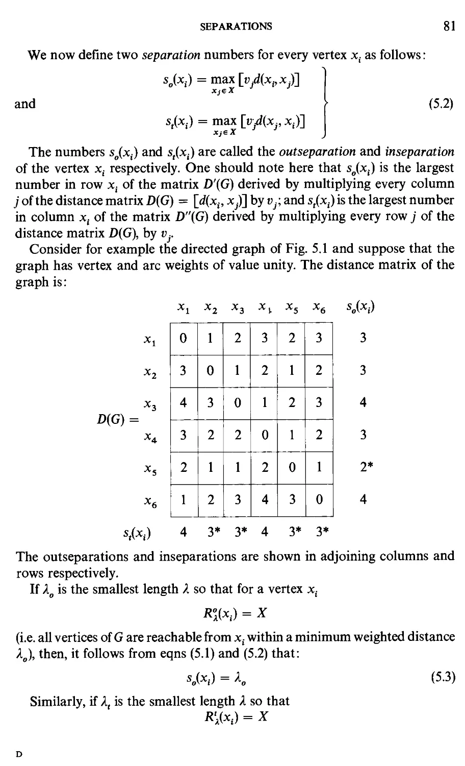
2. Separations 80
3. Centre and Radius 82
4. The Absolute Centre 83
5. Algorithms for the Absolute Centre 85
6. Multiple Centres (p-Centres) 92
7. Absolute p-Centres • 94
8. An Algorithm for Finding Absolute p-Centres 95
9. Problems P5 103
10. References 105
Chapter 6. The Location of Medians
1. Introduction 106

CONTENTS Xlll
2. The Median 106
3. Multiple Medians (p-Medians) 108
4. The Generalized p-Median 110
5. Methods for the p-Median Problem 112
6. Problems P6 118
7. References 120
Chapter 7. Trees
1. Introduction 122
2. The Generation of all Spanning Trees of a Graph 125
3. The Shortest Spanning Tree (SST) of a Graph 135
4. The Steiner Problem 142
5. Problems P7 145
6. References 147
Chapter 8. Shortest Paths
1. Introduction ... ... ... ... ... ... ... ... 150
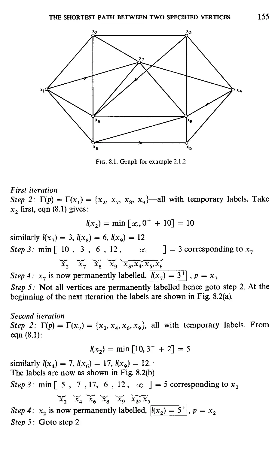
2. The Shortest Path Between Two Specified Verticess and t ... 152
3. The Shortest Paths Between all Pairs of Vertices 163
4. The Detection of Negative Cost Circuits 165
5. The K Shortest Paths Between Two Specified Vertices 167
6. The Shortest Path Between Two Specified Vertices in the Special
Case of a Directed Acyclic Graph 170
7. Problems Related to the Shortest Path 174
8. ProblemsP8 183
9. References 186
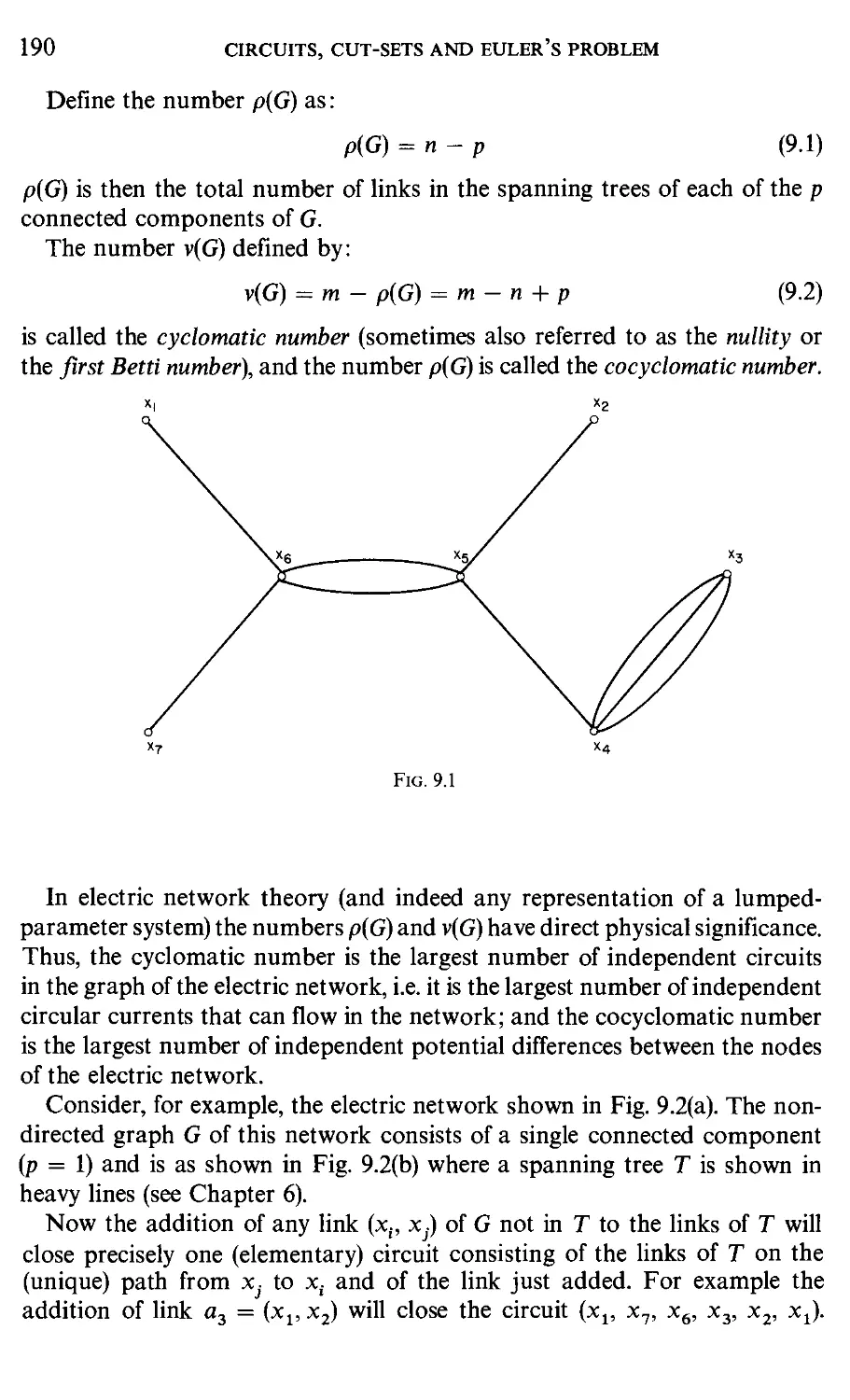
Chapter 9. Circuits, Cut-sets and Eider's Problem
1. Introduction ... ... ... ... ... ... 189
2. The Cyclomatic Number and Fundamental Circuits 189
3. Cut-sets 193
4. Circuit and Cut-set Matrices 197
5. Eulerian Circuits and the Chinese Postman's Problem 199

XIV CONTENTS
6. Problems P9 210
7. References 212
Chapter 10. Hamiltonian Circuits, Paths and the Travelling Salesman Problem
1. Introduction 214
Parti
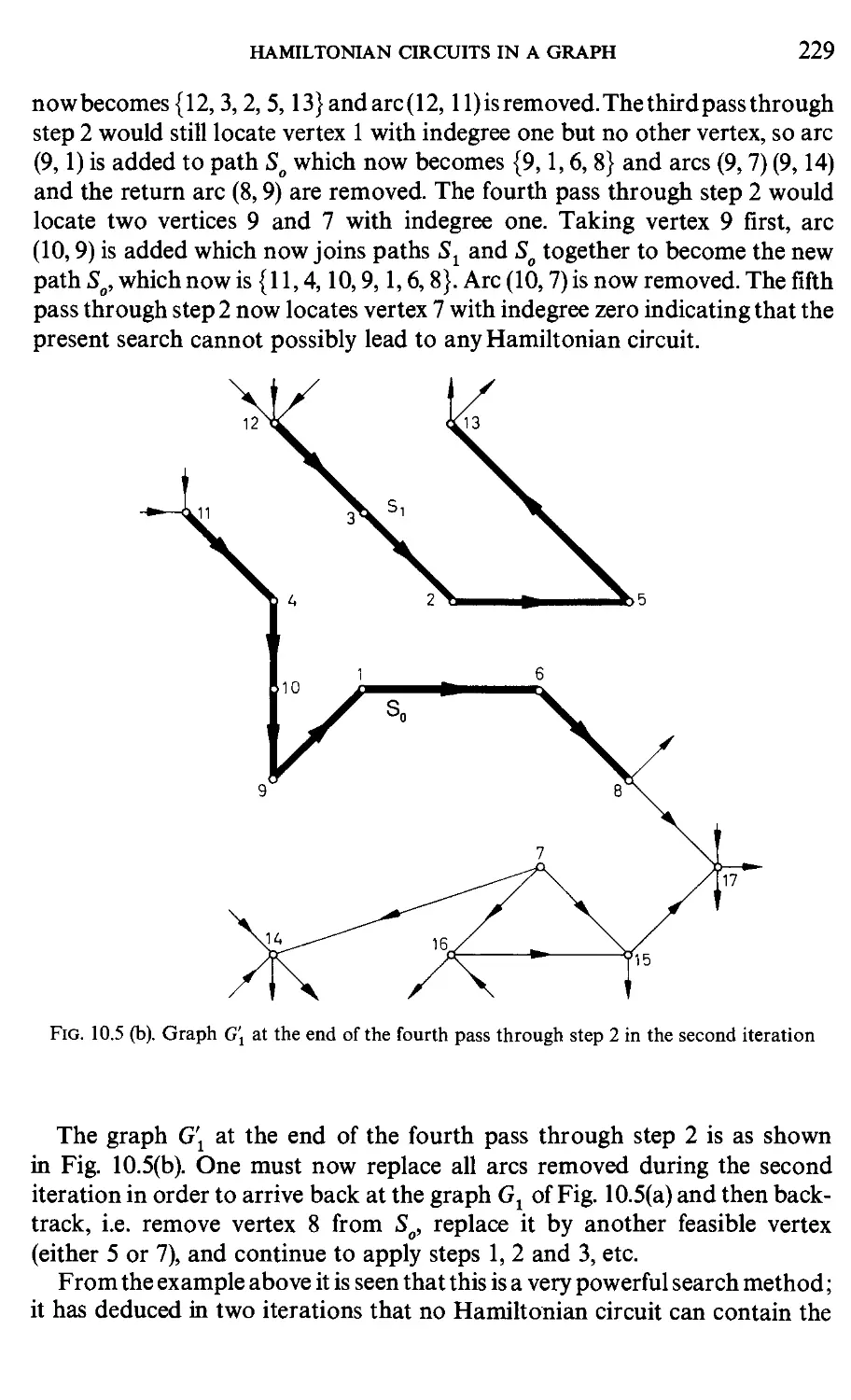
2. Hamiltonian Circuits in a Graph ... ... ... ... ... 216
3. Comparison of Methods for Finding Hamiltonian Circuits ... 230
4. A Simple Scheduling Problem 233
Part II
5. The Travelling Salesman Problem 236
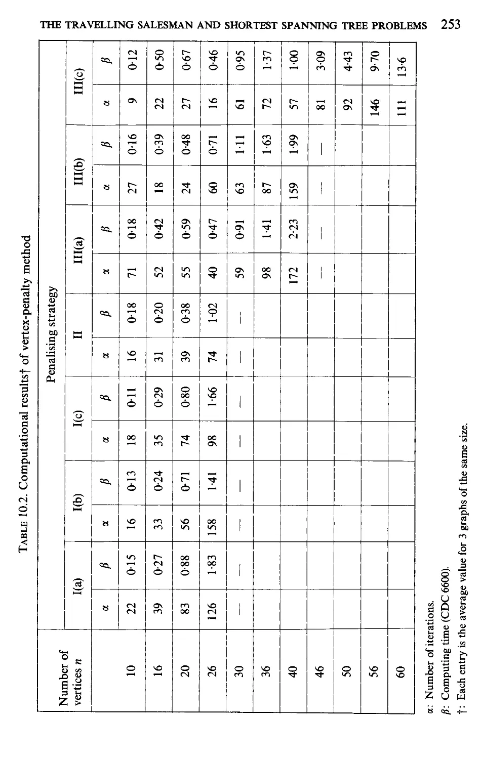
6. The Travelling Salesman and Shortest Spanning Tree Problems 239
7. The Travelling Salesman and Assignment Problems 255
8. Problems P10 276
9. References 278
10. Appendix 279
Chapter 11. Network Flows
1. Introduction 282
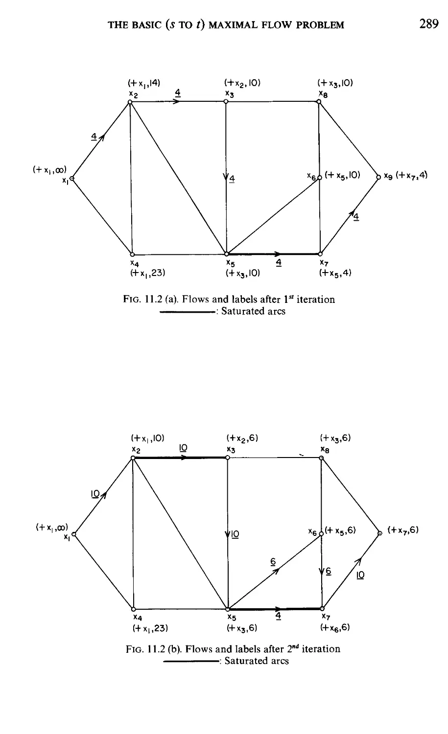
2. The Basic (s to t) Maximum Flow Problem 283
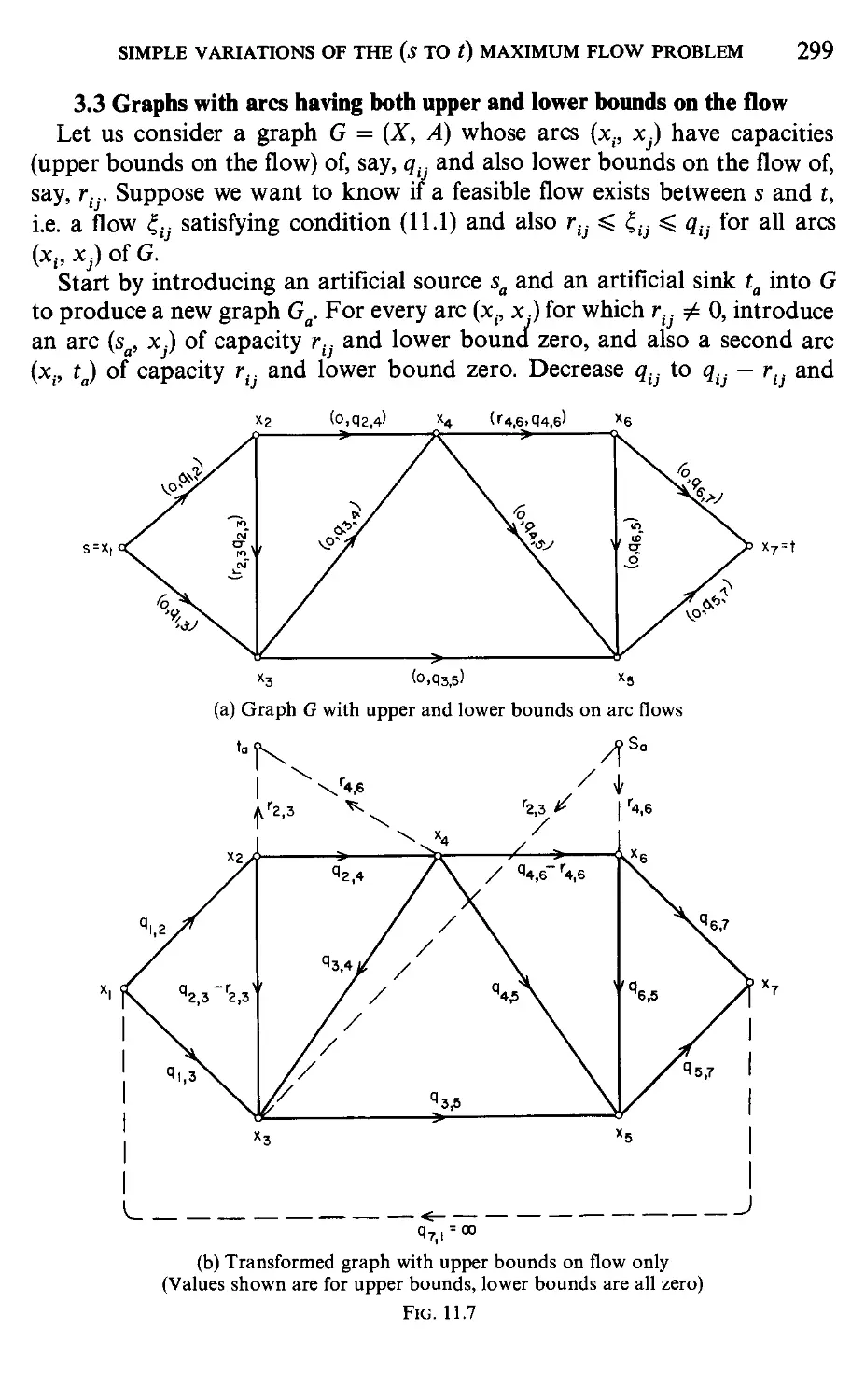
3. Simple Variations of the (s to t) Maximum Flow Problem ... 296
4. Maximum Flow Between Every Pair of Vertices 300
5. Minimum Cost Flow from s to t 308
6. Flows in Graphs with Gains 325
7. Problems Pll 335
8. References 337

CONTENTS XV
Chapter 12. Matchings, Transportation and Assignment Problems
1. Introduction 339
2. Maximum Cardinality Matchings 342
3. Maximum Matchings with Costs 359
4. The Assignment Problem (AP) 373
5. The General Degree-Constrained Partial Graph Problem ... 379
6. The Covering Problem 333
7. Problems P12 384
8. References 387
Appendix I: Decision-Tree Search Methods 390
Subject Index 396

Chapter 1
Introduction
1. Graphs—Definition
A graph G is a collection of points or vertices xv x2,...,xn (denoted by the
set X), and a collection of lines a1,a2,...,am (denoted by the set A) joining
all or some of these points. The graph G is then fully described and denoted
by the doublet (X, A).
If the lines in A have a direction—which is usually shown by an arrow—
they are called arcs and the resulting graph is called a directed graph (Fig.
1.1 (a)). If the lines have no orientation they are called links and the graph is
nondirected (Fig. l.l(b)). In the case where G = (X, A) is a directed graph
but we want to disregard the direction of the arGs in A, the nondirected
counterpart to G will be written as G = {X, A).
Throughout this book, when an arc is denoted by the pair of its initial and
final vertices (i.e. by its two terminal vertices), its direction will be assumed to
be from the first vertex to the second. Thus, in Fig. l.l(a) (x15 x2) refers to arc
av and (x2, Xj) to arc a2.
An alternative and often preferable way to describe a directed graph G,
is by specifying the set X of vertices and a correspondence F which shows how
the vertices are related to each other. F is called a mapping of the set X in X
and the graph is denoted by the doublet G = (X, F).
In the example of Fig. 1.1 (a) we have
F(xj) = {x2, x5} i.e. x2 and x5 are the final vertices of
arcs whose initial vertex is x1.
F(x2) = {x15x3}
F(x3) = {xj
r(*4) = 0, the null or empty set
and
r(x5) = {x4}.
i

INTRODUCTION
a4
Fig. 1.1. (a) Directed, (b) Nondirected and (c) Mixed graphs

GRAPHS—DEFINITION 3
In the case of a nondirected graph, or of a graph containing both arcs and
links (such as the graphs shown in Figs l.l(b) and 1.1 (a)), the correspondences
f will be assumed to be those of an equivalent directed graph in which every
link has been replaced by two arcs in opposite directions. Thus, for the graph
of Fig. l.l(b) for example, r(x5) = {xv x3, x4}, F^) = {x5} etc.
Since F(X;) has been defined to mean the set of those vertices Xj e X for
which an arc (xj; x^) exists in the graph, it is natural to write as r(xi) the
set of those vertices xk for which an arc (xk, x^ exists in G. The relation
T'i(xl) is then called the inverse correspondence. Thus for the graph shown
in Fig. 1.1 (a) we have:
1
etc.
It is quite obvious that for a nondirected graph F~ 1(xl) = r(xf) for all x, e X.
When the correspondence F does not operate on a single vertex but on a
set of vertices such as Xq = {xv x2,..., xq}, then F(.X^) is taken to mean:
T(Xq) = F(x1) u F(x2) u uF(x,)
i.e. T{Xq) is the set of those vertices x^ e X for which at least one arc (xi; x})
exists in G, for some x(eX4. Thus, for the graph of Fig. l.l(a); F({x2, x5})
{l34}{l3}) {25l}
The double correspondence r(F(Xj)) is written as r2(x;). Similarly the triple
correspondence r(F(r(x;))) is written as r3(xf) and so on. Thus, the graph in
Fig.l.l(a):
)) = F({x2,x5}) = {xvx3,x4}
= F({x1,x3,x4}) = {x,,x2lx5}
etc.
Similarly for r(x;), F(x;) and so on.
2. Paths and Chains
A path in a directed graph is any sequence of arcs where the final vertex
of one is the initial vertex of the next one.
Thus in Fig. 1.2 the sequence of arcs:
a6, a5, a9, a8, a4 A.1)
ava6,a5,ag A.2)
ava6,as,a9,a10,a6,a4 A.3)
are all paths.

INTRODUCTION
Arcs a = (x;, x}), xt =£ Xj which have a common terminal vertex are called
adjacent. Also, two vertices x. and Xj are called adjacent if either arc (xt, x})
or arc (Xj, x;) or both exist in the graph. Thus in Fig. 1.2 arcs a1,a10,a3 and a6
are adjacent and so are the vertices x5 and x3; on the other hand arcs a1 and
a5 or vertices x1 and x4 are not adjacent.
A simple path is a path which does not use the same arc more than once.
Thus the paths A.1) and A.2) above are simple but path A.3) is not, since it
uses arc a6 twice.
An elementary path is a path which does not use the same vertex more
than once. Thus the path A.2) is elementary but paths A.1) and A.3) are not.
Obviously an elementary path is also simple but the reverse is not necessarily
true. Note for example that path A.1) is simple but not elementary, that path
A.2) is both simple and elementary and that path A.3) is not simple and not
elementary.
A chain is the nondirected counterpart of the path and applies to graphs
with the direction of its arcs disregarded. Thus a chain is a sequence of links

PATHS AND CHAINS 5
(a , fl2' • ■ ■' **«) *n which every link at, except perhaps the first and last links,
is connected to the links a;_x and ai+1 by its two terminal vertices.
a2,a^,a8,a10 A.4)
a^a^a^a^a^ A.5)
and
are all chains; where a bar above the symbol of an arc means that its direction
is disregarded i.e. it is to be considered as a link.
In an exactly analogous way as we defined simple and elementary paths
we can define simple and elementary chains. Thus, chain A-4) is simple and
elementary, chain A-5) is simple but not elementary and chain A-6) is both
not simple and not elementary.
A path or a chain may also be represented by the sequence of vertices that
are used. Thus, path A.1) may also be represented by the sequence
x2, xs, xA, x3, x5, x6 of vertices, and this representation is often more useful
when one is concerned with finding elementary paths or chains.
2.1 Weights and the length of a path
A number ctj may sometimes be associated with an arc (x{, Xj). These
numbers are called weights, lengths or costs and the graph is then called arc-
weighted. Also a weight v{ may sometimes be associated with a vertex xt
and the resulting graph is then called vertex-weighted. If a graph is both arc
and vertex weighted it is simply called weighted.
Considering a path ft represented by the sequence of arcs (av a2,..., aq),
the length (or cost) of the path 1(jj) is taken to be the sum of the arc weights on
the arcs appearing in n, i.e.
(xu xj) in/j
Thus, the words "length", "cost" and "weight" when applied to arcs,
are all considered to be equivalent, and in specific applications that word will
be chosen which gives the best intuitive meaning and which is in agreement
with the usage found in the literature.
The cardinality of the path /i is q i.e. the number of arcs appearing in the
path.
3. Loops, Circuits and Cycles
A loop is an arc whose initial a_nd final vertices are the same. In Fig. 1.3
for example arcs a2 and a5 form loops.

INTRODUCTION
A circuit is a path av a2,..., aq in which the initial vertex of ax coincides
th the final vertex of aq.
Thus in Fig. 1.3 the sequences:
a3,a6,an
alv a3, a4, a7,
v a12, a
A.7)
A.8)
A.9)
are all circuits.
Circuits A.7) and A.9) are elementary since they do not use the same vertex
more than once (except for the initial and final vertices which are the same),
but circuit A.8) is not elementary since vertex xt is used twice.
An elementary circuit which passes through all the n vertices of a graph G
is of special significance and is known as a Hamiltonian circuit. Of course
not all graphs have a Hamiltonian circuit. Thus, circuit A.9) is a Hamiltonian
circuit of the graph of Fig. 1.3; but the graph of Fig. 1.2 has no Hamiltonian
circuits as can be seen quite easily from the fact that there is no arc having
xx as its final vertex.
Fig. 1.3

LOOPS, CIRCUITS AND CIRCLES '
A cycle is the nondirected counterpart of the circuit. Thus, a cycle is a
chain x1,x2,...,xq in which the beginning and end vertices are the same,
i.e. in which xt = xq.
In Fig. 1.3 the chains:
ava12,a10 A.10)
and
alo,ava3,a4,ai,ava12 A.11)
all form cycles.
4. Degrees of a Vertex
The number of arcs which have a vertex xi as their initial vertex is called the
outdegree of vertex x;, and similarly the number of arcs which have xi as
their final vertex is called the indegree of vertex x;.
Thus, referring to Fig. 1.3, the outdegree of x6, denoted by do(x6), is
|F(x6)| = 2, and the indegree of x6 denoted by dt(x6), is | r~ 1(xG) | = 1.
It is quite obvious that the sum of the outdegrees or indegrees of all the
vertices in a graph is equal to the total number of arcs of G i.e.
.1 do(Xi) = £ d,(Xi) = m A.12)
where n is the total number of vertices and m the total number of arcs of G.
For a nondirected graph G = (X, F) the degree of a vertex x; is similarly
defined by d(xt) = | F(x;) |, and when no confusion can arise it will be written
as dv
5. Partial Graphs and Subgraphs
Given a graph G = (X, A), a partial graph Gp of G is the graph (X, Ap) with
AD a A. Thus a partial graph is a graph with the same number of vertices
but with only a subset of the arcs of the original graph.
If Fig. 1.4(a) represents the graph G, Fig. 1.4(b) is a partial graph Gp.
Given a graph G = {X, F) a subgraph Gs is the graph (Xs, FJ with Xs c X;
and for every x; e Z^, FS(X;) = F(x;) n Xs. Thus, a subgraph has only a sub-
subset Xs of the set of vertices of the original graph but contains all the arcs
whose initial and final vertices are both within this subset. It is often very
convenient to denote the subgraph Gs simply by <XS> and when no confusion
can arise we will use this latter symbolism.

INTRODUCTION
(b) Partial graph
(c) Subgraph
(d) Partial subgraph
Fig. 1.4
Fig. 1.4(c) shows a subgraph of the graph in Fig. 1.4(a) containing only
vertices xv x2, x3 and xA, and those arcs which interconnect them.
The two definitions given above can be combined to define the partial
subgraph, an example of which is given in Fig. 1.4(d) which shows a partial
graph of the subgraph in Fig. 1.4(c).
If a graph represents an entire organization with the vertices representing
people and the arcs representing, say, lines of communication, then the graph
representing only the more important communication channels of the whole
organization is a partial graph; the graph which represents the detailed lines
of communication of only a part of the organization (say a division) is a
subgraph; and the graph which represents only the important lines of
communication within this division is a partial subgraph.
6. Types of Graphs
A graph G = (X, A) is said to be complete if for every pair of vertices
x, and Xj in X, there exists a link {x^x~^) in G = (X, A) i.e. there must be at

TYPES OF GRAPHS 9
least one arc joining every pair of vertices. The complete nondirected graph
on n vertices is denoted by Kn.
A graph (X, A) is said to be symmetric if, whenever an arc (x;, x^ is one of
the arcs in the set A of arcs, the opposite arc (xp x;) is also in the set A.
An antisymmetric graph is a graph in which whenever an arc (x;, Xj) e A,
the opposite arc (Xj, xt)$A. Obviously an antisymmetric graph cannot
contain any loops.
Fig. 1.5(a) shows a symmetric and Fig. 1.5(b) an antisymmetric graph.
For example if the vertices of a graph represents a group of people and an
arc directed from vertex xi to vertex Xj means that x; is the friend or relative
of x ■ then the graph would be symmetric. On the other hand if an arc directed
from x; to Xj means that Xj is a subordinate of x; then the resulting graph
would be antisymmetric.
(a) Symmetric graph
(b) Antisymmetric graph
(c) Complete symmetric graph (d) Complete antisymmetric graph (tournament)
Fig. 1.5
Combining the above definitions one can define the complete symmetric
graph, an example of which is shown in Fig. 1.5(c), and the complete anti-
antisymmetric graph, with an example shown in Fig. 1.5(d). This last type of
graph is also often referred to as a tournament.

10 INTRODUCTION
A nondirected graph G = (X, A) is said to be bipartite, if the set X of its
vertices can be partitioned into two subsets X" and Xb so that all arcs have
one terminal vertex in X" and the other in Xb. A directed graph G is said to be
bipartite if its nondirected counterpart G is bipartite. It is quite easy to show
that:
Theorem 1. A nondirected graph G is bipartite if and only if it contains no
circuits of odd cardinality.
Proof. Necessity. Since X is partitioned into X" and Xb;
XauXb = X and X" n Xb = 0 A.13)
Let an odd cardinality circuit xti, xi2>..., x,, xh exist and without loss of
generality take xh e X". Since, from the definition, two consecutive vertices
on this circuit must belong one to X" and the other to Xb it follows that
xi2 e Xb, xh e X" etc. and, in general, xik eX" if k is odd and xik e Xb, if k is
even. Since we assumed the cardinality of the circuit to be odd, xt e X" which
implies xh e Xb. This is a contradiction since X" n Xb = 0 and no vertex
can belong to both Xa and X".
Sufficiency. Assume that no circuits of odd cardinality exist. Choose any
vertex xt, say, and label it " + ", the iteratively perform the operations:
Choose any labelled vertex x. and label all vertices in r(x;) with the reverse
sign of the label of xt.
Continue applying this operation until either:
(i) all vertices have been labelled and are consistent, i.e. for any two
vertices joined by a link, one is labelled "+" and the other "—", or
(ii) some vertex, say xik, which was labelled with one sign can now be
labelled (from a different vertex) with the opposite sign, or
(iii) for all labelled vertices x;, T(x;) is labelled but other unlabelled vertices
exist.
In case (i) let all vertices labelled " + " be in the set X" and those labelled
" — " be in the set Xb. Since all links are between differently labelled vertices,
the graph G is bipartite.
In case (ii) vertex xiu must have received its " + " label along some path
(jij say) of vertices, alternatingly labelled " + " and " —", starting from xh
and finishing at x;. Similarly the "—" label on x; was obtained along some
path fi2. Let x* be the last but one (the last being xik) vertex common to paths
Hl and n2. If x* is labelled " + " the part of path n2 from x* to xik must be of
even, and the part of path n2 from x* to xik must be of odd cardinality re-
respectively. The opposite is true if x* is labelled " —". Hence the circuit con-
consisting of path /ij from x* to xlk and the reverse part of path fi2 from xik
back to x* is always of odd cardinality. This contradicts the assumption that
no odd cardinality circuits exist in G and hence case (ii) is impossible.
Case (iii) implies that there is no link between any labelled and unlabelled

TYPES OF GRAPHS
11
Fig. 1.6. The Kuratowski nonplanar graphs, (a) K5 and (b) K3 ,
vertex which means that G is disconnected into two or more parts and each
part can then be considered in isolation. Thus, only case (i) is eventually
possible, and hence the theorem.
When a graph is bipartite and this property needs to be emphasized we
will denote the graph as (Xa u Xb, A) with equations A.13) being implied.
A bipartite graph G = (X" u Xb, A) is said to be complete if for every two
vertices x.eXa and x}eXb there exists a link (x^x) in G = {X,A). If \Xa\,
the number of vertices in set X", is r and |X6| = s, then the complete non-
directed bipartite graph G = {X" u Xb, A) is denoted by Krs.
A graph G = (X, A) is said to be planar, if it can be drawn on a plane (or
sphere) in such a way so that no two arcs intersect each other. Figure 1.6(a)
shows the complete graph K5 and Fig. 1.6(b) shows the complete bipartite

12 INTRODUCTION
graph K3 3 both of which are known to be nonplanar [1, 3]. These two
graphs play a central role in planarity and are known as the Kuratowski
graphs.
7. Strong Graphs and the Components of a Graph
A graph is said to be strongly connected or strong if for any two distinct
vertices x, and xp there is at least one path going from xi to xy The above
definition implies that any two vertices of a strong graph are mutually
reachable.
A graph is said to be unilaterally connected or unilateral if for any two
distinct vertices x; and xf there is at least one path going from either xt to xfi
or from Xj to xt, or both.
A graph is said to be weakly connected or weak if there is at least one chain
joining every pair of distinct vertices. If for a pair of vertices such a chain does
not exist, the graph is said to be disconnected [2].
Considering, for example, the graph shown in Fig. 1.7(a) it is easy to check
that this is strong. The graph shown in Fig. 1.7(b) on the other hand is not
strong (there is no path going from Xj to x3), but is unilateral. The graph shown
in Fig. 1.7(c) is neither strong nor unilateral—since there is no path going
from x2 to x5 nor one from x5 to x2. It is, however, weak. Finally, the graph
of Fig. 1.7(d) is disconnected.
Given any property P to characterize a graph, a maximal subgraph (Xs}
if a graph G with respect to that property, is a subgraph which has this
property, and there is no other subgraph (Xs} with Xs => Xs and which
also has the property. Thus, if the property P is strong-connectedness, then
a maximal strong subgraph of G is a strong subgraph of G which is not
contained in any other strong subgraph. Such a subgraph is called a strong
component of G. Similarly a unilateral component is a maximal unilateral
subgraph and a weak component is a maximal weak subgraph.
For example, in the graph G shown in Fig. 1.7(b), the subgraph
<{xt, x4, x5, x6}> is a strong component of G.On the other hand ({xv x6}>
and <{xj, x5, x6}> are not strong components—even though they are strong
subgraphs—since these are contained in <{xj, x4, x5, x6}> and are, therefore,
not maximal. In the graph shown in Fig. 1.7(c) the subgraph <{xx, x4, x5}> is
a unilateral component. In the graph shown in Fig. 1.7(d) the subgraphs
({x^x^Xg}) and ^{x2,x3,x4\') are both weak components and are the
only two such components.
It is quite obvious from the definitions that unilateral components are
not necessarily pairwise vertex-disjoint. A strong component must be con-
contained in at least one unilateral component and a unilateral component
contained in a weak component for any given graph G.

MATRIX REPRESENTATIONS
8. Matrix Representations
13
A convenient way of representing a graph algebraically is by the use of
matrices, as follows.
(a) Strong graph
(b) Unilateral graph
(d) Disconnected graph
Fig. 1.7.
8.1 The adjacency matrix
Given a graph G, its adjacency matrix is denoted by A = [a,.J and is given
by:
atj = 1 if arc (xv x^ exists in G
atj = 0 if arc (xj; x;) does not exist in G.
Thus, the adjacency matrix of the graph shown in Fig. 1.8 is:
1
2
3
4
5
6
*1
0
0
0
0
1
1
X2
1
1
0
0
0
0
*3
1
0
0
1
0
0
x4
0
0
0
0
1
0
x5
0
1
0
0
0
1
X6
0
0
0
0
0
1

14
INTRODUCTION
The adjacency matrix defines completely the structure of the graph. For
example, the sum of all the elements in row xt of the matrix gives the out-
degree of vertex xt and the sum of the elements in column xt gives the in-
degree of vertex xv The set of columns which have an entry of 1 in row x;
is the set r(x;), and the set of rows which have an entry of 1 in column xt is
the set T^)-
Consider the adjacency matrix raised to the second power. An element,
^2) say, of matrix A2 is given by:
<42) = £ aifl* A-14)
Each term in the summation of equation A.14) has the value 1 only if
atJ and ajk are both 1, otherwise it has the value 0. Since atj = ajk = 1 implies
a path of cardinality 2 from vertex xt to vertex xk via vertex xf the term aj2) is
then the total number of cardinality 2 paths from xt to xk.
Similarly, if a%] is an element of Ap, then dfk] is the number of paths (not
necessarily simple or elementary) of cardinality p from xt to xk.
8.2 The incidence matrix
Given a graph G of n vertices and m arcs, the incidence matrix of G is
denoted by B = [b;j and is an n x m matrix defined as follows.
btj = 1 if xi is the initial vertex of arc a,-
bu = — 1 if X; is the final vertex of arc a,,
and btj = 0 if xt is not a terminal vertex of arc ai or if a, is a loop.

MATRIX REPRESENTATIONS
15
For the graph shown in Fig. 1.8, the incidence matrix is:
x, I -
1
2
3
4
5
6
1
-1
0
0
0
0
«2
1
0
-1
0
0
0
a3
0
0
0
0
0
0
aA
0
1
0
0
-1
0
0
0
-1
1
0
0
a6
0
0
0
-1
1
0
a7
0
0
0
0
-1
1
a8
-1
0
0
0
1
0
a9
-1
0
0
0
0
1
0
0
0
0
0
0
Since each arc is adjacent to exactly two vertices, each column of the inci-
incidence matrix contains one 1 and one — 1 entry, except when the arc forms a
loop in which case it contains only zero entries.
If G is a nondirected graph, then the incidence matrix is defined as above
except that all entries of — 1 are now changed to +1.
Fig. 1.9.
9. Problems PI
1- For the graph of Fig. 1.9 find:
(a) Hx2) (e)
(d) k
(g)
d,(x2)
the adjacency matrix A
the incidence matrix B

16 INTRODUCTION
2. For the graph G = (X, A) of Fig 1.9 draw:
(a) The subgraph <{x1(x2,x4,x5}>
(b) The partial graph {X, A'), where (xf, x3) e A' if and only if i + j is odd.
(c) The partial graph as defined in (b) of the subgraph in (a).
3. For a nondirected graph prove that the number of vertices of odd degree is even.
(Zero is an even number).
4. Show that any complete symmetric graph contains a Hamiltonian circuit.
5. Show that the rank of the incidence matrix B of a connected graph is n — 1, and
hence prove that the rank of B for a graph with P (weak) components is n — P.
6. Prove that a nondirected connected graph remains connected after the removal of a
link if and only if that link is part of some circuit.
7. Prove that a nondirected connected graph with n vertices
(a) Contains at least n — 1 links
(b) If it contains more than n — 1 links then it has at least one circuit.
10. References
1. Berge, C, A962). "The theory of graphs", Methuen, London.
2. Harary, F., Norman, R. Z. and Cartwright, D. A965). "Structural models: An
introduction to the theory of directed graphs," Wiley, New York.
3. Kuratowski, G. A930). Sur le probleme des courbes gauches en topologie, Fund.
Match., 15-16, p. 271.
4. Roy, B. A969, 1970). Algebre moderne et theorie des graphes, Vol. 1 A969), Vol. 2
A970), Dunod, Paris.

Chapter 2
Reachability and Connectivity
1. Introduction
In the previous chapter it was mentioned that the communication system
of an organization can be considered in terms of a graph where people are
represented by vertices, and communication channels by arcs. A natural
question to ask of such a system, is as to whether information held by a given
individual xt can be communicated to another individual Xj; that is, whether
there is a path leading from vertex xt to vertex xy If such a path exists we say
that x. is reachable from xr If the reachability is restricted to paths of limited
cardinality, we would like to know if x^. is still reachable from xi. The purpose
of the present Chapter is to discuss some fundamental concepts relating to
the reachability and connectivity properties of graphs and introduce some
very basic algorithms.
In terms of the graph representing an organization, the present chapter
considers the questions:
(i) What is the least number of people from which every other person
in the organization can be reached?
(ii) What is the largest number of people who are mutually reachable?
(iii) How are (i) and (ii) above related?
2. Reachability and Reaching Matrices
The reachability matrix R = [ry] is defined as follows:
r.j = 1 if vertex x} is reachable from vertex xt.
= 0 otherwise.
The set of vertices R(x{) of the graph G which can be reached from a given
vertex x; consists of those elements Xj for which there is an entry of 1 in cell
(x^ X;) of the reachability matrix. Obviously all the diagonal elements of R
are 1 since every vertex is reachable from itself, by a path of cardinality 0.
17

18 REACHABILITY AND CONNECTIVITY
Since F(x;) is that set of vertices x} which are reachable from x( along a
path of cardinality 1 (i.e. that set of vertices for which the arcs (x.,Xj) exist
in the graph) and since F(x.) is that set of vertices reachable from Xj along a
path of cardinality 1; the set of vertices r(F(x;)) = F2(x;) consists of those
vertices reachable from x. along a path of cardinality 2. Similarly F^) is
that set of vertices which are reachable from vertex x, along a path of cardinality
P-
Since any vertex of the graph G which is reachable from x; must be reachable
along a path (or paths) of cardinality 0 or 1 or 2,... or p for some finite but
suitably large value of p, the reachable set of vertices from vertex x. is:
R(xt) = {xt} u r(x;) u r2(xf) u... u r"(x,) B.1)
Thus, the reachable set -R(x;) can be obtained from eqn B.1) by performing
the union operations from left to right until such time when the current total
set is not increased in size by the next union. When this occurs any subsequent
unions will obviously not add any new members to the set and this is then the
reachable set R(x.). The number of unions that may have to be performed
depends on the graph, although it is quite clear that p is bounded from above
by the number of vertices in the graph minus one.
The reachability matrix can therefore be constructed as follows. Find the
reachable sets R(xt) for all vertices xi e X as mentioned above. Set ri} = 1 if
Xj e R(xt), otherwise set ri} = 0. The resulting matrix R is the reachability
matrix.
The reaching matrix Q = \_q..~] is defined as follows:
qtj = 1 if vertex x} can reach vertex x;
= 0 otherwise.
The reaching set Q(xt) of the graph G is that set of vertices which can reach
Fig. 2.1.

REACHABILITY AND REACHING MATRICES
19
vertex x.. In a manner analogous to the calculation of the reachable set R(xt)
from eqn B.1), the set g(x.) can be calculated as:
Q(x,) =
~ V,-) u r~2(x(
etc.
r-'(xf)
B.2)
where F-^x^r-Hr-
The operations are performed from left to right until the next set union
operation does not change the set Q(x().
It is quite apparent from the definitions that column xt of the matrix Q
(found by setting qtj = 1 if xj eQ(x.), and qi} = 0 otherwise), is the same as
row x. of the matrix R; i.e. Q = R', the transpose of the reachability matrix.
2.1 Example
Find the reachability and reaching matrices of the graph G shown in Fig. 2.1.
The adjacency matrix of G is:
A = xA
1
1
0
0
0
0
0
0
0
0
0
0
1
0
0
1
1
0
0
0
1
1
0
0
1
1
0
0
0
0
0
0
0
0
1
The reachable sets are calculated from eqn B.1) as:
RixJ = {xt} u {xv x5} u [x2, x4, x5} u {x2, x4, x5}
= (Xp X2, X4, Xj}
R(x2) = {x2} u {x2, x4} u {x2, x4, x5} u {x2, x4, x5}
= (x2, x4, x5j
*(x3) = {x3} u {x4} u {x5} u {x5}
— (x3, x4, x5)
RbJ = {x4} u {x5} u {x5}
= {x4,x5}

20 REACHABILITY AND CONNECTIVITY
R(x3) = {x5} u {x5}
= (x5}
3> xi) u (X4' xe) u (X3> X5> x?) u (X4> X5'
= (x3, x4, x5, x6, x7)
7) = {x7} u {x4, x6} u {x3, x5, x7} u {x4, x5, x6}
= \X3, x4, x5, Xg, x7 j
The reachability matrix is therefore given by:
xl
x2
X3
R = x4
x5
X6
X,
1
0
0
0
0
0
0
1
1
0
0
0
0
0
0
0
1
0
0
1
1
1
1
1
1
0
1
1
1
1
1
1
1
1
1
0
0
0
0
0
1
1
0
0
0
0
0
1
1
and the reaching matrix is given by:
xl
x2
*3
Q = R' = x4
x5
X6
X,
1
1
0
1
1
0
0
0
1
0
1
1
0
0
0
0
1
1
1
0
0
0
0
0
1
1
0
0
0
0
0
0
1
0
0
0
0
1
1
1
1
1
0
0
1
1
1
1
1
as can easily be checked.
It should be mentioned here that since all entries in the R and Q matrices
are either 0 or 1, each row can be stored in binary form using one (or more)
computer words. Thus, finding the R and Q matrices becomes a computation-
computationally very simple task, since the union of sets indicated by eqns B.1) and B.2)
and the comparison after each union—in order to determine if it is necessary

REACHABILITY AND REACHING MATRICES 21
continue—can then each be done by a single logical operation on a
computer.!
Since R(x) is the set of vertices which can be reached from x; and Q(Xj) the
set of vertices which can reach xJt the set /?(x.) n Q(x}) is then the set of
vertices which are on at least one path going from x. to xf These vertices
are called essential with respect to the two end vertices x; and Xj [7]. All
other vertices xk $ R(x() n Q(Xj) are called inessential or redundant since
their removal does not affect any path from x, to Xj.
The reachability and reaching matrices defined above are absolute, in the
sense that the number of steps in the paths reaching from xt to xj was not
restricted. On the other hand a limited reachability and reaching matrices
can be defined where the cardinality of the path must not exceed a certain
number. These limited matrices can also be calculated from eqns B.1) and
B.2) in an exactly analogous manner to that described previously where p
would now be the upper bound on the allowed path cardinality.
A graph is said to be transitive if the existence of arcs (xt, x}) and {xp xk)
implies the existence of arc (xr xk). The transitive closure of a graph G = (X, A)
is the graph Gtc = (X, A u A') where A' is the minimal number of arcs
necessary to make Gtc transitive. It is then quite apparent that, since a path
from x; to Xj in G must correspond to an arc (x;, x^) in Gtc, the reachability
matrix R of G is the same as the adjacency matrix A of Gtc with all its diagonal
elements set to 1.
3. Calculation of Strong Components
A strong component (SC) of a graph G has been defined in the previous
chapter as being a maximal strongly connected subgraph of G. Since, for a
strongly connected graph, vertex x. is reachable from vertex xi and vice versa
for any x; and x^., the SC containing a given vertex x; is unique and x( will
appear in the set of vertices of one and only one SC. This statement is quite
obvious since if x; appears in two or more strong components, then a path
from any vertex in one SC to any other vertex in another SC would always
exist (via x;), and hence the union of the strong components would be strongly
connected, a fact which is contrary to the definition of the SC.
If vertex x; is taken to be both the initial and terminal vertex then the set
of vertices essential with respect to these two identical ends (i.e. the set of
vertices on some circuit containing x;) is given by i?(x;) n Q(xt). Since all
these essential vertices can reach and be reached from x., they can also
reach and be reached from each other. Moreover, as no other vertex is
t Alternative ways of constructing the sets R(x,) and Q(xt) using a vertex labelling procedure
starting from x., are indicated in Chapter 7 dealing with trees.

22 REACHABILITY AND CONNECTIVITY
essential with respect to the ends xt and x;, the set R(x.) n Q(xt)—which can
be calculated by eqns B.1) and B.2)—defines the vertices of the unique SC
of G containing vertex xr
If these vertices are removed from the graph G = {X, F), the remaining
subgraph G = {X - R(xt) n Q(x.)> can be treated in the same way by
finding a SC containing a vertex Xj e X — R{x.) n Q(x.). This process can be
repeated until all the vertices of G have been allocated to one SC. When this
is done the graph G is said to have been partitioned into its strong components
[3].
The graph G* = (X*, F*) defined so that each of its vertices represents the
vertex set of a strong component of G, and an arc (xf, xj") exists if and only if
there exists an arc (xr x ) in G for some x. e xf and some Xj e x*; is called the
condensed graph of G.
It is quite apparent that the condensed graph G* contains no circuits,
since a circuit would mean that any vertex on that circuit could reach (and
be reached from) any other vertex, and hence the union of these vertices of
G* would be a SC of G* and therefore also a SC of G, a fact which is contrary
to the definition that the vertices of G* correspond to the SC's of G.
3.1 Example
For the graph G given in Fig. 2.2, find the strong components, and the
condensed graph G*.
Let us find the SC of G containing vertex xv
From eqns B.1) and B.2) we find:
-"■v-^i/ \ 1* 2* 4' 5' 6' 7* 8' 9' 10/
and
Q{x1) = {x1,x2,x3,x5,x6}
Therefore the SC containing vertex xt is the subgraph
<R(x1) n Q(Xj)> = <{xj, x2, xs, x6}>
Similarly, the SC containing vertex x8, say, is the subgraph <{x8, xlo}>,
the SC containing x7 is <{x4, x7, x9}>, the SC containing vertex xu is
<{xn, x12, x13}> and the SC containing vertex x3 is <{x3}>. It should be
noted that this last SC contains just a single vertex of G.
The condensed graph G* is then given by the graph of Fig. 2.3.
The operations described above in order to find the SC's of a graph can
also be done most conveniently by the direct use of the R and Q matrices
defined in the previous section. Thus, if we write R ® Q to mean the element-
by-element multiplication of the two matrices, then it is immediately apparent
that row x. of the matrix R ® Q contains values of 1 in those columns x} for

CALCULATION OF STRONG COMPONENTS
23
Fig. 2.2. The graph G
II- X|2, x|3}
Fig. 2.3. The condensed graph G*
which x. and x^. are mutually reachable, and values of 0 in all other places.
Thus, two vertices are in the same SC if and only if their corresponding rows
(or columns) are identical. The vertices whose corresponding rows contain
an entry of 1 under column xp then form the vertex set of the SC containing xy
It is quite apparent that the matrix R ® Q can be transformed by transposi-
transposition of rows and columns into block diagonal form; each of the diagonal
submatrices corresponding to a SC of G and having entries of l's, all other

24
REACHABILITY AND CONNECTIVITY
entries being 0. For the above example the matrix R ® Q arranged in this
form becomes:
R®Q =
V12
C13
1111
1111
1111
1111
0
0
0
0
1 1
1 1
0
0
0
0
0
1 1 1
1 1 1
1 1 1
0
0
0
0
0
1 1 1
1 1 1
1 1 1
0
0
0
0
0
1
4. Bases
A basis B of a graph is a set of vertices from which every vertex of the graph
can be reached and which is minimal in the sense that no subset of B has this
property. Thus, if we write R(B)—the reachable set of B—to mean:
R(B)= \jR(xt)
XinB
then B is a basis if and only if:
R(B) = X and VScB,«(S)#I
B.3)
B.4)
The second condition (R{S) # X, V S <= B) of eqn B.4) is equivalent to the
condition Xj $ R{x.) for any two distinct x;, x;. e B, i.e. a vertex in B cannot be
reached from another vertex also in B. This can be shown as follows:
Since for any two sets H and H' £ i/ we have R(H') £ R{H), the condition
R{S) # X, V S <= B is equivalent to R{B - {x,.}) / X for all x} e B, in other
words R{Xj) £ R(B — {Xj}). This last condition can be satisfied if and only if
x. $ R(B — {x.}), i.e. if and only if x. 4 R(xf) for any xf, Xj e B.

BASES 25
A basis is, therefore, a set B of vertices which satisfies the following two
conditions:
(i) All vertices of G are reachable from some vertex in B and
(ii) No vertex in B can reach another vertex also in B.
From the above two conditions we can immediately state that:
(a) No two vertices in B can be in the same SC of the graph G.
and (b) For any graph without circuits there is a unique basis consisting of
of the set of points with indegree 0.
The proofs of these statements are very simple and follow directly from the
definitions. (See problems P2.3 and P2.4).
Thus, according to (a) and (b) above, since the condensed graph G* of a
graph G has no circuits, its basis B* say, is the set of vertices of G* with
indegree 0. The bases of G itself can then be found by forming sets containing
one vertex from each one of the vertex-sets in B*, i.e. if B* = {Sv S2,..., Sm}
—m being the number of vertex-sets Sj in the basis B* of G*—then B is any
set {x;i,xi2,...,x;m} where x;.eSr
4.1 Example
For the graph G shown in Fig. 2.2 the condensed graph G* is given in Fig. 2.3.
The basis of this graph is {x*, x*} since x* and x* are the only two vertices of
G* with indegree 0. The bases of G are then given by {x3, xu}, {x3, x12} and
{x3,x13}.
A concept dual to that of the basis can be defined in terms of the reaching
sets Q(x;) as follows:
A contra-basis E is a set of vertices of the graph G = (X, F), so that
and *>*B > B.5)
i.e. B is a minimal set of vertices which can be reached from every other vertex.
The properties of E are analogous to those of B where directed concepts are
replaced by the opposite counterparts. For example, the definition of eqn
B.5) is equivalent to two conditions similar to (i) and (ii) above but with B
replaced by E and the words "are reachable from" replaced by "can reach"
and vice versa.
Thus, the contra-basis of a condensed graph G* is the set of vertices of G*
with outdegree 0, and the contra-bases of G itself can then be found by
constructing sets taking one vertex from each vertex-set in the contra-basis
of G*, similar to what was done previously for the bases.
In the example of the graph G shown in Fig. 2.2, the condensed graph G*,
(shown in Fig. 2.3), contains only one vertex x* with out-degree 0. Thus the
contra-basis of G* is {x*} and the contra-bases of G are {x4}, {x7} and {x9}.

26 REACHABILITY AND CONNECTIVITY
4.2 Application to organizational structure
If the graph G represents the authority or influence structure of an organiza-
organization, then members of a strong component of G would have equal authority
and influence over each other such as could, for example, exist in a committee.
A basis of G could then be interpreted as a "coalition" involving the least
number of people which would have authority over every person in the
organization [2, 3].
On the set of vertices representing people of the same organization, let a
new graph G' be constructed to represent channels of communication, so
that arc {xp Xj) implies that x( can communicate with x}. G' will of course be
related to G but in which way is not necessarily obvious. The least number
of people who know or can obtain all the facts about the organization then
form one of the contra-bases of G'. One may then be justified in saying that an
effective coalition to control the organization would be the set H of. people
given by:
H = B{G) u B(G') B.6)
where B(G) and B(G') are one of the bases and contra-bases of G and G
respectively chosen so that \H |, the number of people in H, is a minimum.
The above graph-theoretic description of an organization is, of course,
greatly oversimplified. One of the shortcomings which spring immediately
to mind is that it may not be so desirable for a person outside the basis to
have authority over a person who is inside.
One can, therefore, define a power-basis as the set of vertices Bp £ X, so
that,
R(Bp) = X, Q(Bp) = Bp B.7a)
and
R{S) # X VS cBp B.1b)
The second part of condition B.7a) expresses the fact that only people
within Bp can have authority over other people also in Bp, and could be
replaced by the equivalent condition R(X — Bp) n Bp = 0. This condition
implies that if a vertex in a SC of G is in Bp, then every other vertex in the
same SC must also be in Bp. Since the basis of G* is the set of those of its
vertices with indegree 0 i.e. those not reachable from any other vertex, the
power-basis of G is then the union of the vertex-sets in the basis of G* i.e.
Bp= U St B.8)
S,eB*
For the graph of example 4.1 (Figs. 2.2 and 2.3), the power-basis of G is
{x3, xlv x12, x13}. It may be noted that if this graph represents an organiza-
organization, x3 may be regarded as its top boss having authority over the sets of

BASES 27
people x*, x| and x^, whereas {xt p x12, xt 3} may be regarded as a committee
having authority over the two sets of people x| and x|.
5. Problems Associated with Limiting the Reachability
The basis was defined in the last section from the unrestricted reachability
sets. If the reachability is restricted to those vertices which are reached along
paths of limited cardinality (as mentioned earlier in Section 2), and a restricted
basis is defined in terms of these reachabilities, two complications arise.
(a) The concepts of strong components and condensed graphs, which
simplified the problem of finding bases in the case of unrestricted reachability,
cannot now be used. Extensions of these concepts to the case of restricted
reachability do not lead to any significant reduction in problem complexity.
In the case where reachability is limited to single arcs, the restricted bases
are called minimal dominating sets, and they are considered in greater detail
in Chapter 3. In the case where reachability is limited to, say, q arcs, a graph
G' may be defined whose vertex set is the same as that of G and where
arc (x;, x.) exists if and only if there is a path of cardinality less than or equal
to q leading from x; to Xj (see eqn 2.1). The restricted reachability matrix of
G will then correspond to the adjacency matrix of G' which is a graph that
can be called the restricted transitive closure of G: according to the definition
of the transitive closure given in Section 2. The problem of finding the restricted
bases of G is then equivalent to the problem of finding the minimal dominat-
dominating sets of G'.
(b) In the unrestricted case, all the different bases contain the same number
of elements; this number being given by the number of vertices of the con-
condensed graph having indegree 0. In the restricted case, however, the restricted
bases may contain different numbers of elements and what may now be
required is that particular restricted basis with the smallest number of
elements. Alternatively, if the restriction on the reachability is not given, one
may require that restricted basis which contains exactly p (say) vertices and
which can reach all other vertices of G within the smallest possible restricted
reachability. These problems are very closely related to the problem of finding
a p-centre and which is discussed in much greater detail in Chapter 4.
6. Problems P2
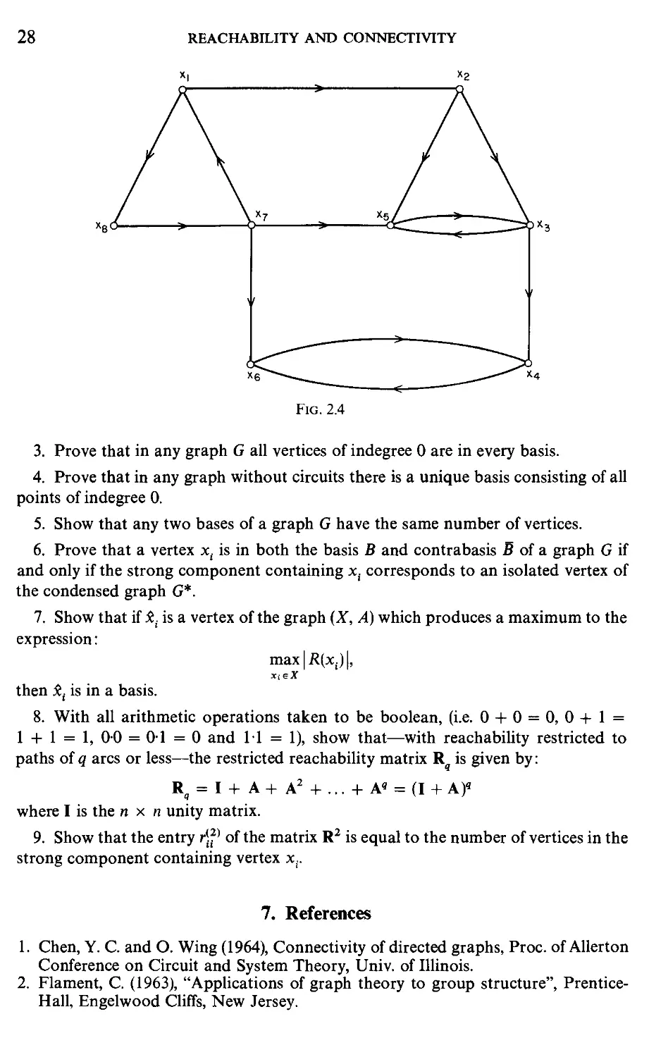
1. For the graph of Fig. 2.4 find the reachability and reaching matrices.
2. For the graph of Fig. 2.4 calculate the strong components, draw the condensed
graph and find all the bases.

28
REACHABILITY AND CONNECTIVITY
Fig. 2.4
3. Prove that in any graph G all vertices of indegree 0 are in every basis.
4. Prove that in any graph without circuits there is a unique basis consisting of all
points of indegree 0.
5. Show that any two bases of a graph G have the same number of vertices.
6. Prove that a vertex xt is in both the basis B and contrabasis B of a graph G if
and only if the strong component containing x, corresponds to an isolated vertex of
the condensed graph G*.
7. Show that if xf is a vertex of the graph (X, A) which produces a maximum to the
expression:
max\R(Xi)\,
then xf is in a basis.
8. With all arithmetic operations taken to be boolean, (i.e. 0 + 0 = 0, 0+1 =
1 + 1 = 1, 00 = 01 = 0 and 11 = 1), show that—with reachability restricted to
paths of q arcs or less—the restricted reachability matrix R is given by:
R? = 1 + A + A2 + ... + A« = (I + A)«
where I is the n x n unity matrix.
9. Show that the entry rj?1 of the matrix R2 is equal to the number of vertices in the
strong component containing vertex xr
7. References
1. Chen, Y. C. and O. Wing A964), Connectivity of directed graphs, Proc. of Allerton
Conference on Circuit and System Theory, Univ. of Illinois.
2. Flament, C. A963), "Applications of graph theory to group structure", Prentice-
Hall, Engelwood Cliffs, New Jersey.

REFERENCES 29
3. Harary, F., Norman, R. Z. and Cartwright, D. A965), "Structural models: An
introduction to the theory of directed graphs", Wiley, New York.
4. Leifman, L. Ya. A966), An efficient algorithm for partitioning an oriented graph
into bicomponents, Kibernetika, 2, p. 19 (in Russian). English translation: Cyber-
Cybernetics, Plenum Press, New York.
5. Marimont, R. B. A959), A new method of checking the consistency of precedence
matrices, Jl. of ACM, 6, p. 164.
6. Moyles, D. M. and Thompson, G. L. A969), An algorithm for finding a minimum
equivalent graph of a digraph. Jl. of ACM, 16, p. 455.
7. Ramamoorthy, C. V. A966), Analysis of graphs by connectivity considerations
Jl. of ACM, 13, p. 211.

Chapter 3
Independent and Dominating Sets
—The Set Covering Problem
1. Introduction
Given a graph G = {X, I"), one is often interested in finding subsets of the set
X of vertices of G which possess some predefined property. For example,
what is the maximum cardinality of a subset S £ X so that the subgraph <S>
is complete? or what is the maximum cardinality of a subset S so that <S> is
totally disconnected? The answer to the first question is known as the clique
number of G and the answer to the second question as the independence
number. Another problem is to find the minimum cardinality of a subset S
so that every vertex of X-S can be reached from a vertex of S by a single arc.
The answer to this problem is known as the dominance number of G.
These numbers and the subsets of vertices from which they are derived,
describe important structural properties of the graph, and have a variety of
direct applications in project scheduling [3], cluster analysis and numerical
taxonomy [36, 2], parallel processing on a computer [17] and in facilities
location and placement of electrical components [66, 56].

INTRODUCTION 31
In the present Chapter algorithms are given for the determination of
the above numbers and several of the application areas are discussed. The
Set Covering Problem—which is a generalization of the problem of determin-
determining the dominance number of graph—is introduced and a method for its
solution is described. This last problem is very important not only because
of the large number of its direct applications, but also in that it appears often
as a subproblem in other areas of graph theory covered by this book. In
particular it plays an important role in the determination of the "chromatic
number" (Chapter 4), graph "centres" (Chapter 5) and "matchings" (Chapter
12).
2. Independent Sets
Consider a nondirected graph G = (X, T). An independent vertex set (also
known as an internally stable set [11]) is a set of vertices of G so that no two
vertices of the set are adjacent; i.e. no two vertices are joined by a link.
Hence, any set S <= X which satisfies the relation:
S n T(S) = 0 C.1)
is an independent vertex set. For the graph of Fig. 3.1 for example, the sets
of vertices: {x7, x8, x2}, {x3, Xj}, {x7, x8, x2, x5} etc. are all independent vertex
sets. When no confusion arises the word "vertex" will be dropped and these
will simply be referred to as independent sets.
An independent set is called maximal when there is no other independent
set that contains it. Thus, a set S is a maximal independent set if it satisfies C.1)
together with the relation
H n r(H) =£(/), \/H => S C.2)
hence for the graph of Fig. 3.1 the set {x7, x8, x2} is not maximal but the set
{x7, x8, x2, x5} is. The sets {xx, x3, x7} or {x4, x6} are also maximal independent
sets of the graph in Fig. 3.1 and, therefore, in general there is more than one
maximal independent set to a given graph. One should also note that the
number of elements (vertices) in the various maximal independent sets is not
the same for all the sets as can be seen from the above example.
If Q is the family of internally stable sets then the number
a[G] = max|S| C.3)
SeQ
is called the independence number of a graph G, and the set S* from which it
is derived is called a maximum independent set.

32 INDEPENDENT AND DOMINATING SETS—THE SET COVERING PROBLEM
In the graph of Fig. 3.1 the family of maximal independent sets is composed
of the sets:
\XS, X-j, X2, X5 j, \XV X3, X-j], \X2, X4, X8j, (X6, X4), [X6, X3)
1*7' X5' X15> \X1> X4l> \X3> XT X8l'
The largest of these sets has 4 elements and hence a[G] = 4. The set
{x8, x7, x2, x5} is a maximum independent set.
2.1 Example: project selection
Consider n projects which must be executed, and suppose that each project
X; requires some subset Rt £ {1,..., p] of p available resources for its execu-
execution. Further assume that each project (given its resource requirements),
can be executed in a single time period. Now form a graph G each vertex of
which corresponds to a project and with links (xt, Xj) added whenever xt
and Xj have some resource requirement in common, i.e. whenever R( n Rj # <j>.
A maximal independent set of G then represents a maximal set of projects
that can be executed simultaneously during the single time period.
In a dynamic system new projects become available for execution after
each time period, so that the family of maximal independent sets of G has
to be found repeatedly in order to choose which maximal set of projects to
execute during the current period. In a practical system, it is not sufficient
simply to execute the set of projects corresponding to the maximum inde-
independent set at every period, since some projects may then be delayed in-
indefinitely. A better way would be to give a penalty pt to every project (vertex)
Xj which increases as the delay in the execution of xt increases, and then at
every point choose from the family of maximal independent sets that set
which maximizes some function of the penalties on the vertices that it
contains.
2.2 Maximal complete subgraphs (cliques)
A concept which is the opposite of that of the maximal independent set is
that of a maximal complete subgraph. Thus, a maximal complete subgraph
(clique) of G is a subgraph based on the set S of vertices which is complete
and which is maximal in the sense that any other subgraph of G based on a
set HdS of vertices is not complete. Hence, in contrast to a maximal
independent set for which no two vertices are adjacent, the set of vertices
of a clique are all adjacent to each other. It is quite obvious, therefore, that
the maximal independent set of a graph G corresponds to a clique of the
graph G and vice versa, where 6 is the graph complementary to G.
It is also quite apparent, that for a nondirected graph, a clique is a concept
which is similar, but more stringent, than that of a strong component of a

INDEPENDENT SETS 33
graph (see Chapter 2). A clique may in fact also be considered as a strong
comp°nent where reachabilities are restricted to single arcs as mentioned in
Section 5 of Chapter 2.
In a way analogous to the definition of the independence number by
equation C.3) we can define the clique number (also known as the density)
as being the maximum number of vertices in a clique. Then, roughly speaking,
for a "dense" graph the clique number is likely to be high and the independence
number low, whereas for a "sparse" graph the opposite is likely to be the
case.
2.3 The computation of all maximal independent sets
Because of the relationship between cliques and maximal independent sets
mentioned above, the methods of computation presented in this section
and which are described in terms of the maximal independent sets can also
be used directly for the computation of cliques. One may, at first sight, suppose
that the computation of all the maximal independent sets of a graph is a
very simple task, which could be done by systematically enumerating inde-
independent sets, testing if they are the largest possible (by attempting to add any
other vertex to the set whilst preserving independence) and storing the
maximal ones. The supposition is certainly true for small graphs of, say, up
to 20 vertices, but as the number of vertices increases this method of generation
becomes computationally unwieldy. This is so, not so much because the
number of maximal independent sets becomes excessive, but owing to the
. fact that during the process a very large number of independent sets are
formed and subsequently rejected because they are found to be contained in
other previously generated sets and are, therefore, not maximal in themselves.
In the current section we will describe a systematic enumerative method
due to Bron and Kerbosch [14], which substantially overcomes this difficulty
so that independent sets—once generated—need not be checked for maxi-
mality against the previously generated sets.
2.3.1 The Basis of the Algorithm. The algorithm is essentially a simple
enumerative tree search during which—at some stage k—an independent set
of vertices Sk is augmented by the addition of another suitably chosen
vertex to produce an independent set Sk+1, at stage k + 1, until no further
augmentation is possible and the set becomes a maximal independent set.
At stage k let Qk be the largest set of vertices for which SpQk = 4>, i.e. any
vertex from Qk added to Sk produces a set Sk+1 which is independent.
At some point during trie algorithm, Qk consists of two types of vertices:
vertices in Qk (say) which have already been used earlier in the search to
augment Sk and vertices in Qk (say) which have not yet been used. A forward
branching during the tree search then involves choosing a vertex xikeQk,

34 INDEPENDENT AND DOMINATING SETS—THE SET COVERING PROBLEM
appending it to Sk to produce
Sk+i = SkKj{xik} C.4)
and creating new sets Qk+1 as:
e;+1 = e*~-nxj C.5)
and
A backtracking step of the algorithm involves the removal of xik from
Sk+1 to revert back to Sk, and the removal of xik from the old set Qk and
its addition to the old set Qk to form two new sets Qk and Qk .
The following observations are quite obvious. A set Sk is a maximal
independent set only if it cannot be augmented further, i.e. only if
Qk = (j>. If Qk =£ 4>, it immediately follows that the current Sk was at some
previous stage augmented by some vertex in Qk and is therefore not maximal.
If Qk = $, the current Sk has not been previously augmented, and since sets
are generated without duplication, Sk is a maximal independent set. Thus, the
necessary and sufficient conditions for Sk to be a maximal independent
set are:
Qt = Q*=4> C-7)
It is now quite apparent that if a stage is reached when some vertex x e Qk
exists for which r(x) n Qk+ = <j>, then regardless of which vertex from Qk+
is used to augment Sk in any number of forward branchings, vertex x can
never be removed from Q~ at any future step p > k. Thus, the condition:
3x e Qk so that T{x) n g+ = <p C.8)
is sufficient for a backtracking step to be taken since no maximal independent
set can result from any forward branching from Sk.
As in all tree search methods, it is obviously beneficial to aim for early
backtracking steps since these tend to limit the unnecessary part of the tree
search. It is therefore worth while to aim at forcing condition C.8) as early
as possible by a suitable choice of the vertices used in augmenting the set Sk.
During a forward step one can choose any vertex xt e Qk with which to
augment set Sk, and on backtracking xik will be removed from Qk and
inserted into Qk. Now if xik is chosen to be a vertex eF(x) for some x e Qk,
then at the corresponding backtracking step the number:
A(x) = |r(x)nQk+| C.9)
will be decreased by one (from its value prior to the completion of the for-
forward and backward steps) so that condition C.8) is now more nearly true.

INDEPENDENT SETS 35
Thus, one possible way of choosing the vertex xik with which to augment
5 , is to first determine the vertex x* e Qk with the smallest possible value
of A(x*) and then choose xik from the set F(x*) n Qk. Such a choice of xik
at every step will cause A(x*) to decrease by one every time a backtracking
step at level k is made, until eventually vertex x* satisfies condition C.8),
at which time backtracking can occur.
It should be noted that since at a backtracking step xik enters Qk, it may
be that this new entry has a smaller value of A than the previously fixed vertex
x* so that this new vertex should now become the target for the attempt to
force condition C.8). This is particularly important in the first forward branch-
branchings when Ql = <j>.
2.3.2 DESCRIPTION OF THE ALGORITHM
Initialisation
Step 1. Set So = Q~ = </>, Q+ = X, k = 0.
Forward step
Step 2. Choose a vertex xikeQk as mentioned earlier and form Sk+l,
Q~ +! and Qf+ x keeping Qk and gt+ intact. Set k = k + 1.
Test
Step 3. If condition C.8) is satisfied to go to step 5, else go to step 4.
Step 4. If Q+ = Q~ = (j> print out the maximal independent set Sk and
go to step 5. If Qk = (j) but Qk # <j> go to step 5. Otherwise go to step 2.
Backtrack
Step 5. Set k = k — 1. Remove xik from Sk+1 to produce Sk. Retrieve Qk
and Qk, remove xik from Q+ and add it to Qk. If k = 0 and Q£ = </>, Stop.
(All maximal independent sets have been printed out). Otherwise goto step 3.
Comments on the implementation of the above algorithm are given in
[14] together with an Algol program listing. This program has been tested
on a number of graphs (including the Moon-Moser graphs—see problem 10),
and the computation times per maximal independent set generated were found
to be almost constant and independent of the size of the graph itself, which
makes the algorithm close to the best possible.
3. Dominating Sets
For a graph G = (.X", F) a dominating vertex set (also known as an externally
stable set [11]), is a set of vertices SsX chosen so that for every vertex x}
not in S, there is an arc from a vertex in S to xy

36 INDEPENDENT AND DOMINATING SETS—THE SET COVERING PROBLEM
Thus S is a dominating vertex set (or simply a dominating set—when no
confusion arises) if:
S u T(S) = X C.10)
For the graph of Fig. 3.2 the vertex sets {x15 x4, x6}, {xv x4}, {x3, xs, x6}
etc. are all dominating sets.
A dominating set is called minimal if there is no other dominating set
which is contained in it. Thus, a set S is a minimal dominating set if it satisfies
eqn C.10) and there is no other set H c S which also satisfies eqn C.10).
Hence, for the graph of Fig. 3.2 the set {x1( x4} is minimal but the set {xvxA, x6}
is not.
The set {x3, x5, x6} is also a minimal dominating set and other such sets
exist for this example. Thus, as in the case of maximal independent sets,
there are in general more than one minimal dominating set and they do not
necessarily all contain the same number of vertices.
If P represents the family of minimal dominating sets then the number
)8[G] =min|S| C.11)
SeP
is called the dominance number of a graph G, and the set S* from which it is
derived is called the minimum dominating set.
For the graph of Fig. 3.2 the minimal dominating set containing the
smallest number of elements is the set {x15 x4} and hence /?[G] = 2.

DOMINATING SETS
37
3.1 Example: Location of "centres" to cover a region
A very wide range of problems fall into this general category. These include:
(a) The location of T.V. or radio transmitters to broadcast to a specified
area.
(b) The location of army posts to control a region.
(c) The location of home bases for salesmen to serve a region.
Suppose that a region—shown by the large square in Fig. 3.3(a)—is
divided into 16 smaller areas as shown. An army post located in an area is
assumed to be able to control not only the square that it is located in, but also
those areas which have common borders with that square. What is then
required is to choose the smallest possible number and the locations of army
posts so that the whole region is under control.
If we represent each small area by a vertex and add a link between two
vertices whenever the corresponding areas have a common border, a graph
1
5
9
13
2
6
10
14
3
7
11
15
4
8
12
16
(a)
15
(b)

38 INDEPENDENT AND DOMINATING SETS—THE SET COVERING PROBLEM
1
8
©
©
36
43
9
16
23
30
37
3
10
17
31
38
45
4
18
25/
32
©
46
5
12
19
©
33
40
47
©
13
20
27
34
41
D8)
7
14
©
42
49
Fig. 3.4
is formed as shown in Fig. 3.3 (b). The problem then reduces to one of finding
(for this graph) a minimum dominating set. The number /?[G] is then the
smallest number of posts to cover the entire region. For the example of Fig.
3.3, /?[G] = 4 and the posts should be in locations {3,5,12,14} or in locations
{2, 9, 15, 8}.
Similarly, for the region shown in Fig. 3.4 the dominance number of the
corresponding graph is 12 and the location of the posts should be
{2, 6, 11, 15, 21, 24, 26, 29, 35, 39, 44, 48}. Only the three shaded squares are
protected by two posts simultaneously.
The relationship between the concept of a minimal dominating set and
that of a basis is quite apparent; as is the relationship between a minimal
dominating set and a p-centre (see Chapter 5). These relationships have been
discussed in Section 5 of Chapter 2, and in Chapter 5 an algorithm for the
computation of the minimum dominating set is used as a basic step in the
more general algorithm for the calculation of p-centres.
In the case of maximal independent sets we have given an algorithm which
generates the complete list of such sets because this list is required in many
practical applications [36,3,2]. In the case of dominating sets, however, what
is invariably required is simply a minimum dominating set and we, therefore,
restrict ourselves here to the computation of such a set. In the next section
we cast the problem of finding a minimum dominating set into a slightly
more general framework, and this helps to highlight relationships with
concepts discussed in other parts of this book.

THE SET COVERING PROBLEM 39
4. The Set Covering Problem
If one considers the transpose of the adjacency matrix A', with all diagonal
elements set to 1, then the problem of finding the minimum dominating set
is equivalent to the problem of choosing the least number of columns so that
every row contains an entry of 1 under at least one of the chosen columns.
This last problem of finding the minimum number of columns to "cover" all
the rows has been studied extensively under the name of the Set Covering
Problem (SCP).
In the general SCP the matrix of 0-1 coefficients need not be square as is
the case with the adjacency matrix. Moreover, associated with each column;,
(vertex Xj in our case), is a cost Cj, and what is required is to choose a cover
(dominating vertex set in the graph case) with the least total cost. One may—
at first sight—suppose that since the problem of finding the minimum dom-
dominating vertex set is a very special covering problem with ci = 1 for all
j = 1, 2, ..., n, the finding of this set may in fact be much simpler than the
solution of the general SCP. However, this is not generally the case and in this
section we will, therefore, be concerned with the solution of the general SCP.
4.1 Problem formulation
The SCP owes its name to the following set-theoretic interpretation. Given
a set R = {rx,..., rM], and a family &> = {Sv ..., SN} of sets S. <= R any sub-
subfamily 9" = {Sh, Sh,..., Sjk} of se such that
U SA = R C.12)
i=l
is called a set-covering of R, and the Sjt are called the covering sets. If, in
addition to equation C.12), S/" also satisfies
ShnSj, = <l>> VMe{l,...,/c}, fc#/ C.13)
i.e. the Sjt (i = 1,..., fe) are pairwise disjoint, then 9" is called a set-partitioning
ofR.
If, with each Sj e 9, there is associated a (positive) cost cp the SCP is to
find that set-covering of R which has minimum cost, the cost of
k
9" = {Sh,..., Sh} being S Cj. The Set Partitioning Problem (SPP) is defined
correspondingly.
In the matrix form referred to earlier—where the rows of an M-row
N-column 0-1 matrix [t..] are to be covered by columns—the SCP can be
formulated as a 0-1 linear program:
N
Minimize: z= Y,cfij

40 INDEPENDENT AND DOMINATING SETS—THE SET COVERING PROBLEM
N
subject to: £ hjZj > l i = 1,2, ...,M. C.14)
where c} ^ 0, and ^is 1, @)depending on S,e y, {SfiZ") and where ti} = 1, @)
depending on r. e Sp (ri $ S}).
For the SPP, the inequalities C.14) become
ttl]Sj = U i = l,2,...,M C.15)
4.2 Problem reduction
Due to the nature of the SCP it is often possible to make certain well-known
a priori deductions and reductions. [6, 26, 27, 28, 30, 50, 51]
Thus:
A) If for some ri e R, r. $ Sj V/ = 1,..., JV, then ri cannot be covered and the
problem has no solution.
B) If 3ri e R so that rt e Sk, and rt $ Sp Vj # fe, then Sfc must be in all
solutions and the problem may be reduced by setting R = R — {r,} and
se = sr - {sk}.
C) Let Vt = {/|r, e S.}. Then, if 3p, 4 e {1,..., M} with Vp s V^ r, may be
deleted from R, since any set that covers rp must also cover rq, i.e. rq is dom-
dominated by rp. _
D) If, for some family of sets ¥ c y we have U S, 3 Sfcand I c, < ck
for any Ske£f —if, then St may be deleted from Sf since it is dominated by
U Sj.
Let us now assume that these reductions, if applicable, have been applied
and the original SCP reformulated in its irreducible form.
4.3 A tree search algorithm for the SPP
As noted earlier, the SPP is closely related to the SCP, being essentially an
SCP with an additional (no-overcovering) restriction. This restriction is
advantageous when we attempt to solve the problem by a tree search method,
since it may allow the early abandonment of potential branches of the tree.
Therefore, we shall first discuss a tree search algorithm for solving the SPP,
and then show how it can be extended to solve the SCP.
Simple tree search methods for solving the SPP were proposed by Garfinkel
and Nemhauser [27] and Pierce [48], and are essentially as follows:
At the start of the process, we make up M "blocks" of columns, one block
for each element rk of R. The fcth block consists of those sets of ^(represented
by columns) which contain element rk but which do not contain any lower-
numbered elements rlr ..., rk_v Each set (column), therefore, appears in

THE SET COVERING PROBLEM
41
exactly one block, and the totality of blocks can in general be arranged in
tableau form as shown in Table 3.1 although some block(s) may be nonexistent
in a particular problem.
During the course of the algorithm, blocks are searched sequentially, with
block k not being searched unless every element rt, 1 < i ^ k — 1, has already
been covered by the partial solution. Thus, if any set in block k were to contain
elements indexed less than k, the set would have to be discarded (at this stage)
due to the no-overcovering requirement.
The sets within each block are arranged (heuristically) in ascending order
of their cost and the sets are now renumbered so that Sj will from now on be
used to mean the set corresponding to the jth column of the tableau.
Block 1
Table 3.1. Initial tableau
Block 2 Block 3 Block 4
1111
Oorl
0
1111
Oorl
0
1111
Oorl
0
1111
Oorl
etc.
At any stage of the tree search a current "best" solution B of cost z is
known, where B represents the family of corresponding covering sets. If B
and z represent the corresponding values in the current state of the search,
and £ is a set representing those elements (i.e. rows) rt covered by the sets in
B, then a simple tree search algorithm proceeds as follows:
Initialization
Step 1. Set up the initial tableau and begin with the partial solution B = <j),
E = (j>, z = 0 and z = oo.
Augmention:
Step 2. Find p = min [i|r. $E~\. Set a marker at the top (lowest cost set) of
block p.

42 INDEPENDENT AND DOMINATING SETS—THE SET COVERING PROBLEM
Step 3. Beginning at the marked position in block p, examine its sets SP, say,
in increasing order of j.
(i) If set S? is found such that Sp n E = 4>, and z + cp < z (where cP is the
cost of SP), go to step 5.
(ii) Otherwise, if block p is exhausted or a set SJ reached for which
z + cP ^ z go to step 4.
Backtrack
Step 4. B cannot lead to a better solution.
If B = 4> (i.e. block 1 has been exhausted), terminate with the optimal
solution. B. Otherwise remove the last set, S[ say, added into B, put p = I,
place a marker on set S[+1, remove the previous marker in block / and go to
step 3.
Test for new solution
Step 5. Update B = Bu {S?}, E = E u S?, z = z + c*.
If £ = i? a better solution has been found. Set B = J3, z = z and go to step 4.
Otherwise goto step 2.
As the search terminates with the exhaustion of block 1 (see step 4 above),
it would seem worthwhile to arrange the blocks in ascending order according
to the number of columns (sets) in each. This can be achieved by renumbering
the elements (rows) r1? ..., rM in increasing order of number of sets in S
containing that element, before setting up the initial tableau.
Before showing how this SPP algorithm can be extended for the case of
the SCP, we briefly mention some of the other methods proposed for solving
the SPP. In [49], Pierce and Lasky give some modifications to the above basic
algorithm, including subsidiary use of a linear program; while, in [45],
Michaud describes another implicit enumeration algorithm which is based
on a linear programming problem corresponding to the SPP, with the block
structure given above being used in a secondary role.
Other algorithms involving simplex-type iterations have been proposed,
both primal, [4, 5], and dual, [58, 37] whereas Jensen [37] has had success
with a dynamic programming method for a certain type of SPP's.
4.4 A tree search algorithm for the SCP
The only step of the algorithm described in Section 4.3 above which is
particular to the SPP, is step 3(i). If the "no-overcovering" requirement
Spj n E = 4> in that step were to be removed, then that algorithm could be
used for the SCP. However, the setting up of the initial tableau would now
have to be somewhat different from that shown in Table 3.2. Thus, let
Sj = {rh, rj2, rj3,...}, withj'j < j2 <j3.... It is not now sufficient to include
Sj only in blockjj, because with the "no-overcovering" requirement removed,

THE SET COVERING PROBLEM 43
it is not now possible to exclude Sj from consideration at, say, block j2 if
r ■ has already been covered by the partial solution. Hence Sj must be entered
once in each of the blocks j1,j2,j3, ■ ■ ■■ On the other hand, since an element
r . of Sj would, by the sequential nature of the search, be covered before
branching on the sets of block /? (/? > jj is considered, it is now possible to
remove all the elements x^ from a set Sj when entering Sj into any block
P > jx without affecting the solution of the problem in any way. This apparently
trivial removal is in fact computationally very beneficial, since the initial
tableau of the SCP now set up can be reduced by the preliminary reduction
tests of Section 4.2 to much smaller dimensions that would have been possible
without the removal of the elements xu (ja < /?) from the sets of block /? [48].
It should be pointed out here that the algorithm of Section 4.3 is a primitive
tree search devoid of any sophistication, and although with careful coding it
can be made quite effective for the SPP [27] it is not, as it stands, an efficient
algorithm for solving SCP's of even moderate size. We will now discuss some
dominance tests and the calculation of lower bounds which can be used to
limit the tree search and improve the efficiency of the basic algorithm.
4.4.1 Some Dominance Tests. We will first illustrate these dominance tests
by an example before stating the general results. Consider a case where
block 1 contains (among others), sets S1 = {rv r4, r6} and S2 = {rv r3, r4}
of costs 3 and 4 respectively, and where block 2 contains (among others),
sets S3 = {r2, r3, rs} and S4 = {r2, r4, r5} each of cost 2.
During the course of the algorithm of Section 4.3 a stage will be reached
where Ba = {Sv S3}, Ea = {rv r2,..., r6}, za = 5; and we will branch forward
from this stage until either we find a better solution than the current B, or
we realize that Sx and S3 cannot both appear in an optimal solution.
Many steps later, we will reach a stage where
Bb = {S2,S3}, Eb = {rv...,r5}, zb = 6.
At this point it becomes apparent that any further branching from this stage
is unnecessary, since Eb c Ea and zb ^ za. A similar situation occurs when the
stage is reached where
BC = {S2,SA}, Ec = {rv...,r5}, zc = 6.
Thus, it may be worthwhile to keep, for each value of z = 1, 2,... z some
(perhaps incomplete) list of the maximal £'s which have already been achieved
for this z, (where by maximal is meant a set not included in another set also
in the list). These lists of £'s can then be used to limit the search by eliminating
branches that later on prove fruitless. It is generally impractical, however,
to save all the maximal sets £, at any cost level. In fact if this is done, the
method would be similar to a Dynamic Programming approach to the

44 INDEPENDENT AND DOMINATING SETS—THE SET COVERING PROBLEM
problem as a whole (or, alternatively, could be considered as a full breadth-
first tree search).
Let us now assume that we have saved some list (L(z,) of previous sets E
that have been attained during the course of the algorithm at a summed-cost
level 2j. Suppose a stage is reached where E = E, B = B',z = z', and we are
about to examine block k (i.e. k = min {i\r,$E'} at step 2 of the algorithm
of Section 4.3), and to consider set Sk of cost ck for the next branching. If
z' + ck < z, the original algorithm would have branched forward from this
stage, and updated
E = E u S), B=Bu {Sk}, z =z + ckp
regardless of any other considerations.
However, one could now also ensure (at step 3), that:
E u S* £ £,; V£, e L{z^), and for all zt, z' < zt < z' + c) C.16)
before branching forward. If the set Sk fails the above test, then it is rejected
and instead the next set, SkJ+ v of block k is considered, etc. If Sk passes test
C.16), one could branch forward on Sk, and continue as previously, after
updating L(z) by introducing the set £' u Sk into L{z' + c^).
Since, as mentioned earlier, it is practically impossible to store the complete
lists L(z{), some heuristic criterion has to be used to decide on the size of these
lists, and how they should be updated during the search.
(A) List size. It is obviously better to eliminate sets Sk which are potential
tree branchings at an early level in the tree, as this would discard larger
portions of the potential search-tree. It would thus seem intuitively worth-
worthwhile to keep larger-sized lists L{zt) for the smaller z,. This argument is
further reinforced by the fact that test C.16) is more likely to be effective when
the sets T contain only a few elements, which is generally the case for small
Zj-levels.
{B) Updating of the Lists. At a particular z;-level, the current £-set (£' say)
is more likely to be a subset of a set E" (in the list Liz^), which was derived
from the same general part of the search-tree. This is so because E and E"
have in common a large section of the path from the start-node to their
respective tree nodes. Thus, it would seem to be advantageous to arrange the
lists LiZf) as stacks and to use a FIFO (first in, first out) policy, with the
bottom-most set being discarded in the event of stack overflow.
4.4.2 The Calculation of a Lower Bound. At some stage of the search,
given by B', £', z', and where block k is the next block to be considered, a
lower bound h on the minimum value of z, can be calculated and used to

THE SET COVERING PROBLEM 45
limit the tree search as follows:
Consider an uncovered element rteR — E' which does not appear in
any of the sets of those blocks k, k + 1,..., i — 1, corresponding to elements
not yet covered by the partial solution. The element ri cannot then be
covered unless some set S'j of block i is chosen to add to B' at a future stage.
Thus, for each such element rv construct a row for matrix D = [d J and a
row for a second matrix D' = [rf^J, where dqs is the number of elements in
set SI and d'qs is its cost.
In addition, append an extra row, 6 say, to D and D' with d6s = s for all
s = 0, 1,..., M-- \E'\ and d'es = s.min [clj|Sj|], the minimum being taken
over all sets S'j with r; £ E'. Note that although the number of elements in a
row qv of D (or D') may be different from that of another row q2, we assume
here that 0's and oo's are entered at the end of some rows of D and D' respect-
respectively, so that all rows have / (say) elements and the matrices become
rectangular.
The following observations can now be made: since the optimal solution
to the current subproblems must cover M — | E' | elements, a choice of one
entry from each row i of D, which satisfies
(d1Sl + d2s2 + ... + dgse)^M-\E'\
and which minimizes the corresponding cost,
v = (d'Ui+... + d'()se)
gives v as a lower bound to the optimal cost of the (covering) subproblem.
Note that the assumption is made that the sets corresponding to the alloca-
allocations in the rows of D are disjoint, which is obviously the best possible
situation. The last row 9 simply ensures that, if
"!**>< M-\E\,
i= 1
the remaining elements are covered in the best possible way, i.e. at minimal
cost-per-additional-element-covered.
The minimum value of
X d'iSi subject to £diSi^M-\
i=i t = i
can easily be derived by a dynamic programming algorithm as follows:
Let gp(v) be the maximum number of elements that can be covered using
only the first p rows of D (i.e. only p of the blocks in the subproblem), and
whose total cost does not exceed v. gp(v) can then be calculated iteratively as:
gp(v)= max [dps + gp_,{v - d'ps)l C.17)
5=1,...,/
where go(v) is initialized to 0 for all v.

46 INDEPENDENT AND DOMINATING SETS—THE SET COVERING PROBLEM
Hence, the lowest value, v*, of v, for which ge(v) > M — | £' | is then the
required lower bound, h, and can be easily obtained from the dynamic pro-
programming tableau derived from the above iterative equation. One should
note that only that range of v where 0 ^ v < z — z' need be considered, since
if h ^ z — z' (i.e. ge(v) < M — \E'\ for v ^ z — z'), a backtracking step may
be taken immediately.
4.5 Computational performance of the SCP algorithm
The computational performance of the algorithm described in Section 4.4
for the SCP is shown in Table 3.2 The numbers of rows and columns shown
are those resulting after the reduction tests have been applied. All problems
are randomly generated and have costs cj = 1 for all columns;.
Table 3.2 Computing times of the SCP algorithm for random problems
Problem
1
2
3
4
5
6
7
8
9
10
11
12
13
14
15
16
17
18
19
20
21
22
23
24
25
Number
of
rows
15
15
15
20
20
20
25
25
25
30
30
30
30
30
30
30
30
30
30
35
35
35
35
35
35
Number
of
columns
20
25
25
' 60
50
75
110
120
170
80
180
250
340
475
500
700
725
875
1000
160
290
460
585
780
1075
Density
0-22
0-25
0-30
0-18
0-20
0-23
0-17
019
0-22
0-12
015
0-17
0-21
0-20
0-23
0-23
0-25
0-26
0-27
009
013
016
018
019
0-20
Computing
timef
005
004
006
0-25
011
0-35
0-60
1-30
1-50
100
10-50
600
9-20
1100
22-00
105-50
32-50
57-20
72-80
18-50
2800
75-50
129-50
141-20
110-00
Nodes
in tree
searchj
002
001
0-02
007
0-02
0-05
006
016
011
0-20
1-60
0-52
0-30
009
0-40
3-02
0-12
018
019
218
2-03
2-95
3-96
5-03
0-55
t CDC 6600 seconds.
| Number of nodes generated by the tree (thousands).

THE SET COVERING PROBLEM 47
Other methods of solving the SCP are given by Lemke, Salkin and Spiel-
Spielberg [41] who use a different type of tree search with an embedded linear
program. The solution of this LP is used as a lower bound during the search
and is also used in determining the next forward tree branching from the
current node. Cutting-plane approaches, similar in principle to those used
for general 0-1 programming [32] are given by House, Nelson and Rado [35]
and by Bellmore and Ratliff [9]. A computational survey and comparison
of these methods is given by Christofides and Korman [19].
5. Applications of the Covering Problem
5.1 Choice of interpreters
Let us assume that an organization wants to hire interpreters to translate
from French, German, Greek, Italian, Spanish, Russian and Chinese into
English, and suppose there are five prospective applicants A, B, C, D and E.
Each applicant requires a certain salary and speaks only a subset of the above
set of languages. What is then required is to find what candidates to hire in
order to be able to translate from all the above languages into English with
the least cost of hiring. This is quite obviously a covering problem.
If, for example, the salary requirements of all the applicants are the same
and the languages they speak are as shown in the T matrix below, then the
solution to the above problem is to hire persons B, C and D.
Person ->
Language A B* C* D* E
I
French
German
Greek
Italian
Spanish
Russian
Chinese
5.2 Information retrieval [21]
Let us suppose that a number of pieces of information are stored on N files
of length Cj = 1, 2, ..., N and that each piece is stored on at least one file.
At some time a request for M pieces of information is made and these can be
obtained by searching the files in a number of ways. In order to obtain all M
pieces of information with the least length of files that have to be searched a
SCP will have to be solved where an element ttj of the matrix T is 1 if informa-
information i is on file j and 0 otherwise.
1
1
0
1
0
0
0
0
1
1
0
0
1
0
1
0
0
0
1
1
0
1
0
0
1
0
0
1
0
0
0
0
0
1
1

48 INDEPENDENT AND DOMINATING SETS—THE SET COVERING PROBLEM
5.3 Airline crew scheduling [1, 55, 64, 65]
Suppose that the vertices of a nondirected graph G represent the places that
an airline can visit and the arcs of G represent the flight "legs" that the airline
must operate at a given time. Any path in this graph (satisfying a number of
constraints that may be imposed in practice) forms a feasible flight schedule
which can be operated. Let there be N such feasible schedules, the cost of the
jth one being calculated in some way to be Cj. The problem of finding the
least-cost set of schedules so that every flight leg is operated at least once is
then a covering problem where the matrix T contains an entry of unity in
position (i,j) if flight leg i is contained in schedule j, and zero otherwise.
A variant to this problem (which also appears often in aircrew scheduling)
is derived by insisting that a flight leg can appear once and only once in the
chosen set of schedules. This leads to a SPP corresponding to the SCP defined
above.
5.4 Simplification of logical (boolean) expressions [30, 50, 51, 67, 44, 43]
When simplifying a logical expression £, which is (say), given in disjunctive
normal form, one need only consider the set P, of prime implicants of E.
A "simplest" form for E is then obtained by finding the lowest-cardinality
subset P £ P subject to the condition that every (conjunctive) term of E be
'covered' by (i.e. by implied by) at least one prime implicant in P. This is
obviously a SCP, where once more the column costs Cj = 1 for allj = l,...,N.
A problem equivalent to finding a minimal representation to logical
expressions occurs in the design of optimal switching circuits.
5.5 Vehicle dispatching [7, 47, 24]
In the vehicle dispatching problem a graph represents a road network with
vertices representing customers except one vertex which represents the
depot. A vehicle leaves the depot, supplies goods to some customers and
returns to the depot thus traversing a circuit. If the "cost" of circuit j is c-
(for example c. could be the mileage of the circuit or the time to complete it),
how many vehicles should be used on which circuits so as to supply all
customers (once only) in any one day and minimize cost? This problem can
obviously be considered as a SPP whose columns represent all possible
feasible (because of the practical constraints), circuits starting and finishing
at the depot. The rows represent the customers.
An almost identical problem involves the routing of a cable to carry
electricity from a substation (depot) to customers in "ring-circuits" [15].
Other practical applications of the SCP or SPP include: assembly line
balancing [59, 25], political districting [29], the calculation of bounds in
general integer programs [18], network planning [20] and network attack
or defence [8, 10].

APPLICATIONS OF THE COVERING PROBLEM 49
5.6 Other graph covering problems
A large number of problems in graph theory can be formulated as SCP's
although many of these problems could be solved more efficiently by
alternative graph-theoretic means discussed in other parts of this book. The
purpose of the present section is to show how some of these problems are
related via the SCP.
5.6.1 The Minimum Dominating Vertex Set. As mentioned in Section 4
of the present Chapter, the problem of finding the minimum dominating
vertex set of a graph G is a SCP with the T matrix being the transpose of the
adjacency matrix of G with all diagonal entries set to 1.
5.6.2 The Maximum Independent Vertex Set. One way of finding the
maximum independent vertex set of a graph G = (X, F) is to generate all
maximal independent vertex sets and choose the one of largest cardinality.
Another way is to consider the problem as a SCP where columns of the
matrix T represent vertices of G and rows represent links, with ttJ = 1 if
vertex Xj is a terminal vertex of link a; and 0 otherwise.
It is then apparent [23] that if X c x is the set of columns in the minimum
solution of this SCP, the set X — X is the maximum independent vertex set
of G. This is no because if X is a set cover of the links of G, then every link
has at least one of its terminal vertices in X and hence two vertices in X — X
cannot be adjacent, i.e. X — X is independent. Moreover, if X — X is
independent, each link can have at most one terminal vertex in X — X and
hence X is a set cover of the links. Hence, the complement of every vertex
set cover of the links of G is an independent set, and since X is the minimum
cardinality such cover X — X is the maximum independent set.
5.6.3 The Minimum Covering and Maximum Matching (see Chapter 12).
What is in the literature referred to as a minimum "covering" is a set £ of
links of a graph G = {X, A) so that every vertex of G is a terminal vertex of
at least one link in E and | E | is minimum. Thus, since E could be considered
as dominating the vertices of G, that E* with minimum | E \ could—in the
terminology used in this Chapter—be called a minimum dominating link set.
A problem equivalent to that of finding a minimum covering is that of finding
a set M of links of a graph G so that no two links in M are adjacent. M is
called a matching and that set M* with maximum cardinality is the maximum
matching, which in the current termonology could also be called a maximum
independent link set. That the maximum matching and minimum covering
problems are equivalent is demonstrated in Chapter 12 dealing with matchings.
It is shown there that if in a minimum covering E* the degree of a vertex xt
is rfE*(x;)—considering only the links in E*—then if for every xt with d£*(x,) > 1

50 INDEPENDENT AND DOMINATING SETS—THE SET COVERING PROBLEM
Minimum dominating
vertex set
Maximum independent
vertex set
Minimum dominating
link set
(minimum covering)
Maximum
clique
Maximum independent
link set
{maximum matching)
Fig. 3.5. Problem-solution implication diagram
a total of dE*(xi) — 1 links incident at xt are removed, the remaining set of
links form a maximum matching. Inversely, if M* is a maximum matching,
and for every vertex xt with dM*(x;) = 0 a link incident at xt is added, the
resulting set of links is a minimum covering.
Maximum matchings and minimum coverings can be formulated as
SCP's. In the case of the coverings, the columns of T represent links of the
graph G, and the rows of T represent vertices, where ttj = 1 if vertex xi is
incident with link ai and 0 otherwise. For this case the matrix T is, therefore,
the incidence matrix of G.
Figure 3.5 shows a problem-solution implication diagram, where an arc
from problem a to problem /? represents the fact that a solution to a implies
the solution of jS [34, 39]. The relation between maximum independent
vertex sets and maximum cliques is via the complementary graph, and that
between maximum independent vertex sets and maximum matchings is via
the line graph of G. (See Chapter 10 for the definition of the line graph.)
5.6.4 Covering a Graph with Subgraphs. A whole family of problems
involves the covering (or partitioning) of the vertices or links of a graph G
with subgraphs or partial graphs of G having prescribed properties. In this

APPLICATIONS OF THE COVERING PROBLEM 51
context the columns of the T matrix of the SCP (or SPP) represent all the
subgraphs or partial graphs of G having the prescribed properties, and the
rows of the matrix represent the vertices or links of G. In Chapter 4, for
example, the problems of finding the chromatic number of a graph G is
considered as a SCP with the rows of the T matrix representing vertices and
the columns representing maximal independent vertex sets of G (i.e. maximal
totally-disconnected subgraphs).
Other problems involve the covering of the links of G with partial graphs
having diameter less than or equal to 1 [13], covering the links of G with
"star" trees or covering them with simple paths and circuits [16, 42].
6. Problems P3
1. Enumerate all maximal independent sets of the graph H shown in Fig. 3.6,
and hence find the independence number a[G].
2. Use the method of Section 2.3.2 to list all maximal independent sets of the
graph of Fig. 3.7. (Note graph symmetry.)
3. Show that for a given graph G = (X, F), an independent set A c= X is maximum
if and only if for any arbitrary independent set B c X — A we have:
B< \T(B)vA\
(See Ref. [63].)
4. In the complete nondirected graph Kn show that each link is contained in
exactly (n — 2) circuits of cardinality 3 (i.e. triangles).
5. It is easy to show that the converse of statement 4 above is not true, i.e. if every
link in a graph G is part of n — 2 circuits of cardinality 3, G is not necessarily Kn.
Fig. 3.6

52 INDEPENDENT AND DOMINATING SETS—THE SET COVERING PROBLEM
X| X2 X3 X4 X5
Fig. 3.7
(Figure 3.8 provides a counterexample in which each link is part of 2 such circuits
but the graph does not contain K4). However, one can use statement 4 above in order
to find an upper bound on the clique number of a graph G—i.e. the largest possible
Kr embedded in G—as follows:
(i) Start with a value of r which is a lower bound on the clique number,
(ii) Remove those links not part of at least r — 2 circuits of cardinality 3.
(iii) Repeat (ii) above for r = r + 1 etc until less than r(r — l)/2 links are left. The
current value of r is then an upper bound on the clique number.
Show that the above algorithm is correct, and apply it to the complementary graph G
of the graph G given in Fig. 3.7. Compare the answer with the value of oc[G] found
in problem 2.
Fig. 3.8

PROBLEMS 53
6. A total of n symbols are to be used for transmitting information. A graph
G = (X, A) is given where link (xj; Xj) e A, if and only if symbol X; could be confused
with symbol Xj at the reception. The symbols are to be used in blocks of fc-symbol
"words". Show that the maximum number of words that could be used for transmitting
information without the possibility of confusion, is the independence number a[Gl]
of the graph G* = G x G x ... x G {k times), where the product G' x G" of two
graphs G' = (X', A') and G" = (X", A") is the graph H = (Y, B) given by
Y = {x.Xjlx^X^XjeX"}
and
B = {(x,Xj, xkxt)\ either xt = xk and {xJt x,) 6 A"
or Xj — x, and (xt, xk) e A"
or (xj; xk) e A' and (xp x,) e A"}
(see Ref. [61]).
7. Given any two graphs G' and G" show that:
a[G' x G"] > a[G'] a [G"]
8. (i) Show that in a nondirected graph G, <x[G] > j?[G], by showing that every
maximal independent set is a dominating set.
(ii) Give an example to show that the minimum dominating set is not necessarily
independent.
9. On a k x fe chessboard show that it is impossible to place k queens which do not
attack each other for the values k < 4. Find a solution for fe = 5.
10. Moon and Moser [46] showed that the largest number of cliques (/(n) say),
that a graph with n vertices can have is given by:
3"'3 if»i=0(mod3)
4.3(»-4)/3 if n = 1 (mod 3)
2.3c-2>/3 ifn = 2(mod3)
and showed that the only graphs G which achieve f(n) are the following:
(a) If n = 0 (mod 3), then G consists of n/3 triples of vertices.
(b) If n — 1 (mod 3), there are two possible classes of graphs: Either G consists of
one quadruple and {n — 4)/3 triples, or it consists of two pairs and (n — 4)/3
triples.
(c) If n = 2 (mod 3), then G consists of one pair and (n — 2)/3 triples.
In all cases a link (xt, Xj) exists if and only if x; and Xj belong to different groups, (pairs,
triples, quadruples).
Verify the above statements for the cases of n = 3, n = 4 and n = 5.
11. Using the reduction tests of Section 4.2 eliminate as many rows and columns
as possible from the covering problem whose [c] and [ttJ] matrices are given below.
(Note: Apply reduction test 4 only for the case f^| = 1.)

54 INDEPENDENT AND DOMINATING SETS—THE SET COVERING PROBLEM
12 3 4 5 6 7 8
1
2
4
5
6
[Cj] = [ 4, 7, 5, 8, 3, 2, 6, 5 ]
12. Solve the SCP remaining after the reduction in problem 11 above using the
method in Section 4.4.
1
1
0
0
0
1
1
0
0
1
0
1
1
1
0
0
0
0
0
0
1
0
0
0
0
0
0
1
1
0
1
1
0
0
1
0
0
0
0
1
1
1
1
1
0
1
0
0
7. References
1. Arabeyre, J. P., Fearnley, J., Steiger, F. C. and Teather, W. A969). The airline
crew scheduling problem: A survey, Transp. Sci., 3, p. 140.
2. Augustson, J. G. and Minker, J. A970). An analysis of some graph-theoretical
cluster techniques, Jl. of ACM, 17, p. 571.
3. Balas, E. A970). Project scheduling with resource constraints, In: "Applications
of mathematical programming techniques", Beale, Ed., English Universities
Press. London.
4. Balas, E. and Padberg, M. W. A972a). On the set covering problem, Ops. Res. 20,
p. 1152.
5. Balas, E. and Padberg, M. W. A972). On the set covering problem. II: An algorithm,
Management Sciences Research Report No. 295, Carnegie-Mellon University.
6. Balinski, M. A965). Integer programming: methods, uses, computation, Man.
Sc»., 12, p. 253.
7. Balinski, M. L. and Quandt, R. E. A964). On an integer program for a delivery
problem, Ops. Res., 12, p. 300.
8. Bellmore, M., Greenberg, H. and Jarvis, J. A970). Multi-commodity disconnecting
sets, Man. Sci., 16, p. 427.
9. Bellmore, M. and Ratliff, H. D. A971). Set covering and involuntary bases, Man.
Sci., 18, p. 194.
10. Bellmore, M. and Ratliff, H. D. A971). Optimal defense of multi-commodity
networks, Man. Sci., 18, p. 174.
11. Berge, C. A962). "Theory of graphs", Methuen, London.
12. Bonner, R. E. A964). On some clustering techniques, IBM Jl. Res. and Dev., 8,
p. 22.
13. Bosak, J., Rosa, A. and Znam, S. A966). On decompositions of complete graphs
into factors with given diameters, In: Int. Symp. on theory of graphs, Dunod,
Paris, p. 37.
14. Bron, C. and Kerbosch, J. A973). Algorithm 457—Finding all cliques of an
undirected graph, Comm. of ACM, 16, p. 575.
15. Burstall, R. M. A967). Tree searching methods with an application to a network

REFERENCES 55
design problem, In: "Machine Intelligence", Colin and Michie, Eds., Vol. 1,
Oliver and Boyd, London.
16. Busacker, R. G. and Saaty, T. L. A965). "Finite graphs and networks", McGraw-
Hill, New York.
17. Chamberlin, D. D. A971). The single assignment approach to parallel processing,
Proc. of AFIPS Conf., 39, p. 263.
18. Christofides, N. A971). Zero-one programming using non-binary tree search,
The Computer //., 14, p. 418.
19. Christofides, N. and Korman, S. (in press). A computational survey of methods for
the set covering problem, Man. Sci.
20. Crowston, W. B. A968). Decision network planning models, Ph.D. Thesis, Carnegie-
Mellon University.
21. Day, R. H. A965). On optimal extracting from a multiple file data storage system:
An application of integer programming, Ops. Res., 13, p. 482.
22. Desler, J. F. A969). Degree constrained subgraphs, covers, codes and fc-graphs,
Ph.D. Thesis, Northwestern University, Evaston, Illinois.
23. Edmonds, J. A962). Covers and packings in a family of sets, Bulletin of American
Mathematical Soc, 68, p. 494.
24. Eilon, S., Watson-Gandy, C. D. T. and Christofides, N. A971). "Distri-
"Distribution management: Mathematical models and practical analysis", Griffin,
London.
25. Freeman, D. R. and Jucker, J. V. A967). The line balancing problem, Jl. of
Industrial Engineering, 18, p. 361.
26. Garfinkel, R. S. A970). Set covering; a survey, presented at XVII TIMS Conf.,
London.
27. Garfinkel, R. S. and Nemhauser, G. L. A969). The set partitioning problem: set
covering with equality constraints, Ops. Res., 17, p. 848.
28. Garfinkel, R. S. and Nemhauser, G. L. A972). "Integer Programming", Wiley,
New York.
29. Garfinkel, R. S. A968). Optimal political districting, Ph.D. Thesis, The John
Hopkins University.
30. Gimpel, J. F. A965). A reduction technique for prime implicant tables, IEEE
Trans, EC-14, p. 535.
31. Glover, F. A971). A note on extreme point solutions and a paper by Lemke,
Salkin and Spielberg, Ops. Res., 19, p. 1023.
32. Gomory, R. A963). An algorithm for integer solutions to linear programs, In:
"Recent Advances in Mathematical Programming", Graves and Wolfe, Eds.,
McGraw-Hill, New York.
33. Hakimi, S. L. and Frank, H. A969). Maximum internally stable sets of a graph,
/. of Math. Anal, and Appl., 25, p. 296.
34. Hakimi, S. L. A971). Steiners' problem in graphs and its implications, Networks,
1, p. 112.
35. House, R., Nelson, L. and Rado, T. A965). Computer studies of a certain class of
linear integer programs, In: "Recent Advances in Optimization Techniques",
Lavi and Vogel, Eds., Wiley, New York.
36. Jardine, N. and Sibson, R. A971). "Mathematical taxonomy", Wiley, London.
37. Jensen, P. A. A971). Optimal network partitioning, Ops. Res., 19, p. 916.
38. Kapilina, R. I. and Shneyder, B. N. A970). The problem of internal stability and
methods of solving it on a universal digital computer, In: "Proc. of Scient. and
Techn. Conf. on the results of scientific research in 1968-1969", Section on

56 INDEPENDENT AND DOMINATING SETS—THE SET COVERING PROBLEM
Automation Computation and Measuring Procedures, Subsection on Graph
Theory, Maskovskiy, Energticheskiy Institut Press.
39. Karp, R. M. A972). Reducibility of combinatorial problems, In: "Complexity of
computer computations", Miller and Thatcher, Eds., Plenum Press, New York,
p. 85.
40. Lawler, E. L. A966). Covering problems: Duality relations and a new method of
solution, Jl. of SI AM (Appl. Math.), 14, p. 1115.
41. Lemke, C. E., Salkin, H. M. and Spielberg, K. A971). Set covering by single
branch enumeration with linear programming subproblems, Ops. Res., 19, p. 998.
42. Lovsaz, L. A966). On covering of graphs, In: "Int. Symp. on theory of graphs",
Dunod, Paris, p. 231.
43. Mayoh, B. H. A967). Simplification of logical expressions, //. of SI AM (Appl.
Math.), 15, p. 898.
44. McCluskey, E. J. Jr. A956). Minimization of boolean functions, Bell. Syst.
Tech. Jl., 35, 1417.
45. Michadu, P. A972). Exact implicit enumeration method for solving the set
partitioning problem, IBM Jl. of Res. and Dev., 16, p. 573.
46. Moon, J. W. and Moser, L. A965). On cliques in graphs, Israel Jl. of Mathematics,
p. 23.
47. Pierce, J. F. A967). On the truck dispatching problem—Part I, IBM Scientific
Centre Technical Report 320-2018.
48. Pierce, J. F. A968). Application of combinatorial programming to a class of
all-zero-one integer programming problems, Man. Sci., 15, p. 191.
49. Pierce, J. F. and Lasky, J. S. A973). Improved combinatorial programming
algorithms for a class of all-zero-one integer programming problems, Man. Sci.,
19, p. 528.
50. Pyne, J. B. and McCluskey, E. J. Jr. A961). An essay on prime implicant tables,
Jl. of SI AM (appl. Math.), 9, p. 604.
51. Quine, W. V. A952). The problem of simplifying truth functions, American Mathe-
Mathematical Monthly, 59, p. 521.
52. Roth, R. A969). Computer solutions to minimum-cover problems, Ops. Res., 17,
p. 455.
53. Roy, B. A972). An algorithm for a general constrained set covering problem, In:
"Computing and Graph Theory", Read, Ed. Academic Press, New York.
54. Roy, B. A969, 1970). "Algebre moderne et theorie des graphes, Vol 1 and Vol 2,
Dunod, Paris.
55. Rubin, J. A971). A technique for the solution of massive set covering problems,
with application to airline crew scheduling, IBM Philadelphia Scientific Center
Technical Rept. No. 320-3004.
56. Rutman, R. A. A964). An algorithm for placement of inter-connected elements
based on minimum wire length, Proc. of AFIPS Conf, 20, p. 477.
57. Salkin, H. M. and Koncal, R. A970). A pseudo dual all-integer algorithm for the
set covering problem, Dept. of O.R. Technical Memo. No. 204, Case Western
Reserve University.
58. Salkin, H. M. and Koncal, R. A971). A dual algorithm for the set covering problem,
Dept. of O.R. Technical Memo. No. 250, Case Western Reserve University.
59. Salveson, M. E. A955). The assembly line balancing problem, //. of Industrial
Engineering, 6, p. 18.
60. Selby, G. A970). The use of topological methods in computer-aided circuit layout,
Ph.D. Thesis, University of London.

REFERENCES 57
61. Shannon, C. E. A956). The zero-error capacity of a noisy channel, Trans. Inst.
Elect. Eng., 3, p. 3.
62. Shneyder, B. N. A970). Algebra of sets applied to solution of graph theory
problems, Engineering Cybernetics '70, English Translation by Plenum Press,
p. 521.
63. Starobinets, S. M. A973). On an algorithm for finding the greatest internally
stable sets of a graph, Engineering Cybernetics '73, English Translation by
Plenum Press, p. 873.
64. Steiger, F. A965). Optimization of Swiss Air's crew scheduling by an integer linear
programming model, Swissair Report O.R. SDK 3.3.911.
65 Steiger, F. and Neiderer, M. A968). Scheduling air crews by integer programming,
presented at IFIP Congress '68, Edinburgh.
66. Steinberg, L. A961). The backboard wiring problem; a placement algorithm,
Jl. of SI AM {Review), 3, p. 37.
67. Thiriez, H. A971). The set covering problem—a group theoretic approach,
Rev. Francaise d'Informatique et de Recherche Operationnelle, V-3, p. 83.
68. Wells, M. B. A962). Application of a finite set covering theorem to the simplifica-
simplification of boolean function expressions, In: "Information Processing '62", Popple-
well, Ed., North Holland, Amsterdam.

Chapter 4
Graph Colouring
1. Introduction
A variety of problems in production scheduling, construction of examination
timetables, storage or transportation of goods etc. can generally be expressed
as problems in graph theory which are closely related to the so-called
"colouring problem". The graphs considered in this Chapter are nondirected
graphs without loops and unless otherwise stated the word "graph" should
henceforth be taken to mean such a graph.
A graph G is said to be r-chromatic if its vertices can be coloured with r
colours in such a way so that no two adjacent vertices are of the same colour.
The smallest number r for which the graph is r-chromatic is called the
chromatic number y(G) of the graph and finding this number is referred to as
the colouring problem. Corresponding to this number is a colouring of the
vertices which partitions them into r sets, each set containing only vertices
coloured with the same colour. These sets are independent since no two
vertices within a set can be adjacent.
Generally speaking the chromatic number of a graph (like the independence
and dominance numbers discussed in the previous Chapter) can not be
determined solely from knowledge of the number of vertices n and links m of
the graph. Knowledge of the degree of each vertex is also not sufficient for
calculating the chromatic number, as can be illustrated by the graphs of
Figs. 4.1 (a) and 4.1(b). These graphs (both of which contain n = 12 vertices,
m = 16 links and the same distribution of vertex degrees dt) have chromatic
numbers of values 4 and 2 respectively. However, upper and lower bounds on
the chromatic number can be calculated using the values of n, m and di and
these bounds are discussed further in the next section.
The problem of determining the chromatic number of an arbitrary graph
has been the subject of a great deal of investigation in the late 19th and during
the present century, with the consequence that there is now a large number of
theoretically interesting results. In the present Chapter, however, we make
no attempt to discuss, or indeed even summarize these results and we intro-
58

SOME THEOREMS AND BOUNDS FOR THE CHROMATIC NUMBER
C
59
(b)
Fig. 4.1. Two graphs with same n, m and vertex degree distribution but with different chromatic
numbers, (a) y(G) = 4, (b) y(G) = 2
duce only selected concepts which may be of significance as far as their
contribution to graph colouring algorithms is concerned. This Chapter is
mainly concerned with algorithms—both exact and approximate—for
determining the chromatic number of an arbitrary graph and its correspond-
corresponding vertex colouring.

60 GRAPH COLOURING
2. Some Theorems and Bounds for the Chromatic Number
In Section 4 of Chapter 3, the concept of the clique number p(G) of a graph G
was introduced as the maximum number of vertices in a complete subgraph
of G, and it was noted that since there is a one-to-one correspondence
between cliques of G and maximal independent sets of the complementary
graph G, it follows that p(G) = ot(G) and p(G) = a(G).
2.1 Lower bounds on y(G)
Obviously, since at least p(G) colours are needed to colour the clique of G
from which the clique number is derived, it follows that p(G) is a lower bound
on the chromatic number i.e.
y{G) > p(G)
D.1)
Zykov [26], however, has shown that there is no further relation possible
between y(G) and p(G) and that the difference y(G) — p(G) can be arbitrarily
large. It has in fact been shown by Tutte [22] that it is possible to construct
10
4 9 3
Fig. 4.2. Graph with p(G) = 2 and y(G) = 5

SOME THEOREMS AND BOUNDS FOR THE CHROMATIC NUMBER 61
a graph G containing no complete subgraph even of order 3 (i.e. for which
p(G) = 2) and which will have any given, arbitrarily large, value for the
chromatic number. Fig. 4.2 shows a graph with p(G) = 2 and y(G) = 5.
Since a(G) is the largest number of vertices of G no two of which are adjacent,
it is also the largest number of vertices which can be coloured with any one
colour, and therefore:
t^m D2)
where n is the total number of vertices of G and [x] is the largest integer less
than or equal to x.
If y(&) is taken to be the chromatic number of the complementary graph 5,
then the following two relations have been given by Nordhaus and Gaddum
[19]
y(G) > |_2V(")J - 7F) D.3)
and
^ D.4)
where [x] means the smallest integer greater than or equal to x.
Yet another lower bound on y(G) was proposed by Geller [8] as:
Myers and Lin [18], however, have shown that the bound of D.1) uniformly
dominates the above bound, and hence the only merit of D.5) is that it is
simpler to calculate than D.1).
2.2 Upper bounds on y(G)
Lower bounds on the chromatic number are inherently more interesting than
upper bounds since (if they are sufficiently tight), they could be used in a tree
search procedure to determine y(G), whereas upper bounds could not.
However, one upper bound which can easily be calculated was given by
Brooks [3] as:
y(G) ^ max [d(x,)] + 1 D.6)
xteX
and other tighter upper bounds also based on the vertex degrees were given
by Welsh [23], and Wilf and Szekeres [21].
Upper bounds relating y(G) and y(G) were given by Nordhaus and Gaddum
[19] as:
y(G) <n+l- y(G) D.7)

62 GRAPH COLOURING
and
The bounds in D.3), D.4), D.7) and D.8) are the best possible in the sense
that there exist graphs for which the bounds can be attained. In most cases,
however, they are too loose to be of practical significance.
2.3 The four-colour conjecture
Graphs which can be drawn in the plane without any two of its links crossing
each other, are called planar graphs. These graphs are of both theoretical and
practical importance and possess some colouring properties which ought
to be mentioned in this chapter.
The five colour theorem [13]
Every planar graph can be coloured with five colours so that no two adjacent
vertices are of the same colour, i.e. if G is planar then y(G) < 5.
The four colour "theorem" (Unproveri)
Every planar graph can be coloured with four colours so that no two adjacent
vertices are of the same colour, i.e. y{G) < 4.
The first appearance of the four colour conjecture is believed to have
occurred in a conversation between Augustus de Morgan and his pupil
F. Guthrie in about 1850, and in printed form in a letter (dated 23rd October
1852) from de Morgan to Sir William Rowan Hamilton. Since then "proofs",
"counterproofs" and other related conjectures and theorems have appeared
with increasing frequency with the result that a very voluminous literature
on the subject has amassed and the "theorem" has become perhaps the most
celebrated unsolved problem in mathematics. The problem will not be
discussed here further and the interested reader is referred to an excellent
book by Ore [20].
3. Exact Colouring Algorithms
In this section we describe some algorithms which are exact in the sense that
they guarantee an optimal colouring and the correct value of the chromatic
number for any arbitrary graph.
3.1 A dynamic programming method
3.1.1 Maximal /--Subgraphs. An /--subgraph of a graph G = (X, T) is a
subgraph <Sr[G]> where Sr[G~\ £ X, and which is /--chromatic. If no set of

EXACT COLOURING ALGORITHMS 63
vertices H => Sr[G\ exists so that the subgraph <//> is /--chromatic; then the
graph <Sr[G]> is called a maximal r-subgraph of G. Obviously, for a specified
value of r there is, in general, a large number of maximal /--subgraphs of a
given graph G. Thus, for example, a subgraph having a maximal independent
set of G as its vertices (this is a totally disconnected subgraph having no links)
can be called a maximal 1-subgraph since there can be no subgraph having
a larger set of vertices which is 1 -chromatic.
The chromatic number of a graph G is then given by the smallest value of
r so that Sr\_G~\ = X for at least one of the maximal r-subgraphs.
Theorem I. If a graph is r-chromatic it can be coloured with r (or fewer)
colours colouring first with one colour a maximal independent set ^[G], next
colouring with another colour a set SX[<Z — ^[G])] and so on, until all the
vertices are coloured.
Proof. The fact that such a colouring using only r colours always exists can
be shown as follows. Say a colouring with r colours exists so that one or more
sets coloured with the same colour are not maximal independent sets in the
above-mentioned sense. Numbering the colours in an arbitrary way we can
always colour with colour 1 those vertices Vt which are not coloured with
colour 1 and which form a maximal independent set together with the vertices
Vl that are already of colour 1. This new colouring is possible because the
set of vertices Vy is not adjacent to the set of vertices F:, and hence those
vertices which are adjacent to V1 have colours different from 1 and are there-
therefore unaffected by the change of the colour of the vertices in Vl. Considering
now the subgraph <Z - F, u F,> the same procedure will lead to a
recolouring containing a maximal independent set of colour 2 and so on.
Colourings of the type indicated in the theorem will be called optimal
independent colourings.
3.1.2 Recurrence Relations. The above theorem can be used to establish
a recurrence relation so that the maximal /--subgraphs of a graph can be
obtained from the maximal (r — l)-subgraphs.
Let Qr_t[G] be the family of maximal (r - l)-subgraphs of G and let
SjL^G] be the vertex set of the jth one of these subgraphs. The set S*[GJ]
is then the vertex set of the feth maximal 1-subgraph (independent set), of
the graph GJ = <X - SjLJG]), formed by those vertices of G not included
in the (r - l)-subgraph (SJr_1[G~\y.
The family 2r[G] of all maximal /--subgraphs of G can then be calculated
as follows:
Form all the sets IP from the expression
D.9)

64 GRAPH COLOURING
for all j = 1, 2, ..., qr_v and k = 1, 2, ..., g{; where gp_j and g{ are the
numbers of (r — l)-subgraphs and 1-subgraphs respectively.
The family of maximal r-subgraphs is then contained in the family & of
the sets H1 (i = 1, 2, ..., qJ1qr_i), and can be obtained from it by excluding
those sets of 0 which are contained in other sets.
Thus Qr[G] is given by:
Q£G~\ = {H* I H'e®, and H1 £ W for any HJe®,j*i} D.10)
3.1.3 An Algorithm Based on Maximal t-Subgraphs. It was mentioned
in the above section that the chromatic number of a graph G is the smallest
value of r so that the set of vertices Sr\G~\ of some maximal r-subgraph is the
complete set X of vertices of G. The recurrence relations D.9) and D.10) can,
therefore, be used to generate progressively maximal 1-subgraphs, 2-sub-
graphs, etc., checking at each stage whether any subgraph that has be -n
generated includes all the vertices of G.t
The following is a description of an algorithm to find the chromatic
number of a graph G and the colouring realizing this number.
Step 1. Set r = 1. Find the vertex sets S;f[G], j = 1, ..., qr of the maximal
r-subgraphs of G. (Say there are qr such sets.) Let Q = {S^[G] \j = 1,..., qr}.
Setj = l.
Step 2. Find a maximal independent set Sx [G*] of the graph G = (X - Sjr[G~\}.
If one exists go to step 3; if all of them have already been found go to step 6.
Step 3. Calculate S = S;[G] u S^V].
Step 4. If S = X, stop. The number (r + 1) is the chromatic number/The
subsets that were introduced into the set S give the required colouring.
(These subsets can be kept separate with markers as they are introduced.)
If S / X, go to step 5.
Step 5. (i) If S s S' for any S' e Q go to step 2.
(ii) If S d S' for any S' e Q, set Q = Q - {S'} for all such S'. Set
Q = Q u {S} and go to step 2.
(iii) If neither of cases (i) and (ii) above apply, set Q = Q u {S} and go
to step 2.
Step 6. If; < <jfr set j = j + 1 and go to step 2.
10' = % set j = 1, r = r + 1, qr = number of sets in Q, and go to step 2.
If the algorithm is not stopped when the first set S = X at step 4, it will
continue to produce an alternative colouring with r + 1 colours, if such a
f The algorithm described in this section can be considered as dynamic programming or
breadth-first tree search. A depth-first version having considerable advantages has recently been
described by Wang, G. ACM, 21, 1974, p. 385).

EXACT COLOURING ALGORITHMS
2 4
65
7 6
Fig. 4.3. Graph for example 3.1.4
colouring exists. One should note, however, that the algorithm will not give
a complete enumeration of all possible colourings with r + 1 colours but will
only produce the optimal independent colourings. Such colourings may be
only a small fraction of the total possible number of colourings using r + 1
colours.
3.1.4 Example. Consider the 7-vertex graph G shown in Fig. 4.3.
Step 1. The vertex sets of the maximal 1-subgraph are:
Sj[G] = {1, 4, 6}; SftG-] = {2, 3, 5}; S?[G] = {2, 5, 7};
Hence qx = 4. Q = {S\[Gl SRG], S?[Gf], *}
= {2, 6}.
Iterative applications of steps 2-5 produces:
for S{[G]
Step 2. G1 = (X - S}[G]> = <{2, 3, 5, 7}>; S^
Step 3. S = {1,4, 6 T 2, 3, 5}.
Step 5. G = [{1,4,612,3,5}].
Step 2. SJG1] = {2, 5, 7}.
Step 3. S = {l,4,6t2,5,7}.
Step 5. Q = [{1, 4, 6 T 2, 3, 5}, {1, 4, 6 T 2, 5, 7}].
= {1, 4, 6}.
Step 2. G2 = <{1, 4, 6, 7}>;
= {2, 3, 5}.

66 GRAPH COLOURING
Step 3. S = {2, 3, 5 T 1,4, 6}, eliminated by step 5 (i).
Step 2. S^G2] = {7}.
Step 3. S = {2, 3, 5 t 7}.
*Step 5. Q = [{1, 4, 6 t 2, 3, 5}, {1, 4, 6 T 2, 5, 7}, {2, 3, 5 t 7}].
for SHG-]
Step 2. G3 = <{1, 3, 4, 6}>; S^G3] = {1, 4, 6}.
Step 3. S = {2, 5, 7 T 1, 4, 6}, eliminated by step 5(i).
Step 2. S^G3] = {3}.
Step 3. S = {2, 5, 7 t 3}, eliminated by step 5(i).
Step 2. G4 = {1, 3, 4, 5, 7}, St[G4] = {1, 4}.
Step 3. S = {2, 6 T 1, 4}, eliminated by step 5(i).
Step 2. S^G*] = {3,5}.
Step 3. S = {2, 6 T 3, 5}, eliminated by step 5(i).
Step 2. S1[G4] = {5,7}.
Step 3. S - {2, 6 t 5, 7}, eliminated by step 5(i).
Thus, at the end of the first iteration through steps 2 to 5 the family Q of
sets S^[G] corresponding to the maximal 2-subgraphs is as shown at the
step marked with an asterisk. It should be noted here that 5 out of the eight
generated sets S were eliminated by the dominance tests of step 5.
Continuing in the same way we can calculate the maximal 3-subgraphs etc.
In fact the next set to be generated S^G] = {1, 4, 6 | 2, 5, 3 t 7} satisfies
S3 [G] = X at step 4 and hence the chromatic number of the graph is 3 with
the optimum colouring being: {1, 4, 6}, {2, 5, 3}, {7}. If one decides to con-
continue, another possible colouring is found as :
all other Sl[G\ are either contained in the previous two sets or do not contain
all the vertices in X.
Notice that colourings such as {5, 3}, {1, 4, 6}, {2, 7} which are possible
but are not optimal independent are not produced.
3.2 Formulation as a zero-one programming problem
Let q be an upper bound to the chromatic number of a graph G. This upper
bound may be any one of the bounds given in Section 4 of this Chapter, or
the number of colours resulting from one of the heuristic methods of solution
to the colouring problem and which are described in detail later on.

EXACT COLOURING ALGORITHMS 67
Let 3 = [£y] be a matrix allocating vertices to colours so that
<jiy = 1 if vertex xt is of colour;
= 0 otherwise.
If A = [a.J is the adjacency matrix of the graph G with all diagonal
elements set to zero, then the following two conditions guarantee a feasible
colouring of the vertices of G (i.e. a feasible allocation matrix [£;]).
£{0 = l (forall» = l,2,...,n) D.11)
f for alii = 1,2,...,n
„ ,1 *,
Condition D.11) ensures that a vertex can be coloured with one and only
one colour.
In condition D.12) L is a very large positive number (any integer greater
than n will do). If vertex x. is coloured with colour ;' (i.e. £.. = 1), then the
first term of D.12) is zero. The second term of D.12) must also then be zero
in order to satisfy the inequality; since both aik and £kj are non-negative. Thus
the condition D.12) guarantees that if vertex xt is of colour j then no adjacent
vertex is of the same colour. If vertex xt is not of colour j {^{j = 0), then the
first term of D.12) becomes L and since the second term of D.12) cannot
possibly attain the value L (the largest value it can attain is in fact (n — 1)),
any number of vertices xk adjacent to vertex xt can be coloured with colour;
and the inequality would still be satisfied. Notice that if x'k and x'k' are both
adjacent to vertex x; and also adjacent to each other, condition D.12) written in
terms of x; will not prevent x'k and x'k' being coloured with the same colour;'.
However condition D.12) written in terms of x'k (or x'k) will ensure that the
colour of these two vertices is not the same.
Let us now associate with each colour; a penalty p., the penalties being
chosen so that:
pj+1 > h.pj (where p1 is taken as unity) D.13)
and where h is an upper bound on the largest number of vertices that can be
coloured with any one colour, i.e. h is any number greater than the in-
independence number a(G) of the graph. In the absence of a better bound, h
may be set equal to n at no extra computational cost.
The problem of colouring the vertices of a graph with the minimum number
of colours can then be expressed as
Minimize
z=t t PAj D-14)
j=l 1 = 1
subject to constraints D.11) and D.12).

68 GRAPH COLOURING
The minimization of expression D.14) ensures that a colour j + 1 is never
used for colouring vertices, if colours 1 to j are sufficient for a feasible
colouring. The vertex-to-colours allocation matrix [<!;*] which is a solution
to the above zero-one linear programming problem is then the optimal
colouring, and the number of colours used is the chromatic number of the
graph.
An alternative condition to D.12) is given by Berge [1] as:
for all k = 1,2,...,m
1
where [bik] is the incidence matrix so that bik = 1 if vertex x, is a terminal
vertex to link ak, and bik = 0 otherwise. Condition D.15) then expresses the
fact that only one, or none, of the two end vertices of any link can be coloured
with a colour j.
Although this condition is more direct than condition D.12) it requires a
total of mq constraints whereas D.12) requires only nq constraints. Since the
number of links (m) in a connected graph is usually much larger than the
number of vertices («), condition D.12) may be preferable from the computa-
computational point of view. An appreciation of the computational saving involved
can be obtained by noting that for a 100-vertex graph which contains only
20% of the links of the corresponding complete graph, condition D.15)
would require 1000 constraints for each colour, whereas condition D.12)
would require only 100 constraints for each colour.
3.3 Formulation as a set covering problem (SCP)
Since, for any feasible colouring of a graph G, the set of vertices coloured with
the same colour must form an independent set, any feasible colouring can
then be considered as a partitioning of the vertices of G into such sets. More-
Moreover, if every independent set is expanded by adding to it other vertices of G
until it becomes maximal, then the colouring may also be considered as a
covering of the vertices of G by maximal independent sets. Obviously, after
such an expansion some vertices of G will belong to more than one maximal
independent set. This suggests alternative feasible colourings (using the same
total number of colours) since it is possible to re-colour such a vertex with
any of the colours corresponding to the maximal independent sets that it
belongs to.
Thus, let us suppose that all t maximal independent sets of G have been
generated—for example using the algorithm given in Section 2.3 of the
previous Chapter—and let us form an n x t matrix M = [mu] so that
mtJ = 1 if vertex xt is in the jth maximal independent set and mi} — 0 other-
otherwise. If we now associate unity costs cj with each maximal independent set j,
the colouring problem simply becomes the problem of finding the least

EXACT COLOURING ALGORITHMS
69
number of columns of M which cover all the rows. Each column in the solution
to this SCP then corresponds to a colour which can be used for all the vertices
in the maximal independent set represented by the column.
Although the number t of columns of the M matrix may be quite large
even for moderate graphs, this formulation of the colouring problem as an
SCP is preferable to the direct formulation as a general zero-one programming
problem because SCP's can be solved for sizes (number of variables) at least
one order of magnitude larger than those of general zero-one programming
problems. (See Chapter 3.)
3.3.1 Example. For the graph of Fig. 4.4 there is a total of 15 maximal
independent sets, and these are shown as the columns of matrix M given
below, where 0 entries are left blank.
Maximal independent sets
1 2 3 4 5 6 7 8 9 10 11 12 13 14 15
M =
1
1
1
1
1
1
1
1
1
1
1
1
1
1
1
1
1
1
1
1
1
1
1
1
1
1
1
1
1
1
1
1
1
1
1
1
1
1
1
1
1
1
t
t
t
T
The solution to this covering problem involves 4 columns although there
is more than one such solution. For example, the column sets {4, 6, 10, 14},
{4, 6, 10, 12}, {4, 6, 10, 11}, {4, 6, 10, 8} and {4, 6, 10, 2} are all solutions to
the covering problem. If we choose the last of these solutions (shown arrowed),
and associate colours a, b, c, d with columns 4, 6, 10 and 12 respectively,
then vertex xi (belonging to both columns 2 and 4) can be coloured with
either colour a or d and vertex x3 (belonging to both columns 2 and 10) can
be coloured with either colour c or d, so that alternative optimal colourings
may be produced.
It may be interesting to note here that since the independence number of
the graph is a[G[ = 3 and n = 10 the lower bound on y[G] is 4, according
to eqn 4.2. This bound is achieved for the present graph.

70
GRAPH COLOURING
Fig. 4.4. Graph for example 3.3.1
3.4 A direct implicit enumeration (tree search) algorithm
A very simple implicit enumeration method could be used to find the chromatic
number of a graph with surprising effectiveness considering the lack of
sophistication [4], [9]. The method proceeds as follows.
Suppose that the vertices are ordered in some way and are renumbered
so that Xj is the ith vertex in this ordering. An initial feasible colouring can
then be obtained as follows:
(i) Colour x. with colour 1.
(ii) Colour each of the remaining vertices sequentially so that a vertex x.
is coloured with the lowest-numbered colour that is "feasible" (i.e.
which has not been used so far to colour any vertices adjacent to x;).
Let q be the number of colours required by the above colouring. If a
colouring using only (q — 1) colours exists, then all vertices coloured with q
must be recoloured with j < q. If xp is the first vertex in the vertex ordering
which has been coloured q, and since (from (ii) above) it has been so coloured
because it could not be coloured with any of the colours j < q, this vertex
can only be recoloured with; < q if at least one of its adjacent vertices is also
recoloured. Thus, a backtracking step from x(, can be taken as follows.
Of these vertices xlf..., x.t_l which are adjacent to xi% find the last one
in the vertex ordering (i.e. the one with the largest index) and let this be xk.
If xk is coloured with colour jk, recolour xk with the lowest-numbered
feasible alternative colour j'k, j'k > jk + 1.

APPROXIMATE COLOURING ALGORITHMS 71
If j'k < q continue by recolouring sequentially all the vertices xk+l to xn
using method (ii) above, and provided that colour q is not needed. If this is
possible a new better colouring using less than q colours has been found,
otherwise if a vertex is encountered which requires colour q, then backtrack-
backtracking can again take place from such a vertex.
If j'k = q, or no alternative feasible colour j'k exists (see (a) below), then
backtracking can take place immediately from vertex xk. The algorithm
terminates when backtracking reaches vertex xt.
The following observations can help to speed up the above implicit
enumeration procedure.
(a) Whatever the vertex ordering, the feasible colours j for vertex xt are
j < i (provided i < q). This is apparent since only i — 1 vertices precede x.
in the vertex ordering and hence colours j > i will never be needed. Thus for
vertex xt the only feasible colour is 1, for vertex x2 the feasible colours are
1 and 2 (unless x2 is adjacent to xl in which case only colour 2 is feasible) etc.
(b) From (a) above it is apparent that it would be computationally
beneficial to order the variables in such a way so that the first p (say) vertices
form the largest clique of G. This would imply that each vertex x. A ^ i: < p)
has only one feasible colour, i.e. colour i, and the algorithm can stop earlier
when backtracking reaches vertex xp.
Although the implicit enumeration procedure described in this section is
a very primitive tree search—in which no bounds are calculated to limit the
search—it has nevertheless been found to be at least as good an algorithm
for graph colouring as any of the other available methods. Thus, a 30-vertex
graph with about ~ the number of links of the equivalent complete graph
could be optimally coloured in approximately 30 seconds on an IBM 1130
computer.
4. Approximate Colouring Algorithms
There are many heuristic graph colouring procedures which can find good
approximations to the chromatic number of those graphs that are too
large for the colouring to be determined optimally using the exact methods
mentioned earlier. In the present section we briefly describe one such
procedure and a number of its variations.
4.1 Sequential methods based on vertex ordering
In this, simplest of all methods, the vertices are initially arranged in descending
order of their degrees.
Colour the first vertex with colour 1 and scan the list of vertices downwards
colouring with 1 any vertex which is not adjacent to another vertex that has
already been coloured with 1. Starting from the top of the list, colour the first

72 GRAPH COLOURING
uncoloured vertex by 2 and again scan the list downwards colouring with 2
any uncoloured vertex which is not connected by a link to another vertex
that has already been coloured with 2. Proceed in the same way with colours
3, 4, etc., until all the vertices have been coloured. The number of colours
used is then taken as an approximation to the chromatic number of the
graph [23, 25].
A simple modification to the above heuristic procedure would be to
reorder—at each stage after a vertex is coloured—the remaining uncoloured
vertices in descending order of their degrees, excluding from the calculation
of the degrees those links which have an already coloured vertex as a terminal.
In the above description of the procedure it was tacitly assumed that if two
vertices have the same degrees, then the order in which they are placed in the
list is random. In such cases, the dilemma could be resolved by calculating
the 2-step degrees dl2) of those vertices x; with the same degrees A -step degrees);
where d|2) is defined as the number of paths of cardinality 2 emanating from
vertex x..f These vertices can then be ordered according to d\2\ If there are
still vertices with the same d{ and df one could calculate their 3-step degree
dj3) (defined in a similar way), and order these according to df] etc.
Alternatively, one could order all the vertices directly according to their
d\2) or their d!3), and apply the same sequential method of colouring [24].
Thus, the colouring method described above is not a single method but a
class of sequential methods all of which depend on a vertex ordering, either
static i.e. once and for all, or dynamic i.e. changing during the colouring
process. The ordering itself can be based on a number of possible criteria
depending on the vertex degrees or some other related measure. Computa-
Computational results and comparisons between sequential colouring methods when
applied to random graphs are given by Matula, Marble and Isaacson [16],
and by Williams [24]. The limitations of these heuristic methods were
demonstrated by Mitchem [17]., who showed that it is possible to construct
graphs for which any of these heuristics yield arbitrarily bad estimates for
the chromatic number.
5. Generalizations and Applications
The colouring problem, in its pure form mentioned earlier in this Chapter,
seldom appears in practical problems. However, generalizations and slight
t If A is the adjacency matrix of the graph G with all diagonal elements set to 0, then di = £ a...
n j= 1
The 2-step degrees are then given by dj2) = £ aijdj and, in general, the /c-step degrees are given
recursively by J= l

GENERALIZATIONS AND APPLICATIONS 73
variants of the problem appear very often in a large number of diverse appli-
application areas. The purpose of this section is to indicate the various generaliza-
generalizations that are most often encountered, and is by no means an exhaustive
list of applications.
5.1 The simple loading problem [6]
Consider the problem of n items to be loaded into boxes. Let each item form
the vertex of a graph G. Whenever two items x. and xj cannot be placed in the
same box (for example if item xt can contaminate item Xj), then a link (xp x.)
is introduced in G. If the boxes are of infinite capacity so that they can each
hold any number of items, the problem of finding the smallest number of
boxes to accommodate the items is that of finding the chromatic number of
of G; where each "colour" corresponds to a box and items coloured similarly
are loaded into the same box.
(i) Boxes of the Same Capacity. In reality boxes have a capacity and
suppose that the capacity Q is the same for all boxes. This is equivalent to
saying that no more than Q vertices can be coloured with the same colour.
In terms of the 0-1 programming formulation given in Section 3 of this
Chapter for the pure colouring problem, the present capacitated problem
can be written as:
Minimize expression D.14)
subject to constraints D.11) and D.12)
and also to
t £;,sse(forallj=l,2,...,<z) D.16)
where the solution [£?.] is once more the optimal item-to-colour (or box)
allocation matrix, and q is an upper bound on the number of boxes that may be
required.
(ii) Boxes of Different Capacities and with Costs. If, on the other hand,
the boxes have all different "weight" capacities and different costs, (say Qj
and Vj respectively, for box j); the vertices have different "weights" (say
w. for item i), and what is required is to load the items into boxes so as to
satisfy:
(a) The conditions imposed by the graph G,
(b) The capacity restrictions imposed by the boxes, and
(c) Minimize the total cost of boxes used,
then the problem becomes:
Minimize z= £ i>Pj D.17)

74 GRAPH COLOURING
subject to constraints D.11), D.12) and also to:
D.18)
and Y, iij ^
i= 1
for all; = l,...,q
D.19)
where variable t/r takes the value 1 if box j is loaded with any item, and 0
otherwise. L is once more any positive integer greater than n; and q is now
the total number of available boxes. Constraint D-18) ensures that no box
is overloaded and constraint D.19) ensures that if ij/} = 0 (i.e. if box j0
is not used), then all £,ijo (i = 1,..., ri) are also zero.
In this most general case, it has become necessary to introduce extra
variables ^ since the boxes (colours) can no longer be penalized in the way
shown in expression D.14). It should be noted that the more the problem is
generalized the less significant becomes its "colouring" aspect. Thus, in the
last-mentioned problem, two subproblems can be recognized with: (a) The
"colouring" aspect represented by constraint D.12), and (b) The "knapsack"f
aspect represented by constraint D.18). The other two constraints, i.e.
D.11) and D.19), being structural in nature.
Because of these two interrelated aspects, the general problem is much
more difficult to solve than the pure colouring problem.
Practical problems which can be formulated as graph colouring problems
(or generalizations thereof), are:
5.2 Scheduling examination timetables [25] [24]
In the timetable problem, examinations are to be scheduled into time slots.
Each examination can be represented by a vertex of a graph and a link
between any two vertices is added if there is any candidate who is taking both
examinations. The problem is to schedule the examinations into the smallest
number of sitting periods, so that no two examinations take place simul-
simultaneously if any one candidate must take both of them. This problem is
precisely equivalent to the problem of colouring the vertices of the related
graph with the smallest number of colours. The chromatic number of the graph
is then the smallest number of sittings so that all the examinations take place.
If the number of examinations that can take place in any one period is
limited (say because of room availability), then the problem becomes one
of type (i) of Section 5.1 above where Q would now be the number of rooms
available for the examinations.
t For the knapsack problem see [10] and the Appendix.

PROBLEMS
75
5.3 Resource allocation
Consider n elementary jobs which are to be executed by allocating m available
resources. Let us suppose that each of these elementary jobs can be executed
in a unit of time but that some set S( of resources must be available for job
i to be performed. We can now form a graph G on n vertices each of which
corresponds to a job. An arc (xt, x}) is added between two vertices of G when-
whenever jobs i and; have at least one resource requirement in common, i.e. when
S; n Sj ^ <j). This implies that jobs i and; cannot be performed at the same
time because of the availability of resources. A colouring of G then implies an
allocation of resources to jobs, so that those jobs corresponding to vertices
with the same colour are performed simultaneously. The greatest resource
utilization (i.e. shortest time required to perform all n jobs) is then achieved
by the optimal colouring of the vertices of G.
6. Problems P4
1. For the graph shown in Fig. 4.5 calculate upper and lower bounds for the
chromatic number using the results given in Section 2.1 and 2.2.
2. For the above graph use the algorithms of Sections 3.1 and 3.4 to calculate the
chromatic number and its associated colouring. Compare the computational effort
involved.
3. For the graph shown in Fig. 3.6 of Chapter 3 calculate the chromatic number
and associated colouring by formulating the problem as an SCP.
*l *2
Fig. 4.5

76
GRAPH COLOURING
4. For the graph shown in Fig. 4.5 use the sequential methods based on dp d\2) and
d\3) to find the "optimal" colouring.
5. Prove that every tree on n vertices (n > 2) has chromatic number 2.
6. Show that a graph is 2-chromatic if and only if all its circuits are of even cardinality.
7. Show that two colours are sufficient for colouring the regions generated by the
intersection of straight lines in the plane, so that no two adjacent regions are of the
same colour.
Terminals
Conductors
Terminals
8. The graph of Fig. 4.6 represents an electrical connection diagram with vertices
corresponding to terminals and links corresponding to straight conducting plated
metal strips. For the connections to be physically possible they must not cross each
other and it is therefore necessary to distribute the links onto a number of parallel
boards so that on any one board the conductors do not cross. (The terminals are
available on all boards).
Find the least number of boards necessary for realizing these connections. (See
References [14] and [7]).
9. Eleven types of products A, B, ..., K are to be manufactured at 3 locations,
with each type being manufactured in only one of the 3 plants. The percentage
commonality of parts and materials used in the products is given by the matrix:
A
B
C
D
E
F
G
H
I
J
K
55
60
85
45
80
50
50
60
45
80
B
—
80
65
90
75
30
60
45
40
70
C
—
40
35
30
70
90
40
45
85
D
—
80
90
35
40
80
35
30
E
—
90
65
35
30
80
35
F
—
30
70
70
20
40
G
—
30
20
90
25
H
—
25
25
75
I
—
85
75
J
—
60
K
—

REFERENCES 77
It is considered desirable to have products with large percentage commonalities
manufactured at the same plant. The problem is to allocate the products to plants in
such a way so that the minimum commonality between any two products allocated
to the same plant is as large as possible.
7. References
1. Berge, C. A962). "Theory of Graphs", Methuen, London.
2. Bondy, J. A. A969). Bounds for the chromatic number of a graph, Jl. of Com-
Combinatorial Theory, 7, p. 96.
3. Brooks, R. L. A941). On colouring the nodes of a network, Proc. Cambridge
Philosophical Soc, 37, p. 194.
4. Brown, J. R. A972). Chromatic scheduling and the chromatic number problem,
Man. Sci., 19, p. 456.
5. Christofides, N. A971). An algorithm for the chromatic number of a graph,
The Computer Jl., 14, p. 38.
6. Eilon, S. and Christofides, N. A971). The loading problem, Man. Sci., 17, p. 259.
7. Even, S. A973). "Algorithmic combinatorics", Macmillan, New York.
8. Geller, D. P. A970). Problem 5713, American Mathematical Monthly, 77, p. 85.
9. Gillian, R. J. A970). The chromatic number of a graph, M.Sc. Thesis, Imperial
College, London University.
10. Gilmore, P. C. and Gomory, R. E. A967). The theory and computation of
knapsack functions, Ops. Res., 15, p. 1045.
11. Graver, J. E. and Yackel, J. K. A968). Some graph theoretic results associated
with Ramsey's theorem, Jl. of Combinatorial Theory, 4, p. 125.
12. Harary, F. A969). "Graph Theory", Addison-Wessley, Reading, Massachusetts.
13. Heawood, P. J. A890). Map-colour theorems, Quart. Jl. of Mathematics, Oxford
Series, 24, p. 322.
14. Lin, C. L. A968). "Introduction to combinatorial mathematics", McGraw-Hill,
New York.
15. Matula, D. W. A968). A min-max theorem for graphs with application to
colouring, Jl. of SI AM (Review), 10, p. 481.
16. Matula, D. W., Marble, G. and Isaacson, J. D. A972). Graph colouring algorithms,
In: "Graph Theory and Computing", Read, Ed., Academic Press, New York,
p. 109.
17. Mitchem, J. (to appear). On various algorithms for estimating the chromatic
number.
18. Myers, B. R. and Lin, R. A972). A lower bound on the chromatic number of a
graph, Networks, 1, p. 273.
19. Nordhous, E. A. and Gaddum, J. W. A956). On complementary graphs, American
Mathematical Monthly, 63, p. 175.
20. Ore, O. A967). "The four colour problem", Academic Press, New York.
21. Szekeres, G. and Wilf, H. S. A968). An inequality for the chromatic number of
a graph, Jl. of Combinatorial Theory, 4, p. 1.
22. Tutte, W. T. (B. Descartes). A954). Solution of advanced problem No. 4526,
American Mathematical Monthly, 61, p. 352.
23. Welsh, D. J. A. and Powell, M. B. A967). An upper bound on the chromatic
number of a graph and its application to timetabling problems, The Computer JL,
10, p. 85.

78 GRAPH COLOURING
24. Williams, M. R. A968). A graph theory model for the solution of timetables,
Ph.D. Thesis, University of Glasgow.
25. Wood, D. C. A969). A technique for colouring a graph applicable to large scale
timetabling problems, The Computer JL, 12, p. 317.
26. Zykov, A. A. A952). On some properties of linear complexes (in Russian),
Mat. Sbornik, 24/26, p. 163, American Math. Soc. Translation, No. 79.

Chapter 5
The Location of Centres
1. Introduction
Problems of finding the "best" location of facilities in networks or graphs,
abound in practical situations. In particular, if a graph represents a road
network with its vertices representing communities, one may have the problem
of locating optimally a hospital, police station, fire station, or any other
"emergency" service facility. In such cases, the criterion of optimality may
justifiably be taken to be the minimization of the distance (or travel time) from
the facility to the most remote vertex of the graph, i.e. the optimization of the
"worst-case". In a more general problem, a large number (and not just one)
of such facilities may be required to be located. In this case the furthest
vertex of the graph must be reachable from at least one of the facilities within
a minimum distance. Such problems, involving the location of emergency
facilities and whose objective is to minimize the largest travel distance to
any vertex from its nearest facility, are, for obvious reasons, called minimax
location problems. The resulting facility locations are then called the centres
of a graph.
In some location problems, however, a more appropriate objective would
be to minimize the total sum of the distances from vertices of the graph to the
central facility (assuming that only one such facility is to be located). Such
objectives are, for example, better suited to the problem of locating a depot in
a road network where the vertices represent customers to be supplied by the
depot, or to the problem of locating switching centres in a telephone network
where the vertices represent subscribers. Problems of this type are generally
referred to as minisum location problems, although the objective function is
often not simply the sum of distances but the sum of various functions of
distance (See Chapter 6). The facility locations resulting from the solution
to a minisum problem are called the medians of a graph.
The purpose of this Chapter is to discuss the minimax location problem
for general weighted graphs with a set of weights ctj (representing lengths),
associated with its arcs, and another set of weights Vj (representing, say, size
79

80
THE LOCATION OF CENTRES
or importance), associated with its vertices. Algorithms for the optimum
location of centres in such graphs are given together with computational
results for medium sized grphs.
The minisum location problem is discussed separately in the next Chapter
and although the two location problems are obviously related, these Chapters
can be read independently since the methods used for solving the two problems
are different.
2. Separations
For any vertex xt of a graph G = (X, T), let £°(x;) be the set of those vertices
Xj of G which are reachable from vertex xt by a path of weighted length
Vjd(xt, xj) less than or equal to A, and let R'x(x) be the set of those vertices
Xj of G from which vertex x; can be reached by a path of weighted length
Vjdixj, Xj) < I.
Thus
X,XjeX}
and
E.1)

SEPARATIONS
81
We now define two separation numbers for every vertex xt as follows:
so(x;)=:
and
st(x;) = max [vjd(xp x,)]
E.2)
The numbers so(xt) and s((x() are called the outseparation and inseparation
of the vertex xf respectively. One should note here that so(x;) is the largest
number in row xf of the matrix D'(G) derived by multiplying every column
j of the distance matrix D(G) = [d(xt, Xj.)] by vy, and st(xt) is the largest number
in column x; of the matrix D"(G) derived by multiplying every row j of the
distance matrix D(G), by vy
Consider for example the directed graph of Fig. 5.1 and suppose that the
graph has vertex and arc weights of value unity. The distance matrix of the
graph is:
3
3
4
3
2*
4
D(G) =
xx
0
3
4
3
2
1
x2
1
0
3
2
1
2
2
1
0
2
1
3
x\
3
2
1
0
2
4
x5
2
1
2
1
0
3
X6
3
2
3
2
1
0
«,(*«)
3* 3* 4
3*
The outseparations and inseparations are shown in adjoining columns and
rows respectively.
If Xo is the smallest length X so that for a vertex x.
(i.e. all vertices of G are reachable from x; within a minimum weighted distance
Xo), then, it follows from eqns E.1) and E.2) that:
s.(*,) = A. E.3)
Similarly, if Xt is the smallest length X so that
R'xix,) = X

82 THE LOCATION OF CENTRES
then s,(Xj) = Xt.
It is quite apparent that for a graph G to have finite outseparation and
inseparation numbers for all the vertices it must be strongly connected, i.e.
every vertex must be able to reach every other vertex along a path of some
finite length.
3. Centre and Radius
A vertex x* for which:
s8(x*) = min[s0(x,)] E.4) (a)
XieX
is called an outcentre of the graph G; and similarly a vertex x* for which:
s,(x*) = min !>«(*()] E-4) (b)
xte X
is called an incentre of G.
For a given graph there may be more than one outcentre or incentre thus
forming outcentral or incentral sets.
The outseparation of the outcentre is called the outradius p0 = so(x*), and
the inseparation of the incentre is called the inradius pt = st(x*).
Thus for the example of Fig. 5.1, and referring to the distance matrix
above, we see that there is only one outcentre (that is vertex x5), giving an
outradius of 2 units; whereas there are four incentres forming the incentral
set {x2, x3, x5, x6}, giving an inradius of 3 units.
3.1. The location of an emergency centre
Consider the problem of a number of communities (interlinked by a road
network), which has to be served by a single hospital, police station or fire
station. It is required for some reason (i.e. availability of manpower, or other
amenities) that these facilities must be located in one of these communities
and not just any arbitrary point along the road.
Let us now assume that the arc "lengths" ctJ of the graph G whose vertices
represent the communities and whose arcs represent the road, form a matrix
corresponding to the travel times between these communities. This matrix
is not necessarily symmetrical, i.e. cy # cJt since the travelling times may be
affected by slopes in the road, one-way streets, etc.
In the case of locating a police station or a fire station, what is of interest
is the time that is required to reach the most distant of these communities
and the problem is, therefore, to locate the police (or fire-station) so as to
minimize this time. The problem can be made more realistic if weights Vj
are assigned to the vertices of a graph representing the probabilities of the

THE ABSOLUTE CENTRE 83
police or fire-brigade being required by the various communities; these
weights may, for example, be taken as proportional to the population of
each community. The vertex which minimizes the time to reach the most
distant community is then the outcentre of the graph.
In the case of locating a hospital, what may be of interest is the time that
an ambulance takes to reach the most distant community and return back
to the hospital. If we define the combined in-outseparation of a vertex xt as:
sOI(x.) = max fy[d(x.,X;) + d(x,,Xj)]}
xjisX
then that vertex x*t which produces a minimum of the expression:
[o,i]
xteX
may be called the combined in-outcentre.
For the graph of Fig. 5.1 having the distance matrix D(G) given earlier,
the combined in-outcentre is x5 having an in-outradius of 5 units.
4. The Absolute Centre
Equations E.3) define the separation numbers for any xt e X. We can now
generalize the definition to include artificial points that may be placed on the
xi o • o xi
t
y
Fig. 5.2. Location on an arc
arcs. Thus, if a = (xt, x})—see Fig. 5.2—represents an arc of a graph whose
weight (length) is cy, a point y placed on the arc can be defined by specifying
the length l(xt, y) of the section (x;, y) and assuming that
l{xi,y) + l(y,xj) = cij E.5)
The separations sg(y) and st(y) of a point y, whether it be a vertex of G or
an artificially placed point on an arc of G, are then given by:
so(y) = max [vtd{y, x,)] E.6)
xteX
and similarly from eqn E.2) for st(y).
A point y* for which:
so{y*) = min [so(y)] E.7)
y on G

84
THE LOCATION OF CENTRES
is called the absolute outcentre of the graph; and similarly for y* the absolute
incentre.
The outseparation of the absolute outcentre is called the absolute outradius
ro = sg(y*), and the inseparation of the absolute incentre is called the
absolute inradius rt = st{y*).
Example. Consider the nondirected graph G of Fig. 5.3, where all the
vertex weights and link lengths are unity. Since the graph is nondirected, the
outseparations and inseparations are the same.
Fig.5.3. Absolute centre
The distance matrix of the graph is:
D(G) = x3
0
1
2
2
1
1
0
1
1
2
2
1
0
2
1
2
1
2
0
1
1
2
1
1
0
from which it is seen that any vertex of G is a centre and the radius is 2 units.

ALGORITHMS FOR THE ABSOLUTE CENTRE
85
If we now choose a point y1 on link (x3, x5) so that l{x5, yt) = \ (and there-
therefore l(yv x3) = j), the distances of this point from the vertices of G are given
by the array:
Ii
MM
2
2
producing a maximum separation of 1§ units. Thus point yY is more "central"
than any of the vertices of G. In fact point y1 is an absolute centre of G and
so are all the points in the middle of links (x1; x2), (x2, x3), (x5, x4), (x4, x2)
and (x5, Xj). None of the vertices of G are absolute centres. Thus, in general,
there may be one or more absolute centres and these may be located either
at the vertices or on the arcs.
5. Algorithms for the Absolute Centre
The centre and radius of a graph can be found directly from the weighted
distance matrix as was shown in Sections 2 and 3. We now give two methods
for finding the absolute centre of a graph, and will illustrate the methods by
an example.
5.1. The method of Hakimi [7]
This method is very simple and for a nondirected graph is as follows: (For a
directed graph the method is unchanged and one could substitute each
nondirected concept with its directed counterpart.)
(i) For each link ak of the graph find that point (or points)
has the minimum separation.
(ii) Of all the y% (k = 1,2,..., m) choose the smallest as the absolute centre
of G.
The first step in the method is done as follows:
Consider the link ak of the graph G as shown in Fig. 5.4. We then have:
(from eqn E.6))
on ak which
s{yk) = max
= max
; min
, xfi)
p, xt), l(yk, xj + d(xx,
E.8)
since the distance d(yk, x;) may be either the length of a path through xa or
that of a path through xr The lengths l(yk, xj and l{yk, xfi) are the lengths of
the respective parts of link ak.

86
THE LOCATION OF CENTRES
link aK
x/3
Fig. 5.4
Now let l(yk, xfi)
eqn E.8) becomes:
£, and since l{yk, xx) = cap - l(yk,x0) = cafi - £;
s(yk) = max min {v^ + d(xfi, x.)}, vt{cx0 + d(xx, x;) -
E.9)
For a given xt, we can find the smallest of the two terms in the square
parentheses of eqn E.9) for every value of £, @ < t; ^ c^), by plotting the two
terms
and
E.10)
separately against t, and taking the lower envelope of the two resulting straight
lines.
We repeat the process for all the other x; e X and obtain all other lower
envelopes on the same plot. We now draw the overall upper envelope to all
the previously obtained lower envelopes and this final envelope—according
to eqn E.9)—gives the separation s^ for all values of £ i.e. for all points yk
on the link ak. The envelope (which is made up of piecewise linear sections)
may have a number of minima. The position of the point yk which produces
the lowest minimum is, according to eqn E.7), the absolute centre yj* subject
to the initial restriction that yk must lie on link ak. Thus, the absolute centre
of the graph is found as the minimum of the yjf for all the links ak (k = 1,2,..., m).
5.2. The location of an emergency centre (general case)
Consider once more the problem of a number of communities which have
to be served by a single hospital, fire station or police station. If the restriction
that these facilities must be located in one of the communities (see Section 3.1)
is relaxed, then the optimum location of the facilities is at the absolute
centre(s) of the corresponding graph.

ALGORITHMS FOR THE ABSOLUTE CENTRE
87
Fig. 5.5. Graph for example in section 5.2
Consider, for example, the nondirected graph of Fig. 5.5 in which each
community is represented by a vertex and the length of a link (xj; x;) is the
time, in minutes, taken to travel from community x; to community xy The
vertices of the graph have unit "weights" and the "distance" (time) matrix of
this graph is:
D(G) =
0
8
8
6
2
8
0
2
10
6
8
2
0
12
8
6
10
12
0
4
2
6
8
4
0
The centre of the graph is obviously either x1 or x5 and the radius is 8.
Let us consider link a^ (Fig. 5.5) first and measure distance £ from x3
towards x1.
The two terms Tj and Tj of eqn E.10) (for i = 1, 2,..., 5) become:
-£ = 8-

THE LOCATION OF CENTRES
similarly:
T2 = $ + 2
T4 = £ + 12
T5 = Z + 8
r2 = 16 -
n = 16 -
t; = 14 -
T'5 = 10 -
These terms are shown plotted in Fig. 5.6(a) against @ < £, ^ 8). There are
two local absolute centres y\ and these are seen to be at distances of 6 and 8
minutes from x3. The separation of both these centres is 8 minutes.
Fig. 5.6 (a). Location on link ai
12-
(from x2tox3)
Fig. 5.6 (b). Location on link a2

ALGORITHMS FOR THE ABSOLUTE CENTRE
16
12
/vali
I absoli
Vrad
» 8
lue of\
solute I.,
dius I
u 2 4 6
/position\| S *
I otglobalH (from Xgtox2)
\centre J
Fig. 5.6 (c). Location on link a3
(from x1
Fig. 5.6 (d). Location on link a4
16
12
(from
Fig. 5.6 (e). Location on link a5

90
THE LOCATION OF CENTRES
(from x. to x,_ )
Fig. 5.6 (f). Location on link a.
Similarly one obtains plots for the other links a2, a3, aA, ... as shown in
Figs. 5.6(b) to (f). The absolute centre (y*) of the graph is that local centre which
has the minimum separation. This is seen to be on link a3 (Fig. 5.6(c)) at a
distance of 2 minutes from x5. The absolute radius r (separation of y*) is
then seen from Fig. 5.6(c) to be 6 minutes.
5.3. Modified Hakimi's method
The previously described method of Hakimi requires a search for a local
centre along every existing link in the graph G. If the number of links in G is
large then the computing time required for the search may be quite excessive.
The present modification to the method determines upper and lower bounds
on the absolute local radii associated with the local centres on each link, and
these bounds may therefore enable one to reduce the number of links that
may have to be searched.
Any local centre located on link (xt, x}) will, (as can be seen from eqn E.8)
with the I terms set to zero), have associated with it an absolute local radius
(rtJ say), which must be at least as large as ptj; where
ptj = max [vs min {d(xs, xt), d{xs, x,.)}] E.11)
Thus p.j is a lower bound on the absolute radius of the graph, provided that
the absolute centre lies on link (x., Xj). Hence the quantity
P= min [py] E.12)
(Xj, Xj)eA
(where A is the set of links in the graph), is a valid lower bound on the absolute
radius.

ALGORITHMS FOR THE ABSOLUTE CENTRE 91
Suppose the absolute centre is in the centre of link (x;, Xj); then, according
to eqn E.8), the absolute radius is ptj + ^v^ctj where v^ is the value of that xs
which produces the maximum ptj according to eqn E.11). Hence the quantity
H= min [py + i»^cy] E.13)
is a valid upper bound on the absolute radius. Thus any link (xio, xjo) for which
Phjo ^ H mav ^e excluded from the search for the absolute centre.
Considering the previous example of the graph of Fig. 5.5 where v{ = 1
for all X; e X; we calculate from eqn E.11):
Centre on a1 = (x3, xx) gives p3 t = max B, 6, 2) = 6
Centre on a2 = (x2, x3) gives p2 3 = max (8, 10, 6) = 10
Centre on a3 = (x5, x2) gives p5 2 = max B, 2, 4) = 4
Centre on a4 = (x15 x5) gives pl 5 = max F, 8, 4) = 8
Centre on a5 = (xv x4) gives p1 4 = max (8, 8, 2) = 8
Centre on a6 = (x4, x5) gives p4 5 = max B, 6, 8) = 8
The upper bound H is, therefore, (according to eqn E.13))
H = min F + 4,10 + 1,4 + 3,8 + 1,8 + 3, 8 + 2) = 7
and hence links a2, a4, a5 and a6 whose ptj > 7 can be excluded as candidates
for the location of the absolute centre. Only the remaining two links a1 and
a3 need be searched as explained previously and shown in Figs. 5.6(a) and
5.6(c). By the use of upper and lower bounds, the search is therefore reduced to
^ of its previous level. The overall lower bound P as calculated by eqn E.12)
is
P = min F,10,4,8, 8,8) = 4
a value which is not realized in practice since the actual value of the absolute
radius (r) of the graph was found in Section 5.2 to be 6.
5.4. An iterative method
Once more, in order to simplify the explanation, the method will be described
in terms of a nondirected graph although the replacement of every nondirected
concept by its directed counterpart will leave the method unchanged.
Let Qx(xt) represent the set of all points y on the graph G from which
vertex x; is reachable within a weighted distance L Thus
Qx{xt) = {y | v,d(y, xt) ^A,yon G} E.14)
which is analogous to eqn E.1)—giving the sets i?°(x;) and K^(x;)—except

92 THE LOCATION OF CENTRES
that now y is any point on G and need not be a vertex. The absolute radius r
is obviously the smallest value of X so that from some point y on G all the
vertices of the graph can be reached within a weighted distance less than or
equal to X. Hence r is the smallest value of X (say Xmin) so that
0 [QAfl s 6a(*i) n to)n • • ■n GiW * 0 E-15)
Therefore, we can start with any small value of X, calculate the sets 2A(x;)
for all i = 1, 2, ..., n, and check eqn E.15). If the equation is not satisfied
increase X by a small increment; recalculate the Qx(xt) with the new value of
X and again check eqn E.15). We can repeat the process until eqn E.15) is
satisfied and the value of X on that iteration would then be the absolute radius
r of the graph G. Moreover, since the increments to X are small the intersection
set
0 [&(*,)] E-16)
will, for all practical purposes, contain on the final iteration not a field but
just a single point which is the absolute centre y*. (It may contain more than
one point if there is more than one absolute centre.)
Since d(xt, Xj) is the shortest distance between any two vertices xt and Xj
then it is quite apparent that if X is smaller than one half the weighted distance
between xt and Xj i.e. if
then: QJxt) n Qx{Xj) = 0
and the total intersection set in expression E.16) would then be empty.
Therefore the iterative method for locating the absolute centre may be
started with a value of X given by
max hrir
since r must be ^ Ainitial. In view of this the value 8 — 2Ainitial may be called
the diameter of the graph, but it should be noted that this is not necessarily
twice the value of the absolute radius as defined in Section 4. (See problem
P5.ll).
A detailed description of a more general algorithm, of which the present
algorithm is only a part, is given later in Section 8.
6. Multiple Centres (p-Centres)
The concept of a centre of a graph can be generalized to more than a single
centre so that a set of p points forms a multi-centre (p-centre).
Let X be a subset (containing p vertices) of the set X of vertices of the

MULTIPLE CENTRES (p-CENTRES) 93
graph G = (X, T). We will write d(Xp, x;) to mean the shortest distance between
any one of the vertices in the set Xp and vertex xf; i.e.
= min
similarly we will write d(xt, Xp) to mean min [d(x., x^)]
In a way analogous to the definition of the separation number of a vertex
(see Section 3), we can define separation numbers for the set of vertices Xp
as follows:
xjeX
and E.18)
st(Xp) = max[vJd(xj,Xpj]
XjeX
where so(Xp) and st(Xp) are the outseparation and inseparation numbers of
the set X
o
the set Xp.
A set X*o for which:
*„(**„) = min [so(Xp)-] E.19)
xx
is called the p-outcentre of the graph G, and similarly for the p-incentre X*t.
In Sections 2 and 3 it was pointed out that the centre of a graph could be
formed very simply from the weighted distance matrix. The p-centre, however,
could be calculated in the same way (by complete enumeration) only for
small graphs and for small values of p. Thus one could generate all possible
sets of vertices Xp s X containing p vertices and then use eqns E.18) and
E.19) directly to find the sets X*o and X*t forming the p-centre. Assuming that
the distance matrix already exists, this direct use of the equations requires a
total of p(« — p) I Jcomparisons which for (say) n = 100 and p = 5 becomes
3-58 x 1010, a number of comparisons that is well above the limit that present
day computers could perform in a reasonable time.
6.1. The location of a number of emergency centres
In Section 3.1 we have discussed the problem of locating a single hospital,
police station or fire station in a graph representing a practical road network.
However, the situation often arises where a single facility will not be able to
meet various requirements and what is then needed is to locate a number of
these facilities in the best possible way. The following problem may then arise.
Find the smallest number and location of fire stations (say) so that no
community is further away than a prespecified distance from a station,
and, with that number of stations given, the distance of the furthest
community from a station is a minimum.

94 THE LOCATION OF CENTRES
If we assume that the fire stations must be located at the vertices of the
corresponding graph G, then the problem is one of finding the p-centres of G
for p = 1, 2, 3, ... until the separation of the p-centre becomes less than or
equal to the prespecified distance. The last value of p will then be the smallest
number of stations, and the p-centre the optimum location of the fire stations
meeting the requirements.
The algorithm for the calculation of p-centres is a special case of an
algorithm for the solution of the more general problem of finding p-centres
without the restriction that they must lie at the vertices of the graph. The dis-
discussion of the algorithm for finding p-centres will therefore be postponed
until the more general problem is discussed. (See Section 8.5.)
7. Absolute p-centres
If the restriction that the points forming the p-centre must lie at the vertices
of a graph is lifted so that points lying on the arcs are also admissible, then
this more general set of p points is called the absolute p-centre. Thus, what
has in Section 5 been called the absolute centre, could, with the present
terminology also be called the absolute 1-centre.
The problem of finding the absolute p-centre can now generally be stated
as follows:
(a) Find the optimal location anywhere on the graph of a given number
(say p) of centres so that the distance (time) required to reach the most remote
vertex from its nearest centre is a minimum.
A second problem, which is very closely related to problem (a) above, and
which—as shown later—can be solved by the same method which solves
problem (a), is:
(b) For a given "critical" distance, find the smallest number (and location)
of centres so that all the vertices of the graph lie within this critical distance
from at least one of the centres.
It is this general problem of finding absolute p-centres which occurs most
often in practice, but this is a considerably more difficult problem to solve
than any of its restricted versions. The method of Hakimi [7, 8], described
in Section 5 for solving the single absolute centre problem, cannot be
generalized to find absolute p-centres, whereas Singer [12] has proposed a
heuristic method for finding such centres.
In this section we present an iterative algorithm for the absolute p-centre
of a graph. This algorithm converges to the optimal solution very rapidly
as can be seen from the computational results given later on. The method has
two further advantages:

AN ALGORITHM FOR FINDING ABSOLUTE p-CENTRES 95
(i) It can be terminated when the required tolerance (accuracy) for the
position of the centres has been reached,
and
(ii) The method can easily be modified to generate suboptimal solutions
and hence enables the analysis of the sensitivity or robustness of solutions.
For simplicity in notation we will only consider graphs which are non-
directed, since any extension to directed graphs is straightforward.
Let Yp be a set of p points anywhere on the graph G.
The separation s(Yp) of the set Yp is then
xJ.)] E.20)
where once more
d(Yn,Xi) = min [d(y.-, x,Y]
The absolute p-centre of G is then defined as the set of points Y* so that:
s(Y*p) = min [5G,)] E.21)
8. An Algorithm for finding Absolute p-Centres
Consider each vertex x; in turn and "penetrate" along all possible routes
leading from it, up to a distance di = X/vi; where A is a predefined constant
which we shall call the penetration.
Let Qx(xt) be the set of all points y on G from which vertex x; is reachable
within a distance <5; for a given value of L The sets Qx{xt) are given by eqn
E.14) Section 5.2. These sets can be calculated quite easily by an algorithm
similar to Dijkstra's algorithm [4] for finding the shortest paths (see Chapter
8).
Let us now define a region <&x as a set of points y on G all of which can reach
exactly the same set of vertices of G within the distances 8t for a given A.
A region may, for example, be a section of a link or may contain just one
point. Thus, for the graph shown in Fig. 5.7, where the vertex weights are all
unity and the link lengths are given by ct 2 = 4, c2 3 = 8 and c3_ x = 6 units;
taking 1 = 3 units (say) gives 8t = 3 for all i and produces the following
different six regions:
Region 1: Point a. (The only point that can reach both xt and x3 within a
distance of 3 units)
Region 2: The section of link (xv x2) from b to c. (Any point in this region
can reach both xt and x2)

96 THE LOCATION OF CENTRES
e d
Fig. 5.7. Regions formed by taking X = 3
6,A):
6,B):
QAC):
Region 3: Composed of link sections (a, x1) and (x15 b). (This region can
reach x1 only)
Region 4: Composed of link sections (a, x3) and (x3, e). (This region can
reach x3 only)
Region 5: Composed of link sections (c, x2) and (x2, rf). (This region can
reach x2 only)
Region 6: The section of link (x2, x3) from e to d. (This region cannot
reach any vertex)
In general the regions <S>X can be calculated from the reachable sets Qx as
follows:
The regions that do not reach any vertex are given by:
OA@) = {y | y on G) - [) Q,(xt) E.22)
i
where the second term excludes all regions of G that can reach some vertex x;.
The regions that can reach the t vertices xti, xi2,..., xit (for any t = 1,2,..., n)
and no other vertex are given by:
OA(xiVxlV...,xit)= H &(*,.)-[ D QA(x»,)]n[ U Qx(xiqj]
9=1,...,f 9=1,...,« « = t+l,...,n
E.23)
where, once more, the second term excludes regions that can reach other
vertices in addition to xti, xJ2, , xi(.
Although the number of regions may—at first sight—be expected (from
eqn 5.23) to be very large, the set intersections soon become empty in practice,
and the number of regions is not excessive. Computationally efficient
methods for calculating the regions and further reducing their number are
given later on in this section.

AN ALGORITHM FOR FINDING ABSOLUTE p-CENTRES 97
8.1. Description of the algorithm
The skeleton of an algorithm for finding the absolute p-centre of a graph
G = {X, A) for a given p can now be outlined as follows.
Step 1. Put X = 0.
Step 2. Increase X by a small amount AX.
Step 3. Find the sets Qk(xt) for all x; e Xn and calculate the regions <&x.
Step 4. Form the bipartite graph G' = (X' u X, A') where X' is a set of
vertices each representing a region, and A' is a set of arcs so that an arc
between a region-vertex and vertex xi exists if and only if xi can be reached
from that region.
Step 5. Find the minimum dominating set of G (See Chapter 3).
Step 6. If the number of regions in the above set is greater than p return to
step 2; otherwise stop. The regions in this set then form the absolute p-centre
of the original graph G.
One should note (see Chapter 3) that the number of regions in the minimum
dominating set represents (by definition) the smallest number of points on G
from which all the vertices of G can be reached within the penetration
distance X for that iteration. It should also be noted that in the process of
deriving the absolute p-centre by the above algorithm one would also derive
the absolute (n - 1), (n - 2) etc. centres. Thus, at the end of any iteration
(going from step 2 to step 6), during which the number of regions in the
minimum dominating set decreases from some level (say 1) to / — 1, the regions
in that set will be the absolute (I — l)-centre, and the value of X for that
iteration will be the "absolute (/ — l)-radius" i.e. it is the "critical" value of
X below which no (/ — l)-centre exists, which can reach every vertex of the
graph within the weighted distance X.
If what is required is the smallest value of p so that every vertex is reachable
from some centre within a given critical distance (problem (b), in Section 8),
then steps 3 to 6 of the above algorithm should be performed just once with X
set to this critical value. The corresponding number of regions in the minimum
dominating set is then the required value of p, and the regions in this set form
the required p-centre.
8.2. Computational aspects
Let us assume that X has a fixed constant value, from which the distances
<5; = X/vi are calculated. Any link of the graph may be reachable either in
whole or in part—or not reachable at all—within a distance 8t from a vertex
X;. If only a portion of a link (from one end to some limit point along the
link) is reachable, a "marker" is placed at the limit point. These markers

98 THE LOCATION OF CENTRES
contain all the information necessary to describe the sets QA(x;). Thus Qx{xt)
consists of all the links (or parts of links) on the shortest paths between any
marker and vertex xt.
When markers have been placed for all vertices the totality of all the
markers will divide each link into a number of sections, a section being
characterized by the vertices which can be reached from it. Thus, each section
can be represented by a binary (zero-one) vector {J1,j2, • • •, jn} of length n;
where jk = 1 if vertex xk is reachable from the section and zero otherwise.
The totality of all link sections with the same binary vector, form a region
and hence all the regions OA given by eqn E.23) can be calculated from the
markers. Since a region is reachable from the set of vertices for which jk = 1
(in the binary vector representing this region), and from no other vertices,
these binary vectors will henceforth be referred to as strict intersections (SI).
The representation of each region by a binary vector does not contain
any information as to where this region lies in the graph. However, this
representation is computationally very advantageous both from the comput-
computing memory and execution times points of view, particularly as far as step 5
of the algorithm is concerned. Once the Si's forming the absolute p-centre
are found by the algorithm it is quite a simple, and computationally
insignificant step, to recalculate to which sections of links these Si's
correspond.
Step 4 of the algorithm requires the construction of a bipartite graph G
with a vertex representing every region. This may lead to quite large graphs
which will greatly affect the computation times for step 5. However, the
following theorem reduces the size of the graph G' by excluding those
regions which cannot affect the optimal answer, although if more than one
optimum answer exists they may also exclude some of these. (Other reduction
tests are given in Section 4.2 Chapter 3.)
Theorem 1. For a given X, a minimal dominating set of G' can be found by
excluding from the set of vertices X' those vertices which correspond to Si's
dominated by other Si's in X'. We say that (SI)j dominates (SIJ if
(SlI ® (SIJ = (SIJ, where ® signifies a Boolean product. The proof of the
above theorem is immediate.
In the outline of the algorithm given in the last section, X is shown (for
reasons of clarity) to be increased by a small amount at each iteration. Many
more efficient ways of varying X exist and the computational results shown in
Section 8.4 are based on a program using a biased binary search on X.
8.3. Example
Consider the graph G shown in Fig. 5.8 where the link lengths are shown
next to the links and the vertex weights are all taken to be unity. What is

AN ALGORITHM FOR FINDING ABSOLUTE p-CENTRES
99
Fig. 5.8. Graph for example 8.3
Underlined numbers are vertex numbers
All other numbers are link costs (lengths)
required is to find the absolute p-centre for the smallest value of p such that
every vertex is within 3^ units from at least one of the p centres.
Setting A = 2>\, the markers representing the sets Qx(xt) are placed im-
immediately by inspection and are shown in Fig. 5.9. The numbers in the circles
attached to each marker are the nodes to which the marker corresponds.
Thus, marker (f^) on link B, 3) means that the marked point is just reached
by vertices 1 and 3 within a distance X = 3^. As an example the reachable
set Qx{5) for vertex 5 is shown marked in Fig. 5.9. There are 33 link sections
in all, including a blank section (from which no vertex can be reached within
"§""""(•) 0 0 "
Fig. 5.9. Markers for reachable sets. 2^E) shown dotted

100
THE LOCATION OF CENTRES
a distance of 3j units), between markers 4 and 5 on link D, 5). Some of these
33 sections have the same Si's and they combine to form a total of 18 regions.
The Si's of those regions are as follows:
A) 000000
B) 010000
C) 001000
D) 000100
E) 000010
F) 000001
G) 000011
(8) 110000
(9) 001100
A0) 100010
A1) 011000
A2) 010001
A3) 000101
A4) 001001
A5) 111000
A6) 011100
A7) 110010
A8) 100011
Thus, for example, the section between markers 1 and 6 on link A, 5)
belongs to a region whose SI is 100011, since any point of the graph between
these two markers can reach vertices 1,5 and 6 (and no other) within a distance
of A = 3^ units.
After elimination of the dominated Si's only 7 regions (SI numbers 12 to
18 above) are left and the graph G' at the end of step 4 of the algorithm is then
as shown in Fig. 5.10. Finding the minimum dominating set of this graph is a
problem that could be solved using the set covering algorithm described
earlier in Chapter 3. However, in this simple case the minimum set is obvious
by inspection and is the set composed of Si's 16 and 18 in the above list. The
15 17 16 12 14 13 18
Vertices of G
Fig. 5.10. Graph G' for example 8.3
• Regions in minimum dominating set

AN ALGORITHM FOR FINDING ABSOLUTE p-CENTRES 101
region corresponding to SI 16 is made up of just one point at the position of
marker [2, 4) on link B, 3) and is shown as point A in Fig. 5.9. The region
corresponding to SI 18 is the section of link A,5) between markers 6 and 1 and
is shown as region B in Fig. 5.9.
Thus, for X = 3j two centres are required, one at point A and the other at
any point in region B. The fact that region A is a point means that these two
centres also form the absolute 2-centre and X = 3^ is the minimum possible
critical distance for the existence of a 2-centre. Thus if X < 3j region A would
disappear altogether and a 3-centre would then be required.
8.4. Computational results
The algorithm for finding the absolute p-centre has been tested on the
CDC 6600 computer. Each binary vector for the Si's is stored in one word
so that set operations can be done most conveniently using the Boolean
functions. Since the word length of the CDC 6600 is composed of 60 bits,
graphs of up to 60 vertices could be handled directly.
In certain problems, particularly when the number of regions in the
absolute p-centre being sought (i.e. the value of p) is large, step 5 of the
algorithm given in Section 8.1 takes a significant percentage of the total
time taken to find the solution. The times taken by this step are therefore
shown separately in Table 5.1 together with the total solution times. Table 5.1
shows the computation times (in seconds) and the number of iterations
necessary to find the absolute 1, 2, 3, 4 and 5 centres of a number of graphs.
An iteration is here taken to mean the number of times that steps 3 to 6 of the
algorithm had to be performed (for different values of A) in order to obtain the
absolute p-centre within the required tolerance. The graphs in Table 5.1
were randomly generated connected nondirected graphs and the tolerance
was in all cases taken to be 1 % of the average of the link lengths.
It can be seen from Table 5.1 that the algorithm given in Section 8.1 can
determine absolute p-centres efficiently for quite large graphs.
8.5. Use of the general algorithm for finding p-centres
The algorithm of Section 8.1 can obviously be used for the more restricted
case of Section 6 i.e. for finding the p-centre. All that is necessary in this case
is to alter step 6 of the present algorithm (see Section 8.1), so that what is
checked is not the number of regions in the minimum dominating set found
at step 5, but the number of vertices of G contained in these regions. If this
number of vertices is greater than p the return to step 2 is made. Otherwise,
the algorithm ends and the set of vertices contained in the set of regions
forming the dominating set is the p-centre of the graph.
Since in this case only the vertices contained in the regions [given by

©
Table 5-1. Computational results for sample graphs
Graph
»t
10
10
20
20
20
20
20
20
30
30
30
30
40
40
50
m%
20
30
30
40
60
80
100
120
40
60
80
100
60
80
80
Number of centres in absolute p-centre (value of p)
5
A
0.44
0-46
1400
3-51
602
1610
31-34
B
008
006
1300
1-94
4-50
1200
25-88
C
7
6
8
7
7
9
12
4
A
0-33
0-35
1-36
0-37
2-58
3-60
4-25
6-38
600
1810
8-40
23-20
24-55
B
006
005
0-45
0-22
106
1-70
1 53
2-86
210
14-50
3-73
18-80
16-60
C
7
6
7
1
7
8
6
6
11
7
6
6
13
3
A
015
0-46
116
1-49
1-29
2-70
2-85
4-21
3-82
2-66
7-20
6-50
11-80
2700
17-70
B
004
009
011
0-43
018
0-41
0-37
0-58
0-45
012
1-56
1-20
2-53
13-50
0-95
C
3
7
8
7
5
6
6
7
10
5
9
6
10
11
12
2
A
0-30
0-55
113
1-73
1-63
3-20
5-41
4-35
3-83
316
6-90
710
11-20
1000
811
B
004
008
005
006
005
010
019
009
005
006
017
0-25
0-22
0-51
011
C
6
7
8
6
6
8
9
6
10
6
10
8
13
8
6
1
A
0-34
051
0-86
105
1-75
2-90
2-20
3-32
500
2-22
3-55
6-60
12-40
7-40
17-80
B
—
C
7
7
6
5
7
8
4
4
12
4
5
8
14
6
12
t Number of vertices.
t Number of links.
A Total computing times (seconds on CDC 6600).
B Computing times for step 5 of the algorithm.
C Number of iterations.

PROBLEMS
103
eqns E.22) and E.23)], are required, the algorithm of Section 8.1 can be used
unchanged in order to find p-centres, if the regions at step 3 are calculated
from eqns E.22) and E.23) using the sets KA(X;) instead of the sets Qx(xt).
Moreover, if all the n(n — 1) distance in the distance matrix are initially
arranged in ascending order as a linear array [/^ f2,...,/„,„_ 1(] then at
step 2 of the algorithm, X need only take these values and not merely be
increased by arbitrary small amounts at each iteration. An obvious search
for k is then to start with X = fx and continue with X = f2, f3, etc. in a
sequential fashion, although it is quite apparent that a binary search of the
set {/1; f2,..., /„(„_ 1}} would be a better alternative.
9. Problems
1. Find the centre of the graph shown in Fig. 5.11, where arc costs are shown next
to the arcs and the vertex weights Vj are given by the vector [5, 3, 1, 7, 4, 6].
xl 7 X2 14 *3
6,
'4 >M2 '
10
Fig. 5.11
2. Find the absolute centre and radius of the nondirected graph shown in Fig. 5.12
assuming that all vertex weights are unity. Use both Hakimi's method and the itera-
iterative method of Section 5.4. Compare the computational effort involved in the two
methods.
3. Show that for any nondirected graph G with unity vertex weights, there exists a
path between some pair of vertices xf and Xj such that the absolute centre y* of G
lies hajf-way between xi and Xj on this path.
4. Use the property given in problem 3 above to find the absolute centre of the
graph in Fig. 5.12.
5. Redefine what is meant by "half-way" and show that the property given in C)
above can be generalized to nondirected graphs with arbitrary vertex weights [t^].
6. Use the algorithm of Section 8 to find the absolute 3-centre of the graph in Fig.
5.12 and to show that all vertices of G can be reached from at least one of the regions in

104
THE LOCATION OF CENTRES
the absolute 3-centre within a distance of k = 6 units. What is the minimum value
of p for the absolute p-centre to be able to reach all vertices of G within a distance of
k = 5f units?
7. Use the algorithm of Section 8.5 to find the 3-centre of the graph in Fig. 5.12 and
show that k = 8 is the least possible value of k for a 3-centre to exist.
8. Prove that if in a nondirected graph G, X* is a p-centre, then we can define a
direction of the links of G so that X* remains a p-(out)centre for the resulting directed
graph and the access-distance d(X*, x,) of all vertices xi remain unchanged.
9. Show that if G is a connected nondirected graph with unity link costs, then the
smallest value of p for a p-centre to exist when reachabilities are restricted to k, is
bounded by:
where [A] is the largest integer less than or equal to k, (See Ref. [5]). Assume n > k.
10. Using the result in problem (9) above, show that for any positive integer 5,
all n vertices of a connected nondirected graph G can be covered by
[6/1] + 1
of its subgraphs having diameters ^;<5. (See Section 5.4 and Ref. [5]).
11. Show that for a connected nondirected graph G the radius p and diameter 6
satisfy the relationships 6/2 *Z p < <5. Give examples in which the equalities in the two
bounds are achieved.

REFERENCES 105
12. Show that for a directed graph G the equivalent relationships to those of problem
A1) above, do not apply.
13. Redefine the outseparation so(y) and the absolute outcentre y* of a graph G
as follows:
so(y) = max [d{y, /)]
y' on G
and y* is a point y for which:
Generalize the methods given in Section 5 to find these redefined absolute outcentres.
so(y*) = min [so(y)~\.
yon G
10. References
1. Bollobas, B. A968). Graphs of given diameter, In: "Theory of Graphs", Erdos and
Katona, Eds., Academic Press, New York.
2. Bosak, J., Rosa, A. and Znam, S. A968). On decomposition of complete graphs
into factors with given diameters, In: "Theory of Graphs", Erdos and Katona,
Eds., Academic Press, New York.
3. Christofides, N. and Viola, P. A971). The optimum location of multi-centres on a
graph, Opl. Res. Quart., 22, p. 45.
4. Dijkstra, D. A959). A note on two problems in connection with graphs, Numerische
Mathematik, 1, p. 269.
5. Erdos, Gerencser, L. and Mate, A. A969). Problems of graph theory concerning
optimal design, Colloquia Mathematica Societatis Janos Bolyai, No. 4, Combi-
Combinatorial theory and its applications, Balatonfured (Hungary), p. 317.
6. Frank, H. and Frisch, I. T. A971). "Communication transmission and transporta-
transportation networks", Addison Wesley, Reading, Massachusetts.
7. Hakimi, S. L. A964). Optimum location of switching centres and the absolute
centres and medians of a graph, Ops. Res., 12, p. 450.
8. Hakimi, S. L. A965). Optimum distribution of switching centres in a communica-
communication network and some related graph theoretic problems, Ops. Res. 13, p. 462.
9. Minieka, E. A970). The m-centre problem, J. of SI AM {Review), 12, p. 138.
10. Rosenthal, M. R. and Smith, S. B. A967). The m-centre problem, Presented at the
31st National ORSA Meeting, New York.
11. Sakowicz, A. F. A970). A planning model for the location of communication centres,
Presented at the 38th National ORSA Meeting, Detroit, Michigan.
12. Singer, S. A968). Multi-centres and multi-medians of a graph with an application
to optimal warehouse location, Presented at the 16th TIMS Conf.
13. Toregas, G, Swain, R., Revelle, C. and Bergman, L. A971). The location of
emergency service facilities, Ops. Res., 19, p. 1363.

Chapter 6
The Location of Medians
1. Introduction
In certain problems associated with the location of facilities on a graph, what
is required is to locate a facility in such a way so as to minimize the sum of all
shortest distances from the facility to the vertices of the graph. The optimum
location of the facility is called the median of the graph, and because of the
nature of the objective function this class of problems is referred to as the
minisum location problem. The problem appears often in practice in a
variety of forms: The location of switching centres in telephone networks,
substations in electric power networks, supply depots in a road distribution
network (where the vertices represent customers), and the location of sorting
offices for letter post are some of the areas where minisum location problems
occur.
In contrast to this type of problem is the minimax location problem which
occurs often in the location of emergency facilities such as fire, police or
ambulance stations, and which was the subject matter of the previous
Chapter. In the present Chapter we discuss the minisum location problem.
In particular, we discuss the problem of finding the p-median of a given graph
G; that is the problem of locating a given number (p say) of facilities optimally
so that the sum of the shortest distances to the vertices of G from their
nearest facility is minimized. The problem of finding the p-median can be
made slightly more general by associating with each vertex Xj a weight v.
(representing, say, size or importance), so that the objective to be minimized
becomes the sum of the "weighted" distances.
2. The Median
For a given graph G = (X, T) let us define two transmission numbers for
every vertex x; e X, as follows:
106

THE MEDIAN
107
= Z v
xX
and
F.1)
where d(xt, Xj) is the shortest distance from vertex xt to vertex Xj. The numbers
<to(Xj) and at{xt) are called the outtransmission and intransmission of the
vertex x, respectively. The number ffo(x,) is the sum of the entries of row x,
of a matrix obtained by multiplying every column j of the distance matrix
D(G) = [d(x,, XjJ] by Vj; and fft(Xj) is the sum of the entries of column xt of
a matrix obtained by multiplying every row 7 of the distance matrix D(G) by
A vertex x_ for which:
<ro(xo) = min [<jo
is called an outmedian of the graph G, and a vertex xt for which:
at(xt) = min
F.2)
F.3)
is called an inmedian of G.
Referring once more to the graph shown in Fig. 5.1 (where all Vj and ctj
are taken to be unity), we find the outtransmission and intransmission
numbers as shown in the rows and columns adjoining the distance matrix:
I
11
9
13
10
7*
13
D(G) =
0
3
4
3
2
1
1
0
3
2
1
2
2
1
0
2
1
3
3
2
1
0
2
4
2
1
2
1
0
3
3
2
3
2
1
0
13
12
11
From the transmission numbers the outmedian is seen to be x5 with
<ro(x5) = 7, whereas there are three inmedians (x2, x3 and x5) all with in-
intransmission 9.

108 THE LOCATION OF MEDIANS
2.1 The location of a depot
Consider the problem of supplying a number of customers from a single depot.
The customers may be grouped together in neighbourhoods so that each
group of customers will require an integral number of vehicle loads. Thus, a
vehicle leaves the depot, supplies a group of customers and returns to the
depot. We can represent the customer groups by the vertices of a graph and
the road network by the arcs. In practice each customer group will be weighted
by a number v} representing the "importance" of that customer (i.e. «. may
be proportional to the total annual demand, or the frequencywith which a
vehicle has to visit that customer group in order to satisfy its demand).
The objective here is to find a location for the depot so that the total
mileage covered by the vehicle fleet is minimized. If the distance matrix D(G)
represents actual mileages, the required location is that vertex x0 ( for which
the sum of the inspanning and outspanning numbers is a minimum. The
vertex x01 may then be called the in-outmedian, and may be calculated from
an equation similar to F.1). It is shown in the next section, that there is no
point (vertex or other arbitrary point) along any road at which the depot can
be located to produce a smaller total mileage than that incurred by the
location at the vertex x01.
3. Multiple Medians (p-Medians)
In the same way that the single centre was generalized to the p-centre in the
previous chapter, the single median can be generalized to the p-median as
follows.
Let Xp be a subset of the set X of vertices of the graph G — (X, T) and let
Xp contain p vertices. Once more we will write
d(Xp,Xj) = min [dix^Xj)} F.4(a))
xtsXp
and
d(xpXp) = min [d^x,)] F.4(b))
XisXp
If x- is the vertex of Xp which produces the minimum in eqns 6.4(a) or (b)
we will say that vertex x} is allocated to x'v The transmission numbers for the
set Xp of vertices are then defined in ways analogous to those for a single
vertex i.e.
oP I Ap}
xjt-X
and [ F.5)
°,(XP)= £ Vjd(Xj,Xp) J
xeX

MULTIPLE MEDIANS (p-MEDIANS) 109
where o0(Xp) and ot(Xp) are the outtransmission and intransmission of the
set Xp of vertices.
A set Xpo for which
ao(Xpo) = min [>o(Xp)] F.6)
Xp Q X
is now called the p-outmedian of the graph G, and similarly for the p-inmedian.
Just as for the case of the p-centres discussed in the previous chapter, it
is not computationally practical to use eqns F.4), F.5) and F.6) directly to
find the p-medians of graphs of even moderate size. Algorithms for the
computation of p-medians will be given in Section 5.
3.1 Absolute p-medians
In order to simplify the discussion, let us consider a nondirected graph G,
drop the suffices o and t and take the case of the median A-median) first. The
question arises as to whether there exists a point y on some link (not necessarily
a vertex) of G so that the transmission number:
is less than that of the median of G. We would then call that point y with the
minimum a(y) the absolute median of G.
In this section we will show [5, 6] that, contrary to the case of the centre
of a graph, there is no point y with a{y) < a{x), i.e.
Theorem 1. There exists at least one vertex x of G = (X, A) for which
a(x) < (j{y) for any arbitrary point y on G.
Proof. Let y be a point on link (xa, xh) distance £, from xa. Then:
d(y, Xj) = min [£ + d(xa, Xj\ cab - £ + d(xb, Xj)] F.7)
where cab is the length of link (xa, xb).
Let Xa be the set of those vertices Xj for which the first term in eqn F.7)
is smallest and let Xb be the set of vertices for which the second term is
smallest. We can then write:
oC')= Z Vjd{y,xj)= X t^K + d^x,)]
x j e X Xj e Xa
+ I vJ[cab-Z + d(XlftX])-] F.8)
Since, from the triangle inequality for distances, we have:
d(xa, Xj) «S cab + d(xb, Xj) F.9)

110 THE LOCATION OF MEDIANS
substitution of d(xa, Xj) for cab + d(xb, Xj) in the second term of eqn F.8)
yields:
j[d(x<,x})-{] F.10)
Noting that ItuI, = I and rearranging F.10) we get:
a[y)> £ Vjd(xa,Xj) + a E ^- E Vj] F-11)
Xj eX xjeXa XjbXj,
Since by a suitable choice of which end vertex of link (xa, xb) to call xa
and which one to call xb we can always have:
and noting that the first term on the right-hand side of F.11) is a(xj, in-
inequality F.11) becomes:
a{y) > a{xa)
Thus, vertex xa has a(xa) at least as low as a(y) and the theorem follows.
Theorem 1 can be generalized quite simply [16] to the case of the absolute
p-median and thus obtain:
Theorem 2. There exists at least one subset Xp <= X containing p vertices, such
that o(Xp) < <j(Yp) for any arbitrary set Yp of p points on the links or vertices
of the graph G = (X, A).
Theorems 1 and 2 above apply when the transmissions <r(x) and o{x )
are defined by expressions of the form F.1) and F.5). Levy [20], Goldman [12],
and Goldman and Mayers [14] later showed that both these theorems
remain valid in cases where the transmissions are defined as the sum of
arbitrary concave functions of the weighted distances.
In view of Theorems 1 and 2, the concept of absolute medians is not a
useful one (contrary to the case for absolute centres discussed in Chapter 5),
and therefore for the rest of this chapter we will concentrate attention on the
p-median problem.
4. The Generalized p-Median
The problem of finding the p-median of a graph is the central problem in a
general class studied in the literature under the names of "facility location
and allocation" [5, 6, 9] or "depot location" [8, 29, 30, 10, 15, 7, 28]. These
problems are somewhat more general than that of the p-median, in that
fixed costs/, are associated with the vertices xt. We then define the generalized
p-median problem as follows.

GENERALIZED p-MEDIAN 111
Given a graph G = (X, A), with shortest distance matrix \d{xt, Xjj],
vertex weights v. and vertex fixed costs ft the problem is to find a subset !Cp
containing p vertices so that
2= X /, + <j(Xp) F.12)
xteXp
is minimized.
Thus, the objective is now to minimize not just the transmission a{X )
of Xj but the total function z which includes a fixed cost f. for every vertex xf
in Xp. In practice ft represents the fixed cost associated with building a
facility (depot, factory, switching centre), at the location represented by
vertex xr The p-median problem then corresponds to the case when all ft
are equal (to say f) so that the first term of eqn F.12) becomes a constant pf
regardless of the choice of the set Xp.
A problem very similar to that of the generalized p-median defined above
is one in which \Xp\ is not required to be exactly p but any number less than
or equal to p. The problem of minimizing expression F.12) subject to \Xp\ ^ p
is a version of the generalized p-median problem that is often encountered in
practice.
Practical depot location problems invariably involve constraints which
do not exist in the pure p-median problem. One usual such constraint is a
restriction on the maximum and minimum values that the number:
j allocated to
can take, for any median vertex xteXp. Expression F.13) is a measure of the
amount of material transmitted from xt (throughput), and is therefore also
a measure of the physical size of depot xt [8, 15, 7, 28].
Obviously, the same kind of generalization introduced by the restrictions
on the value of expression F.13), is also applicable to the problems of finding
p-centres and absolute p-centres in graphs, as discussed in the previous
chapter. However, this generalization is of very much smaller significance
in the practical energency facility location problems which translate into
p-centre problems and, in any case, these restrictions can be introduced into
the algorithm given in Section 8 of the previous chapter with negligible
effort.
The difficulties of solving practical depot location problems, are not due
to the variations and additional restrictions discussed above, but are inherent
in the pure median problem itself. In view of this we will now discuss some
of the available methods for finding the p-median of a graph. In order to
simplify the nomenclature we will drop the suffices o and t for "out" and "in"
medians respectively, since the methods apply equally to both.

112 THE LOCATION OF MEDIANS
5. Methods for the p-Median Problem
5.1 Formulation as an integer programme
Let [£jJ be an allocation matrix so that:
£y = 1 implies that vertex Xj is allocated to vertex x{
= 0 otherwise.
Further, we will take £u = 1 to imply that vertex xi is a median vertex and
£„ = 0 otherwise. The p-median problem can then be stated as follows:
Minimize:
^it/ijZij F-14)
subject to: „
£ £u = lfori/ = l,...,n F.15)
i=l
t «„ = P F-16)
i=l
Ztj^Su forallU=l,...,n F.17)
and
^. = 0 or 1 F.18)
where [dj is assumed to be the weighted distance matrix of the graph, i.e. it
is the distance matrix with every column; multiplied by vy Equation F.15)
ensures that any given Xj is allocated to one and only one median vertex x;.
Equation F.16) ensures that there are exactly p median vertices, and constraint
F.17) guarantees that £,. = 1 only if £u = 1, i.e. allocations are made only to
vertices that are in the median set. If [£,-J is the optimal answer to the problem
defined by eqns F.14) to F.18) above, then the p-median is:
*, = W?« = i}
If constraint F.18) of the above problem is replaced by:
£y > 0 F.19)
then the resulting problem is a linear program (LP) whose solution can
easily be obtained. (Note that an upper bound of value 1 on £y is not needed
since £.. < 1 is already implied by constraint F.15).)
The solution to the LP is not necessarily all integer and fractional values of
£u can occur Revelle and Swain [26] report that such fractional values occur
rarely, and therefore one could use the LP formulation to obtain the p-median
for most problems. In any case, if fractional values of some £y occur, then a

METHODS FOR THE p-MEDIAN PROBLEM 113
resolution of these uncertainties can be obtained by a tree-search procedure
[11] in which one branch fixes some fractional variable £.. to 0 and another
the same £y to 1. One can then proceed to resolve the LP's for each of the two
resulting subproblems and so on until all t,tj become either 0 or 1.
An alternative approach via linear programming is given by Marsten
[23], who shows that the solution [£;J corresponding to the p-median of a
graph as described by eqn F.14) to F.18), is an extreme point of a certain
polyhedron H, and that all other p-medians for 1 ^ p < n are also extreme
points of H. By using Lagrange multipliers and parametric linear programm-
programming, Marsten gives a method of traversing a path among a few of the extreme
points of H. This path successively generates the p-medians of the graph G
in descending order of p, although certain p-medians (for some values of p)
may be missed and never generated, or, conversely, extreme points of H may be
generated which do not correspond to p-medians of G, i.e. contain fractional
values of £y. Thus, although this method is both theoretically and computa-
computationally attractive, it may fail to produce the p-median of a graph for the
specific value of p that may be required. Reference [23] reports the case of a
complete 33-vertex graph all of whose p-medians have been successfully
generated for p = 33, 32,..., 10, but whose 9-median and 8-median could
not be obtained by this method.
5.2 A direct tree search algorithm
Instead of an explicit formulation of the p-median problem as an integer
programme one could use a direct tree search approach which is better
suited to exploiting the structure of the problem. In the present section we
describe one such tree search approach in which each subproblem generated
by the branching from a tree node is produced by setting—for a given vertex
Xj—a variable £y to 1 for some vertex xv The setting of £y = 1 implies that
vertex x, is allocated to vertex xj; and which, obviously, also implies that x.
is a median vertex.
This tree search can be conveniently carried out as follows.
Set up a matrix M = [mw] the jth column of which contains all the
vertices of the graph G arranged in ascending order of their distance from
vertex x.. Thus, if mti = x;, then vertex x, is the feth nearest vertex to x,.
Obviously, the nearest vertex to vertex Xj is itself, i.e. m1J = Xj.
The search proceeds by allocating sequentially—starting from Xj and finish-
finishing with xn—all the vertices x;. of the graph. A vertex Xj is initially allocated to
vertex m1J then m2j, m3j. and so on until all possibilities are implicitly enumera-
enumerated. The following observations can now be made.
1. Since, in the optimal solution there are p median vertices, each alloca-
allocation of a vertex in this solution must be the best of the p possible allocations
to the median vertices, i.e. there are at least p-1 more costly ways of allocating

114 THE LOCATION OF MEDIANS
any one vertex. Hence, the last p-l rows of matrix M can be permanently
removed without any possibility of the optimal p-median solution being
affected.
2. Suppose that an allocation of vertex xp to vertex mk,J,( = xi say) has been
made. For an unallocated vertex \j (/' < j ^ n) corresponding to column
j of the M matrix, let xt be the fcth nearest vertex to Xj i.e. let mkj = xv Then,
obviously, all entries m(j. with I > k could be neglected (marked), since the
allocation of xy to xt has already implied that x; is a median vertex, and x-
can be allocated with lower cost to x{ rather than to any of the vertices mlp
I = k + 1, k + 2,... Clearly, if at some backtracking step during the search
the allocation of vertex xy to xt is altered, then the entries mXj have to be
considered again (unmarked).
3. Let vertex xy be allocated to vertex mk,y, Then all vertices miy, m2j,,...,
"V-i)/ can be assumed not to be median vertices, since if they were, xy
could have been allocated to any one of them—rather than to mk,y—with
lower resultant cost. These vertices could, therefore, be marked (neglected)
in all columns j > f. Once more, the marking of these vertices is temporary
and must be removed whenever the allocation of xf to mk,y is changed.
4. If the top t, say, entries in a column j corresponding to an unallocated
vertex Xj are marked, and the (t + l)-st entry i.e. m(t+1)j is a median vertex,
then Xj must be allocated to vertex m(t+1)j and no other alternative need be
considered until some of the top t entries are again unmarked (due to a
change in the previous allocations that resulted in some of these markings).
This is a direct consequence of observations 2 and 3 above.
5. If at some stage q of the tree search, a total of p median vertices are
implied by the allocations already made, then the remaining unallocated
vertices can now be allocated to their nearest median vertex. This is obviously
the optimal completion of the partial solution corresponding to the alloca-
allocations up to that stage, and the next backtracking step must therefore involve
a change in the allocation at stage q.
5.2.1 Calculation of a lower bound. Observations 1 to 5 above can be
used to limit the size of the tree search by reducing the number of alternative
possible allocations of a vertex Xj at any one stage. In addition, at some stage
when the last vertex to have been allocated is xy, a lower bound on the value
of the overall optimal solution (given the allocations already made), can be
used to limit the search further.
Thus, suppose that the allocations to date (up to and including the alloca-
allocation of vertex x..), imply a total of p' (p' < p) median vertices. Then, the
remaining allocations must imply a total of another p-p' median vertices.
Let J be the set of indices of the as yet unallocated vertices. In general, J
is the set of indices^ where j' < j ^ n, but excluding the indices of those vertices

METHODS FOR THE p-MEDIAN PROBLEM 115
whose allocation might have already been forced by the allocations of the
first/ vertices xv x2,..., xy—according to observation 4 above.
Let mXjj and mp.. be the topmost and second topmost entry in column j
which are unmarked. The best possible allocation of vertex Xj is then to
vertex ma... If the number of distinct vertices mxj for j e J is h and h = p — p',
then all tnese best possible allocations for the as yet unallocated vertices are
feasible (i.e. produce a total of p median vertices). These allocations then
constitute the optimal completion of the partial solution implied by the
current allocations of the vertices xvx2,..., xr In such an event, the result
is noted and backtracking can occur from the current partial solution.
If, however, h > p — p' then at least (h — p + p') of the best assignments
must be changed to second best or worse in order to produce a total of p-
median vertices. The minimum additional cost of allocation is then the sum
of the {h — p + p') smallest differences:
Vjldixj, mM) - d(x}, mXjj)-] F.20)
over all vertices xp j e J.
A lower bound on the cost of the optimal solution given the current
partial solution is then the sum of the costs of the allocations already made,
plus the sum
1 Ap «J
plus the sum of the (h — p + p') smallest differences, given by expression
F.20).
It is also possible that h is less than p — p\ in which case the best completion
of the current partial solution leads to less than p median vertices. However,
since it is quite apparent that the transmission a(Xp) of the optimal p-median
Xp monotonically decreases as p increases, it follows that when h < p — p'
occurs the current partial solution is certainly not part of the optimal p-
median solution and backtracking can then occur.
5.3 An alternative direct search algorithm
The tree search procedure described in Section 5.2 generated subproblems by
considering alternative allocations, i.e. by specifying values for the allocation
variables £, iy A different search procedure [18] is to generate subproblems in
a binary tree search by specifying whether or not a given vertex is to be a
median vertex. In this case, the state of the search can be represented by sets
S+, S~ and F corresponding, respectively, to those vertices currently fixed
as median vertices, those vertices fixed as non-median vertices and those
vertices about which no decision has as yet been made.
A lower bound on the cost of the optimal solution, given the decisions

116 THE LOCATION OF MEDIANS
already made about the vertices in S+ and S~, can then be calculated [18]
in a way similar to that explained in the previous section.
Thus, a vertex Xj e S~ must be allocated to some other vertex in the set
S+ v F and the best such allocation has cost:
u'j = min [vjHxj, x,.)] F.21)
On the other hand, a vertex Xj e F that is not going to become a median
vertex, must incur a cost of at least:
«'/= min M*,-,*;)] F.22)
The lower bound is then calculated as:
X u'j + U" F.23)
xjeS~
where U" is the sum of the n — p — | S~ | smallest numbers u'J. It should be
noted that n — p — \S~\ is the number of vertices which are as yet free but
which in the final solution cannot be median vertices and must therefore be
allocated to others.
Jarvinen et al. [18] use the bound of expression F.23) in an isocost type
of tree search where branching always takes place from the tree node having
the least lower bound. Depth first searches of the type discussed earlier in
this section and employing bounds similar to that of F.23), (slightly modified
to deal with the generalized p-median problems encountered in practical
depot location studies), can also be found in the literature [29, 30, 15, 7, 28].
5.4 An approximate algorithm
A heuristic method based on vertex substitution is described by Teitz and
Bart [32]. The method proceeds by choosing any p vertices at random to
form the initial set S which is assumed to be an approximation to the p-median
set Xp. The method then tests if any vertex Xj€ X — S could replace a vertex
xteS as a median vertex and so produce a new set S' = Su {xj} — {xt}
whose transmission aiS1) is less than <x(S). If so, the substitution of vertex
x; by Xj is performed thus obtaining a set S' which is a better approximation
to the p-median set Xp. The same tests are now performed on the new set S'
and so on, until a set S is finally obtained for which no substitution of a
vertex in S by another vertex in X — S produces a set with transmission less
than <t(S). This final set S is then taken to be the required approximation to
5.4.1 Description of the Algorithm
Step 1. Select a set S of p vertices to form the initial approximation to the
p-median. Call all vertices x. $ S "untried".

METHODS FOR THE p-MEDIAN PROBLEM
117
Step 2. Select some "untried" vertex x} $ S and for each vertex xt e S, compute
the "reduction" Afj. in the set transmission if Xj is substituted for xt, i.e.
compute:
Ay = <j(S) - <r(S u {xj} - {xt}) F.24)
Step 3. Find AioJ. = max [Ay].
(i) If AioJ. ^ 0 call Xj "tried" and go to step 2.
(ii) If A,lj > 0 set S <- S u {x^.} - {*,.} call x} "tried" and go to step 2.
Step 4. Repeat steps 2 and 3 until all vertices in X-S have been tried. This is
referred to as a cycle. If, during the last cycle no vertex substitution at all
has been made at step 3(i), go to step 5. Otherwise, if some vertex substitution
has been made, call all vertices "untried" and return to step 2.
Step 5. Stop. The current set S is the estimated p-median set Xp.
The above algorithm will quite obviously, not produce an optimal answer
in all cases [18]. A counter example is provided by the non-directed graph
of Fig. 6.1 where link costs are shown next to the links and vertex weights are
taken to be all unity. If the 2-median is required and the initial choice of the
set S is {x3, x6} with transmission <r(S) = 8, then no substitution of a single
vertex can lead to a set with lower transmission. However, the set {x3, x6}
is not the 2-median of the graph and there are two 2-median sets {xv x4}
and {x2, x5} both with transmission o(X2) = 7.
The algorithm described in this section is in fact only one of a family of
algorithms based on local optimization and on the idea of l-optimality first
Fig. 6.1. Counterexample to approximate algorithm of section 5.4

118
THE LOCATION OF MEDIANS
introduced by Lin [22] for the travelling salesman problem, and subsequently
extended and used by others [3,4,19] for a variety of combinatorial problems.
In the current problem a set S of p vertices is called A-optimal (X < p),
if the substitution of any X vertices of S by any other X vertices not in S, cannot
produce a new set with transmission less than that of S. Obviously, if S is the
p-median set Xp of a graph, then S is p-optimal. It is also quite obvious that
if S' is a A'-optimal set and S" is a A"-optimal set, then, if A" > X', a{S") ^ ff(S').
According to the above definitions, the answer produced by the algorithm
of Section 5.4.1 could be called 1-optimal, and similar algorithms producing
2-optimal, 3-optimal etc. answers could be described. In order to ensure that
a given set S is A-optimal, a total of:
p\(n - p
x)\ *
potential substitutions (and hence calculations of transmissions a) must
be performed. This number increases rapidly with X and hence practical
algorithms cannot use values of A much above 2 or 3.
6. Problems P6
1. Prove that for any arbitrary set Yp of p points on the links or vertices of a graph
G, there exists at least one subset Xp a X with |Xp| = p such that <r(Xp) ^ <?(Yp).
2. For the graph shown in Fig. 6.2 find the medians, 2-medians, 3-medians and
4-medians.
15
18
9
X8 '
5
13
7
X7 '
4
14
8
16
X6
12
10
xs
X|0
X|2
Fig. 6.2

PROBLEMS 119
3. An iterative technique for solving the 1-median problem for the case of an
infinite graph embedded in a Euclidean plane is as follows: [8].
Let G be the infinite complete graph representing the Euclidean plane and let S
be a specified subset of vertices consisting of the n points with coordinates
{(*,-> ?<) | i = 1» • • •, "}• The problem is to locate one median vertex at a point (xm, yj
in the plane so that the expression:
n
°m = X Vidim
is minimized; where v, is the "weight" of the point with coordinates (xv yt) and dim is
the Euclidean distance:
At the minimum we have:
and
(P7.2)
Equations (P7.1) and (P7.2) can be solved iteratively for xm and ym by rewriting the
expressions as follows:
(P7.3)
(P7.4)
Now starting from a given point (xm, ym) we can calculate the distances dim then use
expressions (P7.3) and (P7.4) to recalculate a new better point (xm, ym). We can now
recalculate the distances dim recompute xm and ym and so on until no further change
in xm or ym takes place.
Using the above iterative scheme find the 1-median for the case where the set S is
made up of points at coordinates: B,2), B,6), D,8), E,5), F,1), (8,6) and (9, 3) with all
weights vt = 1.
Show that the iterations result in the global optimum for (xm, ym) regardless of
the initial starting location of this point.
4. Extend the iterative scheme of problem 3 above to the general case of the p-
median. Does the extended method provide the global optimum for the p-median?
5. If a graph G = (X, T) is a tree and the removal of a link (xt, Xjf separates G into
two connected components Gf = (X{, T) and Gj = {Xj, T) with xt e Xt, Xj e Xj and
Xi u Xj = X, and if we write:
v(S) = t »i.
x,eS
then show that a median vertex x of G satisfies:

120 THE LOCATION OF MEDIANS
(i) If v(X,) > v(Xj), then xeXt
(ii) If v(Xt) j£ v{Xj), then x remains unchanged if G is replaced by Gj with the
weight of Xj changed to Vj + u(.X\).
Hence give an algorithm for finding a median vertex of a tree and which is more
efficient than the direct use of equations G.2) or G.3). (See Ref. [13].)
7. References
1. Beale, E. M. L. A970). Selecting an optimum subset, In: "Integer and nonlinear
programming", Abadie, Ed., North Holland, Amsterdam.
2. Cabot, A. V., Francis, R. L. and Stary, M. A. A970). A network flow solution
to a rectilinear distance facility location problem, AIIE Trans., 2, p. 132.
3. Christofides, N. and Eilon, S. A969). An algorithm for the vehicle dispatching
problem, Opl. Res. Quart., 20, p. 309.
4. Christofides, N. and Eilon, S. A972). Algorithms for large scale travelling
salesman problems, Opl. Res. Quart., 23, p. 511.
5. Cooper, L. A963). Location-allocation problems, Ops. Res., 11, p. 331.
6. Curry, G. R. and Skeith, R. W. A969). A dynamic programming algorithm for
facility location and allocation, AIIE Trans., 1, p. 133.
7. Efroymson, E. and Ray, T. L. A966). A branch and bound algorithm for plant
location, Ops. Res., 14, p. 361.
8. Eilon, S., Watson-Gandy, C. D. T. and Christofides, N. A971). "Distribution
management: mathematical modelling and practical analysis", Griffin, London.
9. Ellwein, L. B. and Gray, P. A971). Solving fixed charge location-allocation
problems with capacity and configuration constraints, AIIE Trans., 3, p. 290.
10. Elson, D. G. A972). Site location via mixed-integer programming, Opl. Res.
Quart., 23, p. 31.
11. Garfinkel, R. S. and Nemhauser, G. L. A972). "Integer programming", Wiley,
New York.
12. Goldman, A. J. A969). Optimal locations for centres in a network, Transp. Set,
3, p. 352.
13. Goldman, A. J. A970). Optimal centre location in simple networks, Paper FP 6.1,
presented at the 38th National Meeting of the Operations Research Soc. of
America, Detroit.
14 Goldman, A. J. and Mayers, P. R. A965). A domination theorem for optimal
locations, Ops. Res., 13, 13-147 (Abstract).
15 Gray, P. A967). Mixed integer programming algorithm for site selection and other
fixed charge problems having capacity constraints, Department of Operations
Research, Report No. 6, Stanford University.
16. Hakimi, S. L. A965). Optimum distribution of switching centres in a communi-
communications network and some related graph theoretical problems.
17. Hakimi, S. L. A964). Optimum locations of switching centres and the absolute
centres and medians of a graph, Ops. Res., 12, p. 450.
18. Jarvinen, P., Rajala, J. and Sinervo, H. A972). A branch and bound algorithm
for seeking the/>-median, Ops. Res., 20, p. 173.
19. Kerningan, B. W. and Lin, S. A970). An efficient heuristic procedure for par-
tioning graphs, Bell Syst. Tech. JL, 49, p. 291.

PROBLEMS 121
20. Levy, J. A967). An extended theorem for location on a network, Opl. Res.
Quart., 18, p. 433.
21. Lin, S. A965). Computer solutions of the travelling salesman problem, Bell. Syst.
Tech. JL, 44, p. 2245.
22. Maranzana, F. E. A964). On the location of supply points to minimize transport
costs, Opl. Res. Quart., 15, p. 261.
23. Marsten, R. E. A972). An algorithm for finding almost all the p-medians of a
network, Paper 23, Northwestern University, Evaston, Illinois.
24. Rao, M. R. A972). The rectilinear facilitities location problem, Working paper
No. F7215, The graduate school of management, University of Rochester,
Rochester, New York.
25. Revelle, C. S., Marks, D. and Liebman, J. C. A970). An analysis of private and
public sector location models, Man. Sci., 16, p. 692.
26. Revelle, C. S. and Swain, R. W. A970). Central facilities location, Geographical
Analysis, 2, p. 30.
27. Rojeski, P. and Revelle, C. S. A970). Central facilities location under an invest-
investment constraint, Geographical Analysis, 2.
28. Sa, G. A964). Branch and bound and approximate solutions to the capacitated
plant-location problem, Ops. Res., 17, p. 1005.
29. Spielberg, K. A969). An algorithm for the simple plant location problem with
some side conditions, Ops. Res., 17, p. 85.
30. Spielberg, K. A969). Plant location with generalized search origin, Man. Sci.,
16, p. 165.
31. Surkis, J. A967). Optimal warehouse location, XIV Int. TIMS Conf., Mexico
City, Mexico.
32. Teitz, M. B. and Bart, P. A968). Heuristic methods for estimating the generalized
vertex median of a weighted graph, Ops. Res., 16, p. 955.

Chapter 7
Trees
1. Introduction
One of the most important concepts of graph theory, and one which appears
often in areas superficially unrelated to graphs, is that of a tree. The present
chapter introduces directed and nondirected trees and gives a brief mention
of the areas of application. Some of these applications are discussed in greater
detail in other chapters of this book, where concepts dual to that of the tree
are also introduced.
Definitions. The following definitions of a nondirected tree can be quite
easily shown to be all equivalent to each other. (See problem P7.1).
A nondirected tree is:
(i) A connected graph of n vertices and (n — 1) links,
or (ii) A connected graph without a circuit,
or (iii) A graph in which every pair of vertices is connected with one and only
one elementary path.
If G = {X, A) is a nondirected graph of n vertices, then a spanning tree of G
is defined as a partial graph of G which forms a tree according to the above
definition. Thus, if G is the graph of Fig. 7.1(a), then the graph of Fig. 7.1(b) is
a spanning tree of G, and so is the graph of Fig. 7.1(c). From the above defini-
definition it can be seen that a spanning tree of G could also be considered as a
minimal connected partial graph of G, where "minimal" is used in the sense of
Chapter 2—i.e. no subset of the links of the tree exists which forms a connected
partial graph of G.
The concept of the tree as a mathematical entity was first proposed by
Kirchhoff [36] in connection with the definition of fundamental circuits used
in the analysis of electrical networks. About 10 years later Cayley [5] re-
rediscovered trees independently and produced most of the early works in this
area.
A directed tree (also called an arbor escence), is defined in a similar way as...
follows.
122

INTRODUCTION
*2
123
Fig. 7.1 (a).
Graph G
Fig. 7.1 (b).
A spanning tree of G
Fig. 7.1 (c).
Another spanning tree of G
Definition. A directed tree is a directed graph without a circuit, for which the
indegree of every vertex, except one (say vertex xj, is unity: the indegree of xt
(called the root of the tree) being zero.
Figure 7.2 shows a graph which is a directed tree with vertex xx as the root.
The above definition immediately implies that a directed tree of n vertices
contains (n — 1) arcs and is connected. It is also quite obvious that not
every directed graph has a spanning directed tree, as can, for example, be
seen from the graph of Fig. 7.3.
It should be noted that a nondirected tree can be converted into a directed
one by arbitrarily picking any vertex for the root and choosing directions
for the links so that there is a path (there can only be one path) between the

124
TREES
■20
Fig. 7.2. A directed tree
root and every other vertex. Conversely, if T = (X, B) is a directed tree,
T = (X, B)—where B is the set of arcs B with their directions disregarded—is
a nondirected one.
The "family tree" in which male persons are represented by vertices and arcs
are drawn from the parents to their children, is one familiar example of a
directed tree, the root being the earliest person in the family that can be
identified.
In the present chapter we give an algorithm for generating all spanning
trees of an arbitrary nondirected graph G, and also methods for calculating
directly the shortest of the spanning trees of G when costs ctJ are associated
with its arcs. The shortest spanning tree (SST) of a graph has obvious applica-
applications in cases where roads (gas pipelines, electric power lines, etc.) are to be
Fig. 7.3. Graph with no directed spanning tree

INTRODUCTION
125
used to connect n points together in such a way so as to minimize the total
length of road that has to be constructed. If the n points to be connected are
on a Euclidean plane, they can be represented as vertices of a complete graph
G with arc costs being the straight line distances between the corresponding
end points. The SST of G is then (provided no road junctions outside the
given n points are allowed) the required minimum-cost road network. If
junctions outside the given n points are allowed, then an even shorter road
network may be possible, and finding it is a problem known as Steiner's
problem. This latter problem is briefly discussed in the last section of this
chapter.
2. The Generation of all Spanning Trees of a Graph
In some situations it is necessary to be able to generate a complete list of all
the spanning tree of a graph G. This may, for example, be the case when the
"best" tree needs to be chosen, but the criterion to be used for deciding what
tree is "best" is very complex (or even subjective in part) so that direct optimiza-
optimization (not involving complete enumeration) is impractical. In other situations,
for example in the computation of the block transfer function of a system
[42, 6], or in the computation of the determinant of certain important
matrices in macroeconomic theory [2], the manipulations could be simplified
by first generating all spanning trees of an associated graph.
The number of distinct spanning trees of a completely connected non-
directed graph of n vertices was first calculated by Cayley [4] to be n"~2.
A bibliography of over 25 papers proving this formula is given by Moon
[45]. (See also problem 6). Formulae giving the number of trees in more
Fig. 7.4. Graph G.

126 TREES
general graphs are given in Riordan [49]. Although these formulae tend to
be very complicated and their derivation is outside the scope of this book it is
perhaps worthwhile to note the following result.
Theorem 1 Given a graph G with no loops, let Bo be its incidence matrix with
one row removed, {i.e. with n — 1 independent rows), and B'o be the transpose of
Bo. Then the determinant \B0. B'o\ gives the number of distinct spanning trees of
G.
The proof of the above theorem can be found in [53] and is reproduced in
[1]. (See also problem 5).
2.1 Elementary tree transformations
Consider two (directed or nondirected) spanning trees Tt = (X, Av) and
T2 = (X, A2) of a graph G = (X, A). The "distance" between these two trees
is denoted by d(T15 T2) and is defined to be the number of arcs in Tt not in T2,
(or equivalently the number of arcs in T2 not in Tt—since both Tx and T2
have n - 1 arcs). If the distance d(Tv T2) = 1, i.e. if
A1u A2 — A1 n A2 = {av a2} where a1 e Ax and a2 e A2
then T2 could be derived from Tt be removing arc ay from Tx and introducing
arc a2. Such a transformation of T± into T2 is called an elementary tree trans-
transformation.
Theorem 2 // To and Tk are spanning trees of a graph and d(T0, Tk) = k then
Tk can be obtained from Toby a series of k elementary tree transformations.
Proof: Let a\, a2B,..., ak0 be k arcs of To not in 7^ and a\, a\,..., a\ be k arcs of
Tk not in To. If arc a\ is added to the tree To a circuit would result by the
definition of a tree. (Fig. 7.5(a) shows a non-directed tree Tg, shown in heavy
lines, with an arc a\ = (x5, x6) of the tree T4 given in Fig. 7.5(e) shown in
dotted lines.) At least one of the arcs on this circuit is not in the set of arcs of
Tk, since Tk is a tree, and hence could be removed thus breaking the circuit
and forming a new tree Tv Since Tj has one more arc in common with Tk (than
To did), and one less arc in common with To; d{Tv Tk) = k — 1. Proceeding in
this way elementary tree transformations will produce trees T2,T3...Tk_1,Tk
where for any two consecutive trees Ti and Ti+V d{Tt, Ti+l) = 1. Figures 7.5(b)
to (e) shows 4 elementary tree transformations to derive T4 from To.
2.2 A search procedure to generate all trees of a graph
From what has already been said at the beginning of this section, it is quite
obvious that since the number of spanning trees of a graph increases so
rapidly with the number of arcs of G, what is needed is an efficient method

THE GENERATION OF ALL SPANNING TREES OF A GRAPH
x, x2
o*4 <s= (a) Spanning tree To of
graph in Fig. 7-4
127
0x4
■^0x4 <s=(c) Spanning tree T2
X4 <s=(e) Spanning tree Tk,(k=4)
Fig. 7.5. Generation of T4 from T() by elementary tree transformations
for generating the list of spanning trees exhaustively and without duplication.
One obvious way of generating this list is to start with an initial spanning tree
To and use the elementary tree transformations of the previous section to
generate subsequent trees. Methods based on this principle have been given
by Mayeda [42], Paul [47], Chen [8], and others [20]. However, there is an

128 TREES
inherent disadvantage in using the elementary tree transformations, in that
access to previously generated trees is required in order to generate a new
tree. With the number of generated trees being so large it is necessary—from
the computational point of view—to store trees that have just been generated
in auxiliary store, since the fast computer store will inevitably be inadequate.
Thus, since access times to the auxiliary store are very much longer than those
to the fast store, any method based on elementary tree transformations is
bound to be inefficient, unless a transformation is used, which when applied
to the last generated tree repeatedly, eventually produces all spanning trees.
(See Section 2.4). It is, therefore, apparent that a better algorithm for generat-
generating all spanning trees of a graph, would be one which produces a list of such
trees without duplication, by placing them in auxiliary store as they are genera-
generated but without requiring access to them again in order to continue.
In the next section one such algorithm is described based on a decision-
tree search principle. Other algorithms, based on generating all major square
submatices of the reduced incidence matrix Bo referred to in Theorem 1,
are given in [10, 9, 43].
2.2.1 The Basic Method. The algorithm is described below for a nondirected
graph G although its extention to the problem of enumerating all spanning
arborescences of a directed graph is quite obvious.
The method starts by indexing the links of G from 1 to m. At each step
(forward branch of the decision-tree search), a link is chosen which—together
with the other links already chosen at previous steps—will form part of the
tree being constructed. Thus, before picking such a link a check is made to
ensure that its addition to the partially formed tree (which at this stage is a
collection of subtrees) does not close any circuit. If a circuit is formed the
link is rejected and a higher-numbered link is considered next. If no circuit
results the link is added to those already chosen and a new forward step is
taken until a spanning tree is formed. Links are considered in ascending order
of their index and this leads to an exhaustive decision-tree search without
duplication.
To facilitate the checking for the formation of a circuit when a link is added,
each vertex Xj carries a double label of the form (r^, p}), and to facilitate the
manipulation of the subtrees, each subtree is arbitrarily "rooted" at one of its
vertices and considered as an arborescence. Similar forms of vertex labelling
for circuit detection are given by Johnson [32], Srinivasan and Thompson [52]
and by Glover and Klingman [15].
The first label r} is the "root" of the subtree to which Xj belongs. Initially
r. = Xj for all vertices xy At some stage, two subtrees Tt and T2 will be merged
by the addition of a link a, = (xx, xp), with xa in Tt and xfi in T2. If at this stage
r1 is the root label of the vertices in Tt and r2 the root label of the vertices in

THE GENERATION OF ALL SPANNING TREES OF A GRAPH
129
T2 and if r1 < r2 (say), then all the vertices in T2 have their root labels updated
from r2 to rt so that the two subtrees Tt and T2 become a single new tree Tv
The second label p} on vertex Xj is the predecessor vertex of x^ i.e. if (xk, x})
is an arc in the subtree then pj = xk. The predecessor label for the root
vertex is set to zero. In the example of the tree shown in Fig. 7.6(a), p5 = x6
Pis = X9 and p9 = 0.
(a)
(b)
Fig. 7.6. Change of root from x9 in (a) to x4 in (b)

130 TREES
A. Change in the root of a tree
If the root of a tree Tis r, a change of the root of Tfrom r to xs can be im-
immediately achieved by simply reversing the direction of the arcs on the path
from r to xs and leaving all other arcs unchanged as shown in Fig. 7.6. Thus
the necessary label changes for a change in root from r to xs are:
To change predecessor labels
1. Let Xj = xs and z = p..
2. Set x; = z and re-set z = pv
3. Update pt = xy
4. If X; = r go to step 5, otherwise set Xj = xt and return to step 2.
5. Set ps = 0, stop.
To change root labels
1. All vertices with root labels r change their labels to xs.
B. Merging of two subtrees
When two subtrees Tx and T2 are to be merged by the addition of a link
(xa, Xp) as mentioned earlier, the following changes to the labels are, therefore,
all that is necessary:
(i) The vertices with root labels r2 have their labels changed to rv
(ii) Change the root of T2 from r2 to x^ using the method explained in A
above, and then change the predecessor label of x^ from pp = 0 to
Pp = x«-
C. Division of a tree in two parts
Since the method of tree generation that is being described below is a
decision-tree search, the need arises (in backtracking steps) to remove some
link in order to try another one. In such a situation the removal of a link would
divide some tree into two parts, Tt and T2 say, and the labels of one of these
subtrees must be updated. If the link to be removed is (xa, x») with xa in
Ti and xp in T2, then if pp = xx (i.e. the arc in the tree is directed from xx to x^)
the labels of Tt can remain unchanged and those of T2 must be changed,
whereas if px = x^ (i.e. the arc is directed from xfi to xa) the labels of T2 can
remain unchanged and those of Tx must be changed. Assuming that the
labels of T2 are to be changed we proceed to re-establish a root for this tree
as follows:
1. Set S = {xp} and pfi = 0 (x^ will be the root of T2).
2. Find all vertices x} with pj e S and change their root labels to ri = xp.
If no such vertices exist stop.
3. Update S = Su {*j|PjeS} and return to step 2.

THE GENERATION OF ALL SPANNING TREES OF A GRAPH
131
One should note that with the exception of the newly formed root vertex
Xg, the predecessor labels of all other vertices do not require any changing.
One should also note that the number of times step 2 and 3 above need to be
executed, is equal to the cardinality of the largest cardinality path in T2
starting from vertex xr
2.2.2 Description of the Algorithm. Choose any arbitrary vertex x* of
the graph and let its degree be d*. Number the d* links incident on x*
sequentially as av a2, ..., ad, and number the remaining links of G arbi-
arbitrarily from ad,+1 to am. The links will be considered for inclusion into the tree
being formed in ascending order of their allocated suffixes.
Step 1: Set all labels (rt, pf) with rt = xt and p; = 0, Vx; e X. Set k = 1.
Step 2: Choose link ak = (xt, x}), say, to investigate. If k < m (the number of
links in the graph) goto 2(i); if k = m + 1, no more links remain, goto step 5.
(i) If ri = rj it implies that x. and Xj are in the same subtree and the addition
of ak would close a circuit. Reject link ak i.e. set k = k + 1 and return to
step 2.
(ii) If r. ^ Tj the link ak can be added to the links of the subtrees. Goto step 3.
Step 3: Merge the two subtrees whose vertices have root labels rf and r}
respectively, using the method described in B above.
Step 4: If n — 1 links have been added a tree has been obtained. Store this
tree and goto step 5. If less than n — 1 links have been added set k — k + 1
and return to step 2.
Fig. 7.7. Graph for example 2.3

132
TREES
Step 5: Backtrack: Remove the last added link, say a,. If a, was the only re-
remaining added link and / = d*, stop. All trees have been generated. (Any
further decision-tree branching will always leave vertex x* isolated.)
Otherwise, update labels as described in C above, set k = I + 1 and return
to step 2.
2.3 Example
We want to generate all spanning trees of the graph shown in Fig. 7.7.
Choosing arbitrarily x* = xv we have d* = 2 and we number links (x15 x2)
and (Xj, x3), at and a2 respectively. All other links are numbered randomly a3
to a7 as shown in Fig. 7.7.
The decision-tree search generated by the algorithm of Section 2.2.2 is
shown in Fig. 7.8. The links (shown in circles), on any path from the top node
of the search-tree to a node on the bottom level, form a tree. These trees are
numbered 1 to 21 and they are shown in Fig. 7.9.
It is quite easy to verify that the total number of spanning trees of the graph
shown in Fig. 7.7 is 21. Thus, from Theorem 1, Section 2, the incidence
rnatrjx B of this graph, with the links given an arbitrary orientation from the
smallest indexed vertex to the largest, is:
1
-1
0
0
0
1
0
_ 1
0
0
0
1
-1
0
0
0
1
0
-1
0
0
1
0
0
-1
0
0
1
-1
0
0
0
0
1
-1
Removing row x2 (say) to form matrix Bo, the product matrix BO.B'O becomes:
12 3 4
B..B' =
2
-1
0
0
_ i
3
-1
0
0
-1
3
-1
0
0
-1
2
and the determinant |B0.B^| = 21 which according to Theorem 1 is the total
number of spanning trees of the graph.

THE GENERATION OF ALL SPANNING TREES OF A GRAPH
133
21 20 19 18 17 16 15 14 13 12 II 10 9 8 7 6 5 4 3 2 I
Fig. 7.8. Complete search-tree for example 2.3
15
19 20
Fig. 7.9. All spanning trees of the graph in Fig. 7.7

134
TREES
2.4 The tree graph
If a vertex is drawn to represent a spanning tree of a graph G, and links are
added between two vertices whenever their two corresponding trees are
neighbouring (i.e. the distance between the trees—as defined in Section 2.1
—is unity), then the resulting graph is called a tree graph. For the graph given
in Fig. 7.10(a) the complete list of spanning trees is shown in Fig. 7.10(b)
and its tree graph is given in Fig. 7.10(c).
(a) Graph G
(b) Spanning trees of G
vis
(c) Tree graph of G
Fig. 7.10. A graph G and its tree graph

THE GENERATION OF ALL SPANNING TREES OF A GRAPH 135
It has been shown by Cummings [15] and Shank [51] that the tree graph
of any connected graph G is Hamiltonian. Methods for finding a Hamiltonian
circuit in the tree graph—and hence of listing all spanning trees of G—were
later given by Kishi and Kajitani [37,38] and by Kamae [33]. These methods
are primarily of theoretical interest and do not lead to computationally
efficient procedures.
3. The Shortest Spanning Tree (SST) of a Graph
Consider a connected nondirected graph G = (X, A) with costs c(j associated
with its links (x{, Xj). Of the many spanning trees of G that may be possible,
we want to find the one for which the sum of the costs of its links is a minimum.
This problem appears, for example, in the case where the vertices are terminals
of an electric network which have to be connected together and one wants
(in order to minimize stray effects) to use as short a length of wire as possible.
Alternatively, if the vertices represent towns to be joined with a pipeline
network, the shortest length of pipe that can be used (provided that out-of-
town pipe junctions are not allowed) is given by the shortest spanning tree
of the corresponding graph. A less direct application of the shortest spanning
tree is as an intermediate step in the solution of the travelling salesman
problem, itself a problem which often appears in practice and which is
discussed in detail in Chapter 10.
One should perhaps note here that the SST of a graph bears no relation to
the tree giving all shortest paths from a chosen vertex. Thus, for the graph
shown in Fig. 7.11(a), where the numbers next to the links represent link
costs, the tree giving all shortest paths from vertex x1 (say) is shown in Fig.
7.1 l(b) whereas the SST is shown in Fig. 7.1 l(c).
The calculation of the shortest spanning tree (SST) of a graph is one of the
few problems in graph theory which can be considered completely solved.
Thus, let T. and Tj be any two subtrees produced by the addition of links
during the construction of the SST. If Tt is also used to represent the set of
vertices of the subtree, then Ay can be defined to be the shortest distance
from a vertex in T, to a vertex in Tj i.e.
Ay = min [min {c{xi,xJ)}~\, i ¥> j G.1)
It can then be quite easily shown that a repeated application of the following
operation will produce the SST of a graph.
Operation I: For some subtree Ts, find that subtree TJt for which
ASJ, = min [ASJ.], and let (xs, x^) be the link whose cost produced Asj. in

136
TREES
x2 (a) Graph G
x2 (b) Shortest path tree
from x.
x4o
(c> Shortest spanning tree
equation G.1). Link (xs, x;,) is then in the SST and can be added to the other
links of the partially formed SST.
Proof: Assuming that the links in the subtrees at some stage, k say, are in the
final SST, let us suppose that link (xs, xf) as chosen above is not in the SST.
Since subtree Ts must, by definition, be finally connected to some other
subtree, some link (x;, Xj) with xt e Ts and Xj $ Ts must be in the SST. The
removal of link (x;, Xj) from this tree will divide it in two connected components,
and its replacement by link (xs, x ») will form a new tree shorter than the SST,

THE SHORTEST SPANNING TREE (SST) OF A GRAPH 137
which is a contradiction. Hence, subject to the above assumption, it is
possible to add {x^lcjj to the links of the partially formed SST at stage k and
proceed to stage k + 1. One should note here that this is regardless of the
subtree Ts chosen. Also, since at the initial stage, i.e. before any links are
chosen, the assumption is nonexistent (and hence true), it follows that repeated
application of the above operation will finally produce the SST of a graph.
The various methods [40, 48, 41, 46, 17, 35, 26] available for finding the
SST are all based on particular cases of the above operation. The first of
these is a method due to Kruskal [40]'and is as follows.
3.1 The Kruskal algorithm
Step 1: Start with a completely disconnected graph T of n vertices.
Step 2: Order the links of G in ascending order of cost.
Step 3: Starting from the top of this list add links into T provided that this
addition does not close a circuit in T.
Step 4: Repeat step 3 until (n — 1) links have been added. T is then the SST
of graph G.
This algorithm chooses to add into the partially formed tree T the absolute
shortest link which is feasible, rather than simply the shortest link between
one subtree of T, Ts say, and any other subtree (as suggested by Operation I).
Since the link chosen is obviously the shortest between some subtree and any
other subtree, the choice rule of this algorithm is a special case of Operation I.
However, the situation may arise in this algorithm in which the next shortest
link chosen from the list of step 2 may be between two vertices of the same
subtree which would then make this link infeasible since its addition would
close a circuit. Thus, during step 3, links must be tested for feasibility before
they are added to T. This test can be performed most effectively—by a single
comparison using the labelling procedure described in Section 2.2.1—in an
exactly analogous manner to that shown in the second step of the algorithm
of Section 2.2.2.
A computationally more expensive step is step 2, which for a graph with
m links would require of the order of m log2 m operations to produce a
complete list of links in ascending order of cost. In general, however, one
would not need the complete list, since it is quite likely that the (n — 1)
feasible links forming the SST may be found after examining only the top
r < m of the links in the list. This immediately suggests that the sorting
procedure used at step 2 should be a multipass routine in which at the end
of the pth pass the top p links are correctly placed. With such a procedure
[34] one could then perform a single pass at step 2 (thus producing the
shortest link at the top of the list), then test the top link in step 3; return to
step 2 for a second pass, test the second-from-the-top link in step 3 etc.,

138 TREES
until after some number r of such tries (n — 1) links have been added to T
thus forming the SST. At the end of this process only r links have been
effectively sorted in r log2 m operations, the remaining (m — r) links not
having been required.
From what has been said above, it is quite obvious that despite the
refinements, the Kruskal algorithm is more suitable for relatively sparse
graphs rather than for complete ones. For these latter graphs m = n(n —1)/2
and for such cases Prim [48] and Dijkstra [17] have described other algorithms
based on a more efficient particularization of Operation I.
3.2 The algorithm of Prim [48]
This algorithm produces in SST by growing only one subtree Ts (say)
containing more than a single vertex and considering the remaining single
vertices to form one subtree each. Subtree Ts is then grown continuously by
adjoining that link (xtXj), xt e Ts, Xj $ Ts with the minimum cost ctj until (n — 1)
links are added and Ts becomes the required SST. This particular form of
Operation I was first suggested by Prim [48] and an efficient technique for
its implementation was given by Dijkstra [17], and by Kevin and Whitney
[35].
The algorithm proceeds by labelling each vertex Xj 4 Ts with \a.p p^\
where at any step o^. is the vertex of Ts nearest to vertex Xj and /?. is the length
of this link (a.p Xj). At any one step during the algorithm that vertex—say Xj,
—with the smallest p. is appended to Ts by the addition of link (o^, Xj.).
Since Ts has now acquired a new vertex Xj., the labels [a-,/?.] for those
vertices Xj $ Ts may now need updating (if, for example, c(xp Xj,) is less than
the existing label P}), and the process continued. This labelling procedure can
be seen to be very similar to that used for the shortest path problem using the
Dijkstra algorithm. (Chapter 8, Section 2.1.)
The algorithm is as follows:
Step 1: Let Ts = {xs}, where xs is any arbitrarily chosen vertex, and As = 0.
(As will be the set of links forming the SST).
Step 2: For all Xj $ Ts find a vertex a, e Ts so that:
c(cc., x.) = min [c(x;, x.)] = P,
XiET,
and set the label of Xj as [o^., /?,.].
If no such vertex a^ can be found, i.e. if r(x;) nTs = 0, set the label of x • as
@, oo).
Step 3: Choose that vertex x^ so that
Pr = min

THE SHORTEST SPANNING TREE (SST) OF A GRAPH 139
Update Ts = Ts u {x;,}, As = As u {(a,,, x,,)}.
If | Ts\ = n, stop. The links in As form the SST.
If \TS\ # n, goto step 4.
Step 4: For all x;.£ Ts and x^e F(xp update labels as follows:
If Pj > c(Xjt, Xj), set Pj = c(Xj,, Xj), otj = xjt and return to step 3.
If Pj ^ c(Xj,, Xj) goto step 3.
3.3 Related problems
Up to now we have addressed ourselves to the problem of finding the SST
of a graph, and in this respect described two algorithms that could be used.
The applicability of these methods, however, is much wider than may be—
at first sight—thought. Operation I on which these methods are based, has
been proven without regard as to the sign of the link costs c-j and hence the
SST methods described are applicable to graphs with arbitrary positive
negative or zero link costs. This immediately implies that the longest spanning
tree of a graph could also be found by simply reversing the signs of the link
costs and applying one of the above SST algorithms.
Moreover, in the proof of Operation I, no use of the fact that the total cost
of a spanning tree is the sum of its link costs, has been made. All that has been
assumed is that if a link of the tree with cost C is replaced by a link of cost
C < C then the cost of the tree decreases. Thus, if the cost of a tree is
represented by any monotonically increasing symmetric! function of its
link costs, the spanning tree which minimizes this cost function would be the
same as the SST (which minimizes the sum of the link costs). For example, if
Cv C2,..., Cm are the costs of the m links of the graph G, then the spanning
tree of G which minimizes (C? + C?2 +... + C\ ) or {Ch x Ch x ... x Cin_)
—where Ch, Ch,..., C,n_i are the costs of any n — 1 links forming a spanning
tree of G—is the same as the SST of G. In addition, since for the first of the
above mentioned functions the power of 3 could be replaced by any other
power p > 0, and since as p -> oo:
-{ max [C,,]}',
1=1 n-l
the spanning tree which minimizes the cost of the most costly link contained,
is also the same as the SST of G.
3.4 Example [48]
In the graph G shown in Fig. 7.12 each vertex represents a person and a link
(x;, Xj) implies that xi could communicate with Xj and vice versa. It is required
t A function is symmetric in variables xv x2, . . . , xm if the exchange of any two variables in
the function leaves its value unchanged. Both the monotonicity and symmetry restrictions are
forced by the condition that C < C should imply a decrease in the cost of the tree.

140
Fig. 7.12. Graph for example 3.4
that a confidential message be circulated amongst the 12 people in such a
way as to minimize the probability of it becoming known to an outsider. For
each transmission of the message from xf to Xj there is a probability py that
the message may be intercepted by an outside person and these probabilities
are given as percentages in Fig. 7.12. Obviously the paths of the message
transmissions should form a spanning tree of G and what is then required is
to find that spanning tree which minimizes :1 — 11A —/>l7), where the product
is taken over those links forming the tree. Since this last function is both
increasing and symmetric in p^, the required spanning tree is the same as the
SST of G where ptj are taken to be the link "costs" ctj.
This problem will now be solved using the algorithm of Section 3.2.
Step 1. Take xs = xv 7\ = {xj, Al = 0.
Step 2. The labels of x2, x4 and xs are calculated as [x15 6], [xr 11] and
[x15 5] respectively, all other labels being [0, oo].
Step 3. The smallest $. label is for x5 and since a5 = Xj link (xv x5) is made.
Ti = {*i.*5}> Ai = {(*i>*5)}-
Step 4. Update the labels of vertices x2, x6, x7 to be:
for x2: j82 = 6 < c(x5, x2) and no updating is necessary
for x6: p6 = oo > c(x5, x6) = 15, hence the label of x6 becomes [x5, 15]

THE SHORTEST SPANNING TREE (SST) OF A GRAPH 141
(x7,7)
OX8
(x7,9)
9
U7,4*)
°x6
(x5ll5)
°X|2 °X|0
(O,co) (x7ll3)
(x7,l2)
Fig. 7.13 (a). Partially formed tree Tl with labels on vertices not in T,
Next link to be added
Fig. 7.13 (b). SST of graph in Fig. 7.12

142
TREES
for x7: /?7 = oo > c(x5, x7) = 9, and the label of x7 becomes [x5, 9].
Since x4 $ F(x5) its label remains at [x15 11] from the previous iteration.
Step 3. The labels are now: for x2: [xv 6], for x4: [xv 11], for x6: [x5, 15],
for x7: [x5, 9]. The smallest ft. is for x2 and since a2 = x1 link (x1? x2) is
made.
Ti = {xv X5> xi}> Ai = {(xv x5), (xv x2)}
Step 4. Similarly, update the labels of vertices x3, x4, x7 to be:
for x3: [x2, 15], for x4: [xv 11] (no updating necessary)
for x7: [x5, 9] (no updating necessary).
The label of x6 £ T(x2) remains at [x5, 15] from the previous iteration.
Step 3. The smallest /?. is for vertex x7 and since a7 = x5 link (x5, x7) is made.
^ 1 = \X^ X^, X2) X'jj, A.-^ ^= \^Xj, X^j, (_Xj, X2J, (,Xj, X-j)f.
Step 4. The labels of the vertices are updated as before and are shown in
Fig. 7.13(a) together with the links that have been added to the tree so far.
Continuing in this way the final SST is derived as shown in Fig. 7.13(b)
and the links are numbered to show the order in which they were introduced
into the tree.
The product 11A - pu) for the links of this tree is 0-5214 which gives a
minimum probability of 47-86 % for the message to be intercepted by an
outside person.
4. The Steiner Problem
In the previous section we looked at the problem of finding the SST i.e. the
shortest tree of a graph G = (X, T) so that all the vertices of X are spanned.
A closely related but very much more difficult problem, is known as the
"Steiner problem in graphs" [27, 18]. In this problem, the shortest tree T is
@,3)
@,1)
D,0)
Fig. 7.14 (a). Shortest spanning tree
Length = 10-123
Fig. 7.14 (b). Shortest Steiner tree
Length = 9196

THE STEINER PROBLEM 143
required which spans a specified subset P c X of the vertices of G. The other
vertices in X — P may be either spanned by the tree or not—as needed in
order to minimize the length of T. Thus, the Steiner problem on a graph is
equivalent to finding the shortest spanning tree of any subgraph G' = (X1, T)
ofG, withPsX'gl.
The Euclidean Steiner problem was, in fact, originally proposed as a problem
in geometry [13,14,44,24], where a set P of points on a Euclidean plane were
to be connected by lines so that the total length of lines drawn was a minimum.
If no two lines are allowed to meet anywhere but at the specified P points,
then the problem becomes one of finding the SST of an equivalent graph of
| P | vertices, with a cost matrix calculated as the Euclidean distance matrix
between the points in P. When, however, other "artificial" vertices (called
Steiner points) can be introduced on the plane, the length of the SST of the
resulting set P' => P of points can be reduced even further. For example,
considering the 4 points shown to scale in Fig. 7.14(a), the SST is as shown,
whereas the introduction of two new points sx and s2 in the middle, produces
an SST spanning all 6 points, whose total length is less than that of the previous
SST. (See Fig. 7.14(b).) Thus, in the original Steiner problem, as many Steiner
points as necessary could be added anywhere in the plane, in order to produce
the shortest tree spanning the specified set of P points. This resulting shortest
tree is then called a shortest Steiner tree.
The Steiner problem on a Euclidean plane has been studied extensively
[44, 24, 11, 12], and many properties of the shortest Steiner tree are known.
Of these, the most important ones are [24], [11]:
(i) For a Steiner point st the degree d(st) = 3. It can be easily shown by
geometrical considerations that the angle between links incident at
any Steiner point must be 120°, and that exactly 3 links are incident
at any Steiner point st. This point is, therefore, the "centre" (Steiner
centre) of an imaginary triangle whose vertices are the other three
points, to which st is linked in the shortest Steiner tree.
Some of the points forming the vertices of this triangle may them-
themselves be other Steiner points. For example in Fig. 7.14(b), Steiner
point s2 is the Steiner centre of the imaginary triangle with vertices
p3, p4 and sv
(ii) For a vertex pi e P, d(p;) ^ 3. If d{pt) = 3, then the angle between any
two of the three links incident at p( must be 120°, and if d(p,) = 2 the
angle between the two links must be greater than or equal to 120°.
(iii) The number k of Steiner points in a shortest Steiner tree is
0 < k ^ n - 2, where n = \P\.
Proof of the above properties can be found in [24].
Despite the attention that the Euclidean Steiner problem has received,
only very small size problems indeed (i.e. ones with no more than about 10

144
TREES
points in P), can be solved optimally using the existing algorithms [44, 11],
and hence the problem can be considered to be unsolved. For larger problems
one must resort to a number of possible heuristics [7] [50].
A later version of the Steiner problem on a plane used rectilinear—rather
than Eucilidean—distances between points. The problem was first suggested
by Hanan [28, 30] in connection with routing wires on printed circuit
boards for electronic components. In this version of the problem, the distance
between two points with coordinates (x1,y1), (x2, y2) is given by
d12 = \xt - x2\ + \yr -y2|
Under these conditions it can be easily shown [44] that if, through each of
the points in P, vertical and horizontal grid lines are drawn, then the solution
to the Steiner problem can be found by considering only the intersections of
these grid lines as possible Steiner point locations.
Thus, let a graph G be formed so that the set X of its vertices is the set of
distinct grid line intersections and the links of G correspond to grid lines
joining two intersection points. The Steiner problem on a plane with a
rectilinear distance metric, then becomes the Steiner problem on the finite
graph G as defined at the beginning of this section [54]. Figure 7.15(b)shows
an example of a shortest Steiner tree of a 6-point rectilinear problem and,
for comparison, Fig. 7.15(a) shows the SST of this problem.
The Steiner problem on a general nondirected graph has been studied by
Hakimi [27] and by Dreyfus and Wagner [18] who gave exact algorithms
,P6
P2
P5,
i——6
\ /
Possible
Steiner
points
p2
P5
Fig. 7.15 (a). Shortest spanning tree
Length = 18
Fig. 7.15 (b). Shortest Steiner tree
Length = 15
EB Steiner points

THE STEINER PROBLEM
145
for its solution. However, these algorithms are computationally inefficient
procedures even though they are much better than the complete enumeration
of SST's of all subgraphs G' of G. Nevertheless (just as is the case with the
Euclidean-distance problems), the maximum size of a Steiner problem on a
graph which can be solved in a reasonable computing time, is still not much
above 10 vertices (in P). Thus, the Steiner problem on a graph can also be
considered to be an unsolved problem and will not be discussed here further.
5. Problems P7
1. Prove that all three definitions of a spanning tree given in the Introduction are
equivalent. Can you find other equivalent definitions?
2. Show that in a tree with more than one vertex there exists at least two vertices of
degree 1.
3. Show that the determinant of any square submatrix of the incidence matrix of a
graph has the values, +1, — 1 or 0.
4. For a matrix of order n x m, any square submatrix of order min (n,m) x min (n,m)
is called a major submatrix. Show that if Bm is a major submatrix of the incidence
matrix of a connected graph, then |Bm| is nonzero ( + 1 or —1), if and only if the
partial graph consisting of all links corresponding to the columns of Bm is a tree.
5. Find all the spanning trees of the graph shown in Fig. 7.16 and verify that their
number is correct by using the result of theorem 1.
Fig. 7.16
6. Show that the matrix product Bo. B'o used in theorem 1 need not be obtained by
multiplying Bo with B'o but may be derived directly from the graph as the n x n
matrix M = [mj defined as follows: A diagonal entry mu is the degree of vertex xt,
and an entry mtJ is minus the number of parallel links between xt and xf Only (n — 1)
rows and columns of M need be constructed in this way to obtain Bo.B'0.

146
TREES
7. Use theorem 1 to show that the number of spanning trees of a completely con-
connected nondirected graph with n vertices is n".
8. For a directed graph let a matrix M = [my] to be defined as follows:
mit = d^xj, the indegree of vertex xt,
rrijj = — k, where k is the number of arcs
in parallel from xt to xy
Show that a directed graph is a directed tree with root xr if and only if: mrr = 0,
mu = 1 for i # r, and the determinant of the minor submatrix resulting from the
erasure of the rth row and column of M has the value 1 (See Ref. [19]).
9. With M defined as in problem 8, use the above result to show that the number of
directed spanning trees with root xr that a directed graph (without loops) has, is given
by the determinant of the minor submatrix resulting from the erasure of the rth row
and column of M (See Ref. [1], p. 163 and Ref. [2]).
10. Write an algorithm for enumerating all spanning trees of a graph without dupli-
duplications using elementary tree transformations (See Ref. [42, 47, 8]).
11. Find the shortest spanning tree of the graph shown in Fig. 7.17 using both
Kruskal's and Prim's algorithms.
12. For the complete graph on the vertex set {xt, x2, x3, x4} as shown in Fig. 7.18,
and assuming the link costs to be the Euclidean distances, find:
(i) TheSST,
(ii) The Steiner tree in the plane. (Use the properties of steiner points given in Section
4 and consider all possible topologies, (i.e. incidence matrices). Repeat the exercise
assuming the link costs to be the rectilinear distances between points.

PROBLEMS
147
y 2
*3
*4
Fig. 7.18
13. Repeat exercise 12 when an extra vertex x5 is added to the problem and note
the increase in the computational effort involved.
6. References
1. Berge, C. A962). "The Theory of Graphs", Methuen, London.
2. Bott, R. and Mayberry, J. P. A954). Matrices and Trees, In: "Economic Activity
Analysis", Wiley, New York.
3. Busacker, R. G. and Saaty, T. L. A965). "Finite Graphs and Networks",
McGraw-Hill, New York.
4. Cayley, A. A874). On the mathematical theory of isomers, Philosophical Maga-
Magazine, 67, p. 444.
5. Cayley, A. A897). Collected papers, Quart. Jl. of Mathematics, 13, Cambridge,
p. 26.
6. Chan, S. P. and Chan, S. G. A968). Modifications of topological formulae,
IEEE Trans., CT-15, p. 84.
7. Change, S.-K. A972). The generation of minimal trees with Steiner topology,
Jl. of ACM, 19, p. 699.
8. Chen, W.-K. A971). "Applied Graph Theory", North-Holland, Amsterdam.
9. Chen, W.-K. A966). On the directed trees and directed k-trees of a digraph and
their generation, Jl. ofSIAM (Appl. Math.), 14, p. 550.

148 TREES
10. Chen, W.K. and Li, H.-C. A973). Computer generation of directed trees and
complete trees, Int. Jl. of Electronics, 34, p. 1.
11. Cockayne, E. J. A970). On the efficiency of the algorithm for Steiner minimal
trees, Jl. of SI AM (Appl. Math.), 18, p. 150.
12. Cockayne, E. J. and Melzak, Z. A. A968). Steiner's problem for set terminals,
Quart. Applied Mathematics, 26, p. 213.
13. Courant, R. and Robbins, H. A941). "What is mathematics", Oxford University
Press, New York.
14. Coxeter, H. S. M. A961). "Introduction to geometry", Wiley, New York.
15. Cummings, R. L. A966). Hamilton circuits in tree graphs, IEEE Trans., CT-13,
p. 82.
16. De Bruijn, N. G. A964). Polyas' theory of counting, In: "Applied Combinatorial
Mathematics", Beckenbach, Ed., Wiley, New York.
17. Dijkstra, E. W. A959). A note on two problems in connection with graphs,
Numerische Mathematik, 1, p. 269.
18. Dreyfus, S. E. and Wagner, R. A. A972). The Steiner problem in graphs, Networks,
1, 195.
19. Even, S. A973). "Algorithmic combinatorics", Macmillan, New York.
20. Fidler, J. K. and Horrocks, D. H. A973). On the generation of k-trees, Int. Jl.
of Electronics, 34, p. 185.
21. Floyd, R. W. A962). TREESORT-Algorithm 113, ACM Collected Algorithms.
22. Floyd, R. W. A964). TREESORT 3-Algorithm 245, ACM Collected Algorithms.
23. Fu. Y. A967). Application of linear graph theory to printed circuits, Proc.
Asilomar Conf. on Systems and Circuits
24. Gilbert, E. N. and Pollack, H. O. A968). Steiner minimal trees, Jl. of SIAM
(Appl. Math.), 16, p. 1.
25. Glover, F. and Klingman, D. A970). Locating stepping-stone paths in distribu-
distribution problems via the predecessor index method, Transp. Sci., 4, p. 220.
26. Gower, J. C. and Ross, G. J. S. A969). Minimum spanning trees and single
linkage cluster analysis, Applied Statistics, 18, p. 54.
27. Hakimi, S. L. A971). Steiner's problem in graphs and its implications, Networks,
1, p. 113.
28. Hanan, M. A966). On Steiner's problem with rectilinear distance, Jl. of SIAM
(Appl. Math.), 14, p. 255.
29. Hanan, M. A972). A counterexample to a theorem of Fu on Steiner's problem,
IEEE Trans., CT-19, p. 74.
30. Hanan, M. and Kurzberg, J. M. A972). Placement techniques, In: "Design
automation of digital systems," Breuer, Ed., Prentice Gall, New Jersey.
31. Holzmann, C. A. and Harary, F. A972). On the tree graph of a matroid, Jl. of
SIAM (Appl. Math.), 22, p. 187.
32. Johnson, E. A962). Networks and basic solutions, Ops. Res., 14, p. 89.
33. Kamae, T. A967). The existence of Hamiltonian circuits in tree graphs, IEEE
Trans., CT-14, p. 279.
34. Kershenbaum, A. and Van Slyke, R. A972). Computing minimum spanning
trees efficiently, Proc. of the Ann. Conf. of ACM, Boston, p. 518.
35. Kevin, V. and Whitney, M. A972). Algorithm 422—Minimal spanning tree,
Comm. of ACM, 15, p. 273.
36. Kirchhoff, G. A847). In: "Annalen der Physik and Chemie," 72, p. 497.
37. Kishi, G. and Kajitani, Y. A968). On Hamilton circuits in tree graphs, IEEE Trans,
CT-15, p. 42.

REFERENCES 149
38. Kishi, G. and Kajitani, Y. A968). On the realization of tree graphs, IEEE Trans.,
CT-15, p. 271.
39. Knuth, D. E. A968). "The art of computer programming, Vol. 1/Fundamental
algorithms", Addison Wesley, Reading, Massachusetts.
40. Kruskal, J. B. Jr. A956). On the shortest spanning subtree of a graph and the
traveling salesman problem, Proc. American Mathematical Soc, 7, p. 48.
41. Loberman, H. and Weinberger, A. A957). Formal procedures for connecting
terminals with a minimum total wire length, 31. of ACM, 4, p. 428.
42. Mayeda, W. A972). "Graph Theory", Wiley-Interscience, New York.
43. Mayeda, W., Hakimi, S. L., Chen, W.-K. and Deo, N. A968). Generation of
complete trees, IEEE Trans., CT-15, p. 101.
44. Melzak, Z. A. A961). On the problem of Steiner, Canadian Mathematical
Bulletin, 4, p. 335.
45. Moon, J. W. A967). Various proofs of Cayley's formula for counting trees,
In: "A seminar on graph theory", Harary, Ed., Holt, Rinehart and Winston,
New York.
46. Obruca, A. A964). Algorithm 1—MINTREE, Computer Bulletin, p. 67.
47. Paul, A. J. Jr. A967). Generation of directed trees and 2-trees without duplication,
IEEE Trans, CT-14, p. 354.
48. Prim, R. C. A957). Shortest connection networks and some generalizations,
Bell Syst. Tech. 31., 36, p. 1389.
49. Riordan, J. A958). "An Introduction to Combinatorial Analysis", Wiley, New
York.
50. Scott, A. A971). "Combinatorial programming, spatial analysis and planning",
Methuen, London.
51. Shank, H. A968). Note on Hamilton circuits in tree graphs, IEEE Trans., CT-15,
p. 86.
52. Srinivasan, V. and Thompson, G. L. A972). Accelerated algorithms for labelling
and relabelling of trees with applications to distribution problems, 31. of ACM,
19, p. 712.
53. Trent, H. M. A954). A note on the enumeration and listing of all possible trees
in a connected linear graph, Proc. Nat. Acad. Sci. U.S.A., 40, p. 1004.
54. Yang, Y. Y. and Wing, O. A972). Suboptimal algorithm for a wire routing
problem, IEEE Trans., CT-19, p. 508.

Chapter 8
Shortest Paths
1. Introduction
For a given arc-weighted graph G = (X, F) with arc costs given by the matrix
C = [cy], the shortest path problem is the problem of finding the shortest
path from a specific starting vertex seltoa specific ending vertex teX,
provided that such a path exists i.e. provided teR{s), where R(s) is the
reachable set of the vertex s as defined in Chapter 2. The elements ctJ of the
cost matrix C can be positive, negative or zero provided that no circuit of G
exists whose total cost is negative. If such a circuit $ does exist and x; is a
vertex on this circuit, then by proceeding from s to x; traversing the circuit O
an arbitrarily large number of times and finally proceeding to t, will result
in a path with an arbitrarily small (-> — oo) cost so that a best path is not
uniquely defined.
If on the other hand such circuits exist but are excluded from considera-
consideration, then finding the shortest (elementary) path between s and t becomes
equivalent to the problem of finding the shortest Hamiltonian path of the
graph with s and t as its ends. This can be seen from the fact that, if an
arbitrarily large number L is subtracted from each entry cy of the cost matrix
C to produce a new cost matrix C" = [c^] with all c'tj negative, then the
shortest path from s to t—excluding negative circuits—must, by necessity,
be Hamiltonian i.e. pass through all other vertices. Since the cost of any
Hamiltonian path under the cost matrix C is equal to its cost under C minus
a constant term (n — 1). L, it follows that the shortest (elementary) path from
s to t under C is the shortest Hamiltonian path from s to t under the initial
matrix C. The problem of finding the shortest Hamiltonian path is of very
much greater complexity than the shortest path problem and is discussed
separately in Chapter 10. We will therefore assume here that all the circuits
of G have non-negative total costs, which also implies that if G contains
nondirected arcs (links) these cannot have negative costs.
The following problems are immediate generalizations of the above
mentioned shortest path problem.
150

INTRODUCTION 151
(i) For a specific starting vertex s find the shortest path between s and
all other vertices xi e X.
and
(ii) Find the shortest path between all pairs of vertices.
It will be noted in the following sections, that almost all methods which
solve the s-to-t shortest path problem also derive (during the process) the
shortest paths from s to x; (Vx,. e X) i.e. they also solve problem (i) above with
very little extra computational cost. Problem (ii) on the other hand, can be
solved either by applying n times an algorithm which solves problem (i),
taking at each iteration a different vertex as the starting vertex s, or can be
solved by a special single pass algorithm.
In this Chapter we will give general algorithms for the solution of the
above mentioned problems, and particular algorithms for the special case
where all c{j are non-negative. These special cases occur often enough in
practice, (for example in cases where the cy represent physical distances), to
warrant the description of these special algorithms. We will assume that the
matrix C does not satisfy the triangularity conditions i.e. ctj is not less than
cik + ckj for all i, j, and k, otherwise the shortest path between x. and xj is
always the single arc (x;, Xj) and the problem becomes nonexistent. In par-
particular, if an arc (x;, x^) does not exist in G, then its cost will be assumed to
have been set to oo.
What is often required in practice is not simply the shortest but also the
second, third etc. shortest paths in a graph. With this information one
could then decide on the best path to choose using also criteria which are
either difficult to incorporate directly into the algorithms or which are
subjective in nature. Moreover, the second, third, etc. shortest paths can be
used in a sensitivity analysis of the shortest path problem. In this chapter we
give a recent algorithm for the computation of the K shortest elementary
paths between two specified vertices in a general graph.
The chapter also discusses the problems of finding the maximum reliability
and maximum capacity paths in graphs. These problems are related to the
shortest path problem although the path characteristic (say cost) is not the
sum of the characteristics (costs) of the arcs forming the path but other
functions of the arc characteristics. These problems can be either reformulated
as shortest path problems, or the methods described for shortest path prob-
problems recast in order to solve the maximum capacity or maximum reliability
path problems directly.
A case is discussed in which arc capacities and reliabilities are combined
to form a maximum expected capacity path problem, and although this
particular problem cannot be solved by the shortest path techniques, an
iterative algorithm using these techniques as basic steps is shown to offer an
effective means of obtaining the optimal answer.

152 SHORTEST PATHS
Shortest path problems in which the paths are restricted or constrained in
some way [4], [12], [23] are not dealt with in this chapter since the labelling
methods which form the basis of all the unconstrained shortest path algorithms
described here are not directly applicable. These constrained problems are
often of such difficulty that algorithms can only solve optimally problems
which are several orders of magnitude smaller (as far as the number of vertices
are concerned), than the equivalent unconstrained path problems. The
important constrained problems such as the problem of the shortest Hamil-
tonian path mentioned earlier are considered in separate chapters.
2. The Shortest Path Between Two Specified Vertices s and t
In the first instance we will describe a very simple and efficient algorithm to
solve this problem for the case ctJ ^ 0 (Vi,j) and later extend the method to
the general case of ctj ^ 0 with the proviso that no negative cost circuits exist.
2.1 Case of non-negative cost matrix
The most efficient algorithm for the solution of the s-t shortest path problem
was given initially by Dijkstra [10]. In general, the method is based on assign-
assigning temporary labels to vertices, the label on a vertex being an upper bound
on the path length from s to that vertex. These labels are then continuously
reduced by an iterative procedure and at each iteration exactly one of the
temporary labels becomes permanent indicating that it is no longer an upper
bound but the exact length of the shortest path from s to the vertex in
question. The details of the method are as follows:
2.1.1 Dijkstra's Algorithm (ci; > 0).
Let /(x,) be the label on vertex x;.
Initialization
Step 1. Set l(s) — 0 and mark the label as permanent. Set l{xt) = oo for all
xi # s and mark these labels temporary. Set p = s.
Updating of labels
Step 2. For all x; e T(p) and which have temporary labels, update the labels
according to:
l(xt) = min [/(x;), l(p) + c(p, xj] (8.1)
Fixing a label as permanent
Step 3. Of all temporarily labelled vertices find xf for which l(xf) = min [/(x;)].
Step 4. Mark the label of xf permanent and set p = xf.
Step 5. (i) (// only the path from s to t is desired)

THE SHORTEST PATH BETWEEN TWO SPECIFIED VERTICES 153
If p = t, l(p) is the required shortest path length. Stop.
If P ¥= t, go to step 2.
(ii) (// the path from s to every other vertex is required)
If all the vertices are permanently labelled, then the labels are the lengths of
the shortest paths. Stop.
If some labels are temporary go to step 2.
The proof that the above algorithm indeed produces the shortest paths is
quite simple and an outline of this proof is given below.
Let us suppose that the permanent labels at some stage are shortest path
lengths. Let S1 be the set of vertices with these labels, whereas S2 is the set
of the vertices which have temporary labels. At the end of step 2 of every
iteration, the temporary label l(xs) is the shortest path from s to xi which
passes entirely through vertices in the set Sv (Because only one vertex enters
S1 at each iteration, the updating of Z(x;) requires only the one comparison
given by step 2.)
Let the shortest path from s to xf not pass entirely through Sl but contain
at least one vertex from S2 and let Xj e S2 be the first such vertex on this path.
Since ctj were assumed non-negative, the part of the path from x3 to xf must
have a non-negative cost A (say) so that l(x}) < l(xf) — A < l(xf). This,
however, contradicts the assertion that l(xf) is the smallest temporary label,
and hence the shortest path to xf passes entirely through vertices in Sx and
l(xf) is therefore its length.
Since S, is initially set to {s} and at every iteration xf is added to Sv the
assumption that l(xt) are shortest path lengths, VxieS1, is valid at every
iteration and hence, by induction, the answer produced by the algorithm is
optimal.
For the case of a n-vertex completely connected graph where the shortest
paths between s and all other vertices are required, the algorithm involves
n(n — l)/2 additions and comparisons at step 2 and another n(n — l)/2
comparisons at step 3. Additionally, at steps 2 and 3 it is necessary to deter-
determine which vertices are temporarily labelled which requires an extra n(n —1)/2
comparisons. These figures are also upper bounds on the number of opera-
operations necessary to find the shortest path from s to a specified t, and can in
fact be realized if t happens to be the last vertex to be permanently labelled.
(In Reference [22] Johnson describes a sorting method whereby the number
of operations at step 3 is reduced further.)
Once the shortest path lengths from s are obtained as the final values of the
vertex labels, the paths themselves can be obtained by a recursive application
of eqn (8.2) below. Thus if xj is the vertex just before x; in the shortest path
from s to X;, then for any given vertex x;, xj can be found as that one of the
remaining vertices for which:
(8.2)

154
SHORTEST PATHS
If the shortest path from s to any x; is unique, then the arcs (x|, x;) on the
shortest paths form a directed tree (see the previous chapter), with s as its
root. If there is more than one "shortest" path from s to any other vertex,
then eqn (8.2) will be satisfied by more than one vertex x- for some x;. In that
case either an arbitrary choice can be made (if only one shortest path between
s and x; is required), or all of the arcs (x';, x;) appearing in any of the shortest
paths can be considered in which case the totality of such arcs do not form a
directed tree but a general graph called the base relative to s or s-base^ for
short.
2.1.2 Example. Consider the graph shown in Fig. 8.1 where nondirected
links are to be considered as two arcs of equal cost in opposite directions. Let
the cost matrix Cx be as shown below. It is required to find all the shortest
paths from vertex xx to any other vertex. We will use the Dijkstra algorithm
and attach a (+) sign to a label whenever the label is permanent, otherwise
the label is considered temporary.
x4
C1=x5
X6
X,
10
6
12
10
18
2
13
18
25
20
25
5
4
5
10
23
20
16
10
14
15
9
3
2
4
14
24
6
15
5
12
13
7
9
24
5
The algorithm proceeds as follows:
Step 1: /(Xj) = 0+, /(x;) = ooVxf # x15 p = xx
f Note that there is no relationship between the s-base, and the basis of a graph defined earlier
in Chapter 2.

THE SHORTEST PATH BETWEEN TWO SPECIFIED VERTICES
155
Fig. 8.1. Graph for example 2.1.2
First iteration
Step 2: F(p) - r(xt) = {x2, x7, x8, x9}—all with temporary labels. Take
x2 first, eqn (8.1) gives:
J(x2) = min[oo,0+ + 10] = 10
similarly /(x7) = 3, Z(x8) = 6, l(x9) = 12
Step 3: min[ 10 , 3 , 6 , 12 , oo ] = 3 corresponding to x7
Step 4: x7 is now permanently labelled, |/(x7) = 3+j ,p = x1
Step 5: Not all vertices are permanently labelled hence goto step 2. At the
beginning of the next iteration the labels are shown in Fig. 8.2(a).
Second iteration
Step 2: T(p) = T(x7) = {x2,x4,x6,x9}, all with temporary labels. From
eqn (8.1):
l(x2) = min[10,3+ + 2] = 5
similarly l(xA) = 7, l(x6) = 17, /(x9) = 12.
The labels are now as shown in Fig. 8.2(b)
Step 3: min[ 5 , 7 ,17, 6 , 12 , oo ] = 5 corresponding to x2
*4 X6 X8
x3,x5
Step 4: x2 is now permanently labelled, |/(x2) = 5 , p = x2
Step 5: Goto step 2

156
SHORTEST PATHS
6 oo
(a) Labels at end of 1st iteration
5 oo
(b) Labels at end of step 2 in 2nd iteration
5+ 23+
6+ 12 +
(c) Final labels and the x,-base
Fig. 8.2

THE SHORTEST PATH BETWEEN TWO SPECIFIED VERTICES 157
Third iteration
Step 2: T(p) = T(x2) = {xvxi,x1,xg}—only {x3, xg} with temporary labels.
Hence from equation (8.1):
/(x3) = min[oo,5+ + 18] = 23
and similarly
l(x9) = 12
Step 3: min [ 23 , 7,17, 6 , 12 , oo ] = 6 corresponding to x8
Step 4: xs is now permanently labelled, \l(xs) = 6+ p = x8
Step 5: Goto step 2.
Continuing in this way, we obtain the final labels shown in Fig. 8.2(c).
To find the shortest path between a vertex (say x2) and the initial vertex xl
we make use of eqn (8.2) iteratively. Thus taking xt = x2 the vertex x'2—
which is the vertex just before x2 on the shortest path from xt to x2—is that
which satisfies the equation:
/(x'2) + c(x2,x2) = /(x2)=5
The only vertex x2 which satisfies the above equation is x7. Proceeding now
with the second application of eqn (8.2) starting with xi = x7 we find the
vertex x7 just before vertex x7 on the shortest path from xx to x2 to be that
which satisfies:
/(x'7) + c(x'7,x7) = /(x7) = 3
The only vertex x'7 which satisfies the above equation is xt itself so that the
shortest path from xl to x2 is (xv x7, x2). The resulting xrbase given all
shortest paths from xv is a tree and is shown with heavy lines in Fig. 8.2(c).
2.2 Case of general cost matrix
The previously given algorithm of Dijkstra only applies when ci} ^ 0 for all
i and j. In cases, however, where the matrix C represents costs then profitable
arcs would have negative "costs" associated with them. In this case the
procedure given below could be used to calculate the shortest paths between
vertex s and all other vertices. The method is again iterative and based on
vertex labelling, where at the end of the /cth iteration the labels represent the
values of those shortest paths (from s to all other vertices) which contain
k + 1 or fewer arcs. Unlike the Dijkstra algorithm no label is considered
final in this process until all are. The method was originally proposed in the
mid-1950's by Ford [14]. Moore [26] and Bellman [2] and is essentially as
follows:

158 shortest paths
2.2.1 Algorithm for General Cost Matrix.
Let /k(xj) be the label on vertex x. at the end of the (k + l)st iteration.
Initialization
Step 1. Set S = F(s), k = 1, l\s) = 0, l1^) = c(s,xf) for all x;er(s), and
^(x.) = oo for all other xr
Updating of labels
Step 2. For every vertex x£ e T(s), (xt # s), update its label according to the
expression:
lk+1(Xi) = min [lk(Xi), min {lk(Xj) + c(Xj, x;)}] (8.3)
where T; = I H*;) n S. (The set S now contains all vertices whose currently
shortest paths from s are of cardinality k).
The set T; contains those vertices for which the currently shortest paths
from s are of cardinality k, (i.e. those vertices in S), and for which an arc to
vertex x; exists. Note that if xt $ T{S), the shortest path from s to x; cannot
possibly be of cardinality k + 1 and no change to the label of xi is necessary.
For those vertices xi $ F(S) set f*+1(xf) = lk{x.).
Termination test
Step 3. (a) If k ^ n — 1 and lk+1{xt) — lk{xt) for all xt, then the optimal answer
has been obtained and the labels are the lengths of the shortest paths. Stop.
(b) If k < n - 1 but lk+1(xi) * /k(x;) for some xp then goto step 4.
(c) If k = n — 1 and /*+1(x;) ^ /fc(x;) for some xt, then a negative cost
circuit exists in the graph and the problem has no solution. Stop.
Preliminaries for next iteration
Step 4. Update the set S as:
S = {xi\lk+\xi)±l\xi)} (8.4)
(The set S now contains all vertices whose currently shortest paths from s
are of cardinality k + 1.)
Step 5. Set k = k + 1 and goto step 2.
Once the shortest path lengths from s to every other vertex are obtained,
it is again an easy matter to find the paths themselves by repeated application
of eqn (8.2). Alternatively, the paths could be obtained immediately if, in
addition to the /k(x() labels, another label ^(x;) is stored for each vertex
during the computations, where 0*(x;) is the vertex just before vertex x; on
the shortest path from s to xf during the fcth iteration. One could start with
B^x.) = s Vx; g T(s) and fl^x,) = arbitrary (say 0) for all other xv The

THE SHORTEST PATH BETWEEN TWO SPECIFIED VERTICES
159
0*(xf) labels could then be updated after eqn (8.3) so that 0fc+1(x;) = 0*(Xj)
if the first term in the square brackets of eqn (8.3) is smallest; or dk+1(xi) = Xj
if the second term in the brackets is smallest. If 0(x;) is the vector of the 6
labels at the end of the algorithm, the shortest path from s to x. is obtained
in reverse order as s, ..., 03(x;), 92(xi), 0(x;), x.: where 02(x;) is written for
6>@(x;)) etc.
The proof that the answer produced by the above algorithm is indeed
optimal is quite simple. This proof is not given here, but is based on the
optimality principle of dynamic programming and the fact that if no optimal
path of k arcs exists, then no optimal path of kf+ 1 arcs can exist either [4].
This algorithm can be used for the case of a non-negative cost matrix although
in general it is much inferior to the Dijkstra algorithm. For the case of a
completely connected graph of n vertices, the algorithm requires of the order
of n3 operations (additions and comparisons), as compared with order n2
operations required by the Dijkstra method. Various improvements to the
above algorithm which were proposed by Yen, reduce the computing effort
by a factor of four although the dependence on the number of vertices in the
graph is still cubic.
2.2.2 Example. Consider the graph of Fig. 8.3 where once more nondirected
links are to be considered as two equal cost arcs in opposite directions. The
arc costs are shown next to the arcs and consist of both positive and negative
-3
Xj 20 . ' x6 -13 xg
Fig. 8.3. Graph for example 2.2.2
numbers. It is required to find the shortest paths from xt to all other vertices,
(provided that the graph does not contain any negative cost circuits) or indicate
that negative cost circuits exist if they do.

160 SHORTEST PATHS
The algorithm proceeds as follows:
Initialization
Step 1: s = xvS = {x2, x5}, ll(Xl) = 0, l\x2) = -3, Z1^) = 2, ll(Xi) = oo
for all other xr Set k = 1.
First iteration
Step 2: T(S) = {x2, x3, x4, xs, x6}. Therefore:
for x2: T2 = {x15x5} n {x2,x5} = {x5} and from eqn (8.3):
/2(x2) = min [-3, {/Hx5) + c(x5,x2)}]
Xj = -x5
= min [-3, B + 12)]
= -3
for x3: T3 = {x2, x4, x7, x8} n {x2, x5} = {x2},
/2(x3) = min [oo, (- 3 - 5)] = - 8
X] = x2
for x4: T4 = {x2, x3, x5, x7, x9} n {x2, x5} = {x2, xs}
I2(x4) = min [oo,min {(-3 + 15), B - 7)}] = -5
x. = x2 x. =
for x5: T5 = {x1? x2, x6} n {x2, x5} = {x2}
/2(x5) = min[2,(-3 + 12)] = 2
forx6: T6 = {x4,x5,x7,x9} n {x2,x5} = {x5}
/2(x6) = min[oo,B + 20)] =22

THE SHORTEST PATH BETWEEN TWO SPECIFIED VERTICES 161
The labels /2(xf) are now: [0, —3, —8, —5, 2, 22, oo, oo, oo] for x; = xv
x2,...,xg respectively.
Step 3(b): Goto step 4.
Step 4: S = {x3,x4,x6}
Step 5: k = 2, goto step 2.
Second iteration
Step 2: T(S) = {xv x3, x4, x5, x6, x7, x8, x9};
for x3: T3 = {x2, x4, x7, x8} n {x3, x4, x6} = {x4}
/3(x3) = min[-8,(-5 + 8)] = -8
xj = x4
for x4: T4 = {x2, x3, x5, x7, x9} n {x3, x4, x6} = {x3}
/3(x4) = min[-5,(-8 + 8)] = -5
x. = x3
for x5: T5 = {x15 x2, x6} n {x3, x4, x6} = {x6}
/3(x5) = min [2, B2 + 20)] = 2
x. = x6
for x6: T6 = {x4, x5, x7, x9} n {x3, x4, x6} = {x4}
/3(x6) = min [22, (-5 + 18)] = 13
Xj = X4
for x7: T7 = {x4, x6, x8} n {x3, x4, x6} = {x4, x6}
/3(x7) = min [oo, min {(-5 + 4), B2 + 9)}] = -1
Xj = X4 Xj = Xg
for x8: T8 = {x3, x7} n {x3, x4, x6} = {x3}
/3(x8) = min [oo,(-8 + 24)] = 16
*J = X3
for x9: Tg = {x4, x8} n {x3, x4, x6} = {x4}
/6(x9) = min[oo,(-5 + 11)] = 6
Xj = X4
The labels ;3(xf) are now: [0, -3, -8, -5, 2, 13, -1, 16, 6] for x; = xv
x2,...,xg respectively.

162 SHORTEST PATHS
Step 3(b): Goto step 4.
Step 4: S = {x6, x7, x8, xg}
Step 5: k = 3, go to step 2.
ETC.
Continuing in this way we obtain the results shown in summary below.
Third iteration
Step 2: F(S) = {x3, x4, x5, x6, x7, x8, x9}
T3 = {x,,x8}, /4(x3) = -11
T4 = {x7,x9}, l\xA)= -5
T5 = {x6}, /4(x5) = 2
T6 = {Xl,xg}, I\x6)= -7
T7 = {x6,x8], /4(x7)= -1
T8 = {x7}, /4(x8)=15
T9 = {x8}, /4(x9) = 6
The vector of the labels /4(x;) is therefore: [0, -3, -11, -5, 2, -7, -1,
15.6]
Step '- S = {x3, x6, x8}
Fourth iteration
Step 2: T(S) = {x3, x4, x5, x7, x8, x9}
T3 = {x8}, /5(x3)= -11
T4 = {x3}, /5(x4)= -5
T5 = {x6}, /5(x5) = 2
Tl = {X6> X8}' l5(Xl) = - 1
T8 = {x3}, /5(x8)=13
T9 = {x8}, /5(x9) = 6
The vector of labels ls(xt) is therefore: [0, -3, -11, -5, 2, -7, -1, 13, 6].
Step4:S = {x8}
Fifth iteration
Step 2: r(S)={x3,x7,x9}
r3 = {x8}, /6(x3)= -11
T7 = {x8}, /6(x7)= -1
T9 = {x9}, /6(x9) = 6

THE SHORTEST PATH BETWEEN TWO SPECIFIED VERTICES
163
Step 3(a): Stop.
The vector of labels I6(xt) is the same as /5(x;) and hence these labels are the
shortest path lengths. The actual paths themselves are obtained from an
iterative equation similar to (8.2) and the resulting x^base is shown by the
heavy lines in Fig. 8.4.
Fig. 8.4. Final vertex labels and the x,-base
3. The Shortest Paths Between all Pairs of Vertices
When the shortest paths between all pairs of vertices of a graph are required,
an obvious way for obtaining the answers is to apply the algorithms of the
last section n times, each time with a different vertex as the starting vertex s.
For the case of a complete graph with a non-negative cost matrix C, the
resulting calculation time would be proportional to n3 whereas for a general
cost matrix it would be proportional to n4. This last relationship, would rule
out the possibility of solving large scale shortest path problems of this type
by repeated application of the algorithm in Section 2.2.
In this section we describe a completely different approach to the problem
of finding the shortest paths between all pairs of vertices. The method given
applies to both non-negative and quite general cost matrices and requires a
computation time proportional to n3. The method, when applied to graphs
with non-negative cost matrices, is in general about 50% faster, [11], than
the application of the Dijkstra algorithm n times. This procedure was des-
described for the first time by Floyd [13] and elaborated upon by Murchland
[27]. It is based on a sequence of n transformations (iterations) of the initial
cost matrix C, so that at the feth iteration, the matrix represents shortest

164 SHORTEST PATHS
path distances between every pair of vertices with the restriction that the
path between x; and x^. (for any x; and Xj) contains only vertices from the
restricted set {xv x2,..., xk] as intermediates.
3.1 Floyd's algorithm (for general cost matrices)
We will assume that the cost matrix has been initialized so that cu = 0 for all
i = 1,2,... ,n, and ctJ = oo whenever arc (xt, x^) is not in the graph G.
Initialization
Stepl. Setfc = 0
An iteration
Step 2. k = k + 1
Step 3. For all i # k such that cik ^ oo and all j # k such that ckj # oo,
perform the operation:
ci} = min [cl7, (cik + ck])~] (8.5)
Termination test
Step 4. (a) If any cu < 0, then a negative cost circuit containing vertex x.
exists in G, and no solution is possible. Stop.
(b) If all cu ^ 0, and k = n, the solution has been reached, and [cy] gives
the lengths of all the shortest paths, Stop.
(c) If all ca ^ 0 but k < n, return to step 2 and continue.
The proof of optimality of the answers obtained by this algorithm is quite
simple [21], [27] and will be left for the reader. The basic operation of eqn
(8.5) in the algorithm described above is called the triple operation and has
wider application to problems of a nature similar to that of the shortest path
problem. Such problems are discussed in later sections.
The shortest paths themselves can once more be obtained from the shortest
path lengths using a recursive relation similar to that of eqn (8.2). Alternatively,
a bookkeeping mechanism suggested by Hu [21] could be used to record
(concurrently with the shortest path lengths) information about the paths
themselves. This last method is similar to that used in Section 2.2.1 and is
especially useful in cases where what is required is to find negative cost
circuits in the graphs, if any such circuits exist. The technique involves the
storage and updating of a second n x. n matrix 0 = [0y] in addition to the
cost matrix C. The entry 0tj implies that 6tj is the vertex just before vertex Xj
on the shortest path from xt to xy The matrix 0 is initialized so that 0tj = x.
for all x, and xy
Following eqn (8.5) in step 3 of the algorithm one would then introduce the
updating of matrix 0 as follows:
Fkj, if (cik + ck]) < ctj in the square brackets of eqn (8.5)
®u ~ i
(. unchanged, if cu «S (cik + ckj).

THE SHORTEST PATHS BETWEEN ALL PAIRS OF VERTICES 165
At the end of the algorithm the shortest paths can be obtained immediately
from the final 0 matrix. Thus, if the shortest path between any two vertices
x; and Xj is required this path is given by the vertex sequence:
iJ v* ' * * > ^S»? /?' a9 j
where xa = 6tJ, x^ = dix, xy = 6if etc. until finally xi = 0iy.
It should perhaps the pointed out here that had all cu been initialized to oo,
(instead of at 0), at the start of the algorithm, then the final values of cu
would be the cost of the shortest circuit through vertex xt. It is also easy to see
that from the state of the matrix 0 at the iteration during which an entry cH
becomes negative, one can identify the negative cost circuit corresponding
to that cu. This facility is used in Chapter 11, to perform a basic step in an
algorithm for finding minimum cost flows in graphs, and is useful in many
other applications as mentioned in the next section.
4. The Detection of Negative Cost Circuits
The problem of detecting negative cost circuits in a general graph is important
both as a problem in its own right and as a basic step in larger algorithms
(see Section 4.1 below and also Chapter 11). This section discusses the problem
in somewhat greater detail than that given in the last section.
It was explained in Section 3.1 that Floyd's algorithm for finding shortest
paths between every pair of vertices could be used to detect negative cost circuits
in a graph. Additionally, in cases where the graph contains a vertex s from
which all other vertices of the graph are reachable, then the algorithm of
Section 2.2.1 (for finding all shortest paths from a given vertex s) could also
be used to detect negative cost circuits as indicated by step 3(c) of that section.
If not all vertices of the graph G can be reached from s (for example if G is a
nondirected graph composed of two or more connected components) then
the algorithm of Section 2.2.1 would terminate (as of course it should) with
finite labels only on the vertices of the component containing s, and oo for
the labels on the vertices in the other components. In this case any negative
cost circuits which may exist in these other components would go undetected.
However, in many important applications of the negative cost circuit algo-
algorithm (see for example Chapter 11, Section 5), a vertex s reaching all other
vertices of G is readily available and the algorithm of Section 2.2.1 is—in such
cases—computationally superior to Floyd's algorithm in detecting negative
cost circuits.
The termination rules of the algorithm of Section 2.2.1 are described so as
to minimize the computations involved in finding shortest paths from s
when no negative cost circuits exist in the graph. These rules could be modi-
modified as follows to detect negative cost circuits sooner.

166 SHORTEST PATHS
After every relabelling of a vertex x; from a particular vertex xf according
to eqn (8.3) one could check if x; is on the currently shortest path (which could
be derived from the current 0 labels), from s to x^,. If so, it implies that Xj,
has been labelled via x; and the fact that now lk(x}.,) + c(xJ>5 x;) < l\x^) means
that the part of the current shortest path from xi to xr plus the arc (Xj,, x;)
must form a negative cost circuit and the algorithm can terminate. If, on
the other hand, the label on vertex x; is either unchanged by eqn (8.3), or
receives a new label from a vertex x^» but x; is not on the current shortest
path from s to xf, then the algorithm can continue to step 3(a) as before.
One should now note that the above modification renders step 3(c) of the
algorithm in Section 2.2.1 redundant, since a negative cost circuit is now
identified as soon as it is generated rather than at the end of the procedure.
4.1 Optimal circuits in doubly-weighted graphs [24, 9]
A problem which arises in a variety of contexts, involves a graph G whose arcs
(x;, x^ are weighted by two numbers; a cost ctj and another number btj (say).
The problem is then to find a circuit O for which the objective function
z(O) = (X"^N1P
is a minimum (or maximum).
For example, consider the problem of operating a ship or airplane on
a route network and suppose that cy is the "profit" and b(j is the "time"
necessary to traverse an arc (x;, x;). The problem of finding which route-
cycle to operate in order to maximize the rate of profit is then a problem of the
form just described. A more realistic problem of this type involving vehicle
capacities etc. is given in [9].
Other problems which can be formulated as problems of finding optimal
circuits in doubly-weighted graphs are: The scheduling of parallel computa-
computations [31] and interference in industrial processes [6].
The problem of finding a circuit O in a doubly weighted graph for which the
ratio z*(O) is a minimum, can be solved using an algorithm for detecting nega-
negative cost circuits in graphs as follows. Let us assume that the weights c.. and bVj
are arbitrary real numbers (positive, negative or zero) but are subject to the
restriction that £ bi} > 0, for all circuits O of G. (In most practical
(Xi, xj)e<b
situations, e.g. those mentioned above, ctj ^ 0 but btJ ^ 0 for all i and J).
Let us choose a trial value z* for the objective function z(O) and consider
the graph G with modified costs:

THE DETECTION OF NEGATIVE COST CIRCUITS 167
An attempt to determine negative cost circuits in G under the cost matrix
[cy] can lead to one of three possible results.
A. There exists a negative cost circuit O~ for which
Z Cy < °-
B. There exists no negative cost circuit and
£ ckj > 0 for all circuits <J>.
C. Thrre exists a zero cost circuit, (but no negative cost one) i.e.
£ ckj = 0 for some circuit(s) Q>°.
In case A we can say that z* (the minimum value of z) is less than zk since:
Z cy = X! cr — zk Yj br < 0
can only be true if:
Z cw
(Xj, Xj) 6
(x(, Xj) e <t>
which obviously implies that z* must also be less than zk.
Similarly, in case B we can say that z* > zk and in case C that z* = zk.
Thus, a binary search procedure immediately suggests itself as follows:
Start with an initial try z1; if it is too large (i.e. case A applies) try z2 < z1;
if it is too small (i.e. case B applies) try z2 > z1. As soon as upper and lower
bounds (zu and z, respectively) on the value z* are established, proceed by
trying z* = (zu + z,)/2 and replacing zu by z* if case A results, or replacing z{
by zk if case B results from this feth trial. Since the number of trials is pro-
proportional to the number of significant digits of accuracy required—i.e. pro-
proportional to log I///, where r\ is the fraction of uncertainty—and since each
trial (negative circuit determination or calculation of complete distance
matrix) requires order n3 operations, the solution to the above double weighted
problem requires O[n3 log \/rf] operations.
5. The K Shortest Paths Between Two Specified Vertices
In Section 2 methods were given for finding the shortest path from s to t in a
general graph G. In many practical applications however, what may be
required is that shortest path having some particular specified attribute.
This problem may, of course, be treated either as a shortest path problem
with the attribute specified in constraints [4], or as a multi-objective problem

168 SHORTEST PATHS
in which the objective is some combination of path length and the particular
path attribute. However, this complication will, in general, greatly increase
the computational effort involved, and a much simpler practical alternative
is simply to list the K shortest paths from s to t and then choose from this
list that path with the required particular attribute. Although this method is
not equivalent to considering the attribute directly (an example of this is
given in Section 7 later in this chapter), it is applicable even in cases where the
attribute is only loosely defined or even subjective in nature. The method
presupposes that the K shortest paths between s and t, of a graph G can be
calculated reasonably efficiently, and this is the subject matter of the present
section.
We will assume here that only elementary paths are to be considered.
Thus, although the shortest path must, by necessity (assuming that the
graph contains no negative cost circuits), be elementary; the second, third,
etc. shortest paths need not be so-even in cases where all the c{j are positive.
The problem of finding the K shortest paths without requiring them to be
elementary is much simpler and iterative methods of solution similar to the
ones given earlier for the shortest paths have been described by Hoffman
and Pavley [20], Sakarovitch [32], Bellman and Kalaba [3] and others.
However, modification of these methods to produce elementary paths is not
at all easy, and since almost all practical applications of a K shortest path
algorithm require paths to be elementary, we will restrict ourselves to describ-
describing a method due to Yen [35] which produces the K shortest elementary
paths.
Let Pk = s, x\, x\, ..., x*, t; be the /cth shortest path from s to t where
xk2, x\,..., xkq are respectively the 2nd, 3rd,..., qkth vertex on the /cth shortest
path. Also le{Pk be a "deviation from path Pk~1 at point i". By this is meant
that P'l is the shortest of the paths that coincide with Pk~x from s up to the
ith vertex and then deviate to a vertex that is different from any of the (i + l)st
vertices of those (previously generated), jth shortest paths Pj (j = 1,2,...,
k — 1) that have the same initial subpaths from s to the ith vertex as does
p*-i pk fjnaiiy reaches t by a shortest subpath not passing through any of
the vertices s, xk2~1, x*~ 1,...,x\~l which formed the first part of Pk. It should
thus be noted here that Pf is, by necessity, elementary.
The first subpath s, x\, x\,..., xk (which is the same as s, x\~l, xk3
kx * k
~ \
3
3
xk~x) of P* is called its root Rk and the second subpath xk,..., t of P\ is called
its spur S\.
The algorithm starts by finding P1 using a suitable s to t shortest path
algorithm as described in Section 2. This path is placed in a list Lo (which is to
contain the /c-shortest paths). In general in order to find Pk the shortest paths
P1, P2, .. ., Pk~1 must have already been determined. A description of the
algorithm is given below.

THE K SHORTEST PATHS BETWEEN TWO SPECIFIED VERTICES 169
5.1 Description of the algorithm
Initialization
Step 1. Find P1. Set k = 2. If there is only one shortest path P1 enter it into
list Lo and goto step 2. If there is more than one but less than K enter one into
Lo and the rest into another list Lr Goto step 2. If there are K or more shortest
paths P1 the problem is finished Stop.
Find all deviations
Step 2. Find all deviations P) of the (k - l)-shortest path P* for all i = 1,
2,... ,qk_1by executing steps 3 to 6 for each i.
Step 3. Check if the subpath consisting of the first i vertices of Pk~' coincides
with the subpath consisting of the first i vertices of any Pj(j = 1,2, ...,k — 1).
If so set c(x\~l, xj+1) = oo, otherwise make no changes. (During the algo-
algorithm x1 will refer to vertex s.) Goto step 4.
Step 4. Use a shortest path algorithm to find the shortest path, 5*, from x*
to t—excluding from consideration vertices s, xk2~~ \ xk3~ \ ..., xk~1. If there
are more than one shortest paths take any one and denote it Sk.
Step 5. Form Pj by joining Rk ( = s, xk2~1, x\~ \ . .., xk~*) with S* and place
P\ into list Lj.
Step 6. Replace the elements of the cost matrix changed at step 3 with their
initial values and return to step 3.
Choose shortest deviation
Step 7. Find the shortest path in list Lv Denote this path P* and move it from
L1toL0.Ifk = K the algorithm is finished and Lo is the required list of K
shortest paths. If k < K set k = k + 1 and return to step 2.
If more than one (say h) shortest paths exist in Ll choose an arbitrary one to
transfer to Lo and continue as above, unless h plus the number of paths already
in Lo is K or more in which case the algorithm is finished.
The justification of the above algorithm follows immediately from the
obvious fact [11], [20] that Pk must be a deviation at the ith step (for some
i ^ 1), from one of the shorter paths P1, P2,..., Pk~1. Therefore, all that is
necessary is to generate all shortest deviations from each Pj and scan the list
in order to find the shortest one, this being Pk. It should be noted, that at the
/cth iteration all shortest deviations for the PJ, j = 1, 2, . . . , k — 2, already
exist in Lt so that only the deviations from Pk~1 are needed in order to com-
complete the list.
The reason for setting the costs c(xf-1, xji+1) = oo at step 3, for those Pj
whose first subpath of i vertices coincides with the first i-vertex subpath of
Pfc~\ is to avoid regenerating PJ as a deviation (at point i) of P* which

170 SHORTEST PATHS
would otherwise be the case since the cost of path PJ ^ the cost of P* if
j < k - 1.
Although in step 5 of the algorithm every generated Pj is placed in list Lv
it is quite apparent that this list need not contain more than the K — k + 1
shortest Pj's at the kth iteration. The computationally most expensive step
of the algorithm is step 4 requiring O(n2) or O(n3) operations per execution
depending on whether all ctj ^ 0 or whether c{j ^ 0. Since this step must be
executed qk times at iteration k and since qkoz n and the number of iterations
is K, the algorithm requires of the order of Kn3 or Kn4 operations to find the
K shortest paths in graphs with non-negative and general cost matrices
respectively/!"
6. The Shortest Path Between Two Specified Vertices in the Special Case of
a Directed Acyclic Graph
The methods given in the previous sections of this chapter could be applied
to quite general graphs. However, a class of graphs which often arises in
practical situations that require the solution of shortest-path type problems,
is the class of directed acyclic graphs. These graphs appear in PERT (Project
Evaluation Research Task), and CPM (Critical Path Method), diagrams as
follows.
Suppose that a large project is to be embarked upon and this project
is made up of a large number of activities. We can represent each activity
by a vertex of a graph and draw an arc from vertex x{ to vertex Xj to indicate
that activity i must precede activity j. With each arc we associate a cost ctj
representing the minimum delay in time that is necessary between the begin-
beginning of activity i and the beginning of activity j. Thus, let us say that the whole
project is the construction of a building; activity i may, for example, be the
building of the walls, activity j the placement of the window frames, activity
k the placement of the wiring ducts on the wall etc. Obviously in this example
there would be arcs from xi to Xj and also from xt to xk. The minimum time
delay ctj between commencing the building of the walls and the placement of
the window frames may, however, well be different from the delay cik between
the building of the walls and the ducting. If, for example, the window frames
are wooden and the walls need to be dry before these are placed whereas the
same does not hold true for the placement of the wiring ducts, then ci} > cik.
t It is easy to see that all shortest paths from s to / remain the same relative to each other when
all arc costs c{, are replaced by c\, = ctj + ht — hj, where the h's are arbitrary numbers associated
with the vertices of the graph. With this observation D. Knuth (in a private communication)
has pointed out that by taking ht = rf(j, xt) one always has c'u > 0. Hence, since the distances
d(s, xt) can be obtained in 0(«3) operations in the general case, it is possible—using this initial
cost transformation—to calculate the K shortest paths in 0(Kn3) operations for the general cost

THE SHORTEST PATH BETWEEN TWO SPECIFIED VERTICES 171
Such a graph is, quite obviously, both directed and acyclic since the existence
of a circuit containing any vertex x; would lead to the illogical result that
there is a positive time delay (equal to the cycle length) between the beginning
of activity i and itself.
What is required is to find the minimum time necessary to complete the
project, i.e. to find the longest path in the graph (constructed as mentioned
above) between a vertex s representing the beginning and another vertex t
representing the end. This longest path is called a critical path since the
activities lying on this path are the ones which determine the overall completion
time for the project, and any delay in starting any activity on the critical path
will be reflected by a delay in the whole project.
The similarity of this problem to the shortest path problem between s and t
is quite obvious, and one could, for example, solve the present problem by
using the algorithm of Section 2.1.1 (since all ctj ^ 0), and replacing all its
min operations with max. However, because of the special structure of the
graph this would be a very wasteful method and the following algorithm
can be used instead in order to find the longest path. The algorithm is described
in terms of the longest path since this is the form that is most often required in
practice, although the shortest path path problem in a directed acyclic
graph can also be solved by the same algorithm when all max operations are
replaced by min.
6.1 Algorithm for finding the longest (critical) path in a directed acyclic graph
It is assumed here that the vertices are numbered in such a way so that an arc
(x;, Xj) is always directed from a vertex numbered x; to a higher numbered
vertex xr For an acyclic graph, this numbering is, quite obviously, always
possible and very easy to achieve. The initial vertex is then numbered 1
and the final vertex numbered n.
To label vertex x} with l{Xj)—the longest path from 1 to Xj—perform the
operation:
/(*,.)= max [*(x;) + Cij.] (8.7)
Xfer-Hxj)
then continue to label vertex (Xj + 1) using eqn (8.7), and so on until the final
vertex n is labelled by l(n). In eqn (8.7) 1A) is initially set to zero. When labelling
vertex Xj the labels /(x,) are all known for the vertices x; e F~ 1(xJ) since,
according to the initial vertex numbering, this implies that x; < Xj and hence
the x; vertices have already been labelled by the algorithm.
The label l(n) is the length of the longest path from 1 to n. The arcs forming
the path itself may be found in the usual way by tracing backwards, so that arc
(x;, x) is on this path if and only if: l(x^ = /(x;) + ciy Starting with Xj equal
to n, Xj is set at each step equal to the value of x; (say xf) satisfying this last
equality until xf = 1, i.e. the initial vertex has been reached.

172
SHORTEST PATHS
The label l(x}) on any vertex Xj quite obviously represents the longest
path from 1 to xp i.e. the earliest possible starting time of the activity represented
by xr Thus, if (xt, x^) is an arc in the graph, then l(Xj) — l(xt) — ctj (a non-
negative quantity as can be seen from eqn (8.7)) is the longest possible time
by which activity i may be delayed without affecting the starting time of
activity;. From what was said above, one should note that if activities i and j
are two consecutive activities on the longest path, then l(Xj) — l(x() — ci} = 0.
30
Start
(a) Graph for example 6.1.1
14
60
(b) Final vertex labels and critical path
Fig. 8.5

THE SHORTEST PATH BETWEEN TWO SPECIFIED VERTICES 173
6.1.1 Example. Consider the PERT diagram shown in Fig. 8.5(a), where
the numbers next to the arcs are the time durations ctJ in days. What is the
shortest possible period for completion of this project? (Assume that vertex
13 is a dummy end vertex corresponding to an activity with zero time duration.)
The vertices of the graph are already numbered so that an arc (x;, x ) exists
only if Xj > xv Immediate application of eqn (8.7) to the graph of Fig. 8.5(a)
results in the vertex labels shown in Fig. 8.5(b), and hence the critical path
is that shown in heavy lines. The length of this path, and hence the shortest
possible completion period for the project is 93 days.
If any one of the activities 1, 2, 3, 6, 10, 11, 12, 13 on the critical path is
delayed by D days, the whole project will be delayed by D days. On the other
hand an activity such as 8 (not on the critical path) can be delayed by up to
79 — 19 — 21 =39 days without any effect on the completion time of the
entire project, since, only when a delay of D > 39 days occurs will the label of
vertex 12 (which is on the critical path) be\affected.
PERT-CPM has been described in this section in terms of the longest
path problem in a graph where vertices represent activities and arcs the
precedence relations with the costs cy on arc (xt, xj} as the time delay between
the beginning of activity i and that of activity;. In practice the representation
of PERT diagrams is somewhat different, with arcs being used to represent
activities and vertices being abstract "events" signifying the beginning or
end of an activity. Although such a representation is in itself incomplete
(because precedence relationships can not necessarily be fully expressed in this
way), this shortcoming is removed by the addition of dummy activities to
express the correct precedence relations [34]. On the other hand, this last
representation has one important advantage in the sense that, usually, a
much simpler diagram results in practice. This is because the time delay ctj
between the beginnings of activities i and j is generally constant for a given i
and quite independent of the following activity, with only a few exceptions
which can always be treated by the addition of some dummy activities. In
such a situation, the representation used in practice produces a simpler
graph (even with the added dummies), whereas the representation used
earlier in this section remains unchanged. Another difference in the
practical use of PERT is that the time durations of the activities are
considered to be stochastic variables rather than deterministic ones as was
done here.
The project scheduling problem as treated by PERT-CPM does not
include constraints as to the availability of resources and does not consider
the resource requirements of the activities. Instead, the "resource levelling"—
i.e. the smoothing of the resource requirements during the project—is done
after a critical path is determined, by delaying non-critical activities by
suitable amounts, within the limits explained earlier. If, on the other hand,

174 SHORTEST PATHS
resource constraints are explicitly included in the scheduling phase, the
problem changes from the very easy one described above to a quite difficult
problem [1, 30, 37], and which can only be solved (optimally) for sizes
of 3 or 4 orders of magnitude lower than the unconstrained problem.
7. Problems Related to the Shortest Path
In Floyd's algorithm (see Section 3 of the present chapter), for calculating
shortest paths between all pairs of vertices, use was made of the triple
operation given by eqn (8.5). The application of this operation n times on the
cost matrix [c;.], ensured that the final values in the matrix were the correct
shortest path lengths. This triple operation, is a particular case of the more
general triple operation:
y>ztt®zw] (8.8)
where z is the path objective to be optimized (minimized or maximized),
and "®" is a general operation. The only restriction on the applicability of
the triple operation to a variety of path finding problems in graphs, is imposed
by the operator ®. Thus if a path from xt to x;. passes through any intermediate
vertex xk, and z is the path characteristic on which the optimization is based,
then (g) must satisfy the condition:
*y = *tt ® hj (8-9)
Some examples on the use of the triple operation are given below.
7.1 The most reliable path
In the shortest path problem the "length" of a path was taken as the sum of the
costs of the arcs forming the path. Consider now the case where the arc
"costs" represent arc reliabilities. The reliability of a path from s to t composed
of the arcs in the set P is then given by:
p(p)= n Pu (8-iQ)
where ptJ is the reliability of arc (x;, x^), i.e. the probability of it being existent;
(or—in the case of a physical system— the probability of the corresponding
entity being in good working order).
The problem of finding the most reliable path from s to t can be trans-
transformed into the s to t shortest path problem by taking the "cost" cl} of an
arc (x^ x^ to be ctj = — log py. Since, taking logartihms of both sides of
eqn (8.8), we have:
logp(P)= X l°gPy=- Z cy,

PROBLEMS RELATED TO THE SHORTEST PATH 175
the shortest path from s to t under the cost matrix [cy] will also be the most
reliable path under the reliability matrix [py] and the reliability of this path
is the antilogarithm of its length.
An alternative formulation of the problem of the most reliable path is by
the direct application of the triple-operation where:
Pi} = max [pv Pik x pk.]
is used as the operation. The initial starting matrix [pj is taken as the arc
reliability matrix, where zero is entered when no arc exists. This formulation
will obviously yield the most reliable paths between all pairs of vertices.
7.2 The largest-capacity path
In this problem each arc (xt, Xj) of the graph has associated with it a capacity
qtj, and what is required is that path from s to t which has the largest capacity.
The capacity of a path P is, of course, determined by that arc in P which has
the smallest capacity, i.e.
g(P)= min |>y] (8.11)
(Xi,Xj)eP
Theorem l.f The capacity of the largest-capacity path from s to t is equal to:
min{ max [4..]}
K (Xi,xj)eK
where K is any s-to-t cut set of arcs.
Proof. Let 0 be the capacity of the largest-capacity path. Since every path
from s to t must contain at least one arc from every s-to-t cut, every cut K
satisfies the relation:
max [qtJ-] > Q (8.12)
(x,, xj)eK
Moreover, since there must be at least one arc of capacity less than or equal
to Q in every s-to-t path, and since taking one such arc from each s-to-t path
forms an s-to-t cut (by definition), there exists at least one cut, K' say, for
which:
max [«y]<0 (8.13)
ixt,xj)eK'
Thus, the cut K which produces the minimum of the expression
min{ max [q ]} (8.14)
K (xt.xj)eK
t One should note the similarity of theorem 1 with the maximum flow/minimum cut theorem
of Chapter 11; it could in fact be considered as a minimax version of this latter theorem.

176 SHORTEST PATHS
must satisfy inequalities (8.12) and (8.13) simultaneously, i.e. equality must
apply; hence the theorem.
An obvious way of finding the largest capacity path based on theorem 1
is as follows:
Step 1. Start with the s-to-t cut K = ({s}, X - {s}), and find the largest
capacity Q of any arc in K.
Step 2. Form the partial graph G' = (X, A') where A' = {(x., x^q^ > Q}.
Step 3. Find the reachable set R'(s) of vertices reachable from s via arcs in A'.
(See Chapter 2 for the computation of R'(s).)
Step 4. If teR'(s), Q = Q and any s-to-t path in the partial graph G will
have the largest capacity possible, i.e. E. If 14 R'{s), goto step 5.
Step 5. Redefine the cut K to be (R'(s),X - R'(s)), andjind the largest
capacity Q of an arc in this new cut. (The current value of Q is less than the
previous one by definition of the set R'(s) at step 3 and the set of arcs A' at
step 2.) Return to step 2.
In the event of the graph G being nondirected, an even simpler procedure
for calculating the largest capacity path was given by Frank and Frisch [16],
and is as follows.
Let Xj be an s-to-t cut set of links, and let Q be the largest capacity of any
link in Kv If now any link (x^x^) with capacity qtJ ^ Q is "shorted", i.e.
vertices x; and Xj are replaced by a single vertex x with
r(x) = r(x;) u r(x.), r-*(x) = r-Hxt) u r-l(X})
and link (x^Xj) removed, then the resulting graph Gt will have the same
largest capacity path as the original graph G. The validity of this statement
follows immediately from the fact that Q is an upper bound on Q (according
to eqn 8.12) and hence links with qtj ^ Q cannot possibly affect the optimal
solution i.e. cannot be in the cut set K. Thus, since by "shorting" a link (x;, x^)
only cuts containing (xf, x^.) are affected (eliminated), the cut set K of graph G
(or all cuts corresponding to the minimum of eqn (8.14), if more than one such
cuts exist), is also a cut to the transformed graph G1.
What was done above for the original graph G can now be repeated for
graph G1 by choosing another s-to-t cut K2 shorting all links of Gl with
capacity greater than or equal to the largest capacity of any link in K2, thus
producing graph G2 etc. The process is finished when s and t are shorted.
Every s-to-t path in the graph G formed by the vertices of G and those links
which have been shorted during the procedure, now has the maximum
possible capacity Q. The restriction of the applicability of the algorithm to
only nondirected graphs is introduced implicitly by the shorting process
since it is assumed that a path of capacity greater than or equal to Q exists

PROBLEMS RELATED TO THE SHORTEST PATH
177
between any two or more vertices which have been replaced by a single vertex
and this is not necessarily so if the shorted arcs are directed.
7.2.1 Example. The problem is to find the largest-capacity s-to-t path (s)
for the nondirected graph shown in Fig. 8.6(a), where the numbers next to
the links refer to the link capacities.
Choosing an arbitrary s-to-t cut Kj as shown dotted in Fig. 8.6(a), the
maximum-capacity link in K1 is (x3, x6) with capacity q3 6 = 16. Shorting
all links with capacity ^ 16 produces the graph Gj shown in Fig. 8.6(b). Let
Fig. 8.6 (a). Graph for example 7.2.1
s,x.
Fig. 8.6 (b). Graph after first contraction

178
SHORTEST PATHS
{s,x4,x3,x6,x9|
t,X5,X8,X,,X2
Fig. 8.6 (c). Graph after second contraction
x4 x7
Fig. 8.6 (d). Graph G and the largest capacity path
us now choose an s to t cut K2 of graph Gt as shown dotted in Fig. 8.6(b).
The largest capacity of the links in K2 is 14 and hence we proceed to short all
links of capacity ^ 14 to form the graph G2 shown in Fig. 8.6(c). Proceeding
to pick K3—shown dotted in Fig. 8.6(c)—as the next s-to-t cut, we obtain
$=13 and the s and t vertices in the resulting graph (formed from G2 by
shorting all links with capacity =% 13) are shorted.
The final graph G is therefore that partial graph of G in which only the
links which have been shorted during the procedure are present; (i.e. only
links (x^Xj) with qi} > 13). This last graph is shown in Fig. 8.6(d) and it is
seen that only one s to t largest-capacity path exists as indicated by the
heavy lines; the critical link in this path being (x2, x6) of capacity 13.

PROBLEMS RELATED TO THE SHORTEST PATH 179
If the largest-capacity paths are required between every pair of vertices in
the graph, then the triple operation of eqn (8.8) can be used directly in the
form:
q.j = max [qlp min {qik, qkj}] (8.15)
since the operator of eqn (8.15) satisfies the applicability conditions imposed
by eqn (8.9). The starting matrix [g0] is the initial arc capacity matrix (with
zero entries where arcs do not exist), and the final [qy] matrix will then give
the capacity of paths between all pairs of vertices.
7.3 The path with the largest expected capacity
Consider a graph G in which every arc (x;, Xj) has two numbers p{j and qtJ
associated with it representing the reliability and capacity of the arc respect-
respectively. The problem of finding the path from s to t with the greatest expected
capacity, is then a combination of the last two path problems discussed under
7.1 and 7.2 above. If the expected capacity of a path P is written as e(P), the
problem is then to find that P which minimizes the expression:
<p)= n pij-i min m (8-16)
(Xi,Xj)eP {Xi,Xj)eP
In this case the triple operation cannot be used, since no operator ® can
be found which (for a path from xa to xb via vertex xc) satisfies eab = eac <S> ecb.
The non-existence of such an operator can be illustrated as follows:
eab = Fl PtJ ■ min [«y]
(xu xj)ea-*b (xt,xj)ea->b
= El Ptj- II Pymin{ min [g ], min [$,]}
(Xi,xj)ea->c (Xi.xj)ec->b (xt,xj)ea->c {xf,xj)ec->b
where a -> b etc. is written for the path from xa to xb and also for the set of
arcs in this path.
Writing:
Pac = Ft Pip Pcb = I! Ptj
(Xi, xj)ea-*c {xu Xj)ec-*b
<lac = min [«y]» Qcb i []
(xi, Xj)ec~*b
and
we get:
lPacecb>

180 SHORTEST PATHS
It is apparent from the form of this expression that since the path reliabilities
p^ and pcb cannot both be written in terms of the path objectives e^. and ecb
and the elementary arc properties p{j and qip it is not possible to find an operator
to satisfy the general condition of eqn (8.9) and hence it is impossible to use
the triple operation directly.
It can, in fact, be demonstrated that the optimal path from xa to xb via xc
is independent of:
(i) the optimal paths from xa to xc and xc to xb
(ii) the largest-capacity paths from xa to xc and xc to xb
(iii) the greatest-reliability paths from xa to xc and xc to xb or any com-
combination of these.
This can be seen from Fig. 8.7 which shows the above three types of paths
from xa to xc and from xc to xb, the optimum value of e which can be
derived from any combination of these paths being 4.20. The figure also shows
a path from xa to xc and another from xc to xb neither of which are—in any of
the above three ways—optimal between their respective terminal vertices,
but whose totality is the optimal path from xa to xb and has a value of 4.48.
z:q=IO,/>=O6 z:q=20,/o=O7
other: q = 8,/o=O7 other: q=9,/5=O-8
Fig. 8.7
7.3.1 A Method of Finding the Largest Expected Capacity Path.
An iterative method of finding the largest expected capacity path from a
specified vertex s to another vertex t of a graph G = {X, A) will now be given.
The method is based on progressively eliminating arcs from the graph when
these cannot possibly form part of the optimal path, until the graph becomes
disconnected.
Begin by finding the path P. of greatest reliability between s and t. Let 0^
be the capacity of this path, i.e.
Qf = min [g ]
(xf, xj)ePfi
where P? will also be used for the set of arcs forming the path. If the set of arcs
Ao = {(Xj,Xj)\(x.,Xj)eA, qtj ^ Q~] are removed from A to form the set

PROBLEMS RELATED TO THE SHORTEST PATH 181
A' = A — Ao, then the graph G' = (X, A') which is a partial graph of G,
either contains the optimal path of G, or P« is the optimal path. This can be
seen as follows:
The optimal path of G must have a reliability less than or equal to that of
Pp by definition. Hence it its value (expected capacity) is to be greater than
the value of Pp, the path must have a capacity greater than O? and therefore
cannot use any of the arcs in Ao.
One can now find the maximum reliability path, P£, of the graph G'.
The capacity of this path, Oi, is greater than Qp but its reliability is less than
or equal to the reliability ot P?. If the value of P^ is greater than that of P-,
P~ is kept as the best path so far otherwise it is rejected. Once more the set of
arcs
can be removed from A' to yield A" = A' — A1 and the partial graph
G" = (X, A"). By the same argument as above either G" contains the optimal
path or the best path so far is the optimal one. This procedure is continued
until the partial graph becomes Gl which:
either: becomes disconnected (no path exists) between s and t
or: the reliability of P\ times the capacity of the largest capacity path in G
(which can be calculated just once at the beginning), is less than the value of
the best path so far in which case, quite obviously, no better solution can be
obtained by any partial graph of G'.
At the end of the procedure the best path so far is the optimal path.
Two factors affect the efficiency of the above method.
First, is the rate with which arcs are removed from the graph. In the worst
case, when the most reliable path uses the smallest capacity arc at every stage,
m-k stages (of computing the best reliability path) would be needed, where
m is the number of arcs in G and k is the number of arcs in the optimal path.
The best case occurs when the first partial graph G' is disconnected and only
one calculation is necessary.
The second factor is the method used to recalculate the most reliable path
in the partial graphs at each stage. In this respect it should be noted that
although the removal of arcs may, in general, eliminate several arcs from the
s-base of the previous graph (giving the most reliable paths from s to all the
other vertices), that part of the s-base containing s together with its vertex
labels remain unchanged, and therefore need not be recalculated.
7.3.2 Example. The problem is to find the s to t path of largest expected
capacity in the graph shown in Fig. 8.8, where each arc is labelled (a, b), a
being its capacity and b its reliability.
The greatest reliability path P0 in this graph is shown by the heavy lines

182
SHORTEST PATHS
F,0-6)
/ A0,08)
A4,0-8) ^<
A0,0-5) X^
(9,0 8)
x3 A2,0-7) x7
Fig. 8.8. Graph for example 7.3.2
in Fig. 8.8 and p = 0-504, Qp = 10 and hence the expected capacity of this
path is e = 504. Removing from G all arcs with capacity ^ 10, we obtain the
graph G' as shown in Fig. 8.9(a). The greatest reliability path P'p in this graph
is shown in heavy lines in the above figure, and for this path p = 0-454,
x3 A2.0-7) X7
Fig. 8.9 (a). Graph G' for example 7.3.2

PROBLEMS RELATED TO THE SHORTEST PATH
183
O".
A6,04)
J/6
■.o.,
'■«]
Fig. 8.9 (b). Graph G" for example 7.3.2
O'~p = 14 and hence the expected capacity of this path is e = 14 x 0-454 = 636
which is better than the previous best E-04) and hence replaces it. Removing
from G all arcs with capacity < 14, we obtain G" as shown in Fig. 8.9(b).
There is only one path in this graph with p = 0-141, Q'i = 15 and hence an
expected capacity of 212 which is worse than the previous best. Removing all
arcs with capacity < 15 from G" disconnects s from t so that the best answer
so far,—i.e. path (s, 1, 2, 5, t) with expected capacity 6-36—is the optimal
answer.
8. Problems P8
1. Find the shortest paths from vertex 1 to all other vertices of the graph in Fig.
8.10. Hence draw the 1-base.
2. Use the method of Section 2.2 to find the shortest paths from vertex 1 to all other
vertices of the graph shown in Fig. 8.11.
3. Repeat problem 2 with the cost of link D,5) changed from 8 to —8. Identify any
negative circuits that may exist as soon as they are detected.
4. The graph of Fig. 8.12 shows a permissible route network for a ship to operate.
Each arc is marked (a, b), "a" being the profit resulting from operating this "leg" of
route and "b" being the time required to do so. Find the most profitable (in terms of the
rate of return of capital), route for the ship to operate.

184
SHORTEST PATHS
3 6 8 8
-14
A,2)
Fig. 8.12

PROBLEMS
185
5. For the graph shown in Fig. 8.10 find the four shortest elementary paths from
vertex 1 to vertex 10. Hence find the shortest elementary path of cardinality 5 from
1 to 10.
6. A PERT diagram is shown in Fig. 8.13, where the duration of activity i is given
by the number attached to all the arcs emanating from the corresponding vertex i.
Find the critical path and the maximum possible delay in the commencement of
activity 5 so that the whole project is not delayed.
Start
10
7. In the graph shown in Fig. 8.14, each link is marked (a, b) where "a" is the
capacity and "b" the reliability of the link. Find:
(a) The maximum-capacity path from vertex 1 to 10.
(b) The maximum-reliability path from vertex 1 to 10.
(c) The maximum expected capacity path from vertex 1 to 10.
8. For the case where all arc costs are non-negative, modify the Dijkstra algorithm
so that labelling proceeds both from vertex s and from vertex t simultaneously. Pay
particular attention to the termination rule (See Ref. [29, 28]).
Fig. 8.14

186 SHORTEST PATHS
9. Prove that the answer obtained by the algorithm of Floyd described in Section
3.1, is optimal and show that its growth is 0(n3). (See Ref. [7]).
10. Let T be a directed spanning tree with root s of a graph G = (X, A), and let
/(x;) denote the distance from vertex s to vertex xt measured along the tree path. Show
that T is an s-base if and only if every arc (xt, Xj) e A satisfies: l(Xj) < /(x;) 4- ciy
11. The theorem in problem 10 above provides the basis for an iterative procedure
for finding the shortest paths from s to all other vertices of a graph as follows: (Here
we assume that all x(eX are reachable from s).
Step 1: Start with T as any directed spanning tree of G, and calculate the vertex
labels /(*,) as the distances of the vertices xi from the root 5 along the tree paths.
Step 2: If every arc (x,, Xj) e A satisfies:
l(Xj) < Z(x,) + cip
stop. The current T is the s-base of G. Otherwise go to step 3.
Step 3: If for some arc (xj, x'j) we have:
l(x'j) > /(xj) + cVJ,
add arc (xj, x's) to the tree and remove from the tree that arc (x, x^) whose final vertex
is x'j to produce a new tree T.
Step 4: Update the labels l(xk) of all vertices xt reachable from x'j along paths of the
tree T. Return to step 2.
Show that the above algorithm is finite and show that its rate of growth for a complete
graph of n vertices is O(n3). Are there any restrictions on the costs cy imposed by the
algorithm? Use this algorithm to verify the answer obtained for problem 2. (See
Ref. [14]).
9. References
1. Balas, E. A969). Project scheduling with resources constraints, IBM New York
Scientific Center, Report No. 320-2960.
2. Bellman, R. A958). On a routing problem, Quart, of Applied Mathematics, 16,
p. 87.
3. Bellman, R. and Kalaba, R. A960). On k^-best policies, Jl. ofSIAM, 8, p. 582.
4. Berry, R. C. A971). A constrained shortest path algorithm, Paper presented at
the 39th National ORSA Meeting, Dallas, Texas.
5. Brucker, P. A972). All shortest distances in networks with a large number of
strong components, Presented at the 41st National Meeting Research Soc. of
America, New Orleans.
6. Cunninghame-Green, R. A. A962). Describing industrial processes with inter-
interference and approximating their steady-state behaviour, Opl. Res. Quart., 13,
p. 95.
7. Dantzig, G. B. A966). All shortest routes in a graph, In: "Int. Symp. on Theory of
Graphs", Dunod, Paris, p. 91.

REFERENCES 187
8. Dantzig, G. B, Blattner, W. O. and Rao, M. R. A966). AU shortest routes from a
fixed origin in a graph. In: "Int. Symp. on Theory of Graphs", Dunod, Paris, p. 85.
9. Dantzig, G. B., Blattner, W. O. and Rao, M. R. A966). Finding a cycle in a
graph with minimum cost to time ratio with applications to a ship routing
problem, In: "Int. Symp. on Theory of Graphs", Dunod, Paris, p. 77.
10. Dijkstra, E. W. A959). A note on two problems in connection with graphs,
Numerische Mathematik, 1, p. 269.
11. Dreyfus, S. E. A969). An appraisal of some shortest path algorithms, Ops. Res.,
17, p. 395.
12. Ermolev, Yu. M. A966). Shortest admissible paths I, Kibemetika, 2, p. 88.
13. Floyd, R. W. A962). Algorithm 97—Shortest path, Comm. of ACM, 5, p. 345.
14. Ford, L. R. Jr. A946). Network flow theory, Rand Corporation Report
P-923.
15. Fox, B. A969). Finding a minimal cost to time ratio circuit, Ops. Res., 17, p. 546.
16. Frank, H. and Frisch, I. T. A971). "Communication, Transmission and Trans-
Transportation Networks", Addison-Wesley, Reading, Massachusetts.
17. Gill, A. and Traiger, T. A968). Computation of optimal paths in finite graphs,
Proc. 2nd Int. Conf. on Comp. Methods in Optimization Problems, San Remo,
Italy.
18. Hitchener, L. E. A968). A comparative investigation of the computational
efficiency of shortest path algorithms, Operations Research Centre, University
of California, Berkeley, Report ORC 68-17.
19. Hoffman, A. J. and Winograd, S. A971). On finding all shortest distance in a
directed network, IBM, Thomas J. Watson Research Center, Report RC 3613.
20. Hoffman, W. and Pavley, R. A959). A method for the solution of the Nth best
path problem, Jl. of ACM, 6, p. 506.
21. Hu, T. C. A969). "Integer programming and network flows", Addison-Wesley,
Reading, Massachusetts.
22. Johnson, E. L. A972). On shortest paths and sorting, Proc. of Annual Conf. of
ACM, Boston, p. 510.
23. Joksch, H. C. A966). The shortest route problem with constraints, Jl. of Math.
Anal. andAppl, 14, p. 191.
24. Lawler, E. L. A966). Optimal cycles in doubly weighted directed linear graphs,
In: "Int. Symp. on Theory of Graphs", Dunod, Paris, p. 209.
25. Minieka, E. A971). All fc-shortest paths in a graph, Internal Report, Department
of Statistics, Trinity College, Dublin.
26. Moore, E. F. A957). The shortest path through a maze, Proc. Int. Symp. on the
Theory of Switching, Part II, p. 285.
27. Murchland J. D. A965). A new method for finding all elementary paths
in a complete directed graph, London School of Economics, Report
LSE-TNT-22.
28. Murchland, J. D. A967). The once-through method of finding all shortest
distances in a graph from a single origin, London Graduate School of Business
Studies, Report LBS-TNT-56.
29. Nicholson, T. A. J. A966). Finding the shortest route between two points in a
network, The Computer JL, 9, p. 275.
30. Raimond, J. F. A969). Minimaximal paths in disjunctive graphs by direct
search, IBM Jl. of Res. and Dev., 13, p. 391.
31. Reiter, R. A968). Scheduling parallel computation, Jl. of ACM, 15, p. 590.
32. Sakarovitch, M. A966). The fc-shortest routes and A>shortest chains in a graph,

188 SHORTEST PATHS
Operations Research Centre, University of California, Berkeley, Report ORC
66-32.
33. Shapiro, J. F. A968). Shortest route method for finite state space dynamic
programming problems, Jl. of SI AM (Appl. Maths.), 16, p. 1232.
34. Taha, H. A. A971). "Operations Research", Macmillan, New-York.
35. Yen, J. Y. A971). Finding the fc-shortest, loopless paths in a network, Man. Sci.,
17, p. 712.
36. Yen, J. Y. A971). On the efficiencies of algorithms for detecting negative loops
in networks, Santa Clara Business Review, p. 52.
37. Zaloom, V. A971). On the resource-constrained project sheduling problem,
AIIE Trans., 3, p. 302.

Chapter 9
Circuits, Cut-sets and Euler's Problem
1. Introduction
The purpose of this Chapter is to study circuits in graphs and to explore
some of their properties and relationships to other concepts (such as that of
a tree) which were introduced earlier. Two particular types of circuits in
graphs, the Eulerian and Hamiltonian circuits, are of special interest due to
their frequent occurrence in problems found in practice. Of these, the former
is considered in this Chapter and the latter considered in the next Chapter.
In the present Chapter we will be concerned with circuits in both directed
and nondirected graphs or a slight generalization of graphs called multi-
graphs. These are graphs in which more than one arc (xt, Xj) may exist
between two given vertices xt and xy If the largest number of arcs in "parallel"
is s, the graph is called an s-graph. Thus, Fig. 9.1 shows a representation of a
3-graph. Obviously an ordinary graph can also be considered as a 1-graph.
s-Graphs occur very frequently in practice whenever a graph is meant to
represent a physical system in natural science, management science, engineer-
engineering and so on. The 3-graph of Fig. 9.1, for example, represents the molecular
structure of the organic chemical compound acrylonitrile. In electrical
engineering the graphs representing electrical networks are almost without
exception s-graphs since many electrical components can be in parallel.
In problems of reliability of equipment or communication networks, vital
components or communication lines are often in duplicate, triplicate and
so on and the resulting redundancies improve the system reliability. The
graphs of such systems are also s-graphs.
2. The Cyclomatic Number and Fundamental Circuits
Consider G to be a nondirected s-graph having n vertices, m links and p
connected components.
189

190 CIRCUITS, CUT-SETS AND EULER'S PROBLEM
Define the number p(G) as:
p(G) = n-p (9.1)
p(G) is then the total number of links in the spanning trees of each of the p
connected components of G.
The number v(G) defined by:
v(G) = m - p{G) = m-n + p (9.2)
is called the cyclomatic number (sometimes also referred to as the nullity or
the first Betti number), and the number p(G) is called the cocyclomatic number.
Fig. 9.1
In electric network theory (and indeed any representation of a lumped-
parameter system) the numbers p(G) and v(G) have direct physical significance.
Thus, the cyclomatic number is the largest number of independent circuits
in the graph of the electric network, i.e. it is the largest number of independent
circular currents that can flow in the network; and the cocyclomatic number
is the largest number of independent potential differences between the nodes
of the electric network.
Consider, for example, the electric network shown in Fig. 9.2(a). The non-
directed graph G of this network consists of a single connected component
(p = 1) and is as shown in Fig. 9.2(b) where a spanning tree T is shown in
heavy lines (see Chapter 6).
Now the addition of any link (x{, Xj) of G not in T to the links of T will
close precisely one (elementary) circuit consisting of the links of T on the
(unique) path from Xj to xt and of the link just added. For example the
addition of link a3 = (xv x2) will close the circuit (x15 x7, x6, x3, x2, xj.

THE CYCLOMATIC NUMBER AND FUNDAMENTAL CIRCUITS
191
Since there are m links in the graph G and (n — 1) of these are in T, the number
of such circuits that can be formed is m — n + 1 which is the cyclomatic
number of G. In the examples of Fig. 9.2 the number of such circuits is
15 — 7 + 1=9 and are shown in the figure as <bv O2,..., O9 by dotted lines.
All these circuits are obviously independent of each other since each one has
at least one link not found in any other circuit. In general, the v(G) circuits
formed by the addition of any link of G not in T to the links of T are called
fundamental circuits. If the family of these circuits is denoted by 0, where
<p = {®v O2,..., $g} in the example, then any other circuit in the graph not
in 4> can be expressed as a linear combination of the circuits in <P if the follow-
following convention is adopted [21].
Let every fundamental circuit <S>P i = 1, ..., v(G), be represented by an
m-dimensional vector where the jth element is 1 (or 0) depending on whether
the yth link is (or is not) part of this circuit. Then, if © is used for modulo 2
addition, any circuit 3>t can be expressed as the mod 2 sum of fundamental
circuits. Thus in Fig. 9.2(b) the circuit <I>10 = (a3, alv a14, a6, a8, at) can be
(a) Electrical network

192
CIRCUITS, CUT-SETS AND EULER S PROBLEM
(b) Fundamental circuits
Fig. 9.2
expressed as:
<j>10 = ®i e o3 e o6 e $8
= A00000000100000) © @01000000111100)
© @00001000000111) © @00000010001001)
= A01001010010010)
However, the reverse of the above statement is not true, i.e. any mod 2 sum
of fundamental circuits is not necessarily a single circuit but may represent
two or more circuits. For example <J>2 © O3 © <56 © O7 produces the two
circuits (av a2, alv a13) and (a6, a7, a15). Thus, if we wish to generate all
circuits of a graph G and take all 2V(G) — 1 combinations of fundamental
circuits to add mod 2, then some of the results will not be valid circuits.
Moreover, if a given combination, say O; © O^ © Ot © ..., is invalid one
cannot discard other combinations containing it, since the mod 2 addition of
4*; © <&j- © 0>k © • • ■ with another combination say \ © O^ © Oy © ...

THE CYCLOMATIC NUMBER AND FUNDAMENTAL CIRCUITS
193
(which could by itself also be invalid) may well lead to a circuit. A method for
overcoming this difficulty so that invalid combinations of fundamental
circuits can be discarded as soon as they are generated, was described by
Welch [26], and depends on ordering the fundamental circuits according
to a specific set of rules.
1 ^ 1
\ /
1 ^ 1
[^y
Fig. 9.3. Independent but not fundamental circuits
It should also be noted that although the number of fundamental circuits
is given by v(G) the circuits themselves are not unique and they depend on the
spanning tree T originally chosen. In fact, sets of v(G) circuits of a graph G
can be found which cannot be derived by adding links to a tree as mentioned
above, but which are nevertheless sets of independent circuits. Such sets of
circuits are not, however, referred to as "fundamental". Figure 9.3 shows a
set of v(G) = 9 independent circuits of a graph G which cannot be derived
by adding links to any spanning tree of G and which is, therefore, not a
fundamental set.
3. Cut-sets
The concept of a cut-set is very closely related to that of a circuit and is
defined as follows:
Definition. If the vertices of a nondirected graph G = (X, A) are partitioned
into two sets Xo and Xo (where Xo c X and Xo is the complement of Xg in X),

194
CIRCUITS, CUT-SETS AND EULER S PROBLEM
then the set of links of G whose terminal vertices lie one in Xo and the other
in X , is called a cut-set of G.
Fig. 9.4. Cut-set {Xo, Xo)
The set of links in the cut-set can be represented by the vertex set doublet
(Xo, Xo). Thus the partial graph Gp = (X, A - (Xo, Xj), formed from G by
the removal of the links in the cut-set, is a disconnected graph composed of
at least two connected components. In the graph of Fig. 9.4 the set of links
shown dotted forms a cut-set given by Xo = {xt\i = 1,...,4} and
Xg = {xt\i = 5,...,11}. The resulting partial graph is then composed of
four connected components i.e.:
, x2, x3, x4>, <x5, x6, x7>, <x8> and <x
xlo,xu>.
A set S of links, whose removal from the graph G causes the partial graph
Gp = (X, A — S) to be disconnected, and there exists no subset S' <= S for
which G'p = (X, A — S') is also disconnected, is called a proper cut-set. This
set can also be represented alternatively by a doublet (Xo, Xo) although now

CUT-SETS
195
the partial graph formed by the removal of a proper cut-set from G will
disconnect G into exactly two connected components one based on the
vertex set Xo and the other on the set Xo. In general, every cut-set is the
union of a number of proper cut-sets. In the graph of Fig. 9.4, for example,
the cut-set shown by the dotted links is the union of the three proper cut-sets:
{(xv x,,), (x4, x9), {x3, x9)}, {{xv x8), (x4, x8)} and {(x3, x7), (x4, x?)}. In the
remainder of this Chapter, and in the Chapters that follow we will use the
word cut-set to imply proper cut-set, unless otherwise stated.
The dual relationship between the spanning tree of a graph G and a cut-set
becomes apparent when it is recalled that a tree is a minimal set of links which
connects all the vertices of G, whereas a cut-set is a minimal set of links which
disconnects some vertices from others. From this observation it is quite
obvious that any spanning tree of G must have at least one link in common
with every proper cut-set.
The cut-set was defined above for a nondirected graph. When the graph
G = (X, A) is directed, then the cut-set of G is defined as the set of arcs
corresponding to the links forming the cut-set of the non-directed counterpart
G of G. Some of the arcs in the cut-set of G will be directed from vertices in Xo
to vertices in Xo and the set of these arcs will be written as (Xo -* Xo), whereas
the set of arcs directed from vertices in Xg to vertices in Xo will be written as
(Xg -> Xg). The arc cut-set {Xg, XJ of a directed graph is therefore given by
(XX) (XX)(XX)
Fig. 9.5. Directed cut-sets

196
CIRCUITS, CUT-SETS AND EULER'S PROBLEM
For the graph of Fig. 9.5, for example, the set of arcs {(x2, x5), (x2, x8),
(x8, x3), (x4, x8), (x7, x4)} is a cut-set separating the set of vertices
Xo = {xj, x2, x3, x4} from the set of vertices Xo = {x5, x6, x7, x8}. This cut-
cutset is composed of the arc subsets (Xg -* Xo) = {(x2, x5), (x2, x8), (x4, x8)}
and (Xo -> Xo) = {(x8, x3), (x7, x4)}.
The set of fundamental circuits of a nondirected graph G was defined in
the previous section as the v(G) circuits formed by the addition of a link not
in a spanning tree T to the links of the tree. In a similar manner, and in view
of the relationship between cut-sets and trees mentioned earlier, the funda-
fundamental cut-sets with respect to a spanning tree T are defined as the n — 1
cut-sets each one of which contains one and only one link which is in the
tree T.
The following theorem gives the relationship between fundamental cut-sets
and fundamental circuits, and suggests a way by which the fundamental cut-
cutsets can be derived.
Theorem 1. If T is a spanning tree of a nondirected graph G, the fundamental
cut-set determined by a link atof T is composed of ai and those links of G not
in T, which when added to T lead to fundamental circuits containing at.
Proof. If link at is removed from the spanning tree T, T is decomposed into
two subtrees T1 and T2 (see Fig. 9.6). Any link whose terminal vertices are
one in T1 and the other in T2 must be in the fundamental cut-set since the
addition of any such link to the links of Tt and T2 will form another spanning
Fig. 9.6. Fundamental circuits using link a,

CUT-SETS
197
tree of G, and hence any set not including such links will not be a cut-set.
The set of such links plus the link at is a cut-set, since their removal separates
the graph into two subgraphs one based on the vertices of Tl and the other
based on the vertices of T2. This cut-set is, therefore, a fundamental cut-set.
Moreover, since link at is only contained on those paths of T starting from a
vertex in T1 and terminating at a vertex in T2, only links whose terminal
vertices are one in T1 and the other in T2 (e.g. links ava2 and a3 in the graph
of Fig. 9.6) will close a fundamental circuit containing a{. Hence the theorem.
4. Circuit and Cut-set Matrices
Let T be a spanning tree of a nondirected graph G. The fundamental circuit
matrix of G is then a v(G)-row, m-column matrix O = [$y], where $y is 1
if link aj is part of circuit <t>;, and zero otherwise. If the links not in the tree T
are numbered consecutively from 1 to v(G) and the links of T numbered from
v(G) + 1 to m, then the circuit matrix <i> takes the form:
where I is the unity matrix. This is because each circuit O; contains one and
only one link not in T, and the circuits can always be numbered with the
number of the non-tree link that they contain, so that all the ones in the first
v(G) x v(G) submatrix of O are on the diagonal.
The fundamental cut-set matrix is similarly defined as the (n — l)-row,
m-column matrix K = [jfc(j.] where ktj is 1 if link aj is part of cut-set Kt and
zero otherwise. Thus, with the same link numbering as before, the matrix K
Fig. 9.7

198 CIRCUITS, CUT-SETS AND EULER'S PROBLEM
takes the form:
since now each fundamental cut-set contains one and only one link from the
links of the tree T.
For the graph shown in Fig. 9.7, for example, and with the spanning tree
T chosen as shown by the heavy lines, the fundamental circuit matrix is:
al
1
0
0
0
0
a2
0
1
0
0
0

0
0
1
0
0
a4
0
0
0
1
0
a5
0
0
0
0
1
0
0
0
1
1
a1
0
0
0
1
1
a8
1
0
0
1
1
a9
1
1
0
0
0
0
0
1
0
1
0
"n
0
1
0
0
0
U12
0
0
1
0
0
3
0
0
1
1
0
and the fundamental cut-set matrix is:
K =
0
0
1
1
0
0
0
0
0
0
0
1
1
1
0
0
0
0
0
0
0
0
1
1
1
1
1
0
1
0
0
1
1
1
1
0
0
0
0
0
1
0
0
0
0
0
0
0
0
1
0
0
0
0
0
0
0
0
1
0
0
0
0
0
0
0
0
1
0
0
0
0
0
0
0
0
1
0
0
0
0
0
0
0
0
1
0
0
0
0
0
0
0
0
1
0
0
0
0
0
0
0
0
1
K,
where cut-set K( corresponds to the tree link numbered v(G) + i = 5 + i.
There are some interesting relationships between the fundamental circuit,
cut-set and incidence matrices when all arithmetic operations are considered
modulo 2. We will consider here nondirected graphs with no loops.
Theorem 2. The incidence matrix B and the transpose 0' of the fundamental
circuit matrix O are orthogonal, i.e. B. <D' = 0.

CIRCUIT AND CUT-SET MATRICES 199
Theorem 3. The fundamental circuit matrix O and the transpose K' of the
fundamental cut-set matrix K are orthogonal i.e. O. K' = 0.
The above two theorems are immediate consequences of the obvious facts
that:
(i) Each vertex in a circuit is incident with an even (two in the case of an
elementary circuit) number of links in the circuit,
and (ii) Each circuit cut by a cut-set has an even number of links in common
with the cut-set.
Theorem 2 follows from (i) and theorem 3 from (ii) when it is remembered
that all operations are done mod 2 so that, for example, 2 = 0 (mod 2).
Moreover, the proofs [21, 17, 6] make no use of the fact that the circuits
or cut-sets are fundamental, and the theorems are valid for any circuit
and cut-set matrices defined in a similar fashion.
From theorem 3 we can write:
= K'11+O12=0
Hence:
K'u = -*12 = *i2 (9-3)
since —1 = 1 (mod 2). The fundamental cut-set matrix can, therefore,
be derived immediately once the fundamental circuit matrix is known and
vice versa. The validity of eqn (9.3) can be checked with the <D and K matrices
given above for the graph shown in Fig. 9.7.
5. Eulerian Circuits and the Chinese Postman's Problem
Definition. Given a nondirected s-graph G, an Eulerian circuit (path) is a
circuit (path) which traverses every link of G once and only once.
Obviously not all graphs have Eulerian circuits (see for example the
graph in Fig. 9.8), but if an Eulerian circuit (or path) exists it means that the
graph can be drawn on paper by following this circuit (or path) and without
lifting the pencil from the paper. The 3-graph of Fig. 9.9 has an Eulerian
circuit given by the sequence: (starting from vertex xj
a1a2a3a4,alsa1Aal3a12allal6al7a10a9asasa7a6
The direction of traversal of each link is shown by the arrows in the figure.
Euler—in his celebrated Konigsberg bridge problem—was the first person
to consider the existence, or otherwise, of such circuits in graphs. Konigsberg

200
CIRCUITS, CUT-SETS AND EULER S PROBLEM
X6 X5
Fig. 9.8. Graph without Eulerian circuit
(now Kaliningrad) is a town built on both banks of the river Pregel and on
two islands in the river. The river banks and the two islands are connected
by seven bridges as shown by the map in Fig. 9.10(a). The question—posed
in 1736—was whether it was possible starting from any point to go for a walk
and cross every bridge once and once only before returning to that point.
If each river bank and island is represented by a vertex and each bridge by a
link, the map of Fig. 9.10(a) can be represented by the 2-graph of Fig. 9.10(b),
and the problem now becomes one of deciding whether an Eulerian circuit
exists in this graph. Euler concluded that the graph contained no Eulerian
circuit and his study is considered to have marked the beginning of graph
theory.
The basic theorem on the existence of an Eulerian circuit is as follows:

EULERIAN CIRCUITS AND THE CHINESE POSTMAN'S PROBLEM
201
Theoerem 4(a). A connected, nondirected s-graph G contains an Eulerian
circuit (path) if and only if the number of vertices of odd degree is 0 @ or 2).
Proof. We will prove the theorem for the case of a circuit, the case of a path
being completely analogous.
c
(a) Map of Koningsberg
(b) Equivalent graph
Fig. 9.10
Necessity. Any Eulerian circuit must use one link to arrive and a different
link to leave a vertex since any link must be traversed exactly once. Hence,
if G contains an Eulerian circuit all vertex degrees must be even.
Sufficiency. Let G be a connected nondirected s-graph with even vertex
degrees. Start a path at some arbitrary vertex x0 and proceed along a previously
unused link to the next vertex until the path returns to x0 and a circuit is
completed. If all links have been used the desired Eulerian circuit has been
established. If some links have not been used, then let O be the circuit just
completed. Since G is connected, O must have passed through some vertex,

202 CIRCUITS, CUT-SETS AND EULER'S PROBLEM
say x-, which is the terminal vertex of some hitherto unused link. If all links
used by <J> are removed, then the resulting graph would still have all vertex
degrees even since <t must use an even number of links @ is an even number),
incident at every vertex.
Starting again from x; we could traverse a circuit <]>' starting and finishing
at X;. Once more if all remaining links are used by O' we are finished. The
part of O from x0 to xi followed by circuit <t>', followed by the part of O from
xt to x0, would be the required Eulerian circuit. If some links are still unused,
let the union of <1> and O' described above be the new circuit O. We could again
find a vertex Xj met by <I> which is the terminal of some unused link. We
could then proceed to form a new circuit O' starting at x- and so on until
finally all links are used in this way and an Eulerian circuit $ has been
obtained. Hence the theorem.
Obviously if G is not connected (excepting isolated vertices), there is no
Eulerian circuit since there is no path from one of its components to another.
In the case of an Eulerian path it is also obvious that if its two end vertices
are p and q then these are the two vertices with the odd degrees.
If G is a directed s-graph a theorem completely analogous to theorem
4(a) above holds, i.e.
Theorem 4(b). A connected directed s-graph G contains an Eulerian circuit
{path) if and only if the indegrees dt(xt) and the outdegrees do(x;) of the vertices
satisfy the condition:
for the case of a circuit: dt(xt) = do(x.), Vx;el
for the case of a path: dt(xt) = do(xt) V xt # p or q.
dt(q) = do{q) + 1
anddt{p) =do(p)-l
where p is the initial and q the final vertex of the Eulerian path.
A very simple rule for tracing an Eulerian circuit in a nondirected graph
(if such a circuit exists) was given by Fleury [16]. The rule can be easily
extended to directed graphs and is as follows: (See also problems 7 and 8).
Rule for finding an Eulerian circuit. Start from any vertex p and each time a
link has been traversed erase it. Never traverse a link if at that particular
moment the removal of this link will divide the graph into two connected
components (excluding isolated vertices).
5.1 Some related problems
A number of questions related to that of whether a nondirected graph G
has an Eulerian circuit or not come immediately to mind. For example:

EULERIAN CIRCUITS AND THE CHINESE POSTMAN'S PROBLEM 203
(i) What is the smallest number of paths or circuits necessary so that every
link of G is contained in exactly one path or circuit. Obviously if G has an
Eulerian path or circuit the answer to these questions is one.f
(ii) If the links of G are weighted with positive costs, find a circuit which
will traverse every link of G at least once and for which the total cost of
traversal (being the sum of nf{a) where n} is the number of times a link a. is
traversed and c{a}) is its cost), is a minimum. Obviously, if G contains an
Eulerian circuit any such circuit is optimal since each link is traversed once
m
and only once, and its cost is then £ c{a}).
Problem (ii), above, is called the Chinese postman's problem [18] and its
solution has a number of potential applications, e.g.:
(a) Refuse collection. Let us consider the problem of collecting household
refuse, and assume that a specified city area is to be served by a single vehicle.
We will take links in the graph to represent roads and take vertices as road
junctions so that if c(a})—the cost of link a-3— is assumed to be the correspond-
corresponding road distance, then the problem of refuse collection from all the streets
in the area is one of finding a circuit in G which traverses every link of G at
least once. What is then required is to find that circuit involving the least
mileage travelled. In reality the vehicle capacity and length of the working
day may place restrictions on the number of streets that a vehicle can serve
in any one day, and what may in fact be required is not a single circuit but a
number Q of circuits, to be operated one a day, say, for a Q-day period; the
circuits being chosen so as not to violate the above-mentioned constraints
[1,2,4,11,22].
(b) Delivery of milk or post. The problems of delivery of milk or post
are two more cases where a route is required which should traverse each and
every street at least once and the problem is to find that route which minimizes
the route mileage (time, cost, etc.).
(c) The inspection of electric power, telephone or railway lines.
The problems of inspection of distributed systems (of which the above are
only a small sample) have the inherent requirement that all "components"
have to be inspected, and they are therefore problems of type (ii) above or
slight variations thereof.
Other applications include the spraying of salt-grit on main roads in winter
in order to prevent ice formation, the best method of operation of an auto-
t This question is recognized as one of finding the least number of link-disjoint subgraphs (in
this case paths or circuits) in order to "cover" the links of the graph G. These types of problems
have also been discussed as variations of the set covering problem in Chapter 3.

204 CIRCUITS, CUT-SETS AND EULER'S PROBLEM
matic draughting machine, the cleaning of offices and corridors in large
office blocks, even the best way to tour a museum!
5.2 An algorithm for the Chinese postman's problem
The Chinese postman's problem with all link costs assumed unity was
considered by Bellman and Cook using dynamic programming [3]. The more
general problem with arbitrary link costs was formulated and solved as a
matching problem (with a shortest path subproblem) by Edmonds [9],
Edmonds and Johnson [10], Busacker and Saaty [7] and Christofides [8].
Consider the non-directed graph G = (X, A). Of the vertices of X some
vertices (say in the set A"+) will have even degrees and some (in the set
X~ = X — X+) will have odd degrees. Now the sum of the degrees dt
of all the vertices x{ e X is equal to twice the number of links in A (since each
link adds unity to the degrees of its two end vertices), and is therefore an even
number 2m. Hence:
Zd, = y ds + Y d, = 1m
XieX xi€ X+ XieX~
and since £ dt is even £ dt is also even, which means that since all di in
Xi e X + Xi e X ~
this last expression are odd the number \X~ | of vertices of odd degree is even.
Let M be a set of paths of G (juy say) between end vertices x; and xr
(Xj, Xj e A"), so that no two paths have any end vertex the same, i.e. the paths
are between disjoint pairs of vertices of X~ and constitute a pair wise vertex
matching. The number of paths /i(j. in M is \\ X~ |, and since \X~\ was shown
to be always even, this number is always integer as, of course, it should be.
Suppose now that all the links forming a path /jy are added into G as artificial
links in parallel with the links of G already there. (In the first instance this
means that all links of G forming fx{j are now doubled.) This is done for every
path fi^eM and the resulting s-graph is called G~(M). Since some links of
G may appear in more than one path /iy, some links of G~(M) may (after all
the paths fi^ have been added in), be in triplicate, quadruplicate etc.
We can now state the following theorem:
Theorem 5. For any circuit traversing G, there is some choice of M for which
G~(M) possesses an Eulerian circuit corresponding to the circuit of G. The
correspondence is such that if a circuit traverses a link (xt, x;.) of GI times, there
are I links (one real and (I — 1) artificial) between xt and x- in G~(M), each of
which links is traversed exactly once by the Eulerian circuit ofG~(M); and con-
conversely.
Proof. If a circuit traverses G, then at least one link incident at every odd-
degree vertex xt must (by theorem 4(a)) be traversed twice. (A link traversed

EULERIAN CIRCUITS AND THE CHINESE POSTMAN'S PROBLEM 205
twice can be considered as two parallel links one real and one artificial both
of which are traversed once.) Let this link be chosen as (xt, xk). If the degree
dk of xk in G is odd then the addition of the aritificial link earlier will make dk
even and only this link need be traversed twice as far as x{ and xk are concerned.
If, however, dk is even then the addition of the artificial link will now make dk
odd and a second link leading from xk must also be traversed twice (i.e.
another artificial link added). The argument continues from xk until a vertex
of odd degree is reached as mentioned above. Thus, in order to satisfy the
condition of traversibility at xt a whole path from x; to some other odd-degree
vertex xr of X~ must be traversed twice. This automatically satisfies the
traversibility condition of vertex xr. Similarly for all other vertices xt of X~,
which means that a whole set M of paths of G, as defined earlier, must be
traversed twice, and since this means that every link of G~(M) must be
traversed once the theorem follows.
The algorithm for the solution of the Chinese postman's problem follows
immediately from the above theorem, since all that is now necessary is to
find that set of paths M* (matching the vertices of odd degree) which produces
the least additional cost. The least cost circuit traversing G would then have
a cost equal to the sum of the costs of the links of G plus the sum of the costs
of the links in the paths of M*. This is the same as the sum of the costs of all
the links—real and artificial—of the graph G~{M*). A description of the
algorithm now follows:
5.2.1 Description of the algorithm. Step 1. Let [c;j] be the link cost
matrix of graph G. Using a shortest path algorithm (see Chapter 8) form the
| X~ | by | X~ | matrix D = [dy] where dtj is the cost of the least-cost path from
a vertex xteX~ to another vertex Xj e X~.
Step 2. Find that pairwise matching M* of the vertices in X~ which produces
the least cost according to the cost matrix D. (This can be done efficiently
by a minimum matching algorithm described in Chapter 12.)
Step 3. If vertex xx is matched to another vertex x^ identify the least cost path
Hxp (from xx to xfi) corresponding to the cost d^ of step 1. Insert artificial links
in G corresponding to links in naf and repeat for all other paths in the matching
M* to obtain the s-graph G~(M*).
Step 4. The sum of the costs from matrix [c(.] of all links in G~(M*)—taking
the cost of an artificial link to be the same as the cost of the real link in parallel
with it—is the minimum cost of a circuit traversing G. The number of times
that this circuit traverses a link (xt, Xj) being the total number of links in
parallel between xt and x^- in G~{M*).
It should be noted here that since at step 2 we are using a minimum matching,

206
CIRCUITS, CUT-SETS AND EULER'S PROBLEM
j and xp to
no two shortest paths ntj and fiM in such a matching (of, say, xt to j p
xq) can now have any link in common; for if they have link (xa, xb) in common
as shown in Fig. 9.11, then a matching of x, to xq (using subpaths xt to xb and
xb to xq), and a matching of xp to x^ (using subpaths xp to xa and xa to x^),
Fig. 9.11. Paths /iy and ^p9 having common link (a, b)
produces an overall matching of cost Ic^ less than the original matching,
which is contrary to the assumption that this matching is minimal. This
means that the graph G~{M*) does not have more than two links in parallel
between any two vertices, i.e. the optimal circuit never traverses any link of
G more than twice.
5.2.2 Example. Consider the graph G of Fig. 9.12 having 12 vertices and
22 links where the link cost is given next to each link. The problem is to find
a circuit which traverses all the links of G at least once and has minimum cost.
The set X~ of odd-degree vertices for this graph is {1, 3, 4, 6, 8, 9}.
Using Dijkstra's shortest path algorithm (see Chapter 8) we find matrix

EULERIAN CIRCUITS AND THE CHINESE POSTMAN'S PROBLEM 207
2 is 3
Fig. 9.12. Graph for example 5.2.2
D of step 1 as:
1
3
4
D =
—
19
17
7
19
15
19
—
20
12
24
20
17
20
—
24
30
11
7
12
24
—
12
22
19
24
30
12
—
19
15
20
11
22
19
—
At step 2 the minimal matching algorithm (see Chapter 12) matches the
following vertices: (two other matchings are also minimal)
1 with 6, path: 1-12-6, cost 7
3 with 8, path: 3-5-6-7-8, cost 24
9 with 4, part: 9-2-4, cost 11

208
CIRCUITS, CUT-SETS AND EULER'S PROBLEM
The graph G (M*) at the end of step 3 is, therefore, as shown in Fig. 9.13,
where the artificial links are shown dotted. From this figure it is seen that the
optimum circuit traversing G traverses links (9,2) B,4) C,5) E,6) A,12) A2,6)
G,6) and (8,7) twice and all other links once. The cost of this circuit is therefore
294 units.
\
\
Fig. 9.13. Graph G~(M*) for example 5.2.2
Real links
Artificial links
Once the graph G~{M*) is found, an Eulerian circuit of this graph and hence
the corresponding optimum circuit traversing the original graph G, can be
constructed immediately by applying Fleury's rule mentioned earlier. For
the graph of Fig. 9.13, for example, one possible Eulerian circuit obtained
from the above rule is given by the vertex sequence: (starting from vertex 1)
1, 4, 3, 5, 3, 2, 4, 2, 1, 12, 5, 6, 7, 8, 10, 1, 7, 6, 12, 6, 5, 11, 9, 2, 9, 10,
11,8,7,12,1.
This circuit is also the corresponding optimum traversal circuit of the
original graph G of Fig. 9.12. Other optimal circuits which traverse the links
of G in a different order to the one shown above—but which traverse the
same set of 8 links twice—are also possible. Thus, once the links of G that
must be traversed twice by an optimal circuit are determined, there may, in
general, be more than one such circuit traversing G.

EULERIAN CIRCUITS AND THE CHINESE POSTMAN'S PROBLEM 209
a 2
f e
(b) Line graph G,
Fig. 9.14

210 CIRCUITS, CUT-SETS AND EULER'S PROBLEM
5.3 Relationship between Eulerian and Hamiltonian circuits
The Hamiltonian circuit of a graph has been defined in Chapter 1, as an
elementary circuit passing once and only once through every vertex of G.
With this kind of duality (substitute link for vertex and vice versa) between
Eulerian and Hamiltonian circuits, it is not surprising to find a close relation-
relationship between these two concepts when applied to a nondirected graph G
and its corresponding line graph G, defined as follows:
Definition. The line graph G, has as many vertices as there are links in G.
A link between two vertices of G, exists if and only if the links of G correspond-
corresponding to these two vertices are adjacent (i.e. incident on the same vertex of G).
If G is the graph of Fig. 9.14(a), for example, then G, is as shown in Fig. 9.14(b).
The following two relationships between Eulerian and Hamiltonian
circuits can then be easily shown to be true [15].
(i) If G has an Eulerian circuit then G, has both Eulerian and Hamiltonian
circuits.
(ii) If G has a Hamiltonian circuit then G, also has a Hamiltonian circuit.
The converse of the above two statements are not true as can be readily
demonstrated. For the graph G shown in Fig. 9.14(a) the degrees of all its
vertices are even and therefore an Eulerian circuit exists. Thus, G,—shown in
Fig. 9.14(b)—also has an Eulerian circuit (since its vertex degrees are again
all even), and in addition has a Hamiltonian circuit given by the vertex
sequence a, g, c, d, e, f, b, h, i, a. If now link b is removed from G, the resulting
graph G' does not have an Eulerian circuit but still has the Hamiltonian
circuit 1,2, 6, 5,4, 3,1. The line graph G\ of G' is then the graph of Fig. 9.14(b)
but with vertex b (and the links incident at b) removed. This graph still has
a Hamiltonian circuit given by a, f, e, d, c, g, h, i, a.
The problem of deciding whether a given nondirected graph G contains
a Hamiltonian circuit or not, and finding such a circuit if one exists, is an
important problem in graph theory from both the theoretical and applications
points of view. If the links of G have associated costs [c>v] and G contains a
number of Hamiltonian circuits, the problem of finding that circuit with
minimum total cost is also of great interest. Because of the importance of
these questions, Hamiltonian circuits are discussed separately in the next
Chapter.
6. Problems P9
1. For the nondirected graph shown in Fig. 9.15 find the cyclomatic and cocyclo-
matic numbers, and the fundamental circuits relative to some spanning tree.
2. For the graph of Fig. 9.15 write the fundamental circuit and fundamental cut-set
matrices 0> and K respectively, and verify theorems 2 and 3 for this example.

PROBLEMS P9
211
3. Using Theorem 2 derive an expression for the fundamental circuit matrix*
in terms of the incidence matrix B.
4. Prove that a set K of links of a nondirected graph G such that K has an even
number of links in common with every circuit, is a cut-set (not necessarily proper).
5. Prove that a nondirected graph G has an Eulerian circuit if and only if G is a
union of link-disjoint circuits.
Fig. 9.15
6. If the columns of matrices B, <b and K are arranged in the same order of links
(relative to a spanning tree T from which the fundamental circuits and cut-sets are
formed), and then partitioned as : B = [Bxl, B12], <D = [I, <D12] and K = [Kn, I],
show that:
and
and hence that one can start with any one of the three matrices B, * and K and
find the others.
7. Show that Fleury's Rule always traces an Eulerian circuit of a graph if such a
circuit exists.
8. Write an algorithm based on Fleury's Rule which traces all Eulerian circuits of
a graph.
9. Show that for a directed graph G = (X, A) with degrees rfo(xI.) = d,(x^, Vx; 6 X,
the number of distinct Eulerian circuits is given by:
\- n (w - Di
where Ar is the number of directed spanning trees of G with root xr and is independent
of the choice of xr. (See Ref. [24].)

212
CIRCUITS, CUT-SETS AND EULER S PROBLEM
10. Use the concept of Eulerian circuits to describe an algorithm for traversing a
labyrinth from a starting point s to a finishing point t without traversing any corridor
twice in the same direction. Assume that the traverser has zero memory and is only
allowed to use two types of markings (e.g. 0 or 1) to mark the entrances and exits of
corridors. (See Ref. [23], [13] and [14].)
11. Solve the Chinese postman's problem for the weighted nondirected graph shown
in Fig. 9.16. (Use an algorithm from Chapter 9 to calculate shortest paths and solve
the matching problem by complete enumeration.)
28
x4
8
5

22
3
4
*7
20
18
16
5
x9
35
Fig. 9.16
7. References
1. Altman, S., Beltrami, E., Rappaport, S. and Schoepfle, G. A971). A nonlinear
programming model for household refuse collection, IEEE Trans., SMC-1,
p. 289.
2. Altman, S., Bhagat, N. and Bodin, L. A971). Extensions of the Clarke and Wright
algorithm for routing garbage trucks, Presented at the 8th International TIMS
Meeting, Washington D.C.
3. Bellman, R. and Cooke, K. L. A969). The Konigsberg bridges problem general-
generalized, Jl. of Math. Anal, and Appl., 25, p. 1.
4. Beltrami, E. J. and Bodin, L. D. A972). Networks and vehicle routing for
municipal waste collection, Proc. 10th Annual Allterton Conference on Circuit
and Systems Theory, University of Illinois, p. 143.
5. Berge, C. and Ghouila-Houri, A. A965). "Programming, game and transporta-
transportation networks", Methuen, London.
6. Berge, C. A962). "Theory of graphs", Methuen, London.
7. Busacker, R. G. and Saaty, T. L. A965). "Finite graphs and networks", McGraw-
Hill, New York.
8. Christofides, N. A973). The optimum traversal of a graph, Omega—The Int. Jl.
of Management Science, 1, p. 1.

REFERENCES 213
9. Edmonds, J. A965). The Chinese postman's problem, Bulletin of the Operations
Research Soc. of America, 13, Supplement 1, p. B-73.
10. Edmonds, J. and Johnson, E. (in press). Matching, Euler tours and the Chinese
postman's problem.
11. Eilon, S., Watson-Gandy and Christofides, N. A971). "Distribution Manage-
Management: Mathematical modelling and practical analysis", Griffin, London.
12. Even, S. A973). "Algorithmic Combinatorics", Macmillan, New York.
13. Fraenkel, A. S. A970). Economic traversal of labyrinths, Mathematical Maga-
Magazine, 43, p. 125.
14. Fraenkel, A. S. A971). Economic traversal of labyrinths (Correction), Mathe-
Mathematical Magazine, 44, p. 1.
15. Harary, F. and Nash-Williams, C. St. J. A. A965). On Eulerian and Hamiltonian
graphs and line graphs, Canadian Mathematical Bulletin, 8, p. 701.
16. Kaufmann, A. A967). "Graphs, dynamic programming and finite games",
Academic Press, New York.
17. Kim, W. H. and Chien, R. T-W. A962). "Topological analysis and synthesis of
communication networks", Columbia University Press, New York.
18. Kwan, M-K. A962). Graphic programming using odd or even points, Chinese
Mathematics, 1, 273.
19. Lovasz, L. A968). On covering of graphs, In: "Theorie des Graphs", Dunod,
Paris, p. 231.
20. Marshall, C. W. A971). "Applied graph theory", Wiley, New York.
21. Seshu, S. and Reed, M. B. A961). "Linear graphs and electrical networks",
Addison -Wesley, Reading, Massachusetts.
22. Strieker, R. A970). Public sector vehicle routing—the Chinese postman problem,
Ph.D. Thesis, Electrical Eng. Dept., M.I.T.
23. Tarry, G. A895). Le probleme des labyrinths, Nouvelles Ann. de Math., 14, p. 187.
24. Van Aardenne-Ehrenfest, T. and de-Bruijn, N. G. A951). Circuits and trees
in oriented linear graphs, Simon Stevin, 28, p. 203.
25. Voss, H. J. A968). Some properties of graphs containing k independent circuits,
In: Theorie des Graphes, Dunod, Paris, p. 321.
26. Welch, J. T. A966). A mechanical analysis of the cyclic structure of undirected
linear graphs, Jl. of ACM, 13, p. 205.

Chapter 10
Hamiltonian Circuits, Paths and The Travelling
Salesman Problem
1. Introduction
In a number of industries, especially the chemical and pharmaceutical
industries, the following basic sheduling problem arises: A number (say n)
of items is to be manufactured using a single processing facility or reaction
vessel. The facility (vessel), may or may not have to be reset (cleaned), after
item p. has been manufactured, (but before production of pj is started);
depending on the item combination (pp p.). The cost of resetting the facility
is constant regardless of the item p; that has just been produced or the item
Pj that is to follow; and, of course, there is no cost incurred if no resetting of
the facility is required.! Suppose that these n items are to be manufactured in
a continuous cyclic manner, so that after the production of the last of the n
items the manufacture of the first item in the fixed cycle is started again.
The problem then arises as to whether a cyclic production sequence for p;
{i = 1,2,..., n) can be found which requires no resetting of the facility. The
answer to this question depends on whether a graph G whose vertices represent
the items and where the existence of an arc (x;, x.) implies that p. can follow
the production of item pt on the facility without resetting, possesses a
Hamiltonian circuit or not. (A Hamiltonian circuit is a circuit passing once
and only once through each vertex of the graph. See Chapter 1.)
If a cyclic production sequence requiring no resetting of the facility cannot
be found, what is the manufacturing sequence which incurs the least addi-
additional resetting cost, i.e. which requires the smallest number of necessary
resettings? The answer to this question can also be derived by an iterative
application of an algorithm which determines a Hamiltonian circuit in a
graph, and the way that this can be done is discussed later on in the Chapter.
Thus, a method for finding whether a graph contains a Hamiltonian circuit
t The above problem can arise in two ways; either the resetting costs are in reality independent
of the items, or, alternatively, detailed cost data is not available and an average constant value
is taken as an approximation.
214

INTRODUCTION 215
or not, has direct applications in problems of sequencing or scheduling of
operations. Equally important, however, is the use of such a method as a
basic step in algorithms for the solution of other, seemingly unrelated, graph
theory problems.
In this Chapter we will be dealing with two questions:
Problem (i). Given a general graph G, find a Hamiltonian circuit of G, (or
alternatively all the circuits), if one or more such circuits exist.
Problem (ii). Given a complete graph G whose arcs have arbitrary costs
C = [c;j] associated with them, find that Hamiltonian circuit, (or path), with
the least total cost. The problem of finding the least cost Hamiltonian circuit
is widely known in the literature as the travelling salesman problem [1,2,15].
It should be noted that if G is not complete, it can be considered as a complete
graph with infinities inserted as the costs of the non-existent arcs.
Solutions to the travelling salesman problem and its variants have a large
number of practical applications in many diverse fields. For example,
consider the problem where a vehicle leaves a central depot to deliver goods
to a given number of customers and return back to the depot. The cost of the
trip is proportional to the total distance travelled by the vehicle so that, given
the distance matrix between customers, the least cost trip is the solution to
the corresponding travelling salesman problem. Similar types of problem
occur in collecting mail from mail boxes, scheduling school buses through a
number of stops, etc. The problem generalizes quite readily to one where more
than one vehicle performs the deliveries, (or collections), although this prob-
problem can also be reformulated into a larger size single travelling salesman
problem [9]. Other applications include the scheduling of operations on
machines [5], the design of electricity supply networks [3], the operation of
sequential machines [17] etc.
It is quite obvious that problem (i) above is a special case of problem (ii).
Thus, for any given graph G, random finite costs can be allocated to the arcs
of G to form a travelling salesman problem. If the solution to this problem—
i.e. the shortest Hamiltonian circuit—has a finite value, then this solution is
indeed a Hamiltonian circuit of G (i.e. the answer to problem (i)). If on the
other hand the solution has infinite value, then G does not possess a Hamil-
Hamiltonian circuit. However, an alternative interpretation can be placed on
problem (i) as follows. Consider once more a complete graph G1 with a general
arc cost matrix [cr], and consider the problem of finding that hamiltonian
circuit of Gt whose longest arc is a minimum. This problem could be called
the minimax travelling salesman problem because of the minimax nature of its
objective, as compared with the classical travelling salesman problem which
could in the present terms also be called the minisum problem. We will now
show that problem (i) above is in fact equivalent to the minimax travelling
salesman problem.

216 HAMILTONIAN CIRCUITS, PATHS AND THE TRAVELLING SALESMAN PROBLEM
In the complete graph Gt mentioned above, we can certainly find a Hamil-
Hamiltonian circuit. Let this circuit be <PX and the cost of the longest arc in <P1 be c1.
Remove from G1 any arc whose cost is greater than or equal to t1 to obtain
the graph G2. Find a Hamiltonian circuit say <J>2 in G2, and let the cost of the
longest arc in O2 be t2. Again remove from G2 any arc with cost greater or
equal to t2 to form G3 and continue in the same way until a graph Gm+1 is
found which contains no Hamiltonian circuit. The Hamiltonian circuit <J>m in
Gm (with cost cm, say) is then, by definition, the solution to the minimax
travelling salesman problem, since the lack of a Hamiltonian circuit in Gm+1
implies that no Hamiltonian circuit exists in Gt which does not use at least
one arc with cost greater than or equal to tm. Thus, an algorithm for finding
a Hamiltonian circuit in a graph also solves the minimax travelling salesman
problem. Conversely, if we possess an algorithm for solving this latter
problem, a Hamiltonian circuit in an arbitrary graph G can be found by con-
constructing a complete graph Gx on the same set of vertices as G, placing unit
costs on the arcs that correspond to arcs in G and infinite costs on all other
arcs. If the solution to the minimax travelling salesman problem for Gx
has a finite cost (in fact unity cost), then a corresponding Hamiltonian circuit
in G has been found; if the solution has infinite cost then no Hamiltonian
circuit in G exists. Hence, since it has been demonstrated that the ability to
find a Hamiltonian circuit in a graph implies the ability to solve the minimax
travelling salesman problem and vice versa, the two problems can be con-
considered equivalent.
In view of the fact that both problems (i) and (ii) above occur frequently
in practical situations, and (as we shall see later) it is much easier to solve
problem (i) as a separate problem rather than as a subproblem of problem (ii);
we will discuss the two problems separately in Parts I and II of the present
Chapter.
PARTI
2. Hamiltonian Circuits in a Graph
Given a graph G, there exists no easy criterion or algebraic method for
deciding whether G contains a Hamiltonian circuit or not Existing criteria
such as those given by Posa [29], Nash-Williams [25] and Ore [26] are

HAMILTONIAN CIRCUITS IN A GRAPH 217
theoretically interesting but are too loose to be of value for arbitrary graphs
encountered in practice (See problem PI0-1). The algebraic methods which
have appeared in the literature for determining Hamiltonian circuits, are
unable to deal with problems of more than a few tens of vertices since they
require large amounts of both computer memory and time. More successful
is the enumerative technique of Roberts and Flores [30, 31] which does not
have large computer storage requirements but whose time requirement still
increases exponentially with the number of vertices in the graph. However,
another implicit enumeration method [35, 6] has a very low order monomial
dependence of computation time with the number of vertices for most types
of graphs, and can therefore be used to find Hamiltonian circuits in very large
graphs. In the present section we will describe an algebraic method and two
enumerative techniques.
2.1 An algebraic method
This method is based on the work of Yau [37], Danielson [11], and
Dhawan [14] and involves the generation of all elementary paths by succes-
successive matrix multiplications.
The "internal vertex product" of a path xv x2, x3,..., xk_ v xk is defined as
the sequence of vertices x2, xy ..., xk_1 excluding the two terminal vertices
Xj and xk. The "modified variable adjacency matrix" B = [/?(i, j)] is an
n x n matrix where P(i,j) = Xj if there is an arc from x. to Xj and zero other-
otherwise. Now suppose we have a matrix P; = [p,(i,j)], where p,(i,j) is the sum of
the internal vertex products of all the elementary paths of cardinality /
between vertices x; and xf for x; # xy Assume pY(i, i) = 0 for all i. The
ordinary algebraic matrix product B-P, = PJ + 1 = [pj+1(s, t)] is now given
by:
A0.1)
i.e. p'l+1(s, t) is the sum of the inner products of all paths from xs to xt of
cardinality I + 1. Since all paths from xk to xt represented by the inner vertex
products of pt{k, t) are elementary, the only non-elementary paths that can
result from expression A0.1) are those whose inner vertex products in pt{k, t)
contain vertex xs. Thus, if all terms containing xs are eliminated from p\ + t(s, t)
(and this can be done with a very simple check), p,+t(s, t) will result. The matrix
**;+i = [Pi+ i(s>J)] witn a^ diagonal terms set to 0, is then the matrix of all
elementary paths of cardinality I + 1.
Continuing in this way B • P,+ x will produce P, + 2 etc. until the path matrix
Pn_! is generated giving all the Hamiltonian paths (which must have a car-
cardinality of n — 1), between all pairs of vertices. The Hamiltonian circuits are
then immediately given by the paths of Pn _ t and those arcs of G which join

218 HAMILTONIAN CIRCUITS, PATHS AND THE TRAVELLING SALESMAN PROBLEM
the end with the initial vertex of each path. Alternatively, the Hamiltonian
circuits are given by the inner vertex product terms in any diagonal cell of
the matrix BPn_ r (All diagonal entries of this matrix are the same.)
The initial value of the matrix P (i.e. Pj), can quite obviously be taken as
the adjacency matrix A of the graph with all diagonal elements set to zero.
2.1.1 Example. Consider the graph shown in Fig. 10.1 whose adjacency
matrix is given by:
A =
a
b
0
0
0
0
1
1
0
1
0
0
0
0
0
1
1
1
1
0
0
0
0
1
1
0
0
and the modified variable adjacency matrix given by:
B =
0
0
0
0
a
b
0
b
0
0
0
0
0
c
c
d
d
0
0
0
0
e
e
0
0
Set P, = A.

HAMILTONIAN CIRCUITS IN A GRAPH
b
Fig. 10.1. Graph for example 2.1.1
P2 = B-P1 now becomes:
219
a
b
= c
0
e
e
0
0
0
0
0
c
a + c
d
d+e
e_
0
0
b
0
b
0
a
b
0
b
c
c
P2 is the same as P'2 with the underlined terms set to 0.
P'3 = B-P2 becomes:
a
b
d
e
be
0
be
ce
ce
dc
dc -t_ea + ec
ea + ec_
0
0
bd
bd
+
0
±.
0
ad
be
be
0
ea
ea
cb
ab + cb
dc
dc
0
cb
ab + cb

220 HAMILTONIAN CIRCUITS, PATHS AND THE TRAVELLING SALESMAN PROBLEM
P3 is the same as P'3 with the underlined terms set to 0. Similarly:
a b c d e
a
b
c
d
e
dee
dee
0
cbe
cbe
0
0
0
cea
adc + cea
0
ead
ead
0
abd + abe
bea
eab + ecb
bea + eab
+ ecb
cea
cea
bdc + bdc
deb
bdc
0
adc
The matrix P4 of Hamiltonian paths is therefore:
abe d
a
b
c
d
e
0
dee
0
cbe
0
0
0
0
cea
adc
0
ead
0
0
abd
0
0
bea + eab
0
0
bdc + deb
0
0
0
0
The Hamiltonian paths abdee and adebe corresponding to element A,4)
of the matrix above lead to the Hamiltonian circuits:
abdcea
and adebea
when the return arc (e, a) is added. All other Hamiltonian paths in P4 lead
to the same two Hamiltonian circuits and these are therefore the only two
such circuits in G.
The disadvantages of this method are quite obvious. Thus, as the matrix
multiplication process continues (i.e. as / increases), each element of the
matrix P, consists of more and more terms up to some critical value of /
beyond which the number of terms starts to decrease again. This is because
for small values oil and for graphs usually encountered in practice, the number
of paths of cardinality I + 1 is likely to be greater than the number of paths
of cardinality /, whereas for large values of / the reverse is likely to be the case.
Moreover, since the length of each inner vertex product term itself is increased
by one whenever I is increased by one, the storage requirements of the matrix
P, increase very rapidly indeed up to a maximum for some critical value of
/ beyond which the requirements start to decrease again.

HAMILTONIAN CIRCUITS IN A GRAPH 221
A slight modification to the above method reduces both its storage
and time requirements by large factors. Since we are interested only in the
Hamiltonian circuits, and as mentioned earlier these can be obtained from the
inner product terms in any diagonal cell of the matrix B • Pn _ x, then only the
cell pn_j(l, 1) is needed. This can be obtained by calculating and keeping
at every stage not the entire matrix P, but only the first column of P(. Thus the
first column of Pi + 1 is derived, (after the deletions of the non-elementary
paths mentioned earlier), by multiplying B with the first column of P(. This
modification reduces both the time and storage requirement of the method
by a factor of n. However, even with these modifications a computer program
[14] written in PL1 to take advantage of both the string manipulation and
variable storage allocation facilities offered by this language, was unable to
find all the Hamiltonian circuits for nondirected graphs of more than about
20 vertices and an average vertex degree of more than 4, on an IBM 360/65
computer with a memory of 120,000 bytes. Morover, even for the above
mentioned size of graph, the method used virtually all memory locations and
the running time was 1-8 minutes, not an insignificant time for such a small
graph.
2.2 The enumeration method of Roberts and Flores
Contrary to the algebraic methods which attempt to find all Hamiltonian
circuits at once and hence have to store all paths which might conceivably
form part of such circuits, the enumeration method considers one path at a
time which is continuously extended until such time as: either a Hamiltonian
circuit is obtained, or it becomes apparent that the path will not lead to a
Hamiltonian circuit. The path is then modified in a systematic way (which will
ensure that in the end all possibilities are exhausted), and the search for
a Hamiltonian circuit continues. In this way only a very small amount of
storage is required for the search and the Hamiltonian circuits are found one
at a time.
The following enumerative scheme which uses the usual backtracking
technique was initially suggested by Roberts and Flores [30,31]. The method
starts by forming a k x n matrix M = [m^.] where element mi} is the ith
vertex (xq say) for which an arc (xp xq) exists in the graph G = (X, T). The
vertices x in the set F(x.) can be arbitrarily arranged to form the entries of
the jth column of the M matrix. The number of rows k of the matrix M is
then the largest outdegree of a vertex.
The method now proceeds as follows. An initial vertex (say xj is chosen as
the starting vertex and forms the first entry of the set S which will store the
search path at any one time. The first vertex, (say vertex a) in column x% is
added to S. Then the first feasible vertex (say vertex b) in column a is added to
S, then the first feasible vertex (say vertex c) in column b is added to S and so

222 HAMILTONIAN CIRCUITS, PATHS AND THE TRAVELLING SALESMAN PROBLEM
on, where by "feasible" we mean a vertex which is not already in S. Two
possibilities now exist which will prevent any vertex being entered into
S = {x1,a,b,c,.. .,xr_1,xr} at some stage r. Either:
A) No vertex in column xr is feasible,
or B) The path represented by the sequence of vertices in S is of cardinality
n — 1, i.e. it forms a Hamiltonian path.
In case B) either:
(i) arc (xr, xj exists in G and a Hamiltonian circuit is therefore found,
or (ii) arc (xr, xj does not exist and no Hamiltonian circuit can be obtained.
In cases A) and B.(ii)) backtracking must occur, whereas in case B.(i)) the
search can either be stopped and the result printed (if only one Hamiltonian
circuit is required), or (if all such circuits are required), the output must be
followed by backtracking.
Backtracking involves the removal of the last-entered vertex xr from S
to produce the set S = {xt, a, b, c, ..., xr_t} and the addition into S of the
first feasible vertex following vertex xr in column xr_1 of the M matrix. If
no such feasible vertex exists a further backtracking step is taken and so on.
The end of the search occurs when the set S consists of the vertex xt only
and no feasible vertex exists for adding into S so that a backtracking step
would leave S empty. The Hamiltonian circuits found up to that time are then
all the Hamiltonian circuits that exist in the graph.
2.2.1 Example. Consider the graph shown in Fig. 10.2. The M matrix is as
shown below, where the vertices in each column are arranged in alphabetical
order:
1
M = 2
3
a
b
b
c
e
c
a
d
d
c
f
e
c
d
f
a
b
e d
Fig. 10.2. Graph for example 2.2.1

HAMILTONIAN CIRCUITS IN A GRAPH
223
The search to find all Hamiltonian circuits now proceeds as follows:
(Vertex a is taken as the starting vertex.)
Set S Notes
I. a : Add first feasible vertex in column a (i.e. vertex b)
—2. a, b : Add first feasible vertex in column b (i.e. vertex c)
3. a,b,c : First vertex (a) in column c is infeasible (a e S), add
next vertex in column c (i.e. vertex d)
4. a, b, c, d : Add vertex /
5. a, b, c, d, f : No feasible vertex in column / exists. Backtrack
6. a, b,c,d : No feasible vertex following vertex / in column
d exists. Backtrack
7. a,b,c : Similar to case above. Backtrack
8. a, b : Add vertex e
-*9. a,b,e : Add vertex c
10. a, b, e, c
11. a,b,e,c,d
12. a. b. e. c. d. f
13. a,b,
14. a, b,
15. a, b,
16. a, b,
17. a, b,
18. a, b,
e,
e,
e
e,
e,
e,
c, d
c
d
d,f
d, f,c
19. a, b, e, d, f
20. a, b, e, d
21. a,b,e
22. a, b
23. a
24. 0
Add vertex d
Add vertex /
Hamiltonian path. Hamiltonian circuit closed by
arc {f, a). Backtrack
Backtrack
Backtrack
Add vertex d
Add vertex /
Add vertex c
Hamiltonian path. Circuit closed by arc(c, a).
Backtrack
Backtrack
Backtrack
Backtrack
Backtrack
Backtrack
End of search
2.2.2 Improvements to the basic method. Let us say that at some stage
during the search, the path being constructed is given by the set S = {xt,
x2,...,xr], and that the next vertex to be considered for addition into S
is x* $ S. Consider now the following two situations in which a vertex is
isolated in the subgraph remaining after deleting from G = (X, F) all the
vertices forming the path constructed so far.
(a) If there exists a vertex x e X - S such that x e T(xr) and F" J(x) s S

224 HAMILTONIAN CIRCUITS, PATHS AND THE TRAVELLING SALESMAN PROBLEM
Fig. 10.3 (a), (x e r(xr) and r~l(x) <= S.) Next arc must be (xr, x)
(see Fig. 10.3(a)), then if any vertex x* other than x is added to S, vertex x
will not later be reachable by any future end vertex of the path being
formed, and the path cannot possibly lead to a Hamiltonian circuit. Thus,
under these conditions, x is the only vertex that can be added to S to
extend the path.
(b)Ifthereexists a vertex* eX — Ssuchthatx^r^^x^andHx) cSu {x*}
for some other vertex x*, then x* cannot be added to S since then no
possible path between x and x1 would exist in the remaining subgraph.
The path composed of Su {**}, therefore, cannot possibly lead to a
Hamiltonian circuit and another vertex, different from x*, should be
considered for addition to the set S. (See Fig. 10.3(b).)
In the example given just above, situation (a) arises at step 2 when the set
S is {a, b}. We then see that for vertex e,T~1(e) = {b} c S so that e must be
the next vertex entered into the set {a, b}. One can therefore skip steps 3-8
of the above example and go immediately from step 2 to step 9 as shown.
The tests for conditions (a) and (b) will, of course, slow down the iterative
procedure and for small graphs (less than about 20 vertices), there is no
improvement over the original Roberts and Flores method. For larger
graphs, however, these tests cause a marked improvement in the required
Fig. 10.3 (b). (
^ and T(x) <= S u {x*}). Next arc must not be (xr, x*)

HAMILTONIAN CIRCUITS IN A GRAPH 225
computation times, usually be factors of 2 or more. Detailed computational
results for the various methods are shown in Fig. 10.7, Section 3.
2.3 The multi-path method
By examining the operation of the enumeration algorithm of Roberts
and Flores, it soon becomes apparent that even with the improvements intro-
introduced earlier, insufficient notice is taken of the consequences of extending the
path being formed, upon the rest of the graph. In general, the formation
of a path So by the search (So will be considered both as an ordered sequence
of vertices and as an ordinary set) implies other paths SvS2,... in other
parts of the graph. These implied paths either help to complete a Hamiltonian
circuit more quickly, or point to the fact that no Hamiltonian circuit exists
which contains the path So as a part, in which case backtracking can occur
immediately.
The method described in this section was originally developed by Selby
[35] for nondirected graphs and a somewhat modified version is described
here for directed ones. The method proceeds as follows.
Suppose that at some stage of the search a path So has been formed and
paths Sv S2,... are implied. Considering any "middle" vertex of any of these
paths (by "middle" here is meant any vertex other than the beginning and
end ones), it is obvious that since this vertex is already linked in a path by
two arcs, all other arcs to or from such a vertex can be removed from the graph.
For any beginning vertex of the above paths all arcs emanating from such a
vertex (except for the arc linking it to the path) can be removed, and for the
end vertex of any of the paths all arcs terminating there (except for the arc
linking it to the path) can also be removed. Moreover, except for the case
where only one path (say So) exists and which passes through all the vertices
of G (i.e. when So is a Hamiltonian path), any existing arcs leading from the
end of any path to the beginning vertex of the same path can be removed
since such arcs would close non-Hamiltonian cycles.
The removal of all these arcs will leave the graph G with many vertices—
all the "middle" vertices of the paths—having only one arc terminating at,
and one arc emanating from them. All these "middle" vertices and the arcs
incident on them are removed from G and instead a single arc is introduced
for each path from its beginning to its end vertex, the result is called a reduced
graph Gk = (Xk, Tk); where k is an index indicating the stage of the search.
Consider now the extension of the path So being formed by the search,
by another vertex x. which is (by itself) a feasible vertex to add to So in the
sense mentioned for the Roberts and Flores algorithm, i.e. there is an arc
in Gk from the end vertex of Sg—call this vertex e(S0)—to vertex x.. The
consequences of adding Xj to So are the following.
A) First remove from Gk all necessary arcs, i.e.

226 HAMILTONIAN CIRCUITS, PATHS AND THE TRAVELLING SALESMAN PROBLEM
(i) All arcs terminating at x. or emanating from e(So), except arc (e(So), x^.
(ii) Any arc from Xj to the beginning vertex of So.
(iii) If Xj happens to be the beginning vertex of another path Sjt remove also
any arc from the end vertex of S. to the beginning vertex of So.
B) Let the graph after the arc removals be called G'k = (Xk, Tk,).
• If there exists a vertex x of G'k which is not the end of any of the paths
So, Sv... etc. and which as a result of the arc deletions now has an indegree
of unity, i.e. | Fk, 1(x)\ = 1, then erase all arcs emanating from vertex v = Tk, i(x)
except for arc (v, x).
• If there exists a vertex x of G'k which is not the beginning of any path and
for which as a result of the arc deletions now has an out-degree of unity, i.e.
| Fk,(x)| = 1, then erase all arcs emanating from x except for arc (x, rk.(x)).
@ Update all paths and remove any arcs from the end to the beginning
vertices.
Repeat step 2 until no further arcs can be removed.
C) Remove from the final graph G'k any vertices which have both an indegree
and outdegree of unity i.e. vertices which have now become "middle" vertices
of paths. This removal is carried out in the way mentioned earlier and the
result is a new reduced graph Gk+1 which replaces the previous graph Gk.
If now the addition of vertex Xj to path Sg causes the indegree or outdegree
(or both) of some vertex x at the end of step 2 to become zero, then quite
obviously, no Hamiltonian circuit exists. Vertex Xj is then rejected and
another vertex x^ is chosen from the set of vertices Ft,[e(S0)] as a possible
extension of path So, until the set rt,[e(S0)] is exhausted and backtracking
then occurs—(i.e. e(S0) is removed from So and replaced by another vertex, etc.)
Note that backtracking now also implies that enough information must be
stored about the arcs being removed by steps 1 and 2 at each stage k, so as to be
able to reconstruct Gk from Gk+1 for any k, when the backtracking step occurs.
If (at some stage) at the end of step 2, it is found that only one path is left
passing through all the vertices, then the existence of a Hamiltonian circuit
can be immediately checked. If no circuit is found (or if one is found but all
are required), backtracking can occur.
A computationally superior way is to check at each iteration of step 2
(instead of at the end) that the indegrees and outdegrees of all vertices in G'k are
non-zero. Thus as soon as one of these becomes zero backtracking can occur
immediately and when a Hamiltonian path is found a Hamiltonian circuit
is implied without any checking for a return arc.
If none of the above cases occur, i.e. if (at stage /c), at the end of step 2,
there is more than one path left and all the in and outdegrees are non-zero,
no conclusions can yet be drawn, x. is now added to So and another vertex
is chosen to extend the new path So even further. Steps 1, 2 and 3 are then
repeated starting from the new reduced graph.

HAMILTONIAN CIRCUITS IN A GRAPH
227
2.3.1 Example. The purpose of this example is to show how the iterative
process of step 2 can lead to many paths implied by the forced path So, and
how these paths can lead to a quick termination of the current search.
Fig. 10.4. Graph for the example of section 2.3.1
Consider the part of a graph as shown in Fig. 10.4. In the first instance all
vertices have indegree and outdegree values greater than unity.
First iteration. Let us begin by taking vertex 1 as the starting vertex of the
path to be formed (So), and let the first attempted addition to So be vertex
6, say, so that So becomes {1,6}.
Step 1 of the method would then remove from G arcs A,2), A, 3), A,10)
and B,6).
Step 2 would now locate vertex 10 as having indegree one which leads to
the implied path S1 = {4,10} and arc D,2) is removed. The second pass
through step 2 locates vertex 2 with indegree one which leads to the implied
path S2 = {3,2} and the removal of arcs C,12), C,5) and C,4). The third pass
through step 2 would locate vertex 4 with indegree one which leads to an
extension of S1 by the addition of arc A1,4) so that S1 is now the path {11,
4,10}. Arc A1,9) is now removed by step 2 and so is arc A0,11) which closes

228 HAMILTONIAN CIRCUITS, PATHS AND THE TRAVELLING SALESMAN PROBLEM
a circuit with path Sr The fourth pass through step 2 does not produce any
further removals and the first reduced graph Gt at the end of step 3 is then as
shown in Fig. 10.5(a), where the paths So, Sx and S2 are shown by heavy lines.
Second iteration. Since more than one path exists and since both the in and
outdegrees of all vertices are non-zero, we continue to extend path Sg even
further. Let us say that of the vertices F[e(So)] = {8, 5,7} vertex 8 is the one
chosen so that So now becomes the path {1,6, 8}.
Fig. 10.5 (a). The first reduced graph Gl
Step 1 would now locate vertex 5 with both in and outdegree of one, and
vertex 1 with indegree of one. Taking vertex 5 first the second pass through
step 2 leads to the addition of arcs B, 5) and E,13) to extend path S2 which
now becomes {3,2,5,13}. Arcs B,13), A2,13) and the return arc A3,1)
are now removed. The second pass through step 2 would locate vertex 3
with indegree one as well as vertex 1 (with indegree one), and which existed
from the previous pass. Taking vertex 3 first, arc A2, 3) is added to S2 which

HAMILTONIAN CIRCUITS IN A GRAPH
229
now becomes {12,3,2,5,13} and arc A2,11) is removed. The third pass through
step 2 would still locate vertex 1 with indegree one but no other vertex, so arc
(9,1) is added to path So which now becomes {9,1,6, 8} and arcs (9,7) (9,14)
and the return arc (8,9) are removed. The fourth pass through step 2 would
locate two vertices 9 and 7 with indegree one. Taking vertex 9 first, arc
A0,9) is added which now joins paths St and So together to become the new
path So, which now is {11,4,10,9,1,6,8}. Arc A0,7) is now removed. The fifth
pass through step 2 now locates vertex 7 with indegree zero indicating that the
present search cannot possibly lead to any Hamiltonian circuit.
Fig. 10.5 (b). Graph G\ at the end of the fourth pass through step 2 in the second iteration
The graph G\ at the end of the fourth pass through step 2 is as shown
in Fig. 10.5(b). One must now replace all arcs removed during the second
iteration in order to arrive back at the graph Gt of Fig. 10.5(a) and then back-
backtrack, i.e. remove vertex 8 from So, replace it by another feasible vertex
(either 5 or 7), and continue to apply steps 1, 2 and 3, etc.
From the example above it is seen that this is a very powerful search method;
it has deduced in two iterations that no Hamiltonian circuit can contain the

230 HAMILTONIAN CIRCUITS, PATHS AND THE TRAVELLING SALESMAN PROBLEM
path 1, 6, 8 as a part. This, considering the fact that the outdegree of vertex
1 is 4 and that of vertex 6 is 3, is l/12th of the total search effort. Moreover,
this conclusion was arrived at only from the part of the graph shown in Fig.
10.4 which may itself belong to a very much larger graph. For a given average
value of vertex degrees one would, therefore, expect this search to be only
slightly dependent on the size (number of vertices) of the graph, a fact which
is demonstrated by the experimental results of the next section.
By contrast, the method of Roberts and Flores (or its improved version)
would require an enormous amount of searching to arrive at the same result
since that method would essentially enumerate all paths starting with 1,6,8,...
before backtracking back to 1, 6,... and the effort involved is obviously
dependent on the size of the graph as well as the vertex degrees.
3. Comparison of Methods for Finding Hamiltonian Circuits
The original version of the Roberts and Flores algorithm, its improved
version, and the multi-path method are compared in the present section.
The three methods are compared on the basis of the computing times required
in order to find a single Hamiltonian circuit if one exists, or indicate that no
such circuit exists. The tests were carried out on randomly generated non-
directed graphs with their vertex degrees lying within predefined ranges. A
total of about 200 graphs were involved in the tests and the results given are
averages. All graphs happened to possess Hamiltonian circuits.
Figure 10.6 shows the computing times required by the original Roberts
and Flores algorithm plotted against the number of vertices in the graph
and where the vertex degrees are in the range 3-5. Because of the very large
time variations that can occur for the same size graphs, three curves are
shown in this figure giving the average, maximum, and minimum computing
times recorded for different graphs having the same number of vertices. It
should be noted that Fig. 10.6 is drawn on semi-logarithmic paper which
indicates that the computing time requirements increase at an exponential
rate with the number of vertices. A formula giving the approximate computa-
computation time Tas a function of the number of vertices n in the graph with vertex
degrees in the range 3-5, is given by:
T = 0-85 x 10~4 x 100155" (seconds—CDC 6600)
The improved version of the Roberts and Flores algorithm is not very
much better than the original and the algorithm still requires a computing
time more or less exponentially increasing with n. The ratio of the computing
times of the two versions for non-directed graphs with vertex degrees in the
range 3-5 is shown in Fig. 10.7. From this figure it is noted that for small

COMPARISON OF METHODS FOR FINDING HAMILTONIAN CIRCUITS 231
graphs the "improved" version is actually worse, although for larger graphs
(with greater than about 20 vertices), there is more than a 50% saving in
computation time by using the improved algorithm.
o
o
o
■05
I -025
■010
■005 -
Vertex degrees
in range 3-5
o Maximum recorded t
& Average n
n Minimum h
I
10
15
N umber
30
20 25
of vertices
Fig. 10.6. Computational performance of Roberts & Flores' algorithm
With the same set of graphs mentioned above, the multi-path algorithm
proved very effective indeed. This is demonstrated by Fig. 10.8 showing
the computation times required by this algorithm. It is seen from this figure
(which is plotted on linear scale), that the time increases very slowly with
the number of vertices in the graphs so that very large graphs can be handled

232 HAMILTONIAN CIRCUITS, PATHS AND THE TRAVELLING SALESMAN PROBLEM
by this algorithm.! A further advantage of the method is that there is remark-
remarkably little variation in the times taken to solve different graphs of the same
size, and therefore one could estimate with reasonable confidence the computa-
computational time requirements for various problems. Moreover, experiments with
graphs whose vertices have degrees in different ranges from the above 3-5
range, have shown that this method is virtually unaffected by the vertex
degrees.
1-2
10
_0-8
0 4
0 2-
0
10
15 20 25
Number of vertices
30
35
Fig. 10.7. Performance of improved Roberts & Flores' algorithm
To: Computing time of original method
Tt: Computing time of improved method
The computational results given in Figs. 10.6 to 10.8 are concerned with
finding a single Hamiltonian circuit in a graph. It may, however, be interesting
to mention some computational experience with the three types of algo-
algorithms when it is required to find all the Hamiltonian circuits. Thus, for a
nondirected graph of 20 vertices with vertex degrees in the range 3-5, the
original Roberts and Flores algorithm took 2 seconds to find all the Hamil-
Hamiltonian circuits (there were 18 in all); the improved version of the same algo-
algorithm took 1-2 seconds and the multi-path algorithm 0-07 seconds, all times
being for the CDC 6600 computer.
t This should not be taken to mean that the algorithm is guaranteed to terminate in time
proportional to nk for some k > 0. Indeed special examples have been constructed which require
much larger times to solve than the times shown in Fig. 10.8. Such counterexamples involve
graphs which do not contain Hamiltonian circuits.

A SIMPLE SCHEDULING PROBLEM 233
o
Q
0 5 10 15 20 25 30 35 40 45 50
Number of vertices
Fig. 10.8. Computational performance of multipath algorithm
4. A Simple Scheduling Problem
In the Introduction we described the case of a manufacturing company
producing items pv p2,...,pn using a single facility on a cyclic rota basis and
asked the question what is the production sequence requiring the smallest
number of facility resettings that is necessary. A graph G = (X, A) was
constructed with vertices x. representing items pi (i = 1, 2,. . ., ri) and arcs
(X;, Xj) indicating that item pi could follow item pt onto the facility without
any resetting.
Now, if the graph G = {X,A) possesses a Hamiltonian circuit say xit,
xh, xh,..., xin then the corresponding sequence of items ph, ph, pi},..., pin
can be manufactured by the facility without any resetting, since by definition
of the Hamiltonian circuit:
(xik, Xj ;) e A for all k = 1,2,..., (x. +i = xh), and A has been defined above
as'the'set {(*,, x,)\ctJ = 0}.
If G possesses no Hamiltonian circuit, we can construct the graph
Gl = (X^AJ where:
and
Ax=Akj {{x,yi)\xeX} u {(yvx)\xeX}

234 HAMILTONIAN CIRCUITS, PATHS AND THE TRAVELLING SALESMAN PROBLEM
i.e. a dummy vertex yx is introduced into G together with arcs leading to, and
from, it to every other real vertex of G.
If the graph Gt possesses a Hamiltonian circuit, this will have the form:
xii,xt2,...,xir, |7j], xtr+i,...,x(n, which can be interpreted to mean that
that the items can be manufactured in a sequence:
with a single facility resetting operation between the finishing of the last and
beginning of the first item in the sequence. Thus the dummy vertex serves the
purpose of a marker indicating the position in the sequence where a facility
resetting is necessary. In terms of the graph, the dummy vertex yt and its
associated arcs provide a path between any two real vertices. Thus if an item
sequence with one resetting operation exists, i.e. if a Hamiltonian circuit
would exist in G provided that one "arc" (x(,x.) $ A could be used, the addi-
addition of Vj to G will always cause a Hamiltonian circuit to exist in G1 since the
extra "arc" (x., x}) needed, can be replaced by the two dummy arcs (xp yj
and (y^Xj).
If the graph G1 possesses no Hamiltonian circuit we construct the graph
G2 = (X2, A2) from the graph Gt, where:
X2 = X,u {y2}
and
A2=A1u{(x,y2)\xeX}v{(y2,x)\xeX}
and continue in the same way.
Theorem 1. If the graph Gm = {Xm, AJ given by:
Am = A uFQ «*>yj)\*eX}\ u[.U {(>V*)l*e*}] A03)
contains a Hamiltonian circuit, but the graph Gm_t defined in a similar way
does not, then m is the minimum number of facility resettings that are necessary
and if the Hamiltonian circuit of Gm is:
etc.,...,xi6,

A SIMPLE SCHEDULING PROBLEM 235
then the products should be produced in m sequences given by:
P«.+.» • • -,Pt, followed by p.0 + i,.. .,piy,... etc....
followed bypie+i,...,pin,ptl,...,pi<t
Proof. The proof follows immediately by induction from the argument
preceding the theorem.
4.1 Computing aspects
In the argument of the preceding section the graph G was increased by a
single dummy vertex at a time. If the optimum solution to the problem
involves m resettings of the facility, then m + 1 attempts have to be made to
find Hamiltonian circuits in the graphs G, G15 ..., Gm, with only the last
one of these attempts being successful and leading to a solution of the problem.
Obviously m is bounded from above by n and in general for practical problems
m will only be a very small fraction of n. Nevertheless, a different procedure
for generating and testing the graphs for Hamiltonian circuits is, in fact,
necessary from the computational point of view, since it turns out [6] that it
is faster to find a Hamiltonian circuit in a graph that possesses one rather
than prove that no Hamiltonian circuit exists in a graph that does not possess
one. This fact immediately suggests that a better algorithm is one which
starts with an upper bound B for the optimal (minimal) number of facility
resettings m, and sequentially forms and tests the graphs GB, GB_1, etc.
until a graph Gm_t is found which possesses no Hamiltonian circuit.
A short description of such an algorithm is given below.
Step 1. Find an upper bound B to be the optimal (minimal) number of
facility resettings that may be necessary. (See Appendix.)
Step 2. Form the graph GB according to eqns A0.2) and A0.3).
Step 3. Does GB possess a Hamiltonian circuit? If yes store the circuit in
vector H overwriting any previous circuit stored there and go to step 4,
else go to step 5.
Step 4. B «- B - 1, go to step 2.
Step 5. Stop, m = B + 1 is the minimal number of facility resettings required
and the last sequence in H is the required item manufacturing sequence.
Step 1 of the above algorithm requires further explanation. Obviously, the
tighter the initial upper bound B is, the fewer will be the number of iterations
of the main algorithm. A procedure for calculating a good initial upper bound
is given in the Appendix, whereas at step 3 above the existence of a Hamil-
Hamiltonian in graph GB could be checked by using the multipath algorithm of
Section 2.3.

236 HAMILTONIAN CIRCUITS, PATHS AND THE TRAVELLING SALESMAN PROBLEM
PART II
5. The Travelling Salesman Problem
The travelling salesman problem is closely related to several other problems
in graph theory and which are discussed in other parts of this book. Here we
will explore two such relationships namely that with the assignment problem
(see Chapter 12), and that with the problem of the shortest spanning tree
(see Chapter 7). Both of these problems can be solved very much more easily
than the travelling salesman problem and one may be able to exploit these
relationships in order to produce an efficient method of solution to the latter
problem.
5.1 A lower bound from the assignment problem
The linear assignment problem for a graph with a general cost matrix
C = [cr] can be stated as follows (see Chapter 12).
Let £.j be an n x n matrix of 0-1 valued variables so that ^y = 1 if vertex x{
is "assigned" to vertex Xj and £M = 0 if xt is not assigned to xy In the travelling
salesman problem we could use a similar scheme where <J,. = 1 would mean
that the salesman travels from xt to Xj directly and itJ = 0 would mean that
he does not. For this last problem we can start by setting all ca{i = 1,..., n)
to oo thus eliminating non-sensical solutions with £tt = 1.
The assignment problem now becomes:
Find 0-1 variables <j;y so as to minimize:
n n
L cifiij A0.4)
subject to
Z£y = E£y=l A05)
(for all j and; = l,2,...,n)
and
£y = 0 or 1 A0.6)
Equations A0.5) simply insure that the solution is cyclic, i.e. one arc enters
and one leaves every vertex.

THE TRAVELLING SALESMAN PROBLEM 237
Equations A0.4)-A0.6) together with the additional constraints that the
solution must form a single (Hamiltonian) circuit and not just a number of
disjoint circuits, can also be used to represent a formulation of the travelling
salesman problem. (Note that the setting of ca = oo at the start could be
interpreted as constraints removing the possibility of circuits of cardinality 1
from appearing in the solution of the assignment problem.) Since the addition
of any constraint to the assignment problem can only increase or leave
unchanged the minimum value of z as calculated from eqns A0.4)-A0.6),
this value of z is a valid lower bound to the cost of the solution to the travelling
salesman problem for a graph with a cost matrix [c;j.].
5.2 A lower bound from the shortest spanning tree
In the case of a graph with a symmetrical cost (distance) matrix C, i.e. a
nondirected graph, a lower bound to the solution of the travelling salesman
problem can be derived from the shortest spanning tree of the graph as
follows. Let us suppose that it is specified that link (xv x2) is in the optimal
travelling salesman circuit. If this link is removed from the circuit, a path of
n — 1 links is obtained going through all the vertices starting at xx and
finishing at x2. Thus, since the cost of the shortest spanning tree, L(SST) say,
is a lower bound to the cost of this path, the length of the shortest spanning
tree plus c(x 1, x2) is a lower bound to the cost of the optimal travelling salesman
solution.
In general no link (xv x2) in the optimal cycle will be known, but the longest
link in the circuit must be [15] at least as long as max [c(x,, s)]; where s is the
second nearest vertex to vertex xr Thus:
L(SST) + max [c(x;, s)] A0.7)
is a valid lower bound to the cost of the solution to the travelling salesman
problem.
5.3 Duality relations
Let us define G(TSP) to be the partial graph of a nondirected graph G,
formed by the vertices and those links of G that are used by the optimal
travelling salesman circuit. Similarly let us define graphs G(AP) and G(SST)
formed by the same vertices but having links which appear in the optimal
solutions of the assignment and shortest spanning tree problems respectively.
The graph G(TSP), which in the case of a 5-vertex graph is shown in Fig.
10.9(a), has the following properties:
(i) The graph is connected; i.e. every vertex can reach every other vertex
via a path using the links.
and

238 HAMILTONIAN CIRCUITS, PATHS AND THE TRAVELLING SALESMAN PROBLEM
(ii) The degree of every vertex is 2; i.e. there are two links incident at each
vertex.
The graph G(AP) does not necessarily possess property (i) above, (as can
be seen from the example of Fig. 10.9(b) but does, by definition, have property
(ii). If, however, it so happens that the solution to the assignment problem does
have property (i) as well, then this is also the solution to the travelling sales-
salesman problem.
The graph G(SST) has property (i), by definition, but does not have property
(ii). If, however, it so happens that the shortest spanning tree does have
(a) G (TSP)
(b) G(AP)
(c) G (SST)
Fig. 10.9. Graphs of travelling salesman, assignment, and shortest spanning tree problems

THE TRAVELLING SALESMAN AND SHORTEST SPANNING TREE PROBLEMS 239
property (ii)—except for two "end" vertices (xt and x2 say) which by necessity
must have a degree of unity—then the shortest spanning tree is also the
shortest path passing through all the n vertices. If, moreover, link {x^x2)
is in the optimal travelling salesman circuit, then the links of the shortest
spanning tree plus link (xv x2) will be the solution to the travelling salesman
problem. (If it is not certain that (xv x2) is in the optimal travelling salesman
circuit then some small modification is needed. See Section 6.)
Thus, the solutions of the assignment and shortest spanning tree problems
are dual in the sense that they possess properties which are complementary
with respect to the properties of the travelling salesman problem. Two possible
avenues of investigation now reveal themselves which can lead to solutions
for this latter problem.
(a) Use the solution of the assignment problem which possesses property
(ii) and force this solution to conform with property (i).
or (b) Use the solution of the shortest spanning tree which possesses property
(i) and force it to conform with property (ii).
In Section 6 of this Chapter we explore avenues based on method (b)
and in Section 7 we consider method (a). It should be remembered, however,
that although the assignment problem is defined for graphs with any arbitrary
cost structure, the shortest spanning tree is only defined for non-directed
graphs—i.e. graphs with symmetrical, (c.. = c.(), cost matrices. For asym-
asymmetrical cost matrices (i.e. directed graphs), the arborescence—a concept
analogous to the spanning tree—was introduced in Chapter 7. Thus, what
is being said about the relationship between the travelling salesman problem
and the shortest spanning tree for non-directed graphs, has an exact equivalent
applying to the relationship between the travelling salesman and the shortest
arborescence for the case of directed graphs. In the section that follows,
however, we will limit ourselves to the symmetrical problem, the extension
to the more general case being quite apparent.
6. The Travelling Salesman and Shortest Spanning Tree Problems
As mentioned in the previous section, the symmetrical travelling sales-
salesman problem is closely related to the shortest spanning tree of G and in
particular the open travelling salesman problem (i.e. that of finding the shortest
Hamiltonian path of a graph), is equivalent to the problem of finding the
shortest spanning tree of G with the restriction that no vertex should have
degree greater than 2. Because of this slightly more direct relationship
between the open (rather than the closed) travelling salesman problem and
the shortest spanning tree, we will begin by considering this problem first

240 HAMILTONIAN CIRCUITS, PATHS AND THE TRAVELLING SALESMAN PROBLEM
and postpone till the end of the section the discussion of the few changes
needed to deal with the closed (ordinary) travelling salesman problem.
The problem of finding the shortest Hamiltonian path was first investigated
by Deo and Hakimi [13] who gave a linear programming formulation of
the problem. For a completely connected graph with n vertices, their formula-
formulation involves n(n + 1) variables and n(n + 3)/2 + 1 constraints which are
considered explicitly, together with a very large number of constraints which
cannot be included explicitly but which can be considered implicitly by
introducing a few of them at a time after each iterative application of the
simplex method. Although the linear programming method always gives a
solution, it has an inherent bulkiness and inefficiency and will not be dis-
discussed here further.
6.1 Definitions
Let G = (X, A) be a link-weighted nondirected graph, and let df be the
degree of vertex x( with respect to graph G. The number of vertices in G
will be denoted by n = | X |.
Given a spanning tree T = {X, AT) of a graph G and denoting the degrees
of the vertices with respect to T as dT, we can define the closeness sT of this
tree to a Hamiltonian path in one of the following ways:
X (df-2) A0.8) (a)
df>2
or eT= X \dJ-2\-2. A0.8)(b)
Equation 10.8(a) bases the closeness only on those vertices whose dT > 2,
whereas 10.fc(b) also includes those vertices which have degree 1. Both of
the above definitions give £T = 0 for a Hamiltonian path and it is assumed
that the larger the value of eT the greater is the departure of the tree T from a
Hamiltonian path.
Two problems will now be considered as follows.
Problem (a): Shortest Hamiltonian path. Find the shortest spanning tree
T* = (X, A*) of the graph G so that the degree of no vertex exceeds 2.
Problem {b): Shortest Hamiltonian path with specified end vertices. Given two
\eTticesx1andx2(x1,x2 eX), find the shortest spanning tree T* 2 = (X, A1 2),
so that the degree of no vertex exceeds 2 and the degree of vertices xt and x2
is one.
The implication in the problems stated above, that a tree T all of whose
vertices have degrees less than or equal to 2 is in fact a Hamiltonian path,
needs justification. Thus, since Tis a tree, the degree of no vertex can be zero
and hence dT = 1 or 2 for all i. Let q of the vertices have degree 1 and n — q

THE TRAVELLING SALESMAN AND SHORTEST SPANNING TREE PROBLEMS 241
vertices have degree 2. The number of links in the tree is given by
mT = ±£dJ A0.9)
since in the summation every link is counted twice, once for each of its end
vertices.
Thus eqn A0.9) becomes
mT = \{q + 2(n - q)~] = n - |
Since the number of links in a tree is n — 1, q = 2 and hence exactly two
vertices have degree 1 and (n — 2) vertices degree 2 i.e. T is a Hamiltonian path.
6.2 A decision-tree search algorithm
6.2.1 Solution of Problem (a). We will consider Problem (a) first and explain
the decision-tree search algorithm with the aid of an example.
Example. The example is a 6-vertex completely connected graph which is the
same as that given by Deo and Hakimi [13], and its link-cost matrix is shown
below:
1
1
2
0
4
10
18
5
10
4
0
12
8
2
6
10
12
0
4
18
16
18
8
4
0
14
6
5
2
18
14
0
16
10
6
16
6
16
0
The shortest spanning tree of this graph (without any restrictions placed
on the df) is found very simply by the method of Chapter 7, and is as shown
in Fig. 10.10 (a). From this figure it is seen that d\ = 3, and since we want the
shortest spanning tree with all dT ^ 2, we can say that at least one of the links
B,1) B,6) or B, 5) must be absent from the final answer. Thus, the solution
to the original problem is a solution to at least one of the three subproblems
represented by nodes B, C and D in the decision-tree of Fig. 10.11. In this
figure node A represents the original problem and nodes B, C and D represent

242 HAMILTONIAN CIRCUITS, PATHS AND THE TRAVELLING SALESMAN PROBLEM
problems whose cost matrices are the same as the cost matrix of the problem
represented by node A but with the costs of links B,1) B,6) or B, 5), respec-
respectively, set to infinity.
(a) T (A) Cost: 22
(b) T (B) Cost :23
(c) T~(C) Cost : 24 (d) T (D) Cost : 25
Fig. 10.10. The SST's during the tree-search
In the decision-tree of Fig. 10.11 the number next to a node is the cost of
the shortest spanning tree corresponding to the subproblem defined by that
node. It should be noted that at any stage of the decision-tree branching, the
smallest of the costs on the free nodes (i.e. the nodes which have not yet been
branched from) is a lower bound to the cost of the final answer.
We now find the shortest spanning tree T(B) T(C) and T(D) corresponding
to nodes B, C and D; the results are shown in Figs. 10.10(b), 10.10(c) and
10.10(d) respectively, and the costs of these trees are shown next to the nodes.
The trees T{B) and T{D) are Hamiltonian paths (all df g 2), whereas tree
T(Q is not. The shortest of the two Hamiltonian paths is T(B) with a cost of
23. The lower bound on the cost of the final answer is the smallest of the costs
of T(B), T{Q and T{D) which is also 23, and therefore T(B) is the optimal
answer, i.e. it is the shortest Hamiltonian path. One should note that no
further branching from node C is necessary because any Hamiltonian path
that may result from such branching will have a cost of at least 24.
Thus, the decision-tree search algorithm has produced the optimal answer

THE TRAVELLING SALESMAN AND SHORTEST SPANNING TREE PROBLEMS 243
to this particular example by applying the shortest spanning tree algorithm
only four times.
The method also has other side advantages in that it often produces
additional Hamiltonian paths which are near optimal and may be alternative
acceptable solutions to a practical problem.
25
hamiltonian nonhamiltonian hanniUonian
path tree path
Fig. 10.11. The decision-tree search
6.2.2 Solution of Problem (b). In Problem (b) the objective is to find the
shortesfHamiltonian path whose two end vertices are specified as xx and x2.
This problem can be transformed into Problem (a) by the use of the following
theorem:
Theorem 2. Let C = [cy] be the link-cost matrix of the original graph G
and kbea large positive number greater than the cost of any Hamiltonian path.
Then the solution to Problem (a) with the link-cost matrix C where:
cn-
cl}-
C2J-
CJ2-
\-k
\-k
\-k
h k
(for all Xj # x1 or x2),
A0.10)
c'tj = ctJ + 2k (for Xj and xj = x: or x2)
c'tj = c;j. (for all x., x^ # xt or x2)
is ffte solution to Problem (b) with the original cost matrix.
Proof. Each Hamiltonian path belongs to one of the following categories:
A) Neither of its end vertices is vertex xt or x2.
B) One of its end vertices is either x1 or x2.
C) One end vertex is xt and the other is x2.
The cost of a Hamiltonian path under cost matrix C is greater than the cost

244 HAMILTONIAN CIRCUITS, PATHS AND THE TRAVELLING SALESMAN PROBLEM
of the same path under matrix C by:
If the path belongs to category A): 4k units;
If the path belongs to category B): 3k units;
If the path belongs to category C): 2k units.
Since k is greater than the cost of any Hamiltonian path, the cost (under
matrix C) of the longest Hamiltonian path in category C) is smaller than the
cost of the shortest Hamiltonian path in category B), and the cost of the longest
Hamiltonian path in category B) is smaller than the cost of the longest
Hamiltonian path in category A). Thus, the solution of Problem (a) under cost
matric C will produce the shortest Hamiltonian path in category C), i.e. it
will be the solution of Problem (b), under cost matrix C. Hence the theorem.
One should note at this point that the relative costs of all Hamiltonian
paths within a category remain unchanged under the transformations
given by eqn A0.10).
6.3 The vertex penalty algorithm
The spirit of this algorithm is similar to that used in establishing theorem 2
above, i.e. to transform the cost matrix C in such a way so that various
categories of trees are penalized differently, but at the same time the relative
costs of all trees within a category remain unchanged. The objective is to
separate the various categories and make the category of Hamiltonian paths
the most attractive (least penalized) so that the application of the minimal
tree algorithm will automatically produce the shortest Hamiltonian path.
Theorem 3. If the cost matrix C is transformed to a matrix C so that
c'u = ctJ + p(i) + p(j) for all i, j = 1, 2,..., n A0.11)
where p(/c) is an n-dimensional vector of real positive or negative constants, then
the relative costs under matrix C of all Hamiltonian paths having specified end
vertices remained unchanged.
Proof. Let Fc be the cost of an arbitrary Hamiltonian path under cost matrix
C having end vertices x1 and x2. Since every vertex is joined to exactly two
other vertices (except for the end vertices xt and x2 which are only joined to
one other vertex each), the cost Fc,, of the same Hamiltonian path under cost
matrix C differs from Fc by
pB) A0.12)
This is a constant amount irrespective of the Hamiltonian path chosen.
Hence the theorem.

THE TRAVELLING SALESMAN AND SHORTEST SPANNING TREE PROBLEMS 245
6.3.1 Solution of Problem (b). An algorithm to find the shortest Hamil-
tonian path with specified end-vertices (problem (b)) and which is based on
theorem 3 will now be explained with the aid of an example.
Example. Consider a completely connected graph G of 10 vertices whose cost
matrix Co is shown in Table 10.1 and suppose that we want the shortest
Hamiltonian path whose end vertices are 8 and 9.
Table 10.1
Cost matrix of the example
3 4 5 6 7
10
0
28
31
28
22
36
50
67
40
74
28
0
31
40
41
64
74
80
63
101
31
31
0
14
53
53
53
50
42
83
28
40
14
0
50
41
39
41
28
69
22
41
53
50
0
40
61
86
53
78
36
64
53
41
40
0
24
58
22
39
50
74
53
39
61
24
0
37
11
30
67
80
50
41
86
58
37
0
36
60
40
63
42
28
53
22
11
36
0
41
74
101
83
69
78
39
30
60
41
0
1
2
3
4
5
6
7
8
9
10
In accordance with theorem 2, we add a large number k (say 1000) to rows
and columns 8 and 9 of the matrix of Table 10.1 and we will call the resulting
cost matrix C.
We now proceed as follows:
Find the shortest spanning tree of G. If this is a Hamiltonian path, the
problem is solved. However, in this example the shortest spanning tree is not
a Hamiltonian path and is shown in Fig. 10.12(a). The degree of vertices 1
and 7 is 4 instead of 2 as a Hamiltonian path demands—we could therefore
"penalize" these vertices in accordance with the spirit of Theorem 3. Suppose
we arbitrarily choose a small step size (say 5 units) so that all penalties are in
multiples of this. (We could have chosen the step size as 1 unit but this would
be unnecessarily fine and would increase the number of iterations required.)
Thus, if we decide to penalize only the vertices which have degrees greater

246 HAMILTONIAN CIRCUITS, PATHS AND THE TRAVELLING SALESMAN PROBLEM
than 2, we will put
p(i) = 5(dJ - 2) A0.13)
Note, however, that this method of penalizing vertices is arbitrary and many
other alternatives exist. (See Section 6.3.4.)
(c) (d)
Fig. 10.12. The shortest spanning trees during the vertex penalty iterations
According to eqn A0.13), the penalties on vertices 1 and 7 become p(l) =
pG) =10, all other p{i) being 0. We now calculate the new cost matrix
according to eqn A0.11) and solve for the shortest spanning tree. The result
is shown in Fig. 10.12(b) and it is seen that this tree is much closer to a Hamil-
tonian path, having e = 1 instead of e = 4 as in the previous case.
In exactly the same way, we continue by penalizing vertex 6 and set
pF) = 5. (One should note that this new penalty is added to the previous
cost matrix and not to the original matrix C.) Thus the total penalty is now
p(l) = pG) = 10, pF) = 5 and all other p{i) = 0. The resulting shortest
spanning tree is shown in Fig. 10.12)c) having an e = 1 which is the same as
that for the previous shortest spanning tree. We now penalize vertex 7,
setting pG) = 5, and the resulting shortest spanning tree reverts to that shown
in Fig. 10.12(b). We continue by penalizing vertex 6 once more, setting pF) = 5,

THE TRAVELLING SALESMAN AND SHORTEST SPANNING TREE PROBLEMS 247
and again solve for the shortest spanning tree. The result is shown in Fig.
10.12(d) from which it is noted that this is now a Hamiltonian path and hence
according to theorem 3, this is the shortest Hamiltonian path. The cost of this
path under the original cost matrix Co is 258 units.
It is worthwhile to note here that when at any stage a shortest spanning tree
is obtained which had also occurred previously, this does not imply that
cycling will occur, and any such cycles may be automatically broken as the
algorithm contines. (However, as pointed out later, convergence of the shortest
spanning tree to the shortest Hamiltonian path is not guaranteed regardless
of the method used to penalise vertices.) We have thus obtained the shortest
Hamiltonian path having end vertices 8 and 9 in 5 iterations involving 5
calculations of the shortest spanning tree, while complete enumeration
would involve cost calculations and comparisons of 8! = 40,320 paths.
An alternative to the above method of penalizing is the following: Instead
of penalizing only the vertices whose dT > 2 according to eqn A0.13), we
may decide to penalize only the vertices (except for the two specified end
vertices) whose dj = 1 < 2, by negative amounts p{i), these penalties being in
unit step sizes. Alternatively, one could employ a combination of the two
penalizing policies or adopt completely different policies as explained in
Section 6.3.4. It should be noted here that the choice of penalizing policy can
greatly affect the number of iterations needed to achieve convergence.
As an example, suppose that at stage two in the above calculation—when
the shortest spanning tree was given by Fig. 10.12(b)—-we had decided to adopt
the second penalizing policy and instead of setting pF) = 5 we were to set
pA0) = —5. The resulting shortest spanning tree would then become as
shown in Fig. 10.12(d), i.e. it would produce the shortest Hamiltonian path
immediately.
It is interesting to note that there is not a unique penalty vector p(i),
i = 1,..., n, according to which the cost matrix C must be transformed so that
the shortest spanning tree becomes a Hamiltonian path and hence the
shortest such path. In the above example, for instance, the final value of the
penalty vector when the first penalizing policy was adopted was p(l) =
pF) = 10, pG) = 15, all other p(i) = 0; whereas when the second penalizing
policy was adopted from step 2 onward, the final vector was p(l) = G) = 10,
pA0) = -5, all other p{i) = 0.
6.3.2 Solution of Problem (a). We have illustrated the application of the
vertex penalty algorithm to problem (b) first, because this is the problem to
which theorem 3 is immediately applicable. Just as problem (b) was made
equivalent to problem (a) for solution by the decision-tree search algorithm,
problem (a) can be made equivalent to problem (b) for solution by the vertex
penalty algorithm with the aid of the following expedient:

248 HAMILTONIAN CIRCUITS, PATHS AND THE TRAVELLING SALESMAN PROBLEM
To the set X of vertices of the graph G add two more vertices, say xt and x2,
to form the new set I' = Iu {xv x2}. To the set A of links of G add the
two sets of links
St=\J {(xpx.)} and S2 = (J {(x2,x,.)}
.7=1 J=l
to produce the new set A' = A u Sx u S2. Set the cost of links (xv x) = a
and (x2, x}) = b for all j = 1,..., n, where a and i> are any two constants.
Theorem 4. The solution of problem (b) for graph G' = (X', A') with end
vertices x1 and x2 is the solution of problem (a) for graph G.
Proof. Any Hamiltonian path of G' with end vertices xx and x2 can be con-
considered as a Hamiltonian path through the vertices of G plus two links
(x1; Xj) and (x2, x^); xj; x^e X. Thus, the cost of a Hamiltonian path of G' is,
say, F' = F + a + b, where F is the cost of some Hamiltonian path of G, and
hence F is a minimum only when F is minimum, i.e. when F corresponds to
the shortest Hamiltonian path of G. Hence the theorem.
6.3.3 Convergence of the vertex-penalty method. The vertex penalty
method described above was developed by Christofides [7] and in a somewhat
different form, at approximately the same time, by Held and Karp [18].
The last authors also show that this iterative method is not necessarily
convergent and give as an example the graph of Fig. 10.13. Despite this great
shortcoming, the method is nevertheless very valuable for two reasons.
Firstly, it converges in the great majority of cases. (As is mentioned later on,
all of 33 randomly generated problems were solved using this method by at
least one strategy for placing penalties.)
Secondly, suppose the iterations are stopped at a time when the shortest
spanning tree under the modified matrix is T', the vertex penalties p(i)
{i = 1, 2, ..., ri) and the vertex degrees dV; and consider the problem when
the shortest Hamiltonian path with end vertices x1 and x2 is required. The
cost of T" under the modified cost matrix is:
FT. = FT, + X p(i)df
■ #1,2
where FT, is the cost of T evaluated under the initial cost matrix.

THE TRAVELLING SALESMAN AND SHORTEST SPANNING TREE PROBLEMS 249
If if is the shortest Hamiltonian path of the graph, then the cost of if under
the modified matrix is:
Since FT. < FH by definition, the difference:
r + Z P(i)(dJ'-2)\ A0.14)
1*1,2 J
is a measure of how near the tree T is to the shortest Hamiltonian path H,
/(p) being 0 when T = H.
The quantity /(/>) can be considered as a function of the penalty vector
P = (Pi\i = 1, • • •, n). Held and Karp gave two methods of finding the penalties
p* which minimize /(p), one based on a column-generation technique and
the other being a steepest descent method. (An alternative and slightly more
general sequential approach based on heuristically guided search was
recently used successfully by Camerini et al. [4].) When the vertex-pentalty
method converges we will have the minimum value /(p*) = 0 since T -> H
and dT = 2 for all i jt 1, 2. On the other hand it was mentioned earlier that
the method is not always convergent in which case the minimum value
/(P*) °f /(p) is not zero but some positive number. In this case it is quite
apparent that the quantity:
p*(i)(df'-2)
A0.15)

250 HAMILTONIAN CIRCUITS, PATHS AND THE TRAVELLING SALESMAN PROBLEM
is a lower bound on the value of the shortest Hamiltonian path. In this latter
case, the bound derived is very tight and could be used with great effect [19]
in a decision-tree search algorithm, similar in spirit to that described in
Section 6.2.1.
6.3.4 Penalizing strategies. Although, as mentioned in Section 6.3.3, two
methods exist [18] for determining the sequence of penalties which will force
the shortest spanning tree to become the shortest Hamiltonian path (if con-
convergence is at all possible), both of these methods are elaborate and quite
time-consuming. In the present section we will investigate, experimentally, the
effect of different strategies for penalizing vertices on the rate of convergence
of the method. In all, 33 randomly generated completely connected graphs
were used for testing the strategies and in all cases at least one strategy con-
converged to the shortest Hamiltonian path. This leads us to believe that even
though problems exist where the vertex penalty method is not convergent
(in fact any connected graph without a Hamiltonian circuit is a case in point),
the majority of unstructured problems not specifically designed as counter-
counterexamples may in fact lead to convergence.
(I) Fixed penalties
(a) Positive penalties only
This is the case where all vertices xt of the tree T, with degrees dj > 2 are
penalized by y{dT — 2) and all other vertices are not penalized. It was found
that the number of iterations to reach a solution (i.e. a Hamiltonian circuit) is
approximately inversely proportional to y—-for small y, but that for a large
enough y it is quite possible for the problem to cycle and not reach a solution.
The best value of y depends on both the number of vertices in the graph and
the distribution of link-costs.
(b) Negative penalties only
This is the case where vertices x; (except for the specified end-vertices) are
penalized by — y if dT = 1 and not penalized otherwise. The conclusions are
roughly the same as case (a) above.
(c) Combined positive and negative penalties
In this case vertices xi are penalized according to (a) or (b) above, depending
on whether dT > 2 or dT = 1 respectively. It was found that a value of y
half the size of those used for cases (a) and (b) above produced convergence
in approximately the same number of iterations as (a) or (b). The method is
in general superior to either (a) or (b).
(II) Reversible decreasing penalties
In using fixed penalties a situation may arise where a vertex x. with dT = 3

THE TRAVELLING SALESMAN AND SHORTEST SPANNING TREE PROBLEMS 251
(say) and penalized by + y at one instant, is left with dT = 1 after the next
iteration, i.e. the vertex x. is "over-penalized". If the combined penalizing
strategy (I-c) above is used, then the vertex will be penalized by — y at the
next iteration and this may (or may not) cause dT to become 3 again, so that
an unnecessarily large number of iterations may result from these oscillations
in dj.
It was found that for large graphs a better method in such circumstances is
to only remove a proportion of the previously added penalty, so that the
next iteration for the above example would involve penalizing x. by - ay,
instead of by —y, where 0 < a < 1.
Similar situations to the one above arise when a vertex with degree dT = 1
is over-penalized by a negative amount so that after the next iteration it has
dT > 2. This case is treated in an analogous way to the one above.
In the computational experiments shown in Table 10.2, a value of a = 0-5
was used.
(Ill) Calculated penalties
(a) Positive penalties only
In this case all vertices xt with dT > 2 are penalized by p(i) where p(i) is
calculated to be the minimum positive penalty which when applied to vertex
x. (in isolation) causes dT to be reduced by one unit after a single iteration.
The p{i) are then applied concurrently to their respective vertices.
The value of p(i) for a given vertex x. is calculated as follows:
Remove from the tree T = (X, AT) just one of the links (x., xr) incident at
xr This separates T into two subtrees Tl and T2. Find the least cost link
joining these two subtrees, i.e. find the link (xT, x£) with cost:
c(xrj,xrk)= min min [c(x,x.)] A0.16)
xeT xeT
where x^. and xrk are the optimizing values of x^ and xk respectively and 7\
and T2 are used to represent both the trees and their corresponding vertex
sets. The cost c(xT, x[) is therefore the least cost of linking subtrees Tt and
T2 into a single tree when the original link (x., xr) is removed. Thus, a penalty
of c(xr, x£) — c(x., xr) imposed on vertex xf is the least penalty that would
remove link (X;, xr) from the shortest spanning tree at the next iteration. If
the penalty p(i) is therefore chosen according to:
p(i)= min [cDx-,)-c(x.,xr)] A0.17)
(xuxr)eAT
then a penalty p(i) imposed on vertex x. alone would (assuming that p(i) is

252 HAMILTON1AN CIRCUITS, PATHS AND THE TRAVELLING SALESMAN PROBLEM
unique), remove just one link (xj5 x*) from the set of links incident at x., i.e.
would reduce df by one. The link (x;, x*) is that link which minimizes
expression A0-17).
It should be noted here that when all penalties p(i), calculated according
to A0.17) are imposed on their respective vertices simultaneously, the degrees
of some vertices may be reduced by more than 1 whereas the degrees of other
vertices may not be reduced at all (or may even increase), due to the combined
interaction of the vertex penalties on the link costs at the next iteration. Thus,
although the use of penalties according to eqn A0.17) does not guarantee an
answer after a given number of iterations, it was found (see Table 10.2), that
this is a superior penalizing method than those of (I) and (II) above,
(b) Negative penalties only
This is a case where all vertices x. with df = 1 are penalized by negative
numbers p(i), where p(i) is calculated to be the maximum (least negative)
penalty which when applied to vertex x( alone causes df to become 2 after
a single iteration, i.e. a second link is attracted to vertex xr The p(i) are,
however, applied concurrently to their respective vertices.
The value of p(i) for a given vertex x. is computed as follows:
Consider the addition of link (x., xr) to the tree T. This addition causes the
closing of a cycle composed of link (x., xr) together with the links of T in the
path from xr to x.. Let the set of links of T in the path xr to x; (excluding the
last link incident at x.), be Sri. Then if link (x., xr) is added to the links of T
and any one of the links of Sri is removed, another tree results in which the
degree of vertex x. is two. Thus if a single penalty p{i) is imposed on vertex x.
where:
p(i) = min [c(x., xr) - min {c(Xj,xt)}] A0.18)
xreX (Xj,Xk)eSri
(i.e. p{i) is the smallest additional cost of adding a link from x; to any other
vertex xr and removing the least cost link on the path from xr to x;), then the
degree of vertex xi will become 2 after a single iteration.
When all p(i) are imposed simultaneously then, as for case (Ill-a) above,
interactions among the penalties make it impossible to predict the changes
to the vertex degrees after one iteration,
(c) Combined positive and negative penalties
This strategy involves penalizing vertices x, according to (Ill-a) or (Ill-b)
above depending on whether df > 2 or df = 1 respectively.
Computational results and comparisons between the seven penalizing
strategies described above are given in Table 10.2. The graphs in this table are
derived by distributing n points in a square according to a uniform distribu-
distribution, and taking the euclidean distance between i and j to be the link cost cr.

THE TRAVELLING SALESMAN AND SHORTEST SPANNING TREE PROBLEMS 253
T3
O
3
s
18
C
o
1
o
U
©
J
S3
as
a
StI
BO
alis
a
-£-
j^
Om
I-H
(-H
t—<
mber of
tices n
Z >
aa.
oa.
8
8
sa.
8
8
=a.
8
12
o
OS
so
1—1
o
oo
©
00
©
SO
-
©
00
2
o
2
in
o
tN
<N
O
©
©
rN
fN
OS
CO
©
oo
fN
©
tN
©
tN
©
fN
©
in
fN
©
fN
©
a
SO
©
fN
OO
©
<N
OS
©
in
oo
m
©
as
©
00
o
©
m
..
oo
00
©
00
©
<N
SO
t—
©
s
©
tN
©
oo
OS
158
rn
oo
126
fN
in
Os
©
SO
^^
ro
SO
Os
©
OS
in
R
rn
■ '
fN
m
so
oo
00
OS
so
g
^>
Os
O"\
159
<N
fN
-
s
CO
00
SO
fN
OS
©
OS
2
1
©
SO
in
1
SO
eratioi
1
S
z
me(C
ing
put
a
o
U
s
val
'eraee
the a\
a
•g

254 HAMILTONIAN CIRCUITS, PATHS AND THE TRAVELLING SALESMAN PROBLEM
The table shows the number of iterations and computing time, (CDC 6600
sec), needed to reach the final answer. It is seen from this table that the
10
(a) The initial shortest spanning tree
19 15
(b) The shortest hamiltonian circuit
obtained after 40 iterations using
penalty IT 1 c
Fig. 10.14. A 24-vertex problem.
performance of all penalizing strategies is problem-dependent although it
can be seen that the best strategy is (III-c), and with this strategy one can
find the shortest Hamiltonian path in graphs of about 60 vertices in less than
15 seconds.

THE TRAVELLING SALESMAN AND SHORTEST SPANNING TREE PROBLEMS 255
Figure 10.14 shows the initial shortest spanning tree and the final shortest
Hamiltonian path of a 24-vertex graph. The lowest and highest numbered
vertices are the specified end vertices.
6.4. The "closed" travelling salesman problem
So far in Section 6, we dealt with the "open" travelling salesman problem,
i.e. with the shortest Hamiltonian path (rather than circuit). This was justified
at the beginning as a means of dealing with the more direct relation of the
"open" problem with the shortest spanning tree. On the other hand, only a
very minor modification is needed to deal with the "closed" travelling sales-
salesman problem. Held and Karp [18], for example, introduce the notion of a
shortest 1-tree of G, this being defined as a shortest spanning tree of the
subgraph of G with vertex 1 removed, plus the two shortest links from vertex 1
to two other vertices of the tree. Obviously, the same relationship exists
between the shortest 1-tree and the "closed" travelling salesman problem as
between the shortest spanning tree and the "open" problem. Thus, penalizing
vertices changes the relative costs of 1-trees but leaves the relative ordering of
Hamiltonian circuits invariant. It is also quite obvious that, just as for the
"open" problem the shortest spanning tree with all vertex degrees of value 2
(except for the two end vertices) became the shortest Hamiltonian path
between those end vertices; similarly for the "closed" problem the shortest
1-tree with all vertex degrees of value 2 is the shortest Hamiltonian circuit of
the graph. The vertex-penalty method discussed earlier on in the present
section can, therefore, be used with virtually no change to solve the "closed"
travelling salesman problem as well.
7. The Travelling Salesman and Assignment Problems
In Section 5 it was pointed out that the assignment problem defined by
eqns A0.4), A0.5) and A0.6) may have solutions composed of a number of
disjoint circuits, and one method of solving the travelling salesman problem
would be to impose restrictions until the solution becomes a single (Hamil-
(Hamiltonian) circuit. In the present section we will investigate procedures of
imposing these restrictions within the framework of a decision-tree search
algorithm, conceptually in much the same way as was done in Section 6.2
for the decision-tree search based on the shortest spanning tree.
7.1 A decision-tree search algorithm
Let the solution of the assignment problem with a cost matrix [cj (and
cH = oo, Vi), be composed of a number of disjoint circuits. For example if the

256 HAMILTONIAN CIRCUITS, PATHS AND THE TRAVELLING SALESMAN PROBLEM
solution ofan8-vertex problem is given by ^ 2 = £2 6 = {35 = £47 = £54 =
^6i = ^78 = ^83 = 1 anc* a^ otner £;j = 0, then the solution corresponds to
the two circuits shown in Fig. 10.15(a). What is now needed is to eliminate
this solution together with as many other solutions as possible without
eliminating the solution to the travelling salesman problem under the same
cost matrix. Since the travelling salesman solution is a Hamiltonian circuit
we will attempt to eliminate any solutions which correspond to more than
one circuit.
(A) A simple branching rule. In general, let the solution to the assignment
problem contain the (non-Hamiltonian) circuit (x15 x2, ..., xk, xt) with
cardinality k. This circuit (and all solutions containing it), can be removed
from further consideration by insisting that at least one of the arcs (xv x2),
{x2, x3)... {xk, xt) must not be in the solution. This can be done quite simply
by subdividing the original problem Po with the cost matrix [cr], into k
subproblems Pv P2,..., Pk. In problem Pv c(x15 x2) is set to oo all other c;.
remaining unchanged (i.e. as for problem Po); in P2, c(x2, x3) = oo, etc., and
for problem Pk, c{xk, xt) = oo. Obviously any solution to problem Pg not
containing the circuit (x1( x2, ..., xk, xt) is a solution to at least one of the
problems Pv...,Pk and hence the optimal travelling salesman solution is the
solution to one or more of these subproblems.
For the example of Fig. 10.15(a), choosing to eliminate the circuit of
cardinality 3 results in the decision-tree of Fig. 10.16 in which the problems
2 7
(a) Solution to problem Pq
2 7
(b) Solution to problem P
10.15. Solutions to assignment problems

THE TRAVELLING SALESMAN AND ASSIGNMENT PROBLEMS
257
Pv P2 and P3 are represented by nodes of the tree derived from the initial
problem Po. Let the problems Pv P2 and P3 be solved as assignment problems
and let the corresponding costs be Cv C2 and C3. Since Ct is a lower bound
on the travelling salesman solution to problem Pt and similarly for P2 and
P3 the number L = min [Cv C2, C3] is a lower bound to the value of the
solution of the initial travelling salesman problem.
Fig. 10.16. Decision-tree with simple branching rule A
Let us now say that L = Cx (i.e. Cx < C2, C3). If the solution to Pt is a
Hamiltonian circuit, then this is the solution to the initial travelling salesman
problem. If not, let us say that the solution is as shown in Fig. 10.15(b).
Choosing to eliminate circuit A, 8, 2, 6, 1) we can again form and solve the
subproblems P4, P5, P6 and P7 as shown in Fig. 10.16. It is seen from this
figure that P4 corresponds to a problem whose cost matrix has the entry
Cj 8 set to oo (in addition to cy 2 which was set to oo earlier), and similarly for
P5, P6 and P7. The lower bound is now redefined as L = min [C2, C3, C4,
C5, C6, C7] and let us say that P3 is the problem corresponding to the cost L
(i.e. L = C3). If the solution to P3 is a Hamiltonian circuit then it is the solution
to the initial travelling salesman problem. Otherwise, further branching must
be resumed from node P3 in exactly the same way as was done for P1; and one
continues in this way until the solution to the problem whose cost is the
current value of L, becomes a Hamiltonian circuit. When this occurs, that
circuit is the final solution, since its cost is (by the definition of L) less than or
equal to the lower bounds on the cost of any other Hamiltonian circuit that
may result by branching further from the remaining nodes in the tree.
From the above description of the algorithm it should be quite apparent
that the decision-tree search employed is of the "breadth-first" type as
explained in Appendix I.

258 HAMILTONIAN CIRCUITS, PATHS AND THE TRAVELLING SALESMAN PROBLEM
(B) A disjoint branching rule. As explained in Appendix I all that is
required for a valid branching from a problem Po to subproblems Pv P2
and P3, is that every feasible solution of Po (except the ones being eliminated)
should be a solution of at least one subproblem. As mentioned in that
Appendix, however, an obviously desirable characteristic for a branching
method to possess, is for the sub-problems created to be disjoint as far as the
feasible solutions of Po are concerned, i.e. that every feasible solution of Pk
should be a solution to one and only one of these subproblems.
The previously described branching rule was based on the fact that a circuit
such as (xv x2, ...,xk,xx) could be removed by excluding one of its arcs. This,
however, does not lead to branching into mutually exclusive subproblems.
Thus, in the example given earlier, the solution of Po corresponding to circuits
A, 3, 6, 1) and B, 5, 4, 7, 8, 2) is a feasible solution to both subproblems Pl
(with ct 2 = oo) and P2 (with c2 6 = oo).
A different branching rule which removes a circuit (xv x2,..., xk) but pro-
produces disjoint subproblems is as follows.
For problem Pt set c(xv x2) = oo
For problem P2 set c{xv x2) = — M and c(x2, x3) = oo
For problems P3 set c{xv x2) = c(x2, x3) = — M and c(x3, x4) = oo
For problem Pk set c(xvx2) = c(x2,x3) = ... = c(xk_vxk) = —M
and c{xk,xx) = oo
where — M is a large negative number to ensure that the arc whose cost is
— M is in the optimal solution.
With this branching rule the subproblems are certainly disjoint since for
any two subproblems there is at least one arc excluded from the solution
in one, and which is definitely included in the solution in the other subprob-
subproblem. It is also easy to see that no feasible solution of Po is lost, i.e. that any
solution to the initial problem Po must also be represented as a solution to
one of the subproblems. This is obvious since any solution of Po has some
sequence of arcs leading from xv such as (xv xx), (xx, xfi) etc. and these must
coincide in the first r arcs with the arcs of the path (xt, x2, x3,..., xk) for some
value of r = 0, 1, ..., k; r = 0 corresponding to the case where there is no
coincidence at all, r = 1 to the case where xx = x2 but xfi ^ x3 etc.
In the example given earlier, the initial problem Po would be partitioned
into the three subproblems as shown in Fig. 10.17, compared to the first-level
partition of Fig. 10.16 which resulted from the previous branching rule.

THE TRAVELLING SALESMAN AND ASSIGNMENT PROBLEMS
259
(C) A better branching rule. Both of the previous two branching rules,
eliminated (at each branching), all solutions containing a given circuit such
as (Xj, x2, ..., xk, Xj). However, not only must this circuit not exist in a
travelling salesman solution but, obviously, there must be at least one arc
leading from the set of vertices S = {xv...,xk} to the set of vertices S — X — S.
In fact the existence of an arc from S to 5 not only guarantees that solutions
containing the circuit based on S are eliminated, but also that solutions in
which the subset of vertices in S are joined to form several circuits (instead
of just one) are also removed. Thus, a branching rule, based on the insistence
that some arc from S to S must exist could be expected to be uniformly better
than the previous two branching rules [2].
Since an arc from S to S must start from some vertex in S, a problem could
be split up into k subproblems Pv P2, ..., Pk where for subproblem P. we
would insist that the initial vertex of the arc is xt e S and the final vertex is
some vertex in S. This can be done by setting c(x., Xj) = oo V Xj e S and leaving
all other costs unchanged. In the solution of the resulting assignment problem
we would then certainly have the arc from x. leading into S since all other
alternatives have had their costs set to oo.
In the example given above, the initial problem Po would—according to
the present branching rule—be partitioned into the three subproblems defined
and shown in Fig. 10.18, and similarly for the following branchings.
C|2=00
Fig. 10.17. Decision-tree with disjoint branching rule B
Fig. 10.18. Decision-tree with improved branching rule C

260 HAMILTONIAN CIRCUITS, PATHS AND THE TRAVELLING SALESMAN PROBLEM
7.2 Example
Find the solution to the travelling salesman problem whose cost matrix is:
1
8
1
2
3
4
5
6
7
8
00
42
48
72
30
66
77
42
76
oo
28
31
52
51
62
58
43
49
oo
29
38
83
93
66
38
26
36
00
47
51
54
76
51
78
53
42
00
22
69
41
42
52
44
49
64
00
38
52
19
39
68
50
75
37
oo
83
80
87
61
38
82
71
26
oo
We will now use the circuit elimination algorithm just described, taking the
least cardinality circuit at each stage and using branching rule C.
The solution of the assignment problem under matrix CA is composed of
the two circuits B, 4, 3) and A, 7, 8, 6, 5) with cost 232. This corresponds to
node A of the decision tree shown in Fig. 10.19. Eliminating circuit B, 4, 3)
according to branching rule C leads to the three subproblems represented by
232
A 1A.7,8,6,5.1) B,4,3)
D H,7,8)B,4,6,5,3)
( 1,4,3,2,7,8,6,?)
^ ^ 266
© © © G
A,4,2,7,8X3,6,5) I A.6,5,3,2,4,7,8) ) A,7,8,3,2,4,6,5)
A,7,8,2,4,3,6,5 ) A.7,6,5,3,2,4,8)
Fig. 10.19. Decision-tree search for example 7.2

THE TRAVELLING SALESMAN AND ASSIGNMENT PROBLEMS
261
nodes B, C and D in Fig. 10.19. The cost matrices of these subproblems, their
assignment problem solutions, and the value of these solutions are: (respect-
(respectively)
12 3 4 5 6 7 8
1
2
3
4
5
6
7
8
00
42
48
72
30
66
77
42
76
oo
28
31
52
51
62
58
43
00
00
29
38
83
93
66
38
oo
36
00
47
51
54
76
51
78
53
42
00
22
69
41
42
52
44
49
64
oo
38
52
19
39
68
50
75
37
oo
83
80
87
61
38
82
71
26
oo
Solution:
A, 4, 3, 2, 7, 8, 6, 5)
Cost: 264
1
2
3
4
5
6
7
8
00
42
48
72
30
66
77
42
76
00
00
31
52
51
62
58
43
49
oo
29
38
83
93
66
38
26
00
00
47
51
54
76
51
78
53
42
co
22
69
41
42
52
44
49
64
oo
38
52
19
39
68
50
75
37
oo
83
80
87
61
38
82
71
26
oo
Solution:
A,7, 8), B, 4), C, 6, 5)
Cost: 248

262 HAMILTONIAN CIRCUITS, PATHS AND THE TRAVELLING SALESMAN PROBLEM
12 3 4 5 6 7 8
1
2
3
4
5
6
7
8
00
42
48
72
30
66
77
42
76
00
28
00
52
51
62
58
43
49
00
00
38
83
93
66
38
26
36
00
47
51
54
76
51
78
53
42
00
22
69
41
42
52
44
49
64
00
38
52
19
39
68
50
75
37
00
83
80
87
61
38
82
71
26
oo
Solution:
A,7, 8), B, 4, 6, 5, 3)
Cost: 250
The solution to subproblem B is a Hamiltonian circuit of value 264.
However, the lower bounds in both nodes C and D are less than this value
so there is a possibility of a better solution by continuing the branching from
there. The lowest of the lower bounds is L = min [248, 250] = 248 corres-
corresponding to node C so branching is continued from this node by eliminating
circuit B,4). Two further subproblems now result as shown by nodes E and F
in Fig. 10.19. The cost matrices, assignment problem solutions and their
costs for these two subproblems are:
12 3 4 5 6 7 8
1
2
3
4
5
6
7
8
00
42
48
72
30
66
77
42
76
00
00
31
52
51
62
58
43
49
CO
29
38
83
93
66
38
oo
00
00
47
51
54
76
51
78
53
42
00
22
69
41
42
52
44
49
64
00
38
52
19
39
68
50
75
37
oo
83
80
87
61
38
82
71
26
00
Solution:
C, 6, 5), A, 4, 2, 7, 8)
Cost: 280

THE TRAVELLING SALESMAN AND ASSIGNMENT PROBLEMS
12 3 4 5 6 7 8
263
1
2
3
4
5
6
7
00
42
48
72
30
66
77
76
00
00
00
52
51
62
43
49
00
29
38
83
93
38
26
00
00
47
51
54
51
78
53
42
oo
22
69
42
52
44
49
64
oo
38
19
39
68
50
75
37
oo
80
87
61
38
82
71
26
Solution:
A, 7, 8, 2, 4, 3, 6, 5)
Cost: 254
8 42 58 66 76 41 52 83
oo
At this stage it should be noted that the solution to subproblem F is a
Hamiltonian circuit with cost 254. This cost is less than that of the previously
best solution (cost 264) and hence replaces it as the current best. Two nodes
(E and D) still have solutions with non-Hamiltonian circuits and are therefore
candidates for continuing the branching. However, the lower bound on node
E is 280 > 254 (the value of the current best solution) and hence no improve-
improvement to the solution can result by branching from there. Node D, with lower
12 3 4 5 6 7 8
1
2
3
4
5
6
7
8
oo
42
48
72
30
66
77
42
76
00
28
00
52
51
62
58
43
49
oo
00
38
83
93
66
38
26
36
oo
47
51
54
76
51
78
53
42
00
22
69
41
42
52
44
49
64
oo
38
52
oo
39
68
50
75
37
oo
83
oo
87
61
38
82
71
26
oo
Solution:
A, 6, 5, 3, 2, 4, 7, 8)
Cost: 21A

264 HAMILTONIAN CIRCUITS, PATHS AND THE TRAVELLING SALESMAN PROBLEM
bound 250 < 254 is therefore the only node from which branching can con-
continue with any possibility of an improvement. Eliminating circuit A, 7, 8)
from the solution to node D then leads to the three subproblems shown as
G, H and / in Fig. 10.19. The corresponding cost matrices and assignment
problem solutions to these subproblems are:
12 3 4 5 6 7 8
00
42
48
72
30
66
CO
42
76
00
28
oo
52
51
62
58
43
49
oo
oo
38
83
93
66
38
26
36
oo
47
51
54
76
51
78
53
42
00
22
69
41
42
52
44
49
64
oo
38
52
19
39
68
50
75
37
oo
83
80
87
61
38
82
71
00
oo
12 3 4 5 6 7 8
00
42
48
72
30
66
77
OO
76
oo
28
oo
52
51
62
58
43
49
00
oo
38
83
93
66
38
26
36
00
47
51
54
76
51
78
53
42
CO
22
69
41
42
52
44
49
64
00
38
52
19
39
68
50
75
37
oo
oo
80
87
61
38
82
71
26
oo
Solution:
A,7,6,5,3,2,4,8)
Cost: 251
Solution:
A, 7, 8, 3, 2, 4, 6, 5)
Cost: 266

THE TRAVELLING SALESMAN AND ASSIGNMENT PROBLEMS 265
At this stage we note that the solution to subproblem H is a Hamiltonian
circuit with cost 251 which is less than the previously best value of 254. The
solution to subproblem H, i.e. A, 7, 6, 5, 3, 2, 4, 8) therefore replaces the
previously best solution. Moreover, the value of 251 is less than the lower
bounds on any terminal node of the tree and hence it is the optimal solution
to the complete problem. (The solutions to all terminal nodes—except node
E from which branching was stopped earlier—are V fact Hamiltonian
circuits and no further branching would be needed from there in any case
regardless of their bounds.)
7.3 Computational comments and performance
The decision-tree search algorithm based on circuit elimination and which
has just been described, depends upon finding solutions to assignment prob-
problems with only minor modification of the cost matrix. It should be noted here
that each of these problems can be solved very easily by storing the solution
to the previous problem from which it was derived. In particular, the modifica-
modifications involved in the case of all three branching rules mentioned above
involve the setting of some entry c(xp x}) to oo for an arc (x., x^) which is in the
current assignment problem solution.
In the hungarian algorithm (see Chapter 12), for the solution of the assign-
assignment problem, the entry c(xp x}) in the final relative cost matrix would have
had the value 0 and an associated marker indicating that the assignment
was in the solution. The change of value of c(x., x;.) would obviously necessi-
necessitate the reallocation of that assignment, but would leave the other (n — 1)
assignments still valid. Thus, starting from the solution (assignments) of the
problem before the modifications to the \ci ] were made, and removing the
affected assignment, the solution of the new modified problem can be derived
by reentering the hungarian algorithm at the last step since a single "break-
"breakthrough", i.e. a single increase in the number of zero-assignments from (n — 1)
to n would in fact produce the optimal solution to the new assignment
problem. (See Chapter 12 for details.)
The performance of the above tree-search algorithm, with circuit elimina-
elimination done according to the branching rule C, was investigated by Bellmore
and Malone [2]. At any one stage branching from a node was continued by
choosing to eliminate the lowest cardinality circuit in the solution of the
problem corresponding to that node. Travelling salesman problems with
random asymmetric cost matrices could be solved in T seconds on the IBM
7094 II, where
TmO-55 x 1(T4 x n346

266 HAMILTONIAN CIRCUITS, PATHS AND THE TRAVELLING SALESMAN PROBLEM
n being the number of vertices in the problem. (The other two branching rules
were shown to be inferior, especially in problems where the graph formed
clusters with arcs between vertices in the same cluster having small costs and
arcs between vertices in different clusters having large costs.)
The above algorithm, however, does not perform at all well in symmetrical
problems, because the solutions of assignment problems are almost always
found to consist of large numbers of circuits of cardinality 2 which require
very many branchings to be completely eliminated. An even worse performance
results in cases where the travelling salesman problem is defined on a graph
which does not contain a Hamiltonian circuit of finite cost.
7.4 A better bound for the tree search
In Section 7.1 we described a tree-search algorithm in which the lower
bound at a node was taken as the value of the solution to the corresponding
assignment problem. In fact it is quite obvious that the method of circuit
elimination remains unchanged whatever lower bound is used for limiting
the search. However, since branching from a node is stopped only when,
either the solution to the subproblem corresponding to that node becomes a
Hamiltonian circuit, or which the lower bound on the node exceeds the value
of the best solution so far; the quality of the bound obviously has a very
marked influence on the number of branchings in the decision-tree and hence
on the computational efficiency of the method. The purpose of the present
section is to describe a lower bound which can be calculated from the solution
to the assignment problem with little extra effort, and which is tighter than the
previously used bound. Let the solution to the assignment problem contain
a number of circuits as shown for example in Fig. 10.20(a). Let the ith of the
circuits be called St . and let their number be nr (We will use the same symbol
St t to also represent the set of vertices in circuit i.)
A contraction is defined as a replacement of a circuit by a single vertex,
thus forming a contracted graph containing n1 vertices Sx ; (i = 1,2,..., nj.
The cost matrix C%= [c1(S1 .,Sl p] of the contracted graph is taken as:
c,(S. .,S, .) = min [/.(fc.,^.)]
n 1,1' i,j> l^iv i' j/j A019)
kieSli \ ' '
where Ft = [/^/c,, kj)~] is the resulting relative cost matrix at the end of the
solution to the assignment problem by (say) the hungarian method (see
Chapter 12).

THE TRAVELLING SALESMAN AND ASSIGNMENT PROBLEMS 267
In Fig. 10.20(a), for example,
Jc6e{6, 14, 15, 16)
Now a second solution to the assignment problem of this contracted
problem under the matrix Ct may still produce circuits having the previous
circuits as vertices. Fig. 10.20(b) shows one possible formation of the new
circuits S2 . (i = 1, 2,..., n2) where n2 is their total number. (n2 = 3 in Fig.
10.20(b)). These circuits may again be contracted into vertices to form a
new problem where the new cost matrix C2 = [c2(S2 ., S2 p] is calculated
from an equation similar to equation A0.19), i.e.
c2(S2,i'S2,)= min [/#;,/c)] A0.20)
where the various S2 are the union of all the sets S1 forming the particular
circuit, and where F2 = [/2(/c;, kj)~\ is the relative cost matrix at the end of the
second solution to the assignment problem.
A solution to the assignment problem of the new doubly contracted graph
may still produce circuits and the iterative process of solution-contraction
can be continued until the problem is reduced to a single vertex.
Compression is defined as the transformation of a matrix which does not
satisfy the triangularity condition of metric space into one that does. Thus, to
compress a matrix M what is necessary is to replace every element m(j for
which
mtj > mik + mkj (for some k)
by the value of min [mik + mkj], and to continue this replacement until all
m.j ^ mik + mkJ for any k.
Theorem 5. The sum of the values of the solutions to the assignment problems
obtained during the "solution-contraction-compression" process {up to the stage
when the contracted problem becomes a single vertex) is a valid lower bound
to the travelling salesman problem.
Proof. It is shown in Chapter 12 that entry (i,j) in the relative cost matrix
resulting at the end of the solution to an assignment problem represents a

First
contraction
Second
contraction
Third
contraction
2
I
Si,, S2,, = S1#, USU
1,6
(b)
Fig. 10.20. The contraction process
(c)
(d)
O
o
C/3
d
i
r
s

THE TRAVELLING SALESMAN AND ASSIGNMENT PROBLEMS 269
lower bound on the extra cost that would result from including arc (i,j) into
the solution.
Consider circuit S1 t formed at the end of the solution to the first assignment
problem. Any Hamiltonian circuit passing through all the n vertices will
have at least two arcs incident (one directed inwards and the other outwards)
from vertices not in St t to one or more of the vertices in Sx t, and the actual
number of such arcs is obviously even. In Fig. 10.21 (a) a Hamiltonian circuit
is shown in heavy lines whereas the solution to the assignment problem is
shown in light lines. After contraction, the Hamiltonian circuit would become
the graph (assignment) of Fig. 10.21(b) with two arcs incident on St 3 and
St 4 but four arcs incident on S1 1 and S1 2.
. /
\ /
V -
10
(a)
s,
, = A
—°3
- Assignment
— Hamiltonian
,2,5)
solution
circuit
., 2 = C,A,6)
Fig. 10.21. Transformation of a Hamiltonian circuit under contraction
Now if the triangularity condition applies, then
and hence the assignment of Fig. 10.22—(in which links (Sl 4, Sul), (S1 v St 2)
and (S1 2, Sj 3) have been replaced by link (St 4, Sl 3)) has a value less than

270 HAMILTONIAN CIRCUITS, PATHS AND THE TRAVELLING SALESMAN PROBLEM
or equal to the value of the assignment of Fig. 10.21(b). Since the assignment
of Fig. 10.22 has two incident arcs per vertex, and the solution to the assign-
assignment problem of the contracted graph is the least-cost assignment, the value
of the solution to the assignment problem, K(APj) say, is a lower bound on
the value of the aissignment of Fig. 10.21(b), i.e. on the value of the increment
in cost that would be necessary in order to join the various circuits together.
Fig. 10.22. Assignment corresponding to Fig. 10.21 (b) with two arcs per vertex
It is apparent that, since the graph of the assignment obtained by any Hamil-
tonian circuit after the first contraction (i.e. the assignment corresponding
to Fig. 10.21(b)) contains an Eulerian circuit, it is always possible to trans-
transform it into an assignment with only two incident arcs per vertex, and having
lower (or equal) cost, by replacing a path of arcs from one vertex to another
by a single arc between the vertices as illustrated above.
If, on the other hand, the relative cost matrix Ct does not satisfy the tri-
triangularity condition, then eqn A0.21) may not apply. In that case the matrix
Cj may be compressed first and the value of the solution to the assignment
problem under the compressed matrix will then be the lower bound on the
value of the increment in cost that would be necessary in order to join the
circuits together. This is so, because compressing a matrix can only reduce
or leave unchanged the cost of any assignment under the original matrix.
Similarly, F(AP2), the cost of the solution to the assignment problem after
the second contraction, is a lower bound on the cost of linking the circuits
resulting from this contraction, and so on for the third, fourth, etc. contrac-
contractions. Therefore,
L = £ V(AP.) A0.22)
i = 0
—where K(APo) is the value of the initial solution to the assignment problem
under the initial matrix C, and k is the number of contractions necessary to
reduce the graph of the problem to a single vertex—is a valid lower bound to

THE TRAVELLING SALESMAN AND ASSIGNMENT PROBLEMS 271
the cost of the solution of the travelling salesman problem. Hence the theorem.
One should perhaps note here that even if the initial cost matrix satisfies
the triangularity condition, the consequent relative cost matrices may not,
and their compression may be necessary at any one stage.
Example for the calculation of the bound
Consider the 10-vertex travelling salesman problem whose cost matrix
is symmetrical and is given in Table 10.3.
The solution to the initial assignment problem gives the value F(APo) = 184.
The resulting relative cost matrix is given in Table 10.4, and the solution
is given by the graph of Fig. 10.23.
The contraction of the graph of Fig. 10.23 produces a 4-vertex graph whose
cost matrix can be calculated according to eqn A0.19) to be as shown in Table
10.5(a). This cost matrix does not satisfy the triangularity condition and is
therefore compressed into the matrix shown in Table 10.5(b).
The solution to the assignment problem under the matrix of Table 10.5(b)
gives the value K(APj) = 20. The resulting relative cost matrix is given in
Table 10.6, and the solution to this assignment problem is given by the graph
of Fig. 10.24.
The contraction of the graph of Fig. 10.24 produces a 2-vertex graph
whose cost matrix is calculated (from eqn 10.20) to be as shown in Table
10.7. (This trivial 2x2 matrix needs no compression since it satisfies the
triangularity condition.)
The solution to the trivial assignment problem under the matrix of Table
10.7 has a value F(AP2) = 10, and the solution is given by the graph of Fig.
10.25, which becomes a single vertex after the next contraction.
Thus, a lower bound on the value of the travelling salesman problem under
the matrix of Table 10.3 is given by
L = F(APo) + F(APt) + K(AP2) = 214
compared with the value of the optimal solution to the travelling salesman
problem of 216, an error of 0-93 %, as compared with an error of 14-8 % when
F(APo) only is used as the lower bound. Although the present lower bound is
not, in general, as tight as for the case of the above example, the results given
in Reference [8] show that the bound is, on average, significantly better than
0
The computation time to obtain the bound on the travelling salesman
problem is, on average, only 9% greater than the time required to solve the
assignment problem under the same cost matrix. The computation time for
the solution to the assignment problem using the hungarian method varies
as kn3 (see Chapter 12), where k is a constant and n is the size of the matrix.

272 HAMILTONIAN CIRCUITS, PATHS AND THE TRAVELLING SALESMAN PROBLEM
The worst possible case for the computation of the bound (as far as the
computation times are concerned), appears when all the circuits at each
contraction contain only two vertices each, in which case the total computing
Fig. 10.23. First solution of the assignment problem
S2,2
Fig. 10.24. Solution after first contraction
S2,2
Fig. 10.25. Solution after second contraction
time spent on solving assignment problems would be:
kn3 + k(pf + k(fj + ■■■ = *kn3 = 1-143 kn3 A0.23)
Hence from eqn A0.23), it can be seen that, at worst, the time required to
calculate the suggested bound to the travelling salesman problem is only
14-3 % greater than the time required to solve an assignment problem of the

Table 10.3. Initial cost Matrix
Table 10.4. Relative cost matrix
23456789 10
2
3
4
5
6
7
8
9
10
1
32
41
22
20
57
54
32
22
45
2
22
50
42
51
61
20
54
51
3
63
41
30
45
10
60
36
4
36
78
72
54
20
64
5
45
36
32
22
28
6
22
32
67
20
7
41
57
10
8
50
32
9
Solution to
assignment problem
10
00
0
19
2
0
25
32
12
2
25
12
00
0
30
22
19
39
0
34
31
31
0
00
53
31
8
33
0
50
26
2
18
41
00
16
46
50
34
0
44
0
10
19
16
00
13
14
12
2
8
37
19
8
58
25
00
0
12
47
0
44
39
33
62
26
0
00
31
47
0
24
0
0
46
24
12
31
00
42
24
2
22
38
0
2
35
35
30
00
30
37
31
26
56
20
0
0
24
42
00
i
i
z
>
f
5S
to

Table 10.5(b) Compressed matrix
12 3 4
CO
0
2
8
12
00
14
8
2
2
00
10
20
8
22
00
Solution
to the
assignment
problem
Table 10.6. Relative cost matrix
12 3 4
00
0
0
0
10
00
12
0
0
2
00
2
10
0
12
00
Table 10.5(a) Matrix of contracted graph
12 3 4
1
2
CO
0
2
8
12
00
30
8
2
18
00
30
20
8
42
CO
Table 10.7. Matrix of contracted graph
1 2
1
2
00
10
0
00
>
z
a
53
VI
>
0
1

THE TRAVELLING SALESMAN AND ASSIGNMENT PROBLEMS
275
same size. (It should be noted here that the computing times required for the
"contraction" and "compression" parts of the process vary as n2).
7.5 The example of Section 7.2 with the improved bound
Consider once more the example of Section 7.2 with the improved bound
described above being used instead of simply using the value of the assign-
assignment problem solution as the bound. The bound obtained for the initial
problem with cost matrix CA (Section 7.2) would then be F(APo) + 7(APt) =
232 + 13 = 245. (A second contraction is needed and the solution to the
contracted assignment problem is 13.) Subproblems B, C and D are generated
as before, but the new bound on subproblem C is F(APo) + F(APj) = 248 +
6 = 254 instead of the previous value of 248. The new bound on subproblem
D is F(APo) + F(APt) = 250 + 0 = 250 unchanged from its previous value.
(The bound on B would naturally remain unchanged since the solution of B
.245
266
Fig. 10.26. Decision-tree search for example 7.2 with the improved AP bound
is in fact a Hamiltonian circuit.) The branching would now continue from D
(since 250 < 254) instead of from C which was the case previously. This
branching leads to the subproblem G, H and / as before with the best solution
(subproblem H) having value 251. Further branching from C—whose solution
is not a Hamiltonian circuit—is now unnecessary since its lower bound of
254 is greater than 251. Previously, the bound on C—which was 248 < 251—
was insufficient to stop further branching from there. Therefore, the improved
bound caused a saving of 2 nodes in the decision-tree search as shown in Fig.
10.26. This represent a saving of only 2/9ths for this small problem, but as the

276 HAMILTONIAN CIRCUITS, PATHS AND THE TRAVELLING SALESMAN PROBLEM
problem size increases, so does the percentage saving in the nodes of the tree,
i.e. in the number of (n by n) assignment problems that have to be solved.
8. Problems P10
1. Show that if a nondirected graph G satisfies the conditions: (i) For every positive
integer k < ^(n — 1), the number of vertices with degree not exceeding k is less than k;
and (ii) The number of vertices with degree not exceeding \{n — 1) is less than or equal
to j(n — 1); then G possesses a Hamiltonian circuit. (See Ref. [25, 29]. Also note that
a graph G consisting of a single Hamiltonian circuit does not satisfy the above
conditions, i.e. the conditions are sufficient but not necessary).
2. Prove that if for a nondirected graph G and any pair of non-adjacent vertices
Xj and Xj we have the degrees satisfying:
d(Xi) + d(Xj) > n,
then G has a Hamiltonian circuit. (See Ref. [26]).
3. Consider the lattice graph G formed by p horizontal and q vertical grid lines
where each intersection point is considered as a vertex and each grid line as a link.
For what values of p and q does G possess a Hamiltonian circuit?
4. Show that the graph whose vertices and links correspond to the vertices and
edges of the n-dimentional hypercube has a Hamiltonian circuit.
5. Show that the graph of problem 4 above has a Hamiltonian path between two
diametrically opposite vertices if and only if n is odd.
6. Prove that in every complete antisymmetric directed graph there exists a
Hamiltonian path
7. Use the methods of Sections 2.1, 2.2 and 2.3 to either find all Hamiltonian
circuits in the graph of Fig. 10.27 (if such circuits exist), or to indicate that no such
circuit can be found. Compare the computational effort involved.
8. Use the method of Section 2.3 to verify that the graph shown in Fig. 10.28
contains no Hamiltonian circuit. Prove the same result by an argument.
9. For the travelling salesman problem defined by the link-cost matrix C given
below, calculate lower bounds to the optimal solution using the assignment and
shortest spanning tree problems.
2
3
C = 4
5
6
7
1
41
12
27
52
62
47
2
30
40
14
25
17
3
19
39
53
38
4
43
65
52
5
31
28
6
15

PROBLEMS PIO
277

278 HAMILTONIAN CIRCUITS, PATHS AND THE TRAVELLING SALESMAN PROBLEM
10. Find the shortest Hamiltonian path between vertices 4 and 7 for the graph of
problem 9.
11. Find the absolute shortest Hamiltonian path of the graph of-problem 9.
12. Solve the travelling salesman problem with the link-cost matrix given in
problem 9 by using the decision-tree search algorithm of Section 7.1 with branching
rule B.
13. Repeat problem 12 above using the same method but calculating the lower
bounds according to the results given in Section 7.4.
9. References
1. Bellmore, M. and Nemhauser, G. L. A968). The travelling salesman problem—
a survey, Ops. Res., 16, p. 538.
2. Bellmore, M. and Malone, J. C. A971). Pathology of travelling salesman subtour-
elimination algorithms, Ops. Res., 19, p. 278.
3. Burstall, R. M. A967). Tree-searching methods with an application to a network
design problem, In: "Machine Intelligence, Vol. 1", Collins and Michie, Eds.,
Oliver and Boyd, London.
4. Camerini, P. M., Fratta, L. and Maffioli, F. (In press). The travelling salesman
problem: heuristically guided search and modified gradient techniques.
5. Charlton, J. M. and Death, C. C. A970). A method of solution for general machine-
scheduling problems, Ops. Res., 18, p. 689.
6. Christofides, N. A973). Large scheduling problems with bivalent costs, The
Computer Jl, 16, p. 263.
7. Christofides, N. A970). The shortest Hamiltonian chain of a graph, Jl. of SI AM
(Appl. Math), 19, p. 689.
8. Christofides, N. A972). Bounds for the travelling salesman problem, Ops. Res., 20,
p. 1044.
9. Christofides, N. and Eilon, S. A969). An algorithm for the vehicle dispatching
problem, Opl. Res. Quart., 20, p. 309.
10. Christofides, N. and Eilon, S. A972). Algorithms for large-scale travelling salesman
problems, Opl. Res. Quart., 23, p. 511.
11. Danielson, G. H. A968). On finding the simple paths and circuits in a graph,
IEEE Trans., CT-15, p. 294.
12. Demoucron, G., Malgrange, Y. and Petruiset, R. A964). Graphes planaires;
reconnaissance at construction de representations planaires topologiques, Rev.
Fran, de Resh. Oper., 8, p. 33.
13. Deo, N. and Hakimi, S. L. A965). The shortest generalized Hamiltonian tree,
Proc. 3rd Allerton Conference on Circuit and Systems Theory, University of
Illinois, Urbana, p. 879.
14. Dhawan, V. A969). Hamiltonian circuits and related problems in graph theory,
M.Sc. Report, Imperial College, London.
15. Eilon, S., Watson-Gandy, C. D. T. and Christofides, N. A971). "Distribution
Management: Mathematical modelling and practical analysis", Griffin,
London.
16. Gilmore, P. C. and Gomory, R. E. A964). Sequencing a one-state variable
machine; a solvable case of the travelling salesman problem, Ops. Res., 12, p.
655.

APPENDIX 279
17. Haring, D. R. A966). Sequential-circuit synthesis, MIT Press, Research Mono-
Monograph 31, Cambridge, Massachusetts.
18. Held, M. and Karp, R. M. A970). The travelling salesman problem and minimum
spanning trees, Ops. Res., 18, p. 1138.
19. Held, M. and Karp, R. M. A971). The travelling salesman problem and minimum
spanning trees. Part II, Math. Prog., 1, p. 6.
20. Krolak, P., Felts, W. and Marble, G. A971). A man-machine approach toward
solving the travelling salesman problem, Comm. of ACM, 14, p. 327.
21. Lawler, E. L. A971). A solvable case of the travelling salesman problem, Math.
Prog., 1, p. 267.
22^Lin, S. A965). Computer solutions of the travelling salesman problem, Bell
Syst. Tech. Jl, 44, p. 2245.
23. Lin, S. and Kernighan, B. W. A971). A heuristic technique for solving a class of
combinatorial optimization problems, Princeton Conf. on System Science.
24. Maffioli, F. A973). The travelling saleman problem and its implications, Report,
Instituto di Elettrotecnica ed Elettronica, Politecnico di Milano.
25. Nash-Williams, C. St. J. A. A966). On Hamiltonian circuits in finite graphs, Proc.
American Mathematical Soc, 17, p. 466.
26. Ore, O. A962). "Theory of Graphs", American Mathematical Society, New York.
27. Pevepeliche, V. A. and Gimadi, E. X. A969). On the problem of finding the minimum
Hamiltonian circuit in a graph with weighted arcs, Diskret Analyz., (In Russian),
15, p. 57.
28. Pohl, J. A970). Heuristic search viewed as path finding in a graph, Artificial
Intelligence, 1, p. 193.
29. Posa, L. A962). A theorem concerning Hamiltonian lines, Magyar Tnd. Akad. Mat.
Kutatd Int. Kozl, 7, p. 225.
30. Roberts, S. M. and Flores, B. A967). An engineering approach to the travelling
salesman problem, Man. Sci., 13, p. 269.
31. Roberts, S. M. and Flores, B. A966). Systematic generation of Hamiltonian
circuits, Comm. of ACM, 9, p. 690.
32. Roy, B. A959). Recherche des circuits elementaires et des circuits Hamiltoniens
dans un graphe quelconque, Mimeographe, Soc. de Math. Appl., Paris.
33. Roy, B. A969, 1970). "Algebre modern et theorie des graphes", Vols 1 and 2,
Dunod, Paris.
34. Rubinshtein, M. I. A971). On the symmetric travelling salesman problem,
Automatica i Telemekanika, 9, p. 126.
35. Selby, G. R. A970). The use of topological methods in computer-aided circuit
layout, Ph.D. Thesis, London University.
36. Syslo, M. M. A973). A new solvable case of the travelling salesman problem,
Math. Prog., 4, p. 347.
37. Yau, S. S. A967). Generation of all Hamiltonian circuits, paths and centres of a
graph and related problems, IEEE Trans., CT-14, p. 79.
10. Appendix
The following is an algorithm for calculating an upper bound B on the
minimum number of facility resettings required in the scheduling problem
of Section 4, and is used for initializing the algorithm of that section.

280 HAMILTONIAN CIRCUITS, PATHS AND THE TRAVELLING SALESMAN PROBLEM
Step 0. index «- 0, B «- 0.
Step 1. Set labels /(x.) = 0 V x. e^Y. Set p = 0.
Step 2. G = (X, .4), choose any xo e A", set S = {x0}.
Step 3. If index = 0 form S = Su T(S); else form S = SuP *(S)
Where:r(x.) = {x.|(x.,x.N^} and r(S) = U H*,)
and also: T"^ = {x.|(x., x.)e A} and r~HS) = {Jg T~*(x)
Step4.liS = S go to step 5, else p <- p + 1, Z(x.) <-pVx.eS - S,S<-Sand
return to step 3.
Step 5. Find x e {x. | Z(x.) = p}.
Sfep 6. If index = 0 find an x' e {x, | l(x.) = p — 1 and (x', x) e ,4}.
else: find an x' e {x. | l(xt) = p — 1 and (x, x') e /!}.
Step 7. X<-X - {x},A<-A - {(x, x.) | x. e X} - {(x., x) | xt e X}.
If x = {xo}, B *- B + \ and go to step 12; else go to step 8.
Step 8. x *- x', p <- p - 1. If x' = xo go to step 9; else go to step 5.
Step 9. If index = 0, index <-1 and go to step 1; else go to step 10.
Step 10. If X = {x0}, B <- B + 1 and go to step 12; else go to step 11.
Step 11. index ♦- 0, B <- B + 1.
X^X - {xo},A*-A - {(xo,x.)|x;6X} - {{Xl,xJ\XleX}.
Step 12. Stop. B is the required upper bound.
The algorithm requires some explanation. When index = 0 forward paths
are traced through the vertices G starting with vertex xo. These paths are
traced by labelling with p those vertices of G that require p arcs to be reached
from xo. (Steps 1,2, 3 and 4.) When none of these paths can be extended the
algorithm proceeds to steps 5, 6 and 7 which trace the longest of these paths
backwards to the vertex xo erasing from the graph vertices (and their associated
arcs), which lie on the longest path. Step 8 terminates the erasing process. Step
9 returns the algorithm to the beginning with index = 1 in order to start
forming backward paths, i.e. paths terminating at xg. Again the longest of
these is found and erased.
The longest of the forward and backward paths (to or from x0), can be
considered together as a single long path which contains x0. The number B
(of path sequences necessary), is then increased by unity at step 11 and the
process continued by choosing another vertex x from the remaining graph

APPENDIX 281
to form new longest forward and backward sequences e.t.c. until the graph
is exhausted.
The final value of B, which is the number of path sequences used to erase
the whole graph (i.e. cover all the vertices) is then, obviously, an upper bound
on the required minimum number of such covering sequences (i.e. on the
minimum number of facility resettings required).

Chapter 11
Network Flows
1. Introduction
One of the most interesting and important problems to do with graphs is
that of determining the value of the maximum flow that can be transmitted
from a specified source vertex s of a graph, to a specified terminal (sink)
vertex t. In this context a capacity qtJ is associated with every arc (xt, x}) of
the graph G, and this capacity represents the largest amount of flow that
can be transmitted along the arc. This problem and its variants can arise in
a large number of practical applications, for example in determining the
maximum rate of traffic flow between two locations on a road map represented
by a graph. In this example, a solution to the maximum flow problem would
also indicate the parts of the road network which are "saturated" and form
a "bottleneck" as far as the flow between the two specified end locations is
concerned.
A method of solution of this (s to t) maximum flow problem, was developed
by Ford and Fulkerson [12] and their "labelling technique" forms the basis
of other solution algorithms for a number of problems that are simple
generalization or extensions of the above problem. Some possible variations
of the (s to t) maximum flow problem, which have been discussed in the
literature are:
(i) Let us suppose that with each arc of the graph is associated not only a
capacity qr giving an upper bound for the flow in arc (xt,Xj), but also a
"capacity" r.. giving a lower bound on the arc flows. In such a case, it is
not even obvious that a feasible set of flows exists which satisfies both the
lower and upper arc capacities. However, if—in general—many such flows
are possible, and if in addition to the capacities there are also costs ctj
associated with a unit flow along the arcs, then the problem becomes
one of the finding the minimum-cost feasible flow from vertex s to vertex t.
(ii) Consider the case where the maximum flow between every pair of vertices
is required. Although this problem can be solved as n(n — l)/2 separate
(s to t) problems, this is a very laborious process. Just as in the case of
282

THE BASIC (S TO t) MAXIMAL FLOW PROBLEM 283
determining the shortest path between every pair of vertices of a graph,
it was not found necessary to consider every (s to t) shortest path problem
individually (see Chapter 8), so with the present problems a method
exists which—for nondirected graphs—does not involve the solution of an
(s to t) maximum flow problem for every pair of vertices s and t.
(iii) If, instead of a single-source single-sink problem one considers a
number of specified source and sink vertices, with different commodities
flowing between different specified source-sink combinations, then the
problem of maximizing the sum of all the flows from the sources to the
sinks is called the multi-commodity flow problem. In this problem the
capacity qtJ of an arc (x., Xj) is a limit on the sum of the flows of all the
commodities along that arc.
(iv) The implicit assumption has been made in all of the above cases that
the flow leaving an arc is the same as the flow that enters it. If we abandon
this assumption and consider the case of a graph where the output flow
of an arc is its input flow multiplied by some non-negative number, then
the (s to t) maximum flow problem is referred to as the problem of flows
in graphs with gains. In this last type of problem flows can be both "generated"
and "absorbed'' by the graph itself, so that the flow entering s and that
leaving t can be varied quite independently.
The general area of graph theory dealing with flows in graphs has been
extensively studied by a large number of workers. The purpose of this
Chapter is to give an overview of the general problems encountered, show
the relations between them and give a description of some important algo-
algorithms used to solve flow problems. This is necessary, firstly as an end in its
own right, secondly because the algorithms themselves reveal relationships
between problems which would not otherwise be apparent, and thirdly
because the algorithms which are described here can be used (either directly
or as elementary steps in larger algorithms), to analyse a wide variety of other
problems.
In this Chapter we will be discussing the basic (s to t) maximum flow
problem and its generalization (i), (ii) and (iv) above. Because the algorithms
for the multi-commodity flow problem are of a different nature, and not at all
as efficient as the labelling methods discussed in this Chapter, we will not
be dealing with this problem here and the interested reader is referred to
[18,27,26,25,24, 15].
2. The Basic (s to t) Maximal Flow Problem
Consider the graph G = (X, A) with arc capacities qtj, a source vertex s
and a terminal vertex t; (s and t e X). A set of numbers {„ defined on the arcs

284 NETWORK FLOW
(x;, Xj) e A are called flows in the arcs if they satisfy the following conditions: f
A1.1)
V if X; = S
0 if x; # s or t
yyp A1.2)
Equation A1.1) is an equation of conservation of flow and states that the
flow into a vertex x; is equal to the flow out of the same vertex except for the
source and sink vertices s and t for which there is a net outflow and inflow
of value v respectively. Equation A1.2) simply states the capacity constraint for
each arc of the graph G. The objective is to find a set of arc flows so that
is maximized where £,sj and £to are written for the flows from vertex s
to Xj and from xk to t respectively.
The labelling algorithm developed by Ford and Fulkerson [12] for the
solution of this problem, is based on the following theorem (see Chapter
9 for the definition of a cut-set).
Theorem 1. (Maximum-flow minimum-cut theorem) [8, 10, 11]. The value
of the maximum flow from s to t is equal to the value of the minimum cut-set
(Xm -* Xm) separating s from t.
A cut-set (Xo -> Xo) separates s from t if seXo and te x0- The value of
such a cut-set is the sum of the capacities of all arcs ofG whose initial vertices
are in Xg and the final vertices in Xg; i.e.
v(X ->1 ) = Y q..
The minimum cut-set (Xm -> Xm) is then the cut-set with the smallest such value.
Proof. A constructive proof of the maximum-flow minimum-cut theorem is
given here and the method of construction immediately suggests the labelling
algorithm which follows.
It is quite apparent that the maximum flow from s to t cannot be greater
than v(Xm -* Xm) since all paths leading from s to t use one of the arcs of
this cut-set. The aim of the proof is, therefore, to show that a flow exists
which attains this value. Let us now assume a flow given by the m-dimensional
vector £, and define a cut set {Xo, Xo) by recursively applying step (b) below:
(a) Start by setting Xo <- {s}
t When ambiguity arises we will also write {(x(> x), q(xt, x?), r(xr Xj) and c(xf, Xj) instead of the
shorthand expressions £tj, qtj, rtJ and ct] respectively.

THE BASIC (s TO t) MAXIMAL FLOW PROBLEM 285
(b) If X; e Xo, and either £.. < q.., or £Jt > 0place Xj in the set Xo and repeat
the step until Xo can not be increased further.
Then two cases can occur, either t e Xg or t ^ Xo.
Case (i) t e Xg According to step (b) above t e Xo, implies that a chain of arcs
from vertex s to vertex t exists so that for every arc (x;, x;) used by the chain in
the forward direction (forward arcs), <!;.. < qtj; and for every arc (xk, x() used
by the chain in the backward direction i.e. in the direction from x, to xk
(backward arcs), £u > 0. (This chain of arcs from s to t will be called a. flow-
augmenting chain.)
Let:
5f = min [qtJ - £lV]; (xt, x}) forward A1.5)
5b = min[^J; (xk, x() backward A1-6)
and 8 = min [5/; <5fc] A1.7)
If now 5 is added to the flow in all forward arcs and subtracted from the
flow in all backward arcs of the chain, the net result is a new feasible flow
with a value <5 units greater than the previous one. This is apparent since the
addition of 3 to the flow in the forward arcs cannot violate any of the arc
capacities of these arcs (since 6 < 6f) and the subtraction of 5 from the flow
in the backward arcs cannot make the flow in these arcs negative (since 3 ^ 8b).
Using the new improved flow one can then reapply steps (a) and (b) above
to define a new cut set (Xo, Xo) and repeat the argument.
Case (ii) t$X0 {i.e. teX0). According to step (b) £,.} = qtJ for all (x;, xJ)e(X0 ->
XJ, and £u = 0 for all (xk, x() e (Xo - Xo).
Hence:
I . itJ = Z qtJ
and: Z £w = 0
i.e. the value of the flow which is
is equal to the value of the cut (Xo -*■ Xo).
Since in case (i) the flow is continuously increased by a least one unit, then
assuming all qu are in integers, the maximum flow must be obtained in a
finite number of steps when case (ii) occurs. That flow then equals the value of
the current cut (Xo -> Xo) which must, therefore, then be the minimum cut.
Hence the theorem.

286 NETWORK FLOW
The constructive method used for the proof of the maximum-flow
minimum-cut theorem immediately suggests an algorithm for the calcula-
calculation of the maximum flow from a given vertex s to a given vertex t in a
capacitated graph. Such an algorithm will now be given.
The algorithm starts with an arbitrary feasible flow (zero flow may be used)
and then tries to increase the flow value by systematically searching all
possible flow-augmenting chains from s to t. The search for a flow-augment-
flow-augmenting chain is carried out by attaching labels to vertices indicating the arc
along which the flow may be increased and by how much. Once such a chain
is found, the flow along it is increased to its maximum value, all vertex labels
are erased and the new flow is used as a basis for relabelling. When no flow-
augmenting chain can be found the algorithm terminates with the maximal
flow. The algorithm proceeds as follows:
2.1 Labelling algorithm for the (s to t) maximum flow problem
A. The labelling process
A vertex can only be in one of three possible states; labelled and scanned
(i.e. it has a label and all adjacent vertices have been "processed"), labelled and
unscanned (i.e. it has a label but not all its adjacent vertices have been pro-
processed) and unlabelled (i.e. it has no label). A label on a vertex x; is composed
of two parts and takes one of the two forms (+x., 8) or (—xp $). The part
+Xj of the first type of label implies that the flow along arc (x;, x;) can be
increased. The part — Xj of the alternative type of label implies that the flow
along arc (x;, x}) can be decreased. 8 represents in both cases the maximum
amount of extra flow that can be sent from s to x; along the augmenting
chain being constructed. The labelling of a vertex xt corresponds to finding a
flow-augmenting chain from s to x..
Initially all vertices are unlabelled.
Step 1. Label s by ( + s, 6{s) = co). s is now labelled and unscanned and all
other vertices are unlabelled.
Step 2. Choose any labelled unscanned vertex x; and suppose its label is
(±xk,S(Xi)).
(i) To all vertices xjeT(x.) that are unlabelled and for which ^tJ < qu
attach the label (-x;, 8(Xj)) where:
x.)
~1(
(ii) To all vertices xJer~1(xl) that are unlabelled and for which £J( > 0
attach the label (— x;, S(Xj)) where:
S(x) = min [S(Xi),i.,.].
(The vertex xi is now labelled and scanned and the vertices x;. labelled by (i)

THE BASIC (S TO t) MAXIMAL FLOW PROBLEM
287
and (ii) above are labelled and unscanned.) Indicate that x, is now scanned by
marking it in some way.
Step 3. Repeat step 2 until either t is labelled in which case proceed to step 4
or t is unlabelled and no more labels can be placed in which case the algo-
algorithm terminates with £ as the maximum flow vector. It should be noted
here that if Xg is the set of labelled vertices and Xo the set of unlabelled ones
then (Xo -> Xo) is the minimum cut.
B. Flow augmenting process
Step 4. Let x = t and go to step 5.
Step 5. (i) If the label on x is of the form (+ z, 8{x)), change the flow along the
arc (z, x) from £(z, x) to £(z, x) + 5(t).
(ii) If the label on x is of the form (— z, S(x)), change the flow along the arc
Step 6. If z = s erase all labels and return to step 1 to repeat the labelling
process starting from the new improved flow calculated in step 5 above.
If z # s set x = z and return to step 5.
2.2 Example
Consider the graph of Fig. 11.1 and take vertex x1 to be the source vertex
s and vertex xg to be the sink vertex t. The capacity of each arc is given by the
number next to the arc, and what is required is to find the maximum flow from
Xj tO Xg.
Fig. 11.1. Graph for example 2.2

288 NETWORK FLOW
Let us start from an initial flow~of value zero in all arcs. The algorithm
then proceeds as follows:
Step 1. Label x1 by ( + xv oo).
Step 2.
(i) The set of vertices {xj \ Xj e r(Xj), £tJ < qi} and x^. unlabelled} is {x2, x4}
label x2 by ( + x1,min[oo, 14 - 0]),.i.e. by ( + xv 14)
label x4 by ( + xp min [oo, 23 - 0]), i.e. by (+xt, 23).
(ii) The set of vertices {Xj.| x;. e F~—(x^, ^jl > 0 and x. unlabelled} is empty.
Hence x1 is labelled and scanned x2 and x4 labelled and unscanned and all
other vertices are unlabelled.
Repeating step 2 and taking x2 to scan first:
(i) The set {Xj|xj e T(x2), £,2j < q2J and Xj unlabelled} is {x3}
label x3 by ( + x2,min [14,10 - 0]) = ( + x2,10).
(ii) The set {x^ xj e Y~ l{x2), £, 2 < 0 and x;. unlabelled} is empty.
Vertices xx and x2 are now labelled and scanned, and x3 and x4 labelled and
unscanned.
Taking x3 to scan next and repeating step 2 we get the following labellings:
label x5 by ( + x3, min [10, 12 - 0]) = ( + x3,10)
label x8 by ( + x3, min [10,18 - 0]) = ( + x3,10).
Taking x4 to scan next we find that no labels can be placed, so continuing
the scanning with x5, etc., we obtain labellings in the following order:
label x6 by ( + x5, min [10, 25 - 0]) = (+x5, 10)
label x7 by ( + x5, min [10,4 - 0]) = ( + x5, 4)
label x9 by ( + x7, min [4, 15 - 0]) = ( + x7, 4)
Going on to steps 4 and 5 we get:
x = x9;
x = x7;
x = x5;
x = x3;
X = X "
«7.
^5.
«3.
9
7
5
3
=0+4=4
= 4
= 4
= 4
= 4
The flow pattern at the end of step 5 and the vertex labels before being
erased by step 6 are as shown in Fig. 11.2(a). All flows are shown underlined.

THE BASIC (s TO t) MAXIMAL FLOW PROBLEM
(+X..I4)
(+x3,IO)
(+xhoo)
x9 (+x
Fig. 11.2 (a). Flows and labels after Is' iteration
: Saturated arcs
(+x,,oo)
(+xh23)
Fig. 11.2 (b). Flows and labels after 2nd iteration
: Saturated arcs
(+x7,6)

290
NETWORK FLOW
(+X|,00)
(+x,,23)
(+X4,23)
Fig. 11.2 (c). Flows and labels after 3r" iteration
Saturated arcs
(+x,,22)
(+X4,22)
Fig. 11.2 (d). Flows and labels after 4 iteration
Saturated arcs

THE BASIC (s TO t) MAXIMAL FLOW PROBLEM
(+x,,oo)
x4 IS x5 4 x7
(+X,,I2) (+x4ll2)
Fig. 11.2 (e). Flows and labels after 5" iteration
Saturated arcs
Minimum cut
Fig. 11.2 (f). Labels at end of 6 iteration
^^—^— Saturated arcs

292 NETWORK FLOW
Erasing the labels on the vertices and returning to step 1 for a second pass
we obtain the following new vertex labels: (labelled and unscanned vertices
are scanned in ascending order of their suffices).
Step 3.
label Xj by ( + xv oo)
label x2 by ( + xv min [oo, 14 - 4]) = ( + xv 10)
label x4 by ( + x1,min[oo, 23 - 0]) = ( + xi;23)
vertex xt is now labelled and scanned.
label x3 by ( + x2, min [10,10 - 4]) = ( + x2, 6)
vertex x2 is now labelled and scanned.
label x5 by ( + x3, min [6,12 - 4]) = ( + x3, 6)
label x8 by ( + x3, mirr{6, 18 - 0]) = ( + x3, 6)
vertex x3 is now labelled and scanned
vertex x4 is also labelled and scanned
label x6 by ( + x5, min [6, 25 - 0]) = (+x5, 6)
vertex x5 is now labelled and scanned
label x7 by ( + x6, min [6, 7 - 0]) = (+x6, 6)
vertex x6 is now labelled and scanned
label x9 by (+ x7, min [6,15 - 4]) = (+x7,6)
Steps 4 and 5.
The new flows are increased as follows:
£79 = 4 + 6 = 10; £6i7 = 0 + 6 = 6; £5 6 = 0 + 6 = 6;
£35=4 + 6 = 10; £2f3 = 4 + 6 = 10; £1-2 = 4 + 6 = 10;
all other values of flow remaining the same.
The new flow pattern and vertex labels before erasing are shown in Fig. 11.2(b).
Proceeding in the same way, the flows and labellings at the end of each
pass through the algorithm are shown successively in Figs. 11.2(c) to 11.2(e).
The algorithm terminates with the labelling shown in Fig. 11.2(f) when x9
cannot be labelled.
The flow in Fig. 11.2(e) is therefore the maximal flow of value 29 and the
corresponding minimum cut is shown dotted in Fig. 11.2(i).

THE BASIC (S TO t) MAXIMAL FLOW PROBLEM 293
2.3 The incremental graph
The process of finding a flow-augmenting chain in a graph G = (X, A)
when the arc flows are given by the vector £, can be considered as an (s to t)
path finding process in an incremental graph C^) = {X", A11) defined as
follows:
X" = X
and
A" = A\ u A\
where: A\ = {(x?,x;)|£;. < qtJ}
with the capacity of an arc (xf, x^) e ^ being g?. = gy - £y,
and X* ={(**, xf)|{y>0}
with the capacity of an arc (x?, xf) e /l^ being q? = £...
The labelling procedure of the algorithm described earlier in Section 2.1
is then no more than a method of calculating the reachable set R(s) in the
incremental graph G"(^). If t e R(s), i.e. if vertex t receives a label, then a
path P from s to f in the graph G"(£) has been found. The flow-augmenting
chain of G is then the path P where those arcs of P in A\ are the forward arcs
and those arcs of P in A* are the backward arcs.
Figure 11.3(a) shows a flow pattern f in a graph G, where the underlined
numbers are the flows, and the numbers next to the arcs are the arc capa-
capacities. Fig. 11.3(b) shows the corresponding incremental graph
2.4 Decomposition of a flow pattern
It is sometimes desirable to represent a complex flow pattern as the sum
of simpler flow patterns. This is useful not so much because such a de-
decomposition is required in practice but because it contributes to a better
understanding of the nature of network flows, and serves as a convenient
means of justifying many of the network flow algorithms.
Let us denote by h o (S) the flow pattern in a graph G in which arcs (x,, Xj) e S
have £;. = h and arcs (x;, x^.) £ S have £.. = 0. Obviously, h o (S) is not a flow
pattern for any arbitrary arc set S since a flow pattern must satisfy the
continuity eqns A1.1) for some value of v. It is quite apparent that for h ° (S)
to represent a flow pattern, the set S of arcs must form either a path in G
from s to t, or a circuit of G.
Given two flow patterns £ and ij/, let us denote by £ + ^r the flow pattern
for which the net flow in arc (x., x^) is <Sjy + ^ry.

294
NETWORK FLOW
Theorem 2. If £ is any (s to t) flow pattern of {integer) value v in a graph G, then
£ can be decomposed as:
where Pv ■■■,PV are elementary (s to t) paths ofG and Q>v ...,Q>k are elementary
circuits of G.
(The P. and O. need not necessarily be distinct.)
(a) Graph G with flows it] shown underlined
(b) Incremental graph
Fig. 11.3

THE BASIC (s TO t) MAXIMAL FLOW PROBLEM 295
Proof. From the graph G = (X, A) with the flow pattern f construct the
unitary graph Ge = (Xe, Ae) as follows: The set Xe of vertices of Ge is the same
as the set X of vertices of G. If £. is the flow in arc (x;, x.) of G, then place
<!;.. arcs in parallel between the corresponding vertices xf and xe of Ge. If
£,.. = 0, then no arc is placed between x? and xl The graph Ge is then an
s-graph and since each arc in Ge corresponds to a unit arc flow in the graph G,
Ge represents the flow £ in G.
In the graph Ge the vertex degrees must (by the continuity conditions 11.1)
Satlsfy: do(xf) = djtf) Vx* # se or f
do(se) = dt(f) = v
Now if r return arcs are added to Ge from vertex f to vertex se, the graph Ge
will then possess an Eulerian circuit. (See Chapter 9). The removal of these v
arcs from the Eulerian circuit then leaves v paths from f to f which in totality
traverse each arc of Ge exactly once. Let these paths be P'v P'2, ..., P'v. The
paths P[ are not necessarily elementary although (by the definition of an
Eulerian circuit), they must be simple. However, since any non elementary
path can be considered as the sum of an elementary (f to f) path and a number
of elementary arc disjoint circuits, we obtain:
«= lo(P1)+ U(P2) + ... + U(Pv)+ lo(<D1) + ... + lo(<Dk),
where the Pt are the elementary (se to f) paths and the <J>; are the elementary
circuits. Hence the theorem.
In general not all the paths and circuits will be distinct. If only the first
v' paths and k' circuits are distinct, with path P. appearing ht times in the list
P1,..., Pv and circuit O; appearing /; times in the list <S>V ..., <S?k, then £ can
be written as:
where the summation is meant to imply the flow pattern addition as explained
earlier.
In the course of the proof of theorem 2 another important result is obtained
namely that the unit flows into which £ has been decomposed are conformal,
i.e. if ^tJ is the net flow in arc (xs, x.) of G, then there is a total number of £.
unit flows all using this arc in the direction from xt to x^.f
Figure 11.4 shows an example of a flow pattern £ and its decomposition
into elementary (s to t) paths and circuits.
•;• The flows would not be conformal, for example, if there was a total number of £tJ + p (say)
unit flows using the arc in the direction x, to x;. and p unit flows using the arc in the opposite
direction thus producing a net flow of £tj from xt to xy
In general two flow patterns £ and tjf are conformal if (ir ij/^ = 0 for any arc (xt, Xj).

296
NETWORK FLOW
(a) Flow pattern S,
(twice)
so-
X4
-ot
(twice) "* "D (twice)
(b) Paths and circuits of i
Fig. 11.4. Decomposition of a flow pattern into elementary (s to t) paths and circuits
3. Simple Variations of the (s to t) Maximum Flow Problem
We will now give some problems concerned with flow which can be
immediately recast into the (s to t) maximum flow problem discussed in the
above section.
3.1. Graphs with many sources and sinks
Consider a graph with ns source vertices and nt sink vertices and assume

SIMPLE VARIATIONS OF THE (s TO /) MAXIMUM FLOW PROBLEM 297
that flow can go from any source to any sink. The problem of finding the
maximum total flow from all the sources to all the sinks can be converted to
the simple (s to t) maximum flow problem by adding a new artificial source
vertex s and a new artificial sink vertex t with added arcs leading from s to
each of the real source vertices and from every real sink to t.
Sources
Graph G
Sinks
Fig. 11.5
Figure 11.5 shows how multiple sources and sinks can be reduced to a
single source and a single sink. The capacities of the arcs leading from s to
the source can be set to infinity, or, in the case where the supply at a source
sk is limited, the capacity of the corresponding arc (s, sk) can be set to this
limit. Similarly the capacities of the arcs leading from the sinks to t can be
set to the limited demand at the sinks or to infinity if there is no such limit.
If the problem is one where certain sinks can be supplied only by certain
sources and vice versa, then the problem ceases to be a simple variation of the
(s to t) maximum flow problem and becomes the multi-commodity flow
problem as mentioned in the Introduction (see problem (iii)).
3.2. Graphs with arc and vertex capacities
For a graph G let the arcs have capacities qip and in addition let the
vertices have capacities wp say (/' = 1, 2,...,«) so that the total flow entering
vertex x. must have a value less than w. i.e.
<* < w, for all x..
Let the maximum flow between vertices s and t for such a graph be required.
Let us define a graph Go so that every vertex x. of graph G corresponds
to two vertices xt and xr in the graph Go, in such a way so that for every arc
(x;, Xj) of G incident at Xj corresponds an arc (xr, x+) of Go incident at xt,
and for every arc (x, x^) of G emanating from x^ corresponds an arc (xj", xk+)
of Go emanating from xr. Moreover, we introduce an arc between x+ and
xj of capacity w}, i.e. equal to the capacity of vertex x^..
Figure 11.6(a) shows an example of a graph with vertex capacities and

298
NETWORK FLOW
Fig. 11.6(b) shows the graph Go constructed as indicated above. Since the
total flow entering a vertex x* must, by necessity, travel along the arc
(x+, xT) whose capacity is wp the maximum flow in the graph G with vertex
capacities, is equal to the maximum flow in the graph Go which has only arc
capacities. One should note that if the minimum cut of Go does not contain
arcs of the form (jc+, xj), then the vertex capacities in G are inactive and
superfluous; if on the other hand the minimum cut of Go contains such arcs
then the corresponding vertices of G are saturated by the maximum flow
solution.
(a) Graph with both vertex and arc capacities
X3
 *5
(b) Equivalent graph with arc capacities only
Fig. 11.6

SIMPLE VARIATIONS OF THE (s TO /) MAXIMUM FLOW PROBLEM 299
3.3 Graphs with arcs having both upper and lower bounds on the flow
Let us consider a graph G = (X, A) whose arcs (x;, x.) have capacities
(upper bounds on the flow) of, say, qtj and also lower bounds on the flow of,
say, r.j. Suppose we want to know if a feasible flow exists between s and t,
i.e. a flow £.j satisfying condition A1.1) and also ri} < £y < qtj for all arcs
(x.,Xj)ofG.
Start by introducing an artificial source sa and an artificial sink ta into G
to produce a new graph Go. For every arc (x., Xj) for which rtj ^ 0, introduce
an arc (sa, x^ of capacity ri} and lower bound zero, and also a second arc
(x;, ta) of capacity rtJ and lower bound zero. Decrease qr to qr — r.. and
s=x,
X3 @.^3,5) 
(a) Graph G with upper and lower bounds on arc flows
q7|, = 00
(b) Transformed graph with upper bounds on flow only
(Values shown are for upper bounds, lower bounds are all zero)
Fig. 11.7

300 NETWORK FLOW
decrease rtj to zero. In addition introduce the arc (£, s) with qts = oo and rts = 0.
For the example of Fig. 11.7(a) where only two arcs have non-zero lower
bounds, these transformations produce the graph of Fig. 11.7(b). Let us now
find the maximum flow between the artificial vertices s and t of the trans-
a a
formed graph Ga. If the value of the maximum flow (sa to ta) is X rtj (i.e. if
all arcs leading from sa, and all arcs leading to ta are saturated) and, say, the
flow along arc (t, s) is £(s; then a feasible flow of value £ts exists in the original
graph. This can be seen as follows: If we subtract rtj from the flow in arcs
(xp ta) and (sa, x) and add rtj to the flow in arc (x;, x^) then the value of the
overall flow from sa to ta is reduced by the amount rtJ, the flow in (x;, ta) and
(sa, Xj) reduced to zero and the flow in the arc (x;, Xj) will take a value
rij < iij ^ %• (The final value of £y is equal to rtj if the original value of ^y
corresponding to the maximum flow is zero, and the final value of £;. is equal
to qtJ if the original value of ^ is the maximum possible, i.e. qtJ — rir) The step
of substracting flow from the maximum flow is the opposite of the flow aug-
augmentation step in the maximum flow algorithm. Since we have assumed the
maximum flow from sa to ta to be equal to E rip the process of flow sub-
rtj # 0
traction will eventually reduce the flow from sa to ta to zero (thus making
these two artificial vertices and their incident arcs superfluous), and the flow
in all arcs with r.. # 0 will be in the range r.. s% ^. ^ qiy The final result is
therefore a "circulation" of flow in the graph, the value of this flow being £ts.
On the other hand:
Theorem 3. // the value of the maximum (sa to tj flow in graph Ga is not
£ r.., then no feasible flow exists in G.
nj*o
The proof of this theorem will be left as an exercise for the reader. (See
problem 5).
4. Maximum Flow Between Every Pair of Vertices
In some cases, for example in the case where the graph represents a tele-
telephone network with the vertices corresponding to stations and the arcs
corresponding to the telephone cables, what may be required is the maximum
rate of communication between any two stations s and t, assuming that only
a single pair of stations can communicate with each other at any one time.
In this example the capacity of a cable is the number of independent calls
that can be routed through it. A similar situation exists in the case where the
graph represents a road network and where, say, a system of one-way
streets is proposed. What is then required is to determine how the one-way

MAXIMUM FLOW BETWEEN EVERY PAIR OF VERTICES 301
streets affect the maximum rate of traffic flow between any two areas, when
those areas are considered in isolation.
As was mentioned in the Introduction, this problem could be solved by
simply considering the (s to t) maximum flow problem for every pair of
vertices (s, t). However, this is an unnecessarily laborious method and here
we give an algorithm due to Gomory and Hu [14] which is much more
efficient for the case of nondirected graphs. Since this algorithm is founded on
two basic concepts these will be discussed first so that the description of the
algorithm which follows becomes clearer.
4.1. Flow equivalence
Theorem 4. Let f.. be the value of the maximum flow from vertex xt to vertex
Xj of G. (Since G is undirected ftj = fj{.) These flows then satisfy the relation:
/.. ^min[/ik,/k.] for all ij and k. A1.8)
Proof. If (Xo, Xo) is the minimum cut-set giving fip i.e.
/;. = t;(Xo,Xo), XieXo, XjeXB;
then if xk e Xo, ftJ ^ fkJ, since (Xo, Xg) is also a cut-set separating xk from Xj;
and if xk e Xg, ftJ ^ fik, since (Xo, XJ is also a cut-set separating x, from xk.
The theorem then flows immediately.
Repeated application of inequality A1.8) to the flows in the parenthesis of
A1.8) then gives:
for any sequence of vertices x(, xki, xk2, xk3,..., xk , x..
If we now consider a hypothetical complete graph of G on n vertices, and
take the "length" of a link (x'k, x'j) to be the maximum flow f.. between the
corresponding vertices x. and xj of G, we can then use these "lengths" to
construct a "longest spanning tree" T* of G' according to one of the methods
for constructing shortest (or longest) spanning trees given in Chapter 7.
We can now say, according to eqn A1.9), that the flow f.. is greater than or
equal to the "length" of the shortest link which lies on the unique path in T*
from xj to x'.. However, if f.. is greater than the "length" of this shortest link,
the removal of this link and the addition of (x\, x'j) would produce a new tree
of G' longer than T*, which is a contradiction of the assumption that T* is
maximal. Thus, /.. must be equal to the "length" of the shortest link on the
unique path from x\ to x'j in the tree T*. Hence, the tree graph T* with link
capacities equal to the corresponding link "lengths" of G', would then be
flow-equivalent to the original graph G. By flow-equivalent is meant that
if the graphs G and T are considered as "black boxes" with the vertices as
"terminals" then the two graphs would be indistinguishable as far as the
maximum flow between terminals is concerned. The above construction of T*

302 NETWORK FLOW
is quite general and shows that for any graph G there is always a flow-equivalent
tree graph T*.
4.2. Vertex condensation
Suppose that the (s to t) maximum flow problem has been solved for a graph
G = (X, F), with s and t being two vertices of G chosen at random. Let us say
that (Xo, Xo) is the minimum cut-set corresponding to this maximum flow
and consider two vertices xt and xj which are both in Xo (or both in Xo).
If we now wish to find ft., the maximum flow from xt to x., then all vertices
of Xo (or Xg if x. and x. e XJ may be "condensed" into a single vertex x0,
say, as far as this flow calculation is concerned. The condensation is such
that links (xa, xb), xa e Xo and xh e Xo are replaced by links (xa, xo), and any
parallel links between the same pair of vertices (which may result) are replaced
by a single link of capacity equal to the sum of the capacities of the parallel
links. Figures 11.8(a), (b) and (c) illustrate the condensation process. The
fact that such a condensation of Xo is possible has been shown by Gomory
and Hu [14, 16] who have developed the method we are about to describe.
The proof involves the demonstration that all vertices of Xo must lie on the
same side of the minimum cut-set (Yo, Yg) separating x. and x. (i.e. either
Xo s Yo or Xo c fo) so that the internal properties of the subgraph ( Xg, F)
of G do not enter into the calculation of the minimum cut-set between x. and
4.3. Algorithm for maximum flow between all pairs of vertices
The algorithm that is given in this section generates a tree T* which is
flow-equivalent to the nondirected graph G. The maximum flow ftJ between
two vertices xt and xj of the graph G can then be found from this tree as:
fij = min [q'ikl, q'w q'klk3,..., q'kJ A1.10)
where (xj, x'ki, x'k2, ..., x'j) is the unique path along links of T* which leads
from x\ to x'.. Every vertex x'k of T* corresponds to a vertex xk of G and
q'kl is the capacity of link (x'k, x',) of T*.
The algorithm uses the fact that since a tree T* flow-equivalent to the
graph G exists and, since T* has only (n — I) links in it, all that is necessary
is to calculate the capacities of these links. The algorithm described in this
section calculates the capacity of these links of T* by (n — 1) flow calculations
on a graph which is continuously condensed as mentioned in Section 4.2
above.
4.3.1. Description of the algorithm Since the algorithm generates T*
gradually, and since at any one of the (n — 1) stages of the algorithm the
"vertices" of T* may in fact be sets composed of vertices of G, we will, in

MAXIMUM FLOW BETWEEN EVERY PAIR OF VERTICES
303
(a) Minimum (s to i) cut-set
Link capacities
<Xn>
(b) Vertex condensation for
x, to x, flow calculation
(c) Condensed graph
Fig. 11.8

304 NETWORK FLOW
order to avoid confusion, refer to the vertices of G as G-vertices and to the
vertices of T* as T*-vertices. Enough comments are given in the following
description to make the algorithm self-explanatory.
Stepl: SetSj = X, N = 1.
At any stage, T* is the graph defined by N T*-vertices SvS2, ...,SN each
one of which corresponds to a set of G-vertices. T* is initialized to be the
single vertex Sl.
Step 2: Find a set S* e{SvS2,...,SN} which contains more than one
G-vertex in it. If none exist go to step 6, otherwise go to step 3.
Step 3: If S* were to be removed from T*, the tree would in general be reduced
to a number of subtrees (connected components). Condense the T*-vertices
in each subtree into single vertices to form the condensed graph. Take any
two vertices xt and x} e S* and calculate the minimum cut-set (Xo, Xo) of G
separating xt from xj by doing an (x; to x^) maximum flow calculation.
Step 4: Remove the T*-vertex S* together with its incident links from T*,
and replace it by two T*-vertices composed of the G-vertex sets S* n Xo
and S* n Xo, and a link of capacity v(Xo, Xo) between them. Also, for all
T*-vertices 5; which were incident on S* (say with a link of capacity c°) before
the replacement, add the link (S., S* n Xo) to T* if St <= Xo; or add the link
(S;, S* n Xo) to T* if S, <= Xo. The capacities of the links being taken as c\,
regardless of which one is added.
Note: As mentioned earlier in Section 4.2 it was shown by Gomory and Hu
[14] that S. is either wholly in Xo or wholly in Xo, so that the only two cases
possible are those mentioned above.
Step 5: Set N = N + 1. The vertices of T* are now the sets of G-vertices
SvS2,...,S*n Xo, S* n Xo, ...,SN where S* has been replaced by the two
T*-vertices S* n Xg and S* n Xo as explained earlier. Goto step 2.
Step 6: Stop. T* is the required flow-equivalent tree of G and its T*-vertices
are now single G-vertices. The link capacities of T* corresponds to the values
of the (n — 1) independent cut-sets of G. Equation A1.10) can then be used
to calculate the /.. (for any xr x.e X), directly from T*.
The fact that the above algorithm produces the optimal answer follows
immediately from the properties of the minimal cut-sets and flow-equivalent
tree of a graph G given in Sections 4.1 and 4.2 earlier, and a formal proof can
be found in Hu [16].
4.4. Example
Consider the nondirected graph G shown in Fig. 11.9 where the link

MAXIMUM FLOW BETWEEN EVERY PAIR OF VERTICES
305
capacities are shown next to the links. It is required to find the maximum flow
between every pair of vertices of G.
Fig. 11.9. Graph for example 4.4
From the above algorithm we get.
Step 1: Sj = {xv x2, x3, x4, xs, x6}; N = 1
Step 2: S* = Sy
Step 3: The graph cannot be condensed. Take xl = x1 and x. = x2 arbi-
arbitrarily. From an (x^to x2) maximum flow calculation we find the minimum
cut-set to be (Xo, Xo) where Xo = {xv x5, x6} and Xo = {x2, x3, x4}, the
value of the cut-set being 24.
Step 4: The tree T* and its link capacities are now shown in Fig. 11.10(a).
Step 5: N = 2 (i.e. T* now has 2 vertices S1 and S2 as shown in Fig. 11.10(a)).
Step 2: TakeS* = S2.
Step 3: Choose xi — x3 and Xj = x4 arbitrarily. The condensed graph now
becomes as shown in Fig. 11.10(b). From this graph a maximum flow calcula-
calculation produces the minimum cut-set (Xo, Xo) where Xo = {x3} and
Xg = {xj, x5, x6, x2, x4}. The value of this cut-set is 23.
Step 4: The T*-vertex S2 = {x2, x3, x4} is now replaced by the two new
T*-vertices {x3} and {x2, x4} with a link of value 23 between them, and since

306
NETWORK FLOW
24
{X|,X5,X6}
X2,x3,x4
Fig. 11.10 (a). T* after the first stage
Fig. 11.10 (b and d). The condensed graph after the 2nd (b) and 3"* stages (d)
(xi,xs,x6j
Fig. 11.10 (c). T* after the 2nd stage
{X|,X5,X6[
24
30
23
Fig. 11.10 (e). T* after the V stage

MAXIMUM FLOW BETWEEN EVERY PAIR OF VERTICES 307
{X2.X3.X4)
= 6 + 2
Fig. 11.10 (f and h). The condensed graph after the 4 (f) and 5'* (h) stages
24
30
23
Fig. 11.10 (g). T* after the 4 stage
xS)—!?—ro 24
30
23
23
Fig. 11.10 (i). Final flow-equivalent tree T*

308
NETWORK FLOW
S1 <= Xo, link (Sv S2) is removed and replaced by the link (Sv S3) where
S3 = {x2, x4}.
Step 5: N = 3 (i.e. T* has now 3 vertices Sv S2 and S3 as shown in Fig.
Step 2: Take S* = S3.
Step 3: Choose x, = x2andx; = x3. The condensed graph becomes as shown
in Fig. 11.10(d). The minimum cut-set (Xo, Xo) with value 30, is given by
Xo = {x4} and Xo = {x2, xy xv x5, x6}.
Step 4: The T*-vertex S3 = {x2, x4} is now replaced by the two new T*-
vertices {x2} and {x4}, and the new tree is shown in Fig. 11.10(e).
Continuing in the same way and taking S* = S1 next, the development of
the flow-equivalent tree is illustrated by Figs. 11.10(f) to 11.10(i). From this
last figure, the maximum flow matrix [/..] of the original graph can be
calculated immediately by applying eqn A1.10), and is shown below:
x, —
Maximum :
flow matrix: :
—
24
23
24
19
23
24
—
23
30
19
23
23
23
—
23
19
23
24
30
23
—
19
23
19
19
19
19
—
19
23
23
23
23
19
—
The 5 (in general n — 1) cut-sets of G corresponding to the links of the tree
T* are shown dotted in Fig. 11.11.
It should be noted that, in general, the flow-equivalent tree T* is not unique
and that other trees exist which are also flow-equivalent to G. One such tree
for the present example—and which is in fact a Hamiltonian path—is shown
in Fig. 11.12.
5. Minimum Cost Flow from s to t
In Section 2 we considered the problem of maximizing the flow from s to t
without reference to any costs. We will now consider the problem of finding

MINIMUM COST FLOW FROM S TO t
309
Fig. 11.11. Cut-sets forming tree T*
19
23
24
30
23
Fig. 11.12. Another flow-equivalent tree
a flow of a given value v from s to t so that the cost of the flow is minimized.
In this problem, each arc (xt, x^ has two numbers associated with it, a
capacity qtJ and a cost per unit flow along that arc of value ciy
Obviously, iff is set to be greater than the value of the maximum flow from
s to t no solution would exist. However, if v is set to be smaller or equal to
this value a number of different flow patterns will, in general, be possible
and what is then required is to find that flow of value v and which incurs the
minimum cost. The best-known procedure for the minimum cost flow problem
is the so-called "out-of-kilter" algorithm of Ford and Fukerson and the
interested reader can find a description of this efficient algorithm in References
[12], [4], and [7]. The algorithms we will describe here are due to Klein [20],
and Busacker and Gowen [6]. These algorithms are conceptually simpler
than the out-of-kilter method and use techniques which have already been
introduced. Computationally the methods are comparable [2].
5.1. An algorithm based on negative circuit determination
Let us suppose that a feasible flow £ of value v exists in the graph and that
this flow pattern is known. Such a flow pattern can be obtained by applying

310 NETWORK FLOW
the (s to t) maximum-flow algorithm of Section 2 and sending along the flow-
augmentation chains (steps 4 to 6 of that algorithm), an amount of flow d(t),
not until the maximum is reached but until the flow fst reaches the value v.
With this feasible flow, define a new incremental graph G"(£) = (X", A"),
in exactly the same way as explained earlier in Section 2.3, and with arc costs
specified as follows:
For each arc (xf, xp 6 A\ set the cost c^. = cy.
For each arc {x"p x?) e A\ set the cost cjj = -ciy
The new graph G"(£) now represents incremental capacities and costs
(relative to the initial flow pattern £) of any extra flow pattern to be introduced
into G. The algorithm is then based on the following theorem:
Theorem 5. £ is a minimum cost flow of value v if and only if there is no circuit
O in C(£) such that the sum of the costs of the arcs in 3> is negative.
Proof. Let c[£] be the cost of flow pattern £ in the graph G and c[
be the sum of the costs of the arcs in circuit O with respect to graph G^f).
Necessity. Let c[<t> | G"(?)] < 0 for some circuit $ of C(§). The circulation
of an additional unit flow around circuit <S> produces the new flow pattern
? + 1 ° (<J>) and leaves the value v of the flow from s to t unchanged. The cost
of flow <* + 1 °(<D) is c[£] + c[$|G"(£)] < c[£] which contradicts the
assumption that £ is the minimum cost flow of value v.
Sufficiency. Assume that c[O | C(£)] ^ 0 for every circuit <D in the. graph
CiZ) and that £* (# £) is the minimum cost flow of value v.
Now let us write £* — £ for the flow pattern for which the flow in arc
(xpx,)is$J-{y.
Since £* and ^ can be decomposed into the sum of flows along (s to t)
paths in G, the construction of the unitary graph Ge (see Section 2.4) for the
flow pattern £* — £ leads to vertex degrees:
<£'(*,) = df'(x,) Vx;€l.
Thus, according to Section 2.4, Ge consists of a collection of conformal unit
circuit flows around circuits <Dt, <J>2,..., Ot, (say), and we can then write:
Since the flows 1 ° (O.), i = 1,..., k are pairwise conformal and we know
that flow £* = § + 1 o (Oj) + ... + 1 ° (Ot) is feasible, any sum { + 1 ° C>x) +
... + 1 o (O;) is feasible for any 1 < I < k. Thus, considering the flow pattern

MINIMUM COST FLOW FROM S TO t 311
+ 1 °(Oj) we have:
Consider now the incremental graph G"(£ + lo^)). The only arcs of
this graph which have their costs reduced as compared with their corre-
corresponding costs in the graph G"(£) are those which are the "reverse" of arcs
in <bv However, since the flows 1 ° (Oj), 1 ° (O2),... are conformal, such arcs
can never be used by any of the remaining circuits $2,..., Ot and hence
become irrelevant to the following argument.
We then have:
c[<D(
for any / = 2,..., k.
The cost of the flow pattern £ + 1 ° (O^) + 1 ° (O2) is then:
c[( + 1 = («\) + 1 o (<D2)] = c[{ + 1 o (<!>>)] + c[<D2 I G"($ + 1
Continuing in the way we finally get c[£*] ^ c[f] which contradicts the
assumption that <![* is a minimum cost flow. Hence the theorem.
Thus, according to the theorem 5, all that is required in order to find a mini-
minimum cost flow of value v in G, is to start with a feasible flow £ of value v, form
the graph C(£) and check it, for negative cost circuits using any of the algo-
algorithms for finding shortest paths which were given in Sections 3 and 4 of
Chapter 9. If no negative cost circuit exists the flow is a minimum cost one.
If a negative cost circuit O exists, find this circuit and send the maximum
possible flow S around the circuit. The overall flow from s to t then remains
unchanged at the value z; although its cost is reduced by 5 . c(O) where c(O) is
the cost of the negative cost circuit <I>. Obviously 6 must be chosen so that
the capacities of the arcs in G"(£) are not violated, i.e.
5= min [<??.] A1.11)
(xf, xj) in O
Because of the original choice of capacities for the arcs of G'Xf); when this
flow E is imposed on the flow £ already in G, the resulting new flow is still
feasible. The process can then be repeated by starting with this new flow f

312
NETWORK FLOW
forming a new graph G"(£) relative to the new flow and checking for negative
cost circuits again.
A description of the algorithm is given below.
5.1.1 Description of the algorithm
Step 1. Use the (s to t) maximum flow algorithm of Section 2 to find a feasible
flow | of value v in the graph G.
Step 2. Relative to this flow £ form the graph G"(£) according to the rules
given earlier.
Step 3. With the cost matrix of the graph C(§) as a starting point, use a
shortest path algorithm (see Sections 3.1 and 4 of Chapter 8) to find whether
any negative cost circuit exists in G"(£). If such a circuit exists, identify the
negative cost circuit <& and go to step 5. If no such circuit can be found stop.
The current flow pattern £ is the minimum cost one.
Step 4. Calculate 8 according to eqn A1.11).
(i) For all (x?, xj) in <t> with t* < 0 change the flow <JJ( in the corresponding
arc (Xj, Xj) of G from ^ to £Jt — S.
and (ii) For all (xj1, xp in O with cf. > 0 change the flow £.. in the correspond-
correspondi ( ) of G f £ t ^ + d
ing arc (x,, Xj) of G from £;j. to
Step 5. With this new flow pattern
+ d.
return to step 2.
5.1.2 Example Consider the graph G shown in Fig. 11.13, where the first
number of the label on each arc is its capacity and the second number its
cost. We want to find the minimum cost flow of value 20 from s to t.
We will use Floyd's shortest path algorithm (Section 3.1 Chapter 8) to
determine negative cost circuits at step 3 of the above method.
S=X|
Fig. 11. 13. Graph for example 5.1.2. First label is arc capacity and second label is arc cost

MINIMUM COST FLOW FROM 5 TO
313
Step 1. The maximum flow algorithm produces the first feasible flow pattern
as shown in Fig. 11.14(a). The cost of this flow is:
16G + 25 + 5) + 4B8 + 7) = 732.
Step 2. Relative to this flow we form the graph G"(£) as shown in Fig. 11.14(b),
where negative cost arcs are shown dotted.
Step 3. Starting with the cost matrix:
X* Xf X.j X>A A - Aj: A .7
0
-7
-28
0
-25
25
0
6
-5
13
4
0
10
0
3
28
5
0
-7
5
12
7
0
(where blank entries are taken as infinities) and applying Floyd's algorithm,
the following least-cost matrices together with their associated path matrices
are obtained.
16
16
Fig. 11.14 (a). Initial flow pattern

x* -
0
-7
-28
0
-25
25
0
6
-5
13
4
0
-15
10
0
3
28
21
5
0
-7
5
12
7
0
1
2
3
4
5
6
7
1
2
3
5
6
7
1
2
3
5
6
7
1
2
3
5
1
7
1
2
3
5
6
7
1
1
3
5
6
7
1
2
3
5
6
7
s
3
Least cost matrix
Path matrix
Matrices at end of first iteration (/c = 1).

0
-7
-32
-28
0
-25
25
0
6
-5
13
4
-21
0
-15
10
-15
0
3
28
21
-4
5
0
-7
5
12
7
0
1
2
2
4
5
6
7
1
2
3
4
5
6
7
1
2
3
4
5
6
7
1
2
2
4
5
1
7
1
2
2
4
5
6
7
1
1
1
4
5
6
7
1
2
3
4
5
6
7
Least cost matrix
Matrices at end of second iteraction (k = 2)
Path matrix
8
S3
I

x. -
0
-7
-32
-26
-28
-37
0
-25
-19
-30
25
0
6
-5
13
4
-21
-15
-15
-26
10
-15
-9
0
3
-20
28
21
-4
2
0
-9
30
5
11
12
7
0
1
2
2
2
5
6
2
1
2
3
3
5
6
3
1
2
3
4
5
6
7
1
2
2
2
5
6
2
1
2
2
2
5
6
2
1
1
1
1
5
6
1
1
3
3
3
5
6
7
3
Least cost matrix
Path matrix
Matrices at end of third iteration (k = 3)

MINIMUM COST FLOW FROM S TO t
A6,-25)
317
Fig. 11.14 (b). G"({) relative to flow in fig. (a)
16
Fig. 11.14 (c). Improved flow pattern
D,-25)
Fig. 11.14 (d). G"({) relative to flow in fig. (c)

318
NETWORK FLOW
16
Fig. 11.14 (e). Improved flow pattern
D,-25)
Fig. H.14 (f). G"({) relative to flow in fig. (e)
Fig. 11.14 (g). Improved flow pattern

MINIMUM COST FLOW FROM S TO t
*2 A7,25)
319
Fig. 11.14. (h). G»($) relative to flow in fig. (g)
Fig. 11.14 (i). Improved flow pattern
Fig. 11.14 (j). G" (?) relative to flow in fig. (i)

320
NETWORK FLOW
During this last iteration c4 4 becomes negative with value — 15 indicating
the existence of a negative cost circuit involving vertex x4. This circuit is
found from the path matrix to be (x4, x3, x2, x4).
Step 4. Equation A1.11) gives the value of <5 as:
3 = min[12 , 16 , 18] = 12
(xjx3) (xjx2) (xJxA)
The new flow pattern after a circulation flow of 8 is introduced into the circuit
is, therefore, as shown in Fig. 11.14(c). The cost of this new flow is 552.
Fig. 11.14 (k). Minimum cost flow pattern
Returning to step 2, the new graph G"(f) is found and is as shown in Fig.
Proceeding in the same way as previously we get:
Step 3. Negative cost circuit (x6, xv x4, x6) of cost —10 detected.
Step 4. 5 = min[4,11,19] = 4.
The new flow pattern with cost 512 is shown in Fig. 11.14(e).
Step 2. The graph G"(^) relative to the new flow is now as shown in Fig. 11.14(f).
Step 3. Negative cost circuit (x7, x3, x2, x5, x7) of cost — 8 detected.
Step 4.6 = min [16,4,16,16] = 4.
The new flow pattern with cost 480 is shown in Fig. 11.14(g).
Step 2. The graph G"(£) now becomes that of Fig. 11.14(h).
Step 3. Negative cost circuit (xv x4, x6, x7, x5, x2, xx) of cost —4 detected.
Step 4.5 = min G,15,1,4,4,16) = 1.
The new flow pattern with cost 476 is shown in Fig. 11.14(i).

MINIMUM COST FLOW FROM S TO t 321
Step 2. The graph G"(£) is now that shown in Fig. 11.14{j).
Step 3. Negative cost circuit (xv x2, x4, xj of cost -2 detected.
Step 4.5 = A,6,5) = 1.
The new flow pattern with cost 474 is shown in Fig. 11.14(k).
No negative cost circuits can now be detected in the incremental graph
so that the flow pattern shown in Fig. 11.14(k) is the least cost flow pattern
of value 20 and its cost is 474.
5.1.3 Step 3 of the algorithm of 5.1.1 In the above example Floyd's
method was used to find negative cost circuits in the incremental cost graph
C(§) at step 3 of the minimum cost flow algorithm given in 5.1.1. However, as
mentioned in Section 4 of Chapter 8, this is not the best method of determining
negative cost circuits in a graph G in which a vertex x0 reaching all other
vertices of G exists. A better way is to use an algorithm which finds shortest
paths from x0 to all other vertices, rather than use Floyd's algorithm which
finds shortest paths between every pair of vertices [2]. In this respect the
shortest path algorithm of Section 2.2.1 of Chapter 8 could be used to advan-
advantage as explained in Section 4 of that Chapter.
For the incremental graph G"{g) it is quite easy to show that at least one
vertex always exists which can reach every other vertex of C(t;), and that in
fact the terminal vertex t has this property. This can be shown as follows.
Since in the incremental graph C(§) there is an arc (x?, xf) for every arc
(x,, Xj) of G along which there is some non-zero flow, all vertices xf of C(S,)
corresponding to vertices x{ of G which lie on the flow paths from s to t,
can be reached from t using the "reverse" paths formed by the arcs (x?, xf).
In this way the source vertex s will also be reached. Now every vertex xf of G
must be reachable from s; (otherwise x, could be removed from G without
any effect on the flow). Therefore, since those arcs (x., x.) not carrying any
flow in G also appear as arcs (xf, xp in GJg) it is apparent that those vertices
xf of G"(|) corresponding to vertices x; of G not lying on the flow paths, could
then be reached from t via s; i.e. by simply reaching s first as mentioned earlier
and then following a path from s to xf.
In the incremental graph G"(f), therefore, all vertices can be reached from
t and if this vertex is used as the source vertex in a shortest path calculation
from t to all other vertices of G'Xf), (for example using the algorithm of Section
2.2.1, Chapter 8), the negative cost circuits of G"(£) could be detected.
Using such an approach for performing step 3 of the main minimum
cost flow algorithm of Section 5.1, Bennington [2] published computational
experience indicating that this algorithm is at least as good as the "out-of-
kilter" algorithm [12,4, 7]. TheJjest least squares fit for the computing time t

322
NETWORK FLOW
in tests performed on randomly generated graphs with n vertices and m
arcs was found to be:
t = -2-3 + 00113w + 000166m (secIBM 360/75).
A graph with 200 vertices and 5000 arcs requiring approximately 8 seconds.
5.1.4 Minimum cost flows in graphs with convex arc costs. We have,
up to now, assumed that the cost of a unit of flow c,tj in an arc (x;, Xj) is ctj,
a constant number. However, this is not a necessary assumption and as
shown by Hu [17] and Klein [20], the algorithm given in 5.1.1 can easily
be adapted to find minimum cost flows in graphs whose arc costs are convex
piecewise linear functions of flow.
Fig. 11.15. Convex arc cost function
H we assume the cost of a flow itj in arc (xt, x^ to be given by the convex
function w^ (*(; as shown in Fig. 11.15, then for any flow pattern £ we can
define the incremental cost graph G"(£) = (X", A* u Aty in exactly the same
way as explained in Section 2.3, except that now the arc capacities eft. and q^
need never be calculated, and where costs are allocated to the arcs as follows:
For an arc (x\. x*} e A\ set:
For an arc (cf. xf) e A\ set:
assuming wi;.@j - 0.

MINIMUM COST FLOW FROM J TO / 323
We could now use the algorithm of Section 5.1.1 directly except that
S—the flow to be sent round any negative cost circuit O that may be found
in G"(£)—is always taken as 1 unit. Notice that all incremental costs have
been defined so that they apply to a single unit increase or decrease in the
value of the flow. Also note that with only unit increments in flows, the
incremental capacities of the arcs in G"(£) need not be calculated since these
are only involved in the computation of 5.
If a lower accuracy in the representation of the cost function is acceptable,
then Wj .(£;.) can be approximated by peicewise linear sections. The restriction
of choosing 3 as a unit of flow can then be lifted and faster convergence to the
minimum cost flow pattern can be achieved. The incremental cost of each arc
can now be defined as the slope of the linear section of the cost function on
which the current flow through this arc lies. Capacities can then be calculated
to ensure that any increase or decrease of flow 8 in this arc will not produce a
net flow beyond the limits of applicability of the current linear section approxi-
approximating the cost function.
5.2 Least cost path flow algorithm
The algorithm of Section 5.1 started with an arbitrary flow pattern £
of value v and continuously improved the flow pattern until the minimum
cost flow £* was obtained. In mathematical programming terminology,
such an algorithm would be called primal, since its first aim is to obtain a
feasible flow £ and then improve the flow whilst maintaining feasibility.
An alternative approach is the dual method which for this problem would
involve the building up of the minimum cost flow pattern \* with value v
by starting with a minimum cost flow pattern having some value v0 < v
and adding extra flow in the network to obtain a new minimum cost flow
having value v1 > v0 etc. until the minimum cost flow pattern §* with value
v is reached. In this respect one should note that a starting minimum cost
flow pattern is always available since the zero flow is the minimum cost flow
of value 0.
The algorithm we are about to describe is based on the calculation of
shortest paths and on the following theorem.
Theorem 6. Given that £ is a minimum cost flow pattern in a graph G having
value v and P* is the shortest {minimum cost) path from s to t in the incremental
graph G"(£), then £ + 1 ° (P*) is the minimum cost flow of value v + 1.
The proof of the theorem is very simple and involves the demonstration
that if G"(£) contains no negative cost circuit, then G"(i* + 1 ° (P*)) also
does not contain such circuits. The result then follows directly from
theorem 5.

324 network flow
5.2.1 Description of the algorithm
Step 1. Start with all arc flows equal to zero and the flow value equals zero.
Step 2. Construct the incremental graph G"(£) = {X", A\ u A) as explained
in Section 2.3, and allocate arc costs as follows:
For any arc (xf, x?) £ A\, set the cost c?. = ciy
For any arc (xfj, xf) e A\, set the cost djt = —c(j.
Step 3. Find the shortest path P* in C(£) from vertex s to vertex t.
Step 4. Calculate the largest amount <5 of flow that can be sent along P* before
the structure of G"(f) changes. 3 is given by:
3 = min
inP*
Step 5. (i) If the value of flow % + 3 ° (P*) is less than the required value v,
update £, <- £ + <5 o (p*) and return to step 2.
(ii) If the value of flow £ + <5 <, (P*) is equal to v, stop. ? + ^o (P*) is the
required minimum cost flow.
(iii) If the value of I + 5 ° (P*) = h > v, stop. { + {3 - h + v) ° (P*) is the
required minimum cost flow.
It is important to note here that the graph G"(£) at step 2 contains both
positive and negative cost arcs, and hence the shortest path algorithm used
at step 3 cannot be Dijkstra's method but could be the (less efficient) algo-
algorithm described in Section 2.2.1 of Chapter 8. However, Edmonds and Karp
[9] have recently described a technique which circumvents the above difficulty
and allows the more efficient shortest path algorithms to be used.
5.2.2 Example Let us recalculate the minimum cost flow of value 20 for the
graph shown in Fig. 11.13.
Initially take £ = 0. The incremental graph C(£) is then as shown in
Fig. 11.13. The shortest path in this graph is P* = {xvxv x4, x3, x7) with
cost 22, and 3 is calculated to be 12.
The flow £ now becomes 12 ° (P!f). The shortest path in the corresponding
incremental graph is P* = (xv x2, x4, x6, x7) with cost 23 and 3 is calculated
to be 4.
The flow £ now becomes 12 ° (P*) + 4 ° (P*). The shortest path in G"(£)
is P* = (xp x4, x6, x7) with cost 25 and 3 is calculated to be 1.
The flow becomes 12 ° (P*) + 4 ° (P*) + 1 ° (P*). The shortest path in
C(£) is PJ = (x1; x4, x2, x5, x7) with cost 31 and along which the remaining
3 units of flow can be sent to produce the minimum cost flow pattern as
shown in Fig. 11.14(k).

FLOWS IN GRAPHS WITH GAINS 325
6. Flows in Graphs with Gains
Up to now in this Chapter the assumption was made that the flow that
leaves an arc is the same as the flow that has entered it. In a number of
practical situations, however, this is not a valid assumption. For example in
pipeline networks carrying liquids or wire networks carrying electricity,
leakage in the system implies loss of flow along an arc. In transportation
systems items may be damaged en route which also implies loss of flow along
the arc representing that route. In a manufacturing process that can be
represented by a graph with arcs corresponding to operations, the value of
materials leaving an arc is greater than the value of materials entering the
arc i.e. there is a gain associated with an arc representing the "valued added"
by the operation. In the problem of exchanging commodities (e.g. the buying
and selling of currencies), the arc gains represent exchange rates which convert
the input flow (measured in one currency) to the output flow (measured in a
different currency).
In this section we will study the problem of finding the maximum flow
from (s to t) in a graph with arbitrary nonnegative gains gtj and capacities
q.. associated with the arcs (xp x.) of a graph G. The problem is analogous to
the (s to t) maximum flow problem discussed in Section 2 although now the
input and output flows are unrelated except through the graph G which is
capable of both "generating" and "absorbing" flow.
If we denote £f. as the entering (input) flow into an arc (xv x) and £". as
the leaving (output) flow from that arc we have
We will further assume that the arc capacities refer to the input flows so that
for any arc we have
regardless of the value of £°iy If we denote the net input flow into s as vs and
the net flow out of t as vt we can then say that a flow pattern S = (^e, £°) is
feasible if it satisfies the flow continuity conditions at the vertices, i.e.
(vs for xt = s
-vtforXi = t A1.14)
0 for xt ¥= s or t
and also conditions A1.12) and A1.13) for every arc (xt, Xj) of G.
We will now introduce two definitions.

326 NETWORK FLOW
Definition. A feasible flow pattern 2 = (|e, |°) is referred to as maximum if it
produces the largest value of vt (say vt) over all feasible flow patterns.
Definition. A feasible pattern 2 = (|e, |°) is referred to as optimum if for any
other feasible flow pattern 2.
either: vt ^ vt when vs = vs
ot:vs > vs when vt = vt
where vs and vt are respectively the net source and sink flows corresponding
to 2.
These last conditions correspond to the intuitive concept of optimality
that: given vs, vt is the largest possible; or given vt, vs is the smallest possible.
Definition. A feasible flow pattern 2 is referred to as optimum-maximum if it
is an optimum and also a maximum flow pattern.
We will illustrate the above definitions by an example. Consider the graph
of Fig. 11.16(a) where the first label on an arc refers to its capacity and the
second to its gain. Then:
(i) The flow shown in Fig. 11.16(b), is a maximum flow pattern of value
vt — 18 and vs = 6.
(ii) The flow shown in Fig. 11.16(c) is an optimum flow pattern of value
vt = 3 and vs = 0. (Note that flow is generated by circulation round a
circuit whose total gain is greater than 1. Also note that vt < vt and hence
this is not a maximum flow, however, vt is the maximum that can be obtained
with vs = 0.)
(iii) The flow shown in Fig. 11.16(d) is optimum maximum having vt = vt,
but vs = 5 < i)s = 6, and in fact, as we shall show later, 5 is the smallest
possible value of vs to produce an output flow of 18.
6.1 Augmenting chains
Consider a graph G with gains and with an existing feasible flow pattern
2 = (£e, £°), flowing in it. We will denote this by G(S). A chain (non necessarily
simple), of arcs from vertex xh to vertex xf is called an augmenting chain from
xfi to xu if flow can be sent in G(S) along the chain from xh to xti. (This is
analogous to the definition of an (s to t) flow augmenting chain defined for the
(s to t) maximum flow problem.) If the chain is given by the vertex sequence
x., x,2,..., xu, then let F be the set of all "forward" arcs in this chain—i.e.
arcs (x; , x, +i) with x; +1 e r(x; )—and let B be the set of all "backward" arcs—
i.e. those with x( e rfx; +i). A chain is then an augmenting chain if for every
forward arc (xi; xj) e F we have £?. < q(j and for every backward arc (xp x.) e B
we have ^ > 0.

FLOWS IN GRAPHS WITH GAINS
327
(9,0-5)
A0,2)
A5,1) x2 B,1-5) x4 F,3)
(a) Graph G. First label is arc capacity, second label is arc gain
s o—>
(b) Maximum flow pattern
Jfi
s o-
-o t
3 2
(c) Optimum flow pattern
s o—>
18
-»—o t
(d) Optimum-maximum flow pattern
Fig. 11.16
A. Chain gain
The gain of a chain S = xh, xh,. .., xu is given by:
= n gtJ- n I/**
(x x)eF (X X)eB
(x,-,
A1.15)

328 NETWORK FLOW
B. Chain capacity
The incremental capacity of an augmenting chain S is the maximum input
flow into xh which can be sent along the chain to xt, up to the level when either
the flow in some forward arc of S is saturated, or the flow in some backward
arc becomes zero.
If S is a simple chain, and a flow of 6 is entered into x( , then the flow
entering x; in arc (x; , Xi +1) of S is
<w,=<5- n 9,}- n 1/0* (n-16)
( )F {)B
where F and B are respectively the forward and backward arcs of the sub-
chain Sp = xh, xi2,..., xip and g{Sp) is the gain of Sp. If (xip, xip + ) is a forward
arc of S carrying flow ^ . , the arc will become saturated when <?? . +
" w lplp + 1 lPlP + 1
<5. . = a. . . If it is a backward arc carrying I". . , it will have its flow
lplp + 1 prP+ ! lP + !*P
reduced to 0 when <5f . = <^° . , i.e. when 5. . = o. . le. . . The
incremental capacity of chain S is then given by:
min
9(SP)
min jg'^'ij/7;'ip H A1.17)
V6Bl »(S)
If S is not a simple chain and some arc appears more than once, an expres-
expression similar to eqn A1.17) above can be easily derived.
For the chain S of Fig. 11.17(a) and the initial flow values given, the addition
of a flow 5 into xl results in the flow pattern shown in Fig. 11.17(b). The
maximum value of 3 which leaves the flow pattern feasible is then q(S) = 0-6.
For this value the flow in arc (x4, x3) is reduced to zero, i.e. S ceases to be an
augmenting chain in the new G{S). Had the initial flow entering arc (x4, x3)
been 8 (say) instead of 2, the maximum feasible value of 3 would then have
been 2-1, the point at which arc (x4, x5) of S becomes saturated.
For the non-simple chain S with the initial flow pattern shown in Fig.
11.17(c), the addition of a flow 3 into x1 results in the flow pattern shown in
Fig. 11.17(d). The incremental capacity of this chain is then \, the point at
which arc (x3, x4) becomes saturated.
6.2 Active cycles
Since a cycle can be considered as a chain with identical initial and final
vertices, the gain of a cycle (and its capacity), may be defined in the same way
as that of a chain. A cycle <I> is said to be active in G(S) with respect to the

FLOWS IN GRAPHS WITH GAINS
(8,2) \I/»2(I5 3) \L/*3 (9,0-2) Xl/M A2,0-5)
"a A I /i\ I 7j\ I
329
>5
(a) Chain S with initial input flows shown underlined. First label in parenthesis is arc capacity
and second is arc gain
X5
28
(b) Chain S with additional flow introduced
1A2,2)
Chain S
(c) Non-simple chain S with initial input flows underlined. First label in parenthesis is arc
capacity and second is arc gain.
Total input flow:
2 + 28-38=2-8
x, ch>
1-58
(d) Chain S with additional flow introduced
Fig. 11.17

330 NETWORK FLOW
vertex t if:
(i) Its gain is greater than unity,
(ii) Its incremental capacity is non-zero,
and (iii) There is some vertex x. on <& so that an augmenting chain from x. to t
exists.
An active cycle with respect to the initial vertex s can be similarly defined:
From the above definition it should be clear that by circulating flow round
an active cycle, extra flow can be created—by property (i)—and this extra
flow can be transmitted to t— by property (iii). In the example of Fig. 11.16(c)
given earlier, flow was created by circulation around active cycle (x4, x2, x3, x4).
An active cycle with respect to t is said to be de-activated if additional flow
is imposed in G so that, either its incremental capacity is reduced to zero, or
the capacities of all augmenting chains from any vertex on the cycle to t
are reduced to zero (i.e. they are no longer augmenting in the new GC)).
In References [13] and [22] it is shown that:
Theorem 7. A flow pattern 3 is optimum if and only ifG(S) does not contain any
active cycles with respect to s or t.
Theorem 8. If 3 is an optimum flow pattern, then if flow is increased along the
(s to t) augmenting chain of highest gain the resulting flow pattern is also optimum.
Theorem 9. A flow pattern 3 is optimum maximum if some cut-set (Xo -* X — Xo),
separating s from t is saturated and there is no active cycle with respect to t and
with all its vertices in X — X.
6.3 Optimum flow algorithm for graphs with gains
From the above three theorems the optimality of the algorithm described
below follows immediately.
Step 1. Start with any feasible flow S in G. (Zero flow in all arcs is acceptable.)
Step 2. Find an active cycle O in G(S), with respect to t.
Step 3. Let x. be the vertex of O so that the augmenting chain is from xi to t.
(Note that x; may be t itself.) Starting from x. circulate flow 5 round the active
cycle and then transmit the excess flow at x, along the augmenting chain to t.
Choose 8 so that (together with the existing flow E, either the incremental
capacity of O or that of the augmenting chain is reduced to zero.
Step 4. Update 3 and return to step 2 until all active cycles are de-activated
and no more active cycles are found, in which case go to step 5. (At this stage 3
is the optimum flow 3 with vs = 0.)

FLOWS IN GRAPHS WITH GAINS 331
Step 5. Find the augmenting chain from s to t with the largest gain. Send flow
along this chain until its incremental capacity is reduced to zero.
Step 6. Update 2 and repeat step 5 until either the net output flow vt is the
required value of the optimum flow, or until no further augmenting chain
can be found in which case the flow is the optimum maximum flow £.
The steps in the above algorithm are very simple and the method is
efficient. Steps 2 and 5 can, once more, be executed by means of a shortest
path algorithm. Thus, corresponding to the graph G(S) let us define the incre-
incremental graph G"{S) = (X", A"-) with vertices X" = X and arcs A" so that:
\Xi > Xj■) e A ll « ^= Cy < <lij,
with incremental "cost"
and capacity
«& = «
and
(xj.xfteyl* if
with incremental "cost"
C% =
and capacity
A cycle O in G{3) with gain greater than unity then corresponds to a circuit
of G"C) with negative "cost". This can be seen by taking logarithms of both
sides of eqn A1.15) corresponding to a cycle O. Thus,
where F and B are once more the set of forward and backward arcs of cycle O.
If g(Q>) > 1 then log [gr(<I>)] > 0 which implies that the cost of cycle O in
G"{S), i.e. £ c?) + Y, cu must then be negative. Conversely, if g{<&) ^ 1 the
F B
cost of fl> in GC) is then non-negative.
Thus, active cycles in G{3)—at step 2 of the above algorithm—can be
computed by attempting to find all shortest (least "cost") paths from the

332
NETWORK FLOW
vertices of G"(£) to the terminal vertex t using the method of Section 2.2.1,
Chapter 8 (as explained in Section 4 of that Chapter), and testing for negative
cost circuits. However, if the flow d circulated round the active cycle O at
step 3 and then transmitted along an augmenting chain to t, does not reduce
the capacity of d> itself to zero but instead reduces to zero the capacity of the
augmenting chain, then at the next execution of step 2 it is only necessary to
find another augmenting chain leading from a vertex of O to t. Such a chain
would render O active again and one can continue to step 3, etc., up to the
time when O is de-activated and some different active cycle then has to be
calculated at step 2.
Step 5 of the above algorithm can also be executed by means of the method
of Section 2.2.1 of Chapter 8 since it is simply a shortest path calculation from
s to t in the graph G"(S). This graph is free of negative cost circuits once the
previous four steps of the algorithm have been executed.
6.4 Example
We wish to find the optimum maximum flow from vertex xt to vertex x8
in the graph of Fig. 11.18 where the first label attached to an arc is its capacity
and the second is its gain.
S=X|
A5,1)
1*2
(8,2)
C,1)
\
158/ ^
,0 5)
in,
o
o"
x3 (8.05) X4 A5,075) Xg (9,2) x?
Fig. 11.18. Graph for example 6.4. First label is arc capacity, second is arc gain
Starting with E = @,0), the first active cycle found is $ = (x5, xA, x2, x5)
with the augmenting chain (xs, x8). Circulating a flow 5 (where 5 is the input
flow of arc (x5, x4)) around this circuit as shown in Fig. 11.18, results in the
maximum feasible value of 8 of If units and for this value the resulting flow
pattern is shown (with underlined numbers), in Fig. 11.19(a)—where arc
{x5, x8) is saturated. The cycle $ itself is not reduced to zero capacity, so at
the next iteration when the shortest path algorithm (proceeding from all
other vertices of CC) to vertex t), labels vertex x4 of O; O becomes active

FLOWS IN GRAPHS WITH GAINS
333
S=x,
X«=t
4-58
Fig. 11.19 (a). Flow pattern after first stage
Saturated arc
\ "
\
X4-,
' 100
¥/
/
<5 3
11258
3
t
3-3758 j
A
2-258J;
^ 7-875
5 25
x43-5 2-625 xB 2-625 5 25 x7
Fig. 11.19 (b). Flow pattern after 2nd stage
Saturated arcs
S=x
Fig. 11.19 (c). Flow pattern after 3rd stage
—^— Saturated arcs

334
NETWORK FLOW
S=x.
\ 1
\ »— - > ■ .<
x4 5 '/3 4 x6 4
Fig. 11.19 (d). Optimum flow pattern
Saturated arcs
§ x7
again with the new flow-augmenting path (x4, x6, x7, x8). Sending flow S
round this cycle and transmitting it along the augmenting path to t as shown
in Fig. 11.19(a) produces the flow pattern shown underlined in Fig. 11.19(b).
A new active cycle (x8, x5, x4, x6, x7, xg) is now determined at step 2 and
the circulation of flow d around this cycle as shown in Fig. 11.19(b) produces
the flow pattern shown underlined in Fig. 11.19(c). Finally the active cycle
(x8, x5, x2, x4, x6, x7, x8) is determined and its deactivation by flow circula-
circulation leads to the flow pattern of Fig. 11.19(d) which is the optimal flow pattern
since no more active cycles can be found.
The (s to t) augmenting chain of largest gain is now {xv x4, x2, x5, x8) of
capacity 1/6. Once this chain is saturated (arc (x4,x2) is saturated), the aug-
augmenting chain with the next largest gain is (xv x2, x5, x8) which when saturated
produces the flow pattern of Fig. 11.19(e) which is the required optimum
maximum flow pattern since no more augmenting (s to t) paths can be found.
Fig. 11.19 (e). Optimum-maximum flow pattern
-^—— Saturated arcs

PROBLEMS Pll
335
6.5 Graphs with gains at vertices
In Section 3.2 the maximum (s to t) flow problem with capacitated vertices
was solved by simply replacing each vertex Xj by a pair of vertices xt and xj.
Similarly, if the vertices of a graph G have associated gains so that the flow
continuity conditions A1.14) are not satisfied, we can form another graph
Go by replacing each vertex x} of G by a vertex pair x+ and x7 with an arc
(x+, xj") between them; the gain of this arc being equal to the gain of vertex xf
For an arc (x;, x}) of G we would then have an arc (xr, x+) in Go and for an arc
(Xj, xk) of G we would have an arc (x7, x*) in Go. The problem now becomes
one of finding optimum flows in a graph G with arc gains only.
7. Problems Pll
1. Find the maximum flow ?* from xx to x7 in the graph G shown in Fig. 11.20,
where arc capacities are shown next to be the arcs.
2. Draw the incremental graph G^d) for the example of problem 1.
3. Decompose the flow pattern found in problem 1 into elementary (s to t) paths
and circuit flows.
Fig. 11.20
4. In the graph shown in Fig. 11.20 assume that lower limits ry are placed on the
i ( ) ( ) d ( ) f l 4 7 ad 3
flows in arcs (x2, x3), (xs, x4) and (x2, x5) of value r
= 4, r5 4 = 7 and r2 5
fl i idi
= 3
2 3 s 4 2 5 2 3 5 4 2 5
respectively. Find the maximum flow from x1 to x7 if a feasible flow exists or indicate
that no such flow is possible.
5. Prove Theorem 3 of Section 3.3.
6. Find the maximum flow between all pairs of vertices of the graph G shown in
Fig. 11.21 and draw a flow-equivalent tree. Identify the cut-sets of G corresponding to
this flow-equivalent tree, and find two other flow-equivalent trees to the graph.
7. Find the minimum cost maximum flow from x, to xg in the graph of Fig. 11.22
where the first number next to an arc is its capacity and the second its cost.

336
NETWORK FLOW
Fig. 11.21
B,25)
D,6)
F,4)
Fig. 11.22
C,1)
G,1) x4 (9,0'5)
Fig. 11.23

REFERENCES 337
8. What simplifications could be introduced into the minimum cost flow algo-
algorithms in the case where the required flow value is the maximum possible?
9. In the (s to t) maximum flow algorithm of Section 2.1, two of the many possible
ways for choosing flow-augmenting chains are:
(i) Choose the flow-augmenting chain of lowest cardinality,
and (ii) Choose that chain which allows an augmenting flow of maximum value 6
to be sent from s to t.
Which one of these two choices would one expect to be computationally superior and
how does this choice depend on the magnitudes of the arc capacities? (See Ref. [9]).
10. Prove theorem 6 of Section 5.2.
11. Prove theorem 7 of Section 6.2.
12. Find the optimum flow, the maximum flow and the optimum maximum flow
in the graph shown in Fig. 11.23, where the first number next to an arc is its capacity
and the second is its gain.
8. References
1. Beale, E. M. L. A959). An algorithm for solving the transportation problem when
the shipping cost over each route is convex, Nav. Res. Log. Quart., 6, p. 43.
2. Bennington, G. E. A972). An efficient minimal cost flow algorithm, Report No.
75, Department of Industrical Engineering, North Carolina State University at
Raleigh.
3. Boldyreff, A. W. A955). Determination of the maximal steady flow of traffic through
a railroad network, Ops. Res., 3, p. 443.
4. Bray, J. A. and Witzgall, C. A968). Algorithm 336 NETFLOW, Comm. of ACM,
11, p. 631.
5. Busacker, R. G. and Saaty, T. L. A965). "Finite graphs and networks", McGraw-
Hill, New York.
6. Busacker, R. G. and Gowen, P. J. A961). A procedure for determining a family
of minimal-cost network flow patterns, Operations Research Office, Technical
paper 15.
7. Clasen, R. J. A967). RS-OKF3, SHARE IBM Users group SDA 3536.
8. Dantzig, G. B. and Fulkerson, D. R. A956). On the max-fiow min-cut theorem of
networks, In: "Linear inequalities and related systems", Ann. Math. Studies, 38,
p. 215.
9. Edmonds, J. and Karp, R. M. A972). Theoretical improvements in algorithmic
efficiency for network flow problems, Jl. of ACM, 19, p. 248.
10. Elias, P., Feinstein, A. and Shannon, C. E. A956). A note on the maximum flow
through a network, IRE Trans., IT-2, p. 117.
11. Ford, L. R. and Fulkerson, D. R. A956). Maximal flow through a network, Can.
Jl. of Math., 18, 399.
12. Ford, L. R. and Fulkerson, D. R. A962). "Flows in networks", Princeton University
Press, Princeton.
13. Frank, H. and Frisch, I. T. A971). "Communication, transmission and transporta-
transportation networks", Addison Wesley, Reading, Massachusetts.
14. Gomory, R. E. and Hu, T. C. A964). Synthesis of a communication network,
Jl. of SI AM (Appl. Math.), 12, p. 348.

338 NETWORK FLOW
15. Grigoriadis, M. D. and White, W. W. A972). A partitioning algorithm for the
multicommodity network flow problem, Math. Prog., 3, p. 157.
16. Hu, T. C. A969). "Integer programming and network flows", Addison Wesley,
Reading, Massachusetts.
17. Hu, T. C. A966). Minimum cost flow in convex cost networks, Nav. Res. Log.
Quart, 13, p. 1.
18. Jewell, W. S. A968). Multicommodity network solutions, In: "Theorie de graphes",
Dunod, Paris, p. 183.
19. Johnson, E. A966). Networks and basic solutions, Ops. Res., 14, p. 619.
20. Klein, M. A967). A primal method for minimal cost flows with applications to the
assignment and transportation problems, Man. Sci., 14, p. 205.
21. Maurras, J. F. A972). Optimization of the flow through networks with gains,
Math. Prog., 3, p. 135.
22. Onaga, K. A967). Optimum flows in general communication networks, Jl. of
the Franklin Institute, 283, p. 308.
23. Potts, R. B. and Oliver, R. M. A972). "Flows in transportation networks",
Academic Press, New York.
24. Sakarovitch, M. A966). The multicommodity maximum flow problem, Report
ORC-66-25, Operations Research Centre, Univ. of California, Berkeley.
25. Siagal, R. A967). Multicommodity flows in directed networks, Report ORC-67-
38, Operations Research Centre, Univ. of California, Berkeley.
26. Tomlin, J. A. A966). Minimum cost multicommodity network flows, Ops. Res., 14,
p. 45.
27. Wollmer, R. D. A970). Multicommodity supply and transportation networks with
resource constraints, The Rand Corporation, Report R.M.-6143-PR.

Chapter 12
Matchings, Transportation and Assignment Problems
1. Introduction
Consider the following problem of constructing a partial graph Gp of a
general nondirected graph G, when the degree of every vertex with respect to
Gp is prespecified.
Degree-constrained partial graph problem: Let G = (X, A) be a
nondirected graph with costs Cj associated with its links a.eA. Further, let
nonnegative integers Si,i = l,...,nbe given. It is required to find a partial
graph G* of G so that the degrees of the vertices xt with respect to G* are
the given numbers St (i.e. df* = d,\ and the sum of the costs of the links of
G* is a maximum (or minimum).
The above problem will be referred to in the present Chapter as the
general problem. Obviously, given a graph G and the number <5. it is quite
possible that no partial graph G of G satisfying these degree constraints
exists. Two necessary (but not sufficient—see Section 5) conditions that the
5i must satisfy in order for some feasible partial graph to exist are:
and
St is even,
A2.1)
the last condition being a direct result of the fact that for any nondirected
graph the sum of its vertex degrees is twice the number of its links.
A matching of a nondirected general graph G = (X, A) is a subset M
of the set A of links of G. chosen so that no two links of M are adjacent (i.e.
have a common terminal vertex). The following problem is then referred
to as the maximum matching problem (MP).
MP: Find that matching M* with the maximum cost; the cost of a matching
339

340 MATCHINGS, TRANSPORTATION AND ASSIGNMENT PROBLEMS
M being:
Cm = I cy
ajsM
M* will be called the maximum matching of G.
The MP can also be expressed as a zero-one linear program:
m
Maximize z = £ cj£j A2.2)
m
subject to Y b. 4. < 1 V i = 1,..., n A2.3)
^ = 0 or 1, A2.4)
where [b.j] is the incidence matrix of G and where ^. = 1 (or 0) depending
on whether a. is (or is not) in the matching.
It is quite obvious that the MP for a graph G is a special case of the general
problem. If the number of vertices of <j is even, all that is required is to add
links of cost — oo to G until a new complete graph G is obtained. The MP
then becomes the general problem for graph G with all <5; set to 1. The solution
to the MP is the solution (partial graph) G* of the general problem, if one
ignores those links of cost — co appearing in G*. If the number of vertices of
G is odd, then an extra isolated vertex is added to G before the graph G is
formed in the same way as explained above.
In the nomenclature of Chapter 3 a matching could reasonably be called
an "independent link set" since no two links of a matching are adjacent. A
"dominating link set" in the sense of Chapter 3 (i.e. a set of links "dominating"
the vertices of G) would then be defined as a subset E of the links of G chosen
so that every vertex has at least one link of E incident to it. Such a set E is
generally referred to in the literature as a covering and this term will be used
in the present Chapter.
Corresponding to the MP is then the minimum covering problem (CP) i.e.
CP: Find that covering E* of G with the minimum cost Y c.
ajeE* '
E* will be called the minimum covering of G.
The zero-one linear programming formulation of the CP is:
m
Minimize z = £ cfi. A2.5)
j=i
subject to £ b.fi ^ 1 V i = 1,..., n A2.6)
£. = 0 or 1 A2.7)
where f. = 1 (or 0) depending on whether a. is (or is not) in the covering.

INTRODUCTION
341
Figure 12.1 (a) shows a graph with a matching shown by the heavy lines
and Figure 12.1(b) shows the same graph with a covering shown by the heavy
lines.
(a) A matching
(b) A covering
Fig. 12.1
In the special case where all link costs c. are unity, the MP and CP are
reduced to the maximum cardinality matching problem (CMP) and the mini-
minimum cardinality covering problem (CCP). If a graph G has n vertices, the car-
cardinality of a matching of G cannot, obviously, exceed [n/2]. This number,

342
MATCHINGS, TRANSPORTATION AND ASSIGNMENT PROBLEMS
however, is not always achieved; for example the "star" graph of Fig. 12.2
has a maximum cardinality matching of value 1.
Fig. 12.2. Star graph
In the special case where the costs cj are arbitrary but the graph itself is
bipartite, the maximum matching problem reduces to the assignment problem
(AP), a problem very well known in Operations Research. With this special
graph structure, the general problem itself becomes another well known
problem, the transportation problem (TP).
In the present Chapter we will give efficient methods of solution of the
MP, CP, AP and TP. The MP appears as a subproblem in the graph traversal
and Chinese postman's problem which occur in distribution problems
such as milk and post delivery, spraying roads with salt grit in winter and
refuse collection (see Chapter 9). The AP and TP are two basic problems
with numerous direct and indirect applications in very many diverse areas
other than the obvious ones from which they derived their names.
2. Maximum Cardinality Matchings
Given a matching M, a vertex xt which is not the terminal vertex of any
link in M is called an exposed vertex. In Fig. 12.3 where the matching is
shown by thick lines, vertices x6 and x9 are exposed.
2.1 Alternating paths and trees
An alternating path is an elementary path whose links are alternately in
M and not in M. (x8, x7, x5, x3, x4, x10, xx) is an example of such a path in

MAXIMUM CARDINALTY MATCHINGS
343
Fig. 12.3. An augmenting path is an alternating path whose initial and final
vertices are exposed, (xg, xl0, x4, xv x2, x3, xs, x6) is an example of such a
path in the graph of Fig. 12.3.
*9 X8
Fig. 12.3. Matching M
The basic theorem in connection with matchings can now be stated as
follows:
Theorem 1 [5,27]. A matching M is a maximum cardinality matching if and
only if there exists no augmenting path in G relative to M.
Proof
Necessity. Suppose an augmenting path P exists and let P also denote the
set of links in the path. No link in the set M — P n M can be adjacent to
any link in P since the two terminal vertices of P are exposed (by definition),
and all other vertices on P are already terminal vertices to some link in
PnM. Hence the set of links M' = (M - PnM)v(P - PnM) = MuP -
PnM, formed by interchanging those links in P not in M (i.e. P — P n M),
with those links in P which are in M (i.e. P n M), is a matching. However,
since both end links of P are not in in M, \P — P n M\ contains one link
more than |PnM| and therefore | M'| = \M\ + 1, so that Mis not a maximum
cardinality matching.
Sufficiency. Let M be a matching which admits no augmenting path and
let M* be a maximum cardinality matching. Form the partial graph G

344
MATCHINGS, TRANSPORTATION AND ASSIGNMENT PROBLEMS
composed of links M u M* — M n M*, together with their associated
vertices. No vertex of G can have degree greater than 2 since this would imply
two or more links of M (or M*) are adjacent which violates the definition
of a matching. Thus Gp is composed of one or more connected components
each one of which is either an isolated vertex, a simple path or a simple
circuit, as shown in Fig. 12.4.
(a) o
(b) o
(c)
(d)
(e)
links in M, links in M*
A path of type (b) cannot exist since it is an augmenting path relative to
M contrary to the initial assumption. A path of type (c) cannot exist since it
is an augmenting path relative to M* and is contrary to the assumption that
M* is maximal. A circuit of type (e) with an odd number of links cannot exist
since then either two links of M or two links of M* would be adjacent to
each other. What are then left are graphs of the form (a), (d), and (e) with an
even number of links. For each one of these graphs the number of links n(M)
in M is equal to the number of links n(M*) in M*. Since this applies to each

MAXIMUM CARDINALITY MATCHINGS
connected component k of Gp we have:
345
where nk(M) and nk{M*) is the number of links of component k belonging to
M and M* respectively. Therefore:
\M\ = \M n M*\ + £ nk(M) = \M n M*| + £ nk(M*) s |M*|
& *
and hence M is a maximum cardinality matching.
Fig. 12.5. Maximum cardinality matching M'
Considering the graph of Fig. 12.3 as an example, the interchange of the
links in the augmenting path P = (x9, x4, x10, xv x2, x3,x5, x6) which are
not in M, with those links in the path which are in M, produces the new
matching M' shown in Fig. A2.5). In this figure there are no exposed vertices,
hence no augmenting path exists and therefore M' is now a maximum car-
cardinality matching according to Theorem 1 above.
An alternating tree relative to a given matching M is a tree Tfor which:
(a) One vertex of Tis exposed and is called the root of T.
(b) All paths starting at the root are alternating paths.
and (c) All maximal paths from the root of T are of even cardinality, i.e.
contain an even number of links.
Starting from the root of the tree and labelling it outer the vertices along
any path starting from the root are labelled alternately inner and outer.
Thus, if a vertex is at the end of an odd cardinality path from the root then

346 MATCHINGS, TRANSPORTATION AND ASSIGNMENT PROBLEMS
the vertex is labelled inner and if it is at the end of an even cardinality path
from the root it is labelled outer. Figure 12.6 shows an alternating tree. In
this .way, all vertices at the ends of the maximal paths from the root receive
an "outer" label according to (c) above. Relative to the alternating tree the
degree of all inner vertices is exactly 2 whereas the degree of an outer vertex
can be any integer greater than or equal to 1.
4>
o
Root
Fig. 12.6. Alternating tree. I: inner, 0: outer
An augmenting tree is an alternating tree relative to a given matching
whenever a link exists from an outer vertex xo of the tree to an exposed vertex
xe not in the tree. The unique path from the root of the tree to xo plus link
(x0, xe) is then an augmenting path.
2.2 Blossoms
A blossom with respect to a matching M is an augmenting path for which
the initial and final exposed vertices are identical—i.e. the path forms a
circuit—and the number of links (or vertices) of the circuit is odd. Figure
12.7 shows a blossom consisting of a circuit of cardinality 5.
In the algorithms for the MP and CMP to be described later, blossoms
are shrunk to derive a new simpler graph. The shrinking of a blossom B
implies the replacement of all vertices of B (say Xg) by a single new pseudo-
vertex xb. Links (xb, x^) are added whenever a link exists ftom some vertex
x. e XB to another vertex xk $ XB. In the simpler graph resulting from such
a shrinking, vertex xh and other pseudo-vertices corresponding to previously
shrunk blossoms may, at some later stage, form a new blossom which is
shrunk again and so on. The final blossom Bo which is not contained in any
other blossom is called an outermost blossom. The justification for the shrinking
of blossoms is based on Theorem 2 given below.
A blossomed tree is an alternating tree relative to a given matching when-
whenever a link (x^, x'^ exists between two outer vertices x'o and x^ of the tree. If
F is the set of links on the path from the root of the alternating tree to x'o

MAXIMUM CARDINALITY MATCHINGS
347
and P" the corresponding set for x"o then the set of links [P' u P" — F n P"]
together with link (x'o, x'^) form a blossom. Figure 12.7 shows a blossomed
tree.
Blossom
Root
Fig. 12.7. Blossomed tree
'1
Link of G
Whenever a blossom B is shrunk, the resulting pseudo-vertex xb is labelled
an outer vertex. Any vertex of B could be labelled inner or outer as desired
since these vertices are ends of one odd and one even cardinality path from
the root of the tree, depending on the route that these paths take after they
meet the first vertex of the blossom. Thus in Fig. 12.7 vertex x6 can be
labelled inner along the path (xp x2, xy x4, xs, x6) or labelled outer along
the path (xv x2, x3, x4, x5, x7, xg, x8, x6). However, when a pseudo-vertex
resulting from the shrinking of a blossom is labelled "outer", then the struc-
structure of the alternating tree remaining after such a shrinking is still correct—
according to the definition of an alternating tree. Thus, after a blossom is
shrunk an alternating tree is available in the resulting new graph.
An example of complex blossom formation and shrinking is shown in
Figs. 12.8(a) to 12.8(d). In Fig. 12.8(a) a graph is shown with a matching M
given by the heavy lines. An alternating tree Trooted at the exposed vertex xl
is shown by continuous lines and other links of the graph not in Tare shown
dotted. Let us say that the last link added to the tree is (xu, x12). When this
link is added the tree is seen to blossom because of the existence of a link
between the two outer vertices x12 and x13. The blossom Bv shown ringed in
Fig. 12.8(a), is shrunk into the pseudo-vertex xbi as shown in Fig. 12.8(b).
The tree of Fig. 12.8(b) now blossoms once more into blossom B2 because
of the existence of link (x10, xb]). This blossom is shrunk into xh2 producing
the graph of Fig. 12.8(c). The tree of Fig. 12.8(c) blossoms yet again because
of the existence of link (x3, xbi) to form blossom B3. The shrinking of B3 into
vertex x6j produces the graph of Fig. 12.8(d). No further blossoming occurs,
and B3 is the outermost blossom.

348
MATCHINGS, TRANSPORTATION AND ASSIGNMENT PROBLEMS
I 
Blossom B,
Root
Fig. 12.8 (a). Shrinking of Bt
: Links in alternating tree and also in matching
: Links in alternating tree but not in matching
: Other links of the graph
Theorem 2. IfB is a blossom based on the odd vertex set Xg, and if x is any
vertex e XB, then there exists a maximum cardinality matching in the subgraph
(XBy which leaves x exposed.
Proof. Let xvx2,...,xa be the odd cardinality circuit forming B. Then,
either x = x. for some i = 1, 2,..., a, or else xex( for some pseudo-vertex xt
corresponding to a previously shrunk blossom Bt.
{X|l>X|2,X|3,X|4,X|5)y
4> '° U-Bli
lossom B2
Fig. 12.8 (b). Shrinking of B2

MAXIMUM CARDINALITY MATCHINGS
349
In the former case x can be left exposed and the other a — 1 vertices of
B matched completely. This is always possible since a — 1 is an even number
of vertices remaining on the circuit. If any one of these vertices, say x , corre-
corresponds to a previously shrunk blossom Bp, the matching of x would imply
the matching of some vertex of Bp leaving once more an even number of
vertices of Bp to be matched etc. until all vertices (other than x) are matched.
Root
Fig. 12.8 (c). Shrinking of B3
Fig. 12.8 (d). Alternating tree after the shrinking
of blossoms
In the latter case vertex xt can be left exposed and the other a — 1 vertices
of B matched as above. Bt can then be expanded into an odd cardinality
circuit, say x\, x'2,. . . , x'p, and one has the same situation relative to Bi as
discussed above relative to B, so finally only vertex x is left exposed.
The importance of blossoms and circuits of odd cardinality in matching
problems can be appreciated from the fact [8, 16, 17] that in the absence of
such circuits, the linear programming formulation of the MP given by eqns
A2.2) and A2.3) has inherently integer solutions so that the integrality
constraints A2.4) are superfluous. Graphs without circuits of odd cardinality
are known as bipartite graphs and are considered in later sections. The general
properties of the polyhedron defined by constraints A2.3) were given by
Balinski [1] as:
Theorem 3. All vertices of the convex polyhedron defined by:
where \bi.] is the incidence matrix of a graph, have coordinate values 0, \,
or 1.

350 MATCHINGS, TRANSPORTATION AND ASSIGNMENT PROBLEMS
The causes of the noninteger (|) values are the odd circuits. For example,
if the graph is a single circuit of odd cardinality as shown in Fig. 12.9, the
solution to the linear program given by eqns A2.2) and A2.3) for the CMP is:
ij = j, for j = 1 to 5. The value of this solution is 2\, whereas obviously the
largest cardinality matching in the graph of Fig. 12.9 has the value 2.
2.3 Hungarian trees
A hungarian tree is an alternating tree in a graph in which all links having an
outer vertex of the tree as one terminal, have an inner vertex also in the tree
as the other terminal. Figure 12.10 shows a hungarian tree with its links drawn
in continuous lines; heavy for those in the matching and light otherwise.
Links of the graph not in the alternating tree are shown dotted.
The importance of hungarian trees in the MP is due to the following property:
Theorem 4. [10]. Let H be a hungarian tree in a graph G = (X, A) and Go =
(X — XHy be the subgraph of G excluding the set XH of vertices ofH. Then,
if MH is the matching in the tree H and M*a is any maximum cardinality
matching in Gg, the set of links MH u M*o is a maximum cardinality matching
inG.
Proof Let the set A of links of G be partitioned into three sets:
AH = {(Xj, x) | (x., x) e A and x;, x. e XH)
ahgo = {(*i>x)I(*>>x)eA,x.eXH and x.eX - XH}
ago = i(xi>x) I (*i>x) e A and xv xje x ~ Xh) ■

MAXIMUM CARDINALITY MATCHINGS 351
If S is any arbitrary matching in G, then S can be partitioned in a way similar
to that used for the partitioning of A so that
S = SH u SHGo u SGo
where SH = S n 4H, SHG = S n /4HG and SG = S n AG .
By the definition of M* we have:
IMSJ > \Sgo\ A2.8)
Consider now the graph G consisting of the links AH u AHG and their
terminal vertices. Relative to MH all vertices xk e X — XH and"which are
Fig. 12.10. Hungarian tree
Links both in the tree and in the matching
Links in the tree but not in the matching
Links not in the tree
terminals of links in AHG are exposed. An alternating path starting from an
exposed vertex xkeX -°XH (or starting from the root vertex of H which is
also exposed) can only be augmenting if it terminates at another vertex
xk e X — XH. However, an augmenting path must be of odd cardinality,
which implies that if the first link of this path is from an exposed to an inner
vertex, the last link must be from an outer to an exposed vertex. Thus, since
by the definition of H all links in AHGo are between inner vertices of H and
vertices in X — Xw no augmenting path in graph G' can exist, and hence MH
is a maximum cardinality matching in G', i.e.
\MB\ > \SH\ + \SHG\ A2.9)

352 MATCHINGS, TRANSPORTATION AND ASSIGNMENT PROBLEMS
Combining eqns A2.8) and A2.9) we get:
5* \S\ A2.10)
i.e. MH u M*o is a maximum cardinality matching in G.
2.4 An algorithm for the CMP
Let an initial matching be given. (The empty matching can be used.) The
algorithm proceeds by systematically searching for augmenting paths in an
attempt to improve on the given matching according to Theorem 1. The
algorithm was developed by Edmonds [10, 11].
An alternating tree is rooted at an exposed vertex and grown by alternately
adding links which are in and not in the matching until:
either (i) The tree becomes augmenting,
or (ii) The tree blossoms,
or (iii) The tree becomes hungarian.
In case (i) the cardinality of the matching can be increased by one simply
by tracing the augmenting path back to the root of the tree and then inter-
interchanging those links of the path that belong to the matching with the ones that
do not. After augmentation the tree is discarded, and a new tree is rooted at
some remaining exposed vertex, if one exists.
In case (ii), the resulting blossom is identified (as explained in Section 2.2),
shrunk, and the growing of the tree continued in search for an augmenting
path. As far as the computing is concerned, the shrinking of a vertex need
not be done explicitly. All that is required is to mark all the vertices of the
blossom as outer and set up labels on the vertices to indicate that they all
belong to this blossom. The order in which these blossoms have been "shrunk"
is important since at the end of the procedure the blossoms must be "expanded"
in reverse order.
In case (iii) the vertices of the hungarian tree and their incident links are
removed from the graph permantly (in accordance with Theorem 4) and the
algorithm is reapplied to the remaining subgraph.
2.4.1 Description of the algorithm
Initialization
Step 1. Choose an initial matching M in G.
Choose root
Step 2. If at least two exposed vertices exist in G, choose one as the root of
the tree, mark it outer and go to step 3, else go to step 8.
Step 3. Choose an outer vertex x0 of the tree. For each link (xo, xt): if x. is an

MAXIMUM CARDINALITY MATCHINGS 353
exposed vertex goto step 4; if x; is an inner vertex goto step 7; if x; is not in
the tree but is not exposed goto step 5.
Step 4. An augmenting path from the root to x, has been found. Form a new
improved matching, discard the current tree and the vertex labels and goto
step 2.
Step 5. Add link (xo, x;) to the alternating tree and mark x; inner. Find the
link (x{, xk) which is in the current matching and add it to the tree marking
xk outer. If there exists a link between xk and another outer vertex goto
Step 6 else goto step 3.
Step 6. Identify and shrink the blossom which is formed. Mark the resulting
pseudo-vertex outer. Update the blossom partial ordering and return to
step 3.
Step 7. Return to step 3 until case 7 is the only case that can occur. In that
event remove the vertices of the tree and all links of G incident on these
vertices. Call the remaining subgraph G and return to step 2.
Step 8. Individually induce into the last graph G, and into each hungarian
graph that has been removed, the optimum matching as follows. Expand the
outermost blossom first and induce a matching which leaves exposed relative
to it that vertex x which is matched in the unexpanded blossom. (See theorem
2.) Continue the expansion in the reverse ordering recorded at step 6 until
the entire graph has been reexpanded and the maximum cardinality matching
has been obtained.
2.5 Example
We wish to find the maximum cardinality matching in the graph shown in
Fig. 12.11 (a) where an initial matching is represented by the heavy lines.
We will apply the algorithm of the previous section with the rules that at
step 3 the outer vertices are scanned in ascending order of their index, and
given an outer vertex, the links leading from it are considered in ascending
order of the index of their second terminal vertex.
Step 2 of the algorithm chooses vertex x1 as the root of the tree, and after
repeated application of steps 3 and 5 the alternating tree of Fig. 12.11(b)
results. At this stage, just after links (x3, xs) and (x8, x9) have been added to
the alternating tree, step 6 identifies the blossom (x3, x8, x9, x5, x4) which is
shrunk into the pseudo-vertex b1 to produce the tree of Fig. 12.11(c).
The next application of step 3 adds links (bv x10)—actually (x4, x10)—and
(x10, xu) as shown in Fig. 12.11(d). A second blossom (bv x10, xlv x7, x6) is

354 MATCHINGS, TRANSPORTATION AND ASSIGNMENT PROBLEMS
Fig. 12.11 (a). Graph for example 2.5
Links in matching
Fig. 12.11 (b). Alternating tree in graph of fig. (a)
Root
Fig. 12.11 (c). Tree after shrinking blossom b1

MAXIMUM CARDINALITY MATCHINGS
b2
XI2 XI3
Fig. 12.11 (d). Blossom b2 formed
Root
Fig. 12.11 (e). Tree after shrinking blossom b2
1*12 XI3
I
Fig. 12.11 (f). Formation of blossom bl
2
4>
-B
Root
Fig. 12.11 (g). Tree after shrinking of b3

356
MATCHINGS, TRANSPORTATION AND ASSIGNEMENT PROBLEMS
Fig. 12.11 (h). Augmenting path found
identified by step 6, which is again shrunk into the pseudo-vertex b2 to
produce the tree of Fig. 12.1 l(e). Expansion of this tree continues from vertex
, A (x14, x.A (x13, x15) and (x.s, x17) are added
x15) is identified as shown in Fig. 12.11 (f)
x13 and after the links (xt
a third blossom (xx
and is shrunk into vertex b3 to produce the tree of Fig. 12.1 l(g).
The next application of step 3 adds link (by x18) and an augmenting path
(Xj, x12, bz, x18) is recognized at step 4. (See Fig. 12.11(h).) When b3 is ex-
expanded (see Fig. 12.11(i)), two possible paths exist from xl to x18; and the
augmenting path is the one of odd cardinality, i.e. P2 = (xv x12, x13, x15,
x17, x16, x14, x18). When links of this path which are in the matching are
interchanged with those that are not, a new improved matching is obtained
as shown in Fig. 12.12(a).
X|7
Fig. 12.11 (i). Expansion of blossom bi. P2 is augmenting path

MAXIMUM CARDINALITY MATCHINGS
357
Fig. 12.12 (a). Improved matching
Discarding the tree and starting again, step 2 chooses vertex xig to be the
new root. After several applications of steps 3, 5 and 6 the tree becomes as
shown in Fig. 12.12(b) where b2 has the same meaning as before. This tree is
recognized as a hungarian tree by step 7 and after its removal the remaining
subgraph is as shown in Fig. 12.13(a).
Step 2 now chooses x20 to be the new root and after several applications of
steps 3 and 5, an augmentation is detected just after links (xl
5) and
(x25, x26) are added by step 5. The final tree is shown in Fig. 12.13(b) and the
augmenting path is (x20, x14, x18, x25, x26, x21). Exchanging links of this path
which are in the matching with those that are not, produces a matching with
O X|9 ROOt
H "o x2
Fig. 12.12 (b). Hungarian tree in the graph of fig. 12.12 (a)

C
5
>
O
1
X|8
Fig. 12.13 (a). Graph after removal of hungarian tree Fig. 12.13 (b). Alternating tree and augmenting path in the graph of fig. 12.13 (a)

MAXIMUM MATCHINGS WITH COSTS
359
"II
VI
xs<
x7
NX
\
X6
/
"9 »8
\
\X3
I
7
/
/
/
\
X2
\
/
X|2
i ^|
\
7
X23
/ X22 (
/
3
X20(
\
\
X|5 J
7
XD
X26 *25 XI8
Fig. 12.14. Maximum cardinality matching for example 2.5
no exposed vertices left. (Note that vertex x19 has been removed with the
hungarian tree earlier.) The resulting matching shown in Fig. 12.14 is, there-
therefore, the maximum cardinality matching.
3. Maximum Matchings with Costs
Consider now the matching problem for the general graph G = (X, A),
with costs c. associated with its links a} e A. In this section we examine the
problem of finding a perfect matching (i.e. a matching where every vertex is
matched to some other vertex), and which has maximum cost. This is the
problem defined by eqns A2.2) to A2.4) except that the inequality in con-
constraint A2.3) is replaced by equality. It is explained in the Introduction how
the problems with equality or inequality constraints can be made equivalent
by adding links of cost — 00 and adding an extra artifical vertex in the case
where the number of vertices is odd. Thus, the MP we consider is:

360 MATCHINGS, TRANSPORTATION AND ASSIGNMENT PROBLEMS
Maximize
2=%cfij A2-U)
subject to
E^- = 1 Vi = l,...,n A2.12)
where
i.e. the set of all links incident at vertex x;; and
^•e{0,1} A2.13)
As mentioned earlier, the integrality constraints A2,13) are not superfluous
when circuits of odd cardinality exist in the graph. Edmonds [10, 11, 12],
however, has shown that these constraints can be replaced by a system of
linear constraints and proved the following theorem.
Theorem 5 [11]. For any graph, the convex hull of the solutions to A2.12)
and A2.13) is the polyhedron defined by A2.12) and in addition:
(i) For every subset Sr c X containing an odd number of vertices (say,
| Sr | = 2qr + 1 for some positive integer qr), add the constraints
I £,<«, A2.14)
ajeAr
where Ar is the set of links of the subgraph <Sr>,
and (ii) Add the constraints £■ ~5* 0 for all] = 1,..., m, A2.15)
Obviously, any matching of G satisfies constraints A2.14); what is not so
obvious is that these constraints are also sufficient. We will show this con-
constructively by providing a perfect matching of G which is a solution to the
linear program defined by A2.11), A2.12), A2.14) and A2.15) for any given
link cost vector [c^].
Let us call the above linear program P. The linear program dual to P is [8]:
Minimize
1 = 1 Sr
subject to
n. + nk+ £ K>cs Vj = l,...,m A2.17)
and
X >0 for all Sr A2.18)

MAXIMUM MATCHINGS WITH COSTS 361
Thus, a variable nt is now associated with each vertex x. of G, and a variable
Xr associated with every odd set, Sr, of vertices. In constraints A2.17) c. is the
cost of link a} assumed to be (xt, xk) and F} = {Sr\ aj e Ar}, i.e. F. is the family
of subsets Sr which contain both xi and xk.
According to the complementary slackness theorem of linear programming
a vector [£*] maximizes z subject to constraints A2.12), A2.14) and A2.15)
and a vector [itf, A*] minimizes u subject to constraints A2.17) and A2.18)
if and only if:
(i) For every X* either k* = 0 or else equality holds for the corresponding
constraint A2.14).
and (ii) For every £* either £* = 0 or else equality holds in the corresponding
constraint A2.17).
We will proceed to prove theorem 5 by describing a procedure which finds
a perfect matching M (and hence a vector [^.]), and also a vector [nf, A*]
which satisfies constraints A2.17), A2.18) and the complementary conditions
(i) and (ii); thus providing a proof that M is optimal.
3.1 An algorithm for the MP
Suppose we start with the graph G and place weights nt on its vertices,
choosing the 7r;'s large enough for constraints A2.17) to be satisfied when all
kr's are taken to be zero. Now let G be the partial graph of G containing only
those links for which equality holds in constraint A2.17). We will call G' the
equality partial graph of G. If in G' we can find a perfect matching (by applying
the algorithm for the CMP described in the last section), then this matching
is guaranteed to be optimal. This is so because [nt, AJ satisfy constraints
A2.17) and A2.18), complementary condition (i) is satisfied automatically
since kr = 0 for all r, and condition (ii) is satisfied by the fact that only links
in G' are considered to be in the matching, so that ^. cannot be # 0 if a,, does
not satisfy constraint A2.17).
In general, however, it will not be possible to find a perfect matching in G'
and the algorithm for the CMP will detect a hungarian tree H. Since, as
mentioned in Section 2.3, the maximum cardinality matching in G' is partly
composed from the matching in H which leaves the root of H exposed, the
existence of a hungarian tree implies that there is no perfect matching in G'.
Thus, when such a tree is detected, the weight vector [np AJ has to be changed
so that a new equality graph G' of G is generated and tested. The way that
such weights are calculated is explained later on.
Let us for the moment assume that for any feasible weight vector [7t;, AJ
(i.e. one which satisfies eqns A2.17) and A2.18)), a given kr is non-zero only if
Sr is a set of vertices contained in a pseudo-vertex of the current G', or in a
pseudo-vertex contained in a pseudo- vertex of G' at any level of the shrinking
process. Moreover, assume that for all the links which at some stage formed

362 MATCHINGS, TRANSPORTATION AND ASSIGNMENT PROBLEMS
blossoms that were later shrunk into the pseudo-vertices of G', equality holds
in expression A2.17). The above two assumptions are certainly true initially,
since the first equality graph G' formed as mentioned earlier, has no pseudo-
\ertices at all, and has all Ar's set to zero.
We will now introduce the following indexing notation in order to clarify
the explanation of the algrithm. The initial graph G will be referred to as Go.
The equality partial graph of Go is G\ and this is the graph in which an
alternating tree is grown as was done in the algorithm for the CMP. When the
first blossom eventually forms and is shrunk, the graph itself will be denoted
Gl and the equality partial graph of Gx will be G'2. After / blossoms are
shrunk the graph will be Gf and its equality partial graph G'f+1.
The general step of the algorithm is then as follows.
Let the current graph (after a number of blossom shrinkings), be G/_1
and its equality partial graph be G'f. In G'f start growing an alternating tree
T—as was done for the CMP—until the tree either:
A. blossoms
B. augments
C. becomes hungarian.
Case A. In this case the blossom is shrunk thus obtaining a new graph Gf
and its equality partial graph G' r As mentioned earlier, the shrinking of a
blossom leaves the remaining T with the correct structure of an alternating
tree so T could be retained and growing of the tree can continue.
Case B. In this case a better matching with larger cardinality is obtained
as explained for the CMP. T must now be discarded and a new tree grown
in the same G'f by choosing some remaining exposed vertex of G'f as the new
root. One should note here, that once T is discarded and a new tree is started
to be grown in G'f some of the pseudo-vertices of G'f (formed by the shrinking
of earlier blossoms which produced Go, Gv ...,Gf_^) can now appear labelled
inner in the new tree.
Case C. In this case the weight vector [n., AJ is changed for the current graph
Gf_l so that a new equality partial graph, different from the current G'f is
obtained. The changes in [nP A J are chosen so that the new G'f will:
(a) Continue to satisfy the assumptions made earlier; i.e. that Ar is nonzero
only for vertex sets corresponding to pseudo-vertices of G/_1, and that
equality holds for all links of blossoms that were shrunk into the pseudo-
vertices of Gf_v
and
(b) Either: the current alternating tree in the old G'f can be grown further,
or it blossoms, or augments—using new links that enter the
new G'f;

MAXIMUM MATCHINGS WITH COSTS 363
Or: some pseudo-vertex of the current alternating tree which was
labelled inner is disposed of;
Or: we prove that no perfect matching exists in Go.
The changes in the weight vector [n^ XJ are calculated as follows:
For the links a} = (xt, xk) in Gf_1 but not in G'f, with one terminal vertex
in the current alternating tree T and labelled outer, and the other terminal
vertex not in T calculate:
A1 = min [nt + nk - c,] A2.19)
For the links a; = (x., xk) in Gf_t but not in G'f, with both terminal
vertices in Tand both labelled outer calculate:
A2 = \ min [jr. + nk - c;] A2.20)
For the sets Sr of vertices of G forming an outermost pseudo-vertex of T
labelled inner calculate:
A3 =Amin[AJ A2.21)
Sr
Take
A = min [Ap A2, A3] A2.22)
Now change the weight vector [np XJ as follows:
For every vertex x. of G which is an outer vertex of T or is contained in a
pseudo-vertex of T labelled outer, decrease ni to ni — A.
For every vertex xx of G which is an inner vertex of T or is contained in a
pseudo-vertex of T labelled inner, increase nt to %i + A.
For every set Sr of vertices of G which forms an outermost pseudo-vertex
of T labelled outer, increase Xr to Xr + 2A.
For every set Sr of vertices of G which forms an outermost pseudo-vertex
of T labelled inner decrease Xr to Xr — 2A.
Regardless of the value of A, all the links of the old G'f which form the
current T remain in the new G'f since the weights n. on all inner and outer
vertices of T are increased and decreased by the same amount so that equality
in expression A2.17) still holds. Equality in expression A2.17) also continues
to hold for all links of blossoms that have been shrunk to produce pseudo-
vertices of Gf_v Thus, let a pseudo-vertex of Gf_1 be labelled outer in the
alternating tree T in the old G'f. Then for some link ai = (x., xk) which was

364 MATCHINGS, TRANSPORTATION AND ASSIGNMENT PROBLEMS
in the blossom whose shrinking produced the pseud o-vertex, we will have
both ni and nk reduced by A. However, Xr for the vertex set Sr corresponding to
this pseudo-vertex is increased by 2A so that equality in expression A2.17)
still holds for link a.. Similarly for links of blossoms which produced pseudo-
vertices of G, x that are labelled inner in the tree T in the old G'f.
Suppose now that A = A: in eqn A2.22) and that the link which produced
this value of A1 in eqn A2.19) is a* After the A-change of the weight vector
[re., AJ, link a* will satisfy expression A2.17) with equality so it will enter the
new G'f. Thus, the tree T (which as mentioned above is still an alternating
tree in the new G'f), can make use of a* to either expand the tree or augment it
depending on whether the terminal vertex of aj not in T is exposed or not.
If now A = A2 in eqn A2.22) and a? is the link which produced the value
A2 in eqn A2.20), then the addition of a* to the tree T will make the tree
blossom.
Finally, if A = A3 in eqn A2.22), then the subtraction of 2A from kr during
the change of the weight vector [n^ 1J will cause some lr (say X*) to become
zero according to eqn A2.21). Let x* be the inner pseudo-vertex of the
current T corresponding to I* and B* be the outermost blossom whose
shrinking produced x*. Pseudo-vertex x* of graph Gf_ x can now be ex-
expanded to B* and this expansion produces another graph Gf_2. (Note,
however, that this Gf_2 is not the same graph from which Gf_: was obtained
after the shrinking of a blossom, since the blossom that is now expanded to
obtain Gf_2 from Gf_1 is not the same outermost blossom that was shrunk
to obtain Gf_r) Let G'f_1 be the equality partial graph of the new Gf_2.
Obviously, since equality holds in expression A2.17) for all links of B*,
these links are also in G'f _ v If B* consists of say 2q + 1 links, a matching of
q links can easily be induced on B* as shown in Fig. 12.15. The expansion of
B* separates the current alternating tree into two components, one com-
component touching the blossom at a vertex xl and the other at a vertex x2.
Using only links of B*, there are two paths (one of even and one of odd
cardinality), between xx and x2 and the addition of the even cardinality
path to the links of the current T will reconnect T into a single tree (see Fig.
12.15(c)). This new alternating tree can then be expanded until cases A, B or C
above occur again.
The algorithm terminates when a perfect matching is obtained in some G',
at a stage /. The corresponding graph Gf_l is then expanded backwards
into the initial graph Go by expanding blossoms in reverse order than the one
in which they were shrunk, and inducing a perfect matching into each
blossom as it is expanded—just as was done at step 8 of the CMP algorithm
of Section 2.4.1.
When a perfect matching is obtained it is a maximum perfect matching
since we then have a solution (i.e. a vector [{,]), and a dual weighting vector

MAXIMUM MATCHINGS WITH COSTS
365
Rest of
tree
Inner pseudo-vertex
(a)
(b)
(b) Expansion of the inner pseudo-vertex into the outmost blossom B*
.'Y\ /
\ b 6
Rest of
tree
-Not in the new tree
(c)
(c) Formation of the new tree
Fig. 12.15
[7t;, ij which satisfy constraints A2.17) and A2.18) and also the comple-
complementarity conditions (i) and (ii) mentioned earlier.
The alternative termination, is when case C occurs but no constraints
A2.19), A2.20) and A2.21) exist. In this case A can be taken as large as desired,
and it is then quite apparent that no perfect matching in G exists.

366 MATCHINGS, TRANSPORTATION AND ASSIGNMENT PROBLEMS
The above method of obtaining a solution to the MP was developed by
Edmonds [11]. It is an efficient algorithm (see Section 3.3) and is also a
constructive proof of theorem 5.
3.1.1 Description of the algorithm
Initialization
Step 1. On the vertices of Go place weights ni so that for all links in Go,
expression A2.17) is satisfied with all Xr set to 0. Set G = Go.
Form G
Step 2. Form the equality partial graph G of the current G.
Grow tree
Step 3. If no alternating tree T exists in G root one at some exposed vertex
of G and grow it. If no exposed vertices remain goto step 8. If an alternating
tree already exists in T continue growing it. If T blossoms goto step 4, if T
augments goto step 5, if T becomes hungarian goto step 6.
Tree blossoms
Step 4. Shrink the blossoms to a pesudo-vertex. Call the resulting graph G,
its equality partial graph G', and the remaining tree T. Goto step 3.
Tree augments
Step 5. Improve current matching by interchanging links that are in, and
not in the matching along the augmenting chain. Discard T and goto step 3.
Tree is hungarian
Step 6. Calculate A15 A2, A3 and A from eqns A2.19) to A2.22). If no con-
constraints A2.19) to A2.21) exist Stop; the graph has no perfect matching.
Otherwise change the weight vector [nt, lr] as mentioned earlier. If A = At
or A = A2, retain the current T and goto step 2. If A = A3 goto step 7.
Step 7. Expand the pseudo-vertex which produced A3 in eqn A2.21) into a
blossom B. Call the resulting graph G and its equality partial graph G. Induce
a perfect matching in B. Reconstruct the alternating tree by adding to the
links of T the necessary path from B and call this tree T. Goto step 3.
End
Step 8. Re-expand all blossoms in reverse order inducing the perfect max-
maximum matching after each expansion.
3.2 Example
We want to find the maximum perfect matching of the graph Go shown
in Fig. 12.16. We start by placing arbitrary weights ni on the vertices xj;
i = 1,..., 12 given by the vector [rc.]1 = (9, 2, 11, 7, 3, 4, 8, 6, 6, 5, 3, 4), and
taking all Xt = 0.
The equality partial graph Q\ of graph Go is shown in Fig. 12.17. Let us
choose vertex x1 to be the root and grow an alternating tree in G\ at step 3
of the algorithm. Step 5 immediately picks link {xv x2) to be in the matching.

MAXIMUM MATCHINGS WITH COSTS
367
\0y
M
II
■\
18
^^
*3
10
13
14
^\
10
11 '
9
10
Fig. 12.16. Graph Go for example 3.2
Choosing vertices xy x5 and x7 (in that order) as roots for new trees, augmenta-
augmentations follow instantly so that a stage is reached where the links in the matching
are those shown by the heavy lines in Fig. 12.17. Choosing vertex x12 as the
root of a new tree, the tree is grown at step 3 of the algorithm until it reaches
the stage shown in Fig. 12.18 when it blossoms. Step 4 shrinks this blossom
into pseudo-vertex xbi and the growth of the tree continued at step 3 until
it reaches the state shown in Fig. 12.19 and becomes hungarian. The graph
*6
<3
<2
Fig. 12.17. Equality partial graph G\

368 MATCHINGS, TRANSPORTATION AND ASSIGNMENT PROBLEMS
X4 
/ Pl
X7
Fig. 12.18. Alternating tree in G\
Root
Corresponding
to S,= {x3, %K, Xs, x6, x7
Fig. 12.19. Hungarian tree in G[

MAXIMUM MATCHINGS WITH COSTS
369
itself (after the shrinking), is G1 and its equality partial graph is G'2 as shown
in Figs 12.20(a) and (b) respectively.
Step 6 of the algorithm calculates:
Aj = min [9 + 6- 10, 11 + 6 - 13, 4 + 3-5]
linkCxpXg) link(x3, x9) link(x12, xu)
= 2 Corresponding to link (x12, xn)
A2 = ^[4 + 4 - 6] = 1 Corresponding to link (x6, x12)
A3 = co (No constraint exists)
Thus A = min [2,1, go] = 1.
The weights are now changed so that the new n vector becomes
[tc.]2 = (8,3,10, 6, 2, 3, 7, 7, 6, 5, 3, 3) and the weight Ax corresponding to the
odd vertex set Sj = {x3, xA, xs, x6, x7} is 2.1 = 2.
2
(a) Graph Gt
Fig.
12.20
X|2
(b) Graph G'2
With the new weight vector [np Ar], the new equality partial graph G'2 of
the graph Gt becomes as shown in Fig. 12.21, i.e. link (x12, xhi) enters the old
G'2. Since the tree T of Fig. 12.19 is kept, the new entering link causes a
blossom to form—consisting of odd circuit (x12, x8, x6i). This is detected
immediately at step 3 and step 4 shrinks this blossom to the pseudo-vertex
xbi to obtain the new tree of Fig. 12.22. The graph itself is now G2 and its
equality partial graph is G'3 as shown in Figs 12.23(a) and (b) respectively.
The tree shown in Fig. 12.22 is a hungarian tree in G'3, so step 6 calculates

370
MATCHINGS, TRANSPORTATION AND ASSIGNMENT PROBLEMS
Corresponds to
New li
just entered
Fig. 12.21. New equality partial graph G'2 for
the graph G( of Fig. 12.20 (a)
Fig. 12.22. Alternating tree in G'2 of Fig.
12.21.
a new change in the weight vector as follows:
Aj = min [8 + 6 - 10, 10 + 6 - 13, 7 + 5-9, 3 + 3-5]
link(x1, x9) link(x3, x9) link(x8, x10) link(x12, xxl)
= 1 Corresponding to link (x12,xll)
A2 and A3 = oo
Therefore A = 1. Using this value of A to change the weight vector we get
[ti.]3 = G, 4, 9, 5, 1, 2, 6, 6, 6, 5, 3, 2) and the weight k2 corresponding to the
odd vertex set So = {x3, x4, x5, x6, x7, x8, x12} is X2 = 2.
9 "9
?xl0
Fig. 12.23 (a). Graph G2
Fig. 12.23 (b). Graph G'3

MAXIMUM MATCHINGS WITH COSTS
371
Fig. 12.24. New equality partial graph G'3 for
the graph G2 of fig. 12.23 (a)
New link
just entered
With these new weights [7t;, Ar], the new equality partial graph of graph G2
is as shown in Fig. 12.24. With the introduction of the new link (x12, xn)
the alternating tree of Fig. 12.22 augments so that the new link enters the
matching. The tree is now discarded and a new tree is rooted at one of the
remaining exposed vertices of G'3, i.e. either at x9 or at x10. In either case
link (x9, x10) immediately enters the matching and a perfect matching results.
This perfect matching of G2 is shown in Fig. 12.25(a). To find the correspond-
corresponding matching in Go we first expand blossom b2 and induce in it a perfect
matching as shown in Fig. 12.25(b), and then expand blossom bl and again
induce in it a perfect matching as shown in Fig. 12.25(c). This last figure then
shows the maximum perfect matching of the graph Go and the cost of the
matching is 66. Since, from linear programming theory, the maximum of z
given by eqn A2.11) is equal to the minimum of u given by eqn A2.16), we have
a check. Thus, since \Sl \ — 2qt + 1 = 5 and \S2\ = 2q2 + 1 = 7 we have
qi = 2 and q2 = 3 so that:
u = G + 4 + 9 + 5 + 1+2 + 6 + 6 + 6 + 5 + 3 + 2) + Bx2 + 3x2)
= 66.
3.3 Some computational results
The algorithm for the CMP, and hence also that for the MP, is a good
algorithm in the sense that the number of operations involved is a polynomial
function of the number of vertices n of the graph. For the CMP the growth in
computation time is theoretically 0[«4] although in practice the growth is
appreciably slower [30]. A computer code given in [30] finds a dependence
of O[n2'7] and another program [29] finds a dependence of O[n2]. Edmonds

372 MATCHINGS, TRANSPORTATION AND ASSIGNMENT PROBLEMS
'X|0
(a) Perfect matching in G2
(b) Matching with b2 expanded
XI2 "II
(c) Maximum matching
Fig. 12.25

THE ASSIGNMENT PROBLEM 373
and Johnston [29] report a typical result for a matching problem (in fact
for the general problem discussed in Section 5 with <5; = 1 or 2 and 1 ^ c. < 10),
with 300 vertices, 1500 links and which took about 30 seconds to solve on an
IBM 360/91.
4. The Assignment Problem (AP)
In this section we consider the special case of matchings in bipartite graphs
[9, 18, 25]. Given a bipartite graph G = (Xa u X\ A), where X" and Xb are
independent sets of vertices and links a. = (xp xk) e A have xt e X", xk e Xb
and cost cp we want to find a perfect matching of G with maximum (or
minimum) cost. The minimization version of this problem is well known in
the literature as the Assignment Problem (AP), and—without loss of generality
—is often discussed in connection with complete bipartite graphs.
Let | X" | = | A"* | = n. Considering the complete Kn n graph, it is easy to
see how the matching problem for this special case can be solved using the
network flow methods of Chapter 11 instead of the general matching
algorithm developed in Section 3 of this chapter. Thus, let an artificial source
vertex s be added with arcs (s, x.), V xt e X" having unit capacity and zero cost,
and an artifical sink vertex t added with arcs (xk, t), VxseXb, also with unit
capacity and zero cost. Then, if the links A are considered as directed arcs
(xr xk) with unit capacity, the maximum-flow minimum-cost calculation
from s to t would have value n, and have nonzero flow (of value l)f in those
arcs of A with minimum summed cost. These arcs of A would then form a
minimum cost perfect matching of G. Obviously, with this special structure
many of the steps of the general minimum cost network flow algorithm can
be particularized to produce a more efficient procedure for the AP.
Alternatively, the AP can be viewed as a special case of the MP and could
be solved by a specialized version of the algorithm of Section 3.1.1. The main
complication associated with this general algorithm—i.e. the formation and
shrinking of blossoms—does not appear for the AP since in a bipartite graph
no odd cardinality circuits can exist. Since it is customary to consider the
AP as a minimization problem, we will follow this custom and describe a
minimizing version of the algorithm of Section 3.1.1 which is applicable to
bipartite graphs only. The change from a maximizing to a minimizing problem
is quite trivial.
4.1 An algorithm for the AP (minimization case)
The algorithm described in this section was developed by Konig [22],
Egervary [15], and Kuhn [23, 24] and is referred to as the Hungarian method.
t Note from Chapter 11, that with all capacities integer, the arc flows are also integers, i.e. either
0 or 1 in this case.

374 matchings, transportation and assignment problems
4.1.1 Description of the algorithm
Initialization
Step 1. On the vertices X" and Xb of G place weights jt? and nbk respectively,
so that for any link a. = (x;, xk) we have tt" + 7t£ ^ cr
Form G
Step 2. Form the equality partial graph G of G given the current [tc] weights.
Grow tree
Step 3. If no alternating tree T exists in G root one at some exposed vertex
x. e X" of G' and grow it. If no exposed vertex remains goto step 7. If an
alternating tree already exists in T continue growing it. If T augments goto
step 4; if the tree becomes hungarian goto step 5.
Tree augments
Step 4. Improve current matching by interchanging links that are in, and not
in the matching along the augmenting chain. Discard T and goto step 3.
Tree is hungarian
Step 5. For those links a. = (xp xk) not in G, with one terminal vertex in the
current tree T and labelled outer and the other terminal vertex not in T,
calculate:
A = min [c} - < - 7t*]
"j
Step 6. For every vertex x. e X" of G which is an outer vertex of T change ?r?
to tt° + A, and for every xk e Xb of G which is an inner vertex of T change
nbk to nhk — A. Retain the current T and goto step 2.
End
Step 7. The current perfect matching is minimal.
4.1.2 The algorithm in matrix form
Often, when the graph is complete, the operations of the above algorithm
are performed on an n x n matrix C whose rows correspond to the vertices
of X" and whose columns correspond to the vertices of Xb. The initial entries
cik are the costs of links (x,, xk).
At step 1 of the algorithm the initial weight 71? for vertex xt e X" is taken
to be the smallest entry in row i. The weight n" is subtracted from all entries
in row i and this is done for all rows. The weight 7t* of vertex xk e Xb is then
taken to be the smallest entry in column k of the resulting matrix. Again nbk
is subtracted from all entries of column k and this is done for all columns to
obtain a new matrix C with c'ik = cik — 7i" — 7t£ > 0. The matrix C is
referred to as the reduced matrix. The partial graph G would then be the
n x n bipartite graph with arcs (x;, xk) only in those positions corresponding
to c'ik = 0. A perfect matching of G would correspond to a choice of 0 entries
in matrix C so that there is exactly one chosen 0 entry in each row and each
column of C.

THE ASSIGNMENT PROBLEM 375
The growing of an alternating tree in this implied partial graph G is done
by labelling the rows and columns of C as follows. Start by forming an
arbitrary matching in G', let us say by marking 0 entries in C so that no two
marked O's are in the same row or column. (A marked zero in position (i, k)
is taken to imply that link (x;, xk) is in the matching, and vice versa.)
Find a row s with no marked entry and set a label ps = 0. If no such row is
found, the current matching is the minimum perfect matching. (Vertex xs
—if one exists—now corresponds to an exposed vertex chosen as the root of
the alternating tree, and the pi are predecessor labels used to store this tree.
For storage purposes the tree is considered as a rooted arborescence so that
if arc (xx, xp) is in the arborescence then pf = xx. For the root of the tree we
take ps = 0. (See Section 2.2.1, Chapter 7.) Starting with the label ps = 0
and with all other rows and columns unlabelled:
(i) Label every unlabelled column k containing an unmarked 0 in a labelled
row i with pk = i. If more than one choice exists pick any one.
(ii) Label every unlabelled row j containing a marked 0 in a labelled
column k with pt = k.
Repeat labellings (i) and (ii). These two operations implicitly grow a tree in
G' the tree being given by the predecessor labels. It is worthwhile to note
here that all "outer" vertices of this tree correspond to rows of C and all
"inner" vertices to columns. Operations (i) and (ii) are repeated until a
column t with no marked entries is labelled (by pt say), or until no further
labelling is possible. In the former case an augmenting path t, pt, pt,, pt,,, ...,s
has been found, where t' = pt, t" = pt, etc. The O's in locations (t, pt), (pt, pt),
ipt,, pt,,), ...,(., s) are then alternately marked and unmarked to produce a
better matching. The labels p. are erased and the procedure repeated. In the
latter case a hungarian tree has been detected. If I+ and K+ are the sets of all
labelled rows and columns and I~ and K~ the set of all unlabelled rows and
columns respectively, calculate:
A = min [c;j
il +
(Note that c'ik = cik - n\ - nbk.)
Update, n. = n{ + A for ;' e / + , nk = nk - A for k e K+, c'ik = c'ik - A for
iel+ and keK~, c'ik = c'ik + A for iel~ and keK + , and cjk unchanged
otherwise. Operations (i) and (ii) can now be re-applied to the new C matrix,
etc.
4.2 Example
Solve the AP for a completely connected bipartite graph G where the cost
matrix C is given by:

c =
376 MATCHINGS, TRANSPORTATION AND ASSIGNMENT PROBLEMS
12 3 4 5 6 7
1
2
3
4
5
6
7
The reduced matrix C is then the 8x8 matrix shown below, where the
vectors to the left and top of the matrix are the weight vectors [nj and [ftJ
respectively.
13
12
35
34
21
42
16
26
21
36
32
54
6
19
34
20
20
25
13
7
45
39
38
5
12
41
36
8
18
15
3
17
8
40
26
12
24
14
34
45
26
11
21
22
34
16
40
31
22
4
13
11
12
28
22
37
11
8
37
40
48
46
24
43
5
0
0
0
0
2
0
3
8
4
13
7
6
14
3
5
1
2
3
4
5
6
7
8
0*
3
17
22
10
23
8
16
13
32
19
47
0*
5
31
15
12
21
0*
0
39
25
35
0
4
37
23
1
12
1
0*
12
0
36
13
5
18
0*
31
40
16
5
6
13
26
0
35
24
14
0*
0
4
6
14
19
32
0
1
21
30
39
29
18
35
7
3
0
4
3
t
Pi
-Pk

THE ASSIGNMENT PROBLEM
377
We start by randomly choosing a matching i.e. choosing any set of O's
no two of which lie on the same row or column. The chosen O's are shown
marked with a star. Row 4 does not have a marked entry so it receives the
label prow4 = 0. The following labels are then placed in order: pcol 3 = 4,
Prow 3 = 3' PCoi.7 = 3> Prow 2 = 7- The final label vectors [pj and [pj are
shown to the right and bottom of the C matrix above.
The labelling cannot continue further. We now have /+ = {2, 3, 4},
K+ = {3,7}, /" = {1,5,6,7,8} and K~ = {1,2,4,5,6,8}. A is calculated
to be 1, and after the change to the weights [nj and [nj, the new matrix
C = [cik — %i — nk~] is as shown below.
i
5
0
-1
0
0
2
-1
3
8
5
14
8
6
14
3
5
1
2
3
4
5
6
7
8
0*
2
16
21
10
23
8
16
13
31
18
46
0*
5
31
15
13
21
>|
[o]
40
26
36
1
4
36
22
0
12
1
0*
12
0
35
12
4
18
0*
31
40
16
4
5
12
26
0
35
24
15
lo]'
4
7
15
20
33
0
- [o]
20
29
39
29
18
35
7
3
0
4
4
3
2
The labelling continues so that pcol 4 = 4 and pcol 8 = 2. Since column 8
has no marked 0 an augmenting path has now been found and is shown
pictorially in the matrix above. Exchanging marked and unmarked O's
along this path gives the new improved matching.

378
MATCHINGS, TRANSPORTATION AND ASSIGNMENT PROBLEMS
At the second iteration the labels are erased, row 8 is chosen as a row with
no marked entries, and marked with prow 8 = 0. The labelling cannot continue
further, A is calculated to be 1,7trowg is changed to 6 and the resulting new C
is shown below. (Note that at this second iteration the hungarian tree is, in
fact, the single isolated—in terms of the current G'—vertex corresponding to
row 8.) The labelling then continues to produce the vectors [pj and [pj as
shown below.
5
0
j
0
0
2
-1
3
8
5
14
8
6
14
3
6
1
2
3
4
5
6
7
8
0*
2
16
21
10
23
8
15
13
31
18
46
0*
5
31
14
13
21
0
0*
40
26
36
0
4
36
22
0
12
1
0*
11
0
35
12
4
18
0*
31
39
16
4
5
12
26
0
35
23
15
0
0*
1
15
20
32
0
0*
20
29
39
29
18
34
3
4
0
8
4
T
Pi
-Pk
Again labelling cannot continue further, A is now calculated to be 4, the
weights [nj and [rcj are changed, and the resulting new matrix C is shown
below.

THE GENERAL DEGREE-CONSTRAINED PARTIAL GRAPH PROBLEM
379
5
0
_5
-4
0
2
-1
3
8
5
14
12
6
14
7
10
1
2
3
4
5
6
7
8
0*
2
16
17
10
23
4
11
13
31
18
42
0*
5
27
10
17
25
4
JIT
44
■30
36
8
40
26
0
16
5
0*
11
0
35
12
18
<—
27
35
16
4
5
8
26
31
19
15
0
0*
0
7
15
16
28
0
0*
20
25
39
29
14
30
7
3
5
4
0
8
4
4
6
4
The labelling now continues with the following labels placed in order:
Pco..5 = Poo!. 7 = 4> Prow 6 = 5> Prow 3 = 7> Pool. 6 = 6- SinCe C°lumn 6 haS n0
marked entry and it is labelled, an augmenting path has been found and is
shown in the above matrix. Changing the marked and unmarked 0's along
this chain results in a perfect matching which is therefore the minimum cost
one. The links in the minimum cost matching are then: A, 1), B, 8), C, 7),
D, 5), E, 2), F, 6), G, 4) and (8, 3) with total cost 76. (As a check note that
5. The General Degree-Constrained Partial Graph Problem
For a given graph G = (X, A) with associated arc costs, the general problem
was defined in the Introduction as the problem of finding a partial graph
G* with respect to which the degrees of the vertices x. are equal to the given
integers 5P and so that the sum of the costs of the links in G* is a maximum
(or minimum). It was mentioned in the Introduction that the MP is a special

380 MATCHINGS, TRANSPORTATION AND ASSIGNMENT PROBLEMS
case of this general problem. We will now show that the general problem can
itself be solved as a MP using the algorithm of Section 3.1.1.
From the graph G let us form a graph G as follows. If dt is required to be the
degree of vertex x; then for every vertex x. of G place St vertices x\, x?,..., xf'
in G. For each link ai = (xt, xk) in G place two additional vertices rj and Sj in
G and add the links (x?, r}), a = 1,..., <5; all with cost |ctt, the links {Sj, x£),
P = 1,..., Sk with cost \cik and link {rp Sj) of cost 0.
It is now quite apparent, that the general problem for graph G corresponds
to the MP for graph G. If link (rr s) is in the matching of G, this corresponds
to link (xj5 Xj) not being in G*. If two links (x*, r}) and (Sj, x£) are in the
matching of G this corresponds to link (x;, xk) being in G*. There is a one-to-
one equivalence between matchings in G and degree-feasible partial graphs
of G. However, since the number of vertices of G is much larger than n, the
above transformation from G to G is computationally inefficient. In fact, it is
unnecessary to construct G explicitly, and it is quite possible [13] to modify
the algorithm of Section 3.1.1 so that it operates on the original graph G
directly, with G being implied.
5.1 The transportation problem
The general problem for a bipartite graph G = (Xa u Xb, A) is well known
as the transporation problem (TP) [8,16,18, 25,4,21], and is a generalization
of the AP discussed in Section 4. The TP receives its name from the following
interpretation. If there are N sources (supply points) and M sinks (demand
points), with source i capable of supplying amount oe; and sink k having
demand Pk, with
N M
Z/v V
a.- = L
k=l
find the least cost transportation pattern from the sources to the sinks, when
the cost of transporting a unit amount from i to k is cik.
When the at and fik are integers, the TP can also be considered as a general
matching problem in a bipartite graph, by first forming the graph G as
explained earlier and then solving the AP for this graph. Alternatively, the
TP could be considered as a network flow problem in a way exactly analogous
to that explained for the AP in Section 4.
Because of the practical importance oT the TP, we will state the matrix
form of the hungarian algorithm for this problem. The algorithm is very
similar to that given in Section 4.1.2 for the AP and no further explanations
are given here.

THE GENERAL DEGREE-CONSTRAINED PARTIAL GRAPH PROBLEM 381
5.1.1 The Hungarian algorithm for the TP
Initialization
Step 1. Starting with the cost matrix C, reduce it to the matrix C.
Find augmenting path
Step 2. Label a row s for which <xs # 0 with ps = 0. If no such row exists goto
step 9.
Step 3. Label every unlabelled column k containing a 0 in a labelled row i
(i.e. having c'ik = 0), with pk = i. If more than one choice exists choose any one.
Step 4. Label every unlabelled row i containing a marked entry in a labelled
column k with pi = k.
Step 5. Repeat steps 3 and 4 until either a column t with fit ^ 0 is labelled in
which case go to step 6, or until no further labelling is possible in which case
goto step 8.
Augment
Step 6. Identify the augmenting path P between s and t and calculate e as the
minimum between the numbers:
min [<xs, jSJ and min [cr.J.
(i, k) on P
and marked
Step 7. Alternatingly add and subtract (in that order) e from all (i, k) entries
on the alternating path P. Mark those entries where e was added and remove
the marks from any entry whose value was reduced to zero after subtracting £.
Reduce as and fit by e. Remove all labels and return to step 2.
Change matrix C
Step 8. Calculate A = min [c']
iel +
keK~
and update c'ik = c'ik — A if iel+ and keK~, c'ik = c'ik + A if iel~ and
ke K+ and c'ik unchanged otherwise. Retain the labels and return to step 3.
Step 9. The optimal solution has been found. The amounts are to be trans-
transported only along the links that are marked, and if entry (i, k) is marked,
c'ik represents the amount to be transported along link (x., xk).
It should be noted that in the above algorithm the matrix C serves two
purposes. The entries which are unmarked represent the costs as previously.
(Some of these entries may be 0.) All the entries which are marked, however,
have zero costs, but the location itself is instead used to store the amount to
be transported along the corresponding link. This removes the necessity of
using a separate matrix in order to store the amounts to be transported.
5.2 Example
Solve the TP with the cost matrix shown below, where the vectors to the
left and top represent the supplies a; and demands fik of the sources and sinks

382 MATCHINGS, TRANSPORTATION AND ASSIGNMENT PROBLEMS
respectively. (The weight vectors [7t;] and [tcJ are not kept here.)
a,
5
4
6
1
2
3
1
5
2
6
3
2
3
6
4
3
3
4
5
3
5
4
5
3
4
2
5
6
2
4
The above matrix is reduced to obtain:
5
4
6
&
1
2
3
2
1
2
0
3
3
2
0
4
1
3
3
1
3
0
5
4
1
0
0
2
5
3
0
1
After several applications of steps 2, 3, 6 and 7 with immediate augmenta-
augmentations occurring, the matrix C, the vectors a. and j8t and the labels become:
ai
2
0
0
h
1
2
3
0
1
2
2*
3
0
2
3*
4
1
1
0
3
1
3
3*
0
4
1
2*
3*
2
5
3
0
1
0
Pi

THE COVERING PROBLEM
A is calculated to be 1 and the new matrix C is shown below:
383
a,
2
0
0
h
1
2
3
•
1
1
2*
3
0
2
3*
5
2
1
0
3
0
3
3*
1
0
4
[E
3*
1
2
5
2
i
2
0
4
3
Pi
Pk
The labels are placed in the following order pcol 3 = pcol 4 = 1, Prow3 = 3
(or 4), prow 2=4, pcol 5 = 2, so that column 5 with p5 = 2 is labelled and an
augmenting path (shown above) is found.
e is calculated to be 2, and after step 7 the matrix is as shown below:
ai
0
0
0
1
2
3
0
1
1
2*
3
0
2
3*
5
2
0
3
0
3
3*
0
4
2*
0
3*
0
5
2
2*
1
Step 2 terminates the algorithm since all a, = 0, and the solution is then shown
by the marked entries in the above matrix. The minimum cost for this TP is
3x3 + 2x5 + 2x2 + 2x2 + 3x3 + 3x4 = 48.
6. The Covering Problem
The minimum cardinality covering problem (CCP), has been defined in
the Introduction as that of finding a set E of links of the graph G = (X, A),
so that the cardinality of £ is a minimum and every vertex of G is the terminal
of at least one link in E. We will now show that the CCP and the CMP are
equivalent by showing that:

384 MATCHINGS, TRANSPORTATION AND ASSIGNMENT PROBLEMS
Theorem 6. If E* is a minimum cardinality covering, and for every vertex xi
having degree df* > 1, all but one of the links incident at x{ are removed, the
resulting set of links M* is a maximum cardinality matching.
Proof. Since with the above construction we have df* ^ 1, no two links in
M* are adjacent and M* is a matching. What we therefore have to show is that
M* is of maximum cardinality. Let us suppose that | M* | is not maximum.
Then, by theorem 1, an augmenting path exists from some exposed (i.e. with
df* = 0) vertex xi to another exposed vertex xk. Since df* = df* = 0, it
implies that at least one link from xt to another vertex (# xk) has been removed,
and conversely for xk. Let one of the removed links incident at xt be av and
one of the removed links incident at xk be a2. Let P be the augmenting path
(of cardinality 2p + 1) from xt to xk. If now the links of M* lying on path P
and the two links a1 and a2 are removed from E* and instead the links of path
P not in M* are entered into £*, the resulting set {E say) would still be a cover-
covering since every vertex of P would be the terminal of some link in the set E*.
However, E has been derived by removing p + 2 links from £* and adding
p + 1 links, hence \E\ < \E*\ which contradicts the assumption that E* is a
minimum cardinality covering. Hence M* constructed according to the
theorem is a maximum cardinality matching.
Corresponding to theorem 6 and having an exactly analogous proof [30] is:
Theorem 7. // M* is a maximum cardinality matching of a graph G, and for
every exposed vertex x; a link incident at x, is added, the resulting set of links
E* is a minimum cardinality covering ofG.
The general CP with costs associated with the links of G, can be solved by
an algorithm very similar to that for the MP and will not be discussed here
further. A detailed algorithm for the CP is given by White [30].
7. Problems P12
1. Find the maximum cardinality matching for the graph shown in Fig. 12.26.
Hence derive the minimum cardinality covering for this graph.
2. Find the maximum matching of the graph given in Fig. 12.27 where the numbers
next to the links are the link costs.
3. Show that in a bipartite graph G = (X" u Xb, A) a perfect matching exists if and
only if for every S a X, \ S \ < | T(S) |. (This is known as the theorem of Konig and
Hall [5]).
4. For the graph shown in Fig. 12.28 find any partial graph Gp with vertex degrees
given by the vector [<5.] = [1, 2,1,1, 2, 3,1, 3, 2].
5. Show that in a matrix having some 0 and some non-zero elements, the minimal

PROBLEMS P12
2 3
385
19
10
V
/ 6
8\
7
*5 II
2
n6
\
10 ^S,
^S^IO
10 x9 8
Fig. 12.27
13

386
MATCHINGS, TRANSPORTATION AND ASSIGNMENT PROBLEMS
number of lines (rows and/or columns) containing all the zeros is equal to the maximum
number of zeros situated in separate rows and columns. (This is known as Konig's
theorem [5]).
6. Find the minimum cost solution to the AP whose cost matrix C is given by:
12 3 4 5 6
C =
7. Define the minimax AP to be the problem of finding an assignment in a matrix
C so that the maximum cost of an entry in this assignment is as small as possible.
Solve the minimax AP for the matrix C of problem 6.
x2
1
2
3
4
5
6
17
15
14
18
7
18
8
13
16
7
16
9
12
18
8
14
11
13
9
15
12
9
14
5
14
10
5
11
6
15
6
4
9
13
10
7
Fig. 12.28
8. Solve the transportation problem given below, where the 4x5 matrix is the
cost matrix C, the column vector is the vector of supplies and the row vector is the
vector of demands.
17
15
14
18
18
13
16
7
12
18
8
14
9
15
12
9
14
10
5
11
(Note: Convert the problem into an equivalent problem in which the sum of
demands is equal to the sum of supplies).

REFERENCES
387
9. Consider the transportation problem with cost matrix C as shown and with the
supply and demands given by the vectors
[/g1
i
C = 2
3
= [10,15,
= [5,
1
25
5
100
20]
12,13,15]
2
10
15
65
3
2
20
0
4
30
10
2
The optimal solution to this problem is given by the shipments shown in the top left
hand corners of the following matrix.
1
5 /
/6
2 /
10 /
/ 9
8 /
/ 6
If\/
/ 15
1
K J = 2
3
The cost of this solution is 241 and the total amount transported is 45 units.
Consider now the problem with the same cost matrix but with supply and demands
given by the vectors:
[a,]2 = [10, 15,21]
[/?J2 = [6,12,13,15]
The optimal solution is now given by the shipments shown in the bottom right hand
corners of matrix [{tt] above.
The cost of this solution is 239 and the total amount transported is 46 units.
Explain how it is possible to transport a larger amount for less total cost for a given
cost matrix and particularly note that the arcs along which the shipments are made
remain the same. (See Ref. [28]).
8. References
1. Balinski, M. L. A965), Integer programming; Methods, uses, computations,
Man. Sci., 12, p. 253.
2. Balinski, M. L. A969), Labelling to obtain a maximum matching, In: "Combina-

388 MATCHINGS, TRANSPORTATION AND ASSIGNMENT PROBLEMS
torial Math, and its Appl.", Bose and Dowling, Eds., Univ. of North Carolina
Press, p. 585.
3. Balinski, M. L. A970), On maximum matching, minimum covering and their
connections, In: "Proc. Princeton Symp. on Math. Programming", Kahn, Ed.,
Princeton Univ. Press, p. 303.
4. Balinski, M. L. and Gomory, R. E. A964). A primal method for the assignment
and transportation problems, Man. Set, 10, p. 578.
5. Berge, C. A962), "The theory of graphs", Methuen, London.
6. Bourgeois, F. and Lassalle, J. C. A971). Algorithm 415—Algorithm for the
assignment problem, Comrh. of ACM, 14, p. 805.
7. Bourgeois, F. and Lassalle, J. C. A971), An extension of the Munkres algorithm
for the assignment problem to rectangular matrices, Comm. of ACM, 14,
p. 802.
8. Dantzig, G. B. A963), "Liner programming and extensions", Princeton Univ.
Press, Princeton, New Jersey.
9. Desler, J. F. and Hakimi, S. L. A969), A graph-theoretic approach to a class of
integer programming problems, Ops. Res., 17, p. 1017.
10. Edmonds, J. A965), Paths, trees and flowers, Canadian Math. JL, 17, p. 449.
11. Edmonds, J. A965), Maximum matchings and a polyhedron with 0-1 vertices,
Jl. of Res., Nat. Bur. of Stand., 69B, p. 125.
12. Edmonds, J. A967), An introduction to matchings, In: "Summer seminar on
mathematics of the decision sciences", Stanford University.
13. Edmonds, J. and Johnson, E. L. A970), Matching: A well solved class of integer
linear programs, In: "Proc. Calgary Intl. Conf. on Combinatorial Structures and
their Appl.", Gordon and Breach, New York, p. 89.
14. Edmonds, J. A962). Covers and packings in a family of sets, Bull. Amer. Math. Soc,
68, p. 494.
15. Egervary, E. A953), On combinatorial properties of matrices, translated by
H. W. Kuhn, Office of Naval Research Logistics Project Report, Dept. Math.,
Princeton University.
16. Ford, L. R. and Fulherson, D. R. A962), "Flows in Networks", Princeton Univ.
Press, Princeton, New Jersey.
17. Garfinkel, R. S. and Nemhauser, G. L. A972), "Integer Programming", Wiley,
New York.
18. Glover, F. A967), Maximum matching in a convex bipartite graph, Nav. Res.
Log. Quart., 14, p. 313.
19. Gordon, B. E. A971), The maximum matching problem—A comparison of the
Edmonds and Balinski algorithms, Graduate School of Management, University
of Rochester.
20. Ivanescu, P. L. and Rudeanu, S. A968). A pseudo-boolean approach to matching
problems in graphs with applications to assignment and transportation problems,
In: Theorie des Graphes", Dunod, Paris.
21. Klein, M. A967). A primal method for minimal cost flows with applications to
the assignment and transportation problems, Man. Sci., 14, p. 205.
22. Konig, D. A950), "Theorie der endlichen und unendlichen Graphen", Chelsea,
New York.
23. Kuhn, H. W. A955), The Hungarian method for the assignment problem, Nav.
Res. Log. Quart., 2, p. 83.
24. Kuhn, H. W. A956). Variants of the Hungarian method for the assignment
problem, Nav. Res. Log. Quart., 3, p. 253.

REFERENCES 389
25. Morrison, D. R. A969). Matching algorithms, Jl. of Combinatorial Theory, 6,
p. 20.
26. Munkres, J. A957). Algorithms for the assignment and transportation problems,
Jl. of SI AM (Appl. Math.), 5, p. 32.
27. Norman, R. Z. and Rabin, M. O. A959). An algorithm for a minimum cover of a
graph, Proc. Amer. Math. Soc, 10, p. 315.
28. Szwarc, W. A970). The transportation paradox, Report 199, Carnegie—Mellon
University, Pittsburg, Pennsylvania.
29. Thacker, B. G. A972). Matchings in weighted graphs, M.Sc. Thesis, Imperial
College, London University.
30. White, L. J. A967), A parametric study of matchings and covering in weighted
graphs, Ph.D. Thesis, University of Michigan.
31. Witzgall, C. and Zahn, C. T. Jr. A965). Modification of Edmonds' maximum
matching algorithm, //. of Res., Nat. Bur. of Stand., 69B, p. 91.
32. Yaspan, A. A966). On finding a maximal assignment, Ops. Res., 14, p. 646.

Appendix I
Decision-tree Search Methods
1. The Decision-tree Search Principle
The basic principle involved in decision-tree search methods is the parti-
partition of an initial problem Po into a number of subproblems Pv P2,..., Pk,
(whose totality represent problem Po), followed by an attempt to resolve
each one of these subproblems. By resolve we mean:
either (i) Find an optimal solution,
or (ii) Show that the value of the optimal solution is worse than the
best solution obtained so far,
or (iii) Show that the subproblem is infeasible.
This partition is represented by the tree of Fig. A. 1, where a vertex represents
a subproblem.
Fig. A.I. Partition of problem Po into subproblems
The reason for partitioning a problem Po into a number of subproblems is
that these subproblems are easier to resolve, either because of their smaller
size, or because of their structure which may not be shared by the initial
problem Po. However, in general, it may still be impossible to resolve a
subproblem P. and this subproblem is then partitioned further into yet
smaller subproblems Pt, P.,..., P( as shown in Fig. A.2. This partitioning,
(also called branching), is repeated for every subproblem which cannot be
resolved.
390

APPENDIX
391
At any one stage the complete set of subproblems requiring resolution is
represented by all the extreme vertices (i.e. vertices of degree 1), on all paths
emanating from the root of the decision-tree. (The root of this tree represents
the initial problem Po). These vertices are called pendant vertices and in
Fig. A.2 they are: Pv ..., Pt_ v Ph,..., Pir, Pi+1,..., Pk.
Fig. A.2. Tree after branching from Pi
Obviously, if the search is to be exhaustive, the set of sub-problems into
which a problem is partitioned must represent the whole problem. Thus, if
problem P( is partitioned into r subproblems P.,..., Pt we must have:
where {P} is used to represent the set of all feasible solutions to problem P.
Since eqn (A.I) must apply for every partition we have:
= UW)| pV) ■ pendant vertex of tree}
(A.2)
In situations where it is required to enumerate all solutions to a problem
Po (rather than just find the optimal solution), it is desirable to be able to
enumerate these by partitioning the problem into subproblems as above and
then enumerate the solutions to each one of the subproblems. What is then
required is to have no duplications in the generated solutions, i.e. a problem
Pi must be partitioned into subproblems Pt,..
{PJ n {P,f} = 0
P. in such a way so that
(A.3)
for any two subproblems P. and P. with s ^ q.
Equation (A.3) then defines a proper partition of problem P.. Although
condition (A.3) is not necessary for a valid decision-tree search it is neverthe-
nevertheless computationally very advantageous since then:

392 APPENDIX
(a) For an optimization problem Po: the optimal solution is a solution to
one and only one subproblem represented by a pendant vertex,
(b) For a complete enumeration problem: the union of the sets of solutions
to the subproblems represented by the pendant vertices is the complete set
of solutions to Po without duplications.
2. Some Examples of Valid Branching
Consider a problem P. involving n variables in which some variable £
can have one of four possible values say a, b, c or d.
fe(a,b)
(a) (b)
Fig. A.3. Three possible ways of branching from P,
(a) One possible partition of P. is into four subproblems P., P., P. and
PiV where for subproblem Ph we set £ = a, for PJ2 we set /; = b, for PJ3 we
set £ = c and for Pu we set £ = d. The subproblems PiV ..., Pu each have
n — 1 variables and hence are easier to solve than problem Pr (Fig. A.3(a)).
(b) Another possible partition of P, is into two subproblems Ph and P,,
where for P. we set £, = a and for P. we set £ ^ a, i.e. t, is either b, c or d.
(Fig.A.3(b)).'
(c) Yet another possible partition of P. is into two subproblems P( and
P.2, where for Pjt we set i — a or b and for PJ2 we set £ = c or rf. (Fig. A.3(c)).
All the above branching possibilities are feasible and satisfy condition A.3.
Which one is preferable depends on the nature of the problem being solved,
with possibilities of types (a) or (b) being the ones which are most often found
to be useful.
3. Types of Decision-tree Search
From what has been said above, any subproblem represented by a pendant
vertex and which cannot be resolved, can be branched from at any time by
partitioning it into smaller subproblems. There are, however, only two basic
types of search depending on the way of choosing the next pendant vertex to
be branched from:

APPENDIX
393
3.1 Depth-first search
In this type of search branching is continued from the latest generated
subproblem until finally a subproblem is generated which can be resolved.
At that point a backtracking step is taken, i.e. the last-but-one subproblem
generated is chosen and branching continues again from the corresponding
vertex. In this type of search problems are stored in a pushdown stack with
the topmost problem chosen for investigation (resolution or partitioning)
at every stage. The newly generated subproblems are put on top of this
stack, and when a subproblem is resolved it is removed from the stack. The
Fig. A.4 (b). Breadth-first tree
•: Problem resolved
Start branchir
from here next
Problem resolved
Fig. A.4 (a). Depth-first tree
shape of the decision tree when the first subproblem is resolved with this
type of search is shown in Fig. A.4(a), where the order of priority for investi-
investigation amongst the existing subproblems at this stage is indicated by the
numbering.
3.2 Breadth-first search
In breadth-first search the branching proceeds from level to level so that
if the initial problem Po is partitioned into subproblems Pt, P2,...,Pk
at level 1, each one of these subproblems is investigated before the investi-
investigation of any subproblem at level 2. The subproblems at level 1 which could
not be resolved, are partitioned into subproblems at level 2 and, once more,
all of these are investigated before investigating any subproblems that may
be produced at level 3 etc. The shape of the decision-tree resulting from this
type of search is shown in Fig. A.4(b).

394 APPENDIX
4. Use of Bounds
If the problem Po to be solved is an optimization problem, then regardless
of the type of search, the search is complete only when all the subproblems
which are represented by pendant vertices are resolved. In order to speed up
this resolution process, lower or upper bounds (for the cases of minimization
or maximization problems respectively), are calculated for each of the pendant
vertices. The bound represents the lowest (or highest) possible value of an
optimal solution to the subproblem corresponding to the pendant vertex.
Thus, (for a minimization problem), if the lower bound for a vertex corre-
corresponding to P. happens to be greater than the value of the best answer
obtained in the search so far, then it is unnecessary to consider further
branching from P. since no solution in {Pt} can be better than the currently
best answer. Subproblem P. is then automatically resolved according to (ii)
of section 1.
5. Branching Functions
In both the depth-first and breadth-first searches the choice of which vertex
to branch from next has not been completely specified.
For the depth-first search where a problem P. has just been branched from
to produce subproblems P. ,..., P. then we have already said that the next
branching must be from one of these last-generated subproblems; we did
not, however, specify which one, and any of these could be considered as
"last-generated". For the breadth-first search we have already said that all
subproblems at a given level must be investigated before proceeding to the
next level but did not specify in which order they are to be investigated.
The branching function is a function that calculates which one of the allow-
allowable vertices should be branched from next. For a vertex corresponding to
subproblem P. this function is some measure of the probability that the
optimal solution to the whole problem Pg is a solution to P.. Quite obviously,
that vertex corresponding to the subproblem with the greatest chance of
containing the optimal solution may be the best choice for the next branching.
Several heuristic measures of this probability can be used, a useful one being
simply related to the lower or upper bounds calculated for the vertices. With
such a measure, a vertex with a low lower bound (for the minimization case)
is considered as having a high probability.
By using a branching function another type of decision-tree search
immediately suggests itself in addition to the depth and breadth-first searches
described earlier. Thus, one could use the branching function to completely
choose which vertex to branch from next. For example, if the vertex bounds

APPENDIX 395
are also used as the branching function as mentioned earlier, then one
could always branch from that pendant vertex whose lower bound is smallest.
This type of search is, in general, a hybrid between the depth and breadth-
first searches, although in the literature it is often referred to as breadth-first.

Index
adjacency matrix, 13
modified variable, 217
adjacent arcs, 4
adjacent vertices, 4
arborescence (see directed tree)
arc, 1
backward, 285, 326
capacity of, 175, 282
cost of, 5
forward, 285, 326
gain of, 325
length of, 5
lower bound on flow in, 282, 299
reliability of, 174
weight of, 5
assembly line balancing, 48
assignment problem, 342, 373-379
an algorithm for, 374
an algorithm for (matrix form), 374,
375
B
base, 254
basis, 24-27
contra, 25
power, 26
Betti number (see cyclomatic number)
blossom, 346-350
shrinking of, 346-350
outermost, 346
boolean expression (logical expression),
48
centre, 79-105
in, 82
out, 82
in-out, 83
absolute, 83-92
absolute in, 84
absolute out, 84
Hakimi's algorithm for absolute, 85,
86
modified Hakimi's algorithm for
absolute, 90, 91
iterative method for absolute, 91, 92
p-centre, 27, 92, 93
algorithm for, 101-103
absolute, 94, 95
algorithm for absolute, 95-103
Chinese postman problem, 203-208
algorithm for, 204, 205
chain, 4
simple, 5
elementary, 5
chromatic number, 58
lower bounds on, 60, 61
upper bounds on, 61, 62
circuit, 6
elementary, 6
Eulerian, 199-212
Eulerian, Fleury's rule for construc-
construction of, 202
fundamental, 191-193
fundamental, matrix of, 198, 211
Hamiltonian, 6, 135, 210, 214-281
Hamiltonian, algebraic method for the
generation of, 217-221
Hamiltonian, algorithm of Roberts &
Flores for the generation of,
221-225
Hamiltonian, multipath method for
the generation of, 225-230
Hamiltonian, comparison of methods
for the generation of, 230-233
independent, 190
optimal, in doubly-weighted graphs,
166, 167
clique, 30, 32, 33
clique number, 30, 33, 60
closeness of tree to a path, 240
396

INDEX
397
cocyclomatic number, 190
colouring, 58-78
optimal independent, 63, 66
colouring problem, 58
a dynamic programming method for,
62-66
a zero-one programming method for,
66-68
a set covering algorithm for, 68-70
a direct tree search algorithm for, 70,
71
approximate algorithms for, 71, 72
4-colour conjecture, 62
5-colour theorem, 62
component, 12
strong, 12, 21-24
unilateral, 12
weak, 12
compression of a matrix, 269
contraction of solution to assignment
problem, 267-269
correspondence, 1
inverse, 3
covering, 49, 50, 340
minimum, 49, 50, 340
problem of minimum (CP), 340, 383,
384
problem of minimum cardinality
(CCP), 341, 383, 384
CPM, 170
crew scheduling, 48
critical path, 171-174
cut-set, 175-179, 193-197, 284, 285
directed, 195, 196
fundamental, 196, 197
fundamental, matrix, 198, 211
proper, 194, 195
value of, 284
cycle, 6
active, 328-334
cyclomatic number, 190
D
degree, 7
k-step, 72
degree-constrained partial graph prob-
problem, 339, 379-383
delivery of post, 203
density (see clique number)
diameter, 92, 104
dominating link set (see covering)
minimum (see minimum covering)
dominating (vertex) set, 27, 35-38
minimal, 35
minimum, 35
dominance number, 30
electrical wiring, 66
externally stable set (see dominating set)
flow, 282
-augmenting chain, 285
-augmenting chain in graphs with gain,
326-328
-augmenting chain in graphs with gain,
capacity of, 328
-augmenting chain in graphs with gain,
gain of, 327
conformal, 295
decomposition of, 293-296
in graphs with many sources and sinks,
296, 297
in graphs with arc and vertex capaci-
capacities, 297, 298
in graphs with upper and lower bounds
on arc flows, 299, 300
in graphs with convex arc costs, 322,
323
in graphs with gains at vertices, 335
-equivalence, 301
optimum, in graphs with gain, 326
maximum, in graphs with gain, 326
optimum maximum, in graphs with
gain, 326
value of, 284
flow problem, 282
multicommodity, 283, 297
(s-to-r) maximum, 282-296
(s-to-f) maximum, labelling algorithm
for, 286, 287
(s-to-0 minimum cost, 282, 308-324
(s-to-r) minimum cost, primal algo-
algorithm for, 309-312
(s-to-t) minimum cost, dual algorithm
for, 323-324
between every pair of vertices, 282-300

398
INDEX
flow problem, 282
between every pair of vertices, algo-
algorithm for, 302-304
in graphs with arc gains, 283, 325-334
in graphs with arc gains, algorithm for,
330, 331
graph, definition 1
antisymmetric, 9
arc-weighted, 5
bipartite, 10, 373, 380
complementary, 32
complete, 8
complete antisymmetric, 9
complete symmetric, 9
directed, 1
disconnected, 12
equality partial, 361
incremental, 293, 310, 312, 322, 324,
331
Kuratowski, 11
line, 210
Moon-Moser, 53
nondirected, 1
nondireeted counterpart to, 1
nonplanar, 12
partial, 7
planar, 11, 62
r-chromatic, 58
reduced, 225
strong, (strongly connected), 12
symmetric, 9
transitive, 21
unilateral, 12
unitary, 295
vertex-weighted, 5
weak, 12
s-graph, 181, 201
H
Hungarian algorithm, 373
for assignment problem, 373-375
for transportation problem, 381
I
incidence matrix, 14, 126, 132, 145, 198,
211, 349
indegree, 7
independence number, 30, 31
independent link set (see matching)
maximum (see maximum matching)
independent (vertex) set, 31
maximal, 31-34, 60, 63, 68, 69
maximum, 31
information, retrieval, 47
transmission, 53
inspection of electric or railway lines, 203
internal vertex product, 217
internally stable set (see independent set)
K
Konig's theorem, 386
Konig and Hall theorem, 384
Konigsberg bridge problem, 199
labyrinth, traversal of, 212
link, definition, 1
artificial, 204, 205
shorting of, 176-178
loading problem, 73, 74
location, 79
of centres, 36, 37, 79-105
of a depot, 108
of an emergency centre, 82, 83, 86-90
of many emergency centres, 93, 94
minimax, problem, 79, 106
minisum, problem, 79, 106
logical expression, simplification of, 48
loop, 5
M
mapping, 1
matching, 49, 50, 339-388
maximum, 49, 50, 340
maximum, algorithm for, 361-366
maximum cardinality, 341
maximum cardinality, algorithm for,
352, 353
perfect, 359
maximum-flow minimum-cut theorem,
284, 285
median, 79, 106-121
absolute, 109, 110
in, 107
out, 107
p-in, 109

INDEX
399
p-out, 109
^-median, 106, 108, 109
absolute, 110
approximate algorithm for, 116-118
generalised, 110, 111, 116
integer programming method for, 112,
113
tree search algorithms for, 113-116
N
negative cost circuit, 158, 164-167, 312,
314, 324
network attack or defence, 48
network flows, 282-338
network planning, 48
null set, 1
nullity (see cyclomatic number)
A-optimality, 117, 118
organisational structure, 26
outdegree, 7
out-of-kilter algorithm, 309, 321
path, definition, 3
alternating, 342
augmenting, (relative to a flow): see
flow-augmenting chain
augmenting, (relative to a matching),
343
capacity of, 175
cardinality of, 5
deviation from, 168, 169
elementary, 4
Eulerian, 199, 201, 202
Hamiltonian, 214-281, (see also
Hamiltonian circuit)
largest capacity, 175-179
largest expected capacity, 179-183
largest expected capacity, algorithm
for, 180, 181
length of, 5
longest, 171-174
most reliable, 174, 175
reliability of, 174
simple, 4
penetration, 95
PERT, 170
political districting, 48
predecessol label, 129
change in, 130
project selection, 32
Q
queens on chessboard, 53
radius, 82
in, 82
out, 82
in-out, 83
absolute in, 84
absolute out, 84
reachable, 17
set, 18
reachability matrix, 17
limited, 21
reaching matrix, 18
limited, 21
reaching set, 19
reduced matrix, 374
refuse collection, 203
region, 95
resource, allocation, 75
levelling, 173
root of alternating tree, 345
root of directed tree, 123
change in, 130
scheduling a processing facility, 214,
233-235
separation, 80-82
in, 81
out, 81
set covering problem, (SCP), 31, 39-47,
100
applications of, 47-51
dominance tests for, 43-44
lower bound for, 44—46
reduction of, 40
tree search algorithm for, 42-46
set partitioning problem (SPP), 39
tree search algorithm for, 40-42
shortest path, 150-188
(s-to-t) shortest path problem, 150-163
with non-negative costs, 152-157
with non-negative costs, Dijkstra's
algorithm for, 152-157
with general costs, 157-163
with general costs, algorithm for, 158
in directed acyclic graphs, 170-174

400
INDEX
fc-shortest (s-to-t) paths, 167-170
algorithm for, 169, 170
shortest paths between all pairs of
vertices, 163-165
Floyd's algorithm for, 164, 165
shortest Steiner tree, 143-145
Steiner point, 143, 144
Steiner problem, 142-145
Euclidean, 143
in graphs, 142, 143
rectilinear, 144, 145
strict intersection (SI), 98
subgraph, definition, 7
maximal, 12
maximal complete (see clique)
partial, 8
r-subgraph, 62
maximal, 62-66
timetable scheduling, 74
tournament, 9
transitive closure, 21
transmission, 106
in, 107
out, 107
transportation problem, 342, 380-383
algorithm for, 381
travelling salesman problem, 214-281
lower bound from assignment
problem, 236, 267-275
lower bound from shortest spanning
tree, 237, 250
minimax, 215
minisum, 215
tree search algorithm based on assign-
assignment problem for, 256-266
vertex penalty algorithm for, 244-256
triple operation, 164, 174, 175
tree, 122-149
alternating, 345
augmenting, 346
blossomed, 346
directed, 122-124, 211
division of, 130
elementary transformations of, 126
flow equivalent, 301-308
-graph, 134, 135
hungarian, 350-352
longest spanning, 139, 301
merging of, 130
spanning, 122, 196
spanning, number of, 125, 126
spanning, algorithm to generate all,
126-132
shortest spanning, 135-137, 237-256
shortest spanning, Kruskal's algo-
algorithm for, 137
shortest spanning, Prim's algorithm
for, 138, 139
tree search, 390-395
branching in, 390
branching functions in, 394
bounds in, 394
breadth first, 393
depth first, 393
partitioning a problem in, 390
pendant vertex in, 391
resolution of problem in, 390
vehicle dispatching, 48
vertex, definition, 1
capacity of, 297, 298
essential, 21
exposed, 342
-final, 1
inessential, (redundant), 21
initial, 1
inner, 345
outer, 345
pseudo, 346
terminal, 1