LR PARSING
THEORY AND PRACTICE
—
NIGEL P. CHAPMAN
LR PARSING
Theory and Practice
NIGEL P. CHAPMAN
Department of Computer Science, University College London
The right of the
Universal of Cambridge
to print and sell
all manner of books
was granted bi
Henry VIII in 1534
The University has printed
and published continuoush
since 1584
CAMBRIDGE UNIVERSITY PRESS
Cambridge
New York New Rochelle
Melbourne Sydney
Published by the Press Syndicate of the University of Cambridge
The Pitt Building, Trumpington Street, Cambridge CB2 1RP
32 East 57th Street, New York, NY 10022, USA
10 Stamford Road, Oakleigh, Melbourne 3166, Australia
© Cambridge University Press 1987
First published 1987
Printed in Great Britain at the University Press, Cambridge
British Library cataloguing in publication data
Chapman, N. P.
LR parsing : theory and practice.
1. Linguistics - Data Processing
I. Title
418 P98
Library of Congress data available
ISBN 0 521 30413 X
Contents
Preface	vii
1	Introduction	1
1.1	Syntax Analysis and its Applications	1
1.2	Historical Notes on LR Parsing	4
1.3	Presentation of Algorithms	6
2	Languages, Grammars and Recognizers	9
2.1	Languages and Grammars	9
2.2	Bottom Up Parsing	19
2.3	Recognizers	23
3	Simple LR Parsing	33
3.1	LR(0) Parsers	33
3.2	The Item Set Construction	40
3.3	Inadequate States and the Use of Lookahead	46
3.4	Augmented Grammars	54
4	Introduction to LR Theory	56
4.1	LR(fc) Parsers and Grammars	56
4.2	Parser Construction	62
4.3	Relationships among Grammars and Languages	69
4.4	Complexity Results	75
5	Practical LR Parser Construction	78
5.1	LALR(fc) Grammars and Parsers	78
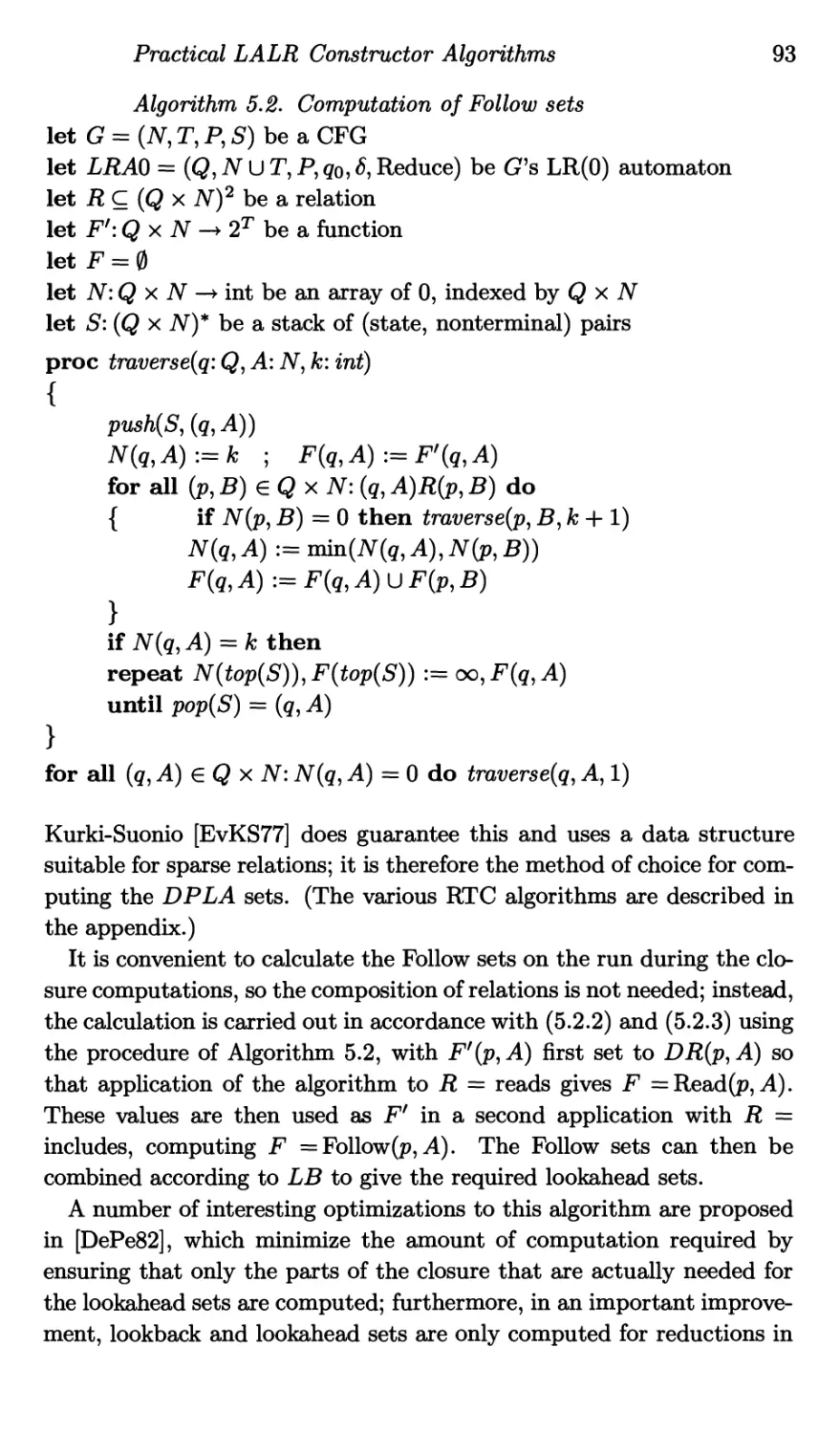
5.2	Practical LALR Constructor Algorithms	87
5.3	A Practical General Method	94
6	Implementation of LR Parsers	98
6.1	Data Structures and Code	98
6.2	Language Dependent Implementations	112
6.3	Optimizing the Parser Tables ,	120
vi	Contents
7	Using LR Parsers	135
7.1	Supplying the Input	135
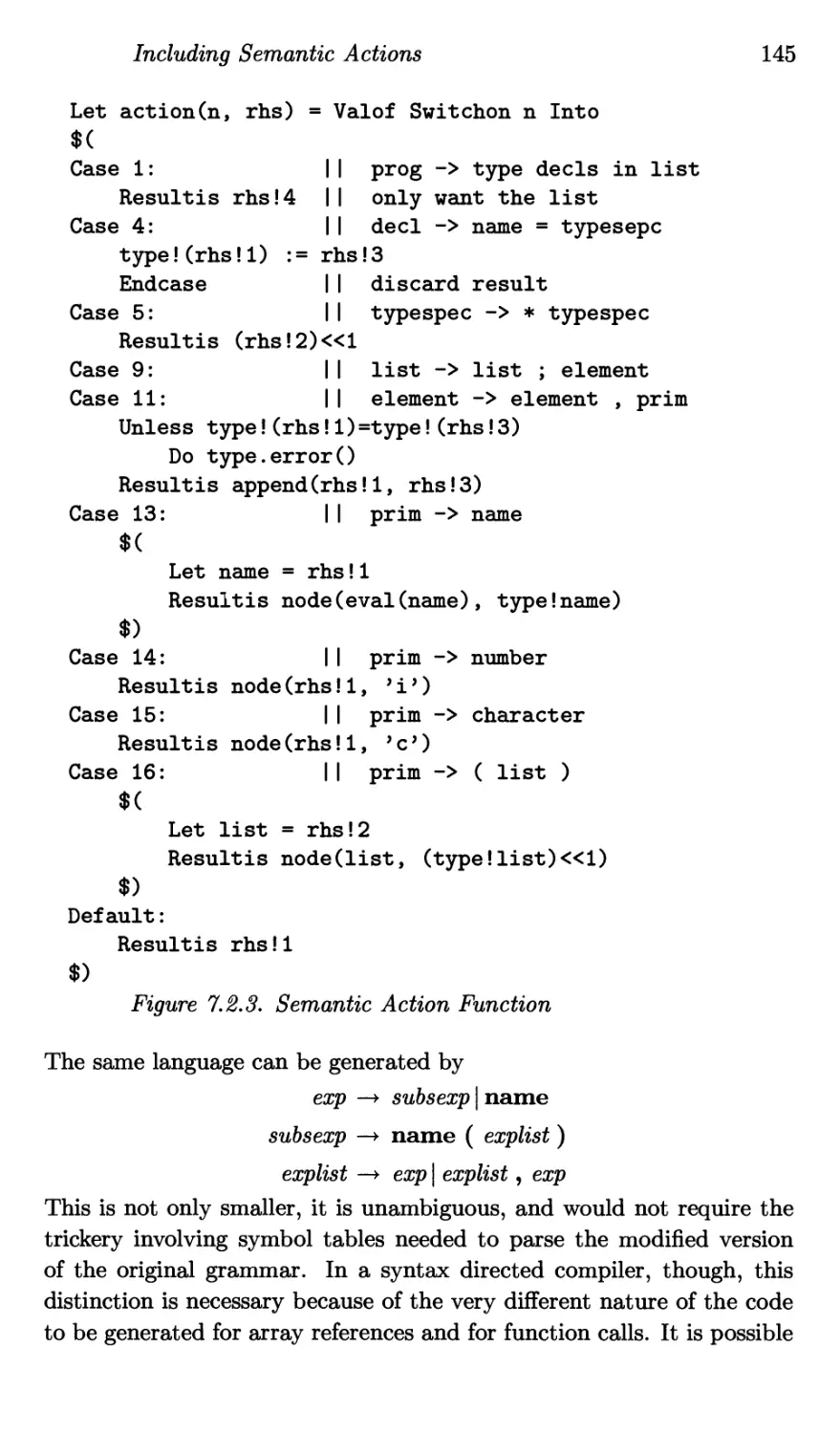
7.2	Including Semantic Actions	140
7.3	Attribute Grammars	149
8	Errors	158
8.1	Detection, Diagnosis and Correction of Errors	158
8.2	Recovery from errors	163
9	Extending the Technique	175
9.1	Use with non-LR grammars	175
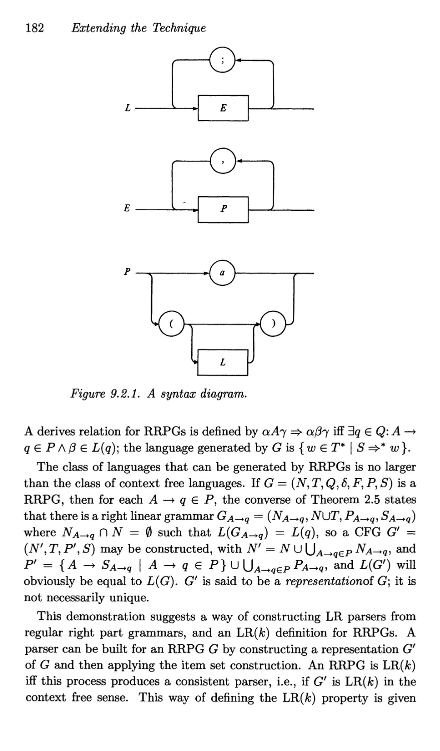
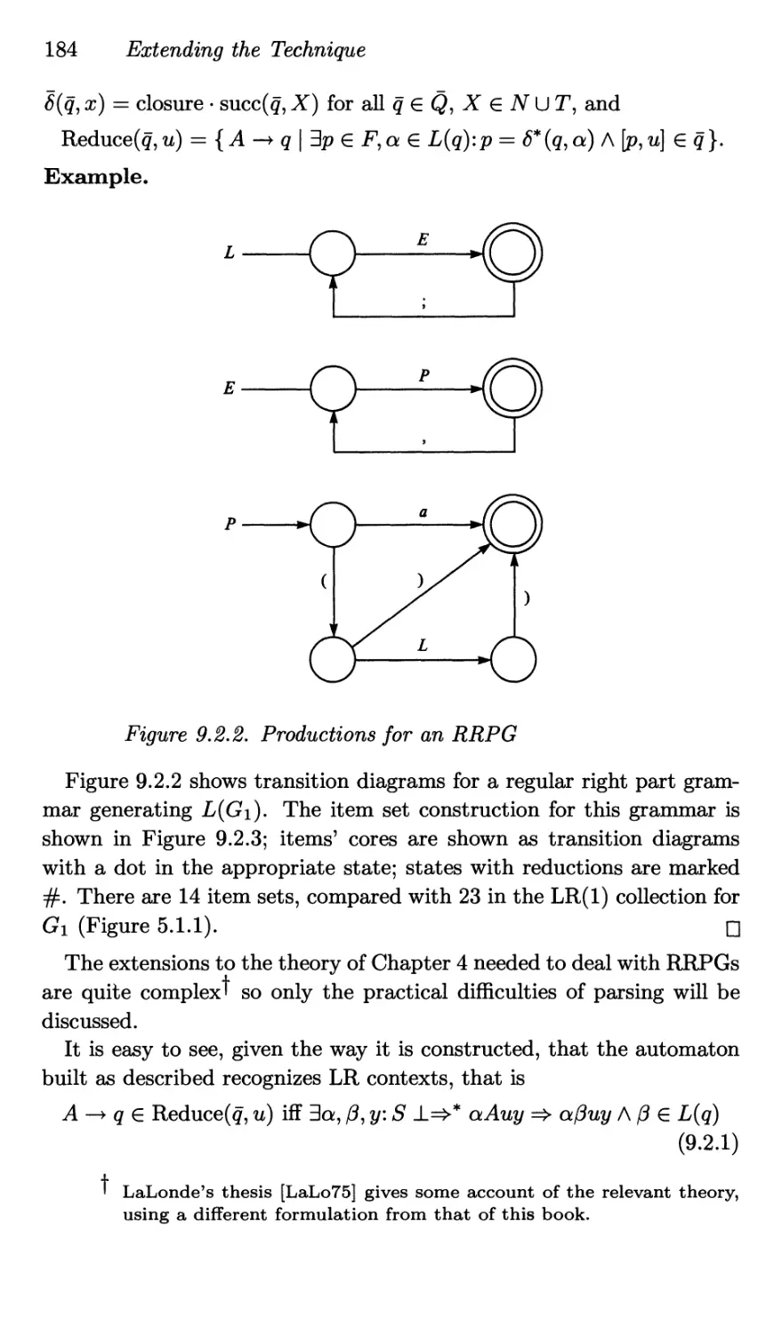
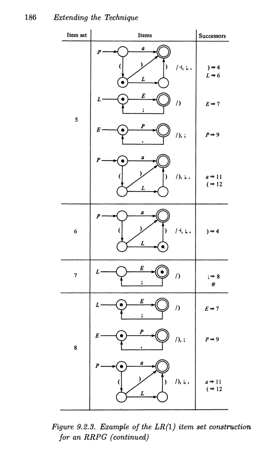
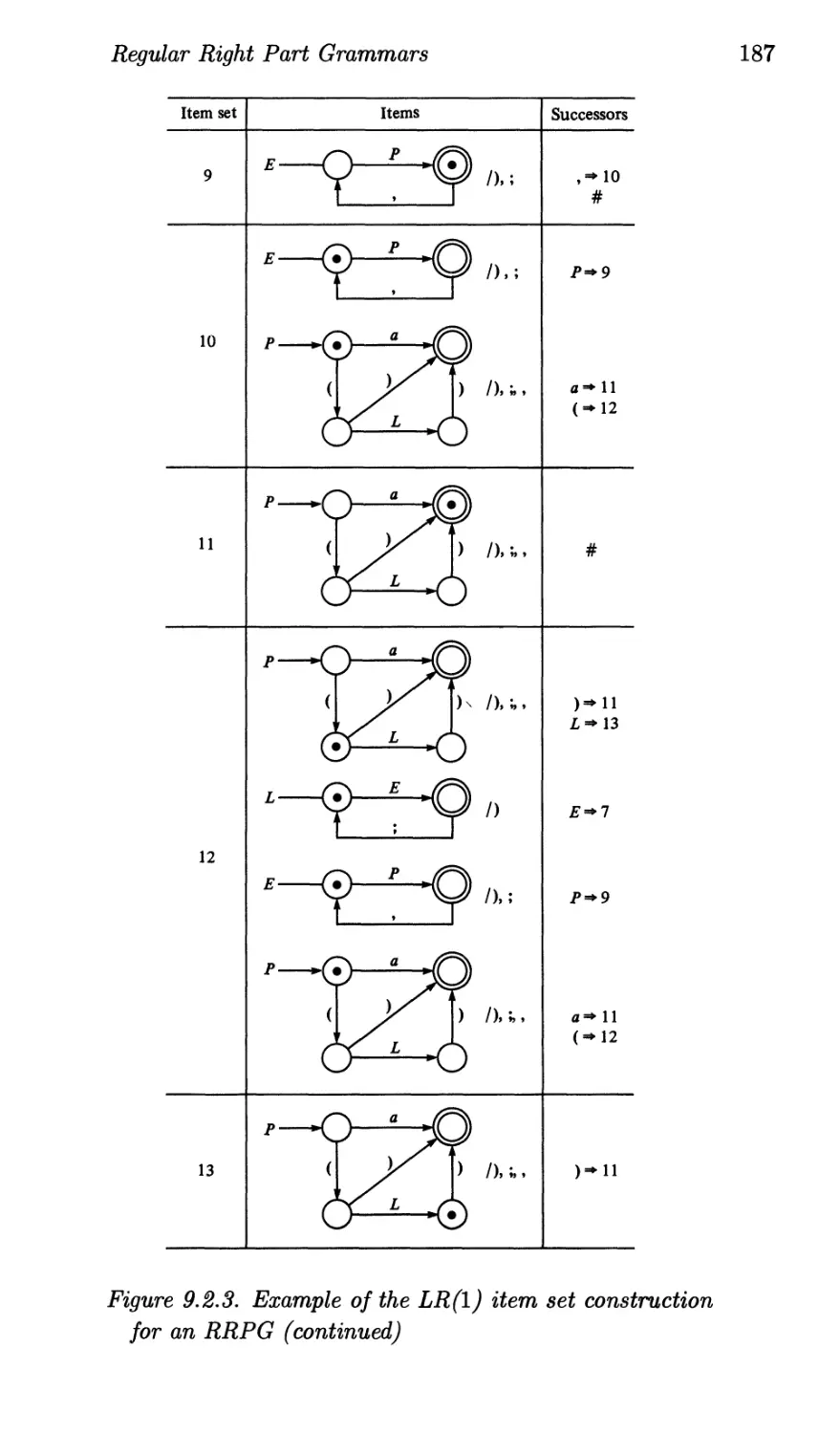
9.2	Regular Right Part Grammars	180
10	LR Parser Generators	191
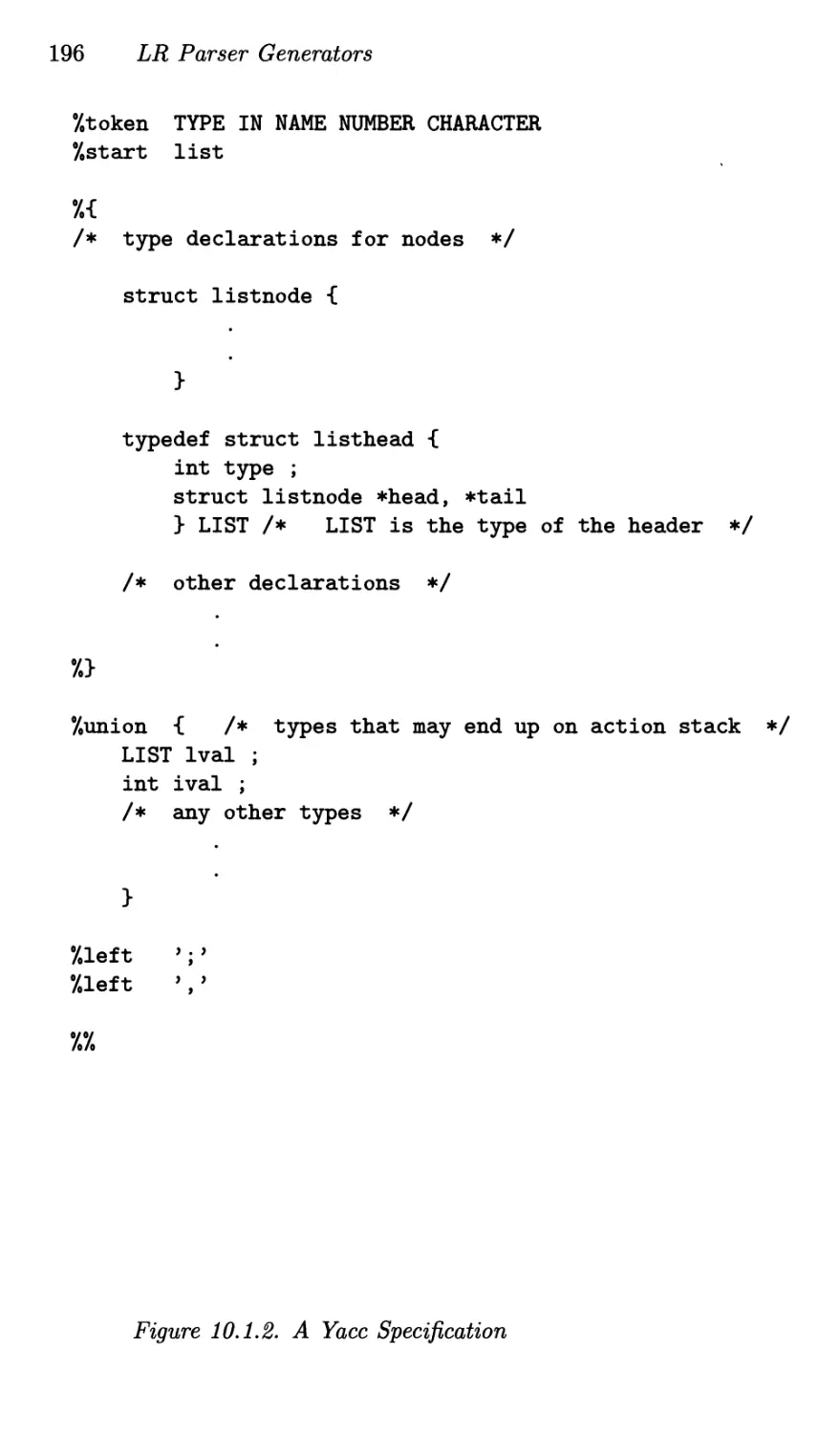
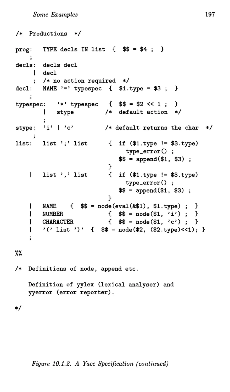
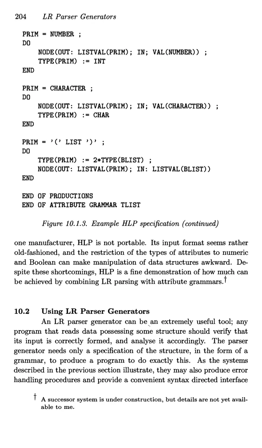
10.1	Some Examples	191
10.2	Using LR Parser Generators	204
10.3	Conclusion	209
Appendix
Relations and the Computation of Reflexive Transitive
Closure	211
Bibliography	219
Index	225
Preface
LR parsing has become a widely used method of syntax analysis; this
is largely due to the availability of parser generators and compiler-
compilers based on LR techniques. However, the readily available ac-
counts of the theory of these techniques are either superficial or are
weighed down with tedious mathematical detail of a merely technical
nature. At the same time, much of the knowledge of practical matters
concerning the implementation and use of LR parsers is scattered in
journals or known only through experience. This book has been written
to bring together an accessible account of LR theory and a description
of the implementation techniques used in conjunction with LR parsers.
It is aimed primarily at users of LR parsers who believe that it is unde-
sirable to use complex tools without understanding how they work.
The book does not quite fall neatly into two parts called ‘Theory’ and
‘Practice’, but most of the theory is to be found in Chapters 2 to 5,
while Chapters 6 to 10 are mainly concerned with practical matters.
Chapter 4 contains the theoretical core, and is based on Heilbrunner’s
account of LR theory, which uses parsing automata and item grammars
to prove that LR parsers do indeed work, and that the widely used parser
construction techniques are correct. In addition, the theory allows the
class of grammars which can be parsed by LR techniques to be related to
other interesting grammar classes, and certain complexity results to be
derived in a straightforward way. This approach to the theory provides
an account of LR parsers more closely in line with the informal notion of
a bottom up parser using lookahead to make its parsing decisions, than
a more traditional method based on ‘valid items’ and ‘viable prefixes’.
The elements of formal language and automata theory required for an
understanding of LR theory are introduced in Chapter 2, and there is an
appendix on relations and reflexive transitive closure computations. No
prior familiarity with this material is assumed, but some mathematical
ability and a little knowledge of set theory and its notation is required.
Detailed proofs of most of the important results are included, but these
may be omitted on a first reading, if necessary.
viii
Preface
The practical chapters deal with data structures and code sequences
used to implement LR parsers as computer programs, and with the ways
in which a parser may interact with other parts of a software system such
as a compiler. One chapter is devoted to methods of dealing with syntax
errors, and there is a chapter describing some ways in which the LR
parsing technique may be usefully extended. The final chapter contains
a survey of a few existing systems and includes practical hints on their
use. A familiarity with the rudiments of data structures is assumed in
these chapters.
As well as material directly referenced in the text, the bibliography
includes extra references to relevant papers. It is not, however, exhaus-
tive; the bibliography [BuJa81] can be consulted for additional references
prior to 1981.
Acknowledgements: It is a pleasure to express my thanks to Stephan
Heilbrunner for carefully reading the draft of this book and for making
many corrections and suggestions for improvement. I am also grateful
to John Washbrook for comments that have led to improvements in the
presentation, especially of some algorithms, and to Simon Peyton-Jones
for advice on functional languages. Finally, acknowledgement is due to
Donald E. Knuth, who first described LR grammars and parsers, and
also attribute grammars, which form an important subsidiary topic of
this book. Professor Knuth is also the designer of IfeX, the typesetting
system which made it possible for me to prepare this book without
exhausting the patience of a typist.
1
Introduction
1.1	Syntax Analysis and its Applications
Syntax is the structure of language. In natural languages, such
as English or French, it is concerned with word order and the relation-
ships and connections that expresses between, for example, a verb, its
subject and its object. The rules defining permissible word orders are
part of the grammar of the language. Syntax analysis is the process
of determining the syntactical structure of a sentence according to the
grammatical rules which define the forms of all permitted sentences.
This process will be familiar, at least to older readers, as being similar
to ‘identifying the parts of speech’: given a sentence, say which class of
word (noun, verb, etc.) each of its constituent words belongs to. This
process is extended to identify larger constituents of the sentence, such
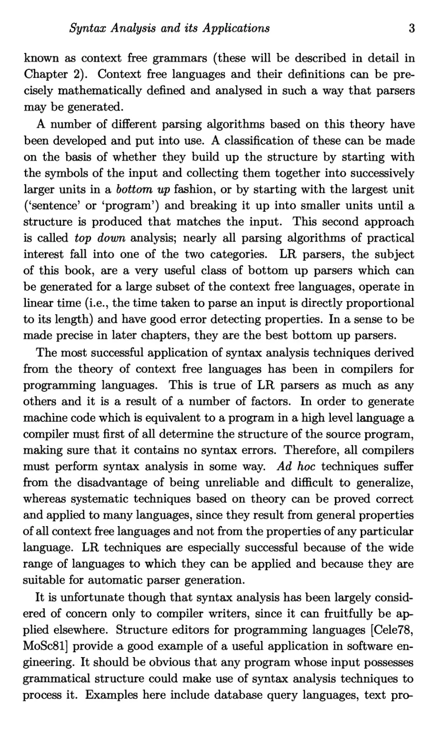
as noun phrase, subject, and so on. The end result is often displayed in
the form of a diagram.
the
mouse
eats the
green cheese
def. article noun
verb def. article adjective noun
noun phrase
subject
noun phrase
sentence
object
The diagram shows that ‘the mouse eats the green cheese’ has the struc-
ture of a simple sentence, consisting of a subject, verb and object, where
the subject is a noun phrase itself consisting of a definite article (the)
followed by a noun (mouse). In itself, it says nothing about the meaning
of the sentence, but only shows how the words are functioning within it:
‘the cheese eats the green mouse’ has an identical syntactical structure
and is perfectly well formed according to the rules of English syntax. It
is nonsense because of the meaning of the words and our experience of
2
Introduction
the habits of mice and cheese.
A similar analysis can be carried out on ‘sentences’ written in a com-
puter programming language. In this context, ‘sentences’ are usually
called ‘programs’, the rules corresponding to natural language gram-
matical rules are those which express restrictions such as ‘the keyword
begin must be matched by a corresponding end’, ‘two arithmetic op-
erators may not appear next to each other’ and so on. The grammar of
a programming language also expresses rules such as ‘the multiplication
operator is more binding than addition’. An analysis made according
to such rules will show that the expression a 4- b * c in an Algol-like
language requires c to be multiplied only by b and not by the sum a 4- b.
This is clearly important if the expression is to be evaluated correctly in
accordance with the intention of the programmer, by a computer. In a
similar way, it is conjectured that a syntactical analysis of a spoken or
written sentence in a natural language is a prerequisite to understanding
it.
It will be apparent that syntax analysis is an algorithmic process: a
syntax analyser implements an algorithm, that is, a procedure for deter-
mining syntactical structure. Such procedures are commonly referred to
as parsing algorithms or simply parsers.
In summary, the purpose of syntax analysis is to discover the structure
of a sentence. This makes the important assumption that the sentence
has a structure; that is that the sequence of words to be analysed is
truly a sentence, properly formed in accordance with the rules of the
language. It is not possible, using the generally accepted rules of English
grammar, to construct a diagram such as the one above, for the sequence
of words ‘green the the eats mouse cheese’. Any algorithm for performing
syntax analysis will fail if presented with an ill-formed sentence, or, in
the context of programming languages, a program containing syntax
errors. It is usual therefore to describe syntax analysis as having a dual
purpose: to determine whether its input is a correctly formed sentence in
a particular language, and, if it is, to determine its syntactical structure.
For certain languages, in particular for contemporary prograpiming
languages, this process can be carried out on a computer. More im-
portantly, it can be carried out systematically, using provably correct
algorithms which can be applied to a large class of languages. Programs
to perform the analysis can themselves be constructed automatically
from a description of the grammatical rules. This is because most of the
syntax of programming languages can be modelled by formal structures
known as context free languages which can be defined by sets of rules
Syntax Analysis and its Applications
3
known as context free grammars (these will be described in detail in
Chapter 2). Context free languages and their definitions can be pre-
cisely mathematically defined and analysed in such a way that parsers
may be generated.
A number of different parsing algorithms based on this theory have
been developed and put into use. A classification of these can be made
on the basis of whether they build up the structure by starting with
the symbols of the input and collecting them together into successively
larger units in a bottom up fashion, or by starting with the largest unit
(‘sentence’ or ‘program’) and breaking it up into smaller units until a
structure is produced that matches the input. This second approach
is called top down analysis; nearly all parsing algorithms of practical
interest fall into one of the two categories. LR parsers, the subject
of this book, are a very useful class of bottom up parsers which can
be generated for a large subset of the context free languages, operate in
linear time (i.e., the time taken to parse an input is directly proportional
to its length) and have good error detecting properties. In a sense to be
made precise in later chapters, they are the best bottom up parsers.
The most successful application of syntax analysis techniques derived
from the theory of context free languages has been in compilers for
programming languages. This is true of LR parsers as much as any
others and it is a result of a number of factors. In order to generate
machine code which is equivalent to a program in a high level language a
compiler must first of all determine the structure of the source program,
making sure that it contains no syntax errors. Therefore, all compilers
must perform syntax analysis in some way. Ad hoc techniques suffer
from the disadvantage of being unreliable and difficult to generalize,
whereas systematic techniques based on theory can be proved correct
and applied to many languages, since they result from general properties
of all context free languages and not from the properties of any particular
language. LR techniques are especially successful because of the wide
range of languages to which they can be applied and because they are
suitable for automatic parser generation.
It is unfortunate though that syntax analysis has been largely consid-
ered of concern only to compiler writers, since it can fruitfully be ap-
plied elsewhere. Structure editors for programming languages [Cele78,
MoSc81] provide a good example of a useful application in software en-
gineering. It should be obvious that any program whose input possesses
grammatical structure could make use of syntax analysis techniques to
process it. Examples here include database query languages, text pro-
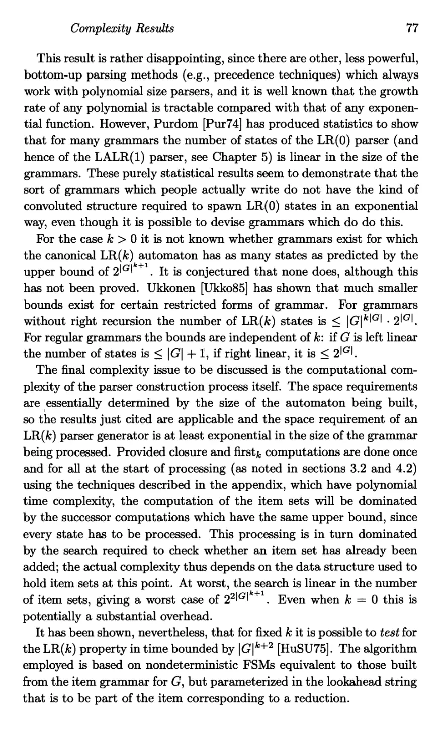
4
Introduction
cessors and operating system command line interpreters. The languages
involved in such applications correspond to the usual notion of a lan-
guage as a system of writing using symbols, but structural systems of
many different kinds may be described as languages, in a formal sense,
and it may then be meaningful to perform syntax analysis. Examples
arise in pattern recognition, where parsing algorithms have been used to
analyse the structure of such things as chromosomes, bubble chamber
photographs and handwritten characters [Fu82]. In the area of human-
computer interaction work has been done using a linguistic approach;
the symbols of the language are the possible user actions and computer
system responses, the syntax specifies which sequences form legitimate
human-computer dialogues [LaBS78, Reis81].
One area in which these techniques have not been much used is in
the analysis of natural language, whether for purposes of translation,
textual analysis or man-machine communication. This is because con-
text free languages do not seem to provide an adequate model for natural
languages, which are widely thought to require a second level ‘deep struc-
ture’ description. However, recently interest in context free analysis of
natural language has revived somewhat (see, for example [JoLe82]) and
it is possible that techniques devised for analysis of computer languages
may be adapted, at least for modest tasks.
1.2	Historical Notes on LR Parsing
Early attempts to perform syntax analysis using computers con-
centrated on the parsing of arithmetic expressions. The major problem
here is to take account of the different binding power of operators used in
ordinary mathematical notation. The very earliest algorithms described
for this process needed to work on the entire formula to be analysed,
but this was improved as early as 1952 by the invention of a sequen-
tial algorithm that only needed to read the formula from left to right,
performing the parsing as it went. By 1959, a number of algorithms,
many of which made use of a stack to hold partially parsed subformu-
las, had been proposed for the analysis of arithmetic expressions and
for the analysis of the structure of computer programs written in some
high level language, which had become recognized as a more general in-
stance of the same problem. (The first Fortran compiler was completed
in 1956 [Back57].) Bauer [Baue76] remarks that, with one apparent ex-
ception, all the algorithms described by that date operated in bottom
up fashion.
Historical Notes on LR Parsing
5
In 1957, Chomsky published a description of context free grammars
and languages, and their usefulness as a descriptive notation for the syn-
tax of programming languages was soon recognized. Their use in this
way became widely known with the publication of the revised report on
Algol 60 in 1963, where the syntax of the language was defined using
Backus Naur Form (BNF), a notation derived from context free gram-
mars. Work on the problem of mechanically producing an analyser from
such a description dates from around this time.
In the previous section, it was explained that a bottom up parser
works by collecting together symbols and combining them into larger
constituents of a sentence, then combining these larger constituents, and
so on. The elements which are to be combined at any step are some-
times referred to as a handle (for a more precise definition of handle, see
section 2.2). A bottom up parser obviously needs some way of finding
handles. In 1964, the notion of a bounded context grammar was devel-
oped [Floy64]. In such a grammar, it is possible to determine whether a
particular collection of symbols is a handle by looking at a finite number
of symbols to each side of it. It became apparent that certain grammars
for which it was intuitively reasonable to suppose that it was possible
to parse using a bottom up approach were not bounded context. In his
1965 paper [Knu65], Knuth generalized the idea to LR(A:) grammars, in
which the entire string to the left of the handle is considered, with a
finite number (k) of lookahead symbols, to its right. (The possibly enig-
matic term LR(A:) will be explained later.) In this paper, he also gave
a parsing algorithm for LR(fc) grammars and two methods of testing
whether a grammar is LR(fc) for some given value of k. One of these
methods, at least, provides a basis for an automatic parser constructor
for LR(fc) grammars. However, as originally described, it was impracti-
cal because the parsers produced had large storage requirements and the
parser generating process was extremely inefficient, with a running time
that increased very rapidly with the size of the grammar. The definition
of LR(fc) grammar seemed, however, to capture the idea of grammars
for which parsing in a single scan of the input using limited lookahead
without having to back up or change a parsing decision once it had been
made, was possible. Furthermore, the parsers operated in linear time,
and although the space occupied by the parser itself was considerable,
the working space it used was also linear in the length of the input.
By 1969, a number of practicable algorithms based on Knuth’s propos-
als appeared. Korenjak [Kore69] used a technique of splitting a grammar
up into sub-grammars and applying Knuth’s algorithm to these sepa-
6
Introduction
rately, combining the resulting sub-parsers into a parser for the whole
grammar. DeRemer, in his thesis [DeRe69], was able to define subsets
of the LR(fc) grammars - so-called SLR(A:) and LALR(A:) grammars -
for which LR-style parsers could be produced efficiently. LaLonde and
others ([LaLH72] and [AnEH73]) built practical parser generators for
SLR(l) and LALR(l) grammars.
Subsequently, several LALR parser generating algorithms have been
devised and used in parser generators which are in daily use. LALR
parser generators are widely considered to be valuable software tools. As
recently as 1979, however, DeRemer and Pennello could claim (with jus-
tification) that ‘.. .no-one heretofore has recognized the essential struc-
ture of the problem [of LALR(l) parser construction] and provided an
algorithm that efficiently exploits that structure’ [DePe79]. Thus, the
development of optimal and practically useful algorithms from Knuth’s
original description of LR(fc) grammars has been a long and difficult
process. It has been helped by the fact that a mathematically rigorous
theory of LR(fc) grammars has been developed over the same period,
so that the practical work on parsing has been supplied with a firm
theoretical base.
1.3	Presentation of Algorithms
Throughout the book, algorithms are described in a pseudo-
programming language in which notations derived from set theory and
those developed in the text are incorporated into the framework of a
conventional imperative language. This framework has been chosen,
despite good reasons for preferring an applicative language, partly be-
cause it is more likely to be familiar to most readers and partly because
it is closer to the way in which these algorithms will have to be pro-
grammed on a present-day computer. The algorithms should be com-
prehensible to anyone with a working knowledge of any of the Algol-
derived languages. The specific syntax employed is mainly influenced
by BCPL[RiWS79] and S-Algol[CoMo82]; the following detailed points
are worthy of note.
The expected statement forms such as assignment, conditional, case
and loops are present. Compound statements are delimited by { and },
instead of begin and end; this usage does not conflict with their also
being used in the conventional way to delimit sets. Assignments may
be combined: a, b := z, у assigns the value of x to a and that of у to
b, conceptually in parallel. Declarations are freely mixed with state-
Presentation of Algorithms
7
ments; the declaration syntax allows for simultaneous declarations (like
the simultaneous assignments just described) and for a limited form of
pattern matching in the style of, for example, Sasl[Turn79]. The way in
which this works should be obvious from the context. The treatment of
types is lax.
Comments, extending from the symbol || to the end of a line are
included. Nevertheless, English text is used to augment the algorithm
when it provides a clearer description than the more formal notation.
Because strings are widely featured in the algorithms, the syntax in-
cludes a general string slicing operation. If s is a string, s(i) is its ith
element, s(i... j) is the substring extending from the ith to the jth el-
ement, and s(i...) is the substring from the ith element to the end.
These expressions are only allowed on the right of an assignment, it is
not possible to assign to the middle of a string.
One construct which may not be familiar to readers who do not know
BCPL is the valof/resultis expression. This takes the form valof { com-
pound statement }, where a statement of the form resultis expression
appears somewhere in the compound statement. The compound state-
ment is executed until the resultis is encountered, when the following ex-
pression becomes the value of the whole valof/resultis expression. This
construct thus provides a means of making a compound statement pro-
duce a value, without losing the distinction between statements and
expressions. It is most commonly used as the body of a function defini-
tion.
In Chapter 6, when implementations are considered, several programs
are given. These are to be distinguished from algorithms; in partic-
ular, objects such as sets are explicitly mapped onto data structures
that can be easily implemented. For most of these examples, BCPL
has been used, partly out of personal prejudice, but also because a
machine-oriented high level language is especially convenient for illus-
trating the implementation issues that arise on a real computer. Again,
readers familiar with an Algol-like language should be able to follow
these examples. The main point to understand is that every value
in a BCPL program is a word and may be used in any way the pro-
grammer wishes. (Thus, the language is either typeless or permits an
infinite number of types, depending on your viewpoint.) Every word
has an address and one of the most important things a word may be
used for is to hold an address and thus serve as a pointer. The oper-
ator ! de-references such pointers: if x holds the address of y, !x has
as its value the contents of y. A vector is a pointer to a contiguous
8
Introduction
number of words, and by definition v!i = ! (v+i) so ! doubles as a
subscription operator. Used in conjunction with named constants, de-
clared by manifest declarations, the ! operator can also be made to
look like a structure field selector. In this way, completely general data
structures may be easily built up, but the facility obviously has its pit-
falls.
A few points about BCPL syntax: the two way conditional takes
the form Test.. .Then.. .Else whereas the single branched conditional
is If.. .DoJ A conditional expression in the style of Lisp is provided:
condition ->expl,exp2 has value expl if condition evaluates to true,
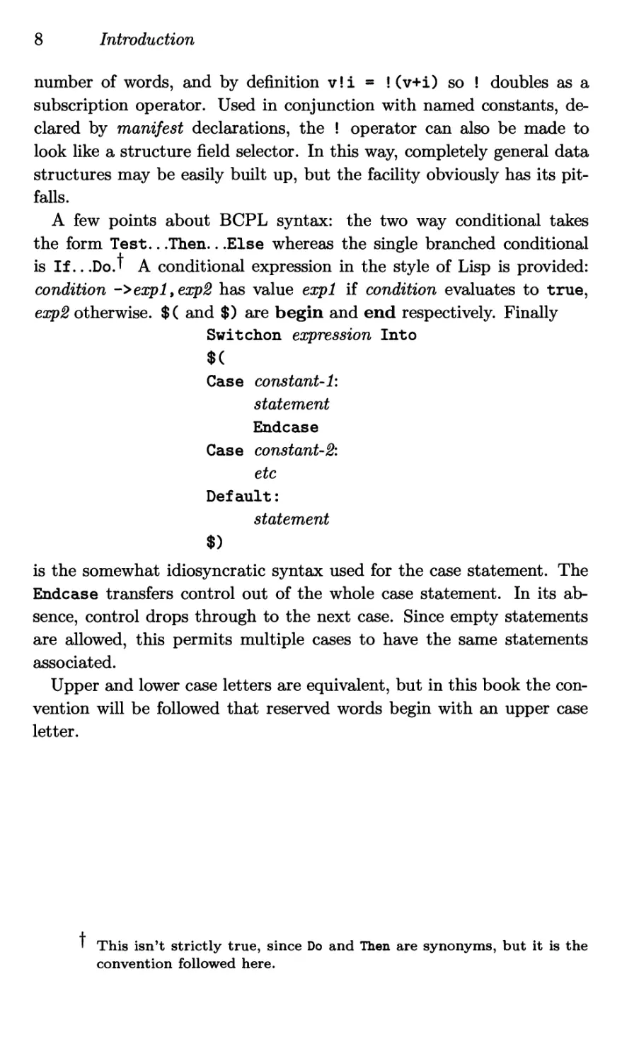
exp2 otherwise. $( and $) are begin and end respectively. Finally
Switchon expression Into
$(
Case constant-1:
statement
Endcase
Case constant-2:
etc
Default:
statement
$)
is the somewhat idiosyncratic syntax used for the case statement. The
Endcase transfers control out of the whole case statement. In its ab-
sence, control drops through to the next case. Since empty statements
are allowed, this permits multiple cases to have the same statements
associated.
Upper and lower case letters are equivalent, but in this book the con-
vention will be followed that reserved words begin with an upper case
letter.
This isn’t strictly true, since Do and Then are synonyms, but it is the
convention followed here.
2
Languages, Grammars and Recognizers
2.1 Languages and Grammars
For the purposes of syntax analysis it is sufficient to consider
text (or programs or whatever it is that is being analysed) purely for-
mally as sequences of symbols into whose meaning, if any, it is unnec-
essary to enquire. A language comprises those particular sequences of
symbols which satisfy certain grammatical constraints which thus define
the language. A programming language such as BCPL is, on this view,
simply the set of all syntactically valid programs. Many languages, in-
cluding BCPL, will be infinite, although all use only a finite number
of symbols; despite this, it is possible to specify languages in a finite
manner. These ideas can be made precise by the introduction of some
simple notation and definitions.
An alphabet E is a finite, non-empty set of indivisible symbols. Ex-
amples of alphabets include the sets
= {0,1} E2 = {a, b,..., z, A, B,..., Z}
S3 = {all BCPL reserved words}
A string over an alphabet E is a finite sequence of members of E. Some
examples of strings over Ei are
0	1	10	10110	000000
Note that the decision as to what constitutes an indivisible symbol is
arbitrary, being determined by the particular area of concern. Thus
Endcase is a symbol in the alphabet S3 but a string over S2.
The length of a string s, written |s| is the number of symbols in s;
if s = XiX2 ... Xn, IsI = n. There is a string of length 0, the empty
string, written A.
If x = X1X2 • • - Xm and у = У1У2...УП are strings, then their
concatenation written x • у (or simply xy where context permits) is
the string XiX2 ... XrnYiY2 .. .Yn formed in an obvious way. Clearly
\xy\ = |z| 4- \y\ and, for any string s, sA — As = s. Furthermore,
the concatenation operation is associative, i.e., for strings x, у and z,
10 Languages, Grammars and Recognizers
x(yz) = (xy)z, so either of these may be written as simply xyz. It fol-
lows that left and right cancellation are possible: xz = yz if and only if
x = у and zx = zy if and only if x = y. If z = xy, then x is a prefix of
z and у is a suffix of z. If x ф Л and x =/=- z, x is a proper prefix; у may
similarly be a proper suffix.
The concatenation operation can be extended to a cartesian product
on sets of strings. If X and Y are sets of strings, then XY = { xy | x €
X Л у € Y }. This, in turn, permits the use of an exponent notation
for such sets by defining X° = {A} and Хг = XX1^ for i > 1. This
notation can also be applied to alphabets, considered as strings of length
1; it is easy to see that for an alphabet E, Ег is the set of all strings of
length i over E.
Finally, define E* = Ц>0 Si and S+ = EE* = E* \ {Л}. E* is thus
the set of all strings over S. t In accordance with the remarks at the
head of this section, a language over E is any subset L С E*.
Small languages can easily be exhibited. Thus {10,11,01} is a lan-
guage over Ei. This becomes impractical for large languages and impos-
sible for infinite ones; some other mechanism is required. The mechanism
which has proved most successful in computer science is the context free
grammar, or CFG, originally proposed by Noam Chomsky as one of the
members of a hierarchy of rewriting systems for defining natural lan-
guages [Chom59]. CFGs have been used successfully for many years as
the basis of the syntax definitions of programming languages.
A CFG is a type of phrase structure grammar: it provides a set of
rules, known as productions, showing how a string in a language, a
sentence, may be built up from its constituent parts, or phrases. Each
type of phrase, such as ‘noun phrase’ or ‘subject’, is called a nonterminal;
each production of the grammar shows a possible way of writing some
nonterminal as a sequence of other nonterminals and possibly symbols
of the alphabet that make up the actual sentences of the language. This
can be expressed in a formal definition, as follows.
A context free grammar is a 4-tuple (АГ, T, P, S) where N is a non-
terminal alphabet, T is a terminal alphabet such that N П T = 0, P C
N x (AT U T)* is a set of productions and S € N is the start symbol.
If, for some A e N, /3 € (TV U T)*, (A,/3) € P, it is custom-
ary to write the production in the form A —> /3. A is the subject
t Technically, S* is the free monoid over S generated by the concate-
nation operator.
Languages and Grammars
11
of the production, /3 is its right hand side. The productions of the
grammar constitute a set of rewriting rules and A —> /3 may be inter-
preted as meaning that where the nonterminal A occurs in a string
it may be replaced by /3. A CFG defines a language by describing
how to generate it: the start symbol of the grammar is taken as a
starting point and strings are derived from it by successively apply-
ing productions to replace nonterminals. The language defined by a
CFG comprises the possibly infinite number of strings consisting of
nothing but terminals which may be produced by this process; it is
thus a language over T. This is captured in the following defini-
tions.
For a, /3,7 e (AT U T)*, A E N : aAy =>g a/3y if and only if A —> (3 is
a production of G. The relation =>g is read ‘directly derives in G\
If there exist strings a^O < i < m such that q0 «i,«i =>g
«2, • • •, O'm-i =>g then «о =>g a™- The relation is the reflexive
transitive closure (RTC) of =>g (see appendix) and is read ‘derives in
G\ Note the possibility that m = 0. If this possibility is excluded, then
o0 =>g meaning that am may be derived from q0 in one or more
steps; is the transitive closure of From now on, whenever no
ambiguity results the subscript G will be dropped from =>g, except for
emphasis.
The language generated by G is L(G) = {w E T* \ S =>q wI- The
strings in L(G) are called sentences-, strings that can be derived from S
but do not consist entirely of terminals (i.e., strings cu € (TV U T)* such
that S =>g a;) are called sentential forms.
A language that can be generated by a context free grammar is known
as a context free language.
Example. Let Gi = ({L, M, E, P}, {;, „ a, (,)}, Pi, L) where Pi is
L-+L-,E	Р-+а
L-+E	P-+(M)
E -► P,P	M -+ A
E-+P	M-+L
L(Gi) is a very simple language consisting of lists of as, variously sep-
arated by commas and semicolons. Lists may have sublists, enclosed in
brackets; the empty list, written as the empty string, must always be
enclosed in brackets. Some of the strings in L(Gi) are
a () (a) a,a;a,a a,(a,a;a);a
One possible derivation for the string a,a;a,a in G is as follows (using
12 Languages, Grammars and Recognizers
an obvious shorthand)
L => L^E => E',E => E,P-,E
=> P,P*,E => a,P;P => a,a;P
(2.1)
=> а,а;Е,Р => a,a;P,P =>
—a,a;a,a
This is not the only way of deriving this string. For example
L => L\E => L^E,P => L;P,a
—t'’ L^P,a —7^ L^8l^8l —7^ E^8l^8l
(2.2)
=> P,P;a,a => Е,щща => P,a;a,a
—a,a;a,a
And there are many others. Derivations (2.1) and (2.2) have not been
chosen entirely at random. In (2.1), at each step in the derivation
the leftmost nonterminal has been replaced, whereas in (2.2) it is the
rightmost nonterminal which is replaced. These two sorts of derivation
provide convenient canonical forms for derivations and, it will be seen
later, occupy a special position in syntax analysis. Formally, a rightmost
derivation is one which consists entirely of steps of the form aAy => a/3y
with 7 € T*. Each sentential form in a rightmost derivation is a right-
most sentential form. A leftmost derivation consists of similar derivation
steps with a € T*. Its sentential forms are leftmost sentential forms.
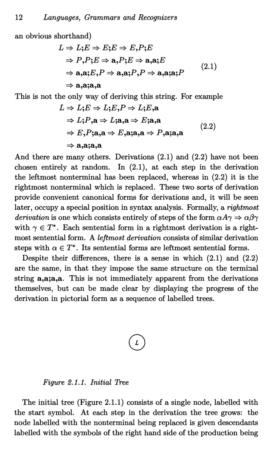
Despite their differences, there is a sense in which (2.1) and (2.2)
are the same, in that they impose the same structure on the terminal
string a,a;a,a. This is not immediately apparent from the derivations
themselves, but can be made clear by displaying the progress of the
derivation in pictorial form as a sequence of labelled trees.
©
Figure 2.1.1. Initial Tree
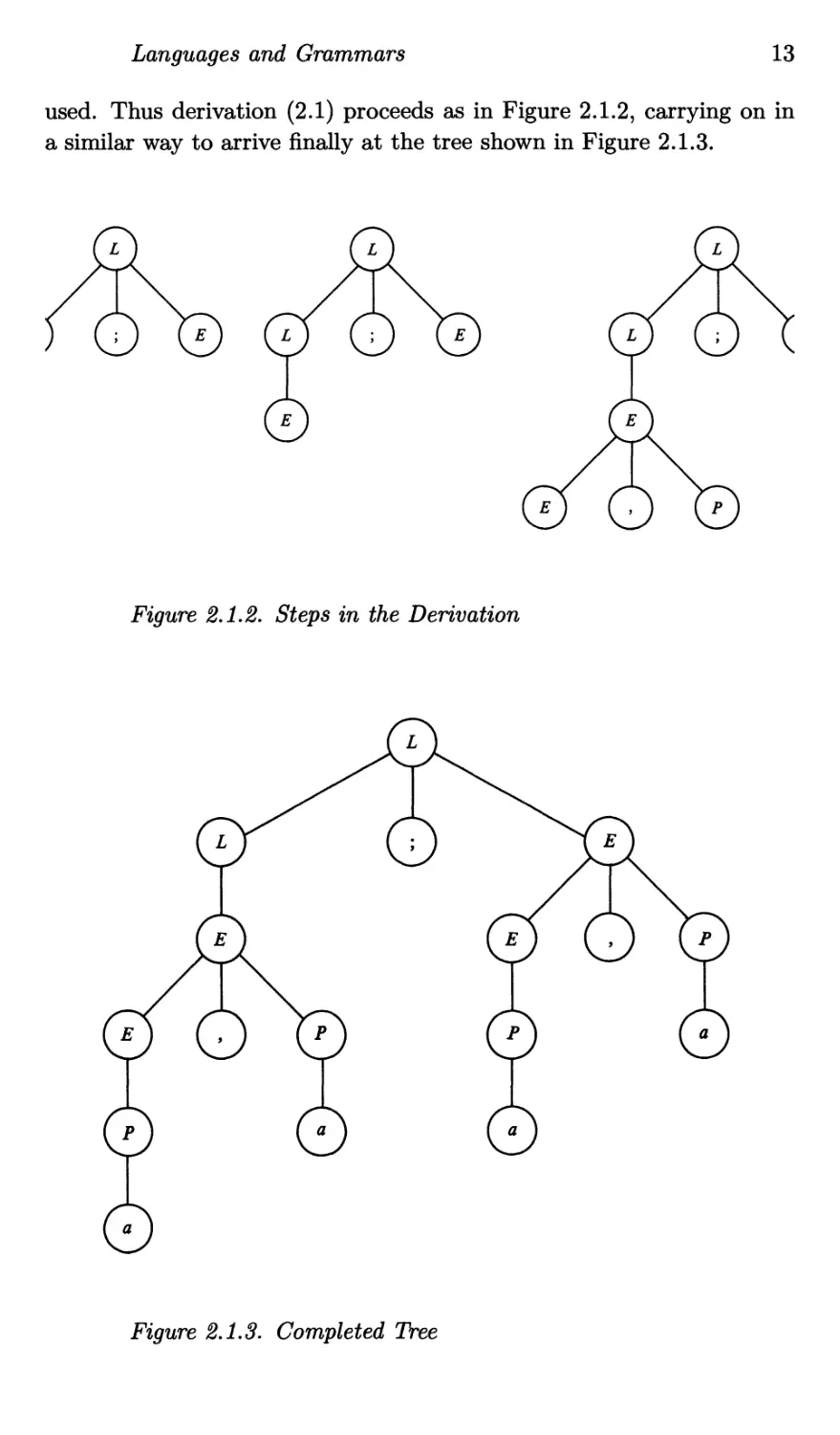
The initial tree (Figure 2.1.1) consists of a single node, labelled with
the start symbol. At each step in the derivation the tree grows: the
node labelled with the nonterminal being replaced is given descendants
labelled with the symbols of the right hand side of the production being
Languages and Grammars
13
used. Thus derivation (2.1) proceeds as in Figure 2.1.2, carrying on in
a similar way to arrive finally at the tree shown in Figure 2.1.3.
Figure 2.1.3. Completed Tree
14 Languages, Grammars and Recognizers
The strings formed from the labels of the leaves of these trees read
in left to right order (their frontiers) are the sentential forms of the
derivation (2.1). The reader should construct the sequence of trees cor-
responding to derivation (2.2). If this is done correctly, the final tree
in the sequence will be identical to Figure 2.1.3. Such a tree is called
a derivation tree and it illustrates the structure of a particular string
in a CFL which is imposed by the grammar being used to define the
language. In this particular case, it shows that of the two list forming
operators (, and ;) provided in L(Gi) the comma is the more strongly
binding.
The two-fold purpose of syntax analysis, to determine whether a given
string belongs to a language and, if it does, to discover its grammatical
structure can thus be expressed in terms of derivation trees: given a
CFG G and a string s purporting to be in L(G), construct a derivation
tree for s or, if this is impossible, announce that s is not in L(G).
It is worth providing a more precise definition of a derivation tree and
examining some of its properties. First some auxiliary definitions are
required.
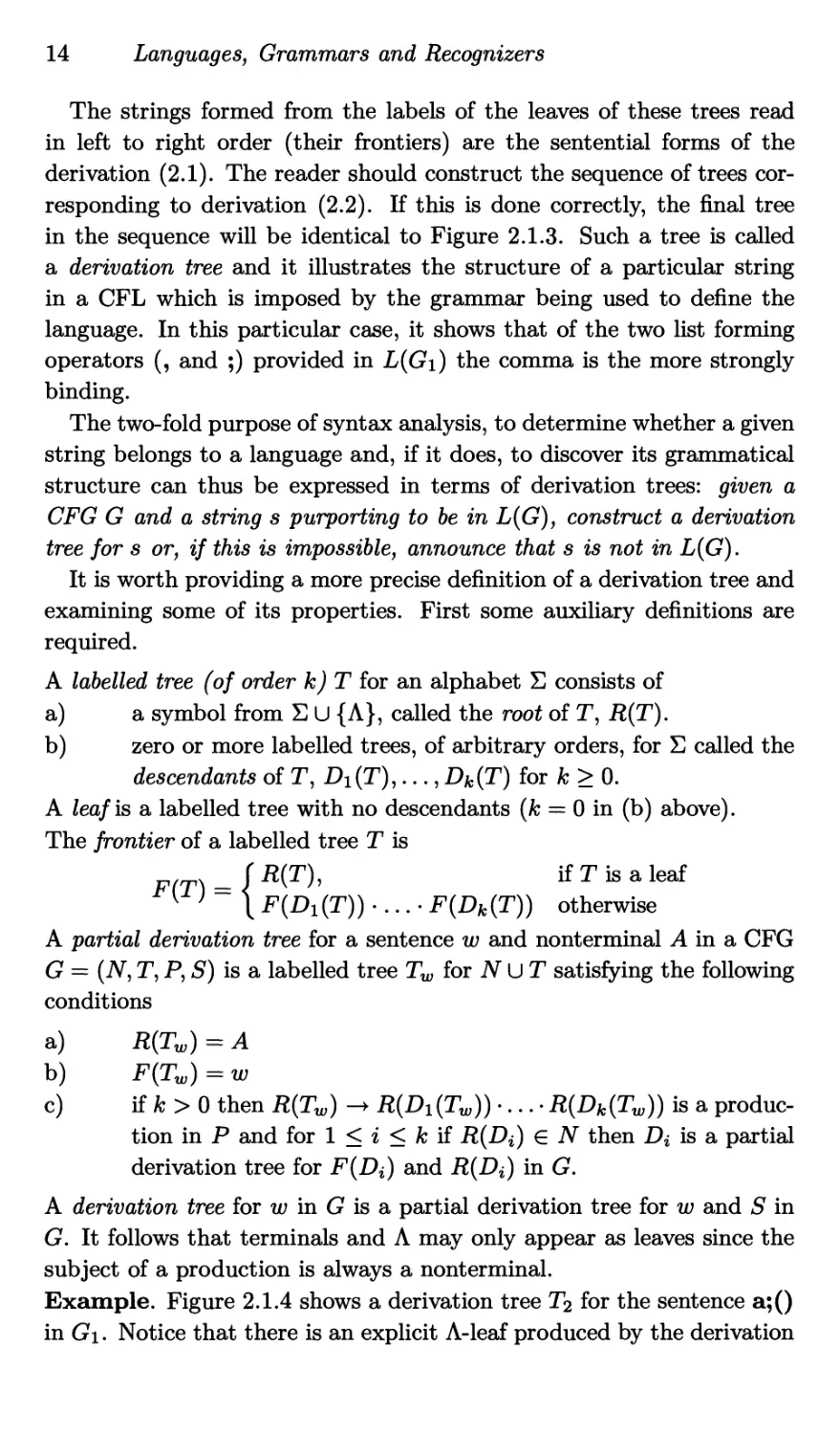
A labelled tree (of order к) T for an alphabet E consists of
a) a symbol from E U {A}, called the root of T, R(T).
b) zero or more labelled trees, of arbitrary orders, for E called the
descendants of T, Di(T),..., Dk(T) for к > 0.
A leaf is a labelled tree with no descendants (k = 0 in (b) above).
The frontier of a labelled tree T is
( } = Г R(T),	if T is a leaf
}	lF(£>i(T))-...-F(£>fc(T)) otherwise
A partial derivation tree for a sentence w and nonterminal A in a CFG
G = (N, T, P, S) is a labelled tree Tw for N U T satisfying the following
conditions
a)	B(TW) = A
b)	F(TW) = w
c)	if к > 0 then R(TW) -+ R(Di(Tw)) •... • R(Dk(Tw)) is a produc-
tion in P and for 1 < i < к if R(Di) € N then Di is a partial
derivation tree for F(Di) and R(Di) in G.
A derivation tree for w in G is a partial derivation tree for w and S in
G. It follows that terminals and A may only appear as leaves since the
subject of a production is always a nonterminal.
Example. Figure 2.1.4 shows a derivation tree T2 for the sentence a;()
in Gi. Notice that there is an explicit Л-leaf produced by the derivation
Languages and Grammars
15
Figure 2.1.4- Example Derivation Tree
step L;(M) =>r L;(). Because Л is the identity for the concatenation
operator, though, F(T2) = a;(), as required.
The definition satisfies the fundamental property that one would ex-
pect for a derivation tree.
Theorem 2.1. Let G = (N, T, P, S) be a CFG.
(1)	A =>* w iff there is a partial derivation tree for A and w in G.
(2)	w € L(G) iff there is a derivation tree for w in G.
Proof. (1) By induction.
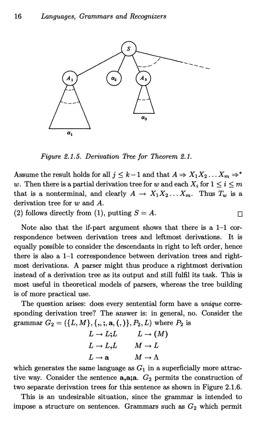
If-part. Assume Tw is a partial derivation tree for w and A. Assume
Tw has descendants Z>i, D2l.. -, Dk- If P(Pi) • R(D2)...R(Dk) = w
then A—> w e P) so A =>* w. Otherwise, each Di is either a leaf or has
R(Di) = Ai for some Ai € N and has frontier 04. For convenience let
«i = R(Di) for the leaf descendants. Then F(TW) = w = qiq2 .. .Q/c
(see Figure 2.1.5).
Assume as inductive hypothesis that the theorem holds for any tree
with fewer nodes than Tw. Then it surely holds for every descendant,
so Ai =>q ai and since A —> R(Di) • ... • R(Dk) it follows that A =>*
ai • R(D2) •... • R(Dk)- By considering each descendant in turn it follows
that A =>* w.
Only-if-part. Assume A =>* w in к steps, for some к > 1. If к = 1
then A —> w and there is certainly a partial derivation tree for w and A.
16
Languages, Grammars and Recognizers
Figure 2.1.5. Derivation Tree for Theorem 2.1.
Assume the result holds for all j < к — 1 and that A=> XiX2 ... Xm =>*
w. Then there is a partial derivation tree for w and each Хг for 1 < i < m
that is a nonterminal, and clearly A —> XiX2 ... Xm. Thus Tw is a
derivation tree for w and A.
(2) follows directly from (1), putting S = A.	□
Note also that the if-part argument shows that there is a 1-1 cor-
respondence between derivation trees and leftmost derivations. It is
equally possible to consider the descendants in right to left order, hence
there is also a 1-1 correspondence between derivation trees and right-
most derivations. A parser might thus produce a rightmost derivation
instead of a derivation tree as its output and still fulfil its task. This is
most useful in theoretical models of parsers, whereas the tree building
is of more practical use.
The question arises: does every sentential form have a unique corre-
sponding derivation tree? The answer is: in general, no. Consider the
grammar G2 = ({L, M}, {„;, a, (,)}, P2, L) where P2 is
L L;L L-+ (M)
L-+L,L	M -+L
L-+a	M-+A
which generates the same language as Gi in a superficially more attrac-
tive way. Consider the sentence a,a;a. G2 permits the construction of
two separate derivation trees for this sentence as shown in Figure 2.1.6.
This is an undesirable situation, since the grammar is intended to
impose a structure on sentences. Grammars such as G2 which permit
Languages and Grammars
17
Figure 2.1.6. Derivation Trees for a,a;a in G2-
more than one structure are said to be ambiguous. That is, a grammar
G is ambiguous if, for some w € L(G) there is more than one derivation
tree. (Equivalently, if there is more than one rightmost derivation.) A
CFL is ambiguous if it is generated by an ambiguous grammar (thus
L(Gi) = L(G2) is ambiguous). It is inherently ambiguous if it is gener-
ated only by ambiguous grammars. Inherently ambiguous languages do
exist (see [HoU179]).
Since an ambiguous grammar is of little direct use for syntax analysis
it would be helpful to have an algorithm for determining whether an
arbitrary CFG is ambiguous.Unfortunately, it can be shown (although
it is outside the scope of this book to do so) that this problem is for-
mally undecidable, i.e., no such algorithm can be devised. However, it is
possible to determine that certain grammars are unambiguous; in par-
ticular, the LR parser generating techniques, which form the subject of
subsequent chapters, are guaranteed to reject any ambiguous grammar.
Before leaving the subject of derivations it is convenient to introduce
a few more definitions related to it.
Given a context free grammar G = (TV, T, P, S), a nonterminal A € N
is said to be left recursive if and only if A Аф for some € (TV UP)*,
right recursive if and only if A фА for some € (AfUT)* and self
embedding if and only if A Ф1АФ2 for some ^1,^2 G (TV U T)+.
The significance of these properties will appear later. For the moment it
is worth remarking that if any symbol in the nonterminal alphabet of a
18 Languages, Grammars and Recognizers
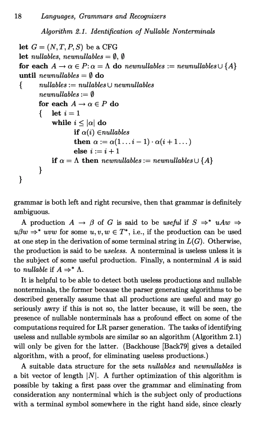
Algorithm 2.1. Identification of Nullable Nonterminals
let G = (TV, T, P, S) be a CFG
let nullables, newnullables = 0, 0
for each A —> a € P:a = k do newnullables := newnullables U {A}
until newnullables = 0 do
{ nullables := nullables U newnullables
newnullables := 0
for each A —> a e P do
{ let i = 1
while i < |q| do
if q(z) ^nullables
then a := a(l... г — 1) • a(i 4-1...)
else i := i 4-1
if a = Л then newnullables := newnullablesU {A}
grammar is both left and right recursive, then that grammar is definitely
ambiguous.
A production A —> /3 of G is said to be useful if S =>* uAw =>
u/3w =>* uvw for some u, v,w € T*, i.e., if the production can be used
at one step in the derivation of some terminal string in L(G). Otherwise,
the production is said to be useless. A nonterminal is useless unless it is
the subject of some useful production. Finally, a nonterminal A is said
to nullable if A =>* A.
It is helpful to be able to detect both useless productions and nullable
nonterminals, the former because the parser generating algorithms to be
described generally assume that all productions are useful and may go
seriously awry if this is not so, the latter because, it will be seen, the
presence of nullable nonterminals has a profound effect on some of the
computations required for LR parser generation. The tasks of identifying
useless and nullable symbols are similar so an algorithm (Algorithm 2.1)
will only be given for the latter. (Backhouse [Back79] gives a detailed
algorithm, with a proof, for eliminating useless productions.)
A suitable data structure for the sets nullables and newnullables is
a bit vector of length |7V|. A further optimization of this algorithm is
possible by taking a first pass over the grammar and eliminating from
consideration any nonterminal which is the subject only of productions
with a terminal symbol somewhere in the right hand side, since clearly
Bottom Up Parsing
19
these cannot be nullable.
2.2 Bottom Up Parsing
The main concern of this book is parsing or, as it has now
been expressed, attempting to construct a derivation tree for a sentence
w = tit2.. -tm of the language generated by a context free grammar.
The properties of the derivation tree indicate that its frontier will match
the given sentence and that its root will be labelled with the start symbol
of the grammar; the parser’s task is to identify the internal structure of
the tree which corresponds to the syntactical structure of the sentence
according to the rules embodied in the productions of the grammar. The
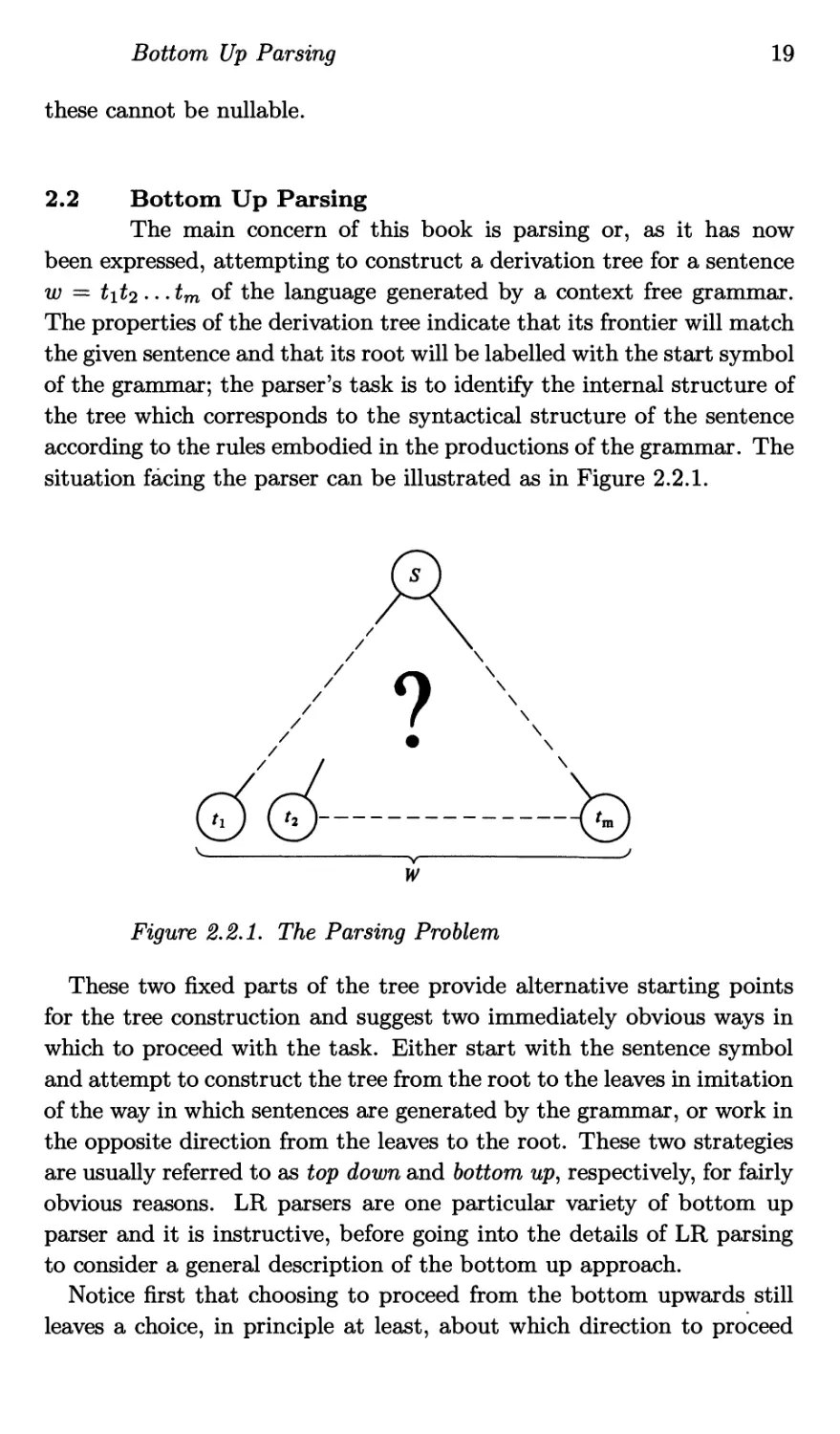
situation facing the parser can be illustrated as in Figure 2.2.1.
Figure 2.2.1. The Parsing Problem
These two fixed parts of the tree provide alternative starting points
for the tree construction and suggest two immediately obvious ways in
which to proceed with the task. Either start with the sentence symbol
and attempt to construct the tree from the root to the leaves in imitation
of the way in which sentences are generated by the grammar, or work in
the opposite direction from the leaves to the root. These two strategies
are usually referred to as top down and bottom up, respectively, for fairly
obvious reasons. LR parsers are one particular variety of bottom up
parser and it is instructive, before going into the details of LR parsing
to consider a general description of the bottom up approach.
Notice first that choosing to proceed from the bottom upwards still
leaves a choice, in principle at least, about which direction to proceed
20 Languages, Grammars and Recognizers
across the tree. In theory either direction is possible but it is more prac-
tical to consider symbols in the order in which they are intended to be
read, conventionally left to right (although it should be understood that
this convention has nothing to do with the way the symbols are written
on paper in their usual form which could quite well be top to bottom
or right to left). This makes input much simpler and also simplifies the
interface between the syntax analyser and any subsequent processing
which may be required.
A bottom up parser, by working from the symbols of a sentence back
towards the sentence symbol of the grammar, is constructing a derivation
in reverse. That is, it performs steps in which a string of the form q/?7
is replaced by aAy where A —> /3 is a production, so that the relation
aAy => a/3y holds, but the replacement goes in the opposite direction to
that implied by the arrow. Such a replacement is called a reduction. If
7 € T*, i.e., A is the rightmost nonterminal in a Ay, the reductions will
form a rightmost derivation in reverse. Most importantly, this reduction
sequence is the one naturally produced by scanning sentential forms from
left to right.
Consider then the operation of a parser which works by repeatedly
scanning a sentential form from left to right to find substrings which
match the right hand side of a production, replacing them by the subject
of that production to produce a new sentential form. Such a parser for
Gi given the string a;a,a could proceed as follows:
string	reduce by
a;a,a	P—> а	(1)
P;a,a	E-+P	(2)
2?;a,a	L->E	(3)
L;a,a	P^a	(4)
L‘,P ,a	E-+P	(5)
L;E,a	LL‘,E	(6)
P,a	Pa	(7)
L.F	E^P	(8)
L,E	L->E	(9)
L,L		
The parser cannot perform another reduction since no substring of L,L
matches the right hand side of any production; indeed, L,L is not a
sentential form in Gi. It is obvious that what has gone wrong is that
the wrong reduction was performed in step (6). One way to cope with
such problems is to allow the parser to backtrack: when it gets stuck, it
21
Bottom Up Parsing
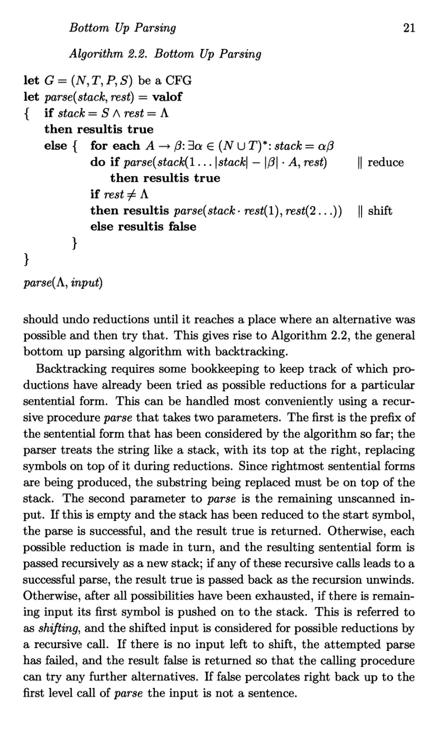
Algorithm 2.2. Bottom Up Parsing
let G = (АГ, T, P, S) be a CFG
let parse(stack) rest) = valof
{ if stack = S A rest = Л
then resultis true
else { for each A -+ /3:3а e (N U T)*: stack = a/3
do if parse(stack(l... |stack\ — |/3| A, rest) || reduce
then resultis true
if rest / Л
then resultis parse(stack- res^(l), rest(2...))	|| shift
else resultis false
}
}
parse(A, input)
should undo reductions until it reaches a place where an alternative was
possible and then try that. This gives rise to Algorithm 2.2, the general
bottom up parsing algorithm with backtracking.
Backtracking requires some bookkeeping to keep track of which pro-
ductions have already been tried as possible reductions for a particular
sentential form. This can be handled most conveniently using a recur-
sive procedure parse that takes two parameters. The first is the prefix of
the sentential form that has been considered by the algorithm so far; the
parser treats the string like a stack, with its top at the right, replacing
symbols on top of it during reductions. Since rightmost sentential forms
are being produced, the substring being replaced must be on top of the
stack. The second parameter to parse is the remaining unscanned in-
put. If this is empty and the stack has been reduced to the start symbol,
the parse is successful, and the result true is returned. Otherwise, each
possible reduction is made in turn, and the resulting sentential form is
passed recursively as a new stack; if any of these recursive calls leads to a
successful parse, the result true is passed back as the recursion unwinds.
Otherwise, after all possibilities have been exhausted, if there is remain-
ing input its first symbol is pushed on to the stack. This is referred to
as shifting, and the shifted input is considered for possible reductions by
a recursive call. If there is no input left to shift, the attempted parse
has failed, and the result false is returned so that the calling procedure
can try any further alternatives. If false percolates right back up to the
first level call of parse the input is not a sentence.
22
Languages, Grammars and Recognizers
Any parser that manipulates a stack of partially parsed input in this
way is called a shift-reduce parser. The recursive mechanism is being
used to create multiple copies of the stack and input, and to remember
previous states, to permit backtracking. As well as the overhead implied,
this means that a backtracking parser must be able to buffer its entire
input; this may present a nontrivial problem in realistic applications,
such as compilers.
Backtracking presents other problems. The first of these is its ineffi-
ciency: the space required by the algorithm to parse a string of length n
is linearly proportional to n but the time in the worst case is exponential
in n. Because of the rate at which exponential functions grow, such be-
haviour is not acceptable. Practically useful algorithms must have time
requirements which only increase with the input length in a polynomial
manner; all else being equal, the preferred algorithm will be a linear one.
A second problem with backtracking concerns the undoing of the ef-
fects of reductions as failed recursive calls return. It is important to
remember that a syntax analyser is never going to be used in isolation;
there will be associated ‘semantic’ actions such as code generation, in-
terpretation or evaluation. At the very least, the syntax analyser will
be producing a tree as its output to be handed on to later stages for
processing. If reductions are to be undone then partially built trees
must be discarded, implying the need for some form of garbage col-
lection in the system, or perhaps code must somehow be un-generated
(which may invalidate the resolution of jump destinations and so on)
or the actions of an interpreter must be reversed, which may simply be
impossible. All these complications can be avoided if backtracking can
be avoided.
Finally, the use of a backtracking algorithm seriously interferes with
the parser’s ability to provide accurate diagnosis of syntax errors in its
input. Indeed, the best that is possible is for such a parser to announce
‘this input contains a syntax error of some sort, somewhere’, which is
hardly satisfactory. It is generally agreed that a primary requirement for
compilers and interactive systems is that they produce good, clear and
accurate error messages. For this reason alone, most compiler writers
would rule out backtracking methods of syntax analysis.
A bottom up parser avoids backtracking if it is able to identify those
substrings of a sentential form whose reduction will eventually lead to
a successful parse. Such a string is colloquially referred to as a handle.
More precisely, if 7 e (TV U T)* is a sentential form of the CFG G =
(N, T, P, S') then a handle of 7 is a triple (A, /3, г) where A e N, /3 €
Recognizers
23
(N U Ту and i > 0 such that
Эа e (N U T)*, w e T*: S aAw =>r a/3w = y Л г = |q/3|
This full definition identifies the position of the substring within 7 and
the particular production it is appropriate to reduce by, as well as impos-
ing the required condition that the reduction be a step in a successful
parse. All these are necessary to unambiguously identify the handle,
but often it is enough to identify the substring /3, and this practice will
usually be followed.
A bottom up parser should, therefore, only perform a reduction if it
has a handle on the top of its stack. The backtracking parser achieves
this by trial and error; to eliminate the backtracking, an algorithm is
needed to identify handles from the information available when the re-
duction is to be performed. LR parsers work in this manner making use
of all the contextual information provided by the progress of the parse
up to that point and also using the next few unshifted characters of the
string being parsed.
2.3 Recognizers
In order to understand how an LR parser works and how it
can be generated from a context free grammar, it is necessary to have a
mathematical description of the operation of a parser and to understand
the relationship between it and a grammar. Appropriate models are
found in automata theory and two in particular are of interest: finite
state machines and pushdown automata.
Finite state machines are useful in modelling a wide range of phenom-
ena which can be characterized as systems capable of being in one of
a finite number of different states and of changing state in response to
discrete inputs. A finite state machine is fully described by specifying
the alphabet from which these inputs are taken, the set of states the
machine can be in, the transitions between states in response to the in-
puts and, additionally, an initial state from which the machine starts its
operation and some final states where it stops.
Accordingly, a finite state machine (FSM) is defined as a 5-tuple
qo,F) where Q is a finite, non-empty set of states, X) is an
alphabet, 6:Q x X —> Q is the transition function, qo € Q is the initial
state and F C.Q are the final states.
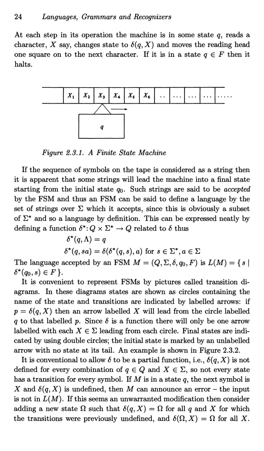
An FSM can be depicted as a black box whose only contact with
the outside world is via a reading head which scans a tape made up of
discrete squares on each of which is a character from X (see Figure 2.3.1).
24 Languages, Grammars and Recognizers
At each step in its operation the machine is in some state q, reads a
character, X say, changes state to X) and moves the reading head
one square on to the next character. If it is in a state q € F then it
halts.
Figure 2.3.1. A Finite State Machine
If the sequence of symbols on the tape is considered as a string then
it is apparent that some strings will lead the machine into a final state
starting from the initial state q$. Such strings are said to be accepted
by the FSM and thus an FSM can be said to define a language by the
set of strings over X) which it accepts, since this is obviously a subset
of E* and so a language by definition. This can be expressed neatly by
defining a function <5*: Q x E* —> Q related to 6 thus
i5*(Q, sa) = 6(6* (q, s), a) for s e S*, a e E
The language accepted by an FSM M = (Q, E, <5, Qo, F) is L(M) = { s |
6*(q0,s)eF}.
It is convenient to represent FSMs by pictures called transition di-
agrams. In these diagrams states are shown as circles containing the
name of the state and transitions are indicated by labelled arrows: if
P = AT) then an arrow labelled X will lead from the circle labelled
q to that labelled p. Since 6 is a function there will only be one arrow
labelled with each X € E leading from each circle. Final states are indi-
cated by using double circles; the initial state is marked by an unlabelled
arrow with no state at its tail. An example is shown in Figure 2.3.2.
It is conventional to allow 6 to be a partial function, i.e., <5(q, X) is not
defined for every combination of q € Q and X € E, so not every state
has a transition for every symbol. If M is in a state q, the next symbol is
X and 6(q, X) is undefined, then M can announce an error - the input
is not in L(M). If this seems an unwarranted modification then consider
adding a new state Q such that 6(q, X) = Q for all q and X for which
the transitions were previously undefined, and <5(Q,X) = Q for all X.
Recognizers
25
Figure 2.3.2. A Transition Diagram.
Then, reading X from q will never lead to acceptance. Nevertheless,
presentation is neater if 6 is partial and so it will be taken to be so from
now on.
It is easier to demonstrate things about the languages accepted by the
class of FSMs by considering similar machines called nondeterministic
finite state machines, or NFSMs for short. As will be shown, these accept
the same class of languages as the FSMs just defined (which are, in fact,
deterministic FSMs) but provide more direct proofs.
An NFSM is just like an FSM except that it relaxes the restriction
that at most one of the arrows leaving a state may be labelled with a
particular symbol X. Formally, an NFSM is a 5-tuple (Q, X), <5, qo? F)
where Q, E, qo and F are as for an FSM but ё: Q x E —> 2^ is the tran-
sition function. For each combination of state and symbol it specifies a
subset of Q as the possible successor states. It may be helpful to imagine
the NFSM as being in several states at once, making state transitions in
parallel. Alternatively, the machine can be imagined trying each possi-
ble transition in turn to see whether any one eventually leads to a final
state. In the latter case, the analogy with the backtracking algorithm of
the previous section should not be missed.
It is somewhat less straightforward to extend ё to <5* in this case. The
requirement is that, for a set of states P, <5*(P, s) should be the set of
states in which the NFSM will be after having read the string s, starting
in some state q € P. The machine still cannot change state without
26
Languages, Grammars and Recognizers
reading an input symbol, so
<5*(Р,Л) = P
The set of states the machine is in after reading a string sa will comprise
all those states it can be in after reading the a from any of the states it
was in after reading the prefix s, so, for any s € X)*, a € X)
<5*(P, sa) =	<5(p, a)
p€tf*(P,s)
The following lemma shows that this behaves in a similar way to that
defined for deterministic FSMs.
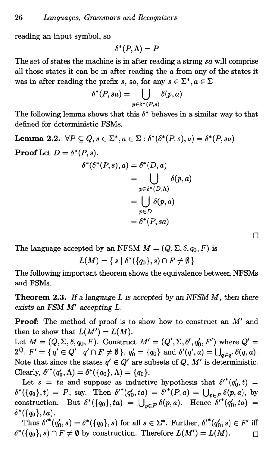
Lemma 2.2. VP C Q, s e E*, a e E: <5*(<5*(P, s), a) = <5*(P,sa)
Proof Let D = 6*(P,s).
6*(6*(P,s),a) = 6*(D,a)
= и
p€^*(P,A)
= |J 6(p,a)
PED
= 6*(P,sa)
□
The language accepted by an NFSM M = (Q, S, 6, qo, F) is
L(M) = {s|/>*({go},s)nF/0}
The following important theorem shows the equivalence between NFSMs
and FSMs.
Theorem 2.3. If a language L is accepted by an NFSM M, then there
exists an FSM Mf accepting L.
Proof: The method of proof is to show how to construct an M' and
then to show that L(M') = L(M).
Let M = (Q,Yi,6,qo,F). Construct M' = (Qf, E, <5',qo,F') where Q' =
2Q, F' = {д' € Q1 I д' П F / 0 }, q'o = {go} and 6'tf, a) = б(д,a).
Note that since the states q' G Q' are subsets of Q, M' is deterministic.
Clearly, 6'*(q'0,A) = 6*({g0}, A) = {go}-
Let s = ta and suppose as inductive hypothesis that S'*(q'o, t) =
<5*({Qo},*) = P, say. Then	= <5'*(P,a) = UPepS(P)a\ by
construction. But <5*({qo}?^) =	Hence S'*(q'0,ta) =
S*({qo},ta).
Thus <5'*(qo? s) = <S*({Qo}? s) for all s e S*. Further, <5'*(qq, s) e F' iff
<5*({qo}? s) A F / 0 by construction. Therefore L(M') = L(M).	□
Recognizers
27
The construction used in this proof provides the basis for an algorithm
for building FSMs from NFSMs. In practice, the size of the set 2^ is
prohibitively large, so it is necessary to generate only those subsets which
are actually accessible from the start state; this is quite easily done and
provides a reasonably efficient algorithm. Further transformations are
then possible to produce an equivalent FSM with the minimum number
of states. See [HoU179,RayS83] for details.
Theorem 2.3 shows that allowing nondeterminism does not extend
the class of languages accepted by FSMs. Therefore, it is legitimate to
determine limits on this class by investigating NFSMs even though, in
practice, it is more useful to construct FSMs. In fact, as will be proved
shortly, FSMs can only be constructed to recognize a subset of the CFLs
known as the regular languages. This class of languages can be defined
in a number of equivalent ways; the most useful for present purposes is
by imposing restrictions on the form of productions permitted in a CFG.
A right linear (RL) grammar is a CFG in which all productions are
of the form:
А,В eN,aeTu{X}
A language generated by a right linear grammar is a regular language.
Sentential forms generated by RL grammars contain at most one non-
terminal and that will be at the right hand end. This rather obvious
fact may be proved formally as follows.
Lemma 2.4. If G = (AT, T, P, S) is a RL grammar and S у then
either у tT* orlat T*,A e N:y = aA.
Proof By induction on the length of derivation.
Base: clearly if 7 = S', а = A and A = S.
Induction: Assume S =>* /3 = a A => 7 for some a € T*, A € TV. Then
either За e T U {Л}: A -+ a A 7 = аа which is in T* or 3B e N, a e
T U {A}: A —> aB A 7 = ааВ, which is in T*N.	□
Clearly right linear grammars are a proper subset of context free gram-
mars; it is also the case, although it will not be proved here, that the
regular languages are a proper subset of the context free languages. The
class of languages recognized by FSMs is precisely the regular languages.
This is proved by showing how to construct an NFSM M from a RL
grammar G such that L(M) = L(G). This construction thus provides a
solution to the parsing problem for the special case of RL grammars.
A —> aB
or A —> а
28
Languages, Grammars and Recognizers
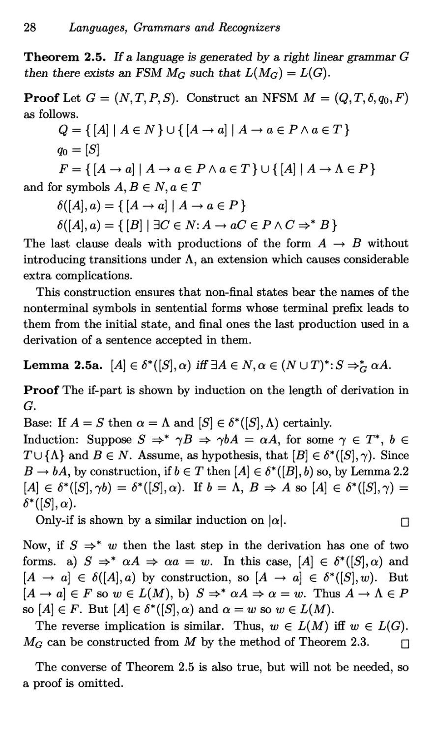
Theorem 2.5. If a language is generated by a right linear grammar G
then there exists an FSM Mg such that L(Mg) = L(G).
Proof Let G = (N,T,P,S). Construct an NFSM M = (Q,T,6,qQ,F)
as follows.
Q = {[A]\AeN}U{[A-+a\\A-+aeP/\aeT}
9o = [S]
F = {[A^a] | A^aePAa6T}u{[A] |
and for symbols A, В e N, a € T
<5([A], a) = {[A-+a\\A-+aeP}
<5([A],a) = { [B] | 3C e N: A -+ aC e Ph C =>* B}
The last clause deals with productions of the form A —> В without
introducing transitions under A, an extension which causes considerable
extra complications.
This construction ensures that non-final states bear the names of the
nonterminal symbols in sentential forms whose terminal prefix leads to
them from the initial state, and final ones the last production used in a
derivation of a sentence accepted in them.
Lemma 2.5a. [A] G <5*([S], a) iff ЗА e N,a G	aA.
Proof The if-part is shown by induction on the length of derivation in
G.
Base: If A = S then a = Л and [S] € <5* ([S'], A) certainly.
Induction: Suppose S =>* yB => ybA = aA, for some 7 G T*, b e
TU{A} and В € N. Assume, as hypothesis, that [B] G <5*([S],7). Since
В —> bA, by construction, if b G T then [A] € <5*([B], 6) so, by Lemma 2.2
[A] e <5*([S],7&) = <5*([S],a). If b = Л, В => A so [A] € <5*([S],7) =
Only-if is shown by a similar induction on |q|.	□
Now, if S =>* w then the last step in the derivation has one of two
forms, a) S =>* aA => aa = w. In this case, [A] € <5*([S],a) and
[A —> a] G <5([A],a) by construction, so [A —> a] G <5*([S],w). But
[A —> a] G F so w E L(M), b) S =>* aA => a = w. Thus A —> A G P
so [A] e F. But [A] G <5*([S],a) and a = w so w G L(M).
The reverse implication is similar. Thus, w G L(M) iff w G L(G).
Mg can be constructed from M by the method of Theorem 2.3.	□
The converse of Theorem 2.5 is also true, but will not be needed, so
a proof is omitted.
Recognizers
29
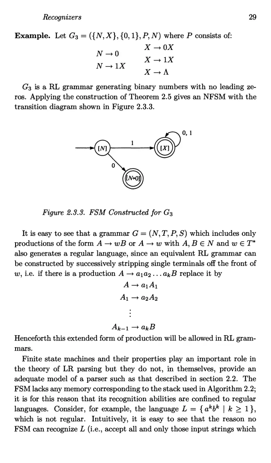
Example. Let G3 = ({TV, A7}, {0,1}, P, AT) where P consists of:
N ->0
N-+1X
X -+ OX
X -+ IX
X -+a
G3 is a RL grammar generating binary numbers with no leading ze-
ros. Applying the construction of Theorem 2.5 gives an NFSM with the
transition diagram shown in Figure 2.3.3.
Figure 2.3.3. FSM Constructed for G3
It is easy to see that a grammar G = (N, T, P, S) which includes only
productions of the form A —> wB or A —> w with A, В € N and w € T*
also generates a regular language, since an equivalent RL grammar can
be constructed by successively stripping single terminals off the front of
w, i.e. if there is a production A —> aiU2 • • • ^kB replace it by
A —> o>iAi
Ai —> GL2A2
Afc—1	> CLkB
Henceforth this extended form of production will be allowed in RL gram-
mars.
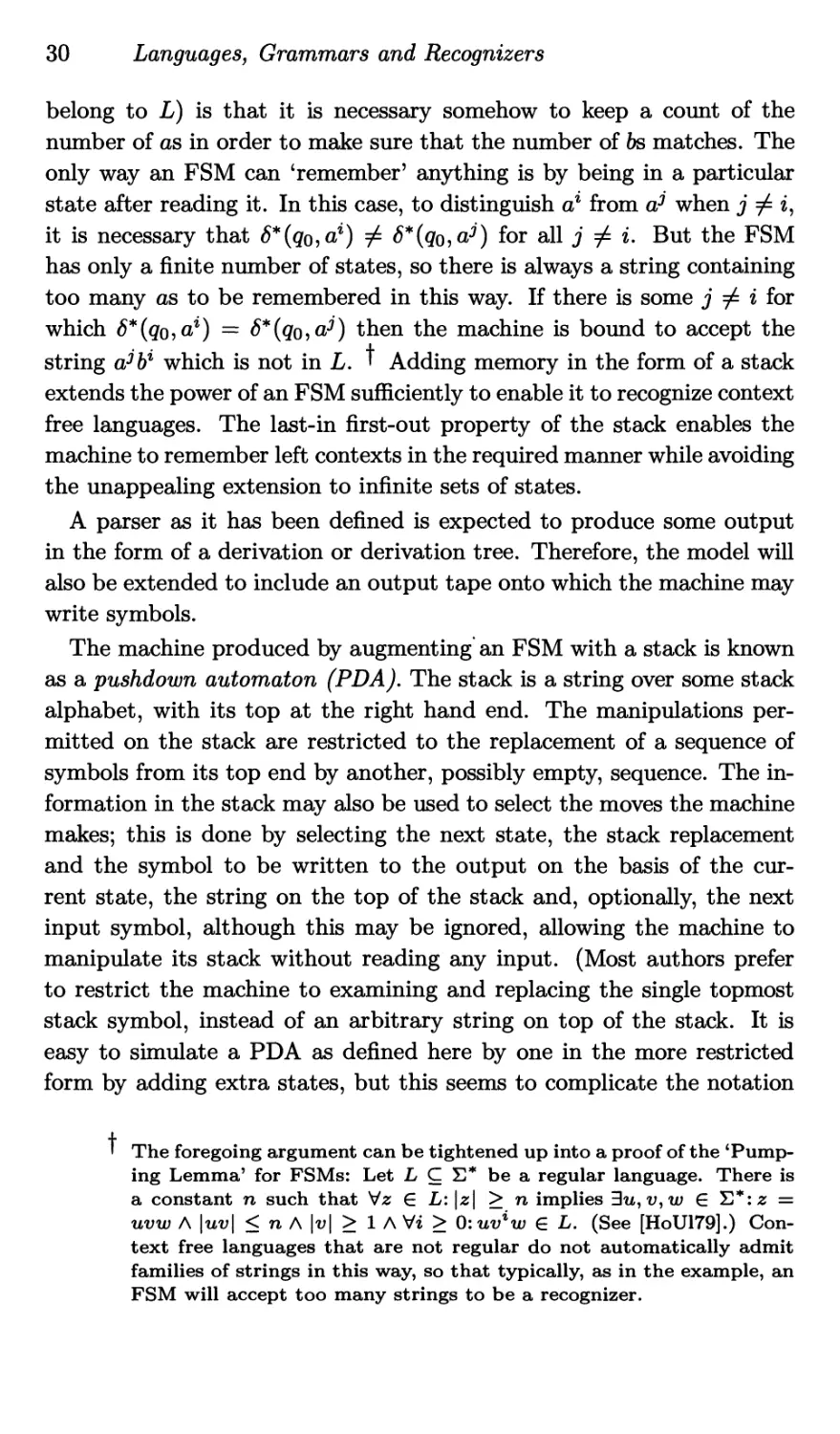
Finite state machines and their properties play an important role in
the theory of LR parsing but they do not, in themselves, provide an
adequate model of a parser such as that described in section 2.2. The
FSM lacks any memory corresponding to the stack used in Algorithm 2.2;
it is for this reason that its recognition abilities are confined to regular
languages. Consider, for example, the language L = {akbk | к > 1},
which is not regular. Intuitively, it is easy to see that the reason no
FSM can recognize L (i.e., accept all and only those input strings which
30 Languages, Grammars and Recognizers
belong to L) is that it is necessary somehow to keep a count of the
number of as in order to make sure that the number of bs matches. The
only way an FSM can ‘remember’ anything is by being in a particular
state after reading it. In this case, to distinguish аг from when j / i,
it is necessary that <5*(до?«г) /	for all j / i. But the FSM
has only a finite number of states, so there is always a string containing
too many as to be remembered in this way. If there is some j / i for
which <5*(до5аг) =	then the machine is bound to accept the
string а^Ьг which is not in L. t Adding memory in the form of a stack
extends the power of an FSM sufficiently to enable it to recognize context
free languages. The last-in first-out property of the stack enables the
machine to remember left contexts in the required manner while avoiding
the unappealing extension to infinite sets of states.
A parser as it has been defined is expected to produce some output
in the form of a derivation or derivation tree. Therefore, the model will
also be extended to include an output tape onto which the machine may
write symbols.
The machine produced by augmenting an FSM with a stack is known
as a pushdown automaton (PDA). The stack is a string over some stack
alphabet, with its top at the right hand end. The manipulations per-
mitted on the stack are restricted to the replacement of a sequence of
symbols from its top end by another, possibly empty, sequence. The in-
formation in the stack may also be used to select the moves the machine
makes; this is done by selecting the next state, the stack replacement
and the symbol to be written to the output on the basis of the cur-
rent state, the string on the top of the stack and, optionally, the next
input symbol, although this may be ignored, allowing the machine to
manipulate its stack without reading any input. (Most authors prefer
to restrict the machine to examining and replacing the single topmost
stack symbol, instead of an arbitrary string on top of the stack. It is
easy to simulate a PDA as defined here by one in the more restricted
form by adding extra states, but this seems to complicate the notation
t The foregoing argument can be tightened up into a proof of the ‘Pump-
ing Lemma’ for FSMs: Let L C S* be a regular language. There is
a constant n such that Vz G L: |z| > n implies Bu, v, w G S*: z =
uvw A |wu| < n A |v| > 1 A Vi > 0:uvzw G L. (See [HoU179].) Con-
text free languages that are not regular do not automatically admit
families of strings in this way, so that typically, as in the example, an
FSM will accept too many strings to be a recognizer.
Recognizers
31
unnecessarily.)
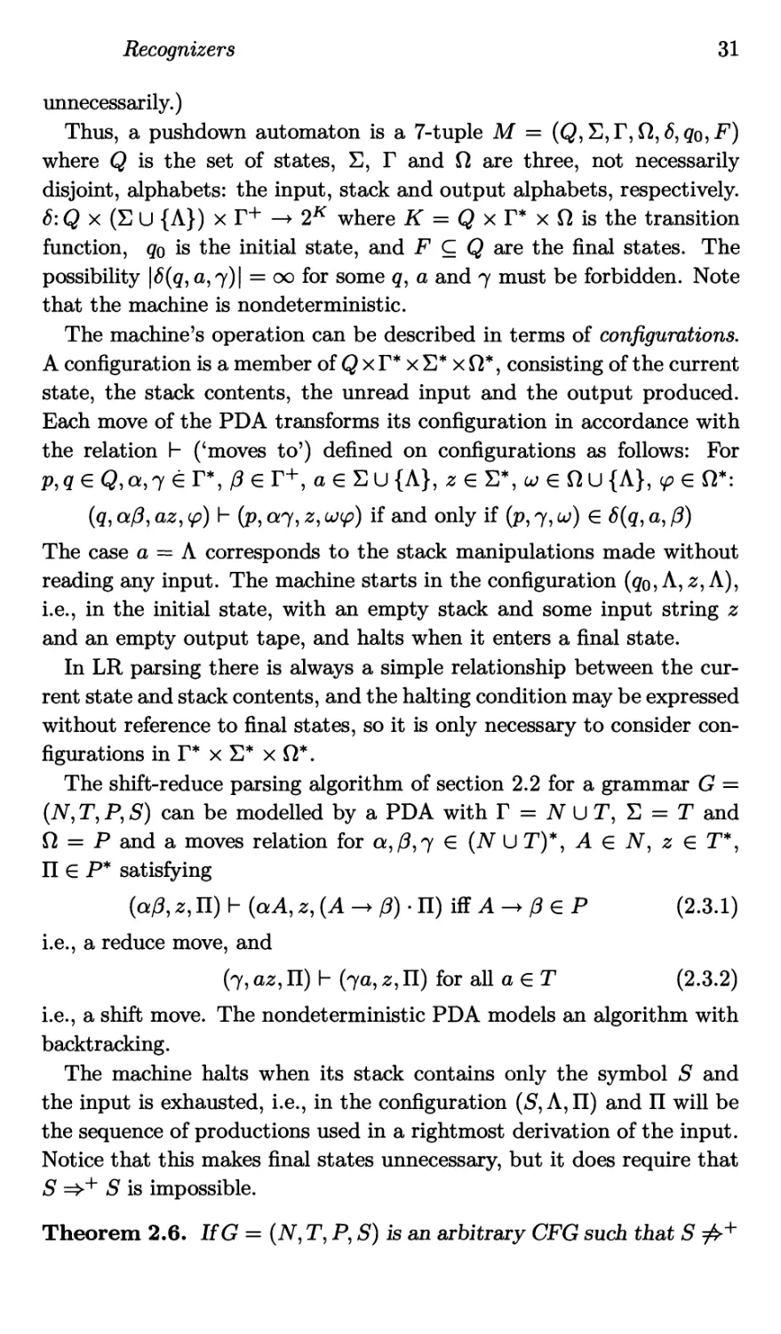
Thus, a pushdown automaton is a 7-tuple M = (Q,E,T, Q, <5, q^F)
where Q is the set of states, X), Г and Q are three, not necessarily
disjoint, alphabets: the input, stack and output alphabets, respectively.
6: Q x (X U {Л}) x Г+ —> 2K where К = Q x Г* x Q is the transition
function, go is the initial state, and F C Q are the final states. The
possibility |<5(g, a,7)| = oo for some g, a and 7 must be forbidden. Note
that the machine is nondeterministic.
The machine’s operation can be described in terms of configurations.
A configuration is a member of Q x Г* x E* x Q*, consisting of the current
state, the stack contents, the unread input and the output produced.
Each move of the PDA transforms its configuration in accordance with
the relation I- (‘moves to’) defined on configurations as follows: For
p,q e Q,q,7 ё Г*, /3 e Г+, a e Eu {A}, z e S*, ш e Qu {A}, e Q*:
(q, q/3, az, ip) h (p, 07,2, wp) if and only if (p, 7, cu) € <5(q, a, /3)
The case a — A corresponds to the stack manipulations made without
reading any input. The machine starts in the configuration (qo, A, 2, A),
i.e., in the initial state, with an empty stack and some input string z
and an empty output tape, and halts when it enters a final state.
In LR parsing there is always a simple relationship between the cur-
rent state and stack contents, and the halting condition may be expressed
without reference to final states, so it is only necessary to consider con-
figurations in Г* x E* x Q*.
The shift-reduce parsing algorithm of section 2.2 for a grammar G =
(N, T, P, S) can be modelled by a PDA with Г = U T, E = T and
Q = P and a moves relation for a,/3,7 € (AT U T)*, A e N, z e T*,
П € P* satisfying
(q/3, z, П) h (qA, z, (A -+ /3) • П) iff A -+ /3 e P (2.3.1)
i.e., a reduce move, and
(7, az, П) h (7a, 2, П) for all a € T	(2.3.2)
i.e., a shift move. The nondeterministic PDA models an algorithm with
backtracking.
The machine halts when its stack contains only the symbol S and
the input is exhausted, i.e., in the configuration (S, Л,П) and П will be
the sequence of productions used in a rightmost derivation of the input.
Notice that this makes final states unnecessary, but it does require that
S =>+ S is impossible.
Theorem 2.6. IfG = (N, T, P, S) is an arbitrary CFG such that S
32
Languages, Grammars and Recognizers
S and h is the moves relation of a PDA satisfying (2.3.1) and (2.3.2)
then \/z eP:S z, using the sequence of productions П € P* if and
only if (A, z, A) h* (S, Л, П).
The proof is quite simple, since the moves relation ensures that, in
any configuration (7,2,П), 72 is a right sentential form. This begs the
question of whether it is possible to construct such a PDA; the proof of
that is similar to that of Theorem 2.5 but depends on a normal form
theorem for CFGs. For details see [HoU179, RayS83, AhU172].
It is possible to define a deterministic PDA by imposing restrictions
on 6. Firstly, insist that each state q € Q has at most one successor
and stack top replacement for each input symbol, top stack string com-
bination. This requires Va € E U {A},q,/3 € Г*: |<5(q, a, (3)\ < 1 and
if a, a/3) / 0 then 6(q, a, /3) = 0. Secondly, there must never be
a choice whether to read the next symbol or not, so, if 6(q, A, /3) / 0
then Vu € E:<5(q, a, /3) = 0. Unfortunately, whereas NFSMs turned
out to be no more powerful than FSMs the corresponding statement is
not true for PDAs: the class of languages recognized by deterministic
PDAs is a proper subset of the CFLs, often known as the deterministic
languages. Fortunately, most programming languages are deterministic,
so the methods of parsing deterministic languages are of considerable
practical interest. The class of languages that can be recognized by LR
parsers is, in fact, the class of deterministic languages.
3
Simple LR Parsing
3.1 LR(O) Parsers
LR(A?) parsers are so called because they operate in the manner
of bottom up parsers described in section 2.2., scanning the input from
Left to right, producing the reverse of a Rightmost derivation, and use к
characters of unscanned input to produce deterministic behaviour. The
family of parsing techniques related to LR(A:) parsers is distinguished by
the fact that, in deciding whether to perform a reduction, they make
use of all the contextual information that is available in the prefix of
the input string that has already been parsed. In the most basic of
the LR techniques, LR(0), this is all the information that is used; the
more powerful variants supplement this left context information by con-
sidering the first few characters of so far unread input. This chapter
describes informally the simplest such variant, SLR(l) parsers, in order
to introduce important ideas behind the whole family of techniques.
First it is necessary to consider LR(0) parsers. If G = (AT, T, P, S) is
a CFG and there is a derivation of the form S a Aw =>r a/3w with
ol,(3 e (N U T)*, A € N and w e T* then, if a shift-reduce parser has
a/3 on its stack it may be correct to reduce by A -4- (3. The set of all
such stack strings for which the reduction could be a step in a successful
parse is known as the LR(Q) context of the production A —> (3, written
LR0C(A -> /3); i.e.,
LR0C(A -> /3)
= { a/3 € (AT U Ту | 3w € T*: S =># aAw =>r a(3w }
A parser should perform a reduction by A —> /3 only if its stack contents
is a member of LR0C(A —> /3). However, it may be the case that some
string a/3 is a member of the LR(0) context set of two or more different
productions. Alternatively, a situation may arise where there is a string
a/3 € LR0C(A —> /3), but there is also a non-empty terminal string t,
such that a/3t € LR0C(B —> 6) for some production В —> 6. In the
first case, the parser cannot choose one reduction in preference to the
34
Simple LR Parsing
other when it has a/3 on its stack. In the second case, since there is a
sequence of shift moves which reads the symbols of t, transforming the
stack contents into a member of LR0C(B —> <5), the parser cannot decide
whether to reduce immediately by A —> /3 or perform a shift move, so
as to eventually be able to reduce by В —> ё. Thus, using the LR(0)
contexts to decide when to reduce only provides a deterministic parser
if neither of these situations can arise, so that the stack contents is all
that is needed to determine whether a particular reduction should take
place. In that case, G is said to be an LR(0) grammar. For an LR(0)
grammar the problem of whether to perform a reduction thus becomes
the problem of identifying LR(0) contexts on the stack. Fortunately,
this is a relatively simple task, because of the following result.
Theorem 3.1. Let G = (N,T,P,S) be a CFG. Then LR0C(G) =
LR0C(A —► /3) is a regular language.
Proof Construct the grammar F = ({ [A] | A e N},N U T,PF, [S'])
where for each production A —> XiX2 ... Xn in P, Pp includes the
productions
[A] -> X1X2 • • -Xj-^Xj] 1 < j < n,Xj e N
and [A] -+XiX2...An
F is right linear, so L(F) is regular. Furthermore, it is easy to see that,
for e (AT U T)*, [S] =>p if and only if
За,/3 € (ATUT)*, AeN,weT*:S =>gr =>gr otf3w/\ф= a/3
since derivations in F ‘shadow’ those in G, with the rightmost nonter-
minal in the sentential forms of G corresponding to a nonterminal [A]
in the sentential forms of F. Thus,	iff ЗА —> /3 € Р-.'ф €
LR0G(A —> /3), so that LROG(G) is a regular language.	□
It is therefore possible, given an LR(0) grammar G, to construct from
it an RL grammar F, and then, using algorithms based on Theorems 2.5
and 2.3 to build a deterministic FSM to recognize strings in LFOG(G).
Because of the LR(0) condition, no final state will have any outgoing
transitions. Such states are therefore reduce states] since a string in
LFOG(G) has just been recognized the handle on top of the stack can
be replaced as one step in the parse. The production to be used can
be obtained by mapping final states to productions of G by a function
Reduce, such that Reduce([[A] -4- XiX2 ... Xn]) = A —> X]X2 ... Xn.
The construction of such a FSM, known as the characteristic FSM
of G, provides the basis of a parser, whose operation is described by
LR(Q) Parsers	35
Algorithm 3.1. LR(O) Parsing
let G = (TV, T, P, S) be an LR(O) CFG
let M = (Q, N U T, 6, q0, F) be G’s characteristic FSM
let Reduce: F —> P map reduce states to corresponding productions
let 7 = input
let stack = Л
let q = go
until stack = S A 7 = Л do
{ if g F
then { || shift
let X = 7(1)
7:= 7(2...)
if <5(g, X) is undefined
then error
else { stack := stack • X ; q := <5(g, X) }
else { || reduce
let A —> /3 = Reduce(g)
stack := stack(l... |stacfc| — |/3|) • A
if stack = S A 7 / Л A 6(qo, S) is undefined
then error
else { q := q0
for i = 1 to |stacfc| — 1 do q := <5(g, stack(i))
unless stack = S/\y = Adoq:= S(q, A)
}
}
}
Algorithm 3.1. This is a shift-reduce algorithm. Since there is no back-
tracking, and thus no need to remember stacks, the recursion of Algo-
rithm 2.2 can be unwrapped into an iterative form. The characteristic
FSM is used to control when a reduction takes place; since the sentential
form produced by a reduction consists of the remaining input appended
to the stack, the FSM must scan the stack after the reduction before
considering any more input symbols, unless the stack contains only the
start symbol. In that case, if there is no remaining input, the parse is
successful; otherwise it is possible that the remaining symbols are super-
fluous. This can be detected, since <5(qo? S) will be undefined if S =>* Sz
is impossible for all z e T+.
36
Simple LR Parsing
There may be strings 7 L(G) which will cause this algorithm to
attempt to shift symbols from beyond the end of 7. To prevent this,
an endmarker symbol H should be appended to 7; it corresponds to an
end of file indication in a real input. <5(q, H) is undefined for all q, so
strings not in L(G) will always cause an error (even if they are a pre-
fix of some string which is in L(G)). It is convenient to assume that
4 € T, but never appears on the right hand side of any production (i.e.,
PC^x^UT\{<).
The algorithm as just presented has another weakness: if the string 7
has the form a/3w before reduction, after reduction it will be aAw. The
characteristic FSM will now return to state qo and scan the updated
stack containing aA. Since it is a deterministic FSM, having re-read
a it will be in the same state it was in after reading it the first time;
the second scanning is wasted if it is possible to remember the state
the machine entered after reading a initially. This is easily done by
providing the parser with a stack on which it pushes each state as it
enters it. When the machine reduces by a production A —> /3, in the
context a/3, |/3| states are popped off the stack and the current state
is set to the new stack top. This state is	the state it would
have been in after re-scanning a. Only the following transition under
A need be made as part of the reduction, so that only the terminals of
the input need be read, in a single scan, left to right, as in Algorithm
3.2.
The А-successor required by the reduction is guaranteed to be de-
fined, except in the special case mentioned above in connection with
Algorithm 3.1: if the start symbol S is not left recursive S^q^S) will
be undefined. This transition will only be required if the input is
some string wz such that S =>* Sz =>* wz, with \z\ > 0. In that
case, wz L(G), so an error should be reported, but a special test
is needed to prevent the parser from trying to change to a nonexis-
tent state. (S might be left recursive, so it is not correct to report
an error whenever A = SAct = qoA7/H; see the following exam-
pie.)
Example.
Let G4 = ({L, Б}, {(,),,, a}, P4, L) where P4 consists of
L —> L,E	E —> a
L-+E	E-+(L)
37
LR(Q) Parsers
Algorithm 3.2. Improved LRfi}) Parsing
let G = (N, T, P, S) be an LR(O) CFG
let M = (Q, NuTJ, F) be G’s characteristic FSM
let Reduce: F —> P map reduce states to corresponding productions
let 7 = input • H
let a = Qo II state stack
let q.X = g0,7(l)
let accepted = false
while -^accepted do
{ if q £ F
then { 7 := 7(2...)
if X) is undefined then error
else { q := <5(q, X) ; X := 7(1) }
a := a • q
}
else { let A —> /3 = Reduce(g)
a := <t(1 ... |cr| - |/3|)
if A = S A a = Qo
then if 7 = 4 then accepted := true
else if <5(qo? S) is undefined then error
unless accepted do { q := 6(a(|cr|), A) ; a := a • q }
The corresponding grammar P4 has productions
[L] -+ [L]
[L]	L,[E]
[L] L,E
[L] -+ [£7]
И-a
[Я]	([£]
[Я]	(L)
In G4 there is a rightmost derivation L => L,E => L,a. Corre-
sponding to this in P4 is the derivation [L] => L,[P] => and
Да € LP0C(P -> a).
The characteristic FSM’s transition diagram is shown in Figure 3.1.1,
where reduce states have been indicated by double circles annotated
with the corresponding production.
Note that no reduce states have outgoing transitions, hence it can be
deduced that G4 is LR(0). Given the input a, (a,a) to parse, Algorithm
38
Simple LR Parsing
Figure 3.1.1 CFSM Transition Diagram for G4
3.2 behaves as shown in Figure 3.1.2.
The LR(0) parsing algorithm can be described abstractly in a succinct
fashion by defining an LR(0) automaton (LRA). An LR(0) automaton
for a CFG G = (AT, T, P, S') is a 6-tuple (Q, V, P, go? <5, Reduce) where Q
is the set of LR(0) states, V — N U T, P is the production set of G,
Qo G Q is the initial state, 6: Q x V —> Q is the transition function and
The Item Set Construction
39
unscanned input	state stack	reduction
a,(a,a)4	0	
,(a,a)H	04	E -> a
,(a,a)H	08	L -> E
,(a,a)H	01	
(a,a)H	012	
a,a)H	0125	
,a)H	01254	E	a
,a)H	01258	L -> E
,a)H	01256	
a)H	012562	
b	0125624	E	a
Ь	0125623	LL,E
b	01256	
H	012567	E(L)
H	0123	L—> L,E accept
Figure 3.1.2. Example Parse by Algorithm 3.2.
Reduce: Q —> 2P is the reduce function.
The operation of Algorithm 3.2 can be described by moves between
configurations as in a PDA. For an LR(0) automaton, the stack compo-
nent of the configuration is a string in Q* and the input is in T* • {4}.
The output should be a representation of the parse; as mentioned
in section 2.1, a convenient representation is the sequence of produc-
tions used to reduce the input. Thus, a configuration is a member of
Q* x T* • {-1} x P*, and the current state of the parser will always be the
top stack element. The moves of the parser are as follows: shift moves,
where
(pg, az, П) h (pqp, z, П) if p = 6(q, a) is defined
and reduce moves, where
(ppcrq, z, П) I- (ppr, z, (A —► /3) • П) if
Reduce(g) = A -+ /3 and |ag| = |/3| and <5(p, A) = r
The initial configuration is (A, z~\, A) where z is the string to be parsed.
The machine halts in a configuration (pq, H, П) if Reduce(g) = S —> a
for some a € (AT U T)* and |q| = \pq\. It should be noted that S =>+ S
must again be impossible.
40
Simple LR Parsing
3.2 The Item Set Construction
The construction of the previous section is rarely used in prac-
tice in the form presented; instead, a method of producing the charac-
teristic FSM directly from the grammar is preferred as the basis of most
LR parser constructors. This method will be described informally in
this section; a more formal description and proof are deferred until the
next chapter.
The method is based on the use of items. An item is a production
with a distinguished position in its right hand side, i.e., it is a triple
(A, q,/3) such that A —> a/3 € P. Usually, an item is written as a
production with a dot in its right hand side: A —> a • /3 represents the
item (A, a, /3). Either a or /3 or both may be Л in which case they are
omitted. The intention of this notation is to indicate how much of a
production has been seen at a particular point in the parsing process.
Thus, if A —> XYZ were a production, the item A -+ X • YZ would
correspond to a situation where a string derivable from X had been
seen as a suffix of the scanned input and a string derivable from YZ
was expected, leading to a reduction of XYZ to A. In the construction
process, items are grouped together into item sets which comprise all
items which might correspond to a particular ‘state of the parse’. The
way this is done is best introduced by an example.
Consider again the grammar G4 whose productions are reproduced
here for convenience.
L —> L,E	E -+ a.
L-+E	E-+(L)
A parser for G4 will start having seen no input and hoping to see a
string derivable from L. This situation can be represented by the items
L —> L,E and L —> E. Since the latter implies that the next thing to
be expected in the input is a string derivable from E, and since E a,
it follows that in this same initial situation a string derivable from a (a
itself) is expected. Thus the item E -+ a also corresponds, as does the
item E (L) taken from the other production with E as its subject.
This gives the initial item set
^ = {L-+L,E
L-+E
E-+ a
The construction of the parser using items works by identifying item
sets with states of the characteristic FSM. is clearly the initial state;
The Item Set Construction
41
the other states can be found by considering its possible successors.
Consider, for example, what should happen if the first character of the
input is a left bracket. In that situation, since E (L) and the opening
bracket has been seen the parser must expect a string derivable from L)
to reduce the whole to E. This corresponds to the item 2? —> ( • L).
Similar reasoning to that used in adding items to leads to an item
set for this situation
%( = {E-+(L)
L -L,E
L-+-E
E-a
E-+ (L)}
Furthermore, if the parser was initially in the state having seen the
left bracket it would change state to 3(, so that <5(3q? () = 9(. will
have successor states for each of the symbols following the dot in items of
and each of these successors will have two parts: a nucleus consisting
of items in which the dot has been moved over to follow the symbol, and
a closure formed by adding items with the dot at the start of the right
hand side of productions whose subject is a symbol following the dot
in an item already in the item set. The symbol, if any, following the
dot in an item is called its successor symbol] the item set whose nucleus
comprises the items formed by moving the dot across successor symbol
X for items in an item set 3 is called 3’s X-successor. An item in which
the dot appears at the end of the production’s right hand side has no
successor and no successor symbol.
Each successor to will have its own successors computed in the
same way as 3(. This computation of successors will eventually halt to
give the LR(0) collection of item sets. For G± this collection is shown
in Figure 3.2.1 where nucleus items are separated from closure items by
a broken line. Several points should be observed: the LR(0) collection
is a set and thus contains no duplicate item sets. Thus the a-successors
to states 0, 2 and 5 are all the same item set 4. It is this fact that
ensures that the computation will terminate (since a grammar is finite
the number of items produced from it is finite, so the number of possible
item sets is finite, although large). Whereas this fact is fairly obvious
in a description of the construction, it must be remembered if the con-
struction is to be programmed: after computing a successor item set, a
program must check that it is not already present before adding it to the
LR(0) collection. The FSM to be produced by the construction process
42
Simple LR Parsing
Item Set	Items	Successors
0	чь 1 T T 1 т T A 1 Eq Eq 1 1	L=>1 E=>8 a => 4 (=>5
1	L L • ,E	9	2
2	bq 1 •J s A I * T 1 T T A 1 Eq Eq 1	£?=> 3 a => 4 ( =► 5
3	L L,E-	#L L,E
4	E—> a-	#E-+a
5	A Eq sZ T 1 т т T T tq 1	Eq Eq 1		L => 6 E=>8 a => 4 (=► 5
6	E^(L-) L^L-,E	b- CM ft ft
7	E (L)-	#£ - (L)
8	L—> E-	#L-+E
Figure 3.2.1. Item Set Construction for G4
is to be deterministic, so each item set can have only one successor for
any symbol. Thus the set 5 has one L-successor (set 6) whose nucleus
comprises both the items obtained by moving the dot over L in items in
set 5.
An item with a dot at the right hand end obviously corresponds to
the situation where a handle has been found and should trigger a reduce
action; in Figure 3.2.1 a reduction by A —> /3 is indicated by the anno-
tation #A —> /3. If the transitions and reductions are abstracted away
from the actual sets of items the result is an FSM identical to that ob-
tained in section 3.1 by the construction of Theorem 3.1. In fact, as will
be shown in Chapter 4, the item set construction will always produce
the LR(0) characteristic FSM.
The item set construction can be neatly summarized by defining a
relation | on items. For all A, В € AT, a, /3,7 € (N UT)*
A-+ a • B/3 J, В -+ -у iff A -+ aB/3 eP/\B eP (3.2.1)
The Item Set Construction
43
and for a set of items 3
closure^) = {I | ЗГ e 3: Г Г I}	(3.2.2)
where is the reflexive transitive closure of |. Thus closure(3) gives
all the items added to 3 by successive | steps. The X-successor nucleus
of an item set 3 is given by
succ(3, X) = {A-+aX -(3\A-+a-X(3	(3.2.3)
(Thus succ(3, X) = 0 if 3 has no X-successor.) The initial item set is
3o = closure({S-+-a \ S-+aeP})	(3.2.4)
If G = (X, T, P, S) is a CFG, then its LR(0) automaton LRA = (Q, N U
T, P, Qo? <5, Reduce) can be constructed with
Qo = So
<5(q, X) = closure • succ(q, X) for q e Q, X e N U T
Reduce(g) = {A-+f3\A-+(3-Eq} for q^Q
where Q is identified with the subset of the set of all item sets for G for
which <5*(qo? w) / 0 for some w. It is thus the smallest Q satisfying
Q = {«o}U{q|3Xe^UT),p€Q:<z = 5(p,X)}U{0}
It is customary to omit the transitions to 0 and use a partial <5, as in
section 2.3; the expressions ‘<5(q, X) = 0’ and ‘<5(q, X) is undefined’ are
to be understood as equivalent.
A recursive algorithm (Algorithm 3.3.) for constructing the LR(0)
automaton follows almost immediately from these definitions.
It is worth looking at the data structures that would be used in imple-
menting this algorithm as part of a parser generator and at the coding-
level improvements that could be made.
The algorithm requires some internal representation of the grammar
and of the nonterminal and terminal symbols. It is worthwhile using a
symbol table for these and performing simple lexical analysis when the
grammar is read by the program so that symbols can be represented by
codes or symbol table addresses internally. The symbol table will have
to distinguish between terminals and nonterminals in such a way that
the predicate ^nonterminal may be implemented. The productions can
most conveniently be represented by a pair of vectors, subject and rhs.
For the ith production (in some ordering), the entry in subject is the code
for its subject, the entry in rhs points to a vector containing the codes
for the symbols of the right hand side. A count in word 0 of this vector
could be used for the length of the right part. An item A -+ a • /3 can
then be represented as a pair (p, j) where A —> /3 is the pth production
44
Simple LR Parsing
Algorithm 3.3. Item Set Construction
let G = (N,T,P,S)
let C = 0 || LR(O) collection
let ё = 0
proc successors(I)
for X e (N U T) do
{ let XsuccI = closure(succ(I, X))
6(1, X) := XsuccI
if XsuccI / 0 A XsuccI C do
{ C -.= CU {XsuccI}
success ors(XsuccI)
}
}
where closure(I) =valof
{ let С = I
repeat
for i € C do
{ let X = succ.sym(i)
if isnonterminal(X) do
for all X -4 (3 e P do С := Си {X -4 /3}
}
until no more items are added to C
resultis C
}
and s?zcc(/, X) =valof
{ let s = 0
for iE I I succ.sym(i) = X do
s := s U { A -+ aX • /3 \ i = A -+ a • X/3 }
resultis s
let initial.set=closure({ S —> -a | S —> a € P })
C := initial, set
successors (initial, set)
and I m I = j. The successor symbol of this item would then be (in BCPL)
rhs!p! (i+1).
Item sets are lists of items. If space is not a serious consideration, it is
worthwhile keeping items’ successor symbols in the list and maintaining
The Item Set Construction
45
Algorithm 3.4- Improved Closure Computation
proc closure(I) = valof
{ let с = I
for i € I do
{ let X =succ.sym(i)
if isn ont ermin al(X) do
{ for X —> a eprods(X) || list of productions with subject X
do c := cU {B -4 ./? | X -4 a В -+ /3}
}
}
resultis c
}
the list in order of successor symbols. This ensures that all items with
the same successor symbol can be dealt with at once; keeping lists in
some order also speeds up the search for item sets already present in C
(the innocuous-looking test XsuccI C in the procedure successors).
A real program would not iterate through all vocabulary symbols, but
only process the actual items present using their successor symbols.
The procedure given for computing closure sets, while effective, is not
particularly efficient, and the computation will be duplicated for many
items. The approach suggested by the abstract version of the algorithm
of precomputing |* using fast RTC techniques is also rather impractical
because the relation is defined on items and the set of all items is a large
one. However, since all items added by the closure operation are of the
form A —> •/? with the dot at the beginning of the right hand side this
relation actually has a more constrained shape. Items are contributed to
the closure set either because an item in the nucleus has a dot before a
nonterminal or because an item already added by closure is for a produc-
tion whose right hand side begins with a nonterminal. This suggests a
better way to compute the closure by keeping a list for each nonterminal
of those productions of which it is the subject and a relation |p defined
on productions such that A —> Ba |p В —> (3, so A —> -a | В —> -/3
iff A —> a В -* /3. This is a much smaller relation whose RTC
can comfortably be computed. The closure can then be computed using
Algorithm 3.4.
Apart from possible diagnostic use, the item sets themselves are of no
use once the LR(0) automaton has been produced, so it is best to map
item sets to integers representing states and to record the transitions of
46 Simple LR Parsing
the characteristic FSM in a data structure completely separate from the
item sets; these can be garbage collected once the item set construction
is complete.
3.3 Inadequate States and the Use of Lookahead
Figure 3.3.1 shows the result of applying the item set con-
struction to the grammar Gi of section 2.1. The corresponding FSM
is shown in Figure 3.3.2, and it will be seen that, unlike the FSM
produced for G4, it includes states (3, 6, 7, and 8) for which a re-
duce action is indicated but which also have outgoing transitions under
grammar symbols. It can be deduced that Gi is not an LR(0) gram-
mar: for example, for any string G LR0C(L —> L;F?), there is a
string ^,a € LR0C(P —> a), following a path from state 3 to state
12. This violates the LR(0) condition. Any state q in an LR(0) au-
tomaton for which |Reduce(g)| = 1 but for which 6(q,X) is defined
for some symbol X is said to have a shift-reduce conflict. The LR(0)
condition can also be violated if a string is in the LR(0) contexts of
two or more different productions. This would manifest itself in the
LR(0) automaton by a state q with |Reduce(g)| > 1; such a state is
said to have a reduce-reduce conflict. Any state of an LR(0) automa-
ton with either a shift-reduce or a reduce-reduce conflict is called an
inadequate state and it is clear that the parsing algorithm given pre-
viously will not work correctly for LR(0) automata with inadequate
states.
Although it is not immediately apparent from the definition given
previously whether or not the LR(0) condition is a severe restriction on
the forms of grammars, experience has shown that most grammars for
programming languages are not LR(0). Indeed, the fact that Gi is not
LR(0) illustrates the fact that the syntax of expressions with more than
one level of operator priority destroys the LR(0)-ness of a grammar.
How can LR techniques be adapted to parse non-LR(O) grammars?
The LR(0) algorithm already makes use of as much information as is
available from the left context of the reduction; to improve on it requires
making use of additional information from its right context, i.e., from the
characters of the so-far unparsed input. The theory to be developed in
chapter 4 considers the use of the next k characters of input, for arbitrary
integer к. However, for practical purposes, к should be small, and in
most cases к = 1 is used. The LR(1) context of a production A /3
Inadequate States and the Use of Lookahead
47
LL;E	E-+P	M -*A
L—> E	P-+a	M-+L
E E,P	P^(M)	
Item Set	Items	Successors
0	L -> -L;E L—>-E E -> -E,P E—^P P (M) P-> a	L^l E=>8 P=>9 (^6 a=> 12
1	L->L-;E	5 2
2	L -> L; • E E E,P E-+-P P -+ (M) P -+ a	3 P=>9 (=^6 a=> 12
3	L -+ L;E- E^E-,P	#L^L-,E ,=>4
4	«4 bq « T T T bq a, a,	(=>6 a=> 12
5	E -► E,P-	#E E,P
6	P^(M) M^- M-+-L L -L-,E L^-E E E,P E^-P P (M) P^-a	10 #М^Л L=>7 P=>8 P=>9 (^6 a^ 12
Figure 3.3.1. Item Set Construction for Gi
48
Simple LR Parsing
Item Set	Items	Successors
7	M-+L- L^L--,E	#M ->L 5	2
8	Q, bq Ki T T 4	*L E ,=►4
9	E-+P-	#E-+P
10	P^(M-)	)=>11
11	P -► (M)-	
12	P—> a-	#P^a
Figure 3.3.1. Item Set Construction for Gi (continued)
can be defined in a similar way to the LR(0) context (see section 3.1) as
LRIC^A -4 /?)
= { af3a € (TV U T)*T | 3w € T*: S~\ aAaw =>r a/3aw }
i.e., the LR(1) context is that portion of a sentential form extending one
symbol beyond the handle. Notice that, in order to deal properly with
the end of the string, it is necessary to consider strings derivable from
S4, where H is the endmarker symbol introduced in section 3.1.
Using the additional context means extending the domain of the func-
tion Reduce of the LR automaton to take account of this lookahead
symbol, as it is called, so that Reduce is defined with functionality
QxT->2p and a reduce move is as follows:
(ppcrg, az, П) I- (ppr, az, (A-+ (3) - П) iff
Reduce(g, a) = A —> /3 A |ag| = |/3| A 6(p, A) = r
The definition of a shift move is unaffected.
The problem, of course, is to compute Reduce so that the LR(1)
automaton makes its reductions in the correct LR(1) context. In
the general case this is quite tricky, but a useful insight into the
operation of LR parsers which do take some right context into ac-
count may be gained by looking at a simplified approximation to
LR(1) parsers: the simple LR(1), or SLR(l), parsers of DeRemer
[DeRe71].
The reasoning behind SLR(l) parsing is as follows: if the parser is
about to reduce by A —> /3 then it should only do so if the next input
symbol could follow the nonterminal A in some right sentential form
Inadequate States and the Use of Lookahead
49
Figure 3.3.2. LR(O) CFSM for Gi
(not necessarily the one resulting from the reduction). This can be sum-
marized by defining a function FOLLOW: N —> 2T as
FOLLOW(A) = { a € T | 3a € (N U T)*, w e T*: S3 aAaw }
Then the simple LR(1) context of a production A —> (3 is
SLR1C(A /3) = LR0C(A /3) • FOLLOW(A)
50 Simple LR Parsing
This, too, is a regular set, but constructing an FSM to recognize it
is not quite what is required to build a parser; the additional infor-
mation from the FOLLOW set should be used to help the LR(0) au-
tomaton, constructed as described in the previous section, to resolve
the parsing conflicts in inadequate states. This is because only the
handle is to be reduced and the SLR(l) context extends one symbol
beyond it. If 7/За € SLR1C(A —> /3) the parser must not actually
shift the a before making its reduction, it should merely investigate it
to see whether to reduce or to perform more shifts. A reduction is
considered appropriate whenever a could follow A so Reduce(g, a) in-
cludes A —> /3 if the LR(0) version of Reduce(g) includes A —> /3 and
a € FOLLOW(A). The parsing algorithm (Algorithm 3.2) is modified
to give Algorithm 3.5. The decision whether to shift or reduce can no
longer be made by checking whether q is a final state of the LR(0) char-
acteristic FSM because of the possibility of shift-reduce conflicts. By
using Reduce, the final states can be dispensed with, leaving a parser
based purely on the LR automaton. The use of a lookahead symbol also
removes the necessity for a special test for errors following a reduction
to S.
The computation of FOLLOW sets must now be considered. As a
first step, it should be apparent that where a nonterminal A occurs
in the right hand side of a production followed by a terminal a then
a € FOLLOW(A). So, for example considering yet again the productions
of Gi, ; e FOLLOW(L), , e FOLLOW(P) and ) e FOLLOW(M).
But this is not all that can be deduced. For example, if the production
E —> E,P is used during a derivation in G\ producing, say, the sentential
form ^E^Pw then there will be sentential forms 7P,v derivable from
it using E -* P, so that , must be a member of FOLLOW(P). In
general, if there is a production of the form A aBay with Д В € TV,
a, 7 € (TV U T)* and a € T, then a € FOLLOW(C) for all nonterminals
C such that В =>* (3C for some /3 e (N U T)*. Furthermore, it is
necessary to consider the case where two nonterminals occur next to each
other on the right hand side of a production. By a similar reasoning, if
A —> aBCy is a production then FOLLOW(B) includes all terminals a
such that C =>* a/3. These possibilities are illustrated in Figure 3.3.3.
Clearly, the possibilities may be combined as in Figure 3.3.4.
To summarize, define, for all X € N U T
START(X) = {a I X =>* a/3, for some /3 e (N U T)*}
and FINISH(X) = {a | X =>* /За, for some /3 e (N U T)*}
51
Inadequate States and the Use of Lookahead
Algorithm 3.5. LR Parsing with One Symbol Lookahead
let G = (N, T, P, S) be an SLR(l) CFG
let LRA = (Q, TV U T, P, go, 5, Reduce) be G’s SLR(l) automaton
let 7 = input • H
let a = go	|| state stack
Jet q,X = g0,7(1)
let accepted = false
while accepted do
{ if Reduce(g, X) is undefined
then { 7 := 7(2...)
if <5(g, X) is undefined
then error
else { g := <5(g, X) ; X := 7(1) }
a := a • g
}
else { let A —> /3 = Reduce(g, X)
a := cr(l... |cr| - |/?|)
accepted :=A = S/\y = -\/\a = qQ
unless accepted do { g := 6(a(|cr|), A) ; a := a • g }
Figure 3.3.3. Contributions to FOLLOW
(hence, if X e T, START(X) = FINISH(X) = X). If A -4 XiX2 ... Xk
52
Simple LR Parsing
Figure 3.3.4. Combining the possibilities
is a production, then START(Xi+i) C FOLLOW(FINISH(Xi)) for 1 <
i < k — 1. A first attempt to compute START and FINISH efficiently
might be to define relations (‘can immediately start with’) and
(‘can immediately finish with’) as follows
X <^Y iff X —> У/3 is a production for some 3e(NU T)*
X ^>Y iff X -4 (3Y is a production for some /3 € (N U T)*
and computing START (X) = {a e T | X «* a} and FINISH(X) =
{a € T I X ^>* a}, using fast RTC techniques. However, this would
not be quite correct, for it is possible for the situations in Figure 3.3.5
to arise. In both cases, a € FOLLOW(^), since D =>* A.
By observing that X =>* a/3 iff Э7: X =>* ya/3 A 7 =>* A, it becomes
apparent that the correct START and FINISH sets are computed from
the reflexive transitive closure of and if these are redefined as
X <C Y iff X -4 7У/3 is a production, for some /3, 7 e (N U T)* where
7 =>* A and X Y iff X -4 /ЗУ7 is a production. A string 7 =^+ A if
and only if 7 consists of nonterminals Ai A2 ... An, such that Ai =>* A,
for 1 < i < n. Such nullable nonterminals can be identified using the
algorithm given in section 2.1.
This is still not quite enough, since it is possible to have the situation
shown in Figure 3.3.6. and similar situations corresponding to the more
elaborate cases just discussed. Here FOLLOW(B) D START(C). Thus,
the amalgamation of START sets to give FOLLOW sets must consider
not just adjacent pairs of symbols, but pairs of symbols separated by
Inadequate States and the Use of Lookahead
53
Figure 3.3.5. Effect of nullable nonterminals
Figure 3.3.6. Intervening nullable nonterminals
nullable nonterminals. Thus, if A -+ X1X2 ... X^ then for 1 < i < к — 1,
START(JQ+i) 2 FOLLOW (FINISH (Aj)) for 1 < j < i such that, for
1 < m < j, Xm —< Л.
Finally, since all strings to be parsed have 4 appended to serve as
an endmarker, it is necessary to add 4 to FOLLOW(A) for all A €
FINISH(S) where S is the start symbol.
54 Simple LR Parsing
These rules can be applied to G\ more or less by inspection since there
are no pairs of adjacent nonterminals. This gives
FOLLOW(L) = {;,),-!}
FOLLOW^) =	4}
FOLLOW(M)= {)}
FOLLOW(F) =	4}
In fact, only FOLLOW(L) and FOLLOW(M) are required to resolve
the parsing conflicts in the inadequate states. In states 3 and 8 the
reduction to L is performed only if the next symbol is ;, ) or H; if it is
a comma, then that is shifted. Similarly, in states 6 and 7, a reduction
to M occurs only if the lookahead symbol is ), otherwise, either a shift
is performed or an error is announced.
3.4 Augmented Grammars
A device often employed to deal with the complications caused
by the end of string is to incorporate the H symbol directly in the lan-
guage, by allowing it to appear on the right hand side of a produc-
tion. Given a CFG G = (N,T,P,S), construct an augmented grammar
G' = (N U {S'}, T, P U {S' —> SH}, S'), where S' N is a new sentence
symbol. Clearly L(G') = L(G) • {-I}; this makes it explicit that strings
end in 4 and simplifies some of the lookahead computations involved in
parser generation. However, it is important to be clear about what is
going on. As a concrete example, consider G[, the augmented grammar
for Gi, which has the following productions.
L' ^L-\	E -> E,T	P^(M)
L-+L-,E	E-+P	
LE	P-+а	M->L
Applying the item set construction to G{ gives the FSM, part of which is
shown in Figure 3.4.1. Consider state 13 which is entered after shifting 4
The appropriate action to take is obviously to reduce to L' and then halt;
however, this is not what happens if Algorithm 3.5 is applied. Instead,
the parser must attempt to look beyond the H to evaluate Reduce(13, a),
which, of course, it cannot - this is precisely the problem that addition of
4 to the input was supposed to solve. What has really been produced by
this construction is a parser for L(Gi) (not L(Gi)) with extra transitions
added so the machine will go from state 0 to 13, under L-\ corresponding
to the right hand side of the augmenting production L' —> ZH. State 13
must, therefore, be specially treated as an accept state, and the action
Augmented Grammars
55
Figure 3.J.I. Part of the CFSM for
in this state is to halt successfully, irrespective of lookahead symbol.
In fact, any grammar which includes a production S —> cH where S is
the start symbol, a € (N U T)+, H is the endmarker symbol and S and
4 do not appear in any other production will have an LR automaton
with a state such as 13 which is entered only under a H-transition and
for which acceptance is the correct parsing action. This is a convenient
way of implementing a parser and makes for clean termination as well
as simplifying lookahead compuations. For purposes of expounding the
theory of LR parsers, however, use of augmented grammars is confusing
and it will be avoided except in some of the practical discussion.
4
Introduction to LR Theory
4.1 LR(fc) Parsers and Grammars
In this section, the behaviour of an LR(A:) parser, for arbitrary
к > 0, will be formalized. This will permit the formulation of a condition
which must be satisfied by derivations if a grammar is to be parsable by
the LR(A:) method. It will also provide a basis for the deduction of some
important properties of such grammars.
Some additional notation is required, and it will be convenient to
observe some notational conventions in order to prevent repetitions
and a plethora of quantifiers. Throughout this chapter, then, let
G = (N, T, P, S) be an arbitrary CFG with no useless symbols in which
S S. Unless otherwise stated, free variables are to be understood
to be universally quantified, with letters denoting members of particular
sets as shown in Figure 4.1.1. Thus, for example, A =>* z... is short-
hand for VA e N,z e T*: A =>* z... . Similarly, ЭА:... A... is short
for ЗА e N:.. .A... . (In turn, of course, \/x € S:px is a shorthand for
Vrc: x € S implies px whereas 3x € S-.px is short for 3x\ x € S /\px.)
Figure 4-1-1- Notational Conventions
G=(N,T,P,S)
early, upper case Roman letters	A,B,C,...	
early, lower case Roman letters	a, 6, c,...	eT
	u, V	€ Tk
	X	eNuT
late, lower case Roman letters	... ,x,y,z	eT*
lower case Greek letters		e(NuT)
except	IT	&P
	П	e P*
Most of these are standard conventions, but note carefully that |u| =
|v| = k; this is an important part of some formulas involving these
LR(k) Parsers and Grammars
57
letters. Subscripted and primed versions of letters naturally obey the
same conventions as their undecorated counterparts.
For any integer k > 0, к : z denotes the prefix of z of length к, i.e.,
к : z = и where z = uv and |u| = к. The possibility that \z\ < к will not
arise: all input strings are assumed to be terminated by к endmarkers.
± will be used to denote -\k.
All derivations will be rightmost. The notation ao^am is used to
mean that q0 =>r and П is the sequence of productions used in the
derivation.
Just as the LR(0) and SLR(l) algorithms were refinements of the
shift-reduce algorithm, so the formal model of the LR(fc) parser is a
refinement of the PDA introduced at the end of section 2.3. Its desired
behaviour can be described by imposing restrictions on the ‘moves to’
relation on configurations. The idea that a parser can make its moves
on the basis of left context and the next к characters of unread input is
captured by insisting that, for a given stack contents (i.e., left context),
the machine makes the same move for all remaining inputs that appear
to be the same on the basis of their first к symbols. Let h denote the
moves relation of such a machine, h will describe a subset of the moves
given by (2.3.1) and (2.3.2), so these become
(a/3, 2, П) I- (aA, 2, (A —> /3) • П) implies A —> /3 € P (4.1.1)
and
(7, az, П) h (7a, 2, П) implies a eT	(4.1.2)
The additional restrictions just described can be expressed as
(a/3, 2, П) I- (aA, 2, (A —> /3) • П) Л к : z = к : у
implies (a/3, ?/,П') I- (aA, ?/, (A —> /3) • П') (4.1.3)
(7, az, П) I- (7a, z, П) Л к : az = к : by
implies (7, by, П') I- (76, у, П') (4.1.4)
The parser is also required to accept exactly the strings in L(G), and
produce a rightmost derivation, so
(A,z±,A)h* (5,1, П) iffS±44z-L	(4.1.5)
Remember that S S is forbidden. I- is referred to as a parsing
relation and whenever the symbol is used it is assumed to have the
properties just given. The important fact about the LR algorithms of
Chapter 3 was that they eliminated backtracking. To be a model of
such an algorithm, an automaton must be deterministic, i.e., h must be
a partial function.
58
Introduction to LR Theory
Since these conditions capture precisely the intuitive notion of an LR
parser as a device which makes its parsing decisions using left context
and restricted lookahead and does not perform backtracking, they will
be taken as the basis of the definition of an LR(fc) grammar.
A grammar G is an LR(k) grammar if and only if it permits an au-
tomaton with a deterministic moves relation I- to satisfy (4.1.3), (4.1.4)
and (4.1.5).
One important property of LR(fc) grammars can be deduced immedi-
ately.
Theorem 4.1. If G is an LR(k) grammar, G is unambiguous.
Proof. Since, for an LR(fc) grammar, I- is a partial function, the parser’s
output is uniquely determined for any input z. (S S rules out
the possibility that (Л, z, Л) h+ (S, ±, П) h+ (S, ±, П' • П) for any z.)
But this output comprises the sequence of productions in a rightmost
derivation of z because of (4.1.1). Hence, this rightmost derivation is
unique, so, by definition, G is unambiguous.	□
Recall that, in section 3.1, an informal argument was given to the
effect that an LR parser must perform a reduction whenever it has a
handle on top of its stack; that is, its reductions must correspond to the
application of a production as part of a rightmost derivation. It can be
shown that this is the case for a parser satisfying (4.1.5).
First, an intermediate result is required.
Lemma 4.2.
S ±=>* aAw^zw implies (Л, zw, A) h* (aA, w, П)
Proof. By induction on the length of S _L=>* a Aw. If the derivation is
of length 0 then a = Л, A = S and w =±. Certainly (Л, zw, Л) h* (S', ±
,П) by (4.1.5).
Suppose that S ± ^yBx^>zw implies (Л, zw,A) h* (7В,ж,П").
Since (Л,zw,A) h* (S,-ЦП' • П") by (4.1.5), and П' defines a unique
sequence of reductions (7В,ж,П") h* (S, ±, П' • П"). If S ±	=>
aAw^zw then П" = (В —> /ЗАу) • П with a = y/3 and w = yx. Then,
by the definition of shift and reduce moves (aA, w, П) h* (7В,ж,П").
But (Л, 2w,A) h* (S, ±,П' • 7Г • П), giving the situation shown in Fig-
ure 4.1.2, so the correct output П' • тг • П will only be produced if
(Л, zw, Л) h* (qA, w, П).	□
LR(k) Parsers and Grammars
59
(A,zx, Л)	П'.(Я~>0Лм).П
(5, 1, П'.(В->0Лу) П)
B-0Ay ______________________
(a A, w, П)
(ув.х, (Л-/ИЮ.П)
Figure 4-1-2. Parser Moves for Proof of Lemma 4-2
Lemma 4.3.
S ± =>* aAw => a/3w implies (a fl w, П) I- (aA, w, (A —> /3) • П))
and S ± =>* pBw => pyw Л фау = py implies
(ф, ayw, П) h (фа, yw, П)
Proof. Since G has no useless nonterminals Bz, П: S ±=>* aAw^zw.
Applying Lemma 4.2 gives (A, zw, A) h* (aA, w, (A—> fl)- П)). But this
reduction must have been performed from the configuration (a/3, w, П),
so (a/3, w, П) h (aA, w, (A —> /3) • П)).
If S ±=>* pBw =>* 'ipayw =>* zayw then ЭП: (A, zayw, A) h*
(pB,w, (B —> 7) • П). As before, this must mean that (A, zayw, A) h*
(p7, w, П) or, rewriting /ry, (A, zayw, A) h* (фау, w, П). Since ay € TT*
and derivations are rightmost, ay can only get onto the stack via a series
of shifts, so (ф, ayw, П) h (фа, yw, П).	□
Since h satisfies (4.1.3), Lemma 4.3 implies that
S ±=>* aAuy => a flay implies (a/3, uz, П) h (aA, uz, (A —> /3) • П))
(4.1.6)
Thus configurations (a/3, uz, П) with a, /3 and и satisfying the above con-
dition precede reductions in the parser; the string aflu contains all the
information which determines this move. Recalling section 3.1 therefore
the set of all such strings is defined to be the LR(fc) context of A —> /3.
LRC(A —> /3) = { aflu | By: S ±=>* aAuy => afluy }.
(Remember that и € Tk.) The LR(fc) contexts of G are the set
LRCiG) = \JA^P LRC(A -4 fl). These contexts are related to the
60 Introduction to LR Theory
moves of a parser as follows.
Lemma 4.4. Any relation h satisfying (4.1.1)-(4.1.4) is a parsing rela-
tion iff
a/3u € LRC(A —> /3) implies (a/3, uw, П) h (qA, uw, (A—> (3) • П)) (a)
Эх: x / Л Л фих G LRC(G) /\k : aw = и implies (ф, aw, П) h (фа, w, П)
(b)
Proof. It is necessary to show that (4.1.5) is true iff (a) and (b) are
true. First, suppose (a) and (b) are true. The ‘only if’ part of (4.1.5) is
a consequence of (4.1.1) and (4.1.2). To show that S ± ^rz ± implies
(Л, z -ЦЛ) h* (S, -ЦП), let the derivation have an intermediate step
S yBvz => y6yvz = фuxz where x / Л. Figure 4.1.3 shows the
relationship between фих = y6yv and any string aw for which (b) holds.
------к------►
7	Sy			V	
		u -	к	►			X -—^0—>
		a	V		V
^1—
Figure 4-1-3. Strings in Proof of Lemma 4-4-
This should help make clear that condition (b) implies (^6, yvz, П) h*
(убу, vz, П). (a) is then applicable, showing (76, yvz, П) h* (yB, vz, (B
—> бу) -• П). Induction shows that this in turn implies S ± Qz iff
(Л, z, Л) h* (S, ±, П), so h is a parsing relation.
If, on the other hand, h is a parsing relation, (a) follows straight
away by expanding the definition of LRC(A -4 /3) and applying (4.1.3).
For (b), assume now В —> 6 € P, so S ±=>* pBz => p6z = фuxz, if
фих G LRC(B 6), where |u| = к and |ж| > 0. Let by = их-, by
Lemma 4.3 (ф, byz,H) h (фЬ, yz,H). Now, к : by = и and и = к : aw
(given) so 4.1.2 (which is true for any parsing relation h) implies
(ф, aw, П) h (фа, w, П).	□
Notice that the implications in (a) and (b) only hold from left to
right: the moves defined thereby are necessary for a parsing relation,
LR(k) Parsers and Grammars
61
but a parser may be able to make other, additional moves and still
parse correctly all the strings in L(G). This is undesirable behaviour
(although, as will be seen in chapter 5, it is necessary if a practical
parser is to be achieved), so a particular parser, the canonical LR(k)
parser is defined to make only the moves it needs to, i.e., for the canonical
parser the implications hold in both directions. This parser is minimal,
since any other correct parser makes at least those moves made by the
canonical parser. Let hc denote the moves relation of the canonical
LR(A:) parser. Then, by definition,
a/3u E LRC(A —> /3) if and only if
(a/3, uw, П) hc (qA, uw, (A-+(3)- П)) (4.1.7)
Eke: x / Л Л фих G LRC(G) /\ к : aw = и if and only if
(V>, aw, П) hc (^a, w, П) (4.1.8)
(4.1.7) and (4.1.8) differ from the conditions (a) and (b) of Lemma 4.4
only in that ‘if and only if’ replaces ‘implies’. Hence hc is a parsing
relation. According to the definition of an LR(A:) grammar, G is LR(fc)
if and only if its canonical LR(fc) parser is deterministic, meaning that
hc associates at most one successor with any configuration. This means
фи G LRC(A -4 /3)/\фи G LRC(B —► <5) Л |гл| = к implies A —> /3 = В
ё to make (4.1.7) deterministic, and фи G LRC(G) Л фих G LRC(G) A
|u| = к implies x = Л to make moves defined by (4.1.7) and (4.1.8)
disjoint. (Compare these with reduce-reduce and shift-reduce conflicts.)
Combining the two conditions provides a succinct characterization of
LR(fc) grammars.
Theorem 4.5	. G is LR(k) if and only if
фих G LRC(B —> 6) Л фи G LRC(A -4 /3) implies
х = А/\А-+/3 = В-+ё.
This theorem permits an alternative characterization of LR(fc) gram-
mars in terms of derivations, which needs to make no reference to the
moves of an automaton.
Consider two derivations S aAuw => a/3uw and S ±=>*
yBvx => y6vx. Suppose that Эх':уёг = a/3uxf, so yBvx => af3uy
where у = x'x. Since уёг E LRC(B —> <5) and a/3u G LRC(A —> /3)
Theorem 4.5 implies that x' = Л whence x = y. Since the theorem also
states that В ё = A-+ (3 if follows that, in fact, a = 7 and и = v by
adding up the length of substrings of ^ёг and a/3u. These conclusions
prove the ‘only if’ part of the following theorem. The ‘if’ part is left to
the reader; the details of both parts may be found in [Heil77].
62 Introduction to LR Theory
Theorem 4.6	. G is LR(k) if and only if
S ± =>* aAuw => a(3uw
and S ± =>* yBvx => af3uy
where |u| = |v| = к implies а = A = B, v = и and x = y.
Or, to paraphrase this result rather crudely, for an LR(A:) grammar, if
two sentential forms appear to be the same on the basis of left context
and к characters of lookahead, then they must be reduced in the same
way. The condition of Theorem 4.6 is often taken as the definition of
LR(A:). The proofs in this section show that it is equivalent to the notion
of a grammar that can be parsed deterministically bottom up, using к
characters of lookahead.
Unfortunately, as Knuth showed in [Knu65], for an arbitrary grammar,
it is not possible to determine whether there is any value of к for which
it is LR(fc).
Theorem 4.7	. For a given CFG G it is undecidable whether there is
any value of к >0 such that G is an LR(k) grammar, t
If, however, some particular value of к is given, it is always possible
to determine whether G is LR(fc) by attempting to construct an LR(fc)
parser for G. The construction of LR(fc) parsers will therefore now be
considered and analysed in detail.
4.2 Parser Construction
The item set construction given in section 3.2 for LR(0) parsers
can be extended to produce LR(fc) parsers by using items which include
a к character lookahead string as an extra component. Thus, an LR(fc)
item for G = (N, T, P, S) is of the form (A, a, /3, u) where A —> а/3 € P
and и € Tk is a lookahead string of length k. The item (A, a, /3, u) is
written [A —> a • /3, u]. The intuitive meaning of the part A —> a • /3 is the
same as in the LR(0) case. The string и is intended to be к characters
which can follow a/3 in some sentential forms of which it is the handle.
The following function is required in order to compute these lookahead
strings.
firstfc(a) = { v | |v| = к Л Ekr: a =>* vx }
t A proof of a general undecidability result from which this theorem
follows as a simple consequence may be found in [Heil83].
Parser Construction
63
The construction of a parser is based on the same functions as were used
in the LR(O) item set construction, and the following details should be
read in conjunction with its description in section 3.2.
As before, items are grouped into item sets and successor item sets
are computed. For any X € N U T the X-successor of an item set is
given by
succ(3,X) = {[A—> aX •/3,u] | [A -4 a • X/3,u] € 3}	(4.2.1)
(c.f. 3.2.3), i.e., the lookahead string remains the same. The computation
of closure items introduces new lookahead strings.
[A —> a • B/3, u] J, [B —> -6, v] , for all v e first*. (/3м) •	(4.2.2)
(c.f. 3.2.1). Again as before, the closure of a set of items is
closure^) = {I I 31' € 3: Г f I}	(4.2.3)
The initial item set is
3o = closure({ [S' —> -a, ±] | S —> a e P })	(4.2.4)
A grammar will be LR(A:) iff, for all item sets 3, if [A —► a-,u] € 3
then, for all items [B —> 6-,u'] € 3, uf / u, and, for items [B —>
7-a/3, v] € S, и firsts (a/3v). This will be proved later, but it should be
clear that if this condition is satisfied a parser based on item sets may
make unique parsing decisions using a к character lookahead string.
Abstracting away from the item sets gives the LR(fc) automaton for
G = (N, T, P, S), LRA = (Q, N U T, P, q0, b, Reduce) where Q is the set
of item sets, qo =	<5(q, X) = closure • succ(q, X) for all q € Q and
X e NUT and Reduce(g, u) = { A —> a | [A —► a-, u] € q } for all q e Q,
ueTk.
Example.
Let G5 = ({S, А, В, C}, {a, b, с}, P5, S)	where P5 consists of
S -+ AB	ВaCb
A-+ a	C	A
A —> aa	С	c
G5 appears to be LR(2), since two characters of lookahead are required
to determine whether an initial a is to be reduced to A or is part of an aa
to be reduced after the second a is shifted. One character of lookahead
is insufficient because an A is followed by a В which begins with an a.
The nucleus of the initial LR(2) item set is [S —> AB, 43]. Closure
gives [A —> -a, v] and [A —> -aa, v] where v € first2(B33). By inspection,
first2(B~H) = {ab,ac}, so the initial item set is {[S —> AB, 33], [A —>
64
Introduction to LR Theory
Item Set	Items	Successors
0	т „ „ T ,	,--c> ,	, <0 ~	e	<0	S «	8	«	8 9	9	9	9 т	T	T	T	T Cq ‘	« ‘	« ‘	« ‘	« *	«	A=> 1 a => 7
1	[5 A • В, 44] [В -> -aCb, 44]	В => 2 a => 3
2	[S' —► AB-,44]	#5-►AB
3	[B -+ a • Cb, 44] [С -> -C, 64]	C=>4 #C^A c => 6
4	[B^aC- b, 44]	b => 5
5	[B -> aCb-, 44]	#B -► aCb
6	[C-^c-.H]	
7	[A —> a-, ab] [A —> a • a, ab] [A —> a-, ac] [A —> a- a, ac\	#A -► a a => 8 #A -► a a => 8
8	[A—> aa-, ab] [A —> aa-, ac]	#A aa -+ aa
Figure 4-2.1. LR(2) Item Sets for G5.
-a, ab], [A —> -aa, ab], [A —> -а, ас], [A —> -aa, ac]}. The successor compu-
tation is straightforward; the complete collection of LR(2) item sets for
G5 is shown in Figure 4.2.1, which shows that G5 is indeed an LR(2)
grammar. For example, if the input is aab~\ and the parser has read a
and gone to state 7, it will perform a reduction since the 2 character
lookahead string is ab and not aa as it would need to be for a shift.
An algorithm is needed to compute firsts. Reasonably efficient algo-
rithms are known for generating firstfc(A) for all A € TV, whence first*,(/3)
can be computed for any /3 as required (see, for example [Back79]).
In general, however, only the case к = 1 is used and the function
START used in computing SLR(l) lookahead sets is sufficient, since
START(A) = firsti(A); the algorithm given in section 3.3 is thus suit-
able for computing one character lookahead strings.
The main question of interest is whether the construction just outlined
produces a parser that is correct. To establish this, it is necessary to
Parser Construction
65
formalize the construction in order to describe the parser produced in
the same terms as the model of section 4.1. The way to approach this
is by considering how items can be related to LR(A?) contexts. This is
done by introducing special right linear grammars whose nonterminals
are LR(A:) items and whose productions model steps in the construction.
(The technique is similar to the one used in section 3.1 to show that
LR(0) contexts are regular.)
The LR(fc) item grammar of G = (N, T, P, S) is 1(G) = (Ik U{[S]}, A^U
T,Pi, [S']} where Ik is the set of LR(fc) items of G and Pj consists of
productions of the form
[A -4 a • X/3,u\ -4 X[A -+ aX • /3,u\
[A —> a • B/3, u] —> [В —> -ё, v] for all v e firsts (J3u)
together with
[S'] [S -a,±] for all S a e P.
Observe in passing that L(I(G)) = 0.
Derivations in /(G) are related to derivations in G by the following
important lemma.
Lemma 4.8.
For Zx,/2 € h, ЗП: ЛЯ772 Л |П| = |71
iff BA, a, /3, utli = [A —> a • 7/З, u]A
(a)
I2 = [A —*• «7 • (3,u]
[Aa •/?,u]4-/(G)7[C'p-tr, v] А |П| > |7|
iff 3a;, w: /Зи wCvw =>g wp&vw = yavw (b)
Proof, (a) If Ii and /2 are of the required form and 7 = Xi X2 • • •
then the item grammar has productions [A —> aXi.. .-X^... Xm/3, u] —>
Xi[A —> aXi ...Xi ... Xm/3) u] for 1 < i < m so there is a deriva-
tion [A —> a • Xi X2 ... Xm(3) u] => Xi [A —+ aXi • X2 ... Xm/3, u] =>*
X1X2 ... Xm[A -+ аХ1Х2 ...Xm-/3,u]. i.e., [A - a • 7/З, u]4-7[A -
07 • /3, u] where |П| = |7|. Similarly, the only derivation of length |7|
must have productions of the same form, so that Д and I2 can only be
as required.
(b) ‘If’ is proved by induction on /Зи wCvw. If this derivation is of
length 0, /Зи = wCvw so [A —> a • /3, u] = [A —> a • cuGrc, u] for some
x € T*. By (a), [A —> a • /3, u] =>* oj[A —> auj • Cx, u] and this derives
w[C —> -pa, v] =>* wp[C p • a, v] = ^[C p • a, v\ and the length of
this derivation is |7| + 1.
66
Introduction to LR Theory
If the length of the initial derivation is greater than 0, then C must
have been introduced somewhere within it so
(3u =>* фВу => 'Ф61С62У =>* фё^игп => фё^сгиио.
Assume as inductive hypothesis that (3u =>* фВу => ^iC^y implies
[A —> a • (З^и^фё^В -4	• Сёу,к : у] Л |П| > |^i|- The derivation
then proceeds as in the previous case, giving 'фёг [В —> <5i • Сёу, к : у] =>*
^<5ip[G —> р • ст, v], so [А —> а • /3, -u]S>7[C —> p • a, v] Л |П'| > I71.
The proof of ‘only if’ proceeds similarly by induction on (7). If |7| = 0
then [A —> a • /3, и] => [G —> p • a, v] which is impossible unless p = Л
and G —> -cr in which case (3u => a/3'и where /3 = C/3'. Furthermore,
v € firstfc(/3'-u) so (Зи => сгиф =>* avw = yavw, since |7| = 0.
For the induction, assume that [A —► a • /3, ,u] =>* y'[B —> в • ф,и'\
implies f3u =>* wBv'w' => шОфи'ш' = Уфи'и)'. This holds for all ф €
(AT U ТУ and thus for ф = Сф'. Now [В -4 0 • Сф'.и'] => [С -+
•pa,v] =>* р[С —> р • a, v] implies С per and v G firsts (?//?/) so
Уфи'и)’ => 7'pa^fvfwf = ypvw.	□
Lemma 4.8 immediately permits item grammars to be related to LR(A?)
contexts.
Theorem 4.9. фи G LRC(A —> /3) if and only if [S] =^z(g) V'H
0-,u].
Proof. Suppose S —> a € P, then [S] =>z(G) [S' —> -a, _L]. Substituting
in Lemma 4.8 shows that [S —> -a, ±] =>* ф[А —> /3-,и] if and only
if a ±=>* wAuw => w(3uw = фии). But, since S ±=> a ± this says
precisely that фи G LRC(A —> /3).	□
Derivations in the item grammar are thus based on LR contexts; tran-
sitions in an FSM built from the item grammar will therefore trace out
LR contexts. Theorems 2.3 and 2.5 show how to construct such a ma-
chine.
If 1(G) = (Ik U {[S]}, N U T, Pz, [S]) is the item grammar for G, then
construct an NFSM Mi = (Ik U {[S]}, N U T, 61, [S], 0) with
ё1([А-+а-Х/3,и],Х) = {1 elk I [A-+aX-/3,u]	1} (4.2.5)
51([S],X) =
{I € Ik I [S -> -a, ±] =>;(G) XIA S -+ a € P} (4.2.6)
Because 1(G) has no productions of the form [A a • /3,и] -+ X for
X e N U TU {A}, there are no final states.
The nondeterminism can be removed from Mi by the construction of
Theorem 2.3 to give М2 = (Qz,N U T, £2, #20,0) where Q2 = 2/fcU^s^,
Parser Construction
67
<720 = {[S]} and for q € Q2, X e N U T, ё2^,Х) = Ц^ё^Х).
It should be clear, <52(q, X) = {I € Ik | 3Ii € q:I\ =>* XI} by this
construction. But, from (4.2.2), Д 112 iff Ii =>z(G) /2, and, from (4.2.1),
succ(S, X) = {I | ЭД € 3:Ii => XI}, whence ё2^Х) = closure-
succ(q, X) = ё(^Х), the transition function of G’s LR(A:) automaton
built by the item set construction. Also q2o = Qo> its initial state. Thus,
the states and transitions of the LR(A:) automaton are the same as those
of the machine built from the item grammar. The transition function ё
can thereby be shown to be related to the LR(fc) contexts as required.
Lemma 4.10. If LRA = (Q, N U T, P, Qo? Reduce) is the LR(k) au-
tomaton built by the item set construction for G then
фи e LRC(A -+/3) iff [A -4 /?., u] € <5* (q0, Ф)	(a)
Ekr: x / Л Л фих e LRC(G) iff
El [A —> а • а/3, v] € <5*(#о> ФУ- и € 6rstk(a/3v) (b)
Proof. From the above discussion, ё = <52, constructed from /(G),
whence ё*(^ф) = {I | [S]	(a) then follows immediately
from Theorem 4.9.
For (b), suppose 3a, ?/, t/: фих = фауи1 where |t/| = к. Certainly x /
Л. If фауи' € LRC(B —> ё) Theorem 4.9 states [S] =>* фау[В —> 6-,v].
The symbol a must have been introduced as part of the right hand side
of some production A -+ aa/3, say, so for some v
[S] =>* ф[А -4 a • a/3, v] => фа[А -+ aa - /3, v] =>* фау[В —> <5-, t/]
If /3 e T*, [A -+ aa/3-,v] = [/?—> 6-,v'] so у = /3 and v = v', фих =
фа/Зи and и G firsts(a/3v). Otherwise, applying Lemma 4.8 to [A —> a •
a/3) v] =>* ay[B —> <5-, t/] gives a/3v =>* ayv’w = uxw so a € firsts (a/3v).
The reverse implication follows a similar pattern. If [A —> a • a/3, v] €
<5*(q, V>) then if (3> € T*, [S] =>* ф[А —> a • a/3,v] so by (а), фа/Зи G
LRC(A -4 aa/3). But и G firsts(a/3v) here means that и = к : a/3v.
Since |u| = |v| = к and |a| = 1, Эх:х / Л Л фих € LRC{A aa/3) C
LRC(G).
Otherwise, since и € firsts (a/3v) there is a derivation a/3v =>*
yBv'w => yzv'w with |v'| = к and и = к : yzv'. Lemma 4.8 here
gives [A —> a • a/3, v] =>* yz[B —> z^v’]. The computation of ё makes
[B -4 z-,v'] € <5*([A -+ a-a/31v]1yz)1 but since [A -+ а-а/З^и] € <5*(qo>
[B z-,v'] e ё^^О1фуг)^ whence, using (a), фyzv, e LRC(B z).
Since a/3v =>* yBv'w, |j/| > 1 so Зж: x / Л Л фих € LRC(G). □
Combining this result with the definition of the canonical LR(fc)
68 Introduction to LR Theory
parser’s moves relation shows that
(V>, aw, П) hc (V>a, w, П) iff
3[A —> a • a/3] € <5*(qo> V0: к : aw e first*, (a/3v) (4.2.7)
(a/3, uw, П) hc (aA, uw, (A—> (3) - П)) iff
[A—>/3-,u] e6*(q0.a/3) (4.2.8).
Alternatively
(a/3, uw, П) hc (qA, uw, (A-+ /3) • П)) iff
A —> /3 € Reduce((5*(go?^/?)?^)-
By definition, G is LR(A:) if and only if hc is deterministic. The condition
required for this to be the case is defined as follows: a set of items q is
consistent if
[A —> /3-, u] e q Л [В —> 6-, u] € q implies A —> /3 = В —> 6
and [A —> a • a/3, v] e q /\[B -+ 6-,u] e q implies и first*,(a/3v).
An automaton is consistent iff all its states are consistent, which imme-
diately gives the following.
Theorem 4.11	. G is an LR(k) grammar iff its LR(k) automaton is
consistent.
The moves defined by (4.2.7) and (4.2.8) require the computation of
<5*(qo? VO f°r stack contents which is naturally done after a reduction,
by scanning the stack as in Algorithm 3.1. The optimization obtained
by stacking states must be incorporated into the model.
If [A -4 а • /3,и] e 6*(q0,^) then, in 1(G), 3a:[S] => [S -+ -a,±]
=>* ф[А —> а • /3, и] by construction of 6. Lemma 4.8 then shows that
S ±=> a ±=>* wAuw => wa/3uw = ^/3uw. i.e.,	= 7». This
means, among other things, that if the parser is in a state q, и is the
lookahead string and [A —> a-,u] € q then a will be on top of the
stack and the machine need not check before making a reduction. The
symbols on the stack are not needed at all and the machine does not
need to re-scan its input to compute 6*(qo,'i/;), so the optimization may
be made by replacing the stack of symbols by a stack of states Q1Q2 • • • Qn
where Vz, 1 < i < n:3Xit6(qi-i,Xi) = qi. Such a sequence is called a
path, and if X1X2 • • • Xn = a, then Q1Q2 • • • Qn may be written [#i : a].
Top(qiq2 • • - Qn) = Qn- The moves of this automaton are given by the
relation h' where
([g0 : ip],aw,W) P ([g0, V’®],«>,П) iff
[A —> a • a/3, v] € Top ([go : Ф]) A к : aw € firsts(a/3v) (4.2.9)
Relationships among Grammars and Languages
69
([go : a/3],uw,II) h' ([g0,aA],uw, (A —> /3) • П)) iff
A —> /3 € Reduce(Top([go • ot/3]),u) (4.2.10)
The initial configuration is ([qo : A], z ±,A) =	±,A). The accept-
ing configuration would appear to be ([qo • S'],-ЦП), but if S does not
appear on the right hand side of any production, 6(qv,S) will be un-
defined. Instead, acceptance must be by configurations ([qo • a],-L,H)
for some a such that S -+ a € P. In practice, this is implemented
by checking whether the stack, after popping the handle, holds only Qo>
whenever a reduction by such a production is made (cf. Algorithm 3.5).
Theorem 4.12	. S	if and only if[S —> a-,±] € <5*(qo?^) and
(q0,w ±,A)H'*([g0 : а],-ЦП).
Proof. By a simple induction on П; the details will be omitted. □
To summarize the results of this section, the item set construction
produces an automaton from G whose transition function S computes
LR(A:) contexts and which is deterministic if and only if G is an LR(fc)
grammar. Because of the results of section 4.1, the moves made by this
automaton are those defined by the canonical LR(fc) parsing relation,
but this is inefficient because it requires the continual re-scanning of the
stack; by stacking states instead of symbols and redefining the moves
relation suitably, a correct and efficient LR(fc) parser is obtained.
4.3 Relationships among Grammars and Languages
The LR(fc) property is a property of grammars, not, as so far
defined, of languages. This is illustrated trivially by the two following
sets of productions.
1 : S -4 Sab 2 : S-+ SaS
S-+b	S-+b
In both cases the language generated is { b(ab)n | n > 0 } but whereas 1
is LR(0), 2, being ambiguous, is not LR(fc) for any k. It is nevertheless
useful to be able to talk about the languages which can be generated by
some LR(fc) grammar, hence the following definitions.
A CFL L is an LR(k) language, к > 0, iff it is L(G) for some LR(fc)
grammar G. L is an LR language iff it is an LR(fc) language for some k.
The set of LR(fc) languages turns out to be the same as another the-
oretically interesting class of languages. A CFL L is an (empty stack)
deterministic context free language (DCFL) iff it is recognized by some
70
Introduction to LR Theory
deterministic pushdown automaton. The PDA used to model a shift-
reduce parser in section 2.3 can be modified to recognize in this way, by
adding the move (S', Л, П) h (Л, Л, П). A string z G X* is recognized by
M iff (A, 2, A) h* (A, A, a;) for some cu, hence the qualification ‘empty
stack’. The original treatments of PDAs included final states in their
definition and recognition was defined analogously to the way it is de-
fined for FSMs, so that, informally, a string is recognized if it causes the
machine to enter a final state when its input is exhausted. In the case of
nondeterministic PDAs these notions define the same languages but in
the deterministic case recognition by final states defines a slightly larger
class. The difference is technical but the effect is that the languages
recognized by empty stack are that subset of the languages recognized
by final state possessing the prefix property: there are no two strings Xi
and X2 in the language such that Bx / A: Xi = X2%- The implication is
that if L is recognized by final state, then L- {4} is recognized by empty
stack. Usually, it is the languages recognized by final state that are re-
ferred to as DCFLs elsewhere in the literature. Where the distinction is
important languages recognized by empty stack will be called es-DCFLs
and those by final state fs-DCFLs.
Theorem 4.13	. If L is an LR language, then L is an fs-DCFL.
Proof. (Outline) Since L is L(G) for some LR(A:) grammar G, its
LR(A:) automaton is deterministic. It is not, however, a PDA, because
of its lookahead capability. It can be turned into one by adding addi-
tional states to remember lookahead strings (for the full details of the
construction, see [Harr78] or [Knu65]). The canonical LR automaton
accepted in a configuration (A, Hfc,II), so the PDA built from it will
be in a configuration (Л, Л, П) having read the fc-lookahead string and
changed state into one of its additional states. There is no guarantee
that this is the only time the stack becomes empty, so it is necessary
that this state be final. The PDA so constructed therefore accepts the
language L • {Hfc} by final state. Ginsburg and Greibach have shown
[GiGr66] that if a language Lq is an fs-DCFL and R is regular, then the
language Lr such that Lq = Lf • R is also an fs-DCFL. {Hfc} is regular,
so L is an fs-DCFL.	□
Perhaps surprisingly, a stronger result than the simple converse of
Theorem 4.13 is true.
Theorem 4.14. If L is an es-DCFL then L is L(G) for some LR(0)
grammar G.
Relationships among Grammars and Languages	71
The proof of this theorem consists in the familiar procedure of defining
a grammar which models the transitions of a PDA accepting L and then
showing that this grammar is LR(0). The detailed proof is lengthy and
tedious; since it is readily available elsewhere, it will be omitted. The
form of the construction permits the deduction of the following.
Corollary. If L is an fs-DCFL then L is L(G) for some LR(1) grammar
G.
This seems intuitively reasonable, since L • {4} is an es-DCFL and
hence LR(0). Since the endmarker only introduces one extra symbol into
the language one might expect that a single symbol of lookahead would
be sufficient to eliminate any parsing conflicts introduced by removing
it, given that the parsing decision to shift it when encountered at the
end of a string could be made without lookahead.
Combining these results demonstrates that the LR languages do not
form a proper hierarchy.
Theorem 4.15. If L is an LR(k) language, for some к > 0, then L is
an LR(1) language and L • {4} is an LR(0) language.
In contrast, the LR(fc) grammars do form a hierarchy: trivially, if G is
LR(fc) then G is LR(m), for all m > k. On the other hand, for all к > 0
there are grammars which are LR(fc) but not LR(A: — 1). In particular,
consider the family of grammars Gk defined as follows, for all к > 0.
Gk = ({S, Ao,..., Afc}, {a}, Pk, S) where Pk consists of:
S —> Ao
Ai -+ a )
> for 0 < i < k.
Ai —> Ai-j-ia J
Ak —> a
Each Gk is an LR(fc) grammar. This can be seen most easily by consider-
ing the LR(m) item set construction applied to Gk for some m > 0. The
initial item set will consist of [S' —> -Aq, Hm] and pairs of items of the form
[Ai —> -Ai+ia, a4m~2] and [Ai —> -а, аг-\т~г] for 0 < i < m, and, in the
case that к > m, [Ai —> -Ai+i, am] and [Ai —> -a, am] for m < i < k, and
finally [Ak —> -a,am] or [Ak —> -a,ak~\m~k], if к < m (see Figure 4.3.1).
This item set has an а-successor consisting of [Ai —> а-,аг~\т~г] for
0 < i < m and, if m < k, [Ai —> a-,am] for m < i < k. Clearly, this
state is inadequate unless m > k, hence G is LR(fc), but not LR(A: — 1).
Theorem 4.15 seems to imply that, providing the endmarker symbol
is incorporated into the language via its grammar, it is only necessary
72
Introduction to LR Theory
 s -+ -Ao				
Ao —> -Ai				
Ai —> -A2	, m : a~\m			
			" Aq —> a-	, m: -\m~
Ai > ’Ai-j-i	, m : аг~\т	has	Ai -+ a-	, m : a~\m
		a-successor		
Afc-i -+ -Aka	, m : ak-\m		_Ak a-	: ak~\m_
Ao -+ -a				
Ai -+ -a	, m : a4m			
Ak > ‘U	,т:атЧт_			
Figure 4-3.1. LR(m) Item Set Construction for Gk-
to consider LR(0) grammars and parsers. Theoretically, this is so, but
the practical difficulties associated with this approach are apparent in
the grammar Gq = ({S', L, Lo, Li, E, P}, {(,), a, „;, 4}, Pq, S) with Pq
comprising	Pa
SL L -► L0E~\ L—^E-\	P-*(JE Lq —* E',
EE,P E-+P	E —> L0E) E.—> E) E-)
L(G§) = L(Gi) • {—1}, where Gi is the grammar for lists used in Chapters
2 and 3. Whereas Gi was LR(1) (with the endmarker being required to
follow all lists, but not explicitly in the language), G§ is LR(0). It is far
from apparent that L(Gq) is what it is supposed to be, and it does a
certain amount of violence to the phrase structure of the language, where
; and , are naturally to be considered binary operators with two sublists
as their operands. It is unlikely that a user of a parser generating system,
with this structure in mind, would come up with Ge as a description of
it. This should be sufficient reason for the writer of a parser generator
to make the additional effort required to deal with LR(1) grammars, or
at least a substantial subset of them, such as the LALR(l) grammars to
be described in Chapter 5. As a further incentive, it will be noticed that
Gq is somewhat larger than Gi and it leads to an LR(0) parser with
more states, many of which correspond to large item sets.
Relationships among Grammars and Languages
73
A further class of grammars of interest consists of the grammars which
can be parsed deterministically top-down. Although it is not the concern
of this book to compare the merits of the two approaches, an examination
of the relationships between the grammars each can handle is instructive.
A top-down parsing method which successively expands nonterminals
until a terminal string is obtained which matches the input is naturally
associated with leftmost derivations, assuming it reads its input from
left to right. The grammars which permit the construction of a leftmost
derivation in a single scan using only к characters of lookahead to as-
sist in making parsing decisions are known as LL(fc) grammars (left to
right scan of the input producing a leftmost derivation with к charac-
ters of lookahead) and are the top-down analogue of LR(fc) grammars.
Formally, they are defined thus:
G is an LL(k) grammar iff S wCw ЛС->у€Р/\С->1)€
P A firsts (70?) A firsts (&j) 0 implies 7 = S. Note that the derivation is
leftmost and that whereas it made sense to define an LR(fc) grammar in
terms of the moves of an automaton, since LR(fc) grammars are asociated
with bottom-up parsing, LL(fc) grammars are best defined directly in
terms of derivations. The definition says that where C appears as the
leftmost nonterminal in a left sentential form, the decision as to which
production to use to expand it may be made uniquely on the basis of
the next к characters of input.
Assuming that G contains no useless symbols, the LL(fc) condition is
immediately violated if G is left recursive. Suppose some nonterminal
A is immediately left recursive in G (the case of indirect left recursion
is almost as simple, but the argument is slightly obscured, so it will be
left as an exercise). Then, since G is reduced, there must be productions
A —> Aa and A —> /3, for some a € (AUT)+ and (3 € (A^UT)* (to avoid
circularities), and a derivation S ±=>l wAw wAakw. Now, the A in
the final sentential form of this derivation may be expanded using either
of the productions with A as subject, so the LL(fc) condition requires
firsts (Aafc+1cu) П firsts (/3afccu) = 0. But A —> /3, so	=> /3afc+1cu,
whence firsts (/3afc+1cu) C firsts (Aafc+1cu), and, whatever the length of
/3, firstk(/3afc+1cj) = firsts (/3afccu), so the LL(fc) condition cannot be
satisfied. However, left recursive grammars have been seen which are
LR(fc) (e.g. Gi). Thus, there are grammars which are LR(fc) but not
LL(fc). Are there, on the other hand, grammars which are LL(fc) but
not LR(fc)?
The answer is negative, and although top-down parsers are usually
implemented by recursive descent, making no use of items or anything
74 Introduction to LR Theory
like them, item grammars can be used to provide a proof of this. Two
rather technical lemmas, both due to Heilbrunnerare required, and will
be quoted without proof (see [Heil81] for these). The first relates leftmost
and rightmost derivations, the second deduces a condition on the item
grammar of an LL(fc) grammar.
Lemma 4.16.
В =>£ wA$ implies zb: (cu =>* w A \fz G L(^): В =># wAz)
В uAz implies zty>: (V> =>* z A Vw G L(cu): В =>£ wA^)
where
L(^) = {xgT* x}.
Lemma 4.17. For LL(k) grammars, if
[S'] =>* *ф[А —> а • /3, u] A [S] =>* ^[B —> p • a, v]
A firstk(/3u) A firstk(<rv) 7^ 0
then [A -4 a • /3] =>* [B —> p • a] or [B —> p • a] =>* [A —> a • /3].
Note all derivations are in the item grammar; [B —► p • a] is shorthand
for [B —► p • a,A].
Theorem 4.18. Every LL(k) grammar is LR(k).
Proof. A grammar is LR(fc) iff its LR(fc) automaton is consistent
(Theorem 4.11), so it is sufficient to show that the consistency con-
ditions are necessarily satisfied by LL(fc) grammars. Suppose, in con-
tradiction, that for some state q there are items [A —► a-,u] G q and
[B —> p-, u] G q, where A —> а В —> S. Then there is a string such
that [S] =>* ф[А —> a-,u] and [S] =>* ^[B —> 6-,u], so, according to
Lemma 4.17 [A —► a-] =>* [B —► <5-] or [B —► <5-] =>* [A —► a-], which is
impossible unless A —► а = В —► 6.
Suppose instead that there are items [A —► a-,u] G q and [B —►
p-acr, v] G q with и G firsts (aav). Then, it follows by the same argument
that
[A —> a-] =>* [B p • aa] or [B —> p • aa] =>* [A —> a]
which is impossible, given the way in which the item grammar is con-
structed.	□
Thus, the LL(fc) grammars are properly contained in the LR(fc) gram-
mars, for any k.
Complexity Results
75
4.4 Complexity Results
It is important to know how much time a parser will take to
analyse an input string and how much space (i.e., memory) it will need.
The precise answer in any implementation depends on the chosen data
representation and the precise code used to perform parsing actions.
General conclusions can be drawn by considering the behaviour of the
abstract model of the parser which has been developed in this chapter. In
this context, the questions to be answered are: how many moves will the
canonical LR(fc) automaton for G make in parsing a string w G L(G)?
How many states are there in the automaton?
The first of these questions can be given an eminently satisfactory
answer.
Theorem 4.19. There exist constants a, b such that the number of
moves made by the canonical LR(k) automaton in parsing a string w is
< a|w| -|- b.
Proof. The proof of this theorem requires two results concerning the
length of derivations. Although these are not entirely obvious, they wil]
be stated without proof, since these are lengthy and technical.
Lemma 4.19a. For every unambiguous context free grammar, there
are constants c and d such that
A w implies j < c|w| + d.
Lemma 4.19b. For every LR(k) grammar, there is a constant p such
that
S ary fly and у =>* A implies |71 < p.
Assume that (A, wz,A) H (^, z, П). Similar reasoning to that used
to justify stacking parser states shows that, for some a and и, фаи G
LRC(G) and З^фаиу for some y. It is not hard to see that ф
may be written as ф = фоХ\ф\X^ ... Хпфп where, for each i, Xi =Ф7г
Xi for some Xi 7^ A and фi A, such that X1X2 • • • xn = w and
Ttji -|- Етщ — |П|. For all i, Lemma 4.19b states that \ф^ < p, so, by
Lemma 4.19a, mi < d-p. Lemma 4.19a also shows that each ji < c\xi\+d,
so that Eji <nd + cE\xi| = nd + c|w| < (c + d)|w\ (because n must be
< |w|). Now, j = |w| 4- |П| = Iwl+EJi + Emi, so j < |w|+dp+(c+d)|w|
whence j < a|w| + b, with а = (c + d + 1), b = d. In particular, if
(A, z, Л) H (S, ±, П) the inequality holds, as required.	□
Since the stack can only grow as a result of a shift or a reduction of
the empty string, its maximum length is bounded by the number of such
moves, and thus by a linear function of |w|.
76 Introduction to LR Theory
It would be surprising indeed if a parser could analyse its input with-
out examining every character of it, so a linear algorithm is an optimum
one (if no use is made of parallelism). Furthermore, it turns out in
practice that the constants of proportionality are small and the prim-
itive moves of the LR(fc) automaton can be efficiently programmed on
present-day computers. It is therefore justifiable to refer to LR parsers
as efficient.
Matters are less clear and less satisfactory when the number of states
of the LR(fc) automatonis considered. The usual approach adopted is
to try and find bounds on the number of states as functions of the size
of the grammar. If G = (N,T,P,S) then the size of G, written |G| is
Each production A —► a produces |Aa| different LR(0) items, each
of which is followed by a terminal string of length к to form an LR(fc)
item. \T\ is certainly less than |G| so the number of different fc-lookahead
strings that may appear in each item is less than | G|k. Thus, the number
of different items is less than |G|fc+1. Each state in the LR(fc) automaton
corresponds to a subset of the set of all items, so the maximum possible
number of states is 21G । . Since this estimate takes no account of
the way the item set construction actually computes lookahead strings,
which depends on the structure of the grammar, it seems highly likely
that for к > 0 this doubly exponential upper bound is too high, and,
indeed, no grammars have been exhibited which actually display this
behaviour. Nevertheless, it has proved difficult to establish tighter upper
bounds.
It is known that for к = 0 there are grammars whose LR(fc) au-
tomata have state sets whose size is exponential in the size of the
grammar. Consider the family of grammars, defined for n > 0 as
Gn = ({Ao,... An}, {1,0, a, ao,... an}, Pn, Ao) with productions
Ao -> a
Ai—i > lAiO>i—j
Ai OAiCli	1 < i < П
Ai > 0Aoa$
An > lAoan
The LR(0) parser for Gn has a number of states proportional to 2clGnl,
for a constant c < 1 [Ukko85]. Energetic readers may convince them-
selves of this by starting the item set construction for a general Gn and
observing how О-successors spawn new states after each Ai is added by
closure.
Complexity Results
77
This result is rather disappointing, since there are other, less powerful,
bottom-up parsing methods (e.g., precedence techniques) which always
work with polynomial size parsers, and it is well known that the growth
rate of any polynomial is tractable compared with that of any exponen-
tial function. However, Purdom [Pur74] has produced statistics to show
that for many grammars the number of states of the LR(0) parser (and
hence of the LALR(l) parser, see Chapter 5) is linear in the size of the
grammars. These purely statistical results seem to demonstrate that the
sort of grammars which people actually write do not have the kind of
convoluted structure required to spawn LR(0) states in an exponential
way, even though it is possible to devise grammars which do do this.
For the case к > 0 it is not known whether grammars exist for which
the canonical LR(fc) automaton has as many states as predicted by the
upper bound of 2'Glfc+1. It is conjectured that none does, although this
has not been proved. Ukkonen [Ukko85] has shown that much smaller
bounds exist for certain restricted forms of grammar. For grammars
without right recursion the number of LR(fc) states is < |G|fclGl • 2lGL
For regular grammars the bounds are independent of k: if G is left linear
the number of states is < |G| + 1, if right linear, it is < 2lGL
The final complexity issue to be discussed is the computational com-
plexity of the parser construction process itself. The space requirements
are essentially determined by the size of the automaton being built,
so the results just cited are applicable and the space requirement of an
LR(fc) parser generator is at least exponential in the size of the grammar
being processed. Provided closure and firsts computations are done once
and for all at the start of processing (as noted in sections 3.2 and 4.2)
using the techniques described in the appendix, which have polynomial
time complexity, the computation of the item sets will be dominated
by the successor computations which have the same upper bound, since
every state has to be processed. This processing is in turn dominated
by the search required to check whether an item set has already been
added; the actual complexity thus depends on the data structure used to
hold item sets at this point. At worst, the search is linear in the number
of item sets, giving a worst case of 22lGlfc+1. Even when к = 0 this is
potentially a substantial overhead.
It has been shown, nevertheless, that for fixed к it is possible to test for
the LR(fc) property in time bounded by |G|fc+2 [HuSU75]. The algorithm
employed is based on nondeterministic FSMs equivalent to those built
from the item grammar for G, but parameterized in the lookahead string
that is to be part of the item corresponding to a reduction.
5
Practical LR Parser Construction
5.1	LALR(fc) Grammars and Parsers
Practical experience appears to bear out the theoretical pre-
diction that, for к > 1, the number of states in an LR(fc) automaton
built using the algorithm of section 4.2 is prohibitively large (see e.g.,
[AnEH73]). LR(0) parsers have a relatively modest number of states
but are nondeterministic for most grammars of interest. This nonde-
terminism can often be resolved by augmenting the LR(0) automaton
with lookahead information, either taken from the LR(fc) automaton or
deduced from the structure of the LR(0) automaton itself. At the time
of writing, this is the most practically important of the LR parser gen-
erating techniques. Its essence is captured by the following definition.
A grammar G is a lookahead LR(k) grammar (LALR(k) grammar)
if and only if parsing conflicts in its LR(0) automaton can be resolved
correctly by computing lookahead sets, LA(q,A —> /3) C Tk for each
reduction by a production A —► /3 in a state q, such that, for all и €
LA(q, A —> /3), A —» /3 € Reduce(g,zz). Conflicts are resolved correctly
if, for all q, u, |Reduce(g, zz)| < 1 and if |Reduce(g,zz)| = 1, V[B —>
7 • a6, v] G q:u firsts (aSv) and the parser still accepts exactly the
strings in L(G).
This definition does not specify any algorithm for computing the
lookahead sets, it merely says that G is LALR(fc) if any such set can
be computed. One example of lookahead computation has already been
seen in section 3.3, where LA(q, A —» /3) was taken as the easily com-
puted set FOLLOW(A). This is not always successful, even in situations
where к symbols of lookahead should be sufficient to resolve conflicts,
because the computation does not take into account the context in which
the reduction is to take place. This is evident because the SLR lookar
head set is independent of q. Making use of this contextual information
leads to smaller lookahead sets (which are more likely to resolve con-
flicts). The problem in producing parsers for LALR(fc) grammars is
that of finding efficient algorithms to compute the smallest lookahead
LALR(k) Grammars and Parsers
79
sets.
The full LR(fc) method of section 4.2 uses all the available contextual
information in its computation. One method of computing lookahead
sets (which is not efficient but conveys most clearly the nature of the
technique) is to take the lookahead strings associated with reductions in
the LR(fc) automaton and use them as the lookahead sets for reductions
in the LR(0) automaton which correspond to them, in a particular sense.
This sense can be understood by considering the relationship between
the LR(fc) and LR(0) automata for the same grammar.
Suppose G = (N,T,P,S) is a CFG. Let LRAO = (Qq,N U T,P,
<5°, Reduce0) be its LR(0) automaton, and let LRA = (Q,N U T, P,
qo, 6, Reduce) its LR(fc) automaton. Define a function core:Q —► Q°
by
core(g) = { A —> a • /3 | [A —> a • /3, u] Eq}.
It follows from the way in which the LR(fc) automaton was constructed
that core(<5(g, X)) = <5°(core(g),X). Hence, by induction, for any
G (7VUT)*, core(<5*(go,V>)) — <5°*(core(goW) = <5°*(Qo^)-
This suggests that to shrink the LR(fc) parser to the size of the LR(0)
parser the latter should be used to compute ё but all items of the LR(fc)
parser which differ only in their lookahead components from the LR(0)
items of a state should be included in that state. Hence, when computing
Reduce the lookahead information in items of the form [A —> a-,u] is
available. More precisely, define the lookahead completion of qQ E Q° as
LAC(g°) = { [A —> a •/3, zz] |
3q E Q: [A —> a • (3, u] G q A core(g) = qQ }
= и я.
g€Q|core(g)=g°
The LALR(fc) automaton for G is LALRA(G) = (Ql,N U T,P,q^,el,
Reduce*) where Ql = { LAC(g°) | qQ E Q° }, ql0 = LAC(g§) and for ql G
Ql, ё1(я1,Х) = q1' iff 3q° E QQ:ql = LAC(g°)Ag*' = LAC(<5°(g°,X)). As
usual, Reduce*(g*, u) = { A —► a | [A —► a-, u] G ql }, whence LA(ql, A —>
a) = { и | [A —> a-, zz] G ql }. The automaton still makes its moves as if
it were the canonical LR(fc) parser, i.e.,
(a/3, uw, П) \~lalra (a A, uw, (A -> /3) • П) iff [A -> /3-, и] E 6l*(qlQ, a/3)
and
(^,aw,H) HLAlRA (^a,w,H) iff
3[A —> a • a(3,v] E ё1*^,^): к : aw E first*. (a/3v)
80
Practical LR Parser Construction
SAbB
S-+B
In practice, the usual optimizations of stacking states and shifting on
the basis of the next symbol only will be made, giving a moves relation
^~lalra analogous to the relation defined by (4.2.9) and (4.2.10).
G is an LALR(fc) grammar iff LALRA(G) is consistent (cf. Theo-
rem 4.11). An LALR(fc) grammar is thus defined in terms of the item
sets in its LALR(fc) automaton. This is somewhat unsatisfactory, since
it is not clear how this can be related to any other properties of the
grammar. However, it seems to be the best one can do (cf. [DePe82]),
suggesting that the LALR property is intimately bound up with the
parser construction method.
The construction is illustratecTm Figures 5.1.1 and 5.1.2 for Gi, whose
LR(0) item sets are in Figure 3.3.1. To save space, the shorthand A —>
a • /3 j ui... un is being used for the set of items [A —> a • /3, ui]... [A —>
a • /3, un\ in an obvious way. Gi is LALR(l), the parsing conflicts of its
LR(0) automaton having been resolved by this construction. In fact, Gi
is SLR(l), but there are LALR(fc) grammars which are not SLR(fc) (for
the same fc). This is illustrated by the grammar with productions
A —> aB
A B->A
A -> c
which is easily verified to be LALR(l) but not SLR(l).
Figures 5.1.1 and 5.1.2 also show how the additional states of the full
LR(1) automaton come about. Consider states 3 and 9 of the LR(1)
parser, which get merged into state 3 of the LALR(l) parser. In the
original state 3 the item [L —► LyE-, 4] corresponds informally to a state
of the parse in which a list at the outermost level has been scanned; it
can only, therefore, be followed by an endmarker. In state 9, on the other
hand, the items [L —►	)] and [L —> L^E-,;] correspond to lists which
are part of a bracketed sublist of a larger list; they must be followed by
either a semicolon or a closing bracket. This case can be distinguished
from state 3 because state 9 is a successor, via 7 and 8, of state 6
which can only be entered after shifting an opening bracket. Merging
the two loses this information, which in this case doesn’t matter, since
the decision of whether to shift or reduce is not affected by bracketing
level, only by the relative binding power of the , and ; operators. State
8 is distinct from state 2, even though it involves no reduction, because
it enables the parser to distinguish shifts which will eventually lead to
a reduction in which ) is a legitimate following symbol from those in
which it is not, but 4 is. Similar remarks apply to all pairs of states
which have been merged in this LALR(l) parser.
LALR(k) Grammars and Parsers
81
L->L-,E
L—> E P->s M->X
E -> E,P P->(M) M->L
E—> P
Item Set	Items	Successors
0	*4 Eq K) ft, 3 « т т т T T T A <| Eq Eq ft, ft,	L=> 1 E^22 P=>21 (^6 a => 20
1	L^L-;E/-i,;	; => 2
2	<4	** T t: T~ 7 q- &q ft, S « T t t t T uq Eq Eq ft, ft,	E=> 3 P=>21 (^6 a =>20
3	L-^L',E-	#L -+ L-,E ,^4
4	E-^E,-P/-\,‘„, P-^-(M)	P=> 5 (^6 a => 20
5	E^E,P-/Н,;,,	#P -+ E,P
6	Eq Eq a, S л т т т T т т T T T ft,^^^^EqEqa,ft,	M=>18 #М-^Л L =>7 £=>13 P => 14 (	12 a=> 17
7	L^L-’,E/>„) M-+L- /)	; =► 8 #M-^L
Figure 5.1.1. LR(1) Item Sets for Gi
82
Practical LR Parser Construction
Item Set	Items	Successors
8	/—-s £	£ ^5^94 q- Eq ft, s « T T T T T A Eq bq ft, ft,	E^9 P^ 14 (^>12 a =>17
9	L->L;E-/•„) E^E-,P/;,„)	#L - L-,E ,=>10
10	E^E,-P/-„„) P “* ’a 19? 9, )	P=> 11 (=>12 a=> 17
11	E—* E,P •/•„„)	#P -> E,P
12	P-+(-M)/-„„) м-^./у L-L;E / •„) L-+-E/-,,) E-+-E,P/'„„) E—>-P/'„„) P * ’a/ 9? 9? )	M=>15 #М->Л L=>7 E => 13 P=> 14 ( => 12 a=> 17
13	L-*E-/;,)	#L-E ,=>10
14	E-P-/;,„)	#P-P
15	P—> (Af •)/;,„)	)	16
16	P —> (Af) • /;, „ )	#P -+ (M)
17	P a ’ / 9,9?)	#P-*a
18	P —► (Af • )/Н,,	)	19
19	P —> (Af) • /Н,;,,	#P-^(M)
20	P-*a- /Н,;,,	#P-a
21	P-^P- /Н,;,,	*E-^P
22	L-^E- E-^E-,P/-{,;,,	#E E,P , =>4
Figure 5.1.1. LR(\) Item Sets for Gi(continued)
LALR(k) Grammars and Parsers
83
Item Set	Items	Successors
0	T" -T .;T К) К) ft s, ? T T T T T T ft uq eq tq a, a,	L^l E^>8 P=>9 (^6 a=> 12
1		9	2
2	q- ft ft S « T T T T T ft ft ft ft ft	P=>3 P=>9 (^6 a=> 12
3	L->L;E-/ —1,) E—> E • ,P /	#L L‘,E ,=►4
4	E-+E,-P/-\,;,„) p -* -a/4>,)	S’ 4 -V- 4
5	E-+E,P-	#P E,P
6	<—^bq bq K) ft, S, « т т T j T т T T T ft^^^i^hqhqftft	M => 10 #М->Л L^7 E^8 P^9 (^6 a => 12
7	M-^L- /) L-^L-;E/;,)	#M ->L
8	L-+E-/;,),H E-+E-,P/-„„)^	#L-+E
9	E-^P-	*E-^P
10		)^U
11		#P-^(M)
12	* a ’ / 9? 9? )? ~l	j	#P-*a
Figure 5.1.2. LALR(1) Item Sets for Gi
84
Practical LR Parser Construction
It may be suspected that such a merger will sometimes introduce pars-
ing conflicts in the LALR parser which are absent in the corresponding
LR parser. This is indeed the case, as is shown by the trivial example in
Figure 5.1.3. Here, states 6 and 12 distinguish between the cases where
an a or a b was the initial symbol of the input. If the former, then an e
is to be reduced to A if a c follows (S —► aAc) but to a В if a d follows
(S —► aBd), whereas the reverse applies in state 12 (using S —► bBc and
S —► bAd). In producing an LALR(l) automaton, these two states are
merged to give the item set
A —> e • / c, d
В —► e • / c, d
and the grammar is not LALR(l).
Before describing algorithms for constructing LALR(fc) parsers with-
out first building the full LR(fc) parser, the theory of Chapter 4 must
be applied to the LALR(A:) definition in order to verify that a parser
constructed in this manner will behave correctly. The theory can also
be used to give some idea of the additional restrictions on grammars
imposed in return for the smaller parsers.
It can easily be shown that the construction of the LALR(fc) automa-
ton ensures that Sl*(qlQ, a) = ТАС(<50*(д§, a)) for all a. Thus, by defini-
tion of LAC, [A —> a • /3, u] € 6l*(ql0, a) iff Bq € Q: [A —> a • /3, u] € q A
core(g) = core(<5*(go, a)). This is always true if [A —> a-/3, u] € <5*(go, a),
of course, but not only if: in the example of Figure 5.1.3, for example,
[B —> e-,c] € <5z*(go,ae), but [B —> e-,c] S*(qo,ae). This is sufficient
to guarantee that if фи € LRC(A —> /3) then [A —> /3-,u] € ё1*^,ф)
and if Eke: x Л Л фих € LRC(G) then 3[A —> a • a/3, v] € <5z*((7o, ^): u £
firsts (a/3v). i.e., the implications of Lemma 4.10 hold in one direction
only. Thus, using the definition of the canonical LR(A:) parser’s moves
relation, it will be the case that
(^, aw, П) Hc (^a, w, П)
implies 3[A —> a • a/3, v] €	^): A:: aw e firsts(a/3?;)
implies (^,aw,П) \~lalra (фа,и),Х1)
and
(a/3, uw, П) Hc (aA, uw, (A —> /3) • П)
implies [A —> /3-, a] € <5z*(go, a/3)
implies (a/3, uw, П) \~lalra (a A, uw, (A —> /3) • П).
However, these unidirectional implications allow for the possibility that
[A —> /3-,a] e <5Z*(go, a/3) when the canonical parser would not make a
LALR(k) Grammars and Parsers
85
S —> aAc
S-+bBc
S->bAd
SaBd
A —> e
B-+e
Item Set	Items	Successors
0	S -► -aAc, H S -> aBd, H S -+ bBc, H S -> -bAd, H	a => 1 b=>7
1	S -> a • Ac, 4 S —> a • Bd, 4 A —► -e, c В —» -e,d	A=>2 В => 4 e => 6
2	S aA  с, H	c => 3
3	S —> aAc-, 4	#S —> aAc
4	S —> aB • d, 4	d => 5
5	S->aBd-,-\	#S -> aBd
6	A —» e-, c В —» e-,d	T T Cq
7	S -> b • Вс, H S b • Ad, 4 В —> e, c A —> -e, d	В =>8 A =► 10 e => 12
8	S-+bB-c,~\	c => 9
9	S->bBc-,~\	#S -> bBc
10	S —> bA- d,-\	d=> 11
11	S->bAd-,~l	#S -> bAd
12	О 43 T T cq	T T cq
Figure 5.1.3. A grammar that is LR(1) but not LALR(1)
reduce move, as has just been seen. The LALR(fc) parser will reduce,
however. The moves of the canonical parser are a subset of those possible
in the LALR parser, which is sufficient to guarantee the correctness of
the latter, but means that it is deterministic in fewer cases. If there
is a state in the LALR parser for which a reduction is appropriate, it
will make it. If it is inappropriate, then the state will also indicate
86
Practical LR Parser Construction
the correct action (a shift or some other reduction), so there must be a
parsing conflict in that state.
For the particular case k = 1, if merging states introduces new con-
flicts, they will be reduce-reduce ones.
Lemma 5.1. The LALR(1) automaton for G has a shift-reduce conflict
if and only if the LR(1) automaton for G does.
Proof. If the LALR(l) automaton has a shift-reduce conflict, there is
a state ql € Ql such that [A —> а • а/3, b] € ql and [B —► <5-, a] e ql.
In the LR(1) automaton there is some state q with core(g) = core(gz)
and [B —► <5-, a] € q. But, by definition of core, there is also an item
[A —► а • a/3, c] € q for some c (which may or may not be equal to 6), so
q also has a shift-reduce conflict on a.	□
This result cannot be extended to k > 2.
The lookahead sets produced using the lookahead completion are,
however, the smallest sets with which the LR(0) parser can be anno-
tated to produce a correct LALR parser, so the LALR grammars de-
fined thereby constitute the largest class that can be parsed using this
technique. This is easily seen by considering an automaton obtained
by augmenting the LR(0) automaton with lookahead sets smaller than
those given by LAC, or equivalently, as in the statement of the next
theorem, omitting some items from LAC.
Theorem 5.2. Let LALRA' = (Q',X U T,P,<5',Qq, Reduce') be an
automaton for G = (N,T,P,S) with Q' C 2/fc, core(gg) = q$ and
\/q' € Q':core(<5'(g', X)) = <5°(core(g'), X) where and 6° are the
initial state and transition function respectively of G’s LR(0) automa-
ton. Let Q be the set of states of G’s canonical LR automaton. Then
Flalra' is a parsing relation iff \/q' € Q',q € Q:core(g) = core(g')
implies V[A —> /3-, a] € q: [A —> /3-, a] € q'.
Proof. Suppose 3q € Q,q' € Q':core(g) = core(g') A 3[A —► /З^и] €
q: [A —> /3-,u] q'. Now, by (4.2.8), (a/3, ш/, П) Hc (aA, uy, (A —> /3)-П),
but, since [A -> /3-,u] £ д', (а/3,ш/,П) Уlalra' (ptA,uy, (A -> /3) • П),
so \-lalra/(£\~c and hence cannot be a parsing relation.	□
Examples have been cited above to show that the LALR(l) grammars
are a proper subset of the LR(1) grammars but include some grammars
which are not SLR(l). These inclusions apply for all k > 0 so, for
any к, the LALR(A;) grammars are an intermediate class lying between
the SLR(A;) and LR(A;) grammars. It is frequently asserted that the
Practical LALR Constructor Algorithms
87
class of LALR(l) grammars is large enough to include grammars for
most programming languages. (This does not mean that the reference
grammars for most programming languages are LALR(l): they are often
ambiguous.)
Since the most popular alternative parsing method is recursive de-
scent, which requires LL(1) grammars, it is useful to compare LL(1)
and LALR(l) grammars. It has often been claimed (e.g., [AhJo74],
[Horn76]) that every LL(1) grammar is SLR(l) and thus LALR(l), but
this is not true; counterexamples can be found in [Heil77] and [HuSz78].
In fact, the classes LL(1) and LALR(l) are incomparable, and Hunt
and Szymanski show that it is undecidable whether an arbitrary LL(1)
grammar is SLR(A;) for any к > 0. Their proof is easily extended to
show that the equivalent problem for LALR(A;) is also undecidable.
Beatty [Beat82] shows that the desired result does hold for certain
restricted LL(1) grammars. A grammar is said to be p-reduced if VA €
N:3t € T+:A =>* t, i.e., every nonterminal derives some non-empty
string. Every p-reduced LL(1) grammar is LALR(l), whereas there are
some LL(1) grammars containing variables deriving only A which are
not LALR(l).
5.2	Practical LALR Constructor Algorithms
The definition of an LALR state as the lookahead completion of
some state of the LR(0) automaton is a good way of discovering which
items belong in it, but it does not directly provide a constructor algo-
rithm for LALR(A;) parsers, because it requires the prior construction of
the entire LR(A;) and LR(0) automata. The obvious thing to do about
this is to merge LR(A;) item sets on the fly as they are generated. That
is, after computing a successor, I say, to some item set, the existing col-
lection of item sets should be examined to determine whether there is an
item set I' already present, with an identical core (rather than one that
is completely identical, as in the full LR(A;) case). If so, then I' should
be replaced by I' U I. Extra items may be introduced by this union,
and their successor items should be propagated into any successors of
I' which may already have been computed, giving extra items in the
successors, differing only in lookahead components from those originally
present. The unioned set is therefore marked in some way, or put in
a queue. After the computation of item sets is complete, another pass
is made in which all item sets which are marked have their successors
recomputed so that the lookaheads are correctly propagated. This may
88
Practical LR Parser Construction
lead to new item sets becoming marked, so the process must be iterated
until all marks are removed.
The algorithm just described, which is that devised by Anderson
et al. [AnEH73] is shown as Algorithm 5.1. If the set C is kept as
some indexed data structure and indices are used as the values of <5,
the recomputation of ё after I' has been replaced by I" will be unnec-
essary. The algorithm does not guarantee that an item set will only
ever be marked once; lookaheads may be propagated from more than
one predecessor or they may have to be propagated around loops in the
LR(0) automaton in a way that requires more than one ‘trip’ around the
loop. This algorithm then, although it is space efficient and produces a
parser with the same number of states as the LR(0) parser, still contains
inefficiencies in its lookahead computation.
A number of improved algorithms for lookahead computation have
been developed, notably the one used in Yacc (see Chapter 10) which
is described at length in [AhU177,section 6.9], and recently published
algorithmsby Kristensen and Madsen [KrMa81] and DeRemer and Pen-
nello [DePe82] (see also [DePe79]). The last of these is claimed to be
optimal in the sense of performing the least number of lookahead unions
necessary. It is also instructive because it computes lookaheads using the
structure not of the grammar but of the LR(0) automaton. Following its
original description, it will be described only for the special case к = 1;
the generalization to к > 1 is claimed in the references to be easy. To
simplify notation, in the rest of this section the superscripts on states
and components of automata will be omitted, except for emphasis, as it
should be obvious which automaton is meant.
In contrast to the previous algorithm, this one computes LA(q, A —» /3)
directly, making no use at all of LR(1) items. The reasoning which en-
ables lookahead sets to be computed from the LR(0) automaton’s struc-
ture is simple. The lookahead symbols for which a reduction is the
correct action are the terminal symbols which may be read in the first
shift move following the reduction, and these can be found by tracing
the intervening moves through the parser. The computation is only non-
trivial, in fact, because of the possibility of extra reductions occurring
before a shift because the subject of the reduction occurs on the right
hand side of a production followed at most by some nullable nontermi-
nals.
DeRemer and Pennello in fact define the lookahead set as the symbols
which may be shifted after a reduction, a definition made easier by
considering the moves of an LR(0) automaton which stacks states defined
Practical LALR Constructor Algorithms
89
Algorithm 5.1. LALR(k) parser construction
let G = (N,T,P,S)
let C = 0
let 6 = 0
proc successors^)
for X € N U T do
{ let XsuccI =closure(succ(J, X))
unless Xsuccl= 0 do
test 31' € C: core(Z') = core(XsuccI) then
{ test I' =XsuccI then 6(1, X) := I'
else
{ let I" = ruXswxL ; С := C U {/"}
6(1, X) .= 1"
for all X e A’UT do 6(1", X) := 6(1', X)
for all J € C: 6(J, X) = I' do 6(J, X) := Г
mark(7") ; С := C \ {/'}
}
}
else { С := C U {XsuccI}
<5(1, X) :=XsuccI
successors (XsuccI)
}
}
closure^) 1 as before in section 4.2.
succ(I,X) J
successors(closure({ [S —> -a, ±] | S —> a € P}))
while BI € C:marked(I) do
for all I e C: marked(I) do
{ unmark(I) ; successors(I) }
by (4.2.9) and (4.2.10). The DeRemer/Pennello lookahead set is
DPLA(q,A-+ =
{ a € T I ([go : a(3],az, П) h'LRAQ ([g0 : aA],az, (A —> /3) • П)Л
Top[g0 : a/3] = q }
where ^LRaq is the moves relation defined by (4.2.9) and (4.2.10) for
the LR(0) automaton for G. (c.f. [DePe82], p620. Since \~lrao is a
parsing relation, the additional condition that the reduction leads to an
accepting configuration is superfluous, and the implication that a is to
be shifted is immediate.)
90
Practical LR Parser Construction
This is the same lookahead set as that computed by using the looka-
head completion definition.
Theorem 5.3. Let LRAO = (Q°, MjT, P,	Reduce0) be the LR(0)
automaton for G = (АГ,T, P, S). For all q° & Q°, [A -> /3-, a] e LACfo0)
if and only if а € DPLA(q°, A —> /3).
Proof. . ‘Only if’ is immediate from Theorem 5.2 and the definition
of DPLA. If a e DPLA(q°, A /3) and A -> /3- & q° then (fog :
a/3], az, П) h'LRA0 (fog : aA],az, (A -> /3) • П) and Top(fog : a/3] = q°.
By definition of a path, q° = 6°* fog, a/3) so a/3 € LROC(A —> /3),
meaning that S ±=>* otAy => ot/3y, for some y, in particular for у = az
(since a(3az is known to be a sentential form), so a/3a G LRIC(A —►
/3) whence, in G’s LR(1) automaton, [A —► /?-,a] € <5* (go, a/3). Now,
core(<5*(go, a/3)) = <5°*(Qo> a0) = Q° so that [A —> /3-, a] € LAC(g°). □
To identify the symbols which may be shifted after the reduction by
A —> /3 in g, one considers the possible states which could be exposed on
top of the stack by the reduction, and their А-successors. The former
are called the lookback states for the reduction by A —> /3 in g, and are
defined as
LB(q, A -+ /3) = { p | 6* (p, /3) = q A 6(p, A) 0 }
It is easy to see that after a reduction the state entered is <5(p, A) for some
p G LB(q,A —> a), so the lookahead symbols are the terminals which
may be read following the transition under A. Let these be denoted
Follow(p, A) (not to be confused with the FOLLOW sets of section 3.3),
then DPLA(q, A -+ (3) = Upglb(q,a-^) Foll°w(p, A)- The follow sets
may be defined as
Follow(p, A) = { a G T U {4} | ([g0 : aA], az, П) (fao : <р], Ч П')Л
Top([go : a]=p/\S —> G P }	(5.2.1)
Notice that it is not correct to define them as {a G T U {-1} | ([go •
a A], az, П) \~lrao ([go ' aAa], z, П) } because of the possibility of inter-
mediate reductions. However, the correctness of LRAO ensures that a
will be shifted eventually, so (5.2.1) is an adequate definition.
Consider the moves that could be made before it is shifted. If A
appears on the right hand side of a production of the form В —► pAacr,
then the shift is immediate. All the symbols which could be shifted in
this manner are available in the LR(O) machine: they are the terminals
that can be read from p’s А-successor, DR(p, A) = {a G T | 6*(p, Aa)
0}. A special case arises if there is an item S a- € 6(p, A), when
Practical LALR Constructor Algorithms
91
4 is obviously a valid next symbol, but it will never be shifted. This
possibility must be specially dealt with by using the set
ПР7 да _ f DR(p, A) U {4}, if За: S —► a e Reduce(<5(p, A))
Я }	( DR(p, A), otherwise.
(Using the LR(0) Reduce function to identify the special case means
there is no need to retain item sets especially for the purpose.) This
special treatment is avoided if augmented grammars are used, as de-
scribed in section 3.4, in which case the H-transitions appear in the
LR(0) automaton.
It may be the case that A occurs in a production В —► pyAa where
7 =>* A. Reductions of the empty string may thus occur and the required
symbols will be found in the corresponding nonterminal successors to
the А-successor of p. This may be made clearer by Figure 5.2.1, where
Ci =>* A for 0 < i < m, (7 = Ci... Cm above).
Figure 5.2.1. The reads Relation
The relationship embodied here may be expressed as a relation reads C
(Q x N)2, where (p, A)reads(r, C) iff C =>* A A <5*(p, AC) 0. The
terminals that can be read following the А-transition are therefore
Read(p, A) = |J{ DR'(r, C) | (p, A)reads* (r, C) }	(5.2.2)
The final source of complications arises when A occurs in a production
В —► pAy with 7 =>* A. The sequence of events following the original re-
duction will then be that, after the А-transition from p € LB(q, A —» /3),
the reductions of the null string to 7 and the corresponding transi-
tions will take place, until the reduction by В —> pAy. This se-
quence corresponds to the reverse of -the derivation 'фВу => 'фрА'уу =>*
г^рАу => 'фрРу. Follow(p, A) must then include Follow(p', B), for some
p' € LB(q',B —> PA7), where q' is the state in which the B-reduction
92
Practical LR Parser Construction
occurs. В may of course occur on the right hand side of productions of
the form B' —► p'B^'a'a' and also B" —► p'B^' with 7' =>* A, i.e., the
above reasoning must be repeated for B.
The relationship between transitions corresponding to the reductions
is expressed by another relation includes C (QxTV)2 where the transition
(p, A) includes (p', B) if and only if В —> pAy A 7 =>* A A p = <5*(p', p).
The final part of the condition results from the fact/that p' € LB(qf, В —►
PA7), since q' must be <5*(p, A7) if the sequence of moves just described
takes place.
Thus, Follow(p', В) C Follow(p, A) if (p, A)includes(p', B) Also, natu-
rally, Read(p, A) C Follow(p, A), Read(p',B) C Follow(p',B) and there
may be p", B"... r, C so
Follow(p, A) = |^J{ Read(r, C) | (p, A) includes* (r, C) }	(5.2.3)
A bit of manipulation shows that
Follow(p, A) = |^J{ DR'(г. С) I (p, A)includes* • reads* (r, C) }
so
DPLA(q,A-+ (3) =
|^J{ DR'(г. С) I (p, A)includes* • reads* (r, C) }
peLB(q,A—>/3)
(Formal proofs of theorems leading to this formulation can be found
in [DePe82].)
DR', LB and the two relations reads and includes can be found by
inspection of the LR(0) automaton, so the lookahead sets can be com-
puted by two RTC computations. The main problem, once the required
sets have been cast in this form, is that of efficiently computing these
closures for the relations found in realistic grammars.
The set Q x N on which includes and reads are defined will typically
have thousands of members so a straightforward use of bit matrices is
impractical. Even if only the (p, A) pairs for which transitions are de-
fined are used, the space demands are excessive: DeRemer and Pennello
give an example of a grammar for which each of the relations requires
a matrix of nearly five million bits. Even if the space is available, the
time required to process such a matrix becomes excessive. In any case,
the relations are typically sparse, except in contrived examples. A sim-
ple iterative algorithm would suffer from the drawback of the algorithm
for merging LR(1) item sets on the fly, namely that the order in which
elements are considered, which is essentially random, does not guaran-
tee that each will only be processed once. The technique of Eve and
Practical LALR Constructor Algorithms
93
Algorithm 5.2. Computation of Follow sets
let G = (TV, T, P, S) be a CFG
let LRAQ = (Q,N UT,P,qo,6, Reduce) be G’s LR(O) automaton
let R C (Q x N)2 be a relation
let F': Q x N —► 2T be a function
let F = 0
let N:Q x N —► int be an array of 0, indexed by Q x N
let S: (Q x V)* be a stack of (state, nonterminal) pairs
proc traverse(q: Q, A: N, k: inf)
{
push(S, (q, A))
N(q, A) := к ; F(q, A) := F'(q, A)
for all (p, B) € Q x N: (q, A)R(p, B) do
{ if N(p, B) = 0 then traverse(p, В, к + 1)
N(q, A) := шт(ЛГ(9, A), N(p, B))
F(q,A) :=F(q,A)UF(p,B)
}
if TV(g, A) = к then
repeat N(top(S)), F(top(S)) := oo, F(q, A)
until pop(S) = (g, A)
}
for all (g, A) € Q x TV: TV(g, A) = 0 do traverse(q, A, 1)
Kurki-Suonio [EvKS77] does guarantee this and uses a data structure
suitable for sparse relations; it is therefore the method of choice for com-
puting the DPLA sets. (The various RTC algorithms are described in
the appendix.)
It is convenient to calculate the Follow sets on the run during the clo-
sure computations, so the composition of relations is not needed; instead,
the calculation is carried out in accordance with (5.2.2) and (5.2.3) using
the procedure of Algorithm 5.2, with F'(p, A) first set to DR(p, A) so
that application of the algorithm to R = reads gives F =Read(p, A).
These values are then used as F' in a second application with R =
includes, computing F = Follow(p, A). The Follow sets can then be
combined according to LB to give the required lookahead sets.
A number of interesting optimizations to this algorithm are proposed
in [DePe82], which minimize the amount of computation required by
ensuring that only the parts of the closure that are actually needed for
the lookahead sets are computed; furthermore, in an important improve-
ment, lookback and lookahead sets are only computed for reductions in
94
Practical LR Parser Construction
LR(O) states with parsing conflicts (see the reference for full implemen-
tation details).
A useful observation is that a similar approach permits the compu-
tation of SLR(l) lookahead sets (FOLLOW sets for nonterminals) from
the LR(0) automaton, since
FOLLOW(A) =
|J{Read(p,B) | 3/3 & (NuT)*:B =>* /М7Л7 =>* АЛб(р,В) / 0}
In the notation of section 3.3
FOLLOW(A) = |J{ Read(p, В) | В »’ A Л 6(p, B) / 0 }.
Thus, applying the closure algorithm a second time to the relation in-
stead of to includes will give the SLR(l) lookaheads. A sensible strategy
is thus to build the LR(0) automaton, check for consistency and if no in-
consistent states are present, do no lookahead computation. Otherwise,
compute Read and then the SLR(l) lookahead sets; if the grammar is
SLR(l) this will be sufficient to resolve conflicts, otherwise, the includes
relation, or as much of it as necessary, is computed and the LALR(l)
lookaheads are obtained for those reductions which cannot be resolved
by the SLR(l) sets.
5.3 A Practical General Method
It is widely believed that the context free syntax of program-
ming languages can easily be described by LALR(l) or SLR(l) gram-
mars (cf. [Horn76], [AhJo74] or [AhU177]) and most parser generators
that are available are based on one or other of these algorithms. It is,
however, the case that there are grammars which are LR(1) but not
LALR(l), such as the one exhibited in Figure 5.1.3; loosely speaking,
in such grammars, distinct left contexts, which are kept separate in
the construction of the canonical LR(A;) automaton, get merged in the
LALR(A;) automaton. It has been asserted [Spec81] that such situa-
tions do arise in practical parsers, especially if incremental changes are
being made to a grammar. There are, in any case, aesthetic reasons
for wishing to be able to produce deterministic bottom-up parsers for
all the grammars for which this is theoretically possible. Further, if it
is desired to use LR techniques for applications, such as natural lan-
guage parsing, where the grammars are not LR, so that it is necessary
to make use of semantic information to assist with parsing decisions, it
is helpful to confine the situations calling for such assistance to those
where the LR approach genuinely fails, without introducing more con-
A Practical General Method
95
flicts by using an algorithm that only works for a subset of the LR
grammars.
The canonical LR parser has too many states and its construction as
described in section 4.2 requires too much time and memory for it to
be considered as a practical proposition. Pager has devised algorithms
that produce parsers of a manageable size for any LR(1) grammar in
an efficient manner [Page77, Page77a]. The simpler of these methods,
that of [Page77], has been used in a successful parser generator called
LR (see Chapter 10) which is reported as having acceptable running
times for ‘Pascal size’ grammars. Acceptable running times for parser
generation using this algorithm have also been reported by Heilbrun-
ner [Heil81].
The basic idea is the same as that employed in Algorithm 5.1: states
of the canonical parser are merged on the fly as they are created,
and lookaheads are propagated from merged states. The difference is
the criterion used for deciding whether two states should be merged.
Lemma 5.1 showed that, for к = 1 (the only case being considered here)
merging items with identical cores could only ever introduce reduce-
reduce conflicts. It is necessary to identify those item sets whose
merger will lead to their successors under some string having a reduce-
reduce conflict. Say a set of items q has a potential conflict, PC(q) if
3^: (closure - succ)* (q, ф) has a reduce-reduce conflict, where closure and
succ are defined by (4.2.3) and (4.2.4). Item sets with identical cores
should not be merged if their union has a potential conflict but the sep-
arate states did not. In Algorithm 5.1 the test core(Ify) = cor e(X sued)
should be replaced by I' RXsued where R is some relation on item sets
satisfying
qRq' implies core(q) = core(q')f\
(~d>C(q) b ~d>C(qr) implies ~d>C(q U g'))	(5.3.1)
How can a relation R with this property be efficiently computed?
Pager provides two answers. Two states gi and q% are weakly compati-
ble,qiRwqz iff core(qi) = corefo) and
-i3[A —> a • /3, a] € q±, [B —> p • a, a] € q^
[A —> a • (3\ [B —> p • a] Л ->3г e {1,2}, 3c: [A —> a • /3, c] € A
[B —> p • a, c] € qt
That is, two items with the same lookahead symbol and different cores
from separate states should not be put together in a merged state unless
there are already two items in one of the states with those cores and a
96
Practical LR Parser Construction
common lookahead.
The intuition behind this definition is simple: suppose [A —► a • /3, c] €
qi and [B —► p • a, c] G gi. Then there are strings ^1 and ^2 such that
[A —> a • /3, c] =>* ^i[C —> 7-,c] and [B —> p • a, c] =>* ^[D —> 6-,c]
for some productions C —► 7 and D —► <5, because of the way the item
grammar is defined. The construction of the LR automaton means that
[C —> 7-,c] G <5*(<7i,^i) and [B —> 6-,c] G <5*(<7i,^2)- Since -iPC(qi),
^1 / ^2 and the items [C —► 7*,c] and [B —► <5-,c] are in different
states. If, in addition, [A —> a • /3, a] G <71 then [C —> 7-, a] G <5*(<7i,^i).
It will be safe to merge an item [B —► p • cr, a] into qi since its
lookahead symbol will be propagated into <$*(<71,^2) / <S*(<7i?^i), so
that no conflict will result. If, however, there are no pairs of items
[A —► a • /3, c] and [B —► p • a, c] G qi this cannot be guaranteed,
unless there are such items in q? when a symmetrical argument fol-
lows. Formal proofs that Rw satisfies (5.3.1) are available in [Page77]
and [Heil81].
It is only a little more difficult to test for the condition qiRwq2
than for core(gi) = core(g2). In fact, it is only necessary to test
items in the nuclei of qi and g2: since core(gi) = core(g2) the looka-
head components of closure items in both states will be identical un-
less there is an item of the form [A —► a • B, a] in the core; but
in that case any conflict introduced in closure items derived from it
will also show up as a conflict with some item [B —► p • cr, a] G
core(g2). Thus the additional overhead incurred by this test may be
very small.
It may be the case, though, that this weak merging criterion is unnec-
essarily pessimistic, and an algorithm based on it will fail to merge some
item sets which could safely be combined. A more restrictive criterion,
called strong compatibility, may be derived from the above argument.
States qi and g2 are strongly compatible, giB5g2, iff core(gi) = core(g2)
and
-d[A —> a • /3, a] G gi, [B —> p • a, a] G g2:
[A —> a • /3] 7^ [B —> p • a] A 3[C —> 7-] 7^ [D —> <5-], Vc:
[A —> a • /3, c] =>* ^[C —> 7-, с] Л [B —> p • cr, c] =>* i/>[D —> <5-, c]
This is just a restatement of the conditions under which merging two
states which are hot weakly compatible would, in fact, lead to a reduce-
reduce conflict.
Evidently, Rs cannot be computed directly. It can be obtained indi-
A Practical General Method
97
rectly via a relation p defined on pairs of LR(0) items as follows:				
(A	->a-X/3'	\ (A ILl I „	->aX-[3'	) for all X
\B	-^p-Xa t	/	pX  a	
(A		\ (c ]P r,	-> -7 \	if S3 =>* Л
\B	-^p-a ,	1 \B	->p-a)	
(A	—> a • /3 ' —> p  Da ,	\ (A I^D	—> a  f3\ ^6 )	if a =>* Л
It can be shown by induction that				
	(A	a • /3\	u*(C ~*	
		p-crj		6)
if and only if				
Va, [A —> a • /3, a] =>* ^[C —> 7-, a] A [B —> p • cr, a] =>* *ф\р —> <5-, a].
Thus a standard RTC procedure can be used to check strong compati-
bility. In the case of strong compatibility, the implication in (5.3.1) can
be tightened to ‘if and only if’, so an algorithm based on Ra will merge
as many states as it is possible to, without introducing conflicts.
If strong compatibility is used, the number of states will be as small as
possible for a deterministic parser. Pager reports that, for most gram-
mars, using the weak criterion is sufficient to produce the minimal parser,
and that a significant improvement is only obtained by using strong com-
patibility in contrived grammars invented for the purpose. This being
so, it would appear unnecessary for practical purposes to go to the ex-
pense of computing and storing Rs, when the much simpler test for Rw
suffices.
The generalization of these algorithms for values of к > 1 also seems
unnecessarily complex. It is claimed in [Page77] that this generalization
is straightforward, but this cannot be entirely true, since Lemma 5.1
does not apply for к > 1 so it would be necessary to consider potential
shift-reduce conflicts also. Additionally, it would no longer be sufficient
to consider nucleus items only, t It appears, once again, that prac-
tical parsers should only consider a single symbol of lookahead. For
that purpose, the algorithm described in this section should be seriously
considered as an alternative to the conventionally accepted LALR(l)
methods.
I am told that the generalization has been done in: Schmitz, L.
Theorie Kettenfreier LR-Zerteiler, Ph.D. Thesis, Fachbereich Informatik,
Hochschule der Bundeswehr, Munich, and it is indeed not straightfor-
ward.
6
Implementation of LR Parsers
6.1 Data Structures and Code
All LR parsers, irrespective of the parser generating algorithm
used to produce them, make only two types of move, shifts and reduc-
tions, each of which is defined as a certain transformation of the stack
contents, input and output. In all practical parsers, the stack will be
a stack of parser states, not symbols, of course. The choice of move
to make at any point in the parse is controlled by the functions 6 and
Reduce. Whereas these functions are dependent on the grammar for
which the parser has been built, the nature of the moves is independent
of it. Because of this fact, LR parsers are well suited to implementation
in a table drwenfashion: the parser is constructed as a set of routines to
implement the shift and reduce moves, with an interpreter to select the
move to make by consulting a set of tables containing some representa-
tion of the S and Reduce functions. Only the tables have to be changed
to produce a parser for a new grammar. The typical arrangement of
software in a system of this sort is shown in Figure 6.1.1.
Such an arrangement has a number of advantages for a programmer
wishing to implement a parser, either as part of a compiler or for one of
the less conventional applications mentioned in section 1.1. Given the
correctness of the parser generator and the fixed part of the parser, cor-
rectness is automatically guaranteed. Verifying that a parser conforms
to a syntactical definition is trivial, since that definition can itself be
the grammar used as input to the parser generator. There is no need
to write entirely new parsers for new applications, all that is required
is a new grammar; this makes it much easier to modify the parser if
the syntax of the language is changed, as is often the case with a new
language under development. There is also nothing ad hoc about the
construction process, so the situation where special tricks are developed
for each new application does not arise; the user need only learn how to
use a parser generating system and all applications implemented using
it can be done with the same knowledge.
Data Structures and Code
99
parser for G
Figure 6.LI. Parser Generator and Table Driven Parser
There are some disadvantages. The main one is that, although the
LR(fc) grammars form a very large set, there are occasional language
features which are convenient and reasonable that cannot be described
using such a grammar; nevertheless, it is possible, using tricks in con-
junction with handwritten parsers, to implement them in a perfectly
satisfactory way. An example is the convention followed in several lan-
guages of allowing the programmer to omit semicolons if they occur at
the end of a line. This is easily done in a compiler based on recursive
descent (see [R1WS79]). It can also be done in an LR(1) parser, but
only by modification of the tables and parsing action functions, not by
using an automatic system in the way it is intended. Some languages
simply have grammars which are so unsystematic (Fortran, Cobol) or
complicated (Algol68) that it is easier to use ad hoc techniques, either
100 Implementation of LR Parsers
wholly or partly, to cope with their idiosyncrasies. Another disadvan-
tage of the automatic approach to parser generation is that it encourages
users to view the parser and parser generator as black boxes. This is
fine, unless something goes wrong. In particular, if an LR parser gen-
erator fails to produce a parser because its input is a grammar that is
not LR(1) (or LALR(l) or SLR(l)) it is difficult for the user to know
what to do to rectify the situation without some understanding of the
way the parser works and is constructed. It is quite difficult for a parser
generator to produce information relating to parsing conflicts without
making reference to item sets and lookahead computation.
There are several possible ways of representing <5 and Reduce and a
choice of physical data structures to be employed in storing them in a
computer. The representation and storage structure will determine the
particular form the shift and reduce actions take, so these two aspects
of the implementation must be considered in conjunction.
In the most common case, of parsers using a single symbol of looka-
head, the obvious representation of the two functions is as two-dimen-
sional arrays, or vectors of vectors. For <5, this requires an array of size
|Q| x |7V U T|, for Reduce, only |Q| x \T\ since the domain of Reduce
does not include N. The matrices produced for an LALR(l) parser for
grammar Gi are shown in Figure 6.1.2. States are represented by small
integers; symbols should also be mapped by some input procedure to a
contiguous range of integers so that the matrix can be directly indexed
by state and symbol (see section 7.1.). All codes for terminals should
be less than those for nonterminals since the latter are not required for
Reduce. In the Reduce matrix, productions are represented by num-
bers, corresponding to the order they appear in the grammar. (These
remarks apply to implementation languages without enumerated types;
if these are allowed they provide a neat way of representing states and
symbols. A mapping to small integers is performed by the compiler for
the implementation language.) Blank entries correspond to arguments
for which the function is undefined. These tables should be compared
with Figure 5.1.2.
Given this representation of the parser tables, it is very easy to write
the rest of the parser. The existence of some auxiliary functions will be
taken for granted for the moment. Since the parsing algorithm uses a
stack, one must be supplied. The specific concrete data structure em-
ployed is irrelevant, the stack will be treated as an occurrence of an
abstract data type with the usual operations, push(S,x) which adds
x to the top of the stack S, pop(S) which removes the top element
Data Structures and Code
101
of S, top(S) which returns the top element. In addition, a predicate
holds(S,x) returns true if x is the only element on S. It will be as-
sumed that overflow is dealt with by the stack manipulation functions.
Underflow will never occur. The function nextsym is assumed to return
the small integer representing the next symbol of the input; error (q,x)
is called when an error is detected in state q on symbol x. Details of
what may happen inside this routine are given in Chapter 8.
The entries in the Reduce matrix are production numbers; in order to
102 Implementation of LR Parsers
perform the reduction the parser needs to know the length of the right
hand side of the production and its subject. These are found in the
vectors plength and psubj respectively. The information is available to
the parser generator so it can easily produce these extra tables as part of
its output. The parser will also need to know the sentence symbol and
the start state; again, these are easily passed on by the parser generator.
The value undefined corresponds to the blank entries in the tables in
Figure 6.1.2.
Under these assumptions, the BCPL code shown in Figure 6.1.3 pro-
vides a parser. It works for any set of tables based on one symbol
lookahead.
Making shift and reduceby into functions that return the successor
state is done only for convenience. The value accept can be any number
that is not a state and is used simply to indicate to the parse routine
that a successful parse has been completed; sym is a global variable that
holds the lookahead symbol. In practice, one would probably put the
code for shift and reduceby in line to avoid the overhead of a procedure
call on every move the parser makes. The loss of clarity is here probably
outweighed by the efficiency gain, because of the number of times the
loop of parse is executed.
In BCPL, and several other languages, it is not possible to declare
vectors with initial values that are not compile-time constants. Since
delta and Reduce are vectors of vectors some code would be required
to set these up, if they are to be indexed as shown (although the individ-
ual rows can be set up by declarations). This code can be incorporated
into the fixed part of the compiler. Alternative approaches are possi-
ble, including representing the tables as a one dimensional vector and
using a simple mapping function to compute an index from q and sym,
or actually reading the tables from a file, and performing all the table
building at run time. This last scheme, although inefficient, does pro-
vide the maximum flexibility. If it is not adopted, the material produced
by the parser generator may be merged with the parsing routines either
textually or by whatever linkage mechanism is supplied by the imple-
mentation language. In this case, global declarations could be made for
psubj, plength, delta, Reduce, qO and sentence, and written into a
header file accessed by the different parts of the parser. All a program
using the parser needs to do is set up the stack, call the table initializing
routine, if necessary, and then call parse.
Although this implementation illustrates many of the practical fea-
tures of an LR parsing program, it is not a very good implementation.
Data Structures and Code
103
Let shift(q, t) = Valof
$(
Let succ = delta!q!t
sym := nextsymO
Test succ = undefined
Then error(q, t)
Or $( push(stack, succ) ; Resultis succ $)
$)
Let reduceby(p) = Valof
$(r
Let s, n = psubj!p, plength!p
For i = 1 To n Do pop(stack)
Test s = sentence /\ sym = eof A holds(stack, qO)
Then Resultis accept
Or
$(
Let q = delta!top(stack)!s
push(q)
Resultis q
$)
$)r
Let parse() Be
$(
Let q = qO
sym := nextsymO ; push(qO)
Until q = accept Do
$(
Let r = Reduce!q! sym
q := r = undefined -> shift(q, sym),
reduceby(r)
$)
$)
Figure 6.1.3. Simple Implementation of the Parsing Functions
In particular, the chosen representation of ё and Reduce is extremely
wasteful of space. There are two aspects to this. Firstly, if the parser
is deterministic, entries in the two matrices must be mutually exclusive,
so if delta!q!t is not equal to undefined then Reduce!q!t must be,
and vice versa. Secondly, most of the entries in the delta matrix are
104 Implementation of LR Parsers
	5	5	a (	) H	L	E	p	M
0			sl2 s6		sl	s8	s9	
1	s2							
2			sl2 s6			s3	s9	
3	rl	s4		rl rl				
4			sl2 s6				s5	
5	r3	r3		r3 r3				
6			s!2 s6	r7	s7	s8	s9	slO
7	s2			r8				
8	r2	s4		r2 r2				
9	r4	r4		r4 r4				
10				sll				
11	r6	r6		r6				
12	r5	r5		r5 r5				
Figure 6.1.4- LALR(1) Parsing Table for Gi
undefined and correspond to errors.
Because of the first of these aspects, the values for Reduce and 6
may both be stored in a single parsing table, providing a mechanism
is supplied to distinguish between the meanings of the two different
sorts of entry. Abstractly, this implies the existence of a function
action: Q x T —► {shift, reduce}, and the LR parsing algorithm is quite
often described using such a function, in the literature. It is easy to see
how action may be constructed from the LR automaton as previously de-
scribed. For implementation, representing action as an array in order to
allow ё and Reduce to share storage is apparently silly, since it requires
exactly the same number of entries as the Reduce function. However,
action only needs to distinguish between two values, so it may be rep-
resented as an array of single bits. Better still, the action values can be
stored in the same array as the parsing functions; a simple convention
is to represent a reduction by the pth production by the entry — p, and
a shift to state q by +q. The parsing table for Gi obtained in this way
is shown in Figure 6.1.4, where a shift to state q is indicated as sq and
a reduction by rp. The entries for nonterminals are conveniently shown
as shifts, although they are not actually used by shift. The main loop
of the procedure parse now becomes
Until q = accept Do
$(
Let pa = parsetable!q!sym
q := pa < 0 -> reduceby(-pa), shift(q, sym, pa)
Data Structures and Code
105
$)
The procedure shift is modified to take an extra parameter, the suc-
cessor state, and no longer has to look this up. The parameter sym is
retained for error reporting. If the code for parsing moves were per-
formed in line this would be unnecessary. The reduceby procedure is
unchanged, except that it looks up the successor state in the combined
table parsetable, not delta, which is no longer distinguished.
This simple modification of the parse table format saves |Q| x \T\
entries. For LALR(l) parsers for most programming languages |Q| is
between about 200 and 450, and \T\ is around 50. (These figures are
based on experience and statistics published in a number of papers, no-
tably [AnEH73] and [DePe82].) For complex languages the figures may
be higher. Assuming most machines’ memories to be byte-organized, at
least two bytes are required for each table entry, so up to 4500 bytes
may be saved. This still leaves around 9 kilobytes being occupied by
parse tables (since |ЛГ| is also typically about 50). This may or may not
be acceptable, but since most of the entries correspond to errors there
is considerable scope for further table compaction.
The running example being used here is not typical in the proportion
of error entries. Realistic grammars will produce tables with between
80% and 95% error entries. This is because the syntax of languages is
often organized in a partitioned way. For example, in a programming
language, declaration syntax may have nothing in common with expres-
sion syntax. This means that states concerned with parsing expressions
will have error actions for all the symbols involved in declarations. This
suggests that sparse matrix techniques will be appropriate for the pars-
ing tables. The well known, general purpose sparse matrix structures
(see [Knu73]) may be used, but, by considering the properties of the
parsing table, it is possible to devise better representations.
One of the commonest storage structures for sparse matrices is based
on the use of lists. The storage structures suitable for holding LR parser
tables can be understood best if they are considered to be based on the
abstract data type list. Specific parsers may implement lists as linked
list structures using pointers, or as contiguous areas of storage. Such
variations at the concrete implementation level will be discussed later,
since the same basic representation is being used in all varieties of list
based representation. For the moment, examples will use linked lists
of nodes with a pointer field link and further data fields, as appropri-
ate.
There is a considerable difference between the columns of the pars-
106 Implementation of LR Parsers
ing table labelled with nonterminals and those labelled with termi-
nals. The former never include reductions and are only ever consulted
by the function reduceby, which does not consult the latter. Fur-
thermore, because of the correctness of the LR automaton, it is im-
possible for an error to be detected on a nonterminal symbol. This
strongly suggests that the parsing table should be split into terminal
and nonterminal columns, and the two parts should be treated differ-
ently.
Figure 6.1.5. Lists for States 3, 4 and 5
Consider first the terminal columns. It is preferable to have a lot of
short lists rather than a few long ones, since this cuts down lookup time,
so this part of the table may be stored as a vector of lists, one list per
state. Each list element contains a symbol code, in the field psym and
the value from the parsing table, in paction. The lists should be kept
sorted in order of symbol codes; this is easily arranged. Figure 6.1.5
shows part of the vector of lists for the running example. The main loop
of parse is again modified.
Until q = accept Do
$(
Let p = ptablelq I I ptable is the vector of lists
Data Structures and Code
107
Until p = nil V psymlp >= sym Do p := linklp
Test p = nil \/ psym!p > sym
Then error(q, sym)
Else
$(
Let act = paction!p
Test act < 0
Then q := reduceby(-act) I I reduction as before
Or
$(	II shift
q := act
push(q)
sym := nextsymO
$)
$)
$)
Since the function shift has become almost trivial it has been incor-
porated into the loop.
In states where there is a reduction the action for many symbols will
be the same, as here in states 3 and 5. Space might be saved by allowing
the psym fields to point to lists of symbols, but this complicates the list
searching. An easier alternative is to make the commonest reduction in
any such state into a default action. Nodes for symbols with this action
are omitted from the lists. Instead, a node is added to the end, with
psym set to some dummy value defit, say, indicating the default action.
States with only shift actions are stored as before. The modified lists
for states 3, 4 and 5 are shown in Figure 6.1.6. Now the main loop is as
follows.
Until q = accept Do
$(
Let p = ptable’q
Until p = nil V psymlp = defit \/ psym!p = sym Do
p := link!p
Test p = nil Then error(q, sym)
Else
I I as before
The lists must now always be searched to the end, so there is no
advantage in their being sorted. Most readers should be able to devise
variations on this representation that could still take advantage of sorting
the lists.
108
Implementation of LR Parsers
Figure 6.1.6. Use of Default Nodes in Lists
It may be the case that using default actions in this way will cause
the parser to make a reduction when the following symbol is not legal
and an error should really be reported. This probably will not matter.
Certainly, an error will be announced when an attempt to shift the
offending symbol is finally made. Intervening reductions will only affect
the stack contents at the time the error is detected, and this may, in
fact, permit a better recovery from it. This subject will be discussed in
Chapter 8.
In this example, which is typical in this respect, the parsing action
entries for terminal symbols are identical in several states. Further space
may thus be saved by sharing lists. In this example, the entries for
states 0, 2, 4, and 6 would all point to the same list.
The parser generating algorithm used will affect the space required
for storing parse tables in list form. Since SLR(l) lookahead sets may
be larger than LALR(l) ones there may be fewer error entries in the
tables for an SLR(l) parser than for an LALR(l) parser for the same
grammar.
Now consider the columns of the parsing table headed by nontermi-
nals. At first sight, these do not present the same opportunities for
storage optimization as the terminal columns did: in the absence of re-
Data Structures and Code
109
Figure 6.1.7. Lists for Nonterminals
ductions, even though no errors can occur, no space can be saved by
the use of defaults, and it is less common to find states with identical
sets of entries. However, looking down the columns, instead of along the
rows, it is seen to be the case that there are relatively few different val-
ues in each column. The reason for this is that the parser construction
algorithm guarantees that each state in the automaton is entered after
some transition under a unique accessing symbol. The number of states
accessed by a transition under a symbol X is usually small, certainly
much smaller than the total number of states. (If X occurs n times on
the right hand side of productions, theoretically there are 2n — 1 pos-
sible states that might be accessed by X. In practice, the structure of
grammars usually leads to few more than n.) If, therefore, nontermi-
110 Implementation of LR Parsers
nal columns are stored as lists, one per nonterminal, of nodes holding
a state and its successor for that nonterminal, then, because there can
be no errors detected on nonterminals, the default mechanism can be
used for the most popular successor state and more space can be saved.
The code for the nonterminal can be used to index the vector of pointers
to these lists. Lists for the nonterminal columns of the example parser,
using this scheme, are shown in Figure 6.1.7.
The code needed to perform a reduction is modified to handle this
storage scheme as follows.
Let reduceby(p) = Valof
$(
Let s, n = psubj!p, plength!p
For i = 1 To n Do pop(stack)
Test s = sentence /\ sym = eof
/\ holds(stack, qO)
Then Resultis accept
Else
$(
Let q = top(stack)
Let t = transitions!(s-ntO)
I I transitions is a vector of lists,
II ntO the lowest nonterminal code
Until state!t = q \/ state!t = defit Do
t := link!t
q := successor!t
push(q)
Resultis q
$)
$)
It should be understood that, as mentioned previously, any concrete
representation of the abstract type list may be used instead of the simple
linked lists of these examples. Because the length of the list is known
to the parser generator, it will often be more sensible to store the values
in contiguous locations. Searching the list then only requires updating
a pointer, not following a chain of indirections. The vector of pointers
to states can be dispensed with if all the table entries are stored in
a contiguous vector, with entries for different states separated by nils,
and states are renumbered nori-consecutively so that the first entry for a
state numbered q can be found at the offset q from the base of the vector.
Data Structures and Code
111
Figure 6.1.8 shows the part of the vector of terminal actions for states 3,
4 and 5, with a suitable renumbering. A similar trick may be applied
to the lists for nonterminals by reassigning their symbol codes. Further,
more elaborate, variants on the implementation of lists, aimed at saving
more space by overlapping shared sublists are described in [AnEH73]
and [AhU177].
State Renumbering			
old	new	13	
0	0		18
1	5		deflt
2	8		-1
3	13		
4	18	18	a
5	23		50
6	26		(
7	31		26
8	36		
9	41	23	deflt
10	44		-3
11	47		
12	50		
Figure 6.1.8. Contiguous Representation of the Lists
A somewhat different approach to representing the parsing tables re-
sults from observing that entries for most states of an LALR(l) parser
consist entirely of shift actions or a reduction by a unique production
(i.e., these states correspond to consistent states of the LR(0) automa-
ton). This suggests that states should be typed, by defining a function
112 Implementation of LR Parsers
type-.Q —► {shift, reduce, look}. States of type shift can be represented
as lists of symbols and successors, those of type reduce need only the
production number. Those of type look need lists of both sorts, just as
before. The main effect of choosing this representation, besides the ne-
cessity to tag states somehow with their types, is to change the parsing
code slightly. The details are left as an exercise. This arrangement does
not have much to commend it, even though look states will be rare. It is,
however, quite often found in the literature and presumably, therefore,
in practical parsers.
The descriptions of LR(fc) style parsers given in this section has been
exclusively for the case к = 1. This is by far the most common case
to arise in practice. Although the theory for к > 1 is interesting, its
practical application is seldom found. In principle, there is no particular
problem in using larger values of k, and the list representation of parsing
tables could be adapted in a straightforward way. However, it appears
to be the case that the substantial additional complications involved in
generating parsers which use more than a single symbol of lookahead,
combined with the extra space inevitably required by the parser, and
the necessity to buffer lookahead strings, outweighs the slight increase in
the size of the class of grammars for which deterministic parsers may be
constructed. It is usually easier to make the slight modification required
to produce an LR(1) grammar than it is to use an LR(fc) parser for some
к > 1. (See section 10.2.)
6.2 Language Dependent Implementations
All the representations described so far are essentially indepen-
dent of the implementation language used for the parser. It is sometimes
the case that a particular programming language will provide (or lack)
features to make one implementation strategy preferable, easier, or more
efficient. Although taking advantage of language dependent feature, or
even compiler features, is perhaps a little unscrupulous, the possibilities
are interesting. Two examples will be given.
Figure 6.2.1 is a BCPL program which comprises an LALR(l) parser
for Gi. Here, the ‘tables’ are actually part of the code, the lists of pre-
vious arrangements being replaced by case statements and conditional
expressions. The format of the tables is really the same as the list rep-
resentations described in the previous section, with default reductions
being employed and successors to reductions being arranged by symbol
instead of by state. Now, additionally, it has been possible to overlap
Language Dependent Implementations
113
state 6 with 0, 2 and 4. It is easy enough for a parser generator to pro-
duce these statements instead of code to initialize a list data structure.
With most BCPL compilers, it is also an efficient table representation.
This is because a language restriction that the labels for each case be
compile time constants enables the compiler to perform substantial op-
timization on case statements.
It is not unreasonable to expect any production compiler for the lan-
guage to make the optimization, which consists in selecting an optimum
code sequence according to the number of cases and their density in the
range which they cover. The large case statement in the main loop of
parse, in which there is a case for every possible value of q would almost
certainly be implemented as a vector of machine addresses, pointing to
the code for each case, and the selection would be done by an indexed
jump. The short statements for each individual state would be imple-
mented in the obvious way as a sequence of tests, resembling a linked
list in the code. A parser generator can easily spot the states where
there are only two actions and produce conditional expressions, as in
state 1, for example. This is slightly more compact than a case state-
ment. Larger case statements where a relatively small proportion of the
range of values is actually used for case labels can be implemented as a
binary search. On some machines, special machine instructions for per-
forming case selections are available, and their use may further speed up
execution. Whether the code occupies more space than an implementa-
tion using pointers will depend on factors such as the quality of the code
generator and the instruction set of the machine on which the parser is
being run. In this respect, using ‘compiled’ tables is less advisable as
good software engineering practice.
The features of functional languages provide scope for interesting im-
plementations of the parser tables, and the novel implementation tech-
niques being developed for such languages (see [PeyJ87]) can provide
unusual optimizations.
Sasl [Turn76] is a typical modern functional language. The distinctive
feature of these languages is the total absence of an assignment state-
ment; this in turn eliminates the possibility of side effects and makes for
a very clean semantics, without any concept of ‘state’ or ‘store’. Rea-
soning about, proving and transforming programs is much more straigh-
forward than in conventional imperative languages. In contrast to some
newer functional languages, which support data abstraction, Sasl’s only
data structures are provided by lists, but, as Lisp has shown over many
years, these can form the basis of an extremely powerful general data
114
Implementation of LR Parsers
I I Declare program-wide variables as ’static’
Static $( sp = 0 ; sym = ? ; stack = ?
plength = ?	; psubj » ?
$)
I I Declare some constants
Manifest $( accept = 999 ; stacksize = 50 $)
I I Stack handling, input and error handling procedures
II go in here
I I push, pop, top, holds, nextsym, eof, synerror
Let shift(q) = Valof
$(
sym := nextsym()
Resultis q
$)
Let reduceby(p) = Valof
$(
Let n, s = plength!p, psubj!p
If p <= 2 /\ eofО /\ holds(stack, 0)
Resultis accept
For i = 1 To n Do pop(stack)
$(
I I Select the nonterminal transition
Let q = top(stack)
Switchon s Into					
$( Case	’L’:	Resultis	q = 0 ->	1,	7
Case	’E’:	Resultis	q = 2 ->	3,	8
Case	’P’ :	Resultis	q = 4 ->	5,	9
Case	’M’:	Resultis	10		
$)
$)
$)
Figure 6.2.1. A Parser Implemented as BCPL Code
structuring facility, provided they are used in a disciplined manner.
The considerable expressive power of functional languages is derived
from their treatment of functions as ‘first class objects’. This means that
functions may be handed as arguments to other functions, returned as
Language Dependent Implementations
115
Let parse() Be
$(
Let q = 0
sym := nextsymO
Until q = accept Do
$(
push(q)
q := Valof Switchon q Into
$(
Case 0: Case 2: Case 4: Case 6:
Switchon sym Into
$(
Case ’a’: Resultis shift(12)
Case *О: Resultis shift(6)
Default:	Test q = 6 /\ sym = ’)’
Then Resultis reduceby(7)
Else synerror(q, sym)
$)
Case 1:	Test sym	=	Then Resultis shift(2) Else synerror(q, sym)
Case 3;	Resultis	sym = ’,’	shift(4), reduceby(l)
Case 5:	Resultis	reduceby(3)
Case 7:	Resultis	sym = ’;’ -> shift(2), reduceby(8)
Case 8:	Resultis	sym = ’,’	shift(4), reduceby(2)
Case 9:	Resultis	reduceby(4)
Case 10:	Test sym	= *)’ Then Resultis shift(ll) Else synerror(q, sym)
Case 11:	Resultis	reduceby(6)
Case 12: $)	Resultis	reduceby(5)
$)
$)
I I The main program must set up the stack and
I I the vectors psubj and plength
Figure 6.2	.1. A Parser Implemented as BCPL Code (continued)
116
Implementation of LR Parsers
the values of other functions, stored in lists, and generally used in any
sensible context where values of any other type may be used. In the
particular example of LR parsers this permits the parse table to be
implemented as a function which returns, for each pair of arguments
comprising a state and a symbol, a function which transforms configu-
rations into new configurations. A configuration naturally consists of a
list with three elements: a stack, an input string, and an output string.
It would be possible to define a separate function for each parse table
entry, but the entries fall into only two types, shifts and reductions.
All the shifts are generically similar and differ only in the new state
which is pushed on top of the stack; similarly, all reductions perform
the same sort of stack manipulation, differing only in details determined
by the production being used in any particular reduction. This suggests
that shift and reduce functions, parameterized in successor state and
production respectively, should be defined to transform configurations,
in accordance with (4.2.9) and (4.2.10).
Figure 6.2.2 shows a possible definition of these functions; some of
the syntactical details require explanation for the sake of readers un-
familiar with the language. Function application is denoted by simple
juxtaposition, although brackets are often necessary to make operators
in arguments bind properly - function application is more binding than
any other operation. The operator : sticks its left hand operand on to
the front of the list which is its right hand operand (i.e., it performs
the Lisp cons operation); it is the major constructor for lists. Lists
may also be constructed by enumerating their elements, separated by
commas. In function definitions, pattern matching is used to eliminate
the need for selector operations being applied to arguments which are
lists. Thus, reduce takes two arguments, the first must be a list of
length two, the second a list of length three. When reduce is applied,
the name A is associated with the first component of the first argument,
beta with its second, and so on. If the arguments do not match the
pattern, a runtime error occurs. The definition of shift shows a more
general form of pattern matching: the second component of the config-
uration is a list, and a will be its first element, z the rest of it. Thus,
the notation used here is closely related to the abstract definitions of
moves in section 4.2. Because of the way the : operator works, both as
a list constructor and a selector in pattern matching, it is convenient
to put the top of the state stack at the left, not, as previously, at the
right. The function bottom is assumed to return the appropriate sublist
of gamma with length beta items removed. The functions length and
Language Dependent Implementations
117
II shift:: state -> configuration -> configuration
shift ql (gamma, a:z, Pi) = (ql:gamma, z, Pi)
II reduce:: production -> configuration -> configuration
reduce (A, beta) (gamma, z, Pi)
= (ql:gammal, z, (A, beta):Pi)
where gammal = bottom (length beta) gamma
ql = nonttransitions (hd gammal) A
Figure 6.2	.2. Sasl definitions of parsing functions
hd are standard Sasl library functions, returning the number of elements
in a list, and its first element, respectively.
The preceding description is slightly misleading in referring to shift
and reduce as functions with two arguments. In fact, shift is a function
of one argument, a state, which returns another function, which in turn
can be applied to one argument, a configuration. Similarly, reduce is
a function of a production which returns a function. The type of these
functions is thus as indicated in the comments. This is the usual way of
defining functions of more than one argument in Sasl, hence the way the
syntax allows the definitions to be collapsed into a single one, as here.
However, it does mean that, if q is a state, then shift q is a legitimate
expression, whose value is a function that takes a configuration and
returns the new configuration obtained by shifting a symbol and stacking
q. But this is exactly what is required as the parse table entries for shift
actions. Similarly reduce (A, beta) gives suitable functions for the
reduce entries. The parse table, or parsing action function, for Gi is
shown in Figure 6.2.3. (In Sasl °/ox denotes the character x, strings are
written between * and ".)
The pattern matching mechanism has been used as a way of imple-
menting some of the storage optimizations previously described. When
a function is applied, each of the separate clauses of its definition is ex-
amined to see whether it matches the arguments supplied. If the formal
parameters in the definition are literals, they will only match themselves,
so a table lookup is in effect being performed. Variable parameters, how-
ever, match anything, so use of clauses such as paction 3 x provide
the default actions for states where this is appropriate. The function
nonttransitions provides the values in the nonterminal columns of
the parse table to be used by reduce and the same technique has been
118 Implementation of LR Parsers
qf = (3,3), (8,1)
qO = 0
nonttransitions 0
nonttransitions 6
nonttransitions 2
nonttransitions X
nonttransitions 4
nonttransitions X
nonttransitions 6
I I final states
I I initial state
XL = 1
XL = 7
7oE = 3
7oE = 8
7oP = 5
°/oP = 9
7oM = 10
paction 0 °/o( = shift 6
paction 0 °/oa = shift 12
paction 1 %; = shift 2
paction 2 x = paction 0 x
paction 3 °/o, = shift 4
paction 3 x = reduce (°/0L, ’LiE")
paction 4 x = paction 0 x
paction 5 x = reduce (°/0E, ’EjP")
paction 6 %) = reduce (°/0M, *")
paction 6 x = paction 0 x
paction 7 %; = shift 2
paction 7 %) = reduce (°/0M, ’L")
paction 8 °/o, = shift 4
paction 8 x = reduce (°/0L, ’E")
paction 9 x = reduce (°/0E, ’P")
paction 10 %) = shift 11
paction 11 x = reduce (°/0M, ’(L)")
paction 12 x = reduce (°/0P, ’a")
paction q x = error
Figure 6.2.3. The Parsing Action Functions
used here. Some function error must be supplied to deal gracefully with
syntax errors.
Remembering that the top of the state stack is always the current
state, a move of the parser is given by a function from configurations
to configurations which applies the correct paction function to its argu-
ment.
move (q:gamma, a:z, Pi) =
(paction q a) (q:gamma, a:z, Pi)
To perform a parse, move must be applied to the initial configuration,
then applied to its result and so on, until an accepting configuration is
Language Dependent Implementations
119
reached. This is done in the following way.
parse input = until accepting move ((0,), (), input++>!")
where accepting (q:gamma, z, Pi) = z = ’!" &
final (q:gamma)
(0,) is the singleton list consisting of 0, the initial state, () is the
empty list, ++ denotes concatenation, the character ! is being used
instead of 4. The function final uses qf, a list of pairs, consisting of
a state with a reduction by a production with the sentence symbol as
its subject, and the length of its right hand side, to check whether the
stack is of the right form for an accepting configuration. The built-in
Sasl function until is defined as follows:
until fgx=fx->x; until f g (g x)
The semicolon separates the then and else parts of a conditional ex-
pression (like the comma in BCPL), so until achieves the effect of iter-
ation using tail recursion.
The efficiency of this implementation is dependent on the efficiency of
the Sasl compiler being used. Any respectable compiler for a functional
language would certainly remove the tail recursion and implement the
parser iteratively. The pattern matching is the main source of ineffi-
ciency, but fairly sophisticated algorithms now exist for the compilation
of definitions of this sort.
Peyton-Jones [PeyJ85] has described a similar implementation of LR
parsers in Sasl. In his scheme, each state is a function taking the stack
and input as arguments and passing a new stack and input to its suc-
cessor. x A general higher order function state is used, parameterized
by the parsing action information for each state. The pattern matching
overhead is thereby decreased, and the cost of using a higher order func-
tion is minimized by the fact that the Sasl system does not apply state
every time a state is entered, but instead creates a customized copy of it
for each state with the fixed parameter bound the first time it is called
for that state. Further self optimizing properties result from this imple-
mentation method; the shift-reduce optimization (see section 6.3) occurs
automatically.
The novel language implementation techniques that are being devel-
oped for functional languages affect the efficiency of particular represen-
tations of parsers in sometimes unexpected ways, as this last example
shows. Efficiency considerations in the use of functional languages may
be expected to change drastically as new hardware and machine ar-
chitectures are developed for their execution. This will mean that the
120 Implementation of LR Parsers
implementations just described will become attractive, practical alter-
natives to more conventional ones, instead of just being entertaining
curiosities.
6.3 Optimizing the Parser Tables
In section 6.1, data structuring techniques for minimizing the
space required to store LR tables were discussed. Further improvements
in storage requirements and increases in parsing speed can be made by
modifying the data in the parsing tables themselves, independently of
their concrete representation. Two important modifications of this type
will be described.
Most grammars have LR parsers with many states for which the only
permissible move for any lookahead symbol is a reduction by one par-
ticular production. If a representation of the action table with default
actions is used, then the parser will never consult the lookahead symbol
when it is in one of these states. Such states, where the parser’s move
may be determined independently of the lookahead, are accordingly re-
ferred to as LR(0) reduce states. They may be completely removed from
the parser by introducing a new type of move: shift-reduce. As its name
signifies, this move comprises a shift followed by a reduction. If q is
an LR(0) reduce state for a production A —> /3, then the parser tables
can be modified in the following way. For all states p, such that, for
some symbol X, 6(p, X) = q, make the action for X in p shift-reduce by
A —> /3. The effect of this action is to read the next symbol and stack p,
pop the stack |/3| times and change state to the А-successor of the state
exposed on the stack top. The state q can now be left out of the parsing
tables. It is necessary to stack p because /3 = A is possible in an LR(0)
reduce state.
Figure 6.3.1 shows the effect of this modification on the tables for Gi
given in Figure 6.1.4; shift-reduce actions are indicated as srn. A second
bit is now required to encode the action type but this is unlikely to cause
difficulties. States 5, 9, 11 and 12 have been eliminated from the original
table and the states have been renumbered accordingly. The list repre-
sentations of the tables, discussed in section 6.1 may still be used. Since,
though, the actions for nonterminals are no longer exclusively shifts, the
lists corresponding to the columns of the table headed by nonterminals
must accomodate shift-reduce entries as well, and reduceby must be
modified appropriately. This does not interfere with the space optimiza-
tions obtained by using default nodes in these lists.
Optimizing the Parser Tables
121
Figure 6.3.1. Parsing Table for Gi with shift-reduce Actions
Groening [Groe84] has published some experimental results on the
efficacy of this modification. For the grammars of five modern program-
ming languages, between 37% and 48% of the states of an LALR(l)
parser were LR(0) reduce states and could be deleted. This had the
effect of reducing the number of entries in parsing tables represented as
lists with default actions by between 5% and 12%. (In the absence of
defaults, the percentage saving in table entries would be much higher,
of the same order as the saving in states.)
#B-+XYZ
Figure 6.3.2. Unit Reduction
122 Implementation of LR Parsers
A more complex optimization, which has received considerable at-
tention, is the elimination of reductions by productions of the form
A —> X, where X is a single symbol. Such productions are referred
to as unit productions, the corresponding reductions are unit reduc-
tions. Unless some semantic action is associated with it, a unit re-
duction is a waste of time, but unit productions are often required in
a grammar to impose the correct structure on sentences. Suppose a
grammar includes productions A —> В and В —> XYZ and that an
LR(1) parser has been constructed for it. If this parser is presented
with an input string wiXYZwz, such that S4 =>* aAw2 => aBw2 =>
aXYZw2 =>* wiXYZw2, for some a, then it will behave as follows.
After reading and parsing the prefix wi and reading XYZ its stack con-
tents will be [go ' aXYZ]. In its current state, p say, it will reduce
by В —> XYZ, exposing some state qi on top of the stack. It now
pushes q2 = 6(qi,B) and changes state to it. If the assumed deriva-
tion is possible, the lookahead symbol will be in LA(q2, A —> B) and a
reduction by A —> В is immediate, so q2 is popped, qi exposed again,
and дз = 6(qi, A) is pushed; parsing now proceeds. This is illustrated in
Figure 6.3.2.
The wasteful unit reduction would be avoided if the В-transition from
qi were made to q^ directly. The problem is to find a way of modifying
the parser so that it avoids making unit reductions, but still accepts
exactly the same set of strings as before, producing derivation trees
differing only in the lack of branches and nodes corresponding to unit
reductions.
Unit reductions are very common in the grammars of programming
languages. One particular area in which they are found is in defining the
binding power of operators. This is normally done by a set of productions
of the form
Eq —> BoOlBi
Eq —> El
Ei —> Ei02E2
Ei —> E2
Bn—i Bn—ionEn
P^n—i ► En
EnP
Optimizing the Parser Tables
123
P^X0
P^Xm
P (Яо)
where the oi are operators in increasing order of binding power and the
Xi are the atomic components of expressions (cf. the productions for ;
and , in Gi). There are sometimes 12 or more different levels of bind-
ing, leading to chains of unit reductions taking place during the parsing
of expressions. The optimization can, therefore, be well worth while.
Correctly eliminating unit reductions is not, however, without its pit-
falls. A survey of various published attempts at devising an elimination
algorithm may be found in [Toku81].
Before any algorithms are described, it will be helpful to formalize
the notion of unit reduction elimination, even though the subsequent
treatment will be largely informal in nature. Let G = (N, T, P, S) and let
U С P be a set of unit productions to be eliminated. Define H: P* —> P*
by
Я(Л) = A
H(A^0) = lA^0
H(A (Л \iA-+0eU
Я(тг • П) = Я(тг) • Я(П).
H erases unit productions. If \-ц is the moves relation of an LR au-
tomaton with reductions by productions in U eliminated, it is necessary
that
(A, z, A) (S, ±, Я(П)) if and only if (A, z, A) h* (S, ±, П). (6.3.1)
This is actually quite a weak condition: it specifies that the modified
parser must correctly parse all and only the sentences in L(G), except
for omitting unit productions. It does not specify what is to happen
in the case of erroneous input, not even that the parser will halt. Of
course, one would like the parser to stop and announce error at the
earliest possible opportunity and to parse correctly the input up to that
point. Remembering the conventions of chapter 4, this can be expressed
as
(Л, xy, Л) у, П) implies ЭЩ, П2, z: ПП1 = Я(П2) A S^xz.
(6.3.2)
A parser satisfying (6.3.2) is said to be prefix correct. Eliminating unit
reductions to produce prefix correct parsers is quite difficult and it may
124
Implementation of LR Parsers
be necessary to settle for parsers satisfying only (6.3.1) or to refrain from
eliminating certain unit reductions.
A simple algorithm of the latter type is obtained by considering only
the particularly easy case that arises when the state in which the unit
reduction takes place is an LR(0) reduce state (in Figure 6.3.2, q2 has no
outgoing transitions or other reductions). If this is so, then it is obvious
that the transition under the right hand side of the unit reduction may be
rerouted to the successor state under its subject as just described. This
can have no effect other than to eliminate the unit reduction provided
the parser was making use of default reductions. If it was not, then
error detection might be delayed as it is when default reductions are
used. This is the case whether the parser is canonical or constructed by
the LALR(l) or SLR(l) methods or that of section 5.3.
A little care is needed to deal efficiently and correctly with chains of
unit reductions such as Eq —> Ei, Ei —> E2, E2 —> Eq.... For suppose
some state q has an Ei successor qi in which a reduction by Eq —► Ei
is made, and an E2 successor q2 in which a reduction by Ei —> E2 is
made, and also an Eq successor go- If ^1 —► E2 is eliminated first, the
E2 transition to q2 will be rerouted to gi, so g will have two transitions
to gi, both of which will have to be redirected to go when Eq —> Ei is
eliminated. If, on the other hand, Eq —> Ei is eliminated first, the Ei
transition will be rerouted to go and when Ei —> E2 is eliminated this
propagates automatically so that the E2 transition is made directly to
go and both reductions will be short circuited when an E2 is found. It is
best therefore to arrange the unit productions according to an ordering
-< such that A —>B^C-> D if С = B.
The elimination of these special unit reductions may be done very
simply if the shift-reduce optimization has already been performed, since
the actions to be changed are all shift-reduce by A —> B. In this case,
Algorithm 6.1 will eliminate unit reductions that would have occurred
in LR(0) reduce states. Notice that it is never possible to eliminate a
unit reduction by a production with the sentence symbol as its subject.
If this algorithm is applied to the table of Figure 6.3.1 it eliminates
reductions by P —> a and E —> P, producing the table shown as Fig-
ure 6.3.3. This small change has quite a dramatic effect on the speed
of the parser. Consider the derivation of the sentence a,a;a,a in Gi
(shown in section 2.1). The sequence of productions used in this deriva-
tion is П = L —>	E —> E,P, P а, E P,P a, L E,E
E,P, P —> a,E —> P,P —> a. With U = {P —> a, E —> P} eliminated,
the new sequence is = L —>	E —> E,P, L —> E,E —> E,P,
Optimizing the Parser Tables
125
Algorithm 6.1. Elimination of Unit Reductions in LR(O) Reduce States
let G = (N,T,P,S) be a CFG
let U = (ui, U2,..., un) be a set of unit productions
to eliminate, partially ordered by -<
let Q be the set of states of G’s LR(1) parser
let action be the parsing table for G
for z = 1 to n do
{ let A —> X = щ
unless A = S do
for q € Q do
if action^ x) = вгщ
then action(q, X) := action(q, A)
}
Figure 6.3.3. Modified Parsing Table for Gi
a reduction in length of 60%. The combined effect of this optimization
and the use of shift-reduce moves is to cut the number of moves made
in parsing the sentence from 17 to 9.
In general, as in this example, Algorithm 6.1 will fail to eliminate some
unit reductions, those that take place in states which also have shift
actions or other reductions. A naive strategy for dealing with these is to
add these other actions to the state to which the transition is rerouted.
Referring to Figure 6.3.2, this means that any shifts or reductions made
from ^2, apart from the unit reduction by A —> B, should be transferred
to q^. This modification is shown as Algorithm 6.2.
At first sight this algorithm is satisfactory. Consider Figure 6.3.2
again. For a canonical parser to have the structure shown, there must
be items of the form [C —> о-A/3, a] € gi, giving rise, by closure, to items
126 Implementation of LR Parsers
Algorithm 6.2. Elimination of Unit Reductions
let G = (N, T, P, S) be a CFG
let U = (ui, , un) be a set of unit productions
to eliminate, partially ordered by -<
let Q be the set of states of G’s LR(1) parser
let action be the parsing table for G
for i = 1 to n do
{ let A —> X = иг
unless A = S do
for q2 E Q do if 3t € T: action(q2,t) = ri Do
for qi € Q do if action(qi, X) = s^2 do
{
let <7з = the A successor of gi, found from action
for Y e NUT do
unless action(q2,Y) = тщ do
action(qz,Y) := action(q2,Y)
}
}
of the form [A —> By, b] for symbols b € firsti(/3a). The nucleus of state
q2 comprises all items of the form [A —> By, b], and its closure all items
that may be derived from them. There is at least one nucleus item with
у = A. Since q2 is consistent, no other item in q2 causes a conflict on
any symbol b € firsti(/3a) for any /3 and a such that [C —> a• A/3, a] € q±.
Therefore, there can be no conflict with any of the items derived from
any of the [C —> aA • /3, a] € q% (all the symbols following the dot,
or lookahead symbols for items with the dot at the end must be in
firsti(/3a) for some /За because of the way the parser is constructed) so
Algorithm 6.2 cannot produce an inadequate state. It will be shown
in Chapter 8 that canonical LR parsers can only detect errors in states
accessed by a terminal symbol so the canonical parser’s ability to detect
syntax errors is not affected by the modification and it satisfies (6.3.1).
Informally, the reason no error can be detected in a state accessed
by a nonterminal is that such a state can only be entered following a
reduction. Because of the structure of the canonical parser, any symbol
that was erroneous could not have been the first symbol in the looka-
head string when the reduction occurred, so any error would have been
detected in the state with the reduction. For noncanonical parsers, this
is not so. An LALR(l) parser will reduce by A —> X in state q for any
Optimizing the Parser Tables	127
lookahead symbol in LA(q, A —> X); these symbols are the followers of
any state that might be entered after the reduction, not just the specific
one that will be entered when the reduction is made in some particular
context. Thus, there is no guarantee that a symbol causing a reduc-
tion is not, in fact, erroneous in its actual context. Figure 6.3.4 shows
an LALR(l) automaton for G? = ({S', A, B}, {a, 5, c, d}, P7, S) with P7
containing the following.
S -+ Aa	A-+B
S-+Bb	A-+c
S-+ a Ab	В -+d
(lookahead sets for reductions are shown in braces). The string cb is
not accepted, but the error on b is detected in state 1, accessed by the
nonterminal A. Applying Algorithm 6.2 with U = {A —> B} produces
an automaton that accepts this erroneous string, t
Although SLR(l) lookahead sets are larger than LALR(l) sets, and
one might expect the situation to be accordingly worse, this is not so.
Suppose Figure 6.3.2 represents part of an SLR(l) parser. Then it will
only announce error in g3 if the erroneous symbol is in FOLLOW(A),
for if it is not, no reduction to A could have been made and g3 would
not have been entered. In <72, the unit reduction takes place for any
symbol in FOLLOW(A); since the parser is consistent, in q? other ac-
tions are only defined for symbols not in FOLLOW(A). Modifying the
parser so that <5(gi,B) becomes g3 and these actions are transferred to
g3 cannot therefore compromise the parser’s error detecting powers: any
symbol in FOLLOW(A) that would have caused an error will still do so.
(Remember, since A —> B, FOLLOW(A) C FOLLOW(B).)
Parsers using default reductions may never consult the lookahead sym-
bol at all so it is not possible to make the same sort of assertions about
when an error will be detected. At best, it will be known that there is a
set of symbols to which an erroneous symbol cannot belong - those for
which actions other than the default are defined. Eliminating unit reduc-
tions by Algorithm 6.2 may lead to parsers accepting erroneous input,
as with the LALR case. Parsers produced by the method of section 5.3
also behave like LALR parsers when unit reductions are eliminated.
The preceding discussion considered only the removal of one unit re-
duction, whereas Algorithm 6.2 purports to remove an entire set of them.
t This example first appeared in [SoiS77].
128 Implementation of LR Parsers
Figure 6.3.4- LALR(l) Automaton for G?
Figure 6.3.5. Two Unit Reductions
t t t t t t t
Optimizing the Parser Tables
129
If more than one is to be removed, it is possible for the removals to in-
teract, so as to invalidate the arguments presented so far. Figure 6.3.5
exemplifies one sort of difficulty that can arise. Here, qi has two suc-
cessors with unit reductions. Removing that by A —> В requires qi to
have an x-transition to q^\ removing that by A —> C requires it to have
an ж-transition to Qg- Clearly, Algorithm 6.2 cannot be used to elimi-
nate both. Figure 6.3.6 shows a more subtle difficulty. The algorithm
is applied to the grammar Gg = ({S^A^Bj^x^y^zj^Pg^S) where P8
contains
S-+Ax
A —> z
A-+B
B-+ By
В -+y
Reductions are eliminated for U = {A —> В, A —> г, В —> у}. A similar
construction to that in the previous example leads to the modified parser
accepting erroneous strings (e.g., zyx). Once A —> z is eliminated, since
the original А-successor to Qo can now be accessed by a terminal, it can
announce error, in particular on the symbol 1/, so it is not legitimate
to give it a new action for у when A —> В is eliminated. In effect, an
action is already defined, as in the previous example. In the original
presentation of Algorithm 6.2, [AhU172a], the special case of grammars
with two or more unit reductions with the same subject was identified
as one the algorithm could not handle. Unfortunately, this special case
often occurs in grammars for programming languages, particularly with
productions defining the atomic components of expressions.
Some of the difficulties can be avoided by eliminating unit reductions
by modifying the parser construction process instead of modifying the
tables it produces. The successor and closure functions can be redefined
so that transitions are rerouted to avoid unit reductions, and these are
omitted from the parser.
If Ik is the set of LR(fc) items for a grammar G and U is a set of unit
reductions to be eliminated, then UFI^, the set of В-free LR(fc) items
for G is
UFIfc =
Ik \ ({[A —► X-,u] I A -» X e В}и {[A -B,u] | A —> В el/}).
Note that X G N U T whereas В G N, so UFI& may include items of
the form [A —> -a,u] with a G T. The U-free LR(fc) automaton for
G is (Quj,N U T,P,quf0,6uf,Redaceuf) where Quf = 2UFIfe, quf0 =
130 Implementation of LR Parsers
Canonical LR( 1) Parser
S -+Ax
A~+z
A -+B
В By
В-у
After eliminating
unit reductions
Figure 6.3.6. Parser for G8 without Unit Reductions
UFIfc A closure({ [S —> -a, ±] | S —> a G P }) and
8uf(q, X) = UFIfc A closure I	succ(g, У) I
\reCHAIN(x)	/
where CHAIN(X) = { Z | Z^X Л П e U* }.
It is not hard to see that, for the special case where Algorithm 6.2
works, this construction produces the same automaton. In cases where
the table modification procedure fails, this modified construction will
succeed because it produces extra states in the automaton, effectively
creating ‘copies’ of those states for which elimination of more than one
unit reduction requires incompatible actions. Figure 6.3.7 shows this
construction applied to the troublesome grammar Gg- Because A is
the subject of only unit reductions the transitions under it could have
been entirely removed from the automaton - they can never be made.
This removal can be extended to any symbol that is the subject of a
unit reduction, as first noted in [Deme75]. In general, this can lead
Optimizing the Parser Tables
131
State	Items	Successors
0	S-Ax / A A-^-zjA В -> By / x,y В -+ -y /x,y	z, A => 1 B,y => 3
1	S —> A- x / A	x => 2
2 3	S->Ax-/A ВB-y/x,y S^A-x/A	Ax У =>4 x => 2
4	B-^ By- j x,y	#B^By
X	CHAIN(X)
s	S
A	A
В	B,A
X	X
У	A,B,y
z	A,z
Figure 6.3.7. U-free Item Set Construction Applied to Gs
to a substantial decrease in the size of the parser tables, and may
also permit the elimination of some states. Performing the necessary
extra rerouting correctly is very complicated, however, see [Schm84]
and [Heil85].
Like the table modification algorithm, the modified construction relies
on the fact that errors cannot be detected in certain states of canoni-
cal or SLR(l) parsers. Schmitz [Schm84] proves that the construction
as described correctly eliminates unit reductions from canonical LR(1),
LALR(l) and SLR(l) parsers. If the transitions under the subjects of
unit reductions are also to be removed, the optimization can be per-
132
Implementation of LR Parsers
formed correctly for canonical LR(1) parsers and SLR(l) parsers with-
out nullable nonterminals (and some with, but the precise restriction is
somewhat technical). In the worst case, unfortunately, the elimination
of unit reductions in this way can lead to a quadratic increase in the
number of states [SoiS80].
Entertainingly, if unit reductions are eliminated from SLR(l) parsers
during their construction, by building a (7-free LR(0) automaton and
then computing FOLLOW sets, consistent parsers may be produced
for grammars that are not SLR(l). This is illustrated by the exam-
ple in Figure 6.3.8 (taken from [KoSS79]). The grammar, G7, is not
SLR(l), but this shows up in its SLR(l) automaton as a shift-reduce
conflict involving the unit production A	В. (The LR(0) parser is
shown in Figure 6.3.4; if SLR(l) lookahead sets are used instead of
LALR(l) state 3 is inconsistent, since FOLLOW(A) = {a, 5}.) The
[/-free SLR(l) parser is free of conflicts, but it accepts illegal strings,
such as da. If all unit reductions are to be eliminated from an SLR(l)
parser, therefore, it is necessary to check beforehand that the grammar
is SLR(l).
Figure 6.3.8. U-free SLR(1) Automaton Constructed for G?
Two approaches have been devised to the elimination of unit reduc-
tions from other noncanonical LR parsers. Pager modified his construc-
tion, described in section 5.3, to permit additional merging of states so
that unit reductions would be avoided; this is essentially the same as
the constructive algorithm just described, but, in order to preserve the
Optimizing the Parser Tables
133
parser’s error detecting properties special ‘exception items’^ must be
added to item sets. These are used to prevent certain mergers, by indi-
cating lookahead symbols with which the item is not compatible, even
though it may be so according to the merging criterion. Heilbrunner
has subsequently refined this algorithm and provided a rigorous proof
that the refined version produces prefix-correct parsers for all LR(1)
grammars [Heil85].
An alternative, avoiding some of the complications, is to leave some
unit reductions intact. This is done by identifying those productions
whose elimination would cause the loss of error detection and then mod-
ifying the definition of UFI^ and the CHAIN function to consider only
the remaining members of U (see [SoiS77]). The advantage of this ap-
proach is that it deals with all parsers performing default reductions,
as well as with LALR(l) parsers. It is difficult to see how such a tech-
nique could be combined with the DeRemer and Pennello algorithm for
computing lookahead sets.
It may be tempting to conclude that the difficulties of eliminating all
unit reductions correctly, particularly from useful, noncanonical parsers,
entail an unjustified amount of effort and that the simple solution of elim-
inating only those in LR(0) reduce states is to be preferred. (This was
argued in [Joli76], for example, where it was reported that an SLR(l)
parser for the programming language XPL was speeded up by 50% by
eliminating just 8 unit productions from the LR(0) reduce states.) The
trouble is that the most important cause of unit reductions is the chains
of productions used to define operator precedence, as exhibited earlier.
Only the unit productions for P and En will be eliminated in LR(0)
reduce states. When parsing an expression consisting of a single atomic
value, n + 2 unit reduce moves will be made; of these, 2 will be elim-
inated, so the percentage of moves saved is less than 50 if the number
of precedence levels exceeds 2. For expressions with a single binary op-
erator of precedence class o^i the number of unit redcutions made is
2n + 3 — i (see Figure 6.3.9). Assuming, perhaps unjustifiably, that the
probability of an operator of precedence class Oi is 1/n for 1 < i < n, the
total number of unit reduce moves made in parsing N such expressions
is ^S^L02n + 3 - i = ^(4n2 + 9n + 6). Of these, 47V are eliminated,
so the proportion eliminated is 8/(4n2 + 9n 4- 6), which is only greater
than one half for n = 1. For expressions involving more operators these
t Called ‘error items’ in [Page79]
134 Implementation of LR Parsers
figures would be improved, as shown by the example and reference given
earlier. It still seems fair to conclude that elimination of unit reductions
in LR(0) reduce states is the least a parser generator should attempt
to do, and it will often be worthwhile going to the trouble of using the
more elaborate elimination algorithms to get rid of more.
Figure 6.3.9. Unit Reductions Made in Parsing a Binary Express
7
Using LR Parsers
7.1 Supplying the Input
A syntax analyser is never used in isolation, it is invariably part
of a larger system and needs to interact with other parts. There are
three areas of interaction: input, output, and errors. The subject of
error handling is sufficiently complex to warrant a chapter to itself; the
remaining two interactions may be dealt with relatively briefly.
The terminals of the string to be parsed must be supplied to the
parser, one at a time, in left to right order, as they are consumed by
shift moves. In the examples given so far, the terminals have been single
characters, which can be found in any computer character set, so all that
is required is a function to read a character from an input stream. In
this respect, though, these examples are unrealistic.
Applications of parsers may usefully be divided into textual and non-
textual, as far as their input is concerned. In textual applications, the
input is built out of characters from some writable alphabet, often the
Latin alphabet augmented with numerals and a few additional symbols.
Textual input corresponds to our usual idea of a language, based on our
experience of written natural languages and mathematical notations.
The most common textual application of LR parsers is in compilers for
programming languages. There is a well developed technology associated
with the input phase of compilers; this will be reviewed briefly, to see
how it interacts specifically with LR parsers.
Usually, the terminal alphabet of a programming language’s grammar
comprises compound symbols made up of more than one character from
an available character set, such as Ascii. The terminals are often referred
to as basic symbols and include things like names, numbers, operators
and keywords. The input may include white space, in the form of spaces,
tabs and newlines, which will be considered irrelevant by the syntax
analyser, and comments, which must also be disregarded.
The input to the syntax analyser is supplied in the form of tokens,
values, usually small integers or the values of an enumerated type, cor-
136 Using LR Parsers
responding arbitrarily to the basic symbols. A routine, called a lexical
analyser, is required to identify basic symbols and convert them to to-
kens, and also to discard white space and comments. Lexical analysers
are usually based on finite state techniques, because the simple structure
of basic symbols does not require more elaborate recognition algorithms.
Descriptions of the construction of lexical analysers may be found in any
of the standard textbooks on compiler construction, such as [АЫЛ77].
All that will be considered here is the interface between lexical and syn-
tax analysis.
A minor point, but one which can cause irritating problems, is that,
since the association between basic symbols and token values is arbitrary,
it is necessary to make sure that the lexical analyser and the parser are
using the same values. This becomes a problem if the two are compiled
separately. The grammar used as the input to a parser generator will
have a terminal alphabet denoting the basic symbols; the parser gener-
ator will have had to perform a mapping from these terminals to token
values in order to produce the tables to be used by the parser. The
problem, therefore, is to ensure that the mapping used by the parser
generator is the same as that implemented by the lexical analyser. The
usual way this is done is for both to use symbolic names for tokens -
most modern languages provide some means of giving names to constant
values. The parser generator can write out a set of definitions for all the
symbolic names corresponding to tokens and these definitions are then
used by both analysers, often by accessing a common header file, if the
implementation language permits this. A common consequence of this
arrangement is that, in order to maintain consistency, the lexical anal-
yser must be re-compiled every time a new parser is generated. This is
easily overlooked and mysterious bugs can appear as a result.
Only a little thought is required to realize that basic symbols are of
two types. There are those such as + or : = which are unique symbols,
standing only for themselves, but there are also things such as names
or integers, which are syntactically equivalent sets of symbols, usually
infinite sets. A parser for arithmetic expressions does not need to dis-
tinguish between 123 and 567, they are both integers syntactically and
should be treated in the same way. When it comes to evaluating expres-
sions, though, the difference is obviously crucial. For symbols of this
sort the lexical analyser must produce two values: a token correspond-
ing to the basic symbol class and also a representation of the particular
instance that has been encountered. So, if the input contained the char-
acters 123, the values required would be the token for integer, which
Supplying the Input
137
L-+1
L —> 9
would be used by the parser to determine its next move, and the num-
ber one hundred and twenty three. The question of what the parser
would do with the second value will be answered later in this chapter.
It may be objected that this device of using a single token to represent
whole sets of symbols is unnecessary. For example, if the decimal digits
0... 9 were used as basic symbols, they would be of the first type, stand-
ing only for themselves, and a number could be defined syntactically by
productions such as the following.
TV—> D
N-+ LN
D-+0
D-+L
(TV stands for number, D for digit and L for leading digit.) This is the
case, but the approach is rarely used because it leads to large grammars
and hence to large parsers, while the sets of symbols being defined are
invariably regular languages and can therefore be recognized efficiently
using FSMs without requiring the full mechanics of an LR parser per-
forming stack manipulations.
For most classes such as integers, strings or characters, it is obvious
what the value passed by the lexical analyser in addition to the token
should be. For names, however, it is not so obvious. One possibility is
to pass a string containing the characters of the name, and leave it to
other parts of the system to determine any of its attributes that may
be useful. A more common arrangement is to give the lexical analyser
access to a symbol table in which are recorded all the names encountered
and any attributes they may be known to possess. The lexical analyser
will look up names in this table, making a new entry if necessary, and
pass back a pointer to the symbol table entry. This may simplify things
in implementation languages with poor string handling facilities; it also
has some other advantages. Firstly, many languages make use of reserved
words (such as If, Then etc.), which are syntactically identical to names
but have special significance and may not be used as identifiers. By
putting entries for these into the symbol table, a cheap method whereby
a lexical analyser may identify reserved words and produce the correct
token for them is provided. Secondly, if other parts of the system also
have access to the symbol table it is possible for them to pass information
back to the lexical analyser which may make parsing easier. An example
will illustrate this.
Suppose in a programming language array subscripting is denoted by
138
Using LR Parsers
following the array name by a list of subscripts, separated by commas,
enclosed in parentheses, as in A(i, j). Suppose also that the same syn-
tax is used for function calls, as in f (x, y). The following productions
would seem suitable to distinguish the two usages. (This example intro-
duces a new notational convention, which is more appropriate for the
implementation oriented material in this chapter. Symbols now have
descriptive names, nonterminals in italics, terminals in boldface. Pro-
ductions with the same subject are combined, with the different right
hand sides separated by a |.)
exp —> fncall | array ref \ name
fncall —> fnname ( explist )
arrayref —> arrayname ( explist )
explist -+ exp | explist, exp
fnname —> name
arrayname —> name
This is ambiguous, but can be disambiguated by making use of type
information in declarations, since presumably it is possible to determine
from a declaration that a name refers to an array or a function. Suppose
then that in addition to the preceding productions there are also the
following.
declaration —> arraydecl | fndecl | vardecl
arraydecl —> array name
fndecl —> function name
vardecl —> var name
and that fnname and arrayname are now terminals in the expression
syntax, the last two productions of which are dropped. Now consider
the following fragment.
function f
array A
var i
var j
f(a(i, j))
When the lexical analyser first encounters the name f it will create a
symbol table entry and pass back the token for name with a pointer
into the table. When the declaration is being processed, the module
Supplying the Input
139
which does this will have access to this pointer (the way in which this
can be arranged will be described shortly). Since it knows it is process-
ing a function declaration it can mark the symbol table entry suitably.
Similarly, when processing the declaration of A the symbol table will be
marked to show that A is the name of an array. The entries for i and j
will not be marked. When the lexical analyser next encounters the name
f, on looking it up in the symbol table it will discover that f has been
declared as a function and return the token for fnname. If something
like i(j) were encountered, since the token for i still corresponds to
name a syntax error would be detected by the parser. In this way, it
is possible to incorporate some context sensitive features of syntax into
a parser, albeit in a rather ad hoc way. Another useful application of
this trick, that the reader might like to investigate, is in handling the
precedence of user defined operators in ‘extensible’ languages.
The structure of basic symbols usually gives little opportunity to the
lexical analyser for detecting errors. The most common type of error
is the presence of completely illegal characters, that cannot appear as
part of any basic symbol. The best response to such an error is for the
lexical analyser to return a special token that does not correspond to any
symbol in the parser’s terminal alphabet. The parser will then detect a
syntax error, and the mechanisms to be described in Chapter 8 can be
invoked to deal with it.
Non-textual applications such as syntax based pattern recognition sys-
tems require a different sort of input processing. Often, the original input
will not be in digital form, so some analogue to digital conversion will
be required: images will be converted to matrices of dots or grey-scale
levels, continuous waveforms will be sampled at suitable intervals and
so on. The values produced by this conversion may provide suitable
input symbols for the parser, but it is more likely that some additional
processing will be required. One form of input processing, which can
never arise in textual applications, consists of filtering and enhancement
- removing noise and interference. This is required, for example, with
signals being received from space probes. Whereas this may be quite a
simple process, carried out by special hardware, it may also be extremely
complex and require a great deal of computing power.
Just as the basic symbols of a programming language are built from
primitive characters, so the analogous components of a pattern, often
called ‘pattern primitives’ can be built out of the elements of the digi-
tized input, and it is necessary to carry out a process similar to lexical
analysis to identify these primitives. This will require the identification
140
Using LR Parsers
of line ends and edges in image processing, or the isolation of phonemes
in speech recognition. This identification is usually done using statis-
tically based techniques. In order to arrive at the pattern primitives
a classification of the elements isolated in this way may also be neces-
sary. For example, lines may be classified into long lines, short lines and
medium lines. Criteria for this classification will have been devised by
the writer of the grammar describing the patterns being recognized.
For further details on techniques of input processing for pattern recog-
nition see [Fu82] and [Pavl77].
7.2 Including Semantic Actions
The real job of a parser is to pass the structural information it
extracts from the input on to another part of the system where some
useful work based on it will be done. For the example grammar Gi,
which describes lists, the useful work might be to build linked list struc-
tures corresponding to the input string. The terms semantic routine
and semantic action are in wide use to describe those parts of a system
making use of the structural information. Often, these routines are not
concerned with semantics at all, but with such non-context-free syntac-
tical matters as type checking. Nevertheless, the terms will be used in
their accepted sense. In theory, a sequence of productions used in the
reverse of a rightmost derivation contains all the information required
by the semantic routines, but it is not then in a very tractable form. It
is quite easy to provide a much more convenient interface between the
parser and the semantic routines.
The grammar itself can be used to provide the structure of this inter-
face. One particular semantic action is associated with each production;
it will be performed whenever a reduction by that production is made.
The action may be specified by the user in some abstract form, perhaps
using attribute grammars (see section 7.3), or it may be necessary to
write some code in a conventional programming language to carry it
out. The latter alternative will be considered first.
The association between actions and productions may be made in
several different ways. The easiest of these to implement is to have the
parser call a routine action whenever it performs a reduction, passing
it some value to identify the production concerned; it is up to the user
to supply a definition of action. This is a rather error-prone arrange-
ment and many parser generators allow the user to specify the code for
each action in the grammar, and the parser generator takes care of the
Including Semantic Actions
141
prog —> type decls in list
decls —> decls decl \ decl
decl —> name = typespec
typespec —> * typespec | stype
stype —> i | c
list —> list; element | element
element —> element, prim | prim
prim —> name | number | character | ( list )
Figure 7.2.1. A Grammar for Typed Lists
book-keeping necessary to ensure that the appropriate piece of code is
executed at each reduction. Such an arrangement is useful for a wide
range of applications. In the jargon, schemes where actions are associ-
ated with productions are referred to as syntax directed. They provide
a convenient structuring method for programs that deal with structured
input.
Consider the task of building a derivation tree for a sentence. Parsing
is proceeding in a bottom up fashion, so the tree will have to be built
by starting at the leaves and collecting up subtrees according to the
definition of derivation tree. This means that whenever a reduction is
performed, the action routine must have access to the trees already
produced for each of the nonterminals on the production’s right hand
side. This can be arranged by giving the parser a second stack, the action
stack. Whenever a shift move is performed the symbol shifted is pushed
on the action stack; whenever a reduction by A —> /3 is performed, the
top \/3\ entries on the action stack will be subtrees or terminals (i.e.,
leaves of the derivation tree) corresponding to the symbols of (3. These
can be unstacked by action and replaced by a new tree whose root is
A and whose descendants are the items just removed from the stack. In
this way, items on the action stack correspond to the grammar symbols
that would be stacked by an LR automaton making moves defined by h
instead of h'. It is therefore guaranteed that the top \(3\ elements of the
action stack will indeed correspond to ft in the required sense. The same
mechanism can be used to pass information between routines performing
arbitrary semantic actions.
For a detailed example, consider the grammar shown in Figure 7.2.1.
This is based on Gi but has been extended in a couple of ways. The
elements of lists are allowed to be names, numbers or characters, and a
142 Using LR Parsers
system of type declarations has been added: types integer and character
are denoted i and c respectively, and these may be preceded by *s to
indicate a list of that type. Thus, *i is a list of integers, ***i is a list of
lists of lists of integers. It is to be a requirement that lists contain only
values of the same type, so
type x = *i
У = i
in (l,y), x
is legal, whereas
type x = *i
У = i
in 1, y, x
is not. All isolated values are lists: 1 is a list of integers with a single
element, not a number. If a list of type t is enclosed in brackets, it is
treated as a single value of type *t. The empty list has been omitted
from the grammar, as the need for it to be compatible with lists of any-
thing somewhat obscures the example. It will be assumed, for simplicity,
that a name can be associated with a value of its declared type when it
is used in a list (perhaps the value is read from some input device).
The grammar is SLR(l), so a parser may easily be constructed. Se-
mantic actions are required to build a list structure and to check that
the type of all its elements is the same. There are many ways of doing
this, the following is a fairly low level implementation, designed primar-
ily to show how the syntax directed organization works at the lowest
implementation level.
First, the parsing functions must be modified so that they update
the action stack. As explained in the previous section, nextsym will be
returning a value in addition to the token; this must be pushed onto the
action stack at the same time as the state is pushed onto the parse stack
when a shift move is made. The code for a reduction is augmented in
the following way.
Let reduceby(p) = Valof
$(
Let s, n = psubj!p, plength!p
Let rhs = Vec maxprodlength
I I Vectors must be fixed length, so a maximum must
I I be imposed.
For i = 0 To n-1 Do
$(
rhs!(n-1) := top(actionstack)
pop(actionstack)
Including Semantic Actions
143
$)
push(actionstack, action(p, rhs))
I I Carry on with a reduction as before.
The vector rhs provides a way of passing the elements of actionstack
corresponding to the symbols of the production’s right hand side into
action where they can be accessed as rhs! 1, rhs 12 and so on. In this
way, the integrity of actionstack is preserved.
Figure 7.2.2. List structure built for (9,3), (7,4)
The actions themselves are naturally dependent on the representation
chosen for lists. The left recursive productions that have been used mean
that, if the lists are built as the expression is parsed, successive elements
must be added to the end. This suggests that a list should be represented
by a pointer to its start and a pointer to its end; the standard insertion
algorithm for this representation (see [Knu73]) can then be used. A list
should carry an indication of its type but since the constraint that all
the elements of a list be of the same type is being enforced, the elements
themselves do not need to record their type once they have been inserted.
The two simple types may be represented by the characters i and c. A
144
Using LR Parsers
simple way of recording the level of list nesting (the number of *s) is
to represent the type *ns by 2ns, where s is a simple type code. A list
structure with a head pointer, tail pointer and type field can thus be
used, with the values held in nodes with a single link field and the value
itself (see Figure 7.2.2). The function node takes a simple value and its
type and makes it into a list of one element; append removes the header
from one list and inserts its elements at the end of another.
Names are most conveniently dealt with using a symbol table. The
lexical analyser can find or create a table entry whenever it encounters a
name, and return a pointer to it, together with the token corresponding
to name. Because of the order in which an LR parser performs its
reductions, and hence its semantic actions, the declarations will all have
been processed before list building starts. The type of a name can be
recorded in its symbol table entry when it is declared. When it is used
in a list, the entry is passed to a function eval, which obtains a value.
This is then passed to node to be put into a form suitable for insertion
into a list. Figure 7.2.3 shows a possible definition of action using these
functions.
Notice that there are unit productions for which semantic actions must
be performed. Reductions by these productions must be made, in order
that the corresponding call to action occurs, they cannot be removed
if the optimization of unit reduction elimination is carried out.
In systems where the actions are specified with the grammar, it is
usual to provide some syntactical expedient for referring to the elements
of the action stack. In Yacc, for example, the pseudo-variables $1, $2,...
refer to the action stack entries corresponding to the first, second, ...
elements of the production’s right hand side. The value assigned to the
pseudo-variable $$ will be pushed onto the action stack following the
reduction (see section 10.1 for an example).
Using the grammar in this way, to structure the actions performed by
the system, can require a larger grammar than is necessary simply for
syntactical purposes. Consider again the grammar used as an example
in section 7.1.
exp —> fncall | array ref \ name
fncall —> fnname ( explist )
arrayref —> arrayname ( explist )
explist —> exp | explist, exp
fnname —> name
arrayname —> name
Including Semantic Actions
145
Let action(n, rhs) = Valof Switchon n Into
$(
Case 1:	II	prog	->	type decls	in	list
Resultis rhs!4 I I	only	want the list
Case 4:	II	decl	->	name = typesepc
type!(rhs!1) := rhs!3
Endcase	I I	discard	result
Case 5:	II typespec -> * typespec
Resultis (rhs! 2) «1
Case 9:	II	list -> list ; element
Case 11:	II	element -> element , prim
Unless type!(rhs!l)=type!(rhs!3)
Do type.error()
Resultis append(rhs!1, rhs!3)
Case 13:	II prim -> name
$(
Let name = rhs!1
Resultis node(eval(name), type!name)
$)
Case 14:	II prim -> number
Resultis node(rhs!1, ’i’)
Case 15:	II prim -> character
Resultis node(rhs!l, ’c’)
Case 16:	II prim -> ( list )
$(
Let list = rhs!2
Resultis node (list, (type! list) «1)
$)
Default:
Resultis rhs!1
$)
Figure 7.2.3. Semantic Action Function
The same language can be generated by
exp —> subsexp | name
subsexp —> name ( explist )
explist —> exp | explist, exp
This is not only smaller, it is unambiguous, and would not require the
trickery involving symbol tables needed to parse the modified version
of the original grammar. In a syntax directed compiler, though, this
distinction is necessary because of the very different nature of the code
to be generated for array references and for function calls. It is possible
146
Using LR Parsers
to generate code if the second grammar is used, but in that case the
action corresponding to subs exp —> name ( explist) would need to
determine whether name was a function or an array name and then
generate code accordingly; the structuring principle of syntax directed
schemes would thereby be lost.
A more serious example is the following. Suppose a grammar for a
programming language includes the following productions.
functiondecl —> function name ( namelist )
readstatement —> read namelist
namelist —> name | namelist, name
The meaning to be associated with the namelist in each of the first two
productions is very different: in the first, it is a list of names of formal
parameters, in the second, a list of variables into which values from the
input are to be read. The different meaning only becomes apparent when
a reduction to functiondecl or readstatement is made, so nothing could
be done with the names until then; it would be necessary to actually
build a list structure to hold the names, to be unpicked by the actions
for those reductions. The grammar can be rewritten.
functiondecl —> function name ( formallist )
readstatement —> read readlist
formallist —> name | formallist, name
readlist —> name | readlist, name
Now actions can be associated with the productions for formallist and
readlist to generate the appropriate code sequence for either sort of
name. New productions and nonterminals have had to be introduced to
get round the fact that when an action is performed the only context
available is that supplied by the production being reduced by. This is a
typical situation, and it leads to extra states in the parsing automaton
and new table entries for the new symbols.
If actions could be performed during shift moves as well as reductions
the rewriting of the grammar could be avoided: as soon as the symbol
function has been read it is known that the parser is processing a
function definition. It would therefore be possible to set some flag, so
that, when the list of names was being processed they would be correctly
treated as formal parameter names. Similarly, the flag could be set to an
alternative value after shifting the symbol read. Associating semantic
actions with shifts in this way is undesirable, though, since it requires
a knowledge of the structure of the parsing automaton and cannot be
Including Semantic Actions
147
based on the grammar, as actions associated with reductions can.
A way of achieving the same effect is to force the parser to make
a reduction after reading the initial keyword. This can be done by
inserting a nullable nonterminal at the point where the action is required
so that it can be performed when the empty string is reduced there. The
productions for the function and read example become
functiondecl —> function fx name ( namelist )
readstatement —> read rx namelist
namelist —> name | namelist, name
fx -+ A
rx —> A
This produces a marginally smaller parser than the previous modifi-
cation, but its main advantage is that it is a general purpose method
for forcing the parser to perform reductions and so to allow actions at
arbitrary places in the grammar.
There is a risk in all these tricks of modifying the grammar to fit
in the actions, that the modified grammar will not be LR(fc) (or, as is
more likely to be necessary, LR(1) or LALR(l)) even though the original
grammar was. In practice, trial and error is usually employed to find a
modified grammar that is suitable for structuring the necessary actions,
but is still parsable. This can be a time consuming and frustrating pro-
cess. For the modification employing nullable nonterminals it is possible
to deduce a little bit about the effects of modification from theoretical
considerations.
The dot notation for LR(0) items already provides a convenient way of
referring to positions in the grammar. The problem is to identify those
items where the dot can be safely replaced by a nullable nonterminal.
These items are said to be free, according to the following definition.
An LR(0) item A —> a • (3 of an LR(fc) grammar G = (N, T, P, S) is
LR free for X iff the grammar Gf = (TV U {X}, T, P U {A —> aX(3, X —>
A} \ {A —> a/3},S) is also LR(fc). Similar definitions may be made of
LALR free and SLR free.
If the grammar happens to be LL(fc)to begin with, then all of its LR(0)
items are LR free for all X TV: consideration of the LL(fc) definition
shows that inserting a new nullable nonterminal into an LL(fc) grammar
leaves it LL(fc), and all LL(fc) grammars are LR(A:). Thus it is possible
to insert any number of nullable nonterminals into an originally LL(fc)
grammar and keep it LR(fc). However, because a grammar into which a
nullable nonterminal has been added in this way has nonterminals that
148
Using LR Parsers
do not derive any non-empty terminal string, this argument cannot be
extended to LALR free (see section 5.1).
In any case, one of the reasons for preferring LR parsing algorithms
is that they work for many grammars that are not LL(fc), and in these
there may be items which are not free for all X. Two possibilities exist:
an item may be forbidden- not free for any X - or it may be contingent,
that is, free for some choice of X and not for others.
If a grammar is LR(0), all its items are forbidden, since introducing a
nullable nonterminal immediately introduces a shift-reduce conflict. In
LR(1) grammars, forbidden items occur in left recursive productions.
Suppose a grammar G has a production A —> Aa, then there must also
be a production A —► otherwise A is useless. If A —> Aa is replaced by
A —> XAa and X —> A, suppose there is some state q in the automaton
for the modified grammar, such that [A —> -XAa,u] € q. State q also
includes [A —> -f3,u] and, for all uf € first & (Асш), [X —> -A, u']. It also
includes all items [C —> -a,v] such that [A -+ -/3,u] =>* [C —> -a,v]. It
follows by Lemma 4.8 that 2w: (3u =>* avw, so firsti (cry) C firsti (J3u) C
firsti (Aau). There must be some C -+ a such that either a = A or
cr = ap for some a 6 T. In the first case, there is a reduce-reduce
conflict, in the second a shift-reduce conflict.
Contingent items are free only for some X € N. This apparently
strange situation can occur if several nullable nonterminals are being
inserted successively at different places in the grammar. Inserting some
nonterminal X at a particular place may mean that other items become
forbidden for all nonterminals except X. This may be seen in the LR(1)
grammar with the following productions.
S-+A	A-+B
A —> Bx	В —> у
A —> Bx and A —> В are both free for all X, so suppose the grammar
is modified to
S-+A
X —> A
A-+XBx
Now A —> В is contingent, because, if some nullable nonterminal Y is
added there, the initial LR(1) item set becomes
S -А/Ч
A -+ -XBx/~\
A -YB/~\
Y -A/y
X -A/y
Attribute Grammars
149
which is inconsistent unless X = Y.
The reason for introducing nullable nonterminals in this way was to
permit actions to be associated with reductions to them. If an item is
contingent, a nonterminal can only be inserted there if the action to
be performed on reducing to it in whatever other place it occurs in the
grammar is also appropriate in this position, otherwise the exercise is
pointless.
Purdom and Brown [PuBr80] have devised an algorithm for classifying
the items of a grammar into free, forbidden and contingent, thereby in-
forming the user where actions can be inserted in the manner described.
The existence of forbidden and contingent items may make it impos-
sible to perform semantic actions at a suitable point in the parse. In any
case, a semantic routine only has access, through the action stack, to
values associated with symbols on the right hand side of the production
being reduced by when it is called. These two problems can mean that it
is not possible for a system incorporating an LR parser to be organized
in a purely syntax directed way. A popular, simple solution to this is
for the semantic actions to build a parse tree, or a simplified version of
one that only retains essential structural information, and for this to be
passed on to some other part of the system. This latter module is free
to traverse the tree in any convenient order, as many times as necessary,
so that arbitrary actions may be performed. In the world of compiler
writers, such an arrangement would be described as a multi-pass orga-
nization, and it is common to find compilers using LR parsers organized
in this way.
7.3 Attribute Grammars
One way of looking at a grammar, when it is the input to a
parser generator, is as an abstract specification of a syntax analyser. It
would be useful to be able to write a similarly abstract specification of
the semantic actions of a system and avoid the mixture of levels and
the confusion of specification with implementation that occurs when
actions can only be written explicitly in some programming language.
Currently, the most popular and successful means of achieving this end
are based on systems known as attribute grammars (AGs), originally
proposed by Knuth in [Knu68]. AGs can be used to describe or specify
many applications based, implicitly or explicitly, on traversals of a parse
tree. Much of the popularity of AGs results from the fact that they are
a simple extension of context free grammars. This means that they are
150 Using LR Parsers
fairly readable, being based on a familiar notation, and also that they
can be easily integrated with the highly developed technology of context
free syntax analysis.
An attribute grammar is a means of associating nodes in a derivation
tree with values in some semantic domains. This is done in a systematic
way by giving each symbol in the terminal and nonterminal alphabets
of a CFG a collection of attributes which map derivation tree nodes
labelled with that symbol to attribute values in the corresponding do-
main. In the extended example of the previous section, the nonterminal
list could have a pair of attributes giving the corresponding linked list
and its type, and the terminal number could have an attribute giving
the integer value it denotes. The productions of the CFG are augmented
with evaluation rules and predicates] the former show how certain at-
tributes may be evaluated as functions of others, and the latter impose
constraints on the values attributes may take. The evaluation rules
and predicates associated with a particular production may only involve
attributes of the symbols appearing in that production; the attributes
provide a means of conveying information from one part of the tree to
another.
The attributes of nonterminals are partitioned into two sorts: syn-
thesized and inherited. If A is a nonterminal and A =>+ и then the
synthesized attributes of A convey information from cu while the inher-
ited attributes convey information about its context. The evaluation
rules will have the effect of passing inherited attributes downwards in
the tree (from the root towards the leaves) and synthesized attributes
upwards. This distinction has no formal significance but it is generally
agreed to make AGs easier to understand; it also has important impli-
cations for implementing systems described in this way. To emphasize
this flow of attribute values, the positions where attributes may occur in
a production are also classified: inherited attributes of the subject and
synthesized attributes of the symbols of the right hand side are said to
be in defining positions, the others are in applied positions. The evalu-
ation rules are restricted to functions giving the values of attributes in
applied positions in terms of those in defining ones. Terminal symbols
cannot have inherited attributes: they could never appear in a defining
position, so no use could be made of them. Terminals may, however,
have synthesized attributes; these correspond to the values produced by
a lexical analyser.
A neat notation for AGs has been devised by Watt and Madsen
[WaMa83]. The symbols in productions of a CFG are replaced by at-
Attribute Grammars
151
tributed symbol forms, comprising a symbol followed by a set of attribute
expressions, one for each attribute of the symbol; synthesized attributes
are preceded by f, inherited ones by |. Attribute expressions may con-
sist of names, constants or the application of a semantic function to an
attribute expression. The use of expressions in this way, in conjunction
with a systematic substitution rule for names, permits evaluation rules
and predicates to be defined implicitly in a way reminiscent of vanWi-
jngarden grammars. A formal definition of the notation and a demon-
stration that it is equivalent to more conventional AGs where evaluation
rules and predicates are added explicitly to the grammar may be found
in [WaMa83] together with a lengthy example.
To make the way this notation works clearer, the typed list example
has been reworked as an AG in Figure 7.3.1. The basic domains Char,
Int and Name are taken as given. They are used to build up structured
domains: Value is the discrimated uniont of Char and Int. List is a
sequence of Values. The domain Type is recursively defined so it com-
prises the basic types and lists of any type. An Environment is a map
from names to their types; an Entry is just a pair, suitable for adding
to an environment.
The meaning of the attributed productions should be mostly self-
evident. The synthesized attributes of decl and decls are used to build
up a symbol table, which is then passed down in the inherited attributes
of the nonterminals used in the list expression syntax. Symbol table ma-
nipulations appear explicitly in the attribute grammar, instead of being
relegated to the lexical analysis. The semantic functions are used in the
same way as in the BCPL version. Type checking is done implicitly. For
example, the production
list T append(VAL, VALUE) f TYPE | ENV
list T VAL J TYPE | ENV ; element f VALUE f TYPE | ENV
specifies that the type of the list corresponding to element must be the
same as that of the list to the left of the ; and that the type of the list
formed by appending the two will also be the same. This is because the
If Ti ... Tn are domains and gi ... gn are distinct names, then U =
(gi (Ti)| ... |pn(Tn)) denotes the discriminated union of T± ... Tn with
selectors g± ... gn; giffb') is abbreviated gi. For all 1 < i < n, a G Ti,
gi(d) G U. Thus, the discriminated union is like a set union that
‘remembers’ the domain its members are from. It is rather like a
variant record structure.
152
Using LR Parsers
Domains
Value = char (Char) | int(Int)
List = Value*
Type = ( character | integer | list (Type) )
Environment = Name —> Type
Entry = Name x Type
Semantic Functions
add : Environment x Entry Environment
append : List x List —> List
node : Value —> List
eval : Entry Value
Symbols
decl T Entry
decls f Environment
element f List f Type | Environment
list f List f Type | Environment
name f NAME
prim f List f Type | Environment
prog f List
stype T Type
typespec f Type
Figure 7.3.1. Example attribute grammar
same value must be substituted for the name TYPE wherever it appears
in the production.
The correspondence between the specification in the attribute gram-
mar and the implementation in section 7.2 is quite close. It should be
obvious that the use of an action stack in the manner described is suf-
ficient to directly evaluate synthesized attributes: if A f a Xi f
Xi... Xn f xn is a production, then x±... xn can be available on the
action stack. Since a must be a function of these only, it can be evalu-
Attribute Grammars
153
Productions
prog T VAL
type decls f ENV in list f VAL j TYPE j ENV
decls T add(ENV, ENTRY)
-	> decls T ENV decl f ENTRY
decls T add(0, ENTRY) -> decl] ENTRY
decl T (NAME, TYPE)
—	> name T NAME = typespec f TYPE
typespec f list (TYPE) —> * typespec f TYPE
typespec j TYPE —► stype f TYPE
stype T integer —► i
stype T character —> c
list T append(VAL, VALUE) f TYPE | ENV
-	► list T VAL T TYPE 1 ENV ;
element f VALUE f TYPE 1 ENV
list T VALUE T TYPE 1 ENV
element f VALUE j TYPE j ENV
element f append(VAL, VALUE) f TYPE | ENV
element J VAL f TYPE 1 ENV ,
prim T VALUE f TYPE ( ENV
element f VALUE f TYPE ( ENV
prim T VALUE f TYPE 1 ENV
prim T eval(node(NAME)) f ENV(NAME) | ENV
—	► name f NAME
prim T node(VALUE) f integer J. ENV
number T VALUE
prim j node(VALUE) f character | ENV
—	> character f VALUE
prim T node(VALUE) f list(TYPE) 1 ENV
( list T VALUE T TYPE ( ENV )
Figure 7.3.1. Example attribute grammar (continued)
ated when an LR parser for the CFG produced by removing all attribute
information from the AG reduces by A —> Xi... Xn, and can be pushed
on the action stack to be used subsequently. If all the productions of the
AG are of that form, then all attributes can be evaluated in parallel with
a bottom up parse. (If symbols have more than one synthesized attribute
the same applies, but the action stack must be able to hold multiple val-
ues.) For such AGs a straightforward translation into semantic routines
154 Using LR Parsers
that make no use of global data is possible.
Although any specification given as an attribute grammar with both
synthesized and inherited attributes can also be given using synthe-
sized attributes alone (see [Knu68]), most AGs make use of inherited
attributes. The distinction between the two sorts is often claimed to be
a major advantage of the AG formalism and to lead to much simpler
productions that are easier to understand and manipulate than those
using only synthesized attributes. Any system for implementing AGs
must therefore be able to deal with inherited attributes.
Since AGs are based on derivation trees, a feasible method of eval-
uating attributes is to use a multi-pass organization and build a tree,
allocating space in the nodes for attribute values. Once the tree is built,
the attributes at each node may be evaluated according to the evalua-
tion rules. There is a problem, though, and that is the order in which
attributes must be evaluated, since, in general, attributes may depend
on each other in arbitrarily complicated ways. In the extreme, it is pos-
sible to write circular AGs, where the value of some attribute of a node
depends indirectly on itself. In that case, there is no order in which all
the attributes may be evaluated t. It is possible to test for circularity,
but the test has a time complexity that is exponential in the size of the
grammar, and the problem of testing for circularity has been shown to
be NP-complete, implying that this is probably the best that can be
done.
Most efficient attribute evaluators work by visiting the nodes in some
specific order (e.g., left to right across the tree) one or more times.
Usually, these evaluators only work for a restricted set of AGs but they
are more general than the evaluation using an action stack, that only
works for synthesized attributes.
Between these two approaches lies the possibility of evaluating some
inherited attributes using an action stack. When a reduction by A —> /3
is made, the inherited attributes of A may be required, but they can only
be evaluated during a reduction by a production of the form В —> yAa,
with A in an applied position, which will take place later. Suppose A
has an inherited attribute a, then, provided the evaluation of a does
not require any synthesized attributes of a it could be performed in the
"I" It is possible sometimes to make an assignment of values to all the
attributes in a circular AG (see [Mads80]), but it is not clear when
such an assignment exists, so it is customary to equate circularity with
ill-formedness of AGs.
Attribute Grammars
155
parser state q containing items with the core В у • Aa. One way of
doing this is to evaluate the inherited attributes of all such Xs during
the shift move that causes the parser to enter q and to store them in
the parse stack with q - the required attribute values will be in the
action stack, below its top. Since there may be more than one such
nonterminal, some of this computation may prove redundant, but the
extent of this is unlikely to be serious. Instead of evaluating attributes
during shifts, extra nullable nonterminals may be inserted before A, as
described in section 7.2 and the attribute evaluation may be performed
during the reduction of Л.
It is possible that q contains items with cores В —> 71 • Aai and
В —> 72 • Aa2 with 71 7^ 72, such that the values defined for a would
be different for each case. If this does not happen and the evalu-
ation can be performed as described, the AG is said to be LR at-
tributed [JoMa80] and all its attributes can be evaluated during pars-
ing by an LR parser, without building a derivation tree. The typed
list AG is LR attributed. For grammars that are not LR attributed,
the preceding discussion demonstrates which attributes can be evalu-
ated; a system can evaluate these as it goes along, deferring evalua-
tion of the remainder until after parsing is complete. It may then only
be necessary to build part of a derivation tree, or some simpler struc-
ture.
A lot of work has been done to devise efficient attribute evaluators
and to build systems incorporating them (see the bibliography [Rai80a]
for an indication of the extent of this work). Recent accounts, [KoRS82],
[Rai80], [Farr82] suggest that such systems have progressed beyond
the experimental stage, although they have not yet achieved the same
widespread use as LR parser generators. There are still problems with
efficiency, especially in respect of space requirements: a large amount of
workspace may be consumed storing the values of attributes. Handwrit-
ten semantic routines often avoid this overhead by using global data;
some attempts have been made to extend AGs by allowing ‘global at-
tributes’ in a similar way, but this tends to obscure the specifications.
New storage management techniques seem to offer a better alterna-
tive.
An interesting postscript to the material on functional languages in
section 6.2 is provided by an attribute evaluation scheme suggested
in [John86]. This scheme is entirely dependent on the ability that is
only available in functional languages to pass around functions in the
same way as other objects. A transformation is applied to a conventional
156 Using LR Parsers
AG so that each symbol has exactly one attribute, a function taking its
inherited attributes (in the original AG) as arguments, and returning
a list of its synthesized attributes as its result. For example, if an AG
included the production
A 1 /1 1 I2 T /(51, s2) В 1 /2(A) T 51 C[ /з(12,51) T 52
the single attribute of A would become the function Af defined by
Af II 12 = f(sl, s2) where si = $1 (±2(11))
s2 = $2 (f3(I2, si))
where the pseudofunctions $1 and $2 are the attributes of В and (7,
respectively (cf., Yacc’s pseudovariables). When the attributes take this
form they can be passed around on an action stack, just like a single syn-
thesized attribute in a conventional implementation. The pseudofunc-
tions $1 and $2 can simply be replaced by references to corresponding
elements of this stack. When a reduction by A —► /3 is made, reduce
should replace the top \/3\ elements of the action stack by the attribute
function defined for A in the AG production corresponding to A —> /3 -
the functions for the symbols of /3 will be bound in to its definition.
Functions must be provided to evaluate predicates explicitly. The
production
list T append(VAL, VALUE) f TYPE | ENV
list T VAL J TYPE j ENV ; element f VALUE f TYPE | ENV
where the type constraint is implicit would have to be transformed to
give
listf ENV = ((append VAL VALUE),
typecheck(TYPE1, TYPE2))
where (VAL, TYPE1) = $1 ENV
(VALUE, TYPE2) = $2 ENV
typecheck T T = T
typecheck T U = error
(Type errors propagate upwards. This is probably too simple minded,
but the question of error handling by attribute evaluators is a vexed one,
and is really outside the scope of this book.)
The evaluation of attributes is started by applying the attribute func-
tion for the sentence symbol to any inherited attributes it may have
(such as an initial environment) to produce its synthesized attributes
when they are required. This scheme will work for all AGs, not just LR
attributed ones, provided the implementation language uses lazy eval-
uation, a mechanism commonly used for modern functional languages.
Attribute Grammars	157
The essence of this mechanism is that expressions are not evaluated un-
til their value is needed. Conversely, they are evaluated when it is, so
inherited attributes that are needed by a function will be evaluated (by
starting off the application of further attribute functions) at the point
it is applied, whatever the dependencies in the grammar. In contrast
to most conventional evaluators, which use a fixed order of evaluation,
the order is demand driven. It is important that the input grammar be
tested for circularitybefore it is transformed, because a lazy evaluator
would otherwise attempt to evaluate the circularly defined attributes.
8
Errors
8.1 Detection, Diagnosis and Correction of Errors
A complete account of the behaviour of a parser must provide
an answer to the question: ‘What happens when it is presented with a
string that is not in the language it recognizes?’ An LR parser will not
accept any such string, but will announce that it contains an error. It is
often asserted that LR parsers possess ‘good’ error detecting properties.
This is because they are correct prefix parsers: they will only continue to
read input as long as there is some possible way of extending the string
read so far to give a sentence in the language. More precisely, a parser
possesses the correct prefix property if and only if
(A,j/w,A) h* (^,w,II) implies Bz:S ±=>* yz.
(The notational conventions introduced in Chapter 4 are used through-
out this chapter; all derivations are rightmost.) If the stack contents is
a prefix of some LR(0) context, then the existence of a suitable contin-
uation is guaranteed.
Lemma 8.1.
(A, yw, A) h* (^, w, П) Л Ясг: фа e LR0C(G) implies Bz: S ±=>* yz.
Proof. Induction on the number of moves shows that (A,?/w,A) h*
(^,w,II) implies ф =>* у. If Ba: фа e L7?0C(G) then, by definition,
Bw, A /3: S ±=>* aAw => a/3w Л фа = a(3, whence S ±=>* фz^ where
z = z'w and a =>* z'. Thus Bz: S ±=>* yz.	□
The stack is bound to have this form when the moves are those of the
canonical LR(0) parser.
Lemma 8.2. Let bo denote the moves relation of the canonical LR(0)
parser. (A, z/w,A) hj (^,w,II) implies Ва: фа e LR0C(G).
Proof. When the configuration (A,w,II) is reached, the parser is in
the state q = <5°*(qo? VO- If the item A a • /3 e q then, in the LR(0)
item grammar, [S] =>* ф[А —> a • /?], so, by its construction, [S] =>*
Detection, Diagnosis and Correction of Errors
159
^P[A a/3-]. By Theorem 4.9, this means that ^(3 e L7?0C(A —> /3),
i.e., Вагфа e LR0C(G).	□
This is sufficient to show that parsers produced by any of the con-
struction algorithms described in Chapters 3 to 5 possess the correct
prefix property.
Theorem 8.3. For к > 0, all LR(k), LALR(k) and SLR(k) parsers are
correct prefix parsers.
Proof. For all of these parsers, if [A —> а • /3, и] e	then A —>
а • /3 e <5°*(M fr°m the properties of the function core (section 5.1).
The proof of Lemma 8.2 can thus be used to show that its result holds
for all the types of parser, so, from Lemma 8.1, they all possess the
correct prefix property.	□
(Here LR(fc) parsers include both canonical parsers and those produced
by the practical algorithm of section 5.3.) Because this proof is in-
dependent of lookahead strings, it is apparent that the use of default
reductions as described in Chapter 6 will not impair the correct prefix
property. Furthermore, because of the properties of paths, Theorem 8.3
applies to parsers stacking states instead of symbols, given the obvious
interpretation of ‘correct prefix’ for that case.
If (Л, yuw,A.) h* (^,uw,n) and there is no z such that S ±=>* yuz
then a canonical parser will be unable to make any further move. Obvi-
ously, no correct prefix parser can shift, but a reduction is only forbidden
by the definition of the canonical moves.
Lemma 8.4.
(Л, yuw, Л) h* (qA, uw, (A —> /3) • П) implies Bz: S ±=>* aAuz
Proof. The automaton can only enter the latter configuration by a
reduction (a/3,uw,lT) h (aA,uw, (A —> /3) • П). By the definition of
the canonical parser’s reduction (4.1.7), a/3u e LRC(A —> /3), i.e.,
Bz: S ±=>* aAuz => a(3uz.	□
As a corollary, it follows that, for A; > 0, for all states q qo of
the canonical LR(fc) automaton, if Bq',A:q =	no error can be
detected in q. This fact was used in section 6.3 to justify the transforma-
tions used to eliminate unit reductions. Clearly, the proof of Lemma 8.4
is not valid for noncanonical automata, including those using default
reductions. These may make additional reductions before announcing
the error and, as already discussed, their optimization is more complex.
160 Errors
Correct prefix parsers are only good at detecting errors in compari-
son with parsers, such as those using operator precedence, that do not
even possess this property; they do not guarantee to detect an error at
the point it actually occurred. This can be seen from a commonplace
example. Pascal programmers learning BCPL are apt to forget that the
two way conditional is introduced by the keyword Test and write If
condition Then statement Else statement. A correct prefix parser will
not detect any error until it tries to read Else, since If condition Then
statement is a perfectly good one way conditional J Since the state-
ment following Then may be compound, the error may be detected an
arbitrary distance from where it occurred.
The point at which a correct prefix parser detects an error is some-
times referred to as a parser defined error. Even for simple languages, a
parser defined error may be an arbitrary distance from the location of an
actual error. Worse, for an arbitrary deterministic CFL it is undecidable
whether a parser defined error is guaranteed to lie within к characters of
an actual error, for all к > 1 (see [Weth78]), so no attempt at imposing
language restrictions to guarantee this can be verified.
If (Л, yuw, A) h* (^, uw, П) and фиш S ± but no further move can
be made, then (^, uw, П) is an error configuration since there is no z such
that S ±=>* yuz. If q =	then q will have neither a reduction
nor a shift defined for u; q is referred to as the error state and, in the
usual case that к = 1, и consists of the single error symbol. Conversely,
whenever the parser finds no action defined for its current state and
lookahead it must be in an error configuration and can announce that
its input string is not a member of L(G). If it is being used as a simple
recognizer, as might be the case in pattern recognition applications, it
can then halt. For most applications, particularly for compilers, a more
sophisticated response is usually required.
Users will expect a system to issue an informative message to help
them identify and correct the error. At the least, the user should be told
where the error was detected; this is best done by printing the text of
the relevant line with a flag of some sort identifying the current symbol,
although a line number and the symbol may sometimes be considered
adequate. Any additional message should attempt to indicate the nature
of the error. At first sight, LR parsers should be able to give a lot of
helpful information, since the current state and the parsing action tables
t Remember that Do and Then are synonyms.
Detection, Diagnosis and Correction of Errors
161
can be used to find all the terminals that would have been acceptable
at this point. Thus, an error message of the form ‘X was found where
A, В or C was expected’ can easily be produced. This may not always
be very helpful, though.
Consider the parsing tables for Gi, as shown in Figure 6.1.4. If an error
were detected in state 6, say on the input (,a), the message produced
would be ‘, was found where (, ) or a was expected’. While not actually
misleading, this does not really capture the essence of the problem, that
is, that a left bracket must be followed by a list, possibly the empty
one. This information can only be conveyed by a message that refers
to the nonterminals for which actions are defined in the state where
the error is detected. If all possibilities are included, then the number of
alternatives becomes bewildering. (Consider state 6 in the example, and
imagine what would happen if a language required 13 levels of operator
precedence.) Given the way the parser is constructed, it seems that the
‘important’ symbols will be those following the dot in nucleus items,
since the closure items are all derived from these. In the state just
considered the only nucleus item has the core L —> ( • M) so, putting
‘possibly empty list’ for M, a message of the form ‘, was found where the
beginning of a possibly empty list was expected’ may be produced. If the
dot precedes a terminal then the form of message originally considered
- ‘X was found where Y was expected’ - will be appropriate. Naturally,
if there is more than one nucleus item the messages should be combined.
If an error is detected in a state whose nucleus includes items of the
form [A —> a-, a] then such a message cannot sensibly be produced.
Even listing the lookahead symbols may be misleading, since, except for
canonical parsers, these may not be valid next symbols in the context of
the error. When default reductions are being used, they may not even
be available in the parse tables. Under these circumstances, it is better
to use the state’s accessing symbol in the error message. Thus, if the
input was a(), an error would be detected in state 12 and the message
‘a cannot be followed by (’ would be produced. This is fairly weak,
but might be augmented by further messages produced when the parser
attempts to recover from the error (see section 8.2).
Provided the designer of the grammar uses meaningful mnemonic
names for nonterminals, or is given a means of associating short descrip-
tive phrases with them specifically for the purpose, messages of this sort
may be produced automatically by the parser generator (see [SiSS83]).
Their usefulness will vary with the structure of the grammar. For ap-
plications where the quality of messages is important, such as compilers
162
Errors
used for introductory programming courses, it is preferable to design
messages for each combination of state and error symbol, using knowl-
edge of likely language idioms and common errors. This does require
some understanding of the way the parser works.
Further advice and conventional wisdom on what error messages
should say and how they should be laid out can be found in [Horn76a].
It might be hoped that, at least under some restrictions, a parser
would have enough information available to permit an error to be cor-
rected by somehow changing the erroneous input, in much the same
way as errors occurring during data transmission can sometimes be cor-
rected. This sort of correction is not possible, but the reasons for this
are quite interesting. A useful model of the desired correction process
helps explain matters.
An error corrector C for a language L is a function from 53* to L,
taking arbitrary strings into members of the language. The mapping
performed by C, whatever it is, can be expressed as a series of primitive
editing operations on single symbols. Usually the operations are taken
to be the deletion or insertion of a symbol, and the replacement of
one symbol by another. Strictly the last of these is redundant, but
intuitively replacement is a single operation and not a deletion followed
by an insertion. The error distance d(x, y) between two strings x and у
is the smallest number of such operations required to change x into у (or
vice versa). C is a minimum distance error corrector if, for every string
у e 53* if Bx e L: d(x, y) = fc, then d(y, С(уУ) = к. Such a C will map у
back into some string in L using as few editing operations as possible.
For true error correction to be possible on strings with fewer than к
errors it is necessary that every minimum distance error corrector maps
a string у with fewer than к errors to a unique x e L. Obviously, this
implies certain restrictions on the strings allowed in L. In fact, it can
be shown that it requires that the minimum value of d(x,y) for any
pair of strings x, у e L with x у be greater than or equal to 2к + 1.
Unfortunately, for an arbitrary CFG G, it is undecidable whether L(G)
satisfies this condition (see [Weth78]). This makes it futile to try and
devise languages that can be corrected, and means there is no point in
trying to look for general algorithms for performing true error correction.
It might be thought that, despite this result, minimum distance error
correction is worthwhile, since it allows a parser to carry on parsing,
and the minimum distance correction is quite likely to be close to the
intended string. Unfortunately, such an approach has to be ruled out on
efficiency grounds, since the best algorithms for performing a minimum
Recovery from errors
163
distance correction to a string of length n have a time complexity of n3
(see [Back79]). This cannot really be considered acceptable for correct-
ing errors in computer programs, which usually have a lot of tokens in
them. Anyway, it is not acceptable for the time spent on error correction
to be dependent not on the number of errors, but on the length of the
program.
8.2 Recovery from errors
Because it is not usually feasible to correct errors, most parsers
attempt to do something else, namely recover, in the sense of trans-
forming the error configuration into some other, from which parsing can
proceed. This is done mainly in order to find as many errors as possible
in a single scan of the input. A recovery can be made by changing the
remaining input, the stack, or both. It is usual to confine these changes
to the first few symbols of the input or the top few elements of the stack,
thus localizing the changes to the vicinity of the point where the error
was detected. This may well be unjustified, since the actual location of
the error may be an arbitrary distance away. Nevertheless, on practi-
cal grounds, it is a sensible strategy. In particular, almost no recovery
schemes attempt to undo the effect of reductions, both because it is an
awkward operation, similar to the backtracking of section 2.2, and be-
cause it might invalidate semantic actions already performed. Because
dealing with errors is a practical matter, in this section only parsers
using single symbol lookahead will be considered.
Several proposed recovery schemes are based on the idea of a phrase
level recovery. This assumes that the input in the region of the error
detection point is a mangled version of some string that can be derived
from a nonterminal. The recovery simulates the shifting of some sym-
bols, followed by a reduce-like move, in which the top stack elements are
replaced by a nonterminal. That is, an error configuration having the
form ('фр, yz,W) is transformed into (^A,z,II'), for some А,П', that is
not an error configuration.
For some sorts of error, it may be possible to effect a phrase level
recovery by the simple expedient of adding extra productions to the
grammar, defining the form of erroneous input. The transformation
from the error configuration to a new one is achieved by normal parser
moves, culminating in a reduction by A py e P, At this point, a
semantic routine may issue an error message. For example, the BCPL
grammar could be augmented by productions defining If-Then-Else as a
164
Errors
two way conditional; when a reduction using these productions is made,
the message ‘the form of a two way conditional is Test-Then-Else’ could
be issued. Productions of this sort can only be added to deal with
common errors, and considerable skill is required to avoid grammatical
ambiguity. When they are used, an excellent recovery can be made
and a good diagnostic issued; examples taken from Pascal are given
in [FiMa80].
In general, the number of ways a user can mangle any language con-
struct is too great for it to be possible to devise productions to describe
them all. It is still possible to make a similar recovery using special
error productions taking the form A a?(3 where a, /3 6 (N U T)* and
? N U T is a special error terminal, which may be thought of as stand-
ing for any arbitrary string. The error production stands for a whole
class of productions defining the form of erroneous sequences of symbols
resembling something derivable from A, thus a and /3 will be chosen as
a prefix and a suffix of the right hand side of some production for A,
When a grammar is augmented with error productions, a parser may
be constructed in the usual way, by treating ? as a terminal. A real
parser will operate with a stack of states, so the recovery can be syn-
chronized by the states with parsing actions for ?. When such a parser
detects an error it may recover by inserting the symbol ? before the
current symbol, popping the stack until it finds a state with some action
defined on ?, performing that action and then skipping input until it
finds something for which an action is defined in the new state. After
some further moves a reduction by the error production should be made,
at which point a message describing the error can be issued, and any
other necessary actions, such as stopping code generation, can be taken.
The effect of this sequence corresponds to transforming (^p,yz,l£) to
(^A, z, П'), but now A py is not a production in P, but there is an er-
ror production A a?/3 such that py = aw/3 and П' = A —+ a?(3-IL
Parsing should be able to resume normally. However, if the error pro-
duction has the form A a?/3 and there is a second error in the input
derived from /3 the error reduction may never be made. For this reason,
it is advisable to restrict error productions to one of the forms A —* a?
or A —> a?a with q e (TV U T)* and a e T. Even with this restric-
tion, since the ? is inserted before the error symbol, it is possible for
the mechanism to start looping under some circumstances (see below).
For this reason, if a second error is detected before any shift moves are
made the current token should be deleted before a second attempt at
recovery.
Recovery from errors
165
Algorithm 8.1 shows how this sort of recovery may be added to the
LR(1) parsing algorithm. Flags are used to control the recovery: re-
covering is set true when a move is made on ?, so that the skipping
of input will be performed afterwards; recent, error remains true until a
successful shift takes place, in order to prevent looping.
Figure 8.2.1 shows part of the LALR(l) parser produced when the
error productions L —> ?, L —> L;? and E —> 2?,? are added to Gp
When it is presented with the erroneous input (aa), this parser will
shift the prefix (a and enter state 12, with the stack holding 0-6-12.
State 12 has no action on a, so an error is announced and a recovery
is started. The error state has no action on ? so it is popped off the
stack, exposing state 6, which has: a shift to state 13. This move is
made, leaving the remaining input as a)H and the state stack 0-6-13.
Here, there is no action on a, so it is discarded, leaving ) as the lookahead
symbol. The action in state 13 on ) is to reduce by L —> ?. The semantic
routine called during this reduction can issue a message including the
words 4a badly formed list’ to augment the message given when the error
was first detected. After the reduction, parsing resumes in state 7 and
continues successfully. If default reductions were being used, the error
would not have been detected until an attempt to shift a from state 7
was made, following reductions by P a, E P and L E. The
recovery would have been identical though, since state 7 has no action for
? and it would have been necessary to pop it, exposing state 6, as before.
However, in the general case, making default reductions in states with
some action on ? can result in a poorer recovery, since such states might
be popped off the stack during reductions made without consulting the
lookahead symbol, and so not be available as starting points for the
error recovery if an error is subsequently detected on that symbol. It
is therefore advisable only to make default reductions in states with no
action on ?.
The recovery from this error is quite good; no spurious messages are
produced, and the action, deleting the second a, corresponds to a feasible
repair. If the input had been (a(a,a)), however, a much less satisfactory
recovery would be made. It begins in the same way, but, in state 13 it
is necessary to delete everything up to the first ) before any action can
be taken. Now, in effect, the string a(a,a is reduced, by L —► ?, as
a malformed list; the significance of the left bracket is lost. The first
closing bracket can be shifted, and a series of reductions takes place, as
shown in Figure 8.2.2. A second error will then be detected in state 1,
since the second ) appears not to be degal. After reducing by the error
166 Errors
Algorithm 8.1. LR(1) parsing with error recovery using
error productions
let G = (X, T, P, S) be a CFG
let LRA = (Q, NUT,P, q0,6, Reduce) be G’s LR(1), LALR(l) or
SLR(l) automaton
let 7 = input • H
let a = qo	|| state stack
let q, X = q0,7(1)
let recent, error, recovering = false, false
let accepted = false
until accepted do
{ recovering := X = 1
if Reduce(g, X) is undefined
then { if 6{q, X) is undefined
then { announce, error
if recent.error do 7 := 7(2...) || delete X
X.= ?
while no.action(q, X) A a 7^ Л do
{	<7 := <y(l... |cr| — 1)
if a = Л then a, у := S,~\	|| give up
else q := cr(|cr|)
}
}
else { q := 8(q, X) ; 7:= 7(2...)
a := a • q ; X := 7(1)
recent.error := false
}
}
else { let A —> /3 = Reduce (q, X)
|| perform semantic action
cr := <7(1... |cr| - |/?|)
accepted :=A = S^y = ~\/\a = qo
unless accepted do
{ g := <5(<т(|<т|),Л) ! a:=a-q}
}
if recovering do
{ while no.action(q, X) do
{ if X = H then a := S || give up
else { 7 := 7(2...) ; X := 7(1) }
}
recovering, recent.error := false, true
}
}
where no.action(q, X) = Reduce(g,X) is undefined A<5(q, X) is undefine
Recovery from errors
167
Figure 8.2.1. LALR(1) parser for Gi with error productions
production, the parser immediately re-enters state 1 and detects the
error again, so the ) is deleted before the ? is inserted this time. Again
the parser reduces by L —> ?. Since the input is only H, it now accepts.
This second example illustrates some pitfalls of error recovery. First,
an arbitrary amount of input may be skipped, and any errors within it
will therefore remain undetected. This means that if the original error
is corrected, a subsequent run of the parser may produce a new crop of
error messages; it is preferable if all the errors present can be detected
at once. Second, because structural information is thrown away, the
parser may get restarted in an inappropriate state, so that spurious
and potentially misleading error messages may be produced later on. A
crude way to deal with the second problem is not to issue any messages
at all, unless a specified minimum number of shift moves has taken place
since the last error. This may mean that some errors that could have
been diagnosed will not be simply because they are too close to another
168 Errors
unscanned input	state stack	output
(a(a,a))H	0	
a(a,))H	06	
(a,a))H	0 6 12	error!
?(a,a))H	06	
(a,a))H	0 6 13	L —> ? ‘malformed list’
))H	067	M -+L
))H	0 610	
)H	0 6 10 11	P-+(M)
)H	09	E-+P
)H	08	L-+E
)H	0 1	error!
?)4	0	
)H	0 13	L —> ? ‘malformed list’
	0 1	(error!)
?H	0	
4	0 13	L-+? accept
Figure 8.2.2. Progress of Error Recovery
preceding one.
The quality of a recovery based on error productions is highly depen-
dent on the particular productions added to the grammar. If L —» LIE
and E —> ЕЧР were used as error productions in Gi, then a much better
recovery would be made for both the examples just described, having
the same effect as the insertion of a missing operator. However, a phrase
derived from E would have to be parsed successfully before a reduction
by L L?E could be made, so the recovery would be very vulnerable
to clusters of errors. Furthermore, the resulting grammar would not be
LR(1). In general, it is very difficult to add enough error productions to
give a good recovery from all common errors without losing the LR(1)
property. Largely for this reason, it is common to confine them to a few
productions for ‘important’ nonterminals, representing major structural
components. In a programming language this would include things such
as statements, expressions and blocks. This means that obvious recov-
eries, such as the insertion of an operator in the examples just given, are
not possible.
To overcome this problem, a two level recovery strategy is sometimes
used: before invoking the phrase level mechanism, an attempt is made
Recovery from errors
169
to patch up the input using primitive editing operations on the current
symbol. That is, a symbol may be inserted before it, it may be replaced
by another, or it may be deleted. This sort of local correction requires
some way of selecting symbols to be inserted or used as a replacement,
and some criteria for evaluating the success of the repair.
A ‘short list’ of candidates for insertion or replacement is provided by
the set of terminals for which a parsing action is defined in the error
state. Here, it does matter whether default reductions are made or not.
By performing them and using only symbols that may be shifted, a
smaller set of candidates is produced that is more likely to produce a
successful repair in noncanonical parsers. As in the case of phrase level
recovery, there is a danger of making too many reductions by default; the
same heuristic can be used to decide when to stop (don’t make default
reductions if a state also has some action on ?), thus leaving the parser
ready for phrase level recovery if local correction fails.
Consider again the example (a(a,a)), and assume that default reduc-
tions are taken. Then the error will be detected in state 7, with the
current symbol (, so the suggested corrections are the insertion of ; or
) before the (, its replacement by either of these symbols, or its dele-
tion. Only the insertion of the semicolon, or replacement by it allows the
parser to make any more moves using the actual input. The replacement
is a less desirable repair, since it makes a bigger change to the input, so
the insertion should be chosen.
For this example, the choice of repair was easy, and in fact produced
the only correction that could lead to a successful parse, but in general
the choice will be harder since more than one choice may allow parsing
to continue. An obvious refinement of the method is to see how far it
continues after each suggested edit is attempted, and select the most
successful. This can be done roughly by buffering a limited number of
input symbols, and for each possible local correction, running the parser
over them and recording how many shifts were made before an error
was detected. If no correction allows the parser to make more than a
specified number of shifts, then the local correction is abandoned and a
phrase level recovery can be attempted instead.
Other techniques may be used to supplement or replace the informa-
tion obtained by running the parser forward on all attempted correc-
tions. One uses a table of a priori costs associated with the insertion or
deletion of each symbol to weight the number of successful shifts. Thus,
taking examples from the syntax of programming languages, the cost
of deleting keywords would be high (they are long, and unlikely to be
170 Errors
inserted accidentally, unless there is a serious misunderstanding on the
user’s part) whereas the cost of deleting punctuation such as semicolons
would be low (they might just be keyboard slips); the cost of inserting
a keyword or operator would be low compared to the cost of inserting
an identifier or constant, and so on. Usually, the cost of a replacement
can be taken as the sum of deleting the old symbol and inserting a re-
placement, but a useful special case is the replacement of a name by a
keyword, when the former is a feasible misspelling of the latter. In this
case, the replacement cost would be very low.
One final source of information to help in selecting a local correction is
semantics. Suppose for example that a Pascal compiler comes across two
identifiers next to each other at the beginning of a statement, that is, at
the point of error detection it has seen something like ...; a b. Among
the local corrections that would be considered for a recovery would be the
insertion of a [, a ( or an assignment operator, corresponding to feasible
statements such as a[b] : = ..., a(b) (a procedure call) or a := b....
In any of these cases, b may be the first symbol of an arbitrarily long
expression, so a restricted forward move might never find the matching ]
or ), if they were there, to select one of these alternatives. However, the
symbol table will contain enough information for a choice to be made,
since inserting [ can only be correct if a has been declared as an array,
( if it has been declared a procedure and : = otherwise.
Systems performing local correction as part of their error recovery
usually produce a message describing the action taken, such as 4a semi-
colon was inserted’. This has two main uses. First, even if the repair
was not exactly what the user originally intended, it often suggests the
true correction. Second, and more importantly, it informs the user of
the parser’s ‘understanding’ of the repaired text, so that any subsequent,
possibly spurious, messages may be more easily understood.
Local correction uses the right context of the point where the error was
detected to select a simple repair. This technique may be generalized to
one where more radical changes, based on information extracted from
the input following the error, are made.
In order to extract as much information as possible from the right
context, recovery can begin by attempting to parse the input from the
point of error detection, for as long as that is possible without alter-
ing the stack below what was its top at the time the error was detected.
That is, if the error configuration was (^, аху, П), the parser is restarted
in some state p, such that <5(p, a) is defined, and parsing proceeds until
another error is detected, suggesting that the choice of p was not appro-
Recovery from errors
171
priate, or some configuration (^7, у, П) is reached, where a reduction
by some production A —> /З7 is required, that would cause some of the
symbols of to be popped off the stack. There will, in general, be more
than one state p from which this forward move may be started; each
must be tried in turn, and each one that gets as far as an attempted
reduction of this sort must be considered as a possibility for the next
phase of the recovery, where an attempt is made to alter (^, аху, П) into
some configuration (^', аху, П') such that p =	by simulating
the insertion of some symbols before a and performing the correspond-
ing parsing actions. If this is possible, then the recovery is successful.
Otherwise, a must be deleted, and a new attempt made. If more than
one recovery is successful, one must be selected, perhaps on the cost of
inserting the particular symbols required. The local correction previ-
ously described now becomes a special case, when a single symbol repair
is immediately successful.
Evidently, proceeding in exactly the manner described is very inef-
ficient, and requires repeated parsing of portions of the right context.
Practical forward move algorithms, such as those described in [MiMo78]
or [PDeR78] retain information between attempts, or make them in par-
allel. Nevertheless, this sort of recovery is difficult to implement, and
suffers from the serious drawback that it is inevitably thrown out if there
are further syntax errors in the forward context.
An alternative is to base the recovery on left context, i.^., the stack
in the error configuration. This leads to a type of phrase level recovery,
similar to that made using error productions. Recall that a phrase level
recovery transforms an error configuration (^p, yz, П) to (^A, z, П'); the
problem is to select A, the reduction goal, and py, the error phrase, when
there are no error productions to guide the choice. In the case of real
parsers, where the stack contains states, the problem is to find some
A, such that there is a state q on the stack with an А-successor, p,
and p has some parsing action on a terminal a, where the remaining
input yz = yaz', for some z'. This formulation is too general to allow
an algorithm to identify unique reduction goals and error phrases, so it
must be refined somehow.
The refinement suggested in [SiSS83] follows from assuming that the
parse up to the error point is correct, so that the stack contents is an
accurate representation of the structure of the left context of the error.
In that case, if the stack holds фр, it only makes sense to consider
reduction goals A such that Bw: A =>* pw. For a given p these symbols
may be computed, either from the grammar or from the transitions of
172
Errors
the parser. (If the stack holds only states, p can easily be deduced
from their accessing symbols.) An approximation may be obtained by
considering all the nonterminals A such that 3w: A =>* Xw where p =
Xa for some X e N U T U {A} and a e (TV U T)*; this is easier to
compute and includes all the reduction goals obtained by considering all
of p. To make the set of reduction goals smaller, a nonterminal should
be excluded from consideration if it can be derived from some other
reduction goal by a chain of unit reductions. If A —+ В and В C,
then if a successful recovery were made with В or C as the reduction
goal, the unit reductions would follow, and the net result would be the
same as if A had been used all along.
Given an error configuration (^,z,II), it is necessary to find strings
p and x and a terminal a such that ф = ф' p and z = xay for some
and у so that there is a unique reduction goal A deriving pw for
some w and a phrase level recovery can be made to the configuration
(^'A, ay, П') where the state 6* (qo, 'Ф'А) has some action on a. Of course,
the stack will really contain states, so the recovery can be controlled
by their transitions. The simplest strategy to find such strings is to
begin with p = x = A. If the top stack state has a transition on any
nonterminal, then that must be a reduction goal; if it is unique, the
recovery is attempted on the basis that a complete string derivable from
it has been missed out. In that case the successor will have an action on
the first symbol of the remaining input, and parsing can recommence.
If such an immediate recovery is not possible then the next state down
the stack is considered; if ф = Xi... Xm this is equivalent to putting
p = Xm. The reduction goals can be computed and an attempt to
recover made if there is a unique one. If it fails, the next state down
is tried (p =	and so on until p = ф. If no state on the
stack permits a recovery, then the first symbol of the remaining input is
deleted and the process is repeated, with all of the stack being considered
again. Thus, attempts to recover are made, varying p from A to ф for
each ж, advancing x one symbol further into the input after each set of
attempts fails.
Making attempts in this order may lead to excessive deletion of states
from the stack. It is possible, by buffering input symbols, to try larger
values of x for each p, and this may sometimes produce a better recovery;
on the other hand, it may instead lead to excessive deletion of input.
Choosing the best order for recovery attempts is not easy, so only the
simplest strategy will be illustrated.
Consider again the example (a(a,a)) and the LALR(l) parser for Gi
Recovery from errors
173
(Figure 5.1.2). The symbol stack in the error configuration will be (P,
the remaining input (a,a)), and the state stack will be 0 • 6 • 9. There
are no reduction goals for p = A, since state 9 has no nonterminal
transitions. With p = P, though, M is a possibility; L, E and P are not
considered, since M => L => E => P. State 10, the M-successor to 9,
has no action on (, so no recovery can be made. With p = (P, L is the
only possibility, but again, no recovery is possible, since state 1 has no
action on (. The ( is deleted and a new attempt is made, but with no
success. Symbols must be deleted up to the first ) before a recovery is
possible, with reduction goal M in state 6. Just as in the recovery using
error productions, a second error will be detected on the second ), but
this will be deleted and a second recovery will be made without special
action.
The main weakness of this strategy is that reduction goals can only
be nonterminals, so, unless a host of unit productions of the form A a
is added, there is no way to simulate single symbol repairs. The method
is best suited to being used in a two level recovery, with a local repair
being attempted first, as previously described.
Since recovery from errors is an essentially practical matter, the ef-
ficiency of any recovery scheme msut be considered important. It is
generally considered unacceptable if a recovery mechanism imposes sub-
stantial extra overheads on the parsing of correct input. Using error
productions inevitably leads to larger parsing tables, and, if a list-based
implementation is used, this may slightly slow down parsing. Since there
are unlikely to be very many error productions, this overhead is usually
acceptable. (In [GHJ79], a figure of 16 error productions out of a total
of 184 is given for a Pascal grammar, leading to 24 out of 337 states
having shifts on ?.) Other mechanisms described impose no overheads.
The subject of error recovery has received a fair amount of attention
in the literature. The most successful techniques seem to be those using
a two level approach. [GHJ79] describes the use of local correction,
assessed using weightings and semantics during a forward move over 5
tokens, augmented by a second level recovery based on error productions.
The automatic selection of reduction goals for a second level strategy is
taken from [SiSS83], where the local correction is based simply on a table
of costs. Another approach, that deals specially with the tricky problem
of unmatched scope delimiters (such as begin) is described in [BuFi82],
while a more sophisticated approach to local repair is given in [MaFi82].
Finally, one more approach to recovery should be considered, namely
handcrafting the recovery routines. A skilled programmer, who under-
174 Errors
stands how an LR parser works, armed with the knowledge and ex-
perience of likely sorts of error can write specific recovery routines for
each combination of error state and symbol, that make plausible cor-
rections and adjust the stack accordingly. The designers of the PL/C
compiler [CoWi73] took this approach (although it did not use an LR
parser), and produced a system that could compile any syntactically
incorrect program, and attempt to execute it. The PL/C recovery was
not based on any general strategy, but on the special knowledge of the
people writing it.
At the opposite extreme,it should be remembered that some parsers
do not need to recover at all, and that in many environments, where
only experienced users are concerned, a poor recovery may be perfectly
adequate.
9
Extending the Technique
9.1 Use with non-LR grammars
It has been tacitly assumed in previous chapters that, if an LR
parser is to be produced for a grammar, then the grammar must be
LR(fc). Indeed, if a useful parser is to be produced by practical methods
it must be LR(1), LALR(l) or even SLR(l). If a parser constructor is
presented with a grammar that does not fall into the class for which
its algorithm produces a consistent parser it announces failure, and the
grammar must be rewritten. It is sometimes the case, though, that
conflicts can be resolved by using additional information.
As an example of how this may be done, consider what would happen
if an attempt was made to construct an SLR(l) parser for the grammar
G2 exhibited in section 2.1. The grammar is ambiguous, so it certainly
is not SLR(l). The item sets produced are shown in Figure 9.1.1, with
the reductions annotated by the appropriate FOLLOW sets. The pars-
ing conflicts in states 3 and 5 have not been resolved, and a parsing
automaton constructed from these item sets would be nondeterministic.
If such a parser was presented with the input a,a;a after a few moves
it would enter the configuration (0145,;ad, L —> a • L —> a), the initial
prefix of the input having been reduced to L,L. There is now a choice of
moves to be made, either reduce this prefix using L —► L,L or shift the
; and enter state 2, and thence state 3, where a reduction by L —► L\L
gives the sentential form L,L. In either case, the parse can then proceed
successfully, in the first case giving a tree corresponding to the derivation
tree on the left in Figure 2.1.6, in the second case, that on the right.
These in turn correspond to the operator , being more binding than
; and vice versa, respectively. This interpretation can be used in the
opposite direction: if it is asserted that , is more binding than ; then in
state 5 a reduction should be performed, not a shift, if the next symbol
is a ;.
In state 3 the opposite situation occurs: if , is the more binding oper-
ator then a reduction by L —► L\L is wrong if , is the lookahead symbol,
L -+ L-,L L—> (M) M—> L
L—> L,L L—> a. MX
Item Set	Items	Successors
0	T T T T A	L^l a=> 10 (^6
1	L L  -,L L—> L -,L	;^2 ,=>4
2	L —> L-, - L L L;L L L,L L—> а L—>-(M)	L=>3 a => 10 (=>6
3	Г Л T T T	#L^L;L{4,),;,,} ;=>2 ,=>4
4	L^L,L L -+ L-,L L L,L L-+ a	L=>5 4» a=> 10 (=>6
5	4 T T T	#L^L,L{4,),;,,} ;=>2 ,=>4
6	L -> (• M) M^- M-+-L L L-,L L L,L L —> a L -(M)	M^8 #M Л{)} L=> 7 a=> 10 (^6
7	M-+L- L-^L",L L^L-,L	#M^L{)} ; => 2 , =>4
8	L^(M-)	)=>9
9	L -+ (M)-	#L^(M){H,),;,,}
10	L —> a-	#L^a{4,),;,,}
Figure 9.1.1. Construction of an SLR(1) parser for G%.
Use with non-LR grammars
177
the shift move should be made instead. In general, if expressions are
defined by ambiguous grammars of this sort, wherever there is a parsing
conflict between a reduction by E EoiE and a shift of operator Oj it
should be resolved in favour of the reduction if Oi is more binding than
Oj, and the shift if it is less. This resolution can be done automatically
if operator precedences are declared to the parser generator.
Operator precedence alone will not remove all the conflicts from this
example. In state 5 there is a conflict between the reduction by L —► L,L
and a shift on the symbol , itself. It is easy to see that in this case
reducing corresponds to the operator being left associative and shifting
to its being right associative. In this case, it doesn’t matter, because
of the semantics to be associated with the operators, but in general, it
might: arithmetic minus is a particularly important example where it
matters a great deal whether a — b — c is equivalent to a — (b — c) or
(a — b) — c. Here, associativity declarations can be used to resolve the
conflict. If there is a parsing conflict between a reduction by E EoiE
and a shift of operator Oj, and the precedence of Oi is equal to the
precedence of Oj (possibly Oi = Oj) then the reduction should be made
if Oi is left associative and the shift if it is right associative. There is
a possibility that Oi may be non-associative, that is, expressions of the
form е^егОгвз may be illegal (Fortran’s .LT. is an example). In this
case an error should be announced.
If the information that , is more binding than ; and they both as-
sociate to the left is added to G2, then a deterministic parser may be
produced by constructing the SLR(l) item sets and then resolving the
remaining conflicts as described. The resulting parser will accept the
same language as a parser for the unambiguous grammar Gi and im-
pose the same structure on it. It is slightly smaller, and, since G2 has
no unit productions except L —► a it will make few unit reductions, so
the complex elimination procedures of section 6.3 will probably not be
considered necessary or worthwhile.
A generalization of the precedence approach, to deal with other types
of ambiguity is possible, by allowing precedences to be associated with
productions, as well as with any terminal symbol. This makes it possi-
ble to deal with operator symbols having different priorities in different
contexts. The best example of this is the symbol — used in arithmetic
expressions either as an infix subtraction operator or as a unary nega-
tion. In the latter case, it must have a higher priority than in the former
if expressions are to be parsed in accordance with normal mathematical
usage.
178 Extending the Technique
Giving precedences to productions can resolve most parsing conflicts.
Reduce-reduce conflicts can be resolved as well as shift-reduce conflicts,
by choosing the reduction by the production of higher precedence. How-
ever, such a facility should be used with discretion. Whereas the ideas
of precedence and associativity of operators are widely understood, and
have a long history, it is not clear that any comparable intuitive un-
derstanding is possible for the idea of precedence of productions, which
only seems to have meaning in the context of shift-reduce parsers. If
this sort of information is included in the input to a parser generator,
then that input cannot provide an easily understood specification, in the
way an unambiguous grammar can, and it is not easy to tell whether
it describes the same language and structure as some other reference
grammar. There would seem to be a particular danger in a system like
Yacc that applies default conflict resolving rules based on the order in
which operators are declared (see Chapter 10). A naive user could easily
find their interpretation of the input grammar at variance with Yacc’s.
Set against this disadvantage is the fact that for certain constructs,
finding an unambiguous grammar may be difficult. A much quoted
example is the following
C if b then C else C
C if b then C
C s
where C stands for conditional statement, and b and s are boolean
expression and statement respectively. The string if b then if b then s
else s can be parsed in two distinct ways, matching the else with one or
other of the ifs. By giving else a higher priority than C if & then C
the conventional interpretation that the else goes with the nearest then
is obtained. It is possible to write an unambiguous grammar for this
construction - the reader is invited to try, but should bear in mind that
most programming languages get round the difficulty by either outlawing
it, using different keywords to introduce single and double branched
conditionals, or using explicit terminating keywords, such as fi.
Another possible source of information for resolving conflicts is the
semantics associated with the grammar. Semantics is what makes it
possible for people to deal with the inherent ambiguity of natural lan-
guages. Although ‘fruit flies like a banana’ is an entertaining example
of syntactical ambiguity in English, it never actually causes any diffi-
culty, because everybody knows that bananas can’t fly, so ‘flies’ cannot
be the verb in the sentence. This use of semantics to disambiguate can
Use with non-LR grammars
179
be approximated in an LR parser by making use of constraints deduced
from an attribute grammar to control the parsing decisions in inadequate
states. This is potentially a very powerful technique.
Every parsing conflict involves at least one reduction. Where semantic
actions are specified by an attribute grammar there may be predicates
associated with the production concerned. If the AG is LR attributed,
it will be possible to evaluate all the attributes of symbols on the left
and right hand sides of the production by the time the inadequate state
is entered, and thence to test whether the predicate is satisfied. If it is,
the reduction should be made, otherwise, in the case of a reduce-reduce
conflict further predicates may be tested, or, for a shift-reduce conflict
the shift move will be made. Parsing tables will need a new type of entry,
conflict n, where n identifies a list of possible actions and their associated
predicates. The corresponding modification to the parsing functions is
straightforward. If q is an inadequate state in an LR(1) parser, and,
for every t e T no more than one of the predicates governing each
production in Reduce(q, t) can be true for any combination of attribute
values, then using the predicates in this way will resolve the conflicts to
give a deterministic parser.
This method is sufficient to deal with the problem of function and
array names discussed in Chapter 7. An AG for these constructions
could include productions
functiondecl | ENV T ENVU{(NAME, ftype)}
function name f NAME
arraydecl | ENV T ENVU{(NAME, atype)}
array name f NAME
for the declarations, and
arrayref I ENV...
identifier | ENV T atype (subscripts | ENV...)
functioncall j, ENV...
identifier | ENV T ftype (subscripts | ENV...)
identifier j ENV f ENV(NAME) name f NAME
for the references. A parser constructed from the CFG part of this gram-
mar would include a state with a parsing conflict between arrayref —>
identifier (subscripts) and functioncall —> identifier ( subscripts) which
could not be resolved by lookahead alone, if the grammar allowed the
two to appear in the same context, as expressions. However, the AG
180 Extending the Technique
stipulates that, for an array reference, the synthesized attribute of iden-
tifier must have the value atype, for a function reference, ftype. This
is sufficient to resolve the conflict. (If it is neither of these values, an
error should be reported.) Provided declarations precede the use of the
names they declare, a grammar such as this will be LR attributed, so
an LR parser could evaluate the necessary attributes during the parsing
and use them to check this condition.
This example will be recognizable as the symbol table fix described in
section 7.1, in a slightly different guise. Using attribute grammars here
has some advantages, primarily that there is no need to introduce mys-
terious new terminals and thereby lose the connection between names in
declarations and in expressions. The use of attributes can also be gen-
eralized to cope with other parsing conflicts; many examples of conflicts
and ambiguities that can be resolved in this way are given in [Watt80].
Attributes can only be used automatically in a system incorporating an
attribute evaluator, of course. Since the values are needed to direct the
parse, this evaluator must work during it, and not need to build a tree
and make multiple passes (at least not for the attributes involved in
predicates used to resolve parsing conflicts). This means that the gram-
mar must be LR attributed. The technique cannot therefore be used to
parse an ambiguous grammar for arithmetic expressions, since this could
only be done using inherited attributes dependent on the right context
of the productions for expressions.
9.2 Regular Right Part Grammars
LR theory and parser construction methods are based on con-
text free grammars, but context free grammars are rarely used nowadays
as syntax definitions. Backus-Naur Form, or BNF, the metalanguage
used in the Algol 60 report for describing the syntax of that language is
just a cosmetic variant of the standard CFG notation, but subsequent
descriptions of programming languages have introduced notational ex-
tensions to overcome some of its less convenient aspects. In particular,
it is common to find special notations used for repetition, optional items
and alternatives within the right part of a production. For example, the
language generated by Gi might be described in the following way.
L-^E{\E}
E-+P{ ,P}
P-a|([L])
Regular Right Part Grammars
181
Items enclosed between the metacharacters { and } may appear zero or
more times, those between [ and ] are optional, | indicates alternatives. A
production for arithmetic expressions using the operators + or — might
take the form E —> E(+|—)T, where the brackets are metacharacters
being used to delimit the alternative part of the right hand side. Nota-
tions such as this provide more compact, and arguably more readable,
syntax descriptions than ‘pure’ CFGs or BNF. Quite a lot of research
has been done into producing LR parsers directly from them, both be-
cause the resulting parser will often be smaller than one produced from
an equivalent CFG, and because it is desirable to be able to go on using
the same grammar as a language description and a parser specification
despite the extensions.
The important difference between these extended notations and CFGs
is that the right hand sides of productions denote entire sets of strings,
infinite ones in the case of productions using repetition. For these par-
ticular extensions, these sets will always be regular languages over NUT,
(Readers familiar with regular expressions should understand why this
is so.)
Another form of syntax description, popularized by its use for Pascal,
is the syntax diagram, as illustrated in Figure 9.2.1. Each diagram is a
production, with its subject shown to the left. Nonterminals are drawn
in rectangular boxes, terminals in round ones. The strings generated by
the subject are those encountered in the boxes on any path leading from
the left side of the diagram to its right; the path may have loops in it. A
syntax diagram is really just an FSM transition diagram drawn ‘inside
out’ - the states are shrunk to points and the labels are moved inside the
arrows. Again, therefore, the language denoted by each diagram must
be regular.
Regular right part grammars are a formal abstraction of notations
using productions with right parts denoting regular languages. It turns
out to be most convenient, for LR parser construction at least, to use
FSMs as the right parts of the productions. This is achieved by the
following definition.
A (deterministic) regular right part grammar (RRPG) G is a 7-tuple
(N,T\Q,6,F,P,S) where N and T are finite nonterminal and terminal
alphabets, respectively, with 7VnT = 0, Qisa finite set of right part
states, 6: Q x (NUT) —> Q is the transition function, FCQ are the final
states, P C N x Q is a set of productions, and S is the start symbol.
The production (A, q) will be written Aq.
For all q e Q define L(q) = { q | 6*(q,a) e F} and assume L(q) 0.
182
Extending the Technique
Figure 9.2.1. A syntax diagram.
A derives relation for RRPGs is defined by aAy => a[3y iff Bq e Q: A —»
q e P A /3 e L(q)- the language generated by G is { w e T* | S =>* w }.
The class of languages that can be generated by RRPGs is no larger
than the class of context free languages. If G = (N, T, Q, 6, F, P, S) is a
RRPG, then for each A q e P, the converse of Theorem 2.5 states
that there is a right linear grammar Ga^q =	NUT, Pa^q, $A^q)
where Na-^ A N = 0 such that L(Ga^q) = L(q\ so a CFG G' =
(Nf, T, P', S) may be constructed, with N' = N U Ua-^gp Na-^, and
P' = {A SA^q \ A -+ q e P}U \JA^qePPA^ and L(G') will
obviously be equal to L(G). G' is said to be a representationof G, it is
not necessarily unique.
This demonstration suggests a way of constructing LR parsers from
regular right part grammars, and an LR(fc) definition for RRPGs. A
parser can be built for an RRPG G by constructing a representation G'
of G and then applying the item set construction. An RRPG is LR(fc)
iff this process produces a consistent parser, i.e., if G' is LR(fc) in the
context free sense. This way of defining the LR(fc) property is given
Regular Right Part Grammars
183
added credibility by the fact, shown in [Heil79], that if an RRPG has
some LR(fc) representation constructed using unambiguous right linear
grammars, then every representation so constructed will be LR(fc), so
this seems to reflect an inherent property of the RRPG.
As a method of parser construction this transformation is not so sat-
isfactory, because the original grammar’s structure is not being directly
used to control the parser, and no advantage is taken of the opportu-
nities for producing smaller parsers offered by the more compact de-
scription given by RRPGs. These advantages can only be obtained by
constructing the parser directly from the RRPG. This turns out to be
more complicated than might at first be expected.
Considering the intuitive idea of an item, as corresponding to a par-
ticular stage in the recognition of a handle (see Chapter 3), it seems
reasonable to identify the cores of items for a regular right part gram-
mar with the right part states. Thus, an LR(fc) item of an RRPG
G = (N,T,Q,6,F,P,S) is a pair, written [q, u], in Q x Tk. The item
set construction is modified so that the nucleus of the X successor to an
item set 9 is
succ(^, X) = { [q, u] I 3p e Q: [p, u] e 9 Л <5(p, X) = q }.
That is, it comprises all the right part states that could be reached via a
transition under X from the states in 3. The closure is computed from
the relation | defined by
[9, u] J. [p, v] iff
34 € N: 6(q, Л)/0ЛЛ—> p € P /\v € firstfc(L(6(g, Л)) • {w})
where the firsts function is defined using the => relation for RRPGs and
extended to sets of strings in the obvious way. The closure of a set of
items 9 is
closure^) = { [q, u] I 3[p, v] €	[p, v] [q, u] }
The reasoning behind this is similar to that justifying the closure com-
putation in CFGs: if <5(q, A) is defined, then a string derived from A is
expected on the input when the parser is in the state corresponding to
this item set. Thus, all items with cores consisting of a state p such that
A p e P must be added to the item set with lookaheads derived from
the context of the item [q, u].
The LR(fc) automaton for G is (Q, X U T, P, qo, Reduce) where Q is
the set of item sets (bars are used to distinguish LR automaton compo-
nents from grammar components), qo = closure({ [q, ±] | S —* q G P}),
184 Extending the Technique
x) = closure • succ(q, X) for all q e Q, X e N U T, and
Reduce(g, u) = { A —> q | 3p e F,a E L(q\.p = 6*(q,a) A [p, u] Eq}.
Example.
Figure 9.2.2. Productions for an RRPG
Figure 9.2.2 shows transition diagrams for a regular right part gram-
mar generating L(Gi). The item set construction for this grammar is
shown in Figure 9.2.3; items’ cores are shown as transition diagrams
with a dot in the appropriate state; states with reductions are marked
#. There are 14 item sets, compared with 23 in the LR(1) collection for
Gi (Figure 5.1.1).	□
The extensions to the theory of Chapter 4 needed to deal with RRPGs
are quite complex t so only the practical difficulties of parsing will be
discussed.
It is easy to see, given the way it is constructed, that the automaton
built as described recognizes LR contexts, that is
A —> q e Reduce(g, u) iff 3a, /3, y: S ±=>* otAuy => a/3uy A /3 E L(q)
(9.2.1)
t LaLonde’s thesis [LaLo75] gives some account of the relevant theory,
using a different formulation from that of this book.
Regular Right Part Grammars
185
Figure 9.2.3. Example of the LR(1) item set construction
for an RRPG
186 Extending the Technique
Figure 9.2.3, Example of the LR(1) item set construction
for an RRPG (continued)
Regular Right Part Grammars
187
Figure 9.2.3. Example of the LR(1) item set construction
for an RRPG (continued)
188 Extending the Technique
where => denotes RRPG derivation (cf. Lemma 4.10). If this algorithm
is to be used to control a parsing algorithm similar to Algorithm 3.3,
then, whenever the parser is in a state q, such that A q e Reduce(g, u)
and the lookahead string is u, it must make a reduction, replacing the
string (3 € L(q) on the top of the stack by A. The peculiar problem of
LR parsing of RRPGs is that /3 is not unique, and its length, the number
of stack items to be popped, is, in general, unknown.
Several solutions have been devised (see [PuBr81, MaKr76, NaSa86]);
the most general, and elaborate, is that of LaLonde [LaLo79]. The idea
is to construct FSMs to examine the stack from top to bottom in order
to find the left end of (3. It is not sufficient to construct FSMs for
each production A q to recognize the reverse of L(q) (consider the
productions S —> aaA and A —> {a}). Instead, the readback machines,
as they are called, are used in conjunction with the usual LR parsers
that use a stack of states, not symbols, and they are built to recognize
the reverse of the sequences of states entered by the LR automaton
as it reads strings in L(q). These states distinguish between different
contexts in which a symbol appears, so they can be used to find the
context corresponding to the first symbol of a handle. The required state
sequences must start with some state p where q was added by closure
(and from which A can therefore be shifted) and must end in the state
with the reduction. That is, for each reduction by a production A q
in a state q a readback machine B(q, A q) = (QB,Q,6B,qoB, FB)
is constructed. Using the path notation introduced in chapter 4, the
language recognized by this machine can be defined thus:
L(B(q, A -> q)) = { [p : 0]R | /3 e L(q) A Top(p : /3]) = q
[q, v] e p A 3[<f, v'] e p: [q', v'] 1 [q, v] }	(9.2.2)
(xR means the reverse of x).
The automaton built from the RRP item sets can be augmented with
these machines to produce an LR(k) automaton with readback LRB =
(Q, N U T, P, qo, 6, Reduce, R, p, I, F). The first six components are the
same as in LRA. R = |JQB is the set of readback states, p = |J6B
is the readback transition function, I:Q x P —> R selects an initial
readback state for a reduction, so I(q, A q) = qB for B(q,A —> q),
F C R = |J FB is the set of final readback states.
The moves of this automaton must be described using configurations
consisting of a State stack, input string and output, and an extra com-
ponent, the current state, a member of Q U R, since during readback
this will no longer be on top of the stack. The moves are as follows:
Regular Right Part Grammars
189
Algorithm 9.1. LR(1) parsing for regular right part grammars.
let G = (TV, T, Q, 6, F, P, S) be a RRPG
let LRB =(Q, TV U T, F, q0, Reduce, 7?, p, I, F) be G’s
LR(1) automaton with readback
let 7 =input-~\
let a = qo
let q,X = g0,7(l)
let accepted = false
until accepted do
{	while Reduce(^, TV) is undefined do
{	7 := 7(2 • • •)
if <5(g, X) = 0 then error
else { q := 6(q,X) ; X := 7(1) }
a := a • q
}
let A q = Reduce(q, X)
let r = I(q,A —> q)
until r e F do
{ r := p(r, cr(|cr|) ; a := cr(l... |cr| — 1) }
accepted:= A = S/\y = ~\/\cr = qQ
unless accepted do { q := 6(сг(|сг|), Л) ; a := a • q }
}
([q : a],tz,H,p) h ([q : at],z,II,f) iff
3[q, v] e p: 6(q,a)	0 Лк : aw e firstfc(L(g) • {v})
([q : a],uw,H,p) h ([q : a],uw, (A q) • B.,I(q,A —> g)) iff
A q e Reduce (p, u)
([q : aX],z,II,r) h ([q : a],z,II,r') iff
rf = p(r, Top([g : aX]) is defined
([£:Q!],z, (4->д)-П,г)
h ([q : aA],z, (A —> q) • П,6(Тор([д : a]), A)) iff r e F
Whenever the current state is in Q, it is equal to the stack top. Algo-
rithm 9.1 shows how these moves may be implemented for к = 1.
The operation of the readback machine is linear, so the parser oper-
ating in this way is efficient. There is one pit fall, however, and that is
that the stack may grow excessively. For example, if a grammar for a
190 Extending the Technique
programming language included the production
program	statement { ; statement }
then the parse stack would grow until it had as many entries as there were
statements in the program being parsed. Care must be taken to avoid
overflow, and it may be necessary to define lists of things recursively
when it is known that they may become very long.
The readback machines can be constructed by identifying R with
the subset of Q x (Q x Tk)^ the set of state-item pairs, such that,
for all (q, [q, u]) e 7?, [q,u] e q. Then I(q, A —> q) is (q, [p, u]) where
<5*(q, a) = p e F, i.e., \p,u] is the item triggering the reduction. F
consists of the pairs (p, [p, u]) such that, for some [q,v] 6 p, [q,v] | [p, u]
(cf. 9.2.2). Finally, p is obtained by putting p((p, [p, u]),q) = (q, [q,u])
where BX:6(q, X) = p and <5(q,X) = p, so p is tracing backwards
through the items corresponding to shift moves and successor computa-
tions.
The construction as described is based on LR(A?) items and is thus un-
suitable for generating practical parsers. A method of building LALR(l)
parsers for RRPGs, based on the lookahead algorithm of DeRemer
and Pennello described in chapter 5, is given in [Chap84]. The com-
putation is made more complex for RRPGs because parser states do not
have unique accessing symbols, and so the computation of both lookback
states and the includes relation requires the recognition of regular sets,
instead of simply strings matching production right hand sides.
A readback machine can never detect an error, since the top states
on the stack necessarily form a path. This means that many read-
back states can be merged and the part of the parser concerned with
readback can be very compact. Further optimizations can be made by
introducing new actions that simply pop the stack a fixed number of
times when the readback action is independent of the state exposed - a
common occurrence caused by successive right part transitions involving
no alternatives. These optimizations do impose a considerable overhead
during parser construction but are usually worthwhile.
To avoid backtracking, the LR automaton with readback must be de-
terministic. This means both that all the states in Q must be consistent
and that the readback must be deterministic. Deterministic LR(fc) au-
tomata with readback provide another way of defining the LR(fc) regular
right part grammars, as those grammars for which a deterministic ma-
chine can be built. It is not clear whether this class is the same as that
defined by representations using LR(fc) CFGs.
10
LR Parser Generators
10.1 Some Examples
All LR parser generators do the same basic job of taking a gram-
mar and producing a parser from it. They differ in the class of grammars
they accept, the support for adding semantic actions and error handling
to the parser, their ease of use and portability, and the efficiency of the
parser construction process and of the parsers produced. A few repre-
sentative examples will be described briefly, to illustrate the range of
currently available systems.
In most respects LR [WeSh81] represents the crudest type, in that
it does little more than parser generation; there is no automatic error
recovery mechanism in the parsers produced, a lexical analyser must be
supplied by the user, and the interface with semantic actions consists
simply of a call to a routine, made just before each reduction is per-
formed. Unlike most other parser generators, though, LR will accept
any LR(1) grammar, since it uses Pager’s algorithm. It was designed to
be highly portable, to which end it is entirely written in Ansi Standard
Fortran 66. This causes some inefficiencies, because of the limited sup-
port for data structuring and the poor text handling, but has allowed
LR to be ported to at least nine systems; only two subroutines need
to be changed when it is moved, provided a compiler conforming to the
standard is available.
The input is a grammar written in a notation resembling BNF. The
names of nonterminals and of basic symbol classes are enclosed between
< and >; all symbols that do not appear as the subject of a production
are taken to be terminals; the start symbol is deduced from context. All
productions with the same subject must be grouped together. A group of
productions consists of a nonterminal (the subject) immediately followed
by the right hand sides, separated by the sequence &a if there is more
than one. The group is terminated by &p and the whole grammar by &g.
Comments may be added, extending from the sequence &c to the end
of the line. Directives controlling the form of output and the amount of
192
LR Parser Generators
information produced may be inserted in the form of flags, preceded by
&. This form of input is unattractive, but it does overcome some of the
portability problems presented by differing character sets. Figure 10.1.1
shows the input corresponding to the typed list grammar of section 7.2.
&c
&c This is the grammar for typed lists, given in
&c Figure 7.2.1.
&c
&j &k &c flags to generate Fortran 66 tables
&c
<prog> type <decls> in <list> &p
<decls> <decls> <decl> &a
<decl> &p
<decl> <name> = <typespec> &p
<typespec> * <typespec> &a
<stype> &p
<stype> i &a c &p
<list> <list> ; <element> &a
<element> &p
<element> <element> , <prim> &a
<prim> &p
<prim> <name> &a <number> &a <character> &a
( <list> ) &p
&g
Figure 10.1.1. An example of input to LR.
LR will produce a lot of informative output if it is required: a pret-
ty printed listing of the grammar, a vocabulary and cross-reference list-
ing, a list of nullable nonterminals, and various sets which are used
internally and can be helpful for debugging grammars which are not
LR(1). It will also produce a fairly readable listing of all the item sets
and the transitions of the parser it builds.
Parser tables may be produced as either Fortran DATA statements or
raw data tables. The latter format may be processed by some program
provided by the user in order to produce a representation such as those
described in Chapter 6, to be used with parsing routines written in any
language. The Fortran tables may be inserted straight into a standard
skeleton to create a complete parser. The data stucture employed is
not efficient in its use of space, but it is portable, because it makes no
assumptions about how values may be packed into a machine word. The
format appears to be list based, with default reductions.
Some Examples
193
LR is reported as being widely used in constructing system utilities,
such as a debugger, and front ends for data analysis programs. It has
also been used by students to build compilers, and for research into
programming languages.
The next example is a system that provides more facilities for speci-
fying semantic actions, and an automatic error recovery scheme. Yacc
[Joh78] is probably the most widely available LR parser generator. It
was developed under the Unixt operating system, and is distributed as
one of its standard utilities; it has now become more widely available
and versions for a variety of operating systems and machines, including
personal computers, now exist.
A Yacc specification consists of three parts: declarations, productions
and programs, the parts separated by the sequence XX. The productions
correspond to the input grammar; productions with the same subject
may be grouped together, but this is not required. If they are, the dif-
ferent right hand sides are separated by vertical bars (I) and the group
is terminated by a semicolon. A colon separates the subject from the
right hand sides. The symbols used may be either single character lit-
erals, enclosed in single quotes, representing terminals, or names, made
up of letters, underscores, dots and digits ( a name may not begin with
a digit). These are taken to be nonterminals, unless they are declared
as ‘tokens’ among the declarations.
Actions may be associated with each production. They take the form
of arbitrary statements in the programming language C, enclosed in
braces. They may call procedures and alter the values of global vari-
ables declared in the specification. Additionally, pseudovariables $1, $2
and so on may be used to access values on the action stack, and $$ may
be used to store values on it, as described in section 7.2. If no action is
associated with a production, the default $$=$1 is performed. Actions
are normally specified at the end of a right hand side, but may be placed
anywhere within a production. Yacc transforms a production with ac-
tions anywhere except at the end by inserting a nullable nonterminal.
For example
X: A { do.something() } В C ;
is transformed into
X: A Y В C ;
"I" Unix is a registered trade mark of Bell Laboratories, who get very
annoyed with people who don’t mention the fact.
194
LR Parser Generators
Y: { do ..something () } ;
The action must therefore appear in a free position, unless a parsing
conflict is to result. All actions are performed during reduce moves in
the transformed grammar.
The declarations section must include definitions of all global variables
accessed by the actions. These take the from of ordinary C declarations,
enclosed in special brackets ’/{ and ’/}. Type definitions for any struc-
tures used by the actions may also appear, as may a definition of the
type of values appearing on the action stack; this will typically be the
union of several basic types, and is introduced by the keyword ’/union.
There must also be declarations of any names used as terminals; these
are introduced by the keyword ’/token. Optionally, the start symbol
may be declared using the keyword ’/start. If it is not, it is taken to be
the subject of the first production.
Additionally, there may be declarations of the associativity and prece-
dence of terminals, usually operators. The keywords ’/deft, ’/right and
’/nonassoc may appear at the beginning of a line, followed by a list of
terminals; they signify associativity in the obvious way. All symbols
on the same line are given the same precedence, and the lines are in
order of increasing precedence. These declarations are used in the way
described in section 9.1 to resolve parsing conflicts, and they allow Yacc
to produce parsers from ambiguous grammars.
The definitions of any procedures called by the actions appear in the
programs section. These are simply C code, but may access the global
variables used by the actions. Also in the programs section may be the
definition of a lexical analysis function. This must return a token value,
an integer, to be used by the parsing routines, and may assign a value to
a special variable yylval, to be used by the actions (cf. section 7.1). Yacc
automatically assigns token values to each name declared by ’/token, and
the lexical analyser can use the token name as if it had been declared
a constant, thus ensuring that parser and lexical analyser use the same
values. Literals are returned as themselves. Another utility, called Lex,
is available, which can produce analysers from a lexical specification
using regular expressions; these are compatible with parsers produced
by Yacc.
The essential parts of a Yacc specification for typed lists, using an
ambiguous grammar, are shown in Figure 10.1.2, which should be com-
pared with Figure 7.2.3. Text between /* and */ is a comment; the
use of upper case letters for terminal names follows convention. The
typedef declaration is the way, in C, the type LIST must be declared as
Some Examples
195
a list header; in actions, the operator 4. ’ is used with values of this type,
to select fields from the structure pointed to. In C, - is the assignment
operator, and semicolons are mandatory statement terminators.
The output consists of a C function, with the parsing tables embedded
in it in the form of declarations of arrays that constitute a compressed
list representation (see [AhU177]). Additionally, a listing of the item sets
and the parsing actions for each state may be obtained. Yacc reports the
number of parsing conflicts, but will use precedence and associativity to
resolve most of them. If no relevant declarations have been given, all
shift-reduce conflicts are resolved in favour of shift, and reduce-reduce
ones in favour of whichever of the productions involved appears first
in the specification. Because of its conflict resolving mechanism, Yacc
will produce parsers from a large class of grammars, even though its
constructor algorithm is only LALR(l).
Error recovery is based on error productions, as described in sec-
tion 8.2. When an error is detected, a procedure yyerror is called to
print a message. By default, this is simply ‘syntax error’, but the user
may supply a definition of yyerror in the programs section of the specifi-
cation, to give a more helpful message. If there are no error productions,
the parser stops after printing the message, otherwise the recovery will
lead to a reduction by an error production, and the action associated
with it can issue further information and perform any other necessary
action. Yacc will not attempt a full recovery unless at least three suc-
cessful shift moves have been made. If they have not, the error symbol
is simply deleted. This prevents the recovery mechanism looping, and
helps reduce the possibility of a cascade of spurious messages. A ver-
sion of Yacc is available under some Unix systems that incorporates an
improved, two level, recovery scheme described in [GHJ79].
Yacc has been used in the construction of production compilers for
languages including C, Pascal, APL and SasL It has also been used
to provide the input handling routines of a number of diverse system
utilities on Unix, including a preprocessor for a typesetting system and
a desk calculator simulator. It is very fast, and produces efficient parsers.
Despite its recent more widespread availability, it remains very much a
part of the Unix environment, embracing many of its conventions and
shortcomings, most notably the paucity of informative messages and the
lack of support for any programming language but C.
Yacc’s weakness is that its specifications are a rather unhappy mixture
of a grammar, at a fairly high level of abstraction, and actions written at
a much lower level in a poorly designed and somewhat old-fashioned sys-
196
LR Parser Generators
7.token TYPE IN NAME NUMBER CHARACTER
7.start list
7o{
/* type declarations for nodes */
struct listnode {
typedef struct listhead {
int type ;
struct listnode *head, *tail
} LIST /* LIST is the type of the header */
/* other declarations */
7J
Xunion {	/* types that may end up on action stack */
LIST Ival ;
int ival ;
/* any other types */
Heft ’; ’
e/olef t ’, ’
7.7.
Figure 10.1.2. A Yacc Specification
Some Examples
197
/* Productions */
prog:	TYPE decls IN list { $$ = $4 ; }
>
decls: decls decl
I decl
;	/* no action required */
decl:	NAME typespec { $l.type = $3 ; }
typespec:
typespec	{ $$ = $2 « 1 ; }
stype	/* default action */
stype:	’i’ I ’c’
/* default returns the char */
list:	list list { if ($l.type != $3.type)
type_error() ;
$$ = append($l, $3) ;
I list list { if (Sl.type != $3.type)
type_error() ;
$$ = append($1, $3) ;
I NAME { $$ = node(eval(&$1), $l.type) ; }
I	NUMBER	{	$$ = node($l,	>i>) ;	}
I	CHARACTER	{	$$ = node($l,	’c’) ;	}
I list { $$ = node($2, ($2.type)«1); }
7.7.
/* Definitions of node, append etc.
Definition of yylex (lexical analyser) and
yyerror (error reporter).
*/
Figure 10.1.2. A Yacc Specification (continued)
198 LR Parser Generators
terns programming language. The problem is neatly described in [Joh78],
where a description of recommended formating conventions for Yacc
specifications is followed by the comment: ‘... the central problem ... is
to make the rules visible through the morass of action code’. The mixed
metaphor seems entirely appropriate.
Mixed levels of specification are less of a problem if attribute gram-
mars are used to specify both syntax and semantics, when much low level
detail can be taken over by the attribute evaluator. A good example of
a system accepting such specifications is HLP (the Helsinki Language
Processor) [Rai83]. This systenTis primarily aimed at the implementa-
tion of programming languages, and can produce complete compilers.
The input to HLP may comprise a lexical specification, describing the
basic symbols, an attribute grammar, describing syntax and semantics,
and a set of translation rules, describing the output to be produced by
the resulting compiler.
The details of the lexical specification will not be described; it is
turned into a lexical analyser by HLP, so the interface between lexi-
cal and syntax analysis is dealt with automatically. Since the semantic
actions are also produced automatically, the details of how values asso-
ciated with tokens are passed around can also be handled by the system,
the user need only specify how the values are to be computed, and may
subsequently use them as attributes. The use of translation rules will
not be described either. They simply specify output to be produced
on a final traversal of the derivation tree, after all attributes have been
evaluated. This is a practical alternative to making the output be a
synthesized attribute of the start symbol.
The format used for productions in HLP is similar to that used by
Yacc, except that = is used to separate subject and right parts. In
attribute grammars, each production with semantics must be given sep-
arately, but, for those without, alternative right hand sides may be
grouped together, separated by !. Names are used for nonterminals
and basic symbol classes; other basic symbols, referred to as ‘proper
terminals’ are written enclosed in single quotes. Nonterminals must be
declared explicitly and each name used for a basic symbol class must
have an entry in the lexical specification describing the form of its mem-
bers.
HLP does not support the extended attribute grammar notation used
in section 7.3, but instead uses an older notation, more closely resembling
a programming language. Each nonterminal has a collection of attribute
names associated with it (by declaration); each production may be fol-
Some Examples
199
lowed by evaluation rules showing how the value of some attributes may
be computed from others. The rules take one of two forms: either a
simple rule, assigning the value of an arithmetic or Boolean expression
to one attribute of a symbol, or a compound rule, when a procedure is
called to perform a more elaborate computation, and assign values to
one or more attributes. In rules, the attribute A of a symbol S is written
as A(S), if there is only one occurrence of S in the production. Other-
wise, A(S) refers to the leftmost occurrence, the next is referred to as
A(S*), then A(S**), and so on. A curious syntax is used for the proce-
dure calls in compound rules. The expressions passed as parameters to
the procedure are preceded by the keyword IN:, the attributes receiving
values by OUT:. This conveys information to the system, allowing it to
devise an evaluation order for attributes. The order in which evaluation
rules are written is not important. There are no predicates, as such, in
HLP specifications, but conditional expressions are available, and these
may be used to achieve a vaguely similar effect.
A complete specification requires a fair amount of declarative informa-
tion in addition to the actual attribute grammar. The names and types
of all attribute names must be declared; their types may be integer, real
or Boolean only, but an attribute may be an array, of up to seven dimen-
sions, of one of these types. Each nonterminal must be declared with a
list of the names of its attributes. The start symbol must be declared ex-
plicitly, and declarations of any procedures called in the evaluation rules
must be given; these are written in the language Burroughs Extended
Algol. Other procedures used, but not called directly from a rule, must
also be declared; the ones called directly are distinguished by preceding
their declaration by an &. There is also a facility for giving mnemonic
names to constants used in evaluation rules.
Figure 10.1.3 shows a final version of the grammar for typed lists,
based on the AG of Figure 7.3.1, in a form suitable for input to HLP.
The example illustrates the details of the syntax, which is quite straight-
forward; lines beginning % are comments. Because of the restricted types
allowed for attributes in HLP, the lists have to be represented as inte-
gers, which can be taken to be indices for some large array, in which
space allocation is handled by routines supplied by the user. It will be
noticed that some productions have no rules attached. This is because
HLP implements a default copy rule, that performs a copy of attributes
with the same name. (There are technical details about what is copied,
depending on whether inherited or synthesized attributes are involved,
and whether they are on the right or left of the production. Essentially,
200 LR Parser Generators
it does what you would expect.) The use of exclusively upper case letters
is a regrettable HLP restriction.
The parser produced by HLP consists of a single procedure in Bur-
roughs Extended Algol. The tables are embedded in the code as case
statements, in the manner described in section 6.2. They are optimized
by removing LR(0) reduce states; the use of default reductions can be
selected as an option. During reduce moves of the parser, a derivation
tree is built for the input, with space in its nodes for the values of at-
tributes. The attributes will be evaluated by alternating left-to-right
and right-to-left, depth-first traversals of the tree; the code for perform-
ing the evaluation rules at each node is also produced as Extended Algol
procedures. The evaluation process and the allocation of space for at-
tribute values are carefully and extensively optimized. In particular,
large attributes, such as symbol tables, are not copied unless necessary,
instead pointers to them are used.
HLP will produce listings and detailed diagnostic information, if de-
sired. It also has options to control whether it produces a complete
system, with lexical analyser, parser and attribute evaluator, or just a
parser. It may also just check whether its input grammar is LR(fc) or
SLR(fc) for some given value of k.
The treatment of syntax errors is completely automatic. Both the
messages issued when an error is detected and the recovery routines are
produced from the input grammar; no extra information, such as error
productions, is required. The recovery is a two level one, as described in
section 8.2., with automatic selection of reduction goals for the phrase
level part.
The parser construction algorithm is LALR(l), based on the merger
of LR(1) item sets rather than the addition of lookahead to an LR(0)
automaton. The particular attribute evaluation strategy used does not
work for all non-circular AGs, so it is possible for semantic conflicts
to arise, as well as parsing conflicts. The user must therefore know
something about attribute evaluation to understand such conflicts, but
the necessary knowledge is little more than an understanding of the way
attribute values may depend on each other.
HLP was designed specifically as a compiler writing tool, and has been
applied to the production of compilers for programming languages in-
cluding Pascal, Simula and Euclid. Its designers also envisage it being
used for application-oriented, special-purpose languages. It has been
heavily used as an educational tool in compiler writing courses. Because
its output is produced in a language supported only on the machines of
Some Examples
201
ATTRIBUTE GRAMMAR TLISTS
% The AG would be preceded by a lexical specification
7. describing the classes name, number and character.
MNEMONICS ARE
EMPTYLIST = -1 %
ENVSIZE = 100 %
ENTRYSIZE = 2 %
E.NAME = 1 %
E.TYPE = 2 %
illegal pointer index
max number of entries
number of fields in an entry
name field
type field
END OF MNEMONICS
SYNTHESIZED ATTRIBUTES ARE
INTEGER
LISTVAL,	% used as pointers
TYPE;
INTEGER ARRAY
ENVIRON [1:ENVSIZE, 1:ENTRYSIZE],
ENTRY [1:ENTRYSIZE]
END OF SYNTHESIZED ATTRIBUTES
INHERITED ATTRIBUTES ARE
INTEGER ARRAY
ENVIRONMENT [1:ENVSIZE, 1:ENTRYSIZE]
END OF INHERITED ATTRIBUTES
NONTERMINALS ARE
DECL	HAS ENTRY ;
DECLS	HAS ENVIRON ;
ELEMENT, LIST, PRIM
HAVE LISTVAL, TYPE, ENVIRONMENT ;
PROG HAS LISTVAL ;
STYPE, TYPESPEC
HAVE TYPE
END OF NONTERMINALS
START SYMBOL IS LIST
Figure 10.1.3. Example HLP specification
202
LR Parser Generators
PROCEDURES ARE
&PROCEDURE APPEND ...
% declaration of a procedure called from a rule
PROCEDURE GETNODE ...
% declaration of a procedure not called directly
% other procedure declarations
&END OF PROCEDURES
PRODUCTIONS ARE
PROG = ’TYPE’ DECLS ’IN’ LIST ;
DO
LISTVAL(PROG) := LISTVAL(LIST) ;
ENVIRONMENT(LIST) := ENVIRON(DECLS)
END
DECLS = DECLS DECL ;
DO
ADD(OUT: ENVIRON(DECLS) ;
IN: ENVIRON(DECLS*), ENTRY(DECL))
END
DECLS = DECL ;
DO
NEWENVIRONMENT(OUT: ENVIRON(DECLS) ;
IN: ENTRY(DECL))
END
DECL = NAME ’ = ’ TYPESPEC ;
DO
ENTRY(DECL)[E_NAME] := VAL(NAME) ;
ENTRY(DECL)[E.TYPE] := TYPE(TYPESPEC)
END
TYPESPEC = ’*’ TYPESPEC ;
DO
TYPE(TYPESPEC) = 2*TYPE(TYPESPEC*)
END
Figure 10.1.3. Example HLP specification (continued)
Some Examples
203
TYPESPEC = STYPE ;
% default copying rule
STYPE = ’i’ ;
DO
TYPE(STYPE) := INT
END
STYPE = >c> ;
DO
TYPE(STYPE) := CHAR
END
LIST = LIST ’;’ ELEMENT ;
DO
APPEND(OUT: LISTVAL(LIST) ;
IN: LISTVAL(LIST*), LISTVAL(ELEMENT)) ;
TYPE(LIST) := IF TYPE(LIST*) = TYPE(ELEMENT)
THEN TYPE(LIST*)
ELSE ERRORTYPE
7. environments inherited by default
END
LIST = ELEMENT ;
ELEMENT = ELEMENT ’;’ PRIM ;
DO
APPEND(OUT: LISTVAL(ELEMENT) ;
IN: LISTVAL(ELEMENT*), LISTVAL(PRIM)) ;
TYPE(ELEMENT) := IF TYPE(ELEMENT*) = TYPE(PRIM)
THEN TYPE(ELEMENT*)
ELSE ERRORTYPE
% environments inherited by default
END
ELEMENT = PRIM ;
PRIM = NAME ;
DO
NODE(OUT: LISTVAL(PRIM); IN: EVAL(VAL(NAME))) ;
LOOKUP(OUT: TYPE(PRIM) ;
IN: VAL(NAME), ENVIRONMENT(PRIM))
END
Figure 10.1.3. Example HLP specification (continued)
204
LR Parser Generators
PRIM = NUMBER ;
DO
NODE(OUT: LISTVAL(PRIM); IN; VAL(NUMBER)) ;
TYPE(PRIM) := INT
END
PRIM = CHARACTER ;
DO
NODE(OUT: LISTVAL(PRIM); IN; VAL(CHARACTER)) ;
TYPE(PRIM) := CHAR
END
PRIM = ’ (’ LIST ’)’ ;
DO
TYPE(PRIM) := 2*TYPE(BLIST) ;
NODE(OUT: LISTVAL(PRIM); IN: LISTVAL(BLIST))
END
END OF PRODUCTIONS
END OF ATTRIBUTE GRAMMAR TLIST
Figure 10.1.3. Example HLP specification (continued)
one manufacturer, HLP is not portable. Its input format seems rather
old-fashioned, and the restriction of the types of attributes to numeric
and Boolean can make manipulation of data structures awkward. De-
spite these shortcomings, HLP is a fine demonstration of how much can
be achieved by combining LR parsing with attribute grammars.t
10.2 Using LR Parser Generators
An LR parser generator can be an extremely useful tool; any
program that reads data possessing some structure should verify that
its input is correctly formed, and analyse it accordingly. The parser
generator needs only a specification of the structure, in the form of a
grammar, to produce a program to do exactly this. As the systems
described in the previous section illustrate, they may also produce error
handling procedures and provide a convenient syntax directed interface
"I" A successor system is under construction, but details are not yet avail-
able to me.
Using LR Parser Generators
205
to the rest of the system being constructed. Because of the convenience
they offer, parser generators have become popular in recent years; they
can, however, present some problems to the naive user.
Logically, the very first question that should be asked when it is pro-
posed to use any software tool is: 4Is this the right tool for the job?’
Regrettably, this question is sometimes overlooked. Because LR parser
generators will produce analysers for a large class of grammars, it is
easy to assume that they should be used for any grammar. Often, how-
ever, grammars are sufficiently simple for less complex methods of anal-
ysis, such as finite state machines, to be suitable. Indeed, in many
applications, the input is of such a restricted form, for example, a list
of keywords followed by parameters, that a hand-built, special-purpose
analyser, based on no particular parsing algorithm, is the best solution.
In general, it is a good rule that simple methods are to be preferred to
complex ones, and it must be acknowledged that LR parser generators
are complex.
Once the decision to use an LR parser generator has been made,
the user’s task is to write a grammar that describes the form of in-
put and is acceptable to the constructor algorithm used by what-
ever system is available. This will usually mean that the grammar
must be LALR(l). If it is not, and most first attempts are not,
then some rewriting will be necessary. A parser generator should
produce at least a listing of the item sets involved in any parsing
conflicts, and this can be used to identify the productions and sym-
bols immediately involved in the conflict. Unfortunately, no algo-
rithm for removing all sources of parsing conflicts from a grammar is
available, but there are a few simple methods that work in common
cases.
The most common reason for parsing conflicts is that the grammar
is ambiguous, and thus not LR(fc) for any k. (This is an observation
about the sort of grammars people write, there is no apparent theoret-
ical reason for it.) Certain patterns of ambiguity are quite common.
One involves nonterminals that are both left and right recursive. Thus,
the grammar with the two productions L —> L,L and L —> a is am-
biguous. The two derivation trees for the string a,a,a correspond to
left and right associativity for the comma, so there is a genuine struc-
tural ambiguity. The information about associativity can be incorpo-
rated in the grammar by adding an extra nonterminal and using either
a left recursive production, for left associativity, or a right recursive
one, for right. Thus, if the latter were chosen, the grammar would be-
206 LR Parser Generators
come
L-+E,L
L-+E
E-+8L
A similar ambiguity concerns precedence; this has been seen in G2, in
section 2.1, and the solution again lies in the introduction of new non-
terminals and productions, this time to provide levels of precedence, as
in Gi. As previously described, this sort of ambiguity may, in some
systems, be resolved by the parser generator instead, using precedence
and associativity declarations.
Another common type of ambiguity can occur when an attempt is
made to include semantic information (in the sense used in Chapter 7)
in the grammar. A typical example is the grammar given in section 7.2.
exp —> fncall | array ref\ name
fncall —> friname ( explist )
arrayref —> arrayname ( explist )
explist —> exp | explist, exp
fnname —> name
arrayname —> name
As explained there, this can be disambiguated by removing the nonter-
minals fncall and arrayref replacing them by subsexp, and using symbol
table information to select the appropriate semantics for any particu-
lar subscripted expression, depending on the type of the name. Again,
there is an alternative to rewriting the grammar, namely resolving the
parsing conflict using predicates derived from an attribute grammar (see
section 9.1). This facility is rarely available, though.
Some ambiguities should be taken as an indication that the proposed
structure is not perspicuous. The ‘dangling else’ (see section 9.1) is
an example of this type, where rewriting the grammar is difficult, and
imposes an arbitrary choice of interpretation. For cases such as this, the
best thing to do is redesign the language construct.
Grammars that are not LR(1) are not necessarily ambiguous. Some-
times, a grammar is LR(fc), for some к > 1; the case к = 2 is quite
common, but LR(2) parser generators are rarely found. The language
generated by such a grammar can always be generated by some LR(1)
grammar (Theorem 4.15). It is possible to devise a procedure for sys-
tematically transforming any LR(fc) grammar, for к > 1, into an LR(1)
grammar generating the same language and imposing a similar struc-
ture. Such a procedure is described in [MiLS76], but the ideas behind
Using LR Parser Generators
207
it can often be applied heuristically.
Consider a grammar that is LR(2) but not LR(1). If there is an
LR(1) shift-reduce conflict, say between items [A —> q • a/3, b] and
[B —> 7*,a], but there is no corresponding conflict in the LR(2) parser,
then adding a new nonterminal, designated [Ba] and replacing the
production В —> 7 by [Ba] —> 7a will remove the conflict by forc-
ing a shift of the a before a reduction is needed, when the looka-
head symbol will be the second of the LR(2) lookahead string that
was able to resolve the conflict. Similarly, a reduce-reduce conflict
between [A a-, a] and [B —> /3-,a] can be removed by introduc-
ing [Aa] aa and [Ba] —> /За. Of course, productions with A and
В occurring on their right hand sides must be replaced by new ones
with [Aa] and [Ba] instead, and any other productions for A and
В must be replaced, in such a way that the language generated by
the original grammar is preserved. (So [Aa] =>* aa if and only if
A =>* a.)
The transformation can obviously be carried out if, whenever nonter-
minals that must be replaced occur on the right hand side of a produc-
tion, they are followed by a terminal (unless they are also its subject).
The grammar
S —> Abb	A aA	В	aB
S —> Bbc	A-+ a	В	a
is LR(2). Its LR(1) parser will have a reduce-reduce conflict between
[A a, b] and [B —> a, &]. It can be transformed by adding nonterminals
[Ab] and [Bb] and productions that derive from them the right hand sides
of productions for A and B, followed by a b. Thus, the new grammar is
S	[Ab]b	[Ab]	a[Ab]	[Bb]	a[Bb]
S	[Bb]c	[Ab]	ab	[Bb]	ab
which is LR(1). This transformation is called premature scanning.
If a nonterminal involved in a conflict occurs in the right hand side of a
production followed by another nonterminal, an additional transforma-
tion must be carried out first. If the production in question is D —> AC,
a new nonterminal, designated [a/C] must be introduced, that derives
the strings { a | C =>* aa }, for each a such that this set is not empty.
In the simplest case that there is a production C aa, it is replaced by
[a/C] a and D —> AC can be replaced by D —> Aa[a/C]. Premature
scanning can now be applied.
These two transformations will turn the LR(2) grammar G5 given in
208 LR Parser Generators
section 4.2 into an LR(1) grammar. The original productions are
S AB	B-^aCb
A-+a	C-+A
A aa	C c
and there is a shift-reduce conflict between A a and A aa in the
LR(1) parser for G5. It is necessary to introduce a nonterminal [a/B]
so that the production S —> AB can be replaced by S' —> Aa[a/B]. This
means that В —> aCb must be replaced by [a/B] —> Cb, This leaves the
grammar suitable for premature scanning, which gives
S-+ [Aa] [a/B]	~ [a/B]-+Cb
[Ла] aa	С	Л
[Ла] —> aaa	С	c
which is LR(1).
In more complex cases, unless an implementation of the systematic
transformation procedure is available, it may be easier to redesign the
language, or to use the lexical analyser to perform extra lookahead in
an ad hoc way. For example, the following grammar fragment might
be used to define labelled statements and assignments in an Algol-like
language.
statement Ihs : = expression | labeller statement
Ihs —> name |...
labeller —> name :
An LR(1) shift-reduce conflict on the colon would result. The grammar
is LR(2), so it could be transformed into LR(1) form, but not easily, if
the remaining alternatives for Ihs were many and complex. The usual so-
lution adopted is to treat := as a single symbol for syntactical purposes.
The lexical analyser can use one character lookahead to distinguish it
from an isolated colon.
Since most LR parser generators are based on LALR(l) algorithms,
reduce-reduce conflicts may arise for grammars that are LR(1) but not
LALR(l). If there is no full LR(1) parser generator available, the prema-
ture scanning transformation can often be used to rewrite the grammar
and remove the conflict. The grammar of Figure 5.3, with productions
S —> aAc	S —> bAd	A	e
S bBc	S —> aBd	В	e
is LR(1) but not LALR(l). It can be transformed to the LALR(l)
Conclusion
209
grammar
S	a[Ac]	S	b[Ad]
S	b[Bc]	S	a[Bd\
[Ac]	ec	[Be]	ec
[Ad]	ed	[Bd]	ed
In this case there is a simpler solution: remove the offending nontermi-
nals and productions entirely, giving
S —> aec	S —> bed
S —> bee	S —> aed
This only works here because the grammar is a toy one, designed to
illustrate a specific point, but the trick can sometimes be used, even
with real grammars.
Two different sorts of problem can arise from the use of right recursive
productions. The first is typified by the following grammar.
prog —> decls ; statements
decls —> decl | decl; decls
statements statement | statement; statements
Since the semicolon both separates declarations and terminates the list
of declarations, a shift-reduce conflict occurs between items [ decls —>
decl; decls, ; ] and [ decls —> decl, ; ]. This disappears if left recursive
productions are used to define decls. More insidiously, if a program
contained many statements, a parser based on a grammar with right
recursive production for statements might overflow its parse stack. This
is because reductions by statements —> statement; statements only
begin to occur after the last statement has been read, so the parse stack
will have approximately twice as many entries as there are statements.
If a left recursive production is used instead, then reductions take place
as each statement is read, so the stack never has more than three entries
corresponding to these productions. Left recursion should always be
used in preference to right if at all possible, therefore. The only common
situations when right recursion is necessary are for defining expressions
with right associative operators, or when it results from the application
of a premature scanning transformation.
10.3 Conclusion
The examples described in section 10.1 show that LR parser
generators have been developed into useful practical tools. They are
210 LR Parser Generators
widely available and have been used extensively for a variety of appli-
cations. There remain some areas in which one would expect or hope
to see further development in coming years. These include continued
research into automatic diagnosis of and recovery from errors, better
methods for removing the sources of parsing conflicts from grammars,
and the investigation of efficient representations of parsing automata to
be used with the next generation of programming languages, especially
functional languages. It is to be hoped that more systems will be based
on the algorithms of section 5.3, accepting all LR(1) grammars.
Finally, it seems likely that simple parser generators, such as LR or
Yacc will disappear, to be replaced by systems producing executable
programs from specifications in the form of attribute grammars. An
LR parser generator will be an essential part of such a system, but its
presence will become transparent to the users.
Appendix
Relations and the Computation of
Reflexive Transitive Closure
A.l Relations and their Reflexive Transitive Closure
Statements such as 47 is less than 9’, ‘London is the capital of
England’ and ‘7? is a subset of S’ express relationships or associations
between things. Many pairs of objects may be associated in the same
way, thus ‘5 is less than 9’ and ‘5 is less than 7’, and so on; ‘is less
than’ is a relationship that can hold between pairs of numbers. This
is a common, intuitively understandable, idea but it is quite difficult
to give a definition of relationship which corresponds to this intuitive
understanding and makes it possible to talk about and manipulate the
relationship independently of any particular objects that are related.
The mathematical analogue of a relationship is called a relation, which
is defined to be a set of ordered pairs. That is, if 7? is a relation, then Vz 6
7?: 3a, b: z = (a, &). This captures the idea of a relationship by identifying
it with the set of pairs of objects between which the relationship holds.
Thus ‘less than’ is simply the set {(a,b) | a < b}. Relation defines
a very general concept of association, which certainly encompasses the
examples ‘less than’, ‘capital of’ and ‘subset’.
If 7? is a relation, then it is possible to identify a pair of sets X and
Y such that, if (a, b) e 7?, a e X and b G Y. X is called the domain
of 7?, Dom(7?) and Y its range, Rng(7?), and 7? С X x Y. Identifying
the domain and range of a relation makes it possible to specify the
sorts of things between which the relationship can hold. Thus if C is
the relation { (a,b) | a is the capital of b}, then Dom(C) = cities and
Rng(C) = countries. Following colloquial usage, if (a, b) G 7? it is usual
to write aRb. Also 7?(a) is used to denote { b | aRb }.
An idea closely associated with relations is that of a graph. A graph
is a pair (V, E) comprising a set V of vertices and a set E of edges,
where E С V x V. It is usual to draw graphs as diagrams, with dots
representing vertices, and arrows representing edges: if fyi,V2) € E
there is an arrow from vi to A sequence of edges leading from vi to
Vk is called a path', its length is equal to the number of edges. Every
212 Relations and the Computation of Reflexive Transitive Closure
relation has a graph associated with it in an obvious way: if R С X x Y
is a relation, the graph induced by R is Gr = (X U У, { (a, b) | aRb }) =
Example. In section 3.3 the relation ‘can immediately start with’ is
defined. If G = (N,T,P,S) then for all X, Y G N U Г, X < Y iff
3/3,7 e (N U T)*:7 =>* Л Л X yYfl G P. If G has the following
productions
S Ax
С -+AE F-^Fz
A-+B
E F	F у D
A-+C
E-+z	D-+A
Вx
then the graph induced by is as shown in Figure A.l. There are paths
of length 3г for i > 1 from D to ж, and one of length 1 from F to itself.
□
у
Figure A.l. Example of the Graph Induced by a Relation
If R С X x Y and S C Y x Z are relations, their composition is
RS = { (a, c) | 36: aRbhbRc }; this is only defined if Rng(7?) = Dom(S).
In the quite common case that Rng(7?) = Dom(7?) it is possible to
compose a relation with itself, and this leads to the idea of powers of a
relation. If R C A x A, let I a = {(a, a) | a G A}; I a is the identity
Algorithms for RTC Computation.	213
Algorithm Al. Iterative Computation of RTC
let R C A x A be a relation
let 7?* = Ia, the identity relation in A
for a e A do
{ let R' = R(a)
until R = 0 do
{ let R" = R
R*(a) := R*(a)UR'
R := 0
for b e R" do
for c e R(b) do
if c 7?* (a) then R := R U 7?*(c)
}
}
relation in A. Define 7?° = I a and, for i > 1, 7?г = 7?г-17?. In the graph
induced by 7?, if aRb there is a path from a to & of length i. In the
example D <^C3 x.
The transitive closure of a relation R C A x A, written 7?+ is { (a, b) |
Bj > 0:aR^b}. Graphically, if aR+b then there is a a path of some
length > 1 between a and b. The reflexive transitive closure, or RTC, of
7?, written 7?* is 7?+ UI a • (So, for all a, aR*a.)
A note on the terminology is in order. A relation R C A x A is
reflexive iff aRa for all a e A; it is transitive iff Va, b, c e A: aRb A bRc
implies aRc. It can be shown that 7?+ is the smallest transitive relation
such that R C 7?+. 7?* is reflexive, as just noted, and 7?* is the smallest
reflexive and transitive relation which includes R. (In fact, this is an
alternative way of defining RTC.)
There are many examples of RTCs in this book. Perhaps the most
important is the derives relation =>*, which is the RTC of =>, the im-
mediately derive^ relation. More examples can be found in the item set
construction, and in lookahead computations. It is only feasible to carry
out the computation of reflexive transitive closure on a computer if the
relations are finite; for these, a number of good algorithms exist.
A.2 Algorithms for RTC Computation.
The methods for computing the RTC of a relation can most easily
be understood by thinking about the graphical representation, in which
214
Relations and the Computation of Reflexive Transitive Closure
case the problem becomes that of finding all vertices reachable by a
path of any length from each vertex in the graph. If R C A x A, a
simple strategy for computing R* is, for each member a of A, to add
first those elements directly reachable from a, then to proceed iteratively,
adding at each stage the elements directly reachable from those added
in the previous step. In order to ensure the algorithm terminates, it is
necessary to check whether an element is already present before adding
it; the algorithm will terminate when nothing new is added during one
iteration.
This algorithm can be improved slightly, by making use of informa-
tion that may be available from elements which have already been dealt
with. If 7?* is initialized to I a then on each iteration, instead of adding
elements that are directly reachable from those added in the previous
step, their 7?* values can be added. If these have already been computed,
this will immediately add all reachable elements, if not, just the directly
reachable ones, as before. This algorithm is shown as Algorithm Al.
This is not a very clever way of computing 7?*, since the extent to
which information already computed can be re-used depends on the or-
der in which elements are considered. For example, if the algorithm
was applied to compute for the example given earlier, if R*(S) and
R* (7?) were computed before R* (A) then R* (A) would actually be com-
puted three times. This suggests a better way of computing the closure
would be to use a recursive procedure RTC as shown in Algorithm A2,
to compute each RTC value as it is required. The intention is to com-
pute 7?* (a) = {a} U Ubiaflb ^*(&)> by considering each b reachable from
a, in turn. If b has already been considered, so 7?*(&)	0, the procedure
immediately returns and the value already computed is used, otherwise
RTC is called recursively to compute 7?* (&) from all the elements reach-
able from b. Unfortunately this algorithm gives the wrong answer for
relations whose graphs include loops.
For the example relation, if the computation starts with RTC(S), this
will call RTC(A), which sets 71* (A) to A then calls RTC(B), which calls
RTC(C), which calls RTC(A); this returns immediately, so 7?*(C) is set
incorrectly to {A, C}. Clearly, a value for 7?* (A) should not be allowed
to percolate back until all the recursive calls made from A have returned.
This may be achieved by using an auxiliary stack to hold elements
whose 7?* values have not yet been computed. When RTC is called to
consider an element a e A, a is pushed on the stack, and the current
stack depth is recorded in an array, as N(a). After each recursive call of
RTC has considered an element В e 7?(a), N(a) is set to the minimum
Algorithms for RTC Computation.	215
Algorithm A 2. Recursive, Incorrect Computation of RTC
let R C A x A be a relation
let 7?* = 0
proc RTC(a)
{ if 7?* (a) = 0 do
{	:= {a}
for b e R(a) do
{ RTC(b) ; R* (a) := R* (a) U R* (6) }
}
}
for a e A do RTC(a)
of its current value and N(b). This will have no effect unless a takes
part in a loop in Gr. After all the recursive calls have been made,
N(a) is compared with its original value. If they are the same, either
a is not involved in a loop, or it is the first element of a loop that was
encountered. In that case, each element of the loop will be in the stack
on top of a, and they should be popped and all have their 7?* values
set to that computed for a. Since all the elements reachable from a
have been considered this will be correct. As elements are popped off
the stack, their N values should be set to infinity, so that they will not
interfere with the subsequent computation.
A version of this algorithm (which is based on a well-known method
of topological sorting) was first proposed for the computation of the
RTC of a relation by Eve and Kurki-Suonio, who show in [EvKS77] that
the algorithm deals correctly with loops within loops and short-circuits
across loops. Algorithm A3 shows how RTCs may be computed in this
way; the parameter к to RTC will be the stack depth. The algorithm
may be improved slightly by not computing values of 7?* for elements
inside a loop until they are popped off the stack. The optimization is
left as an exercise.
The presentation so far has not considered how relations are to be
represented in a computer’s memory. There are a number of suitable
data structures; perhaps the best to use in Algorithm A3 is a vector of
lists, one per element a of A, holding the values of 7?(a). These can be
kept sorted, in order to facilitate the set union operations. Elements
of a can be mapped to integers to index the vector. Variations on this
structure are possible; the precise structure to be chosen will depend on
the number of elements of A and R.
There is one way of representing relations that is quite different, and
216 Relations and the Computation of Reflexive Transitive Closure
Algorithm A3. Eve and Kurki-Suonio’s Algorithm
let R C A x A be a relation
let 7?* = 0
let N: A —► int be an array of 0, indexed by elements of A
let S be a stack
proc RTC(a,k)
{ push(S, a)
N(a) := к ; R*(a) := {a}
for all b e 7?(a) do
{ if N(b) = 0 then RTC(b, к + 1)
AT(a) := min(7V(a), 7V(&))
R*(a) := fl*(a)U R*(b)
}
if A^a) = к then until top(S) = a do
{ N(top(S)),R*(top(Sy) ~oo,R*(a)
pop(S)
}
pop(S) || this pops a, in any case
}
for all a & A: N(a) - 0 do RTC(a, 1)
SABCDEFx у z
s A В c D E F X У z	(F T F F F F F F F F\ FFTTFFFFFF FFFTFFFTFF FTFFFFFFFF FTFFFFFFFF FFFFFFTFFT FFFFFFTFTF FFFFFFFFFF FFFFFFFFFF \F FFFFFFFFF)
Figure A 2. Matrix Representation of a Relation
permits an alternative approach to computing the closure. A relation
R C A x A can be held as an n x n matrix, M, of Boolean values, where
n = |A|, and Mij = true iff aiRaj for any pair of elements € A.
(A must be ordered in some manner.) Figure A2 shows the matrix
for the example relation given earlier. It should be obvious that if the
Algorithms for RTC Computation.	217
Algorithm A4. Simple Computation by Boolean Matrix
let R C A x A be a relation
let M = 7?’s matrix representation
let M+ = M
let n = |A|
for m = 1 to n do
for i = 1 to n do
for j' = 1 to n do
for к = 1 to n do
M+(zJ) := M+(zJ) V (M+(z\fc) AM(fcJ))
Algorithm A5. WarshalTs Algorithm
let R C A x A be a relation
let M = 7?’s matrix representation
let = M
let n = IA|
for i = 1 to n do
for j = 1 to n do
if	do
for к = 1 to n do k) := к) V М+(г,А?)
product P of two such matrices R and S is computed by setting =
Vfc=i Rik Л Skj, then P will represent the composition of the relations
represented by R and S. By noting that, for a finite relation R C A x A,
if I A| = n, then Rn = R* (in graphical terms, if there is a path from a to
b, it can have length at most n — 1, otherwise it will run out of vertices),
and that VI < i < n: 7?г C 7?t+1, a method of computing R+ by matrix
multiplication, as in Algorithm A4, is suggested.
7?* can be obtained by inserting true on the leading diagonal of M+
after this computation.
Algorithm A4 requires O(n4) Boolean operations. A little thought
and juggling with the loops shows that this can be improved to O(n3),
as shown in Algorithm A5, Warshall’s Algorithm [Wars62].
Algorithm A5 has another advantage. Since the innermost loop vari-
able iterates along rows of the matrix, if the Boolean elements are rep-
resented by a single bit and these are packed into machine words, the
computation can be carried out on whole words at a time, in parallel.
Although this only produces a linear improvement in performance, for
many relations the size of n is only 2 or 3 times the wordlength of many
computers, so the effect is noticeable.
218 Relations and the Computation of Reflexive Transitive Closure
Warshall’s algorithm is often the most efficient way of computing RTC,
although Eve and Kurki-Suonio’s method is superior for sparse relations
(ones whose graphs have relatively few edges). If bit matrix techniques
are to be used, the overhead of setting up the initial bit matrix repre-
sentation and extracting values from it must be considered. On most
machines, this will involve shift and masking operations.
Bibliography
[AhJo7	4] Aho, A.V. and Johnson, S.C., “LR parsing”, ACM Computing Surveys, 6, 99-124 (1974).
[AhJU7	5] Aho, A.V., Johnson, S.C. and Ullman, J.D., “Deterministic parsing of ambiguous grammars”, Communications of the ACM, 18, 441-452 (1975).
[AhU17	2] Aho, A.V. and Ullman, J.D., The Theory of Parsing, Translation and Compiling, Volume 1: Parsing, Prentice-Hall, Englewood Cliffs, N.J. (1972).
[AhU172	a] Aho, A.V. and Ullman, J.D., “Optimization of LR(fc) parsers”, Journal of Computer and System Sciences, 6, 573-602 (1972).
[AhU17	3] Aho, A.V. and Ullman, J.D., “A technique for speeding up LR(fc) parsers”, SIAM Journal on Computing, 2, 106-127 (1973).
[AhU17	7] Aho, A.V. and Ullman, J.D., Principles of Compiler Design, Addison- Wesley, Reading, Mass. (1977).
[AHSt8	6] Al-Hussainin, A.M.M. and Stone, R.G., “Yet another storage tech- nique for LR parsing tables”, Software - Practice and Experience, 16, 389-401 (1986).
[AnEH7	3] Anderson, T., Eve, J. and Horning, J.J., “Efficient LR(1) parsers”, Acta Informatica, 2, 12-39 (1973).
[Back7	6] Backhouse, R.C., “An alternative approach to the improvement of LR(fc) parsers”, Acta Informatica, 6, 277-296 (1976).
[Back7	9] Backhouse, R.C., Syntax of Programming Languages - Theory and Prac- tice, Prentice-Hall, Englewood Cliffs, N.J. (1979).
[Back5	7] Backus, J.W. and others, “The FORTRAN automatic coding sys- tem” in Proceedings of the Western Joint Computer Conference (1957), ppl88—198.
[Baue7	6] Bauer, F.L., “Historical remarks on compiler construction” in Bauer, F.L. and Eickel, J., Compiler Construction - An Advanced Course (2nd ed.), Springer Verlag, Berlin (1976), pp603-621.
[Beat8	2] Beatty, J.C., “On the relationship between the LL(1) and LR(1) grammars”, Journal of the ACM, 29, 1007-1022 (1982).
[Boch7	6] Bochmann, G.V., “Semantic evaluation from left to right”, Commu- nications of the ACM, 19, 55-62 (1976).
[BuJa8	1] Burgess, C. and James, L., “An indexed bibliography for LR gram- mars and parsers”, Sigplan Notices, 16,8, 14-26 (1981).
[BuFi8	2] Burke, M. and Fisher, G.A., “A practical method for syntactic er- ror diagnosis and recovery” in Proceedings of Sigplan 82 Conference on Compiler Construction (1982), pp67-78.
220 Bibliography
[Cele78]	Celentano, A., “Incremental LR parsers”, Acta Informatica, 10, 307— 321 (1978).
[Chap84]	Chapman, N.P., “LALR(1,1) parser generation for regular right part grammars”, Acta Informatica, 21, 29-45 (1984).
[Chom59]	Chomsky, N., “On certain formal properties of grammars”, Informa- tion and Control, 2, 137-167 (1959).
[CoMo82]	Cole, A.J. and Morrison, R., An Introduction to Programming with S- Algol, Cambridge University Press, Cambridge (1982).
[CoWi73]	Conway, R.W. and Wilcox, T.R., “Design and implementation of a diagnostic compiler for PL/I”, Communications of the ACM, 16, 169- 179 (1973).
[Deme75]	Demers, A.J., “Elimination of single productions and merging non- terminal symbols of LR(1) grammars”, Computer Languages, 1, 105— 119 (1975).
[DeRe69]	DeRemer, F.L., Practical Translators for LR(k) Languages, Ph.D. The- sis, MIT, Harvard, Mass. (1969).
[DeRe71]	DeRemer, F.L., “Simple LR(fc) grammars”, Communications of the ACM, 14, 453-460 (1971).
[DePe79]	DeRemer, F.L. and Pennello, T.J., “Efficient computation of LALR(l) lookahead sets”, Sigplan Notices, 8, 176-187 (1979).
[DePe82]	DeRemer, F.L. and Pennello, T.J., “Efficient computation of LALR(l) lookahead sets”, ACM Transactions on Programming Languages and Systems, 4, 615-649 (1982).
[EvKS77]	Eve, J. and Kurki-Suonio, R., “On computing the transitive closure of a relation”, Acta Informatica, 8, 303-314 (1977).
[Farr82]	Farrow, R., “LINGUIST-86, yet another translator writing system based on attribute grammars” in Proceedings of Sigplan 82 Conference on Compiler Construction (1982), ppl60-171.
[FiMa80]	Fischer, C.N. and Mauney, J., “On the role of error productions in syntactic error correction”, Computer Languages, 5, 131—139 (1980).
[FiWe79]	Fisher, G.A., Jr. and Weber, M., “LALR(l) parsing for languages without reserved words”, Sigplan Notices, 14,11, 26-30 (1979).
[Floy 64]	Floyd, R.W., “Bounded context syntactic analysis”, Communications of the ACM, 7, 62-67 (1964).
[Fu82]	Fu, K.S., Syntactic Pattern Recognition and Applications, Prentice-Hall, Englewood Cliffs, N.J. (1982).
GhMa79]	Ghezzi, G. and Mandrioli, D., “Incremental parsing”, ACM Transac- tions on Programming Languages and Systems, 1, 58-70 (1979).
[GiLe78]	Gillett, W.D. and Leach, S., “Embedding semantics in LR parser tables”, Software - Practice and Experience, 8, 731-753 (1978).
[GiGr66]	Ginsburg, S. and Greibach, S., “Deterministic context-free lan- guages”, Information and Control, 9, 602-648 (1966).
[GHJ79]	Graham, S.L., Haley, C.B. and Joy, W.N., “Practical LR error re- covery”, Sigplan Notices, 8, 168-175 (1979).
[Groe84]	Groening, K., “Combined actions to reduce LR parser tables (ex- perimental results)”, Sigplan Notices, 19,3, 42-45 (1984).
Bibliography
221
[Harr78]	Harrison, M.A., Introduction to Formal Language Theory, Addison- Wesley, Reading, Mass. (1978).
[Heil77]	Heilbrunner, S., Using item grammars to prove LR(k) theorems, Bericht Nr. 7701, Fachbereich Informatik, Hochschiile der Bundeswehr, Mu- nich (1977).
[Heil79]	Heilbrunner, S., “On the definition of ELR(fc) and ELL(fc) gram- mars”, Acta Informatica, 11, 169-176 (1979).
[Heil81]	Heilbrunner, S., “A parsing automata approach to LR theory”, The- oretical Computer Science, 15, 117-157 (1981).
[Heil83]	Heilbrunner, S., “A metatheorem for undecidable properties of for- mal languages and its application to LRR and LLR grammars and languages”, Theoretical Computer Science, 23, 49—68 (1983).
[Heil85]	Heilbrunner, S., “Truly prefix-correct chain-free LR(1) parsers”, Acta Informatica, 22, 499-536 (1985).
[HoU179]	Hopcroft, J.E. and Ullman, J.D., Introduction to Automata Theory, Languages and Computation, Addison-Wesley, Reading, Mass. (1979).
[Horn76]	Horning, J.J., “LR grammars and analysers” in Bauer, F.L. and Eickel, J., Compiler Construction - an Advanced Course (2nd ed.), Springer Verlag, Berlin (1976), pp85-108.
[Horn76a]	Horning, J.J., “What the compiler should tell the user” in Bauer, F.L. and Eickel, J., Compiler Construction - An Advanced Course (2nd ed.), Springer Verlag, Berlin (1976), pp525-548.
[HuSz78]	Hunt, H.B.,111 and Szymanski, T.G., “Corrigendum to ‘Lower bounds and reductions between grammar problems’ ”, Journal of the ACM, 25, 687-688 (1978).
[HuSU75]	Hunt, H.B.,III, Szymanski, T.G. and Ullman, J.D., “On the com- plexity of LR(fc) testing”, Communications of the ACM, 18, 707-716 (1975).
[Joh78]	Johnson, S.C., Yacc: Yet Another Compiler-Compiler, Computing Science Report 32, Bell Laboratories, Murray Hill, N.J. (1978).
[John86]	Johnsson, T., “Attribute grammars and functional programming”, to appear (draft, 1986).
[Joli74]	Joliat, M.L., “Practical minimisation of LR(fc) parser tables” in Proceedings of the IFIP Congress (1974), pp376-380.
[Joli76]	Joliat, M.L., “A simple technique for partial elimination of unit productions from LR(fc) parsers”, IEEE Transactions on Computers, C-25, 763-764 (1976).
[JoMa80]	Jones, N.D. and Madsen, C.M., “Attribute-influenced LR pars- ing” in N.D. Jones, Semantics-Directed Compiler Generation, LNCS94, Springer Verlag, Berlin (1980), pp393-407.
[JoLe82]	Joshi, A.K. and Levy, L.S., “Phrase structure trees bear more fruit than you would have thought”, American Journal of Computational Linguistics, 8, 1-11 (1982).
[Kemp73]	Kemp, R., “An estimation of the set of states of the minimal LR(0) acceptor” in Nivat, M., Automata, Languages and Programming, North- Holland, Amsterdam (1973), pp563-574.
222 Bibliography
[Knu65] Knuth, D.E., “On the translation of languages from left to right”,
Information and Control, 8, 607-639 (1965).
[Knu68] Knuth, D.E., “Semantics of context-free languages”, Mathematical
Systems Theory, 2, 127-145 (1968).
[Knu73] Knuth, D.E., The Art of Computer Programming, Volume 1: Fundamental
Algorithms (2nd ed.), Addison-Wesley, Reading, Mass. (1973).
[Kore69] Korenjak, A.J., “A practical method for constructing LR(fc) proces-
sors”, Communications of the ACM, 12, 613-623 (1969).
[KoSS79] Koskimies, K. and Soisalon-Soininen, E., “On a method for opti-
mizing LR parsers”, International Journal of Computer Mathematics, 7,
287-295 (1979).
[KoRS82] Koskimies, K., Raiha, K-J. and Sarjakoski, M., “Compiler construc-
tion using attribute grammars” in Proceedings of Sigplan82 Conference
on Compiler Construction (1982), ppl53—159.
[KrDe73] Kral, J. and Demner, J., “A note on the number of states of the
DeRemer recognizer”, Information Processing Letters, 2, 22-23 (1973).
[KrMa81] Kristensen, B.B. and Madsen, O.L., “Methods for computing
LALR(fc) lookahead”, ACM Transactions on Programming Languages
and Systems, 3, 60-82 (1981).
[LaLo75] LaLonde, W.R., Practical LR analysis of regular right part grammars,
Ph.D. thesis, University of Waterloo, Waterloo, Ontario (1975).
[LaLo77] LaLonde, W.R., “Regular right part grammars and their parsers”,
Communications of the ACM, 20, 731-741 (1977).
[LaLo79] LaLonde, W.R., “Constructing LR parsers for regular right part
grammars”, Acta Informatica, 11, 177-193 (1979).
[LaLo81] LaLonde, W.R., “The construction of stack-controlling LR parsers
for regular right part grammars”, ACM Transactions on Programming
Languages and Systems, 3, 168-206 (1981).
[LaLH72] LaLonde, W.R., Lee, L.S. and Horning, J.J., “An LALR(fc) parser
generator” in Proceedings of the IFIP Congress 1971 (1972), pp513-519.
[LaBS78] Lawson, H.W., Jr., Bertran, M. and Sanagustin, J., “The formal
definition of human/machine communications”, Software - Practice
and Experience, 8, 51-58 (1978).
[Levi78] Levinson, L.E., “The effects of syntactic analysis on word recogni-
tion accuracy”, Bell Systems Technical Journal, 57, 1627—1644 (1978).
[Mads80] Madsen, O.L., “On defining semantics by means of extended at-
tribute grammars” in Jones, N.D., Semantics-Directed Compiler Genera-
tion, LNCS94, Springer Verlag, Berlin (1980), pp259-299.
[MaKr76] Madsen, O.L. and Kristensen, B.B., “LR parsing of extended con-
text free grammars”, Acta Informatica, 7, 61-73 (1976).
[MaFi82] Mauney, J. and Fischer, C., “A forward move algorithm for LL and
LR parsers” in Proceedings of Sigplan82 Conference on Compiler Con-
struction (1982), pp67-78.
[MiLS76] Mickunas, M.D., Lancaster, R.L. and Schneider, V.B., “Transform-
ing LR(fc) grammars to LR(1), SLR(l) and (1,1) bounded right-
context grammars”, Journal of the ACM, 23, 511-533 (1976).
Bibliography
223
[MiMo78] Mickunas, M.D. and Modry, J.A., “Automatic error recovery for LR
parsers”, Communications of the ACM, 21, 459-465 (1978).
[MoSc81] Morris, J.M. and Schwartz, M.D., “The design of a language-
directed editor for block-structured languages”, Sigplan Notices, 16,6,
28-33 (1981).
[NaSa86] Nakata, I. and Sassa, M., “Generation of efficient LALR parsers for
regular right part grammars”, Acta Informatica, 23, 149—162 (1986).
[Page77] Pager, D., “A practical general method for constructing LR(fc)
parsers”, Acta Informatica, 7, 249-268 (1977).
[Page77a] Pager, D., “The lane tracing algorithm for constructing LR(fc)
parsers and ways of enhancing its efficiency”, Information Science,
12, 19-42 (1977).
[Page79] Pager, D., “Eliminating unit productions from LR parsers”, Acta
Informatica, 9, 31-59 (1979).
[PaCC85] Park, J.C.H., Choe, K.M. and Chang, C.H., “A new analysis of
LALR formalisms”, ACM Transactions on Programming Languages and
Systems, 7, 159-175 (1985).
[Pavl77] Pavlidis, T., Structural Pattern Recognition, Springer Verlag, Berlin
(1977).
[PDeR78] Pennello, T.J. and DeRemer, F., “A forward move algorithm for LR
error recovery” in Conference Record of the 5th Annual ACM Symposium
on Principles of Programming Languages (1978), pp241-254.
[PeyJ85] Peyton-Jones, S.L., “Yacc in Sasl - an exercise in functional pro-
gramming”, Software - Practice and Experience, 15, 807-820 (1985).
[PeyJ87] Peyton-Jones, S.L., The Implementation of Functional Programming Lan-
guages, Prentice-Hall, Englewood Cliffs, N.J. (to appear, 1987).
[Pitt81] Pittl, J., “Negative results on the size of deterministic right parsers”
in Gruska, J. and Chytil, M., Mathematical Foundations of Computer
Science 1981, LNCS118, Springer Verlag, Berlin (1981), pp442-451.
[Pur74] Purdom, P., “The size of LALR(l) parsers”, BIT, 14, 326-337
(1974).
[PuBr80] Purdom, P. and Brown, C.A., “Semantic routines and LR(fc)
parsers”, Acta Informatica, 14, 299-315 (1980).
[PuBr81] Purdom, P.W. and Brown, C.A., “Parsing extended LR(fc) gram-
mars”, Acta Informatica, 15, 115-127 (1981).
[Rai80] Raiha, K-J., “Experiences with the compiler writing system HLP”
in Jones, N.D., Semantics-Directed Compiler Generation, LNCS94,
Springer Verlag, Berlin (1980), pp350-362.
[Rai80a] Raiha, K-J., “Bibliography on attribute grammars”, Sigplan Notices,
15,3, 35-44 (1980).
[Rai83] Raiha, K-J., Saarinen, M., Sarjakoski, M., Sippu, S., Soisalon-
Soininen, E. and Tienari, M., Revised Report on the Compiler Writing
System HLP, Department of Computer Science Report A-1983-1, Univer-
sity of Helsinki, Helsinki (1983).
[RayS83] Rayward-Smith, V.J., A First Course in Formal Language Theory,
Blackwell Scientific, Oxford (1983).
224 Bibliography
[Reis81]	Reisner, P., “Formal grammar and human factors design of an in- teractive graphics system”, IEEE Transactions on Software Engineering, SE-7, 229-240 (1981).
[RiWS79]	Richards, M. and Whitby-Strevens, C., BCPL - the Language and its Compiler, Cambridge University Press, Cambridge (1979).
[Schm84]	Schmitz, L., “On the correct elimination of chain productions from LR parsers”, International Journal of Computer Mathematics, 15, 99—116 (1984).
[SiSS83]	Sippu, S. and Soisalon-Soininen, E., “A syntax-error-handling tech- nique and its experimental analysis”, ACM Transactions on Program- ming Languages and Systems, 5, 656—679 (1983).
[SoiS77]	Soisalon-Soininen, E., “Elimination of single productions from LR parsers in conjunction with the use of default reductions” in Proceed- ings of the 4th ACM Symposium on Principles of Programming Languages (1977), ppl83-193.
[SoiS80]	Soisalon-Soininen, E., “On the space optimizing effect of eliminat- ing single productions from LR parsers”, Acta Informatica, 14, 157- 174 (1980).
[SoiS82]	Soisalon-Soininen, E., “Inessential error entries and their use in LR parser optimization”, ACM Transactions on Programming Languages and Systems, 4, 179-195 (1982).
[Spec81]	Spector, D., “Full LR(1) parser generation”, Sigplan Notices, 16,8, 58-66 (1981).
[Tai78]	Tai, K.C., “On the implementation of parsing tables”, Sigplan No- tices, 14, 100-101 (1979).
[Toku81]	Tokuda, T., “Eliminating unit reductions from LR(fc) parsers using minimum contexts”, Acta Informatica, 15, 447-470 (1981).
[Turn79]	Turner, D.A., Sasl Language Manual (Revised edition), CS/79/3, St. An- drews University Department of Computational Science, St. An- drews (1979).
[Ukko83]	Ukkonen, E., “Lower bounds on the size of deterministic parsers”, Journal of Computer and System Sciences, 26, 153-170 (1983).
[Ukko85]	Ukkonen, E., “Upper bounds on the size of LR(fc) parsers”, Informa- tion Processing Letters, 20, 99-103 (1985).
[Wars62]	Warshall, S., “A theorem on Boolean matrices”, Journal of the ACM, 9, 11-12 (1962).
[Watt74]	Watt, D.A., LR Parsing of Affix Grammars, Report no. 7, University of Glasgow Computing Department, Glasgow (1974).
[Watt80]	Watt, D.A., “Rule-splitting and attribute-directed parsing” in Jones, N.D., Semantics-Directed Compiler Generation, Springer Verlag, Berlin (1980), pp363-392.
WaMa83]	Watt, D.A. and Madsen, O.L., “Extended attribute grammars”, The Computer Journal, 26, 142-153 (1983).
[Weth78]	Wetherell, C., “Why automatic error correctors fail”, Computer Lan- guages, 2, 179-186 (1977).
[WeSh81]	Wetherell, C. and Shannon, A., “LR - automatic parser generator and LR(1) parser”, IEEE Transactions on Software Engineering, SE-7, 274-278 (1981).
Index
accept state, 54
accessing symbol, 109, 161
action stack, 141, 144, 152, 154
ad hoc techniques, 3, 98, 99, 139,
208
AGs, see attribute grammars
alphabet, 9, 23
ambiguous grammars, 17, 175,
194, 205
ambiguous languages, 17
Anderson, T., 88
applied positions, 150
arrays, 100
associativity, 177, 194
attribute evaluators, 154
attribute expressions, 151
attribute grammars, 149-157, 179-
181, 198-204
circular, 154, 157
LR attributed, 155, 179
attributed symbol forms, 150
attributes, 150
augmented grammars, 54
backtracking, 21, 25, 31
Backus Naur Form, 5, 191
extensions, 180
basic symbol classes, 136-137, 198
basic symbols, 135-136
BCPL, 6, 7-8, 102, 112-115
bit matrices, 92, 216
BNF, see Backus Naur Form
bottom up parsing, 3, 4, 18—23
bounded context grammars, 5
Brown, C.A., 149
Burroughs Extended Algol, 199
C programming language, 193
canonical LR(0) parser, 158
canonical LR(fc) parser, 61, 84, 95
case statements, 112
CFG, 10
chains of unit reductions, 124
characteristic FSM, 34, 37, 40
Chomsky, N., 5, 10
closure items, 41, 42-45, 63
clusters of errors, 168
combined table, 105
comments, 7
compilers, 3, 135, 198
multi-pass, 149, 154
complexity results, 75-77, 154, 163
composition of relations, 212
concatenation, 9
configurations
of a PDA, 31
of an LR(fc) automaton, 39
of an LR(fc) automaton with
readback, 188
consistent, 68
construction of FSMs from RL
grammars, 27
context free grammars, 3, 5, 10
context free languages, 2, 11
contingent items, 148
core function, 79, 87, 159
correct prefix parsers, 158
correct prefix property, 158
dangling else, 178
data structures, 43, 88
DCFLs, see deterministic context free
languages
declarations, 138, 142, 194
default actions, 107, 117
default reductions, 159, 200
defining positions, 150
DeRemer, F.L., 6, 88
DeRemer/Pennello lookahead set,
89
derivations, 11—12
leftmost, 12, 16, 73
226 Index
rightmost, 12, 16
in an RRPG, 182
derivation tree, 12, 14-16, 141
derives relation, 11
deterministic context free lan-
guages, 32, 69, see also es-DCFLs
and fs-DCFLs
discrimated union, 151
domain, 211
editing operations, 162, 169
efficiency, 119, 173
empty stack, 69
empty string, 9
endmarker symbol, 36, 54-55, 57,
71
error configuration, 160
error correction, 162
error corrector, 162
error distance, 162
error entries, 105
error messages, 22, 160—161
in HLP, 200
spurious, 167
error phrase, 171
error productions, 164
error recovery, 163-174
handcrafted, 173
in HLP, 200
in Yacc, 195
error state, 160
error symbol, 160
error terminal, 164
errors, 35, 139, 158-174
es-DCFLs, 70
evaluation rules, 199
exception items, 133
final states of a PDA, 31
FINISH, 50
finite state machines, 23-27, 136
deterministic, 25
nondeterministic, 25
firstfc, 62, 64
FOLLOW, 49, 78, 94
Follow sets, 90
computation of, 93
forbidden items, 148
Fortran, 191
forward move, 169, 171
free items, 147
frontier, 14
fs-DCFLs, 70
FSMs, see finite state machines
functional languages, 113, see also
Sasl
and attribute grammars, 155
*
global attributes, 155
graph, 211
Groening, K., 120
handle, 5, 22, 34, 48
Heilbrunner, S., vii, 74
Helsinki Language Processor
(HLP), 198
human-computer interaction, 4
identification of nullable nontermi-
nals, 18
identity relation, 212
inadequate states, 54
includes relation, 92
inherently ambiguous languages,
17
inherited attributes, 150, 154-155
initial configuration, 39
initial item set, 40, 43, 63
item grammar, 65
item set construction
LR(0), 40-46
LR(fc), 62-64
for RRPGs, 183
item sets, 40, 63
items, 40
Knuth, D.E., 5, 149
Korenjak, A.J., 5
Kristensen, B.B., 88
labelled tree, 14
LaLonde, W.R., 6, 188
LALR(fc) automaton, 79
LALR(fc) grammars, 6, 78, 86
language, 10
accepted by an FSM, 24
generated by a CFG, 11
lazy evaluation, 156
leaf, 14
left recursion, 148, 209
left recursive, 17, 73
leftmost sentential forms, 12
Lex, 194
lexical analysis, 135-139, 194
linearity, 75
Index
227
lists, 105-111, 113
LL(1) grammars, 87
LL(fc) grammars, 73, 147
local correction, 169
look states, 112
lookahead completion, 79, 86, 88
lookahead LR(fc) grammars, see
LALR(k) grammars
lookahead sets, 78, 88-90
lookahead symbol, 48
lookback states, 90
LR languages, 69-71
LR (parser generator), 191-193
LR(0) automaton, 38-39, 43
LR(0) collection of item sets, 41
LR(0) contexts, 33
LR(0) grammars, 34, 46, 72
LR(0) parsers, 33-39, 78
LR(0) reduce states, 120-121, 133,
200
LR(1) contexts, 46
LR(fc) automaton, 63
LR(fc) contexts, 59, 66
LR(fc) grammars, 5, 58, 61, 68, 74
LR(fc) item set construction, 63
LR(fc) parsers, 33, 56-62
Madsen, O.L., 88
minimum distance error corrector,
162
moves relation of a PDA, 31, 57
natural languages, 4
nonterminal alphabet, 10
nonterminal columns, 108
nontextual applications, 135, 139-
140
notational conventions, 56
nucleus, 41
nullable nonterminals, 18, 52, 147,
155, 193
operator precedence, 177
Pager, D., 95
Pager’s algorithm, 95, 191
parser defined errors, 160
parser generators, 98, 191-204
parser tables, 100
parsing conflicts, 33, 54, 78, 84,
178, 205, see also reduce-reduce
conflicts and shift-reduce conflicts
parsing relation, 57, 60
partial derivation tree, 14
path, 68, 90
in a graph, 211
pattern matching, 117
pattern recognition, 4, 140
PDA, see pushdown automaton
Pennello, T.J., 88
phrase level recovery, 163, 171
phrase structure grammar, 10
powers of a language, 10
powers of a relation, 212
precedence, 194, 206
precedence techniques, 77, 160
p-reduced grammars, 87
prefix, 10
prefix correct parsers, 123, 133
prefix property, 70
premature scanning, 207
presentation of algorithms, 6-8
productions, 10
pseudovariables, 144, 193
Pumping Lemma, 30n
Purdom, P.A., 149
pushdown automaton, 30, 57, 70
range, 211
readback machines, 188
reads relation, 91
recursive descent, 87, 99
reduce states, 34
reduce-reduce conflicts, 46, 61, 86,
195, 207
reductions, 20, 31, 39, 48, 103,
110, 114, 117
reduction goals, 171, 200
reflexive transitive closure, 45, 52,
92, 97, 213
regular languages, 27, 34
regular right part grammars, 180-
190
representation of, 182
relations, 211-213
reserved words, 137
right hand side, 11
right linear grammars, 27, 65, 183
right recursive nonterminals, 17,
209
rightmost sentential forms, 12
RL grammars, see right linear gram-
mars
RRPGs, see regular right part gram-
mars
228
Index
RTC, see reflexive transitive closure
S-Algol, 6
Sasl, 7, 113-120
self embedding, 17
semantic actions, 140-149
semantic domains, 150
semantic routines, 140
sentences, 11
sentential forms, 11
shared lists, 108
shift moves, 21, 31, 39, 103, 104-
105, 107, 117
shift-reduce conflicts, 46, 61, 195,
207
shift-reduce optimization, 120-121
shift-reduce parsing, 20-22, 31, 35
size of LR parsers, 120
size of LR(fc) automata, 76
size of parser tables, 105
size of a grammar, 76
SLR(l) contexts, 49-50
SLR(l) parsers, 48
sparse matrix techniques, 105
START, 50, 64
start symbol, 10
strings, 7, 9
strong compatibility, 96
structured domains, 151
subject, 10
successor, 41, 43, 63, 87
successor symbol, 41, 44
suffix, 10
symbol tables, 137, 144, 151, 180
syntax, 1
syntax analysis, 1-4, 14
syntax diagram, 181
syntax directed schemes, 141
synthesized attributes, 150, 152—
153
table driven parsers, 98
table initializing, 102
terminal alphabet, 10
terminal columns, 106
textual applications, 135
token classes, 137
tokens, 135, 194
Top, 68
top down parsing, 3, 19, 73
topological sorting, 215
transition diagrams, 24
transition function
of a FSM, 23
of a PDA, 31
transitive closure, 213
two level recovery, 168, 173
typing of states, 112
unambiguous grammars, 58
undecidability results, 17, 62, 87,
160, 162
unit productions, 122, 144
unit reduction elimination, 122—
134, 159
by modifying the parser con-
struction process, 129-130
from LALR(l) automata, 126—
127
from SLR(l) automata, 127,
131-132
unit reductions, 122, 177
useless nonterminals, 18, 59
useless productions, 18
user defined operators, 139
valof/resultis, 7
Warshall’s Algorithm, 217
weak compatibility, 95
Yacc, 88, 144, 178, 193-198
5
Parsing is the analysis of syntactical structure. It is important to
computer scientists because it constitutes a phase in the compila-
tion of programs written in high-level languages.
This book is a self-contained account of LR parsing and LR
parser generation. It includes such elementary formal language
theory and automata theory as is necessary for an undertaking of
the specialised LR theory. This is presented in a way that empha-
sises its connection with easily understood intuitive descriptions of
the parser’^ operation. The book also considers the practicalities of
implementing and using LR parsers: the data structures and code
that may be employed, optimisation that may be made, and ways in
which a pdrser may be fitted in with the other posts of a program.
One chapter is devoted to the treatment of syntax errors.
I he text will be useful to anyone interested in making use of these
well-developed techniques and in understanding the internal op-
erations of LR parsers and parser generators. For specialists, it
also provides a simple introduction to the often intimidating theory
of LR parsing, and provides proofs of the various algorithms
employed. ।
Cover design, by Ken Vail
ISBN 0-551-30Ч13-Х
Cambridge University Press
9 780521 304139
US 1087