GRAPH THEORY
AND COMBINATORIAL OPTIMIZATION

GERAD 25th Anniversary Series
■ Essays and Surveys in Global Optimization
Charles Audet, Pierre Hansen, and Gilles Savard, editors
■ Graph Theory and Combinatorial Optimization
David Avis, Alain Hertz, and Odile Marcotte, editors
■ Numerical Methods in Finance
Hatem Ben-Ameur and Michele Breton, editors
■ Analysis, Control and Optimization of Complex Dynamic
Systems
El-Kebir Boukas and Roland Malhame, editors
■ Column Generation
Guy Desaulniers, Jacques Desrosiers, and Marius M. Solomon, editors
■ Statistical Modeling and Analysis for Complex Data Problems
Pierre Duchesne and Bruno Remillard, editors
■ Performance Evaluation and Planning Methods for the Next
Generation Internet
Andre Girard, Brunilde Sanso, and Felisa Vazquez-Abad, editors
■ Dynamic Games: Theory and Applications
Alain Haurie and Georges Zaccour, editors
■ Logistics Systems: Design and Optimization
Andre Langevin and Diane Riopel, editors
■ Energy and Environment
Richard Loulou, Jean-Philippe Waaub, and Georges Zaccour, editors

GRAPH THEORY
AND COMBINATORIAL OPTIMIZATION
Edited by
DAVID AVIS
McGill University and GERAD
ALAIN HERTZ
Ecole Polytechnique de Montreal and GERAD
ODILE MARCOTTE
Universite du Quebec a Montreal and GERAD
Springer

David Avis Alain Hertz
McGill University & GERAD Ecole Polytechnique de Montreal & GERAD
Montreal, Canada Montreal, Canada
Odile Marcotte
Universite du Quebec a Montreal and GERAD
Montreal, Canada
Library of Congress Cataloging-in-Publication Data
A C.I.P. Catalogue record for this book is available
from the Library of Congress.
ISBN-10: 0-387-25591-5 ISBN 0-387-25592-3 (e-book) Printed on acid-free paper.
ISBN-13: 978-0387-25591-0
© 2005 by Springer Science+Business Media, Inc.
All rights reserved. This work may not be translated or copied in whole or in
part without the written permission of the publisher (Springer Science +
Business Media, Inc., 233 Spring Street, New York, NY 10013, USA), except
for brief excerpts in connection with reviews or scholarly analysis. Use in
connection with any form of information storage and retrieval, electronic
adaptation, computer software, or by similar or dissimilar methodology now
know or hereafter developed is forbidden.
The use in this publication of trade names, trademarks, service marks and
similar terms, even if the are not identified as such, is not to be taken as an
expression of opinion as to whether or not they are subject to proprietary rights.
Printed in the United States of America.
987654321 SPIN 11053149
springeronline.com

Foreword
GERAD celebrates this year its 25th anniversary. The Center was
created in 1980 by a small group of professors and researchers of НЕС
Montreal, McGill University and of the Ecole Polytechnique de Montreal.
GERAD's activities achieved sufficient scope to justify its conversion in
June 1988 into a Joint Research Centre of НЕС Montreal, the Ecole
Polytechnique de Montreal and McGill University. In 1996, the Uni-
versite du Quebec a Montreal joined these three institutions. GERAD
has fifty members (professors), more than twenty research associates and
post doctoral students and more than two hundreds master and Ph.D.
students.
GERAD is a multi-university center and a vital forum for the
development of operations research. Its mission is defined around the following
four complementarily objectives:
■ The original and expert contribution to all research fields in
GERAD's area of expertise;
■ The dissemination of research results in the best scientific outlets
as well as in the society in general;
■ The training of graduate students and post doctoral researchers;
■ The contribution to the economic community by solving important
problems and providing transferable tools.
GERAD's research thrusts and fields of expertise are as follows:
■ Development of mathematical analysis tools and techniques to
solve the complex problems that arise in management sciences and
engineering;
■ Development of algorithms to resolve such problems efficiently;
■ Application of these techniques and tools to problems posed in
related disciplines, such as statistics, financial engineering, game
theory and artificial intelligence;
■ Application of advanced tools to optimization and planning of large
technical and economic systems, such as energy systems,
transportation/communication networks, and production systems;
■ Integration of scientific findings into software, expert systems and
decision-support systems that can be used by industry.
One of the marking events of the celebrations of the 25th
anniversary of GERAD is the publication of ten volumes covering most of the
Center's research areas of expertise. The list follows: Essays and
Surveys in Global Optimization, edited by C. Audet, P. Hansen
and G. Savard; Graph Theory and Combinatorial Optimization,

vi GRAPH THEORY AND COMBINATORIAL OPTIMIZATION
edited by D. Avis, A. Hertz and 0. Marcotte; Numerical Methods in
Finance, edited by H. Ben-Ameur and M. Breton; Analysis,
Control and Optimization of Complex Dynamic Systems, edited
by E.K. Boukas and R. Malhame; Column Generation, edited by
G. Desaulniers, J. Desrosiers and M.M. Solomon; Statistical Modeling
and Analysis for Complex Data Problems, edited by P. Duchesne
and B. Remillard; Performance Evaluation and Planning
Methods for the Next Generation Internet, edited by A. Girard, B. Sanso
and F. Vazquez-Abad; Dynamic Games: Theory and
Applications, edited by A. Haurie and G. Zaccour; Logistics Systems:
Design and Optimization, edited by A. Langevin and D. Riopel; Energy
and Environment, edited by R. Loulou, J.-P. Waaub and G. Zaccour.
I would like to express my gratitude to the Editors of the ten volumes,
to the authors who accepted with great enthusiasm to submit their work
and to the reviewers for their benevolent work and timely response.
I would also like to thank Mrs. Nicole Paradis, Francine Benoit and
Louise Letendre and Mr. Andre Montpetit for their excellent editing
work.
The GERAD group has earned its reputation as a worldwide leader
in its field. This is certainly due to the enthusiasm and motivation of
GERAD's researchers and students, but also to the funding and the
infrastructures available. I would like to seize the opportunity to thank
the organizations that, from the beginning, believed in the potential
and the value of GERAD and have supported it over the years. These
are НЕС Montreal, Ecole Polytechnique de Montreal, McGill University,
Universite du Quebec a Montreal and, of course, the Natural Sciences
and Engineering Research Council of Canada (NSERC) and the Fonds
quebecois de la recherche sur la nature et les technologies (FQRNT).
Georges Zaccour
Director of GERAD

Avant-propos
Le Groupe d'etudes et de recherche en analyse des decisions (GERAD)
fete cette annee son vingt-cinquieme anniversaire. Fonde en 1980 par
une poignee de professeurs et chercheurs de НЕС Montreal engages dans
des recherches en equipe avec des collegues de l'Universite McGill et
de l'Ecole Polytechnique de Montreal, le Centre comporte maintenant
une cinquantaine de membres, plus d'une vingtaine de professionnels de
recherche et stagiaires post-doctoraux et plus de 200 etudiants des cycles
superieurs. Les activites du GERAD ont pris suffisamment d'ampleur
pour justifier en juin 1988 sa transformation en un Centre de recherche
conjoint de НЕС Montreal, de l'Ecole Polytechnique de Montreal et de
l'Universite McGill. En 1996, l'Universite du Quebec a Montreal s'est
jointe a ces institutions pour parrainer le GERAD.
Le GERAD est un regroupement de chercheurs autour de la discipline
de la recherche operationnelle. Sa mission s'articule autour des objectifs
complementaires suivants :
■ la contribution originale et experte dans tous les axes de recherche
de ses champs de competence;
■ la diffusion des resultats dans les plus grandes revues du domaine
ainsi qu'aupres des differents publics qui forment l'environnement
du Centre;
■ la formation d'etudiants des cycles superieurs et de stagiaires post-
doctoraux ;
■ la contribution a la communaute economique a travers la resolution
de problemes et le developpement de coffres d'outils transferables.
Les principaux axes de recherche du GERAD, en allant du plus theo-
rique au plus applique, sont les suivants :
■ le developpement d'outils et de techniques d'analyse mathematiques
de la recherche operationnelle pour la resolution de problemes
complexes qui se posent dans les sciences de la gestion et du genie;
■ la confection d'algorithmes permettant la resolution efficace de ces
problemes;
■ Papplication de ces outils a des problemes poses dans des disciplines
connexes a la recherche operationnelle telles que la statistique, l'in-
genierie financiere, la theorie des jeux et l'intelligence artificielle;
■ l'application de ces outils a l'optimisation et a la planification de
grands systemes technico-economiques comme les systemes energe-
tiques, les reseaux de telecommunication et de transport, la logis-
tique et la distributique dans les industries manufacturieres et de
service;

viii GRAPH THEORY AND COMBINATORIAL OPTIMIZATION
■ l'integration des resultats scientifiques dans des logiciels, des sys-
temes experts et dans des systemes d'aide a la decision transferables
a l'industrie.
Le fait marquant des celebrations du 25е du GERAD est la publication
de dix volumes couvrant les champs d'expertise du Centre. La liste suit :
Essays and Surveys in Global Optimization, edite par C. Audet,
P. Hansen et G. Savard; Graph Theory and Combinatorial
Optimization, edite par D. Avis, A. Hertz et 0. Marcotte; Numerical
Methods in Finance, edite par H. Ben-Ameur et M. Breton;
Analysis, Control and Optimization of Complex Dynamic Systems,
edite par E.K. Boukas et R. Malhame; Column Generation, edite par
G. Desaulniers, J. Desrosiers et M.M. Solomon; Statistical Modeling
and Analysis for Complex Data Problems, edite par P. Duchesne
et B. Remillard; Performance Evaluation and Planning Methods
for the Next Generation Internet, edite par A. Girard, B. Sanso et
F. Vazquez-Abad; Dynamic Games : Theory and Applications,
edite par A. Haurie et G. Zaccour; Logistics Systems : Design and
Optimization, edite par A. Langevin et D. Riopel; Energy and
Environment, edite par R. Loulou, J.-P. Waaub et G. Zaccour.
Je voudrais remercier tres sincerement les editeurs de ces volumes, les
nombreux auteurs qui ont tres volontiers repondu a l'invitation des
editeurs a soumettre leurs travaux, et les evaluateurs pour leur benevolat
et ponctualite. Je voudrais aussi remercier Mmes Nicole Paradis, Fran-
cine Benoit et Louise Letendre ainsi que M. Andre Montpetit pour leur
travail expert d'edition.
La place de premier plan qu'occupe le GERAD sur l'echiquier mondial
est certes due a la passion qui anime ses chercheurs et ses etudiants,
mais aussi au financement et a l'infrastructure disponibles. Je voudrais
profiter de cette occasion pour remercier les organisations qui ont cru des
le depart au potentiel et a la valeur du GERAD et nous ont soutenus
durant ces annees. И s'agit de НЕС Montreal, l'Ecole Polytechnique de
Montreal, l'Universite McGill, l'Universite du Quebec a Montreal et,
bien sur, le Conseil de recherche en sciences naturelles et en genie du
Canada (CRSNG) et le Fonds quebecois de la recherche sur la nature et
les technologies (FQRNT).
Georges Zaccour
Directeur du GERAD

Contents
Foreword ν
Avant-propos vii
Contributing Authors xi
Preface xiii
1
Variable Neighborhood Search for Extremal Graphs. XI. Bounds 1
on Algebraic Connectivity
S. Belhaiza, N.M.M. de Abreu, P. Hansen, and C.S. Oliveira
2
Problems and Results on Geometric Patterns 17
P. Brass and J. Pach
3
Data Depth and Maximum Feasible Subsystems 37
K. Fukuda and V. Rosta
4
The Maximum Independent Set Problem and Augmenting Graphs 69
A. Hertz and V. V. Lozin
5
Interior Point and Semidefinite Approaches in Combinatorial 101
Optimization
K. Krishnan and T. Terlaky
6
Balancing Mixed-Model Supply Chains 159
W. Kubiak
7
Bilevel Programming: A Combinatorial Perspective 191
P. Marcotte and G. Savard
8
Visualizing, Finding and Packing Dijoins 219
F.B. Shepherd and A. Vetta
9
Hypergraph Coloring by Bichromatic Exchanges 255
D. de Werra

Contributing Authors
Nair Maria Maia de Abreu
Universidade Federal do Rio de Janeiro,
Brasil
nair@pep.ufrj.br
Sum Belhaiza
Ecole Polytechnique de Montreal,
Canada
Slim.BelhaizaOpolymtl.ca
Peter Brass
City College, City University of New
York, USA
peterOcs.ccny,cuny.edu
Komei Fukuda
ΕΤΗ Zurich, Switzerland
komei.fukudaOifor.math.ethz.ch
Pierre Hansen
НЕС Montreal and GERAD, Canada
Pierre ,HansenOgerad. ca
Alain Hertz
Ecole Polytechnique de Montreal and
GERAD, Canada
alain.hertzOgerad.ca
Kartik Krishnan
McMaster University, Canada
kartikOoptlab.mcmaster.ca
Wieslaw Kubiak
Memorial University of Newfoundland,
Canada
wkubiakOmun.ca
Vadim V. Lozin
Rutgers University, USA
lozinOrutcor.rutgers.edu
Patrice Marcotte
Universite de Montreal, Canada
marcotteOiro.umontreal.ca
Carla Silva Oliveira
Escola Nacional de Ciencias Estatisticas,
Brasil
carlasilvaOibge.gov.br
Janos Pach
City College, City University of New
York, USA
pachOcims.nyu.edu
Vera Rosta
Alfred Renyi Institute of Mathematics,
Hungary & McGill University, Canada
rostaOrenyi.hu
GlLLES SAVARD
Ecole Polytechnique de Montreal and
GERAD, Canada
gilles.savardOpolymtl.ca
F.B. Shepherd
Bell Laboratories, USA
bshepOresearch.bell-labs.com
Tamas Terlaky
McMaster University, Canada
terlakyOmcmaster.ca
A. Vetta
McGill University, Canada
vettaOmath.mcgill.ca
Dominique de Werra
Ecole Polytechnique Federale de
Lausanne, Switzerland
dewerraQdma.epf1.ch

Preface
Combinatorial optimization is at the heart of the research interests
of many members of GERAD. To solve problems arising in the fields of
transportation and telecommunication, the operations research analyst
often has to use techniques that were first designed to solve classical
problems from combinatorial optimization such as the maximum flow
problem, the independent set problem and the traveling salesman
problem. Most (if not all) of these problems are also closely related to graph
theory. The present volume contains nine chapters covering many
aspects of combinatorial optimization and graph theory, from well-known
graph theoretical problems to heuristics and novel approaches to
combinatorial optimization.
In Chapter 1, Belhaiza, de Abreu, Hansen and Oliveira study several
conjectures on the algebraic connectivity of graphs. Given an
undirected graph G, the algebraic connectivity of G (denoted a(G)) is the
smallest eigenvalue of the Laplacian matrix of G. The authors use the
AutoGraphiX (AGX) system to generate connected graphs that are not
complete and minimize (resp. maximize) a(G) as a function of η (the
order of G) and m (its number of edges). They formulate several
conjectures on the structure of these extremal graphs and prove some of
them.
In Chapter 2, Brass and Pach survey the results in the theory of
geometric patterns and give an overview of the many interesting problems
in this theory. Given a set S of η points in ri-dimensional space, and an
equivalence relation between subsets of S, one is interested in the
equivalence classes of subsets (i.e., patterns) occurring in S. For instance, two
subsets can be deemed equivalent if and only if one is the translate of
the other. Then a Turan-type question is the following: "What is the
maximum number of occurrences of a given pattern in S*?" A Ramsey-
type question is the following: "Is it possible to color space so that there
is no monochromatic occurrence of a given pattern?" Brass and Pach
investigate these and other questions for several equivalence relations
(translation, congruence, similarity, affine transformations, etc.), present
the results for each relation and discuss the outstanding problems.
In Chapter 3, Fukuda and Rosta survey various data depth measures,
first introduced in nonparametric statistics as multidimensional
generalizations of ranks and the median. These data depth measures have been
studied independently by researchers working in statistics, political
science, optimization and discrete and computational geometry. Fukuda
and Rosta show that computing data depth measures often reduces to

xiv GRAPH THEORY AND COMBINATORIAL OPTIMIZATION
finding a maximum feasible subsystem of linear inequalities, that is, a
solution satisfying as many constraints as possible. Thus they provide a
unified framework for the main data depth measures, such as the half-
space depth, the regression depth and the simplicial depth. They survey
the related results from nonparametric statistics, computational
geometry, discrete geometry and linear optimization.
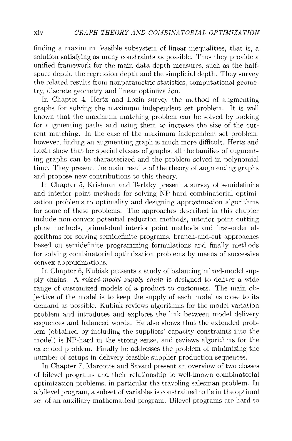
In Chapter 4, Hertz and Lozin survey the method of augmenting
graphs for solving the maximum independent set problem. It is well
known that the maximum matching problem can be solved by looking
for augmenting paths and using them to increase the size of the
current matching. In the case of the maximum independent set problem,
however, finding an augmenting graph is much more difficult. Hertz and
Lozin show that for special classes of graphs, all the families of
augmenting graphs can be characterized and the problem solved in polynomial
time. They present the main results of the theory of augmenting graphs
and propose new contributions to this theory.
In Chapter 5, Krishnan and Terlaky present a survey of semidefinite
and interior point methods for solving NP-hard combinatorial
optimization problems to optimality and designing approximation algorithms
for some of these problems. The approaches described in this chapter
include non-convex potential reduction methods, interior point cutting
plane methods, primal-dual interior point methods and first-order
algorithms for solving semidefinite programs, branch-and-cut approaches
based on semidefinite programming formulations and finally methods
for solving combinatorial optimization problems by means of successive
convex approximations.
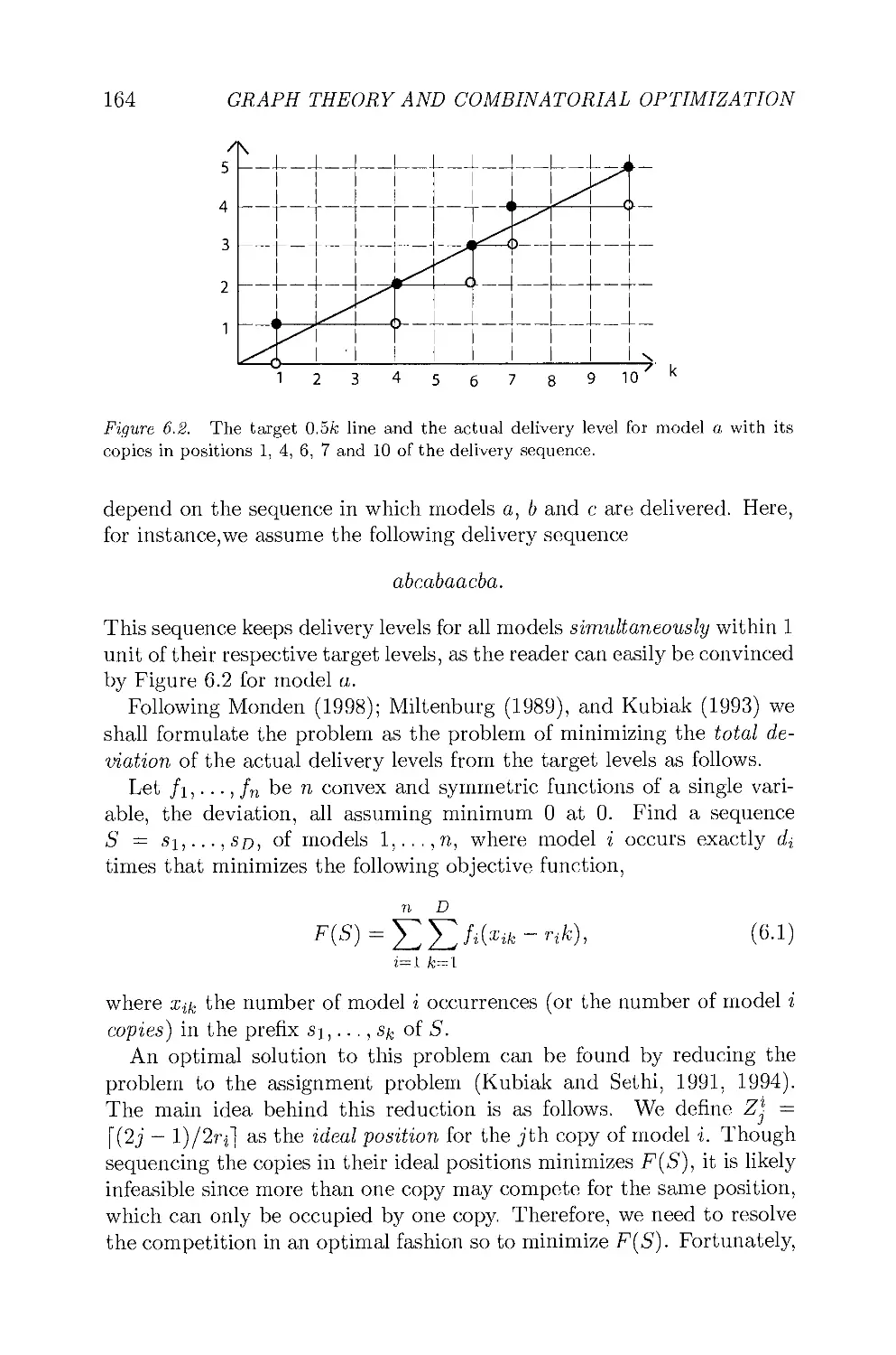
In Chapter 6, Kubiak presents a study of balancing mixed-model
supply chains. A mixed-model supply chain is designed to deliver a wide
range of customized models of a product to customers. The main
objective of the model is to keep the supply of each model as close to its
demand as possible. Kubiak reviews algorithms for the model variation
problem and introduces and explores the link between model delivery
sequences and balanced words. He also shows that the extended
problem (obtained by including the suppliers' capacity constraints into the
model) is NP-hard in the strong sense, and reviews algorithms for the
extended problem. Finally he addresses the problem of minimizing the
number of setups in delivery feasible supplier production sequences.
In Chapter 7, Marcotte and Savard present an overview of two classes
of bilevel programs and their relationship to well-known combinatorial
optimization problems, in particular the traveling salesman problem. In
a bilevel program, a subset of variables is constrained to lie in the optimal
set of an auxiliary mathematical program. Bilevel programs are hard to

PREFACE
xv
solve, because they are generically non-convex and non-differentiable.
Thus research on bilevel programs has followed two main avenues, the
continuous approach and the combinatorial approach. The
combinatorial approach aims to develop algorithms providing a guarantee of global
optimality. The authors consider two classes of programs amenable to
this approach, that is, the bilevel programs with linear or bilinear
objectives.
In Chapter 8, Shepherd and Vetta present a study of dijoins. Given
a directed graph G — (V,A), a dijoin is a set of arcs В such that the
graph (V, AU B) is strongly connected. Shepherd and Vetta give two
results that help to visualize dijoins. They give a simple description of
Frank's primal-dual algorithm for finding a minimum dijoin. Then they
consider weighted packings of dijoins, that is, multisets of dijoins such
that the number of dijoins containing a given arc is at most the weight
of the arc. Specifically; they study the cardinality of a weighted packing
of dijoins in graphs for which the minimum weight of a directed cut is
at least a constant, k, and relate this problem to the concept of skew
submodular flow polyhedron.
In Chapter 9, de Werra generalizes a coloring property of unimodular
hypergraphs. A hypergraph Η is unimodular is its edge-node incidence
matrix is totally unimodular. А к-coloring of Η is a partition of its
node set X into subsets Si, S2,. ■ ·, Sk such that no Si contains an edge
Ε with IΕ | > 2. The new version of the coloring property implies that
a unimodular hypergraph has an equitable /c-coloring satisfying
additional constraints. The author also gives an adaptation of this result to
balanced hypergraphs.
Acknowledgements The Editors are very grateful to the authors for
contributing to this volume and responding to their comments in a timely
fashion. They also wish to thank Nicole Paradis, Francine Benoit and
Andre Montpetit for their expert editing of this volume.
David Avis
Alain Hertz
Odile Marcotte

Chapter 1
VARIABLE NEIGHBORHOOD SEARCH
FOR EXTREMAL GRAPHS. XL BOUNDS
ON ALGEBRAIC CONNECTIVITY
Slim Belhaiza
Nair Maria Maia de Abreu
Pierre Hansen
Carla Silva Oliveira
Abstract The algebraic connectivity a(G) of a graph G = (V,E) is the second
smallest eigenvalue of its Laplacian matrix. Using the AutoGraphiX
(AGX) system, extremal graphs for algebraic connectivity of G in
function of its order η = \V\ and size m = \E\ are studied. Several
conjectures on the structure of those graphs, and implied bounds on the
algebraic connectivity, are obtained. Some of them are proved, e.g., if
СфКп
a(G) < [-1 4- y/ΐ 4- 2mJ
which is sharp for all m > 2.
1. Introduction
Computers are increasingly used in graph theory. Determining the
numerical value of graph invariants has been done extensively since the
fifties of last century. Many further tasks have since been explored.
Specialized programs helped, often through enumeration of specific families
of graphs or subgraphs, to prove important theorems. The prominent
example is, of course, the Four-color Theorem (Appel and Haken, 1977a,b,
1989; Robertson et al., 1997). General programs for graph
enumeration, susceptible to take into account a variety of constraints and exploit
symmetry, were also developped (see, e.g., McKay, 1990, 1998). An
interactive approach to graph generation, display, modification and study
through many parameters has been pioneered in the system Graph of
Cvetkovic and Kraus (1983), Cvetkovic et el. (1981), and Cvetkovic and

2
GRAPH THEORY AND COMBINATORIAL OPTIMIZATION
Simic (1994) which led to numerous research papers. Several systems
for obtaining conjectures in an automated or computer-assisted way have
been proposed (see, e.g., Hansen, 2002, for a recent survey). The Auto-
Graphix (AGX) system, developed at GERAD, Montreal since 1997 (see,
e.g., Caporossi and Hansen, 2000, 2004) is designed to address the
following tasks: (a) Find a graph satisfying given constraints; (b) Find optimal
or near-optimal values for a graph invariant subject to constraints; (c)
Refute conjectures (or repair them); (d) Suggest conjectures (or sharpen
existing ones); (e) Suggest lines of proof.
The basic idea is to address all those tasks through heuristic search of
one or a family of extremal graphs. This can be done in a unified way,
i.e., for any formula on one or several invariants and subject to
constraints, with the Variable Neighborhood Search (VNS) metaheuristic
of Mladenovic and Hansen (1997) and Hansen and Mladenovic (2001).
Given a formula, VNS first searches a local minimum on the family of
graphs with possibly some parameters fixed such as the number of
vertices η or the number of edges m. This is done by making elementary
changes in a greedy way (i.e., decreasing most the objective, in case of
minimization) on a given initial graph: rotation of an edge (changing
one of its endpoints), removal or addition of one edge, short-cut (i.e.,
replacing a 2-path by a single edge) detour (the reverse of the previous
operation), insertion or removal of a vertex and the like. Once a local
minimum is reached, the corresponding graph is perturbed increasingly,
by choosing at random another graph in a farther and farther
neighborhood. A descent is then performed from this perturbed graph. Three
cases may occur: (i) one gets back to the unperturbed local optimum, or
(ii) one gets to a new local optimum with an equal or worse value than
the unperturbed one, in which case one moves to the next
neighborhood, or (iii) one gets to a new local optimum with a better value than
the unperturbed one, in which case one recenters the search there. The
neighborhoods for perturbation are usually nested and obtained from the
unperturbed graph by addition, removal or moving of 1, 2,.. ., к edges.
Refuting conjectures given in inequality form, i.e., i\(G) < 12(G)
where i\ and г 2 are invariants, is done by minimizing the difference
between right and left hand sides; a graph with a negative value then refutes
the conjectures. Obtaining new conjectures is done from values of
invariants for a family of (presumably) extremal graphs depending on some
parameter(s) (usually η and/or m). Three ways are used (Caporossi
and Hansen, 2004): (i) a numerical way, which exploits the
mathematics of Principal Component Analysis to find a basis of affme relations
between graph invariants satisfied by those extremal graphs considered;
(ii) a geometric way, i.e., finding with a "gift-wrapping" algorithm the

1 VNS for Extremal Graphs. XL Bounds on Algebraic Connectivity 3
convex hull of the set of points corresponding to the extremal graph in
invariants space: each facet then gives a linear inequality; (iii) an
algebraic way, which consists in determining the class to which all extremal
graphs belong, if there is one (often it is a simple one such as paths, stars,
complete graphs, etc); then formulae giving the value of individual
invariants in function of η and/or m are combined. Obtaining possible
lines of proof is done by checking if one or just a few of the elementary
changes always suffice to get the extremal graphs found; if so, one can
try to show that it is possible to apply such changes to any graph of the
class under study.
Recall that the Laplacian matrix L(G) of a graph G = (V, E) is the
difference of a diagonal matrix with values equal to the degrees of vertices
of G, and the adjacency matrix of G. The algebraic connectivity of G is
the second smallest eigenvalue of the Laplacian matrix (Fiedler, 1973).
In this paper, we apply AGX to get structural conjectures for graphs
with minimum and maximum algebraic connectivity given their order
η = \V\ and size m = \E\, as well as implied bounds on the algebraic
connectivity.
The paper is organized as follows. Definitions, notation and basic
results on algebraic connectivity are recalled in the next section. Graphs
with minimum algebraic connectivity are studied in Section 3; it is
conjectured that they are path-complete graphs (Harary, 1962; Soltes, 1991);
a lower bound on a(G) is proved for one family of such graphs. Graphs
with maximum algebraic connectivity are studied in Section 4. Extremal
graphs are shown to be complements of disjoint triangles, paths P3, edges
K4 and isolated vertices K\. A best possible upper bound on a(G) in
function of m is then found and proved.
2. Definitions and basic results concerning
algebraic connectivity
Consider again a graph G = (V(G),E(G)) such that V(G) is the
set of vertices with cardinality η and E(G) is the set of edges with
cardinality m. Each e G E{G) is represented by ец = {v{,Vj} and
in this case, we say that Vi is adjacent to Vj. The adjacency matrix
A — [dij] is an η χ η matrix such that ац = 1, when щ and Vj are
adjacent and a^ = 0, otherwise. The degree of v^, denoted d(vi), is the
number of edges incident with -щ. The maximum degree of G, A(G),
is the largest vertex degrees of G- The minimum degree of G, o(G), is
defined analogously. The vertex (or edge) connectivity of G, k(G) (or
n'(G)) is the minimum number of vertices (or edges) whose removal from
G results in a disconnected graph or a trivial one. A path from ν to w

4
GRAPH THEORY AND COMBINATORIAL OPTIMIZATION
in G is a sequence of distinct vertices starting with ν and ending with
w such that consecutive vertices are adjacent. Its length is equal to its
number of edges. A graph is connected if for every pair of vertices, there
is a path linking them. The distance cIg{v,w) between two vertices ν
and w in a connected graph is the length of the shortest path from ν to
w. The diameter of a graph G, do, is the maximum distance between
two distinct vertices. A path in G from a node to itself is referred to as
a cycle. A connected acyclic graph is called a tree. A complete graph,
Kn, is a graph with η vertices such that for every pair of vertices there
is an edge. A clique of G is an induced subgraph of G which is complete.
The size of the largest clique, denoted w(G), is called clique number. An
empty graph, or a trivial one, has an empty edge set. A set of pairwise
non adjacent vertices is called an independent set. The size of the largest
independent set, denoted a(G), is the independence number. For further
definitions see Godsil and Royle (2001).
As mentionned above, the Laplacian of a graph G is defined as the
η χ η matrix
L(G) = A-A, (1.1)
when A is the adjacency matrix of G and Δ is the diagonal matrix whose
elements are the vertex degrees of G, called the degree matrix of G. L(G)
can be associated with a positive semidefinite quadratic form, as we can
see in the following proposition:
PROPOSITION 1.1 (Merris, 1994) Let G be a graph. If the quadratic
form related to L{G) is
q(x) = xL{G)x\ x G Kn,
then q is positive semidefinite.
The polynomial pL{G)(X) = det(A/ - L(G)) = Xn + giAn_i + · · ■ +
qn_iA + qn is called the characteristic polynomial of L(G). Its spectrum
is
C(G) = (Ab...,An_i,An), (1.2)
where Vz, 1 < i < n, Xi is an eigenvalue of L(G) and Ai > ... > Xn.
According to Proposition 1.1, Vz, 1 < i < n, Xi is a non-negative real
number. Fiedler (1973) defined Xn-i as the algebraic connectivity of G,
denoted a(G).
We next recall some inequalities related to algebraic connectivity of
graphs. These properties can be found in the surveys of Fiedler (1973)
and Merris (1994).

1 VNS for Extremal Graphs. XL Bounds on Algebraic Connectivity 5
Proposition 1.2 Let G\ and G2 be spanning graphs of G such that
E(GX) П E(G2) = Φ- Then a{G{) + a(G2) < a(Gk U G2).
PROPOSITION 1.3 Let G be a gra,ph and, G\ a subgraph obtained from, G
by removing к vertices and all adjacent edges in G. Then
a(Gi) >a(G)-k.
Proposition 1.4 Let G be a graph. Then,
0) a.(G)<[n/(n-l)}S(G)<2\E\/(n-l);
(2) a(G) > 25(G) -n + 2.
Proposition 1.5 Let G be a graph with η vertices and G φ Κη.
Suppose that G contains an independent set with ρ vertices. Then,
a(G) < η — p.
PROPOSITION 1.6 Let G be a graph with η vertices. If G φ Κη then
a(G) <n-2.
Proposition 1.7 Let G be a graph with η vertices and m edges. If
G φ Κη then
/о™ \ (n-l)/n
\n — 1
Proposition 1.8 If G φ Kn then a(G) < S(G) < k(G). For G = Kn,
we have a(Kn) = η and δ(Κη) = κ(Κη) = η — 1.
Proposition 1.9 If G is a connected graph with η vertices and diameter
dG, then a(G) > 4/ndG and dG < y/2A(G)/a(G) log2(n2).
Proposition 1.10 Let Τ be a tree with η vertices and diameter άψ-
Then,
π
a(T) < 2
1 — cos
dT + l
A partial graph of G is a graph G\ such that V(G\) = V(G) and
E{G{) С E(G).
Proposition 1.11 If Gi is a partial graph of G then a(G\) < a(G).
Moreover
Proposition 1.12 Consider a path Pn and a graph G with η vertices.
Then, a(Pn) <a(G).

6
GRAPH THEORY AND COMBINATORIAL OPTIMIZATION
Consider graphs Gx = {V(Gi),E{G{)) and G2 = (V(G2),E(G2)).
The Cartesian product of G\ and G2 is a graph G\ x G2 such that
^(Gi x G2) = V(G{) x y(G2) and ((ubu2), (υΐ)υ2)) e E(GX χ G2) if
and only if either u\ = щ and (u2,v2) e E(G2) or (ui,v\) e E(G\) and
n2 = v2.
Proposition 1.13 Let Gi and G2 be graphs. Then,
a(Gi xG2)=min{a(G1),a(G2)}.
3. Minimizing a(G)
When minimizing a(G) we found systematically graphs belonging to a
little-known family, called path-complete graphs by Soltes (1991). They
were previously considered by Harary (1962) who proved that they are
(non-unique) connected graphs with η vertices, m edges and maximum
diameter. Soltes (1991) proved that they are the unique connected
graphs with η vertices, m edges and maximum average distance between
pairs of vertices. Path-complete graphs are defined as follows: they
consist of a complete graph, an isolated vertex or a path and one or several
edges joining one end vertex of the path (or the isolated vertex) to one
or several vertices of the clique, see Figure 1.1 for an illustration. We
will need a more precise definition:
For η and t € N when 1 < t < η — 2, we consider a new family of
connected graphs with η vertices and mt{r) edges as follows:
G(n, mt(r)) = {G | for t < r < η — 2, G has nit(r) edges,
mt{r) = (n- t)(n - t - l)/2 + r}.
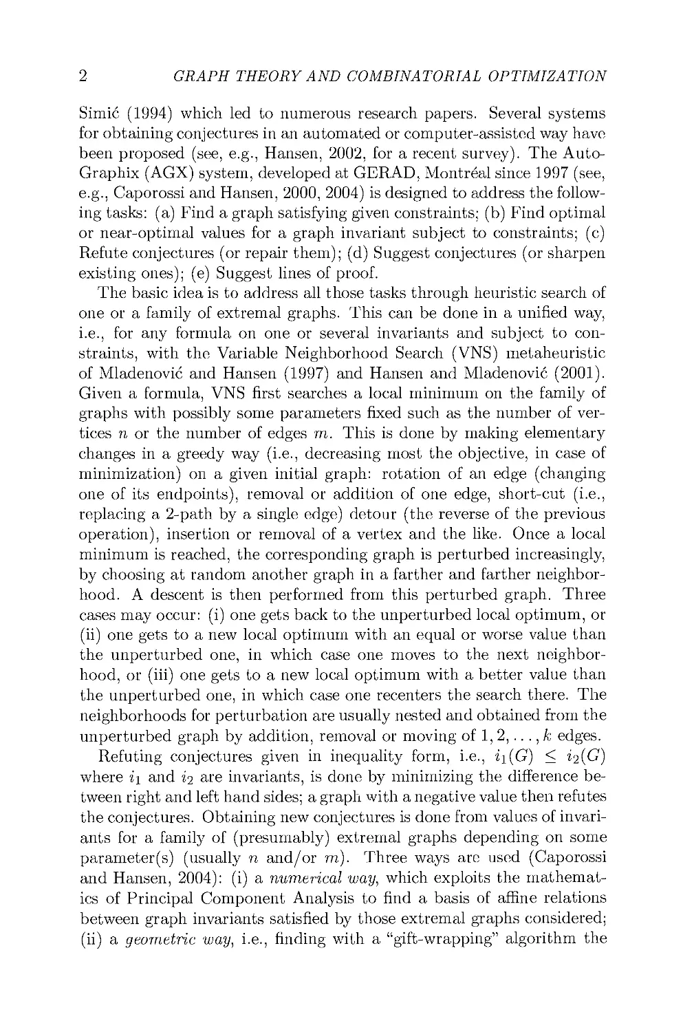
Definition 1.1 Let n,m,t,p e N, with 1 < t < η - 2 and 1 < ρ <
η — ■ t — 1. A graph with η vertices and rn edges such that
(n-t)(n-t-l) (n-t)(n-t-l)
+ t < m < '- + n-2
2 - - 2
is called (n,p,t) path-complete graph, denoted PCniP)t, if and only if
(1) the maximal clique of PCniPit is Kn^t]
(2) PCniPit has a t-path Pt+\ = [^ο,^ι, v2,.. ., vt] such that vq e Kn-t Π
Pt+i and v\ is joined to Kn~t by ρ edges;
(3) there are no other edges.
Figure 1.1 displays a (n,p,t) path-complete graph.
It is easy to see that all connected graphs with η vertices can be
partitioned into the disjoint union of the following subfamilies:
G(n, mi) Θ G(n, m2) θ · · · θ G(n, mn_2).
Besides, for every (η,ρ.ί), PCniP)t e G(n,mt).

1 VNS for Extremal Graphs. XL Bounds on Algebraic Connectivity 7
ρ edges
v2 vll
Figure 1.1. A (n,p,t) path-complete graph
(m = 37; a(G) = 1) (m = 30; a(G) = 0.435) (m = 24; a(G) = 0.256)
Figure 1,2. Path-complete graphs
3.1 Obtaining conjectures
Using AGX, connected graphs G φ Κη with (presumably) minimum
algebraic connectivity were determined for 3 < η < 11 and η — 1 < m <
n(n — l)/2 — 1. As all graphs turned out to belong to the same family,
a structural conjecture was readily obtained.
CONJECTURE 1.1 TTie connected graphs G φ Κη with minimum
algebraic connectivity are all path-complete graphs.
A few examples are given in Figure 1.2, for η = 10.
Numerical values of a(G) for all extremal graphs found are given in
Table 1.1, for n = 10andra-l<m< n(n - l)/2 - 1.
For each n, a piecewise concave function of m is obtained. From this
table and the corresponding Figure 1.3 we obtain:

8 GRAPH THEORY AND COMBINATORIAL OPTIMIZATION
Table 1.1. η = 10; mina(G) on m
m
a(G)
m
a(G)
m
a(G)
m
a(G)
9
0.097
18
0.175
27
0.406
36
0.981
10
0.103
19
0.177
28
0.419
37
1
11
0.109
20
0.208
29
0.428
38
2
12
0.115
21
0.238
30
0.435
39
3
13
0.123
22
0.247
31
0.673
40
4
14
0.134
23
0.252
32
0.801
41
5
15
0.137
24
0.256
33
0.876
42
6
16
0.151
25
0.345
34
0.924
43
7
17
0.170
26
0.384
35
0.957
44
8
Figure 1.3. mina(G); a(G) on m
Conjecture 1.2 For each η > 3, the minimum algebraic connectivity
of a graph G with η vertices and m edges is an increasing, piecewise
concave function of m. Moreover, each concave piece corresponds to a
family PCn^t of path-complete graphs. Finally, for t = 1, a(G) = S(G),
and fort > 2, a{G) < 1.
3.2 Proofs
We do not have a proof of Conjecture 1.1, nor a complete proof of
Conjecture 1.2. However, we can prove some of the results of the latter.

1 VNS for Extremal Graphs. XL Bounds on Algebraic Connectivity 9
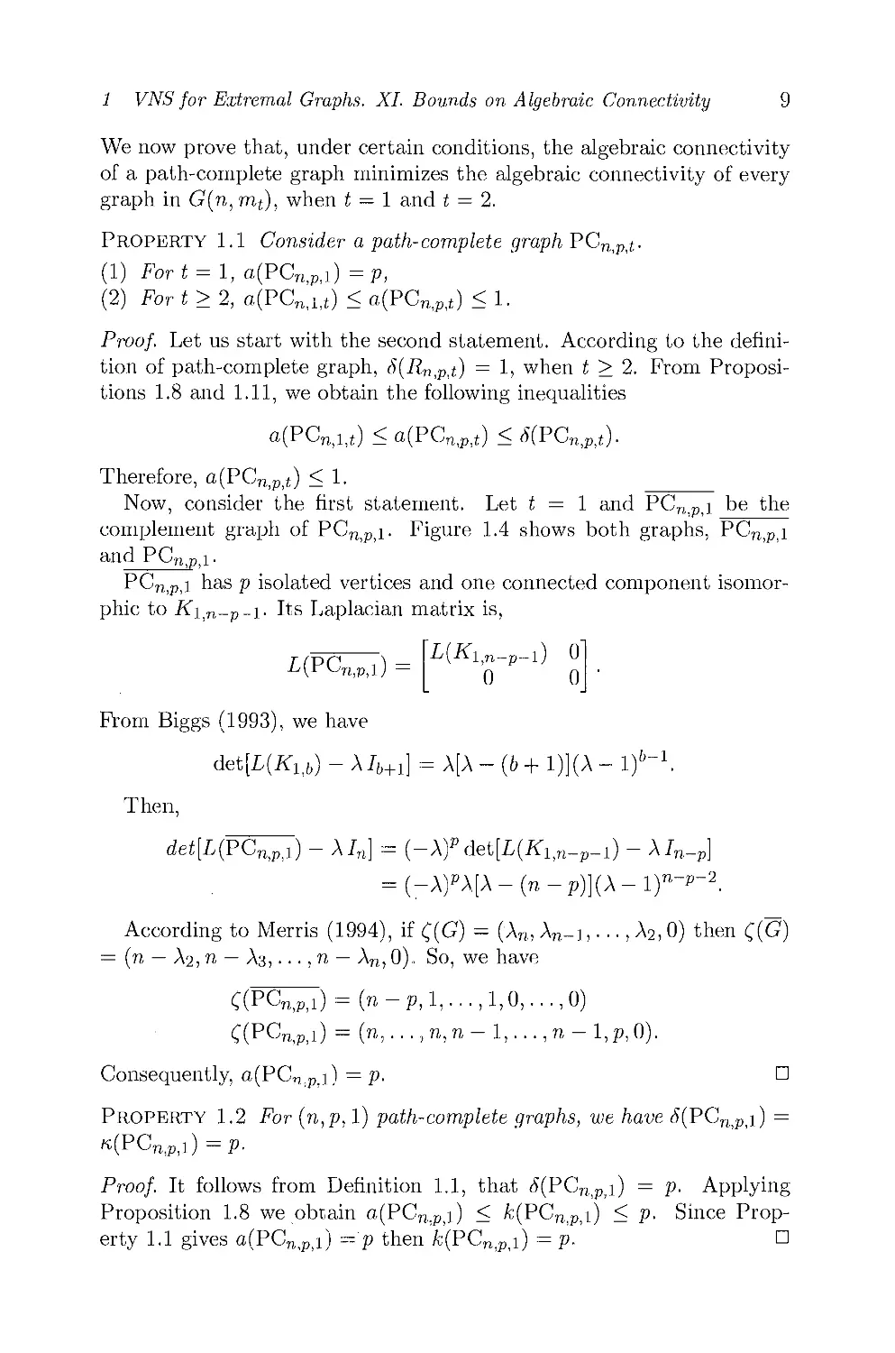
We now prove that, under certain conditions, the algebraic connectivity
of a path-complete graph minimizes the algebraic connectivity of every
graph in G(n, nit), when t — 1 and t = 2.
Property 1.1 Consider a path-complete graph РСПф^.
(1) Fori = l, а(РСп,р,1)=р,
(2) For t > 2, a(PCn,i,t) < a(PCn,p,t) < 1.
Proof. Let us start with the second statement. According to the
definition of path-complete graph, S(RntPit) = 1> when t > 2. From
Propositions 1.8 and 1.11, we obtain the following inequalities
a(PCn,i,t) < a(PCnj>,t) < <5(PC„,p>t).
Therefore, a(PCn,P)t) < 1.
Now, consider the first statement. Let ί = 1 and РСП)Рд be the
complement graph of РСП)Рд. Figure 1.4 shows both graphs, РСП)Рд
and PCTt|P)1.
РСП)Рд has ρ isolated vertices and one connected component
isomorphic to Kitn-p-i. Its Laplacian matrix is,
T(vr л - \L(Ki,n-P-i) 0
-b^W.P.lJ — Q Q ·
From Biggs (1993), we have
det[L(K1<b) - A/6+i] = A[A - (b + 1)](A - l)6"1.
Then,
dei[L(PC^T) - A/n] = (-A)pdet[L(K1)n_p_!) - λ/η_ρ]
= (-Χ)ρλ[λ-(η-ρ)}(λ-1)η~Ρ~2.
According to Merris (1994), if £(G) = (λ„, λη-ι, ■ ■ ■, A2, 0) then C(G)
= (n — X2, η — Аз,..., η — Χη, 0). So, we have
C(PC^P7) = (n-p,l,...,l,0,...,0)
C(pcn>P,i) = (n,...,n,n- Ι,...,η - Ι,ρ,Ο).
Consequently, a(PCniP.i) = p. □
Property 1.2 For (n,p, 1) path-complete graphs, we have £(PCniPii) =
«(PCn,p,i) = P-
Proof. It follows from Definition 1.1, that S(PCn#ti) = p. Applying
Proposition 1.8 we obtain а(РСп.рд) < /с(РСп^д) < р. Since
Property 1.1 gives a(PCHiP>i) ='p then /с(РСП)Рд) = р. □

10
GRAPH THEORY AND COMBINATORIAL OPTIMIZATION
n.p
■n,p
Figure Ц. PCn,p,i and its complement PCn,p,i
\ v2
Ί,η-Ι
Figure 1.5. Graphs Kit„-i and Gi
Proposition 1.14 Among all G G G(n,mi) with maximum degree n —
I, a{G) is minimized by РСпдд.
Proof. Let G be a graph with η vertices. Consider spanning graphs
of G К\>п-\ and G\ such that Ε(Κ\,η-ι) Π E(G\) = φ and G\ has two
connected components, one of them with n — \ vertices. Figure 1.5 shows
these graphs.
We may consider G = (V,E) where V{G) = V(Ki<n-i) = V{GX)
and E(G) = Ε(Κίιη-ι) U E(Gi). Then, A(G) = η - 1. According
to Proposition 1.2, we have α{Κ\^η-\) + a(G\) < a(G). From Biggs
(1993), а(К\)П-\) = 1. Since G\ is a disconnected graph then a{G\) = 0.
However, a(PCni i) = 1, therefore a(G) > 1. □

1 VNS for Extremal Graphs. XL Bounds on Algebraic Connectivity 11
Proposition 1.15 For every G G G(n, mi) such that 5(G) > (n - 2)/2
+ p/2, where 1 < ρ < η — 2, we have
a(G) > а(РСп,рЛ) = p.
Proof. Consider G G G(n, mi) with S(G) > (n - 2)/2 + p/2. According
to Proposition 1.4, we have
a(G) > 25(G) -n+2>2
V
η + 2 = p.
2 2_
Consequently, a(G) > а(РСП)Рд) = р. □
Proposition 1.16 For every G G G(n, 7П2) such that 5(G) > (n-l)/2,
we have
a(G) > 1 > a(PCn>P)2).
Proof. Consider G G G(n,rri2) with 5(G) > (n — l)/2. According to
Proposition 1.4, we have
a(G) > 2S{G) - η + 2 > 2
1
n + 2= 1.
2
From Property 1,1, а(РСП)Р)2) < 1. Then, a(G) > 1 > a(PCn>P)2). □
To close this section we recall a well-known result.
Proposition 1.17 Let Τ be a tree with η vertices. For every T, a(T)
is minimized by the algebraic connectivity of a single path Pn, where
a(Pn) = 2[1 — cos(7r/n)]. Moreover, for every graph G with η vertices
a(Pn)<a(G).
4. Maximizing a(G)
4.1 Obtaining conjectures
Using AGX, connected graphs G φ Κη with (presumably)
maximum algebraic connectivity a(G) were determined for 3 < η < 10 and
(n — l)(n — 2)/2 < m < n(n — l)/2 — 1. We then focused on those
among them with maximum a(G) for a given m. These graphs having
many edges, it is easier to understand their structure by considering
their complement G. It appears that these G are composed of disjoint
triangles K3, paths P3, edges K4 and isolated vertices Κι.
A representative subset of these graphs G is given in Figure 1.6.

12 GRAPH THEORY AND COMBINATORIAL OPTIMIZATION
0000
G(n=10;m = 44) G(n = 10; m = 43) G(n = 10; m = 42) G(n = 10; m = 39)
Figure 1.6.
Figure 1.7. max a(G) ; a(G) on m
Conjecture 1.3 For allm > 2 ί/iere zs α graph G φ Κη with maximum
algebraic connectivity a(G) the complement G of which is the disjoint
union of triangles Kj,, paths P3, edges K2 and isolated vertices K\.
Values of a(G] for all extremal graphs obtained by AGX are
represented in function of m in Figure 1.7.
It appears that the maximum a(G) follow an increasing "staircase"
with larger and larger steps. Values of a(G), m and η for the graphs of
this staircase (or upper envelope) are listed in Table 1.2.
An examination of Table 1,2 leads to the next conjecture,

1 VNS for Extremal Graphs, XL Bounds on Algebraic Connectivity
13
Table 1.2. Value of a(G), m and η for graphs, with maximum a(G) for m given,
found by AGX
a(G)
m
η
a(G)
m
η
.
5
23
8
1
2
3
6
24
8
1
3
4
6
25
8
2
4
4
6
26
8
2
5
4
6
27
8
2
6
5
6
28
8
2
7
5
6
29
8
3
8
5
6
30
9
3
9
5
6
31
9
3
10
6
7
32
9
3
11
6
7
33
9
4
12
6
7
34
9
4
13
6
7
35
9
4
14
6
7
36
9
4
15
7
7
37
9
4
16
7
7
38
10
4
17
7
7
39
10
5
18
7
8
40
10
5
19
7
8
41
10
5
20
7
8
42
10
5
21
7
8
43
10
5
22
7
8
44
10
Conjecture 1.4 For all η > 4 ί/ier-e are η — 1 consecutive values of
m (beginning at 3) for which a graph G φ Κη with maximum algebraic
connectivity a(G) has η vertices. Moreover, for the first [(n — l)/2j of
them a(G) = η — 2 and for the last \(n — l)/2] of them a(G) = η — 3,
Considering the successive values of a{G) for increasing m, it appears
that for a(G) — 2 onwards their multiplicities are 4, 4, 6, 6, 8, 8,.. .
After a little fitting, this leads to the following observation:
'a(G)(a{G) + 2)
2
< m
and to our final conjecture:
Conjecture 1,5 If G is a connected graph such that G φ Κη then
a{G) < [-1 + Vl + 2mJ
and this bound is sharp for all m > 2.
One can easily see that this conjecture improves the bound already
given in Proposition 1.7, i.e., a(G) < (2m/{n — 1)) .
4.2
Proofs
We first prove Conjectures 1.3 and 1.4. Then, we present a proof for
the last conjecture. The extremal graphs found point the way.
Proof of Conjectures 1.3 and 1.4- From Propositions 1.6 and 1.8 if G φ
Kn, a(G) < S(G) < n — 2. For this last bound to hold as an equality one
must have S(G) ~ η — 2, which implies G must contain all edges except
up to [n/2\ of them, i.e., n(n - l)/2 - [n/2j_< m < n(n - l)/2 - 1.
Moreover, the missing edges of G (or edges of G) must form a matching,
Assume there are 1 < r < j_n/2j missing edges and that they form a

14
GRAPH THEORY AND COMBINATORIAL OPTIMIZATION
matching. Then from Merris (1994) det[L(G)-XIn] = -Xn~2rXr{X-2)r.
Hence
C(G) = (21_JL2,0,...,0), ζ(0) = (η,...,η,η-2, ...,η-2,0)
r times η—г —1 times r times
and a(G) = η — 2. If there are r > [n/2\ missing edges in G, a(G) <
S(G) < η — 3. Several cases must be considered to show that this bound
is sharp, in all of which r < η , as otherwise S(G) < η — 3. Moreover,
one may assume r < η — 1 or otherwise there is a smaller η such that
all edges can be used and with S(G) as large or larger:
(i) r mod 3 = 0. Then there is a i 6 N such that r = St. Assume
the missing edges of G form disjoint triangles in G. Then (Biggs,
1993)
det[L(K3)-A/3] = A(A-3)2
and
Hence
n—r \t( \ o\2t
det[L(G) - A In] = (~X)n~rX\X - 3)
C(G) = (31:;;;3,0)...,0),
2i times
C(G) — (n,..., η, η — 3,..., η — 3,0)
η— 2t— I times It times
and a(G) — η — 3.
(ii) r mod 3 = 1. Then there is a i £ N such that r = 3t + 1. Assume
the missing edges of G form t disjoint triangles and a disjoint edge.
Then, as above,
det[L(G) - A In] = (-A)n-r~1A(r+2^3(A - 2)(λ - 3)(2r~2)/3,
and a{G) = η — 3.
(iii) r mod 3 = 2. Then there is a t € N such that r = 3i + 2. Assume
the missing edges of G form ί disjoint triangles and a disjoint path
Рз with 2 edges. From the characteristic polynominal of L{P^) and
similar arguments as above one gets a(G) = η — 3. □
Proof of Conjecture 1.5. Let S* 7^ Kn a graph with all edges except up
to [n/2\ of them. So, n(n - l)/2 - Ln/2J < m < n(n - l)/2 - 1.
(i) If η is odd then,
n(n — 1) η — I n(n — 1)
-Ц-—^ < m < -Ц;—^ - 1.

1 VNS for Extremal Graphs. XL Bounds on Algebraic Connectivity 15
Since n2 - 2n + 1/2 > n(n - 2)/2, m > n(n - 2)/2.
(ii) If η is even, then
n(n — 1) η n(n — 1)
— < m < 1.
2 2 - ~ 2
So, 2m > n(n — 2) and η — 2 < [—1 + \/l + 2m . From
Proposition 1.6, a(G) < η - 2. Then, a(G) < [-1 + y/\ + 2mJ.
Now, consider (n - l)(n - 2)/2 < m < ra(ra-l)/2-(|_ra/2j +1). This
way, m = n(n - l)/2 - r, with [«/2j + l<r<n-l. So, r < |(n - 1).
We can add n2 to each side of the inequality above. After some algebraic
manipulations, we get (n — 2)2 < 2m + 1. So, η — 3 < —1 + \j2m + 1.
From the proof of Conjecture 1.4, we have a(S) < η — 3. Then,
a(S) < [-1 + y/\ + 2mJ. As we can consider every G 7^ Kn with η
vertices as a partial (spanning) graph of S*, from Proposition 1.11, we
then have a(G) < a(S) < [-1 + \Л + 2mJ. Π
References
Appel, K. and Haken, W. (1977a). Every planar map is four colorable.
I. Discharging. Illinois Journal of Mathematics, 21:429-490.
Appel, K. and Haken, W. (1977b). Every planar map is four colorable.
II. Reducibility. Illinois Journal of Mathematics, 21:491-567.
Appel, K. and Haken, W. (1989). Every Planar Map Is Four Colorable.
Contemporary Mathematics, vol. 98. American Mathematical Society,
Providence, RI.
Biggs, N. (1993). Algebraic Graph Theory, 2 ed. Cambridge University
Press.
Caporossi, G. and Hansen, P. (2000). Variable neighborhood search for
extremal graphs. I. The AutoGraphiX system. Discrete Mathematics,
212:29-44.
Caporossi, G. and Hansen, P. (2004). Variable neighborhood search for
extremal graphs. V. Three ways to automate finding conjectures.
Discrete Mathematics, 276:81-94.
Cvetkovic, D., Kraus, L., and Simic, S. (1981). Discussing Graph Theory
with a Computer. I. Implementation of Graph Theoretic Algorithms.
Univ. Beograd Publ. Elektrotehn. Fak, pp. 100-104.
Cvetkovic, D. and Kraus, L. (1983). "Graph" an Expert System for the
Classification and Extension of Knowledge in the Field of Graph
Theory, User's Manual. Elektrothen. Fak., Beograd.
Cvetkovic, D. and Simic, S. (1994). Graph-theoretical results obtained
by the support of the expert system "graph." Bulletin de I'Academie
Serbe des Sciences et des Arts, 19:19-41.

16 GRAPH THEORY AND COMBINATORIAL OPTIMIZATION
Diestel, R. (1997). Graph Theory, Springer.
Fiedler, M. (1973). Algebraic connectivity of graphs. Czechoslovak
Mathematical Journal, 23:298-305.
Godsil, C. and Royle, G. (2001). Algebraic Graph Theory, Springer.
Hansen, P. (2002). Computers in graph theory. Graph Theory Notes of
New York, 43:20-34.
Hansen, P. and Mladenovic, N. (2001). Variable neighborhood search:
Principles and applications. European Journal of Operational
Research, 130(3) :449-467.
Harary, F. (1962). The maximum connectivity of a graph. Proceedings
of the National Academy of Sciences of the United States of America,
48:1142-1146.
McKay, B.D. (1990). Nauty User's Guide (Version 1.5). Technical
Report, TR-CS-90-02, Department of Computer Science, Australian
National University.
McKay, B.D. (1998). Isomorph-free exhaustive generation. Journal of
Algorithms, 26:306-324.
Merris, R. (1994). Laplacian matrices of graphs: A survey. Linear
Algebra and its Applications, 197/198:143-176.
Mladenovic, N. and Hansen, P. (1997). Variable neighborhood search.
Computers and Operations Research, 24(11):1097- 1100.
Robertson, N., Sanders, D., Seymour, P., and Thomas, R. (1997).
The four-colour theorem. Journal of Combinatorial Theory, Series B,
70(l):2-44.
Soltes, L. (1991). Transmission in graphs: A bound and vertex removing.
Mathematica Slovaca, 41(1): 11 -16.

Chapter 2
PROBLEMS AND RESULTS ON
GEOMETRIC PATTERNS
Peter Brass
Janos Pach
Abstract Many interesting problems in combinatorial and computational
geometry can be reformulated as questions about occurrences of certain
patterns in finite point sets. We illustrate this framework by a few typical
results and list a number of unsolved problems.
1. Introduction: Models and problems
We discuss some extremal problems on repeated geometric patterns in
finite point sets in Euclidean space. Throughout this paper, a geometric
pattern is an equivalence class of point sets in d-dimensional space under
some fixed geometrically defined equivalence relation. Given such an
equivalence relation and the corresponding concept of patterns, one can
ask several natural questions:
(1) What is the maximum number of occurrences of a given pattern
among all subsets of an η-point set?
(2) How does the answer to the previous question depend on the
particular pattern?
(3) What is the minimum number of distinct k-element patterns
determined by a set of η points ?
These questions make sense for many specific choices of the underlying
set and the equivalence relation. Hence it is not surprising that
several basic problems of combinatorial geometry can be studied in this
framework (Pach and Agarwal, 1995).
In the simplest and historically first examples, due to Erdos (1946),
the underlying set consists of point pairs in the plane and the defining
equivalence relation is the isometry (congruence). That is, two point
pairs, {p\,P2} and {<7ь<?2}, determine the same pattern if and only if

18
GRAPH THEORY AND COMBINATORIAL OPTIMIZATION
\Pi — P2I = \qi ~ <Ы· In this case, (1) becomes the well-known Unit
Distance Problem: What is the maximum number of unit distance pairs
determined by η points in the plane? It follows by scaling that the
answer does not depend on the particular distance (pattern), For most
other equivalence relations, this is not the case: different patterns may
have different maximal multiplicities, For к = 2, question (3) becomes
the Problem of Distinct Distances: What is the minimum number of
distinct distances that must occur among η points in the plane? In spite
of many efforts, we have no satisfactory answers to these questions, The
best known results are the following,
Theorem 2,1 (Spencer et al,, 1984) Letf(n) denote the maximum
number of times the same distance can be repeated among η points in
the plane. We have
nen(logn/loglogn) < дп) < 0(η4/3)_
THEOREM 2,2 (ΚΑτζ and Tardos, 2004) Let g(n) denote the
minimum number of distinct distances determined by η points in the plane,
We have
Щп0-8Ш)<д(п)<о(-^=].
In Theorems 2,1 and 2,2, the lower and upper bounds, respectively, are
conjectured to be asymptotically sharp. See more about these questions
in Section 3,
Erdos and Purdy (1971, 1977) initiated the investigation of the
analogous problems with the difference that, instead of pairs, we consider
triples of points, and call two of them equivalent if the corresponding
triangles have the same angle, or area, or perimeter, This leads to
questions about the maximum number of equal angles, or unit-area resp,
unit-perimeter triangles, that can occur among η points in the plane,
and to questions about the minimum number of distinct angles,
triangle areas, and triangle perimeters, respectively, Erdos's Unit Distance
Problem and his Problem of Distinct Distances has motivated a great
deal of research in extremal graph theory. The questions of Erdos and
Purdy mentioned above and, in general, problems (1), (2), and (3) for
larger than two-element patterns, require the extension of graph
theoretic methods to hypergraphs, This appears to be one of the most
important trends in modern combinatorics,
Geometrically, it is most natural to define two sets to be equivalent
if they are congruent or similar to, or translates, homothets or affme
images of each other, This justifies the choice of the word "pattern"
for the resulting equivalence classes, Indeed, the algorithmic aspects

2 Problems and Results on Geometric Patterns
19
Figure 2.1. Seven coloring of the plane showing that χ(Κ2) < 7
of these problems have also been studied in the context of geometric
pattern matching (Akutsu et al., 1998; Brass, 2000; Agarwal and Sharir,
2002; Brass, 2002). A typical algorithmic question is the following.
(4) Design an efficient algorithm for finding all occurrences of a given
pattern in a set of η points.
It is interesting to compare the equivalence classes that correspond to
the same relation applied to patterns of different sizes. If A and A' are
equivalent under congruence (or under some other group of
transformations mentioned above), and α is a point in A, then there exists a point
a' G A' such that A \ {a} is equivalent to A' \{a'}. On the other hand,
if A is equivalent (congruent) to A' and A is large enough, then usually
its possible extensions are also determined: for each a, there exist only
a small number of distinct elements a1 such that A U {a} is equivalent to
A' U {a'}. Therefore, in order to bound the number of occurrences of a
large pattern, it is usually sufficient to study small pattern fragments.
We have mentioned above that one can rephrase many extremal
problems in combinatorial geometry as questions of type (1) (so-called Turan-
type questions). Similarly, many Ramsey-type geometric coloring
problems can also be formulated in this general setting.
(5) Is it possible to color space with к colors such that there is no
monochromatic occurrence of a given pattern?
For point pairs in the plane under congruence, we obtain the famous Had-
wiger- Nelson problem (Hadwiger, 1961): What is the smallest number
of colors χ(Κ2) needed to color all points of the plane so that no two
points at unit distance from each other get the same color?
Theorem 2.3 4 < χ(Μ2) < 7.

20 GRAPH THEORY AND COMBINATORIAL OPTIMIZATION
Another instance of question (5) is the following open problem from
Erdos et al. (1973): Is it possible to color all points of the
three-dimensional Euclidean space with three colors so that no color class contains
two vertices at distance one and the midpoint of the segment determined
by them? It is known that four colors suffice, but there exists no such
coloring with two colors. In fact, Erdos et al. (1973) proved that for
every d, the Euclidean d-space can be colored with four colors without
creating a monochromatic triple of this kind.
2. A simple sample problem: Equivalence under
translation
We illustrate our framework by analyzing the situation in the case
in which two point sets are considered equivalent if and only if they
are translates of each other. In this special case, we know the (almost)
complete solution to problems (l)-(5) listed in the Introduction.
Theorem 2.4 Any set В of η points in d-dimensional space has at most
η + 1 — к subsets that are translates of a fixed set A of к points. This
bound is attained if and only if A — {p,p + v,... ,p + (k — l)t>} and
В = {q,q + v,... ,q + (n — l)v} for some p,q,v € M.d.
The proof is simple. Notice first that no linear mapping φ that keeps
all points of В distinct decreases the maximum number of translates: if
A + t С В, then φ(Α) + (p(t) С ψ{Β). Thus, we can use any
projection into R, and the question reduces to the following one-dimensional
problem: Given real numbers a\ < ■ ■ ■ < a^, b\ < ..., bn, what is the
maximum number of values t such that t + {αϊ,..., a^} С {bi,... bn}.
Clearly, a\ + t must be one of fci,..., 6η_^+ι, so there are at most
η + 1 — к translates. If there are η + 1 — к translates t + {αχ,..., a^}
that occur in {b\,.. .bn}, for translation vectors t\ < ■■■ < in_fc+i,
then ti = bi — a\ = bj+i — a.2 — bi+j — fli+j, for i = 1,..., η — к + 1 and
j = 0,... ,/c-l. But then α2-αχ = bi+1-bj = aj+i~aj = bi+j-bi+j-i,
so all differences between consecutive aj and bi are the same. For higher-
dimensional sets, this holds for every one-dimensional projection, which
guarantees the claimed structure. In other words, the maximum is
attained only for sets of a very special type, which answers question (1).
An asymptotically tight answer to (2), describing the dependence on
the particular pattern, was obtained in Brass (2002).
THEOREM 2.5 Let A be a set of points in d-dimensional space, such
that the rational affine space spanned by A has dimension k. Then the
maximum number of translates of A that can occur among η points in
d-dimensional space is η — 9(mfc-1)/'c).

2 Problems and Results on Geometric Patterns
21
Any set of the form {p,p + v,... ,p + (k — l)v} spans a one-dimensional
rational affine space. An example of a set spanning a two-dimensional
rational affine space is {0,1, \/2}, so for this set there are at most η —
Θ(η1'2) possible translates. This bound is attained, e.g., for the set
{i + jy/2\l<i,j<y/E}.
In this case, it is also easy to answer question (3), i.e., to determine the
minimum number of distinct patterns (translation-inequivalent subsets)
determined by an η-element set.
Theorem 2.6 Any set of η points in d-dimensional space has at least
(fe-l) distinct k-element subsets, no two of which are translates of each
other. This bound is attained only for sets of the form {p,p + v,...,
ρ + (η - l)v} for some ρ, ν G M.d.
By projection, it is again sufficient to prove the result on the line.
Let f(n,k) denote the minimum number of translation inequivalent k-
element subsets of a set of η real numbers. Considering the set {1,..., n},
we obtain that /(n, k) < (^Ζχ) > since every equivalence class has a unique
member that contains 1. To establish the lower bound, observe that, for
any set of η real numbers, there are (™I2) distinct subsets that
contain both the smallest and the largest numbers, and none of them is
translation equivalent to any other. On the other hand, there are at
least /(n — 1, k) translation inequivalent subsets that do not contain the
last element. So we have f(n,k) > f(n — 1,/c) + (]!l2), wmcn> together
with f(n, 1) = 1, proves the claimed formula. To verify the structure
of the extremal set, observe that, in the one-dimensional case, an
extremal set minus its first element, as well as the same set minus its last
element, must again be extremal sets, and for η — к + 1 it follows from
Theorem 2.4 that all extremal sets must form arithmetic progressions.
Thus, the whole set must be an arithmetic progression, which holds, in
higher-dimensional cases, for each one-dimensional projection.
The corresponding algorithmic problem (4) has a natural solution:
Given two sets, A — {αχ,..., α^} and В — {b\,..., bn}, we can fix any
element of A, say. αϊ, and try all possible image points b{. Each of them
specifies a unique translation t = b{ — αϊ, so we simply have to test for
each set A + {pi — αχ) whether it is a subset of B. This takes Θ(/οη log n)
time. The running time of this algorithm is not known to be optimal.
Problem 1 Does there exist an o(kn)-time algorithm for finding all real
numbers t such that t + А С В, for every pair of input sets A and В
consisting of к and η reals, respectively?
The Ramsey-type problem (5) is trivial for translates. Given any set A
of at least two points αϊ, α2 £ A, we can two-color R^ without generating

22
GRAPH THEORY AND COMBINATORIAL OPTIMIZATION
any monochromatic translate of A. Indeed, the space can be partitioned
into arithmetic progressions with difference 02 — αχ, and each of them
can be colored separately with alternating colors.
3. Equivalence under congruence in the plane
Problems (l)-(5) are much more interesting and difficult under
congruence as the equivalence relation. In the plane, considering two-
element subsets, the congruence class of a pair of points is determined
by their distance. Questions (1) and (3) become the Erdos's famous
problems, mentioned in the Introduction.
Problem 2 What is the maximum number of times the same distance
can occur among η points in the plane?
Problem 3 What is the minimum number of distinct distances
determined by η points in the plane?
The best known results concerning these questions were summarized
in Theorems 2.1 and 2.2, respectively. There are several different proofs
known for the currently best upper bound in Theorem 2.1 (see Spencer et
al., 1984; Clarkson et al., 1990; Pach and Agarwal, 1995; Szekely, 1997),
which obviously does not depend on the particular distance (congruence
class). This answers question (2). As for the lower bound of Katz and
Tardos (2004) in Theorem 2.2, it represents the latest improvement over
a series of previous results (Solymosi and Toth, 2001; Szekely, 1997;
Chung et al., 1992; Chung, 1984; Beck, 1983; Moserl952).
The algorithmic problem (4) can now be stated as follows.
Problem 4 How fast can we find all unit distance pairs among η points
in the plane?
Some of the methods developed to establish the 0(nAlz) bound for
the number of unit distances can also be used to design an algorithm
for finding all unit distance pairs in time O(n4/3logn) (similar to the
algorithms for detecting point-line incidences; Matousek, 1993).
The corresponding Ramsey-type problem (5) for patterns of size two
is the famous Hadwiger - Nelson problem; see Theorem 2.3 above.
Problem 5 What is the minimum number of colors necessary to color
all points of the plane so that no pair of points at unit distance receive
the same color?
If we ask the same questions for patterns of size к rather than point
pairs, but still in the plane, the answer to (1) does not change. Given

2 Problems and Results on Geometric Patterns
23
Figure 2.2. A unit equilateral triangle and a lattice section containing many
congruent copies of the triangle
a pattern A = {αϊ,. .., a^}, any congruent image of A is already
determined, up to reflection, by the images of αϊ and 0,4. Thus, the maximum
number of congruent copies of a set is at most twice the maximum
number of (ordered) unit distance pairs. Depending on the given set, this
maximum number may be smaller, but no results of this kind are known.
As η tends to infinity, the square and triangular lattice constructions
that realize neclogn/loglogn unit distances among η points also contain
roughly the same number of congruent copies of any fixed set that is a
subset of a square or triangular lattice. However, it is likely that this
asymptotics cannot be attained for most other patterns.
PROBLEM 6 Does there exist, for every finite set A, a positive constant
c(A) with the following property: For every n, there is a set of η points
in the plane containing at least nec(A)"iosn/io^0&n congruent copies of A?
The answer is yes if \A\ = 3.
Problem (3) on the minimum number of distinct congruence classes
of /c-element subsets of a point set is strongly related to the Problem of
Distinct Distances, just like the maximum number of pairwise congruent
subsets was related to the Unit Distance Problem. For if we consider
ordered /c-tuples instead of /c-subsets (counting each subset /c! times),
then two such /c-tuples are certainly incongruent if their first two points
determine distinct distances. For each distance s, fix a point pair that
determines s. Clearly, any two different extensions of a point pair by
filling the remaining к — 2 positions result in incongruent /c-tuples. This
leads to a lower bound of Ω(η'°~2+0'8641) for the minimum number of

24
GRAPH THEORY AND COMBINATORIAL OPTIMIZATION
distinct congruence classes of /c-element subsets. Since a regular n-gon
has 0(nk~l) pairwise incongruent /c-element sets, this problem becomes
less interesting for large k.
The algorithmic question (4) can also be reduced to the corresponding
problem on unit distances. Given the sets A and B, we first fix αϊ, αϊ £ A
and use our algorithm developed for detecting unit distance pairs to find
all possible image pairs 61,62 £ В whose distance is the same as that
of αχ and 0,4. Then we check for each of these pairs whether the rigid
motion that takes a% to b{ (i = 1,2) maps the whole set A into a subset
of B. This takes C>*(n4/3/c) time, and we cannot expect any substantial
improvement in the dependence on n, unless we apply a faster algorithm
for finding unit distance pairs. (In what follows, we write O* to indicate
that we ignore some lower order factors, i.e., 0*(na) = 0(ηα+ε) for every
ε>0).
Many problems of Euclidean Ramsey theory can be interpreted as
special cases of question (5) in our model. We particularly like the
following problem raised in Erdos et al. (1975).
Problem 7 Is it true that, for any triple A = {01,02,03} С R2 that
does not span an equilateral triangle, and for any coloring of the plane
with two colors, one can always find a monochromatic congruent copy of
A?
It was conjectured in Erdos et al. (1975) that the answer to this
question is yes. It is easy to see that the statement is not true for equilateral
triangles A. Indeed, decompose the plane into half-open parallel strips
whose widths are equal to the height of A, and color them red and blue,
alternately. On the other hand, the seven-coloring of the plane, with no
two points at unit distance whose colors are the same, shows that any
given pattern can be avoided with seven colors. Nothing is known about
coloring with three colors.
Problem 8 Does there exist a triple A = {01,02,03} С R2 such that
any three-coloring of the plane contains a monochromatic congruent copy
of A?
4. Equivalence under congruence in higher
dimensions
All questions discussed in the previous section can also be asked in
higher dimensions. There are two notable differences. In the plane,
the image of a fixed pair of points was sufficient to specify a congruence.
Therefore, the number of congruent copies of any larger set was bounded
from above by the number of congruent pairs. In d-space, however, one

2 Problems and Results on Geometric Patterns
25
has to specify d image points to determine a congruence, up to reflection.
Hence, estimating the maximum number of congruent copies of a /c-point
set is a different problem for each к = 2,..., d.
The second difference from the planar case is that starting from four
dimensions, there exists another type of construction, discovered by
Lenz, that provides asymptotically best answers to some of the above
questions. For к = [d/2\, choose к concentric circles of radius l/\/2
in pairwise orthogonal planes in R^ and distribute η points on them as
equally as possible. Then any two points from distinct circles are at
distance one, so the number of unit distance pairs is (^ — l/(2/c) + o(l))n2,
which is a positive fraction of all point pairs. It is known (Erdos, 1960)
that this constant of proportionality cannot be improved. Similarly, in
this construction, any three points chosen from distinct circles span a
unit equilateral triangle, so if d > 6, a positive fraction of all triples can
be congruent. In general, for each к < [d/2\, Lenz's construction shows
that a positive fraction of all /c-element subsets can be congruent.
Obviously, this gives the correct order of magnitude for question (1). With
some extra work, perhaps even the exact maxima can be determined,
as has been shown for к = 2, d = 4 in Brass (1997) and van Wamelen
(1999).
Even for к > d/2, we do not know any construction better than Lenz's,
but for these parameters the problem is not trivial. Now one is forced
to pick several points from the same circle, and only one of them can be
selected freely. So, for d = 3, in the interesting versions of (1), we have
к = 2 or 3 (now there is no Lenz construction). For d > 4, the cases
[d/2\ < к < d are nontrivial.
Problem 9 What is the maximum number of unit distances among η
points in three-dimensional space?
Here, the currently best bounds are Ω(η4/3 log log η) (Erdos, 1960)
and 0*(n3/2) (Clarkson et al., 1990).
Problem 10 What is the maximum number of pairwise congruent
triangles spanned by a set of η points in three-dimensional space?
Here the currently best lower and upper bounds are Ω(η '3) (Erdos et
al., 1989; Abrego and Fernandez-Merchant, 2002) and 0*(n5/3) (Agar-
wal and Sharir, 2002), respectively. They improve previous results in
Akutsu et al. (1998) and Brass (2000). For higher dimensions, Lenz's
construction or, in the odd-dimensional cases, a combination of Lenz's
construction with the best known three-dimensional point set (Erdos et
al., 1989; Abrego and Fernandez-Merchant, 2002), are most likely to be

26 GRA PH THEOR Υ AND COMBINA TORI A L OP TIMIZA TION
optimal. The only results in this direction, given in Agarwal and Sharir
(2002), are for d < 7 and do not quite attain this bound.
Problem 11 Is it true that, for any [d/2\ < к < d, the maximum
number of congruent k-dimensional simplices among η points in d-di-
mensional space is 0(nd'2) if d is even, and 0{nd'2~1·) if d is odd?
Very little is known about problem (2) in this setting. For point
pairs, scaling again shows that all two-element patterns can occur the
same number of times. For three-element patterns (triangles), the
aforementioned Ω(η4/3) lower bound in Erdos et al. (1989) was originally
established only for right-angle isosceles triangles. It was later extended in
Abrego and Fernandez-Merchant (2002) to any fixed triangle. However,
the problem is already open for full-dimensional simplices in 3-space. An
especially interesting special case is the following.
Problem 12 What is the maximum number of orthonormal bases that
can be selected from η distinct unit vectors?
The upper bound 0(n4/3) is simple, but the construction of Erdos
et al. (1989) that gives 0(η4/3) orthogonal pairs does not extend to
orthogonal triples.
Question (3) on the minimum number of distinct patterns is largely
open. For two-element patterns, we obtain higher-dimensional versions
of the Problem of Distinct Distances. Here the upper bound 0{n2ld) IS
realized, e.g., by a cubic section of the d-dimensional integer lattice. The
general lower bound of Vl(nl'd) was observed already in Erdos (1946).
For d = 3, this was subsequently improved to Ω*(η77'141) (Aronov et
al., 2003) and to Ω(ηα564) (Solymosi and Vu, 2005). For large values of
d, Solymosi and Vu (2005) got very close to finding the best exponent
by establishing the lower bound Ω(η2/6ί"2/^^+2^). This extends, in the
same way as in the planar case, to a bound of n(nb-i+yd~2/(d(d+2))^ for
the minimum number of distinct /c-point patterns of an η-element set,
but even for triangles, nothing better is known. Lenz-type constructions
are not useful in this context, because they span Ω(η'°~1) distinct /c-point
patterns, as do regular n-gons.
As for the algorithmic problem (4), it is easy to find all congruent
copies of a given /c-point pattern A in an η-point set. For any к > d,
this can be achieved in 0(ndk log n) time: fix a d-tuple С in A, and
test all d-tuples of the η-point set B, whether they could be an image
of С'. If yes, test whether the congruence specified by them maps all
the remaining к — d points to elements of B. It is very likely that
there are much faster algorithms, but, for general d, the only published
improvement is by a factor of log η (de Rezende and Lee, 1995).

2 Problems and Results on Geometric Patterns
27
The Ramsey-type question (5) includes a number of problems of
Euclidean Ramsey theory, as special cases.
PROBLEM 13 Is it true that for every two-coloring of the
three-dimensional space, there are four vertices of the same color that span a unit
square?
It is easy to see that if we divide the plane into half-open strips of
width one and color them alternately by two colors, then no four vertices
that span a unit square will receive the same color. On the other hand,
it is known that any two-coloring of four-dimensional space will contain
a monochromatic unit square (Erdos et al., 1975). Actually, the (vertex
set of a) square is one of the simplest examples of a Ramsey set, i.e.,
a set В with the property that, for every positive integer c, there is a
constant d = d(c) such that under any c-coloring of the points of R^ there
exists a monochromatic congruent copy of B. All boxes, all triangles
(Frankl and Rodl, 1986), and all trapezoids (Kfiz, 1992) are known to
be Ramsey. It is a long-standing open problem to decide whether all
finite subsets of finite dimensional spheres are Ramsey. If the answer
is in the affirmative, this would provide a perfect characterization of
Ramsey sets, for all Ramsey sets are known to be subsets of a sphere
(Erdos et al., 1973).
The simplest nonspherical example, consisting of an equidistant
sequence of three points along the same line, was mentioned at the end of
the Introduction.
5. Equivalence under similarity
If we consider problems (1) - (5) with similarity (congruence and
scaling) as the equivalence relation, again we find that many of the
resulting questions have been extensively studied. Since any two point
pairs are similar to each other, we can restrict our attention to patterns
of size at least three. The first interesting instance of problem (1) is
to determine or to estimate the maximum number of pairwise similar
triangles spanned by η points in the plane. This problem was almost
completely solved in Elekes and Erdos (1994). For any given triangle,
the maximum number of similar triples in a set of η point in the plane
is Θ(η2). If the triangle is equilateral, we even have fairly good bounds
on the multiplicative constants hidden in the Θ-notation (Abrego and
Fernandez-Merchant, 2000). In this case, most likely, suitable sections
of the triangular lattice are close to being extremal for (1). In general,
the following construction from Elekes and Erdos (1994) always gives a
quadratic number of similar copies of a given triangle {a, b, c}.
Interpreting a, b, с as complex numbers 0, 1, z, consider the points (ίχ/η)ζ,

28
GRAPH THEORY AND COMBINATORIAL OPTIMIZATION
h/n + (1 — Ϊ2/η)ζ, and (i?,/n)z + (1 — iz/n)z2, where 0 < i\.,12,13 < n/3.
Then any triangle (β — a)z, a + (1 - a)z, /3z + (1 - β)ζ2 is similar to 0,
1, z, which can be checked by computing the ratios of the sides. Thus,
choosing a = 12/n, β = гз/п, we obtain a quadratic number of similar
copies of the triangle 0, 1, z.
The answer to question (1) for /c-point patterns, к > 3, is more or
less the same as for к = 3. Certain patterns, including all /c-element
subsets of a regular triangular lattice, permit Θ(η2) similar copies, and
in this case a suitable section of the triangular lattice is probably close
to being extremal. For some other patterns, the order Θ(η2) cannot be
attained. All patterns of the former type were completely characterized
in Laczkovich and Ruzsa (1997): for any pattern A of к > 4 points,
one can find η points containing Θ(η2) similar copies of A if and only if
the cross ratio of every quadruple of points in A, interpreted as complex
numbers, is algebraic. Otherwise, the maximum is slightly subquadratic.
This result also answers question (2).
In higher dimensions, the situation is entirely different: we do not
have good bounds for question (1) in any nontrivial case. The first open
question is to determine the maximum number of triples in a set of η
points in 3-space that induce pairwise similar triangles. The trivial upper
bound, 0(n3), was reduced to 0(n2-2) in Akutsu et al. (1998). On the
other hand, we do not have any better lower bound than Ω(η2), which
is already valid in the plane. These estimates extend to similar copies
of /c-point patterns, к > 3, provided that they are planar.
Problem 14 What is the maximum number of pairwise similar
triangles induced by η points in three-dimensional space?
For full-dimensional patterns, no useful constructions are known. The
only lower bound we are aware of follows from the lattice L which, in
three dimensions, spans Ω(η4'3) similar copies of the full-dimensional
simplex formed by its basis vectors or, in fact, of any /c-element subset
of lattice points. However, to attain this bound, we do not need to allow
rotations: L spans Ω(η '3) homothetic copies.
Problem 15 In three-dimensional space, what is the maximum number
of quadruples in an η-point set that span pairwise similar tetrahedra?
For higher dimensions and for larger pattern sizes, the best known
lower bound follows from Lenz's construction for congruent copies, which
again does not use the additional freedom of scaling. Since, for d > 3, we
do not know the answer to question (1) on the maximum number
occurrences, there is little hope that we would be able to answer question (2)
on the dependence of this maximum number on the pattern.

2 Problems and Results on Geometric Patterns
29
Problem (3) on the minimum number of pairwise inequivalent patterns
under similarity is an interesting problem even in the plane.
PROBLEM 16 What is the minimum number of similarity classes of
triangles spanned by a set of η points in the plane?
There is a trivial lower bound of Ω(η): if we choose two arbitrary
points, and consider all of their η — 2 possible extensions to a triangle,
then among these triangles each (oriented) similarity class will be
represented only at most three times. Alternatively, we obtain asymptotically
the same lower bound Ω(η) by just using the pigeonhole principle and
the fact that the maximum size of a similarity class of triangles is 0(n2).
On the other hand, as shown by the example of a regular n-gon, the
number of similarity classes of triangles can be 0(n2). This leaves a huge
gap between the lower and upper bounds.
For higher dimensions and for larger sets, our knowledge is even more
limited. In three-dimensional space, for instance, we do not even have an
Ω(η) lower bound for the number of similarity classes of triangles, while
the best known upper bound, 0(n2), remains the same. For four-element
patterns, we have a linear lower bound (fix any triangle, and consider
its extensions), but we have no upper bound better than 0(ηΆ)
(consider again a regular n-gon). Here we have to be careful with the precise
statement of the problem. We have to decide whether we count
similarity classes of full-dimensional simplices only, or all similarity classes of
possibly degenerate four-tuples. A regular (n — l)-gon with an additional
point on its axis has only Θ(η2) similarity classes of full-dimensional
simplices, but θ(η3) similarity classes of four-tuples. In dimensions larger
than three, nothing nontrivial is known.
In the plane, the algorithmic question (4) of finding all similar copies
of a fixed /c-point pattern is not hard: trivially, it can be achieved in time
O(n2/clogn), which is tight up to the logn-factor, because the output
complexity can be as large as Ω(η2/ο) in the worst case. For dimensions
three and higher, we have no nontrivial algorithmic results. Obviously,
the problem can always be solved in O(ndk\ogn) time, by testing all
possible d-tuples of the underlying set, but this is probably far from
optimal.
The Ramsey-type question (5) has a negative answer, for any finite
number of colors, even for homothetic copies. Indeed, for any finite set
A and for any coloring of space with a finite number of colors, one can
always find a monochromatic set similar (even homothetic) to A. This
follows from the Hales-Jewett theorem (Hales and Jewett, 1963), which
implies that every coloring of the integer lattice Zd with a finite number

30 GRAPH THEORY AND COMBINATORIAL OPTIMIZATION
!:·'■;■·:''·:/■·'■·■■'■ '·
:;?":>:^Дл.ч·.-.
гугйда-у·.'··-··
-ι^ΛγΛ^,·:.· ,
.:··:.·>Λ··.···'.' ·
Figure 2.3. Three five-point patterns of different rational dimensions and three sets
containing many of their translates
of colors contains a monochromatic homothetic copy of the lattice cube
{1,..., m}d (Gallai- Witt theorem; Rado, 1943; Witt, 1952).
6. Equivalence under homothety or afflne
transformations
For homothety-equivalence, questions (1) and (2) have been
completely answered in all dimensions (van Kreveld and de Berg, 1989;
Elekes and Erdos, 1994; Brass, 2002). The maximum number of
homothetic copies of a set that can occur among η points is Θ(η2); the
upper bound 0(n2) is always trivial, since the image of a set under a
homothety is specified by the images of two points; and a lower bound
of Ω(η2) is attained by the homothetic copies of {1,..., k} in {1,..., n}.
The maximum order is attained only for this one-dimensional example.
If the dimension of the afline space induced by a given pattern A over
the rationals is k, then the maximum number of homothetic copies of A
that can occur among η points is Θ(η1+1' ), which answers question (2).
Question (3) on the minimum number of distinct homothety classes
of /c-point subsets among η points, seems to be still open. As in the case
of translations, by projection, we can restrict our attention to the one-
dimensional case, where a sequence of equidistant points {0,..., η — 1}
should be extremal. This gives ©(n^1) distinct homothety classes. To
see this, notice that as the size of the sequence increases from η — 1 to
n, the number of additional homothety classes that were not already
present in {0,... η - 2}, is Q(nk~2). (The increment certainly includes
the classes of all /c-tuples that contain 0, η — 1, and a third number
coprime to η — 1.) Unfortunately, the pigeonhole principle gives only
an Q.(nk~2) lower bound for the number of pairwise dissimilar /c-point
patterns spanned by a set of η numbers.

2 Problems and Results on Geometric Patterns
31
Problem 17 What is the minimum number of distinct homothety
classes among all k-element subsets of a set of η numbers?
The algorithmic problem (4) was settled in van Kreveld and de Berg
(1989) and Brass (2002). In O(n1+1>dklogn) time, in any η-element set
of d-space one can find all homothetic copies of a given full-dimensional
/c-point pattern. This is asymptotically tight up to the log n-factor.
As mentioned in the previous section, the answer to the corresponding
Ramsey-type question (5), is negative: one cannot avoid monochromatic
homothetic copies of any finite pattern with any finite number of colors.
The situation is very similar for affine images. The maximum number
of affine copies of a set among η points in d-dimensional space is Q(nd+1).
The upper bound is trivial, since an affine image is specified by the
images of d + 1 points. On the other hand, the d-dimensional "lattice
cube," {1,..., nlld}d, contains Q.(nd+l) affine images of {0, l}d or of any
other small lattice-cube of fixed size.
The answer to question (2) is not so clear.
Problem 18 Do there exist, for every full-dimensional pattern A in d-
space, η-element sets containing Q(nd+1) affine copies of A?
PROBLEM 19 What is the minimum number of affine equivalence classes
among all k-element subsets of a set of η points in d-dimensional space?
For the algorithmic problem (4), the brute force method of trying all
possible (d + l)-tuples of image points is already optimal. The Ramsey-
type question (5) has again a negative answer, since every homothetic
copy is also an affine copy.
7. Other equivalence relations for triangles in
the plane
For triples in the plane, several other equivalence relations have been
studied. An especially interesting example is the following. Two ordered
triples are considered equivalent if they determine the same angle. It
was proved in Pach and Sharir (1992) that the maximum number of
triples in a set of η points in the plane that determine the same angle
a is 9(n2logn). This order of magnitude is attained for a dense set of
angles a. For every other angle a, distribute as evenly as possible η — 1
points on two rays that emanate from the origin and enclose angle a,
and place the last point at the origin. Clearly, the number of triples
determining angle a is Ω(η2), which "almost" answers question (2). As
for the minimum number of distinct angles determined by η points in
the plane, Erdos conjectured that the answer to the following question
is in the affirmative.

32
GRAPH THEORY AND COMBINATORIAL OPTIMIZATION
Problem 20 Is it true that every set of η points in the plane, not all
on a line, determine at least η — 2 distinct angles?
This number is attained for a regular n-gon and for several other
configurations.
The corresponding algorithmic question (4) is easy: list, for each point
ρ of the set, all lines i through p, together with the points on I. Then we
can find all occurrences of a given angle in time 0(n2 log η + α), where
a is the number of occurrences of that angle. Thus, by the above bound
from Pach and Sharir (1992), the problem can be solved in 0(n2logn)
time, which is optimal. The negative answer to the Ramsey-type
question (5) again follows from the analogous result for homothetic copies:
no coloring with a finite number of colors can avoid a given angle.
Another natural equivalence relation classifies triangles according to
their areas.
Problem 21 What is the maximum number of unit-area triangles that
can be determined by η points in the plane?
An upper bound of 0(n7/3) was established in Pach and Sharir (1992),
while it was pointed out in (Erdos and Purdy, 1971) that a section of the
integer lattice gives the lower bound Ω(η2 log log η). By scaling, we see
that all areas allow the same multiplicities, which answers (2). However,
problem (3) is open in this case.
Problem 22 Is it true that every set of η points in the plane, not all
on a line, spans at least [(n — 1)/2J triangles of pairwise different areas?
This bound is attained by placing on two parallel lines two
equidistant point sets whose sizes differ by at most one. This construction is
conjectured to be extremal (Erdos and Purdy, 1977; Straus, 1978). The
best known lower bound, 0.4142n —0(1), follows from Burton and Purdy
(1979), using Ungar (1982).
The corresponding algorithmic problem (4) is to find all unit-area
triangles. Again, this can be done in 0(n2 log η + a) time, where a
denotes the number of unit area triangles. First, dualize the points to
lines, and construct their arrangement, together with a point location
structure. Next, for each pair (p, q) of original points, consider the two
parallel lines that contain all points r such that pqr is a triangle of
unit area. These lines correspond to points in the dual arrangement,
for which we can perform a point location query to determine all dual
lines containing them. They correspond to points in the original set that
together with ρ and q span a triangle of area one. Each such query takes
log η time plus the number of answers returned.

2 Problems and Results on Geometric Patterns
33
Concerning the Ramsey-type problem (4), it is easy to see that, for
any 2-coloring of the plane, there is a monochromatic triple that spans
a triangle of unit area. The same statement may hold for any coloring
with a finite number of colors.
Problem 23 Is it true that for any coloring of the plane with a finite
number of colors, there is a monochromatic triple that spans a triangle
of unit area ?
The perimeter of triangles was also discussed in the same paper (Pach
and Sharir, 1992), and later in Pach and Sharir (2004), where an
upper bound of 0(n16'7) was established, but there is no nontrivial lower
bound. The lattice section has ^(neclogn'loglogn) pairwise congruent
triangles, which, of course, also have equal perimeters, but this bound is
probably far from being sharp.
PROBLEM 24 What is the maximum number of unit perimeter triangles
spanned by η points in the plane?
By scaling, all perimeters are equivalent, answering (2). By the
pigeonhole principle, we obtain an Ω(η5/7) lower bound for the number of
distinct perimeters, but again this is probably far from the truth.
Problem 25 What is the minimum number of distinct perimeters
assumed by all (3) triangles spanned by a set of η points in the plane?
Here neither the algorithmic problem (4) nor the Ramsey-type
problem (5) has an obvious solution. Concerning the latter question, it is
clear that with a sufficiently large number of colors, one can avoid unit
perimeter triangles: color the plane "cellwise," where each cell is too
small to contain a unit perimeter triangle, and two cells of the same
color are far apart. The problem of determining the minimum
number of colors required seems to be similar to the question addressed by
Theorem 2.3.
Acknowledgements Research supported by NSF CCR-00 98246,
NSA H-98230, by grants from OTKA and PSC-CUNY.
References
Abrego, B.M. and Fernandez-Merchant, S. (2000). On the maximum
number of equilateral triangles. I. Discrete and Computational Geom-
t etry, 23:129-135.
Abrego, B.M. and Fernandez-Merchant S. (2002). Convex polyhedra in
R3 spanning Ω(η4/3) congruent triangles, Journal of Combinatorial
Theory. Series A, 98:406-409.

34 GRAPH THEORY AND COMBINATORIAL OPTIMIZATION
Agarwal, P.K. and Sharir, M. (2002). On the number of congruent sim-
plices in a point set. Discrete and Computational Geometry, 28:123-
150.
Akutsu, Т., Tamaki, H., and Tokuyama, T. (1998). Distribution of
distances and triangles in a point set and algorithms for computing the
largest common point sets. Discrete and Computational Geometry,
20:307-331.
Aronov, В., Pach, J., Sharir, M., and Tardos, G. (2003). Distinct
distances in three and higher dimensions. In: 35th ACM Symposium on
Theory of Computing, pp. 541-546. Also in: Combinatorics,
Probability and Computing, 13:283-293.
Beck, J. (1983). On the lattice property of the plane and some problems
of Dirac, Motzkin and Erdos in combinatorial geometry. Combinator-
ica, 3:281-297.
Beck, J. and Spencer, J. (1984). Unit distances. Journal of Combinatorial
Theory. Series A, 3:231-238.
Brass, P. (1997). On the maximum number of unit distances among η
points in dimension four. In: I. Barany et al. (eds.), Intuitive
Geometry, pp. 277-290 Bolyai Society Mathematical Studies, vol. 4. Note
also the correction of one case by K. Swanepoel in the review MR
98j:52030.
Brass, P. (2000). Exact point pattern matching and the number of
congruent triangles in a three-dimensional pointset, In: M. Paterson (ed.),
Algorithms ~ESA 2000, pp. 112-119. Lecture Notes in Computer
Science, vol. 1879, Springer-Verlag.
Brass , P. (2002). Combinatorial geometry problems in pattern
recognition. Discrete and Computational Geometry, 28:495-510.
Burton, G.R. and Purdy, G.B. (1979). The directions determined by
η points in the plane. Journal of the London Mathematical Society,
20:109-114.
Cantwell, K. (1996). Finite Euclidean Ramsey theory. Journal of
Combinatorial Theory. Series A, 73:273-285.
Chung, F.R.K. (1984). The number of different distances determined
by η points in the plane. Journal of Combinatorial Theory. Series A,
36:342-354.
Chung, F.R.K., Szemeredi, E., and Trotter, W.T. (1992) The number
of different distances determined by a set of points in the Euclidean
plane. Discrete and Computational Geometry, 7:1-11.
Clarkson, K.L., Edelsbrunner, H., Guibas, L., Sharir, M., and Welzl, E.
(1990). Combinatorial complexity bounds for arrangements of curves
and spheres. Discrete and Computational Geometry, 5:99-160.

2 Problems and Results on Geometric Patterns
35
Elekes, G, and Erdos, P. (1994). Similar configurations and pseudo grids.
In: K. Boroczky et. al. (eds.), Intuitive Geometry, pp. 85-104. Collo-
quia Mathematica Societatis Janos Bolyai, vol. 63.
Erdos, P. (1946). On sets of distances of η points. American
Mathematical Monthly, 53:248-250.
Erdos, P. (1960). On sets of distances of η points in Euclidean
space. Magyar Tudomanyos Akademia Matematikai Kutato Intezet
Kozlemenyei 5:165-169.
Erdos, P., Graham, R.L., Montgomery, P., Rothschild, B.L., Spencer,
J., and Straus, E.G. (1973). Euclidean Ramsey theorems. I. Journal
of Combinatorial Theory, Series A, 14:341-363.
Erdos, P., Graham, R.L., Montgomery, P. Rothschild, B.L., Spencer, J.,
and Straus, E.G. (1975). Euclidean Ramsey theorems. III. In: A. Ha-
jnal, R. Rado, and V.T. Sos (eds.), Infinite and Finite Sets, pp. 559-
584. North-Holland, Amsterdam.
Erdos, P., Hickerson, D., and Pach, J. (1989). A problem of Leo
Moser about repeated distances on the sphere, American
Mathematical Monthly, 96:569-575.
Erdos, P. and Purdy, G. (1971). Some extremal problems in geometry,
Journal of Combinatorial Theory, Series A, 10:246-252.
Erdos, P.and Purdy, G. (1977). Some extremal problems in geometry.
V, In; Proceedings of the Eighth Southeastern Conference on
Combinatorics, Graph Theory and Computing, pp. 569-578. Congressus
Numerantium, vol. 19.
Frankl, P. and Rodl, V. (1986). All triangles are Ramsey. Transactions
of the American Mathematical Society, 297:777-779.
Hadwiger, H. (1961). Ungeloste Probleme No. 40. Elemente der Mathe-
matik, 16:103-104.
Hales, A.W. and Jewett, R.I. (1963). Regularity and positional games.
Transactions of the American Mathematical Society, 106:222-229.
Jozsa, S. and Szemeredi, E. (1975). The number of unit distances in
the plane. In: A. Hajnal et al. (eds.), Infinite and Finite Sets, Vol. 2,
pp. 939-950. Colloquia Mathematica Societatis Janos Bolyai vol. 10,
North Holland.
Katz, N.H. and Tardos, G. (2004). Note on distinct sums and distinct
distances. In: J. Pach (ed.), Towards a Theory of Geometric Graphs,
pp. 119-126. Contemporary Mathematics, vol.342, American
Mathematical Society, Providence, RI.
van Kreveld, M.J. and de Berg, M.T. (1989). Finding squares and
rectangles in sets of points. In: M. Nagl (ed.), Graph-Theoretic Concepts in
Computer Science, pp. 341-355. Lecture Notes in Computer Science,
vol. 411, Springer-Verlag.

36 GRAPH THEORY AND COMBINATORIAL OPTIMIZATION
Kfiz, I. (1992). All trapezoids axe Ramsey. Discrete Mathematics,
108:59-62.
Laczkovich, M. and Ruzsa, I.Z. (1997). The number of nomothetic
subsets, In: R.L. Graham et al. (eds.), The Mathematics of Paul
Erdos. Vol. II, pp. 294-302. Algorithms and Combinatorics, vol. 14,
Springer-Verlag.
Matousek, J. (1993). Range searching with efficient hierarchical cuttings.
Discrete and Computational Geometry, 10:157-182.
Moser, L. (1952). On different distances determined by η points.
American Mathematical Monthly , 59:85-91.
Pach, J. and Agarwal, P.K. (1995).Combinatorial Geometry. Wiley, New
York.
Pach, J. and Sharir, M. (1992). Repeated angles in the plane and related
problems. Journal of Combinatorial Theory. Series A, 59:12-22.
Pach, J. and Sharir, M. (2004). Incidences. In: J. Pach (ed.), Towards
a Theory of Geometric Graphs, pp. 283-293. Contemporary
Mathematics, vol. 342, American Mathematical Society, Providence, RI.
Rado, R. (1943). Note on combinatorial analysis. Proceedings of the
London Mathematical Society, 48:122-160.
de Rezende, P.J. and Lee, D.T. (1995). Point set pattern matching in
d-dimensions. Algorithmica, 13:387-404.
Solymosi, J. and Toth, CD. (2001). Distinct distances in the plane.
Discrete and Computational Geometry, 25:629-634.
Solymosi, J. and Vu, V. (2005). Near optimal bounds for the number of
distinct distances in high dimensions. Forthcoming in Combinatorica.
Spencer, J., Szemeredi, E., and Trotter, W.T. (1984). Unit distances in
the Euclidean plane. In: B. Bollobas (ed.), Graph Theory and
Combinatorics, pp. 293-304. Academic Press, London, 1984,
Straus, E.G. (1978). Some extremal problems in combinatorial
geometry. In: Combinatorial Mathematics, pp. 308-312. Lecture Notes in
Mathematics, vol. 686.
Szekely, L.A. (1997). Crossing numbers and hard Erdos problems in
discrete geometry. Combinatorics, Probability and Computing, 6:353 -
358.
Tardos, G. (2003). On distinct sums and distinct distances. Advances in
Mathematics, 180:275-289.
Ungar, P. (1982). 2N noncollinear points determine at least 2N
directions. Journal of Combinatorial Theory. Series A, 33:343-347.
van Wamelen, P. (1999). The maximum number of unit distances among
η points in dimension four. Beitrage Algebra Geometrie, 40:475-477.
Witt, E. (1952). Ein kombinatorischer Satz der Elementargeometrie.
Mathematische Nachrichten, 6:261-262.

Chapter 3
DATA DEPTH AND MAXIMUM
FEASIBLE SUBSYSTEMS
Komei Fukuda
Vera Rosta
Abstract Various data depth measures were introduced in nonparametric
statistics as multidimensional generalizations of ranks and of the median. A
related problem in optimization is to find a maximum feasible
subsystem, that is a solution satisfying as many constrainsts as possible, in a
given system of linear inequalities. In this paper we give a unified
framework for the main data depth measures such as the halfspace depth, the
regression depth and the simplicial depth, and we survey the related
results from nonparametric statistics, computational geometry, discrete
geometry and linear optimization.
1. Introduction
The subject of this survey is a discrete geometric problem which was
raised independently in statistics, in discrete and computational
geometry, in political science and in optimization. The motivation in statistics
to generalize the median and ranks to higher dimensions is very natural,
as the mean is not considered to be a robust measure of central location.
It is enough to strategically place one outlier to change the mean. By
contrast, the median in one dimension is very robust, or has high
breakdown point, as half of the observations need to be bad to corrupt the
value of the median.
As a consequence, in nonparametric statistics, several data depth
measures were introduced as multivariate generalizations of ranks to
complement classical multivariate analysis, first by Tukey (1975), then followed
by Oja (1983), Liu (1990), Donoho and Gasko (1992), Singh (1993),
Rousseeuw and Hubert (1999a,b) among others. These measures, though
seemingly different, have strong connections. In this survey we present
ideas for unifying some of the different measures.

38
GRAPH THEORY AND COMBINATORIAL OPTIMIZATION
The halfspace depth, also known as location depth or Tukey depth
introduced by Tukey (1974a,b) is perhaps the best known among the data
depth measures in nonparametric statistics, and in discrete and
computational geometry. It also has a strong connection to the maximum
feasible subsystem problem, Max FS, in optimization. The halfspace
depth of a point ρ relative to a data set S of η points in Euclidean space
R , is the smallest number of points of S in any closed halfspace with
boundary through p. It is easy to see that the halfspace depth of ρ is
the smallest number of points of S in any open halfspace containing p.
A point of deepest location is called a Tukey median. Exact and
heuristic algorithms are presented in Fukuda and Rosta (2004) to compute
the halfspace depth of a point in any dimension using the hyperplane
arrangement construction.
For a given data set S, the set D^ of all points in M.d with depth at
least к is called the contour of depth к in statistics (Donoho and Gasko,
1992), though this expression is sometimes used just for the boundary of
Dfc. In discrete geometry, D^ is known as the k-core (Avis, 1993; Onn,
2001). This double terminology is a consequence of parallel research in
several fields. It turns out that the halfspace depth computation is
equivalent to the Max FS computation though the only common reference was
the early complexity result of Johnson and Preparata (1978). The depth
regions are convex and nested, that are critical in statistical estimation.
Donoho and Gasko (1992) show that the halfspace depth measure has
other statistically good properties, namely it leads to affme equivariant
and robust estimators as the Tukey median has high breakdown point in
any dimension (Donoho, 1982) (see (3.3) for the formal definition). It is
not completely evident how to construct high breakdown estimators in
high dimension, as shown by Donoho (1982). Many suggested location
estimators do not have high breakdown points, namely, the iterative
ellipsoidal trimming (Gnanadesikan and Kettenring, 1972), the sequential
deletion of apparent outliers (Dempster and Gasko, 1981), the convex
hull peeling (Bebbington, 1978) and the ellipsoidal peeling (Titterington,
1978).
For any dimension d > 0, as a consequence of Helly's theorem (Danzer
et al., 1963), the maximum location depth is at least ["jttj;"]· The set of
points with at least this depth is called the center in computational
geometry, and its computation in the plane drew considerable attention
(Matousek, 1992; Langerman and Steiger, 2000; Rousseeuw and Ruts,
1996; Naor and Sharir, 1990). While the problem is solved to optimal-
ity in the plane, in higher dimensions the computation of the center is
much more challenging. Using Radon partitions Clarkson et al. (1993)
compute approximate center points in any dimension, finding a point of

3 Data Depth and Maximum Feasible Subsystems
39
depth at least n/d2 with high probability. This terminology of center
might be misleading as for symmetric data the maximum depth is n/2,
as observed by Donoho and Gasko (1992). They also mentioned that if
Lhe data set consists of the vertices of nested "aligned" simplices, then
the lower bound is attained. Miller et al. (2001) proposed a method
to compute the depth regions and their boundaries in the plane
using a topological sweep. Unfortunately their method may not be easily
generalized to higher dimensions. An exact and heuristic algorithm is
presented (Fukuda and Rosta, 2004) in any dimension to compute the
depth regions and their boundaries. Not surprisingly these are very high
complexity computations and there is necessity for improvement.
Some of the main additional data depth measures have strong
connection to the halfspace depth. The regression depth defined by Rousseeuw
and Hubert (1999a,b) is a measure of how well a regression hyperplane
fits a given data set (see (3.5) for the formal definition). It has been
pointed out (Eppstein, 2003; Fukuda and Rosta, 2004; van Kreveld et
al., 1999) that the computation of the regression depth of a hyperplane Η
can be done using enumeration of the dual hyperplane arrangement. The
algorithm (Fukuda and Rosta, 2004) for the computation of halfspace
depth of a point is based on a memory efficient hyperplane arrangement
enumeration algorithm and can be immediately applied to compute the
regression depth of a hyperplane. Amenta et al. (2000) showed that for
any data set S there is a hyperplane whose regression depth is at least
the Helly bound and thus the lower bound for the maximum regression
depth is the same as for the maximum halfspace depth. Discrete
geometry gives the theoretical background for many algorithms. Helly's
theorem and its relatives (Danzer et al., 1963), the theorems of Tver-
berg, Charatheodory, and extensions by Barany (1982); Barany; Barany
and Onn (1997a); Matousek (2002); Onn (2001); Tverberg (1966);
Wagner (2003); Wagner and Welzl (2001) are essential for the unification
of different data depth measures, and to describe their properties. For
example there are bounds relating halfspace depth and simplicial depth
based on these discrete geometry theorems, see Barany (1982); Wagner
(2003); Wagner and Welzl (2001). The simplicial depth of a point ρ
relative to a given data set S in R^ was defined by Liu (1990) as the
number (or proportion) of simplices containing p.
For d = 2, the problem of computing halfspace depth has been solved
to optimal efficiency by computational geometers, Cole et al. (1987),
Naor and Sharir (1990), Matousek (1992), Langerman and Steiger (2000),
Miller et al. (2001) and statisticians Rousseeuw and Ruts (1996).
In higher dimensions, the situation is very different. Let S be a set of
η points on the d-dimensional sphere centered at the origin. The closed

40
GRAPH THEORY AND COMBINATORIAL OPTIMIZATION
(open) hemisphere problem is to find the closed (open) hemisphere
containing the largest number of points of S. Johnson and Preparata (1978)
proved that the closed (open) hemisphere problem is NP-complete, which
clearly implies that the computation of the halfspace depth of a given
point is also NP-complete, As a consequence very little effort was given
to design exact and deterministic algorithm or even approximate one
to compute the halfspace depth of a point relative to a given data set
in higher dimensions. NP-hardness results concentrate on the worst
case, that might hinder the possibility of computing partial information
quickly in practice. For statistical applications, primal-dual algorithms
might be more valuable, i.e., those algorithms that update both upper
and lower bounds of the depth, and terminate as soon as the bounds
coincide. Such an algorithm can provide useful information on the
target depth even when the user cannot afford to wait for the algorithm
to terminate. In addition, unlike "enumeration-based" algorithms whose
termination depends on the completion of enumeration (of all halfspace
partions), primal-dual algorithms might terminate much earlier than the
worst-case time bound. The exact, memory efficient and highly paral-
lelizable algorithm (Fukuda and Rosta, 2004) for computing the half-
space depth is primal-dual type.
Already Johnson and Preparata reformulated the closed (open)
hemisphere problem to the equivalent form of finding the maximal feasible
subsystem of a system of strict (weak) homogeneous linear inequalities,
Max FS. There is an extensive literature for the complexity and
computation of Max FS, using results of integer programming, independent from
the computational geometry or statistics literature for data depth. The
exact and heuristic algorithms (Fukuda and Rosta, 2004) for the
computation of halfspace depth and related data depth measures, based on
hyperplane arrangement construction algorithms can easily be adapted
to solve Max FS.
In this survey we analyze the data depth literature in statistics, the
related results in computational geometry, in discrete geometry and in the
optimization literature. The importance of this area is evident for non-
parametric statisticians for whom the computational efficiency is vital.
Considering the high complexity of the problem this is a real challenge.
Seeing the limits of existing results perhaps leads to new modified
notions that hopefully will be computationally tractable. It make sence to
go to this direction if all the computational difficulties of the existing
definitions are examined. On the other hand the Max FS research can
also profit from the results of others. Max FS computation has been
applied extensively in many areas, for example in telecommunications
(Rossi et al., 2001), neural networks (Amaldi, 1991), machine learning

3 Data Depth and Maximum Feasible Subsystems
41
(Bennett and Bredensteiner, 1997), image processing (Amaldi and Mat-
tavelli, 2002) and in computational biology (Wagner et al., 2002).
2. Generalization of the median and
multivariate ranks
Different notions of data depth were defined by Mahalanobis (1936);
Tukey (1974a,b); Oja (1983); Liu (1990); Donoho and Gasko (1992);
Singh (1993); Rousseeuw and Hubert (1999a,b) among others and were
proposed as location parameters in the statistical literature, see Liu
(2003). Depth ordering was used to define descriptive statistics and
various statistical inference methods. Liu et al. (1999) introduce multivariate
scale, skewness and kurtosis and present them graphically in the plane
by simple curves. Liu and Singh (1993) proposed a quality index and
Liu (1995) applied it with data depth based ordering to construct non-
parametric control charts for monitoring multivariate processes. Other
applications include multivariate rank tests by Liu (1992); Liu and Singh
(1993), construction of confidence regions by Yeh and Singh (1997) and
testing general multivariate hypotheses by Liu and Singh (1997).
An often referred paper in nonparametric statistics on the multivariate
generalizations of the median is by Donoho and Gasko (1992) which
continues earlier works of both and of many other statisticians. We follow
their notations. In the statistical literature a good deal of effort is spent
to demonstrate favorable properties of the various location estimates or
data depth measures from the statistical point of view.
Tukey (1974a,b, 1977) introduced the notion of the halfspace depth of
a point in a multivariate data set as follows: Let X — {Χι, Xi-, · · ·, Xn}
be a data set in M.d, If d = 1, the depth of a point or of the value χ is
defined as
depth^^X) =min(|{i : Xi < x}\,\{i : Хг > x}\). (3.1)
If d > 1 the depth of a point χ G R^ is the least depth of χ in any
one-dimensional projection of the data set:
depth^a^Y) = mindepth1(u x,{u Xi})
= min |{г : итХг > итх}\. (3.2)
In dimension one, the minimum and the maximum are points of depth
one, the upper and lower quartiles are of depth n/4 and the median is of
depth n/2. Tukey considered the use of contours of depth, the boundary
of the regions determined by points of same depth, to indicate the shape
of a two-dimensional data set and suggested to define multivariate rank

42 GRAPH THEORY AND COMBINATORIAL OPTIMIZATION
statistics. Since the median has the maximum depth value in dimension
one, in higher dimensions a point with maximum depth could be
considered a multivariate median. The data depth regions are convex whose
shapes indicate the scale and correlation of the data.
The resulting measures have good statistical properties, for
example they are affine equivariant, i.e. they remain the same after linear
transformations of the data, and they are robust in any dimension.
Donoho and Gasko (1992) proved that the generalization of the
median has a breakdown point of at least l/(d + 1) in dimension d and it
can be as high as 1/3 for symmetric data set. A formal definition of a
finite-sample breakdown point is in Donoho (1982). Let χ(η> denote a
given data set of size η and let Τ be the estimator of interest. Consider
adding to X^ another data set y(m) of size m. If it is possible to make
T(X(") U У(т)) - T(X(n)) arbitrarily large, we say that the estimator
breaks down under contamination fraction m/(n + m). The breakdown
point e*(T, X) is the smallest contamination fraction under which the
estimator breaks down:
e* = min(^^- : sup \\T{X^ U У(т)) - Γ(χ(η))|| = ool (3.3)
[η + m y(m) J
Thus the mean has breakdown point l/(n + 1) and the one-dimensional
median has breakdown point ~. We can say that the median is a robust
measure, but not the mean.
Among location estimates the median has the best achievable
breakdown point, as for translation equivariant estimators e* < ^, Maronna
(1976) and Huber (1977) found that affine equivariant Μ estimates of
location have breakdown points bounded above by 1/d in dimension d,
i.e., such estimators can be upset by a relatively small fraction of
strategically placed outliers. Donoho (1982) gives several other examples of
affine equivariant estimators which do not have high breakdown points.
(a) Convex hull peeling: Iteratively the points lying on the boundary
of a sample's convex hull are discarded, peeled away and finally the
mean of the remaining observations is taken as the peeled mean. If
the data set is in general position the breakdown point of any peeled
mean is at most (l/(d + 1)) ((n + d + l)/(n + 2)) (Donoho, 1982).
(b) Data cleaning or sequential deletion of outlyers uses the Mahalanobis
distance
D2(Xi,X) = (Xi - Ave(X))T Соу~\Х)(Хг - Ave(X)) (3.4)
to identify the most discrepant observation relative to the data set
X. At each stage the most discrepant data point relative to the

3 Data Depth and Maximum Feasible Subsystems
43
remaining data is removed. At some point a decision is made that
all the outliers have been removed and the average of the
remaining point is the "cleaned mean". If X is in general position, the
breakdown point of any "cleaned mean" is at most l/(d + 1).
Both convex hull peeling and cleaned mean are affine equivariant. If
the affine equivariance condition is relaxed to rigid-motion equivariance
or to location equivariance, then it is easy to find high breakdown point
estimators, for example the coordinatewise median is location
equivariant and has breakdown point 1/2 in any dimension. The difficulty
is being both coordinate free and robust (Donoho and Gasko, 1992).
Rousseeuw (1985) showed that the center of the minimum volume
ellipsoid containing at least half the data provided a method with breakdown
point of nearly 1/2 in high dimensions, see Lopuhaa and Rousseeuw
(1991). Oja (1983) introduced an affine equivariant multivariate median
with interesting breakdown properties based on simplicial volumes, see
Niinimaa et al. (1990). From the point of view of robustness, halfspace
depth is considered interesting by Donoho and Gasko (1992) since the
estimator T^ = Ave{Xj : depth(Xj;^) > k} has breakdown point
6* = k/{n + k), which means that the maximum depth controls what
robustness is possible. Since the maximum depth is between \n/(d+ 1)]
and η/2 the breakdown point is close to ^ for centrosymmetric
distribution and it is at least l/(d + 1) for X in general position.
Another important statistical property for good data depth measure
requires that the data depth regions be nested. This property follows
easily for the halfspace depth. The simplicial depth of a point χ G K^
with respect to a given data set X was defined by Liu (1992), as the
number (proportion) of simplices formed with points in X, that contain
the point x. The simplicial depth is affine equivariant, but surprisingly
the corresponding depth regions are not necessarily nested, as shown by
examples already in the plane (Burr et al., 2003; Zuo and Serfling, 2000).
This data depth measure is conceptually attractive by its simplicity but
some modification to this definition might be necessary. Some modified
definitions are suggested in Burr et ai. (2003); Rafalin and Souvaine
(2004). It turns out, see Fukuda and Rosta (2004), that the halfspace
depth of a point χ is actually the cardinality of the minimum transversal
of the simplices containing x.
Regression is one of the most commonly used statistical tools for
modeling related variables. Linear regression is optimal if the errors are
normally distributed, but when outliers are present or the error distributions
are not normal, linear regression is not considered robust. Rousseeuw
and Hubert (1999a) introduced the notion of regression depth by
generalizing the halfspace depth to the regression setting. In linear regres-

44
GRAPH THEORY AND COMBINATORIAL OPTIMIZATION
sion the aim is to fit to a data set Zn = {zj = {хц,..., Χχ d~i, Vi)',i =
l,...,n} С M.d a hyperplane of the form у = Θι^ι + 62^2 + ··· +
Qd-iXd-i + &d with Θ = (Θι,..., Od)T G Rd. The ж-part of each data
point Zj is denoted by Xj = {хц, ■ ■ ■, %ί4~ι)Τ G Kd_1 and the residuals
of Zn relative to the fit Θ by η{Θ) = Vi-Qixn Θ^-ιζ^-ι-Θ^.
The regression depth of a fit Θ G Rd relative to a data set Zn С Rd is
given by
rdepth(0, Zn) = min{\{i : π{Θ) > 0 and xf u < v}\
+ \{г:п{&) < 0 andxfu> v}\) (3.5)
where the minimum is over all unit vectors u = {щ,..., Ud~\)T G R^"1
and all ν £ R with x^u φ ν for all (x^, yi) G Zn.
Let h be a hyperplane in d-dimension and let р/г be the point dual to
h in the dual hyperplane arrangement. The regression depth of a
hyperplane h in d-dimension is the minimum number of hyperplanes crossed
by any ray starting at the point Ph in the dual hyperplane arrangement.
This geometric definition is the dual of the original definition given by
Rousseeuw and Hubert (1999a). van Kreveld et al. (1999) mentioned
that the regression depth can be computed by the enumeration of all
unbounded cells of the dual hyperplane arrangement. The incremental
hyperplane arrangement enumeration algorithm of Edelsbrunner et al.
(1986) has 0{n ) time complexity and O^"1) space requirement,
the time complexity is optimal but the space complexity might be
prohibitive for computation. Using in Fukuda and Rosta (2004) a memory
efficient hyperplane arrangement enumeration code from Ferrez et al.
(2005) makes possible the computation of the regression depth, though
for high dimension it can also be too time consuming. An alternative
definition of halfspace depth of a point ρ was given (Eppstein, 2003) as
the minimum number of hyperplanes crossed by any ray starting at the
point p, in the hyperplane arrangement determined by the given data
set X. This looks identical to the regression depth definition given here
showing that the two data depth measures are essentially the same.
Hyperplanes with high regression depth fit the data better than
hyperplanes with low depth. The regression depth thus measures the quality
of a fit, which motivates the interest in computing deepest regression
depth. In Rousseeuw and Hubert (1999a) it is shown that the
deepest fit is robust with breakdown value that converges to 1/3 for a large
semiparametric model in any dimension d > 2. For general linear models
they derive a monotone equivariance property. It seems that the data
depth measures having the best statistical properties are the halfspace
depth and the regression depth. It is not a surprise then, that these

3 Data Depth and Maximum Feasible Subsystems
45
measures attracted the most attention in all the relevant fields and thus
justifies our concentration on these.
3. Helly's theorem and its relatives
In discrete geometry the following theorem is essential.
Theorem 3.1 (Helly (Danzer et ax., 1963)) Suppose К is a
family of at least d + 1 convex sets in Rd, and К is finite or each member
of К is compact. If each d+1 member of К have a common point, then
there is a point common to all members of K.
The characterization of the halfspace depth regions Dk and their
boundaries is a direct consequence of Helly's theorem.
Proposition 3.1 Let S be a set of η points in Rd and к > 0. Then
(a) the halfspace depth region Dk is the intersection of all closed halfs-
paces containing at least η — к + 1 points of S,
(b) Dk+1 С Dk,
(c) Dfc is not empty for all к < ["^τγ],
(d) every full dimensional Dk is bounded by hyperplanes containing at
least d points of S that span a (d — I)-dimensional subspace.
Helly's theorem has many connections to other well-known discrete
geometry theorems relevant for our study.
Theorem 3.2 (Tverberg, 1966) Let d and к be given natural
numbers. For any set S С M.d of at least (d+ l)(k — 1) + 1 points there exist к
pairwise disjoint subsets Si, S*2,..., Sk С S such that njLj conv(S'j) φ 0.
Here conv^j) denotes the convex hull of the point set Si. The sets
Si, S*2,..., Sk, as in the theorem, are called a Tverberg partition and a
point in the intersection of their convex hulls is called a Tverberg point,
or a k-divisible point. The special case к = 2 is the Radon theorem, and
accordingly we have a Radon partition and Radon points. Radon points
are iteratively computed in an approximate center point algorithm by
Clarkson et al. (1993). The algorithm finds a point of depth n/d2 with
high probability.
In order to design algorithms for the computation of the halfspace
depth regions Dk, or to be able to decide whether Dk is empty for given
k, or to find a point in Dk if not empty, it would be useful to know as
much as possible about these regions. Unfortunately the existing discrete
geometry results do not give too much hope for good characterization
of Dfc and their boundaries. In the discrete geometry literature Dk

46
GRAPH THEORY AND COMBINATORIAL OPTIMIZATION
is sometimes called the k-core or Helly-core, and the set of /c-divisible
points is the k-split. It is easy to see that if the /c-split is not empty, then
any point in the /c-split has halfspace depth at least k. In particular if
к = \n/(d + 1)], then the /c-split is not empty as a consequence of the
Tverberg's theorem, and a Tverberg point is also a center point.
It was conjectured by Reay (1982), Sierksma (1982) and others that
the /c-core equals the /c-split in any dimension. In the plane, for d = 2,
the /c-split equals the /c-core (Reay, 1982), but in higher dimensions the
conjecture is not true. In fact the /c-split can be a proper subset of the
/c-core, as shown by Avis (1993), Barany, and Onn (2001) independently.
Their respective examples are interesting. Avis' counterexample consists
of nine points on the moment curve in R3. He showed that there are
extreme points of the 3-core that are not 3-divisible, i.e., not in the 3-
split. Onn generates many examples in dimensions higher than nine and
interestingly reduces the NP-complete problem of edge 3-colourability of
a 3-regular graph to the decision problem of checking whether the 3-split
is empty or not. It follows that this is also an NP-complete problem.
Barany and Onn (1997a) also proved that to decide whether the /c-split
is empty or not, or to find a /c-divisible point are strongly NP-complete,
by showing that these are polynomial time reducible to the decision
and search variants of the colourful linear programming problem. They
prove that, if sets ("coloured points") Si, S*2,..., S^ С Q^ and a point
b G <Qd are given, it is strongly NP-complete to decide whether there is
a colourful Τ = {si, S2, ■ ■ ■, s/;}, where Sj G Si for 1 < г < к, such that
b G conv(T), or if there is one to find it. (When all Si-s are equal this is
standard linear programming.)
Although the boundary of the halfspace depth regions D^ have no
satisfactory characterization, it is still possible to design algorithm to
compute D^, for all k. The algorithm in Fukuda and Rosta (2004) for
computing .Dfc is based on the enumeration of those cells in the dual
hyperplane arrangement, that correspond to /c-sets. A subset X of an
η-point set S is called a k-set if it has cardinality к and there is an open
halfspace Η such that HnS = X. Therefore there is a hyperplane h, the
boundary of Я, that "strictly" separates X from the remaining points
of S. A well-known problem in discrete and computational geometry is
the k-set problem, to determine the maximum number of /c-sets of an
η-point set in Rd, as a function of η and k. This problem turned out to
be extremely challenging even in the plane, only partial results exist and
mostly for d < 3. Some of these results were obtained using a coloured
version of Tverberg's theorem (Alon et al., 1992).
Let S be a set of η points in general position in M.d. An S-simplex is
a simplex whose vertices belong to S. Boros and Furedi (1984) showed

3 Data Depth and Maximum Feasible Subsystems
47
that in the plane any centerpoint of S is covered by at least | (g) S-
triangles, giving a connection between halfspace depth and simplicial
depth in R2. Barany (1982) and Barany and Onn (1997a) studied
similar problems in arbitrary dimension. The Charatheodory theorem
(Barany, 1982) says, that if S С Rd and ρ € conv(S'), then there is
an S-simplex containing the point p. The maximal simplicial depth
is therefore at least 1. The colourful Charatheodory theorem due to
Barany (1982) states that if there is a point ρ common to the convex hull
of the sets, Μχ, Мч,..., М^+1 С S, then there is a colourful S-simplex,
Τ = {mi, mi-,..., rrid+χ} where пц G M; for all i, containing ρ in its
convex hull. Barany (1982) combines the colourful Charatheodory theorem
and Tverberg's theorem to show the following positive fraction theorem,
also known as first selection lemma, that gives a non-trivial lower bound
for the maximal simplicial depth of points in M.d with respect to S.
Theorem 3.3 (Barany, 1982) Let S be an η-point set in Rd. Then
there exists a point ρ in R contained in at least сА^Л S-simplices,
where Cd is a constant depending only on the dimension d.
The proof gives Cd = (d + l)~d and Cd = (d + l)-^1) is given in
Barany and Onn (1997b). The value C2 = § obtained in Boros and
Furedi (1984) is optimal. A recent result of Wagner (2003); Wagner and
Welzl (2001) shows that in d > 3 dimensions every centerpoint is also
covered by a positive fraction (depending only on d) of all S-simplices. In
the proof for a more general first selection lemma they are using known
discrete geometry results on face numbers of convex polytopes and the
Gale transform.
Moreover, if the /c-split is not empty, then any Tverberg point in the
/c-split is covered by at least (d+1) 5-simplices (Barany, 1982). The k-
split, when not empty, is the subset of the /c-core, in this case there
is a point with halfspace depth at least к contained in at least (d+1)
simplices. This gives a lower bound on the maximum simplicial depth
of a point with halfspace depth at least k, and Barany (1982) gives an
upper bound for the maximum simplicial depth, showing that no point
can be covered by more than (1/2ά)((ί"ι) S-simplices, if the points of
S are in general position. General bounds on the simplicial depth as a
function of the halfspace depth are given in the special case of d = 2 in
Burr et al. (2003).
The regression depth defined by Rousseeuw and Hubert (1999a,b) is
a measure of how well a regression hyperplane fits a given data set.
Amenta et al. (2000) showed that for any data set S there is a
hyperplane whose regression depth is at least the Helly bound. It has been
pointed out several times (Eppstein, 2003; Fukuda and Rosta, 2004; van

48
GRAPH THEORY AND COMBINATORIAL OPTIMIZATION
Kreveld et al., 1999) that the computation of the regression depth of
a hyperplane Η can be done using enumeration of the dual hyperplane
arrangement. The algorithm in Fukuda and Rosta (2004) for the
computation of the halfspace depth of a poinL is also based on I he construction
of the dual hyperplane arrangement and thus it can be immediately
applied to compute the regression depth of a hyperplane. The fact that
the same algorithm can be used to compute the halfspace depth of a
point and the regression depth of a hyperplane indicates the equivalence
of these two measures. Therefore we hope that it is possible to show
that for any data set S there is a hyperplane whose regression depth is
at least the Helly bound, using only Helly's theorem and its relatives
instead of using Brouwer's fixpoint theorem as Amenta et al. do.
From the above basic discrete geometry results it is clear that Helly's
theorem and its relatives give a theoretical framework for a unified
treatment of the three basic data depth measures, namely the halfspace depth,
the simplicial depth and the regression depth.
4. Complexity
Johnson and Preparata's 1978 paper, entitled "The densest
hemisphere problem," contains the main complexity result related to this
survey. It was motivated by a geometric problem that originated as a
formalization of a political science situation. Let К be a set of η points
on the unit sphere Sd. Find a hemisphere of Sd containing the largest
number of points from K. The coordinates of the points in К correspond
to preferences of η voters on d relevant political issues; the axis of the
maximizing hemisphere corresponds to a position on these issues which
is likely to be supported by a majority of the voters.
In Johnson and Preparata (1978) the problem is reformulated in terms
of vectors and inner products, namely let К = {pi, p2, ■ ■ ■, pn} be a finite
subset of <Qd and consider the following two parallel problems:
(a) Closed hemisphere:
Find χ G M.d such that \\x\\ = 1 and |{z : pi G К and Pi ■ χ > 0}| is
maximized.
(b) Open hemisphere:
Find χ G M.d such that \\x\\ = 1 and |{г : pi G К and pi · χ > 0}| is
maximized.
This formulation is more general than the original geometric problem
since it allows more than one point along a ray. The restriction to use
only rational coordinates is useful as it places the problem in discrete
form, to which computational complexity arguments can be applied. The
closed hemisphere problem is the same as the computation of the half-

3 Data Depth and Maximum Feasible Subsystems
49
space depth of the origin, therefore the complexity result of the closed
hemisphere problem can be applied immediately. Moreover the closed
hemisphere problem is identical to the Max FS problem for homogeneous
system of linear inequalities, and the open hemisphere problem is
identical to the Max FS problem for strict homogeneous system of inequalities.
A variant discussed by Reiss and Dobkin (1976) is to determine if there
is a hemisphere which contains the entire set K. This is equivalent to
linear programming, the question whether there is a feasible solution to
the given system of linear inequalities.
In the same paper Johnson and Preparata showed that both the
Closed and Open hemisphere problems are NP-complete and thus there
is no hope to find polynomial time algorithm in general. They
obtained this complexity result by reducing the previously known NP-
complete MAX 2-SAT (maximum 2-satisfiability) problem to the
hemisphere problems. The complexity results of Johnson and Preparata were
extended by Teng (1991). Testing whether the halfspace depth of a point
is at least some fixed bound is coNP-complete, even in the special case
of testing whether a point is a center point.
The above mentioned NP-hardness results make very unlikely the
existence of polynomial time methods for solving the halfspace depth
problem. Approximate algorithms that provide solution that are guaranteed
to be a fixed percentage away from the actual depth could be sometimes
sufficient. There are studies comparing the approximability of
optimization problems and various approximability classes have been defined
(Kann, 1992). Strong bounds exist about the approximability of
famous problems like maximum independent set, minimum set cover or
minimum graph colouring and these results had strong influence on the
study of approximability for other optimization problems.
It follows from Johnson and Preparata's result that Max FS with >
or > relations is NP-hard even when restricted to homogeneous
systems. Amaldi and Kann (1995, 1998) studied the approximability of
maximum feasible subsystems of linear relations. Depending on the
type of relations, they show that Max FS can belong to different
approximability classes. These ranges from APX-complete problems which
can be approximated within a constant but not within every constant
unless Ρ = NP, to NPO PB-complete problems that are as hard to
approximate as all NP optimization problem with polynomially bounded
objective function. Max FS with strict and nonstrict inequalities can be
approximated within two but not within every constant factor.
Struyf and Rousseeuw (2000) propose a heuristic approximation
algorithm for high-dimensional computation of the deepest location. The
algorithm calculates univariate location depths in finite directions and con-

50 GRAPH THEORY AND COMBINATORIAL OPTIMIZATION
tinues as long as it monotonically increases univariate location depths.
Only an approximation of location depth is computed at each step, using
projections to a randomly chosen finite number of directions. There is
no measure of how good this approximation is and there is no proof that
the algorithm converges to a Tukey median.
Fixing the dimension as a constant is a common practice in
computational geometry when a problem is hard. It is possible though that a very
large function of d is hidden in the constants and these algorithms are
rarely implemented in higher than 3 dimensions. Johnson and Preparata
(1978) presented an algorithm to compute the closed hemisphere
problem, if the dimension is fixed, based on iterative projections to lower
dimensions. No implementation of this algorithm is known for arbitrary
dimension. This algorithm has Θ(η log η) time complexity. They
considered this algorithm as an attractive method for cases in which d
is a small integer, four or less. They also presented an algorithm for
the open hemisphere problem when the dimension is fixed, that require
0(d2d~2nd~l logn) time. Rousseeuw and Ruts (1996) and Struyf and
Rousseeuw (2000) rediscovered the same deterministic algorithm when
the dimension is fixed for the computation of the location depth of a
point, requiring 9(nci_1logn) time, corresponding to the closed
hemisphere problem, and implemented it for d < 3.
Matousek (1992) briefly describes approximation algorithms for the
computation of a center point, of the center and of a Tukey median for
point sets in fixed dimension which could theoretically be called efficient.
A point is called an e-approximate centerpoint for the data set S, if it
has depth at least (1 — e)n/(d + 1). For any fixed e, an e-approximate
centerpoint can be found in 0(n) time with the constant depending
exponentially on d and e, and then a 0(n ) algorithm is given to find a
centerpoint. As he points it out, a large constant of proportionality can
be hidden in the big-Oh notation. This algorithm has no suggested
implementations and considered impractical if the dimension is not small.
Clarkson et al. (1993) proposed approximation of a center point,
finding n/d2-depth points with proven high probability, using Radon points
computation. It has a small constant factor, it is subexponential and
can be optimally parallelized to require О (log2 d log log η) time. Since
the center is nonempty, this approximation of a center point can be far
from the deepest location.
Given an η-point set S in the plane, Matousek (1992) finds a Tukey
median of S in time 0{n log5 n). A 9(nlogn) lower bound was
established for computing a Tukey median, and the upper bound was
improved to 0{nlog n) by Langerman and Steiger (2000). For d = 2,
Cole et al. (1987) described an 0(n log5 n) algorithm to construct a cen-

3 Data Depth and Maximum Feasible Subsystems
51
terpoint, ideas in Cole (1987) could be used to improve the complexity
to 0(n log n). Finally Jadhav and Mukhopadhyay (1994) gave a linear
time algorithm to construct a center point in the plane. Naor and Sharir
(1990) gave an algorithm to compute a center point in dimension three
in time 0(n2 log n).
Given an η-point set S in the plane, D^, the set of points with half-
space depth at least к can be computed in time 0{n log n) (Matousek,
1992). In the statistics community the program HALFMED (Rousseeuw
and Ruts, 1996) and BAGPLOT (Rousseeuw et al., 1999) have been
used for this purpose. Miller et al. (2001) proposed an optimal
algorithm that computes all the depth contours for a set of points in the
plane in time 0(n2) and allows the depth of a point to be queried in time
O(log n). This algorithm uses a topological sweep technique. Compared
to HALFMED their algorithm seem to perform much better in practice.
Krishnan et al. (2002), based on extensive use of modern graphics
architectures, present depth contours computation that performs significantly
better than the currently known implementations, outperforming them
by at least one order of magnitude and having a strictly better
asymptotic growth rate. Their method can only be used in the plane.
Rousseeuw, Hubert, Ruts and Struyf described algorithms for testing
the regression depth of a given hyperplane, requiring time 0(ηΆ) in the
plane (Rousseeuw and Hubert, 1999a) or time 0(n2d~l logn) in fixed
dimensions d > 3 (Rousseeuw and Hubert, 1999b; Rousseeuw and Struyf,
1998). In the plane van Kreveld et al. (1999) found an algorithm for
finding the optimum regression line in time 0{n log2 n) and it was improved
by Langerman and Steiger (2003) to O(nlogn). In any fixed dimension
standard e-cutting methods (Mulmuley and Schwarzkopf, 1997) can be
used to find a linear time approximation algorithm that finds a
hyperplane with regression depth within a factor (1 — e) of the optimum. By
a breadth-first search of the dual hyperplane arrangement one can find
theoretically the hyperplane of maximum depth for a given point set
in time 6(nd), (van Kreveld et al., 1999). There is no known
implementation of this algorithm and the memory requirement is also Q(nd),
prohibitive in higher dimensions.
5. Bounding techniques and primal-dual
algorithms
Known complexity results in Section 4 suggest that even an ideal
algorithm for any of the main problems might require too much time.
In such circumstances, it is important to have an algorithm that gives
useful information even if the computation is stopped before its comple-

52 GRAPH THEORY AND COMBINATORIAL OPTIMIZATION
tion. Typically, upper bounds and lower bounds of the optimal value
are helpful for the user. Surprisingly, these informations are also useful
for designing exact algorithms that might terminate much earlier than
the worst-case complexity bounds.
We shall use the term primal-dual for algorithms that update both
upper and lower bounds of the target measure and terminate as soon as
the two bounds coincide.
5.1 Primal-dual algorithms for the halfspace
depth
Let S = {pi, ■ ■ ■ ,Pn} be an n-point set and ρ be a given point in
№.d. Here we explain how can one design a primal-dual algorithm for
the computation of the halfspace depth of p, based on the ideas used in
Fukuda and Rosta (2004).
First of all, one can easily see thai any hyperplane llirough ρ gives
an upper bound for the halfspace depth of p. Any heuristic algorithm,
such as the "LP-walk" method that starts from a random hyperplane to
a better one in the neighborhood, can find a good candidate hyperplane
quickly.
In our algorithm such a random walk is used. To compute exactly
the halfspace depth of a point ρ with respect to the η-point set S =
{pi,... ,pn}, an oriented hyperplane h is represented by the signvector
X G {+, —, 0}n of a cell in the dual hyperplane arrangement, so that an
index j is in the positive support X+ of the cell X, iff the corresponding
point pj is in the positive halfspace h+ bounded by h. It is possible
to restrict the dual hyperplane arrangement so that the point ρ is in
the positive halfspace. Then the halfspace depth of the point ρ is the
minimum
\x+\ over all restricted cells X. The greedy heuristic random
walk starts at an arbitrary cell and uses LP successively to move to a
neighboring cell with smaller cardinality of positive support if it exists.
Successive application define a path starting at the first randomly
selected cell, through cells whose signvectors have monotone decreasing
number of positive signs, until no more local improvement can be made,
arriving to a local minimum. Any local minimum gives an upper bound
of the halfspace depth of the point p.
Lower bounds of the halfspace depth can be obtained using integer
programming techniques and LP relaxation. In fact the halfspace depth
problem, as pointed out by Johnson and Preparata (1978) is an
optimization problem and therefore it is natural to use optimization
techniques besides geometric or computational ones. A subset R of S is
called minimal dominating set (MDS) for the point p, if the convex hull

3 Data Depth and Maximum Feasible Subsystems
53
of R contains p, and it is minimal with this property. It follows from
Charatheodory's theorem, that an MDS must be a simplex. It is easy
to see that the cardinality of a minimum transversal of all MDS's is the
halfspace depth of the point p. Assume that the heuristics stops at a
cell X. Then, for each j G X+, there exists at least one MDS Rj such
that Rj П X+ = {j}. Let / be any collection of MDS's containing at
least one such Rj for each j G X+. Then X+ is a minimal transversal
of /. To compute a minimum transversal for /, first the sets X~ Li j are
generated for all j G X+. Using successive LP's these are reduced to
MDS's, forming the set /. Let с be the characteristic matrix of /, where
each row corresponds to an MDS. Let yT = (yi,..., yn) be a 0/1 vector
representing a transversal. The minimum transversal of / is a solution
to the integer program: min^P"=1 y, subject to cy > 1, у G {0, l}n. Let
us denote by c/, the cardinality of the minimum transversal of the set /,
and by c, the cardinality of the minimum transversal for all MDS's. The
optimum value cl obtained through the LP relaxation (with 0 < y, < 1),
satisfies cl < с/ < с = depth (the halfspace depth of p). If this lower
bound equals the upper bound obtained heuristically, then the global
minimum is reached. A lower bound of the halfspace depth can be
computed each time an upper bound is obtained by heuristics.
In order to guarantee the termination, one has to incorporate an
enumeration scheme in a primal-dual type algorithm. Our primal-dual
algorithm incorporates a reverse search algorithm of time complexity
О(nLP(n,d)\C^\) and space complexity O(nd), that constructs all \C^\
cells of the dual hyperplane arrangement, for any given S and p, where
LP(n, d) denotes the time complexity of solving a linear program of
d variables and η inequality constraints. While the algorithm
terminates as soon as the current upper bound and lower bound coincide, the
(worst-case) complexity of the primal-dual algorithm is dominated by
the complexity of this enumeration algorithm.
To accelerate the termination, this algorithm incorporates a branch-
and-bound technique that cuts off a branch in the cell enumeration tree
when no improvement can be expected. The bound is based on the
elementary fact that no straight line can cross a hyperplane twice. In the
preprocessing the repetition of the above mentioned random walk
heuristics gives reasonably good local minimum cell С which can become the
root cell of the search enumeration tree. The algorithm enumerates the
dual hyperplane arrangement's cells keeping in memory the current
minimum positive support cardinality. The enumeration is done in reverse
using an LP based oracle that can tell the neighbors of any given cell and
a function f(X), that computes for any given cell X its neighbor that is
on the opposite side of the hyperplane that is first hit by a ray directed

54
GRAPH THEORY AND COMBINATORIAL OPTIMIZATION
from X to the root cell С. The branch-and-bound technique makes use
of the simple observation that if j G C~ Π X+ then j G У+ for any cell
У below X on the search tree. If the number g(X) of such indices j
is larger than the current minimum depth, then no improvement can be
made below the cell X, thus the corresponding branch is cut.
As we have seen previously, known and recent discrete geometry
theorems (Barany, 1982; Wagner and Welzl, 2001) give upper and lower
bounds on the simplicial depth, some of them as a function of the half-
space depth when the data set S satisfies certain additional conditions.
In this section we pointed out a different connection between the
simplicial depth and the halfspace depth, namely that the halfspace depth
of the point ρ is the minimum cardinality transversal of the simplices
containing p.
5.2 Regression depth
The regression depth is a measure of how well a hyperplane fits the
data, by checking how many data points must be crossed to obtain a
nonfit, a vertical hyperplane, parallel to the dependent variable y's
coordinate axis. Let Ζ = {z\, 22,..., zn} be a set of η points in Rd, h be
a hyperplane in R^ and let the point Ph be the dual of h in the oriented
dual hyperplane arrangement. The regression depth of the hyperplane
h, with respect to Ζ is the minimum number of hyperplanes in the dual
arrangement crossed by any ray starting at the point Ph- The same
reverse search hyperplane arrangement enumeration algorithm can be used
to compute the regression depth of a hyperplane as the one we used to
compute the halfspace depth of a point. The regression depth becomes
computable, as the algorithm is memory efficient, requiring 0(nd) space.
Let α be a direction and ra be the ray starting at р/г in the direction
a, in the dual hyperplane arrangement. There is an unbounded cell U
in the direction a, for any direction a. The point p^ has a signvector
corresponding to the face it is located in and each hyperplane crossed
by the ray ra will change the corresponding index to the one in U. To
compute the regression depth of a hyperplane h relative to a point set
Ζ = {ζχ, Ζ2,.. ., Zn} is equivalent to finding an unbounded cell U of the
dual oriented hyperplane arrangement that has the mimimum difference
between its signvector, a(U) and the signvector of the point Ph, <j{Ph)·
The regression depth of the hyperplane h is
mm\a(U)-a(Ph)\. (3.6)
U GW
The algorithm enumerates the unbounded cells using the same reverse
search algorithm in one lower dimension. It keeps in memory the lowest

3 Data Depth and Maximum Feasible Subsystems
55
current difference and outputs the one with minimal difference obtaining
the regression depth.
5.3 Heuristics for the halfspace depth regions
and deeper points
The bounding techniques and our primal-dual algorithms can be used
for the computation of the halfspace depth regions. Let us choose an
appropriate starting point s\. Using the random walk greedy heuristics
one can obtain the upper bound of the halfspace depth of the starting
point si, that corresponds to a sign vector with locally minimum number
к of positive signs. The aim is to find a point with halfspace depth at
least к + 1.
The cell with к positive signs corresponds to a /c-cell, or a hyperplane
h\, such that hi strictly separates к data points in hf from the remaining
ones in h~[. Since it is a local minimum, the vertices of the cell are also
vertices of the neighboring cells, all of them with /c + 1-positive signs. The
hyperplanes in the primal corresponding to those vertices with at least d
zeros in their signvectors are candidates to be boundary hyperplanes of
-D/c+i. The attention is restricted to those vertices of the local minimum
/c-cell in the dual hyperplane arrangement, which have d zeros replacing
the negative signs of the /c-cell. Any point with halfspace depth at least
(/c + 1) has to be in the feasible region determined by the hyperplanes
corresponding to these vertices in the primal. If these hyperplanes do not
determine a feasible region, then -Dfc+i must be empty and the deepest
point has halfspace depth k.
Therefore one strategy to get deeper and deeper points can be the
following: compute heuristically the halfspace depth of si, say it is /c, by
finding a local minimum cell with к positive signs. List all the vertices
of this cell. All vertices have at most к positive signs and thus the
corresponding closed halfspaces in the primal contain at least η — к data
points. Check whether the intersection of the halfspaces is empty. If
it is empty, we have a certificate that the maximum depth is at most
k. Otherwise we choose a point S2 in this region away from si that is
in h^ . Compute heuristically its halfspace depth. If it is /c, redo the
same with hi, getting a new smaller region. Then choose a point S3 in
h^ Ci'h^, deeper in the data than si,S2. If the halfspace depth of S2
is less than /c, choose the midpoint of the line segment connecting si
and §2 and redo the same by computing first the halfspace depth of this
midpoint. Continue this procedure until the halfspaces corresponding to
the vertices of a local minimum cell have empty intersection.

56
GRAPH THEORY AND COMBINATORIAL OPTIMIZATION
Rousseeuw and Hubert (1999b) designed a heuristic algorithm to find
maximum regression depth in the plane, called the "catline."
6. The maximum feasible subsystem problem
The doctoral theses of Parker (1995) and Pfetsch (2002) consider the
maximum feasible subsystem problem as their main subject of study. We
follow the definitions and notations in Pfetsch (2002). Let Σ: Ax < b
be an infeasible linear inequality system, with A G Rnxd and b G Mn.
To fit into the complexity theory the coefficients are finitely represented,
rational or real algebraic numbers. The maximum feasible subsystem
problem Max FS is to find a feasible subsystem of a given infeasible
system Σ: Ax < b, containing as many inequalities as possible.
A subsystem Σ' of an infeasible system Σ: Ax < b is an irreducible
inconsistent subsystem IIS, if Σ' is infeasible and all of its proper
subsystems are feasible.
The minimum irreducible inconsistent subsystem problem Min IIS is
to find a minimum cardinality IIS of a given infeasible system Σ: Ax <
b. The Min IIS Transversal problem is to find an US-transversal Τ
of minimum cardinality, where Τ is an US-transversal,1 if ΤПС φ 0
for all IIS С of Σ. The Min US-transversal problem has the following
integer programming formulation:
η
min^yi (3.7)
i=\
subject to V, Уг > 1 f°r an US С of Σ, and (3-8)
ieC
Уг G {0,1} for all 1 < i < n. (3.9)
The complexity of Max FS is strongly NP-hard, see Chakravarti (1994)
and Johnson and Preparata (1978), even when the matrix A has only
— 1,1 coefficients, or A is totally unimodular and b is an integer. In
the special case when [A b] is totally unimodular Max FS is solvable
in polynomial time, see Sankaran (1993). The complexity of Max FS
approximation was studied by Amaldi and Kann (1995, 1998). They
showed that Max FS can be approximated within a factor of two, but it
does not admit a polynomial-time approximation scheme unless Ρ = NP.
Max FS and Min IIS Transversal are polynomially equivalent, but their
1IIS-transversal is sometimes called IIS cover. We chose not to use this terminology in this
paper, as it must be dualized to casted as a special case of the set cover problem.

3 Data Depth and Maximum Feasible Subsystems
57
approximation complexities are very different, namely Min IIS
Transversal cannot be approximated within any constant.
Parker (1995) and Parker and Ryan (1996) developed an exact
algorithm to solve Min IIS Transversal which solves the above mentioned
integer program for a partial list of IISs, using an integer programming
solver. Then either the optimal transversal is obtained, or at least one
uncovered IIS is found and the process is iterated. The algorithm uses
standard integer programming techniques, in particular branch-and-cut
method, cutting planes combined with branch-and-bound techniques and
linear programming relaxations.
Parker (1995) studied the associated 0/1 polytope, i.e. the convex hull
of all incidence vectors of feasible subsystems of a given infeasible linear
inequality system, Amaldi et al. (2003) continued the polyhedral study.
They found a new geometric characterization of IISs and proved various
NP-hardness results, in particular they proved that the problem of
finding an IIS of smallest cardinality is NP-hard and hard to approximate.
The IISs are the supports of the vertices of the alternative (Farkas-dual)
polyhedron Ρ = {у € MP : yrA = 0,yTb = —l,y > 0}, where the
number of IISs in the worst case is Θ(η^ /2J) and d! = η — (d + 1). Our
experiments indicate that already for d = 5 and η = 40 this number
is too large for the type of computation these algorithms suggest and
the memory requirement is also prohibitive. Compared to this the exact
algorithm developed in Fukuda and Rosta (2004) is memory efficient.
Additionally our worst case time complexity is also much smaller. One
of the main differences is that in our algorithm the time complexity is
0(nd), the number of cells in the hyperplane arrangement given by Σ,
while the IIS enumerating algorithms of Parker, Ryan and Pfetsch has
time complexity 0{n^-n~d~1^2) that corresponds to the number of
vertices of the dual polytope given by Farkas's lemma, which is much larger
if η is large compared to d. It might be useful to combine all the existing
ideas and proceed in parallel with the original and the Farkas dual, using
all information obtained in both to improve the primal-dual aspects of
these algorithms.
Parker, Ryan and Pfetsch also studied the HS-hypergraphs, where
each node corresponds to an inequality and each hyperedge corresponds
to an IIS. An US-transversal hypergraph corresponds to an HS-transver-
sal. It is unknown whether there is an output sensitive algorithm,
i.e., polynomial in the input and output sizes, that enumerates all IIS-
transversals.
Pfetsch (2002) remarks that if an infeasible linear inequality system
Σ: {Ax < b} is given, the IIS-transversal hypergraph corresponding to
Σ can be computed using the affine oriented hyperplane arrangement

58
GRAPH THEORY AND COMBINATORIAL OPTIMIZATION
corresponding to Σ. For each point ζ e Rd there are inequalities
violated and the corresponding indices form the negative support S~(z). If
we remove the inequalities in S~(z) from Σ a feasible system remains
therefore S~(z) is an US-transversal for each ζ G M.d. Moreover if Σ does
not contain implicit equations then every minimal US-transversal
corresponds to a cell in the affine oriented hyperplane arrangement. Thus the
US-transversal hypergraph can be generated by enumerating all cells of
the arrangement. In Pfetsch (2002) it is suggested that all cells could
be enumerated with the reverse search algorithm of Avis and Fukuda
(1996), and then the ones that correspond to minimal US-transversals
could be found. No details or implementation are reported in Pfetsch
(2002).
Several greedy type heuristics were proposed to solve Min IIS
Transversal in order to deal with infeasibility of large linear inequality systems.
First the problem of identifying IISs with a small and possibly minimum
number of inequalities was considered (Greenberg and Murphy, 1991)
which is the same as solving Min IIS. Chinneck (1997) and Chinneck and
Dravnieks (1991) proposed several greedy type heuristics, now available
in commercial LP-solvers, such as CPLEX and MINOS, see Chinneck
(1996a). Improved versions by Chinneck (1996b, 2001) give greedy type
heuristic algorithms for Min IIS Transversal to avoid overlapping IISs
and the resulting lack of information.
One main application consists of finding a linear classifier that
distinguishes between two classes of data. A set of points is given in R^ each
belonging to one of two classes. The aim is to find a hyperplane that
separates the two classes with minimum possible number of misclassifi-
cation. This hyperplane has good chance to classify a new data point
correctly. The linear classification problem can be easily formulated as a
Min IIS Transversal in Μ^+1. For this Min IIS Transversal application in
machine learning several heuristics use methods from nonlinear
programming, see Bennett and Bredensteiner (1997), Bennett and Mangasarian
(1992) and Mangasarian (1994). Mangasarian (1999) introduced
heuristics for Min IIS.
Agmon (1954) and Motzkin and Schoenberg (1954) developed the
relaxation method to find a feasible solution of a system of linear
inequalities. If the system is feasible and full-dimensional the fixed stepsize
iteration process terminates in finite steps. If applied to an infeasible
system, the procedure neither terminates nor converges, but decreasing
step length after each iteration can result in convergence. Randomized
decisions can also be incorporated together with other variants as used
by Amaldi (1994) and Amaldi and Hauser (2001) successfully in some
applications. This method can only be applied if no implicit equations

3 Data Depth and Maximum Feasible Subsystems
59
are present in the system, but many applications can be formulated with
strict inequalities only, for example in machine learning, protein folding
and digital broadcasting.
7. Conclusion
It became evident by looking at the respective literature in statistics,
discrete and computational geometry and optimization that closely
related problems have been studied in these fields. Though there has been
strong interaction between researchers of statistics and computational
geometers, the optimization community appears to be rather isolated.
We reviewed many available tools from geometric and optimization
computations, the combination of exact, primal-dual, heuristic and random
algorithms for multivariate ranks, generalization of median,
classification or infeasibility related questions. The purpose of this survey is
to demonstrate that pooling together all relevant areas can help to get
ahead in this very difficult subject. Since we have to deal with NP-hard
problems which are also hard to approximate, there is almost no hope
for finding a polynomial algorithm. However, this does not mean that
we should give up hope for finding practical algorithms. The Travelling
Salesman Problem (TSP) is a famous hard problem that has been solved
successfully by the team Applegate et al. (1998). We strongly hope that
similar efforts will be made to develop practical algorithms and
implementations, perhaps exploiting parallel computation, for the data depth
and maximum feasibility subsystem problems.
Acknowledgments. We would like to thank the referees for many
helpful comments. The research of K. Fukuda is partially supported by
an NSERC grant (RGPIN 249612),· Canada. The research of V. Rosta
is partially supported by an NSERC grant (RGPIN 249756), Canada.
References
Agmon, S. (1954). The relaxation method for linear inequalities.
Canadian Journal of Mathematics, 6:382-392.
Alon, N., Barany, I., Fiiredi Z., and Kleitman, D. (1992). Point
selections and weak e-nets for convex hulls. Combinatorics, Probability and
Computing, l(3):189-200.
Aloupis, G., Cortes, C, Gomez, F., Soss, M., and Toussaint, G. (2002).
Lower bounds for computing statistical depth. Computational
Statistics and Data Analysis, 40(2):223-229.
Aloupis, G., Langerman, S., Soss, M., and Toussaint, G. (2001).
Algorithms for bivariate medians and a Fermat - Toricelli problem for

60
GRAPH THEORY AND COMBINATORIAL OPTIMIZATION
lines. Proceedings of the 13th Canadian Conference on Computational
Geometry, pp. 21-24.
Amaldi, E. (1991). On the complexity of training perceptrons. In: T.
Kohonen, K. Makisara, 0. Simula, and J. Kangas (eds.), Artificial
Neural Networks, pp. 55-60. Elsevier, Amsterdam.
Amaldi, E. (1994). From Finding Maximum Feasible Subsystems of
Linear Systems to Feedforward Neural Network Design. Ph.D. thesis,
Dept. of Mathematics, EPF-Lausanne, 1994.
Amaldi, E. and Hauser, R. (2001). Randomized relaxation methods for
the maximum feasible subsystem problem. Technical Report 2001-90,
DEI, Politecnico di Milano.
Amaldi, E. and Kann, V. (1995). The complexity and approximability of
finding maximum feasible subsystems of linear relations. Theoretical
Computer Science, 147:181-210.
Amaldi, E. and Kann, V. (1998). On the approximability of minimizing
nonzero variables or unsatisfied relations in linear systems. Theoretical
Computer Science, 209(l-2):237-260.
Amaldi E. and Mattavelli, M. (2002). The MIN PCS problem and piece-
wise linear model estimation. Discrete Applied Mathematics, 118:115-
143.
Amaldi, E., Pfetsch M.E., and Trotter, L.E., Jr. (2003). On the
maximum feasible subsystem problem, IISs, and HS-hypergraphs.
Mathematical Programming, 95(3):533-554.
Amenta, N., Bern, M., Eppstein D., and Teng, S.H. (2000).
Regression depth and center points. Discrete and Computational Geometry,
23:305-323.
Andrzejak A. and Pukuda, K. (1999). Optimization over /c-set poly-
topes and efficient /c-set enumeration. In: Proceedings of the 6th
International Workshop on Algonthms and Data Structures (WADS'99),
pp. 1-12. Lecture Notes in Computer Science, vol. 1663, Springer,
Berlin.
Applegate, D., Bixby, R., Chvatal, V., and Cook, W. (1998). On the
solution of traveling salesman problems. Proceedings of the
International Congress of Mathematicians, Vol. III. Documenta Mathematica,
1998:645-656.
Avis, D. (1993). The m-core properly contains the m-divisible points in
space. Pattern Recognition Letters, 14(9):703-705.
Avis, D. and Pukuda, K. (1992). A pivoting algorithm for convex hulls
and vertex enumeration of arrangements of polyhedra. Discrete and
Computational Geometry, 8:295-313.
Avis, D. and Pukuda, K. (1996). Reverse search for enumeration.
Discrete Applied Mathematics, 65(l-3):21-46.

3 Data Depth and Maximum Feasible Subsystems
61
Barany, I. (1982). A generalization of Caratheodory's theorem. Discrete
Mathematics, 40:141-152.
Barany, I. Personal communication.
Barany, I. and Onn, S. (1997a). Colourful linear programming and its
relatives. Mathematics of Operations Research, 22:550-567.
Barany, I. and Onn, S. (1997). Caratheodory's theorem, colourful and
applicable. In: Intuitive Geometry (Budapest, 1995), pp. 11-21. Bolyai
Society Mathematical Studies, vol. 6. Janos Bolyai Math. Soc,
Budapest.
Barnett, V. (1976). The ordering of multivariate data. Journal of the
Royal Statistical Society. Series A, 139(3):318-354.
Bebbington, A.C. (1978). A method of bivariate trimming for robust
estimation of the correlation coefficient. Journal of the Royal Statistical
Society. Series C, 27:221-226.
Bennett, K.P. and Bredensteiner, E.J. (1997). A parametric
optimization method for machine learning. INFORMS Journal of Computing,
9(3):311-318.
Bennett, K.P. and Mangasarian, O.L. (1992). Neural network training
via linear programming. In: P.M. Pardalos (ed.), Advances in
Optimization and Parallel Computing, pp. 56-67. North-Holland,
Amsterdam.
Boros, E. and Z. Furedi, Z. (1984). The number of triangles covering the
center of an η-set. Geometriae Dedicata, 17:69-77.
Burr, M.A., Rafalin E., and Souvaine, D.L. (2003). Simplicial depth: An
improved definition, analysis, and efficiency for the finite sample case.
DIMACS, Technical Reports no. 2003-28.
Chakravarti, N. (1994). Some results concerning post-infeasibility
analysis. European Journal of Operational Research, 73:139-143.
Cheng, A.Y. and Ouyang, M. (2001). On algorithms for simplicial depth.
In:Proceedings of the 13th Canadian Conference on Computational
Geometry, pp. 53-56.
Chinneck, J.W. (1996a). Computer codes for the analysis of infeasible
linear programs. Operational Research Society Journal, 47(l):61-72.
Chinneck, J.W. (1996b). An effective polynomial-time heuristic for the
minimum-cardinality IIS set-covering problem. Annals of Mathematics
and Artificial Intelligence, 17(1-2):127-144.
Chinneck, J.W. (1997). Finding a useful subset of constraints for
analysis in an infeasible linear program. INFORMS Journal of Computing,
9(2):164-174.
Chinneck, J.W. (2001). Fast heuristics for the maximum feasible
subsystem problem. INFORMS Journal of Computing, 13(3):210-223.

62 GRAPH THEORY AND COMBINATORIAL OPTIMIZATION
Chinneck, J.W. and Dravnieks, E.W. (1991). Locating minimal infeasi-
ble constraint sets in linear programs. ORSA Journal on Computing,
3(2):157-168.
Clarkson, K.L., Eppstein, D., Miller, G.L., Sturtivant, C, and Teng,
S.H. (1996). Approximating center points with iterative Radon points.
International Journal of Computational Geometry and Applications,
6:357-377.
Cole, R. (1987). Slowing down sorting networks to obtain faster sorting
algorithms. Journal of the ACM, 34:200-208.
Cole, R., Sharir, M., and Yap, C. (1987). On /c-hulls and related
problems. SIAM Journal on Computing, 16(1):61—67.
Danzer, L., Grunbaum, В., and Klee, V. (1963). Helly's theorem and
its relatives. In: Proceedings of Symposia in Pure Mathematics, vol. 7,
pp. 101-180. Amer. Math. Soc, Providence, RI.
Dempster, A.P. and Gasko, M.G. (1981). New tools for residual analysis.
The Annals of Statistics, 9:945-959.
Donoho, D.L. (1982). Breakdown properties of multivariate location
estimators. Ph.D. qualifying paper, Dept. Statistics, Harvard Univ.
Donoho, D.L. and Gasko, M. (1992). Breakdown properties of location
estimates based on halfspace depth and projected outlyingness. The
Annals of Statistics, 20(4):1803-1827.
Donoho, D.L. and Huber, P.J. (1982). The notion of breakdown point.
In: P.J. Bickel. K.A. Doksum and J.I. Hodges, Jr. (eds.), Festschrift
for Erich L. Lehmann in honor of his sixty-fifth birthday, pp. 157-184.
Wadsworth, Belmont, CA.
Eddy, W. (1982). Convex hull peeling. In: H. Caussinus (ed.), COMP-
STAT, pp. 42-47. Physica-Verlag, Wien.
Edelsbrunner, H., O'Rourke, J., and Seidel, R. (1986). Constructing
arrangements of lines and hyperplanes with applications. SIAM Journal
on Computing, 15:341-363.
Eppstein, D. (2003). Computational geometry and statistics.
Mathematical Sciences Research Institute, Discrete and Computational
Geometry Workshop.
Ferrez, J.Α., Fukuda, K., and Liebling, T. (2005). Solving the fixed
rank convex quadratic maximization in binary variables by a
parallel zonotope construction algorithm, European Journal of Operations
Research, to appear.
Fukuda, K. (2002). cddlib reference manual, cddlib Version 092b. Swiss
Federal Institute of Technology, Zurich.
Fukuda, K. and Rosta, V. (2004). Exact parallel algorithms for the
location depth and the maximum feasible subsystem problems. In: C.A.
Floudas and P.M. Pardalos (eds.), Frontiers in Global Optimization,

3 Data Depth and Maximum Feasible Subsystems
63
pp. 123-134. Kluwer Academic Publishers.
Gil, J., Steiger, W., and Wigderson, A. (1992). Geometric medians.
Discrete Mathematics, 108(l-3):37-51.
Gleeson, J. and Ryan, J. (1990). Identifying minimally infeasible
subsystems of inequalities. ORSA Journal on Computing, 2(1):61—63.
Gnanadesikan, R. and Kettenring, J.R. (1972). Robust estimates,
residuals and outlier detection with multiresponse data. Biometrics, 28:81-
124.
Greenberg, H.J. and Murphy, F.H. (1991). Approaches to diagnosing
infeasible linear programs. ORSA Journal on Computing, 3(3):253-
261.
Hettmansperger, T. and McKean, J. (1977). A robust alternative based
on ranks to least squares in analyzing linear models. Technometrics,
19:275-284.
Hodges, J. (1955). A bivariate sign test. The Annals of Mathematical
Statistics, 26:523-527.
Huber, P.J. (1977). Robust covariances. In: S.S. Gupta and D.S. Moore
(eds.), Statistical Decision Theory and Related Topics. II, pp. 165-191.
Academic, New York.
Huber, P.J. (1985). Projection pursuit (with discussion). The Annals of
Statistics, 13:435-525.
Jadhav, S. and Mukhopadhyay, A. (1994). Computing a centerpoint of a
finite planar set of points in linear time. Discrete and Computational
Geometry, 12:291-312.
Johnson, D.S. and Preparata, F.P. (1978). The densest hemisphere
problem. Theoretical Computer Science, 6:93-107.
Kann, V. (1992). On the Approximability of NP-Complete Optimization
Problems. Ph.D. Thesis, Department of Numerical Analysis and
Computing Science, Royal Institute of Technology, Stockholm.
van Kreveld, M., Mitchell, J.S.B., Rousseeuw, P.J., Sharir, M., Snoeyink,
J., and Speckmann, B. (1999). Efficient algorithms for maximum
regression depth. In: Proceedings of the 15th Symposium on
Computational Geometry, pp. 31-40. ACM.
Krishnan, S., Mustafa, N.H., and Venkatasubramanian, S. (2002).
Hardware-assisted computation of depth contours. In: 13th ACM-
SIAM Symposium on Discrete Algorithms, pp. 558-567.
Langerman, S. and Steiger, W. (2000). Computing a maximal depth
point in the plane. Tn: Proceedings of the Japan Conference on Discrete
and Computational Geometry (JCDCG 2000).
Langerman, S. and Steiger. W. (2003). The complexity of hyperplane
depth in the plane. Discrete and Computational Geometry, 30(2):299-
309.

64 GRAPH THEORY AND COMBINATORIAL OPTIMIZATION
Liu, R. (1990). On a notion of data depth based on random simplices.
The Annals of Statistics, 18(1):405-414.
Liu, R. (1992). Data depth and multivariate rank tests, L\. In: Y. Dodge
(ed.), Statistical Analysis and Related Methods, pp. 279-294. Elsevier,
Amsterdam.
Liu, R. (1995). Control charts for multivariate processes. Journal of the
American Statistical Association, 90:1380-1388.
Liu, R. (2003). Data depth: Center-outward ordering of multivariate
data and nonparametric multivariate statistics. In: M.G. Akritas and
D.N. Politis (eds.), Recent advances and Trends in Nonparametric
Statistics, pp. 155-167. Elsevier.
Liu, R., Parelius, J., and Singh, K. (1999). Multivariate analysis by data
depth: Descriptive statistics, graphics and inference (with discussion).
The Annals of Statistics, 27:783-858.
Liu, R. and Singh, K. (1992). Ordering directional data: concepts of data
depth on circles and spheres. The Annals of Statistics, 20:1468-1484.
Liu, R. and Singh, K. (1993). A quality index based on data depth and
multivariate rank tests. Journal of the American Statistical
Association, 88:257-260.
Liu, R. and Singh, K. (1997). Notions of limiting P-values based on data
depth and bootstrap. Journal of the American Statistical Association,
91:266-277.
Lopuhaa, H.P. (1988). Highly efficient estimates of multivariate location
with high breakdown point. Technical report 88-184, Delft Univ. of
Technology.
Lopuhaa, H.P. and Rousseeuw, P.J. (1991). Breakdown points of affine
equivariant estimators of multivariate location and covariance
matrices. The Annals of Statistics, 19:229-248.
Mahalanobis, P.C. (1936). On the generalized distance in statistics.
Proceedings of the National Academy India, 12:49-55.
Mangasarian, O.L. (1994). Misclassification minimization. Journal of
Global Optimization, 5(4):309-323.
Mangasarian, O.L. (1999). Minimum-support solutions of polyhedral
concave programs. Optimization, 45(1-4):149-162.
Maronna, R.A. (1976). Robust M-estimates of multivariate location and
scatter. The Annals of Statistics, 4:51-67.
Matousek, J. (1992). Computing the center of a planar point set. In:
J.E. Goodman, R. Pollack, and W. Steiger (eds.), Discrete and
Computational Geometry, pp. 221-230. Amer. Math. Soc.
Matousek, J. (2002). Lectures on Discrete Geometry, Graduate Texts in
Mathematics, Springer-Verlag, New York.

3 Data Depth and Maximum Feasible Subsystems
65
Miller, K., Ramaswami, S., Rousseeuw, P., Sellares, Т., Souvaine, D.,
Streinu I., and Struyf, A. (2001). Fast implementation of depth
contours using topological sweep. Proceedings of the Twelfth ACM-SIAM
Symposium on Discrete Algorithms, Washington, DC, pp. 690 699.
Motzkin, T.S. and Schoenberg, I.J. (1954). The relaxation method for
linear inequalities. Canadian Journal of Mathematics, 6:393-404.
Mulmuley K. and Schwarzkopf, 0. (1997). Randomized algorithms.
In: Handbook of Discrete and Computational Geometry, Chapter 34,
pp. 633-652. CRC Press.
Naor N. and Sharir, M. (1990). Computing a point in the center of a point
set in three dimensions. Proceedings of the 2nd Canadian Conference
on Computational Geometry, pp. 10-13.
Niinimaa, Α., Oja, H., and Tableman, M. (1990). On the finite-sample
breakdown point of the bivariate median. Statistics and Probability
Letters, 10:325-328.
Oja, H. (1983). Descriptive statistics for multivariate distributions.
Statistics and Probability Letters, 1:327-332.
Onn, S. (2001). The Radon-split and the Helly-core of a point
configuration. Journal of Geometry, 72:157-162.
Orlik, P. and Terao, H. (1992). Arrangements of Hyperplanes. Springer.
Parker, M. (1995). A Set Covering Approach to Infeasibility Analysis
of Linear Programming Problems and Related Issues. Ph.D. thesis,
Department of Mathematics, University of Colorado at Denver.
Parker M. and Ryan, J. (1996). Finding the minimum weight IIS cover
of an infeasible system of linear inequalities. Annals of Mathematics
and Artificial Intelligence, 17(1-2):107—126.
Pfetsch, M. (2002). The Maximum Feasible Subsystem Problem and
Vertex-Facet Incidences of Polyhedra. Ph.D. thesis, Technischen Uni-
versitat Berlin.
Rafalin, E. and Souvaine, D.L. (2004). Computational geometry and
statistical depth measures, theory and applications of recent robust
methods. In: M. Hubert, G. Pison, A. Struyf and S. Van Aelst (eds.).
Theory and applications of recent robust methods, pp. 283-295.
Statistics for Industry and Technology, Birkhauser, Basel.
Reay, J.R. (1982). Open problems around Radon's theorem. In: D.C.
Kay and M. Breen (eds.), Convexity and Related Combinatorial
Geometry, pp. 151-172. Marcel Dekker, Basel.
Reiss, S. and Dobkin, D. (1976). The complexity of linear programming.
Technical Report 69, Department of Computer Science, Yale
University, New Haven, CT.
Rossi, F., Sassano, Α., and Smriglio, S. (2001). Models and algorithms
for terrestrial digital broadcasting. Annals of Operations Research,

66 GRAPH THEORY AND COMBINATORIAL OPTIMIZATION
107(3):267-283.
Rousseeuw, P.J. (1985). Multivariate estimation with high breakdown
point. In: W. Grossman, G. Pflug, I. Vincze and W. Wertz (eds.),
Mathematical Statistics and Applications, Vol. B, pp. 283-297. Reidel,
Dordrecht.
Rousseeuw, P.J. and Hubert, M. (1999a). Regression depth. Journal of
American Statistical Association, 94:388-402.
Rousseeuw, P.J. and Hubert, M. (1999b). Depth in an arrangement of
hyperplanes. Discrete and Computational Geometry, 22:167-176.
Rousseeuw, P.J. and Leroy, A.M. (1987). Robust Regression and Outlier
Detection. Wiley, New York.
Rousseeuw, P.J. and Ruts, I. (1996). Computing depth contours of bi-
variate clouds. Computational Statistics and Data Analysis, 23:153-
168.
Rousseeuw, P.J., Ruts, I., and Tukey, J.W. (1999). The bagplot: A
bivariate boxplot. The American Statistician, 53(4):382-387.
Rousseeuw, P.J. and Struyf, A. (1998). Computing location depth and
regression depth in higher dimensions. Statistics and Computing,
8:193-203.
Ryan, J. (1991). Transversals of HS-hypergraphs. Congressus Numeran-
tium, 81:17-22.
Ryan, J. (1996). HS-hypergraphs. SIAM Journal on Discrete
Mathematics, 9(4):643-653.
Sankaran, J.K. (1993). A note on resolving infeasibility in linear
programs by constraint relaxation. Operations Research Letters, 13:19-
20.
Sierksma, G. (1982). Generalizations of Helly's theorem: Open problems.
In: D.C. Kay and M. Breen (eds.), Convexity and related
Combinatorial Geometry, pp. 173-192. Marcel Dekker, Basel.
Singh, K. (1993). On the majority data depth. Technical Report, Rutgers
University.
Struyf, A. and Rousseeuw, P.J. (2000). High-dimensional computation
of the deepest location. Computational Statistics and Data Analysis,
34:415-426.
Teng, S.H. (1991). Points, Spheres and Separators: A Unified Geometric
Approach to Graph Partitioning. Ph.D. Thesis, Carnegie-Mellon Univ.
School of Computer Science.
Titterington, D.M. (1978). Estimation of correlation coefficients by
ellipsoidal trimming. Journal of the Royal Statistical Society. Series C,
27:227-234.
Tukey, J.W. (1974a). Order statistics. In mimeographed notes for
Statistics 411, Princeton Univ.

3 Data Depth and Maximum Feasible Subsystems
67
Tukey, J.W. (1974b). Address to International Congress of Mathematics,
Vancouver.
Tukey, J.W. (1975). Mathematics and the picturing of data. In:
Proceedings of the International Congress of Mathematicians, Vol. 2, pp. 523-
531.
Tukey, J.W. (1977). Exploratory Data Analysis. Addison-Wesley,
Reading, MA.
Tverberg, H. (1966). A generalization of Radon's theorem, Journal of
the London Mathematical Society, 41:123-128.
Wagner, M., Meller, J., andElber, li. (2002). Large-scale linear
programing techniques for the design of protein folding potentials. Technical
Report TR-2002-02, Old Dominion University.
Wagner, U. (2003). On k-Sets and Applications. Ph.D. Thesis,
Theoretical Computer Science, ΕΤΗ Zurich.
Wagner, U. and Welzl, E. (2001). A continuous analogue of the upper
bound theorem. Discrete and Computational Geometry, 26(3) :205-
219.
Yeh, A. and Singh, K. (1997). Balanced confidence sets based on the
Tukey depth. Journal of the Royal Statistical Society. Series B, 3:639-
652.
Zuo, Y. and Serfling, R. (2000). General notions of statistical depth
functions. Annals of Statististics, 28(2):461-482.

Chapter 4
THE MAXIMUM INDEPENDENT SET
PROBLEM AND AUGMENTING GRAPHS
Alain Hertz
Vadim V. Lozin
Abstract In the present paper we review the method of augmenting graphs, which
is a general approach to solve the maximum independent set problem.
Our objective is the employment of this approach to develop polynomial-
time algorithms for the problem on special classes of graphs. We report
principal results in this area and propose several new contributions to
the topic.
1. Introduction
The maximum independent set problem is one of the central problems
of combinatorial optimization, and the method of augmenting graphs is
one of the general approaches to solve the problem. It is in the heart of
the famous solution of the maximum matching problem, which is
equivalent to finding maximum independent sets in line graphs. Recently, the
approach has been successfully applied to develop polynomial-time
algorithms to solve the maximum independent set problem in many other
special classes of graphs, The present paper summarizes classical results
and recent advances on this topic, and proposes some new contributions
to it.
The organization of the paper is as follows. In the rest of this section
we introduce basic notations. Section 2 presents general information on
the maximum independent set problem, describes its relationship with
other problems of combinatorial optimization, shows some applications,
etc. In Section 3 we outline the idea of augmenting graphs and prove
several auxiliary results related to this notion. Section 4 is devoted to
the characterization of augmenting graphs in some special classes, and

70
GRAPH THEORY AND COMBINATORIAL OPTIMIZATION
yj 1 U;
Figure ^Λ. The graph Sij:k-
Section 5 describes algorithms to identify augmenting graphs of various
types.
All graphs in this paper are undirected, without loops and multiple
edges. For a graph G, we denote by V(G) and E(G) the vertex set
and the edge set of G, respectively, and by G the complement of G.
Given a vertex χ in G, we let N(x) := {y G V(G) \ xy G b'(G')} denote
the neighborhood of x, and deg(a;) := |iV(a;)| the degree of x. The
degree of G is A(G) := maxxeVrG^ deg(a;). If W is a subset of V(G),
we denote by Nw{%) '■= N(x) Π W the neighborhood of χ in the subset
W, and by N(W) := \JxeW Nv^_w{x) the neighborhood of W. Also,
Nu(W) := ^(W) П С/ is the neighborhood of W in a subset С/ С V{G).
As usual, Pn is the chordless path (chain), Cn is the chordless cycle and
Kn is the complete graph on η vertices. By Kn^m we denote the complete
bipartite graph with parts of size η and m, and by Sij^ the graph
represented in Figure 4.1. In particular, θΊ,ι,ι = Κχ$ is a claw, Si,1,2
is a fork (called also a chair), and SOj^ = Pj+fc+i- The graph obtained
from 5*!д^ by adding a new vertex adjacent to the two vertices of degree
1 of distance 1 from the vertex of degree 3 will be called Banner^. This is
a generalization of Banneri known in the literature simply as a banner.
2. The maximum independent set problem
An independent set in a graph (called also a stable set) is a subset
of vertices no two of which are adjacent. There are different problems
associated with the notion of independent set, among which the most
important one is the maximum independent Set problem. In the
decision version of this problem, we are given a graph G and an integer
K, and the problem is to determine whether G contains an independent
set of cardinality at least К. The optimization version deals with finding

4- The Maximum Independent Set Problem and Augmenting Graphs 71
in G an independent set of maximum cardinality. The number of vertices
in a maximum cardinality independent set in G is called the independence
[stability) number of G and is denoted a(G). One more version of the
same problem consists in computing the independence number of G. All
three versions of this problem are polynomially equivalent and we shall
refer to any of them as the maximum independent SET (MIS) problem.
The MAXIMUM independent SET problem is NP-hard in general
graphs and remains difficult even under substantial restrictions, for
instance, for cubic planar graphs (Gareyet al., 1976)). Alekseev (1983) has
proved that if a graph Η has a connected component which is not of the
form Sijfi, then the MIS is NP-hard in the class of H-iree graphs. On
the other hand, it admits polynomial-time solutions for graphs in special
classes such as bipartite or, more generally, perfect graphs (Grotschel et
al., 1984).
An independent set S is called maximal if no other independent set
properly contains S. Much attention has been devoted in the
literature to the problem of generating all maximal independent sets in a
graph (see for example Johnson and Yannakakis, 1988; Lawler et al.,
1980; Tsukiyama et al., 1977). Again, there are different versions of this
problem depending on definitions of notions of "performance" or
"complexity" (see for example Johnson and Yannakakis, 1988, for definitions):
polynomial total time, incremental polynomial time, polynomial delay,
specified order, polynomial space.
One more problem associated with the notion of independent set is
that of finding in a graph a maximal independent set of minimum
cardinality, also known in the literature as the independent dominating
set problem. This problem is more difficult than the MAXIMUM
independent set in the sense that it is NP-hard even for bipartite graphs,
where MIS can be solved in polynomial time.
In the present paper, we focus on the maximum independent set
problem. This is one of the central problems in graph theory that is
closely related to many other problems of combinatorial optimization.
For instance, if S is an independent set in a graph G = (V,E), then S
is a clique in the complement G of G and V — S is a vertex cover of
G. Therefore, the maximum independent set problem in a graph G
is equivalent to the MAXIMUM CLIQUE problem in G, and the MINIMUM
VERTEX COVER in G. A matching in a graph G = (V,E), i.e., an
independent set of edges, corresponds to an independent set of vertices in
the line graph of G, denoted L(G) and defined as follows: the vertices
of L(G) are the edges of G, and two vertices of L(G) are adjacent if and
only if their corresponding edges in G are adjacent. Thus, the
maximum matching problem coincides with the maximum independent

72 GRAPH THEORY AND COMBINATORIAL OPTIMIZATION
SET problem restricted to the class of line graphs. Unlike the general
case, the MIS can be solved in polynomial time in the class of line graphs,
which is due to the celebrated matching algorithm proposed in Edmonds
(1966).
The weighted version of the maximum independent set problem,
also known as the vertex PACKING problem, deals with graphs whose
vertices are weighted with positive integers, the problem being to find an
independent set of maximum total weight. In Ebenegger et al. (1984),
this problem has been shown to be equivalent to maximizing a pseudo-
Boolean function, i.e., a real-valued function with Boolean variables.
Notice that pseudo-Boolean optimization is a general framework for a
variety of problems of combinatorial optimization such as MAX-SAT or
MAX-CUT (Boros and Hammer, 2002).
There are numerous generalizations and variations around notions of
independent sets and matchings (independent sets of edges). Consider,
for instance, a subset of vertices inducing a subgraph with vertex degree
at most k. For к = 0, this coincides with the notion of independent set.
For к = 1, this notion is usually referred in the literature as a
dissociation set. As shown in Yannakakis (1981), the problem of finding a
dissociation set of maximum cardinality is NP-hard in the class of
bipartite graphs. Both the MAXIMUM independent set and the MAXIMUM
DISSOCIATION SET problems belong to a more general class of
hereditary subset problems (Halldorsson, 2000). Another generalization of the
notion of independent set has been recently introduced under the name
k-insulated set (Jagota et al., 2001).
Consider now a subset of vertices of a graph G inducing a subgraph Η
with vertex degree exactly 1. The set of edges of Η is called an induced
matching of G (Cameron, 1989). Similarly to the ordinary MAXIMUM
MATCHING problem, the MAXIMUM induced MATCHING can be reduced
to the maximum independent SET problem by associating with G an
auxiliary graph, which is the square of L(G), where the square of a
graph Η = (V,E) is the graph with vertex set V in which two vertices
χ and у are adjacent if and only if the distance between χ and у in Η
is at most 2. However, unlike the MAXIMUM MATCHING problem, the
MAXIMUM induced MATCHING problem is NP-hard even for bipartite
graphs with maximum degree 3 (Lozin, 2002a).
One more variation around matchings is the problem of finding in a
graph a maximal matching of minimum cardinality, known also as the
minimum independent EDGE DOMINATING SET problem (Yannakakis
and Gavril, 1980). This problem reduces to MIS by associating with the
input graph G the total graph of G consisting of a copy of G, a copy of
L(G) and the edges connecting a vertex ν of G to a vertex e of L(G) if and

4- The Maximum Independent Set Problem and Augmenting Graphs 73
only if ν is incident to e in G. By exploiting this association, Yannakakis
and Gavril (1980) proved NP-hardness of the maximum independent
set problem for total graphs of bipartite graphs. Some more problems
related to the notion of matching can be found in Muller (1990), Plaisted
and Zaks (1980), and Stockmeyer and Vazirani (1982).
Among various applications of the maximum independent set
(maximum clique) problem let us distinguish two examples. The origin
of the first one is the area of computer vision and pattern recognition,
where one of the central problems is the matching of relational
structures. In graph theoretical terminology, this is the GRAPH ISOMORPHISM,
or more generally, MAXIMUM COMMON subgraph problem. It reduces
to the MAXIMUM CLIQUE problem by associating with a pair of graphs
G\ = (Vi,Ei) and G^ = (V2,E2) a special graph G = (V,E) (known as
the association graph Barrow and Burstal, 1976; Pelilloet al., 1999) with
vertex set V = V\ x Vi so that two vertices (i,j) G V and (k,l) G V are
adjacent in G if and only if г ф к, j φ I and ik G E\ <==> jl G E%. Then
a maximum common subgraph of the graphs G\ and G2 corresponds to
a maximum clique in G.
Another example comes from information theory. The graph
theoretical model arising here can be roughly described as follows. An
information source sends messages in the alphabet X — {%ΐι ^Ί·, · ■ ■ ·, %n
}. Along
the transmission some symbols of X can be changed to others because
of random noise. Let G be a graph with V(G) = X and XiXj G E{G)
if and only if χι and xj can be interchanged during transmission. Then
a noise-resistant code should consist of the symbols of X that
constitute an independent set in G. Therefore, a largest noise-resistant code
corresponds to a largest independent set in G.
For more information about the maximum clique (maximum
independent set) problem, including application, complexity issues, etc.,
we refer to Bomze et al. (1999).
In view of the NP-hardness of the MAXIMUM independent SET
problem, one can distinguish three main groups of algorithms to solve this
problem:
(1) non-polynomial-time algorithms,
(2) polynomial-time algorithms providing approximate solutions,
(3) polynomial-time algorithms that solve the problem exactly for graphs
belonging to special classes.
Non-polynomial-time algorithms are generally impractical even for
graphs of moderate size. It has been recently shown in Hastad (1999)
that non-exact polynomial-time algorithms cannot approximate the size
of a maximum independent set within a factor of n1_e, which is viewed

74 GRAPH THEORY AND COMBINATORIAL OPTIMIZATION
as a negative result. The objective of the present paper is the algorithms
of the third group.
As we mentioned already, the MAXIMUM INDEPENDENT SET problem
has a polynomial-time solution in the classes of bipartite graphs and
line graphs. In both cases, MIS reduces to the maximum MATCHING
problem. For line graphs, this reduction has been described above. For
bipartite graphs, the reduction is based on the fundamental theorem
of Konig stating that the independence number of a bipartite graph G
added to the number of edges in a maximum matching of G amounts to
the number of vertices of G.
A polynomial-time solution to the MAXIMUM MATCHING problem is
based on Berge's idea (Berge, 1957) that a matching in a graph is
maximum if and only if there are no augmenting chains with respect to
the matching. The first polynomial-time algorithm to find augmenting
chains has been proposed by Edmonds in 1965. The idea of
augmenting chains is a special case of a general approach to solve the MAXIMUM
independent SET problem by means of augmenting graphs. The next
section presents this approach in its general form.
3. Method of augmenting graphs
Let S be an independent set in a graph G. We shall call the vertices
of S black and the remaining vertices of the graph white. A bipartite
graph Η = (W, B, E) with the vertex set W U В and the edge set Ε
is called augmenting for S (and we say that S admits the augmenting
graph) if
(1) BCS, W CV(G)-S,
(2) N(W)n(S-B) = Q,
(3) \W\ > \B\.
Clearly if Η = (W,B,E) is an augmenting graph for S, then S is not
a maximum independent set in G, since the set S' = (S — B) U W is
independent and \S'\ > \S\. We shall say that the set S' is obtained
from S by H-augmentation and call the number \W\ — \B\ = \S'\ — \S\
the increment of Η.
Conversely, if S is not a maximum independent set, and S' is an
independent set such that |S"| > \S\, then the subgraph of G induced
by the set (S — S') U (S" — S) is augmenting for S. Therefore, we have
proved the following key result.
Theorem OF AUGMENTING GRAPHS An independent set S in a graph
G is maximum if and only if there are no augmenting graphs for S.

4- The Maximum Independent Set Problem and Augmenting Graphs 75
This theorem suggests the following general approach to find a
maximum independent set in a graph G: begin with any independent set
S in G and as long as S admits an augmenting graph H, apply H-
augmentation to S. Clearly the problem of finding augmenting graphs
is generally NP-hard, as the maximum independent set problem is NP-
hard. However, this approach has proven to be a useful tool to
develop approximate solutions to the problem (Halldorsson, 1995), to
compute bounds on the independence number (Denley, 1994), and to solve
the problem in polynomial time for graphs in special classes. For a
polynomial-time solution, one has to
(a) find a complete list of augmenting graphs in the class under
consideration,
(b) develop polynomial-time algorithms for detecting all augmenting
graphs in the class.
Section 4 of the present paper analyzes problem (a) and Section 5
problem (b) for various graph classes. Analysis of problem (a) is based
on characterization of bipartite graphs in classes under consideration.
Clearly not every bipartite graph can be augmenting. For instance, a
bipartite cycle is never augmenting, since the condition (3) fails for it.
Moreover, without loss of generality we may exclude from our
consideration those augmenting graphs, which are not minimal. An augmenting
graph Η for a set S is called minimal if no proper induced subgraph of
Η is augmenting for S. Some bipartite graphs that may be augmenting
are never minimal augmenting. To give an example, consider a claw
Κχβ. If it is augmenting for some independent set S, then its subgraph
obtained by deleting a vertex of degree 1 also is an augmenting graph
for S. The following lemma describes several necessary conditions for
an augmenting graph to be minimal.
Lemma 4.1 If Η = (B,W,E) is a minimal augmenting graph for an
independent set S, then
(i) Η is connected;
(ii) |B| = \W\ - 1;
(iii) for every subset AC B, \A\ < \NW(A)\.
Proof. Conditions (i) and (ii) are obvious. To show (iii), assume |Л| >
\NW(A)\ for some subset A of B. Then the vertices in (B - A) U (W -
Nw(A)) induce a proper subgraph of Η which is augmenting too. □
Another notion, which is helpful in some cases, is the notion of
maximum augmenting graph. An augmenting graph Η for an independent
set S is called maximum, if the increment of any other augmenting graph

76 GRAPH THEORY AND COMBINATORIAL OPTIMIZATION
for S does not exceed the increment of H. The importance of this notion
is due to the following lemma.
LEMMA 4.2 Let S be an independent set in a graph G, and Η an
augmenting graph for S. Then the independent set obtained by
Η-augmentation is maximum in G if and only if Η is a maximum augmenting
graph for S.
To conclude this section, let us mention that an idea similar to
augmenting graphs can be applied to the INDEPENDENT DOMINATING SET
problem. In this case, given a maximal independent set S in a graph G,
we want to find a smaller maximal independent set. So, we define a
bipartite graph Η = (В, W, Ε) to be a decreasing graph for S if
(1') В С S, W С V{G) - S,
(2') N(W)n(S-B) = <H,
(3') \W\ < \B\,
(4') (S-B)UWisa maximal independent set in G.
The additional condition (4') makes the problem of finding decreasing
graphs harder than that of finding augmenting graphs, though some
results exploiting the idea of decreasing graphs are available in the
literature (Boliac and Lozin, 2003a).
4. Characterization of augmenting graphs
The basis for characterization of augmenting graphs in a certain class
is the description of bipartite graphs in that class. For a bipartite graph
G = {V\,V2,E), we shall denote by G the bipartite complement of G,
i.e. G = (Vi, V2, (Vi x V2) — E). We call a bipartite graph G prime if
any two distinct vertices of G have different neighborhoods.
Claw-free (£i,i,i-free) graphs. In the class of claw-iree graphs,
no bipartite graph has a vertex of degree more than 2, since otherwise
a claw arises. Therefore, every connected claw-iree bipartite graph is
either an even cycle or a chain. Cycles of even length and chains of
odd length cannot be augmenting graphs, since they have equal number
of black and white vertices. Thus, every minimal claw-iree augmenting
graph is a chain of even length.
-P4-free (£o,i,2-free) graphs. It is a simple exercise to show that
every connected P4-free bipartite graph is complete bipartite. Therefore,
every minimal augmenting graph in this class is of the from Knn+i for
some value of n.

4- The Maximum Independent Set Problem and Augmenting Graphs 77
Fork-free (S^i^-free) graphs. Connected bipartite fork-free
graphs G have been characterized in Alekseev (1999) as follows: either
A(G) < 2 or A{G) < 1. A bipartite graph G with Δ(<5) < 1 has been
called a complex. Thus, every minimal fork-free augmenting graph is
either a chain of even length or a complex.
Рб-free (>SO,2,2-free) graphs. It has been shown independently by
many researchers (and can be easily verified) that every connected P5-
free bipartite graph is 2K2-iree, where a 2K2 is the disjoint union of two
copies of К 2- The class of 21<2-fcee bipartite graphs was introduced in the
literature under various names such as chain graphs (Yannakakis, 1981)
or difference graphs (Hammeret al.. 1990). The fundamental property
of a chain graph is that the vertices in each part can be ordered under
inclusion of their neighborhoods. Unfortunately, this nice property does
not help in finding maximum independent sets in Ps-free graphs in
polynomial time (the complexity status of the problem in this class is still
an open question). So, augmenting graphs in many subclasses of Ps-free
bipartite graphs have been characterized, among which we distinguish
(P5, banner)-free and {Ρΐ,,Κ-^β — e)-free graphs.
It has been shown in Lozin (2000a) that in the class of (P5, banner-
free graphs every minimal augmenting graph is complete bipartite. Here
we prove a more general proposition, which is based on the following two
lemmas.
LEMMA 4.3 Let Η be a connected bipartite banner-free graph. If Η
contains a C4, then it is complete bipartite.
Proof. Denote by H' a maximal induced complete bipartite subgraph of
Η containing the C4. Let χ be a vertex outside H' adjacent to a vertex
in the subgraph. Then χ must be adjacent to all the vertices in the
opposite part of the subgraph, since otherwise Η contains an induced
banner. But then H' is not maximal. This contradiction proves that
Η = Η' is complete bipartite. □
Lemma 4.4 No minimal (>5Ί,2,2, С4)-free augmenting graph Η contains
a Ki£ as an induced subgraph.
Proof. Let vertices a, b, c, d induce a Κχ$ in Η with a being the center.
Assume first that a is the only neighbor of b and с in the graph H. Then
Η is not minimal. Indeed, in case that α is a white vertex, this follows
from Lemma 4.1(iii). If α is a black vertex, then H[a,b,c] is a smaller
augmenting graph. Now suppose without loss of generality that b has
a neighbor e/α, and с has a neighbor / φ a in the graph Η. Since

78
GRAPH THEORY AND COMBINATORIAL OPTIMIZATION
Η is Q-free, e φ f and ec,ed, fb,fd ^ E(H). But now the vertices
a, b, c, d, e, / induce an 5i,2,2· Π
Combining these two lemmas with the characterization of claw-iree
minimal augmenting graphs, we obtain the following conclusion.
Theorem 4.1 Every minimal (5*1,2,2, banner)-free augmenting graph is
either complete bipartite or a chain of odd length. In particular, every
minimal (P5, banner)-free augmenting graph is complete bipartite.
The class of (Рб,Кз,з — e)-free graphs generalizes (P5, banner)-free
graphs. The minimal augmenting (Ρ^,Κ^^ - e)-free graphs have been
characterized in Gerber et al. (2004b) as follows.
THEOREM 4.2 Every minimal augmenting (Ρ^,,Κ^^ — e)-free graph is
either complete bipartite or a graph obtained from a complete bipartite
graph Knn by adding a single vertex with exactly one neighbor in the
opposite part.
Si^^-free graphs. The class of 5i,2,2-free bipartite graphs has
been provided in Lozin (2000b) with the following characterization.
THEOREM 4.3 Every prime Sit2t2-free bipartite graph is either Κχ^-free
or Ρζ,-free.
The class of 5i,2,2-free graphs is clearly an extension of Ps-free graphs.
Since the complexity of the problem is still open even for Ps-free graphs,
it is worth characterizing subclasses of 5i,2,2-free graphs that do not
contain the entire class of Ps-free graphs. One of such characterizations
is given in Theorem 4.1. Now we extend this theorem to (5*1,2,2, -A)-free
bipartite graphs, where A is the graph obtained from a Pq by adding an
edge between two vertices of degree 2 at distance 3.
Theorem 4.4 A prime connected {S\t2^,A)-free bipartite graph G is
5i,i,2-/ree.
Proof. By contradiction, assume G contains an 5ii,2 with vertices a, b,
c, d, e and edges ab, be, cd, ce. Since G is prime, there must be a vertex
/ adjacent to e but not to d. Since G is bipartite, / is not adjacent to
a and с But then the vertices a, b, c, d, e, / induce cither an 5i,2,2, if /
is not adjacent to b, or an A, otherwise. □
^2,2,2-free graphs. This is a rich class containing all the previously
mentioned classes. Moreover, the bipartite graphs in this class include

4- The Maximum Independent Set Problem and Augmenting Graphs 79
also all bipartite permutation graphs (Spinrad et al., 1987) and all
biconvex graphs (Abbas and Stewart, 2000). So, again we restrict ourselves
to a special subclass of 52,2,2-free bipartite graphs that does not entirely
contain the class of P^-iree graphs. To this end, we recall that a complex
is a bipartite graph every vertex of which has at most one non-neighbor
in the opposite part. A caterpillar is a tree that becomes a path by
removing the pendant vertices. A circular caterpillar G is a graph that
becomes a cycle C^ by removing the pendant vertices. We call G a long
circular caterpillar if к > 4. The following theorem has been proven in
Boliac and Lozin (2001).
Theorem 4.5 A prime connected (52,2,2, A)-free bipartite graph is
either a caterpillar or a long circular caterpillar or a complex.
.Pfc-free graphs with к > 6 and Sx^j-free graphs with j > 3.
It has been shown in Mosca (1999) that (Pe, C4)-free augmenting graphs
are simple augmenting trees (i.e., graphs Mtq with r > 0 in Figure 4.2).
This characterization as well as the characterization of (P5, banner)-free
augmenting graphs has been extended in Alekseev and Lozin (2004) in
two different ways.
Theorem 4.6 In the class of (P7, banner)-free graphs every minimal
augmenting graph is either complete bipartite or a simple augmenting
tree or an augmenting plant (i.e., a graph Zy 0 with r > 2 in Figure 4.2).
In the class of (5*1,2,3, banner)-free graphs every minimal augmenting
graph is either a chain or a complete bipartite graph or a simple
augmenting tree or an augmenting plant.
Finally, in Gerber et el. (2004a), these results have been generalized
in the following way.
Theorem 4.7 A minimal augmenting (P%, banner)-free graph is one of
the following graphs (see Figure J^.2 for definitions of the graphs):
- a complete bipartite graph Xr,r+i with r > 0,
- a L\ s or a L?r s with r > 2 and s > 0,
- a Mrs with r > 1 and r > s > 0,
- a Ns with s > 0.
- one of the graphs F2,..., F5.
A minimal augmenting (5*1,2,4, banner) -free graph is one of the following
graphs:
- a complete bipartite graph Кг<г+\ with r > 0,
- a path Pk with k odd > 7,
-sLj0 with r > 2,

80
GRAPH THEORY AND COMBINATORIAL OPTIMIZATION
Fl F2 F3 F4 F5
Figure 4.2. Minimal augmenting graphs
- a Mrfl with r > 1,
- one of the graphs F\,.,., F5, L\ q.L\i, Nq, N\.
Notice that the set of (P%, banner)-free augmenting graphs can be
partitioned into two general groups. The first one contains infinitely many
graphs of high vertex degree and "regular" structure, while the second
group consists of finitely many graphs of bounded vertex degree. It is not
a surprise. With simple arguments it has been shown in Lozin and Raut-
enbach (2003) that for any к and n, there are finitely many connected
bipartite {Pk,Kxn)-ivee graphs. This observation has been generalized
in Gerber et al. (2003) by showing that in the class of («Si.ij, Ki,n)-free
graphs there are finitely many connected bipartite graphs of maximum
vertex degree more than 2. Now we extend this result as follows.
THEOREM 4.8 For any three integers j, к and n, the class of (Si^j,
Banner^, KitV,)-free graphs contains finitely many minimal augmenting
graphs different from chains.
Proof. To prove the theorem, consider a minimal augmenting graph Η
in this class that contains а К [β with the center oq. Denote by Αχ the
subset of vertices of Η of distance г from uq. In particular, Aq = {uq}.

4- The Maximum Independent Set Problem and Augmenting Graphs 81
Let m be an integer greater than max(/c + 2, j + 2). Consider a vertex
am G Am, and let Ρ = (αο, «ι, · · ·, %η) with aj G Л^ (г = l,...,m)
denote a shortest path connecting αο to am. Then a^ has no other
neighbor in Αχ, except for αχ, since otherwise the vertices of Ρ together
with this neighbor would induce а Ваппегш_2·
Since αο is the center of a Κχβ, we may consider two vertices in Αχ
different from αχ, say b and с Assume b has a neighbor d in A2. Then
d is not adjacent to аз, since otherwise аз is the vertex of degree 3 in
an induced й^г.т-з (if da\ ^ E(H)) or in an induced Ваппегш_з (if
da\ G E(H)). Consequently, d is not adjacent to αχ, since otherwise αχ
is the vertex of degree 3 in an induced Bannerm_i. But now αο is the
vertex of degree 3 either in an induced Sx^,m (if cd ^ E(H)) or in an
induced Bannerm (if cd G E(H)). Therefore, vertices b and с have degree
1 in Η, but then Η is not minimal. This contradiction shows that Aj = 0
for each i > max(/c + 2, j + 2). Since Η is Kii7rfree, there is a constant
bounding the number of vertices in each Αχ for i < max(/c + 2,j + 2).
Therefore, only finitely many minimal augmenting graphs in the class
under consideration contain a Κχ$. □
We conclude this section with the characterization of prime Si^^-free
bipartite graphs found in Lozin (2002b), which may become a source
for many other results on the maximum independent set problem in
subclasses of 5Ί;2 3-free graphs.
THEOREM 4.9 A prime Sχ 2,3-free bipartite graph G is either
disconnected or G is disconnected or G can be partitioned into an independent
set and a complete bipartite graph or G is Κχ^-free or G is Κχβ-free.
5. Finding augmenting graphs
5.1 Augmenting chains
Let S be an independent set in the line graph L(G) of a graph G,
and let Μ be the corresponding matching in G. The problem of finding
an augmenting chain for S in L(G) is equivalent to the problem of
finding an augmenting chain with respect to Μ in G, and this problem can
be solved by means of Edmonds' polynomial-time algorithm (Edmonds,
1965). In 1980, Minty and Sbihi have independently shown how to
extend this result to the class of claw-iree graphs that strictly contains
the class of line graphs. More precisely, both authors have shown that
the problem of finding augmenting chains in claw-iree graphs is poly-
nomially reducible to the problem of finding an augmenting chain with
respect to a matching. This result has recently been generalized in two
different ways:

82
GRAPH THEORY AND COMBINATORIAL OPTIMIZATION
(1) Gerber et al. (2003) have proved that by slightly modifying Minty's
algorithm, one can determine augmenting chains in the class of
5*i,2,3-free graphs;
(2) it is proved in Hertz et al. (2003) that the problem of finding
augmenting chains in (S\t2,i, banner)-free graphs, for a fixed i > 1, is
polynomially reducible to the problem of finding augmenting chains
in claw-iree graphs.
Both classes of ($1,2,1ι banner)-free graphs (г > 1) and Si дз-free graphs
strictly contain the class of claw-iree graphs. In this section, we first
describe Minty's algorithm for finding augmenting chains in claw-iree
graphs. We then describe its extensions to the classes of Si^-free and
(5*1,2,1, banner)-free graphs.
5.1.1 Augmenting chains in claw-iree graphs. Notice first
that an augmenting chain for a maximal independent set S necessarily
connects two non-adjacent white vertices β and 7, each of which has
exactly one black neighbor, respectively, β and 7. If β = 7, then the
chain (/3, /3,7) is augmenting for S. We can therefore assume that β ψ^·
We may also assume that any white vertex different from β and 7 is not
adjacent to β and 7, and has exactly two black neighbors (the vertices
not satisfying the assumption are out of interest, since they cannot occur
in any augmenting chain connecting β to 7).
Two white vertices having the same black neighbors are called
similar. The similarity is an equivalence relation, and an augmenting chain
clearly contains at most one vertex in each class of similarity. The
similarity classes in the neighborhood of a black vertex b are called the wings
of b. Let b be a black vertex different from β and 7: if b has more than
two wings, then b is defined as regular, otherwise it is irregular. In what
follows, R denotes the set of black vertices that are either regular or
equal to β or 7. For illustration, the graph G depicted in Figure 4.3.a
has one regular black vertex (vertex 6), one irregular black vertex (vertex
d), and R is equal to {b, β, η}.
Definitions An alternating chain is a sequence {xq, x\, ..., x^) of
distinct vertices in which the vertices are alternately white and black.
Vertices xq and Xk are called the termini of the chain. If xq and x^ are both
black (respectively white) vertices, then the sequence is called a black
(respectively white) alternating chain.
Let b\ and 62 be two distinct black vertices in R. A black
alternating chain with termini b\ and 62 is called an IBAP (for irregular black
alternating path) if it is chordless and if all black vertices of the chain,
except b\ and 62, are irregular. An IWAP (for irregular white alternating

4- The Maximum Independent Set Problem and Augmenting Graphs 83
A graph G b- Tlle bipartite graph H(b)
с The corresponding Edmond's graph
Figure 4.3. Illustration of Minty's algorithm.
path) is a white alternating chain obtained by removing the termini of
an IBAP.
For illustration, the graph G depicted in Figure 4.3.a has four IWAPs:
(α)ι (/)' {я) and (c!^ic)· With this terminology, one can now represent
an augmenting chain as a sequence (/0 = (β), bo — β-,Ιχ-, bi, h, ■ ■ ■, bfc-i,
4_i, bk = 7, 4 = (7)) such that
(a) the bi (0 < г < k) are distinct black regular vertices,
(b) the I{ (0 < i < k) are pairwise mutually disjoint IWAPs,
(c) each b{ (0 < i < k) is adjacent to the final terminus of 1{ and to the
initial one of /j+i,
(d) the white vertices in I\ U · · · U 4-1 are pairwise non-adjacent.
Minty has proved that the neighborhood of each black vertex b can
be decomposed into at most two subsets N\(b) and N2$), called node
classes, in such a way that no two vertices in the same node class can
occur in the same augmenting chain for S. For vertices β and 7, such
a decomposition is obvious: one of the node classes contains the vertex
β (respectively 7) and the other class includes all the remaining vertices
in the neighborhood of β (respectively 7). We assume that Ν\(β) = {β}
and ^1(7) = {7}. For an irregular black vertex b, the decomposition
also is trivial: the node classes correspond to the wings of b.
Now let b be a regular black vertex. Two white neighbors of b can
occur in the same augmenting chain for S only if they are non-similar
and non-adjacent. Define an auxiliary graph H(b) as follows:
- the vertex set of H{b) is N(b)

84 GRAPH THEORY AND COMBINATORIAL OPTIMIZATION
- two vertices и and ν of H(b) are linked by an edge if and only if и and
υ are non-similar non-adjacent vertices in G.
Minty has proved that H(b) is bipartite. The two node classes N\{b)
and N2(b) of a regular black vertex b therefore correspond to the two
parts of the bipartite graph H(b). For illustration, the bipartite graph
H(b) associated with b in the graph of Figure 4.3.b defines the partition
of N(b) into two node classes N\(b) = {a, g} and N2(6) = {c, /}.
We now show how to determine the pairs (u, v) of vertices such that
there exists an IWAP with termini и and v. Notice first that и and ν
must have a black neighbor in R. So let bo be a black vertex in R, and
let W\ be one of its wings (Wi = Ν2(β) if b0 = /3, and W\ = N2(7) if
b$ = 7). The following algorithm determines the set Ρ of pairs ('u,v)
such that и belongs to W\ and is a terminus of an IWAP:
(1) Set к := 1;
(2) Let bk denote the second black neighbor of the vertices in W^; If b^
has two wings then go to Step 3. If b^ is regular and different from
bo then go to Step 4. Otherwise STOP: Ρ is empty;
(3) Let Wfc+i denote the second wing of b^. Set к := к + 1 and go to
Step 2;
(4) Construct an auxiliary graph with vertex set W\ U · · · U Wk and link
two vertices by an edge if and only if they are non-adjacent in G and
belong to two consecutive sets W% and Wj+i- Orient all edges from
Wi to Wi+i;
(5) Determine the set Ρ of pairs (u,v) such that и G W\,v G Wfe and
there exists a path from и to υ in the auxiliary graph.
The last important concept proposed by Minty is the Edmonds' Graph
which is constructed as follows:
- For each black vertex b G R do the following: create two vertices b\
and &2i link them by a black edge, and identify b\ and 62 with the
two node classes N\{b) and N2$) of b. In particular, βι represents
Νι(β) = {/3} and 7X represents N1(7) = {7^;
- Create two vertices β and 7, and link β to /31 and 7 to 71 by a white
edge.
- Link bj (г = 1 or 2) to 6'- (j = 1 or 2) with a white edge if there are
two white vertices и and ν in G such that и G Ni(b), ν G Nj(b'), and
there exists an IWAP with termini и and υ. Identify each such white
edge with a corresponding IWAP.
The black edges define a matching Μ in the Edmonds' graph. If
Μ is not maximum, then there exists an augmenting chain of edges
(eo, ·. ·, e2fc) such that the even indexed edges are white, the odd-indexed
edges are black, eo is the edge linking β to βχ, and &2k is the edge

4- The Maximum Independent Set Problem and Augmenting Graphs 85
linking 7 to η γ. Such an augmenting chain of edges in the Edmonds'
graph corresponds to an alternating chain С in G. Indeed, notice first
that each white edge ej with 2 < г < 2k — 2 corresponds to an IWAP
whose termini will be denoted li^-i and iuj. Also, each black edge e$
with 1 < i < 2k — 1 corresponds to a black vertex bj. The alternating
chain С is obtained as follows:
- replace eo by /3, e<ik by 7, and each white edge e$(2 < i < 2k ~ 2) by
an IWAP with termini Wi-\ and №j;
- replace each black edge ej(l < i < 2k — 1) by the vertex frj·
Minty has proved that С is chordless, and is therefore an augmenting
chain for S in G. He has also proved that an augmenting chain for S in G
corresponds to an augmenting chain with respect to Μ in the Edmonds'
graph. Hence, determining whether there exists an augmenting chain
for S in G, with termini β and 7, is equivalent to determining whether
there exists an augmenting chain with respect to Μ in the Edmonds'
graph.
For illustration, the Edmonds' graph associated with the graph in
Figure 4.3.a is represented in Figure 4.3.с with bold lines for the black
edges and regular lines for the white edges. The four IWAPs (a), (/),
(g) and (c, d, e) correspond to the four white edges /32&ь /92&2, ^172
and 62721 respectively. The Edmonds' graph contains two augmenting
chains: (β, β1: β2, Ьь fr2,72,7i' τ) and (Α βχ, β2, h, &ΐ,72.7ι>7) which
correspond to the augmenting chains (β, β, a, b, c, d, e, 7,7) and (β, /3, /,
b,9,l,l) for S in С
In summary, given two non-adjacent white vertices β and 7, each of
which has exactly one black neighbor, the following algorithm either
builds an augmenting chain for S with termini β and 7, or concludes
that no such chain exists.
Minty's algorithm for finding an augmenting chain for S with
termini β and 7 in a cZaw-free graph.
(1) Partition the neighborhood of each regular black vertex b into two
node classes Ni(b) and N2$) by constructing the bipartite graph
H(b) in which two white neighbors of b are linked by an edge if and
only if they are non-adjacent and non-similar;
(2) Determine the set of pairs (it, v) of (not necessarily distinct) white
vertices such that there exists an IWAP with termini и and v;
(3) Construct the Edmonds' graph and let Μ denote the set of black
edges;
(4) If the Edmonds' graph contains an augmenting chain of edges with
respect to M, then it corresponds to an augmenting chain for S in

86
GRAPH THEORY AND COMBINATORIAL OPTIMIZATION
V"lO 0W4
w2Q—Qw5
О
b.
The associated
bipartite graphH(b\)
Figure 4-4- Bipartite graph associated with a regular black vertex.
G with termini β and 7; otherwise, there are no augmenting chains
for S with termini β and 7.
5.1.2 Augmenting chains in S\ 2,3-free graphs. Gerber et
al. (2003) have shown that Minty's algorithm can be adapted in order to
detect augmenting chains in the class of Si 2,3-free graphs that strictly
contains the class of claw-free graphs. The algorithm described in Gerber
et al. (2003) differs from Minty's algorithm in only two points. The first
difference occurs in the definition of H(b) where an additional condition
is imposed for creating an edge in H(b). More precisely, let us first define
special pairs of vertices.
Definition A pair (it, v) of vertices is special if и and ν have a common
black regular neighbor b, and if there is a vertex w £ N(b) which is
similar neither to и nor to ν and such that either both of uw and vw or
none of them is an edge in G.
It is shown in Gerber et al. (2003) that if (it, v) is a special pair of
non-adjacent non-similar vertices in a Si^^-free graph, then и and ν
cannot occur in a same augmenting chain. For a regular black vertex
b, the graph H(b) is defined as follows: the vertex set of H(b) is iV(fc),
and two vertices и and ν in H(b) are linked by an edge if and only if
(u,v) is a pair of non-special non-similar non-adjacent vertices in G. It
is proved in Gerber et al. (2003) that H(b) is bipartite. For illustration,
the bipartite graph H(bi) associated with the regular black vertex b\ in
Figure 4.4.a is represented in Figure 4.4.b.
An isolated vertex in H{b) cannot belong to an augmenting chain.
Hence, an IWAP in an augmenting chain necessarily connects two white
a.
A graph with a
regular black vertex b.

4- The Maximum Independent Set Problem and Augmenting Graphs 87
vertices that are not isolated in the respective bipartite graphs associated
with their black neighbors in R. This motivates the following definition.
Definition Let (bi,wi,... ,Wk-i, fyc) be an IBAP. The IWAP
obtained by removing b\ and b^ is interesting if w\ and w^-i are
nonisolated vertices in H(b\) and Н(Ь^), respectively.
Let W denote the set of white vertices w which have a black neighbor
b £ R such that w is an isolated vertex in H(b). The set of pairs (u,v)
such that there is an interesting IWAP with termini u and ν can be
determined in polynomial time by using the algorithm of the previous
section that generates all IWAPs, and by removing a pair (it, v) if и
or/and ν belongs to W.
The Edmonds' graph is then constructed as in Minty's algorithm,
except that white edges in the Edmonds' graph correspond to interesting
IWAPs.
Now let S be an independent set in a Si^^-free graph G, let β and 7
be two non-adjacent white vertices, each of which has exactly one black
neighbor, and let Μ denote the set of black edges in the corresponding
Edmond's graph. It is proved in Gerber et al. (2003) that determining
whether there exists an augmenting chain for S with termini β and 7
is equivalent to determining whether there exists an augmenting chain
with respect to Μ in the Edmonds' graph. In summary, the algorithm
for finding augmenting chains in 5*1^,3-free graphs works as follows.
Algorithm for finding an augmenting chain for S with termini
β and 7 in a Ξχ^,Ά- free graph.
(1) Partition the neighborhood of each regular black vertex b into two
node classes Ni(b) and N2$) by constructing the bipartite graph
H(b) in which two white neighbors и and ν of b are linked by an
edge if and only if (it, г;) is a pair of non-special non-adjacent non-
similar vertices;
(2) Determine the set of pairs (it, υ) of (not necessarily distinct) white
vertices such that there exists an interesting IWAP with termini и
and v;
(3) Construct the Edmond's graph and let Μ denote the set of black
edges;
(4) If the Edmond's graph contains an augmenting chain of edges with
respect to M, then it corresponds to an augmenting chain in G with
termini β and 7; otherwise, there are no augmenting chains with
termini β and 7.
The above algorithm is very similar to Minty's algorithm. It only
differs in step 1 where an additional condition is imposed for introduc-

88 GRAPH THEORY AND COMBINATORIAL OPTIMIZATION
ing an edge in H(b), and in step 2 where only interesting IWAPs are
considered.
5.1.3 Augmenting chains in (Siy2,ii banner)-free graphs.
Let G — (V, E) be a (δΊ^,ί, banner)-free graph, where i is any fixed
strictly positive integer, and let S be a maximal independent set in G.
An augmenting chain for S is of the form Ρ = (xq, χι, X2,... , x/t-i, x/t)
(к is even) where the even-indexed vertices of Ρ are white, and the
odd-indexed vertices are black.
Definition Let (xq, x^) be a pair of white non-adjacent vertices, each
of which has exactly one black neighbor. A pair (L, R) of disjoint chord-
less alternating chains L — (xq,x\,X2) and R — (а^-гт ж^-т+ь · · ·,
Xk-i,Xk) is said candidate for (χο,χ^) if
- no vertex of L is adjacent to a vertex of R,
- each vertex Xj is white if and only if j is even, and
- m = 2|_i|.
Augmenting chains with at most i + 3 vertices can be detected in
polynomial time by inspecting all subsets of black vertices of cardinality
at most ^i-. It is proved in Hertz et al. (2003) that larger augmenting
chains can be detected by applying the following algorithm for each pair
(xo,Xk) of white non-adjacent vertices, each of which has exactly one
black neighbor.
(a) Remove from G all white vertices adjacent to xq or x^ as well as all
white vertices different from x0 and x^ which have 0, 1 or more than
3 black neighbors.
(b) Find all candidate pairs (L, R) of alternating chains for (xq, x^), and
for each such pair, do steps (b.l) through (b.4):
(b.l) remove all white vertices that have a neighbor in L or in R,
(b.2) remove the vertices of L and R except for Х2 and Xk-m,
(b.3) remove all the vertices that are the center of a claw in the
remaining graph,
(b.4) in the resulting claw-iree graph, determine whether there
exists an augmenting chain for S with termini X2 and Xk-m-
Step (b.4) can be performed by using the algorithm described in
Section 5.1.1.
5.2 Complete bipartite augmenting graphs
In the present section we describe an approach to finding augmenting
graphs every connected component of which is complete bipartite, i.e.,

4- The Maximum Independent Set Problem and Augmenting Graphs 89
P4-free augmenting graphs. This approach has been applied first to
fork-free graphs (Alekseev, 1999) and (P5, Bannei)-free graphs (Lozin,
2000a). Then it has been extended to the entire class of Banner-free
graphs (Alekseev and Lozin, 2004) and to the entire class of Рб-free
graphs (Boliac and Lozin, 2003b). We now generalize this approach to
the class of Banner-free graphs that contains all the above mentioned
classes.
Throughout the section G stands for a Banner-free graph and S for
a maximal independent set in G. Let us call two white vertices χ and у
with Ns(x) = Ns(y) similar. First, we partition the set of white vertices
into similarity classes. Next, each class of similarity С is partitioned into
co-components, i.e., subsets each of which forms a connected component
in the complement to G\C]. Every co-component of a similarity class
will be called a node class. Two node classes are non-similar if their
vertices belong to different similarity classes.
Without loss of generality we shall assume that for any node class Qi
the following conditions hold:
|tfs(Q»)|>3, (4.1)
each vertex in Qi has a non-neighbor in the same node class. (4.2)
To meet condition (4.1), we first find augmenting graphs of the form
Kit2 or K2^. If S does not admit such augmenting graphs, we may delete
node classes non-satisfying (4.1). Under condition (4.1), any vertex that
has no non-neighbor in its own node class is of no interest to us. So,
vertices non-satisfying condition (4.2) can be deleted.
Assuming (4.1) and (4.2), we prove the following lemma.
Lemma 4.5 Let Q\ and Q2 be two non-similar node classes. If there
is a pair of non-adjacent vertices χ £ Q\ and у £ Qi, then one of the
following statements holds:
(a) max(|iVs(Qi) - NS(Q2)\, \NS(Q2) ~ Ns(Qi)\) < 1,
(b) Ns(Qi) С NS(Q2) or NS(Q2) С Ns(Qi),
(c) Ns(Qi) П Ns(Q2) — 0 and no vertex in Q\ is adjacent to a vertex
in Q2.
Proof. Assume first that the intersection Ns{Q\) Л Ns(Q2) contains a
vertex a, and suppose (b) does not hold. Then we denote by b a vertex
in Ns(Qi) - NS(Q2) and by с a vertex in NS(Q2) - Ns(Qi). We also
assume by contradiction that Ns(Q2) — Ns(Qi) contains a vertex d φ с,
and finally, according to the assumption (4.2), we let ζ be a vertex in Q2
non-adjacent to y. If χ is not adjacent to z, then the vertices a, b, c, x, y, ζ
induce a Banner in G. If χ is adjacent to z, then a Banner-2 is induced
by b,c,d,x,y,z.

90
GRAPH THEORY AND COMBINATORIAL OPTIMIZATION
Now we assume that Ns(Qi)(^Ns(Q2) = 0, and we denote by a and b
two vertices in Ns(Qi) and by с and d two vertices in Ns(Q2)· Suppose
by contradiction that a vertex ζ in Q\ is adjacent to a vertex w in Qi-
If χ is not adjacent to w then one can find two vertices v\ and Ό2 on
the path connecting ζ to χ in G[Qi] such that го is adjacent to vy but
not to ^2- But then vertices a,b,c,v\,V2,w induce a Banner in G, a
contradiction. So we can assume that χ is adjacent to w. But one can
now find two vertices v\ and vi on the path connecting w to у in G4O2]
such that χ is adjacent to v\ but not to V4. Hence, vertices b, c, d, χ, v\, V2
induce a Banner in G, a contradiction. □
Let us associate with G and S an auxiliary graph Г as follows. The
vertices of Г are the node classes of G, and two vertices Qi and Qj are
defined to be adjacent in Г if and only if one of the following conditions
holds:
- nrnx{\Ns(Qi) - Ns(Qj)\, \Ns(Qj) - Ns(Qi\} < 1,
- Ns(Qi) С Лад) or ЛВД,) С лад),
- each vertex of Qi is adjacent to each vertex of Qj in graph G.
In other words, due to Lemma 4.5, Qi and Qj are non-adjacent in Г
if and only if Ns(Qi) Л Ns(Qj) — 0 and no vertex in Qi is adjacent to a
vertex in Qj· To each vertex Qj of Г we assign an integer number, the
weight of the vertex, equal to a(G[Qj]) — \Ns(Qj)\-
Consider now an independent set Q = {Qi,..., Qp} in the graph Г.
Let us associate with each vertex Qj 6 Q a complete bipartite graph
Hj — (Bj,Wj,Ej) with Bj — Ns(Qj) and Wj being an independent
set of maximum cardinality in G[Qj]. By definition of the graph Г,
subsets Βχ,,.,,Βρ are pairwise disjoint and the union (J?=i Wj is an
independent set in G. Hence the union of graphs Hi,..., Hp, denoted
Hq, is a P4-free bipartite graph.
The increment of Hq, equal to ]C?=1(|Wj| — \Bj\), coincides with the
weight of Q, equal to E?=i(a(G[Qj]) ~ \Ns{Qj)\)· К the weight of Q is
positive, then Hq is an augmenting graph for S. Moreover, if Q is an
independent set of maximum total weight in Г, then the increment of
Hq is maximum over all P4-free augmenting graphs for S. Indeed, if Η
is a P4-free augmenting graph for S with larger increment, then the node
classes corresponding to the components of Η form an independent set
in Γ the weight of which is obviously at least as large as the increment
of Η and hence is greater than that of Q, contradicting the assumption.
We thus have proved the following lemma
LEMMA 4.6 If Q is an independent set of maximum weight in the graph
Γ, then the increment of the corresponding graph Hq is maximum over
all possible P^-free augmenting graphs for S.

4· The Maximum Independent Set Problem and Augmenting Graphs 91
Assume now that S admits no augmenting graphs containing a P4,
and let Η be a P^-free augmenting graph for S with maximum
increment. Then, obviously, the independent set obtained from S by H-
augmcntation is of maximum cardinality. This observation together
with Lemma 4.6 provide a way to reduce the independent set problem
in Banner2-free graphs to the following two subproblems:
(Pi) finding augmenting graphs containing a P4;
(P2) finding an independent set of maximum weight in the auxiliary
graph Γ.
We formally fix the above proposition in the following recursive
procedure.
ALPHA(G).
Input: A Banner-free graph G.
Output: An independent set S of maximum size in G.
(1) Find an arbitrary maximal under inclusion independent set S in G.
If S = V(G) go to 7.
(2) As long as possible apply ii-augmentations to S with Η containing
aP4.
(3) Partition the vertices of V(G) — S into node classes Qi,. ■ ■ ,Qk·
(4) For every j — l,...,k, find a maximum independent set Wj —
ALPHA(G[Qj·]).
(5) Construct the auxiliary graph Γ and find an independent set Q —
{Qi, ■ ■ ■ > Qp} of maximum weight in it.
(6) If the weight of Q is positive, augment S by exchanging Ns(Qi) by
Wi for each i = 1,. .. ,p.
(7) Return S and STOP.
In the rest of this section we show that the problem (P2), i.e., finding
an independent set of maximum weight in the auxiliary graph Γ, has a
polynomial-time solution whenever G is a Banner-free graph.
Let us say that an edge QiQj in the graph Γ is of type A if Ns(Qi) С
Ns(Qj) or Ns(Qj) С Ns(Qi) or max(\Ns(Qi) - Ns(Qj)\,\Ns(Qj) ~
Ns(Qi\) < 1, and of type В otherwise. Particularly, for every edge QiQj
of type B, we have Ns(Ql) - Ns(Qj) φ 0, Ns(Qj) - Ns(Qi) φ 0 and
each vertex of Qi is adjacent to each vertex of Qj in the graph G.
Claim 4.1 If vertices Qi, Q2, Q3 induce a P3 in Γ with edges Q1Q2 and
Q2Q3, then at least one of these edges is of type A.
Proof. Assume to the contrary that both edges are of type B. Denote
by α a vertex of G in Ns(Qi) — N$(Q2) and by b a vertex of G in
NsiQa) ~ NS(Q2)· Let qj G Qj for j = 1,2,3. By the assumption (4.2),

92
GRAPH THEORY AND COMBINATORIAL OPTIMIZATION
qi must have a non-neighbor с in Q\. Since Qi is not adjacent to Q3 in
Г, b has no neighbor in Q\ and α has no neighbor in Q3 in G. But now
the vertices a, b, c, q\, (/2, Чз induce a Banner in G. □
Claim 4.2 If vertices Qi,Q2,Q3,Q<i induce a P4 in Г шй/ί edges Q1Q2,
Q2Q3, Q3Q4, then the mid-edge Q2Q3 is of type В and the other two
edges are of type A.
Proof. Assume by contradiction that the edge Q1Q2 is of type B. Then
from Claim 4.1 it follows that Q2Q3 is of type A. Let qj G Qj for
j = 1, 2, 3, 4. Denote by α a vertex of G in NS(Q]) - NS(Q2) and by 6
a vertex in Q\ non-adjacent to q\. If q2 is not adjacent to (73, then we
consider a vertex с G Ns(Q2)^Ns(Q3) and conclude that a, 6, c, q\, (/2, <7з
induce in G a Banner. Now let (/2 be adjacent to (/3. If (/3 is adjacent to
(/4, then G contains a Banner induced by vertices a,b,qi,q2,q3,qA· If <7з
is not adjacent to (/4, then the edge Q3Q4 is of type A and hence there is
a vertex с in Nsiqs) Π Ns(q/i). But then G contains a Banner induced
by vertices a,b,qi,q2,q3,c. This contradiction proves that Q1Q2 is of
type A. Symmetrically, Q3Q4 is of type A.
To complete the proof, assume that the mid-edge Q2Q3 is of type A
too. Remember that \Ns{Qi)\ > 3 and hence \Ns(Qi) Π iVs(Qj)| > 2
for any edge QiQj of type A. Since Ns(Qi) and Ns(Q3) are disjoint,
we conclude that iVs(Qi) U WS(Q3) С NS(Q2). Similarly, ^s(g2) U
iVs(Q4) С ^S(Q3). This is possible only if Ns(Qi) = NS(Q4) = 0,
which contradicts the maximality of S. □
Remark In the concluding part of the proof of Claim 4.2 we did not
use the fact that vertices Qi and Q4 are non-adjacent in Г, which means
that no induced C4 in Г has three edges of type A. In conjunction with
Claim 4.1 this implies
CLAIM 4.3 In any induced C4 in the graph Г, adjacent edges have
different types.
Combining Claims 4.1, 4.2 and 4.3, we obtain
Claim 4.4 Graph Г contains no induced /£2,3, P5, C5 and Banner.
Finally, we prove
Claim 4.5 Graph Г contains no induced C^ with odd к > 5.
Proof. By contradiction, let Ck = (x\, %2, ■ ■ ■ , %k) be an induced cycle
of odd length к > 5 in the complement to Г. Consider two consecutive
vertices of the cycle, say x\ and x<i- It is not hard to see that pairs x^-2X\

4- The Maximum Independent Set Problem and Augmenting Graphs 93
and 2:22:5 form mid-edges of induced P^s in Γ. Hence by Claim 4.2
both edges are of type B. Now let us consider the set of edges F =
{х\хь, xix&, · ■ ·, xiXk-ъ-, xiXk-2} in Γ. Any two consecutive edges x\Xj
and x\Xj+i in F belong to a C4 induced by vertices X[, Xj, χ·2, Xj+ι in Γ.
Hence, by Claim 4.3, edges of type A in F strictly alternate with edges
of type B. Since x\x^-2 is of type В and к is odd, we conclude that
2:12:5 is an edge of type В in Г. But then vertices x\, 2:5, 2:2 induce a P3
in Г with both edges of type B, contradicting Claim 4.1. □
From Claims 4.4 and 4.5 we deduce that Г is a Berge graph. It is
known (Barre and Fouquet, 1999; Olariu, 1989) that the Strong Perfect
Graph Conjecture is true in (P5, banner)-free graphs. We hence conclude
that
LEMMA 4.7 GraphT is perfect.
Lemma 4.7 together with the result in Grotschel et al. (1984) show
that an independent set of maximum weight in the graph Г can be found
in polynomial time. The weights a(G[Qj]) to the vertices of Г are
computed recursively. Obviously, if every step of a recursive procedure can
be implemented in polynomial time, and the number of recursive calls is
bounded by a polynomial, then the total time of the procedure is
polynomial as well. In algorithm ALPHA the recursion applies to vertex-disjoint
subgraphs. Therefore, the number of recursive calls is polynomial.
Every step of algorithm ALPHA, other than Step 2, has a polynomial time
complexity. Thus, polynomial-time solvability of Step 2 would imply
polynomiallity of the entire algorithm. The converse statement is
trivial. As a result we obtain
Theorem 4.10 The maximum independent set problem in the class of
Banner2-/ree graphs is polynomially equivalent to the problem of finding
augmenting graphs containing a P4.
5.3 Other types of augmenting graphs
In this section we give additional examples of algorithms that detect
augmenting graphs in particular classes of graphs. Throughout this
section we assume that G is a (P%, banner)-free graph. As mentioned in
Section 4, a minimal augmenting (P%, banner)-free graph is one of the
following graphs (see Figure 4.2 for definitions of the graphs):
- a complete bipartite graph Kr>r+i with r > 0,
- a L\ s or a Ζγ s with r > 2 and s > 0,
- а МГу8 with 7* > 1 and r > s > 0,
- a Ns with s > 0,

94 GRAPH THEORY AND COMBINATORIAL OPTIMIZATION
- one of the graphs F2, ■ ■., F5.
An augmenting Fi (2 < г < 5) can be found in polynomial time since
these graphs have a number of vertices which does not depend on the
size of G. Moreover, we know from the preceding section that
complete bipartite augmenting graphs can be detected in polynomial time
in banner-free graphs. In the present section we show how the remaining
graphs listed above can be detected in polynomial time, assuming that
G is (Ps, banner)-free.
We denote by Wl the set of white vertices having exactly i black
neighbors. Given a white vertex w, we denote by B{w) = N(w) Π S the
set of black neighbors of w. We first show how to find an augmenting
MrtS with r > 1 and r > s > 0. We assume there is no augmenting K\^i
(such augmenting graphs can easily be detected).
Consider three black mutually non-adjacent vertices αϊ, с, е such that
αϊ G W1, \B(c)\ > \B(e)\, В((ц) П B(c) = {bi}, B(c) П B(e) = {d} and
Β (αχ) Π B(e) = 0. Notice that we have chosen, on purpose, the same
labeling as in Figure 4.2. The following algorithm determines whether
this initial structure can be extended to an augmenting MTtS in G (with
r = \B(c)\ - 1 and s = \B(e)\ - 1) (Gerber et al., 2004a).
(a) Determine A = (B(c) U B(e)) - {bu d}.
(b) For each vertex и £ A, determine the set Ni(u) of white neighbors
of и which are in W1, and which are not adjacent to αϊ, с or e.
(c) Let G' be the subgraph of G induced by IJueA -^i('u):
- if a(G") = \A\ then AU{ai, b\, c, d, e} together with any maximum
independent set in G' induce the desired MriS;
- otherwise, Mr^s does not exist in G.
As shown in Gerber et al. (2004a), G' is (banner, P5, C5, fork)-free
when G is (Pg, banner)-free. Since polynomial algorithms are available
for the computation of a maximum independent set in this class of graphs
(Alekseev, 1999; Lozin, 2000a), the above Step (c) can be performed in
polynomial time.
Finding an augmenting Ns with s > 0 is even simpler. Indeed,
consider five white non-adjacent vertices x\,..., x§ such that X{ G W2 (i =
15···)4), Ut=i{{xi}uB(xi)) induces a C8 = (х1,У1,Х2,У2,хз,Уз,Х4,У4)
in G, and B(x*,)n{yi,..., 2/4} = {y2, Уа}· The following algorithm
determines whether this initial structure can be extended to an augmenting
Na in G (with s = \B(x5)\ - 2) (Gerber et al, 2004a).
(a) Determine A = B(x5) - {y2, уа}-
(b) For each vertex «ei, determine the set N\(u) of white neighbors
of и which are in W1, and which are not adjacent to χι,. . . , Χ4.
(c) Let G' be the subgraph of G induced by Uu6/l Ni(u):

4- The Maximum Independent Set Problem and Augmenting Graphs 95
- if a(G') = \A\ then A U {x\,. . . , χ 5, yi,..., y^} together with any
maximum independent set in G' induce the desired Ns.
- otherwise, Ns does not exist in G.
If G is (P$, banner)-free then G' is the union of disjoint cliques (Gerber
et al., 2004a), which means that a maximum independent set in G' can
easily be obtained by choosing a vertex in each connected component of
a.
We finally show how augmenting L\. s and L2 s with r > 2 and s >
0 can be found in polynomial time, assuming there is no augmenting
P3 — Kit2, Рь = Λ^ι,ο and Py = M11 (these can easily be detected
in polynomial time). Consider four white non-adjacent vertices bi,b2,d
and χ such that χ belongs to W1, b\ and 62 belong to W2, {bi,b2,d} U
B(bi) U B(b2) induces a C§ = (c\, b\, a, 62, C2, d) in G, and χ is adjacent
to a or (exclusive) c\. Notice that we have chosen, on purpose, the same
labeling as in Figure 4.2. The following algorithm determines whether
this initial structure can be extended to an augmenting L\ s or L2. s in G
(with r + s = \B(d)\) (Gerber et al., 2004a).
(a) Determine A — B(d) — {c\, C2} as well as the set W of white vertices
which are not adjacent to x, b\, 62 or d.
(b) For each vertex 11С-Д determine the set Ni(u) of white neighbors
of и which are in W1 Π W as well as the set N2(11,) of white vertices
in W2 П W which are adjacent to both a and u.
(c) Let G' be the subgraph of G induced by the vertices in the set
\JueA{N1(u)UN2(u)):
- if a(G') = \A\ then A Li {a,b\,b2,ci,C2,d,x} together with any
maximum independent set in G' induce the desired L\ s (if χ is
adjacent to c\) or L2S (if χ is adjacent to a).
- otherwise, L\ s and L2 s do not exist in G.
Once again, it is proved in Gerber et al. (2004a) that the subgraph G'
is (banner, P5, C5, fork)-free when G is (P%, banner)-free, and this implies
that the above Step (c) can be performed in polynomial time.
6. Conclusion
In this paper we reviewed the method of augmenting graphs, which
is a general approach to solve the maximum independent set problem.
As the problem is generally NP-hard, no polynomial-time algorithms
are available to implement the approach. However, for graphs in some
special classes, this method leads to polynomial-time solutions. In
particular, the idea of augmenting graphs has been used to solve the
problem for line graphs, which is equivalent to finding maximum matchings

96 GRAPH THEORY AND COMBINATORIAL OPTIMIZATION
in general graphs. The first polynomial-time algorithm for the
maximum matching problem has been proposed by Edmonds in 1965.
Fifteen years later Minty (1980) and Sbihi (1980) extended independently
of each other the solution of Edmonds from line graphs to claw-free
graphs. The idea of augmenting graphs did not see any further
developments for nearly two decades. Recently Alekseev (1999) and Mosca
(1999) revived the interest in this approach, which has led to many
new results on the topic. This paper summarizes most of those results
and proposes several new contributions. In particular, we show that
in the class of (Sit2,j, Banners-free graphs for any fixed j and k, there
are finitely many minimal augmenting graphs of bounded vertex
degree different from augmenting chains. Together with polynomial-time
algorithms to find augmenting chains in (Si^j, Banneri)-free graphs
(Hertz et al., 2003) and S^^-free graphs (Gerber et al., 2003) this
immediately implies polynomial-time solutions to the maximum
independent set problem in classes of (Si^j, Banneri, Kiin)-free graphs and
(5*1,2,3, Banner^, Kijn)-free graphs, both generalizing claw-free graphs.
The second class extends also (P5, Ki>n)-free graphs and (P2 + -Рз, Κι,η)-
free graphs for which polynomial-time solutions have been proposed by
Mosca (1997) and Alekseev (2004), respectively. We believe the idea of
augmenting graphs may lead to many further results for the maximum
independent set problem and hope the present paper will be of assistance
in this respect.
References
Abbas, N. and Stewart, L.K. (2000). Biconvex graphs: ordering and
algorithms. Discrete Applied Mathematics, 103:1-19.
Alekseev, V.E. (1983) On the local restrictions effect on the complexity
of finding the graph independence number. Combinatorial-Algebraic
Methods in Applied Mathematics, Gorkiy University Press, Gorky,
pp. 3-13, in Russian.
Alekseev, V.E. (1999). Л polynomial algorithm for finding largest
independent sets in fork-free graphs, Diskretnyj Analiz i Issledovanie
Operatsii, Seriya 1 6(4):3-19. (In Russian, translation in Discrete
Applied Mathematics, 135:3-16, 2004).
Alekseev, V.E. (2004). On easy and hard hereditary classes of graphs
with respect to the independent set problem, Discrete Applied
Mathematics, 132:17-26.
Alekseev, V.E. and Lozin, V.V. (2004) Augmenting graphs for
independent sets. Discrete Applied Mathematics, 145:3-10.

4- The Maximum Independent Set Problem and Augmenting Graphs 97
Barre, V. and Fouquet, J.-L. (1999). On minimal imperfect graphs
without induced P§. Discrete Applied Mathematics, 94:9-33.
Barrow, H.G. and Burstal, R.M. (1976). Subgraph isomorphism,
matching relational structures, and maximal cliques. Information Processing
Letters, 4:83-84.
Berge, C. (1957). Two theorems in graph theory. Proceedings of the
National Academy of Sciences of the United States of America, 43:842-
844.
Boliac, R. and Lozin, V.V. (2001). An attractive class of bipartite graphs.
Discussiones Mathematicae Graph Theory, 21:293-301.
Boliac, R. and Lozin, V.V. (2003a). Independent domination in finitely
defined classes of graphs. Theoretical Computer Science, 301:271 -284.
Boliac, R. and Lozin, V.V. (2003b). An augmenting graph approach
to the independent set problem in Ps-free graphs. Discrete Applied
Mathematics, 131:567-575.
Bomze, I.M., Budinich, M., Pardalos, P.M., and Pelillo, M. (1999). The
maximum clique problem. In: D.-Z. Du and P.M. Pardalos (eds),
Handbook of Combinatorial Optimization - Suppl. Vol. A, Kluwer
Academic Publishers, pp. 1-74, Boston, MA.
Boros, E. and Hammer, P.L. (2002). Pseudo-Boolean optimization.
Discrete Applied Mathematics, 123:155-225.
Cameron, K. (1989). Induced matchings. Discrete Applied Mathematics,
24:97-102.
Denley, T. (1994). The independence number of graphs with large odd
girth. Electronic Journal of Combinatorics, l:Research Paper 9, 12 pp.
De Simone, C. and Sassano, A. (1993). Stability number of bull- and
chair-free graphs. Discrete Applied Mathematics, 41:121-129.
Ebenegger, Ch., Hammer, P.L., and de Werra, D. (1984). Pseudo-
Boolean functions and stability of graphs. Annals of Discrete
Mathematics, 19:83-98.
Edmonds, J. (1965). Path, trees, and flowers. Canadian Journal of
Mathematics, 17:449-467.
Garey, M.R., Johnson, D.S., and Stockmeyer, L. (1976). Some simplified
NP-complete graph problems. Theoretical Computer Science, 1:237-
267.
Gerber, M.U., Hertz, Α., and Lozin, V.V. (2003). Augmenting Chains
in Graphs Without a Skew Star. RUTCOR Research Report, Rutgers
University, USA.
Gerber, M.U., Hertz, Α., and Lozin, V.V. (2004a). Stable sets in two
subclasses of banner-free graphs. Discrete Applied Mathematics, 132:121 -
136.

98 GRAPH THEORY AND COMBINATORIAL OPTIMIZATION
Gerber, M.U., Hertz, Α., and Schindl, D. (2004b). P5-free augmenting
graphs and the maximum stable set problem. Discrete Applied
Mathematics, 132:109-119.
Grotschel, M., Lovasz, L., and Schrijver, A. (1984). Polynomial
algorithms for perfect graphs. Annals of Discrete Mathematics, 21:325-
356.
Halldorsson, M.M. (1995). Approximating discrete collections via local
improvements. Proceedings of the Sixth S'AIM-ACM Symposium on
Discrete Algorithms (San Francisco, CA, 1995), pp. 160-169.
Halldorsson, M.M. (2000). Approximation of weighted independent sets
and hereditary subset problems. Journal of Graph Algorithms and
Applications, 4:1-16.
Hammer, P.L., Peled, U.N., and Sun, X. (1990). Difference graphs.
Discrete Applied Mathematics, 28:35-44.
Hastad, J. (1999). Clique is hard to approximate within n1_e. Acta Math-
ematica, 182:105-142.
Hertz, Α., Lozin, V.V., and Schindl, D. (2003). On finding
augmenting chains in extensions of claw-free graphs. Information Processing
Letters 86:311-316.
Jagota, Α., Narasimhan, G., and Soltes, L. (2001). A generalization of
maximal independent sets. Discrete Applied Mathematics, 109:223-
235.
Johnson, D.S., Yannakakis, M., and Papadimitriou, C.H. (1988). On
generating all maximal independent sets. Information Processing Letters,
27:119-123.
Lawler, E.L., Lenstra, J.K., and Rinnooy Kan, A.H.G. (1980).
Generating all maximal independent sets: NP-hardness and polynomial-time
algorithms. SIAM Journal on Computing, 9:558-565.
Lozin, V.V. (2000a). Stability in P5- and Banner-free graphs. European
J. Operational Research, 125:292-297, 2000a.
Lozin, V.V. (2000b). E'-free bipartite graphs. Discrete Analysis and
Operations Research, Ser.l, 7:49-66, in Russian.
Lozin, V.V. (2002a). On maximum induced matchings in bipartite
graphs. Information Processing Letters, 81:7-11.
Lozin, V.V. (2002b). Bipartite graphs without a skew star. Discrete
Mathematics, 257:83-100.
Lozin, V.V. and Rautenbach, D. (2003). Some results on graphs without
long induced paths. Information Processing Letters, 86:167-171.
Minty, G.J. (1980). On maximal independent sets of vertices in claw-free
graphs. Journal of Combinatorial Theory, Ser.B, 28:284-304.
Mosca, R. (1997). Polynomial algorithms for the maximum independent
set problem on particular classes of Ps-free graphs. Information Pro-

4· The Maximum Independent Set Problem and Augmenting Graphs 99
cessing Letters, 61:137-144.
Mosca, R. (1999). Independent sets in certain P^-iree graphs. Discrete
Applied Mathematics, 92:177-191.
Miillcr, H. (1990). Alternating cycle-free matchings. Order, 7:11 -21.
Olariu, S. (1989). The strong perfect graph conjecture for pan-free
graphs. Journal of Combinatorial Theory, Ser. B, 47:187-191.
Pelillo, M., Siddiqi, K., and Zucker, S.W. (1999). Matching hierarchical
structures using association graphs. IEEE Transactions on Pattern
Analysis and Machine Intelligence, 21:1105- 1120.
Plaisted, D.A. and Zaks, S. (1980). An NP-complete matching problem.
Discrete Applied Mathematics, 2:65-72.
Sbihi, N. (1980). Algorithme de recherche d'un independent de cardi-
nalite maximum dans un graphe sans etoile. Discrete Mathematics,
29:53-76.
Spinrad, J., Brandstadt, Α., and Stewart, L. (1987). Bipartite
permutation graphs. Discrete Applied Mathematics, 18:279-292.
Stockmeyer, L. and Vazirani, V.V. (1982). NP-completeness of some
generalizations of the maximum matching problems. Information
Processing Letters, 15:14-19.
Tsukiyama, S., Ide, M., Ariyoshi, H., and Shirakawa, I. (1977). A new
algorithm for generating all maximal independent sets. SIAM Journal
on Computing, 6:505-516.
Yannakakis, M. (1981). Node-deletion problems on bipartite graphs.
SIAM Journal on Computing, 10:310-327.
Yannakakis, M. and Gavril, F. (1980). Edge dominating sets in graphs.
SIAM Journal on Applied Mathematics, 38:364-372, 1980.

Chapter 5
INTERIOR POINT AND SEMIDEFINITE
APPROACHES IN COMBINATORIAL
OPTIMIZATION
Kartik Krishnan
Tamas Terlaky
Abstract Conic programming, especially semidefinite programming (SDP), has
been regarded as linear programming for the 21st century. This
tremendous excitement was spurred in part by a variety of applications of SDP
in integer programming (IP) and combinatorial optimization, and the
development of efficient primal-dual interior-point methods (IPMs) and
various first order approaches for the solution of large scale SDPs. This
survey presents an up to date account of semidefinite and interior point
approaches in solving NP-hard combinatorial optimization problems to
optimality, and also in developing approximation algorithms for some
of them. The interior point approaches discussed in the survey have
been applied directly to non-convex formulations of IPs; they appear in
a cutting plane framework to solving IPs, and finally as a subroutine
to solving SDP relaxations of IPs. The surveyed approaches include
non-convex potential reduction methods, interior point cutting plane
methods, primal-dual IPMs and first-order algorithms for solving SDPs,
branch and cut approaches based on SDP relaxations of IPs,
approximation algorithms based on SDP formulations, and finally methods
employing successive convex approximations of the underlying
combinatorial optimization problem.
1. Introduction
Optimization problems seem to divide naturally into two categories:
those with continuous variables, and those with discrete variables, which
we shall hereafter call combinatorial problems. In continuous problems,
we are generally looking for a set of real numbers or even a function;
in combinatorial optimization, we are looking for certain objects from a
finite, or possibly countably infinite set, typically an integer, graph etc.

102 GRAPH THEORY AND COMBINATORIAL OPTIMIZATION
These two kinds of problems have different flavors, and the methods for
solving them are quite different too. In this survey paper on interior
point methods (IPMs) in combinatorial optimization, we are in a sense
at the boundary of these two categories, i.e., we are looking at IPMs, that
represent continuous approaches towards solving combinatorial problems
usually formulated using discrete variables.
To better understand why one would adopt a continuous approach to
solving discrete problems, consider as an instance the linear
programming (LP) problem. The LP problem amounts to minimizing a linear
functional over a polyhedron, and arises in a variety of applications in
combinatorial optimization. Although the LP is in one sense a
continuous optimization problem, it can be viewed as a combinatorial
problem. The set of candidate solutions are extreme points of the underlying
polyhedron, and there are only a finite (in fact combinatorial) number
of them. Before the advent of IPMs, the classical algorithm for solving
LPs was the simplex algorithm. The simplex algorithm can be viewed as
a combinatorial approach to solving an LP, and it deals exclusively with
the extreme point solutions; at each step of the algorithm the next
candidate extreme point solution is chosen in an attempt to improve some
performance measure of the current solution, say the objective value. The
improvement is entirely guided by local search, i.e., the procedure only
examines a neighboring set of configurations, and greedily selects one
that improves the current solution. As a result, the search is quite
myopic, with no consideration given to evaluate whether the current move is
actually useful globally. The simplex method simply lacks the ability for
making such an evaluation. Thus, although, the simplex method is quite
an efficient algorithm in practice, there are specially devised problems
on which the method takes a disagreeably exponential number of steps.
In contrast, all polynomial-time algorithms for solving the LP employ a
continuous approach. These include the ellipsoid method (Grotschel et
al., 1993), or IPMs that are subsequent variants of the original method
of Karmarkar (1984). It must be emphasized here that IPMs have both
better complexity bounds than the ellipsoid method (we will say more
on this in the subsequent sections), and the further advantage of
being very efficient in practice. For LP it has been established that for
very large, sparse problems IPMs often outperform the simplex method.
IPMs are also applicable to more general conic (convex) optimization
problems with efficiently computable self-concordant barrier functions
(see the monographs by Renegar, 2001, and Nesterov and Nemirovskii,
1994). This includes important classes of optimization problems such as
second order cone programming (SOCP) and semidefinite programming
(SDP). For such problems, IPMs are indeed the algorithm of choice.

5 IPM and SDP Approaches in Combinatorial Optimization
103
We now present the underlying ideas behind primal-dual IPMs (see
Roos et al., 1997; Wright, 1997; Ye, 1997; Andersen et al., 1996) the
most successful class of IPMs in computational practice. For ease of
exposition, we consider the LP problem. We will later consider extensions
to convex programming problems, especially the SDP, in Section 4.2.
Consider the standard linear programming problem (LP)
τ
mm с χ
s.t. Ax = b, (LP)
x > 0,
with dual
max b у
s.t. ATy + s = c, (LD)
s > 0,
where m and η represent the number of constraints and variables in
the primal problem (LP), with m < n. Also, с, ж, and s are vectors
in IRn, b and у are vectors in Rm, and A is an m χ η matrix with full
row rank. The constraints x, s > 0 imply that these vectors belong to
IR", i.e., all their components are non-negative. Similarly, χ > 0 implies
that χ G M"+ (the interior of M"), i.e., all components of χ are strictly
positive.
The optimality conditions for LP include primal and dual feasibility
and the complementary slackness conditions, i.e.,
x> 0,
S>0, (5.1)
where χ ο s = (xiSi), i = 1,..., η is the Hadamard product of the vectors
χ and s.
Consider perturbing the complementarity slackness conditions in (5.1)
to χ ο s = /xe, where e is the all-ones vector and μ > 0 is a given scalar.
Neglecting the inequality constraints in (5.1) for the moment this gives
the following system:
Ax = b,
ATy + s = c, (5.2)
χ ο s = μβ.
A typical feasible primal-dual IPM for LP starts with a strictly feasible
(x,y,s) solution in K" + , i.e., x,s > 0. The perturbed system (5.2)
has an unique solution (a;^,yM,s^) for each μ > 0. Moreover, the set
Ax = b,
ATy + s = c,
χ ο s = 0,

104 GRAPH THEORY AND COMBINATORIAL OPTIMIZATION
{{χμ, 2/μ> 5μ), l·1 > 0}, also called the central path, is a smooth, analytic
curve converging to an optimal solution (x*,y*,s*) as μ —> 0. In fact,
this limit point is in the relative interior of the optimal set, and is a
strictly complementary solution, i.e., x* + s* > 0 and χ* ο s* = 0.
If we solve (5.2) by Newton's method, we get the following linearized
system
AAx = 0,
ATAy + As = 0,
sAx + xAs = με — χ ο s.
This system has a unique solution, namely
Ay = (AXS^ATy1^ - /Ms™1),
As = -АтДу, (5.3)
Да; = μβ~~ — χ — χ ο s™1 ο As,
where X = Diag(a;) and 5 = Diag(s) are diagonal matrices, whose
entries are the components of χ and s, respectively. Since the constraints
x,s > 0 were neglected in (5.2), one needs to take damped Newton
steps. Moreover, the central path equations (5.2) are nonlinear and so
it is impossible Lo obtain the point (Χμ,νμ,δμ) on the central path via
damped Newton iterations alone. One requires a proximity measure
δ(χ,β,μ) (see Roos et al., 1997; Wright, 1997) that measures how close
the given point (x,y,s) is to the corresponding point (χμ^μ,δμ) on
the central path. Finally, IPMs ensure that the sequence of iterates
{(x, y, s)} remain in some neighborhood of the central path by requiring
that δ(χ, s, μ) < τ for some r > 0, where r is either an absolute constant
or may depend on n.
We are now ready to present a generic IPM algorithm for LP.
Generic Primal-Dual IPM for LP.
Input. A,b,c, a starting point (x°,y°,s°) satisfying the interior
point condition (see Roos et al., 1997; Wright, 1997), i.e., x°,s° > 0,
Ax° = b, ATy° + s° = c, and x° о s° = e, a barrier parameter μ = 1, a
proximity threshold r > 0 such that δ(χ°, s°, μ) < r, and an accuracy
parameter e > 0.
(1) Reduce the barrier parameter μ.
(2) If δ(χ,3,μ) > r compute (Ax, Ay, As) using (5.3).
(3) Choose some a £ (0,1] such that χ + aAx, s + aAs > 0, and
proximity δ(χ, s, μ) appropriately reduced.
(4) Set (x, y, s) = (x + aAx, у + aAy, s + aAs).

5 IPM and SDP Approaches in Combinatorial Optimization 105
(5) If the duality gap xTs < e then stop,
else if S(x, s, μ) < τ goto step 1,
else goto step 2.
We can solve an LP problem with rational data, to within an accuracy
6 > 0, in 0(y/nlog(l/e)) iterations (see Roos et al., 1997, for more
details). This is the best iteration complexity bound for a primal-dual
interior point algorithm. Most combinatorial optimization problems,
other than flow and matching problems are NP-complete, all of which
are widely considered unsolvable in polynomial time (see Garey and
Johnson, 1979; Papadimitriou and Steiglitz, 1982, for a discussion on
intractability and the theory of NP completeness). We are especially
interested in these problems. One way of solving such problems is to
consider successively strengthened convex relaxations (SDP/SOCP) of
these problems in a branch-cut framework, and employing IPMs to
solving these relaxations. On the other hand, semidefinite programming
(SDP) has been applied with a great deal of success in developing
approximation algorithms for various combinatorial problems, the
showcase being the Goemans and Williamson (1995) approximation algorithm
for the maxcut problem. The algorithm employs an SDP relaxation of
the maxcut problem which can be solved by IPMs, followed by an
ingenious randomized rounding procedure. The approximation algorithm
runs in polynomial time, and has a worst case performance guarantee.
The technique has subsequently been extended to other combinatorial
optimization problems.
We introduce two canonical combinatorial optimization problems,
namely the maxcut and maximum stable set problems, that will appear
in the approaches mentioned in the succeeding sections.
(1) Maxcut Problem: Let G = (V,E) denote an edge weighted
undirected graph without loops or multiple edges. Let V = {1,..., n},
Ε С {{ij\ : 1 < г < j < η}, and w G IR^I, with {i,j} the edge with
endpoints i and j, with weights и)ц. We assume that η = |V|, and
m = \E\. For S С V, the set of edges {i,j} £ Ε with one endpoint
in S and the other in V\S form the cut denoted by S(S). We define
the weight of the cut as w(S(S)) — /, wij· The maximum cut
problem, denoted as (MC), is the problem of finding a cut whose
total weight is maximum.
(2) Maximum Stable Set Problem: Given a graph G = (V, E), a
subset V С V is called a stable set, if the induced subgraph on V'
contains no edges. The maximum stable set problem, denoted by
(MSS), is to find the stable set of maximum cardinality.

106 GRAPH THEORY AND COMBINATORIAL OPTIMIZATION
It must be mentioned that although (MC) and (MSS) are NP-complete
problems, the maxcut problem admits an approximation algorithm,
while no such algorithms exist for the maximum stable set problem
unless Ρ = NP (see Arora and Lund, 1996, for a discussion on the hardness
of approximating various NP-hard problems).
This paper is organized as follows: Section 2 deals with non-convex
potential function minimization, among the first techniques employing
IPMs in solving difficult combinatorial optimization problems. Section 3
deals with interior point cutting plane algorithms, especially the
analytic center cutting plane method (ACCPM) and the volumetric center
method. These techniques do not require a knowledge of the entire
constraint set, and consequently can be employed to solve integer programs
(IPs) with exponential or possibly infinite number of constraints. They
can also be employed as a certificate to show certain IPs can be solved in
polynomial time, together with providing the best complexity bounds.
Section 4 discusses the complexity of SDP and provides a generic IPM
for SDP. This algorithm is employed in solving the SDP formulations and
relaxations of integer programming problems discussed in the
succeeding sections. Although IPMs are the algorithms of choice for an SDP,
they are fairly limited in the size of problems they can handle in
computational practice. We discuss various first order methods that exploit
problem structure, and have proven to be successful in solving large scale
SDPs in Section 5. Section 6 discusses branch and cut SDP approaches
to solving IPs to optimality, advantages and issues involved in
employing IPMs in branching, restarting, and solving the SDP relaxations at
every stage. Section 7 discusses the use of SDP in developing
approximation algorithms for combinatorial optimization. Section 8 discusses
approaches employing successive convex approximations to the
underlying IP, including recent techniques based on polynomial and copositive
programming. We wish to emphasize that the techniques in Section 8
are more of a theoretical nature, i.e., we have an estimate on the number
of liftings needed to solve the underlying IP to optimality, however the
resulting problems grow in size beyond the capacity of current state of
the art computers and software; this is in sharp contrast to the
practical branch and cut approaches in Section 6. We conclude with some
observations in Section 9, and also highlight some of the open problems
in each area.
The survey is by no means complete; it represents the authors
biased view of this rapidly evolving research field. The interested reader
is referred to the books by Chvatal (1983), Papadimitriou and Steiglitz
(1982) on combinatorial optimization, and Schrijver (1986) on linear and
integer programming. The books by Roos et al. (1997), Wright (1997),

5 IPM and SDP Approaches in Combinatorial Optimization 107
and Ye (1997) contain a treatment of IPMs in linear optimization. A
recent survey on SOCP appears in Alizadeh and Goldfarb (2003).
Excellent references for SDP include the survey papers by Vandenberghe
and Boyd (1996), Todd (2001), the SDP handbook edited by Wolkowicz
et al. (2000), and the recent monograph by De Klerk (2002). A
repository of recent papers dealing with interior point approaches to solving
combinatorial optimization problems appear in the following websites:
Optimization Online, IPM Online, and the SDP webpage maintained
by Helmberg. Finally, recent surveys by Laurent and Rendl (2003) and
Mitchell et al. (1998) also complement the material in this survey.
2. Non-convex potential function minimization
The non-convex potential function approach was introduced by Kar-
markar (1990); Karmarkar et al. (1991) as a nonlinear approach for
solving integer programming problems. Warners et al. (1997a,b) also
utilized this approach in solving frequency assignment problems (FAP), and
other structured optimization problems. We present a short overview of
the approach in this section.
Consider the following binary { — 1,1} feasibility problem:
find χ G {-1, l}n such that Ax < b. (5.4)
Let 1 denote the feasible set of (5.4). Binary feasibility problems arise in
a variety of applications. As an example, we can consider the stable set
problem on the graph G = (V, E) with η = \V\. The constraints Ax < b
are given by χι + Xj < 0, {i,j} £ E, where the set of {—1,1} vectors
χ £ M.n correspond to incidence vectors of stable sets in the graph G,
with Xi = 1 if node i is in the stable set, and Xi = — 1 otherwise.
The problem (5.4) is NP-complete, and there is no efficient algorithm
that would solve it in polynomial time. Therefore, we consider the
following polytope V, which is a relaxation of 1.
Г={хеШп :Ax < b},
where A = (A I —/) , and b = (b e e) . Here / is the η χ η
identity matrix, and e is the vector of all ones. Finding a vector χ £
V amounts to solving an LP problem, and can be done efficiently in
polynomial time. Let V° denote the relative interior of V, i.e., V° =
{x G MP : Ax < b}. Since — e < χ < e, Ух G V, we have xTx < n,
with equality occurring if and only if χ G 1. Thus, (5.4) can also be
formulated as the following concave quadratic optimization problem with

108 GRAPH THEORY AND COMBINATORIAL OPTIMIZATION
max
s.t.
η
i=\
x G V.
linear constraints.
η
max > Xi
(5.5)
Since the objective function of (5.5) is non-convex, this problem is NP-
complete as well. However, the global optimum of (5.5), when (5.4) is
feasible, corresponds to ±1 binary solutions of this problem.
Consider now a non-convex potential function φ(χ), where
m
1 ill·
φ(χ) = log ν η — xTx у log s
and
η
Si = bi-^aijXj, г = 1,...,т
are the slacks in the constraints Ax < b. We replace (5.5) in turn by the
following non-convex optimization problem
min ф{х)
s.t. x&V. {Рф)
Assuming Ι φ φ, a, simple observation reveals that x* is a global
minimum of (Ρφ) if and only if x* G 1. To see this, note that since
φ(χ) = log ((η - xTx)1/2/UT=i(bi - ajx)llm), the denominator of the
log term of φ{χ) is the geometric mean of the slacks, and is maximized
at the analytic center of the polytope V, whereas the numerator is
minimized when χ G I, since — e < χ < e, Ух G V- Karmarkar (1990);
Karmarkar et al. (1991) solve (Ρφ) using an interior point method. To
start with, we will assume a strictly interior point, i.e., x° G V■ The
algorithm generates a sequence of points {x } in V''. In every iteration
we perforin the following steps:
(1) Minimize a quadratic approximation of the potential function over
an inscribed ellipsoid in the feasible region V around the current
feasible interior point, to get the next iterate.
(2) Round the new iterate to an integer solution.
If this solution is feasible the problem is solved,
else goto step 1.
(3) When a local minimum is found, modify the potential function to
avoid running into this minimum again, and restart the process.
These steps will be elaborated in more detail in the subsequent sections.

5 IPM and SDP Approaches in Combinatorial Optimization 109
2.1 Non-convex quadratic function minimization
We elaborate on Step 1 of the algorithm in this subsection. This step
is an interior point algorithm to solve (Ρφ). It mimics a trust region
method, except that the trust region is based on making good global
approximations to the polytope V.
Given χ G V°, the next iterate xk+1 is obtained by moving in a
descent direction Ax from xk, i.e., a direction such that ф(хк + aAx) <
ф(х ), where a is an appropriate step length. The descent direction Ax
is obtained by minimizing a quadratic approximation of the potential
function about the current point xk over the Dikin ellipsoid, which can
be shown to be inscribed in the polytope V. The resulting problem (Pr)
solved in every iteration is the following:
min ±(Ax)TH(Ax) + hT(Ax)
s.t. (Ax)TATS~2A(Ax) < r\ {Pr)
for some 0 < r < 1. Here S = Diag(s) and Η and h are the Hessian,
and the gradient of the potential function φ(χ), respectively.
The problem (Pr), a trust region subproblem for some rg < r < ru, is
approximately solved by an iterative binary search algorithm (see Conn
et al., 2000; Karmarkar, 1990; Vavasis, 1991), in which one solves a series
of systems of linear equations of the form
(Η + μΑτ3~2Α)Αχ = -h,
where μ > 0 is a real scalar. This system arises from the first order KKT
optimality condition for (P)- Since there are two iterative schemes at
work, we will refer to the iterations employed in solving (Ρφ) as outer
iterations, and the iterations employed in solving (Pr) as inner
iterations. In this terminology, each outer iteration consists of a series of
inner iterations. We concentrate on the outer iterations first. Assume
for simplicity that (Pr) is solved exactly in every outer iteration for a
solution Ax*. Let us define the S-norm of Ax* as
\\Ax*\\s = ^(Ax*)TATS~2A(Ax*).
Since Η is indefinite, the solution to (Pr) is attained on the boundary
of the Dikin ellipsoid, giving r = ||Δχ*||5. On the other hand, the
computed direction Ax* need not be a descent direction for φ(χ), since
the higher order terms are neglected in the quadratic approximation.
Karmarkar et al. (1991) however show that a descent direction can always
be computed provided the radius r of the Dikin ellipsoid is decreased
sufficiently. In the actual algorithm, in each outer iteration we solve (Pr)

110 GRAPH THEORY AND COMBINATORIAL OPTIMIZATION
for a priori bound (re, ru) on r, and if the computed Ax* is not a descent
direction, we reduce ru, and continue with the process. Moreover, we
stop these outer iterations with the conclusion that a local minimum
is attained for (Рф) as soon as the upper bound ru falls below a user
specified tolerance e > 0.
We now discuss the inner iterations, where a descent direction Δ a; is
computed for (Pr): assuming we are in the /cth outer iteration we have
as input the current iterate xk, a multiplier μ, lower and upper bounds
(re, ru) on r, a flag ID, which is false initially, and is set to true if during
any inner iteration an indefinite matrix (Η + μΑτ S~2 A) is encountered.
The algorithm computes Αχ* (μ) by solving the following system of linear
equations.
Αχ*(μ) = -(Η + μΑΤ8~2Α)Η.
We are assuming that μ > 0 is chosen so that (Η + μΑΊ S~~2A) is positive
definite. If this is not true for the input μ, the value of μ is increased,
and the flag ID is set to true. This process is repeated until we have a
nonsingular coefficient matrix. Once Αχ* (μ) is computed, we compute
r* — ||Δ:Ε*(μ)||5. One of the following four cases can then occur:
(1) If r* < re and ID is false, an upper bound on μ has been found; set
Mupper = μ, and μ is decreased either by dividing it by a constant
> 1, or if a lower bound /xi0Wer on μ already exists by taking the
geometric mean of the current μ and /xi0Wer· The direction Ax is
recomputed with this new value of μ.
(2) If r* > ru, a lower bound on μ has been found; set /xi0Wer = μ, and
μ is increased, either by multiplying it with some constant > 1, or if
Mupper already exists, by taking the geometric mean of μ and /iupper·
The direction Ax is recomputed with this new value of μ.
(3) If r* < re, and ID is true, decreasing μ will still lead to an indefinite
matrix; in this case the lower bound re is reduced, and the direction
Ax is recomputed.
(4) Finally, if re < r* < ru, the direction Ax is accepted.
2.2 Rounding schemes and local minima
We discuss Steps 2 and 3 of the algorithm in this subsection. These
include techniques to round the iterates to ±1 vectors, and schemes
to modify the potential function to avoid running into the same local
minima more than once.
(1) Rounding schemes: In Step 2 of the algorithm, the current
iterate xk is rounded to a ±1 solution x. Generally these rounding
techniques are specific to the combinatorial problem being solved,
but two popular choices include:

5 1PM and SDP Approaches in Combinatorial Optimization
111
(a) Round to the nearest ±1 vertex, i.e.,
xi = 1 if A > 0;
χι = -1 if xk < 0.
(b) We can obtain a starting point x° by solving a linear relaxation
of the problem, using an IPM. The rounding can then be based
on a coordinate-wise comparison of the current solution point
with the starting point, i.e.,
*-*' i — -L LL mJj j -^ Jb a ,
jj j — у ll Jb л *"~v. Jb j .
(2) Avoiding the same local minima: After a number of iterations,
the interior point algorithm may lead to a local minimum. One way
to avoid running into the same local minimum twice is the following:
Let χ be the rounded ±1 solution and suppose χ ^ 1. It can be easily
seen that
χ у = η, for у = χ
χ
τ
У<п-2, Vy£{y£Rn : Vi G {-1, \},уф х}.
Thus we can add the cut xTy < η — 2 without cutting off any
integer feasible solution. After adding the cut the process is restarted
from the analytic center of the new polytope. Although there is no
guarantee that we won't run into the same local minimum again, in
practice, the addition of the new cut changes the potential function
and alters the trajectory followed by the algorithm.
Warners et al. (1997a,b) consider the following improvement in the
algorithm arising from the choice of a different potential function: For the
potential function φ(χ) discussed earlier in the section, the Hessian Η
at the point xk is given by
Я = У2ф{хк)
= _!/_ 2 νΤ + -Λτ5"2Λ.
/о /о п
For a general xk this results in a dense Hessian matrix, due to the outer
product term xkxk . This increases the computational effort in
obtaining Ax since we have now to deal with a dense coefficient matrix. The
sparsity of A can be utilized by employing rank 1 updates. Instead,
Warners et al. (1997a,b) introduce the potential function.
m
фги(х) = (η - XTx) -^Ыг log Su
i=l

112 GRAPH THEORY AND COMBINATORIAL OPTIMIZATION
where w — (u>i,... ,wm)T is a nonnegative weight vector. In this case
the Hessian Hw = -21 + ArS~~1WS~~1A, where W = Diag(w). Now Hw
is a sparse matrix, whenever the product ATA is sparse, and this fact
can be exploited to solve the resulting linear system more efficiently. The
weights wk —» 0 during the course of the algorithm. Thus, initially when
wk > 0, the iterates xk avoid the boundary of the feasible region, but
subsequently towards optimality, these iterates approach the boundary,
as any ±1 feasible vector is at the boundary of the feasible region.
The technique has been applied to a variety of problems including
satisfiability (Kamath et al., 1990), set covering (Karmarkar et al., 1991),
inductive inference (Kamath et al., 1992), and variants of the frequency
assignment problem (Warners et al., 1997a,b)).
3. Interior point cutting plane methods
In this section we consider interior point cutting plane algorithms,
especially the analytic center cutting plane method (ACCPM) (Goffin
and Vial, 2002; Ye, 1997) and the volumetric center method (Vaidya,
1996; Anstreicher, 1997, 2000, 1999). These techniques are originally
designed for convex feasibility or optimization problems. To see how
this relates to combinatorial optimization, consider the maxcut problem
discussed in Section 1. The maxcut problem can be expressed as the
following { — 1,1} integer programming problem.
τ
max w χ
s.t. x(C\F) - x(F) < \C\ - 2 V circuits С С Е and
all F С С with \F\ odd, ^°" '
x&{-l,l}m.
Here Wij represents the weight of edge {i,j} G E. Let CHULL(G)
represent the convex hull of the feasible set of (5.6). We can equivalently
minimize the linear functional wTx over CHULL(G), i.e., we have
replaced the maxcut problem via an equivalent convex optimization
problem. Unfortunately, an exact description of CHULL(G) is unknown, and
besides this may entail an exponential set of linear constraints.
However, we can solve such problems by using interior point cutting plane
methods discussed in this section.
Although we are primarily interested in optimization, we motivate
these cutting plane methods via the convex feasibility problem; we will
later consider extensions to optimization. Let С С IRm be a convex set.
We want to find a point у € С. We will assume that if the set С is
nonempty then it contains a ball of radius e for some tolerance e > 0.
Further, we assume that С is in turn contained in the m dimensional

5 IPM and SDP Approaches in Combinatorial Optimization
113
unit hypercube given by {y G Km : 0 < у < e}, where e is the all ones
vector. We also define L — log(l/e).
Since each convex set is the intersection of a (possibly infinite)
collection of halfspaces, the convex feasibility problem is equivalent to the
following (possibly semi-infinite) linear programming problem.
Find у satisfying ATy < c,
where A is a m χ η matrix with independent rows, and с G Ш.п. As
discussed earlier, the value of η could be infinite. We assume we have
access to a separation oracle. Given у G Km, the oracle either reports
that у G C, or it will return a separating hyperplane a G Rm such that
aTy < aTy for every у G C. Such a hyperplane which passes through
the query point у ^ С will henceforth be referred to as a central cut. A
weakened version of this cutting plane, hereafter referred to as a shallow
cut, is aTy < aTy + /3, for some β > 0. It is interesting to note that
the convex sets that have polynomial separation oracles are also those
that have self-concordant barrier functionals whose gradient and Hessian
are easily computable; the latter fact enables one to alternatively apply
IPMs for solving optimization problems over such convex sets.
Generic cutting plane algorithm.
Input. Let V 2 С be a computable convex set.
(1) Choose j/ePCR™.
(2) Present у to the separation oracle.
(3) If у G С we have solved the convex feasibility problem.
(4) Else use the constraint returned by the separation oracle to update
Ρ = Ρ U {у : ату < а1 у} and goto step 2.
We illustrate the concept of an oracle for the maxcut problem. The max-
cut poly tope CHULL(G) does not admit a polynomial time separation
oracle, but this is true for polytopes obtained from some of its faces.
One such family of faces are the odd cycle inequalities; these are the
linear constraints in (5.6). These inequalities form a polytope called the
metric polytope. Barahoha and Mahjoub (1986) describe a polynomial
time separation oracle for this polytope, that involves the solution of η
shortest path problems on an auxiliary graph with twice the number of
nodes, and four times the number of edges.
The cutting plane approach to the feasibility problem can be extended
to convex optimization problems by cutting on a violated constraint
when the trial point is infeasible, and cutting on the objective function
when the trial point is feasible but not optimal,

114 GRAPH THEORY AND COMBINATORIAL OPTIMIZATION
Interior point cutting plane methods set up a series of convex
relaxations of C, and utilize the analytic and volumetric centers of these
convex sets as test points y, that are computed in polynomial time by
using IPMs, The relaxations are refined at each iteration by the addition
of cutting planes returned by the oracle; some cuts may even conceivably
be dropped. We will assume that each call to the oracle takes unit time.
We discuss the analytic center cutting plane method in Section 3.1,
and the volumetric center method in Section 3.2.
3.1 Analytic center cutting plane methods
A good overview on ACCPM appears in the survey paper by Goflin
and Vial (2002), and the book by Ye (1997), The complexity analysis
first appeared in Goflin et al. (1996). The algorithm was extended to
handle multiple cuts in Goflin and Vial (2000), and nonlinear cuts in
Mokhtarian and Goflin (1998), Luo and Sun (1998), Sun et al. (2002),
Toh et al. (2002), and Oskoorouchi and Goflin (2003a,b). The method
has been applied to a variety of practical problems including stochastic
programming (Bahn et al., 1997), multicommodity network flow
problems (Goflin et al., 1997). A version of the ACCPM software (Gondzio
et al., 1996) is publicly available, Finally, ACCPM has also appeared
recently within a branch-and-price algorithm in Elhedhli and Goflin
(2004).
Our exposition in this section closely follows Goflin and Vial (2002)
and Goflin et al. (1996). We confine our discussion to the convex
feasibility problem discussed earlier.
For the ease of exposition, we will assume the method approximates С
via a series of increasingly refined polytopes Fd = {y : ATy < c}. Here
A is an m χ η matrix, с G Ш.п, and у G Rm. We will assume that A has
full row rank, and Fd is bounded with a nonempty interior. The vector
of slack variables s = с - ATy G Kn, Vy G Fd-
The analytic center of Fd is the unique solution to the following
minimization problem,
η
min φρ{β) = -У^ log ^
i=l
rp
s.t. А у + s — c,
s >0.
If we introduce the notion that F(y) = фв{с — ATy), then the analytic
center y* of Τ в is the minimizer of F(y).
Assuming that С С {у : 0 < у < е}, the complete algorithm is the
following:

5 IPM and SDP Approaches in Combinatorial Optimization 115
Analytic center cutting plane method.
Input. Let T% = {y : 0 < у < e}, and F0(y) = - £™ ι log(^(l -
j/i)). Set y° = e/2.
(1) Compute yk an approximate minimizer of Fk{y).
(2) Present yk to the oracle.
If yk G С then stop,
else the oracle returns the separating hyperplane with normal ak
passing through yk. Update
FkD+1=FkDn{y:(ak)Ty<(ak)Tyk},
Fk+X(y) = Fk{y) - log((afe)V - У))-
Set /с = к + 1 and goto step 1.
The formal proof of convergence of the algorithm is carried out in three
steps. We will assume that the algorithm works with exact analytic
centers.
■ One first shows that a new analytic center can be found quickly
after the addition of cuts. This is done in an iterative fashion
using damped Newton steps, that are the inner iterations in the
algorithm. Goflin and Vial (2002) show that an analytic center
can be found in 0(1) iterations when one central cut is added in
each iteration. In Goflin and Vial (2000), they also show that it is
possible to add ρ cuts simultaneously and recover a new analytic
center in O(plog(p)) Newton iterations.
■ One then proceeds to establish bounds on the logarithmic barrier
function F(y). Let yk be the exact analytic center of the polytope
JF^,, i.e., the minimizer of
2m+k
Fk(y) = - £ log(cfc - (Ак)тук)г.
i=l
We now establish upper, and lower bounds on Fk(yk). If we are not
done in the /cth iteration, the polytope J-ρ still contains a ball of
radius 6. If у is the center of this ball, then we have s = с — ATy >
ее, giving
Fk(yk) < Fk(y)
< (2m + fc)logf-V (5.7)
This is an upper bound on Fk[yk). We can also obtain a lower
bound on Fk(yk) in the following manner. We only outline the

116 GRAPH THEORY AND COMBINATORIAL OPTIMIZATION
main steps, more details can be found in Goffin et al. (1996). Let
Hi denote the Hessian of F(y) evaluated at yl. We first obtain the
bound
Fk(yk) > -± logQ £(^ЯГ-1*)) + 2mlog(£) (5.8)
by exploiting the following self-concordance property of Fj(y)
rP"
Fj(y) > Fj$) + V(y - yj)TH3(y - y
- log(l + Viy-ffH^y-f)),
and applying this property recursively on Fii(y). The bound is
simplified in turn by bounding the Hessian Hi from below by a
certain matrix, which is simpler to analyze. This yields the
following upper bound on 5Zi=1 ajH^-yCbi
Σ afHr_\ai < 2m2 log (l + ^ j ,
that is employed in the complexity analysis. Substituting this
relation in (5,8) and simplifying the resulting formulas we have
f*(S*) >-fclog(V2)
+ Η°8(ΐο8(ΐ%Μ^))-2""°8(ί)· (5'9)
A comparison of the two bounds (5.7) and (5.9) on Fk(yk) yields
the following upper bound on the number of outer iterations
/ k/rn2 \ /l
fclog . ' . . 2J < (2m + k) log'
log(l+/c/m2)y - v ; b\e/
+ Hog(v/2) + 2mlogQj. (5.10)
This provides the proof of global convergence of the algorithm. It is
clear from (5.10) that the algorithm terminates in a finite number
of iterations, since the ratio (к/т2)/ log(l + /c/m2) tends to infinity
as к approaches infinity, i.e., the left hand side grows superlinearly
in k. Neglecting the logarithmic terms, an upper bound on the
number of outer iterations is given by 0*(m2/e2) (the notation 0*
means that logarithmic terms are ignored).

5 IPM and SDP Approaches in Combinatorial Optimization
117
The analysis presented above can be extended to approximate analytic
centers (see Goffin et al., 1996) to yield a fully polynomial time
algorithm for the convex feasibility problem. The ACCPM algorithm is
not polynomial, since the complexity is polynomial in 1/e not log(l/e),
There is a variant of ACCPM due to Atkinson and Vaidya (1995) (see
also Mitchell (2003) for an easier exposition) which is polynomial with
a complexity bound of О {ml?) calls to the oracle, but the algorithm
requires dropping constraints from time to time, and also weakening the
cuts returned by the oracle making them shallow. In the next section,
we will discuss the volumetric center method which is a polynomial
interior point cutting plane method, with a better complexity bound than
ACCPM for the convex feasibility problem,
3.2 Volumetric center method
The volumetric center method is originally due to Vaidya (1996), with
enhancements and subsequent improvements in Anstreicher (1997, 1999,
2000) and Mitchell and Ramaswamy (2000).
The complexity of the volumetric center algorithm is O(mL) calls to
the oracle, and either 0(mL) or 0(m1,5L) approximate Newton steps
depending on whether the cuts are shallow or central. The complexity
of 0{mL) calls to the separation oracle is optimal — see Nemirovskii and
Yudin (1983).
As in Section 3, we approximate the convex set С by the polytope
jF-p(y) = {y G IRm : ATy < c} D C, where A is an m χ η matrix, and с is
an η dimensional vector. Let у be a strictly feasible point in jF-p, and let
s = с - ATy > 0. The volumetric barrier function for Ττ> at the point у
is defined as
V(y) = ~log{det(AS-2AT)). (5.11)
The volumetric center у of FD(y) is the point that minimizes V(y).
The volumetric center can also be defined as the point у chosen to
maximize the volume of the inscribed Dikin ellipsoid {z £ IRm : (z —
у)1\AS~~2AT)(z - y) < 1} centered at y.
The volumetric center is closely related to the analytic center of the
polytope discussed in Section 3.1. It is closer to the geometrical center
of the polytope, than the analytic center.
We also define variational quantities (Atkinson and Vaidya, 1995) for
the constraints ΑΊ у < с as follows:
aJ(AS-2AT)-1aj
Oj = 2 ' j = 1,...,П.
sj

118 GRAPH THEORY AND COMBINATORIAL OPTIMIZATION
These quantities give an indication of the relative importance of the
inequality ajy < Cj. The larger the value of σ,·, the more important the
inequality. A nice interpretation of these quantities appears in Mitchell
(2003). The variational quantities are used in the algorithm to drop
constraints that are not important.
We present the complete algorithm below.
Volumetric center IPM.
Input. Given F°D(y) = {y e Rm ·. 0 < у < e} with С С F°D{y)
and η = 2m be the total number of constraints. Set y° = e/2, and let
0 < 6 < 1 be the desired tolerance.
(1) If V(yk) is sufficiently large then stop with the conclusion that С is
empty.
Else goto step 2.
(2) Compute σ$ for each constraint.
If aj = ттг=2т+1,...,пСП > е goto step 4,
else goto step 3.
(3) Call the oracle at the current point yk.
If yk G С then stop,
else the oracle returns a separating hyperplane with normal ak
passing through yk.
Update F^1 = F^ П {y : (ak)Ty < {ak)Tyk}, η = η + 1, and goto
step 5.
(4) Drop the ith constraint from the current feasible set, i.e., FD+ =
Fp\{y : aTy < q}, update η = η - 1, and goto step 5.
(5) Take a series of damped Newton steps to find a new approximate
volumetric center. Set к = к + 1 and goto step 1.
We note that the box constraints 0 < у < е defining the initial polyhedral
approximation are never dropped, and hence the polyhedral
approximations have at least 2m constraints. In every iteration we either add or
drop a constraint. It follows that in the /cth iteration, the algorithm
must have previously visited Step 4 where we add a constraint at least
k/2 times, and Step 5 where we drop a constraint on no more than k/2
occasions. Else, the number of constraints would fall below 2m. The
formal proof of convergence of the algorithm proceeds in the following
way:
■ First, one shows that the number of Newton iterations in one call
to Step 6 of the algorithm to find an approximate volumetric center
is bounded. These are the inner iterations in the algorithm. The
condition for a point to be an approximate volumetric center can
be expressed as a condition on the norm of the gradient of the

5 IPM and SDP Approaches in Combinatorial Optimization
119
volumetric barrier function in the norm given by an approximation
to the Hessian of the volumetric barrier function. Formally, a point
у is an approximate volumetric center if
Р\Ш\\р{у)-1 <7> (5-12)
for some appropriate 7 < |, where
/3 = min{(2^-a,rV2,^/i±^})
g(y), and P(y) are the gradient and an approximation to the
Hessian of the volumetric barrier function V(y) at the point y,
respectively. In Step 6 one take a series of damped Newton steps of the
form у = у + ad, where P(y)d = —g(y). Anstreicher (1999) shows
that when a central cut is added in Step 4, then an approximate
volumetric center satisfying (5.12) could be recovered in 0(\/rn)
Newton steps. In this case, the direction first proposed in Mitchell
and Todd (1992) is used to move away from the added cut, and
the damped Newton iterations described above are used to recover
an analytic center. On the other hand, when a cut is dropped
in Step 5, Vaidya (1996) showed that an approximate
volumetric center could be obtained in just one Newton iteration. In the
original volumetric barrier (Vaidya, 1996), Vaidya weakened the
cuts returned by the oracle (shallow cuts), and showed that a new
approximate volumetric center could be obtained in 0(1) Newton
steps (these are the number of Newton steps taken to recover an
approximate analytic center in ACCPM with central cuts).
■ The global convergence of the algorithm is established by showing
that eventually the volumetric barrier function becomes too large
for the feasible region to contain a ball of radius e. This
establishes an upper bound on the number of iterations required. For
ease of exposition we shall assume that we are dealing with the
exact volumetric center of the polyhedral approximation in every
iteration. In reality this is not possible, however the analysis can
be extended to include approximate volumetric centers. For
example, Anstreicher (1997, 1999) shows that if the current polyhedral
approximation Fd of С has η constraints, then if the value of the
barrier functional at the volumetric center у of Fp is greater than
Vmax = mL + mlogn, then the volume of С is smaller than that
of an m dimensional sphere of radius e. He then establishes that
the increase in the barrier function, when a constraint is added,
is at least AV+, and also the decrease is no more than AV~, for

120 GRAPH THEORY AND COMBINATORIAL OPTIMIZATION
constants AV+ and AV" satisfying 0 < AV" < AV+, and where
AV = AV+ - AV~~ > 0 is 0(1). Thus, we can bound the increase
in the value of the volumetric barrier functional in the /cth iteration
as follows:
V(yk) - V(y°)
> (no of constraints added and still in relaxation) x AV+
(no of constraints added and subsequently dropped) χ AV
> AV χ (total no of constraints added)
к x AV
where the last inequality follows from the fact that the algorithm
must have visited the separation oracle in Step 4 previously at least
on к/2 occasions. Combining this with the maximum value Vmax,
gives the complexity estimate that the volumetric center cutting
plane algorithm either finds a feasible point in C, or proves that it is
empty in 0(mL) calls to the oracle, and 0(mlbL) Newton steps.
The actual results in Anstreicher (1997) deal with approximate
volumetric centers. The number of Newton steps can be brought
down to 0(mL) if shallow cuts are employed as in Vaidya (1996).
The overall complexity of the volumetric center method is 0(mLT +
m 5L) arithmetic operations, where Τ is the complexity of the oracle, for
central cuts, and 0(mLT + m4:L) for shallow cuts. The ellipsoid method
(see Grotschel et al., 1993) on the other hand takes 0(m2LT + m^L)
arithmetic operations to solve the convex feasibility problem. Although
the original algorithm due to Vaidya (1996) had the best complexity, it
was not practical since the constants involved in the complexity analysis
were very large, of the order of 107. The algorithm was substantially
refined in Anstreicher (1997, 1999) significantly bringing down the
maximum number of constraints required in the polyhedral approximation
to 25n in Anstreicher (1999). Also, since the algorithm employs central
cuts the number of Newton steps required in Step 6 is 0(л/гп)1 which
is significantly more than the 0(1) steps employed in the ACCPM
algorithm in Section 3.1; whether this can be achieved for the volumetric
center method is still an open question. Finally, we must mention that
the computational aspects of the volumetric center method have not yet
been entirely tested.

5 IPM and SDP Approaches in Combinatorial Optimization
121
4. Complexity and IPMs for SDP
We consider the complexity of SDP in Section 4.1, and a generic
interior point method (IPM) for solving the SDP, together with issues
involved in an efficient implementation is presented in Section 4.2. This
algorithm is employed in solving the SDP relaxations of combinatorial
problems as discussed in the subsequent sections. Our exposition in this
section is sketchy, and for details we refer the interested reader to the
excellent surveys by De Klerk (2002), Todd (2001), Monteiro (2003), the
habilitation thesis of Helmberg (2000a), and the Ph.D. dissertation of
Sturm (1997).
Consider the semidefmite programming problem
(SDP)
X^0,
with dual
max b у
(SDD)
where the variables X, S G Sn the space of real symmetric nxn matrices,
b e Rm. Also С · X = Y™j=i CijXij is the Frobenius inner product
of matrices in Sn. The linear operator A: Sn —> IRm, and its adjoint
AT: Rm -* Sn are:
min
s.t.
max
s.t.
CmX
A(X) = b,
x^o,
bTy
Ary + S = C
S>-0,
Άι·Χ~
;
_Am · X_
G Sn, г
m
and ATy = y~]yjAi,
i=l
= 1,... ,m, and С G Sn
A(X)
where the matrices Αι G Sn, i = 1,..., m, and С G Sn are the given
problem parameters. The constraints X >; 0, S >: 0 are the only
nonlinear (actually convex) constraints in the problem requiring that these
matrices X and S are symmetric positive semi-definite matrices. We
will hereafter assume that the matrices Ai, i = l,...,m are linearly
independent, that implies m < (n^ ).
If both the primal (SDP) and the dual (SDD) problems have strictly
feasible (Slater) points, then both problems attain their optimal
solutions, and the duality gap X · S = 0 is zero at optimality. Most SDPs
arising in combinatorial optimization satisfy this assumption. For more
on strong duality we refer the reader to Ramana et al. (1997), and De
Klerk et al. (1998) who discuss how to detect all cases that occur in SDP.

122 GRAPH THEORY AND COMBINATORIAL OPTIMIZATION
4.1 The complexity of SDP
In this section, we briefly review the complexity of SDP. Most results
mentioned here can be found in the book by Grotschel et al. (1993),
the Ph.D. thesis of Ramana (1993), the review by Ramana & Pardalos
in the IPM handbook edited by Terlaky (1996), Krishnan and Mitchell
(2003a), and Porkolab and Khachiyan (1997).
We will assume that the feasible region of the SDP is contained in
a ball of radius R > 0. The ellipsoid algorithm (see Theorem 3.2.1
in Grotschel et al., 1993) can find a solution X* to this problem such
that \C · X* - OPT| < 6 (OPT is the optimal objective value), in a
number of arithmetic operations that is polynomial in m, n, logR, and
log(l/e) in the bit model. In Krishnan and Mitchell (2003a), for the
particular choice of R = 1/e, it is shown that the ellipsoid method,
together with an oracle that computes the eigenvector corresponding to
the most negative eigenvalue of S during the course of the algorithm,
takes 0[(m2n3 + m3n2 + m4) log(l/e)) arithmetic operations. We can
employ the volumetric barrier algorithm, discussed in Section 3, to
improve this complexity. In Krishnan and Mitchell (2003a) it is shown
that such an algorithm, together with the oracle mentioned above, takes
0((mn3 + m2n'2 + m4)log(l/e)) arithmetic operations. This is also
slightly better than the complexity of primal-dual interior point
methods to be discussed in Section 4.2, when there is no structure in the
underlying SDP.
On the other hand, no polynomial bound has been established for
the bit lengths of the intermediate numbers occurring in interior point
methods solving an SDP (see Ramana & Pardalos in Terlaky, 1996).
Thus, strictly speaking, these methods for SDP are not polynomial in
the bit model.
We now address the issue of computing an exact optimal solution of an
arbitrary SDP, when the problem data is rational. Rigorously speaking,
this is not a meaningful question since the following pathological cases
can occur for a feasible rational semidefinite inequality, that cannot occur
in the LP case.
(1) It only has irrational solutions.
(2) All the rational solutions have exponential bitlength.
As a result, the solution may not be representable in polynomial size
in the bit length model. However we can still consider the following
semidefinite feasibility problem (SDFP).

5 IPM and SDP Approaches in Combinatorial Optimization 123
Definition 5.1 Given rational symmetric matrices Aq, ...,Am
determine if the semidefinite system
m
i=l
is feasible for some real χ G IRm.
Ramana (1997) established that SDFP cannot be an NP-complete
problem, unless NP = co-NP. In fact, Porkolab and Khachiyan (1997)
have shown that SDFP can actually be solved in polynomial time, if
either m or η is a fixed constant. The complexity of SDFP remains one
of the unsolved problems in SDP.
4.2 Interior Point Methods for SDP
In this section we consider primal-dual IPMs for SDP. These are in
fact extensions of the generic IPM for LP discussed in Section 1.
The optimality conditions for the SDP problem (compare with (5.1)
for LP in Section 1) include the following:
A(X) = b, X b 0,
ATy + S = C, SbO, (5.13)
XS = 0.
The first two conditions represent primal and dual feasibility while the
third condition gives the complementary slackness condition. Consider
perturbing the complementary slackness conditions to XS — μΐ for some
μ > 0. Ignoring the inequality constraints X, S >z 0 for the moment this
gives the following system:
A(X) = b,
ATy + S = C, (5.14)
XS = μΐ.
We denote the solution to (5.14) for some fixed μ > 0 by (Χμ^μ, 3μ).
The set {(Χμ, νμ,3μ)} forms the central path that is a smooth analytical
curve converging to an optimal solution (X*, y*, S*), as μ —■» 0.
If we solve (5.14) by Newton's method, we get the following linearized
system
AAX = 0,
ATAy + AS = 0, (5.15)
AXS + XAS = μΙ- XS.

124 GRAPH THEORY AND COMBINATORIAL OPTIMIZATION
Since X and S are matrices, they do not always commute i.e., XS φ SX.
In fact, we have m + n2 + n(n + l)/2 equations, but only m + n(n + 1)
unknowns in (5.15), which constitutes an overdetermined system of
linear equations. This is different from the LP case in Section 1, where
X and S are diagonal matrices and hence commute. As a result, the
solution AX may not be symmetric, and X + AX is not in the cone of
symmetric positive semidefinite matrices «S™. To ensure the symmetry
of AX, Zhang (1998) introduces the symmetrization operator
HP(M) = \(PMP~l + (PMP~l)T), (5.16)
where Ρ is a given nonsingular matrix, and uses this to symmetrize the
linearized complementary slackness conditions, i.e., we replace the last
equation in (5.15) by
HP(AXS + XAS + XS) = μΐ. (5.17)
A family of directions arises for various choices of P, that vary with
regard to their theoretical properties, and practical efficiency, and it is
still unclear which is the best direction in the primal-dual class. The
Nesterov and Todd (1998) (NT) direction has the most appealing
theoretical properties, and is shown to arise for a particular choice of Ρ =
(X~1/2(X1/2SXl/2y1/2Xl/2S)1/2 in Todd et al. (1998). On the other
hand, the H..K..M direction (proposed independently in Helmberg et
al., 1996, Kojima et al., 1997, and Monteiro, 1997) is very efficient in
practice (see Tutuncu et al., 2003), and also requires the least number
of arithmetic operations per iteration. It arises for Ρ = S1'2, and a nice
justification for this choice appears in Zhang (1998). However, since the
NT direction employs a primal-dual scaling in Ρ as opposed to a dual
scaling in H..K..M, it is more efficient in solving difficult SDP problems.
The H..K..M direction is also obtained in Helmberg et al. (1996) by
solving the Newton system (5.15) for AX, and then symmetrizing AX
by replacing it with \{AX + AXT). Finally, a good survey of various
search directions appears in Todd (1999). As in IPMs for LP in
Section 1, we need to take damped Newton steps. Similarly we introduce a
proximity measure S(X, S, μ) that measures the proximity of (X, y, S) to
(Χμ,ΊΙμ,Ξμ) on the central path. We present the generic IPM for SDP.
For simplicity, we shall consider the H..K..M direction using the original
interpretation of Helmberg et al. (1996).
Generic primal-dual IPM for SDP.
Input. A,b,C, a feasible starting point (X°,y°,S°) also satisfying
the interior point condition, i.e., X° y- 0, S° y- 0, A(X°) = b, and

5 IPM and SDP Approaches in Combinatorial Optimization
125
ATy° + S° = C. Further, we may assume without loss of generality
that X°S° = /. Other parameters include a barrier parameter μ = 1, a
proximity threshold τ > 0 such that S(X°, S°, μ) < τ, and an accuracy
parameter e > 0.
(1) Reduce the barrier parameter μ.
(2) If δ(Χ,3,μ) > τ compute (AX, Ay, AS) from (5.15) and replacing
AX by ±(AX + AXT).
(3) Choose some a G (0,1] so that (X + a AX), (S + a AS) y- 0, and
proximity S(X, S, μ) is suitably reduced.
(4) Set (X, y, S) = (X + aAX, у + aAy, S + aAS).
(5) If X · S < e then stop,
else if S(X, y, μ) < τ goto step 1,
else goto step 2.
One can solve an SDP with rational data to within a tolerance e in
0(-y/nlog(l/e)) feasible iterations (see Todd, 2001, for more details).
This is the best iteration complexity bound for SDP. Interestingly, this
is the same bound as in the LP case.
We now examine the work involved in each iteration. The main
computational task in each iteration is in solving the following normal system
of linear equations.
A(XAT(Ay)S~l) = b (5.18)
This system results from eliminating AS, and AX from (5.15). Let
M: Rm -> Rm be the linear operator given by My = A(XAT(y)S~1).
The ith row of Μ Ay is given by
m
Аг · XAT(Ay)S'1 = Σ Ayj Trace^AiS-1 A,·)·
Each entry of the matrix Μ thus has the form Мц = Тгасе(ХAiS'1 Aj).
This matrix is symmetric and positive definite, if we assume matrices A{,
i = 1,..., m are linearly independent in Sn.
Solving for Ay requires m3/3 flops, when the Cholesky decomposition
is used. Moreover, Μ has be to recomputed in each iteration. An
efficient way to build one row of Μ is the following
(1) Compute XAiS~l once in 0(n3) time;
(2) Determine the m single elements via XAiS'1 · Aj in 0(mn2)
arithmetic operations.
In total the construction of Μ requires 0(mn3+m2n'2) arithmetic
operations, and this is the most expensive operation in each iteration. On the
whole, an interior point method requires O(m(n3+mn2 + m2)y/nlog(l/e))

126 GRA Ρ Η THEOR Υ AND COMBINA TORI A L OP TIMIZA TION
arithmetic operations. For most of the combinatorial problems such as
maxcut, the constraint matrices Ai have a rank one structure, and this
reduces the computation of Μ to 0(mn2 + m'2n) operations.
Excellent software based on primal-dual IPMs for SDP include CSDP
by Borchers (1999), SeDuMi by Sturm (1999), and SDPT3 by Tutuncii
et al. (2003). An independent benchmarking of various SDP software
appears in Mittleman (2003).
In many applications the constraint matrices A{ have a special
structure. The dual slack matrix S inherits this sparsity structure, while
the primal matrix X is usually dense regardless of the sparsity. Benson
et al. (2000) proposed a dual scaling algorithm that exploits the
sparsity in the dual slack matrix. Also, Fukuda et al. (2000) and Nakata
et al. (2003) employ ideas from the completion of positive semidefinite
matrices (Grone et al., 1984; Laurent, 1998) to deal with dense X in a
primal-dual IPM for SDP. Burer (2003) on the other hand utilizes these
ideas to develop a primal-dual IPM entirely within the space of partial
positive semidefinite matrices.
However, in most approaches, the matrix Μ is dense, and the necessity
to store and factorize this dense matrix Μ limits the applicability of
IPMs to problems with around 3000 constraints on a well equipped work
station.
One way to overcome the problem of having to store the matrix Μ via
the use of an iterative scheme, which only accesses this matrix through
matrix vector multiplications, is discussed in Toh and Kojima (2002).
This approach is not entirely straightforward since the Schur matrix Μ
becomes increasingly ill-conditioned as the iterates approach the
boundary. Hence, there is a need for good pre-conditioners for the iterative
method to converge quickly. Recently, Toh (2003) has reported excellent
computational results with a choice of a good preconditioner in solving
the normal system of linear equations.
5. First order techniques for SDP
Interior point methods discussed in Section 4.2 are fairly limited in
the size of problems they can handle. We discuss various first order
techniques with a view of solving large scale SDPs in this section. As
opposed to primal-dual interior point methods, these methods are mostly
dual-only, and in some cases primal methods. These methods exploit the
structure prevalent in combinatorial optimization problems; they are
applicable in solving only certain classes of SDPs. Unlike IPMs there is no
proof of polynomial complexity, and moreover these methods are not
recommended for those problems, where a high accuracy is desired. Never-

5 IPM and SDP Approaches in Combinatorial Optimization 127
theless excellent computational results have been reported for problems
that are inaccessible to IPMs due to demand for computer time and
storage requirements. A nice overview of such methods appears in the
recent survey by Monteiro (2003). In this section, we will focus on the
first order techniques which are very efficient in practice.
The first method is the spectral bundle method due to Helmberg and
Rendl (2000). The method is suitable for large m, and recent
computational results are reported in Helmberg (2003). The method is first order,
but a second order variant which converges globally and which enjoys
asymptotically a quadratic rate of convergence was recently developed
by Oustry (2000).
The spectral bundle method works with the dual problem (SDD).
Under an additional assumption that Trace(X) = β, for some constant
β > 0, for all X in the primal feasible set, the method rewrites (SDD)
as the following eigenvalue optimization problem.
max pXmin(C-ATy) + bTy, (5.19)
where Amin(S') denotes the smallest eigenvalue of S. Problem (5.19) is a
concave non-smooth optimization problem, that is conveniently tackled
by bundle methods for non-differentiable optimization. In the spectral
bundle scheme the maximum eigenvalue is approximated by means of
vectors in the subspace spanned by the bundle Ρ which contains the
important subgradient information. For simplicity we mention (see Kr-
ishnan and Mitchell, 2003b, for a discussion) that this can be interpreted
as solving the following problem in lieu of (5.19)
max /3Amln(PT(C - ATy)P) + bTy,
whose dual is the following SDP
min (PTCP) · W
s.t. (PTAiP) · W = h, i = l,...,m
I»W = p
W >Q.
In the actual bundle method, instead of (5.20), we solve an SDP with a
quadratic objective term; the quadratic term arises from the regulariza-
tion term employed in the bundle method. For more details we refer the
reader to Helmberg (2000a); Helmberg and Rendl (2000); Helmberg and
Oustry (2000). In (5.21), we are approximately solving (SDP), by
considering only a subset of the feasible X matrices. By keeping the number
of columns r in Ρ small, the resulting SDP can be solved quickly. The
(5.20)

128 GRAPH THEORY AND COMBINATORIAL OPTIMIZATION
dimension of the subspace Ρ is roughly bounded by the square root of
number of constraints. This follows from a bound by Pataki (1998) on
the rank of extreme matrices in SDP. The optimum solution of (5.20)
typically produces an indefinite dual slack matrix S = (С ~ ATy). The
negative eigenvalues and corresponding eigenvectors of S are used to
update the subspace, Ρ and the process is iterated. A recent primal active
set approach for SDP which also deals with (5.21) has been recently
developed by Krishnan et al. (2004).
Another variation of the low rank factorization idea mentioned above
has been pursued by Burer and Monteiro (2003a). They consider
factorizations X = RRT, where R G IRnxr, and instead of (SDP) they solve
the following formulation for R
min C*(RRT)
s.t. A(R.RT) = b.
This is a non-convex optimization problem that is solved using a modified
version of the augmented Lagrangian method. The authors claim via
extensive computational experiments that the method converges to the
exact optimum value of (SDP), while a recent proof of convergence for
a variant of this approach appears in Burer and Monteiro (2003b). As a
particular case of this approach, Burer & Monteiro have employed rank
two relaxations of maximum cut Burer et al. (2002b), and maximum
stable set Burer et al. (2002c) problems with considerable computational
success. The rank two relaxation is in fact an exact formulation of the
maximum stable set problem.
We now turn to the method due to Burer et al. (2002a). This method
complements the bundle approach discussed previously; it recasts the
dual SDP as a non-convex but smooth unconstrained problem. The
method operates on the following pair of SDPs.
max С · X
s.t. diag(X) = d,
A(X) = b,
X t0,
S = C, (5.23)
S>-0.
(5.22)
with dual
min d
rp rp
min d ζ + b у
s.t. А у + Diag(^)

5 1PM and SDP Approaches in Combinatorial Optimization
129
Burer et al. consider only strictly feasible solutions of (5.23). i.e., S =
(ATy + Diag(z) - С) у- 0. Consider now a Cholesky factorization of
S = (Diag(v) + LQ) (Diag(v) + L0)T, (5.24)
where ν £ K++, and Lq is a strictly lower triangular matrix. In (5.24),
there are n(n + l)/2 equations, and m +η+ n(n +l)/2 variables. So one
can use the equations to write n(n + l)/2 variables, namely ζ and Lq,
in terms of the other variables ν and y. Thus one can transform (5.23)
into the following equivalent nonlinear programming problem
inf <Fz{v,y) + Fy
s.t. υ > 0,
where ζ (ν, у) indicates that ζ has been written in terms of ν and у using
(5.24). We note that the nonlinearity in (5.23) has been shifted from the
constraints to the objective function, i.e., in the term z(v,y) in (5.25).
The latter problem does not attain its optimal solution, however we can
use its intermediate solutions to approach the solution of (5.23) for a
given 6 > 0. Moreover, the function z(v, y) is a smooth analytic function.
The authors then use a log-barrier term introducing the ν > 0 constraint
into the objective function, and suggest a potential reduction algorithm
to solve (5.25); thus their approach amounts to reducing SDP to a non-
convex, but smooth unconstrained problem. The main computational
task is the computation of the gradient, and Burer et al. (2003) develop
formulas that exploit the sparsity of the problem data. Although the
objective function is non-convex, the authors prove global convergence
of their method, and have obtained excellent computational results on
large scale problems.
Other approaches include Benson and Vanderbei (2003), a dual La-
grangian approach due to Fukuda et al. (2002), and PENNON by Koc-
vara and Stingl (2003) that can also handle nonlinear semidefinite
programs. A variant of the bundle method has also been applied to the
Quadratic Assignment Problem (QAP) by Rendl and Sotirov (2003);
their bounds are the strongest currently available for the QAP and this
is one of the largest SDPs solved to date.
6. Branch and cut SDP based approaches
We discuss an SDP based branch and cut approach in this section that
is designed to solving combinatorial optimization problems to optimality
via a series of SDP relaxations of the underlying problem. Our particular
emphasis is on the maxcut problem.
A branch and cut approach combines the advantages of cutting plane,
and branch and bound methods. In a pure branch and bound approach

130 GRAPH THEORY AND COMBINATORIAL OPTIMIZATION
max 2_, wij- (MC)
the relaxation is improved by dividing the problem into two subproblems,
where one of the variables is restricted to taking certain values. The
subproblems form a tree known as the branch and bound tree, rooted at
the initial relaxation.
In a branch and cut approach cutting planes are added to the
subproblems in the branch and bound tree, improving these relaxations until it
appears that no progress can be made. Once this is the case, we resort
to branching again. We do not discuss branch and cut LP approaches
in this survey, but rather refer the reader to the survey by Mitchell et
al. (1998).
Consider now the maxcut problem. As discussed in Section 1, for
S С V with cut S(S), the maxcut problem (MC) can be written as
scv
{iJ}eS(S)
Without loss of generality, we can assume that our graph is complete.
In order to model an arbitrary graph in this manner, define Шу = О,
{i,j} $. E. Finally, let A = (wij) be the weighted adjacency matrix of
the graph.
We consider an SDP relaxation of the maxcut problem in this section.
The maxcut problem can be formulated as the following integer program
(5.26) in the χ variables, where ж, = 1 if vertex i G S, and -1 if г £ V\S
n 1 - ■ ■
max >^ wu —. (5.26)
*6{-i,i}" .4^ 3 4 V '
A factor of \ accounts the fact that each edge is considered twice.
Moreover, the expression (1 - XiXj)/2 is 0 if χι = Xj, i.e., if i and j are in
the same set, and 1 if χι = —Xj. Thus (1 - XiXj)/2 yields the incidence
vector of a cut associated with a cut vector x, evaluating to 1 if and only
if edge {i,j} is in the cut. Exploiting the fact that x\ = 1, we have
1 η ι η / η η
- ς w^i - xtxj) = ^ΣίΣ^'ΐ ~ Σ™4χιχϊ
ij=l i=l \j = l j=l
= -zr(Diag(Ae) - A)x. (5.27)
The matrix L = Diag(Ae) - A is called the Laplacian matrix of the
graph G. Letting С = |L, we find that the maxcut problem can be
interpreted as a special case of the following more general {+1,-1}
integer programming problem
max xTCx. (5.28)
xe{-i,i}n

5 IPM and SDP Approaches in Combinatorial Optimization
131
We arc now ready to derive a semidefinite programming relaxation for
the maxcut problem. First note that xTCx = Trace^Cxx'1). Now
consider X = xxT, i.e., Xij = XiXj. Since χ G {-l,l}n, the matrix X is
positive semidefinite, and its diagonal entries are equal to one. Thus
(5.28) is equivalent to the following problem
max С · X
s.t. diag(X) = e,
rank(X) = 1.
The rank restriction is a non-convex constraint. To get a convex problem
one drops the rank one restriction, and arrives at the following
semidefinite programming relaxation of the maxcut problem
max С · X
s.t. diag(X) = e,
X tO,
and its dual
τ
mm e у
s.t. S — Diag(y) - C,
Lemarechal and Oustry (1999) and Poljak et al. (1995) derive the SDP
relaxation (5.30) by taking the dual of the Lagrangian dual of (5.26),
which incidentally is (5.31). We will refer to the feasible region of (5.30)
as the elliptope. A point that must be emphasized is that the elliptope is
no longer a polytope. Thus (5.30) is actually a non-polyhedral relaxation
of the maxcut problem.
These semidefinite programs satisfy strong duality, since X = I is
strictly feasible in the primal problem, and we can generate a strictly
feasible dual solution by assigning у an arbitrary positive value. In fact,
setting yi = 1 + Υ^=ι \Cij\ and S = Diag(y) - С should suffice.
We can improve the relaxation (5.30) using the following linear
inequalities.
(1) The odd cycle inequalities
X(C\T) - X(T) < \C\ - 2
for each cycle C, Τ С С, \F\ odd. (5.32)
These include among others the triangle inequalities. They provide a
complete description of the cut polytope for graphs not contractible
(5.29)
(5.30)
(5.31)

132 GRAPH THEORY AND COMBINATORIAL OPTIMIZATION
to K5 (see Barahona, 1983; Seymour, 1981). Although there are an
exponential number of linear constraints in (5.32), Barahona and
Mahjoub (1986) (see also Grotschel et al., 1993) describe a
polynomial time separation oracle for these inequalities, that involves
solving η shortest path problems on an auxiliary graph with twice
the number of nodes, and four times the number of edges. Thus it is
possible to find the most violated odd cycle inequality in polynomial
time.
(2) The hypermetric inequalities
These are inequalities of the form (5.33)
η
aaT · X > 1, where a £ Zn, V] ai odd
and min{(ar2;)2 : χ e {-1, l}n} = 1. (5.33)
For instance, the triangle inequality Хц + X^ + Xjk > -1 can be written
as a hypermetric inequality by letting a to be the incidence vector of the
triangle (г, j, k). On the other hand the other inequality Xij-X^—Xj^ >
-1 can be written in a similar way, except that a^ — -1. Although
there are a countably infinite number of them, these inequalities also
form a polytope known as the hypermetric polytope (Deza and Laurent,
1997). The problem of checking violated hypermetric inequalities is NP-
hard (Avis, 2003; Avis and Grishukhin, 1993). However, Helmberg and
Rendl (1998) describe simple heuristics to detect violated hypermetric
inequalities.
We sketch a conceptual SDP cutting plane approach for the maxcut
problem in this section.
An SDP cutting plane approach for maxcut.
(1) Initialize. Start with (5.30) as the initial SDP relaxation.
(2) Solve the current SDP relaxation. Use a primal-dual IPM as
discussed in Section 4.2. This gives an upper bound on the optimal
value of the maxcut problem.
(3) Separation. Check for violated odd cycle inequalities. Sort the
resulting violated inequalities, and add a subset of the most violated
constraints to the relaxation.
If no violated odd cycle inequalities are found goto step 5.
(4) Primal heuristic. Use the Goemans and Williamson (1995)
randomized rounding procedure (discussed in Section 7) to find a good
incidence cut vector. This is a lower bound on the optimal value.
(5) Check for termination. If the difference between the upper
bound and the value of the best cut is small, then stop.

5 IPM and SDP Approaches in Combinatorial Optimization 133
If no odd cycle inequalities were found in step 3 then goto step 4.
Else goto step 2.
(6) Branching. Resort to branch and bound as discussed in Section 6.1.
The choice of a good SDP branch and cut approach hinges on the
following:
■ Choice of a good initial relaxation: The choice of a good initial
relaxation is important, and provides a tight upper bound on the
maxcut value. The SDP relaxation (5.30) is an excellent choice;
it is provably tight in most cases. Although, better initial SDP
relaxations (Anjos and Wolkowicz, 2002a,b; Lasserre, 2002;
Laurent, 2004) do exist, they are more expensive to solve. In contrast
the polyhedral cutting plane approaches rely on poor LP
relaxations, the ratio of whose bounds to the maxcut optimal value can
be as high as 2 (Poljak and Tuza, 1994). Recently, Krishnan and
Mitchell (2004) have proposed an semidefinite based LP cut-and-
price algorithm for solving the maxcut problem, where one uses an
LP cutting plane subroutine for solving the dual SDP relaxation
(5.31).
■ Generating good lower bounds: The Goemans - Williamson
rounding procedure in Step 4 is an algorithm for generating
incidence cut vectors, that provide good lower bounds. We will see in
Section 7 that this procedure is instrumental in developing a 0.878
approximation algorithm for the maxcut problem.
■ Choice of good cutting planes: It is important to use good
cutting planes that are facets of the maxcut polytope, and use
heuristics for finding such constraints quickly. In the above cutting
plane approach for instance we might first check for violated
triangle inequalities by complete enumeration, and use the Barahona-
Mahjoub separation oracle when we run out of triangle inequalities
(Mitchell, 2000).
■ Choice of the branching rule: Typically we may have to resort
to branch and bound in Step 6. It is important to choose a good
branching rule to keep the size of the branch and bound tree small.
We present a short discussion on branch and bound in an SDP
branch and cut framework in Section 6.1.
■ Warm start: One of the major shortcomings of an SDP branch
and cut approach, where a primal-dual IPM is employed in solving
the SDP relaxations is the issue of restarting the SDP relaxations
after the addition of cutting planes. Although some warm start
strategies do exist for the maxcut problem (Mitchell, 2001), they
are prohibitively expensive. We will discuss some of these
strategies in Section 6.2. There do exist simplex-like analogues for SDP

134 GRAPH THEORY AND COMBINATORIAL OPTIMIZATION
6.1
(Pataki, 1996a,b; Krishnan et al., 2004), and dual simplex variants
of these schemes could conceivably be used to re-optimize the SDP
relaxations after the addition of cutting planes.
Branch and bound in the SDP context
We provide a short overview on branch and bound within the SDP
context in this section. Some excellent references for branch and bound
within the SDP context of the maxcut problem are Helmberg and Rendl
(1998), and Mitchell (2001).
Consider X = VTV, with V = (v\,. ■., vn)· We want to branch based
on the values of X
υ
ΚνΪ4
Typically this is the most fractional
variable, i.e., the X^ closest to zero. The branching scheme is based on
whether vertices i and j should be on the same side of the cut or on
opposite sides. With this branching rule Хы and Хщ are also then
constrained to be either the same or different, V/c = {1,..., n}\{i,j}. This
means that the problem can be replaced by an equivalent semidefinite
program of dimension one less. Without loss of generality let us assume
that we are branching on whether vertices η — 1 and η are on the same
or opposite sides. Let we write the Laplacian matrix L in (5.30) as
L
L pi P2
p\ α β
ΡΪ β Ί.
and α, β, and 7 G R- The SDP relaxation
HereL &Sn~2,pi,p2 GK
that corresponds to putting both η — 1 and η on the same side is
with dual
1
max -
4
L
pi +ρϊ
s.t. diag(X) = e,
X >r 0,
τ
mm e у
Pi +P2
a + 2/3 + 7
X
(5.34)
s.t. S = Diag(y)
5^-0.
L P1+P2
ΡΪ+ΡΪ a + W + Ί.
Г5.35)
Note that X, S G Sn" , and у G R™ , i.e., not only do we have, a
semidefinite program of dimension one less, but the number of
constraints in (5.34) has dropped by one as well. This is because performing

5 IPM and SDP Approaches in Combinatorial Optimization
135
the same transformation (as the Laplacian) on the nth coefficient
matrix e„e„ leaves it as en-ie^_-y, which is in fact the (n — l)th coefficient
matrix.
On the other hand, putting η — 1 and η on opposite sides, we get a
similar SDP relaxation, with the Laplacian matrix now being
L pi - p2
V[-Vl α-2/3+ 7
It is desirable that we use the solution of the parent node, in this case
the solution of (5.30), to speed up the solution of the child (5.34). As
we mentioned previously, this is a major issue in the SDP, since there
is no analogue to the dual simplex method, unlike the LP case for re-
optimization. More details on this can be found in Mitchell (2001).
Another important issue is determining good bounds for each of the
subproblcms, so that some of these subproblems in the branch and bound
tree could be fathomed, i.e., not explicitly solved. In the LP approach,
we can use reduced costs to estimate these bounds, and hence fix some
of the variables without having to solve both subproblems. In the SDP
case things are not so easy, since the constraints — 1 < Xij < 1 are
not explicitly present in the SDP relaxation (they are implied through
the diag(X) = e and X >z 0 constraints). Thus, the dual variables
corresponding to these constraints are not directly available. Helmberg
(2000b) describes a number of approaches to fix variables in semidefinite
relaxations.
6.2 Warm start strategies for the maxcut
problem
In cutting plane algorithms it is of fundamental importance that re-
optimization is carried out in reasonable time after the addition of
cutting planes. Since the cutting planes cut off the optimal solution XPrev
to the previous relaxation, we need to generate a new strictly feasible
point Xstart for restarting the method.
We first discuss two strategies of restarting the primal problem since
this is the more difficult problem.
(1) Backtracking along iterates:
This idea is originally due to Mitchell and Borchers (1996) for the
LP. The idea is to store all the previous iterates on the central path,
during the course of solving the original SDP relaxation (5.30), and
restart from the last iterate that is strictly feasible with respect to
the new inequalities. Also, this point is hopefully close to the new

136 GRAPH THEORY AND COMBINATORIAL OPTIMIZATION
central path, and the interior point algorithm will work better if this
is the case.
(2) Backtracking towards the analytic center:
This was employed in Helmberg and Rendl (1998). The idea is to
backtrack towards I along a straight line between the last iterate
Xprev and /. Thus we choose Xstart = (AXprev + (1 - X)I) for some
λ G [0,1). Since the identity matrix / is the analytic center of the
feasible region of (5.30), it is guaranteed that the procedure will
terminate with a strictly feasible primal iterate.
Restarting the dual which has additional variables corresponding to the
number of cutting planes in the primal is relatively straightforward, since
we can get into the dual SDP cone S >z 0, by assigning arbitrarily large
values to the first η components of у (that originally appear in Diag(y)).
7. Approximation algorithms for combinatorial
optimization
One of the most important applications of SDP is in developing
approximation algorithms for various combinatorial optimization problems.
The euphoria began with an 0.878 GW approximation algorithm (Goe-
mans and Williamson, 1995) for the maxcut problem, and the technique
has since been applied to a variety of other problems. For some of
these problems such as MAX 3SAT, the SDP relaxation (Karloff and
Zwick, 1997) provides the tightest approximation algorithm possible
unless Ρ = NP.
We discuss the GW algorithm in detail below. The algorithm works
with the SDP relaxation (5.30) for the maxcut problem we introduced
in Section 6. We outline the main steps in the algorithm as follows:
The Goemans-Williamson (GW) approximation algorithm for
maxcut.
(1) Solve the SDP relaxation (5.30) to get a primal matrix X.
(2) Compute V = (νχ,..., vn) such that X = VTV. This can be done
either by computing the Cholesky factorization of X, or by
computing its spectral decomposition X = PAPT, with V = \ΖλΡΊ .
(3) Randomly partition the unit sphere in Rn into two half spheres
Hi and Я2 (the boundary in between can be on either side), and
form the bipartition consisting of V\ = {i : гц & Hi} and Vi =
{i : Vi G H2}. The partitioning is carried out in practice by
generating a random vector r on the unit sphere, and assigning i to
V\ if vjr > 0, and V2 otherwise. In practice, one may repeat this
procedure more than once, and pick the best cut obtained.

5 IPM and SDP Approaches in Combinatorial Optimization
137
Hereafter, we refer to Step 3 as the GW rounding procedure. It is
important to note that Step 3 gives a lower bound on the optimal maxcut
solution, while the SDP relaxation in Step 1 gives an upper bound. The
entire algorithm can be derandomized as described in Mahajan and Har-
iharan (1999).
A few notes on the GW rounding procedure: For any factorization
of X = V7V in Step 2, the columns of V yield vectors Vi, i = 1,..., n.
Since we have diag(X) = e, each vector Vi is of unit length, i.e., \\vi\\ = 1.
Associating a vector Vi with node i, we may interpret v% as the relaxation
of X{ £ { — 1,1} to the η dimensional unit sphere. Thus we are essentially
solving
η
1,J'=1 (5.36)
s.t. ||vj|| = 1 Vi = 1,..., n,
Vi G R".
This vector formulation provides a way to interpret the solution to the
maxcut SDP. Since v% and Vj are unit vectors, vfvj is the cosine of the
angle between these vectors. If all the edge weights изц are nonnegative,
the off diagonal entries of the Laplacian matrix are negative. Thus, if the
angle between the vectors is large, we should separate the corresponding
vertices, if it is small we put them in the same set (since this would
improve the objective function in the vector formulation). In order to
avoid conflicts, Goemans and Williamson (1995) consider the random
hyperplane technique mentioned in Step 3. This step is in accord with
our earlier intuition, since vectors with a large angle between them are
more likely to be separated, since the hyperplane can end up between
them.
The hyperplane with normal r in Step 3 of the algorithm divides the
unit circle into two halfspheres, and an edge {i,j} belongs to the cut
S(S) if and only'if the vectors Vi and Vj do not belong to the same half-
sphere. The probability that an edge {i, j} belongs to S(S) is equal to
arccosfvj1^)/^, and the expected weight E(w(S)) of the cut S(S) is
г
E(w(S))
ΣΙ/у arccos(vITVj)
4 τ
H?' = l
η
Lij 1 — v{ Vj 2 arccos(v/ Vj)
~ ^; 4 2 π 1 - vfvj
> 0.878 x (objective value of relaxation (5.36))
> 0.878 x (optimal maxcut value).

138 GRAPH THEORY AND COMBINATORIAL OPTIMIZATION
The second to last inequality holds if we assume that all the edge weights
are nonnegative, and from the observation that
2 arccosia;)
mm — > 0.878.
-1<я<1 7Γ 1-Х
The last inequality from the fact that the objective value of relaxation
(5.36) provides an upper bound on the maxcut solution. Hence, we have
an 0.878 approximation algorithm for the maxcut problem, when all
the edge weights are nonnegative. On the negative side Hastad (1997)
showed that it is NP-hard to approximate the maxcut problem to within
a factor of 0.9412.
For the general case where L >z 0, Nesterov (1998) showed that the
GW rounding procedure gives an ~ approximation algorithm for the
maxcut problem.
Interestingly, although, the additional inequalities such as triangle
inequalities (mentioned with regard to the metric polytope) improve
the SDP relaxation, they do not necessarily give better approximation
algorithms. On the negative side Karloff (1999) exhibited a set of graphs
for which the optimal solution of relaxation (5.30) satisfies all the triangle
inequalities as well, so after the GW rounding procedure we are still left
with a 0.878 approximation algorithm.
Goemans and Williamson (1995) show that the randomized rounding
procedure performs well if the ratio of the weight of the edges in the cut,
to those in the graph is more than 85%. If this is not true, then it pays
to introduce more randomness in the rounding procedure. Zwick (1999)
considers the randomized rounding as applied to (7/ + (1 — *y)X) rather
than X, for some appropriate 7 G [0,1].
There have been several extensions of SDP and the randomized
rounding technique to other combinatorial optimization problems. These
include quadratic programming (Nesterov, 1998; Ye, 1999), maximum
bisection (Frieze and Jerrum, 1997; Ye, 2001), max /c-cut problem (Frieze
and Jerrum, 1997; Goemans and Williamson, 2001) and more recently in
De Klerk et al. (2004b), graph coloring (Karger et al., 1998), vertex cover
(Kleinberg and Goemans, 1998), maximum satisfiability problem
(Goemans and Williamson, 1995; De Klerk and Van Maaren, 2003; De Klerk
et al. , 2000; Anjos, 2004), Max 2SAT (Feige and Goemans, 1995), Max
3SAT (Karloff and Zwick, 1997), and finally the maximum directed cut
problem (Goemans and Williamson, 1995; Feige and Goemans, 1995).
A nice survey on the techniques employed in designing approximation
algorithms for these problems can be found in Laurent and Rendl (2003),
while a good overview of the techniques for satisfiability, graph coloring,
and max /c-cut appears in the recent monograph by De Klerk (2002).

5 IPM and SDP Approaches in Combinatorial Optimization 139
8. Convex approximations of integer
programming
The results in this section are based on recent results by Nesterov
(2000), Lasserre (2001, 2002), Parrilo (2003) and De Klerk and Pasechnik
(2002); Bomze and De Klerk (2002). A nice survey of these methods also
appears in Laurent and Rendl (2003).
8.1 Semidefinite approximations of polynomial
programming
Consider the following polynomial programming problem
mm go(x)
s-t. gk{x) > 0, к = 1,.
(5.37)
where gk{x), к = 0,..., m are polynomials in χ = (χχ,.. ., xn). This is
a general problem which encompasses {0,1} integer programming
problems, since the condition хг £ {0,1} can be expressed as the polynomial
equation x\ — x^ = 0. The importance of (5.37) is that, under some
technical assumptions, this problem can be approximated by a sequence of
semidefinite programs. This result, due to Lasserre (2001), relies on the
fact that certain nonnegative polynomials can be expressed as sums of
squares (SOS)1 of other polynomials. Also, see Nesterov (2000), Parrilo
(2003), and Shor (1998) for using SOS representations of polynomials
for approximating (5.37).
We give a brief overview of some of the main ideas underlying this
approach. For ease of exposition we shall confine our attention to the
unconstrained problem
g* = min{g(x),xeRn} (5.38)
where without loss of generality we assume g{x) is a polynomial of even
degree 2d. Let
г 9 9 9 9ί7 9ί7π
[l, Χχ, X2, ■ ■ ■ , Χχΐι %ι, %lX2> ■ ■ ■ ■> З^З.З'ГИ -^2> -^З^З) · · · > ^ηί ■ ' ' > χ1 > · ■ · > χη Ι
be a basis for g(x). Let
S2d=ia€Zl:y a{<2d
Σ·
This is not to be confused with specially ordered sets commonly used in integer programming.

140 GRAPH THEORY AND COMBINATORIAL OPTIMIZATION
and let s(2d) = | S^l· The above basis can then be conveniently
represented as {xa}, a G Ssd- We write g(x) = J2aeS Ίαχ°Ί with xa =
χ^ιχψ ... x"n, where 7 = {7a} G RS(M) is the coefficient vector of g(x)
in the basis. Then problem (5.38) can also be written as
g* = max{A s.t. g(x) - λ > 0, Ух G Rn}. (5.39)
This problem encompasses integer and non-convex optimization
problems, and consequently is NP hard. However, lower bounds on g*
can be obtained by considering sufficient conditions for the polynomial
g(x) — λ > 0 on R". One such requirement is that g(x) — λ be
expressible as a sum of squares of polynomials, i.e., have an SOS representation.
Thus,
g* > max{A s.t. g(x) — λ has an SOS representation}. (5.40)
Problem (5.40) can be expressed as a semidefmite program. To see
this, let ζ = {xa} with a G Sd be the basis vector consisting of all
monomials of degree < d. Then one can easily verify that g{x) has
an SOS representation if and only if g(x) = zTXζ for some positive
semidefmite matrix X. For 7 G S^, let
a,fieSd
where Εαβ is the elementary matrix with all zero entries except entries
1 at positions (α, β) and (β, a). Using this we have:
zrXz= £ Χαβχα+Ρ,
a,fJeSd
7652d a,fieSd,
a+/3=7
= £ χΐ(ΒΊ.Χ).
Assuming the constant term go in the polynomial g(x) is zero, and
comparing coefficients in g(x) — λ = Σ765 χΊ{ΒΊ · X) for 7 = 0, we have
λ = — Во · X- Hence, one can cquivalcntly write (5.40) as the following
SDP
max - Bq · X
s.t. Βί.Χ = 9ί, jGS2d\{0}, (5.41)
X^0.

5 IPM and SDP Approaches in Combinatorial Optimization
141
with dual
min Σ 9аУа
a^2d (5.42)
S.t. 2_j ВаУа ^ °-
aeS2d
The dual (5.42) has an equivalent interpretation in the theory of
moments, and forms the basis for the original approach of Lasserre (2001).
Another advantage of this dual approach of Lasserre (2001), over the
primal approach of Parrilo (2003), is that it also yields certificates
ensuring that an optimal solution is attained in the series of relaxations,
and also gives a mechanism for extracting these solutions (see Henrion
and Lasserre, 2003b).
In general for a polynomial with even degree 2d in η variables, the
SDP (5.41) has (™^M) constraints, where X is a matrix in «s("d ). The
lower bound from (5.41) is equal to g* if the polynomial g(x) — λ has an
SOS representation; this is true for η = 1, but not in general if η > 2. In
such cases, one can estimate g* asymptotically by a sequence of SDPs,
if one assumes that an upper bound R is known a priori on the norm
of a global minimizer χ of g(x) (Lasserre, 2001), by using a theorem
of Putinar (1993) for SOS representations of the positive polynomial
g(x) — λ + 6 on the set {x : \\x\\ < R}. This gives a sequence of SDP
approximations, whose objective values asymptotically converge to g*. A
similar approach has been adopted by Lasserre (2001) for the constrained
case (5.37).
In the {0,1} case, when the constraints x\ — ж, = 0 are part of the
polynomials in the constraint set, Lasserre (2002) shows there is finite
convergence in η steps. Laurent (2003) shows that the Lassere approach
is actually a strengthened version of the Sherali and Adams (1990) lift
and project procedure, and since the latter scheme converges in at most
η steps so does the above approach. Other lift and project methods
include Lovasz and Schrijver (1991), and Balas et al. (1993) in the context
of estimating the convex hull of the feasible set of {0,1} programming
problems, and the successive convex approximations to non-convex sets
introduced in Kojima and Tuncel (2000). We also refer the reader to
Laurent (2003), and the recent survey by Laurent and Rendl (2003) for
a comparison of these various approaches. Finally, MATLAB code based
on the above approach have been developed by Prajna et al. (2002) and
Henrion and Lasserre (2003a).

142 GRAPH THEORY AND COMBINATORIAL OPTIMIZATION
8.2 Copositive formulations of IP and SDP
approximations of copositive programs
As another instance of convex approximations to integer
programming, we consider the problem of finding the stability number of a
graph. This problem can be expressed as a copositive program (Quist
et al., 1998; Bomze et al., 2000), that is a convex optimization
problem. Recently, De Klerk and Pasechnik (2002) apply the technique of
approximating the copositive cone through a series of semidefinite
approximations introduced by Parrilo (2003), and use this to estimate the
stability number of the graph to any degree of accuracy. We present a
brief overview of their approach in this section.
The stability number of a graph G = (V, E), denoted by a(G), can be
expressed as the solution to a copositive programming problem (Quist
et al., 1998); this is based on an earlier representation of a(G) due to
Motzkin and Strauss (1965) that amounts to minimizing a particular
quadratic function over the simplex. This copositive program (5.43) is
given by:
min λ
s.t. S = XI + yA-eeT, (5.43)
with dual
max ее · X
s.t. Ι·Χ = 1,
Α·Χ = 0,
X Ь0,
where λ, у G R, e is the all-ones vector, A is the adjacency matrix of
the graph G = {V,E), and Cn = {X e Sn : drXd > 0,Vd > 0} is
the set of η χ η symmetric copositive matrices. The problem (5.43) is
not solvable in polynomial time since the decision problem whether a
matrix is copositive or not is NP-hard (Murthy and Kabadi, 1987). In
fact, De Klerk and Pasechnik (2002) show that the equality constraints
in (5.44) can be combined together as (A + I) · X = 1. Thus, we can
drop the additional variable у in (5.43), and rewrite the slack matrix as
S = X(I + A) - eeT.
A sufficient condition for a matrix Μ to be copositive is Μ ^ 0. In
fact, setting S >: 0 in (5.43) gives a constrained version of (5.45) which
represents the Lovasz theta function (see Lovasz, 1979; Grotschel et al.,
1993) and is given by
(5.44)

5 IPM and SDP Approaches in Combinatorial Optimization 143
minA
s.t. S = XI + Σ νυΕυ ~ ^ > (5.45)
{iJ}eE
Here Eij G 5" is the elementary matrix with all zero entries, except
entries 1 in positions (i,j) and (j,i), corresponding to edge {i,j} in the
graph. In the search for stronger sufficient conditions for copositivity,
Parrilo (2003, 2000) proposes approximating the copositive cone using
SOS representations of polynomials. To see this, note that a matrix
Μ G Cn if and only if the polynomial
η
дм(х) = Σ ЩХ1Х]
is nonnegative on Rn. Therefore, a sufficient condition for Μ to be
copositive is that дм{х) has an SOS representation, or more generally the
polynomial ^м(ζ)(ΣΓ=ι xlY nas an ^013 representation for some integer
r > 0. In fact a theorem due to Polya suggests that Μ is copositive,
then 9μ(^)(Σ^\1=ι xf)r has an SOS representation for some r. An upper
bound on r is given by Powers and Reznick (2001).
71 xlY
Let K7n to be the set of symmetric matrices for which #μ(2;)(ΣΓ=ι
has an SOS representation. We then have the following hierarchy of
approximations to Cn.
C!Crn=Cn. (5.46)
For each /C£, one can define the parameter
7r(G) = min λ s.t. XI + у A - eeT G KTn, (5.47)
where 7r(G) = a(G) for some r. It was remarked in Section 8.1 that
the SOS requirement on a polynomial can be written as a semidefinite
program, and so (5.47) represents a hierarchy of semidefinite programs,
whose objective values eventually converge to the stability number of the
graph. Parrilo (2003) gives explicit SDP representations for /C^, r = 0,1.
For instance S G /C°, if and only if S = P+N, for Ρ >z 0, and N > 0. For
the stable set problem, this first lifting gives the Schrijver formulation
(Schrijver, 1979) of the Lovasz theta function. In particular, using the
estimate in Powers and Reznick (2001), De Klerk and Pasechnik (2002)
show that
a(G) = l7r(G)J, iir>a2(G).

144 GRAPH THEORY AND COMBINATORIAL OPTIMIZATION
One obtains the same result by applying the hierarchy of SDP
approximations due to Lasserre (discussed in Section 8.1) on the original
Motzkin and Strauss (1965) formulation for the maximum stable set
problem. In fact, De Klerk et al. (2004a) have shown that the copos-
itive programming approach mentioned in this section and polynomial
programming approach of Section 8.1 are equivalent for the problem of
minimizing a quadratic function over the simplex (standard quadratic
programming problem).
Recently, Bomze and De Klerk (2002) developed the first polynomial
time approximation scheme (PTAS) for the standard quadratic
programming problem, by applying a similar technique of LP and SDP
approximations to the copositive cone. A good account also appears in the
recent survey by De Klerk (2002).
As of now, copositive programming has only been applied to the
standard quadratic programming problem De Klerk (2003). It is therefore
interesting to speculate on other classes of problems that can be
modelled as copositive programs.
9. Conclusions
We have presented an overview of some of the most recent
developments in IPMs for solving various combinatorial optimization problems.
IPMs are adapted in a number of ways to solving the underlying
discrete problem; directly via a potential reduction approach in Section 2,
in conjunction with an oracle in a cutting plane approach in Section 3, or
applied to SDP relaxations or other convex reformulations of these
problems as discussed in Sections 6 and 8. SDP is a major tool in continuous
approaches to combinatorial problems, and IPMs of Section 4 can also
be used in conjunction with ingenious randomized rounding schemes to
generate solutions for various combinatorial optimization problems with
provable performance guarantees. This was the topic of Section 7.
We conclude with a summary of some of the important issues, and
open problems in the topics discussed:
(1) The interior point cutting plane methods of Section 3, especially
ACCPM, and its variants have been applied to solve a variety of
convex optimization problems with some degree of practical success.
It is interesting to speculate whether ACCPM is indeed a
polynomial time solution procedure for the convex feasibility problem. The
volumetric center IPM on the other hand has the best complexity
among cutting plane methods which is provably optimal, and has
rendered the classical ellipsoid algorithm obsolete. Recent work by
Anstreicher (1999) has considerably improved the constants involved

5 IPM and SDP Approaches in Combinatorial Optimization 145
in the analysis of the algorithm, and it would be interesting to
consider practical implementations of this algorithm in the near future.
(2) The primal-dual IPMs described in Section 4.2 are indeed the
algorithms of choice for SDP; however as of now they are fairly limited
in the size of problems they can handle in computational practice.
The ability of future IPMs to handle large SDPs will depend to a
great extent on the design of good pre-conditioners (see Toh, 2003;
Toh and Kojima, 2002), that are required in an iterative method to
solve the normal system of equations. On the other hand, the first
order approaches discussed in Section 5 exploit the structure in the
underlying SDP problem, and arc consequently able to solve larger
problems; albeit to a limited accuracy.
(3) On the theoretical side, the complexity of the semidefinite feasibility
problem (SDFP) discussed in Section 4.1 is still an open problem.
(4) There have been several applications of SDP to hard discrete
optimization problems as discussed in Section 7 of this survey. However,
to the best of our knowledge, there have been relatively few
applications of second order cone programming (SOCP) in combinatorial
optimization. In this regard we note the work of Kim and Kojima
(2001) and Muramatsu and Suzuki (2002). An open question is
whether one could develop good approximation algorithms for
combinatorial optimization using SOCP relaxations of the underlying
problem, since the SOCP can be solved more quickly than SDP
using IPMs.
(5) An important issue in the branch and cut approaches discussed in
Section 6 is that of restarting the new relaxation with a strictly
interior point after branching, or the addition of cutting planes. In
this regard, it is interesting to consider dual analogues of the primal
active set approaches investigated in Krishnan et al. (2004), which
conceivably (like the dual simplex method for LP) could be employed
for re-optimization.
(6) One of the major applications of the SDP is its use in
developing approximation algorithms for various combinatorial
optimization problems as discussed in Section 7. In many cases, such as
the MAX 3 SAT problem, the SDP in conjunction with rounding
schemes provides the tightest possible approximation algorithms for
these problems unless Ρ = NP. Recently, there has been renewed
interest in SDP approximations to polynomial and copositive
programming, which are provably exact in the limit. We discussed some
of these ideas in Section 8. Although, there are a variety of problems
that can be modelled as polynomial programs, the situation with
respect to copositive programming is far less clear. In this regard it

146 GRAPH THEORY AND COMBINATORIAL OPTIMIZATION
is interesting to speculate on the classes of problems, that can be
written as copositive programs.
Acknowledgments The authors would like to thank an anonymous
referee whose comments greatly improved the presentation of the paper.
References
Alizadeh, F. and Goldfarb, D. (2003). Second-order cone programming.
Mathematical Programming, 95:3-51.
Alizadeh, F., Haeberly, J.PA., and Overton, M.L. (1998). Primal-dual
interior-point methods for semidefinite programming: Convergence
rates, stability and numerical results. SIAM Journal on Optimization,
8:746-751.
Andersen, E.D., Gondzio, J., Meszaros, Cs., and Xu, X. (1996).
Implementation of interior point methods for large scale linear
programming. In: T. Terlaky (ed.), Interior Point Methods for Linear
Programming, pp. 189-252. Kluwer Academic Publishers, The
Netherlands.
Anjos, M.F. (2004). An improved semidefinite programming relaxation
for the satisfiability problem. Mathematical Programming, to appear.
Anjos, M.F. and Wolkowicz, H. (2002a). Geometry of semidefinite max-
cut relaxations via matrix ranks. Journal of Combinatorial
Optimization, 6:237-270.
Anjos, M.F. and Wolkowicz, H. (2002b). Strengthened semidefinite
relaxations via a second lifting for the maxcut problem. Discrete Applied
Mathematics, 119:79-106.
Anstreicher, K.M. (1997). On Vaidya's volumetric cutting plane method
for convex programming. Mathematics of Operations Research, 22:63-
89.
Anstreicher, K.M. (1999). Towards a practical volumetric cutting plane
method for convex programming. SIAM Journal on Optimization,
9:190-206.
Anstreicher, K.M. (2000). The volumetric barrier for semidefinite
programming. Mathematics of Operations Research, 25:365-380.
Arora, S. and Lund, C. (1996). Hardness of approximations. In: D.
Hochbaum (ed.), Approximation Algorithms for NP-hard Problems,
Chapter 10. PWS Publishing.
Atkinson, D.S. and Vaidya, P.M. (1995). A cutting plane algorithm for
convex programming that uses analytic centers. Mathematical
Programming, 69:1 - 43.
Avis, D. (2003). On the complexity of testing hypermctric, negative type,
k-gonal and gap inequalities. In: J. Akiyama, M. Kano (eds.), Discrete

5 IPM and SDP Approaches in Combinatorial Optimization 147
and Computational Geometry, pp. 51-59. Lecture Notes in Computer
Science, vol. 2866, Springer.
Avis, D. and Grishukhin, V.P. (1993). A bound on the k-gonality of facets
of the hypermetric cone and related complexity problems.
Computational Geometry: Theory & Applications, 2:241-254.
Bahn, 0., Du Merle, 0., Goffin, J.L., and Vial, J.P. (1997). Solving
nonlinear multicommodity network flow problems by the analytic center
cutting plane method. Mathematical Programming, 76:45-73.
Balas, E., Ceria, S., and Cornuejols, G. (1993). A lift and project cutting
plane algorithm for mixed 0-1 programs. Mathematical Programming,
58:295-324.
Barahona, F. (1983). The maxcut problem in graphs not contractible to
K^- Operations Research Letters, 2:107-111.
Barahona, F. and Mahjoub, A.R. (1986). On the cut polytope.
Mathematical Programming, 44:157-173.
Benson, H.Y. and Vanderbei, R.J. (2003). Solving problems with
semidefinite and related constraints using interior-point methods for
nonlinear programming. Mathematical Programming, 95:279-302.
Benson, S.J., Ye, Y., and Zhang, X. (2000). Solving large-scale
semidefinite programs for combinatorial optimization. SI A M Journal on
Optimization, 10:443-461.
Bomze, I., Dur, M., De Klerk, E., Roos, C., Quist, A.J., and Terlaky,
T. (2000). On copositive programming and standard quadratic
optimization problems, Journal of Global Optimization, 18:301-320.
Bomze, I. and De Klerk, E. (2002). Solving standard quadratic
optimization problems via linear, semidefinite and copositive programming.
Journal of Global Optimization, 24:163-185.
Borchers, B. (1999). CSDP: А С library for semidefinite programming.
Optimization Methods and Software, 11:613-623.
Burer, S. (2003). Semidefinite programming in the space of partial
positive semidefinite matrices. SIAM Journal on Optimization, 14:139 —
172.
Burer, S. and Monteiro, R.D.C. (2003a). A nonlinear programming
algorithm for solving semidefinite programs via low-rank factorization.
Mathematical Programming, 95:329-357.
Burer, S. and Monteiro, R.D.C. (2003b). Local minima and convergence
in low-rank semidefinite programming. Technical Report, Department
of Management Sciences, University of Iowa.
Burer, S., Monteiro, R.D.C, and Zhang, Y. (2002a). Solving a class
of semidefinite programs via nonlinear programming. Mathematical
Programming, 93:97-102.

148 GRAPH THEORY AND COMBINATORIAL OPTIMIZATION
Burer, S., Monteiro, R.D.C., and Zhang, Y. (2002b). Rank-two
relaxation heuristics for max-cut and other binary quadratic programs.
SIAM Journal on Optimization, 12:503-521.
Burer, S., Monteiro, R.D.C., and Zhang, Y. (2002c). Maximum stable set
formulations and heuristics based on continuous optimization.
Mathematical Programming, 94:137-166.
Burer, S., Monteiro, R.D.C., and Zhang, Y. (2003). A computational
study of a gradient based log-barrier algorithm for a class of large-
scale SDPs. Mathematical Programming, 95:359-379.
Chvatal, V. (1983). Linear Programming. W.H. Freeman and Company.
Conn, A.R., Gould, N.I.M., and Toint, P.L. (2000). Trust-Region
Methods. MPS-SIAM Series on Optimization, SIAM, Philadelphia, PA.
De Klerk, E. (2002). Aspects of Semidefinite Programming: Interior
Point Algorithms and Selected Applications. Applied Optimization
Series, vol. 65, Kluwer Academic Publishers.
De Klerk, E. (2003). Personal communication.
De Klerk, E., Laurent, M., and Parrilo, P. (2004a). On the equivalence
of algebraic approaches to the minimization of forms on the simplex.
In: D. Henrion and A. Garulli (eds.), Positive Polynomials in Control,
LNCIS, Springer, to appear.
De Klerk, E. and Pasechnik, D. (2002). Approximating the stability
number of graph via copositive programming. SIAM Journal on
Optimization, 12:875-892.
De Klerk, E., Pasechnik, D.V., and Warners, J.P. (2004b). Approximate
graph coloring and max-k-cut algorithms based on the theta function.
Journal of Combinatorial Optimization, to appear.
De Klerk, E., Roos, C, and Terlaky, T. (1998). Infeasible-start
semidefinite programming algorithms via self-dual embeddings. Fields
Institute Communications, 18:215-236.
De Klerk, E. and Van Maaren, H. (2003). On semidefinite programming
relaxations of 2+p-SAT. Annals of Mathematics of Artificial
Intelligence, 37:285-305.
De Klerk, E., Warners, J., and Van Maaren, H. (2000). Relaxations of
the satisfiability problem using semidefinite programming. Journal of
Automated Reasoning, 24:37-65.
Deza, M.M. and Laurent, M. (1997). Geometry of Cuts and Metrics.
Springer-Verlag, Berlin.
Elhedhli, S. and Goflin, J.L. (2004). The integration of an interior-point
cutting plane method within a branch-and-price algorithm.
Mathematical Programming, to appear.
Feige, U. and Goemans, M. (1995). Approximating the value of two
prover proof systems withe applications to MAX-2SAT and MAX-

5 IPM and SDP Approaches in Combinatorial Optimization 149
DICUT. Proceedings of the 3rd Isreal Symposium on Theory of
Computing and Systems, pp. 182- 189. Association for Computing
Machinery, New York.
Frieze, A. and Jerrum, M.R. (1997). Improved approximation algorithms
for max k-cut and max bisection. Algorithmica, 18:61-77.
Fukuda, M., Kojima, M., Murota, K., and Nakata, K. (2000). Exploiting
sparsity in semidefinite programming via matrix completion I: General
framework. SI AM Journal on Optimization, 11:647-674.
Fukuda, M., Kojima, M., and Shida, M. (2002). Lagrangian dual interior-
point methods for semidefinite programs. SlAM Journal on
Optimization, 12:1007-1031.
Garey, M.R., and Johnson, D.S. (1979). Computers and Intractability: A
Guide to the Theory of NP-Completeness. W.H. Freeman & Company,
San Francisco, CA.
Goemans, M. and Williamson, D.P. (1995). Improved approximation
algorithms for max cut and satisfiability problems using semidefinite
programming. Journal of the ACM, 42:1115-1145.
Goemans, M. and Williamson, D.P. (2001). Approximation algorithms
for MAX-3-CUT and other problems via complex semidefinite
programming. In: Proceedings of the 33rd Annual ACM Symposium on
Theory of Computing, pp. 443-452. Association for Computing
Machinery, New York.
Goffin, J.L., Gondzio, J., Sarkissian, R., and Vial, J.P. (1997).
Solving nonlinear multicommodity flow problems by the analytic center
cutting plane method. Mathematical Programming, 76:131-154.
Goffin, J.L.; Luo, Z.Q., and Ye, Y. (1996). Complexity analysis of an
interior point cutting plane method for convex feasibility problems.
SI AM Journal on Optimization, 6:638-652.
Goffin, J.L. and Vial, J.P. (2000). Multiple cuts in the analytic center
cutting plane method. SI A M Journal on Optimization, 11:266-288.
Goffin, J.L. and Vial, J.P. (2002). Convex nondifferentiable
optimization: A survey focused on the analytic center cutting plane method.
Optimization Methods and Software, 17:805-867.
Gondzio, J., du Merle, 0., Sarkissian, R., and Vial, J.P. (1996). AC-
CPM — A library for convex optimization based on an analytic
center cutting plane method. European Journal of Operations Research,
94:206-211.
Grone, В., Johnson, C.R., Marques de Sa, E., and Wolkowicz, H. (1984).
Positive definite completions of partial Hermitian matrices. Linear
Algebra and its Applications, 58:109-124.
Grotschel, M., Lovasz, L., and Schrijver, A. (1993). Geometric
Algorithms and Combinatorial Optimization. Springer Verlag.

150 GRAPH THEORY AND COMBINATORIAL OPTIMIZATION
Hastad, J. (1997). Some optimal inapproximability results. Proceedings
of the 29th ACM Symposium on Theory and Computing, pp. 1 -10.
Helmberg, C. (2000a). Semidefinite Programming for Combinatorial
Optimization. Habilitation Thesis, ZIB-Report ZR-00-34, Konrad-Zuse-
Zentrum Berlin.
Helmberg, C. (2000b). Fixing variables in semidefinite relaxations. SI AM
Journal on Matrix Analysis and Applications, 21:952-969.
Helmberg, C. (2003). Numerical evaluation of SB met hod. Mathematical
Programming, 95:381 - 406.
Helmberg, C. and Oustry, F. (2000). Bundle methods to minimize
the maximum eigenvalue function. In: H. Wolkowicz, R. Saigal,
and L. Vandenberghe (eds.), Handbook of Semidefinite Programming,
pp. 307-337. Kluwer Academic Publishers.
Helmberg, C. and Rendl, F. (1998). Solving quadratic (0,1) problems
by semidefinite programs and cutting planes. Mathematical
Programming, 82:291-315.
Helmberg, C. and Rendl, F. (2000). A spectral bundle method for
semidefinite programming. SIAM Journal on Optimization, 10:673-
696.
Helmberg, C, Rendl, F., Vanderbei, R., and Wolkowicz, H. (1996). An
interior point method for semidefinite programming. SIAM Journal
on Optimization, 6:673-696.
Helmberg, C. Semidefinite programming webpage.
http://www-user.tu-chemnitz.de/~helmberg/semidef.html
Henrion, D. and Lasserre, J. (2003a). Gloptipoly; Global optimization
over polynomials with MATLAB and SeDuMi. Transactions on
Mathematical Software, 29:165- 194.
Henrion, D. and Lasserre, J. (2003b). Detecting global optimality and
extracting solutions in Globtipoly. Technical Report LAAS-CNRS.
Interior-Point Methods Online.
http://www-unix.mcs.anl.gov/otc/InteriorPoint
Kamath, A.P., Karmarkar, N., Ramakrishnan, K.G., and Resende
M.G.C. (1990). Computational experience with an interior point
algorithm on the satisfiability problem. Annals of Operations Research,
25:43-58.
Kamath, A.P., Karmarkar, N., Ramakrishnan, K.G., and Resende,
M.G.C. (1992). A continuous approach to inductive inference.
Mathematical Programming, 57:215-238.
Karger, D., Motwani, R., and Sudan, M. (1998). Approximate graph
coloring by semidefinite programming. Journal of the ACM, 45:246-
265.

5 IPM and SDP Approaches in Combinatorial Optimization
151
Karloff, H. (1999). How good is the Goemans-Williamson MAX CUT
algorithm? SIAM Journal on Computing, 29:336-350.
Karloff, H. and Zwick, U. (1997). A 7/8 approximation algorithm for
MAX 3SAT? In: Proceedings of the 38th Annual IEEE Symposium
on Foundations of Computer Science, pp. 406-415. IEEE Computer
Science Press, Los Alamitos, CA.
Karmarkar, N. (1984). A new polynomial time algorithm for linear
programming. Combinatorica, 4:373-395.
Karmarkar, N. (1990). An interior point approach to NP-complete
problems. Contemporary Mathematics, 114:297-308.
Karmarkar, N., Resende, M.G.C., and Ramakrishnan, K.G. (1991). An
interior point approach to solve computationally difficult set covering
problems. Mathematical Programming, 52:597-618.
Kim, S. and Kojima, M. (2001). Second order cone programming
relaxations of nonconvex quadratic optimization problems. Optimization
Methods & Software, 15:201-224.
Kleinberg, J. and Goemans, M. (1998). The Lovasz theta function and
a semidefinite programming relaxation of vertex cover. SIAM Journal
on Discrete Mathematics, 11:196-204.
Kocvara, M. and Stingl, M. (2003). PENNON: A code for convex
nonlinear and semidefinite programming. Optimization Methods & Software,
18:317-333.
Kojima, M., Shindoh, S., and Hara, S. (1997). Interior-point methods for
the monotone linear complementarity problem in symmetric matrices.
SIAM Journal on Optimization, 7:86-125.
Kojima, M. and Tuncel, L. (2000). Cones of matrices and successive
convex relaxations of nonconvex sets. SIAM Journal on Optimization,
10:750-778.
Krishnan, K. and Mitchell, J.E. (2003a). Properties of a cutting plane
method for semidefinite programming. Technical Report, Department
of Computational L· Applied Mathematics, Rice University.
Krishnan, K. and Mitchell, J.E. (2003b). An unifying survey of existing
cutting plane methods for semidefinite programming. Optimization
Methods & Software, to appear; AdvOL-Report No. 2004/1, Advanced
Optimization Laboratory, McMaster University.
Krishnan, K. and Mitchell, J.E. (2004). Semidefinite cut-and-price
approaches for the maxcut problem. AdvOL-Report No. 2004/5,
Advanced Optimization Laboratory, McMaster LIniversity.
Krishnan, K., Pataki, G., and Zhang, Y. (2004). A non-polyhedral
primal active set approach to semidefinite programming. Technical
Report, Dept. of Computational L· Applied Mathematics, Rice
University, forthcoming.

152 GRAPH THEORY AND COMBINATORIAL OPTIMIZATION
Lasserre, J.B. (2001). Global optimization with polynomials and the
problem of moments. SIAM Journal on Optimization, 11:796-817.
Lasserre, J.B. (2002). An explicit exact SDP relaxation for nonlinear 0-1
programs. SIAM Journal on Optimization, 12:756-769.
Laurent, M. (1998). A tour d'horizon on positive semidefinite and
Euclidean distance matrix completion problems. In : Topics in
Semidefinite and Interior Point Methods, The Fields Institute for Research
in Mathematical Sciences, Communications Series, vol. 18, American
Mathematical Society, Providence, RI, AMS.
Laurent, M. (2003). A comparison of the Sherali-Adams, Lovasz -
Schrijver and Lasserre relaxations for 0-1 programming. Mathematics
of Operations Research, 28:470-496.
Laurent, M. (2004). Semidefinite relaxations for max-cut. In: M.
Grotschel (ed.), The Sharpest Cut, Festschrift in honor of M. Pad-
berg's 60th birthday, pp. 291-327. MPS-SIAM.
Laurent, M. and Rendl, F. (2003). Semidefinite programming and integer
programming. Technical Report PNA-R0210, CWI, Amsterdam.
Lemarechal, C. and Oustry, F. (1999)· Semidefinite relaxations and
Lagrangian duality with applications to combinatorial optimization.
Technical Report RR-3710, INRIA Rhone-Alpes.
Lovasz, L. (1979). On the Shannon capacity of a graph. IEEE
Transactions on Information Theory, 25:1-7.
Lovasz, L. and Schrijver, A. (1991). Cones of matrices and set functions
and 0-1 optimization. SIAM Journal on Optimization, 1:166- 190.
Luo, Z.Q. and Sun, J. (1998). An analytic center based column
generation method for convex quadratic feasibility problems. SIAM Journal
on Optimization, 9:217-235.
Mahajan, S. and Hariharan, R. (1999). Derandomizing semidefinite
programming based approximation algorithms. SIAM Journal on
Computing, 28:1641-1663.
Mitchell, J.E. (2000). Computational experience with an interior point
cutting plane algorithm. SIAM Journal on Optimization, 10:1212-
1227.
Mitchell, J.E. (2003). Polynomial interior point cutting plane methods.
Optimization Methods & Software, 18:507-534.
Mitchell, J.E. (2001). Restarting after branching in the SDP approach to
MAX-CUT and similar combinatorial optimization problems. Journal
of Combinatorial Optimization, 5:151-166.
Mitchell, J.E. and Borchers, B. (1996). Solving real-world linear ordering
problems using a primal-dual interior point cutting plane method.
Annals of Operations Research, 62:253-276.

5 IPM and SDP Approaches in Combinatorial Optimization 153
Mitchell, J.E., Pardalos, P., and Resende, M.G.C. (1998). Interior point
methods for combinatorial optimization. Handbook of Combinatorial
Optimization, Kluwer Academic Publishers, 1:189-297.
Mitchell, J.E. and Ramaswamy, S. (2000). A long step cutting plane
algorithm for linear and convex programming. Annals of Operations
Research, 99:95-122.
Mitchell, J.E. and Todd, M.J. (1992). Solving combinatorial
optimization problems using Karmarkar's algorithm. Mathematical
Programming, 56:245-284.
Mittleman, H.D. (2003). An independent benchmarking of SDP and
SOCP software. Mathematical Programming, 95:407-430.
Mokhtarian, F.S. and Goffin, J.L. (1998). A nonlinear analytic center
cutting plane method for a class of convex programming problems.
SIAM Journal on Optimization, 8:1108-1131.
Monteiro, R.D.C. (1997). Primal-dual path following algorithms for
semidefinite programming. SIAM Journal on Optimization, 7:663-
678.
Monteiro, R.D.C. (2003). First and second order methods for
semidefinite programming. Mathematical Programming, 97:209-244.
Motzkin, T.S. and Strauss, E.G. (1965). Maxima for graphs and a
new proof of a theorem of Turan. Canadian Journal of
Mathematics, 17:533-540.
Muramatsu, M. and Suzuki, T. (2002). A new second-order cone
programming relaxation for maxcut problems. Journal of Operations
Research of Japan, to appear.
Murthy, K.G. and Kabadi, S.N. (1987). Some NP-complete problems
in quadratic and linear programming. Mathematical Programming,
39:117-129.
Nakata, K. Fujisawa, K., Fukuda, M., Kojima, M., and Murota, K.
(2003). Exploiting sparsity in semidefinite programming via matrix
completion II: Implementation and numerical results. Mathematical
Programming, 95:303-327.
Nemirovskii, A.S. and Yudin, D.B. (1983). Problem Complexity and
Method Efficiency in Optimization. John Wiley.
Nesterov, Y.E, (1998). Semidefinite relaxation and nonconvex quadratic
optimization. Optimization Methods and Software, 9:141-160.
Nesterov, Y.E. (2000). Squared functional systems and optimization
problems. In: J.B.G. Frenk, C. Roos, T. Terlaky, and S. Zhang (eds.).
High Performance Optimization, pp. 405-440. Kluwer Academic
Publishers.
Nesterov Y.E. and Nemirovskii, A. (1994). Interior-Point Polynomial
Algorithms in Convex Programming. SIAM Studies in Applied Math-

154 GRAPH THEORY AND COMBINATORIAL OPTIMIZATION
ematics, SIAM, Philadelphia, PA.
Nesterov, Y.E. and Todd, M.J. (1998). Primal dual interior point
methods for self-scaled cones. SIAM Journal on Optimization, 8:324-364.
Optimization Online, http://www.optimization-online.org
Oskoorouchi, M. and Goffin, J.L. (2003a). The analytic center cutting-
plane method with semidefinite cuts. SIAM Journal on Optimization,
13:1029-1053.
Oskoorouchi, M. and Goffin, J.L. (2003b). An interior point cutting plane
method for convex feasibility problems with second order cone
inequalities. Mathematics of Operations Research, to appear; Technical
Report, College of Business Administration, California State University,
San Marcos.
Oustry, F. (2000). A second order bundle method to minimize the
maximum eigenvalue function. Mathematical Programming, 89:1-33.
Papadimitriou, C.H. and Steiglitz, K. (1982). Combinatorial
Optimization: Algorithms and Complexity. Prentice Hall.
Parrilo, P.A. (2000). Structured Semidefinite Programs and Semialge-
braic Methods in Robustness and Optimization. Ph.D. Thesis,
California Institute of Technology.
Parrilo, P.A. (2003). Semidefinite programming relaxations for semial-
gebraic problems. Mathematical Programming, 96:293-320.
Pataki, G. (1996a). Cone-LPs and semidefinite programs: geometry
and simplex type method. Proceedings of the 5th IPCO Conference,
pp. 162-174. Lecture Notes in Computer Science, vol. 1084, Springer.
Pataki, G. (1996b). Cone Programming and Nonsmooth Optimization:
Geometry and Algorithms. Ph.D. Thesis, Graduate School of
Industrial Administration, Carnegie Mellon University.
Pataki, G. (1998). On the rank of extreme matrices in semidefinite
programs and the multiplicity of optimal eigenvalues. Mathematics of
Operations Research, 23:339-358.
Poljak, S., Rendl, F., and Wolkowicz, H. (1995). A recipe for
semidefinite relaxations for {0,1}-quadratic programming. Journal of Global
Optimization, 7:51-73.
Poljak, S. and Tuza, Z. (1994). The expected relative error of the
polyhedral approximation of the maxcut problem. Operations Research
Letters, 16:191-198.
Porkolab, L. and Khachiyan, L. (1997). On the complexity of semidefinite
programs. Journal of Global Optimization, 10:351-365.
Powers, V. and Reznick, B. (2001), A new bound for Polya's theorem
with applications to polynomials positive on polyhedra. Journal of
Pure and Applied Algebra, 164:221-229.

5 IPM and SDP Approaches in Combinatorial Optimization
155
Prajna, S., Papachristodoulou, Α., and Parrilo, P.A. (2002). SOS-
TOOLS: Sum of squares optimization toolbox for MATLAB.
http://www.cds.caltech.edu/sostools.
Putinar, M. (1993). Positive polynomials on compact semi-algebraic sets.
Indiana University Mathematics Journal, 42:969-984.
Quist, A.J., De Klerk, E., Roos, C, and Terlaky, T. (1998). Copositive
relaxations for general quadratic programming. Optimization Methods
and Software, 9: 185-209.
Ramana, M. (1993). An Algorithmic Analysis of Multiquadratic and
Semidefinite Programming Problems. Ph.D. Thesis, The John
Hopkins University.
Ramana, M. (1997). An exact duality theory for semidefinite
programming and its complexity implications. Mathematical Programming,
77:129-162.
Ramana, M., Tuncel, L., and Wolkowicz, H. (1997). Strong duality for
semidefinite programming. SIAM Journal on Optimization, 7:641 -
662.
Rendl, F, and Sotirov, R. (2003). Bounds for the quadratic assignment
problem using the bundle method. Technical Report, University of
Klagenfurt, Universitaetsstrasse 65-67, Austria.
Renegar, J. (2001). A Mathematical View of Interior-Point Methods in
Convex Optimization. MPS-SIAM Series on Optimization.
Roos, C, Terlaky, Т., and Vial, J.P. (1997). Theory and Algorithms
for Linear Optimization: An Interior Point Approach. John Wiley &
Sons, Chichester, England.
Schrijver, A, (1979). A comparison of the Delsarte and Lovasz bounds.
IEEE Transactions on Information Theory, 25:425-429.
Schrijver, A (1986). Theory of Linear and Integer Programming. Wiley-
Interscience, New York.
Seymour, P.D. (1981). Matroids and multicommodity flows. European
Journal of Combinatorics, 2:257-290.
Sherali, H.D. and Adams, W.P. (1990). A hierarchy of relaxations
between the continuous and convex hull representations for zero-one
programming problems. SIAM Journal on Discrete Mathematics, 3:411 -
430.
Shor, N. (1998). Nondifferentiable Optimization and Polynomial
Problems. Kluwer Academic Publishers.
Sturm, J.F. (1997). Primal-Dual Interior Point Approach to Semidefinite
Programming. Tinbergen Institute Research Series, vol. 156, Thesis
Publishers, Amsterdam, The Netherlands; Also in: Frenk et al. (eds.),
High Performance Optimization, Kluwer Academic Publishers.

156 GRAPH THEORY AND COMBINATORIAL OPTIMIZATION
Sturm, J.F. (1999). Using SeDuMi 1.02, a MATLAB toolbox for
optimization over symmetric cones. Optimization Methods and Software,
11-12:625-653.
Sun, J., Ton, K.C., and Zhao, G.Y. (2002). An analytic center cutting
plane method for the semidefinite feasibility problem. Mathematics of
Operations Research, 27:332-346.
Terlaky, T. (ed.) (1996). Interior Point Methods of Mathematical
Programming. Kluwer Academic Publishers.
Todd, M.J. (1999). A study of search directions in interior point methods
for semidefinite programming. Optimization Methods and Software,
12:1-46.
Todd, M.J. (2001). Semidefinite optimization. Acta Numerica, 10:515 —
560.
Todd, M.J., Toh, K.C., and Tutuncu, R.H. (1998). On the Nesterov-
Todd direction in semidefinite programming. SI A M Journal on
Optimization, 8:769-796.
Toh, K.C. (2003). Solving large scale semidefinite programs via an
iterative solver on the augmented system. SIAM Journal on Optimization,
14:670-698.
Toh, K.C. and Kojima, M. (2002). Solving some large scale
semidefinite programs via the conjugate residual method. SIAM Journal on
Optimization, 12:669-691.
Toh, K.C, Zhao, G.Y., and Sun, J. (2002). A multiple-cut analytic
center cutting plane method for semidefinite feasibility problems. SIAM
Journal on Optimization, 12:1026-1046.
Tutuncu, R.H., Toh, K.C, and Todd, M.J. (2003). Solving semidefinite-
quadratic-linear programs using SDPT3. Mathematical Programming,
95:189-217.
Vaidya, P.M. A new algorithm for minimizing convex functions over
convex sets. Mathematical Programming, 73:291-341, 1996.
Vandenberghe, L. and Boyd, S. (1996). Semidefinite programming. SIAM
Review, 38:49-95.
Vavasis, S.A. (1991). Nonlinear Optimization. Oxford Science
Publications, New York.
Warners, J.P., Jansen, В., Roos, C, and Terlaky, T. (1997a). A potential
reduction approach to the frequency assignment problem. Discrete
Applied Mathematics, 78:252-282.
Warners, J.P., Jansen, В., Roos, C, and Terlaky, T. (1997b).
Potential reduction approaches for structured combinatorial optimization
problems. Operations Research Letters, 21:55-65.
Wright, S.J. (1997). Pnmal-Dual Interior Point Methods. SIAM,
Philadelphia, PA.

5 IPM and SDP Approaches in Combinatorial Optimization 157
Wolkowicz, H., Saigal, R., and Vandenberghe, L. (2000). Handbook on
Semidefinite Programming, Kluwer Academic Publishers.
Ye, Y. (1997). Interior Point Algorithms: Theory and Analysis. John
Wiley h Sons, New York.
Ye, Y. (1999). Approximating quadratic programming with bound and
quadratic constraints. Mathematical Programming, 84:219-226.
Ye, Y. (2001). A .699 approximation algorithm for max bisection.
Mathematical Programming, 90:101-111.
Zhang, Y. (1998). On extending some primal-dual interior point
algorithms from linear programming to semidefinite programming. SI A M
Journal on Optimization, 8:365-386.
Zwick, U. (1999), Outward rotations: A tool for rounding solutions of
semidefinite programming relaxations, with applications to maxcut
and other problems. Proceedings of 31st STOC, pp. 496-505.

Chapter 6
BALANCING MIXED-MODEL
SUPPLY CHAINS
Wieslaw Kubiak
Abstract This chapter studies balancing lean, mixed-model supply chains. These
supply chains respond to customers' demand by setting rates for
delivery of each model and pull supplies for model production from upstream
suppliers whenever needed. The chapter discusses algorithms for
obtaining balanced model delivery sequences as well as suppliers option
delivery and productions sequences. It discusses various factors that
shape these sequences. The chapter also explores some insights into the
structure and complexity of the sequences gained through the concept of
balanced words developed in word combinatorics. The chapter discusses
open problems and further research.
1. Introduction
Benchmark supply chains offer their members a sustainable
competitive advantage through difficult to replicate business processes. The
growing awareness of this fact has made supply chains the main focus
of successful strategies for an increasing number of business enterprises,
see Shapiro (2001), Bowersox et al. (2002) and Simchi-Levi et al. (2003).
The main insight gained through preliminary research on supply
chains is that information sharing between different nodes of a chain
counteracts harmful effects of unbalanced and unsynchronized supply
and demand in the chain (Lee et al., 1997). This shared information
includes both demand and production patterns as well as, though less
often, capacity constraints. Improved balance of supply and demand in
the chain achieved by sharing information reduces inventories and
shortages throughout the chain and consequently allows the chain members
to benefit from lower costs.
A mixed-model supply chain is intended to deliver a large number of
customized models of a product (for example a car or a PC computer)

160 GRAPH THEORY AND COMBINATORIAL OPTIMIZATION
to customers. Each model is differentiated from other models by its
option and supplier content. The main objective of such chain is to
keep the supply of each model as close to its demand as possible. For
instance, if the chain is to supply three models a, b and с such that
the demand for a is 50%, for b 30%. and for с the remaining 20% of the
total demand for the product, then the chain should ideally produce and
deliver each model at the rates 0.5, 0.3 and 0.2, respectively. This has
reportedly been the main goal of many benchmark lean, mixed-model
supply chains, see for example an excellent account of Toyota just-in-
time supply chain by Monden (1998). Accordingly, the chain sets its
model delivery sequence, that is the order in which it intends to deliver
the models to its customers, to follow the rate of demand for each model
as closely as possible at any moment during the sequence time horizon.
By doing so the chain satisfies the customer demands for a variety of
models without holding large inventories or incurring large shortages of
the models.
Due to the "pull" synchronization of lean supply chains, once the model
delivery sequence is fixed at the final (or model) level of the chain, the
option delivery sequences at all other levels are also inherently fixed.
Consequently, suppliers have to precisely follow the delivery sequence
of each option they deliver to the next level of the chain. The model
delivery sequence is thus a pace-maker for the whole chain. The supply
chain pace is set by the external demand through the demand rates for
various models and the model delivery sequences are designed so that
the actual rates deviate from these rates only minimally. Since the model
delivery sequence is discrete not continuous there always will be some
deviation from demand rates. Furthermore, since this pace is set for the
chain according to external demand rates, it is generally independent
of the internal capacity constraints of supply chain. These capacity
constraints, unfortunately, distort the delivery sequence. For instance,
to address capacity constraints at a supplier node the model delivery
sequence may be set so that models supplied by the supplier be paced at
the rate 1:10, meaning at most one out of each 10 models in the sequence
should be supplied by the supplier.
These two main factors, external demand rates and internal capacity
constraints, shape the model delivery sequence so that it features
different models evenly spread throughout the sequence. This form of the
sequence, however, may remain at odds with the most desirable supplier
production sequence. The latter's goal, being upstream the supply chain,
is often to take advantage of the economies of scale by reducing setup
costs incurred by frequent switching production from one option to
another. The supplier prefers long runs or batches over short passed from

6 Balancing Lean Supply Chains
161
the model level. The model level being closer to customer can hardly
afford the luxury of long production runs. To minimize his costs the
supplier maintains some inventory of finished options that allows him to
batch together few orders of the same option. Therefore, the supplier
needs to decide which orders to batch and how to schedule the batches
to meet all deadlines imposed by model delivery sequence and, at the
same time, to minimize the number of setups.
The chapter is organized as follows. Section 2 formally defines lean,
mixed-model supply chains. Section 3, reviews algorithms for the model
variation problem which consists in generating model delivery sequences
to minimize deviations between the model demand and supply levels.
Section 5 shows how much this deviation increases for suppliers
upstream the supply chain. Section 4 introduces and explores a link
between model delivery sequences and balanced words. The latter have
been shown to minimize expected workload of resources in computing
and communication networks by Altman et al. (2000) and thus appear
promising for balancing mixed-model supply chain as well. In balanced
words the numbers of occurrences of each letter in any two of their
factors of the same size differ by at most one. These words feature a number
desirable properties, for instance there is only polynomial number of
distinct factors of a given size in any balanced word. However, one of the
main insights gained from the famous Frankel's Conjecture for balanced
words is that they can only be built for very special sets of model
demand rates. Therefore, model delivery sequences being balanced words
are extremely rare in practice. Interestingly, it is always possible to
obtain a 3-balanced sequence for any set of demand rates. Section 6 shows
that the incorporation of supplier's temporary capacity constraints into
the model delivery sequence renders the model variation problem NP-
hard in the strong sense. The section also reviews algorithms for this
extended problem. Section 7 discusses minimization of the number of
setups in delivery feasible supplier production sequences. These
production sequences can be converted into required delivery sequences with
the use of an inventory buffer of limited size. We show that
obtaining such sequences with minimum number of setups is NP-hard in the
strong sense. However, we prove that for fixed buffer size this can be
done in polynomial time. Finally, Section 8 gives concluding remarks
and directions for further research.
2. Lean, mixed-model supply chains
A mixed-model supply chain has a set {0,1,..., S} of suppliers. The
supplier s offers supplies from its list Ss = {{s, 1),..., (s, ns)} of ns

162 GRAPH THEORY AND COMBINATORIAL OPTIMIZATION
supplies. The supplies of different suppliers are connected by directed
arcs as follows. There is an arc from (sj,p) to (sj, q) if and only if Sj asks
sj to supply q for its p. The arc ((sj,p), (sj, q)) is weighted by the number
(or amount) of q needed for a unit of p. The set of supplies (Js=o $s and
the set of arcs Λ between supplies make up a weighted, acyclic digraph.
Without loss of generality we shall assume that Sj < Sj for any arc
((si,p), (sj,q)) in this graph. The supplies SO = {(0,1),..., (0, no)} at
Level 1 will be called models. For simplicity, we denote model (0, j) by
j and the number of models no by n. To avoid duplicates in the supply
chain, we assume that any two nodes of the digraph have different
outsets and no node has out-degree 1. In fact we assume that the digraphs
are multistage digraphs, as virtually all supply chains appear to have
this structure simplifying feature, see Shapiro (2001); Bowersox et al.
(2002), and Simchi-Levi et al. (2003).
Each path ρ from model m to (s,i) represents a demand for (s,i)
originating from m. The size of this demand is the product of all weights
along the path. Therefore, the total demand for (s, г) originating from
m is the sum of path demands over all paths from m to (s,i). For
instance, in Figure 6.1, there are two paths from model 1 to (4,1) both
with weight 1, therefore the total demand for (4,1) originating from 1
equals 2. Each supplier s aggregates its demand over all supplies on its
list Ss. For supplier 4 the demand originating from model 1 is (112), from
model 2, (12233). and from model 3, (233). In our notation, supply i for
a given model is listed the number of times equal to the unit demand for
i originating from the model. Each of these lists will be referred to as a
kit to emphasize the fact that suppliers do not deliver an individual part
or a subassembly required by models but rather a complete collection
required by the model, a common practice in manufacturing (Bowersox
et al., 2002). Thus, model 1 needs the entire kit (112) from supplier 4
rather than two l's and one 2 delivered separately. We shall also refer
to kit as option. Notice that a model may require at most one kit from
a supplier. The supplier content of models is defined by an η by S + 1
matrix C, where Qs = 1 if model i requires a kit (option) from supplier
s and CiS = 0 otherwise.
We assume that the supply chain operates in a pull mode. That is any
supply at a higher level is drawn as needed by a lower level. Therefore, it
is a sequence of models at Level 1 that determines the delivery sequence
of each supplier at every level higher than 1 (upstream) and the supplier
must exactly follow this delivery sequence. For instance a sequence of
models 1231121321 at Level 1 results in the option delivery sequence
(12)(1)(12)(12)(1)(12)(1)(12)

6 Balancing Lean Supply Chains
163
Figure 6.1. Mixed-model supply chain with three levels and five suppliers (or chain
nodes): one at Level 1 supplying three models, two at Level 2, and two at Level 3.
for supplier 1 at Level 2, and the option delivery sequence
(112)(12233)(233)(112)(112)(12233)(112)(233)(12233)(112)
for supplier 4 at Level 3. The demand for model j is denoted by dj and
assumed given. The demand for any other supply can easily be derived
from demand for models and the option content of each model.
3. The model rate variation problem
This section formulates the model variation problem and presents
algorithms for its solution. For models 1,... , η of a product with their
positive integer demands d\,..., dn during a time horizon, for instance
a daily, a weekly or a monthly demand, the demand rate for model i
is defined as the ratio r% = di/D, where D = Σ™-ι ^ί· We require the
actual delivery level of each model to remain as close as possible to the
ideal level, пк, к = 1,. .., D, at any moment к during the time
horizon. Conveniently, the rates sum up to 1 and consequently can be also
looked at as the probabilities of a discrete probability distribution over
models in a possible stochastic analysis of the chains, however, we shall
not proceed with this analysis here leaving it for further research.
Figure 6.2 illustrates the problem for an instance with model a
produced along with two other models b and с In the example, the demands
for models a, b and с axe da = 5, db = 3, and dc ~ 2, respectively.
Consequently, the demand rates for the three models are ra = 0.5, гь = 0.3,
and rc — 0.2. The ideal delivery level for a is set by the straight line
0.5/c in Figure 6.2. For convenience, we assume that к takes on real
values in the interval [0, Dj. The actual delivery levels, on the other hand,

164 GRAPH THEORY AND COMBINATORIAL OPTIMIZATION
Figure 6.2. The target 0.5/c line and the actual delivery level for model a with its
copies in positions 1, 4, 6, 7 and 10 of the delivery sequence.
depend on the sequence in which models a, b and с axe delivered. Here,
for instance,we assume the following delivery sequence
abcabaacba.
This sequence keeps delivery levels for all models simultaneously within 1
unit of their respective target levels, as the reader can easily be convinced
by Figure 6.2 for model a.
Following Monden (1998); Miltenburg (1989), and Kubiak (1993) we
shall formulate the problem as the problem of minimizing the total
deviation of the actual delivery levels from the target levels as follows.
Let /i,.. ·, /n be η convex and symmetric functions of a single
variable, the deviation, all assuming minimum 0 at 0. Find a sequence
S = si,...,sd, of models l,...,n, where model i occurs exactly di
times that minimizes the following objective function,
η D
ηβ) = ΣΣίάχ*-ηΐή, (6.i)
where x^ the number of model i occurrences (or the number of model i
copies) in the prefix s\,..., s/c of S.
An optimal solution to this problem can be found by reducing the
problem to the assignment problem (Kubiak and Sethi, 1991, 1994).
The main idea behind this reduction is as follows. We define ZJj =
\(2j — l)/2rj] as the ideal position for the jth copy of model i. Though
sequencing the copies in their ideal positions minimizes F(S), it is likely
infeasible since more than one copy may compete for the same position,
which can only be occupied by one copy. Therefore, we need to resolve
the competition in an optimal fashion so to minimize F(S). Fortunately,

6 Balancing Lean Supply Chains 165
this can be done efficiently by solving an assignment problem, which we
now define.
Let X = {(г, j, k) | i = 1,. .., n; j = 1,..., df, к = 1,. . ., D}. Define
cost CL· > 0 for (г, j, k) Ε X as follows:
Cljk = \0, iffc = Z}, (6.2)
Et~i<4- iffc>4
where for symmetric functions /j, Z%- = [(2j — l)/2rj] is the ideal position
for the jth copy of product i, and
4 = ΙΛϋ-Μ-/ιΟ'-ι-Ή)Ι
= //iC7'-^i)-/i(j-l-Zri), ifZ<ZJ,
\/i(J-l-/ri)-/i(j-Zri), if/>4 l '
Notice that the point (2j — l)/2n is the crossing point of fi(j — 1 — /crj)
and fi(i - kn), j = l,...,di.
Let S С X, we define V(iS) = ^\j ^ fcw s Clfc, and call S feasible if it
satisfies the following three constraints:
(Л) For each /c, /c = 1,...,D, there is exactly one pair (i,j), i =
1,... , n; j = 1,..., di such that (г, j, k) £ S.
(B) For each pair (г, j), г = 1,..., η; j = 1,..., dit there is exactly one
к, к = 1,.. ., D, such that (г, j, k) £ S*.
(C) If (г, j\ fc), (г, j'. A:') G 5 and к < к1, then j < j'.
Constraints (A) and (B) axe the well known assignment problem
constraints, constraints (C) impose an order on copies of a product and will
be elaborated upon later.
Consider any set S of D triples (i,j,k) satisfying (A), (B), and (C).
Let a(S) = a(S)i}... ,o>(S)d, where a(S)k = i if (i,j,k) € S for some
j, be a sequence corresponding to S. By (A) and (β) sequence a(S) is
feasible for d\,..,, dn. The following theorem ties F(a(S)) and V(S') for
any feasible S.
Theorem 6.1 We have
η D
F(a(S)) = V(S) + Y^yin£fi(j - kn). (6.4)
Proof. See Kubiak and Sethi (1994). □

166 GRAPH THEORY AND COMBINATORIAL OPTIMIZATION
Notice that Σ™=1 Σ&=ι mfj fi(j ~ ^ri) m (6-4) is constant, that is
independent of S. An optimal set S can not be found by simply solving
the assignment problem with constraints (A) and (B). and the costs as
in (6.2), for which many efficient algorithms exist. The reason being
constraint (C), which is not of the assignment type. Informally, (C) ties
up copy j of a product with the j-th ideal position for the product and
it is necessary for Theorem 6.1 to hold. In other words, for a set S
satisfying (A) and (B) but not (C) we may generally have inequality
in (6.3). However, the following theorem remedies this problem.
THEOREM 6.2 If S satisfies (A) and (B), then S' satisfying (A), (B)
and (C), and such that
V(S) > V(S'),
can be constructed in 0(D) steps. Furthermore, each product occupies
the same positions in a(S') as it does in a(S).
Proof See Kubiak and Sethi (1994). Π
We have the following two useful properties of optimal solutions.
First, the set of optimal solutions S* includes cyclic solutions
whenever functions fi are symmetric. That is, if the greatest common divisor
g = gcd(di,..., dn) of demands d\,. .., dn is greater than 1, then the
optimal solution for demands d\/g,.. . , dn/g repeated g times gives an
optimal solution for d\,..., dn (Kubiak, 2003b). Second, if α € S*, then
a G S* where a is a mirror reflection of a.
This approach to solving the model variation problem applies to any
/p-norm (F = lp), in particular to Zoo-norm. In the latter case the
approach minimizes maximum deviation where the objective function
becomes
H(S) = minrnax fi(xik - rik).
i,k
Steiner and Yeomans (1993) considered the same absolute deviation
function, fi(xik — rik) = \xik — 7*iA;|, for all models, and suggested an
algorithm based on the following theorem of Steiner and Yeomans (1993);
Brauner and Crama (2001), and Kubiak (2003c).
Theorem 6.3 If a sequence S with maximum absolute deviation not
exceeding В exists, then copy j of model i, i = 1,.. ., η and j = 1,. . ., di
occupies a position in the interval [E(i,j),L(i,j)]t where
η

6 Balancing Lean Supply Chains
167
and
тс ·\ 3-1 +В
+ 1
Гг
The feasibility test for a given В is based on Glover (1967) Earliest
Due Date algorithm for testing the existence of a perfect matching in
a convex bipartite graph G. The graph G = (V\ U V2,£) is made of
the set V\ = {1,...,D} of positions and the set Vi = {(i,j) \ i =
1,..., n; j = 1,..., di} of copies. The edge (k, (i,j)) G £ if and only
if к G [E(i,j),L(i,j)]. The algorithm assigns position к to the copy
(i,j) with the smallest value of L(i,j) among all the available copies
with (k,(i,j)) G £, if such exist. Otherwise, no sequence for В exists.
The results of Brauner and Crama (2001); Meijer (1973), and Tijdeman
(1980) show the following bounds on the optimal B*.
Theorem 6.4 The optimal value B* satisfies the following inequalities
1
B* >
Аг
for i = 1,..., n, where Δ$ = D/ gcd(dj, D) and
B* < 1 - max ' l l
D'2(n-1)
The quota methods of apportionment introduced by Balinski and
Young (1982), see also Balinski and Shahidi (1998), and studied by Still
(1979) proved the existence of solutions with B* < 1 already in the
seventies.
Theorem 6.4 along with the fact that the product DB* is integer
allow the binary search to find the optimum B* and the corresponding
matching by doing O(logD) tests for B.
Other efficient algorithms based on the reduction to the bottleneck
assignment problem were suggested, by Kubiak (1993) and developed
by Bautistaet al. (1997).
Corominas and Moreno (2003) recently observed that optimal
solutions for the total deviation problem may result in maximum
deviation being greater than 1 for some instances, they give η = 6 models
d\ = ^2 = 23, and cfo = άι = ά$ = d6 = 1 as an example. However,
it is worth noticing that a large computational study, Kovalyov et al.
(2001), tested 100,000 randomly selected instances always finding that
optimal solution to the total absolute deviation problem have maximum
absolute deviation less or equal 1, which indicates that most solutions
minimizing total deviation will have maximum deviation В < 1.

168 GRAPH THEORY AND COMBINATORIAL OPTIMIZATION
4. Balanced words and model delivery sequences
This section explores some insights into the solutions to the model
rate variation problem gained from combinatorics on words. We use the
terminology and the notation borrowed from this area which we now
briefly review as they will be also used in the following sections.
The models {1,.... n} will be viewed as the letters of a finite alphabet
Λ = {1,.. ., η}. We consider both finite and infinite words over А. А
solution to the model variation problem will then be viewed a finite word
of length D on A, where the letter г occurs exactly d-L times. This word
can be concatenated ad infinitum to obtain a periodic, infinite word on
A. We write S = s\S2 ■ ■ ■ , where Si Ε A is the г-th letter of S. The index
i will be called the position of the letter Sj in the word s. A factor of
length (size) b > 0 of S is word χ such that χ = Si. .. s1+b~i- The length
of word χ is denoted by \x\. The empty word is the word of length 0. If
a; is a factor of a word, then \x\i denotes the number of z's in x.
We recall from Section 3 that sequencing copy j of model i in its
ideal position |"(2j — l)/2ri\ minimizes both the total deviation and the
maximum deviation, however, leads to an infeasible solution whenever
more than one copy competes for the same ideal position in the sequence.
The algorithms discussed in Section 3 show how to efficiently resolve
the conflicts so that the outcome is an optimal sequence, minimizing
either total or maximum deviations. Let us now drop the ceiling in the
definition of ideal positions and consider an infinite, periodic sequence of
numbers (2j-l)/2rj = jD/di-D/2di = (j - l)D/di + D/2аг. We build
an infinite word on A using these numbers as follows. Label the points
{(j-1)D/di + D/2di,j Ε Щ by the letter i. Consider \J?=1{(j-l)D/di +
D/2di, j Ε Ν} and the corresponding sequence of labels. Each time there
is a tie we chose i over j whenever i < j. Notice that here higher priority
is always given to a lower index whenever a conflict needs to be settled.
This way we obtain what Vuillon (2003) refers to as an hypercubic billiard
word with angle vector a = (D/di, Ό jd^ ■ ■ ■, D/dn) and starting point
β = (D/2di,D/2d2,...,D/2dn). Vuillon (2003) proves the following
theorem.
THEOREM 6.5 Let χ be an infinite hypercubic billiard word in dimension
η of angle a and starting point β. Then χ is (n — l)-balanced.
The c-balanced words, с > 0, arc defined as follows.
Definition 6.1 (c-Balanced Word) A c-balanced word on alphabet
{1,2, ... ,n} is an infinite sequence S = s\S2 ■ ■ ■ such that
(1) sj Ε {1, 2,..., η} for all j Ε Ν, and

6 Balancing Lean Supply Chains
169
(2) if χ and у are two factors of S of the same size, then \\x\i~\y\i\ < c,
for all i = 1,2,..., n.
Theorem 6.5 shows that the "priority based conflict resolution applied
whenever there is a competition for an ideal position results in с being
almost of the size of the alphabet, in fact 1 less than this size. However,
Jost (2003) proves that the conflict resolution provided by any algorithm
minimizing maximum deviation leads to с being constant. He proves the
following theorem.
THEOREM 6.6 For a word S obtained by infinitely repeating a sequence
with maximum deviation В for η models with demands d\,..., dn. We
have:
• If В < 7j, then S is 1-balanced.
• // В < |, then S is 2-balanced.
• If В < 1, then S is 3- balanced.
For instance, the infinite word generated by the word
abcabaacba
is 2-balanced as its maximum deviation equals -^ but not 1-balanced,
factors be and aa differ by 2 on the latter a.
The opposite claim does not hold, for instance, any sequence for η
models with their demands all equal 1 is a 1-balanced word though its
maximum deviation equals 1 — 1/n, and thus greater than half for η > 3.
It remains an open question to show whether or not there always is a
2-balanced word for any given set of demands άχ,. .., dn.
In the hierarchy of balanced words, the 1-balanced words, or just
balanced words, have attracted most attention thus far, see Vuillon (2003);
Altman et al. (2000) and Tijdeman (2000) for review of recent results
on balanced words. Berthe and Tijdeman (2002) observe that the
number of balanced words of length m is bounded by a polynomial of m,
which makes the balanced words very rare. The polynomial complexity
of balanced words would reduce a number of possible delivery sequences
through the supply chain which could have obvious advantages for their
management, as well balanced words would optimally balance suppliers
workload according to the results of Altman et al. (2000). However,
balanced words turn out to be out of reach in practice. Indeed, according to
Frankel's conjecture, Altman et al. (2000) and Tijdeman (2000), there
is only one such word on η letter alphabet with distinct densities.
Conjecture 6.1 (Fraenkel's conjecture) There exists a periodic,
balanced word on η > 3 letters with rates rx < ri < ■ · · < rn if and only
%fn = T-ll(2n-\).

170 GRAPH THEORY AND COMBINATORIAL OPTIMIZATION
Though this conjecture remains open, a simpler one for periodic,
symmetric and balanced words has recently been proven by Kubiak (2003a),
see also Brauner et al. (2002), which indicates that the balanced words
will indeed be very rare generally and as the solutions to the model rate
variation problem in particular.
THEOREM 6.7 (FRAENKEL'S SYMMETRIC CASE) There exists a
periodic, symmetric and balanced word on η > 3 letters with rates π < Г2 <
• · · < rn, if and only if the rates verify r\ = 2г~1/(2п - 1).
Theorem 6.4 shows that there always is an optimal solution with В <
1, and the Theorem 6.6 shows that such solutions are 3-balanced. These
two ensure that 3-balaiiced words can be obtained for any set of demands
d\,. . ., dn. However, Berthe and Tijdeman (2002) observe the number
of c-balanced words of length m is exponential in m for any с > 1.
5. Option delivery sequences
A supplier s option delivery sequence can be readily obtained from the
model delivery sequence S and the supplier content matrix С by deleting
from S all models i not supplied by s, that is those with ds = 0. This
deletion increases deviation between the ideal and actual option delivery
levels for suppliers as we show in this section. Let us first introduce some
necessary notation.
• Λ^{1,..., η} — the subset of models supplied by s.
• Asj С As — the subset of models requiring option j of supplier s.
• rsj = l^m&ASJ ""in/ Z^meAs ""πι-
• ГДа] = (Στη6Λ„- dm)/D = ЕтбЛ», гш-
• ГАз = (ЕтбЛ, dm)/D = Ет6Д5 гт-
We notice that
'si —
ГА3
First, we investigate the maximum deviation in the option delivery
sequence of supplier s. Supplier s has total derived demand Ds = J2meAsdm
and the derived demand for its option j equals dsj — Σ-meA dm- A
model delivery sequence S with xm^ copies of model m out of first к
copies delivered results in actual total derived demand ^т6д хтк f°r
supplier s out of which J2meA x™k is demand for option j of s.
Therefore, the maximum deviation for the option delivery sequence of supplier
s equals
max
/ j xmk rsj / j xmk
meAsi meA3
(6.5)

6 Balancing Lean Supply Chains
However, for S with maximum deviation B* we have
krm - B* < xmk < krm + B*
for any model m and k, and consequently
krAsj - \Asj\B* < Y^ xmk <krAsj +\Asj\B*
171
(6.6)
meAs
and
Thus,
krAs - \AS\B* < Σ xmk < krAs + \AS\B*
meAs
Υ Xmk = krA*i +eA
meAsj
where \eAsj\ < \Asj\B* and
Υ Xmk = кгАа + еЛз
meAs
where |ед8| < |AS|S*.
Therefore, (6.5) becomes
sj '
j,k
or
τ A
rAs
rA .
max| 3 eAs eA.\.
hb rAs
(6.7)
(6.8)
Notice that in fact both eAs and eAsj depend on k. Obviously,
ед3 = eAs\Aaj + tA3i ■
Thus,
max
rA,i I rAsj
~sAAA^\~s]Asi
< max{raj\As\B* + (1 - 2rsj)\Asj\B*} (6.9)
1
■j
but, since \Asj\ < \AS\ and 1 — 1rsj < 1 — rSj, we have
rsj\As\ + {l-27sj)\ASJ\<\As
Finally,
max
/ j Xmk rsj / J Xmk
keAs
meAs
< \A8\B*.
(6.10)

172 GRAPH THEORY AND COMBINATORIAL OPTIMIZATION
We have just proved the following theorem.
Theorem 6.8 The maximum deviation of the option delivery sequence
for supplier s who supplies \AS\ different models out of η produced may
increase \AS\ times in comparison with the maximum deviation of the
model delivery sequence.
Theorems 6.4 and 6.6 show that the model delivery sequence
minimizing maximum deviation are 3-balanced. However, Theorem 6.8 proves
that the maximum deviation of the option delivery sequence of supplier s
grows proportionally to the number of models s supplies. Therefore, the
option delivery sequence becomes less balanced. We have the following
result.
Theorem 6.9 The option delivery sequence for supplier s is |_4|.AS|.B*J-
balanced.
Proof. For supplier s consider к and /сд, Δ > 1 such that between к and
k/\ there are exactly Δ copies of models requiring some option from s.
That is
/ j %mkt\ / j xmk = £±·
της. As της. As
We then have
~~ |-<4-s|-E> < / J Xmk~Tsj У j Xmk < |-<4-s|-E> ,
k&Aaj τηςΑ3
and
— l-^-sl-D ^ / _, xmk& ~ rsj / J Xmk& 5; |-^s|-£» >
keA3j πιςΑ3
which results in
-2\AS\B* < Σ xmkA~ Σ Xmk-rsjA<2\As\B*
for each k. Therefore, the numbers of option j occurrences in any two
supplier s delivery subsequences of length Δ differ by at most |_4|As|i3*J.
D
6. Temporal supplier capacity constraints
Thus far, we have required that the model deliver sequence S keeps up
with the demand rates for models but ignored the capacity constraints of
suppliers in a supply chain. This may render S difficult to implement in

6 Balancing Lean Supply Chains
173
the chain since S may temporarily impose too much strain on supplier's
resources by setting too high a temporal delivery pace for their options.
This section addresses this temporal suppliers capacity constraints. We
assume that supplier s is a subject to a capacity constraint in the form
ps : qs, which means that at most ps models of S in each consecutive
sequence of qs models of S may need options supplied by s. The problem
consists in finding a sequence S of length D over models {1,..., n} where
i occurs exactly d{ times and which respects capacity constraints for each
supplier s. Clearly, in order for a feasible model sequence S to exist the
capacity constraints must satisfy the condition D/qsps > J2ie{i-s =i| ^
for all s, otherwise the demands di for models will not be met. For
instance, in the example from Table 6.1 demand for supplier 4 equals 6
which is less than 11 ■ 2/3, with 2 : 3 capacity constraint for supplier 2.
Table 6.2 presents a feasible sequence for this example.
We now prove that the problem to decide whether or not there is a
model delivery sequence that respects suppliers capacity constraints is
NP-complete in the strong sense. This holds even if all suppliers have
the same capacity constraints 1 : a for some positive integer a, that is
for each supplier s at most 1 in each consecutive a models of the model
deliver sequence may require an option delivered by s. We refer to the
problem as temporal supplier capacity problem. We have the following
theorem.
Table 6.1. An instance of the temporary supplier capacity problem.
supplier
1
2
3
4
5
capacity
2:3
2:3
1:2
3:5
2:5
demands
1
1
0
1
1
0
2
2
0
0
0
1
0
3
models
3
0
1
0
0
1
1
4
0
1
0
1
0
1
5
1
0
1
0
0
2
6
1
1
0
0
0
2
Table 6.2. A feasible sequence of models.
supplier
л
1
2
3
4
2
0
0
0
1
2
0
0
0
]
1
1
0
1
1
3
0
1
0
0
sequence
5
1
0
1
0
2
0
0
0
1
2
1
0
1
1
1
J.
1
0
0
4
0
1
0
1
5
1
0
1
0
6
1
1
0
0
5 00010000000

174 GRAPH THEORY AND COMBINATORIAL OPTIMIZATION
Theorem 6.10 The temporal supplier capacity problem is strongly
NP-complete.
Proof. Our transformation is from the graph coloring problem, see Garey
and Johnson (1979). Let graph G = (V,E) and к > 2 make up an
instance of the graph coloring problem. Let \V\ = η and \E\ = т. Take
к disjoint isomorphic copies of G, G1 — (V1, E1),..., Gk — (Vk,Ek).
Let Q = (V = \Ji=1V\£ = ик=1Е*) be the union of the к copies.
Now, consider an independent set S on η nodes, that is the graph S =
(N = {1,..., n},0). Take к + 1 disjoint copies isomorphic of 5, S1 =
(iV1, 0),..., Sk = (Nk,0). Add an edge between any two nodes of
Μ = (JjJ^ Nl being in different copies of S to make a graph S = (TV, X =
Utyj Μ x Nj). Notice that iV1,..., Nk+i are independent sets of TV each
with cardinality n. Finally, consider a disjoint union of Q and TV, that is
П = guAf = (νΐ)λί,εΐ)Χ). Clearly, the union has nk + n(k + l) nodes
and mk + k2n edges, and thus its size is polynomially bounded in n, m
and к and consequently polynomial in the size of the input instance of
the graph coloring problem.
Consider the node-arc incidence matrix I of graph TL. In fact, its
transposition Ϊ1 . The columns of IT correspond to the nodes of Η and
they, in turn, correspond to models. The rows of IT correspond to the
edges of Η and they, in turn, correspond to suppliers. The demand for
each model equals one. The capacity constraint for each supplier in £ is
1 : (n + 1), and the capacity constraint for each supplier in X is 1 : (n + 1)
as well. We shall refer to any supplier in £ as the ^-supplier, and to any
supplier in X as A'-supplier.
(if) Assume there is a coloring of G using no more than к colors.
Then, obviously, there is a coloring of G using exactly к colors. The
coloring defines a partition of V into к independent sets W\,.. ., W^.
Let Wj С V1 be a copy of the independent set Wj inside of the copy G%
of G. Define the sets
Αχ = W\ U W'l U ■ ■ ■ П W^,
A2 = W\ U W'i U ■ ■ · П Wf,
Ak = W^UWfu---nW^_v
These sets partition set V, moreover, each of them is an independent
set of Q of cardinality n. Given the sets, let us sequence them as follows
N1A1N2A2...AkNk+1.
(6.11)

6 Balancing Lean Supply Chains
175
To obtain a sequence of models we sequence models in each set
arbitrarily. Next, we observe that each set Nd is independent thus no ^-supplier
is used twice by models in Nd. Furthermore, there are η models with no
.-Y-supplier between N] and N^+1, j = 1,..., k. Consequently, any two
models with an ^-supplier are separated by at least η models without
this ^-supplier, and therefore the sequence (6.11) respects the 1 : (n + 1)
capacity constraint for each ^-supplier. Finally, we observe that each
set Aj, j = 1,..., η is independent, thus no ^-supplier is used twice by
models in Aj. Moreover, there are η models with no ^-supplier between
A3 and A3+1, j = 1,... ,k — 1. Thus, any two models with an ^-supplier
are separated by at least η models without this ^-supplier, and therefore
the sequence (6.11) respects the 1 : (n + 1) capacity constraint for each
^-supplier. Therefore, sequence (6.11) is a feasible model sequence in
the supplier capacity problem.
(only if) Let s be a feasible sequence of models. Let us assume for
the time being that s is of the following form
S = NiM1N2M2...MkNk+1 (6.12)
where (Ь=1 ^4? = V anc^ \Mj\ = η fov j = 1,... ,k. Consider models in
Vх and the sets
Vi = Mir\V\i = l,...,k.
Obviously, (Ji=1 Vi = V1 and the sets Vi are independent. Otherwise,
there would be an edge (a, b) between some models a and b of some
Vi. Then, however, the ^-supplier (a, b) would be used by both a and b
models in Mi of length η which would make s infeasible by violating the
1 : (n + 1) capacity constraint for the ^-supplier (a, b). Consequently,
coloring each Vi with a distinct color would provide a coloring of G1
using к colors. Since G1 is an isomorphic copy of G, then the coloring
would be a required coloring of G itself.
It remains to show that a feasible sequence of the form (6.12) always
exists. To this end, let us consider the following decomposition of s into
2/c + 1 subsequences of equal length n,
S = 7i72---72fe+b
where
Ъ = δ(ί..!)η+ι ■ · · sin, г = 1,..., 2/c + 1, (6.13)
For each ^ there is at most one JVJ whose models are in 7j.
Otherwise, the 1 : (n + 1) constraint for some ^-supplier would be violated.
Consequently, no N1 can share 7$, г = 1,. -., 2/c + 1 with any other Nl,
j φ I. However, since there are only 2/c -r 1 subsequences 7j. then there

176 GRAPH THEORY AND COMBINATORIAL OPTIMIZATION
must be N3 which models completely fill in one of the subsequences л.
Let us denote this sequence by 7. Neither the subsequence immediately
to the left of 7, if any, nor to the right of 7, if any, may include models
from Ujij* 1=1^· Otherwise, the 1 : (n + 1) constraint for some X-
supplier would be again violated. Consequently, there are at most 2k —1
subsequences with models from (J.-i* 7=i N]' in s, but this again implies
the existence of iV·7'**, j* φ j**, which models completely fill in one of
the subsequences ji, say 7*. Furthermore, neither the subsequence
immediately to the left of 7*, if any, nor to the right of 7*, if any, may
include models from |Li„„ ·=1 iV·7'. By continuing this argument we
reach a conclusion that for any feasible s there is a one-to-one mapping
/ of {N1,..., Nk+1} into {71,... ,72/c+i} such that the sequence f(Nl)
is made up of models from Nl only, г = 1,... ,k + 1. Also, if л and 7/
are mapped into then \i — j\ > 2. This mapping / is only possibly if s is
of the form (6.11), which we needed to prove. □
The temporary supplier capacity problem is closely related to the car
sequencing problem. The latter was shown NP-complete in the strong
sense by an elegant transformation from the Hamiltonian path problem
by Gent (1998), though his transformation requires different capacity
constraints for different car options. The car sequencing problem is
often solved by constraint programming, ILOG (2001). Drexl and Kimms
(2001) propose an integer programming model to minimize maximum
deviation from optimal positions, which is different from though
related to the model variation problem discussed in Section 3, over all
sequences satisfying suppliers capacity constraints. The LP-relaxation
of their model is then solved by column generation technique to provide
lower bound which is reported tight in their computational experiments.
See also Kubiak et al. (1997) for a dynamic programming approach the
temporal supplier capacity problem.
7. Optimization of production sequence
Suppliers do not need to assume their option delivery sequence to
become exactly their production sequence. In fact the two may be quite
different, which leaves suppliers some room for minimization of number
of setups in their production sequence. For instance, in car industry
when it comes to supplying components of great diversity and
expensive to handle, an order is sent to a supplier, for example electronically,
when a car enters assembly line. The supplier then has to produce the
component, and to deliver it within a narrow time window, following the
order sequence, Guerre-Chaley et al. (1995) and Benyoucef et al. (2000).
However, if production for a local buffer is allowed, then the buffer per-

6 Balancing Lean Supply Chains
177
mits permutation of production sequence to obtain the required option
delivery sequence. The options may leave the buffer in different order
than they enter it, the former being the option delivery order, the latter
the production order. The size b of the buffer limits the permutations
that can be thus obtained. The goal of the supplier is to achieve the
delivery sequence at minimal costs, in particular to find the best
tradeoff between the buffer size and the number of setups in the production
sequence, Benyoucef et al. (2000).
Let us consider, for instance, an option.delivery sequence
S = ababacabaca.
This sequence, is 2-balanced (though В = 10/11) and has 11 batches
thus, by definition, the same number of setups.
A batch is a factor of S made of the same letter, which can not be
extended cither to the right or to the left by the same letter. Thus, the
decomposition of S into batches is unique. The number of letters in a
batch will be referred to as the batch size and the position of the batch
last letter will be referred to as the batch deadline.
On the other hand the following production sequence
Ρ = aaabbbccaaa,
has 4 batches only. Table 6.3 shows how a buffer of size 3 allows to
convert Ρ into S. Therefore, a buffer of size 3 allows to reduce the
number of setups more than twice.
Though the buffer allows for the reduction of the number of setups,
it does not prevent an option from being produced too early arid
consequently waiting in the buffer for too long for its position in S. To remedy
this undesirable effect we put a limit, e, on flow time, that is the time
between entering and leaving the buffer by an option.
We call a production sequence Ρ (b, e)-delivery feasible, or just
delivery feasible, for S if it can be converted into S by using a buffer of size
b so that the maximum flow time does not exceed e. The permutation
defined by Ρ will be denoted by πρ. We have the following lemma.
LEMMA 6.1 The production sequence Ρ is (b,e)-delivery feasible if and
only if Tip(i) — i < b and i — ιτρ(ΐ) < e for each i = 1,..., \P\.
Proof. Assume that тг p(i)—i < b and ί—ττρ(ϊ) < e for each z = l,...,|P|.
The position i in delivery sequence S becomes ττρ(ί) in the production
sequence P. Thus, Tip(i) is among 1,..., i + b — 1, and at the same time
among i — e + l,...,|P|. The former ensures that the i must be in the
buffer and thus ready for delivery The latter ensures that the i waits

178 GRAPH THEORY AND COMBINATORIAL OPTIMIZATION
Table 6.3. The build up of delivery sequence S from production sequence Ρ using
buffer of size 3.
time
1
2
3
4
5
6
7
8
9
10
11
11
delivery
-
a
ab
aba
abab
ababa
ababac
ababaca
ababacab
ababacaba
ababacabac
ababacabaca
buffer
{ *а,а,а}
{a,a, b }
{V,a,b}
{a, b ,b}
{V,b,c}
{b,V,c}
{b,c,oT}
{ b ,c,a}
{*cT,a,a}
{V,-,a}
{-r,*a}
{-.-,-}
production
bbbccaaa
bbccaaa
bccaaa
CC»9i»
CaiOiOi
aaa
aa
a
-
-
-
-
no longer than e for its position in S. Thus, Ρ is delivery feasible. Now
assume that irp(i) — i > b or i — τΐρ{ΐ) > e for some i = 1,..., |P|.
Consider the smallest such i. Thus, πρ{ΐ) — i>bor i — np(i) > e. Thus,
i is not among 1,.. . ,i + b — 1, thus not in the buffer and not ready for
delivery or, it is among 1,..., г — e, thus waits in the buffer for at least
e + 1. Thus Ρ is not delivery feasible. □
We assume that the production sequence respects batches of S, that is
if S = si . .. sm where si,..., sm are batches in S, then the permutation
Tip of options (letters) translates in a permutation σ of batches such that
Ρ = 5σ(1) · · · Sa(m)
7.1 The limits on setup reduction, buffer size
and flow time
In this section, we develop some bounds on the buffer size b and flow
time e, but first we investigate the limits on reduction of the number of
setups in production sequence for given buffer size b and flow time e.
Theorem 6.11 The buffer of size b > 2 with the limit on maximum flow
e > 2 can reduce the number of batches, and consequently the number of
setups, at most 2min{6, e} — 1 times in comparison with S.
Proof. Consider an option delivery sequence S = s\ ... sm, where Sj, i =
1,. .. ,m, are batches of S, and its delivery-feasible production sequence
Ρ = 5σ-ΐ(ΐ) · · · sc-iim\ = pi .. .pi, where I < m and p% are batches of P,
i = 1,... , I. We have a(i) — i < b for all i since Ρ is delivery feasible.

6 Balancing Lean Supply Chains
179
Next, consider a batch pj = Sq-i^.n .. . 5σ-ΐ(ι*+/ο-ΐ) of type t in P. We
shall prove that к < 2b. By contradiction, suppose к > 2b. Then, there
are at least 2b—1 non-ί batches between σ~ι(ί*) and ст_1(г* + /с —1) in S,
for there must be at least one non-ί batch between any two consecutive
t batches sa-i^,+j\ and •So-i^+j+i) oi S, j = 0,... ,k — 2. Then, a > 0
of them would end up in p\ .. -Pj-i, and β > 0 in pj+i .. .pi, where
a + P = k>2b— 1. Furthermore, all batches s\,..., δσ-1 (ΐ*)—ι of S
must be in pi .. -Pj-i- Otherwise, let a < σ~ι(ί*) be the earliest of them
to end up in pj+i .. .pi, that is σ(α) > i* + к > i* + 2b — 1. Then all
batches s\ to sa_i would be in p\ .. -Pj-i and thus i* > a. Therefore,
σ(α) — a > 2b — 1 + (г* — α) > b, which leads to a contradiction since Ρ
is delivery-feasible. Consequently,
Γ > σ_1(ίί*) + α,
Moreover, α < 6 for otherwise, σ(ΐ*) — i* = a > b and Ρ would not
be delivery feasible. Now, consider the earliest non-ί batch between t
batches σ~ι{ί*) and σ~ι(ί* +k — l) that ends up in pj+i .. .pi in P. Let
it be sc. Then,
o(c) — с > i* + к > σ~ι(г) + α + к — с.
Since there are β t batches among δσ-ι^.) ... sCr-1(i*-i-fc—l) that follow с
in S, we have
a_1(i* + к - β) = σ~ι(ί* + a) > с,
and, thus, it remains to show that
o-A(i*) + k + a~o-\i* + a) > b.
However,
σ~ι(ί* + α)-σ~ι(ί*) = 2a + 1,
and thus
-2a -1 + /с + а = /с-а-1>/с-Ь-1>Ь-1,
which again leads to a contradiction since Ρ is delivery-feasible, and
proves that к < 2b. That is the number of batches in Ρ is no more than
2b — 1 times higher than in S. To complete the proof we observe that
by taking the mirror reflection of S and e instead of b we can repeat
the argument that we just presented showing that к < 2е. Therefore,
к < min{26, 2e}, which completes the proof. □
We now develop some bounds on the buffer size b and flow time e.
The rate-based bound on b follows from the following theorem.

180 GRAPH THEORY AND COMBINATORIAL OPTIMIZATION
Theorem 6.12 Any option delivery sequence S which is a c-balanced
word will keep copies of all i 's with η > j in buffer of size b at any time.
Proof. For i with demand di there always is a factor of S of size b with
at least di/\D/b~\ Vs. If di is sufficiently large so that di/\D/b] > c, then
each of the factors of size b must include at least one i. Otherwise, there
would be one such factor'with at least с + 1 Vs and at least one such
factor with none, which would lead to a contradiction for S is c-balanced.
However, i with di/\D/b~\ > с implies that
which proves the theorem. Π
Consequently, only the Vs with rates not less than | can always be
found in a factor of size b of the delivery sequence, for those Vs with
с
п<-ь
this cannot be ensured. The Theorem 6.12 suggests choosing b based on
a threshold rate r* by requiring that b is large enough so that all Vs with
гг > г* be always present in the buffer of size b.
Other bounds on b and e can be obtained from the well known result
of Jackson (1955) on the optimality of earliest due date sequences (EDD)
for the maximum lateness problem on a single machine. The minimum
buffer size b* required to ensure the number of batches equal the number
of options \A\ is determined by the maximum lateness, denoted by Lm&xi
of the EDD sequence of letters (options). The EDD sequence puts a
single batch of letter i in position г according to the ascending order of
due dates d\ < ■ ■ ■ < dn, where di = f\ + Pi — 1 and fi is the position
of the first letter i in S and Pi ~ \S\i is the number of Vs in S. It is
well known, Jackson (1955), that the EDD order minimizes maximum
lateness of a set of jobs with processing times pi and due dates dj on
a single machine. Therefore, extending a deadline of each job (batch)
by I/max will result in a sequence with no job being late. Equivalently,
the buffer of size b* = Lmax + 1 will produce a (b*, oo)-delivery feasible
production sequence having \A\ batches. By the optimality of L max ПО
smaller buffer is able to ensure this feasibility. The minimum flow time
e* required to ensure \A\ batches can be calculated similarly. To this
end, we define η = U — pi + 1, where 1г is the position of the last letter
i in S. The earliest release date first (ERD) sequence orders a single
batch of letter i in position i according to the ascending order of release
dates π < ■ ■ · < rn. This sequence minimizes maximum earliness EmiiX,

6 Balancing Lean Supply Chains
181
which follows again from Jackson (1955). Therefore, reducing a release
date of each job by Emax will result in a sequence with no job being
started before its release dates. Equivalently, the flow e* = Emax + 1
will produce a (oo, e*)-delivery-feasible production sequence having \A\
batches.
7.2 Complexity of the number of setups
minimization
We prove computational complexity of the number of setups
minimization problem subject to the (b, e)-constraint in this section.
THEOREM 6.13 The problem of obtaining a (b,e)-delivery feasible
production sequence with minimum number of setups is NP-hard in the
strong sense.
Proof. The transformation is from the 3-partition problem, Garey and
Johnson (1979). We sketch the proof for an instance with the set of 3n
elements Ε = {1,..., 3n} with positive integer sizes αϊ,..., азп such that
Σί=ι ai = nB- Let us define b = e = (n + l)B + n in the (b, e)-constraint,
and the option delivery sequence S as follows
1Li2L2 ■ ■ ■ (n + l)Ln+ilMi2M2 ■. .nMn(n+l)RxlR22 ... i?n+i(n+l).
In S, all batches Li and Рц are of the same letter (option) L and R,
respectively, and all of them of the same length В + 2. Moreover, each
Mi is of length B, and all M,;'s hold 3n letters corresponding to the
3n elements of A in an arbitrary but fixed order. Therefore, there are
|.4| = (n + 1) + 2 + 3n letters in S which obviously is also the minimum
possible number of batches. We show that there is a 3 partition of A if
and only if there is a (6, e)-constrained production sequence for S with
\A\ batches.
(if) Let Αχ,..., An be a 3 partition, then the following sequence
LlllAi222A2333 ... nnnAn(n + l)(n + l)(n + 1)R
has \A\ batches and respects the (b, e)-constraints.
(only if) Consider the three batches of letter i, i = 1,..., η + 1 in S.
If the earliest of them is in position j, then the next is in position j + e
and the last in position j + 2e in S. Thus, if one wants to create one
batch for this option, then one needs to find a permutation η such that
tt(J) = tt(J + e) - 1
and
7r(j + 2e) = 7r(j + e) + 1.

182 GRAPH THEORY AND COMBINATORIAL OPTIMIZATION
Since the production sequence defined by ж must be delivery feasible,
then
Hi) -j\ = K(i + e) - ι - j| < e
and
\n(j + 2e) - j - 2e| = \-n(j + e) + 1 - j - 2e| < e.
Thus, from the first equation we get
tt(J + e) < e + j + 1
and from the second
e + j + 1 < 7r(j + e).
Consequently
7r(i + e) = e +j + 1.
Therefore, the production sequence has the letter i in positions j + e,
j + e + 1, and j + e + 2. Obviously, j = (i — l)(B + 2) + г. Consequently,
letter i occupies positions (г — 1)(В + 2) + г + е, (г— l)(B + 2) + i + e + 1,
and (г — 1)(Б + 2) + г + e + 2. This pattern leaves a gap of size г(Б +
2) + i + 1 + e - ((i - 1)(Б + 2) + г + e + 2) - 1 = В in between batches of
letter i and of letter i + 1 for other letters. These gaps, however, cannot
be filled in be either L or R since the two require long batches of size nB
in a solution with |.4| batches. Thus, the gaps can only be filled by the
short batches of letters 1,..., 3n. None of them, however, can be split
as this would violate the optimality of the solution. Therefore, if letters
/, j and к occur in between batches of letters i and i + 1, then
щ + a,j +ait = B.
Notice that by definition of the 3 partition problem the total size of any
two elements in Ε is less than В and the total size of any four is greater
than B. Therefore, the letters 1,..., η + 1 partition the letters 1,..., 3n
into η sets with the total size of each equal B, which gives the required
3 partition. □
The problem of obtaining a (b, oo)-feasible sequence that minimizes
the number of setups is NP-hard provided that S is succinctly coded as a
sequence of batches, where each batch is specified by its letter and size,
we refer the reader to Kubiak et al. (2000) for this complexity proof.
However, it remains open whether or not there is a pseudo-polynomial
time algorithm for the (b, oo)-constrained problem.

6 Balancing Lean Supply Chains
183
7.3 Algorithm for minimization of the number
of setups
Consider an option delivery sequence S = s\...sm, where Sj, i =
1,..., m, are batches of S, and \S\ = T. Let option (letter) i has its пц
batches in positions i\,..., imi of S. For batch ij let its size be pi- and
its deadline di,.. Recall form the beginning of Section 7 that the size of
a batch equals the number of letters in the batch and the deadline of a
batch is the position of its last letter.
For any letter i, an optimal production sequence Ρ merges some
batches of S into a single batch of P. The batch [j,k] of i obtained
by merging batches ij,..., i^ for 1 < j < к < nii has size
к
НзМ =ΣΡΰ,
deadline, that is the position of its last letter
di[j,k] = di3 +Pi\j+i,k] + b-l,
and release date, that is the position of its first letter
ri[j,k] = dik ~Pi[j,k] -e+ 1.
Since any batch must meet the (b, e)-constraint in P, the deadline
ensures that the batch [j, k] is not too late for any of composing it batches
of S, whereas the release date ensures that the batch [j,k], is not too
early for any of composing it batches of S. Meeting the two
simultaneously can only be possible if di — p{. > r-juw- Otherwise, the batch
[j, k] can be discarded for it will never occur in a production sequence
respecting the (e,fr)-constraint. From now on, we consider only feasible
candidates for batches in the production sequence.
Let (i,[j,k],s), where i = Ι,.,.,η, feasible batch [j,k], and s =
1,..., T. We build a digraph Q where a node is any triple (г, ([j, k], s)
with a possible starting point s of \j,k] in the interval [г^/ф ^i[j,fe]]· In
addition, we have two nodes, start В and finish F. There is an arc
between S and any (г, \j, k],s = 1). and an arc between any (г, [j, mi], s =
Τ — Pi\jtmi] ~ 1) and tne F· Finally, there is an arc between (г, [j, k],s)
and (г', \j', к'], s') if and only if
and
s' = s+Pi[jtk}.

184 GRAPH THEORY AND COMBINATORIAL OPTIMIZATION
The length of each arc starting with В is 1. The arc linking (г, [j, k], s)
with (г', [У, к'], s'), has length 1 as it, represents a setup between a batch
of г and a batch of i' which are by definition different. The length of any
arc finishing with F is 0. There are 0(nm2T) nodes and 0(nmAT) arcs
in Q. For any path
l) · · · (гт; [jm-, km], Sm~)F
from В to F, we have s\ — 1, si — S{-\ + Рцу^], for I — 2,..., m and
Sm = T — Pim\jmkm] in Q. Furthermore, the length of the shortest path in
Q is a lower bound on the number of setups. However, the path may not
be feasible as it may pass two nodes (г, [j, k],s) and (г, \j',k'],s') with
overlapping intervals [j, к] and [j', к']. In order to avoid this overlap along
a path we need to keep track of the batches used in reaching a given node
v. We now describe how this can be done. For ν — (г, [j. к], s) define,
μν — \tbij, Kij+i,..., Kifcj,
where fey, hj+i,..., k^ are the positions of batches j,... ,k of г in the
delivery sequence S. We associate with each node ν of Q a set Mv
calculated as follows.
Start at В and recursively calculate the set Mv for each node υ of Q
finishing once the Mp is calculated. Proceed as follows, initially
Ms = {(0,0)}.
Next, let 1,..., I be all immediate predecessors of υ, ν φ F, with their
sets Μχ,..., Mi, respectively. Define
A,= {μ: 3Μ(μ,ί)€ Mfe},
and
Cy = {μ : μ G Dv, μΓ\μν- 0}.
If Су = 0, then delete υ for it overlaps on some batch with any path
leading to υ. Otherwise, for each μ £ Cv let
ίμ = πΰη{ί:3*(μ,ί)€Λ4}.
Then,
Mv = {(/x U ^, ίμ + 1) : /x € Су}.
We observe that if (μ, t) G My, then there is a path from В to υ of
length t that uses all, and only, batches in positions in μ, and there is no
shorter path from В to ν using all, and only, batches in positions in μ.

6 Balancing Lean Supply Chains 185
Finally, let 1,..., I be all immediate predecessors of F with their sets
Mi,..., Μι, respectively. Define
tF = min{i : 3*(μ,ί) € Mk},
the number of setups in the solution to the problem. We have the
following lemma.
Lemma 6.2 The tF is the minimum number of setups subject to the
(e,b)- constraints. The solution can be found by backtracking the
sequence tp,tF — 1, · · ·, 0 from F to B.
Proof. For any t in the sequence tF, tF — 1, · · · , 0 from F to B, there is
μ and ν such that (μ, t) £ Mv. Therefore, there is a path from В to ν
of length t that uses all, and only batches, in positions in μ, and there
is no shorter path from В to ν using, all and only, batches in positions
in μ. □
We now estimate the number of pairs [μ, t) that need to be generated
by this algorithm in order to eliminate infeasible paths.
LEMMA 6.3 The number of different pairs (μ. t) does not exceed m2/2 x
(b + e)2mini6'eK
Proof. We begin by calculating the number of distinct sets μ С {1,..., т}
constructed by the algorithm. Consider any non-empty μ. Then, there is
к such that {1,..., к} С μ. Let к* be the largest such k. Then, k* + 1 ^
μ. Also, let I* be the largest element of μ. Thus, {/* + l,... ,ηι}Πμ = 0.
We have |μ\{1, ·. ·, k*}\ < b. Otherwise, the batch k*+l would end up in
position /ο* + |μ\{1,.. ., /с*}|+1 > k*+b+l, that is too late. Furthermore,
/* — k* — |μ \ {1,..., k*}\ < e. Otherwise, the batch I* would end up in
the position not latter than I* — (I* -k* — \μ\ {1,..., k*}\) < I* — e, that
is too early. Consequently,
|μ\{1,...,Γ}|<6
and
|{1,...,Г}\М|<е.
Therefore, for given k* and Γ, 1 < k* < I* < m, I* — k* > 2, there are
at most 2i*~k*~l sets μ. Denote ζ = I* — k*. Then the total number of
number of sets μ is
rain{6-|-e-l,m} min{6,e,z} . ч

186 GRAPH THEORY AND COMBINATORIAL OPTIMIZATION
Finally, t < m. Thus the lemma holds. Π
The following corollary follows immediately from Lemma 6.2.
Corollary 6.1 If at least one ofb and e is constant then the algorithm
is polynomial.
The reader is referred to Benyoucef et al. (2000) for review of the
literature on a closely related problem of changeover minimization problem.
8. Concluding remarks and further research
This chapter studied balancing lean, mixed-model supply chains.
These chains respond to customers' demand by setting demand rates for
each model produced and pulling supplies required for production
whenever they are needed. To balance and synchronize these supply chains,
it is important to find a balanced model delivery sequence for a given set
of demand. Two main goals shape this sequence. The external, meeting
demand rates, and, the internal, satisfying the temporary chain capacity
constraints. The chapter discussed algorithms for setting up the model
delivery sequence as well as supplier option delivery and productions
sequences. The chapter introduced and explored a link between model
delivery sequences and balanced words, and showed that though
balanced words result in optimal workload balancing, Altman et al. (2000),
they are not sufficient for all possible sets of demand rates. The real-live
model delivery sequences are either 2-balanced or 3-balanced at best,
that is if they disregard temporary capacity constraints. It is,
however, an open problem to show how well these sequences balance the
chain workload in comparison with balanced words. As well, it would
be interesting to further investigate the concept of complexity of model
delivery sequences based on their numbers of factors. By reducing this
complexity supply chain could reduce the number of different demand
patterns in option delivery sequences and thus reduce variability present
in the chain. Finally, the chapter discussed optimization of suppliers
production sequences. In particular, it discussed the problem of
minimizing the number of setups for a given buffer size and maximum flow
time limit. It proved the problem complexity and proposed algorithms
for the problem.
Acknowledgments This research has been supported by NSERC
Grant OGP0105675.

6 Balancing Lean Supply Chains
187
References
Altman, E., Gaujal, В., and Hordijk, A. (2000). Balanced sequences and
optimal routing. Journal of the Association for Computing Machinery,
47:754-775.
Balinski, M. and Shahidi, N. (1998). A simple approach to the product
rate variation problem via axiomatics. Operations Research Letters,
22:129-135.
Balinski, M. and Young, H.P. (1982). Fair Representation: Meeting the
Ldeal of One Man, One Vote. Yale University Press, New Haven, CT.
Bautista, J., Companys, R., and Corominas, A. (1997). Modelling and
solving the production rate variation problem. Trabajos de Investiga-
cion Operativa, 5:221-239.
Benyoucef, L., Kubiak, W., and Penz, B. (2000). Minimizing the number
of changeovers for a multi- product single machine scheduling problem
with deadlines. International Conference on Management and Control
of Production and Logistics-MCPL'2000, CD-Rom, Grenoble, France.
Berthe, V. and Tijdeman, R. (2002). Balance properties of
multidimensional words. Theoretical Computer Science 273:197-224.
Bowersox, D.J., Closs, D.J., and Cooper, M.B. (2002). Supply Chain
Logistics Management. McGraw-Hill Irwin.
Brauner, N. and Crama, Y. (2001). Facts and Questions About the
Maximum Deviation Just-In-Time Scheduling Problem. Research Report
G.E.M.M.E. No 0104, University of Liege, Liege.
Brauner, N., Jost, V., and Kubiak, W. (2002). On Symmetric Fraenkel's
and Small Deviations Conjectures. Les cahiers du Laboratoire Leibniz-
IMAG, no 54, Grenoble, France.
Corominas, A. and Moreno, N. (2003). About the relations between
optimal solutions for different types of min-sum balanced JIT optimisation
problems. Forthcoming in Information Processing and Operational
Research.
Drexl, A. and Kimms, A, (2001). Sequencing JIT mixed-model
assembly lines under station-load and part-usage constraints. Management
Science, 47:480-491.
Garey, M.R. and Johnson, D.S. (1979). Computers and Intractability: A
Guide to the Theory of NP-Completeness. Freeman, San Francisco.
Gent, LP. (1998). Two Results on Car-Sequencing Problems. Report
APES-02-1998, Dept. of Computer Science, University of Strathclyde.
Glover, F. (1967). Maximum matching in a convex bipartite graph. Naval
Research Logistics Quarterly, 4:313-316.
Guerre-Chaley, F., Frien, Y., and Bouffard-Vercelli, R. (1995). An
efficient procedure for solving a car sequencing problem. 1995 IN-

188 GRAPH THEOR Υ AND С ОМ BIN A TORI A L OP TIMIZA TION
RIA/IEEE Symposium on Emerging Technologies and Factory
Automation, Volume 2, pp. 385-394. IEEE.
ILOG, Inc. (2001). ILOG Concert Technology 1.1. User's Manual.
Jackson, J.R. (1955). Scheduling a Production Line to Minimize
Maximum Tardiness. Research Report 43, Management Science Research
Project, University of California, Los Angeles.
Jost, V. (2003). Deux problemes d'approximation diophantine : Le par-
tage proportionnel en nombres entiers et les pavages equilibres de z.
DEA ROCO, Laboratoire Leibniz-IMAG.
Kovalyov, M.Y., Kubiak, W., and Yeomans, J.S. (2001). A
computational study of balanced JIT optimization algorithms. Information
Processing and Operational Research, 39:299-316.
Kubiak, W. (1993). Minimizing variation of production rates in just-in-
time systems: A survey. European Journal of Operational Research,
66:259-271.
Kubiak, W.(2003a). On small deviations conjecture. Bulletin of the
Polish Academy of Sciences, 51:189-203.
Kubiak, W. (2003b). Cyclic just-in-time sequences are optimal. Journal
of Global Optimization, 27:333-347.
Kubiak, W. (2003c). The Liu-Layland problem revisited. Forthcoming
in Journal of Scheduling.
Kubiak, W. and Sethi, S.P. (1991). A note on level schedules for mixed-
model assembly lines in just-in-time production systems. Management
Science, 37:121-122.
Kubiak, W. and Sethi, S.P. (1994). Optimal just-in-time schedules for
flexible transfer lines. The International Journal of Flexible
Manufacturing Systems, 6:137-154.
Kubiak, W., Benyoucef, L., and Penz, B. (2000). Complexity of the Just-
In-Time Changeover Cost Minimization Problem. Gilco Report RR
2000-02.
Kubiak, W., Steiner, G., and Yeomans, S. (1997). Optimal level
schedules in mixed-model, multi-level just-in-time assembly systems. Annals
of Operations Research, 69:241 -259.
Lee, H.L., Padmanabhan, P., and Whang, S. (1997). The paralyzing
curse of the bullwhip effect in a supply chain. Sloan Management
Review, 93-102.
Meijer, H.G. (1973). On a distribution problem in finite sets. Koninklijke
Nederiandse Akademie van Wetenschappen. Indagationes Mathemati-
cae, 35:9-17.
Miltenburg, J.G. (1989). Level schedules for mixed-model assembly lines
in just-in-time production systems. Management Science, 35:192-207.

6 Balancing Lean Supply Chains
189
Monden, Y. (1998). Toyota Production Systems, 3rd edition. Institute of
Industrial Engineers.
Shapiro, J.F. (2001). Modeling the Supply Chain. Duxbury.
Simchi-Levi, D., Kaminski, Ph., and Simchi-Levi, E. (2003). Designing
and Managing the Supply Chain, 2nd edition. McGraw-Hill Irwin.
Steiner, G. and Yeomans, S. (1993). Level schedules for mixed-model,
just-in-time production processes. Management Science, 39:728-735.
Still, J.W. (1979). A class of new methods for congressional
apportionment. SIAM Journal on Applied Mathematics 37:401-418.
Tijdeman, R. (1980). The chairman assignment problem. Discrete
Mathematics, 32:323-330.
Tijdeman, R. (2000). Exact covers of balanced sequences and Fraenkel's
conjecture. In: F. Halter-Koch and R.F. Tichy (eds.), Algebraic
Number Theory and Diophantine Analysis, pp. 467-483. Walter de
Gruyter, Berlin-New York.
Vuillon, L. Balanced Words, Rapports de Recherche 2003-006, LIAFA
CNRS, Universite Paris 7.

Chapter 7
BILEVEL PROGRAMMING:
A COMBINATORIAL PERSPECTIVE
Patrice Marcotte
Gilles Savard
Abstract Bilevel programming is a branch of optimization where a subset of
variables is constrained to lie in the optimal set of an auxiliary
mathematical program. This chapter presents an overview of two specific classes
of bilevel programs, and in particular their relationship to well-known
combinatorial problems.
1. Introduction
In optimization and game theory, it is frequent to encounter situations
where conflicting agents are taking actions according to a predefined
sequence of play. For instance, in the Stackelberg version of duopolistic
equilibrium (Stackelberg, 1952), a leader firm incorporates within its
decision process the reaction of the follower firm to its course of action.
By extending this concept to a pair of arbitrary mathematical programs,
one obtains the class of bilevel programs, which allow the modeling of
many decision processes. The term "bilevel programming" appeared for
the first time in a paper by Candler and Norton (1977), who considered
a multi-level formulation in the context of agricultural economics. Since
that time, hundreds of papers have been dedicated to this topic. The
reader interested in the theory and applications of bilevel programming
is referred to the recent books by Shimizu et al. (1997), Luo et al. (1996),
Bard (1998), and Dempe (2002).
Generically, a bilevel program assumes the form
min f(x, y)
s.t. (x,y) £ X
у еОД,

192 GRAPH THEORY AND COMBINATORIAL OPTIMIZATION
where S(x) denotes the solution set of a mathematical program
parameterized in the vector x, i.e.,
S(x) = argmin g(x,y)
s.t. (x,y) еУ.
In this formulation, the leader is free, whenever the set S(x) does not
shrink to a singleton, to select an element of S(x) that suits her best.
This corresponds to the optimistic formulation. Alternatively, the
pessimistic formulation refers to the case where the leader protects herself
against the worst possible situation, and is formulated as
minmax fix y)
χ у
s.t. (x,y) £ X
yeS(x).
The scope of this chapter is limited to the optimistic formulation. The
reader interested in the pessimistic formulation is referred to Loridan
and Morgan (1996).
In many applications, the lower level corresponds to an equilibrium
problem that is best represented as a (parametric) variational
inequality or, equivalently, a generalized equation. We then obtain an Μ PEC
(Mathematical Program with Equilibrium Constraints), that is expressed
as1
MPEC : min f(x,y)
s.t. (x, y) € X
yeY(x)
-G(x,y) £NY{x)(y),
where Y(x) = {y : (x,y) £ Y} and Nc(z) denotes the normal cone to
the set С at the point z. If the vector function G represents the gradient
of a differentiable convex function g and the set У is convex, then MPEC
reduces to a bilevel program. Conversely, an MPEC can be reformulated
as a standard bilevel program by noting that a vector у is solution of
the lower level variational inequality if and only if it globally minimizes,
with respect to the argument y, the strongly convex function gap(a;,y)
'Throughout the paper, we assume that vectors on the left-hand side of an inner product
are row vectors. Symmetrically, right-hand side vectors are understood to be column vectors.
Thus primal (respectively dual) variables usually make up column (respectively row) vectors.
Transpose are only used when absolutely necessary.

7. Bilevel Programming: a Combinatorial Perspective
193
defined as (see Fukushima, 1992):
gap(z,y) = max G(x,y)(y - y') --\\y - y'f.
y'eY(x) Δ
Being generically non-convex and non-differentiable, bilevel programs
are intrinsically hard to solve. For one, the linear bilevel program which
corresponds to the simple situation where all functions involved are
linear, is strongly MV-hard (see Section 2.2). Further, determining whether
a solution is locally optimal is also strongly TV'P-ha.rd (Vicente et al.,
1994). In view of these results, most research has followed two main
avenues, either continuous or combinatorial. The continuous approach
is mainly concerned with the characterization of necessary optimality
conditions and the development of algorithms that generate sequences
converging toward a local solution. Along that line, let us mention works
based on the implicit function approach (Kocvara and Outrata, 1994),
on classical nonlinear programming techniques such as SQP
(Sequential Quadratic Programming) applied to a single-level reformulation of
the bilevel problem (Scholtes and Stohr, 1999) or smoothing approaches
(Fukushima and Pang, 1999; Marcotte et al., 2001)]). Most work done
on MPECs adopts the latter point of view.
The combinatorial approach takes a global optimization point of view
and looks for the development of algorithms with a guarantee of global
optimality. Due to the intractability of the bilevel program, these
algorithms are limited to specific subclasses possessing features such as
linear, bilinear or quadratic objectives, which allow for the development
of "efficient" algorithms. We consider two classes that are amenable to
a global approach, namely bilevel programs involving linear or bilinear
objectives. The first class is important as it encompasses a large number
of combinatorial problems (e.g., 0-1 mixed integer programs) while the
second allows for the modeling of a rich class of pricing applications.
This chapter focuses on the combinatorial structure of these two classes.
2. Linear bilevel programming
The linear/linear bilevel problem (LLBP) takes the form

194 GRAPH THEORY AND COMBINATORIAL OPTIMIZATION
LLBP ·. m&xcix + diy
s.t. Αχχ + Biy < b1
у G argmaxc?2y
у
s.t. A2x + B2y < b2
where cx G R"*, db d2 G КПу, Λι G Rn«xn*, A2 G Μη'χ"-, ^ G Rn",
Bi G Rn«x"y, B2 G Rnixn«, 62 € R"(. The constraints Ац + Вц/ < bi
(respectively A2a; + B2y < b2) are the upper (respectively lower) level
constraints. The linear term c\x + d\y (respectively d2y) is the upper
(respectively lower) level objective function, while χ (respectively y) is
the vector of upper (respectively lower) level variables.2 To characterize
the solution of LLBP, the following definitions are useful.
Definition 7.1 (1) The feasible set of LLBP is defined as
Ω = {(χ, y):x>0,y>0,AlX + Biy < bb A2x + B2y < b2}.
(2) For every χ > 0, the feasible set of the lower level problem is
defined as
Ω„(ζ) = {у: у >0, В2у <b-A2x}.
(3) The trace of the lower level problem with respect to the upper level
variables is
Ω2 = {x : χ >0, Пу(х) ^0}.
(4) For a given vector χ G Ω2., the set of optimal solutions of the lower
problem is
S(x) = {y : у G argm&x{d2y : у G tty{x)}.
A point (x, y) is said to be rational if χ G Ω£ and у G S(x).
(5) The optimal value function for χ G Ω2. is
v(x) = d2y, у G S(x).
(6) The admissible set (also called induced region) is
Τ = {(χ, y):x>0, AlX + В1У < Ьь у G S(x)}.
2We slightly abuse notation and use the letter у to denote both the optimal solution (left-hand
side) and the argument (right-hand side) of the lower level program.

7. Bilevel Programming: a Combinatorial Perspective
195
A point (x, y) is admissible if it is feasible and lies in S(x).
Based on the above notations, we characterize optimal solutions for
the LLBP.
Definition 7.2 A point (x*, y*) is optimal for LLBP if it is admissible
and, for all admissible (x,y), there holds c\x* + d\y* > c\x + d\y.
Note that, whenever the upper level constraints involve no lower level
variables, then rational points are also admissible. The converse may
fail to hold in the presence of joint upper level constraints.
To illustrate some geometric properties of bilevel programs (see
Figure 7.1), let us consider the following two-dimensional example:
max—a; — 4y
s.t. χ >0
у G argmaxy
у
s.t. - 2x - у < 8
- 3x + 2y < 6
5x + 6y < 60
2x + y < 16
2x -5y<0
3/>0.
The left-hand side graphs (b) and (d) illustrate the example's
geometry, while right-hand side graphs (c) and (e) correspond to the bilevel
program obtained after moving the next-to-last constraint from the lower
to the upper level, showing the impact of upper level constraints on the
admissible set. We observe that the admissible set, represented by thick
lines, is not convex. Indeed, its analytic expression is
Τ = {(χ, y):x> 0, Axx + Biy<h}n Ts
where
Ts = {(x, y) : x G Ω£, d2y = v(x)}
represents the union of a finite (possibly empty) set of polyhedra (Savard,
1989). Based on a result of Hogan (1973), one can show that the
multivalued mapping S(x) is closed, whenever the set Ω is compact. In the
particular case where S(x) shrinks to a singleton for every χ G Ω^, it
follows that the reaction function y(x) = S(x) is continuous.

196 GRAPH THEORY AND COMBINATORIAL OPTIMIZATION
(a)
±yh
V/i
Induced
region
[x\ V*
"ΠΓ
(c)
aa Induced re
(d)
(β)
Figure 7.1. Two linear/linear bilevel programs

7. Bilevel Programming: a Combinatorial Perspective 197
Ι ι
У У
(a) (b)
Figure 7.2. A disconnected admission set
As seen in Figure 7.1 the presence of joint upper level constraints may
considerably modify the structure of the admissible set. It can make this
set disconnected, finite or even empty. This is illustrated in Figure 7.2,
where a single upper level constraint is slided. In the next section, we
will construct a bilevel program with an admissible set corresponding
solely of integer points.
The following theorem is a direct consequence of the polyhedral nature
of the admissible set. It emphasizes the combinatorial nature of the
LLBP.
Theorem 7.1 If LLBP has a solution, an optimal solution is attained
at an extreme point ο/Ω.
The combinatorial nature of bilevel programming can also be
observed by studying the single-level reformulation obtained by replacing
the lower level problem by its (necessary and sufficient) optimality
conditions:
LLBPi : maxcia; + d\y
x,y,X
s.t. A\x + B\y < b\
A2x + B2y < b2
XB2 > d2
X(b2 - A2x - B2y) = 0
(XB2 - d2)y = 0
x >0, у >0, λ >0,
where λ G Rn'. The combinatorial nature is entirely captured by the two
orthogonality constraints; which can actually be added to form a single

198 GRAPH THEORY AND COMBINATORIAL OPTIMIZATION
constraint. Their disjunctive nature relates the LLBP to linear mixed
integer programming and allows for the development of algorithms based
on enumeration and/or cutting plane approaches.
2.1 Equivalence between LLBP and classical
problems
In this section, we show that simple polynomial transformations
allow to formulate linear mixed 0-1 integer programs (MIPo_i) and bilinear
disjoint programs (BDP) as linear bilevel programs, and vice versa. The
interest in these reformulations goes beyond the complexity issue.
Indeed, Audet (1997) and Audet et al. (1997) have uncovered equivalences
between algorithms designed to solve mixed integer programs and LLBP.
They have shown that the HJS algorithm of Hansen et al. (1992) designed
for solving the LLBP can be mapped onto a standard branch-and-bound
method (see for instance Beale and Small, 1965) for addressing an
equivalent mixed 0-1 program, provided that mutually consistent branching
rules are implemented. One may therefore claim that the mixed 0-1
algorithm is subsumed (the authors use the term embedded) by the bilevel
algorithm. This result shows that the structure of both problems is
virtually indistinguishable, and that any algorithmic improvement on
one problem can readily be adapted to the other (Audet et al., 1997):
solution techniques developed for solving mixed 0-1 programs may be
tailored to the LLBP, and vice versa.
2.1.1 LLBP and MIPo-i· The linear mixed 0-1 programming
problem (MIPo_i) is expressed as
MIPo_i : ma,xcx + eu
s.t. Ax + Eu <b
χ > 0, и binary valued,
where с G R"*, e G Kn", A G R"^"*, Ε G RmXn«, b G Rm.
We first note that the binary condition is equivalent to:
0 < и < 1
0 = minjit, 1 — it},
where 1 denotes the vector of "all ones". Next, by introducing an
upper level variable y, and defining a second level problem such that the
optimal solution corresponds to this minimum, we obtain the equivalent

7. Bilevel Programming: a Combinatorial Perspective
199
bilevel
programming reformulation:
LLBP2 :
max ex + eu
x,y,u
s.t. Ax + Eu < b
0<u<l
x>0
nu
у G arg max } \
w ·<-—'
i=l
s.t. w < и
w<l-
Щ
u.
where y,w G ШПи. In this formulation, the integrality constraints are no
more required, as they are enforced by the upper level constraints у = 0,
together with the lower level optimality conditions.
In general, upper level constraints make the problem more difficult
to solve. Actually, some algorithms only address instances where such
constraints are absent. However, as suggested by Vicente et al. (1996),
the constraint у — 0 can be enforced by incorporating an exact penalty
within the leader's objective, i.e., there exists a threshold value M* such
that, whenever Μ exceeds M*, the solution of the following bilevel
program satisfies the condition у = 0, i.e., the integrality condition:
LLBP3 : maxcx + eu — Mly
x,y,u
s.t. Ax + Eu < b
0<u<l
x>0
Пи
у £ arg max } uii
i=l
S.t. W < U
w < 1 — и.
Conversely, LLBP may be polynomially reduced to MIP0-1. First, one
replaces the lower level problem by its optimality conditions, yielding a
single-level program with the complementarity constraints
X{b2 - A2x - B2y) = 0
(XB2 - d2)y = 0.

200 GRAPH THEORY AND COMBINATORIAL OPTIMIZATION
The second transformation consists in linearizing the complementarity
constraints by introducing two binary vectors и and υ and a sufficiently
large finite constant L > 0, the existence of which is discussed in Vicente
et al. (1996):
b2 - A2x - B2y < L(l -it), \<LuJ,
y<L(l-v) XB2-d2<LvJ.
This leads to the equivalent MIPo_i reformulation of LLBP:
MIPllbp : max c^x + d\_y
x,y,X,u,v
s.t. A\x + B\y < bi
x>0
A2x + B2y <b2 ~ \B2 < -d2
У>0 λ>0
- A2x -B2y + Lu<Ll-b2 λ - LuT < 0
y + Lv<Ll XB2 - LvT < d2
и binary valued ν binary valued.
2.1.2 LLBP and BILP. The disjoint bilinear programming
problem BILP was introduced by Konno (1971) to generalize Mills' approach
(Mills, 1960) for computing Nash equilibra (Nash, 1951) of bimatrix
games. It can be expressed as follows:
BILP: maxcx — uQx + ud
x,u
s.t. Ax < b\
uB < b2
x> 0
и >0,
where с G Kn*, d G Κη", Q G R"«x«-, A G Rn«XB«, В G R^x^,
b\ G Rn", b2 G R"", and the matrix Q assumes no specific structure.
By exploiting the connection between LLBP and BILP, Audet et al.
(1999) and Alarie et al. (2001) have been able to construct improved
branch-and-cut algorithms for the BILP. Their approach relies on the
separability, with respect to the vectors χ and u, of the feasible set of
BILP. Let us introduce the sets X = {x > 0 : Ax < bi} and U = {u >
0 : uB < b2}. If both sets are nonempty and the optimal solution of
BILP is bounded, we can rewrite BILP as
BILPo : maxcx + maxu(d — Qx).
xex ueu

7. Bilevel Programming: a Combinatorial Perspective
201
For fixed χ G X, one can replace the inner optimization problem by its
dual, to obtain
max еж + min fey
x&X у
s.t. Qx + By > d
У>0-
Under the boundedness assumption, the dual of the inner problem is
feasible and bounded for each χ G X. In a symmetric way, one can
reverse the roles of χ and и to obtain the equivalent formulation
max ud + min vfe
ueu ν
s.t. uQ + vA > с
ν >0.
Thus, the solution of BILP can be obtained by solving either one of the
symmetric bilevel programs
LLBP4 LLBP5
max ex + fej
s.t. Ax < 61
χ >0
У е arg
s.t.
/
min
г/
Qa;
62y
+ Бу
y>o
>d
max ud + г>&1
s.t.
uB < b2
u>0
υ £ arg minimi
s.t. «Q + г
υ>0,
These two problems correspond to "max-min" programs, i.e., bilevel
program involving opposite objective functions.
If BILP is unbounded, the above transformations are no longer valid
as the inner problem may prove infeasible for some values of χ G X (or
и G U). For instance, the existence of a ray (unbounded direction) in
u-space implies that there exist χ G X and и with uB < 0 such that
u(d — Qx) > 0. Equivalently there exists a vector χ such that the inner
problem in BILP2 is unbounded, which implies in turn that its dual is
infeasible with respect to x.
In order to be equivalent to BILP, LLBP4 should therefore select an
x-value for which the lower level problem is infeasible. However, this
is inconsistent with the optimal solution of a bilevel program being
admissible. Actually, Audet et al. (1999) have shown that determining
whether there exists an χ in X such that
Y{x) = {y >0:By > d-Qx]

202 GRAPH THEORY AND COMBINATORIAL OPTIMIZATION
is empty, is strongly TVP-complete. Equivalently, determining if BILP
is bounded is strongly TVP-complete. This result was achieved by
constructing an auxiliary bilinear program BILP' (always bounded) such
that BILP is unbounded whenever the optimal value of BILP' is positive.
Based on this technique, the bilevel reformulation can be used to "solve"
separable bilinear programs, whether they are bounded or not.
2.2 Complexity of linear bilevel programming
While one may derive complexity results about bilevel programs via
the bilinear programming connection, it is instructive to perform
reductions directly from standard combinatorial problems. After Jeroslow
(1985) initially showed that LLBP is AfT-hard, Hansen et al. (1992)
proved MV-hardness, using a reduction from KERNEL (see Garey and
Johnson, 1979)). Vicente et al. (1994) strengthened these results and
proved that checking strict or local optimality is also ./V'P-hard. In this
section, we present different proofs, based on a reduction from 3-SAT.
Let χι,..., xn be η Boolean variables and
m
%=i
be a 3-CNF formula involving m clauses with literals hj.3 To each clause
{hi V hi V ^з) we associate a linear Boolean inequality of the form
vn + va + vi3 > 1
where
) xk iihj = xk,
Vij = S _
[1 - xk iihj = xk.
According to this scheme, the inequality
x'l + (1 - xa) + x& > 1
corresponds to the clause {x\ V X4 V xq). Using matrix notation, the
inequalities take the form
Asx > 1 + с
where As is a matrix with entries in {0,1, —1}, and the elements of the
vector с lie between —3 and 0. By definition, S is satisfiable if and only
3A literal consists in a variable or its negation.

7. Bilevel Programming: a Combinatorial Perspective
203
if a feasible binary solution of this linear system exists. We have seen
that it is indeed easy to force variables to take binary values trough a
bilevel program. The reduction makes use of this transformation.
THEOREM 7.2 The linear bilevel program LLBP is strongly MV-hard.
Proof. Consider the following LLBP:
mm F(x,z) = /^zi
i=l
s.t. Asx > 1 + с
0 < Xi < 1 i = 0,.
ζ G argmax< \_, zi
U=l
..,n
• %i S 2-i
Zi<\- Xi
ζ >0
We claim that S is satisfiable if and only if the optimal solution of
the LLBP is 0 (note that 0 is a lower bound on the optimal value).
First assume that, S is satisfiable and let χ = (χι,. ■ ■ ,xn) ne a truth
assignment for S. Then the first level constraints are verified and the sole
feasible lower level solution corresponds to setting zi = 0 for all i. Since
this rational solution (x,z) achieves a value of 0, it is optimal. Assume
next that S is not satisfiable. Any feasible ж-solution must be fractionary
and, since every rational solution satisfies Z{ = min{a;?;, 1 — xi}, at least
one Zi must assume a posilive value, and the objective F(x, z) cannot
be driven to zero. This completes the proof. □
Corollary 7.1 There is no fully polynomial approximation scheme for
LLBP unless V = MV.
To prove the local optimality results, Vicente, Savard and Judice
adapted techniques developed by Pardalos and Schnitger (1988) for non-
convex quadratic programming, where the problem of checking (strict
or not) local optimality was proved to be equivalent to solving a 3-SAT
problem. The present proof differs slightly from the one developed in
Vicente et al. (1994).
The main idea consists in constructing an equivalent but degenerate
bilevel problem of 3-SAT. For that, we augment the Boolean constraints
with an additional variable xq, change the right hand-side to 3/2, and
bound the a; variables. For each instance S of 3-SAT, let us consider the

204 GRAPH THEORY AND COMBINATORIAL OPTIMIZATION
constraint set:
Asx + /жо > f + с
\ — XQ<Xi<\+XQ 1=1,..., П
x% > 0 i = 0,..., n.
Obviously, the solution x* = (0, ^,. .., ^) satisfies the above linear
inequalities, but this does not guarantee that S is satisfiable. Hence, we
will consider a bilevel program that will have, at this solution, the same
objective value than we would obtain if S is satisfiable.
THEOREM 7.3 Checking strict local optimality in linear bilevel
programming is MV-hard.
Proof. Consider the following instance of a linear bilevel program:
η
min F(x,l,m, z) = y z%
χ,Ι,τη,ζ —'
i=l
s.t. Asx + Ixq > | + с
2
5 - xq < Xi < 5 + xq, г = 1,.... η
Χί > 0, г = 0,..., η
Г п
1,т, ζ G argmax< j> z%: х% — /, = ^ ~ хо
^г=1 „ ι ™ _ 1 ι „
Xi + ГГЦ = 2 + ^0
Zi <k, гг < тг г = 1,... ,п
z>0
Let χ* = (0, \,..., \) and Г = т* = ζ* = 0. We claim that S is
satisfiable if and only if the point (χ*, l*,m*, z*) is not a strict minimum.
Since all variables z% are forced to be nonnegative then:
F(x,lm,z) > 0.
First, assume that S is satisfiable. Let xi,..., xn be a true assignment
for S and set, for any xq G [0, g]
χ =
5 - xq iixi = 0,
I + Xq if Xi = 1,
i.e., χ satisfies the upper level constraints. Furthermore I = 0, m = 0
and ζ = 0 is the optimal solution of the lower level problem for χ fixed.

7. Bilevel Programming: a Combinatorial Perspective
205
Hence (x, I, rh, z) belongs to the induced region associated with the linear
bilevel program. Since F(x,l,fh,z) = 0, we claim that (χ,Ί,πι,ζ) is a
global minimum of the linear bilevel program.
Clearly, F(x,l,m, z) = 0 if and only if x\ € {^ — xq, \ + xq}, for all
i = 1,... ,n. If this last condition holds, then /, = 0 or m, = 0 and
Zi = 0 for all i = 1,. .., η and F(x, I, m, z) = 0. Since xq can be chosen
arbitrarily close to 0, x* cannot be a strict local minimum.
Assume next that (x*, /*, m*, z*) is not a strict local minimum. There
exists a rational point (x1,I1, m1, z1) such that F(xi, l[,ml, ζ1) = 0, and
this point satisfies I1 = m1 = z1 = 0 and x\ = \ — xo or x\ — \ + xo f°r
all i and some xq. Then the assignment
Xi = 0 if x* = 7j — xo,
Xj = 1 if x\ = \ + Xq
is a truth assignment for S. □
Theorem 7.4 Checking local optimality in linear bilevel programming
is MV-hard.
The proof, which is based on complexity results developed in Pardalos
and Schnitger (1988) and Vicente et al. (1994), will not be presented.
Let us however mention that the underlying strategy consists in slightly
discriminating against the rational points assuming value 0, through the
addition of penalty factor with respect to xq, yielding the LLBP
η
η ι η
min F(x,l,m, z,w) = V гг - — V
г=1 i=l
s.t. Asx > \ + с
\- Xq <Xi<\ + XQ i=l,...,n
Xi > 0 г = 0,. .., η
l,m, z,w £ argmax·^ 2_, zi ~~ / jWi
i=l i=\
Xi ('i — η &0
Щ + m-i = \ + Xq
Zi < U, Zi <пц i = 1,. .. , η
Wi -^ X% 2 ^i — 2 ^' ' — ' '
z.w > 0.

206 GRAPH THEORY AND COMBINATORIAL OPTIMIZATION
3. Optimal pricing via bilevel programming
Although much attention has been devoted to linear bilevel programs,
their mathematical structure does not fit many real life situations, where
it is much more likely that interaction between conflicting agents occurs
through the model's objectives rather than joint constraints. In this
section, we consider such an instance that, despite its simple structure,
forms the paradigm that lies behind large-scale applications in revenue
management and pricing, such as considered by Cote et al. (2003).
3.1 A simple pricing model
Let us consider a firm that wants to price independently (bundling
is not allowed) a set of products aimed at customers having specific
requirements and alternative purchasing sources. If the requirements
are related in a linear manner to the resources (products), one obtains
the bilinear-bilinear bilevel program (BBBP):
BBBP : maxtx
t,x,y
s.t. (x, y) € argmin(c+ t)x + dy
Ax + By — b
x,y > 0,
where t denotes the upper level decision vector, (c, d) the "before tax"
price vector , (x, y) the consumption vector, (A, B) the "technology
matrix" and b the demand vector. In the above, a trade-off must be achieved
between high t-values that price the leader's products away from the
customers), and low prices that induce a low revenue.
In a certain way, the structure of BBBP is dual to that of LLBP, in that
the constraint set is separable and interaction occurs only through the
objective functions. The relationship between LLBP and BBBP actually
goes further. By replacing the lower level program by its primal-dual
characterization, one obtains the equivalent bilinear and single-level
program
maxia;
t,x,v
s.t. Ax + By = b
x,y >0
XA < с + t
XB <d
(c + t~XA)x = 0
(d-XB)y = 0.

7. Bilevel Programming: a Combinatorial Perspective
207
Without loss of generality, one can set t = XA - с Indeed, if X{ > 0,
ti = (XA)i — c% follows from the next-to-last orthogonality conditions
whereas, if X{ = 0, the leader's objective is not affected by the value of
ti. Now, a little algebra yields:
tx = XAx — ex = X(b — By) — ex = Xb — (ex + dy)
and one is left with a program involving a single nonlinear (actually
bilinear and separable) constraint, that can be penalized to yield the
bilinear program
PENAL: max Xb - (ex + dy) - M(d - XB)y
s.t. Ax + By = b
x,y>0
XB <d.
Under mild feasibility and compactness assumptions, it has been shown
by Labbe et al. (1998) that there exists a finite value M* of the penalty
parameter Μ such that, for every value of Μ larger than M*, any
optimal solution of the penalized problem satisfies the orthogonality
constraint (d — XB)y = 0, i.e., the penalty is exact.4 Since the penalized
problem is bilinear and separable, optimality must be achieved at some
extreme point of the feasible polyhedron. Moreover, the program can,
using the techniques of Section 2.1.2, be reformulated as a linear bilevel
program of a special type.
The reverse transformation, from a generic LLBP to BBBP, is not
straightforward and could not be achieved by the authors. However,
since BBBP is strongly ΛΓΡ-hard, such polynomial transformation must
exist.
3.2 Complexity
In this section, we consider a subclass of BBBP initially considered by
Labbe et al., where the feasible set {(x, y) : Ax + By = b, x, у > 0} is that
of a multicommodity flow problem, without upper bound constraints on
the links of the network, For a given upper level vector t, a solution
to the lower level problem corresponds to assigning demand to shortest
4Be careful though: the stationary points of the penalized and original problems need not be
in one-to-one relationship!

208 GRAPH THEORY AND COMBINATORIAL OPTIMIZATION
paths linking origin and destination nodes. This yields:
TOLL: maxiVa;*
s.t. (xk, yk) G arg min txk + dyk'
Axk + Byk = bk
xk,yk>0
where (A, B) denotes the node-arc incidence matrix of the network, and
b denotes the demand vector associated with the origin-destination pair,
or "commodity" к G K.
Note that since a common toll vector t applies to all commodities,
TOLL does not quite fit the format of BBBP. However, by setting
χ = Σΐζζκ χΙΐ f°r both objectives5 and incorporating the compatibility
constraint χ = J2keK x^ (a^ either level), we obtain a bona fide BBBP.
Theorem 7.5 TOLL is strongly AfV-hard, even when \K\ = 1.
The proof relies on the reduction on the reformulation of 3-SAT as
toll problem involving a single origin-destination pair, and is directly
adapted form the paper by Roch et al. (2004). Let xi,...,xn be η
Boolean variables and
m
F = Д (hi V li2 V Zi3) (7.1)
i=l
be a 3-CNF formula consisting of m clauses with literals (variables or
their negations) 1ц. For each clause, we construct a "cell", i.e., a
subnetwork comprising one toll arc for each literal. Cells are connected by a
pair of parallel arcs, one of which is toll-free, and by arcs linking literals
that cannot be simultaneously satisfied (see Figure 7.3).
The idea is the following: if the optimal path goes through toll arc
Tij, then the corresponding literal 1ц is TRUE. The sub-networks are
connected by two parallel cirCS, £1 toll-free arc of cost 2 and a toll arc of
cost 0, as show.n in Figure 7.3.
If F is satisfiable, we want the optimal path to go through a single
toll arc per sub-network (i.e., one TRUE literal per clause) and
simultaneously want to make sure that the corresponding assignment of variables
is consistent; i.e., paths that include a variable and its negation must
5This is allowed by the fact that the lower level constraints are separable by commodity.
VfeGK,

7. Bilevel Programming: a Combinatorial Perspective
t
209
Figure 7,3. Network for the formula (χχ V12V жз) Л (ж2 V xs V Ж4) Λ (χι V Ж3 V Ж4)
Inter-clause arcs are bold. Path through Г12, X22, З'зг is optimal (x-2 = хз =true).

210 GRAPH THEORY AND COMBINATORIAL OPTIMIZATION
be ruled out. For that purpose, we assign to every pair of literals
corresponding to a variable and its negation an inter-clause toll-free arc
between the corresponding toll arcs (see Figure 7.3). As we will see, this
implies that inconsistent paths, involving a variable and its negation,
are suboptimal.
Since the length of a shortest toll-free path is m + 2(m — 1) = 3m — 2
and that of a shortest path with zero tolls is 0, 3m —2 is an upper bound
on the revenue. We claim that F is satisfiable if and only if the optimal
revenue is equal to that bound.
Assume that the optimal revenue is equal to 3m — 2. Obviously, the
length of the optimal path when tolls are set to 0 must be 0, otherwise
the upper bound cannot be reached. To achieve this, the optimal path
has to go through one toll arc per sub-network (it cannot use inter-clause
arcs) and tolls have to be set to 1 on selected literals, С + 1 on other
literals and 2 on tolls Τ/;, V k. We claim that the optimal path does
not include a variable and its negation. Indeed, if that were the case,
the inter-clause arc joining the corresponding toll arcs would impose a
constraint on the tolls between its endpoints. In particular, the toll T^
immediately following the initial vertex of this inter-clause arc would
have to be set at most to 1, instead of 2. This yields a contradiction.
Therefore, the optimal path must correspond to a consistent assignment,
and F is satisfiable (note: if a variable and its negation do not appear
on the optimal path, this variable can be set to any value).
Conversely if F is satisfiable, at least one literal per clause is true in
a satisfying assignment. Consider the path going through the toll arcs
corresponding to these literals. Since the assignment is consistent, the
path does not simultaneously include a variable and its negation, and
no inter-clause arc limits the revenue. Thus, the upper bound of 3m — 2
is reached on this path.
Another instance, involving several commodities but restricting each
path to use a single toll arc, also proved ΛΓΡ-hard. Indeed, consider
the "river tarification problem", where users cross a river by either using
one of many toll bridges, or by flying directly to their destination on a
toll-free arc. The proof of ΛΛΡ-completeness also makes use of 3-SAT,
but there is a twist: each cell now corresponds to a variable rather than
a clause, and is thus "dual" to the previous transformation (see Grigoriev
et al., 2004, for details). Apart of its elegance, the dual reduction has the
advantage of being related to the corresponding optimization problem,
i.e., one can maximize the number of satisfied clauses by solving the
related TOLL problem. This is not true of the primal reduction, where
the truth assignment is only valid when the Boolean formula can be
satisfied. Indeed, the solution of the TOLL reduction may attain a near-

7. Bilevel Programming: a Combinatorial Perspective 211
optimal value of 3m — 3 with only one clause being satisfied, thus making
the truth assignment of the variables irrelevant. For instance, consider
an instance where a variable and its negation appear as literals in the first
and last clauses.6 Then, a revenue of 3m — 3, one less than the optimal
revenue, is achieved on the path that goes through the two literals and
the toll-free link between them, by setting the tolls on the two toll arcs
of that path to 0 and 3m — 3 respectively.
We conclude this section by mentioning that TOLL is polynomially
solvable when the number of toll arcs is bounded by some constant. If the
set of toll arcs reduces to a singleton, a simple ordering strategy can be
applied (see Labbe et al., 1998). In the general case, path enumeration
yields a polynomial algorithm that is unfortunately not applicable in
practice (see Grigoriev et al., 2004). Other polynomial cases have been
investigated by van Hoesel et al. (2003).
3.3 The traveling salesman problem
Although the relationship between the traveling salesman problem
(TSP in short) and TOLL is not obvious, the first complexity result
involved TSP or, to be more precise, the Hamiltonian path problem
(HPP). The reduction considered in Labbe et al. (1998) goes as follows:
Given a directed graph with η nodes, among them two distinguished
nodes: an origin s and a destination t the destination, we consider the
graph obtained by creating a toll-free arc from s to i, with length dst =
η — 1. Next, we endow the remaining arcs, all toll arcs, with cost —1 and
impose a lower bound of 2 on all of them. Then, it is not difficult to see
that the maximal toll revenue, equal to 2n ~ 2, is obtained by setting
ta = 2 on the arcs of any Hamiltonian path, and ta = η + 1 elsewhere.
The weakness of that reduction is that it rests on two assumptions
that are not required in the reductions presented in the previous
sections, that is, negativity of arc lengths and lower bounds on toll values.
Notwithstanding, the relationship between TOLL and TSP has proved
fruitful. To see this, let us follow Marcotte et al. (2003) and consider a
TSP involving a graph G and a length vector с First, we transform the
TSP into an HPP by duplicating the origin node s and replacing all arcs
(г, s) by arcs from i to t. It is clear that the solutions to TSP and HPP
are in one-to-one correspondence. Second, we incorporate a toll-free arc
(s, t) with cost n, we set the fixed cost of the remaining arcs to — l + ca/L
and the lower bounds on tolls to 2 — ca/L^ where L is some suitably large
6Remark: The clauses involving the two opposite literals can always be made the first and
the last, through a straightforward permutation. This shows that the model is sensitive to
the rearrangement of clauses-

212 GRAPH THEORY AND COMBINATORIAL OPTIMIZATION
constant, L = η χ maxu{ca} for instance. Then, any solution to the toll
problem on the modified, network yields a shortest Hamiltonian path.
This toll problem takes the form
max V" taxa
t,x,y Δ—'
a
x,y) G argmin^ (-1 + ca/L + t a)%a ~Ь Щ),
х,У
st
a
s.t. flow conservation
χ >0.
Replacing the lower level linear program by its optimality conditions,
one obtains a linear program including additional complementarity
constraints. The latter, upon the introduction of binary variables, can be
linearized to yield a MIP formulation of the TSP that, after some
transformations, yields:
x.u
mm 2_jc,ijxlj
S.t. 2_j xij = 1 Vi
3
i
Щ — Uj < (n — 2) + (1 — n)xij + (3 — n)xji y{i,j)
Uj < (n - 2) + (3 - n)xij + Xj(n+i) Vj φ 1
Uj > {n - 3)x^n+1) - хц + 2 Mj φ 1
χ binary valued,
where и corresponds to the dual vector associated with the lower level
program. It is in a certain way surprising, and certainly of theoretical
interets that, through standard manipulations, one achieves the mixed
integer program Note that this program is nothing but the lifted
formulation of the Miller - Tucker - Zemlin constraints derived by Desrochers
and Laporte (1991), where the three constraints involving the vector и
are facet-defining.
In the symmetric case, the analysis supports a multicommodity
extension, where each commodity is assigned to a subtour between two
prespecified vertices. More precisely, let [ν^,ν^, ■ ■ ■ ,ν\κ\] be a sequence
of vertices. Then, the flow for commodity к & К must follow a path
from vertex v^ to ν^+ι? and the sequence of such paths must form a
7By convention, υκ+ι = νι-

7. Bilevel Programming: a Combinatorial Perspective 213
Hamiltonian circuit. If the number of commodity is 3 or less, the
ordering of the vertices is irrelevant. In the Euclidean case and if \K\ is
more than 3, it is yet possible to find a set of vertices that are extreme
points of the convex hull of vertices, together with the order in which
they must be visited in some optimal tour (see Flood, 1956).
When applied to graphs from the TSPLIB library (TSPLIB), the
linear relaxation of the three-commodity reformulation provides lower
bounds of quality comparable to those obtained by the relaxation
proposed by Dantzig et al. (1954). This is all the more surprising in the
view that the latter formulation is exponential, while the former is in
0(n2).
3.4 Final considerations
This chapter has provided a very brief overview of two important
classes of bilevel programs, from the perspective of combinatorial
optimization. Those classes are not the only ones to possess a combinatorial
nature. Indeed, let us consider a bilevel program (or an Μ Ρ EC) where the
induced region is the union of polyhedral faces.8 A sufficient condition
that an optimal solution be attained at an extreme point of the induced
region is then that the upper level objective be concave in both upper
and lower level variables. An interesting situation also occurs when the
upper level objective is quadratic and convex. In this case, the solution
of the problem restricted to a polyhedral face occurs at an extreme point
of the primal-dual polyhedron, and it follows that the problem is also
combinatorial.
Actually, bilevel programs almost always integrate a combinatorial
element. For instance, let us consider the general bilevel program:
mm/(a;,;ty)
s.t. у £ 8igmmg(x,y)
у
G(x,y)<0.
Under suitable constraints (differentiability, convexity and regularity of
the lower level problem), one can replace the lower level problem by its
8This situation is realized when the lower level is a, linear, a convex quadratic, or a, linear
complementarity problem, and joint constraints, whenever they exist, are linear.

214 GRAPH THEORY AND COMBINATORIAL OPTIMIZATION
Kuhn-Tucker conditions and obtain the equivalent program
BLKKT: min/(a;,y)
s.t. G(x,y) <0
Vyg{x,y) + XVyG(x,y) =0
XG(x,y) =0.
If the set of active constraints were known a priori, BLKKT would
reduce to a standard nonlinear program. Provided that /, g and each of
the Gj's be convex, the last constraint could yet make it non-convex,
albeit "weakly," in the sense that replacing all functions by their quadratic
approximations would make the bilevel problem convex. The main
computational pitfall is actually the identification of the active set. This two-
sided nature of bilevel programming and Μ Ρ EC is well captured in the
formulation proposed by Scholtes (2004), which distinguishes between
the continuous and combinatorial natures of MPECs. By rearranging
variables and constraints, one can reformulate BLKKT as the generic
program
min/(a;)
s.t. G[x) G Z.
If Ζ is the negative orthant, this is nothing more than a standard
nonlinear program. However, special choices of Z, may force pairs of variables
to be complementary. It is then ill-advised to linearize Z, and the right
approach is to develop a calculus that does not sidestep the
combinatorial nature of the set Z. Along that line of reasoning, Scholtes proposes
an SQP (Sequential Quadratic Programming) algorithm that leaves Ζ
untouched and is guaranteed, under mild assumptions, to converge to a
strong stationary solution. While this approach is satisfactory from a
local analysis point of view, it does not settle the main challenge, that
is, aiming for an optimal or near-optimal solution. In our view, progress
in this direction will be achieved by addressing problems with specific
structures, such as the BBBP.
Acknowledgments We would like to thank the following
collaborators with whom most of the results have been obtained: Charles Au-
det, Luce Brotcorne, Benoit Colson, Pierre Hansen, Brigitte Jaumard,
Joachim Judice, Martine Labbe, Sebastien Roch, Frederic Semet and
Luis Vicente.

7. Bilevel Programming: a Combinatorial Perspective
215
References
Alarie, S., Audet, C, Jaumard, В., and Savard, G. (2001). Concavity
cuts for disjoint bilinear programming. Mathematical Programming,
90:373-398.
Audet, C. (1997). Optimisation globale structured : proprietes,
equivalences et resolution. Ph.D. thesis, Ecole Polytechnique de Montreal.
Audet, C, Hansen, P., Jaumard, В., and Savard, G. (1997). Links
between linear bilevel and mixed 0-1 programming problems. Journal of
Optimization Theory and Applications, 93:273-300.
Audet, C., Hansen, P., Jaumard, В., and Savard, G. (1999). A
Symmetrical linear maxmin approach to disjoint bilinear programming.
Mathematical Programming, 85:573-592.
Bard, J.F. (1998). Practical Bilevel Optimization — Algorithms and
Applications. Kluwer Academic Publishers.
Beale, E. and Small, R. (1965). Mixed integer programming by a branch
and bound technique. In: Proceedings of the 3rd IFIP Congress.
pp. 450-451.
Candler, W. and Norton, R. (1977). Multilevel programing. Technical
Report 20, World Bank Development Research Center, Washington,
DC.
Cote, J.-P., Marcotte, P., and Savard, G. (2003). A bilevel modeling
approach to pricing and fare optimization in the airline industry. Journal
of Revenue and Pricing Management, 2:23-36.
Dantzig, G., Fulkerson, D., and Johnson, S. (1954). Solution of a large-
scale traveling salesman problem. Operations Research, 2:393-410.
Dempe, S. (2002). Foundations of Bilevel Programming. Nonconvex
Optimization and Its Applications, vol. 61. Kluwer Academic Publishers,
Dordrecht, The Netherlands.
Desrochers, M. and Laporte, G. (1991). Improvements and extensions
to the Miller -- Tucker - Zemlin subtour elimination constraints.
Operations Research Letters, 10:27-36.
Flood, M. (1956). The traveling salesman problem. Operations Research,
4:61-75.
Fukushima, M. (1992). Equivalent differentiable optimization problems
and descent methods for asymmetric variational inequality problems.
Mathematical Programming, 53:99-110.
Fukushima, M. and Pang, J. (1999). Complementarity constraint
qualifications and simplified B-stationarity conditions for mathematical
programs with equilibrium constraints. Computational Optimization
and Applications, 13:111-136.

216 GRAPH THEORY AND COMBINATORIAL OPTIMIZATION
Garey, M. and Johnson, D. (1979). Computers and Intractability: A
Guide to the Theory of NP-Completeness. W.H. Freeman, New York.
Grigoriev, Α., van Hoesel, S., van der Kraaij, Α., Uetz, M., and Bouhtou,
M. (2004). Pricing network edges to cross a river. Technical Report
RM04009, Maastricht Economic Research School on Technology and
Organisation, Maastricht, The Netherlands.
Hansen, P., Jaumard, В., and Savard, G. (1992). New branch-and-bound
rules for linear bilevel programming. SI A M Journal on Scientific and
Statistical Computing, 13:1194-1217.
Hogan, W. (1973). Point-to-set maps in mathematical programming.
SIAM Review, 15:591-603.
Jeroslow, R. (1985). The polynomial hierarchy and a simple model for
competitive analysis. Mathematical Programming, 32:146-164.
Konno, H. (1971). Bilinear Programming. II. Applications of Bilinear
Programming. Technical Report Technical Report No. 71-10,
Operations Research House, Department of Operations Research, Stanford
University, Stanford.
Kocvara, M. and Outrata, J. (1994). On optimization of systems
governed by implicit complementarity problems. Numerical Functional
Analysis and Optimization, 15:869-887.
Labbe, M., Marcotte, P., and Savard, G. (1998). A bilevel model of
taxation and its applications to optimal highway pricing. Management
Science, 44:1608-1622.
Loridan, P. and Morgan, J. (1996). Weak via strong Stackelberg problem:
New results. Journal of Global Optimization, 8:263-287.
Luo, Z., Pang, J., and Ralph, D. (1996). Mathematical Programs with
Equilibrium Constraints. Cambridge University Press.
Marcotte, P., Savard, G., and Semet, F. (2003). A bilevel programming
approach to the travelling salesman problem. Operations Research
Letters, 32:240-248.
Marcotte, P., Savard, G., and Zhu, D. (2001). A trust region
algorithm for nonlinear bilevel programming. Operations Research Letters,
29:171-179.
Mills, H. (1960). Equilibrium points in finite games. Journal of the
Society for Industrial and Applied Mathematics, 8:397-402.
Nash, J. (1951). Noncooperative games. Annals of Mathematics, 14:286-
295.
Pardalos, P. and Schnitger, G. (1988). Checking local optimality in
constrained qu adratic programming is NP-hard. Operations Research
Letters, 7:33-35.
Roch, S., Savard, G., and Marcotte, P. (2004). An Approximation
Algorithm for Stackelberg Network Pricing.

7. Bilevel Programming: a Combinatorial Perspective
217
Savard, G. (1989). Contribution a la programmation mathematique a
deux niveaux. Ph.D. thesis, Ecole Polytechnique de Montreal, Univer-
site de Montreal.
Scholtes, S. (2004). Nonconvex structures in nonlinear programming.
Operations Research, 52:368-383.
Scholtes, S. and Stohr, M. (1999). Exact penalization of mathematical
programs with equilibrium constraints. SI A M Journal on Control and
Optimization, 37:(2):617-652.
Shimizu, K., Ishizuka, Y., and Bard, J. (1997). Nondifferentiable and
Two-Level Mathematical Programming. Kluwer Academic Publishers.
Stackelberg, H. (1952). The Theory of Market Economy. Oxford
University Press, Oxford.
TSPLIB. A library of traveling salesman problems. Available at
http://www.iwr.uni-heidelberg.de/groups/comopt/software/
TSPLIB95.
van Hoesel, S., van der Kraaij, Α., Mannino, C, Oriolo, G., and Bouh-
tou. M. (2003). Polynomial cases of the tarification problem. Technical
Report RM03053, Maastricht Economic Research School on
Technology and Organisation, Maastricht, The Netherlands.
Vicente, L., Savard, G., and Judice, J. (1994). Descent approaches for
quadratic bilevel programming. Journal of Optimization Theory and
Applications, 81:379-399.
Vicente, L., Savard, G., and Judice, J. (1996). The discrete linear bilevel
programming problem. Journal of Optimization Theory and
Applications, 89:597-614.

Chapter 8
VISUALIZING, FINDING AND PACKING
DIJOINS
F.B. Shepherd
A. Vetta
Abstract We consider the problem of making a directed graph strongly connected.
To achieve this, we are allowed for assorted costs to add the reverse
of any arc. A successful set of arcs, called a dijoin, must intersect
every directed cut. Lucchesi and Younger gave a min-max theorem
for the problem of finding a minimum cost dijoin. Less understood is
the extent to which dijoins pack. One difficulty is that dijoins are not
as easily visualized as other combinatorial objects such as matchings,
trees or flows. We give two results which act as visual certificates for
dijoins. One of these, called a lobe decomposition, resembles Whitney's
ear decomposition for 2-connected graphs. The decomposition leads to a
natural optimality condition for dijoins. Based on this, we give a simple
description of Frank's primal-dual algorithm to find a minimum dijoin.
Our implementation is purely primal and only uses greedy tree growing
procedures. Its runtime is 0(n2m), matching the best known, due to
Gabow. We then consider the function f(k) which is the maximum
value such that every weighted directed graph whose minimum weight
of a directed cut is at least k, admits a weighted packing of f(k) dijoins
(a weighted packing means that the number dijoins containing an arc
is at most its weight). We ask whether f(k) approaches infinity. It is
not yet known whether f(ko) > 2 for some constant ku. We consider
a concept of skew submodular flow polyhedra and show that this dijoin-
pair question reduces to finding conditions on when their integer hulls
are non-empty. We also show that for any k, there exists a half-integral
dijoin packing of size k/2.
1. Introduction
We consider the basic problem of strengthening a network D = (V, A)
so that it becomes strongly connected. That is, we require that there
be a directed path between any pair of nodes in both directions. To

220 GRAPH THEORY AND COMBINATORIAL OPTIMIZATION
achieve this goal we are allowed to add to the graph (at varying costs)
the reverse of some of the network arcs. Equivalently, we are searching
for a collection of arcs that induce a strongly connected graph when they
are either contracted or made bi-directional. It is easy to see that our
problem is that of finding a dijoin, a set of arcs that intersects every
directed cut.
Despite its fundamental nature, the minimum cost dijoin problem is
not a standard modelling tool for the combinatorial optimizer in the
same way that shortest paths, matchings and network flows are. We
believe that widespread adoption of these other problems stems from the
fact that they can be tackled using standard concepts such as dynamic
programming, greedy algorithms, shrinking, and tree growing.
Consequently, simple and efficient algorithms can be implemented and also,
importantly, taught. One objective of this paper, therefore, is to
examine dijoins using classical combinatorial optimization techniques such
as decomposition, arborescence growing and negative cycle detection.
Under this framework, we present a primal version of Frank's seminal
primal-dual algorithm for finding a minimum cost dijoin. The running
time of our implementation is 0(n2m), which matches the fastest known
running time (due to Gabow, 1995). We also consider the question of
packing dijoins and along the way we present open problems which
hopefully serve to show that the theory of dijoins is still a rich and evolving
topic. We begin, though, with some dijoin history.
1.1 Background
We start by discussing the origins of the first polytime algorithm
(based on the Ellipsoid Method) for this problem: the Lucchesi - Younger
Theorem. A natural lower bound on the number of arcs in a dijoin is the
size of any collection of disjoint directed cuts. The essence of Lucchesi-
Younger is to show that such lower bounds are strong enough to certify
optimality. A natural generalization also holds when an integer cost
vector с is given on the arcs. A collection С of directed cuts is a c-packing
if for any arc a, at most ca of the cuts in С contain a. The size of a
packing is \C\.
Theorem 8.1 (Lucchesi and Younger, 1978) Let D be a digraph
with a cost ca on each arc. Then
min< У ca:T is a dijoin > = max{|C| : С is a c-packing}.
This was first conjectured for planar graphs in the thesis of Younger
(1963). It was conjectured for general graphs in Younger (1969) and

8. Dijoins
221
independently by Robertson (cf. Lucchesi and Younger, 1978). (A
preliminary result for bipartite graphs appeared in McWhirter and Younger,
1971.) This theorem generated great interest after it was announced at
the 1974 International Congress of Mathematicians in Vancouver. It
proved also to be a genesis of sorts; we describe now some of the
historical developments and remaining questions in combinatorial optimization
which grew from it.
Consider the 0-1 matrix С whose rows correspond to the incidence
vectors of directed cuts in D. Theorem 8.1 implies that the dual of the
linear program min{ca; : С χ > 1, χ > 0} always has an integral optimum
for each integral vector с Obviously, the primal linear program also
always has integral optimal solutions since any 0 — 1 solution identifies a
dijoin. Matrices with this primal integrality property are called ideal. As
discussed shortly, this new class of ideal matrices did not behave as well
as its predecessors, such as matrices arising from bipartite matchings and
network flows, each of which consisted of totally unimodular matrices.
Consider next an integer dual of the minimum dijoin problem where
we reverse the roles of what is being minimized with what is being
packed. Formally, for a 0- 1 matrix C, its blocking matrix is the matrix
whose rows are the minimal 0 — 1 solutions χ to С χ > 1. A result of
Lehman (1990) states that a matrix С is ideal if and only if its blocking
matrix is ideal. Note that the blocking matrix of our directed cut
incidence matrix C, is just the dijoin incidence matrix, which we denote by
M. It follows that a minimum cost directed cut in a graph is obtained
by solving the linear program min{ca; : Mx > 1, χ > 0}.
Unlike the directed cut matrix, however, Schrijver (1980), showed
that the dual of this linear program does not always possess an integral
optimum. In particular, this implies that Μ is not totally
unimodular. Figure 8.1 depicts the example of Schrijver. Note that it is a
0-1-weighted digraph whose minimum weight directed cut is 2, but for
Figure 8.1. The Schrijver Example (bold arcs have weight 1)

222 GRAPH THEORY AND COMBINATORIAL OPTIMIZATION
which there does not exist a pair of disjoint dijoins amongst the arcs
of positive weight. The example depends critically on the use of zero-
weight arcs. Indeed, the following long-standing unweighted conjecture
is still unresolved.
WOODALL'S Conjecture The minimum cardinality of a directed cut
equals the maximum cardinality of a collection of disjoint dijoins.
Schrijver (1982) and Feofiloff and Younger (1987) verified the
conjecture (even in the weighted case) if the digraph is source-sink connected,
that is, there is a directed path from each source to each sink. Note
that restricting the conjecture to planar graphs, and then translating to
the dual map, one has the following question which is also open. In a
planar digraph with no directed cycle of length less than k, there is a
partition of its arcs into к disjoint feedback arc sets (collections of arcs
whose deletion destroys all directed cycles).1 Observe that two disjoint
feedback arc sets can be trivially found in any graph. If we take an
ordering of the nodes v\,V2, · · ·, % then A' = {(vi, Vj) G A : i < j} and
A — A' are feedback arc sets. Nothing is evidently known for к > 2,
except in the case of series-parallel digraphs for which the problem was
recently settled by Lee and Wakabayashi (2001).
We define a function f(k) which is the maximum value such that
every weighted digraph, whose minimum weight directed cut is at least k,
contains a weighted packing of f(k) dijoins. By weighted packing, we
mean that the number of dijoins containing an arc is at most the arc's
weight. We ask whether f(k) goes to infinity as к increases. Currently
it is not even known if /(/со) > 2 for some ко. As suggested by Pulley-
blank (1994), one tricky aspect in verifying Woodall's Conjecture is that
dijoins are not as easily visualized as directed cuts themselves or other
combinatorial objects such as trees, matchings, flows, etc. For a given
subset Τ of arcs, one must resort to checking whether each directed cut
does indeed include an element of T. Motivated by this, in Section 2,
we devise two "visual" certificates for dijoins. One of these, called a lobe
decomposition, resembles Whitney's well-known ear decompositions for
2-connected and strongly connected graphs. This decomposition is used
later to define augmenting structures for dijoins, and it also immediately
implies the following.
THEOREM 8.5 Let D be и digraph with arc weights w whose minimum
directed cut is of weight at least 2. If each component of the graph induced
It was actually the feedback arc problem which originally motivated Younger (1963).

8. Dijoins
223
by the support ofw induces a 2-edge-connected undirected graph, then the
set of positive weight arcs contains two disjoint dijoins.
In Section 4 we discuss an approach to determining whether there
exists a constant ко such that f(ko) > 2. We conjecture that dijoins
have an "Erdos-Posa property," that is, f(k) approaches infinity. Even
more strongly we propose:
CONJECTURE 8.1 Let D be a weighted digraph whose minimum weight
directed cut is of size к. Then there is a weighted packing of dijoins of
size Ω(/ο).
We prove the weaker result that there always exists such a "large"
half-integral packing.
THEOREM 8.2 Let D be a weighted digraph whose minimum weight dicut
is of size k. Then there is a half-integral packing of dijoins of size k/2.
We also discuss a possible approach for finding integral packings based
on a notion of skew supermodularity. This is related to a number of other
recent results on generalized Steiner problems in undirected graphs and
on network design problems with orientation constraints. Skew submod-
ular flows may themselves be an interesting direction for future research.
1.2 Algorithms
Frank's original 0(n3m) combinatorial algorithm (Frank, 1981) for
the minimum dijoin problem2 is a primal-dual algorithm which
essentially looks for an augmenting cycle of negative cost much like Klein's
cycle cancelling algorithm for minimum cost network flows. It differs
in two main respects. First, in some iterations, no progress is made in
the primal, but rather some of the dual variables are altered. Second,
the negative cycles are not computed in the residual digraph associated
with the current dijoin. Rather, such cycles are computed in an extended
graph which contains new arcs called jumping arcs; these arcs may not
correspond to any arc in the original digraph. Avoiding jumping arcs
altogether is a difficult task, but there are two reasons to attempt this.
The first is that it is more natural to work in a residual digraph
associated with the original digraph; for example, this is what is done for
minimum cost network flows. The second is that computation of these
arcs has proved to be the bottleneck operation in terms of running time.
2More complex algorithms for the problem were found also by Lucchesi (1976) and Karzanov
(1979).

224 GRAPH THEORY AND COMBINATORIAL OPTIMIZATION
Frank's original algorithm computed these arcs in time 0(n2m) per
iteration. Gabow developed a sophisticated theory of centroids and used
it to compute these arcs in 0(nm) time. In Section 3.2 we discuss a
simple primal 0(n2m) implementation of Frank's algorithm. There we
give a simple 0(nm) primal algorithm for computing the jumping arcs.
Putting this together, we exhibit an 0(n2m) algorithm which is based
only on negative cycle detection and arborescence growing routines.
The Lucchesi - Younger Theorem led Edmonds and Giles (1977) to
develop submodular flows, a common generalization of network flows and
dijoins. Frank's algorithm for dijoins proved to be the prototype for the
original "combinatorial" algorithms for submodular flows, see for
example Cunningham and Frank (1985). In particular, the notion of jumping
arc carried over to that of an exchange capacity which is at the heart of
every algorithm for submodular flows. Computation of exchange
capacities corresponds to the problem of minimizing a submodular function
(a problem for which combinatorial algorithms have only recently been
devised Iwata et al., 2001; Schrijver, 2000).
Recently, it was shown by Fleischer and Iwata (2000) how to compute
minimum cost submodular flows without an explicit call to a submodular
flow minimization routine; instead they capitalize on a structural result
of Schrijver (2000) on submodular flow extreme points. In a similar vein,
we seek optimality conditions in terms of the original topology given by
D. In this direction, we describe a cycle flushing operation (similar to
augmentations), inspired by the above-mentioned lobe decomposition,
which allows one to work in a modified auxiliary graph whose arcs are
parallel to those of D (and so no expensive computation is required to
build it). We show that any pair of minimal dijoins can be obtained
from one another by a sequence of cycle flushings. Unlike network flows,
however, we may not always be guaranteed to be able to improve the
cost on each flushing operation. That is, we may not restrict to negative
cost cycle augmentations. We show instead that a dijoin is optimal if and
only if there is no negative cost strongly connected subgraph structure
in the modified auxiliary graph. Specifically, for a dijoin Τ we define a
residual graph T>(T) which includes the arcs Τ U {A — T) each with cost
zero, the arcs A — Τ each with their original cost, and the arcs Τ each
with the negative of their original cost (for a set X of arcs, X denotes
the set of arcs that are the reverse of arcs in X).
THEOREM 8.7 Л dijoin Τ is optimal if and only if V(T) contains no
negative cost strongly connected subgraph, without any negative cycle of
length two.

8. Dijoins
225
Detecting such negative cost subgraphs is NP-hard in general, as
shown in Section 3.1.2, although in this specific setting there is evidently
a polytime algorithm to find such subgraphs. This result effectively
determines a "test set" for local search. In other words, call two dijoins
neighbourly whenever one can be obtained from the other by flushing
along the cycles in such a strong strongly connected subgraph. Then
the result implies that the set of neighbourly pairs includes all adjacent
dijoins on the dijoin polyhedron. We have not characterized the adjacent
pairs however (cf. Chvatal, 1975, where adjacent sets on the stable set
polytope are characterized).
2. Visualizing and certifying dijoins
In this section we describe two "visual certificates" concerning whether
a set of arcs forms a dijoin. They have a similar flavour but are of
independent use depending on the setting. First we introduce the necessary
notation and definitions. We consider a digraph D = (V, A). For a
nonempty, proper subset S С V, we denote by S+(S) the set of arcs
with tail in S and head inV-S. We let S~(S) = S+{V - S). We also
set S(S) = S^{S) U S~(S) and call S(S) the cut induced by S. A cut is
directed if S+(S), or S~(S), is empty. We then refer to the set of arcs as
a directed cut and call S its shore. The shore of a directed cut induces
an in-cut if S+(S) = 0, and an out-cut otherwise. Clearly if S induces
an out-cut, then V — S induces an in-cut. We may abuse terminology
and refer to the cut S(S) by its shore S.
A dijoin Τ is a collection of arcs that intersects every directed cut,
i.e., at least one arc from each cut is present in the dijoin. An arc, a £ T,
is said to be critical if, for some directed cut S+(S), it is the only arc in
Τ belonging to the cut. In this case we say that S+(S) is a justifying cut
for a. A dijoin is minimal if all its arcs are critical.
Observe that if a £ A induces a cut edge in the underlying undirected
graph then a set of arcs A' is a dijoin if and only if α € A' and A' — {a}
is a dijoin of D — a. Thus, we make the assumption throughout that the
underlying undirected graph is 2-edge connected. Notice, also, that we
may assume that the graph is acyclic since we may contract the nodes
in a directed cycle without affecting the family of directed cuts.
A (simple) path Ρ in an undirected graph is defined as an alternating
sequence vq, eo, νχ, e\,..., e/_i, щ of nodes and edges such that each ei
has endpoints vi and Vi+\. We also require that none of the nodes are
repeated, except possibly vq = V{ in which case the path is called a
cycle. Note that the path υι, e/__i, ·υ/_ι,..., eo, vq is distinct from P, and
is called the reverse of P, denoted by P~. A path in a digraph D is

226 GRAPH THEORY AND COMBINATORIAL OPTIMIZATION
defined similarly as a sequence Ρ = vq, αο,^ι, ai, ■ ■ ■, al~i,vl of nodes
and arcs where for each i, the head and tail of щ are {vi,Vi+i}. If the
head of <Xj is Wj+i, then it is called a forward arc of P. Otherwise, it is
called a backward arc. Such a path is called a cycle if vq = i>/. The path
(cycle) is directed if every arc is forward. Finally, for an arc a with tail
s and head t, we denote by α a new arc associated to a with tail t and
head s. For a subset F С A, we let F = {a : α G F}. We also let D
denote the digraph (V,A).
2.1 A decomposition via cycles
A cycle (or path), C, is complete with respect to a dijoin, T, if all of
its forward arcs lie in T. In McWhirter and Younger (1971) the notion
of a complete path (called minus paths) is already used. A complete
cycle (or path) is flush if, in addition, none of its backward arcs is in the
dijoin.
Lemma 8.1 Let Τ be a dijoin of D and С be a complete cycle in D.
Then either С is flush or Τ is not minimal.
Proof. Suppose that a G Τ is a reverse arc of С and 6+(S) is a justifying
cut for a. Since S+(S) is a directed cut, С intersects it in an equal
number of forward and reverse arcs. In particular, S+(S) Π Τ contains
some forward arc of C. It follows that Τ — {a} is a dijoin. □
Theorem 8.3 Every dijoin contains a complete cycle.
Proof. We actually show that every non-dijoin arc is contained in a
complete cycle. Since the underlying graph is 2-edge connected there is a
non-dijoin arc (otherwise any cycle in D is complete). Let a = (s,t) be
such an arc. We grow a tree Τ rooted at s. Initially, let V(T) = s and
A{T) = 0. At each step we consider a node ν G Τ which we have yet to
examine and consider the arcs in δ(ν)Πδ(Τ). We add such an arc a' to Τ
if α' G δ~(Τ) or if a' G δ+(Τ)ΠΤ. It follows that this process terminates
either when Τ = V or when δ(Τ) consists only of out-going, non-dijoin
arcs. This later case can not occur, otherwise δ(Τ) is a directed cut that
does not intersect the dijoin T. So we have t G T. In addition a = (s,t)
is not in Τ as α was an out-going, non-dijoin arc when it was examined
in the initial stage. Now take the path Ρ £ Τ connecting s and t. All
of its forward arcs are dijoin arcs and by adding a we obtain a complete
cycle, C, in which α is a backward arc. □
The preceding tree algorithm also gives the following useful check of
whether or not a dijoin arc is critical.

8. Dijoins
227
LEMMA 8.2 A dijoin arc a = (s,t) is critical if and only if there is no
flush path from s to t path in D — {a}. Moreover, any such arc lies on
a flush cycle.
Proof. This is equivalent to the following. A dijoin arc a = (s, t) is
critical if and only if the tree algorithm fails to find an s — t path when
applied to D — {a}. To prove this, remove a from D and grow Τ from
s as before. If t £ Τ upon termination of the algorithm then let Ρ be
the path from s to t in T. All the forward arcs in Ρ are in the dijoin.
So С = Ρ U {α} is a complete cycle. However, α is a backward arc with
respect to С and it too is in the dijoin. Thus, by Lemma 8.1, a is not
critical. Suppose then, on termination, t ^ Τ (notice that since we have
removed a dijoin arc it is possible that the algorithm terminates with
Τ φ V). Clearly δ(Τ) is a justifying cut for a, and so a is critical. □
Corollary 8.1 Л dijoin Τ is minimal if and only if every complete
cycle in Τ is flush.
Consider a complete cycle С with respect to T. We denote by D • С
(there is an implied dependency on T) the digraph obtained by
contracting С to a single node, and then contracting the strong component
containing that node to make a new node vc- The subgraph of D
corresponding to vc is denoted by H(C). Hence, D • С = D/H(C), where
/ denotes the contraction operation. Observe that any cut of D that
splits the nodes of H(C) either contains a dijoin arc α £ Τ Π Cor is
not a directed cut. This observation lies behind our consideration of the
digraph D • C.
Lemma 8.3 Let D be an acyclic digraph and Τ a dijoin. If С is a
complete cycle, then Τ — Η {С) is a dijoin in D * C. If Τ is minimal in
D then Τ — A(C) is also minimal in D * C.
Proof. First, note that any directed cut in D*C corresponds to a directed
cut, S+(S), in D (with V(H(C)) С S or V{H(C)) CV-S). It follows
that Τ — V(C) is a dijoin in D * C. Now suppose that Τ is minimal. We
first show that every arc a £ H(C) — A(C) is contained in a complete
cycle Ca whose forward arcs are a subset of C's forward arcs. For if a
is such an arc, then since H(C)/V{C) is strongly connected, there is a
directed path Ρ which contains a, is internally disjoint from V(C), and
whose endpoints lie in V(C); the endpoints, say χ and y, are distinct as
Ρ is itself not a directed cycle in D. We may then identify a complete
cycle by traversing a subpath of С from χ to y, and then traversing Ρ
in the reverse direction. Lemma 8.1 now implies that no arc of Ρ lies in
Γ. In particular, this shows that Τ П H(C) - A(C) = 0.

228 GRAPH THEORY AND COMBINATORIAL OPTIMIZATION
Figure 8.2. A lobe decomposition
Now consider a GT — A(C) and let Sa be a justifying cut in D for a.
If V(H(C)) С Sa or V(H(C)) C\Sa = 0, then it is a justifying cut for a
(with respect to Τ — A(C)) in D • C. Otherwise, <S+(5a) must contain
an arc a' G -ff(C) — A(C). But then Ca' must intersect S+(Sa) in some
arc of Τ П С, contradicting the fact that S+(Sa) Π Γ = {α}. □
Set Do = D and let Co be a complete cycle in Do· A lobe
decomposition (which supports T) is a sequence 5 = {Co, V°, C\, V1,..., С^,Тк}
such that
■ For each i > 0, Q is a complete cycle for Τ in Dj = -Dj-i * Ci-i
containing the special node vci_1-
■ For each i > 0, 731 = {Pq, P[, ■.., P^.} is a directed ear
decomposition of Hi/(Hi-i U d). Here Я, = H(d), that is, V(#i) =
и;=0(и4р/ис,).
■ -Dfc+i consists of a single node (iifc+i = V).
Alternatively, we could replace the first condition, by one which does
not look for a complete cycle in A-i * Сг-i but rather for a complete
path with distinct endpoints x, у £ fli-i and whose internal nodes lies in

8. Dijoins
229
V — i?i_i. An example of a lobe decomposition is shown in Figure 8.2.
We refer to the Cj's as the lobes of the decomposition. The ears for
some particular lobe are the directed paths Pl in any directed ear
decomposition for the subgraph ii(Cj). Each Pi or Cj is called a segment
of the decomposition. We say that a lobe decomposition S is flush if Cj
is a flush for each i. We remark that, whilst each Cj is only a complete
cycle in Dj and not necessarily D, it can easily be extended to give a
complete cycle C\ in Hi С D using arcs of -ffj-i (possibly using arcs in
some Cj,j < i). Thus, we may also think of Τ as being generated by a
sequence of C0, C[,..., C'k of flush cycles in D.
This leads to the following decomposition theorem.
Theorem 8.4 (Lobe Decomposition) A set of arcs Τ is a dijoin if
and only if it has a lobe decomposition. A dijoin Τ is minimal if and
only if every such decomposition is flush with respect to Τ.
Proof. Suppose that Τ = Tq is a dijoin in D = Dq. Then we may find
a complete cycle Co in Do by Lemma 8.3. Now set D\ = Dq * Cq.
By Lemma 8.3, T\ = Τ — A(Cq) is again a dijoin in D\. Thus we
may find a complete cycle C\ in D\. We may repeat this process on
Dj+i = Di* Ci until some D^ consists of a single node. Hence the Cj
give rise to a lobe decomposition. Conversely, first suppose that Τ has
a lobe decomposition S = {C0,V° ,CuVl,..., Ck,Vk} and let S(S) be
a directed cut. Since D^ consists of a single node, the nodes in S and
V — S must have been contracted together at some point. Suppose this
occurs for the first time in stage j. Thus there is some node χ £ S and
у G V — S which are 'merged' at this point by contracting the arcs within
Cj or one of its ears. Since S(S) is a directed cut and since Dj either
lies entirely in S or entirely in V — S, none of Cj's ears may intersect
the cut S+(S). Hence χ and у were merged via the complete cycle Cj.
Hence Τ intersects S(S) and is, therefore, a dijoin.
Now suppose that Τ is minimal but there is a lobe decomposition for
which some Cj is not flush. Let i be the smallest index of such a cycle.
Lemma 8.3 implies that Ti is minimal in Dj. However, Cj is complete but
not flush, contradicting Corollary 8.1 applied to Xj. Conversely, suppose
that every lobe decomposition is flush. If Τ is not minimal, then we may
find a non-flush complete cycle С by Corollary 8.1. But then we may
start with this cycle Co = C, and proceed to obtain a non-flush lobe
decomposition, a contradiction. □
This theorem immediately implies:
Theorem 8.5 Let D be a digraph with arc weights w whose minimum
directed cut is of weight at least 2. If each nontrivial component of the

230 GRAPH THEORY AND COMBINATORIAL OPTIMIZATION
graph induced by the support of' w induces a 2-edge-connected undirected
graph, then D contains two disjoint dijoins made up of positive weight
arcs.
Proof. Let Hi, Ή.2, Щ,..., Ht be the nontrivial connected components
of the subgraph induced by positive weight arcs. For each component,
create a lobe decomposition and let Fi be those arcs that are traversed
in the forward direction of this decomposition. Now set F := (J^ Fi, and
F1 := Ц(А(Яг) - Fi). We claim that F,F' are the desired dijoins. This
is because if S+(S) is a directed cut, then since it has positive w-weight,
for some i, SnV(Hi) is a proper, nonempty subset of V(Hi). One easily
sees that Fi, and А(Щ) — Fi intersect this cut, hence the result. □
This clearly extends to the cardinality case, for which two disjoint
dijoins was first observed by Frank (cf. Schrijver, 2003).
COROLLARY 8.2 If D is a connected digraph with no directed cut of size
1, then it contains two disjoint dijoins.
2.2 A decomposition via trees
We now discuss a decomposition based on building a connected
subgraph on the underlying undirected graph. We begin with several more
definitions. Given our acyclic digraph D = (V, A), we denote by V+ and
V~ the set of sources and sinks, respectively. An ordered pair of nodes
(u, v) is legal if и is a source, ν is a sink, and there is a directed path
from и to ν in D. A (not necessarily directed) path is called a source-sink
path if its start node is a source node и of D and its terminating node
ν is a sink of D. A source-sink path is legal if the pair (u,v) is legal.
A cedar is a connected (not necessarily spanning) subgraph /C that
contains every source and sink, and can be written in the form
A{K) = (J A{P)
PeV
where V is a collection of legal source-sink paths. We call V the
decomposition of the cedar. Given a cedar /C, we denote by F{K) the
set arcs that are oriented in a forward direction along some path in the
source-sink decomposition.
We start with several lemmas.
Lemma 8.4 If К is a cedar, then F(K) is a dijoin.
Proof. Suppose that S+(S) is a directed cut. Note that since D is acyclic,
there must be some source in S and some sink in V — S. Since /C is a

8. Dijoins
231
cedar, it is connected and hence there is a path Ρ G V joining a node
of S to some node of V — S. Let и and ν be the source and sink of this
path. Since Ρ is legal, it can not be the case that и G V — S and ν G S.
It is easy to see that, in each of the remaining three cases, Ρ must have
traversed an arc of S+(S) in the forward direction. Thus F(JC) does
indeed cover the cut. Π
Thus, the complete paths induced by a cedar form a dijoin. Now, for
each source v, we denote by Tv the maximal out-arborescence rooted at
ν in D. Let ΊΖ be the subgraph obtained as the union of the T^'s. The
following lemma follows trivially from the acyclicity of D.
LEMMA 8.5 There is a directed path from any node to some sink in D.
There is also a dipath to any node from some source. In particular, each
node lies m some Tv.
Lemma 8.6 The digraph ΊΖ is connected.
Proof. Suppose that S φ V is a connected component of 1Z. By the
connectivity of D, we may assume that there is an arc (x, y) such that
χ G S and у i S. By Lemma 8.5, there exists a source ν G 1Z such that
χ G Tv The existence of the arc (x,y) then contradicts the maximality
οίΤυ. □
Associated with a digraph D is a derived digraph, denoted by D'. The
node set of D' is V+ U V~ and there is an arc (u, v) for each legal pair
(u,v) such that и G V+ and ν &V~.
LEMMA 8.7 The derived graph D' is connected.
Proof. Let S be a nonempty proper subset of V+ U V~. It is enough
to show that δο'(β) is nonempty. By Lemma 8.5, we may assume that
both S and V — S contain a source nodes. Let v\,..., vp be those sources
in S, and let w\,..., wq be those sources in V — S. Evidently, no TVi
contains a sink in V — S and no Tw contains a sink in S. On the other
hand, by Lemma 8.6, there exists some i and j for which Тщ and TWj
share a common node, χ say. Hence, by Lemma 8.5, there is a dipath
from χ to some sink node y. Therefore, there is a dipath to у from both
Vi and Wj. It follows that 0£,i(S) φ 0 as required. □
Lemma 8.8 If Τ is a minimal dijoin, then there exists a cedar /C such
thatT = F{K).
Proof. Given a minimal dijoin T, we construct the desired cedar /C.
For any legal pair (u, v) in distinct components of/C, there is a complete

232 GRAPH THEORY AND COMBINATORIAL OPTIMIZATION
path, Puv, from и to v. Suppose that such a complete path does not exist.
Then there is a subset S such that и G S and ν ^ S with <S- (S) = 0 and
that S+(S)f]T = 0. That is, S defines a directed cut which is not covered
by T, a contradiction. Now we add the arcs of Puv to the cedar. The
desired cedar is then obtained from the final subgraph /C by throwing
out any singleton nodes. The resulting digraph is necessarily connected
by Lemma 8.7 and, hence, is a cedar. Moreover, by Lemma 8.4, F{K)
is a dijoin. Since F(K) С Τ, we have that F(K) = T, by the minimality
of Γ, □
One simple consequence is the following.
Corollary 8.3 (Cedar decomposition) A set of arcs Τ is a dijoin
if and only if there is a cedar /C with Τ С F{K). Moreover, Τ is minimal
if and only if Τ = F{K) for every cedar /C with Τ С F{K).
3. Finding minimum cost dijoins
In this section, we consider the problem of finding minimum cost
dijoins. We begin by presenting a "flushing" operation that can be used
to transform one dijoin into another. We then use this operation to
characterize when a dijoin is optimal. Finally, we give a simple efficient
primal implementation of Frank's algorithm.
3.1 Augmentation and optimality in the original
topology
Our approach, in searching for a minimum cost dijoin, is to transform
a non-optimal dijoin into an instance of lower cost by augmenting along
certain cycle structures. The augmentation operation is motivated by
the lobe decomposition in Section 2.1. In due course, we will develop a
primal algorithm for the dijoin problem along the lines of that given by
Klein (1967) for minimum cost flows.
Given a dijoin Τ and a cycle C, let X" — Τ <S> С be the resultant graph
where С is made into a flush cycle. We call this operation flushing the
cycle С We may make the resultant flush cycle have either clockwise
or anti-clockwise orientation by adjusting whether we flush on С or C.
These two possibilities are shown in Figure 8.3. Similar operations have
been applied in various ways previously to paths instead of cycles (see,
for example, Frank, 1981; Fujishige, 1978; Lucchesi and Younger, 1978;
McWhirter and Younger, 1971; Zimmermann, 1982). One key difference
is that we introduce the reverse of arcs from outside the current dijoin.
We now formalize this operation and introduce a cost structure. Given
T, we construct an auxiliary digraph, V(T), as follows. Add each arc

8. Dijoins
233
Figure 8.3. Flushing a cycle
a G Τ to V(T) and give it cost 0; also add a reverse copy a with cost — ca
(corresponding to the action of removing a from T). For each a ^ T, add
arc α to V(T) with cost ca (corresponding to the action of adding a to T),
and include a reverse copy with cost 0. We call the arcs Τ U (A — T) the
zero arcs (or benign arcs) of the auxiliary digraph. Now for a directed
cycle С in £>(T), we define Τ ® С as Τ U {a G С : a $ T} - {a G Τ :
a G C}); we also define Τ ® A' in the obvious fashion for an arbitrary
set of arcs A'. The value of this operation is illustrated by the following
simple lemma.
Lemma 8.9 Let Τ be a dijoin in D, and let С be a cycle of length at
least 3 in V(T). Then Τ ® С is also a dijoin.
Proof. If S induces an out-cut, then if С crosses this cut, then it crosses it
at least once in the forward direction, and hence an arc oiT®C intersects
this cut. If С did not cross this cut, then Τ П S+(S) = (T <g> С) П S+(S).
Thus Τ <S> С is indeed a dijoin. □
We now see that one may move from one dijoin to another by
repeatedly flushing along cycles. To this end, consider a directed graph Q
whose nodes correspond to the dijoins of D and for which there is an arc
(Τ,Τ1) whenever there is a cycle C, of length at least 3 in P(T), such
that Τ" = Τ <g> C. We have the following result.
Theorem 8.6 Given a dijoin Τ and a minimal dijoin T* there is a
directed path in Q from Τ to Τ*. hi particular, thtrt is a directed path
in Q from a minimal dijoin to any other minimal dijoin.
Proof. Let T* have a flush lobe decomposition that is generated by the
flush cycles C0, С χ,..., Ck. Take T0 = Τ and let Ti+i = Г» ® С». Note

234 GRAPH THEORY AND COMBINATORIAL OPTIMIZATION
that T* С Tfc+i. If T* = Tfc_|_i then we are done. Otherwise take an
arc a £ T^+i — T*. Since T* is a dijoin, the arc a is not critical. So
there is a complete cycle Ca for which a is a backward arc. Applying
Tfc+2 = Tfc+i ® Ca removes the arc a. We may repeat this process for
each arc in Tt+ι — T*. The result follows. □
Observe that there is a cost associated with flushing along the cycle
С. This cost is precisely Σαβο·αέτ c°> ~ Σαβτ-αβο c°-· We call a directed
cycle C, of length at least 3 in T>(T), augmenting (with respect to c)
if it has negative cost. (We note that the general problem of detecting
such a negative cycle is NP-hard as is shown in Section 3.1.2.) Clearly,
if С is augmenting, then c(T <S> C) < c(T). Hence if V(T) contains an
augmenting cycle, then Τ can not be optimal.
3.1.1 Auxiliary networks and optimality certificates.
Ideally one could follow the same lines as Klein's negative cycle
cancelling algorithm for minimum cost flows. He uses the well-known
residual (auxiliary) digraph where for each arc a, we include a reverse arc
if it has positive flow, and a forward arc if its capacity is not yet
saturated. A current network flow is then optimal if and only if there is
no negative cost directed cycle in this digraph. This auxiliary digraph
is not well enough endowed, however, to provide such optimality
certificates for the dijoin problem. Instead Frank introduces his notion of
jumping arcs which are added to the auxiliary digraph. In this
augmented digraph the absence of negative cost directed cycles does indeed
characterize optimality of a dijoin.
We attempt now to characterize optimality of a dijoin working only
with the auxiliary digraph V(T) since it does not contain any jumping
arcs. We describe an optimality certificate in this auxiliary digraph.
Conceptually this avoids having to compute or visualize jumping arcs;
note that V(T) is trivial to compute since all its arcs are parallel to those
of D. This comes at a cost, however, in that the new certificate gives
rise to a computational task which seems not as simple as detecting a
negative cycle (at least not without adding the jumping arcs!). This
is forewarned by several complexities possessed by the dijoin problem
which are absent for network flows. For instance, if a network flow / is
obtained from a flow /' by augmenting on some cycle C, then we may
obtain /' back again, by augmenting the (topologically) same cycle. The
same is not true for dijoins. Figure 8.4 shows gives two examples in which
two dijoins can each be obtained from the other in a single cycle flushing.
Any such cycles, however, are necessarily topologically distinct.

8. Dijoins
235
"V Τ "Λ
• ] { )
V τ
V—*
τ2
Τι П Τ2
A-(T!UT2)
Figure 8.4- The asymmetry of flushing
One might hope that any non-optimal dijoin T, could be witnessed by
the existence in V(T) of an augmenting cycle. Unfortunately, Figure 8.5
shows that this is not the case. The dijoin T\ is non-optimal; there is,
however, no augmenting cycle in V{T\). We remark that we do not
know whether the non-existence of an augmenting cycle
guarantees any approximation from an optimal dijoin. (Neither do we
know, whether this approach leads to a reasonable heuristic algorithm
in practice.)
An alternative optimality condition is suggested by the fact that,
whereas any network flow can be decomposed into directed flow cycles,
dijoins admit a lobe decomposition. Thus we focus instead on strongly
connected subgraphs of the auxiliary graph. We say that a subgraph
is clean if it contains no digons (directed cycles of length two). Now
take a dijoin Τ and consider a clean strongly connected subgraph Η of
T>(T). Since Η can be written as the union of directed cycles, it
follows by Lemma 8.9 that the flushing operation produces another dijoin
Τ = Τ <g> Я. The resulting dijoin has cost c(T) = c(T) + Σα&Ηοα.
Consequently, if Η has negative cost then we obtain a better dijoin.
The absence of a negative cost clean strongly connected subgraph will,
in fact, certify optimality. In order to prove this, we need one more
definition. Given a clean subgraph Η and a directed cycle C, we define
Η о С as follows: firstly, take Η U С and remove any multiple copies of
any arc; secondly, if a and a are in Η U С then keep only the arc from
C. Our certificate of optimality now follows.

236 GRAPH THEORY AND COMBINATORIAL OPTIMIZATION
Ά
T2
А-^иТг)
forward arc
reverse arc
Figure 8.5. A non-optimal dijoin with no augmenting cycle
Theorem 8.7 A dijoin Τ is of minimum cost if and only ifV(T)
induces no negative cost clean strongly connected subgraph.
Proof. As we have seen, if Τ is of minimum cost, then clearly V(T)
contains no negative cost clean strongly connected subgraph. So suppose
that Τ is not a minimum cost dijoin and let T* be an optimal dijoin.
Then, by Theorem 8.6, there are cycles C\,..., Ct such that Τ* = Τ <g>
Ci®C2 ■ --®Ct. Let Я1 = Ci and Hr+1 = ЯгоСг+1. We now show that
Hl is a negative cost, strongly connected, clean subgraph. The theorem
will then follow as Г* = Γ <g> Η1.
(i) By the use of the operation o, no digons may be present in Hl and,
hence, Hl is clean.
(ii) Since Γ* = Τ Ο H\ we have that c{Hl) = c(T*) - c(T) < 0.
Therefore the cost of Hb is negative.
(iii) We prove that Hl is a strongly connected subgraph by induction,
H1 = C\ is strongly connected since C\ is a directed cycle. Assume
that Hl~l is strongly connected. Then, clearly, Hl~l U Cj is also
strongly connected. Now H% is just Hl~l U Cj minus, possibly, the
complements of some of the arcs in Cj. Suppose, a = (it, v) G Hl~l
is the complement of an arc in in Cj. Now a ^ Hl but since all the
arcs in Cl are in Hl there is still a directed path from и to ν in Hl.
Thus, Hl is a strongly connected subgraph. □

8. Dijoins
237
Corollary 8.4 A dijoin Τ is of minimum cost if and only if D(T)
induces no negoiive cost strongly connected subgraph that contains no
negative cost digon.
Proof. If Τ is not optimal then by Theorem 8.7 there is a negative
cost clean strongly connected subgraph Η in V(T), Clearly, Η is a
negative cost strongly connected subgraph containing no negative cost
digon. Conversely, take a negative cost strongly connected subgraph Η
that contains no negative cost digon. Suppose that Η contains a digon
С = (α, α). This digon has non-negative cost and, therefore α is a non-
dijoin arc. If we then flush along Η (insisting here that for a digon, the
non-digon arc a is flushed after a) we obtain a dijoin of lower cost, □
These results can be modified slightly so as to insist upon spanning
subgraphs. For example we obtain:
THEOREM 8,8 A dijoin Τ is of minimum cost if and only ifV{T)
contains no spanning negative cost clean strongly connected subgraph.
Theorem 8.8 follows directly from Theorem 8.7 and the following
lemma.
LEMMA 8.10 If Τ is a minimal dijoin, then the zero arcs induce a
strongly connected subgraph.
Proof. Recall that the zero arcs are those arcs in Τ U (A — T). Now,
consider any pair of nodes и and v. If there is no dipath consisting only
of zero arcs, then there is a subset S С V containing и but not ν such
that S+(S) С A-T and S~(S) С Г, Moreover, S~(S) φ 0 and so
contains some arc a. One now sees that a cannot be contained on a
flush cycle, contradicting Lemma 8,2. □
3.1.2 A hardness result. We have now developed our opti-
mality conditions. In this section, however, we present some bad news.
The general problem of finding negative cost clean subgraphs is hard.
We consider a digraph D and cost function c: A —> Q. Consider the
question of determining whether D contains a negative cost directed
cycle whose length is at least three. The corresponding dual problem is
to find shortest length clean paths. As we now show, this problem is
difficult.
We note that the question of whether there exists any cycle of length
greater than 2 is answered in polytime as follows. A Ы-tree is a directed
graph obtained from a tree by replacing each edge by a directed digon.
A long acyclic order for digraph D is an ordered partition Vy, V2, ■ ■ ■, Vq

238 GRAPH THEORY AND COMBINATORIAL OPTIMIZATION
such that each Vi induces a bi-tree and any arc (u, v) with и G Vi and
ν £ Vj with i φ j, satisfies i < j. One may prove the following fact
Proposition 8.1 A digraph D has no directed cycle of length at least
3 if and only if it has a long acyclic order.
We now return to examine the complexity of finding a negative cost
such circuit.
Theorem 8.9 Given a digraph D with a cost function с The task of
finding shortest path distances is NP-hard, even in the absence of
negative cost clean cycles.
Proof. So our directed graph D may contain negative cost digons but
no negative cost clean cycles. By a reduction from 3-SAT we show that
the problem of finding shortest path distances is NP-hard. Given an
instance, C\ Л Сч Л · · - Л C„, of 3-SAT we construct a directed graph D
as follows. Associated with each clause Cj is a clause gadget. Suppose
Cj = (x V у V ζ) then the clause gadget consists of 8 disjoint directed
paths from a node Sj to a node tj. This is shown in Figure 8.6.
Each of the paths contains 5 arcs. For each path, the three interior
path arcs represent one of the 8 possible true-false assignments for the
variables ж, у and z. The two end arcs associated with each path have
a cost 0, except for the path corresponding to the variable assignment
(x, y, z). Here the final arc has a cost 1. Assume for a moment that the
three interior path arcs also have cost 0. Then the 7 variable assignments
that satisfy the clause Cj correspond to paths of cost 0, whilst the non-
satisfying assignment corresponds to a path of cost 1.
Now, for 1 < j < η — 1, we identify the node tj of clause Cj with
the node Sj+χ of clause Cj+\. Our goal then is to find a shortest path
from s = s\ to t = tn. Such a path will correspond to an assignment of
the variables that satisfies the maximum possible number of clauses. We
do, though, need to ensure that the variables are assigned consistently
throughout the path. This we achieve as follows. Each arc representing
a variable will in fact be a structure, called a variable gadget.
Note that a variable appears an equal number of times in its unnegated
form χ and its negated form x. This is due to the fact that we have four
occurrences of χ and four of χ for each clause containing χ or x. Thus
if χ and χ appear in a total of nx clauses we have 4пж occurrences of
χ and of x. The variable gadget representing a; or χ will be a directed
path consisting of 8nx arcs, with the arcs alternating in cost between L
and —L. We link together the Anx directed paths corresponding to the χ
assignments with the Anx directed paths corresponding to the χ
assignments as follows. Each of the Anx negative cost arcs in an χ structure

8. Dijoins
239
ι—Μ ,'—> t .-*
V Η
/"^
Figure 8.6. The clause gadget for aC3 = (iVjVz)
forms a digon with a negative cost arc from one of the χ structures, and
vice versa. This is shown in Figurew 8.7. Here the positive cost arcs
are solid whilst the negative cost arcs are dashed. In addition, the 4nx
gadgets corresponding to χ are labelled τΖ/ * mjC ***** mjC x etc. Hence each
pair of variable gadgets x% and x? meet at a unique negative cost digon.
This completes the description of the directed graph corresponding to
our 3-SAT instance. Note that any consistent assignment of the variables
corresponds to a unique clean s — t path. This path has the property
that it either traverses every arc in a variable gadget or none of the arcs.
Note that if a gadget corresponding to χ is completely traversed, then
none of the gadgets corresponding to χ may be completely traversed,
since our shortest paths must be clean.
We say that a variable gadget is semi-traversed if some but not all of
the arcs in the gadget are traversed. We do not require any gadget to
explicitly enforce consistency within the variables. Instead we show that
in an optimal path, none of the variable gadgets may be semi-traversed.

240 GRAPH THEORY AND COMBINATORIAL OPTIMIZATION
Figure 8.7. Interleaving variable gadgets.
By our previous observation, this implies that the path corresponds to a
consistent variable assignment. To see that none of the variable gadgets
are semi-traversed note that, in any path, the arcs immediately before
and after an arc of cost — L must have cost L. This follows as we may
not use both arcs in a negative cost digon. However, if we have a semi-
traversed gadget, then locally, with respect to that gadget, the path
must contain two consecutive arcs of cost L. As a result the overall cost
of the path is at least L. For L > n, though, clearly there are paths
corresponding to consistent variable assignments with smaller cost. The
result follows. □
Fortunately, as we will now see, the residual graph (associated with a
dijoin) that we consider has enough structure to allow us to find negative
cost clean strongly connected subgraphs efficiently.
3.2 A primal algorithm
We now present a simple primal implementation of Frank's primal-
dual algorithm for the minimum cost dijoin problem. We also show
how this algorithm fits into the framework we have just formulated. As
discussed in the introduction, Frank's algorithm looks for augmentations
of a dijoin in a residual digraph that contains a collection of jumping arcs
that are not necessarily parallel to any arc of D. We begin by defining
this residual digraph. To do this we require the concept of a strict set.

8. Dijoins
241
For a dijoin T, a directed cut S(S) is strict if the number of dijoin arcs
in S(S) equals the number of weakly connected components in D — S.
The minimal strict set containing a node ν is defined as
P(v) = {i : J a directed cut S+(S) s.t.
x£S,v<£S and \S+(S) Γ\Τ\ = 1}.
From these minimal strict sets, we obtain a collection of jumping arcs
J = {{u,v) : и G P(v)}. The residual digraph is then T(T) = (V, AF),
where AF = ArUAfli J and Ar = {a : a G Г} and A/ = {a : a ^
T}. Frank actually generates dual variables and uses them to select a
subgraph of (V, AF) to work on.3 We add the following cost structure
to (V, AF). Each arc a of Ar receives a cost of — сй, each arc a £ Af
receives a cost ca, and all jumping arcs have cost 0. Given these costs,
the following result is then implied by the analysis of Frank's algorithm.4
Theorem 8.10 (Optimality Theorem, Frank) A dijoinT is
optimal if and only if J-{T) has no negative cycle.
Frank does not actually look for negative cycles but rather finds node
potentials in the aforementioned subgraph of !F{T). He then either
improves the primal dijoin, or updates his dual variables. He shows that
this need be done at most 0(n) times. The running time of each
iteration is dominated by the time to build the jumping arcs, which he does in
0{n2m) time. Gabow showed how to compute these arcs in 0{nm) time
and, thus, improved the total running time of Frank's algorithm from
0(n3m) to 0(n2m), Gabow's approach is based on so-called centroids
of a poset and is applicable to a broader class of problems. His method
is very general and also rather complex to describe and implement. In
Section 3.2.1 we give an elementary O(nm) algorithm for building the
jumping arcs for a given dijoin.
We now describe a simple primal implementation of Frank's
algorithm that builds directly on the Optimality Theorem. We call this
the PENDING-ARC algorithm. The algorithm assumes the availability of
a subroutine (such as is given in the next section) for computing the
jumping arcs of a dijoin.
The pending-arc algorithm. In each iteration г, we have a current
dijoin Ti and subgraph Gi of Τ{Τΐ) that contains no negative cost cycles.
3Prank works in the digraph where all arcs are reversed,
4We remark that phrasing optimality in terms of negative cycles was first done by Fujishige
(1978) for independent-flows and Zimmermann (1982) for submodular flows.

242 GRAPH THEORY AND COMBINATORIAL OPTIMIZATION
The (negative cost) arcs in !F(Ti) — Gi are called the pending ARCS at
time i; we denote by Pj this set of arcs. Initially we find any (minimal)
dijoin To, and let Go consist of the jumping and forward arcs of T(Tq).
Iteration i + 1 consists of adding some arc a of Pj to Gi. We then look
for a negative cycle containing a. If none exists, then Gj+i = Gi + a has
no negative cost cycles and Pj+i = Pi — a is a smaller set of pending arcs.
Otherwise, we find a negative cost cycle С containing a and we augment
on it (dijoin and non-dijoin arcs have their status reversed, jumping
arcs are ignored) to obtain Τϊ+i. Provided that this cycle is chosen (as
detailed below) to be a minimal length cycle of minimum cost, one can
show that Gj+i = JF(Tj+i) — (Pt — a) also has no negative cost cycle.
Since |Po| = |7o| < η and the number of pending arcs decreases by one
in each iteration, we have that Pn = 0 and so Gn = Ρ(Τη). Since Gn
has no negative cycles, the Optimality Theorem implies that Tn is a
minimum cost dijoin.
Note that, in each iteration, we may clearly determine whether a lies
in a negative cost cycle in time 0(nm) (an 0(m) implementation is given
below). If one is found, then we must recompute the jumping arcs for
the new dijoin Ti+i. This can also be done in 0(nm) time, and hence
the total running time of the algorithm is 0(n2m).
Since one of our aims is to motivate thought on solving dijoin
optimization in the original topology, without explicit reference to jumping
arcs, we now show how the augmenting structure from Section 3.1.1 is
obtained directly from a negative cycle С in V(T).
LEMMA 8.11 The cycle С gives rise to a negative cost clean strongly
connected subgraph in D(Tj).
Proof. The arcs in С — J are present in Ό(Τΐ) and have a negative total
cost. In addition, it follows from Frank that augmenting on С produces
a dijoin Ti+\ of lower cost than Tj. Hence, repeating the arguments
used in the proof of Theorem 8.7, we see that Ti+\ = Τ <g> H, where Η
is a negative cost clean strongly connected subgraph. Moreover, Η is
the union of С — J and a collection of zero arcs, and is therefore easily
obtained. □
We now describe a faster implementation of (and fill in some technical
details concerning) the pending-arc algorithm. In particular, we show
how to compute a suitable cycle С in 0(m) time. Therefore, letting J{n)
denote the worst case time needed to update the set of jumping arcs in
an η-node graph after a cycle augmentation is performed, we obtain the
following result.

8. Dijoins
243
Theorem 8.11 The algorithm pending-arc solves the minimum di-
join problem in 0(nm + nJ(n)) time.
Theorem 8.11 suggests there may be hope of finding even more
efficient methods for making a digraph strongly connected. It clearly levels
the blame for inefficiency squarely on the shoulders of computation of
the jumping arcs. We discuss the implications of this in the next
section. Here, however, we prove Theorem 8.11, that is, correctness of the
PENDING-ARC algorithm. This amounts to showing two things: (1) After
each iteration, Τϊ+ι is again a dijoin and (2) Gi+\ has no negative cycle.
Clearly if we do not augment on a negative cycle, then both these
conditions hold. So we assume that we do apply an augmentation. Frank's
work indeed shows (see also Lemma 8.13) that if С is chosen as a
minimal length minimum cost cycle, then Tj+i is again a dijoin. In order to
prove (2) we need to more completely describe how to find the cycle C.
The simplest way to establish the result, is to maintain shortest path
distances (from an arbitrary fixed node r) in each Gi as we go along. Let
di(x), or simply d(x), denote this distance for each node x. Let a = (u, v)
be the new pending arc to be included. We are looking for a shortest path
from ν to и in the digraph Gi. This can be achieved in 0(m) time by
allowing Dijkstra's algorithm to revisit some nodes which were already
placed in the shortest path tree (this is described in Bhandari (1994) in a
special setting arising from minimum cost flows, but his technique works
for any digraph without negative cycles). A more traditional approach,
however, is as follows. For each arc b = (x, у) е Gi let сь denote its cost
in this auxiliary digraph, and set c'b = d(x) + q, — d(y). Consequently,
each c'b is non-negative since the shortest path values satisfy Bellman's
inequalities: d(y) < d(x) + c^x^ for each arc (x, y). In the following, we
refer to an arc as tight, relative to the d-values, if c'b = 0.
Grow a shortest path tree F from ν using the costs d. If the shortest
path to и is at least the auxiliary cost \ca\ of a then there is no negative
cost cycle in Gi U{a}. In this case, there may be a shorter path from r to
ν using the arc (u, v). We can then easily update the rest of the distance
labels simply by growing an arborescence from v. So assume there is a
negative cost cycle in Gi U {a}. We obtain such a cycle С in T{Ti) via
the union of a with a ν — и path in F. Note that since d > 0, we may
assume without loss of generality that С does not contain any shortcuts
via a jumping arc (these have auxiliary cost 0). We now perform an
augmentation on Tj along C, and let Ί\+] be the resulting set of arcs.
We also set Pi+i = Pi - {a} and Gi4-i = F(Ti+i) - Pi+i-
It remains to show that Gj+i has no negative cost cycle. In order to do
this we show how to update the shortest path distances d(x). Note that
it is sufficient to find new values that (i) satisfy the Bellman inequalities

244 GRAPH THEORY AND COMBINATORIAL OPTIMIZATION
and (ii) for each node χ φ r, there is a tight arc entering x. In order
to establish these facts we need one technical lemma, whose proof is
deferred to the end of the section.
Lemma 8.12 If (x,y) is a jumping arc on C, then after augmenting T,
along С', there is a jumping arc (y, x).
Let δ be the length of the path in F from ν to u. For each integer
i < δ < \ca\, and each node χ £ F at distance i from v, we set d(x) =
d(x) — (δ—i). In particular, we reduce d(v) by δ. One easily checks that
after performing this change, every arc of С — a becomes tight under
the new d{x) values. Thus, using Lemma 8.12, the reverse of all of these
arcs occurs in Gj+i and each of these arcs is tight. One also checks that
the Bellman inequalities still hold for all arcs of G, - С = Gj+i — C.
We have thus established (i). Moreover, one checks that the above facts
imply that (ii) holds for every node except possibly u. In addition, it
fails at и only if there was only a single tight arc into и previously and
this arc was on C.
To correct this, we grow an arborescence R from и as follows. First
increase d(u) until a becomes tight; that is, d(u) = d(v) + \ca\. Now и
has a tight arc entering it, but this may have destroyed condition (ii) for
some other node if its only tight arc came from и (and, in fact, was the
reverse of an arc on C!). We scan u's out-neighbours to check for this.
If we find such a neighbour x, we add it and the tight arc to R. We then
update x's label; this involves searching х'я in-neighbours and, possibly,
discovering a new tight arc. We then repeat this process until no further
growing is possible. The process terminates in 0(m) time provided we
do not revisit a node. Such a revisitation would correspond to a directed
cycle of tight arcs. This, however, could not be the case, since each of
these tight arcs was the unique such arc entering its head and every node
originally had a directed path of tight arcs from the source node r. Thus
after completing this process, we have amended the labels d(x) so that
every node satisfies (ii), and every arc satisfies (i). Thus we have new
shortest path labels.
We now prove Lemma 8.12 and, thus, Theorem 8.11. To do so, we
invoke the following result from the work of Frank.
LEMMA 8.13 (FRANK) Let S induce a directed in-cut in D and let j be
the number of jumping arcs in ΟΠδ~(3). Then |^~(5) DTi\ > 1 + j.
One easily checks that this lemma implies that Tj+i is again a dijoin.
From this we also obtain the following structure on directed cuts that
become "strict" after augmentation.

8. Dijoins
245
Lemma 8.14 Suppose that S induces a directed in-cut with \S (S) Π
Tj_|_i| = 1. Then either С did not cross the cut induced by S, or
(i) Every arc of С П Sq.(S) is the reverse of an arc ofT{.
(ii) Every arc of С DSq,(S) is a jumping arc except possibly one which
is an arc of A — T{.
Proof. Since S induces an in-cut, each arc of С in S+(S) is either a
jumping arc or the reverse of an arc of Tj. Let j\ be the number of
jumping arcs, and t be the number of negative cost arcs. Similarly, each
arc of С in S~(S) must be either a jumping arc or an arc of A — Tj.
Let j be the number of jumping arcs and к be the number of arcs of
A - Ti. Note that \S~(S) Π Ti+1\ > к and hence к G {0,1}. Note next
that ji + t = j + k. Moreover, by the previous lemma we have that
\S~(S) П Ti\ > 1 + j. Thus 1 = \S~(S) П Ti+i\ > j + 1 - t + k, and so
j + к — t < 0 which implies j\ = 0. This completes the proof. Π
Using this, our desired result follows.
Proof of Lemma 8.12. Suppose that (y, x) is not a jumping arc after Tj
is augmented along C. Then there is a directed cut induced by a set S
such that χ G S, у ^ S and \S~(S)C\Ti+i\ = 1. But then by Lemma 8.14
every arc of S+(S) Π С must be the reverse of a dijoin arc, contradicting
the fact that (x,y) lies in this set. □
3.2.1 Computing the jumping arcs. The bottleneck
operation in obtaining a minimum cost dijoin is obtaining the set J of
jumping arcs. In order to find the jumping arcs we have to find the
minimal strict set, denoted P(v), with respect to each node v. Frank
(1981) showed how to construct all the minimal strict sets in 0(ηΆηι)
time, and also proved that this need be done at most η times, giving a
total running time of 0(n2m). He then asserted that "it would be useful
to have a procedure with running time 0(n3) (or perhaps 0(n2))."
Gabow (1995) described such a procedure that runs in 0(nm),
improving the running time of Frank's algorithm to 0{n2m). Underlying
Gabow's result is the following simple observation. Consider the
digraph obtained from D by replacing each arc in D by two parallel arcs
and adding the reverse of every dijoin arc. Then a node и is in P(v) if
and only if there are two arc-disjoint paths from ν to и in this digraph.
Gabow developed a general method which builds efficient
representations of arbitrary posets of strict sets. This is achieved by repeatedly
finding a centroid (like a separator) of the poset. He then uses the
final representation to answer 2-arc connection queries and, thus, find the
jumping arcs.

246 GRAPH THEORY AND COMBINATORIAL OPTIMIZATION
Here we describe an elementary 0(nm) algorithm, based upon ar-
borescence growing, for computing the minimal strict sets. We also
discuss the hardness of improving upon this. We use the terminology
that, for a dijoin arc a, an out-cut 6+(S) is α-separating (for v) if a is
the unique arc of Τ in S+(S) and ν ^ S. We refer to the set S as being
α-separating (for v) as well. Observe that any node that is not in P(v)
is contained in (the shore of) a separating cut for v. If no such cut exists
then the node is in P(v). This motivates the following question: given
a dijoin arc a and a node v, find the α-separating cut for ν (if it exists)
which is induced by a maximal set Sa(v). We use the notation Sa instead
of Sa(v) if the context is clear. We call such a question a red query, and
using such queries we can compute each P(v) in 0(m) time. To do this
we grow an arborescence, called the jumping tree, rooted at ν in D U D.
As we proceed, the nodes are coloured blue and red depending upon the
outcome of the query. At the end of the algorithm, the minimal strict
cut P(v) consists exactly of those nodes coloured blue.
Growth of the jumping tree Τ alternates between blue phases and
red phases. A blue phase consists of repeatedly finding a blue node и
in the tree and a node w not yet in the tree, for which there is an arc
(u,w) G D. We then add the arc to the tree and label w as blue. We
repeat this until no such arcs exist. At this point the nodes of Τ induce
an in-cut. We then choose a dijoin arc a = (u, w) in this in-cut, and
attempt to determine the colour of v. More precisely, we make a red
query with respect to a and u, the result of which is an arborescence Sa
rooted at u. If Sa is empty, in which case there are no α-separating cuts
for v, we colour и blue. Otherwise, Sa identifies a maximal α-separating
cut, and all nodes in this set are coloured red. The algorithm is formally
described below. Here r+(S*) denotes the set of out-neighbours of S, that
is, those nodes у ^ S such that there is an arc (x, y) for some χ G S.
The jumping-tree algorithm.
Colour ν blue; set Τ=({υ},0)
While V(T) φ V
If there is an arc (it, w) G A(D) such that и G T, w ^ Τ
Colour w blue; add w and (u,w) to Τ
Otherwise there exists α = (u,w) G Τ such that и ^ Τ, w G Τ
Add u, a to Τ and let Sa —-redquery^)
If V(Sa) = 0 then colour и blue
Else colour all nodes of Sa red and add Sa to Τ
Colour all nodes of T+(Sa)-V(T) blue
EndWhile
THEOREM 8.12 The algorithm JUMPING-TREE correctly calculates Ρ (ν).

8. Dijoins
247
Proof. Notice that a node и can only be coloured red if there is a dijoin
arc a for which there is a justifying cut S+(S) with и G S and oeV-S.
Since this is a separating cut, such a node is not contained in P(v) and
is, therefore, correctly labelled. Next we show that any blue nodes is in
P(v). This we achieve using induction beginning with the observation
that the blue node ν is correctly labelled. Now a node w may be coloured
blue for one of two reasons. First, there is a blue node и and an arc
(u,w). Now, if и is correctly labelled then w must be as well. Suppose
the converse, and let S+(S) be a separating cut with respect to υ that
contains w in its shore. Clearly и must then also be in this shore, a
contradiction. A node и can also be coloured blue if there is a dijoin arc
a inducing a maximal separating cut S+(S) with respect to v, contains
a non-dijoin arc (y,u). Suppose that there is a dijoin arc a' inducing a
maximal separating cut S+(S') with respect to ν whose shore contains
u. Since there is an arc (y,u), we have у G S' and therefore S arid S'
intersect. It follows that S С S', otherwise S+(S Π S') is not a maximal
α'-separating cut for v. This implies that the head of arc a, say ζ is in
S'. We obtain a contradiction since ζ must be coloured blue. □
Lemma 8.15 The algorithm jumping-tree can be used to find the
jumping arcs in 0(nm) time.
Proof. The algorithm jumping-tree evidently runs in 0(m) time if the
red queries can be answered in say 0(],!ja|)-tinie. To achieve this, we
implement an 0(nm) time preprocessing phase. In particular, for each
dijoin arc a = (u,w) G T, we spend 0(m) time to build a structure that
allows us later to find an arbitrary set Sa in time 0(\Sa\)·
Our method is as follows. Let Da = DU(T — a). Initially, we call node
и alive. We then repeatedly grow, in Da, maximal in-arborescences Ax
from any existing alive node x. In building such arborescences we may
spawn new alive nodes. As we proceed, we let X be the set of visited
nodes. We add a new node to some Ax only if it is not already in X.
If it is added, then it is marked as visited and put in X. In addition, if
this node had been labelled alive, then this label is now removed. Each
node ζ in Ax is also marked by an (x) so we know that it was node x's
tree that first visited z.
After Ax is completed, observe that X induces a strict cut containing
a as its only dijoin arc. All out-neighbours of X, except w, are then
marked as alive, i.e., put on a stack of candidates for growing future
trees. Upon completion, we have generated a poset structure for the
α-strict sets. We use this structure to create an acyclic graph Η which
has a node у for each arborescence Ay which was grown. There is an arc
(x,y) G Η if there is an arc with tail in Ax and head in Ay. In other

248 GRAPH THEORY AND COMBINATORIAL OPTIMIZATION
words, Η is obtained by contracting each Ax to a single node. This
graph is easily built as the algorithm runs.
Given this preprocessing, we now show how to find the maximal a-
separating sets for v. Consider a partial arborescence Τ created during
the course of the jumping tree algorithm for v. Observe that if some
node у £ Η lies in Sa, then Ay С V(Sa) by construction of Ay. Thus,
our task amounts to determining which nodes of Η lie in Sa. In addition,
observe that if some node у £ Η lies in V — T, then either (i) ν £ Ay
or (ii) Ay С V — V(T). To see this, suppose that ν ^ Ay and that
Ay Π Τ φ 0. Then Τ must have grown along some arc into Ay Π Т.
However, no such arc exists in D U Τ — a. In particular, this also shows
that Sa С V — Т. It then follows that a node у £ Η lies in Sa if and
only if у ^ Τ.
Consequently, we may build Sa by starting with the node of Η which
contains the tail of a and growing a maximal arborescence in Η — Т.
Then Sa is the union of those Ay's which were visited in this process.
Given Η and the Д/s, this can be done in OdS^I) time, as required. □
We remark that Gabow also showed how fast matrix multiplication
can be used to find all the strict minimal cuts in 0(n,MM(")) time (here,
MM(n) denotes the time to do matrix multiplication). Our algorithm
may also be implemented in this time. We end this section by
commenting on the hardness of finding a more efficient algorithm for calculating
the P(v). In particular, we show that finding all the minimal strict sets
is as hard as boolean matrix multiplication. To achieve this we show
that transitive closure in acyclic graphs is a special case of the minimal
strict set problem.
Lemma 8.16 The minimal strict set problem is as hard as transitive
closure.
Proof. Given an acyclic graph D we form a new graph D' as follows.
Add two new nodes s and t with an arc (s, i). In addition, add an arc
from s to every source in D and add an arc to t from every sink in D.
Clearly, the arc (s,i) is itself a dijoin Τ in D'. Now observe that, for
each node ν in D, there is a correspondence between the reachability
sets for ν in D and the minimal strict set, with respect to T, containing
ν in D'. The result follows. □
To see that transitive closure is as hard as Boolean matrix
multiplication. Take two matrices A and В and consider the acyclic graph defined

8. Dijoins
249
0
0
A
I
0
0
в
I
by the adjacency matrix
Μ
Now the transitive closure of Μ is then:
(Ι Α ΑΒλ
C1(M) = 0 / В
\0 0 /
Therefore, trying to speed up the minimum cost dijoin algorithm by
finding more efficient methods to calculate the minimal strict cuts may
be difficult. One possible way around this would be to avoid calculating
the minimal strict cuts from scratch at each iteration. Instead, it may
well be possible to more efficiently update the minimal strict cuts after
each augmentation.
4. Packing dijoins
As mentioned in the introduction, an important question regarding
dijoins is the extent to which they pack. Here, we discuss this topic
further. We consider a digraph D with a non-negative integer vector и
of arc weights, and denote by wd(u) the minimum weight of a directed
cut in D. An initial question of interest is: determine the existence of
a constant ко such that every weighted digraph D, with wd(u) > ко,
admits a pair of disjoint dijoins contained in the support of u. (The
unweighted case was discussed in Section 2.) We approach this by
considering subinodular network design problems with associated orientation
constraints (as were recently studied in Frank, Kiraly, and Kiraly, 2001,
and Khanna et al., 1999). First, however, we look at the problem of
fractionally packing dijoins.
4.1 Half-integral packing of dijoins
By blocking theory and the Lucchesi - Younger Theorem (see
Section 1.1), any digraph D with arc weighting vector и has a fractional
■и-packing of dijoins (a packing such that each arc a is in at most ua of
the dijoins) of size ujd(u). We show now that there is always a large
^-integral packing of dijoins.
THEOREM 8.13 For any digraph D and non-negative arc vector u, there
is a half-integral u-packing of dijoins of size ud(u)/2.
Proof. Let к = ujd{u) > 2- We now fix a node ν and consider a partition
of the set of directed cuts S+(S) into two sets. Following a well-known

250 GRAPH THEORY AND COMBINATORIAL OPTIMIZATION
trick, let 0 = {S :S-(S) = 0,v G S} and 1 = {S : S+(S) = 0,v£ S}.
Next note that an arc vector χ identifies a (fractional) dijoin if and only
if x(S+(S)) > 1 for each S G О and x(S~(S)) > 1 for each S el.
Consider now the digraph Η obtained from D by deleting any zero-
weight arcs and adding infinitely many copies of each reverse arc. It
follows that for each proper S С V containing ν we have |^(>5)| >
k. The Branching Theorem of Edmonds (1973) then implies that Η
contains к disjoint spanning out-arborescences rooted at v. Call these
arborescences Οχ, Οι-, · · ·, Ofc, and for each г, let x% be the 0 — 1 incidence
vector in RA of the set of forward arcs Ог- П A. Obviously for each
arc a, we have Σι xa ^ 1· Similarly, there are к disjoint spanning in-
arborescences rooted at ν and an associated sequence y% of arc vectors.
We thus have, for each г and j, that xl(S+(S)) > 1 for each S & О and
y:>(S+(S)) > 1 for each S G 1. Hence, the support of the integral vector
xl + y3 identifies a dijoin Tij for each i,j pair. Since any arc is in at
most two of the dijoins T^i, 1\2, ■ ■ ■, Tfe^, a ^-integral dijoin-packing of
size k/2 is obtained by giving each such dijoin weight one half. □
We speculate that the structure of the above proof may also be used in
order to settle Conjecture 8.1. Namely, consider the digraph Η obtained
in the proof, and let ν be any node in H. Is it the case that for each r =
0,1,..., ud(u) there exists r arc-disjoint out-arborescences Τχ, Ί\,.. ■ ,Tr
in Η rooted at ν with the following property? In H' — ((J^ A{Ti)) each
cut Sh'{S) with ν G S, contains at least ud{u) incoming arcs. Thus we
could also pack wd(u) — r incoming arborescences at v. If such an out-
and-in arborescence packing result holds, then Conjecture 8.1 holds by
taking r = [lod(u)/2\ and then combining each out-arborescence with
each in-arborescence to obtain a dijoin.
4.2 Skew supermodularity and packing dijoins
We begin this section by recalling some definitions. Two sets A and
В are intersecting if each of A — В, В — Α, Α Π Β are non-empty; the
sets are crossing if, in addition, V — (A U B) is non-empty. A family
of sets Τ is a crossing family (respectively, intersecting family) if for
any pair of crossing (respectively, intersecting) sets А, В £ Τ we have
ΑΠΒ,ΑυΒ G Τ. The submodular flow polyhedra of Edmonds and Giles
are given in terms of set functions defined on such crossing families of
sets. We consider a larger family of set functions based on a notion
of skew submodularity, a concept introduced for undirected graphs in
Williamson et al. (1995). A set family Τ is skew crossing if for each
intersecting pair A and В either An B, All BGf or А-В,В-АеТ.

8. Dijoins
251
A real-valued function / defined on Τ is skew supermodular if for each
intersecting pair А, В G Τ one of the following holds:
(i) AnB,iU5ef and f(A) + f(B) < f(A П B) + f(A U B).
(ii) A - В, В - A G Τ and f(A) + f(B) < f(A - B) + f{B - A).
We claim that for an arbitrary digraph D, the family ^(D) = {S :
S+(S) = 0 or S~{S) = 0} is skew crossing. Indeed, consider intersecting
members A and В of T^. Suppose first that both A and В induce out-
cuts (or in-cuts). If A and В are crossing then АП B, AU В are also
out-cuts (respectively in-cuts). If A and В are not crossing then both
А — В and B — A induce in-cuts (respectively out-cuts). Finally, suppose
that A induces an out-cut and В induces an in-cut. Then A — В is an
out-cut and В — A is an in-cut. Thus the claim is verified.
We are interested in skew supermodular network design problems with
orientation constraints. That is, we have a digraph D = (V, A) and
a skew supermodular function / defined on a skew crossing family Τ
of subsets of V. We are also given a partition of arcs into pairs a
and a, and for each such pair there is a capacity ua. We then define
Vd(J,u) to be the polyhedron of all non-negative vectors χ G QA such
that x(S+(S)) > f(S) for each S £ Τ and xa + Xa < ua for each arc pair
a and a. In general, the region ?д(/, it) need not be integral and we are
interested in finding minimum cost vectors in its integer hull. There are
a number of related results in this direction. Notably, Melkonian and
Tardos (1999) show that if / is crossing supermodular and if the
orientation constraints are dropped, then each extreme point of this polyhedron
contains a component of value at least |. Khanna et al. (1999) describe
a 4-approximation algorithm for the case with orientation constraints
provided that f(S) = 1 for every proper subset S. They also show that
the polyhedron is integral in the case that / is intersecting
supermodular (see Frank, Kiraly, and Kiraly, 2001, for generalizations of this latter
result).
In terms of packing dijoins, we are interested in the polyhedron
VH(f,u) where Я = D U D~ and /(5) = 1 for each S G T±.
Observe that, for any digraph D and weighting и with ud(u) > 2, we have
T~>ti{f)u) is non-empty since we may assign ^ to each arc variable. For
now, we may as well assume и is a 0 — 1 vector. Suppose that Vh{I-, u)
has an integral solution x. Let F be those arcs a G D such that xa = 1,
and let К = A — F. We claim that the arc sets of D associated with both
F and К are dijoins. For suppose that S induces an out-cut. Then the
constraint x(S+(S)) > 1 implies that F contains an arc from this cut,
whereas the constraint x(S+(V — S)) > 1 implies that К intersects this

252 GRAPH THEORY AND COMBINATORIAL OPTIMIZATION
cut.5 The example of Schrijver (1980) implies that there is a weighted
digraph with lu£,{u) = 2 for which Vn{f, u) has no integral point (since
D does not have a pair of disjoint dijoins amongst the support of it). We
ask:
Conjecture 8.2 Is there a constant ко such that, for every weighted
digraph D, if U£>(u) > ко then 7Ή-(/, it) contains an integral point? Is
this true for ко = 4 ?
We note that, if ud(u) > 4/c were to imply that Vn(kf,u) contains
an integral point, then the methods used at the beginning of this section
can be made to yield an Щк) packing of dijoins.
Acknowledgments. The first author is grateful to Dan Younger for
the most pleasurable introduction to this topic. The authors are also
grateful to Bill Pulleyblank for his insightful suggestions.
References
Bhandari, R. (1994). Optimal diverse routing in telecommunication fiber
networks. Proceedings of IEEE Infocom, pp. 1498-1508.
Chvatal, V. (1975). On certain polytopes associated with graphs. Journal
of Combinatorial Theory, Series B, 18:138-154.
Cook, W., Cunningham, W., Pulleyblank, W., and Schrijver, A. (1998).
Combinatorial Optimization. WileyTnterscience, New York.
Cui, W. and Fujishige, S. (1998). A primal algorithm for the submodu-
lar flow problem with minimum-mean cycle selection. Journal of the
Operations Research Society of Japan, 31:431-440.
Cunningham, W. and Frank, A. (1985). A primal-dual algorithm for
submodular flows. Mathematics of Operations Research, 10(2):251-
261.
Edmonds, J. (1973). Edge-disjoint branchings. In: R. Rustin (ed.), Com-
binatorial Algorithms, pp. 91-86, Alg. Press, New York.
Edmonds, J. and Giles, R. (1977). A min-max relation for submodular
functions on graphs. Annals of Discrete Mathematics, 1:185-204.
Frank, A. (1981). How to make a, digraph strongly connected. Combina-
torica, 1:145-153.
Frank, Α., Kiraly, Т., and Kiraly, Z. (2001). On the Orientation
of Graphs and Hypergraphs. Technical Report TR-2001-06 of the
Egervary Research Group, Budapest, Hungary.
5We remark, that we could have also cast this as a "skew" submodular flow model as well; this
could be achieved by defining f(S) = !<5(S)| —1 and then requiring x(S+(S))—x(S~ (S)) < f(S)
for each Ssf.

8. Dijoins
253
Feofiloff, P. and Younger, D. (1987). Directed cut transversal packing
for source-sink connected graphs. Combinatorica, 7:255-263.
Fleischer, L. and Iwata, S. (2000). Improved algorithms for submodular
function minimization and submodular flow. STOC, 107-116.
Fujishige, S. (1978). Algorithms for solving the independent flow
problem. Journal of the Operations Research Society of Japan, 21(2):189-
204.
Fujishige, S. (1991). Submodular functions and optimization. Annals of
Discrete Mathematics, 47, Monograph, North Holland Press,
Amsterdam.
Gabow, H. (1995). Centroids, representations, and submodular flows.
Journal of Algorithms, 18:586-628.
Iwata, S., Fleischer, L., and Fujishige, S. (2001). A combinatorial
strongly polynomial time algorithm for minimizing submodular
functions. Journal of the ACM, 48(4):761-777.
Iwata, S., McCormick, S., and Shigeno, M. (2003). Fast cycle
canceling algorithms for minimum cost submodular flow. Combinatorica,
23:503-525.
Jain, K. (2001). A factor 2 approximation algorithm for the generalized
steiner network problem. Combinatorica, 21(l):39-60.
Karzanov, A.V. (1979). On the minimal number of arcs of a digraph
meeting all its directed cutsets. Abstract in Graph Theory
Newsletter, 8.
Khanna, S., Naor, S., and Shepherd, F.B. (1999). Directed network
design problems with orientation constraints. SODA, 663-671.
Klein, M. (1967). A primal method for minimal cost flows. Management
Science, 14:205-220.
Lee 0. and Wakabayashi, Y. (2001). Note on a min-max conjecture of
Woodall. Journal of Graph Theory, 14:36-41.
Lehman, A. (1990). Width-length inequality and degenerate projective
planes. In: P.D. Seymour and W. Cook (eds.), Polyhedral
Combinatorics, pp. 101-106, Proceedings of the DIM ACS Workshop, Morris-
town, New Jersey, June 1989. American Mathematical Society.
Lovasz, L. (1976). On two minmax theorems in graphs. Journal of
Combinatorial Theory, Series B, 21:96-103.
Lucchesi, C. (1976). A Minimax Equality for Directed Graphs. Ph.D.
thesis, University of Waterloo.
Lucchesi, C. and Younger, D. (1978). A minimax theorem for directed
graphs. Journal of the London Mathematical 5oczeiy,17:369-374.
McWhirter, I. and Younger, D. (1971). Strong covering of a bipartite
graph. Journal of the London Mathematical 5odeiy,3:86-90.

254 GRAPH THEORY AND COMBINATORIAL OPTIMIZATION
Melkonian, V. and Tardos, E. (1999). Approximation algorithms for a
directed network design problem. IPCO, 345-360.
Pulleyblank, W.R. (1994). Personal communication.
Schrijver, A. (1980). A counterexample to a conjecture of Edmonds and
Giles. Discrete Mathematics, 32:213-214.
Schrijver, A. (1982). Min-max relations for directed graphs. Annals of
Discrete Mathematics, 16:261-280.
Schrijver, A. (2000). A combinatorial algorithm minimizing submodu-
lar functions in strongly polynomial time. Journal of Combinatorial
Theory, Series B, 80:346-355.
Schrijver, A. Combinatorial Optimization: Polyhedra and Efficiency.
Springer Verlag, Berlin.
Wallacher, C. and Zimmermann, U. (1999). A polynomial cycle canceling
algorithm for submodular flows. Mathematical Programming, Series
A, 86(1):1-15.
Williamson, D., Goemans, M., Mihail, M., and Vazirani, V. (1995). A
primal-dual approximation algorithm for generalized Steiner network
problems. Combinatorica, 15:435-454.
Younger, D. (1963). Feedback in a directed graph. Ph.D. thesis, Columbia
University.
Younger, D. (1969). Maximum families of disjoint directed cuts. In:
Recent Progress in Combinatorics, pp. 329-333, Academic Press, New
York.
Zimmermann, U. (1982). Minimization on submodular flows. Discrete
Applied Mathematics, 4:303-323.

Chapter 9
HYPERGRAPH COLORING BY
BICHROMATIC EXCHANGES
Dominique de Werra
Abstract A general formulation of hypergraph colorings is given as an
introduction, In addition, this note presents an extension of a known coloring
property of unimodular hypergraphs; in particular it implies that a uni-
modular hypergraph with maximum degree d has an equitable fc-coloring
(Si,...,^) with l + {d- l)\Sk\ > | Si | > ·· > \Sk\. Moreover this also
holds with the same d for some transformations of II (although the
maximum degree may be increased), An adaptation to balanced
hypergraphs is given,
1. Introduction
This paper presents some basic concepts on hypergraph coloring and
in particular it will use the idea of bichromatic exchanges to derive some
results on special classes of hypergraphs, In de Werra (1975) a result on
coloring properties of unimodular hypergraphs is formulated in terms of
"parallel nodes"; it is a refinement of a basic property of unimodular
hyper gap hs given in de Werra (1971). As observed recently by Bostelmann
(2003), the proof technique given in de Werra (1975) may fail in some
situations. The purpose of this note is to provide a stronger version of
the result in de Werra (1975) together with a revised proof technique,
We will use the terminology of Berge (see Berge, 1987, where all terms
not defined here can be found).
A hypergraph Η = (X, £) is characterized by a set X of nodes and a
family ε = (Ε{\ϊ£ I) of edges Et С X; if |Ej| = 2 for all i G / Я is a
graph.
In order to extend in a non trivial way the concepts of node coloring
(and also of edge coloring) of graphs to hypergraphs, we shall define a
k-coloring С = (Si,.,., S^) of a hypergraph Η = (X,£) as a partition

256 GRAPH THEORY AND COMBINATORIAL OPTIMIZATION
of the node set X of Η into subsets S\,..., S^ (called stable sets) such
that no Sj contains all nodes of an edge E^ with \E^\ > 2.
Notice that if \Ei\ = 2 for each edge E^ in £, then this defines precisely
classical node fc-colormgs in graphs: the two end nodes of an edge must
receive different colors.
The adjacency matrix A = (a,ij \ i G I,j G X) of a hypergraph
is defined by setting ац = 1 if node j is in edge E{ or a^ = 0 else.
So a /c-coloring of ii may be viewed as a partition of the column set
into subsets S\,..., Sk such that for each row i with at least two non
zero entries, there are at least two subsets Sp, Sq of columns for which
ΣΚ· 13 e sp) > ι, ΣΚ I з e S,) > 1.
Notice that if we consider the transposed matrix AT of A, it may be
viewed as the adjacency matrix of some hypergraph H* = (J', X) called
the dual of H; it is obtained by interchanging the roles of nodes and
edges of H. In other words each edge E$ of Η becomes a node e^ of H*;
each node j of Η becomes an edge X3 of H*. Edge Xj contains all nodes
&i such that Ei э j in H.
The dual of a hypergraph is another hypergraph, so coloring the edges
of Η is equivalent to coloring the nodes of its dual H* (in an edge coloring
of a hypergraph, we would require that for each node j contained in more
than two edges, not all edges containing j have the same color).
So edge colorings and node colorings are equivalent concepts for
general hypergraphs.
Notice however that the dual of a graph G is generally a hypergraph.
So coloring the edges of G in such a way that no two adjacent edges
have the same color is equivalent to coloring the nodes of hypergraph
G* in such a way that in each edge of G* all nodes have different colors.
But this is simply a node coloring problem in the graph G obtained by
replacing each edge of G* by a clique.
So in the remainder of this note we shall consider only node colorings
of hypergraphs without loss of generality. We will review some special
types of colorings (which are more restricted than usual colorings of
hypergraphs in the sense that the subsets Si have to satisfy some additional
conditions) and this will lead us to consider some classes of hypergraphs
in which such colorings may be constructed.
This will provide some opportunity to illustrate how some classical
coloring techniques like bichromatic exchanges can be extended to
hypergraphs.
The results to be derived by such procedures are simple generalizations
of some edge coloring problems in graphs and the reader is encouraged
to derive them from their hypergraph theoretical formulations.

9 Hypergraph Coloring by Bichromatic Exchanges
257
We also refer the reader to the seminal book of Berge (Berge, 1987)
for additional illustrations and basic properties of hypergraphs.
Η is unimodular if its adjacency matrix A = (ajj \ i £ I,j £ X) is
totally unimodular.
For к > 2, an equitable k-coloring of Η is a partition of the node set X
into к subsets Si,...,Sk such that for each color r and for each edge F,,
we have
[\Ei\/k\ <\Eir\Sr\ < \\Ei\/k] (9.1)
It is known (see Chapter 5 in Berge, 1987) that, Η is unimodular if and
only if every subhypergraph H' of Η has an equitable bicoloring. From
this it can be seen (see de Werra, 1971) that for any к > 2 a unimodular
Η has an equitable /c-coloring.
Let d be the maximum degree of the nodes of H, i.e., d = maxj J2i aij
where A is the edge-node incidence matrix of H. Two nodes of Η are
parallel if they arc contained in exactly the same edges; parallelism is
an equivalence relation on X; let Νχ,...,Νρ be its classes.
In de Werra (1975) the following result was given:
PROPOSITION 9.1 Let Η be a unimodular hypergraph with maximum
degree d. Then for any к > 2 Η has an equitable к-coloring С =
(Si,...,Sk) satisfying
(a) maxr \Sr\ < 1 + (d — 1) minr \Sr\
(b) -1 < |iVs П Sr\ - |JVS П St| < 1 (r,t<k)
for every class N? of parallel nodes.
We will state a simple extension of this result and give a proof
technique which can be used to derive Proposition 9,1.
2. An extension and a revised proof
Let Η = (X£) be a hypergraph; we call χ-augmented hypergraph of
Η any hypergraph H(x) = (Χ',ε1) obtained from Η as follows:
X' = (X\x) U {χχ,. , ,, xq} where χχ,, , ,, xq are new nodes (9.2)
% = № 'UEi*X (9.3)
\{El\x)U{xb...,xq] -пЕгЭх.
Let F0 = {,xi; .. ,,xq}.
Furthermore, let ε" = (Fs J s G J) be any family of edges Fs С Fo
such that:
(a) Fo G £"
(b) (Fo, ε") is unimodular

258 GRAPH THEORY AND COMBINATORIAL OPTIMIZATION
Then for H(x) we set
£' = (Ц\г(=1)и£".
PROPOSITION 9.2 If Η is unimodular and χ is a node of H, then H(x)
is also unimodular.
Proof. We simply have to prove that H(x) has an equitable bicoloring
(it will follow that every subhypergraph of H(x) also has an equitable
bicoloring).
This can be seen as follows: let us assume that we have a hypergraph
H1 obtained from Η by simply considering that in H{x) we have £" =
{Fo}(i.e.,|J| = l).
Claim 9.1 The hypergraph H' = H(x) with J = {0} and all its subhy-
pergraphs have an equitable bicoloring.
Proof of the Claim. Let С = (Sa, Sb) be an equitable bicoloring of H;
we now extend С to a bicoloring С of H' as follows: assume χ had color
a in C; we then color χχ, X2, . ■ ., xq alternately with colors a and b while
starting with color a. Since x\,.. ., xq are contained in exactly the same
edges of H', we notice that the bicoloring С is equitable for H'.
This ends the proof of the claim. □
Claim 9.2 Any equitable bicoloring С of Η' can be extended to an
equitable bicoloring of H{x).
Proof of the Claim. Let С = (S'a,S'b) be an equitable bicoloring of H'
which exists from Claim 9.1. We clearly have —1 < \Fq nS'a\ - \FQr\S'b\
< 1.
Assume w.l.o.g. that \S'a Π F0\ > \S'bnF0\.
Now (Fo, £") has an equitable bicoloring (S'a, Sb) since by assumption
(b) it is unimodular. This coloring satisfies —1 < \S"nFo\ - |S^nFo| < 1
since by (a) Fo is an edge and we may also assume w.l.o.g that \S"CiFq\ >
|S£nF0|.
Let
Sa = (Sa - Fo) U (F0 П Sii)
~Sb = (Sb-Fo)U(F0r]S'b').
Then it is easy to see that (since all nodes of Fd are contained in
exactly the same edges of £'— £") С = (Sa, Sb) is an equitable bicoloring
of H(x). This ends the proof of the claim. □
Now the result follows since the construction of equitable bicolorings
given above is trivially valid for any subhypergraph. □

9 Hypergraph Coloring by Bichromatic Exchanges
259
We will say that Η is an augmentation of Η if it is obtained by
successively choosing distinct nodes χ (of the initial H) and constructing
an ^-augmented hypergraph. Then we have from Proposition 9.2:
Corollary 9.1 If Η is an augmentation of a unimodular hypergraph
Η, then Η is also unimodular.
We can now state the announced extension.
Proposition 9.3^ Let Η be a unimodular hypergraph with maximum
degree d and let Η be an augmentation of Η; then for any к > 2 Η has
an equitable k-coloring (Si,..., Sfe) satisfying
max \Sr\ < 1 + (d — 1) min \Sr\.
r r
Notice that the maximum degree of Η may be strictly larger than d
when introducing the subhypergraphs (Fq, (£")s) according to the
augmentation procedure.
Proof. From Corollary 9.1, we know that Η is unimodular; so let С =
(Si,..., Sfe) be an equitable /c-coloring of H. Let Fq1, Fq, ... ,Fq be the
disjoint sets of nodes which have been introduced consecutively in the
augmentation operations. We remove all but the edge Fq from each
family {£")s introduced during the augmentations. Let H' be the resulting
hypergraph; clearly С is also an equitable /c-coloring for H'.
Then we show there exists an equitable /c-coloring С = (S[,..., (S'k))
of H' with:
i + (d-iK>«i>4>->4
where s'r = \S'r\ for all r < k. Here d is the maximum degree of H.
Let us assume that if Sj = |Sj| (г = 1,..., к) the colors are ordered in
such a way that s\ > · · · > s^.
(1) So we assume s\ = Sk + К > 1 + (d - l)sfe. We construct a simple
graph G whose nodes are those of Si U S^; its edges are obtained in the
following way: we examine consecutively all edges E[ of H' (except the
edges Fq, Fq, ..., Fq); in each E\ we join by an edge as many disjoint
pairs of nodes x,y with χ G Si, у G S^ provided they have not been
joined yet. For doing this we associate to each Fq an edge E'^s) such
that E[{s) D Fq. Such edges do exist by construction. We consider
consecutively all edges E[ (starting by the edges E'^s); when we consider
Fj'(s) we first join as many pairs x, у within Fq and we continue with
the nodes in E'^s) - Fq. For the other edges, we join the pairs x,y in
any order.
We recall that the sets F0S are disjoint; so the construction is possible.

260 GRAPH THEORY AND COMBINATORIAL OPTIMIZATION
We will get a simple bipartite graph G' with maximum degree at most
d since each node in H' belongs to at most d edges E[ (not considering
the edges Fq).
(2) Now G' has at most d.Sk edges and since s-\ +S£ > 2+d.Sk, G' is not
connected. So there exists a connected component G" = (S* U Sk,E*)
of G' for which s*k < s\ = s*k + L < 1 + (d - l)s*k. We have 0 < L <
l + (d- 2)s*k < l + (d- 2)s/c < K. Interchanging the nodes of S* and Sk
we get a partition (Si, S^) of the nodes of the subhypergraph induced by
S\ U Sk. If (possibly after permutation of indices 1 and /c) we still have
li > 1 + (d — 1)1 k we repeat the procedure. Finally we get an equitable
bicoloring (S[, S'k) with s'k < s[ < 1 + (d — l)s'k.
Now letting S'r = Sr for r φ 1, к we have an equitable /c-coloring; after
permuting the indices if necessary we have s\ > s'2 > · · · > s'k but the
number of pairs a, b of colors for which s'a — s'b = maxCtCi(s'c — s'd) = si — s^
has decreased by at least one.
Repeating this we will finally get an equitable fc-coloring C" =
(S'{,...,s'k') of h' with ι + (d - i)4 > s'{ > ■ ■ ■ > 4.
(3) We now have to transform C" into an equitable /c-coloring С =
(Si,.. . ,Sk) of Η satisfying the same cardinality constraints, i.e., 1 +
(d- l)?fc > ?x > ··· > ?fc.
Consider now the first edge Fq = {χι,..., 2;^} introduced into (E")l\
since C" is an equitable /c-coloring of H' (which contains Fq as an edge)
we have
LI^I/fcJ^l^nFo^n^lAl forr = i)...)fc.
Let csr = \S" П FqsI for r = 1,..., k; s = 1,..., t.
Now construct any equitable /c-coloring of (Fq, (£")1); such a coloring
C1 = (S\,...,Sk) exists since by (b) (Fq,(E")1) is unimodular. Since
by (a) (Fq1 is an edge of this hypergraph, the values \S\ Л-Fg1!, \S\ Π Fq\,
... ,\Sk Π Fq1] are a permutation of c\, c\,..., c\. So we may reorder
the colors in C' in such a way that we have an equitable /c-coloring
C1 = (S\,Sl..., Si) of (F0\ (O^with l^nFdl = c\ for τ = 1,..., к.
Now, setting ~S'l = (S'J - F1) U S1 for r = 1,..., k.
We get an equitable /c-coloring С = (βι,..., Sk) of Η', which is also
equitable for the edges in (£")1.
Moreover we have \Sr \ = \S'r!\ for r = 1,.. ., k.
Repeating this procedure for Fq, . . ., Fq we will get the required
equitable /c-coloring С = (Si,.. .,Sfc); it will satisfy \Sr\ = \S"\ for r =
1,..., к so that we will have:
l + (d-l)sk >?x> ···>% □

9 Hypergraph Coloring by Bichromatic Exchanges
261
Corollary 9.2 (de Werra, 1975) Let Η be a unimodular
hypergraph with maximum degree d; let N\, N2, . . ., Np be the maximal
subsets of nodes such that all nodes in N1 are exactly in the same edges
(s = 1,... ,p). For any к > 2, II as an equitable k-coloring (Si,..., S^)
such that
(a) maxr \Sr\ < 1 + (d — 1) minr \Sr\
(b) [\Ns\/k\ <|iVsflSr|< \\Ns\/k], r = l,..., k, s = l,...,p.
Proof. Η can be viewed as an augmentation of a unimodular hypergraph
Η with maximum degree d where \NS\ = 1 for each s; we transform
Η into Η by replacing each Ns by Fq = Ns (if |JVS| > 2) so that in
(Fq , (£")s) we have a single edge F0S (for s = 1,..., i). □
Remark Consider the unimodular hypergraph with edges {1234},
{3456}, {17}, {18}. In the original proof of Corollary 9.2, (de Werra,
1975) one starts from a bicoloring which is equitable except possibly
for some of the subsets Nf. here Νχ = {34}, N2 = {56}. For instance
Si = {1256}, S*2 = {3478}; one removes the largest possible even
number of nodes in each Ni (here all 4 nodes are removed). Then one
constructs an equitable bicoloring of the remaining hypergraph. Si = {1},
S2 = {278} from which one gets S{ = {135}, S2 = {24678}. But one has
I^21 ~~ IS'iI > \Si\ — 15*21 =0. So it may happen that maxr |S^| — minr \S'r\
does increase at some iteration of the recoloring process.
If Η = (Χ, ε) is the dual of a graph G (the edge-node incidence
matrix A of Η is the node-edge incidence matrix of G), then coloring
the nodes of Η is equivalent to coloring the edges of G. In such a case,
the maximum degree d of Η is at most two. So that the "balancing"
inequalities maxr \Sr\ < 1 + (d — 1) minr \Sr\ become simply
max(|SV| — \SS|) < 1.
The "parallel nodes" in Η correspond to parallel edges and so
Corollary 9.2 states that for any к a bipartite multigraph has an equitable
edge /c-coloring such that in each family of parallel edges the coloring is
equitable and furthermore the cardinalities of the different color classes
are all within one (see de Werra, 1975).
The above properties have been extended to totally unimodular
matrices with entries 0. +1, —1; but in these formulations the conditions on
the cardinalities \Sr\ are not as immediate as in the 0,1 case.
Balanced hypergraphs have been defined in Berge (1987) as hyper-
graphs which have a balanced 0,1-matrix as edge-node incidence matrix.
A 0,1 matrix is balanced if it does not contain any square submatrix of
odd order with exactly two ones in each row and in each column.

262 GRAPH THEORY AND COMBINATORIAL OPTIMIZATION
It is known (Berge, 1987) that balanced hypergraphs have a good k-
coloring (Si,..., Sk) for any к > 2, i.e., a partition of the node set X
into к subsets Sr such that for each edge Ε and for each color r
|5,.Л£|(£1 "1^*·
{> 1 if |Я| > k.
Now Proposition 9.3 can be formulated as follows for balanced
hypergraphs:
Proposition 9.4 Let Η be a balanced hypergraph with maximum degree
d; then for any k>2,H has a good k-coloring (Si,..., S^) satisfying
max \Sr\ < 1 + (d — 1) min \Sr\.
r r
Proof. We use the same technique as in the proof of Proposition 9.3.
We start from a good /с-coloring (Si,..., Sk) with si > S2 > ■ ■ ■ > s^
and si > 1 + (d — l)sfc. We consider the subhypergraph H' generated
by Si USt; in each edge Ε with \E\ > 2 we link one pair x, у of nodes
with χ G Si, у G Sfc.
As before we get a bipartite graph С with maximum degree d; we
can interchange colors as in the proof of Proposition 9.3 and we finally
get a good bicoloring (S[, S^) with s'k < s[ < 1 + (d — l)s^.
Setting S'r = Sr for r φ 1, к we get again a good /c-coloring. The
number of pairs a, b of colors for which s'a — s'b = maxCtd(s'c — s'd) = si — s^
has decreased by at least one.
Repeating this will finally give the required /c-coloring. □
3. Final remarks
One should notice that the augmentation operation described here is
the analogous of transformations which are known for perfect graphs:
replacement of a node a; in a perfect graph G by a perfect graph G
whose nodes are linked to all neighbors of χ in G (see for instance Schri-
jver (1993) for a review of results and for references). Here we replace a
node by a unimodular hypergraph (Fq, S") but in order to have a simple
recoloring procedure in the transformed hypergraph which is still
unimodular, the set Fo of all new nodes is introduced as an edge of (Fq, £").
So one may furthermore wonder whether such an augmentation
procedure can be defined for balanced hypergraphs. However in the case
where |Fo| > k, we cannot use the same procedure as for unimodular
hypergraphs: while for unimodular hypergraphs, it is always possible to
extend an equitable /c-coloring C" oiH' to an equitable /c-coloring С of Η
without changing the cardinalities of the color classes, this is a priori not

9 Hypergraph Coloring by Bichromatic Exchanges
263
possible for balanced hypergraphs. The reason lies in the fact that for a
given Fq and a given k, there is a unique vector s\ > S2 > ■ ■ ■ > Sk which
gives the cardinalities of the color classes of an equitable /c-coloring, while
for good colorings (associated to balanced hypergraphs) it may not be
unique. For instance for |Fo| = 5, к = 3, we have (si,S2,sz) = (2,2,1)
for any equitable 3-coloring, while we may have (2,2,1) or (3,1,1,) for
good 3-colorings. So the proof technique used in Proposition 9.2 cannot
be used in the same way.
Finally one should recall that these chromatic properties have been
extended to the case of 0, +1, —1 balanced matrices. These can be
characterized by a bicoloring property in a similar way to totally unimodular
matrices. Such matrices correspond to "oriented balanced hypergraphs";
they have been extended to a class called r-balanced matrices (see Con-
forti et al. (2005)) which is also characterized by a bicoloring property.
We just mention the basic definitions: a 0, ±1 matrix A has an r-equitable
bicoloring if its columns can be partitioned into 2 color classes in such a
way that:
(i) The bicoloring is equitable for the row submatrix determined by
all rows with at most 2r non zero entries.
(ii) Every row with more than 2r non zero entries contains r pairwise
disjoint pairs of non zero entries such that each pair contains either
entries of opposite sign in columns of the same color class or entries
of the same sign in columns of different color classes.
In Conforti et al. (2005) it is shown that a 0, ±1 matrix A is r-balanced
if and only if every sabmatrix of A has an r-equitable coloring. Clearly
1-balanced matrices are precisely the balanced matrices. Also if r >
[n/2] (where A has η columns) the r-balanced matrices are the totally
unimodular matrices.
Acknowledgments. The author would like to express his gratitude
to Ulrike Bostelmann for having raised a stimulating question related to
the original proof of Corollary 9.2.
References
Berge, C. (1987). Hypergraphes. Gauthier-Villars, Paris.
Bostelmann, U. (2003). Private communication.
Conforti, M., Cornuejols, G , and Zambelli, G. (2005). Bi-colorings and
equitable bi-colorings of matrices. Forthcoming.
Schrijver, A. (1993). Combinatorial Optimization. Springer Verlag, New
York.

264 GRAPH THEORY AND COMBINATORIAL OPTIMIZATION
de Werra, D. (1971). Equitable colorations of graphs. Revue frangaise
d'informatique et de recherche operationnelle, R-3:3-8.
de Werra, D. (1975). A few remarks on chromatic scheduling. In: B.
Roy (ed.), Combinatorial Programming, Methods and Applications,
pp. 337-342, D. Reidel Publishing Company, Dordrecht.