/


Текст
FRANK HARAR Y
Prof essor of Mathematics
University of Michigan
GRAPH THEORY
...
TT
ADDISON-WESLEY PUBLISHING COMPANY
Reading, Massachusetts' Menlo Park, California . London' Don Mills, Ontario
This book is in the
ADDISON-WESLEY SERIES lN MATHEMATICS
Copyright (Q 1969 by Addison-Wesley Publishing Company, Inc. Philippines copyright 1969
by Addison-Wesley Publishing Company, Inc.
Ali rights reserved. No part ohhis publication may be reproduced, stored in a retrieval system,
or transmitted, in any form or by any means, electronic, mechanicaI, photocopying, recording,
or otherwise, without the prior written permission ofthe publisher. Printed in the United States
of America. Published simultaneously in Canada. Library of Congress Catalog Card
No. 69-19989.
K5:
To KASIMIR KURATOWSKI
Who gave Ks and K 3 . 3
To those who thought planarfty
'Was nothing but topology.
Ka,a:
PREFACE
When 1 was a boy of 14 my father was so ignorant 1 could hardly
stand to have the old man around. But when 1 got to be 21,
1 was astonished at how much the old man had learned in 7 years.
MARK TWAIN
There are several reasons for the acceleration of interest in graph theory. It
has become fashionable to mention that there are applications of graph
the or y to some areas of physics, chemistry, communication science, computer
technology, electrical and civil engineering, architecture, operational research,
genetics, psychology, sociology, economics, anthropology, and linguistics.
The theory is also intimately related to many branches of mathematics,
including group theory, matrix theory, numerical analysis, probability,
topology, and combinatorics. The fact is that graph theory serves as a
mathematical model for any system involving a binary relation. Partly
because of their diagrammatic representation, graphs have an intuitive and
aesthetic appeal. Although there are many results in this field of an ele-
mentary nature, there is also an abundance of problems with enough
combinatorial subtlety to challenge the most sophisticated mathematician.
Earlier versions of this book have been used since 1956 when regular
courses on graph theory and combinatorial theory began in the Department
of Mathematics at the University of Michigan. It has been found pedagogi-
cally advantageous not to include proofs of aIl theorems. This device has
permitted the inclusion of more theorems than would otherwise have been
possible. The book can thus be used as a text in the tradition of the "Moore
Method," with the student gaining mathematical power by being encouraged
to prove aIl theorems stated without pro of. Note, however, that some of the
missing proofs are both difficult and long. The reader who masters the
content of this book will be qualified to continue with the study of special
topics and to apply graph theory to other fields.
An effort has been made to present the various topics in the theory of
graphs in a logical order, to indicate the historical background, and to
clarify the exposition by including figures to illustrate concepts and results.
ln addition, there are three appendices which provide diagrams of graphs,
v
VI PREFACE
directed graphs, and trees. The emphasis throughout is on theorems rather
than algorithms or applications, which however are occasionally mentioned.
There are vast differences in the level of exercises. Those exercises which
are neither easy nor straightforward are so indicated by a bold-faced number.
Exercises which are really formidable are both bold faced and starred. The
reader is encouraged to consider every exercise in order to become familiar
with the material which it contains. Many of the "easier" exercises may be
quite difficult if the reader has not first studied the material in the chapter.
The reader is warned not to get bogged down in Chapter 2 and its many
exercises, which alone can be used as a miniature course in graph theory for
college freshmen or high-school seniors. The instructor can select material
from this book for a one-semester course on graph theory, while the entire
book can serve for a one-year course. Some of the later chapters are suitable
as topics for advanced seminars. Since the elusive attribute known as "mathe-
matical maturity" is really the only prerequisite for this book, it can be used
as a text at the undergraduate or graduate level. An acquaintance with
elementary group theory and matrix theory would be helpful in the last four
chapters.
1 owe a substantial debt to many individuals for their invaluable as-
sistance and advice in the preparation of this book. Lowell Beineke and
Gary Chartrand have been the most helpful in this respect over a period of
many years! For the past year, my present doctoral students, Dennis Geller,
Bennet Manvel, and Paul Stockmeyer, have been especially enthusiastic in
supplying comments, suggestions, and insights. Considerable assistance was
also thoughtfully contributed by Stephen Hedetniemi, Edgar Palmer, and
Michael Plummer. Most recently, Branko Grünbaum and Dominic Welsh
kindly gave the complete book a careful reading. 1 am personally responsible
for aIl the errors and most of the off-color remarks.
Over the past two decades research support for published papers in the
theory of graphs was received by the author from the Air Force Office of
Scientific Research, the National Institutes of Health, the National Science
Foundation, the Office of Naval Research, and the Rockefeller Foundation.
During this time 1 have enjoyed the hospitality not only of the University
of Michigan, but also of the various other scholarly organizations which 1
have had the opportunity to visit. These include the Institute for Advanced
Study, Princeton University, the Tavistock Institute of Human Relations in
London, University College London, and the London School of Economies.
Reliable, rapid typing was supplied by Alice Miller and Anne Jenne of the
Research Center for Group Dynamics. Finally, the author is especially
grateful to the Addison-Wesley Publishing Company for its patience in
waiting a full decade for this manuscript from the date the contract was
signed, and for its cooperation in aIl aspects of the production of this book.
July 1968
F. H.
CONTENTS
1 hate quotations. Tell me what you know.
R. W. EMERSON
Discovery . 1
The Konigsberg bridge problem 1
Electric networks 2
Chemical isomers 3
Around the world 4
The Four Color Conjecture. 5
Graph theory in the 20th century . 5
2 Graphs 8
Varieties of graphs 8
Walks and connectedness 13
Degrees 14
The problem of Ramsey 15
Extremal graphs 17
Intersection graphs 19
Operations on graphs . 21
3 Blocks 26
Cutpoints, bridges, and blocks 26
Block graphs and cutpoint graphs 29
4 Trees 32
Characterization of trees 32
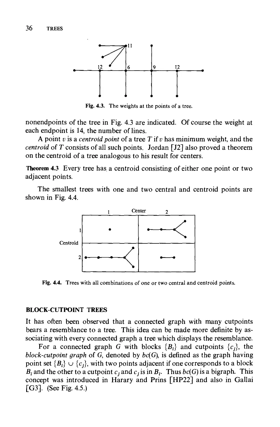
Centers and centroids . 35
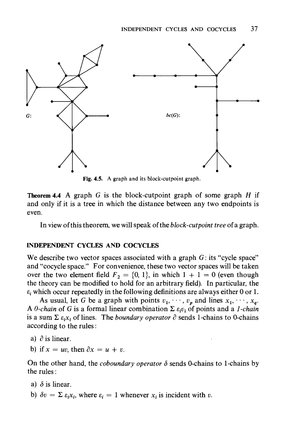
Block-cutpoint trees 36
Independent cycles and cocycles 37
Matroids . 40
vii
Vlll CONTENTS
5 Connecth;ity 43
Connectivity and line-connectivity 43
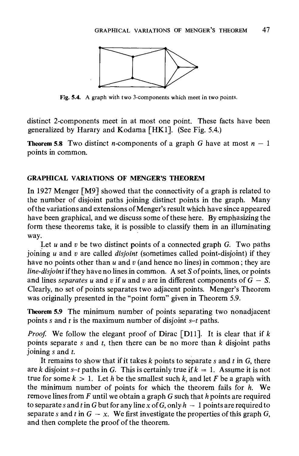
Graphical variations of Menger's theorem 47
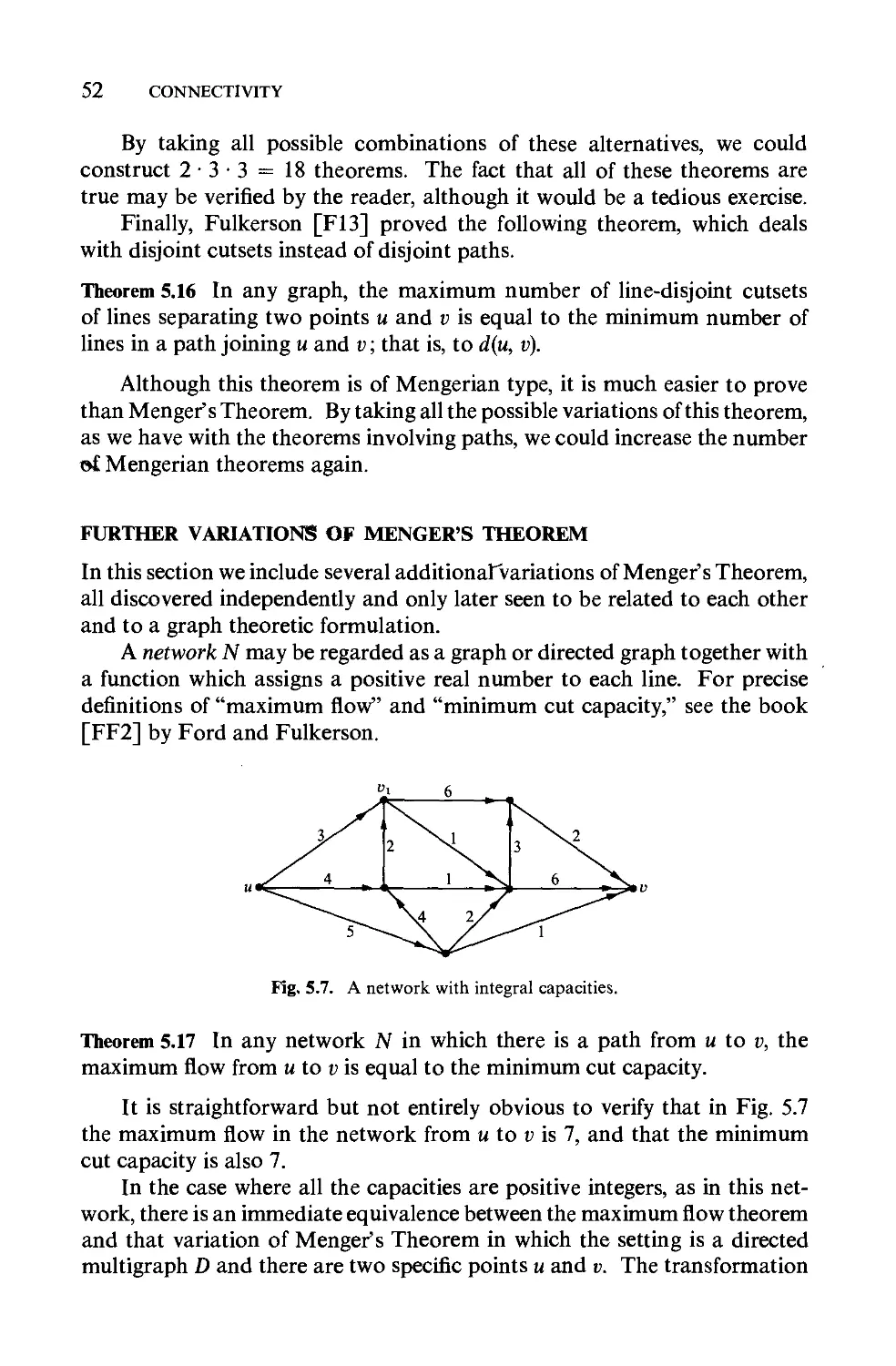
Further variations of Menger's theorem 52
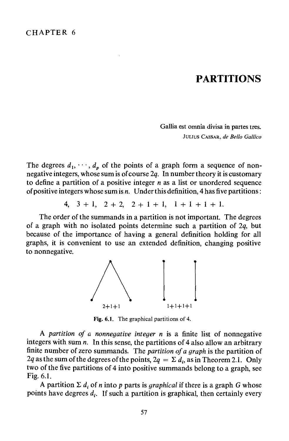
6 Partitions . 57
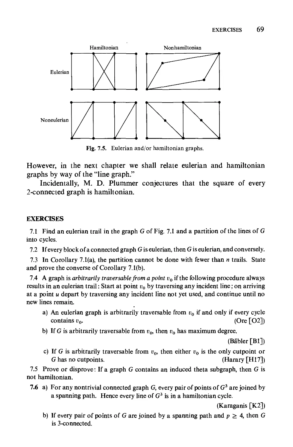
7 TraversabiIity 64
Eulerian graphs . 64
Hamiltonian graphs 65
8 Line Graphs 71
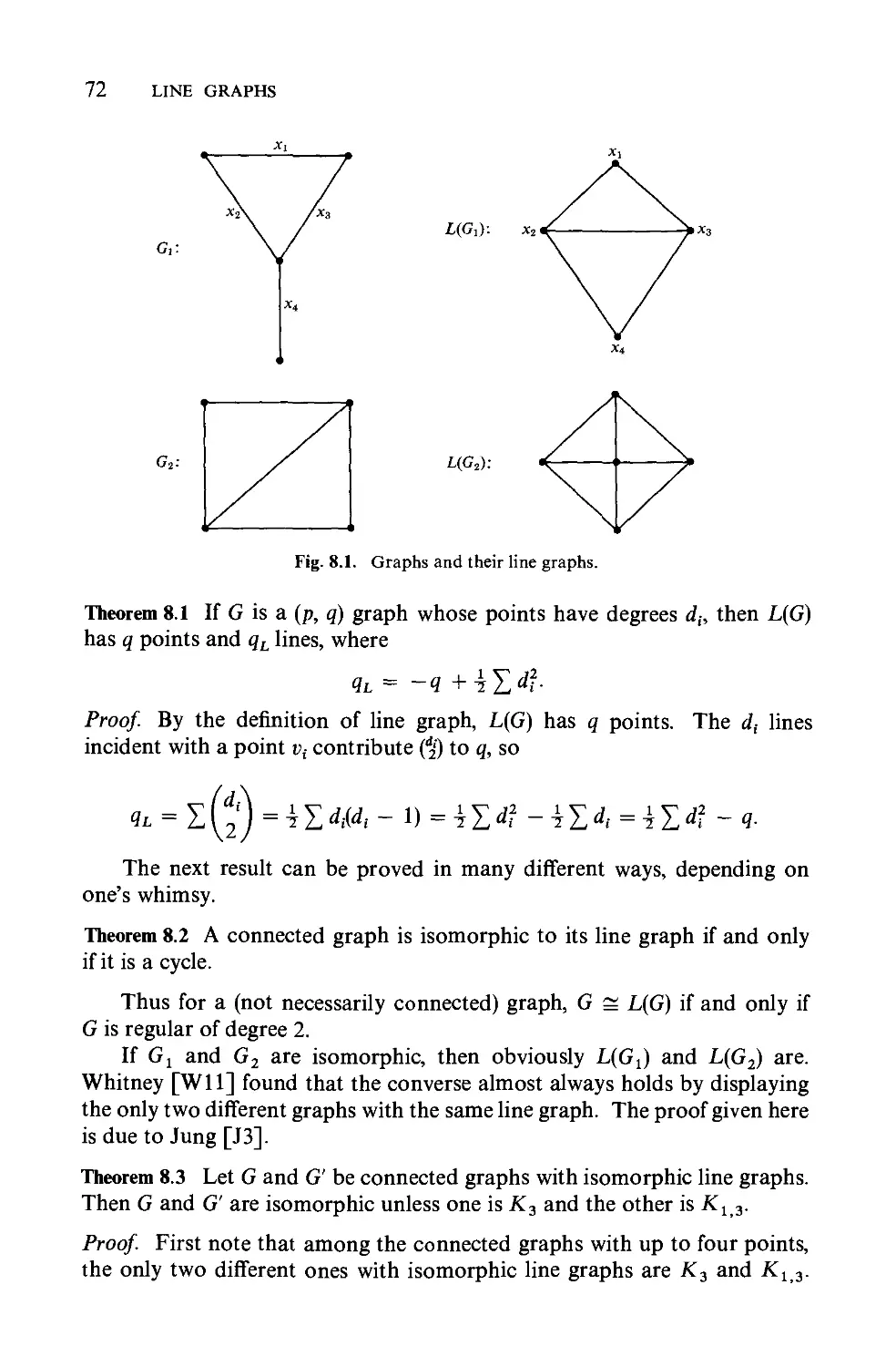
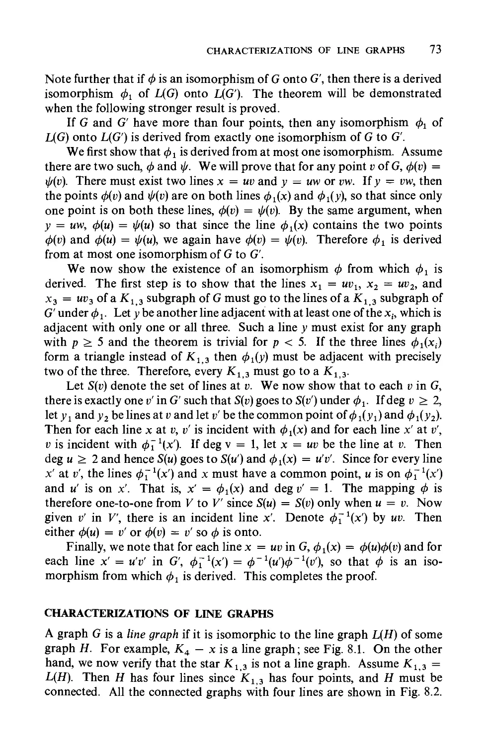
Some properties of line graphs 71
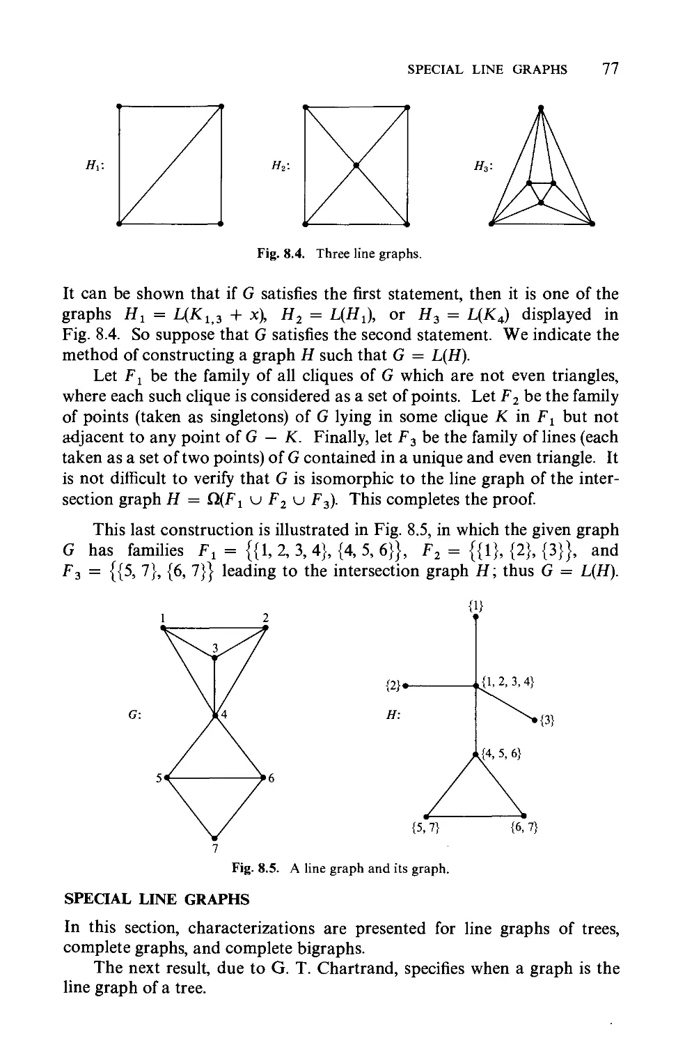
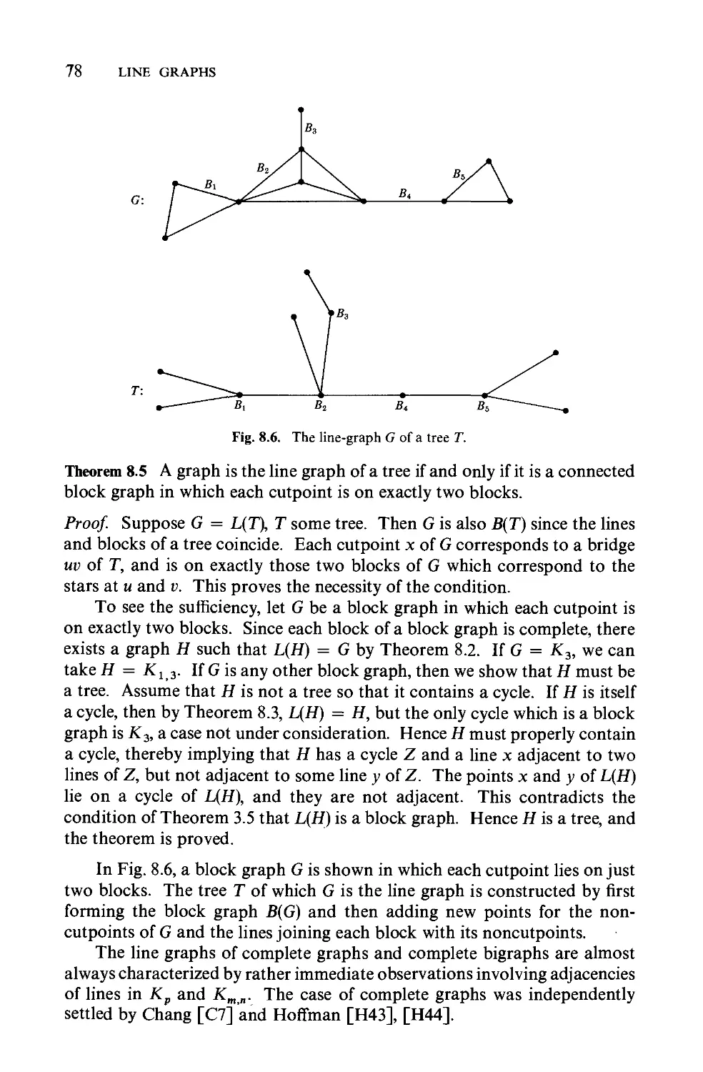
Characterizations of line graphs 73
Special line graphs n
Line graphs and traversability 79
Total graphs 82
9 Factorization 84
1- factorization 84
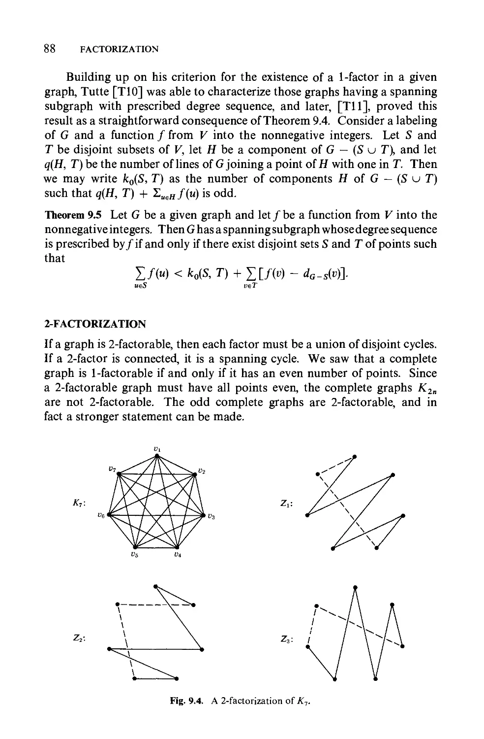
2-factorization 88
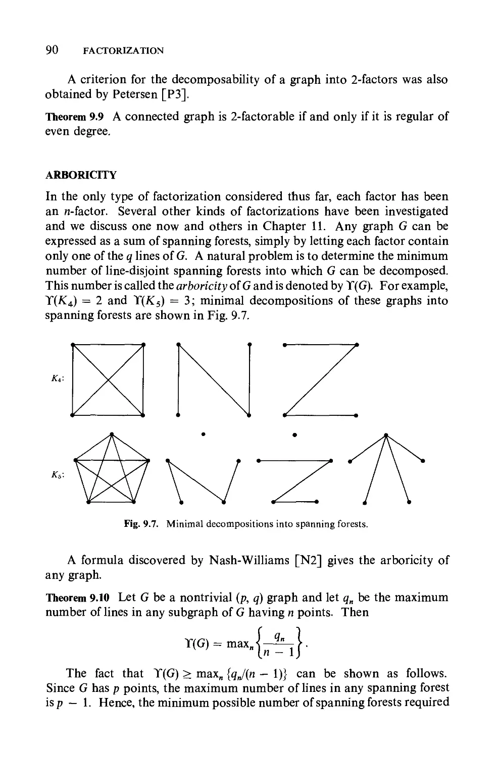
Arboricity. 90
10 Coverings . 94
Coverings and independence 94
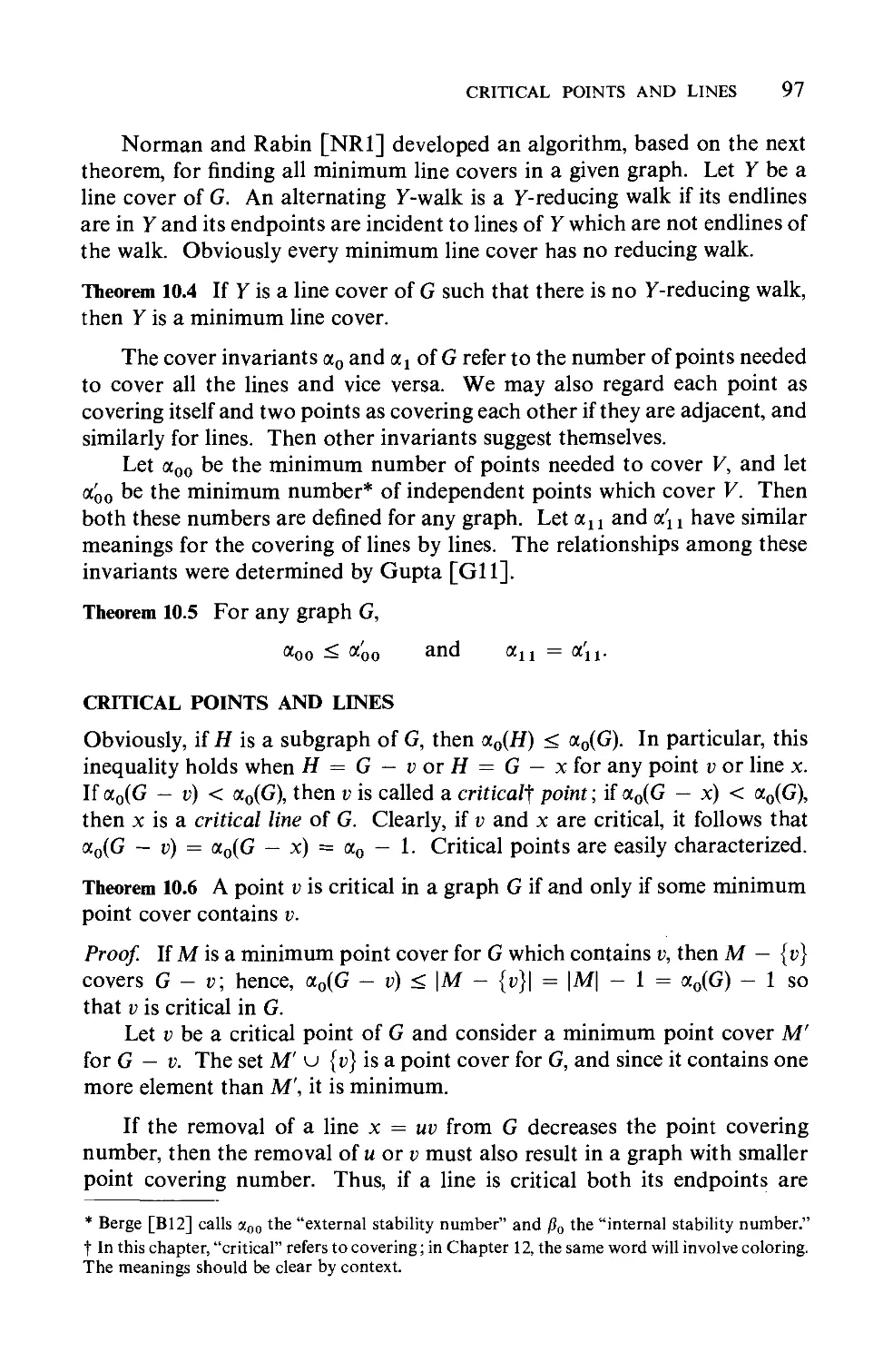
Critical points and lines 97
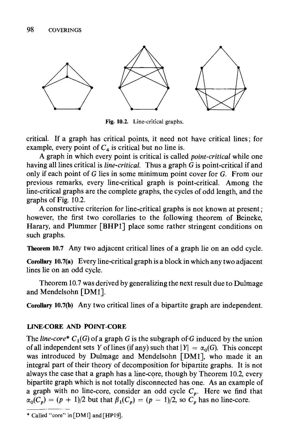
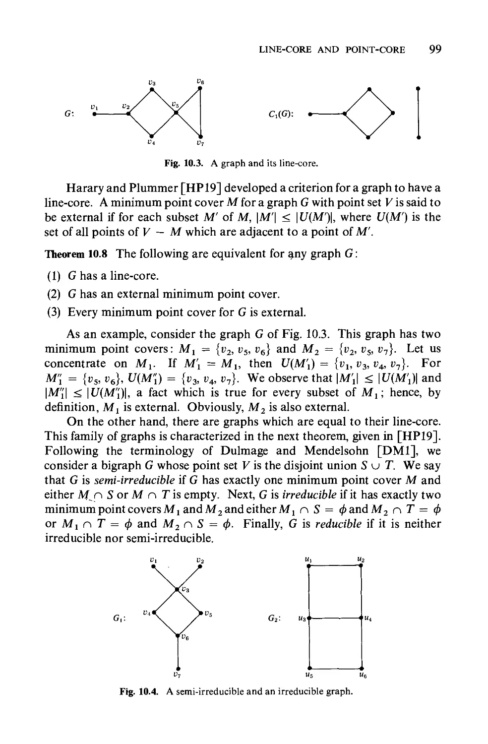
Line-core and point-core 98
11 Planarity 102
Plane and planar graphs 102
Outerplanar graphs 106
Kuratowski's theorem 108
Other characterizations of planar graphs 113
Genus, thickness, coarseness, crossing number 116
12 ColorabiIity 126
The chroma tic number 126
The Five Color Theorem 130
The Four Color Conjecture. 131
The Heawood map-coloring theorem 135
Uniquely colorable graphs 137
Critical graphs 141
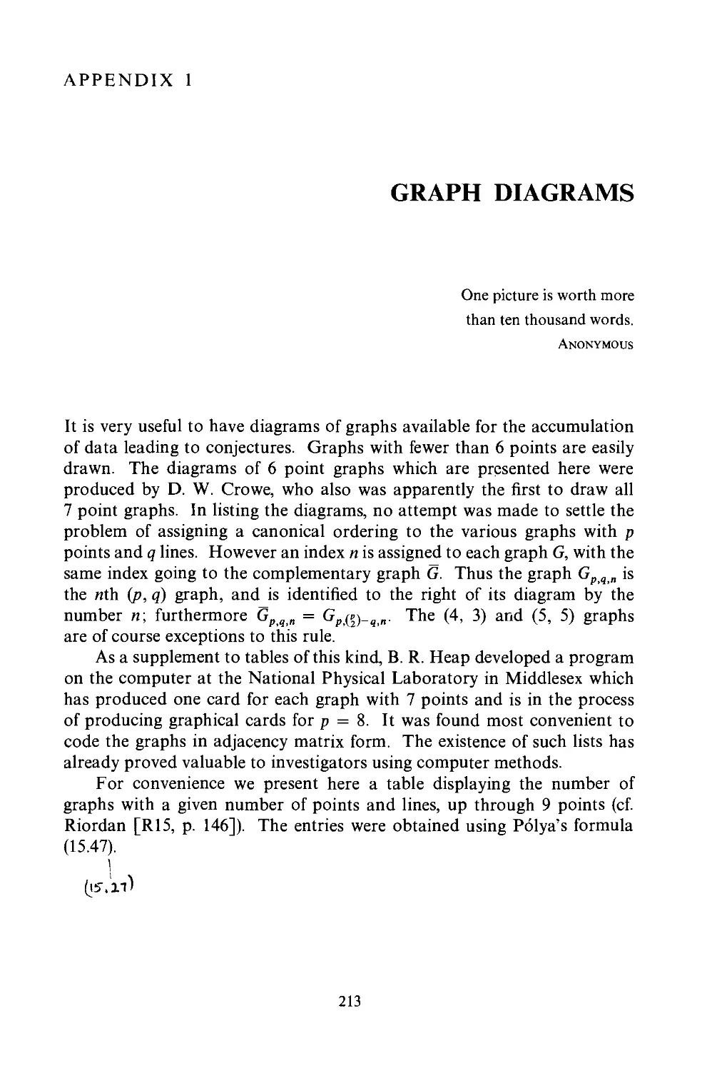
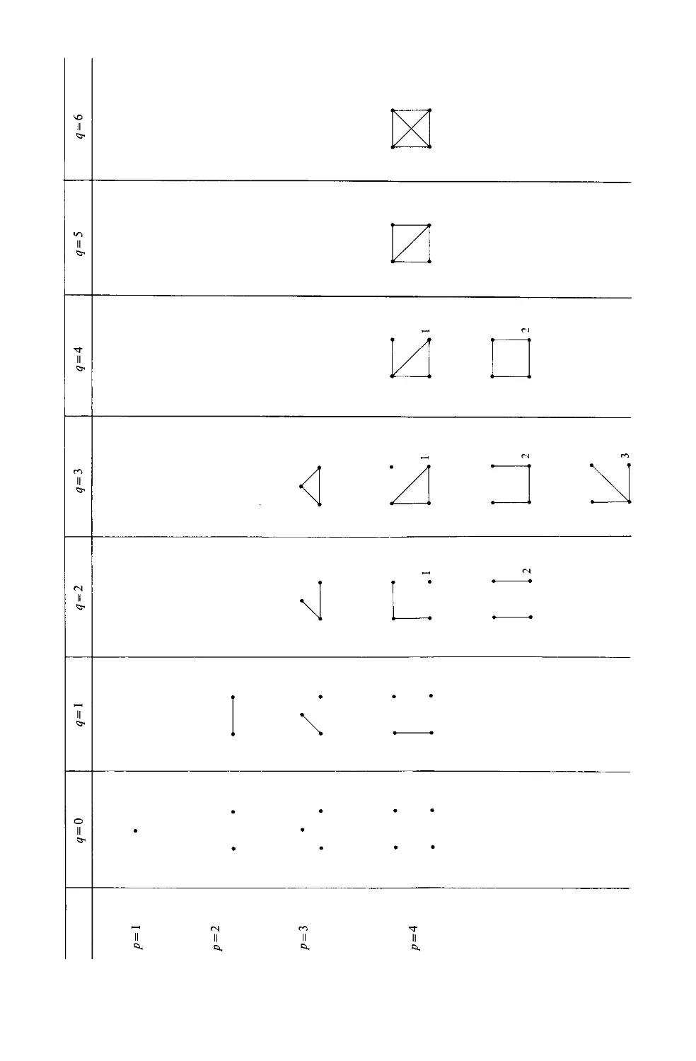
Appendix'
Graph Diagrams
CONTENTS IX
143
145
150
150
152
154
160
160
163
165
168
171
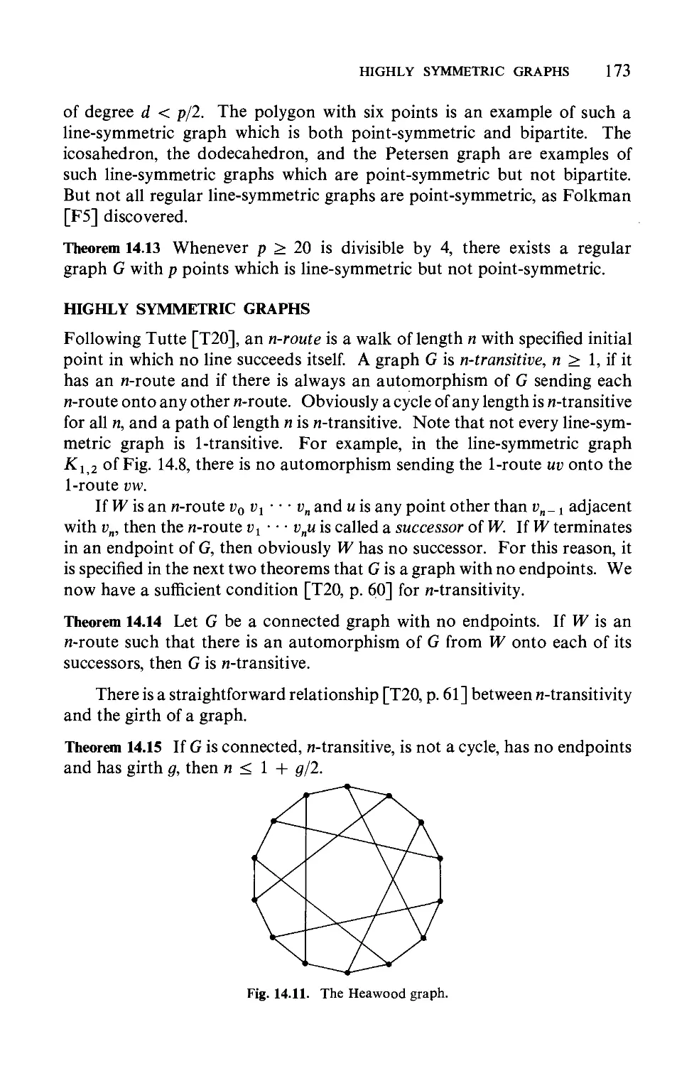
173
178
178
180
185
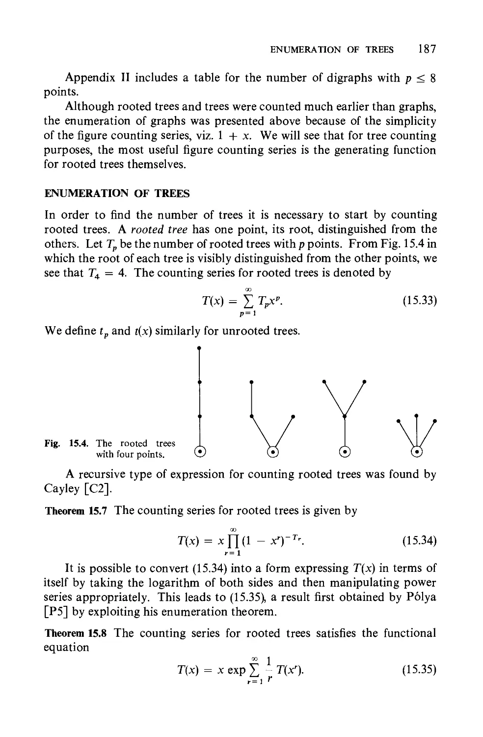
187
191
192
198
198
200
202
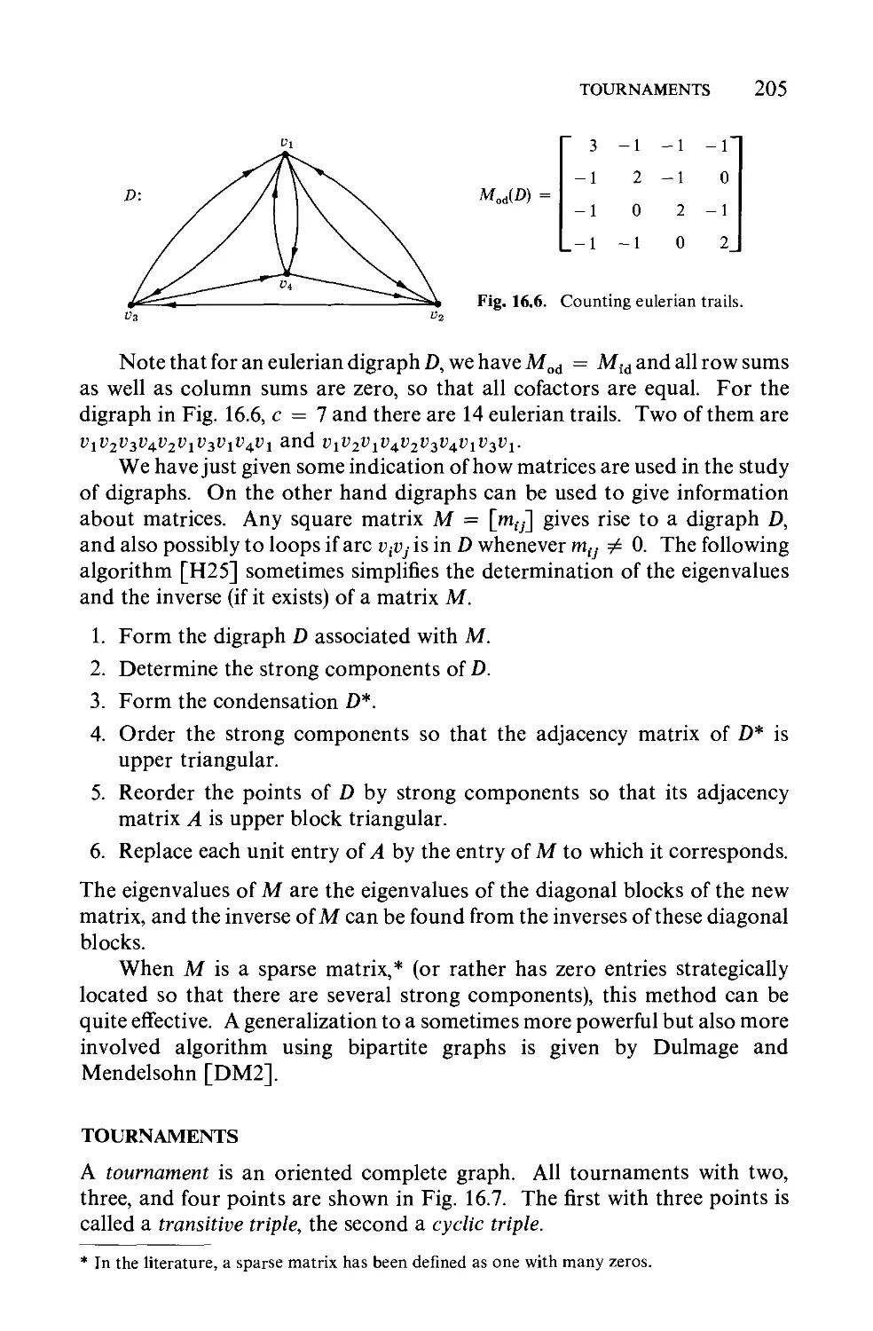
205
213
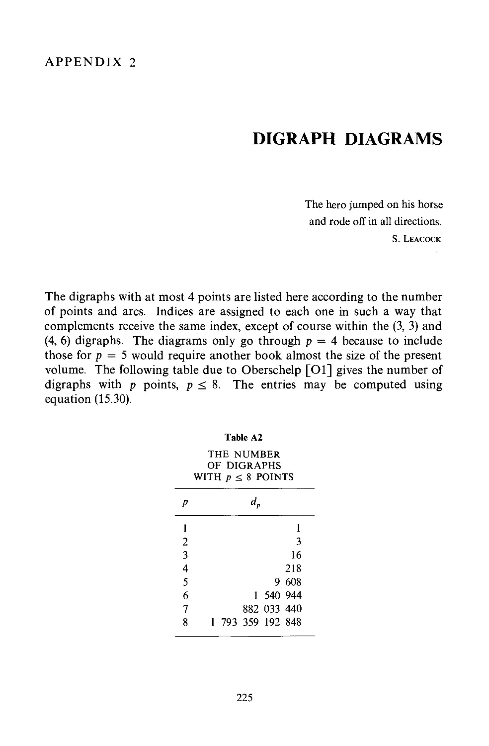
225
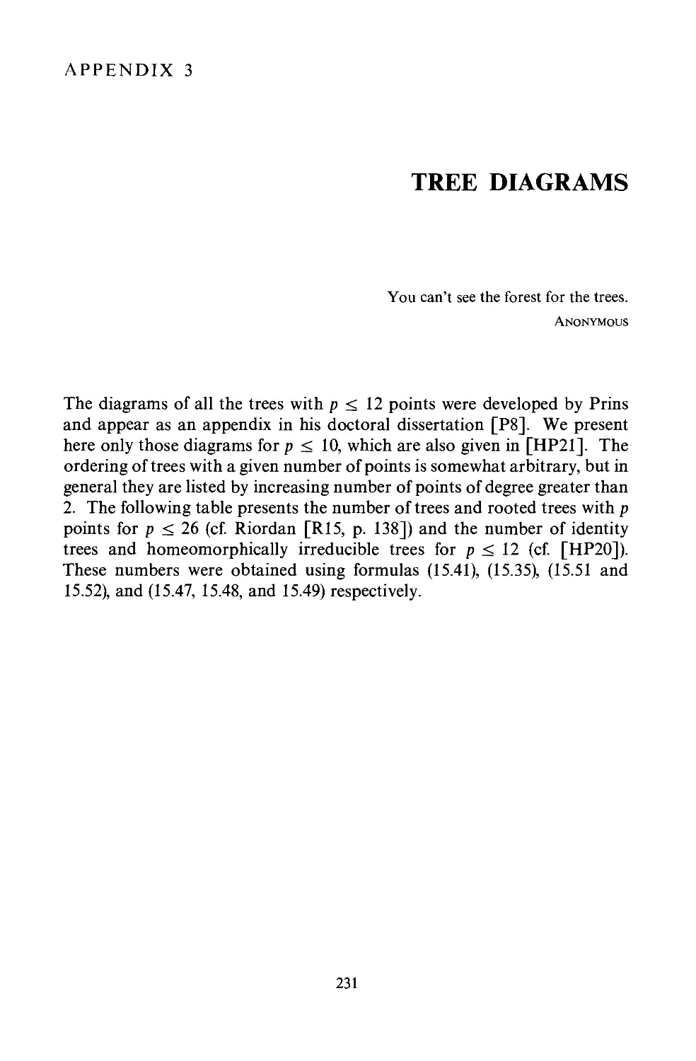
231
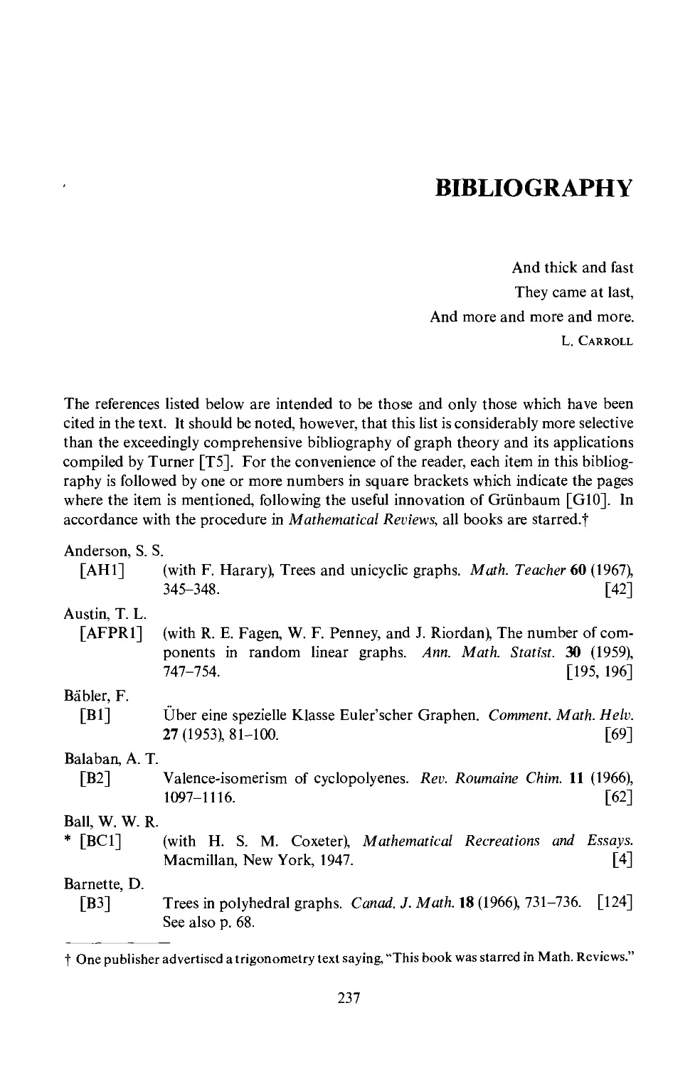
237
269
273
Homomorphisms
The chromatic polynomial
13 Matrices .
The adjacency matrix .
The incidence matrix
The cycle matrix
14 Groups
The automorphism group of a graph
Operations on permutation groups
The group of a composite graph
Graphs with a given group
Symmetric graphs
Highly symmetric graphs
15 Enumeration
Labeled graphs
P6lya's enumeration theorem
Enumeration of graphs
Enumeration of trees .
Power group enumeration theorem
Solved and unsolved graphical enumeration problems
16 Digraphs .
Digraphs and connectedness
Directional duality and acyclic digraphs
Digraphs and matrices
Tournaments
Appendix Il Digraph Diagrams
Appendix III Tree Diagrams
Bibliography
Index of Symbols
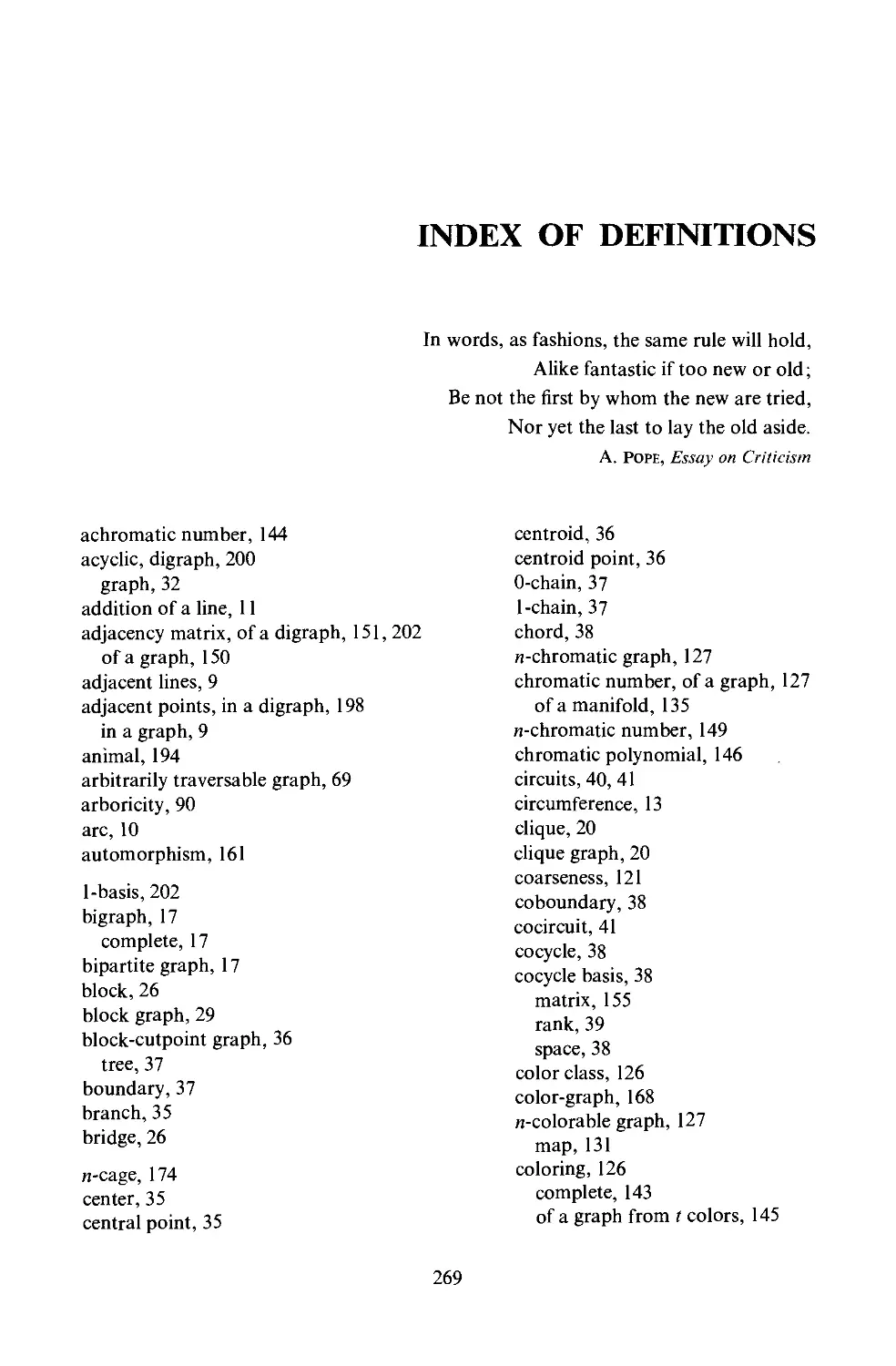
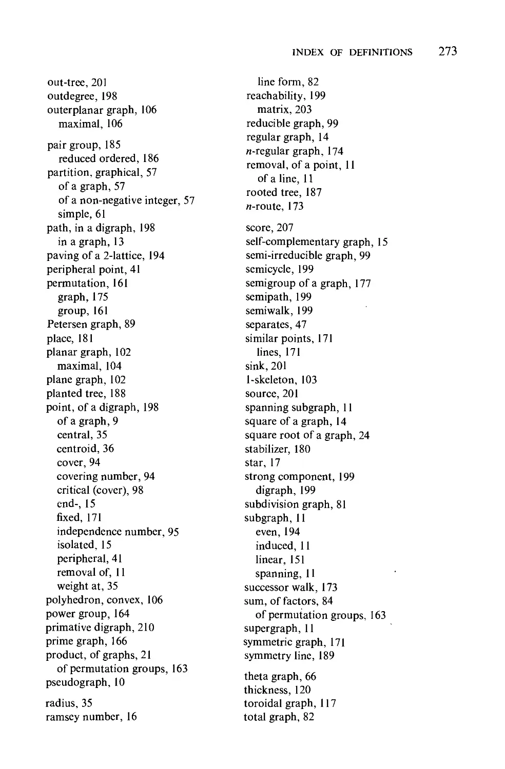
Index of Definitions
CHAPTER 1
DISCOVERY!
Eureka!
ARCHIMEDES
It is no coincidence that graph theory has been independently discovered
many times, since it may quite properly be regarded as an area of applied
mathematics.* Indeed, the earliest recorded mention of the subject occurs in
the works of Euler, and although the original problem he was considering
might be regarded as a somewhat frivolous puzzle, it did arise from the
physical world. Subsequent rediscoveries of graph theory by Kirchhoff
and Cayley also had their roots in the physical world. Kirchhoff's investiga-
tions of electric networks led to his development of the basic concepts and
theorems concerning trees in graphs, while Cayley considered trees arising
from the enumeration of organic chemical isomers. Another puzzle approach
to graphs was proposed by Hamilton. After this, the celebrated Four Color
Conjecture came into prominence and has been notorious ever since. ln
the present century, there have already been a great many rediscoveries of
graph theory which we can only mention most briefly in this chronological
account.
THE KONIGSBERG BRIDGE PROBLEM
Euler (1707-1782) became the father of graph theory as weIl as topology
when in 1736 he settled a famous unsolved problem of his day called the
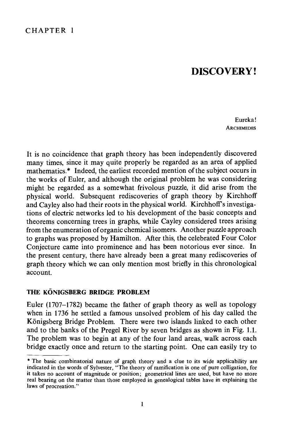
Kônigsberg Bridge Problem. There were two islands linked to each other
and to the banks of the Pregel River by seven bridges as shown in Fig. 1.1.
The problem was to begin at any of the four land are as, walk across each
bridge exactly once and return to the starting point. One can easily try to
* The basic combinatorial nature of graph theory and a clue to its wide applicability are
indicated in the words of Sylvester, "The theory of ramification is one of pure colligation, for
it takes no account of magnitude or position; geometricallines are used. but have no more
real bearing on the matter than those employed in genealogical tables have in explaining the
laws of procreation."
2 DlSCOVER y!
c
t-
1
1
1
A
B
Fig. 1.1. A park in Kônigsberg, 1736.
solve this problem empiricaIly, but aIl attempts must be unsuccessful, for
the tremendous contribution of Euler in this case was negative, see [E5].
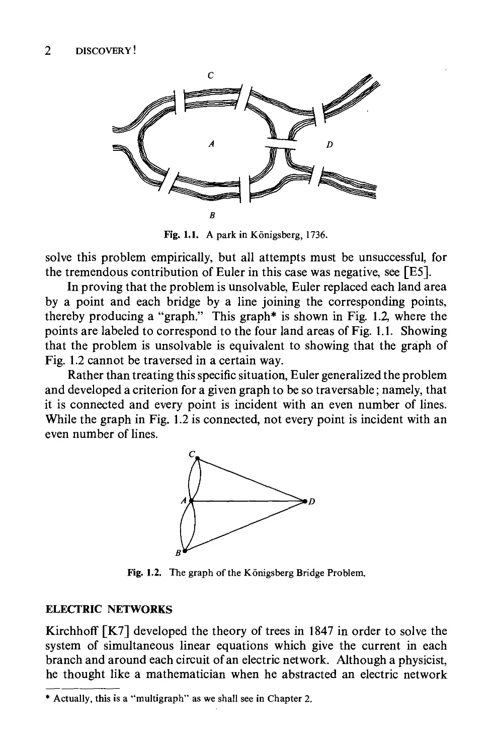
ln proving that the problem is unsolvable, Euler replaced each land area
by a point and each bridge by a line joining the corresponding points,
thereby producing a "graph." This graph* is shown in Fig. 1.2, where the
points are labeled to correspond to the four land areas of Fig. 1.1. Showing
that the problem is unsolvable is equivalent to showing that the gràph of
Fig. 1.2 cannot be traversed in a certain way.
Rather than treating this specifie situation, Euler generalized the problem
and developed a criterion for a given graph to be so traversable; namely, that
it is connected and every point is incident with an even number of lines.
While the graph in Fig. 1.2 is connected, not every point is incident with an
even number of lines.
D
Fig.1.2. The graph of the Kônigsberg Bridge Problem.
ELECTRIC NETWORKS
Kirchhoff [K7] developed the theory of trees in 1847 in order to solve the
system of simultaneous linear equations which give the current in each
branch and around each circuit of an electric network. Although a physicist,
he thought like a mathematician when he abstracted an electric network
* Actually, this is a "multigraph" as we shall see in Chapter 2.
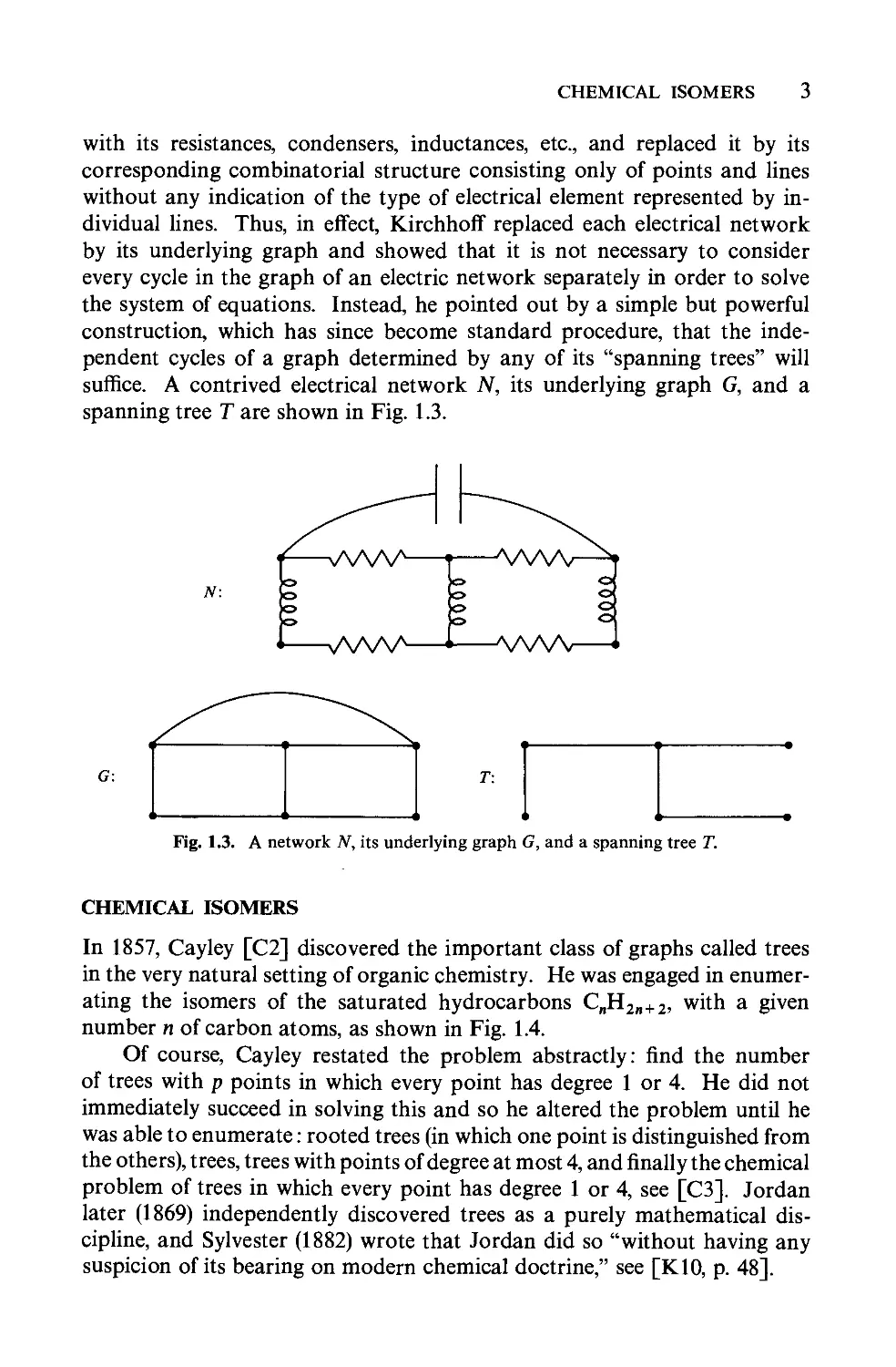
CHEMICAL ISOMERS 3
with its resistances, condensers, inductances, etc., and replaced it by its
corresponding combinatorial structure consisting only of points and lines
without any indication of the type of electrical element represented by in-
dividual lines. Thus, in effect, Kirchhoff replaced each electrical network
by its underlying graph and showed that it is not necessary to consider
every cycle in the graph of an electric network separately in order to solve
the system of equations. Instead, he pointed out by a simple but powerful
construction, which has since become standard procedure, that the inde-
pendent cycles of a graph determined by any of its "spanning trees" will
suffice. A contrived electrical network N, its underlying graph G, and a
spanning tree Tare shown in Fig. 1.3.
N:
(]]
:
T 1
1
G:
Fig. 1.3. A network N, its underlying graph G, and a spanning tree T.
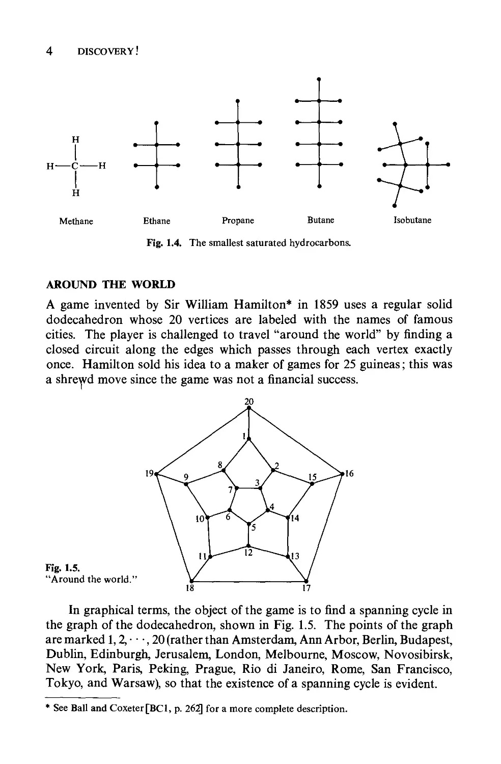
CHEMICAL ISOMERS
ln 1857, Cayley [C2] discovered the important class of graphs called trees
in the very natural setting of organic chemistry. He was engaged in enumer-
ating the isomers of the saturated hydrocarbons C n H 2n + 2 , with a given
number n of carbon atoms, as shown in Fig. 1.4.
Of course, Cayley restated the problem abstractly: find the number
of trees with p points in which every point has degree 1 or 4. He did not
immediately succeed in solving this and so he altered the problem until he
was able to enumerate: rooted trees (in which one point is distinguished from
the others), trees, trees with points of degree at most 4, and finally the chemical
problem of trees in which every point has degree 1 or 4, see [C3]. Jordan
later (1869) independently discovered trees as a purely mathematical dis-
cipline, and Sylvester (1882) wrote that Jordan did so "without having any
suspicion of its bearing on modem chemica1 doctrine," see [KlO, p. 48].
4 DlSCOVERY!
H *
1
H-C-H
1
H
Methane Ethane Propane Butane
Isobutane
Fig. 1.4. The smallest saturated hydrocarbons.
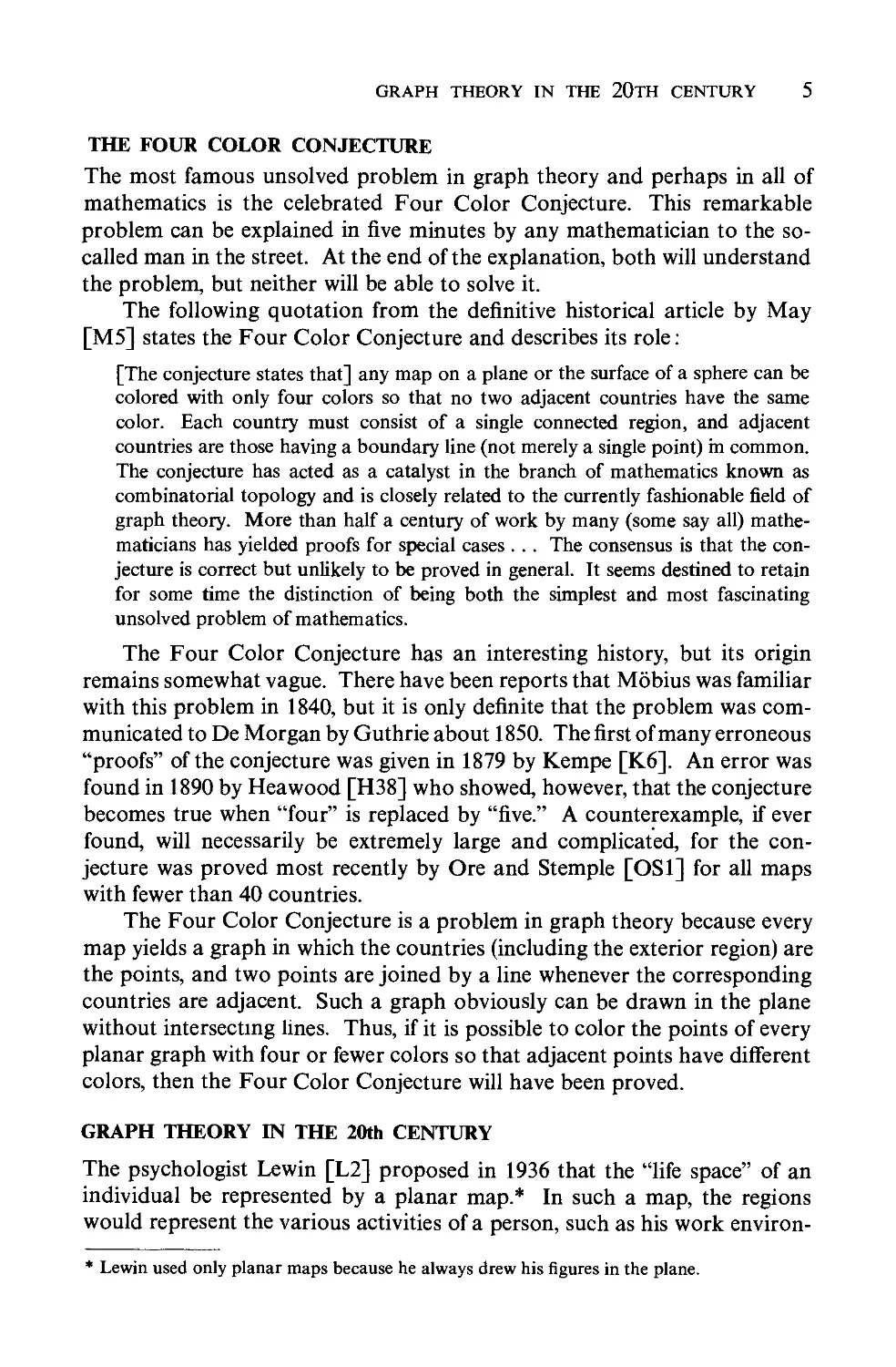
AROUND THE WORLD
Agame invented by Sir William Hamilton* in 1859 uses a regular solid
dodecahedron whose 20 vertices are labeled with the names of famous
cities. The player is challenged to travel "around the world" by finding a
closed circuit along the edges which passes through each vertex exactly
once. Hamilton sold his idea to a maker of games for 25 guineas; this was
a shrefd move since the game was not a financial success.
20
19
Fig.l.5.
"Around the world."
ln graphical terms, the object of the game is to find a spanning cycle in
the graph of the dodecahedron, shown in Fig. 1.5. The points of the graph
are marked 1, 2, . . ., 20 (rather than Amsterdam, Ann Arbor, Berlin, Budapest,
Dublin, Edinburgh, Jerusalem, London, Melbourne, Moscow, Novosibirsk,
New York, Paris, Peking, Prague, Rio di Janeiro, Rome, San Francisco,
Tokyo, and Warsaw), so that the existence of a spanning cycle is evident.
* See Bali and Coxeter[BCI, p. 262] for a more complete description.
GRAPH THEOR y lN THE 20TH CENTUR y 5
THE FOUR COLOR CONJECTURE
The most famous unsolved problem in graph theory and perhaps in aIl of
mathematics is the celebrated Four Color Conjecture. This remarkable
problem can be explained in five minutes by any mathematician to the so-
called man in the street. At the end of the explanation, both will understand
the problem, but neither will be able to solve it.
The following quotation from the definitive historical article by May
[M5] states the Four Color Conjecture and de scribes its role:
[The conjecture states that] any map on a plane or the surface of a sphere can be
colored with only four colors so that no two adjacent countries have the same
color. Each country must consist of a single connected region, and adjacent
countries are those having a boundary line (not merely a single point) in common.
The conjecture has acted as a catalyst in the branch of mathematics known as
combinatorial topology and is closely related to the currently fashionable field of
graph theory. More than half a century of work by many (some say ail) mathe-
maticians has yielded proofs for special cases. .. The consensus i8 that the con-
jecture is correct but unlikely to be proved in general. It seems destined to retain
for some time the distinction of being both the simplest and most fascinating
unsolved problem of mathematics.
The Four Color Conjecture has an interesting history, but its origin
remains somewhat vague. There have been reports that Môbius was familiar
with this problem in 1840, but it is only definite that the problem was com-
municated to De Morgan by Guthrie about 1850. The first ofmany erroneous
"proofs" of the conjecture was given in 1879 by Kempe [K6J. An error was
found in 1890 by Heawood [H38] who showed, however, that the conjecture
becomes true when "four" is replaced by "five." A counterexample, if ever
found, will necessarily be extremely large and complicated, for the con-
jecture was proved most recently by Ore and Stemple [OS1] for aIl maps
with fewer than 40 countries.
The Four Color Conjecture is a problem in graph theory because every
map yields a graph in which the countries (including the exterior region) are
the points, and two points are joined by a line whenever the corresponding
countries are adjacent. Such a graph obviously can be drawn in the plane
without intersectmg !ines. Thus, if it is possible to color the points of every
planar graph with four or fewer colors so that adjacent points have different
colors, then the Four Color Conjecture will have been proved.
GRAPH THEORY lN THE 20th CENTURY
The psychologist Lewin [L2] proposed in 1936 that the "life space" of an
individual be represented by a planar map. * ln such a map, the regions
would represent the various activities of a person, such as his work environ-
* Lewin used only planar maps because he always drew his figures in the plane.
6 DlSCOVER y!
Fig. 1.6. A map and its corresponding graph.
ment, his home, and his hobbies. It was pointed out that Lewin was actually
dealing with graphs, as indicated by Fig. 1.6. This viewpoint led the psy-
chologists at the Research Center for Group Dynamics to another psycho-
logical interpretation of a graph, in which people are represented by points
and interpersonal relations by lines. Such relations include love, hate,
communication, and power. ln fact, it was precis el y this approach which led
the author to a personal discovery of graph theory, aided and abetted by
psychologists L. Festinger and D. Cartwright.
The world of theoretical physics discovered graph theory for its own
purposes more than once. ln the study of statistical mechanics by Uhlenbeck
[UI], the points stand for molecules and two adjacent points indicate
nearest neighbor interaction of some physical kind, for example, magnetic
attraction or repulsion. ln a similar interpretation by Lee and Yang [L YI],
the points stand for small cubes in euclidean space, where each cube may or
may not be occupied by a molecule. Then two points are adjacent whenever
both spaces are occupied. Another aspect of physics employs graph theory
rather as a pictorial device. Feynmann [F3] proposed the dia gram in
which the points represent physical particles and the lines represent paths of
the particles after collisions.
The study of Markov chains in probability theory (see, for example,
Feller [F2, p. 340]) involves directed graphs in the sense that events are
represented by points, and a directed line from one point to another indicates
a positive probability of direct succession of these two events. This is made
explicit in the book [HNCI, p. 371] in which a Markov chain is defined as a
network with the sum of the values of the directed lines from each point
equal to 1. A similar representation of a directed grapn arises in that part
of numerical analysis involving matrix inversion and the calculation of
eigenvalues. Examples are given by Varga [V2, p. 48]. A square matrix is
given, preferably "sparse," and a directed graph is associated with it in the
following way. The points den ote the index of the rows and columns of the
GRAPH THEORY lN THE 20TH CENTURY 7
given matrix, and there is a directed line from point i to point j whenever
the i, j entry of the matrix in nonzero. The similarity between this approach
and that for Markov chains is immediate.
The rapidly growing fields of linear programming and operational
research have also made use of a graph theoretic approach by the study of
flows in networks. The books by Ford and Fulkerson [FF2], Vajda [VI]
and Berge and Ghouila-Houri [BG2] involve graph theory in this way. The
points of a graph indicate physical locations where certain goods may be
stored or shipped, and a directed line from one place to another, together
with a positive number assigned to this line, stands for a channel for the
transmission of goods and a capacity giving the maximum possible quantity
which can be shipped at one time. '
Within pure mathematics, graph theory is studied in the pioneering
book on topology by Veblen [V3, pp. 1-35]. A simplicial complex (or
briefly a complex) is defined to consist of a collection V of "points" together
with a prescribed collection S of nonempty subsets of V, called "simplexes,"
satisfying the following two conditions.
1. Every point is a simplex.
2. Every nonempty subset of a simplex is also a simplex.
The dimension ofa simple x is one less than the number of points in it; that
of a complex is the maximum dimension of any simplex in il. ln these terms,
a graph may be defined as a complex of dimension 1 or O. We calI a 1-
dimensional simplex a line, and note that a complex is O-dimensional if and
only if it consists of a collection of points, but no lines or other higher
dimensional simplexes. Aside from these "totally disconnected" graphs,
every graph is a I-dimensional complex. It is for this reason that the subtitle
of the first book ever written on graph theory [KlO] is "Kombinatorische
Topologie der Streckenkomplexe."
It is precisely because of the traditional use of the words point and line
as undefined terms in axiom systems for geometric structures that we have
chosen to use this terminology. Whenever we are speaking of "geometric"
simplicial complexes as subsets of a euclidean space, as opposed to the
abstract complexes defined above, we shall then use the words vertex and
edge. Terminological questions will now be pursued in Chapter 2, together
with some of the basic concepts and elementary theorems of graph theory.
CHAPTER 2
GRAPHS
What's in a narne? That which we cali a rose
By any other narne would smell as sweet.
WILLlAM SHAKESPEARE, Romeo and Juliet
Most graph theorists use personalized terminology in their books, papers,
and lectures. ln order to avoid quibbling at conferences on graph- theory,
it has been found convenient to adopt the procedure that each man state in
a vance the graph theoretic language he would use. Even the very word
"graph" has not been sacrosanct. Some authors actually define a "graph"
as a graph, * but others intend such alternatives as multigraph, pseudograph,
directed graph, or network. We believe that uniformity in graphical
terminology will never be attained, and is not necessarily desirable.
Alas, it is necessary to present a formidable number of definitions in
order to make available the basic concepts and terminology of graph theory.
ln addition, we give short introductions to the study of complete subgraphs,
extremal graph theory (which investigates graphs with forbidden subgraphs),
intersection graphs (in which the points stand for sets and nonempty inter-
sections determine adjacency), and some useful operations on graphs.
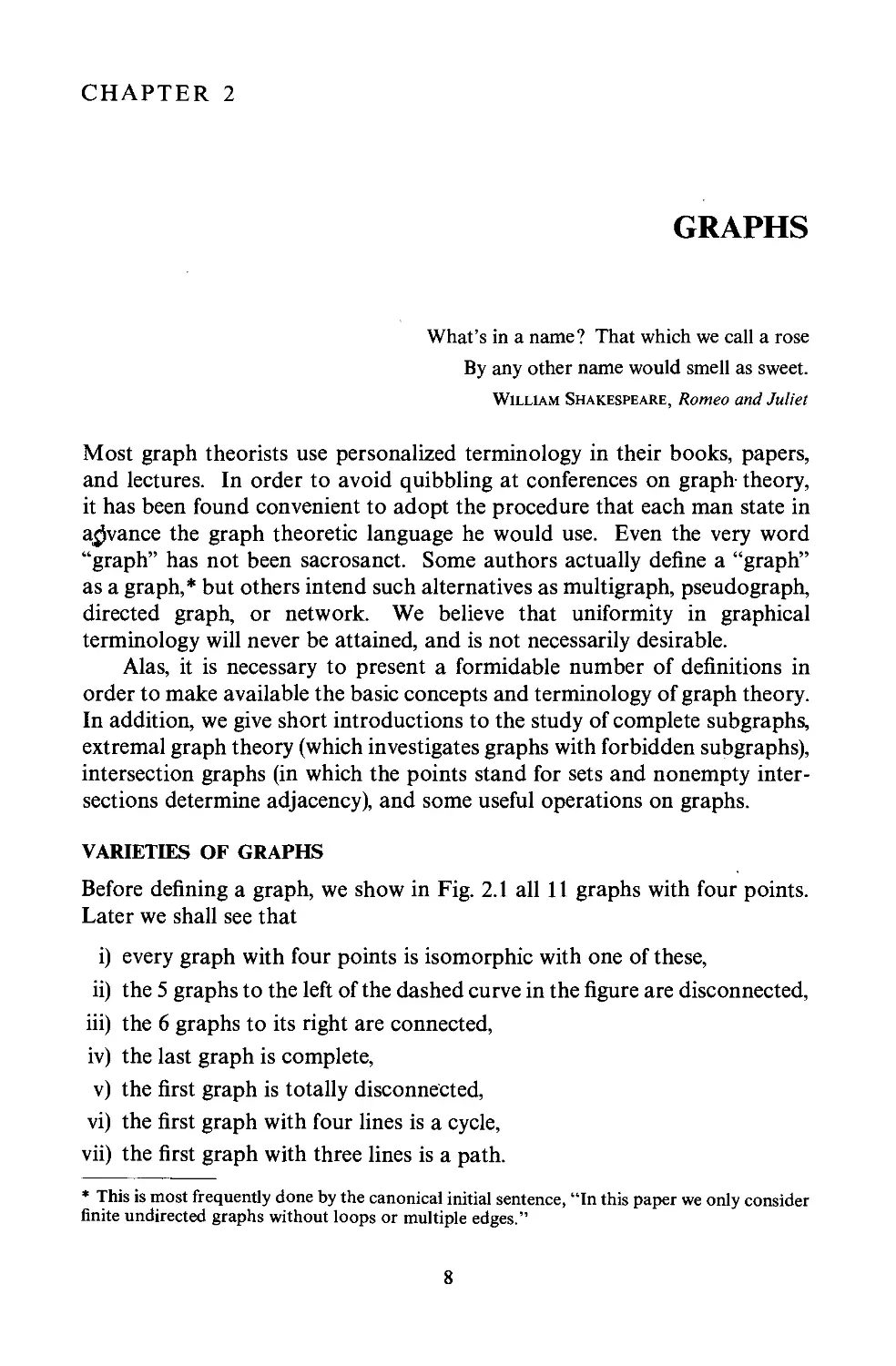
V ARIETIES OF GRAPHS
Before defining a graph, we show in Fig. 2.1 aIl 11 graphs with four points.
Later we shall see that
i) every graph with four points is isomorphic with one of the se,
ii) the 5 graphs to the left of the dashed curve in the figure are disconnected,
iii) the 6 graphs to its right are connected,
iv) the last graph is complete,
v) the first graph is totally disconnected,
vi) the first graph with four lines is a cycle,
vii) the first graph with three lines is a path.
* This is most frequently done by the canonical initial sentence, "ln this paper we only consider
finite undirected graphs without loops or multiple edges."
8
V ARIETIES OF GRAPHS 9
.
.
--
1
1
iU
ri lL: 0 IZ1
! ! L l [71
1
1
Fig. 2.1. The graphs with four points.
18J
.
.
. .
Rather than continue with an intuitive development of additional
concepts, we proceed with the tedious but essential sequence of definition
upon definition. A graph G consists of a finite nonempty set V of p points*
together with a prescribed set X of q unordered pairs of distinct points of
V. Each pair x = {u, v} of points in X is a line* of G, and x is said to join u
and v. We write x = uv and say that u and v are adjacent points (sometimes
denoted u adj v); point 'U and line x are incident with each other, as are v
and x. If two distinct lines x and y are incident with a common point, then
they are adjacent lines. A graph with p points and q lines is called a (p, q)
graph. The (1, 0) graph is trivial.
u
w
G:
Fig. 2.2. A graph to iIIustrate adjacency.
1 t is customary to represent a graph by means of a diagram and to refer
to it as the graph. Thus, in the graph G of Fig. 2.2, the points u and v are
adjacent but u and w are not; lines x and y are adjacent but x and z are not.
Although the lines x and z intersect in the diagram, their intersection is not
a point of the graph. .
* The following is a list of synonyms which have been used in the literature, not always with the
indicated pairs:
point, vertex,
line, edge,
node, junction, O-simplex, element,
arc, branch, I-simplex, element.
10 GRAPHS
There are several variations of graphs which deserve mention. Note that
the definition of graph permits no loop, that is, no line joining a point to
itself. ln a multigraph, no loops are allowed but more than one line can join
two points; the se are called multiple lines. If both loops and multiple lines
are permitted, we have a pseudograph. Figure 2.3 shows a multigraph and
a pseudograph with the same "underlying graph," a triangle. We now see
why the graph (Fig. 1.2) of the Kônigsberg bridge problem is actually a
multigraph.
Fig. 2.3. A multigraph and a pseudograph.
A directed graph or digraph D consists of a finite nonempty set V of
points together with a prescribed collection X of ordered pairs of distinct
points. The elements of X are directed lines or arcs. By definition, a digraph
has no loops or multiple arcs. An oriented graph is a digraph having no
symmetric pair of directed lines. ln Fig. 2.4 aIl digraphs with three points and
three arcs are shown; the last two are oriented graphs. Digraphs constitute
the subject of Chapter 16, but we will encounter them from time to time in
the interim.
LL
Fig. 2.4. The digraphs with three points and three arcs.
A graph G is labeled when the p points are distinguished from one another
by names* such as V l , V2,' . ., vp- For example, the two graphs G l and G 2 of
Fig. 2.5 are labeled but G 3 is not.
Two graphs Gand H are isomorphic (written G H or sometimes
G = H) if there exists a one-to-one correspondence between their point
sets which preserves adjacency. For example, G l and G 2 of Fig. 2.5 are
isomorphic under the correspondence Vi +-+ Ui, and incidentally G 3 is iso-
* This notation for points was chosen since v is the first letter of vertex. Another author caBs
them vertices and writespl> P2, . . . ,PU'
V ARIETIES OF GRAPHS Il
G , :
G 2 :
V,
V2
V.
U,
V.
V.
Vo
U.
Fig. 2.5. Labeled and unlabeled graphs.
G.:
U.
morphic with each of them. It go es without saying that isomorphism is an
equivalence relation on graphs.
An invariant of a graph G is a number associated with G which has the
same value for any graph isomorphic to G. Thus the numbers p and q are
certainly invariants. A complete set of invariants determines a graph up to
isomorphism. For example, the numbers p and q constitute such a set for
aIl graphs with less than four points. No decent complete set of invariants
for a graph is known.
A subgraph of Gis a graph having aIl of its points and lines in G. If G l
is a subgraph of G, then G is a supergraph of G l . A spanning subgraph is a
subgraph containing aIl the points of G. For any set S of points of G, the
induced subgraph (S) is the maximal subgraph of G with point set S. Thus
two points of S are adjacent in (S) if and only if they are adjacent in G. ln
Fig. 2.6, G 2 is a spanning subgraph of G but G l is not; G l is an induced
subgraph but G 2 is not.
G:
G , :
Fig. 2.6. A graph and Iwo subgraphs.
G 2 :
The removal of a point Vi from a graph G results in that subgraph G - Vi
of G consisting of aIl points of G except Vi and aIl lines not incident with
Vi' Thus G - Vi is the maximal subgraph of G not containing Vi' On the
other hand, the removal of a line Xj from G yields the spanning subgraph
G - Xj containing aIl lines of G except Xj' Thus G - x j is the maximal
su bgraph of G not containing x j' The removal of a set of points or lines from
G is defined by the removal of single elements in succession. On the other
hand, if Vi and Vj are not adjacent in G, the addition of line ViVj results in the
12 GRAPHS
G:
v.
G-v,:
v.
V2 v.
V,
G-V2V,:
G+v,v. :
v.
V,
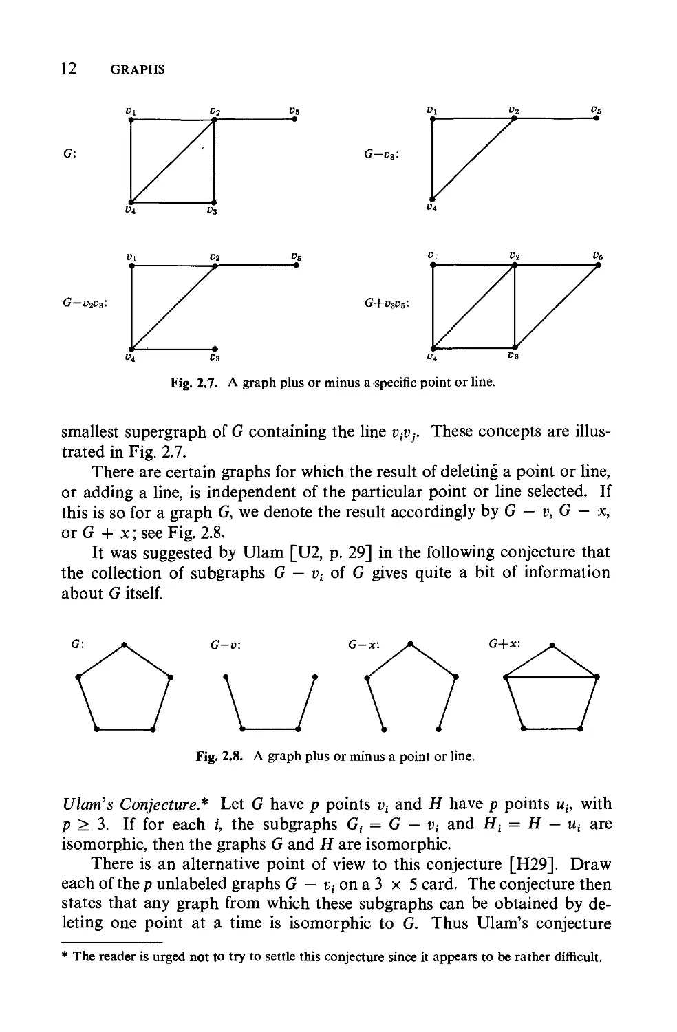
Fig. 2.7. A graph plus or minus a ,specifie point or line.
v.
V.
smallest supergraph of G containing the line ViVj' These concepts are illus-
trated in Fig. 2.7.
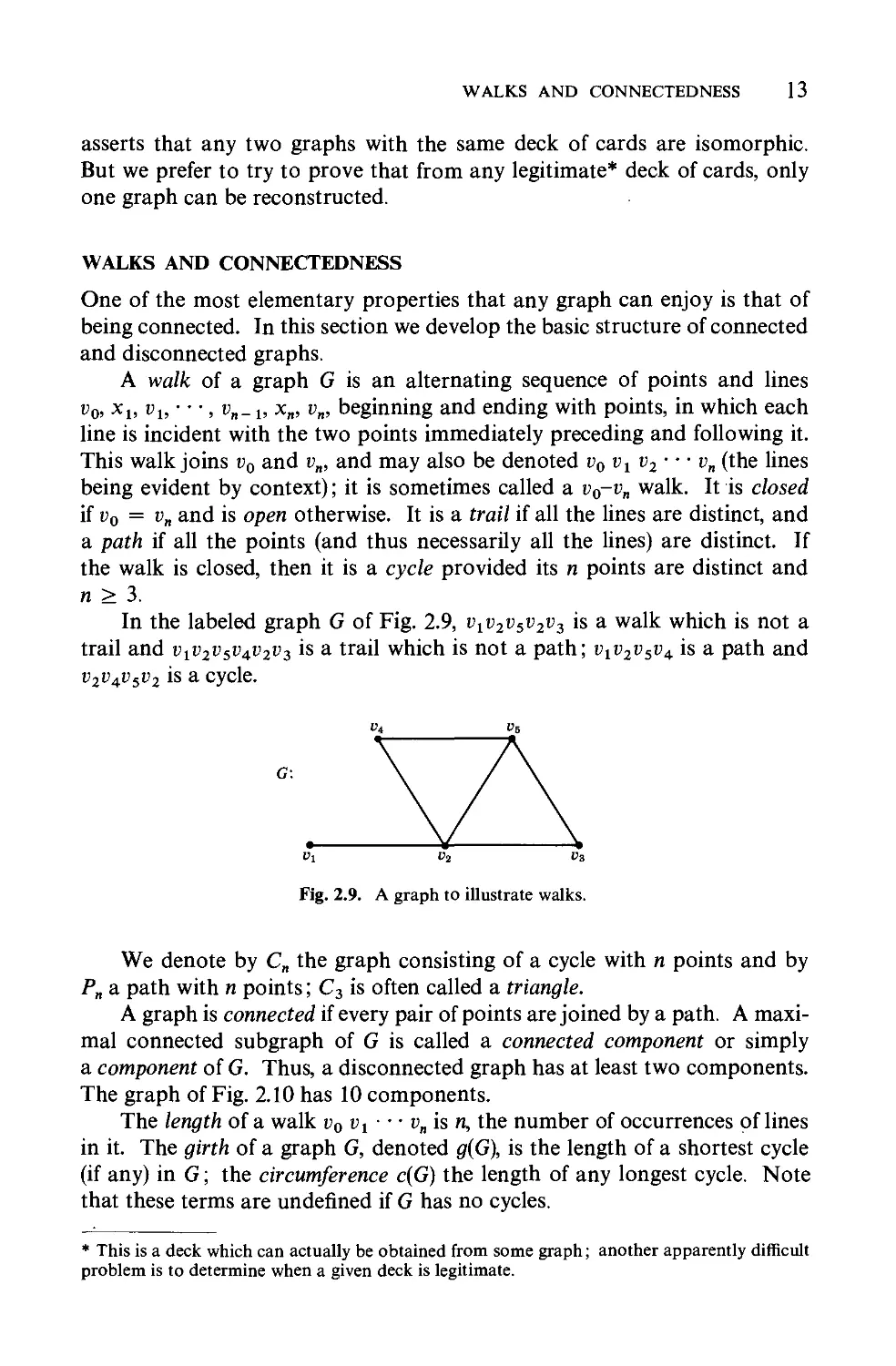
There are certain graphs for which the result of deleting a point or line,
or adding a line, is independent of the particular point or line selected. If
this is so for a graph G, we denote the result accordingly by G - v, G - x,
or G + x; see Fig. 2.8.
It was suggested by Ulam [U2, p. 29] in the following conjecture that
the collection of subgraphs G - Vi of G gives quite a bit of information
about G itself.
o Gu G_\; Go
Fig. 2.8. A graph plus or minus a point or line.
Ulam's Conjecture.* Let G have p points Vi and H have p points Ui, with
p 3. If for each i, the subgraphs G i = G - Vi and Hi = H - 1Ii are
isomorphic, then the graphs Gand H are isomorphic.
There is an alternative point of view to this conjecture [H29]. Draw
each of the p unlabeled graphs G - Vi on a 3 x 5 card. The conjecture then
states that any graph from which these subgraphs can be obtained by de-
leting one point at a time is isomorphic to G. Thus Ulam's conjecture
* The reader is urged not 10 try to seule this conjecture since it appears to be rather difficult.
W ALKS AND CONNECTEDNESS 13
asserts that any two graphs with the same deck of cards are isomorphic.
But we prefer to try to prove that from any legitimate* deck of cards, only
one graph can be reconstructed.
W ALKS AND CONNECTEDNESS
One of the most elementary properties that any graph can enjoy is that of
being connected. ln this section we develop the basic structure of connected
and disconnected graphs.
A walk of a graph G is an alternating sequence of points and lines
Vo, Xl' V b . . ., Vn-l' X n , Vn' beginning and ending with points, in which each
line is incident with the two points immediately preceding and following it.
This walk joins V o and Vn' and may also be denoted Vo V l V 2 . . . V n (the lines
being evident by context); it is sometimes called a VO-Vn walk. It is closed
if Vo = V n and is open otherwise. It is a trail if aIl the lines are distinct, and
a pa th if aIl the points (and thus necessarily aIl the lines) are distinct. If
the walk is closed, then it is a cycle provided its n points are distinct and
n 3.
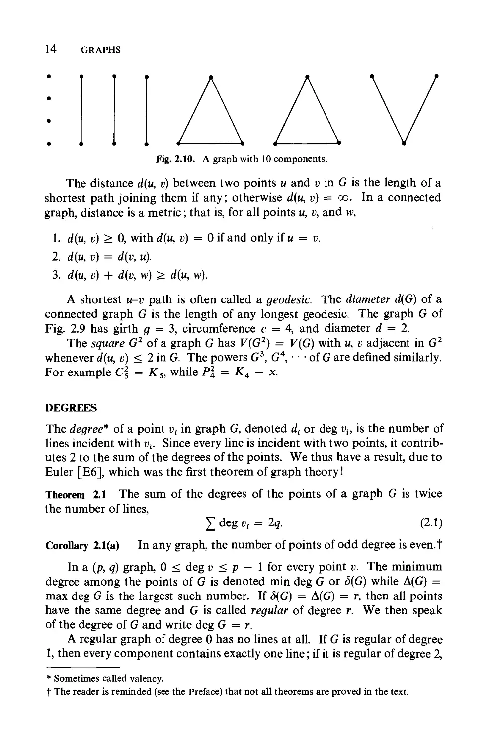
ln the labeled graph G of Fig. 2.9, VIV2VSV2V3 is a walk which is not a
trail and VIV2VSV4V2V3 is a trail which is not a path; VIV 2 V S V 4 is a path and
V2V4VSV2 is a cycle.
G:
'\1\
V2 Vg
.
v,
Fig. 2.9. A graph to illustrate walks.
We denote by C n the graph consisting of a cycle with n points and by
Pn a path with n points; C 3 is often called a triangle.
A graph is connected if every pair of points are joined by a path. A maxi-
mal connected subgraph of G is called a connected component or simply
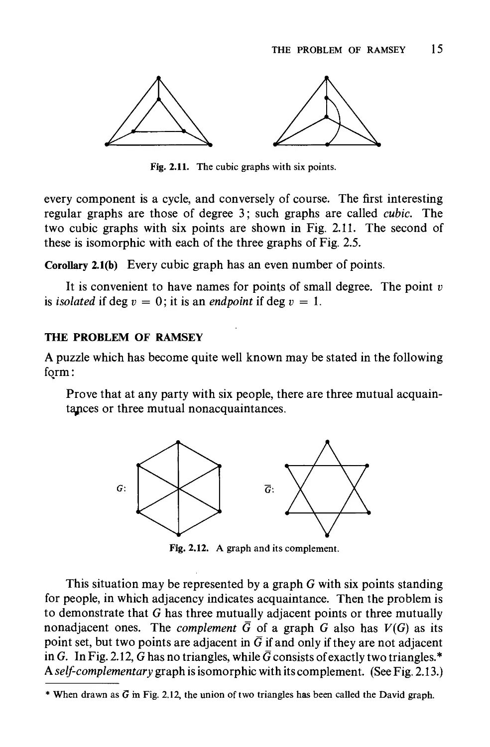
a component of G. Thus, a disconnected graph has at least two components.
The graph of Fig. 2.10 has 10 components.
The length of a walk Vo v l . . . V n is n, the number of occurrences of lines
in it. The girth of a graph G, denoted g(G), is the length of a shortest cycle
(if any) in G; the circumference c(G) the length of any longest cycle. Note
that these terms are undefined if G has no cycles.
* This is a deck which can actually be obtained from some graph; another apparently difficult
problem is to determine when a given deck is legitimate.
14 GRAPHS
.
.
.
.
DDV
Fig. 2.10. A graph with 10 components.
The distance d(u, v) between two points u and v in G is the length of a
shortest path joining them if any; otherwise d(u, v) = 00. ln a connected
graph, distance is a metric; that is, for aIl points u, v, and w,
1. d(u, v) 0, with d(u, v) = 0 if and only if u = v.
2. d(u, v) = d(v, u).
3. d(u, v) + d(v, w) d(u, w).
A shortest u-v path is often called a geodesic. The diameter d(G) of a
connected graph G is the length of any longest geodesic. The graph G of
Fig. 2.9 has girth g = 3, circumference c = 4, and diameter d = 2.
The square G 2 of a graph G has V(G 2 ) = V(G) with u, v adjacent in G 2
whenever d(u, v) ::; 2 in G. The powers G 3 , G 4 , . . . of Gare defined similarly.
For example C = Ks, while Pi = K4 - X.
DEGREES
The degree* of a point Vi in graph G, denoted di or deg Vi' is the number of
lines incident with Vi' Since every line is incident with two points, it contrib-
utes 2 to the sum of the degrees of the points. We thus have a result, due to
Euler [E6], which was the first theorem of graph theory J
Theorem 2.1 The sum of the degrees of the points of a graph G is twice
the number of lines,
L deg Vi = 2q.
(2.1 )
CoroUary 21(a) ln any graph, the number of points of odd degree is even. t
ln a (p, q) graph, 0 ::; deg v ::; p - 1 for every point v. The minimum
degree among the points of G is denoted min deg G or J(G) while .1(G) =
max deg G is the largest such number. If J( G) = .1( G) = r, then aIl points
ha ve the same degree and G is called regular of degree r. We then speak
of the degree of Gand write deg G = r.
A regular graph of degree 0 has no lines at aIl. If G is regular of degree
1, then every component contains exactly one line; if it is regular of degree 2,
* Sometimes called valency.
t The reader is reminded (see the Preface) that not all theorems are proved in the tex!.
THE PROBLEM OF RAMSEY 15
Fig. 2.11. The cubic graphs with six points.
every component is a cycle, and conversely of course. The first interesting
regular graphs are those of degree 3; such graphs are called cubic. The
two cubic graphs with six points are shown in Fig. 2.11. The second of
these is isomorphic with each of the three graphs of Fig. 2.5.
CoroUary 2.1(b) Every cubic graph has an even number of points.
It is convenient to have names for points of small degree. The point v
is isolated if deg v = 0; it is an endpoint if deg v = 1.
THE PROBLEM OF RAMSEY
A puzzle which has become quite weIl known may be stated in the following
fQrm:
Prove that at any party with six people, there are three mutual acquain-
ta.Pces or three mutual nonacquaintances.
G:
G:
Fig. 2.12. A graph and its complement.
This situation may be represented by a graph G with six points standing
for people, in which adjacency indicates acquaintance. Then the problem is
to demonstrate that G has three mutually adjacent points or three mutually
nonadjacent ones. The complement G of a graph G also has V(G) as its
point set, but two points are adjacent in G if and only if they are not adjacent
in G. ln Fig. 2.12, G has no triangles, while G consists of exactly two triangles. *
A selfcomplementary graph is isomorphic with its complement. (See Fig. 2.13.)
* When drawn as G in Fig. 2.12, the union of two triangles has been called the David graph.
16 GRAPHS
UOA
Fig. 2.13. The smallest nontrivial self-complementary graphs.
The complete graph Kp has every pair of its p points* adjacent. Thus
Kp has m lines and is regular of degree p - 1. As we have seen, K3 is
called a triangle. The graphs Kp are totally disconnected, and are regular
of degree O.
ln these terms, the puzzle may be reformulated.
Theorem 2.2 For any graph G with six points, G or G contains a triangle.
Proof. Let v be a point of a graph G with six points. Since v is adjacent
either in G or in G to the other five points of G, we can assume without
loss of generality that there are three points U l , U 2 , u 3 adjacent to v in G.
If any two of these points are adjacent, then they are two points of a triangle
whose third point is v. If no two of them are adjacent in G, then U l , u 2 , and
u 3 are the points of a triangle in G.
The result of Theorem 2.2 suggests the general question: What is the
smallest integer r(m, n) such that every graph with r(m, n) points contains
Km or Kn?
The values r(m, n) are called Ramsey numbers. t Of course r(m, n) =
r(n, m). The determination of the Ramsey numbers is an unsolved problem,
although a simple bound due to Erdôs and Szekeres [ES1] is known.
r(m, n) (m 2) (2.2)
This problem arose from a theorem of Ramsey. An infinite grapht has
an infinite point set and no loops or multiple lines. Ramsey [R2] proved
(in the language of set theory) that every infinite graph contains o mutually
adjacent points or o mutually nonadjacent points.
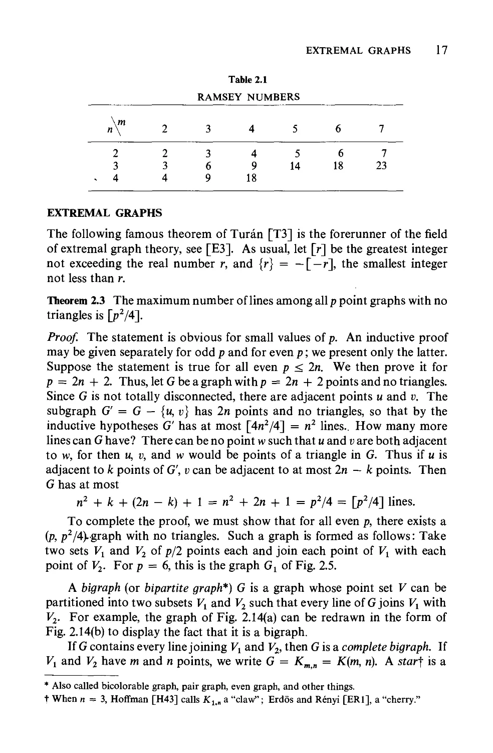
AlI known Ramsey numbers are given in Table 2.1, in accordance with
the review article by Graver and Yakel [GY1J.
* Since v is not empty, p 1. Some authors admit the "empty graph" (which we would
denote Ka if it existed) and are then faced with handling its properties and specifying that
certain theorems hold only for nonempty graphs, but we coflsider such a concept pointless.
t Mter Frank Ramsey, late brother of the present Archbishop of Canterbury. For a pro of
that rem, n) exists for all positive integers m and n, see for example Hall [H7, p. 57].
t Note that by definition, an infinite graph is not a graph. A review article on infinite graphs
was written by Nash-Williams [N3].
EXTREMAL GRAPHS 17
Table 2.1
RAMSEY NUMBERS
n\m
2
3
4
5
6
7
2
3
4
2
3
4
3
6
9
4
9
18
5
14
6
18
7
23
EXTREMAL GRAPHS
The following famous theorem of Tunin [T3] is the forerunner of the field
of extremal graph theory, see [E3]. As usual, let Cr] be the greatest integer
not exceeding the real number r, and {r} = -[ -r], the smallest integer
not less than r.
Theorem 2.3 The maximum number oflines among aIl p point graphs with no
triangles is [P2/4].
Proof. The statement is obvious for small values of p. An inductive proof
may be given separately for odd p and for even p ; we present only the latter.
Suppose the statement is true for aIl even p :::;; 2n. We then prove it for
p = 2n + 2. Thus, let G be a graph with p = 2n + 2 points and no triangles.
Since G is not totally disconnected, there are adjacent points u and v. The
subgraph G' = G - {u, v} has 2n points and no triangles, so that by the
inductive hypotheses G' has at most [4n 2 /4] = n 2 lines.. How many more
lines can G have? There can be no point w such that u and v are both adjacent
to w, for then U, v, and w would be points of a triangle in G. Thus if u is
adjacent to k points of G', v can be adjacent to at most 2n - k points. Then
G has at most
n 2 + k + (2n - k) + 1 = n 2 + 2n + 1 = p2/4 = [P2/4] lines.
To complete the pro of, we must show that for aIl even p, there exists a
(p, p2/4)..graph with no triangles. Such a graph is formed as follows: Take
two sets V l and V 2 of p/2 points each and join each point of V l with each
point of Vz. For p = 6, this is the graph G l of Fig. 2.5.
A bigraph (or bipartite graph*) G is a graph whose point set V can be
partitioned into two subsets V l and V 2 such that every line of G joins V l with
V 2 . For example, the graph of Fig. 2.14(a) can be redrawn in the form of
Fig. 2.14(b) to display the fact that it is a bigraph.
If G con tains every line joining V l and V z , then G is a complete bigraph. If
V l and V z have m and n points, we write G = Km,n = K(m, n). A start is a
* Also called bicolorable graph, pair graph, even graph, and other things.
t When n = 3, Hoffman [H43] calls K 1 . n a "c1aw"; Erdôs and Rényi [ER!], a "cherry."
18 GRAPHS
t , U, v, W ,
t , U2
W2 v,
t 2 U2 V2 W2
(a) (b)
Fig.2.14. A bigraph.
complete bigraph Kl,n' Clearly Km,n has mn lines. Thus, if p is even,
K(pj2, pj2) has p2j4 lines, while if pis odd, K([Pj2], {pj2}) has [pj2]{pj2} =
[P2j4] lines. That aIl such graphs have no triangles foIlows from a theorem
of Kônig [KlO, p. 170].
Theorem 2.4 A graph is bipartite if and only if aIl its cycles are even.
Proof. If G is a bigraph, then its point set V can be partitioned into two sets
V l and V 2 so that every line of G joins a point of V l with a point of Vz. Thus
every cycle VIV2 '" VnVl in G necessarily has its oddly subscripted points
in V l , say, and the others in V 2 , so that its length n is even.
For the converse, we assume, withoui loss of generality, that G is
connected (for otherwise we can consider the components of G separately).
Take any point Vl E V, and let V l consist ofv l and aIl points at even distance
from Vl' while V 2 = V - V l . Since aIl the cycles of Gare even, every line
of G joins a point of V l with a point of Vz. For suppose there is a line uv
joining two points of V l . Then the union of geodesics from Vl to v and from
V l to u together with the line uv contains an odd cycle, a contradiction.
Theorem 2.3 is the first instance of a problem in "extremal graph theory":
for a given graph H, find ex (p, H), the maximum number of lines that a
graph with p points can have without containing the forbidden subgraph H.
Thus Theorem 2.3 states that ex (p, K 3 ) = [p2j4]. Some other results [E3]
in extremal graph theory are:
ex (p, C p ) = 1 + p(p + 1)j2, (2.3)
ex (p, K4 - x) = [p2j4], (2.4)
ex (p, K l ,3 + x) = [P2j4]. (2.5)
Tunin [T3] generalized his Theorem 2.3 by determining the values of
ex (p, Kn) for aIl n ::; p,
(p K ) = (n - 2)(P2 - r 2 ) ( r )
ex , n 2(n _ 1) + 2 '
(2.6)
INTERSECTION GRAPHS 19
where P == r mod (n - 1) and 0 :::; r < n - 1. A new proof of this result
was given by Motzkin and Straus [MSl].
It is also known that every (2n, n 2 + 1) graph con tains n triangles, every
(p, 3p - 5) graph contains two disjoint cycles for p 6, and every
(3n, 3n 2 + 1) graph contains n 2 cycles oflength 4.
INTERSECTION GRAPHS
Let S be a set and F = {S l' . . . , Sp} a family of distinct nonempty subsets
of S whose union is S. The intersection graph of Fis denoted O(F) and defined
by V(O(F)) = F, with Si and Sj adjacent whenever i #- j and Si n Sj #- H.
Then a graph G is an intersection graph on S if there exists a family F of
subsets of S for which G O(F). An early result [M4] on intersection
graphs is now stated.
Theorem 2.5 Every graph is an intersection graph.
Proof. For each point Vi of G, let Si be the union of {V;} with the set of lines
incident with Vi' Then it is immediate that G is isomorphic with O(F) where
F = {S;}.
ln view of this theorem, we can meaningfully define another invariant.
The intersection number w(G) of a given graph G is the minimum number of
elements in a set S such that G is an intersection graph on S.
CoroUary 2.5(a) If Gis connected and p 3, then w(G) :::; q.
Proof. ln this case, the points can be omitted from the sets Si used in the
proof of the theorem, so that S = X(G).
CoroUary 2.5(b) If G has Po isolated'points, then w(G) :::; q + Po.
The next result tells when the upper bound in Corollary 2.5(a) is attained.
Theorem 2.6 Let G be a connected graph with p > 3 points. Then w( G) = q
if and only if G has no triangles.
Proof. We first prove the sufficiency. ln view of Corollary 2.5(a), it is only
necessary to show that w( G) q for any connected G with at least 4 points
having no triangles. By definition ofthe intersection number, Gis isomorphic
with an intersection graph O(F) on a set S with ISI = w(G). For each point
Vi of G, let Si be the corresponding set. Because G has no triangles, no
element of Scan belong to more than two of the sets Si' and Si n Sj #- ff
if and only if ViVj is a line of G. Thus we can form a 1 1 correspondence
between the lines of Gand those elements of S which belong to exactly two
sets Si' Therefore w(G) = ISI q so that w(G) = q.
To prove the necessity, let w(G) = q and assume that G has a triangle.
Then let G l be a maximal triangle-free spanning subgraph of G. By the
preceding paragraph, w(G l ) = ql = IX(Gl)l. 'Suppose that G l = Q(F),
20 GRAPHS
where F is a family of subsets of some set S with cardinality q l' Let x be a line
of G not in Gland consider G 2 = G l + x. Since G l is maximal triangle-free,
G 2 must have some triangle, say UIU 2 U 3 , where x = U 1 U 3 . Denote by
Sl, S2' S3 the subsets of S corresponding to Ul, U2, U3' Now if U2 is adjacent
to only Ul and u 3 in G l , replace S2 by a singleton chosen from S l n S2, and
add that element to S3' Otherwise, replace S3 by the union of S3 and any
element in Sl n S2' ln either case this gives a family F' of distinct subsets
of S such that G 2 = O(F'). Thus w(G 2 ) = ql while IX(G 2 )1 = ql + 1. If
G 2 G, there is nothing to prove. But if G 2 #- G, then let
IX(G)I - IX(G 2 )1 = qo.
It follows that G is an intersection graph on a set with q l + qo elements.
However, ql + qo = q - 1. Thus w(G) < q, completing the proo£.
The intersection number of a graph had previously been studied by
Erdôs, Goodman, and Posa [EGP1]. They obtained the best possible upper
bound for the intersection number of a graph with a given number of
points.
Theorem 2.7 For any graph G with p 4 points, w(G) ::; [p2j4].
Their proof is essentially the same as that of Theorem 2.3.
There is an intersection graph associated with every graph which depends
on its complete subgraphs. A clique of a graph is a maximal complete
subgraph. The clique graph of a given graph G is the intersection graph of
the family of cliques of G. For ex ample, the graph G of Fig. 2.15 obviously
has K4 as its clique graph. However, it is not true that every graph is the
clique graph of some graph, for Hamelink [H9] has shown that the same
graph G is a counterexample J F. Roberts and J. Spencer have just char-
acterized clique graphs :
Theorem 2.8 A graph G is a clique graph if and only if it contains a family
F of complete subgraphs, whose union is G, such that whenever every pair
of such complete graphs in some subfamily F' have a nonempty inter-
section, the intersection of aIl the members of F' is not empty.
Fig. 2.15. A graph and its clique graph.
Excursion
A special c1ass of intersection graphs was discovered in the field of genetics
by B nzer [B9] when he suggested that a string of genes representing a
OPERATIONS ON GRAPHS 21
bacterial chromosome be regarded as a closed interval on the real line.
Haj6s [H2] independently proposed that a graph can be associated with
every finite family F of intervals Si' which in terms of intersection graphs, is
precisely Q(F). By an interval graph is meant one which is isomorphic to
some graph Q(F), where F is a family of intervals. Interval graphs have been
characterized by Boland and Lekkerkerker [BL2] and by Gilmore and
Hoffman [GH2].
G, 1
G 2 :
G,uG" 1
G,+G 2 :
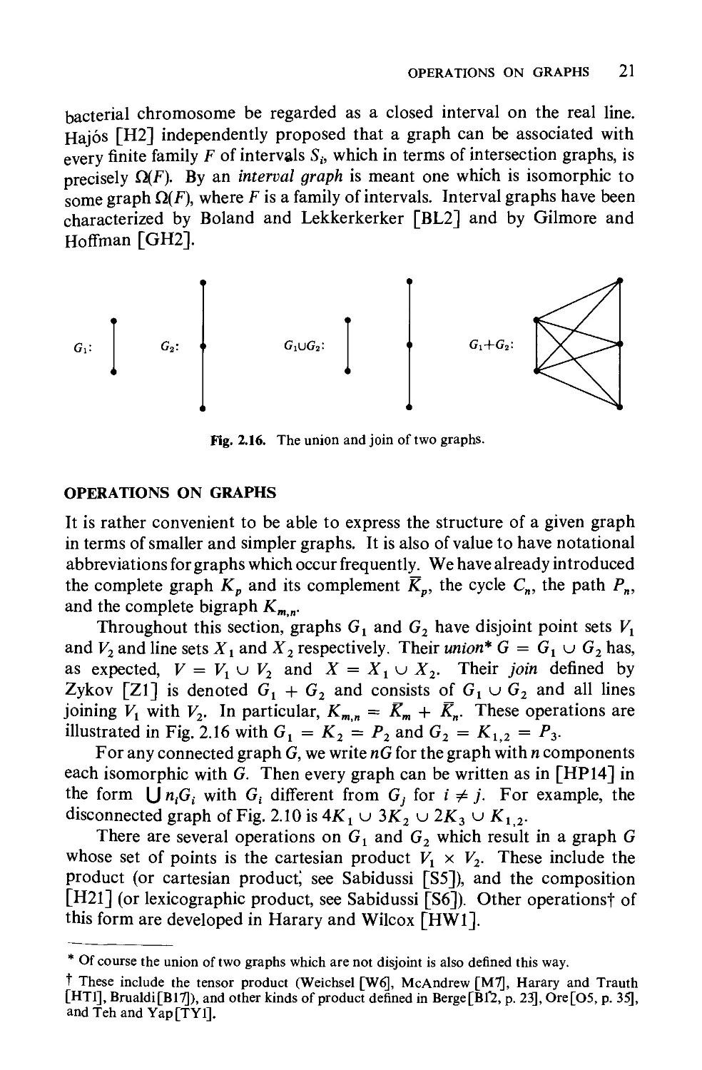
Fig. 2.16. The union and join of two graphs.
OPERATIONS ON GRAPHS
It is rather convenient to be able to express the structure of a given graph
in terms of smaller and simpler graphs. It is also of value to have notational
abbreviations for graphs which occurfrequently. We have already introduced
the complete graph Kp and its complement Kp, the cycle Cn, the path Pn,
and the complete bigraph Km.n.
Throughout this section, graphs G l and G 2 have disjoint point sets V l
and V 2 and line sets Xl and X 2 respectively. Their union* G = G l U G 2 has,
as expected, V = V l U V 2 and X = Xl U X 2 . Their join defined by
Zykov [Zl] is denoted G l + G 2 and consists of G l U G 2 and aIl lines
joining V l with V 2 . ln particular, Km.n = Km + Kn. These operations are
illustrated in Fig. 2.16 with G l = K 2 = P 2 and G 2 = Kl,2 = P 3 .
For any connected graph G, we write nG for the graph with n components
each isomorphic with G. Then every graph can be written as in [HP14] in
the form U nPi with G i different from G j for i #- j. For ex ample, the
disconnected graph of Fig. 2.10 is 4Kl U 3K 2 U 2K3 U K l . 2 .
There are several operations on Gland G 2 which result in a graph G
whose set of points is the cartesian product V l x V 2 . These include the
product (or cartesian product; see Sabidussi [S5]), and the composition
[H21] (or lexicographie product, see Sabidussi [S6]). Other operationst of
this form are developed in Harary and Wi1cox [HW1].
* Of course the union of two graphs which are not disjoint is also defined this way.
t These inc1ude the tensor product (Weichsel [W6], McAndrew [M7], Harary and Trauth
[HTl], Brualdi[Bl7]), and other kinds of product defined in Berge [Bf'2, p. 23], Ore [05, p. 35],
and Teh and Yap[TYl].
22 GRAPHS
Ut
G t : ] G 2 : u,
.
v,
(u" U2)
(u" V2)
(u" W2)
V2
.
W 2
.
G,XG 2 :
(v" U2)
(v" V2)
(v" W2)
Fig.2.17. The producl of Iwo graphs.
(U2, u,)
(V2' u,)
(u" U2)
G t [G 2 ]:
G 2 [G,):
(v!, V2) (v" W2)
Fig. 2.18. Two compositions of graphs.
To define the product G l x G 2 , consider any two points u = (u l , U2)
and v = (Vl, v 2 ) in V = V l X V 2 . Then u and v are adjacent in G l x G 2
whenever CUl = V l and u 2 adj V2] or [u 2 = v 2 and Ul adj Vl]. The product
of G l = P 2 and G 2 = P 3 is shown in Fig. 2.17.
The composition G = G l [G 2 ] also has V = V l X V 2 as its point set,
and U = (Ul, u 2 ) is adjacent with v = (v l , v 2 ) whenever CUl adj Vl] or
[u l = V l and u 2 adj V2]. For the graphs G l and G 2 of Fig. 2.17, both com-
positions G l [G 2 ] and G 2 [G l ], which are obviously not isomorphic, are
shown in Fig. 2.18.
If G l and G 2 are (Ph ql) and (P2, q2) graphs respectively, then for each of
the above operations, one can calculate the number of points and lines in the
resulting graph, as shown in the following table.
Table 2.2
BINARY OPERATIONS ON GRAPHS
Operation
Number of points
Number of lines
Union G 1 U G 2
Join G 1 + G 2
Product G 1 x G 2
Composition G 1 [G 2 ]
Pl + P2
Pl + P2
PtP2
PtP2
ql + q2
ql + q2 + PtP2
Plq2 + P2ql
Plq2 + P ql
EXERCISES 23
101
01 11
D 001
Q2: Q3:
()()()
00 10
100
Fig.2.19. Two cubes.
The complete n-partite graph K(Pl, P2, . . . , Pn) is defined as the iterated
join KpI + K P2 + . . . + Kpn' It obviously has Pi points and i<j PiPj
lines.
An especially important class of graphs known as cubes are most naturally
expressed in terms of products. The n-cube Qn is defined recursively by
Ql = K 2 and Qn = K 2 X Qn-l' Thus Qn has 2 n points which may be
labeled al a 2 . . . am where each ai is either 0 or 1. Two points of Qn are
adjacent if their binary representations differ at exactly one place. Figure
2.19 shows both the 2-cube and the 3-cube, appropriately labeled.
If Gand H are graphs with the property that the identification of any
point of G with an arbitrary point of H results in a unique graph (up to
isomorphism), then we write G . H for this graph. For ex ample, in Fig. 2.16
G 2 = K 2 . K 2 , while in Fig. 2.7 G - V 3 = K3. K 2 .
EXERCISES*
2.1 Draw ail graphs with five points. (Then compare with the diagrams given in
Appendix 1.)
2.2 Reconstruct the graph G from its subgraphs G i = G - Vi' where G 1 = K4 - X,
G 2 = P 3 U KI> G 3 = K 1 . 3 , G 4 = G s = Kl.3 + x.
2.3 A closed walk of odd length contains a cycle.*
2.4 Prove or disprove:
a) The union of any two distinct walks joining two points contains a cycle.
b) The union of any two distinct paths joining two points contains a cycle.
2.5. A graph G is connected if and only if for any partition of V into two subsets VI and
V 2 , there is a line of G joining a point of VI with a point of V 2 .
2.6 If d(u, v) = m in G, what is d(u, v) in the nth power Gn?
* Whenever a bald statement is made, it is to be proved. An exercise with number in bold face
is more difficult, and one which is also starred is most difficult.
24 GRAPHS
27 A graph H is a square root of G if H 2 = G. A graph G with P points has a square
root if and only if it contains P complete subgraphs G i such that
1. Vi E G i ,
2. Vi E G j if and only if v j E G t ,.
3. each line of Gis in some G t . (Mukhopadhyay [M18])
28 A finite met rie space (S, d) is isomorphic to the distance space of some graph if
and only if
1. The distance between any two points of S is an integer,
2. If d(u, v) 2, then there is a third point w such that d(u, w) + d(w, v) = d(u, v).
(Kay and Chartrand [KC1])
2.9 ln a connected graph any two longest paths have a point in common.
2.10 It is not true that in every connected graph ail longest paths have a point in
common. Verify that Fig. 2.20 demonstrates this. (Walther [W4])
Fig. 2.20. A counterexample for Exercise 2.10.
211 Every graph with diameter d and girth 2d + 1 is regular. (Singleton [S13])
2.12 Let G be a (p, q) graph ail of whose points have degree k or k + 1. If G has
Pk > 0 points of degree k and PH 1 points of degree k + l, then Pk = (k + l)p - 2q.
2.13 Construct a cubic graph with 2n points (n 3) having no triangles.
2.14 If G has P points and b(G) (p - 1)/2, then Gis connected.
2.15 If G is not connected then Gis.
2.16 Every self-complementary graph has 4n or 4n + 1 points.
2.17 Draw the four self-complementary graphs with eight points.
218 Every nontrivial self-complementary graph has diameter 2 or 3.
(Ringel [Rll], Sachs [S8])
2.19 The Ramsey numbers satisfy the recurrence relation,
rem, n) :S rem - 1, n) + rem, n - 1).
(Erd6.s [E4])
2.20 Find the maximum number of Hnes in a graph with p points and no even cycles.
EXERCISES 25
2.21 Find the extremal graphs which do not con tain K4'
2.22 Every (p, p + 4) graph contains two line-disjoint cycles.
2.23 The only (p, [p2j4]) graph with no triangles is K([pj2], {pj2}).
2.24 Prove or disprove: The only graph on p points with maximum intersection number
is K([Pj2], {pj2}).
2.25 The smallest graph having every line in at least two triangles but some line in no
K4 has 8 points and 191ines. Construct il. (J. Cameron and A. R. Meetham)
2.26 Determine w(K p ), w(C n + KI), w(C n + CJ, and w(CJ.
2.27 Prove or disprove:
(Turan [T3])
(Erdos [E3])
a) The number of cliques of G does not exceed w(G).
b) The number of cliques of Gis not less than w(G).
2.28 Prove that the maximum number of cliques in a graph with p points where
p - 4 = 3r + s, s = 0, 1 or 2, is 2 2 -'3'+'. (Moon and Moser [MM1])
2.29 A cycle of length 4 cannot be an induced subgraph of an interval graph.
2.30 Let sen) denote the maximum number of points in the n-cube which induce a
cycle. Verify the following table:
n 234 5
sen)
4 6 8 14
(Danzer and Klee [DKl])
2.31 Prove or disprove: If G l and G 2 are reguiar, then so is
a) G l + G 2 . b) G l X G 2 . c) G l [G 2 ].
2.32 Prove or disprove: If G l and G 2 are bipartite, then so is
a) G l + G 2 . b) G 1 X G,. c) G l [G 2 ].
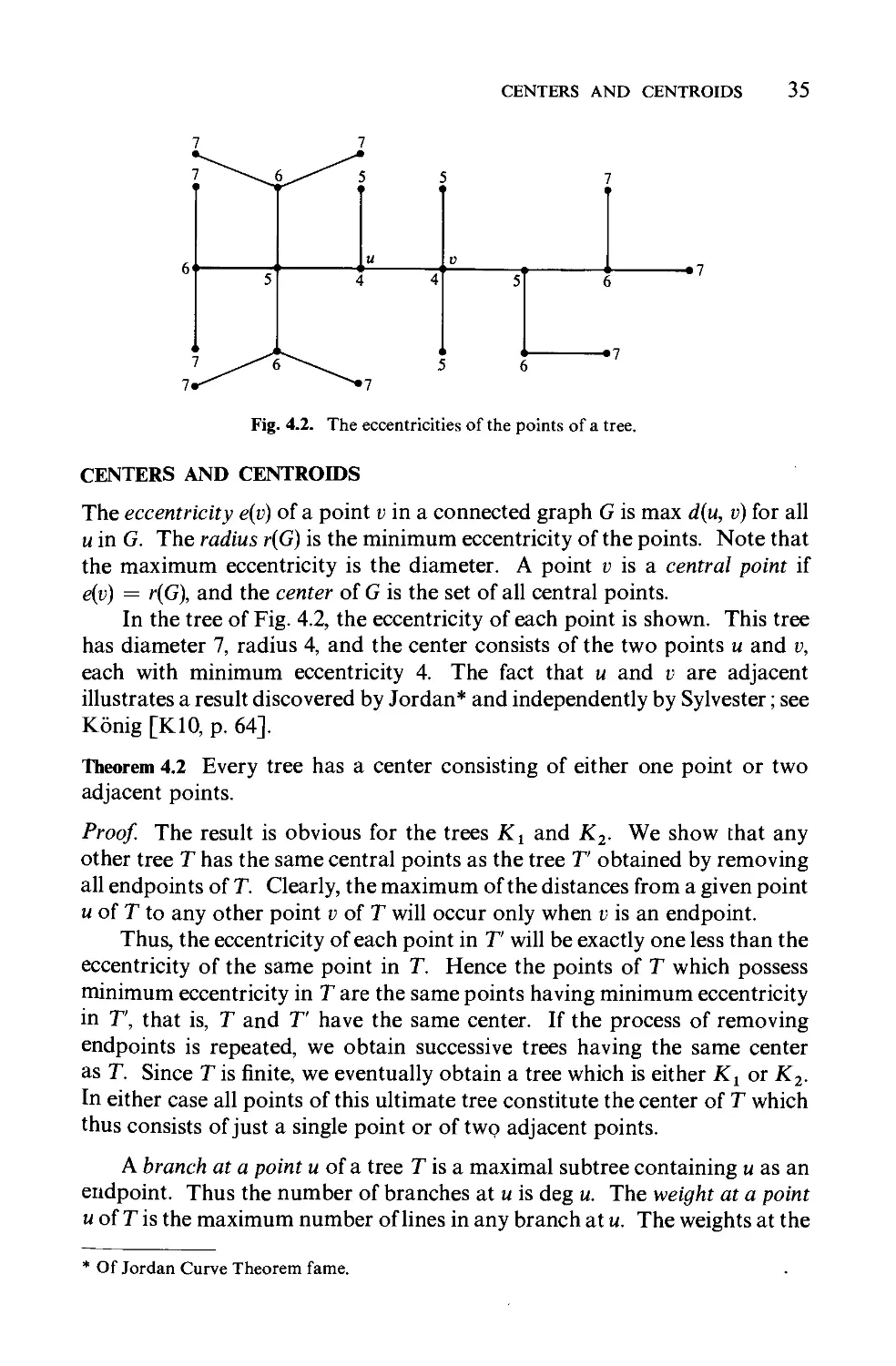
2.33 Pro ve or dis prove:
a) G l + G 2 = G l + G 2 . b) G l X G 2 = G l X G 2 . c) G l [G 2 ] = G l [G 2 ].
2.34 a) Calculate the number of cycles in the graphs (a) C n + KI> (b) Kp, (c) Km.n.
(Harary and Manvel [HMl])
b) What is the maximum number of line-disjoint cycles in each of these three
graphs? (Chartrand, Geller, and Hedetniemi [CGH2])
2.35 The conjunction G 1 1\- G 2 has VI x V 2 as its point" set and U = (u l , u 2 ) is adjacent
to v = (VI' V 2 ) whenever U l adj VI and U 2 adj V 2 . Then G l x G 2 G l 1\ G 2 if and
only if G l G 2 C 2m +1' (Miller [MIl])
2.36 The conjunction G 1 1\ G 2 of two connected graphs is connected if and only if
G 1 or G 2 has an odd cycle.
*2.37 There exists a regular graph of degree r with r + 1 points and diameter 2 only
for r = 2,3,7, and possibly 57. (Hoffman and Singleton [HSl])
*2.38 A graph G ith p = 2n has the property that for every set S of n points, the
induced subgraphs (S) and (V - S) are isomorphic if and only if G is one of the
following: K 2n , Kn x K2' 2Kn> 2C 4 , and their complements.
(Kelly and Merriell [KMl])
CHAPTER 3
BLOCKS
Not merely a chip of the old block,
but the old block itself.
EDMUND BURKE
Some connected graphs can be disconnected by the removal of a single
point, called a cutpoint. The distril;mtion of such points is of considerable
assistance in the recognitioIf of the structure of a connected graph. Lines
with the analogous cohesive property are known as bridges. The fragments
of a graph held together by its cutpoints are its blocks. After characterizing
these three concepts, we study two new graphs associated with a given
graph: its block graph and its cutpoint graph.
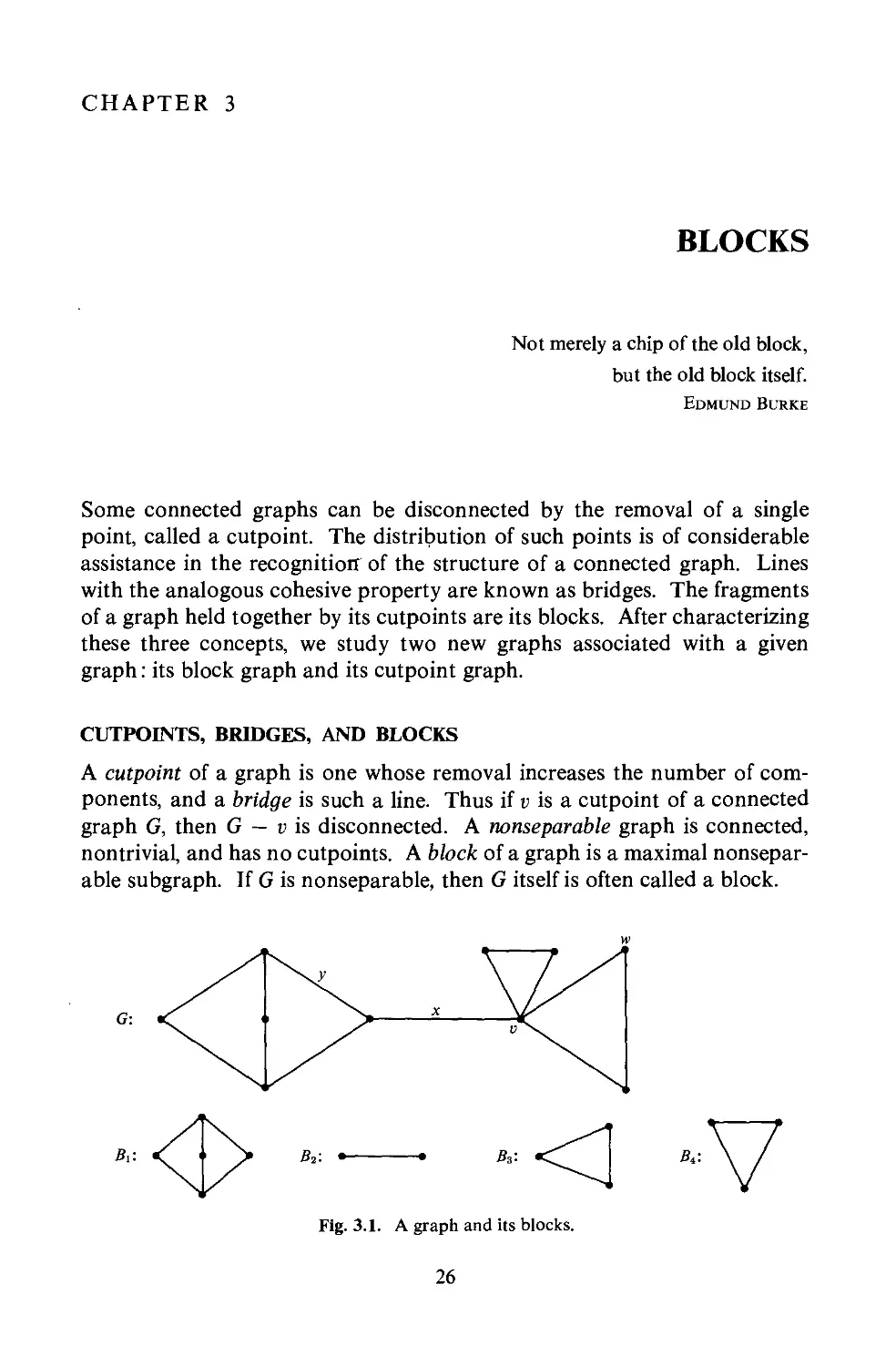
CUTPOINTS, BRIDGES, AND BLOCKS
A cutpoint of a graph is one whose removal increases the number of com-
ponents, and a bridge is such a line. Thus if v is a cutpoint of a connected
graph G, then G - v is disconnected. A nonseparable graph is connected,
nontrivial, and has no cutpoints. A block of a graph is a maximal nonsepar-
able subgraph. If G is nonseparable, then G itself is often called a block.
w
G:
x
B'<}>
D 2 : ·
.
D3: <J
B., \7
Fig. 3.1. A graph and its blocks.
26
CUTPOINTS, BRIDGES, AND BLOCKS 27
ln Fig. 3.1, v is a cutpoint while w is not ; x is a bridge but y is not; and
the four blocks of Gare displayed. Each line of a graph lies in exactly one
ofits blocks, as does each point which is not isolated or a cutpoint. Further-
more, the lines of any cycle of G also lie entirely in a single block. Thus in
particular, the blocks of a graph partition its lines and its cycles regarded
as sets of lines. The first three theorems of this chapter present several
equivalent conditions for each of these concepts.
Theorem 3.1 Let v be a point of a connected graph G. The following state-
ments are equivalent :
(1) v is a cutpoint of G.
(2) There exist points u and w distinct from v such that v is on every u-w
path.
(3) There exists a partition of the set of points V - {v} into subsets U and
W such that for any points u E U and w E W, the point v is on every
u-w path.
Proof (1) implies (3) Since v is a cutpoint of G, G - vis disconnected and has
at least two components. Form a partition of V - {v} by letting U consist
of the points of one of these components and W the points of the others.
Then any two points u E U and w E W lie in different components of G - v.
Therefore every u-w path in G con tains v.
(3) implies (2) This is immediate since (2) is a special case of (3).
(2) implies (1) If v is on every path in G joining u and w, then there cannot be
a path joining these points in G - v. Thus G - v is disconnected, so v is a
cutpoint of G.
Theorem 3.2 Let x be a line of a connected graph G. The following statements
are equivalent :
(1) x is a bridge of G.
(2) x is not on any cycle of G.
(3) There exist points u and v of G such that the line x is on every path
joining u and v.
(4) There exists a partition of V into subsets U and W such that for any
points u E U and w E W, the line x is on every path joining u and w.
Theorem 3.3 Let G be a connected graph with at least three points. The
following statements are equivalent:
(1) Gis a block.
(2) Every two points of G lie on a common cycle.
(3) Every point and line of G lie on a common cycle.
28 BLOCKS
(4) Every two lines of G lie on a common cycle.
(5) Given two points and one line of G, there is a path joining the points
which contains the line.
(6) For every three distinct points of G, there is a path joining any two of
them which contains the third.
(7) For every three distinct points of G, there is a path joining any two of
them which does not contain the third.
Proof (1) implies (2) Let u and v be distinct points of G, and let U be the set of
points different from u which lie on a cycle containing u. Since G has at
least three points and no cutpoints, it has no bridges; therefore, every point
adjacent to u is in U, so U is not empty.
u
w
Po
u
P'
Pl
v
v
P 2
(a)
Fig. 3.2. Paths in blocks.
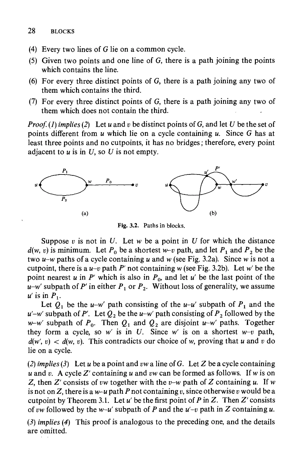
Suppose v is not in U. Let w be a point in U for which the distance
d( w, v) is minimum. Let Po be a shortest w-v path, and let Pl and P 2 be the
two u-w paths of a cycle containing u and w (see Fig. 3.2a). Since w is not a
cutpoint, there is a u-v path P' not containing w (see Fig. 3.2b). Let w' be the
point nearest u in P' which is also in Po, and let u' be the last point of the
u-w' subpath of P' in either Pl or P 2. Without loss of generality, we assume
u' is in Pl.
Let Ql be the u-w' path consisting of the u-u' subpath of Pl and the
u'-w' subpath of P'. Let Q2 be the u-w' path consisting of P 2 followed by the
w-w' subpath of Po. Then Qi and Q2 are disjoint u-w' paths. Together
they form a cycle, so w' is in U. Since w' is on a shortest w-v path,
d(w', v) < d(w, v). This contradicts our choice of w, proving that u and v do
lie on a cycle.
(2) implies (3) Let u be a point and vw a line of G. Let Z be a cycle containing
u and v. A cycle Z' containing u and vw can be formed as follows. If w is on
Z, then Z' consists of vw together with the v-w path of Z containing u. If w
is not on Z, there is a w-u path P not containing v, since otherwise v would be a
cutpoint by Theorem 3.1. Let u' be the first point of Pin Z. Then Z' consists
of vw followed by the w-u' subpath of P and the u'-v path in Z containing u.
(3) implies (4) This proof is analogous to the preceding one, and the details
are omitted.
BLOCK GRAPHS AND CUTPOINT GRAPHS 29
(4) implies (5) Any two points of G are incident with one line each, which lie on
a cycle by (4). Hence any two points of G lie on a cycle, and we have (2), so
also (3). Let u and v be distinct points and x a line of G. By statement (3), there
are cycles Z l containing u and x, and Z 2 containing v and x. If v is on Z 1 or
u is on Z2, there is clearly a pathjoining u and v containing x. Thus, we need
only consider the case where v is not on Zl and u is not on Z2. Begin with
u and proceed along Z l until reaching the first point w of Z2' then take the
path on Z2 joining w and v which contains x. This walk constitutes a path
joining u and v that contains x.
(5) implies (6) Let u, v, and w be distinct points of G, and let x be any line in-
cident with w. By (5), there is a path joining u and v which contains x, and
hence must contain w.
(6) implies (7) Let u, v, and w be distinct points of G. By statement (6), there
is a u-w path P containing v. The u-v subpath of P does not contain w.
(7) implies (1) By statement (7), for any two points u and v, no point lies on
every u-v path. Hence, G must be a block.
Theorem 3.4 Every nontrivial connected graph has at least two points
which are not cutpoints.
Proof Let u and v be points at maximum distance in G, and assume v is a
cutpoint. Then there is a point w in a different component of G - v than u.
Hence v is in every path joining u and w, so d(u, w) > d(u, v), which is im-
possible. Therefore v and similarly u are not cutpoints of G.
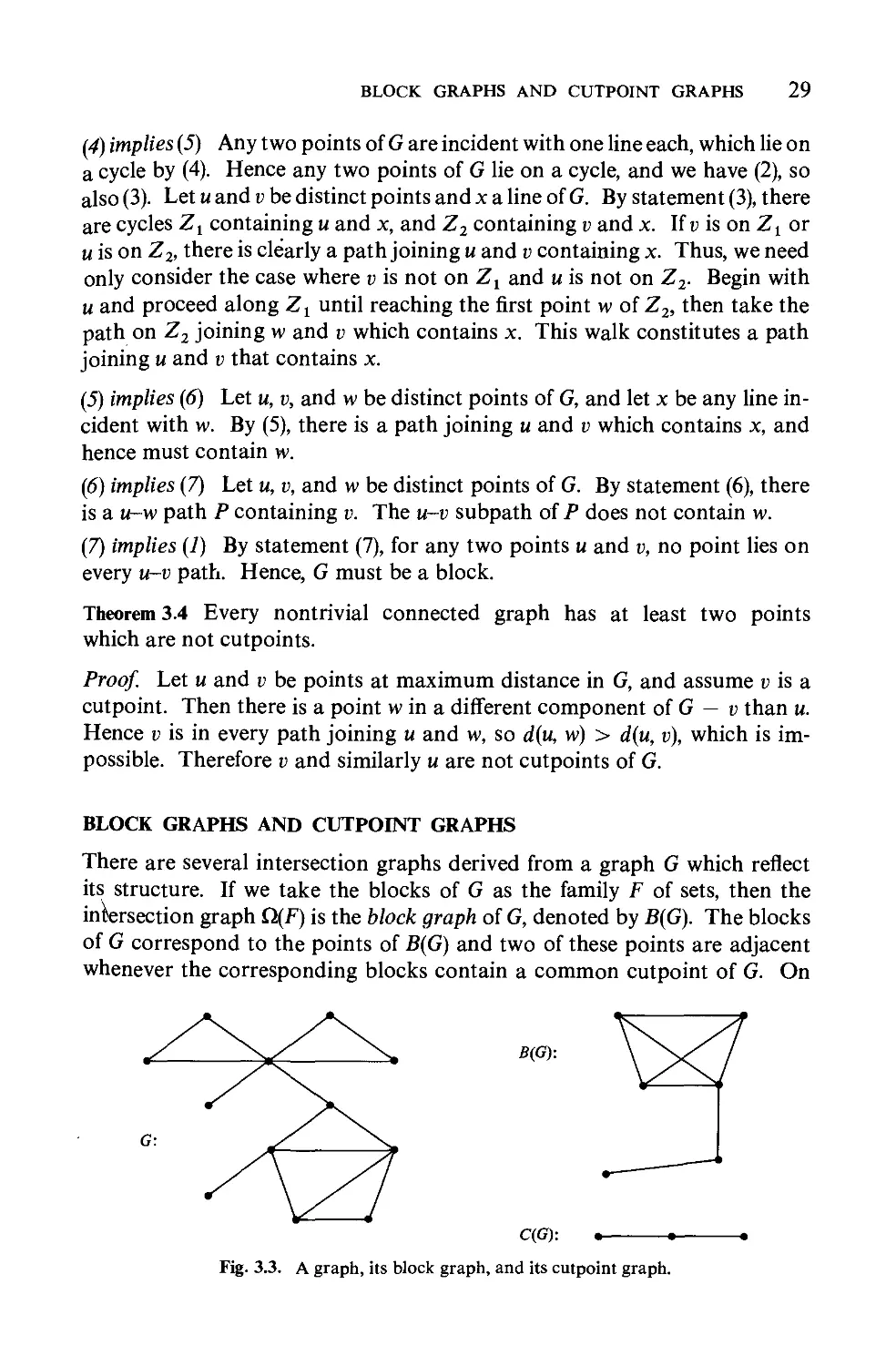
BLOCK GRAPHS AND CUTPOINT GRAPHS
There are several intersection graphs derived from a graph G which reflect
its structure. If we take the blocks of G as the family F of sets, then the
intersection graph Q(F) is the block graph of G, denoted by B(G). The blocks
of G correspond to the points of B(G) and two of these points are adjacent
whenever the corresponding blocks contain a common cutpoint of G. On
O(G):
C(G):
.
.
.
Fig. 3.3. A graph, its block graph, and its cutpoint graph.
30 BLOCKS
the other han d, to obtain a graph whose points correspond to the cutpoints
of G, we can take the sets Si to be the union of aIl blocks which contain the
cutpoint Vi. The resulting intersection graph Q(F) is called the cutpoint
graph, qG). Thus two points of qG) are adjacent if the cutpoints of G to
which they correspond lie on a common block. Note that qG) is defined
only for graphs G which have at least one cutpoint. Figure 3.3 illustrates
these concepts, which were introduced in [H28].
Theorem 3.5 A graph H is the block graph of some graph if and only if every
block of H is complete.
Proof Let H = B(G), and assume there is a block Hi of H which is not
complete. Then there are two points in Hi which are nonadjacent and lie on
a common cycle Z of length at least 4. But the union of the blocks of G
corresponding to the points of Hi which lie on Z is then connected and has no
cutpoint, so it is itself contained in a block, contradicting the maximality
property of a block of a graph.
On the other han d, let H be a given graph in which every block is com-
plete. Form B(H), and then form a new graph G by adding to each point Hi
of B(H) a number of endlines equal to the number of points of the block Hi
which are not cutpoints of H. Then it is easy to see that B(G) is isomorphic
to H.
Clearly the same criterion also characterizes cutpoint graphs.
EXERCISES
3.1 What is the maximum number of cutpoints in a graph with p points?
3.2 A cubic graph has a cutpoint if and only if it has a bridge.
3.3 The smallest number of points in a cubic graph with a bridge is 10.
3.4 If v is a cutpoint of G, then v is not a cutpoint of the complement G.
(Harary [H15])
3.5 A point v of G is a cutpoint if and only if there are points u and w adjacent to
v such tOOt v is on every u-w path.
3.6 Prove or disprove: A connected graph G with p 3 is a block if and only if
given any two points and one line, there is a path joining the points which does not
contain the line.
3.7 A connected graph with at least two lines is a block if and only if any two adjacent'
lines lie on a cycle.
3.8 Let G be a connected graph with at least three points. The following statements
are equivalent:
1. G has no bridges.
2. Every two points of G lie on a common closed trail.
3. Every point and line of G lie on'a common closed traii.
EXER CISES 31
4. Every two lines of G lie on a common closed trail.
5. For every pair of points and every line of G, there is a trail joining the points
which contains the line.
6. For every pair of points and every line of G, there is a path joining the points
which does not contain the line.
7. For every three points there is a trail joining any two which contains the third.
3.9 If G is a block with b 3, then there is a point v such that G - v is also a block.
(A. Kaugars)
3.10 The square of every nontrivial connected graph is a block.
3.11 If G is a connected graph with at least one cutpoint, then B(B(G» is isomorphic
to qG).
3.12 Let b(v) be the number of blocks to which point v belongs in a connected graph
G. Then the number of blocks of G is given by
b(G) - 1 = L [b(v) - 1]. (Harary [H22])
3.13 Let c(B) bethe number of cutpoints of a connected graph G which are points of
the block B. Then the number of cutpoints of G is given by
c(G) - 1 = L [c(B) - 1]. (Gallai [Œ])
3.14 A block G is line-critical if every subgraph G - x is not a block. A diagonal of G
is a line joining two points of a cycle not containing il. Let G be a line-critical block
with p 4.
a) G has no diagonals.
b) G contains no triangles.
c) p q 2p - 4.
d) The removal of ail points of degree 2 results in a disconnected graph, provided
G is not a cycle. (Plummer [P4])
CHAPTER 4
TREES
Poems are made by fools like me,
But only God can make a tree.
JOYCE KILMER
There is one simple and important kind of graph which has been given the
same name by aIl authors, namely a tree. Trees are important not only for
sake of their applications to many different fields, but also to graph theory
itself. One reason for the latter is that the very simplicity of trees make it
possible to investigate conjectures for graphs in general by first studying
the situation for trees. An example is provided by Ulam's conjecture
mentioned in Chapter 2.
Several ways of defining a tree are developed. Using geometric termin-
ology, we study centrality of trees. This is followed by a discussion of a tree
which is naturally associated with every connected graph: its block-cutpoint
tree. Finally, we see how each spanning tree of a graph G gives ri se to a
collection of independent cycles of G, and mention the dual (complementary)
construction of a collection of independent cocycles from each spanning
cotree.
CHARACTERIZATION OF TREES
A graph is acyclic if it has no cycles. A tree is a connected acyclic graph. 'Any
graph without cycles is a forest, thus the components of a forest are trees.
There are 23 different trees* with eight points, as shown in Fig. 4.1. There
are numerous ways of defining trees, as we shall now see.
Theorem 4.1 The following statements are equivalent for a graph G:
(1) Gis a tree.
(2) Every two points of Gare joined by a unique path.
* It is interesting 1.0 ask people to draw the trees with eight points. Some trees will frequently
be missed and others duplicated.
32
CHARACTERIZATION OF TREES 33
.-000000 ° l ° 000 0 --1(
-r--r !TT -r-r-
------c- l-:-: ° --+r *-
-1 ° 0 0 · -+---- +--r *
TL --b -rt
Fig. 4.1. The 23 trees with eight points.
(3) G is connected and p = q + 1.
(4) Gis acyclic and p = q + 1.
(5) Gis acyclic and if any two nonadjacent points of Gare joined by a line x,
then G + x has exacdy one cycle.
(6) Gis connected, is not Kp for p 3, and if any two nonadjacent points
of G are joined by a line x, then G + x has exactly one cycle.
(7) Gis not K3 u KI or K3 u K 2 , P = q + 1, and if any two nonadjacent
points of Gare joined by a line x, then G + x has exactly one cycle.
Proof (1) implies (2) Since G is connected, every two points of Gare joined by
a path. Let Pl and P 2 be two distinct paths joining u and v in G, and let w
be the first point on Pl (as we traverse Pl from u to v) such that w is on both
Pl and P 2 but its successor on Plis not on P 2. If we let w' be the next point
on Pl which is also on P 2, then the segments of P land P 2 which are between
w and w' together form a cycle in G. Thus if Gis acyclic, there is at most one
path joining any two points.
(2) implies (3) Oearly Gis connected. We prove p = q + 1 by induction. Il
is obvious for connected graphs of one or two points. Assume it is true
for graphs with fewer than p points. If G has p points, the remova1 of any
line of G disconnects G, because of the uniqueness of paths, and in fact this
new graph will have exactly two components. By the induction hypothesis
each component has one more point than line. Thus the total number of
1ines in G must be p - 1.
(3) implies (4) Assume that G has a cycle oflength n. Then there are n points
and n 1ines on the cycle and for each of the p - n points not on the cycle,
34 TREES
there is an incident line on a geodesic to a point of the cycle. Each such line
is different, so q 2 p, which is a contradiction.
(4) implies (5) Since G is acyclic, each component of Gis a tree. Ifthere are k
components, then, since each one has one more point than line, p = q + k, so
k = 1 and G is connected. Thus G is a tree and there is exactly one path
connecting any two points of G. If we add a line uv to G, that line, together
with the unique path in G joining u and v, forms a cycle. The cycle is unique
because the path is unique.
(5) implies (6) Since every Kp for p 2 3 con tains a cycle, G cannot be one of
them. Graph G must be connected, for otherwise a line x could be added
joining two points in different components of G, and G + x would be
acyclic.
(6) implies (7) We prove that every two points of Gare joined by a unique
path and thus, because (2) implies (3), p = q + 1. Certainly every two points
ofG arejoined by some path. Iftwo points of G arejoined by two paths, then
by the proof that (1) implies (2), G has a cycle. This cycle cannot have four or
more points because, if it did, then we could produce more than one cycle
in G + x by taking x joining two nonadjacent points on the cycle (if there
are no nonadjacent points on the cycle, then G itself has more than one
cycle). So the cycle is K 3 , which must be a proper subgraph of G since by
hypothesis G is not complete with p 2 3. Since G is connected, we may
assume there is another point in G which is joined to a point of this K3'
Then it is clear that if any line can be added to G, then one may be added so as
to form at least two cycles in G + x. If no more lines may be added, so- that
the second condition on G is trivially satisfied, then G is Kp with p 2 3,
contrary to hypothesis.
(7) implies (1) If G has a cycle, that cycle must be a triangle which is a com-
ponent of G, by an argument in the preceding paragraph. This component
has three points and three lines. AlI other components of G must be trees
and, in order to make p = q + 1, there can be only one other component. If
this tree contains a path oflength 2, it will be possible to add a line x to Gand
obtain two cycles in G + x. Thus this tree must be either K 1 or K 2 . So
G must be K3 u KI or K3 u K 2 , which are the graphs which have been
excluded. Thus G is acyclic. But if G is acyclic and p = q + 1, then G is
connected since (4) implies (5) implies (6). So Gis a tree, and the theorem is
proved.
Because a nontrivial tree has L di = 2q = 2(p -'- 1), there are at least
two points with degree less than 2.
CoroUary 4.1(a) .Every nontrivial tree has at least two endpoints.
This result also follows from Theorem 3.4.
CENTERS AND CENTROIDS 35
7 7
7 6 5 5 7
6 u v
5 4 4 5 6 7
7 6 5 7
6
7 7
Fig.4.2. The eccentricities of the points of a tree.
CENTERS AND CENTROIDS
The eccentricity e(v) of a point v in a connected graph G is max d(u, v) for aIl
u in G. The radius r(G) is the minimum eccentricity of the points. Note that
the maximum eccentricity is the diameter. A point v is a central point if
e(v) = r(G), and the center of Gis the set of aIl central points.
ln the tree of Fig. 4.2, the eccentricity of each point is shown. This tree
has diameter 7, radius 4, and the center consists of the two points u and v,
each with minimum eccentricity 4. The fact that u and v are adjacent
illustrates a result discovered by Jordan* and independently by Sylvester; see
Kônig [KlO, p. 64].
Theorem 4.2 Every tree has a center consisting of either one point or two
adjacent points.
Proo! The result is obvious for the trees KI and K 2 . We show that any
other tree T has the same central points as the tree T' obtained by removing
aIl endpoints of T. Clearly, the maximum of the distances from a given point
u of T to any other point v of Twill occur only when v is an endpoint.
Thus, the eccentricity of each point in T' will be exactly one less than the
eccentricity of the same point in T. Rence the points of T which possess
minimum eccentricity in T are the same points having minimum eccentricity
in T', that is, T and T' have the same center. If the process of removing
endpoints is repeated, we obtain successive trees having the same center
as T. Since T is finite, we eventually obtain a tree which is either KI or K 2 .
ln either case aIl points of this ultimate tree constitute the center of T which
thus consists of just a single point or of tWQ adjacent points.
A branch at a point u of a tree T is a maximal subtree containing u as an
endpoint. Thus the number of branches at u is deg u. The weight at a point
u of T is the maximum number oflines in any branch at u. The weights at the
* Of Jordan Curve Theorem fame.
36 TREES
9 12
Fig. 4.3. The weights at the points of a tree.
nonendpoints of the tree in Fig. 4.3 are indicated. Of course the weight at
each end point is 14, the number oflines.
A point v is a centroid point of a tree T if v has minimum weight, and the
centroid of T consists of aIl such points. Jordan [12J also proved a theorem
on the centroid of a tree analogous to his result for centers.
Theorem 4.3 Every tree has. a centroid consisting of either one point or two
adjacent points.
The smallest trees with one and two central and centroid points are
shown in Fig. 4.4.
Center 2
2
. . . <
. . . < --
Centroid
Fig. 4.4. Trees with ail combinations of one or two central and centroid points.
BLOCK-CUTPOINT TREES
It has often been observed that a connected graph with many cutpoints
bears a resemblance to a tree. This idea can be made more definite by as-
sociating with every connected graph a tree which displays the resemblance.
For a connected graph G with blocks {BJ and cutpoints {Cj}, the
block-cutpoint graph of G, denoted by bc(G), is defined as the graph having
point set {BJ U {c j }, with two points adjacent if one corresponds to a block
Bi and the other to a cutpoint Cj and Cj is in Bi. Thus bc(G) is a bigraph. This
concept was introduced in Harary and Prins [HP22J and also in Gallai
[G3]. (See Fig. 4.5.)
INDEPENDENT CYCLES AND COCYCLES 37
bc(G):
Fig.4.5. A graph and its block-cutpoint graph.
Theorem 4.4 A graph G is the block-cutpoint graph of some graph H if
and only if it is a tree in which the distance between any two endpoints is
even.
ln view ofthis theorem, we will speak of the block-cutpoint tree of a graph.
INDEPENDENT CYCLES AND COCYCLES
We describe two vector spaces associated with a graph G: its "cycle space"
and "cocycle space." For convenience, these two vector spaces will be taken
over the two element field F 2 = {O, 1}, in which 1 + 1 = 0 (even though
the theory can be modified to ho Id for an arbitrary field). ln particular, the
Bi which occur repeatedly in the following definitions are always either 0 or 1.
As usual, let G be a graph with points VI> . . . , v p and lines XI> . . . , Xq'
A O-chain of G is a formallinear combination L BiVi of points and a J -chain
is a sum L BiXi of lines. The boundary operator a sends 1-chains to O-chains
according to the mIes:
a) ais linear.
b) if x = UV, then OX = u + v.
On the other hand, the coboundary operator c5 sends O-chains to 1-chains by
the mIes:
a) c5 is linear.
b) c5v = L BiXi, where Bi = 1 whenever Xi is incident with v.
38 TREES
VI
V.
Fig. 4.6. A graph to illustrate the boundary and coboundary operators.
ln Fig. 4.6, the 1-chain 0"1 = Xl + X2 + X4 + X 9 has boundary
00"1 = (VI + V2) + (VI + V3) + (V2 + V 4 ) + (V 5 + V 6 )
= V3 + v 4 + v 5 + V 6 ,
and the O-chain 0"0 = V3 + V4 + V 5 + V 6 has as its coboundary
150"0 = (X2 + X3 + X 6 + X7) + (x 4 + Xg)
+ (x 5 + X6 + Xg + x 9 ) + (X7 + x 9 )
= X2 + X3 + X 4 + X 5 .
Al-chain with boundary 0 is a cycle vector* of Gand can be regarded as
a set of line-disjoint cycles. The collection of aIl cycle vectors forms a vector
space over F 2 called the cycle space of G. A cycle basis of G is defined as a
basis for the cycle space of G which consists entirely of cycles. We say a
cycle-vector Z depends on the cycles Zb Z2, . . ., Zk if it can be written
as L = 1 BiZ i . Thus a cycle basis of G is a maximal collection of independent
cycles of G, or a minimal collection of cycles on which aIl cycles depend.
A cutset of a connected graph is a collection of lines whose removal
results in a disconnected graph. A cocycle is a minimal cutset. A coboundary
of Gis the coboundary of some O-chain in G. The coboundary of a collection
U of points is just the set of alllines joining a point in U to a point not in
U. Thus every coboundary is a cutset. Since we define a cocycle as a minimal
cutset of Gand any minimal cutset is a coboundary, we see that a cocycle
is just a minimal nonzero coboundary. The collection of aIl coboundaries
of G is called the cocycle space of G, and a basis for this space which consists
entirely of cocycles is called a co cycle basis for G.
We proceed to construct for the cycle space of G a basis which corre-
sponds to a spanning tree T. ln a connected graph G, a chord of a spanning
tree T is a line of G which is not in T. Clearly the subgraph of G consisting
of T and any chord of T has exactly one cycle. Moreover, the set Z(T)
* Most topologists and some graph theorists cali this a "cycle." They then use "circuits" or
"elementary cycles" or "polygons" for our cycles.
INDEPENDENT CYCLES AND COCYCLES 39
.
T*: .
/
.
.
Fig. 4.7. Graph, tree, and cotree.
21 / / .,
.
.
v
. .
./\
Fig. 4.8. A cocycle basis for G of Fig. 4.7.
of cycles obtained in this way (one from each chord) is independent, since
each contains a line not in any of the others. Also, every cycle Z depends
on the set Z(T), for Z is the symmetric difference of the cycles determined by
the chords of T which lie in Z. Thus if we define m(G), the cycle rank, to be
the number of cycles in a basis for the cycle space of G, we have the following
result.
Theorem 4.5 The cycle rank of a connected graph G is equal to the number
of chords of any spanning tree in G.
CoroUary 4.5(a) If Gis a connected (p, q) graph, then m(G) = q - p + 1.
Corollary 4.5(b) If G is a (p, q) graph with k components, then
m( G) = q - p + k.
Similar results are true for the cocycle space. The cotree T* of a spanning
tree T in a connected graph G is the spanning subgraph of G containing
exactly those lines of G which are not in T. A cotree of G is the cotree of
some spanning tree T. ln Fig. 4.7, a spanning tree T and its cotree T*
are displayed for the same graph G as in Fig. 4.6. The lines of G which are
not in T* are called its twigs. The subgraph of G consisting of T* and any
one of its twigs con tains exactly one cocycle. The collection of cocycles
obtained by adding twigs to T*, one at a time, is seen to be a basis for the
cocycle space of G. This is illustrated in Fig. 4.8 for the graph Gand cotree
T* of Fig. 4.7, with the cocycles indicated by heavy lines. The cocycle rank
m*(G) is the number of cocycles in a basis for the cocycle space of G.
40 TREES
Theorem 4.6 The cocycle rank of a connected graph G is the number of
twigs in any spanning tree of T.
As in the case of cycles, we have two immediate corollaries.
CoroUary 4.6(a) If Gis a connected (p, q) graph, then m*(G) = p - 1.
CoroUary4.6(b) IfGisa(p, q)graphwithkcomponents,thenm*(G) = p - k.
Excursion
The 1-dimensional case of an important general result about simplicial
complexes can be derived from Theorem 4.5. The Euler-Poincaré equation
CX o - CX1 + CX 2 - . . . = /30 - /31 + /32 - . . . ,
where the /3n are the Betti numbers and the CX n are the numbers of simplexes
of each dimension, holds for every simplicial complex. By definition, /3n is
the rank of the vector space of n-dimensional cycles. Recall from Chapter 1
that every graph is a simplicial complex, with its points O-simplexes and its
lines l-simplexes. For a graph, /30 = k, the number of connected components,
and /31 = m(G), the number of independent cycles of G. Since no graph
contains an n-simplex with n > 1, CX n = /3n = 0, for aIl n > 1. Thus
CX o - CX1 = /30 - /31 so P - q = k - m(G) and we see that Corollary 4.5(b)
is the Euler-Poincaré equation for graphs.
MATROIDS
This subject was first introduced by Whitney [W15]. A discussion of the
basic properties ofmatroids, as weIl as several equivalent axiomatic formula-
tions, may be found in Whitney's original paper.
A matroid consists of a finite set M of elements together with a family
rc = {C 1> C 2 , . . .} of nonempty subsets of M, called circuits, satisfying the
axioms :
1. no proper subset of a circuit is a circuit;
2. if x E CI n C 2 , then CI U C 2 - {x} contains a circuit.
With every graph G, one can associate a matroid by taking its set X of
lines as the set M, and its cycles as the circuits. It is easily seen that the two
axioms are satisfied. It is slightly less obvious that G yields another matroid
by taking the cocycles of G as the circuits. These are called respectively the
cycle matroid and the cocycle matroid of G.
Another, equivalent, definition of matroid is as follows. A matroid
consists of a finite set M of elements together with a family of subsets of M
called independent sets such that:
1. the empty set is independent;
MATROIDS 41
2. every subset of an independent set is independent;
3. for every subset A of M, aIl maximal independent sets contained in A
have the same number of elements.
A graph G yields a matroid in this sense by taking the lines of G as set
M and the acyclic subgraphs of G as the independent sets.
The duality (cycles ys. cocycles, trees ys. cotrees) which appears in the
preceding section is closely related to duality in matroids. Minty [M12J
constructed a self-dual axiom system for "graphoids" which displays matroid
duality explicitly.
A graphoid consists of a set M of elements together with two collections
rc and Çfi ofnonempty subsets of M, called circuits and cocircuits respectively,
such that:
1. for any C E rc and D E Çfi, 1 C n DI =f- 1;
2. no circuit properly contains another circuit and no cocircuit properly
contains another cocircuit:
3. for any painting of M which col ors exactly one element green and the
rest either red or blue, there exists either
a) a circuit C containing the green element and no red elements, or
b) a cocircuit D containing the green element and no blue elements.
While the cycles of every graph form a matroid, not every matroid can
so arise from a graph, as we shall see in Chapter 14. Two comprehensive
references on matroid theory are Minty [M12J and Tutte [T19J.
Excursion
Ulam's conjecture is still as unsolved as ever for arbitrary graphs. But
Kelly [K5J proved its validity for trees. As we have se en, the point of view
toward this conjecture proposed in [H29J is that if G has p 3 and one is
presented with the p unlabeled subgraphs G i = G - Vi' then the graph G
itself can be reconstructed uniqjlely from the G i . Kelly's result for trees
was extended in [HP6J where it is shown that every non trivial tree T can be
reconstructed from only those subgraphs 1; = T - Vi which are themselves
trees, that is, such that Vi is an end point. This has been improved, in turn, by
Bondy, who showed [BI5J that a tree T can be reconstructed from its
subgraphs T - Vi with the Vi the peripheral points, those whose eccentricity
equals the diameter of T. Manvel [M2J then showed that almost* every tree
T can be reconstructed using only those subtrees T - Vi which are non-
isomorphic. Another class of graphs has been reconstructed by Manvel
[M3J, namely unicyclic graphs, which are connected and have just pne cycle.
* With just two pairs of exceptional trees.
42 TREES
EXERCISES
4.1 Draw ail trees with nine points. Then compare your diagrams with those in
Appendix II.
4.2 Every tree is a bigraph. Which trees are complete bigraphs?
4.3 The following four statements are equivalent.
(1) G is a forest.
(2) Every line of G is a bridge.
(3) Every block of Gis K 2 .
(4) Every nonempty intersection of two connected subgraphs of G is connected.
4.4 The following four statements are equivalent.
(1) Gis unicyclic.
(2) G is connected and p = q.
(3) For some line x of G, the graph G - x is a tree.
(4) G is connectOO and the set oflines of G which are not bridges form a cycle.
(Anderson and Harary [AH1])
4.5 For any connected graph G, r(G) d(G) 2r(G).
4.6 Construct a tree with disjoint center and centroid, each having two points.
4.7 The center of any connected graph lies in a block. (Harary and Norman [HN2])
4.8 Given the block-cutpoint tree bc(G) of a connected graph G, determine the block-
graph B(G) and the cutpoint-graph qG).
4.9 Determine the cycle ranks of (a) Kp, (b) Km,., (c) a connected cubic graph with
p points.
4.10 The intersection of a cycle and a cocycle contains an even number oflines.
4.11 A graph is bipartite if and only if every cycle in some cycle basis is even.
4.12 Every connected graph has a spanning tree.
4.13 Show how the block-cutpoint graph of any graph can be defined as an intersection
graph.
4.14 A cotree of a connected graph is a maximal subgraph containing no cocycles.
4.15 A tree has diameter 2 if and only if it is a star.
4.16 Prove or disprove :
a) If G has diameter 2, then it has a spanning star.
b) If G has a spanning star, then it has diameter 2.
4.17 Determine ail connected graphs G for which G bc(G).
*4.18 The maximum number of lines in a graph with p points and radius r is
( ) if r = 1,
[p(p - 2)/2] if r = 2,
jep2 _ 4rp + 5p + 4r 2 - 6r) if r 3. (Vizing [V5])
4.19 Gis a block if and only if every two lines lie on a common cocycle.
CHAPTER 5
CONNECTIVITY
We must ail hang together,
or assuredly we shall ail hang separately.
B.FRANKLIN
The connectivity of graphs is a particularly intuitive area of graph theory
and extends the concepts of cutpoint, bridge, and block. Two invariants
called connectivity and line-connectivity are useful in deciding which of two
graphs is "more connected."
There is a rich body of theorems concerning connectivity. Many of
these are variations of ac1assical result of Menger, which involves the number
of disjoint paths joining a given pair of points in a graph. We will see that
several such variations have be n discovered in areas of mathematics other
than graph theory.
CONNECTIVITY AND LlNE-CONNECTIVITY
The connectivity K = K( G) of a graph G is the minimum number of points
whose removal results in a disconnected or trivial graph. Thus the con-
nectivity of a disconnected graph is 0, while the connectivity of a connected
graph with a cutpoint is 1. The complete graph Kp cannot be disconnected
by removing any number of points, but the trivial graph results after re-
moving p - 1 points; therefore, K(K p ) = P - 1. Sometimes K is called the
point-connectivity.
Analogously, the line-connectivity À = À(G) of a graph G is the minimum
number of lines whose removal results in a disconnected or trivial graph.
Thus À(K 1 ) = 0 and the line-connectivity of a disconnected graph is 0, while
that of a connected graph with a bridge is 1. Connectivity, line-connectivity,
and minimum degree are related by an inequality due to Whitney [W11].
Theorem 5.1 For any graph G,
K( G) s À( G) s c5( G).
43
44 CONNECTIVITY
Proo! We first verify the second inequality. If G has no line s, then À = O.
Otherwise, a disconnected graph results when aIl the lines incident with a
point of minimum degree are removed. ln either case, À s 15.
To obtain the first inequality, various cases are considered. If G is
disconnected or trivial, then K = À = O. If Gis connected and has a bridge x,
then À = 1. ln this case, K = 1 since either G has a cutpoint incident with x
or G is K 2 . FinaIly, suppose G has À 2 lines whose removal disconnects
it. Clearly, the removal of À - 1 of these lines produces a graph with a
bridge x = uv. For each ofthese À - 1lines, select an incident point different
from u or v. The removal of these points also removes the À - 1 lines and
quite possibly more. If the resulting graph is disconnected, then K < À; if
not, x is a bridge, and hence the removal of u or v will result in either a
disconnected or a trivial graph, so K S À in every case. (See Fig. 5.1.)
Fig. 5.1. A graph for which K = 2, Â. = 3, and (j = 4.
Chartrand and Harary [CH4] constructed a family of graphs with
prescribed connectivities which also have a given minimum degree. This
result shows that the restrictions on K, À, and 15 imposed by Theorem 5.1
cannot be improved.
Theorem 5.2 For aIl integers a, b, c such that 0 < a s b s c, there exists a
graph G with K(G) = a, À(G) = b, and c5(G) = c.
Chartrand [C8] pointed out that if 15 is large enough, then the second
inequality of Theorem 5.1 becomes an equality.
Theorem 5.3 If G has p points and c5(G) [p/2], then À(G) = c5(G).
For ex ample, if G is regular of degree r p/2, then À(G) = r. ln
particular, À(K p ) = p - 1.
The analogue of Theorem 5.3 for connectivity does not hold. The
problem of determining the largest connectivity possible for a graph with a
given number ofpoints and lines was proposed by Berge [B11] and a solution
was given in [H26].
Theorem 5.4 Among aIl graphs with p points and q lines, the maximum
connectivity is 0 when q < P - 1 and is [2q/p], when q p - 1.
CONNECTIVITY AND LlNE-CONNECTIVITY 45
Outline of proo! Since the sum of the degrees of any (p, q) graph G is 2q, the
mean degree is 2qjp. Therefore c5( G) s [2qjp J, so K( G) s [2qjp J by Theorem
5.1. To show that this value can actually be attained, an appropriate family
of graphs can be constructed. The same construction also gives those
(p, q) graphs with maximum line-connectivity.
CoroUary 5.4(a) The maximum line-connectivity of a (p, q) graph equals the
maximum connectivity.
Only very recently the question of separating a graph by removing a
mixed set of points and lines has been studied. A connectivity pair of a graph
Gis an ordered pair (a, b) of nonnegative integers such that there is some set
of a points and b lines whose removal disconnects the graph and there
is no set of a - 1 points and b lines or of a points and b - 1 lines with this
property. Thus in particular the two ordered pairs (K, 0) and (0, À) are
connectivity pairs for G, so that the concept of connectivity pair generalizes
both the point-connectivity and the line-connectivity of a graph. It is readily
se en that for each vaiue of a, 0 sas K, there is a unique connectivity pair
(a, b a ); thus G has exactly K + 1 connectivity pairs.
The connectivity pairs of a graph G determine a function f from the
set {O, 1, . . . , K} into the nonnegative integers such that f(K) = 0 (cf.
Theorem 5.1). This is called the connectivity function of G. It is strictly
decreasing, since if (a, b) is a connectivity pair with b > 0 there is obviously
a set of a + 1 points and b - 1 lines whose removal disconnects the graph
or leaves only one point. The following theorem, proved by construction in
Beineke and Harary [BH6J, shows that these are the only conditions which
a connectivity function must satisfy.
Theorem 5.5 Every decreasing function f from {O, 1, . . . , K} into the non-
negative integers such that f(K) = 0 is the connectivity function of some
graph.
A graph G is n-connected if K(G) n and n-line-connected if À(G) n.
We note that a nontrivial graph is 1-connected if and only if it is connected,
and that it is 2-connected if and only if it is a block having more than one
line. So K 2 is the only block not 2-connected. From Theorem 3.3, it
therefore follows that G is 2-connected if and only if every two points of G
lie on a cycle. Dirac [D8J extended this observation to n-connected
graphs.
Theorem 5.6 If G is n-connected, n 2, then every set of n points of G lie
on a cycle.
By taking G to be the cycle C n itself, it is seen that the converse is not
true for n > 2.
A characterization of 3-connected graphs also exists, although its
formulation is not as easily given. ln order to present this result, we need
46 CONNECTIVITY
W 6 =K,+C.:
Fig.5.2. A wheel.
the "wheel" invented by the eminent graph theorist W. T. Tutte. For n 2 4,
the wheel Jv" is defined to be the graph KI + C n - l . (See Fig. 5.2.)
Tutte's theorem [TB] characterizing 3-connected graphs can now be
stated.
Theorem 5.7 A graph G is 3-connected if and only if G is a wheel or can be
obtained from a wheel by a sequence of operations of the following two
types:
1. The addition of a new line.
2. The replacement of a point v having degree at least 4 by two adjacent
points Vi, v" such that each point formerly joined to v is joined to exactly
one of Vi and v" so that in the resulting graph, deg Vi 2 3 and deg v" 2 3.
The graph G of Fig. 5.3 is 3-connected since it can be obtained from the
wheel W 5 as indicated.
An n-component of a graph G is a maximal n-connected subgraph. ln
particular, the 1-components of G are the nontrivial components of G while
the 2-components are the blocks of G with at least 3 points. It is readily
seen that two different 1-components have no points in common, and two
w. C8J
Vi
(a)
(b)
G:
(c)
(d)
Fig. 5.3. Demonstration that a graph is 3-connected.
GRAPHICAL VARIATIONS OF MENGER'S THEOREM 47
Fig. 5.4. A graph with two 3-components which meet in two points.
distinct 2-components meet in at most one point. These facts have been
generalized by Harary and Kodama [HK1]. (See Fig. 5.4.)
Theorem 5.8 Two distinct n-components of a graph G have at most n -
points in common.
GRAPHICAL VARIATIONS OF MENGER'S THEOREM
ln 1927 Menger [M9J showed that the connectivity of a graph is related to
the number of disjoint paths joining distinct points in the graph. Many
of the variations and extensions ofMenger's result which have since appeared
have been graphical, and we discuss sorne ofthese here. By emphasizing the
form these theorems take, it is possible to classify them in an illuminating
way.
!--et u and v be two distinct points of a connected graph G. Two paths
joining u and v are called disjoint (sometimes called point-disjoint) if they
have no points other than u and v (and hence no lines) in common; they are
line-disjoint ifthey have no lines in common. A set S ofpoints, lines, or points
and lines separates u and v if u and v are in different components of G - S.
Clearly, no set of points separates two adjacent points. Menger's Theorem
was originally presented in the "point form" given in Theorem 5.9.
Theorem 5.9 The minimum number of points separating two nonadjacent
points sand t is the maximum number of disjoint s-t paths.
Proof. We follow the elegant proof of Dirac [011]. It is clear that if k
points separate s and t, then there can be no more than k disjoint paths
joining sand t.
It remains to show that if it takes k points to separate sand t in G, there
are k disjoint s-t paths in G. This is certainly true if k = 1. Assume it is not
true for some k > 1. Let h be the smallest such k, and let F be a graph with
the minimum number of points for which the theorem fails for h. We
remove lines from F until we obtain a graph G su ch that h points are required
to separate sand t in G but for any line x of G, only,h - 1 points are required to
separate sand t in G - x. We first investigate the properties ofthis graph G,
and then complete the proof of the theorem.
48 CONNECTIVITY
By the definition of G, for any line x of G there exists a set S(x) of h - 1
points which separates sand t in G - x. Now G - S(x) con tains at least
one s-t path, since it takes h points to separate sand t in G. Each such s-t
path must contain the line x = uv since it is not a path in G - x. So
u, v rt S(x) and if u =f- s, t th en S(x) u {u} separates sand t in G.
If there is a point W adjacent to both sand t in G, then G - w requires
h - 1 points to separate sand t and so it has h - 1 disjoint s-t paths.
Replacing w, we have h disjoint s-t paths in G. So we have shown:
(1) No point is adjacent to both sand t in G.
Let W be any collection of h points separating sand t in G. An s- W
path is a path joining s with some W i E W and containing no other point of
W. CalI the collections ofall s-W paths and W-tpaths Ps and Pt respectively.
Then each s-t path begins with a member of Ps and ends with a member of
Pt, because every such path contains a point of W. Moreover, the paths in
Ps and Pt have the points of W and no others in common, since it is clear
that each W i is in at least one path in each collection and, if some other point
were in both an s- W and a W -t path, then there would be an s-t path con-
taining no point of W. Finally, either Ps - W = {s} or Pt - W = {t},
since, if not, then both Ps plus the lines {w i t, W2t, . . .} and Pt plus the lines
{sw l , SW 2 , . . .} are graphs with fewer points than G in which sand tare
nonadjacent and h-connected, and therefore in each there are h disjoint
s-t paths. Combining the s-W and W-t portions of these paths, we can
construct h disjoint s-t paths in G, and thus have a contradiction. Therefore
we have proved:
(II) Any collection W of h points separating sand t is adjacent either to
s or to t.
Now we can complete the proof of the theorem. Let P = {s, Ub U2, . . ., t}
be 'a shortest s-t path in G and let U I U2 = x. Note that by (1), U2 =f- t. Form
S(x) = {VI' V2, . . . , Vh- d as above, separating sand t in G - x. By (11
UI t rt G, so by (II), with W = S(x) u {ud, SVi E G, for aIl i. Thus by (1),
v;t rt G, for aIl i. However, if we pick W = S(x) U {u 2 } instead, we have by
(II) that SU2 E G, contradicting our choice of P as a shortest s-t path, and
completing the proof of the theorem.
ln Fig. 5.5 we display a graph with two nonadjacent points sand t
which can be separated by removing three points but no fewer. ln accordance
with the theorem, the maximum number of disjoint s-t paths is 3.
Chronologically the second variation of Menger's Theorem was pub-
lished by Whitney in a paper [W11] in which he included a criterion for a
graph to be n-connected.
Theorem 5.10 A graph is n-connected if and only if every pair of points are
joined by at least n point-disjoint paths.
GRAPHICAL VARIATIONS OF MENGER'S THEOREM 49
Fig. 5.5. A graph illustrating Menger s Theorem.
An indication of the relationship between Theorems 5.9 and 5.10 is easily
supplied by introducing the concept of local connectivity. The local con-
nectivity of two nonadjacent points u and v of a graph is denoted by K(U, v)
and is defined as the smallest number of points whose removal separates
U and v. ln these terms, Menger's Theorem asserts that for any two specifie
nonadjacent points U and v, K(U, v) = f.1o(u, v), the maximum number of
point-disjoint paths joining U and v. Obviously both theorems hold for
complete graphs. If we are dealing with a graph G which is not complete,
th en the observation which links Theorems 5.9 and 5.10 is that K(G) =
min K(U, v) over aIl pairs of non adjacent points U and v.
Strangely enough, the theorem analogous to Theorem 5.9 in which the
pair of points are separated by a set of lines was not discovered until much
later. There are several nearly simultaneous discoveries of this result which
appeared in papers by Ford and Fulkerson [FFI] (as a special case oftheir
"max-ftow, min-eut" theorem) and Elias, Feinstein, and Shannon [EFS1],
and also in unpublished work of A. Kotzig.
Theorem 5.11 For any two points of a graph, the maximum number of line-
disjoint paths joining them equals the minimum number of lines which
separate them.
Referring again to Fig. 5.5, we see that u and v can be separated by
the removal of five lines but no fewer, and that the maximum number of
line-disjoint u-v paths is five. '
Even with only these three theorems available, we can see the beginnings
of a scheme for classifying them. The difference between Theorems 5.9 and
5.10 may be expressed by saying that Theorem 5.9 involves two specifie
points ofa graph while Theorem 5.10 gives a bound in terms oftwo general
points. This distinction, as weIl as the obvious one between Theorems 5.9
and 5.11, is indicated in Table 5.1.
Thus we see that with no additional effort we can get another variation of
Menger's Theorem by stating the line form of the Whitney result.
50 CONNECTIVITY
Table 5.1
Theorem Objects separated Maximum number Minimum number
5.9 specifie U. v disjoint paths points separating u, v
5.10 general u, v disjoint paths points separating u, v
5.11 specifie u, v line-disjoint paths lines separating u, v
Theorem 5.12 A graph is n-line-connected if and only if every pair of points
are joined by at 1east Il liae-disjoint paths.
ln Menger's original paper there a1so appeared the foUowing variation
involving sets of poÏII.ts radter than individua1 points.
Theorem 5.13 For any two disjoint nonempty sets of points VI and V 2 , the
maximum number of dIsjoint paths joining VI and V 2 is equa1 to the minimum
number of points which separate VI and V 2 .
Of course it must be specified that no point of VI is adjacent with a
point of V 2 for the same reason as in Theorem 5.9. Two paths joining VI
and V 2 are understood to be disjoint ifthey have no points in common other
than their endpoints. A proof of the equivalence of Theorems 5.9 and 5.13
is extreme1y straightforward and only invo1ves shrinking the sets of points
VI and V 2 to individual points.
Another variation is given in the next theorem, considered by Dirac
[010]. Because the proofmvolves typica1 methods in the demonstration of
equiva1ence of these variations, we inc1ude it in full.
Theorem 5.14 A graph with at 1east 2n points is n-connected if and only if
for any two disjoint sets VI and V 2 of n points each, there exist n disjoint
paths joining these two sets of points.
Note that in this theorem these n disjoint paths do not have any points
at aU in co mm on, not even their endpoints!
Proo! To show the sufficiency of the condition, we form the graph G' from
G by adding two new points W I and W2 with Wi adjacent to exactly the points
of fi, i = 1, 2. (See Fig. 5.6.)
Since G is n-connected, so is G', and hence by Theorem 5.9 there are n
disjoint paths joining WI and W2' The restrictions of these paths to G are
clearly the n disjoint V I -V 2 paths we need.
To prove the other "halÇ' let S be a set of at 1east n - 1 points which
separa tes G into G I and G 2 , with points sets V'I and V respective1y. Then.
since IV'II 2 1, IV I ;;::: 1, and IV'II + IV I + ISI = IVI ;;::: 2n, there is a
partition of S into two disjoint subsets SI and S2 such that IV'I U S II ;;::: n
and IV U S21 ;;::: n. Picking any n-subsets VI of V'I u Sh and V 2 of V u S2'
GRAPHICAL VARIATIONS OF MENGER'S THEOREM 51
VI
V 2
WI
G
W2
Fig. 5.6. Construction of G '.
we have two disjoint sets of n points each. Every path joining V l and V 2
must con tain a point of S, and since we know there are n disjoint V c V 2
paths, we see that ISI n, and G is n-connected.
We have defined connectivity pairs for a graph. Similarly, one can define
connectivity pairs for two specifie points u ahd v. It is then natural to ask for
a mixed form of Menger's Theorem involving connectivity pairs. The
following theorem of Beineke and Harary [BH6] is one such result; a proof
can be readily supplied by imitating that of Theorem 5.9.
Theorem 5.15 The ordered pair (a, b) is a connectivity pair for points u and v
in a graph G if and only if there exist a point-disjoint u-v paths and also b
line-disjoint u-v paths which are line-disjoint from the preceding a paths,
and further these are the maximum possible numbers of such paths.
ln general, aIl of the theorems we have mentioned have corresponding
digraph forms, and in fact Dirac points out that his proof of Menger's
Theorem works equally weIl for directed graphs. At this point, then, we
could add eleven more theorems to Table 5.1, namely Theorems 5.12 through
5.15, and the directed forms of Theorems 5.9 through 5.15. This wou1d be a
somewhat futile effort, however, since it should be c1ear that the table would
still be far from complete. To count the total number of variations which
have been suggested up to this point, we note that we may consider either a
graph G or a digraph D, in which we may separate
i) specifie points u, v,
ii) general points u, v,
iii) two sets of points V b V 2 (as in Theorem 5.13).
This separation may be accomplished by removing
i) points,
ii) lines, or
iii) points and lines (as in Theorem 5.15).
52 CONNECTIVITY
By taking aIl possible combinations of these alternatives, we could
construct 2 . 3 . 3 = 18 theorems. The fact that aIl of these theorems are
true may be verified by the reader, although it would be a tedious exercise.
FinaIly, Fulkerson [F13] proved the foIlowing theorem, which deals
with disjoint cutsets instead of disjoint paths.
Tbeorem 5.16 ln any graph, the maximum number of line-disjoint cutsets
of lines separating two points u and v is equal to the minimum number of
lines in a path joining u and v; that is, to d(u, v).
Although this theorem is of Mengerian type, it is much easier to prove
than Menger' s Theorem. By taking aIl the possible variations of this theorem,
as we have with the theorems involving paths, we could increase the number
N Mengerian theorems again.
FURTHER V ARIATIO OF MENGER'S THEOREM
ln this section we inc1ude several additionalvariations of Menger's Theorem,
aIl discovered independently and only later seen to be related to each other
and to a graph theoretic formulation.
A network N ma y be regarded as a graph or directed graph together with
a function which assigns a positive real number to each line. For precise
definitions of "maximum flow" and "minimum cut capacity," see the book
[FF2] by Ford and Fulkerson.
VI
u
V
Fig. 5.7. A network with integral capacities.
Tbeorem 5.17 ln any network N in which there is a path from u to v, the
maximum flow from u to vis equal to the minimum cut capacity.
It is straightforward but not entirely obvious to verify that in Fig. 5.7
the maximum flow in the network from u to v is 7, and that the minimum
cut capacity is also 7.
ln the case where aIl the capacities are positive integers, as in this net-
work, there is an immediate equivalence between the maximum flow theorem
and that variation of Menger's Theorem in which the setting is a directed
multigraph D and there are two specific points u and v. The transformation
FURTHER VARIATIONS OF MENGER'S THEOREM 53
VI
V,
u
u
Fig. 5.8. The transformation from network to muItigraph.
which makes this equivalence apparent is displayed in Fig. 5.8 in which
the directed line from u to V l in Fig. 5.7 which has capacity 3 is transformed
into three directed lines without any capacity indicated.
Let us define a line of a matrix as either a row or a column. ln a binary
matrix M, a collection of lines is said to cover aIl the unit entries of M
if every 1 is in one ofthese lines. Two l's of Mare called independent if they
are neither in the same row nor in the same column. Kônig [K9] obtained
the next variation of Menger's Theorem in these terms; compare Theorem
10.2.
Theorem 5.18 ln any binary matrix, the maximum number of independent
unit elements equals the minimum number oflines which cover aIl the units.
[ 0 1 0 0 ] [ 0 1 0 0 ]
1 0 1 0 0 0 0 0
M= 0 1 0 0 M'= 0 0 0 0
1 1 0 1 1 0 0 0
0 1 0 0 0 0 0 0
We illustrate Theorem 5.18 with the binary matrix M above. AlI the
unit entries of Mare covered by rows 2 and 4 and columns 3 and 6, but there
is no collection ofthree lines of M which covers aIl its l's. ln the matrix M'
there are shown four independent unit entries of M and there is no set offive
independent l's in M.
When this matrix M is regarded as an incidence matrix of sets versus
elements, Theorem 5.18 becomes very closely related to the celebrated
theorem of P. Hall [H8], which provides a criterion for a collection of finite
sets S10 S2, . . ., Sm to possess a system of distinct representatives. This
means a set {el' e2, . . . , e m } of distinct elements such that e i is in Si' for each i.
We present here the pro of of Hall's Theorem which is due to Rado [RI].
Theorem 5.19 There exists a system of distinct representatives for a family
of distinct sets Sb S2, . . ., Sm if and only if the union of any k of these sets
contains at least k elements, for aIl k from 1 to m.
Proo! The necessity is immediate. For the sufficiency we first prove that if
the collection {SJ satisfies the stated conditions and ISml 2, then there is an
element e in Sm such that the collection of sets S l, S 2, . . . , Sm _ l' Sm - {e} .
54 CONNECTIVITY
also satisfies the conditions. Suppose this is not the case. Then there are
elements e and f in Sm and subsets J and K of {l, 2, . . . , m - 1} such that
!( Si) U (Sm - {en! < IJI + 1 and !C s) U (Sm - {i})! < IKI + 1.
But then
IJI + IKI Z !(Y Si) U (Sm - {en! + !( Si) U (Sm - {i})!
Z IC /) U Sml + IJ /il
Z IJ U KI + 1 + IJ n KI > IJI + IKI,
which is a contradiction.
The sufficiency now follows by induction on the maximum of the
numbers ISJ If each set is a singleton, there is nothing to prove. The in-'
duction step is made by application (repeated if necessary) of the above
result to the sets of largest order.
B:
a,
a2
a3
a4
a5
a6
a7
Fig. 5.9. A bipartite graph illustrating Hall's Theorem.
ln Fig. 5.9 we show a bipartite graph G in which the points refer either to
sets Si or to elements a j . Two points of B are adjacent if and only if one is a
set point, the other is an element point, and the element is a member of the
set. The link between Theorem 5.19 and Menger's Theorem is accompli shed
by introducing two new points into a graph of the form of Fig. 5.9. Call
these points u and v andjoin u to every set point Si and v with every element
point a j to obtain a new graph. Theorem 5.19 can then be proved by applying
either the maximum flow theorem or the appropriate line form of Menger's
Theorem to this graph.
Although the following theorem due to Dilworth [D4] is expressed in
terms of lattice theory, * it has been established (see Mirsky and Perfect
[MP1]) that the result is equivalent to Hall's Theorem. Two elements of a
lattice (see Birkhoff [B13]) are incomparable if neither dominates the other.
* More generally the result holds for partially ordered sets.
EXERCISES 55
By a chain in a lattice is meant a downward path from an upper element to a
lower element in the "Hasse diagram" of the lattice.
Theorem 5.20 ln any finite lattice, the maximum number of incomparable
elements equals the minimum number of chains which include aIl the
elements.
For example, in the lattice of the 3-cube, there are at most three incom-
parable elements; it is easy to cover aIl the elements with three chains but
impossible to do so with only two chains.
We have se en in this section several theorems of Mengerian type
occurring in settings which are not graph theoretic. A more extensive
treatment of such results appears in the review article [H33]. For an elegant
summary of the vast literature on theorems involving systems of distinct
representatives, see Mirsky and Perfect [MP 1].
EXERCISES
5.1 The connectivity of
a) the octahedron K 2 + C 4 is 4.
b) the square of a polygon Cn' n ;?: 5, is 4.
5.2 Every n-connected graph has at least pn/2 lines.
5.3 Construct a graph with K = 3, À = 4, b = 5.
5.4 Theorem 5.3 does not hold if À(G) is replaced by K(G).
5.5 There exists no 3-connected graph with seven lines.
5.6 The connectivity and line-connectivity are equal in every cubic graph.
5.7 Determine which connectivity pairs can occur in 4-regular graphs.
5.8 If Gis regular of degree rand K = l, then À :5; [r/2].
5.10 Let G be a complete n-partite graph other than C 4 . Then every minimum line
eut set is the coboundary of some point. (M. D. Plummer)
5.11 Find the connectivity function for sand t in the graph of Fig. 5.5.
5.12 Find a graph with points sand t fdr which the connectivity function is (0, 5), (l, 3),
(2, 2), (3, 0).
5.13 Use Tutte's Theorem 5.7 to show that the graph of the cube is 3-connected.
5.14 Every block of a connected graph G is a wheel if and only if q = 2p - 2 and
K(U, v) = 1 or 3 for any two nonadjacent points U, v. (Bollobas [B14])
5.15 Every cubic triply-connected graph can be obtained from K4 by the following
construction. Replace two distinct lines U1V l and U2V2 (u l = U 2 is permitted) by the
subgraph with two new points W l , W2 and the new lines U1Wl, W1V b U2W2, W2V2, and
W 1 W 2 .
56 CONNECTIVITY
5.16 Given two disjoint paths Pl and P 2 joining two points U and v ofa 3-connected
graph G, is it always possible to find a third path joining U and v which is disjoint from
both Pl and P 2 ?
5.17 State the result analogous to Theorem 5.9 for the maximum number of disjoint
paths joining two adjacent points of a graph.
*5.18 Ifj,.(p) is the smallest number such that for q j,.(p) every (p, q) graph has two
points joined by r disjoint paths, then
f2(P) = p, i3(p) = [(3p - 1)/2], and Üp) = 2p - 1.
(Bollobas [B14])
5.19 If G has diameter d and K l, then p K(d + 1) - 2. (Watkins [W5])
5.20 Let ( be the maximum number such that every set of ( points in G is contained in
some cycle. ln a triply connected graph G, K = ( if and only if G has a set S of K
points such that K(G - S) K + 1. (Watkins [W5])
5.21 If G is connected, then
K(G) = 1 + min K(G - v)
veV
5.22 ln any graph, the maximum number of disjoint cutsets of points separating two
points U and v equals d(u, v) - 1.
5.23 ln a K-minimal graph G, K(G - x) < K(G) for every line x.
a) Gis K-minimal ifand only ifK(u, v) = K(G) for every pair of adjacent points u, v.
b) If Gis K-minimal then b = K. (Halin [H5])
5.24 Prove the equivalence of Theorems 5.18 and 5.19. (See for example M. Hall
[H7, p. 49]).
5.25 If Gis n-connected, n 2, and b(G) (3n - 1)/2, then there exists a point vin G
such that G - vis n-connected. (Chartrand, Kaugars, and Lick [CKLl])
CHAPTER 6
PARTITIONS
Gallia est omnia divisa in partes tres.
Juuus CAESAR, de Bello Gallico
The degrees dl, . . . , d p of the points of a graph form a sequence of non-
negative integers, whose sum is of course 2q. ln number theory it is customary
to define a partition of a positive integer n as a list or unordered sequence
of positive integers whose sum is n. Under this definition, 4 has five partitions:
4, 3 + 1, 2 + 2, 2 + 1 + 1, 1 + 1 + 1 + 1.
The order of the summands in a partition is not important. The degrees
of a graph with no isolated points determine such a partition of 2q, but
because of the importance of having a general definition holding for aIl
graphs, it is convenient to use an extended definition, changing positive
to nonnegative.
1\ l l
2+1+1
1+1+1+1
Fig. 6.1. The graphie al partitions of 4.
A partition of a nonnegative integer n is a finite list of nonnegative
integers with sum n. ln this sense, the partitions of 4 also allow an arbitrary
finite number of zero summands. The partition of a graph is the partition of
2q as the sum ofthe degrees ofthe points, 2q = L db as in Theorem 2.1. Only
two of the five partitions of 4 into positive summands belong to a graph, see
Fig. 6.1.
A partition L di of n into p parts is graphical if there is a graph G whose
points have degrees di' If such a partition is graphical, then certainly every
57
58 PARTITIONS
di p - 1, and n is even. These two conditions are not sufficient for a
partition to be graphical, as shown by the partition 10 = 3 + 3 + 3 + 1.
Two related questions arise. First, how can one tell whether a given partition
is graphical? Second, how can one construct a graph for a given graphical
partition? An existential answer to the first was given by Erdôs and Gallai
[EG 1]. Another answer found independently by Havel [H36] and Hakimi
[H4] is constructive in nature, and so answers the second question as weIl.
We first give this result.
Theorem 6.1 A partition II = (db d 2 , . . ., d p ) of an even number into p
parts with p - 1 Z dl Z d 2 Z . . . z d p is graphical if and only if the
modified partition
II' = (d 2 - 1, d 3 - 1, . . . , ddl + l - 1, ddl + 2' . . . , d p )
is graphical.
Proof If II' is graphical, then so is II, since from a graph with partition II'
one can construct a graph with partition II by adding a new point adjacent
to points of degrees d 2 - 1, d 3 - 1,' . ., dd l + l - 1.
Now let G be a graph with partition II. If a point of degree dl is adjacent
to points of degrees di for i = 2 to dl + 1, then the removal of this point
results in a graph with partition II'.
Therefore we will show that from G one can get a graph with such a
point. Suppose that G has no such point. We assume that in G, point Vi has
degree di' with Vl being a point of degree dl for which the sum of the degrees
of the adjacent points is maximum. Then there are points Vi and v j with
di > d j such that VIVj is a line but VIVi is not. Therefore some point V k is
adjacent to Vi but not to v j . Removal of the lines vlv j and VkVi and addition
of VIVi and VkVj results in another graph with partition II in which the sum
of the degrees of the points adjacent to V l is greater than before. Repeating
this process results in a graph in which V l has the desired property.
The theorem gives an effective algorithm for constructing a graph with a
given partition, if one exists. If none exists, the algorithm cannot be applied
at some step.
CoroUary 6.1 (Algorithm) A given partition II = (dl' d 2 , . . . , d p ) with
p - 1 Z dl Z d 2 Z . . . z d p
is graphical if and only if the following procedure results in a partition with
every summand zero.
1. Determine the modified partition II' as in the statement of Theorem 6.1.
2. Reorder the terms of II' so that they are nonincreasing, and caU the
resulting partition II l'
PARTITIONS 59
Va
V.
V5
Va
V7
Fig. 6.2. An example of the algorithm for graphical partitions.
3. Determine the modified partition II'' of III as in step 1, and the re-
ordered partition II 2 .
4. Continue the process as long as nonnegative summands can be obtained.
If a partition obtained at an intermediate stage is known to be graphical,
stop, since II itself is then established as graphical. To illustrate this algorithm,
we test the partition
II = (5, 5, 3, 3, 2, 2, 2)
II' = ( 4, 2, 2, 1, 1, 2)
III = ( 4, 2, 2, 2, 1, 1)
II''=( 1,1,1,0,1).
Clearly II'' is graphical, so II is also graphical. The graph so constructed is
shown in Fig. 6.2.
The theorem of Erdos and Gallai [EG 1] is existential in nature, but its
pro of uses the same construction.
Theorem 6.2 Let II = (dl> d 2 , . . . , d p ) be a partition of 2q into p parts,
dl d 2 . .. dp- Then II is graphical if and only if for each integer r,
1 r p - 1,
p
L di r(r - 1) + L min {r, d;}.
i= 1 i=r+ 1
(6.1)
Proof The necessity of these conditions (6.1) is straightforward. Given
that II is a partition of 2q belonging to a graph G, the sum of the r largest
degrees can be considered in two parts, the first being the contribution to this
sum of lines joining the corresponding r points with each other, and the
second obtained from lines joining one of these r points with one of the
remaining p - r points. These two parts are respectively at most r(r - 1) and
Lf=r+ l min {r, d;}.
60 PARTITIONS
The proof of the sufficiency is by induction on p. Clearl y the result holds
for sequences of one or two parts. Assume that it holds for sequences of p
parts, and let dl, d 2 , . . . , d p + l be a sequence satisfying the hypotheses of the
theorem.
Let m and n be the smallest and largest integers such that
dm - l = . . . = dd! + l = . .. = d n .
Form a new sequence of p terms by 1etting
e. = { d H l - 1
, d i + l
for i = 1 to m - 1 and n - (dl - m) to n.
otherwise.
If the hypotheses of the theorem hold for the new sequence el' . . . , e p ,
then by the induction hypothesis, there will be a graph with the numbers e i
as degrees. A graph having the given degree sequence di will be formed by
adding a new pomt of degree dl adjacent to points of degrees corresponding
to those terms ei which were obtained by subtracting 1 from terms di+ l as
above.
Clearly p > el e2 . . . ep- Suppose that condition (6.1) does not
hold and let h be the 1east value of r for which it does not. Then
h p
Lei> h(h - 1) + L min {h, ei}.
i=l i=h+l
(6.2)
But the following inequa1ities do hold :
h+l p+l
L di :-s:; h(h + 1) + L min {h + 1, di}' (6.3)
i= l i=h+2
h-l p
Lei :-s:; (h - 1)(h - 2) + Lmin {h - 1, eJ, (6.4)
i= l i=h
h-2 p
Lei :-s:; (h - 2)(h - 3) + L min {h - 2, eJ (6.5)
i= l i=h-l
Let s denote the number of values of i :-s:; h for which ei = d i + l - 1.
Then (6.3)-(6.5) when combined with (6.2) yie1d
P
dl + s < 2h + L (min {h + 1, di+l} - min {h, ei}1 (6.6)
i=h+l
p
eh > 2(h - 1) - min {h - 1, eh} + L (min {h, ei} - min {h - 1, ei}J,
i=h+l
(6.7)
eh - l + eh > 4h - 6 - min {h - 2, eh _ l} - min {h - 2, eh}
p
+ L (min {h, ei} - min {h - 2, ei}). (6.8)
i=h+ l
PARTITIONS 61
Note that eh Z h sinee otherwise inequality (6.7) gives a contradiction.
Let a, b, and c denote the number of values of i > h for which e i > h, e i = h,
and e i < h, respectively. Furthermore, let a', b ' , and e' denote the numbers
of these for which ei = di + l - 1. Then
dl = s + a' + b ' + e'.
(6.9)
The inequalities (6.6)-(6.8) now become
dl + s < 2h + a + b ' + e',
eh Z h + a + b,
(6.10)
(6.11 )
p
e h - l + eh Z 2h - 1 + L (min {h, e;} - min {h - 2, e;}). (6.12)
i=h+ l
There are now several cases to consider.
CASE 1. e' = O. Sinee dl Z eh' we have from (6.11),
h + a + b :<::;; dl.
But a combination of (6.9) and (6.10) gives
2d l < 2h + a + a' + 2b ' ,
which is a contradiction.
CASE 2. e' > 0 and d h + l > h. This means that di + l = e i + 1 whenever
d i + l > h. Therefore since d h + l > h, s = h and a = a'. But the inequalitiès
(6.10) and (6.9) imply that
dl + h < 2h + a' + b ' + e' = dl + h,
a contradiction.
CASE 3. e' > 1 and dh+l = h. Under the se circumstanees, eh = h and a =
b = 0, so dl = s + e'. Furthermore, since eh = d h + l' e i = h - 1 for at
least e' values of i > h. Renee inequality (6.12) implies
e h - l Z h - 1 + e' > h
so that e h - l = d h - 1. Therefore s = h - 1, and
dl = h - 1 + e' :<::;; e h - l < d h ,
a contradiction.
CASE 4. c' = 1 and dh+l = h. Again, eh = h, a = b = 0, and dl = s + e'.
Since s :<::;; h - 1, dl = h. But this implies s = 0 and dl = 1, so aIl di = 1.
Thus (6.1) is obviously satisfied, which is a contradiction.
Sinee eh Z h and dh+l Z eh' we see that dh+l cannot be less than h.
Thus aIl possible cases have been considered and the pro of is complete.
62 PARTITIONS
T,: T 2 :
Fig.6.3. Two trees with the same partition.
Sometimes, it can be determined quite rapidly whether a given partition
is graphical and, if it is, the nature of the graphs having this partition may
also be discernible. For ex ample, it is easy to give a criterion for a partition
to belong to a tree. This result answers a question posed by Ore [05, p. 62];
it has been found independently man y times.
Tbeorem 6.3 A partition 2q = L di belongs to a tree if and only if each di is
positive and q = p - 1.
As an illustration, consider the partition 16 = 5 + 3 + 2 + 1 + 1 +
1 + 1 + 1 + 1. Here di > 0 for each i and q = 8 while p = 9. Thus
Theorem 6.3 assures us that this is the partition of a tree. Two trees to which
this partition belongs are shown in Fig. 6.3.
EXERCISES
6.1 Which of the following partitions are graphical?
a) 4 + 3 + 3 + 3 + 2 + 2 + 2 + 1.
b) 8 + 7 + 6 + 5 + 4 + 3 + 2 + 2 + 1.
5+5+5+3+3+3+3+1
d) 5 + 4 + 3 + 2 + 1 + 1 + 1 + 1 + 1 + 1 + 1 + 1.
6.2 Draw ail the graphs having the partition 5 + 5 + 3 + 3 + 2 + 2.
6.3 The partition 16 = 5 + 3 + 2 + 1 + 1 + 1 + 1 + 1 + 1 belongs to each of
the trees in Fig. 6.3. Are there any other trees with this partition?
6.4 Construct ail regular graphs with six points.
6.5 Construct ail 5 connected cubic graphs with 8 points; ail 20 with 10 points.
(Balaban [B2])
6.6 There is no graphical partition in which the parts are distinct. Whenever p :?: 2,
there are exactly two graphs with p points in which just two parts of the partition are
equal, and these graphs are complementary. (Behzad and Chartrand [BC3])
6.7 A graphical partition is simple if there is exactly one graph with this partition.
Every graphical partition with four parts is simple, and the smallest number of parts
in a graphical partition which is ot simple is five.
6.8 A partition (d h d 2 , . . ., d p ) belongs to a pseudograph (note that a loop contributes
2 to the degree of its point) if and only if 1: dl is even. (Hakimi [H4])
EXERCISES 63
6.9 If a partition of an even integer 2q has the form n = (db d 2 , . . ., d p ) with
dl d 2 .., d p , then n belongs to some multigraph if and only if q dl'
(Hakimi [H4])
*6.10 A partition n which belongs to some multigraph (see preceding exercise) belongs
to exactly one if and only if at least one of the following conditions holds:
1. p:S3
2. dl = d 2 + . . . + d p
3. dl + 2 = d 2 + . . . + d p and d 2 = d 3 + . . . + d p
4. P = 4 and d 3 > d 4 = 1
5. d 2 = . . . = d p = 1. (Senior [Sl1]; Hakimi [H4])
6.11 Prove or disprove: A tree partition belongs to more than one tree if and only if
at least one part is greater than 2, three parts are greater than l, and if only three, then
they are not equal.
6.12 Let n = (db d 2 , . . . , d p ) with dl d 2 . . . d p and P 3 be a graphical
partition. Then
a) n belongs to some connected graph if and only if d p > 0 and 1: di 2(p - 1).
b) n belongs to some block if and only if d p > 1 and 1: di 2(p - 1 + dd.
6.13 A graphical partition n as in the preceding exercise belongs to some n-line-
connected graph with n 2 if and only if every di n. (Edmonds [El])
6.14 For any nontrivial graph G and for any partition P = Pl + P2, there exists a
partition V = V l U such that lfil = Pi and (Vl» + (V2» :S (G).
(Lovasz [L4])
CHAPTER 7
TRA VERSABILITY
A lie will get you a long way,
but it won't take you home.
ANONYMOUS
One feature of graph theory that has helped to popularize the subject lies in
its applications to the area of puzzles and games. Often a puzzle can be
converted into a graphical problem: to determine the existence or non-
existence of an "eulerian trail" or a "hamiltonian cycle" within a graph. As
mentioned in Chapter 1, the concept of an eulerian graph was formulated
when Euler studied the problem of the Konigsberg bridges. Two char-
acterizations of eulerian graphs are presented. Hamiltonian graphs are
studied next and some necessary conditions and some sufficient conditions for
graphs to be hamiltonian are given. However, it still remains a challenging
unsolved problem to discover an elegant, useful characterization of
hamiltonian graphs, rather than onl y a disguised paraphrase of the definition.
EULERIAN GRAPHS
As we have seen in Chapter 1, Euler's negative solution of the Konigsberg
Bridge Problem constituted the first publicized discovery of graph theory.
The perambulatory problem of crossing bridges can be abstracted to a
graphical one: given a graph G, is it possible to find a walk that traverses
each line exactly once, go es through aIl points, and ends at the starting point?
A graph for which this is possible is called eulerian. Thus, an eulerian graph
has an eulerian trail, a closed trail containing aIl points and lines. Clearly,
an eulerian graph must be connected.
Tbeorem 7.1 The following statements are equivalent for a connected
graph* G:
(1) G is eulerian.
(2) Every point of G has even degree.
(3) The set of lines of G can be partitioned into cycles.
* The theorem clearly holds for multigraphs as weil.
64
HAMILTONIAN GRAPHS 65
Proo! (1) implies (2) Let T be an eulerian trail in G. Each occurrence of a
given point in T contributes 2 to the degree of that point, and since each line
of G appears exactly once in T, every point must have even degree.
(2) implies (3) Since G is connected and nontrivial, every point has degree at
least 2, so G contains a cycle 2. The removal of the lines of 2 results in a span-
ning subgraph G l in which every point still has even degree. If G l has no
line s, then (3) already holds ; otherwise, a repetition of the argument applied
to G l results in a graph G 2 in which again aIl points are even, etc. When a
totally disconnected graph G n is obtained, we have a partition of the lines of
G into n cycles.
(3) implies (1) Let 2 l be one ofthe cycles ofthis partition. If G consists only
of this cycle, then G is obviouslyeulerian. Otherwise, there is another cycle
2 2 with a point v in common with 2 1 . The walk beginning at v and con-
sisting of the cycles 2 land 2 2 in succession is a closed trail containing the
lines of these two cycles. By continuing this process, we can construct a
closed trail containing aIllines of G ; hence G is eulerian.
Fig. 7.1. An eulerian graph.
For example, the connected graph of Fig. 7.1 in which every point has
even degree has an eulerian trail, and the set of lines can be partitioned into
cycles.
By Theorem 7.1 it follows that if a connected graph G has no points of
odd degree, then G has a closed trail containing aIl the points and lines of G.
There is an analogous result for connected graphs with some odd points.
Corollary 7.1(a) Let G be-a connected graph with exactly 2n odd points,
n 1. Then the set of lines of G can be partitioned into n open trails.
Corollary 7.1(b) Let G be a connected graph with exactly two odd points. Then
G has an open trail containing aIl the points and lines of G (which begins at
one of the odd points and ends at the other).
HAMILTONIAN GRAPHS
Sir William Hamilton suggested the class of graphs which bears his name
when he asked for the construction of a cycle containing every vertex of a
dodecahedron. If a graph G has a spanning cycle 2, then G is called a
hamiltonian graph and Z a hamiltonian cycle. No elegant characterization
66 TRA VERSABILITY
Fig. 7.2. A nonhamiItonian block.
of hamiltonian graphs exists, although several necessary or sufficient con-
ditions are know.n.
A theta graph is a block with two nonadjacent points of degree 3 and aIl
other points of degree 2. Thus a the ta graph consists of two points of degree
3 and three disjoint paths joining them, each of length at least 2.
Tbeorem 7.2 Every hamiltonian graph is 2-connected. Every nonhamiltonian
2-connected graph has a theta subgraph.
It is easy to find a theta subgraph in the nonhamiltonian block of Fig. 7.2.
The next theorem, due to Posa [P7], gives a sufficient condition for a
graph to be hamiltonian. It generalizes earlier results by Ore and Dirac
which appear as its corollaries.
Tbeorem 7.3 Let G have p 3 points. If for every n, 1 n < (p - 1)/2,
the number of points of degree not exceeding n is less than n and if, for odd p,
the number of points of degree (p - 1)/2 does not exceed (p - 1)/2, then
G is hamiltonian.
Proof Assume the theorem does not hold and let G be a maximal non-
hamiltonian graph with p points satisfying the hypothesis of the theorem.
It is easy to see that the addition of any line to a graph satisfying the con-
ditions of the theorem results in a graph which also satisfies the se conditions.
Thus since the addition of any line to G results in a hamiltonian graph, any
two nonadjacent points must be joined by a spanning path.
We first show that every point of degree at least (p - 1)/2 is adjacent
to every point of degree greater than (p - 1)/2. Assume (without loss of
generality) that deg V l (p - 1)/2 and deg v p p/2, but V l and v p are not
adjacent. Then there is a spanning path v l V2 . . . v p connecting Vl and v p '
Let the points adjacent to v l be Vi" . . . , Vin where n = deg v l and 2 =
il < i 2 < . .. < i n . Clearly v p cannot be adjacent to aIiy point of G of the
form Vij-l, for otherwise there would be a hamiltonian cycle
V l V2'" Vij-l v p v p - l '" VijVl
in G. Now since n (p - 1)/2, we have p/2 deg v p p - 1 - n < p/2
which is impossible, so v l and v p must be adjacent.
HAMILTONIAN GRAPHS 67
G, )<J
V5
V2
G 2 :
Ga:
V4
Va
Fig. 7.3. Illustrations for the theorem of Posa.
It follows that if deg V z p/2 for aIl points V, then G is hamiltonian.
(This is stated below as Corollary 7.3(b).) For the above argument implies
that every pair of points of G are adjacent, so G is complete. But this is a
contradiction sin ce Kp is hamiltonian for aIl p z 3.
Therefore there is a point V in G with deg v < p/2. Let m be the maximum
degree among aIl such points and choose v l so that deg v l = m. By hypoth-
esis the number of points of degree not exceeding m is at most m < p/2.
Thus there must be more than m points having degree greater than m and
hence at least p/2. Therefore there is some point, say v p , of degree at least p/2
not adjacent to v l . Since v l and v p are not adjacent, there is a spanning path
v l v 2 . . . vp- As above, we write Vil' . . . , Vi m as the points of G adjacent to
v l and note that v p cannot be adjacent to any of the m points Vij-l for
1 :-s:; j :-s:; m. But since v l and v p are not adjacent and v p has degree at least
p/2, m must be less than (p - 1)/2, by the first part of the proof. Thus, by
hypothesis, the number of points of degree at most m is less than m, and so
at least one of the m points Vij-l, say v', must have degree at least p/2.
We have thus exhibited two nonadjacent points v p and v', each having
degree at least p/2, a contradiction which completes the proof.
These sufficient conditions are not necessary. The cubic graph G l in
Fig. 7.3 is hamiltonian, yet it clearly does not satisfy the conditions of the
theorem. However, the theorem is best possible in that no weaker form of it
will suffice. For example, choose p z 3 and 1 :-s:; n < (p - 1 )/2, and form
a graph G 2 with one cutpoint and two blocks, one of which is K n + l and the
other Kp-n' This graph is not hamiltonian, but it violates the theorem only
in that it has exactly n points of degree n. The construction is illustrated in
Fig. 7.3 for p = 8 and n = 3. If we choose p = 2n + 1, n > 1, and form the
graph G = Kn,n+ l' th en G is not hamiltonian but violates the theorem only
68 TRA VERSABILITY
Fig, 7,4. The Tutte graph.
by having (p - 1)/2 + 1 points of degree (p - 1)/2. The graph G 3 = K2,3
of Fig. 7.3 illustrates this construction for p = 5.
By specializing Posa's Theorem, we obtain simpler but less powerful
sufficient conditions due to Ore [03] and Dirac [D6] respectively.
CoroUary 7.3(a) If p 3 and for every pair u and v of nonadjacent points,
deg u + deg v p, then G is hamiltonian.
Corollary 7.3(b) If for aIl points v of G, deg v p/2, where p > 3, then G is
hamiltonian.
ActuaIly, the cubic hamiltonian graph G l of Fig. 7.3 has four spanning
cycles. The smallest cubic hamiltonian graph, K 4 , has three spanning cycles.
These observations serve to illustrate a theorem of C. A. B. Smith which
appears in a paper by Tutte [T6].
Theorem 7.4 Every cubic hamiltonian graph has at least three spanning
cycles.
Tait [Tl] conjectured that every 3-connected planar graph* contains
a spanning cycle. Tutte [T6] settled this in the negative by showing that the
3-connected planar graph with 46 points of Fig. 7.4 is not hamiltonian.
The smallest known nonhamiltonian triply connected planar graph,
having 38 points, was constructed independently by J. Lederberg, J. Bosak,
and D. Barnette; see Grünbaum [G10, p. 359].
The apparent lack of any relationship between eulerian and hamiltonian
graphs is illustrated in Fig. 7.5 where each graph is a block with eight points.
* See Chapter II for a discussion of planarity. Tait's conjecture, if true, would have settled
the Four Color Conjecture.
Hamiltonian
Eulerian
Noneulerian
EXERCISES 69
Nonhamiltonian
Fig. 7.5. Eulerian and/or hamiltonian graphs.
However, in the next chapter we shall relate eulerian and hamiltonian
graphs by way of the "line graph."
Incidentally, M. D. Plummer conjectures that the square of every
2-connected graph is hamiltonian.
EXERCISES
7.1 Find an eulerian trail in the graph G of Fig. 7.1 and a partition of the lines of G
into cycles.
7.2 If every block of a connected graph Gis eulerian, then G is eulerian, and conversely.
7.3 ln Corollary 7.1(a), the partition cannot be done with fewer than n trails. State
and prove the converse of Corollary 7.1(b).
7.4 A graph is arbitrarily traversable from a point V o if the following procedure always
results in an eulerian trail : Start at point Vo by traversing any incident line; on arriving
at a point u depart by traversing any incident line not yet used, and continue until no
new lines remain.
a) An eulerian graph is arbitrarily traversable from V o if and only if every cycle
contains vo. (Ore [02])
b) If Gis arbitrarily traversable from vo, then V o has maximum degree.
(Biibler [BI])
c) If G is arbitrarily traversable from vo, then either V o is the only cutpoint or
G has no cutpoints. (Harary [H17])
7.5 Prove or disprove: If a graph G contains an induced theta subgraph, then G is
not hamiltonian.
7.6 a) For any nontrivial connected graph G, every pair of points of G 3 are joined by
a spanning path. Hence every line of G 3 is in a hamiltonian cycle.
(Karaganis [K2])
b) If every pair of points of Gare joined by a spanning path and p 4, then G
is 3-connected.
70 TRA VERSABILITY
7.7 Give an example of a nonhamiltonian graph with 10 points such that for every
pair of nonadjacent points u and v, deg u + deg v p - 1.
7.8 How many spanning cycles are there in the complete bigraphs Ku and K 4 . 3 ?
7.9 A graph Gis called randomly traceable [randomly hamiltonian] if a spanning
path [hamiltonian cycle] always results upon starting at any point of Gand then
successively proceeding to any adjacent point not yet chosen until no new points are
available.
a) A graph G with p 3 points is randomly traceable if and only ifit is randomly
hamiltonian.
b) A graph G with p 3 points is randomly traceable if and only if it is one of the
graphs C p , Kp, or Kn.n with p = 2n. (Chartrand and Kronk [CK1])
7.10 Theorem 7.3 can be regarded as giving sufficient conditions for a graph to be
2-connected. This can be generalized to the n-connected case.
Let G be nontrivial and let 1 < n < p. The following conditions are sufficient
for G to be n-connected:
1. For every k such that n - 1 :::;; k < (p + n - 3)/2, the number of points of
degree not exceeding k does not exceed k + 1 - n.
2. The number of points of degree not exceeding (p + n - 3)/2 does not exceed
p - n. (Chartrand, Kapoor, and Kronk [CKK1])
7.11 P6sa's theorem can also be generalized in another way.
Let G have p 3 and let 0 :::;; k :::;; p - 2. If for every integer i with k + 1 :::;;
i < (p + k)/2, the number of points not exceeding i is less than i - k, then every path of
length k is contained in a hamiltonian cycle. (Kronk [K13])
7.12 Recall that two labeled graphs are isomorphic if there is a label-preserving
isomorphism between them. By an e-graph is meant one in which every point has even
degree.
a) The number of labelOO graphs with p points is 2 P (p-1)/2.
b) The number of labeled e-graphs with p points equals the number of labeled
graphs with p - 1 points. (R. W. Robinson)
7.13 If G is a (p, q) graph with p 3 and q (p2 - 3p + 6)/2, then G is hamiltonian.
(Ore [04])
7.14 If for any two nonadjacent points u and v of G, deg u + deg v p + l, then there
is a spanning path joining every pair of distinct points. (Ore [06])
7.15 If G is a graph with p 3 points such that the removal of any set of at most n
points results in a hamiltonian graph, then G is (n + 2)-connected.
(Chartrand, Kapoor, Kronk [CKK1])
7.16 Consider the nonhamiltonian graphs G such that every subgraph G - v is
hamiltonian. There is exactly one such graph with 10 points and none smaller.
(Gaudin, Herz, and Rossi [GHR1])
7.17 Do there exist nonhamiltonian graphs with arbitrarily high connectivity?
CHAPTER 8
LINE GRAPHS
A straight line is the shortest distance between two points.
EUCLID
The concept of the line graph of a given graph is so natural that it has been
independently discovered by many authors. Of course, each gave it a different
name*: Ore [05] caBs it the "interchange graph," Sabidussi [S7] "derivative"
and Beineke [B8] "derived graph," Seshu and Reed [SRl] "edge-to-vertex
dual," Kasteleyn [K4] "covering graph," and Menon [MlO] "adjoint."
Various characterizations of line graphs are developed. We also introduce
the total graph, first studied by Behzad [B4], which has surprisingly been
discovered only once thus far, and hence has no other names. Relationships
between line graphs and total graphs are studied, with particular emphasis
on eulerian and hamiltonian graphs.
SOME PROPERTIES OF LINE GRAPHS
Consider the set X of lines of a graph G as a family of 2-point subsets of
V( G). The line graph of G, denoted L( G), is the intersection graph Q(X). Thus
the points of L( G) are the lines of G, with two points of L( G) adjacent whenever
the corresponding lines of G are. If x = uv is a line of G, then the degree of
x in L(G) is c1early deg u + deg v - 2. Two examples of graphs and their
line graphs are given in Fig. 8.1. Note that in this figure G 2 = L(G l ), so that
L(G 2 ) = L(L(G l )). We write IJ(G) = L(G I3(G) = L(L(G)), and in general
the iterated line graph is (G) = L( - l"(G)).
As an immediate consequence of the definition of L(G), we note that
everycutpoint of L(G) is a bridge ofG which is not an endline, and conversely.
When defining any c1ass of graphs, it is desirable to know the number of
points and lines in each; this is easy to determine for line graphs.
* Hoffman[H46] uses "line graph" even though he chooses "edge." Whitney[Wll] was the
first to discover these graphs but didn't give them a name.
71
72 LINE GRAPHS
L(G,): Xz
Xa
G,:
X.
X.
G z :
L(G z ):
Fig. 8.1. Graphs and their line graphs.
Theorem 8.1 If G is a (p, q) graph whose points have degrees di, then L(G)
has q points and qL lines, where
qL = - q + i L df,
Proof By the definition of line graph, L(G) has q points. The di lines
incident with a point Vi contribute ( ) to q, so
qL = L ( ) = iL dMi - 1) = iL d? - iL di = iL d? - q.
The next result can be proved in many different ways, depending on
one's whimsy.
Theorem 8.2 A connected graph is isomorphic to its line graph if and only
if it is a cycle.
Thus for a (not necessarily connected) graph, G L(G) if and only if
G is regular of degree 2.
If G l and G 2 are isomorphic, then obviously L(G l ) and L(G 2 ) are.
Whitney [W11] found that the converse almost a1ways holds by displaying
the only two different graphs with the same line graph. The proof given here
is due to Jung [13].
Theorem 8.3 Let Gand G ' be connected graphs with isomorphic line graphs.
Then Gand G' are isomorphic unless one is K3 and the other is K l . 3 .
Proof First note that among the connected graphs with up to four points,
the only two different ones with isomorphic line graphs are K3 and K l . 3 .
CHARACTERIZATIONS OF LINE GRAPHS 73
Note further that if c/J is an isomorphism of G onto G ' , then there is a derived
isomorphism c/Jl of L(G) onto L(G'). The theorem will be demonstrated
when the foIlowing stronger result is proved.
If Gand G' have more than four points, then any isomorphism c/Jl of
L(G) onto L(G') is derived from exactly one isomorphism of G to G'.
We first show that c/J l is derived from at most one isomorphism. Assume
there are two such, c/J and t/J. We will prove that for any point v of G, c/J(v) =
t/J(v). There must exist two lines x = uv and y = uw or vw. If y = vw, then
the points c/J(v) and t/J(v) are on both lines c/Jl(X) and c/Jl(Y)' so that since only
one point is on both these lines, c/J(v) = t/J(v). By the same argument, when
y = uw, c/J(u) = t/J(u) so that since the line c/Jl(X) contains the two points
c/J(v) and c/J(u) = t/J(u), we again have c/J(v) = t/J(v). Therefore c/Jl is derived
from at most one isomorphism of G to G'.
We now show the existence of an isomorphism c/J from which c/Jl is
derived. The first step is to show that the lines Xl = uv l , X2 = UV2, and
X3 = UV3 of a K 1.3 subgraph of G must go to the lines of a K 1.3 subgraph of
G' under c/Jl' Let y be another line adjacent with at least one of the Xi' which is
adjacent with only one or aIl three. Such a line y must exist for any graph
with p 5 and the theorem is trivial for p < 5. If the three lines c/Jl(X;}
form a triangle instead of Kl.3 then c/Jl(Y) must be adjacent with precisely
two of the three. Therefore, every Kl.3 must go to a K l . 3 .
Let S(v) denote the set oflines at v. We now show that to each vin G,
there is exactly one v' in G' such that S( v) goes to S( v') under c/J l' If deg v 2,
let y land Y2 be lines at v and let v' be the common point of c/J l (Yi) and c/J l (Y2).
Then for each line X at v, v' is incident with c/Jl(X) and for each line X' at v',
v is incident with c/Jïl(x'). If deg v = 1, let X = uv be the line at v. Then
deg u 2 and hence S(u) goes to S(u') and c/Jl(X) = u'v'. Since for every line
x' at v', the lines c/Jïl(x') and x must have a common point, u is on c/Jïl(X ' )
and u' is on x'. That is, x' = c/Jl(X) and deg v' = 1. The mapping c/J is
therefore one-to-one from V to V' since S(u) = S(v) only when u = v. Now
given v' in V', there is an incident line x'. Denote c/Jïl(x') by uv. Then
either c/J(u) = v' or c/J(v) = v' so c/J is onto.
FinaIly, we note that for each line x = uv in G, c/Jl(X) = c/J(u)c/J(v) and for
each line x' = u'v ' in G', c/Jïl(X ' ) = c/J - l (u')c/J -l(V'), so that c/J is an iso-
morphism from which c/Jl is derived. This completes the proo£.
CHARACTERIZA TIONS OF LINE GRAPHS
A graph G is a line graph if it is isomorphic to the line graph L(H) of some
graph H. For example, K4 - x is a line graph; see Fig. 8.1. On the other
hand, we now verify that the star K l 3 is not a line graph. Assume K l 3 =
L(H). Then H has four lines since K 1,3 has four points, and H mu t be
connected. AlI the connected graphs with four lines are shown in Fig. 8.2.
74 LINE GRAPHS
.
.
.
---<+
Fig. 8.2. The connected graphs with four lines.
Since L(C 4 ) = C 4 by Theorem 8.3 and L(Kl.3 + x) = K4 - x (see Fig. 8.1),
it follows that H is one of the three trees. But the line graphs of these trees
are the path P 4 , the graph K3' K 2 , and K 4 , showing that Kl.3 is not a line
graph. We will seethat the star K l . 3 plays an important role in characterizing
line graphs. The first characterization of line graphs, statement (2) of
the next theorem and due to Krausz [K12], was rather close to the defini-
tion. The situation was improved by van Rooij and Wilf [RW1] who were
able to descrihe in (3) a structural criterion for a graph to be a line graph.
Finally, Beineke [B8] and N. Robertson (unpublished) displayed exactly
those subgraphs which cannot occur in line graphs. Recall that an induced
subgraph is one which is maximal on its point set. A triangle T of a graph G
is called odd if there is a point of G adjacent to an odd number of its points,
and is even otherwise.
Theorem 8.4 The following statements are equivalent :
(1) G is a line graph.
(2) The lines of G can be partitioned into complete subgraphs in such a
way that no point lies in more than two of the subgraphs.
(3) G does not have Kl.3 as an induced subgraph, and iftwo odd triangles
have a common line then the subgraph induced by their points is K4'
(4) None of the nine graphs of Fig. 8.3 is an induced subgraph of G.
Proof (1) implies (2) Let G be the line graph of H. Without loss of generality
we assume that H has no isolated points. Then the lines in the star at each
point of H induce a complete subgraph of G, and every line of G lies in exactly
one such subgraph. Since each line of H belongs to the stars of exactly
two points of H, no point of G is in more than two of these complete
subgraphs.
(2) implies (1) Given a decomposition of the lines of a graph G into complete
subgraphs Sl, S2, . . ., Sn satisfying (2), we indicate the construction of a
graph H whose line graph is G. The points of H correspond to the set S of
G 1 :
G.:
G 7 :
CHARACTERIZATIONS OF LINE GRAPHS 75
G 2 :
Ga:
G.:
Go:
Go:
Go:
Fig.8.3. The nine forbidden subgraphs for line graphs.
subgraphs of the decomposition together with the set U of points of G
belonging to only one ofthe subgraphs Si' Thus SuU is the set of points of
H and two of these points are adjacent whenever they have a nonempty
intersection; that is, H is the intersection graph Q(S u U).
(2) implies (4) It can be readily verÏfied that none of the nine graphs ofFig. 8.3
can have its set of lines partitioned into complete subgraphs satisfying the
given condition. Since every induced subgraph of a line graph must itself
be a line graph, the result follows.
(4) implies (3) We show that if G does not satisfy (3), then it has one of the ni ne
forbidden graphs as an induced subgraph. Assume that G has odd triangles
abc and abd with c and d not adjacent. There are two cases, depending on
whether or not there is a point v adjacent to an odd number of points of
both odd triangles.
76 LINE GRAPHS
CASE 1. There is a point v adjacent to an odd number of points of triangle
abc and of triangle abd. Nowthere are two possibilities: either v is adjacent to
exactly one point of each of these triangles or it is adjacent to more than one
point of one of them. ln the latter situation, v must be adjacent to all four
points of the two triangles, giving G 3 as an induced subgraph of G. ln the
former, either v is adjacent only either to a or b, giving G 1 , or to both e and d,
giving G 2 .
CASE 2. There is no point adjacent to an odd number of points of both
triangles. ln this case, let u and v be adjacent to an odd number of points in
triangles abc and abd, respectively. There are three subcases to consider :
Case 2.1. Each of u, v is adjacent to exactly one point of the corre-
sponding triangle.
Case 2.2. One of u, v is adjacent to aIl three points of "its" triangle, the
other to only one.
Case 2.3. Each of u, v is adjacent to aIl three points of the corresponding
triangle.
Before these alternatives are considered, we note two facts. If u or v
is adjacent to a or b, then it is also adjacent to e or to d, since otherwise G l is
an induced subgraph. AIso, neither u nor v can be adjacent to both e and
d since then G 2 or G 3 is induced.
CASE 2.1. If ue, vd E G then, depending on whether or not line uv is in G, we
have G 4 or G 7 as an induced subgraph. If ub, vd E G then it follows from
the preceding remarks that ud E G while ve G; if uv G then points
{a, d, u, v} induce G l , while if uv E G, then {a, b, e, d, u, v} induce G s . If
ub, va E G then necessarily ud, ve E G, so that if uv G, G s is induced, while if
uv E G then G 2 appears. Finally if ub, vb E G, then again ud, ve E G from which
it follows that either G 9 or G l is an induced subgraph of G, depending on
whether or not uv E G.
CASE 2.2. Let ua, ub, ue E G. Clearly if ud E G then G 3 is induced; thus
ud G. Now v can be adjacent to d or b. If vd E G, then depending on
whether or not uv E G, we find G 2 or G s induced. If vb E G then either G 3
or G l is induced, depending on whether or not v is adjacent to both e and u.
CASE 2.3. If ud, ve, or uv E G, then G 3 is induced. The only other possibility
gives G 6 .
3. implies 1. Suppose that G is a graph satisfying the conditions of the
statement. We may c1early take G to be connected. Now, exactly one ofthe
following statements must be true :
1. G contains two eventriangles with a common line.
2. Whenever two triangles in G have a line in common, one of them is odd.
Hl:
H 2 :
Fig. 8.4. Three line graphs.
SPECIAL LINE GRAPHS 77
It can be shown that if G satisfies the first statement, then it is one of the
graphs Hl = L(K 1,3 + x H 2 = L(H 1), or H 3 = L(K 4 ) displayed in
Fig. 8.4. So suppose that G satisfies the second statement. We indicate the
method of constructing a graph H such that G = L(H).
Let F l be the family of aIl cliques of G which are not even triangles,
where each such clique is considered as a set of points. Let F 2 be the family
of points (taken as singletons) of G lying in some clique K in F l but not
adjacent to any point of G - K. FinaIly, let F 3 be the family of lines (each
taken as a set oftwo points) of G contained in a unique and even triangle. It
is not difficult to verify that G is isomorphic to the line graph of the inter-
section graph H = Q(F l u F 2 U F 3)' This completes the proof.
This last construction is illustrated in Fig. 8.5, in which the given graph
G has families Fl = {{l, 2, 3, 4}, {4, 5, 6}}, F 2 = {{1}, {2}, {3}}, and
F 3 = {{ 5, 7}, {6, 7}} leading to the intersection graph H; thus G = L(H).
{l}
2
G:
6
5
7
Fig. 8.5. A line graph and its graph.
{2}
{3}
H:
{5,7} {6,7}
SPECIAL LINE GRAPHS
ln this section, characterizations are presented for line graphs of trees,
complete graphs, and complete bigraphs.
The next result, due to G. T. Chartrand, specifies when a graph is the
line graph of a tree.
78 LINE GRAPHS
Ba
G:
Ba
T:
BI
Bz
B.
B.
Fig. 8.6. The line-graph G of a tree T.
Theorem 8.5 A graph is the line graph of a tree if and only if it is a connected
block graph in which each cutpoint is on exactly two blocks.
Proof Suppose G = L(T), T some tree. Then G is also B(T) since the lines
and blocks of a tree coincide. Each cutpoint x of G corresponds to a bridge
uv of T, and is on exactly those two blocks of G which correspond to the
stars at u and v. This proves the necessity of the condition.
To see the sufficiency, let G be a block graph in which each cutpoint is
on exactly two blocks. Since each block of a block graph is complete, there
exists a graph H such that L(H) = G by Theorem 8.2. If G = K 3 , we can
take H = K l . 3 . If Gis any other block graph, then we show that H must be
a tree. Assume that H is not a tree so that it con tains a cycle. If H is itself
a cycle, then by Theorem 8.3, L(H) = H, but the only cycle which is a block
graph is K 3 , a case not under consideration. Hence H must properly contain
a cycle, thereby implying that H has a cycle Z and a line x adjacent to two
lines of Z, but not adjacent to some line y of Z. The points x and y of L(H)
lie on a cycle of L(H), and they are not adjacent. This contradicts the
condition of Theorem 3.5 that L(H) is a block graph. Hence H is a tree, and
the theorem is proved.
ln Fig. 8.6, a block graph Gis shown in which each cutpoint lies on just
two blocks. The tree T of which G is the line graph is constructed by first
forming the block graph B(G) and then adding new points for the non-
cutpoints of G and the lines joining each block with its noncutpoints.
The line graphs of complete graphs and complete bigraphs are almost
always characterized by rather immediate observations involving adjacencies
of lines in Kp and Km.n. The case of complete graphs was independently
settled by Chang [C7] and Hoffman [H43], [H44].
LINE GRAPHS AND TRA VERSABILITY 79
Theorem 8.6 Unless p = 8, a graph Gis the line graph of Kp if and only if
1. G has m points,
2. G is regular of degree 2(p - 2),
3. Every two nonadjacent points are mutually adjacent to exactly four
points,
4. Every two adjacent points are mutually adjacent to exactly p - 2
points.
It is evident that L(K p ) has these four properties. It is not at aIl obvious
that when p = 8, there are exactly three exceptional graphs satisfying the
conditions.
For complete bigraphs, the corresponding result was found by Moon
[M13], and Hoffman [H46J.
Theorem 8.7 Unless m = n = 4, a graph G is the line graph of Km.n if and
only if
1. G has mn points,
2. G is regular of degree m + n - 2,
3. Every two nonadjacent points are mutually adjacent to exactly two
points,
4. Among the adjacent pairs of points, exactly n( ) pairs are mutually
adjacent to exactly m - 2 points, and the other mm pairs to n - 2
points.
There is only one exceptional graph satisfying these conditions. It has
16 points, is not L(K 44 ), and was found by Shrikhande [S12] when he
proved Theorem 8.7 fo the case m = n.
LINE GRAPHS AND TRA VERSABILITY
We now investigate the relationship of eulerian and hamiltonian graphs
with line graphs.
If x = uv is a line of G, and w is not a point of G, then x is subdivided
when it is replaced by the lines uw and wv. If every line of Gis subdivided, the
G:
S(G):
Fig.8.7. A graph and its subdivision graph.
80 LINE GRAPHS
L(G):
Fig. 8.8. A counterexample.
G
L(G)
Fig. 8.9. Another counterexample.
L 2 (G)
resulting graph is the subdivision graph S( G); see Fig. 8.7. If we den ote by
Sn(G) the graph obtained from G by inserting n new points of degree 2 into
every line of G, so that S(G) = Sl(G), we can then define a new graph
Ln(G) = L(Sn_l(G)). Note that, in general, Ln(G) £'(G), the nth iterated
line graph of G.
Theorem 8.8 If G is eulerian, then L( G) is both eulerian and hamiltonian. If
G is hamiltonian, then L( G) is hamiltonian.
It is easy to supply counter-examples to the converses ofthese statements.
For example in Fig. 8.8, L(G) is eulerian and hamiltonian while G is not
eulerian; in Fig. 8.9, L( G) is hamiltonian while G is not.
A refinement ofthe second statement in Theorem 8.8 is provided by the
following result of Harary and Nash-Williams [HN1] which follows readily
from the preceding theorem and the fact that L 2 (G) = L(S(G)).
Theorem 8.9 A sufficient condition for L 2 (G) to be hamiltonian is that G
be hamiltonian and a necessary condition is that L(G) be hamiltonian.
The graphs of Figs. 8.10 and 8.9 show that the first of these conditions
is not necessary and the second is not sufficient for L 2 (G) to be hamiltonian.
We note also (see Fig. 8.11) that L(G) = Ll(G) and L 2 (G) may be hamiltonian
LINE GRAPHS AND TRA VERSABILITY 81
G:
G
L 2 (G):
Fig.8.10. StiU another counterexample.
L(G)
Fig.8.11. A sequence of graphs L.CG).
L 2 (G)
L 3 (G)
without G being eulerian. However, the next graph L3(G) in this series
provides the link between these two properties.
Thl:orem 8.10 A graph G is eulerian if and only if L 3 (G) is hamiltonian.
For almost every connected graph G, however, nearly all of the graphs
(G) are hamiltonian, as shown by Çhartrand [C9].
Theorem 8.11 If Gis a nontrivial connected graph with p points which is not
a path, then (G) is hamiltonian for all n p - 3.
An example is given in Fig. 8.12 in which a 6-point graph G, as weIl as
L(G), I3(G), and the hamiltonian graph V(G) are shown.
G
L(G)
Fig. 8.12. A sequence of iterated line graphs.
U(G)
£3(G)
82 LINE GRAPHS
Ka:
T(J{3):
VI
Va
Fig.8.13. Formation ofa total graph.
TOTAL GRAPIIS
The points aud lines of a graph are called its elements. Two elements of a
graph are neighbors if the y are either incident or adjacent. The total graph
T(G) has point set V(G) u X(G), and two points ofT(G) are adjacent whenever
they are neighbors in G. Figure 8.13 depicts the formation of the total
graph T(K 3 ). It is easy to see that T(G) always contains both Gand L(G) as
induced subgraphs.
An alternative characterization of total graphs was given by Behzad
[B4].
Theorem 8.12 The total graph T(G) is isomorphic to the square of the sub-
division graph S(G).
Corollary 8. 12(a) If v is a point of G, then the degree of point v in T(G) is
2 deg v. If x = uv is a line of G, then the degree of point x in T(G) is
deg u + deg v.
Corollary 8.12(b) If Gis a (p, q) graph whose points have degrees di, then the
total graph T(G) has PT = P + q points and qT = 2q + iL d; lines.
The Ramsey function r(m, n) was defined in Chapter 2, where it was noted
that its general determination remains an unsolved problem. Behzad and
Radjavi [BR1] defined and solved an analogue of the Ramsey problem,
suggested by line graphs. The line Ramsey number rl(m, n) is the smallest
positive integer p such that every connected graph with p points con tains
either n mutually disjoint lines or m mutually adjacent lines, that is, the star
Kl,m' Thus rl(m, n) is the smallest integer p such that for any graph G
with p points, L(G) contains Km or L(G) contains Kn'
Theorem 8.13 For n > 1, we always have r l (2, n) = 3. For all other m and n,
rl(m, n) = (m - l)(n - 1) + 2.
Note that it is not always true that rl(m, n) = rl(n, m). Furthermore,
in contrast with Ramsey numbers, rl(m, n) is defined only for connected
graphs.
EXERCISES 83
EXERCISES
8.1 Under what conditions can the lines of a line graph be partitioned into complete
subgraphs so that each point lies in exactly two of these subgraphs?
8.2 Determine the number of triangles in L(G) in terms of the number n of triangles of
G and the partition of G.
8.3 Determine a criterion for a connected graph to have a regular line graph.
8.4 A graph G can be reconstructed from the collection of q spanning subgraphs
G - x j if and only if its line graph L(G) satisfies Ulam's Conjecture (p. 12).
(Hemminger [H41])
8.5 If G is n-line-connected, then
1. L( G) is n-connected,
2. L(G) is (2n - 2)-line-connected, and
3. I3(G) is (2n - 2)-connected.
(Chartrand and Stewart [CS1])
8.6 a) Construct a connected graph G with p ;?: 4 such that L(G) is not eulerian but
L 2 (G) is.
b) There is no connected graph G with p ;?: 5 such that I3(G) is not eulerian and
E(G) is.
8.7 The smallest block whose line graph is not hamiltonian is the theta graph with
8 points in which the distance between the points of degree 3 is 3. (J. W. Moon)
8.8 L(G) is hamiltonian if and only if there is a closed trail in G which includes at
least one point incident with each line of G.
8.9 The graph L 2 (G) is hamiltonian if and only if G has a closed spanning trail.
(Harary and Nash-Williams [HN1])
8.10 The following statements are equivalent
(1) L( G) is eulerian.
(2) The degrees of ail the points of G are of the same parity.
(3) T( G) is eulerian.
8.11 T(K p ) is isomorphic to L(K p + 1)' (Behzad, Chartrand, and Nordhaus [BCN1])
8.12 Define a family F of subsets of elements of G such that T(G) = Q(F).
8.13 a) If Gis hamiltonian, so is T(G). If Gis eulerian, then T(G) is both eulerian and
hamiltonian.
b) The total graph T( G) of every nontrivial connected graph G contains a spanning
eulerian subgraph.
c) If a nontrivial graph G contains a spanning eulerian subgraph, then T(G) is
hamiltonian.
d) If Gis nontrivial and connected, then T2(G) is hamiltonian.
(Behzad and Chartrand [BC2])
8.14 For any multigraph M, define the line graph L(M) by V(L(M» = X(M) and
x adj y in L(M) whenever x and y are distinct lines meeting at either one or two points.
Then a graph G is the line graph of some multigraph if and only if it has no induced
subgraph of the form G 1 , G g , or G 9 of Fig. 8.3. (D. P. Geller)
CHAPTER 9
FA.CTORIZATION
The whole is equal to the sum of its parts.
EUCLID, Elements
The whole is greater than the sum of its parts.
MAX WERTHEIMER, Productive Thinking
A problem which occurs in varying contexts is to determine whether a given
graph can be decomposed into line-disjoint spanning subgraphs possessing
a prescribed property. Most frequently, this property is that of regularity
of specified degree. ln particular, a criterion for the existence in a graph of a
spanning regular subgraph of degree 1 was found by Tutte. Some observa-
tions are presented concerning the decomposition of complete graphs into
spanning subgraphs regular of degree 1 and 2.
The partitioning of the lines of a given graph into spanning forests is
also studied and gives rise to an invariant known as "arboricity." A formula
for the arboricity of a graph in terms of its subgraphs was derived by N ash-
Williams, and explicit constructions for the minimum number of spanning
forests in complete graphs and bigraphs have been devised.
I-FACTORIZATION
A factor of a graph G is a spanning subgraph of G which is not totally dis-
connected. We say that G is the sum* of factors G i if it is their line-disjoint
union, and such a union is called afactorization ofG. An n-factor is regular of
degree n. If G is the sum of n-factors, their union is called an n-factorization
and G itself is n-factorable. Unless otherwise stated, the results presented in
this chapter appear in or are readily inferred from theorems in Kônig
[K10, pp. 155-195], where the topic is treated extensively.
When G has a 1-factor, say G b it is clear that p is even and the lines of G l
are independent. ln particular, K 2n +l cannot have a 1-factor, but K 2n
certainly cano
· Some call this product; others direct sumo
84
I-FACTORIZATION 85
VI V2
K6:
V6 V"
e.j
e.
j
.
V5 V4
.. \
: ;
'x: \
G 3 :
Fig.9.1. A I-factorization of K6'
Theorem 9.1 The complete graph K 2n is 1-factorable.
Proo! We need only display a partition of the set X of lines of K 2n into
(2n - 1) 1-factors. For this purpose we denote the points of G by
Vi> V2, . . . , V2n, and define, for i = 1, 2, . . . , 2n - 1, the sets of lines
Xi = {V i V2n} U {Vi-jVi+j;j = 1,2,"', n - 1}, where each of the subscripts
i - j and i + j is expressed as one of the numbers 1, 2, . . . , (2n - 1) modulo
(2n - 1). The collection {Xi} is easily seen to give an appropriate partition
of X, and the sum of the subgraphs G i induced by Xi is a 1-factorization of
K 2n .
For example, consider the graph K6 shown in Fig. 9.1. The 1-factoriza-
tion presented in the proof of the theorem produces the five 1-factors G i .
Although the complete bigraphs Km,n have no 1-factor if m ¥- n, the
graphs Kn,n are 1-factorable, as seen by the next statement.
Theorem 9.2 Every regular bigraph is 1-factorable.
It is not an easy problem to determine whether a given graph is 1-
factorable, or, indeed, to establish whether there exists any 1-factor. Beineke
and Plummer [BP2] have shown, however, that many graphs cannot have
exactly one 1-factor.
Theorem 9.3 If a 2-connected graph has al-factor, then it has at least two
different 1-factors.
The graph G in Fig. 9.2 is a block with exactly two 1-factors, and they
have one common line.
The most significant result on factorization is due to Tutte [T7] and
characterizes graphs possessing a 1-factor. ln general, this test for al-factor
is quite inconvenient to apply. The proof given here is based on Oallai [01].
86 FACTORIZATION
G:
G'
.
.
G"
.
.
Fig.9.2. Two l-factors of a block.
A set of mutualIy nonadjacent lines is calIed independent. By an odd
component of G we mean one with an odd number of points.
Theorem 9.4 A graph G has a 1-factor if and only if pis ev en and there is no
set S of points such that the number of odd components of G - S exceeds
ISI.
Proo! The easier half of this theorem is its necessity. Let S be any set of
points of G and let H be a component of G - S. ln any 1-factor of G, each
point of H must be paired with either another point of H or a point of S.
But if H has an odd number of points, then at least one point of H is matched
with a point of S. Let ko be the number of odd components of G - S. If
G has al-factor then ISI ko, since in al-factor each point of Scan be
matched with at most one point of G - Sand therefore can take care of
at most one odd component.
ln order to prove the sufficiency, assume that G does not have al-factor,
and let S be a maximum set of independent lines. Let T denote the set of
lines not in S, and let Uo be a point incident only with lines in T. A path is
calIed alternating if the lines alternately lie in Sand T. For each point
v ¥- u o , calI v a O-point if there are no uo-v alternating paths ; if there is such
a path, calI v an S-point if aIl these paths terminate il1 a line of S at v, a T-
point if each terminates in a line of T at v, and an ST-point if some terminate
in each type of line. The folIowing statements are immediate consequences.
Every point adjacent to Uo is a T- or an ST-point.
No S- or O-point is adjacent to any T- or ST-point.
No T-point is joined by a line of S to any T- or O-point.
Therefore, each S-point is joined by a line of S to aT-point. Furthermore,
each T-point v is incident with a line of S since otherwise the lines in an
alternating uo-v path could be switched between Sand T to obtain a larger
independent set.
I-FACTORIZATION 87
Let H be the graph obtained by deleting the T-points. One component
of H contains uo, and any other points in it are ST-points. The other com-
ponents either consist of an isolated S-point, only ST-points, or only
O-points.
We now show that any component Hl of H containing ST-points has an
odd number of them. Obviously Hl either contains Uo or has a point U l
joined in G to aT-point by a line of S such that some alternating UO-U l
path contains this line and no other points of Hl' If Hl contains uo, we take
u l = Uo. The following argument will be used to show that within Hl every
point v other than Ul is incident with some line of S. This is accomplished by
showing that there is an alternating ucv path in Hl which terminates in a
line of S.
The first step in doing this is showing that if there is an alternating
ucv path Pb then there is one which terminates in a line of S. Let P 2 be
an alternating uo-v path ending in a line of T, and let u'v' be the last line of
P 2 , if any, which does not lie in Hl' Then u' must be a T-point and u'v' a line
in S. Now go along Pl from U l until a point w' of P 2 is reached. Continuing
along P 2 in one of the two directions must give an alternating path. If
going to v' results in an alternating path, then the original UO-U l path Po
followed by this new path and the line v'u' would be a UO-u l path terminating
in a line of Sand u' could not be a T-point. Renee there must be a UI-V
path terminating in a line of S.
Now we show that there is necessarily a ucv alternating pa th by as-
suming there is not. Then there is a point w adjacent to v for which there is a
ucw alternating path. If line wv is in S, then the ucw alternating path
terminates in a line of T, while if wv is in T, the preceding argument shows
there is a ucw path terminating in a line of S. ln either case, there is a
ucv alternating path.
This shows that the component Hl has an odd number of points, and
that if Hl does not contain uo, exactly one of its points is joined to aT-point
by a line of S. Renee, with the exception of the component of H containing
U o and those consisting entirely of O-points, each is paired with exactly one
T-point by a line in S. Since each of these and the component containing
Uo is odd, the theorem is proved.
The graph of Fig. 9.3 has an even number of points but contains no 1-
factor, for if the set S = {v l , V2} is removed from G, four isolated points
(and therefore four odd components) remain.
VI
Vo
Fig. 9.3. A graph with no l-factor.
88 FACTORIZATION
Building up on his criterion for the existence of al-factor in a given
graph, Tutte [TlO] was able to characterize those graphs having a spanning
subgraph with prescribed degree sequence, and later, [T11], proved this
result as a straightforward consequence of Theorem 9.4. Consider a labeling
of G and a function f from V into the nonnegative integers. Let 8 and
T be disjoint subsets of V, let H be a component of G - (8 uT), and let
q(H, T) be the number oflines of G joining a point of H with one in T. Then
we may write ko(8, T) as the number of components H of G - (8 u T)
such that q(H, T) + L UEH f(u) is odd.
Theorem 9.5 Let G be a given graph and let f be a function from V into the
nonnegativeintegers. Then G has a spanningsubgraph whosedegree sequence
is prescribed by f if and only if there exist disjoint sets 8 and T of points such
that
Lf(u) < ko(8, T) + L [j(v) - dG-s(v)].
ueS veT
2-FACTORIZATION
If a graph is 2-factorable, then each factor must be a union of disjoint cycles.
If a 2-factor is connected, it is a spanning cycle. We saw that a complete
graph is 1-factorable if and only if it has an ev en number of points. Since
a 2-factorable graph must have aIl points even, the complete graphs K 2n
are not 2-factorable. The odd complete graphs are 2-factorable, and in
fact a stronger statement can be made.
VI
Va
2.:
K7:
V3
V5
V4
2 2 :
23:
Fig. 9.4. A 2-factorization of K7'
2-FACTORIZATION 89
Theorem 9.6 The graph K 2n + l is the sum of n spanning cycles.
Proo! ln order to construct n line-disjoint spanning cycles in K 2n + b first
label its points v l , V2, . . ., V2n+ l' Then construct n paths Pi on the points
Vl, 1.'2, ..., V2n as follows: Pi = Vi V i - l V i + l V i - 2 '" Vi-n V i + n . Thus the jth
point of Pi is V k , where k = i + (-1)i+ l [j/2] and aIl subscripts are
taken as the integers 1, 2, . . . , 2n (mod 2n). The spanning cycle Zi is then
constructed by joining V2n+ l to the end points of Pi'
This construction is illustrated in Fig. 9.4 for the graph K7' The lines
of the paths Pi are solid and the two added lines are dashed.
There is a decomposition of K 2n which embellishes the result ofTheorem
9.1.
Theorem 9.7 The complete graph K 2n is the sum of a 1-factor and n - 1
spanning cycles.
Of course, every regular graph of degree 1 is itself a 1-factor and every
regular graph of degree 2 is a 2-factor. If every component of a regular
graph G of degree 2 is an even cycle, then G is also 1-factorable since it can
be expressed as the sum oftwo 1-factors. Ifa cubic graph con tains al-factor,
it must also have a 2-factor, but there are many cubic graphs which do not
have 1-factors.
The graph of Fig. 9.5 has three bridges. Petersen [P3] proved that any
cubic graph without al-factor must have a bridge.
Fig.9.5. A cubic graph with no l-factor.
Fig. 9.6. The Petersen graph.
Theorem 9.8 Every bridgeless cubic graph is the sum of a 1-factor and a
2-factor.
Petersen showed that this result could not be strengthened by exhibiting
a bridgeless cubic graph which is not the sum of three 1-factors. This weIl-
known graph, shown in Fig. 9.6, is called the Petersen graph. By Theorem 9.8,
it is the sum of a 1-factor and a 2-factor. The pentagon and pentagram
together constitute a 2-factor while the five lines joining the pentagon with
the pentagram form al-factor.
90 FACTORIZATION
A criterion for the decomposability of a graph into 2-factors was also
obtained by Petersen [P3].
Theorem 9.9 A connected graph is 2-factorable if and only if it is regular of
even degree.
ARBORICITY
ln the only type of factorization considered thus far, each factor has been
an n-factor. Several other kinds of factorizations have been investigated
and we discuss one now and others in Chapter 11. Any graph G can be
expressed as a sum of spanning forests, simply by letting each factor contain
only one of the q lines of G. A natural problem is to determine the minimum
number of line-disjoint spanning forests into which G can be decomposed.
This number is called the arboricity of Gand is denoted by Y(G). For example,
Y(K 4 ) = 2 and Y(Ks) = 3; minimal decompositions of these graphs into
spanning forests are shown in Fig. 9.7.
x.cg] N Z
x'@Nz1\
Fig.9.7. Minimal decompositions into spanning forests.
A formula discovered by Nash-Williams [N2] gives the arboricity of
any graph.
Theorem 9.10 Let G be a nontrivial (p, q) graph and let qn be the maximum
number of lines in any subgraph of G having n points. Then
Y(G) = max n { n 1 }'
The fact that Y(G) max n {qj(n - 1)} can be shown as follows.
Since G has p points, the maximum number of lines in any spanning forest
is p - 1. Renee, the minimum possible number of spanning forests required
ARBORICITY 91
to fill G, which by definition is Y(G), is at least q/(p - 1). But the arboricity
of Gis an integer, so Y( G) {q/(p - 1)}. The desired inequality now follows
from the fact that for any subgraph H of G, Y(G) Y(H).
Among aIl subgraphs H with n p points, max Y(H) will occur in those
induced subgraphs containing the greatest number of lines. Thus if H is a
subgraph of G, Y(H) can be greater than {q/(p - 1)}. The (10, 15) graph in
Fig. 9.8 illustrates this observation. Taking n = 5 and qn = 10 (for H = K s ),
we have
Y(H) { n 1 } = 3 > 2 = { p 1 }'
For Kp, the maximum value of qn clearly occurs for n = p so that
Y(K p ) = {p/2}. Similarly, for the complete bigraph Kr,s' {qj(n - 1)}
assumes its maximum value when n = p = r + s.
G:
Fig. 9.8. A graph G with a dense subgraph H.
CoroUary 9.10(a) The arboricities of the complete graphs and bigraphs are
Y(K p ) = { } and Y(K r ..) = t + :s _ 1 }'
Although Nash-Williams' formula gives the minimum number of
spanning forests into which an arbitrary graph can be factored, his proof
does not display a specifie decomposition. Beineke [B5] accompli shed this
for complete graphs and bigraphs, the former ofwhich we present here. For
p = 2n, K p can actually be decomposed into n spanning paths. Labeling the
points Vl' V2, . . . , V2n, we consider the same n paths
Pi = Vi Vi-l V i + l Vi-2 Vi+2'" Vi-n Vi+m
as in proof of Theorem 9.6. For p = 2n + 1, the arboricity of Kp is n + 1
by Corollary 9.10(a). A decomposition is obtained by taking the paths just
described, adding an extra point labeled V 2n + l to each, and then constructing
92 FACTORIZATION
VI
.
Va
V6 Vs
Fig. 9.9. A minimal decomposition of Ko into spanning forests.
a star by joining V2n+ l to the other 2n points. The construction for p = 9
is shown in Fig. 9.9. It is easily seen to consist ofthe star at one ofthe points
of Kg together with spanning subforests corresponding to the four spanning
paths of Ks indicated above.
EXERCISES
9.1 The graph K4 has a unique 1-factorization. Find the number of 1-factorizations
of K3.3 and of K6'
9.2 Displaya 1-factorization for Kg.
9.3 The number of 1-factors in K 2n is (2n)!j(2 n n!).
9.4 K 6n - 2 has a 3-factorization.
9.5 For n 2:: l, K 4n + 1 is 4-factorable.
9.6 Use Tutte's Theorem 9.4 to show that the graph of Fig. 9.5 has no 1-factor.
9.7 If an n-connected graph G with p even is regular of degree n, then G has al-factor.
(Tutte [T7])
9.8 Let G be a graph with al-factor F. A line of G is in more than one
1-factor if and only if it lies on a cycle whose lines are alternately in F.
(Beineke and Plummer [BP2])
9.9 Express K9 as the sum of four spanning cycles.
9.10 Is the Petersen graph hamiltonian?
EXERCISES 93
*9.11 Corresponding to any two integers d 2 3 and g 2 3, there exists a graph G with
the following properties:
1. G is regular of degree d.
2. G has girth g.
3. G is hamiltonian.
4. The cycles of length g are line-disjoint and constitute a 2-factor of G.
5. Gis the sum ofthis 2-factor and (d - 2) 1-factors. (Sachs [S9])
9.12 Display a minimal decomposition of K4,4 into spanning forests.
9.13 Find the smallest conneeted (p, q) graph G such that
max, {q,/(r - ln > {q/(p - ln,
where q, is the maximum number of lines in any induced subgraph of G with r points.
CHAPTER 10
COVERINGS
Through any point not on a given line, there passes
a unique line having no points in common with the given line.
EUCLID
Through any point not on a given line, there passes
no line having no points in common with the given line.
RIEMANN
Through any point not on a given line, there pass
more than one line having no points in common with the given line.
BOL y AI
It is natural to say that a line x = uv of G covers the points u and v. Similarly,
we may consider each point as covering aIllines incident with it. From this
viewpoint, one defines two invariants of G: the minimum number of points
(lines) which cover aIl the lines (points). Two related invariants are the
maximum number of nonadjacent points and lines. These four numbers
associated with any graph satisfy several relations and also suggest the study
of special points and lines which are critical for covering purposes. These
concepts lead naturally to two special subgraphs of G called the line-core
and point-core. Criteria for the existence of such subgraphs are established
in terms of covering properties of the graph.
COVERINGS AND INDEPENDENCE
A point and a line are said to cover each other if they are incident. A set of
points which covers aIl the lines of a graph G is called a point cover for G,
while a set of lines which covers aIl the points is a line cover. The smallest
number of points in any point cover for Gis called its point covering number
and is denoted by O:o(G) or 0: 0 , Similarly, O:l(G) or 0: 1 is the smallest number of
lines in any line cover of Gand is called its line covering number. For example,
O:o(K p ) = P - 1 and O:l(K p ) = [(P + 1)/2]. A point cover (line cover) is
called minimum if it contains 0: 0 (respectively 0( 1 ) elements. Observe that a
94
COVERINGS AND INDEPENDENCE 95
Fig.l0.l. The graph K4' K4'
point cover may be minimal without being minimum; such a set of points
is given by the 6 noncutpoints in Fig. 10.1. The same holds for line covers;
the 6 lines incident with the cutpoint serve.
A set of points in G is independent if no two of them are adjacent. The
largest number of points in such a set is called the point independence number
of Gand is denoted by Po(G) or Po. Analogously, an independent set of lines
of G has no two of its lines adjacent and the maximum cardinality of such a
set is the line independence number Pl(G) or Pl' For the complete graph,
Po(K p ) = 1andPl(K p ) = [pj2J. ObviouslyPl(G) = pj2 if and onlyifGhas
a 1-factor. The numbers just detined are Po(G) = 2 and Pl(G) = 3 for the
graph G of Fig. 10.1.
For this graph as weIl as for Kp, 0: 0 + Po = 0: 1 + Pl = p. Gallai [G2]
proved that this identity always holds.
Theorem 10.1 For any nontrivial connected graph G,
0: 0 + Po = p = 0: 1 + Pl'
Proof Let Mo be any maximum independent set ofpoints, so that lM 01 = Po.
Since no line joins two points of Mo, the remaining set of p - Po points
constitutes a point cover for G so that 0: 0 P - Po. On the other han d,
if No is a minimum point cover for G, then no line can join any two of the
remaining p - 0: 0 points of G, so the set V - No is independent. Hence,
Po p - 0: 0 , proving the tirst equation.
To obtain the second equality, we begin with an independent set Ml of
Pl lines. A line cover Y is then produced by taking the union of Ml and a
set of lines, one incident line for each point of G not covered by any line
in Ml' Since IMll + IYI = p and IYI 0: 1 , it follows that 0: 1 + Pl p.
ln order to show the inequality in the other direction, let us consider a
minimum line cover N l of G. Clearly, N l cannot contain a line both of whose
endpoints are incident with lines also in N l' This implies that N l is the sum
of stars of G (considered as sets of lines). If one line is selected from each of
these stars, we obtain an independent set W oflines. Now, INll + 1»1 = p
and IWI 0: 1 ; thus, 0: 1 + Pl p, completing the proof of the theorem.
96 COVERINGS
Hedetniemi [H39] noticed that the proof of the tirst equation III
Theorem 10.1,
0: 0 + Po = p,
applies in a more general setting. A property P of a graph G is hereditary
if every subgraph of G also has this property. Examples of hereditary
properties include a graph being totally disconnected, acyclic, and bipartite.
A set S of points of Gis called a P-set ifthe induced subgraph < S) has property
P; it is called a P-set if every subgraph of G without property P contains a
point of S. Let Po{P) be the maximum cardinality of a P-set of G and let
O:o{P) be the minimum number of points of a P-set. Then the pro of of the
next statement is obtained at once from that of Theorem 10.1.
Corollary 10.I(a) If Pis an hereditary property of G, then O:o{P) + Po{P) = p.
A collection of independent lines of a graph G is sometimes called a
matching of G since it establishes a pairing ofthe points incident to them. For
this reason, a set of P l independent lines in Gis called a maximum matching of G.
If Gis bipartite, then more can be said. The next theorem due to Kônig [K9]
is intimately related to his Theorem 5.18 on systems of distinct representatives
stated in matrix form, in fact it is the same result.
Theorem 10.2 If G is bipartite, then the number of lines in a maximum
matching equals the point covering number, that is, Pl = 0: 0 ,
The problem of tinding a maximum matching, the so-called matching
problem, is closely related to that of tinding a minimum point cover.
Let M c X{G) be a matching of G. ln an alternating M-walk, exactly
one of any two consecutive lines is in M. An augmenting M-walk is an
alternating M-walk whose endpoints are not incident with any line of M.
Such a walk must be a path because Mis a matching. If G has no augmenting
M-walk, then matching M is unaugmentable. Clearly every maximum
matching is un augment able ; the converse is due to Berge [B10] and the
proof given below appears in Norman and Rabin [NR1J.
Theorem 10.3 Every unaugmentable matching is maximum.
Proof Let M be un augment able and choose a maximum matching M' for
which lM - M'l, the number of lines which are in M but not in M', is
minimum. If this number is zero then M = M'. Otherwise, construct a
walk W of maximum length whose lines alternate in M - M' and M'. Since
M' is unaugmentable, walk W cannot begin and end with lines of M - M'and
has equally many lines in M - M'and in M'. Now we form a maximum
matching N from M' by replacing those lines of W which are in M' by the lines
of W in M - M'. Then lM - NI < lM - M'l, contradicting the choice of
M'and completing the proof.
CRITICAL POINTS AND UNES 97
Norman and Rabin [NR1] developed an algorithm, based on the next
theorem, for finding aIl minimum line covers in a given graph. Let Y be a
line cover of G. An alternating Y-walk is a Y-reducing walk if its endlines
are in Y and its endpoints are incident to lines of Y which are not endlines of
the walk. Obviously every minimum line cover has no reducing walk.
Theorem 10.4 If Y is a line cover of G such that there is no Y-reducing walk,
then Y is a minimum line cover.
The cover invariants 0: 0 and 0: l of G refer to the number of points needed
to cover aIl the lines and vice versa. We may also regard each point as
covering itself and two points as covering each other if they are adjacent, and
similarly for lines. Then other invariants suggest themselves.
Let 0: 00 be the minimum number of points needed to cover V, and let
O: o be the minimum number* of independent points which cover V. Then
both these numbers are defined for any graph. Let 0: 11 and 0:'11 have similar
meanings for the covering of lines by lines. The relationships among these
invariants were determined by Gupta [Gll].
Theorem 10.5 For any graph G,
0: 00 O: o
and
0: 11 = 0:'11'
CRITICAL POINTS AND UNES
Obviously, if H is a subgraph of G, then O:o(H) O:o(G). ln particular, this
inequality holds wh en H = G - v or H = G - x for any point v or line x.
If O:o(G - v) < O:o(G), then v is called a criticalt point; if O:o(G - x) < O:o(G),
then x is a criticalline of G. Clearly, if v and x are critical, it follows that
O:o(G - v) = O:o(G - x) = 0: 0 - 1. Critical points are easily characterized.
Theorem 10.6 A point v is critical in a graph G if and only if some minimum
point cover contains v.
Proof. If Mis a minimum point cover for G which contains v, then M - {v}
covers G - v; hence, O:o(G - v) lM - {v}1 = IMI - 1 = O:o(G) - 1 so
that v is critical in G.
Let v be a critical point of Gand consider a minimum point cover M'
for G - v. The set M' u {v} is a point cover for G, and since it contains one
more element than M', it is minimum.
If the removal of a line x = uv from G decreases the point covering
number, then the removal of u or v must also result in a graph with smaller
point covering number. Thus, if a line is critical both its endpoints are
* Berge [BI2] caUs 0(00 the "external stability number" and /30 the "internai stability number."
t ln this chapter, "critical" refers to covering; in Chapter 12, the sa me word will involve coloring.
The meanings should be clear by context.
98 COVERINGS
Fig. 10.2. Line-critical graphs.
critical. If a graph has critical points, it need not have critical lines; for
example, every point of C 4 is critical but no line is.
A graph in which every point is critical is called point-critical while one
having aIllines critical is line-critical. Thus a graph G is point-critical if and
only if each point of G lies in some minimum point cover for G. From our
previous remarks, every line-critical graph is point-critical. Among the
line-critical graphs are the complete graphs, the cycles of odd length, and the
graphs of Fig. 10.2.
A constructive criterion for line-critical graphs is not known at present;
however, the tirst two corollaries to the following theorem of Beineke,
Harary, and Plummer [BHP1] place some rather stringent conditions on
such graphs.
Theorem 10.7 Any two adjacent criticallines of a graph lie on an odd cycle.
Corollary 10.7(a) Every line-critical graph is a block in which any two adjacent
lines lie on an odd cycle.
Theorem 10.7 was derived by generalizing the next result due to Dulmage
and Mendelsohn [DM1].
Corollary 10.7(b) Any two criticallines of a bipartite graph are independent.
LINE-CORE AND POINT-CORE
The line-core* C l (G) of a graph G is the subgraph ofG induced by the union
of aIl independent sets Y oflines (if any) such that 1 YI = IXo(G). This concept
was introduced by Dulmage and Mendelsohn [DM1], who made it an
integral part of their theory of decomposition for bipartite graphs. It is not
always the case that a graph has a line-core, though by Theorem 10.2, every
bipartite graph which is not totally disconnected has one. As an example of
a graph with no line-core, consider an odd cycle C p . Here we tind that
IXo(C p ) = (p + 1)/2 but that fJl(C p ) = (p - 1)/2, so C p has no line-core.
* Called "core" in[DM1] and [HPI9].
LINE-CORE AND POINT-CORE 99
Va v.
v, V2 ---<> !
G: C,(G):
v. V7
Fig. 10.3. A graph and its line-core.
Harary and Plummer [HP19] developed a criterion for a graph to have a
line-core. A minimum point cover M for a graph G with point set Vis said to
be external if for each subset M'of M, IM'I 1 U(M')I, where U(M') is the
set of aIl points of V - M which are adjacent to a point of M'.
Theorem 10.8 The following are equivalent for ny graph G:
(1) G has a line-core.
(2) G has an external minimum point cover.
(3) Every minimum point cover for G is external.
As an example, consider the graph G of Fig. 10.3. This graph has two
minimum point covers: Ml = {V2, vs, v 6 } and M 2 = {V2' v s , V7}' Let us
concentrate on Ml' If M'l = Mb then U(M'l) = {Vb V3, V 4 , v 7 }. For
M' = {vs, v 6 }, U(M'D = {V3, V 4 , V7}' We observe that IM'll IU(M'l)1 and
IM'n 1 U(M'DI, a fact which is true for every subset of Ml; hence, by
definition, Ml is external. Obviously, M 2 is also external.
On the other hand, there are graphs which are equal to their line-core.
This family of graphs is characterized in the next theorem, given in [HP19].
Following the terminology of Dulmage and Mendelsohn [DM1], we
consider a bigraph G whose point set V is the disjoint union SuT. We say
that G is semi-irreducible if G has exactly one minimum point cover M and
either MJ"\ S or M (\ T is empty. Next, G is irreducible if it has exactly two
minimum point covers Ml and M 2 and either Ml (\ S = et> and M 2 (\ T = et>
or Ml (\ T = et> and M 2 (\ S = et>. FinaIly, G is reducible if it is neither
irreducible nor semi-irreducible.
VI
V2
U,
U2
G I ,
v.
Vs
G 2 :
Ua
U.
v.
V7
Us
U.
Fig. 10.4. A semi-irreducible and an irreducible graph.
100 COVERINGS
Theorem 10.9 A graph Gand its line-core el (G) are equal if and only if G is
bipartite and not reducible.
Consider the bigraphs G l and G 2 of Fig. 10.4. ln G l , let Sl = {V3' V6}
and Tl = {Vl, V 2 , V4, V S , V7}' The bigraph G l has the unique minimum point
cover Ml = {V3, V6}' and since Ml (\ = C/>, G l is seini-irreducible and
hence equals its line-core. InG 2 , set S2 = {Ul, U 4 , us} and T 2 = {U2, U 3 , u 6 }.
There are two minimum point covers, namely, M 2 = {Ub U 4 , us} and
N 2 = {U2' u 3 , U6}' However, M 2 (\ 'Tz = c/> and N 2 (\ S 2 = c/>; therefore,
G 2 is irreducible and also equals its line-core.
EXERCISES
10.1 Prove or disprove: Every point co ver of a graph G contains a minimum point
cover.
10.2 Prove or disprove: Every independent set of lines is contained in a maximum
independent set of lines.
10.3 For any graph G, IXo(G) 2:: Pl(G) and IX 1 (G) 2:: Po(G).
10.4 Find a necessary and sufficient condition that IX 1 (G) = p](G).
10.5 If G has a closed trail containing a point cover, then L(G) is hamiltonian.
10.6 For any graph G, IXo(G) 2:: b(G).
10.7 If Gis a bigraph then q .::; IXoPo, with equality holding only for complete bigraphs.
10.8 If G is a complete n-partite graph, then
a) IXo = b = K = A.
b) Gis hamiltonian if and only if p .::; 2IXo.
c) If Gis not hamiltonian, then its circumference c = 2IXo and G has a unique
minimum point co ver. (M.D. Plummer)
d) Pl = min {b, [pj2]}. (Chartrand, Geller, Hedetniemi [CGH2])
10.9 a) Let PK be the maximum number of points in a set S c V(G) such that (S) is
disconnected. Then K = P - PK'
b) Defining P). analogously, A = q - P).. (Hedetniemi [H39])
10.10 Calculate:
a) IX 11 (K p ), b) IXoo(Km.n), c) IX 11 (K m . n ).
10.11 The "chess-queen graph" has the 64 squares of a chess board as its points, two
of which are adjacent whenever one can be reached from the other by a single move of a
queen; the chess-knight, chess-bishop, and chess-rook graphs are defined similarly.
What is the number IXoo f each of these four graphs?
(Solutions are displayed in Berge [B12, pp. 41---42])
10.12 Some relationships among IXo, IXoo, and IX o are as follows:
a) IXoo .::; IXo.
b) For some graphs, IXo < IX o'
c) For some graphs, IX o < IXo.
d) For some graphs, IXoo < IX o'
EXERCISES 101
10.13 Prove or disprove: A line x is critical in a graph G if and only ifthere is a minimum
line cover containing x.
10.14 Prove or disprove: Every 2-connected line-critical graph is hamiltonian.
10.15 The converse of Corollary 1O.6(a) does not hold. Construct a block which is not
line-critical in which any two adjacent lines lie on an odd cycle.
10.16 A tree T equals its line-core if and only if T is a block-cutpoint tree.
(Hararyand Plummer [HP19])
10.17 For any graph G, the following are equivalent:
1. G has a line-core,
2. IXo(G) = Pl(G),
3. IX 1 (G) = Po(G). (Hararyand Plummer [HP19])
10.18 If G is a connected graph having a line-core C 1 (G), then
a) C 1 (G) is a spanning subgraph of G,
b) C 1 (C 1 (G» = C 1 (G),
c) the components of CI (G) are bipartite subgraphs of G which are not reducible.
(Harary and Plummer [HP19])
10.19 If Gis a graph with line-core C 1 (G) and Bis a bipartite subgraph of G properly
coniaining Cl(G then Bis reducible. (Hararyand Plummer [HP 19])
10.20 The point-core Co(G) is the subgraph of G induced by the union of ail independent
sets S of IXI(G) points. A graph G has a point-core if and only if it has a line-core.
(Hararyand Plummer [HP 18])
10.21 If G = Co(G), then G has al-factor. (Harary and Plummer [HP 18])
10.22 If Gis regular of degree n, then there is a partition of V into at most 1 + [nj2]
subsets such that each point is adjacent to at most one other point in the same subset.
(Gerencsér [G6])
CHAPTER Il
PLANARITY
Return with me a while to the plains of Flatiand,
and 1 will shew you that which you have often
reasoned and thought about. . .
EDWIN A. ABBOTT, Platland
Topological graph theory was tirst discovered in 1736 by Euler (V - E +
F = 2) and then was dormant for 191 years. The subject was revived when
Kuratowski found a criterion for a graph to be planar. Another pioneer in
topological graph theory was Whitney, who developed some important
properties of the embedding of graphs in the plane.
AlI the known criteria for planarity are presented. These include the
theorems of Kuratowski and Wagner, which characterize planar graphs in
terms of forbidden subgraphs, Whitney's result in terms of the existence of a
combinatorial dual, and MacLane's description of the existence of a pre-
scribed cycle basis.
Several topological invariants of a graph are introduced. The genus of
a graph has been determined for the complete graphs and bipartite graphs,
the thickness for "most" of them, and the crossing number for only a few.
PLANE AND PLANAR GRAPHS
A graph is said to be erobedded in a surface S when it is drawn on S so that
no two edges intersect. As noted in Chapter 1, we shalI use "points and lin es"
for abstract graphs, "vertices and edges" for geometric graphs (embedded
in some surface). A graph is planar if it can be embedded in the plane; a
t><>V<1
(a)
(b)
Fig.ll.1. A planar graph and an embedding.
102
PLANE AND PLANAR GRAPHS 103
plane graph has already been embedded in the plane. For example, the cubic
graph of Fig. l1.1(a) is planar since it is isomorphic to the plane graph in
Fig. l1.1(b).
We will refer to the regions defined by a plane graph as its faces, the
unbounded region being called the exterior face. When the boundary of
a face of a plane graph is a cycle, we will sometimes refer to the cycle as a
face. The plane graph of Fig. 11.2 has three faces, fl' f2 and the exterior
face f3' Of these, only f2 is bounded by a cycle.
Fig. 11.2. A plane graph.
The subject of planar graphs was discovered by Euler in his investigation
of polyhedra. With every polyhedron there is associated a graph consisting
only of its vertices and edges, called its I-skeleton. For example, the graph
Q3 is the 1-skeleton of the cube and K2.2.2 that of the octahedron. The
Euler formula for polyhedra is one of the classical results of mathematics.
Theorem 11.1 (Euler Polyhedron Formula). For any spherical polyhedron
with V vertices, E edges, and F faces,
V - E + F = 2.
(11.1 )
For the 3-cube we have V = 8, E = 12, and F = 6 so that (11.1) holds;
for a tetrahedron, V = F = 4 and E = 6. Before proving this equation, we
will recast it in graph theoretic terms. A plane map is a connected plane
graph together with aIl its faces. One can restate (11.1) for a plane map in
terms of the numbers p of vertices, q of edges, and r of faces,
p - q + r = 2.
(11.1')
It is easy to prove this theorem by induction. However, this equation
has already been proved in Chapter 4 where it was established that the cycle
rank m of a connected graph G is given by
m=q-p+1.
Since it is easily seen that if (11.1') holds for the blocks of G separately, then
(11.1') holds for G also, we assume from the outset that G is 2-connected.
Thus every face of a plane embedding of G is a cycle.
We have just noted that p = V and q = E for a plane map. It only
remains to link m with F. We now show that the interior faces of a plane
graph G constitute a cycle basis for G, so that they are m in number. This
holds because the edges of every cycle Z of G can be regarded as the symmetric
104 PLANARITY
difference of the faces of G contained in Z. Since the exterior face is thus the
sum (mod 2) of aIl the interior faces (regarded as edge sets), we see that
m = F - 1. Hence m = q - p + 1 becomes F - 1 = E - V + 1.
Euler's equation has man y consequences.
CoroUary 11.1(a) If G is a (p, q) plane map in which every face is an n-cycle,
then
q = n(p - 2)/(n - 2).
(11.2)
Proof Since every face of G is an n-cycle, each line of G is on two faces and
each face has n edges. Thus nr = 2q, which when substituted into (11.1')
gives the result.
A maximal planar graph is one to which no line can be added without
losing planarity. Substituting n = 3 and 4 into (11.2) gives us the next
result.
Corollary 11.1(b) If G is a (p, q) maximal plane graph, then every face is a
triangle and q = 3p - 6. If Gis a plane graph in which every face is a 4-cycle,
then q = 2p - 4.
Because the maximum number of edges in a plane graph occurs when
each face is a triangle, we obtain a necessary condition for planarity of a
graph in terms of the number of lines.
CoroUary 11.1(c) If G is any planar (p, q) graph with p 3, then q 3p - 6.
If G is 2-connected without triangles, then q 2p - 4.
CoroUary 11.1(d) The graphs Ks and K3,3 are nonplanar.
Proof The (5, 10) graph Ks is nonplanar because q = 10 > 9 = 3p - 6;
for K 3 ,3' q = 9 and 2p - 4 = 8.
As we will soon see, the graphs Ks and K3 3 play a prominent role in
characterizing planarity. The above coroIlari s are extremely useful in
investigating planar graphs, especially maximal planar graphs.
CoroUary 11.1(e) Every planar graph G with p 4 has at least four points
of degree not exceeding 5.
Clearly, a graph is planar if and only if each of its components is planar.
Whitney [W12] showed that in studying planarity, it is sufficient to consider .
2-connected graphs.
Theorem 11.2 A graph is planar if and op.ly if each of its blocks is planar.
It is intuitively obvious that any planar graph can be embedded in the
sphere, and conversely. This fact enables us to embed a planar graph in the
plane in many different ways.
PLANE AND PLANAR GRAPHS 105
Theorem 11.3 Every 2-connected plane graph can be embedded in the plane
so that any specified face is the exterior.
Proof Letfbe a nonexterior face of a plane block G. Embed G on a sphere
and caB some point interior to fthe "North Pole." Consider a plane tangent
to the sphere at the South Pole and project* G onto that plane from the
North Pole. The result is a plane graph isomorphic to G in which fis the
exterior face.
Corollary 11.3(a) 'Every planar graph can be embedded in the plane so that a
prescribed line is an edge of the exterior region.
Whitney also proved that every maximal planar graph is a block,
and more.
Theorem 11.4 Every maximal planar graph with p 4 points is 3-connected.
W" ca
(a) (b)
Fig. 11.3. Plane wheels.
There are five ways of embedding the 3-connected wheel. W s in the
plane: one looks like Fig. l1.3(a), and the other four look like Fig. l1.3(b).
However, there is only one way of embedding W s on a sphere, an observation
which holds for aB 3-connected graphs (Whitney [WB]).
Theorem 11.5 Every 3-connected planar graph is uniquely embeddable on
the sphere.
G,:
G 2 :
Fig. 11.4. Two plane embeddings of a 2-eonneeted graph.
To show the necessity of 3-connectedness, consider the isomorphic
graphs G l and G 2 of connectivity 2 shown in Fig. 11.4. The graph G l is
embedded on the sphere so that no ne of its regions are bounded by five
edges while G 2 has two regions bounded by five edges.
* This is usually ealled stereographie projection.
106 PLANARITY
A polyhedron is convex if the straight line segment joining any two of its
points lies entirely within it. The next theorem is due to Steinitz and
Rademacher [SR2].
Theorem 11.6 A graph is the 1-skeleton of a convex 3-dimensional polyhedron
if and only if it is planar and 3-connected.
One of the most fascinating areas of study in the theory of planar
graphs is the interplay between considering a graph as a combinatorial
object and as a geometric figure. Very often the question arises of placing
geometric constraints on a graph. For example, Wagner [W1], Fary [FI],
and Stein [S15] independently showed that every planar graph can be
embedded in the plane with straight edges.
Theorem 11.7 Every planar graph is isomorphic with a plane graph in which
aIl edges are straight line segments.
OUTERPLANAR GRAPHS
A planar graph is outerplanar if it can be embedded in the plane So that aIl its
vertices lie on the same face; we usuaIly choose this face to be the exterior.
Figure 11.5 shows an outerplanar graph (a) and two outerplane embeddings
(b) and (c). ln (c) aIl vertices lie on the exterior face.
(a)
(b)
(c)
Fig. 11.5. An outerplanar graph and two outerplane embeddings.
ln this section we develop theorems for outerplanar graphs paraIlel
with those for planar graphs. The analogue of Theorem 11.2 is immediate.
Theorem 11.8 A graph G is outerplanar if and only if each of its blocks is
outerplanar.
An outerplanar graph G is maximal outerplanar if no line can be added
without losing outerplanarity. Clearly, every maximal outerplane graph is
a triangulation of a polygon, while every maximal plane graph is a tri-
angulation of the sphere. The three maximal outerplane graphs with 6
venices are shown in Fig. 11.6.
Theorem 11.9 Let G be a maximal outerplane graph with p 3 vertices aIl
Iying on the exterior face. Then G has p - 2 interior faces.
(a)
(b)
Fig. 11.6. Three maximal outerplanar graphs.
(c)
OUTERPLANAR GRAPHS 107
K a . 3 :
Fig. 11.7. The forbidden graphs for outerplanarity.
Proof Obviously the result holds for p = 3. Suppose it is true for p = 1I
and let G have p = n + 1 vertices and m interior faces. Clearly G must have
a vertex v of degree 2 on its exterior face. ln fonning G - v we reduce the
number of interior faces by 1 so that m - 1 = n - 2. Thus m = n - 1 =
p - 2, the number of interior faces of G.
This theorem has several consequences.
Corollary 11.9(a) Every maximal outerplanar graph G with p points has
a) 2p - 3lines,
b) at least three points of degree not exceeding 3,
c) at least two points of degree 2,
d) K(G) = 2.
AlI plane embeddings of K4 and K2.3 are ofthe forms shown in Fig. 11.7,
inwhich each has a vertex inside the exterior cycle. Therefore, neither of these
graphs is outerplanar. We now observe that these are the two basic non-
outerplanar graphs, folIowing [CH3].
Two graphs are homeomorphic if both can be obtained from the same
graph by a sequence of subdivisions of lines. For example, any two cycles
are homeomorphic, and Fig. 11.8 shows a homeomorph of K4'
Theorem 11.10 A graph is outerplanar if and only if it has no subgraph
homeomorphic to K4 or K2.3 except K4 - X.
It is often important to investigate the complement of a graph with a
given property. For planar graphs, the folIowing theorem due to Battle,
108 PLANARITY
Fig. 11.8. A homeomorph of K4'
Harary, and Kodama [BHK1] and proved less clumsily by Tutte [Tl 6],
provides a sufficient condition for the complement of a planar graph to be
planar.
Theorem 11.11 Every planar graph with at least nine points has a nonplanar
complement, and nine is the smallest such number.
This result was proved by exhaustion; no elegant or even reasonable
proof is known.
The analogous observation for outerplanar graphs was made in [G5].
Theorem 11.12 Every outerplanar graph with at least seven points has a
nonouterplanar complement, and seven is the smallest such number.
Fig. 11.9. The four maximal outerplanar graphs with seven points.
Proof To prove the tirst part, it is sufficient to verify that the complement
of every maximal outerplanar graph with seven points is not outerplanar.
This holds because there are exactly four maximal outerplanar graphs with
p = 7 (Fig. 11.9) and the complement of each is readily seen to be non-
outerplanar. The minimality follows from the fad that the (maximal)
outerplanar graph of Fig. 11.6(b) with six points has an outerplanar
complement.
KURATOWSKI'S THEOREM
Until Kuratowski's paper appeared [K14], it was a tantalizing unsolved
problem to characterize planar graphs. The following proof of his theorem
is based on that by Dirac and Schuster [DS1].
KURATOWSKI'S THEOREM 109
Theorem 11.13 A graph is planar if and only if it has no subgraph homeo-
morphic to Ks or K3,3'
Proof Since Ks and K3,3 are nonplanar by Corollary l1.1(d), it follows that
if a graph contains a subgraph homeomorphic to either of the se, it is also
nonplanar.
The proof ofthe converse is a bit more involved. Assume it is false. Then
there is a nonplanar graph with no subgraph homeomorphic to either K s
or K 3,3' Let G be any such graph having the minimum number oflines. Then
G must be a block with b(G) 3. Let Xo = uov o be an arbitrary line of G.
The graph F = G - Xo is necessarily planar.
We will find it convenient to use two lemmas in the development of the
proof.
Lemma 11.13(a) There is a cycle in F containing U o and Vo.
Proof of Lemma. Assume that there is no cycle in F containing U o and Vo.
Then U o and V o lie in different blocks of F by Theorem .3. Hence, there
exists a cutpoint w of F lying on every uo-v o path. We fonn the graph F 0
by adding to F the lines wuo and wvo if they are not already present in F.
ln the graph F 0, Uo and V o stilllie in different blocks, say Bl and B 2 , which
necessarily have the point win common. Certainly, each of Bl and B 2 has
fewer lines than G, so either Bl is planar or it contains a subgraph homeo-
morphic to Ks or K3,3' If, however, the insertion ofwuo produces a subgraph
H of Bl homeomorphic to Ks or K 3 ,3' then the subgraph of G obtained by
replacing wu o by a path from U o to w which begins with Xo is necessarily
homeomorphic to H and so to Ks or K 3 ,3' but this is a contradiction. Hence,
Bl and similarly B 2 is planar. According to Corollary 11.3(a), both Bl and
B 2 can be drawn in the plane so that the Unes wu o and wv o bound the exterior
region. Hence it is possible to embed the graph Foin the plane with both
wu o and wv o on the exterior region. Inserting Xo cannot then destroy the
planarity of F o. Since G is a subgraph of F 0 + Xo, G is planar; this contra-
diction shows that there is a cycle in F containing U o and vo.
Let F be embedded in the plane in such a way that a cycle Z containing
U o and V o has a maximum number of regions interior to it. Orient the edges
of Z in a cyclic fashion, and let Z [u, v] denote the oriented path from u to v
along Z. If v does not immediately follow u on Z, we also write Z(u, v) to
indicate the subpath of Z[ u, v] obtained by removing u and V.
By the exterior of cycle Z, we mean the subgraph of F induced by the
vertices lying outside Z, and the components of this subgraph are called the
exterior components of Z. By an outer piece of Z, we mean a subgraph of
F induced by aIl edges incident with at least one vertex in some exterior
component or by an edge (if an y) exterior to Z meeting two vertices of Z.
ln a like manner, we define the interior of cycle Z, interior component, and
inner piece.
11 0 PLANARITY
----
/ .....
./ "-
/ "-
C / "
/ \
/ '
/ \
1 \
1 \
1 \
1 \
u.
Fig. 11.10. Separating cycle Z illustrating lemma.
An outer or inner piece is called u-v separating if it meets both Z(u, v)
and Z( v, u). Clearly, an outer or inner piece cannot be u-v separating if u and
v are adjacent on Z.
Since F is connected, each outer piece must meet Z, and because F has
no cutvertices, each outer piece must have at least two vertices in common
with Z. No outer piece can meet Z(u o , vo) or Z(v o , u o ) in more than one
vertex, for otherwise there would exist a cycle containing U o and V o with more
interior regions th an Z. For the sa me reaSOi1, no outer piece can me et U o or
vo. Hence, every outer piece meets Z in exactly two vertices and is Uo-V o
separating. Furthermore, since Xo cannot be added to F in planar fashion,
there is at least one Uo-V o separating inner piece.
Lemma 1l.13(b) There exists a uo-v o separating outer piece meeting Z(u o , vo),
say at Ul> and Z(v o , u o ), say at Vl' such that there is an inner piece which is
both Uo-V o separating and UCVl separating:
Proof of Lemma. Suppose, to the contrary, that the lemma does not hold.
It will be helpful in understanding this proof to refer to Fig. 11.1 O.
We order the Uo-V o separating inner pieces for the purpose of relocating
them in the plane. Consider any Uo-V o separating inner piece 1 l which is
Vo
Vo
(a)
(b)
VO=Wl
(e)
(f)
Fig. 11.11. The possibilities for nonplanar subgraphs.
KURA TOWSKI'S THEOREM III
Vo
Vo
(c)
(d)
Vo
(g)
(h)
nearest to Uo in the sense of encountering points of this inner piece on moving
along Z from U o . Continuing out from u o , we can index the Uo-V o separating
inner pieces 1 2 , 1 3 , and so on.
Let U 2 and U 3 be the first and last points of 1 l meeting Z(u o , vo) and V 2
and V 3 be the first and last vertices of 1 l meeting Z(v o , u o ). Every outer piece
necessarily has both its common vertices with Z on either Z[ v 3 , u 2 ] or
Z[ u 3 , V2], for otherwise there would exist an outer piece meeting Z(u o , Vo)
at U l and Z(v o , u o ) at V l and an inner piece which is both Uo-V o separating
and UCVl separating, contrary to the supposition that the lemma is false.
Therefore, a curve C joining V3 and U 2 can be drawn in the exterior region so
that it meets no edge of F. (See Fig. 11.10.) Thus, 1 l can be transferred outside
of C in a planar manner. Similarly, the remaining uo-v o separating inner
pieces can be transferred outside of Z, in order, so that the resulting graph
is plane. However, the edge Xo can then be added without destroying the
planarity of F, but this is a contradiction, completing the lemma.
Proof of Theorem. Let H be the inner piece guaranteed by Lemma 11.13(b)
which is both Uo-V o separating and UI-V l separating. ln addition, let
w o , w , W l , and W'l be vertices at which H meets Z(u o , Vo), Z(V o , u o ), Z(u l , Vl),
and Z(v l , Ul), respectively. There are now four cases to consider, depending
on the relative position on Z of these four vertices.
CASE 1. One of the vertices W l and W'l is on Z(u o , vo) and the other is on
Z(v o , u o ). We can then take, say, W o = Wl and w = W'l, in which case G
112 PLANARITY
contains a subgraph homeomorphic to K 3 . 3 , as indicated in Fig. 11.11(a), in
which the two sets of vertices are indicated by open and closed dots.
CASE 2. Both vertices W l and W'l are on either Z(u o , Vo) or Z(Vo, u o )' Without
loss of generality we assume the first situation. There are two possibilities :
either V l of. w or V l = w . If V l of. w , then G contains a subgraph homeo-
morphic to K 3 ,3' as shown in Fig. 11.11(b) or (c), depending on whether w
lies on Z(u l , Vl) or Z(Vl, u l ), respectively. If V l = W (see Fig. 11.11d),
then H contains a vertex r from which there exist disjoint paths to W l , W'b
and Vl' aIl of who se vertices (except W l , W'l, and Vl) belong to H. ln this case
also, G contains a subgraph homeomorphic to K 3 . 3 .
CASE 3. W l = V o and W'l of. U o . Without loss of generality, let W'l be on
Z(u o , Vo). Once again G contains a subgraph homeomorphic to K 3 . 3 . If
w is on (v o , Vl), then G has a subgraph K3 3 as shown in Fig. 11.11(e). If, on
the other hand, w is on Z(v l , u o ), there is K3.3 as indicated in Fig. 11.11(f).
This figure is easily modified to show G con tains K3.3 if w = Vl'
CASE 4. w l = V o and W'l = U o . Here we assume W o = U l and w = Vl' for
otherwise we are in a situation covered by one of the first 3 cases. We
distinguish between two subcases. Let Po be a shortest path in H from U o
to Vo, and let Pl be such a path from U l to Vl' The paths Po and Pl must
intersect. If Po and Pl have more than one vertex in common, then G
contains a subgraph homeomorphic to K 3 ,3' as shown in Fig. 11.11(g);
otherwise, G contains a subgraph homeomorphic to K 5 as in Fig. 11.11(h).
Since these are aIl the possible cases, the theorem has been proved.
ln his paper "How to draw a graph," Tutte [Tl7] gives an algorithm
for drawing in the plane as much of a given graph as possible and shows
that whenever this process stops short of the entire graph, it must contain
a subgraph homeomorphic to Ks or K3,3' Thus his algorithm furnishes an
independent proof of Theorem 11.13.
An elementary contraction of a graph G is obtained by identifying two
adjacent points U and v, that is, by the removal of u and v and the addition
U,
w,
Us
"2 W5
U.
U3
w.
W3
(a)
(b)
(c)
Fig.ll.12. Nonplanarity of the Petersen graph.
OTHER CHARACTERIZA TIONS OF PLANAR GRAPHS 113
of a new point w adjacent to those points to which u or v was adjacent.
A graph G is contractible to a graph H if H can be obtained from G by a
sequence of elementary contractions. For example, as indicated in Fig.
11.12(a) and (b), the Peter sen graph is contractible to Ks by contracting
each of the five lines UiV i joining the pentagon with the pentagram to a new
point W i . A dual form of Kuratowski's theorem (in the sense of duality in
matroid theory) was found independently by Wagner [W2] and Harary
and Tutte [HT3].
Theorem 11.14 A graph is planar if and only if it does not have a subgraph
contractible to Ks or K3,3'
We have just seen that the Petersen graph is contractible to Ks. Since
every point has degree 3, it clearly does not have a subgraph homeomorphic
to Ks; Fig. 11.12(c) shows one homeomorphic to K3,3'
OTHER CHARACTERIZATIONS OF PLANAR GRAPHS
Several other criteria for planarity have been discovered since the original
work of Kuratowski. We have already noted the "dual form" in terms of
contraction in Theorem 11.14. Tutte's algorithm for drawing a graph in
the plane may also be regarded as a characterization.
Whitney [W12, W14] expressed planarity in terms of the existence of
dual graphs. Given a plane graph G, its geometric dual G* is constructed
as follows : place a vertex in each region of G (including the exterior region)
and, if two regions have an edge x in common, join the corresponding
vertices by an edge x* crossing only x. The result is always a plane pseudo-
graph, as indicated in Fig. 11.13 where G has solid edges and its dual G*
dashed edges. Clearly G* has a loop if and only if G has an endvertex, and G*
has multiple edges if and only if two regions of G have at least two edges in
common. Thus, a 2-connected plane graph always has a graph or multi-
graph as its dual, while the dual of a 3-connected graph is always a graph.
Other examples of geometric duals are given by the Platonic graphs: the
tetrahedron is self-dual, whereas the cube and octahedron are duals, as are
the dodecahedron and the icosahedron.
Fig. 11.13. A plane graph and its geometric dual.
114 PLANARITY
G: :
H*:
Fig. 11.14. Different geometric duals ofthe same abstract graph.
As detined, the geometric dual of a plane graph G is also plane, and it
follows that the dual of the dual of G is the original graph G. However, an
abstract graph with more than one embedding on the sphere can give rise to
more than one dual graph. This is illustrated in Fig. 11.14 in which graphs
Gand H are abstractly isomorphic, but as embedded they have different
duals G* and H*. However, since a triply connected graph has only one
spherical embedding, as noted in Theorem 11.5, it must have a unique
geometric dual.
Whitney gave a combinatorial detinition of dual, which is an abstract
formulation of the geometric dual. To state this, we recall from Chapter 4
that for a graph G witb k components, the cycle rank is given by m(G) =
q - p + k and the cocycle rank by m*( G) = p - k.
The relative complement G - H of a subgraph H of G is detined to be
that subgraph obtained by deleting the lines of H. A graph G* is a combina-
torial dual of graph G if there is a one-to-one correspondence between their
sets of lines such that for any choice Y and y* of corresponding subsets of
lines,
m*(G - Y) = m*(G) - m«Y*»),
(11.3)
where <Y*) is the subgraph of G* with line set Y*. This detinition is illus-
trated by Fig. 11.15 where the correspondence is Xi +-+ Yi. Here Y =
{X 2 , X 3 , X4, X6}, so that m*(G - Y) = 1, m*(G) = 4, and m(Y*) = 3, so
OTHER CHARACTERIZA TIONS OF PLANAR GRAPHS 115
G:
x.
x.
G*:
x.
y,
HI
(y*):
Fig. 11.15. Combinatorial duals.
the defining equation is satisfied. It is of course very difficult to check
whether two graphs are duals using (11.3) since it involves verifying this
equation for every set y of lines in G.
As with geometric duals, combinatorial duals of planar graphs are not
necessarily unique. However, if two graphs are combinatorial duals of
isomorphic graphs, there is a one-to-one correspondence between their sets
of lines which preserves cycles as sets of lines (that is, their cycle matroids
are isomorphic). The correspondence Xi +-+ Yi of G* and H* in Fig. 11.14
illustrates this.
Whitney proved that combinatorial duals are equivalent to geometric
duals, giving another criterion for planarity.
Theorem 11.15 A graph is planar if and only if it has a combinatorial dual.
Another criterion for planarity due to MacLane [Ml] is expressed in
terms of cyclic structure.
Theorem 11.16 A graph G is planar if and only if every block of G with at least
three points has a cycle basis Zl, Z2' . . ., Zm and one additional cycle Zo
such that every line occurs in exactly two of these m + 1 cycles.
We only indicate the necessity, which is much easier. As mentioned
in the proof of Theorem 11.1, aIl the interior faces of a 2-connected
plane graph G constitute a cycle basis Zl, Z2' . . ., Zm, where m is the cycle
rank of G. Let Zo be the exterior cycle of G. Then obviously each edge of
G lies on exactly two of the m + 1 cycles Zi.
To prove the sufficiency, it is necessary to construct a plane embedding
of a given graph G with the stipulated properties.
116 PLANARITY
AlI of these criteria for planarity are summarized III the foIlowing
list of equivalent conditions for a graph G.
(1) Gis planar.
(2) G has no subgraph homeomorphic to Ks or K3,3'
(3) G has no subgraph contractible to Ks or K3,3'
(4) G has a combinatorial dual.
(5) Every nontrivial block of G has a cycle basis Zl, Z2' .. ., Zm and one
additional cycle Zo such that every line x occurs in exactly two of these
m + 1 cycles.
GENUS, THICKNESS, COARSENESS, CROSSING NUMBER
ln this section four topological invariants of a graph Gare considered.
These are genus: the number of handles needed on a sphere in order to
embed G, thickness: the number of planar graphs required to form G,
coarseness: the maximum number of line-disjoint nonplanar subgraphs
in G, and crossing number: the number of crossings there must be when G
is drawn in the plane. We will concentrate on three classes of graphs-<:om-
pIete graphs, complete bigraphs, and cubes-and indicate the values of
these invariants for them as far as they are known.
Fig. 11.16. Embedding a graph on an orientable surface.
As observed by Konig, every graph is embeddible on some orientable
surface. This can easily be seen by drawing an arbitrary graph G in the plane,
possibly with edges that cross each other, and then attaching a handle to
the plane at each crossing and aIlowing one edge to go over the handle
and the other under il. For example, Fig. 11.16 shows an embedding of Ks
in a plane to which one handle has been attached. Of course, this method
often uses more handles than are actuaIly required. ln fact, Konig also
showed that any embedding of a graph on an orientable surface with a
minimum number of handles has aIl its faces simply connected.
GENUS, THICKNESS, COARSENESS, CROSSING NUMBER 117
6 4 6
2
3 3
6 4 6
Fig. 11.17. An embedding of K7 on the
toms.
VI VI
V2 V2
Fig. 11.18. A toroidal embedding of
K 4 . 4 .
We have already noted that planar graphs can be embedded on a sphere..
A toroidal graph can be embedded on a torus. Both Ks and K3 3 are toroidal;
in fact Figs. 11.17 and 11.18 show embeddings of K7 and K4, on the torus,
represented as the familiar rectangle in which both pairs of opposite sides
are identified. No characterization of toroidal graphs analogous to Kura-
towski's Theorem has been found. However, Vollmerhaus [V6] settled a
conjecture of Erdos in the affirmative by proving that for the torus as weIl
as any other orientable surface, there is a finite collection of forbidden
subgraphs.
The genus y(G) of a graph G is the minimum number of handles which
must be added to a sphere so that G can be embedded on the resulting surface.
Of course, y( G) = 0 if and only if Gis planar, and homeomorphic graphs have
the same genus.
The first theorem of this chapter presented the Euler characteristic
equation, V - E + F = 2, for spherical polyhedra. More generally, the
genus of a polyhedron* is the number of handles needed on the sphere for
a surface to contain the polyhedron. Theorem 11.1 has been generalized
to polyhedra of arbitrary genus, in a result also due to Euler. A proof may
be found in Courant and Robbins [CRI].
Theorem 11.17 For a polyhedron of genus y with V vertices, E edges and
F faces,
V - E + F = 2 - 2y.
(11.4)
This equation is particularly use fui in proving the easy half of the results
to follow on the genus and thickness of particular graphs. Its corollaries,
which offer no difficulty, are often more convenient for this purpose.
* For a combinatorial treatment of the theory of polyhedra, see Grünbaum [G 10].
118 PLANARITY
Corollary 11.17(a) If G is a connected graph of genus y in which every face
is a triangle, then
q = 3(p - 2 + 2y);
(11.5)
when every face is a quadrilateral,
q = 2(p - 2 + 2y).
(11.6)
As mentioned in [BH2], it is easily verified from these two equations
that the genus of a graph has the following lower bounds.
Corollary 11.17(b) If G is a connected graph of genus y, then
y i,q - p - 2); (11.7)
if G has no triangles, then
y iq - - 2).
(11.8)
The determination of the genus of the complete graphs has been a long,
interesting, difficult, successful struggle. ln its dual form, it was known as
the Heawood Conjecture and stood unproved from 1890 to 1967. We
return to this aspect of the problem in the next chapter. There have been
many contributors to this result and the coup de grace, settling the conjecture
in full, was administered by Ringel and Youngs [RY1].
Theorem 11.18 For every positive integer p, the genus of the complete
graph is
( K ) = { (P - 3)(P - 4) }
Y p 12'
(11.9)
The proof of the easier half of equation (11.9) is due to Heawood [H38].
It amounts to substituting q(K p ) into inequality (11.7) to obtain
( K ) > ( p ) _ (P _ 2 ) = (P - 3)(P - 4)
Y p - 6 2 2 12'
Then since the genus of every graph is an integer,
( K ) > { (p - 3)(P - 4) } .
Y p - 12
The proof that this expression is also an upper bound for y(K p) can only be
accomplished by displaying an embedding of Kp into an orientable surface
of the indicated genus. When Heawood originally stated the conjecture
in 1890, he proved that y(K7) = 1, as verified by the embedding shown in
Fig. 11.17, which triangulates the torus.
Heffter proved (11.9) in 1891 for p = 8 through 12. Not until1952 did
Ringel prove it for p = 13. At that stage, it was realized that because of its
form, it was natural to try to settle the question for one residue class of p
GENUS, THICKNESS, COARSENESS, CROSSING NUMBER 119
modulo 12 at a time. Writing p = 128 + r, Ringel (see [RIO]) proved (11.9)
in 1954 for aIl complete graphs Kp with r = 5. During 1961-65, Ringel
extended the result to r = 7, 10, and 3, and concurrently Y oungs [YI] with
his colleagues Gustin, Terry, and Welch settled the cases r = 4,0, 1,9,6. ln
1967-68, Ringel and Youngs [RY1, 2] worked together to achieve appro-
priate embeddings of Kp for r = 2, 8, and 11. The isolated cases p = 18,
20, and 23 remained unproved by these methods. The proof was completed
by the Prof essor of French Literature at the University of Montpellier,
named Jean Mayer, when he embedded Kp for these three values of p,
see [M6].
For complete bigraphs, the corresponding result is less involved, and
was obtained by Ringel alone. Since inequality (11.8) applies to the graph
Km,n we have
1 1 (m - 2)(n - 2)
y( K » -mn-- ( m+n-2 ) = .
m,n - 4 2 4
The other inequality is demonstrated [R12] by displaying a suitable em-
bedding of Km.no
Theorem 11.19 The genus of the complete bigraph is
( K ) = { (m - 2)(n - 2) }
Y m,n 4'
(11.10)
The genus of the cube was derived by Ringel [R13] and Beineke and
Harary [BH3]. For the graph Qn, we have p = 2 n and q = n2 n - l , so that
by (11.8),
y(Qn) 1 + (n - 4)2 n - 3,
proving the easier half of the next equation.
Theorem 11.20 The genus of the cube is
y(Qn) = 1 + (n - 4)2 n - 3 .
(11.11)
We now mention some more general considerations involving genus.
It was shown in Battle, Harary, Kodama and Youngs [BHKYl] that the
genus of a graph depends only on the genus of its blocks, as anticipated in
Theorem 11.2.
Theorem 11.21 If a graph G has blocks Bh B 2 , . . . , Bn, then
n
y( G) = L y(B;).
i= l
(11.12)
This result was generalized slightly by Harary and Kodama [HK1].
Recall from Theorem 5.8 that two n-components of a graph have at most
n points in common.
120 PLANARITY
Theorem 11.22 Let an n-connected graph G be the union of two (n + 1)-
components Band C. Let Vl' . . . , v n be the set of points of B (\ C. CalI Gij
the graph obtained by adding line viv j to G. If y(Gij) = y(G) + 1 whenever
1 i < j n, then
y(G) = y(B) + y(C) + n - 1.
(11.13)
We have already observed in Theorem 11.10 that every planar graph
with 9 points has a nonplanar complement. Define the thickness O( G) of a
graph as the minimum number of planar subgraphs whose union is G.
Then Theorem 11.11 can be stated in the form O(K 9 ) > 2. ActualIy the thick-
ness of K9 is 3 but K9 is critical with respect to thickness since O(K 9 - x) = 2.
Therefore O(K p ) = 2 for p = 5 to 8. Of course O(G) = 1 if and only if G
is planar. Since a maximal planar graph has q = 3p - 6 lines, it folIows
that the thickness 0 of any (p, q) graph has the bound,
0 > q
- 3p - 6 .
(11.14)
This observation is useful in making conjectures about thickness and proving
the easier half.
The thickness of the complete graphs was investigated in [BH5] and
Beineke [B6]. Applying (11.14) to KI" we find
O ( K ) > p(p - 1)/2
p - 3(p - 2) .
Applying some algebraic manipulations, we obtain
O(K ) > [ p(P - 1)/2 + 3(p - 2) - 1 J = [ p + 7 J .
p - 3(p - 2) 6
Theorem 11.23
is
Whenever p =!= 4 (mod 6), the thickness of the complete graph
O(K p ) = [p : 7 J (11.15)
unless p = 9.
When p == 4 (mod 6), sometimes equation (11.15) holds and sometimes
it doesn't. For O(K IO ) = 3 of. [ ln , but Hobbs and Grossman [HG1]
produced a decomposition of Kn into 4 = [2lJ planar subgraphs and
Beineke [B6] showed that O(K 2S ) = 5 = [3i ]' Very recently, Jean Mayer
(again!) obtained constructions showing that O(K 34 ) = 6 and O(K 40 ) = 7.
The only value of p 45 for which O(K p ) is not yet known is p = 16. It is
conjectured that O(K 16 ) = 4, but for aIl p == 4 (mod 6), and p 46, that
(11.15) holds.
The thickness of complete bigraphs was studied in [BHM 1] and Beineke
[B7].
GENUS, THICKNESS, COARSENESS, CROSSING NUMBER 121
Theorem 11.24 The thickness of the complete bigraph is
O(Km.n) = { 2(m +m: _ 2) }
except possibly when m < n, mn is odd, and there exists an integer k such
that n = [2k(m - 2)/(m - 2k)].
(11.16)
Corollary 11.24(a) The thickness of Kn,n is [(n + 5)/4].
The corresponding problem for the cube was settled by Kleinert [K8].
Theorem 11.25 The thickness of the cube is
O( Qn) = t : 1 }.
(11.17)
P. Erdos (verbal communication) made a fortuitous slip, while trying
to de scribe the concept of thickness. By speaking of the maximum number
of line-disjoint nonplanar subgraphs contained in the given graph G, he
first defined the coarseness ç(G). Thus both thickness and coarseness involve
constructions which factor a graph into spanning subgraphs (planar and
nonplanar respectively) in the sense of Chapter 9. Formulas for the coarse-
ness of a complete graph are not as neat as those for other topological
invariants. The reason is that K 3 ,3 or a homeomorph thereof is a most
convenient subgraph for coarseness constructions. This suggests the reason
for the form of the next result due to Guy and Beineke [GB1]. Figure 11.19
shows four line-disjoint homeomorphs of K3.3 contained in KIO'
Theorem 11.26 The coarseness of the complete graphs is given by
fG)
ç(K,,) l G) + [ J
ç(K 3n + 1) = G) + 2[ ]
ç(K 3n + 2 ) = G) + [ 14n 1 : I l
(p = 3n 15),
(p = 3n 30),
(11.18)
(p = 3n + 1 19
and p =1- 9r + 7),
AlI ofthe values of ç(K p ) are either known exactly from (11.18) or have the
value given in Table 11.1 or 1 greater; see [GB1].
For the coarseness of the complete bigraph, the results of Beineke and
Guy [BG 1] are incomplete and involve many cases.
122 PLANARITY
o
4
2
5
3
2
o
7
8
3
9
o
6
8
4
5
6
5
3
9
Fig. 11.19. Four nonplanar subgraphs of Klo,
7
8
6
4
2
Theorem 11.27 The coarseness of the complete bigraph Km,n satisfies
ç(K 3r + d ,3s+e) = rs + min ( [ J [ sJ )
for d = 0 or 1 and e = 0 or 1.
ç(K 3r + 2,3s) = rs + [ J
. ([ J [ 2S J [ 8r + 16s + 2 J)
rs + mm 3' 3 ' 39
rs + max( [s; 2J min(GJ[ sJ ))
ç(K 3r + 2,3s+ 1)
when r 1.
(These are equal when r 2s.)
(11.19)
for r 2, s 7.
! < m' ([ J [ J [ 16r + 16s + 4 J)
- rs + m 3 ' 3' 39
rs + [ J + G J + [ J for 1 r s.
ç(K 3r + 2,3s+ 2)
The crossing number v( G) of a graph G is the minimum number of
pairwise intersections of its edges when G is drawn in the plane. Obviously
v( G) = 0 if and only if G is planar. The exact value of the crossing number
has not yet been determined for any of the three families of graphs; only
upper bounds are definitely established. The prevailing conjecture is that
the bounds in (11.20) and (11.21) are exact. Several authors have deluded
themselves into thinking they had proved equality. For details, see Guy
[GI2].
EXERCISES 123
Table 11.1
CONJECTURED VALUES FOR ç(K p )
P 13 18 21 24 27 9n + 7
ç(K p ) 7 15 21 28 36 (9n 2 + 13n + 2)(2
Theorem 11.28 The crossing number of the complete graph satisfies the
inequality
v(K p ) [ J [p ; IJ [ P ; 2][P ; 3 ].
( 11.20)
Theorem 11.29 The crossing number of the complete bigraph satisfies the
inequality
v(Km,n) [I J[ m 1J [ J[ n ; 1].
(11.21 )
T. Saaty showed that (11.20) is an equation for P 10 while D. Kleitman
proved equality in (11.21) for m 6. These are the only known values of
v(K p ) and y(Km,n)' For the cubes, no one has even conjectured what is v.
EXERCISES
11.1 If a (Pl' ql) graph and a (P2, q2) graph are homeomorphic, then
Pl + q2 = P2 + ql'
11.2 Every plane eulerian graph contains an eulerian trail that never crosses itself.
11.3 A 3-connected graph with P :::0: 6 is nonplanar if and only if no subgraph is
homeomorphic to K 3 . 3 . (D. W. Hall [H6])
*11.4 Every 4-connected planar graph is hamiltonian. (Tutte [T6])
11.5 Every 5-connected planar graph has at least 12 points. Construct one.
11.6 There is no 6-connected planar graph.
*11.7 If Gis a maximal plane graph in which every triangle bounds a region, then Gis
hamiltonian. (Whitney [W12])
11.8 Not every maximal planar graph is hamiltonian. (Whitney [W12])
11.9 If, in a drawing of G in the plane, every pair of nonadjacent edges cross an even
number oftimes, then G is planar.
(R. L. Brooks, C. A. B. Smith, A. H. Stone, and W. T. Tutte)
11.10 Prove or disprove: every connected nonplanar graph has Ks or K3.3 as a
contraction.
124 PLANARITY
11.11 Prove or disprove: A graph is planar if and only if every subgraph with at most
six points of degree at least 3 is homeomorphic to a subgraph of K 2 + P4'
1 U2 Prove or disprove: The cycle basis of a plane graph consisting of the interior
faces always cornes from a tree (cf. Chapter 4).
*11.13 Every triply connected planar graph has a spanning tree with maximum degree 3.
(Barnette [B3])
11.14 A plane graph is 2-connected if and only if its geometric dual is 2-connected.
11.15 Ali wheels are self-dual.
11.16 The square ofa connected graph G is outerplanar if and only if Gis K3 or a path.
11.17 The following statements are equivalent:
(1) The line graph L(G) is outerplanar.
(2) The maximum degree (G) :$ 3 and every point of degree 3 is a cutpoint.
(3) The total graph T(G) is planar.
(Chartrand, Geller, and Hedetniemi [CGH2], Behzad [B4])
11.18 A graph G has a planar square if and only if (G) :$ 3, every point of degree 3
is a cutpoint, and ail blocks of G with more than 3 points are even cycles.
(Harary, Karp, and Tutte [HKTl])
11.19 A graph G has a planar line graph if and only if Gis planar, (G) :$ 4, and every
point of degree 4 is a cutpoint. (Sedlacek [SlO])
11.20 Find the genus and crossing number of the Peter sen graph.
11.21 Prove or disprove: A nonplanar graph G has v = 1 if and only if G - x is
planar for some line x.
Il.22 The arboricity of every planar graph is at most 3. Construct a planar graph with
arboricity 3.
11.23 Every graph is homeomorphic to a graph with arboricity 1 or 2, and hence of
thickness 1 or 2.
11.24 The skewness of G is the minimum number of lines whose removal results in a
planar graph. Find the skewness of
a) Kp, b) Km... c) Qn. (A. Kotzig)
11.25 If G is outerplanar without triangles, then
q :$ (3p - 4)/2.
11.26 If Gis a graph such that for any two points, there are at most two point-disjoint
paths of length greater than 1 joining them, then
a) G is planar.
b) q :$ 2p - 3.
c) If G is non separable and p ;:::: 5, then there is a unique hamiltonian cycle.
(Tang [T2])
11.27 Embed the cube Q4 on the surface of a torus.
EXERCISES 125
11.28 The genus y of any graph G with girth g has the lower bound
y [(1 - n q - (p - 2)]-
(Beineke and Harary [BH2])
*11.29 y(Kn.n.n) = (n 1). (G. Ringel)
11.30 If G 1 and G 2 are homeomorphic, then ç(G 1 ) = ç(G 2 ) and v(G 1 ) = v(G 2 ).
11.31 The maximum number of line-disjoint K3.3 subgraphs in Km.n is
Thus for ail n,
min ([I U JI [ [ I JJ}
ç(Kn.n) [ [ J}
(Beineke and Guy [BG 1])
CHAPTER 12
COLORABILITY
Suppose there's a brown calf and a big brown dog, and an artist
is making a picture of them . " He has got to paint them so you can
tell them apart the minute you look at them, hain't he? Of course.
Weil, then, do you want him to go and paint both ofthem brown?
Certainly you don't. He paints one of them blue, and then you can't
make no mistake. It's just the same with maps.
That's why they make every state a different color . . .
SAMUEL CLEMENS (MARK TWAIN)
The Four Color Conjecture (4CC) can truly be renamed the "Four Color
Disease" for it exhibits so many properties of an infection. It is highly
contagious. Some cases are benign and others malignant or chronic. There
is no known vaccine, but men with a sufficiently strong constitution have
achieved life-Iong immunity after a mild bout. It is recurrent and has been
known to cause exquisite pain although there are no terminal cases on record.
At least one case of the disease was transmitted from father to son, so it
may be hereditary.
It is this problem which has stimulated results on colorability of graphs,
which have led in turn to the investigation of several other areas of graph
theory. After describing the coloring of a graph and its chromatic number,
the stage is set for a proof of the Five Color Theorem and a discussion of
the Four Color Conjecture. We then introduce uniquely colorable graphs,
which can only be colored in one way, and critical graphs, which are minimal
with respect to coloring. The intimate relationship between homomorphisms
and colorings is investigated. The chapter concludes with a development
of the properties of the chromatic polynomial.
THE CHROMATIC NUMBER
A coloring of a graph is an assignment of colors to its points so that no two
adjacent points have the same col or. The set of aIl points with any one
color is independent and is called a color class. An n-coloring of a graph G
uses n colors; it thereby partitions V into n color classes. The chromatic
126
THE CHROMATIC NUMBER 127
1 8 2 2 8 3 2 8 3
2 1 1 2 1 4
1 2 3 1 3 2
(a)
(h)
(c)
Fig. 12.1. Three colorings of a graph.
number X(G) is defined as the minimum n for which G has an n-coloring.
A graph Gis n-colorable if X(G) :::;; n and is n-chromatic if X(G) = n.
Since G obviously has a p-coloring and a X(G)-coloring, it must also
have an n-coloring whenever X(G) < n < p. The graph of Fig. 12.1 is
2-chromatic; n-colorings for n = 2, 3, 4 are displayed, with positive integers
designating the colors.
The chromatic numbers of some of the familiar graphs are easily
determined, namely X(K p ) = p, X(K p - x) = p - 1, xCK p ) = 1, X(Km.n) = 2,
X(C 2n ) = 2, X(C 2n + 1) = 3, and for any non trivial tree T, X(T) = 2.
Obviously, a graph is 1-chromatic if and only if it is totally disconnected.
A characterization of bicolorable (2-colorable) graphs was given by Kônig
[KlO, p. 170], as Theorem 2.4 already indicates.
Theorem 12.1 A graph is bicolorable if and only if it has no odd cycles.
It is likely to remain an unsolved problem to pro vide a characterization
of n-colorable graphs for n 2 3, since such a criterion even for n = 3 would
help to settle the 4CC. No convenient method is known for determining the
chromatic number of an arbitrary graph. However, there are several known
bounds for X(G) in terms of various other invariants. One obvious lower
bound is the number of points in a largest complete subgraph of G. We now
consider upper bounds, the first of which is due to Szekeres and Wilf [SW1].
Theorem 12.2 For any graph G,
x(G) :::;; 1 + max b(G'),
(12.1 )
where the maximum is taken over aIl induced subgraphs G' of G.
Proo! The result is obvious for totally disconnected graphs. Let G be an arbi-
trary n-chromatic graph, n 2 2. Let H be any smallest induced subgraph such
that X(H) = n. The graph H therefore has the property that X(H - v) = n - 1
for aIl its points v. It follows that deg v 2 n - 1 so that b(H) 2 n - 1 and
hence
n - 1 :::;; b(H) :::;; max b(H') :::;; max b(G'),
the first maximum taken over aIl induced subgraphs H' of H and the second
128 COLORABILITY
over aIl induced subgraphs G' of G. This implies that
x(G) = n :$; 1 + max b(G').
Corollary 12.2(a) For any graph G, the chromatic number is at most one
greater than the maximum degree,
x :$; 1 + d.
(12.2)
Brooks [B16] showed, however, that this bound can often be improved.
Theorem 12.3 If d(G) = n, then Gis n-colorable unless
i) n = 2 and G has a component which is an odd cycle, or
ii) n > 2 and K n + lis a compone nt of G.
A lower bound, noted in Berge [B12, p. 34] and Ore [05, p. 225], and
an upper bound, Harary and Hedetniemi [HH1], involve the point inde-
pendence number /30 of G.
Theorem 12.4 For any. graph G,
p//3o :$; X :$; P - /30 + 1.
(12.3)
Proo! If X( G) = n, then V can be partitioned into n color classes V h V 2 , . . . ,
v", each ofwhich, as noted ab ove, is an independent set of points. Ifl J-';I = Pt,
then every Pt :$; /30 so that P = I: Pi :$; n/3o.
To verify the upper bound, let S be a maximal independent set containing
/30 points. It is clear that X(G - S) X(G) - 1. Since G - S has P - /30
points, X(G - S) :$; P - /30' Therefore, X(G) :$; X(G - S) + 1 :$; P - /30 + 1.
None of the bounds presented here is particularly good in the sense
that for any bound and for every positive integer n, there exists a graph G
such that X( G) differs from the bound by more than n.
From the discussion thus far, one may very weIl be led to believe that
aIl graphs with large chromatic number have large cliques and hence contain
triangles. ln fact, Dirac [D7] asked if there exists a graph with no triangles
but arbitrarily high chromatic number. This was answered affirmatively
and independently by Blanche Descartes* [D3], Mycielski [M19], and
Zykov [ZlJ. Their result was extended by Kelly and Kelly [KK1], who
proved that for aIl n 2, there exists an n-chromatic graph whose girth
exceeds 5. ln the same paper, they conjectured the following theorem,
which was first proved by Erdôs [E2] using a probabilistic argument and
later by Lovasz [U] constructively.
* This so-called lady is actually a nonempty subset of {Brooks, Smith, Stone, Tutte}; in this
case {Tutte}.
THE CHROMA TIC NUMBER 129
Theorem 12.5 For every two positive integers m and n, there exists an n-
chromatic graph whose girth exceeds m.
The number X = X(G) = X(G) is the minimum number of subsets which
partition the point set of G so that each subset induces a complete subgraph
of G. It is clear that X(G) 2 f3o(G). Bounds on the sum and product of the
chromatic numbers of a graph and its complement were developed by
Nordhaus and Gaddum [NG1].
Theorem 12.6 For any graph G, the sum and product of X and X satisfy the
inequalities:
2JP ::; X + X ::; P + 1,
(12.4)
_ ( p + 1 ) 2
P ::; XX::; .
(12.5)
Proo! Let G be n-chromatic and let V l , V 2 , . . ., v" be the color classes of G,
where 1 J-';I = Pi' Then of course I: Pi = P and max Pi 2 pin. Since each J-';
induces a complete subgraph of G, X 2 max Pi 2 pin so that XX 2 p. Since
the geometric mean of two positive numbers never exceeds their arithmetic
mean, it follows that X + X 2 2JP. This establishes both lower bounds.
To show that X + X ::; P + 1, we use induction on P, noting that
equality holds when P = 1. We thus assume that X(G) + X(G) ::; P for aIl
graphs G having P - 1 points. Let H and H be complementary graphs
with P points, and let v be a point of H. Then G = H - v and G = H - v
are complementary graphs with P - 1 points. Let the degree of v in H
be d so that the degree of v in H is P - d - 1. It is obvious that
If either
X(H) ::; X(G) + 1
X(H) < X(G) + 1
and
X(H) ::; X( G) + 1.
or
X(H) < i(G) + 1,
then X(H) + X(H) ::; P + 1. Suppose then that X(H) = X(G) + 1 and
X(H) = X( G) + 1. This implies that the removal of v from H, producing G,
decreases the chromatic number so that d 2 X(G). Similarly
p - d - 1 2 X( G) ;
thus X(G) + X(G) ::; p - 1. Therefore, we always have
X(H) + X(H) ::; p + 1.
FinaIly, applying the inequality 4XX ::; (X + X)2 we see that
XX ::; [(p + 1)/2Y
130 COLORABILITY
THE FIVE COLOR THEOREM
Although it is not known whether aIl planar graphs are 4-colorable, they
are certainly 5-colorable. ln this section we present a proof of this famous
result due to Heawood [H38].
Theorem 12.7 Every planar graph is 5-colorable.
Proo! We proceed by induction on the number p of points. For any planar
graph having p 5 points, the result follows trivially since the graph is
p-colorable.
As the inductive hypothesis we assume that aIl planar graphs with p
points, p 5, are 5-colorable. Let G be a plane graph with p + 1 vertices.
By Corollary l1.1(d), G contains a vertex v of degree 5 or less. By hypothesis,
the plane graph G - vis 5-colorable.
Consider an assignment of colors to the vertices of G - v so that a
5-coloring results, where the colors are denoted by Ci> 1 i 5. Certainly,
if some color, say C j' is not used in the coloring of the vertices adjacent with
v, then by assigning the color c j to v, a 5-coloring of G results.
This leaves only the case to consider in which deg v = 5 and five colors
are used for the vertices of G adjacent with v. Permute the col ors, if necessary,
so that the vertices colored Cl' C2, C 3 , C 4 , and Cs are arranged cyclically
about v. Now label the vertex adjacent with v and colored Ci by Vi' 1 i 5
(see Fig. 12.2).
v,
v.
v,
Va
V.
Fig. 12.2. A step in the proof of the Five Color Theorem.
Let G 13 den ote the subgraph of G - v induced by those vertices colored
C l or C 3' If V l and V 3 belong to different components of G 13, then a 5-coloring
of G - v may be accomplished by interchanging the col ors of the vertices
in the component of G l3 containing Vl' ln this 5-coloring, however, no
vertex adjacent with v is colored C l' so by coloring v with the color C l' a
5-coloring of G results.
If, on the other hand, V l and V 3 belong to the same component of G 13 ,
then there exists in G a path between V l and V 3 aIl of whose vertices are
co10red C l or C 3 . This path together with the path V I VV 3 produces a cycle
which necessarily encloses the vertex V2 or both the vertices V 4 and V s . ln any
THE FOUR COLOR CONJECTURE 131
case, there exists no pathjoining V 2 and V4, aIl ofwhose vertices are colored C2
or c 4 . Rence, if we let G 24 den ote the subgraph of G - v induced by the
vertices colored C2 or c 4 , then V 2 and V 4 belong to different components
of G 24 . Thus if we interchange colors of the vertices in the component of
G 24 containing v 2 , a 5-coloring of G - v is produced in which no vertex
adjacent with v is colored C2' We may then obtain a 5-coloring of G by
assigning to v the col or C 2 .
THE FOUR COLOR CONJECTURE
ln Chapter 1 we mentioned that the 4CC served as a catalyst for graph
theory through attempts to settle it. We now present a graph-theoretic
discussion of this infamous problem. A coloring of a plane map G is an
assignment of colors to the regions of G so that no two adjacent regions are
assigned the sa me color. The map G is said to be n-colorable if there is a
coloring of G which uses n or fewer colors. The original conjecture as
described in Chapter 1 asserts that every plane map is 4-colorable.
Four Color Conjecture (4CC) Every planar graph is 4-colorable.
We emphasize that coloring a graph always refers to coloring its vertices
while coloring a map indicates that it is the regions which are colored!
Thus the conjecture that every plane map is 4-colorable is in fact equivalent
to this statement of the Four Color Conjecture. To see this, assume the
4CC holds and let G be any plane map. Let G* be the underlying graph of
the geometric dual of G. Since two regions of G are adjacent if and only
if the corresponding vertices of G* are adjacent, map G is 4-colorable
because graph G* is 4-colorable.
Conversely, assume that every plane map is 4-colorable and let H be
any planar graph. Without loss of generality, we suppose H is a connected
plane graph. Let H* be the dual of H, so drawn that each region of H*
encloses precisely one vertex of H. The connected plane pseudograph H*
can be converted into a plane graph H' by introducing two vertices into each
loop of H* and adding a new vertex into each edge in a set of multiple edges.
The 4-colorability of H' now implies that H is 4-colorable, completing the
verification of the equivalence.
If the 4CC is ever proved, the result will be best possible, for it is easy
to give examples of planar graphs which are 4-chromatic, such as K4 and
W 6 (see Fig. 12.3).
Each of the graphs K4 and W 6 has more than 3 triangles, which is
necessary according to a theorem of Grünbaum [G9J.
Theorem 12.8 Every planar graph with fewer than 4 triangles is 3-colorable.
From this the following corollary is immediate ; it was originally proved
by Grotzsch [G8J.
132 COLORABILITY
W 6 '
Fig. 12.3. Two 4-chromatic planar graphs.
CoroUary 12.8(a) Every planar graph without triangles is 3-colorable.
Any plane map which requires 5 colors will necessarily contain a large
number of regions, for Ore and Stemple [OSl] showed that aIl plane maps
with up to 39 regions are 4-colorable, increasing by 4 regions the earlier
result of this kind.* AlI evidence indicates that the Four Color Conjecture
is true. However, attempts to prove the 4CC using the plane map formulation
can be directed at a special c1ass of plane maps, as we shaIl now see.
Theorem 12.9 The Four Color Conjecture holds if and only if every cubic
bridgeless plane map is 4-colorable.
Prao! We have already seen that every plane map is 4-colorable if and
only if the 4CC holds. This is also equivalent to the statement that every
bridgeless plane map is 4-colorable since the elementary contraction of
identifying the endvertices of a bridge affects neither the number of regions
in the map nor the adjacency of any of the regions.
Certainly, if every bridgeless plane map is 4-colorable, then every cubic
bridgeless plane map is 4-colorable. ln order to verify the converse, let G
be a bridgeless plane map and assume aIl cubic bridgeless plane maps are
4-colorable. Since G is bridgeless, it has no endvertices. If G contains a
vertex v of degree 2 incident with edges y and z, we subdivide y and z, denoting
the subdivision vertices by u and w, respectively. We now remove v, identify u
with one of the vertices of degree 2 in a copy of the graph K4 - x and identify
w with the other vertex of degree 2 in K4 - x. Observe that each new
vertex added has degree 3 (see Fig. 12.4). If G contains a vertex V o of degree
n ;:::: 4 incident with edges Xl> X2, . . . , X m arranged cyc1icaIly about Vo, we
subdivide each Xi producing a new vertex Vi' We then remove V o and add
the newedges V I V2, V2V3"", vn-lv m VnVl' Againeachoftheverticessoadded
has degree 3.
Denote the resulting bridgeless cubic plane map by G', which, by
hypothesis, is 4-colorable. If for each vertex v of G with deg v #- 3, we
* Finck and Sachs [FS 1] proved that every plane graph with at most 21 triangles is 4-colorable.
Before
deg v=2 y
.
v
deg vo=n 4
x.
THE FOUR COLOR CONJECTURE 133
After
x
w
y
x
u
X,
. X2
X.
Fig. 12.4. Conversion of a graph into a cubic graph.
identify aIl the newly added vertices associated with v in the formation of
G', we arrive at G once again. Thus let there be given a 4-coloring of G'.
The aforementioned contraction of G' into G induces an m-coloring of G,
m 4, which completes the proof.
Another interesting equivalence was proved by Whitney [W16].
Theorem 12.10 The Four Col or Conjecture holds if and only if every
hamiltonian planar graph is 4-colorable.
As there are equivalents of the Four Color Conjecture involving the
coloring of regions, so too is there an equivalent of the 4CC concerned
with the coloring of lines.
A line-coloring of a graph G is an assignment of colors to its lines so that
no two adjacent lines are assigned the sa me col or. An n-line-coloring of G
is a line-coloring of G which uses exactly n colors. The line-chromatic
number* x'( G) is the minimum n for which G has an n-line-coloring. It follows
that for any graph G which is not totally disconnected, X'(G) = X(L(G)).
Tight bounds on the line-chromatic number were obtained** by Vizing [V4].
Theorem 12.11 For any graph G, the line-chromatic number satisfies the
inequalities:
x' +1.
(12.6)
* Sometimes called the chromatic index.
** A proof in English can be found in Ore [07, p. 248].
134 COLORABILITY
rQj
X'=
X' +l
Fig. 12.5. The two values for the line-chromatic number.
The two possible values for X'( G) are illustrated in Fig. 12.5. It is not
known in general for which graphs X' = .
Theorem 12.12 The Four Color Conjecture is true if and only if X'(G) = 3
for every bridgeless cubic planar graph G.
Prao! We have already shown in Theorem 12.9 that the 4CC is equivalent
to the statement that every cubic bridgeless plane map is 4-colorable. We
show now that a cubic bridgeless plane map G is 4-colorable if and only
if X'(G) = 3.
First we assume that G is a bridgeless, cubic plane map which is 4-
colorable. Without loss of generality, we take G to be connected and therefore
a plane map which, by hypothesis, is 4-colorable. For the set of col ors we
select the elements of the Klein four-group F, where addition in F is defined
by k i + k i = ko and k l + k 2 = k 3 , with ko the identity element.
Let there be given a 4-coloring of the map G. We define the color of an
edge to be the sum of the colors of the two distinct regions which are incident
with the edge.. It is now immediate that the edges are colored with elements
of the set {k l , k 2 , k 3 } and that no two adjacent edges are assigned the same
color; thus X'(G) = 3.
Conversely, let G be a bridgeless cubic plane graph with X'(G) = 3,
and color its edges with the three nonzero elements of F. Select some region
Ro and assign to it the color ko. To any other region R of G, we assign a
color in the following manner. Let C be any curve in the plane joining the
interior of Ro with the interior of R such that C does not pass through a
point of G. We then define the color of R to be the sum of the colors ofthose
edges which intersect C.
That the colors of the regions are well-defined depends on the fact that
the sum of the colors of the edges which intersect any simple c10sed curve
not passing through a vertex of G is ko. Let S be such a curve, and let
Cl' C2, . . . , C n be the col ors of the edges which intersect S. ln addition, let
db d 2 , . . . , dm be the colors of those edges interior to S. Observe that if
c(v) denotes the sum of the col ors of the 3 edges incident with a vertex v,
then c(v) = ko. Rence for aIl vertices v interior to S, c(v) = ko. On the
THE HEAWOOD MAP-COLORING THEOREM 135
other hand, we also have
L c(v) = C l + C2 + . . . + C n + 2(d l + d 2 + . . . + dm)
= C l + c 2 + . . . + c n
since every element of Fis self-inverse. Thus C l + C2 + . . . + C n = ko. It
is now a routine matter to show that this constitutes a 4-coloring of the regions
of G, completing the proof.
Since each line color c1ass resulting from an n-line coloring of a regular
graph G of degree n is a 1-factor of G, the preceding result produces another
equivalent of the Four Color Conjecture.
CoroUary 12.12(a) The Four Color Conjecture holds if and only if every
bridgeless, cubic planar graph is 1-factorable.
Theorem 12.12 has been generalized in terms of factorization (see Ore
[07, p. 103]).
Theorem 12.13 A necessary and sufficient condition that a connected planar
map G be 4-colorable is that G be the sum ofthree subgraphs G b G 2 , G 3 such
that for each point v, the number of lines of each G i incident with v are aIl
even or aIl odd.
Although it is the 4CC which has received the preponderance of publicity,
there are several other conjectures dealing with coloring. One of the most
interesting of these involves contractions and is due to Hadwiger [Hl J.
Hadwiger's Conjecture. Every connected n-chromatic graph is contractible
to Kn.
Not surprisingly, this conjecture is related to the 4CC. Hadwiger's
Conjecture is known to be true for n 4, a result of Dirac [D5]. For n = 5,
this conjecture states that every 5-chromatic graph G is contractible to K 5'
By Theorem 11.14, every such graph G is necessarily nonplanar. Thus
Hadwiger's Conjecture for n = 5 implies the 4CC. The converse was
established by Wagner [W3J.
.Theorem 12.14 Hadwiger's Conjecture for n = 5 is equivalent to the Four
Color Conjecture.
THE HEA WOOD MAP-COLORING THEOREM
Let Sn be the orientable surface of genus n; thus, Sn is topologicaIly equivalent
to a sphere with n handles. The chromatic number of Sm denoted X(Sn), is the
maximum chromatic number among aIl graphs which can be embedded
on Sn. The surface So is simply the sphere and the determination of X(So)
is the problem we have already encountered on several occasions. The Four
136 COLORABILITY
Color Conjecture states that X(So) = 4 although, of course, we know only
(by Theorem 12.7) that X(So) is 4 or 5.
For the torus, Heawood [H38] was able to prove that X(Sl) = 7. The
inequality X(S 1) ;:::: 7 follows from the fact that it is possible to embed K7
onthetorus. ThisisshowninFig.11.18. The equality X(Sl) = 7 comesfrom
the fact that Heawood was also able to prove (see the pro of of Theorem 12.15
below) that the chromatic number of the orientable surface of positive
genus n has the upper bound
X(Sn):O;; [ 7 + J + 48n J
(n > 0).
(12.7)
For n = 1, we have X(Sl) :0;; 7, so that x(Sd = 7.
Heawood, who found the error in Kempe's "proof' of the Four Color
Conjecture, was himself not infallible. He believed that he had proved
equality in his formula, but just one year later, Heffter [H40] pointed out
errors of omission in Heawood's arguments resulting in only the inequality
(12.7). Heffter did prove equality for 0 < n :0;; 6. Eventually, the statement
that equality holds in Heawood's formula became known as the Heawood
Map-Coloring Conjecture. We now show that when Ringel and Youngs
proved that y(K p ) = {(p - 3)(p - 4)/12}, Theorem 11.18, they settled this
conjecture.
Theorem 12.15 (Heawood Map-Coloring Theorem). For every positive
integer n, the chromatic number of the orientable surface of genus n is
given by
X(Sn) = [ 7 + J + 48n J (n > 0). (12.8)
Prao! We tirst prove inequality (12.7). Let G be a (p, q) graph embedded
on Sn. We may assume G is a triangulation, since any graph can be aug-
mented to a t!iangulation of the same genus by adding edges, without
reducing X. If dis the average degree of the vertices of G, then p, q, and r (the
number of regions) are related by the equations
dp = 2q = 3r.
(12.9)
Solving for q and r in terms of p and using Euler's equation (11.4), we obtain
d = 12(n - l)/p + 6.
(12.10)
Since d :0;; p - 1, this gives the inequality
p - 1 ;:::: 12(n - l)/p + 6.
Solving for p and taking the positive m ot, we o btain
[ 7 + J I + 48n J
P > .
- 2
(12.11 )
(12.12)
UNIQUEL y COLORABLE GRAPHS 137
Let H(n) be the right-hand si de of (12.8). Then we must show that
H(n) col ors are sufficient to col or the points of G. Clearly if p = H(n) we
have enough colors. If, on the other han d, p > H(n), we substitute H(n) for
pin (12.10), to obtain the inequality
d < 12(n - l)/H(n) + 6 = H(n) - 1,
(12.13)
with the latter equality obtained by routine algebraic manipulation. Thus
when p > H(n), there is a point v of degree at most H(n) - 2. Identify v
and any adjacent point (by an elementary contraction) to obtain a new
graph G'. If p' = p - 1 = H(n), then G' can be colored in H(n) colors.
If p' > H(n), repeat the argument. Eventually an H(n)-colorable graph will
be obtained. It is then easy to see that the coloring of this graph induces a
coloring of the preceding one in H(n) colors, and so forth, so that G itself
is H(n)-colorable.
The other half of the theorem is the difficult part, but Ringel and Youngs
have provided the means. If the complete graph Kp can be embedded in
Sm then by equation (11.9),
> ( K ) = { (p - 3)(p - 4) }
n - y p 12 .
(12.14)
Since the quantity in braces increases by less than one for each unit increase
in p, for each n there will be a greatest value of p which gives equality in
(12.14). Then solving (12.14) for pin te rms of n gives
p = [ 7 + j + 48n J.
(12.15)
Since X(K p ) = p, we have found a graph with genus n and chromatic
number equal to H(n). This shows that H(n) is a lower bound for X(Sn) and
completes the proof.
Note that (12.8) specialized to n = 0 is precisely the 4CC.
UNIQUEL y COLORABLE GRAPHS
Let G be a labeled graph. Any X(G)-coloring of G induces a partition of the
point set of G into X(G) color classes. If X(G) = n and every n-coloring of G
induces the same partition of V, then G is called uniquely n-colorable or
simply uniquely colorable. The graph G of Fig. 12.6 is uniquely 3-colorable
since every 3-coloring of G has the partition {u l }, {U2, u 4 }, {U3' us} while
the pentagon is not uniquely 3-colorable; indeed, five different partitions
of its point set are possible.
We begin with a few elementary observations concerning uniquely
colorable graphs. First, in any n-coloring of a uniquely n-colorable graph G,
every point v of G is adjacent with at least one point of every color different
from that assigned to v; for otherwise a different n-coloring of G could be
138 COLORABILITY
U,
Us
U2
G:
Fig. 12.6. A uniquely colorable graph.
obtained by recoloring v. This further implies that J(G) 2 n - 1. A
necessary condition for a graph to be uniquely colorable was found by
Cartwright and Harary [CH2].
Theorem 12.16 ln the n-coloring of a uniquely n-colorable graph, the
subgraph induced by the union of any two color classes is connected.
Prao! Consider an n-coloring of a uniquely n-colorable graph G, and
suppose there exist two col or classes of G, say C l and C 2 , such that the
subgraph S of G induced by C l U C 2 is disconnected. Let Sl and S2 be two
components of S. From our earlier remarks, each of Sl and S2 must contain
points of both C l and C 2 . An n-coloring different from the given one can
now be obtained if the color of the points in C l ri S l is interchanged with
the col or of the points in C 2 ri Sl' This implies that G is not uniquely
n-colorable, which is a contradiction.
The converse of Theorem 12.16 is not true, however. This can be seen
with the aid of the 3-chromatic graph G of Fig. 12.7. It has the property
that in any 3-coloring, the subgraph induced by the union of any 2 color
classes is connected, but Gis not uniquely 3-colorable.
From Theorem 12.16, it now follows that every uniquely n-colorable
graph, n 2 2, is connected. However, a stronger result can be given, due
to Chartrand and Geller [CG1].
Theorem 12.17 Every uniquely n-colorable graph is (n - l)-connected.
Prao! Let there be given an n-coloring of a uniquely n-colorable graph
G. If Gis complete, it is necessarily Kn and so is (n - l)-connected. Assume
G[X]
Fig.12.7. A counterexample to the converse of Theorem 12.16.
UNIQUEL y COLORABLE GRAPHS 139
that G is neither complete nor (n - l)-connected so that there exists a set U
of n - 2 points whose removal disconnects G. Thus, there are at least two
distinct colors, say C l and C 2 , not assigned to any point of U. By Theorem
12.16, a point colored C l is connected to any point colored C 2 by a path aIl
of whose points are colored C l or C 2 . Hence, the set of points of G colored
C l or C 2 lies within the same component of G - U, say G l . Another n-
coloring of G can therefore be obtained by taking any point of G - U which
is not in G l and recoloring it either C l or C 2 . This contradicts the hypothesis
that Gis uniquely n-colorable; thus Gis (n - l)-connected.
Since the union of any k color classes of a uniquely n-colorable graph,
2 k n, induces a uniquely k-colorable graph, we arrive at the following
consequence.
Corollary 12.17(a) ln any n-coloring of a uniquely n-colorable graph, the
subgraph induced by the union of any k color classes, 2 k n, is
(k - l)-connected.
It is easy to give examples of 3-chromatic graphs containing no triangles;
indeed we have seen in Theorem 12.5 that for any n, there exist n-chromatic
graphs with no triangles and hence no subgraphs isomorphic to Kn. ln this
connection, a stronger result was obtained by Harary, Hedetniemi, and
Robinson [HHR1 J.
Theorem 12.18 For aIl n 2: 3, there is a uniquely n-colorable graph which
contains no subgraph isomorphic to Kn.
For n = 3, the graph G of Fig. 12.8 illustrates the theorem.
NaturaIly, a graph is uniquely 1-colorable if and only if it is 1-colorable,
that is, totally disconnected. It is also weIl known that a graph Gis uniquely
2-colorable if and only if G is 2-chromatic and connected. As might be
expected, the information concerning uniquely n-colorable graphs, n 2: 3, is
G:
Fig. 12.8. A uniquely 3-colorable graph having no triangles.
140 COLORABILITY
very sparse. ln the case where the graphs are planar, however, more can be
said, although in view of the Five Color Theorem, we need to consider only
the values 3 n 5. The results in this area are due to Chartrand and
Geller [CG1].
Theorem 12.19 Let G be a 3-chromatic plane graph. If G contains a triangle
T such that for each vertex v of G there is a sequence T, Tl' T 2 , . . ., Tm of
triangles with v in Tm such that consecutive triangles in the sequence have
an edge in common, then Gis uniquely 3-colorable.
The next result is now immediate.
Corollary 12.19(a) If a 2-connected 3-chromatic plane graph G has at most
one region which is not a triangle, then Gis uniquely 3-colorable.
The converse of Corollary 12.19(a) is not true, for a uniquely 3-colorable
planar graph may have more than one region which is not a triangle; see
Fig. 12.9. However, every uniquely 3-colorable planar graph must contain
triangles.
.
Fig. 12.9. A uniquely 3-colorable planar graph.
Theorem 12.20 If G is a uniquely 3-colorable planar graph with at least 4
points, then G con tains at least two triangles.
ln the case of uniquely 4-colorable planar graphs, the situation is
particularly simple.
Theorem 12.21 Every uniquely 4-colorable planar graph is maximal planar.
Prao! Let there be given a 4-coloring of a uniq uely 4-colorable planar graph
G with the color classes denoted by V;, 1 i 4, where 1 V;I = Pi' Since the
subgraph indueed by V; u V;, i #- j, is connected, G must have at least
}:.(Pi + Pj - 1) lines, 1 i < j 4. However, this sum is obviously
3p - 6. Henee q 2: 3p - 6 and so by Corollary 11.l(b), G is maximal
planar. , ' 5-ch OMQt<C.
Although 1he existence of a 5-tolorable planar graph is still open, a
result of Hedetniemi given in [CG 1] settles the problem for unique 5-color-
ability; its proof is similar to that of the preceding theorem.
Theorem 12.22 No planar graph is uniquely 5-colorable.
CRITICAL GRAPHS 141
CRITICAL GRAPHS
If the Four Color Conjecture is not true, then there must exist a smallest
5-chromatic planar graph. Such a graph G has the property that for every
point v, the subgraph G - vis 4-chromatic. Thus we have a natural approach
to a possible pro of of the 4CC in its contrapositive formulation. This suggests
the basic problem of investigating such 5-chromatic graphs G or, more
generaIly,thosen-chromaticgraphsGwiththepropertythatX(G - v) = n - 1
for aIl points v of G.
Following Dirac [D5], a graph Gis called critical* if X(G - v) < X(G)
for aIl points v; if X( G) = n, then G is n-critical. Of course, if G is critical, then
X(G - v) = X(G) - 1 for every point v.
Obviously, no graph is 1-critical. The only 2-critical graph is K 2 , while
the only 3-critical graphs are the odd cycles. For n 2: 4, the n-critical
graphs have not been characterized.
Ordinarily, it is extremely difficult to determine whether a given graph
is critical; however, every n-chromatic graph, n 2: 2, contains an n-critical
subgraph. ln fact, if H is any smallest induced subgraph of G such that
X(H) = X(G), then H is critical.
It is clear that every critical graph G is connected; furthermore, since
X(G) = max X(B) over aIl blocks B of G, it follows that G must be a block.
This is only one of several properties which critical graphs enjoy.
The next statement has already been demonstrated within theproof
of Theorem 12.2.
Theorem 12.23 If Gis an n-critical graph, then J(G) 2: n - 1.
We now make an observation on the removal of points.
Theorem 12.24 No critical graph can be separated by a complete subgraph.
Corollary 12.24(a) Every cutset of points of a critical graph contains two
nonadjacent points.
Every complete graph is critical; indeed for U c V(K p ), X(K p - U) =
p - 1 UI. For any other critical graph, however, it is always possible to
remove more than one point without decreasing the chromatic number by
more than one; in fact, if S is any independent set of points of an n-critical
graph, then X(G - S) = n - 1. This further implies that if u and v are any
two points of an n-critical graph G which is not complete, there exists an
n-coloring of G such that u and v are in the same col or class and an n-coloring
of G such that u and v are in different color classes.
* If other kinds of critical graphs are present, these should be called color-critical.
142 COLORABILITY
One are a of research on critical graphs deals with cycle length, in partic-
ular with circumference and girth. By Theorem 12.23 and Corollary 7.3(b), if
G is an n-critical graph with p points such that p :s:; 2n - 1, then G is
hamiltonian. More generally, Dirac [D6] proved the following result.
Theorem 12.25 If Gis an n-critical graph, n 2: 3, then either Gis hamiltonian
or the circumference of G is at least 2n - 2.
Dirac [D6] once conjectured that every 4-critical graph is hamiltonian ;
however, Kelly and Kelly [KK1] showed this conjecture is not true. Dirac
[D6] also conjectured that for aIl m and n, n 2: 3, there exists a sufficiently
large value of p such that aIl n-critical graphs with at least p points have
circumference exceeding m. Kelly and Kelly proved this to be true. It is a
consequence of Theorem 12.5 that for aIl m and n, there exists an n-critical
graph whose girth exceeds m.
A critical graph G may have the added property that for any line x of G,
X( G - x) = X( G) - 1; in such a case, Gis called line-critical, and if x( G) = n,
G is n-line-critical. Although every line-critical graph is necessarily critical,
the converse does not hold. For example, the graph G of Fig. 12.10 is 4-
critical but is not line-critical since X(G - x) = 4.
G <J1/
Fig. 12.10. A critical graph which is not line-critical.
Thus every property of critical graphs is also possessed by line-critical
graphs; but in some instances more can be said about the latter.
Theorem 12.26 If G is a connected n-chromatic graph containing exactly one
point of degree exceeding n - 1, then G is n-line-critical.
Prao! Let x be any line of G, and consider G - X. Certainly, J(G - x) :s:;
n - 2,and,moreover,foreveryinducedsubgraphG'ofG - x,J(G'):s:; n - 2.
Thus by Theorem 12.2, X(G - x) :s:; n - 1, implying that X(G - x) = n - 1
and that Gis n-line-critical.
According to Theorem 12.23, if G is an n-critical graph, then 2q 2:
(n - l)p. For line-critical graphs, however, Dirac [D7] improved this
result.
Theorem 12.27 If G is an n-line-critical graph, n 2: 4, which is not complete,
then
2q 2: (n - l)p + n - 3.
HOMOMORPHISMS 143
HOMOMORPHlSMS
It is convenient to consider only connected graphs in this section. An
elementary homomorphism of G is an identification of two nonadjacent
points. A homomorphism of Gis a sequence of elementary homomorphisms.
If G' is the graph resulting from a homomorphism 4J of G we can consider 4J
as a function from V onto V' such that if u and v are adjacent in G, then 4Ju
and 4Jv are adjacent in G'. Note that every line of G' must corne from some
line of G, that is, if u' and v' are adjacent in G', then there are two adjacent
points u and vin G such that 4Ju = u' and 4Jv = v'. We say that 4J is a homo-
morphism of G onto G', that G' is a homomorphie image of G, and write G' = 4JG.
Thus in particular every isomorphism is a homomorphism. The path
p 4 has just 4 homomorphie images, shown in Fig. 12.11.
.
.
.
6
.
.
.
.
.
Fig. 12.11. The homomorphie images of path P 4'
A homomorphism 4J of Gis complete of order n if 4JG = Kn. Note that
any homomorphism 4J of G onto Kn corresponds to an n-coloring of G since
the points of Kn can be regarded as col ors and by definition ofhomomorphism
no two points of G with the same color are adjacent. Each coloring defined by
a complete homomorphism has the property that for any two colors, there
are adjacent points u and v of G colored with these colors. ln this case we have
a complete coloring. Figure 12.12 shows a graph with complete colorings
of order 3 and 4, where col ors are indicated by positive integers. Obviously
the smallest order of aIl complete homomorphisms of G must be X( G).
The next theorem [HHP1] generalizes an earlier result due to Hajos
[H3] which appears as its corollary.
Theorem 12.28 For any graph Gand any elementary homomorphism E of G,
x(G) :0;; X(EG) :0;; 1 + X(G).
(12.16)
4
2
3
2
4
4
Fig. 12.12. Two complete eolorings of a graph.
144 COLORABILITY
Prao! Let E be the elementary homomorphism of G which identifies the
nonadjacent points u and D. Then any coloring of EG yields a coloring of G
when the same color is used for u and D, so X( G) X(EG). On the other hand,
a coloring of EG is obtained from a coloring of G when the new point is given
a color different from aIl those used in coloring G, so that X(EG) 1 + X(G).
CoroUary 12.28(a) For any homomorphism 4J of G, X(G) X(4JG).
It is now natural to consider the maximum order of aIl complete homo-
morphisms of G. This invariant is called the achromatic number and is denoted
1jJ( G). Since G can be colored with p colors, it is obvious that X( G) 1jJ( G) p.
Neither of these inequalities is a particularly good bound for 1jJ.
Theorem 12.29 For any graph Gand any elementary homomorphism E of G,
IjJ(G) - 2 IjJ(EG) IjJ(G).
( 12.17)
The example in Fig. 12.13 shows that the lower bound can be attained,
and hence is best possible. It is easy to verify that 1jJ( G) = 5 while IjJ(EG) = 3.
G:
.G:
u
v
Fig. 12.13. A homomorphism which decreases '" by 2.
The next result, called the Homomorphism Interpolation Theorem in
[HHP1] depends quite strongly on the bounds given in (12.16).
Theorem 12.30 For any graph Gand any integer n between X and 1jJ, there is a
complete homomorphism (and hence a complete coloring) of G of order n.
Prao! Let 1jJ( G) = t and let 4J be a homomorphism of G onto Kt. If cP is
just an isomorphism, then Gis Kt and X(G) = IjJ(G). Otherwise, we can write
4J = Em'" E2 El whereeachE;isan elementaryhomomorphism. Let G l = El G,
G 2 = E2 G i>"',K t = G m = EmGm-l' We know from (12.16)that X(Gi+l)
X(G;} + 1 for each i. Since X(G m ) = IjJ(G), it follows that for each n with
X(G) n t = IjJ(G), there exists one graph in the sequence (G;), say G"
with chromatic number n. But then G s has a complete homomorphism 4J'
of order n, and so 4J'E s . . . E2 El is a homomorphism of G onto Kn.
Many upper bounds for X(G) are also bounds for IjJ(G). As an example,
we extend the upper bounds in (12.3) and (12.4), as in [HH1].
THE CHROMATIC POLYNOMIAL 145
Theorem 12.31 For any graph G,
l/J+x:O;;p+1.
The next result follows from (12.18) and the fact that X .2: /30'
Corollary 12.31(a) For any graph G,
I/J :0;; P - /30 + 1.
(12.18)
(12.19)
This inequality can also be proved directly using the pro of of (12.3),
which it sharpens.
THE CHROMA TIC POL YNOMIAL
The chromatic polynomial of a graph was introduced by Birkhoff and Lewis
[BU] in their attack on the 4CC. Let G be a labeled graph. A coloring of G
from t colors is a coloring of G which uses t or fewer col ors. Two colorings of
G from t colors will be considered different if at least one of the labeled
points is assigned different colors.
Let us denote by f(G, t) the number of different colorings of a labeled
graphGfromtcolors. Ofcoursef(G, t) = Oift < X(G). Indeedthesmallest
t for which f(G, t) > 0 is the chromatic number of G. The 4CC therefore
asserts that for every planar graph G,f(G, 4) > O.
For example, there are t ways of coloring any given point of K3' For a
second point, any of t - 1 col ors may be used, while there are t - 2 ways of
coloring the remaining point. Thus
f(K3' t) = t(t - l)(t - 2).
This can be generalized to any complete graph, *
f(Kp, t) = t(t - l)(t - 2) . . . (t - p + 1) = t(p)'
(12.20)
The corresponding polynomial of the totally disconnected graph Kp is
particularly easytofind since each ofits p points may be colored independently
in any of t ways:
f(K p , t) = t p .
(12.21)
The central point V o of Kl,4 in Fig. 12.14 may be colored in any of t ways
while each endpoint may be colored in any of t - 1 ways. Therefore
f(K l ,4, t) = t(t - 1)4. ln each ofthese examples,f(G, t) is a polynomial in t.
This is always the case, as we are about to see.
Theorem 12.32 If u and v are nonadjacent points in a graph G, and E is the
elementary homomorphism which identifies them, then
f(G, t) = f(G + uv, t) + f(EG, t).
(12.22)
* Following Riordan [RIS], we denote the expression for the falling factorial by tep)'
146 COLORABILITY
V, V.
V4 V3
Fig. 12.14. A labeled copy of K , . 4 .
Proo! The equation follows directly from two observations. First, the
number of ways of coloring G from t colors where u and v are colored
differently is precisely the number of ways of coloring G + uv from t colors.
Second, the number of ways of coloring G from t colors where u and v are
colored the same is exactly the number of ways of coloring the homomorphie
image EG from t colors, where E identifies u and v.
This theorem now implies that if G is any noncomplete (p, q) graph, then
there are graphs G l with q + 1 lines and G 2 with p - 1 points such that
f(G, t) = f(G l , t) + f(G 2 , t). The equation (12.22) can then be applied to
G l and G 2 , and so on, until only complete graphs are present. Renee
f(G, t) is the sum of expressions of the formf(K p , t). Roweverf(K p , t) = t(p)
is a polynomial in t.
CoroUary 12.32(a) For any graph G,f(G, t) is a polynomial in t.
We thus refer to f(G, t) as the chromatic polynomial of G. To illustrate
the theorem, we employa device introduced by Zykov [Zl] where a diagram
of the graph is used to denote its chromatic polynomial, with t understood.
We indicate by u and v the nonadjacent points considered at each step,
following the exposition of Read [R6J.
Thus for the graph G of Fig. 12.15,
f(G, t) = t(5) + 3t(4) + t(3) = t 5 - 7t 4 + 18t 3 - 20t 2 + 8t.
ln particular, the number of ways of coloring G from 3 colors isf(G, 3) = 6.
There are several properties of chromatic polynomials which now follow
directly from Theorem 12.32.
Theorem 12.33 Let G be a graph with p points, q lines, and k components
G l , G 2 , . . . , G k . Then
1. f(G, t) has degree p.
2. The coefficient of t P inf(G, t) is 1.
3. The coefficient of t p - l inf(G, t) is -q.
4. The constant term inf(G, t) is O.
5. f(G, t) = rr = l f(G i , t).
6. The smallest exponent of t inf(G, t) with a nonzero coefficient is k.
THE CHROMATIC POL YNOMIAL 147
u u
f(G, t) €::J' = @ +
u v
v
u
@; + 2 [8J +
v
@ + 3 [8J +
f(K., t)+3f(K 4 , t)+f(K3' t)
Fig. 12.15. The determination of a chromatic polynomial.
Not quite so obvious is the foIlowing result discovered by Whitney
[W10] and generalized by Rota [R20] using his powerful methods involving
M6bius inversion.
Theorem 12.34 The coefficients of every chromatic polynomial alternate in
sIgn.
Certainly, every two isomorphic graphs have the same chromatic
polynomial. However, there are often several nonisomorphic graphs with
the same chromatic polynomial; in fact, aIl trees with p points have equal
chromatic polynomials.
Theorem 12.35 A graph G with p points is a tree if and only if
f(G, t) = t(t - 1)P-l.
Prao! First we show that every labeled tree T with p points has t(t - 1)P- l
as its chromatic polynomial. We proceed by induction on p, the result being
obvious for p = 1 and p = 2. Assume the chromatic polynomial of aIl trees
with p - 1 points is given by t(t - 1)P- 2. Let v be an end point of T and sup-
pose x = uv is the line of T incident with v. By hypothesis, the tree T' = T - v
has tU - 1)P- 2 for its chromatic polynomial. The point v can be assigned
148 COLORABILITY
any color different from that assigned to u, so that v may be colored in any
of t - 1 ways. Thusf(T, t) = (t - l)f(T', t) = t(t - 1)P-l.
Conversely, let G be a graph such thatf(G, t) = t(t - 1)P-l. Since the
coefficient of t in f(G, t) is nonzero, G is connected by Theorem 12.33(6).
Furthermore, the coefficient of t p - l is - (p - 1) so that G has p - 1lines by
Theorem 12.33(3). Theorem 4.1 now guarantees that Gis a tree.
It remains an unsolved problem to characterize graphs which have the
same chromatic polynomial. Of a more basic nature is the unsolved problem
of determining what polynomials are chromatic. For example, the poly-
nomial t 4 - 3t 3 + 3t 2 satisfies aIl the known properties of a chromatic
polynomial, but is not chromatic. For ifit weref(G, t) for some graph G, then
necessarily G would have 4 points, 3 lines, and 2 components so that
G = K3 U Kl' However, the chromatic polynomial ofthis graph is
J(G, t) = t(3)t = t 4 - 3t 3 + 2t 2 .
It has been conjectured by Read [R6] that the absolute value of the
coefficients of every chromatic polynomial are strictly increasing at first,
then become strictly decreasing and remain so.
EXERCISES
12.1 Concerning the join of two graphs,
a) X(G I + G 2 ) = X(G I ) + X(G 2 ),
b) G I and G 2 are critical if and only iftheir join G I + G 2 is.
12.2 If n 3 is the length of the longest odd cycle of G, then X(G) ::;; n + 1.
(Erdos and Hajnal [EHl])
12.3 If the points of Gare labeled v b V b . . . , v p so that dl d 2 . . . d p , then
X(G) ::;; maximin {i, di + 1}. (Welsh and Powell [WPl])
12.4 If not every line lies on a hamiltonian cycle, then X ::;; 1 + p/2.
12.5 The chromatic number of the conjunction G I 1\ G 2 of two graphs does not
exceed that of either graph. (S. T. Hedetniemi)
12.6 The only regular graph of degree n 3 which is (n + 1)-chromatic is Kn+ l'
12.7 The following regular graphs are ail those for which the upper bounds in (12.4)
and (12.5) are realized:
a) X + X = p + 1 only for Kp, Rp, and Cs.
b) XX = [Cep + 1)/2)2] only for Kb Rb Kb and Cs. (Finck [F4])
12.8 a) If p = p(G) is a prime, then xX = p only for Rp and Kp.
b) X2 + X2 = p2 + 1 if and only if G = Kp or R p ; otherwise
X2 + X2 ::;; (p - 1)2 + 4. (Finck [F4])
12.9 Every outerplanar map is 3-colorable.
12.10 Every 4-connected plane map is 4-colorable.
EXERCISES 149
12.11 ln any coloring of a line-graph, each point is adjacent with at most two points
of the same color.
12.12 Consider a connected graph G which is not an odd cycle. If ail cycles have the
same parity, then x'(G) = (G). (J. A. Bondy and D. J. A. Welsh)
12.13 Find the line-chromatic numbers of Kp and of Km,n'
(Behzad, Chartrand, and Cooper [BCC1])
12.14 If H is the graph obtained from G by taking V(H) = X(G) and x, y are adjacent
in H whenever they do not both lie in a complete subgraph of G, then X(H) is the minimum
number of complete subgraphs whose union is V u X. (Havel [H37])
12.15 Every toroidal graph has b 6, and hence has X 7.
12.16 There is a 5-critical graph with 9 points.
12.17 What is the smallest uniquely 3-colorable graph which is not complete?
12.18 What is the minimum number of lines in a uniquely n-colorable graph with
p points? (Cartwright and Harary [CH2])
12.19 Obviously the chromatic number of any graph is at least as large as Po. For any
odd cycle C 2n + h n 2, Po is 2 and X is 3. Construct a graph with no triangles,
Po = 2, and X = 4.
(This can be done with only Il points.)
12.20 If X(G) = n 5, then there are n points such that each pair are connected by at
least four disjoint paths. (Dirac [D9])
12.21 For any integers d and n such that 1 < d n, there exists an n-critical graph
with Po = d. (House [H47])
12.22 a) Every 3-chromatic maximal planar graph is uniquely 3-colorable.
b) An outerplanar graph G with at least 3 points is uniquely 3-colorable if and
only ifit is maximal outerplanar. (Chartrand and Geller [CG1])
12.23 An n-critical graph cannot be separated by the points of a uniquely (n - 1)-
colorable subgraph. (Harary, Hedetniemi, and Robinson [HHR1])
12.24 For any independent set S of points of a critical graph G, X(G - S) = X(G) - 1.
(Dirac [D12])
12.25 For any elementary contraction 1'/ of a graph G, Ix(G) --x(I'/G)1 1.
(Harary, Hedetniemi, and Prins [HHP1])
12.26 Determine the achromatic number of Pn, Cn, J¥", anq Km,n'
12.27 The n-chromatic number xi G) is the smallest number m of colors needed to color
G such that not ail points on any path of length n are colored the same.
a) For any n there is an outerplanar graph G such that xiG) = 3.
b) For any n there is a planar graph G such that xiG) = 4.
(Chartrand, Geller, and Hedetniemi [CGH1])
12.28 If e is the length of a longest path in G then X(G) e + 1. (Gallai [G4])
12.29 The chromatic number of any graph G satisfies the lower bound
X(G) p2j(p2 - 2q).
CHAPTER 13
MATRICES
ln orderly disorder they
Wait coldly columned, dead, prosaic.
Poet, breathe on them and pray
They bum with life in your mosaic.
J. LUZZATO
A graph is completely determined by either its adjacencies or its incidences.
This information can be conveniently stated in matrix form. Indeed, with a
given graph, adequately labeled, there are associated several matrices,
including the adjacency matrix, incidence matrix, cycle matrix, and cocycle
matrix. It is often possible to make use of these matrices in order to identify
certain properties of a graph. The classic theorem on graphs and matrices
is the Matrix-Tree Theorem, which gives the number of spanning trees in
any labeled graph. The matroids associated with the cycle and cocycle
matrices of a graph are discussed.
THE ADJACENCY MATRIX
The adjacency matrix A = [aij] of a labeled graph G with p points is the
p x p matrix in which aij = 1 if Vi is adjacent with V j and aij = 0 otherwise.
Thus there is a one-to-one correspondence between labeled graphs with p
points and p x p symmetric binary matrices with zero diagonal.
Figure 13.1 shows a labeled graph Gand its adjacency matrix A. One
immediate observation is that the rOw sums of A are the degrees of the points
ofG. ln general, because of the correspondence between graphs and matrices,
any graph-theoreticconcept is reflected in the adjacency matrix. For example,
recall from Chapter 2 that a graph G is connected if and only if there is no
partition V = V l U V 2 of the points of G such that no line joins a point of V l
with a point of V 2 . ln matrix terms we may say that Gis connected if and only
if there is no labeling of the points of G such that its adjacency matrix has the
reduced form
A = [AOl A J,
150
THE ADJACENCY MA TRIX 151
v,
0 0
0 0 0
VI V.
G: A= 0
0 0 0
0 0
V5 V.
Fig. 13.1. A !abe!ed graph and its adjacency matrix.
where Ali and A 22 are square. If Al and A 2 are adjacency matrices which
correspond to two different labelings of the same graph G, then for some
permutation matrix P, Al = p- l A 2 P. Sometimes a labeling is irrelevant,
as in the following results which interpret the entries of the powers of the
adjacency matrix.
Theorem 13.1 Let G be a labeled graph with adjacency matrix A. Then the
i, j entry of An is the number of walks of length n from Vi to Vj'
Corollary 13.1(a) For i "# j, the i, j entry of A 2 is the number of paths of
length 2 from Vi to V j' The i, i entry of A 2 is the degree of Vi and that of A 3
is twice the number of triangles containing Vi'
Corollary 13.1(b) If G is connected, the distance between Vi and v j for i "# j
is the least integer n for which the i, j entry of An is nonzero.
The adjacency matrix of a labeled digraph D is defined similarly: A =
A(D) = [aij] has aij = 1 if arc ViVj is in D and is 0 otherwise. Thus A(D)
is not necessarily symmetric. Some results for digraphs using A(D) will
be given in Chapter 16. By definition of A(D), the adjacency matrix of a
given graph can also be regarded as that of a symmetric digraph. We now
apply this observation to investigate the determinant of the adjacency
matrix of a graph, following [H27].
A linear subgraph of a digraph D is a spanning subgraph in which each
point has indegrce one and outdegree one. Thus it consists of a disjoint
spanning collection of directed cycles.
Theorem 13.2 If Dis a digraph whoselinear subgraphs are Di' i = 1, . . . , n,
and Di has e i even cycles, then
n
det A(D) = l (-lt i .
i= l
Every graph G is associated with that digraph D with arcs ViVj and VjVi
whenever Vi and v j are adjacent in G. Under this correspondence, each linear
subgraph of D yields a spanning subgraph of G consisting of a point disjoint
collection of lines and cycles, which is called a linear subgraph of a graph.
152 MATRICES
Those components of a linear subgraph of G which are lines correspond to
the 2-cycles in the linear subgraph of D in a one-to-one fa shi on, but those
components which are cycles of G correspond to two directed cycles in D.
Since A(G) = A(D) when Gand D are related as above, the determinant of
A( G)' can be calculated.
CoroUary 13.2(a) If Gis a graph whose linear subgraphs are G i , i = 1, . . . , n,
where G i has e i even components and Ci cycles, then
n
det A(G) = l (-lt i 2 ci .
i= l
THE INCIDENCE MATRIX
A second matrix, associated with a graph G in which the points and lines are
labeled, is the incidence matrix B = [bu]. This p x q matrix has bu = 1
if Vi and x j are incident and bu = Ootherwise. As with the adjacency matrix,
the incidence matrix determines G up to isomorphism. ln fact any p - 1
rows of B determine G since each row is the sum of aIl the others modulo 2.
The next theorem relates the adjacency matrix of the line graph of G to
the incidence matrix of G. We denote by BT the transpose of matrix B.
Theorem 13.3 For any (p, q) graph G with incidence matrix B,
A(L(G)) = BTB - 2Iq.
Let M denote the matrix obtained from - A by replacing the ith diagonal
entry by deg Vi' The following theorem is contained in the pioneering work
of Kirchhoff [K 7].
Theorem 13.4 (Matrix- Tree Theorem) Let G be a connected labeled graph
with adjacency matrix A. Then aIl cofactors of the matrix Mare equal and
their common value is the number of spanning trees of G.
Prao! We begin the proof by changing either of the two l's in each column
of the incidence matrix B of G to -1, thereby forming a new matrix E. (We
will see in Chapter 16 that this amounts to arbitrarily orienting the lines of
Gand taking E as the incidence matrix of this oriented graph.)
The i, j entry of EE T is eil e jl + ei2ej2 + . . . + eiqe jq , which has the
value deg Vi if i = j, -1 if Vi and v j are adjacent, and 0 otherwise. Hence
EE T = M.
Consider any submatrix of E consisting of p - 1 of its columns. This
p x (p - 1) matrix corresponds to a spanning subgraph H of G having
p - 1 lines. Remove an arbitrary row, say the kth, from this matrix to
ob tain a square matrix F of order p - 1. We will show that Idet FI is 1 or
o according as H is or is not a tree. First, if H is not a tree, then because
H has p points and p - 1 line s, it is disconnected, implying that there is a
THE INCIDENCE MATRIX 153
G:
,,'''- ULn
{S}
NS
v,
x,
v,
Fig. 13.2. K4 - x and its spanning trees.
component not containing V k . Since the rows corresponding to the points of
this component are d pendent, det F = O. On the other hand, suppose H is a
tree. ln this case, we can relabel its lines and points otber than v k as follows :
Let U l "# v k be an endpoint of H (who se existence is guaranteed by Corollary
4.1(a)), and let Yl be the line incident with it; let U2 "# v k be any endpoint of
H - Ul and Y2 its incident line, and so on. This relabeling of the points and
lines of H determines a new matrix F' which can be obtained by permuting
the rows and columns of F independently. Thus Idet F'I = Idet FI. However,
F' is lower triangular with every diagonal entry + 1 or -1; hence, Idet FI = 1.
The following algebraic result, usually called the Binet-Cauchy Theorem,
will now be very use fuI.
Lemma 13.4(a) If P and Q are m x n and n x m matrices, respectively, with
m :::;; n, then det PQ is the sum of the products of corresponding major
determinants of P and Q.
(A major determinant of P or Q has order m, and the phrase "corre-
sponding major determinants" means that the columns of P in the one
determinant are numbered like the rows of Qin the other.)
We apply this lemma to calculate the first principal cofactor of M.
Let El be the (p - 1) x q submatrix obtained from E by striking out its
first row. By letting P = Eland Q = EI, we fin d, from the lemma, that the
first principal cofactor of M is the sum of the products of the corre-
sponding major determinants of Eland Er Obviously, the corresponding
major determinants have the same value. We have seen that their product is
1 if the columns from El correspond to a spanning tree of Gand is 0 otherwise.
Thus the sum of these products is exactly the number of spanning trees.
The equality of aIl the cofactors, both principal and otherwise, holds for
every matrix whose row sums and column sums are aIl zero, completing the
proof.
To illustrate the Matrix- Tree Theorem, we consider a labeled graph G
taken at random, say K4 - x. This graph, shown in Fig. 13.2, has eight
154 MATRICES
x.
X5
Fig. 13.3. Two graphs with the same cycle matrix.
spanning trees, since the 2,3 cofactor, for example,
[ 3 -1 -1 - ]
of M = = _ î - _ 1
-1 0 -1 2
The number oflabeled trees with p points is easily found by applying the
Matrix-Tree Theorem to Kp. Each principal cofactor is the determinant
of order p - 1;
IS
3
-1
-1
-1
-1
o
-1
-1 = 8.
2
p - 1
-1
-1
p - 1
-1
-1
-1
-1
p - 1
Subtracting the first row from each of the others and adding the last p - 2
columns to the first yields an upper triangular matrix whose determinant
is pr 2 .
CoroUary 13.4(a) The number of labeled trees with p points is pr 2 .
There appear to be as many different ways of proving this formula as
there are independent discoveries thereof. An interesting compilation of
such proofs is presented in Moon [M15].
THE CYCLE MA TRIX
Let G be a graph whose lines and cycles are labeled. The cycle matrix
C = [cij] of G has a row for each cycle and a column for each line with
c ij = 1 if the ith cycle contains line Xj and cij = Ootherwise. ln contrast to
the adjacŒcy and incidence matrices, the cycle matrix does not determine
a graph up to isomorphism. Obviously the presence or absence of lines
which lie on no cycle is not indicated. Even when such lines are excluded,
however, C does not de termine G, as is shown by the pair of graphs in Fig. 13.3,
THE CYCLE MA TRIX 155
which both have cycles
Zl = {Xl' X 2 , X 3 }
Z3 = {X6, X 7 , Xs}
Zs = {X2, X 4 , Xs, X 7 , Xs}
Z2 = {X2> X 4 , Xs, X6}
Z4 = {Xl' X 3 , X 4 , Xs, X6}
Z6 = {Xl' X 3 , X 4 , Xs, X 7 , Xs}
and therefore share the cycle matrix
Xl X2 X 3 X 4 Xs X 6 X 7 Xs
1 1 1 0 0 0 0 0 Zl
0 1 0 1 1 1 0 0 Z2
C= 0 0 0 0 0 1 1 1 Z3
1 0 1 1 1 1 0 0 Z4
0 1 0 1 1 0 1 1 Zs
1 0 1 1 1 0 1 1 Z6
The next theorem provides a relationship between the cycle and incidence
matrices. ln combinatorial topology this result is described by saying that
the boundary of the boundary of any chain is zero.
Theorem 13.5 If G has incidence matrix B and cycle matrix C, then
CB T == 0 (mod 2).
Prao! Consider the ith row of C and jth column of B T , which is the jth row
of B. The rth entries in these two rows are both nonzero if and only if X r is
in the ith cycle Zi ànd is incident with Vj' If X r is in Zi, then V j is also, but
if v j is in the cycle, then there are two lines of Zi incident with Vj so that the
i, j entry of CB T is 1 + 1 == 0 (mod 2).
Analogous to the cycle matrix, one can define the co cycle matrix C*(G).
If Gis 2-connected, then each point of G corresponds to the cocycle (minimal
cutset) consisting of the lines incident with it. Therefore, the incidence matrix
of a block is contained in its cocycle matrix.
Since every row of the incidence matrix B is the sum modulo 2 of the
other rows, it is clear that the rank of Bis at most p - 1. On the other hand,
if the rank of B is less than p - 1, then there is some set of fewer than p rows
whose sum, modulo 2, is zero. But then there can be no line joining a point
in the set belonging to those rows and a point not in that set, so G cannot be
connected. Thus we have one part of the next theorem. The other parts
follow directly from the results in Chapter 4 which give the dimensions ofthe
cycle and cocycle spaces of G.
'-.
Theorem 13.6 For a connected graph G, the ranks of the cycle, incidence,
and cocycle matrices are r(C) = q - p + 1 and r(B) = r(C*) = p - 1.
ln view of Theorem 13.6, an important submatrix of the cycle matrix C
of a connected graph is given by any m = q - p + 1 rows representing a
156 MA TRI CES
V, VI Xl V,
G: T: X,
V3 X3 V. V3 X3 V.
Fig. 13.4. A graph and a spanning tree.
cycle basis. Each such reduced matrix Co(G) is an m x q submatrix of C, and
similarly a reduced cocyle matrix ct(G) is m* x q, where m* = p - 1.
Then by Theorem 13.5, we have immediately CC*T == 0 (mod 2) and hence
also coct T == 0 (mod 2). A reduced incidence matrix Bo is obtained from B
by deletion of the last row. By an earlier remark, no information is lost by
so reducing B.
If the cycles and cocycles are chosen in a special way, then the reduced
incidence, cycle, and cocycle matrices of a graph have particularly nice
forms. Recall from Chapter 4 that any spanning tree T determines a cycle
basis and a cocycle basis for G. ln particular, if Xl = {Xl' X2> . . . , Xp- dis
the set of twigs (lines) of T, and X 2 = {xp, X p + l, . . . , Xq} is the set of its
chords, then there is a unique cycle Zi in G - X 2 + Xi> P :::;; i :::;; q, and a
unique cocycle Zr in G - Xl + Xj' 1 :::;; j :::;; p - 1, and the se collections of
cycles and cocycles form bases for their respective spaces. For example, in the
graph G of Fig. 13.4 the cycles and cocycles determined by the particular
spanning tree T shown are
Z! = {Xl> X4, xs},
Z! = {X2> X4, xs},
Z! = {X3' xs}.
The reduced matrices, which are determined both by G and the choice of T,
are:
Z4 = {Xl> X2> x 4 },
Zs = {Xl' X2, X 3 , Xs},
Xl X 2
,.-"-..
Xl X2 X 3 1X 4 Xs
1
V l [ 1 1 0 1 0 0 ]
Bo(G, T) = v 2 1 0 0: 1 1 ,
v 3 0 1 1 1 1 0
1
Xl X 2
,.-"-.. 1
( Z4 [ 1 1 0 1 1 0 J
Co G, T) = Z s 1 1 1: 0 1 '
THE CYCLE MATRIX 157
and Xl X 2
Z* [ 1 0 0 1 1 1 ]
Ct( G, T) = Z! 0 1 0: 1 1.
Z* 0 0 1 1 0 1
3 1
It is easy to see that this is a special case of the following equations (aIl
modulo 2) which hold for any connected graph Gand spanning tree T:
Xl
,-'"-,
Bo = Bo(G, T) = [Bl
X 2
,-'"-,
B 2 ],
Xl
,-'"-,
Co = Co(G, T) = [Cl
X 2
,-'"-,
lm],
and
Xl X 2
,-'"-, ,-'"-,
ct = ct( G, T) = [lm* Cn
where cf = B1l B 2 = q and ct = B1l Bo = [I m* Cf], It follows from
the se equations that, given G and T, each of the partitioned matrices Bo,
Co, and ct determines the other two.
Excursion-Matroids Revisited
The cycle and cocycle matrices are particular representations of the cycle
matroid and cocycle matroid of a graph, introduced in Chapter 4. A matroid
is called graphical if it is the cycle matroid of some graph, and cographical if it
is a cocycle matroid. Tutte [T12] has determined which matroids are
graphical or cographical, thereby inadvertently solving a previously open
problem in electric network theory.
The smallest example of a matroid which is not graphical or cographical is
the self-dual matroid obtained by taking M = {l, 2, 3, 4} and the circuits
aIl 3-element subsets of M.
r=JLJuQ
Fig.13.5. The new circuits in the whirl of W s .
Another example, Tutte [T19], of a matroid which is not graphical
involves the wheel fv,,+ l = Kl + Cn. Its cycle matroid has n 2 - n + 1
circuits since there are that many cycles in a wheel. If in this matroid we
remove from the collection of circuits the cycle C n which forms the rim of the
wheel, and add to it aIl of the "spoked rims" (the sets oflines in the subgraphs
shown in Fig. 13.5), then it can be shown that the result is a new matroid
158 MATRICES
which is not graphical or cographical. This is called a whirl of order n and is
generated by n 2 circuits.
Even if a matroid is graphical, it need not be cographical. For example,
the cycle matroid of K 5 is not cographical. ln fact a matroid is both graphical
and cographical if and only if it is the cycle matroid of some planar graph.
EXERCISES
13.1 a) Characterize the adjacency matrix of a bipartite graph.
b) A graph Gis bipartite if and only iffor ail odd n every diagonal entry of An is O.
13.2 Let G be a connected graph with adjacency matrix A. What can be said about A if
a) Vi is a cutpoint?
b) vivi is a bridge?
13.3 If cn(G) is the number of n-cycles of a graph G with adjacency matrix A, then
a) c 3 (G) = -l,tr(A 3 ).
b) c 4 (G) = t[tr(A 4 ) - 2q - 2 'Li*} al]>],
c) cs(G) = M tr(A s ) - 5tr(A 3 ) - 5'Lf=1 'Lf=1 (ai} - 2)alf J ].
(Harary and Manvel [HM 1])
13.4 a) If G is a disconnected labeled graph, then every cofactor of Mis O.
b) If G is connected, the number of spanning trees of G is the product of the
number of spanning trees of the blocks of G.
(Brooks, Smith, Stone, and Tutte [BSSTl])
13.5 Let G be a labeled graph with lines Xl> x 2 , . . . , Xq' Define the p x p matrix
Mx = [mij] by
mi} = {;Xk
if X k = vivi
for i #- j,
if Vi and v} are not adjacent
mu = Lmi""
'l'Fi
By the term of a spanning tree of Gis meant the product of its hnes. The tree polynomial
of G is defined as the sum of the terms of its spanning trees.
The Variable Matrix Tree Theorem asserts that the value of any cofactor of the
matrix Mx is the tree polynomial of G.
13.6 Do there exist two different graphs with the same cycle matrix which are smaller
than those in Fig. 13.3?
13.7 The "cycle-matroid" and "cocycle-matroid" of a graph do indeed satisfy the
first definition of matroid given in Chapter 4.
13.8 Two graphs G 1 and G 2 are cospectral if the polynomials det (Al - tI) and
det (A 2 - tI) are equal. There are just two different co spectral graphs with 5 points.
(F. Harary, C. King, and R. C. Read)
13.9 If the eigenvalues of A(G) are distinct, then every nonidentity automorphism of
G has order 2. (Mowshowitz [M17])
EXERCISES 159
13.10 Let f(t) be a polynomial of minimum degree (if any) such that every entry of
f(A) is l, where A is the adjacency matrix of G. Then a graph has such a polynomial if
and only if it is connected and regular. (Hoffman [H45])
13.11 An eulerian matroid has a partition of its set S of elements into circuits.
a) A graphical matroid is eulerian if and only if it is the cycle matroid of an
eulerian graph,
b) Not every eulerian matroid is graphical.
13.12 ln a binary matroid, the intersection of every circuit and cocircuit has even
cardinality. Every cocircuit ofa binary eulerian matroid has even cardinality. ln other
words, the dual of a binary eulerian matroid is a "bipartite matroid," defined as expected.
(Welsh [W9])
CHAPTER 14
GROUPS
Tyger! Tyger! burning bright
ln the forests of the night,
What immortal hand or eye
Could frame thy fearful symmetry?
WILLlAM BLAKE
From its inception, the theory of groups has provided an interesting and
powerful abstract approach to the study of the symmetries of various con-
figurations. It is not surprising that there is a particularly fruitful interaction
between groups and graphs. ln order to place the topic in its proper setting,
we recall some elementary but relevant facts about groups. ln particular, we
develop several operations on permutation groups. These operations play
an important role in graph theory as the y are closely related to operations on
graphs and are fundamental in graphical enumeration.
Any model of a given axiom system has an automorphism group, and
graphs are no exception. It is observed that the group of a composite graph
may be characterized in terms of the groups of its constituent graphs under
suitable circumstances. Results are also presented on the existence of a
graph with given group and given structural properties. The chapter is
concluded with a study of graphs which are symmetric with respect to their
points or lines.
THE Ali'TOMORPHISM GROUP OF A GRAPH
First we recall the usual definition of a group. The nonempty set A together
with a binary operation, denoted by the juxtaposition IX I IX 2 for IXh 1X 2 in A,
constitutes a group whenever the following four axioms are satisfied:
Axiom 1 (cIosure) For alllX1' 1X 2 in A, IX I IX2 is also an element of A.
Axiom 2 (associativity) For alllX1' 1X2> 1X3 in A,
1X 1 ( 1X 2 1X 3) = (IX I IX 2)1X 3 .
160
THE AUTOMORPHISM GROUP OF A GRAPH 161
Fig. 14.1. Two identity graphs.
Axiom 3 (identity) There is an element i in A such that
Ùx = ai = a
for aIl a in A.
Axiom 4 (inversion) IfAxiom 3 holds, then for each a in A, there is an element
denoted a- l such that
aa- l = a-la = i.
A 1-1 mapping from a fini te set onto itself is called a permutation. The
usual composition ofmappings provides a binary operation for permutations
on the same set. Furthermore, whenever a collection of permutations is
closed with respect to this composition, Axioms 2, 3, and 4 are automatically
satisfied and it is called a permutation group. If a permutation group A acts
on object set X, then lAI is the order of this group and IXI is the degree.
When A and B are permutation groups acting on the sets X and Y
respectively, we will write A B to mean that A and B are isomorphic
groups. However A == B indicates not only isomorphism but that A and B
are identical permutation groups. More specifically A B if there is a 1-1
map h: A +-+ B between the permutations such that for aIl ah a2 in A,
h(a l a2) = h(a l )h(a2)' To define A == B precisely, we also require another
1-1 map f: X +-+ Y between the objects such that for aIl x in X and a in A,
f(ax) = h(a)f(x).
An automorphism of a graph G is an isomorphism of G with itself. Thus
each automorphism a of G is a permutation of the point set V which preserves
adjacency. Of course, a sends any point onto another of the same degree.
Obviously any automorphism followed by another is also an automorphism,
hence the automorphisms of G form a permutation group, r(G), which acts
on the points of G. It is known as the group of G, or sometimes as the point-
group of G. The group r(D) of a digraph Dis defined similarly.
The identity map from V onto V is of course always an automorphism
of G. For some graphs, it is the only automorphism; these are called identity
graphs. The smallest nontrivial identity tree has seven points and is shown in
Fig. 14.1, as is an identity graph with six points.
The point-group of G induces another permutation group rl(G), called
the line-group of G, which acts on the lines of G. To illustrate the difference
between these two groups, consider K4 - x shown in Fig. 14.2 with points
162 GROUPS
K.-x:
{2J,
V4 X3 V3
Fig. 14.2. A graph with labeled points and
lines.
labeled V l , V2> V 3 , V 4 and lines Xl' X2, x 3 , x 4 , x 5 . The point-group r(K 4 - x)
consists of the four permutations:
(V l )( V2)( V 3 )(V 4 ),
(Vl)( V 3 )(V2 v 4),
(V2)(V 4 )(V I V 3 ),
(Vl V 3 )(V 2 V 4 ).
The identity permutation of the point-group induces the identity
permutation on the line s, while (Vl)(V3)(V2V4) induces a permutation on the
lines which fixes x 5 , interchanges Xl with X 4 and X2 with x 3 . ln this way, one
sees that the line-group r l (K 4 - X) consists of the following permutations,
induced respectively by the above members of the point-group:
(x 1)(X2)(X 3 )(X 4 )(x 5), (x l X 4 )(X2 X 3)(X 5)' (Xl X 2 )(X 3 X 4 )(X 5), (x l X3)(X2 X 4)(X 5)'
Of course the line-group and the point-group of K4 - x are isomorphic.
But they are certainly not identical permutation groups since r 1(K4 - x)
has degree 5 and r(K 4 - x) has degree 4. Note that the line X 5 is fixed by
every member of the line-group. Even the permutation group obtained from
r l (K 4 - x) by restricting its object set to Xl' X2> x 3 , X 4 is not identical with
r(K 4 - x), since these two isomorphic permutation groups of the same
degree have different cycle structure. Furthermore, it can be shown that
ev en when two permutation groups have the same degree and the same cycle
structure, they still need not be identical; see P61ya [P5, p. 176].
The next theorem [HP15] answers the question: when are r(G) and
r l (G) isomorphic? Sabidussi [SI] demonstrated the sufficiency using group
theoretic methods.
Theorem 14.1 The line-group and the point-group of a graph Gare isomorphic
if and only if G has at most one isolated point and K 2 is not a component
ofG.
Proof Let IX' be the permutation in r l(G) which is induced by the permuta-
tion IX in r(G). By the definition of multiplication in rl(G), we have
IX' 13' = (IXI3),
for alla., 13 in r(G). Thus the mapping IX ..... IX' is a group homomorphism
from r(G) onto rl(G). Hence r(G) rl(G) if and only if the kernel ofthis
mapping is trivial.
To prove the necessity, assume r(G) rl(G). Then IX "# i (the identity
permutation) implies IX' "# i. If G has distinct isolated points V l and V2, we
can define IX E r(G) by IX(V l ) = V2, IX(V2) = V l , and IX(V) = v for aIl v "# Vi> V2'
OPERATIONS ON PERMUTATION GROUPS 163
Then a "# i but a' = i. If K 2 is a component of G, take the line of K 2 to be
x = V l V2 and define a E r(G) exactly as above to obtain a "# i but a' = i.
To prove the sufficiency, assume that G has at most one isolated point
and that K 2 is not a component of G. If r(G) is trivial, then obviously r l(G)
fixes every line and hence r l (G) is trivial. Therefore, suppose there exists
a E r(G) with a(u) = v "# u. Then the degree of u is equal to the degree of v.
Since u and v are not isolated, this degree is not zero.
CASE 1. u is adjacent to v. Let x = uv. Since K 2 is not a component, the
degrees of both u and v are greater th an one. Hence there is a line y "# x
which is incident with u and a'(y) is incident with v. Therefore a'(y) "# y
and so a' "# i.
CASE 2. u is not adjacent to v. Let x be any line incident with u. Then
a'(x) "# x and so a' "# i, completing the proof.
OPERATIONS ON PERMUTATION GROUPS
There are several important operations on permutation groups, which
produce other permutation groups. We now develop four such binary
operations: sum, product, composition, and power group.
Let A be a permutation group of order m = lA 1 and degree d acting on the
set X = {Xi> X2> . . ., Xd}' and let B be another permutation group of order
n = IBI and degree e acting on the set Y = {Yi> Y2, .. ., Ye}' For ex ample, let
A = C 3 , the cyclic group of degree 3, which acts on X = {l, 2, 3}. Then the
three permutations of C 3 may be written (1)(2)(3), (123), and (132). With
B = S2, the symmetric group of degree 2, acting on Y = {a, b}, we have the
permutations (a)(b) and (ab). We will use these two permutation groups to
illustrate the binary operations defined here.
Their sum* A + B is a permutation group which acts on the disjoint
union X u Y and whose elements are aIl the ordered pairs of permutations
a in A and {3 in B, written a + {3. Any element z of X u Y is permuted by
a + {3 according to the mIe:
{ az,
(a + {3)(z) = {3z,
ZEX
ZE Y'
(14.1)
Thus C 3 + S2 con tains 6 permutations each ofwhich can be written as the
sum of permutations a E C 3 and {3 E S2 such as (123)(ab) = (123) + (ab).
The product** A x B of A and B is a permutation group which acts on
the set X x Y and whose permutations are aIl the ordered pairs, written
a x {3, of permutations a in A and {3 in B. The element (x, y) of X x Y is
* Sometimes called product or direct product and denoted accordingly.
** Also known as cartesian product; see[H18].
164 GROUPS
Table 14.1
OPERATIONS ON PERMUTATION GROUPS
Sum Product Composition Power
group A B A+B AxB A[B] BA
objects X Y XuY X x Y X x Y yx
order m n mn mn mn d mn d
degree d e d+e de de e d
permuted by rx x 13 as expected:
(rx x f3)(x, y) = (rxx, f3y).
(14.2)
The product C 3 x S2 also has order 6 but while the degree of the sum
C 3 + S2 is 5, that of the product is 6. The permutation in C 3 x S2 corre-
sponding to (123) + (ab) in the sum is (la 2b 3a 1b 2a 3b), where for brevity
la denotes (1, a).
The composition* A[B] of"A around B" also acts on X x Y. For each rx
in A and any sequence (f3b 132, . . . , f3d) of d (not necessarily distinct) permuta-
tions in B, there is a unique permutation in A[B] written (rx; f3b 132' . . ., f3d)
such that for (Xi' Yj) in X x Y:
(rx; 131,132> . . ., f3d)(X i , y) = (rxx i , f3iY)'
(14.3)
The composition C 3 [S2] has degree 6 but its order is 24. Each permutation
in C 3 [S2] may be written in the form in which it acts on X x Y. Using the
same notation la for the ordered pair (1, a) and applying the definition (14.3),
one can verify that ((123); (a)(b), (ab), (a)(b)) is expressible as (la 2a 3b tb 2b 3a).
Note that S2[C 3 ] has order 18 and so is not isomorphic to C 3 [S2].
The power group** denoted by BA acts on yx, the set of aIl functions
from X into Y. We will always assume that the power group acts on more than
one function. For each pair of permutations rx in A and 13 in B there is a
unique permutation, written f3Πin BA. We specify the action of f3Πon any
function fin yX by the following equation which gives the image of each
X E X under the function f3Œf:
(f3Œf)(X) = f3f(rxx).
(14.4)
The power group S 3 has order 6 and degree 8. It is easy to see by applying
(14.4) that the permutation in this group obtained from rx = (123) and
13 = (ab) has one cycle of length 2 and one of length 6.
Table 14.1 summarizes the information concerning the order and degree
of each of these four operations.
* Called "Gruppenkranz" by P6Iya[P6] and "wreath product" by Littlewood [L3] and others.
** Not called by any other name as yet.
THE GROUP OF A COMPOSITE GRAPH 165
Table 14.2
PERMUTATION GROUPS OF DEGREE p
Symbol
Order
Definition
Symmetric
Alternating
Cyclic
Dihedral
Identity
Sp
Ap
C p
Dp
Ep
p!
p!j2
p
2p
1
Ali permutations on {l, 2, . . . , p}
Ali even permutations on {l, 2, . . . , p}
Generated by (12 . . . p)
Generated by (12' . . p) and (lp)(2 p-1) . . .
(1)(2) . . . (P) is the only permutation.
We now see that three of these operations are not aIl that different.
Theorem 14.2 The three groups A + B, A x B, and BA are isomorphic.
It is easy to show that A + B A x B. To see that A + B BA, we
define the map f: BA ..... A + B by f( a. ; {3) = a. - l {3, and verify that f is an
isomorphism. Note that these three operations are commutative; in fact,
A + B == B + A, A x B == B x A, and BA AB.
Table 14.2 introduces notation for five well-known permutation groups
of degree p. ln these terms, we can describe the groups of two familiar
graphs with p points.
Theorem 14.3 a) The group r(G) is Sp if and only if G = Kp or G = Kp.
b) If G is a cycle oflength p, then r(G) == Dp.
Thus two particular permutation groups of degree p, namely Sp and Dp,
belong to graphs with p points. For aIl p ;;::: 6, there exists an identity graph
with p points and in fact whenever p ;;::: 7, there is an identity tree.
THE GROUP OF A COMPOSITE GRAPH
Now we are ready to study the group associated with a graph formed from
other graphs by various operations. Since every automorphism of a graph
preserves both adjacency and nonadjacency, an obvious but important
result immediately follows.
Theorem 14.4 A graph and its complement have the same group,
r(G) = r(G).
(14.5)
A "composite graph" is the result of one or more operations on disjoint
graphs. The group of a composite graph may often be expressed in terms of
the groups of the constituent graphs. Frucht [FlO] described the group of
a graph nG which consists of n disjoint copies of a connected graph G.
166 GROUPS
Theorem 14.5 If G is a connected graph, then
r(nG) = Sn[r(G)].
(14.6)
To illustrate the theorem, consider the graph G = 5K 3 , whose group is
SS[S3]. An automorphism of G can always be obtained by performing an
arbitrary automorphism on each of the five triangles, and then following this
by any permutation of the triangles among themselves.
Theorem 14.6 If G l and G 2 are disjoint, connected, nonisomorphic graphs,
then
r(G l u G 2 ) == r(G l ) + r(G 2 ).
(14.7)
Any graph G can be written as G = n l G l U n2G2 U . . . u nrG r , where
ni is the number of components of G isomorphic to G i . Applying the last
two theorems, we have the result,
r(G) == Sn.[r(G l )] + Sn2[r(G 2 )] + . . . + Sn,.[r(G r )]. (14.8)
CoroUary 14.6(a) The group of the union of two graphs is the sum of their
groups,
r(G l u G 2 ) == r(G l ) + r(G 2 ),
(14.9)
if and only if no component of G l is isomorphic with a component of G 2 .
The next corollary follows from Theorem 14.4, the preceding corollary,
and the fact that the complement of the join of two graphs is the union of
their complements, that is,
G l + G 2 = al u a 2 . (14.10)
CoroUary 14.6(b) The group of the join of two graphs is the sum of their
groups,
r(G l + G 2 ) == r(G l ) + r(G 2 ),
(14.11)
if and only if no component of al is isomorphic with a component of a 2'
A nontrivial graph Gis prime if G = G l X G 2 implies that G l or G 2 is
trivial; G is composite if it is not prime. Sabidussi [S5] observed that the
cartesian product of graphs is commutative and associative. He also devel-
oped a criterion for the group of the product of two graphs to be the product
of their groups. Since he proved that every non trivial graph is the unique
product of prime graphs, the meaning of relatively prime graphs is clear.
Theorem 14.7 The group of the product of two graphs is the product of their
groups,
r(G l x G 2 ) == r(G l ) x r(G 2 ),
(14.12)
if and only if G l and G 2 are relatively prime.
Sabidussi [S4] settled the question raised in [H21] by providing a
criterion for the group of the lexicographie product (composition) of two
THE GROUP OF A COMPOSITE GRAPH 167
Table 14.3
THE GROUPS OF THE LITTLE CONNECTED GRAPHS
Graph Group Graph Group
. SI IZ1 S2 + S2
S2 Dl S2 + E 2
L S3 IZ1 D4
/\ El + S2 U S2[E 2 ]
C8J S4 El + S3
graphs to be the composition oftheir groups. The neighborhood of a point u is
the set N(u) consisting of aIl points v which are adjacent with u. The closed
neighborhood is N[u] = N(u) u {u}.
Theorem 14.8 If G l is not totally disconnected, then the group of the composi-
tion of two graphs G l and G 2 is the composition of their groups,
r(G l [G 2 ]) == r(G l )[r(G 2 )],
(14.13)
if and only if the following two conditions hold:
1. If there are two points in G l with the same neighborhood, then G 2 is
connected.
2. If there are two points in G l with the same closed neighborhood, then
G 2 is connected.
With these results, the groups of aIl graphs with p :::;; 4 points can be
symbolized. The group of one of these graphs, namely K4 - x, has already
been illustrated. The groups of the disconnected graphs are not given in
Table 14.3 but can be obtained by using Theorem 14.4.
The conditions for the group of the lexicographie products of two
graphs to be identical to the composition of their groups are rather complex.
This suggests that another operation on graphs be constructed for the purpose
of reafizing the composition of their groups only up to group isomorphism.
The corona G l 0 G 2 oftwo graphs G l and G 2 was defined by Frucht and
Harary [FH1] as the graph G obtained by taking one copy of G l (which has
168 GROUPS
G 1 :
]
G,:
Fig. 14.3. Two graphs and their two coronas.
Pl points) and Pl copies of G b and then joining the ith point of G l to every
point in the ith copy of G 2 . For the graphs G l = K 2 and G 2 = K l . b the
two different coronas G l 0 G 2 and G 2 0 G l are shown in Fig. 14.3. It follows
from the definition of the corona that G l 0 G 2 has Pl(l + P2) points and
ql + PIQ2 + PIP2 lines .
Theorem 14.9 The group of the corona of two graphs G l and G 2 can be
written explicitly in terms of the composition of their groups,
r(Glo G 2 ) == r(Gl)[E l + r(G 2 )],
(14.14)
if and only if G l or G 2 has no isolated points. The term El in (14.14) when
applied to Corollary 14.6(a) gives the next result.
CoroUary 14.9(a) The group of the corona G l 0 G 2 oftwo graphs is isomorphic
to the composition r(G l )[r(G 2 )] of their groups if and only if G l or G 2 has
no isolated points.
GRAPHS WITH A GIVEN GROUP
Konig [KlO, p. 5] asked: When is a given abstract group isomorphic with
the group of some graph? An affirmative answer to this question was given
constructively by Frucht [F8]. His proof that every group is the group of
some graph makes use of the Cayley "color-graph ofa group" [C4] which we
now define. Let F ,; {Jo, Il' . . . , ln _ d be a finite group of order n whose
identity element is 10' Let each nonidentity element!ï in F have associated
with it a different color. The color-graph of F, denoted D(F), is a complete
symmetric digraph whose points are the n elements of F. ln addition, each
arc of D(F), say from!ï to fj, is labeled with the color associated with the
element li- Ifj of F. Of course, in practice we simply label both points and
arcs of D(F) with the elements of F.
For example, consider the cyclic group of order 3, C 3 = {O, 1, 2}. The
color-graph D(C 3 ) is shown in Fig. 14.4.
Frucht observed the next result, which is simple but very useful.
o
2
Fig. 14.4. The color graph of the
cyclic group C 3 .
GRAPHS WITH A GIVEN GROUP 169
Vi+l
.
1
1
Uj 1
. .
1 1
1 1
1 1
. .
1 1
1 1
1 1
. . . .
fi Ui Vi fj
Fig. 14.5. Doubly-rooted graph to replace arc J;Jj.
(a)
Fig. 14.6. Frucht's graph whose group is C 3 and a smaller such graph.
(b)
Lemma 14.10(a) Every finite group F is isomorphic with the group of those
automorphisms of D(F) which preserve arc colors.
To construct a graph G whose group r(G) is isomorphic with F, Frucht
replaced each arcfJj in D(F) by a doubly rooted graph. This is done in such a
way that every arc of the same color is replaced by the same graph. We
show in Fig. 14.4 the graph which replaces the arc fJj. Let fi-lfj = h and
introduce new points {u m } and {v m } so that in Fig. 14.5 the paths joining U i
with u j and Vi with V j + l contain 2k - 2 and 2k - 1 points respectively. ln
effect, Frucht's construction assigns a colorful undirected arrow to each arc
lifj. Thus the resulting graph G has n 2 (2n - 1) points and r(G) F.
Theorem 14.10 For every finite abstract group F, there exists a graph G such
that r(G) and Fare isomorphic.
The graph obtained by this method from the cyclic group C 3 is shown in
Fig.14.6(a). It should be clear from this example that the number of points in
170 GROUPS
any graph so constructed is excessive. Graphs with a given group and fewer
points can be obtained when the group is known to have m < n generators.
ln that case the color-graph is modified to include only directed lines which
correspond to the m generators. Thus a graph containing n(m + 1)(2m + 1)
points can be obtained for the given group, Since C 3 can be generated by
oneelement, thereisagraph with 18 points for C 3 . Itis shownin Fig. 14.6(b).
Fig. 14.7. A smallest graph whose group
is C 3 .
The inefficiency of even this improvement of the method of construction
is shown by the graph of Fig. 14.7. This is one of the two smallest graphs
whose automorphism group is cyclic of order three [HP3] and it has only
9 points and 15 lines.
Later Frucht [F9] showed that one could also specify that G be cubic.
It was becoming apparent that requiring G to have a given abstract group of
automorphisms was not a severe restriction. ln fact Sabidussi [S2] showed
that there are many graphs with a given abstract group ha ving one of several
other specified properties such as connectivity, chromatic number, and
degree of regularity.
.
Theorem 14.11 Given any finite, abstract, nontrivial group F and an integer
j (1 :::;; j :::;; 4), there are infinitely many nonhomeomorphic graphs G such
that Gis connected, has no point fixed by every automorphism, r(G) F,
and G also has the property Pj' defined by
Pl:K(G)=n, n l
P 2 : X(G) = n, n 2
P 3: G is regular of degree n, n 3
P 4: G is spanned by a subgraph homeomorphic to a given graph.
When Theorem 14.11 was published, Izbicki [Il] looked into the problem
of constructing a graph with a given group which satisfies several of these
conditions simultaneously. By exploiting the results of Sabidussi [S2]
on the product of two graphs and making some constructions, he was able
to ob tain a corresponding result involving regular graphs of arbitrary
degree and chromatic number.
SYMMETRIC GRAPHS 171
Corollary 14.11(a) Given any finite group F and integers n and m where
n ;;::: 3 and 2 :::; m :::; n, there are an infinite number of graphs G such that
r( G) F, x( G) = m, and G is regu1ar of degree n.
SYMMETRIC GRAPHS
The study of symmetry in graphs was initiated by F oster [F6], who made
a tabu1ation of symmetric cubic graphs. Two points u and v of the graph G
are similar if for some automorphism IX of G, IX(U) = v. Afixed point is not
simi1ar to any other point. Two 1ines Xl = UIV l and X2 = U2V2 are called
similar if there is an automorphism IX of G such that IX({U l , vd) = {u 2 , v 2 }.
We consider on1y graphs with no iso1ated points. A graph is point-symmetric
if every pair of points are simi1ar; it is line-symmetric if every pair of 1ines are
simi1ar; and it is symmetric if it is both point-symmetric and line-symmetric.
The smallest graphs that are point-symmetric but not 1ine-symmetric
(the triangu1ar prism K3 x K 2 ) and vice versa (the star K 1,2) are shown in
Fig. 14.8.
Fig. 14.8. A point-symmetric and a line-symmetric graph.
Note that if IX is an automorphism of G, then it is c1ear that G - U and
G - IX(U) are isomorphic. Therefore, if U and v are simi1ar, then G - U
G - v. Surprising1y, the converse of this statement is not true. * The graph
in Fig. 14.9 provides a counterexamp1e. It is the smallest graph which has
dissimi1ar points U and v such that G - U G - v, see [HP5].
/\, /\,
.
.
Fig. 14.9. A counterexample to a conjecture.
The degree of a line X = uv is the unordered pair (db d 2 ) with
dl = deg u, and d 2 = deg v. A graph is line-regular if all 1ines have the
same degree. ln Fig. 14.10, the complete bipartite graph K 2 ,3 is shown; it is
1ine-symmetric but not point-symmetric and is 1ine-regu1ar of degree (2, 3).
* A purported proof of Ulam's conjecture depended heavily on this converse.
172 GROUPS
K 2 .,:
Fig. 14.10. A line-regular line-symmetric
graph.
We next state a theorem due to E1ayne Dauber whose corollaries describe
properties of 1ine-symmetric graphs. Note the obvious but important
observation that every 1ine-symmetric graph is 1ine-regu1ar.
Theorem 14.12 Every 1ine-symmetric graph with no iso1ated points is point-
symmetric or bipartite.
Proo! Consider a 1ine-symmetric graph G with no iso1ated points, having
q 1ines. Then for any line x, there are at 1east q automorphisms oc l , oc 2 , . . . , oc q
ofGwhichmapx ontothe 1inesofG. Letx = V I V 2 ' V l = {OC1(Vl),..., OCiVl)}'
and V 2 = {OC1(V2), .. ., OCiV2)}. Since G has no iso1ated points, the union of
V l and V 2 is V. There are two possibi1ities: V l and V 2 are disjoint or they
are not.
CASE 1. If V l and V 2 are disjoint, then G is bipartite.
Consider any two points U l and W l in V l . If the y are adjacent, th en
there is a line y joining them. Hence for some automorphism OCb we have
OCi(X) = y. This imp1ies that one of these two points is in V l and the other is
in V 2 , a contradiction. Hence V l and V 2 constitute a partition of V such that
no line joins two points in the same subset. By definition, G is bipartite.
CASE 2. If V l and V 2 are not disjoint, then G is point-symmetric.
Let U and W be any two points of G. We wish to show that U and ware
simi1ar. If u and w are both in V l or both in V 2 , let oc be an automorphism
mapping x onto a line incident with u and let f3 map x onto a line incident
with w. Then f3oc- l (u) = w so that any two points u and win the same subset
are simi1ar. If u is in V l and w is in V 2 , let v be a point in both V l
and V 2 . Since v is simi1ar with u and with w, u and w are simi1ar to each other.
Corollary 14.12(a) If G is 1ine-symmetric and the degree of every line is
(db d 2 ) with dl #- d 2 , th en Gis bipartite.
CorolIary 14.12(b) IfG is 1ine-symmetric, has an odd number of points, and the
degree of every line is (dl' d 2 ) with dl = d 2 , then G is point-symmetric.
Corollary 14.12(c) If G is 1ine-symmetric, has an even number of points, and is
regu1ar of degree d p/2, th en G is point-symmetric.
With these three corollaries, the on1y 1ine-symmetric graphs not yet
characterized are those having an even number of points which are regu1ar
HIGHLY SYMMETRIC GRAPHS 173
of degree d < pj2. The po1ygon with six points is an examp1e of such a
1ine-symmetric graph which is both point-symmetric and bipartite. The
icosahedron, the dodecahedron, and the Petersen graph are examp1es of
such 1ine-symmetric graphs which are point-symmetric but not bipartite.
But not aH regu1ar 1ine-symmetric graphs are point-symmetric, as Fo1kman
[F5] discovered.
Theorem 14.13 Whenever p 20 is divisible by 4, there exists a regu1ar
graph G with p points which is 1ine-symmetric but not point-symmetric.
HIGHLY SYMMETRIC GRAPHS
FoHowing Tutte [T20], an n-route is a wa1k of 1ength n with specified initial
point in which no line succeeds itse1f. A graph G is n-transitive, n 1, if it
has an n-route and if there is a1ways an automorphism of G sending each
n-route onto any other n-route. Obvious1y a cycle of any 1ength is n-transitive
for aH n, and a path of 1ength n is n-transitive. Note that not every 1ine-sym-
metric graph is 1-transitive. For ex ample, in the 1ine-symmetric graph
K l ,2 of Fig. 14.8, there is no automorphism sending the 1-route uv onto the
1-route vw.
If W is an n-route V o V l . . . V n and u is any point other than v n - l adjacent
with vn> then the n-route V l . . . vnu is caHed a successor of W. If W terminates
in an endpoint of G, th en obvious1y W has no successor. For this reason, it
is specified in the next two theorems that Gis a graph with no end points. We
now have a sufficient condition [T20, p. 60] for n-transitivity.
Theorem 14.14 Let G be a connected graph with no endpoints. If W is an
n-route such that there is an automorphism of G from W onto each of its
successors, then Gis n-transitive.
There is a straightforward re1ationship [T20, p. 61] between n-transitivity
and the girth of a graph.
Theorem 14.15 If Gis connected, n-transitive, is not a cycle, has no end points
and has girth g, th en n :::; 1 + gj2.
Fig. 14.11. The Heawood graph.
174 GROUPS
Using Theorem 14.14, it can be shown that the Heawood graph in
Fig. 14.11 is 4-transitive. Furthermore, it is easi1y seen from Theorem 14.15
that this graph is not 5-transitive.
There are regu1ar graphs called "cages" which are, in a sense, even more
high1y symmetric th an n-transitive graphs. A graph Gis n-unitransitive* ifit is
connected, cubic, and n-transitive, and if for any two n-routes W l and W 2 ,
there is exactly one automorphism IX of G such that IXW l = W 2 . An n-cage,
n 3, is a cubic graph of girth n with the minimum possible number of
points. Information about cages is presented in the next statement
[T20, pp. 71-83].
vI a . V2
V3 . . V4
Us . . V6
V7 8 . Vg
Fig. 14.12. The 7-cage is the union of the above subgraphs as labeled.
Dg
D.
D,
DS
* Ca lied n-regular in [T20, p. 62].
Fig. 14.13. The 8-cage is the union of the above subgraphs as labeled.
HIGHLY SYMMETRIC GRAPHS 175
Table 14.4
THE KNOWN CAGES
n The n-cage n The n-cage
3 K4 (shown in Fig. 2.1) 6 Heawood graph (Fig. 14.11)
4 K 3 . 3 (Fig. 2.5) 7 McGee graph (Fig. 14.12)
5 Petersen graph (Fig. 9.6) 8 Levi graph (Fig. 14.13)
Theorem 14.16 There exists an n-cage for aH n ;;::: 3. For n = 3 to 8 there is
a unique n-cage. Each of these n-cages is t-unitransitive for some t = t(n),
name1y, t(3) = 2, t(4) = t(5) = 3, t(6) = t(7) = 4, and t(8) = 5.
AH the known cages are now specified.
There are no n-transitive cubic graphs for n > 5, hence no n-unitransitive
ones; see Tutte [T8]. However, there are other n-unitransitive graphs,
n :::; 5, in addition to the cages. ln particu1ar, Frucht [FIl] constructed
a 1-unitransitive graph of girth 12 with 432 points, the cube Q3 and the
dodecahedron (Fig. 1.5) are 2-unitransitive, and Coxeter [CIO] found 3-
unitransitive graphs other than the 4-cage and 5-cage. One of these is
shown in Fig. 14.14.
This graph is a member of a class of graphs defined in [CH3]. For any
permutation iX in Sp, the iX-permutation graph of a 1abe1ed graph G is the
union of two disjoint copies G l and G 2 of G together with the 1ines joining
point Vi of G l with VŒU) of G 2 . Thus Fig. 14.14 shows a permutation graph
of the cycle el o. The dust jacket of this book shows aH four permutation
graphs of C 5.
Fig. 14.14. Another 3-unitransitive graph.
176 GROUPS
EXERCISES
14.1 Find the groups of the following graphs: (a) 3K 2 , (b) K 2 + C 4 , (c) Km.n,
(d) K1.2[K 2 ], (e) K4 u C 4 .
14.2 If G bas a point which is not in a cycle oflength four, then G is prime.
(Sabidussi [S2])
14.3 Let G be connected with p > 3. Then L(G) is prime if and only if Gis not Km.n
for m, n 2. (Palmer [P 1])
14.4 Construct a graph of9 points and 151ines (different from Fig. 14.7) whose group
is cyclic of order 3. (Harary and Palmer [HP3])
14.5 Construct a connected graph with Il points whose group is cyclic of order 6.
14.6 Construct a graph with 14 points whose group is cyclic of order 7.
(Sabidussi [S3])
*14.7 Let c(m) be the smallest number of points in a graph whose group is isomorphic
to Cm' Then the values of c(m) for m = n'and n prime are
a) c(2) = 2, and c(2') = 2' + 6 when r > 1.
b) c(n') = n' + 2n for n = 3,5.
c) c(n') = n' + n for n 7.
[Note: c(m) can be calculated when m is not a prime power, but the expression is
complicated.] (R. L. Meriwether)
14.8 There are no nontrivial identity graphs with less than 6 points.
14.9 There are no cubic identity graphs with less than 12 points.
14.10 Construct a cubic graph whose group is cyclic of order 3.
14.11 The group of the Petersen graph is identical to the line-group of Ks.
14.12 There exists a graph G whose group is the dihedral group Dp such that G is not
a cycle or its complement. What is the smallest value of p for which this holds?
14.13 For p 3 there are no graphs G such that reG) == Ap or C p ' And when p 4
there are no digraphs D with reD) == Ap' (Kagno [KI], Harary and Palmer [HPlO])
14.14 The only connected graph with group isomorphic to Sn' n 3,
a) with n points is Kn,
b) with n + 1 points is KI.n,
c) with n + 2 points is KI + KI.n. (Gewirtz and Quintas [GQ1])
14.15 Given a finite group F, letG(F) be the graph obtained by Frucht's Theorem.
Then every nonidentity automorphism of G(F) leaves no point fixed.
14.16 What is the smallest tree T containing dissimilar points u and v such that
T - u T - v? (Harary and Palmer [HP2])
14.17 Every connected, point-symmetric graph G is a block.
14.18 A starred polygon is a graph G containing a spanning cycle VI V2 . . . v p VI such
that whenever the line VI V n is in G, so are alllines VjV j where j - i == n - 1 (mod p). A
connected graph with a prime number p of points is point-symmetric if and only if it is
a starred polygon. (Turner [T4])
EXERCISES 177
14.19 Prove or disprove the following eight statements: If two graphs are point-
symmetric (line-symmetric), then so are their join, product, composition, and corona.
14.20 Every symmetric, connected graph of odd degree is 1-transitive.
(Tutte [T20, p. 59])
14.21 Every symmetric, connected, cubic graph is n-transitive for some n.
(Tutte [T20, p. 63])
14.22 Find necessary and sufficient conditions for the point-group and line-group of a
graph to be identical. (Harary and Palmer [HP15])
14.23 If Gis connected, then re G) reL( G» if and only if G ¥ K 2 , K 1.3 + x, K4 - x,
or K4' (Whitney [WU])
14.24 IfG is point-symmetric, then reG) is a group of the form S2 + S2 + ... + S2'
(McAndrew [M8])
14.25 The only doubly transitive graphical permutation group of degree pis Sp'
14.26 Let A and B be two permutation groups acting on the sets X = {x b X2, . . ., x d }
and Y respectively. The exponentiation group, denoted [B]A, acts on the functions
yX. For each permutation IX in A and each sequence of permutations PI' P2, . . . , Pd
in B there is a unique permutation [IX; PI' P2"'.' Pd] in [B]A such that for Xi in X
and fin yX
[IX; Pb P2"..' Pd]f(x i ) = PJ(IXXi)'
Then the group of the cube Qn is [S2]Sn and the line-group of Kn.n is [SnYz.
(Harary [H18])
*14.27 There exists a unique, smallest graph of girth 5 which is regular of degree 4. It
has 19 points and its group is isomorphic to the dihedral group D 12 .
(Robertson [R18])
14.28 Let G be a triply connected planar (p, q) graph whose group has order s. Then
4qj s is an integer and s = 4q if and only if G is one of the five platonic graphs.
(Weinberg [W8], Harary and Tutte [HT4])
14.29 The group of any tree can be obtained from symmetric groups by the operations
of sum and composition. (P6lya [P5, p. 209])
14.30 A collection of p - 1 transpositions (UI VI), (u2 V2), . .. on n objects geI1erates
the symmetric group S p if and only if the graph with p points and the p - 11ines UiVi is
a tree. (P6lya [P5])
14.31 The IX-permutation graph of a labeled 2-connected graph G is planar if and only
if G is outerplanar and can be drawn in the plane with a cyclic labeling of its points so
that rl is in the dih dral group Dp. (Chartrand and Harary [CH3])
*14.32 An endomorphism of G is a homomorphism from G into itself. The semigroup
of a graph is the collection of ail its endomorphisms. Every finite semigroup with unit
is isomorphic with the semigroup of some graph. (Hedrlin and Pultr [HP23])
*14.33 The smallest nontrivial graph having only the identity endomorphism has 8
points. (Hedrlin and Pultr [HP24J)
CHAPTER 15
ENUMERATION
How do 1 love thee? Let me count the ways.
ELIZABETH BARRETT BROWNING
There is something to be said for regarding enumerative methods in com-
binatoria1 ana1ysis as more of an art th an a science. With the discovery and
deve10pment of more genera1 and powerfu1 viewpoints and techniques, it is
to be hoped that this situation will become reversed. The pioneers in
graphica1 enumeration theory were Cayley, Redfie1d, and P61ya. ln fact,
as noted in [HP11], aU graphica1 enumeration methods in current use were
anticipated in the unique paper by Redfie1d [R8] pub1ished in 1927 but
unfortunate1y over1ooked.
We begin with the easiest enumeration prob1ems, those for 1abe1ed graphs.
We then present P61ya's classica1 enumeration theorem and use it to derive
counting series for trees and various other kinds of graphs. P61ya's theorem
has been genera1ized to the Power Group Enumeration Theorem which is
use fuI for certain counting prob1ems where the equiva1ence classes are
determined by two permutation groups. For the sake of comp1eteness, we
conclude with 1ists of both solved and unso1ved prob1ems in graphica1
enumeration.
LABELED GRAPHS
AU of the 1abe1ed graphs with three points are shown in Fig. 15.1. We
see that the 4 different graphs with 3 points become 8 different 1abe1ed
graphs. To obtain the number of 1abe1ed graphs with p points, we need
on1y observe that each of the m possible 1ines is either present or absent.
Theorem 15.1 The number of 1abe1ed graphs with p points is 2 m .
178
LABELED GRAPHS 179
V2 .
/\ '
a V3 V2 V3
I v, '\ /\
V2 ev, V2 V' V2 V'
\ ' L ,
V3 V2 V3
ev,
eVl
v2e
ev,
V2 e
Fig. 15.1. The labeled graphs with three points.
CoroUary 15.1(a) The number of 1abe1ed '(p, q) graphs is
(( ) )
Cayley [C6] was the first to state the corresponding result for trees:
The number oflabe1ed trees with p points is pP- 2. Since 1889, when Cay1ey's
paper appeared, many different proofs have been found for obtaining his
formula. Moon [MIS] presents an outline of these various methods of
praof, one of which was given in CoroHary 13.3(a).
ln Fig. 15.2 are aH the 161abe1ed trees with 4 points. The labels on these
trees are understood to be as in the first and 1ast trees shown. We note
that among these 16 1abe1ed trees, 12 are isomorphic to the path P 4 and 4
to K l ,3' The order of r(P 4 ) is 2 and that of r(K1,3) is 6. We observe that
since p = 4 here, we have 12 = 4!jjr(P 4 )1 and 4 = 4!jjr(K l ,3)1. The
UCnJSNV1Z
k</î r\ t>< X1 l\x
V4 V3
Fig. 15.2. The labeled trees with four points.
180 ENUMERATION
expected genera1ization of these two observations ho1ds not on1y for trees,
but a1so for graphs, digraphs, relations, and so forth; see [HR1] and [HPR1].
Theorem 15.2 The number of ways in which a given graph G can be 1abe1ed
is p!jjr(G)I.
Outline ofproof. Let A be a permutation group acting on the set X of objects.
For any e1ement x in X, the orbit of x, denoted 8(x), is the subset of X which
consists ofall e1ements y in X such that for some permutation IX in A, IXX = y.
The stabilizer of x, denoted A(x), is the subgroup of A which consists of all
the permutations in A which 1eave x fixed. The result follows from an
application of the well-known formula 18(x)1 . IA(x)1 = lAI and its inter-
pretation in the present context.
POLYA'S ENUMERATION THEOREM
Many enumeration prob1ems are formu1ated in such a way that the answer
can be given by finding a formula for the number of orbits (transitivity
systems) determined by a permutation group. Often, weights are assigned
to the orbits and P61ya [P5] showed how to obtain a formula which enumer-
ates the orbits according to weight and which depends on the cycle structure
of the permutations in the given group. P61ya's theorem in turn depends on
a genera1ization of a well-known counting formula due to Burnside
[B20, p. 191].
Theorem 15.3 Let A be a permutation group acting on set X with orbits
8 1 , 8 2 , . . . , 8n, and let w, be a function which assigns a weight to each orbit.
Furthermore, w is defined on X so that w(x) = w(8;) whenever x E 8 i . Then
the sum of the weights of the orbits is given by
n
lAI l w(8 i ) = l l w(x).
i= 1 iXeA x=(Xx
(15.1 )
Proof. We have a1ready seen that the order lAI of the group A is the product
IA(x)1 . 18(x)1 for any x in X, where A(x) is the stabi1izer of x. A1so, sin ce the
weight function is constant on the e1ements in a given orbit, we see that
18 i l w(8;) = l w(x),
XE(}i
for each orbit 8 i . Combining these facts, we find that
lAI w(8;) = IIA(x)1 w(x).
XE(}i
Summing over all or bits, we have
n n
lAI l w(8;) = l l IA(x)1 w(x),
i= 1 i= 1 XE(h
from which (15.1) follows readily.
POLYA'S ENUMERATION THEOREM 181
The conventiona1 form of Burnside's Lemma can now be stated as a
corollary to this theorem. For a permutation IX, expressed as a product of
disjoint cycles, let jk(IX) denote the number of cycles of 1ength k.
CoroUary 15.3(a) (Burnside's Lemma) The number N(A) of orbits of the
permutation group A is given by
1
N(A) = lAI Π/l(IX).
Let A be a permutation group of order m and degree d. The cycle
index Z(A) is the po1ynomia1 in d variables al' a 2 , . . . , ad given by the
formula
1 d
Z(A) = - l n a{k(Œ).
lAI ŒEA k= l
Since, for any permutation IX, the numbers jk = jk(IX) satisfy
(15.2)
1j l + 2h + . . . + djd = d,
they constitute a partition of the integer d. It is usefu1 to emp10y the vector
notation G) = (j l' h, . . . , jd) in describing IX. We note that this method of
expressing partitions differs from that used in Chapter 6; for examp1e, the
partition 5 = 3 + 1 + 1 corresponds to the vector G) = (2, 0, 1, 0, 0).
The classica1 counting prob1ems to which P61ya's Theorem app1ies all
have the same genera1 form. Let there be given a domain D, a range R, and
a weight function w defined on R. To illustrate with a particu1ar wlight
function, let w assign to each r ER an ordered pair w(r) = (wlr, W2r) of
nonnegative integers. The objects to be counted will then appear as functions
from D to R. To complete the statement of the prob1em, we need to stipu1ate
when two functions in RD are considered the same. This is done by specifying
a group A which acts on D, so that two functions are equiva1ent when they
are in the same or bit of E A , where E is the identity group of degree IRI.
We digress for a moment to illustrate these ideas with the "neck1ace
prob1em." Consider neck1aces which are to have say 4 beads, some red and
some b1ue. Two such neck1aces are regarded as equiva1ent if they can be
made "congruent," with preservation of the co10rs of their beads. Here the
domain D is the set of locations where the beads are to be put, the range R is
the set {red bead, b1ue bead}, and a functionfE RD is an assignment of one
bead to each place, giving a neck1ace. ln this examp1e, A is the dihedra1
group D 4 , and the weIght function w can be taken as w(red bead) = (1,0)
d w(b1ue bead)= (0, 1).
Following the intuitive termino10gy of P61ya, domain e1ements are
places, range e1ements are figures, functions are configurations, and the
permutation group A is the configuration group. We assign a weight W(f)
to each f E RD by the equation
W(f) = n x w t!(d)yw 2f (d). (15.3)
dED
182 ENUMERATION
It is easy to see that each function in a given orbit of RD under E A has the
same weight, so that the weight of an or bit can be defined as the weight of
any function in il.
Suppose there are C mn figures of weight (m, n) in Rand C mn orbits
(equiva1ence classes of configurations) of weight xmyn in RD. The figure
counting series
c(x, y) = l cmnxmyn (15.4)
enumerates the e1ements of R by weight, and the configuration counting
series
C(x, y) = l Cmnxmyn
is the generating function for e ;iva1ence c(asses Î functions. P61ya's
Theorem [P5] expresses C(x, y) in terms of c(x, y).
If in (15.2) we write Z(A) = Z(A; ab a 2 , . . . , ad), th en for any function
h(x, y), we define
Z(A, h(x, y)) = Z(A; h(x, y), h(x 2 , y2), . . . , h(x d , yd)).
(15.5)
(15.6)
Theorem 15.4 (P61ya's Enumeration Theorem) The configuration counting
series is obtained by substituting the figure counting series into the cycle
index of the configuration group,
C(x, y) = Z(A, c(x, y)).
(15.7)
Proof. Let 0( be a permutation in A, and let be the corresponding permuta-
tion in the power group E A . Assume first thatfis a configuration fixed by
and that ( is a cycle of 1ength k in the disjoint--cycle decomposition of 0(.
Thenf(d) = f((d) for every e1ement d in the representation of" so that aH
e1ements permuted by ( must have the same image under f. Converse1y,
if the e1ements of each cycle of the permutation 0( have the same image under
a configumtion f, then fixes f. Therefore, aH configurations fixed by
are obtained by independently se1ecting an e1ement r in R for each cycle ( of
0( and setting f(d) = r for aH d permuted by (. Then if the weight w(r) is
(m, n) where m = wlr and n = w 2 r and ( has 1ength k, the cycle ( contributes
a factor On: rER (xmyn)k to the sum L f=iif W(f). Therefore, since
l (xmyn)k = c(x k , /),
rER
we have, for each 0( in A,
s
l W(f) = n c(x k , /)jk(Œ).
f=iif k= l
Summing both sides of this equation over aH permutations 0( in A (or
equiva1ently over aH in EA) and dividing both sides by lAI = IEAI, we
obtain
4 l l W(f) = l fI c(x k , /)jk(Œ).
lE 1 iiEE A f=iif lAI ŒEA k= l
(15.8)
POLYA'S ENUMERATION THEOREM 183
The right hand side of this equation is Z(A, c(x, y)). To see that the 1eft
hand side is C(x, y), we app1y the version of Burnside's 1emma given in
Theorem 15.3. First note that for the power group EA, the sum of the weights
of the orbits is given by
n
l w(8;) = l Cmnxmyn = C(x, y).
i l
(15.9)
But it follows at once from (15.1) that the 1eft sides of (15.9) and (15.8) are
equa1, so that Z(A, r:(x, y)) = C(x, y), proving the theorem.
Returning to the neck1ace prob1em with four beads mentioned ab ove,
we note that the cy... e inde;:.:: of the dihdra1 group D 4 is
Z(D 4 ) = i(at + 2aîa 2 + 3a + 2a 4 ) (15.10)
and the figure counting series is c(x, y) = Xl yO + xOi = X + y. Sub-
stituting X + y into (15.10) in accord an ce with (15.6), we obtain
Z(D4> X + y) = i{(x + y)4 + 2(x + y)2(X 2 + i)
+ 3(x 2 + y2)2 + 2(x4 + y4)}
= x 4 + x 3 y + 2x2y2 + xy3 + y4. (15.11)
The coefficient of xmyn in (15.11) is the number of different neck1aces with
four beads, m red and n b1ue. The 6 different neck1aces are shown in
Fig. 15.3. D
Ali red Ali blue
Figure 15.3
Incidentally, neck1aces can a1so be counted by using 1 + X as the figure
counting series instead of X + y. ln this case a red bead has weight 1 and a
b1ue bead weight O. Then in Z(D 4' 1 + x) = x 4 + x 3 + 2X2 + x + 1, the
coefficient of x m is the number of neck1aces with m red beads and hence
4 - m b1ue ones; compare (15.11). As we shall see in the next section, the
figure counting series 1 + x p1ays an important raIe in enumeration prob1ems,
since XO indicates absence of a figure and x l presence. The reason is indicated
in the following consequence [H31] of P61ya's Theorem. An n-subset of a
set X is a subset with exactly n e1ements.
Corollary 15.4(a) If A is a permutation group acting on X, then the number of
orbits of n-subsets of X induced by A is the coefficient of x n in Z(A, 1 + x).
184 ENUMERA TION
ln applications of P61ya's Enumeration Theorem, certain permutation
groups occur frequently. The formulas for the cycle indexes of the five
important permutation groups 1isted in Table 14.2 are now given. ln (15.12)
and (15.13), the sum is over aH partitions G) of p. ln (15.14), cjJ(k) is the
"Euler cjJ-function," the number of positive integers 1ess than k and re1ative1y
prime to k, with cjJ(l) = 1.
1 l p! .. .
Z ( S ) = - . a ll a l2 . . . a lp
p ' I1 P k lk" l 2 P
p. (j) k=l Jk'
1 p![1+(-1)h+j4+"'].. .
Z ( A ) = - " . al! a l2 . . . a lp
p , L, I1 p k lk" l 2 P
p. (j) k= l Jk'
(15.12)
(15.13)
Z(C p ) = l cjJ(k)aflk (15.14)
p klp
1 { .la a(p- 1)/2 p odd
Z(D p ) = "2 Z(C p ) + i(; /; + afa<[-2)/2), p even (15.15)
Z(E p ) = a (15.16)
There are severa1 ver y usefu1 formulas which give the cycle indexes of
the binary operations of the suffi, product, composition, and power group of
A and B in terms of Z(A) and Z(B). They are given in equations (15.17H15.22)
and appear in [H31]. By Z(A)[Z(B)] we mean the po1ynomia1 obtained by
rep1 cinf. each variab1 ak in Z(A) b the 01ynomia1 which is the result of
mu1tIp1)j1ng the subscnpts of the van ables III Z(B) by k.
,
Z(A + B) = Z(A)Z(B).
1 1 d,e
Z(A x B) = - - l n ad(r,S)jr(Œ)js(JJ)
IAIIBI (Œ,P) r,s= l m(r,s)
wherè d(r, s) and m(r, s) are the g.c.d. and 1.c.m. respective1y.
(15.17)
(15.18)
; Z(A[B]) = Z(A)[Z(B)]. (15.19)
Z(B A ) = l a{k(Œ;P) (15.20)
IAI'IBI (Œ;P)
where {Ix; {3) = {3Πand
d ( r(Œ)
jl(rx; {3) = n l sU{3) (15.21)
k = l sik
and for k > 1 . 1 (k).
A(rx; {3) = k l J1 - 11(rx s ; {3') (15.22)
slk s
with J1 the fami1iar number-theoretic môbius function.*
* By definition J1.(n) = 0 unless n is the product of distinct primes Pl' . . . , Pm in which case
J1.(n) = (_l)m.
ENUMERATION OF GRAPHS 185
ENUMERATION OF GRAPHS
We now describe how to obtain the po1ynomia1 gp(x) which enumerates
graphs with a given number p of points. Let gpq be the number of (p, q)
graphs and let
gix) = l gpqX q . (15.23)
q
By inspection of all graphs with 4 points, one easi1y verifies that
g4(X) = 1 + x + 2X2 + 3x 3 + 2x 4 + x 5 + x 6 . (15.24)
Let Y = {l, 2,..., p} and let R = {0,1}. We denote by D = y(2) the
collection of subsets {i, j} of distinct e1ements of Y, that is, of 2-subsets of Y.
Then each function f from D into R represents a graph whose p points
are the e1ements of Y, in which i is adjacent with j whenever f {i, j} = 1.
Thus the image of {i, j} under fis 1 or 0 in accordance with the presence or
absence of a line joining i and j. The weight function w on R is defined by
w(O) = 0 and w(l) = 1, so that it is the identity function. Hence the figure
counting series is c(x) = 1 + x. Specia1izing (15.3) to one variable, the
weight of a functionfis given by
W(f) = xI w(f{i, j})
(15.25)
where the sum is taken over all pairs {i, j} in y(2). Thus the weight of function
fis the number of 1ines in the graph corresponding to f
Now let £2 be the identity group acting on R and let Sp act on Y. We
denote by S 2) the pair group which acts on y(2) whose permutations are
induced by Sp. That is, for each permutation oc in Sp, there is a permutation
oc' in S 2) such that oc'{i, j} = {oci, ocj}. App1ying P61ya's theorem to the
configuration group S 2), we have the next result, a1so due to P61ya; see
[H 11 ].
Theorem 15.5 The counting po1ynomia1 for graphs with p points is
gp(x) = Z(S 2), 1 + x),
(15.26)
where
1 p' [p/2]
Z(S 2») = , l IF :, k jk n (aka k l)hk.
p. (j) k=llk. k=1
[(p-l)/2] [p/2].
n akhk+ 1 n ak( ) n ad(r,s)j.js
2k + l k m(r,s)
k=O k=1 l r<s p-l
(15.27)
A derivation of (15.27) is a1so given in [H31, p. 38]. ln Appendix l, the
number of (p, q)-graphs is tabu1ated through p = 9.
Simi1ar counting formulas have been obtained which enumerate rooted
graphs and connected graphs. Various classes of graphs have a1so been
enumerated by modifications of this method. These include directed
graphs, pseudographs, and multigraphs. We illustrate some of these
186 ENUMERATION
enumeration formulas by describing how they follow readi1y from the
preceding theorem. First to enumerate rooted graphs, it is necessary to fix
the root point and regard the remaining p - 1 points as interchangeable
before forming the pair group.
Corollary 15.5(a) The counting po1ynomia1 for rooted graphs with p points
is
r p(x) = Z((S 1 + Sp_ d 2 ), 1 + x).
(15.28)
When there are at most two 1ines joining each pair of points, we need
on1y replace the figure counting series for graphs by 1 + x + x 2 .
CorolIary 15.5(b) The counting po1ynomia1 for multigraphs with at most
two 1ines joining each pair of points is
g;(x) = Z(S 2), 1 + x + x 2 ). (15.29)
For arbitrary multigraphs, the figure counting series becomes
1
1 + x + x 2 + x 3 + . . . = -.
1 - x
Corollary 15.5(c) The counting po1ynomia1 for mu1tigraphs with p points is
mp(x) = Z (S 2), 1 x ). (15.30)
The enumeration of digraphs [H11] is a1so accomp1ished, as for graphs,
by finding a formula for the cycle index of the appropriate configuration
group and applying P61ya's theorem. For digraphs, we need to use the
reduced ordered pair group, denoted S 2]. As before Sp acts on
y = {l, 2, . . ., p}. By definition, S 2] acts on y[2], the ordered pairs of
distinct elements of Y, as induced by Sp' Thus every permutation oc in Sp
induces a permutation oc' in S 2] such that oc'(i, j) = (oci, ocj) for (i, j) in y[2].
Applying P61ya's theorem to the cycle index of S 2], we ob tain dp(x), the
polynomial in which the coefficient of x q is the number of digraphs with q
directed lines.
Theorem 15.6 The counting polynomial for digraphs with p points is
dp(x) = Z(S 2], 1 + x),
(15.31)
where
1 ,p .
Z ( S[2] ) = -" p. fl dk-l)jk+2k("ik), fl a2jrjsd(r.s). ( 15.32 )
p , L, IF ., kA k m(r,s)
p. (j) k= 1 lk' k= 1 l';;r<s,;;p-l
Of course this theorem has corollaries analogous to those of Theorem
15.5.
ENUMERATION OF TREES 187
Appendix II includes a table for the number of digraphs with p :<:;; 8
points.
Although rooted trees and trees were counted much earlier than graphs,
the enumeration of graphs was presented above because of the simplicity
of the figure counting series, viz. 1 + x. We will see that for tree counting
purposes, the most useful figure counting series is the generating function
for rooted trees themselves.
ENUMERATION OF TREES
ln order to find the number of trees it is necessary to start by counting
rooted trees. A rooted tree has one point, its root, distinguished from the
others. Let Tp be the number of rooted trees with p points. From Fig. 15.4 in
which the root of each tree is visibly distinguished from the other points, we
see that T4 = 4. The counting series for rooted trees is denoted by
00
T(x) = l TpXp.
p=1
(15.33)
We define t p and t(x) similarly for unrooted trees.
Fig. 15.4. The rooted trees
with four points.
\V
.
A recursive type of expression for counting rooted trees was found by
Cayley [C2].
Theorem 15.7 The counting series for rooted trees is given by
00
T(x) = x fl (1 - X')-T r .
,= l
(15.34)
It is possible to convert (15.34) into a form expressing T(x) in terms of
itself by taking the logarithm of both sides and th en manipulating power
series appropriately. This leads to (15.351 a result first obtained by P6lya
[P5] by exploiting his enumeration theorem.
Theorem 15.8 The counting series for rooted trees satisfies the functional
equation
00 1
T(x) = x exp l - T(x').
,= 1 r
(15.35)
188 ENUMERATION
Proof. Let y<n)(x) be the generating function for those rooted trees in which
the root has degree n, so that
00
T(x) = l T(n)(x).
n=O
(15.36)
Thus for example, T(O)(x) = x counts the rooted trivial graph, while the
planted trees (rooted at an endpoint) are counted by T(l)(x) = xT(x). ln
general a rooted tree with root degree n can be regarded as a configuration
whose figures are the n rooted trees obtained on removing the root. Figure
15.5 illustrates this for n = 3.
v
.
Fig. 15.5. A given rooted tree T and its constituent rooted trees.
Sin ce these n rooted trees are mutually interchangeable without altering
the isomorphism c1ass of the given rooted tree, the figure counting series is
T(x) and the configuration group is Sn, giving
T(n)(x) = xZ(Sn' T(x)).
(15.37)
The factor x accounts for the removal of the root of the given tree since the
weight of a tree is the number of points.
Fortunately, there is a well-known and easily derived identity which
may now be invoked (where Z(So) is defined as 1):
00 00 1
l Z(Sn' h(x)) = exp l - h(x').
n=O '=l r
(15.38)
On combining the last three equations, we ob tain (15.35).
Cayley [C5] was the first to derive an expression for t p in terms of the
numbers T,. with n < p. He did this by counting separately the number of
centered and bicentered trees. P6lya [P5] obtained an alternate expression
for t p by considering separately trees with 1 and 2 centroid points. OUer
[08] discovered the neatest possible formula for the number of trees in
terms of the n um ber of rooted trees, entirely by means of generating functions.
ENUMERATION OF TREES 189
Actually, Otter's equation (15.41) can be derived directly from the Cayley
or P6lya expressions for t p , as shown in [H12], by repeated application of the
adage, "Whenever you see two consecutive summation signs, interchange
the order of summation." Otter derived (15.41) from the next observation,
which is of independent interest; it is sometimes called "the dissimilarity
characteristic equation for trees." A symmetry line joins two similar points.
Theorem 15.9 For any tree T, let p* and q* be the number of similarity
classes of points and lines, respectively, and let s be the number of symmetry
lines. Then s = 0 or 1 and
p* - (q* - s) = 1. (15.39)
Outline of proo! Whenever T has one central point or two dissimilar central
points, there is no symmetry line, so s = o. ln this case there is a subtree
of T which contains exactly one point from each similarity class of points
in T and exactly one line from each class of lin es. Since this subtree has p*
points and q* lines, we have p* - q* = 1.
The other possibility is that T has two similar central points and hence
s = 1. ln this case there is a subtree which con tains exactly one point from
each similarity class of points in T and, except for the symmetry line, one
line from each class ofIines. Therefore this subtree has p* points and q* - 1
lines and so p* - (q* - 1) = 1. Thus in both cases (15.39) holds.
We also require a special theorem of P6lya [P5] which was designed for
counting 1-1 functions. For convenience we use Z(A n - Sn) as an abbrevia-
tion for Z(A n ) - Z(Sn)'
Theorem 15.10 The configuration counting series C(x) for 1-1 functions
from a set of n interchangeable elements into a set with figure counting
series c(x) is obtained by substituting c(x) into Z(A n - Sn):
C(x) = Z(An - Sn, c(x)).
(15.40)
Although we will only use (15.40) in the case n = 2, it provides a useful
enumeration device in other contexts [HP20], and it enables us to present
a very concise proof of Otter's formula for counting trees.
Theorem 15.11 The counting series for trees in terms of rooted trees is given
by the equation
t(x) = T(x) - HT2(X) - T(x 2 )].
(15.41 )
Proo! For i = 1 to t n , let pt, qt, and Si be the numbers of similarity classes
of points, lines, and symmetry lines for the ith tree with n points. Since
1 = pt - (qt - s;) for each i, by (15.391 we sum over i to ob tain
t n = T" - l (qt - sJ
i
(15.42)
190 ENUMERATION
Furthermore L (qf - Si) is the number of trees having n points which are
rooted at a line, not a symmetry line. Consider a tree T and take any line
y of T which is not a symmetry line. Then T - Y may be regarded as two
rooted trees which must be nonisomorphic. Thus each nonsymmetry line
of a tree corresponds to an unordered pair of differen t rooted trees. Coun ting
these pairs of trees is equivalent to counting 1-1 functions from a set of two
interchangeable elements into the collection of rooted trees. Therefore we
apply Theorem 15.10 with T(x) as the figure counting series to ob tain
00 [ ln ]
n l i l(qf - Si)X n = Z(A 2 - S2, T(x)).
(15.43)
Since Z(A 2 ) = ai and Z(S2) = -!(ai + a 2 ), we have
Z(A 2 - S2, T(x)) = t[T 2 (x) - T(x 2 )].
(15.44)
Now the formula in the theorem follows from (15.42H15.44).
Using (15.35) and (15.41) we obtain the explicit numbers of rooted and
unrooted trees through p = 12,
T(x) = x + x 2 + 2x 3 + 4x 4 + 9x 5 + 20x 6 + 48x 7
+ 115x 8 + 286x 9 + 719x lO + 1842x 11 + 4766x12 + . . .
(15.45)
t(x) = x + x 2 + x 3 + 2x 4 + 3x 5 + 6x 6 + 11x 7 + 23x 8
+ 47x 9 + 106x lO + 235x 11 + 551x 12 + . . .
(15.46)
The diagrams for the trees counted in the first 10 terms of (15.46) may
be found in Appendix III, along with a table displaying t p and Tp for p ::; 26.
The methods used to derive Theorem 15.11 can be extended to count
various species of trees. We illustrate with two species, homeomorphically
irreducible trees and identity trees [HP20] ; others can be handled similarly,
for example colored trees [R14], trees with a given partition [HP20], and
so on. Let h(x), H(x), and H(x) be the counting series for homeomorphically
irreducible trees, rooted trees, and planted trees respectively.
Theorem 15.12 Homeomorphically irreducible trees are counted by the
three equations,
_ x 2 00 H(xr)
H(x) = _ 1 exp L -----,:- (15.47)
+x r=1 rx
1 + x - 1 [ -2 - 2 ]
H(x) = -H(x) - _ 2 H (x) - H(x).
x x
h(x) = H(x) - [H2(X) - H(x 2 )J.
X
(15.48)
(15.49)
POWER GROUP ENUMERA nON THEOREM 191
The number of homeomorphically irreducib1e trees through 12 points is
found to be:
h(x) = x + x 2 + x 4 + x 5 + 2x 6 + 2x 7 + 4x 8 + 5x 9
+ lOx lO + 14x ll + 26x 12 + . .. (15.50)
Let u(x) and U(x) be the counting series for identity trees and rooted
trees for which the automorphism group is the identity group.
Theorem 15.13 Identity trees are counted by the equations
00 U(xn)
U(x) = x exp l (-1)"+ l - .
n= l n
u(x) = U(x) - ![U 2 (x) + U(x 2 )J.
The number of identity trees through 12 points is given by
u(x) = x + x 7 + x 8 + 3x 9 + 6x lO + 15x ll + 29x 12 + . . .
(15.51)
(15.52)
(15.53)
POWER GROUP ENUMERATION THEOREM
There is a c1ass of enumeration prob1ems which can be solved using a power
group as the configuration group. Consider the power group BA acting on
RD. The number of configurations (equiva1ence classes of functions deter-
mined by BA) can be derived from P61ya's Theorem as shown in [HP8],
and was discovered by deBruijn [B18] and [B19] in another formulation.
The equation (15.54) given by the next theorem can be readi1y modified to
count functions with respect to their weights.
Theorem 15.14 (Power Group Enumeration Theorem) The number of
equiva1ence classes of functions in RD determined by the power group BA is
1
N(B A ) = I B I l Z(A; m l (f3), m 2 (f3), . . . , mif3))
pEB
(15.54)
where
m k (f3) = l sjs(f3).
slk
To illustrate, we consider once again the neck1ace prob1em illustrated in
Fig. 15.3, but here we allow the two co1ors a, b of beads (say red and b1ue)
to be interchangeable. C1ear1y the number of neck1aces with 4 beads of two
interchangeable co1ors is N(Sf4), the number of orbits of the power group
Sf4. For the identity permutation (a)(b) of S2 we have from(15.55)
(15.55)
mk((a)(b)) = 2
for all k. For the transposition (ab) in S2' mk((ab)) is 0 or 2 according as k is
odd or even. App1ying (15.54) we see that the number of neck1aces with
192 ENUMERA nON
interchangeable co10rs is
![Z(D 4 ; 2, 2, 2, 2) + Z(D 4 ; 0,2,0,2)].
By substitution in formula (15.10) for Z(D 4 ) we find that the number of such
neck1aces is 4. This calcu1ation is easi1y verified by observing that the 1ast
two neck1aces of Fig. 15.3 are equiva1ent to the first two, wh en red and b1ue
are interchangeable.
The se1f-comp1ementary graphs with 4 and 5 points are shown in Fig. 2.13.
The result of Read [R5] for the number sp of se1f-comp1ementary graphs with
p points is easi1y obtained from the Power Group Enumeration Theorem.
For this purpose we define a new equiva1ence relation for graphs with
p points, name1y G l G 2 if G l G 2 or G l G 2 . Let c p be the number of
such equiva1ence classes of graphs with p points. Since we are dea1ing with
graphs on p points, we take A = S 2) acting on D(2). Because a graph and its
complement are equiva1ent we let B = S2 act on R = {O, 1}. Then under
the power group BA, two functionsfl andf2 from D(2) into Rare equiva1ent
whenever they represent the same graph or one represents the complement
of the other. We have a1ready seen the result of app1ying (15.55) to the
permutations of S2' Hence we have
C p = t[Z(S 2); 2,2,2,2,"') + Z(S 2); 0,2,0,2," .)].
(15.56)
But since sp = 2c p - gp' we have the foHowing formula obtained by Read.
Theorem 15.15 The number sp of se1f-comp1ementary graphs on p points is
sp = Z(S 2); 0,2,0,2," '). (15.57)
Finite automata have a1so been counted using the Power Group
Enumeration Theorem by Harrison [H34] and Harary and Palmer [HP12].
The groups for this prob1em are subgroups of the product of two power
groups.
SOLVED AND UNSOLVED GRAPHICAL ENUMERATION PROBLEMS
There have now been three 1ists ofunso1ved graphica1 enumeration prob1ems
in the 1iterature, [H24], [H30], and most recently [H32, p. 30]. It is freq uently
necessary to bring these 1ists up to date. Because of the fact that new prob-
lems arise as old ones are solved, the number of unso1ved prob1ems has
remained constant at 27. It is worth noting that it is extreme1y un1ike1y that
aH of these enumeration prob1ems will soon be settled. For inc1uded among
such solutions there wou1d be enough information to decide the va1idity of the
Four Co10r Conjecture by comparing the number of p1anar graphs with the
number of 4-co10rab1e p1anar graphs.
Table 15.1 presents the fourth 1ist of unso1ved graphica1 enumeration
prob1ems and is so titled. AH of these prob1ems can, of course, be proposed
GRAPHICAL ENUMERATION PROBLEMS 193
Table 15.1
UNSOLVED GRAPHICAL ENUMERATION PROBLEMS IV
Category
Enumerate
Digraph
Strong digraphs
Unilateral digraphs
Digraphs with a source
Transitive digraphs
Digraphs which are both self-complementary and self-converse
Traversability
Hamiltonian graphs
Hamiltonian cycles in a given graph
Eulerian trails in a given graph
Topological
Simplicial complexes
k-colorable graphs
Planar k-colorable graphs
Rooted planar graphs
Edge-rooted plane maps
Symmetry
Symmetric graphs
Identity graphs
Graphs with given automorphism
Applications
Even subgraphs of a labeled 3-lattice
Even subgraphs of a labeled 2-lattice with given area
Even subgraphs of a given labeled graph
Pavings of a 2-lattice
Animais
Miscellaneous
Line graphs
Latin squares
Graphs with given radius or diameter
Graphs with given girth or circumference
Graphs with given connectivity
Graphs with given genus, thickness, chromatic number, etc.
for 1abe1ed graphs as well, and severa1 ofthem have been solved in the 1abe1ed
case. A few additiona1 definitions are needed for understanding these
prob1ems, each of which challenges the mathematician to determine the
number of configurations named in terms of suit able parameters. Definitions
needed for the digraph category may be found in the next chapter.
Tutte [T15] studied the enumeration of plane maps rooted in the
following way to destroy any symmetry that might be present.' An edge-
rooted plane map is obtained from a plane map by orienting an arbitrary
194 ENUMERA nON
edge and by then designating one of the two faces incident with this edge
as the exterior face of the map.
A 2-lattice is a graph whose points are ordered pairs of integers (i, j)
where i = 0, 1, . . . , m and j = 0, 1, . . . , n; two of these points are adjacent
whenever their distance in the carte sian plane is 1. A 3-lattice is defined
similar1y. An even subgraph H of a graph G is one in which every point has
even degree. Thus every even subgraph of a 2-1attice has a certain area,
the number of squares contained in its cycles.
By a paving of a 2-1attice is meant a covering of the sq uares of the 1attice
by a given number of single unit squares and double squares 1ike dominoes.
Of course 1arger and more comp1icated paving prob1ems can be proposed.
There are three kinds of cell growth prob1ems, one each for the triangle,
the square, and the hexagon, the on1y three regu1ar po1ygons which can cover
the plane. Then an animal is a simp1y connected configuration containing
a given number of triangles, squares, or hexagons; see [H32, pp. 33-38].
We inc1ude here a comprehensive 1ist of solved prob1ems (which will
inevitab1y be incomp1ete) in the hope that unnecessary duplication of
combinatoria1 effort will be minimized. References are given to papers
where solutions are reported; unpub1ished solutions are credited on1y by the
name of the (eventua1) author. These solved prob1ems (Table 15.2) are
divided into four categories: trees, graphs, digraphs, and miscellaneous.
Table 15.2
SOLVED GRAPHICAL ENUMERATION PROBLEMS
Trees
Trees
Labeled trees
Rooted trees
Rooted trees with given height
Endlessly labeled trees
Plane trees
Plane trees with given partition
Homeomorphically irreducible trees
Identity trees
Trees with given partition
Trees with given group
Trees with given diameter
Directed trees
Oriented trees
Signed trees
Trees of given strength
Trees of given type
Block-cutpoint trees
Colored trees
F orests
P61ya [P5], Otter [08]
Cayley [C6], Moon [MI5]
P61ya [P5]
Riordan [RI6]
Harary, Mowshowitz, Riordan [HMRI]
Harary, Prins, Tutte [HPTl]
Tutte [Tl 8], Harary, Tutte [HT2]
Harary, Prins [HP20]
Harary, Prins [HP20]
Harary, Prins [HP20]
Prins [P8]
Harary, Prins [HP20]
Harary, Prins [HP20]
Harary, Prins [HP20]
Harary, Prins [HP20]
Harary, Prins [HP20]
Harary, Prins [HP20]
Harary, Prins [HP20]
Riordan [RI4]
Harary, Palmer [HPI6]
GRAPHICAL ENUMERATION PROBLEMS 195
Graphs
Graphs
Rooted graphs
Line rooted graphs
Graphs rooted at an oriented line
Connected graphs
Multigraphs
Graphs of given strength
Graphs of given type
Spanning subgraphs and supcrgraphs of G
Self-complementary graphs
Signed graphs
Unicyclic graphs
Eulerian graphs
Graphs with given partition
Pseudographs with given partition
Supcrposed graphs
Supcrposed graphs with interchangeable
col ors
Cubic graphs
Nonseparable graphs
k-colored graphs
Bicolorable graphs
Edge-rooted triangulated maps
Cacti
Graphs with given blocks
Block graphs
P61ya [HII], Davis [DI]
Harary [HII]
Harary [H31]
Harary, Palmer [HPI]
Riddell, Uhlenbeck [RUI], Harary [HII]
Harary [HIl]
Harary [H II ]
Harary [HIl]
Harary [HI3], [HI4], [HI9]
Read [RS]
Harary [HIO], Halary, Palmer [HPI3]
Austin, Fagen, Penney, Riordan [AFPRI]
(R. W. Robinson)
Parthasarathy [P2]
Read [R3]
Read [R3]
Palmer, Robinson [PRI]
(R. W. Robinson)
(R. W. Robinson)
Robinson [R 19]
Harary, Prins [HP21]
Tutte [T!4]
Harary, Norman [HN2], Harary,
Uhlenbeck [HUI]
Ford, Norman, Uhlenbeck [FNUI]
Harary, Prins [HP22]
Digraphs
Digraphs
Weakly connected digraphs
Self -complementary digraphs
Self-converse digraphs
Oriented graphs
Orientations of a given graph
Tournaments
Strong tournaments
Labeled transiâve digraphs
Digraphs with given partition
Digraphs with ail points of outdegree 2
Acyclic digraphs
Functional digraphs
Eulerian trails in a given digraph
Harary [HII], Davis [DI]
Harary [HII]
Read [RS]
Harary, Palmer [HP9]
Harary [HI6]
Harary, Palmer [HP4]
Davis [D2]
Moon [MI6]
Evans, Harary, Lynn [EHLI]
Harary, Palmer [HP7]
(C. P. Lawes)
(R. W. Robinson)
Harary [H23], Read [R4]
de Bruijn, Ehrenfest [BEI], Smith, Tutte
[ST! ]
196 ENUMERATION
Table 15.2 (continued)
Miscellaneous
Automata
Necklace problems
Aigebras of various kinds
Boolean functions
Labeled series-parallel networks
Periodic sequences
Acyclic simplicial complexes
Harrison [H34], Harary, Palmer [HPI2]
Harary [H31]
Harrison [H35]
Polya [P5], Siepian [SI4]
Carlitz, Riordan [CRI]
Gilbert, Riordan [GRI]
Harary, Palmer [HPI7], Beineke, Moon
[BMI], Beineke, Pippert [BPI]
EXERCISES
15.1 ln how many ways can the graphs (a) K3 + K 2 , (b) K3 x K 2 , (c) K 1 ,2[K 2 ]
be labeled?
15.2 Write expressions for the cycle indexes of S3 + S2, S3 x S2, S3[S2]' S z, and
S 3.
15.3 There is an integer k such that Z(C n , 2) = Z(D n , 2) holds for ail n k and fails
whenever n > k. Find k.
15.4 The number of partitions of n into at most m parts is the coefficient of x n in
Z ( Sm' ) '
1 - x
15.5 Calculate Z(S 2) and gs(x). Verify this result using Appendix 1.
15.6 Find a counting series for unicyclic graphs.
(Austin, Fagen, Penney, Riordan [AFPR1])
15.7 Let g(x, y) = I:;'= 1 gp(X)YP be the generating function for graphs and let c(x, y)
be that for connected graphs. Then
00 1
g(x, y) = exp l - c(x', y').
,= 1 r
[Note the similarity to equation (15.38).]
15.8 Find the number of trees with p points which are (a) planted and labeled,
(b) rooted and labeled.
15.9 Let G be a labeled graph obtained from Kp by deleting r independent lines. The
number of spanning trees of Gis (p - 2)'pP-z-,. (Weinberg [W7])
15.10 The number of rooted trees satisfies the inequality T,,+1 I:?=1 7;Tn-i+l' Jt
follows that
1 ( 2n - 2 )
T,,<- .
-n n-1
(Otter [08])
EXERCISES 197
15.11 Define the numbers R ) by the equation R ) = R i 1 + T n + 1 - i . Then the
number of rooted trees can be found using
'T' _ " . TR (i)
nln+l - L,.l i n.
i=l
(Otter [08])
15.12 Determine the number sp of self-complementary graphs for p = 8 and 9, both
by formula (15.57) and by constructing them.
15.13 Derive a counting formula for self-complementary digraphs. (Read [R5])
15.14 Let sp and sp be the numbers of self-complementary graphs and digraphs,
respectively. Then S4n = S2n' (Read [R5])
15.15 For any permut'ation group A with cycle index Z(A) as given in (15.2), the
number of orbits of A is
N(A) = Z(A) !
Ja 1 ail a, = 1.
Therefore the number of similarity classes of points in a given graph G (whose permuta-
tion group reG) has the variables Yi in its cycle index) is
p* = z(re G » !
JYl ail y, = 1.
15.16 Let G be a connected graph with n similarity classes ofblocks. If p* is the number
of dissimilar points of G and pt is the number of dissimilar points in blocks of the kth
similarity class, then
n
p* - 1 = l (p* - 1).
k=1
Prove Theorem 15.9 as a corollary.
(Harary and Norman [HN3])
CHAPTER 16
DIGRAPHS
1 shot an arrow in the air,
It feU to earth 1 know not where.
ROBERT LoUIS STEVENSON
There is so much to digraph theory that it is possible to write an entire book
on the subject.* For the most part we shall emphasize in this chapter those
properties of digraphs which set them apart from graphs. Thus we begin
by deve10ping three different kinds of connectedness: strong, unilateral, and
weak. After presenting the Directiona1 Dua1ity Princip1e, we study matrices
re1ated to digraphs and the analogue of the Matrix Tree Theorem for graphs.
We close with a brief description of tournaments.
DIGRAPHS AND CONNECTEDNESS
We have a1ready seen all the digraphs with 3 points and 3 arcs in Fig. 2.4.
For comp1eteness, we begin with definitions, inc1uding a few from Chapter 2.
A digraph D consists of a finite set V of points and a collection of ordered
pairs of distinct points. Any such pair (u, v) is called an arc or directed line
and will usually be denoted uv. The arc uv goes from u to v and is incident
with u and v. We a1so say that u is adjacent to v and v is adjacent from u.
The outdegree od(v) of a point v is the number of points adjacent from it, and
the indegree id(v) is the number adjacent to il.
A (directed) walk in a digraph is an alternating sequence of points and
arcs, vo, x b vl> . . . , X n , V n in which each arc Xi is Vi-l Vi' The length of such
a wa1k is n, the number of occurrences of arcs in il. A closed walk has the
same first and 1ast points, and a spanning walk contains all the points. A
path is a wa1k in which all points are distinct; a cycle is a non trivial c10sed
wa1k with all points distinct (except the first and 1ast). Ifthere is a path from
* ln fact this has been done, [HNCI]. Most of the theorems in this chapter are proved in that
book. Aiso Moon [M 16] has written a monograph on tournaments.
198
DIGRAPHS AND CONNECTEDNESS 199
u to v, then v is said to be reachable from u, and the distance, d(u, v), from u to
v is the 1ength of any shortest such path.
Each wa1k is directed from the first point Vo to the 1ast v n . We a1so need a
concept which does not have this property of direction and is ana10gous to a
wa1k in a graph. A semiwalk is again an alternating sequence Vo, Xl> vI, . . . ,
X n , V n of points and arcs, but each arc Xi may be either Vi _ l Vi or ViVi - l' A
semipath, semicycle, and so forth, are defined as expected.
Whereas a graph is either connected or it is no t, there are three different
ways in which a digraph may be connecte d, and each has its own idio-
syncrasies. A digraph is strongly connected, or strong, if every two points
are mutually reachab1e; it is unilaterally connected, or unilateral, if for any
two points at 1east one is reachab1e from the other ; and it is weakly connected,
or weak, if every two points are joined by a semipath. Clearly, every strong
digraph is unilateral and every unilateral digraph is weak, but the converse
statements are not true. A digraph is disconnected ifit is not even weak. We
note that the trivial digraph, consisting of exactly one point, is (vacuous1y)
strong since it does not contain two distinct points.
We may now state necessary and sufficient conditions for a digraph to
satisfy each of the three kinds of connectedness.
Theorem 16.1 A digraph is strong if and on1y if it has a spanning c10sed wa1k,
it is unilateral if and on1y if it has a spanning wa1k, and it is weak if and on1y
if it has a spanning semiwa1k.
Corresponding to connected components of a graph, there are three
different kinds of components of a digraph. A strong component of a digraph
is a maximal strong subgraph; a unilateral component is a maximal unilateral
subgraph; and a weak component is a maximal weak subgraph. It is very
easy to verify that every point and every arc of a digraph D is in just one weak
component and in at 1east one unilateral component. Furthermore each
point is in exactly one strong compone nt, and an arc lies in one strong com-
ponent or none, depending on whether or not it is in some cycle.
The strong components of a digraph are the most important among
these. One reason is the way in which they yie1d a new digraph which,
D:
Sa
S' V Sa
D*;
S2
S2
Fig. 16.1. A digraph and its condensation.
200 DIGRAPHS
although simp1er, retains some structural properties of the original. Let
Sb S2, . . ., Sn be the strong components of D. The condensationD* of D
has the strong components of D as its points, with an arc from Si to Sj
whenever there is at 1east one arc in D from a point of Si to a point in Sj'
(See Fig. 16.1.)
It follows from the maxima1ity of strong components that the con-
densation D* of any digraph D has no cycles. Obvious1y the condensation of
any strong digraph is the trivial digraph. It can be shown that a digraph is
unilateral if and on1y if its condensation has a unique spanning path.
DIRECTIONAL DUALITY AND ACYCLIC DIGRAPHS
The converse digraph D'of D has the same points as D and the arc uv is in D'
if and on1y if the arc vu is in D. Thus the converse of Dis obtained by reversing
the direction of every arc of D. We have a1ready encountered other converse
concepts, such as indegree and outdegree, and these concepts concerned
with direction are re1ated by a rather powerfu1 princip1e. This is a classica1
result in the theory of binary relations.
Principle of Directional DuaHty For each theorem about digraphs, there is a
corresponding theorem obtained by rep1acing every concept by its conver:>e.
We now illustrate how this princip1e generates new results. An acyclic
digraph con tains no directed cycles.
Theorem 16.2 An acyclic digraph has at 1east one point of outdegree zero.
Proo! Consider the 1ast point of any maximal path in the digraph. This
point can have no points adjacent from it since otherwise there wou1d be a
cycle or the path wou1d not be maximal.
The dua1 theorem follows immediate1y by app1ying the Princip1e of
Directiona1 Dua1ity. ln keeping with the use of D' to denote the converse of
digraph D, we shall use primes to denote dua1 results.
Theorem 16.2' An acyclic digraph D has at 1east one point of indegree zero.
It was noted that the condensation of any digraph is acyclic, and the
preceding results give some information about acyclic digraphs. We now
pro vide severa1 characterizations.
Theorem 16.3 The following properties of a digraph D are equiva1ent.
1. D is acyclic.
2. D* is isomorphic to D.
3. Every wa1k of D is a path.
4. It is possible to order the points of D so that the adjacency matrix A(D)
is upper triangu1ar.
DIRECTIONAL DUALITY AND ACYCLIC DIGRAPHS 201
Fig. 16.2. An out-tree and the converse in-tree.
Two dual types of acyclic digraphs are of particular interest. A source
in D is a point which can reach aIl others; a sink is the dual concept. An
out-tree* is a digraph with a source having no semicycles; an in-tree is its
dual, see Fig. 16.2.
Theorem 16.4 A weak digraph is an out-tree if and only if exactly one point
has indegree 0 and aIl others have indegree 1.
Theorem 16.4' A weak digraph is an in-tree if and only if exactly one point has
outdegree 0 and aIl others have outdegree 1.
We next consider some digraphs which are closely related to the above.
Afunctional digraph is one in which every point has outdegree 1; a contra-
functional digraph is dual, see Fig. 16.3. The next theorem and its dual
provide structural characterizations.
Theorem 16.5 The following are equivalent for a weak digraph D.
1. D is functional.
2. D has exactly one cycle, the removal of whose arcs results in a digraph
in which each weak component is an in-tree.
3. D has exactly one cycle Z, and the removal of any arc of Z results in an
in-tree.
A point basis of Dis a minimal collection ofpoints from which aIl points
are reachable. Thus, a set S ofpoints ofa digraph D is a point basis if and only
if every point of Dis reachable from a point of S and no point of Sis reachable
from any other.
Theorem 16.6 Every acyclic digraph has a unique point basis consisting of
aIl points of indegree O.
* This is called an "arborescence" by Berge [B12, p. 13].
202 DlGRAPHS
Fig. 16.3. A weak functional digraph.
Corollary 16.6(a) Every point basis of a digraph D consists of exactly one
point from each of those strong components in D which form the point
basis of D*.
A I-basis is a minimal collection S of mutually nonadjacent points such
that every point of D is either in S or adjacent from a point of S. Every
digraph has a point basis, but not every digraph has a 1-basis. For ex ample,
no odd cycle has one. A criterion for an arbitrary digraph to have a 1-basis
has not yet been found. The theorem by Richardson [R9] generalizes its
corollary, due to von Neumann and Morgenstern [NM1], and discovered
in their study of game theory.
Theorem 16.7 Every digraph with no odd cycles has a 1-basis.
Corollary 16.7(a) Every acyclic digraph has a 1-basis.
DIGRAPHS AND MATRICES
The adjacency matrix A(D) of a digraph D is the p x p mat ri x [aij] with
aij = 1 if DiDj is an arc of D, and 0 otherwise. As the example in Fig. 16.4
shows, the row sums of A(D) give the outdegrees of the points of D and the
column sums are the indegrees.
As in the case ofgraphs, the powers of the adjacency matrix A of a digraph
give information about the number of walks from one point to another.
VI V 2 V 3 V 4 V s Row sum
VI 0 0 0 0 0 0
D: . V 5 V 2 0 0 3
A(D): V3 0 0 0 0
v 4 0 0 0 0
V s 0 0 0 0 0 0
Va V, Column sum 2 0 2 0
Fig. 16.4. A digraph and its adjacency matrix.
DIGRAPHS AND MATRICES 203
Theorem 16.8 The i, j entry al}) of An is the number of walks of length n from
Vi to v j .
We mention briefly three other matrices associated with D, namely the
reachability matrix, the distance matrix, and the detour matrix. ln R, the
reachability matrix, rij is 1 if v j is reachable from Vi' and 0 otherwise. The
i, j entry in the distance matrix gives the distance from the point Vi to the
point v j , and is infinity if there is no path from Vi to v j . ln the detour matrix,
the i, j entry is the length of any longest path from Vi to v j , and again is
infinity if there is no such path. These three matrices for the digraph D
of Fig. 16.4 are:
Reachability Distance Detour
Matrix Matrix Matrix
1 0 0 0 0 0 00 00 00 00 0 00 00 00 00
1 1 1 1 0 1 0 1 1 00 3 0 2 1 00
1 0 1 0 0 1 00 0 00 00 1 00 0 00 00
1 0 1 1 0 2 00 1 0 00 2 00 1 0 00
0 0 0 0 1 00 00 00 00 0 00 00 00 00 0
Corollary 16.8(a) The entries of the reachability and distance matrices can
be obtained from the powers of A as follows:
(1) for aIl i, r ii = 1 and dii = O.
(2) rij = 1 if and only if for some n, al}) > O.
(3) d(v i , v) is the least n (if any) such that al}) > 0, and is 00 otherwise.
There is no efficient method for finding the entries of the detour matrix.
This problem is closely related to several other long-standing algorithmic
questions of graph theory, such as finding spanning cycles and solving the
traveling salesman problem.*
The elementwise product** B x C of two matrices B = [bij] and C =
[cij] has bijcij as its i, j entry. The reachability matrix can be useful in finding
strong components.
Corollary 16.8(b) Let Vi be a point of a digraph D. The strong component of
D containing Vi is determined by the entries of 1 in the ith row (or column)
of the matrix R x R T .
The number of spanning in-trees in a given digraph was found by Bott
and Mayberry [BM2] and proved by Tutte [T9J. To give this result, called
* Consider a network N obtained from a strong digraph D by assigning a positive integer
(cost) to every arc of D. The traveling salesman problem asks for an algorithm for finding a
walk in N whereby the salesman can visit each point and return to the starting point while
traversing arcs with a minimum total cost.
** Sometimes called the "Hadamard product."
204
DlGRAPHS
D:
'M_(DJ-[-; ;
3 -1
o _ ] [ _ - _ _ ]
M,iD) =
2 -1 0 -1 -1
o 0 0 0 0 2
n N
Vl V4
K'n
VI V4
Fig. 16.5. Spanning in-trees and out-trees.
the matrix tree theorem for digraphs, we need some other matrices related
to D. Let MOd denote the matrix obtained from - A by replacing the ith
diagonal entry by od(vJ The matrix Mid is defined duaIly.
Theorem 16.9 For any labeled digraph D, the value of the cofactor of any
entry in the ith row of MOd is the number of spanning in-trees with Vi as
sink.
Theorem 16.9' The value of the co factor of any entry in the jth column of
Mid is the number of spanning out-trees with v j as source.
ln accordance with Theorem 16.9, the matrix Mod of the digraph of
Fig. 16.5 has aIl cofactors of its entries in the fourth row equal to 3 and the
three spanning in-trees of D with V4 as sink are displayed; the directional
dual, Theorem 16.9', is also illustrated by the second column of Mid and the
two spanning out-trees with V 2 as source.
An eulerian trail in a digraph D is a closed spanning walk in which each
arc of D occurs exactly once. A digraph is eulerian if it has such a trail. Just
as in Theorem 7.1 for graphs, one can easily show that a weak digraph D is
eulerian if and only if every point of D has equal indegree and outdegree.
We will now state a theorem giving the number of eulerian trails in an eulerian
digraph. It is sometimes referred to as the BEST theorem after the initiaIs
of de Bruijn, van Aardenne-Ehrenfest, Smith, and Tutte; the first two
[BEI] and the last two [Sn] discovered the theorem independently. It
can be elegantly proved using the matrix tree theorem for digraphs, see
Kasteleyn [K4, p. 76J.
Corollary 16.9(a) ln an eulerian digraph, the number of eulerian trails is
p
C . TI (di - 1)!
i: l
where di = id(v i ) and c is the common value of aIl the cofactors of MOd'
TOURNAMENTS 205
VI
[ 3 - 1 - 1 - 1 J
-1 2 -1 0
MoiD) =
-1 0 2-1
-1 -1 0 2
V2
Fig. 16.6. Counting eulerian trails.
Va
Note that for an eulerian digraph D, we have M od = Mid and aIl row sums
as weIl as column sums are zero, so that aIl cofactors are equal. For the
digraph in Fig. 16.6, c = 7 and there are 14 eulerian trails. Two of them are
VIV2V3V4V2VIV3VIV4Vl and VIV2VIV4V2V3V4VIV3Vl'
We havejust given some indication ofhow matrices are used in the study
of digraphs. On the other hand digraphs can be used to give information
about matrices. Any square mat ri x M = [mij] gives rise to a digraph D,
and also possibly to loops if arc ViVj is in D whenever mij =f. O. The foIlowing
algorithm [H25] sometimes simplifies the determination of the eigenvalues
and the inverse (if it exists) of a mat ri x M.
1. Form the digraph D associated with M.
2. Determine the strong components of D.
3. Form the condensation D*.
4. Order the strong components so that the adjacency matrix of D* is
upper triangular.
5. Reorder the points of D by strong components so that its adjacency
mat ri x A is upper block triangular.
6. Replace each unit entry of A by the entry of M to which it corresponds.
The eigenvalues of M are the eigenvalues of the diagonal blocks of the new
matrix, and the inverse of M can be found from the inverses ofthese diagonal
blocks.
When M is a sparse mat ri x, * (or rather has zero entries strategicaIly
located so that there are several strong components), this method can be
quite effective. A generalization to a sometimes more power fuI but also more
involved algorithm using bipartite graphs is given by Dulmage and
Mendelsohn [DM2].
TOURNAMENTS
A tournament is an oriented complete graph. AlI tournaments with two,
three, and four points are shown in Fig. 16.7. The first with three points is
caIled a transitive triple, the second a cyclic triple.
* ln the literature, a sparse matrix has been defined as one with many zeros.
206
DlGRAPHS
. ...
66
Fig. 16.7. Small tournaments.
ln a round-robin tournament, a given collection of players or teams
play agame in which the rules of the game do not allow for a draw. Every
pair of players encounter each other and exactly one from each pair emerges
victorious. The players are represented by points and for each pair of
points an arc is drawn from the winner to the loser, resulting in a tournament.
The first theorem on tournaments ever found is due to Rédei [R7];
for small tournaments, it can be verified using Fig. 16.7.
Theorem 16.10 Every tournament has a spanning path.
Prao! The proofis by induction on the number of points. Every tournament
with 2, 3, or 4 points has a spanning path, by inspection. Assume the result
is true for aIl tournaments with n points, and consider a tournament T
with n + 1 points. Let Vo be any point of T. Then T - V o is a tournament
with n points, so it has a spanning path P, say V l V2 . . . V n . Either arc VOVl
or arc Vl V o is in T. If VoV l is in T, then Vo v l V2 . . . V n is a spanning path of T.
If V l V o is in T, let Vi be the first point of P for which the arc VOVi is in
T, if any. Then Vi-l V o is in T, so that v l V2 . . . Vi- l Vo Vi . . . V n is a spanning
path. If no such point Vi exists, then V l V 2 . . . V n Vo is a spanning path. ln
any case, we have shown that T has a spanning path, completing the proof.
Szele [S16] extended this result by proving that every tournament has
an odd number of spanning paths. Another type of extension of Rédei's
theorem was provided by Gallai and Milgram [GM1] who showed that
every oriented graph D contains a collection of at most f3o(D) point-disjoint
paths which cover V(D).
The next theorem is due to Moser [HM2] ; its corollary was discovered
by Foulkes [F7] and Camion [CI] and is the analogue for strong tourna-
ments of the preceding theorem for arbitrary tournaments.
Theorem 16.11 Every strong tournament with p points has a cycle of length n,
for n = 3, 4, . . . , p.
Prao! This proof is also by induction, but on the length of cycles. If a
tournament T is strong, then it must have a cyclic triple. Assume that T
TOURNAMENTS 207
has a cycle Z = V l V 2 . . . V n V l of length n < p. We will show that it has a
cycle of length n + 1. There are two cases: either there is a point U not
in Z both adjacent to and adjacent from points of Z, or there is no such
point.
CASE 1. Assume there is a point u not in Z and points v and w in Z such
that arcs uv and wu are in T. Without loss of generality, we assume that arc
Vl u is in T. Let Vi be the first point, going around Z from Vh for which arc UVi
is in T. Then Vi-lU is in T, and Vl V2 . . . Vi-lU Vi' . . V n Vi is a cycle oflength
n + 1.
CASE 2. There is no such point u as in Case 1. Hence, aIl points of T which
are not in Z are partitioned into the two subsets U and W, where U is the
set of aIl points adjacent to every point of Z and W is the set adjacent from
every point of Z. Clearly these sets are disjoint, and neither set is empty
since otherwise T would not be strong. Furthermore, there are points u in
U and w in W such that arc wu is in T. Therefore UVl V 2 . . . Vn-l wu is a
cycle of length n + 1 in T.
Hence, there is a cycle of length n + 1, completing the proof.
Corollary 16.11(a) A tournament is strong if and only if it has a spanning
cycle.
Using terminology from round-robin tournaments, we say that the
score of a point in a tournament is its outdegree. The next theorem due to
Landau [LI J was actually discovered during an empirical study of tourna-
ments (so-called "pecking orders") in which the points were hens and the
arcs indicated pecking.
Theorem 16.12 The distance from a point with maximum score to any other
point is 1 or 2.
The number of transitive triples can be given in terms of the scores
of the points; see Harary and Moser [HM2]. As a corollary, one can
readily obtain the well-known formula of Kendall and Smith [KSI J, which
has proved useful in statistical analysis. It was generalized from cyclic
triples to larger strong subtournaments by Beineke and Harary [BH4].
Theorem 16.13 The number of transitive triples in a tournament with score
sequence (Sh S2,' . ., sp) is L Si(Si - 1)/2.
Corollary 16.13(a) The maximum number of cyclic triples among aIl tourna-
ments with p points is { 3
P - P if p is odd,
24
tep, 3) = 3
P - 4p if p is even.
24
208 DIGRAPHS
(a)
(b)
(c)
(d)
Fig. 16.8. Two pairs of nonreconstructable strong tournaments.
Excursion on Reconstruction of Tournaments
The special case of Ulam's Conjecture for tournaments has been parti aIl y
solved. Just as for graphs, each tournament T with p points de termines p
subtournaments Ii = T - Vi' We proved* that any nonstrong tournament
with at least five points can be reconstructed. However, the conjecture does
not hold for strong tournaments with p = 5 and 6. This was established
by L. W. Beineke and E. M. Parker, who found that the two pairs of tourna-
ments, Fig. 16.8(a, b) and Fig. 16.8(c, d), are counterexamples.
No larger such examples are yet known, and we conjecture that there
are none!
EXERCISES
16.1 A digraph is strictly weak if it is weak but not unilateral; it is strictly unilateral
if it is unilateral but not strong. Let Co contain ail disconnectOO digraphs, CI the
strictly weak ones, C 2 strictly unilateral, and C 3 those which are strong. Then the
maximum and minimum possible number q of arcs among ail p point digraphs in
connectedness category Ci' i = 0 to 3 is given in the following table:
Category
Minimum Number
of Arcs
Maximum Number
of Arcs
o
1
2
3
o
p - 1
p - 1
p
(p - l)(p - 2)
(p - 1 )(p - 2)
(p _ 1)2
p(p - 1)
(Cartwright and Harary [CHI]
* F. Harary and E. M. Palmer, On the problem of reconstructing a tournament from sub-
tournaments, Monatsheftefur Math. 71,14--23 (1967).
EXER CISES 209
16.2 The cartesian product Dl x D 2 of two digraphs has VI x V 2 as its point set,
and (u 1 , U2) is adjacent to (v h V2) whenever [Ul = VI and U2 adj V2] or [U2 = V2 and
Ul adj VI]. (This is defined just as for graphs in Chapter 2, except that adjacency is
directed.) When D is in connectedness category Cn' we write c(D) = n. Then
c(D I x D 2 ) = min {c(D 1 ),c(D 2 )}unlessc(D 1 ) = c(D 2 ) = 2inwhichcasec(DI x D 2 = 1.
(Harary and Trauth [HTl])
16.3 No strictly weak digraph contains a point whose removal results in a strong
digraph. (Harary and Ross [HR2])
*16.4 There exists a digraph with outdegree sequence (SI' S2, . . . , sp), where p - 1 2':
SI 2': S2 2': .. . 2': sp, and indegree sequence (th t 2 , . . ., t p ) where every t j :::;; p - 1
if and only if 1: Si = 1: t i , and for each integer k < p,
k k p
ISi:::;; Imin {k - l, t;} + l min {k, tJ
i=l i=l i=k+l
(Ryser [R21], Fulkerson [F12])
*16.5 There exists a strong digraph with outdegree and indegree sequences as in the
preceding exercise if and only if 1: Si = 1: th each Si > 0, each t i > 0, and for each
integer k < p, the following strict inequality holds:
k k p
l Si < l t i + l min {k, t;}.
Î=l Î=l i=k+l
(Beineke and Harary [BH1])
16.6 The line digraph L(D) has the arcs of the given digraph D as its points, and x is
adjacent to y in L(D) whenever arcs x, y induce a walk in D. Calculate the number of
points and arcs of L(D) in terms of D. (Harary and Norman [HN4])
16.7 The line digraph L(D) of a weak digraph D is isomorphic to D if and only if D or
D' is functional. (Harary and Norman [HN4])
16.8 If D is disconnected, the assertion in the preceding exercise does not hold.
*16.9 Let Sand T be disjoint sets of points of D and let X(S, T) be the set of ail arcs
from S to T. Then D is a line digraph if and only if there are no two-point sets Sand
T such that IX(S, T)I = 3. (Geller and Harary [GH1], Heuchenne [H42])
16.10 The number of eulerian trails of a digraph D equals the number of hamiltonian
cycles of L(D). (Kasteleyn [K3])
16.11 Let Tl consist of one point with 2 directed loops. Let T 2 = L(Td be the line
digraph (more precisely pseudodigraph) of Tl defined as expected, and recursively let
1;, = L(1;,-I)' The structures 1;, have been called "teleprinter diagrams." Then the
number of eulerian trails in 1;, is
2 2n - L 1. (deBruijn and Ehrenfest [BEI])
*16.12 Every digraph in which id v, od V 2': p/2 for ail points V is hamiltonian.
(Ghouila-Houri [G7])
16.13 Consider those digraphs in which for every point u, the sum 1: d(u, v) of the
distances from u is constant. Construct such a digraph which is not point-symmetric.
(Harary [H20])
210 DIGRAPHS
16.14 The complement jj and the converse D' both have the same group as D.
16.15 Let A be the adjacency matrix ofthe line digraph of a complete symmetric digraph.
Then A 2 + A has ail entries 1. (Hoffman [H45])
16.16 Two digraphs are cospectral iftheir adjacency matrices have the same character-
istic polynomial. There exist just three different cospectral strong digraphs with 4 points.
(F. Harary, C. King, and R. C. Read)
16.17 The conjunction D = Dl 1\ D 2 of two digraphs Dl and D 2 has V = VI X V 2
as its point set, and u = (Ul> u 2 ) is adjacent to v = (VI' V2) in D whenever U I adj VI in
Dl and U2 adj V 2 in D 2 . The adjacency matrix A of the conjunction D = DI 1\ D 2 is
the tensor product of the adjacency matrices of Dl and D 2 .
(Harary and Trauth [HTl])
16.18 Let Dl and D 2 be digraphs and let di be the greatest common divisor of the
lengths of ail the cycles in Di' i = 1,2. Then the conjunction Dl 1\ D 2 is strong if and
only if Dl and D 2 are strong and dl and d 2 are relatively prime. (McAndrew [M7])
16.19 A digraph is called primitive if some power of its adjacency matrix A has ail its
entries positive. A digraph is primitive if and only if it is strong and the lengths of its
cycles have greatest common divisor 1. (see Dulmage and Mendelsohn [DM3, p. 204])
*16.20 Let D be a primitive digraph.
a) If n is the smallest integer such that An > 0, then n ::;; (p - 1)2 + 1.
(Wielandt [W 17])
b) Ifnhasthemaximumpossiblevalue(p - 1)2 + 1,thenthereexistsapermuta-
tion matrix P such that P AP- 1 has the form [a ij ] where aij = 1 whenever
j = i + 1 and a p . 1 = l, but aij = Ootherwise.
(Dulmage and Mendelsohn [DM3, p. 209])
16.21 An orientation of a graph G is an assignment of a direction to each line of G.
A graph has a strongly connected orientation if and only if it is connected and bridgeless.
(Robbins [Rl7])
16.22 Let B be the p x q incidence matrix of an arbitrary orientation D of a given
labeled gra h G, so that the entry bij of B is + 1 if oriented line Xi is incident to point
v j ' -1 if Xi is incident from v j , and 0 otherwise. Then det BB T is the number of spanning
trees of G. (Compare the matrix BB T with M of Chapter 13.) (Kirchhoff [K7])
16.23 Recall from Chapter 5 that in a graph G, Je(u, v) is the minimum number of lines
whose removal separates u and v. Similarly, when u and v are points of a digraph D,
let l(u, v) be the minimum number of arcs whose removalleaves no path from u to v.
For any orientation D of an eulerian graph G, l(u, v) = l(v, u) = 1Je(u, v) for every
pair of points.
[Note: The generalization to an arbitrary graph G is much more difficult to prove: A
graph G has an orientation D such that l(G) :;::: n if and only if Je(G) :;::: 2n.]
(Nash-Williams [NI])
16.24 Every orientation of an n-chromatic graph G contains a path of length n - 1.
(Gallai [G4])
16.25 The scores Si of a tournament satisfy 1: s? = 1: (p - Si)2.
EXERCISES 211
16.26 Ali but two tournaments have a spanning path VI V 2 . . . v p with a shortcut, the
arc VI v p ' The two exceptions are the cyclic triple and tournament of Fig. 16.8(a).
(B. Grünbaum)
16.27 a) The number of cycles of length 4 in any p point tournament is equal to the
number of strong subtournaments with 4 points.
b) The maximum number of strong subtournaments with 4 points in any p
point tournament is tep, 4) = ¥.P - 3)t(p, 3). See Corollary 16.l3(a).
(Beineke and Harary [BH4])
16.28 A group is isomorphic to the point-group of some tournament if and only if it
has odd order. (Moon [M14])
16.29 Let r be the point-group and ri the arc-group of a tournament T. Then ri is
transitive if and only if the pair-group of r is transitive. (Jean [11])
16.30 Let tex) and s(x) be the generating functions for tournaments and strong tourna-
ments, respectively. Then
tex)
s(x) = 1 + tex) .
(Moon [M16, p. 88])
16.31 Consider a sequence of nonnegative integers S 1 S2 . . . Sp'
a) This is the score sequence of some tournament T if and only if
p
l Si = p(p - 1)/2
1
and for ail k < p,
k
l Si k(k - 1)/2.
1
(Landau [Ll])
b) Further, T is strong if and only if for ail k < p,
k
l Si > k(k - 1)/2.
1
(Harary and Moser [HM2])
APPENDIX 1
GRAPH DIAGRAMS
One picture is worth more
than ten th ou sand words.
ANONYMOUS
It is very use fuI to have diagrams of graphs available for the accumulation
of data leading to conjectures. Graphs with fewer than 6 points are easily
drawn. The diagrams of 6 point graphs which are pr sented here were
produced by D. W. Crowe, who also was apparently the first to draw aIl
7 point graphs. ln listing the diagrams, no attempt was made to settle the
problem of assigning a canonical ordering to the various graphs with p
points and q lines. However an index n is assigned to each graph G, with the
sa me index going to the complementary graph G. Thus the graph Gp,q,n is
the nth (p, q) graph, and is identified to the right of its diagram by the
number n; furthermore Gp,q,n = Gp,( )-q,n' The (4, 3) and (5, 5) graphs
are of course exceptions to this mIe.
As a supplement to tables of this kind, B. R. Heap developed a program
on the computer at the National Physical Laboratory in Middlesex which
has produced one ca rd for each graph with 7 points and is in the process
of producing graphical cards for p = 8. It was found most convenient to
code the graphs in adjacency matrix form. The existence of such lists has
already proved valuable to investigators using computer methods.
For convenience we present here a table displaying the number of
graphs with a given number of points and lines, up through 9 points (cf.
Riordan [R15, p. 146]). The entries were obtained using P6lya's formula
(15.47).
\
5 . '11 )
213
214 APPENDIX 1
Table Al
THE NUMBER OF GRAPHS WITH p 9 POINTS AND q UNES
X 1 2 3 4 5 6 7 8 9
0 1 1 1 1 1 1 1 1 1
1 1 1 1 1 1 1 1 1
2 1 2 2 2 2 2 2
3 1 3 4 5 5 5 5
4 2 6 9 10 Il Il
5 1 6 15 21 24 25
6 1 6 21 41 56 63
7 4 24 65 115 148
8 2 24 97 221 345
9 1 21 131 402 771
10 1 15 148 663 1637
Il 9 148 980 3252
12 5 131 1312 5995
13 2 97 1557 10120
14 1 65 1646 15615
15 1 41 1557 21933
16 21 1312 27987
17 10 980 32403
18 5 663 34040
gp 1 2 4 Il 34 156 1044 12344 308168
'"
Il
""
or, [Z1
Il
""
- ,
"" LI D
Il
""
- N '"
'" <j LJ
Il
""
- N
N L 0-------0
Il
""
0-------0
- l . . .
Il
""
0-------0
. . . .
0
Il . .
""
. . . .
- N '" ""
Il Il Il Il
'" '" '" '"
216 APPENDIX 1
p=5
q=O
q=!
q=2 q=3
( :, 0
Ul
0 0
l L 2
0
L3
L,
o
l
q=4 q=5
0 (j, 0 L,
DI [21
0 L, Û, t,
Ld2
1\, t'J. [1 el
GRAPH DlAGRAMS 217
p = 5 (cant.)
q 6 q=7 q 8
21, 6<1, r2J, @,
I2], r2J. , ,
. ,
3
r2J, ,
q 9 q= 10
218 APPENDIX 1
f' 6
q=O
q=!
q 2
q 3
o
0 1
<J
o
<
0 4
/
0-------0 5
q=4
O 0 4 / 7
o D O 2 05
8
03 <J /9
0 6
GRAPH DIAGRAMS 219
p 6 (cont.)
q=5
co] ° [SJ °5 9
(] ° 2 ° 6 10 13
3 07 " ]4
1] ° 4 Us <J >12 <L- 15
q=6
° 0] ° IT4 07 <L>IO
1] ° 2 ° I2Ys 0s G"
° 3 ° LY6 9 12
220 APPENDIX 1
p = 6 (cont.)
q=6
Vl3 15 <J VI7 19
14 Vl6 018 20
021
q=7
.I 05 U9 13
<1SJ . 2 CJ>6 <1LV 10 Ôl4
. 3 07 1Zr Il 15
.4 8 Vl2 Ul6
GRAPH DIAGRAMS 221
p 6 (cont.)
q 7
1:} 17 19 1& 21 <LI> 23
18 G20 22 24
q=8
I <D6 ll Vl6
G2 07 <IS) 12 17
3 Gs 13 .IS
4 G9 <QI> 14 .19
<CI> 5 10 15 20
222 APPENDIX 1
p=6 (cant.)
q=8
21 22 0023 <18/24
q=9
I 67 613 19
2 Vs 14 Œ>20
3 09 °15 <r:gy 21
G4 elO 16
5 <IZJ> Il 0017
6 12 IS
GRAPH DIAGRAMS 223
p
6 (con!.)
q=1O
1 @s W9 -@ ° 13
W2 W6 010 014
W3
7 <il Il
IS
W4
s
12
q=11
I
4 œ6 Os
@2
s 87
9
3
224 APPENDIX
p = 6 (con!.)
q 12 q= 13 q=14 q= 15
I I e
e2 2
3
4
05
APPENDIX 2
DIGRAPH DIAGRAMS
The hero jumped on his horse
and rode off in ail directions.
S. LEACOCK
The digraphs with at most 4 points are listed here according to the number
of points and arcs. Indices are assigned to each one in such a way that
complements receive the same index, except of course within the (3, 3) and
(4, 6) digraphs. The diagrams only go through p = 4 because to include
those for p = 5 would require another book almost the size of the present
volume. The following table due to Oberschelp [01] gives the number of
digraphs with p points, p'::;; 8. The entries ma y be computed using
equation (15.30).
Table A2
THE NUMBER
OF DIGRAPHS
WITH P :s: 8 POINTS
p d p
1 1
2 3
3 16
4 218
5 9 608
6 1 540 944
7 882 033 440
8 793 359 192 848
225
226 APPENDIX 2
\0
Il
""
V)
Il
""
- '"" ""' .,.
...
Il
""
- '"" ""' .,.
'" « <1 <1 «
Il
""
- '"" ""' .,.
N . < < <
Il
""
j .
-
Il
""
. .
a
Il . .
""
. .
- N '"
Il Il Il
'" '" '"
DIGRAPH DIAGRAMS 22/
00 '" s =
V V
'"
Il
""
- '"" ""' .,. or> '" l"-
r r l n n n n
- '"" ""' .,. or>
. . l l
N
Il
""
. .
-
Il
""
. .
a
Il
""
. .
...
Il
'"
228 APPENDIX 2
p =4 (cont.)
q=4 q=5
I
14
27 :JI
14 N27
::2
15 :J2
15 N28
:J3 016 :J3
16 029
:J4 017
4
17 030
5 018
5
18 031
6 019
6
19 032
7
20 []7 N20 [2]33
d8
21 []8 N21 034
:J9
22 []9 N22 035
/V 10
23 0 10
23 [2] 36
/VII
24
II N24 037
/V 12
25
12
25 038
13
26
13 f:J26
DIGRAPH DIAGRAMS 229
p=4 (con!.)
q=6 q=7
l AI4 027 040
I 014
2 AIs IZJ28
41 02 015
:]3
16 IZJ29
42
3 016
04
17
30 IZ143
4 017
o 5
18 031 IZ144
5 IZl18
06
19 [2J32
45
6 [gl19
07
20 IZJ33
46 12L 020
08
21 [2J34
47 r2L 021
9 0 22 IZJ 35
48 [2] 9 [gl 22
10 [2J 23 [2J 36 010 IZ123
ll 024 IZJ37 011 024
12 I2J 25 [2J 38 012 025
A13 I2J 26 G2139 013 026
230 APPENDIX 2
p=4 (con!.)
q 7 q=8
027 34 I 08 15 22
028 35 02 09 16 23
29 36 03 010 17 24
30 37 04 II 18 25
31 38 rg]5 12 19 26
32 L . 13 20 27
33 7 14 21
q=9 q 10 q= Il q= 12
I 6 II I rm m
2 7 12 2
03 8 13 3
4 9 4
5 IO 5
APPENDIX 3
TREE DIAGRAMS
You can't see the forest for the trees.
ANONYMOUS
The diagrams of aIl the trees with p 12 points were developed by Prins
and appear as an appendix in his doctoral dissertation [P8]. We present
here only those diagrams for p 10, which are also given in [HP21]. The
ordering oftrees with a given number of points is somewhat arbitrary, but in
general the y are listed by increasing number of points of degree greater than
2. The following table presents the number of trees and rooted trees with p
points for p 26 (cf. Riordan [R15, p. 138]) and the number of identity
trees and homeomorphically irreducible trees for p 12 (cf. [HP20]).
These numbers were obtained using formulas (15.41), (15.35), (15.51 and
15.52), and (15.47, 15.48, and 15.49) respectively.
231
232 APPENDIX 3
Table A3
THE NUMBER OF TREES, ROOTED TREES, IDENTITY TREES,
AND HOMEOMORPHICALL y IRREDUCIBLE TREES WITH P POINTS
P t p Tp i p hp p t p Tp
1 1 1 1 1 13 1 301 12 486
2 1 1 0 1 14 3 159 32 973
3 1 2 0 0 15 7 741 87 811
4 2 4 0 1 16 19 320 235 381
5 3 9 0 1 17 48 629 634 847
6 6 20 0 2 18 123 867 1 721 159
7 II 48 1 2 19 317 955 4 688 676
8 23 115 1 4 20 823 065 12 826 228
9 47 286 3 5 21 2 144 505 35 221 832
JO 106 719 6 10 22 5 623 756 97 055 181
Il 235 1842 15 14 23 14 828 074 268 282 855
12 551 4766 29 26 24 39 299 897 743 724 984
25 104 636 890 2 067 174 645
26 279 793 450 5 759 636 510
TREE DIAGRAMS 233
p=1 ..
p=2 .....
p=3 ..........
p=4 ..........-.. -<
p=5 ____ _-< +
p=6 .. .... ---< + :t= K
p=7 ....... . .. . < ----< --t +
-f: * >--< >-< >+
, 8 ........ ..... < .... <' -< --+
--T + -f: .( --* :f(. >--< r:< >--<
y >-+ >+-- >+ *.y
p=9 ....... . .. ... < ..... < ----<
-< ....+ -+ -+- -+ +
>t --*. ..X.. 4 *
:>.. < r-< >-< '>-( >-< ri
>< >< >< r+ >--t-- >+ :+-
+* :k.t:k )+
;+ -tt- -# .y. Y Y >y< *
234 APPENDIX 3
p=1O .......... .......< ......< .....(
....-< < --( -< .....+ .....t-
--+-+-+ .....
-<)-- * ---* '>* ):
7I(: >....< >--(
r<':-(K./
y><y><X><
>--+H>4->+>-+->-t->+
>f/:+-+(-+<-:t-)+
>r*+H
>t: >K >-* *» ++-++
4t- tl 4 # *
--{ + -Ç..ç:.
.t '* >t<>-k -?
* *.x- -{
BIBLIOGRAPHY
BIBLIOGRAPHY
And thick and fast
They came at last,
And more and more and more.
L. CARROLL
The references listed below are intended to be those and only those which have been
cited in the text. Jt should be noted, however, that this list is considerably more selective
than the exceedingly comprehensive bibliography of graph theory and its applications
compiled by Turner [T5]. For the convenience of the reader, each item in this bibliog-
raphy is followed by one or more numbers in square brackets which indicate the pages
where the item is mentioned, following the useful innovation of Grünbaum [GlO]. ln
accordance with the procedure in Mathematical Reviews, ail books are starred.t
Anderson, S. S.
[AH1] (with F. Harary), Trees and unicyclic graphs. Math. Teacher 60 (1967),
345-348. [42]
Austin, T. L.
[AFPR1]
(with R. E. Fagen, W. F. Penney, and J. Riordan), The number of com-
ponents in random linear graphs. Ann. Math. Statist. 30 (1959),
747-754. [195, 196]
Bâbler, F.
[BI] Über eine spezielle Klasse Euler'scher Graphen. Comment. Math. Helv.
27 (1953),81-100. [69]
Balaban, A. T.
[B2] Valence-isomerism of cyclopolyenes. Rev. Roumaine Chim. 11 (1966),
1097-1116. [62]
Bali, W. W. R.
* [BC1] (with H. S. M. Coxeter), Mathematical Recreations and Essays.
Macmillan, New York, 1947. [4]
Barnette, D.
[B3]
Trees in polyhedral graphs. Canad. J. Math. 18 (1966), 731-736. [124]
See also p. 68.
t One publisher advertised a trigonometry text saying, "This book was starred in Math. Reviews."
237
238 BIBLIOGRAPHY
Battle, J.
[BHK1 ]
[BHKY1]
Behzad, M.
[B4]
[BC2]
[BC3]
[BCCl ]
[BCN1 ]
[BR 1]
(with F. Harary and Y. Kodama), Every planar graph with nine points
has a nonplanar complement. Bull. Amer. Math. Soc. 68 (1962),
569-571. [108]
(with F. Harary, Y. Kodama, 1. W. T. Youngs), Additivity of the genus of
a graph. Bull. Amer. Math. Soc. 68 (1962),565-568. [119]
A criterion for the planarity of a total graph. Proc. Cambridge Philos.
Soc. 63 (1967), 679-681. [71,82, 124]
(with G. Chartrand), Total graphs and traversability. Proc. Edinburgh
Math. Soc. 15 (1966),117-120. [83]
(with G. Chartrand), No graph is perfect. Amer. Math. Monthly 74
(1967),962-963. [62]
(with G. Chartrand and 1. Cooper), The colour numbers of complete
graphs. J. London Math. Soc. 42 (1967), 226--228. [149]
(with G. Chartrand and E. A. Nordhaus), Triangles in line-graphs and
total graphs. Indian J. Math. (to appear). [83]
(with H. Radjavi), The line analog of Ramsey numbers. Israel J. Math.
5 (1967), 93-96. [82]
Beineke, L. W.
[B5] Decompositions of complete graphs into forests. Magyar Tud. Akad.
Mat. Kutato Int. Kozl. 9 (1964),589-594. [91]
[B6] The decomposition of complete graphs into planar subgraphs. Chapter 4
in Graph Theory and Theoretical Physics (F. Harary, ed.) Academic
Press, London, 1967, pp. 139-154. [120]
[B7] Complete bipartite graphs: decomposition into planar subgraphs.
Chapter 7 in A Seminar in Graph Theory (F. Harary, ed.) Holt, Rinehart
and Winston, New York, 1967, pp. 42-53. [120]
[B8] Derived graphs and digraphs. Beitriige zur Graphentheorie (H. Sachs,
H. Voss, and H. Walther, eds.) Teubner, Leipzig, 1968, pp. 17-33.
[71, 74]
[BG1] (with R. K. Guy), The coarseness of Km,n. Canad. J. Math. (to appear).
[121, 125]
[BH1] (with F. Harary), Local restrictions for various classes of directed
graphs. J. London Math. Soc. 40 (1965),87-95. [209]
[BH2] (with F. Harary), Inequalities involving the genus of a graph and its
thickness. Proc. Glasgow Math. Assoc. 7 (1965), 19-21. [118, 125]
[BH3] (with F. Harary), The genus of the n-cube. Ca nad. J. Math. 17 (1965),
494---496. [119]
[BH4] (with F. Harary), The maximum number of strongly connected sub-
tournaments. Canad. Math. Bull. 8 (1965),491---498. [207,211]
[BH5] (with F. Harary), The thickness of the complete graph. Canad. J. Math.
17 (1965), 850-859. [120]
[BH6] (with F. Harary), The connectivity function of a graph. Mathematika
14 (1967),197-202. [45,51]
[BHM1] (with F. Harary and 1. W. Moon), On the thickness of the complete
bipartite graph. Proc. Cambridge Philos. Soc. 60 (1964), 1-5. [120]
[BHP 1 ]
[BM 1]
[BPI]
[BP2]
Benzer, S.
[B9]
Berge, C.
[BlO]
* [B 11 ]
* [B12]
* [BG2]
BIBLIOGRAPHY 239
(with F. Harary and M. D. Plummer), On the criticallines of a graph.
Pacific J. Math. 22 (1967), 205-212. [98]
(with J. W. Moon), The number of labelled k-trees. Proof Techniques
in Graph Theory (F. Harary, ed.) Academic Press, New York, 1969.
[195]
(with R. E. Pippert), The enumeration of labelled k-dimensional trees.
J. Combinatorial Theory (to appear). [195]
(with M. D. Plummer), On the 1-factors of a non separable graph.
J. Combinatorial Theory 2 (1967), 285-289. [85, 92]
See also [GB1].
On the topology of the genetic fine structure. Proc. Nat. Acad. Sei. USA
45 (1959), 1607-1620. [20]
Two theorems in graph theory. Proc. Nat. Acad. Sei. USA 43 (1957),
842-844. [96]
Theorie des Graphes et ses Applications. Dunod, Paris, 1958. [44]
The Theory of Graphs and its Applications. Methuen, London, 1962.
[21,97, 100, 128,201]
Games, and Transportation
[7]
(with A. Ghouila-Houri), Programming,
Networks. Methuen, London, 1965.
Binet, J. P. M. See p. 153.
Birkhoff, G.
* [B13]
Lattice Theory. Amer. Math. Soc. Colloq. Publ., Vol. 25, Third Edition,
Providence, 1967. [54]
Birkhoff, G. D.
[BLl] (with D. Lewis), Chromatic polynomials. Trans. Amer. Math. Soc. 60
(1946),355---451. [145]
Boland, J.
[BL2]
Bollobas, B.
[B14]
Bondy, 1. A.
[BIS]
Bosak, J.
Bott, R.
[BM2]
Brooks, R. L.
[B16]
(with C. Lekkerkerker), Representation of a finite graph by a set of
intervals on the realline. Fund. Math. 51 (1962),45-64. [21]
On graphs with at most three independent paths connecting any two
vertices. Studia Sci. Math. Hungar. 1 (1966), 137-140. [55,56]
On Kelly's congruence theorem for trees.
65 (1969),1-11.
See also p. 149.
See p. 68.
Proc. Cambridge Philos. Soc.
[41]
(with 1. P. Mayberry), Matrices and trees. Economic activity analysis.
(O. Morgenstern, ed.) New York, Wiley, 391---400. [203]
On colouring the nodes of a network. Proc. Cambridge Philos. Soc. 37
(1941) 194-197. [128]
240 BIBLIOGRAPHY
[BSSTl] (with C. A. B. Smith, A. H. Stone, and W. T. Tutte), The dissection of
rectangles into squares. Duke Math. J. 7 (1940),312-340. [158]
See also p. 123.
Kronecker products of fully indecomposable matrices and of ultrastrong
digraphs, J. Combinatorial Theory 2 (1967), 135-139. [21]
deBruijn, N. G.
[B18] Generalization of Polya's fundamental theorem in enumeration com-
binatorial analysis. Indagationes Math. 21 (1959), 59-69. [191]
Polya's theory of counting. Applied Combinatorial Mathematics
(E. F. Beckenbach, ed.) Wiley, New York, 1964, pp. 144-184. [191]
(with T. van Aardenne-Ehrenfest), Circuits and trees in oriented graphs.
Simon Stevin 28 (1951),203-217. [195,204,209]
(with 1. Riordan), The number of labelled two-terminal series-parallel
networks. Duke Math. J. 23 (1955), 435---445. [195]
Cartwright D.
[CH 1] (with F. Harary), The number oflines in a digraph of each connectedness
category. SIAM Review 3 (1961), 309-314. [208]
(with F. Harary), On colorings of signed graphs. Elem. Math. 23
(1968), 85-89. [138, 149]
See also [HNCI].
See p. 153.
Brualdi, R. A.
[B17]
[B19]
[BEI]
Burnside, W.
* [B20]
Cameron, 1.
Camion, P.
[CI]
Carlitz, L.
[CRI]
[CH2]
Cauchy, A. L.
Cayley, A.
[C2]
[C3]
[C4]
[CS]
[C6]
Chang, L. C.
[C7]
Theory of Groups of Finite Order (second edition) Cambridge Univ.
Press, Cambridge, 1911. [180]
See p. 25.
Chemie et circuits hamiltoniens des graphes complets. c.R. Acad. Sci.
Paris 249 (1959), 2151-2152. [206]
On the theory of the analytical forms called trees. Philos. Mag. 13 (1857),
19-30. Mathematical Papers, Cambridge 3 (1891),242-246. [3,187]
On the mathematical theory ofisomers. Philos. Mag. 67 (1874),444---446.
Mathematical Papers, Cambridge 9 (1895),202-204. [3]
The theory of groups, graphical representation. Mathematical Papers,
Cambridge 10 (1895), 26--28. [168]
On the analytical forms called trees. Amer. Math. J. 4 (1881), 266--268.
Mathematical Papers, Cambridge 11 (1896), 365-367. [188]
A theorem on trees. Quart. J. Math. 23 (1889), 376--378. Mathematical
Papers, Cambridge 13 (1897), 26--28. [179, 195]
The uniqueness and nonuniqueness of the triangular association scheme.
Sei. Record 3 (1959), 604-613. [78]
BIBLIOGRAPHY 241
Chartrand, G.
[C8] A graph-theoretic approach to a communications problem. J. SIAM
Appl. Math. 14 (1966), 778-781. [44]
[C9] On Hamiltonian line graphs. Trans. Amer. Math. Soc. (to appear).
[81]
[CG 1] (with D. Geller), Uniquely colorable planar graphs. J. Combinatorial
Theory (to appear). [138, 140, 149]
[CGH1] (with D. Geller and S. Hedetniemi), A generalization of the chromatic
number. Proc. Cambridge Philos. Soc. 64 (1968),265-271. [149]
[CGH2] (with D. Geller and S. Hedetniemi), Graphs with forbidden subgraphs.
J. Combinatorial Theory (to appear). [25, 100, 124]
[CH3] (with F. Harary), Planar permutation graphs. Ann. Inst. Henri Poincaré
Sec. B 3 (1967),433---438. [107, 175, 177]
[CH4] (with F. Harary), Graphs with prescribed connectivities. Theory of
Graphs (P. Erdos and G. Katona, eds.) Akadémiai Kiad6, Budapest,
1968,61-63. [44]
[CKK1] (with S. F. Kapoor and H. V. Kronk), The Hamiltonian hierarchy.
(to appear). [70]
[CKLl] (with A. Kaugars and D. R. Lick), Critically n-connected graphs.
Proc. Amer. Math. Soc. (submitted). [56]
[CK1] (with H. V. Kronk), Randomly traceable graphs. J. SIAM App/. Math.
(to appear). [70]
[CS 1] (with M. 1. Stewart), The connectivity of line-graphs. Math. Ann.
(submitted). [83]
See also [BC2], [BC3], [BCCl], [BCN1], [KC1], and p. 77.
Cooper, 1. See [BCC1].
Courant, R.
* [CRI]
(with H. E. Robbins) What is M athematics? Oxford U. Press, London,
1941. [117]
Coxeter, H. S. M.
[CIO] Self-dual configurations and regular graphs.
56 (1950), 413---455.
See also [BC1].
Crowe, D. W. See p. 213.
Bull. Amer. Math. Soc.
[175]
Danzer, L.
[DK1]
(with V. Klee), Lengths of snakes in boxes. J. Combinatorial Theory
2 (1967), 258-265. [25]
Dauber, E. See p. 172.
Davis, R. L.
[Dl]
[D2]
The number of structures of finite relations.
(1953),486---495.
Structures of dominance relations. Bull. Math. Biophys.
131-140.
Proc. Amer. Math. Soc. 4
[195]
16 (1954),
[195]
242 BIBLIOGRAPHY
Descartes, B.
[D3] Solution to advanced problem no. 4526. Amer. Math. Monthly 61
(1954), 352. [128]
Dilworth, R. P.
[D4] A decomposition theorem for partially ordered sets. Ann. Math. 51
(1950), 161-166. [54]
A property of 4-chromatic graphs and some remarks on critical graphs.
J. London Math. Soc. 27 (1952),85-92. [135,141]
Some theorems on abstract graphs. Proc. London Math. Soc., Ser. 3, 2
(1952),69-81. [68, 142]
The structure of k-chromatic graphs. Fund. Math. 40 (1953), 42-55.
[128, 142]
4-chrome Graphen und vollstandige 4-Graphen. Math. N achr. 22
(1960),51-60. [45]
ln abstrakten Graphen verhandene vollstandige 4-Graphen und ihre
Unterteilungen. Math. Nachr. 22 (1960), 61-85. [149]
Généralisations du théorème de Menger. c.R. Acad. Sei. Paris 250
(1960), 4252---4253. [50]
Short proof of Menger's graph theorem. Mathematika 13 (1966),
42---44. [47]
On the structure of k-chromatic graphs. Proc. Cambridge Philos. Soc.
63 (1967), 683-691. [149]
(with S. Schuster), A theorem of Kuratowski. Neder/. Akad. Wetensch.
Proc. Ser. A 57 (1954), 343-348. [108]
Dulmage, A. L.
[DM1] (with N. S. Mendelsohn), Coverings of bipartite graphs. Canad. J. Math.
10 (1958),517-534. [98,99]
(with N. S. Mendelsohn), On the inversion of sparse matrices. Math.
Comp. 16 (1962), 494---496. [205]
(with N. S. Mendelsohn), Graphs and matrices. Chapter 6 in Graph
Theoryand Theoretical Physics (F. Harary, ed.) Academic Press, London,
1967, pp. 167-229. [210]
Dirac, G. A.
[DS]
[D6]
[D7]
[D8]
[D9]
[DlO]
[Dl 1 ]
[D12]
[DS 1 ]
[DM2]
[DM3]
Edmonds, 1.
[El]
Existence of k-edge connected ordinary graphs with prescribed degrees.
J. Res. Nat. Bur. Stand., Sect.B 68 (1964),73-74. [63]
Ehrenfest, T. van Aardenne-. See [BEI].
Elias, P.
[EFS1 ]
Erdos, P.
[E2]
[E3]
(with A. Feinstein and C. E. Shannon), A note on the maximum flow
through a network. IRE Trans. Inform. Theory, IT-2, (1956), 117-119.
[49]
Graph theory and probability II. Canad. J. Math. 13 (1961), 346--352.
[ 128]
Extremal prob1ems in graph theory. Chapter 8 of A Seminar on Graph
[E4]
[EG1]
[EGP1 ]
[EH1]
[ER1]
[ES1]
Euler, L.
[ES]
[E6]
Evans, J. W.
[EHLl ]
Fagen, R. E.
Fary, I.
[FI]
F einstein, A.
BIBLIOGRAPHY 243
Theory (F. Harary, ed.) Holt, Rinehart and Winston, New York, 1967,
pp. 54-59. [17, 18,25]
Applications of probabilistic methods to graph theory. Chapter 9 in
A Seminar on Graph Theory (F. Harary, ed.) Holt, Rinehart and Winston,
New York, 1967, pp. 60-64. [24]
(with T. Gallai), Graphs with prescribed degrees ofvertices (Hungarian).
Mat. Lapok 11 (1960), 264-274. [58,59]
(with A. Goodman and L. Posa), The representation of a graph by set
intersections. Canad. J. Math. 18 (1966), 106--112. [20]
(with A. Hajnal), On chromatic numbers of graphs and set-systems.
Acta Math. Acad. Sei. Hungar. 17 (1966),61-99. [148]
(with A. Rényi), Asymmetric graphs. Acta Math. Acad. Sei. Hungar. 14
(1963),295-315. [17]
(with G. Szekeres), A combinatorial problem in geometry. Compositio
Math. 2 (1935), 463---470. [16]
See also p. 121.
Solutio problematis ad geometriam situs pertinentis. Comment. Acade-
miae Sei. 1. Petropo!itanae 8 (1736), 128-140. Opera Omnia Series 1-7
(1766),1-10. [2]
The Kônigsberg bridges. Sei. Amer. 189 (1953), 66--70. [14]
See also p. 64 and 103.
(with F. Harai"Y and M. S. Lynn), On the computer enumeration of finite
topologies. Comm. Assoc. Comp. Mach. 10 (1967), 295-298. [195]
See [AFPR 1 ].
On straight line representation
Szeged. 11 (1948), 229-233.
See [EFS1].
of planar graphs. Acta Sei. Math.
[ 106]
Feller, W.
* [F2] An Introduction to Probability Theory and its Applications, Vol. l,
(2nd ed.) Wiley, New York, 1957. [6]
Feynmann, R. P.
[F3] Space-time approaches to quantum electrodynamics. Physical Review
76 (1949),769-789. [6]
Finck, H. 1.
[F4]
[FSI]
Folkman, J.
[F5]
Über die chromatischen Zahlen eines Graphen und Seines Komplements,
1 and II. Wiss. Z. T. H. I/menau 12 (1966), 243-251. [148]
(with H. Sachs), Über eine von H. S. Wilf angegebene Schranke für
die chromatische Zahl endlicher Graphen. Math. Nachr. 39 (1969),
373-386. [132]
Regular line-symmetric graphs. J. Combinatorial Theory (to appear).
[173]
244 BIBLIOGRAPHY
Ford, G. W.
[FNU1 ]
Ford, L. R.
[FF 1 ]
* [FF2]
Foster, R. M.
[F6]
Foulkes, J. D.
[F7]
Frucht, R.
[F8]
[F9]
[FlO]
[Fll]
(with R. Z. Norman and G. E. Uhlenbeck), Combinatorial problems in
the theory of graphs, II. Proc. Nat. Acad. Sei. USA 42 (1956), 529-535.
[195]
(with D. R. Fulkerson), Maximal flow through a network, Canad. J.
Math. 8 (1956), 399---404. [49]
(with D. R. Fulkerson), Flows in Networks. Princeton University Press,
Princeton, 1962. [7, 52]
Geometrical circuits of electrical networks. Trans. Amer. Inst. Elec.
Engrs. 51 (1932), 309-317. [171]
Directed gn,phs and assembly schedules. Proc. Symp. Appl. Math.,
Amer. Math. Soc. 10 (1960), 281-289. [206]
Herstellung von Graphen mit vorgegebener abstrakten Gruppe.
Compositio Math. 6 (1938), 239-250. [168]
Graphs of degree three with a given abstract group. Canad. J. Math. 1
(1949),365-378. [170]
On the groups of repeated graphs. Bull. Amer. Math. Soc. 55 (1949),
418---420. [165]
A one-regular graph of degree three. Canad. J. Math. 4 (1952),240-247.
[175]
Aequationes Math.
[167]
(with F. Harary), On the corona of two graphs.
(to appear).
See also p. 168.
Fulkerson, D. R.
[F12] Zero-one matrices with zero trace.
[FH 1 ]
Pacific J. Math. 10 (1960),831-836.
[209]
Networks, frames, and blocking systems. Mathematics of the Decision
Seiences. Vol. II, Lectures in Applied Mathematics, (G. B. Dantzig
and A. F. Scott, eds.) 303-334. [52]
See also [FFI], and [FF2].
Gaddum, 1. W. See [NG1].
Gallai, T.
[G1]
[F13]
[G2]
[G3]
[G4]
On factorisation of graphs. Acta Math. Acad. Sci. Hungar. 1 (1950),
133-153. [85]
Über extreme Punkt- und Kantenmengen. Ann. Univ. Sei. Budapest,
Eôtvôs Sect. Math. 2 (1959), 133-138. [95]
Elementare relationen bezüglich der glieder und trennenden punkte von
graphen. Magyar Tud. Akad. Mat. Kutato Int. Kozl. 9 (1964),235-236.
[31, 36]
On directed paths and circuits. Theory of Graphs (P. Erdôs and G.
Katona, eds.) Akadémiai Kiad6, Budapest, 1968. Also Academic Press,
New York, 1968, pp. 115-119. [149,210]
[GMI]
Gaudin, T.
[GHR1]
Geller, D. P.
[G5]
[GH1]
Gerencsér, L.
[G6]
BIBLIOGRAPHY 245
(with A. N. Milgram), Verallgemeinerung eines graphen theoretischen
Satzes von Rédei, Acta Scient. Math. 21 (1960), 181-186. [206]
See also [EG 1 ].
(with 1. C. Herz and P. Rossi), Solution du problème no. 29. Rev. Franc.
Rech. Oper. 8 (1964), 214-218. [70]
Outerplanar graphs. (to appear).
(with F. Harary), Arrow diagrams are line digraphs.
Math. 16 (1968), 1141-1145.
See also [CG1], [CGH1], [CGH2], and p. 83.
[108]
J. SI AM Appl.
[209]
On coloring problems (Hungarian). Mat. Lapok 16 (1965), 274-277.
[101]
Gewirtz, A.
[GQ1] (with L. V. Quintas), Connected extremal edge graphs having symmetric
automorphism group. Recent Progress in Combinatorics (W. T. Tutte,
ed.) Academic Press, New York, 1969. [176]
Ghouila-Houri, A.
[G7] Un résultat relatif à la notion de diamétre. C. R. Acad. Sei. Paris 250
(1960),4254---4256. [209]
See also [BG2].
Gilbert, E. N.
[GR1]
Gilmore, P.
[GH2]
(with J. Riordan), Symmetry types ofperiodic sequences. Illinois J. Math.
5 (1961),657-665. [195]
(with A. 1. Hoffman), A characterization of comparability graphs and
interval graphs. Canad. J. Math. 16 (1964), 539-548. [21]
Goodman, A. See [EGP1].
Graver, 1. E.
[GY1] (with 1. Yackel), Some graph theoretic results associated with Ramsey's
theorem. J. Combinatorial Theory 3 (1968), 1-51. [16]
Grossman, J. W. See [HG1].
Grôtzsch, H.
[G8]
Ein Dreifarbensatz für dreikreisfreie Netze auf der Kugel. Wiss. Z.
Martin-Luther Univ. Halle-Wittenberg. Math. Naturwiss. Reihe 8 (1958),
109-120. [131]
Grünbaum, B.
[G9] Grôtzsch's theorem on 3-colorings. Michigan Math. J. 10 (1963),
303-310. [131]
Convex Polytopes, Wiley (Interscience), New York, 1967.
[G10]
[68, 117, 235]
See also p. 211.
246 BIBLIOGRAPHY
Gupta, R. P.
[G11]
Guy, R. K.
* [GI2]
[GB1]
Hadwiger, H.
[Hl]
Hajnal, A.
Hajôs, G.
[H2] .
[H3]
Hakimi, S.
[H4]
Halin,R.
[H5]
Hall, D. W.
[H6]
Independence and covering numbers of line graphs and total graphs.
Proof Techniques in Graph Theory (F. Harary, ed.) Academic Press,
New York, 1969. [97]
The decline and fall of Zarankiewicz's theorem. Proof Techniques in
Graph Theory (F. Harary, ed.) Academic Press, New York, 1969. [122]
(with L. W. Beineke), The coarseness of the complete graph. Canad. J.
Math. 20 (1966),888-894. [121]
See also [BG 1].
Über eine Klassifikation der Streckenkomplexe.
forsch. Ges. Zürich 88 (1943), 133-142.
See [EH 1 ].
Vierteljschr. N atur-
[135]
Über eine Art von Graphen. Internat. Math. Nachr. 2 (1957), 65. [20]
Über eine Konstruktion nicht n-farbbarer Graphen. Wiss. Z. Martin
Luther Univ. Halle-Wittenberg Math.-Natur. Reihe. 10 (1961),116--117.
[143]
On the realizability of a set of integers as degrees of the vertices of a
graph. J. SIAM Appl. Math. 10 (1962), 496--506. [58,62,63]
A theorem on n-connected graphs. J. Combinatorial Theory (to appear).
[56]
A note on primative skew curves. Bull. Amer. Math. Soc. 49 (1943),
935-937. [123]
Hall, M.
* [H7] Combinatorial Theory, Blaisdell, Waltham, 1967. [16, 56]
Hall, P.
[H8] On representations of subsets. J. London Math. Soc. 10 (1935), 26--30.
. [53]
Hamelmk, R. C.
[H9] A partial characterization of clique graphs. J. Combinatorial Theory
(to appear). [20]
Harary, F.
[HlO]
[H11]
[Hl 2 ]
[H13]
On the notion of balance of a signed graph. Micn.. 1ath. J. 2 (1953),
143-146. [195]
The number of linear, directed, rooted, and connected graphs. Trans.
Amer. Math. Soc. 78 (1955), 445---463. [185, 186, 195]
Note on the P61ya and Otter formulas for enumerating trees. Mich.
Math. J. 3 (1956),109-112. [189]
On the number of dissimilar line-subgraphs of a given graph. Pacific J.
Math. 6 (1956),57-64. [195]
[H14]
[H15]
[H16]
[H17]
[H18]
[H19]
[H20]
[H21 ]
[H22]
[H23]
[H24]
[H25]
[H26]
[H27]
[H28]
[H29]
[H30]
[H31 ]
[H32]
[H33]
[HH1]
[HHP1]
BIBLIOGRAPHY 247
The number of dissimilar supergraphs of a linear graph. Pacific J. Math.
7 (1957), 903-911. [195]
Structural duality. Behavioral Sei. 2 (1957), 255-265. [30]
The number of oriented graphs. Mich. Math. J. 4 (1957), 221-224.
[195]
On arbitrarily traceable graphs and directed graphs. Scripta Math. 23
(1957),37---41. [69]
On the number of bicolored graphs. Pacific J. Math. 8 (1958), 743-755.
[163, 177]
On the number of dissimilar graphs between a given graph-subgraph
pair. Canad. J. Math. 10 (1958),513-516. [195]
Status and contrastatus. Sociometry 22 (1959), 23---43. [209]
On the group of the composition of two graphs. Duke Math. J. 26
(1959),29-34. [21, 166]
An elementary theorem on graphs. Amer. Math. Monthly 66 (1959),
405---407. [31]
The number of functional digraphs. Math. Ann. 138 (1959),203-210.
[195]
Unsolved problems in the enumeration of graphs. Pub!. Math. Inst.
Hung. Acad. Sei. 5 (1960), 63-95. [192]
A graph theoretic approach to matrix inversion by partitioning. Numer.
Math. 4 (1962), 128-135. [205]
The maximum connectivity of a graph. Proc. Nat. Acad. Sei. USA 48
(1962),1142-1146. [44]
The determinant of the adjacency matrix of a graph. SI AM Review 4
(1962),202-210. [151]
A characterization of block-graphs. Canad. Math. Bull. 6 (1963), 1-6.
[30]
On the reconstruction of a graph from a collection of subgraphs. Theory
of Graphs and its Applications (M. Fiedler, ed.). Prague, 1964, 47-52;
reprinted, Academic Press, New York, 1964. [12,41]
Combinatorial problems in graphical enumeration. Applied Combina-
torial Mathematics (E. F. Beckenbach, ed.) Wiley, New York, 1964,
pp. 185-220. [192]
Applications of P6lya's theorem to permutation groups. Chapter 5 in
A Seminar on Graph Theory (F. Harary, ed.) Holt, Rinehart and Winston,
New York, 1967, pp. 25-33. [183, 184, 185, 195]
Grat'hical enumeration problems. Chapter 1 in Graph Theory and
The reiicàl Physics (F. Harary, ed.) Academic Press, London, 1967,
pp. 1---41. [192, 194]
Variations on a theorem by Menger. J. SIAM App!. Math. (to appear).
[55]
(with S. Hedetniemi), The achromatic number of a graph. J. Combina-
torial Theory (to appear). [128, 144]
(with S. Hedetniemi and G. Prins), An interpolation theorem for graphical
homomorphisms. Port. Math. (to appear). [143,144,149]
248 BIBLIOGRAPHY
[HHR1] (with S. T. Hedetniemi and R. W. Robinson), Uniquely colorable graphs.
J. Combinatorial Theory (to appear). [139, 149]
[HKTl] (with R. M. Karp and W. T. Tutte), A criterion for planarity of the
square of a graph. J. Combinatorial Theory 2 (1967), 395---405. [124]
[HK1] (with Y. Kodama), On the genus of an n-connected graph. Fund. Math.
54 (1964), 7-13. [47, 119]
[HM1] (with B. Manvel), On the number of cycles in a graph. Math. casopis
(to appear). [25, 158]
[HM2] (with L. Moser), The theory of round robin tournaments. Amer. Math.
Monthly 73 (1966),231-246. [206,207,211]
[HMR1] (with A. Mowshowitz and 1. Riordan), Labeled trees with unlabeled
endpoint. J. Combinatorial Theory 6 (1969), 60-64. [195]
[HN1] (with C. St. 1. A. Nash-Williams), On Eulerian and Hamiltonian graphs
and line-graphs. Canad. Math. Bull. 8 (1965),701-709. [81, 83]
[HN2] (with R. Z. Norman), The dissimilarity characteristic of Husimi trees.
Ann. of Math. 58 (1953), 134-141. [42, 195]
[HN3] (with R. Z. Norman), Dissimilarity characteristic theorems for graphs.
Proc. Amer. Math. Soc. 11 (1960), 332-334. [197]
[HN4] (with R. Z. Norman), Some properties of line digraphs. Rend. Circ.
Mat. Palermo 9 (1961),161-168. [209j
* [HNCl] (with R. Z. Norman and D. Cartwright), Structural Models: an introduc-
tion to the theory of directed graphs. Wiley, New York, 1965. [6, 198]
[HP1] (with E. M. Palmer), The number of graphs rooted at an oriented line.
ICC Bull. 4 (1965),91-98. [195]
[HP2] (with E. M. Palmer), A note on similar points and similar lines of a
graph. Rev. Roum. Math. Pures et Appt. 10 (1965),1489-1492. [176]
[HP3] (with E. M. Palmer), The smallest graph whose group is cyclic. Czech.
Math. J. 16 (1966), 70-71. [170, 176]
[HP4] (with E. M. Palmer), On the number of orientations of a given graph.
Bull. Acad. Polon. Sci. Ser. Sei. Math. Astronom. Phys. 14 (1966),
125-128. [195]
[HP5] (with E. M. Palmer), On similar points of a graph. J. Math. Mech. 15
(1966),623-630. [171]
[HP6] (with E. M. Palmer), The reconstruction of a tree from its maximal
proper subtrees. Canad. J. Math. 18 (1966), 803-810. [41]
[HP7] (with E. M. Palmer), Enumeration oflocally restricted digraphs. Canad.
J. Math. 18 (1966),853-860. [195]
[HP8] (with E. M. Palmer), The power group enumeration theorem. J.
Combinatorial Theory 1 (1966), 157-173. [191J
[HP9] (with E. M. Palmer), Enumeration of self-converse digraphs. Mathe-
matika 13 (1966), 151-157. [195]
[HP 10] (with E. M. Palmer), The groups of the small digraphs. J. Indian Statist.
Assoc. 4 (1966), 155-169. [176]
[HP11] (with E. M. Palmer), The enumeration methods of Redfield. Amer. J.
Math. 89 (1967),373-384. [178]
[HP12] (with E. M. Palmer), Enumeration of finite automata. Information and
Controll0 (1967), 499-508. [192, 195]
[HP13]
[HP14]
[HP15]
[HP16]
[HP17]
[HPR 1 ]
[HP18]
[HP19]
[HP20]
[HP21 ]
[HP22]
[HPTl ]
[HR1]
[HR2]
[HTl ]
[HT2]
[HT3]
[HT4]
[HU 1 ]
[HW 1]
BIBLIOGRAPHY 249
(with E. M. Palmer), On the number of balanced signed graphs. Bull.
Math. Biophysics 29 (1967), 759-765. [195]
(with E. M. Palmer), On the group of a composite graph. Studia Sei.
Math. Hungar. 3 (to appear). [21]
(with E. M. Palmer), On the point-group and line-group of a graph.
Acta Math. Acad. Sci. Hung. 19 (1968), 263-269. [162, 177]
(with E. M. Palmer), Note on the number of forests. Mat. casopis
(to appear). [195]
(with E. M. Palmer), On acyclic simplicial complexes. Mathematika
15 (1968), 119-122. [195]
(with E. M. Palmer and R. C. Read), The number of ways to label a
structure. Psychometrika 32 (1967), 155-156. [180]
(with M. D. Plummer), On the point-core of a graph. Math. Z. 94
(1966), 382-386. [101]
(with M. D. Plummer), On the core of a graph. Proc. London Math.
Soc. 17 (1967),305-314. [98,99,101]
(with G. Prins), The number of homeomorphically irreducible trees,
and other species. Acta Math. 101 (1959),141-162. [189,231]
(with G. Prins), Enumeration of bicolourable graphs. Canad. J. Math.
15 (1963), 237-248. [195]
(with G. Prins), The block-cutpoint-tree of a graph. Publ. Math.
Debrecen 13 (1966), 103-107. [36,195]
(with G. Prins and W. T. Tutte), The number of plane trees. Indagationes
Math. 26 (1964),319-329. [195]
(with R. C. Read), The probability of a given 1-choice structure. Psycho-
metrikd 31 (1966), 271-278. [180]
(with I. C. Ross), A description of strengthening and weakening group
members. Soeiometry 22 (1959), 139-147. [209]
(with C. A. Trauth, Jr.), Connectedness of products of two directed
graphs. J. SIAM Appl. Math. 14 (1966), 250-254. [21,209,210]
(with W. T. Tutte), The number of plane trees with a given partition.
Mathematika 11 (1964), 99-101. [195]
(with W. T. Tutte), A dual form of Kuratowski's theorem. Canad. Math.
Bull. 8 (1965), 17-20, 373. [113]
(with W. T. Tutte), On the order of the group of a planar map. J. Com-
binatorial Theory 1 (1966), 394-395. [177]
(with G. E. Uhlenbeck), On the number of Husimi trees, 1. Proc. Nat.
Acad. Sei., USA 39 (1953),315-322. [195]
(with G. Wilcox), Boolean operations on graphs. Math. Scand. 20
(1967),41-51. [21]
See also [AH1], [BHK1], [BHKY1], [BH1], [BH2], [BH3], [BH4],
[BH5], [BH6], [BHM1], [BHP1], [CHI], [CH2], [CH3], [CH4],
[EHLl], [FH1], [GH1], and pp. 158 and 208.
Harrison, M. A.
[H34] A census offinite automata. Canad. J. Math. 17 (1965), 100-113.
[192, 195]
250 BIBLIOGRAPHY
[H35] Note on the number of finite algebras. J. Combinatorial Theory 1
(1966), 394. [195]
Havel, V.
[H36]
A remark on the existence of finite graphs (Hungarian). Casopis Pest.
Mat. 80 (1955), 477---480. [58]
On the completeness-number of a finite graph. Beitrage zur Graphen-
theorie (H. Sachs, H. Voss, and H. Walther, eds.) Teubner, Leipzig,
1968, pp. 71-74. [149]
Heawood, P. J.
[H38] Map colour theorems. Quart. J. Math. 24 (1890), 332-338.
[5, 118, 130, 136]
Hedetniemi, S.
[H39] On hereditary properties of graphs. Studia Sei. Math. Hungar. (to
appear). [96, 100]
See also [CGH1], [CGH2], [HH1], [HHP1], [HHR1], and pp. 140
and 148.
[H37]
Hedrlin, Z.
[HP23]
[HP24]
Heffter, L.
[H40]
(with A. Pultr), Symmetric relations (undirectOO graphs) with given
semigroup. Monatsh. Math. 69 (1965),318-322. [177]
(with A. Pultr), On rigid undirected graphs. Canad. J. Math. 18 (1966),
1237-1242. [177]
Über das Problem der Nachbargebiete. Ann. Math. 38 (1891),477-508.
[136]
Hemminger, R. L.
[H41] On reconstructing a graph. Proc. Amer. Math. Soc. 20 (1969),185-187.
[83]
Herz, 1. C. See [GHR1].
Heuchenne, C.
[H42] Sur une certaine correspondance entre graphes. Bull. Soc. Roy. Sei.
Liège 33 (1964), 743-753. [209]
(with J. W. Grossman), Thickness and connectivity in graphs. J. Res.
Nat. Bur. Stand. Sect. B (to appear). [120]
Hoffman, A. J.
[H43] On the uniqueness of the triangular association scheme. Ann. Math.
Statist. 31 (1960),492---497. [17,78]
On the exceptional case in a characterization of the arcs of complete
graphs. IBM J. Res. Develop. 4 (1960), 487---496. [78]
On the polynomial of a graph. Amer. Math. Monthly 70 (1963), 30-36.
[159, 210]
On the line-graph of the complete bipartite graph. Ann. Math. Statist.
35 (1964), 883-885. [71, 79]
(with R. R. Singleton), On Moore graphs with diameters 2 and 3. IBM
J. Res. Develop. 4 (1960),497-504. [25]
See also [GH2].
Hobbs, A. M.
[HGI]
[H44]
[H45]
[H46]
[HS1 ]
House, L. C.
[H47]
Izbicki, H.
[Il]
Jean, M.
[11]
Jordan, C.
[12]
Jung, H. A.
[13]
Kagno, I. N.
[KI]
BIBLIOGRAPHY 251
A k-critical graph of given density. Amer. Math. Monthly 74 (1967),
829-831. [149]
U nendliche Graphen endlichen Grades mit vorgegebenen Eigenschaften.
Monatsh. Math. 63 (1959), 298-301. [170]
Edge-similar tournaments. Recent Progress in Combinatorics (W. T.
Tutte, ed.). Academie Press, New York, 1969. [211]
Sur les assemblages de lignes. J. Reine Angew. Math. 70 (1869), 185-190.
[36]
See also p. 35.
Zu einem Isomorphiesatz von Whitney für Graphen. Math. Ann.
164 (1966), 270-271. [72]
Linear graphs of degree ::;;6 and their groups. Amer. J. Math. 68 (1946),
505-520; 69 (1947), 872; 77 (1955), 392. [176]
Kapoor, S. F. See [CKK1].
Karaganis, J. J.
[K2] On the cube of a graph. Canad. Math. Bull. (to appear).
Karp, R. M. See [HKTl].
[69]
Kasteleyn, P. W.
[K3] A soluble self-avoiding walk problem. Physica 29 (1963), 1329-1337.
[209]
[K4] Graph theory and crystal physics. Chapter 2 in Graph Theory and
Theoretical Physics (F. Harary, ed.) Academie Press, London, 1967,
pp.44-110. [71,204]
Kaugars, A. See [CKLl] and p. 31.
Kay, D. C.
[KC1]
Kelly, J. B.
[KK1]
(with G. Chartrand), A characterization of certain ptolemaic graphs.
Canad. J. Math. 17 (1965), 342-346. [24]
(with L. M. Kelly), Paths and circuits in critical graphs. Amer. J. Math.
76 (1954),786--792. [128, 142]
Kelly, L. M. See [KK1].
Kelly, P. J.
[K5]
[KM1]
A congruence theorem for trees. Pacifie J. Math. 7 (1957), 961-968.
[41]
(with D. Merriell), A class of graphs. Trans. Amer. Math. Soc. 96 (1960),
488---492. [25]
252 BIBLIOGRAPHY
Kempe, A. B.
[K6]
On the geographical problem of four colors. Amer. J. Math. 2 (1879),
193-204. [5]
Kendall, M. G.
[KSI] (with B. B. Smith), On the method of pairOO comparisons. Biometrika 31
(1940), 324-345. [207]
King, C. See pp. 158 and 210.
Kirchhoff, G.
[K7]
Über die Auflôsung der Gleichungen, auf welche man bei der Unter-
suchung der linearen Verteilung galvanischer Strôme geführt wird.
Ann. Phys. Chem. 72 (1847), 497-508. [2, 152,210]
Klee, V. See [DK1].
Kleinert, M.
[K8]
Die Dicke des n-dimensionalen Würfel-Graphen. J. Combinatorial
Theory 3 (1967),10-15. [121]
Kleitman, D. See p. 123.
Kodama, Y. See [BHK1], [BHKY1], and [HK1J.
Kônig, D.
[K9]
* [KlO]
Kotzig, A.
[K II ]
Krausz, J.
[K12]
Kronk, H. V.
[K13]
Graphen und Matrizen. Mat. Fiz. Lapok 38 (1931), 116--119. [53,96]
Theorie der endlichen und unendlichen Graphen. Leipzig, 1936, Reprinted
Chelsea, New York, 1950. [3, 7, 18, 35, 84, 127, 168]
See also p. 116.
On certain decompositions of a graph (in Siovakian). Mat.-Fyz.
Casopis 5 (1955), 144-151. [55]
See also pp. 49 and 124.
Démonstration nouvelle d'une théorème de Whitney sur les réseaux.
Mat. Fiz. Lapok 50 (1943), 75-89. [74]
Generalization of a theorem of Posa. Proc. Amer. Math. Soc.
[70]
See also [CKK1] and [CK1].
Kuratowski, K.
[KI4] Sur le problème des courbes gauches en topologie. Fund. Math. 15
(1930),271-283. [108]
Landau, H. G.
[U] On dominance relations and the structure of animal societies, III; the
condition for a score structure. Bull. Math. Biophys. 15 (1955), 143-148.
[207,211]
Lawes, P. See p. 195.
Lederberg, J. See p. 68.
BIBLIOGRAPHY 253
Lee, T. D.
[L YI] (with C. N. Yang), Many-body problems in quantum statistical mechan-
ics. Phys. Rev. 113 (1959), 1165-1177. [6]
Lekkerkerker, C. See [BL2].
Lewis, D. See [BLl].
Lewin, K.
* [L2]
Principles of Topological Psychology, McGraw-Hill, New York, 1936.
[5]
Lick, D. R. See [CKLl].
Littlewood, J. E.
* [U] The Theory ofGroup Characters. Clarendon, Oxford, 1940. [164]
Lovasz, L.
[L4]
[LS]
On decomposition of graphs. Studia Sei. Math. Hungar.
237-238.
On chromatic number of finite set-systems.
Hungar. 19 (1968), 59-67.
1 (1966),
[63]
Acta Math. Acad. Sei.
[128]
Lynn, M. S. See [EHLl].
MacLane, S.
[Ml] A structural characterization of planar combinatorial graphs. Duke
Math. J. 3 (1937), 340---472. [115]
Manvel, B.
[M2]
[M3]
Reconstruction of trees. Canad. J. Math. (to appear). [41]
Reconstruction of unicyclic graphs. Proof Techniques in Graph Theory
(F. Harary, ed.) Academie Press, New York, 1969. [41]
See also [HM 1 ].
Marczewski, E.
[M4] Sur deux propriétés des classes d'ensembles. Fund. Math. 33 (1945),
303-307. [19]
May, K. O.
[M5] The origin of the four-color conjecture. Isis 56 (1965),346--348.
Mayberry, J. P. See [BM2].
Mayer, J.
[M6]
[5]
Le problème des regions voisines sur les surfaces closes orientables.
J. Combinatorial Theory (to appear). [119]
See also p. 120.
McAndrew, M. H.
[M7] On the product of directed graphs.
600-606.
The polynomial of a directed graph.
303-309.
Meetham, A. R. See p. 25.
Mendelsohn, N. S. See [DM1], [DM2], and [DM3].
[M8]
Proc. Amer. Math. Soc. 14 (1963),
[21, 210]
Proc. Amer. Math. Soc. 16 (1965),
[177]
254 BIBLIOGRAPHY
Menger, K.
[M9] Zur allgemeinen Kurventheorie. Fund. Math. 10 (1927),96--115. [47]
Menon, V.
[M 10]
On repeatOO interchange graphs. Amer. Math. Monthly 13 (1966),
986--989. [71]
Meriwether, R. L. See p. 176.
Merriell, D. See [KM 1].
Milgram, A. N. See [GM1].
Miller, D. J.
[M Il] The categorical product of graphs. Canad. J. Math. 20 (1968), 1511-
1521. [25]
Minty, G.
[MI2]
Mirsky, L.
[MPI]
Moon, J.
[MI3]
[M14]
[MIS]
* [MI6]
[MM1]
On the axiomatic foundations of the theories of directed linear graphs,
electrical networks and network-programming. J. Math. Mech. 15
(1966),485-520. [41]
(with H. Perfect), Systems of representatives. J. Math. Anal. Applic.
15 (1966),520-568. [54,55]
On the line-graph of the complete bigraph. Ann. Math. Statist. 34 (1963),
664-667. [79]
An extension of Landau's theorem on tournaments. Pacifie J. Math.
13 (1963), 1343-1345. [211]
Various proofs of Cayley's formula for counting trees. Chapter II in
A Seminar on Graph Theory (F. Harary, 00.) Holt, Rinehart and Winston,
New York, 1967, pp. 70-78. [154, 179, 195]
Topics on Tournaments. Holt, Rinehart and Winston, New York, 1968.
[195, 198,211]
(with L. Moser), On cliques in graphs. Israel J. Math. 3 (1965), 23-28.
[25]
See also [BHM1], [BM1], and p. 83.
Morgenstern, O. See [NM1].
Moser, L. See [HM2] and [MM1].
Motzkin, T. S.
[MS1] (with E. G. Straus), Maxima for graphs and a new proof of a theorem of
Turan. Canad. J. Math. 17 (1965), 533-540. [19]
Mowshowitz, A.
[M17] The group of agraph whose adjacency matrix has ail distinct eigenvalues.
Proof Techniques in Graph Theory (F. Harary, ed.) Academie Press,
New York, 1969. [158]
See also [HM RI].
Mukhopadhyay, A.
[M18] The square root of a graph. J. Combinatorial Theory 2 (1967), 290-295.
[24]
BIBLIOGRAPHY 255
Mycielski, J.
[M19] Sur le coloriage des graphes. Colloq. Math. 3 (1955), 161-162. [128]
Nash-Williams, C. St. J. A.
[NI] On orientations, connectivity and odd-vertex pairings in finite graphs.
Canad. J. Math. 12 (1960), 555-567. [210]
[N2] Edge-disjoint spanning trees of finite graphs. J. London Math. Soc.
36 (1961),445---450. [90]
[N3] Infinite graphs-a survey. J. Combinatorial Theory 3 (1967), 286--301.
[16]
See also [HN 1 ].
von Neumann, J.
* [NM1] (with O. Morgenstern), Theory of Games and Economie Behavior.
Princeton University Press, Princeton, 1944. [202]
Nordhaus, E. A.
[NG1] (with J. W. Gaddum), On complementary graphs. Amer. Math. Monthly
63 (1956), 175-177. [129]
See also [BCN1].
Norman, R. Z.
[NR1] (with M. Rabin), Aigorithm for a minimal cover of a graph. Proc.
Amer. Math. Soc. 10 (1959),315-319. [96,97]
See also [FNUl], [HN2], [HN3], [HN4], and [HNC1].
Oberschelp, W.
[01] Kombinatorische Anzahlbestimmungen in Relationen. Math. Ann. 174
(1967),53-78. [225]
Ore,O.
[02]
[03]
[04]
* [05]
[06]
* [07]
[OSl]
Otter, R.
[08]
A problem regarding the tracing of graphs. Elemente der Math. 6
(1951),49-53. [69]
Note on Hamilton circuits. Amer. Math. Monthly 67 (1960),55. [68]
Arc coverings of graphs. Ann. Mat. Pura Appl. 55 (1961), 315-322.
[70]
Theory of Graphs. Amer. Math. Soc. Colloq. Publ. 38, Providence,
1962. [21, 62, 71, 128]
Hamilton connected graphs. J. Math. Pures Appl. 42 (1963),21-27.
[70]
The Four Color Problem. Academie Press, New York, 1967.
[133, 135]
(with G. J. Stemple), Numerical methods in the four color problem.
Recent Progress in Combinatorics (W. T. Tutte, ed.) Academie Press,
New York, 1969. [5,132]
The number of trees. Ann. of Math. 49 (1948),583-599.
[188, 195, 1,96]
Palmer, E. M.
[P 1] Prime line-graphs. Elem. Math. (to appear). [176]
[PR1] (with R. W. Robinson), The matrix group of two permutation groups.
Bull. Amer. Math. Soc. 73 (1967),204-207. [195]
256 BIBLIOGRAPHY
See also [HP1], [HP2], [HP3], [HP4], [HP5], [HP6], [HP7], [HP8],
[HP9], [HP10], [HPll], [HP12], [HP13], [HP14], [HP15], [HP16],
[HPI7], [HPR1], and p. 208.
Parthasarathy, K. R.
[P2] Enumeration of ordinary graphs with given partition. Canad. J. Math.
20 (1968), 40---47. [195]
Penney, W. F. See [AFPR1].
Perfect, H. See [MP1].
Petersen, J.
[P3]
Die Theorie der regularen Graphen. Acta Math. 15 (1891), 193-220.
[89, 90]
Pippert, R. E. See [BPI].
Plummer, M. D.
[P4] On line-critical blocks. Trans Amer. Math. Soc. [31]
See also [BHP1], [BP2], [HPI8], [HPI9], and pp. 55, 69, and 100.
Polya, G.
[P5]
[P6]
Kombinatorische Anzahlbestimmungen für Gruppen, Graphen und
chemische Verbindungen. Acta Math. 68 (1937), 145-254.
[162,177,180,182,187,188,189,195]
Sur les types des propositions composées. J. Symb. Logic 5 (1940),
98-103. [164]
See also p. 195.
Posa, L.
[P7] A theorem concerning hamilton lines.
Int. Kozl. 7 (1962), 225-226.
See also [EGP1].
Powell, M. G. See [WP1].
Prins, G.
[P8]
Magyar Tud. Alad. Mat. Kutato
[66]
The automorphism group of a tree. Doctoral dissertation, University
of Michigan, 1957. [195,231]
See also [HHPI], [HP20], [HP21], [HP22], and [HPTl].
Pultr, A. See [HP23] and [HP24].
Quintas, L. V. See [GQ1].
Rabin, M. See [NRI].
Rademacher, H. See [SR2].
Radjavi, H. See [BR1].
Rado, R.
[RI]
Ramsey, F. P.
[R2]
Note on the transfinite case of Hall's theorem on representatives. J.
London Math. Soc. 42 (1967),321-324. [53]
On a problem of formai logic. Proc. London Math. Soc. 30 (1930),
264-286. [16]
The enumeration oflocally restricted graphs. 1 and II. J. London Math.
Soc. 34 (1959),417---436; 35 (1960), 344-351. [195]
A note on the number of functional digraphs. Math. Ann. 143 (1961),
109-110. [195]
On the number of self-complementary graphs and digraphs. J. London
Math. Soc. 38 (1963),99-104. [192, 195, 196]
An introduction to chromatic polynomials. J. Combinatorial Theory
4 (1968), 52-71. [146, 148]
See also [HPR1], [HR1], and pp. 158 and 210.
Rédei, L.
[R7] Ein kombinatorischer Satz. Acta Litt. Szeged 7 (1934), 39---43. [206]
Redfield, J. H.
[R8] The theory of group-reduced distributions. Amer. J. Math. 49 (1927),
433---455. [178]
Reed, M. See [SRI].
Rényi, A. See [ER1].
Richardson, M.
[R9] On weakly ordered systems. Bull. Amer. Math. Soc. 52 (1946), 113-116.
[202]
Read, R. C.
[R3]
[R4]
[R5]
[R6]
Riddell, R. J.
[RUl]
Ringel, G.
* [RIO]
[RII ]
[R12]
[RI3]
[RY1]
[RY2]
Riordan, J.
[R14]
* [RIS]
[R16]
BIBLIOGRAPHY 257
(with G. E. Uhlenbeck), On the theory of the vi rial development of the
equation of state of monoatomic gases. J. Chem. Physics 21 (1953),
2056--2064. [195]
Fiirbungsprobleme auf Flachen und Graphen. Deutscher Verlag der
Wissenschaften, Berlin, 1962. [119]
Selbstkomplementare Graphen. Arch. Math. 14 (1963), 354-35R [24]
Das Geschlecht des vollstandiger paaren Graphen. Abh. Math. Sem.
Univ. Hamburg 28 (1965), 139-150. [119]
Über drei kombinatorische Probleme am n-dimensionalen Würfel und
Würfelgitter. Abh. Math. Sem. Univ. Hamburg 20 (1955),10-19. [119]
(with J. W. T. Youngs), Solution of the Heawood map-coloring problem.
Proc. Nat. Acad. Sei. USA 60 (1968),438---445. [119]
(with J. W. T. Youngs), Remarks on the Heawood conjecture. Proof
Techniques in Graph Theory (F. Harary, ed.) Academie Press, New York,
1969. [119]
See also p. 125.
The number of labelled colored and chromatic trees. Acta Math. 97
(1957), 211-225. [190, 195]
An Introduction to Combinatorial Analysis. Wiley, New York, 1958.
[145,213,231]
The enumeration oftrees by height and diameter. IBM J. Res. Develop.
4 (1960),473---478. [195]
See also [AFPR1], [CRI], [GR1], and [HMR1].
258 BIBLIOGRAPHY
Robbins, H. E.
[R17] A theorem on graphs with an application to a problem of traffic co nt roI.
Amer. Math. Monthly 46 (1939), 281-283. [210]
Seè also [CRI].
Robertson, N.
[R 18] The smallest graph of girth 5 and valency 4. Bull. Amer. Math. Soc.
70 (1964), 824-825. [177]
See also p. 74.
Robinson, R. W.
[R19] Enumeration of colored graphs. J. Combinatorial Theory 4 (1968),
181-190. [195]
See also [HHR1], [PR1], and p. 70.
(with H. Wilf), The interchange graphs of a finite graph.
Acad. Sei. Hungar. 16 (1965), 263-269.
Ross, I. C. See [HR2].
Rossi, P. See [GHR1].
Rota, G.-c.
[R20]
van Rooij, A.
[RW1]
Ryser, H. J.
[R21]
Acta Math:
[74]
On the foundations of combinatorial theory, 1: Theory of Mobius
functions. Z. Wahrscheinlichkeitstheorie und Verw. Gebiete 2 (1964),
340-368. [147]
Matrices of zeros and ones. Bull. Amer. Math. Soc. 66 (1960), 442---464.
[209]
Saaty, T. See p. 123.
Sabidussi, G.
[SI]
[S2]
[S3]
[S4]
[S5]
[S6]
[S7]
Sachs, H.
[S8]
[S9]
Schuster, S.
Loewy-groupoids related to linear graphs. Amer. J. Math. 76 (1954),
447---487. [162]
Graphs with given group and given graph-theoretical properties.
Canad. J. Math. 9 (1957), 515-525. [170, 176]
On the minimum order of graphs with given automorphism group.
Monatsh. Math. 63 (1959),124-127. [176]
The composition of graphs. Duke Math. J. 26 (1959),693-696. [166]
Graph multiplication. Math. Z 72 (1960), 446---457. [21, 166]
The lexicographie product of graphs. Duke Math. J. 28 (1961), 573-578.
[21]
[71]
Graph derivatives. Math. Z. 76 (1961),385---401.
Über selbstkomplementare Graphen. Pub!. Math. Debrecen 9 (1962),
270-288. [24]
Regular graphs with given girth and restricted circuits. J. London Math.
Soc. 38 (1963), 423---429. [93]
See also [FS 1 ].
See [DS1].
Sedlacek, J.
[S10]
Senior, J. K.
[SI1]
BIBLIOGRAPHY 259
Some properties of interchange graphs. Theory of Graphs and its
Applications (M. Fiedler, ed.) Prague, 1962; Reprinted, Academie Press,
New York, 1962, pp. 145-150. [124]
Partitions and their representative graphs. Amer. J. Math. 73 (1951),
663-689. [63]
Seshu, S.
* [SRI] (with M. Reed), Linear Graphs and Electrical Networks. Addison-Wesley,
Reading, 1961. [71 ]
Shannon, C. E. See [EFS1].
Shrikhande, S. S.
[S12] On a characterization of the triangular association scheme. Ann.
Math. Statist. 30 (1959), 39---47. [79]
Singleton, R. R.
[S13] There is no irregular Moore graph. Amer. Math. Monthly 75 (1968),
42---43. [24]
See also [HS1].
Siepian, D.
[S14] On the number of symmetry types of Boolean functions of n variables.
Canad. J. Math. 5 (1953), 185-193. [195]
Smith, B. B. See [KSI].
Smith, C. A. B.
[STl] (with W. T. Tutte), On unicursal paths in a network of degree 4. Amer.
Math. Monthly 48 (1941),233-237. [195,204]
See [BSSTl] and pp. 68 and 123.
Stein, S. K.
[SIS] Convex maps. Proc. Amer. Math. Soc. 2 (1951),464---466. [106]
(with H. Rademacher),
Springer, Berlin, 1934.
Stemple, G. J. See [OSl].
Stewart, M. J. See [CS1].
Stone, A. H. See [BSSTl] and p. 123.
Straus, E. G. See [MS1].
Sylvester, J. J. See pp. l, 3, and 35.
Szekeres, G.
[SW1]
Steinitz, E.
* [SR2]
Szele, T.
[S16]
V orlesungen über die Theorie der Polyeder.
[106]
(with H. S. Wilt), An inequality for the chromatic number of a graph.
J. Combinatorial Theory 4 (1968), 1-3. [127]
See also [ES 1 ].
Kombinatorische Untersuchungen über den gerichteten vollstandigen
graphen. Mat. Fiz. Lapok 50 (1943), 223-256. [206]
260 BIBLIOGRAPHY
Tait, P. G.
[Tl]
Tang, D. T.
[T2]
Remarks on the colouring of maps. Proc. Royal Soc. Edinburgh 10
(1880), 729. [68]
Bi-path networks and multicommodity flows. IEEE Trans. Circuit
Theory 11 (1964), 468---474. [124]
Teh, H, H,
[TY1] (with H. D. Yap), Some construction problems ofhomogeneous graphs.
Bull. Math. Soc. Nanyang Univ. (1964),164-196. [21]
Trauth, C. A., Jr. See [HTl] and [HT2].
Turan, P.
[T3]
Turner, 1.
[T4]
[TS]
Tutte, W. T.
[T6]
[T7]
[T8]
[T9]
[Tl 0]
[T 11]
[Tl 2]
[T13]
[Tl 4]
[Tl 5]
[Tl 6]
[Tl 7]
[Tl 8 ]
[Tl 9]
Eine Extremalaufgabe aus der Graphentheorie. Mat. Fiz. Lapok 48
(1941),436---452. [17, 18,25]
Point-symmetric graphs with a prime number of points. J. Combinatorial
Theory 3 (1967), 136--145. [176]
A bibliography of graph theory. ProoJ. Techniques in Graph Theory
(F. Harary, ed.) Academie Press, New York, 1969. [235]
On Hamilton circuits. J. London Math. Soc. 21 (1946), 98-101.
[68, 123]
The factorizations of linear graphs. J. London Math. Soc. 22 (1947),
107-111. [85,92]
A family of c\lbical graphs. Proc. Cambridge Philos. Soc. 43 (1947),
459---474. [175]
The dissection of equilateral triangles into equilateral triangles. Proc.
Cambridge Philos. Soc. 44 (1948),463---482. [203]
The factors of graphs. Canad. J. Math. 4 (1952), 314. [88]
A short proof of the factor theorem for finite graphs. Canad. J. Math.
6 (1954), 347-352. [88]
An algorithm for determining whether a given binary matroid is graphie.
Proc. Amer. Math. Soc. 11 (1960), 905-917. [157]
A theory of 3-connected graphs. Indag. Math. 23 (1961),441---455. [46]
A census of planar triangulations. Canad. J. Math. 14 (1962),21-38.
[195]
A new branch of enumerative graph theory. Bull. Amer. Math. Soc.
68 (1962), 500-504. [193]
On the non-biplanar character of the complete 9-graph. Canad. Math.
Bull. 6 (1963),319-330. 1 [108]
How to draw a graph. Proc. London Math. Soc. 13 (1963), 743-767.
[112]
The number of planted plane trees with a given partition. Amer. Math.
Monthly 71 (1964), 272-277. [195]
Lectures on matroids. J. Res. Nat. Bur. Stand. Sect. B 69 (1965),
1---47. [41,156]
BIBLIOGRAPHY 261
* [T20] The Connectivity ofGraphs. Toronto Univ. Press, Toronto, 1967.
[173,174,177]
See also [BSSTl], [HKTl], [HPTl], [HT3], [HT4], [STl], and pp. 123
and 128.
Uhlenbeck, G. E.
[U1] Successive approximation methods in classical statistical mechanics.
Physica 26 (1960), 17-27. [6]
See also [FNUl], [HUl], and [RUl].
Ulam, S. M.
* [U2]
Vajda, S.
* [VI]
Varga, R. S.
* [V2]
Veblen, O.
[V3]
Vizing, V. G.
[V4]
A Collection ofMathematical Problems. Wiley (Interscience), New York,
1960. [12]
Mathematical Programming. Addison-Wesley, Reading, 1961. [7]
Matrix Iterative Analysis. Prentice Hall, Englewood Cliffs, 1962 [6]
Analysis Situs. Amer. Math. Soc. Colloq. Publ. Vol. 5, Cambridge, 1922.
Second edition, New York, 1931. [7]
On an estimate of the chromatic class of a p-graph (Russian) Diskret.
Analiz. 3 (1964),25-30. [133]
On the number of edges in a graph with given radius (Russian) Dokl.
Akad. Nauk. SSSR 173 (1967),1245-1246. [42]
Vollmerhaus, H.
[V6] Über die Einbettung von Graphen in zweidimensionale orientierbare
Mannigfaltigkeiten kleinsten Geschlechts. Beitrage zür Graphentheorie
(H. Sachs, H. Voss, and H. Walther, eds.) Teubner, Leipzig, 1968,
pp.163-168. [117]
[V5]
Wagner, K.
[WI]
[W2]
[W3]
Walther, H.
[W4]
Bemerkungen zum Vierfarbenproblem. Jber. Deutsch. Math.-Verein.
46 (1936), 26--32. [106]
Über eine Eigenschaft der ebenen Komplexe. Math. Ann. 114 (1937),
570-590. [113]
Beweis einer Abschwachung der Hadwiger-Vermutung. Math. Ann.
153 (1964), 139-141. [135]
On intersections of paths in a graph. J. Combinatorial Theory (to appear).
[24]
Watkins, M. E.
[W5] A lower bound for the number of vertices of a graph. Amer. Math.
Monthly 74 (1967),297. [56]
Weichsel, P. M.
[W6] The Kronecker product of graphs. Proc. Amer. Math. Soc. 13 (1963),
47-52. [21]
262 BIBLIOGRAPHY
Weinberg, L.
[W7]
[W8]
Number oftrees in a graph. Proc. IRE 46 (1958),1954-1955. [196]
On the maximum order of the automorphism group of a planar triply
connected graph. SIAM J. 14 (1966),729-738. [177]
Welsh, D. J. A.
[W9] Euler and bipartite matroids. J. Combinatoria/ Theory (to appear).
[159]
(with M. B. Powell), An upper bound for the chromatic number of a
graph and its application to timetabling problems. Computer J. 10
(1967), 85-87. [148]
See also p. 149.
[WPI]
Whitney, H.
[W10]
[W11]
[W12]
[W13]
[W14]
[W15]
[WI6]
Wielandt, H.
[W17]
The coloring of graphs. Ann. Math. (2) 33 (1932),688-718. [147]
Congruent graphs and the connectivity of graphs. Amer. J. Math. 54
(1932),150-168. [43,48,71,72,177]
Non-separable and planar graphs. Trans Amer. Math. Soc. 34 (1932),
339-362. [104, 113, 123]
A set of topological invariants for graphs. Amer. J. Math. 55 (1933),
231-235. [105]
Planar graphs. Fund. Math. 21 (1933), 73-84. [113]
On the abstract properties of linear dependence. Amer. J. Math. 57
(1935), 509-533. [40]
A theorem on graphs. Anna/s Math. 32 (1931),378-390. [133]
Unzerlegbare, nichtnegative Matrizen. Math. Z. 52 (1950),642-648.
[210]
Wilcox, G. See [HW1].
Wilf, H. S. See [RW1] and [SW1].
Yackel, J. See [GY1].
Yang, C. N. See [L y 1].
Yap, H. D. See [TY1].
y oungs, J. W. T.
[YI] The Heawood map colouring conjecture. Chapter 12 in Graph Theory
and Theoretica/ Physics (F. Harary, ed.) Academie Press, London, 1967,
pp. 313-354. [119]
See also [BHKY1], [RY1], and [RY2].
Zykov, A. A.
[Zl]
On some properties of linear complexes. (Russian) Mat. Sbornik 24
(1949), 163-188. Amer. Math. Soc. Translation N. 79, 1952.
[21, 128, 146]
INDEX OF SYMBOLS
INDEX OF SYMBOLS
The Greeks had a word for it . . .
Z. AKINS
Most of the letters in the Roman and Greek alphabets have been used as symbols in
this book. Those symbols which occur most often are listed here, separated into three
categories: Roman letters, Greek letters, and operations on graphs and groups.
A adjacency matrix 150, 151
Ap alternating group 165
B incidence matrix 152
B(G) block graph of G 29
C cycle matrix 154
C* cocycle matrix 155
C n cycle ofIength n 13
C p cyclic group 165
qG) cutpoint graph of G 30
D digraph 198
D* condensation of D 200
D' converse of D 200
Dp dihedral group 165
Ep identity group 165
G graph 9
G - u removal of a point Il
G - x removal of a line Il
G + x addition of a line Il
G 2 square of G 14
G* dual of G 113
Kp complete graph 16
Km.n complete bigraph 17
L(D) line digraph of D 209
L( G) line graph of G 71
Pn path 13
Qn n-cube 23
S( G) subdivision graph of G 81
Sp symmetric group 165
S 2) pair group 185
S 2] reduced ordered pair group
186
T tree 32
T tournament 205
T* cotree of T 39
T(G) total graph of G 84
V set of points of G 9
W n wheel 46
X set of lines 9
Z(A) cycle index of A 181
bc(G) block-cutpoint tree of G 36
c( G) circumference 13
di degree of Vi 14
d(G) diameter 14
d(u, v) distance 14, 199
e( v) eccentricity 35
g(G) girth 13
id(v) indegree 198
jk(IX) number of k-cycles 181
k(G) number of components 40
265
266 INDEX OF SYMBOLS
m(G) cycle rank 39
m*(G) cocycle rank 39
od(v) outdegree 198
p number of points 9
(p, q) p points, q lines 9
q number ofIines 9
reG) radius 35
U, v, w points 9
x, y, z lines 9
IXo point covering number 94
IX 1 line covering number 94
Po point independence number
95
Pl line independence number
95
y genus 117
reG) group of G 161
r 1 (G) linegroupofG 161
b minimum degree 14
maximum degree 14
(J thickness 120
K connectivity 43
K(U, v) local connectivity 49
Je line-connectivity 43
v crossing number 122
ç coarseness 121
n(G) partition of a graph 57
Y(G) arboricity 90
X chromatic number 127
x' line-chromatic number 133
I/J achromatic number 144
w intersection number 19
Q(F) intersection graph 19
(S) induced subgraph II
G 1 u G 2 union of graphs 21
G 1 + G 2 join of graphs 21
A + B sum of groups 163
G 1 x G 2 product of graphs 21
A x B product of groups 163
G 1 [G 2 ] composition of graphs 22
A[B] composition of groups 164
G 1 1\ G 2 conjunction of graphs 25
BA power group 164
G 1 0 G 2 corona of graphs 167
INDEX OF DEFINITIONS
achromatic number, 144
acyclic, digraph, 200
graph, 32
addition of a line, II
adjacency matrix, of a digraph, 151, 202
of a graph, 150
adjacent lines, 9
adjacent points, in a digraph, 198
in a graph, 9
animal, 194
arbitrarily traversable graph, 69
arboricity, 90
arc, 10
automorphism, 161
l-basis,202
bigraph, 17
complete, 17
bipartite graph, 17
block, 26
block graph, 29
block-cutpoint graph, 36
tree, 37
boundary, 37
branch,35
bridge, 26
n-cage, 174
center,35
central point, 35
INDEX OF DEFINITIONS
ln words, as fashions, the same mie will hold,
Alike fantastic if too new or old;
Be not the first by whom the new are tried,
Nor yet the last to lay the old aside.
A. POPE, Essay on Criticism
centroid, 36
centroid point, 36
O-chain, 37
l-chain,37
chord, 38
n-chromatic graph, 127
chromatic number, of a graph, 127
ofa manifold, 135
n-chromatic number, 149
chromatic polynomial, 146
circuits, 40, 41
circumference, 13
clique, 20
clique graph, 20
coarseness, 121
coboundary, 38
cocircuit,41
cocycle, 38
co cycle basis, 38
matrix,155
rank, 39
space,38
color class, 126
color-graph, 168
n-colorable graph, 127
map, 131
coloring, 126
complete, 143
of a graph from t colors, 145
269
. 270 INDEX OF DEFINITIONS
of a plane map, 131
n-coloring, 126
complete bigraph, 17
complete graph, 16
complete n-partite graph, 23
complement, 15
complex, simplicial, 7
component, 13
n-component, 46
composite graph, 166
composition, of graphs, 22
of permutation groups, 164
condensation, 200
configuration, 181
counting series, 182
group,181
conjunction, of digraphs, 210
of graphs, 25
connected graph, 13
connected, strongly, 199
unilaterally, 199
weakly, 199
n-connected graph, 45
connectivity, 43
function, 45
local, 49
pair, 45
contractible, 113
contraction, elementary, 112
contrafunctional digraph, 201
converse, 200
corona, 167
cospectral digraphs, 210
graphs, 158
cotree,39
co ver, minimum, 94
covering, in a graph, 94
in a matrix, 53
critical graph (color), 141
(co ver), 98
n-critical graph (color), 141
criticalline (co ver), 97
critical point (cover), 97
crossing number, 122
n-cube, 23
cubic graph, 15
cutpoint, 26
graph, 30
cutset, 38
cycle, in a digraph, 198
in a graph, 13
cycle basis, 38
matrix, 154
rank,39
space,38
vector,38
cycle index, 181
cyclic triple, 205
degree, of a line, 171
ofa permutation group, 161
of a point, 14
detour matrix, 203
diameter, 14
digraph, 198
acyclic, 200
adjacency matrix of, 151,202
contrafunctional, 201
disconnected, 199
eulerian, 204
functional,201
line, 209
primitive, 210
strong, 199
trivial, 199
unilateral, 199
weak,199
dimension of a simplex, 7
directed graph, 10
directed line, 10, 198
disjoint paths, 47
distance, in a digraph, 199
in a graph, 14
matrix,206
dual, combinatorial, 114
geometric, 113
eccentricity, 35
elementwise product, 203
embedding, 102
endomorphism, 177
endpoint, 15
eulerian digraph, 204
graph, 64
matroid, 159
INDEX OF DEFINITIONS 271
genus, 117
geodesic, 14
girth, 13
graph, 7, 9
acyclic, 32
arbitrarily traversable, 69
bipartite, 17
block, 29
block-cutpoint, 36
n-chromatic, 127
clique, 20
color-, 168
n-colorable, 127
complement of, 15
complete, 16
complete n-partite, 23
composite, 166
connected, 13
n-connected, 45
critical, 98,141
n-critical (color), 141
cubic, 15
cutpoint, 30
directed, 10
eulerian, 64
n-factorable, 84
hamiltonian, 65
identity, 161
infinite, 16
intersection, 19
interval, 20
irreducible, 99
labeled, 10
line, 70
n-line connecte d, 45
line-critical, 98, 142
n-line critical (color), 142
line-regular, 171
line-symmetric, 171
nonseparable, 26
oriented, 10
outerplanar, 106
planar, 102
plane, 102
point critical (cover), 98
point-symmetric, 171
prime, 166
reducible,99
regular, 14
n-regular, 174
self-complementary, 15
semi-irreducible, 99
subdivision, 81
symmetric, 171
theta, 66
toroidal, 117
total, 82
totally disconnected, 16
n-transitive, 173
trivial, 9
unicyclic,41
uniquely colorable, 137
n-unitransitive, 174
graphoid,41
group, 160
color graph of, 168
configuration, 181
exponentiation, 177
pair, 185
permutation, 161
power, 164
group of a graph, 161
trail, in a digraph, 204
trail, in a graph, 64
exponentiation group, 177
face, 103
exterior, 103
factor, 84
n-factor,84
n-factorable graph, 84
n-factorization, 84
figure, 181
counting series, 182
fixed point, 171
forest, 32
functional digraph, 201
hamiltonian cycle, 65
graph, 65
hereditary property, 96
homeomorphic graphs, 107
homomorphism, 143
272 INDEX OF DEFINITIONS
complete of order n, 143
elementary, 143
identical permutation groups, 161
identity graph, 161
in-tree, 201
incidence, in a digraph, 198
in a graph, 9
matrix, 152
indegree, 198
independent points, 95
lines, 86
set, 40
set of lines, 95
unit entries, 53
induced subgraph, II
infini te graph, 16
intersection graph, 19
intersection number, 19
interval graph, 20
invariant, II
irreducible graph, 99
isolated point, 15
isomorphic, graphs, 10
groups, 161
join,21
joins, 9
labeled graph, 10
2-lattice, 194
3-lattice, 194
length, in a digraph, 199
in a graph, 13
line, of a graph, 9
of a matrix, 53
addition of, II
cover, 94 .
covering number, 94
critical (cover), 97
directed, 198
independence number, 95
ramsey number, 82
removal of, II
symmetry, 189
line digraph, 209
line graph, 71, 73
iterated, 133
line-chromatic number, 133
line-coloring, 133
n-line coloring, 133
n-line connected graph, 45
line-connectivity, 43
line-core, 98
line-covering number, 94
line-critical graph (color), 142
(cover),98
n-line critical graph (color), 142
line disjoint paths, 47
line-group, 161
line-regular graph, 171
line-symmetric graph, 171
linear subgraph, 151
lines, multiple, 10
100p,10
map, edge-rooted plane, 193
plane, 103
matching, maximum, 96
unaugmentable, 96
matrix, adjacency, of a digraph, 151,202
adjacency, of a graph, 150
cocycle, 155
cycle, 154
degree, 152
detour,203
distance, 206
incidence, 152
reachability, 203
matroid, 40, 157
binary, 159
cocycle,40
cographical, 157
cycle, 40
eulerian, 159
graphical, 157
multigraph, 10
neighborhood, 167
closed, 167
network, 52
nonseparable graph, 26
orbit, 180
order of a permutation group, 161
orientation, 210
oriented graph, 10
out-tree, 201
outdegree, 198
outerplanar graph, 106
maximal, 106
pair group, 185
reduced ordered, 186
partition, graphical, 57
of a graph, 57
of a non-negative integer, 57
simple, 61
path, in a digraph, 198
in a graph, 13
paving of a 2-lattice, 194
peripheral point, 41
permutation, 161
graph, 175
group, 161
Petersen graph, 89
place, 181
planar graph, 102
maximal, 104
plane graph, 102
planted tree, 188
point, of a digraph, 198
of a graph, 9
central, 35
centroid, 36
co ver , 94
covering number, 94
critical (cover), 98
cnd-, 15
fixed, 171
independence number, 95
isolated, 15
peripheral, 41
removal of, II
weight at, 35
polyhedron, convex, 106
power group, 164
primative digraph, 210
prime graph, 166
product, of graphs, 21
of permutation groups, 163
pseudograph, 10
radius, 35
ramsey number, 16
INDEX OF DEFINITIONS 273
line form, 82
reachability, 199
matrix, 203
reducible graph, 99
regular graph, 14
n-regular graph, 174
removal, of a point, II
of a line, Il
rooted tree, 187
n-route, 173
score, 207
self-complementary graph, 15
semi-irreducible graph, 99
semicycle, 199
semigroup of a graph, 177
semipath, 199
semiwalk,199
separates,47
similar points, 171
lines, 171
sink,201
I-skeleton, 103
source, 201
spanning subgraph, II
square of a graph, 14
square root of a graph, 24
stabilizer, 180
star, 17
strong component, 199
digraph, 199
subdivision graph, 81
subgraph, II
even, 194
induced, II
linear, 151
spanning, II
successor walk, 173
sum, of factors, 84
of permutation groups, 163
supergraph, II
symmetric graph, 171
symmetry line, 189
theta graph, 66
thickness, 120
toroidal graph, 117
total graph, 82
274 INDEX OF DEFINITIONS
totally disconnected graph, 16
tournament, 205
trail, 13
eulerian, 64, 204
n-transitive graph, 173
transitive triple, 205
tree, 32
block-cutpoint, 37
planted, 188
rooted, 187
triangle, 13
trivial digraph, 199
graph, 9
twig, 39
unicyclic graph, 41
unilateral component, 199
digraph, 199
BCDE79876S43210
unilaterally connected, 199
union, 21
uniquely colorable graph, 137
n-unitransitive graph, 174
walk, in a digraph, 198
in a graph, 13
closed, in a digraph, 198
closed, in a graph, 13
open, 13
spanning, 198
weak component, 199
digraph, 199
weakly connected, 199
weight at a point, 35
weight function, 180
wheel,46
whirl, 158