/


Текст
AN INTRODUCTION TO
RAY
TRACING
V
\ ' \\
\ \
\
\
w v \
EDITED BY ANDREW S.GLASSNER
An Introduction to
Ray Tracing
An Introduction to
Ray Tracing
Edited by
ANDREW S. GLASSNER
Xerox PARC
3333 Coyote Hill Road
Palo Alto CA 94304
USA
ACADEMIC PRESS
Harcourt Brace Jovanovich, Publishers
London • San Diego • New York • Boston
Sydney • Tokyo • Toronto
ACADEMIC PRESS LIMITED
24/28 Oval Road, London NW1 7DX
United States Edition Published by
ACADEMIC PRESS INC
San Diego, CA 92101
Copyright © 1989 by
ACADEMIC PRESS LIMITED
Third printing 1990
Reprinted 1991
All rights reserved. No part of this book may be reproduced in any form by photostat, microfilm,
or any other means, without written permission from the publishers
British Library Cataloguing in Publication Data
An Introduction to ray tracing.
1. Computer systems. Graphic displays. Three-dimensional images.
I. Glassner, Andrew
006.6
ISBN 0-12-286160-4
This book is printed on acid-free paper ^S
Typeset by Mathematical Composition Setters Ltd, Salisbury
Printed in Great Britain at the University Press, Cambridge
Contributors
James Arvo, Apollo Computer Inc., 330 Billerica Road, Chelmsford,
MA 01824, USA.
Robert L. Cook, Pixar, 3240 Kerner Blvd. San Rafael, CA 94901, USA.
Andrew S. Glassner, Xerox PARC, 3333 Coyote Hill Road, Palo Alto
CA 94304, USA.
Eric Haines, 3D/Eye Inc., 2359 North Triphammer Road, Ithaca, NY
14850, USA.
Pat Hanrahan, Pixar, 3240 Kerner Blvd., San Rafael, CA 94901, USA
Paul S. Heckbert, 508-7 Evans Hall, UC Berkeley, Berkeley, CA 94720,
USA.
David Kirk, Apollo Computer Inc., 330 Billerica Road, Chelmsford, MA
01824, USA. (Current address: California Institute of Technology,
Computer Science 256-80, Pasadena, CA 91125, USA.)
Contents
Contributors v
Preface ix
1. An Overview of Ray Tracing by Andrew S. Glassner .... 1
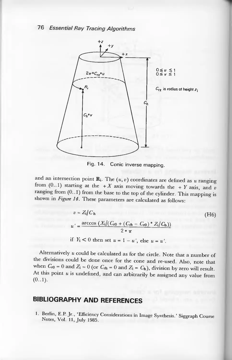
2. Essential Ray Tracing Algorithms by Eric Haines 33
3. A Survey of Ray-Surface Intersection Algorithms
by Pat Hanrahan 79
4. Surface Physics for Ray Tracing
by Andrew S. Glassner 121
5. Stochastic Sampling and Distributed Ray Tracing
by Robert L. Cook 161
6. A Survey of Ray Tracing Acceleration Techniques
by James Arvo and David Kirk 201
7. Writing A Ray Tracer by Paul S. Heckbert 263
8. A Ray Tracing Bibliography by Paul S. Heckbert
and Eric Haines 295
9. A Ray Tracing Glossary by Andrew S. Glassner 305
Index 323
Preface
This is a book about computer graphics, and the creation of realistic images.
By 'realistic' we mean an image that is indistinguishable from a photograph of
a real, three-dimensional scene. Of the many computer techniques that have
been developed to create images, perhaps the algorithm called 'ray tracing' is
now the most popular for many applications. Part of the beauty of ray tracing
is its extreme simplicity — once you know the necessary background, the
whole thing can be summed up in a paragraph.
This book begins with an introduction to the technique of ray tracing,
describing how and why it works. Following chapters describe many of the
theoretical and practical details of the complete algorithm.
I'd like to say something about how ray tracing came about in computer
graphics, and how this book in particular came to be. Then I'll briefly
summarize the various chapters.
A BIT OF HISTORY
Finding a way to create 'photorealistic' images has been a goal of computer
graphics for many years. Generally, graphics researchers make progress by
first examining the world around them, and then looking at the best
computer-generated images made to date. If the computer image doesn't look
as good (and even now, it usually doesn't), one asks, 'What's missing from the
computer picture?' In the beginning, many features of real scenes were
rapidly included in computer-generated images. Some of these improvements
were made by noting that opaque objects hide objects behind them, shiny
objects have highlights, and many surfaces have a surface texture, such as a
wooden grain. Methods were developed to include these effects into computer-
generated scenes, and so those images looked better and better.
One of the first of these successful image synthesis methods started with an
idea from the physics literature. When designing lenses, physicists
traditionally plotted on paper the path taken by rays of light starting at a light source,
then passing through the lens and slightly beyond. This process of following
the light rays was called 'ray tracing'.
Several computer graphics researchers thought that this simulation of light
physics would be a good way to create a synthetic image. This was a good
idea, but unfortunately in the early 1960s computers were too slow to make
images that looked better than those made with other, cheaper image
x. Preface
synthesis methods. Ray tracing fell out of favor, and not much attention was
paid to it for several years.
As time went by, a flurry of ofher algorithms were developed to handle all
kinds of interesting aspects of real photographs: reflections, shadows, motion
blur of fast-moving objects, and so on. But most of these algorithms only
worked in special cases, and they usually didn't work very well with each
other. Thus you would find a picture with shadows, but no transparency, or
another image with reflection, but no motion blur.
As computers became more powerful, it seemed increasingly attractive to
go back and simulate the real physics. The ray tracing algorithm was extended
and improved, giving it the power to handle many different kinds of optical
effects.
Today ray tracing is one of the most popular and powerful techniques in the
image synthesis repertoire: it is simple, elegant, and easily implemented.
There are some aspects of the real world that ray tracing doesn't handle very
well (or at all!) as of this writing. Perhaps the most important omissions are
diffuse inter-reflections (e.g. the 'bleeding' of colored light from a dull red file
cabinet onto a white carpet, giving the carpet a pink tint), and caustics
(focused light, like the shimmering waves at the bottom of a swimming pool).
Ray tracing may one day be able to create images indistinguishable from
photographs of real scenes — or perhaps some other, more powerful
algorithm will be developed to take its place. Nevertheless, right now many
people feel that ray tracing is one of the best overall image synthesis
techniques we've got, and as work continues it will become even more efficient
and realistic.
HOW THIS BOOK CAME TO BE
This book is a revised and edited version of reference material prepared for an
intensive one-day course on ray tracing. Since this book grew out of the
organization and goals of the course. I'd like to describe how the course came
about, and what we were trying to do with this material.
In late 1986, I felt that there was a need to have an introductory course on
ray tracing at the annual meeting of SiGGRAPH (the Special Interest Group on
Computer Graphics, which is part of the ACM, the society of computer
professionals). Each year SiGGRAPH mounts a very large conference, covering
many aspects of computer graphics. An important part of each SiGGRAPH
conference is the presentation of one-day courses. There have been several
courses at recent SiGGRAPHs reviewing developments in ray tracing for
experts, but I felt that ray tracing had become popular enough that there
should be an introductory course.
Preface xi
I made some phone calls, and gathered together a group of internationally-
recognized researchers in the field to present our new course. Our goal from
the beginning was to teach to a 'typical' SlGGRAPH audience: artists,
managers, scientists, programmers, and anyone else who was interested!
Most SlGGRAPH courses include some kind of 'course notes' handed out to
attendees. Since part of the reason we were teaching the course was that there
was no introductory material available, we decided to write our own. As
chairman of the course, 1 decided to ask everyone to write original,
high-quality material for our course notes, and happily most of the speakers
had the time and energy to do so.
The course's name was An Introduction To Ray Tracing. It was a great
success at SlGGRAPH '87 in Anaheim — it was one of the two most
heavily-attended courses. The response in 1987 was very good, so we decided
to give the course again. With a slightly different cast we repeated the course
at SlGGRAPH '88 in Atlanta. We took the opportunity to revise and improve
the notes.
This book is essentially the notes from SlGGRAPH '88, edited and
improved. It includes a few things we couldn't get into the notes, or that
didn't come across well: color plates, good black-and-white images, a
bibliography, and a glossary.
A QUICK LOOK AT THE CONTENTS
As you look over the book, remember that the level of the material varies
considerably from chapter to chapter. Some chapters are very basic and
assume little background, while others expect you to have some mathematical
experience. The more complex chapters are for more advanced study: you can
get quite far with just the less mathematical chapters.
The book begins with 'An Overview of Ray Tracing'. This opening chapter
assumes little background from the reader. We tell how a synthetic image is
produced, and how ray tracing works to create an image. When you're done
reading this, you won't be in a position to write a program, but you should be
able to understand ray tracing discussions, including most of the other
chapters.
We then discuss 'Essential Ray Tracing Algorithms'. The fundamental
operation in any ray tracing program is the intersection of a ray with an
object. Because it's such an important step, it is important to understand it
clearly. We show how to find the intersection of a ray with several important
shapes, and how to write the necessary computer procedures.
More complicated kinds of objects are discussed in 'A Survey of Ray-
Object Intersection Algorithms'. Because more complex shapes have more
xii Preface
complex mathematical descriptions, the math in this section is necessarily
more involved. You don't need to understand everything in this chapter to get
started in ray tracing: it's more of a springboard to help you move on to more
advanced topics, once you've got some momentum.
To properly compute how rays interact with surfaces, we discuss "Surface
Physics for Ray Tracing'. This chapter gives a lot of basic information that
you'll need to actually get your programs running, including color
descriptions, laws of optics, and surface coloring.
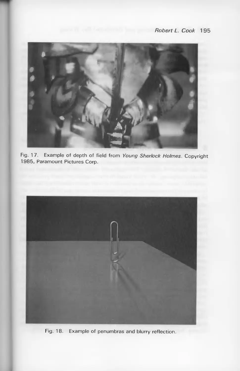
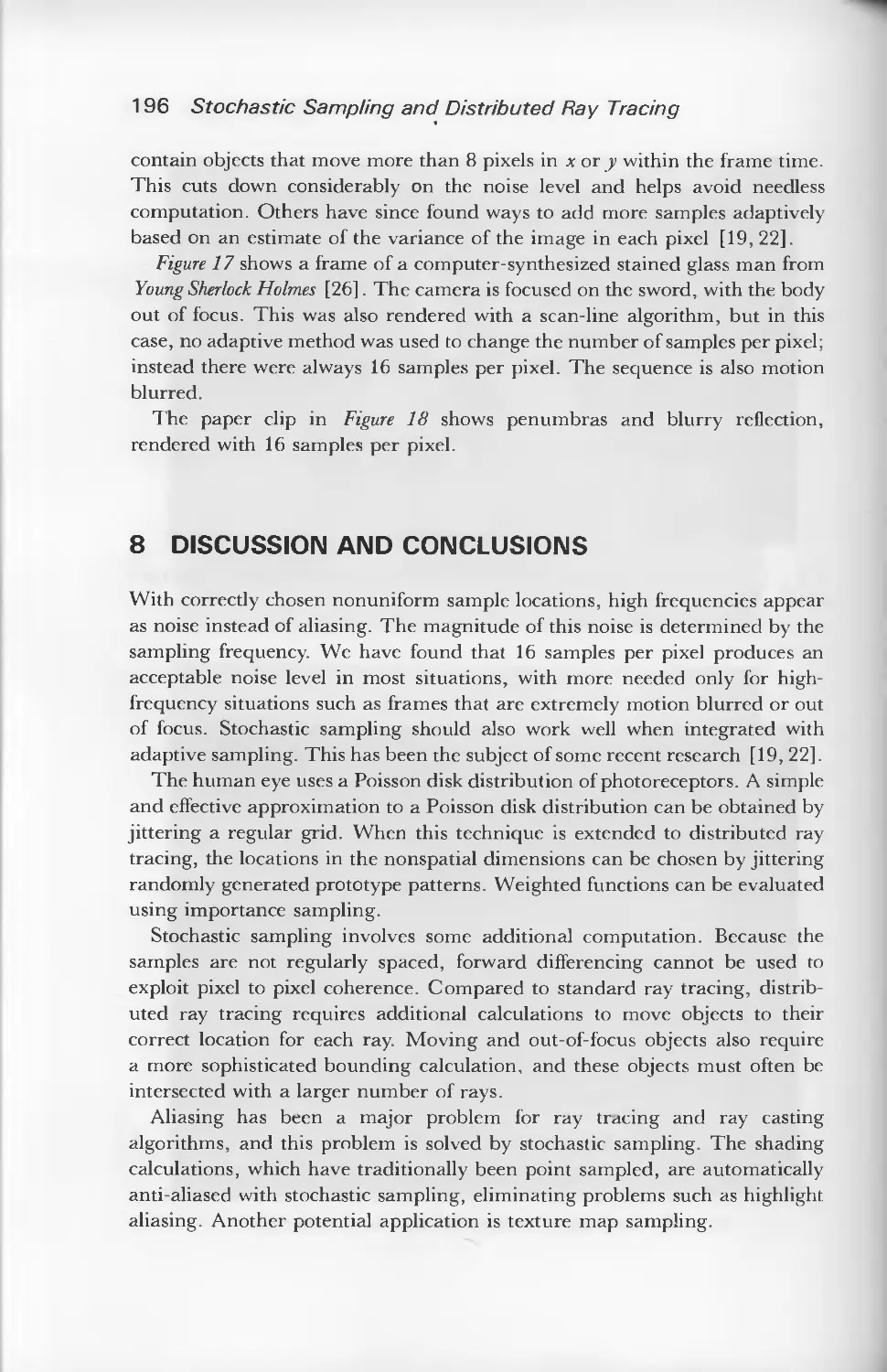
If you're not careful, computer-generated pictures will contain lots of ugly
artifacts that don't belong in a picture, due to the nature of digital computers
and the ray tracing process itself. We discuss those artifacts and how to avoid
them in 'Stochastic Sampling and Distributed Ray Tracing'. The material in
this chapter will help your pictures avoid nasty artifacts that don't belong in a
'realistic' picture.
'A Survey of Ray Tracing Acceleration Techniques' addresses the issue of
speed. The basic ray tracing algorithm is extremely simple, but also extremely
slow. It's like saying, 'To build a sand dune, pick up a grain of sand, and
carry it over to where you're building the dune: do this over and over again'.
The instructions are correct, but painfully slow. Lots of research has gone into
ways to make ray tracing programs run faster. The bad news is that most of
these techniques greatly complicated the basically simple and elegant ray
tracing algorithm. The good news is that by using these methods you can
make a picture much faster than with straightforward techniques.
By the time you reach the end of the book, you'll be ready for hints on
'Writing A Ray Tracer'. Writing a program is usually greatly simplified if
you have a plan of attack, or a structure for building the various pieces and
describing their interconnections. In this chapter we give a good organization
for a ray-tracing program that is both simple to build and easy to extend. The
concepts are illustrated with sample code in the C programming language.
Where can you go for more information? Well, each chapter in the book
comes with its own bibliography, keyed to the material in that chapter. If you
want more, then you can consult the 'Ray Tracing Bibliography'.
If you forget the meaning of a word, you can probably find it in 'A Ray
Tracing Glossary'. Here we give definitions for most of the important terms
used in this book, plus some other terms that you might find in the literature.
Some of the entries are illustrated, since after all this is a book on graphics!
ACKNOWLEDGEMENTS
The SlGGRAPH course and this book represent the combined efforts of many
people. Thanks to Mike and Cheri Bailey, who together administered the
Preface xiii
SlGGRAPH courses in 1987 and 1988. Thanks also to the A/V squad and
student volunteers at both conferences, who helped keep the courses running
smoothly.
While putting together both courses and then this book, I was a graduate
student in Computer Science at the University of North Carolina at Chapel
Hill. My department generously made available to me its resources to help
manage these projects. I thank my advisors Dr Frederick P. Brooks, Jr. and
Dr Henry Fuchs, for their support.
I know that we have enjoyed writing this book. I hope some of our
excitement about ray tracing and image synthesis comes through, and before
too long you'll be making pictures of your own. Good luck!
Andrew S. Glassner
Palo Alto, California
4 An Overview of
' Ray Tracing
ANDREW S. GLASSNER
1 IMAGE SYNTHESIS
1.1 Introduction
Ray tracing is a technique for image synthesis: creating a 2-D picture of a 3-D
world.
In this article we assume you have some familiarity with basic computer
graphics concepts, such as the idea of a frame buffer, a pixel, and an image plane.
We will use the term pixel in this article to describe three different, related
concepts: a small region of a monitor, an addressable location in a frame
buffer, and a small region on the image plane in the 3-D virtual world.
Typically, these three devices (monitor, frame buffer, and image plane) are
closely related, and the region covered by a pixel on one has a direct
correspondence to the others. We will find it convenient to sometimes blur the
distinction between these different devices and refer to the image plane as 'the
screen.'
Most computer graphics are created for viewing on a flat screen or piece of
paper. A common goal is to give the viewer the impression of looking at a
photograph (or movie) of some three-dimensional scene. Our first step in
simulating such an image will be to understand how a camera records a
physical scene onto film, since this is the action we want to simulate.
After that we'll look at how the ray tracing algorithm simulates this physical
process in a computer's virtual world. We'll then consider the issues that arise
when we actually implement ray tracing on a real computer.
1.2 The Pinhole Camera Model
Perhaps the simplest camera model around is the pinhole camera, illustrated in
Figure 1. A flat piece of photographic film is placed at the back of a light-proof
2 An Overview of Ray Tracing
Pinhole
Film
Fig. 1. The pinhole camera model.
box. A pin is used to pierce a single hole in the front of the box, which is then
covered with a piece of opaque tape. When you wish to take a picture, you
hold the camera steady and remove the tape for a while. Light will enter the
pinhole and strike the film, causing a chemical change in the emulsion. When
you're done with the exposure you replace the tape over the hole. Despite its
simplicity, this pinhole camera is quite practical for taking real pictures.
The pinhole is a necessary part of the camera. If we removed the box and
the pinhole and simply exposed the entire sheet of film to the scene, light from
all directions would strike all points on the film, saturating the entire surface.
We'd get a blank (white) image when we developed this very overexposed
film. The pinhole eliminates this problem by allowing only a very small
number of light rays to pass from the scene to the film, as shown in Figure 2. In
particular, each point on the film can receive light only along the line joining
that piece of film and the pinhole. As the pinhole gets bigger, each bit of the
film receives more light rays from the world, and the image gets brighter and
more blurry.
Although more complicated camera models have been used in computer
graphics, the pinhole camera model is still popular because of its simplicity
and wide range of application. For convenience in programming and
Fig. 2. The pinhole only allows particular rays of light to strike the film.
Andrew S. Glassner 3
<!
I
Eye
Viewing frustum
Fig. 3. The modified pinhole camera model as commonly used in computer
graphics.
i modeling, the classic computer graphics version of the pinhole camera moves
the plane of the film out in front of the pinhole, and renames the pinhole as the
eye, as shown in Figure 3. If we built a real camera this way it wouldn't work
well at all, but it's fine for a computer simulation. Although we've moved
things around, note that each component of the pinhole camera is accounted
for in Figure 3. In particular, the requirement that all light rays pass through
the pinhole is translated into the requirement that all light rays pass through
the eyepoint. For the rest of our discussion we will use this form of the pinhole
camera model.
You may want to think of the model in Figure 3 as a Cyclopean viewer
looking through a rectangular window. The image he sees on the window is
determined by where his eye is placed and in what direction he is looking.
In Figure 3 we've drawn lines from the eye to the corners of the screen and
then beyond. You can think of these lines as the edges of walls that include the
eye and screen. The only objects which the eye can directly see (and thus the
film directly image) are those which lie within all four of the walls formed by
these bounds. We also arbitrarily say that the only objects that can show up on
the image plane are those in front of the image plane, i.e. those on the other
side of the plane than the eye. This makes it easy to avoid the pitfall of having
our whole image obscured by some large, nearby object. The eye also cannot
directly see any objects behind itself.
All these conditions mean that the world that finally appears on the screen
lies within an infinite pyramid with the top cut off (such a point-less pyramid is
called & frustum). The three-dimensional volume that is visible to the eye, and
may thus show up on the screen, is called the viewing frustum. The walls that
form the frustum are called clipping planes. The plane of the screen is called the
image plane. The location of the eye itself is simply referred to as the eye position.
mage plane, or screen
4 An Overview of Ray Tracing
1.3 Pixels and Rays
When we generate an image we're basically determining what color to place
in each pixel. One way to think of this is to imagine each pixel as a small,
independent window onto the scene. If only one color can be chosen to
represent everything visible through this window, what would be the correct
color? Much of the work of 3-D computer graphics is devoted to answering
that question.
One way to think about the question is within the context of the pinhole
camera model. If we can associate a region of film with a given pixel, then we
can study what would happen to that region of the film in an actual physical
situation and use that as a guide to determine what should happen to its
corresponding pixel in the computer's virtual world. If we use the computer
graphics pinhole camera of Figure 3, this correspondence is easy.
In Figure 4, one pixel in particular and its corresponding bit of film have
been isolated. A small distribution of light rays can arrive from the scene, pass
through the pinhole, and strike the film. After the exposure has completed and
the pinhole is covered, that small region of film has absorbed many different
rays of light. If we wish to describe the entire pixel with a 'single' color, a good
first approximation might be to simply average together all the colors of all the
light that struck it.
Fig. 4. Every pixel on the screen in the computer graphics camera model
corresponds directly to a region of film in the pinhole camera.
Andrew S. Glassner 5
This 'averaging' of the light in a pixel is in fact the way we eventually
determine a single color for the pixel. The mathematics of the averaging may
get somewhat sophisticated (as we'll see in later chapters), but we'll always be
looking at lots of light rays and somehow combining their colors.
From this discussion we can see that the eventual goal is to fill in every pixel
with the right color, and the way to find this color is to examine all the light
rays that strike that pixel and average them together somehow. From now on,
when we refer to the 'pinhole camera model,' or even just 'the camera,' we'll
be referring to the computer graphics version of Figure 3.
2 TRACING RAYS
2.1 Forward Ray Tracing
We saw in the last section that one critical issue in image synthesis is the
determination of the correct color for each pixel, and that one way to find that
color is to average together the colors of the light rays that strike that pixel in
the pinhole camera model. But how do we find those rays, and what colors are
they? Indeed, just what do we mean by the 'color' of a light ray?
The color of a ray is not hard to define. We can think of a light ray as the
straight path followed by a light particle (called a photon) as it travels through
space. In the physical world, a photon carries energy, and when a photon
enters our eye that energy is transferred from the photon itself to the receptor
cells on our retina. The color we perceive from that photon is related to its
energy. Different colors are thus carried to our retina by photons of different
energies.
One way to talk of a photon's energy is as energy of vibration. Although
photons don't actually 'vibrate' in any physical sense, vibration makes a
useful mathematical and intuitive model for describing a photon's energy. In a
vibrating photon model, different speeds of vibration are related to different
energies, and thus different colors. For this reason we often speak of a given
color as having a certain frequency. Another way to describe the rate of
vibration is with the closely related concept of wavelength. For example, we can
speak of frequency and say that our eyes respond to light between about 360
and 830 terahertz (abbreviated THz; 1 THz = 10l cycles per second).
Alternatively, we can speak of wavelength and describe the same range as
360-830 nanometers (1 nm = 1 billionth of a meter). In mathematical
formulae, it is typical to use the symbol / to represent the frequency of a
photon, and X to represent its wavelength.
Generally speaking, each unique frequency has an associated energy, and
thus will cause us to see an associated color. But colors can add both on film
6 An Overview of Ray Tracing
and in the eye; for example, if a red photon and a green photon both arrive at
our eye simultaneously, we will perceive the sum of the colors: yellow.
Consider a particular pixel in the image plane. Which of the photons in a
three-dimensional scene actually contribute to that pixel?
Figure 5 shows a living room, consisting of a couch, a mirror, a lamp, and a
table. There's also a camera, showing the position of the eye and the screen.
Photons must begin at a light source. After all, exposing a piece of film in a
completely dark room doesn't cause anything to happen to the film; no light
hits it. If the lamp in the living room is off, then the room is completely dark
and our picture will be all black. So imagine that the light is on. The lamp
contains a single, everyday white light bulb. The job of the bulb is to create
photons at all the visible frequencies and send them out in all directions. In
order to get a feel for how the photons eventually contribute to the
photograph, let's follow a few photons in particular.
We will not consider all the subtleties and complexities that actually occur
when light bounces around in a three-dimensional scene; that discussion could
fill several books! Instead, we'll stick to the most important concepts.
Let's say photon A is colored blue (that is, if the photon struck our eye we
would say that we were looking at blue light). It leaves the light source in the
direction of the wall, and then strikes the wall. Some complicated things can
happen when the photon hits the wall's surface, which we'll talk about later in
Fig. 5. Some light rays (like A and E) never reach the image plane at all. Others
follow simple or complicated routes.
Andrew S. Glassner 7
the Surface Physics section. For now, we'll say that the light hits the wall, and
is mostly absorbed. So photon A stops here, and doesn't contribute to the
picture.
Photon C is also blue. It leaves the light and strikes the couch. At the couch,
the photon is somewhat absorbed before being reflected. Nevertheless, a
(somewhat weaker) blue photon leaves the couch and eventually passes
through the screen and into our eye. So that's why we get to actually see the
couch: light from the light source strikes the couch and gets reflected to our
eye through the screen.
The reflection can get more complex. Photon B is reflected off the mirror
before it hits the couch; its path is light, mirror, couch, film. Alternatively,
photon D leaves the light source, strikes the couch, and then strikes the mirror
to be reflected onto the film. Photon E follows a very similar path, but it never
strikes the film at all. Other photons may follow much more complicated paths
during their travels.
So in general, photons leave the light source and bounce around the scene.
Usually, the light gets a little dimmer on each bounce, so after a couple of
bounces the light is so dim you can't seen it anymore. Only photons that
eventually hit the screen and then pass into our eye (when they're still bright)
actually contribute to the image. You might want to look around yourself
right now, identify some light source, and imagine the paths of some photons
as they leave that light, bounce around the objects near you, and eventually
reach your eye. Notice that if you're looking into a mirror, you can probably
see some objects in the mirror that you can't see directly. The photons are
leaving the light source, hitting those objects, then hitting the mirror, and
eventually finding your eyes.
We've just been ray tracing. We followed (or traced) the path of a photon (or
ray of light) as it bounced around the scene. More specifically, we've been
forward ray tracing; that is, we followed photons from their origin at the light
and into the scene, tracing their path in a forward direction, just as the
photons themselves would have travelled it.
2.2 Forward Ray Tracing and Backward Ray Tracing
The technique of forward ray tracing described above is a first approximation
to how the real world works. You might think that simulating this process
directly would be a good way to make pictures, and you would be pretty much
correct. But there is a problem with such a direct simulation, and that's the
amount of time it would take to produce an image. Consider that each light
source in a scene is generating possibly millions of photons every second,
where each photon is vibrating at a slightly different frequency, going in a
8 An Overview of Ray Tracing
slightly different direction. Many of these photons hit objects that you would
never see at all, even indirectly. Other just pass right out of the scene, for
example by flying out through a window. If we were to try to create a picture
by actually following photons from their source, we would find a depressingly
small number of them ever hit the screen with any appreciable intensity. It
might take years just to make one dim picture!
The essential problem is not that forward ray tracing is no good, but rather
that many of the photons from the light source play no role in a given image.
Computationally, it's just too expensive to follow useless photons.
The key insight for computational efficiency is to reverse the problem, by
following the photons backwards instead of forwards. We start by asking
ourselves, "Which photons certainly contribute to the image?" The answer is
those photons that actually strike the image plane and then pass into the eye.
Each of those photons travelled along some path before it hit the screen; some
may have come directly from a light source, but most probably bounced
around first.
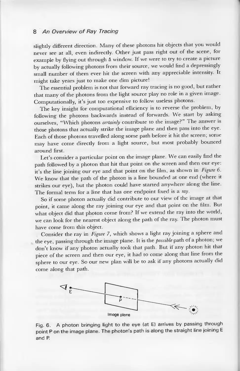
Let's consider a particular point on the image plane. We can easily find the
path followed by a photon that hit that point on the screen and then our eye:
it's the line joining our eye and that point on the film, as shown in Figure 6.
We know that the path of the photon is a line bounded at one end (where it
strikes our eye), but the photon could have started anywhere along the line.
The formal term for a line that has one endpoint fixed is a ray.
So if some photon actually did contribute to our view of the image at that
point, it came along the ray joining our eye and that point on the film. But
what object did that photon come from? If we extend the ray into the world,
we can look for the nearest object along the path of the ray. The photon must
have come from this object.
Consider the ray in Figure 7, which shows a light ray joining a sphere and
the eye, passing through the image plane. It is the possible path of a photon; we
don't know if any photon actually took that path. But if any photon hit that
piece of the screen and then our eye, it had to come along that line from the
sphere to our eye. So our new plan will be to ask if any photons actually did
come along that path.
Image plane ''<^
Fig. 6. A photon bringing light to the eye (at E) arrives by passing through
point P on the image plane. The photon's path is along the straight line joining E
and P.
Andrew S. Glassner 9
Fig. 7. A photon leaving the sphere could fly through a pixel and into the eye.
In this approach we're following rays not forward, from the light source to
objects to the eye, but backward, from the eye to objects to the light source.
This is a critical observation because it allows us to restrict our attention to
rays that we know will be useful to our image—the ones that enter our eye!
Now that we've found the object a photon may have left to strike our eye,
we must find out if any photon really did travel that path, and if so what its
color is. We will address those topics below.
Because forward ray tracing is so expensive, the term 'ray tracing' in
computer graphics has come to mean almost exclusively backward ray
tracing. Unfortunately, some of the notions of backward ray tracing have led
to some possibly confusing notation. Recall that we follow a ray backwards to
find out where it may have begun. Nevertheless, we often carry out that
search in a program by following the path of the light ray backwards,
imagining ourselves to be riding along a path taken by a photon, looking for
the first object along our path; this is the object from which the ray began. So
we sometimes speak of looking for the "first object hit by the ray," or the "first
object on the ray's path". What we're actually referring to is the object that
may have radiated the photon that eventually travelled along this ray. This
backwards point of view is prevalent in ray tracing literature and algorithms,
so it may be best to think things through now and not get confused later. In
summary, the "first object hit by a ray" means "the object which might have
emitted that ray."
2.3 Ray Combination
When we want to find the color of a light ray, we need to find all the different
light that originally contributed to it. For example, if a red light ray and a
green light ray find themselves on exactly the same path at the same time, we
might as well say that together they form a single yellow ray (red light and
10 An Overview of Ray Tracing
green light arriving at your eye simultaneously give the impression of yellow).
So in Figure 7, where the light at a given pixel came from a sphere, we need to
find a complete description of all the light leaving that point of the sphere in
the direction of our eye. We'll see that we can rig our examination of the point
so that we're only studying the light that will actually contribute to the pixel.
To aid in our discussion, we'll conceptually divide light rays into four
classes: pixel rays or eye rays which carry light directly to the eye through a pixel
on the screen, illumination rays or shadow rays which carry light from a light
source directly to an object surface, reflection rays which carry light reflected by
an object, and transparency rays which carry light passing through an object.
Mathematically, these are all just rays, but it's computationally convenient to
deal with these classes.
The pixel rays are the ones we've just studied; they're the rays that carry
photons that end at the eye after passing through the screen (or in backwards
ray tracing, they're rays that start at the eye and pass through the screen).
Let's look at the other three types of rays individually.
The whole idea is to find out what light is arriving at a particular point on a
surface, and then proceeding onward to our eye. Our discussion may be
broken into two pieces: the illumination at a point on the object (which
describes the incoming light), and the radiation of light from that point in a
particular direction. We can determine the radiated light at a point by first
finding the illumination at that point, and then considering how that surface
passes that light on in a given direction (of course, if the object is a light source
it could add some additional light of its own).
Knowing the illumination and surface physics at a point on a surface, we
can determine the properties of the light leaving that point. We broke up rays
into the three classes of shadow, reflection, and transparency because they're
the three principle ways that light arrives at (and then leaves from) a surface.
Some light comes directly from the light source and is then re-radiated away;
the properties of this incoming light are determined by the shadows rays.
Some light may strike the object and then be reflected; the reflection rays
model this light. Lastly, some light comes from behind the object and may
pass through; this light is modeled by the transparency rays.
2.4 Shadow and Illumination Rays
Imagine yourself on the surface of an object, such as point P in Figure 8. Is any
light coming to you from the light sources? One way to answer that question is
to simply look at each light. If you can see the light source, then there's a clear
path between you and the light, and at least some photons will certainly travel
along this path. If any opaque objects are in your way, then no light is coming
directly from the light into your eye, and you are in shadow with respect to
that light.
Andrew S. Glassner 11
3
Fig. 8. To determine the illumination at a point P, we ask if photons could
possibly travel from each light source to P. We answer this by sending shadow
ray La towards light source A. It arrives at A, so P LA is actually an illumination
ray from P to A. But ray Lb is blocked from light source B by sphere S, so no
light arrives at P from B.
We can simulate this operation of standing on the object and looking
towards the light source with a light ray called a shadow ray. In practice, a
shadow ray is like any other ray, except that we use it to 'feel around' for
shadows; thus this kind of ray is sometimes also called a shadow feeler. Basically
we start a ray at the object and send it to the light source (remember, we're
following the paths of photons backwards). If this backwards ray reaches the
light source without hitting any object along the way, then certainly some
photons will come forwards along this ray from the light to illuminate the
object. But if any opaque objects are in our way, then the light can't get
through the intervening object to us; we would then be in shadow relative to
that light source. Figure 8 shows two shadow rays leaving a surface, ray La
going to light source A, and ray Lb going to light source B. Ray La gets to its
light source without interruption, but ray Lb hits an opaque object along the
way. Thus we deduce that light can (and will!) arrive from light A, but not
from light B.
When a shadow ray is able to reach a light source without interruption, we
stop thinking of it as a 'shadow feeler' and turn it around, thinking of it as an
illumination ray, which carries light to us from the light source.
In summary, the first class of illumination rays that contribute to the color
of the light leaving an object are the light rays coming directly from the light
source, illuminating the object. We determine whether there actually are any
photons coming from a given light by sending out a shadow ray to each light
source. If the ray doesn't encounter any opaque objects along the way to the
12 An Overview of Ray Tracing
light, that's our signal that photons will arrive from that light to the object. If
instead there is an opaque object in the way, then no photons arrive and the
object is in shadow relative to that light source.
Throughout this discussion we've only discussed what happens when the
shadow ray hits a matte, opaque object. When it hits a reflective or
transparent object the situation is much more complicated. For many years,
people used a variety of ad hoc tricks to handle situations where shadow rays
hit reflective or transparent surfaces. We now know some better ways to
handle this situation; these will be discussed later in the book when we cover
stochastic ray tracing.
2.5 Propagated Light
Recall that our overall goal is to find the color of the light leaving a particular
point of a surface in a particular direction. We said that the first step was to
find out which light was striking the object; some of that light would perhaps
continue on in our direction of interest.
In the spirit of backward ray tracing, we'll look only for the incoming light
that will make a difference to the radiated light in the direction we care about.
After all, if some light strikes the surface but then proceeds away in a direction
we don't care about, there's no need to really know much about that incoming
light.
We will use the term propagated light to describe the illuminating light about
which we care. Of all light that is striking a surface, which light is propagated
just in our direction of interest? In ray tracing, we assume that most light
interaction can be accounted for with four mechanisms of light transport
(more about this in the Surface Physics chapter). For now, we'll concentrate
exclusively on the two mechanisms called specular reflection and specular"
transmission—and since they're our only topics at the moment, well often
leave off the adjective 'specular' in this section.
The general idea is that any illumination that falls on a surface and then is
sent into our direction of interest either bounced off the surface like a
basketball bouncing off a hardwood floor (reflection), or passed through the
surface after arriving on the other side like a car driving through a tunnel
(transmission). In the case of perfect (specular) reflection and transmission for
a perfectly flat, shiny surface, there is exactly one direction from which light
can arrive in order to be (specularly) reflected or transmitted into our eye.
When we are trying to determine the illumination at a point, recall that we
originally found that point by following a ray to the object. Since we followed
that ray backwards to the object, it is called the incident ray. Thus, our goal is
to find the color of the light leaving the object in the direction opposite to the
incident ray.
Andrew S. Glassner 13
2.6 Reflection Rays
If we look at a perfectly flat, shiny table, we will see reflections of other objects
in the tabletop. We see those reflections because light is arriving at the
tabletop from the other objects, bouncing off of the tabletop, and then arriving
in our eye. For a fixed eyepoint, each position on the table has exactly one
direction from which light can come that will be bounced back into our eye.
For example, Figure 9 shows a photon of light bouncing around a scene,
ending up finally passing through the screen and into the eye. On its last
bounce, the photon hit point P and then went into the eye. Photon B also hit
point P, but it was bounced (or reflected) into a direction that didn't end up
going into our eye. So for that eyepoint and that object, only a photon
travelling along the path marked A could have been reflected into our
direction of interest.
When we wish to find what light is reflected from a particular point into the
direction of the incident ray, we find the reflected ray (or reflection ray) for that
point and direction; this is the ray that can carry light to the surface that will
be perfectly reflected into the direction of the incident ray. To find the color of
the reflected ray, we follow it backwards to find from which object it began.
The color of the light leaving that object along the line of the reflected ray is
the color of that reflected ray. When we know the reflected ray's color, we can
contribute it to any other light leaving the original surface struck by the
incident ray.
Note the peculiar terminology of backward ray tracing: light arrives along
the reflected ray and departs along the incident ray.
Light
source
Reflected
B
Fig. 9. The color of perfectly reflected light is dependent on the color of the
object and the color of the incoming light that bounces off in the direction we
care about. For example, at point P we want to know the color of the light
coming in on ray A, since that light is then bounced into the eye.
14 An Overview of Ray Tracing
Once we know the color of the light coming to the surface from the light
sources, the reflected ray, and the transparency ray, we combine them
according to the properties of the surface, and thus determine the total color
leaving the surface in the direction of the incident ray.
We will see later in the book that more subtle effects can be accounted for if
we use more than one transparency or reflected ray, sending them in a variety
of (carefully chosen) directions and then weighting their results.
The subject of determining the way light behaves at a surface is called
surface physics. This topic covers the geometry of light rays at a surface as well
as what color changes happen to the light itself. We'll have an entire section of
the course devoted to surface physics later on.
2.7 Transparency Rays
Just as there was a single direction from which light can be perfectly reflected
into the direction of the incident ray, so is there a single direction from which
light can be transmitted into the direction of the incident ray. The ray we
create to determine the color of this light is called the transmitted ray or
transmitted ray. Figure 10 shows a possible path of a transmitted ray. Notice the
bending, or refraction, of the light as it passes from one medium to another.
We follow the transmitted ray backwards to find which object might have
radiated it, and then determine the color radiated by that object in the
direction of the transmitted ray. When we know that color, we know the color
of the transmitted ray, which (by construction) will be perfectly bent into the
direction of the incident ray.
3 RECURSIVE VISIBILITY
The previous sections have discussed finding the color of light leaving a
surface as a combination of different kinds of light arriving at the surface. In
essence, the color of the radiated light is a function of the combined light from
the light sources, light the object reflects, and light the object transmits. We
found the colors of the reflected and transmitted light by finding the objects
from which they started. But what was the color leaving this previous object?
It was a combination of the light reaching it, which can be found with the
same analysis.
This observation suggests a recursive algorithm, and indeed the whole ray
tracing technique fits into that view very nicely.
The ray tracing process begins with a ray that starts at the eye; this is an eye
ray or pixel ray. Figure 11 shows one viewing set-up and a particular eye ray,
labelled E.
Andrew S. Glassner 1 5
Fig. 10. Transmitted light arrives from behind a surface and passes through.
3.1 Surface Physics
We've mentioned above for reflection and transparency rays that we first find
the direction they might have come from, and then look backwards along that
path for a possible object at their source. The technique of determining these
directions may be as simple or complicated as you like; we're approximating
physical reality here, and physical reality is often complex in its details. The
more accuracy you want from your model, the more detailed it will have to be.
Happily, even fairly simple models seem to work very well for today's typical
images.
The next step is the one that we'll repeat over and over again. We simply
ask, "which object does this ray hit?" Remember that we're doing backwards
ray tracing, so this question is really a confused form of the question, "given
that a photon travelled along this ray to the eye, from which object did it
start?"
In Figure 11, the eye ray hits plane 3, which we'll say is both somewhat
transparent and reflective. We have two light sources, so we'll begin by
sending out a shadow ray from plane 3 to each light: we'll call these rays Si
and S2. Since ray Si reaches light A without interruption, we know that plane
3 is receiving light from light A. But ray S2 hits sphere 4 before it hits light B,
so no illumination comes in along this path. Because plane 3 is both
transparent and reflective, we also have to find the colors of the light it
transmits and reflects; such light arrived along rays Ti and Ri.
Following ray Ti, we see that it hits sphere 6, which we'll say is a bit
reflective. We send out two shadow rays S3 and S4 to determine the light
hitting sphere 6, and create reflection ray R2 to see what color is reflected.
Both S3 and S4 reach their respective light sources. Ray R2 leaves the scene
entirely, so we'll say that it hits the surrounding world, which is some constant
background color. That completes ray Ti from our original intersection with
the primary ray E.
Let's now go back and follow reflected ray Ri. It strikes plane 9. which is a
bit reflective and transparent. So we'll send out two shadow rays as always (S5
and Se), and reflected and transmitted rays T2 and R3. We'll then follow each
of T2 and R3 in turn, generating new shadow and secondary rays at each
intersection.
16 An Overview of Ray Tracing
Fig. 11. An eye ray E propagated through a scene. Many of the intersections
spawn reflected, transmitted, and shadow rays.
Figure 12 shows this whole process in a schematic form, called a ray tree.
What ever causes the ray tree to stop? Like the non-opaque shadow ray
question, the answers to this question are not easy. One ad hoc technique that
usually works pretty well is to stop following rays either when they leave the
scene, or their contribution gets too small. The former condition is handled by
saying that if a ray leaves our world, then it just takes on the color of the
surrounding background. The second condition is a bit harder.
How much contribution does ray E make to our picture? If it's the only ray
at that pixel, then we'll use 100% of E; if the color E brings back is pure red,
then that pixel will be pure red. But how about rays Ti and Ri? Their
contributions must be less than that of E since E is formed by adding them
together. Let's arbitrarily say that plane 3 passes 40% of its transmitted light,
and 20% of its reflected light (i.e. plane 3 is 40% transparent and 20%
reflective).
Now recall that Ti is composed of the light radiated by sphere 6, given by
S3, S4, and R2. Let's again be arbitrary, and say that object 6 is 30%
transparent; thus R2 contributes 30% to Ti. Since Ti contributes 40% to E,
and R2 contributes 30% to Ti, then R2 contributes only 12% to the final color
of E. The farther down the ray tree we go, the less each ray will contribute to
the color we really care about, the color of E.
So we can see that as we proceed down the ray tree, the contribution of
Andrew S. Glassner 1 7
S,-
S2
Eye ray
. I
Object 3
/
T, R,
S*\ / S5 ^ •
^Object 6 Object 9
R2 7z R?
\ / \
Fig. 12. The ray tree in schematic form.
individual rays to the final image becomes less and less. As a practical matter,
we usually set a threshold of some kind to stop the process of following rays. It
is interesting to note that although this technique, called adaptive tree-depth
control, sounds plausible, and in fact works pretty well in practice, there are
theoretical arguments that show that it can be arbitrarily wrong.
4 ALIASING
Synthesizing an image with a digital computer is very different from exposing
a piece of film to a real scene. The differences are endless, although much of
computer graphics research is directed to making the differences as small as
possible. But there's a fundamental problem that we're stuck with: the
modern digital computer cannot represent a continuous signal.
Consider using a standard tape recorder to record a trumpet. Playing the
trumpet causes the air to vibrate. The vibrating air enters a microphone,
where it is changed into a continually changing electrical signal. This signal is
applied to the tape head, which creates a continually changing magnetic field.
This field is recorded onto a piece of magnetic tape that is passing over the
head.
Now let's consider the same situation on a digital computer. The music
enters the microphone, and is changed into a continuous electrical signal. But
the computer cannot record that signal directly; it must first turn it into a
series of numbers. In formal terms, it samples the signal so that it can store it
18 An Overview of Ray Tracing
digitally. So our continuous musical tone has been replaced with a sequence of
numbers. If we take enough samples, and they are of sufficiently high
precision, then when we turn those numbers back into sound it will sound like
the original music.
It turns out that these notions of 'enough samples' and 'sufficiently high
precision' are critically important. They have been studied in detail in a
branch of engineering mathematics called signal processing, from which
computer graphics has borrowed many important results.
Let's look at a typical sampling problem by analogy. Imagine that you're at
a county fair, standing by the carousel. This carousel has six horses,
numbered 1 to 6, and it's spinning so that the horses appear to be galloping to
the right. Now let's say that someone tells you that the carousel is making one
complete rotation every 60 seconds, so a new horse passes by every 10
seconds. You decide to confirm this claimed speed of revolution.
Now just as you're watching horse 3 pass in front of you, someone calls
your name. You turn and look for the caller, but you can't find anyone. It
took you 10 seconds to look around. When you turn back to the carousel, you
see that now horse 4 is in front of you. You might sensibly assume that the
carousel has spun one horse to the right during your absence.
Say this happens again and again; you look away for 10 seconds, and then
return. Each time you turn back you see the next-numbered horse directly in
front of you. You could conclude that the carousel is spinning 1/6 of the way
around every 10 seconds, so it takes 60 seconds to complete a revolution. Thus
the claim appears true.
Now let's say that a friend comes back the next day to double-check your
observations. As soon as she reaches the carousel (looking at horse 3) she hears
someone calling her name. She looks around, but although you looked only
for 10 seconds, your friend searches the crowd for 70 seconds. When she turns
back to the carousel, she sees exactly what you saw yesterday; horse 4 is in
front of her. If this happened again and again, she could conclude that the
carousel is spinning 1/6 of the way around every 70 seconds. Thus she could
reasonably state that the claim is false.
We know from your observations that it is certainly going faster than that,
but there's no way for your friend to know that she's wrong if she only takes
one look every 70 seconds.
In fact someone's measurements in such a situation can be arbitrarily
wrong. Because as long as you regularly look at the carousel, look away, and
look back, you have no idea what went on when you were looking away: 1 can
always claim that it went around any number of full turns when you weren't
looking!
The computer is prone to exactly the same problem. If it samples some
signal too infrequently, the information that gets recorded can be wrong, just
Andrew S. Glassner 19
as our determination of the carousel's speed was wrong. The problem is that
one signal (1/6 revolution every 10 seconds) is masquerading as another signal
(1/6 revolution every 70 seconds); they're different signals, but after sampling
we can't tell them apart. This problem is given the general term aliasing, to
remind us that one signal is looking like another.
The problem of aliasing thoroughly permeates computer graphics. It shows
up in countless ways, and almost always looks noticeably bad. The problem is
that, if one is not careful, aliasing will almost always occur somewhere, simply
due to the nature of digital computers and the nature of the ray tracing
algorithm itself. Luckily, there are techniques to avoid aliasing, known
collectively as anti-aliasing techniques. They are the weapons we employ to
solve or reduce the aliasing problem.
We'll first look at some of the symptoms of aliasing, and then look briefly at
some of the ways to avoid these problems.
4.1 Spatial Aliasing
When we get aliasing because of the uniform nature of the pixel grid, we often
call that spatial aliasing. Figure 13 shows a quadrilateral displayed at a variety
of screen resolutions. Notice the chunky edges; this effect is colloquially called
Fig. 13. A quadrilateral shown on grids of four different resolutions. Note that
the smooth edges turn into stairsteps—commonly called 'jaggies.' No matter
how high we increase the resolution, the jaggies will not disappear; they will
only get smaller. Thus the strategy 'use more pixels' will never cure the jaggies!
20 An Overview of Ray Tracing
Fig. 14. No matter how closely the rays are packed, they can always miss a
small object or a large object far enough away.
thejaggies, to draw attention to the jagged edge that should be smooth. Notice
that the jaggies seem to become less noticeable at higher resolution. You
might think that with enough pixels you could eliminate the jaggies
altogether, but that won't work. Suppose you find that on your monitor can't see
thejaggies at a resolution of 512 by 512. If you then take your 512-by-512
image to a movie theater and display it on a giant silver screen, each pixel
would be huge, and the tiny jaggies would then be very obvious. This is one of
those situations where you can't win; you can only suppress the problem to a
certain extent.
Another aspect of the same problem is shown in Figure 14. Here a small
object is falling between rays. Again, using more rays or pixels may diminish
the problem, but it can never be cured that way. No matter how many rays
you use, or how closely you space them together, I can always create an object
that you'll miss entirely. You might think that if an object is that small, then it
doesn't matter if it makes it into the image or not. Unfortunately, that's not
true, and some good examples come from looking at temporal (or time)
aliasing.
4.2 Temporal Aliasing
We often use computer graphics to make animated sequences. Of course, an
animation is nothing more than many still frames shown one after another.
It's tempting to imagine that if each still frame was very good, the animation
would be very good as well. This is true to some extent, but it turns out that
Andrew S. Glassner 21
Fig. 15. A wheel with one black spoke.
when a frame is part of an animation (as opposed tojust a single still, such as a
slide), the notion of 'very good' changes. Indeed, new problems occur exactly
because the stills are shown in an animated sequence: these problems fall
under the class of temporal aliasing (temporal comes from the Latin tempus,
meaning time).
Our example of the rotating carousel above was an example of this type of
aliasing. Another, classical example of temporal aliasing is a spinning wheel.
You may have noticed on television or in the movies that as a wagon wheel
accelerates it seems to go faster and faster, and then it seems to slow down and
start going backwards! When the wheel is going slowly, the camera can
faithfully record its samples of the image on film (usually about 24 or 30
samples per second).
Figure 15 shows a wheel, with one spoke painted black. We're going to
sample this clockwise-spinning wheel at 6 frames per second.
Figure 16(a) shows our samples when the wheel is spinning at 1 revolution
per second; no problem, watching this film we would perceive a wheel slowly
spinning clockwise. Figure 16(b) shows the same wheel at 3 revolutions per
second: now we can't tell at all which way the thing is spinning. Finally, Figure
16(c) shows the same wheel at 5 revolutions per second; watching this film, we
would believe that the wheel was spinning slowly backwards. This 'slowly
backwards motion' is aliasing for the proper, forwards motion of the wheel.
The critical notion here is that things are happening too fast ior us to record
accurately.
Another problem occurs with the small objects mentioned in the previous
section. As a very small object moves across the screen, it will sometimes be
hit by a ray (and will thus appear in the picture), and sometimes it won't be hit
by any rays. Thus, as the object moves across the screen it will blink on and
off, or pop. Even for very small objects this can be extremely distracting,
especially if they happen to contrast strongly with the background (like white
stars in black space).
Another bad problem is what happens to some edges. Figure 17 shows a
horizontal edge moving slowly up the screen. Every few frames, it rises from
22 An Overview of Ray Tracing
No. revolutions: 0 | 5 f , f '
(a)
No. revolutions^ 0 \ 1 li 2 2£ 3
(b)
No. revolutions: 0 « 1e 2e 3e' 4* 5
(c)
Fig. 16. A spinning wheel sampled at a constant 6 samples per second. In
row (a) the wheel is spinning at 1 revolution per second and is correctly
sampled. In row (b) the wheel is spinning at 3 revolutions per second; after
sampling, we cannot tell in which direction the wheel is spinning! In row (c) the
wheel is spinning at 5 revolutions per second, but appears to be spinning
backwards at 1 revolution per second. Thus the very fast speed is aliasing as a
slower speed after sampling.
one row of pixels to the next. This is another aspect of popping: the smoothly
moving edge appears to jump from one line to the next in a very distracting
manner.
Techniques that solve temporal aliasing problems usually create still frames
that look blurry where things are moving fast. It's easy to see that this is just
what happens when we use a camera to take a picture of quickly moving
objects. Imagine taking a picture of a speeding race car as it whizzes past.
Even though the shutter is open for a very brief moment, the car still moves
fast enough to leave a streak, or blur, behind it on the film. Because of this
characteristic of the frames, solutions to the problem of temporal aliasing are
sometimes referred to as techniques for including motion blur.
4.3 Anti-aliasing
Aliasing effects can always be tracked down to the fundamental natures of
digital computers and the point-sampling nature of ray tracing. The essential
Andrew S. Glassner 23
Fig. 17. A moving edge suddenly 'pops' when a new row of pixels is covered.
problem is that we're trying to represent continuous phenomena with discrete
samples. Other aliasing effects abound in computer graphics; for example,
frequency aliasing is very common but rarely handled correctly.
We will now consider several of the popular approaches to anti-aliasing.
We'll focus on the problems of spatial aliasing, since they're easier to show on
the written page than temporal aliasing. Nevertheless, many of these
techniques apply to solving aliasing problems throughout computer graphics, and
can be applied to advanced topics related to aliasing such as motion blur,
correct texture filtering, and diffuse inter-reflections.
4.4 Supersampling
The easiest way to alleviate the effects of spatial aliasing is to use lots of rays to
generate our image, and then find the color at each individual pixel by
averaging the colors of all the rays within that pixel. This technique is called
supersampling. For example, we might send nine rays through every pixel, and
let each ray contribute one-ninth to the final color of the pixel.
Supersampling can help reduce the effects of aliasing, because it's a means
for getting a better idea of what's seen by a pixel. If we send out nine rays in a
given pixel, and six of the rays hit a green ball, and the other three hit a blue
24 An Overview of Ray Tracing
ball, the composite color in that pixel will be two-thirds green and one-third
blue: a more 'accurate' color than either pure green or pure blue.
As we mentioned above, this technique cannot really solve aliasing
problems, it just reduces them. Another problem with supersampling is that it's
very expensive; our example will take nine times longer to create a picture
than if we used just a single ray per pixel. But supersampling is a good starting
point for better techniques.
4.5 Adaptive Supersampling
Rather than blindly firing off some arbitrary, fixed number of rays per pixel,
let's try to concentrate extra rays where they'll do the most good. One way to
go is to start by using five rays per pixel, one through each corner and one
through the center, as in Figure 18. If each of the five rays is about the same
color, we'll assume that they all probably hit the same object, and we'll just
use their average color for this pixel.
If the rays have sufficiently different colors, then we'll subdivide the pixel
into smaller regions. Then we'll treat each smaller region just as we did the
whole pixel: we'll find the rays through the corners and center, and look at the
resulting colors. If any given set of five rays are about the same color, then
we'll average them together and use that as the color of the region; if the colors
are sufficiently different, we'll subdivide again. The idea is that we'll send
more rays through the pixel where there's interesting stuff happening, and in
the boring regions where we just see flat fields of color we'll do no more
additional work. Because this technique subdivides where the colors change, it
Fig. 18. Adaptive supersampling begins at each pixel by tracing the four
corner rays and the center ray.
«
Andrew S. Glassner 25
adapts to the image in a pixel, and is thus called adaptive supersampling. A
detailed example of the process is shown in Figure 19.
This approach is easy, not too slow, and often works fairly well. But its
fundamental assumption is weak. It's just not fair to assume that if some fixed
number of rays are about the same color, that we have then sampled the pixel
well enough. One problem that persists is the issue of small objects: little
objects can slip through the initial five rays, and we'll still get popping as they
travel across the screen in an animated sequence.
The central problems of adaptive supersampling are that it uses a fixed,
arbitrary number of rays per pixel when starting off, and that it still uses a
fixed, regular grid for sampling (although that grid gets smaller and smaller as
we subdivide). Often this technique is fine when you need to quickly crank out
a picture that just needs to look okay, but it can leave a variety of aliasing
artifacts in your pictures. Happily, there are other approaches that solve
aliasing problems better.
4.6 Stochastic Ray Tracing
As we saw above, adaptive supersampling still ends up sending out rays on a
regular grid, even though this grid is somewhat more finely subdivided in
some places than in others. Thus, we can still get popping edges, jaggies, and
all the other aliasing problems that regular grids give us, although they will
usually be somewhat reduced. Let's get rid of the fixed grid, but continue to
say that each pixel will initially be sampled by a fixed number of rays—we'll
use nine. The difference will be that we'll scatter these rays evenly across the
pixel. Figure 20(a) shows a pixel with nine rays plunked down more or less at
random, except that they cover the pixel pretty evenly.
If each pixel gets covered with its nine rays in a different pattern, then
we've successfully eliminated any regular grid. Figure 20(b) shows a small
chunk of pixels, each sampled by nine rays, each of which is indicated by a
dot. Now that we've gotten rid of the regular sampling grid, we've also gotten
rid of the regular aliasing artifacts the grid gave us. Because we're randomly
(or stochastically) distributing the rays across the space we want to sample,
this technique is called stochastic ray tracing. The particular distribution that we
use is important, so sometimes this technique is called distributed ray tracing.
Let's consider another problem with the ray tracing algorithms described in
preceding sections. Consider an incident ray which will carry light away from
a somewhat bumpy surface. We'll see later in the course that when we
consider diffuse reflection, there are many incoming rays that will send some
of their energy away from the surface along the direction of the incident ray.
There's no one 'correct' ray; they all contribute. One might ask which of these
incoming rays should be followed? The answer that stochastic ray tracing
26 An Overview of Ray Tracing
When we start a pixel, we trace rays through the four
corners and the center. We then compare the colors of
rays AE,BE,CE,and OE. Suppose A and E are similar
and so are 0 and E,but both BEand CE are toodifferent
We'll start by looking more closely at the region
bounded by B and E. We fire new rays F, G, H to
find all four corners and the center of this region.
We now compare FG,BG,HG, and EG. Suppose each
pair is very similar, except G and E. So we look
more closely at the region bounded by G and E.
A
o—
F
-9-
ea
G
O
OH
So now we fill in the square region bounded by BE
with the three new rays J , K , and L . Let's suppose
they're all sufficiently similar.
Now we return to the pair CE which we
identified earlier.Since we already have H, we
trace the new rays M and N . We compare the
colors between EM,HM,CM , and NM. Suppose
they are all similar except CM.
J'
E<
C
Ko
<
I
C
^—
'
j>G
)M
(
■>H
J<
E<
i 1
K°
j>G
L
■.
@
4H
P
To complete the region we trace the new rays P,Q, and R.
We compare MQ,PQ ,CQ, andRQ. At this point we'll
assume they're all sufficiently similar. These are no pairs
of colors left to examine, so we're now done.
Andrew S. Glassner 27
A
Q-
F
-Q-
B
-Q
0-
D
\
4
JO QG
KO
EO
N R C
So now its time to determine
the final color. The rays on the
left will end up with relative
weights indicated by the diagram
on the right. Basically,for each
quadrant we average its four
subquadrants recursively. The
final formula for this example
could then be expressed as-
/A + E , D + E . 1 fF+G.B + G.H+G , 1/J+K G+ K , L+K E+KVl
\22 4L222 +4l 2.*2. + 2.*Z}\
1 [ E+M H+M N+M l/M+Q P+Q C+Q R+qA 1 \
4 L 2 2 2 4l 2 2 2 2 JJ/
Fig. 19. Adaptive supersampling.
provides is that there is no single best incoming ray direction. Instead, choose
a random ray direction. The next time you hit a surface and need to spawn
new rays, choose a new random direction. The trick is to bias your random
number selection in such a way that you send lots of rays in directions where
it's likely a lot of light is arriving, and relatively few rays in directions where
the incoming light is sparse.
We can describe this problem mathematically as an integration problem,
where we want to find the total light arriving at a given point. But because we
can't solve the integration equation directly, we sample it randomly and hope
that after enough random samples we'll start getting an idea of the answer. In
(b)
(a)
Fig. 20. We can use stochastic sample points within each pixel to help reduce
spatial aliasing.
28 An Overview of Ray Tracing
fact, our random selections can be carefully guided to help us obtain a good
answer with a small number of samples.
The techniques of stochastic ray tracing lead to a variety of new effects that
the deterministic ray tracing algorithms described above don't handle well or
at all. For example, stochastic ray tracing helps us get motion blur, depth of field,
and soft edges on our shadows (known as the penumbra region).
But although stochastic ray tracing solves many of the problems of regular
ray tracing, we've picked up something new: noise. Since we're getting a
better average with this technique, every pixel comes out more or less correct,
but it's usually not quite right. This error isn't correlated to a regular grid like
many of the other aliasing problems we've discussed, but instead it spreads
out over the picture like static in a bad TV signal. It turns out that the human
visual system is much more forgiving of this form of random noise than
regular aliasing problems like the jaggies, so in this way stochastic ray tracing
is a good solution to aliasing problems.
But we're still using all those rays for every pixel, even where we don't need
them. Sometimes we do need them: consider a pixel that's looking out on a
patchwork quilt, where one pixel sees just one red square. Then just one or
two rays certainly give us the correct color in this pixel. On the other hand,
consider a pixel that can see 16 differently colored squares of material. We'll
need at least 16 rays, just to get one of each color. It's not clear from the above
discussion how to detect when we need more samples, nor how to go about
getting them.
4.7 Statistical Supersampling
One way to try getting just the right number of rays per pixel is to watch the
rays as they come in. Imagine a pixel which has had four rays sent through it,
distributed uniformly across the pixel. We can stop sampling if those four rays
are a 'good enough' estimate of what's really out there.
We can draw upon the vast body of statistical analysis to measure the
quality of our estimate and see whether some set of samples are 'good
enough.' We'll look at the colors of the rays we've sent through the pixel so
far, and perform some statistical tests on them. The results of these tests are a
measure of how likely it is that these rays give us a good estimate of the actual
color that pixel can see. If the statistics say that the estimate is probably poor,
we'll send in more rays and run the statistics again. As soon as the color
estimate is 'good enough,' then we'll accept that color for that pixel and move
on. This is called statistical supersampling.
The important thing here is to determine how good is 'good enough.' In
general, you can specify just how confident you'd like to be about each pixel.
For example, you might tell your program to continue sending rays through
Andrew S. Glassner 29
pixels until the statistics say that it's 90% likely that the color you have so far
is the 'true,' or correct, color. If you want the picture to finish faster, you
might drop that requirement to 40%, but the quality will probably degrade.
4.8 The Rendering Equation
We can express how light bounces around in a scene mathematically, with a
formula called the rendering equation. A solution to the rendering equation tells
us just how light is falling on each of the objects in our scene. If one of those
objects is an image plane, then the solution to the rendering equation is also a
solution to the problem of computer graphics: what light is falling on that
image plane?
The rendering equation is useful for several reasons. In one respect, it acts
as a scaffolding upon which we can hang most of what we know about how
light behaves when it bounces off a surface. In another respect, it tells us how
light 'settles down' when a light source has been turned on in a scene and left
on for a while. In this sense the rendering equation can help us use the power
of radiosity techniques to model diffuse inter-reflections. The rendering
equation also provides a nice synopsis of most of what we know about the
behavior of light for image synthesis, and may provide for some new effects,
such as caustics.
We mention the rendering equation here because one powerful way to solve
it is by ray tracing. Specifically, an enhanced version of stochastic ray tracing
(using techniques called importance sampling and path tracing) can help us find
solutions to the rendering equation.
ANNOTATED BIBLIOGRAPHY
Key
[AA] Anti-aliasing; [AN] animation; [EF] efficiency; [OI] object intersections; [RT]
ray tracing technique; [SH] shading; [VI] visibility.
Siggraph '77: Comput. Graph. 11(2), July 1977.
Siggraph '78: Comput. Graph. 12(3), August 1978.
Siggraph '79: Comput. Graph. 13(2), August 1979.
Siggraph '80: Comput. Graph. 14(3), July 1980.
Siggraph '81: Comput. Graph. 15(3), August 1981.
Siggraph '82: Comput. Graph. 16(3), July 1982.
Siggraph '83: Comput. Graph. 17(3), July 1983.
Siggraph '84: Comput. Graph. 18(3), July 1984.
Siggraph '85: Comput. Graph. 19(3), July 1985.
Siggraph '86: Comput. Graph. 20(4), August 1986.
30 An Overview of Ray Tracing
1. Amanatides, J., Ray tracing with cones. Siggraph '84 [AA].
2. Barr, A.H., Ray tracing deformed surface. Siggraph '86 [OI].
3. Blinn, J.F., Models of light reflection for computer synthesized pictures. Siggraph
'77 [SH].
4. Bouville, C, Bounding ellipsoids for ray-fractal intersection. Siggraph '85 [EF].
5. Bronsvoort, W.F. and Klok, F. Ray tracing generalized cylinders. ACM Trans.
Graph. 4(4), October 1985 [OI].
6. Bui-Tuong Phong, Illumination for computer generated pictures. Commun. ACM
18(6), June 1975 [SH].
7. Clark, J.H., Hierarchical geometric models for visible surface algorithms.
Commun. ACM 19(10), October 1976 [EF].
8. Cook, R.L. and Torrance, K.E., A reflectance model for computer graphics.
ACM Trans. Graph. 1(1), January 1982 [SH].
9. Cook, R.L., Porter, T. and Carpenter, L., Distributed ray tracing. Siggraph '84
[RT].
10. Crow, F.C., 'The aliasing problem in computer-generated shaded images.'
Commun. ACM 20(11), November 1977 [AA].
11. Dippe, M.A.Z. and Wold, E.H., Antialiasing through stochastic sampling.
Siggraph '85 [AA].
12. Fujimoto, A., Tanaka, T. and Iwata, K., ARTS: Accelerated Ray Tracing
System. IEEE Comput. Graph. Appl. 6(4), April 1986 [EF].
13. Glassner, A.S., Fast ray tracing by space subdivision. IEEE Comput. Graph. Appl.
4(10), October 1984 [EF].
14. Glassner, A.S., Spacetime ray tracing for animation. IEEE Comput. Graph. Appl.
8(2), March 1988 [EF, RT, AN].
15. Hall. R.A. and Greenberg D.P., A testbed for realistic image synthesis. IEEE
Comput. Graph. Appl. 3(8), November 1983 [SH].
16. Hanrahan, P., Ray tracing algebraic surface. Siggraph '83 [OI].
17. Heckbert, P.S. and Hanrahan, P., Beam tracing polygonal objects. Siggraph '84
[RT].
18. Joy, K.I. and Bhetanobhotla, M.N., Ray tracing parametric surface patches
utilizing numerical techniques and ray coherence. Siggraph '86 [OI].
19. Kajiya, J.T, Ray tracing parametric patches. Siggraph '82 [OI].
20. Kajiya, J.T, New techniques for ray tracing procedurally defined objects.
Siggraph '83 [OI].
21. Kajiya, J.T. and Von Herzen, B., Ray tracing volume densities, Siggraph '84
[OI].
22. Kajiya, J.T, The rendering equation. Siggraph '86 [RT].
23. Kay, D.S., Transparency, Refraction, and Ray Tracing for Computer
Synthesized Images. M.S. Thesis, Cornell University, January 1979 [RT].
24. Kay, T.L. and Kajiya J., Ray tracing complex scenes. Siggraph '86 [EF].
25. Lee, M.E., Redner, R.A. and Uselton, S.P, Statistically optimized sampling for
distributed ray tracing. Siggraph '85 [RT].
26. Newman, W. and Sproull R.F., Principles of Interactive Computer Graphics, 2nd
Edition. McGraw-Hill, New York, 1979 [VI].
27. Potmesil, M. and Chakravarty, I., Synthetic image generation with a lens and
aperture camera model. ACM Trans. Graph. 1(2), April 1982 [VI].
28. Roth, S., Ray casting for modelling solids. Comput. Graph. Image Process. 18, 1982
[RT].
AndrewS. Glassner 31
29. Rubin, S.M. and Whitted T., A 3-dimensional representation for fast rendering of
complex scenes. Siggraph '80 [EF].
30. Sederberg, T., Ray tracing steiner patches. Siggraph '84 [OI].
31. Speer, R., DeRose T.D., and Barsky B.A., A theoretical and empirical analysis of
coherent ray tracing. Proceedings of Graphics Interface 85, May 1985 [EF].
32. Sweeney, M.A.J, and Bartels R.H., Ray tracing free-form B-spline surfaces.
IEEE Comput. Graph. Appl. 6(2), February 1986 [OI].
33. Toth, D.L., On ray tracing parametric surfaces. Siggraph '85 [OI].
34. Weghorst, H., Hooper G. and Greenberg D.R, Improved computational methods
for ray tracing, ACM Trans. Graph. 3(1), January 1984 [EF].
35. Wijk, J.J. Van, Ray tracing objects defined by sweeping planar cubic splines.
ACM Trans. Graph. 3(3), July 1984 [OI].
36. Wijk, J.J. Van, Ray tracing objects defined by sweeping a sphere. In Proceedings of
the Eurographics '84 Conference, North-Holland, Amsterdam, 1984 [OI].
37. Whitted. T., An improved illumination model for shaded display. Commun. ACM
23(6), June 1980 [RT].
O Essential Ray
^ Tracing
Algorithms
ERIC HAINES
1 INTRODUCTION
The heart of any ray tracing package is the set of ray intersection routines. No
matter what lighting models, texture mappings, space subdivision techniques,
anti-aliasing schemes, or other elaborations of the ray tracing algorithm are
desired, there is always the need to find the intersection point of a ray and an
object.
When a ray is sent out into the modelled environment there are a few
different kinds of questions to answer about the ray. What information is
needed depends on the ray's purpose. For a ray spawned from the eye, an
object intersector must return (at least) the closest intersection point and the
surface's normal at this point. For a ray sent towards a light (a.k.a. a shadow
feeler), all that is needed is whether the intersection point is closer than the
light—if so, it blocks or filters the light. Further information may be desired
for filtering, depending on the shading model. For any ray tested against a
bounding volume, a simple hit/not hit determination is sometimes all that is
required. However, more efficient ray tracers will take advantage of the
distance along the ray (e.g. [9]).
Another piece of information that is useful in ray tracing is the intersection
point's location relative to some reference frame for the surface. This location
is typically used in texture mapping to find the surface properties at that point.
See [7] for a good overview of texture mapping.
For anyone wishing to write a ray tracer, the ray/object algorithms are
usually derived and coded from scratch. As educational as this process can be,
many programmers simply do not care to go through it. Also, making these
algorithms efficient is often an evolutionary procedure, as mathematically
elegant solutions often make for slow algorithms. This document outlines the
34 Essential Ray Tracing Algorithms
basic algorithms used to perform a variety of ray intersection tests and retrieve
the essential data. Rather than presenting abstract equations, derivations are
shown in a nuts and bolts fashion, with an example of use following each
algorithm. The overarching philosophy is to present an efficient algorithmic
approach.
This document covers only objects whose ray/object intersection can be
found by using simple algebra. This effectively limits the discussion to quadric
surfaces, of which the plane and the sphere are special cases. As the sphere is
one of the simplest and most popular primitive objects, it will be discussed
first. Planes are then covered, along with the additional algorithms needed for
polygons. Bounding box intersection is then presented. Finally, intersection of
quadric surfaces is explained. Interspersed are relevant inverse mapping
techniques and other topics.
Note that the focus of this presentation is the study of algorithms used in ray
tracing, though there are also uses for these methods in other rendering
schemes and in other interactive graphical processes, such as hit-testing
(a.k.a. picking).
Ray tracing shadows of transmitters, CSG (constructive solid geometry)
trees, and some other applications [13] requires that all intersection points for
the ray be found. To extend the algorithms explained in this document is
fairly straightforward, and so normally will not be discussed. Another subset
of ray tracing which is not addressed is ray tracing finite length rays. Such
rays have uses for activities such as shadow testing, where the ray's length
cannot exceed the distance to the light.
1.1 Notes on Notation
The following conventions will be used:
* means 'multiply'
• means 'dot product'
® means 'cross product'
= means 'is equivalent to', and is used to show notation equivalences
± means 'plus/minus,' signifying that two values are produced
abs(j>) means 'absolute value of y'
arccos (y) means 'inverse cosine of y
x mod y means 'the remainder of x\y
sin(j>) means 'sine of y'
sqrt(j) means 'square root of y'
ir stands for 3.1415926...
All angle calculations are in radians
Eric Haines 35
V denotes a vector
M denotes a matrix
Capital letters normally denote parameters; lower case, variables
Examples
Ta, where T is a scalar with subscript 'a.'
Bo = [1 2 4 8], where B is a four element vector with subscript '0.'
Qri is a matrix Q with subscript 'rl.'
2 RAY/SPHERE INTERSECTION AND MAPPING
The sphere is one of the mostly commonly used primitives in ray tracing.
Also, its ease of testing for intersection with a ray makes it useful as a
bounding volume. As such, an in-depth look at the solutions to this problem is
made. First the straightforward algebraic solution is derived. Then the special
conditions of the problem are examined and a more efficient geometric
solution is presented. A comparison of the results of the analysis shows the
underlying equivalence of the two algorithms.
A study of a common bug found in ray tracing is made and some solutions
are presented.
The algorithm for the most common inverse mapping of a sphere concludes
the section.
2.1 Intersection of the Sphere—Algebraic Solution
Define a ray as:
Rorigin = Ro — [Xq Yq Zq]
Rdirection = Rd = [^d Yd Za]
where Xa + Yd + Za = 1 (i.e. normalized)
which defines a ray as:
set of points on line R(<) = Ro + Rd * t, where t > 0. (Al)
Points on the line where t < 0 are behind the ray's origin. Why t = 0 is not
included as a point on the ray is explained in the 'Precision Problems' section.
Note that the ray direction does not have to be normalized for these
calculations. However, such normalization is recommended, otherwise t will
represent the distance in terms of the length of the direction vector.
Normalizing the direction vector once for the ray before intersection testing
36 Essential Ray Tracing Algorithms
ensures that t will equal the distance from the ray's origin in terms of world
coordinates.
Equation (Al) is the parametric or explicit form of the ray equation. This
means that all the points on the ray can be generated directly by varying the
value of t.
The sphere is defined by:
Sphere's center = Sc = [Xc Yc Zc]
Sphere's radius = 5r (A2)
Sphere's surface is the set of points [Xs Ys Zs]
where (Xs - Xc)2 + ( Ys - Fc)2 + (Zs - Zc)2 = S2.
The sphere's surface is expressed as an implicit equation. In this form points
on the surface cannot be directly generated. Instead, each point [Xs Ys Zs]
can be tested by the implicit equation; if it fulfills the equation's conditions,
the point is on the surface.
To solve the intersection problem, the ray equation is substituted into the
sphere equation and the result is solved for t. This is done by expressing the
ray equation (Al) as a set of equations for the set of points [X YZ] in terms of
t:
X = X0 + Xd * t
Y= Y0+ Ya*t (A3)
Z = Zo + Zd * t.
Substituting this set of equations into the sphere equation's variables
[Xs Ys Zs], we obtain:
(X0+ Xd*t-Xc)2 +
(Y0+ Yd*t- Yc)2+ (A4)
(Z0 + Zd * t - Zc)2 = Si
In terms of t, this simplifies to:
A*t2 + B*t+C=0 (A5)
where
A = Xl + Yl + Zl=\
B = 2*(Xd*(Xo-Xc)+ Fd*(Fo- Fc) + Zd * (Z0 - Zc))
C = (X0 - Xc)2 + ( F0 - Yc)2 + (Z0 - Zc)2 - Si
Note that coefficient A is always equal to 1, as the ray direction is normalized.
Eric Haines 37
Also note that St could be pre-computed for the sphere. This equation is
quadratic, and the solution for t is (with A = 1):
-B-J(B2-4*C)
to =
-B + :(B2-4*C) (A6)
When the discriminant (the part in the sqrt() function) is negative, the line
misses the sphere. A more accurate formulation for the solution of to and ti is
found in Section 5.5 of [11].
Since t > 0 is part of the ray definition, the roots to and t\ are examined.
The smaller, positive real root is the closest intersection distance on the ray. If
no such root exists, then the ray misses the sphere. Some calculation can be
avoided by calculating to, checking if it is greater than 0, then calculating t\ if
it is not.
Once the distance t is found, the actual intersection point is:
rintersect =r\= [x\yi z\\ = [Xo + XA * t Y0 + Fd * t Z0 + Zd * t]. (A7)
The unit vector normal at the surface is then simply:
(A8)
= _ , Ac) (ji - Yc) (zi - Zc)
Tnormal I*n — | ^
If the ray originates inside the sphere (and so hits the inside), rn should be
negated so that it points back towards the ray.
Note that it may be more profitable to pre-calculate the multiplicative
inverse of the radius and multiply by this in (A8), since division often takes a
fair bit longer than multiplication.
To summarize, the steps in the algorithm are:
Step 1: calculation of A, B, and C of the quadratic.
Step 2: calculation of discriminant.
Step 3: calculation of to and comparison.
Step 4: possible calculation of ti and comparison.
Step 5: intersection point calculation.
Step 6: calculation of normal at point.
Assuming the most is made out of pre-calculated constants (such as ST) and
intermediate results, the calculations associated with each step are:
Step 1
Step 2
Step 3
8 additions/subtractions and 7 multiplies.
1 subtraction, 2 multiplies, and 1 compare.
1 subtraction, 1 multiply, 1 square root, and 1 compare.
38 Essential Ray Tracing Algorithms
Step 4: 1 subtraction, 1 multiply, and 1 compare.
Step 5: 3 additions, 3 multiplies.
Step 6: 3 subtractions, 3 multiplies.
For the worst case this gives a total of 17 additions/subtractions, 17
multiplies, 1 square root, and 3 compares.
Example
Given a ray with an origin at [1 -2 -1] and a direction vector of [1 2 4],
find the nearesl intersection point with a sphere of radius Sr = 3 centered at
[3 0 5].
First normalize the direction vector, which yields:
direction vector magnitude = ,,(1*1 +2*2 + 4*4) = %,21
Rd=[l/,21 2/„/21 4/J21]
= [0.218 0.436 0.873].
Now find A, B, and C, using equation (A5):
A = 1 (because the ray direction is normalized)
fi = 2*(0.218*(l -3)+ 0.436*(-2 -0) + 0.873 *(-l -5))
= -13.092
C = (1 - 3)2 + ( -2 - 0)2 + ( - 1 - 5)2 - 32
= 35.
We now check if the discriminant is positive (A6):
Is B2 - 4*C>0?
Substituting: is - 13.0922 - 4 * 35 > 0?
Yes, 31.400 > 0.
This means the ray intersects the sphere. From this we can calculate to from
(A6):
-l-,(l2-4*C)
'o = g
13.092 -,;(31.400)
2
= 3.744
Since to is positive, we don't have to calculate t\. The actual intersection point
Eric Haines 39
is, by (A7):
r; = [Xo + XA * t Y0 + Yd*tZo + Zd* t]
= [1+0.218*3.744 -2 + 0.436*3.744 -1+0.873*3.744]
= [1.816 -0.368 2.269].
The unit vector normal is, by (A8):
Fn [ Sr Sr S, J
= [ (1.816 - 3)/3 ( -0.368 - 0)/3 (2.269 - 5)/3]
= [-0.395 -0.123 -0.910].
2.2 Intersection of the Sphere—Geometric Solution
Now that a simple sphere intersection routine has been outlined, the next
question is, "How can we make it run faster?" Some basic ideas about
computing efficiency are useful here.
One observation which generally holds is that using the square root
function should be avoided when possible. Check timings on the machine
used: often the sqrtQ function takes 15-30 times as long as a multiply.
Similarly, divisions usually take longer than multiplications, so it is often
worthwhile to use the multiplicative inverse to avoid division. For clarity these
substitutions are not made within this text, and most should be obvious to the
implementer.
Another observation is that calculations can often be cut short. In the case
of a sphere, there are a number of tests which can be made to check whether
an intersection takes place. The purpose of these tests is to avoid calculations
until they are needed.
By studying the geometry of the situation, other properties of the problem
become apparent. For example, often the ray points away from the sphere and
so does not intersect it. By studying such possibilities, another strategy for
testing the intersection of the ray and the sphere was discovered:
(1) Find if the ray's origin is outside the sphere.
(2) Find the closest approach of the ray to the sphere's center.
(3) If the ray is outside and points away from the sphere, the ray must miss
the sphere.
(4) Else, find the squared distance from the closest approach to the sphere
surface.
(5) If the value is negative, the ray misses the sphere.
40 Essential Ray Tracing Algorithms
(6) Else, from the above, find the ray/surface distance
(7) Calculate the [xi y\ z\\ intersection coordinates.
(8) Calculate the normal at -the intersection point.
This strategy essentially breaks up the equations (A5) and (A6) into shorter
expressions, which are evaluated as needed. Conditions (3) and (5) detect
when the ray misses the sphere, allowing an early halt to calculations.
The above strategy will now be fleshed out and explained. Begin with the
original ray (Al) and sphere (A2) equations. To start, find whether the ray's
origin is inside the sphere by calculating:
origin to center vector = OC = Sc - Ro
length squared of OC = L2oc = OC • OC. ^ '
If L20C < Sr then the ray origin is inside the sphere. If Lioc ^ Sr then the
origin is on or outside the sphere, and the ray may not hit the sphere.
Examples for these two cases are shown in Figure 1. For the sake of efficiency,
5r could be pre-computed and stored.
Note that a ray originating on a sphere is considered not to hit the sphere at
the ray's origin. This is standard in ray tracing, where reflected and refracted
rays originate on a surface previously intersected. The problem of avoiding
these intersections at the origin is discussed in the 'Precision Problems'
section.
In either case, the next step is to calculate the distance from the origin to the
point on the ray closest to the sphere's center. This is equivalent to finding the
intersection of the ray with the plane perpendicular to it which passes through
so origin is outside sphere so orgin is inside sphere
Fig. 1. The ray origin with respect to sphere location.
Eric Haines 41
/ca>0,sotheray /ca< 0, so the ray
points toward the sphere points away from the sphere
Fig. 2. Ray/sphere pointing directions.
the center of the sphere. This calculation is:
closest approach along ray = tca = OC • Rd. (A10)
If tca < 0 then the center of the sphere lies behind the origin. This is not all
that important for rays originating inside the sphere, since these must
intersect. For rays originating outside this means that the ray cannot hit the
sphere and testing is completed. Another way of saying this is that if tca < 0,
the ray points away from the center of the sphere. Examples of these cases are
shown in Figure 2.
Once the closest approach distance is calculated, the distance from this
point to the sphere's surface is determined. This distance is:
half chord distance squared = the = tehc = S2 — D2 (Al 1)
where D is the distance from the ray's closest approach to the sphere's center.
Calculate D by the Pythagorean theorem:
D2 = L2oc - t2a. (A12)
Substituting this into (All):
fehc = Sr - L20C + tca. (A13)
The geometric meaning of these equations is shown in Figure 3. This
calculation leads to another test as to whether the ray hits the sphere. If
42 Essential Ray Tracing Algorithms
/?(/)
/. */. = S *S -D*D
hC "1C
Fig. 3. Geometry of sphere intersection.
fchc < 0, then the ray misses the sphere. This can happen, of course, only
when the ray originates outside the sphere.
At this point all factors have been calculated to determine the actual
intersection point's distance along the ray. It is:
t = tca - vfehc for rays originating outside the sphere,
t = tea + „<2hc for rays originating inside or on the sphere.
The difference in these formulae is simply that different intersection points
along the rays' lines are needed in different cases. Rays which hit (and are not
tangent) have two distinct intersection points along the ray's line. When the
ray originates outside the sphere, the smaller distance along the ray is desired.
If inside, the smaller distance is negative (behind the ray), so the larger
distance is used.
Use equations (A7) and (A8) as before to calculate the intersection point
and normal.
To summarize, the steps in the algorithm are:
Step 1: find distance squared between ray origin and center.
Step 2: calculate ray distance which is closest to center.
Step 3: test if ray is outside and points away from sphere.
Step 4: find square of half chord intersection distance.
Step 5: test if square is negative.
Step 6: calculate intersection distance.
Step 7: find intersection point.
Step 8: calculate normal at point.
Assuming the most is made out of pre-calculated constants and
intermediate results, the calculations associated with each step are:
Eric Haines 43
Step 1: 5 additions/subtractions and 3 multiplies.
Step 2: 2 additions and 3 multiplies.
Step 3: 2 compares (1 if origin inside sphere).
Step 4: 2 additions/subtractions and 1 multiply.
Step 5: 1 compare (none if origin inside sphere).
Step 6: 1 addition/subtraction and 1 square root.
Step 7: 3 additions, 3 multiplies.
Step 8: 3 subtractions, 3 multiplies.
At worst this gives a total of 16 additions/subtractions, 13 multiplies, 1
square root, and 3 compares. Note that this is less than our original method,
and that a determination of when the ray misses the sphere can take place
after fewer calculations.
Example
Given a ray with an origin at [ 1 - 2 - 1 ] and a direction vector of [ 1 2 4], find
the intersection point with a sphere of radius Sr = 3 centered at [3 0 5].
As before, first normalize the direction vector, which yields:
direction vector magnitude = ,,'(1*1 + 2*2 + 4* 4) = ^21
Rd = [1/J21 2/v21 4/J21]
= [0.218 0.436 0.873].
First find the ray to the center and its length squared (A9):
OC= [3 0 5] - [1 -2 -1]
= [2 2 6]
L2oc = [2 2 6] • [2 2 6]
= 44.
Checking if L20C ^ Sr, it is found that the ray originates outside the sphere.
Now calculate the closest approach along the ray to the sphere's center (A10):
fca =[226]- [0.218 0.436 0.873]
= 6.546.
Checking if tca < 0, it is found that the center of the sphere lies in front of the
origin, so calculation must continue. Calculate the half chord distance
squared (A 13):
t2hc = 3 * 3 _ 44 + 6.546 * 6.546
= 7.850.
44 Essential Ray Tracing Algorithms
fehc > 0, so the ray must hit the sphere. The intersection distance is then, by
(A14):
t = 6.546-^7.850
= 3.744
This is the same answer calculated for to in the earlier algebraic example. As
before, the intersection point is, by (A7):
r; = [X0 + XA * t Y0 + Yd*tZo + Zd* t]
= [1+0.218*3.744 -2+0.436*3.744 -1+0.873*3.744]
= [1.816 -0.368 2.269]
The unit vector normal is, by (A8):
[(xi - Xc) pi - Ye) (zi - Zc)l
= [(1.816-3)/3 (-0.368-0)/3 (2.269 - 5)/3]
= [-0.395 -0.123 -0.910]
2.3 Comparison of Algebraic and Geometric Solutions
The algebraic solution is certainly valid, and is fairly close to the geometric
solution in number of operations. The strength of the geometric solution lies
in its timely use of comparisons. The first geometric test is to find whether the
ray is outside and pointing away from the sphere. This test is pretty
worthwhile, considering that a randomly placed ray will face away from a
sphere half of the time. The original algebraic algorithm does not include this
test.
The question arises of why these two solutions should be different at all.
The explanation is simple enough: the algebraic algorithm is just inefficient.
Compare the operations to calculate A, B, and C in equation (A5) with the
geometric calculations of (A9) through (A13). The following relationships can
be identified:
<-> — J-'Ioq — Or-
Eric Haines 45
With these in hand, equation (A14) becomes:
t = <Ca ± ^ '2hc
= -Bl2±J((-Bl2)2-C)
-B±J(B2-4*C)
2
This is the algebraic solution (A6). However, the algebraic solution is still
more complicated than the geometric, as there is still a negation, a
multiplication by 4 and a division by 2. Looking at equation (A5), we see that B is
calculated by a multiplication by 2. Instead, calculate NB, which is set to
-B\2. Substituting -2 * NB for B in (A6) and simplifying:
- ( -2 * NB) ± ,,'(( -2 * NB)2 - 4 « C)
2
_ -(-2«M?)±2*;(M?2-C) (A16)
= NB ± ^(NB2 - C).
These equations are almost as clean as geometric equation (A14), except for
the ' ± operation. From substituting -2 * NB for B in (A5), NB is simply:
NB = Xd*(Xc-X0)+ Fd*(Fc- Y0) + Zd*(Zc-Z0).
Note that NB is equivalent to tca (equation (A10)).
To eliminate the ' ±' problem, where two values to and t\ must be
calculated for the sphere and the smaller positive value accepted, we need to
look deeper. A flaw in the algebraic solution was a lack of a way to cut the
processing short. By the equivalences in (A15) we can tell the ray origin lies
outside the sphere only if C > 0. This eliminates the need for calculating to
and t\, as the criterion of (A14) can be used to know whether to subtract or
add the discriminant from NB.
Similarly, the ray must point away from the sphere's center if NB < 0. This
fact gives a complete equivalence of the two algorithms. The algebraic
solution originally did not have a number of useful features. Using insight into
the geometry of the situation, a better algorithm was found. Looking back on
the algebraic solution, the efficiencies inherent in the situation became clear.
The point here is that studying the nature of the problem can yield
algorithmic speed-ups. The algebraic solution was straightforward, but it was
aimed at solving the general problem of finding the intersection points of a line
46 Essential Ray Tracing Algorithms
and a sphere. The geometric approach homed in on the special characteristics
of the ray (i.e. that a ray defines only part of a line) and the requirements of
the problem (i.e. that only the closest intersection point is required).
2.4 Precision Problems
Doing floating-point calculations is like moving piles of sand around. Every
time you move a pile you lose a little sand and pick up a little dirt [5].
Imprecision can cause a number of errors which must be addressed. A
discussion of general numerical problems in computer graphics appears in
[5]. What follows is a brief discussion of a common problem to all ray tracing
intersection routines.
In ray tracing often the origin of the ray Ro is a point on the sphere itself.
Theoretically, / = 0 for these points, which are ignored by testing for this
condition. However, in practice, calculational imprecision will creep in and
throw these tests off. This imprecision will cause rays shot from the surface to
hit the surface itself. Computationally what occurs is that t's are found which
are very close to, but not necessarily equal to, zero. If uncorrected, those
larger than zero will be considered valid intersections. The result is the
nonsensical situation in which a small surface area is shadowed by itself. This
problem is shown in Figure 4. The practical effect of this imprecision is a case
of 'surface acne.' The surface will sometimes shadow itself, causing blotches
and spots to appear. Some method of coping with this imprecision is necessary
to clean up this problem. The discussion below also applies to any other
primitive intersected, as all surfaces have this potential problem.
One method to avoid imprecision is to pass a flag telling whether the origin
^
&
^/\<^
Due to precisian problems
the calculated intersection.
is beneath the surface
2. When a shadow ray
starts from this point,
it hits the sphere
surface, and is in
shadow
Fig. 4. Problem in surface intersection.
Eric Haines 47
is actually on the sphere. In ray tracing, the last intersection point is known,
so the procedure can be informed that the ray starts on the surface. However,
if the sphere is a transmitter some testing must be done to allow refraction rays
to pass through the sphere and hit its other side. The same problem arises with
reflections from the inside of the sphere. In these cases the t\ solution is the
valid answer.
A simple solution is to check if t is within some tolerance. For example, if
abs(t) < 0.00001, then that t describes the origin as being on the sphere.
Scaling this tolerance to the size of the environment is advisable. For example,
if the spheres were atoms and the radii were expressed in meters, 0.00001
meters would be much larger than any atom. Choosing these tolerances can
be done empirically or, more accurately, by numerical methods for error
analysis. For example, the tolerance could also be based on the radius of the
sphere intersected.
Root polishing methods may also be useful in solving imprecision
problems. For example, say a ray is traced and the t of the closest object (i.e. the
object the ray first hits) is found. Find this intersection point (equation (A7))
and use this as the origin of a new ray which uses the same direction. By
intersecting the sphere with this new ray and accepting the solution for t
closest to zero (even if t is negative), a more accurate intersection point can be
found. While t is greater than some given tolerance this procedure is repeated.
This method does not eliminate the need for a tolerance factor, but it does
allow the programmer to be confident that the intersection point is within a
certain distance of the surface.
A fourth solution is to move the intersection point outside or inside the
sphere as needed. That is, when the intersection point is found and new rays
are spawned, assure that the new origins are on the proper sides of the surface.
This can be done by moving each new ray's origin along the normal until it is
found to be on the proper side of the sphere. This involves testing if the point
is inside or outside by substituting the intersection point into the sphere
equation and checking on which side of the surface the point lies (which is
done by checking the sign of the surface expression). If not on
the desired side, the point is moved by some tolerance along the normal,
then tested again. Note that reflection and shadow rays will always move
positively along the normal, refraction rays negatively. This method assures
that the origin of the spawned ray will be on the correct side of the sphere, so
that the ray will not intersect the sphere.
All of the above methods will work to varying degrees. If possible, the first
method should be implemented as it is practically foolproof (almost tangent
rays can sometimes have problems; however, these are rare). For spheres and
other quadrics this is possible. If not, then some design decisions have to be
made to choose the solution proper to the application.
48 Essential Ray Tracing Algorithms
2.5 Spherical Inverse Mapping
Once an intersection point and normal are found on a sphere, further
operations may be desired. A common shading trick is texture mapping, in
which the position of the intersection point on the sphere's surface is used
to vary the surface characteristics [2]. For example, say a globe is to be
rendered, and there is a map of the world stored in the computer. Each time
the sphere is intersected the proper color is found on the map and used to color
that pixel.
The problem is simply to convert the intersection point into a longitude and
latitude. The derivation is fairly straightforward, though it involves some
time-consuming trigonometric operations.
The input to this process is the normal Sn (A8) at the point of intersection Ri
(A7) and the following description of the sphere and its axes:
^pole ^p L-^-p Ip <£p]
•^equator == ^e == 1-^-e ^e ^ej
by definition, Sp • Se = 0 (i.e. are perpendicular).
(Bl)
Sp is a unit vector which points from the sphere's center to the north pole of
the sphere. Se is a unit vector which points to a reference point on the equator.
The parameter u varies along the equator from zero to one. It is traced in the
standard direction of the coordinate system used (e.g. if the right hand
coordinate system is used, then it varies counterclockwise around the
equator). At the poles, define u to be zero. The parameter v varies from zero
to one from the south pole to the north (technically speaking, -Sp to +SP).
This mapping is shown in Figure 5.
1-—------ 1 °
— — — ^^~*
I
I
V
0.0
1.0
Fig. 5. Inverse mapping for a sphere.
Eric Haines 49
The point of intersection's normal rn is the same as the unit vector formed
by the center and the intersection point.
From these definitions, first obtain the latitudinal parameter. This is equal
to the arccosine of the dot product between the intersection's normal and the
north pole:
(j) = arccos ( - Sn • Sp)
v = 4>\*. (B2)
Note the division by ir can be changed into a multiplication for extra speed. If
v is equal to zero or one, then u is defined to be equal to zero. Otherwise
calculate the longitudinal parameter:
arccos ((Se • Sn)/ sin (<£))
2 * 7T
Now take the cross product of the two sphere axes defining angles and
compare this direction with the direction of the normal:
if((Sp®Se)-S„)>0 (B4)
then u = 6;
else u = 1 - 6.
Note that the cross product can be pre-calculated once in advance. The effect
of this test is to determine which side of the Se vector the intersection point lies
upon.
Example
Begin with an intersection point normal Sn = [0.577 - 0.577 0.577] on a
sphere whose axes are:
Sp = [0 0 1]
Se= [10 0].
From these first find the latitudinal parameter (B2):
<t> = arccos (-[001]- [0.577 -0.577 0.577]) = 2.186
y = 2.186/3.14159 = 0.696.
50 Essential Ray Tracing Algorithms
The longitudinal parameter calculations are (B3):
arccos ([100]- [0.577 - 0.577 0.577]/ sin (2.186))
2*3.14159
= 0.125.
Now test which side of the axis Se the point is on (B4):
([0 0 1] (x) [1 0 0]) • [0.577 - 0.577 0.577]) = - 0.577.
This value is less than 0, so:
u= 1 -0.125 =0.875.
The final answer is then (u, v) = (0.875, 0.696).
3 RAY/PLANE ALGORITHMS
This section consists of algorithms which deal with intersecting a ray with a
polygon. First the ray/plane intersection itself is presented. Next is an
algorithm for testing whether the intersection point is inside a polygon on the
plane. Mapping onto polygons is also discussed.
3.1 Ray/Plane Intersection
Define a ray in terms of its origin and a direction vector:
Rorigin = Ro = [^0 ^0 Zq\
Rdirection — Rd = [Xd Yd Zd]
where Xd + Yd + Zd = 1 (i.e. normalized)
which defines a ray as:
set of points on ray R(<) = Ro + Rd * t, where t > 0. (Cl)
The ray direction does not need to be normalized for these calculations.
However, such normalization is recommended, otherwise t will represent the
distance in terms of the length of the direction vector.
Eric Haines 51
Define the plane in terms of [A B C D], which defines the plane as:
Plane = A*x+B*y+C*z + D = 0 „
where A2 + B2 + C2 = 1. ^
The unit vector normal of the plane is defined as:
"normal == "n — \.A B CJ
and the distance from the coordinate system origin [0 0 0] to the plane is
simply D. The sign of D determines which side of the plane the system origin
is located. This is the implicit formulation of the plane.
The distance from the ray's origin to the intersection with the plane P is
derived by simply substituting the expansion of equation (Cl) into the plane
equation (C2):
A * (X0 + Xd * t) + B * ( y0 + Yd * t) + C * (Z0 + Zd * t) + D = 0
and solving for t:
__ - (A * Xp + B * Yp + C * Zp + D)
A * Xd + B * Yd + C * Zd
(C3)
In vector notation, this equation is:
,= -(F"-Ro + Z)>- (C4)
Pn • Rd
To use (C3) more efficiently, first calculate the dot product:
vd = Pn • Rd = A * Xd + B * Yd + C* Zd.
If Vd = 0, then the ray is parallel to the plane and no intersection occurs.
Admittedly, a ray could be in the same plane, but this case is irrelevant in
practice; hitting a polygon edge-on has no effect on rendering. Also, if Vd > 0,
the normal of the plane is pointing away from the ray. If the modelling system
uses one-sided planar objects, testing could end here, as the plane is culled. If
the ray passes these tests, calculate the second dot product:
oo = - (Pn • Ro + D) = - {A*X0 + B*Y0+ C*Z0+ D). (C6)
52 Essential Ray Tracing Algorithms
Now calculate the ratio of the dot products:
t = vo/vd (C7)
If t < 0, then the line defined by the ray intersects the plane behind the ray's
origin and so no actual intersection occurs. Else, calculate the intersection
point:
ri = [xi y\ zj] = [X0 + Xd * t Y0 + Yd * t Z0 + Zd*t]. (C8)
Usually, the surface normal desired is for the surface facing the ray, and so the
sign of the normal vector Pn may be adjusted depending on its relationship
with the direction vector Ra. The sign of the normal should be reversed in
order to point back toward the ray origin.
If P„ • Rd < 0 (C9)
(in other words, if va < 0)
then rn = Pn;
else rn = - Pn-
For those with memory to burn, the reversed normal could be pre-computed
and saved.
To summarize, the steps in the algorithm are:
Step 1: calculate vd and compare it to zero.
Step 2: calculate vo and t and compare t to zero.
Step 3: compute intersection point.
Step 4: compare vo to zero and reverse normal.
Assuming the most is made out of pre-calculated constants and
intermediate results, the calculations associated with each step are:
Step 1: 2 additions, 3 multiplies, and 1 compare.
Step 2: 3 additions, 3 multiplies, and 1 compare
Step 3: 3 additions and 3 multiplies.
Step 4: 1 compare.
This gives a total of 8 additions/subtractions, 9 multiplies, and 3 compares
for the worst case.
Example
Given a plane [10 0 - 7] (which describes a plane where x = 7) and a ray
with an origin of [2 3 4] and a direction of [0.577 0.577 0.577], find the
intersection with a plane. Assume the plane is two-sided.
Eric Haines 53
First calculate va by (C5):
v<\ = 1 * 0.577 + 0 * 0.577 + 0 * 0.577 = 0.577.
In this case, vd > 0, so the plane points away from the ray. For this example
the plane has two sides, so in this case there is no early termination. Calculate
vo:
v0= - (1 * 2 + 0 * 3 + 0 * 4 + ( - 7)) = 5.
Now calculate t:
t = 5/0.577 = 8.66.
Distance t is positive, so the point is not behind the ray. This value represents
the distance from the ray's origin to the intersection point. The intersection
point components are:
x\ = 2 + 0.577*8.66 = 7
y\ = 3 + 0.577*8.66 = 8
zi = 4 + 0.577*8.66 = 9.
So Ri = [7 8 9]. To determine whether the plane's normal points in a
direction towards the ray's origin, check if va > 0. It is, which means that the
plane faces away from the ray. Simply negating the normal will give a normal
which faces towards the ray, i.e. [-100].
3.2 Polygon Intersection
This section deals with finding if a point on a plane is inside a polygon on that
plane. The polygon is assumed to be entirely within the plane. The plane
equation is assumed to be known. If the plane equation is not given, it must be
derived. See Rogers' excellent book [12] for methods of deriving the normal.
Point/polygon inside/outside testing
Once the plane equation is derived, ray/polygon intersection can be
performed. After calculating the ray/plane intersection, the next step is to
determine if the intersection point is inside the polygon.
A number of different methods are available to solve this problem. Berlin
[1] gives a good overview of some techniques. The method presented here is a
modified version of the 'ray intersection' algorithm presented in [14]. This
54 Essential Ray Tracing Algorithms
algorithm works by shooting a ray in an arbitrary direction from the
intersection point and counts the number of line segments crossed. If the
number of crossings is odd, the point is inside the polygon; else it is outside.
This is known as the Jordan curve theorem. Figure 6 depicts the use of this
theorem. The modified algorithm presented below elegantly handles the
special cases where the test ray intersects a vertex in the polygon. It is my own
invention, and appears to be an optimal solution.
Define the polygon as a set of N points:
polygon = set of G„ = [X„ Y„ Z„], where n = (0, l,...,N - 1).
The plane defined by these points is:
plane = A * X + B* Y+ C*Z + D = 0. (Dl)
The (not necessarily normalized) normal of the plane is defined as:
"normal == "n = \.A B CJ
Begin with an intersection point:
Ri= [Xi YiZi]
which is given as being on the plane [A BCD].
The first step is to project the polygon onto a two-dimensional plane. In this
plane all points are specified by a pair (C/, V). So, all that is desired is a (U, V)
1 intersection = inside
2 intersections = outside
4 intersections = outside
2 intersections - outside
3 intersections = inside
Fig. 6. Jordan curve theorem.
Eric Haines 55
pair for each [X YZ] coordinate, such that the topology of the situation is
unchanged.
One method would be to rotate around some axis until the normal became
parallel to some other axis (say Z). After this is done, the two remaining axes
(X and y, in this case) could be used to generate the (£/, V) pairs. The
drawback of this scheme is that a rotation matrix must be generated and
stored for each polygon, and that a matrix multiply must be performed for
each coordinate.
These costs can be eliminated by simply throwing away one of the [X Y Z\
coordinates and using the other two. This action projects the polygon onto the
plane defined by the two chosen coordinates. The area of the polygon is not
preserved, but the topology stays the same. Choosing which coordinate to
throw away is defined as follows: throw away the coordinate whose
corresponding plane equation value is of the greatest magnitude. For example, for a
polygon with a Pn = [0 - 5 3] the Y coordinates would be thrown away, with
Zand Zassigned to [/and V(which is Uand which is Fis arbitrary). We'll
refer to the coordinate with largest magnitude as the dominant coordinate.
Once the polygon has been projected upon a plane, the inside-outside test
is fairly simple. Translate the polygon so that the intersection point is at the
origin, i.e. subtract the intersection point's coordinates (£/,, V\) from each
vertex. Label these new vertices as (£/', V). Now imagine a ray starting from
this origin and proceeding along the + U' axis. Each edge of the polygon is
tested against the ray. If the edge crosses the ray, note this fact. If the total
count of crossings is odd, the point is inside the polygon. This operation is
shown in Figure 7.
As Berlin [1] points out, vertices exactly on the ray must be dealt with as
special cases. These special cases can be avoided by defining them away. The
+ k"
Number of crossings on + l/axis
is odd,so point (t/j ,v-t) is inside polygon
Fig. 7. Polygon inside/outside test.
56 Essential Ray Tracing Algorithms
ray extending along the + U' axis splits the plane into two parts. However,
there are also points which are on the U' axis itself. The definition which must
be added is to declare that vertices which lie on the ray (i.e. where V = 0) are
to be considered on the + V side of the plane. In this way no points actually
lie on the ray, and the special cases disappear. The ray itself has to be
redefined to be infinitesimally close to the original ray, but not to pass through
any points. It is now a dividing line, instead of a family of points.
The algorithm is then:
For the NV vertices [X„ Y„ Zn], where n = 0 to NV - 1, project these
onto the dominant coordinate's plane, creating a list of vertices (U„, Vn).
Translate the (U, V) polygon so that the intersection point is the origin.
Call these points
Set the number of crossings NC to zero.
Set the sign holder SH as a function of V6, the V value of the first vertex
of the first edge: (D2)
Set to - 1 if V6 is negative.
Set to + 1 if Vo is zero or positive.
For each edge of the polygon formed by points (£/a, Vi) and (£/b, V&),
where a = 0 to NV - 1, b = (a + 1) mod NV:
Set the next sign holder NSH: (D3)
Set to - 1 if Vb is negative.
Set to +1 if V& is zero or positive.
If SH is not equal to NSH: (D4)
If Ui is positive and U\, is positive then (D5)
the line must cross + U', so NC = NC + 1.
Else if either Ua is positive or U\, is positive then (D6)
the line might cross, so compute intersection on U' axis:
UUi-Vi*(Ui- Ul)\{Vi - Vi) > 0 then (D7)
the line must cross + U', so NC = NC + 1.
Set SH = NSH. (D8)
Next edge
If NC is odd, the point is inside the polygon, else it is outside. (D9)
The algorithm's first test (D4) checks whether the edge crosses the U' axis.
If it does not, the edge can be ignored. For those edges that do cross, the
Eric Haines 57
vertices are checked (D5) to see if both endpoints are on the + U' part of the
plane. If so, the + U' axis must be crossed. Else, if either of the endpoints are
in the + U' part (D6), then the exact U' location of where the edge hits the U'
axis must be found. If (D7) this U' location is positive (i.e. on the + U' axis),
then the edge indeed crosses + U'.
This method is highly efficient because most edges can be trivially rejected
or accepted. Only when the edge extends from diagonally opposite quadrants
does any serious calculation have to be performed.
A minor problem with this and other inside-outside test algorithms is that
intersection points exactly on an edge are arbitrarily determined to be inside
or outside. There are solutions to this problem, but in practice intersection
points on the edges are mostly irrelevant. This is because if an intersection
point falls on an edge between two polygons, and both polygons are projected
onto the same plane, the algorithm determines that the point is inside one and
only one of these polygons (regardless of precision error).
Example
Given a triangle:
Go - [-3 -3 7]
d= [ 3-4 3]
G2= [ 4-5 4]
and an intersection point Ri = [ - 2 -24], find if the point lies within the
triangle. The plane equation is:
P= [1 2 1 -2]
The dominant coordinate in the plane equation is Y, so these coordinates are
discarded leaving:
GuM= [-3 7]
Gum = [ 3 3]
Guv2 =[44]
R»i* = [-2 4]
The situation at this point is shown in Figure 8.
Translating the intersection point [-24] to the coordinate system origin,
the triangle is now:
GiuO = [ - 1 3]
GL„i = [ 5-1]
Gi,a- [ 6 0].
58 Essential Ray Tracing Algorithms
"uvi
[-2.4]
y
13.3]
U
Fig. 8. Inside/outside test example.
The first edge is defined by {Ui, Vi) = { - 1, 3), {Ui, Vi) = (5, - 1). The sign
holder SH is + 1 since Vi is positive.
NSH is - 1 since Vi is negative. The first edge passes (D4), since SH and
NSH don't match. Since Ui is positive and Ui is not, (D5) fails and (D6)
passes, so the true intersection point must be calculated (D7):
Ui- Vi*{Ui- Ui)l{Vi- Vi)= -1 -3*(5-(-l))/(-l -3) = 3.5.
This means that the intersection point is on the + U' axis at 3.5. By the (D7)
test, this is considered to be a crossing, and so NC is incremented to 1. At the
end of testing SH is changed to - 1 by being set to NSH (D8).
The second edge is defined by {Ui, Vi) = (5, -1), {Ui, Vi) = (6,0). By
(D3), NSH is +1, and since SH doesn't match NSH, (D4) is passed, so the
line segment must intersect the U' axis. Ui and Ui are positive, so by (D5) a
crossing takes place, and NC is incremented to 2. SH is set to +1 by NSH
(D8).
The third edge is defined by {Ui, Vi) = (6, 0), {Ui, Vi) = (-1,3). NSH is
+1, and since SH matches NSH, no crossing takes place.
Abends as 2, which is an even number, so the point is decided to be outside
the polygon. Note how the vertex ({/', V) = (6, 0) lay on the + U' axis, and
how it was dealt with by considering the vertex to be consistently above the
+ U' axis ray.
Winding number testing
In Figure 6 the center pentagon of the star is not considered inside the star, as
Eric Haines 59
the number of crossings is even. An alternate definition of the polygon is to
consider these points to be inside the polygon.
To perform the inside-outside test for this class of polygons requires a
simple change to the previous algorithm. The change is to increment NC
when the edge crossing the + U' axis passes from + V to - V, and
decrement NC when it passes from - V to + V. If NC is 0, the point is
outside the polygon, else it's inside.
The number NC is called the winding number. Imagine the polygon is made
of string, and a pencil point is put on the intersection point. If the string is
pulled taut, the winding number is how many times the string goes around the
point. The sign of NC is the direction of the rotation: ' + ' is clockwise, ' - '
counterclockwise.
3.3 Convex Quadrilateral Inverse Mapping
Once an intersection point has been found within a polygon, a number of
other operations can be performed. If the polygon has been assigned a color
pattern, the color at the intersection point must be retrieved. Similar
operations must be performed for other texture mapping procedures, such as
bump maps. If the polygon is a patch on a curved surface, the exact normal
must be derived from the differing normals of the vertices.
This section will present the algorithm for obtaining the location of a point
within a convex quadrilateral, since this shape is frequently used in a variety
of applications. The parametric values (u, v) are calculated by the algorithm.
This coordinate pair represents the location of the point with respect to the
four edges, taken as pairs of coordinate axes ranging from 0 to 1. The problem
is shown in Figure 9.
Note that the mapping itself can also be used as an inside-outside test. If
the point is outside the quadrilateral, the (u, v) pair(s) calculated will fall
outside the range (0..1,0..1).
Begin with an intersection point on the quadrilateral's plane:
Ri = [Xi Yi Zj]
and a convex quadrilateral defined by four points:
Quadrilateral = set of PUv, where u = 0, 1 and v = 0, 1, with (El)
[Xuv
The points define the axes of u and v, e.g. (Poo, Pio) defines the u axis at v = 0.
The normal of the plane (which does not have to be normalized) is called Pn.
60 Essential Ray Tracing Algorithms
Given/?j .where
find (u,v) with
respect to the
given quadrilateral
Fig. 9. Quadrilateral inverse mapping.
The derivation is rather involved, so will not be included in this discussion.
It is fully covered in [15]. A number of factors must be calculated for the
interpolation. These factors divide into two classes: point-plane dependent
and plane dependent. Those which are plane dependent can (and should,
unless there are other limiting factors such as memory space) be calculated in
advance and passed to the algorithm. These plane-dependent factors are:
£>u0 = Nc • Pd
Dui - Na • Pd + Nc
Du2 = Nd • Pb
Na = Pa <8> P„
Nc = Pc ® P„
(E2)
where:
Pa = Poo - Pio + Pn
Pb = Pio - Poo
Pc = Poi - Poo
Pd = Poo.
foi
The basic idea is to define a function for u describing the distance of the
perpendicular plane (defined by that u and the quadrilateral's axes) from the
Eric Haines 61
coordinate system origin:
D{u) = (Nc + Na * u) • (Pd + Pb * u). (E3)
The factors computed in (E2) are used to represent this plane-dependent
equation. Given n, the distance of the perpendicular plane containing this
point is:
Dr(u) = (Nc + Na * u) • Ri. (E4)
Setting D(u) equal to Z)r(«), solving for u and simplifying:
A*u2 + B*u+C=0, (E5)
where
A = Du2
B=DU1- (Ri • Na)
C = Du0 - (Ri • Nc).
This is simply a quadratic equation, the solution of which is straightforward
and so will not be shown. To gain further efficiency, some other factors are
worth computing once for each quadrilateral and storing. Note that these can
be calculated only when Du2 ^ 0. These factors are:
Qux - Na/(2 * Du2)
A,x= -Dull(2*Du2)
Qw--Nc/£)112 C >
Aiy = DuolDu2.
With the nine factors from (E2) and (E6) the value of u can be calculated. The
solution takes two forms, dependent upon whether the u axes are parallel.
Determine whether the axes are parallel by the condition:
If Dui = 0, then the 'u axes are parallel. (E7)
If the axes are parallel, the solution is:
ap - - C/£ = (Nc ■ Ri - Duo)l(Dui - Na ■ Ri). (E8)
If not parallel, calculate the following:
Ka = Dux + (Q,,* • Ri)
#b = Duy + (Qny ■ Ri).
62 Essential Ray Tracing Algorithms
There are two answers:
u0 = Ka - J(Kl - Kh)
m = Ka + J(Kl - Kb). (^>
At most one value of these two will lie in the range (0..1), so it is the useful
value. If the final u value does not lie in (0..1), then the point is outside of the
quadrilateral. One quick test is to test if Ka is less than the discriminant. If it is
not, calculate uo, else ui. Then check the final u value to see if it is less than 1.
Note that if both uo and ui are in the valid range, then the quadrilateral is not
convex.
The value v can be calculated in a similar fashion. The corresponding
factors of (E2) are:
Dv0 = Nb • Pd
Dvi = Na • Pd + Nb • Pc
Dv2 = Na • Pc (E10)
Na = Pa ® P„
Nb = Pb ® Pn
and of (E6) are:
Q„ = Na/(2 * Dv2)
Dvx= - Dvll(2*Dv2)
Q^-Nb/A* C }
Dvy = DvolDia.
The corresponding equations for (E7) to (E9) are formed by substituting V for"
u and substituting N6 for Nc.
The calculations needed for the point-plane-dependent process itself are,
per u or v value, 8 additions/subtractions, 7 multiplies, 1 square root, and 4
compares.
Example
Given a quadrilateral:
Poo =[-5 1 2]
P10= [-2 -3 6]
Pn= [ 2 -1 4]
Poi = [ 1 4-1]
and an intersection point [-2 -14], find the (u, v) inverse mapping. The
Eric Haines 63
plane equation is:
B + C - 3 = 0, so
P„- [0 1 1].
The factors can be calculated from (E2):
Pa=[-2-l 1]
Pb= [ 3-4 4]
Pc= [ 6 3-3]
Pd=[-5 1 2]
so:
Na= [-2-1 1] ® [0 1 1] = [-22 -2]
Nc= [6 3 -3] ® [0 1 1] = [6 -6 6]
£U= [6 -6 6] • [-512]= -24
Dui=[ -2 2 -2] • [ -5 1 2] + [6 -6 6] • [3 -4 4] = 74
Du2= [-2 2 -2] • [3 -4 4] = -22.
The other factors are, from (E6):
Qfix = [0.0455 -0.0455 0.0455]
Dux= 1.68
0^,= [0.272 -0.272 0.272]
Duy= 1.09.
Because D„2 < 0, the u axes are not parallel. This leads to solving (E9):
Ka = 1.68 + [0.0455 -0.0455 0.0455] • [ -2 -1 4] = 1.82
Kb= 1.09 + [0.272 -0.272 0.272] -[-2-14] = 1.91
so:
uo = 1-82 - J(1.82 * 1.82 - 1.91) = 0.636.
v is calculated by:
Na = [-2 2 -2] (from before)
Nb = [3 -4 4] ® [0 1 1] = [ -8 -3 3]
Ax>= [-8 -3 3] • [-5 1 2] =43
D„i= [-2 2 -2] -[-512]+ [-8 -33] • [63 -3] = -58
A,2= [-2 2 -2] • [6 3 -3] =0.
64 Essential Ray Tracing Algorithms
Since DV2 = 0, the v axes must be parallel. By analog of (E8):
»p = ([-8 -3 3] • [-2 -1 4] _43)/(-58- [-2 2-2] • [-2 -14])
= 0.231.
The solution is then that the points lie at (u, v) = (0.636, 0.231) within the
quadrilateral.
Triangle inverse mapping
Inverse mapping can also be applied to triangles. One technique is to pass the
triangle to the algorithm, doubling the last vertex in order to give the routine
four points to work with. For example, if the standard routine accepts the
quadrilateral's points in the order Poo, Pio, Pn, Poi, then the triangle's last
point Pn is sent again for Poi. In this case the mapping of (u, v) would appear
as in Figure 10. Note that the u axes are defined as being parallel.
A special case occurs when the point to be mapped is at the doubled vertex.
At this vertex, all values of one parameter converge. In the example, at Pn in
Figure 10 all u values are correct. Since this singularity has no valid answer,
we can choose to either consider it as an invalid point which is outside the
polygon, or can assign it an arbitrary value (zero is a likely candidate). Test
for this special case by checking if the divisor in equation (E8) is equal to zero.
For triongles,
double the last
vertex
Fig. 10. Inverse mapping for a triangle.
Eric Haines 65
4 RAY/BOX INTERSECTION
A common form used within ray tracing is the rectangular box. This primitive
object is used both for objects which are visible and for bounding volumes,
which are used to speed the intersection testing of complex objects.
Kay and Kajiya presented a method of handling these objects based on
slabs [9]. A slab is simply the space between two parallel planes. The
intersection of a set of slabs defines the bounding volume. The method relies
on intersection of each pair of slabs by the ray, keeping track of the near and
far intersection distances. If the largest near value is greater than the smallest
far value, then the ray misses the bounding volume; otherwise, it hits.
One of the simplest finite bounding volumes is the intersection of two
parallel planes each aligned so that their normals are in the same direction as
the X, Y, and Z axes. This configuration has a number of properties which
make it efficient to test for intersection. The following algorithm uses these
properties to allow quick testing of a bounding box. It is written so as to return
a boolean value: TRUE if the box has hit, FALSE otherwise.
Define the orthogonal box by two coordinates:
box's minimum extent = B, = [X\ Y\ Z\] .
box's maximum extent = Bh = [Xh Yh Zh].
Define a ray in terms of its origin and a direction vector:
Rorigin = Ro = [^0 Yo Zo]
Rdirection = Rd = [Xd Yd Z&\
which defines a ray as:
set of points on ray = R(<) = Ro + Rd * t (F2)
where t > 0. We do not require the ray direction to be normalized for these
calculations, though this normalization is desirable if the intersection distance
is needed.
The algorithm is as follows, returning TRUE if the box is hit:
Set <near = - oo and <far = oo (i.e. arbitrarily large).
For each pair of planes PP associated with X, Y, and Z (shown here for the
set of X planes):
If the direction Xa is equal to zero, then the ray is parallel to the planes,
so:
If the origin X0 is not between the slabs, i.e. X0 < Xx or X0 > Xb, then
return FALSE.
66 Essential Ray Tracing Algorithms
Else, if the ray is not parallel to the planes, then
begin:
Calculate intersection distances of planes:
'i = (Xi - X0)IXd
'2 = (Xh - Xo)\Xd
If t\ > '2, swap h and
till tl > 'near, set 'near = fj.
It t2 < 'far, set 'far = t2.
If 'near > 'far, box is missed so return FALSE.
If 'far < 0, box is behind ray so return FALSE,
end.
end of for loop.
Since the box survived all tests, return TRUE.
If the box is hit, the intersection distance is equal to 'near, and the ray's exit
point is 'far- The intersection point can be calculated as shown in the
'Ray/Plane Intersection' section, equation (C8). Figure 11 shows two cases for
the intersection test. For a more efficient algorithm, unwrap the loop, expand
the swap of 'i and '2 into two branches, and change the calculations to
multiply by the inverse of the ray's direction to avoid divisions. Unwrapping
the loop allows elimination of comparing '1 and '2 to 'near and 'far for the X
planes, as 'near will always be set to the smaller and 'far the larger of '1 and '2.
near
'far/
/'*
s
s
'"1, Vi
">x
»- jt s
1 ab -»
%x
V'h
I
/slab
1
'near5* 'far • s0 rcV misses box
'near < 'far- and 'near>0'so
Fig. 11. Ray/box intersection testing.
Eric Haines 67
Example
Given a ray with origin [0 4 2] and direction [0.218 - 0.436 0.873] and a
box with corners:
B, = [-1 2 1]
Bh = [3 3 3]
find if the ray hits the box. The algorithm begins by looking at the X slab,
defined by X = - 1 and X = 3. The distances to these are:
<lx = (-l -0)/0.218= -4.59
<2x = (3 -0)/0.218 = 13.8
and so set <near = - 4.59 and <far = 13.8. Neither tnea.i > frar (impossible for the
first slabs test) nor frar < 0, so the Y slab is examined:
hy = (2-4)/-0.436 = 4.59
t2y = (3-4)/-0.436 = 2.29.
Since t\y > ky, swap these values. Update <near = 2.29 and frar = 4.59. Again,
neither test was failed, so check the Z slab:
tu = (l -2)/0.873= -1.15
tiz = (3 - 2)/0.873 = 1.15.
'near is not updated and so is still 2.29, and <far = 1.15. foear > 'far at this stage,
so the ray must miss the box.
5 RAY/QUADRIC INTERSECTION AND MAPPING
A general class of objects which are relatively simple to intersect with a ray are
the quadrics: cylinders, cones, ellipsoids, paraboloids, hyperboloids, etc.
Spheres and planes are special subclasses of this family of objects. For reasons
of efficiency, such simple objects are often given their own intersection
routines. For example, see [13] for a quicker cylinder intersection method.
This section will cover the generalized intersection of these objects. Again, a
parametric ray formulation and an implicit surface equation are used to solve
the intersection problem. Standard mappings are discussed at the section's
end.
68 Essential Ray Tracing Algorithms
5.1 Ray/Quadric Intersection
The technique for intersection is to use the ray equation:
Rorigin — Ro = [-^0 Yo Zo]
Rdirection = Rd = [Xd Id Zd\
where Xd + Yd + Zd = 1 (i.e. normalized)
which defines a ray as:
set of points on line R(<) = Ro + Rd * t, where t > 0.
Using the formulation in [4], the quadric surface equation is:
(Gl)
[XYZ\]»
ABCD'
BEFG
CFHI
DGIJ
' X~
Y
Z
1
(G2)
The matrix is labelled Q and is useful for performing transformations and
other operations on the quadric. See [6] and [4] for further discussion of these
operations. This equation is equivalent to where the function F(X, Y, Z) = 0:
.. * _,* _.* -
* _,* ,,*,
F(X, Y, Z) = A X2- + 2 B X Y+ 2 C X Z + 2 D X +
E* Y2 + 2* F* Y*Z + 2* G* Y +
H*Z2 + 2*I*Z + J
Substituting (Gl) into (G2) and solving for t yields coefficients for the
quadratic formula:
Aq = A*X\ + 2*B*Xd* Yd + 2*C*Xd*Zd +
E* Yl + 2* F* Yd*Zd +
H'ZI
Bq = 2*(A*X0'cXd + B*(X0* Yd + Xd* Y0) + C*(X0*Zd + Xd*Z0) +
D*Xd + E* Yo* Yd + F*( Y0*Zd + Yd*Z0) + G* Yd +
H*Z0*Zd + I*Zd)
Cq = A*X\ + 2*B*X0* Yo + 2*C*Xo*Z0 + 2*D*Xo +
E* Yo + 2*F*Y0*Zo + 2* G* Y0 +
H*Zl + 2*I*Zo + J.
Eric Haines 69
If Aq ^ 0, then check the squared discriminant. If Bq - 4 Aq Cq < 0, no
intersection takes place. Otherwise calculate to and possibly t\, if needed. The
smallest positive value of t is used to calculate the closest intersection point.
fl,-j(£g-4*ycq)
2 Aq
to
(G3)
-£q + J(^-4*yCq)
t\ — *
2^4q
If y4q = 0, then the equation to be solved is simply:
t = - Cq/fiq (G4)
Once t has been computed, the intersection point t\ is calculated using
equation (C8). The normal of a quadric surface is formed by taking partial
derivatives of the function F with respect to X, Y, and Z:
Tn=[xnynzn]= [dF/dX dF/dY dFJdZ] (G5)
xn = 2*(A*Xi + B*yi + C*Zi + D)
> = 2*(£*xi + E*yi + F*Zi + G)
zn = 2*(C* xi + F*y\. + H*z\ + I).
Note that rn is not normalized. The multiplication by 2 can be deleted,
since the length of the normal is unimportant at this point. Also, the normal
should be for the surface facing the ray, so the direction of this vector must be
reversed depending on its relationship with the direction vector Rd. If
rn' Rd > 0, then the normal should be reversed.
Example
Given a ray with an origin at [4 5 - 3] and a direction vector of
[0.577 0.577 -0.577], find the intersection point with an ellipsoid at
[6 9 -2] with the axes lengths Xa = 12, Ya = 24, Za = 8.
From basic analytic geometry, the ellipsoid's equation is:
(X-6f (F-9)2 (Z-(-2))2 1
122 242 82
Simplifying, the quadric function is then:
F(X, Y,Z) = 4*X2 -48*X+ Y2 - 18* Y+ 9*Z2 + 36*Z- 315 = 0
70 Essential Ray Tracing Algorithms
The equivalent matrix (G2) is formed by finding equivalences to the
parameters A through J, and is:
[XYZ1]*
The coefficients for t are:
4 0 0 -24
0 10-9
0 0 9 18
■24 -9 18 315
X
Y
Z
1
= 0
(G2)
Aq = 4*0.577*0.577 + 2*0*0.577*0.577 + 2*0*0.577*( - 0.577) +
1*0.577*0.577 + 2*0*0.577*( - 0.577) +
9*(-0.577)*(-0.577)
= 4.67
fiq = 2*(4*4*0.577 + 0*(4*0.577 + 0.577*5) + 0*(4*( - 0.577) +
0.577*(-3))-24*0.577 +
1*5*0.577 + 0*(5*( - 0.577) + 0.577*( - 3)) - 9*0.577 +
9*( _ 3)*( _ 0.577) + 18*( - 0.577))
= - 3.46
Cq = 4*4*4 + 2*0*4*5 + 2*0*4*( - 3) + 2*( - 24)*4 +
1*5*5 + 2*0*5*( - 3) + 2*( - 9)*5 +
9*( _ 3)*( _ 3) + 2*18*( - 3) - 315
= - 535.
The expression Bq - 4 Aq Cq is positive, so an intersection point exists The
distance t is then either to or t\. First check to by (G3):
_ -(-3.46)-V((-3.46)2-4*4.67*(-535))
'° ~ 2*4.67
= -10.3.
to is negative (behind the ray), so check t\\
_ -(-3.46)+ v/((-3.46)2-4*4.67*(-535))
ll ~ 2*4.67
- 11.1.
tt is positive, so this is the intersection point distance t. Note that the origin is
Eric Haines 71
inside the ellipsoid because only t\ is positive. The intersection point is then
(A8):
r;= [4 + 0.577*11.1 5 + 0.577*11.1 -3 + ( - 0.577)* 11.1]
= [10.4 11.4 -9.4].
Calculate the normal at the surface (G5):
xn = 4*10.4 + 0*11.4 + 0*( -9.4) - 24 - 17.6
yn = 0*10.4 + 1*11.4 + 0*( -9.4) - 9 - 2.4
zn = 0*10.4 + 0*11.4 + 9*( -9.4)+ 18= -66.6.
Normalizing, we get:
rn= [0.255 0.0348 -0.966].
This is a vector whose dot product with Ra:
[0.255 0.0348 -0.966] • [0.577 0.577 -0.577]
is 0.725, which means that the surface normal faces in the direction of the ray.
This means that the direction of the normal should be reversed so as to point
toward the ray's origin.
Efficiency concerns
There are quite a few techniques which can be applied to this algorithm to
make it more computationally efficient. One important idea is factoring out
common values in an equation. This makes for less elegant-looking formulae,
but for efficiency buffs this is unimportant. For example, the formula for
calculating Aq in (G3) could be rewritten:
Aq = XA*(Z*X& + 2*5* Yd + 2*C*Zd) +
Yd*(E*Yd + 2*F*Zd) +
H*Z\
thereby getting rid of 3 multiplies. Another simple change is to factor all
constant multiplications (i.e. '2 ...') into the factors given, creating new
factors as needed. This is recommended only if memory constraints are not a
problem. Finally, modifying the quadratic equation in a manner similar to
(A16) will save a few more operations. In essence, substitute NBq = fiq/2 into
the equation (G3) and solve.
72 Essential Ray Tracing Algorithms
Kernighan and Plauger's [10] basic programming rule is "Write
clearly—don't be too clever." This should be balanced against Press' comment
[11], "Come the (computer) revolution, all persons found guilty of such
criminal behavior [of not factoring] will be summarily executed, and their
programs won't be!" A good "route is to carefully comment any confusing
formulae that are created for efficiency reasons.
Incorporating all of these changes leads to a modified (G3):
to = K* - ]{K\ - Kb)
h = Ka + ](K\ - Kb)
where:
Ka = - NBJA^
Kb = Cq/v4q
Aq = Xd*(A*Xd + NB* Yd + NC*Zd) +
Yd*(E* Yd + NF*Zd) +
H*Z\
NB^ = Xd*(A*X0 + B*Y0+ C*Z0 + D) +
Yd*(B*X0 + E* Y0 + F*Z0 + G) +
ZA*{C*X0 + F* Y0 + H*Z0 + I)
Cq = X0*(A*X0 + NB* Y0 + NC*Z0 + ND) +
Y0*(E* y0 + NF*Z0 + NG) +
Zo*(H*Z0 + NI) + J
where:
NB = 2*B, NC = 2*C, ND = 2*D, NF = 2*F, NG = 2*G, NI = 2*1.
For reasons of efficiency, the normal calculation could be separate from the
intersection routine [16]. Of all the surfaces tested, only one will actually be
closest to the ray's origin, which means that this object would be the only one
where the normal was relevant. For calculations such as shadow testing the
normal is never needed. After all calculations, the normal could be computed
if desired.
The problems of floating point arithmetic imprecision must again be
addressed. This imprecision affects the tests for Aq and fiq almost equal to 0.
The case where the origin of the ray begins on the quadric surface must also
be addressed. Refer to 'Precision Problems' in the 'Ray/Sphere Intersection'
section to find a discussion of the problem and its possible solutions. The
Eric Haines 73
quadratic formula calculation as given in section 5.5 of [11] is recommended
to help avoid precision problems.
The steps of the algorithm are:
Step 1: calculate coefficients.
Step 2: if /4q is not zero, compute Kz and Kb.
Step 3: if Kz - K\, is less than zero, no solution exists.
Step 4: compute the intersection distance to or t\.
Step 5: compute the intersection point.
Step 6: compute the normal, without normalizing or sign change.
Step 7: redirect normal.
Step 8: normalize normal.
Assuming precomputation and following the worst case, the calculations for
each step are:
Step 1: 25 additions and 30 multiplies.
Step 2: 1 subtraction, 2 divides, 1 compare.
Step 3: 1 subtraction, 1 multiply and 1 compare.
Step 4: 1 subtraction, 1 multiply, 1 square root and 1 compare.
Step 5: 3 additions and 3 multiplies.
Step 6: 9 additions and 9 multiplies.
Step 7: 2 additions, 3 multiplies, 1 compare.
Step 8: 2 additions, 6 multiplies, 1 division, 1 square root.
The total is 44 additions/subtractions, 53 multiplies, 3 divisions, 2 square
roots, and 4 compares.
5.2 Standard Inverse Mappings
How to perform inverse mappings from a quadric intersection point to (u, v)
parametric space is mostly a matter of choice. This is especially true for the
less used quadrics, such as the hyperboloid sheets. However, there are objects
used in solid modelling and other computer graphics-related fields which have
standard mapping definitions. These algorithms are included here, as they
can aid both graphical functions such as texture mapping and also a number
of non-graphical applications. Mapping parametric coordinates to world
coordinates is not covered, as this mapping is not normally needed within
most ray tracing applications.
Inverse mapping for a circle
The inverse mapping of a circle is mostly just a problem of converting from
Cartesian to polar coordinates. Define a circle laying on the XYplane with its
74 Essential Ray Tracing Algorithms
+y
Fig. 12. Circle inverse mapping.
center at the origin and a radius Cr:
Xl + Yl = Cr (HI)
Obviously, in an environment a circle will have a different orientation and
location than this simple definition. Assume that some transformation matrix
is associated with the circle, so that the circle and related data can be made to
coincide with the definition.
Also given is an intersection point:
Ri = [Xi Yi Zi]
which lies on the XYplane (i.e. Z\ = 0). The (u, v) coordinates are defined as u
ranging from (0..1) starting at the + A'axis moving towards the + Faxis, and
v ranging from (0.. 1) from the origin to the edge of the circle. This mapping is
shown in Figure 12. These parameters are calculated from Ri as follows:
B-J((ATf+ y?)/C?)
(H2)
u,_arccos(Xi/J(X/!+ Yj2))
2*7T
if Yi < 0 then set u = 1 - u', else set u = u'.
Note that we could eliminate a multiply and a division by setting Ct = 1. This
Eric Haines 75
+y
2w*Cf*u
Ctfv
■*■+*
Ch
Fig. 13. Cylindrical inverse mapping.
could be performed by concatenating a scaling matrix into the earlier
transformation matrix for the object so that the circle is a unit circle.
Inverse mapping for a cylinder
Define a cylinder of radius Cr and height Ch as:
X\ + Yl= C?, with 0 Sj Zc Sj Ch
(H3)
and again have an intersection point Ri vec |i. The (u, v) coordinates are
defined as u ranging from (0..1) starting at the +^3x15 moving towards the
+ Faxis, and v ranging from (0..1) from the base to the top of the cylinder.
This mapping is shown in Figure 13. These parameters are calculated as
follows:
v = Zi/Ch
, arccos (X\]Cr)
u = i—'—-
2*7T
(H4)
if Y\ < 0 then set u = 1 - u', else u = u'.
Inverse mapping for a cone
Define a cone of height Ch with radius G-o at Z = 0 and Crh at Z = Ch as:
J(Xi + Yl) = Cr0 + (Crh - Cr0) * Zc/Ch,
with 0 ^ Zc ^ Ch
(H5)
76 Essential Ray Tracing Algorithms
+z
4^«
0£u < 1
Q£ v < 1
Crz is radius at height Z\
Fig. 14. Conic inverse mapping.
and an intersection point Ri. The (u, v) coordinates are defined as u ranging
from (0..1) starting at the +X axis moving towards the + Y axis, and v
ranging from (0..1) from the base to the top of the cylinder. This mapping is
shown in Figure 14. These parameters are calculated as follows:
v = Zi/Ch (H6)
, _ arccos (Xj/(Cr0 + (Crh - Cr0) * Zj/Ch))
2*7T
if Y\ < 0 then set u = 1 - u', else u = u'.
Alternatively u could be calculated as for the circle. Note that a number of
the divisions could be done once for the cone and re-used. Also, note that
when CVo = 0 and Z\ = 0 (or Crh = 0 and Z\ = Ch), division by zero will result.
At this point u is undefined, and can arbitrarily be assigned any value from
(0..1).
BIBLIOGRAPHY AND REFERENCES
1. Berlin, E.P. Jr., 'Efficiency Considerations in Image Synthesis.' Siggraph Course
Notes, Vol. 11, July 1985.
Eric Haines 77
2. Blinn, J.F. and Newell, M.E., Texture and reflection in computer generated
images. Commun. ACM 19(10), 542-547, October 1976.
3. Blinn, J.R, A homogeneous formulation for lines in 3 space, Comput. Graph. 11 (2)
Summer 1977.
4. Blinn, J.F., 'The Algebraic Properties of Homogenous Second Order Surface.'
Siggraph Course Notes, Vol. 12, July 1984.
5. Duff, T., 'Numerical Methods for Computer Graphics'. Siggraph Course Notes,
Vol. 15, July 1984.
6. Goldman, R.N., Two approaches to a computer model for quadric surfaces.
IEEE Comput. Graph. Appl. 3(6), 21-24, September 1983.
7. Heckbert, P.S., Survey of texture mapping IEEE Comput. Graph Appl. 6(11),
56-67, November 1986
8. Kajiya, J.T., 'Siggraph '83 Tutorial on Ray Tracing.' Siggraph '83 State of the
Art in Image Synthesis Course Notes, July 1983.
9. Kay, T.L. and Kajiya, J.T., 'Ray Tracing Complex Scenes.' Siggraph '86
Proceedings, p. 269-278, August 1986.
10. Kernighan, B.W. and Plauger, P.J., The Elements of Programming Style, McGraw-
Hill, New York, 1978.
11. Press, W.H. et al., Numerical Recipes, Cambridge University Press, Cambridge,
England, 1986.
12. Rogers, D.F., Procedural Elements for Computer Graphics, McGraw-Hill, New York,
1985.
13. Roth, S.D., 'Ray casting for modeling solids.' Comput. Graph. Image Process. 18(2),
109-144, Peb. 1982.
14. Sedgewick, R., Algorithms, Addison-Wesley, Reading, Mass., pp. 315-317.
15. UUner, M.K., Parallel Machines for Computer Graphics. PhD Thesis, California
Institute of Technology, Computer Science Technical Report 5112, 1983.
16. Whitted, T, 'The Hacker's Guide to Making Pretty Pictures.' Siggraph '85
Image Rendering Tricks Course Notes, July 1985.
3 A Survey of
Ray-Surface
Intersection
Algorithms
PAT HANRAHAN
1 INTRODUCTION
Complicated scenes will often consist of many different types of geometric
primitives. In order to generate an image of such scenes, the rendering system
must be able to handle this diversity. One of the major advantages of ray
tracing is that it has a simple object-oriented structure. The program has a ray
tracing section, which computes the optical properties by casting or tracing
the appropriate rays, and an intersection section, which checks whether rays
intersect different types of objects. Since the interface is so well defined, new
objects can be integrated into the program if a few basic operations on them
are provided. An important theme when performing these calculations is to
retain the geometric primitives in their natural form and not to prematurely
reduce them to other primitives. The intersection calculations are significantly
speeded up by exploiting special properties, such as symmetries, knowledge
about the number of potential intersections, hierarchy or coherence, which
are lost if the object is converted to another representation.
In this chapter we begin with a general discussion of surface models,
emphasizing similarities and differences between implicit versus explicit or
parametric surfaces. Various types of geometric calculations are then discussed.
Transformations are emphasized since they are prevalent in both viewing and
modeling, and can be used to reduce the number of calculations required.
Following that is a survey of different types of surfaces and how to solve for
their intersection with a ray.
80 A Survey of Ray-Surface Intersection Algorithms
2 BASIC GEOMETRY
2.1 Types of Geometric Models
To model the geometry of three-space we need mathematical models of
volumes, surfaces and curves. Two basic methods exist to do this, classification
and enumeration.
The basic idea of the first method is that there exists a point-membership
classification function. This is given by either a formula or a three-valued
procedure, that given the coordinates of a point, returns whether the point is
inside; outside, or on the shape. Mathematically, this can be expressed as
!< 0 inside
= 0 on
> 0 outside.
The locus of points where the function is 0 defines the boundary between the
inside and the outside. Assuming there are no degeneracies, this boundary is a
surface. Since the points on the surface are not known without performing the
above test, surfaces defined in this way are called implicit. Surfaces can be
further classified depending on the types of arithmetic operations used to
calculate F. If only polynomials are used, the surface is an algebraic surface, and
if smooth functions are used, the surface is an analytic surface. More generally,
Fcan be computed with an arbitrary procedure. Two common examples are:
(i) Julia and Mandelbrot sets, where F is calculated by following the path of a
point and testing whether it converges to a stable position or diverges, and (ii)
constructive solid geometry, where F is given by a regularized boolean
equation involving primitive classification functions. Volume density arrays,
such as that produced by CT or NMR scans, also can be thought of as an
implicit function which naturally defines iso-density surfaces.
The second method enumerates the points of interest by explicitly generating
them. In this case, the function is a mapping from a set of parameters to a set
of points. Calling the function with a given parameter set generates a point on
the shape. If the object is a curve, there is only one parameter; if it's a surface
there are two parameters; and if it's a volume there are three parameters. In
the case of surfaces, this can be mathematically expressed as
(x(u, v),y(u, v), z(u, v), w(u, v))
where x,y, z and w are independent functions of the parameters u and v. A
surface defined in this way is often called an explicit or parametric surface. The
most common example of this type of surface is a bicubic patch, which is given
Pat Hanrahan 81
by the tensor product of two cubic polynomials, one in u and the other in v. A
more common example is a sphere which is parameterized by its latitude and
longitude.
A mathematical model of a shape is not unique and the two methods
described above are not mutually exclusive. For many primitive shapes both
types of descriptions can be used. A plane, for example, is represented
implicitly with the equation
ax + by + cz + dw = 0
or parametrically as
X
y
z
= u
Xu
yu
. z"
+ V
Xv
yv
. Zv
+
xo
yo
. zo .
where (xo,yo, zo) is a point in the plane, and two non-parallel vectors,
(xu,yu,zu) and (xv,yv, zv), are contained in the plane. Motivation for having
both forms for a surface is provided by the surface-surface intersection
problem. The parametric equations for each coordinate from one surface can
be inserted into the implicit equation for the other surface to yield an implicit
equation involving only the parametric coordinates. This equation represents
the curve of intersection in parametric coordinates. Another example of this is
curve-surface or line—surface intersection which yields an implicit equation
in a single parameter; this is discussed in great detail below.
The advantages of implicit surface over explicit surfaces are:
■ Point-membership classification functions are needed for solid modeling
systems based on constructive solid geometry (CSG).
■ Ray-surface intersection calculations reduce to solving for the roots of
univariate functions.
■ Algebraic surfaces, in particular, have several additional advantages.
Intersections of algebraic surfaces are closed; that is, a curve
corresponding to the intersection of two algebraic surfaces is an algebraic
curve. Algebraic parametric surfaces can be considered a subset of the
general algebraic surface [61] Parametric surfaces can always be
converted to algebraic surfaces using a process of implicitization. The
reverse process, finding the parameters given a point on the surface, is
called inversion.
The advantages of explicit surface descriptions are:
■ It's very easy to generate polygons or line segments that cover the
surface.
82 A Survey of Ray-Surface Intersection Algorithms
■ Bounding volumes are usually easier to compute.
■ BREP-based modeling systems specify solids as surface sections joined
along their curve boundaries. With a parametric surface, a subset of the
surface can be specified by giving the range of its parameters.
■ A surface parametrization is needed for some types of texture mapping.
2.2 Generic Operations
It must be possible to perform certain operations on geometric primitives to
utilize them in a modeling or rendering system. Some of these are:
■ Transformations are used to instance objects in different positions and
orientations and to view objects from different viewpoints with different
types of projections.
■ Rectangular boxes or spheres are often used to bound the spatial extent
of an object so that calculations can take advantage of spatial coherence.
■ Surface normals must be computed for shading. The normal is also used
in ray tracing to generate the reflected and transmitted rays.
■ Point classification against primitives is needed if CSG is used to model
more complicated objects.
■ Surface-surface and curve-surface intersections must often be
computed. For ray tracing, the ray(line)-surface calculation is critical.
■ Texture mapping methods require surface parameters to be generated
for any given point on the surface. Converting a point on a surface to a
parameter is called inversion.
■ Conversion to other representations. This can take many forms,
converting to a print representation, converting to a database
representation, converting to line segments, to polygons.
2.3 Points, Planes, Lines and Rays
In this section we briefly review vector and homogeneous representations of
points, planes and lines. In projective three-space a point is represented as the
four-component vector
x = (x,y,z,w)
and its coordinates in Euclidean three-space are
(-'-'4
If w equals 1, we may safely ignore the fourth component. One of the
Pat Hanrahan 83
advantages of the homogeneous representation is that points and planes are
duals of each other. This means that all calculations involving operations
between points can be replaced by calculations involving operations between
planes. The representation of a plane is
a = (a, b, c, d).
A point with a homogeneous coordinate of 0 corresponds to a point at infinity.
These points can be considered direction vectors. One advantage of the
homogeneous representation is that directions and finite points can be used
interchangably. This isn't always true when using vector arithmetic.
A line is all linear combinations of two points,
p = s x + ty,
or two planes,
p = sa. + th
In the above equations, the same point or plane is generated for all parameter
values which give the same ratio of s\t. The point form of the line equation is
more commonly interpreted in the following way
p = o + td
Where o is a finite point (homogeneous coordinate equal to 1), and d is a
direction (homogeneous coordinate equal to 0). If we restrict t to only positive
values, the above equation represents a ray, where o is its origin and d is the
direction in which its moving. As we'll see later, the plane form of a line is
useful for intersecting lines with parametric surfaces.
2.4 Modeling and Viewing Transformations
In most computer graphics applications it's necessary to transform geometry.
Linear 4x4 transformations are particularly important since they allow
translation, rotation, shear and skew, scale, and projection to be performed.
Non-linear local and global transformations are also a very powerful modeling
tool. More details about linear transformations can be found in the standard
references [22,48,50] and about non-linear transformation in Barr's paper
[3].
Transformations exist in two forms, a point form and a plane form. Most
84 A Survey of Ray-Surface Intersection Algorithms
transformations are expressed in the point form since they are easy tcr visualize
and define in that form.
x' = Tx
where T is a 4 x 4 matrix representing the linear transformation. This
equation is also used to transform directions. Since in this case w = 0, the
translation terms have no effect which is consistent with the interpretation of
the point as a direction vector. Given a point transformation, there is a dual
plane transformation:
a'=Tta
where Tt is the transpose of the adjoint (the inverse can also be used) of T.
The correct way to transform a surface normal is to treat it as a tangent plane.
It's not correct to treat it as a direction.
Lines are normally transformed into lines by linear transformations (lines
will transform into more complicated curves under non-linear
transformations).
r' = Tr = To + fXA.
If the ray is represented as two planes, T t is used instead.
The input to a ray tracing program is a camera position modeled as a
viewing transformation and a scene consisting of a collection of objects. The
viewing transformation transforms from world space to the screen or raster
coordinate system. The objects are usually defined in an object coordinate
system and they are positioned in world space using a modeling
transformation. The outer loop of the ray tracing program generates one or more rays
per pixel. Rays are defined in the screen coordinate system since that is most
convenient, but then must be transformed to either world or object
coordinates. If the viewing transformation involves perspective, the eye or focal
point can be transformed once into world space. This can be done by applying
the inverse of the point transformation from world space to screen space to the
point (0, 0, -1,0). Notice that this reduces to extracting a single row from the
viewing matrix. Another point on the ray is given by transforming the screen
location of the pixel into world coordinates. If the viewing transformation is
orthographic, the eye point is at infinity. Rays can be still generated with a
single transformation by observing that all rays are parallel and hence travel
in the same direction. In the viewing coordinate system this direction is
(0, 0, 1, 0) and can be transformed once to find the corresponding world space
direction. Once again the ray is defined by transforming the screen space
coordinates of the pixel into world space.
Pat Hanrahan 85
Ray tracers usually trace rays in world coordinates. One reason for this is
that the reflected and transmitted rays must be generated in an orthogonal
coordinate system—that is, a coordinate system such that the angle of
incidence will equal the angle of reflection, etc. Modeling and viewing
transformations involving skew or perspective do not preserve angles and thus
can give rise to strange shading effects. Another reason for tracing rays in a
fixed reference coordinate system is that many of the algorithms used to speed
the search for ray intersections are based on spatial coherence. All the objects
should be placed in this coordinate system so that their spatial extents can be
directly compared. It's always possible to transform an object into this
coordinate system but as will be seen it is often more convenient to transform
a ray to the object's coordinate system to perform the intersection calculation.
The advantage of transforming the object to world coordinates is that it only
has to be done once per object whereas transforming the ray must be done
once per ray. Unfortunately, when an object is transformed not only are its
coordinates affected but it may be transformed into an object of a different
type. For example, a common modeling technique is to scale a sphere into an
ellipsoid. Perspective transformations can change a sphere into an arbitrary
quadric surface such as a hyperboloid or paraboloid. Non-rational curves and
surfaces may be transformed into rational curves and surfaces by 4 x 4
transformations. Because the type of surface changes under transformation,
the type of ray-surface intersection calculation required also changes.
3 RAY-SURFACE INTERSECTIONS
3.1 Implicit Surfaces
General ray-implicit surface
In the remainder of the chapter the ray equation will be represented as
x = -x.it + xo
or, writing each coordinate out separately,
x = x\t + xo
y = y\t + yo
Z = Z\t + Zo-
Given an implicit surface defined by
F(x,y,z) = 0,
86 A Survey of Ray—Surface Intersection Algorithms
the points of intersection are obtained by substituting the ray equation into
the implicit surface equation, yielding a new equation in the single variable t.
F{x\t + x0,y\t + y0, zit + z0) = F (t) = 0
The solutions (sometimes called the roots or zeros) to, t\,...,tn of this equation
give us the parameter values at which intersections occur. These can be
ordered by their distance from the origin of the ray; the first positive root
corresponds to the nearest intersection. The corresponding points of
intersection are given by substituting these values of I into the ray equation.
(xito + *o,yito + yo, z\U> + 20)
(xi*i + x0,yiti + y0, ziti + z0)
(xit„ + x0,yit„ + y0, z\t„ + z0).
Sometimes the roots are complex numbers, in which case the points would
also be complex, and can be safely ignored. There may also exist multiple
solutions corresponding to the same value of t. These generally occur if either
the ray has intersected a silhouette, or has intersected a singularity where the
surface is self-intersecting or contains a cusp.
In the simplest ray tracers only the first root is important and the others
need never be computed. Algorithms which avoid these unnecessary
computations are a big win. Sometimes, however, all the roots need to be computed.
The major example of this is CSG; where all the intersections of the ray with
all the objects in the CSG tree may be required. In this case it is also important to
consider intersections behind the ray origin. Another case of interest is when
only intersections within a finite interval need be considered since the root
finder can be optimized for this case. Finally, it is sometimes necessary to only
test whether a ray intersection has occurred, but it is not necessary to compute
the actual point of intersection. These last two situations occur when doing
shadow computations. An object is in shadow only if another object intersects
the ray between its origin and the light.
Algebraic surfaces
An algebraic surface is an implicit surface that can be written as a polynomial
equation involving the coordinates. Common examples are planes, spheres,
cones, cylinders, and toruses. A recent survey of machined parts indicates that
95% of them can be modeled with the above primitives. The general algebraic
surface is given by the equation
l m n
P(x>y>z)= Jj 2 XI aijkx'yJzk.
i=0j=0 k=0
Pat Hanrahan 87
The degree of the surface is equal to the maximum combined degree of the
coordinates, d = I + m + n. The number of terms in a surface of degree d is
(n + l)(n + 2)(n + 3)/6. A d = 2 or quadric surface has 10 terms; on the other
hand, an 18th-degree surface representing a bicubic patch may have 1330
terms.
For an algebraic surface a univariate polynomial is formed after
substituting the ray equation
d
P*(t)= £ aft'
i = 0
where the a* are linear combinations of the original at. The coefficients are
polynomials in the ray coordinates. In general, performing the substitution
and generating the coefficients of the univariate polynomial is a messy and
error-prone procedure for all but the simplest cases. Fortunately, symbolic
math systems have the capabilities to perform the above substitution and
simplify to a univariate polynomial. It's also very important to simplify these
equations so common subexpressions are not reevaluated [29].
Many of the equations of interest have degree less than 5. For these
equations there exist analytical solutions requiring the nth root of a real
number. Linear equations can be trivially solved; quadratic equations can be
solved by the quadratic formula, requiring a square root. Closed-form
methods for the roots of cubics and quartics are also known. These techniques
are described in the standard mathematical references [72]. Unfortunately,
these methods are susceptible to numerical provision problems; see [53] for a
description of how to reliably solve the quadratic formula. To our knowledge
no equivalent analysis has been done for the cubic and quartic formulas.
Higher order equations can be solved numerically by adapting standard
techniques such as binary search, Newton's method, and regula falsi to
polynomial root finding [16]. The most reliable technique seems to be
Laquerre's method which approximates the polynomial with a second-degree
curve in the neighborhood of the current estimate [54]. The convergence of
the above methods depends on the accuracy of the initial approximation and
whether singularities or multiple roots are present. These problems can often
be avoided by using properties of polynomials to first find an interval
containing a single root. Sturm's sequences can be used to find the exact
number of roots in an interval, and Descartes' rule of sign can be used to
detect whether an interval has 0, 1 or more roots. If all the points of
intersection need to be found, the root-finding algorithm can be reapplied to
the polynomial resulting after (t - to)'\s factored from the original polynomial.
More detail about general polynomial root finders and ray tracing can be
found in [11,29,34,74]. Figure 1 shows an interesting algebraic surface,
Steiner's quartic surface.
88 A Survey of Ray-Surface Intersection Algorithms
f
Fig. 1. Steiner's quartic surface
Plane
A plane is given by the equation
ax + by + cz + dw = 0.
Substituting the ray equation into the above yields
ax0 + by0 + cz0 + dw0
axx + by1 + cz1 + dw1
Note that the plane equations for a stack of parallel planes differ from each
other only by the value of d. In this case, the first three terms in the numerator
and denominator remain the same and therefore need only be computed once
[39].
Another common situation is where the plane is perpendicular to one of the
coordinate axes. Assuming the plane equation is
2=0
Pat Hanrahan 89
the solution is simply
z\
This optimization is similar to that used in clipping lines to the viewing
frustum [9, 66]. Since planes transform into planes there is no real advantage
to performing the above calculations in one coordinate system over another
unless the normal is parallel to one of the axes (of course, this can always be
arranged by a suitable transformation).
Quadrics
In this section algorithms for ray tracing quadric surfaces are discussed.
Because they are second-degree implicit surfaces they have the advantage that
the intersection of a ray and a quadric surface can be found using the
quadratic formula. Quadrics were used as the earliest ray tracers developed at
MAGI [25]; more recent references include [57] and [8]. Figure 2 shows the
principal quadrics.
Ellipsoid Paraboloid Hyperbolic paraboloid
Hyperboloid Hyperboloid Cone Cylinder
of one sheet of two sheets
Fig. 2. Quadric classes (from Paul Heckbert).
90 A Survey of Ray-Surface Intersection Algorithms
General CJUadrJC The general implicit equation for a quadric surface
can be written as
ax + 2bxy + Icxz + Idxw + ey + Ijyz + 2gyw + hz + lizw + jw = 0.
This can be succinctly expressed with the following matrix equation
x'Qx = 0
where Q is the symmetric 4x4 matrix
Q =
and x is a column vector and x' (transpose) is a row vector. Substituting the
ray equation into this equation yields
a
b
c
d
b c
e f
f h
g *
d
g
i
J
ait + a\t + ao = 0
where
fl2 = x'lQxi
a\ = 2x\Qxo
ao = xoQxo.
This is a quadratic polynomial in t and can be solved with the quadratic
equation.
Note that Q can be transformed into the world coordinate system to form a
new quadric Q' = TQTt- As mentioned previously, quadrics transform into
quadrics but the type of the quadric does not necessarily remain invariant.
Alternatively, a quadric can be transformed so that only diagonal terms
remain [19,43]. A subset of the general quadric, but which contains all but
the degenerate quadrics (two planes, etc.) are the quadrics of revolution. These
are given by the following general equation
2.2, 2
x + y + az
+ bz + c = 0
in their canonical coordinate system. Since this equation has fewer terms than
the general quadric the intersection calculation can usually be done more
rapidly. Spheres, cylinders and cones are sometimes referred to as the natural
quadrics since they are the natural result of basic machining processes [26].
Pat Hanrahan 91
Sphere The equation of a sphere in its canonical coordinate system is
x2 +/ + z2- 1 =0.
Substituting the ray equation into the above yields
t (x\ + j/i + z\) + 2t(x0xi + y0yi + z0zi) + (xo + yo + zo) - 1 = 0.
If the sphere is positioned at arbitrary location, and if it has an arbitrary
radius, it's still possible to use this equation. Just translate the origin of the ray
so that it is relative to the center of the sphere and use the radius squared
instead of 1. Another optimization to take note of is that if the ray direction
has been unitized, x\+y\ + z\ = 1.
Cylinder The canonical equation for an infinite cylinder is
x2 +y2 - 1 =0.
Substituting the ray equation into the above yields
t2(x2 +yl) + 2t(x0xi +y0yi) + (*o + yo) - 1 = 0
which involves even less computation than the sphere.
Cone The canonical equation for an infinite cone is
x + y - z =0.
Substituting the ray equation into the above yields
t (xi + y\ - z\) + 2t{xox\ + y0yi - zozi) + (xo + yo - zo) = 0.
Paraboloid The canonical equation for a paraboloid is
x2 + y2 + z = 0.
This yields the following quadratic equation
t\x\+y\)+2l{x0x1+yay1 + z1) + {xl+yl + z0)=Q.
Hyperboloid The canonical equation for a hyperboloid of two sheets is
x2 + y2 - z2 + 1 = 0
92 A Survey of Ray-Surface Intersection Algorithms
and of one sheet is
x2 + y2 - z2 - 1 = 0.
These give rise to the following equations for t, respectively.
o 'y 'y o o o 'j
t (*i + yi - z\ ) + 2<(*o*i + yoyi - zozx) + (x\ + y0 - z0 ) + 1 = 0,
t (xi + yi - z\ ) + 2t{x$x\ + y0yi - zozi) + (x0 + yo - z0 ) - 1 = 0.
Tori
Another common implicit surface is the torus, sometimes called an anchor-
ring or doughnut. The cross section of the classic torus consists of two circles
of radius b centered at x = ± a,z = 0 (see Figure 3). The equations of two
circles is given by
((x - a)2 + z2 - b2)((x + a)2 + z2 - b2) = 0.
This equation can be rearranged to yield the following equation
{x2 + z2 - (a2 + b2))2 = 4a2(i2 - z2).
A three-dimensional torus is formed by revolving the two circles about the z
2 2,2
axis. This is most simply done by replacing x by the radius r = x + y
I 2 , 2 , 2 , 2 , i2v,2 , 2/J.2 2X
(x + y + z - (a + b )) = 4a (b - z ).
Fig. 3. A cross section of the common circular torus.
Pat Hanrahan 93
Substituting the ray equation into this equation yields the following quartic:
,2 2 2>.2
<24 = (*1 + J>\ + Zi)
03 = 4(*0*i + yoyi +■ zozi )(*i +■ y\ + zi)
a2 = 2(x2 + y2 + zi)((xo + yi + zi) - {a2 + b2)) + 2(x0*i + yoyi
+ zozi) - 4a z\
a\ = 4(xo-*i + yoy\ + zozi )((*o +^o + ^o)-(a + 6 )) - 8a zo^i
ao = ((xo + JJ'o + 4) - (a2 + i2)) - 4a2(i2 - zi).
The roots of the quartic can be found analytically.
There are several other interesting tori. The Fichter-Hunt or fecund torus is
the surface swept out by two series-connected rotational linkages. Many other
toroidal surfaces can be derived systematically from any bounded, planar
quartic curve of the form f(x ,y) = 0 by substituting x +y for x and z for y.
Examples are the eminscate and oval of cassini. These are discussed in [28].
Other implicit surfaces
Here we briefly describe other types of algebraic surfaces that have appeared
in the literature.
Blend and join Surfaces Various researchers [32, 45] have described
methods for blending between two intersecting or adjoining surfaces. This
method is based on the idea that most implicit surfaces can be used to generate
a family of surfaces. Suppose we are given two surfaces,
fi(x,y,z) = si
Mx,y,z) = s2
then by varying si and sz a series of 'concentric' surfaces is created. If we
create a new surface
g(s\,s2) = S(fi(x,y,z),f2(x,y,z)) = 0,
it blends between the two other surfaces. To smoothly blend between f\ and
fi, Hoffman and Hopcroft propose that g should have the following
properties: (i) g should intersect each surface in a curve, (ii) g should be tangent to
these surfaces along the curve of intersection, and (iii) g should be smooth
between these curves. One choice is the following ellipse
. (^ - a)2 (s2 - b)2
g(s\, si) = * r^- + i—-r^- -1=0
a b
94 A Survey of Ray-Surface Intersection Algorithms
Fig. 4. A quartic blend surface between two cylinders (from Hoffmann and
Hopcroft).
where a is the value of s\ where f\ intersects /2 and b is the value of S2 where Ji
intersects j\. Using this method, the degree of the blend surface is 2deg (/i)
deg (/2) which in the case of quadric primitives yields a surface of degree 4.
Other conies can also be used to give different types of blends. A quartic blend
between two perpendicular cylinders is shown in Figure 4.
Another method for joining two surfaces is to combine them with a
homotopy. A simple example of this method is to use z to join between f\ at
z = 1 to Ji at z = 0.
g(x,y) = z2fi + (z - l)2/2 = 0.
If the original functions are quadrics, this again leads to a quartic surface.
Implicitization of tensor product surfaces—bilinear and
bicubic patches The parametric form of a uniform bicubic patch is
x = u Xv
y = u'Yv
z = u Zv
where u = (u , u2, u, 1) and v = (v ,v ,v,l) and X, Y and Z are matrices of
control points. Similar equations can be written for bilinear, biquadratic and
Pat Hanrahan 95
higher order surfaces by simply changing the highest degree of u in u and v in
v to 1,2, or n. The corresponding rational surfaces will also have a w term.
Sederberg [61-63], reviving several techniques from classical algebraic
geometry, discusses several techniques for turning these surfaces into implicit
surfaces. In general, the degree of the implicit surface is equal to 2 mn, where
m and n are the degrees of the u and v polynomials, respectively. Thus, a
bilinear patch leads to a surface of degree 2, a biquadratic patch to a surface of
degree 8, and a bicubic patch to a surface of degree 18. This last observation
means that a line can intersect a bicubic patch in as many as 18 points.
Steinberg also discusses techniques for converting biquadratic and bicubic
patches to implicit surfaces [65].
One problem that occurs when solving for intersections with parametric
surface patches using implicitization is that intersections may occur outside
the parameters which define the path. The problem of finding the parameters
of a patch given a point on the patch is termed inversion. Fortunately, for
polynomial patches it is possible to derive algebraic equations for the
parameters of patch in terms of the point of intersection. The parameters will
typically be the ratio of two polynomials of degree Imn [61 ].
Methods to directly ray trace patches in their parametric forms using
numerical technique or subdivision algorithms are discussed below.
Simplicial splines and Steiner patches a disadvantage of tensor
product surfaces is that not all surfaces can be covered with quadrilaterals. In
these cases it's convenient to have a surface patch defined on a triangle. A
simplicial spline [14], sometimes referred to as a B-net, Bezier or triangular
spline, or Bernstein basis, has a similar parametric form to the tensor product
surface except that only the upper diagonal of X. Y. and Z have non-zero
elements. In general, implicitization of a triangular patch will yield an implicit
surface of degree n .
An example of this is the Steiner patch, which is a biquadratic Bezier patch.
This can be implicitized using an elegant construction based on its triple point
to give a surface of degree 4 [63]. Since this is a quartic it is easy to ray trace.
Superquadrics
Barr and Edwards [20] have developed techniques for ray tracing
superquadrics. Superquadrics are most easily defined as the spherical products of
superconics. A spherical product surface formed from two curves,
£(") = (£x(").£y(«)) and h(v) = (hx(v), hy{v)) is
x(u, v) = gx(u)hx(v)
y{u,v)=gy{u)hx{v)
z{u,v) = hy(v)
96 A Survey of Ray—Surface Intersection Algorithms
The most common example of this is a sphere, where the curves g(u) =
(cos (u), sin (u)) and h(v) = (cos (v), sin (i>)) are circles, and u is interpreted as
the longitude and v as the latitude of the sphere. Other quadric surfaces can be
formed by forming the spherical products of other conies, for example, ellipses
and hyperbolas. The hyperboloid of one sheet is the product of a hyperbola
and a circle; a hyperboloid of two sheets is the product of two hyperbolas.
Superconics are similar to normal conies except the trigonometric terms are
raised to arbitrary power. A superellipse is
x = a cos (8)ei
y = b sin (6)"'
and a superhyperbola is
x = a sec (6) '
y = b tan (0)Cl
The parameter e\ controls the roundness of the curve. If e\ equals 1, the curve is
a conic. If it is less than 1, the curve becomes squarer and in the limit, the
superellipse actually becomes a rectangle. If it is greater than 2, the ellipse
becomes pinched and is concave.
Superquadric surfaces are to quadric surfaces as superconics are to conies.
Superellipsoids are the spherical product of two superellipses (see Figure 5).
Similarly, superhyperboloids of one and two sheets are the product of a
superhyperbola and a superellipse and superhyperbola, respectively. A super-
torus can also be formed by taking the spherical product of two superellipses,
if the origin of one is translated relative to the origin of the other.
Superquadrics can all easily be converted into an implicit form. The point
Fig. 5. A series of superellipsoids (from Barr).
Pat Hanrahan 97
membership classification function of a superellipsoid is:
^■>-((r-ferr-(r--*
Implicit equations for other superquadrics are described in [2].
Edwards' technique for solving for the intersection of a ray with a
superquadric involves first isolating intervals in which only a single root
occurs. Once such an interval is found the true root can be found by using
binary search or regula falsi along the ray. Intervals containing roots can be
found by first finding the intersection of the ray with the bounding box
surrounding the superquadric and interior planes at 45 degrees. The planes
divide the ray into intervals and the transitions between intervals can be
classified with respect to the superquadric. Because of the nature of the
superquadric at most one root can be contained in each interval. If the
superquadric is convex, there are at most two intersections, and the number of
intervals that need to be considered is fewer than in the case where the
superquadric is concave (a pinchy).
Blobs
A system for generating pictures of blobs made from superimposed
exponential density distributions has been described in [10]. The density distribution is
n
F(x,y,z) = Tjbie"11- T=0
1=0
where T is a threshold and
di = flj(x'Qx)
is a quadratic surface. A sum of two density functions is shown in Figure 6. In
most cases the quadric matrix corresponds to a sphere, so that di =
a\ (ji - Ri ), where n is the distance of a point from the center of the z'th
sphere and Ri is its radius. Because the kernel is quadratic, Blinn was able to
transform the volume density into the viewing coordinate system to yield the
following equation
di{x,y, z) = a(x,y)z2 + b(x,y)z + c(x,y) = 0.
Alternatively, the ray equation can be directly substituted into the quadratic
kernel to yield a quadratic equation in t
dj(x,y,z) = A(no, x.i)t2 + £(xo, xi)£ + C(xo,xi) = 0.
98 A Survey of Ray-Surface Intersection Algorithms
Fig. 6. Two superimposed density distributions.
Many of the heuristic techniques described in his paper can be used to solve
for the roots of this equation. It's possible to solve for the intersection with a
single blob by first taking the logarithm of the density function and then
solving a quadratic equation. To solve for the intersection with a group of
blobs, these single-blob intersections and the centers of each individual blob
can be used as the initial guesses to a numerical root finder. More details
about these models are described in [10].
Omura has described a modeling primitive, a metaball, which is a variation
of this technique [49]. Instead of using an exponential density function they
use a piecewise quadratic.
dt =
ai[\ - 3n ]
(3/2)«[l - rl]
0
0 < n < 1/3
1/3 < n < 1
1 < n
where n = x'Qx. Once the ray equation is substituted into the above
equation, t is broken into intervals where the spheres of various radii intersect
the ray. The centers of the intervals correspond to the closest point to the
center of the sphere. Immediately on either side of that are intervals where
n < 1/3, and on either side of those, an interval where 1/3 < r,- < 1. The ray
can thus be intersected with each quadratic, and if an intersection occurs the
point is tested to see if it lies in the relevant interval. The neat thing about this
system is that if a sum of density distributions is used these can be
■ superimposed along the ray. The intervals for each metaball are superimposed
and broken into new intervals each of which has a sum of quadratic densities
associated with it. Since the sum of quadratics is still a quadratic, the points of
intersection with the superimposed density distribution can be directly solved
by using the quadratic formula. Unfortunately, details of this technique have
Pat Hanrahan 99
not been published but the results have been widely seen in Kawaguchi's
movies.
A variation of the above technique is to use a density function which is a
hermite cubic whose slope is 0 at 0 and n, and whose value is equal to 0 and 1
at those points [77]. n is substituted directly into this polynomial to give rise
to a sixth-degree polynomial. Blobs of this type could also be ray traced,
although since the degree of this polynomial is higher than with the metaball
method, it would not seem to be better.
Voxel arrays and spatial subdivisions
Ray tracing has also been used to display three-dimensional arrays. Such
arrays arise naturally in medical imaging and scientific simulation
[41,60, 70]. The three-dimensional array of values can be interpreted as an
implicit function whose value at a point is equal to the value of the array at the
corresponding lattice position. As for any implicit function, a surface is
defined to be the locus of points where the implicit function has the same
value. For a voxel array, the surface is formed by picking a threshold:
V[x][y][z]- r=0.
A ray can be traced through this three-dimensional array by using an
incremental line drawing algorithm such as Bresenhahm's algorithm [23].
However, instead of terminating when the endpoint is reached, the line
drawing is terminated when the first interior voxel is reached. Although
converting to a binary solid introduces jaggy surfaces, storing a true normal
with each voxel allows reasonably smooth shading. More sophisticated
shading models can also be applied to volumes [36].
The major use of voxel techniques, however, has not been to display
volumetric data but to exploit spatial coherency when ray tracing many
objects [26]. Each voxel contains a list of surfaces which intersect it. The ray
is traced by incrementally moving through the voxel array testing only those
surfaces contained in each voxel. It's also possible to trace rays through
hierarchical spatial subdivisions such as octrees [24, 38, 77] or BSP-trees [46]
although the methods of traversal are more complicated because it is harder to
find a cell's immediate neighbors. Once again, these methods are usually used
to guide intersection searches, but if an object can be modeled as spatial
subdivision they could serve as geometric primitives.
3.2 Explicit Surfaces
General techniques
A very general technique for ray tracing parametric surfaces can be derived if
100 A Survey of Ray-Surface Intersection Algorithms
we treat a line as the intersection of two planes. These planes can be any plane
through the line.
a \x = a\x + b\y + c\z + d\w = 0
a\~x. = a2x + b2y + C2Z + d.2W = 0
(for methods to compute these planes given the point form of the ray see [67]
or [51]). A vector representing all points of a parametric surface,
{x{u, v),y{u, v), z{u, v), w(u, v)),
can be inserted into the above line equations to yield two implicit equations
involving the parametric coordinates u and v.
Fi(u, v) = aix(u, v) + b\y(u, v) + C\z(u, v) + dtw(u, v) = 0
F2(u, v) = a2x(u, v) + b2y(u, v) + C2z(u, v) + (hw{u, v) = 0.
c C2
M
u
Fig. 7. Parametric surface intersected by two planes.
Pat Hanrahan 101
Each of these equations represent a curve in parameter space which
corresponds to the curve of intersection between the parametric surface and the two
planes. Since the planes both contain the line, these curves intersect where the
line intersects the surface (see Figure 7). Two basic methods have been
proposed for solving these equations: if the parametric surface is a
polynomial, these equations can be solved using polynomial techniques such as
elimination or resultants. Alternatively, the above equations can be solved
using numerical techniques.
Bicubic patches
In the case of bicubic patches, F\ and Fz are sixth-degree polynomials [34]. If
we write these in the following form
F\{u, v) = a-i(u)v + a2(u)v + ai(u)v + ao(u) = 0
Fi(u, v) = b$(u)v + bi{u)v2 + bi(u)v + bo(u) = 0,
we can eliminate v from these two equations to form a single univariate
equation in u which will be of sixth degree. Since each of these values of v can
then be substituted in one of the above equations to yield a cubic equation in
u, this cubic will have three solutions, so the total number of possible solutions
is 18. Kajiya [34] discusses one method for doing this; Sederberg discuss
several others [62]. If the surface patches are biquadratic polynomials, the
above equations represent conies so there are at most eight solutions. When
using this technique all the solutions must be generated; if only the closest
point of intersection is needed this can involve extra computation.
Numerical methods
Numerical techniques for solving simultaneous implicit curve equations can
be derived using two-dimensional Newton iteration. Given the two functions,
Fj and Fz, and a guess at the surface parameters corresponding to the point of
intersection, (u ,v ), Newton's method attempts to improve on these using
the following iterative equation:
ui+l= ul + Aui+i
j/'+'^'-l-A^1,
where the deltas are calculated from the following equation:
Avi+l \ [ F2(ui,vi)_
dFi dFj
du dv
dFi 8F2
du dv
102 A Survey of Ray-Surface Intersection Algorithms
Solving this equation requires that the Jacobian always has an inverse. This is
true if
. /ox dx \
(aixa2)fex^r°
which has the geometric interpretation that the normal to the surface is never
perpendicular to the ray.
Another approach is to formulate the ray-surface intersection problem as one
of solving for
f(u, v, t) = 0
where u and v arc surface parameters and t is the ray parameter [4, 69]. This can
be done directly using three-dimensional multivariate Newton iteration. One
iteration has the geometric interpretation of solving for the intersection of the ray
with the tangent plane to the surface at the point given by (u, v). The problem
with Newton iteration is that if the initial guess is not close to the final solution it
will not converge. Toth describes a method, based on interval mathematics, for
finding an interval in which simple Newton iteration will converge to a solution.
The problem of solving for roots can also be cast as one of minimizing the
distance from a point on a ray to a point on the surface [33]. If this distance is 0,
an intersection has been found. They discuss quasi-Newton methods, based on
BFGS update of the inverse Hessian, for more rapidly iterating to the solution.
They also discuss exploiting ray to ray coherence when employing numerical
methods.
The above numerical methods are very general and may be applied to any
parametric surface—not just bicubic patches. One example of this is an offset
surface—that is, a surface which is displaced a constant amount in the direction
of its normal relative to the original surface. If the original surface is a bicubic
patch, the resulting surface will not be a bicubic. Another example of more
complicated surfaces are those generated by deformations; these are discussed
further below.
3.3 Procedural Surfaces
Polygons
The major complication when ray tracing polygons is that not only must the ray
intersect the plane, but the point of intersection also must lie inside the polygon.
Two basic methods have been used to test whether the point is actually inside the
polygon: (i) transform the point to a surface coordinate system in which the test is
trivial, or (ii) perform a general point-in-polygon test. The process of finding
Pat Hanrahan 103
surface coordinates is just the inversion problem discussed previously. However,
since the equation of a plane is linear in its coordinates, the problem reduces to
just a linear homogeneous transformation. In most cases this transformation can
be done trivially, by just using two of the three Cartesian coordinates, either
xy,yz or zx in the object's coordinate system. In the general case, however, this
transformation may involve a perspective term, and require a division. This
transformation is analogous to the one mapping screen coordinates to texture
coordinates when performing texture mapping [30]. This transformation can be
concatenated with the world to object transformation, so there is no extra cost.
The extents of triangles and rectangles can be simply parameterized once
in their canonical coordinate system. A triangle is given by the region in
parameter space
u>0
u + v< 1.
Any triangle can be mapped to this coordinate system using a simple affine
transformation (no homogeneous term). A rectangle can be mapped to the
unit square and any quadrilateral can be mapped to a rectangle using a 3 x 3
homogeneous transformation. Note that a quadrilateral can be modeled as a
bilinear patch but then the mapping to the unit square is more complicated
(requiring a square root).
If the polygon has more sides, the inside test is more complicated. One
method is to represent the polygon as a boolean combination of line halfspaces
and evaluate the point against these halfspaces. Convex polygons are simplest
since the point must be inside all the halfspaces. Once a test against a line
equation fails, the point is outside the polygon [5]. Another point-in-polygon
algorithm based on set operations models the polygon as the union of triangles
and applies the triangle inside test described above [7,58]. A well-known
result in computational geometry is that the inside test for convex polygons
can be done in O(log n) steps (with preprocessing) [44, 52]. This result also
holds for arbitrary polygons [52] although it is unclear whether these
algorithms are practical for polygons with a small number of sides (say less
than 10). The most common way to test whether a point is inside an arbitrary
polygon is to exploit the Jordan curve theorem. This theorem states the
intuitively obvious result: for regions bounded by curves that are not
self-intersecting, a point is inside the region if a ray from the point to infinity
intersects the curve an odd number of times. (A variation of this theorem also
holds in three dimensions and can be used to test whether a point is inside a
polyhedron [37, 40, 42].) Details concerning algorithms for point-in-polygon
tests may be found in [5,8,27,59]. These algorithms are made more
104 A Survey of Ray-Surface Intersection Algorithms
complicated by singularities in which case neighborhoods need to be
considered [68]. Finally, if the polygons are self-intersecting, there are two
methods for defining inside points: one based on the Jordan curve theorem
and the other based on winding or wrapping numbers. These definitions are
discussed in [47].
Parallelpiped, cube
The test for ray intersection against a cube defined as the region
- 1 < x< 1
- 1 < y < 1
- 1 < z< 1
is easily done. Since the faces exist on three sets of parallel planes and the
normals to these planes are parallel to the coordinate axis, the intersection
calculations can be performed more quickly than in the general case. Also,
since the edges of the faces are also parallel to the coordinate axis it is very
easy to test whether a ray is inside the face.
Polyhedra
Ray intersections with convex polyhedra can be performed by intersecting
with each plane and then classifying the point of intersection against the
polyhedra. This is done by testing whether the point is inside the halfspaces
defined by all the other planes.
Kay and Kajiya describe an algorithm for intersecting a ray with a
polyhedra defined by pairs of parallel planes [39]. Their algorithm is similar
to the Cyrus-Beck clipping algorithm [18].
Techniques from computational geometry are also applicable to polyhedra
although to our knowledge they have not been published.
Sweep surfaces
Translational sweeps: cylinders and cones
A large number of interesting objects can be modeled by translating a planar
curve along a straight line to form a cylinder. A variation allows the radius of
the cylinder to change to form a cone. These two types of sweeps are shown in
Figure 8. Procedures to ray trace these shapes have been developed by MAGI
[25] and [8,35,75].
The basic idea in these algorithms is to reduce the intersection from a 3-D
line-surface problem to a 2-D line-curve intersection problem. One
advantage of reducing the problem to 2-D is that now the equation oi the line can be
Pat Hanrahan 105
</U = 1)
x i/(z = 0)
v(z = \) u(z = \)
'U = 1)
Fig. 8. Translational sweeps (from Van Wijk).
represented as an implicit equation and therefore it's easily intersected with
parametric curves.
Assume the curve defining the cross section lies in the x-y plane and the
sweep is along the ^-axis. Projecting the ray onto the x-y plane gives rise to
the following parametric equations representing the ray
X = Xl t + XO
y = yit + yo
which is equivalent to the 2-D line equation
(j>i) *~ (xi)y~ Kji-Jo*!) = 0.
If the sweep is a cone, we need to scale the u-v coordinates of the curve to get
the x-y coordinates.
ZU = X
zv =y.
Substituting the ray equations into this gives
(zit + zo)u = x\t + xo
(zit+ zo)v =y\t + y0.
106 A Survey of Ray-Surface Intersection Algorithms
This can also be turned into an implicit equation (relabeling (u, v) as (x,y))
(jozi - z0yi)x - (xozi - z0xi)y + (xoyi -yoxi) = 0.
Given a parametric polynomial curve (x(s),y(s)), it can be inserted into the
above line equation to yield an univariate polynomial in s [75]
(j0Z! - zoyi)x(s) - (x0zi - zoxi)y(s) + (x0yi - yoxi) = 0.
This equation has the same degree as the parametric curve. For the common
case of a cubic curve finding intersections involves finding the roots of a cubic
polynomial.
Kajiya describes how to intersect a 2-D line with a polygon containing
many segments using strip trees [35].
Surfaces of revolution
Another common modeling technique is to revolve a curve around an axis.
This problem can be solved by reducing it from a 3-D intersection to a 2-D
intersection problem just as in translational sweep (see Figure 9).
The equations relating a position in the object's coordinates to the
coordinates of the curve being revolved are
u =x +y = (xit + xo) + (jit + yo)
V = Z = Z\t + ZQ.
Fig. 9. Surface of revolution and the ray-curve intersection diagram (based
on Van Wijk).
Pat Hanrahan 107
Eliminating t from these two equations gives us the following implicit
equation which represents the path of the ray in the (u, v) coordinate system
au + bv + cv + d = 0
where
2
a = — z\
L 2 2
c = 2(xoo + ^l (xo*i + yoyi))
d = (xozi - zoxi ) + (joz\ - z0yi ).
This equation is an implicit second degree equation in the curve coordinates.
Substituting the curve into this equation (relabeling (u, v) as (x,y))
ax(s)2 + by(s)2 + cy(s) + d = 0.
If cubic polynomials are used to represent the curve being rotated, the
root-finder must solve a sixth-degree equation in s.
Intersections with polygonal curves containing many vertices can be done
using strip trees [35].
Another method for handling surfaces of revolution is to turn them into
series of stacked cones. Each cone is bounded by the two planes where it is
joined with the previous and next cone [8]. If the surface needs to be
continuous in the y direction three consecutive points along the polygon can
be used to define a piecewise parabola with C1 continuity.
General swept surfaces: sweeping a sphere
There is a well-developed theory for computing the envelope of a moving part
[21]. This is the region in space that the part may occupy during some part of
its movement. These techniques can be modified to generate shapes which are
generated by sweeping along paths. Given a surface which changes through
time
f(x,y,z,t) = 0
the envelope can be computed by eliminating t from the above equation and
the following equation
df(x,y,z, t) _
dt
108 A Survey of Ray-Surface Intersection Algorithms
Fig. 10. A swept sphere of varying radius (from Van Wijk).
If f(x,y, z, t) is algebraic, this can always be done using elimination. A
similar theory also exists for parametric surfaces.
Van Wijk has applied this method to ray tracing a sphere moving along a
cubic space curve with cubically varying radius (see Figure 10). For this shape,
/is
(x-rx(u)r+{y-rv(u))*+(z-rz(u)y-a(u)=0
where (rx, ry, rz) is the center of the sphere and a(u) is the radius. In the general
case, the resulting implicit equation will have degree = 2(2d - 1) where d is
the degree of the trajectory. Thus, for a cubic trajectory the result will be a
tenth-degree equation.
Generalized cylinders
A generalized cylinder is the surface defined by sweeping a two-dimensional
contour along a three-dimensional trajectory. To make this definition exact
the position and orientation of the contour relative to the trajectory must also
be specified. The most natural method to do this is to orient the contour
relative to the Frenet frame of the trajectory. Methods for performing the ray
intersection calculation for this primitive are described in [13].
Constructive solid geometry—CSG
One of the most popular methods to model solid objects or volumes is
constructive solid geometry. Solids of more complicated objects are constructed
from simpler objects by performing set operations, usually union or
difference. A composite object can be represented as a binary tree where each
node contains a set operation and two child nodes which may also be
Pat Hanrahan 109
Fig. 11. Example of a solid object formed using CSG (from Roth).
composite solids. The leaves of this tree are primitive objects such as spheres,
planes, etc. This is shown in Figure 11. One of the advantages of this
representational scheme is its completeness; another advantage is the ease
with which it can be ray traced.
Evaluating set operations usually reduces to classification of geometry with
respect to other geometry [55]. A curve, surface or volume is deemed to be
inside, outside or on another solid. When ray tracing, it is necessary to classify
a ray with respect to the solid the ray is being intersected against. This
intersection path may be represented with a Roth diagram (see Figure 12) [57].
This diagram is a line from - oo to oo where each point represents a value of
the ray parameter t. Each point on this line is either inside, on or outside the
solid. The transitions from inside to outside, and vice versa, will be at
intersections of the ray with the primitive volumes comprising the solid. If the
solid is a primitive, it is easy to generate the Roth diagram. Each intersection
of the ray with the solid is shown on the line. Ignoring singularities, any point
of the line can be classified by testing an interior point (between two
intersections) with respect to the primitive. Sometimes this is unnecessary
since it is known a priori what the classification of the origin of the ray is with
respect to the primitive (for example, if the ray starts at the eye and it is known
that eye point is outside all the objects, or if the origin of the ray corresponds
to a previous intersection which has already been classified). Once one
110 A Survey of Ray-Surface Intersection Algorithms
L+R L8R L-R
Fig. 12. Example of a Roth diagram for analyzing CSG operations (from Roth).
interval has been classified, all other intervals are alternately classified inside
or outside (assuming the surfaces of the primitives are not self-intersecting and
there are no singularities). (For a discussion of how to handle the more general
problem of curve-solid classification see [68] or [55].) If the surface is
orientable, whether a transition is from inside to outside or vice versa can be
determined directly from the surface normal at the point of intersection. Note
that in order to create a Roth diagram for a solid it is necessary to find all the
intersections of a ray with a primitive volume.
Roth describes a method to combine these diagrams using set operations.
This allows the Roth diagram for a composite solid to be recursively
computed. First the Roth diagrams of the two solids being combined are
computed and then these diagrams are merged to form the diagram for the
composite solid. The diagrams of two solids can be combined by using the
one-dimensional set operation on the line intervals comprising the diagram.
This is done in a three-step process. (1) The intersection points from the two
diagrams are merged together into a single diagram (this takes time
proportional to the total number of intersections). (2) The intersection points are
classified depending on the classification of the original two diagrams and the
set operation being performed. (3) The interval is simplified by removing
intersections which do not result in a change in the classification. The rules for
combining classifications are given in Table 1 based on well-known rules of
Pat Hanrahan 111
Table 1. Rules for combining classifications.
Set operator
Union
Intersection
Difference
L
IN
IN
OUT
OUT
IN
IN
OUT
OUT
IN
IN
OUT
OUT
R
IN
OUT
IN
OUT
IN
OUT
IN
OUT
IN
OUT
IN
OUT
Composite
IN
IN
IN
OUT
IN
OUT
OUT
OUT
OUT
IN
OUT
OUT
boolean algebra. Once again, these rules for combining intervals are only
valid when there are no singularities—that is, no ON classifications. If this
occurs a table does not suffice and the classification must make use of
neighborhood information [68]. Fortunately, when ray tracing this is seldom
a problem.
As will be mentioned below, ray tracing is significantly speeded up if the
scene is arranged in a tree of bounding volumes. A CSG tree can serve as this
tree (although it may not be the best choice) by combining bounding volumes
of the subtrees according to the set operation. Usually, all the bounding
volumes in the tree are either spheres or boxes so it is reasonably easy to form
a new bounding volume from them. The union of the two bounding volumes
can be formed by enclosing both of them; the intersection by enclosing the
intersection of the two bounding volumes. If the operation is difference, the
bounding volume of the composite is the same as the bounding volume of the
object not being subtracted.
Roth also observed that the result of a set operation is sometimes known
after the ray has been classified with respect to only one of the two child solids.
For example, if the operator is intersection and one solid has no intersections
with the ray, there is no need to intersect the ray against the other solid. A
similar situation occurs when doing a difference; if the ray is outside the
positive solid no intersection can possibly occur.
Hierarchical bounding volumes
Many ray tracing algorithms use a hierarchical tree of bounding volumes to
either speed up the search for an intersection or to control the generation of
112 A Survey of Ray-Surface Intersection Algorithms
the recursively defined surface. In the second use, a ray piercing a volume
signals the surface associated with that volume to continue subdividing.
Subdivision either produces a simpler primitive, such as a polygon, or
terminates for some other rea'sons, for example, the screen space size of the
bounding volume is below some threshold or the recursion limit is reached.
The straightforward application of this algorithm tests for intersections with
all volumes and then sorts them to find the closest intersection [58]. Since the
search is depth first and the arrangement of branches at each level is arbitrary,
the order in which bounding volumes are searched is essentially random.
Objects that are distant from the ray origin are just as likely to be tested as
near objects. An improvement to this method is to search objects in the order
in which the ray intersects their volumes, in the hope that an early intersection
will avoid unnecessary intersection tests [11, 35, 39, 51, 67],
A primitive node of the tree is one that intersects the ray and in which the
point of intersection can be computed exactly (or to the resolution needed). A
candidate node is a node which is not a primitive and thus contains child nodes.
Associated with each candidate node is also a bounding volume. If the ray
intersects the bounding volume of the candidate node, the node is considered
active—that is, it may potentially generate a real intersection. The following
code fragment searches active nodes in ray order:
Initialize closest intersection point to infinity;
Initialize active node heap;
while (active node list is not empty) {
Set node equal to top of active node heap;
if (closest intersection point is closer than node)
break;
if (node is primitive) {
Compute intersection with primitive;
if (ray intersects primitive)
if (intersection is closer than closest intersection point)
Update closest intersection point;
}
else (
for (each child of the node) {
Compute intersection with bounding volume;
if (ray intersects bounding volume)
Insert node into active node heap;
}
}
}
Pat Hanrahan 113
Subdivision algorithms for patches
Many subdivision methods have been employed to solve for the intersection of
a ray with a bicubic patch. Whitted [73] used an algorithm similar to
CatmuU's early patch-rendering algorithm [15]. Each patch was modeled as a
hierarchy of bounding spheres which was created on demand. If a ray
intersected the bounding sphere of a patch, the patch was subdivided and each
subpatch was bounded by another sphere. An intersection is recorded if the
ray intersects a sphere below the size of a pixel. The recursion can also be
terminated when the patch has been reduced to a size where it can be
approximated with another geometric primitive and the intersection can be
performed directly. Various researchers have subdivided the patch into planar
rectangles either based on size or flatness [58,71].
Another approach is to refine the patch until the bounding volume is
reasonably small or at given level of detail and then to numerically solve for
the point of intersection. Associated with each leaf node in the tree is a starting
(u, v) and a valid parameter range for the numerical iteration [67],
subdivided the patch into a fixed size rectangular mesh. The bounding box of the
leaf nodes was centered at the b-spline control vertices of this mesh (since
these control points are closest to the patch) and extended towards the
neighboring vertices. This extent, although it required a heuristic overlap
parameter, was tighter than the bounding box surrounding the 16 control
points. [51] converted the b-spline basis to a Bezier basis and then enclosed
the 16 control points with a bounding box. Because some of the control points
of the Bezier patch are on the patch, the bounding volumes were tighter than
those based on B-splines. When using these methods it is important that the
numerical iteration does not converge to parametric coordinates that lie
outside the valid range. When reflected or refracted rays are generated it is
also important to insure that the solution does not iterate to the origin of the
ray on the surface.
Fractals
The above subdivision algorithms can also be adapted to fractal subdivision
algorithms [35]. One method to generate a fractal height field is to subdivide a
triangle. Each edge is split in two, and the height at the midpoint is set
randomly such that the mean is given by the average of the two original
vertices and its variance is proportional to the edge length raised to the fractal
dimension. The height field inside a triangle can be bounded by a cheesecake
extent or triangular prism. Since there is a chance the fractal could reach any
height, there is no way to choose an absolute extent; instead the extent must
be chosen such that the probability that the fractal will lie outside the extent is
below some predetermined minimum (Loren Carpenter has observed that if
114 A Survey of Ray-Surface Intersection Algorithms
the random numbers are generated with tables, that an absolute extent can be
determined). Each time the fractal is subdivided, the original triangular prism
is replaced with 4 new triangular prisms. The subdivision is terminated either
when an intersection occurs with small prism or a preset maximum level of
subdivision is reached. Following a suggestion of Kajiya, that the maximum
possible height is greatest at the midpoint of the edge, [12] added bounding
ellipsoids to the triangular prism. Elliptical extents are probably quite useful
for other primitives.
Height fields
Fractals are often used to generate terrains. However, real terrain data sets
are available as digital terrain or elevation models. A height field is an altitude
function z{x,y) defined on a rectangular mesh. Special purpose hidden line
[1, 76] and hidden surface [56] are available for displaying height fields. The
computational complexity of displaying height fields has also been recently
addressed.
These methods benefit from two important properties of terrains: (i) the
priority of individual terrain elements can be easily determined from just the
direction of view, and (ii) the height field is a function and the ray-surface
intersection problem is easier than the intersection problem for general
surfaces. The mesh cells of the terrain which needed to be tested for
intersection are those whose domains intersect the projection of the ray onto
the plane z = 0. The cells are searched in order along the direction of the ray
so that the first intersection found is the visible terrain element. The
intersection test at each mesh element can often be avoided by comparing the
range of heights in the terrain with the range of heights of the ray as it enters
and exits that mesh element. A height of a ray can be parameterized by one of
the principal directions of the terrain (without loss of generality choose x):
ji = yo + y\x
Zi = ZO + Z\X.
The terrain itself is also parameterized by (x,y):
zt = z{x,y).
The quadrilateral terrain mesh cell is usually broken into two triangles in
which case the solution requires only solving linear equations, or the terrain is
bilinearly interpolated from the corners of the quadrilateral in which case the
solution requires solving a quadratic [17].
Ray tracing height fields defined on other topologies can use many of the
same techniques. For example, a triangular irregular network (TIN) can be
Pat Hanrahan 115
Fig. 13. Deforming a ray rather than an object (from Barr).
traversed by following a two-dimensional ray through the two-dimensional
triangulation. Each time a ray enters a triangle, that triangle is tested for
surface intersection. If none is found, the ray is tested against the other edges
of the triangle to find which one it exits from. If triangle-triangle adjacency is
stored, the ray-surface intersection test can quickly proceed to the next
triangle.
Deformed surfaces
Recently, Al Barr has shown how to use non-linear local and global
transformations to deform models [3]. Examples include bending, twisting
and tapering. Piecewise transformations based on trivariate Bernstein
polynomials can also be used to deform volumes [64]. Numerical methods, similar
in many ways to those discussed above, can be adapted to solve for the
intersection of rays with deformed surfaces [4]. These methods are based on
numerical methods developed for solving ordinary differential equations. An
interesting approach is to deform the ray into the original object's coordinate
system rather that deforming the object (see Figure 13).
These methods have begun to be applied to more complicated objects such
asJELL-0[31].
REFERENCES
1. Anderson, D.P., Hidden line elimination in projected grid surfaces ACM Trans.
Graph. 1(2), 274-288, April 1982.
116 A Survey of Ray-Surface Intersection Algorithms
2. Barr, A.H., Superquadrics and angle preserving transformations, IEEE Comput.
Graph. Appl. 1(1), i 1-23, January 1981.
3. Barr, A.H., Global and local deformations of solid primitives. Comput. Graph.
(Siggraph '84 proceedings) 18(3), 21-30, July, 1984.
4. Barr, A.H., Ray tracing deformed surfaces. Comput. Graph. (Siggraph '86
Proceedings) 20(4), 287-296, Aug. 1986.
5. Barton E.E. and Buchanon, I., The polygon package. Comput. Aided Des. 12(1),
3-11, January 1980.
6. Baumgart, B.G., Geometric Modeling for Computer Vision. Ph.D. Dissertation,
Computer Science Department, Stanford University, 1974.
7. Berlin, E.R, Efficiency considerations in image synthesis. Siggraph '85 Course
Notes, July 1985.
8. Bier, E.A., Solidviews, An Interactive Three-Dimensional Illustrator. BS & MS
thesis, Dept. of EE & CS, MIT, May 1983.
9. Blinn, J.F. and Newell, M.E., Clipping using homogeneous coordinates. Comput.
Graph. (Siggraph '78 Proceedings) 12(3), 245-251, July 1978.
10. Blinn, J.F., A generalization of algebraic surface drawing. ACM Trans. Graph.
1(3), 235-256, July 1982.
11. Bouville, C, Dubois, J.L. and Marchal, I., Generating high quality pictures by
ray tracing. In Eurographics '84, 161-177 Copenhagen (Sept. 1984); Comput.
Graph. For. 4(2), 87-99, June 1985.
12. Bouville, C, Bounding ellipsoids for ray-fractal intersection. Comput. Graph.
(Siggraph '85 Proceedings) 19(3), 45-52, July 1985.
13. Bronsvoort, W.E and Klok, F., Ray Tracing General Sweep-Defined Objects,
84-36, Dept. of Mathematics and Informatics, Delft U. of Tech., Delft,
Netherlands, 1984.
14. Casteljau, P. De, Courbes et surfaces a poles, Andres Citroen Automobiles 1959.
15. Catmull, E.E., A Subdivision Algorithm for Computer Display of Curved
Surfaces. Ph.D. Dissertation, University of Utah, December 1974.
16. Conte, S.D. and De Boor, D., Elementary Numerical Analysis, McGraw Hill, 1972.
17. Coquillart, S. and Gangnet, M., Shaded display of digital maps. IEEE Comput.
Graph. Appl. 35-42, July 1984.
18. Cyrus, M. and Beck, J., Generalized two and three dimensional clipping. Comput.
Graph. 3(1), 23-28, 1978.
19. Dresden, A., Solid Analytical Geometry and Determinants, Dover, New York, 1930.
20. Edwards, B.E., Implementation of a Ray-Tracing Algorithm for Rendering
Superquadric Solids. Masters thesis, TR-82018, Rensselaer Polytechnic Institute,
Troy, NY, Dec. 1982.
21. Faux, I.D. and Pratt, M.J., Computational Geometry for Design and Manufacture, Ellis
Horwood, 1979.
22. Foley, J.D. and Van Dam A., Fundamentals of Interactive Computer Graphics,
Addison-Wesley, 1982.
23. Fujimoto, A., Tanaka, T. and Iwata, K., ARTS: Accelerated Ray-Tracing
System. IEEE Comput. Graph. Appl. 16-26, April 1986.
24. Glassner, A.S., Space subdivision for fast ray tracing. IEEE Comput. Graph. Appl.
4(10) 15-22, Oct. 1984.
25. Goldstein, R. A. and Nagel, R., 3-D visual simulation. Simulation 16(1), 25-31,
Jan. 1971.
26. Hakala, D.G., Hillyard, R.C., Malraison, P.J. and Nourse, B.E., Natural
quadrics in mechanical design. Seminar: Solid Modeling, Siggraph '81 Course
Notes, August 1981.
Pat Hanrahan 117
27. Hall, J.K., PTLOC—FORTRAN subroutine for determining the position of a
point relative to a closed boundary. J. Math. Geol. 7(1), 75-79, 1975.
28. Hanrahan, P., Tori: algebraic definitions and display algorithms (unpublished),
1982.
29. Hanrahan, P., Ray tracing algebraic surfaces. Comput. Graph. (Siggraph '83
Proceedings) 17(3), 83-90, July 1983.
30. Heckbert, P.S., Survey of texture mapping. IEEE Comput. Graph. Appl. November
1986.
31 Heckbert, P.S., Ray tracing JELL-O brand gelatin. Comput Graph. (Siggraph '87
Proceedings), 1987.
32. Hoffmann, CM. and Hopcroft, J.E., Automatic surface generation in computer
aided design. The Visual Computer 1. 92-100, 1985.
33. Joy, K. I. and Bhetanabhotla, M.N., Ray tracing parametric surface patches
utilizing numerical techniques and ray coherence. Comput. Graph. (Siggraph '86
Proceedings) 20(4), 279-285, Aug. 1986.
34. Kajiya, J.T., Ray tracing parametric patches. Comput. Graph. (Siggraph '82
Proceedings) 16(3), 245-254, July 1982.
35. Kajiya, J.T., New techniques for ray tracing procedurally defined objects. ACM
Trans. Graph. 2(3), 161-181, July 1983; also appeared in Siggraph '83
Proceedings.
36. Kajiya, J.T. and Von Herzen, B.P., Ray tracing volume densities. Comput. Graph.
(Siggraph '84 Proceedings) 18(3), 165-174, July 1984.
37. Kalay, Y., Comput. Vis. Graph. Image Process. 1985.
38. Kaplan, M.R., Space-tracing, a constant time ray-tracer. In Siggraph '85 State of
the Art in Image Synthesis, Seminar Notes, July 1985.
39. Kay, T.L. and Kajiya, J.T., Ray tracing complex scenes. Comput. Graph (Siggraph
'86 Proceedings) 20(4), 269-278, Aug. 1986.
40. Lane, J., Magedson, R. and Rarick, M., An efficient point in polyhedron
algorithm. Comput. Vis. Graph. Image Process. 26(1), 118-125, April 1984
41. Levoy, M., Display of surfaces from volume data. IEEE Comput. Graph. Appl.,
May 1988.
42. Mantyla, M., CG Tokyo, 1985.
43. Maxwell, E.A., General Homogeneous Coordinates in Space of Three Dimensions,
Cambridge University Press, Cambridge, England 1951.
44. Mellhorn, K., Multi-dimensional Searching and Computational Geometry, Springer-
Verlag 1984.
45. Middlevitch, A.E. and Sears, K.H., Blend surfaces for set theoretic volume
modeling systems. Comput. Graph. (Siggraph '85 Proceedings) 19(3), 161-170,
July 1985.
46. Naylor, B.F and Thibault, W.C., Application of BSP trees to ray-tracing and
CSG evaluations (unpublished) 1986.
47. Newell, M. and Sequin, C, The inside story on self-intersecting polygons.
Lambda 1(2), 20-24, 1980.
48. Newman, W.M. and Sproull, R.F., Principles of Interactive Computer Graphics,
McGraw Hill. 1979.
49. Nishimura, H., Hirai, M., Kawai, T, Kawata, T., Shirakawa, I. andOmura, K.,
Object modeling by distribution function and a method of image generation (in
Japanese). Proc. Electronics Communication Conference, J68-D(4), 1985.
50. Paul, R.P, Robot Manipulators, MIT Press, 1981.
51. Peterson, J.W., Ray tracing general B-splines. Proc. ACM Mountain Regional
Conference, p. 87, April 1986.
118 A Survey of Ray-Surface Intersection Algorithms
52. Preparata, F.P and Shamos, M.I., Computational Geometry: An Introduction,
Springer- Verlag, 1985.
53. Press, W.H., Numerical Recipes, Cambridge University Press, Cambridge,
England, 1986.
54. Ralston, A. and Rabinowitz, P., A First Course in Numerical Analysis, McGraw Hill,
1978.
55. Requicha, A.A.G. and Voelcker, H.B., Boolean operations in solid modeling:
boundary evaluations and merging algorithms, Proc. IEEE 30-44, January 1985.
56. Robertson, P.K., Fast perspective views of images using one-dimensional
operations. IEEE Comput. Graph. Appl. 47-56, February 1987.
57. Roth, S.D., Ray casting for modeling solids. Comput. Graph. Image Process. 18(2),
109-144, Feb. 1982.
58. Rubin, S.M. and Whitted, T., A three-dimensional representation for fast
rendering of complex scenes. Comput. Graph. (Siggraph '80 Proceedings) 14(3),
110-116, July 1980.
59. Salomon, K.B., An efficient point-in polygon algorithm. Comput. Geosci. 4,
173-178, 1978.
60. Schlusselberg, D.S., Smith, W.K. and Woodward, D.J., Three-dimensional
display of medical image volumes, Proc. NCGA, March 1986.
61. Sederberg, T.W., Implicit and Parametric Curves and Surfaces for Computer
Aided Geometric Design. Ph.D. Dissertation, Purdue University, August 1983.
62. Sederberg, T.W., Anderson, D.C. and Goldman, R.N., Implicit representation of
curves and surfaces. Comput. Vis. Graph. Image Process. 28, 72-84, 1984.
63. Sederberg, T.W. and Anderson, D.C, Ray tracing of steiner patches. Comput.
Graph. (Siggraph '84 Proceedings) 18(3), 159-164, July 1984.
64. Sederberg, T.W. and Parry, S.R., Free-form deformations of solid geometric
models. Comput. Graph. 20(4), 151-160, July, 1986.
65. Steinberg, H.A., A smooth surface based on biquadratic patches. IEEE Comput.
Graph. Appl. 4(9), 20-23, Sept. 1984.
66. Sutherland, I. and Hodgman, G.W., Reentrant polygon clipping, CACM 17(1),
32-42, January 1974.
67. Sweeney, M. and Bartels, R.H., Ray tracing free-form B-spline surfaces. IEEE
Comput. Graph. Appl. 6(2), 41, Feb. 1986.
68. Tilove, R.B., Set membership classification: a unified approach to geometric
intersection problems. IEEE Trans. Comput. C-29(10), 219-220, October 1980.
69. Toth, D.L., On ray tracing parametric surfaces. Comput. Graph. (Siggraph '85
Proceedings) 19(3) 171-179, July 1985.
70. Tuy, H.K. and Lee Tan Tuy, Direct 2-D display of 3-D objects. IEEE Comput.
Graph. Appl. 4(10), 29-34, October 1984.
71. Ullner, M.K., Parallel Machines for Computer Graphics. PhD thesis, California
Institute of Technology, 1983.
72. Uspensky, J. V, Theory of Equations, McGraw Hill, 1948.
73. Whitted, T, An improved illumination model for shaded display. CACM 23(6),
343-349, June 1980.
74. Wijk, J.J. Van, Ray tracing objects defined by sweeping a sphere. In Eurographics
'84, pp. 73-82, Copenhagen (Sept. 1984), reprinted in Comput. Graph. 9(3),
283-290, 1985.
75. Wijk, J.J. Van, Ray tracing objects defined by sweeping planar cubic splines.
ACM Trans. Graph. 3(3), 223-237, July 1984.
76. Wright, T.J., A two-space solution to the hidden-line problem for plotting
functions of two variables. IEEE Trans. Comput. C-20(l), 28-33, January 1973.
Pat Hanrahan 119
77. Wyvill, G., Mcpheeters, C. and Wyvill, B., Data structures for soft objects. The
Visual Computer 2, 227-234, 198.
78. Wyvill, G., Kunil, T.L. and Shirai, Y., Space subdivision for ray tracing CSG.
IEEE Comput. Graph Appl. 28-34, April 1986.
A Surface Physics
" for Ray Tracing
ANDREW S. GLASSNER
1 LIGHT AND ILLUMINATION
1.1 Color
When we want to describe the appearance of some object, we often talk about
its color. We might describe a flower as 'pale red,' or its stem as 'bright
green.' But just how do we sense these colors? And what do we mean by 'red'?
Of course, from one point of view this last question is meaningless. Many
people have wondered whether when two people say something is 'red,' they
are really both perceiving the 'same' color. Maybe what I call red you would
call green if you saw it through my eyes, but we both use the same word for
that sensation.
There is a practical point of view which sidesteps these problems. We can
speak of colors in some way that we can measure with a piece of hardware,
which will be a standard to which we can all refer. This doesn't resolve the
above dilemma of whether we're 'really' seeing the 'same' colors, but it lets us
pass that issue by and start to study what color is all about.
Thus we're going to approach the issue of color from a physical point of
view. We'll first talk about light rays, and how they carry light information,
including color. Then we'll see how light interacts with objects, such as
through absorption or reflection. Then we'll look at how the human eye and
brain responds to incoming light, giving the perception of colors.
1.2 Photons, Frequency, and Wavelength
Nobody completely understands the nature of light. There are two popular
models that describe many of the features of light, but neither one is
completely correct. On one hand we have the wave model, which makes an
122 Surface Physics for Ray Tracing
analogy comparing light to water waves. On the other hand we have the
particle model, which says that light is made up of many little particles.
The techniques of ray tracing are based mostly on the particle model, which
essentially says that a light ray is the straight path of a particle of light. In
principle, we could work with the wave model instead, but in some ways it
would be more difficult and expensive. And neither model is really complete
or correct; under some circumstances light behaves like a wave, but under
other circumstances it behaves like a particle. Physicists sometimes say that
light seems to exhibit a wave-particle duality. Nevertheless, the particle
model alone can go a long way towards understanding and explaining light,
and that's what we're going to use in the following discussion.
The basic particle of light is called the photon (it is perhaps surprising to note
that Einstein won the 1921 Nobel Prize not for relativity, but for his theory of
the photon, introduced in a 1905 paper). We can think of the photon as a little
billiard ball flying through space. But the photon is not just moving in a
straight line; it is also vibrating. Now this 'vibration' is actually a kind of
mathematical abstraction. It's useful because much of the mathematics that
describe vibrations seem to work in describing the behavior of light. So
although there's nothing actually shaking around, just as a photon isn't really
a billiard ball, the vibration explanation for color is very useful and powerful,
and it gives us a start on understanding color.
It turns out that with every photon we can associate a particular frequency of
vibration. An alternative way of describing the photon's vibration is with a
measure called its wavelength. The wavelength and the frequency are very
closely related.
Imagine that the photon is vibrating in some fixed pattern (say up and
down) as it moves forward in space, as in Figure 1. When the photon is at
point A, it's just beginning to move downwards in its cycle. The photon
moves forward in space, vibrating down and then up as it goes. After some
time, it will eventually finish its up-and-down cycle, and begin to move down
again. The point where it begins to repeat its cycle is marked B. If the photon
-*—One wavelength »-
Fig. 1. As a photon moves through space, it is also vibrating at a constant
rate. The distance travelled during the time required to complete one full cycle
is called the wavelength of the vibration.
v7
Andrew S. Glassner 123
is moving forward at a constant speed, then each time it crosses the same
amount of space as the distance from A to B it will also go through one
complete cycle of its vibration. This distance is the wavelength of the photon.
If we increase the frequency, the photon will complete its cycle in less time,
and so it will cross less space before it begins to repeat. So when the frequency
goes up, the wavelength goes down. Similarly, if we slow down the frequency,
it will take longer for the photon to repeat its cycle. Since it's moving forward
at a constant speed, it will cross more space before it repeats, so when the
frequency goes down, the wavelength goes up.
We know from the theory of relativity that the speed of light is a constant in
any medium. We can summarize these observations with the equation
where X = wavelength (meters)
/= frequency (cycles second- )
c = the speed of light (in a vacuum, c « 3.00 x 10 ms~~ ).
In some situations it will be convenient to speak of the frequency of a
photon; in other situations it will be more natural to speak of its wavelength.
Keep in mind that both terms describe the same thing in different ways, and
that in a given medium we can switch back and forth with equation (1). It is
also useful to know that the energy of a photon is directly related to its
frequency:
E-hf (2)
where E = energy (J)
h = Planck's constant (h « 6.63 x 10~34 Js).
Now you might wonder what this all gets us. Well, it turns out that there is
a direct correlation between the frequency (and thus the energy) of a photon
that strikes your eye and the color you see in response. The individual
frequencies of different photons are also what give rise to the perceived colors
of everyday objects that don't radiate light themselves, but only reflect it.
1.3 Light at Surfaces
In order to generate realistic images we need to understand how light
behaves at the surfaces of objects. This is not an easy issue; indeed, many of
the subtleties of light interaction are still poorly understood if at all. But there
124 Surface Physics for Ray Tracing
are some simple approximations that we can use to generate surprisingly good
images.
We divide the interaction of light and a surface into four classes: specular
reflection, diffuse reflection, specular transmission, and diffuse transmission. When a
given photon hits a surface, it will undergo changes in direction and color as a
result of these four effects. The amount of influence of each effect on the
photon is mostly dependent on the surface material. But this material may
behave differently for light arriving at different frequencies and angles of
incidence.
Before we actually study how light behaves at surfaces of different types, we
need some background. Specifically, we need to understand the spectrum of
incident light, and how and why that spectrum changes when light hits a
colored surface.
We will first look at the issues of light spectra and reflection in general, and
then we'll focus on the four particular effects listed above.
1.4 Color and Spectra
When we look at an ordinary 'white' light bulb, we see 'whitelight.' Now you
might ask yourself where that white light is coming from; for example, have
you ever seen a white band in a rainbow? Probably not. White is not a pure
spectral color; no single vibrating photon can give you the impression of white
light. Instead, the impression of white arises when photons of many different
colors strike the same region of your eye nearly simultaneously. Your eye
blends together all these colors, giving the impression of a single, white light.
So a white light bulb is actually generating photons at many different
frequencies, but they're coming so fast and furious that your eye gathers them
together and calls it white light. It is interesting and useful to know just how
many photons of each frequency are being generated by a given light source.
We can set up a measuring instrument to count the average number of
photons at each visible wavelength over some period of time, and then plot the
results. Such an intensity versus amplitude plot is often called ^frequency
spectrum plot, which is often abbreviated simply as spectrum. Figure 2 shows the
spectrum of a light source known as CIE Standard Illuminant D6500, which
approximates the spectrum of the sun on a cloudy day.
From now on, we'll often be speaking pretty generally about color, spectra,
and photons. The important thing to keep in mind is this: although we'll be
illustrating principles with single photons, it is usually photons at all
wavelengths that give rise to color phenomena. Thus, when we talk about a
photon in some situation, imagine that we're talking about a whole fleet of
Andrew S. Glassner 125
130p
110 -
fc 90-
70-
400 500 600 700
Wavelength (nm)
Fig. 2. The spectrum of CIE Standard llluminant D6500, which approximates
sunlight on a cloudy day.
photons, arriving pretty much at the same time and along the same ray, but
with different wavelengths. When we speak of the intensity of light at a given
wavelength, we're talking about how many photons at that wavelength are
riding along that ray.
One convenient way for us to represent all this information will be to
associate a spectrum with a ray, as shown in Figure 3. In this model, the
spectrum summarizes all the photons travelling along that ray, but the
convenience of having all that information in one place makes the abstraction
useful. A problem with this model is that it cannot model refraction very well.
Fig. 3. One way to handle color is to attach a spectrum with each ray,
describing the light travelling along that ray. The spectrum is given by points on
an intensity vs wavelength plot.
126 Surface Physics for Ray Tracing
When a light ray passes between two media, it usually changes direction by an
amount dependent on wavelength (we'll look at this in more detail later). If
we're using a single ray to model all the visible wavelengths simultaneously,
then there's no single direction that is going to work correctly.
A better way to go is to assign a particular single wavelength to each ray. If
we want to know the amplitude of many wavelengths of light leaving a surface
we must use many rays, one for each wavelength in which we have interest.
1.5 Reflection
Imagine a living room with a blue couch, lit by a single white light bulb. Why
do we see the couch as blue? This has to do with how the surface of the couch
reflects the light that strikes it. We'll talk about the geometry of the reflection
in a later section. Here, we'll be more concerned with how an object
selectively responds to incoming photons at different wavelengths.
Our goal will be to understand the result of reflection. But we'll look for a
moment at the mechanism of reflection; often understanding how something
works makes it easier to understand the results.
Suppose that we illuminated a gold bar with the D6500 light of Figure 2, as
shown in Figure 4. One way to describe how gold would react to this incoming
light (at a particular angle) is to draw a reflectance spectrum. At a particular
angle of incidence, this spectrum indicates the percentage of the incoming
light that the gold surface reflects at each wavelength. Thus, to find the color
of the light leaving the gold surface, we multiply the amount of incoming light
by the percentage reflectance of the gold at each wavelength. Thus, incoming
'sun-colored' light leaves the gold as 'golden-colored light.' How does this
happen?
The mechanism takes us back to the idea that a photon is 'vibrating.' If
you're at a table with wine glasses, you can slightly wet your finger and run it
around the rim of an empty wine glass, making it 'sing.' But other empty
wine glasses on the table will usually start to sing as well. This is an example of
sympathetic resonance. To a certain extent, all physical objects have a frequency
at which they will vibrate most easily; this is their resonant frequency. If a
vibrating object is brought near to another (initially still) object with a similar
resonant frequency, the originally unmoving object will begin to vibrate as
well.
Consider a vibrating photon striking the surface of some object. The atoms
of that object are themselves always vibrating, at a variety of frequencies.
When a photon strikes an atom, it has the chance to transfer some or all of its
energy. If the photon has exactly enough energy to promote the atom to its
next stable energy state, the photon will be absorbed and the atom will sit at
Andrew S. Glassner 127
380 780
CIE MluminantD6500
380 780
Reflected light
Gold surface
1.0r
380
780
Gold
Fig. 4. When light interacts with a surface, we multiply the incoming
spectrum and the appropriate surface spectrum wavelength by wavelength,
creating a reflected spectrum.
the higher energy level for a while. If there isn't enough energy for this
transfer, the atom will absorb just some of the photon's energy for a moment,
but then lose it very soon by radiating that energy away in the form of heat.
But if the photon has just the right frequency to transfer its energy to the
atom sympathetically, the atom will absorb the photon's energy (destroying
the photon) and oscillate at an increased level. The atom can't keep this up,
though, so after a while it drops back down to the energy it had before the
photon struck. In the process of shedding this energy a new photon is
generated, carrying the energy released by the transition. But recall that that
was just the energy that the photon imparted to the atom in the first place. So
the photon struck an atom, the atom absorbed the photon and started to
vibrate more quickly, and then the atom calmed down and lost this additional
vibration, simultaneously emitting a new photon at just about the same
frequency as the incoming photon. In effect, the resonant photon appeared to
be reflected off the surface. The process is diagrammed in Figure 5.
So now we have a rough view of how a blue couch appears blue: non-blue
photons are absorbed and converted to heat, but because of the nature of the
surface of the couch, blue photons are absorbed and re-radiated. From now
128 Surface Physics for Ray Tracing
5
Before arrival Arrival of photon Absorption of energy
The atom cannot stay at this excited state indefinitely.
Eventually, it drops back to i^,,and in the process it
emits a new photon of energy £",- EQ
E0 •L
Excited state
At a higher level, it appears that the incoming photon
was reflected from the surface.
Fig. 5.
One result of quantum mechanics is that atoms move from one
AA t
discrete energy state to another. We can ^_f
Ez 3
diagram the allowable energy levels with £■
horizontal lines, one at each permissible £
energy level. Increasing energy rises states
from bottom to top. If a photon arrives with insufficient
energy to boost the atom to the next energy level, the
photon is effectively absorbed and converted into heat.
On the other hand, suppose the atom is in energy state E0
and a photon with energy E-E-E arrives. The photon
is absorbed, and the atom is at a higher energy level.
Andrew S. Glassner 129
on, we'll simply say that blue photons are reflected from the surface. This
shouldn't all be too much of a surprise: in the summer at roads near the beach,
the black tar is usually much hotter than the white paint on it. The black tar is
absorbing all the incoming light and turning it into heat, while the white paint
is reflecting the incoming light.
1.6 Color and the Eye
Recall that we mentioned that we don't really see 'white' light, but rather our
eye averages many incoming photons into white. That's really the way most of
what we see takes place; our world has very few monochromatic (single
frequency) light sources (lasers are a notable exception). It's natural to
wonder what spectrum gives rise to a given perceived color.
Physiologists and psychologists have studied this question extensively, and
they arrived at a surprising answer. Let's say someone reports seeing orange
light. It turns out that there are an infinite number of color spectra that can
give rise to that same, perceived color of orange!
This is not to say that we don't understand color and the eye at all. Given a
particular perceived color, we know how to make spectra that will give rise to
that color. But as we mentioned above, there are an infinite number of these
spectra; each of these spectrally different but perceptually equivalent colors
are called metamers. So there is no one 'correct' spectrum for orange; they all
look exactly the same.
This phenomenon is important when we talk about color spectra and
photons bouncing around in a 3-D scene. The final spectra at two different
pixels may appear absolutely unrelated when we look just at their frequency vs
amplitude plots, yet both spectra might produce the same perceived color at
the eye.
1.7 Surface Normals
When we study what happens to light at the surfaces of objects, we will often
care about geometric property of the surface called the surface normal. The
surface normal is a vector that indicates a direction perpendicular to the
surface at that point. Usually we represent the surface normal as a vector that
begins at a point on the surface and points away from the object's 'inside.'
The surface normal to a plane is the same everywhere, as shown in Figure
6(a). The surface normal to a sphere at a given point follows the radius line
from the center of the sphere to that point and beyond, as in Figure 6(b). Some
other objects and representative normals are shown in Figure 6(c). Except for
unusual situations, most objects have a surface normal at every point.
130 Surface Physics for Ray Tracing
,, i Except for sign, the plane
'■ i -. has the same surface normal
& everywhere. The direction
$ of the normal may be chosen
| Jr arbitrarily, or in accordance
I ^ to some convention.
T
(b)
The normal to a sphere
is an extension of the
radius vector to the point
in question. Thus, the
normal at a point on the
sphere is perpendicular to
the surface at that point,
and points away from the
inside of the sphere
Fig. 6. Some surfaces and surface normals.
When we work with surface normals in this article, we'll usually represent
them with the letter N. The normal will be assumed to be a normalized vector
(that is, N has a length of 1.0).
2 FOUR MECHANISMS OF LIGHT TRANSPORT
We mentioned earlier that there are four fundamental mechanisms (or modes)
by which light interacts with surfaces (and media). These are called light
transport modes. In general, the interaction of light has geometric considerations
and color considerations. In the next four sections, we will look only at the
geometrical issues. We will then follow with a discussion of how to handle
color phenomena.
Remember that our goal is to find what light is being emitted by the object
in one particular direction—the direction of the ray which originally hit the
surface. In backward ray tracing, this is the ray that will carry light away from
the surface, eventually back to our eye. We will find it convenient to call this
the incident ray in the following discussions, and compute other rays as though
A
Andrew S. Glassner 131
this ray was carrying light to the surface. But when we are actually computing
shading, our program will use the reverse convention; i.e. light is carried to
the surface by the reflected and transmitted rays and carried away from the
surface and ultimately to our eye by the incident ray.
2.1 Perfect Specular Reflection
Imagine that you're on a basketball court, and you want to send your
basketball to a teammate by bouncing it on the ground. You'd probably aim
the ball to bounce about halfway between you and your friend. This is because
of your experience with balls bouncing off of hard floors.
It turns out that perfect specular reflection works in just the same way (this
kind of reflection is light that bounces off of the top of a surface of an object,
and is not subject to the absorption and re-radiation we studied before). Note
that we'll be discussing only perfect specular reflection in this section even
though there are no perfectly specular surfaces out there. We'll see how to
adjust for imperfect specular reflection in the real world later, but this ideal
model will prove to be very useful.
As an example, most of what you see in a mirror is specular reflection of the
incoming light. The highlights on a shiny surface are also an example of
specular reflection.
Light from the light source is striking the top of the object's surface and
then bouncing off, so it is barely subject to absorption and re-radiation by the
object itself. We'll see later that for some surfaces the light which appears to
be specularly reflected is actually getting slightly affected by the coloration of
the surface on each bounce.
Figure 7 shows a photon arriving at a hard, flat surface and bouncing off.
The angle between the surface normal, marked N, and the direction of the
incoming (or incident) ray, marked I, is called the angle of incidence, which we
8-,= 8,, R=aI+/3N
Fig. 7. The geometry of reflection.
132 Surface Physics for Ray Tracing
denote as 0\. The angle between the surface normal and the reflected ray,
marked R is called the angle of reflection, denoted 0X. Given N and I we wish to
find R.
Two physical laws help us find an expression for R. The first is that the
incident ray, the surface normal, and the reflected ray all lie in the same plane;
thus the reflected ray is a linear combination of the incident ray and the
normal. The second principle is that the angle of incidence is equal to the
angle of reflection.
We can find R in many ways; two of the most popular are algebraic and
geometrical (we can also use other principles of optics). Many geometric
derivations are possible; most are straightforward and make for a good
exercise (some examples by Paul Heckbert can be found at the end of Chapter
7). We present an algebraic solution.
We begin by writing our two physical laws mathematically:
R = al + /3N (3a)
0\ = 6i. (3b)
We can see from Figure 7 that cos(0i) = -I ■ N (observe that we need to
reverse the direction of I to get the acute angle labelled ft in the figure). We
also see that cos(ft) = N ■ R. So we can rewrite (3b) as:
cos(ft) = cos(ft) (3c)
-IN=NR
= N-(aI + /3N)
= a(N-I) + /3(N-N)
= a(N-I) + j3.
The last step is justified by recalling that since |N| = 1, N • N = 1. If we
arbitrarily set a = 1, then
/3--2(N-I). (3d)
So our complete formula for the direction of a specularly reflected ray is
R = I - 2(N • I )N (3e)
where I is the incident ray
N is the surface normal
R is the reflected ray.
Andrew S. Glassner 133
As a check, let us confirm that the vector R in (3c) has unit length (recall
that for a vector A, length (A) = |A| = J(A ■ A) so if A • A = 1, then |A| = 1):
1=RR
= (al +0N)- (aI + 0N)
= a2(I- I) + 2a|3(I •N) + |82(N-N)
= a2 + 2a!8(I ■~N) + f32 (4)
= 1 + 2[-2(N-I)](I-N) + [-2(N- I)]2
= 1 -4(N- I)2 + 4(N-I)2
= 1.
In step 3 we used: (I-I) = (N*N) = 1, and in step 4: a = 1,
&= -2(N-I).
Make sure that your incident and normal vectors I and N are normalized
(i.e. have length 1) when you use equation (3e) to compute R.
2.2 Perfect Diffuse Reflection
The nice, clean situation of specular reflection discussed above usually holds
only for hard, shiny surfaces. A rougher surface behaves in quite a different
manner; the characteristics of the reflected light don't have such a simple
geometry for a rough surface.
Recall our discussion of absorption and re-radiation of light at surfaces.
Specularly reflected light is only slightly subject to these phenomena since it
bounces off of the top surface of an object. But diffusely reflected light actually
interacts with the surface. When a photon is absorbed by an atom of the
surface, the photon may be turned into heat or it may eventually be
re-radiated. If the photon is re-radiated, there's nothing that determines in
which direction the photon ought to proceed. Although any given photon will
go in only one direction, many photons over the course of time will tend to go
in all possible directions. The upshot is that diffusely reflected light is reflected
away from the surface in all directions with equal intensity.
The only geometry that we must take into account is how much of the
surface is visible to the light source. We can find this from the angle between
the incident light vector and the surface normal. The amount of light reaching
the surface is proportional to the cosine of that angle, as shown in Figure 8.
This is the Lambertian reflection model of perfectly diffuse reflection, and of
course it's as idealized a model as perfectly specular reflection.
As far as we're concerned right now, there are no other geometric
considerations that we need to study for diffuse reflection; light from all
directions can contribute to the light carried out by the incident ray.
134 Surface Physics for Ray Tracing
"tHiMkiHik:
e=8o°
Fig. 8. Diffusely reflected light is reflected in all directions with equal
amplitude. That amplitude is proportional to the cosine of the angle between the
incident light and the normal.
2.3 Perfect Specular Transmission
In a transparent object, light can arrive from behind the object's surface and
pass through, contributing to the light leaving the surface. Such light is called
transmitted light.
It is not necessary that the media on both sides of the object be the same.
For example, we could have a fishbowl filled with water. Light could pass from
the air into the glass, then from the glass to the water, than water to glass, and
then again from glass to air. Each of these transitions can cause the apparent
direction of the ray to bend. For example, consider Figure 9, which shows a
ruler in a glass of water. The appearance of the bent ruler is due to the
bending of the light rays as they pass from the water to the glass, and then the
glass to the air.
To properly handle transmitted light, we need to handle the bending of the
light as it crosses the boundary (or interface) between two media. This bending
is called transmission or refraction. It is important to note that each medium has
an index of refraction, which actually describes the speed of light in that medium
compared to the speed of light in a vacuum. To determine how the light bends
Andrews. Glassner 135
Fig. 9. Refraction causes the ruler to appear bent in a glass of water.
when crossing media, we compare the indices of refraction of the two
materials and the angle of the incident light.
Figure 10 shows an incoming light ray (again marked I), striking a surface
with normal N. The incident light makes an angle 6\ (the angle of incidence) with
the surface normal. The transmitted light T makes an angle of 6t (the angle of
refraction) with the reflected normal. The incident light, normal, and refracted
light again all lie in the same plane. The equation relating the angles of the
incident and transmitted light is called Snell's Law:
sin(Pi) ?72
sin(02) Vi
(5)
where r)i is the index of refraction of medium 1 with respect to vacuum
772 is the index of refraction of medium 2 with respect to vacuum
?72i is the index of refraction of medium 2 with respect to medium 1.
Medium 1
Medium 2
sin 62
— ,T = aI+/3N
Fig. 10. The geometry of transmission.
136 Surface Physics for Ray Tracing
Sun
Fig. 11. Sunlight passes through the pinhole, strikes the prism, and is
reflected to form a spectrum on a distant screen. Diagram adopted from
Newton's Optiks, 1704.
(a ) 1 480r
1.475-
U 1.470-
2 1.465-
o
1.460-
1.455 -
1.450
(b)
Medium
Water
Ethyl alcohol
Carbon bisulfide
Air(1atm,20°C)
Methylene iodide
Fused quartz (seeleft)
Glass, crown
Glass, dense flint
Sadium chloride
Index of
refraction
1.33
1.36
1.63
1.0003
1 74
1.46
1.52
1.66
1.53
300 800
Wavelength (nm) in air at
standard temperature and pressure
Measured with respect to vacuum
Fig. 12. (a) The index of refraction of fused quartz with respect to vacuum as
a function of wavelength, (b) Some indices of refraction.
It turns out that the index of refraction is dependent on the wavelength of
the incoming light. This is why a prism separates incoming light into a
spectrum: the different wavelengths are refracted by different amounts. This
was noticed by Newton in his book on optics; Figure 11 shows a diagram of a
prism refracting sunlight into a spectrum based on one of Newton's diagrams.
Figure 12(a) shows the index of refraction as a function of wavelength for
fused quartz. Some useful indices of refraction are listed in Figure 12(b).
Although these are all measured with respect to vacuum, the values relative to
air are very similar.
2.4 Total Internal Reflection
One phenomenon of light behavior at boundaries between media is called total
internal reJkction(TlK). TIR is a physical phenomenon which occurs when light
Andrew S. Glassner 137
Air
Glass
i
.)
Fig. 13. Below the critical angle, light is both transmitted through and
reflected from the interface. At angles greater than or equal to the critical
angle, only reflection occurs. This phenomenon is called total internal
reflection.
tries to pass from a dense medium to a less-dense medium at too shallow an
angle. The result is that the light instead glances off the interface between the
media, and is in effect specularly reflected instead of transmitted. This effect is
the basic mechanism behind optical fibers; they 'trap' the light within the tube
of the fiber by making sure that TIR occurs whenever the light tries to get out.
If we wish, we can find a mathematical formula for the critical angle beyond
which total internal reflection occurs. But in computer graphics we usually
just want to detect when TIR occurs—then we use the equations for perfect
specular reflection to compute the 'transmitted' ray. Figure 13 shows light
striking an interface between glass and air at various angles; this interface has
a critical angle of 41.8 .
We will see below how to detect when TIR occurs. At that point we forget
about our equations for transmitted light, and instead compute the direction
for perfect specular reflection.
2.5 Optics for Transmission
We can derive the formula for the transmitted ray direction with the help of
Figure 14.
Our two physical laws are that the transmitted ray is coplanar with the
incident ray and the normal, and Snell's Law from equation (5) above. We
will adopt the space-saving notation that So = sin(0), Ce = cos(0), and
Te = tan(0). Our physical laws are:
j = r)it (6a)
T = cd + |SN.
(6b)
138 Surface Physics for Ray Tracing
V(I'-(-N')) = *(I' + N')
J.,it.T*«I+/gN
Fig 14. Geometry for computing the transmitted ray.
Note that in (6b) we are computing ?7it, not rjti as you might expect from the
form of (5). The relationship is r)t\ = (l/?7it); the term rjit will prove to be more
useful to us later.
Our goal is to find a and |3 in (6b). As in the case of specular reflection, we
have at least two major methods at our disposal: algebraic and geometric. In
the algebraic approach, we solve this pair of equations simultaneously using
equation manipulation. In the geometric approach, we analyze the geometry
of the situation and write all the relationships we can find; simplification then
leads to expressions for the unknowns. Some people find the algebraic solution
much easier to follow than the geometric, and of course there are those who
prefer the geometry to the algebra. Since both approaches are interesting and
non-trivial, we'll give an example of how to solve for a and /8 with both
techniques, starting with the algebraic.
In both approaches we will use the following values (note that we must 'turn
around' the incident vector when dotting it with the normal, and similarly
'turn around' the normal when dotting it with the transmitted ray):
cos(0i)= Ci = (N- -I) (6c)
cos(0,)= C, = (-N-T). (6d)
2.6 Algebraic Solution for T
We can square both sides of (6a) and rewrite it:
•Si Tjit = St.
(7a)
AndrewS. Glassner 139
Since S$ + C$ = 1, we replace this with
(1 - C?) r)l = (1 - C,2). (7b)
which we can rewrite:
(1 - C?>j£ - 1 = C,2 (7c)
= [-N-T]2
= [-N- (cd + pT)]2
= [a(-N-I) + l8(-N-N)]2
= [aCi-,3]2
The last step is justified by noting that (N • N) = 1 (since |N| = 1).
Equation (7c) is our first condition on a and p\ Since we want our new vector
T to have unit length, we can state our second condition:
1 = T • T (7d)
= (aI + |SN)- (cd + pTNT)
= a2(I • I) + 2ap"(I • N) + p"2(N • N)
= a2 - 2aPQ + (32
where again we use the fact that (I • I) = (N*N)= 1, and replace (I • N ) by
- Ci from (6c). We can write the results of these two derivations in one place:
(1-C?)ijS-1= [aCi-0]2 (7e)
1 = a2 - 2a(3Q + (32
and then solve these two equations simultaneously for a and /8. The square
roots involved mean that we have four values of a and /8 that will work.
Defining the temporary variables:
w-ijitCi, r-„(l+ijft(Cf-l)) (7f)
We can now write
ai = ?7it, /8i = w - f (7-y)
oiz = ?;it, 182 = w + v
a3 rjit, 183 w+ v
OiA ??it, 184 = -0)- V.
The first set of a and /8 correspond to the T vector we seek; the others
represent reflections of that vector into the other three quadrants formed by
the normal and the surface's tangent.
140 Surface Physics for Ray Tracing
Thus our final formula for T is
T = i,itI + (ijuCi - J(l + vl{Ci - 1))N. (7h)
Now it can certainly occur that the expression under the radical for v in (7f)
is negative, leading to an imaginary solution. This is our signal that total
internal reflection is taking place at this boundary, and that in effect no light is
transmitted through.
2.7 Geometric Solution for T
Let's begin by noting from Figure 14 that the transmitted ray T may be
decomposed into two simpler vectors. One is a scaled version of the reflected
normal, which we call — N'. The other is a scaled version of the vector that
connects the head of - N' to the head of I' (a scaled version of the incident ray
I but with its tail at the origin). Thus this vector is k(T - -N') = k(I' + N').
So another formula for T is
T= -N' + k{Y +N') (8a)
= AT + {k- 1)N'.
We can now solve for k, I', and N' with the help of some trigonometric
relations. As with the algebraic solution, we start by squaring both sides of
(6a) and rewriting:
SiVt - S?. (8b)
Since S$ + C$ = 1, we can solve for Si and Ct:
S?=\-C? (8c)
= J(l - i,?t(l - C?)) = J(l + Vl(C? - 1)).
We will solve (8a) by finding the vectors I' and N', and then the value of k.
Since I' is nothing but a scaled version of I, we can write I' = |I'|I. From
Figure 14, we can see that the projection of I' onto N (|I'|Ci) is of the same
length as the projection of T onto N (|T|CV = Ct, since |T| = 1). Thus,
r = |r|i=|i. (8d)
We can follow the same procedure for N', writing N' = |N'|N. The length
AndrewS. Glassner 141
of N' is precisely the projection of T onto N (|T| Ct = Ct, since |T| = 1). Thus,
N'= |N'|N= C,N. (8e)
Lastly, we solve for k by noting that it scales (I' + N') by precisely the ratio
of the projections of T and I' onto this vector. These projections may be found
from the sines of the relevant angles:
£ = lTl'St = & = StQ = T\
|I'|5i G CtSi 71" l ^
cr
We now have all the information we need to explicitly write the equation of
the transmitted ray. We will rewrite (8a) using the values for I', N', and k
found from (8d), (8e), and (8f):
T-*■♦(*-!,»-||](.S,) +[5-
(C,N) (8g)
Si
VitI+[VitQ
1 C,N
= 7/itI + (yuCi - C,)N.
Recalling the expression for Ct from (8c), we are led to:
T = i,itI + (i/itCi -^(1 + vUCi - 1))N. (8h)
When Ct is not a real number, then the light is subject to total internal
reflection, as discussed above.
Note that the algebraic solution in (7h) and geometric solution in (8h) are
the same!
2.8 Perfect Diffuse Transmission
We saw that in a medium that supported perfect specular transmission, the
light passed right through without interference. This is an ideal situation that
is never quite realized in practice; fine crystal comes close. At the other
extreme is a medium that has many small particles that interfere with the
travelling photons. One example of such a material is translucent plastic; it
142 Surface Physics for Ray Tracing
allows light to pass, and colors it along the way, but it is not possible to clearly
see anything on the other side of the plastic.
If we could find an ideal example of such a medium, we would say it
supported perfect diffuse transmission. Certainly the diffuse transmission part is
easily satisfied by many materials. A perfectly diffuse transparent medium
would scatter light evenly in all directions as it passes through, just as a
perfectly diffuse reflective surface scatters light in all directions as it is
reflected. Thus, the intensity of diffusely transmitted light would be the same
in all directions.
As with the diffuse reflection case, there are no special geometric
considerations that we must take into account to model diffusely transmitted light;
light arriving from all directions (on the side of the material opposite to the
side hit by the incident ray) can contribute to light carried out by the incident
ray. It is primarily the cosine of the angle between the incident ray and the
normal that we care about most, just as with diffuse reflection.
3 PRACTICAL REFLECTION AND TRANSMISSION
3.1 Geometry and Color
Our previous discussion of light transport focused just on the geometry in
several idealized circumstances. The most important simplification that we
made in discussing reflection was assuming that there was just one perfect
direction (R) from which light can arrive to be specularly reflected into the
direction of interest. This is not true in general; if a surface has some
roughness to it, then light striking nearby points can still be bounced away
parallel to the direction we care about. The same situation is true for specular
transmission.
We also ignored any coloring of the light during its interaction with the
surface. If you look at a shiny copper kettle illuminated by a white light
somewhere near your head, the highlight in the kettle looks a lot more
copper-colored than white-colored. Something is happening at the surface of
the kettle to color the incident light.
If we're going to make realistic-looking images, we need to handle these two
important phenomena: rough surfaces and color shifting. The ideal situation
would be handle them both in a single model, and happily such a model exists.
So rather than look at these two phenomena separately and then try to paste
them together, we'll look at them both in the context of a complete shading
model that does the whole job.
A few points bear mentioning up front. The first is that the nature of the
I
Andrew S. Glassner 143
interaction between the incident light and the surface is a function both of the
wavelength of the light and the angle of incidence with which it strikes the
surface. Secondly, the amount of color you see at a point on a surface can be
influenced by where you're standing. This second point is familiar to us all:
what I see in a mirror will be different than what you see if we're standing in
different places. Thus the same point on an object can reflect differently
colored light in different directions; your view direction can make a difference
to the color you see.
Much of the literature on shading models considers a simplified case for
specular transport, where light is arriving on one ray and departing on
another. The vector pointing from the surface in the direction of the arriving
light is called the light vector; the vector pointing from the surface in the
departing direction of interest is called the viewing vector. Thus in ray tracing,
the ray that hit the surface and caused us to spawn new rays takes the place of
the viewing vector. Those new rays (reflected, transmitted, and shadow) in
turn take the place of the light vector. Since the light vector can come from a
light source, it is not a certainty that it will be specularly reflected into the
viewing vector. This will depend on the roughness of the surface and the exact
directions of the view and light vector. Of course, when the light vector is the
reflection ray we can be pretty sure that it will reflect into the viewing
vector—we built it that way!
Another result of this point of view is that shadow rays now become
illumination rays\ When we determine that a light source is visible from a given
point, we will proceed to shade that point with the light arriving from that
object, and calculate how much light (and of what color) is headed in the
direction of the viewing vector.
This business of handling illumination from lights separately from
illumination from other objects is prevalent in the shading literature; it's an artifact
of convenience, both from the standpoint of exposition and programming.
When computers get fast enough we'll probably use shading models
sophisticated enough to look everywhere for incoming light and the distinction will
disappear, but for now we pay attention to those places where we know we
have a good chance of finding incoming light: from the lights themselves, and
along reflection and transmission rays.
4 A SHADING MODEL
Our discussion of reflected and transmitted light above looked at the two
extremes: perfect mirror-like specular reflection and transmission, and perfect
Lambertian (or diffuse) reflection and transmission. The area in between is
not simple. In this section we'll look closely only at the issues involved in
144 Surface Physics for Ray Tracing
handling reflected light. The results will be directly applicable to the study of
transmitted light. Recall that we'll phrase everything in terms of a viewing
vector and a light vector, whose roles may be assumed by a variety of
characters when we're ray tracing.
The actual distribution of reflected light from rough surfaces has been
studied both with physical measurements and with theoretical models. The
approach has been to consider the reflected light as a combination of diffuse
and specular components. This simplifies our study of reflected light into a
study of the two components.
4.1 Diffuse Reflection ldr(X)
The description we gave above for diffuse light reflection is actually pretty
complete: the color of the absorbed and re-radiated light is only weakly
dependent on the angle of incidence through about 70 of the surface normal.
And since the same light is radiated in all directions, it doesn't matter from
where we're looking. So diffuse reflection is simply a matter of the color of the
incoming light, the absorption curve of the object, and the angle between the
surface normal and the light vector:
/dr(X) = /lj(X)Fdr(X)(N-L) (9)
where 7dr(X) is the diffusely reflected light
/lj(X) is the spectrum of light source j
^dr(X) is the diffuse reflection curve
N is the surface normal
L, is the light vector.
If this were part of a complete shading system, we would loop over all light
sources and accumulate the light diffusely reflected as a result of each one
4.2 Specular Reflection lsr(X)
In this section we will derive an expression for the color of the specularly
reflected light, which we call 7sr(X).
How shall we think of a rough surface, when our only understanding at this
point is in terms of perfect reflectors? We can think of the surface as actually
composed of many tiny, flat reflectors, of microfacets. Thus, the surface of a
slightly rough object, when viewed up close, looks like a mountain range!
Consider Figure 15(a), which shows a rough surface. Light is arriving from
a direction roughly normal to the overall surface, which is also where the eye
is located. We would like to follow the path of light from the light source as it
Andrew S. Glassner 145
(b)
Fig. 15. (a) Light arriving at near-normal incidence to the overall surface may
bounce specularly off of many microfacets before leaving the surface, (b) Light
arriving at a grazing angle can be specularly reflected to the eye off of
appropriately oriented microfacets. Much of this light (such as rays B and C) are
blocked by the surface.
specularly reflects off these microfacets into the eye. This light is specularly
reflected from one microfacet to another several times. On each bounce, the
light is slightly colored by the material. If it bounces only one or two times,
this effect is barely noticeable. But light coming in at this orientation can in
fact bounce between the microfacets many times. After enough bounces, the
color of the light is strongly affected by the material. So in this orientation, the
color of a highlight is the color of the object subject to the spectrum of the
incident light.
Figure 15(b) shows light arriving at a grazing angle to the surface. If it is to
bounce into the observer's eye, then it can only strike one or two microfacets.
Since the light must travel in almost a straight line, any other light would get
blocked or redirected along the way. Since the light only strikes a small
number of microfacets, it is hardly colored at all. So in this orientation, the
color of a highlight is the color of the light source, and is largely irrelevant of
the object color.
We can summarize these observations with the following statement: the
color and intensity of the specularly reflected light leaving a given point may
be dependent on the direction and color of the incoming light, the color of the
object, and the distribution of the microfacets on the surface.
The microfacet model is a theoretical model, and it is described by several
equations. We'll follow the presentation in [4] and [19]. The math may look
146 Surface Physics for Ray Tracing
complex, but don't let it be overwhelming. Basically researchers have found
equations that do a pretty good job in describing the real world, which is not
simple. Thus the equations aren't simple either. We're not going to re-derive
these results, but we will summarize them and discuss their meaning.
Figure 16(a) shows a typical viewing set-up. A surface is illuminated, and we
want to find the light that is reflected back to the observer. The point on the
surface is P. The vector in the direction of the observer from P is indicated by
V. The normal at P is N. The vector pointing towards light source j from P is
Lj. We also draw a vector exactly between V and Lj, called Hj. Thus, V, Lj,
and Hj are all in the same plane. We've also marked the angle between V and
Hj (which is the same as between Lj and Hj) as 6, and the angle between Hj
and N as a. Keep in mind that all of these vectors are normalized; i.e. they
have length 1.0.
Recall that perfect specular reflection takes place when the angle of
incidence is equal to the angle of reflection. This is exactly the case for
microfacets with a surface normal parallel to Hj, since Hj makes an equal
angle with the viewer and the light source.
So light can come from the light (i.e. along vector Lj) and be specularly
reflected to the eye (i.e. into vector V), if it hits a microfacet with normal Hj.
Perfectly specular
reflecting microfacet
orientation
Perfectly specular
transmitting microfacet
orientation
Fig. 16. (a) Geometry for specular reflection of a light source, (b) Geometry
for specular transmission of a light source.
Andrew S. Glassner 147
The expression for 7sr(X) is complex, because here's where we begin getting
subtle effects that depend on the material and the viewing geometry. For
example, the more the light bounces around, hitting microfacets, the more the
color will change because of the interaction with the surface. To account for
this we need to have some detailed expressions for how the microfacets are
sitting on the surface.
7sr(X) tells us how incident light gets colored by the material before being
specularly reflected. The light is reduced in intensity at each wavelength by an
amount dependent on that wavelength and the angle of incidence. Thus,
7Sr(X) tells us the reflectance curve for a material, given incident light at a
given angle.
The specular light /sr(X) is
K ' 7T (N-L)(N-V) *■ ;
where 7sr(X) = the specularly reflected light
F(\,6) describes reflection for a wavelength X at angle of incidence 6
G(N, V, L) describes microfacet orientation
D{a) describes how many microfacets are oriented in the direction H
N is the surface normal
L is the light vector
V is the viewing vector.
4.3 The Geometry Term G
The equation for G (G stands for geometry) is pretty complex. You can find
details for its derivation in [1] and [19]. This is the part of the equation that
compensates for the fact that after a reflection off a microfacet, some rays hit
another microfacet before they leave the surface. Of course, this can happen
time and again.
One of the vectors used in computing G is H; this is the vector which would
perfectly reflect the incoming light to the viewer. We'll be needing H again
when we look at the Fterm later. Since H would perfectly reflect light from L
into V, H lies exactly between the two vectors (remember to normalize it!):
H=L + Vr (11)
|L + V| ^ ;
The expression for G incorporating shadowing and masking effects is:
7 = 2(V-'h}' G = min<1-T(N-V),7(N-L)}. (12)
148 Surface Physics for Ray Tracing
4.4 The Distribution Term D
The term D stands for distribution. It tells us how many microfacets are
oriented parallel to a reflection vector H. Recall that these are the microfacets
which will reflect light from the source to the observer in a single, perfectly
specular bounce. The value of D depends on the value of another variable, m.
The value of m describes the 'roughness' of the surface. When m is small (e.g.
0.2), then we're describing a pretty smooth surface. When m is large (e.g.
0.7), then we're dealing with a rather rough surface.
The value of D also depends on a, the angle between L and H. There are
several popular expressions for evaluating D, based on different criteria, such
as evaluation speed and physical accuracy. A fast formula for computing D is
D{m,c,a) = ce-icl/mf (13)
where c is an arbitrary constant
e is Euler's constant.
This is known as the Gaussian model, and is good at matching reality as
well as being pretty fast.
If we're willing to spend more time (or build tables, indexed by a, one for
each value of m needed in our picture), a more accurate function is the
Beckmann distribution function:
D(m, a) = 2 * e-«'"*»»""la (14)
m cos (a)
This also has the advantage that there are no arbitrary constants that the
user must choose.
Consider that some surfaces may have several scales of roughness, each
with a different value of m. For example, we might have a little bit of very
rough stuff on the surface, but it's mostly pretty smooth. We can model this by
expressing D as a weighted sum of the different distributions factors. If we
consider k different values of m (mi, mi, ..., ink), then we can write:
D=YjivkD(mk,a). (15)
k
4.5 The Fresnel Term F
Unfortunately, the expression for F isn't quite as straightforward as for D and
G. Notice that nowhere in the expressions for D or G did we include the
values of 6 or X, the angle and wavelength of the incident light. Yet we know
Andrew S. Glassner 149
that these values make a difference in the final color; this is where we account
for them.
Here is an equation for F which models unpolarized light at a given
wavelength:
F(e c) _i (*-*)2 d . [g(g+Q-Hz] (16)
where c = cos (6) = V ■ H
g2 = 7,1 + C2~1
r/x = index of refraction at this wavelength.
Unfortunately, rj\ depends on wavelength, and the values of this curve are
generally not measured. On the other hand, there are some properties of
materials which have been studied and cataloged extensively in a variety of
reference works [15-17]. One of these properties is the reflectance curve for
the material at normal incidence; that is, F(\,6 = 0) for a variety of values
ofX.
We will sometimes want to refer to the entire curve of F(\, 6) for some fixed
value of 6; in such cases we will write Fe(X), so F(\,6 - 0) * Fo(\).
In practice, researchers obtain a sample of some material. They clean the
sample, place it perpendicular to a light source, and measure the intensity of
the reflected light at many wavelengths. Knowing the intensity of the incident
light at these wavelengths enables the creation of a graph that expresses the
reflectivity spectrum of the material when illuminated with light parallel to the
surface normal of the sample (i.e. at normal incidence).
The advantage of this is that we effectively have solutions to the Fresnel
equation above when 0 = 0. We can then solve for n at each wavelength,
proceeding as follows. We note that at normal incidence, 6»0, so
( = cos(0)=l, so c2 = 1, We can now solve for g: g2 = rj2 + c2 - 1 =
i)\ + 1 - 1 = ?7x, so g = r]\. Plugging these values (6 - 0, c » 1, g •» rj\) into the
Fresnel equation we get:
fox + lj
^(Xj-p-- (17)
We really want rj\, so we can take the square root of both sides and solve:
So now we have a value for ?jx at several values of X at normal incidence
(i.e. when 6 = 0). We can find the value of rj\ at each wavelength in which
150 Surface Physics.for Ray Tracing
we're interested. Now that we know rj\, we can solve the Fresnel equation at
any other angle of incidence.
The computation of f may be speeded up with a variety of techniques. One
might build a table indexed by angle of incidence and wavelength for each
material. Another option is to build a much sparser table and interpolate
between the entries; this costs less space than a full table but the interpolation
will take more time than a simple look-up.
The effect of Fon the color of highlights is worth consideration. When light
strikes a rough surface with near-normal incidence, the color of the specularly
reflected light will be nearly the color of the object. As the light moves away
from normal incidence, the specularly reflected light moves towards the color
of the light source. This 'color shift' can be expensive to compute. We can
make do with a linear interpolation between the colors at normal and
perpendicular incidence. This interpolation misses some fine detail in the
color transitions.
The plan will be to interpolate from the color we would see at normal
incidence to the color we would see at grazing incidence. At normal incidence
we'd see the color of the light source multiplied by the reflectance spectrum of
the object. At grazing incidence we'd see the color of the light source, basically
unaffected by the object's reflectance curve. We'll use linear interpolation to
blend these two colors, based on how far the Fresnel function itself has moved
between its two extremes at normal and grazing incidence.
Let's establish some notation for the two extremes. At 6 = 0, we write FoQ\)
to represent that 2-D slice of the Fresnel reflectance curve; the color
we would see is the product of the surface's specular reflectance curve FoQ^)
and the incoming light's spectrum /ij(X), so our color Cfl(X) at 0 = 0 is
Co(X) = F0(\)Iij(\).
The corresponding 2-D Fresnel curve at 6 = 7r/2 is iv/2(X); here we would
see the color of the light source itself, so Gr/2(X) = /ij(X). The Fresnel curve
right at some other value of 6 is Fe(X).
So finally here's the formula for estimating the intensity at wavelength X
and angle of incidence 6. Note that we clamp the value of the Fresnel curve to
a minimum of zero in case parts of the middle happen to dip below the
endpoints:
C.(X) - Co(X) + [C^(X) - Co(X)] maXF(°'^(X):^(X)) (19)
-*^»*'-«*»"£(y«!r)-
Andrew S. Glassner 151
So now we have Ce(X) written just in terms of the incident light /ij(X), the
reflectance curve at 6 = 0, Fo(X), and the Fresnel reflectance function at
6, Fe(X). The final value of Ce(X) that we get out of (19) is the value we use
for Fin the overall shading model equation (10).
4.6 Summary of the Shading Model
So now we know how to compute both 7dr(X) and 7sr(X). It requires somewhat
lengthy computation, and evaluation of the terms F, G, and D. But the result
is that we get light that correctly bounces off complex surfaces, and very
realistic shading.
We can use straightforward analogies to the above equations to build
another set of formulae which will cover diffuse and specular transparency.
The end result would be seven equations: two reflection and two refraction
equations (specular and diffuse for each) for direct illumination from light
sources, two to handle specular reflection and refraction from other bodies,
and one to lump together diffuse reflection and refraction ('ambient light')
from other bodies.
Each of the diffuse equations looks just like (9); each of the specular
equations looks just like (10). The only difference is the spectrum and
direction of the illuminating light.
In the next section we present a faster, but more simplistic shading model.
5 FASTER SHADING
The preceding discussion presented a shading model of high quality.
Unfortunately, it can also be very slow. Table-driven functions and efficient
programming can reduce the running time, but only so far. For faster work a
simpler shading model is appropriate, and we present one here. It's less
accurate and realistic, but it is faster! It's a common technique to debug your
images with a faster, cheaper shading model, and then produce the final,
high-quality renderings with a more accurate shading equation.
Our fast model is described in [8]. Our discussion will proceed along the
same lines as [8] and [18].
The literature describing shading models usually speak in terms of an
'observer' or 'viewer' who is looking at an object. In ray tracing, our 'viewer'
is the ray which originally struck this surface. After all, that's the ray that's
going to carry the light information back to the viewer (perhaps after passing
through or bouncing off other surfaces along the way). For simplicity, we'll
usually follow convention and speak of a viewer, but remember that this is
really the ray that originally hit the surface, causing the shading to occur, and
only for eye rays is it related to the actual view position for the image.
152 Surface Physics for Ray Tracing
5.1 The Hall Shading Model
The intensity of light leaving a surface in a given direction is a function of the
illuminating light, the properties and geometry of the surface itself, and the
direction of the viewer. The Hall model divides incoming light into two
classes: light arriving directly from light sources and light arriving from other
bodies. As we have seen, there are four convenient classes in which to place
the light leaving a surface: diffuse reflection, diffuse transmission, specular
reflection, and specular transmission. Thus, we have two kinds of incident
light and four modes of light transport, giving us a total of eight classes of
light-surface interaction to consider.
Figure 18 gives the eight categories of emitted light that we've identified.
Each category contains the expression in the Hall model with which it is
modeled. Note that there is no expression for diffuse light source transmission,
and that diffuse transmission and reflection from other sources are lumped
together into an 'ambient' term.
Here is the complete Hall model in one equation for light leaving an object
towards an observer:
/(X) = ferXl /lj(X)Fsr(X,0r,j)(cOS 0r,j)"
J
+ *stS /ij(X)Fs,(XAj)(cos e,,j)"'
(20)
+ ^drS/lj(X)Fdr(X)(N-Lj)
j
Asl
*sr/Sr(X)Fsr(X,0R):rfr + kstist(\)Fst{\,eT)Tr + kdIia{\) Fdr(X)
^r
Fig. 17. Geometry for perfectly specularly reflected (R) and transmitted (T)
light from other bodies.
Andrew S. Glassner 153
Specular
reflection
Specular
transmission
Diffuse
reflection
Diffuse
transmission
Light sources
<-srI/lilX)Fsr(X,flI)lM-Hi)n
i J
*s, I^.lXlFsjlX.S.MN-HJ)"'
^p^XJ/frUHN-Lj)
-
Other bodies
*sr/sr(X)Fsr(X,er)rrAsr
A-s./stlXl^lX.e,)^3'
A-a/alXIFalX)
Fig. 18. A summary of the terms in the Hall shading model.
where:
k&x = the diffuse reflectance coefficient
kst = the specular reflectance coefficient
kst = the specular transmissive coefficient
^sr(X) = the spectrum of the reflected ray
/st(X) = the spectrum of the transmitted ray
Zij(X) = the spectrum of light source j
^dr(X) = the diffuse reflection curve for the surface at wavelength X
FSI(\,6) = the specular reflection curve at wavelength X and angle 6
^st(X,0) = the specular transmission curve at wavelength X and angle 6
0r,j = cos_1(N-Hj)
0,,j= cos-1(N-Hj')
0r = the angle between the normal and the reflected ray
8j = the angle between the normal and the transmitted ray
Tr = transmissitivity per unit length of the medium containing the reflected
ray
Tt = transmissitivity per unit length of the medium containing the
transmitted ray
Asr = the distance travelled by the reflected ray
Ast = the distance travelled by the transmitted ray
n = specular reflection highlight coefficient
ri = specular transmission highlight coefficient
N = the surface normal
Lj = the vector towards light source j
V = the direction towards the viewer (or the ray that requires shading)
Hj = the perfect specular reflection microfacet normal for light source j
Hj = the perfect specular transmission microfacet normal for light source j
1 54 Surface Physics for Ray Tracing
and k^ + kSt = 1
*dt + Ast = 1
0 ^ «dr, Asr, kdt, kst ^ 1
0 ^ Tt, Tt < 1.
Remember that all vectors are assumed to be normalized (i.e. have length
1).
Figures 16 and 17 give the geometry of the equation. We are studying the
light leaving point P on the surface and travelling to the viewer. The viewer
lies in the direction indicated by vector V. We can construct a vector pointing
to each light source, to help find the angle of incident light on the surface; such
vectors are Lj for each light source j.
The vector Hj is the same H we encountered when studying the color shift
of reflected light at a surface. It tells us the normal vector for microfacets that
specularly reflect the incoming light source j back to the observer:
Hj=T^^T. (11)
3 |L + V| V '
The vector Hj serves the same purpose for transmission, giving the normal
of those microfacets which will transmit light directly to the viewer. We can
compute Hj using Snell's law. If media 1 and 2 have indices of refraction 171
and 772, then:
H] -5^, where ft-*. (21)
P- 1 771
There's a lot of stuff in this shading equation, but we've seen most of the
pieces before. The only real surprises come in the approximations. We'll look
at each term one by one.
5.2 Diffuse Reflection of Light Sources
*dr£ /ij(X)JFdr(X)(N ■ Lj)
j
This term describes the amount of light that leaves the surface due to diffuse
reflection of light from the light sources. The coefficient Adr describes to what
extent this type of reflection occurs for this material. A shiny mirror would
have a diffuse reflectance of 0, while a piece of cardboard would have a diffuse
reflectance probably above 0.9.
For each light, the dot product computes the cosine of the angle between the
direction of that light and the normal to the surface. We use this result to scale
Andrew S. Glassner 155
the spectrum of the light source, /ij(X). We next multiply the reflected
intensity at each frequency by the diffuse reflection curve for this material,
^dr(X); this curve is independent of the angle of incidence of the incoming
light. After we've summed together the diffuse reflection for each light source,
we multiply the composite by kit, the diffuse reflectivity coefficient of the
surface.
5.3 Specular Reflection of Light Sources
A»E AKMMMr.jXcOsflr.j)"
J
This term is similar to the diffuse reflection of light sources. We first notice
that the Fresnel reflectance is now a function of the angle of incidence,
0r,j = cos" (N • Hj). This is the angle between the surface normal and the
direction of the microfacet that would cause perfect specular reflection of the
light into the direction of the viewer. The particular curve we're using now is
the specular reflectance curve.
We also see a dependence on cos 6t, j = (N • Hj) raised to an exponent, n.
This term replaces D and G in the shading model of equation (10). This term
was first developed by Phong to exert control on the highlights generated by
specular reflection. If n is 1, then we'll get very spread out highlights. But as
n rises to 5, 10, or higher, the highlight will get sharper. Figure 19 shows a
cosine curve (which is after all the dot product curve) raised to several
different powers. Notice how the gentle cosine curve becomes a sharp bump.
1CT\
0.8- N.
0.6- \
0.4- \
0.2- \
pl I I—I L_Sl
0" 20°4CP60°80° 90°
COS(0)
LL
cos8!©) cos16!©) cos32(£)
Fig. 19. Exponentiating the cosine of the angle between N and H or N and H'
gives control over the spread of the reflective or transmissive highlight. Higher
powers yield sharper highlights.
cos2!©) cos4(0)
1 56 Surface Physics for Ray Tracing
Very shiny surfaces will have a large exponent generating very sharp
highlights. More matte surfaces have a smaller exponent.
The last difference is that we multiply the result by the specular reflectance
coefficient kSi.
Thus for each light, we find its spectrum and scale it on a wavelength-by-
wavelength basis as a result of the value from the Fresnel reflectance curve.
The whole spectrum is then scaled by the exponentiated dot product, and then
scaled again by the overall specularity of the surface.
5.4 Specular Transmission of Light Sources
*S.E /ij(X)Fst(X,et,j)(cose,,j)"'
j
This expression is basically similar to the expression for the specular
reflectance of light sources. Recall that 0t, j = cos-1( -N • Hj). Here we care
about the dot product with H' instead of H, since we want to transmit the
lights, not reflect them. The exponent ri controls the sharpness of the
transmitted highlight, just as n controlled the sharpness of the reflected
highlight.
The spectral transmission curve Fst(\,6t) can be derived from principles
regarding the conservation of energy. The bottom line is:
F«(\,8)=l - F„{\,0). (22)
The result is then scaled by the transmissive coefficient kst-
5.5 Specular Reflection of Light from Other Bodies
ksrhr(\)FSI(\,6R)TfSI
Not only are light sources reflected to the viewer; so is any other light arriving
along the proper angle to be bounced in the direction of the viewer. We
sample this light with a reflected ray.
The spectrum of the incoming light (the color of the 'reflected ray'
generated when ray tracing) is represented here as /sr(X). Since it is specularly
reflected, we multiply it wavelength-by-wavelength by the specular reflectance
curve Fsi(\,6r), computed for the appropriate angle of incidence 0r, and
then scale the result by the specular reflectance coefficient kSi.
We would like to account for the fact that this light is arriving from a distant
source, and is diminishing as it travels. The term Tr models how much the
light falls off per unit of travel within the media through which it is moving.
Andrew S. Glassner 1 57
The term Asr is the distance travelled by the ray from the last intersection to
this point. Thus, the composite term Tr sr compensates for the dispersion of
the light. As an aside, it sometimes looks better to cheat the geometry here and
use l/(ar + Asr) (where aT is an arbitrary constant) instead of Tr sr; this has
the effect of still diminishing the light as it travels, but the effect is somewhat
less drastic.
Note that we don't need to take the dot product of the specularly reflected
ray with the surface normal at this point. This is because we know that we
generate the perfect specular ray when we are ray tracing, so whatever color
comes along this ray is going to be reflected at full strength, modulated by the
specular reflectance functions and coefficients.
5.6 Specular Transmission of Light from Other Bodies
kstIst(\)Fst(\,6T)Tt*st
This term is similar to the specular reflection of light from other bodies just
discussed. The coefficient is now kst because this is the light coming along the
(specularly) transmitted ray. This color of the transmitted ray is /st(X). The
reflectance curve is Fst(\,Bt). Recall that equation (22) tells us this curve in
terms of FSI. We also compensate for the distance the light travels with Tt (the
reduction in intensity per unit travel) and Ast (the distance travelled), so that
7iAst reduces the intensity of the light the further it needs to travel. As before,
we could use l/(at + Ast) (where at is an arbitrary constant) instead of Tt s for
a less drastic reduction of the light intensity.
5.7 Ambient Light
Adr/a(X)/^dr(X)
This is a catch-all term to approximate the effects of diffusely reflected light
from other bodies. A spectrum of 'ambient' light is defined by /a(X). The light
is diffusely reflected and therefore modulated by the diffuse reflectance curve
Fdr(X). The diffuse reflection coefficient kat then scales the resulting spectrum.
5.8 An Extension
We can make a couple of extensions to the shading model of (20). Of the four
transport modes we've discussed, (20) leaves out diffuse transmission
altogether. It's easy enough to add a term for the diffuse transmission of light
sources. We need to then add some intelligence to our program: if a light is on
the same side of the surface as the viewer, we use diffuse reflection, otherwise
158 Surface Physics for Ray Tracing
diffuse transmission. Note that we need to turn the normal around before
computing the dot product for transmitted light.
We also observe that the ambient light can be passed on by all four
transport modes, not just diffuse reflection. We can move the ambient light
term into the diffuse reflection and transmission curves with no harm. It
would be more difficult to add it into the specular terms; we would need some
measure of the solid angle that these terms are sampling, and the model is not
sophisticated enough to provide that sort of information without some work.
The extended model with these changes is presented in equation (23).
/(X) = ksr S /ij(X)JFsr(X,6»r,j)(cos 0rJ)" (23)
j
+ *s, S 7iJ(X)Fst(X,et,j)(cos exA)n'
j
+ *drfdr(X)[/a(X) + £ /ij(X)(N ■ Lj)l
+ kdiFdt(\)\la(\) + E 7ij(X)( - N ■ Lj)l
+ *sr/sr(X)JFsr(X,0R)rrASr+ *s./s.(X)Fst(X,0T)7?5,
where (for other terms see (20)):
kdt = the diffuse transmission coefficient
fdt(X) = the diffuse reflection curve for the surface at wavelength X.
We note that the diffuse reflectance term can be found from:
Fd.(M)=l- fdr(X,0). (24)
Notice also that for efficiency we have moved the multiplication of the
diffuse components by the diffuse Fresnel terms outside of the summation.
ACKNOWLEDGEMENTS
Thanks to Robert and Raphael Seidl for discussions about shading models,
and Doug Turner for conversations about intuitive ray tracing.
Andrew S. Glassner 1 59
REFERENCES
Siggraph '77: Comput. Graph. 11(2), July 1977.
Siggraph '78: Comput. Graph. 12(3), August 1978.
Siggraph '79: Comput. Graph. 13(2), August 1979.
Siggraph '80: Comput. Graph. 14(3), July 1980.
Siggraph '81: Comput. Graph. 15(3), August 1981.
Siggraph '82: Comput. Graph. 16(3), July 1982.
Siggraph '83: Comput. Graph. 17(3), July 1983.
Siggraph '84: Comput. Graph. 18(3), July 1984.
Siggraph '85: Comput. Graph. 19(3), July 1985.
Siggraph '86: Comput. Graph. 20(4), August 1986.
1. Blinn,J.F., Models of light reflection for computer synthesized pictures. Siggraph
'77.
2. Blinn, J.F., Light reflection functions for simulation of clouds and dustv surfaces.
Siggraph '82.
3. Bui-Tuong, Phong, Illumination for computer generated images. Communications
of the ACM, v. 18, no. 6, pp. 311-317, 1975.
4. Cook, R.L. and Torrance, K.E., A reflectance model for computer graphics.
ACM Trans. Graph. 1, 7-24, 1982.
5. Cook, R.L., Shade Trees. Siggraph '84.
6. Goral, CM., Torrance K.E., Greenberg, D.P. and Battaile, B., Modeling the
interaction of light between diffuse surfaces. Siggraph '84.
7. Gouraud, H., Computer display of curved surfaces. IEEE Trans. C-20, 623-628,
1971.
8. Hall, R.A. and Greenberg, D., A testbed for realistic image synthesis. ACM
Trans. Graph. 3, 10-20, 1983.
9. Judd, D.B. and Wyszecki, G., Color in Business, Science, and Industry, Wiley, New
York, 1975.
10. Kajiya, J.T., Anisotropic reflection models. Siggraph '85.
11. Kajiya, J.T., The rendering equation. Siggraph '86.
12. Kay, D.S. and Greenberg, D., Transparency for computer synthesized images.
Siggraph '79.
13. Max, N.L., Atmospheric illumination and shadows. Siggraph '86.
14. Moravec, H.P., 3D graphics and the wave theory. Siggraph '81.
15. Purdue University, Thermophysical Properties of Matter, vol. 7: Thermal Radiative
Properties of Metals, Plenum, New York, 1970.
16. Purdue University, Thermophysical Properties of Matter, vol. 8: Thermal Radiative
Properties of Nonmetallic Solids, Plenum, New York, 1970.
17. Purdue University, Thermophysical Properties of Matter, vol. 9 Thermal Radiative
Properties of Coatings, Plenum, New York, 1970.
18. Rogers, D.F., Procedural Elements for Computer Graphics, McGraw-Hill, NY, 1985.
19. Torrance, K.E. and Sparrow, E.M., Theory for off-specular reflection from
roughened surfaces. J. Opt. Soc. Am. 57, 1105-1114, 1967.
20. Whitted, T, An improved illumination model for shaded display Commun. ACM
23, 343-349, 1980.
160 Surface Physics for Ray Tracing
Additional References
Upton, B. and Upton, J., Photography, 2nd Edition, Little, Brown, and Company,
1980.
Preparata, F. and Shamos, M., Computational Geometry: An Introduction, Springer-
Verlag, 1985.
Edwards, C. and Penney, D., Calculus and Analytic Geometry, Prentice-Hall, 1982.
Halliday, D. and Resnick, R., Physics, 3rd Edition, John Wiley, 1978.
Oppenheim, A. and Schafer, R., Digital Signal Processing, Prentice-Hall, 1975.
Press, W., Flannery, B., Teukolsky, S. and Vetterling, W., Numerical Recipes in C,
Cambridge University Press, 1988.
5 Stochastic
Sampling and
Distributed Ray
Tracing
ROBERT L. COOK
1 INTRODUCTION
Because pixels are discrete, computer graphics is inherently a sampling
process. The pixel size determines an upper limit to the frequencies that can
be displayed. This limit, one cycle every two pixels, is called the Nyquist limit.
An attempt to display frequencies greater than the Nyquisi limit can produce
aliasing artifacts, such as 'jaggies' on the edges of objects [12], jagged
highlights [38], strobing and other forms of temporal aliasing [30], and
Moire patterns in textures [12], These artifacts are tolerated in some real time
applications in which speed is more vital than beauty, but they are
unacceptable in realistic image synthesis.
Rendering algorithms can be classified as analytic or discrete according to
how they approach the aliasing problem. Analytic algorithms can filter out the
high frequencies that cause aliasing before sampling the pixel values. This
filtering tends to be complicated and time consuming, but it can eliminate
certain types of aliasing very effectively [3,12,14,15,25]. Discrete
algorithms, such as ray tracing, only consider the image at regularly spaced
sample points. Since they ignore everything not at these points, they appear
by their nature to preclude filtering the image. Thus they have been plagued
by seemingly inherent aliasing artifacts. This is unfortunate, for these
algorithms are much simpler, more elegant, and more amenable to hardware
implementation than the analytic methods. They are also capable of many
features that are difficult to do analytically, such as shadows, reflection,
162 Stochastic Sampling and Distributed Ray Tracing
refraction [20,36], constructive solid geometry [32], motion blur, and depth
of field [9].
There are two existing discrete approaches to alleviating the aliasing
problem: supersampling and adaptive sampling. Supersampling involves using
more than one regularly spaced sample per pixel. It reduces aliasing by
raising the Nyquist limit, but it does not eliminate aliasing. No matter how
many samples are used, there are still frequencies that will alias. In adaptive
sampling, additional rays are traced near edges [36]; the additional rays are
traced midway between previously traced rays. Unlike supersampling, this
approach can anti-alias edges reliably, but it may require a large number of
rays, and it complicates an otherwise simple algorithm.
In this paper, a new discrete approach to anti-aliasing called stochastic
sampling is presented. Stochastic sampling is a Monte Carlo technique [17] in
which the image is sampled at appropriate nonuniformly spaced locations
rather than at regularly spaced locations. This approach is inherently different
from either supersampling or adaptive sampling, though it can be combined
with either of them. Stochastic sampling can eliminate all forms of aliasing,
including unruly forms such as highlight aliasing.
With stochastic sampling, aliasing is replaced by noise of the correct
average intensity. Frequencies above the Nyquist limit are still inadequately
sampled, and they still appear as artifacts in the image. But a highly
objectionable artifact (aliasing) is replaced with an artifact that our visual
systems tolerate very well (noise).
In addition to providing a solution to the aliasing problem, stochastic
sampling also provides new capabilities for discrete algorithms such as ray
tracing. The physical equations simulated in the rendering process involve
integrals over time, lens area, specular reflection angle, etc. Image synthesis
algorithms have usually avoided performing these integrals by resorting to
crude approximations that assume instantaneous shutters, pinhole cameras,
mirror or diffuse reflections, etc. But these integrals can be easily evaluated by
stochastically sampling them, a process called Monte Carlo integration. In a
ray tracing algorithm, this involves stochastically distributing the rays in time,
lens area, reflection angle, etc. This is called probabilistic or distributed ray tracing
[9]. Distributed ray tracing allows the simulation of fuzzy phenomena, such
as motion blur, depth of field, penumbras, gloss, and translucency.
2 UNIFORM POINT SAMPLING
Before discussing stochastic sampling, we first review uniform sampling and
the source of aliasing. In a point-sampled picture, frequencies greater than the
Nyquist limit are inadequately sampled. If the samples are uniformly spaced,
Robert L. Cook 163
these frequencies can appear as aliases, i.e. they can appear falsely as low
frequencies [4,27,31].
To see how this happens, consider for the moment one-dimensional
sampling; we shall refer to that dimension as time. Let a signal f(t) be
sampled at regular intervals of time, i.e. at times nTfor integer n, where T is
the time period between samples, so that 1/7" is the sampling frequency. The
Nyquist limit is half the sampling frequency, or 0.5/7". This sampling is
equivalent to multiplication by the shah function III(//7"), where
III(*)= S Hx-n)
(1)
where 5 is the Kronecker delta function. After sampling, information about
the original signal f(t) is preserved only at the sample points. The sampling
theorem states that if f(t) contains no frequencies above the Nyquist limit,
then sampling followed by an ideal reconstruction filter reproduces the
original signal f(t) exactly.
/K /T\ /T\ /T\ /T\ /K /1\ /T\ /I\
/Is /j\ /1\ /|\ /[s
T T
Fig. 1. Point sampling in the spatial domain. The arrows indicate the sample
locations, and the circles indicate the sampled values. In (a), the sine wave is
within the Nyquist limit, so the sampled values eccurately represent the signal.
In (b), the sine wave frequency is above the Nyquist limit, and the sampled
values incorrectly represent a low-frequency sine wave that is not present in
the signal.
164 Stochastic Sampling and Distributed Flay Tracing
This situation is shown in Figure 1 for a sine wave. In Figure 1(a), the
frequency of the sine wave is below the Nyquist limit of the samples, and the
sampled values accurately represent the function. But in Figure 1(b), the
frequency of the sine wave is above the Nyquist limit of the samples. The
sampled values do not accurately represent the sampled sine wave; instead
they look like they came from a low-frequency sine wave. The high-frequency
sine wave appears incorrectly under the alias of this low-frequency sine wave.
Figure 2 shows this situation in the frequency domain. The Fourier
transform of / is denoted by F; the Fourier transform of the shah function
111(7/T) is another shah function, (1/ T)lIl(tT). Figure 2(a) shows the Fourier
transform of the signal in Figure 1(a), a single sine wave whose frequency is
below the Nyquist limit. Sampling involves convolving the signal with the
sampling grid of Figure 2(b) to produce the spectrum shown in Figure 2(c). An
(a ) Original signal F (x) ( f ) Original signal F (x)
(b ) Samplingfunctionin (* ) (g)SamplingfunctionID(x)
(c ) Sampled signal Ft, x )*m( x) (h ) Sampled signal F( x )*ffl( x)
(d ) Ideal reconstruction filter ir{ x) ( i ) Ideal reconstruction filter it (x)
(e ) Final result
Fig. 2. Point sampling shown in the frequency domain. The original signal
Fix) is convolved with the sampling grid lll(x) and the result is multiplied by an
ideal reconstruction filter n(x). The process is shown for a sine wave with a
frequency below the Nyquist limit in (a) through (e) and above the Nyquist limit
in (f) through (j).
(j ) Final result
Robert L. Cook 165
ideal reconstruction filter, shown in Figure 2(d), would extract the original
signal, as in Figure 2(e). In Figures 2(f)-2(j), the same process is repeated for
the signal in Figure 1(b), a single sine wave whose frequency is above the
Nyquist limit. In this case, the sampling process can fold the high-frequency
sine wave into low frequencies, as shown in Figure 2(h). These false
frequencies, or aliases, cannot be separated from frequencies that are a part of
the original signal. The part of the spectrum extracted by the reconstruction
filter contains these aliases, as shown in Figure 2(j).
Sampling theory thus predicts that with a regular sampling grid,
frequencies greater than the Nyquist limit can alias. The inability to reproduce those
frequencies is inherent in the sampling process, but their appearance as aliases
is a consequence of the regularity of the sampling grid. If the sample points
are not regularly spaced, the energy in those frequencies can appear as noise,
an artifact that is much less objectionable than aliasing. In the case of uniform
sampling, aliasing is precisely defined; in the case of nonuniform sampling,
we use the term aliasing to mean artifacts with distinct frequency components,
as opposed to noise.
3 POISSON DISK SAMPLING
An excellent example of a nonuniform distribution of sample locations is
found in the human eye. The eye has a limited number of photoreceptors,
and, like any other sampling process, it has a Nyquist limit. Yet our eyes are
not normally prone to aliasing [37]. In the fovea, the cells are tightly packed
in a hexagonal pattern, and aliasing is avoided because the lens acts as a low
pass filter. Outside of the fovea, however, the cells are further apart and thus
the sampling rate is lower, so we might expect to see aliasing artifacts. In this
region, aliasing is avoided by a nonuniform distribution of the cells.
The distribution of cones in the eye has been studied by Yellott [39]. Figure
3(a) is a picture of the distribution of cones in an extrafoveal region of the eye
of a rhesus monkey, which has a photoreceptor distribution similar to that in
the human eye. Yellott took the optical Fourier transform of this distribution,
with the result shown in Figure 3(b). This distribution is called a Poisson disk
distribution, and it is shown schematically in the frequency domain in Figure
4(b). There is a spike at the origin (the d.c. component) and a sea of noise
beyond the Nyquist limit. In effect, the samples are randomly placed with the
restriction that no two samples are closer together than a certain distance.
Now let us analyze point sampling using a Poisson disk sampling
distribution instead of a regular grid. Figure 4(a) shows a signal that is a single sine
wave whose frequency is below the Nyquist limit. Convolution with the
Poisson sampling grid of Figure 4(b) produces the spectrum in Figure 4(c). The
166 Stochastic Sampling and Distributed Ray Tracing
(a)
(b)
.. ♦ '»
Fig. 3. (a) Monkey eye photoreceptor distribution, (b) Optical transform of
monkey eye.
(a ) Original signal F{ x)
(f) Original signal F{ x)
( b ) Sampling function P[x )
(g ) Sampling function P (x)
(c ) Sampled signal F( x )*P (x) (h ) Sampled signal F( x )*P (x)
(d ) Ideal reconstruction filter TT( x) ( i ) Ideal reconstruction filter IT (x)
(e) Final result (j ) Final result
Fig. 4. Poisson sampling shown in the frequency domain.
Robert L. Cook 167
ideal reconstruction filter of Figure 4(d) would extract the original signal,
Figure 4(e). Figure 4(f) shows a sine wave whose frequency is above the
Nyquist limit. Convolution with the Poisson sampling grid produces the
spectrum in Figure 4(h). An ideal reconstruction filter would extract noise, as
shown in Figure 4(j). This noise replaces the aliasing of Figure l(j).
The minimum distance restriction decreases the magnitude of the noise.
For example, film grain appears to have a random distribution [34], but
without the minimum distance restriction of a Poisson disk distribution. With
a purely random distribution, the samples tend to bunch up in some places
and leave large gaps in other places. Film does not alias, but it is more prone
to noise than the eye.
One possible implementation of Poisson disk sampling to image rendering
is straightforward, though expensive. A look-up table is created by generating
random sample locations and discarding any locations that are closer than
a certain distance to any of the locations already chosen. Locations are
generated until the sampling region is full. Filter values are calculated that
describe how each sample affects the neighboring pixels, and these filter values
must be normalized. The locations and filter values are stored in a table. This
method would produce good pictures, but it would also require
a large look-up table. An alternative method, jittering a regular grid, is
discussed in the next section.
4 JITTERING A REGULAR GRID
4.1 Theory
Jittering, or adding noise to sample locations, is a form of stochastic sampling
that can be used to approximate a Poisson disk distribution. There are many
types of jitter; among these is additive random jitter, which can eliminate
aliasing completely [33]. But the discussion in this paper is limited to one
particular type of jitter, the jittering of a regular grid. This type of jitter
produces good results and is particularly well suited to image rendering
algorithms. The results are not quite as good as those obtained with Poisson
disk sampling, in that the images are somewhat noisier and some very small
amount of aliasing can remain.
Jitter was analyzed in one dimension ('time') by Balakrishnan [2], who
calculated the effect of time jitter, in which the nth sample is jittered by an
amount f„ so that it occurs at time nT + f„, where T is the sampling period
(see Figure 5(a)). If the f„ are uncorrelated, Balakrishnan reports that jittering
168 Stochastic Sampling and Distributed Ray Tracing
'" H M H M M H M
Time
(b)
l< I >|< i >l< i >l< i >l< i >l< i >l< i >l
Time
Fig. 5. (a) Time jitter. Regularly spaced sample times are shown as dashed
lines, and the corresponding jittered times are shown as solid lines. Each
sample time is jittered by an amount f so that the nth sample occurs at time
nT+ f„ instead of at time nT, where T is the sample period, (b) White noise
jitter for y = 0.5. Regularly spaced samples, shown as dashed lines, are jittered
so that every time has an equal chance of being sampled.
has the following effects:
■ High frequencies are attenuated.
■ The energy lost to the attenuation appears as uniform noise. The
intensity of the noise equals the intensity of the attenuated part of the
signal.
■ The basic composition of the spectrum otherwise does not change.
Sampling by itself cannot be regarded as a filter, because sampling is not a
linearly shift-invariant process. Balakrishnan showed, however, that the
combination of jittered sampling plus an ideal reconstruction filter is a linearly
shift-invariant process, even though the sampling by itself is not [2], so it is in
this context that we can talk about frequency attenuation.
Uncorrelated jitter is jitter in which any two jitter amounts f„ and fm are
uncorrelated. Balakrishnan analyzed two types of uncorrelated jitter: Gaussian
jitter and white noise jitter. For Gaussian jitter the values of f are chosen
according to a Gaussian distribution with a variance of a . The gain as a
function of frequency v is then
e
-(2irvo) /n\
This function is plotted with a solid line in Figure 6 for a = T/6.5. With white
noise jitter, the values off are uniformly distributed between - y T and yT
(see Figure 5(b)). The gain in this case is
rsin^TrypT)
|_ lisyvT
(3)
as shown with a dashed line in Figure 6 for y = 1/2.
Robert L Cook 169
Gain
0.5/T
2/r i/(frequency)
Fig. 6. Attenuation due to jitter. The broken line shows the filter for white
noise jitter, the solid line for Gaussian jitter. The shaded area is inside the
Nyquist limit.
From this we can see that jittering a regular grid does not eliminate aliasing
completely, but it does reduce it substantially. The Nyquist limit of 0.5/T is
indicated in the figure by the shaded area. Notice that the width of the filter
can be scaled by adjusting y or a. This gives control of the trade-off between
decreased aliasing and increased noise.
For an intuitive explanation of these equations, consider the sine wave
shown in Figure 7(a), with samples at regularly spaced intervals X as shown.
These samples are inside the Nyquist limit and therefore sample the sine wave
properly. Jittering the location of each sample n by some f„ in the range
- X/2 < fn < X/2 is similar to adding some noise to the amplitude; note that
the basic sine wave frequency is not lost. This noise is less for sine waves with
a lower frequency relative to the sampling frequency.
Now consider the sine wave shown in Figure 7(b). Here the sampling rate is
not sufficient for the frequency of the sine wave, so regularly spaced samples
can alias. The jittered sample, however, can occur at any amplitude. If there
are exactly a whole number of cycles in the range - X/2 < f„ < X/2, then the
amplitude we sample is random, since there is an equal probability of
sampling each part of the sine wave. In this case, none of the energy from the
sine wave produces aliasing; it all becomes noise. This corresponds to the zero
points of the dashed line in Figure 6. If the sine wave frequency is not an exact
multiple of X, then some parts of the wave will be more likely to be sampled
than others. In this case there is some attenuated aliasing, and some noise
170 Stochastic Sampling and Distributed Ray Tracing
n-\ n n+\
MM
S/7
Fig. 7. (a) The effect of white noise jittering on a sine wave with a frequency
below the Nyquist limit. Sample n occurs at a random location in the dotted
region. The jitter indicated by the horizontal arrow results in a sampled value
that can vary by the amount indicated by the vertical arrow, (b) The effect of
white noise jittering on a sine wave with a frequency above the Nyquist limit.
The jitter indicated by the horizontal arrow results in a sampled value that is
almost pure noise.
because there is some chance of hitting each part of the wave. This attenuation
is greater for higher frequencies, because with more cycles of the wave there is
less preference for one part of the wave over another. Note also that the
average signal level of the noise (the d.c. component or gray level) is equal
to the average signal level of the sine wave. The gray level of the signal is
preserved.
4.2 Implementation
The extension of jittering to two dimensions is straightforward. Consider a
pixel as a regular grid of one or more rectangular subpixels, each with one
sample point. Each sample point is placed in the middle of a subpixel, and
then noise is added to the x and y locations independently so that each sample
point occurs at some random location within its subpixel.
Once the visibility at the sample points is known, the sample values are
filtered with a reconstruction filter and resampled on a regular grid of pixel
Robert L. Cook 171
locations to obtain the pixel values. How to do this reconstruction properly is
an open problem. The easiest reconstruction filter to compute is a box filter.
Each pixel value is obtained by simply averaging the sample values in that
pixel. Weighted reconstruction filters with wider filter kernels give better
variance reduction. In this case, the filter values are a function of the position
of each sample point relative to the surrounding pixels. The value of each
pixel is the sum of the values of the nearby sample points multiplied by their
respective filter values; this total is normalized by dividing by the total of the
filter values.
If the random components of the sample locations are small compared to
the width of the filter, the effect of the random components on the filter values
can usually be ignored. The filter values can then be calculated in advance for
the regularly spaced grid locations. These filter values can be prenormalized
and stored in a look-up table. Changing filters is simply a matter of changing
the look-up table.
5 DISTRIBUTED RAY TRACING
In the previous section, we applied stochastic sampling to the two-dimensional
distribution of the sample points used for determining visibility in a z buffer or
ray-casting algorithm. But the intensity of a pixel on the screen is an analytic
function that may involve several nested integrals: integrals over time, over
the pixel region, and over the lens area, as well as an integral of reflectance
times illumination over the reflected hemisphere and an integral of trans-
mittance times illumination over the transmitted hemisphere. These integrals
can be tremendously complicated.
Image-rendering algorithms have made certain simplifying assumptions in
order to avoid the evaluation of these integrals. But the evaluation of these
integrals is essential for rendering a whole range of fuzzy phenomena, such as
penumbras, blurry reflections, translucency, depth of field, and motion blur.
Thus image rendering has usually been limited to sharp shadows, sharp
reflections, sharp refractions, pinhole cameras, and instantaneous shutters.
Recent exceptions to this are the radiosity method [16] and cone tracing [1].
The rendering integrals can be evaluated with stochastic sampling. If we
regard the variables of integration as additional dimensions, we can perform a
Monte Carlo evaluation of the integrals by stochastically distributing the
sample points (rays) in those additional dimensions. This is called
probabilistic ray tracing or distributed ray tracing.
■ Distributing reflected rays according to the specular distribution
function produces gloss (blurry reflection).
172 Stochastic Sampling and Distributed Ray Tracing
■ Distributing transmitted rays produces translucency (blurry
transparency).
■ Distributing shadow rays through the solid angle of each light source
produces penumbras.
■ Distributing ray origins over the camera lens area produces depth of
field.
■ Distributing rays in time produces motion blur.
In this section, we describe some of the situations in which distributed ray
tracing is applicable. In the next section, we discuss the application of
stochastic sampling to the distribution of the rays.
5.1 Shading
The intensity / of the reflected light at a point on a surface is an integral over
the hemisphere above the surface of an illumination function L and a
reflection function R [5].
I(4>t, Or) = \ \ L{(t>i, 0i)tf (&, 6u <!>r, 0r) d<fc d0i
(4)
where (0i,0i) is the angle of incidence, and
(0r, 6i) is the angle of reflection.
The complexity of performing this integration has been avoided by making
some simplifying assumptions. The following are some of these
simplifications:
■ Assume that L is a b function, i.e. that L is zero except for light source
directions and that the light sources can be treated as points. The
integral is now replaced by a sum over certain discrete directions. This
assumption causes sharp shadows.
■ Assume that all of the directions that are not light source directions can
be grouped together into an ambient light source. This ambient light is
the same in all directions, so that L is independent of <fo and 6i and may
be removed from the integral. The integral of R may then be replaced
by an average, or ambient, reflectance.
■ Assume that the reflectance function R is a b function, i.e. that the
surface is a mirror and reflects light only from the mirror direction.
This assumption causes sharp reflections. A corresponding assumption
for transmitted light causes sharp refraction.
The shading function may be too complex to compute analytically, but we
can point sample its value by distributing the rays, thus avoiding these
Robert L Cook 173
simplifying assumptions. Illumination rays are not traced toward a single light
direction, but are distributed according to the illumination function L.
Reflected rays are not traced in a single mirror direction but are distributed
according to the reflectance function R.
Gloss
Reflections are mirror-like in computer graphics, but in real life reflections are
often blurred or hazy. The distinctness with which a surface reflects its
environment is called gloss [18]. Blurred reflections have been discussed by
Whitted [36] and by Cook [6]. Any analytic simulation of these reflections
must be based on the integral of the reflectance over some solid angle.
Mirror reflections are determined by tracing rays from the surface in the
mirror direction. Gloss can be calculated by distributing these secondary rays
about the mirror direction. The distribution is weighted according to the same
distribution function that determines the highlights.
This method was originally suggested by Whitted [36], and it replaces the
usual specular component. Rays that reflect light sources produce highlights.
Translucency
Light transmitted through an object is described by an equation similar to that
for reflected light except that the reflectance function R is replaced by a
transmittance function T and the integral is performed over the hemisphere
behind the surface. The transmitted light can have ambient, diffuse and
specular components [18].
Computer graphics has included transparency, in which T is assumed to be
a 5 function and the images seen through transparent objects are sharp.
Translucency differs from transparency in that the images seen through
translucent objects are not distinct. The problem of translucency is analogous
to the problem of gloss. Gloss requires an integral of the reflected light, and
translucency requires a corresponding integral of the transmitted light.
Translucency is calculated by distributing the secondary rays about the
main direction of the transmitted light. Just as the distribution of the reflected
rays is defined by the specular reflectance function, the distribution of the
transmitted rays is defined by a specular transmittance function.
Penumbras
Penumbras occur where a light source is partially obscured. The reflected
intensity due to such a light is proportional to the solid angle of the visible
portion of the light [7]. The solid angle is part of the Cook and Torrance
shading model, but no one has suggested an algorithm for determining this
solid angle because of the complexity of the computation involved. The only
attempt at penumbras known to the authors seems to solve only a very special
case [24].
174 Stochastic Sampling and Distributed Ray Tracing
Shadows can be calculated by tracing rays from the surface to the light
sources, and penumbras can be calculated by distributing these secondary
rays. The shadow ray can be traced to any point on the light source, not just to
a single light source location. The distribution of the shadow rays must be
weighted according to the projected area and brightness of different parts of
the light source. The number of rays traced to each region should be
proportional to the amount of the light's energy that would come from that
region if the light was completely unobscured. The proportion of lighted
sample points in a region of the surface is then equal to the proportion of the
light's intensity that is visible in that region.
5.2 Depth of Field
Cameras and the eye have a finite lens aperture, and hence their images have
a finite depth of field. Each point in the scene appears as a circle on the image
plane. This circle is called the circle of confusion, and its size depends on the
distance to the point and on the lens optics. Depth of field can be an unwanted
artifact, but it can also be a desirable effect.
Most computer graphics has been based on a pinhole camera model with
every object in sharp focus. Potmesil simulated depth of field with a
postprocessing technique. Each object is first rendered in sharp focus (i.e. with
a pinhole camera model), and later each sharply rendered object is convolved
with a filter the size of the circle of confusion [29]. The program spends most
of its time in the focus postprocessor, and this time increases dramatically as
the aperture decreases.
Such a postprocessing approach can never be completely correct. This is
because visibility is calculated from a single point, the center of the lens. The
view of the environment is different from different parts of the lens, and the
differences include changes in visibility and shading that cannot be accounted
for by a postprocessing approach.
For example, consider an object that is extremely out of focus in front of an
object that is in focus. Visible surface calculations done with the pinhole
model determine the visibility from the center of the lens. Because the front
object is not in focus, parts of the focused object that are not visible from the
center of the lens will be visible from other parts of the lens. Information aboui
those parts will not be available for the postprocessor, so the postprocessor
cannot possibly get the correct result.
There is another way to approach the depth of field problem. Depth of field
occurs because the lens is a finite size. Each point on the lens 'looks' at the
same point on the focal plane. The visible surfaces and the shading may be
different as seen from different parts of the lens. The depth of field calculations
Robert L Cook 175
should account for this and be an integral part of the visible surface and
shading calculations.
Depth of field can be calculated by starting with the traditional ray from the
center of the lens through point p on the focal plane. A point on the surface of
the lens is selected and the ray from that point to p is traced. The camera
specifications required for this calculation are the focal distance and the
diameter of the lens F\n, where F is the focal length of the lens and n is the /
stop.
This gives exactly the same circle of confusion as presented by Potmesil
[29]. Because it integrates the depth of field calculations with the shading and
visible surface calculations, this method gives a more accurate solution to the
depth of field problem, with the exception that it does not account for
diffraction effects.
Figure 8 shows why this method gives the correct circle of confusion. The
lens has a diameter of F\n and is focused at a distance P so that the image
plane is at a distance Vp, where
VP = y^forP>F. (5)
Points on the plane that is a distance D from the lens will focus at
VD=j^-FiorD>F (6)
and have a circle of confusion with diameter C of [29]
C=\Vd-Vp\^-. (7)
Fig. 8. Circle of confusion.
176 Stochastic Sampling and Distributed Ray Tracing
For a point /on the image plane; the rays we trace lie inside the cone whose
radius at D is
rAF ID-Pi
2 n P K '
The image plane distance from a point on this cone to a point on the axis of
the cone is r multiplied by the magnification of the lens
-B)
It is easily shown that
R-r\-^) (9)
R-j (10)
Hence any points on the cone have a circle of confusion that just touches the
image point /. Points outside the cone do not affect the image point and points
inside the cone do.
The depth of field calculations can also be done in perspective space. It is
not obvious at first that this can be done, since the perspective matrix is
determined for one eye location, and lens jitter involves changing that location
for every ray As we shall see, however, correct screen space locations for a
jittered eye point can be determined in the perspective space of the center of
the lens.
We assume that objects are already in eye space. In eye space, the center of
the lens is at the origin, the line of sight is down the z axis, and the x and y
axes are aligned with the x and y axes of screen space. The perspective
transformation from eye space to screen space assumes a pinhole camera
located at the origin in eye space, and transforms each point (xe,ye, ze) in eye
space to a point (xs,ys,zs) in screen space. For depth of field, however,
different sample points assume pinhole cameras located at different points on
the lens. In eye space, a point on the lens at some location (r ■ xl, r • yl, 0),
where
|*/| <i,|y| <i (ii)
F
r = — = lens radius. (12)
2n
The values of xl and yl for each sample point are determined by jittering a
pattern that assures that the samples are well distributed over the lens;
Robert L. Cook 177
jittering in distributed ray tracing is described later. This section describes
what to do once xl and yl have been determined.
A point that is at (xe,ye, ze) in eye space of the center of the lens is at
(xeiij'ei, zel) in the eye space of the point (r • xl, r • yl, 0) on the lens. In
actuality,
222
Zel = Ze + T
(xl2+yl2)
(13)
but ze is always large compared to r and the order of the object's ze\ values is
the same as the relative order of their z values, so we may safely assume that
2el = zt. From the geometry of Figure 8, it is easy to show using similar
triangles that
*el — xe = (r • xl - 0)
r • xl
ytl- > = r- yl ■
D-ze
D-0
f-sj
i-f£
D
(14)
(15)
(16)
where D is the distance from the lens to the focal point. For a given lens
location specified by xl and yl, points are shifted in eye space according to the
above formulas. But what we really need is the shift in screen space.
Given our definition of eye space, we know that the perspective matrix that
transforms from eye space to screen space must be of the form
a
0
c
g
0
b
d
h
0
0
e
i
0
0
/
0
(17)
so that the screen location (xs,^s) of the point (xe,ye, ze) is
*s
a
b
Xe
Xe
+
/
+
c •
• Zt
d-
Ze
Ze
+ .?
+ h
/■*
(18)
(19)
1 78 Stochastic Sampling and Distributed Ray Tracing
and from a point on the lens, the screen space location (xsi,ysl) is
a ■ xei + c • ze + g
*sl
^sl = -
b • xei + d • ze + h
(20)
(21)
We want to calculate {xs\,ys\) given that we already know (xs,^>s). So we are
interested in the difference between the two screen space locations:
where
Similarly,
*si - *s =
a ' (*el - *e)
a- r- xl fj_ _ J_1
= xl • — + bx\
Ue J
bx--
J
q • r — 1
y%i - ys=yl • — + by
(22)
(23)
(24)
(25)
(26)
(27)
v'here
qy
by
J
b- r -1
(28)
(29)
Note that only ax, bx, ay, and by depend on the lens parameters. These
values can be calculated directly from the elements of the perspective matrix
Mirror morphine This scene is composed entirely of spheres: the 40-sphere
morphine molecule is tucked in the corner between two large mirrored balls and the
yellow ground ball. The image was calculated at a resolution of 2048 x 2048 with 10
levels of reflections, 3x3 supersampling, and analytic penumbra calculations (not
probabilistic methods), in 8 days of VAX 11/780 time. For a discussion of shadows
and penumbrae, see Section 5.1. (Copyright © Paul Heckbert, NYIT, 1983)
/
Beam tracing demonstration This beam traced scene consists of a mirrored cube
inside a room with four texture mapped walls and two mirrored walls creating a
hall-of-mirrors effect. The beam tracer outputs a decomposition of the screen into
non-overlapping, possibly texture-mapped polygons. The 512 x 480 image was beam
traced in several seconds and the polygons scan converted in about 2 minutes on a
VAX 11/780 beam tracing is discussed in Section 6.9. (Copyright©Paul Heckbertand
Pat Hanrahan, NYIT, 1984)
Dino swallowing This frame is a still from the short film "Dino's Lunch". Here we
see Dino preparing to swallow the yellow ball as it flies into his mouth. The ball is
moving very fast, and thus leaves behind a blurry trail. Motion blur is discussed in
Section 1.4.2. (Copyright © Andrew Glassner, UNC-Chapel Hill, 1988)
• •
Dino watching Another still from "Dino's Lunch". Here we see the ball flying by Dino
for the first time. (Copyright © Andrew Glassner, UNC-Chapel Hill, 1988)
\ \ \ \ \
"Dino's Lunch" This image contains 64 frames from the short film "Dino's Lunch".
Read them top-to-bottom, left-to-right, to follow the story. The animation was built as
a single, static structure in four-dimensional spacetime. Individual rays sampled this
structure in both direction and time, to create a motion-blurred animation more
efficiently than by rendering each frame individually. The colors in the film are
derived from actual materials; for example, Dino's body has the spectral reflectance
of purple and red gladiolus petals, and the ground color is that of dirt from Virginia
seen on a sunny day. Note that fast-moving objects leave behind blurry trails. Colors
and spectra are discussed in Section 4.1; spacetime ray tracing is discussed in Section
6.12. (Copyright © Andrew Glassner, UNC-Chapel Hill, 1988)
I
i I.
Simulated office This was generated using an accelerated ray-tracing algorithm
from the image synthesis testbed of Cornell's Program of Computer Graphics (Hank
Weghorst and Gary Hooper). This scene was used to test algorithms which used
hierarchical bounding volumes for efficiency and used Z-buffering to quickly compute
the rays from the eye. The research was part of a NSF grant entitled "Computer
Graphics Input and Display Techniques", under the direction of Professor Donald P.
Greenberg
i
J
Chessboard scene All objects are polygonalized, creating 4944 polygons. Texture
maps are used for additional realism. (Copyright © Eric Haines, Cornell University
Program of Computer Graphics)
Kitchen countertop Kitchen scene with quadric surfaces (see Section 3.3.1),
constructive solid geometry (Section 3.3.3) and texture mapping. The use of non-
polygonal surfaces reduces both the database size and the rendering time for the
scene. (Copyright © Eric Haines, Cornell University Program of Computer Graphics)
i.
* *
Sphereflake "Sphereflake" is a test image from a software package used in testing
ray tracing efficiency schemes (Chapter 6). The rendering database itself is created
using a short recursive program. A procedural texture map was added to the plane.
(Copyright © Eric Haines, 3D/Eye Inc.)
, »'M
1 ^ t
Lego The helicopter was modeled on the solids modeler ME-30. Ray tracing this
exact surface description results in a more accurate rendering than rendering a
polygonalized version of the database. In addition, time and memory space are
minimized. (Copyright © Eric Haines, 3D/Eye Inc. Helicopter model courtesy Hewlett
Packard MDDBBN)
/ I
Calendar: July This image and the two which follow are from a ray-traced calendar.
Reflection was used as an analogy for looking backwards in time to review.
Transparency indicated looking forward in time to plan.
if
Calendar: August
Calendar: November (All calendar images copyright © Smart Art, Inc.; Michael
Sciulli, Creative Director; Melissa White, Designer; Apollo Computer AG, Zurich,
Switzerland; James Arvo and David Kirk, Ray Tracing Software)
TV 'X
A,
T
^
\
v?
/'
«
Trellis and ivy Shown here is a simple trellis with ivy which has been algorithmically
grown using "environment-sensitive automata" (see Arvo and Kirk, 1988). The
technique constructs botanical forms using particle systems which stochastically
navigate through the environment using ray tracing. For ivy, the particles maintain
close proximity to surfaces while avoiding collisions. Once modeled, the scene can be
rendered in many ways, including ray tracing. (Copyright © James Arvo and David
Kirk, 1988)
r
The six platonic solids Pictured here are the five platonic solids along with an object
which has become just as fundamental to the field of computer graphics: the
"teapotahedron". This image was ray traced using the ray classification technique
described in Section 6.6.4. The columns were given the appearance of marble
through solid texturing. (Copyright © James Arvo and David Kirk, 1988)
. If* '
•I
s
V.
* «■" .T*
r*
>
r
4
*
f
vqflti
w/y
'<
-i
u
t
>4rc/? a/?d /Vy This is another application of "environment-sensitive automata." Here
ivy has been algorithmically grown over the surface of a marble arch. (Copyright©
James Arvo and David Kirk. 1988)
Robert L. Cook 179
or alternatively by first finding the screen space coordinates of the points
ft-(0,0,1) and ft-(1,1,1):
A>-£l°±fll±I-£±* (30)
Q,s=^^ (31)
so that
/
Q*-A,=-2 (32)
and similarly
/
Qy*-Py,=-T. (33)
/
It then follows that
ax = '—^ = r ■ (Q*s - Ai) (34)
"J> = Ly-r-(Qy.-Pyi) (35)
for = ^^ (36)
D V '
4V-^ (37)
Here is a C code fragment that performs this calculation:
struct {float x,y,z;} Pe = (0,0,1), Qe = (1,1,1), Ps, Qs;
r = 0.5 * FocalLength / FStop ;
EyeToScreen(&Pe,&Ps) ;
EyeToScreen(&Qe,&Qs) ;
ax = r * (Qs.x - Ps.x) ;
ay = r * (Qs.y - Ps.y) ;
bx = -ax / FocalDistance ;
by = -ay / FocalDistance ;
180 Stochastic Sampling and Distributed Ray Tracing
5.3 Motion Blur
Distributing the rays or sample points in time solves the motion blur problem.
Before we discuss this method and how it works, let us first look in more detail
at the motion blur problem and at previous attempts to solve it.
The motion blur method described by Potmesil [30] is not only very
expensive, it also separates the visible surface calculation from the motion blur
calculation. This is acceptable in some situations, but in most cases we cannot
just calculate a still frame and blur the result. Some object entirely hidden in
the still frame might be uncovered for part of the time sampled by the blur.
If we are to blur an object across a background, we have to know what the
background is.
Even if we know what the background is, there are problems. For example,
consider a biplane viewed from above, so that the lower wing is completely
obscured by the upper wing. Because the upper wing is moving, the scenery
below it would be seen through its blur, but unfortunately the lower wing
would show through too. The lower wing should be hidden completely
because it moves with the upper wing and is obscured by it over the entire
time interval.
This particular problem can be solved by rendering the plane and
background as separate elements, but not all pictures can easily be separated into
elements. This solution also does not allow for changes in visibility within a
single object. This is particularly important for rotating objects.
The situation is further complicated by the change in shading within a
frame time. Consider a textured top spinning on a table. If we calculate only
one shade per frame, the texture would be blurred properly, but unfortunately
the highlights and shadows would be blurred too. On a real top, the highlights
and shadows are not blurred at all by the spinning. They are blurred, of
course, by any lateral motion of the top along the table or by the motion of a
light source or the camera. The highlights should be blurred by the motion of
the light and the camera, by the travel of the top along the table, and by the
precession of the top, but not by the rotation of the top.
Motion-blurred shadows are also important and are not rendered correctly
if we calculate only one shade per frame. Otherwise, for example, the blades
of a fan could be motion blurred, but the shadows of those blades would
strobe.
All of this is simply to emphasize the tremendous complexity of the motion
blur problem. The prospects for an analytic solution are dim. Such a solution
would require solving the visible surface problem as a function of time as well
as space. It would also involve integrating the texture and shading function of
the visible surfaces over time. Point sampling seems to be the only approach
that offers any promise of solving the motion blur problem.
Robert L. Cook 181
One point sampling solution was proposed by Korein and Badler [21].
Their method, however, point samples only in space, not in time. Changes in
shading are not motion blurred. The method involves keeping a list of all
objects that cross each sample point during the frame time, a list that could be
quite long for a fast-moving complex scene. They also impose the unfortunate
restriction that both vertices of an edge must move at the same velocity. This
creates holes in objects that change perspective severely during one frame,
because the vertices move at drastically different rates. Polygons with edges
that share these vertices cannot remain adjoining. The algorithm is also
limited to linear motion. If the motion is curved or if the vertices are allowed
to move independently, the linear intersection equation becomes a higher
order equation. The resulting equation is expensive to solve and has multiple
roots.
Distributing the sample points in time solves the motion blur problem. The
path of motion can be arbitrarily complex. The only requirement is the ability
to calculate the position of the object at a specific time. Changes in visibility
and shading are correctly accounted for. Shadows (umbras and penumbras),
depth of field, reflections and intersections are all correctly motion blurred. By
using different distributions of rays, the motion can be blurred with a box
filter or a weighted filter or can be strobed.
6 IMPLEMENTATION OF DISTRIBUTED RAY TRACING
The visible surface calculation is straightforward. Since each ray occurs at a
single instant of time, the first step is to update the positions of the objects for
that instant of time. The next is to construct a ray from the lens to the sample
point and find the closest object that the ray intersects. Care must be taken in
bounding moving objects. The bound should depend on time so that the
number of potentially visible objects does not grow unacceptably with their
speed.
Intersecting surfaces are handled trivially because we never have to
calculate the line of intersection; we merely have to determine which is in
front at a given location and time. At each sample point only one of the
surfaces is visible. The intersections can even be motion blurred, a problem
that would be terrifying with an analytic method.
The union, intersection, difference problem is easily solved with ray tracing
or point sampling [32]. These calculations are also correctly motion blurred.
6.1 Nonspatial Jittering
One way to distribute the rays in the additional dimensions is with
uncorrected random values. For example, one could pick a random time for each
182 Stochastic Sampling and Distributed Ray Tracing
ray or a random point on a light source for each shadow ray. This approach
produces pictures that are exceedingly noisy, due to the bunching up of
samples. We can reduce the noise level by using a Poisson disk distribution,
insuring that the samples do not bunch up or leave large gaps that are
unsampled. As before, we use jittering to approximate a Poisson disk
distribution.
To jitter in a nonspatial dimension, we use randomly created prototype
patterns in screen space to associate the sample points with a range of that
dimension to sample, then jitter to pick the exact location within each range.
In the case of sampling in time to produce motion blur, we divide the frame
time into slices and randomly assign a slice of time to each sample point. The
exact time within each slice is then determined by jittering.
For example, to assign times in a pixel with a 4 by 4 grid of sample points,
one could use a random distribution of the numbers 1 through 16, such as the
one shown in Figure 9(a). The sample in the xth column and the yth row would
(a )
7
4
16
6
11
15
1
10
3
13
8
5
14
9
12
2
(b)
Fig. 9. (a) Example of a prototype time pattern, (b) Importance sampling.
Samples are distributed so that each samples a region of equal area under the
weighting function. The prototype sample location and jitter range is shown for
two of the sampling regions.
Robert L. Cook 183
have a prototype time
«„-^f5 (38)
where Pyy is the value shown in the xth column and the ^th row of the
prototype pattern in Figure 9(a). A random jitter of ± 1/32 is then added to
this prototype time to obtain the actual time for a sample. For example, the
sample in the upper left subpixel would have a time 6/16 ^ I ^ 7/16.
Note that correlation between the spatial locations and the locations in
other dimensions can cause aliasing. For example, if the samples on the left
side of the pixel are consistently at an earlier time than those on the right side
of the pixel, an object moving from right to left might be missed by every
sample while an object moving from left to right might be hit by every sample.
6.2 Weighted Distributions
Sometimes we need to weight the samples. For example, we may want to
weight the reflected samples according to the specular reflection function, or
we may want to use a weighted temporal filter. One approach would be to
distribute the samples evenly, and then later weight each ray according to the
filter. A better approach is importance sampling [17], in which the sample points
are distributed so that the chance of a location being sampled is proportional
to the value of the filter at that location. This avoids the multiplications
necessary for the weighting and also puis the samples where they will do the
most good.
In order to use jitter to do importance sampling, we divide the filter in
regions of equal area, as shown in Figure 9(b). Each region is sampled by one
sample point, with the samples spaced further apart for smaller filter values
and closer together for larger filter values. Each sample point is positioned at
the center of its region and then jittered to a random location in the region.
Note that the size of jitter varies from sample to sample. If the filter shape is
known ahead of time, a list of the centers and jitter magnitudes for each region
can be precomputed and stored in a look-up table.
For example, for the reflection ray, we create a look-up table based on the
specular reflection function. Given the angle between the surface normal and
the incident ray, this look-up table gives a range of reflection angles plus a
jitter magnitude for determining an exact reflection angle within that range.
For any given reflection ray, the index into this table is determined using its
ancestral primary ray in screen space to associate it with a randomly
generated prototype pattern of table indices.
184 Stochastic Sampling and Distributed Ray Tracing
6.3 Summary of Distributed Ray Tracing
The distributed ray tracing algorithm is illustrated in Figure 10. For each
primary ray:
■ Determine the spatial screen location of the ray by jittering.
■ Determine the time for the ray from jittered prototype patterns.
■ Move the camera and the objects to their location at that time.
■ Determine the focal point by constructing a ray from the eye point
(center of the lens) through the screen location of the ray. The focal
point is located on this ray so that its distance from the eye point is
equal to the focal distance.
■ Determine the lens location for the ray by jittering a location selected
from a prototype pattern of lens locations.
■ The primary ray starts at the lens location and goes through the focal
point. Determine the visible point for this ray using standard ray
casting or ray tracing techniques.
■ Trace a reflection ray. The direction of the reflection ray is determined
by jittering a set of directions that are distributed according to the
specular reflection function. This is done with a look-up table; the
look-up table index is based on a screen space prototype pattern that
assigns indices to primary rays and their descendants. The reflection
direction is obtained from the look-up table and then jittered. The
range of the jitter is also stored in the table.
■ Trace a transparency ray if the visible object is transparent. The
direction of the transparency ray is determined by jittering a set of
Film plane Lens Focal point Transmitted ray
Fig. 10. Typical distributed ray path
Robert L. Cook 185
directions that are distributed according to the specular transmission
function.
■ Trace the shadow rays For each light source, determine the location
on the light for the shadow ray, and trace a ray from the visible point to
that location on the light. The chance of tracing the ray to a location on
the light should be proportional to the intensity and projected area of
that location as seen from the visible point on the surface.
6.4 The Effect of Jitter on the Bound Calculations
Many image synthesis algorithms rely on object bounds to limit the number of
intersection calculations. An object's bound is often much simpler than the
object itself, so that intersecting a ray with the bound is much faster than
intersecting the ray with the object or objects in that bound. If the ray misses
the bound, it must also miss the objects in that bound, so the more costly
object intersection calculations can be avoided. Stochastic sampling may
complicate the calculation of these object bounds.
With stochastic sampling, the bound calculations must take into account
the effects of jitter. For example, each jittered reflection ray samples the scene
at a specific time. To intersect this reflection ray with a particular object, we
must first move that object to its position at the exact time of the ray before we
can perform the intersection calculation. If we can test the ray against the
object's bound only after moving the object and its bound into their positions
at the time of the ray, we have lost much of the advantage of having a bound in
the first place, because moving the object can be as expensive as the
intersection calculation itself. We need a bound around the object that is good
for the entire frame time, so that if a ray does not intersect that bound, it is
guaranteed not to intersect the object, regardless of the time of the ray.
So we want to determine which rays can possibly hit an object without
having to consider the specific jitter of each ray. The easiest method for doing
this is to modify the object bounds themselves to account for the maximum
amount that any ray will possibly be jittered.
For spatial jitter, this change is trivial. After the object has been bounded in
screen space in the usual manner, simply expand the bound by the maximum
jitter amount in x and in y. Intersections with the bounds can then be done
using the regularly spaced, unjittered rays. The rays that potentially intersect
the screen space bound are simply those whose unjittered x and y locations are
inside the bound. The regularly spaced ray locations make this determination
easy, and the calculation is especially trivial if the bound is a box. This is one
reason why jittering a regular grid lends itself more easily to image synthesis
algorithms than a pure Poisson disk distribution.
For lens jitter (depth of field), the screen space bounds must be expanded an
186 Stochastic Sampling and Distributed Ray Tracing
additional amount that depends on the focal length and /stop of the lens, the
focal distance, and the z range of the bound. The lens jitter (from the previous
section) in x is
xl-
— +bx\ (39)
with | xl\ < 1, with a similar equation for y. Thus for a particular ze value,
the maximum change in the screen space location is
— + bx (40)
in x and
■^ + by (41)
in y. Given a bound on ze, the eye space z, we can calculate the maximum
magnitude of this value. It is easy to show that it must occur at one of the two
ze extremes, so we just need to calculate this value for the two extremes and
take the maximum. This amount is then added to the screen bound for the
object.
For time jitter (motion blur), a bound should be placed around the object
over its entire path of motion during the frame. The more complicated the
motion, the more complicated is this bound calculation. Linear motion is the
easiest, and more complicated motion can often be approximated by piecewise
linear motion or with cubic splines. More complicated motion may require a
custom bound routine. Here we just describe the bound calculations for linear
motion.
The simplest and most obvious way to calculate a bound for linear motion is
to bound the object at the instant the frame begins (i.e. when the shutter
opens), bound the object at the end of the frame (when the shutter closes), and
then bound those two bounds. This method produces a reliable bound, in that
any ray that misses this bound cannot possibly hit the object. This bound can
be computed in screen space for primary rays and in eye space for secondary
rays.
If the bound is a bounding box, however, this method may have problems.
A bounding box, though reliable, is not always a tight bound, and objects can
be considered for many more rays than is necessary. For example, consider a
pixel-size object that moves 100 pixels in x and 100 pixels in y. With this
method it be considered for the rays in 100 • 100 = 10 000 pixels, when in
Robert L. Cook 187
actuality it only crosses about 200 or so pixels. This sort of thing can be
devastating, in that the program may suddenly become very slow when an
object starts moving in the wrong direction.
What's needed, of course, is a better bound, one that either has sloped
boundaries in addition to horizontal and vertical ones, or that bounds the
object in y and then calculates a bound in x for each scanline. The tighter
bound is not difficult to calculate, but it does involve some additional
computation. Without motion blur, the tighter bounds are not always worth
the extra effort, because they usually only make a significant difference for
skinny objects. With motion blur, though, the tighter bound can become
important for all objects.
7 EXAMPLES
The jitter used in these examples is white noise jitter with y = 0.5. An
example of this distribution is shown in Figure 11(a), and the Fourier
transform of Figure 11(a) is shown in Figure 11(b). Notice how Figure 11(b)
resembles the Fourier transform of a Poisson disk distribution (shown in
Figure 4(b)). By contrast, a pure Poisson disk distribution of samples with no
minimum distance restriction is shown in Figure 11(d), and the Fourier
transform of Figure 11(d) is shown in Figure 11(e). The C code in Figure 11(c)
was used to generate Figure 11(a), and the C code in Figure 11(f) was used to
generate Figure 11(d).
In Figures 12 and 13, a box filter was used for a reconstruction filter to
accentuate the noise problems. In all of the other examples, the following
Gaussian filter was used:
where d is the distance from the center of the sampling region to the center of
the pixel, and w = 1.5 is the filter width distance, beyond which the filter was
set to zero. The effect of jitter on the filter values was ignored.
Consider the comb of triangular slivers illustrated in Figure 12(a). Each
triangle is 1.01 pixels wide at the base and 50 pixels high. The triangles are
placed in a horizontal row 1.01 pixels apart. If the comb is sampled with a
regular grid, aliasing can result as depicted in Figure 12(b). A comb containing
200 such triangular slivers is rendered in Figures 12(c)—(f)
In Figure 12(c), the comb is rendered with a single sample at the center of
each pixel. Figure 12(d) also has one sample per pixel but the sample location is
jittered by f = ± 1/2 pixel in x andy. Figure 12(c) is grossly aliased: there are
just a few large triangles spaced 100 pixels apart. This aliasing is replaced by
188 Stochastic Sampling and Distributed Ray Tracing
(a) (b)
(c)
/* Draw a jittered sample pattern in a 512 x 512 frame buffer. There is one */
* sample in each sample region of 8 x 8 pixels, for a total of 4096 samples. */
DrawJitterPatternO |
double Random 0; /* returns a random number in the range 0—1 */
int x, y; /* (x, y) is the corner of the sample region */
int jx, jy; /» (jx,jy) is the jitter */
for (y = 0; y < 512; y+ =8) {
for (x = 0; x < 512; x+ =8) {
jx = 8* Random!);
jy = 8* Random));
SetPixelToWhitelx + jx, y + jy);
I
I
I
Fig. 11. (a) Distribution pattern of jittered samples, (b) Fourier transform of
the pattern in (a), (c) C program that generated the pattern in (a), (d)
noise in Figure 12(d). Because there is only one sample per pixel, each pixel can
only be white or black, but in any given region, the percentage of white pixels
equals the percentage of that region that is covered by the triangles. Note that
the white pixels are denser at the bottom, where the triangles are wider.
In Figure 12(e), the same comb is rendered with a regular 4 by 4 grid of
samples. In Figure 12(f), the regular 4 by 4 grid is jittered by f = ±1/8 pixel
Robert L Cook 189
(f)
/* Draw a random sample pattern with 4096 samples. */
DrawPoissonPatternO (
double Random (); /« returns a random number in the range 0—7*1
int n, sx, sy; /» (sx, sy) is the sample location */
for (n = 0; n < 4096; n + + ) {
sx = 512*Random();
sy = 51 2* Random));
SetPixelToWhitelsx, sy);
Distribution pattern of randomly placed samples, (e) Fourier transform of the
pattern in (d). (f) C program that generated the pattern in (d).
in x and J). Again the regularly spaced samples alias; this time there are a few
large overlapping triangles spaced 100/4 = 25 pixels apart. This aliasing is
replaced by noise in the jittered version, Figure 12(f). Notice, though, that the
noise is greatly reduced compared to Figure 12(d).
Figure 13 shows a small white square moving across the screen. Figure 13(a)
was rendered with no jitter and one sample per pixel, so the image is still.
190 Stochastic Sampling and Distributed Ray Tracing
(a) |(-1.01Pixels-)|
Fig. 12. (a) Schematic diagram of the comb of triangles example. The
triangl'es are 50 pixels high and 1.01 pixels apart, (b) The comb of triangles
aliases when rendered with a regular grid of sample points in the manner shown
here. Samples are shown as circles, and pixels are shown as rectangles. Pixels
Figure 13(b) was rendered with jitter and one sample per pixel; the image is
now blurred but is extremely noisy because, with only one sample, each pixel
can be only one of two colors, the color of the square or the color of the
background. Notice, though, that in any given region the number of pixels
that are white is proportional to the amount of time the square covered that
region; thus the percentage of white pixels is constant in the middle and ramps
off at the ends. Figure 13(c) was rendered with no jitter and 16 samples per
pixel, and Figure 13(d) with jitter and 16 samples per pixel. Notice the
reduction in the noise level with the additional samples.
Figure 14 illustrates motion-blurred intersections. The green beveled cube is
stationary, and the red beveled cube is moving in a straight line,
perpendicular to one of its faces. Notice that the intersection of the faces is blurred
except in the plane of motion, where it is sharp.
Robert L. Cook 191
lc) (d)
le) (f)
with samples inside a triangle are shaded, (c) Comb rendered with a regular
grid, one sample per pixel, (d) Comb rendered with a jittered grid, one sample
per pixel, (e) Comb rendered with a regular grid, 16 samples per pixel, (f) Comb
rendered with a jittered grid, 16 samples per pixel.
Figure 15(a) is the ray-traced picture 1984, with a closeup of the 4 ball shown
in Figure 15(b). Notice that the motion is not linear: the 9 ball changes
direction abrupdy in the middle of the frame, the 8 ball moves only during the
middle of the frame, and the 4 ball only starts to move near the end of the
frame. The shadow from the stationary 1 ball is sharper where the ball is
closer to the table. The penumbras and reflections are motion blurred. The
blur is quite extreme, and yet the image looks noisy instead of aliased. This
picture was made with 16 samples per pixel.
Figure 16 contains two frames from the short film The Adventures of Andre and
Wally B. [28]. These extreme examples of motion blur were rendered with a
scan-line algorithm that uses point sampling and a z buffer to determine
visibility. In these frames, a very simple adaptive method automatically used
16 samples per pixel for most pixels and 64 samples per pixel for pixels that
192 Stochastic Sampling and Distributed Ray Tracing
'$$$®$S&&Mt'^i.
(a) (b)
HI IIIIIIIII
(c) (d)
Fig. 13. Fast-moving polygon, (a) One sample per pixel, no jitter, (b) One
sample per pixel, with jitter, (c) Sixteen samples per pixel, no jitter, (d) Sixteen
samples per pixel, with jitter.
Fig. 14. Motion-blurred intersections.
Robert L. Cook 193
/
fr. ^
(a)
\
S
(b)
Fig. 1 5. (a) 1984, By Thomas Porter, (b) Close-up of 1984.
194 Stochastic Sampling and Distributed Ray Tracing
^^H^[
I
**!*
**
f i
■*s -•' :- '■> .<fe * r"- ■*.•
■"-•*
4». vi'vA
'V"-
: mm. sc-
•£& "'
X*' ■*•
L .1 . ■ #* '
■"-.**
Fig. 16. Two examples of motion blur from The Adventures of Andre and
Wally B.
Robert L. Cook 195
» r r :
Fig. 17. Example of depth of field from Young Sherlock Holmes Copyright
1985, Paramount Pictures Corp.
>
*■
Fig. 18. Example of penumbras and blurry reflection
196 Stochastic Sampling and Distributed Ray Tracing
contain objects that move more than 8 pixels in x or y within the frame time.
This cuts down considerably on the noise level and helps avoid needless
computation. Others have since found ways to add more samples adaptively
based on an estimate of the variance of the image in each pixel [19, 22].
Figure 17 shows a frame of a computer-synthesized stained glass man from
Young Sherlock Holmes [26]. The camera is focused on the sword, with the body
out of focus. This was also rendered with a scan-line algorithm, but in this
case, no adaptive method was used to change the number of samples per pixel;
instead there were always 16 samples per pixel. The sequence is also motion
blurred.
The paper clip in Figure 18 shows penumbras and blurry reflection,
rendered with 16 samples per pixel.
8 DISCUSSION AND CONCLUSIONS
With correctly chosen nonuniform sample locations, high frequencies appear
as noise instead of aliasing. The magnitude of this noise is determined by the
sampling frequency. We have found that 16 samples per pixel produces an
acceptable noise level in most situations, with more needed only for high-
frequency situations such as frames that are extremely motion blurred or out
of focus. Stochastic sampling should also work well when integrated with
adaptive sampling. This has been the subject of some recent research [19, 22].
The human eye uses a Poisson disk distribution of photoreceptors. A simple
and effective approximation to a Poisson disk distribution can be obtained by
jittering a regular grid. When this technique is extended to distributed ray
tracing, the locations in the nonspatial dimensions can be chosen by jittering
randomly generated prototype patterns. Weighted functions can be evaluated
using importance sampling.
Stochastic sampling involves some additional computation. Because the
samples are not regularly spaced, forward differencing cannot be used to
exploit pixel to pixel coherence. Compared to standard ray tracing,
distributed ray tracing requires additional calculations to move objects to their
correct location for each ray. Moving and out-of-focus objects also require
a more sophisticated bounding calculation, and these objects must often be
intersected with a larger number of rays.
Aliasing has been a major problem for ray tracing and ray casting
algorithms, and this problem is solved by stochastic sampling. The shading
calculations, which have traditionally been point sampled, are automatically
anti-aliased with stochastic sampling, eliminating problems such as highlight
aliasing. Another potential application is texture map sampling.
Robert L. Cook 197
Extended to distributed ray tracing, stochastic sampling also provides a
solution to motion blur, depth of field, penumbras, blurry reflections, and
translucency. All of these phenomena are related, and this solution accounts
for all of the interrelationships: differences in shading, in penumbras, and in
visibility are included for in the depth of field calculations; changes in the
depth of field and in visibility are motion blurred; the penumbra and shading
calculations are motion blurred.
Others have extended the research described here [8-11]. Jim Kajiya
developed the rendering equation, an improved version of the shading
equation given in this paper [19]. Others have explored ways to improve the
performance and noise characteristics of stochastic sampling [13,19,22,
23,35].
ACKNOWLEDGMENTS
I would especially like to thank Tom Porter, who made the 1984 picture,
suggested the extension of the two-dimensional technique to motion blur, and
helped test many of the ideas. Alvy Ray Smith found the article on the
distribution of cells in the eye. Andy Moorer and Jim Kajiya helped with the
theory, and a number of discussions with Loren Carpenter were invaluable.
The idea of dithering sample locations originally came from Rodney Stock,
who provided inspiration and motivation for this work. Jack Yellott provided
the pictures in Figure 3. Thanks also to the many people at Lucasfilm who
made The Adventures of Andre and Wally B. and the stained glass man sequence
from Young Sherlock Holmes.
REFERENCES
1. Amanatides, J., Ray tracing with cones. Comput. Graph. (Siggraph'84
Proceedings) 18(3), 129-145, July 1984.
2. Balakrishnan, A.V., On the problem of time jitter in sampling. IRE Trans.
Inform. Theory, 226-236, April 1962.
3. Blinn, J.F., Computer Display of Curved Surfaces. PhD dissertation, University
of Utah, Salt Lake City, 1978. (TR 1060-126, Jet Propulsin Lab., Pasadena.)
4. Bracewell, R.N., The Fourier Transform and Its Applications, McGraw-Hill, New
York, 1978.
5. Cook, R.L., Whitted, T. and Greeenberg, D.P., A Comprehensive Model for Image
Synthesis, unpublished report.
6. Cook, R.L., A Reflection Model for Realistic Image Synthesis. Master's thesis,
Cornell University, Ithaca, NY, December 1981.
7. Cook, R.L. and Torrance, K.E., A reflection model for computer graphics.
ACM Trans. Graph. 1(1), 7-24, January 1982.
198 Stochastic Sampling and Distributed Ray Tracing
8. Cook, R.L., Antialiased Point Sampling. Technical Memo #94, Lucasfilm Ltd,
San Rafael, CA., 3 October, 1983.
9. Cook, R.L., Porter, T. and Carpenter, L., Distributed ray tracing. Comput.
Graph. (Siggraph "84 Proceedings) 18(3), 137-145, July 1984.
10. Cook, R.L., Stochastic sampling in computer graphics. ACM Trans. Graph. 5(1),
51-72, January 1986.
11. Cook, R.L., Practical aspects of distributed ray tracing. In Siggraph '86
Developments in Ray tracing course notes, August 1986.
12. Crow, F.C., The use of grayscale for improved raster display of vectors and
characters. Comput. Graph. (Siggraph '78 Proceedings) 12(3), 1-5, August 1978.
13. Dippe, M.A.Z. and Wold, E.H., Antialiasing through stochastic sampling.
Comput. Graph. 19(3), 69-78, July 1985.
14. Feibush, E., Levoy, M. and Cook, R. L., Synthetic texturing using digital
filtering Comput. Graph. 14(3), 294-301, July 1980.
15. Gardner, G.Y., Simulation of natural scenes using textured quadric surfaces.
Comput. Graph. (Siggraph '84 Proceedings) 18(3), 11-20, July 1984.
16. Goral, CM., Torrance, K.E., Greenberg, D.P. and Battaile, B., Modeling the
interaction of light between diffuse surfaces. Comput. Graph. 18(3), 213-222, July
1984.
17. Halton, J.H.. A retrospective and prospective survey of the Monte Carlo
method. SI AM Rev. 12(1), January 1970.
18. Hunter, R.S., The Measurement of Appearance, John Wiley, New York, 1975.
19. Kajiya, J.T., The rendering equation. Comput. Graph. 20(4), 143-150, August
1986.
20. Kay, D.S. and Greenberg D.P., Transparency for computer synthesized images.
Comput. Graph. 13(2), 158-164, August 1979.
21 Korein, J. and Badler, N., Temporal anti-aliasing in computer generated
animation. Comput. Graph. 17(3), 377-388, July 1983.
22. Lee, M.E., Redner, R.A. and Uselton, S.P., Statistically optimized sampling for
distributed ray tracing, Comput. Graph. (Siggraph '79 Proceedings) 19(3), 61-67,
July 1985.
23. Mitchell, D., personal communication.
24. Nishita, T, Okamura, I. and Nakamae, E., Shading models for point and linear
sources. ACM Trans. Graph. 4(2), 124-146, April 1985.
25. Norton, A., Rockwood, A.P. and Skolmoski, P.T., Clamping: a method of
antialiasing textured surfaces by bandwidth limiting in object space. Comput.
Graph. 16(3), 1-8, July 1982.
26. Paramount Pictures Corporation, Young Sherlock Holmes, stained glass man
sequence by Pixar and Lucasfilm Ltd., 1985.
27. Pearson, D. E., Transmission and Display of Pictorial Information, Pentech Press,
London, 1975.
28. Pixar, The Adventures of Andre and Wally B., July 1984.
29. Potmesil, M. and Chakravarty, I., Synthetic image generation with a lens and
aperture camera model. ACM Trans. Graph. 1(2), 85-108, April 1982.
30. Potmesil, M. and Chakravarty, I., Modeling motion blur in computer-generated
images. Comput. Graph. 17(3), 389-399, July 1983.
31. Pratt, W.K., Digital Image Processing, Wiley, New York, 1978.
32. Roth, S. D., Ray casting for modeling solids. Comput. Graph. Image Process. (18),
109-44, 1982.
Robert L. Cook 199
33. Shapiro, H.S. and Silverman, R.A., Alias-free sampling of random noise. SIAM
J. 8(2), 225-248, June 1960.
34. Society of Photographic Scientists and Engineers, SPSE Handbook of Photographic
Science and Engineering, Wiley, New York, 1973.
35. Whitted, T., Personal communication.
36. Whitted, T.. An improved illumination model for shaded display. Commun. ACM
23, 343-349, 1980.
37. Williams, D.R. and Collier, R., Consequences of spatial sampling by a human
photoreceptor mosaic. Science 221, 385-387, 22 July 1983.
38. Williams, L., Pyramidal parametrics. Comput. Graph. (Siggraph '83
Proceedings) 17(3), 1-11, July 1983.
39. Yellott, J.I. Jr., Spectral consequences of photoreceptor sampling in the Rhesus
retina. Science 221, 382-385, 22 July 1983.
f± A Survey of
™ Ray Tracing
Acceleration
Techniques
JAMES ARVO AND DAVID KIRK
1 INTRODUCTION
One of the greatest challenges of ray tracing is efficient execution. Despite its
impressive repertoire, ray tracing is often dismissed as being too
computationally exorbitant to be useful. Efficiency is therefore a critical issue and has
been the focus of much research from the beginning. This has led to creative
approaches involving novel data structures [2,33,37,52,56,], numerical
methods [32,58,59,62], computational geometry [13,44], optics [54],
statistical methods [10,15,42,48], and distributed computing
[7, 14, 22, 41, 45, 60] among many others. A would-be implementer now has
a tremendous assortment of techniques to choose from and many
considerations to balance, some of which are listed in Figure 1. Nearly all these
techniques give rise to useful combinations, further increasing the
possibilities.
Though this area is still undergoing rapid development, it is a worthwhile
exercise to examine what has been done. As Sutherland et al. [57]
demonstrated in their characterization of ten hidden-surface algorithms, identifying
a taxonomy of current methods can sometimes provide a perspective from
which new approaches become apparent. Since several important themes
have emerged in the area of efficient ray tracing, the time is ripe for such a
taxonomy. Toward this end we attempt to unify some of the terminology and
methods which have evolved independently yet build upon similar concepts.
One shortcoming of this survey is the absence of quantitative comparisons.
The information contained herein is insufficient to make a clear and absolute
202 A Survey of Ray Tracing Acceleration Techniques
Applicability:
■ Does it apply to all rays or just a special class of rays?
■ Is it applicable in the context of constructive solid geometry?
■ Does it impose a restriction on the class of primitive objects?
■ Is it applicable when a temporal dimension is added?
Performance:
■ Will it be fast enough to meet the application requirements?
■ How well does it scale to very complex environments?
■ Does the cost of pre-processing eventually outweigh its benefit?
■ How well does it exploit available coherence?
Resources:
■ What are the storage limitations of the host machine?
■ Can the algorithm make appropriate space/time trade-offs?
■ What is the cost of floating point arithmetic relative to integer
arithmetic?
■ Does the host machine have multiple processors?
Simplicity:
■ How difficult is the algorithm to implement?
■ How dependent is it on machine architecture?
■ Can it extend existing code or does it require a complete rewrite?
■ Does it require a priori selection of unintuitive parameters?
Fig. 1. Some of the considerations which affect the choice of acceleration
technique(s).
decision about which algorithm is best for a given application. This deficiency
is a reflection of the current state of the art, and is due in part to the difficulty
of a priori performance analysis. Though there is a movement toward
quantitative comparisons through standard benchmarks [26], this is not yet
widely practiced. Consequently, we shall concentrate on the underlying
concepts and build a framework which highlights differences and similarities.
We also discuss pitfalls uncovered by experience and identify several
unexplored possibilities.
We begin with background material in Section 2, and proceed in Section 3
to classify acceleration techniques into four broad categories. The first of these
categories deals with efficient operations on individual geometrical objects.
Sections 4, 5, and 6 cover three families of techniques which fall into the
second and largest category of acceleration techniques, those which reduce the
cost of 'tracing a ray' in the context of complex environments. In Section 7 we
discuss coherence, a concept which appears in many guises and is utilized to
some degree by all acceleration techniques. The statistical methods in Section
8 fall into the third category of techniques, those which reduce the total
James Arvo and David Kirk 203
number of rays which need to be processed. Section 9 covers the techniques of
the fourth category, those which generalize the concept of a ray in order to
more efficiently exploit coherence. Sections 10 and 11 describe special
optimizations for CSG (constructive solid geometry) and parallel architectures
respectively. Finally, in Section 12 we discuss ways in which many of these
techniques can be used in unison. With few exceptions, the techniques of each
section are discussed in the order of their chronological development.
2 BACKGROUND
The generality of ray tracing is due to its almost exclusive dependence upon a
single operation; calculating the point of intersection between a ray in three-
space and an atomic geometrical entity, or primitive object. Examples of
primitive objects include elementary shapes such as polygons, spheres, and
cylinders, as well as more complex shapes such as parametric surfaces [58, 59]
and swept surfaces [62]. The task we are primarily concerned with in this
survey is that of intersecting rays with a large collection of primitive objects
defining an environment. For each ray this ultimately reduces to computing the
point of intersection closest to the ray origin which results from any of the
individual primitive objects in the environment. The cost of this operation
typically overshadows everything else, accounting for the vast bulk of the time
consumed by ray tracing. An often-quoted statistic reported by Whitted [65]
is that better than 95 % of the time can be spent performing this operation for
complex environments. Despite dramatic algorithmic improvements, the
demand for ever increasing complexity tends to keep this figure realistic or
even conservative. Therefore, the search for more efficient techniques
continues to be a lively topic of research.
Following common practice, we shall limit our discussion to this
'intersection problem' and assume that a negligible amount of time is spent in all
remaining tasks, such as shading calculations and common bookkeeping
operations. We note at the outset that the intersection problem has a trivial
but usually impractical solution which is commonly referred to as 'standard'
(or 'traditional') ray tracing. This solution entails intersecting each ray with
the environment by simply testing each and every primitive object and
retaining the nearest point of intersection (if one exists). This has a time
complexity which is linear in the number of objects. We shall refer to this as
exhaustive ray tracing in preference to the word 'standard,'which tends to imply
widespread application or at least a long history as the method of choice. It is
far more appropriate to reserve the term 'standard ray tracing' for the
illumination model introduced by Whitted [65], which is independent of the
mechanism for computing ray-environment intersections. Nevertheless,
204 A Survey of Ray Tracing Acceleration Techniques
exhaustive ray tracing is by far the most intuitive solution, and it continues
to play a role in the processing of subproblems within more complicated
techniques.
3 A BROAD CLASSIFICATION
Faced with the task of accelerating the process of ray tracing, there are three
very distinct strategies to consider: (1) reducing the average cost of intersecting
a ray with the environment, (2) reducing the total number of rays intersected
with the environment, and (3) replacing individual rays with a more general
entity. These appear in Figure 2 as 'faster intersections,' 'fewer rays,' and
'generalized rays,' respectively. The category of 'faster intersections' further
separates into the subcategories of 'faster' and 'fewer' ray-object
intersections. The former consists of efficient algorithms for intersecting rays with
specific primitive objects, while the latter addresses the larger problem of
intersecting a ray with an environment using a minimum of ray-object
intersection tests. The distinction between these two subcategories is blurred
J
;/Ray tracing Acceleration techniques •'
Faster . *
Intersections
/ \
i Faster
ray-object
intersections
Fewer Rays
Fewer
ray-object
intersections
Examples' 1
Object bounding
volumes
Efficient intersectors
for parametric
surfaces,fractals,
etc.
Examples' 2
Bounding volume
hierarchies
Space subdivision
Directional
techniques
\
^W^;- " \:>*
Examples 3
Adaptive tree-
depth control
Statistical optim-
mizations for
anti-aliasing
Examples ■ 4
Beam tracing
Cone tracing
Pencil tracing
Fig. 2. A broad classification of acceletation techniques.
James Arvo and David Kirk 205
somewhat by algorithms which decompose what is normally thought to be a
single primitive object into many simpler pieces for the sake of efficiency. An
example of this is the approach developed by Sweeney et al. for intersecting
B-spline surfaces [58]. By subdividing a single surface into easily handled
fragments and constructing a bounding volume hierarchy, the algorithm
resembles the techniques described in the next section for dealing with
collections of autonomous objects.
Other primitive object intersection algorithms are extremely special-
purpose, often embodying analytic solutions for the point of intersection with
a ray. Though it frequently requires considerable ingenuity to formulate such
closed-form expressions, as with algebraic surfaces [28] and Steiner patches
[53], these algorithms will not be explored in this survey. Nearly all
procedural object approaches have as their basis some technique for efficiently
computing the intersection, making the distinction between object definition
and acceleration vague as well.
The category labeled 'fewer rays' consists of techniques which allow us to
reduce the number of rays which need to be intersected with the environment.
This includes first-generation rays as well as those created by reflection,
refraction, and shadowing. The first such technique was adaptive tree-depth
control introduced by Hall et al. [27]. Instead of terminating the ray tree at a
predefined depth or at nonreflective opaque surfaces, Hall's termination
criterion took into consideration the maximum contribution to the pixel color
which could result by continuing the recursion. Setting a threshold on this
contribution made it possible to eliminate the processing of many rays deep in
the ray tree without altering the result perceptibly. This led to considerable
savings even for environments with many highly reflective surfaces.
Other techniques for reducing the number of rays are applicable when
anti-aliasing through supersampling. By detecting situations in which a
relatively small number of samples produce statistically reliable results over
some region of the image, many first-generation rays (hence entire ray trees)
can be eliminated. Though often thought of as part of the anti-aliasing
algorithms, these statistical techniques are, first and foremost, performance
optimizations.
The last category, labeled 'generalized rays,' consists of a number of
techniques which begin by replacing the familiar concept of a ray with a more
general entity which subsumes rays as a special (degenerate) case. For
instance, cones of both circular [1] and polygonal [30] cross section have been
used successfully. Though the essential concepts of ray tracing remain largely
intact, at the heart of these techniques lies the idea of tracing many rays
simultaneously. As we shall see in Section 9, this presents many interesting
advantages, but limitations as well.
206 A Survey of Ray Tracing Acceleration Techniques
4 BOUNDING VOLUMES AND HIERARCHIES
The most fundamental and ubiquitous tool for ray tracing acceleration is the
bounding volume (also known as an extent or enclosure). This is a volume which
contains a given object and permits a simpler ray intersection check than the
object. Only if a ray intersects the bounding volume does the object itself need
to be checked for intersection. Though this actually increases the computation
for rays which come near enough to an object to pierce its bounding volume,
in a typical environment most rays closely approach only a small fraction of
the objects. The result is a significant net gain in efficiency. Whitted [65]
initially used spheres as bounding volumes, observing that they are the
simplest shapes to test for intersection.
Used in this way, bounding volumes substitute simple intersection checks
for more costly ones, but do not decrease their number. From a theoretical
standpoint this may reduce the computation by a constant factor, but cannot
improve upon the linear time complexity of exhaustive ray tracing. To
alleviate this problem, Rubin and Whitted [51] introduced the notion of
hierarchical bounding volumes to ray tracing in order to attain a theoretical
time complexity which is logarithmic in the number of objects instead of
linear. By enclosing a number of bounding volumes within a larger bounding
volume it was possible to eliminate many objects from further consideration
with a single intersection check. If a ray did not intersect the parent volume,
there was no need to test it against the bounding volumes or objects contained
within. A hierarchy was formed by repeated application of this principle.
This type of 'logarithmic search' was previously employed by Clark [6] to
accelerate clipping during display of hierarchically organized data. If a
bounding volume was entirely outside the viewing frustrum, its contents could
be immediately rejected, whether it enclosed displayable elements or
additional bounding volumes. If a bounding volume was entirely inside the
viewing frustrum, all of its descendants could be rendered with no further
clipping operations. The relationship between this algorithm and that of
Rubin and Whitted is quite close. If we consider a ray to be a degenerate
viewing frustrum possessing no interior, the algorithms are virtually identical
from the standpoint of hierarchy traversal.
The volumes employed by Rubin and Whitted were rectangular
parallelepipeds, more commonly known as bounding boxes, which are oriented so as to
closely fit their contents and minimize their size. In order to perform the
ray—box intersection tests, each ray was first transformed into the coordinate
space of the bounding box. This made the subsequent test between the
transformed ray and the axis-aligned box very straightforward. The simplicity
of this operation motivated the use of bounding boxes for representing the
geometry at the terminal nodes of the hierarchy as well. For instance, Rubin
James Arvo and David Kirk 207
procedure BVH Intersectdn ray, node)
begin
if node is a leaf then
lntersect(ray, node.object)
else if Intersect P(ray, node.bounding volume) then
for each child of node do
BVH lntersect(ray, child);
end
Fig. 3. A procedure for intersecting a ray with a collection of objects
organized in a bounding volume hierarchy. Procedure 'Intersect' and function
'Intersect P' hide many of the common low-level details.
and Whitted chose to represent polygons by one or more bounding boxes
which were degenerate along one axis.
Figure 3 is an outline of procedure 'BVH Intersect' which intersects a ray
with a collection of objects organized in a bounding volume hierarchy. The
data structure for this hierarchy is assumed to be a tree (or more generally a
directed acyclic graph, or DAG) with an arbitrary branching factor at each
internal node. Thus, bounding volumes may enclose any number of other
bounding volumes. Each leaf node of the tree is a single primitive object while
each interior node consists of a bounding volume and a list of pointers to other
nodes in the tree. The procedure 'Intersect' called from within 'BVH
Intersect' is responsible for invoking the appropriate ray-object intersection
procedure for the type of primitive object passed to it, and the 'ray' parameter
encodes a 3-D origin, a direction vector, and a distance interval. Points of
intersection which fall outside the distance interval (measured along the ray)
are to be ignored. We will assume that 'Intersect' observes this rule because
it simplifies this and subsequent examples. In addition, when a new point of
intersection is found, 'Intersect' is assumed to shrink the far end of the
distance interval to that point and save away whatever additional information
will be needed for shading, such as the surface normal. These conventions
hide some of the common mechanisms, such as identifying the closest
intersection among several candidates, and therefore allow us to concentrate
on the more important algorithmic features.
The function 'Intersect P' (where the 'P' stands for predicate) is very
similar to 'Intersect' except that it returns a boolean value indicating whether
an intersection was found and it does not alter the ray's distance interval. This
function is used exclusively to determine if a bounding volume is hit by a ray,
whereas the automatic adjustment of the distance interval is only appropriate
for true object intersections.
Given 'Intersect' and 'Intersect P,' the task of intersecting a ray with a
208 A Survey of Ray Tracing Acceleration Techniques
given bounding volume hierarchy is quite straightforward. The process begins
with the root node of the tree, representing a bounding volume enclosing the
entire environment, and an 'unbounded' ray, that is, one whose distance
interval is zero to 'infinity.' Each recursive reference of 'BVH Intersect'
descends another level of the hierarchy, and the recursion terminates with
ray-object intersection tests at the leaves. At each level, the ray is tested
against all the sibling bounding volumes and we only descend into the ones
which are hit by the ray. The others are not processed any further, allowing us
to prune the branches which they enclose.
An additional benefit of adjusting the ray's distance interval in the way we
have described is that it performs a useful optimization [19, 50]. Once a point
of intersection has been found with some object, and an upper bound placed
on the distance interval, all objects or bounding volumes which intersect the
ray completely beyond this bound can be ignored. This provides a second
mechanism by which branches can be pruned from the hierarchy during the
processing of a ray. An example of this is shown in Figure 4. If bounding
volume V\ is processed before V2, the contents of the latter need not be tested
because the point of intersection with object 0\ is closer than any which might
occur within V2. This saves at least one ray-object intersection test and
potentially many in cases where V2 encloses other bounding volumes. If
sibling bounding volumes are processed in some fixed order (e.g via a static
linked list or array), this technique will take advantage of fortuitous instances
in which a nearby intersection is found early on. In Section 4.4 we describe an
algorithm introduced by Kay and Kajiya [37] which uses a sorting operation
to more consistently benefit from this optimization.
Fig. 4. An optimization which results from shrinking the distance interval
associated with a ray whenever an intersection is found. The contents of
volume V2 need not be tested against this ray if the intersection with object 0\
is found first.
James Arvo and David Kirk 209
4.1 Heuristics for Bounding Volume Optimization
To further improve the efficiency of bounding volumes, Weghorst et al. [63]
investigated the trade-offs between two competing factors: tightness of fit and
cost of intersection. By selecting a sphere, box, or cylinder depending on the
characteristics of each object (or cluster of objects) to be enclosed, they were
able to increase the efficiency of individual and hierarchically organized
bounding volumes. The criterion for this selection began with the observation
that the total computational cost associated with an object and its bounding
volume is given by
Cost = n *B + m *I (1)
where n is the number of rays tested against the bounding volume, B is the
cost of each test, m is the number of rays which actually hit the bounding
volume, and / is the cost of intersecting the object within. Assuming both n
and / are fixed, we would like to select a bounding volume which is both
inexpensive, making B small, and as tight fitting as possible, minimizing m.
One must usually settle for a compromise, however, and making the right
trade-off requires estimating both cost and fit. Weghorst et al. used the
enclosed volume as a measure of fit, observing that it is related to the projected
void area with respect to any direction; that is, to the difference in the projected
areas of the bounding volume and the enclosed object. This difference in area
indicates how likely a ray is to hit the bounding volume without hitting the
enclosed object. A large void area, resulting from a loose fit, can increase m
and cause many unnecessary object intersection checks. Reducing m even at
the expense of an increase in B is sometimes warranted. Weghorst el al.
introduced a simple heuristic to determine when such a trade-off is likely to be
advantageous. First, each type of bounding volume was assigned a relative
complexity factor to rank the computational cost of the ray intersection tests.
In their implementation, spheres were given the lowest complexity rating and
cylinders the highest. Then, each volume was 'tried' in turn as a potential
bound, and the one producing the smallest product of volume and complexity
factor was selected. This applies equally well to the bounding volumes of the
internal nodes of a hierarchy. Because this heuristic did not take the
complexity of the enclosed object into account, however, an interactive
program was used to occasionally override the algorithmically selected
bounding volume.
Figure 5 shows a number of possible bounding volumes for a complex
object, perhaps a surface of revolution. The shaded region represents the
projected void area. In most instances this void area is dependent upon the
direction along which we form the two-dimensional projection. Assuming for
210 A Survey of Ray Tracing Acceleration Techniques
Fig. 5. A comparison of three different types of bounding volumes for the
same primitive object. Each presents a different cost/fit ratio, (a) Bounding
sphere, (b) Axis-aligned bounding box. (c) Oriented bounding box.
simplicity that the rays which we are tracing through the environment are
effectively randomized by multiple reflections and refractions, the average
projected void area (over all directions) becomes the relevant measure of fit.
As we shall see in the following section, the surface area of the bounding
volume is closely related to this average.
Volumes (b) and (c) in Figure 5 are axis-aligned and transformed (oriented)
bounding boxes, respectively. The latter clearly produces a better fit in this
case but carries with it the extra cost of a ray transformation for every
ray-bounding volume intersection check. Hence, these are effectively different
types of bounding volumes because they present different cost/fit trade-offs. In
the case of a complex object, however, the relatively small additional cost of
the ray transformation in the bounding volume intersection test may be paid
back many times over through a significant reduction in number of
ray-object intersection tests. This type of transformation can also be applied to other
types of bounding volume; to orient cylinders for example, or to deform
spheres into ellipsoids.
Another strategy for achieving a better fit is to use multiple bounding
volumes for a single object. For instance, we can enclose the object within the •
Fig. 6. The intersection and union of multiple bounding volumes can be used
to obtain a better fit. Each approach requires a different ray-intersection
algorithm for best performance, (a) Intersection of box and sphere, (b) Union of
box and sphere, (c) Intersection of slabs.
James Arvo and David Kirk 211
intersection of two or more bounding volumes, as in Figure 6(a). A ray must
then intersect all the volumes before the enclosed object needs to be tested.
The cost of this composite bounding volume is the sum of the individual
volume costs in the case of a ray which hits them all, but is only the cost of the
'first' volume in the case of a distant miss. Alternatively, the object may be
covered by the union of two or more bounding volumes, as in Figure 6(b).
Here the object must be tested if any of the bounding volumes are hit, making
the cost of a complete miss more expensive in this case. Finally, Figure 6(c)
shows a bounding volume created by the intersection of infinite slabs. This
type of bounding volume will be discussed in Section 4.3.
4.2 Predicting the Effectiveness of a Hierarchy
In order to better predict the effectiveness of a bounding volume we need to
have information about the distribution of rays which will be tested against it.
If every ray were to hit the enclosed object, no bounding volume would be
beneficial. That is, every type of bounding volume, no matter how simple,
would only increase the average cost of the intersection tests. On the other
hand, if no ray even approaches the enclosed object, any bounding volume
which is less expensive to test than the object is an advantage. In such a case
the cheapest bounding volume is the best, independent of any other factor. In
most situations the collection of rays tested against a given bounding volume
falls somewhere between these two extremes, and in this mid-ground fit
becomes a relevant factor as well as cost.
One way to extract useful information about ray distributions is to consider
the effect of one bounding volume upon another instead of examining them in
isolation. In particular, we will examine how one bounding volume affects the
distribution of rays seen by one or more bounding volumes nested completely
within it.This leads to a very natural way of predicting the performance of an
entire bounding volume hierarchy. Following the approach of Goldsmith and
Salmon [23] we consider the conditional probability of a ray hitting an inner
volume, B, given that it has hit a surrounding volume, A. See Figure 7(a). The
standard notation for this conditional probability is Pr(r hits B\ r hits A),
where r is a 'random' ray. For simplicity we assume that all rays which hit A
are 'equally likely' (i.e. uniformly distributed). Even though the distribution
of rays is usually far from uniform in practice, this scenario nevertheless gives
a more realistic picture with respect to B than if we had considered it in
isolation. The conditional probability expresses the important fact that A
'filters out' most of the rays which would not have hit B.
Under this randomness assumption, a simple calculation shows that Pr(r
hits B | r hits A ) is equal to the ratio of the average projected area of B to the
average projected area of A. This is quite convenient because the average
212 A Survey of Ray Tracing Acceleration Techniques
Fig. 7. (a) We wish to compute the conditional probability of a ray hitting B
given that it has hit A. This can be used in cases like (b) to compute the average
cost of intersecting a ray with the arbitrary contents of a bounding volume.
projected area of a convex body is equal to one quarter of its surface area
[61, p. 110]. Therefore, if both A and B are convex (as most bounding
volumes are), we have that
D, U- Dl U- AS < P(B'd)> S(B)
Pr(r hits B r hits A ) = ——- = —^^
V ' ' <P(A,d)> S(A)
(2)
where P(V, d) is the projected area of V along direction d, < > means the
average taken over all directions d, and S( V) is the surface area of volume V.
This relationship will be the key to analyzing the expected cost of
hierarchically arranged bounding volumes.
There are two relevant costs associated with a bounding volume within a
hierarchy: (1) the fixed cost of a ray intersection test with the volume itself,
and (2) the average cost of a ray intersection test with its contents given that
that ray has hit the volume {Figure 7(b)). We shall call these the external cost and
the internal cost, denoted EC and IC, respectively. These correspond to the
constant B and a generalization of the constant / in equation (1). Given
equation (2) for conditional probability we can compute the (average) internal
cost of a bounding volume, A. There are two components to this cost, and
they can be expressed in terms of the costs of the enclosed items. First, there is
the fixed cost of testing a ray against all of A's immediate children. This must
be done for every ray which hits A. There is also the cost of testing the
contents of the children which are actually hit by a given ray (neglecting the
distance interval optimization). The former are external costs of the children
and the latter are internal costs of the children weighted by the conditional
probability that they are hit. This is expressed by equation (3) for a bounding
volume, A, enclosing child volumes Bi, Bi, ... B„.
IC{A)
lh+f)^]-
(3)
James Arvo and David Kirk 213
By definition the internal cost of a primitive object is zero, and this implies
that we needn't know its surface area. Recursive application of equation (3)
results in an average cost of intersecting a ray with a given bounding volume
hierarchy expressed in terms of surface areas and external costs. This is valid
regardless of the types of primitive objects or bounding volumes used,
provided we have a measure of their surface areas and costs of intersection
(i.e. their external costs).
We hasten to point out that equation (3), though based on important
geometric relationships among bounding volumes, is still a heuristic and not
an infallible measure of cost. Many simplifying assumptions have been made
in order to arrive at this convenient equation. In addition to the proper
nesting, convexity, and randomness assumptions noted earlier, an implicit
assumption has been that the external cost of a bounding volume is constant
for all rays and independent of whether or not the volume is hit by the ray. We
have also neglected the effects of objects occluding one another. For example,
in Figure 7(b) any of the rays shown which hit an object within B\ need not be
tested against the contents of Bz due to the distance interval optimization.
Occlusion such as this serves to increase efficiency slightly above that which is
predicted by equation (3). However, nonuniformity in the distribution of rays
can be far more significant and can drastically change the actual cost in either
direction from the predicted value.
4.3 Constructing a Hierarchy
Constructing a bounding volume hierarchy involves two types of decisions:
which clusters of objects (or bounding volumes) to enclose and what type of
bounding volume to enclose them with. In Section 4.1 we described one
heuristic for selecting the volume type, and in Section 4.2 we derived an
expression for predicting the effectiveness of a given hierarchy. We now turn
to the problem of selecting the clusters of objects or bounding volumes when
constructing the hierarchy initially. This is a challenging problem because the
number of possible hierarchical groupings of objects grows exponentially with
the number of objects, making exhaustive search totally impractical. Rubin
and Whitted [51] first attacked this problem through the use of a structure
editor, an interactive program for constructing successive levels of a hierarchy
beginning with the unstructured collection of primitive objects. It allowed the
user to look for object coherence in the form of closely clustered objects and to
select tight-fitting bounding boxes to enclose them. A means of performing
this operation automatically was also suggested in [51]. By viewing the
environment as a 3-D histogram and identifying the largest peaks, it should be
possible to automate what the human operator was attempting to do by visual
inspection.
214 A Survey of Ray Tracing Acceleration Techniques
Weghorst et al. [63] suggested that modeling hierarchies used in the
construction of an environment are often adequate for the task of ray tracing.
The model builder typically groups objects which are in close proximity to one
another, and this practice tends to reduce the average projected void area of
the resulting bounding volume. Goldsmith and Salmon [23] noted, however,
that such hierarchies tend to have large branching factors, thereby reducing
the benefits of tree pruning during ray intersection testing. To avoid this
problem, they developed a method of automatic generation of bounding
volume hierarchies which is closely tied to equation (3), and therefore more
appropriate for ray tracing. In their approach, the hierarchy is constructed
incrementally, inserting the primitive objects into the growing structure one at
a time while striving to minimize the resulting increases in the bounding
volume surface areas. Each object is inserted by beginning at the root of the
tree and selecting the subtree which would incur the smallest increase in
surface area if the new object were to become a child of it. This selection
process continues until a leaf of the tree is reached. In the case of a tie at any
level, all minimal subtrees are searched, and the one which ultimately
produces the smallest increase in the estimated cost of the tree is used.
Goldsmith and Salmon observed that the order in which the objects are
inserted into the hierarchy is very important because it can greatly influence
the eventual form of the tree. The order imposed by the modeler can be used,
but other alternatives include sorting along a line and randomizing. Sorting
usually proved to be detrimental, while the best trees were discovered by
trying a number of different random shuffles. Since the cost of tree generation
is very small compared to the time for ray tracing we can afford to examine
many alternatives in the search for an efficient hierarchical organization.
4.4 Approximate Convex Hulls
Convexity is a geometrical property which can often be used to great
advantage. It is a particularly desirable property for bounding volumes, for
example, because it guarantees that any ray will interesect the volume at most
twice, and this is virtually a prerequisite for a simple intersection test. The
convex hull of an object is a uniquely defined convex volume. It is the
intersection of all convex volumes which contain the object, and is therefore
the smallest such volume. Together, these facts suggest that convex hulls may
be exemplary bounding volumes. However, computing and representing the
exact convex hull of an object or collection of objects can be difficult. If we
elect to use an approximation of the true convex hull, we can eliminate these
problems and, moreover, ensure that the resulting volume will be extremely
easy to test for intersection.
The best example of this is a method introduced by Kay and Kajiya [37].
James Arvo and David Kirk 215
The bounding volumes in their approach are many-sided parallelepipeds
which can be made to conform arbitrarily closely to the actual convex hulls of
the enclosed objects. The algorithm uses the concept of plane-sets which are
families of parallel planes. Each plane-set is defined by a single unit vector
called the plane-set normal, and each plane within a family is uniquely
determined by its signed distance from the origin (equal to the inner product
of the plane-set normal and any point on the plane). Given a plane-set normal
and an arbitrary (bounded) object, there are two unique planes of the family
which most closely bracket the object. The infinite region between these
planes is called a slab, and is conveniently represented by a min-max interval
associated with the plane-set normal as shown in Figure 8(a). For polyhedral
objects, these values can be computed by forming the dot product of the
plane-set normal with each of the object's vertices (in world coordinates), then
finding the minimum and maximum of these values. For implicit surfaces
such as quadrics the values defining the slab can be computed using the
method of Lagrange multipliers [37].
The intersection of several different slabs can define a bounded region
enclosing the object, as shown in Figure 8(b). In three-space this requires three
slabs whose plane-set normals are linearly independent (two suffice in
two-space), but we are by no means limited to three. The greater the number
of slabs, the more closely we can approximate the actual convex hull of the
object. To intersect a ray with such a volume we first compute the interval
along the ray, measured from its origin, which lies within each of the slabs.
This amounts to computing two ray-plane intersections for each slab. If the
intersection of these intervals is empty, the ray misses the volume. Otherwise,
the ray hits the volume and the maximum of the minimum interval values is
the distance to the point of intersection.
Fig. B. A plane-set normal defines a family of parallel planes orthogonal to it.
Two values associated with a plane-set normal select two of these planes and
define a slab. The intersection of several such slabs forms a parallelepiped
bounding volume, ia) A single slab bracketing an object, (b) Three slabs
defining a bounding volume.
216 A Survey of Ray Tracing Acceleration Techniques
The shape of this type of bounding volume is unaffected by object
translation which merely changes the min-max plane constants. Object
rotation, on the other hand, affects the quality of approximation. For
example, a fairly tight-fitting volume is defined by the three slabs shown in
Figure 6(c), but considerably more void area is introduced by a slight rotation
of the object relative to the plane-set normals.This suggests that we should
select the number and orientation of the plane sets for each individual object
in order to obtain very tight-fitting volumes. However, there are tremendous
computational advantages to using the same collection of plane-set normals
for all the objects of the environment, despite their individual
orientations.The most significant advantage is that the task of intersecting a ray with
a number of bounding volumes can be greatly accelerated. Common
expressions in the ray-plane intersection calculations can be 'factored out' and done
once per ray instead of once per bounding volume. When thi« is done, the
calculation requires only two subtracts, two multiplies and a comparison for
each slab of a bounding volume [37].
As with other bounding volume techniques, introducing hierarchical
nesting is a critical step for efficient execution. To construct a parallelopiped
which tightly bounds two or more parallelopipeds (with respect to the same
plane-set normals),we compute the new plane constants by finding the
minimum and the maximum of all the plane constants associated with each of
the plane-set normals. This is directly analogous to constructing nested
procedure Hull Sort Intersect! in ray, root )
begin
pre-compute constants for efficient slab intersection;
initialize heap to contain root bounding volume;
while heap is not empty do begin
remove candidate from top of heap;
if candidate.key > ray.interval.max then return;
if candidate is a leaf then
Intersect! ray, candidate.object )
else for each child of candidate do
if Intersect P( ray, child.approx hull ) then
add child to heap with key= "estimated distance";
endwhile
end
Fig. 9. A procedure for intersecting a ray with a collection of objects
organized in the hierarchical structure proposed by Kay and Kajiya. In this example
'Intersect P' makes use of the precomputed constants and also computes the
'estimated distance.'
James Arvo and David Kirk 217
axis-aligned bounding boxes. In fact, bounding boxes are a special case which
results from using the three coordinate axes as the plane-set normals.
Another aspect of the algorithm described in [37] is an efficient method of
traversing a bounding volume hierarchy which fully exploits the distance
interval optimization described in Section 4. This requires a sorting operation
with respect to each ray based on the distances to the points of intersection
with the bounding volumes. Kay and Kajiya call these the estimated distances
because they roughly approximate the distances to the enclosed objects. Using
the estimated distance as a key to sort on results in a priority queue for the
objects relative to the ray and insures that they are processed in approximately
the order that they are encountered by the ray. Figure 9 is an outline of a
procedure which applies this technique to a hierarchy of parallelepipeds
formed by intersecting slabs. Here, a candidate is any parallelopiped which is
intersected by the ray, and each candidate encloses either a single object or a
collection of other parallelopipeds. The sorting of the candidates is performed
using a heap because, as Kay and Kajiya point out, the efficiency of this
operation is quite critical to the performance of the algorithm.
5 3-D SPATIAL SUBDIVISION
The further an object is from the path of a ray, the less work we can afford to
do in eliminating it from consideration. As we have seen, bounding volume
hierarchies provide a means of recursively narrowing the focus of the search to
more promising candidates for intersection. This is a natural divide-and-
conquer approach for examining a collection of objects, seeking the member
producing the closest intersection. Spatial subdivision begins with a different
philosophy. Here we also rely upon simple volumes to identify objects which
are good candidates for intersection, but these volumes are constructed by
applying a divide-and-conquer technique to the space surrounding the objects
instead of considering the objects themselves. Rather than constructing the
volumes in a bottom-up fashion by successively enveloping larger collections
of objects, we proceed top-down, partitioning a volume bounding the
environment into smaller pieces. The smaller volumes thus formed are then
assigned collections of objects which are totally or partially contained within
them. Therefore a fundamental difference between bounding volume
hierarchies and spatial subdivision techniques is that the former selects volumes based
on given sets of objects, whereas the latter selects sets of objects based on given volumes.
This leads to a very different approach which places the emphasis on space
instead of the objects.
A concept common to all the current techniques of this family is the voxel.
This is a 'cuboid,' or axis-aligned rectangular prism, and it is the fundamental
218 A Survey of Ray Tracing Acceleration Techniques
compartment created by a process of partitioning space. The term itself
connotes the extension of 2-D 'picture elements,' or pixels, to 3-D 'volume
elements.' A pre-processing step is responsible for constructing
nonoverlapping voxels which, taken together, constitute a volume containing the
environment. Within these constraints there are different methods of defining the
voxels, and these differences lead to the most significant variations within this
family. The ramifications of uniform versus nonuniform size are particularly
important. Once defined, however, the voxels play the same role in all cases.
They are the means of restricting attention to only those objects which are
close to the path of a ray.
It the point of intersection between a ray and an object lies within a voxel,
both the ray and the object clearly must intersect that voxel. Because the
voxels contain the entire environment, every possible point of intersection
must lie within some voxel. Therefore, the only objects which we must test for
intersection are those which intersect the voxels pierced by the ray. For any
given ray, this can potentially eliminate the vast majority of the objects in the
environment from consideration. An equally important observation is that
a ray imposes a strict ordering on the pierced voxels based on the distance to
the point at which the ray first enters each voxel. Because the voxels are
nonoverlapping, this ordering guarantees that all intersections occurring
within one voxel are closer to the ray origin than those in all subsequent
voxels. Consequently, if we process the voxels in the order in which they are
encountered along the ray, we needn't consider the contents of any further
voxels once we have found a point of intersection (see caveats discussed in
Section 5.3). This feature is closely related to the distance interval
optimization used in processing bounding volume hierarchies. It can drastically reduce
the number of objects which need to be tested and is one of the most attractive
features of these techniques.
Spatial subdivision techniques offer an efficient means of identifying the
objects which are near the path of a ray while at the same time performing a
virtual 'bucket sort' on those objects. In programming terminology, this latter
property means that we have moved a portion of the sorting problem from the
'inner loop' of the ray tracing algorithm (as in Figure 9) into a pre-processing
stage [36]. Naturally, this relies upon the ability to efficiently access the voxels
in the order defined by the path of the ray. As we shall see, this operation plays
a prominent role in each technique of this family.
5.1 Nonuniform Spatial Subdivision
Nonuniform spatial subdivision techniques are those which discretize space
into regions of varying size in order to conform to features of the
environment. This variation in size allows more subdivision to be performed in
James Arvo and David Kirk 219
densely populated regions of space and, conversely, it allows large voxels to
cover regions which are sparsely populated or entirely void. An octree is one
possible data structure for creating and organizing such a collection of voxels.
Octrees are hierarchical data structures used for efficiently indexing data
associated with points in three-space and have been applied to problems such
as hidden surface elimination and computation of 3-D digital convex hulls (see
[69] and included references). They are constructed by recursively
subdividing rectangular volumes into eight subordinate octants until the resulting leaf
volumes, or voxels, meet some criterion for simplicity. In most applications
the voxels are examined to determine how much of their volume lies within
some three-dimensional solid and marked as 'empty,' 'full,' or 'mixed'
accordingly.
Glassner [20] introduced an octree variation for use in ray tracing. In this
approach each voxel is assigned a list of objects whose surfaces penetrate that
volume {Figure 10), and these are the intersection candidates for every ray
which pierces the voxel. The candidate objects of a given voxel are identified
by testing their surfaces against the six faces of the voxel. If a surface intersects
one of the faces, the object is immediately added to a candidate list associated
with the voxel. For those which do not intersect any of the faces, an additional
test for proper containment within this voxel is performed by considering a
single point on the object's surface. If the point is inside the voxel, the entire
object must be as well (assuming its surface is a connected set), and it is added
to the candidate list.
The creation of these candidate lists guides the top-down construction of the
octree. A box containing the environment is recursively subdivided until each
Fig. 10. A 2-D analogy of a sphere and the octree voxels penetrated by its
surface. The sphere must be added to the candidate list associated with each
of the shaded voxels.
220 A Survey of Ray Tracing Acceleration Techniques
procedure Octree lntersect( in ray )
begin
Q = ray.origin;
repeat { walk through the voxels )
locate the voxel which contains Q;
for each object associated with voxel do
lntersect( ray, object );
if no intersection has been found then
Q = a point in the next voxel pierced by ray;
until an intersection is found or Q as outside
the bounding box of the environment
end
Fig. 11. A procedure for intersecting a ray with a collection of objects
' organized in an octree. These essential features are present in both Glassner's
[20] and Kaplan's [35] approach.
voxel contains fewer than some threshold number of intersection candidates
or until a storage limitation is reached. Once the octree is constructed, the
algorithm outlined in Figure 11 is used to perform- fast ray-environment
intersections. Accessing the voxels which are pierced by a ray is accomplished
by two fundamental operations within the main loop of this algorithm:
(1) 'locating' a voxel which contains a given point in three-space, and
(2) constructing a point which is guaranteed to be in the 'next' voxel. The first
of these is intimately related to the particular representation of the octree.
In Glassner's approach, nodes of the octree are linked and accessed by
uniquely defined names rather than storing explicit pointers to descendent
nodes. To construct these names a convention of labeling the eight children
with the digits 1...8 is adopted. When a node is subdivided the children
derive their names by appending their single digit to the name of the parent.
Thus, each node of the tree receives a unique integer name consisting of digits
which encode the path to that node from the root (which is named '1'). Given
the name of a node, the name of any child is obtained by multiplying by 10
and adding the appropriate digit. To access data associated with a node name,
such as the candidate list in the case of leaf nodes, the name is used to retrieve
a pointer from a hash table. Glassner observed that simply computing the
name modulo the size of the hash table serves as a good hashing function. This
mechanism is used to retrieve the candidate list associated with a leaf node
(voxel) containing a given point. Beginning at the root node we determine
which of the eight octants the point lies within, construct the name of the child
corresponding to that octant, and consult the hash table to determine the
status of that child. The process is repeated until we reach a leaf node or
produce the name of a non-existent node, indicating an empty candidate list.
James Arvo and David Kirk 221
If a ray hits nothing within a voxel we must proceed to the next voxel
pierced by that ray. In Glassner's algorithm, this is accomplished by finding a
point within the next voxel and performing the look-up described above. To
find such a point we first compute where the ray exits the current voxel using a
standard ray-box intersection calculation, then move a small distance into the
interior of the neighboring voxel, taking care not to step too far. This can be
done using the length of the shortest voxel edge in the entire octree; call it
'minlen.' If the exit point is interior to a face of the current voxel, we move the
exit point directly away from this face by a distance of minlen/2 If the ray
exits through an edge or a vertex of the current voxel we need to make a
similar adjustment for each face containing the exit point. The result is a point
which lies within the desired voxel.
Kaplan [35] introduced a very similar approach based on binary space
partitioning trees (BSP trees), an alternative method for subdividing space
into voxels. A BSP tree partitions space into two pieces at each level by means
of a separating place. Though Fuchs's hidden surface algorithm [16] employs
BSP trees with arbitrarily oriented partitioning planes, Kaplan's approach
restricts these to be axis-orthogonal planes and consequently performs nearly
the same voxel subdivision as the octree method. One difference between this
and Glassner's approach is that the nodes of the BSP tree are constructed with
explicit pointers to their two children.This obviates the need for voxel names
and hashing at the expense of a potential increase in storage; a typical
space/time trade-off.
Jansen [31] introduced a spatial subdivision algorithm based on BSP trees
which differs fundamentally from both of the previous methods in the way it
identifies the voxels pierced by the ray. Instead of finding the next voxel by
creating a point guaranteed to fall within it and traversing the hierarchical
structure from the root, we recursively descend all the branches of the BSP
tree which terminate at pierced voxels, making use of each partition node only
once per ray. Jansen calls the previous method sequential traversal and the new
method recursive traversal. The recursive traversal algorithm is outlined in
Figure 12. As the BSP structure is traversed, a ray is recursively 'clipped' by
each partitioning plane it pierces. That is, the ray's distance interval is divided
into two intervals which correspond to segments of the ray on either side of the
plane. The segment closest to the ray origin continues the recursive
partitioning process first. If this 'near' segment of the ray is found to intersect an
object, the 'far' segment is discarded. Otherwise, the far segment of the ray is
also recursively partitioned. Frequently the entire ray interval will be entirely
to one side of a partitioning plane. When this happens, one of the segments of
the ray ('near' or 'far' in Figure 12) will be empty, causing the corresponding
recursive call to 'BSP Intersect' to terminate immediately, pruning one of
the branches of the BSP tree.
222 A Survey of Ray Tracing Acceleration Techniques
procedure BSP lntersect( in ray, node )
begin
if ray.interval is empty or node is nil then return;
if node is a leaf then | this is a "voxel" node ]
for each object associated with the node do
Intersect! ray, object );
else begin { this is a "partition" node }
near = ray clipped to near side of node.partition;
BSP Intersect! near, pointer to near half-space);
if no intersection has been found then begin
far = ray clipped to far side of node.partition;
BSP Intersect! far, pointer to far half-space);
endif
endelse
end
Fig. 12. A 'recursive traversal' procedure for intersecting a ray with a
collection of objects organized in a BSP tree. Rays are 'clipped' using the
distance interval.
Figure 13 shows a 2-D analogy of an environment and the voxels defined by
octree subdivision. For simplicity only spheres are depicted here, though the
principle is independent of the types of primitive objects used. The
subdivision heuristics used to construct this octree were (1) subdivide any voxel
with two or more intersection candidates, but (2) subdivide no more than
three levels deep. These heuristics are typical of octree approaches, though the
values used in this example may not be realistic. Limits placed on the depth
HHHi Processed voxels
[ ] Tested objects
Fig. 13. Non-uniform spatial subdivision via an octree. The ray shown here
causes five of the voxels to be examined and three of the eight objects to be
tested for intersection. Finer subdivision can decrease the number of
ray-object tests at the expense of additional voxel processing overhead.
James Arvo and David Kirk 223
are usually needed to guard against situations in which the recursion would
not terminate based on other criteria. This can occur, for example, when
several objects overlap, making them impossible to separate by further
subdivision. The processed voxels and tested objects are shaded in this figure
for a particular ray. These are independent of the type of traversal algorithm
used: sequential or recursive. The ray shown here is a rather bad case, passing
through the environment without hitting anything. Nevertheless, only three
of the eight objects are tested, and this ratio tends to become more favorable as
the complexity of the environment increases. If the ray happens to hit
something in a voxel close to the ray origin, fewer voxels need be processed
and consequently fewer objects are tested.
5.2 Uniform Spatial Subdivision
Fujimoto etal. [17] introduced a different approach to spatial subdivision in
which voxels of uniform size are organized in a regular 3-D grid (or lattice).
This organization was given the acronym SEADS, for Spatially Enumerated
Auxiliary Data Structure. The overall strategy is quite similar to the
nonuniform subdivision techniques. Lists of candidate objects are retrieved
from voxels which are pierced by a ray and these voxels are processed in the
order they are pierced. However, there are two distinguishing features of this
approach which are direct consequences of the voxel regularity: (1) the
subdivision is totally independent of the structure of the environment, and (2)
the voxels pierced by a ray can be accessed very efficiently by incremental
calculation. The first is a disadvantage which must be weighed against the
obvious benefits of the second. The test cases in [17] are examples where the
procedure Grid lntersect( in ray, node )
begin
compute i, j, k for the voxel containing ray.origin;
set up 3DDDA based on ray.direction and ray.origin;
repeat {walk through the voxels]
for each object associated with voxel [i,j,k] do
lntersect( ray, object );
if no intersection has been found then
use 3DDDA to compute new i, j, k;
until an intersection is found or i, j, k as outside
the limits of the voxel array:
end
Fig. 14. A procedure for intersecting a ray with a collection Of objects
organized in a uniform grid. The 3DDDA is similar to a line rasterization routine.
224 A Survey of Ray Tracing Acceleration Techniques
speed of voxel access proyes to be the dominant factor, indicating that the
SEADS approach can sometimes offer significant gains in performance over
nonuniform subdivision techniques.
The key to efficient voxel access is that finding the voxels along the path of a
ray in a regular lattice is the 3-D analogy of representing a line on a regular
array of pixels. To exploit this, Fujimoto et al. developed a three-dimensional
digital difference analyzer, or 3DDDA, to incrementally compute successive voxel
indices in the same way that efficient line rasterization algorithms
incrementally compute pixel coordinates. One minor difference is that the 3DDDA
must step through each voxel which is pierced by the given ray (Figure 15),
whereas line rasterization algorithms identify pixels which are merely close to
a line in some sense. This requires a departure from the common property of
line rasterization algorithms which forces a step to be taken along the
dominant axis unconditionally with every iteration.Nevertheless, incremental
error terms can still be used to signal discrete steps along the coordinate axes
just as in line rasterization. These error terms require careful initialization to
correctly handle rays which do not originate from the exact center of a voxel.
This is analogous to sub-pixel positioning in line rasterization.
Usually just one of the three indices, i, j, and k, are incremented (or
decremented) by the 3DDDA in each iteration of the loop. Exceptions occur
when a ray goes through an edge or a corner of a voxel. Because a 3DDDA
generates integer coordinate triples, data associated with the voxels is most
conveniently stored as a three-dimensional array. In procedure 'Grid
Intersect' (Figure 14) this array is named 'voxel' and it is assumed to provide
access to the intersection candidates, perhaps by storing a pointer to the head
of the list. Given the coordinates of any point interior to a voxel, this
J Processed voxels
[. ,~-;\ Tested objects
Fig. 15. A 2-D analogy of uniform spatial subdivision. The ray shown here
pierces 14 voxels and results in one object being tested for intersection. The
uniformity of the grid makes the process of voxel walking similar to
representing a line on a rectangular array of pixels.
James Arvo and David Kirk 225
arrangement allows quick access to its associated data through direct
calculation of the voxel indices. This can make the initial construction of the
candidate lists quite efficient and is another benefit of uniform subdivision.
The advantages of this approach cannot always compensate for the lack of
adaptivity, however. Though the voxels which 'digitize' a ray can be made to
approximate the ray with arbitrary precision by increasing the resolution of
the grid, two limitations begin to emerge as we do so. First, it becomes more
costly to pass rays through empty regions of space, and second, the storage for
the corresponding three-dimensional array quickly becomes unmanageable.
Of course the storage problem can be alleviated by only storing the voxels
which have non-empty candidate lists as Glassner did with octrees [20]. This
could be accomplished through a voxel look-up scheme similar to that used by
Wyvill et al. [67] to construct polygonal approximations of implicitly defined
surfaces. This is another space/time trade-off because of the overhead which
the hash table look-up adds to the voxel walking process.
Fujimoto et al. [17] also made use of the 3DDDA in accessing octree voxels.
Because the 3DDDA is applicable only to uniform subdivision, this restricts
its use to walking 'horizontally' among sibling voxels of the octree. Each
group of eight siblings can be viewed as a small uniform grid and, as such, the
3DDDA provides an efficient means of passing a ray through them. After
stepping through at most four voxels, 'vertical' traversal must be performed
again in order to locate the next block of eight siblings.
5.3 Two Caveats
There are a number of potential pitfalls which one must be careful to avoid
when implementing spatial subdivision techniques. Two in particular stem
from the fact that a single object may intersect several voxels, and these
pertain to both uniform and nonuniform subdivision techniques. The first is
the problem of repeated ray-object intersection tests between the same ray
and object. Multiple tests can result from situations such as that depicted in
Figure 16. As the ray passes through voxels 1 and 2, it finds object A in the
candidate list of each. To avoid testing it twice we can employ a mailbox as
described by Arnaldi etal. [2]. A mailbox, in this context, is a means of
storing intersection results with individual objects. Each object is assigned a
mailbox and each distinct ray is tagged with a unique number. When an
object is tested for intersection, the results of the test and the ray tag are stored
in the object's mailbox. Before testing every object, the tag stored in its
mailbox is compared against that of the current ray. If they match, the object
has been previously tested against this ray and the results can be retrieved
without being recalculated.
The second caveat is more serious because it can cause erroneous results. A
226 A Survey of Ray Tracing Acceleration Techniques
Fig. 16. We can avoid testing object A in voxel 2 after having tested it in voxel
1 by using a mailbox. We must be careful to terminate the voxel walking
process only when the point of intersection is contained within the current
voxel. Otherwise, object C could be missed in the situation shown here.
situation in which this problem arises is also depicted in Figure 16. Notice that
object B will be in the candidate list of voxel 3, and this object is indeed
intersected by the ray shown. If this affirmative test causes the voxel walking
to terminate at voxel 3, the closer intersection with object C will not be found.
This can cause disappearing objects. To remedy this we require that the point
of intersection be within the 'current' voxel before terminating the search.
That is, we only terminate the voxel walking process if the point of
intersection is known to be the closest resulting from any object associated
with a voxel up to and including the one which contains that point. By using
mailboxes we can save the intersection results computed on behalf of an
earlier voxel until it is reached by the voxel walking process.
5.4 A Comparison through Graphs
Thus far we have discussed three fundamentally different methods for
organizing data in order to accelerate ray intersection calculations: bounding
volume hierarchies, uniform spatial subdivision, and nonuniform spatial
subdivision. Each involves a relationship between objects and volumes, and
each requires a special algorithm for accessing objects based on which volumes
are intersected by a given ray. The differences are easy to see if we depict the
object-volume organizations required by these algorithms as graphs, as in
Figure 17. Here, circles represent bounding volumes, squares represent
primitive objects, thick lines represent ray intersection tests, and thin lines
represent point containment tests (such as used in descending an octree).
Figure 17(a) is the graph resulting from a bounding volume hierarchy.
Because there is exactly one path to each of the leaf nodes, the graph is a tree.
The children of a node are processed only if the node is intersected by a ray.
Different types of bounding volumes and different orders of testing give rise
to some of the variations within this family of algorithms. Figure 17(b) is the
James Arvo and David Kirk 227
Fig. 17. A bounding volume hierarchy results in (a) a tree, nonuniform spatial
subdivision results in (b) a directed acyclic graph, or DAG, and uniform spatial
subdivision results in (c) a bipartite graph.
graph resulting from nonuniform spatial subdivision. The subgraph
connected by the thin lines is a tree because there is exactly one path to reach any
given leaf volume (voxels in this case). These leaf volumes can be associated
with any number of objects, and some objects may belong to more than one
leaf volume. This makes the overall graph a DAG (directed acyclic graph).
Finally, Figure 17(c) is the graph resulting from uniform spatial subdivision.
Each object belongs to one or more volumes, and each volume contains zero
or more objects. There are no explicit edges connecting the volumes because
they are accessed by direct index calculation, not by paths through other
volumes. Because each edge has one vertex in the set of objects ancTthe other
in the set of volumes, the graph is bipartite.
These graphs clearly do not convey all of the features of the corresponding
algorithms, but they do serve to highlight the more fundamental differences.
Given this representation it is natural to ask which other graphs represent
useful algorithms. As a partial answer to this we refer to Section 12 in which
combinations of various acceleration techniques are discussed. The
corresponding graphs of these hybrid algorithms contain any or all of the ones
shown here as subgraphs.
6 DIRECTIONAL TECHNIQUES
The most recent category to emerge is that of directional techniques. Though
every ray tracing approach must take ray direction into account, the
directional techniques are those which exploit this information at a level above
that of individual rays. To see how this differs from other approaches,
consider the use of ray direction within a typical 3-D spatial subdivision
scheme. Here the direction is used in selecting the subset of voxels pierced by
the ray. This eliminates most of the voxels from consideration and defines an
228 A Survey of Ray Tracing Acceleration Techniques
efficient order for processing those which remain. However, this selection and
ordering of voxels must be performed on a ray-by-ray basis because direction
is not taken into account during the construction of the voxels. In contrast,
directional techniques explicitly incorporate directional information into data
structures which allow more of the overhead to be moved from the 'inner loop'
into a less costly stage. Operations such as backface culling and candidate
sorting can be done on behalf of many rays instead of individual rays. A
common penalty which accompanies these advantages is a very large storage
requirement.
There are currently three members in the family of directional techniques:
the 'Light Buffer' [25], the 'Ray Coherence' algorithm [47], and 'Ray
Classification' [3]. An important mechanism employed by all the members of
this family is direction subdivision. Before describing how this is used in each
of the algorithms, we introduce some useful terminology and machinery.
6.1 The Direction Cube
A concept which has appeared independently in all three of the algorithms
discussed in this section is something which we shall call the direction cube. A
direction cube plays a similar role to that of the 'hemi-cube' used in the
radiosity method [8]. It is a means of discretizing directions into a finite
number of square or rectangular direction cells and is analogous to spatial
subdivision methods which discretize bounded regions of space into a finite
number of voxels. More precisely, a direction cube is an axis-aligned cube
centered at the world coordinate origin. The six faces of this cube correspond
to six dominant axes which we label + X, - X, + Y, - Y, + Z and - Z (see
Figure 18(a)). Each of these faces subtends a solid angle of 27r/3 steradians
from a vantage point of the coordinate origin.
The direction cube allows us to translate 3-D directions into the language of
2-D rectangular coordinates. To account for 47r steradians (i.e. all possible
directions) we define these 2-D rectangular coordinates, designated u and v,
on six independent squares corresponding to the faces of the direction cube.
For any given ray, we can then construct an alternative representation for its
direction by imagining it translated to the coordinate origin, determining
which face of the direction cube it intersects (i.e. finding the dominant axis of
the ray) and then computing the u-v coordinates of the point of intersection
{Figure 18(a)). Scaling the U and V axes so that the cube edges are of length
two guarantees that all points of intersection will have coordinates between
- 1 and 1. This convention makes calculations particularly efficient. Figure 19
shows a procedure for performing this mapping by defining U and V axes on
each face as synonyms for two of the world coordinate axes, X, Y, or Z. The
exact correspondence chosen in each case is immaterial, so this procedure
James Arvo and David Kirk 229
Fig. 18. The direction cube is used to translate 3-D directions 2-D rectangular
coordinates. This provides a means of applying subdivision techniques in the
context of directions, (a) Three of the dominant axes associated with a
direction cube, (b) Uniform subdivision, (c) Adaptive subdivision.
simply selects U and V to be the two axes, in lexicographic order, which are
parallel to the face.
This translation to 2-D rectangular coordinates allows us to easily and
efficiently apply subdivision techniques in the context of directions. Just as
in spatial subdivision, we can choose to subdivide the squares uniformly or
nonuniformly, and in the latter case, standard techniques such as BSP trees or
quadtrees are applicable. Examples of uniform and nonuniform direction
subdivision are depicted in Figures 18(b) and 18(c), respectively. Each
direction cell resulting from subdivision defines an infinite skewed pyramid
with its apex at the coordinate origin and its edges through the cell corners.
We shall refer to these as direction pyramids. A direction pyramid is the volume
of space accessible to rays which begin at the coordinate origin and pass
through the given direction cell. Notice that even in the case of uniform
subdivision the direction cells do not all subtend equal solid angles. This poses
no problem, however, because it is the efficiency of the translation from
directions to 2-D coordinates which is important to the algorithms in the
following sections, not the exact shapes of the direction pyramids.
230 A Survey of Ray Tracing Acceleration Techniques
procedure Direction to UV( in direction; out axis, u, v )
begin
ax = | direction.x |
ay = | direction.y |
az = | direction.z |
if ax > ay and ax > az then begin | X is dominant )
if direction.x > 0 then axis = pos X else axis = neg X
u = direction.y / ax
v = direction.z / ax
endif
else if ay > az then begin ( Y is dominant )
if direction.y > 0 then axis = pos Y else axis = neg Y
u = direction.x / ay
v = direction.z / ay
endif
else begin ( Z is dominant )
if direction.z > 0 then axis = pos Z else axis = neg Z
u = direction.x / az
v = direction.y / az
endelse
end
Fig. 19. A procedure for mapping 3-D direction vectors into points in one of
six 2-D rectangular coordinate systems indexed by the six dominant axes.
Given a subdivided direction cube, it is a simple matter to determine which
direction cell is pierced by any ray. We begin by determining the ray's
dominant axis and u—v coordinates, as discussed above. Then, in the case
of uniform subdivision, the row and column indices of the direction cell
containing this 2-D point are found by direct calculation. In the case of
nonuniform subdivision more work is required, such as traversing a
hierarchical partitioning structure for that face. These cases are the exact analogs
of problems encountered in uniform and nonuniform spatial subdivision
techniques. Furthermore, the role played by the direction cells is similar to
that of voxels. Both are used to access lists of candidate objects, indexed by
direction neighborhoods in one case and by spatial neighborhoods in the
other. In both cases the purpose of locating the appropriate neighborhood is to
retrieve the associated candidate list.
We now turn to applications of this directional information. The key to
understanding the connection between the three algorithms in this section is to
observe that they each begin by associating direction cubes with specific
collections of rays. The most straightforward application is to consider only
James Arvo and David Kirk 231
rays which originate from a finite number of isolated points. Special points
which are particularly appropriate are point light sources (which we can think
of as emitting the rays used in shadow testing) and the eye point. The 'Light
Buffer' algorithm [25] was developed to take advantage of the former case.
Other collections of rays which can be associated with direction cubes are
those which originate from the surfaces of individual objects. The 'Ray
Coherence' algorithm [47] takes this approach. Finally, we can associate
direction cubes with collections of rays which originate from 3-D voxels. The
'Ray Classification' [3] algorithm is closely related to this concept, although
as we shall see it partially removes the distinction between direction cells and
voxels.
6.2 The Light Buffer
The Light Buffer, introduced by Haines and Greenberg [25], is a directional
technique which accelerates the calculation of shadows with respect to point
light sources. One of the facts exploited by this algorithm is that points can be
determined to be in shadow without finding the closest occluding object. Since
any opaque occluding object will suffice, shadowing operations are inherently
easier that normal ray-environment intersections. Furthermore, constraining
light sources to be single points allows a particularly effective application of
the direction cube to these operations.
The search for an occluding object can be narrowed to a small set of objects
by making use of the direction from the light source to the point in question.
The light buffer algorithm accomplishes this by associating a uniformly
subdivided direction cube with each light source, and a complete list of
candidate objects with each of the direction cells. That is, each candidate list
contains every object which can be 'seen' through the corresponding direction
cell. These candidate lists are retrieved by finding the direction cell pierced by
each light ray which is (conceptually) cast from the light source. The objects in
this list are the only ones which can block the ray and thereby cast a shadow.
The light buffers are constructed as a pre-processing step, before ray tracing
begins. The candidate lists are created by projecting each object of the
environment onto the six faces of each direction cube, adding them to the
candidate lists of those direction cells which are partially or totally covered by
the projection. For polygonal objects this is performed efficiently by applying
a modified scan-line algorithm to the projected edges. Nonpolygonal objects
can be enclosed in polyhedral hulls for the purpose of creating the candidate
lists, although the actual shadow intersection testing must use the object itself.
Once all the lists are created, they are sorted into ascending order according to
depth.
There are several observations which can lead to simplified candidate lists.
232 A Survey of Ray Tracing Acceleration Techniques
First, all polygons which face away from the light and are part of opaque solids
may be culled. Also, any list which consists of exactly one polygon can be
deleted, because a polygon cannot occlude itself unless it is facing away from
the light. Finally, if the projection of an object completely covers a direction
cell, the candidate list can be terminated by a full-occlusion record at the object
depth, and all candidates at a greater depth can be eliminated. The direction
pyramid from this depth onward is completely in shadow with respect to that
light source. In order to exploit this optimization for objects with curved
surfaces, we can detect totally covered direction cells by using enclosed
polygonal meshes instead of bounding hulls.
To determine if a point on a given surface is in shadow, we first check the
orientation of the surface with respect to the light source. If it is facing away,
the polygon is known to be in shadow. Otherwise, we retrieve the list of
potential occluding objects from the light buffer using the direction of the light
ray. The objects in the list are then tested for intersection, in order of
increasing depth, until an occlusion is found or until we reach an object whose
depth is beyond the point we are testing. In the former case the point is in
shadow, and in the latter case it is illuminated. If the list is marked with a full
occlusion record and the point we are testing is at a greater depth, we can
immediately conclude that the point is in shadow without performing any
intersection tests. Note that this optimization is one of the benefits of the
special treatment of light rays. It is irrelevant whether the object causing full
occlusion is the first one hit by the light ray.
6.3 The Ray Coherence Algorithm
In this and the following section we describe algorithms which extend the use
of directional information to the acceleration of general intersection
calculations. Ohta and Maekawa [47] achieved this through application of what they
have termed the 'ray coherence theorem.' This is a mathematical tool for
placing a bound on the directions of rays which originate at one object and
then hit another, making it possible to broaden the application of direction
cubes from single points to bounded objects. In its simplest form, the ray
coherence theorem applies to objects which are bounded by nonintersecting
spheres, as in Figure 20.
Any ray which originates within sphere Si and terminates within sphere S2
defines an acute angle, 6, with the line through the sphere centers. Inequality
(4) is a bound on this angle in terms of the sphere radii and the distance
between their centers.
James Arvo and David Kirk 233
Fig. 20. A bound on the angle between lines 0\Oi and PQ can be computed
in terms of the distance between the centers of the two bounding spheres and
their radii. This can be used to bound the directions of the rays which originate
at one object and intersect the other.
Ohta and Maekawa also used a version of this theorem which is applicable
when the objects are bounded by convex polyhedra instead of spheres. The
resulting direction bound is phrased in terms of a 2-D convex hull on the
surface of a sphere. In either case, approximations of these direction bounds
are stored by means of uniformly subdivided direction cubes associated with
each entity in the environment from which rays can originate. This includes
the eye point, light sources, and reflective or refractive objects. Each of these
direction cubes is constructed and used in nearly the same manner as a light
buffer. A pre-processing operation creates depth-sorted lists of intersection
candidates for each direction cell of each direction cube. These candidate lists
determine the objects which need to be tested for intersection with any ray
based on its direction and the entity whence it originated. The direction cube
therefore accelerates the process of finding the 'next' object hit, providing an
efficient way of progressing from object to object as the path of a ray is traced.
This essentially reduces to a light buffer in the case of shadow tests with
respect to point light sources.
Departures from the light buffer algorithm occur in both the construction
and intersection testing of the candidate lists. During candidate list
construction, objects are associated with individual direction cells by means of a
relationship such as (4) rather than by projecting the objects (or their
bounding volumes) on to a single point. This is equivalent to sweeping the
center of projection over the object from which the rays originate and
identifying all the direction cells which are touched by the projections. The
difference in testing a candidate list for intersection is that nonshadowing rays
require that the closest point of intersection be found. Objects in the list are
tested in order until the list is exhausted or the minimum distance, given by d in
234 A Survey of Ray Tracing Acceleration Techniques
for each entity. A, from which rays can originate do begin
for each object B do begin
d = lower bound on distance between A and B;
S = direction bound for rays from A which hit B;
for each direction cell of A which intersects S do begin
insert B into the cell's sorted candidate list
according to the distance d;
endfor
endfor
endfor
Fig. 21. The pre-processing algorithm of the 'ray coherence' algorithm. The
sorting operation can be performed by insertion, as shown here, or after all the
candidate lists have been formed.
Figure 21, is greater than the distance to a known point of intersection. This is
the distance interval optimization yet again.
An outline of the pre-processing algorithm which creates the candidate lists
is shown in Figure 21. It is assumed that bounding volumes are all spheres or
all convex polyhedra. The direction bound, S, will be a unit vector and an
angle (or cosine) defining a cone in the case of bounding spheres and a
spherical convex hull in the case of bounding polyhedra.
6.4 Ray Classification
The ray classification algorithm, described by Arvo and Kirk [3], does not use
explicit direction cubes except in the special case of first-generation rays. The
data structure used to accelerate the intersection process for other rays is.
closely tied to the concept of a direction cube, however. Ray classification is
based upon the observation that rays in three-space have five degrees of
freedom and correspond to the points of R x S , where S is the unit sphere
in three-space. The algorithm proceeds by partitioning the five-dimensional
space of rays into small neighborhoods, encoded as 5-D hypercubes, and
associating a complete list of candidate objects with each. A hypercube
represents a collection of rays with similar origins and similar directions, and
its associated candidate list contains all objects which are hit by any of these
rays (neglecting occlusion). To intersect a ray with the environment, we locate
the hypercube which contains the 5-D equivalent of the ray and test only the
objects in the associated candidate list.
Rays with a given dominant direction can be conveniently encoded as
5-tuples, (x, y, z, u, v), where the first three elements specify the origin of the
ray, and the last two are the UV direction coordinates obtained from a face of
the direction cube. Any ray in three-space can be specified by such a 5-tuple
James Arvo and David Kirk 235
and an element of the set ( + X, -X, + Y, - Y, + Z, -Z). If B is a 3-D box
which contains the environment, then a set containing all rays which are
relevant to this environment can be represented by six 'copies' of the space
B x [-1,1] x [-1,1]. These bounding hypercubes, corresponding to the six
dominant axes, are a basis for combined spatial and directional subdivision
using a hyper-octree, a 5-D analog of an octree. The 5-D hypercubes at the
leaves of the hyper-octree are assigned lists of candidate objects in direct
analogy with the voxels of a 3-D spatial subdivision scheme. We find the
candidate list for a given ray by converting the ray into a 5-tuple and,
beginning at the root of the hyper-octree corresponding to the ray's dominant
axis, traversing the tree until we find the leaf node containing that 5-tuple.
The most recently accessed hypercubes can be cached in order to avoid this
hierarchy traversal in most cases.
To construct the candidate lists, we observe that a 5-D hypercube
represents a collection of rays which originate from a 3-D voxel and possess
directions given by a single direction cell. This collection of rays sweeps out
an unbounded 3-D polyhedral volume called a beam. See Figure 22. The
candidate list of a hypercube must contain all objects which intersect this
beam. As the nodes of the hyper-octree are subdivided, a child's candidate list
can be obtained from the parent list by removing those objects which fall
outside of its narrower beam. By bounding objects with convex polyhedra, the
operation of comparing objects with a beam reduces to detecting polyhedral
(a)
Directions
Origins
Beam
+
Directions
Origins
Beam
Fig. 22. Beams in (a) 2-space and in (b) 3-space. A beam can be defined as
the set sum of the direction pyramid and the voxel. That is, every point of the
beam can be expressed as the vector sum of a point within the pyramid volume
and a point within the voxel.
236 A Survey of Ray Tracing Acceleration Techniques
intersections. This can be solved by linear programming, for example,
however Arvo and Kirk found this to be too costly. An effective alternative is
to bound objects by spheres and beams by cones. The cone-sphere
intersection test is only a rough approximation, but it is very fast. It is also possible to
use object hierarchies for efficient creation of candidate lists. The techniques
described by Dadoun and Kirkpatrick [13] for the acceleration of 'beam
tracing' may be useful here.
As with the other directional techniques, the candidate lists are sorted by
depth in order to most effectively apply the distance interval optimization. A
difference in the ray classification approach is that only the candidate lists
associated with the original bounding hypercubes need be sorted. These lists
contain all the objects in the environment and the sorting is with respect to
minimum object extents along the six dominant directions. All subsequent
lists are derived from these by deleting entries, so the sorted order can be
passed down with no additional work.
Because the hyper-octrees and associated candidate lists can potentially
become very large, there are a number of important space-saving measures
which can be applied. By far the most critical of these is restricting subdivision
to occur only in regions of 5-space which are actually populated by rays of
interest. The best way of achieving this is to subdivide only on demand, as
rays are being traced. Building the entire data structure by lazy evaluation
saves a vast amount of storage because the rays which are actually used
occupy a very sparse subset of the rays represented by the bounding
hypercubes.
Another means of saving space is to store only partial candidate lists. We
can truncate a candidate list at a given distance from the beam origin and
discard all of the objects which lie entirely beyond this distance. In order to
complete the tracing of a ray which is not intercepted by any of the remaining
objects, we 'push' the ray origin up to the truncation plane and begin anew
with this ray. Carried to an extreme, this discarding of information makes the
ray classification algorithm resemble non-uniform 3-D spatial subdivision
with sequential traversal (see Section 5.1).
Figure 23 shows the organization of the ray classification algorithm. The
notation C(H) means the candidate list associated with hypercube H, and
C(H) fl Beam(H) means the subset of this candidate list which intersects the
beam defined by H. Another aspect of lazy evaluation is that we do not form
the candidate list of any hypercube until it is actually needed. When we
subdivide a hypercube into 32 children (by splitting along each of 5 axes), only
one of the children receives a newly created candidate list. The others simply
inherit (a pointer to) the parent's list. Only when these other children are
visited by a ray will their candidate lists be intersected with their beams.
James Arvo and David Kirk 237
procedure RC Intersect! ray )
begin
classification
of the ray
lazy
subdivision
& candidate
list creation
{
p = the 5-tuple corresponding to ray;
axis = dominant axis of ray;
H = the leaf hypercube of hyper-octree [ axis ] containing p;
if C(H) is "inherited" then C(H) = C(H) n Beam(H);
while C(H) is too large and H is not too small do begin
partition H along each of the 5 axes;
Let all the new children "inherit" C(H);
H = the child hypercube which contains p;
C(H) = C(H) n Beam(H); [ reclassify candidates ]
endwhile;
for each candidate in C(H) do begin | stepping in
ascending order ]
d = projection of ray.interval.max onto axis;
if d < candidate.min then return; [ past distance interval }
Intersect! ray, candidate );
endfor
end
Fig. 23. An outline of the ray classification algorithm. The construction of the
5-D hierarchy is an integral part of the algorithm because it occurs as a side
effect of tracing rays. Subdivision continues until the candidate list is
sufficiently small, or H becomes too small.
candidate
processing
6.5 Comparing the Directional Techniques
Figure 24 shows a number of important similarities and differences among the
directional techniques. Only features in which there is some variation are
shown. Most of the differences are a direct result of nonuniform versus
uniform direction subdivision. For instance, nonuniform subdivision leads
naturally toward lazy evaluation and also requires more parameters and
heuristics to control it. Conversely, uniform subdivision requires few
parameters and leads to very efficient look-up, but also encourages construction as a
pre-processing step. Note that these are not necessarily immutable properties
but merely a reflection of the initial descriptions of these algorithms.
Improvements and generalizations are no doubt possible in each case.
238 A Survey of Ray Tracing Acceleration Techniques
Directions
crossed with
Applies to
When data
structure is
built
Construction
of candidate
list
Direction
subdivision
Parameters
Candidate list
look-up
Light buffer
Points
(representing light sources)
shadowing rays
preprocessing
modified scan-line
algorithm
uniform
direction cube
resolution
direct calculation
given ray direction
and light source
Ray coherence
Objects
(including light sources)
all rays
preprocessing
'coherence theorem'
applied to pairs of
objects
uniform
direction cube
resolution
direct calculation
given ray direction
and object of origin
Ray classification
Space
(bounding environment)
all rays
lazily during
ray tracing
object classification
using hierarchy of
beams
nonuniform
max tree depth,
max candidates,
truncation size, etc.
traversal of 2-D or
5-D hierarchy and
caching
Fig. 24. Comparisons within the family of directional techniques.
7 EXPLOITING COHERENCE
Why is it that we can expect to design algorithms which perform better than
exhaustive ray tracing? The answer lies in properties of the environment
which are often tacitly assumed. These are properties which insure that the
environment is well behaved in some sense, and are usually expressed in
terms of some form of coherence.
Sutherland et al. [57] identified many types of coherence which can be
exploited by hidden surface algorithms. There are four types which are
commonly exploited in the context of ray tracing. Of these, object coherence is
the most fundamental. It expresses the fact that objects tend to consist of
pieces which are connected, smooth, and bounded, and that distinct objects
tend to be largely disjoint in space. Objects are not typically intermingled
clouds of randomly scattered fragments. Image (or scene) coherence is the
view-dependent version of object coherence. It expresses the fact that object
coherence carries over to 2-D projections of the environment. That is, we
James Arvo and David Kirk 239
have at least the same degree of connectedness, smoothness, etc. in the image
plane as existed among the original 3-D objects. Ray coherence means that
similar rays are likely to intersect the same object in the environment. Thus,
two rays which have nearly the same origin and nearly the same direction are
likely to trace out similar paths through the environment, hitting the same
objects in nearly the same places. This is clearly related to connectedness and
smoothness properties of the objects, and is therefore another manifestation of
object coherence. Frame coherence is essentially image coherence with an added
temporal dimension. It means that the projection of an environment tends to
change continuously over time. In other words, two successive 'frames' of an
animation are likely to be similar if the difference in time is small. This again
depends upon object coherence, but with the added property that objects
(including the eye and light sources) tend not to move chaotically with time.
Spatial subdivision techniques rely heavily upon coherence, though this
dependence is rarely stated explicitly. The fact that small voxels tend to
intersect relatively few objects in the environment (i.e. that objects tend to be
'locally separable') is directly attributable to object coherence. This property
is precisely what makes spatial subdivision work. If the candidate lists
associated with voxels could not be made significantly simpler (on average)
than the original environment, spatial subdivision would gain nothing over
exhaustive ray tracing. In addition, other aspects of object coherence tend to
lessen the impact of 'difficult' voxels.If the objects associated with a voxel are
not separable by further subdivision, they will tend to intercept most rays
which pierce the voxel. As a result, the penalty of large candidate lists is at
least partially counterbalanced by a greater likelihood of terminating the voxel
walking. Kaplan [36] observed that this compensating effect can keep the cost
of ray tracing relatively insensitive to the number of objects in the
environment. Though the complexity of individual voxels may increase, fewer voxels
are processed per ray on average.
Ray coherence is more difficult to exploit directly than object coherence,
though several approaches do so successfully. Among these are the generalized
ray techniques which will be described in Section 9. These rely upon the fact
that bundles of similar rays interact with the environment in a fairly uniform
way, making it significantly more efficient to process them as a group than
individually. As with individual rays, we can expect a narrow cone or beam to
miss most of the objects in the environment. This fact allows much of the work
involved in ray-environment intersection testing to be shared among many
rays.
Perhaps the most direct use of ray coherence in the setting of standard ray
tracing was attempted by Speer et al. [56]. In this approach the entire ray tree
resulting from a first-generation ray is retained in order to serve as a guide for
240 A Survey of Ray Tracing Acceleration Techniques
the construction of one or more subsequent ray trees. Ray coherence implies
that similar first-generation rays are likely to produce similar ray trees. The
problem addressed by Speer et al. was that of quickly identifying situations in
which a ray tree will have exactly the same structure as the previous one,
intersecting the same objects in the same order. If this were known a priori, the
new tree could be constructed very efficiently from the old one, performing
exactly one ray-object intersection calculation for each ray.
In the absence of such a priori knowledge, Speer's approach examines each
ray of the new tree to determine which of them 'behaves coherently' That is,
to identify the rays which (1) hit the same object as the corresponding ray of
the previous tree, and (2) do not hit any new intervening objects. The first can
be verified by a direct ray-object intersection calculation. In order to quickly
verify the second, each ray of the retained tree is given a cylindrical safety zone
which is as large as possible without intersecting any objects aside from those
at which the ray originates and terminates. Figure 25(a) shows the safety zones
for a ray tree consisting of two rays. If the corresponding rays of the next tree
intersect the same objects and do not pierce any of these cylinders, then no
other objects need be checked. This is the case of the dashed ray in Figure
25(a). If any cylinder is pierced, a more costly method is needed to find the
appropriate point of intersection, and the retained ray tree must be updated
with new objects and safety zones. Test results reported in [56] indicated that
a large percentage of the rays can be handled in a 'coherent' manner.
Unfortunately, the cost of testing and maintaining the cylindrical safety zones
were found to negate the benefits of this coherence.
Hanrahan [29] achieved better success with a related method. This method
also retains an entire ray tree but differs from Speer's approach in that it does
not attempt to guarantee unobstructed passage from one object to the next.
Instead, all objects which can possibly prevent a ray from reaching the
previously hit object are identified using cones circumscribed around pairs of
objects (Figure25(b)) and are associated with the retained ray tree. This
retained tree is used as a cache, indicating which objects are likely to be hit by
each ray of a new ray tree, and also providing enough information to
determine when the 'hint' fails. A cache miss occurs when the ray either
misses the previously hit object or hits one of the potential blockers. When a
cache miss occurs, the tree is updated and new potentially blocking objects are
identified. Though the number of potential blockers may be large, requiring
an equal number of ray-object intersection tests, a greater number of
coherent rays are tracked and no ray-cylinder intersection checks are needed.
The directional techniques of Section 6 all exploit ray coherence in a natural
way. Each algorithm constructs candidate lists which are associated with
neighborhoods of similar rays, though these neighborhoods are defined
James Arvo and David Kirk 241
Fig. 25. Two methods of using a previous ray tree to accelerate subsequent
intersection tests. In (a) cylindrical safety zones are used to determine when a
new object may be hit. In (b), objects which intersect the circumscribed cones
are potential blockers which cause cache misses.
differently in each case. One such collection of candidates can be efficiently
shared among all the rays of a neighborhood by virtue of the fact that similar
rays tend to interact with the environment similarly.
8 STATISTICAL OPTIMIZATIONS
Statistical methods have begun to play an important role in ray tracing. Cook
et al. [10] described a stochastic sampling technique which provided a means
of anti-aliasing as well as simulating effects such as motion blur, penumbrae,
depth of field, and dull reflections. Kajiya's rendering equation [34] extended
these ideas to simulate effects such as caustics and diffuse interreflection of
light between objects. In most implementations, the color to be displayed at a
single pixel can be viewed as a weighted integral of the image function over a
neighborhood of the pixel, where the weight may be a filter for anti-aliasing
[42]. Stochastic sampling serves to compute reliable estimates of these
integrals via Monte Carlo integration. Naturally there is always a degree of
uncertainty in such estimates, although we can produce results of arbitrarily
high precision by computing the mean of a large number of samples.
To reduce the expense we wish to draw only enough samples to produce an
estimate of the desired accuracy. For example, we may wish to draw the
minimum number of samples which will place the estimate within 1 % of the
true solution with 95% confidence. For maximal efficiency we need to
establish a relationship between the number of samples and the quality of the
estimate without resorting to rules of thumb such as ' n is usually enough.' If
242 A Survey of Ray Tracing Acceleration Techniques
we knew the variance of the image function over each pixel a priori, we could
pre-'compute the appropriate number of samples which need to be drawn from
each. Unfortunately, this type of information is very hard to produce,
especially when the number of dimensions being sampled is large due to
effects such as motion blur and depth of field [9]. A more practical solution is
to rely upon the samples which are drawn not only to estimate the integral of
the image function, but also the variance of the estimator. If the variation
among the initial samples is sufficiently small, no further samples need to be
drawn.
After obtaining each sample we can compute a new estimate of the true
variance over the pixel. Such an estimator is itself a random variable, and its
distribution is related to the chi-square distribution if we assume that the
original samples are normally distributed. Lee et al. [42] used this fact to
devise a convenient stopping criterion for the stochastic sampling process.
Two parameters, T and /8 are used to control the quality of the image. The
tolerance, T, specifies the acceptable variance of the computed pixel values,
and /8 is the probability of stopping too early. That is, /3 is the probability of
incorrectly inferring that the true variance is sufficiently low that the samples
drawn thus far will provide a good estimate. The parameters T and /8
determine threshold values which are pre-computed and stored in a table.
When the Nth sample is drawn, the estimated variance is incrementally
updated and compared with the Nth entry in the table. If the computed value
is less than the table entry, the sampling stops and the mean of the A^ samples
is used as the pixel value. A very similar approach based on the Student /-test
was described by Purgathofer [48].
9 GENERALIZED RAYS
The difficulty of anti-aliasing and exploiting coherence in ray tracing stems
from its use of infinitesimally thin rays. Though the simple form of these rays
leads to easy representation, efficient intersection calculations, and great
generality, some of these benefits can be traded in exchange for others. One
way to do this is to dispense with individual rays and, instead, operate
simultaneously on entire families of rays which are bundled as beams [30],
cones [1], or pencils [54]. Each of these generalized rays requires some type of
sacrifice. For instance, we may need to impose constraints on the
environment, such as restricting the types of primitive objects, or we may need to
abandon the notion of 'exact' intersection calculations, accepting an
approximation instead. The advantages gained in return can include faster execution,
effective anti-aliasing, and even additional optical effects.
Amanatides [1] generalized rays to right circular cones which are
James Arvo and David Kirk 243
represented by an apex, center line, and spread angle. For the purpose of
anti-aliasing, the intersection calculation not only needs to detect when a cone
and an object intersect, but how much of the cone is blocked by the object. A
sorted list of the closest few objects which intersect the cone is required so that
the partial coverages can be properly combined. For reflection and refraction,
the new center line is computed using standard ray tracing techniques. The
calculation of the new virtual origin and spread angle required knowledge of
the surface curvature. The method of cone tracing also extends the repertoire
of ray tracing to include penumbrae (from area light sources) and dull
reflections. Due to the difficulty of the cone intersection and partial coverage
calculation for most objects, the environment is restricted to spheres, planes,
and polygons.
Kirk [38] extended the cone technique by accelerating the processing of
partial intersections. The projected area of cone-sphere and cone-plane
intersections can be pre-calculated for a wide range of cases and stored in a
table. Using a table look-up instead of a direct calculation produces an
approximate but fast partial coverage calculation. The cone area at the
intersection can also be used to properly anti-alias procedural textures. The
cone radius at the intersection determines the aperture size of the smallest
feature which should be represented in the texture.
Heckbert and Hanrahan [30] introduced a different ray generalization in
their beam tracing algorithm. In this approach rays are replaced by beams
which are cones with arbitrary polygonal cross section. That is, a beam
consists of a collection of rays which originate at a common apex and pass
through some planar polygon. Note that this is different from the definition of
a beam in the context of the ray classification algorithm discussed in Section
6.4. There the rays are restricted to pass through a rectangular polygon and
the origins are not restricted to a single point.
The restriction placed on the environment by this algorithm is that all
objects must be constructed with planar polygonal facets. This preserves the
basic characteristics of beams under various interactions with the
environment. For instance, the portion of a beam which continues past a partially
occluding object still has polygonal cross section {Figure 26), as do beams
which are reflected from any surface {Figure 27). Refraction is the one
phenomenon which does not preserve the nature of beams. Because of
nonlinearity, a refracted beam may no longer be a cone. One remedy is to
approximate the effect of refraction with a linear transformation. This is
another compromise which must be made in order to obtain the benefits of
beam tracing.
Many aspects of the beam tracing algorithm are very similar to those of
standard ray tracing. A beam tree is constructed by recursive reflection and
transmission of beams, though the process of applying these operations to
244 A Survey of Ray Tracing Acceleration Techniques
Clipped beam
cross-section
Polygonal
obstruction
Fig. 26. A polygonal obstruction is clipped out of the cross section of a beam.
This operation can quickly lead to cross sections which are non-simple
polygons (e.g. disconnected with holes).
Reflected beam
Eye
Original beam
Clipped polygon
Reflection
plane
Reflective object
Virtual eye
Fig. 27. A top view of the arrangement in Fig. 26. When a reflective face is
encountered by a beam, the reflected beam is formed by reflecting the original
apex through the plane of the polygon, and clipping the polygon against the
beam.
beams is more complex than the corresponding operations used in
constructing a standard ray tree. When reflective surfaces are encountered, a 'virtual
eye' point is computed by reflecting the apex of the beam through the plane of
the polygon. The reflected beam has the virtual eye as its apex and its cross
section is obtained by (effectively) intersecting the reflective polygon with the
beam. See Figure 27. An important property of beams is that they can be
partially occluded, whereas rays either hit an object or not. When a beam is
partially occluded we 'clip out' the silhouette of the obstruction from the beam
cross section and continue processing the remainder. See Figure 26. This
clipping of the beam is a generalization of the distance interval optimization
James Arvo and David Kirk 245
for rays. It makes it possible to avoid processing far away objects which are
occluded by near ones. Heckbert and Hanrahan [30] therefore performed a
sorting operation on the polygons intersected by the beam before processing
them.
The beam clipping at the heart of the beam tracer requires operations on
polygons similar to those described by Weiler and Atherton [64]. We must be
able to subtract one polygon from another, or find their intersection, and
express the result as another polygon. These operations can quickly lead to
nonconvex or fragmented polygons containing holes. Because of the recursive
nature of the beam tracing algorithm, the output of one such operation may
become the input to another. This requires robust methods which can operate
on arbitrarily complex polygons.
Beam tracing can be broken down into three basic subproblems:
intersection, sorting, and clipping. Dadoun and Kirkpatrick [13] showed that all
three of these can be accelerated by introducing a hierarchical scene representation.
This data structure employs both nested convex hulls and partitioning planes,
combining aspects of bounding volume hierarchies with spatial subdivision.
To construct it, the environment is first recursively subdivided, top-down,
using a BSP tree. As in Fuch's hidden surface algorithm [16], the partitioning
planes may be selected to contain given polygons in the environment. All
remaining polygons are grouped according to the two half-spaces defined by
the plane, which requires splitting polygons which straddle the plane. After
the BSP decomposition, we build a binary tree of nested convex hulls,
bottom-up, beginning at the leaves of the BSP tree. The convex hulls at
intermediate levels of the tree are constructed from the convex hulls of the two
linearly separated child nodes. This operation is linear in the number of hull
points, making this part of the pre-processing phase very fast. As Dadoun and
Kirkpatrick [13] point out, the hierarchy thus constructed allows us to exploit
convexity even in highly nonconvex environments. It can greatly accelerate
beam intersection testing by rejecting objects in clusters rather than
individually, which is exactly analogous to the bounding volume hierarchy
techniques of Section 4.
The hierarchical scene representation is a binary tree of convex hulls
separated by planar partitions. Given a beam origin, the partitions provide an
efficient means of assigning a priority to the groups of enclosed objects in
exactly the same way that polygons are prioritized in the BSP hidden surface
algorithm [16]. This moves much of the sorting operation into the initial
construction of this data structure. The recursive traversal algorithm shown
in Figure 12 is based upon the same principle and requires little modification to
be applicable in this context. The result is similar to that achieved by the
algorithm of Kay and Kajiya shown in Figure 9. Hierarchically nested convex
hulls are examined in the order in which they are encountered by the beam.
246 A Survey of Ray Tracing Acceleration Techniques
To further accelerate the beam-hull intersection testing, Dadoun and
Kirkpatrick [13] augment the beam and each convex hull of the hierarchy
with an outer sequence [12]. This is a nested sequence of successively large and
simpler convex polyhedra which are formed by removing bounding half-
spaces. Given two polyhedra with n and m hull points, respectively, if both
are augmented by an outer sequence the intersection test can be done in
0(log(m) + log(n)) time [12].
A pencil is another type of generalized ray. It is comprised of rays which are
in the vicinity of a special ray called the axial ray. Each of these nearby paraxial
rays can be represented as a 4-D vector encoding its deviation from the axial
ray. Shinya et al. [54] used techniques from paraxial approximation theory to
determine how these pencils interact with surfaces encountered in an
environment, viewing it as an optical system. By restricting attention to small
deviations from the axial ray, the pencil transformations could be assumed to
be linear, and therefore representable as 4 x 4 system matrices. Propagation of
rays grouped as pencils could then be carried out by combining the system
matrices corresponding to the individual surfaces. The approximation is only
valid for sufficiently smooth surfaces, however, so it can only be applied to
pencils which do not encounter edges or surface discontinuities. Shinva et al.
traced individual rays in the areas which posed these problems.
10 OPTIMIZATIONS FOR CSG
Using the method of CSG (Constructive Solid Geometry), solid objects are
represented by combining primitive solids with the boolean set operators
intersection (&), union ( + ), and difference ( - ). One way to generate shaded
images from a CSG model is to generate a boundary surface representation
from the model and then render those surfaces using some hidden-surface
algorithm. In contrast, ray tracing can generate images of CSG models by
intersecting rays directly with the CSG tree. A straightforward method for
intersecting rays with CSG trees is to 'classify' each ray against the CSG tree,
determining the intervals along the ray which intersect the solid. Roth [50]
described this process as a recursive walk down the tree structure, intersecting
the ray with each primitive in the tree, and combining the resultant intervals
on the way back up the tree.
This algorithm can be accelerated by the use of object bounding volumes.
Roth [50] discussed the application of 2-D box and 3-D sphere bounding
volumes in this manner and reported a factor-of-two speed-up. The 2-D box
aids in the first-generation rays only, but the sphere may be used for other rays
as well. In addition, the ray distance interval optimization described in
Section 4 can be used to eliminate some CSG subtrees from consideration.
James Arvo and David Kirk 247
Gervautz [19] used both of these techniques and also applied 3-D bounding
boxes within the tree to reduce the number of ray/primitive intersection
checks.
It is possible to reduce the number of intersections by using known
characteristics of the CSG operators. In the case of union ( + ), the tree can be
rearranged without affecting the root object. Gervautz [19] pointed out that
this can be advantageous in terms of reducing the size of aggregate bounding
volumes. One can also take advantage of potential subtree elimination with
the ' - ' and '&' operators [50]. For instance, in the combination 'A-B,' if the
ray does not intersect 'A,' there is no value in checking the 'B' subtree for
intersection with the ray, since it cannot affect the outcome.
Since the process of ray-CSG tree intersection is recursive, it is
advantageous to reduce the overhead typically associated with recursion, such as
procedure calls and dynamic memory allocation [50]. Unfortunately, the
organization of the task is such that the classification and combination of
intervals must be performed independently for each ray, regardless of any
coherence which exists. Also, the entire set of 1-D ray intervals must be
computed since it is not known a priori which will be the closest. The
classification, which is essentially a depth sorting operation, must be
performed on all of the intervals. Atherton [4] proposed using a hybrid
scan-line/ray tracing algorithm to solve this problem. The primitives in the
CSG tree are decomposed into polygonal approximations, and a Y-X-Z
scan-line algorithm is applied. Spans are maintained which represent
simplifications of the original CSG tree. At each pixel, the CSG problem is only
solved for the first intersection.
Bronsvoort et al. [5] described an alternative way to utilize the coherence
properties of scan-line algorithms. The ray-bounding volume check described
by Roth [50] is replaced by a point/scan-line interval test. At each scan line,
only part of the CSG tree may contribute to the image. It is possible,
therefore, to maintain an active subtree of the CSG tree which is analogous to
the active polygon list in a typical scan-line algorithm. This greatly reduces
the complexity of the ray-CSG tree intersection which must be performed.
Maintaining a list of intervals instead of a hierarchy of bounding boxes is
more efficient because the intervals represent a tighter bound. The
performance improvement is lessened due to the extra cost of computing and sorting
the intervals. A greater gain is realized by the simplification of the CSG tree
which can be performed.
Gervautz [19] also created "temporary' active subtrees to accelerate the ray
tracing process. The subtrees for first-generation rays are created by
projecting the bounding volumes of primitive objects onto the view plane and
maintaining a quadtree structure. Each pixel in the quadtree can be
associated with those objects which penetrate it. In order to accelerate the
248 A Survey of Ray Tracing Acceleration Techniques
tracing of shadowing rays, another quadtree can be generated for a projection
plane from a point light source. For other rays (reflection and transparent), an
octree was used. The CSG object tree must be quite complicated before the
savings in ray tracing time are negated by the cost of constructing the
subtrees, particularly in the octree case.
Youssef [71] described a variation of CSG in which the objects are
restricted to interval representations in some coordinate space. Examples of
such objects are boxes in Cartesian coordinates, spheres in spherical
coordinates, and cylinders in cylindrical coordinates. Aggregate objects are
constructed by combining the coordinate spaces using the union ( + ) or
subtraction ( - ) operators. Intersection (&) is not provided. The process of
ray tracing is carried out by tracing rays through the coordinate volumes in which
the objects are represented. This approach is most effective when representing
many regularly spaced similar objects, such as bricks in a wall.
Wyvill et al. [68] also considered the use of an octree to subdivide space.
Within each voxel of the octree, the space can be classified with respect to the
solid represented by the CSG tree (or DAG). The possible classifications are:
(1) full (completely contained within some solid); (2) empty (completely
outside all solids); (3) contains boundaries between empty space and one
primitive object; (4) contains boundaries between full space and one
subtracted primitive object; (5) volume is below some minimum size threshold.
Cases (1)—(4) are straightforward to ray trace directly, but case (5) is more
complex. In their early paper [66], Wyvill and Kunii labeled these voxels as
'nasty cells' and either ignored them or colored them black. In [68] each of the
voxels in case (5) is represented as a pruned CSG subtree which contains only
those primitives which are present in that voxel. The subtrees are constructed
as part of the process of generating the octree. The full CSG tree is traversed,
subdividing each primitive into its component octree voxels. The different
octree structures are then combined according to the CSG operators linking
them together. The CSG tree simplification is implicit in this process in which
only relevant primitives ever appear in a given voxel. In the process of ray
tracing, the octree structure is traversed and only those subtrees which are
encountered are intersected with the rays. This simplification of a CSG tree
into smaller subtrees is a theme which recurs in almost all of the approaches
for ray tracing acceleration in the context of CSG.
Fujimoto et al. [18] described a similar approach, but used the SEADS
approach described in Section 5.2. The task of filling this data structure was
performed by a pre-processor termed B-COM, for 'boolean compiler.' The
B-COM classified voxels as being either homo or hetero. The homo case
corresponds to cases (1) and (2) from [68], and the hetero case corresponds to
cases (3), (4) and (5). In the process ofiracing rays, all homo voxels can be
ignored and rays need only be intersected with the contents of hetero voxels
James Arvo and David Kirk 249
which the ray pierces. Fujimoto's results indicate that SEADS outperforms the
octree method if the pre-processing time is ignored.
Arnaldi et al. [2] also described a voxel structure within which simplified
CSG subtrees can be used to accelerate ray intersection calculations. The
structure is hierarchical but not regular. The image plane is divided into
parallelepiped cells which closely surround projections of the primitive
objects. These cells are constructed around the bounding boxes of the
primitives and intermediate nodes. Some minimization of the bounding boxes
at the intermediate intersection (&) nodes is possible by computing the
intersections of the bounding boxes. A Binary Space Partitioning (BSP)
algorithm is used to perform the subdivision and classification of bounding
boxes with respect to the voxels.
After the 2-D partitioning has been performed, each resulting frustrum is
subdivided in depth to generate a stack of frustra. This presents some
difficulty in determining which voxel is a neighbor when a ray passes from one
column of voxels to another. To accelerate the voxel walking, a set of pointers
is maintained to express the connectivity. The adjacency is expensive to
compute, but the cost can be reduced by calculating it as subdivision proceeds
and updating it continuously. Tracing first-generation rays is efficient because
each ray traverses a single column. Other rays are much more costly due to
the added expense of calculating the neighbor across columns.
The main optimization which underlies all of the approaches for
accelerating ray tracing of CSG is to subdivide space and pre-process or compile the
CSG structure into the spatial hierarchy. Subtrees of the main CSG tree can
be generated for individual spatial hierarchy nodes by intersecting the volume
of the node (or voxel) with the CSG tree. This process allows the ray tracer to
take advantage of the coherence present due to the locality of primitives.
11 PARALLELIZATION AND VECTORIZATION
Acceleration of ray tracing can also be achieved by performing some of the
operations concurrently. Several approaches to this have been attempted,
including: (1) vectorization; (2) execution on a collection of general-purpose
computers; (3) execution on a general-purpose multicomputer; and (4)
custom special-purpose hardware.
In addition, a number of parallel algorithms have been developed which are
broadly applicable. We will discuss the different classes independently,
progressing in roughly chronological order. Approach (2), execution on a
collection of general-purpose computers, has not really been directly
addressed in any research, although it clearly has a place in this taxonomy.
Although we will not explicitly discuss this case, it is interesting to note that
250 A Survey of Ray Tracing Acceleration Techniques
many of the special-purpose architectures are described in terms of simulated
performance on one or more general-purpose computers.
11.1 Vectorization
Max [43] organized a restricted procedural ray tracer for the vectorizing
compiler on a Cray-1 supercomputer. The procedural model rendered ocean
waves and islands. The waves are represented as a height field constructed
from superimposed traveling sine waves. The islands are also represented as
height fields composed of elliptical paraboloids with superimposed cosine
terms to give rolling hills. First-generation rays are traced against the water
and islands, as are up to two reflections from the water. No shadow rays are
traced, although island surfaces which face away from the light source (sun)
are considered to be in shadow. This relatively uniform organization allows
the ray tracing to be vectorized more efficiently.
The ocean height field points which are relevant for a given scan line are
bounded by an ellipse. Using this bound, only a subset of the possible points
must be generated. The set of points is passed through a depth-buffer to
determine the visible points. The first-generation rays are processed as a
vector, and the resulting shading calculations are also vectorized. Similarly,
those rays which are reflected are gathered into smaller vectors to be processed
as a unit.
Plunket and Bailey [49] described a more general implementation of ray
tracing on a CDC Cyber 205. The task is organized to trace a list of rays
sequentially against all of the surfaces in the scene. The list accumulates until
it is large enough to be traced, and each ray is considered concurrently and
totally independently. In other words, there is no advantage taken of
coherence between rays. A simple implementation of vectorized ray tracing
was described as follows.
While there are still unfinished pixels:
(1) Add first-generation, reflection, and shadowing rays to the queue until
it is full.
(2) Intersect the entire queue of rays with each surface in the scene using
vector code.
(3) Determine the visible surface for each ray using CSG evaluation
techniques.
(4) Spawn additional rays for modeling special effects and add these to the
queue.
(5) Determine the intensity of pixels which have complete visible surface
calculations.
This algorithm is necessarily more complex than the scalar version since
James Arvo and David Kirk 251
more than one pixel is being processed at the same time. An additional
problem is that given that CSG operations are going to be performed based on
the intersection distances, the results of processing the queue must include
enough information to resolve the CSG tree. The storage space required for
results is proportional to the product of the number of rays and the number of
objects. This conflicts with the desire to make the vector queue as long as
possible to most effectively use the vector capabilities. A compromise is to
process rays in groups of 500.
The process of traversing the CSG tree is also vectorized because the time
spent in this operation becomes significant once the intersection calculations
are vectorized. Vectorizing the tree traversal requires that the tree be
traversed in the same order for all rays and therefore precludes the subtree
simplifications of many other CSG algorithms. Though more arithmetic
operations are required in the vectorized organization, there is a net gain in
performance due to the absolute speed of the vector processing.
11.2 Special-purpose Hardware
An example of special purpose ray tracing hardware is the LINKS-1
multicomputer [46]. This is a rare specimen among special-purpose
rendering architectures because it has actually been built and is in operation
generating ray traced images. LINKS-1 is similar to the vectorized
approaches in that each ray is traced concurrently and independently. The
LINKS-1 architecture consists of 64 node computers interconnected with a single
controlling root computer. The root computer can dynamically reconfigure
the organization of the node computers, using them in parallel, as a pipeline,
or in any combination. Communication between node computers is achieved
through an intercomputer memory swapping unit, which is a device for transferring
large amounts of data between node computers.
Each node computer consists of a Zilog Z8001 control processor (CU), an
Intel 8086/8087 arithmetic processor (APU), 1 Mbyte of local memory, and is
attached to two intercomputer memory swapping units (IMSU). The APU
operates as a slave of the CU. Each node computer N(z') is connected to its
nearest neighbor N(z' + 1) by an IMSU. It is also connected to the root
computer via another IMSU. These connections allow rapid swapping of data
between processors.
The process of ray tracing on the LINKS-1 is described as a pipelined
sequence of object sorting, ray tracing, and shading. The node computers can
be configured as a set of parallel pipelines to render a sequence of images. It is
assumed that each pipeline retains the entire world database, and rays are
distributed among different pipelines. Timings for execution of such a
configuration provided parallel utilization of up to 65 %, largely because of the
252 A Survey of Ray Tracing Acceleration Techniques
ray tracing component of the pipe which is kept busy. However, the first and
third stages of the pipe (object sorting and shading, respectively) are often
kept waiting.
While the LINKS architecture duplicates the entire database and
distributes rays, Kobayashi etal. [41] proposed a parallel machine in which the
database is distributed over a set of intersection processors (IPs). Each IP
receives only a portion of the world which corresponds to spatial subdivision
and rays are passed from one processor to another as they are propagated
through space. A host computer generates the initial viewing rays and
distributes them to the appropriate IP based on the ray direction. Each IP
checks its rays for intersection with its objects and passes on the rays which do
not intersect anything. Each IP is also responsible for calculation of the next
IP. Rays which do intersect an object are passed to a network of shading
processors (SP) which resolve the ray tree and generate final pixel colors.
The space bounding the environment is subdivided using an octree. To
ease the problem of stepping between voxels of varying size, a quadtree is
maintained on each voxel face to keep track of the neighbors. The octree is
first generated based on the distribution of objects, and then the face-neighbor
quadtree is constructed. This method was termed an adaptive division graph. The
resulting space was mapped onto a 6-D hypercube computer, allowing
nearest-neighbor communication for face-adjacent voxels of identical size.
Due to the sixfold connectivity of a hypercube, neighbors at different levels of
the octree are also close in terms of the number of message hops. Timing
results were presented for a512 x 512 image, ignoring the time for
constructing the subdivided space. The ray tracing time for environments containing
between 1 and 4096 objects was found to be almost constant. The
performance for the adaptive division graph appeared to be better than both regular
grid subdivision and a normal octree without the quadtree face-neighbor
structure.
Dippe and Swenson [15] also described an adaptive subdivision algorithm
and a parallel architecture for ray tracing. The world was initially subdivided
into a regular grid in three dimensions, which was mapped on to a
hypothetical 3-D array of processors. Viewing rays are generated by the
processor responsible for the region containing the eye, and are propagated to
other processors based on their paths. The load at each processor, defined as
the product of the number of rays to and the number of objects, was used as a
metric for redistribution of objects and rays. The redistribution was achieved
by relaxing the requirements of regularity and reshaping the voxels. Several
different geometries for the voxels were discussed, including orthogonal
parallelepipeds, general cubes, and tetrahedra.
The orthogonal case was dismissed because it does not allow for local
redistribution. A local redistribution request forces other regions to shift
James Arvo and David Kirk 253
regardless of the utility of shifting them. Tetrahedra were also dismissed since
they can too easily become inappropriately shaped for bounding objects. The
case of general cubes was used for most of the discussion. General cubes or
loosely termed hexahedra are regions with six (possibly non-planar) faces, six
neighbors, and eight vertices. Loads are transferred between regions when a
processor determines that its load is greater than its neighbors by more than a
fixed threshold. The shift was accomplished by moving one vertex and then
reshuffling the objects and rays based on the new region shape.
A proposed implementation of this mechanism would have a 3-D array of
autonomous computers, which communicate by passing messages.
Computers on the edge would be connected to frame buffers, disks and other
peripherals. A preliminary analysis of the performance of the algorithm
suggests an upper bound of 0(S ), where S is the number of processors. A
problem which arises when load is transferred by moving a vertex is that eight
regions are affected. In order to do well with this redistribution, we must
efficiently determine which vertex to move by how much and in what
direction. This is a nontrivial problem. Also, in order to redistribute objects,
we must intersect them with the boundaries of these general cubes, and
intersect rays with them.
Nemoto and Omachi [45] attempted to address some of these problems.
They simulated a similar 3-D processor grid using a simpler redistribution
algorithm. The basis of the approach was to subdivide space using a regular
grid structure (Fujimoto etal. [18]) and distribute the voxels to different
processors. Each processor generates a portion of the viewing rays and passes
them to the appropriate processor for intersection checking. Rays are
propagated efficiently between processors using a variant of Fujimoto's
3DDDA. The redistribution was performed only along one axis. It was
determined which axis had the most variation in number of objects and the
boundaries of the voxels were allowed to 'slide' along this 'driving axis.'
Redistribution occurred when the load, defined as running time/idle time was
determined to be above a given threshold compared to the neighbors along the
driving axis. The object intersection with the new boundaries was a simple
plane intersection check, and ray propagation was only slightly complicated
from the normal 3DDDA case. After the 3DDDA step, an adjustment might
have to be made along the driving axis to find the correct voxel.
This method achieved far greater efficiency in tracing rays and speed of load
balancing at the cost of less effective load balancing. A software simulation of
this algorithm operating on a 1, 8, 64, and 512 processor version of this
architecture showed reasonable performance improvements when
redistribution was used, as compared to a normal 3-D grid spatial subdivision. The
measurements indicated very near linear performance increases for multiple
processors, when the scene complexity was high.
254 A Survey of Ray Tracing Acceleration Techniques
Cleary et al. [7] independently analyzed the performance of ray tracing
with 2-D and 3-D space subdivisions on multiprocessor systems. No attempt
was made at load balancing, but a detailed performance analysis was offered.
The analysis was performed for an empty scene, assuming that the
intersection times for real scenes would scale down with larger numbers of processors.
The upper bound for the speedup of a 3-D network was given as N2/3, and for
a 2-D network varied from N to N as the number of processors increased.
The conclusion was that given a small number of processors, a 2-D spatial
subdivision may be more efficient. Simulation was performed for a number of
processors varying from 1 to 10000, and a number of objects varying from 1
to 8.
Ullner [60] examined the mathematics involved in the actual task of
intersecting rays with objects, specifically convex quadrilaterals. A ray tracing
peripheral was described which used special purpose hardware to intersect the
environment of polygons with each ray. This task was decomposed into three
stages: fetching each polygon, computing the distance to the point of
intersection (if one exists), and comparing these distances to find the nearest
one. These three stages can be pipelined and each stage can be further
pipelined and parallelized. Exhaustive ray tracing was performed using one or
more of these peripherals. The performance of one of these theoretical devices
was quite impressive (for 1983), being able to compute a new ray-polygon
intersection every 1/3 microsecond once the pipe was full. This is comparable
to the speed of a CRAY-1 supercomputer. It would thus be able to
exhaustively ray trace an anti-aliased 512 x 512 image containing 1000
polygons in approximately 10 minutes.
Ullner also observed that a 3-D regular grid subdivision could be applied,
producing commensurate performance improvements. This additional
intelligence of walking voxels and retrieving only a subset of polygons is beyond the
scope of the original hardware and requires an additional processor. This
processor uses the voxel data structure to determine which polygons may
potentially intersect the ray, and passes them to the pipeline containing the
ray. Using a test scene of 1000 polygons, Ullner's simulation achieved optimal
results with a grid of approximately llxllxll voxels. Other test scenes
produced similar results.
Another parallel hardware approach suggested by Ullner involved massive
use of VLSI circuits. A relatively slow (5 ms/intersection) ray-polygon
intersection processor could be implemented on a chip. A large scale machine
could be constructed by stringing together a large number of such chips in a
pipeline.
A more practical solution, also described by Ullner, is to use a 2-D grid of
special purpose intersection processors to implement the 3-D regular grid
subdivision described above. In order to balance the load more evenly
James Arvo and David Kirk 255
between these processors, it was suggested that the voxels can be shifted so
that a given processor is responsible for a stairstep pattern of voxels, instead of
a slab.
11.3 General-purpose Multicomputers
Goldsmith and Salmon [22] described an actual implementation of a ray
tracer on a hypercube. A hypercube is a multicomputer with 2 processors
connected with the topology of an A^-dimensional hypercube. Messages are
passed between processors via these connections and it may require several
hops to get from one processor to another. An important property of the
hypercube topology is that no more than N hops are ever required to pass a
message from one processor to another. Thus, in a hypercube of dimension 5,
there are 32 processors, each of which is directly connected to 5 other
processors, and the most widely separated processors are a 'distance' of 5
hops apart. Frequently the message passing speed is much slower than the
processing speed, so it is important to minimize interprocess communication.
In Goldsmith's approach, first-generation rays are treated as being completely
independent and are distributed among the processors of the hypercube with
no interaction between rays. Therefore, rays traced on one processor do not
affect the outcome of rays traced on any other processor.
Two basic methods are described in [22]. One involves replicating the
entire database and distributing rays, while the other involves partitioning the
database among the processors and distributing the rays. In the first method,
assuming that the entire database is replicated in each processor, one must
decide on the optimal distribution of rays between processors. A scattered
decomposition is preferred because it balances the load of sparse and difficult
pixels among the processors. A disadvantage is that in anti-aliasing, the
nearest neighbors are important and are not readily available in the scattered
decomposition. Therefore, it is reasonable to switch from a scattered to a
regular decomposition after the intersections have been computed.
In the second method, a bounding volume hierarchy is distributed among
multiple processors. Each processor maintains the top few levels of the
hierarchy, but the lower (larger) structures are distributed among the
processors. Each processor maintains the following data structures: (1) its
subset of the pixel array; (2) the top of the bounding volume hierarchy (known
to all processors); (3) one or more subtrees of the hierarchy (private to this
processor); (4) the database for the background (known to all processors).
This method is reasonable assuming that the communication time does not
overwhelm the actual computation. Because of the hypercube connection
scheme, the time to communicate between two processors is proportional to
the number of bits which differ between the processor numbers. Therefore,
256 A Survey of Ray Tracing Acceleration Techniques
the average time can be reduced by duplicating subtrees into processors whose
ids are 1 's complements of each other. If each subtree connection chooses the
nearest neighbor of the two, the average communication time is cut in half
Another potential optimization described by Goldsmith and Salmon [22] is
that the load between processors can be adaptively balanced by processors
which complete early and request additional work. However, this increases
communication requirements and could actually degrade performance. This
approach was not implemented, so there are no results to indicate its
effectiveness.
12 COMBINING OPTIMIZATIONS
The spatial subdivision methods described in Section 5 simply change one
large problem into many small problems which are typically handled by
exhaustive ray tracing. This needn't be the case. Bounding volumes may still
be appropriate within voxels, as well as virtually any other optimization
technique. Because there may be a large number of these reduced problems,
and more than one may be encountered per ray, the start-up overhead and
space requirements of the techniques applied to them must be minimal. A
number of recent contributions have addressed the idea of combining several
acceleration techniques to gain some of the benefits of each. By constructing a
hierarchy comprised of several different techniques, the performance can be
superior to that of any individual technique.
Snyder and Barr [55] compared the performance of uniform 3-D spatial
subdivision, octree-based nonuniform subdivision, bounding volume
hierarchies, and lists of primitive objects. They observed that for large numbers of
homogeneously distributed objects of similar scale, a regular grid outperforms
octree methods due to the efficiency of voxel walking. In the event that the
primitive objects are not all of the same scale or are unevenly distributed, the
regular divisions become costly. A compromise involves defining an object
abstraction which allows primitive objects, regular 3-D grids, and lists to be
handled similarly. This is achieved by defining a C-language structure for
these objects in which a representation of any one of these constructs may be
stored. Each of the elements of the environment hierarchy may be one of these
objects. In this way the environment can be constructed from a hierarchy of
regular 3-D grids, lists and primitive objects. Through instancing, this
allowed Snyder and Barr to render environments containing billions of
objects.
Scherson and Caspary [52] described a similar mechanism. By analyzing
the complexity of ray tracing several environments, they were able to identify
some general situations in which octrees are likely to outperform bounding
James Arvo and David Kirk 257
volume hierarchies, and other cases in which the reverse is true. They
concluded that octrees performed well in cases where the the first intersection
was likely to be found near the perimeter of the environment, before many
voxels had been processed. The costs associated with fragmentation (objects
appearing in more than one voxel) and voxel walking diminished effectiveness
if most of the intersections were found deep within the environment. In the
latter case, bounding volume hierarchies were found to be superior. Scherson
and Caspary found that a compromise between these methods was effective.
They created a hybrid structure in which the top levels of the hierarchy are
formed by octree spatial subdivision while the lower levels consist of bounding
volume hierarchies. The method described by Kay and Kajiya [37] was used
in the latter case.
Glassner [21] developed a different approach which combines advantages
of both bounding volume hierarchies and nonuniform spatial subdivision.
Glassner observed that bounding volumes can offer tight bounds but usually
produce hierarchies in which the volumes overlap, thereby decreasing overall
efficiency. On the other hand, nonuniform spatial subdivision produces
hierarchies in which the volumes are disjoint, though they do not provide tight
object bounds. By using nonuniform space subdivision to guide the
construction of a bounding volume hierarchy, volumes can be selected which are both
tight fitting and disjoint. This is done by top-down construction of an octree
followed by a bottom-up construction of bounding volumes based on the
plane-set approach of Kay and Kajiya [37]. Each bounding volume is chosen
to tightly enclose only the portions of the objects which are within each voxel.
The bounding volumes are therefore guaranteed to be disjoint because they
are contained within disjoint voxels. This is quite similar to the approach
described by Dadoun and Kirkpatrick [13] for constructing a hierarchical
scene representation. Glassner also generalized this technique to four
dimensions representing space-time in order to accelerate the creation of animated
sequences complete with motion blur. Instead of ray tracing objects which are
moving in 3-D space, the technique processes static objects in 4-D space-time.
A very general mechanism for combining optimizations was described by
Kirk and Arvo [39]. In their approach, acceleration techniques are
encapsulated in such a way that they present essentially the same interface as
procedurally defined primitive objects. That is, an acceleration technique
becomes an aggregate object which is responsible for computing ray intersections
with a collection of subordinate objects, or children. The children may include
other aggregate objects as well as primitive objects. By adhering to a uniform
procedural interface among all primitive and aggregate objects, it is possible
to create meta hierarchies consisting of any number of diverse algorithms
including octrees, uniform grids, bounding volume hierarchies, and
directional techniques. Though the nesting of different techniques through this
258 A Survey of Ray Tracing Acceleration Techniques
mechanism carries additional costs which might be avoided by special-
purpose implementations, Kirk and Arvo found that its flexibility allowed
easy experimentation and proved to be effective in constructing and rendering
environments containing millions of objects.
13 FUTURE DIRECTIONS
As mentioned at the outset, there is currently a lack of meaningful
quantitative comparisons among acceleration techniques. A fertile area for future
research is to provide quantitative techniques for performing such analysis.
This will require more sophisticated statistical tools which can accurately
predict average case behavior in very complex environments. Such tools may
also provide an important ingredient for more intelligent algorithms which
are 'self-tuning' and can adjust to the local complexity of the environment.
This may prove to be the next logical step beyond automatic construction
of bounding volume hierarchies. Goldsmith and Salmon's [23] work has
provided an excellent start in terms of characterizing how well a given
hierarchy will perform. They also achieved good results without resorting to
an exhaustive search of all of the possibilities. Perhaps methods such as
simulated annealing [40] can be applied in more complex settings to achieve
similar results.
New areas of research such as directional techniques have only begun to be
investigated. Thus far these techniques have improved performance only at
the cost of greatly increased storage requirements. More investigation is
needed to determine if this is an inherent shortcoming or merely a drawback
of the particular implementations which have been explored. Storage
reduction may be achievable through hybrid algorithms which combine features
of directional techniques with bounding volume hierarchies or spatial
subdivision techniques.
The rendering equation [34] poses new problems for acceleration. Since the
role of ray tracing in the solution of the rendering equation involves random
walks, many of the acceleration techniques will fail to take advantage of
environment coherence. Efficient solution will require new variance reduction
techniques which can characterize the energy balance in the environment and
increase the statistical efficiency of the random paths which are traced.
Conversely, the use of techniques which rely heavily on ray coherence can be
extended to have a wider application to acceleration. Generalized rays such as
cones [1, 38], beams [13, 30] and pencils [54] can be used to characterize sets
of rays before application of other techniques.
Another opportunity exists in the area of parallelization and concurrent
execution of ray tracing. The only approaches which have made efficient use
James Arvo and David Kirk 259
of multiple processors to date have distributed first-generation rays to different
processors, each supplied with a complete copy of the environment. This is
unreasonable for extremely complex environments and wasteful of coherence
information which could further accelerate the process. Algorithms which
utilize multiple processors yet minimize both storage and communication
requirements need to be developed.
ACKNOWLEDGMENTS
We wish to thank Christian Bremser, John Francis, Semyon Nisenzon, Ken
Severson, Cary Scofield, and in particular Douglas Voorhies for their
assistance in preparing this paper.
REFERENCES
1. Amanatides, J., Ray tracing with cones. Comput. Graph. 18(3), 129-135, July
1984.
2. Arnalldi, B., Priol, T. and Bouatouch, K., A new space subdivision method for
ray tracing CSG modelled scenes. The Visual Computer, Springer-Verlag, Vol. 3,
pp. 98-108, 1987.
3. Arvo, J. and Kirk, D., Fast ray tracing by ray classification. Comput. Graph.
21(4), 55-64, July 1987.
4. Atherton, P., A scan-line hidden surface removal procedure for constructive solid
geometry. Comput. Graph. 17(3), 73-82, July 1983.
5. Bronsvoort, W.F., van Wijk, J.J. and Jansen, F.W., Two methods for improving
the efficiency of ray casting in solid modeling. Comput. Aided Design 16, 51-55,
1984.
6. Clark, J.H., Hierarchical geometric models for visible surface algorithms.
Commun. ACM 19(10), 547-554, October 1976.
7. Clearly, J.G., Wyvill, B.M., Birtwistle, G.M. and Vatti, R., Multiprocessor ray
tracing. Comput. Graph. For. 5, 3-12, 1985.
8. Cohen, M.F., and Greenberg, D.P., The hemi-cube: a radiosity solution for
complex environments. Comput. Graph. 19(3), 31-41, July 1985.
9. Cook, R.L., Porter, T and Carpenter, L., Distributed ray tracing. Comput.
Graph. 18(3), 137-145, July 1984.
10. Cook, R.L., Stochastic sampling in computer graphics. ACM Trans. Graph 5(1),
January 1986.
11. Coquillart, S., An improvement of the ray-tracing algorithm. Proceedings
Eurographics '85 (ed. C.E. Vandoni), Elsevier (North-Holland), pp. 77-88, 1985.
12. Dobkin, D.P and Kirkpatrick, D.G., Fast detection of polyhedral intersection.
Theor. Comput. Sci. 17, 241-253, 1983.
13. Dadoun, N. and Kirkpatrick, D.G., The geometry of beam tracing. Proc. of the
Symposium on Computational Geometry, pp. 55-61, June 1985.
14. Dippe, M. and Swensen, J., An adaptive subdivision algorithm and parallel
260 A Survey of Ray Tracing Acceleration Techniques
architecture for realistic image synthesis. Compvl. Graph. 18(3), 149-158, July
1984.
15. Dippe, M. and Wold, E.H., Antialiasing through stochastic sampling. Comput.
Graph. 19(3), 69-78, July 1985.
16. Fuchs, H., On visible surface generation by a priori tree structures. Comput.
Graph. 14(3), 124-133, July 1980.
17. Fujimoto, A., Tanaka, T. and Iwata, K., ARTS: Accelerated Ray-Tracing
System. IEEE Comput. Graph. Appl. 6(4), 16-26, April 1986.
18. Fujimoto, A., Perrott, C.G. and Iwata, K., Environment for fast elaboration of
constructive solid geometry. Adv. Comput. Graph. (Proc. of Computer Graphics
Tokyo '86),' 20-32, April. 1986.
19. Gervautz, M.. Three improvements of the ray tracing algorithm for CSG trees.
Comput. Graph. 10(4), 333-339, 1986.
20. Glassner, A.S., Space subdivision for fast ray tracing. IEEE Comput. Graph. Appl.
4(10), 15-22, October 1984.
21. Glassner, A.S., Spacetime ray tracing for animation. IEEE Comput. Graph. Appl.
8(3), 60-70, March 1988.
22. Goldsmith, J. and Salmon, J., A ray tracing system for the hypercube. Caltech
Concurrent Computing Project Memorandum HM154, California Institute of
Technology, 1985.
23. Goldsmith, J. and Salmon, J., Automatic creation of object hierarchies for ray
tracing. IEEE Comput. Graph. Appl. 7(5), 14-20, May 1987.
24. Goldstein, R.A. and Nagel, R., 3-D visual simulation. Simulation 16(1), 25-31.
January 1971.
25. Haines, E.A. and Greenberg, D.R, The light buffer: a shadow testing
accelerator. IEEE Comput. Graph. Appl. 6(9), 6-16, September 1986.
26. Haines, E., A proposal for standard graphics environments. IEEE Comput.
Graph. Appl. 7(11) 3-5, November 1987.
27. Hall, R.A. and Greenberg, D.P, A testbed for realistic image synthesis. IEEE
Comput. Graph. Appl. 3(10), 10-20, November 1983.
28. Hanrahan, P., Ray tracing algebraic surfaces. Comput. Graph. 17(3), 83-89, July
1983.
29. Hanrahan, P., Using caching and breadth-first search to speed up ray-tracing,
Proc. of Graphics Interface '86, Vancouver, B.C., 56-61, May 1986.
30. Heckbert, P.S. and Hanrahan, P., Beam tracing polygonal objects. Comput.
Graph. 18(3), 119-127, July 1984.
31. Jansen, F.W., Data structures for ray tracing. In Data Structures for Raster Graphics,
Proceedings Workshop (eds L.R.A. Kessener, F.J. Peters, M.L.P Lierop)
pp. 57-73, Eurographics Seminars, Springer Verlag, 1986.
32. Joy, K.l. and Bhetanabhotla, M.N., Ray tracing parametric surface patches
utilizing numerical techniques and ray coherence. Comput. Graph. 20(4),
279-285, August 1986.
33. Kajiya, J.T., New techniques for ray tracing procedurally defined objects.
Comput. Graph. 17(3), 91-102, July 1983.
34. Kajiya, J.T, The rendering equation. Comput. Graph. 20(4), 143-150, August
1986.
35. Kaplan, M.R., Space tracing a constant time ray tracer. State of the Art in
Image Synthesis (Siggraph '85 Course Notes), Vol. 11, July 1985.
36. Kaplan, M.R., The use of spatial coherence in ray tracing. In Techniques for
Computer Graphics (eds David F. Rogers and Rae A. Earnshaw), Springer-Verlag,
New York, 1987.
James Arvo and David Kirk 261
37. Kay, T.L., and Kajiya, J., Ray tracing complex scenes. Comput. Graph. 20(4),
269-278, August 1986.
38. Kirk, D.B., The simulation of natural features using cone tracing. The Visual
Computer, Springer-Verlag, Vol. 3, No. 2, pp. 63-71, 1987.
39. Kirk, D. and Arvo, J., The ray tracing kernel. Proc. ofAusgraph '88, Melbourne,
Australia, pp. 75-82, July 1988.
40. Kirkpatrick, S., Gelatt, Jr., CD., and Vecchi, M.R, Optimization by simulated
annealling. Science 220, 671-680, 13 May 1983.
41. Kobayashi, H., Nakamura, T. and Shigei, Y., Parallel processing of an object
space for image synthesis using ray tracing. The Visual Computer, Springer-
Verlag, Vol. 3, No. 1, pp. 13-22, 1987.
42. Lee, M., Redner, R.A. and Uselton, S.P., Statistically optimized sampling for
distributed ray tracing. Comput. Graph. 19(3), 61-67, July 1985.
43. Max, N.L., Vectorized procedural models for natural terrain: waves and islands
in the sunset. Comput. Graph. 15(3), 317-324, August 1981.
44. Muller, H., Imge generation by space sweep. Comput. Graph. For. 5, 189-196,
1986.
45. Nemoto, K. and Omachi, T., An adaptive subdivision by sliding boundary
surfaces. Proc. of Graphics Interface '86, Vancouver, B.C., pp. 43-48, May 1986.
46. Nishimura, H., Ohno, H., Kawata, T, Shirakawa, I. and Omura, K.,
LINKS-1: a parallel pipelined multimicrocomputer system for image creation.
Proc. of the 10th Symposium on Computer Architecture, SIGARCH, pp. 387-394,
1983.
47. Ohta, M. and Maekawa, M., Ray coherence theorem and constant time ray
tracing algorithm. Computer Graphics 1987 (Proc. of CG International '87) (ed.
T.L. Kunni), pp. 303-314.
48. Purgathofer, W., A statistical method for adaptive stochastic sampling, Proc.
Eurographics '86 (ed. A.A.G. Requicha), Elsevier (North-Holland), pp. 145-152.
1986.
49. Plunkett, D.J. and Bailey, M.J.. The vectorization of a ray-tracing algorithm
for improved execution speed. IEEE Comput Graph. Appl. 5(8), 52-60, August
1985.
50. Roth, S.D., Ray casting for modeling solids. Comput. Graph. Image Process. 18
109-144, 1982.
51. Rubin, S. and Whitted, T., A three-dimensional representation for fast
rendering of complex scenes. Comput. Graph. 14(3), 110-116, July 1980.
52. Scherson, I.D. and Caspary, E., Data structures and the time complexity of ray
tracing. The Visual Computer, Springer-Verlag, Vol. 3, pp. 201-213, 1987.
53. Sederberg, T.W. and Anderson, D.C., Ray tracing of Steiner patches. Comput.
Graph 18(3), 159-164, July 1984.
54. Shinya, M., Takahashi, T. and Naito, S., Principles and applications of pencil
tracing. Comput. Graph. 21(4), 45-54, July 1987.
55. Synder, J.M. and Barr, A.H.. Ray tracing complex models containing surface
tessellations. Comput. Graph. 21(4), 119-126, July 1987.
56. Speer, L.R., DeRose, TD.,and Barsky, B.A., A theoretical and empirical
analysis of coherent ray tracing. Computer-Generated Images (Proc. of Graphics
Interface '85), 27-31 May 1986, pp. 11-25.
57. Sutherland, I.E., Sproull, R.F. and Schumacker, R.A., A characterization often
hidden-surface algorithms. Comput. Sura 6(1), 1-55, March 1974.
58. Sweeney, M.A.J, and Bartels, R.H., Ray tracing free-form B-spline surfaces.
IEEE Comput. Graph. Appl. 6(2), 41-49, February 1986.
262 A Survey of Ray Tracing Acceleration Techniques
59. Toth, D.L., On ray tracing parametric surfaces. Comput. Graph. 19(3), 171-179,
July 1985.
60. Ullner, M.K., Parallel machines for computer graphics. Ph.D. Dissertation,
California Institute of Technology, Pasadena, California, 1983, 5112:TR:83.
61. van de Hulst, H.C., Light Scattering by Small Particles, Dover Publications, New
York, 1981.
62. van Wijk, J.J., Ray tracing objects defined by sweeping planar cubic splines.
ACM Trans. Graph. 3, 223-237, (3), July 1984.
63. Weghorst, H., Hooper, G. and Greenberg, D., Improved computational
methods for ray tracing. ACM Trans. Graph. 3(1), 52-69, January 1984.
64. Weiler, K. and Atherton, P., Hidden surface removal using polygon area
sorting. Comput. Graph. 11(2), 214-222, July 1977.
65. Whitted, T., An improved illumination model for shaded display. Commun. ACM
23(6), 343-349, June 1980.
66. Wyvill, G. and Kunii, T.L., A functional model for constructive solid geometry.
The Visual Computer, Vol. 1, No. 1, pp. 3-14, July 1985.
67. Wyvill, G., McPheeters, C. and Wyvill, B., Soft objects. Advanced Computer
Graphics (Proc. of Computer Graphics Tokyo '86), pp. 113-128, April 1986.
68. Wyvill, G., Kunii, T.L. and Shiral, Y., Space division for ray tracing in CSG.
IEEE Comput., Graph. Appl. 6(4), 28-34, April 1986.
69. Yau, Mann-May and Srihari, S.N., A hierarchical data structure for
multidimensional digital images. Commun. ACM 26(7), 504-515, July 1983.
70. Youssef, S., Vectorized Simulation and Ray Tracing. Supercomputer
Computations Research Institute, October 1987, FSU-SCRI-87-63.
71. Youssef, S., A new algorithm for object oriented ray tracing. Comput. Vis. Graph.
Image Process. 34, 125-137, 1986.
■y Writing a Ray
* Tracer
PAUL S. HECKBERT
1 INTRODUCTION
Writing a ray tracer is much like any other large software development
project: a good fraction of the work involves researching algorithms and
designing the structure of the software. Once the design is determined and the
algorithms, data structures, and modules have been chosen, coding the
program is fairly straightforward. We assume the reader is already familiar
with ray tracing algorithms, so this document focuses on software design.
2 OPTIONS FOR A RAY TRACER
The first step of design is deciding on goals. As shown in the outline below, a
number of options are possible in a ray tracer. Some features listed require
only minor modifications to a standard ray tracer but others require major
redesign of the data structures, algorithms, and interfaces.
The options are grouped into four categories: geometry, optics,
optimization, and systems. Within each category the options are ordered roughly by
difficulty and the major implementation implications of each option are listed.
2.1 Geometry
■ Extensible set of primitives
Adding a new class of primitives should be easy =» use object oriented
programming.
■ Simple operations on primitives
Implement the following operations for each primitive class.
■ read
Read a primitive specification from a model file. Parameterized,
hierarchical models are convenient => develop a modeling language
264 Writing a Ray Tracer
■ intersect
Find the first intersection of a ray with an object—the fundamental
operation of ray tracing. For some primitives, intersection calculation
is best done by transforming the ray into its local coordinate
system =» store a transformation matrix with each object.
■ normal
Find normal vector at a surface point.
■ bound
Tight bounding volumes around each object are desirable for
optimization =» do not use unbounded primitives such as infinite planes and
cylinders.
■ Complex operations on primitives
The following modeling operators can be specified in the model file.
They need not be implemented for each primitive class, however.
■ transform
Translation, scaling, and rotation are convenient modeling
operations =» read transformation commands in modeling language and store a 4 x 4
matrix with each object.
■ deform
Warping of objects beyond the usual linear transformations is a
powerful modeling operator => either rays become bent or objects are
subdivided and transformed; both schemes increase ray-object intersection time.
■ CSG (constructive solid geometry)
Difference and intersection operators ease modeling => the intersection
routine must return a list of all intersection points [105], not just the first. This
slows every ray—object intersection calculation (see 'optimize CSG union case'
below). =» Use of CSG requires all (or most) primitives to be closed solids.
■ Primitive types
Some common primitive types:
■ polygon
=» Implement line—plane intersection, 2-D-point-in-polygon testing, polygon
data structure.
■ polyhedron
=> To optimize ray-polyhedron intersection use a polyhedron data structure
with topological information, e.g. winged-edge.
■ quadric surface
second degree implicit surfaces
■ sphere
=> Trivial.
■ cylinder, cone,
=» If CSG is used and objects are bounded then caps are needed on cylinders,
cones, and other infinite quadrics.
Paul S. Heckbert 265
■ torus
Can have four intersection points with ray =» quartic root finder needed.
■ blob
=» numerical root finder needed [14].
■ parametric patch
=» If implicitization methods are used, a high-degree 1-D polynomial root finder
is needed [70]. If the parametric method is used, a 2-D Newton's method root
finder is needed [117]. Preprocessing is recommended to create a hierarchy of
bounding volumes [114].
■ fractal
=» A method to bound each perturbation is needed [83].
2.2 Optics
A number of optical effects can be simulated in a ray tracing algorithm. Some
of the techniques listed below are applicable to almost any rendering
algorithm, however.
■ Camera
The primary or pixel rays.
■ orthographic projection
Parallel rays (viewpoint at infinity).
■ perspective projection
All rays pass through a viewpoint within the scene.
■ other (fisheye, Omnimax, etc.)
Use a procedural camera to generate a ray given an (x,y) screen
location.
■ Shadows
The first step in global shading models. => Send shadow rays toward each
light and test for occluding objects. These secondary rays random access the entire
scene.
■ Specular reflection
=> Trace a ray in the specular reflection direction by stacking or recursing. These
secondary rays random access the entire scene.
■ Transmission (refraction)
=» Trace a ray in the transmitted direction by stacking or recursing. These
secondary rays random access the entire scene.
=> Store an index of refraction with each solid object. Choose precedence rules:
which object's material properties are used inside intersecting transparent objects?
■ Fog
Attenuate intensities exponentially with distance to simulate
absorption. =» Store a translucency parameter and body color with each solid object.
266 Writing a Ray Tracer
■ Light falloff
Light intensity from a point source is proportional to 1/distance . This
fall-off is an effect often ignored in computer graphics. =» This has major
ramifications in animation: an automatic gain control system is needed to set picture
brightness. Either the global gain for an image must be precomputed by guessing
what the brightest pixel in an image will be or the gain must be set after
post-processing the entire image.
■ Fresnel reflection law
Gives the coefficients of specular reflection and refraction as functions of
incident angle and index of refraction.
■ Programmable shading
=» Develop a language for shading formulas [34] Write an interpreter or compiler
for it. In the extreme, this language would allow explicit control over the spawning
of new rays.
■ Texture mapping
=> Compute surface parameters u and v and pass these on to the shader as texture
map coordinates.
■ Procedural texture
An extension to programmable shading. => Develop band-limited texture
primitives.
■ Probabilistic ray tracing
To compute the color returned along a ray, a number of spatial,
angular, temporal, and spectral distributions must be integrated. These
can be integrated numerically by firing rays within some probability
distribution.
■ numerical integration techniques
Numerical integration techniques are used since analytic integration
is not possible in general.
■ point sampling
Approximates all probability distributions with the 5 function.
■ uniform supersampling
Samples at fixed spacing are used. In the case of supersampling a
pixel, n samples are typically used.
■ stochastic sampling (Monte Carlo integration)
Random sample points are chosen, often jittered from a uniform
grid rather than totally random [35,36]. =» Incremental techniques
cannot be used when sample spacing is nonuniform.
■ adaptive sampling
Both uniform and stochastic sampling can be done adaptively,
subdividing more finely in areas of high variance. =» Rays must be
buffered to avoid redundant tracing. Subdivision can be based on
various criteria:
Paul S. Heckbert 267
■ intensity and ray tree difference
Do the intensities at four corners of a pixel differ a lot [126]?
Does the ray tree intersect different objects from pixel to
pixel? => To compare ray trees, hash the ray tree into an integer
'signature' at each pixel.
■ variance estimate
Subdivide each pixel until variance of a subpixel is below a
threshold or size is too small [45,83].
■ distributions needing integration
The following effects have some domain over which integration may
be performed [34-36]. the parameters of that domain can be
position, direction, time, wavelength, or other variables. Many of
these distributions can be integrated simply by spawning the right set
of rays.
■ pixel area (edge anti-aliasing)
=» Trace rays throughout pixel area.
■ texture area (texture anti-aliasing)
Texture filtering is fairly independent of ray tracing. =» Sample
texture throughout texture area. Either texture area information for each ray is
needed [1-3] or adaptive techniques must be used [45].
■ lens area (depth of field)
=> Trace rays throughout lens area. Additional camera parameters are needed
to specify focal distance and depth of field.
■ specular reflection angle (gloss, highlight anti-aliasing)
=> Trace rays throughout solid angle of specular reflection. Solid angle
information and surface curvature measures are needed for good highlight
an ti-aliasing [ 1 - 3 ].
■ specular transmission angle (surface translucency)
=> Trace rays throughout solid angle of specular transmission.
■ exposure time (motion blur)
=» Trace rays throughout exposure time. Object positions must be undated for
each time snapshot. This implies that the model has access to its animation
database.
■ light angle (penumbras)
Soft shadows give important visual cues and enhance realism.
=> Trace rays throughout solid angle of light to determine fractional occlusion.
Lights must have a solid angle if infinite, or be geometric objects in the scene if
local.
■ diffuse reflection angle (indirect lighting, radiosity)
Illumination in indoor scenes is often dominated by indirect diffuse
reflection (radiosity). Radiosity can be simulated as a pre-process
which calculates the incident illumination on each surface
268 Writing a Ray Tracer
or => trace rays throughout the visible hemisphere to calculate diffuse
illumination on the fly. This distribution is so broad that many rays must be
traced. The numerical integration is very susceptible to small, intense lights.
■ spectral integration
Reflectance is wavelength-dependent [B,62]. => Store colors as
spectral distributions sampled at more than 3 frequencies and convert to rgb for
output.
■ spectral refraction angle (dispersion)
Index of refraction is a function of wavelength, so different
wavelengths of light are refracted at different angles. =» Trace rays at
different wavelengths and combine the results to compute an rgb color [116].
■ atmosphere (fog, material translucency)
=> Integrate absorption and scattering along ray. Compute atmospheric
density from a volume of data or a space function [73].
■ Relativistic effects
=> Photons (and hence rays) don't travel instantaneously. Moving along a ray takes
you back in time.
■ Light ray tracing
Trace rays along photon paths (backward relative to pixel rays) [66]
and accumulate incident illumination as a texture on each surface.
=> Lots of preprocessing and memory are required to store a texture for each object.
Every surface must be parameterized.
2.3 Optimization
After adding all of the above options, your program will need optimization.
■ Algorithmic optimizations
Most optimization methods for ray tracing involve reducing the
number of rays generated or reducing the number of objects against which
each ray must be tested.
■ reduce the number of rays
The following methods for reducing the number of rays have been
proposed:
■ adaptive supersampling and subsampling
Supersampling for anti-aliasing is most important near high
contrast edges [126]. If supersampling resolution is proportional to
intensity variance then the sampling resolution can be reduced in
flat shaded areas, even becoming sparser than the pixel spacing
(subsampling) [105].
■ ray insignificance test
If the weight for a ray's color drops below a threshold then its effect
Paul S. Heckbert 269
can be considered negligible and recursion can be aborted [62].
=> Weights must be passed down the ray tree. Some shading must be done on
the fly.
■ importance sampling
Numerical integration is most efficiently done by sampling more
densely in heavily weighted areas [74]. =» Reduce the ray tree
branching factor by firing only one of shadow, reflected, and transmitted rays at each
interface, with probability proportional to weight.
■ Reduce number of objects tested against each ray
■ use a fast hidden surface algorithm for primary rays
Z-buffer or scanline algorithms can be used to quickly determine the
objects intersected by primary rays [123]. In scenes with little
reflection and transmission the primary rays form a large fraction of
the total. =» Write a conventional renderer.
■ bounding volumes
Testing for intersection with a hierarchy of nested bounding volumes
can quickly cull out most ray-object intersection tests. => Pre-process
the model to create the hierarchy of bounding volumes, develop software to fit
bounds tightly. This may involve implementing a 3-D convex hull algorithm.
Common bounding volumes are:
■ sphere
=> Has simplest intersection test, but nesting is trickier than box.
■ box
A rectangular parallelepiped parallel to world space axes. =»
Intersection test is more difficult than sphere's, but nesting is simpler.
■ spatial subdivision
World space can be subdivided into cubical cells through which a ray
steps. Each cell contains a list of the surfaces which intersect it.
=> Pre-process the model to initialize the cell lists. Write cell stepping code. Cell
lists can use a lot of memory. There are two competing subdivision
schemes:
■ uniform
Stepping is easy in a uniform grid; a 3-D variant of Bresenham's
algorithm is used [49]. =» A uniform grid uses substantially more memory
than an octree in some cases. A tight box around the scene is needed.
■ octree
An octree adapts better to the local density of objects than a
uniform grid. =» An octree uses less memory than a unifoYm grid for non-
homogeneous scenes, but stepping is slower.
■ coherence
Intersected objects can be cached for quick look-up. =» Caching works
best in simple scenes with high ray-to-ray coherence [65, 110].
270 Writing a Ray Tracer
■ shadow rays
Rays shot toward each light account for a large fraction of the total
rays in most scenes.
■ stop at light
=> Stop tracing as soon as you find an object between the shadow ray origin
and the light source.
■ light buffer
By rendering the scene from the point of view of each light source,
one can create a list of potential light blockers of any point [59].
=> Write a special renderer to create the light buffers.
■ Make each intersection test cheaper
■ optimize CSG union case
If a CSG subtree uses the union operator only, then intersection
calculations needn't keep a list of all intersected points, just the first.
=> Preprocess the CSG tree to create union-only subtrees.
■ don't shade shadow rays
We care only if the ray intersects anything, not about the
intersection's position or color. => Make separate trace and intersect modules; the
former shades but the latter does not.
■ don't compute normal until needed
=> don't compute normal in intersection routine.
■ Conventional optimization techniques
These techniques are not limited to ray tracing [A].
■ change hardware
=» Port program to a faster machine or a parallel processor. This can reduce
software portability.
■ change programming languages
Use a language with better floating point support or a lower level
language such as assembler or microcode. => This can reduce portability.
■ change data structures or data types
Optimize commonly used data structures (such as ray and color) for
your machine. Integer arithmetic may help speed some
computations.
=> Precision problems, reduced portability.
■ isolate hot spots
Profile program to locate hot spots (the most commonly executed
code). => Optimize only the hot spots, not the entire program. Fast, single
precision math routines may be worth investigating. In-line code instead of
subroutine calls can help (in C, use macros in place of subroutines).
2.4 System
Systems issues must be addressed to create a production tool.
Paul S. Heckbert 2 71
Modularity
Add features in a modular fashion so they can be switched in and out.
=» Make module interfaces simple and clean.
Debugging and testing
=> Develop a set of test scenes and options which exercise all features of the
program.
Interaction
Since ray tracers are typically used in batch mode with multi-hour
turnaround, any interactive tools which speed the design of
composition, shading, and lighting will be great time savers.
■ option selection
=> Put all options which the user might want to change (e.g. image resolution,
maximum tree depth, and various tolerances) under user control. Develop
consistent schemes for option selection, model specification, picture output, and
error handling. Develop a true language for model specification, not just a crude
ascii file format.
■ previewing
Since ray tracing is so slow, you'll probably want to use another
display algorithm for interactive previewing. => Develop software
compatible with your ray tracer's modeling language for line drawing or other fast
display. For 'interactive ray tracing' use a tablet or mouse and trace rays only
where the user points [12].
■ quick shading
Quick schemes for adjusting colors and lighting are desirable. => Save
the ray tree at each pixel and shade image as a post-process [126]. This requires
a lot of memory or disk space. Trace routine must return a ray tree, not just a
color.
Animation
=> Develop an animation system integrated with your modeling language.
Distributed computing
Since ray tracers tend to take hours per frame, it's tempting to spread
the compute among all available computers. =» This can require porting
your program to other languages and operating systems. Develop distributed
computing and network communication tools.
3 DESIGN
Novice programmers often neglect the design phase, instead diving into
coding without giving thought to the evolution of a piece of software over
time. The result is haphazard, poorly modularized code which is difficult to
maintain and modify. A few minutes of planning short-term and long-term
goals at the beginning is time well spent.
272 Writing a Ray Tracer
The remainder of this paper illustrates the design and implementation
process for a ray tracer with the following features:
■ standard Whitted reflection, transmission, and shadows
■ extensible primitives
■ CSG
■ anti-aliasing.
Code samples are given in the C programming language.
3.1 Modules
Clear definition of modules and the interfaces between them is one of the most
important design steps. Figure 1 is a block diagram of modules for our CSG
MAIN
READSCENE
■read model file
■create data structures
[read)
normal
intersect
routines for each prim type
SCREEN
■generate primary rays
■ adaptive supersampling
for antialiasing
TRACE
if intersection
then shade point
PIC
picture file
input/output
SHADE
■test for shadows
■compute diffuse
■ possibly recurse for
spec and Iran.
INTERSECT
■find intersection of ray
with CSG tree
• if composite then recurse
else intersect primitive
Fig. 1. CSG ray tracer modules.
Paul S. Heckbert 273
ray tracer. Ignoring the primitive-related routines for a moment, the
modularization is fairly standard, with perhaps a few exceptions:
(1) All shading operations have been pulled out of the TRACE module,
where they are often put, to facilitate experimentation with various
shaders.
(2) The INTERSECT module is recursive because of CSG. For composite
solids it recurses on the left and right branches of a CSG tree.
In addition to these major modules, we will also need some utility routines
for standard vector and matrix operations and a library of routines to read our
modeling language.
3.2 Object Oriented Programming
Our goal of extensible primitives can be met in various ways. Probably the
most obvious method in C for handling a variety of primitives is to put a large
switch statement in the INTERSECT module with one case for each
primitive type. Unfortunately, this would require recompiling INTERSECT
each time a new primitive is added.
A better approach is object oriented programming. Rather than group the
software by procedure, we group it by data structure. Thus, instead of
collecting all the intersection methods into one file and all the normal vector
formulas into another, we split the problem the other way, collecting
procedures for each primitive type into a file of its own. There will be one file
containing sphere-related routines, another file for polygon-related routines,
etc. This has the advantage that primitive-dependent information can be
hidden in data structures local to each file and the procedure interfaces can be
very simple and generic. Adding new primitives to the system becomes easy
with this scheme.
Since the details of each primitive's data structure will be local to that
sub-module, all operations on the primitive must be supported by generic
procedures, the most important of which are:
read Read a primitive specification from a model file and create an
instance of that primitive,
intersect Find intersection points of a ray with a primitive. Since we're
supporting CSG, a list of all intersection points must be returned,
normal Return a normal vector given a point on the surface.
3.3 Data Types
First, we'll need some basic data types:
274 Writing a Ray Tracer
typedef double Fit; I* floating point data type * I
typedef Fit Vec[3]; I* a 3 vector *l
typedef Vec Point; /* xyz point data type */
typedef Vec Color; /* rgb color data type */
We will use Fit as our Abating point data type throughout. During
debugging we will leave Fit as a double (double precision real) but we may
want to switch to float later if our compiler supports single precision
calculations well. We define the Vec,Point, and Color datatypes identically
so that we can use the same vector routines to manipulate all three types. As a
convention, we use capital letters for Point and Vec data types to help
distinguish them from scalars and colors. Before proceeding with other data
types, we can define a few of the basic vector routines we'll be needing.
Vec A, B, C; Fit a,b;
Fit VecLen(A) vector length: returns Ia|.
Fit VecDot (A, B) dot product: returns A«B.
VecCopy (A, B) vector copy: B = A.
VecAdd(A, B, C) addition: C = A + B.
7$ -> ->
VecSub (A, B, C) subtraction: C = A - B.
VecComb(a, A, b, B, C) linear combination: C = aA + bB.
VecAddS(a, A, B, C) add scalar multiple: C = aA + B.
Fit VecUnit(A, B) vector unitize (normalize): B = A/|a1, returns |A|.
To optimize these we could implement them as macros.
We'll also want a ray data type to represent the vector P + tD for t > 0:
typedef struct Ray { /* A RAY */
Point P; /* position (origin) *l
Point D; /* direction (unitized) *l
1 Ray;
Note that we'll assume that D is unit in all rays. A point on ray with
parameter t can be calculated with
♦define RayPoint(ray, t, point)
VecAddS(t, (ray)->D, (ray)->P, point)
A clean implementation of the above vector routines provides a sound
foundation for the higher level routines.
Next we will need some data types for geometric solids. We've decided to
support CSG, so the model will consist of a binary tree of solids [105], each
solid being a composite (Comp) or primitive (Prim). Restricting the CSG tree
Paul S. Heckbert 275
to have branching factor of two is not limiting; it is easy to construct a binary
tree trom a general tree and the CSG intersection routine will be simpler if we
make this restriction.
Composite solids form the inner nodes of the CSG tree and primitives form
the leaves. To allow the tree to be built out of a mixture of these nodes we will
use a trick: start the two structures the same and include a
composite/primitive flag at the beginning. Routines can check the flag of the node to determine
which type it is, and cast a Prim pointer to a Comp pointer or vice versa if
necessary. Note that this sort of runtime type checking is easier in some other
languages.
The composite solid structure is quite simple, consisting merely of an
operation code:
'&' intersection
'|' union
'-' difference
and pointers to its two subsolids, which can be either composite or primitive.
typedef struct Comp { /* A COMPOSITE SOLID *l
int compflag; /* =1 */
int op; /* operation: intersection, union or difference *l
struct Comp *left; /* pointer to left sub-solid */
struct Comp * right; /* pointer to right sub-solid *l
\ Comp;
Another of our design goals is extensible primitives, so our primitive structure
Prim should be very generic. We'll collect all primitive-dependent
information in its own little structure and put a pointer to it (cast to a character
pointer) in Prim. This primitive-dependent information varies from type to
type; for example, the info for a sphere is a center point and radius, while a
polygon is defined by a list of vertices and perhaps a plane equation. For speed
and code simplicity, we can store pointers to the generic routines for a
primitive type in Prim as well. Prim should also include a transform matrix
between world space and that primitive's local (object) space. This is helpful
for some primitive types (cylinders and cones, for instance) which can perform
intersections more quickly by transforming the ray into their object space
instead of transforming the object into world space. The final item in the Prim
structure is a pointer to its surface description.
typedef struct Prim { /* A PRIMITIVE SOLID */
int compflag; /* =0 */
char *info;
/* ptr to prim-dependent info (must be cast) */
276 Writing a Ray Tracer
struct PrimProcs *
Matrix mat;
struct Surf *surf;
} Prim;
procs; /* generic procedures for this primitive type */
/* world to object transform (optional) *l
I* surface description *l
The above composite and primitive structures are fairly minimal. Likely
additions to each would be a bounding volume pointer and solid name or id.
Note how we've isolated PrimProcs and Surf; the Prim structure contains
only pointers to them, not copies. This is done both for modularity—primitive
types should be independent of surface types—and for storage economy. We
need only one PrimProcs structure for each type of primitives and one Surf
structure for each type of surface. It would be wasteful to make a copy of this
information for each instance of a primitive.
PrimProcs is a collection of pointers to the generic procedures for a given
primitive type. The structure is shown below:
typedef struct PrimProcs { /* GENERIC PROCEDURES ON PRIMITIVES *l
char *(*name) (),
int (*print) ();
Prim *(*read) (),
int (*intersect)
int (*normal) (),
PrimProcs;
0;
/* primitive type name *l
I* print *l
I* read from model file *l
I* intersect with ray *l
I* compute normal vector *l
If we have designed Prim andPrimprocs well then they should require no
modification as new primitives are added to the system.
The Surf structure will contain all the optical parameters associated with a
surface type. Since we are doing CSG, this entails material (body) attributes
as well as surface attributes. We will describe a very simplistic implementation
which assumes constants for the diffuse, specular, and transparency
coefficients.
typedef struct Surf {
Fit kdiff;
Fit kspec;
Fit ktran;
Color color;
Fit refrindex;
} Surf;
/* A SURFACE TYPE *l
I* diffuse reflection coefficient *l
I* specular reflection coefficient */
/* transmission coefficient */
/* surface and body color */
/* index of refraction *l
A more accurate optical model would include a translucency coefficient for
solid body color and employ Fresnel's formulas to compute the reflection and
Paul S. Heckbert 277
transmission coefficients as a function of incidence angle and wavelength. We
leave the definition of lights and camera as an exercise for the reader.
The last data type we'll need is an intersection point. This structure is a
grab bag of information returned by the primitive intersection routines. The
following must be included in this structure or derivable from it: ray
parameter t, intersection point, surface normal, primitive hit, type of surface
intersected, and exiting and entering solid materials (to compute relative
index or refraction).
typedef struct I sect [ /* AN INTERSECTION POINT*/
Fit t; /* line parameter at intersection (as in P+tD) */
Prim *prim; /* primitive we hit */
int enter; /* entering=l, exiting=0 */
Surf *medium; /* primitive whose material we're in when < t */
} Isect;
3.4 Global Variables
We will need a few global variables and constants:
Comp *modelroot; /* the root of the CSG tree, contains entire scene */
int maxlevel = 5; /* maximum ray tree depth */
Fit minweight = .01; /* significance threshold for ray weights */
Fit rayeps = le-7; /* roundoff error tolerance */
In practice there will be more globals than this. Any parameters which are the
same for all rays are potential globals. We try to keep global variables to a
minimum, however, as they encourage violation of modularity.
3.5 Interfaces
Given these data structures, we can now define the interfaces between
modules. Refer to the block diagram.
MAIN parses arguments and calls the READSCENE module to read a
model file and create data structures:
Comp *SceneRead(file)
char *file;
/* read model file and return CSG tree for entire scene */
278 Writing a Ray Tracer
and calls SCREEN to generate and trace primary rays and write a picture file.
SCREEN needs to know the scene, camera, and display parameters and the
name of an output file.
Screen(scene, view, display, picfile)
Comp *scene; Camera *view; Display *display; char *picfile;
/* generate rays according to view and display to ray trace scene,
output to picfile */
Camera would be a structure containing information such as viewpoint,
look-at point, up vector, angle of view, and image aspect ratio (the preceding
can be encapsulated in a 4 x 4 matrix if you like) andDisplaywould contain
image resolution, pixel aspect ratio, and. window of interest.
SCREEN generates primary rays according to the view and display, calls
the TRACE module to do the actual ray tracing, and writes a picture file using
the PIC module. We'll define the PIC interface quite generally so it can be
used for both picture files and frame buffers. Buffering writes by scan line is a
good idea for either output style. The PIC interface routines are:
Pic *PicQpen(file, mode)
char *file, *mode;
/* open named file and return structure pointer, much like fopen */
PicWriteLine(pic, y, buf)
Pic *pic; int y; Pixel *buf;
/* write scanline buf to picture file at line y */
/* Pixel might be "struct { unsigned char r, g, b;}", for example */
PicClose(pic)
Pic *pic;
/* close picture file */
Additional routines are needed to set the picture resolution, pixel derth, and
other parameters. SCREEN must also .set the global mode 1 TOOt and then call
TRACE on all primary rays. In addition to the input ray and the output color,
we'll pass a level number and a ray weight to help determine recursion
termination.
Trace(level, weight, ray, color)
int level; Fit weight; Ray *ray; Color *color;
/* trace ray at given level and weight and return color */
TRACE is quite simple, merely calling the INTERSECT module to see if the
ray intersects any objects, and if so, calling SHADE to compute the returned
color, else calling a background shader routine. SHADE requires three
Paul S. Heckbert 279
primary arguments (a point, a normal, and a returned color) for standard
shading, plus the incident ray direction and surface information to support
specular reflection and refraction.
Shade(P, N, I, hit, color)
Point P, N, I; Isect *hit; Color color;
/* return color at point P with normal N, incident direction I,
and intersection list hit */
Both TRACE and SHADE call INTERSECT, which computes a list of
intersection points of a ray with a CSG tree:
Intersect(ray, solid, hit)
Ray *ray; Comp *solod; Isect *hit;
/* compute intersection list hit of ray with CSG tree solid */
The generic procedures in the PRIM module have the following interlace:
char *PrimNanie(prim)
Prim *prim
/* print type name of primitive */
PrimPrint(prim)
Prim *prim;
/* print prim->info (for debugging) */
Prim *PrimRead(fp)
FILE *fp;
/* read a primitive from input stream f p and return a primitive pointer */
I* note that this interface might change depending on the modeling format *l
Primlntersect(ray, prim, hit)
Ray *ray; Prim *prim; Isect *hit;
/* intersect ray with prim, return intersection list hit */
PrimNormal(prim P, N)
Prim *prim; Point P, N;
/* compute normal N of prim at surface point P */
In the above routines, Prim is the primitive type name, e.g. Sphere
Polygon Quadric, etc. There is one set of these routines for each primitive
type. These procedures are always called through the function pointers in
PrimProcs.
280 Writing a Ray Tracer
3.6 Procedures
With the data structures and interfaces defined, we can now start writing
procedures. We will begin with the generic procedures for each primitive:
name, print, read, intersect, and normal. We illustrate them for the sphere
primitive.
/* all coordinates in world space (other primitives might use object space) *l
typedef struct { /* SPHERE (pointed to by prim->info.) */
Point CEN; /* center of sphere */
Fit rad, rad2; /* radius and radius^ */
} Sph;
PrimProcs SphProcs =
(SphName, SphPrint, SphRead, Sphlntersect, SphNormal};
char *SphNanie(prim)
Prim *prim;
{
return "sphere";
}
SphPrint(prim)
Prim *prim;
{
Sph *s;
s = (Sph *)prim->info;
printf("sphere: center(%g, %g, %g) radius %g\n",
S->CEN[0], s->CEN[l], s->CEN[2], s->rad);
}
/*
* Sphlntersect: intersect ray with sphere prim and put intersections in hit for.
* The intersection of ray X=P+tD with sphere IC-Xr^r*
* solves e^tiD'VWV'V-r2)^ at t=D-V±^(D-Vf-V'V+r1.
Paul S. Heckbert 281
* where V=C—P, assuming \D\=]
*l
Sphlntersect(ray, prim, hit)
Ray *ray;
Prim *prim;
Isect *hit;
{
int nroots;
Fit b, disc, tl, t2;
Point V;
Sph *s;
s = (Sph *)prim->info;
VecSub(s->CEN, ray->P, V) ;
b = VecDot(V, ray->D);
disc = b*b-vecDot(V, V)+s->rad2;
if (disc<=0.) return 0;
disc = sqrt(disc);
t2 = b+disc;
if (t2<=rayeps) return 0;
tl = b-disc;
/* add intersection points to hit list *l
if (tl>rayeps) {
IsectAdd(hit, tl, prim, 1, 0),
hit++;
nroots =2;
}
else nroots = 1;
IsectAdd(hit, t2, prim, 0, prim->surf) ; I* exiting sphere * I
return nroots; /* return number of roots *l
I* doesn't hit */
/* 2nd root */
/* behind ray origin */
/* 1st root */
/* entering sphere */
/*
* SphNormal: compute normal N given prim and point P.
*/
SphNormal(prim, P, N)
Prim *prim;
Point P, N;
{
Sph *s;
s = (Sph *)prim->info;
VecSub(P, s->CEN, N);
VecUnit(N, N);
282 Writing a Ray Tracer
Note that the Sph structure need not (and should not) be known outside the
above source file.
We will only rough out the Screen routine, as it varies significantly
depending on the supersampling scheme used. Let's say we use adaptive,
non-recursive supersampling. Rays will be traced at the corner of each pixel
and only those pixels whose four corner colors differ by more than some
threshold will be supersarapled. Some sort of caching scheme should be used
to avoid tracing each corner ray four times.
Screen(scene, view, display, picfile)
Comp *scene;
Camera *view;
Display *display;
char *picfile;
{
Pixel buf[XMAX];
modelroot = scene;
pic = PicOpen(picfile, "w");
for y=ymin to ymax {
for x=xmin to xmax {
compute world space primary ray which passes through
screen point (x+.5.y+.5)
Trace(0, 1., ray, color);
save color in cache
if pixel's four corner colors at (x±.5,y±.5) differ by more than a threshold
then supersample with an nxn grid and average the n2 colors
else average the four corner colors
buf[x] = avgcolor
}
PicWriteLine(pic, y, buf);
}
PicClose(pic);
}
The Trace, Shade, and Intersect routines form the heart of the ray tracer:
/*
* Trace: Trace a ray (in world space) through the scene and return its color.
* Find first intersection for t>0 and shade it.
*/
Paul S. Heckbert 283
Trace(level, weight, ray, col)
int level;
Fit weight;
Ray *ray;
Color col;
{
Prim *prim;
Point P, N;
Isect hit[ISECTMAX];
/* intersect ray with everything in scene */
if (Intersect(ray, modelroot, hit)) {
/* find prim, point P, and normal N at first intersection *l
prim = hit[0].prim;
RayPoint(ray, hit[0].t, P);
(*prim->procs->normal) (&hit[0], P, N);
if (VecDot (ray->D, N) > 0.) /* flip normal if necessary *I
VecNegate(N, N);
/* shade that surface point *l
Shade(level, weight, P, N, ray->D, hit, col);
}
else {
/* if no intersections return background color */
ShadeBackground(ray, col) ;
}
}
/*
* Shade: shade a surface point (recursively if necessary)
* Stop recwsing when level>maxlevel or when weight<minweight
* weight is cumulative weight for this ray's color in final pixel value
* P is point on surface, N is normal, I is incident ray
* hit is intersection list containing misc. info
* col (returned) is color of light returning along ray
*/
Shade(level, weight, P, N, I, hit, col)
int level;
Fit weight;
Point P, N, I;
284 Writing a Ray Tracer
Isect *hit;
Color col;
{
Ray tray;
Color tcol;
Surf *surf;
/* compute diffuse */
col=0
for all lights
L=direction vector from P to light
ifN-L>0 and Shadowfrffy from P toward light, distance to light)>0
then col += (N'L)*lightcol
/* if we're not too deep then recurse */
if (level+l<maxlevel) {
VecCopy (P, tray.P); /* start point for new rays */
surf = hit[0].prim->surf;
/* recurse on specular reflection ray if significant *l
if (surf->kspec*weight > minweight) {
SpecularDirection(I, N, tray.D);
Trace(level+1, surf->kspec*weight, &tray, tcol);
VecAddS(surf->kspec, tcol, col, col) ;
}
/* recurse on transmission ray if significant */
if (surf->ktran*weight > minweight) {
/* hit [0] .medium and hit [1] .medium
are exiting and entering media *l
if (TransmissionDirection(hit[0].medium,
hit[1].medium, I, N, tray.D)) {
Trace(level+1, surf->ktran*weight,
&tray, tcol);
VecAddS(surf->ktran, tcol, col, col);
}
}
}
}
/*
* Shadow: determine fraction of unblocked light in ray direction for
* a light at l=tmax.
* For penumbras, this routine would return a fraction.
Paul S. Heckbert 285
*/
Fit Shadow(ray, tmax);
Ray *ray;
Fit tmax;
{
int nhit;
Isect hit[ISECTMAX];
nhit = Intersect(ray, modelroot, hit);
if (nhit==0 II hit[0].t > tmax-rayeps) return 1.;
else return 0.;
1
Below is code for SpecularDirection and TransmissionDirection,
the routines which compute secondary ray directions. See the attached
'Derivation of Refraction Formulas' for a discussion of these formulas. The
following formulas generate unit output vectors if given unit input vectors.
/*
* SpecularDirection: compute specular direction R from incident direction I
* and normal N.
* All vectors unit.
*l
SpecularDirection(I, N, R)
Point I, N, R;
{
VecAddS(-2.*VecDot(I, N), N, I, R) ;
1
/*
* TransmissionDirection: compute transmission direction T from incident
* direction I, normal N, going from medium ml to m2, with refraction governed
* by the relative index of refraction according to Snell's law: T),sin6I=4]2sine2
* If there is total internal reflection, return 0, else set T and return 1.
* All vectors unit. Formula from [Heckbert-Hanrahan84].
*/
TransmissionDirection(ml, m2, I, N, T)
Surf *ml, *m2;
Point I, N, T;
{
286 Writing a Ray Tracer
Fit nl, n2, eta, cl, cs2;
nl = ml ? ml->refrindex : 1.;
n2 = m2 ? m2->refrindex : 1.;
eta = nl/n2; /* relative index of refraction *l
cl = -VecDot(I, N) ; /* cose, */
cs2 = l.-eta*eta* (l.-cl*cl) ; /* COS282 */
if (cs2<0.) return 0; I* total internal reflection */
VecComb(eta, I, eta*cl-sqrt(cs2), N, T) ;
return 1;
}
The intersect routine intersects a ray with a CSG tree. If the root of the tree is
composite then it recurses on the left and right halves and merges the resultant
lists by calling InteraectMerge [105], else it calls the primitive's intersection
routine.
/*
* Intersect: Intersect a ray with the solid, which can be either composite
* or primitive.
* Put a sorted list of intersections in hit and return the number of intersections.
* Note that shade expects this routine to set hit [1] .medium always.
* Recursive because of CSG.
*l
Intersect(ray, solid, hit)
Ray *ray;
Comp *solid;
Isect *hit;
{
int nl, nr; /* Mntersections on left and right *l
Isect lhit[ISECTMAX], rhit[ISECTMAX];
/* intersection lists on left and right */
if (solid->compflag) { /* composite solid */
/* recursive on left */
nl = Intersect(ray, solid->left, lhit)
if (nl==0 && solid->op!='I') {
/* optimization: if I is null then l&r and l-r are null, so skip r */
return 0;
Paul S. Heckbert 287
}
else {
/* recurse on right */
nr = Intersect(ray, solid->right, rhit);
/* merge left and right lists */
return IntersectMerge(solid->op, nl, lhit,
nr, rhit, hit);
}
}
else /* primitive solid */
return (*((Prim *)solid)->procs->intersect) (ray,
(Prim *)solid, hit) ;
}
This code may look over-modularized now, but as new options are added
(bounding volumes, probabilistic ray tracing, etc.) these routines will grow.
It is better to modularize the software cleanly at first and then make a
simplifying pass later than to restrict the generality by premature
optimization.
3.7 Testing
Collecting statistics throughout the ray tracer aids debugging and
optimization. You may want to print the following statistics at the end of each run:
■ average number of rays per pixel
■ average ray tree branching factor
■ average number of objects tested against each ray
■ percentages of rays which are (a) primary rays, (b) secondary rays, or
(c) shadow rays
■ for bounding volume testing: percentages of bounding box tests which
(a) miss bound, (b) hit bound but miss object, or (c) hit both
■ for spatial subdivision testing: average number of voxels stepped
through by each ray
■ CPU time per ray.
Debugging a model is often a slow and tedious process with a ray tracer.
Each interaction of adjustments to shapes, camera, lighting, or surfaces can
take hours if done naively. Short of optimizing the program, a number of
simple shortcuts can be used to speed rendering:
■ render at low resolution (e.g. 64 x 64) or render only the window of
interest to reduce the number of pixels computed
288 Writing a Ray Tracer
■ turn the maximum ray tree depth (maxlevel) down and minimum ray
weight (minweight) up to reduce the ray tree depth
■ turn pixel supersampling down or off to reduce the number of rays per
pixel
■ turn off some lights to reduce the number of shadow rays
■ turn off expensive shading options such as textures, motion blur, and
diffuse reflection
■ disable (comment out) irrelevant parts of the model to reduce the
number of objects tested against each ray, in effect switching to a lower
level of detail representation.
4 EXERCISES FOR THE READER
Change the modules, data structures, and algorithms in the ray tracer
outlined above to:
■ trace primary rays only; no secondary or shadow rays
■ remove CSG; allow union of solids only
■ add more geometric primitives: polygons, quadrics, bicubic patches,
surfaces of revolution, tori, ...
■ add fog to the shader
■ add bounding volumes
■ add spatial subdivision
■ add probabilistic ray tracing for penumbras, motion blur, and other
effects
■ do spectral integration (sample the spectrum at more than 3
frequencies)
■ save the ray tree at each pixel to allow post-process shading
■ port to a SIMD parallel processor (e.g. array processor, CRAY,
Connection Machine)
■ port to a MIMD parallel processor (e.g. Transputers, cluster of Suns).
5 DERIVATION OF REFRACTION FORMULAS
5.1 Whitted's Method
We first derive the refraction formulas which appeared in Whitted's original
paper [126]. Referring to Figure 2, we are given the incident ray direction I
and surface normal N, and we need to calculate the transmitted (refracted) ray
direction T". Whitted assumes that N is unit, but not I. First, we scale the
Paul S. Heckbert 289
&/ a(I+N)
Fig. 2.
tang.
Fig. 3.
incident ray I so that its projection on N is equal to N. Recall from geometry
that the component of I parallel to N is Ipar = N(I • N)/(N • N). But N is a
unit vector, so Ipar = N(I • N). As shown in Figure 3, by similar triangles we
have
J_
r
lv
N
= I-N
so I' = I/( -1 • N ). The vector I' + N is thus parallel to the surface (a surface
tangent), so we can write the refracted ray as T' = a (I' + N) - N for some a
290 Writing a Ray Tracer
Note that this refracted ray is not necessarily a unit vector. We must now
express a in terms of I, N, and I'. As shown in Figure 3, 11' | = sec 0i,
11' + N | = tan 0i, and a 11' + N | = tan 02, so
tan 02 sin 62 cos 0i (^1/^2) cos 0i
tan 61 sin 0i cos 62 J(i - sin 82)
(Vilyi) cos fli 1
J(l - rillvi sin2 0,) ~ J(n2 sec2 0, - tan2 0i)
where n = ^2/^1, employing Snell's law to eliminate the ratio of sines. We can
now eliminate the trigonometric terms:
a = («2|r|2- |r + N|2)-1/2.
Total internal reflection occurs when a is imaginary (square root of a
negative number). This happens when rays travel from a dense material to a
sparser one (n < 1) and the incident angle is above a critical angle:
01 > 0c = sin-1 n.
In Whitted's article, he used slightly different notation than the above: V
for I, V for I', P for T', k„ for n, and k/ for a.
5.2 Heckbert's Method
The second formula comes from [66]. Referring to Figure 4, the basic idea is
to decompose I into its components parallel and perpendicular to N and then
synthesize the transmitted ray T from these components. In this formula we
assume that I is unit in addition to N, and we'll guarantee that T will be unit.
Since I is unit, c\ = cos 0i = - I • N. The parallel and perpendicular
components of I can then be written: Ipar = - fiN and Iperp = I + ciN. As a
bonus, we can easily compute the unit reflected ray direction as shown by the
parallelogram in Figure 5:
R = I + 2ciN.
The refracted ray can be expressed as T = sin 02M - cos 02N where M is a
unit surface tangent vector in the plane of I and N:
M _ Iperp _ I + ClN
I Iperp I sin 01
Paul S. Heckbert 291
**3 /
I ^^^
Surface 1 ^M
plane 1
\ T /
/
^7T
A
~~~^
~N_z
/-\ \
of>
V)
\
I+2<r,N
Therefore,
T =^-~ (I + ciN) - cos 02N.
sin 0i
But by Snell's law, the relative index of refraction t\ is: t] = sin fo/sin 6\ =
i\\\i\l = 1/n, so
T = T7I + (r]ci - C2)N.
where q = cos 62- We can easily express cos 62 in terms of known quantities:
c2 = cos 62 = J(l - sin202) = J(1 - V2 sin20,) = J(1 - >j2(l - c2)).
292 Writing a Ray Tracer
Total internal reflection occurs when C2 is imaginary (square root of a negative
number).
5.3 Other Method
The third formulation is a slight variation on Heckbert's simply replacing t\
with \\n:
T = r,l+(r1c1-J(l-r,2(l-c2i)))N =
I | (ci - W(l ~ (1 - c\)\n2) N _ I + (Cl - ]{n2 - 1 + C?)N)
n n n
5.4 Comparison of Methods
The formulas are all equivalent, of course, so the only advantage of one over
another comes from computational speed and perhaps numerical precision.
We count the number of arithmetic operations (square roots, divisions,
multiplications, and additions/subtractions) required by each method below:
Whitted's method
I I x +
1 n = r\i\r\\
3 3 2 I' = l/( — I - IM)
3 J = l' + N
118 5 a=1/J(A?2(l'-l')-(J-J))
3 3 T' = aJ - N
1 3 3 2 T = T'/|T'|
2 8
17
15
Total
Note: 1 is not required to be unit in Whitted's method.
Heckbert's method
\ 1
1
1
1 1
X
3
3
7
13
+
2
2
4
8
v = yilv2
c, = -IN
C2 = p-r,2(1-cl))
T = r)\ + (i)Ci - c2)N
Total
Note: Heckbert's method uses ?/ = \\n, not n.
Paul S. Heckbert 293
Other method
<
1
1
/
1
3
4
X
CO CM CO
8
+
2
3
3
8
c,= -IN
j8 = c, - >2 - 1 + c\)
T = (1 + /3IM)/a?
Total
Either the second or third method will be fastest depending on the relative
speed of division on a particular machine.
REFERENCES
The references cited are listed in chapter 8, with the following exceptions:
A. Bentley, J. L., Writing Efficient Programs. Prentice-Hall, Englewood Cliffs, NJ,
1982.
B. Cook, R. L. and Torrance K. E., A reflectance model for computer graphics. ACM
Trans. Graph. 1(1), 7-24, Jan. 1982.
C. Nishita, T and Nakamae, E., Half-tone representation of 3-D objects illuminated
by area sources or polyhedron sources. COMPSAC '83, Proc. IEEE 7th Intl. Comp.
Soft, and Applications Con/., Nov. 1983, pp. 237-242.
D. Feynman, R. P., Leighton, P., and Sands, M., The Feynman Lectures on Physics,
Addison-Wesley, Reading, Mass., 1963, p. 26-3.
8 A Ray Tracing
Bibliography
Collected and annotated by
PAUL S. HECKBERT and ERIC HAINES
1. Amanatides, J. and Foumier, A., Ray casting using divide and conquer in
screen space. Int. Conf. on Engineering and Computer Graphics, Beijing,
China, Aug. 1984, similar to Siggraph '84 paper but more emphasis on recursive
screen subdivision, extents [screen subdivision, bounding volume].
2. Amanatides, J., Ray tracing with cones. Comput. Graph. (Siggraph '84
Proceedings), 18(3), 129-135, July 1984. Ray tracing spheres and polygons with
circular conical rays [cone tracing, anti-aliasing].
3. Amanatides, J., Ray tracing with cones. Proceedings of Graphics Interface '84, May
1984, 97-98. Brief summary of his Siggraph paper [cone tracing].
4. Amanatides, J., A fast voxel traversal algorithm for ray tracing. Eurographics '87,
North-Holland, Amsterdam. Uniform grid space subdivision.
5. Appel, A., Some techniques for shading machine renderings of solids. AFIPS
1968 Spring Joint Computer Conf, 32, 37-45, 1968. First ray tracing paper, light
ray tracing, b&w pictures on Calcomp plotter.
6. Arnaldi, B., Priol, T., and Bouatouch, K., A new space subdivision method for
ray tracing CSG modelled scenes. Vis. Comput. 3, 98-108, 1987 [CSG].
7. Arvo, J., Backward ray tracing. Siggraph '86 Developments in Ray Tracing
seminar notes, Aug. 1986. Light ray tracing.
8. Arvo, J. and Kirk, D., Fast ray tracing by ray classification. Comput. Graph.
(Siggraph '87 Proceedings), 21(4), 55-64, July 1987 [octree], five dimensional
space subdivision.
9. Atherton, P. R., A scanline hidden surface removal procedure for constructive
solid geometry. Comput. Graph. (Siggraph '83 Proceedings), 17(3), 73-82, July
1983 [CSG].
10. Barr, A. H., Decal projections. Siggraph '84 Mathematics of Computer
Graphics seminar notes, July 1984 [texture mapping].
11. Barr, A. H., Ray tracing deformed surfaces. Comput. Graph. (Siggraph '86
Proceedings), 20(4), 287-296, Aug. 1986.
12. Bier, E. A., Solidviews, an interactive three-dimensional illustrator. BS & MS
thesis, Dept. of EE&CS, MIT, May 1983. Use of Roth's CSG ray tracer as part
of an interactive system [CSG].
296 A Ray Tracing Bibliography
13. Blinn, J. F. and Newell, M. E., Texture and reflection in computer generated
images. CACM 19(10), 542-547, Oct. 1976. Early paper on texture mapping,
discusses spherical sky textures [texture mapping, reflection].
14. Blinn, J. F., A generalization of algebraic surface drawing. ACM Trans. Graph.
1(3), 235-256, July 1982. Ray tracing 'blobby' models: finding roots of sums of
gaussians [blob, root finding].
15. Bouatouch, K., A new algorithm of space tracing using a CSG model.
Eurographics '87, North-Holland, Amsterdam.
16. Bouville, C., Brusq, R., Dubois, J. L. and Marchal, L., Image synthesis by
ray-casting (in French). Acta Electron. (France) 26(3/4), 249-259, 1984.
17. Bouville, C., Dubois, J. L., and Marchal, L., Generating high quality pictures
by ray tracing. Eurographics '84, Copenhagen, Sept. 1984, pp. 161-177 (also
Comput. Graph. For. 4(2), 87-99, June 1985).
18. Bouville, C., Bounding ellipsoids for ray-fractal intersection. Comput. Graph.
(Siggraph '85 Proceedings) 19(3), 45-52, July 1985 [bounding volume].
19. Bouville, C., Image synthesis through ray tracing. Banc-Titre, France, 50 pp.,
Mar. 1985 [hardware].
20. Bronsvoort, W. F. and Klok, F., Ray tracing general sweep-defined objects.
84-36, Dept. of Mathematics and Informatics, Delft U. of Tech., Delft,
Netherlands, 1984.
21. Bronsvoort, W. F., Jansen, F. W. and van Wijk, J. J., The use of ray casting in
solid modeling. Informatie (Netherlands), 26, 50-59, Jan. 1984 [CSG].
22. Bronsvoort, W. F, van Wijk, J. J. and Jansen, F. W., Two methods for
improving the efficiency of ray casting in solid modeling. Computer-Aided Design
16(1), 110-116, Jan. 1984 [CSG], enhancements to Roth: scanline interval
enclosures, CSG tree optimization, and recursive screen subdivision.
23. Bronsvoort, W. F. and Klok, F., Ray tracing generalized cylinders. ACM Trans.
Graph, (note corrigendum in ACM TOG July 1987 issue, Vol. 6, No. 3,
pp. 238-239), 4(4), 291-303, Oct. 1985.
24. Brooks, J., Extension and adjuncts to the BRL-COMGEOM Program (for
Ballistic Research Laboratories), Aug. 1974, NTIS AD/A-000 897, MAGI:
intersection of ray and ellipsoid, ray tracing in the punch card era [CSG,
quadric].
25. Brooks, J., Murarka, R., Onuoha, D., Rahn, F. and Steinberg, H. A., An
extension of the combinatorial geometry technique for modeling vegetation and
terrain features, (for Ballistic Research Laboratories), June 1974, NTIS AD-782
883, MAGI: hierarchical bounding boxes, adaptive subsampling, pine tree
models [CSG, bounding volume, botanical tree].
26. Brown, C, Special purpose computer hardware for mechanical design systems,
Proc. 1981 Nat. Comput. Graph. Assoc. Con/., 403-414.
27. Bukow, H. M. T, Bailey, M.J. and Stevenson, W. H., Simulation of reflectance
sensors using image synthesis techniques, Comput. Mech. Eng. 3(4), 69-74, Jan.
1985 [CAM], simulating assembly line optical sensors.
28. Chang, A. G., Parallel architectural support for ray tracing graphics techniques,
Masters thesis, EECS Dept, UC Berkeley.
29. Chattopadhyay, S. and Fujimoto, A., Bi-directional ray tracing, Comput. Graph.
1987, Tosiyasu Kunii ed., Springer Verlag, Tokyo, 335-343, 1987.
30. Chung, W. L., A new method of view synthesis for solid modelling, CAD84,
Butterworth & Co, Guildford, Surrey, UK, 470-480, Apr. 1984 [CSG].
31. Cleary, J. G., Wyvill, B., Vatti, R. and Birtwistle, G. M., Design and analysis of
Paul S. Heckbert and Eric Haines 297
a parallel ray tracing computer, Proceedings Graphics Interface '83, 33-34, May
1983, (also Proceedings XI Association of Simula Users Conference, 1983),
[hardware], short note describing their project.
32. Cleary, J. G., Wyvill, B., Birtwistle, G. M. and Vatti, R., Multiprocessor ray
tracing, Technical Report No. 83/128/17, Dept. of CS, U of Calgary, Oct. 1983,
[hardware], analysis of square and cubical processor arrays for ray tracing.
33. Cleary, J. G. and Wyvill, G., An analysis of an algorithm for fast ray tracing
using uniform space subdivision, Research Report 87/264/12, U. of Calgary,
Dept. of CS, 1987.
34. Cook, R. L., Porter, T. and Carpenter, L., Distributed ray tracing, Comput.
Graph. (Siggraph '84 proceedings), 18(3), 137-145, July 1984, Monte Carlo
distribution of rays to get gloss, translucency, penumbras, depth of field, motion
blur [probabilistic ray tracing, monte carlo, motion blur, stochastic sampling].
35. Cook, R. L., Stochastic sampling in computer graphics, ACM Trans. Graph.,
5(1), 51-72, Jan. 1986.
36. Cook, R. L., Practical aspects of distributed ray tracing, Siggraph '86
developments in ray tracing seminar notes, Aug. 1986 [probabilistic ray tracing].
37. Coquillart, S., An improvement of the ray tracing algorithm, Eurographics '85,
77-88, Sept. 1985, North-Holland, Amsterdam.
38. Cordonnier, E., Bouville, C, Marchal, 1. and Dubois, J. L., Creating CSH
modelled pictures for ray casting display, Eurographics '85, Sept. 1985, North-
Holland, Amsterdam.
39. Dadoun, N., Kirkpatrick, D. G. and Walsh, J. P., The geometry of beam
tracing, Proc. qftheSymp. on Comput. Geometry, 55-61, June 1985, the use of BSP
trees and hierarchical bounding volumes for fast beam intersection testing.
40. Davis, J. R., Nagel, R. and Guber, W., A model making and display technique
for 3-D pictures, Proceedings of the 7th Annual Meeting of UAIDE, San Francisco,
47-72, Oct. 1968 [CSG], synthavision genesis: CSG, primitives, optimization
by region adjacency lists and adaptive subdivision for line drawings.
41. Davis,J. E., Bailey, M.J. and Anderson, D. C, Realistic image generation and
the modeling of mechanical solids, Computers in Mechanical Engineering, 1(1), Aug.
1982, intro to CAD, solid modeling, and Whitted ray tracing, pre-Roth.
42. Davis, J. E., Recursive ray tracing for the realistic display of solid models,
MSME thesis, dept of ME, Purdue U., May 1982 [CAD].
43. Deguchi, H., Nishimura, H., Yoshimura, H., Kawata, T., Shirakawa, I. and
Omura, K., A parallel processing scheme for three-dimensional image creation,
Conf. Proc. Int. Symp. on Circuit and Systems (ISCAS '84), 1285-1288, 1984
[hardware], LINKS-1 hardware.
44. Deguchi, H., Nishimura, H., Tatsumi, T, Kawata, T, Shirakawa, I. and
Omura, K., Performance evaluation of parallel processing in computer graphics
system LINKS-1, submitted to Siggraph '85, 1985 [hardware].
45. Dippe, M. A. Z. and Wold, E. H., Antialiasing through stochastic sampling,
Comput. Graph. (Siggraph '85 proceedings), 19(3), 69-78, July 1985
[probabilistic ray tracing, stochastic sampling].
46. Dippe, M. E. and Swensen, J., An adaptive subdivision algorithm and parallel
architecture for realistic image synthesis, Comput. Graph. (Siggraph '84
proceedings), 18(3), 149-158, July 1984, 3-D network of processors, algorithm for
adaptive load distribution [hardware].
47. Edwards, B. E., Implementation of a ray tracing algorithm for rendering
superquadric solids, Masters thesis, TR-82018, Rensselaer Polytechnic Insti-
298 A Ray Tracing Bibliography
tute, Troy, NY, Dec. 1982, ray traced unions and differences of superquadrics
[superquadric].
48. Fitzhorn, R A., Realistic image synthesis: A time complexity analysis of ray
tracing, Masters thesis, Dept. of CS, Colorado State U., Fort Collins, CO,
Spring 1982.
49. Fujimoto, A. and Iwata, K., Accelerated ray tracing, Comput. Graph.: Visual
Technology and Art (Proceedings of Computer Graphics Tokyo '85), Tosiyasu
Kunii ed., Springer Verlag, Tokyo, 41-65, 1985 [octree].
50. Fujimoto, A., Tanaka, T and Iwata, K., ARTS: accelerated ray-tracing system,
IEEE Comput. Graph, and Appl., 16-26, Apr. 1986 [octree].
51. Gjoystdal, H., Reinhardsen, J. E. and Astebol, K., Computer representation of
complex 3-D geological structures using a new 'solid modeling' technique,
Geophy. Prospect. {Netherlands), 33(8), 1195-1211, Dec. 1985 [dynamic ray
tracing].
52. Glassner, A. S., Space subdivision for fast ray tracing, IEEE Comput. Graph, and
Appl. 4(10), 15-22, Oct. 1984, use of octrees to speed intersection testing
[bounding volume, octree].
53. Glassner, A. S., Spacetime ray tracing for animation, IEEE Comput. Graph, and
Appl. 8(2), 60-70, March 1988.
54. Goldsmith, J. and Salmon, J., A ray tracing system for the hypercube, Caltech,
1984 [parallel processing].
55. Goldsmith, J. and Salmon, J., Automatic creation of object hierarchies for ray
tracing, IEEE Comput. Graph, and Appl. 1987 [ray tracing, bounding volume].
56. Goldstein, R. A., A system for computer animation of 3-D objects, Proceedings
of the 10th Annual UAIDE Meeting, 1971.
57. Goldstein, R. A. and Nagel, R., 3-D visual simulation, Simulation, 16(1),
25-31, Jan. 1971, introduction to CSG, ray tracing, director's language [CSG].
58. Graham, E., Graphic scene simulations, Amiga World, 18 pp., May/June 1987,
C source for sphere ray tracer (runs on Amiga).
59. Haines, E. A. and Greenberg, D. P., The light buffer: A ray tracer shadow
testing accelerator, IEEE Comput. Graph, and Appl. 6(9), 6-16, Sept. 1986
[shading, ray tracing, shadows].
60. Haines, E., A proposal for standard graphics environments, IEEE Comput.
Graph, and Appl. 7(11), 3-5, Nov. 1987 [benchmark], Tenderer bench-marking
environments and how to obtain them.
61. Hall, R. A., A methodology for realistic image synthesis, Masters thesis, Cornell
U., 1983 [shading, color].
62. Hall, R. A. and Greenberg, D. P., A testbed for realistic image synthesis, IEEE
Comput. Graph, and Appl. 3(8), 10-20, Nov. 1983, concerns shading and color
more than ray tracing, but nice pictures! [shading, color].
63. Hanrahan, P., Ray tracing algebraic surfaces, Comput. Graph. (Siggraph '83
proceedings), 17(3), 83-90, July 1983, numerical techniques for finding roots of
polynomials [root finding, algebraic surface].
64. Hanrahan, P. and Heckbert, P. S., Introduction to beam tracing, Intl. Conf. on
Engineering and Comput. Graph, Beijing, China, 286-289, Aug. 1984, early
version of their Siggraph paper.
65. Hanrahan, P., Using caching and breadth-first search to speed up ray tracing,
Graphics Interface '86, 56-61, May 1986 [seed fill, coherence].
66. Heckbert, P. S. and Hanrahan, P., Beam tracing polygonal objects, Comput.
Graph. (Siggraph '84 proceedings), 18(3), 119-127, July 1984, Weiler-Atherton
algorithm applied to ray tracing [polygon].
Paul S. Heckbert and Eric Haines 299
67. Heckbert, P. A., Ray tracing JELL-O (R) brand gelatin, Comput. Graph.
(Siggraph '87 proceedings), 21(4), 73-74, July 1987.
68. Jansen, R, Data Structures for Ray tracing, Kessener L. R. A. Peters, F. J. and
van Lierop M. L. P. eds, Data Structures for Raster Graphics, (Eurographic
Seminar), New York, Springer-Verlag, 57-73, 1986, (data structures, CSG),
overview of published algorithms for ray tracing using spatial subdivision.
69. Joy, K. I. and Bhetanobhoktla, M. N., Ray tracing parametric surface patches
utilizing numerical techniques and ray coherence, Comput. Graph. (Siggraph '86
Proceedings), 20(4), 279-285, Aug. 1986.
70. Kajiya, J. T., Ray tracing parametric patches, Comput. Graph. (Siggraph '82
proceedings) 16(3), 245-254, July 1982, ray tracing bivariate polynomial
patches, [patches].
71. Kajiya, J. T., New techniques for ray tracing procedurally defined objects, ACM
Trans, on Graph. 2 (3) 161-181, July 1983, (also appeared in Siggraph '83
proceedings), ray tracing fractals, prisms, and surfaces of revolution, [fractal].
72. Kajiya, J. X, Siggraph '83 tutorial on ray tracing, Siggraph '83 State of the Art
in Image Synthesis seminar notes, July 1983, good survey of ray tracing.
73. Kajiya, J. T. and Von Herzen, B. P., Ray tracing volume densities, Comput.
Graph. (Siggraph '84 proceedings), 18(3), 165-174, July 1984, ray tracing and
meterological simulation of clouds, [cloud].
74. Kajiya, J. T., The Rendering Equation, Comput. Graph. (Siggraph '86
Proceedings), 20(4) 143-150, Aug. 1986, [shading, diffuse reflection, radiosity].
75. Kaplan, M. R., Space-tracing, a constant time ray tracer,. Siggraph '85 State of
the Art in Image Synthesis seminar notes, July 1985, like Glassner.
76. Kay, D. S. and Greenberg, D. P., Transparency for computer synthesized
images', Comput. Graph. (Siggraph '79 proceedings), 13(2) 158-164, Aug. 1979,
2.5-D ray tracing: refraction by warping background image, contains better
refraction formula than Whitted.
77. Kay, D. S., Transparency, refraction, and ray tracing for computer synthesized
images, Masters thesis, Cornell U., Jan. 1979.
78. Kay, T L. and Kajiya, J. T, Ray tracing complex scenes, Comput. Graph.
(Siggraph '86 Proceedings), 20(4) 269-278, Aug. 1986, [bounding volume].
79. Kedem, G. and Ellis, J. L., The Raycasting Machine, Proc. IEEE Intl. Conf. on
Computer Design: VLSI in Computers (ICCD '84), (Port Chestner, NY 8-11
Oct. 1984), IEEE Computer Society Press, Silver Spring, MD, 533-538, 1984.
80. Kirk, D. B., The simulation of natural features using cone tracing, Advanced
Computer Graphics (Proc. of CG Tokyo '86), Tosiyasu Kunii ed., 129-144,
Springer Verlag, Tokyo, 1986, [antialiasing].
81. Kitaoka, S., Kit: An experimental solid modelling system, MS thesis, University
of Utah, April 1985, Roth-style ray tracer with the addition of several new
surfaces including patches, sweeps, etc. Produced 'Scene with Corkscrew;' on
Siggraph '85 back cover, [solid modeling, primitive shapes].
82. Kitaoka, S., KIT: An experimental solid modeling system, The Visual Computer,
2(1), 9, Jan 1986, Roth-style ray tracer with the addition of several new surfaces
including patches, sweeps etc., [solid modeling, primitive shapes].
83. Lee, M. E., Redner, R. A. and Uselton, S. P., Statistically optimized sampling
for distributed ray tracing, Comput. Graph. (Siggraph '85 Proceedings), 19(3)
61-67, July 1985, [probabilistic ray tracing, stochastic sampling].
84. Levner, G., Tassinari, P. and Marini, D., A simple method for ray tracing
bicubic surfaces, Comput. Graph. 1987, Tosiyasu Kunii ed., 285-302, Springer
Verlag, Tokyo, 1987.
300 A Ray Tracing Bibliography
85. Martin, R. R., Recent advances in graphical techniques, 1985 European
Conference on Solid Modeling, (London, 9-10 Sept. 1985), Oyez Sci. and Tech.
Services, London, 1985, [texture mapping].
86. Max, N. L., Vectorized procedural models for natural terrain: waves and islands
in the sunset, Comput. Graph. (Siggraph '81 Proceedings), 15(3), 317-324, Aug.
1981, ray tracing on a CRAY + many tricks, [orientation code, colormap
animation, hardware, wave].
87. Max, N. L., An anti-aliased wave reflection algorithm, Siggraph '82 Advanced
Image Synthesis seminar notes, July 1982, improved ray tracing of waves,
[wave].
88. Miller, G. S. and Hoffman, C. R., Illumination and reflection maps: simulated
objects in simulated and real environments, Siggraph '84 Advanced Computer
Graphics Animation seminar notes, July 1984, reflection maps: how to make and
use them [illumination map].
89. Montcel, B. and du Tezenas, A. N., An Illumination Model for Ray-Tracing,
Eurographics '85, Sept. 1985.
90. Moravec, H. P., 3D graphics and the wave theory, Comput. Graph. (Siggagraph
'81 Proceedings), 15(3), 289-296, Aug. 1981, illumination by wave fronts,
rather than light rays [wave theory].
91. Marakami, K. and Hitoshi Matsumoto, Ray tracing with octree data structure,
Proc. 28th Information Processing Conf., 1983.
92. Nemoto, K. and Omachi, T, An adaptive subdivision by sliding boundary
surfaces for fast ray tracing, Graphics Interface '86, 43-48, May 1986, [adaptive
subdivision algorithm on a parallel architecture].
93. Nishimura, H., Ohno, H., Kawata, T, Shirakawa, I. and Omura, K., Links-1:
a parallel pipelined multimicrocomputer system for image creation, Conference
Proceedings of the 10th Annual International Symposium on Computer
Architecture, SIGARCH, 1983, 387-394, a parallel hardware architecture being used
for ray traced animation; the paper does not discuss ray tracing or their software,
[hardware].
94. Ohta, M. and Maekawa, M., Ray coherence theorem and constant time ray
tracing algorithm, Comput. Graph. 1987, Tosiyasu Kunii ed., Springer Verlag,
Tokyo, 303-314, 1987.
95. Peachey, D. R., PORTRAY—An image synthesis system for realistic computer
graphics, TR 84-18, Dept of Computational Science, U. of Saskatchewan,
Saskatoon, Saskatchewan, Canada, 1984, [modeling, shading], excellent survey
of image synthesis, system issues.
96. Peachey, D. R., PORTRAY—an image synthesis system, Graphics Interface '86,
37-42, May 1986, [modeling, shading], image formats, condensed version of U
of Sask tech report.
97. Peng, Q_. S., A fast ray tracing algorithm using space indexing techniques,
Eurographics '87, North-Holland, Amsterdam.
.98. Peterson, J. W., Ray tracing general B-splines, Proceedings of the ACM
Mountain Regional Conference April, 1986, 87 pp., [B-splines, surfaces],
extensions to Sweeney's patch algorithm to handle a wider range of surfaces.
99. Plunkett, D. J. and Bailey, M. J., The vectorization of a ray-tracing algorithm
for improved execution speed, IEEE Comput. Graph, and Appl. 5(3) 52-60, Aug.
1985.
100. Potmesil, M., Generating three-dimensional surface models of solid objects from
Paul S. Heckbert and Eric Haines 301
multiple projections, PhD thesis, IPL-TR-033, Oct. 1982, Image Processing
Laboratory, RPI, Troy, NY, contains brief description of his ray tracer, camera
model and motion blur as post-processes, appendix on ray-patch intersection
methods, [computer vision, patch, quadtree].
101. PuUeyblank, R. and Kapenga, J., The feasibility of a VLSI chip for ray tracing
bicubic patches, IEEE Comput. Graph, and Appl. 7(3), 33-44, March 1987,
[ bicubic, patch ].
102. Purgathofer, W., A statistical method for adaptive stochastic sampling,
Eurographics '86, North-Holland, Amsterdam, 145-152, 1986, [probablistic ray
tracing].
103. Reddy, D. R. and Rubin, S. M., Representation of three dimensional objects,
CMU-CS-78-113, Dept. of CS, Carnegie-Mellon U., Apr. 1978, [bounding
volume].
104. Rogers, D. F., Procedural Elements for Computer Graphics, McGraw-Hill, New York,
1985, [hidden surface], the only book on image synthesis, good summary of ray
tracing.
105. Roth, S. D., Ray casting for modeling solids, Comput. Graph, and Image Processing,
18(2), 109-144, Feb. 1982, the other classic ray tracing paper [CSG, hidden
line].
106. Rubin, S. M. and Whitted, T, A 3-dimensional representation for fast
rendering of complex scenes, Comput. Graph. (Siggraph'80 Proceedings), 14(3),
110-116, July 1980, hierarchical bounding boxes, used to speed up ray tracing
& other algs, [bounding volume].
107. Sederberg, T. W. and Anderson, D. C, Ray tracing of steiner patches, Comput.
Graph. (Siggraph '84 Proceedings), 18(3), 159-164, July 1984, implicitization of
Steiner patch, solution of resulting quartic, [patch, root finding].
108. Shinya, M., Takahashi, T. and Naito, S., Principles and applications of pencil
tracing, Comput. Graph. (Siggraph '87 Proceedings), 21(4), 45-54, July 1987.
109. Snyder, J. M. and Barr, A. H., Ray tracing complex models containing surface
tessellations, Comput. Graph. (Siggraph '87 Proceedings) 21(4), 119-128, July
1987, [parametric surface, tessellation, 3D grid].
110. Speer, L. R., DeRose, T. D. and Barsky, B. A., A theoretical and empirical
analysis of coherent ray-tracing, Graphics Interface '85, May 1985, [coherence],
they conclude that their cylinder-piercing optimization doesn't work.
111. Steinberg, H. A., A smooth surface based on biquadratic patches, IEEE Comp.
Graph. Appl. 4(9), 20-23, Sept. 1984, ray tracing biquadratic and bicubic Coons
patches, [patch].
112. Steinberg, H. A., Ray tracing and CSG applications, Siggraph '85 Introduction
to Solid Modeling seminar notes, July 1985, [CSG],
113. Sweeney, M. A. J., The Waterloo ray tracing package, CS-85-35 (Master's
thesis), Dept of CS, U. of Waterloo, Oct. 1985.
114. Sweeney, M. and Bartels, R. H., Ray tracing free-form B-spline surfaces, IEEE
Comp. Graph. Appl., 6(2), 41, Feb. 1986.
115. Tamminen, M., Karonen, O. and Mantyla, M., Ray-casting and block model
conversion using a spatial index, Computer Aided Design, 16, 203-208, July 1984.
116. Thomas, S., Dispersive refraction in ray tracing, The Visual Computer, 2(1), 3-8,
Jan. 1986, prismatic effects.
117. Toth, D. L., On ray tracing parametric surfaces, Comput. Graph. (Siggraph '85
Proceedings), 19(3), 171-179, July 1985.
302 A Ray Tracing Bibliography
118. Ullner, M. K., Parallel machines for computer graphics, PhD thesis, California
Institute of Technology, 1983, hardware for ray tracing, [hardware].
119. Vatti, B. R., Multiprocessor ray-tracing, MS thesis, Dept. of CS, U of Calgary,
May 1985, [parallel processing, space subdivision], multiprocessor algorithm
and uniprocessor simulation results, regular space subdivision to reduce
object/ray intersections.
120. Verbeck, Channing P., Extended geometries and directional intensity variation
for light sources, Banc-Titre, France, 53-54, Mar. 1985, [shading, ray tracing,
numerical integration].
121. Wallace, J. R., Cohen, M. F. and Greenberg, D. P., A two-pass solution to the
rendering equation: a synthesis of ray tracing and radiosity methods, Comput.
Graph. (Siggraph '87 Proceedings), 21(4), 311-320, July 1987, [radiosity,
probabilistic ray tracing, z-buffer].
122. Warren, V, Geometric hashing for rendering complex scenes, MS thesis,
University of Utah, May 1986, Divides the scene into a volume of regular small
cubes, and traces the rays between cubes, [geometric hashing].
123. Weghorst, H., Hooper, G. and Greenberg, D. P., Improved computational
methods for ray tracing, ACM Trans, on Graphics, 3(1), 52-69, Jan. 1984,
discussion of bounding volumes, hierarchical structures and the 'item buffer',
[bounding volume].
124. Whelan, D. S., A multiprocessor architecture for real-time computer animation,
Computer Science TR 5200, Caltech, 1985, [hardware].
125. Whitted, T., Processing requirements for hidden surface elimination and
realistic shading, IEEE Digest of Papers, COMPCON, 245-250, Spring '82,
discussion of various visible surface and illumination methods, including ray
tracing [efficiency].
126. Whitted, T., An improved illumination model for shaded display, CACM, 23(6),
343-349, June 1980, the classic ray tracing paper.
127. Whitted, T., The Hacker's guide to making pretty pictures, Siggraph '85 Image
Rendering Tricks seminar notes, July 1985, general tricks for image synthesis,
includes C sourced for simple ray tracer.
128. Wijk, J. van, J. andjansen, F. W., Realism in raster graphics, Comput. Graph.,
8(2), 217-219, [image synthesis].
129. Wijk, J. van, J., Ray tracing objects defined by sweeping planar cubic splines,
ACM Trans. Graphics, 3(3) 223-237, July 1984, ray tracing prisms, cones, and
surfaces of revolution.
130. Wijk, J. van, J., Ray tracing objects defined by sweeping a sphere, Eurographics
'84, Copehagen, 73-82, Sept. 1984, (reprinted in Computers and Graphics, 9(3),
283-290, 1985).
131. Wyvill, G., Ward, A. and Brown, T, Sketches by ray tracing, Research Report
1/1/87, Dept. of CS, U. of Otago, New Zealand, [hidden line], line drawing.
132. Wyvill, G., Kunii, T. L. and Shirai, Y., Space division for ray tracing in CSG,
IEEEComp. Graph. andAppi, 28-34, Apr. 1986, [CSG].
133. Yamamoto, T, The three dimensional computer Graphics, CQ Publishing,
1983, a Japanese book on ray tracing! No English, but some BASIC(!) listings of
ray tracing programs.
134. Yasuda, T, Yokoi, S., Toriwaki, J. I., Tsurouoka, S. and Miyake, Y., An
improved ray tracing algorithm for rendering transparent objects (in Japanese),
Trans. Inf. Process.. Soc. of Japan, 25(6), 953-959, 1984.
Paul S. Heckbert and Eric Haines 303
135. Yokoi, S., Yasuda, T. and Toriwaki, J., Simplified ray tracing algorithms for
rendering transparent objects. Technical Report, Information Engineering
Dept., Nagoya University, Japan.
136. Youssef, S., A new algorithm for object oriented ray tracing, Computer Vision,
Graphics and Image Processing 34, 125-137, 1986.
ADDITIONAL BIBLIOGRAPHY
Badt, Jr. S., Two algorithms for taking advantage of temporal coherence in ray tracing.
Vis. Comput., 4(3), 123 132, September 1988.
Bouatouch, K., Theoretical developments on polygonal approximation of parametric
surfaces for ray tracing. Comput. Graph. For., 7(4), 257-264, December 1988.
Bouatouch, K. and Priol, T., Parallel space tracing: An experience on an iPSC
hypercube, In New Trends in Computer Graphics, (eds N. Magnenat-Thalmann and
D. Thalmann), 170-187, 1988.
Buckalew, C. and Fussell, D., Illumination networks: Fast realistic rendering with
general reflectance functions. Comput. Graph. (Siggraph '89 Proceedings), 23(3),
89-98, July 1989.
Caspary, E. and Scherson, 1. D., A self-balanced parallel ray tracing algorithm,
Parallel Processing for Computer Vision and Display, feds P. M. Dew, T. R. Heywood
and R. A. Earnshaw), Addison Wesley, Mass., 408-419, 1989, [parallelism].
Crow, F. C, Demos, G., Hardy, J., McLaughlin, J. and Sims, K., 3D Image synthesis
on the connection machine, In Parallel Processing for Computer Vision and Display, (eds,
P. M. Dew, T. R. Heywood and R. A. Earnshaw). Addison Wesley, Mass., 254-269,
1989, [parallelism].
Devillers, O., Puech, C. and Sillion, F., Efficiency of space subdivision structures for
ray tracing, Technical Report 88-2, Laboratoire dTnformatique de l'Ecole Normale
Superieure, Paris, France, 1988.
Devillers, O., The macro-regions: an efficient space subdivision structure for ray
tracing, Technical Report 88-13, Laboratoire dTnformatique de l'Ecole Normale
Superieure, Paris, France, 1988, [using grid subdivision, save time by finding empty
blocks of grid cubes].
Forgue, M.-C, Ray-tracing parallelization on a SIMD/SPMD machine, (PhD),
Laboratoire de Signaux et Systems (LASSY), Universite de Nice, Nice, France,
September 1988.
Gaudet, S., Hobson, R., Chilka, P. and Calvert, T., Multiprocessor experiments for
high-speed ray tracing, ACM Trans. Graph., 7(3), 151 179, July 1988.
Gervautz, M., Three improvements of the ray tracing algorithm for CSG trees, Comp.
Graph., 10(4), 333- 339, 1986, [image synthesis].
Green, S. A., Paddon, D.J. and Lewis, E.. A parallel algorithm and tree-based
computer architecture for ray traced computer graphics. TR-89-02, University of
Bristol Computer Science Department, 1989, [parallelism].
Green, S. A. and Paddon, D. J., A parallel algorithm and tree-based computer
architecture for ray traced computer graphics, In Parallel Processingfor Computer Vision
and Display, (eds P. M. Dew, T. R. Heywood and R. A. Earnshaw), Addison Wesley.
Mass., 431-442, 1989, [parallelism].
Green, S. A. and Paddon, D. J., Exploiting coherence for multiprocessor ray tracing,
IEEE Comput. Graph, and Appl., 9(6), 12-26, 1989, [parallelism].
304 Additional Bibliography
Hall, R.. Illumination and Color in Computer Generated Imagery, Springer- Verlag, New York,
1989.
Hart, J. C, Sandin, D. J. and Kauffman, L. H., Ray tracing deterministic 3-D fractals,
Comput. Graph. (Siggraph '89 Proceedings), 23(3), 289-296, July 1989, [fractal].
Jevans, D. and Wyvill, B., Ray tracing implicit surfaces, Technical Report 88/292/04,
University of Calgary, 1988, [voxel and octree hybrid efficiency structure].
Jevans, D. A. J., Optimistic multi-processor ray tracing, In New Advances in Computer
Graphics, (eds R. A. Earnshaw and B. Wyvill), Springer Verlag, New York, 507 522,
1989.
Jevans, D. and Wyvill, B., Adaptive voxel subdivision for ray tracing, Proc. Graph.
Interface '89. 164- 172, June 1989.
Kajiya, J. T. and Kay, T. L., Rendering fur with three dimensional textures, Comput.
Graph. (Siggraph '89 Proceedings), 23(3), 271 280, July 1989, (textel rendering),
[teddy bear].
Kalra, D. and Barr, A. H., Guaranteed ray intersections with implicit surfaces, Comput.
Graph. (Siggraph '89 Proceedings), 23(3), 297-306, July 1989, (Automatic interval
finding for implicit surface intersection), [root finding].
Kaplan, M. R., The use of spatial coherence in ray tracing, In Techniques for Computer
Graphics, (eds David E. Rogers and Rae A. Earnshaw) Springer Verlag, New York,
173 193, 1987, [octree].
Kobayashi, H., Nakamura, T. and Shigei, Y., Parallel processing of an object space for
image synthesis using ray tracing, Vis. Comput.. 3il), 13-22, February 1987.
Kobayashi, H., Nishimura, S., Kubota, H., Nakamura, T. and Shigei, Y., Load
balancing strategics for a parallel ray-tracing system based on constant subdivision,
Vis. Comput., 4(4), 197-209, October 1988.
Kobayashi, H., Horiguchi, S., Kubota, H. and Nakamura, T., Effective parallel
processing for synthesizing continuous images. In New Advances in Computer Graphics
(eds Ray A. Earnshaw and B. Wyvill), Springer Verlag, New York, 343-352, 1989.
Kobayashi, H., Nakamura, T. and Shigei, Y., A strategy for mapping parallel ray-
tracing into a hypercubc multiprocessor system, In New Trends in Computer Graphics
(eds N. Magnenat-Thalmann and D. Thalmann), 160 169, 1988.
Kuchkuda, R., An introduction to ray tracing, In Theoretical Foundations of Computer
Graphics and CAD, (ed. R. A. Earnshaw), Springer-Verlag, Berlin, 1039 1060, 1988.
Leister, W., Maus, Th., Muller, H., Neidecker, B. and Stosser, A., "Occursus cum
novo" Computer animation by ray tracing in a network, In New Trends in
Computer Graphics, (eds, N. Magnenat-Thalmann and D. Thalmann), 89 92, 1988.
MacDonald, D., Space subdivision algorithms for ray tracing. Masters Thesis),
L'niversity of Waterloo, 1988.
MacDonald, J. D. and Booth, K. S., Heuristics for ray tracing using space subdivision,
Proc. Graph. Interface '89, 152-163, June 1989.
Magnenat-Thalmann, N. and Thalmann, D., Image Synthesis, Springer-Verlag, Tokyo,
1987, (includes summaries of ideas from many articles in this bibliography).
Marsh, S. C, Fine grain parallel architectures and the creation of high-quality images,
In Theoretical Foundations of Computer Graphics and CAD, (ed. R. A. Earnshaw),
Springer-Verlag, Berlin, 727 -754, 1988.
Muller, H.. Ray-tracing complex scenes by grids, Technical Report 22, Universitat
Karlsruhe,, Fakultat fur Informatik, December 1985.
Musgrave, F. K., Kolb, C. E. and Mace, R. S., The synthesis and rendering of eroded
fractal terrains, Comput. Graph. (Siggraph '89 Proceedings), 23(30, 41-50, July 1989,
(info on efficiently ray tracing height fields), [fractal, height fields].
Paul S. Heckbert and Eric Haines 305
Painter, J. and Sloan, K., Antialiased ray tracing by adaptive progressive refinement,
Comput. Graph. (Siggraph '89 Proceedings), 23(3), 281-288, July 1989, (adaptive
stochastic sampling), [antialiasing, filtering].
Pearee, A., An implementation of ray tracing using multiprocessor and spatial
subdivision, (Master's thesis), University of Calgary, Dept. of Computer Science,
1987.
Peng, 0_. S., A fast ray tracing algorithm using space indexing techniques, Eurographics
'87, North-Holland, Amsterdam, August 1987.
Perlin, K. and HofTert, E. M., Hypertexture, Comput. Graph. (Siggraph '89 Proceedings),
23(3), 253 262, July 1989, (volume-related texturing via a "ray marching"
algorithm).
Potmesil, M. and HofTert, E. M., The pixel machine: A parallel image computer,
Comput. Graph. (Sigraph '89 Proceedings), 23(3), 69 78, July 1989, (architecture of
a machine which can ray trace quickly), [parallel].
Priol, T. and Bouatouch, K., Static load balancing for a parallel ray tracing on a
MIMD hypercube, Vis. Comput.. 5(1/2), 109- 119, March 1989.
Salmon, J. and Goldsmith, J., A hypercube ray-tracer, Proceedings of the Third Conference
on Hypercube Computers and Applications, 1988.
Scherson, I. D. and Caspary, E., Data structures and the time complexity of ray
tracing, Vis. Comput., 3(4), 201-213, December 1987.
Scherson, I. D. and Caspary. E.. Multiprocessing for ray tracing: a hierarchical self-
balancing approach, Vis. Comput., 4(4), 188- 196, October 1988.
Schmitt, A., Mueller, H. and Leister, W., Ray tracing algorithms theory and
practice. In Theoretical Foundations of Computer Graphics and CAD (ed. R. A. Earnshaw),
Springer-Verlag, Berlin, 997-1030, 1988.
Sequin, C. H. and Smyrl, E. K., Parameterized ray tracing, Comput. Graph. (Siggraph
'89 Proceedings), 23(3), 307-314, July 1989, (store ray tree data to allow quick
material changes).
Shinya, M., Saito, T. and Takahashi, T., Rendering techniques for transparent
objects, Proc. Graph. Interface '89, 173 182, June 1989.
Sillion, F. and Pucch, C, A general two-pass method integrating specular and diffuse
reflection, Comput. Graph. (Siggraph '89 Proceedings), 23(3), 335-344, July 1989,
[radiosity].
Stettncr, A. and Grccnberg, D. P., Computer graphics visualization for acoustic
simulation, Comput. Graph. (Siggraph '89 Proceedings), 23(3), 195 206. July 1989,
(using ray tracing for acoustics), [acoustics, simulation, scientific visualization,
monte carlo].
Wallace, J. R., Elmquist, K. A. and Haines, E. A., A ray tracing algorithm for
progressive radiosity, Comput. Graph. (Siggraph '89 Proceedings), 23(3), 315-324,
July 1989, (calculating form-factors via ray tracing to avoid hemicube problems),
[radiosity].
Ward, G. J., Rubinstein, F. M. and Clear, R. D., A ray tracing solution for diffuse
interrcflection, Comput. Graph. (Siggraph '88 Proceedings), 22(4), 85 92, August
1988, [radiosity].
Williams, N. S., Buxton, B. F. and Buxton, H., Distributed ray tracing using a SIMD
processor array, In Theoretical Foundations of Computer Graphics and CAD, (ed. R. A.
Earnshaw), Springer-Verlag, Berlin, 703-725, 1988.
Wno, A., Shadow determination accelerators for ray tracing, Master's thesis),
University of Toronto, Ontario, 1989.
306 Additional Bibliography
Yokio, S., Kurashige, K. and Toriwaki, J.-I., Rendering gems with asterism or
chatoyancy, Vis. Comput. 2(5), 307-312, 1986.
Yuan, Y., Kunii, T. L., Inamato, N. and Sun, L., Gemstone fire: Adaptive dispersive
ray tracing of polyhedrons, Vis. Comput., 4(5), 259-270, November 1988.
Zeitler, K. D., Algorithms for ray tracing, (Master's thesis), University of Waterloo,
Ontario, 1988, [parallelism].
9 A Ray Tracing
Glossary
ANDREW S. GLASSNER
acceleration The use of efficiency techniques to speed up the process of generating a
ray-traced image.
adaptive sampling Using a quality estimate to control the sampling density of some
parameter.
adaptive tree-depth control Each ray ultimately makes some contribution to the
color of an eye ray. Higher generation rays generally contribute less. Adaptive
tree-depth control is a mechanism which causes the system to stop tracing any ray
whose contribution is below some threshold.
algebraic surface A surface defined by the points in space where a given 3-D
algebraic equation has constant value (usually 0). Algebraic surfaces are a class of
implicit surface.
aliasing When a signal is undersampled, high-frequency components of the original
signal can appear as lower frequency components in the sampled version. These
high frequencies assume the alias (or false identity) of the low frequencies, because
after sampling these very different phenomena cannot be distinguished. Some
common computer graphics artifacts due to aliasing are jagged lines, missing
objects and jerky motion.
ambient light An imaginary light that is presumed to strike every point on every
object with equal color and intensity. It is used to approximate the large-scale effects
of diffuse inter-reflections, a phenomenon not usually well modeled by ray tracing
programs. This approximation may be left out of the shading model when using a
technique that takes into account the diffuse reflection of light between surfaces.
anti-aliasing The act of taking special precautions to limit or eliminate aliasing
artifacts. Also used to refer to these precautions, as in 'a new anti-aliasing
technique.'
anti-aliasing, analytic Using mathematical techniques to directly find (within the
tolerance of machine arithmetic) exact solutions for the information needed to
perform anti-aliasing. For example, finding the visible area of a polygon within a
308 A Ray Tracing Glossary
Visible area
Pixe
Polygon
Analytic
Find exact shape
of intersection and
compute exact area
of overlap
Numerical
Look at several
samples and estimate
overlap numerically
Fig. 1. Anti-aliasing.
pixel by finding the exact shape of the intersection between the polygon and the
pixel, and then calculating its exact area {Figure 1).
anti-aliasing, numerical Using numerical techniques to find estimates for the
information needed to perform anti-aliasing. For example, estimating the visible
area of a polygon within a pixel by examining many points within the pixel, and
calculating the ratio of those hitting the polygon to those missing it {Figure 1).
angle of incidence The acute angle between an incident ray and the surface normal
at the point of intersection with a surface (6-, in Figure 2).
angle of reflection The acute angle between a reflected ray and the surface normal at
the point on the surface from which it was reflected (6t in Figure 2).
angle of refraction The acute angle between a transmitted (refracted) ray and the
line colinear with the surface normal at the point on the surface from which it began
(0t in Figure 2).
aperture The size of the lens opening through which light passes. The relative
aperture is measured as the focal length of the lens divided by the diameter of the
opening; this is expressed as an /-number: e.g. //8, //ll.
backward ray tracing Following light rays in the direction opposite to that in which
they travel. Backward ray tracing is computationally attractive because one may
Andrew S. Glassner 309
I = Incident ray
R - Reflected ray
T - Transmitted ray
N - Surface normal
Fig. 2. Reflection and refraction.
direct attention on only those rays that are known to be important for a particular
image. This is the most popular mode of ray tracing in use today.
beam tracing By using a polygonal cone as a primitive imaging element, one may
take advantage of the coherence between rays with a common origin. In some
situations, beam tracing can provide very accurate estimates of the incident light,
useful for high-quality shading and anti-aliasing techniques. Under certain
circumstances, the computational savings from using a single plane to represent many rays
can outweigh the additional cost per plane.
bidirectional reflectance A function which relates incoming intensity in a given
direction to outgoing intensity in another direction, within a small solid angle.
binary space partition (BSP) tree A data structure for space subdivision.
bleeding The effect of diffuse inter-reflections between objects. One object is said to
'bleed' color to another, such as a red carpet 'bleeding' a pink tinge to nearby white
walls.
blue noise A set of samples with a frequency distribution close to that of a Poisson
distribution.
bounce light Synonym for bleeding.
bounding volume This term (sometimes abbreviated as bound) usually refers to a
mathematically simple surface that encloses one or more objects. Bounding
volumes are usually designed so that it is less expensive to intersect a ray with the
310 A Ray Tracing Glossary
bounding volume than with its contents. Bounding volumes are often arranged in a
hierarchy, each level typically enclosing several smaller objects (or bounding
volumes). Rays that do not intersect a bounding volume need not examine the
objects within; rays that do penetrate a bounding volume typically must consider
each enclosed object. Hierarchies of bounding volumes are a popular acceleration
technique.
candidate list A list of objects which have a high probability of intersection with a
given ray.
caustic An optical term referring to light focused by reflection from or refraction
through a curved object. For example, when a magnifying glass is used to burn a
piece of paper, the intense point of focused light at the paper's surface (and the body
of light rays that create it) forms a caustic. Ray tracing algorithms typically have
difficulty correctly detecting and handling this phenomenon.
child A node in a hierarchy which is the direct descendant of another node, called the
parent.
chromatic aberration A lens characteristic that bends rays of different colors at
different angles and therefore focuses them on different planes.
circle of confusion The tiny circle of light formed by a lens as it projects the image of
a single point of a subject. The smaller the diameters of all the circles of confusion in
an image, the sharper the image will be.
classification An efficiency technique which assigns a given ray to one of a finite
number of classes. Every ray in each of these classes shares some common attributes
(direction, frequency, starting point, etc.) within some tolerance. Any pre-
computed information for a given class may be used to accelerate processing for
each ray assigned to that class.
coherence When information can be shared across different computations, we say
this is a use of coherence. For example, if we save information about one ray to help
us process another, our algorithm is making use of ray coherence. If we use
information from one frame of an animation to help us create the next frame, we
are using frame coherence. Seeking out new forms of coherence and ways to
capitalize on them is a central theme in the study of efficient ray tracing.
complete candidate list A candidate list guaranteed to include the nearest object
intersected by a ray (if one exists).
cone tracing An image synthesis technique that replaces light rays with cones.
Rather than sending several independent rays outward from a surface to sample the
incident light, a smaller number of circular cones are generated; each has its apex at
the same point, but spreads out symmetrically to its axis. In some situations, cone
tracing can provide very accurate estimates of the incident light, useful for
high-quality shading and anti-aliasing techniques. Under certain circumstances,
the computational savings from using a single cone to represent many rays can
outweigh the additional cost per cone.
Andrew S. Glassner 311
constructive solid geometry (CSG) A modeling technique where primitive objects
are combined into a tree using the operators union, subtraction, and difference in
order to form more complex shapes.
contrast The difference between the brightest and darkest values in some set of
samples.
contribution factor The percentage contribution of a given ray to the eye ray at the
top of its ray tree.
convex A region of space with the property that for any two points in the region, the
straight line connecting those points is entirely within the region.
convex hull The smallest convex shape (or its polygonal or polyhedral
approximation) that contains some set of points or objects.
critical angle That angle for a given pair of media where light is refracted into the
plane of the interface. Light arriving with an angle of incidence equal to or greater
than the critical angle thus undergoes total internal reflection.
depth of field The area between the nearest and farthest points from the camera that
are acceptably sharp in the focused image.
diffraction A deviation from rectilinear propagation arising when a light wave is
obstructed by some object with features whose size are on the order of the
wavelength of visible light. Diffraction is a difficult phenomenon for ray tracing
programs.
diffuse inter-reflections When an object reflects or transmits light diffusely, this
scattered light may fall upon another object. Ray tracing algorithms typically have
difficulty correctly handling this form of light transport.
diffuse reflection A mode of light transport, in which incident light on an object's
surface is absorbed and re-radiated. The radiated light is distributed uniformly
from the point of incidence on the same side of the surface as the incident light. The
reflected light has a spectrum equal to the product of the spectrum of the incident
light and the absorption spectrum of the surface {Figure 3(a).)
diffuse transmission A mode of light transport, in which incident light on an
object's surface is absorbed and re-radiated. The radiated light is distributed
uniformly from the point of incidence on the side of the surface opposite to the side
on which the light arrives. The radiated light has a spectrum equal to the product of
the spectrum of the incident light and the absorption spectrum of the surface. Since
the light passes through the material, the intensity of the radiated light is reduced
by a factor related to the distance travelled in the medium {Figure 3(b).)
digital signal processing A field of engineering mathematics which studies the
relationship between continuous (or analog) signals and their digital counterparts,
as well as techniques for analyzing and processing digital signals. Computer
graphics techniques often find their theoretical basis (or lack of it) from techniques
in this field.
312 A Ray Tracing Glossary
(a )
(b)
Fig. 3. (a) Diffuse reflection, (b) Diffuse transmission.
direction cube An axis-aligned cube with subdivided faces, used for directional
queries.
directional data structure A data structure that helps classify rays based on their
direction.
distributed ray tracing A multidimensional form of stochastic ray tracing.
emittance The light emitted by a surface.
enclosure A surface that surrounds another surface.
environment bound A simple, convex object that surrounds the environment.
When a ray strikes the environment bound it will never again enter the
environment. It is common to assign the environment bound the color desired for the scene
background, or to assign it a texture representing the distant sky.
environment map A projection of the environment onto a 2-D surface, as seen from
some 3-D point of view. Useful as a texture to simulate reflection of far-away
objects.
environment The collection of all objects of interest in a 3-D scene, and the volume
of space enclosing them. The environment may or may not include the camera and
light sources, depending on the rendering system and the model.
exhaustive testing The process of testing a ray with every object when seeking the
first intersected object. This is a very simple but expensive way to perform ray
tracing.
explicit surface A surface in space given by some set of parameters which directly
create the surface as they are swept through their ranges. An explicit description
can directly generate all the points on a surface.
extent The minima and maxima of an object's surface along the three primary
spatial directions.
Andrew S. Glassner 313
external cost The average cost of intersecting a ray with a node in a bounding
volume hierarchy.
eye ray A ray beginning at the eyepoint and passing through the screen. This ray
occupies the root of the ray tree, and contributes directly to the color of some pixel
in the image.
eyepoint The 3-D position of the viewer's virtual eye.
/■number A number that equals the focal length of a lens divided by the diameter of
the aperture at a given stop. Theoretically, all lenses at the same /-number produce
images of equal brightness.
film plane Synonym for focal plane.
focal length The distance from the lens to the focal plane when the lens is focused on
infinity. The longer the focal length, the greater the magnification of the image.
focal plane The plane or surface on which a focused lens forms a sharp image.
focus (1) The position at which rays of light fiom a lens converge to form a sharp
image. (2) To adjust the distance between lens and image to make the image as
sharp as possible.
forward ray tracing Following light rays in the same direction in which they travel.
Forward ray tracing thus starts with light rays at the light source and follows them
until they become sufficiently weak or are guaranteed to have no further effect on
the image. Forward ray tracing is computationally unattractive because it expends
virtually all of one's resources on rays that will be unimportant for the particular
image being generated.
fractal A set which is self-similar under magnification.
frame buffer A two-dimensional memory usually used for storing images. Each
entry in the memory is large enough to hold a color value for a single pixel.
frequency aliasing An aliasing effect due to undersampling of the visible light
spectrum. Because light is insufficiently sampled as it passes through and reflects off
of surfaces, the final color in the image is incorrect. This is a common problem in
systems that only trace rays with wavelengths corresponding to the display device
primaries (typically hues of red, green, and blue).
frequency The speed of a regular oscillation in cycles per second.
Fresnel reflection law The reflectance of a perfectly smooth surface in terms of the
index of refraction, the extinction coefficient, the wavelength of the incident light,
and the angle of icidence.
frustum A frustum is a pyramid minus its top. Typically a frustum is used as a
viewing volume in computer graphics: the viewing plane is the top of the frustum;
the eye is at the apex {Figure 4).
gaze direction The direction in which the viewer of a virtual environment is looking.
Usually the viewing plane is perpendicular to and centered about this vector.
314 A Ray Tracing Glossary
Fig. 4. A frustum.
generalized cylinder The surface generated when a (possibly changing) 2-D contour
is swept along a 3-D trajectory.
generalized ray The primitive imaging element used in some image synthesis
algorithms structurally similar to ray tracing. A generalized ray is usually more
geometrically sophisticated than a ray. Beams and cones are examples of
generalized rays.
generation The level in the ray tree for a given ray. The eye ray is a zero-generation
ray; the first reflected ray is first generation, and so on.
geometrical optics A branch of optics that studies light with the assumption that all
objects in the environment are much larger than the wavelengths of visible light;
this allows one to ignore diffraction effects. Ray tracing is a standard tool in this
field.
hierarchy A system of organizing a multitude of elements into a tree or directed
acyclic graph. The hierarchy entry associated with a particular element is called a
node. If two nodes are in a hierarchy such that one is above the other, the higher
one is called the parent; the lower is called the child. Nodes with no children are
called leaves. Nodes with no parents are called roots.
highlight That portion of radiated light from a surface that was propagated by
specular reflection and transmission.
hypercube A multi-dimensional cube. In H-space it has In faces and 2" vertices.
hyperfocal distance The distance to the nearest plane of the depth of field (the
nearest object in focus) when the lens is focused on infinity. Also the distance to the
plane of sharpest focus when infinity is at the farthest plane of the depth of field.
Focusing on the hyperfocal distance extends the depth of field from half the
hyperfocal distance to infinity.
illumination The complete description of all light striking a particular point on a
particular surface.
illumination model Synonym for shading model.
illumination ray A hypothetical ray that carries light from a light source to an
Andrew S. Glassner 315
object. An illumination ray is pointed in the direction opposite to its associated
shadow ray.
image plane The plane or surface on which a focused lens forms a sharp image.
implicit surface A surface defined by those points that satisfy j(x,y, z) = c for some
constant c. If / happens to be an algebraic function, then this is an algebraic
surface. Implicit surfaces provide for easy inside/outside testing.
index of refraction The ratio of the angle of incidence to the angle of refraction for
light entering a given medium from a vacuum.
inside/outside function An equation which accepts as arguments a 3-D point and
an object of interest, and produces a scalar value. If the scalar is less than 0, the
point is within the object; if the scalar is greater than 0, the point is outside. The
surface itself is composed of all points that evaluate to 0. The analysis of some
classes of objects may allow the creation of specialized inside/outside functions that
are particularly efficient. These functions may even be expressed in algorithmic
form (e.g. polygon inside/outside testing).
inside/outside test The act of evaluating the inside/outside function for a given
point.
interface The suface defined by the meeting of two different media. If the media
have different indices of refraction then light will bend as it passes through the
interface.
internal cost The average cost of intersecting a ray with the contents of a bounding
volume, given that the ray is known to have hit that volume.
intersection In ray tracing algorithms, this term usually refers to a point that is both
on a surface and on a particular ray.
inverse mapping Given a point on a surface, this is the task of finding the
parameters of the explicit representation of the surface that generate that point.
inverse-square law A law of physics stating that the intensity of illumination is
inversely proportional to the square of the distance between light and subject.
jaggy A colloquial term for the stairstep appearance of a tilted edge that has not been
correctly anti-aliased.
jittering A mechanism for efficiently generating a series of samples that approximate
a Poisson distribution. Jittered samples may be used for numerical anti-aliasing.
Jordan Curve Theorem The Jordan Curve Theorem states that a simple closed
curve partitions the plane into two disjoint regions, a bounded interior and an
unbounded exterior, which are separated by the curve. This theorem may be used
to implement an efficient polygon inside/outside test.
Lambert's law Lambert's law is the fundamental description of diffuse light
transnort. It states that diffuselv reflected and transmitted light is scattered in all
316 A Ray Tracing Glossary
radiated directions with equal intensity, and that this intensity is proportional to the
intensity of the incident light, the reflectance of the surface, and the cosine of the
angle between the incident light and the surface normal.
lazy evaluation A programming technique which may be used to help manage
potentially large or expensive data structures. The program assumes such
structures exist, but only calculates necessary parts on demand. These structures may be
used as part of a ray tracing acceleration technique.
leaf A node in a hierarchy that has no descendent (child) nodes.
light buffer A shadow-testing acceleration scheme where each point light source is
surrounded by a direction cube, which contains a list of the objects visible through
each cell. The direction of an illumination ray is first looked up in the light buffer
associated with that light source as a means of fast shadow testing.
light transport A mechanism for the transfer of light through a medium or from one
surface to another.
lighting model Synonym for shading model.
metamer One of an infinite number of spectra that give rise to the same perceived
color.
microfacet A single planar facet of a rough surface, with an average orientation
given by the microfacet distribution equation.
monochromatic light Light that contains photons of only a single frequency.
motion blur The blurry path left on a time-averaged image by a fast-moving object.
Animation that includes correct motion blur often looks more fluid and smooth than
the same animation without motion blur.
node An entry in a hierarchy
normal Shorthand for surface normal.
normalization The process of scaling a vector so that it has length 1.0. A vector V
may be normalized into V by V = V/ | V | = V/J(V • V).
Nyquist limit The highest frequency in a signal that may be reliably sampled. The
theoretical limit is at half the sampling rate.
object buffer A ray tracing acceleration technique where the image is first rendered
using traditional techniques into a frame buffer. Rather than record colors, each
entry in the buffer is assigned the object number of the nearest intersected object.
For each pixel, this object is then known to be the first object intersected by the ray
passing through the center of the pixel.
octree A 3-dimensional data structure which subdivides space into axis-aligned
boxes of varying size. The result is a tree with 8 branches at each node. The
contents of the boxes vary between applications of the data structure. When used to
accelerate ray tracing, each node usually contains a list of objects within its box.
Andrew S. Glassner 317
When a ray enters a box corresponding to a leaf node it attempts to intersect each
object; if none are hit the ray proceeds to the next leaf node on its path.
optics A branch of physics that studies light.
parallel processing Using several computers simultaneously to solve a problem
more quickly than with one. Ray tracing is very amenable to parallel processing
since each ray may be treated essentially independently. Techniques that use ray
coherence are more difficult to frame in a parallel-processing context.
parameterization Finding a set of equations that assign unique coordinates (or
parameters) to each point on a surface. These coordinates and equations are
typically used for intersection calculations or texture mapping.
parent A node in a hierarchy that has one or more (child) nodes beneath it.
patch A bounded piece of surface. Usually patches have a small number of
distinguishable sides, and may be characterized by the degree of the equation with
which they are described (linear, quadric, cubic, etc.). Typically patches are
parameterized in two coordinates called u and v. A popular form of patch is cubic
along both coordinates; it is called bicubic. When ray tracing, patches are often
subdivided until they are locally flat.
path tracing Following the path of a single photon backwards from the eye, rather
than branching out several rays at each intersection.
penumbra The soft edge on a shadow, caused by a light source with finite shape (as
opposed to a point light source).
Phong illumination An illumination model. The original Phong model has been
extended so that it now handles diffuse reflection, diffuse transmission, specular
reflection, and specular transmission.
photon An imaginary particle of light. A photon's energy is related to its speed of
vibration, which is also related to the color with which it is perceived within the eye.
pinhole camera A simple camera model consisting of a box with a piece of film on
the inside of one wall, and a pinhole in the center of the opposite wall.
pinhole The tiny opening in the front of a pinhole camera.
pixel The smallest addressable region in a frame buffer.
Poisson disk distribution A frequency distribution that has a spike at the origin,
and a flat sea of noise beyond the Nyquist limit. In the spatial domain, this
corresponds to a random set of points, with the constraint that no two points are
closer than a fixed distance.
polygon A region of a plane bounded by a set of linear edges. In practice, any shape
you can cut out of a piece of stiff cardboard. A polygon may include holes.
polyhedron A 3-D structure constructed of polygons.
318 A Ray Tracing Glossary
pop When a moving object is detected in some frames but not in others, it will blink
on and off over time. This phenomenon is also called 'popping.'
primitive object In ray tracing techniques, this is any object that can be intersected
directly with a ray.
prism The shape formed by extruding some 2-D contour along a linear path not in
the plane of the contour.
procedural texture A function that accepts as input a ray/object intersection point or
texture coordinates, and produces texture values in response. The function may
simply look the texture value in a table index by the coordinates, or it may involve
complex calculation.
propagated light Light that arrives at a surface and then is subsequently sent
outward again by some mechanism.
quadric surface The set of points that satisfy a general second-degree equation in 3
variables. Important special cases include the sphere, ellipsoid, linear cone, elliptic
paraboloid (blunt cone), and hyperbolic paraboloid (saddle).
quartic surface The set of points that satisfy a general fourth-degree equation in 3
variables. The torus is the most common quartic.
radiated light The sum total of light leaving a point on a surface, also called the
point's radiosity.
radiosity A technique for balancing the distribution of light energy in an
environment. One of radiosity's main strengths is the accurate modeling of diffuse
inter-reflections between objects. Once the balancing has been performed, image
generation from a particular viewpoint only requires hidden surface removal.
Radiosity has been extended to include specular reflections, and has been merged
with ray tracing algorithms.
ray An infinite line bounded at one end. We describe a ray with an origin (a point in
space) and a direction (a 3-D vector).
ray tracing An image synthesis technique using geometrical optics and rays to
evaluate recursive shading and visibility
ray tree The complete description of all rays traced to determine the color of a
particular eye ray.
ray—object intersection. The act of finding any or all points that simultaneously lie
on a particular ray and a particular object.
recursion See recursion.
recursive shading A technique for estimating the parameters in a shading model,
where the incident light at a surface is determined by generating new rays to detect
the sources of that light.
Andrew S. Glassner 319
reflected ray A ray generated at a surface to aid in shading calculations. A reflected
ray samples the incident light that is then reflected in the direction of interest.
reflection A general term for light that strikes a surface and then leaves again from
the same side.
rendering equation A formal statement of light balancing in an environment. Most
image synthesis algorithms may be viewed as solutions to an equation written as an
approximation of the rendering equation.
root (1) A value or set of values that satisfy a particular equation; in ray tracing, a
root typically lies on a surface of interest. (2) The node in a hierarchy that has no
parent node.
root-finding Any procedure that seeks to find the roots of an equation.
root-polishing Improving an estimated root by using a high-precision iterative
technique, starting with the original estimate.
sampling density The quantity of samples used to find the average value of a
distribution. Typically a higher sampling density yields a more accurate estimate,
but at higher cost.
shading model The particular equation used when performing shading.
shading The general technique of determining the incident and radiated light at a
surface. In ray tracing, usually three steps are involved: finding the incident light,
evaluating the interaction of this light and the surface, and determining the light
finally radiated from the surface into a given direction.
shadow ray A ray sent from a surface towards a light source to determine if the
surface is directly illuminated by the light. The same ray in the opposite direction
carries light from the light source; this is called the illumination ray.
shadow That region of space or an object's surface which is not directly illuminated
by a given light source.
slab A region of space bounced by two parallel planes. For a given plane normal, a
slab may be described by only two numbers. Collections of slabs can approach the
convex hull, and make a computationally attractive bounding volume.
Snell's law One of the fundamental laws of refraction; it states that n\ sin 6\
= n\ sin St, where n\ and fit are the indices of refraction for the incident and
transmitted media, and 6\ and 0t are the angles of incidence and refraction with
respect to the surface normal at the point of intersection.
solid texture A 3-D texture function. Useful for modeling objects that are to appear
'carved' out of some material, such as wood or stone.
space subdivision A data structure that considers an environment to be a collection
of disjoint regions of space. Space subdivision structures are used in ray tracing as
320 A Ray Tracing Glossary
an acceleration strategy. Popular variations include uniform subdivision and
adaptive subdivision.
spectrum The forms of radiant electromagnetic energy arranged by size from
thousand millionths of a millimeter (gamma rays) to several kilometers (radio
waves). The visible spectrum is the part that the human eye sees as light:
wavelengths of about 380 to 730 nanometers produce the sensation of the colors
violet, indigo, blue, green, yellow, orange, and red.
specular reflection A mode of light transport, in which incident light on an object's
surface is reflected off the outer layers of the surface. The directional distribution of
the reflected light is dependent on the surface roughness, but occurs on the same
side of the surface that the light hit. The reflected light has a spectrum dependent on
the spectrum of the incident light, the surface color, and the angle of incidence
(Figure 5(a)).
specular transmission A mode of light transport, in which incident light on an
object's surface is transmitted through the surface. The directional distribution of
the transmitted light is dependent on the surface roughness and thickness, but
occurs on the opposite side of the surface that the light hit. The transmitted light has
a spectrum dependent on the spectrum of the incident light, the surface color, the
surface thickness, and the angle of incidence (Figure 5(b).)
specularity
shiny.'
A measure of a surface's 'shinyness.' High specularity means 'very
sphere The surface formed by the collection of all points at the same distance from a
given point.
steradian A unit of measure for solid angles. The unit sphere measures 47T
steradians.
stochastic ray tracing An image-synthesis technique which uses pseudo-random,
discrete sampling to estimate continuous phenomena. With the correct distribution
(b )
VI
i
8,
k
N
%
Air
Glass
|kT
Fig. 5. (a) Specular reflection: 6, = 6,. (b) Specular transmission:
?ji sin(0i) = 7j, sin(0,)
Andrew S. Glassner 321
of samples, aliasing errors will appear in the image as uncorrelated noise, instead of
the regular features seen in images with uniform sampling. The human visual
system is much more forgiving of this noise, so the resulting image looks better than
an equivalent image generated with uniform sampling. Stochastic ray tracing
provides a single, elegant algorithm for alleviating many sampling problems.
strobing When viewing a piece of animation that has not been motion blurred,
fast-moving objects may appear to jump, or have two different images appear
superimposed as a double image. These effects are due to discrepancies between
where the brain expects the object to appear and where the eye perceives it, and are
known as strobing.
subdivision The act of reducing a complex structure into several smaller structures,
each of which is usually simpler in some relev ant way.
supersampling The process of taking additional samples of a signal usually under
the control of some quality-estimation function.
surface normal A vector (usually of unit length) perpendicular to some point on a
surface. The normal usually points outward from the surface. For rough surfaces,
the normal may be denned to point in the average perpendicular direction.
surface of revolution The surface formed by taking a 2-D contour and sweeping it
around a given axis. Examples include a cylinder, a vase, and anything produced
on a lathe.
temporal aliasing The phenomena that result when motion blur is not accounted for
in an image. Typical examples are popping edges, strobing, and doubled-up
images of fast-moving objects.
texel The fundamental unit of texture space.
texture map A stored table of texture.
texture mapping The act of applying detail to a surface without explicitly modeling
it as part of the surface geometry. Typically one assigns some parameterization to a
surface, and uses the parameters at a particular point to access a texture map (or
procedural texture). Values retrieved from the texture may determine or modify
any surface characteristic, including color, reflectivity, transparency, or even
surface normal.
torus A 3-D shape generated by revolving a circle in the xz plane around the z-axis.
Intuitively, a ring doughnut.
total internal reflection (TIR) When light passes from a dense medium into a
sparser medium, its angle of incidence must be considered. If the angle of incidence
is less than the critical angle (whose value is a function of the two media), the light
will pass through into the sparser medium, refracted into a direction farther away
from the normal than the incident ray. If the incident angle is greater than the
critical angle, the light undergoes total internal reflection: it is reflected off of the
interface back into the denser medium (Figure 6).
322 A Ray Tracing Glossary
Fig. 6. Total internal reflection. Light rays arriving at greater than the critical
angle are bounced back into the denser medium.
transmission A general term for light that strikes a surface and then leaves again
from the opposite side.
transmitted ray A ray generated at a surface to aid in shading calculations. A
transmitted ray samples the incident light that is transmitted by the surface in the
direction of interest.
tree depth The maximum number of generations in a ray tree.
tree The form of hierarchy typically used in ray tracing acceleration schemes. Each
node in a tree has only a single parent. A tree typically has only a single root.
uniform sampling A distribution of samples for numerically estimating some signal,
where all samples are equally spaced in all dimensions.
vectorization The process of restructuring an algorithm to run efficiently on a vector
computer.
viewing plane The virtual focus plane in the computer graphics analogy of a pinhole
camera.
voxel An axis-aligned box; typically an element in a space subdivision structure.
wave optics A physical model which assumes a wave model of light; it includes
geometrical optics as an important limiting case. This model has not proven
popular in image synthesis due to its computational cost.
wavelength The distance travelled by a photon during the time it takes to complete a
single oscillation.
white noise A set of samples with a flat frequency distribution.
winding number The number of times the boundary of a polygon goes around a
particular point. This value may be used to implement an efficient polygon
inside/outside test.
Andrew S. Glassner 323
world bound Synonym for environment bound.
world map Synonym for environment map.
ACKNOWLEDGMENT
Thanks are due to Jim Arvo, Eric Haines, and Doug Turner
Index
Accelerating ray tracing,
background to, 203-204
classification, 204-205
Active subtree, 247
Adaptive division graph, 252
Adaptive sampling, 162
Adaptive supersampling, 24-25
Adaptive tree-depth control, 17, 205
Aggregate object, 257
A.k.a. picking, 34
Algebraic surface, 80, 86-89
Aliasing, 17-29, 196
spatial, 19-20
temporal, 20-22
Ambient light, 157
Analytic algorithms, 161
Analytic surface, 80
Angle of incidence, 131, 135
Angle of reflection, 132
Angle of refraction, 135
Anti-aliasing, 19, 22-23
Axial ray, 246
Backward ray tracing, 7-9
Beam, 235
Beam tracing, 243
Beam tree, 243
Bernstein basis, 95
Bezier patches, 113
Bezier spline, 95
Bicubic patches, 94, 101
Bilinear patches, 94
Binary search, 87
Binary Space Partitioning (BSP)
algorithm, 249
Binary space partitioning trees (BSP-
trees), 99, 221, 245
Blend and join surfaces, 93-94
Blobs, 97-99
B-net, 95
Bounding boxes, 206
Bounding hypercubes, 235
Bounding volume, 206-208
optimization 209-211
Bresenhams's algorithm, 99
B-spline surfaces, 205
BSP-trees, 99, 221, 245
Candidate, 217
Candidate nodes, 112
Cheesecake extent, 113
Classification, 80
Clipping plane, 3
Coherence, 238-241
Color, 121
definition, 5
and the eye, 129
of photon, 6-7
and spectra, 124-126
Cone, 91
inverse mappings, 75-76
quadrics, 91
Constructive solid geometry, (CSG),
81, 82, 86, 108-111
optimizations for, 246-249
Contributions of rays, 16
Control points, 94
Convex quadrilateral inverse mapping,
59-64
Convexity, 214-217
Cook and Torrance shading model, 173
Coordinate volumes, 248
Critical angle, 137
Cube, 104
Cylinder, 91
inverse mapppings, 74-75
quadrics, 91
Cyprus-Beck clipping algorithm, 104
Deformed surfaces, 115
Depth of field, 28, 174-179
Descartes' rule of sign, 87
326 Index
Diffuse reflection, 124, 144
of light surfaces, 154-155
Diffuse transmission, 124
Directed acyclic graph, 227
Direction cells, 228
Direction cube, 228-231
Direction pyramids, 229
Directional techniques, 227-238
comparison of, 237-238
Discrete algorithms, 161
Distance interval, 207
Distributed ray tracing, 25, 162,
171-181
implementation of, 181-187
summary, 184-185
Distribution term (D), 148
Edwards' technique, 97
Eminscate, 93
Enumeration, 80
Environment, 203
Estimated distances, 217
Exhaustive ray tracing, 203
Explicit ray equations, 36
Explicit surfaces, 79, 80
advantages, 81-82
general techniques, 99-101
External cost, 212
Eye position, 3
Eye rays, 10, 14
Eye space, 176
Face-neighbor quadtree, 252
Fecund torus, 93
Fichter-Hunt torus, 93
Forward ray tracing, 5-9
Fractals, 113-114
Frame buffer, 1
Frame coherence, 239
Frequency, 5, 122
Frequency spectrum plot, 124
Fresnel term (F), 148-151
Frustum, 3
Fuch's hidden surface algorithm, 221
245
Gaussian jitter, 168
Generalized cylinders, 108
Generalized rays, 242-246
Geometry term (G), 147
Glassner's algorithm, 221
Gloss, 173
Hall shading model, 152-154
Heckbert's method of deriving
refraction formulas, 290-292
Height fields, 114-115
Hetero voxels, 248
Hierarchical bounding volumes,
111-112
Hierarchical scene representation, 245
Hierarchies, 206-208
constructing, 213-214
effectiveness of, 211-213
meta, 257
Hit-testing, 34
Homo voxels, 248
Hyperboloid quadrics, 91-92
Illumination model, 203
Illumination rays, 10-12, 143
Image coherence, 239
Image function, 241
Image plane, 1, 3
Implicit ray equations, 36
Implicit surface, 79, 80
advantages, 81
general, 85-86
numerical technique for solving,
101-102
Implicitization, 81
of tensor product surfaces, 94-95
Importance sampling, 29, 183
Incident ray, 12, 130
Index of refraction, 134
Intercomputer memory swapping unit,
251
Interface, 134, 137
Internal cost, 212
intersection polygons, 53-58
Inverse mappings,
for a cone, 75-76
Index 327
for a cylinder, 74-75
spherical, 48-50
standard, 73-76
triangle, 64
Inversion, 81, 82, 95
Jaggy, 19-20, 161
Jittering, 167-171
effect of, on bound calculations,
185-187
examples, 187-196
Gaussian, 168
implementation, 170-171
nonspatial, 181-183
time, 167, 186
white noise, 168
Jordan curve theorem, 54, 103, 104
Kronecker delta function, 163
Rummer's quartic surface, 87
Lambertian reflection, 133
Laquerre's method, 87
Light at surfaces, 123-124
Light Buffer algorithm, 228, 231-232
Light transport modes, 130
Light vector, 143
Mailbox, 225
Metaball, 98
Meta hierarchies, 257
Metamers, 129
Microfacets, 144-147
Minlen, 221
Modeling and viewing transformations,
83-85
Moire patterns, 161
Monochromatic light, 129
Monte Carlo integration, 182, 241
Motion blur, 22, 28, 180-181
Multicomputers, 255-256
Newton's method, 87
Node computers, 251
Noise, 28
Nonspatial jittering, 181-183
Nyquist limit, 161-165
Object oriented programming, 273
Octree, 99, 219-220, 222
Optics for transmission 137-138
Optimizations, combining, 256-258
Outer sequence, 246
Oval of cassini, 93
Paraboloid quadrics, 91
Parallelization, 249-256
Parallelpiped, 104
Parametric ray equations, 36
Parametric surface, 79, 80, 81
Paraxial rays, 246
Parent volume, 206
Particle model, 122
Patches, 113
Bezier, 113
bicubic, 94, 101
bilinear, 94
Path racing, 29
Penumbra, 28, 173-174
Perfect diffuse reflection, 133-134
Perfect diffuse transmission, 141 — 142
Perfect specular reflection, 131-133
Perfect specular transmission, 134-136
Phong illumination, 155
Photon, 5, 122
color of, 6-7
Pinchy, 97
Pinhole camera, 1-3
Pixel, 1, 4-5, 218
Plan, 88-89
Plane-set normal, 215
Plane-sets, 215
Point at infinity, 83
Point-in-polygon test, 102
Point-membership classification, 80
Poisson disk distribution, 165-167,
182, 187, 196
328 Index
Polygons, 102-104
intersection, 53-58
Polyhedra, 104
Primitive nodes, 112
Primitive object, 203
Probabilistic ray tracing, 162
Procedural surfaces, 102-104
Projected void area, 209
Propagated light, 12
Pure spectral color, 124
Quadrics, 89-97
cone, 91
cylinder, 91
general, 90
hyperboloid, 91-92
natural, 90
paraboloid, 91
of revolution, 90
sphere, 91
tori, 92-93
Radiosity, 29
Ray/box intersection, 65-67
Ray classification, 228, 234-237
Ray coherence, 239
Ray coherence algorithm, 228, 232-!
Ray combination, 9-10
Ray/object algorithms, 33-34
Ray/plane algorithms, 50-64
Ray/plane intersection, 50-53
Ray/quadric intersection and mapping,
67-76
efficiency, 71-73
Ray/sphere intersection, 35-50
algebraic solution, 35-39, 44-46
geometric solution, 39-46
precision problems, 46-47
Ray/surface intersections, 85-115
Ray tracer, writing,
design, 271-288
data types, 273-277
exercises, 288
global variables, 277
interfaces, 277-279
modules, 272-273
object oriented programming, 273
procedures, 280-287
testing, 287-288
options, 263-271
geometry, 263-265
optics, 265-268
optimization, 268-270
system, 270-271
Ray tracing, definition, 7
Ray tree, 16
Recursive traversal, 221
Reflection, 126-128
Refraction, 14, 134
deriving formulas, 288-293
Refraction rays, 10, 13
Reliable bound, 186
Rendering equation, 29
Resonant frequency, 126
Roth diagram, 109-111
Roundness of curve, 96
Safety zones, 240
Scene coherence, 239
SEADS, 223, 224
Self-tuning, 258
Sequential traversal. 221
Shading, 172-173
Shading model, 142, 143-151
extensions to, 157-158
faster, 151-158
Shadow feeler, 11
Shadow rays, 10-12
Shah function, 163
Signal processing, 18
Signal sampling, 17
Simplicial splines, 95
Slab, 215
Snell's Law, 135, 137
Spatial aliasing, 19-20
Spatial subdivisions, 99
non-uniform, 218-223
three-dimensional, 217-227
uniform, 223-225
Spatially Enumerated Auxiliary Data
Structure (SEADS), 223, 224
Spectrum, 124
and color, 124-126
Index 329
Specular reflection, 124, 131, 144-147
of light from other bodies, 156-157
of light sources, 155-156
Specular transmission, 124
of light sources, 156
from other bodies, 157
Sphere quadrics, 91
Spherical inverse mapping, 48-50
Statistical optimizations, 241-242
Steiner patches, 95
Stochastic ray tracing, 25-28
Stochastic sampling, 162
Structure editor, 213
Sturm's sequences, 87
Subdivision algorithms, 113
Subpixels, 170
Superellipse, 96
Superquadrics, 95-97
Supersampling, 23-24, 162
adaptive, 24-25
statistical, 28-29
Surface acne, 46
Surface normals, 129-130
Surface physics, 15-17
Surfaces of revolution, 106-107
Sweep surfaces, 104-106
Sweeping a sphere, 107-108
Sympathetic resonance, 126
System matrices, 246
Temporal aliasing, 20-22
Tensor product, 81
implicitization of surfaces, 94-95
Three-dimensional digital difference
analyzer, 224-225
Tight bound, 186
Time jitter, 167, 186
Torus, 91
fecund, 93
Fichter-Hunt, 93
quadrics, 92-93
Total Internal Reflection (TIR),
136-137
Translation sweeps, 104-106
Translucency, 173
Transmission, 134
Transmitted light, 134
Transmitted ray, 14
algebraic solution, for 138-140
geometric solution for, 140-141
Transparency rays, 10
Triangle inverse mapping, 64
Triangular Bernstein polynomials, 115
Triangular Irregular Network (TIN),
114
Triangular spline, 95
Triple point, 95
Uncorrelated jitter, 168
Vectorization, 249-256
Viewing frustum, 3
Viewing vector, 143
Voxel, 217
Voxel arrays, 99
Wave model, 121
Wavelength, 5, 122
Weighted distributions, 183
White noise jitter, 168
Whitted's method of deriving refraction
formulas, 288-290
Winding number,
definition, 59
testing, 58-59
AN INTRODUCTION TO
RAY
TRACING
The creation of realistic 3-D images is one of the most
powerful applications of Computer Graphics. The Ray
Tracing technique has quickly become one of the most
popular approaches to creating synthetic images. The
algorithm is simple, elegant, and easily implemented by the
professional and novice programmer alike. Ray Tracing is a
powerful tool both for understanding image rendering, and
for creating new pictures.
An Introduction to Ray Tracing begins with the basic ideas of
ray tracing, and builds to a survey
of the state-of-the-art in efficient
implementations. Along the way
the book covers the basic
algorithms in depth, and reviews • •
important material from surface
physics, the geometry of shapes
and surfaces, and a detailed analysis
of the intersection routines at trie
heart of every ray tracing program.
The book is heavily illustrated with
color and black-and-white figures.
This book will be welcomed by
anyone interested in the art and science of creating realistic
3-D computer graphics for applications ranging from
science to art.
■ti'W
ACADEMICPRES m%
k
.fl.n. r
ir
Harcourt Brace Jovanovich, Publish:
LONDON • SAN DIEG* ' 4>i'j"S
NEW YORK • BOSTON . ASS' V
SYDNEY • TOKYO UP >£'* "• » A.
j. *■ t inc. - -J * " " *■'