Introduction to Fourier Optics


Introduction to
Fourier Optics
THIRD EDITION
Joseph W. Goodman
Stanford University
OBERTS & COMPANY lglewood, Colorado


Roberts & Company Publishers
4950 S. Yosemite Street, F2 #197 Greenwood Village, CO 80111 UNITED STATES
Internet: www.roberts-publishers.com
Telephone: (303) 221-3325 Facsimile: (303) 221-3326
Order information Telephone: (800)351-1161
Facsimile: (516)422-4097
Internet: www.roberts-publishers.com
Distributed in Europe by Scion Publishing Ltd. Internet: www.scionpublishing.com
Telephone: +44 (0) 1295 722873 Facsimile: +44 (0) 1295 722875
Publisher: Ben Roberts
Production Manager: Leslie Galen, Integre Technical Publishing Co., Inc. Designer: Mark Ong, Side by Side Studios Compositor: Integre Technical Publishing Co., Inc.
Printer and Binder: Malloy Incorporated
Copyright © 2005 by Roberts & Company Publishers
Reproduction or translation of any part of this work beyond that permitted by Section 107 or 108 of the 1976 United States Copyright Act without the permission of the copyright owner is unlawful. Requests for permission or further information should be addressed to the Permissions Department, Roberts & Company Publishers.
Library of Congress Cataloging-in-Publication Data
Goodman, Joseph W.
Introduction to Fourier Optics / Joseph W. Goodman - 3rd ed. p. cm.
Includes bibliographical references and index.
ISBN 0-9747077-2-4 (hardcover)
1. Fourier transform optics. I. Title.
QC355.G65 2004 621.36'01'5152433-dc22
2004023213
Printed in the United States of America 10 98765432


To the memory of my Mother, Doris R. Goodman, and my Father, Joseph Goodman, Jr.,
£ £


The Author
Joseph W. Goodman came to Stanford in 1958 as a graduate student, and remained there his entire professional career. He was the primary dissertation advisor for 49 graduate students, many of whom are now prominent in the field of optics. He held the William Ayer Chair in Electrical Engineering at Stanford, and also served in several administrative posts, including Chair of the Department of Electrical Engineering, and Senior Associate Dean of Engineering for Faculty Affairs. He is now the William Ayer Professor Emeritus.
His work has been recognized by a variety of awards and honors, including the F.E. Terman Award of the American Society for Engineering Education, the Dennis Gabor Award of the International Society for Optical Engineering (SPIE), the Max Bom Award, the Esther Beller Hoffman Award, the Ives Medal from the Optical Society of America, and the Education Medal of the Institute of Electrical and Electronics Engineers. He is a member of the National Academy of Engineering and has served as president of the Optical Society of America and the International Commission for Optics.


Preface
ourier analysis is a ubiquitous tool that has found application to diverse areas of physics and engineering. This book deals with its applications in optics, and in particular with applications to diffraction, imaging, optical data processing, and holography.
Since the subject covered is Fourier Optics, it is natural that the methods of Fourier analysis play a key role as the underlying analytical structure of our treatment. Fourier analysis is a standard part of the background of most physicists and engineers. The theory of linear systems is also familiar, especially to electrical engineers. Chapter 2 reviews the necessary mathematical background. For those not already familiar with Fourier analysis and linear systems theory, it can serve as the outline for a more detailed study that can be made with the help of other textbooks explicitly aimed at this subject. Ample references are given for more detailed treatments of this material. For those who have already been introduced to Fourier analysis and linear systems theory, that experience has usually been with functions of a single independent variable, namely time. The material presented in Chapter 2 deals with the mathematics in two spatial dimensions (as is necessary for most problems in optics), yielding an extra richness not found in the standard treatments of the one-dimensional theory.
The book can be used as a textbook to satisfy the needs of several different types of courses. It is directed toward both physicists and engineers, and the portions of the book used in the course will in general vary depending on the audience. However, by properly selecting the material to be covered, the needs of any of a number of different audiences can be met. This Preface will make several explicit suggestions for the shaping of different kinds of courses.
First a one-quarter or one-semester course on diffraction and image formation can be constructed from the materials covered in Chapters 2 through 6, together with all four appendices. If time is short, the following sections of these chapters can be omitted or left as reading for the advanced student: 3.8, 3.9, 5.4, and 6.6.
vii


viii
Preface
A second type of one-quarter or one-semester course would cover the basics of Fourier Optics, but then focus on the application area of analog optical signal processing. For such a course, I would recommend that Chapter 2 be left to the reading of the student, that the material of Chapter 3 be begun with Section 3.7, and followed by Section 3.10, leaving the rest of this chapter to a reading by those students who are curious as to the origins of the Huygens-Fresnel principle. In Chapter 4, Sections 4.2.2 and 4.5.1 can be skipped. Chapter 5 can begin with Eq. (5-10) for the amplitude transmittance function of a thin lens, and can include all the remaining material, with the exception that Section 5.4 can be left as reading for the advanced students. If time is short, Chapter 6 can be skipped entirely. For this course, virtually all of the material presented in Chapter 7 is important, as is much of the material in Chapter 8. If it is necessary to reduce the amount of material, I would recommend that the following sections be omitted: 8.2, 8.8, and 8.9. It is often desirable to include some subset of the material on holography from Chapter 9 in this course. I would include sections 9.4, 9.6.1, 9.6.2, 9.7.1, 9.7.2, 9.8, 9.9, and 9.12.5. The four appendices should be read by the students but need not be covered in lectures.
A third variation would be a one-quarter or one-semester course that covers the basics of Fourier Optics but focuses on holography as an application. The course can again begin with Section 3.7 and be followed by Section 3.10. The coverage through Chapter 5 can be identical with that outlined above for the course that emphasizes optical signal processing. In this case, the material of Sections 6.1, 6.2, 6.3, and 6.5 can be included. In Chapter 7, only Section 7.1 is needed, although Section 7.3 is a useful addition if there is time. Chapter 8 can now be skipped and Chapter 9 on holography can be the focus of attention. Chapter 10 provides several possibilities for enrichment once the basics of holography have been covered. If time is short, Sections 9.10 and 9.11 can be omitted. All of the appendices should be read by the students.
In some universities, more than one quarter or one semester can be devoted to this material. In two quarters or two semesters, most of the material in this book can be covered.
The above suggestions can of course be modified to meet the needs of a particular set of students or to emphasize the material that a particular instructor feels is most appropriate. I hope that these suggestions will at least give some ideas about possibilities.
There are many people to whom I owe a special word of thanks for their help with the earlier editions of the book. Early versions of the manuscript were used in courses at several different universities. I would in particular like to thank Profs. A. A. Sawchuk, J.F. Walkup, J. Leger, P. Pichon, D. Mehrl, and their many students for catching so many typographical errors and in some cases outright mistakes. Helpful comments for the second edition were also made by I. Erteza and M. Bashaw, for which I am grateful. Several useful suggestions were also made by anonymous manuscript reviewers engaged by the publisher. A special debt is owed to Prof. Emmett Leith, who provided many helpful suggestions. I would also like to thank the students in my 1995 Fourier Optics class, who competed fiercely to see who could find the most mistakes.
This third edition differs from the second edition through corrections of earlier typos and errors, addition of chapter 10, which is entirely new, and addition of a new appendix on the grating equation. For chapter 10,1 am indebted to Prof. Andrew Weiner, Mr. Gregory Brady, Dr. Dmitry Starodubov, Dr. Jane Lam, and Prof. James Fienup for their helpful


Preface
ix
comments and suggestions. I would also like to thank the publisher of the third edition, Ben Roberts of Roberts & Company Publishers, for his encouragement and support throughout the preparation of this edition. Undoubtedly there are others to whom I owe thanks, and I apologize for not mentioning them explicitly here.
Finally, I thank Hon Mai, without whose patience, encouragement, and support this book would not have have been possible.
Joseph W. Goodman
Note for Instructors
A complete manual with solutions to all of the problems found in this book is available from the publisher, but only to instructors. For a copy, contact Mr. Ben Roberts at www.roberts-publishers.com or (303) 221-3325. You can also write to the publisher at Roberts and Company Publishers, 4950 S. Yosemite Street, F2 #197, Greenwood Village, CO, 80111, USA.


Contents
Preface vii
1 Introduction 1
1.1 Optics, Information, and Communication 1
1.2 The Book 2
2 Analysis of Two-Dimensional Signals and Systems 3
2.1 Fourier Analysis in Two Dimensions 4
2.1.1 Definition and Existence Conditions 4
2.1.2 The Fourier Transform as a Decomposition 6
2.1.3 Fourier Transform Theorems 7
2.1.4 Separable Functions 9
2.1.5 Functions with Circular Symmetry: Fourier-Bessel Transforms 10
2.1.6 Some Frequently Used Functions and Some Useful Fourier
Transform Pairs 12
2.2 Spatial Frequency and Space-Frequency Localization 15
2.3 Linear Systems 18
2.3.1 Linearity and the Superposition Integral 19
2.3.2 Invariant Linear Systems: Transfer Functions 20
2.4 Two-Dimensional Sampling Theory 22
2.4.1 The Whittaker-Shannon Sampling Theorem 22
2.4.2 Space-Bandwidth Product 26
xi


xii Contents
3 Foundations of Scalar Diffraction Theory 31
3.1 Historical Introduction 31
3.2 From a Vector to a Scalar Theory 35
3.3 Some Mathematical Preliminaries 38
3.3.1 The Helmholtz Equation 38
3.3.2 Green’s Theorem 39
3.3.3 The Integral Theorem of Helmholtz and Kirchhoff 39
3.4 The Kirchhoff Formulation of Diffraction by a Planar Screen 42
3.4.1 Application of the Integral Theorem 42
3.4.2 The Kirchhoff Boundary Conditions 44
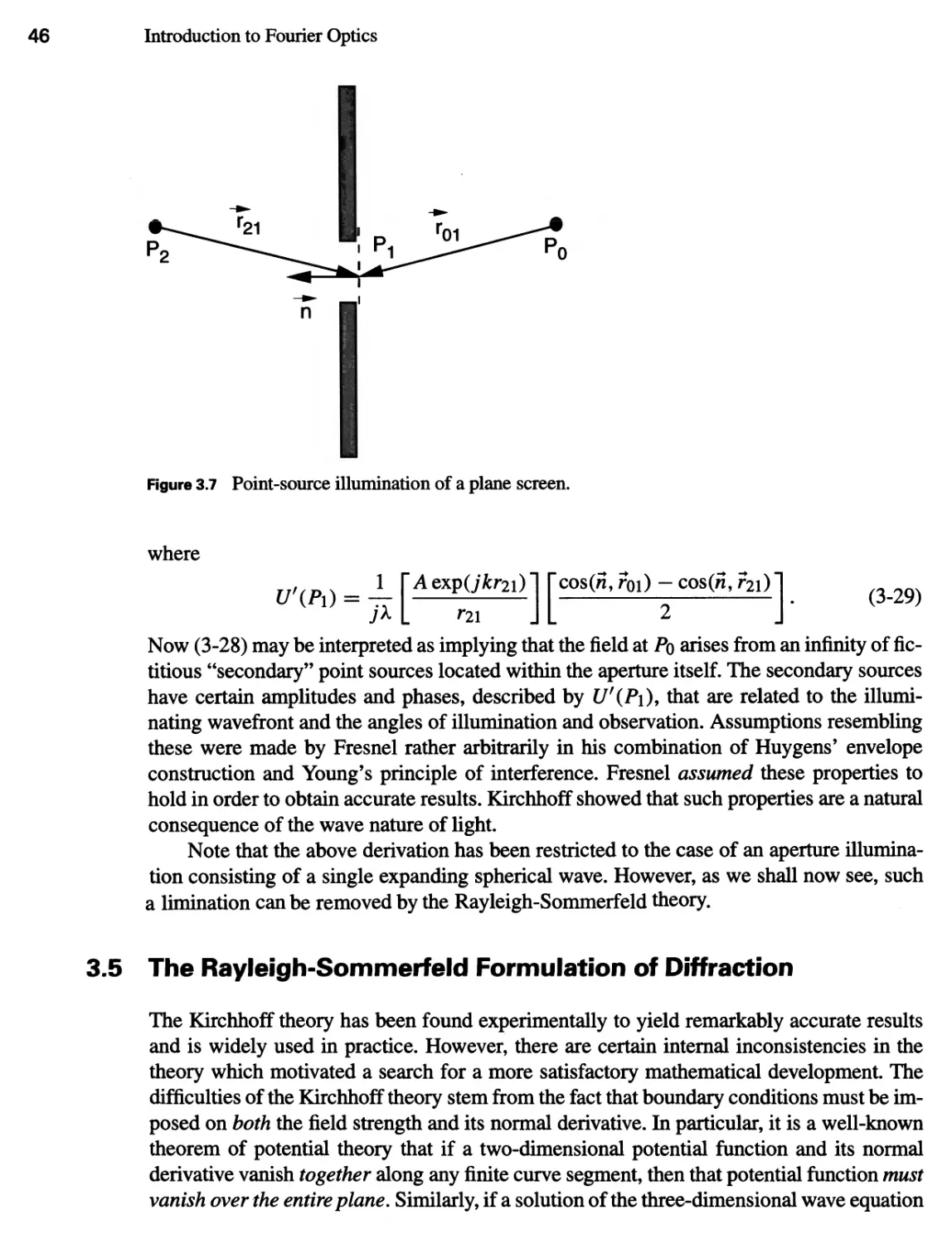
3.4.3 The Fresnel-Kirchhoff Diffraction Formula 45
3.5 The Rayleigh-Sommerfeld Formulation of Diffraction 46
3.5.1 Choice of Alternative Green’s Functions 47
3.5.2 The Rayleigh-Sommerfeld Diffraction Formula 49
3.6 Comparison of the Kirchhoff and Rayleigh-Sommerfeld Theories 50
3.7 Further Discussion of the Huygens-Fresnel Principle 52
3.8 Generalization to Nonmonochromatic Waves 53
3.9 Diffraction at Boundaries 54
3.10 The Angular Spectrum of Plane Waves 55
3.10.1 The Angular Spectrum and Its Physical Interpretation 55
3.10.2 Propagation of the Angular Spectrum 57
3.10.3 Effects of a Diffracting Aperture on the Angular Spectrum 59
3.10.4 The Propagation Phenomenon as a Linear Spatial Filter 60
4 Fresnel and Fraunhofer Diffraction 63
4.1 Background 63
4.1.1 The Intensity of a Wave Field 63
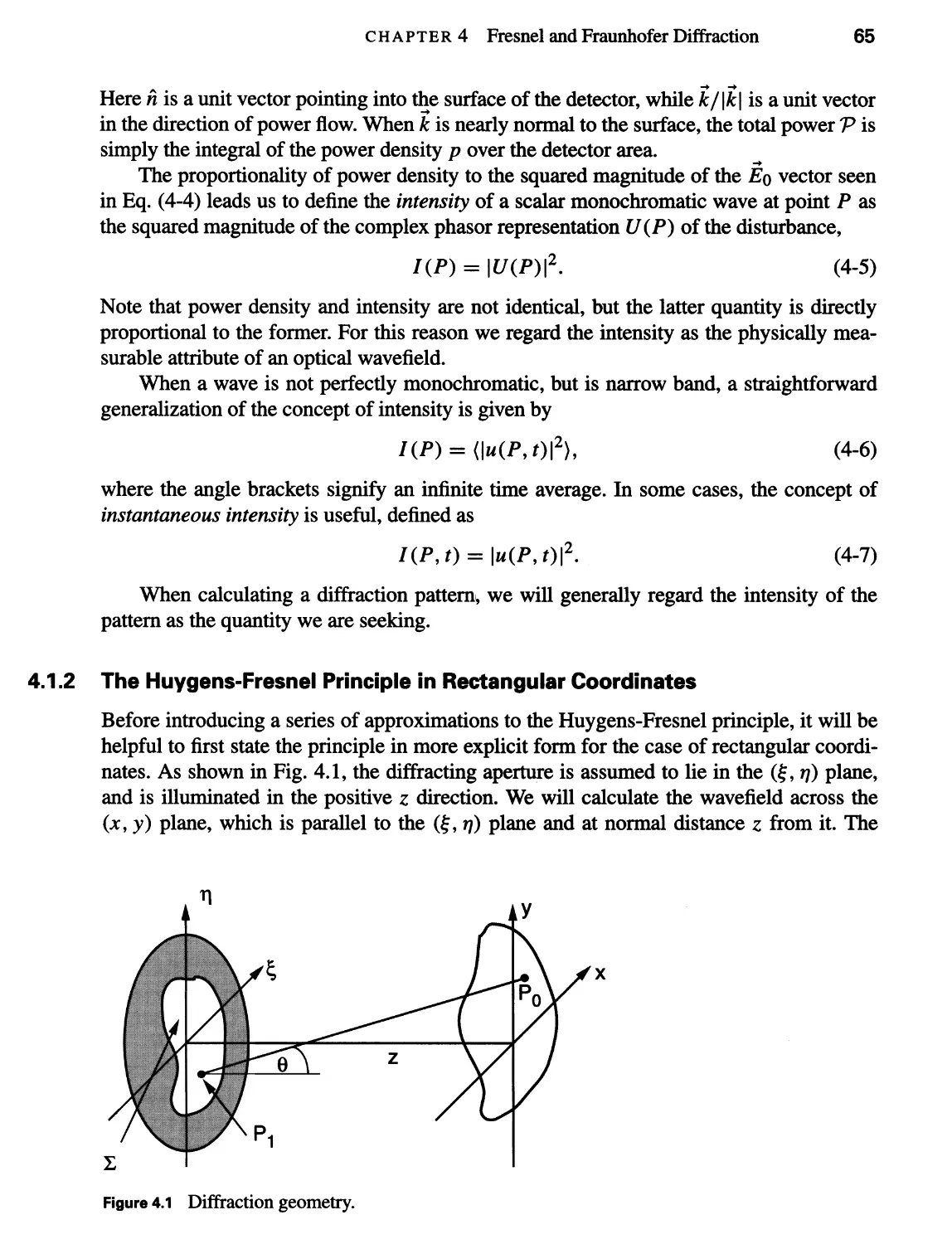
4.1.2 The Huygens-Fresnel Principle in Rectangular Coordinates 65
4.2 The Fresnel Approximation 66
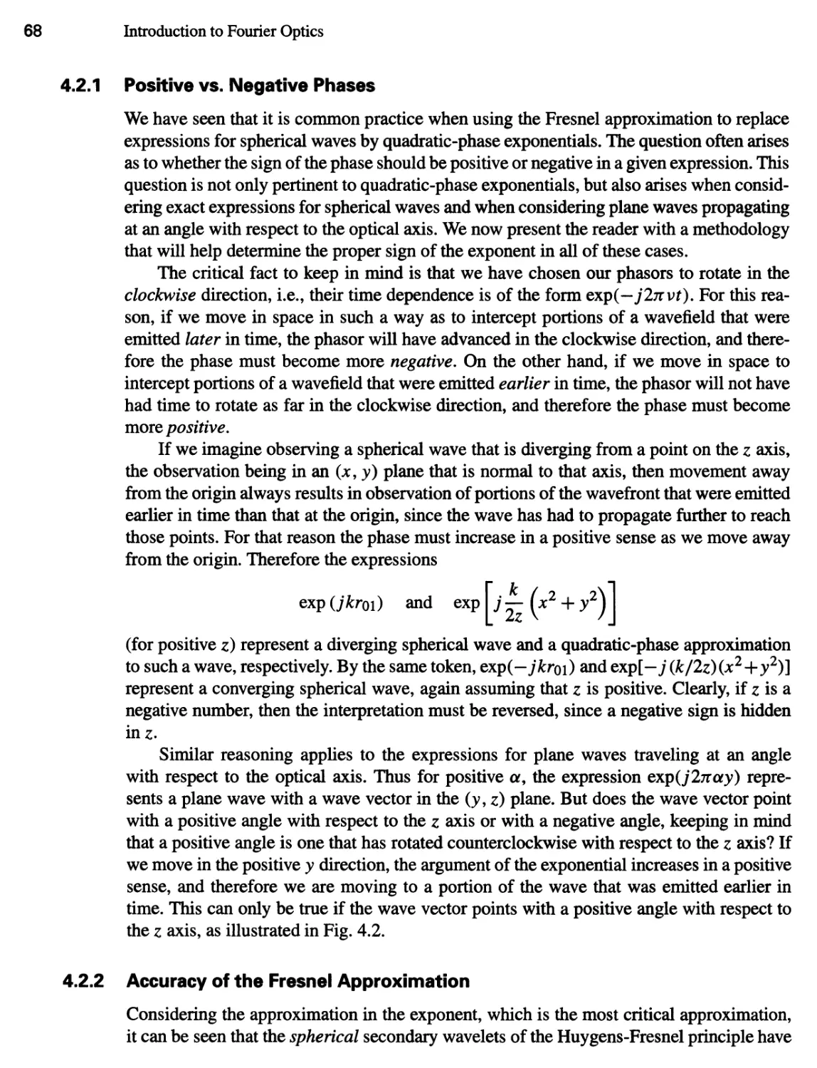
4.2.1 Positive vs. Negative Phases 68
4.2.2 Accuracy of the Fresnel Approximation 68
4.2.3 The Fresnel Approximation and the Angular Spectrum 72
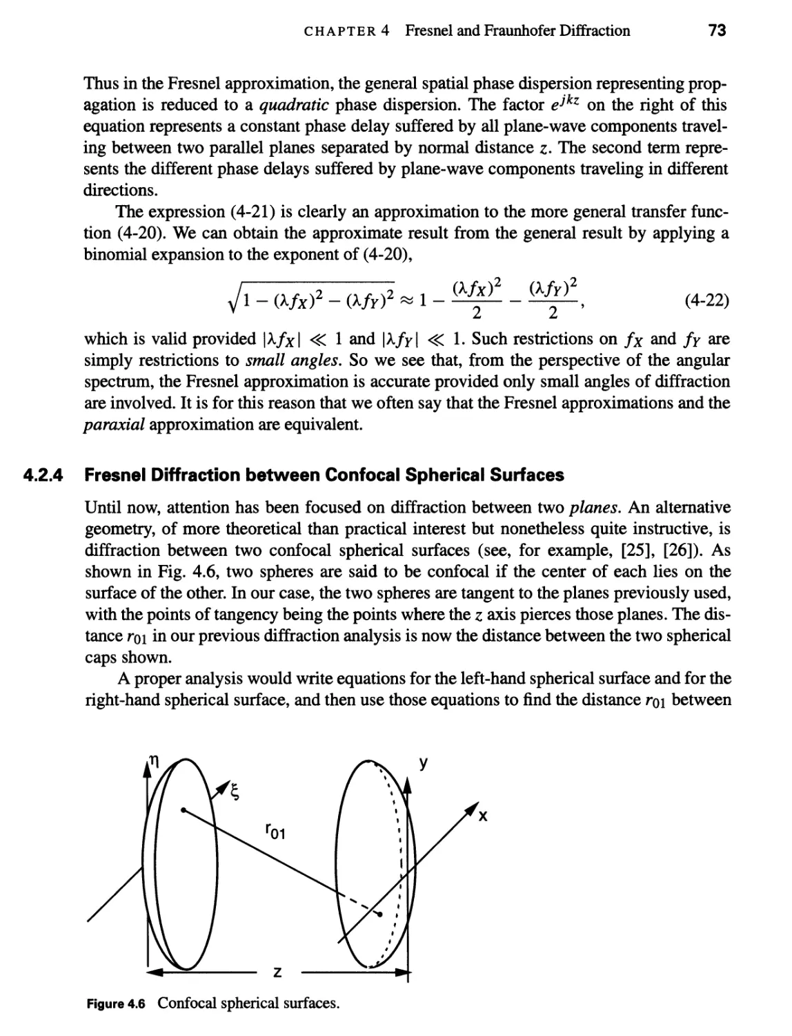
4.2.4 Fresnel Diffraction between Confocal Spherical Surfaces 73
4.3 The Fraunhofer Approximation 74
4.4 Examples of Fraunhofer Diffraction Patterns 75
4.4.1 Rectangular Aperture 76
4.4.2 Circular Aperture 76
4.4.3 Thin Sinusoidal Amplitude Grating 78
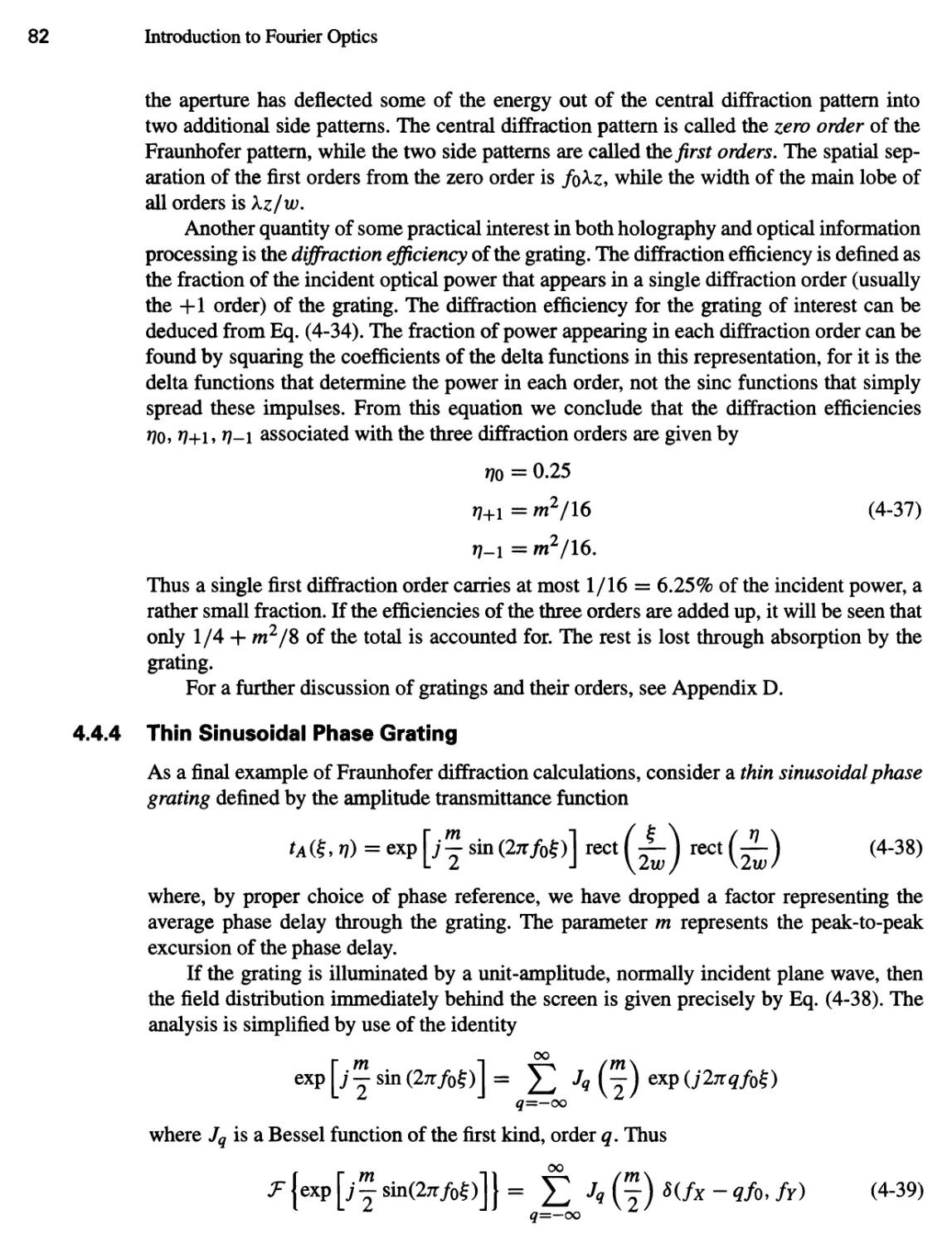
4.4.4 Thin Sinusoidal Phase Grating 82
4.5 Examples of Fresnel Diffraction Calculations 84
4.5.1 Fresnel Diffraction by a Square Aperture 84
4.5.2 Fresnel Diffraction by a Sinusoidal Amplitude Grating—Talbot
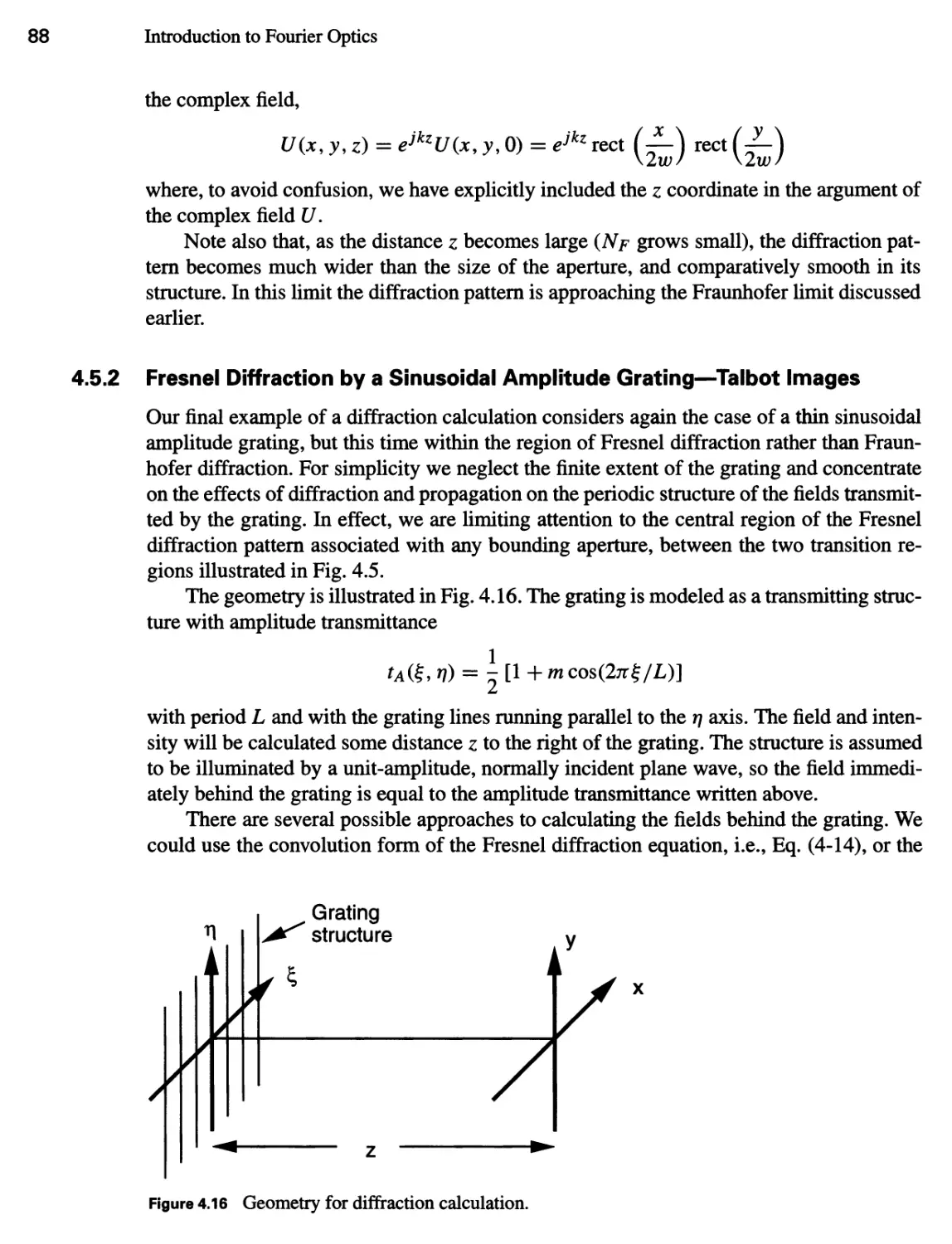
Images 88


Contents xiii
5 Wave-Optics Analysis of Coherent Optical Systems 97
5.1 A Thin Lens as a Phase Transformation 97
5.1.1 The Thickness Function .98
5.1.2 The Paraxial Approximation 100
5.1.3 The Phase Transformation and Its Physical Meaning 100
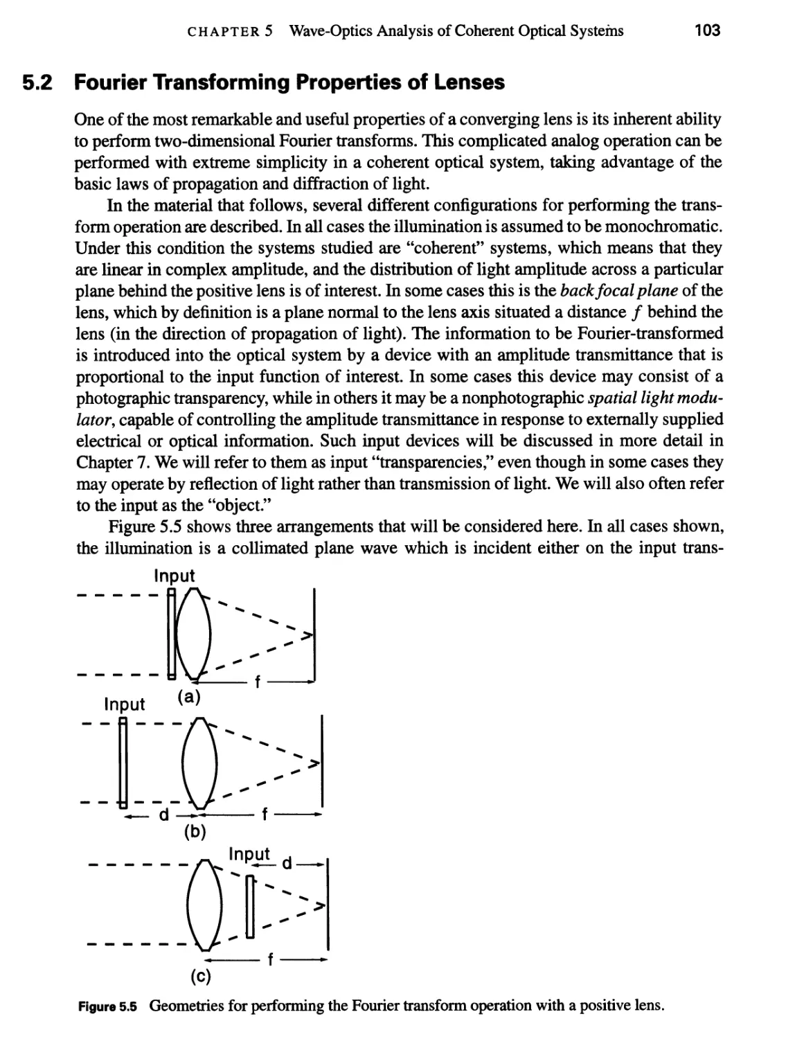
5.2 Fourier Transforming Properties of Lenses 103
5.2.1 Input Placed against the Lens 104
5.2.2 Input Placed in Front of the Lens 105
5.2.3 Input Placed behind the Lens 107
5.2.4 Example of an Optical Fourier Transform 108
5.3 Image Formation: Monochromatic Illumination 108
5.3.1 The Impulse Response of a Positive Lens 109
5.3.2 Eliminating Quadratic Phase Factors: The Lens Law Ill
5.3.3 The Relation between Object and Image 114
5.4 Analysis of Complex Coherent Optical Systems 115
5.4.1 An Operator Notation 115
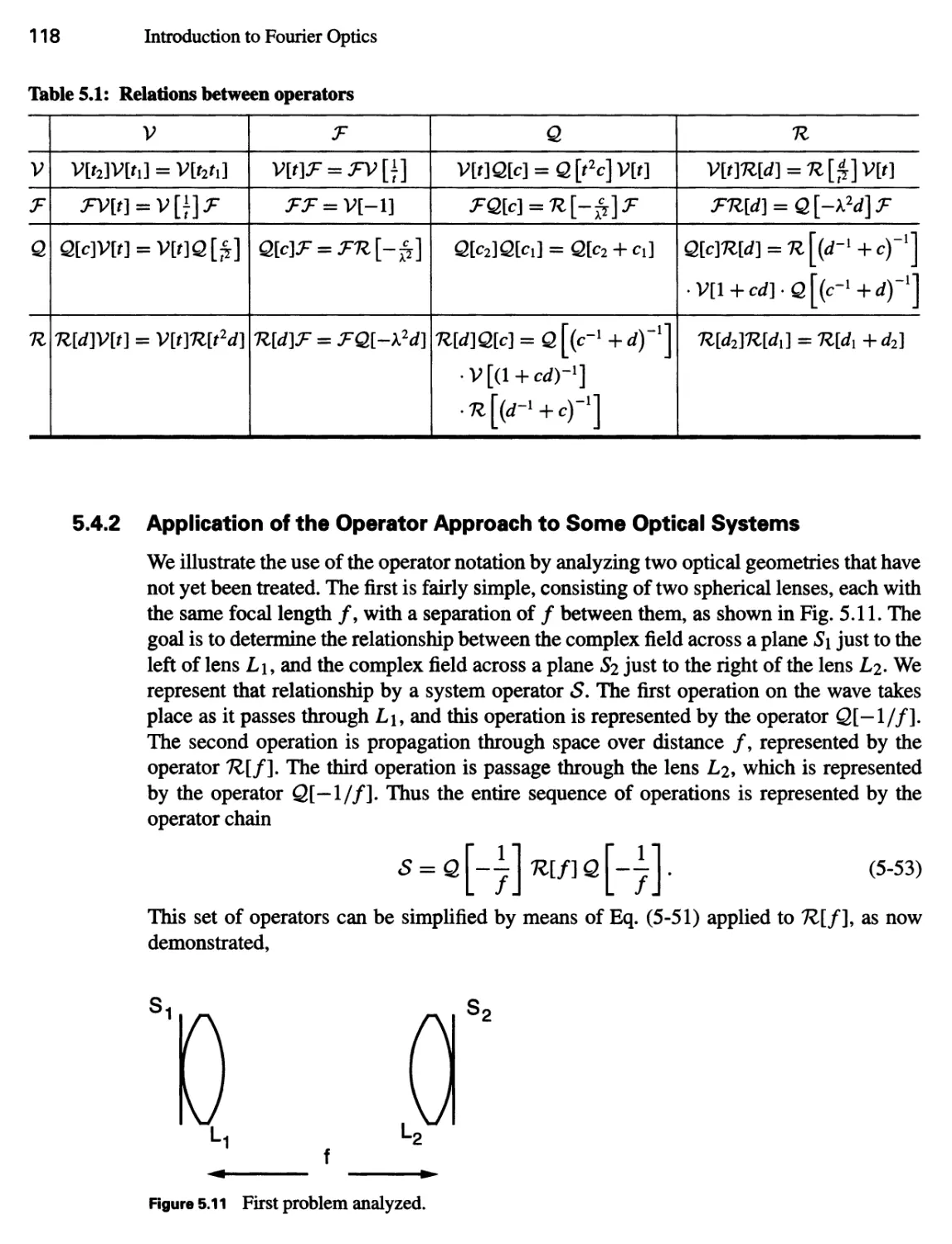
5.4.2 Application of the Operator Approach to Some Optical Systems 118
6 Frequency Analysis of Optical Imaging Systems 127
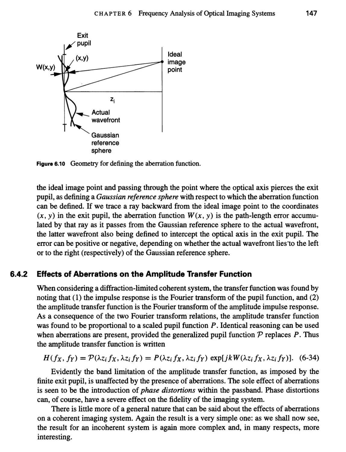
6.1 Generalized Treatment of Imaging Systems 128
6.1.1 A Generalized Model 128
6.1.2 Effects of Diffraction on the Image 129
6.1.3 Polychromatic Illumination: The Coherent and Incoherent Cases 131
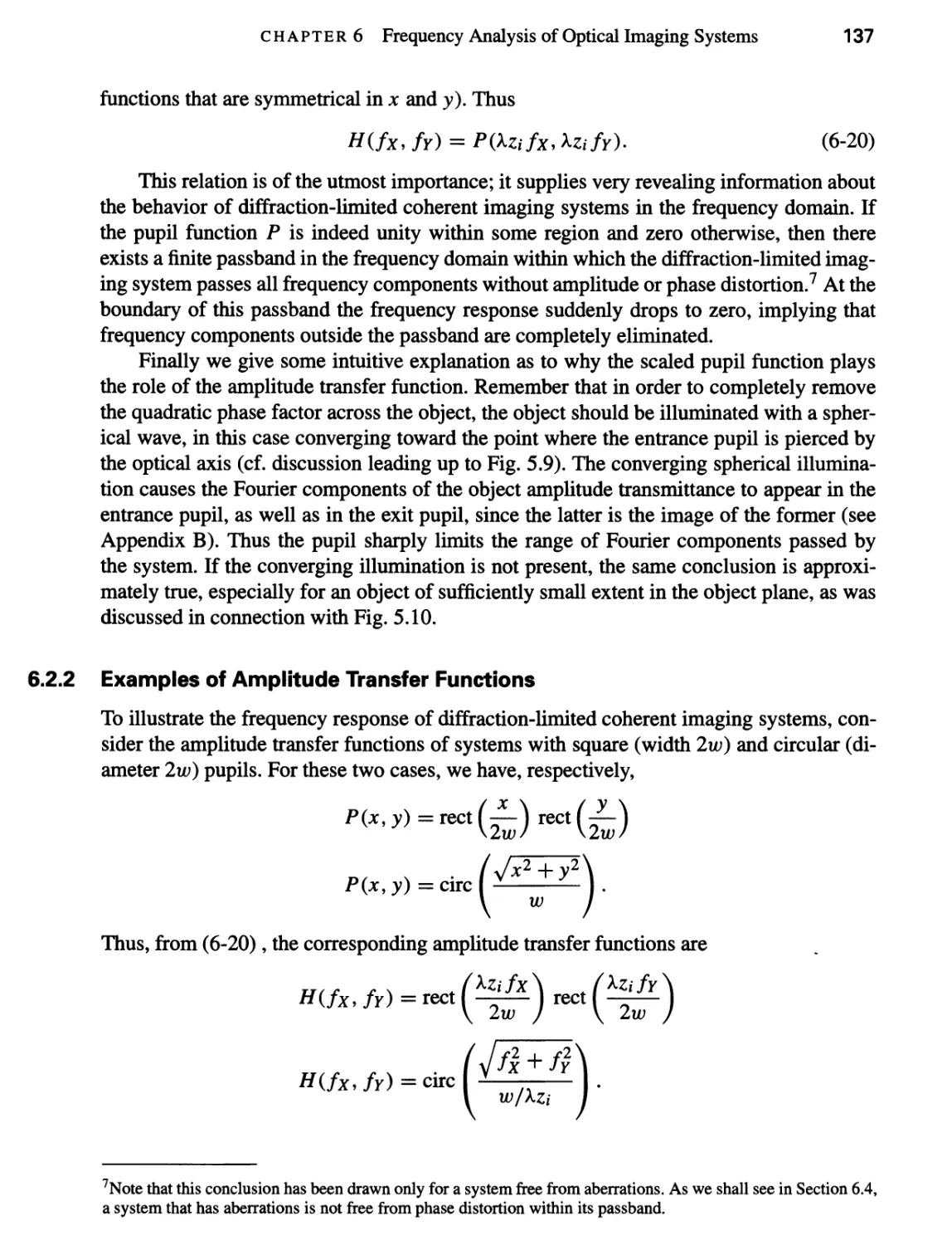
6.2 Frequency Response for Diffraction-Limited Coherent Imaging 135
6.2.1 The Amplitude Transfer Function 136
6.2.2 Examples of Amplitude Transfer Functions 137
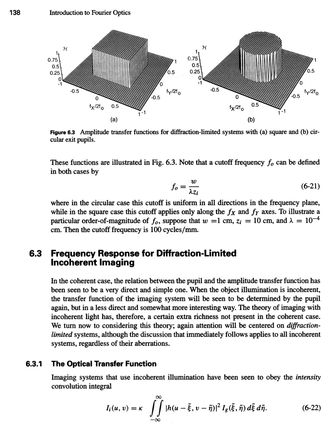
6.3 Frequency Response for Diffraction-Limited Incoherent Imaging 138
6.3.1 The Optical Transfer Function 138
6.3.2 General Properties of the OTF 140
6.3.3 The OTF of an Aberration-Free System 141
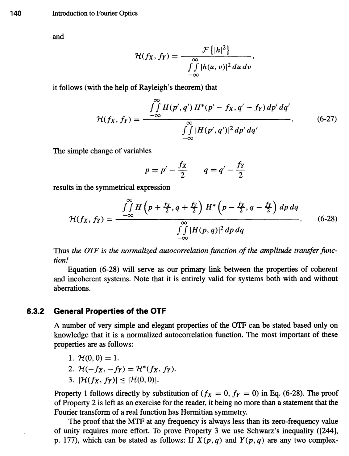
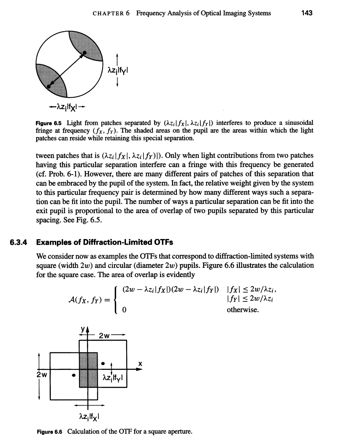
6.3.4 Examples of Diffraction-Limited OTFs 143
6.4 Aberrations and Their Effects on Frequency Response 145
6.4.1 The Generalized Pupil Function 145
6.4.2 Effects of Aberrations on the Amplitude Transfer Function 147
6.4.3 Effects of Aberrations on the OTF 148
6.4.4 Example of a Simple Aberration: A Focusing Error 149
6.4.5 Apodization and Its Effects on Frequency Response 152
6.5 Comparison of Coherent and Incoherent Imaging 154
6.5.1 Frequency Spectrum of the Image Intensity 156
6.5.2 Two-Point Resolution 158
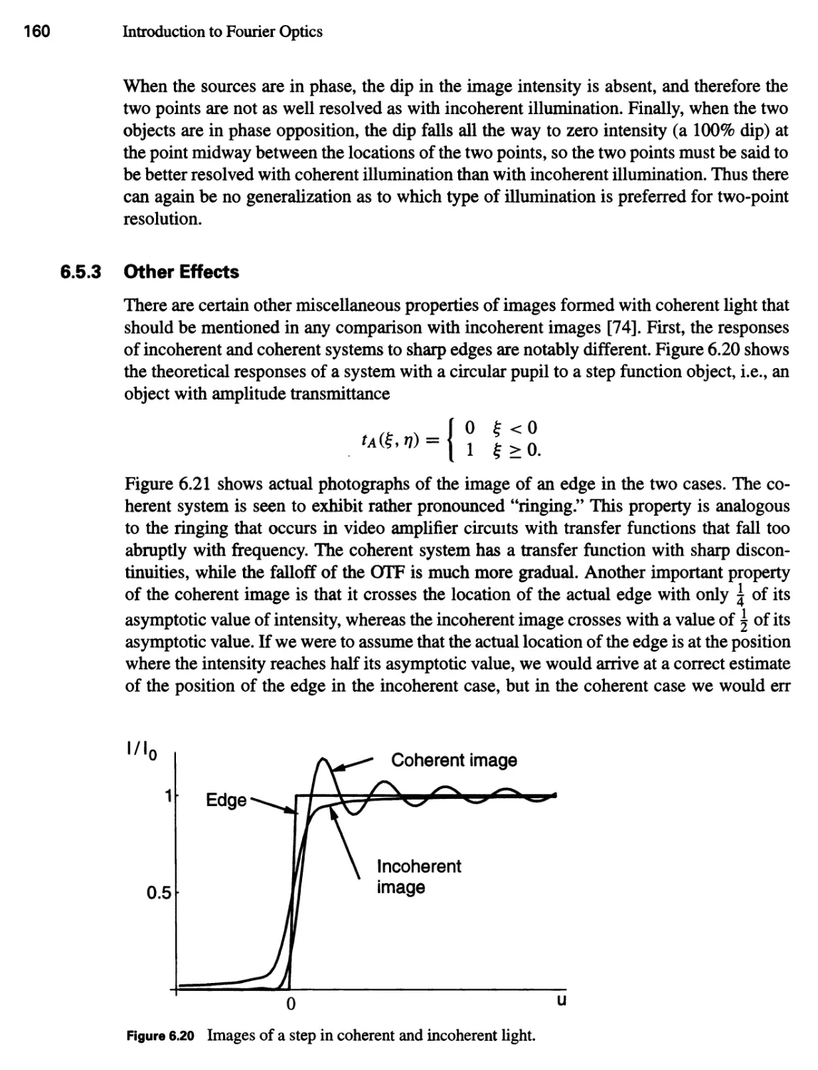
6.5.3 Other Effects 160


xiv Contents
6.6 Resolution beyond the Classical Diffraction Limit 162
6.6.1 Underlying Mathematical Fundamentals 162
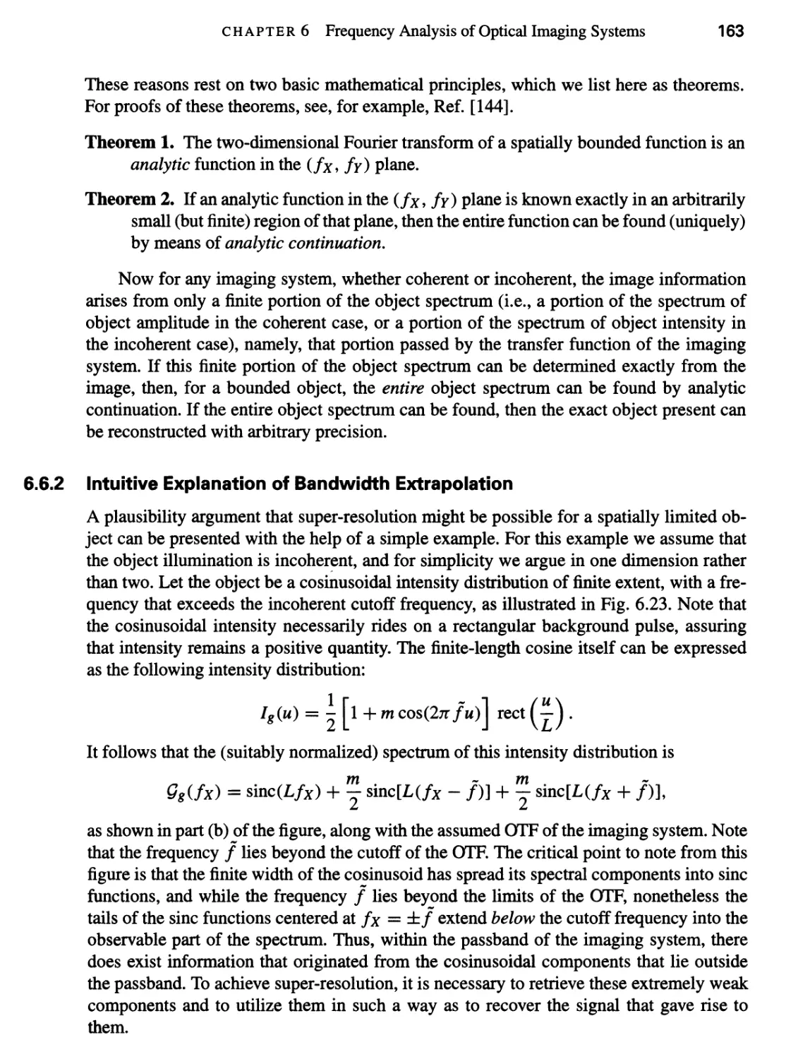
6.6.2 Intuitive Explanation of Bandwidth Extrapolation 163
6.6.3 An Extrapolation Method Based on the Sampling Theorem 164
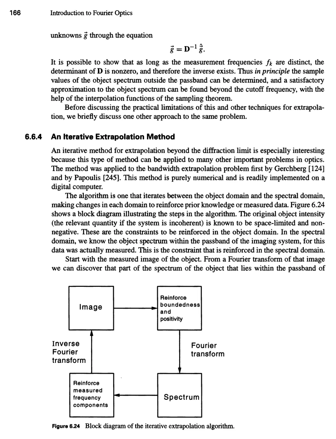
6.6.4 An Iterative Extrapolation Method 166
6.6.5 Practical Limitations 167
7 Wavefront Modulation 173
7.1 Wavefront Modulation with Photographic Film 174
7.1.1 The Physical Processes of Exposure, Development, and Fixing 174
7.1.2 Definition of Terms 175
7.1.3 Film in an Incoherent Optical System 178
7.1.4 Film in a Coherent Optical System 179
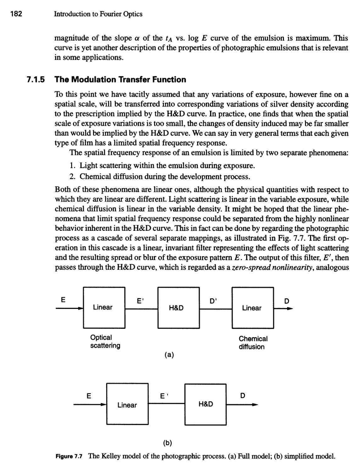
7.1.5 The Modulation Transfer Function 182
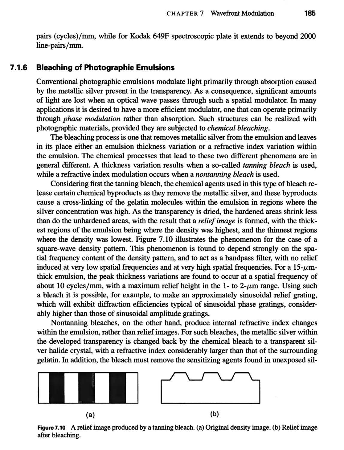
7.1.6 Bleaching of Photographic Emulsions 185
7.2 Spatial Light Modulators 186
7.2.1 Properties of Liquid Crystals 187
7.2.2 Spatial Light Modulators Based on Liquid Crystals 195
7.2.3 Magneto-Optic Spatial Light Modulators 199
7.2.4 Deformable Mirror Spatial Light Modulators 202
7.2.5 Multiple Quantum Well Spatial Light Modulators 204
7.2.6 Acousto-Optic Spatial Light Modulators 208
7.3 Diffractive Optical Elements 212
7.3.1 Binary Optics 212
7.3.2 Other Types of Diffractive Optics 216
7.3.3 A Word of Caution 216
8 Analog Optical Information Processing 219
8.1 Historical Background 220
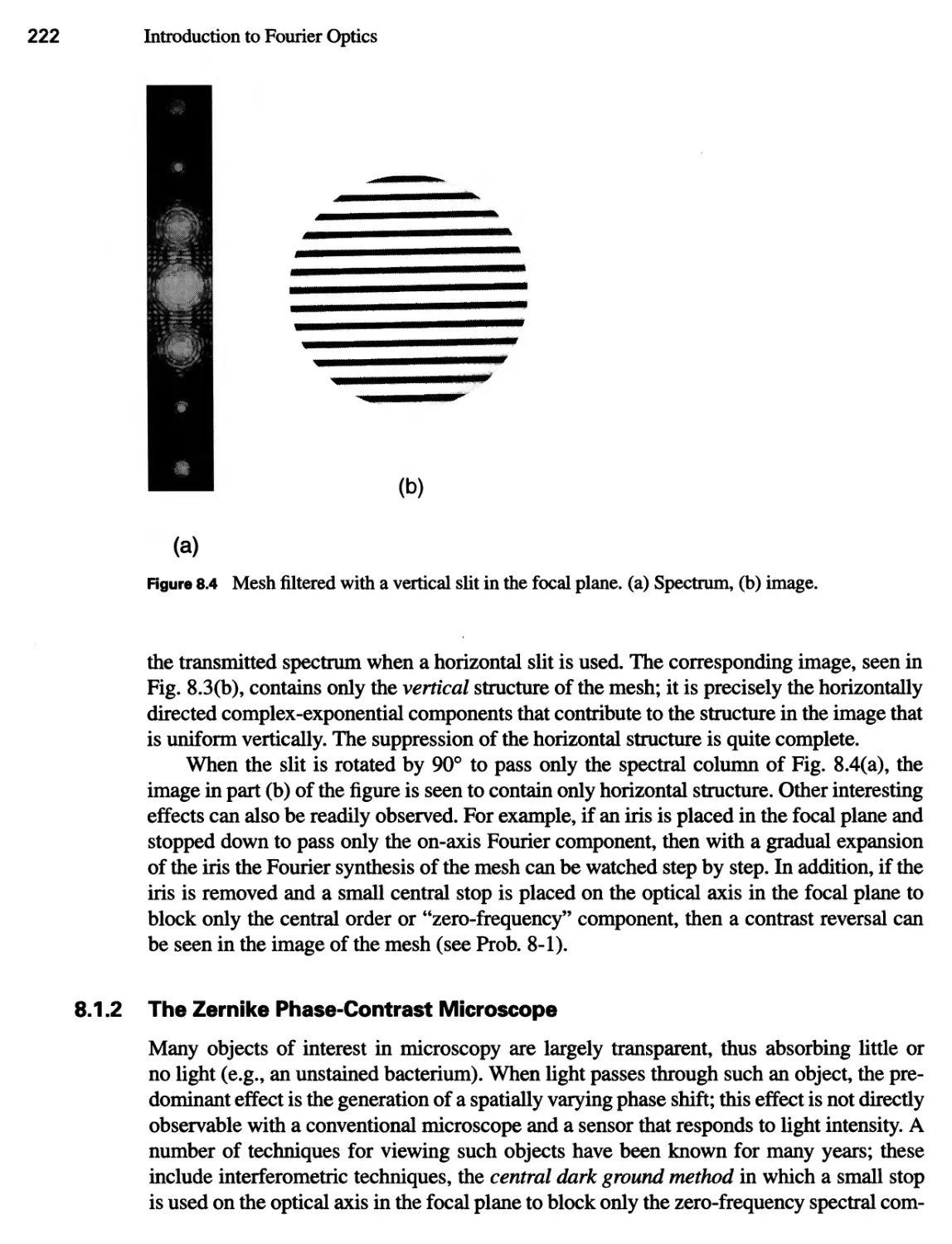
8.1.1 The Abbe-Porter Experiments 220
8.1.2 The Zemike Phase-Contrast Microscope 222
8.1.3 Improvement of Photographs: Marechal 224
8.1.4 The Emergence of a Communications Viewpoint 226
8.1.5 Application of Coherent Optics to More General Data Processing... 226
8.2 Incoherent Image Processing Systems 226
8.2.1 Systems Based on Geometrical Optics 227
8.2.2 Systems That Incorporate the Effects of Diffraction 232
8.3 Coherent Optical Information Processing Systems 234
8.3.1 Coherent System Architectures 234
8.3.2 Constraints on Filter Realization 237


Contents xv
8.4 The VanderLugt Filter 239
8.4.1 Synthesis of the Frequency-Plane Mask 239
8.4.2 Processing the Input Data 242
8.4.3 Advantages of the VanderLugt Filter 244
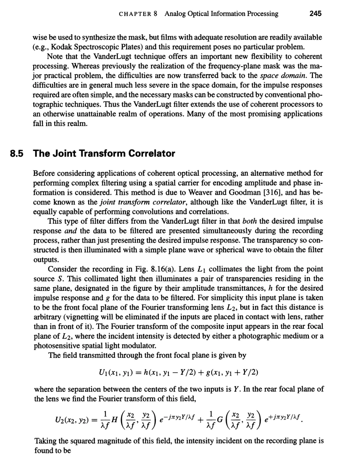
8.5 The Joint Transform Correlator 245
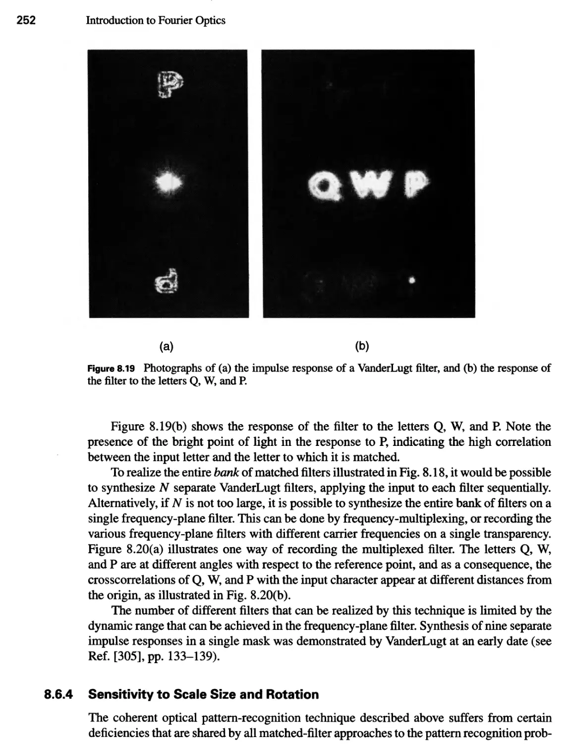
8.6 Application to Character Recognition 248
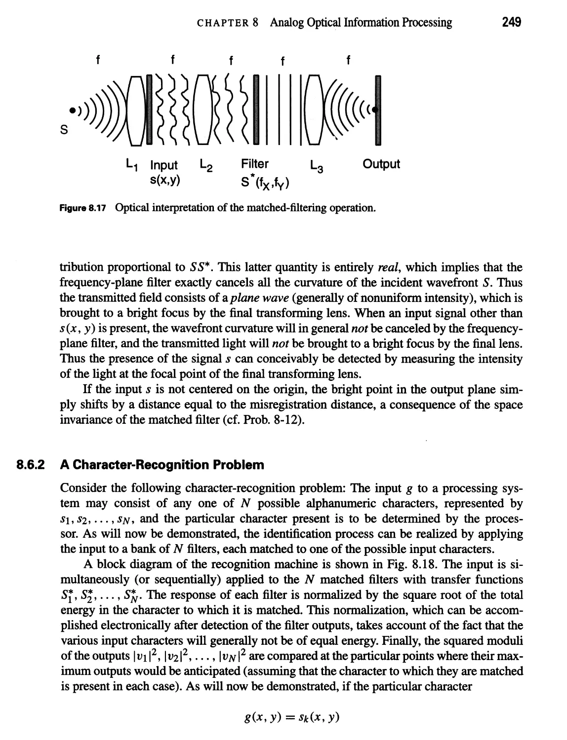
8.6.1 The Matched Filter 248
8.6.2 A Character-Recognition Problem 249
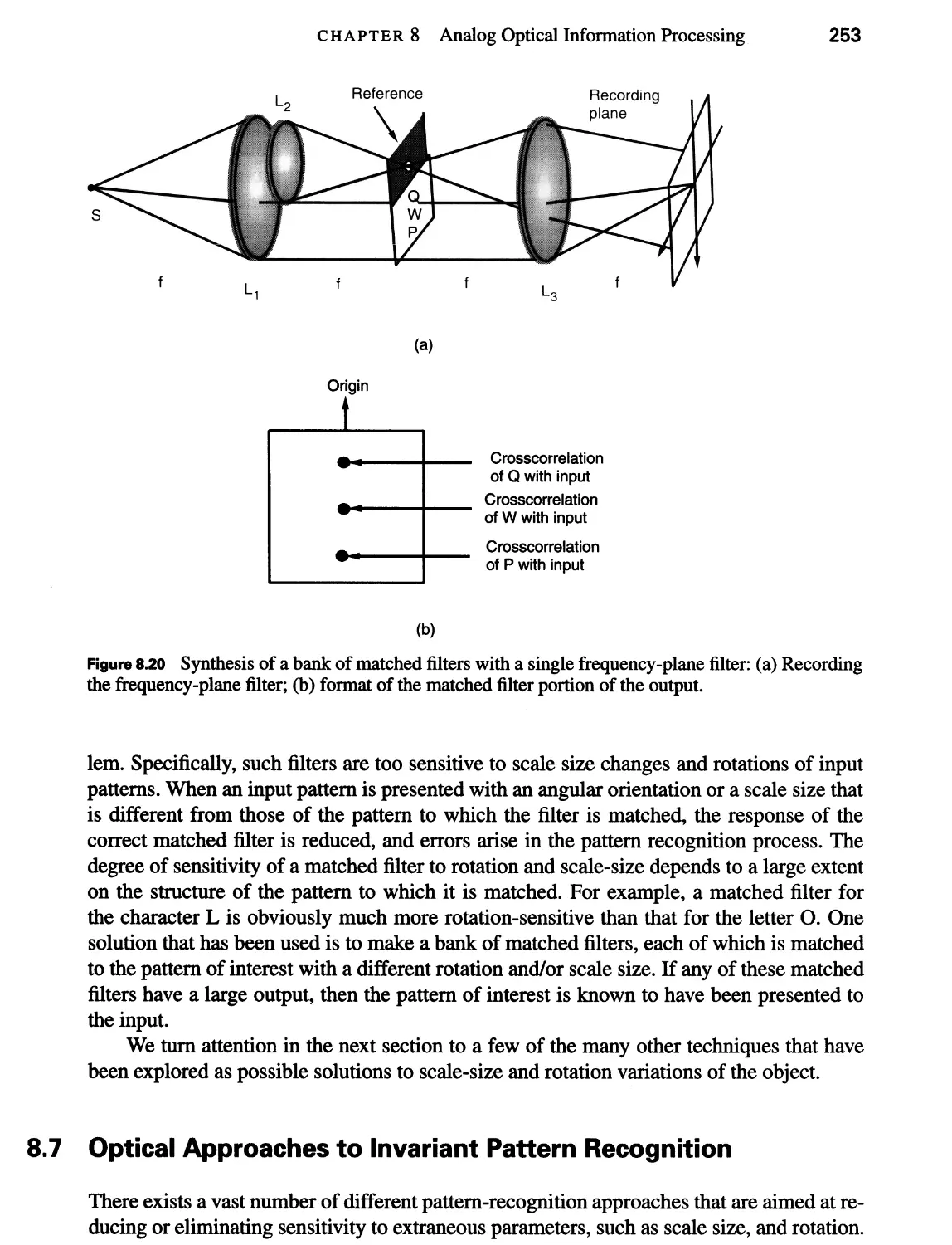
8.6.3 Optical Synthesis of a Character-Recognition Machine 251
8.6.4 Sensitivity to Scale Size and Rotation 252
8.7 Optical Approaches to Invariant Pattern Recognition 253
8.7.1 Mellin Correlators 254
8.7.2 Circular Harmonic Correlation 256
8.7.3 Synthetic Discriminant Functions 257
8.8 Image Restoration 259
8.8.1 The Inverse Filter 259
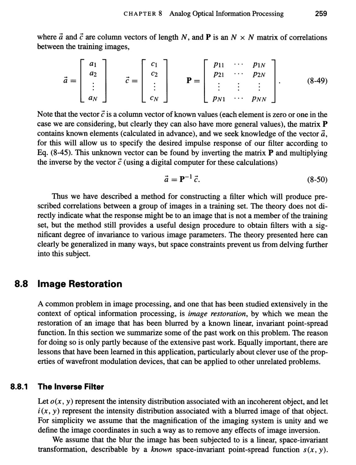
8.8.2 The Wiener Filter, or the Least-Mean-Square-Error Filter 261
8.8.3 Filter Realization 262
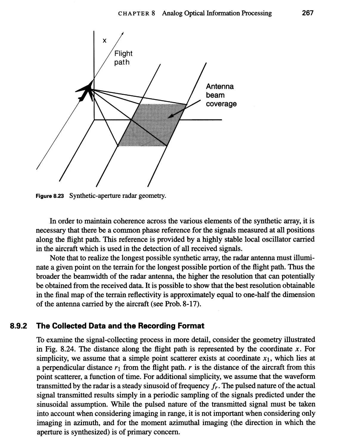
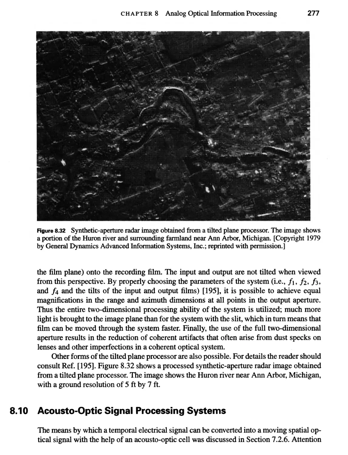
8.9 Processing Synthetic-Aperture Radar (SAR) Data 265
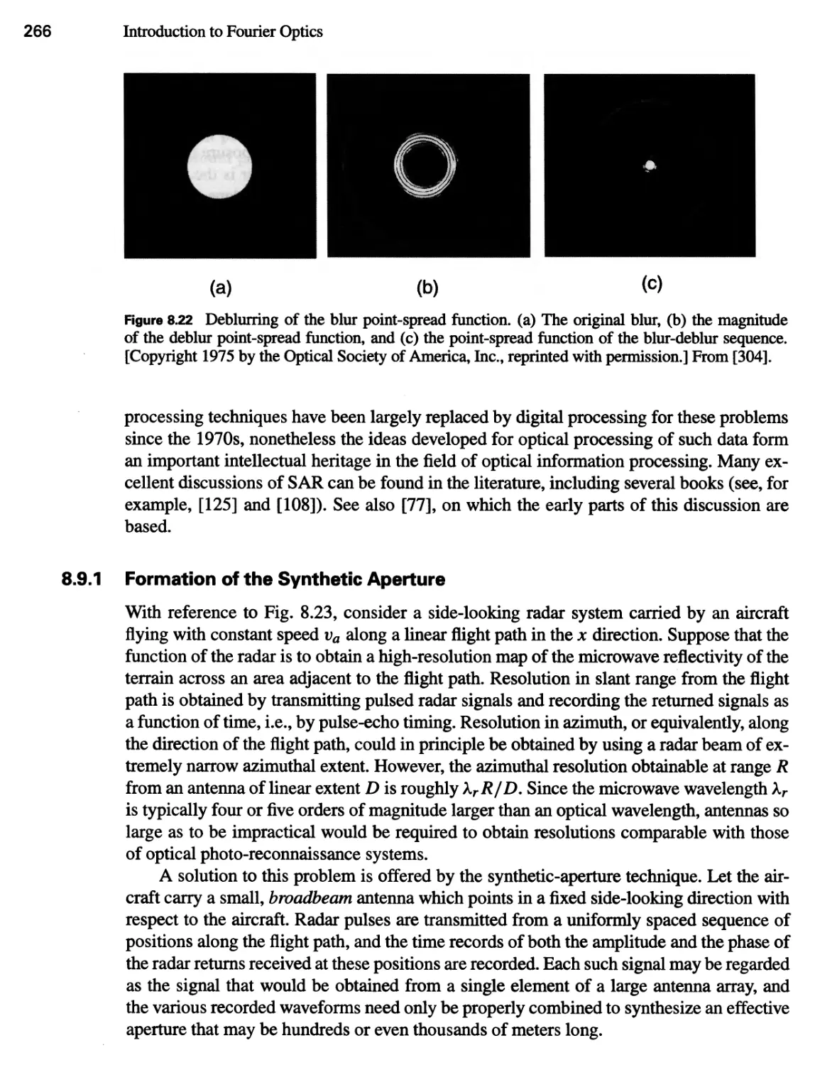
8.9.1 Formation of the Synthetic Aperture 266
8.9.2 The Collected Data and the Recording Format 267
8.9.3 Focal Properties of the Film Transparency 269
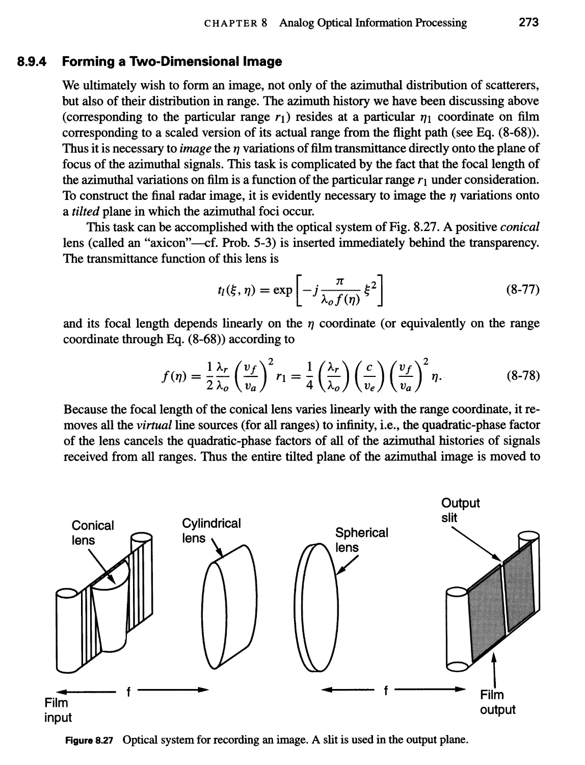
8.9.4 Forming a Two-Dimensional Image 273
8.9.5 The Tilted Plane Processor 274
8.10 Acousto-Optic Signal Processing Systems 277
8.10.1 Bragg Cell Spectrum Analyzer 278
8.10.2 Space-Integrating Correlator 280
8.10.3 Time-Integrating Correlator 281
8.10.4 Other Acousto-Optic Signal Processing Architectures 283
8.11 Discrete Analog Optical Processors 284
8.11.1 Discrete Representation of Signals and Systems 284
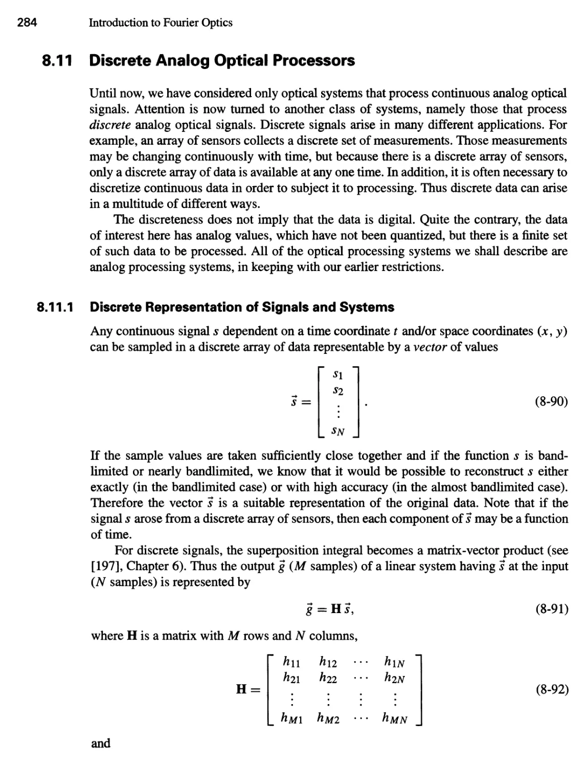
8.11.2 A Serial Matrix-Vector Multiplier 285
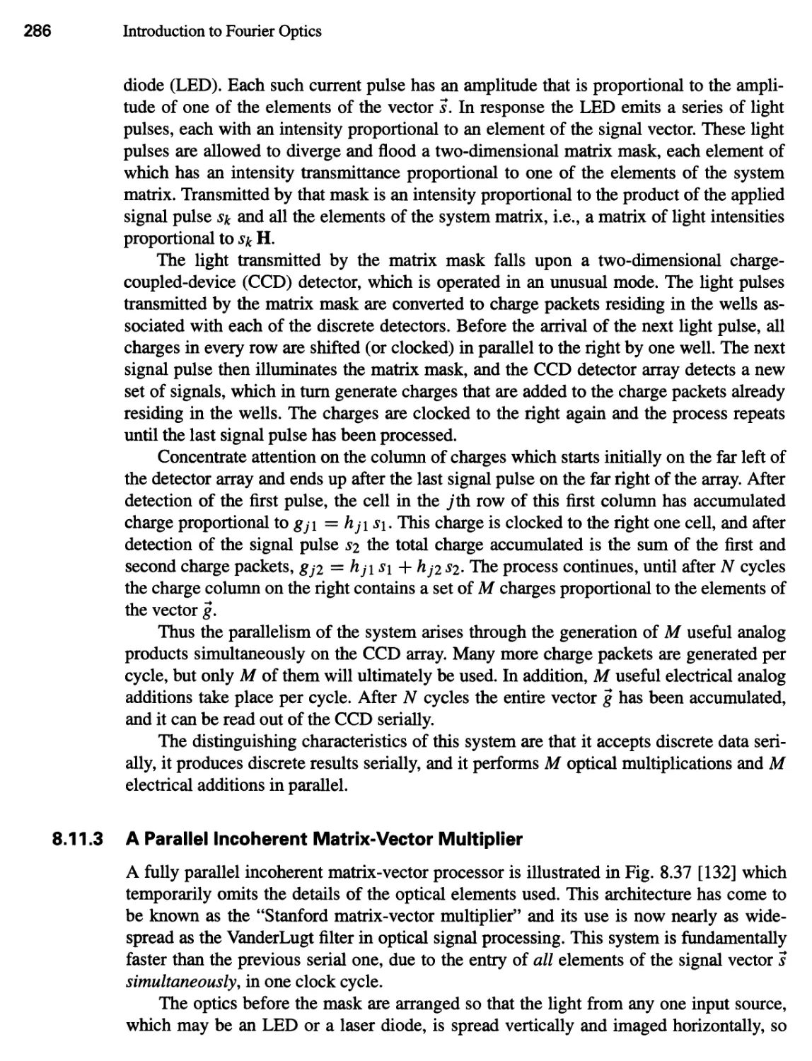
8.11.3 A Parallel Incoherent Matrix-Vector Multiplier 286
8.11.4 An Outer Product Processor 288
8.11.5 Other Discrete Processing Architectures 290
8.11.6 Methods for Handling Bipolar and Complex Data 290
9 Holography 297
9.1 Historical Introduction 297
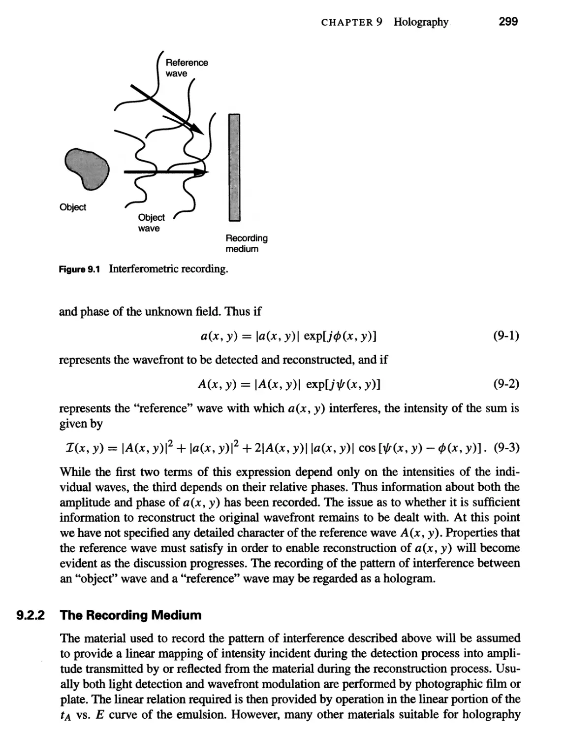
9.2 The Wavefront Reconstruction Problem 298
9.2.1 Recording Amplitude and Phase 298
9.2.2 The Recording Medium 299


xv i
Contents
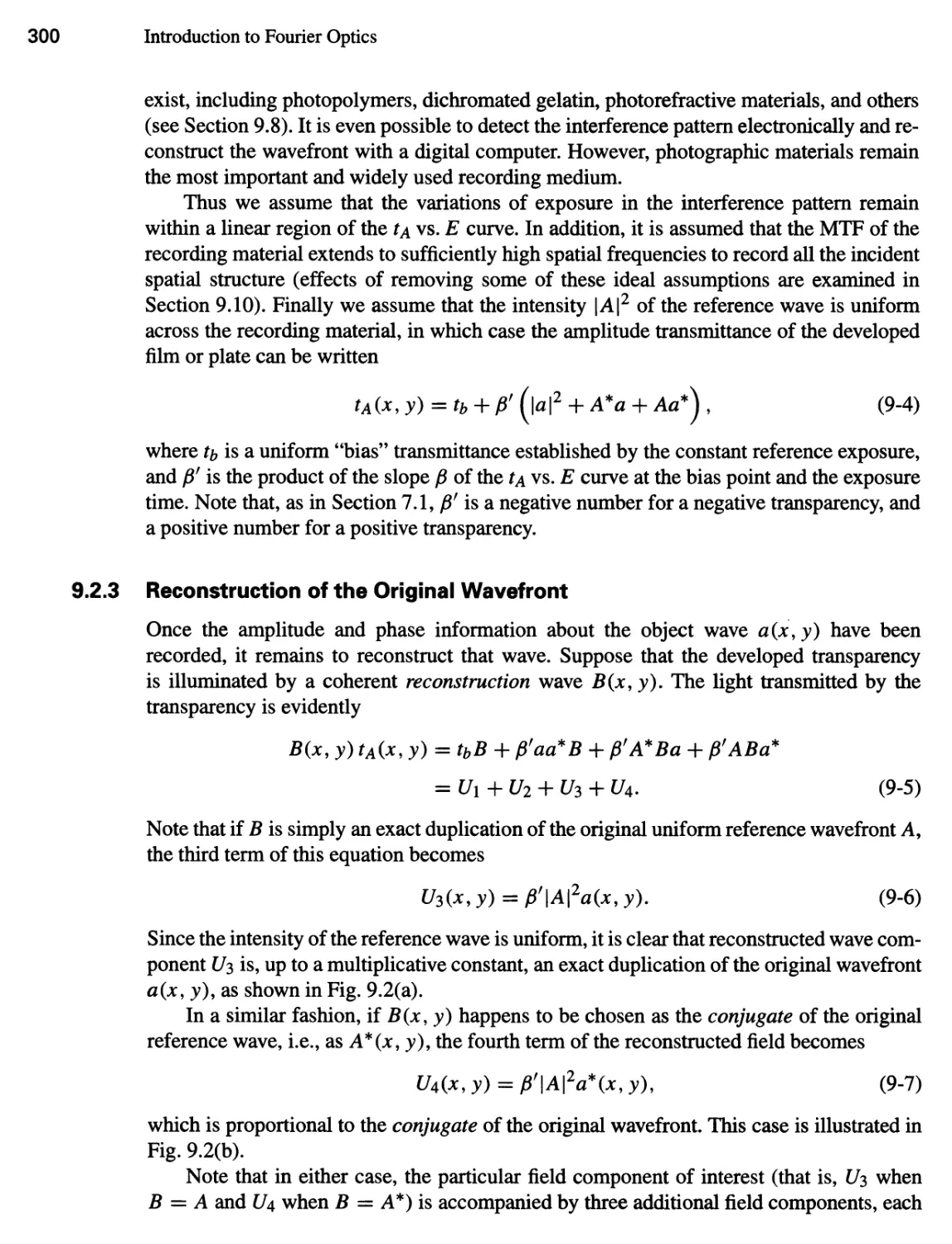
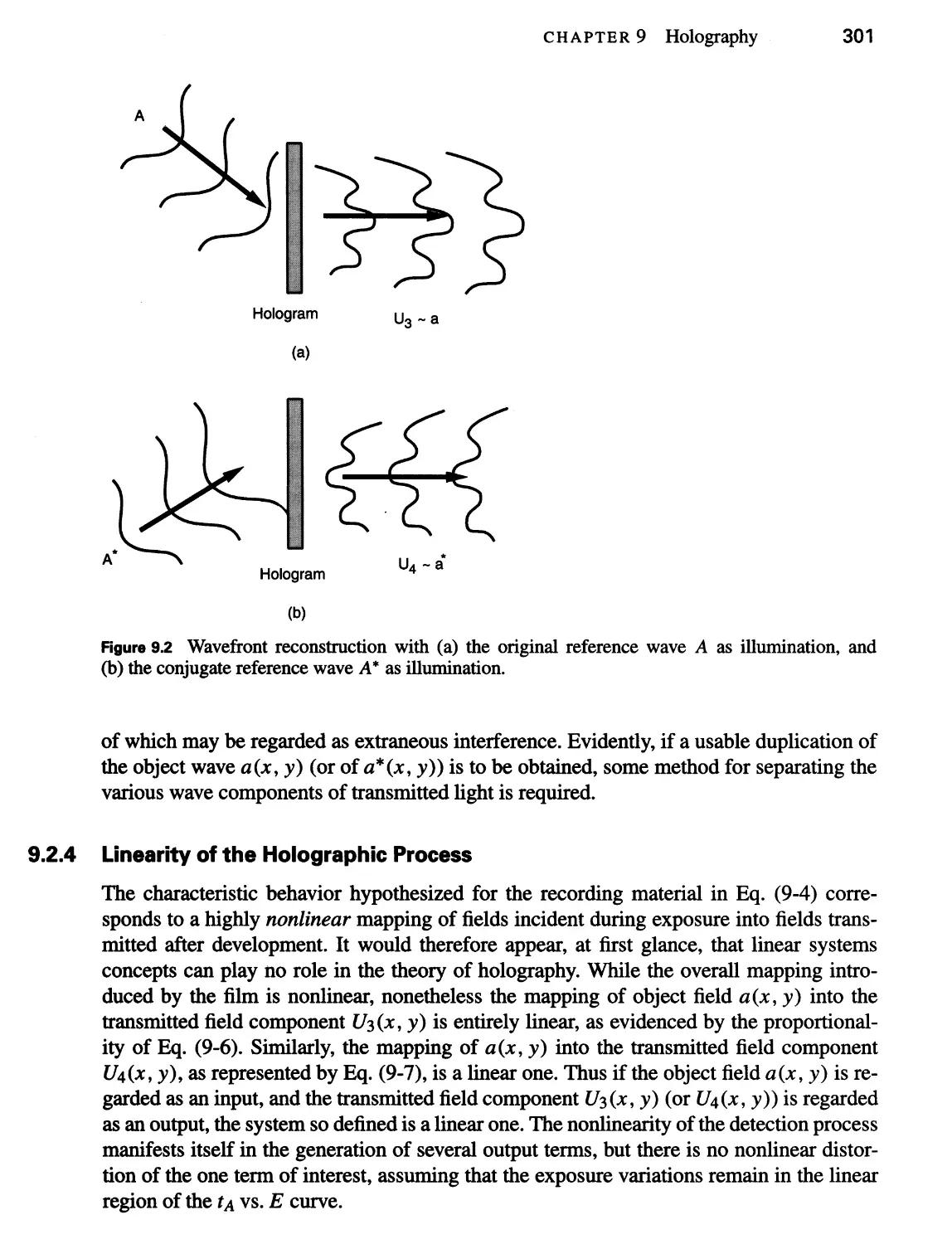
9.2.3 Reconstruction of the Original Wavefront 300
9.2.4 Linearity of the Holographic Process 301
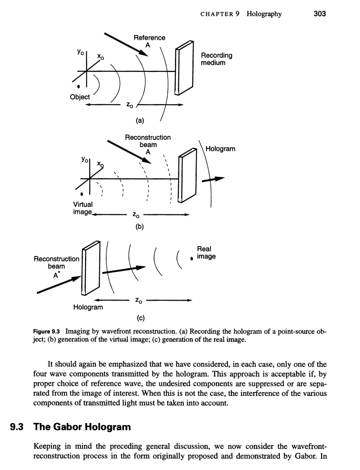
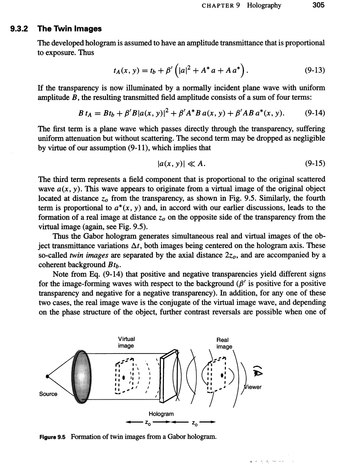
9.2.5 Image Formation by Holography 302
9.3 The Gabor Hologram 303
9.3.1 Origin of the Reference Wave 304
9.3.2 The Twin Images 305
9.3.3 Limitations of the Gabor Hologram 306
9.4 The Leith-Upatnieks Hologram 306
9.4.1 Recording the Hologram 307
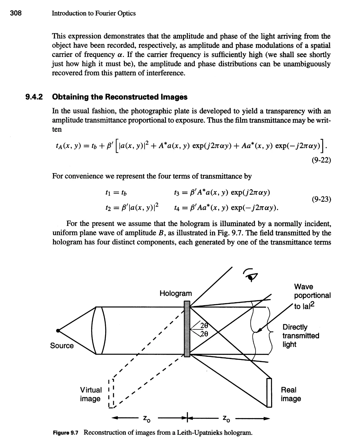
9.4.2 Obtaining the Reconstructed Images 308
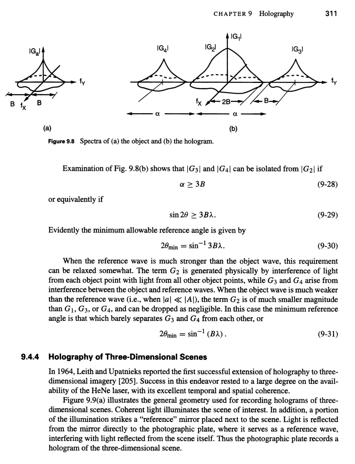
9.4.3 The Minimum Reference Angle 310
9.4.4 Holography of Three-Dimensional Scenes 311
9.4.5 Practical Problems in Holography 314
9.5 Image Locations and Magnification 316
9.5.1 Image Locations 316
9.5.2 Axial and Transverse Magnifications 319
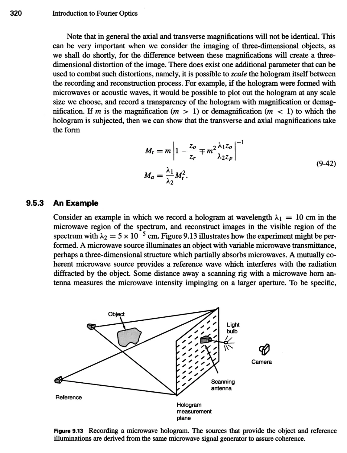
9.5.3 An Example 320
9.6 Some Different Types of Holograms 321
9.6.1 Fresnel, Fraunhofer, Image, and Fourier Holograms 322
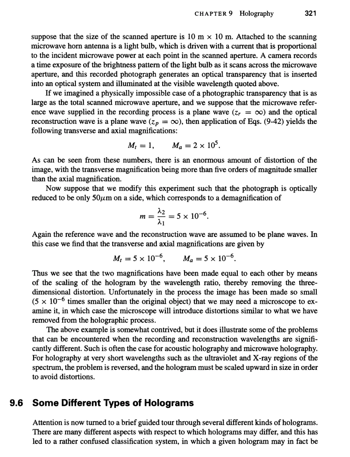
9.6.2 Transmission and Reflection Holograms 323
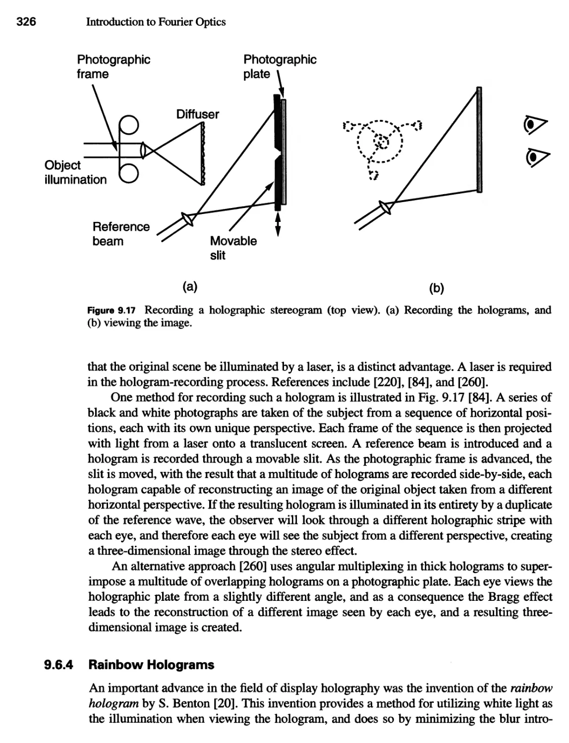
9.6.3 Holographic Stereograms 325
9.6.4 Rainbow Holograms 326
9.6.5 Multiplex Holograms 329
9.6.6 Embossed Holograms 331
9.7 Thick Holograms 332
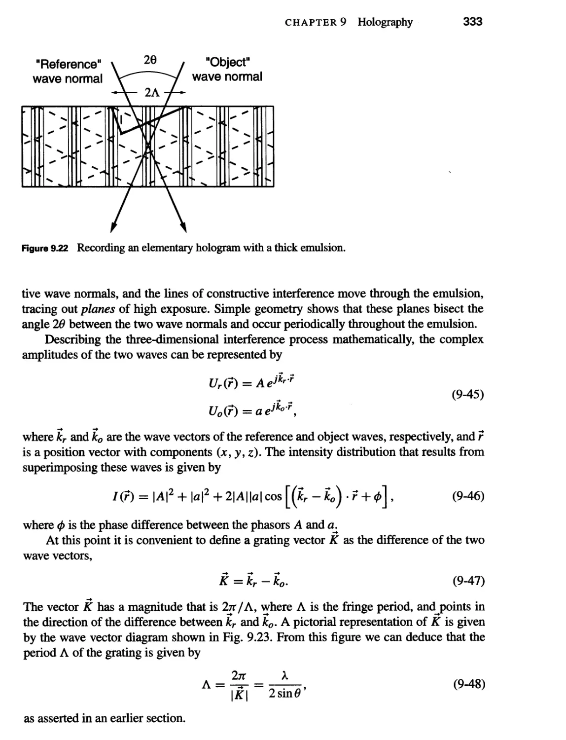
9.7.1 Recording a Volume Holographic Grating 332
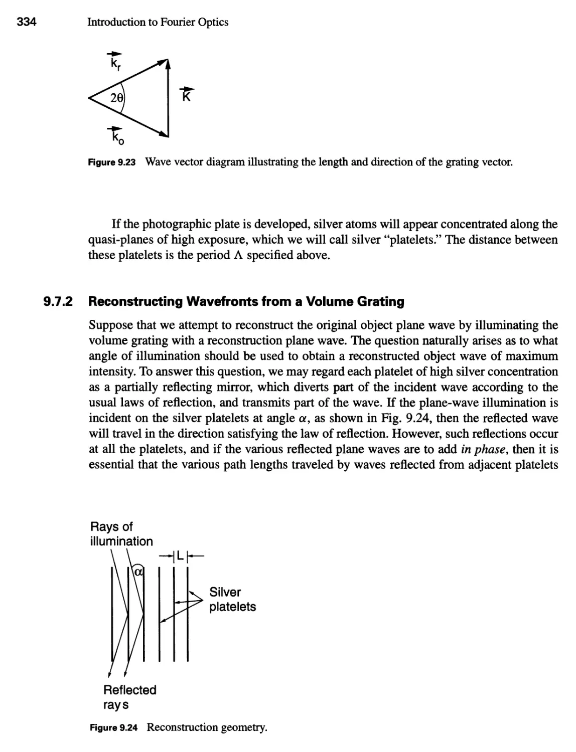
9.7.2 Reconstructing Wavefronts from a Volume Grating 334
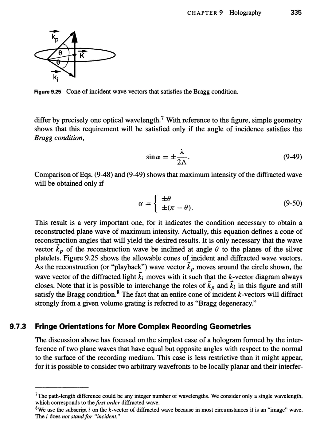
9.7.3 Fringe Orientations for More Complex Recording Geometries 335
9.7.4 Gratings of Finite Size 337
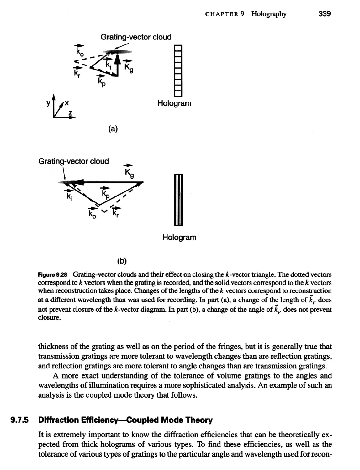
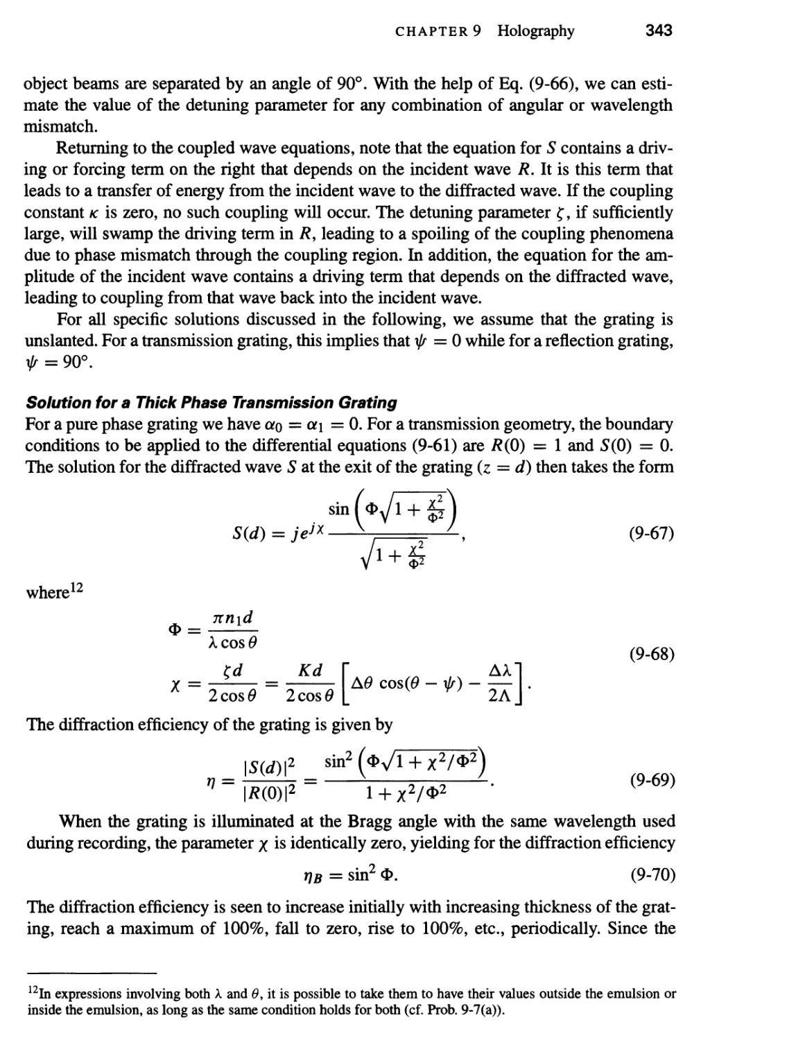
9.7.5 Diffraction Efficiency—Coupled Mode Theory 339
9.8 Recording Materials 350
9.8.1 Silver Halide Emulsions 350
9.8.2 Photopolymer Films 351
9.8.3 Dichromated Gelatin 352
9.8.4 Photorefractive Materials 352
9.9 Computer-Generated Holograms 355
9.9.1 The Sampling Problem 356
9.9.2 The Computational Problem 359
9.9.3 The Representational Problem 359
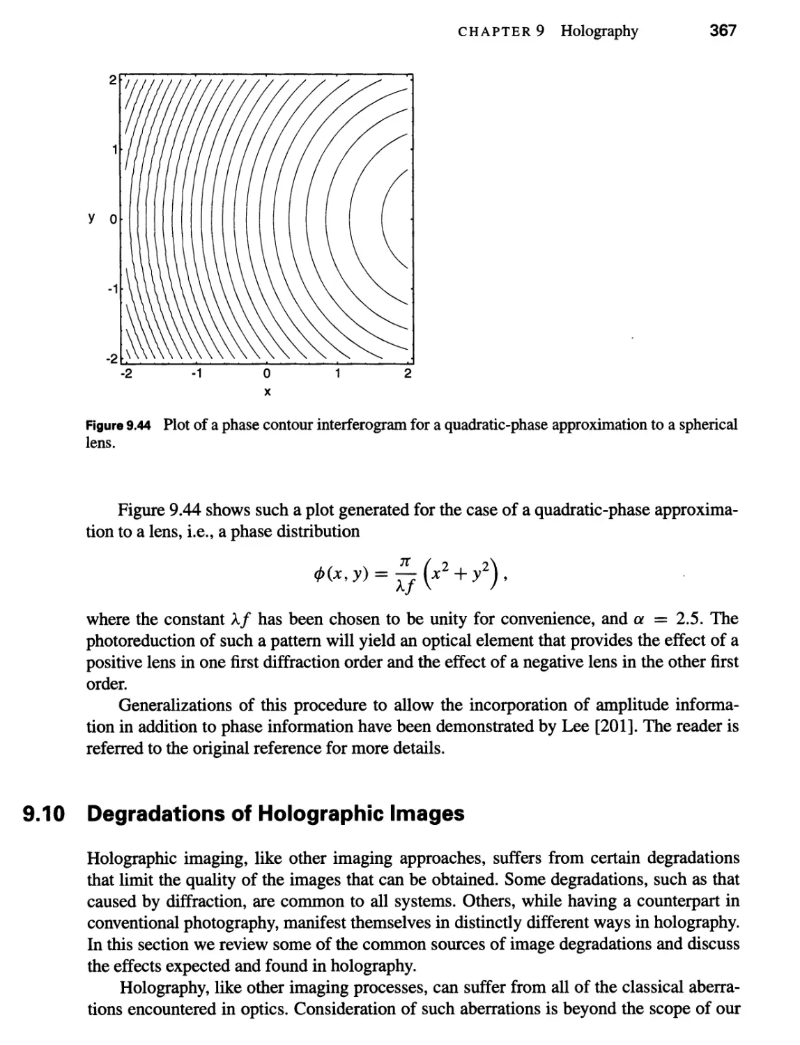
9.10 Degradations of Holographic Images 367
9.10.1 Effects of Film MTF 368
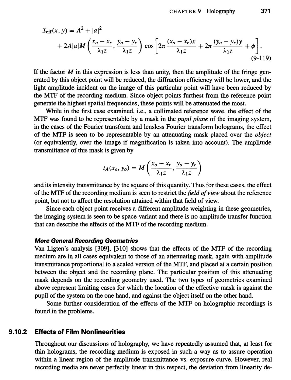
9.10.2 Effects of Film Nonlinearities 371
9.10.3 Effects of Film-Grain Noise 372
9.10.4 Speckle Noise 373


Contents xvii
9.11 Holography with Spatially Incoherent Light 374
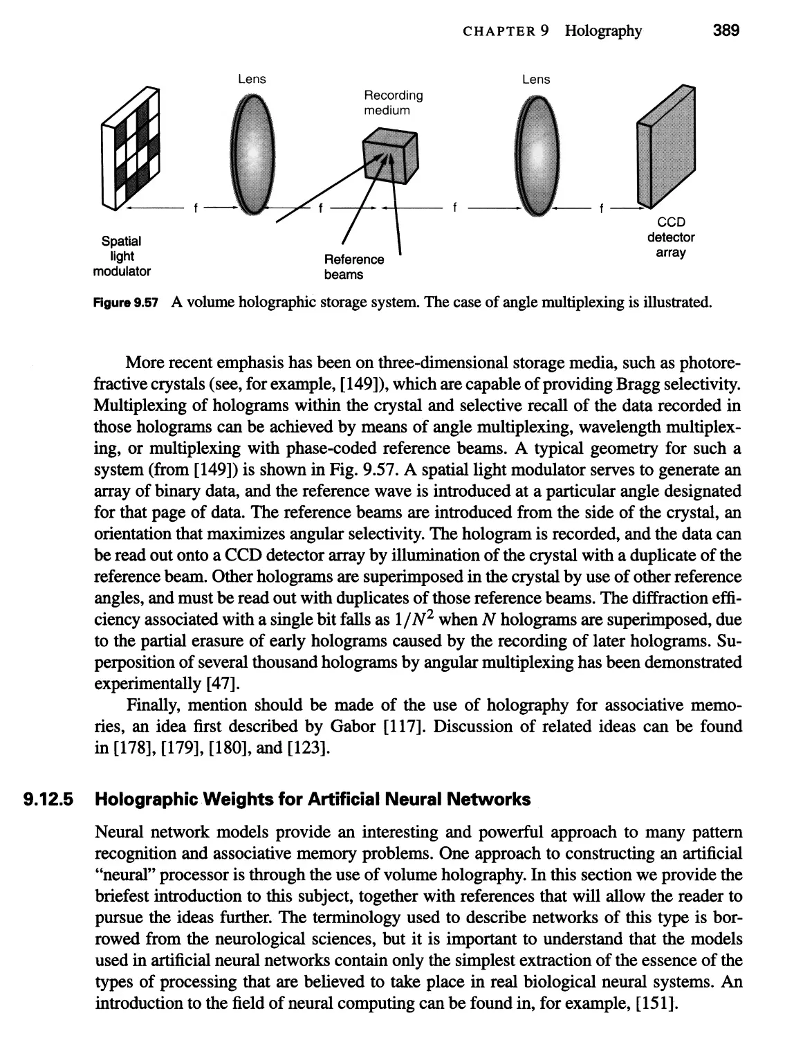
9.12 Applications of Holography 377
9.12.1 Microscopy and High-Resolution Volume Imagery 377
9.12.2 Interferometry 378
9.12.3 Imaging through Distorting Media 384
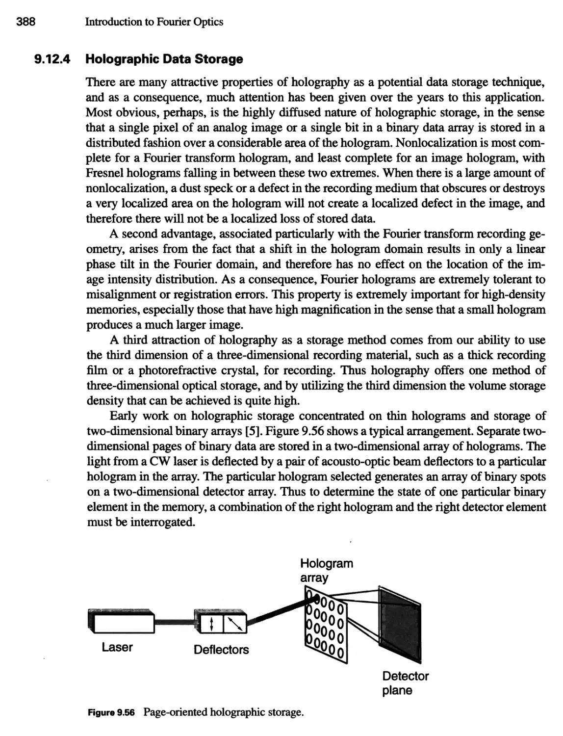
9.12.4 Holographic Data Storage 388
9.12.5 Holographic Weights for Artificial Neural Networks 389
9.12.6 Other Applications 393
10 Fourier Optics in Optical Communications 399
10.1 Introduction 399
10.2 Fiber Bragg Gratings 400
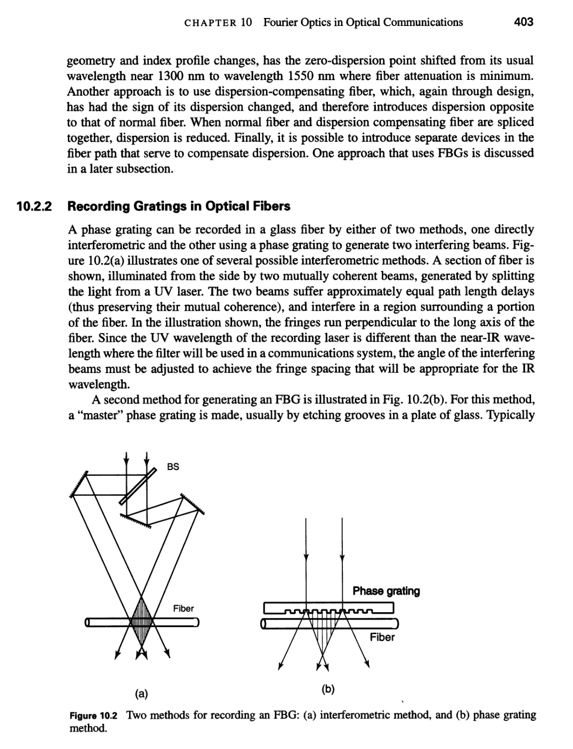
10.2.1 Introduction to Optical Fibers 400
10.2.2 Recording Gratings in Optical Fibers 403
10.2.3 Effects of an FBG on Light Propagating in the Fiber 404
10.2.4 Applications of FBGs 407
10.2.5 Gratings Operated in Transmission 409
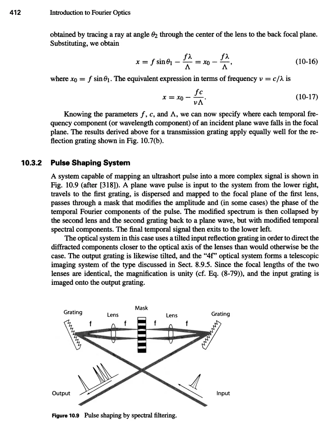
10.3 Ultrashort Pulse Shaping and Processing 410
10.3.1 Mapping of Temporal Frequencies to Spatial Frequencies 410
10.3.2 Pulse Shaping System 412
10.3.3 Applications of Spectral Pulse Shaping 413
10.4 Spectral Holography 415
10.4.1 Recording the Hologram 415
10.4.2 Reconstructing the Signals 417
10.4.3 Effects of Delay between the Reference Pulse and the
Signal Waveform 420
10.5 Arrayed Waveguide Gratings 420
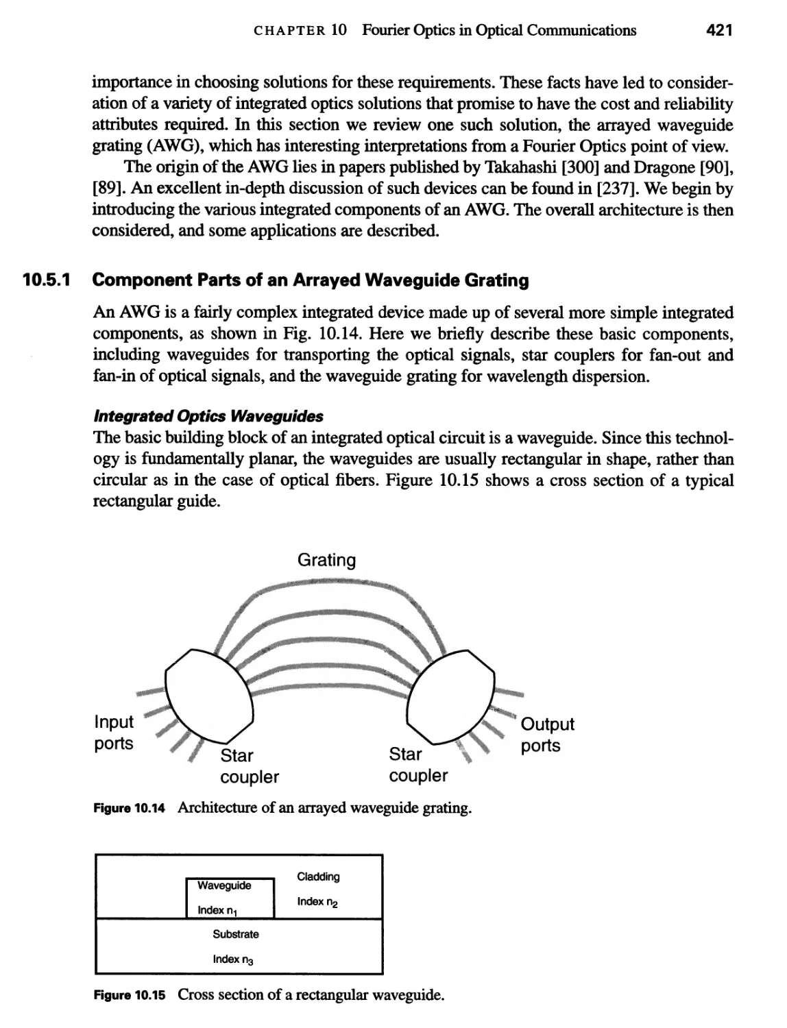
10.5.1 Component Parts of an Arrayed Waveguide Grating 421
10.5.2 Applications of AWGs 427
A Delta Functions and Fourier Transform Theorems 433
A. 1 Delta Functions 43 3
A.2 Derivation of Fourier Transform Theorems 435
B Introduction to Paraxial Geometrical Optics 441
B.l The Domain of Geometrical Optics 441
B.2 Refraction, Snell’s Law, and the Paraxial Approximation 443
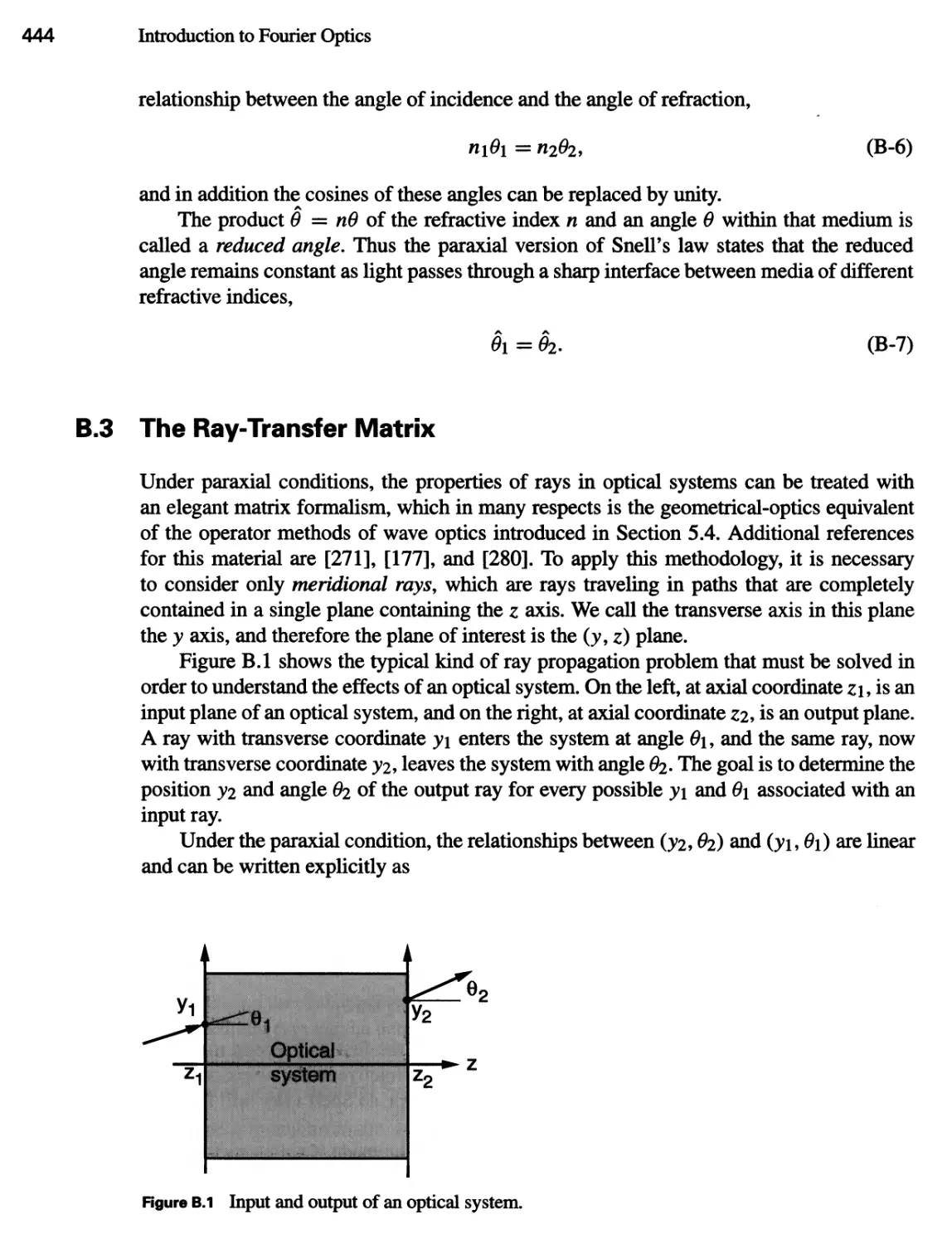
B.3 The Ray-Transfer Matrix 444
B.4 Conjugate Planes, Focal Planes, and Principal Planes 447
B.5 Entrance and Exit Pupils 451


xviii
Contents
C Polarization and Jones Matrices 455
C. 	1 Definition of the Jones Matrix 455
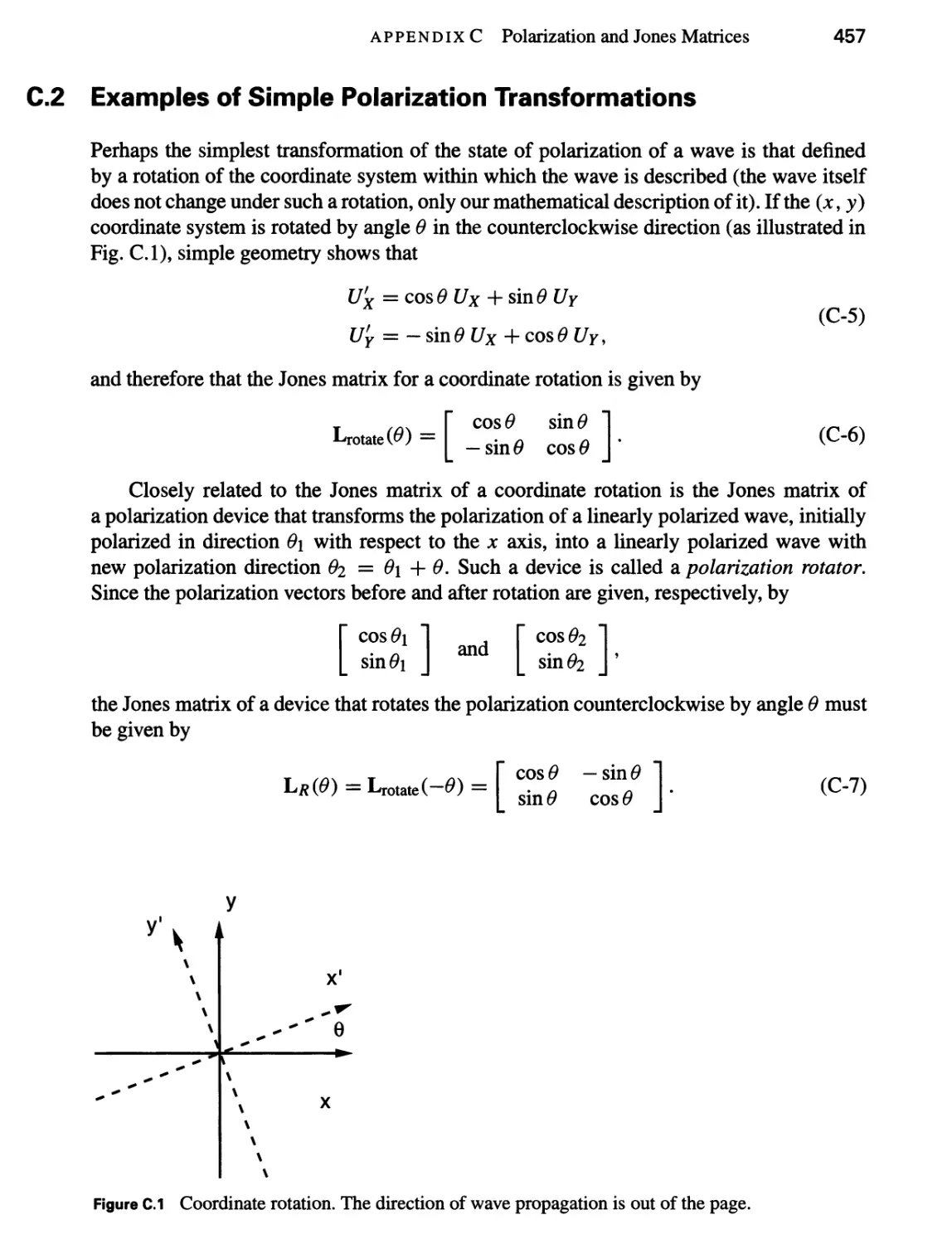
C.2 Examples of Simple Polarization Transformations 457
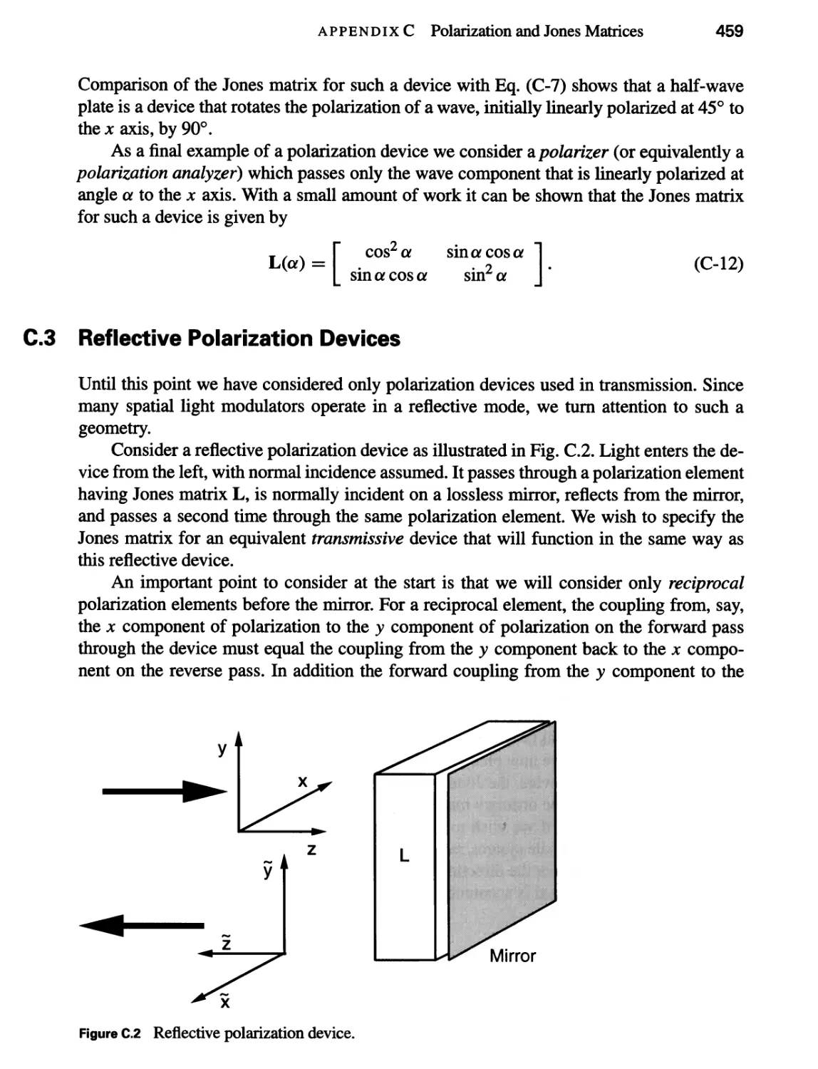
C.3 Reflective Polarization Devices 459
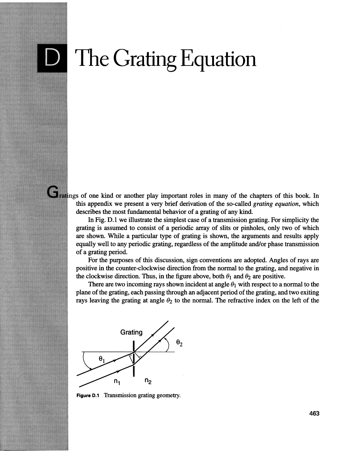
D Hie Grating Equation 463
Bibliography 465
Index 481


H Introduction
f 1.1 Optics, Information, and Communication
Since the late 1930s, the venerable branch of physics known as optics has gradually developed ever-closer ties with the communication and information sciences of electrical engineering. The trend is understandable, for both communication systems and imaging systems are designed to collect or convey information. In the former case, the information is generally of a temporal nature (e.g., a modulated voltage or current waveform), while in the latter case it is of a spatial nature (e.g., a light amplitude or intensity distribution over space), but from an abstract point of view, this difference is a rather superficial one.
Perhaps the strongest tie between the two disciplines lies in the similar mathematics which can be used to describe the respective systems of interest—the mathematics i of Fourier analysis and systems theory. The fundamental reason for the similarity is not merely the common subject of “information,” but rather certain basic properties which communication systems and imaging systems share. For example, many electronic networks and imaging devices share the properties called linearity and invariance (for definitions see Chapter 2). Any network or device (electronic, optical, or otherwise) which possesses these two properties can be described mathematically with considerable ease using the techniques of frequency analysis. Thus, just as it is convenient to describe an audio amplifier in terms of its (temporal) frequency response, so too it is often convenient to describe an imaging system in terms of its (spatial) frequency response.
The similarities do not end when the linearity and invariance properties are absent. Certain nonlinear optical elements (e.g., photographic film) have input-output relationships which are directly analogous to the corresponding characteristics of nonlinear electronic components (diodes, transistors, etc.), and similar mathematical analysis can be applied in both cases.
It is particularly important to recognize that the similarity of the mathematical structures can be exploited not only for analysis purposes but also for synthesis purposes. Thus, just as the spectrum of a temporal function can be intentionally manipulated in a prescribed fashion by filtering, so too can the spectrum of a spatial function be modified in various
1


Introduction to Fourier Optics
desired ways. The history of optics is rich with examples of important advances achieved by application of Fourier synthesis techniques—the Zemike phase-contrast microscope is an example that was worthy of a Nobel prize. Many other examples can be found in the fields of signal and image processing.
The Book
The readers of this book are assumed at the start to have a solid foundation in Fourier analysis and linear systems theory. Chapter 2 reviews the required background; to avoid boring those who are well grounded in the analysis of temporal signals and systems, the review is conducted for functions of two independent variables. Such functions are, of course, of primary concern in optics, and the extension from one to two independent variables provides a new richness to the mathematical theory, introducing many new properties which have no direct counterpart in the theory of temporal signals and systems.
The phenomenon called diffraction is of the utmost importance in the theory of optical systems. Chapter 3 treats the foundations of scalar diffraction theory, including the Kirchhoff, Rayleigh-Sommerfeld, and angular spectrum approaches. In Chapter 4, certain approximations to the general results are introduced, namely the Fresnel and Fraunhofer approximations, and examples of diffraction-pattem calculations are presented.
Chapter 5 considers the analysis of coherent optical systems, which consist of lenses and free-space propagation. The approach is that of wave optics, rather than the more common geometrical optics method of analysis. A thin lens is modeled as a quadratic phase transformation; the usual lens law is derived from this model, as are certain Fourier transforming properties of lenses.
Chapter 6 considers the application of frequency analysis techniques to both coherent and incoherent imaging systems. Appropriate transfer functions are defined and their properties discussed for systems with and without aberrations. Coherent and incoherent systems are compared from various points of view. The limits to achievable resolution are derived.
In Chapter 7 the subject of wavefront modulation is considered. The properties of photographic film as an input medium for incoherent and coherent optical systems are discussed. Attention is then turned to spatial light modulators, which are devices for entering information into optical systems in real time or near real time. Finally, diffractive optical elements are described in some detail.
Attention is turned to analog optical information processing in Chapter 8. Both continuous and discrete processing systems are considered. Applications to image enhancement, pattern recognition, and processing of synthetic-aperture radar data are considered.
Chapter 9 is devoted to the subject of holography. The techniques developed by Gabor and by Leith and Upatnieks are considered in detail and compared. Both thin and thick holograms are treated. Extensions to three-dimensional imaging are presented. Various applications of holography are described, but emphasis is on the fundamentals.
Finally, Chapter 10 covers applications of Fourier Optics to devices or techniques that are important for optical communications.


2
Analysis of Two-Dimensional Signals and Systems
|
M any physical phenomena are found experimentally to share the basic property that their response to several stimuli acting simultaneously is identically equal to the sum of the responses that each component stimulus would produce individually. Such phenomena are called , and the property they share is called linearity. Electrical networks composed of resistors, capacitors, and inductors are usually linear over a wide range of inputs. In addition, as we shall soon see, the wave equation describing the propagation of light through most media leads us naturally to regard optical imaging operations as linear mappings of “object” light distributions into “image” light distributions.
The single property of linearity leads to a vast simplification in the mathematical description of such phenomena and represents the foundation of a mathematical structure which we shall refer to here as linear systems theory. The great advantage afforded by linearity is the ability to express the response (be it voltage, current, light amplitude, or light intensity) to a complicated stimulus in terms of the responses to certain “elementary” stimuli. Thus if a stimulus is decomposed into a linear combination of elementary stimuli, each of which produces a known response of convenient form, then by virtue of linearity, the total response can be found as a corresponding linear combination of the responses to the elementary stimuli.
In this chapter we review some of the mathematical tools that are useful in describing linear phenomena, and discuss some of the mathematical decompositions that are often employed in their analysis. Throughout the later chapters we shall be concerned with stimuli (system inputs) and responses (system outputs) that may be either of two different physical quantities. If the illumination used in an optical system exhibits a property called spatial
3


4
Introduction to Fourier Optics
coherence, then we shall find that it is appropriate to describe the light as a spatial distribution of complex-valued field amplitude. When the illumination is totally lacking in spatial coherence, it is appropriate to describe the light as a spatial distribution of real-valued intensity. Attention will be focused here on the analysis of linear systems with complexvalued inputs; the results for real-valued inputs are thus included as special cases of the theory.
2.1 	Fourier Analysis in Two Dimensions
A mathematical tool of great utility in the analysis of both linear and nonlinear phenomena is Fourier analysis. This tool is widely used in the study of electrical networks and communication systems; it is assumed that the reader has encountered Fourier theory previously, and therefore that he or she is familiar with the analysis of functions of one independent variable (e.g., time). For a review of the fundamental mathematical concepts, see the books by Papoulis [243], Bracewell [33], and Gray and Goodman [139]. A particularly relevant treatment is by Bracewell [34]. Our purpose here is limited to extending the reader’s familiarity to the analysis of functions of two independent variables. No attempt at great mathematical rigor will be made, but rather, an operational approach, characteristic of most engineering treatments of the subject, will be adopted.
2.1.1 	Definition and Existence Conditions
The Fourier transform (alternatively the Fourier spectrum or frequency spectrum) of a (in general, complex-valued) function g of two independent variables x and y will be represented here by F{g} and is defined by1
00
F{g) = J J g(x, y) exp [—j2n(fxx + /r;y)] dx dy. (2-1)
—00
The transform so defined is itself a complex-valued function of two independent variables fx and fy, which we generally refer to as frequencies. Similarly, the inverse Fourier transform of a function G(fx, fy) will be represented by Jr~l{G] and is defined as
00
T~l{G} = Jj G(fx, fr) cxp[j2n(fxx + fry)] dfx dfr. (2-2)
—00
Note that as mathematical operations the transform and inverse transform are very similar, differing only in the sign of the exponent appearing in the integrand. The inverse Fourier transform is sometimes referred to as the Fourier integral representation of a function
g(x, y)•
1When a single limit of integration appears above or below a double integral, then that limit applies to both integrations.


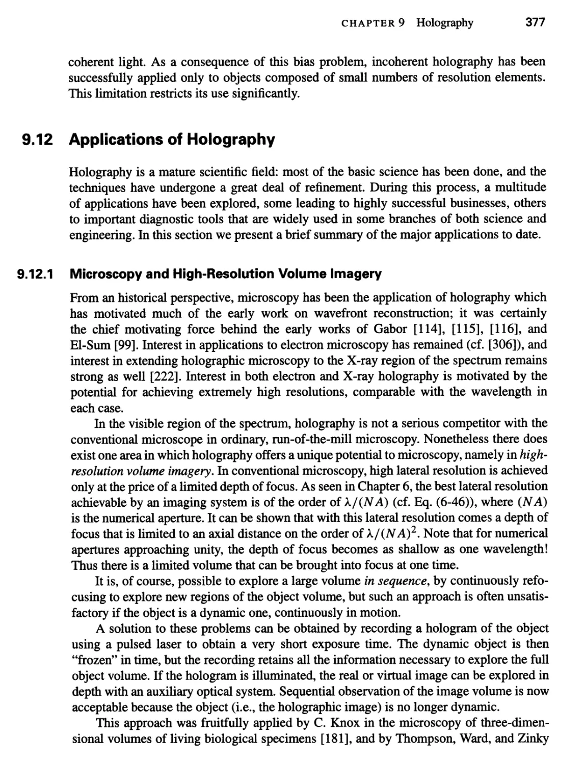
CHAPTER2 Analysis of Two-Dimensional Signals and Systems
5
Before discussing the properties of the Fourier transform and its inverse, we must first decide when (2-1) and (2-2) are in fact meaningful. For certain functions, these integrals may not exist in the usual mathematical sense, and therefore this discussion would be incomplete without at least a brief mention of “existence conditions.” While a variety of sets of sufficient conditions for the existence of (2-1) are possible, perhaps the most common set is the following:
1. g must be absolutely integrable over the infinite (jc, y) plane.
2. g must have only a finite number of discontinuities and a finite number of maxima and minima in any finite rectangle.
3. g must have no infinite discontinuities.
In general, any one of these conditions can be weakened at the price of strengthening one or both of the companion conditions, but such considerations lead us rather far afield from our purposes here.
As Bracewell [33] has pointed out, “physical possibility is a valid sufficient condition for the existence of a transform.” However, it is often convenient in the analysis of systems to represent true physical waveforms by idealized mathematical functions, and for such functions one or more of the above existence conditions may be violated. For example, it is common to represent a strong, narrow time pulse by the so-called Dirac delta function2 often represented by
8(t) = lim Afexp(—N2nt2), (2-3)
N-+ oo
where the limit operation provides a convenient mental construct but is not meant to be taken literally. See Appendix A for more details. Similarly, an idealized point source of light is often represented by the two-dimensional equivalent,
<$(x, y) = lim N2 exp[—N2n(x2 + y2)]. (2-4)
N-*oo
Such “functions,” being infinite at the origin and zero elsewhere, have an infinite discontinuity and therefore fail to satisfy existence condition 3. Other important examples are readily found; for example, the functions
f{x, y) = 1 and /(*, y) = cos(27r/x*) (2-5)
both fail to satisfy existence condition 1.
If the majority of functions of interest are to be included within the framework of Fourier analysis, some generalization of the definition (2-1) is required. Fortunately, it is often possible to find a meaningful transform of functions that do not strictly satisfy the existence conditions, provided those functions can be defined as the limit of a sequence of functions that are transformable. By transforming each member function of the defining
sequence, a corresponding sequence of transforms is generated, and we call the limit of
this new sequence the generalized Fourier transform of the original function. Generalized
2For a more detailed discussion of the delta function, including definitions, see Appendix A.


6
Introduction to Fourier Optics
transforms can be manipulated in the same manner as conventional transforms, and the distinction between the two cases can generally be ignored, it being understood that when a function fails to satisfy the existence conditions and yet is said to have a transform, then the generalized transform is actually meant. For a more detailed discussion of this generalization of Fourier analysis the reader is referred to the book by Lighthill [209].
To illustrate the calculation of a generalized transform, consider the Dirac delta function, which has been seen to violate existence condition 3. Note that each member function of the defining sequence (2-4) does satisfy the existence requirements and that each, in fact, has a Fourier transform given by (see Table 2.1)
Note that the spectrum of a delta function extends uniformly over the entire frequency domain.
For other examples of generalized transforms, see Table 2.1.
2.1.2 	The Fourier Transform as a Decomposition
As mentioned previously, when dealing with linear systems it is often useful to decompose a complicated input into a number of more simple inputs, to calculate the response of the system to each of these “elementary” functions, and to superimpose the individual responses to find the total response. Fourier analysis provides the basic means of performing such a decomposition. Consider the familiar inverse transform relationship
expressing the time function g in terms of its frequency spectrum. We may regard this expression as a decomposition of the function g(t) into a linear combination (in this case an integral) of elementary functions, each with a specific form exp(j2nft). From this it is clear that the complex number G(f) is simply a weighting factor that must be applied to the elementary function of frequency / in order to synthesize the desired g(t).
In a similar fashion, we may regard the two-dimensional Fourier transform as a decomposition of a function g(x, y) into a linear combination of elementary functions of the form exp [j2n (fxx + fyy)]. Such functions have a number of interesting properties. Note that for any particular frequency pair (fx, fy) the corresponding elementary function has a phase that is zero or an integer multiple of 2n radians along lines described by the equation
9 999 “b fy')
T{N2 exp[-N2n(x2 + y2)]} = exp yJx JY>
(2-6)
Accordingly the generalized transform of 5(x, y) is found to be
(2-7)
(2-8)
(2-9)


CHAPTER2 Analysis of Two-Dimensional Signals and Systems
7
y
X
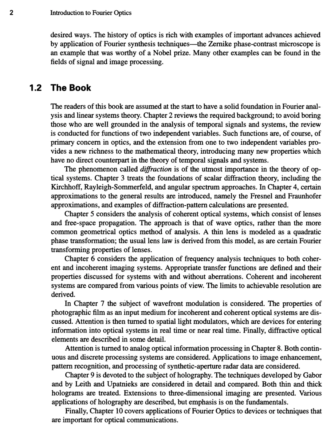
Figure 2.1 Lines of zero phase for the function exp [j2tc (fxx + /yy)].
where n is an integer. Thus, as indicated in Fig. 2.1, this elementary function may be regarded as being “directed” in the (x, y) plane at an angle 0 (with respect to the x axis) given by
In conclusion, then, we may again regard the inverse Fourier transform as providing a means for decomposing mathematical functions. The Fourier spectrum G of a function g is simply a description of the weighting factors that must be applied to each elementary function in order to synthesize the desired g. The real advantage obtained from using this decomposition will not be fully evident until our later discussion of invariant linear systems.
2.1.3 	Fourier Transform Theorems
The basic definition (2-1) of the Fourier transform leads to a rich mathematical structure associated with the transform operation. We now consider a few of the basic mathematical properties of the transform, properties that will find wide use in later material. These properties are presented as mathematical theorems, followed by brief statements of their physical significance. Since these theorems are direct extensions of the analogous onedimensional statements, the proofs are deferred to Appendix A.
In addition, the spatial period (i.e., the distance between zero-phase lines) is given by
(2-10)
(2-11)


8
Introduction to Fourier Optics
1. Linearity theorem. T{ag + f$h) = ctF{g} + $T{h}\ that is, the transform of a weighted sum of two (or more) functions is simply the identically weighted sum of their individual transforms.
2. Similarity theorem. If T {g(x, y)} = G(fx, fy), then
(2-12)
that is, a “stretch” of the coordinates in the space domain (x, y) results in a contraction of the coordinates in the frequency domain (fx, fy)> plus a change in the overall amplitude of the spectrum.
3. Shift theorem. If F{g(x, y)} = G(fx, fy), then
F{g(x ~ a, y - b)} = G(fXl fy) exV[-j2n(fxa + frb)]; (2-13)
that is, translation in the space domain introduces a linear phase shift in the frequency domain.
4. Rayleighys theorem (Parseval’s theorem). If F{g(x, y)} = G(fx, fy), then
00 oo
j f \g(x,y)\2dxdy= J J \G(fx,fY)\2dfxdfY. (2-14)
—OO —00
The integral on the left-hand side of this theorem can be interpreted as the energy contained in the waveform g (x, y). This in turn leads us to the idea that the quantity \G(fx, fy)|2 can be interpreted as an energy density in the frequency domain.
5. Convolution theorem. If F{g(x, y)} = G(fx, fy) and T{h(x, y)} = H(fx, fy), then
oo
If8^'
rj) h(x — I;, y — rj) dl= dr}
= G(fx,fy)H(fx,fr). (2-15)
The convolution of two functions in the space domain (an operation that will be found to arise frequently in the theory of linear systems) is entirely equivalent to the more simple operation of multiplying their individual transforms and inverse transforming.
6. 	Autocorrelation theorem. If F{g(jc, y)} = G(fx, fy), then
oo
//*«•'
= IG(fx, fY)|2. (2-16)
ri)g*(H - x,ri - y)d%dri
—oo
Similarly,
oo
^{ls(*,)0l2) = JI GG,Ti)G*(S-fx,ri-fy)dSdfi. (2-17)


CHAPTER2 Analysis of Two-Dimensional Signals and Systems
9
This theorem may be regarded as a special case of the convolution theorem in which we convolve g(x, y) with g*(—x, —y).
7. 	Fourier integral theorem. At each point of continuity of g,
{*(*, y)) = F~lF[g(x, y)} = g(x, y). (2-18)
At each point of discontinuity of g, the two successive transforms yield the angular average of the values of g in a small neighborhood of that point. That is, the successive transformation and inverse transformation of a function yields that function again, except at points of discontinuity.
The above transform theorems are of far more than just theoretical interest. They will be used frequently, since they provide the basic tools for the manipulation of Fourier transforms and can save enormous amounts of work in the solution of Fourier analysis problems.
2.1.4 	Separable Functions
A function of two independent variables is called separable with respect to a specific coordinate system if it can be written as a product of two functions, each of which depends on only one of the independent variables. Thus the function g is separable in rectangular coordinates (jc, y) if
g(x, y) = gx(x) gy(y), (2-19)
while it is separable in polar coordinates (r, 0) if
gir, 0) = gR(r) g@(Q). (2-20)
Separable functions are often more convenient to deal with than more general functions, for separability often allows complicated two-dimensional manipulations to be reduced to more simple one-dimensional manipulations. For example, a function separable
in rectangular coordinates has the particularly simple property that its two-dimensional
Fourier transform can be found as a product of one-dimensional Fourier transforms, as evidenced by the following relation:
oo
?{#(*> y)} = J J g(x,y) exp[-j2n(fxx + fyy)] dx dy
—OO
/OO /»oo
gx(x) exp[-j2nfxx]dx / gy(y) exp[-j2nfYy]dy
-OO J—OO
= fx {gx} fy {gy}. (2-21)
Thus the transform of g is itself separable into a product of two factors, one a function of fx only and the second a function of fy only, and the process of two-dimensional transformation simplifies to a succession of more familiar one-dimensional manipulations.
Functions separable in polar coordinates are not so easily handled as those separable in rectangular coordinates, but it is still generally possible to demonstrate that two¬


10
Introduction to Fourier Optics
dimensional manipulations can be performed by a series of one-dimensional manipulations. For example, the reader is asked to verify in the problems that the Fourier transform of a general function separable in polar coordinates can be expressed as an infinite sum of weighted Hankel transforms
oo
?{g(r,0))= ^ Ck(-j)kexp(jk<p)Hk{gR(r)} (2-22)
k=—oo
where
1 f2yt
ck = — g&(d)exp(-jkd)dO and Hk{] is the Hankel transform operator of order k, defined by
r OO
Hk {gtf(r)} = In / r gR(r)Jk(2nrp) dr. (2-23)
Jo
The function Jk is the fcth-order Bessel function of the first kind.
2.1.5 	Functions with Circular Symmetry: Fourier-Bessel Transforms
Perhaps the simplest class of functions separable in polar coordinates is composed of those possessing circular symmetry. The function g is said to be circularly symmetric if it can be written as a function of r alone, that is,
g(r,0) = gR(r). (2-24)
Such functions play an important role in the problems of interest here, since most optical systems have precisely this type of symmetry. We accordingly devote special attention to the problem of Fourier transforming a circularly symmetric function.
The Fourier transform of g in a system of rectangular coordinates is, of course, given
by
(X)
G(fx,fy)= J J S(x, y) exp[-j2n(fxx + fYy)] dx dy. (2-25)
—OO
To fully exploit the circular symmetry of g, we make a transformation to polar coordinates in both the (x, y) and the (fx, fy) planes as follows:
r = yjx2 + y2 x = r cos 0
0 = arctan ^ y = r sin 6
, — (2-26)
P = yJfx + fY fx = pcos<t>
0 = arctan f ) fy — P sin0.


CHAPTER2 Analysis of Two-Dimensional Signals and Systems
11
For the present we write the transform as a function of both radius and angle,3
F{g} = G0(p,<l>). (2-27)
Applying the coordinate transformations (2-26) to Eq. (2-25), the Fourier transform of g can be written
pin poo
G0(p,<t>)= I dO I dr rgR(r)txp[—y27rr/o(cos0 cos0 + sin# sin0)] (2-28) Jo Jo
or equivalently,
poo pin
G0(p,</>)= drrgR(r)/ dO exp[-y27rrpcos(0 - </>)]. (2-29)
Jo Jo
Finally we use the Bessel function identity
1 f2n
Jo(a) = — I exp[—ja cos(0 — <f>)] dO, (2-30)
2tt Jo
where Jo is a Bessel function of the first kind, zero order, to simplify the expression for the transform. Substituting (2-30) in (2-29), the dependence of the transform on angle 0 is seen to disappear, leaving Go as the following function of radius p,
poo
Go(p, 0) = G0(p) = 27t rgR(r)J0(2nrp) dr. (2-31)
Jo
Thus the Fourier transform of a circularly symmetric function is itself circularly symmetric and can be found by performing the one-dimensional manipulation of (2-31). This
particular form of the Fourier transform occurs frequently enough to warrant a special
designation; it is accordingly referred to as the Fourier-Bessel transform, or alternatively as the Hankel transform of zero order (cf. Eq. (2-23)). For brevity, we adopt the former terminology.
By means of arguments identical with those used above, the inverse Fourier transform of a circularly symmetric spectrum G0(p) can be expressed as
p oo
gR(r) = 2n pG0(p)Jo(2nrp)dp. (2-32)
Jo
Thus for circularly symmetric functions there is no difference between the transform and the inverse-transform operations.
Using the notation B {} to represent the Fourier-Bessel transform operation, it follows directly from the Fourier integral theorem that
BB~l {£R(r)} = B~lB {**(/•)} = BB te*(r)} = gR(r) (2-33)
3Note the subscript in Ga is added simply because the functional form of the expression for the transform in polar coordinates is in general different than the functional form for the same transform in rectangular coordinates.


Introduction to Fourier Optics
at each value of r where gR(r) is continuous. In addition, the similarity theorem can be straightforwardly applied (see Prob. 2-6c) to show that
When using the expression (2-31) for the Fourier-Bessel transform, the reader should remember that it is no more than a special case of the two-dimensional Fourier transform, and therefore any familiar property of the Fourier transform has an entirely equivalent counterpart in the terminology of Fourier-Bessel transforms.
Some Frequently Used Functions and Some Useful Fourier Transform Pairs
A number of mathematical functions will find such extensive use in later material that considerable time and effort can be saved by assigning them special notations of their own. Accordingly, we adopt the following definitions of some frequently used functions:
Rectangle function
(2-34)
1 |x| <i
rect(x) = ■ i \x\ = \
0 otherwise
Sine function
sinc(jt)
sin(7rx)
7xx
Signum function
1 x > 0
sgn(x) = 0 x = 0
— 1 x < 0
Triangle function
AW =
1-1*1 1*1 <1 0 otherwise
Comb function
oo
comb(jt) = ^ 8(x —n)
Circle function
The first five of these functions, depicted in Fig. 2.2, are all functions of only one independent variable; however, a variety of separable functions can be formed in two dimensions


CHAPTER 2 Analysis of Two-Dimensional Signals and Systems 13
rect(>0
sgn(x)
1
-2 -1
1 2
X
*
comb(x)
-3
Figure 2.2 Special functions.
by means of products of these functions. The circle function is, of course, unique to the case of two-dimensional variables; see Fig. 2.3 for an illustration of its structure.
We conclude our discussion of Fourier analysis by presenting some specific two- dimensional transform pairs. Table 2.1 lists a number of transforms of functions separable in rectangular coordinates. For the convenience of the reader, the functions are presented with arbitrary scaling constants. Since the transforms of such functions can be found directly from products of familiar one-dimensional transforms, the proofs of these relations are left to the reader (cf. Prob. 2-2).


FOO
Introduction to Fourier Optics
(a)
Figure 2.3 The circle function and its transform.
Table 2.1: Transform pairs for some functions separable in rectangular coordinates
Function
Transform
expf-^aV + 6V)] ^ exp [-* (J + |)]
rect(ax) rect (fry)
A (ax) A (fry)
8(ax, by) exp[jn(ax + by)] sgn(ax) sgn(by)
comb (ax) comb (fry)
exp[</7r(a2x2 + b2y2)]
— sinc(/x/a) sine (fY/b) \ab\
1
sine2(fx/a) sine2(/y/fr)
M>l 1
l^i
8(fx-a/2,fY-b/2)
ab _L 1_
l«^l j*fx jnfr
-i-comb (/*/a) comb(/K/fc)
iSi [-'* (f + ?)]
exp[-(a|x|+fc|;y|)] ——
\ab\ 1 + (2nfx/a)2 1 + (2jr/K/fc)2


CHAPTER2 Analysis of Two-Dimensional Signals and Systems
15
On the other hand, with a few exceptions (e.g., exp[—tx(x2 + y2)], which is both separable in rectangular coordinates and circularly symmetric), transforms of most circularly symmetric functions cannot be found simply from a knowledge of one-dimensional transforms. The most frequently encountered function with circular symmetry is:
circ(r) =
1 r < 1
2 r = 1
0 otherwise
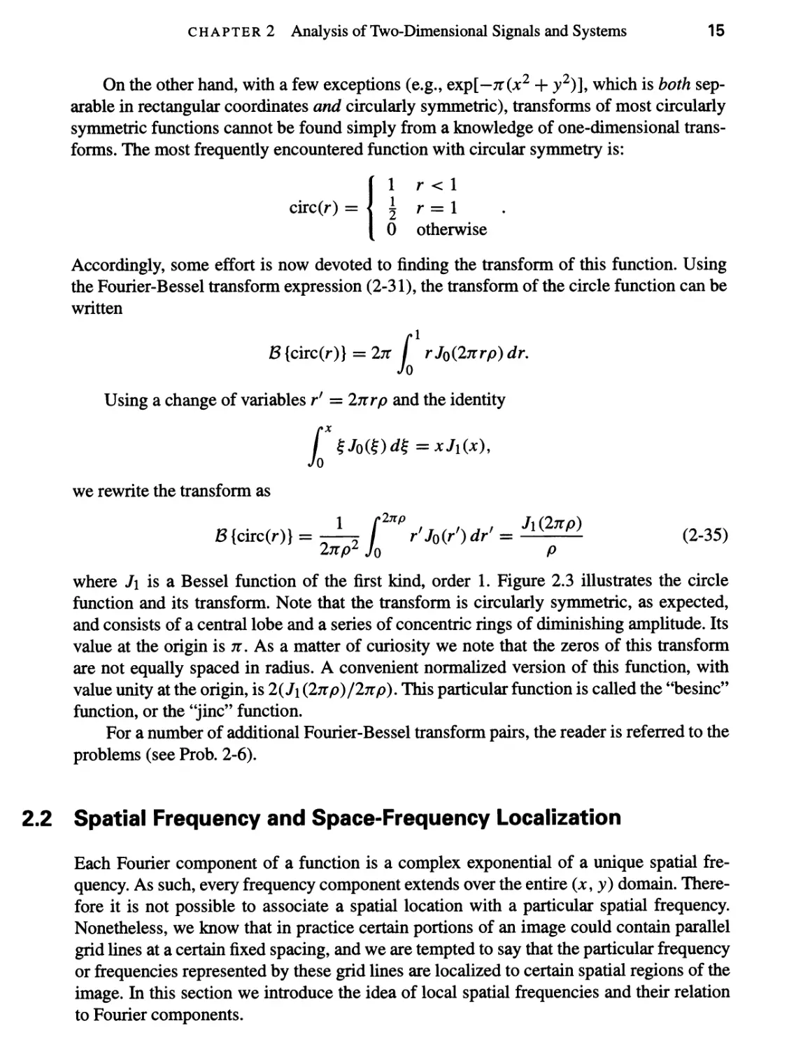
Accordingly, some effort is now devoted to finding the transform of this function. Using the Fourier-Bessel transform expression (2-31), the transform of the circle function can be written
B{circ(r)} = 27T f rJo(2jvrp)dr.
Jo
Using a change of variables rf = 2nrp and the identity
f
Jo
we rewrite the transform as
B{circ(r)} = -U f ** r'J0(r')dr' = Jl(2np) (2-35)
2 np2 Jo P
where J\ is a Bessel function of the first kind, order 1. Figure 2.3 illustrates the circle function and its transform. Note that the transform is circularly symmetric, as expected, and consists of a central lobe and a series of concentric rings of diminishing amplitude. Its value at the origin is n. As a matter of curiosity we note that the zeros of this transform are not equally spaced in radius. A convenient normalized version of this function, with value unity at the origin, is 2( J\ (2np)/2np). This particular function is called the “besinc” function, or the “jinc” function.
For a number of additional Fourier-Bessel transform pairs, the reader is referred to the problems (see Prob. 2-6).
Spatial Frequency and Space-Frequency Localization
Each Fourier component of a function is a complex exponential of a unique spatial frequency. As such, every frequency component extends over the entire (x, y) domain. Therefore it is not possible to associate a spatial location with a particular spatial frequency. Nonetheless, we know that in practice certain portions of an image could contain parallel grid lines at a certain fixed spacing, and we are tempted to say that the particular frequency or frequencies represented by these grid lines are localized to certain spatial regions of the image. In this section we introduce the idea of local spatial frequencies and their relation to Fourier components.


Introduction to Fourier Optics
For the purpose of this discussion, we consider the general case of complex-valued functions, which we will later see represent the amplitude and phase distributions of monochromatic optical waves. For now, they are just complex functions. Any such function can be represented in the form
g(x, y) = a(x, y) exp[j(/)(x, y)] (2-36)
where a(x, y) is a real and nonnegative amplitude distribution, while (/>(x,y) is a real phase distribution. For this discussion we assume that the amplitude distribution a(x, y) is a slowly varying function of (x, y), so that we can concentrate on the behavior of the phase function 0(x, y).
We define the local spatial frequency of the function g as a frequency pair (fix, fly) given by
fix = y) fly = t-t-4>(x, y)- (2-37)
2n ox 2tt 3y
In addition, both fix and fy are defined to be zero in regions where the function g(x, y) vanishes.
Consider the result of applying these definitions to the particular complex function g(x, y) = exp[j2n(fxx + fYy)] representing a simple linear-phase exponential of frequencies (fx, fy)- We obtain
13 13
fix = -Z-— [2n(fxx + fyy)] = fx fir = — — [2n(fxx + fYy)] = fy.
2n ox 2n 3y
Thus we see that for the case of a single Fourier component, the local frequencies do indeed reduce to the frequencies of that component, and those frequencies are constant over the entire (x, y) plane.
Next consider a space-limited version of a quadratic-phase exponential function,4 which we call a “finite chirp” function,5
g(x, y) = exp ^jnP(x2 + y2)] rect (2^) rect (2^) ' ^2’38^
Performing the differentiations called for by the definitions of local frequencies, we find that they can be expressed as
fix = px rect(2!^) flY = Py rect(217) • (2'39)
We see that in this case the local spatial frequencies do depend on location in the (jc, y) plane; within a rectangle of dimensions 2Lx x 2Ly, fix varies linearly with the
4For a tutorial discussion of the importance of quadratic-phase functions in various fields of optics, see [246].
5The name “chirp function,” without the finite length qualifier, will be used for the infinite-length quadratic phase exponential, exp[jnP(x2 + y2)].


CHAPTER2 Analysis of Two-Dimensional Signals and Systems
17
x-coordinate while fy varies linearly with the y-coordinate. Thus for this function (and for most others) there is a dependence of local spatial frequency on position in the (x, y) plane.6
Since the local spatial frequencies are bounded to covering a rectangle of dimensions 2Lx x 2Ly, it would be tempting to conclude that the Fourier spectrum of g(x, y) is also limited to the same rectangular region. In fact this is approximately true, but not exactly so. The Fourier transform of this function is given by the expression
G(fx,fy)= [LX I1* e^+y^e-Wfxx+ftyUxdy.
J-Lx J-Ly
This expression is separable in rectangular coordinates, so it suffices to find the onedimensional spectrum
Gx(fx) = fLX e^x2e-Wx* dx.
J-LX
Completing the square in the exponent and making a change of variables of integration from x to t = y/lfi (x — yields
r ,,, 1 -1*4
Gx(fx) = —j= e ~ / exp
\/20 J-j%(Lx+!f)
.nt2 7 2
dt.
This integral can be expressed in terms of tabulated functions, the Fresnel integrals, which are defined by
C(z) = jTZ cos dt 5(z) = j*sin (^Y j dt- (2-4°)
The spectrum Gx can then be expressed as
-w lc (Lx - f)] -c (~l* - f)]
JS(lx - &)]-ys[v5(^-f)]}.
+ .
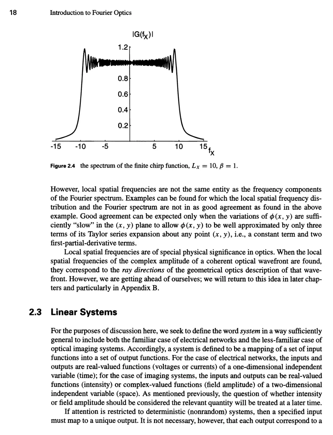
The expression for Gy is of course identical, except the Y subscript replaces the X subscript. Figure 2.4 shows a plot of |Gx(/x)l vs. fx for the particular case of Lx = 10 and 0 = 1.
As can be seen, the spectrum is almost flat over the region (—Lx, Lx) and almost zero outside that region. We conclude that local spatial frequency has provided a good (but not exact) indication of where the significant values of the Fourier spectrum will occur.
6From the definition (2-37) the dimensions of fix and fiy are both cycles per meter, in spite of what might appear to be a contrary implication of Eq. (2-39). The dimensions of f are meters"2.


Introduction to Fourier Optics
Figure 2.4 the spectrum of the finite chirp function, Lx = 10, p = 1.
However, local spatial frequencies are not the same entity as the frequency components of the Fourier spectrum. Examples can be found for which the local spatial frequency distribution and the Fourier spectrum are not in as good agreement as found in the above example. Good agreement can be expected only when the variations of (f)(x, y) are sufficiently “slow” in the (x, y) plane to allow (p(x, y) to be well approximated by only three terms of its Taylor series expansion about any point (x, y), i.e., a constant term and two first-partial-derivative terms.
Local spatial frequencies are of special physical significance in optics. When the local spatial frequencies of the complex amplitude of a coherent optical wavefront are found, they correspond to the ray directions of the geometrical optics description of that wave- front. However, we are getting ahead of ourselves; we will return to this idea in later chapters and particularly in Appendix B.
Linear Systems
For the purposes of discussion here, we seek to define the word system in a way sufficiently general to include both the familiar case of electrical networks and the less-familiar case of optical imaging systems. Accordingly, a system is defined to be a mapping of a set of input functions into a set of output functions. For the case of electrical networks, the inputs and outputs are real-valued functions (voltages or currents) of a one-dimensional independent variable (time); for the case of imaging systems, the inputs and outputs can be real-valued functions (intensity) or complex-valued functions (field amplitude) of a two-dimensional independent variable (space). As mentioned previously, the question of whether intensity or field amplitude should be considered the relevant quantity will be treated at a later time.
If attention is restricted to deterministic (nonrandom) systems, then a specified input must map to a unique output. It is not necessary, however, that each output correspond to a


chapter2 Analysis of Two-Dimensional Signals and Systems
19
unique input, for as we shall see, a variety of input functions can produce no output. Thus we restrict attention at the outset to systems characterized by many-to-one mappings.
A convenient representation of a system is a mathematical operator, S{}, which we imagine to operate on input functions to produce output functions. Thus if the function gl(*i> yi) represents the input to a system, and g2(*2, yi) represents the corresponding output, then by the definition of S {}, the two functions are related through
g2(x2,y2) = <S{si(*i,yi)}. (2-41)
Without specifying more detailed properties of the operator S {}, it is difficult to state more specific properties of the general system than those expressed by Eq. (2-41). In the material that follows, we shall be concerned primarily, though not exclusively, with a restricted class of systems that are said to be linear. The assumption of linearity will be found to yield simple and physically meaningful representations of such systems; it will also allow useful relations between inputs and outputs to be developed.
2.3.1 	Linearity and the Superposition Integral
A system is said to be linear if the following superposition property is obeyed for all input functions p and q and all complex constants a and b:
S {ap(xi,yi) + bq(xi,yi)} = aS {p(xi, yi)} + bS {q(x\, yi)}. (2-42)
As mentioned previously, the great advantage afforded by linearity is the ability to express the response of a system to an arbitrary input in terms of the responses to certain “elementary” functions into which the input has been decomposed. It is most important, then, to find a simple and convenient means of decomposing the input. Such a decomposition is offered by the so-called sifting property of the 8 function (cf. Section 1 of Appendix A), which states that
oo
-//
gl(x\,yi)= / gl(^r])8(xi-^yi-r])d^dr]. (2-43)
This equation may be regarded as expressing g\ as a linear combination of weighted and displaced 8 functions; the elementary functions of the decomposition are, of course, just these 8 functions.
To find the response of the system to the input gi, substitute (2-43) in (2-41):
gi(x2, yi) = S
oo
Jf -l.yi - r})d%dt)
(2-44)
Now, regarding the number gi (§, r?) as simply a weighting factor applied to the elementary function <5(jci —yi—rj), the linearity property (2-42) is invoked to allow S {} to operate on the individual elementary functions; thus the operator S {} is brought within the integral,


20
Introduction to Fourier Optics
yielding
00
g2(x2, yi)= J j gi ($,»?) $ {<S(*i - yi - tl)} d% dr). (2-45)
—00
As a final step we let the symbol h(x2, y2\ §> V) denote the response of the system at point (x2, y2) of the output space to a 8 function input at coordinates (£, rj) of the input space; that is,
h(x2, y2\ £, r?) = S {8(xi - £, yi - rj)}. (2-46)
The function h is called the impulse response (or in optics, the point-spread function) of the system. The system input and output can now be related by the simple equation
00
g2(*2, yi) = f f gi(%,r))h(x2,y2>%, r))d$dr). (2-47)
—00
This fundamental expression, known as the superposition integral, demonstrates the very important fact that a linear system is completely characterized by its responses to unit impulses. To completely specify the output, the responses must in general be known for impulses located at all possible points in the input plane. For the case of a linear imaging system, this result has the interesting physical interpretation that the effects of imaging elements (lenses, stops, etc.) can be fully described by specifying the (possibly complexvalued) images of point sources located throughout the object field.
2.3.2 	Invariant Linear Systems: Transfer Functions
Having examined the input-output relations for a general linear system, we turn now to an important subclass of linear systems, namely invariant linear systems. An electrical network is said to be time-invariant if its impulse response h(t; r) (that is, its response at time t to a unit impulse excitation applied at time r) depends only on the time difference (t — r). Electrical networks composed of fixed resistors, capacitors, and inductors are time- invariant since their characteristics do not change with time.
In a similar fashion, a linear imaging system is space-invariant (or equivalently, iso- planatic) if its impulse response h(x2, yi\ £, rj) depends only on the distances (*2 — £) and {yi — i)) (i*e., the x and y distances between the excitation point and the response point). For such a system we can, of course, write
h(x2, yr, §, Vt) = h(x2 - ?2 - *?)• (2-48)
Thus an imaging system is space-invariant if the image of a point source object changes only in location, not in functional form, as the point source explores the object field. In practice, imaging systems are seldom isoplanatic over their entire object field, but it is usually possible to divide that field into small regions (isoplanatic patches), within which the system is approximately invariant. To completely describe the imaging system, the impulse response appropriate for each isoplanatic patch should be specified; but if the


CHAPTER2 Analysis of Two-Dimensional Signals and Systems
21
particular portion of the object field of interest is sufficiently small, it often suffices to consider only the isoplanatic patch on the optical axis of the system. Note that for an invariant system the superposition integral (2-47) takes on the particularly simple form
00
g2(.X2, y2)= J J gi(£, n) h(x 2 - £, y2 - rj) d$ dri (2-49)
—00
which we recognize as a two-dimensional convolution of the object function with the impulse response of the system. In the future it will be convenient to have a short-hand notation for a convolution relation such as (2-49), and accordingly this equation is written symbolically as
gi = gi ® h
where a 0 symbol between any two functions indicates that those functions are to be convolved.
The class of invariant linear systems has associated with it a far more detailed mathematical structure than the more general class of all linear systems, and it is precisely because of this structure that invariant systems are so easily dealt with. The simplicity of invariant systems begins to be evident when we note that the convolution relation (2-49) takes a particularly simple form after Fourier transformation. Specifically, transforming both sides of (2-49) and invoking the convolution theorem, the spectra G2(fx, fy) and G\(fx, fy) of the system output and input are seen to be related by the simple equation
G2(fx, fy) = H(fx, fy) Gi(fx, fy), • (2-50)
where H is the Fourier transform of the impulse response
00
H (fx, fy) = j J h(%, rj) exp[-j2n(fx% + fYrj)] d$ dr}. (2-51)
—00
The function H, called the transfer function of the system, indicates the effects of the system in the “frequency domain.” Note that the relatively tedious convolution operation of (2-49) required to find the system output is replaced in (2-50) by the often more simple sequence of Fourier transformation, multiplication of transforms, and inverse Fourier transformation.
From another point of view, we may regard the relations (2-50) and (2-51) as indicating that, for a linear invariant system, the input can be decomposed into elementary functions that are more convenient than the 8 functions of Eq. (2-43). These alternative elementary functions are, of course, the complex-exponential functions of the Fourier integral representation. By transforming g\ we are simply decomposing the input into complex- exponential functions of various spatial frequencies (fx, fy). Multiplication of the input spectrum Gi by the transfer function H then takes into account the effects of the system on each elementary function. Note that these effects are limited to an amplitude change and a phase shift, as evidenced by the fact that we simply multiply the input spectrum by a complex number H(fx, fy) at each (fx, fy). Inverse transformation of the output spectrum G2 synthesizes the output g2 by adding up the modified elementary functions.


22 Introduction to Fourier Optics
The mathematical term eigenfunction is used for a function that retains its original form (up to a multiplicative complex constant) after passage through a system. Thus we see that the complex-exponential functions are the eigenfunctions of linear, invariant systems. The weighting applied by the system to an eigenfunction input is called the eigenvalue corresponding to that input. Hence the transfer function describes the continuum of eigenvalues of the system.
Finally, it should be strongly emphasized that the simplifications afforded by transfer- function theory are only applicable for invariant linear systems. For applications of Fourier theory in the analysis of time-varying electrical networks, the reader may consult Ref. [170]; applications of Fourier analysis to space-variant imaging systems can be found in Ref. [214].
2.4 Two-Dimensional Sampling Theory
It is often convenient, both for data processing and for mathematical analysis purposes, to represent a function g(jc, y) by an array of its sampled values taken on a discrete set of points in the (jc, y) plane. Intuitively, it is clear that if these samples are taken sufficiently close to each other, the sampled data are an accurate representation of the original function, in the sense that g can be reconstructed with considerable accuracy by simple interpolation. It is a less obvious fact that for a particular class of functions (known as bandlimited functions) the reconstruction can be accomplished exactly, provided only that the interval between samples is not greater than a certain limit. This result was originally pointed out by Whittaker [324] and was later popularized by Shannon [278] in his studies of information theory.
The sampling theorem applies to the class of bandlimited functions, by which we mean functions with Fourier transforms that are nonzero over only a finite region 1Z of the frequency space. We consider first a form of this theorem that is directly analogous to the one-dimensional theorem used by Shannon. Later we very briefly indicate improvements of the theorem that can be made in some two-dimensional cases.
2.4.1 	The Whittaker-Shannon Sampling Theorem
To derive what is perhaps the simplest version of the sampling theorem, we consider a rectangular lattice of samples of the function g, as defined by
gs(x, y) = comb (^) comb (p) g(x, y). (2-52)
The sampled function gs thus consists of an array of 8 functions, spaced at intervals of width X in the x direction and width Y in the y direction, as illustrated in Fig. 2.5. The area under each 8 function is proportional to the value of the function g at that particular point in the rectangular sampling lattice. As implied by the convolution theorem, the spectrum Gs of gs can be found by convolving the transform of comb(jc/X) comb(y/F) with the transform of g, or
Gs{fx, fy) = T {comb (J) comb (£) J <g> G(fx, fy)


CHAPTER 2 Analysis of Two-Dimensional Signals and Systems
23
where the (g> again indicates that a two-dimensional convolution is to be performed. Now using Table 2.1 we have
T |comb comb (^)j = comb(X/x) comb(y/y)
while from the results of Prob. 2-lb,
00 oo
XYcomb(Xfx)comb(YfY) = £
n——oo m=—oo
It follows that
OO 00
Gs(fx,fY)= £ £ G(2-53)
n=—oo m=—oo
Evidently the spectrum of g5 can be found simply by erecting the spectrum of g about each point Cn/X, m/F) in the (/x, fy) plane as shown in Fig. 2.6.
Since the function g is assumed to be bandlimited, its spectrum G is nonzero over only a finite region 71 of the frequency space. As implied by Eq. (2-53), the region over which the spectrum of the sampled function is nonzero can be found by constructing the region 7Z about each point (n/X, m/Y) in the frequency plane. Now it becomes clear that if X and Y are sufficiently small (i.e., the samples are sufficiently close together), then the separations l/X and 1/F of the various spectral islands will be great enough to assure that the adjacent regions do not overlap (see Fig. 2.6). Thus the recovery of the original spectrum G from Gs can be accomplished exactly by passing the sampled function gs through a linear invariant filter that transmits the term (n = 0, m = 0) of Eq. (2-53)


Introduction to Fourier Optics
(a) (b)
Figure 2.6 Spectra of (a) the original function and (b) the sampled data (only three periods are shown in each direction for this infinitely periodic function).
without distortion, while perfectly excluding all other terms. Thus, at the output of this filter we find an exact replica of the original data g(jc, y).
As stated in the above discussion, to successfully recover the original data it is necessary to take samples close enough together to enable separation of the various spectral regions of Gs. To determine the maximum allowable separation between samples, let 2Bx and 2By represent the widths in the fx and fy directions, respectively, of the smallest rectangle7 that completely encloses the region TZ. Since the various terms in the spectrum (2-53) of the sampled data are separated by distances l/X and 1/y in the fx and fy directions, respectively, separation of the spectral regions is assured if
Xs55 a"d rs5?
The maximum spacings of the sampling lattice for exact recovery of the original function are thus (2Bx)~l and (2By)~l.
Having determined the maximum allowable distances between samples, it remains to specify the exact transfer function of the filter through which the data should be passed. In many cases there is considerable latitude of choice here, since for many possible shapes of the region 71 there are a multitude of transfer functions that will pass the (n = 0, m = 0) term of Gs and exclude all other terms. For our purposes, however, it suffices to note that if the relations (2-54) are satisfied, there is one transfer function that will always yield the desired result regardless of the shape of 7Z, namely
(2-55)
The exact recovery of G from Gs is seen by noting that the spectrum of the output of such a filter is
7For simplicity we assume that this rectangle is centered on the origin. If this is not the case, the arguments can be modified in a straightforward manner to yield a somewhat more efficient sampling theorem.


CHAPTER2 Analysis of Two-Dimensional Signals and Systems
25
GAfx, fy) ren (^) *ct (- Gif,, fy).
The equivalent identity in the space domain is
[comb comb (y) g(x, y)j ® h(x, y) = g(x, y) (2-56)
where h is the impulse response of the filter,
\2BxJ \2ByJJ
Noting that
comb comb g(x, y) = XY ^ ^ g(nXf mY) 8(x — nX, y — mY),
Eq. (2-56) becomes
OO 00
g(x, y) = ABxByXY £ g(nX,mY)smc[2Bx(x-nX)]smc[2BY(y-mY)].
Finally, when the sampling intervals X and Y are taken to have their maximum allowable values, the identity becomes
Equation (2-57) represents a fundamental result which we shall refer to as the Whittaker-Shannon sampling theorem. It implies that exact recovery of a bandlimited function can be achieved from an appropriately spaced rectangular array of its sampled values; the recovery is accomplished by injecting, at each sampling point, an interpolation function consisting of a product of sine functions, where each interpolation function is weighted according to the sampled value of g at the corresponding point.
The above result is by no means the only possible sampling theorem. Two rather arbitrary choices were made in the analysis, and alternative choices at these two points will yield alternative sampling theorems. The first arbitrary choice, appearing early in the analysis, was the use of a rectangular sampling lattice. The second, somewhat later in the analysis, was the choice of the particular filter transfer function (2-55). Alternative theorems derived by making different choices at these two points are no less valid than Eq. (2-57); in fact, in some cases alternative theorems are more “efficient” in the sense that fewer samples per unit area are required to assure complete recovery. The reader interested in pursuing this extra richness of multidimensional sampling theory is referred to the works of Bracewell [32] and of Peterson and Middleton [247]. A more modem treatment of multidimensional sampling theory is found in Dudgeon and Mersereau [91].
x smc
K('-4)]SinC[2i,'(y-2i)]' <2-57)


26
Introduction to Fourier Optics
2.4.2 	Space-Bandwidth Product
It is possible to show that no function that is bandlimited can be perfectly space-limited as well. That is, if the spectrum G of a function g is nonzero over only a limited region TZ in the (fx, fy) plane, then it is not possible for g to be nonzero over only a finite region in the (x, y) plane simultaneously. Nonetheless, in practice most functions do eventually fall to very small values, and therefore from a practical point-of-view it is usually possible to say that g has significant values only in some finite region. Exceptions are functions that do not have Fourier transforms in the usual sense, and have to be dealt with in terms of generalized Fourier transforms (e.g., g(x, y) = 1, g(x, y) = cos[27r(/xx + fyy)], etc.).
If g(x, y) is bandlimited and indeed has significant value over only a finite region of the (x, y) plane, then it is possible to represent g with good accuracy by a finite number of samples. If g is of significant value only in the region — Lx < x < Lx, I — Ly <y < Ly, and if g is sampled, in accord with the sampling theorem, on a rectangular lattice with spacings (2Bx)~l, (2By)~l in the x and y directions, respectively, then the total number of significant samples required to represent g(x, y) is seen to be
which we call the space-bandwidth product of the function g. The space-bandwidth product can be regarded as the number of degrees of freedom of the given function.
The concept of space-bandwidth product is also useful for many functions that are not strictly bandlimited. If the function is approximately space-limited and approximately bandlimited, then a rectangle (size 2Bx x 2By) within which most of the spectrum is contained can be defined in the frequency domain, and a rectangle (size 2Lx x 2Ly) within which most of the function is contained can be defined in the space domain. The space-bandwidth product of the function is then approximately given by Eq. (2-58).
The space-bandwidth product of a function is a measure of its complexity. The ability of an optical system to accurately handle inputs and outputs having large space-bandwidth products is a measure of performance, and is directly related to the quality of the system.
M = 16 LxLy BxBy,
(2-58)
Problems - Chapter 2
2-1. Prove the following properties of 8 functions:
(a) 8(ax, by) = y).
2-2. Prove the following Fourier transform relations:
(a) T{rect(x) rectO)} = sinc(/x) sinc(/y).
(b) T(A(x) AO)} = sinc2(/x) sinc2(/y).


chapter 2 Analysis of Two-Dimensional Signals and Systems
Prove the following generalized Fourier transform relations:
(c) JF{1 } = S(fx,fr).
(d)^sg„wsg.w}.(-i-) (jL-y
2-3. Prove the following Fourier transform theorems:
(a) TT {g(x, y)} = {g(x, y)} = g(—x, —y) at all points of continuity of g.
(b) T {g(x, y) h(x, y)} = T {g(x, y)} ® T {/*(*, y)}.
(c) Jr{V2g(x, y)} = —47r2(/| + fy)? {g(x, y)} where V2 is the Laplacian operator
v2 = —
3x2 8y2
2-4. Let the transform operators Ta {} and Tb {} be defined by
oo
JrAlg} = ^ JJ g($, + d$dij
—OO
OO
drB{g} = ^ JJ g(S, n) exp d% dr>
—OO
(a) Find a simple interpretation for
FB{FA{g(x,y)}}.
(b) Interpret the result for a > b and a < b.
2-5. The “equivalent area” AXy of a function g(x, y) can be defined by
ffg(x,y)dx dy
A XY = ,
*(0.0)
while the “equivalent bandwidth” A fx fY of g is defined in terms of its transform G by
f f G( fx, fy) dfx dfy
Afxfy =
G(0,0)
Show that Axy Afxfy = 1.
2-6. Prove the following Fourier-Bessel transform relations:
(a) If gR(r) = S(r - r0), then
B(gR(r)} = 2nr0Jo(2nrop).
(b) If gn(f) = 1 for a < r < 1 and zero otherwise, then
J\(2np) -aJiilnap) B {g«(r)} = .


Introduction to Fourier Optics
(c) 	IfB{gR(r)} = G(p),then
B{gft(ar)} = ^g(-).
a1 \a/
(d) 	B{exp(-nr2)} = exp(-np2).
2-7. Let g(r, G) be separable in polar coordinates,
(a) 	Show that if g(r, 6) = gR(r)ejme, then
G)} = {gR(r)}
where Tim {} is the Hankel transform of order m,
poo
/Hm {g/?(r)} = 2n rgR(r) Jm(2nrp)dr
and (p, <t>) are polar coordinates in the frequency space.
(Hint: exp O'a sinx) = YlkL-oo Jk(d) exp (jkx))
(b) 	With the help of part (a), prove the general relation presented in Eq. (2-22) for functions separable in polar coordinates.
2-8. Suppose that a sinusoidal input
is applied to a linear system. Under what (sufficient) conditions is the output a real sinusoidal function of the same spatial frequency as the input? Express the amplitude and phase of that output in terms of an appropriate characteristic of the system.
2-9. Show that the zero-order Bessel function Jo(27tp0r) is an eigenfunction of any invariant linear system with a circularly symmetric impulse response. What is the corresponding eigenvalue?
2-10. The Fourier transform operator may be regarded as a mapping of functions into their transforms and therefore satisfies the definition of a system as presented in this chapter.
(a) Is this system linear?
(b) Can you specify a transfer function for this system? If yes, what is it? If no, why not? 2-11. The expression
defines a periodic function, with period X in the x direction and period Y in the y direction,
(a) 	Show that the Fourier transform of p can be written
g(x, y) = cos [2n(fxx + fYy)]
p(.x, y) = g(x, y) 0 [comb (^) comb
where G is the Fourier transform of g.


chapter 2 Analysis of Two-Dimensional Signals and Systems
29
(b) 	Sketch the function pix, y) when
g(x, y) = rect (2^) rect (2^)
and find the corresponding Fourier transform P(fx, fy)-
2-12. Show that a function with no nonzero spectral components outside a circle of radius B in the frequency plane obeys the following sampling theorem:
«*•»-£ £*(5.5)5
n=—oo m=—oo
7, [2nBJ(x-%)2 + (y-%)2 2nBy/(x-f-B)2 + (y-%)2
2-13. The input to a certain imaging system is an object complex field distribution Ua(x, y) of unlimited spatial frequency content, while the output of the system is an image field distribution Ui (x, y). The imaging system can be assumed to act as a linear, invariant lowpass filter with a transfer function that is identically zero outside the region \fx\ < Bx, \fy\ < By in the frequency domain. Show that there exists an “equivalent” object U'Q(x, y) consisting of a rectangular array of point sources that produces exactly the same image £/, as does the true object U0, and that the field distribution across the equivalent object can be written
U'0(x,y)= £ £
n=—oo m=—oo
j j U0(^,rj) sinc(n — 2 Bx%) sinc(m — 2 BYrj) d^drj
—oo
Jl( n m \
2-14. The Wigner distribution function of a one-dimensional function g(x) is defined by
/oo
g(x + ?/2)g*(x - f/2) exp(—j27tf%) d%
■OO
and is a description of the simultaneous (one-dimensional) space and spatial-ffequency occupancy of a signal.
(a) Find the Wigner distribution function of the infinite-length chirp function by inserting g(x) = exp(jTTfix2) in the definition of W(/, x).
(b) Show that the Wigner distribution function for the one-dimensional finite chirp
g(x) = exp(jnfix2) rect
is given by
W(f, x) = (2L - \x\) sine [(2L - |x|) (fix - /)] for |jc| <2L and zero otherwise.
(c) If you have access to a computer and appropriate software, plot the Wigner distribution function of the finite-length chirp for L = 10 and = 1, with x ranging from —10 to 10 and / ranging from —10 to 10. To make the nature of this function clearer, also plot W(0, x) for \x\ < 1.


3
Foundations of Scalar Diffraction Theory
1 he phenomenon known as diffraction plays a role of utmost importance in the branches of physics and engineering that deal with wave propagation. In this chapter we consider some of the foundations of scalar diffraction theory. While the theory discussed here is sufficiently general to be applied in other fields, such as acoustic-wave and radio-wave propagation, the applications of primary concern will be in the realm of physical optics. To fully understand the properties of optical imaging and data processing systems, it is essential that diffraction and the limitations it imposes on system performance be appreciated. A variety of references to more comprehensive treatments of diffraction theory will be found in the material that follows.
3.1 	Historical Introduction
Before beginning a discussion of diffraction, it is first necessary to mention another phenomenon with which diffraction should not be confused—namely refraction. Refraction can be defined as the bending of light rays that takes place when they pass through a region in which there is a gradient of the local velocity of propagation of the wave. The most common example occurs when a light wave encounters a sharp boundary between two regions having different refractive indices. The propagation velocity in the first medium, having refractive index n\, is t>i = c/n\, c being the vacuum velocity of light. The velocity of propagation in the second medium is V2 = c//i2.
As shown in Fig. 3.1, the incident light rays are bent at the interface. The angles of incidence and refraction are related by Snell's , which is the foundation of geometrical


Introduction to Fourier Optics
Figure 3.1 Snell’s law at a sharp boundary.
optics,
ni sin 0i = 7t2 sin 02, (3-1)
where in this example, 712 > tii and therefore 02 < 0i- Light rays are also bent upon reflection, which can occur at a metallic or dielectric interface. The fundamental relation governing this phenomenon is that the angle of reflection is always equal to the angle of incidence.
The term diffraction has been defined by Sommerfeld (Ref. [289]) as “any deviation of light rays from rectilinear paths which cannot be interpreted as reflection or refraction.” Diffraction is caused by the confinement of the lateral extent of a wave, and is most appreciable when that confinement is to sizes comparable with a wavelength of the radiation being used. The diffraction phenomenon should also not be confused with the penumbra effect, for which the finite extent of a source causes the light transmitted by a small aperture to spread as it propagates away from that aperture (see Fig. 3.2). As can be seen in the figure, the penumbra effect does not involve any bending of the light rays.
There is a fascinating history associated with the discovery and explanation of diffraction effects. The first accurate report and description of such a phenomenon was made by Grimaldi and was published in the year 1665, shortly after his death. The measurements reported were made with an experimental apparatus similar to that shown in Fig. 3.3. An aperture in an opaque screen was illuminated by a light source, chosen small enough to introduce a negligible penumbra effect; the light intensity was observed across a plane some distance behind the screen. The corpuscular theory of light propagation, which was
Screen with pinhole


chapter3 Foundations of Scalar Diffraction Theory
33
Screen
Light
Observation
plane
Figure 3.3 Arrangement used for observing diffraction of light.
the accepted means of explaining optical phenomena at the time, predicted that the shadow behind the screen should be well defined, with sharp borders. Grimaldi’s observations indicated, however, that the transition from light to shadow was gradual rather than abrupt. If the spectral purity of the light source had been better, he might have observed even more striking results, such as the presence of light and dark fringes extending far into the geometrical shadow of the screen. Such effects cannot be explained by a corpuscular theory of light, which requires rectilinear propagation of light rays in the absence of reflection and refraction.
The initial step in the evolution of a theory that would explain such effects was made by the first proponent of the wave theory of light, Christian Huygens, in the year 1678. Huygens expressed the intuitive conviction that if each point on the wavefront of a disturbance were considered to be a new source of a “secondary” spherical disturbance, then the wavefront at a later instant could be found by constructing the “envelope” of the secondary wavelets, as illustrated in Fig. 3.4.
Progress on further understanding diffraction was impeded throughout the entire 18th century by the fact that Isaac Newton, a scientist with an enormous reputation for his many contributions to physics in general and to optics in particular, favored the corpuscular theory of light as early as 1704. His followers supported this view adamantly. It was not until 1804 that further significant progress occurred. In that year, Thomas Young, an English physician, strengthened the wave theory of light by introducing the critical concept of interference. The idea was a radical one at the time, for it stated that under proper conditions, light could be added to light and produce darkness.
The ideas of Huygens and Young were brought together in 1818 in the famous memoir of Augustin Jean Fresnel. By making some rather arbitrary assumptions about the amplitudes and phases of Huygens’ secondary sources, and by allowing the various wavelets to mutually interfere, Fresnel was able to calculate the distribution of light in diffraction patterns with excellent accuracy.


Introduction to Fourier Optics
Figure 3.4 Huygens envelope construction.
At Fresnel’s presentation of his paper to a prize committee of the French Academy of Sciences, his theory was strongly disputed by the great French mathematician S. Poisson, a member of the committee. He demonstrated the absurdity of the theory by showing that it predicted the existence of a bright spot at the center of the shadow of an opaque disk. F. Arago, who chaired the prize committee, performed such an experiment and found the predicted spot. Fresnel won the prize, and since then the effect has been known as “Pois- son’s spot.”
In 1860 Maxwell identified light as an electromagnetic wave, a step of enormous importance. But it was not until 1882 that the ideas of Huygens and Fresnel were put on a firmer mathematical foundation by Gustav Kirchhoff, who succeeded in showing that the amplitudes and phases ascribed to the secondary sources by Fresnel were indeed logical consequences of the wave nature of light. Kirchhoff based his mathematical formulation upon two assumptions about the boundary values of the light incident on the surface of an obstacle placed in the way of propagation of light. These assumptions were later proved to be inconsistent with each other, by Poincare in 1892 and by Sommerfeld in 1894.1 As a consequence of these criticisms, Kirchhoff’s formulation of the so-called Huygens-Fresnel principle must be regarded as a first approximation, although under most conditions it yields results that agree amazingly well with experiment. Kottler [189] attempted to resolve the contradictions by reinterpreting Kirchhoff’s boundary value problem as a saltus problem, where saltus is a Latin word signifying a discontinuity or jump. The Kirchhoff theory was also modified by Sommerfeld, who eliminated one of the aforementioned assumptions concerning the light amplitude at the boundary by making use of the theory of Green’s functions. This so-called Rayleigh-Sommerfeld diffraction theory will be treated in Section 3.5.
^or a more detailed discussion of these inconsistencies, see Section 3.5.


CHAPTER3 Foundations of Scalar Diffraction Theory 35
It should be emphasized from the start that the Kirchhoff and Rayleigh-Sommerfeld theories share certain major simplifications and approximations. Most important, light is treated as a scalar phenomenon, neglecting the fundamentally vectorial nature of the electromagnetic fields. Such an approach neglects the fact that, at boundaries, the various components of the electric and magnetic fields are coupled through Maxwell’s equations and cannot be treated independently. Fortunately, experiments in the microwave region of the spectrum [281] have shown that the scalar theory yields very accurate results if two conditions are met: (1) the diffracting aperture must be large compared with a wavelength, and (2) the diffracting fields must not be observed too close to the aperture. These conditions will be well satisfied in the problems treated here. For a more complete discussion of the applicability of scalar theory in instrumental optics the reader may consult Ref. [29] (Section 8.4). Nonetheless, there do exist important problems for which the required conditions are not satisfied, for example in the theory of diffraction from high-resolution gratings and from extremely small pits on optical recording media. Such problems are excluded from consideration here, since the vectorial nature of the fields must be taken into account if reasonably accurate results are to be obtained. Vectorial generalizations of diffraction theory do exist, the first satisfactory treatment being due to Kottler [187].
The first truly rigorous solution of a diffraction problem was given in 1896 by Sommerfeld [287], who treated the two-dimensional case of a plane wave incident on an infinitesimally thin, perfectly conducting half plane. Kottler [188] later compared Som- merfeld’s solution with the corresponding results of Kirchhoff’s scalar treatment.
Needless to say, an historic introduction to a subject so widely mentioned in the literature can hardly be considered complete. The reader is therefore referred to more comprehensive treatments of diffraction theory, for example Refs. [13], [30], and [156].
From a Vector to a Scalar Theory
The most fundamental beginning for our analysis is Maxwell’s equations. In MKS units and in the absence of free charge, the equations are given by
VxS = .fI__
VxW = e M (3-2)
dt
VeS = 0 V • ixii = 0.
Here £ is the electric field, with rectilinear components (£x, £y, £z), and H is the magnetic field, with components (Hx, Hy, 'Hz)- M and € are the permeability and permittivity, respectively, of the medium in which the wave is propagating. £ and H are functions of both position P and time t. The symbols x and • represent a vector cross product and a


36
Introduction to Fourier Optics
vector dot product, respectively, while
d * d * d *
V = + T~j +
ox ay az
where i, j and k are unit vectors in the jc, y, and z directions, respectively.
We assume that the wave is propagating in a dielectric medium. It is important to further specify some properties of that medium. The medium is linear if it satisfies the linearity properties discussed in Chapter 2. The medium is isotropic if its properties are independent of the direction of polarization of the wave (i.e. the directions of the £ and H vectors). The medium is homogeneous if the permittivity is constant throughout the region of propagation. The medium is nondispersive if the permittivity is independent of wavelength over the wavelength region occupied by the propagating wave. Finally, all media of interest in this book are nonmagnetic, which means that the magnetic permeability is always equal to /zo, the vacuum permeability.
Applying the V x operation to the left and right sides of the first equation for £, we make use of the vector identity
V X (V X £) = V(V • S) - V2£. (3-3)
If the propagation medium is linear, isotropic, homogeneous (constant e), and nondispersive, substitution of the two Maxwell’s equations for £ in Eq. (3-3) yields
o -» n^ d^£
where n is the refractive index of the medium, defined by
1/2
■-G) •
(3-5)
eo is the vacuum permittivity, and c is the velocity of propagation in vacuum, given by
c = ——. (3-6)
The magnetic field satisfies an identical equation,
2/C/ «2 d2W .
V2H- -j-tt =0. c2 dt2
Since the vector wave equation is obeyed by both £ and H, an identical scalar wave equation is obeyed by all components of those vectors. Thus, for example, £x obeys the equation
2 ft2 92£x


CHAPTER3 Foundations of Scalar Diffraction Theory 37
and similarly for £y, £z, HxuHy, and Hz• Therefore it is possible to summarize the behavior of all components of £ and H through a single scalar wave equation,
9 n2 d2u(P, t)
VV,0-?4^=0, (3-7)
where u(P,t) represents any of the scalar field components, and we have explicitly introduced the dependence of u on both position P in space and time t.
From above we conclude that in a dielectric medium that is linear, isotropic, homogeneous, and nondispersive, all components of the electric and magnetic field behave identically and their behavior is fully described by a single scalar wave equation. How, then, is the scalar theory only an approximation, rather than exact? The answer becomes clear if we consider situations other than propagation in the uniform dielectric medium hypothesized.
For example, if the medium is inhomogeneous with a permittivity e(P) that depends on position P (but noton time t), it is a simple matter to show (see Prob. 3-1) that the wave equation satisfied by £ becomes
9 -» -» n2 d2£
V £ + 2V(£ ■ Vlnn) r-r = 0, (3-8)
cL atL
where n and c are again given by Eqs. (3-5) and (3-6). The new term that has been added to the wave equation will be nonzero for a refractive index that changes over space. More
importantly, that term introduces a coupling between the various components of the electric field, with the result that £x, £y, and £z may no longer satisfy the same wave equation. This type of coupling is important, for example, when light propagates through a “thick” dielectric diffraction grating.
A similar effect takes place when boundary conditions are imposed on a wave that propagates in a homogeneous medium. At the boundaries, coupling is introduced between £ and H, as well as between their various scalar components. As a consequence, even when the propagation medium is homogeneous, the use of a scalar theory entails some degree of error. That error will be small provided the boundary conditions have effect over an area that is a small part of the area through which a wave may be passing. In the case of diffraction of light by an aperture, the £ and H fields are modified only at the edges of the aperture where light interacts with the material of which the edges are composed, and the effects extend over only a few wavelengths into the aperture itself. Thus if the aperture has an area that is large compared with a wavelength, the coupling effects of the boundary conditions on the £ and H fields will be small. As will be seen, this is equivalent to the requirement that the diffraction angles caused by the aperture are small.
With these discussions as background, we turn away from the vector theory of diffraction to the simpler scalar theory. We close with one final observation. Circuit theory is based on the approximation that circuit elements (resistors, capacitors, and inductors) are small compared to the wavelength of the fields that appear within them, and for this reason can be treated as lumped elements with simple properties. We need not use Maxwell’s equations to analyze such elements under these conditions. In a similar vein, the scalar theory of diffraction introduces substantial simplifications compared with a full vectorial theory. The scalar theory is accurate provided that the diffracting structures are large com-


38 Introduction to Fourier Optics
pared with the wavelength of light. Thus the approximation implicit in the scalar theory should be no more disturbing than the approximation used in lumped circuit theory. In both cases it is possible to find situations in which the approximation breaks down, but as long as the simpler theories are used only in cases for which they are expected to be valid, the losses of accuracy will be small and the gain of simplicity will be large.
3.3 	Some Mathematical Preliminaries
Before embarking on a treatment of diffraction itself, we first consider a number of mathematical preliminaries that form the basis of the later diffraction-theory derivations. These initial discussions will also serve to introduce some of the notation used throughout the book.
3.3.1 	The Helmholtz Equation
In accord with the previous introduction of the scalar theory, let the light disturbance at position P and time t be represented by the scalar function w(P, t). Attention is now restricted to the case of a purely monochromatic wave, with the generalization to polychromatic waves being deferred to Section 3.8.
For a monochromatic wave, the scalar field may be written explicitly as
m(P, t) = A(P) cos[2txvt - <£(P)] (3-9)
where A(P) and 0(P) are the amplitude and phase, respectively, of the wave at position P, while v is the optical frequency. A more compact form of (3-9) is found by using complex notation, writing
w(P, 0 = Re {U(P) exp{-j2nvt)}, (3-10)
where Re {} signifies “real part of,” and U(P) is a complex function of position (sometimes called a phasor),
£/(P) = A(P) exp[70(P)]. (3-11)
If the real disturbance w(P, t) is to represent an optical wave, it must satisfy the scalar wave equation
V2m-^Vt= 0 (3-1.2)
c2 dt2
at each source-free point. As before, V2 is the Laplacian operator, n represents the refrac- five index of the dielectric medium within which light is propagating, and c represents the
vacuum velocity of light. The complex function U(P) serves as an adequate description
of the disturbance, since the time dependence is known a priori. If (3-10) is substituted in (3-12), it follows that U must obey the time-independent equation
(V2 + k2) U = 0. (3-13)
n2 32u


CHAPTER3 Foundations of Scalar Diffraction Theory 39
Here k is termed the wave number and is given by
V 27V k = 2nn- = —, c k
and k is the wavelength in the dielectric medium (k = c/nv). The relation (3-13) is known as the Helmholtz equation; we may assume in the future that the complex amplitude of any monochromatic optical disturbance propagating in vacuum (n = 1) or in a homogeneous dielectric medium (n > 1) must obey such a relation.
3.3.2 Green's Theorem
Calculation of the complex disturbance U at an observation point in space can be accomplished with the help of the mathematical relation known as Green's theorem. This theorem, which can be found in most texts on advanced calculus, can be stated as follows:
Let U(P) and G(P) be any two complex-valued functions of position, and let 5 be a closed surface surrounding a volume V. If U, G, and their first and second partial derivatives are single-valued and continuous within and on 5, then we have
/ / fWG-GWU.- (3-14)
V s
where d/dn signifies a partial derivative in the outward normal direction at each point on S.
This theorem is in many respects the prime foundation of scalar diffraction theory. However, only a prudent choice of an auxiliary function G and a closed surface S will allow its direct application to the diffraction problem. We turn now to the former of these problems, considering Kirchhoff’s choice of an auxiliary function and the consequent integral theorem that follows.
3.3.3 The Integral Theorem of Helmholtz and Kirchhoff
The Kirchhoff formulation of the diffraction problem is based on a certain integral theorem which expresses the solution of the homogeneous wave equation at an arbitrary point in terms of the values of the solution and its first derivative on an arbitrary closed surface surrounding that point. This theorem had been derived previously in acoustics by H. von Helmholtz.
Let the point of observation be denoted Po, and let S denote an arbitrary closed surface surrounding Po, as indicated in Fig. 3.5. The problem is to express the optical disturbance at Po in terms of its values on the surface S. To solve this problem, we follow Kirchhoff in applying Green’s theorem and in choosing as an auxiliary function a unit-amplitude spherical wave expanding about the point Po (the so-called free space Green’s function).


Introduction to Fourier Optics
S
Figure 3.5 Surface of integration.
Thus the value of Kirchhoff’s G at an arbitrary point P\ is given by2
(3-15)
where we adopt the notation that roi is the length of the vector roi pointing from Po to P\.
Before proceeding further, a short diversion regarding Green’s functions may be in order. Suppose that we wish to solve an inhomogeneous linear differential equation of the form
where V(jc) is a driving function and U (jc) satisfies a known set of boundary conditions. We have chosen a one-dimensional variable jc but the theory is easily generalized to a multidimensional jc. It can be shown (see Chapter 1 of [240] and [16]) that if G(jc) is the solution to the same differential equation (3-16) when V(x) is replaced by the impulsive driving function 8 (x — jc') and with the same boundary conditions applying, then the general solution U(jc) can be expressed in terms of the specific solution G(jc) through a convolution integral
The function G(x) is known as the Green's function of the problem, and is clearly a form of impulse response. Various solutions to the scalar diffraction problem to be discussed in the following sections correspond to results obtained under different assumptions about the Green’s function of the problem. The function G appearing in Green’s theorem may be regarded either as simply an auxiliary function which we cleverly choose to solve our
2The reader may wish to verify that, for our choice of clockwise rotation of phasors, the description of an expanding wave should have a + sign in the exponential.
a2~TT VaoiU — V(x)
axz ax
(3-16)
(3-17)


CHAPTER3 Foundations of Scalar Diffraction Theory 41
problem, or it may eventually be related to the Green’s function of the problem. Further consideration of the theory of Green’s functions is beyond the scope of this treatment.
Returning now to our central discussion, to be legitimately used in Green’s theorem, the function G (as well as its first and second partial derivatives) must be continuous within the enclosed volume V. Therefore to exclude the discontinuity at Po, a small spherical surface S€, of radius €, is inserted about the point Po- Green’s theorem is then applied, the volume of integration V' being that volume lying between S and S€, and the surface of integration being the composite surface
sf = s + s€
as indicated in Fig. 3.5. Note that the “outward” normal to the composite surface points outward in the conventional sense on 5, but inward (towards Po) on S€.
Within the volume V', the disturbance G, being simply an expanding spherical wave, satisfies the Helmholtz equation
(V2 + k2)G = 0. (3-18)
Substituting the two Helmholtz equations (3-13) and (3-18) in the left-hand side of Green’s theorem, we find
/ / / (Gv2g ~ gv2[/) dv = ~ f / /(c/GJk2 - GUk2) dv - °-
V' V'
Thus the theorem reduces to
S'
or
Note that, for a general point P\ on S', we have
0(PI) = WV*™)
roi
and
dn \ roi J roi
where cos(n, roi) represents the cosine of the angle between the outward normal n and the vector roi joining Po to Pi. For the particular case of Pi on Se, cos(n, roi) = —1* and these equations become
^ A 9G<Pl) eJk€ (l v\
G(Pi) = and — = I jk).
€ dn € \€ )


42
Introduction to Fourier Optics
Letting e become arbitrarily small, the continuity of U (and its derivatives) at Po allows us to write
This result is known as the integral theorem of Helmholtz and Kirchhoff; it plays an important role in the development of the scalar theory of diffraction, for it allows the field at any point Po to be expressed in terms of the “boundary values” of the wave on any closed surface surrounding that point. As we shall now see, such a relation is instrumental in the further development of scalar diffraction equations.
3.4 	The Kirchhoff Formulation of Diffraction by a Planar Screen
Consider now the problem of diffraction of light by an aperture in an infinite opaque screen. As illustrated in Fig. 3.6, a wave disturbance is assumed to impinge on the screen and the aperture from the left, and the field at the point Po behind the aperture is to be calculated. Again the field is assumed to be monochromatic.
3.4.1 	Application of the Integral Theorem
To find the field at the point Po, we apply the integral theorem of Helmholtz and Kirchhoff, being careful to choose a surface of integration that will allow the calculation to be performed successfully. Following Kirchhoff, the closed surface S is chosen to consist of two parts, as shown in Fig. 3.6. Let a plane surface, S\, lying directly behind the diffracting screen, be joined and closed by a large spherical cap, S2, of radius R and centered at the observation point Po. The total closed surface S is simply the sum of S\ and £2- Thus, applying (3-21),
Substitution of this result in (3-19) (taking account of the negative sign) yields
s
Si+S2
where, as before,
_ expQ’fcroi) roi


chapter 3 Foundations of Scalar Diffraction Theory
43
Figure 3.6 Kirchhoff formulation of diffraction by a plane screen.
As R increases, S2 approaches a large hemispherical shell. It is tempting to reason that, since both U and G will fall off as l/R, the integrand will ultimately vanish, yielding a contribution of zero from the surface integral over S2. However, the area of integration increases as R2, so this argument is incomplete. It is also tempting to assume that, since the disturbances are propagating with finite velocity c/n, R will ultimately be so large that the waves have not yet reached S2, and the integrand will be zero on that surface. But this argument is incompatible with our assumption of monochromatic disturbances, which must (by definition) have existed for all time. Evidently a more careful investigation is required before the contribution from S2 can be disposed of.
Examining this problem in more detail, we see that, on S2,
exp(jkR)
g = —r—
and, from (3-20),
where the last approximation is valid for large R. The integral in question can thus be reduced to
II[®£ - H * - L(S -'«')
Si


Introduction to Fourier Optics
where £2 is the solid angle subtended by S2 at Po- Now the quantity |PG| is uniformly bounded on 52. Therefore the entire integral over S2 will vanish as R becomes arbitrarily large, provided the disturbance has the property
uniformly in angle. This requirement is known as the Sommerfeld radiation condition [288] and is satisfied if the disturbance U vanishes at least as fast as a diverging spherical wave (see Prob. 3-2). It guarantees that we are dealing only with outgoing waves on 52, rather than incoming waves, for which the integral over S2 might not vanish as R 00. Since only outgoing waves will fall on S2 in our problem, the integral over S2 will yield a contribution of precisely zero.
The Kirchhoff Boundary Conditions
Having disposed of the integration over the surface 52, it is now possible to express the disturbance at Po in terms of the disturbance and its normal derivative over the infinite plane S\ immediately behind the screen, that is,
The screen is opaque, except for the open aperture which will be denoted E. It therefore seems intuitively reasonable that the major contribution to the integral (3-23) arises from the points of S\ located within the aperture E, where we would expect the integrand to be largest. Kirchhoff accordingly adopted the following assumptions [176]:
1. Across the surface E, the field distribution U and its derivative dU/dn are exactly the same as they would be in the absence of the screen.
2. Over the portion of S\ that lies in the geometrical shadow of the screen, the field distribution U and its derivative dU/dn are identically zero.
These conditions are commonly known as the Kirchhoff boundary conditions. The first allows us to specify the disturbance incident on the aperture by neglecting the presence of the screen. The second allows us to neglect all of the surface of integration except that portion lying directly within the aperture itself. Thus (3-23) is reduced to
While the Kirchhoff boundary conditions simplify the results considerably, it is important to realize that neither can be exactly true. The presence of the screen will inevitably perturb the fields on E to some degree, for along the rim of the aperture certain boundary conditions must be met that would not be required in the absence of the screen. In addition, the shadow behind the screen is never perfect, for fields will inevitably extend behind the screen for a distance of several wavelengths. However, if the dimensions of the aperture are
(3-22)
(3-23)
(3-24)


CHAPTER3 Foundations of Scalar Diffraction Theory 45
3.4.3
large compared with a wavelength, these fringing effects can be safely neglected,3 and the two boundary conditions can be used to yield results that agree very well with experiment.
The Fresnel-Kirchhoff Diffraction Formula
A further simplification of the expression for U(Po) is obtained by noting that the distance roi from the aperture to the observation point is usually many optical wavelengths, and therefore, since k » 1/roi, Eq. (3-20) becomes
dG(Pi) 1 \ expC/fcroi)
= cos(n, r0i) jk
dn \ r0i / r0i
*jtco!(8,™l)S2y*5»>. (3-25)
roi
Substituting this approximation and the expression (3-15) for G in Eq. (3-24), we find
U^ = 4^ // CXP^rQ1^ “ Jku cos(h, hi) j ds. (3-26)
E
Now suppose that the aperture is illuminated by a single spherical wave,
Aexp(jkr2i)
U(Pi) =
r2l
arising from a point source at P2, a distance r2i from P\ (see Fig. 3.7). If r2i is many optical wavelengths, then (3-26) can be directly reduced (see Prob. 3-3) to
U(P0) = — [ [ exPl/fc(r2i + rpi)] f cos(n, rpQ - cos(n, r2i)1 ^
° j*- J J r2\r0i L 2 \ S'
This result, which holds only for an illumination consisting of a single point source, is known as the Fresnel-Kirchhoff diffraction formula.
Note that Eq. (3-27) is symmetrical with respect to the illumination point source at P2 and the observation point at Po- Thus a point source at Po will produce at P2 the same effect that a point source of equal intensity placed at P2 will produce at Po. This result is referred to as the reciprocity theorem of Helmholtz.
Finally, we point out an interesting interpretation of the diffraction formula (3-27), to which we will return later for a more detailed discussion. Let that equation be rewritten as follows:
U(P0)= [ [ U'(Pi)-P(jkr°l) ds (3-28)
J J r0i
3 As we shall see, objections to the use of the Kirchhoff boundary conditions arise, not because of the fringing effects, but rather because of certain internal inconsistencies.


Introduction to Fourier Optics
Figure 3.7 Point-source illumination of a plane screen, where
U'(Pi) = — [ AexP^fcr21)1 [cos(n,r0i) -cos(n,r2i)1 ^ ^
1 " j*. [ r21 J L 2 J'
Now (3-28) may be interpreted as implying that the field at Po arises from an infinity of fictitious “secondary” point sources located within the aperture itself. The secondary sources have certain amplitudes and phases, described by U'(P\), that are related to the illuminating wavefront and the angles of illumination and observation. Assumptions resembling these were made by Fresnel rather arbitrarily in his combination of Huygens’ envelope construction and Young’s principle of interference. Fresnel assumed these properties to hold in order to obtain accurate results. Kirchhoff showed that such properties are a natural consequence of the wave nature of light.
Note that the above derivation has been restricted to the case of an aperture illumination consisting of a single expanding spherical wave. However, as we shall now see, such a limination can be removed by the Rayleigh-Sommerfeld theory.
The Rayleigh-Sommerfeld Formulation of Diffraction
The Kirchhoff theory has been found experimentally to yield remarkably accurate results and is widely used in practice. However, there are certain internal inconsistencies in the theory which motivated a search for a more satisfactory mathematical development. The difficulties of the Kirchhoff theory stem from the fact that boundary conditions must be imposed on both the field strength and its normal derivative. In particular, it is a well-known theorem of potential theory that if a two-dimensional potential function and its normal derivative vanish together along any finite curve segment, then that potential function must vanish over the entire plane. Similarly, if a solution of the three-dimensional wave equation


chapter 3 Foundations of Scalar Diffraction Theory 47
vanishes on any finite surface element, it must vanish in all space. Thus the two Kirchhoff boundary conditions together imply that the field is zero everywhere behind the aperture, a result which contradicts the known physical situation. A further indication of these inconsistencies is the fact that the Fresnel-Kirchhoff diffraction formula can be shown to fail to reproduce the assumed boundary conditions as the observation point approaches the screen or aperture. In view of these contradictions, it is indeed remarkable that the Kirchhoff theory has been found to yield such accurate results in practice.4
The inconsistencies of the Kirchhoff theory were removed by Sommerfeld, who eliminated the necessity of imposing boundary values on both the disturbance and its normal derivative simultaneously. This so-called Rayleigh-Sommerfeld theory is the subject of this section.
3.5.1 	Choice of Alternative Green's Functions
Consider again Eq. (3-23) for the observed field strength in terms of the incident field and its normal derivative across the entire screen:
The conditions for validity of this equation are:
1. The scalar theory holds.
2. Both U and G satisfy the homogeneous scalar wave equation.
3. The Sommerfeld radiation condition is satisfied.
Suppose that the Green’s function G of the Kirchhoff theory were modified in such a way that, while the development leading to the above equation remains valid, in addition, either G or dG/dn vanishes over the entire surface S\. In either case the necessity of imposing boundary conditions on both U and dU/dn would be removed, and the inconsistencies of the Kirchhoff theory would be eliminated.
Sommerfeld pointed out that Green’s functions with the required properties do indeed exist. Suppose G is generated not only by a point source located at Po, but also simultaneously by a second point source at a position Po which is the mirror image of Po on the opposite side of the screen (see Fig. 3.8). Let the source at Po be of the same wavelength X as the source at Po, and suppose that the two sources are oscillating with a 180° phase difference. The Green’s function in this case is given by
Clearly such a function vanishes on the plane aperture E, and the Kirchhoff boundary conditions may be applied to U alone, leaving the following expression for the observed
(3-30)
G-(Pi) =
exp(jkroi) expO'fcroi)
(3-31)
4The fact that one theory is consistent and the other is not does not necessarily mean that the former is more accurate than the latter.


Introduction to Fourier Optics
field:
-£//■
Ui(P0) = — I lU^ds. (3-32)
We refer to this solution as the first Rayleigh-Sommerfeld solution.
To specify this solution further let roi be the distance from Po to Pi. The corresponding normal derivative of G_ is
dG-,D\ ~ \(-i 1 \ expO’fcroi)
-(Pi) = cos(n,r0i) r
dn \ roi / roi
- cos(h,roi) | jk - 17- | °1'>. (3-33)
r0i
Now for P\ on S\, we have
7*01 = 7*01 cos(n, roi) = — cos(n, roi)
and therefore on that surface
dG~m = 2cos(n, ?„,) (jk- -L) . (3-34)
dn \ roi / roi
For roi » A., the second term above can be dropped, leaving
9G_(Pi) __ exp(jfcr0i)
— = 2jkcos(n,r0i) , (3-35)
dn roi


CHAPTER3 Foundations of Scalar Diffraction Theory 49
which is just twice the normal derivative of the Green’s function G used in the Kirchhoff analysis, i.e.,
^2dG(Pi) dn dn
With this result, the first Rayleigh-Sommerfeld solution can be expressed in terms of the more simple Green’s function used by Kirchhoff,
= ^ //<'£«"• (3-36)
£
An alternative and equally valid Green’s function is found by allowing the two point sources to oscillate in phase, giving
G+(Pi) = eXrUkrm) + cg-¥**»>. (3-37)
7*01 7*01
It is readily shown (see Prob. 3-4) that the normal derivative of this function vanishes across the screen and aperture, leading to the second Rayleigh-Sommerfeld solution,
1 f f dU
Un(po) = ^ J (3-38)
E
It can be shown that, on E and under the condition that roi K G+ is twice the Kirchhoff Green’s function G,
G+ = 2G.
This leads to an expression for U(Po) in terms of the Green’s function used by Kirchhoff,
u"w=b fJbGds- <3-39>
E
3.5.2 	The Rayleigh-Sommerfeld Diffraction Formula
Let the Green’s function G_ be substituted for G in Eq. (3-23). Using (3-35), it follows directly that
Ui(Po) = \ f f U(Pi)eXpijk— cos(n,roi)ds (3-40)
jX J J roi
Si
where it has been assumed that roi ^ The Kirchhoff boundary conditions may now be applied to U alone, yielding the general result
-iff'
Ui(Po) = -nr I I U(Pl)^(jkr— cos(tt, rn)ds. (3-41)
7*01
E


50 Introduction to Fourier Optics
Since no boundary conditions need be applied to dU/dn, the inconsistencies of the Kirchhoff theory have been removed.
If the alternative Green’s function of (3-37) is used, the result can be shown to be
-hi!
= ^ (/220^2!),, (3A2)
3 n r0i
We now specialize Eq. (3-41) and Eq. (3-42) to the case of illumination with a diverging spherical wave, allowing direct comparison with Eq. (3-27) of the Kirchhoff theory. The illumination of the aperture in all cases is a spherical wave diverging from a point source at position P2 (see Fig. 3.7 again):
mPl) =
7*21
Using G- we obtain
it , A f f exp[yfc(r2i + r0i)] - w „
Ui(Po) = — I I cos(«, r0i) ds. (3-43)
jk J J nir0i
£
This result is known as the Rayleigh-Sommerfeld diffraction formula. Using G+, and assuming that r2i A, the corresponding result is
</„<«,) = ~ II cos.S, ?2i) d, (3-44)
7*217*01
E
E
where the angle between n and ?2i is greater than 90°.
3.6 Comparison of the Kirchhoff and Rayleigh-Sommerfeld Theories
We briefly summarize the similarities and differences of the Kirchhoff and the Rayleigh- Sommerfeld theories. For the purposes of this section, let Gk represent the Green’s function for the Kirchhoff theory, while G_ and G+ are the Green’s functions for the two Rayleigh-Sommerfeld formulations. As pointed out earlier, on the surface E, G+ = 2Gk and dG-/dn = 2 8Gk/3n. Therefore the general results of interest are as follows. For the Kirchhoff theory (cf. Eq. (3-24))
E
for the first Rayleigh-Sommerfeld solution (cf. Eq. (3-36))
(3-46)


CHAPTER3 Foundations of Scalar Diffraction Theory 51
and for the second Rayleigh-Sommerfeld solution (cf. Eq. (3-39))
1 f f dU
U'dPa)=2^ J j ^GKds-
(3-47)
A comparison of the above equations leads us to an interesting and surprising conclusion: the Kirchhoff solution is the arithmetic average of the two Rayleigh-Sommerfeld solutions!
Comparing the results of the three approaches for the case of spherical wave illumination, we see that the results derived from the Rayleigh-Sommerfeld theory (i.e., Eqs. (3-43) and (3-44)) differ from the Fresnel-Kirchhoff diffraction formula, Eq. (3-27), only through what is known as the obliquity factor which is the angular dependence introduced by the cosine terms. For all cases we can write
For the special case of an infinitely distant point source producing normally incident plane wave illumination, the obliquity factors become
where 0 is the angle between the vectors n and roi.
Several authors have compared the two formulations of the diffraction problem. We mention in particular Wolf and Marchand [327], who examined differences between the two theories for circular apertures with observation points at a sufficiently great distance from the aperture to be in the “far field” (the meaning of this term will be explained in the chapter to follow). They found the Kirchhoff solution and the two Rayleigh-Sommerfeld solutions to be essentially the same provided the aperture diameter is much greater than a wavelength. Heurtley [152] examined the predictions of the three solutions for observation points on the axis of a circular aperture for all distances behind the aperture, and found differences between the theories only close to the aperture.
When only small angles are involved in the diffraction problem, it is easy to show that all three solutions are identical. In all three cases the obliquity factors approach unity as the angles become small, and the differences between the results vanish. Note that only small angles will be involved if we are far from the diffracting aperture.
In closing it is worth noting that, in spite of its internal inconsistencies, there is one sense in which the Kirchhoff theory is more general than the Rayleigh-Sommerfeld theory. The latter requires that the diffracting screens be planar, while the former does not. How-
(3-48)
where
\ [cos(n, roi) — cos(iz, ?2i)] Kirchhoff theory
f = « cos(n, roi)
— cos(n, ?2i)
First Rayleigh-Sommerfeld solution (3-49) Second Rayleigh-Sommerfeld solution.
i/s = « COS0 1
\ [1 + cos 0] Kirchhoff theory
cos 0 First Rayleigh-Sommerfeld solution (3-50)
1 Second Rayleigh-Sommerfeld solution,


Introduction to Fourier Optics
ever, most of the problems of interest here will involve planar diffracting apertures, so this generality will not be particularly significant. In fact, we will generally choose to use the first Rayleigh-Sommerfeld solution because of its simplicity.
Further Discussion of the Huygens-Fresnel Principle
The Huygens-Fresnel principle, as predicted by the first Rayleigh-Sommerfeld solution5 (see Eq. (3-40)), can be expressed mathematically as follows:
= f f U(Pi)CXP(jkr°l) cosOds, (3-51)
jk J J r0i
E
where 0 is the angle between the vectors n and roi. We give a “quasi-physical” interpretation to this integral. It expresses the observed field U(Po) as a superposition of diverging spherical waves expO’fcroO/roi originating from secondary sources located at each and every point P\ within the aperture £. The secondary source at P\ has the following properties:
1. It has a complex amplitude that is proportional to the amplitude of the excitation U(Pi) at the corresponding point.
2. It has an amplitude that is inversely proportional to X, or equivalently directly proportional to the optical frequency v.
3. It has a phase that leads the phase of the incident wave by 90°, as indicated by the factor l/j.
4. Each secondary source has a directivity pattern cos 0.
The first of these properties is entirely reasonable. The wave propagation phenomenon is linear, and the wave passed through the aperture should be proportional to the wave incident upon it.
A reasonable explanation of the second and third properties would be as follows. Wave motion from the aperture to the observation point takes place by virtue of changes of the field in the aperture. In the next section we will see more explicitly that the field at Po contributed by a secondary source at P\ depends on the time-rate-of-change of the field at Pi. Since our basic monochromatic field disturbance is a clockwise rotating phasor of the form exp(—jln vt), the derivative of this function will be proportional to both v and to
-j = !/;•
The last property, namely the obliquity factor, has no simple “quasi-physical” explanation, but arises in slightly different forms in all the theories of diffraction. It is perhaps expecting too much to find such an explanation. After all, there are no material sources within the aperture; rather, they all lie on the rim of the aperture. Therefore the Huygens- Fresnel principle should be regarded as a relatively simple mathematical construct that
5Hereafter we drop the subscript on the first Rayleigh-Sommerfeld solution, since it will be the solution we use exclusively.


chapter 3 Foundations of Scalar Diffraction Theory 53
allows us to solve diffraction problems without paying attention to the physical details of exactly what is happening at the edges of the aperture.
It is important to realize that the Huygens-Fresnel principle, as expressed by Eq. (3-51), is nothing more than a superposition integral of the type discussed in Chapter 2. To emphasize this point of view we rewrite (3-51) as
U(P0) = h(P0,Pi)U(Pi)ds, (3-52)
E
where the impulse response h(Po, P\) is given explicitly by
*(fb. ^,) = J_2SPi^2l) cos,,. (3.53)
jk m
The occurrence of a superposition integral as a result of our diffraction analysis should not be a complete surprise. The primary ingredient required for such a result was previously seen to be linearity, a property that was assumed early in our analysis. When we examine the character of the impulse response h(Po, P\) in more detail in Chapter 4, we will find that it is also space-invariant, a consequence of the homogeneity assumed for the dielectric medium. The Huygens-Fresnel principle will then be seen to be a convolution integral.
3.8 Generalization to Nonmonochromatic Waves
The wave disturbances have previously been assumed to be ideally monochromatic in all cases. Such waves can be closely approximated in practice and are particularly easy to analyze. However, the more general case of a nonmonochromatic disturbance will now be considered briefly; attention is restricted to the predictions of the first Rayleigh-Sommerfeld solution, but similar results can be obtained for the other solutions.
Consider the scalar disturbance u(Po, t) observed behind an aperture £ in an opaque screen when a disturbance u(P\, t) is incident on that aperture. The time functions w(Po, 0 and u(P\, t) may be expressed in terms of their inverse Fourier transforms:
/oo
U(P\, v)txp(j2nvt)dv
-00
(3-54)
/oo
U(Po. v) exp(j27Tvt) dv,
-00
where U(Po, v) and U(P\, v) are the Fourier spectra of w(Po> 0 and U(P\ > 0> respectively, and v represents frequency.
Let Eqs. (3-54) be transformed by the change of variables v' = — v, yielding
/oo
U(P\, — v')exp(—jlnv't) dv'
-00
/oo
U(Po, —v') exp(—j2nv't) dv'.
■oo
(3-55)


Introduction to Fourier Optics
Now these relations may be regarded as expressing the nonmonochromatic time functions u(P\, t) and w(Po, t) as a linear combination of monochromatic time functions of the type represented by Eq. (3-10). The monochromatic elementary functions are of various frequencies v', the complex amplitudes of the disturbance at frequency v' being simply U(P\, — v') and U(Po, — v'). By invoking the linearity of the wave-propagation phenomenon, we use the results of the previous section to find the complex amplitude at Po of each monochromatic component of the disturbance, and superimpose these results to yield the general time function w(Po, t).
To proceed, Eq. (3-51) can be directly used to write
v' f f . exp (j27Tv'roi/v)
U(Po, — v ) = —j— / U(Pu-v')-^ ——^ cos(n, roi) ds, (3-56)
v J J m
E
where v is the velocity of propagation of the disturbance in a medium of refractive index n (v = c/n), and the relation v'k = v has been used. Substitution of (3-56) in die second of Eqs. (3-55) and an interchange of the orders of integration give
w(Po,0= j j C<^-— J — j2nv'U(P\, — v') exp jlnv' dv'ds.
E °°
Finally, the identity
d d r°° , ,
--w(Pi,0 =-7- / U(P\,-v)exp(-j2jrvt)dv
dt dt J—oo
/oo
—jlnv'UiPi, — v')exp(~7‘27rv'r) dv'
-00
can be used to write
11
The wave disturbance at point Po is seen to be linearly proportional to the time derivative of the disturbance at each point P\ on the aperture. Since it takes time roi/v for the disturbance to propagate from P\ to Po, the observed wave depends on the derivative of the incident wave at the “retarded” time t — (ro\/v).
This more general treatment shows that an understanding of diffraction of monochromatic waves can be used directly to synthesize the results for much more general nonmonochromatic waves. However, the monochromatic results are directly applicable themselves when the optical source has a sufficiently narrow spectrum. See Prob. 3-6 for further elucidation of these points.
Diffraction at Boundaries
In the statement of the Huygens-Fresnel principle, we found it convenient to regard each point on the aperture as a new source of spherical waves. It was pointed out that such


chapter 3 Foundations of Scalar Diffraction Theory 55
sources are merely mathematical conveniences and have no real physical significance. A more physical point of view, first qualitatively expressed by Thomas Young in 1802, is to regard the observed field as consisting of a superposition of the incident wave transmitted through the aperture unperturbed, and a diffracted wave originating at the rim of the aperture. The possibility of a new wave originating in the material medium of the rim makes this interpretation a more physical one.
Young’s qualitative arguments were given added impetus by Sommerfeld’s rigorous electromagnetic solution of the problem of diffraction of a plane wave by a semi-infinite, perfectly conducting screen [287]. This rigorous solution showed that the field in the geometrical shadow of the screen has the form of a cylindrical wave originating on the rim of the screen. In the directly illuminated region behind the plane of the screen the field was found to be a superposition of this cylindrical wave with the directly transmitted wave.
The applicability of a boundary diffraction approach in more general diffraction problems was investigated by Maggi [217] and Rubinowicz [267], who showed that the Kirchhoff diffraction formula can indeed be manipulated to yield a form that is equivalent to Young’s ideas. More recently, Miyamoto and Wolf [268] have extended the theory of boundary diffraction. For further discussion of these ideas, the reader should consult the references cited.
Another approach closely related to Young’s ideas is the geometrical theory of diffraction developed by Keller [175]. In this treatment, the field behind a diffracting obstacle is found by the principles of geometrical optics, modified by the inclusion of “diffracted rays” that originate at certain points on the obstacle itself. New rays are assumed to be generated at edges, comers, tips, and surfaces of the obstacle. This theory can often be applied to calculate the fields diffracted by objects that are too complex to be treated by other methods.
3.10 The Angular Spectrum of Plane Waves
It is also possible to formulate scalar diffraction theory in a framework that closely resembles the theory of linear, invariant systems. As we shall see, if the complex field distribution of a monochromatic disturbance is Fourier-analyzed across any plane, the various spatial Fourier components can be identified as plane waves traveling in different directions away from that plane. The field amplitude at any other point (or across any other parallel plane) can be calculated by adding the contributions of these plane waves, taking due account of the phase shifts they have undergone during propagation. For a detailed treatment of this approach to diffraction theory, as well as its applications in the theory of radio-wave propagation, the reader is referred to the work of Ratcliffe [258].
3.10.1 	The Angular Spectrum and Its Physical Interpretation
Suppose that, due to some unspecified system of monochromatic sources, a wave is incident on a transverse (jc, y) plane traveling with a component of propagation in the positive z direction. Let the complex field across that z = 0 plane be represented by U(x, y, 0); our


Introduction to Fourier Optics
ultimate objective is to calculate the resulting field U(x,y,z) that appears across a second, parallel plane a distance z to the right of the first plane.
Across the z = 0 plane, the function U has a two-dimensional Fourier transform given
by
00
Mfx, fy; 0) = j J U(x, y, 0) exp[-j2n(fxx + fyy)] dx dy. (3-58)
— 00
As pointed out in Chapter 2, the Fourier transform operation may be regarded as a decomposition of a complicated function into a collection of more simple complex-exponential functions. To emphasize this point of view, we write U as an inverse Fourier transform of its spectrum,
00
U(x, y, 0) = J J A(fx, fy, 0) cxp[j2n(fxx + fyy)] dfx dfy. (3-59)
—00
To give physical meaning to the functions in the integrand of the above integral, consider the form of a simple plane wave propagating with wave vector k, where k has magnitude 2n/k and has direction cosines (a, p, y), as illustrated in Fig. 3.9. Such a plane wave has a complex representation of the form
p(x, y, z; t) = exp[j(k • r - 2nvt)] (3-60)
where r = xx + yy + zz is a position vector (the"symbol signifies a unit vector), while
k= ^(ax + py + yz).
Dropping the time dependence, the complex phasor amplitude of the plane wave across a constant z-plane is
P(x, y, Z) = expO'ifc • r) = (3-61)


CHAPTER3 Foundations of Scalar Diffraction Theory 57
3.10.2
Note that the direction cosines are interrelated through
y = yjl -a2-p2.
Thus across the plane z = 0, a complex-exponential function cxp[j2n(fxx + fyy)] may be regarded as representing a plane wave propagating with direction cosines
a = Xfx P = XfY y = y/l- (kfx)2 - (kfY)2. (3-62)
In the Fourier decomposition of U, the complex amplitude of the plane-wave component with spatial frequencies (fx, fy) is simply A(/x, fy\ 0)dfxdfy, evaluated at (fx = <*/X, fy = j#A). For this reason, the function
00
A = J j U(x, y, 0) exp j2n j dx dy (3-63)
—00
is called the angular spectrum of the disturbance U(x, y, 0).
Propagation of the Angular Spectrum
Consider now the angular spectrum of the disturbance U across a plane parallel to the (jc, y) plane but at a distance z from it. Let the function A(a/X, fi/X; z) represent the angular spectrum of U(x, y, z); that is,
00
A(l’x:z)= f J u(x’y’Z)exP^-j2* (j^x + jyj^dxdy. (3-64)
—00
Now if the relation between A(a/X, fi/X; 0) and A(a/X, f/X\ z) can be found, then the effects of wave propagation on the angular spectrum of the disturbance will be evident.
To find the desired relation, note that U can be written
00
U(x,y,z)= ^
—00
In addition, U must satisfy the Helmholtz equation,
V2t/ + k2U = 0
at all source-free points. Direct application of this requirement to Eq. (3-65) shows that A must satisfy the differential equation


Introduction to Fourier Optics
An elementary solution of this equation can be written in the form
This result demonstrates that when the direction cosines (a, fi) satisfy
a2 + p2 < 1,
(3-67)
as all true direction cosines must, the effect of propagation over distance z is simply a change of the relative phases of the various components of the angular spectrum. Since each plane-wave component propagates at a different angle, each travels a different distance between two parallel planes, and relative phase delays are thus introduced.
However, when (a, fi) satisfy
a different interpretation is required. Note that since A (a/A, p/k\ 0) is the Fourier transform of a field distribution on which boundary conditions are imposed in the aperture plane, it is quite possible that this spectrum will contain components that satisfy the above equation. Under such a condition, a and are no longer interpretable as direction cosines. Now the square root in Eq. (3-66) is imaginary, and that equation can be rewritten
Since /i is a positive real number, these wave components are rapidly attenuated by the propagation phenomenon. Such components are called evanescent waves and are quite analogous to the waves produced in a microwave waveguide driven below its cutoff frequency. As in the case of the waveguide driven below cutoff, these evanescent waves carry no energy away from the aperture.6
Finally, we note that the disturbance observed at (jc, y, z) can be written in terms of the initial angular spectrum by inverse transforming Eq. (3-66), giving
a2 + f}2 > 1,
(3-68)
where
00
— 00
— 00
6Note that evanescent waves are predicted only under the very same conditions for which the use of the scalar theory is suspect. Nonetheless, they are a real phenomenon, although perhaps more accurately treated in a full vectorial theory.


CHAPTER 3 Foundations of Scalar Diffraction Theory 59
3.10.3
where the circ function limits the region of integration to the region within which Eq. (3-67) is satisfied.7 Note that no angular spectrum components beyond the evanescent wave cutoff contribute to U(x, y, z). This fact is the fundamental reason why no conventional imaging system can resolve a periodic structure with a period that is finer than the wavelength of the radiation used. It is possible, though, to couple to evanescent waves with very fine structures placed in very close proximity to the diffracting object, and thereby recover information that would otherwise be lost. However, we will focus here on conventional optical instruments, for which the evanescent waves are not recoverable.
Effects of a Diffracting Aperture on the Angular Spectrum
Suppose that an infinite opaque screen containing a diffracting structure is introduced in the plane z = 0. We now consider the effects of that diffracting screen on the angular spectrum of the disturbance. Define the amplitude transmittance function of the aperture as the ratio of the transmitted field amplitude t/* (jc, y; 0) to the incident field amplitude Ui (jc, y; 0) at each (jc, y) in the z = 0 plane,
, , V Ut(x,y; 0)
tA(x, y) = — —. (3-70)
Ui(x,y;0)
Then
Ut(x9y9 0) = Ui(x9y90)tA(x9y)
and the convolution theorem can be used to relate the angular spectrum A,- (a/k9 fi/k) of the incident field and the angular spectrum At(a/k9 fi/k) of the transmitted field,
where
00
T (l’ k) = j J tA^x';v)exp [-y'2jr (x* + A^)] dxdy' (3'72)
—00
and 0 is again the symbol for convolution.
The angular spectrum of the transmitted disturbance is thus seen to be the convolution of the angular spectrum of the incident disturbance with a second angular spectrum that is characteristic of the diffracting structure.
For the case of a unit amplitude plane wave illuminating the diffracting structure normally, the result takes a particularly simple form. In that case
7We can usually assume that the distance z is larger than a few wavelengths, allowing us to completely drop the evanescent components of the spectrum.


60 Introduction to Fourier Optics
and
Thus the transmitted angular spectrum is found directly by Fourier transforming the amplitude transmittance function of the aperture.
Note that, if the diffracting structure is an aperture that limits the extent of the field distribution, the result is a broadening of the angular spectrum of the disturbance, from the basic properties of Fourier transforms. The smaller the aperture, the broader the angular spectrum behind the aperture. This effect is entirely analogous to the broadening of the spectrum of an electrical signal as its duration is decreased.
3.10.4 	The Propagation Phenomenon as a Linear Spatial Filter
Consider again the propagation of light from the plane z = 0 to a parallel plane at nonzero distance z. The disturbance (/(jc, y, 0) incident on the first plane may be considered to be mapped by the propagation phenomenon into a new field distribution (/(jc, y, z). Such a mapping satisfies our previous definition of a system. We shall, in fact, demonstrate that the propagation phenomenon acts as a linear space-invariant system and is characterized by a relatively simple transfer function.
The linearity of the propagation phenomenon has already been discussed; it is directly implied by the linearity of the wave equation, or alternatively, by the superposition integral (3-52). The space-invariance property is most easily demonstrated by actually deriving a transfer function that describes the effects of propagation; if the mapping has a transfer function, then it must be space-invariant.
To find the transfer function, we return to the angular spectrum point of view. However, rather than writing the angular spectra as functions of the direction cosines (a, ft), it is now more convenient to leave the spectra as functions of spatial frequencies (fx, fy). The spatial frequencies and the direction cosines are related through Eq. (3-62).
Let the spatial spectrum of U(x, y, z) again be represented by A(fx, fy\ z), while the spectrum of (/(jc, y; 0) is again written A(fx, fy; 0). Thus we may express (/(jc, y, z) as
00
U (x, y, z) = J J A(fx, fy; z) exp[j27r(/xx + fYy)] dfx dfy.
—00
But in addition, from Eq. (3-69),
00
U(x, y,z)= JJ A(fx, fy; 0) circ (fkfx)2 + (kfy)2^
—00
x exp [jff - (kfx)1 - (A.fy)2 zj exp [)2n (fxx + fyy)] dfx dfy,
where we have again explicitly introduced the bandwidth limitation associated with evanescent waves through the use of a circ function. A comparison of the above two equations


CHAPTER 3 Foundations of Scalar Diffraction Theory
61
shows that
Mfx, fy', z) = A(fx, fy\0) circ (A.fx)2 + (A./y)2^
x exp ^J2n 1 - (Xfx)2 - (A./y)2J . (3-73)
Finally, the transfer function of the wave propagation phenomenon is seen to be
H(fx, fr) = \ 6XP [^y1 ~ (kfx)2 ~ {kfr)2] Jfx + fr < X (3-74)
[ 0 otherwise.
Thus the propagation phenomenon may be regarded as a linear, dispersive spatial filter with a finite bandwidth. The transmission of the filter is zero outside a circular region of radius A""1 in the frequency plane. Within that circular bandwidth, the modulus of the transfer function is unity but frequency-dependent phase shifts are introduced. The phase dispersion of the system is most significant at high spatial frequencies and vanishes as both fx and fy approach zero. In addition, for any fixed spatial frequency pair, the phase dispersion increases as the distance of propagation z increases.
In closing we mention the remarkable fact that, despite the apparent differences of their approaches, the angular spectrum approach and the first Rayleigh-Sommerfeld solution yield identical predictions of diffracted fieldsl This has been proved most elegantly by Sherman [279].
Problems - Chapter 3
3-1. Show that in an isotropic, nonmagnetic, and inhomogeneous dielectric medium, Maxwell’s equations can be combined to yield Eq. (3-8).
3-2. Show that a diverging spherical wave satisfies the Sommerfeld radiation condition.
3-3. Show that, if r2\ A., Eq. (3-26) can be reduced to Eq. (3-27).
3-4. Show that the normal derivative of Eq. (3-37) for G+ vanishes across the screen and aperture.
3-5. Assuming unit-amplitude normally incident plane-wave illumination, find the angular spectrum of
(a) A circular aperture of diameter d.
(b) A circular opaque disk of diameter d.
3-6. Consider a real nonmonochromatic disturbance u(P, t) of center frequency v and bandwidth Av. Let a related complex-valued disturbance U-(P, t) be defined as consisting of only the negative-ffequency components of u(P, t). Thus
u-(P,t)= f U(P, v)exp(j27tvt)dv


Introduction to Fourier Optics
where U(P, v) is the Fourier spectrum of u(P, t). Assuming the geometry of Fig. 3.6 show that if
Av 1
— « 1 v
then
//
—oo
where k = v/v and k = 2n/k. In the above equations, n is the refractive index of the medium and v is the velocity of propagation.
3-7. For a wave that travels only in directions that have small angles with respect to the optical axis, the general form of the complex field may be approximated by
U(x, y, z) « A(x, y, z) exp(yfcz),
where A(jc, y, z) is a slowly varying function of z.
(a) Show that for such a wave the Helmholtz equation can be reduced to
V,2A +,2*^=0,
where V2 = d2/dx2 + d2/dy2 is the transverse portion of the Laplacian. This equation is known as the paraxial Helmholtz equation.
(b) Show that a solution to this equation is given by
Ar s T-v2 -I- y2”|
for any complex q(z) having j~zq{z) = 1.
(c) Given
11 k
g(z) ~R(z)+JnW2(z)’ show that the solution U (x, y, z) takes the form
£/(«.,. z) . A, ^ „p [-^] «, [yb + J*^+
where Wo is a constant (independent of z) and 0(z) is a phase angle that changes with z- Note that this is a beam with a Gaussian profile and with a quadratic-phase approximation to a spherical wavefront.
i nroi
and — »
Av v
.^PO'troi) ^ N . U-(P\, t) cos(«, r0i)ds
roi


4
Fresnel and Fraunhofer Diffraction
I** $l| preceding chapter the results of scalar diffraction theory were presented in their most general forms. Attention is now turned to certain approximations to the general theory, approximations that will allow diffraction pattern calculations to be reduced to comparatively simple mathematical manipulations. These approximations, which are commonly made in many fields that deal with wave propagation, will be referred to as Fresnel and Fraunhofer approximations. In accordance with our view of the wave propagation phenomenon as a “system,” we shall attempt to find approximations that are valid for a wide class of “input*’ field distributions.
'
4.1 	Background
In this section we prepare the reader for the calculations to follow. The concept of the intensity of a wave field is introduced, and the Huygens-Fresnel principle, from which the approximations are derived, is presented in a form that is especially well suited for approximation.
41.1 	The Intensity of a Wave Field
In the optical region of the spectrum, a photodetector responds directly to the optical power falling on its surface. Thus for a semiconductor detector, if optical power V is incident on the photosensitive region, absorption of a photon generates an electron in the conduction band and a hole in the valence band. Under the influence of internal and applied fields,
63


Introduction to Fourier Optics
the hole and electron move in opposite directions, leading to a photocurrent i that is the response to the incident absorbed photon. Under most circumstances the photocurrent is linearly proportional to the incident power,
i = nv. (4-1)
The proportionality constant 7Z is called the responsivity of the detector and is given by
(4-2)
hv
where rjqe is the quantum efficiency of the photodetector (the average number of electron- hole pairs released by the absorption of a photon, a quantity that is less than or equal to unity in the absence of internal gain), q is the electronic charge (1.602 x 10-19 coulombs), h is Planck’s constant (6.626196 x 10-34 joule-second), and v is the optical frequency.1
Thus in optics the directly measurable quantity is optical power, and it is important to relate such power to the complex scalar fields u(P, t) and U(P) dealt with in earlier discussions of diffraction theory. To understand this relation requires a return to an electromagnetic description of the problem. We omit the details here, referring the reader to Ref. [271], Sections 5.3 and 5.4, and simply state the major points. Let the medium be isotropic, and the wave monochromatic. Assuming that the wave behaves locally as a transverse electromagnetic plane wave (i.e., £, H, and k form a mutually orthogonal triplet), then the electric and magnetic fields can be expressed locally as
£ = Re {Eq exp[—j (2nvt —k -r)]}
(4-3)
H = Re {Ho exp [—j (2nvt — k-r)]},
where Eo and Ho are locally constant and have complex components. The power flows in the direction of the vector k and the power density can be expressed as
_ Eq • Eq _ EqX + E$y + £qZ 2r] 2q
where rj is the characteristic impedance of the medium and is given by
In vacuum, q is equal to 377 £2. The total power incident on a surface of area A is the integral of the power density over A, taking into account that the direction of power flow is in the direction of k,
= IJpt~Wdxdy'
lrThe reader may wonder why the generation of both an electron and a hole does not lead to a charge 2q rather than q in this equation. For an answer, see [271], p. 653.


chapter 4 Fresnel and Fraunhofer Diffraction 65
Here his a unit vector pointing into the surface of the detector, while k/\k\ is a unit vector in the direction of power flow. When k is nearly normal to the surface, the total power V is simply the integral of the power density p over the detector area.
The proportionality of power density to the squared magnitude of the Eq vector seen in Eq. (4-4) leads us to define the intensity of a scalar monochromatic wave at point P as the squared magnitude of the complex phasor representation U(P) of the disturbance,
I(P) = |l/(P)|2. (4-5)
Note that power density and intensity are not identical, but the latter quantity is directly proportional to the former. For this reason we regard the intensity as the physically measurable attribute of an optical wavefield.
When a wave is not perfectly monochromatic, but is narrow band, a straightforward generalization of the concept of intensity is given by
I(P) = {\u(Pf)|2>, (4-6)
where the angle brackets signify an infinite time average. In some cases, the concept of instantaneous intensity is useful, defined as
I(P,t) = \u(P,t)\2. (4-7)
When calculating a diffraction pattern^ we will generally regard the intensity of the pattern as the quantity we are seeking.
4.1.2 	The Huygens-Fresnel Principle in Rectangular Coordinates
Before introducing a series of approximations to the Huygens-Fresnel principle, it will be helpful to first state the principle in more explicit form for the case of rectangular coordinates. As shown in Fig. 4.1, the diffracting aperture is assumed to lie in the (£, )plane, and is illuminated in the positive z direction. We will calculate the wavefield across the (x, y) plane, which is parallel to the (£, rj) plane and at normal distance z from it. The


66 Introduction to Fourier Optics
z axis pierces both planes at their origins. According to Eq. (3-41), the Huygens-Fresnel principle can be stated as
U(P0) = 2- f f t/(Pi)eXp0fcroi) cos 0 ds, (4-8)
jk J J m
E
where 6 is the angle between the outward normal h and the vector roi pointing from Po
to P\. The term cos 0 is given exactly by
z
cos 0 = —, roi
and therefore the Huygens-Fresnel principle can be rewritten
V<*,y) = ± (4-9)
where the distance roi is given exactly by
roi = y/z2 + (x- f)2 + (y - rj)2. (4-10)
There have been only two approximations in reaching this expression. One is the approximation inherent in the scalar theory. The second is the assumption that the observation distance is many wavelengths from the aperture, roi A.. We now embark on a series of additional approximations.
4.2 The Fresnel Approximation
To reduce the Huygens-Fresnel principle to a more simple and usable expression, we introduce approximations for the distance roi between P\ and Po- The approximations are based on the binomial expansion of the square root in Eq. (4-10). Let b be a number that is less than unity, and consider the expression V1 + b. The binomial expansion of the square root is given by
(4-11)
where the number of terms needed for a given accuracy depends on the magnitude of b.
To apply the binomial expansion to the problem at hand, factor a z outside the expression for roi, yielding
roi =zj 1 +
(4-12)
Let the quantity b in Eq. (4-11) consist of the second and third terms under the square root in (4-12). Then, retaining only the first two terms of the expansion (4-11), we have
roi ^ z 1 +
(4-13)


chapter 4 Fresnel and Fraunhofer Diffraction 67
The question now arises as to whether we need to retain all the terms in the approximation (4-13), or whether only the first term might suffice. The answer to this question depends on which of the several occurrences of roi is being approximated. For the r^ appearing in the denominator of Eq. (4-9), the error introduced by dropping all terms but z is generally acceptably small. However, for the roi appearing in the exponent, errors are much more critical. First, they are multiplied by a very large number k, a typical value for which might be greater than 107 in the visible region of the spectrum (e.g., X = 5 x 10_7meters). Second, phase changes of as little as a fraction of a radian can change the value of the exponential significantly. For this reason we retain both terms of the binomial approximation in the exponent. The resulting expression for the field at (x, y) therefore becomes
jkz °°
U{x,y) = irz II u^,r,) exp {7 h. [(*_ 1)2+^ "tl)2]}d? dr)' (4'14)
—oo
where we have incorporated the finite limits of the aperture in the definition of U (£, 77), in accord with the usual assumed boundary conditions.
Equation (4-14) is readily seen to be a convolution, expressible in the form
00
U(x’y) = IIU(n) h(x -S’y-rid* dr> (4‘15)
—00
where the convolution kernel is
h^X' y= Jxz exp [2Z (*2 + •y2)] ■ <‘416^
We will return to this viewpoint a bit later.
Another form of the result (4-14) is found if the term
exp
is factored outside the integral signs, yielding
jkz °°
u(x,y) = J^;ej^(x2+y2) J j { rj)ej^2+ri2} J e~j^(^+yr,) d^dt], (4-17)
—OO
which we recognize (aside from multiplicative factors) to be the Fourier transform of the product of the complex field just to the right of the aperture and a quadratic phase exponential.
We refer to both forms of the result, (4-14) and (4-17), as the Fresnel diffraction integral. When this approximation is valid, the observer is said to be in the region of Fresnel diffraction, or equivalently in the near field of the aperture.2
2Recently an interesting relation between the Fresnel diffraction formula and an entity known as the “fractional Fourier transform” has been found. The interested reader can consult Ref. [242] and the references contained therein.


68
Introduction to Fourier Optics
4.2.1 	Positive vs. Negative Phases
We have seen that it is common practice when using the Fresnel approximation to replace expressions for spherical waves by quadratic-phase exponentials. The question often arises as to whether the sign of the phase should be positive or negative in a given expression. This question is not only pertinent to quadratic-phase exponentials, but also arises when considering exact expressions for spherical waves and when considering plane waves propagating at an angle with respect to the optical axis. We now present the reader with a methodology that will help determine the proper sign of the exponent in all of these cases.
The critical fact to keep in mind is that we have chosen our phasors to rotate in the clockwise direction, i.e., their time dependence is of the form exp(—jlnvt). For this reason, if we move in space in such a way as to intercept portions of a wavefield that were emitted later in time, the phasor will have advanced in the clockwise direction, and therefore the phase must become more negative. On the other hand, if we move in space to intercept portions of a wavefield that were emitted earlier in time, the phasor will not have had time to rotate as far in the clockwise direction, and therefore the phase must become more positive.
If we imagine observing a spherical wave that is diverging from a point on the z axis, the observation being in an (jc, y) plane that is normal to that axis, then movement away from the origin always results in observation of portions of the wavefront that were emitted earlier in time than that at the origin, since the wave has had to propagate further to reach those points. For that reason the phase must increase in a positive sense as we move away from the origin. Therefore the expressions
(for positive z) represent a diverging spherical wave and a quadratic-phase approximation to such a wave, respectively. By the same token, exp(—jkro\) and exp[—j (k/2z)(x2+y2)] represent a converging spherical wave, again assuming that z is positive. Clearly, if z is a negative number, then the interpretation must be reversed, since a negative sign is hidden in z-
Similar reasoning applies to the expressions for plane waves traveling at an angle with respect to the optical axis. Thus for positive a, the expression exp(j2nay) represents a plane wave with a wave vector in the (y, z) plane. But does the wave vector point with a positive angle with respect to the z axis or with a negative angle, keeping in mind that a positive angle is one that has rotated counterclockwise with respect to the z axis? If we move in the positive y direction, the argument of the exponential increases in a positive sense, and therefore we are moving to a portion of the wave that was emitted earlier in time. This can only be true if the wave vector points with a positive angle with respect to the z axis, as illustrated in Fig. 4.2.
4.2.2 	Accuracy of the Fresnel Approximation
Considering the approximation in the exponent, which is the most critical approximation, it can be seen that the spherical secondary wavelets of the Huygens-Fresnel principle have


CHAPTER4 Fresnel and Fraunhofer Diffraction
69
Figure 4.2 Determining the sign of the phases of exponential representations of (a) spherical waves and (b) plane waves.
been replaced by wavelets with parabolic wavefronts. The accuracy of this approximation is determined by the errors induced when terms higher than first order (linear in b) are dropped in the binomial expansion (4-11). A sufficient condition for accuracy would be that the maximum phase change induced by dropping the b2/8 term be much less than 1 radian. This condition will be met if the distance z satisfies
»^[(x-^)2 + (y-rl)2}2m
(4-18)
For a circular aperture of size 1 cm, a circular observation region of size 1 cm, and a wavelength of 0.5 /jlm, this condition would indicate that the distance z must be 25 cm for accuracy. However, as the next comment will explain, this sufficient condition is overly stringent, and accuracy can be expected for much shorter distances.
For the Fresnel approximation to yield accurate results, it is not necessary that the higher-order terms of the expansion be small, only that they not change the value of the Fresnel diffraction integral significantly. Considering the convolution form of the result, Eq. (4-14), if the major contribution to the integral comes from points (§, rj) for which f « x and r] « y, then the particular values of the higher-order terms of the expansion are unimportant.
To investigate this point more completely, expand the quadratic-phase exponential of Eq. (4-16) into its real and imaginary parts,
7bexp [b b+/)]= b |cos [h (*2+^+1 sin [tz (*2+,2)] I ■
(4-19)
where we have dropped the unit magnitude phasor e^kz simply by redefining the phase reference, and we have replaced k by 2tc/X. The volume under this function can readily be shown to be unity (Prob. 4-1). Figure 4.3 shows plots of one-dimensional quadratic- phase cosine and sine functions cos(7Tjc2) and sin(7rjc2). Each of these functions has area I/n/2. Using this fact it can be shown that all of the unit area under the two-dimensional quadratic-phase exponential is contributed by the two-dimensional sinusoidal term.


Introduction to Fourier Optics
Figure 4.3 Quadratic phase cosine and sine functions.
Figure 4.4 shows the magnitude of the integral of a quadratic-phase exponential function,
which has also been expressed in terms of the Fresnel integrals C(z) and S(z) mentioned in Section 2.2. As can be seen from the figure, the integral grows toward its asymptotic value of unity with increasing X. Note in particular that the integral first reaches unity when X = 0.5, and then oscillates about that value with diminishing fluctuations. We conclude that, to a reasonable approximation, the major contributions to a convolution of this function with a second function that is smooth and slowly varying will come from the range —2 < X < 2, due to the fact that outside this range the rapid oscillations of the integrand do not yield a significant addition to the total area.


chapter 4 Fresnel and Fraunhofer Diffraction 71
Figure 4.4 Magnitude of the integral of the quadratic-phase exponential function.
For the scaled quadratic-phase exponential of Eqs. (4-14) and (4-16), the corresponding conclusion is that the majority of the contribution to the convolution integral comes from a square in the (£, rf) plane, with width 4 and centered on the point ($ = x, rj = y).This square grows in size as the distance z behind the aperture increases.
In effect, when this square lies entirely within the open portion of the aperture, the field observed at distance zis, to a good approximation, what it would be if the aperture were not present. When the square lies entirely behind the obstruction of the aperture, then the observation point lies in a region that is, to a good approximation, dark due to the shadow of the aperture. When the square bridges the open and obstructed parts of the aperture, then the observed field is in the transition region between light and dark. The detailed structure within these regions may be complex, but the general conclusions above are correct. Figure 4.5 illustrates the various regions mentioned. For the case of a one-dimensional
Aperture^
stop
Incident wavefront
Figure 4.5 Light, dark, and transition regions behind a rectangular slit aperture.


72 Introduction to Fourier Optics
rectangular slit, the boundaries between the light region and the transition region, and between the dark region and the transition region, can be shown to be parabolas (see Prob. 4-5).
Note that if the amplitude transmittance and/or the illumination of the diffracting aperture is not a relatively smooth and slowly varying function, the above conclusions may not hold. For example, if the amplitude of the field transmitted by the aperture has a high- spatial-frequency sinusoidal component, that component may interact with the high frequencies of the quadratic-phase exponential kernel to produce a nonzero contribution from a location other than the square mentioned above. Thus the restriction of attention to the square of width 4 VXz must be used with some caution. However, the idea is valid when the diffracting apertures do not contain fine structure and when they are illuminated by uniform plane waves.
If the distance z is allowed to approach zero, i.e., the observation point approaches the diffracting aperture, then the two-dimensional quadratic-phase function behaves in the limit like a delta function, producing a field U(x,y) that is identical to the aperture field £/(£,*?) in the aperture. In such a case, the predictions of geometrical optics are valid, for such a treatment would predict that the field observed behind the aperture is simply a geometrical projection of the aperture fields onto the plane of observation.
Our discussion above is closely related to the principle of stationary phase, a method for finding the asymptotic values of certain integrals. A good discussion of this method can be found in Appendix III of Ref. [29]. For other examinations of the accuracy of the Fresnel approximation, see Chapter 9 of Ref. [244] and also Ref. [290]. The general conclusions of all of these analyses are similar, namely, the accuracy of the Fresnel approximation is extremely good to distances that are very close to the aperture.
4.2.3 	The Fresnel Approximation and the Angular Spectrum
It is of some interest to understand the implications of the Fresnel approximations from the point of view of the angular spectrum method of analysis. Such understanding can be developed by beginning with Eq. (3-74), which expresses the transfer function of propagation through free space,
This result, which is valid subject only to the scalar approximation, can now be compared with the transfer function predicted by the results of the Fresnel analysis. Fourier transforming the Fresnel diffraction impulse response (4-16), we find (with the help of Table 2.1) a transfer function valid for Fresnel diffraction,
H(fx, fr) =
exp 2?r fjl - (Xfx)2 - (A/y)2] Jfx + fy
(4-20)
0
otherwise
(4-21)


CHAPTER4 Fresnel and Fraunhofer Diffraction 73
Thus in the Fresnel approximation, the general spatial phase dispersion representing propagation is reduced to a quadratic phase dispersion. The factor e^kz on the right of this equation represents a constant phase delay suffered by all plane-wave components traveling between two parallel planes separated by normal distance z. The second term represents the different phase delays suffered by plane-wave components traveling in different directions.
The expression (4-21) is clearly an approximation to the more general transfer function (4-20). We can obtain the approximate result from the general result by applying a binomial expansion to the exponent of (4-20),
y 1 - a/x)2 - a/r)2 « 1 - <4-22)
which is valid provided \kfx\ 1 and \Xfy\ 1. Such restrictions on fx and fy are simply restrictions to small angles. So we see that, from the perspective of the angular spectrum, the Fresnel approximation is accurate provided only small angles of diffraction are involved. It is for this reason that we often say that the Fresnel approximations and the paraxial approximation are equivalent.
4.2.4 	Fresnel Diffraction between Confocal Spherical Surfaces
Until now, attention has been focused on diffraction between two planes. An alternative geometry, of more theoretical than practical interest but nonetheless quite instructive, is diffraction between two confocal spherical surfaces (see, for example, [25], [26]). As shown in Fig. 4.6, two spheres are said to be confocal if the center of each lies on the surface of the other. In our case, the two spheres are tangent to the planes previously used, with the points of tangency being the points where the z axis pierces those planes. The distance roi in our previous diffraction analysis is now the distance between the two spherical caps shown.
A proper analysis would write equations for the left-hand spherical surface and for the right-hand spherical surface, and then use those equations to find the distance roi between
Figure 4.6 Confocal spherical surfaces.


Introduction to Fourier Optics
the two spherical caps. In the process it would be helpful to simplify certain square roots by using the first two terms of their binomial expansions (i.e., to make paraxial approximations to the spherical surfaces). The result of such an analysis is the following simple expression for roi, valid if the extent of the spherical caps about the z-axis is small compared with their radii:
roi ^ z — x%/z - yrj/z.
The Fresnel diffraction equation now becomes
jkz °°
U(X'y) = j>^ J J (4-23)
—OO
which, aside from constant multipliers and scale factors, expresses the field observed on the right-hand spherical cap as the Fourier transform of the field on the left-hand spherical cap.
Comparison of this result with the previous Fourier-transform version of the Fresnel diffraction integral, Eq. (4-17), shows that the quadratic-phase factors in (x, y) and (£, rj) have been eliminated by moving from the two planes to the two spherical caps. The two quadratic phase factors in the earlier expression are in fact simply paraxial representations of spherical phase surfaces, and it is therefore reasonable that moving to the spheres has eliminated them.
One subtle point worth mention is that, when we analyze diffraction between two spherical caps, it is not really valid to use the Rayleigh-Sommerfeld result as the basis for the calculation, for that result was explicitly valid only for diffraction by a planar aperture. However, the Kirchhoff analysis remains valid, and its predictions are the same as those of the Rayleigh-Sommerfeld approach provided paraxial conditions hold.
The Fraunhofer Approximation
Before presenting several examples of diffraction pattern calculations, we consider another more stringent approximation which, when valid, greatly simplifies the calculations. It was seen in Eq. (4-17) that, in the region of Fresnel diffraction, the observed field strength U(x, y) can be found from a Fourier transform of the product of the aperture distribution U(t=,rj) and a quadratic phase function exp [j (k/2z)(§2 + rj2)]. If in addition to the Fresnel approximation the stronger (Fraunhofer) approximation
z » ~y?2)max (4-24)
is satisfied, then the quadratic phase factor under the integral sign in Eq. (4-17) is approximately unity over the entire aperture, and the observed field strength can be found (up to a multiplicative phase factor in (x, y)) directly from a Fourier transform of the aperture distribution itself. Thus in the region of Fraunhofer diffraction (or equivalently, in the far


chapter4 Fresnel and Fraunhofer Diffraction
75
field),
d% dr(4-25)
—OO
Aside from multiplicative phase factors preceding the integral, this expression is simply the Fourier transform of the aperture distribution, evaluated at frequencies
At optical frequencies, the conditions required for validity of the Fraunhofer approximation can be severe ones. For example, at a wavelength of 0.6 /im (red light) and an aperture width of 2.5 cm (1 inch), the observation distance z must satisfy
An alternative, less stringent condition, known as the “antenna designer’s formula,” states that for an aperture of linear dimension D, the Fraunhofer approximation will be valid provided
where the inequality is now > rather than ^>. However, for this example the distance z is still required to be larger than 2,000 meters. Nonetheless, the required conditions are met in a number of important problems. In addition, Fraunhofer diffraction patterns can be observed at distances much closer than implied by Eq. (4-24) provided the aperture is illuminated by a spherical wave converging toward the observer (see Prob. 4-16), or if a positive lens is properly situated between the observer and the aperture (see Chapter 5).
Finally, it should be noted that, at first glance, there exists no transfer function that can be associated with Fraunhofer diffraction, for the approximation (4-24) has destroyed the space invariance of the diffraction equation (cf. Prob. 2-10). The secondary wavelets with parabolic surfaces (as implied by the Fresnel approximation) no longer shift laterally in the (jc, y) plane with the particular (§, rj) point under consideration. Rather, when the location of the secondary source shifts, the corresponding quadratic surface tilts in the (jc, y) plane by an amount that depends on the location of the secondary source. Nonetheless, it should not be forgotten that since Fraunhofer diffraction is only a special case of Fresnel diffraction, the transfer function (4-21) remains valid throughout both the Fresnel and the Fraunhofer regimes. That is, it is always possible to calculate diffracted fields in the Fraunhofer region by retaining the full accuracy of the Fresnel approximation.
fx = x/Xz fy = y/Xz.
(4-26)
z » 1,600 meters.
Examples of Fraunhofer Diffraction Patterns
We consider next several examples of Fraunhofer diffraction patterns. For additional examples the reader may consult the problems (see Probs. 4-7 through 4-10).


76
Introduction to Fourier Optics
The results of the preceding section can be applied directly to find the complex field distribution across the Fraunhofer diffraction pattern of any given aperture. However, of ultimate interest, for reasons discussed at the beginning of this chapter, is the intensity rather than the complex field strength. The final descriptions of the specific diffraction patterns considered here will therefore be distributions of intensity.
4.4.1 	Rectangular Aperture
Consider first a rectangular aperture with an amplitude transmittance given by
rect
The constants wx and wy are the half-widths of the aperture in the § and r] directions. If the aperture is illuminated by a unit-amplitude, normally incident, monochromatic plane wave, then the field distribution across the aperture is equal to the transmittance function £a- Thus using Eq. (4-25), the Fraunhofer diffraction pattern is seen to be
ejtz Jtz (*2+y2)
U(x, y) = rj)}
jXz
fx=x/Xz, fy=y/Xz
Noting that T {£/(§, rj)} = A sine (2wxfx) sine (2 wy fy), where A is the area of the aperture (A = 4wxwy)> we find
eJkz ejTz(x2+y2>>
U(x, y) =
jXz
and
. (2wxx\ . (2wYy\
A smc I I smc ( I,
v Xz J \ Xz )
Figure 4.7 shows a cross section of the Fraunhofer intensity pattern along the x axis. Note that the width of the main lobe (i.e., the distance between the first two zeros) is
Ax = —. (4-29)
wx
Figure 4.8 shows a photograph of the diffraction pattern produced by a rectangular aperture with a width ratio of wx/wy = 2.
4.4.2 	Circular Aperture
Consider a diffracting aperture that is circular rather than rectangular, and let the radius of the aperture be w. Thus if q is a radius coordinate in the plane of the aperture, then
tA(q) = circ (-) .


cH apter 4 Fresnel and Fraunhofer Diffraction 77
2\Nyx/Xz
Figure 4.7 Cross section of the Fraunhofer diffraction pattern of a rectangular aperture.
Figure 4.8 The Fraunhofer diffraction pattern of a rectangular aperture (wx/wY = 2).
The circular symmetry of the problem suggests that the Fourier transform of Eq. (4-25) be rewritten as a Fourier-Bessel transform. Thus if r is the radius coordinate in the observation plane, we have
e*kz I kr2\
= 7^expV 2rJ
U<T) = — exp [j— | B {U(q)} , (4-30)
p—r/Xz


78 Introduction to Fourier Optics
Table 4.1: Locations of maxima and minima of the Airy pattern.
X
[2^f
max,
min
0
1
max
1.220
0
min
1.635
0.0175
max
2.233
0
min
2.679
0.0042
max
3.238
0
min
3.699
0.0016
max
where q = y/%2 + rj2 represents radius in the aperture plane, and p = + fy rep-
resents radius in the spatial frequency domain. For unit-amplitude, normally incident plane-wave illumination, the field transmitted by the aperture is equal to the amplitude transmittance; in addition,
J\(l7twp)
sicirc©i='4;
<w/3 nwp
where A = nw2. The amplitude distribution in the Fraunhofer diffraction pattern is seen to be
jkz L kwr/z J
and the intensity distribution can be written
This intensity distribution is referred to as the Airy pattern, after G.B. Airy who first derived it. Table 4.1 shows the values of the Airy pattern at successive maxima and minima, from which it can be seen that the width of the central lobe, measured along the x or y axis, is given by
d = 1.22—. (4-32)
w
Figure 4.9 shows a cross section of the Airy pattern, while Fig. 4.10 is a photograph of the Fraunhofer diffraction pattern of a circular aperture.
4.4.3 	Thin Sinusoidal Amplitude Grating
In the previous examples, diffraction was assumed to be caused by apertures in infinite opaque screens. In practice, diffracting objects can be far more complex. In accord with


CHAPTER4 Fresnel and Fraunhofer Diffraction 79
Normalized
Figure 4.9 Cross section of the Fraunhofer diffraction pattern of a circular aperture.
Figure 4.10 Fraunhofer diffraction pattern of a circular aperture.
our earlier definition (3-68), the amplitude transmittance *l) of a screen is defined as the ratio of the complex field amplitude immediately behind the screen to the complex amplitude incident on the screen. Until now, our examples have involved only transmittance functions of the form
t (t \ { 1 in the aperture
{ 0 outside the aperture.
It is possible, however, to introduce a prescribed amplitude transmittance function within a given aperture. Spatial attenuation can be introduced with, for example, an absorbing photographic transparency, thus allowing real values of between zero and unity to be


Introduction to Fourier Optics
realized. Spatial patterns of phase shift can be introduced by means of transparent plates of
unit circle in the complex plane.
As an example of this more general type of diffracting screen, consider a thin sinusoidal amplitude grating defined by the amplitude transmittance function
where for simplicity we have assumed that the grating structure is bounded by a square aperture of width 2w. The parameter m represents the peak-to-peak change of amplitude transmittance across the screen, and fo is the spatial frequency of the grating. The term thin in this context means that the structure can indeed be represented by a simple amplitude transmittance. Structures that are not sufficiently thin cannot be so represented, a point we shall return to in a later chapter. Figure 4.11 shows a cross section of the grating amplitude transmittance function.
If the screen is normally illuminated by a unit-amplitude plane wave, the field distribution across the aperture is equal simply to t\- To find the Fraunhofer diffraction pattern, we first Fourier transform that field distribution. Noting that
varying thickness, thus extending the realizable values of tA to all points within or on the
tA <M> = [ j + ~ cosWoi)] rect (i) rect (^) (4-33)
cos(2jt/o£)
= fr)
+ fWfx + fo, fy) + f&ifx _ fo, fy) (4-34)
and
tr
lA
1.0 +
X
Figure 4.11 Amplitude transmittance function of the sinusoidal amplitude grating.


CHAPTER4 Fresnel and Fraunhofer Diffraction 81
the convolution theorem can be used to write
F{U(£, rj)} = ^sinc(2w/y) |sinc(2u)/x) + ysine [2w(fx + fo)]
m l
+ —sine [2w{fx - /o)]|,
where A signifies the area of the aperture bounding the grating. The Fraunhofer diffraction pattern can now be written
t,(x, y) = ^
+ ysmc + /o*z)J + ysinc - fyXz) j J . (4-35)
Finally, the corresponding intensity distribution is found by taking the squared magnitude of Eq. (4-35). Note that if there are many grating periods within the aperture, then fo l/w , and there will be negligible overlap of the three sine functions, allowing the intensity to be calculated as the sum of the squared magnitudes of the three terms in (4-35). The intensity is then given by
0
j 1 m2 o T 2w ~\)
-(x + fokz) + “4"sinc ■£-(*- fote) 1. (4-36)
m . 2
H—— smc 4
This intensity pattern is illustrated in Fig. 4.12. Note that some of the incident light is absorbed by the grating, and in addition the sinusoidal transmittance variation across
Normalized
Figure 4.12 Fraunhofer diffraction pattern for a thin sinusoidal amplitude grating.


82
Introduction to Fourier Optics
the aperture has deflected some of the energy out of the central diffraction pattern into two additional side patterns. The central diffraction pattern is called the zero order of the Fraunhofer pattern, while the two side patterns are called the first orders. The spatial separation of the first orders from the zero order is fokz, while the width of the main lobe of all orders is kz/w.
Another quantity of some practical interest in both holography and optical information processing is the diffraction efficiency of the grating. The diffraction efficiency is defined as the fraction of the incident optical power that appears in a single diffraction order (usually the +1 order) of the grating. The diffraction efficiency for the grating of interest can be deduced from Eq. (4-34). The fraction of power appearing in each diffraction order can be found by squaring the coefficients of the delta functions in this representation, for it is the delta functions that determine the power in each order, not the sine functions that simply spread these impulses. From this equation we conclude that the diffraction efficiencies *70, *7+1, *7-1 associated with the three diffraction orders are given by
Thus a single first diffraction order carries at most 1/16 = 6.25% of the incident power, a rather small fraction. If the efficiencies of the three orders are added up, it will be seen that only 1/4 + m2/8 of the total is accounted for. The rest is lost through absorption by the grating.
For a further discussion of gratings and their orders, see Appendix D.
4.4.4 	Thin Sinusoidal Phase Grating
As a final example of Fraunhofer diffraction calculations, consider a thin sinusoidal phase grating defined by the amplitude transmittance function
where, by proper choice of phase reference, we have dropped a factor representing the average phase delay through the grating. The parameter m represents the peak-to-peak excursion of the phase delay.
If the grating is illuminated by a unit-amplitude, normally incident plane wave, then the field distribution immediately behind the screen is given precisely by Eq. (4-38). The analysis is simplified by use of the identity
770 = 0.25 r)+1 = m2/16 t]-i = m2/l6.
(4-37)
exp [y^sin(27r/o£)] = ^ J<i (y) exPO'2^/o?)
where Jq is a Bessel function of the first kind, order q. Thus
? {exp [j^sin(2nM)]\ = ^ (y) s(fx ~ qfo, fv) (4-39)


chapter4 Fresnel and Fraunhofer Diffraction 83
and
oo
= [A sinc(2u>/*) sinc(2u>/r)] ® X Jq f—J S(fx - qfo, fy)
jq——oo
oo
- X AJ<1 (t) sinc [2w(/x - qfo)] sinc(2u>/y).
q——oo
Thus the field strength in the Fraunhofer diffraction pattern can be written
u(JC, y) = -^ ejkz eJ^(x2+y2) X) Jq (y) sine ~ ?/o^z)j sine •
9 (4-40)
If we again assume that there are many periods of the grating within the bounding aperture (fo 1 /w), there is negligible overlap of the various diffracted terms, and the corresponding intensity pattern becomes
y) a (c) (i)stac2 -,/oiz)] *tac* (ir) • (,wi)
The introduction of the sinusoidal phase grating has thus deflected energy out of the zero order into a multitude of higher orders. The peak intensity of the #th order is [A Jq(m/2)/kz]2, while the displacement of that order from the center of the diffraction pattern is qfokz- Figure 4.13 shows a cross section of the intensity pattern when the peak- to-peak phase delay m is 8 radians. Note that the strengths of the various orders are symmetric about the zero order.
0.2
A
Normalized intensity
0.1
AaA.^\
A
- 4)i- 2Azf0 Hh 2Xz1q Xz/Vii
4XzL
Figure 4.13 Fraunhofer diffraction pattern for a thin sinusoidal phase grating. The ±1 orders have nearly vanished in this example.


84
Introduction to Fourier Optics
Jq2(m/2)
0.5
Figure 4.14 Diffraction efficiency J^(m/2) vs. m/2 for three values of q.
The diffraction efficiency of the thin sinusoidal phase grating can be found by determining the squared magnitude of the coefficients in Eq. (4-39). Thus the diffraction efficiency of the q\h order of this grating is
Figure 4.14 shows a plot of rjq vs. m/1 for various values of q. Note that whenever m/1 is a root of Jo, the central order vanishes entirely! The largest possible diffraction efficiency into one of the +1 and —1 diffraction orders is the maximum value of j\. This maximum is 33.8%, far greater than for the case of a thin sinusoidal amplitude grating. No power is absorbed by this grating, and therefore the sum of the powers appearing in all orders remains constant and equal to the incident power as m is changed.
4.5 	Examples of Fresnel Diffraction Calculations
In a previous section, several different methods for calculating Fresnel diffraction patterns have been introduced. For the beginner, it is difficult to know when one method will be easier than another, and therefore in this section two examples are presented that provide some insight in this regard. The first example, Fresnel diffraction by a square aperture, illustrates the application of the classical approach based on the convolution representation of the diffraction calculation. The second example, Talbot imaging, illustrates a case in which a frequency-domain approach has a large advantage.
4.5.1 	Fresnel Diffraction by a Square Aperture
Suppose that a square aperture of width 2w is normally illuminated by a monochromatic plane wave of unit amplitude. The distribution of complex field immediately behind the
(4-42)


CHAPTER4 Fresnel and Fraunhofer Diffraction 85
aperture is
The convolution form of the Fresnel diffraction equation is most convenient for this problem, yielding
jkz W
U^X’y^ = ~jkz //+ d^dr}-
—w
This expression can be separated into the product of two one-dimensional integrals,
eJkz
U(x,y) = —l(x)l(y) (4-43)
J
where
To reduce these integrals to expressions that are related to the Fresnel integrals mentioned on several previous occasions, make the following change of variables:
yielding
i rh hi
where the limits of integration are
1 C011 / n
w = apV2“)d“ rw=^£“p(^2)^
Pi = -A/ — (w + y) P2 = y — (^ - y) •
At this point we define the Fresnel number, Nf = w2/kz, and we introduce normalized distance variables in the observation region, X = x/y/kz and Y = y/y/kz, yielding sim-


Introduction to Fourier Optics
pier expressions for the limits of integration,
ai = -V2 + *) «2 = V2 (VNf ~ *)
pi = -V2(yW^+Y^ P2 = J2(/NF~Yy
(4-44)
The integrals l(x) and J(y) are related to the Fresnel integrals C(z) and S(z) of Sections
2.2 	and 4.2. Noting that
Now recall from Section 4.1 that the measurable physical quantity is the intensity of the wavefield, /(*, y) = \U(x, y)|2, which in this case is given by
The Fresnel integrals are tabulated functions and are available in many mathematical computer programs (e.g., see Ref. [328], p. 576).3 It is therefore a straightforward matter to calculate the above intensity distribution. Note that, for fixed w and A, as z increases the Fresnel number Nf decreases and the normalization increasingly enlarges the true physical distance represented by a fixed distance on the x axis. Figure 4.15 shows a series of graphs of the normalized intensity distribution along the x axis (y = 0) for various normalized distances from the aperture, as represented by different Fresnel numbers.
Attention is called to the fact that, as the observation plane approaches the plane of the aperture (A/> becomes large), the Fresnel kernel approaches the product of a delta
the aperture itself. In fact, the limit of this process is the geometrical optics prediction of
we can write
l(x) = {[C(«2) - C(«!>] + j [5(«2) - £(«!)]}
i(y) = jn {[C(pi) - c(pi)] + j [S(p2) - S(Pi)]).
(4-45)
Finally, substitution of (4-45) in (4-43) yields a complex field distribution
U(x, y) = — {[C(«2) - C(«i)] + j[S(a2) - S(ai)]}
,jkz
X {[C(fc) - C{fi 1)] + j[S(P2) - 5(A)]}.
(4-46)
I(x, y) = \{\C(ct2) - C(ai)]2 + [5(a2) - 5(«i)]2} x {[C(A) - C(A)]2 + [5(A) - 5(A)]2}.
(4-47)
function and a factor e^kz, and the shape of the diffraction pattern approaches the shape of
3In the past it has been customary to introduce a graphical aid known as “Cornu’s spiral” as a tool for estimating values of Fresnel integrals. Modem computer software packages that contain the Fresnel integrals have made this graphical aid largely obsolete, so we have omitted it here.


chapter 4 Fresnel and Fraunhofer Diffraction 87
NF=10
X
Figure 4.15 Fresnel diffraction patterns at different distances from a square aperture. Distance increases as the Fresnel number NF shrinks. The size of the original rectangular aperture is indicated by the shaded boxes.


Introduction to Fourier Optics
the complex field,
UO, y, z) = e^kzU(.x, y, 0) = e^kz rect rect (^)
where, to avoid confusion, we have explicitly included the z coordinate in the argument of the complex field U.
Note also that, as the distance z becomes large (Nf grows small), the diffraction pattern becomes much wider than the size of the aperture, and comparatively smooth in its structure. In this limit the diffraction pattern is approaching the Fraunhofer limit discussed earlier.
Fresnel Diffraction by a Sinusoidal Amplitude Grating—Talbot Images
Our final example of a diffraction calculation considers again the case of a thin sinusoidal amplitude grating, but this time within the region of Fresnel diffraction rather than Fraunhofer diffraction. For simplicity we neglect the finite extent of the grating and concentrate on the effects of diffraction and propagation on the periodic structure of the fields transmitted by the grating. In effect, we are limiting attention to the central region of the Fresnel diffraction pattern associated with any bounding aperture, between the two transition regions illustrated in Fig. 4.5.
The geometry is illustrated in Fig. 4.16. The grating is modeled as a transmitting structure with amplitude transmittance
*a(S, n) = ^ [1 +mcos(27r£/L)]
with period L and with the grating lines running parallel to the rj axis. The field and intensity will be calculated some distance z to the right of the grating. The structure is assumed to be illuminated by a unit-amplitude, normally incident plane wave, so the field immediately behind the grating is equal to the amplitude transmittance written above.
There are several possible approaches to calculating the fields behind the grating. We could use the convolution form of the Fresnel diffraction equation, i.e., Eq. (4-14), or the
Figure 4.16 Geometry for diffraction calculation.


chapter 4 Fresnel and Fraunhofer Diffraction 89
Fourier transform form of Eq. (4-17). Alternatively, we could use the transfer function approach represented by Eq. (4-21), and reproduced here as
where we have omitted a constant term exp (jkz). In this problem, and indeed in any problem that deals with a purely periodic structure, the transfer function approach will yield the simplest calculations, and we adopt that approach here.
The solution begins by first finding the spatial frequency spectrum of the field transmitted by the structure. To that end we Fourier transform the amplitude transmittance above, yielding
Now the above transfer function has value unity at the origin, and when evaluated at fre- quencies (fx, fy) = (±0) yields
Thus after propagation over distance z behind the grating, the Fourier transform of the field becomes
Inverse transforming this spectrum we find the field at distance z from the grating to be given by
We now consider three special cases of this result that have interesting interpretations.
1. 	Suppose that the distance z behind the grating satisfies
H{fx, fy) = exp {-7»Xz(/| + /y2)) .
(4-48)
n)} = ^ 8 (fx, fy) + (fx - fy^ <5 (fx + ^ • (4-49)
(4-50)
F{U(x, y)) = \s (fx, fy) + je 8 (fx - i /y)
which can be simplified to
(4-51)
Finally, the intensity distribution is given by
I(x, y) = 1 ^1 + 2m cos cos (~Z“) + m2 °°s2 (~Z~)] ' ^4’52^
TtXz
2nL2


Introduction to Fourier Optics
where n is an integer. Then the intensity observed at this distance behind the grating is
which can be interpreted as a perfect image of the grating. That is, it is an exact replica of the intensity that would be observed just behind the grating. A multiplicity of such images appear behind the grating, without the help of lenses! Such images are called Talbot images (after the scientist who first observed them), or simply self-images. A good discussion of such images is found in Ref. [301].
2. 	Suppose that the observation distance satisfies
This distribution is also an image of the grating, but this time with a 180° spatial phase shift, or equivalently with a contrast reversal. This, too, is called a Talbot image.
3. 	Finally, consider distances satisfying
This image has twice the frequency of the original grating and has reduced contrast. Such an image is called a Talbot subimage. Note that if m 1, then the periodic image will effectively vanish at the subimage planes.
Then
Then
and
1 + m2 cos2
Figure 4.17 shows the locations of the various types of images behind the original grating.
The Talbot image phenomenon is much more general than just the particular case analyzed here. It can be shown to be present for any periodic structure (see Prob. 4-18).


chapter 4 Fresnel and Fraunhofer Diffraction Talbot subimages
91
Grating
Phase-
reversed
Talbot
image
- 2L2lX-
Talbot
image
Phase-
reversed
Talbot
image
Talbot
image
Figure 4.17 Locations of Talbot image planes behind the grating.
Problems - Chapter 4
4-1. Consider the quadratic-phase exponential
(a) Show that the volume (with respect to x and y) under this function is unity.
(b) Show that the two-dimensional quadratic-phase sinusoidal part of this function contributes all of the volume and the two-dimensional quadratic-phase cosinusoidal part contributes none of the volume. (Hint: Make use of Table 2.1.)
4-2. Consider a spherical wave expanding about the point (0,0, —Zo) in a Cartesian coordinate
system. The wavelength of the light is k, and zo > 0.
(a) Express the phase distribution of the spherical wave across an (x, y) plane located normal
to the z axis at coordinate z = 0.
(b) Using a paraxial approximation, express the phase distribution of the parabolic wavefront that approximates this spherical wavefront.
(c) Find an exact expression for the phase by which the spherical wavefront lags or leads the phase of the parabolic wavefront. Does it lag or lead?
4-3. Consider a spherical wave converging toward the point (0, 0, +zo) in a Cartesian coordinate
system. The wavelength of the light is k and Zo > 0.
(a) 	Express the phase distribution of the spherical wave across an (x, y) plane located normal to the z axis at coordinate z = 0.


Introduction to Fourier Optics
(b) Using a paraxial approximation, express the phase distribution of the parabolic wavefront that approximates this spherical wavefront.
(c) Find an exact expression for the phase by which the spherical wavefront lags or leads the phase of the parabolic wavefront. Does it lag or lead?
4-4. Fresnel propagation over a sequence of successive distances zu Z2, • • •, zn must be equivalent
to Fresnel propagation over the single distance z = Z\ + Zi H h zn- Find a simple proof
that this is the case.
4-5. Show that the top “transition region” shown in Fig. 4.5 is bounded by the parabola (w — x)2 = 4kz and the bottom transition region by (w + x)2 = 4kz, where the aperture is 2w wide, the origin of the coordinates is at the center of the aperture, z is the distance from the plane of the aperture, and x is the vertical coordinate throughout the figure.
4-6. A spherical wave is converging toward a point (0, 0, zo) to the right of a circular aperture of radius R, centered on (0, 0,0). The wavelength of the light is k. Consider the field observed at an arbitrary point (axial distance z) to the right of the aperture. Show that the wavefront error made in a paraxial approximation of the illuminating spherical wave and the error incurred by using a quadratic phase approximation in the Fresnel diffraction equation partially cancel one another. Under what condition does complete cancellation occur?
4-7. Assuming unit-amplitude, normally incident plane-wave illumination:
(a) 	Find the intensity distribution in the Fraunhofer diffraction pattern of the double-slit aperture shown in Fig. 4.18.
Figure 4.18
(b) 	Sketch normalized cross sections of this pattern that appear along the x and y axes in the observation plane, assuming X/kz = 10m_1, Y/kz = lm'1, and A /kz = 3/2 m-1, z being the observation distance and k the wavelength.
4-8. (a) Sketch the aperture described by the amplitude transmittance function
tA(M, Vi) = { [rect rect (£)] ® [icomb (J) ««)] } rect (JL
where A is an odd integer and A > Y.


CHAPTER 4 Fresnel and Fraunhofer Diffraction
93
(b) Find an expression for the intensity distribution in the Fraunhofer diffraction pattern of that aperture, assuming illumination by a normally incident plane wave.
(c) What relationship between Y and A can be expected to minimize the strength of the even-order diffraction components while leaving the zero-order component approximately unchanged?
4-9. Find an expression for the intensity distribution in the Fraunhofer diffraction pattern of the aperture shown in Fig. 4.19. Assume unit-amplitude, normally incident plane-wave illumination. The aperture is square and has a square central obscuration.
4-10. Find an expression for the intensity distribution in the Fraunhofer diffraction pattern of the aperture shown in Fig. 4.20. Assume unit-amplitude, normally incident plane-wave illumination. The aperture is circular and has a circular central obscuration.
4-11. Two discrete spectral lines of a source are said to be “just resolved” by a diffraction grating if the peak of the ^th-order diffraction component due to source wavelength falls exactly on the first zero of the ^th-order diffraction component due to source wavelength k2. The
Figure 4.19
Figure 4.20


94
Introduction to Fourier Optics
resolving power of the grating is defined as the ratio of the mean wavelength k to the minimum resolvable wavelength difference A A.. Show that the resolving power of the sinusoidal phase grating discussed in this chapter is
±-=2qwfo = qM
where q is the diffraction order used in the measurement, 2w is the width of the square grating, and M is the number of spatial periods of the grating contained in the aperture. What phenomenon limits the use of arbitrarily high diffraction orders?
4-12. Consider a thin periodic grating whose amplitude transmittance can be represented by a complex Fourier series,
k——oo
where L is the period of the grating and
ck = jf/ tA<M)es^dt;.
L J-L/2
Neglect the aperture that bounds the grating, since it will not affect the quantities of interest here.
(a) Show that the diffraction efficiency into the kth order of the grating is simply r}k = \ck\2.
(b) Calculate the diffraction efficiency into the first diffraction order for a grating with amplitude transmittance given by
(a(Z) = |cos^Y^|
4-13. The amplitude transmittance function of a thin square-wave absorption grating is shown in Fig. 4.21. Find the following properties of this grating:
(a) The fraction of incident light that is absorbed by the grating.
(b) The fraction of incident light that is transmitted by the grating.
(c) The fraction of light that is transmitted into a single first order.
Figure 4.21


CHAPTER4 Fresnel and Fraunhofer Diffraction 95
4-14. A thin square-wave phase grating has a thickness that varies periodically (period L) such that the phase of the transmitted light jumps between 0 radians and </> radians.
(a) Find the diffraction efficiency of this grating for the first diffraction orders.
(b) What value of <j> yields the maximum diffraction efficiency, and what is the value of that
4-15. A “sawtooth” phase grating is periodic with period L and has a distribution of phase within one period from 0 to L given by
(a) Find the diffraction efficiencies of all of the orders for this grating.
(b) Suppose that the phase profile of the grating is of the more general form
Find a general expression for the diffraction efficiency into all the orders of this new
grating.
4-16. An aperture E in an opaque screen is illuminated by a spherical wave converging towards a point P located in a parallel plane a distance z behind the screen, as shown in Fig. 4.22.
(a) Find a quadratic-phase approximation to the illuminating wavefront in the plane of the aperture, assuming that the coordinates of P in the (x, y) plane are (0, Y).
(b) Assuming Fresnel diffraction from the plane of the aperture to the plane containing P, show that in the above case the observed intensity distribution is the Fraunhofer diffraction pattern of the aperture, centered on the point P.
maximum efficiency?
Figure 4.22
4-17. Find the intensity distribution on the aperture axis in the Fresnel diffraction patterns of apertures with the following transmittance functions (assume normally incident, unit-amplitude,


Introduction to Fourier Optics
plane-wave illumination):
(a) 	tA(%, ij) = circV?2 + rj2.
(b) 	tA(S, r,) = { J
where a < 1, b < 1, and a < b.
4-18. Consider a one-dimensional periodic object with an amplitude transmittance having an arbitrary periodic profile. Neglect the size of any bounding aperture, ignore the evanescent wave phenomenon, and assume that paraxial conditions hold. Show that at certain distances behind this object, perfect images of the amplitude transmittance are found. At what distances do these “self-images” appear?
4-19. A certain two-dimensional non-periodic object has the property that all of the frequency components of its amplitude transmittance fall on circles in the frequency plane, the radii of the circles being given by
where a is a constant. Assume uniform plane-wave illumination, neglect the finite size of the object and the evanescent wave phenomenon, and assume that paraxial conditions hold. Show that perfect images of the object form at periodic distances behind the object. Find the locations of these images.
4-20. A certain circularly symmetric object, infinite in extent, has amplitude transmittance
where Jo is a Bessel function of the first kind, zero order, and r is radius in the two-dimensional plane. This object is illuminated by a normally incident, unit-amplitude plane wave. Paraxial conditions are assumed to hold. At what distances behind this object will we find a field distribution that is of the same form as that of the object, up to possible complex constants? (Hint: The Fourier transform of the circularly symmetric function Jo(2nr) is the circularly symmetric spectrum ^ 8(p — 1).)
4-21. An expanding cylindrical wave falls on the “input” plane of an optical system. A paraxial approximation to that wave can be written in the form
where k is the optical wavelength, while zo and yo are given constants. The optical system can be represented by a paraxial ABCD matrix (see Appendix B, Section B.3) that holds between the input and output planes of the system. Find a paraxial expression for the complex amplitude of the field across the “output” plane of the optical system, expressing the results in terms of arbitrary elements of the ray matrix. Assume that the refractive index in the input and output planes is unity. You may treat this problem as one-dimensional.
Pm — >/2ma m = 0,1, 2, 3,...,
fA(r) = 2nJo(2nr) + An JoiAnr)


5
Wave-Optics Analysis of Coherent Optical Systems
imaging and data processing systems are lenses. While a thorough discussion of geometrical optics and the properties of lenses would be helpful, such a treatment would require a rather lengthy detour lb provide the most rudimentary background, Appendix B presents a short description of the matrix theory of paraxial geometric optics, defining certain quantities that will be important in our purely “wave-optics” approach in this chapter. The reader will be referred to appropriate material in the appendix when needed. However, the philosophy of our approach is to make minimum use of geometrical optics, and instead to develop purely wave-optic analyses of the systems of interest. The results of this approach are entirely consistent with the results of geometrical optics, with the added advantage that diffraction effects are entirely accounted for in the wave-optics approach, but not in the geometrical-optics approach. Our discussions will be limited to the case of monochromatic illumination, with generalization to nonmonochromatic light being deferred to Chapter 6.
5.1 A Thin Lens as a Phase Transformation
j
A lens is composed of an optically dense material, usually glass with a refractive index of approximately 1.5, in which the propagation velocity of an optical disturbance is less than f HI 1 the velocity in air. With reference to Appendix B, a lens is said to be a thin lens if a ray
entering at coordinates (*, y) on one face exits at approximately the same coordinates on the opposite face, i.e., if there is negligible translation of a ray within the lens. Thus a thin MU; lens simply delays an incident wavefront by an amount proportional to the thickness of the
lens at each point.


98 Introduction to Fourier Optics
(a) (b)
Figure 5.1 The thickness function, (a) Front view, (b) side view
Referring to Fig. 5.1, let the maximum thickness of the lens (on its axis) be Ao, and let the thickness at coordinates (jc, y) be A(jc, y). Then the total phase delay suffered by the wave at coordinates (jc, y) in passing through the lens may be written
0(x, y) = knA(x, y) + k[A0 - A(x, y)]
where n is the refractive index of the lens material, knA(x, y) is the phase delay introduced by the lens, and fc[Ao — A(jc, y)] is the phase delay introduced by the remaining region of free space between the two planes. Equivalently the lens may be represented by a multiplicative phase transformation of the form
ti(x, y) = expfjfcAo] exp[jk(n - 1)A(x, y)]. (5-1)
The complex field JJ[ (x, y) across a plane immediately behind the lens is then related to the complex field Ui (jc, y) incident on a plane immediately in front of the lens by
Ul(x,y) = ti(x,y)Ui(x,y). (5-2)
The problem remains to find the mathematical form of the thickness function A(jc, y) in order that the effects of the lens may be understood.
5.1.1 	The Thickness Function
In order to specify the forms of the phase transformations introduced by a variety of different types of lenses, we first adopt a sign convention: As rays travel from left to right, each convex surface encountered is taken to have a positive radius of curvature, while each concave surface is taken to have a negative radius of curvature. Thus in Fig. 5.1(b) the radius of curvature of the left-hand surface of the lens is a positive number R\, while the radius of curvature of the right-hand surface is a negative number J?2-
To find the thickness A(jc, y), we split the lens into three parts, as shown in Fig. 5.2, and write the total thickness function as the sum of three individual thickness functions,
A(x, y) = Ai(x, y) + A2(x, y) + A3(x, y).
(5-3)


CHAPTER5 Wave-Optics Analysis of Coherent Optical Systems
99
R1-/R12 -x2-y2
A02
(a)
(b)
-RgVRg2 -x2-y2
a03 —\/ r—
(c)
Figure 5.2 Calculation of the thickness function, (a) Geometry for Ai, (b) geometry for A2, and
(c) 	geometry for A3.
Referring to the geometries shown in that figure, the thickness function Ai(x, y) is given by
The second component of the thickness function comes from a region of glass of constant thickness A02. The third component is given by
(5-4)
(5-5)


100 Introduction to Fourier Optics
5.1.2
5.1.3
where we have factored the positive number —R2 out of the square root. Combining the three expressions for thickness, the total thickness is seen to be
where Aq = Aqi + A02 + A03.
The Paraxial Approximation
The expression for the thickness function can be substantially simplified if attention is restricted to portions of the wavefront that lie near the lens axis, or equivalently, if only paraxial rays are considered. Thus we consider only values of x and y sufficiently small to allow the following approximations to be accurate:
11 _ x2 + y2 w 1 _ x +y fZ ~ 2 r\
(5-7)
/ _ x2 + y2 ^ _ x2 + y2
V R2 2R\
The resulting phase transformation will, of course, represent the lens accurately over only a limited area, but this limitation is no more restrictive than the usual paraxial approximation of geometrical optics. Note that the relations (5-7) amount to approximations of the spherical surfaces of the lens by parabolic surfaces. With the help of these approximations, the thickness function becomes
The Phase Transformation and Its Physical Meaning
Substitution of Eq. (5-8) into Eq. (5-1) yields the following approximation to the lens transformation:
ti(x, y) = exp[jknA0] exp
-jkin - 1)
x2 + y2
(-—!-) VRi «2!
The physical properties of the lens (that is, n, R\, and R2) can be combined in a single number / called the focal length, which is defined by
“(s-a-
(5-9)


CHAPTER5 Wave-Optics Analysis of Coherent Optical Systems 101
Neglecting the constant phase factor, which we shall drop hereafter, the phase transformation may now be rewritten
This equation will serve as our basic representation of the effects of a thin lens on an incident disturbance. It neglects the finite extent of the lens, which we will account for later.
Note that while our derivation of this expression assumed the specific lens shape shown in Fig. 5.1, the sign convention adopted allows the result to be applied to other types of lenses. Figure 5.3 illustrates several different types of lenses with various combinations of convex and concave surfaces. In Prob. 5-1, the reader is asked to verify that the sign convention adopted implies that the focal length / of a double-convex, plano-convex, or positive meniscus lens is positive, while that of a double-concave, plano-concave, or negative meniscus lens is negative. Thus Eq. (5-10) can be used to represent any of the above lenses, provided the correct sign of the focal length is used.
The physical meaning of the lens transformation can best be understood by considering the effect of the lens on a normally incident, unit-amplitude plane wave. The field distribution Ui in front of the lens is unity, and Eqs. (5-1) and (5-10) yield the following expression for U[ behind the lens:
(5-10)
Double-convex
Plano-convex
Positive
meniscus
Double-concave
Plano-concave
Negative
meniscus
Figure 5.3 Various types of lenses.


Introduction to Fourier Optics
f>0
f<0
Figure 5.4 Effects of a converging lens and a diverging lens on a normally incident plane wave.
We may interpret this expression as a quadratic approximation to a spherical wave. If the focal length is positive, then the spherical wave is converging toward a point on the lens axis a distance / behind the lens. If / is negative, then the spherical wave is diverging about a point on the lens axis a distance / in front of the lens. The two cases are illustrated in Fig. 5.4. Thus a lens with a positive focal length is called a positive or converging lens, while a lens with a negative focal length is a negative or diverging lens.
Our conclusion that a lens composed of spherical surfaces maps an incident plane wave into a spherical wave is very much dependent on the paraxial approximation. Under non- paraxial conditions, the emerging wavefront will exhibit departures from perfect sphericity (called aberrations—see Section 6.4), even if the surfaces of the lens are perfectly spherical. In fact, lenses are often “corrected” for aberrations by making their surfaces aspherical in order to improve the sphericity of the emerging wavefront.
We should emphasize, however, that the results which will be derived using the multiplicative phase transformation (5-10) are actually more general than the analysis leading up to that equation might imply. A thorough geometrical-optics analysis of most well- corrected lens systems shows that they behave essentially in the way predicted by our more restrictive theory.


CHAPTER5 Wave-Optics Analysis of Coherent Optical Systems
103
Fourier Transforming Properties of Lenses
One of the most remarkable and useful properties of a converging lens is its inherent ability to perform two-dimensional Fourier transforms. This complicated analog operation can be performed with extreme simplicity in a coherent optical system, taking advantage of the basic laws of propagation and diffraction of light.
In the material that follows, several different configurations for performing the transform operation are described. In all cases the illumination is assumed to be monochromatic. Under this condition the systems studied are “coherent” systems, which means that they are linear in complex amplitude, and the distribution of light amplitude across a particular plane behind the positive lens is of interest. In some cases this is the back focal plane of the lens, which by definition is a plane normal to the lens axis situated a distance / behind the lens (in the direction of propagation of light). The information to be Fourier-transformed is introduced into the optical system by a device with an amplitude transmittance that is proportional to the input function of interest. In some cases this device may consist of a photographic transparency, while in others it may be a nonphotographic spatial light modulator, capable of controlling the amplitude transmittance in response to externally supplied electrical or optical information. Such input devices will be discussed in more detail in Chapter 7. We will refer to them as input “transparencies,” even though in some cases they may operate by reflection of light rather than transmission of light. We will also often refer to the input as the “object.”
Figure 5.5 shows three arrangements that will be considered here. In all cases shown, the illumination is a collimated plane wave which is incident either on the input trans¬
Input
Input
(b)
f
(c)
Figure 5.5 Geometries for performing the Fourier transform operation with a positive lens.


104 Introduction to Fourier Optics
5.2.1
parency or on the lens. In case (a), the input transparency is placed directly against the lens itself. In case (b), the input is placed a distance d in front of the lens. In case (c), the input is placed behind the lens at distance d from the focal plane. An additional, more general case, will be studied in Section 5.4.
For alternative discussions of the Fourier transforming properties of positive lenses, the reader may wish to consult Refs. [261], [76], or [252].
Input Placed against the Lens
Let a planar input transparency with amplitude transmittance (x, y) be placed immediately in front of a converging lens of focal length /, as shown in Fig. 5.5(a). The input is assumed to be uniformly illuminated by a normally incident, monochromatic plane wave of amplitude A, in which case the disturbance incident on the lens is
Ui(x, y) = A tA(x, y). (5-11)
The finite extent of the lens can be accounted for by associating with the lens a pupil function P(x,y) defined by
p( x { 1 inside the lens aperture 0 otherwise.
Thus the amplitude distribution behind the lens becomes, using (5-10),
ui(X, y) = Ui(x, y) P(x, y) exp + ?2)j • <5'12)
To find the distribution U/ (u, v) in the back focal plane of the lens, the Fresnel diffraction formula, Eq. (4-17), is applied. Thus, putting z = /,
JKf
exp [j Jfj(u2 + v2)]
Jm
OO
j J tf/(*>y)exp|yL(*2 + ;y2)j + dxdy,
OO
X
—00
(5-13)
where a constant phase factor has been dropped. Substituting (5-12) in (5-13), the quadratic phase factors within the integrand are seen to exactly cancel, leaving
«p[;A(«2 + v2)]
Uf(u,v) = L 7 J
j^f
oo
X
-00
oo
Jj Ui(x, y)P(x,y)exp + yt>)J dxdy. (5-14)
Thus the field distribution Uf is proportional to the two-dimensional Fourier transform of that portion of the incident field subtended by the lens aperture. When the physical extent


CHAPTER5 Wave-Optics Analysis of Coherent Optical Systems
105
of the input is smaller than the lens aperture, the factor P(x, y) may be neglected, yielding exp +1>2)]
Uf(u, v) =
OO
x //c/,(*,;y)exp[-70(*M + ;yt;)] dxdy- (5'15>
—oo
Thus we see that the complex amplitude distribution of the field in the focal plane of the lens is the Fraunhofer diffraction pattern of the field incident on the lens, even though the distance to the observation plane is equal to the focal length of the lens, rather than satisfying the usual distance criterion for observing Fraunhofer diffraction. Note that the amplitude and phase of the light at coordinates («, v) in the focal plane are determined by the amplitude and phase of the input Fourier component at frequencies (fx = u/kf fy = v/kf).
The Fourier transform relation between the input amplitude transmittance and the focal-plane amplitude distribution is not a complete one, due to the presence of the quadratic phase factor that precedes the integral. While the phase distribution across the focal plane is not the same as the phase distribution across the spectrum of the input, the difference between the two is a simple phase curvature.
In most cases it is the intensity across the focal plane that is of real interest. This phase term is important if the ultimate goal is to calculate another field distribution after further propagation and possibly passage through additional lenses, in which case the complete complex field is needed. In most cases, however, the intensity distribution in the focal plane will be measured, and the phase distribution is of no consequence. Measurement of the intensity distribution yields knowledge of the power spectrum (or more accurately, the energy spectrum) of the input. Thus
2 o° 2
if(u, v) = J j y) exP dxdy
(5-16)
5.2.2 	Input Placed in Front of the Lens
Consider next the more general geometry of Fig. 5.5(b). The input, located a distance d in front of the lens, is illuminated by a normally incident plane wave of amplitude A. The amplitude transmittance of the input is again represented by tA. In addition, let F0(fx, fy) represent the Fourier spectrum of the light transmitted by the input transparency, and Fi(fx, fy) the Fourier spectrum of the light incident on the lens; that is,
F0(fx, fr) = f{AtA] Fi(fx, fy) = f{Ui}.
Assuming that the Fresnel or paraxial approximation is valid for propagation over distance d, then F0 and F/ are related by means of Eq. (4-21), giving
Fi(fx, fy) = F0(fx, fy) exp + ffr] , (5-17)
where we have dropped a constant phase delay.


Introduction to Fourier Optics
For the moment, the finite extent of the lens aperture will be neglected. Thus, letting P = 1, Eq. (5-14) can be rewritten
exp[; i(M2 + i»2)l /„ „ \
"/<*■>--4 If Mv’v)' (5-18)
Substituting (5-17) into (5-18), we have
r, V exp[^(1-7)(“2 + ,'2>] (u v\
B) = JTf W' Tf) ’
or
Aexp\j£(l - f) (u2 + v2)]
Uf(u<v)=—Liy
oo
X f ftA^’^exp[-*/^^M + ^] (5-19) —00
Thus the amplitude and phase of the light at coordinates (m, v) are again related to the amplitude and phase of the input spectrum at frequencies ( v/kf). Note that a quadratic phase factor again precedes the transform integral, but that it vanishes for the very special case d = f.Evidently when the input is placed in the front focal plane of the lens, the phase curvature disappears, leaving an exact Fourier transform relation!
To this point we have entirely neglected the finite extent of the lens aperture. To include the effects of this aperture, we use a geometrical optics approximation. Such an approximation is accurate if the distance d is sufficiently small to place the input deep within the region of Fresnel diffraction of the lens aperture, if the light were propagating backward from the focal plane to the plane of the input transparency. This condition is well satisfied in the vast majority of problems of interest. With reference to Fig. 5.6, the light amplitude at coordinates (mi, iq) is a summation of all the rays traveling with direction
Input plane Lens Focal plane
Figure 5.6 Vignetting of the input. The shaded area in the input plane represents the portion of the input transparency that contributes to the Fourier transform at («i, i>i).


CHAPTER 5 Wave-Optics Analysis of Coherent Optical Systems
107
cosines (§ « u\/f,r) ~ v\//). However, only a finite set of these rays is passed by the lens aperture. Thus the finite extent of the aperture may be accounted for by geometrically projecting that aperture back to the input plane, the projection being centered on a line joining the coordinates (mi, v\) with the center of the lens (see Fig. 5.6). The projected lens aperture limits the effective extent of the input, but the particular portion of tA that contributes to the field U/ depends on the particular coordinates (mi, v\) being considered in the back focal plane. As implied by Fig. 5.6, the value of Uf at (m, v) can be found from the Fourier transform of that portion of the input subtended by the projected pupil function P, centered at coordinates [§ = —(<dff)u, t] = ~(d/f)v]. Expressing this fact mathematically,
A exp [y ^ (l - jr'j (u2 + u2)]
A/
OO
X J J fA(l, n) P ^ + ju, T] + yvj exp d% dr).
Uf(u,V) = jxf
(5-20)
The limitation of the effective input by the finite lens aperture is known as a vignetting effect. Note that for a simple Fourier transforming system, vignetting of the input space is minimized when the input is placed close to the lens and when the lens aperture is much larger than the input transparency. In practice, when the Fourier transform of the object is of prime interest, it is often preferred to place the input directly against the lens in order to minimize vignetting, although in analysis it is generally convenient to place the input in the front focal plane, where the transform relation is unencumbered with quadratic phase factors.
5.2.3 	Input Placed behind the Lens
Consider next the case of an input that is placed behind the lens, as illustrated in Fig. 5.5(c). The input again has amplitude transmittance tA, but it is now located a distance d in front of the rear focal plane of the lens. Let the lens be illuminated by a normally incident plane wave of uniform amplitude A. Then incident on the input is a spherical wave converging towards the back focal point of the lens.
In the geometrical optics approximation, the amplitude of the spherical wave impinging on the object is Af/d, due to the fact that the linear dimension of the circular converging bundle of rays has been reduced by the factor d// and energy has been conserved. The particular region of the input that is illuminated is determined by the intersection of the converging cone of rays with the input plane. If the lens is circular and of diameter /, then a circular region of diameter Id/f is illuminated on the input. The finite extent of the illuminating spot can be represented mathematically by projecting the pupil function of the lens down the cone of rays to the intersection with the input plane, yielding an effective illuminated region in that plane described by the pupil function P[^(f/d), rj(f/d)]. Note that the input amplitude transmittance tA will also have a finite aperture associated with it; the effective aperture in the input space is therefore determined by the intersection


Introduction to Fourier Optics
of the true input aperture with the projected pupil function of the lens. If the finite input transparency is fully illuminated by the converging light, then the projected pupil can be ignored.
Using a paraxial approximation to the spherical wave that illuminates the input, the amplitude of the wave transmitted by the input may be written
Uo{S,ri) = CXP+ (5'21)
Assuming Fresnel diffraction from the input plane to the focal plane, Eq. (4-17) can be applied to the field transmitted by the input. If this is done it is found that the quadratic phase exponential in (§, rj) associated with the illuminating wave exactly cancels the similar quadratic phase exponential in the integrand of the Fresnel diffraction integral, with the result
+ v2>] f
= Ju ~d
OO
x J J tA($, rj) P exP + dtl-(5-22)
—OO
Thus, up to a quadratic phase factor, the focal-plane amplitude distribution is the Fourier transform of that portion of the input subtended by the projected lens aperture.
The result presented in Eq. (5-22) is essentially the same result obtained when the input was placed directly against the lens itself. However, an extra flexibility has been obtained in the present configuration; namely, the scale of the Fourier transform is under the control of the experimenter. By increasing d, the distance from the focal plane, the size of the transform is made larger, at least until the transparency is directly against the lens (i.e., d = /). By decreasing d, the scale of the transform is made smaller. This flexibility can be of utility in spatial filtering applications (see Chapter 8), where some potential adjustment of the size of the transform can be of considerable help.
Example of an Optical Fourier Transform
We illustrate with a typical example the type of two-dimensional Fourier analysis that can be achieved optically with great ease. Figure 5.7 shows a transparent character 3, which is placed in front of a positive lens and illuminated by a plane wave, yielding in the back focal plane the intensity distribution shown in the right-hand part of the figure. Note in particular the high-frequency components introduced by the straight edges in the input.
Image Formation: Monochromatic Illumination
Certainly the most familiar property of lenses is their ability to form images. If an object is placed in front of a lens and illuminated, then under appropriate conditions there will appear across a second plane a distribution of light intensity that closely resembles the object. This distribution of intensity is called an image of the object. The image may be


CHAPTER5 Wave-Optics Analysis of Coherent Optical Systems
109
7
I
J
iv,
I
Figure 5.7 Optically obtained Fourier transform of the character 3.
real in the sense that an actual distribution of intensity appears across a plane behind the lens, or it may be virtual in the sense that the light behind the lens appears to originate from an intensity distribution across a new plane in front of the lens.
For the present we consider image formation in only a limited context. First we restrict attention to a positive, aberration-free thin lens that forms a real image. Second, we consider only monochromatic illumination, a restriction implying that the imaging system is linear in complex field amplitude (see Prob. 6-18). Both of these restrictions will be removed in Chapter 6, where the problem of image formation will be treated in a much more general fashion.
5.3.1 	The Impulse Response of a Positive Lens
Referring to the geometry of Fig. 5.8, suppose that a planar object is placed a distance zi in front of a positive lens and is illuminated by monochromatic light. We represent the complex field immediately behind the object by £/0(§, rj). At a distance zi behind the lens there appears a field distribution that we represent by I/, (m, v). Our purpose is to find the conditions under which the field distribution £// can reasonably be said to be an “image” of the object distribution U0.
U0 u, U,1 Uj
z1 —► Z2 —
Figure 5.8 Geometry for image formation.


110 Introduction to Fourier Optics
In view of the linearity of the wave propagation phenomenon, we can in all cases express the field Ui by the following superposition integral:
oo
Ut(u,v)= j J h(u,v,%,rj)U0(£,r])d%dri, (5-23)
—OO
where h(u, v; §, rj) is the field amplitude produced at coordinates (m, v) by a unit- amplitude point source applied at object coordinates (§, rj). Thus the properties of the imaging system will be completely described if the impulse response h can be specified.
If the optical system is to produce high-quality images, then Ui must be as similar as possible to U0- Equivalently, the impulse response should closely approximate a Dirac delta function,
h(u, v; %,ri) & K 8(u ±M%,v± Mrj), (5-24)
where K is a complex constant, M represents the system magnification, and the plus and minus signs are included to allow for the absence or presence of image inversion, respectively. We shall therefore specify as the “image plane” that plane where (5-24) is most closely approximated.
To find the impulse response h, let the object be a 8 function (point source) at coordinates (§, rj). Then incident on the lens will appear a spherical wave diverging from the point (§, rj). The paraxial approximation to that wave is written
Ui(x, y) = jexp |y 2~[(* - £)2 + (y - n)2] J • (5-25)
After passage through the lens (focal length /), the field distribution becomes
U'l (x, y) = Ui(x, y) P(x, y) exp [“•/’■ (5'26)
Finally, using the Fresnel diffraction equation (4-14) to account for propagation over distance Z2, we have
00
h(u,v,%,rj) = -jj— j j U{(x,y) exp ^j^[(u-x)2 +(v-y)2]^ dxdy (5-27)
—OO
where constant phase factors have been dropped. Combining (5-25), (5-26), and (5-27), and again neglecting a pure phase factor, yields the formidable result
h(u, v; §, rj) = j2~ exP (j7 2^(“2 + CXp {/2i^2 +1*'*]
OO
x j|p(,,y,exp[4(i + I-I)(,2 + /)]
—OO
x exp |-jk x + ^ ^ yj j dxdy. (5-28)


CHAPTER5 Wave-Optics Analysis of Coherent Optical Systems
111
Equations (5-23) and (5-28) now provide a formal solution specifying the relationship that exists between the object UG and the image Ui. However, it is difficult to determine the conditions under which Ui can reasonably be called an image of UQ unless further simplifications are adopted.
5.3.2 	Eliminating Quadratic Phase Factors: The Lens Law
The most troublesome terms of the impulse response above are those containing quadratic phase factors. Note that two of these terms are independent of the lens coordinates, namely
while one term depends on the lens coordinates (the variables of integration), namely
We now consider a succession of approximations and restrictions that eliminate these factors. Beginning with the term involving the variables of integration (jc, y) first, note that the presence of a quadratic phase factor in what otherwise would be a Fourier transform relationship will generally have the effect of broadening the impulse response. For this reason we choose the distance zi to the image plane so that this term will identically vanish. This will be true if
Note that this relationship is precisely the classical lens law of geometrical optics, and must be satisfied for imaging to hold.
Consider next the quadratic phase factor that depends only on image coordinates (w, u). This term can be ignored under either of two conditions:
1. It is the intensity distribution in the image plane that is of interest, in which case the phase distribution associated with the image is of no consequence.
2. The image field distribution is of interest, but the image is measured on a spherical surface, centered at the point where the optical axis pierces the thin lens, and of radius Z2-
Since it is usually the intensity of the image that is of interest, we will drop this quadratic phase factor in the future.
Finally, consider the quadratic phase factor in the object coordinates (§, rj). Note that this term depends on the variables over which the convolution operation (5-23) is carried out, and it has the potential to affect the result of that integration significantly. There are three different conditions under which this term can be neglected:
and
(5-29)
1. 	The object exists on the surface of a sphere of radius z\ centered on the point where the optical axis pierces the thin lens.


112
Introduction to Fourier Optics
Ui
Figure 5.9 Converging illumination of the object.
2. The object is illuminated by a spherical wave that is converging towards the point where the optical axis pierces the lens.
3. The phase of the quadratic phase factor changes by an amount that is only a small fraction of a radian within the region of the object that contributes significantly to the field at the particular image point (w, v).
The first of these conditions rarely occurs in practice. The second can easily be made to occur by proper choice of the illumination, as illustrated in Fig. 5.9. In this case the spherical wave illumination results in the Fourier transform of the object appearing in the pupil plane of the lens. The quadratic phase factor of concern is exactly canceled by this converging spherical wave.
The third possibility for eliminating the effect of the quadratic phase factor in object coordinates requires a more lengthy discussion. In an imaging geometry, the response of the system to an impulse at particular object coordinates should extend over only a small region of image space surrounding the exact image point corresponding to that particular object point. If this were not the case, the system would not be producing an accurate image of the object, or stated another way, it would have an unacceptably large image blur. By the same token, if we view the impulse response for a fixed image point as specifying the weighting function in object space that contributes to that image point, then only a small region on the object should contribute to any given image point. Figure 5.10 illustrates this point of view. The gray patch on the left in this figure represents the area from which significant contributions arise for the particular image point on the right. If over this region the factor k/2zi($2-hrj2) changes by an amount that is only a small fraction of a radian, then
T1 V
Figure 5.10 Region of object space contributing to the field at a particular image point.


CHAPTER5 Wave-Optics Analysis of Coherent Optical Systems
113
the quadratic phase factor in the object plane can be replaced by a single phase that depends on which image point (u, v) is of interest but does not depend on the object coordinates (§, rj). The replacement can be stated more precisely as
exp
#2 + v
M2
(5-30)
where M = —zi/zi is the magnification of the system, to be defined shortly. This new quadratic phase factor in the image space can now be dropped provided that image intensity is the quantity of interest.
Tichenor and Goodman [303] have examined this argument in detail and have found that the approximation stated above is valid provided the size of object is no greater than about \ the size of the lens aperture. For further consideration of this problem, see Prob. 5-12.
The end result of these arguments is a simplified expression for the impulse response of the imaging system,
00
h(u, v; f, rjj) « kxz~Z2 J j P(x’
—OO
x exp {-Jk [(i + |) , + + |) „] | ix dy. (5-31)
Defining the magnification of the system by
M = — —, (5-32)
z\
the minus sign being included to remove the effects of image inversion, we find a final simplified form for the impulse response,
00
h(u, v;i=,rj) « ±r ff P(X, y)
OO
kll
—00
• ^ [(“ - MU)* + (v- Mr])y] j
x exp |[(“ - M^x + (v ~ M»7)y]j dxdy. (5-33)
Thus, if the lens law is satisfied, the impulse response is seen to be given (up to an extra scaling factor 1/Xzi) by the Fraunhofer diffraction pattern of the lens aperture, centered on image coordinates (u = Af£, v = Mr]). The occurrence of a Fraunhofer diffraction formula should not be entirely surprising. By choosing Z2 to satisfy the lens law, we have chosen to examine the plane toward which the spherical wave leaving the lens is converging. From the results of Prob. 4-16, we should expect the distribution of light about this point of convergence to be precisely the Fraunhofer diffraction pattern of the lens aperture that limits the extent of the spherical wave.


114 Introduction to Fourier Optics
5.3.3 	The Relation between Object and Image
Consider first the nature of the image predicted by geometrical optics. If the imaging system is perfect, then the image is simply an inverted and magnified (or demagnified) replication of the object. Thus according to geometrical optics, the image and object would be related by
<5'34>
Indeed we can show that our wave optics solution reduces to this geometrical optics solution by using the common artifice of allowing the wavelength k to approach zero, with the result that (see Prob. 5-15)
*<«,»: <5'35)
Substitution of this result in the general superposition equation (5-23) yields (5-34).
The predictions of geometrical optics do not include the effects of diffraction. A more complete understanding of the relation between object and image can be obtained only if such effects are included. Toward this end, we return to the expression (5-33) for the impulse response of the imaging system. As it currently stands, the impulse response is that of a linear space-variant system, so the object and image are related by a superposition integral but not by a convolution integral. This space-variant attribute is a direct result of the magnification and image inversion that occur in the imaging operation. To reduce the object-image relation to a convolution equation, we must normalize the object coordinates to remove inversion and magnification. Let the following normalized object-plane variables be introduced:
| = Af§ rj = Mr] in which case the impulse response of (5-33) reduces to
h(u
oo
ffp(x'y)
—00
x exp | -j [(« - f)* + (v - rj)yj J dx dy, (5-36)
which depends only on the differences of coordinates (u — f, v — rj).
A final set of coordinate normalizations simplifies the results even further. Let
* y u 1 u
x = y = h = h.
kZ2 ^Z2 \M\
Then the object-image relationship becomes
00 r / ~ \ -
«(.,.)= //so.-!,»-?) itAh-is)
— OO L. ' / -
dt; drj, (5-37)


CHAPTER5 Wave-Optics Analysis of Coherent Optical Systems
115
(5-38)
(5-39)
is the geometrical-optics prediction of the image, and
00
h(u, v) = P(Xz2X, ^ziy) exp [—j2n(ux + vy)] dxdy
(5-40)
—00
is the point-spread function introduced by diffraction.
There are two main conclusions from the analysis and discussion above:
1. The ideal image produced by a diffraction-limited optical system (i.e., a system that is free from aberrations) is a scaled and inverted version of the object.
2. The effect of diffraction is to convolve that ideal image with the Fraunhofer diffraction pattern of the lens pupil.
The smoothing operation associated with the convolution can strongly attenuate the fine details of the object, with a corresponding loss of image fidelity resulting. Similar effects occur in electrical systems when an input with high-frequency components passes through a filter with a limited frequency response. In the case of electrical systems, the loss of signal fidelity is most conveniently described in the frequency domain. The great utility of frequency-analysis concepts in the electrical case suggests that similar concepts might be usefully employed in the study of imaging systems. The application of filtering concepts to imaging systems is a subject of great importance and will be considered in detail in Chapter 6.
Analysis of Complex Coherent Optical Systems
In the previous sections we have analyzed several different optical systems. These systems involved at most a single thin lens and at most propagation over two regions of free space. More complex optical systems can be analyzed by using the same methods applied above. However, the number of integrations grows as the number of free-space regions grows, and the complexity of the calculations increases as the number of lenses included grows. For these reasons some readers may appreciate the introduction of a certain “operator” notation that is useful in analyzing complex systems. Not all readers will find this approach attractive, and for those the methods already used can simply be extended to the more complex systems.
An Operator Notation
Several different operator methods for analyzing coherent optical systems have been introduced in the literature. The first was that of VanderLugt [313] who exploited certain


116
Introduction to Fourier Optics
properties of quadratic-phase exponentials to simplify their manipulation. Later papers by Butterweck [48], and Nazarathy and Shamir [235] used what can be called a true operator notation to simplify calculations. We shall follow the approach of Nazarathy and Shamir here.
There are several simplifying assumptions that will be used in the analysis. As has been the case in previous analyses, we restrict attention to monochromatic light, an assumption that will be seen in the next chapter to limit consideration to what we call “coherent” systems. In addition, only paraxial conditions will be considered, a limitation also inherent in the usual geometrical optics treatment using ray matrices, as discussed in Appendix B. Finally, for simplicity we will treat the problems in this section as one-dimensional problems rather than two-dimensional problems. For problems with apertures that are separable in rectangular coordinates, this is not a significant restriction, since the separability of quadratic-phase exponentials allows each of two orthogonal directions to be considered independently. However, if the optical system contains apertures that are not separable in rectangular coordinates, a two-dimensional extension of the treatment is necessary. This extension is not difficult to make, but we will not present it here.
The operator approach is based on several fundamental operations, each of which is represented by an “operator.” Most operators have parameters that depend on the geometry of the optical system being analyzed. Parameters are included within square brackets [ ] following the operator. The operators act on the quantities contained in curly brackets {}.
The basic operators of use to us here are as follows:
Multiplication by a quadratic-phase exponential. The definition of the operator Q
where k = 2n/X and c is an inverse length. The inverse of Q[c] is Q[—c].
Scaling by a constant. This operator is represented by the symbol V and is defined by
where b is dimensionless. The inverse of V[b] is V[1 /b\.
Fourier transformation. This operator is represented by the usual symbol T and is defined by
The inverse Fourier transform operator is defined in the usual way, i.e., with a change of the sign of the exponent.
Free-space propagation. Free-space propagation is represented by the operator 7£, which is defined by the equation
is
Q[c]{t/(*)} = e^cx2 U(x),
(5-41)
V[b]{U(x)} = \b\l/2U(bx),
(5-42)
(5-43)


CHAPTER5 Wave-Optics Analysis of Coherent Optical Systems
117
where d is the distance of propagation and X2 is the coordinate that applies after propagation. The inverse of 7Z[d] is TZ[—d].
These four operators are sufficient for analyzing most optical systems. Their utility arises from some simple properties and certain relations between them. These properties and relations allow complicated chains of operators to be reduced to simple results, as will shortly be illustrated. Some simple and useful properties are listed below:
V[t2\V[n] = V[t2ti] (5-45)
^V[f] = v |j j T (5-46)
TT = V [-1] (5-47)
Q[c2]Q[ci] = Q[c2 + ci] (5-48)
TZ[d] = Q[-k2d] T (5-49)
GMV[f] = V[f]G[£] (5-50)
Relations (5-45) and (5-48) are quite obvious and simple to prove. Relation (5-46) is a statement of the similarity theorem of Fourier analysis, while relation (5-47) follows from the Fourier inversion theorem, slightly modified to account for the fact that both transforms are in the forward direction. Relation (5-49) is a statement that free-space propagation over distance d can be analyzed either by a Fresnel diffraction equation or by a sequence of Fourier transformation, multiplication by the transfer function of free space, and inverse Fourier transformation. The left-hand and right-hand sides of relation (5-50) are shown to be equal simply by writing out their definitions.
A slightly more sophisticated relation is
<5-5i>
which is a statement that the Fresnel diffraction operation is equivalent to premultiplication by a quadratic-phase exponential, a properly scaled Fourier transform, and postmultiplication by a quadratic-phase exponential. Another relation of similar complexity is
v [*?]T=nif] Q [”?]nifl (5‘52)
which is a statement that the fields across the front and back focal planes of a positive lens are related by a properly scaled Fourier transform, with no quadratic-phase exponential multiplier, as proved earlier in this chapter.
Many useful relations between operators are summarized in Table 5.1. With these relations to draw on, we are now ready to apply the operator notation to some simple optical systems.


118 Introduction to Fourier Optics
Table 5.1: Relations between operators
V
T
Q
n
V
V[r2]V[r,] = Vfefi]
VM^ = ^V[i]
V[f]Q[c] = Q [f2c] V[f]
V[Wld]=K[$]V[t}
F
fvw = v\}]f
FT = V[-l]
FQLc\ = H[-fi'\F
TTl\d] = Q [~k2d] T
Q
Q[c]V[f] = V[f]Q[>]
Q[c]F = FTZ[-^\
Qlc2]Q[ci] = Q[c2 + ci]
Q[c]U[d] = n •V[l +cd]Q
\d-l+c)-'' '(.c~l+d)-*'
K
n[d]V[t] = v[t]n[t2d]
K[d]F = FQ[-X2d]
'W]Q[c] = fi[(c-1+</)"*] •V[(l+ «*)-*]
[(</->+C)-1]
K[d2md{\ =
n[d{ +d2]
5.4.2 	Application of the Operator Approach to Some Optical Systems
We illustrate the use of the operator notation by analyzing two optical geometries that have not yet been treated. The first is fairly simple, consisting of two spherical lenses, each with the same focal length /, with a separation of / between them, as shown in Fig. 5.11. The goal is to determine the relationship between the complex field across a plane S\ just to the left of lens L\, and the complex field across a plane Si just to the right of the lens Li. We represent that relationship by a system operator 5. The first operation on the wave takes place as it passes through L\, and this operation is represented by the operator Q[—1//]. The second operation is propagation through space over distance /, represented by the operator TZ[f ]. The third operation is passage through the lens Li, which is represented by the operator Q[—1//]. Thus the entire sequence of operations is represented by the operator chain
<S = Q^-yJ W]Q[-y]- (5-53)
This set of operators can be simplified by means of Eq. (5-51) applied to 7Z[f], as now demonstrated,
Figure 5.11 First problem analyzed.


CHAPTER5 Wave-Optics Analysis of Coherent Optical Systems 119
where the relations
have been used to simplify the equation. Thus we see that this system of two lenses separated by their common focal length / performs a scaled optical Fourier transform, without quadratic-phase exponentials in the result, similar to the focal-plane-to-focal-plane relationship derived earlier. Stating the result explicitly in terms of the input and output fields,
where U0 is the field just to the left of L\ and Uf is the field just to the right of L2.
The second example we would classify as a complex optical system. Even though its appearance may be simple, the analysis required to find its properties is relatively complex. In addition, the information gleaned from its solution is quite revealing. As shown in Fig. 5.12, the system contains only a single lens. However, the object or the input to the system, located distance d to the left of the lens, is illuminated by a diverging spherical wave, emanating from a point that is distance z\ > d to the left of the lens. The output of interest here will be in the plane where the point source is imaged, at distance zi to the right of the lens, where zu Z2, and the focal length / of the lens satisfy the usual lens law,
where the Q operator furthest to the right represents the fact that the input is illuminated by a diverging spherical wave, the 7Z operator second from the right represents propagation over distance d to the lens, the Q operator next to the left represents the effect of the positive lens, and the operator TZ furthest to the left represents the final propagation over distance Z2- It is simplest to apply the lens law immediately, replacing Q[—l/f] by Q[—\/z\ — I/Z2L
(5-54)
z[l+z?-rl = o.
The sequence of operators describing this system is
(5-55)
Figure 5.12 Second problem analyzed.


120
Introduction to Fourier Optics
There are several different ways to simplify this sequence of operators. Our approach will be to first use the relationship in the 4th row and 3rd column of Table 5.1 to replace the two operators furthest to the left as follows:
r_± _ ±i _ q f v f-5il wi-z.i.
L ZI Z2\ z\ J L Z2j
K[Z2l Q
The two remaining adjacent TZ operators can now be combined using the relation given in the 4th row and 4th column of Table 5.1. The operator sequence is now of the form
S=Q
Zl +Z2
]v[-a]w.nlc[_i5].
Next Eq. (5-51) is applied to write
w-aI-ck^]v[«rd™[*hr]-
Substitution of this result yields an operator sequence
S = Q
4
where the last two Q operators on the right canceled each other. The last steps are to apply the relation (5-50) to invert the order of the V and Q operators in the middle of the chain, following which the two adjacent V operators and the two adjacent Q operators can be combined. With some algebra the final result becomes
S = Q
(zi + Z2)d - Z1Z2 z\{d - Zi)
]v[ssr=3>]*
(5-56)
A more conventional statement of the relationship between in the input field U\ (f) and the output field U2(u) is
exp
U2(u) =
\ :k (z\+z2)d-z\Z2 u2\
[J2 z\(d-zi) U J
Mz2(Z1 -~d)
V zi
,5-57)
Thus the field is again seen to be a Fourier transform of the input amplitude distribution. The results of this analysis reveal some important general facts not explicitly evident in our earlier analyses. We emphasize these results because of their generality:
The Fourier transform plane need not be the focal plane of the lens performing the transform! Rather, the Fourier transform always appears in the plane where the source is imaged.
While it is not obvious without some further thought and analysis, our results show that the quadratic-phase factor preceding the Fourier transform operation is always


CHAPTER5 Wave-Optics Analysis of Coherent Optical Systems
121
the quadratic-phase factor that would result at the transform plane from a point source of light located on the optical axis in the plane of the input transparency.
The result presented in Eq. (5-57) can be shown to reduce to the results of the previous cases considered if zi, Z2> and d are properly chosen to represent those cases (see Prob. 5-16).
We conclude with a few general comments about the operator method of analysis. Its advantage is that it allows a methodical approach to complex calculations that might otherwise be difficult to treat by the conventional methods. However, the method also has some drawbacks. Being one step more abstract than the diffraction integrals it replaces, the operator method is one step further from the physics of the experiment under analysis. Second, to save time with the operator approach, it is necessary that one be rather familiar with the operator relations of Table 5.1. Good intuition about which operator relations to use on a given problem comes only after experience with the method.
5-1. Show that the focal lengths of double-convex, plano-convex, and positive meniscus lenses are always positive, while the focal lengths of double-concave, plano-concave, and negative meniscus lenses are always negative.
5-2. Consider a thin lens that is composed of a portion of a cylinder, as shown in Fig. 5.13.
(a) 	Find a paraxial approximation to the phase transformation introduced by a lens of this
5-3. A prism (illustrated in Fig. 5.14), which deflects the direction of propagation of a normally incident plane wave to angle 0 with respect to the optical axis (the z axis) in the (y, z) plane, can be represented mathematically by an amplitude transmittance
Problems - Chapter 5
Axis
Figure 5.13
form.
(b) What is the effect of such a lens on a plane wave traveling down the optical axis?
(a) Consider a thin transmitting structure with amplitude transmittance given by
(a(x, y) = exp [-jn [aV + (by + c)2]},


Introduction to Fourier Optics
y
, Incident
x ray
v. 0
Transmitted
ray
Pictorial
view
Side
view
Figure 5.14
with a, b,c all real and positive constants. It is claimed that this structure can be considered to consist of a sequence of one spherical lens, one cylindrical lens, and one prism, all placed in contact. Describe such a combination of thin elements that yields this transmittance, specifying the focal lengths of the lenses and the angle of deflection of the prism in terms of a, b, c, and the wavelength k.
(b) Can you think of a way to use two cylindrical lenses to achieve an amplitude transmittance
(a) 	Show that a paraxial approximation to the phase transformation introduced by such a lens is (under the thin lens assumption)
(b) 	What is the effect of such a lens on a plane wave traveling normal to the (jc, y) plane?
tA&, y) = exp(-jndxy)
where d is a constant? Explain your conclusion.
5-4. Consider a lens that consists of the portion of a cone illustrated in Fig. 5.15.
\
!
\
Figure 5.15
ti(x, y) = exp
2/00
])
where


CHAPTER5 Wave-Optics Analysis of Coherent Optical Systems 123
5-5. An input function UD, bounded by a circular aperture of diameter D and illuminated by a normally incident plane wave, is placed in the front focal plane of a circular positive lens of diameter L. The intensity distribution is measured across the back focal plane of the lens. Assuming L > D:
(a) Find an expression for the maximum spatial frequency of the input for which the measured intensity accurately represents the squared modulus of the input’s Fourier spectrum (free from the effects of vignetting).
(b) What is the numerical value of that spatial frequency (in cycles/mm) when L = 4 cm, D = 2 cm, / (focal length) = 50 cm, and X = 6 x 10“7 meters?
(c) Above what frequency does the measured spectrum vanish, in spite of the fact that the input may have nonzero Fourier components at such frequencies?
5-6. An array of one-dimensional input functions can be represented by t/0(f, rjk), where rji, rj2, • • •, rjk,..., rjN are N fixed rj coordinates in the input plane. It is desired to perform a one-dimensional Fourier transform of all N functions in the $ direction, yielding an array of transforms
Neglecting the finite extent of the lens and object apertures, use the Fourier transforming and imaging properties of lenses derived in this chapter to show how this can be done with
(a) Two cylindrical lenses of different focal lengths.
(b) A cylindrical and a spherical lens of the same focal length.
SIMPLIFICATION: You need only display |G0|2, so phase factors may be dropped.
5-7. A normally incident, unit-amplitude, monochromatic plane wave illuminates a converging lens of 5 cm diameter and 2 meters focal length (see Fig. 5.16). One meter behind the lens and centered on the lens axis is placed an object with amplitude transmittance
Assuming L = 1 cm, X = 0.633 /zm, and fQ = 10 cycles/mm, sketch the intensity distribution across the u axis of the focal plane, labeling the numerical values of the distance between diffracted components and the width (between first zeros) of the individual components.
'a(£, rj) = ^ [1 + cos(27T/0f)] rect


124
Introduction to Fourier Optics
Figure 5.17
5-8. In Fig. 5.17, a monochromatic point source is placed a fixed distance z\ to the left of a positive lens (focal length /), and a transparent object is placed a variable distance d to the left of the lens. The distance z\ is greater than /. The Fourier transform and the image of the object appear to the right of the lens.
(a) How large should the distance d be (in terms of Z\ and /) to assure that the Fourier plane and the object are equidistant from the lens?
(b) When the object has the distance found in part (a) above, how far to the right of the lens is its image and what is the magnification of that image?
5-9. A unit-amplitude, normally incident, monochromatic plane wave illuminates an object of maximum linear dimension £>, situated immediately in front of a larger positive lens of focal length / (see Fig. 5.18). Due to a positioning error, the intensity distribution is measured across a plane at a distance / — A behind the lens. How small must A be if the measured intensity distribution is to accurately represent the Fraunhofer diffraction pattern of the object?
o
A
D
f
Figure 5.18
2f
Figure 5.19
5-10. Consider the optical system shown in Fig. 5.19. The object on the left is illuminated by a normally incident plane wave. Lens L\ is a negative lens with focal length —/, and lens L2


CHAPTER5 Wave-Optics Analysis of Coherent Optical Systems 125
is a positive lens with focal length /. The two lenses are spaced by distance /. Lens L\ is a distance 2/ to the right of the object. Use the simplest possible reasoning to predict the distances d and Z2, respectively, to the Fourier plane and the image plane to the right or left of lens L2 (specify right or left in the answers).
5-11. In the optical system shown in Fig. 5.20, specify the locations of all Fourier and image planes to the left and right of the lens. The lens shown is positive and has focal length /. The illumination of the object is a converging spherical wave, as indicated.
■2f ►
Figure 5.20
5-12. With reference to Eq. (5-30):
(a) At what radius r0 in the object plane has the phase of exp [j(k/2zi)(t;2 + rj2)] changed by 1 radian from its value at the origin?
(b) Assuming a circular pupil function of radius R, what is the radius (in the object plane) to the first zero of the impulse response h, assuming that the observation point in the image space is the origin?
(c) From the results obtained so far, what relation between R, A,, and z\ will allow the quadratic-phase exponential exp [j(k/2zi)(t;2 + rj2)\ to be replaced by a single complex number, assuming observation near the lens axis?
5-13. A diffracting structure has a circularly symmetric amplitude transmittance function given by
(a) In what way does this screen act like a lens?
(b) Give an expression for the focal length of the screen.
(c) What characteristics might seriously limit the use of this screen as an imaging device for polychromatic objects?
5-14. A certain diffracting screen with an amplitude transmittance
'a 00 = ^ + isgn(cosyr2)J circ(^)
is normally illuminated by a unit-amplitude, monochromatic plane wave. Show that the screen
acts as a lens with multiple focal lengths. Specify the values of these focal lengths and the relative amounts of optical power brought to focus in the corresponding focal planes. (A diffracting structure such as this is known as a Fresnel zone plate. Hint: The square wave shown in


126
Introduction to Fourier Optics
f(x)
+1
X/2
x
Figure 5.21
Fig 5.21 can be represented by the Fourier series
5-15. Show that in the limit k ->■ 0, Eq. (5-33) approaches the impulse response shown in Eq. (5-35). 5-16. Find the form of the general result of Eq. (5-57) under the following limiting conditions:
(a) zi oo and d 0.
(b) z\ oo and d /.
(c) z\ oo, general distance d.
5-17. Consider the simple optical system shown in Fig. 5.22.
(a) Write the operator sequence that describes the successive propagation between planes and through lenses for this system.
(b) Reduce this operator sequence to a simple scaling operator.
fi+t2
Figure 5.22


..
I
I
Frequency Analysis of Optical j Imaging Systems
I
I
considering the long and rich history of optics, the tools of frequency analysis and linear systems theory have played important roles for only a relatively short period of time. Nevertheless, in this short time these tools have been so widely and successfully used that they now occupy a fundamental place in the theory of imaging systems.
A realization of the utility of Fourier methods in the analysis of optical systems arose rather spontaneously in the late 1930’s when a number of workers began to advocate the use • ■' j of sinusoidal test patterns for system evaluation. Much of the initial stimulus was provided by a French scientist, P.M. Duffieux, whose work culminated in the publication of a book, 1 in 1946, on the use of Fourier methods in optics [92]. This book has recently been translated
into English [93]. In the United States, much of the interest in these topics was stimulated by an electrical engineer, Otto Schade, who very successfully employed methods of linear I systems theory in the analysis and improvement of television camera lenses [274]. In the
United Kingdom, H.H. Hopkins led the way in the use of transfer function methods for the assessment of the quality of optical imaging systems, and was responsible for many of the first calculations of transfer functions in the presence of common aberrations [157]. However, it must be said that the foundations of Fourier optics were laid considerably earlier, particularly in the works of Ernst Abbe (1840-1905) and Lord Rayleigh (1842- j 1919).
In this chapter we shall consider the role of Fourier analysis in the theory of coherent and incoherent imaging. While historically the case of incoherent imaging has been the more important one, nonetheless the case of coherent imaging has always been important in microscopy, and it gained much additional importance with the advent of the laser. For example, the field of holography is predominantly concerned with coherent imaging.
6
127


128
Introduction to Fourier Optics
For additional discussions of various aspects of the subject matter to follow, the reader may wish to consult any of the following references: [240], [110], [211], [79], [326].
6.1 Generalized Treatment of Imaging Systems
In the preceding chapter, the imaging properties of a single thin positive lens were studied for the case of monochromatic illumination. In the material to follow, we shall first broaden our discussion beyond a single thin positive lens, finding results applicable to more general systems of lenses, and then remove the restriction to monochromatic light, obtaining results for “quasi-monochromatic” light, both spatially coherent and spatially incoherent. To broaden the perspective, it will be necessary to draw upon some results from the theory of geometrical optics. The necessary concepts are all introduced in Appendix B.
6.1.1 	A Generalized Model
Suppose that an imaging system of interest is composed, not of a single thin lens, but perhaps of several lenses, some positive, some negative, with various distances between them. The lenses need not be thin in the sense defined earlier. We shall assume, however, that the system ultimately produces a real image in space; this is not a serious restriction, for if the system produces a virtual image, to view that image it must be converted to a red! image, perhaps by the lens of the eye.
To specify the properties of the lens system, we adopt the point of view that all imaging elements may be lumped into a single “black box,*’ and that the significant properties of the system can be completely described by specifying only the terminal properties of the aggregate. Referring to Fig. 6.1, the “terminals” of this black box consist of the planes containing the entrance and exit pupils (see Appendix B for a discussion of these planes).1
Entrance Exit
pupil pupil
Object
Black box"
Image
Figure 6.1 Generalized model of an imaging system.
*In general it is not necessary that the entrance pupil lie to the left of the exit pupil as shown in Fig. 6.1. However the conceptual idea of a system mapping the light incident on the entrance pupil to the light leaving the exit pupil remains valid, regardless of the order of the two pupils.


CHAPTER6 Frequency Analysis of Optical Imaging Systems 129
It is assumed that the passage of light between the entrance pupil and the exit pupil is adequately described by geometrical optics.
The entrance and exit pupils are in fact images of the same limiting aperture within the system. As a consequence there are several different ways to visualize the origin of the spatial limitation of the wavefront that ultimately gives rise to diffraction. It can be viewed as being caused by the physical limiting aperture internal to the system (which is the true physical source of the limitation). Equivalently it can be viewed as arising from the entrance pupil or from the exit pupil of the system.
Throughout this chapter, we shall use the symbol z0 to represent the distance of the plane of the entrance pupil from the object plane, and the symbol Zi to represent the distance of the plane of the exit pupil from the image plane.2 The distance Zi is then the distance that will appear in the diffraction equations that represent the effect of diffraction by the exit pupil on the point-spread function of the optical system. We shall refer either to the exit pupil or simply to the “pupil” of the system when discussing these effects.
An imaging system is said to be diffraction-limited if a diverging spherical wave, emanating from a point-source object, is converted by the system into a new wave, again perfectly spherical, that converges toward an ideal point in the image plane, where the location of that ideal image point is related to the location of the original object point through a simple scaling factor (the magnification), a factor that must be the same for all points in the image field of interest if the system is to be ideal. Thus the terminal property of a diffraction-limited imaging system is that a diverging spherical wave incident on the entrance pupil is converted by the system into a converging spherical wave at the exit pupil. For any real imaging system, this property will be satisfied, at best, over only finite regions of the object and image planes. If the object of interest is confined to the region for which this property holds, then the system may be regarded as being diffraction-limited.
If in the presence of a point-source object, the wavefront leaving the exit pupil departs significantly from ideal spherical shape, then the imaging system is said to have aberrations. Aberrations will be considered in Section 6.4, where it is shown that they lead to defects in the spatial-frequency response of the imaging system.
6.1.2 	Effects of Diffraction on the Image
Since geometrical optics adequately describes the passage of light between the entrance and exit pupils of a system, diffraction effects play a role only during passage of light from the object to the entrance pupil, or alternatively and equivalently, from the exit pupil to the image. It is, in fact, possible to associate all diffraction limitations with either of these two pupils. The two points of view that regard image resolution as being limited by (1) the finite entrance pupil seen from the object space or (2) the finite exit pupil seen from the image space are entirely equivalent, due to the fact that these two pupils are images of each other.
The view that diffraction effects result from the entrance pupil was first espoused by Ernst Abbe in 1873 [1] in studies of coherent imagery with a microscope. According
2We reserve the symbols zi and zi for the distances from the object to the first principal plane and the distance from the second principal plane to the image, respectively.


130 Introduction to Fourier Optics
to the Abbe theory, only a certain portion of the diffracted components generated by a complicated object are intercepted by this finite pupil. The components not intercepted are precisely those generated by the high-frequency components of the object amplitude transmittance. This viewpoint is illustrated in Fig. 6.2 for the case of an object that is a grating with several orders and an imaging system composed of a single positive lens.
A view equivalent to regarding diffraction effects as resulting from the exit pupil was presented by Lord Rayleigh in 1896 [259]. This is the viewpoint that was used in Section 5.3, and we shall adopt it again here.
Again the image amplitude3 is represented by a superposition integral
00
-//
mu,v)= // h(u, v; f, rj) £/<,(£, rj) d% d (6-1)
where h is the amplitude at image coordinates (w, v) in response to a point-source object at (|, rj),and U0 is the amplitude distribution transmitted by the object. In the absence of aberrations, the response h arises from a spherical wave (of limited extent) converging from the exit pupil toward the ideal image point (u = Af£, v = Mr}). We allow the magnification to be either negative or positive, according to whether the image is inverted or not.
From the result of Prob. 4-16, the discussions of Section 5.3, and in particular, Eq. (5-33), the light amplitude about the ideal image point is simply the Fraunhofer diffraction pattern of the exit pupil, centered on image coordinates (« = Af|, v = Mr}). Thus
00
h(u, v;£, rj) = j J P(x,y)exp j^-[(u - M%
—00
(6-2)
where the pupil function P is unity inside and zero outside the projected aperture, A is a constant amplitude, Zi is the distance from the exit pupil to the image plane, and (x, y) are
3 We have retained the assumption of monochromatic illumination but will remove it in the section to follow.


CHAPTER6 Frequency Analysis of Optical Imaging Systems 131
coordinates in the plane of the exit pupil. In writing this equation, we have again neglected quadratic phase factors over the object and image planes, as justified in Section 5.3.
In order to achieve space invariance in the imaging operation, it is necessary to remove the effects of magnification and image inversion from the equations. This can be done by defining reduced coordinates in the object space4 according to
f = M% rj — Mr],
in which case the amplitude point-spread function becomes
oo
h(u -I, v - fj) = A jj P(*,y)exp ~i)x + (v - >ji);y]J dxdy.
—OO
At this point it is convenient to define the ideal image, or the geometrical-optics prediction of the image for a perfect imaging system as
(*■«)■ (M)
yielding a convolution equation for the image,
00
Ui(u, v)= j jh{u -1, v - rj) Ug(M, rj) dl drj, (6-4)
— OO
where
oo
h(u,v) = ^- J J P(x, y)exp j— y^-(ux + vy) J dxdy, (6-5)
—oo
Thus in this general case, for a diffraction-limited system we can regard the image as being a convolution of the image predicted by geometrical optics with an impulse response that is the Fraunhofer diffraction pattern of the exit pupil.
6.1.3 	Polychromatic Illumination: The Coherent and Incoherent Cases
The assumption of strictly monochromatic illumination has been present in all our discussions of imaging systems up to this point. This assumption is overly restrictive, for the illumination generated by real optical sources, including lasers, is never perfectly monochromatic. The statistical nature of the time variations of illumination amplitude and phase can, in fact, influence the behavior of an imaging system in profound ways. We therefore digress temporarily to consider the very important effects of polychromaticity.
4Often advantages are gained by using much more complex changes of coordinates, particularly when the analysis is nonparaxial. We have chosen to remain with the simplest coordinate system consistent with a paraxially space- invariant system. For discussions of other coordinate mappings (many of which are due to H.H. Hopkins) and their advantages, see Ref. [326].


132
Introduction to Fourier Optics
To treat this subject in a completely satisfactory way, it would be necessary to take a rather long detour through the theory of partial coherence. However, for our purposes such a detailed detour would not be practical. We therefore treat the subject from two points of view, one entirely heuristic, and the second more rigorous but not entirely complete. The reader interested in a more complete treatment may wish to consult Refs. [21], [218], [29], or [131].
In the case of monochromatic illumination it was convenient to represent the complex amplitude of the field by a complex phasor U that was a function of space coordinates. When the illumination is polychromatic but narrowband, i.e., occupying a bandwidth that is small compared with its center frequency, this approach can be generalized by representing the field by a time-varying phasor that depends on both time and space coordinates. For the narrowband case, the amplitude and phase of the time-varying phasor are readily identified with the envelope and phase of the real optical wave.
Consider the nature of the light that is transmitted by or reflected from an object illuminated by a polychromatic wave. Since the time variations of the phasor amplitude are statistical in nature, only statistical concepts can provide a satisfactory description of the field. As we have seen previously, each object point generates an amplitude impulse response in the image plane. If the amplitude and phase of the light at a particular object point vary randomly with time, then the overall amplitude and phase of the amplitude impulse response will vary in a corresponding fashion. Thus the statistical relationships between the phasor amplitudes at the various points on the object will influence the statistical relationships between the corresponding impulse responses in the image plane. These statistical relationships will greatly affect the result of the time-averaging operation that yields the final image intensity distribution.
We shall consider only two types of illumination here. First, we consider object illumination with the particular property that the phasor amplitudes of the field at all object points vary in unison. Thus while any two object points may have different relative phases, their absolute phases are varying with time in a perfectly correlated way. Such illumination is called spatially coherent. Second, we consider object illumination with the opposite property that the phasor amplitudes at all points on the object are varying in totally uncorrelated fashions. Such illumination is called spatially incoherent. (In the future we shall refer to these types of illumination as simply coherent or incoherent.) Coherent illumination is obtained whenever light appears to originate from a single point.5 The most common example of a source of such light is a laser, although more conventional sources (e.g., zirconium arc lamps) can yield coherent light, albeit of weaker brightness than a laser, if their output is first passed through a pinhole. Incoherent light is obtained from diffuse or extended sources, for example gas discharges and the sun.
When the object illumination is coherent, the various impulse responses in the image plane vary in unison, and therefore must be added on a complex amplitude basis. Thus a
5This is a sufficient but not necessary condition for complete coherence. For example, when light from a point source is passed through a stationary diffuser, the relative phases of the light at any two points behind the diffuser remain correlated. Therefore the transmitted light is still spatially coherent, even though it no longer appears to originate from a point source. Note, however, that before impinging on the diffuser it did originate from a point source.


CHAPTER6 Frequency Analysis of Optical Imaging Systems 133
coherent imaging system is linear in complex amplitude. The results of the monochromatic analysis can therefore be applied directly to such systems, with the understanding that the complex amplitude U is now a time-invariant phasor that depends on the relative phases of the light.
When the object illumination is incoherent, the various impulse responses in the image plane vary in uncorrelated fashions. They must therefore be added on a power or intensity basis. Since the intensity of any given impulse response is proportional to the intensity of the point source that gave rise to it, it follows that an incoherent imaging system is linear in intensity; and the impulse response of such a system is the squared magnitude of the amplitude impulse response.
The preceding arguments have been entirely heuristic, and in fact have certain assumptions and approximations hidden in them. We therefore turn to a more rigorous examination of the problem. To begin, note that in the monochromatic case we obtain the phasor representation of the field by suppressing the positive-frequency component of the cosinusoidal field, and doubling the remaining negative frequency component. To generalize this concept to a polychromatic wave w(P, t), we suppress all positive-frequency components of its Fourier spectrum, and double its negative-frequency components, yielding a new (complex) function w_(P, t). If we further write
where v represents the mean or center frequency of the optical wave, then the complex function U(P, t) may be regarded as the time-varying phasor representation of w(P, t).
Under the narrowband condition assumed above, the amplitude impulse response does not change appreciably for the various frequencies contained within the optical spectrum. Therefore it is possible to express the time-varying phasor representation of the image in terms of the convolution of a wavelength-independent impulse response with the time varying phasor representation of the object (in reduced object coordinates),
general, r is a function of the coordinates involved).
To calculate the image intensity, we must time average the instantaneous intensity represented by |£/*(w, v\ t)|2, due to the fact that the detector integration time is usually extremely long compared with the reciprocal of the optical bandwidth, even for narrowband optical sources. Thus the image intensity is given by /z(w, v) = (|C/,*(w, v; t)|2), or, after substitution of Eq. (6-6) and interchanging orders of averaging and integration,
w_(P,0 = U(P,t) exp(—jlnvt)
oo
Ui(u,v;t)= I I h(u — f,u — f})Ug(%,fj\t — r)dfdfj (6-6)
—oo
where r is a time delay associated with propagation from (f, rj) to (w, v) (note that in
oo
oo


134
Introduction to Fourier Optics
Now for a fixed image point, the impulse response h is nonzero over only a small region about the ideal image point. Therefore the integrand is nonzero only for points (fi, r\\) and (h> *72) that are very close together. Hence we assume that the difference between the time delays ri and T2 is negligible under the narrowband assumption, allowing the two delays to be dropped.
The expression for image intensity can now be written
00 00
Ii(u,v)= J j dl\diji j J dhdrjz
—00 —OO
x h(u - |i, v - m)h*(u -12, v - rj2) Jg(% 1, m; h, m), (6-8)
where
Jg(h, m; h, m) = [ug(h, m\t)U*g{h, m\ o) (6-9)
is known as the mutual intensity, and is a measure of the spatial coherence of the light at the two object points.
When the illumination is perfectly coherent, the time-varying phasor amplitudes across the object plane differ only by complex constants. Equivalently we may write
- ~ - Uo(0,0;t)
Ugdiu m; t) = ug(h, m)—g ,
{\Ug(0,0; r)l2)5
(6-10)
ug(h,h;t) = ug(hm) -
(1^(0,0; Ol2)
2
where the phase of the time-varying phasor at the origin has arbitrarily been chosen as a phase reference, the time-independent Ug are phasor amplitudes relative to the time varying phasor amplitude at the origin, and tiie normalizations have been performed to allow the time-independent phasors to retain correct information about the average power or intensity. Substituting these relations in the definition of mutual intensity, Eq. (6-9), for the coherent case we obtain
Jgili, m; h, m) = ug{fi, m) m)- (6-11)
When this result is in turn substituted into Eq. (6-8) for the intensity, the result is
oo 2
J J h(u-l,v-rj)Ug(^,fj)d^dfj
(6-12)
Finally, defining a time-invariant phasor amplitude 27, in the image space relative to the corresponding phasor amplitude at the origin, the coherent imaging system is found to be described by an amplitude convolution equation,


CHAPTER6 Frequency Analysis of Optical Imaging Systems
135
Ui(u, v)
OO
= J J h{u-l,v -fi)Ug{l,fi)dldfi, (6-13)
the same result obtained in the monochromatic case. We thus confirm that coherent object illumination yields an imaging system that is linear in complex amplitude.
When the object illumination is perfectly incoherent, the phasor amplitudes across the object vary in statistically independent fashions. This idealized property may be represented by the equation
(ug(h, t) u;d2, fir, o) = */,(fi, m)Hh - h, m - m) (6-14)
where k is a real constant. Such a representation is not exact; in actuality, the minimum distance over which coherence can exist is of the order of one wavelength (see Ref. [21], Section 4.4, for more details). Nonetheless, provided the coherence area on the object is small compared with a resolution cell size in object space, Eq. (6-14) is accurate. When used in Eq. (6-9), the result
00
Ii(u,v)=K j j \h(u-^,v-rj)\2Ig(^,rj)d^dfj (6-15)
—00
is obtained. Thus for incoherent illumination, the image intensity is found as a convolution of the intensity impulse response \h\2 with the ideal image intensity Ig. Hence we have confirmed that an incoherent imaging system is linear in intensity, rather than amplitude. Furthermore, the impulse response of the incoherent mapping is just the squared modulus of the amplitude impulse response.
When the source of illumination is an extended incoherent source, it is possible to specify the conditions under which the imaging system will behave substantially as an incoherent system and substantially as a coherent system (see Ref [131], page 324). Let Os represent the effective angular diameter of the incoherent source that illuminates the object, Op the angular diameter of the entrance pupil of the imaging system, and 0o the angular diameter of the angular spectrum of the object, all angles being measured from the object plane. Then the system can be shown to behave as an incoherent system provided Os > 0o + Op and will behave as a coherent system when Os <£ Op. For conditions between these extremes, the system will behave as a partially coherent system, the treatment of which is beyond the scope of this discussion. For information on partially coherent imaging systems, see, for example, [131].
Frequency Response for Diffraction-Limited Coherent Imaging
We turn now to the central topic of this chapter, the frequency analysis of imaging systems. Attention in this section is devoted to imaging systems with coherent illumination. Systems with incoherent illumination will be treated in Section 6.3.
As emphasized previously, a coherent imaging system is linear in complex amplitude. This implies, of course, that such a system provides a highly nonlinear intensity mapping.


136 Introduction to Fourier Optics
If frequency analysis is to be applied in its usual form, it must be applied to the linear amplitude mapping.
6.2.1 	The Amplitude Transfer Function
Our analysis of coherent systems has yielded a space-invariant form of the amplitude mapping, as evidenced by the convolution equation (6-13). We would anticipate, then, that transfer-function concepts can be applied directly to this system, provided it is done on an amplitude basis. To do so, define the following frequency spectra6 of the input and output, respectively:
00
Gg(fx, fr)= J J Ug(u, v) exp[—j2n(fxu + fYv)]dudv
—00
(6-16)
00
Giifx, fr)= j j Ui(u, v) exp[-j2n(fxu + fYv)]dudv.
—00
In addition, define the amplitude transfer function H as the Fourier transform of the space-invariant amplitude impulse response,
00
H(fx, fY)= J J h(u, v) exp[-j2n(fxu + fYv)]dudv. (6-17)
—00
Now applying the convolution theorem to (6-13), it follows directly that
Gi(fx, fr) = H(fx, fy) Gg{fx, /r). (6-18)
Thus the effects of the diffraction-limited imaging system have been expressed, at least
formally, in the frequency domain. It now remains to relate H more directly to the physical characteristics of the imaging system itself.
To this end, note that while Eq. (6-17) defines H as the Fourier transform of the amplitude point-spread function h, this latter function is itself a Fraunhofer diffraction pattern and can be expressed as a scaled Fourier transform of the pupil function (cf. Eq. 6-5). Thus
H(fx, fy) = T
^7 j j P(x,y)&xp\-j^-(ux + vy)\dxdy
Xzi
= (Akzi) P(-Xzifx, -kzifY). (6-19)
For notational convenience we set the constant Akzi equal to unity and ignore the negative signs in the arguments of P (almost all applications of interest to us here have pupil
6Here and throughout, we shall retain the subscripts X and Y on frequency variables, even though the space variables to which they correspond may have different symbols.


chapter 6 Frequency Analysis of Optical Imaging Systems
137
functions that are symmetrical in x and y). Thus
H(fX,fY) = P&Zifx^ZifY).
(6-20)
This relation is of the utmost importance; it supplies very revealing information about the behavior of diffraction-limited coherent imaging systems in the frequency domain. If the pupil function P is indeed unity within some region and zero otherwise, then there exists a finite passband in the frequency domain within which the diffraction-limited imaging system passes all frequency components without amplitude or phase distortion.7 At the boundary of this passband the frequency response suddenly drops to zero, implying that frequency components outside the passband are completely eliminated.
Finally we give some intuitive explanation as to why the scaled pupil function plays the role of the amplitude transfer function. Remember that in order to completely remove the quadratic phase factor across the object, the object should be illuminated with a spherical wave, in this case converging toward the point where the entrance pupil is pierced by the optical axis (cf. discussion leading up to Fig. 5.9). The converging spherical illumination causes the Fourier components of the object amplitude transmittance to appear in the entrance pupil, as well as in the exit pupil, since the latter is the image of the former (see Appendix B). Thus the pupil sharply limits the range of Fourier components passed by the system. If the converging illumination is not present, the same conclusion is approximately true, especially for an object of sufficiently small extent in the object plane, as was discussed in connection with Fig. 5.10.
6.2.2 	Examples of Amplitude Transfer Functions
To illustrate the frequency response of diffraction-limited coherent imaging systems, consider the amplitude transfer functions of systems with square (width 2w) and circular (diameter 2w) pupils. For these two cases, we have, respectively,
Thus, from (6-20), the corresponding amplitude transfer functions are
7Note that this conclusion has been drawn only for a system free from aberrations. As we shall see in Section 6.4, a system that has aberrations is not free from phase distortion within its passband.


138 Introduction to Fourier Optics
(a) (b)
Figure 6.3 Amplitude transfer functions for diffraction-limited systems with (a) square and (b) circular exit pupils.
These functions are illustrated in Fig. 6.3. Note that a cutoff frequency fG can be defined in both cases by
fo = t~~(6-21)
A Zi
where in the circular case this cutoff is uniform in all directions in the frequency plane, while in the square case this cutoff applies only along the fx and fy axes. To illustrate a particular order-of-magnitude of fG, suppose that w =1 cm, Zi = 10 cm, and X = 10-4 cm. Then the cutoff frequency is 100 cycles/mm.
6.3 	Frequency Response for Diffraction-Limited Incoherent Imaging
In the coherent case, the relation between the pupil and the amplitude transfer function has been seen to be a very direct and simple one. When the object illumination is incoherent, the transfer function of the imaging system will be seen to be determined by the pupil again, but in a less direct and somewhat more interesting way. The theory of imaging with incoherent light has, therefore, a certain extra richness not present in the coherent case. We turn now to considering this theory; again attention will be centered on diffraction- limited systems, although the discussion that immediately follows applies to all incoherent systems, regardless of their aberrations.
6.3.1 	The Optical Transfer Function
Imaging systems that use incoherent illumination have been seen to obey the intensity convolution integral
oo
Ii(u,v)=K j J \h(u-^,v(6-22)
-OO


CHAPTER 6 Frequency Analysis of Optical Imaging Systems 139
Such systems should therefore be frequency-analyzed as linear mappings of intensity distributions. To this end, let the normalized frequency spectra of Ig and f be defined by
oo
/fIg(u, v)exp[-j2n(fxu + fYv)]dudv Qgifx. fr) = — 53 (6-23)
/f Igiu, v) dudv
—OO
OO
// Ii(u, v)exp[-j2n(fxu + fYv)]dudv Gi (fx, fy) = 55 • (6-24)
// /,(«, v) dudv
—OO
The normalization of the spectra by their “zero-frequency” values is partly for mathematical convenience, and partly for a more fundamental reason. It can be shown that any real and nonnegative function, such as Ig or /;, has a Fourier transform which achieves its maximum value at the origin. We choose that maximum value as a normalization constant in defining Qg and Gi. Since intensities are nonnegative quantities, they always have a spectrum that is nonzero at the origin. The visual quality of an image depends strongly on the “contrast” of the image, or the relative strengths of the information-bearing portions of the image and the ever-present background. Hence the spectra are normalized by that background.
In a similar fashion, the normalized transfer function of the system can be defined by
oo
// \h(u, v)|2 exp[—j2n(fxu + fYv)]dudv
n(fx,fr) = 55 . (6-25)
f f \h(u, v)\2dudv
—OO
Application of the convolution theorem to Eq. (6-22) then yields the frequency-domain relation
Giifx, fy) = H(fx, fy)Gg(fx, /r). (6-26)
By international agreement, the function H is known as the optical transfer function (abbreviated OTF) of the system. Its modulus \H\ is known as the modulation transfer function (MTF). Note that H(fx, fy) simply specifies the complex weighting factor applied by the system to the frequency component at (fx, fy), relative to the weighting factor applied to the zero-frequency component.
Since the definitions of both the amplitude transfer function and the optical transfer function involve the function h, we might expect some specific relationship between the two. In fact, such a relationship exists and can be readily found with the help of the autocorrelation theorem of Chapter 2. Since
H(fx,fy)=F{h)


Introduction to Fourier Optics
and
F{\h\2}
mfx,fy) = -
f f \h(u, v)\2 dudv —oo
it follows (with the help of Rayleigh’s theorem) that
oo
f f H(p>, q’) H*(p' fr) dp' dq'
Wx, fy) = — 53 • (6-27)
f f\H(p',q')\2 dp' dq'
—OO
The simple change of variables
?/_ fx , fr
results in the symmetrical expression
// H (p + *T’4 + "t) H* {p~ Q’V ~ 41) dpdq
H(fx,fy) = 33 • (6-28)
ff\H(p, q)\2dpdq
—OO
Thus the OTF is the normalized autocorrelation function of the amplitude transfer function!
Equation (6-28) will serve as our primary link between the properties of coherent and incoherent systems. Note that it is entirely valid for systems both with and without aberrations.
General Properties of the OTF
A number of very simple and elegant properties of the OTF can be stated based only on knowledge that it is a normalized autocorrelation function. The most important of these properties are as follows:
1. «(0,0) = 1.
2. H(-fx,-fY)=H*(fx,fY)-
3. IWx,/r)l<|W(0,0)|.
Property 1 follows directly by substitution of (fx = 0, fy = 0) in Eq. (6-28). The proof of Property 2 is left as an exercise for the reader, it being no more than a statement that the Fourier transform of a real function has Hermitian symmetry.
The proof that the MTF at any frequency is always less than its zero-frequency value of unity requires more effort. To prove Property 3 we use Schwarz’s inequality ([244], p. 177), which can be stated as follows: If X(p, q) and Y(p, q) are any two complex-


chapter 6 Frequency Analysis of Optical Imaging Systems 141
valued functions of (/?, q), then
I If
XYdpdq
<jj \X\2dpdq J J \Y\2dpdq (6-29)
with equality if and only if Y = KX* where K is a complex constant. Letting
X(p,q) = H^p + ^,q + ^fj and Y(p, q) = H* (p - q - ^
we find
00 *
//»(p+f.«+f) «* (p ■- f.«■-
—00
5 ff\H(p+%’9 + %)\ dpdq //\H(p~^'q~^)\ dpdq
oo
//
\H(p,q)\2dpdq
Normalizing by the right-hand side of the inequality, it follows that |H(fx, fy)I is never greater than unity.
Finally, it should be pointed out that while the OTF is always unity at the zero frequency, this does not imply that the absolute intensity level of the image background is the same as the absolute intensity level of the object background. The normalization used in the definition of the OTF has removed all information about absolute intensity levels.
6.3.3 	The OTF of an Aberration-Free System
To this point, our discussions have been equally applicable to systems with and without aberrations. We now consider the special case of a diffraction-limited incoherent system. Recall that for coherent systems we have
H(fx, fy) = P&Zifx, kzify).
For an incoherent system, it follows from Eq. (6-28) (with a simple change of variables) that
ff p(X +*£[.' y+ hyp) dxdy
mfx, fr) = — 53 ,
f f P(jc, y) dx dy
—00
(6-30)


142
Introduction to Fourier Optics
where, in the denominator the fact that P equals either unity or zero has been used to replace P2 by P.
The expression (6-30) for H lends itself to an extremely important geometrical interpretation. The numerator represents the area of overlap of two displaced pupil functions, one centered at (Xzi fx/2, Xzi fy/2) and the second centered on the diametrically opposite point (—Xzifx/2, —Xzify/2). The denominator simply normalizes the area of overlap by the total area of the pupil. Thus
„x area of overlap
mfx,fY) = ——:—
total area
To calculate the OTF of a diffraction-limited system, the steps indicated by this interpretation can be directly performed, as illustrated in Fig. 6.4. For simple geometrical shapes, closed-form expressions for the normalized overlap area can be found (see examples to follow). Note that this geometrical interpretation of the OTF implies that the OTF of a diffraction-limited system is always real and nonnegative. It is not necessarily a monoton- ically decreasing function of frequency, however (see, for example, Prob. 6-3).
For complicated pupils, the OTF can be calculated with the help of a digital computer. A straightforward way to perform such a calculation is to inverse Fourier transform the reflected pupil function P(— jc, — y)(or equivalently to Fourier transform the pupil function P(x, y)), thereby finding the amplitude point-spread function, take the squared magnitude of this quantity (thus finding the intensity point-spread function), and take the Fourier transform of this result to find the unnormalized OTF. A final normalization to unity at the origin should then be performed.
To lend further physical insight into the OTF, consider the ways in which a sinusoidal component of intensity at a particular frequency pair (fx, fy) can be generated in the image. We claim that such a fringe can be generated only by interference of light in the image plane from two separate patches on the exit pupil of the system, with a separation be-
Area of overlap
(a)
tajifx1 (b)
Figure 6.4 Geometrical interpretations of the OTF of a diffraction-limited system, (a) The pupil function—total area is the denominator of the OTF; (b) two displaced pupil functions—the shaded area is the numerator of the OTF.


CHAPTER 6 Frequency Analysis of Optical Imaging Systems 143
Figure 6.5 Light from patches separated by (Xzi\fx\, Xzi\fy\) interferes to produce a sinusoidal fringe at frequency (fx, fy)• The shaded areas on the pupil are the areas within which the light patches can reside while retaining this special separation.
tween patches that is (kzi I /x I, A.z, I /y) |). Only when light contributions from two patches having this particular separation interfere can a fringe with this frequency be generated (cf. Prob. 6-1). However, there are many different pairs of patches of this separation that can be embraced by the pupil of the system. In fact, the relative weight given by the system to this particular frequency pair is determined by how many different ways such a separation can be fit into the pupil. The number of ways a particular separation can be fit into the exit pupil is proportional to the area of overlap of two pupils separated by this particular spacing. See Fig. 6.5.
6.3.4 Examples of Diffraction-Limited OTFs
We consider now as examples the OTFs that correspond to diffraction-limited systems with square (width 2w) and circular (diameter 2 w)pupils. Figure 6.6 illustrates the calculation
for the square case. The area of overlap is evidently
A(fx, fr) =
(2w- Xzi\fxl)(2u> - kzi| |) 2w/Xzi,
\/y\ < 2w/kzi 0 otherwise.
yi
8 ill!!
* 'mm
2w
2w
mmm
mmm
tltii
llii
AZj Ify I
XZjlfxl
Figure 6.6 Calculation of the OTF for a square aperture.


144 Introduction to Fourier Optics
Figure 6.7 The optical transfer function of a diffraction-limited system with a square pupil.
When this area is normalized by the total area 4u;2, the result becomes
WA.M- A (£) A (A) <„„
where A is the triangle function of Chapter 2, and is the cutoff frequency of the same
system when used with coherent illumination,
Note that the cutoff frequency of the incoherent system occurs at frequency 2 f0 along the fx and fy axes.8 The OTF represented by Eq. (6-31) is illustrated in Fig. 6.7.
When the pupil is circular, the calculation is not quite so straightforward. Since the OTF will clearly be circularly symmetric, it suffices to calculate H along the positive fx axis. As illustrated in Fig. 6.8, the area of overlap may be regarded as being equal to four
— XZjfx/2—
(a) (b)
Figure 6.8 Calculation of the area of overlap of two displaced circles, (a) Overlapping circles, (b) geometry of the calculation.
8This should not be taken to imply that the incoherent system has twice the resolving power of the coherent system. See Section 6.5.


CHAPTER6 Frequency Analysis of Optical Imaging Systems 145
times the shaded area B of the circular sector A + B. But the area of the circular sector is A,e.(A + S) = [±]H = [=22!^>]M while the area of the triangle A is
Finally, we have
Wx, 0) =
4[area (A + B) — area (A)]
7rur
or, for a general radial distance p in the frequency plane,
W) =
310008 (2^) - 2k J1 - (2k)
P < 2 po
0 otherwise.
The quantity pG is the cutoff frequency of the coherent system,
w
Po
A.Zi
(6-32)
Referring to Fig. 6.9, the OTF is again seen to extend to a frequency that is twice the coherent cutoff frequency.
6.4 	Aberrations and Their Effects on Frequency Response
In the development of a generalized model of an imaging system, it was specifically assumed that the presence of a point-source object yielded at the exit pupil a perfect spherical wave, converging toward the ideal geometrical image point. Such a system was called diffraction-limited. We consider now the effects of aberrations, or departures of the exit- pupil wavefront from ideal spherical form. Aberrations can arise in a variety of ways, ranging from a defect as simple as a focusing error to inherent properties of perfectly spherical lenses, such as spherical aberration. A complete treatment of aberrations and their detailed effects on frequency response is beyond the scope of this development. Rather we concentrate on very general effects and illustrate with one relatively simple example. For a more complete treatment of various types of aberrations and their effects on frequency response, see, for example, Refs. [326], [157], or [322].
6.4.1 	The Generalized Pupil Function
When an imaging system is diffraction limited, the (amplitude) point-spread function has been seen to consist of the Fraunhofer diffraction pattern of the exit pupil, centered on the ideal image point. This fact suggests a convenient artifice which will allow aberrations to


146
Introduction to Fourier Optics
Figure 6.9 The optical transfer function of a diffraction-limited system with a circular pupil, (a) Three-dimensional perspective, (b) cross section.
be directly included in our previous results. Specifically, when wavefront errors exist, we can imagine that the exit pupil is illuminated by a perfect spherical wave, but that a phase- shifting plate exists in the aperture, thus deforming the wavefront that leaves the pupil. If the phase error at the point (x, y) is represented by kW(x, y), where k = 2n/X and W is an effective path-length error, then the complex amplitude transmittance V(x, y) of the imaginary phase-shifting plate is given by
P(x, y) = P(x, y) exp[jkW(x, y)]. (6-33)
The complex function V may be referred to as the generalized pupil function. The amplitude point-spread function of an aberrated coherent system is simply the Fraunhofer diffraction pattern of an aperture with amplitude transmittance P. The intensity impulse response of an aberrated incoherent system is, of course, the squared magnitude of the amplitude impulse response.
Figure 6.10 shows the geometry that defines the aberration function W. If the system were free from aberrations, the exit pupil would be filled by a perfect spherical wave converging toward the ideal image point. We regard an ideal spherical surface, centered on


CHAPTER6 Frequency Analysis of Optical Imaging Systems
147
Exit
sphere
Figure 6.10 Geometry for defining the aberration function.
the ideal image point and passing through the point where the optical axis pierces the exit pupil, as defining a Gaussian reference sphere with respect to which the aberration function can be defined. If we trace a ray backward from the ideal image point to the coordinates (jc, y) in the exit pupil, the aberration function W(x, y) is the path-length error accumulated by that ray as it passes from the Gaussian reference sphere to the actual wavefront, the latter wavefront also being defined to intercept the optical axis in the exit pupil. The error can be positive or negative, depending on whether the actual wavefront lies'to the left or to the right (respectively) of the Gaussian reference sphere.
6.4.2 Effects of Aberrations on the Amplitude Transfer Function
When considering a diffraction-limited coherent system, the transfer function was found by noting that (1) the impulse response is the Fourier transform of the pupil function, and (2) the amplitude transfer function is the Fourier transform of the amplitude impulse response. As a consequence of the two Fourier transform relations, the amplitude transfer function was found to be proportional to a scaled pupil function P. Identical reasoning can be used when aberrations are present, provided the generalized pupil function V replaces P. Thus the amplitude transfer function is written
H(fx> fy) = V(Xzifx, kzifr) = P&Zifx, teify) exp[jkW(kzifx, teify)]- (6-34)
Evidently the band limitation of the amplitude transfer function, as imposed by the finite exit pupil, is unaffected by the presence of aberrations. The sole effect of aberrations is seen to be the introduction of phase distortions within the passband. Phase distortions can, of course, have a severe effect on the fidelity of the imaging system.
There is little more of a general nature that can be said about the effects of aberrations on a coherent imaging system. Again the result is a very simple one: as we shall now see, the result for an incoherent system is again more complex and, in many respects, more interesting.


148 Introduction to Fourier Optics
6.4.3
Effects of Aberrations on the OTF
Having found the effects of aberrations on the amplitude transfer function, it is now possible, with the help of Eq. (6-28), to find the effects on the optical transfer function. To simplify the notation, the function A(fx, fy) is defined as the area of overlap of
n( A.Zifx AZify\ ( Aztfx , teify\
“■> '’(*+—■■>’ + — j-
Thus the OTF of a diffraction-limited system is given, in this new notation, by
Wx, fr) =
f f dxdy Ajfx.fr) f f dxdy .4(0,0)
(6-35)
When aberrations are present, substitution of (6-34) into (6-35) yields
fy) —
Ajfx.fr)
I f dxdy .4(0,0)
(6-36)
This expression allows us, then, to directly relate the wavefront errors and the OTF.
As an important general property, it can be shown that aberrations will never increase the MTF (the modulus of the OTF). To prove this property, Schwarz’s inequality (6-29) will be used. Let the functions X and Y of that equation be defined by
w n \.,m( , *Zf/x , tetfy\]
X(x, y) = exp jkW lx + , y + —— J
v, \ T jti t( teifx
y(x,y) = exp \-jkW lx —,y —J .
Noting that \X\2 = \Y\2 = 1, it follows that
I 'Hifx > fy ) I with aberrations
j fAw(x+^'^)-W(x-^'^)]dxdy
A(Jx,fir)
/ f dxdy' AUx.fr) f f dxdy .4(0,0)
f f dxdy .4(0,0)
11f(fx) fy ) Iwithout aberrations*


CHAPTER6 Frequency Analysis of Optical Imaging Systems 149
Thus aberrations cannot increase the contrast of any spatial-frequency component of the image, and in general will lower the contrast. The absolute cutoff frequency remains unchanged, but severe aberrations can reduce the high-frequency portions of the OTF to such an extent that the effective cutoff is much lower than the diffraction-limited cutoff. In addition, aberrations can cause the OTF to have negative (or even complex) values in certain bands of frequencies, a result that never occurs for an aberration-free system. When the OTF is negative, image components at that frequency undergo a contrast reversal; i.e., intensity peaks become intensity nulls, and vice versa. An example of this effect will be seen in the section that follows.
6.4.4 	Example of a Simple Aberration: A Focusing Error
One of the easiest aberrations to deal with mathematically is a simple error of focus. But even in this simple case, the assumption of a square aperture (rather than a circular aperture) is needed to keep the mathematics simple.
When a focusing error is present, the center of curvature of the spherical wavefront converging toward the image of an object point-source lies either to the left or to the right of the image plane. Considering an on-axis point for simplicity, this means that the phase distribution across the exit pupil is of the form
where za / z/. The path-length error W(x, y) can then be determined by subtracting the ideal phase distribution from the actual phase distribution,
which is seen to depend quadratically on the space variables in the exit pupil.
For a square aperture of width 2w, the maximum path-length error at the edge of the aperture along the x or y axes, which we represent by Wm, is given by
If the path-length error W given by (6-40) is substituted in the expression (6-36) for the OTF, a number of straightforward manipulations yield the result
(6-37)
The path-length error is thus given by
(6-38)
(6-39)
The number Wm is a convenient indication of the severity of the focusing error. Using the definition of Wm, we can express the path-length error as
(6-40)


150
Introduction to Fourier Optics
**.*,-*(£).(£) ..pa, (A)(,-(g)]
-['(4)('-g)]-
Plots of this OTF are shown in Fig. 6.11 for various values of Wm/k. Note that the diffraction-limited OTF is indeed obtained when Wm = 0. Note also that, for values of Wm greater than A/2, sign reversals of the OTF occur. These reversals of contrast can readily be observed if the “spoke” target of Fig. 6.12(a) is used as the object. The “local spatial frequency” of this target changes slowly, increasing as the radius from the center is decreased. The local contrast of fringes is thus an indication of the value of the MTF at various frequencies. The position of the fringes is determined by the phase associated with the OTF at each frequency.
When the system is out of focus, a gradual attenuation of contrast and a number of contrast reversals are obtained for increasing spatial frequency, as illustrated in Fig. 6.12(b).
Finally, consider the form of the OTF when the focusing error is very severe (that is, when Wm A). In such a case, the frequency response drops toward zero for relatively small values of fx/2fG and fy/2fa. We may therefore write
i_ 1A1 f«i i_\M &i
2 fo2fo
Figure 6.11 OTF for a focusing error in a system with a square pupil, (a) Three-dimensional plot with fx/2 f0 along one axis and Wm/A along the other axis, (b) Cross section along the fx axis with Wm/A as a parameter.


chapter 6 Frequency Analysis of Optical Imaging Systems
(a)
(b)
Figure 6.12 (a) Focused and (b) misfocused images of a spoke target.


Introduction to Fourier Optics
Figure 6.13 Geometrical optics prediction of the point-spread function of a system having a square pupil function and a severe focusing error.
and the OTF reduces to
«“2>
The interested reader can verify that this is precisely the OTF predicted by geometrical optics. Geometrical optics predicts a point-spread function that is the geometrical projection of the exit pupil into the image plane, and therefore the point-spread function should be uniformly bright over a square and zero elsewhere (see Fig. 6.13). The Fourier transform of such a spread function yields the OTF of (6-42). More generally, aberrations of any kind are severe, the geometrical optics predictions of the intensity point-spread function may be Fourier-transformed to yield a good approximation to the OTF of the system. The fundamental reason for this behavior lies in the fact that, when severe aberrations are present, the point-spread function is determined primarily by geometrical-optics effects, and diffraction plays a negligible role in determining its shape.
Apodization and Its Effects on Frequency Response
The point-spread function of a diffraction-limited imaging system generally has side-lobes or side-rings of noticeable strength. While such extraneous responses may be of little concern in many imaging problems, they are of concern in a certain class of situations, such as when we wish to resolve a weak point-source next to a stronger point-source. Such a problem is of considerable importance in astronomy, where the presence or absence of weak companion stars next to a brighter star may often be of interest.
In an attempt to reduce the strength of side-lobes or side-rings, methods known as apodization have been developed. The word apodize is taken from the Greek language, and literally means “to remove the feet.” The “feet” being referred to are in fact the side- lobes and side-rings of the diffraction-limited impulse response. Similar techniques are well known in the field of digital signal processing, where they are known by the term windowing (see, for example, [91], Section 3.3).
Generally speaking, apodization amounts to the introduction of attenuation in the exit pupil of an imaging system, attenuation that may be insignificant at the center of the pupil but increases with distance away from the center. Thus it amounts to a “softening” of the edges of the aperture through the introduction of an attenuating mask. Remembering that diffraction by an abrupt aperture can be thought of as coming from edge waves originat-


CHAPTER6 Frequency Analysis of Optical Imaging Systems 153
ing around the rim of the aperture, a softening of the edge has the effect of spreading the origin of these diffracted waves over a broader area around the edges of the pupil, thereby suppressing ringing effects caused by edge waves with a highly localized origin. Figure 6.14(a) shows a plot of the unapodized and apodized intensity transmissions through a square pupil with and without a Gaussian intensity apodization that falls to (1/e)2 at the edge of the aperture. Part (b) of the figure shows cross sections of the intensity point- spread functions for the two cases. The logarithm of intensity is plotted vertically in order to emphasize the side-lobes, and the intensity normalization is proportional to the total integrated intensity passed by the pupil in each case. Note that the side-lobes have been significantly suppressed by the apodization. Also note that the width of the main lobe is increased somewhat by apodization, and that the maximum intensity is also reduced due to extra absorption in the pupil.
The effects of apodization on the frequency response of both coherent and incoherent imaging systems are also of interest. In the coherent case the answer is straightfor-
Pupil
Intensity Transmission
log 10 ('/'o)
-1
-2
-3
-4
1 2 3 4 2wu/?tZj
(b)
Figure 6.14 Apodization of a rectangular aperture by a Gaussian function, (a) Intensity transmissions with and without apodization. (b) Point-spread functions with and without apodization.


Introduction to Fourier Optics
ward due to the direct correspondence between the pupil and the amplitude transfer function. Attenuation that increases with distance from the center of the pupil results in an amplitude transfer function that falls off more rapidly with increasing frequency than it would in the absence of apodization. In the incoherent case, the less direct relationship between the OTF and the pupil makes the effects more subtle. Figure 6.15 shows a plot of cross sections of the apodized and unapodized OTFs of a system with a rectangular pupil, where the apodization is of the Gaussian form described above. As can be seen, the effect of the apodization has been to boost the relative importance of midrange and low frequencies, while diminishing the strength of high frequencies.
While the term apodization originally meant a tapering of the transmittance through the pupil near its edges in order to suppress side-lobes of the point-spread function, over time the term has come to be used to describe any introduction of absorption into the pupil, whether it lowers or raises the side-lobes. Perhaps a better term for weightings that increase the sidelobes of the point-spread function would be “inverse” apodization. Figure 6.16 shows the amplitude transmittance through the pupil with and without a triangular amplitude weighting that gives extra emphasis to portions of the pupil near the edges, and de-emphasizes the importance of the center of the pupil. Also shown are cross sections of the OTF with and without this weighting. Note that this type of weighting emphasizes the importance of high frequencies relative to low frequencies.
As a closing remark regarding this subject, note that while the OTF of a system with or without apodization always has the value unity at the origin, nonetheless it is not true that the amount of light transmitted to the image is the same in the two cases. Naturally the introduction of absorbing material in the pupil diminishes the light that reaches the image, but the normalization of the OTF suppresses this fact. Note also that, unlike the case of aberrations, inverse apodization can raise the value of the OTF at certain frequencies, as compared with its unapodized values.
Comparison of Coherent and Incoherent Imaging
As seen in previous sections, the OTF of a diffraction-limited system extends to a frequency that is twice the cutoff frequency of the amplitude transfer function. It is tempting, therefore, to conclude that incoherent illumination will invariably yield “better” resolution than coherent illumination, given that the same imaging system is used in both cases. As we shall now see, this conclusion is in general not a valid one; a comparison of the two types of illumination is far more complex than such a superficial examination would suggest.
A major flaw in the above argument lies in the direct comparison of the cutoff frequencies in the two cases. Actually, the two are not directly comparable, since the cutoff of the amplitude transfer function determines the maximum frequency component of the image amplitude while the cutoff of the optical transfer function determines the maximum frequency component of image intensity. Surely any direct comparison of the two systems must be in terms of the same observable quantity, image intensity.
Even when the quantity to be compared is agreed upon, the comparison remains a difficult one for an additional fundamental reason: the term better has not been defined. Thus we have no universal quality criterion upon which to base our conclusions. A number


CHAPTER6 Frequency Analysis of Optical Imaging Systems 155
Figure 6.15 Optical transfer functions with and without a Gaussian apodization.
P(x)
Figure 6.16 Pupil amplitude transmittance and the corresponding OTF with and without a particular “inverse” apodization.


156 Introduction to Fourier Optics
of potential criteria might be considered (e.g., least-mean-square difference between the object and image intensities), but unfortunately the interaction of a human observer is so complex and so little understood that a truly meaningful criterion is difficult to specify.
In the absence of a meaningful quality criterion, we can only examine certain limited aspects of the two types of images, realizing that the comparisons so made will probably bear little direct relation to overall image quality. Nonetheless, such comparisons are highly instructive, for they point out certain fundamental differences between the two types of illumination.
6.5.1 	Frequency Spectrum of the Image Intensity
One simple attribute of the image intensity which can be compared in the two cases is the frequency spectrum. Whereas the incoherent system is linear in intensity, the coherent system is highly nonlinear in that quantity. Thus some care must be used in finding the spectrum in the latter case.
In the incoherent case, the image intensity is given by the convolution equation
Ii = \h\2®Ig = \h\2®\Ug\2.
On the other hand, in the coherent case, we have
/, = \h ® Ug\2.
Let the symbol ★ represent the autocorrelation integral
00
X(fx, fr) * X(fx, fr) = Jj X(p, q)X*(P -fx,q~fr) dp dq. (6-43)
—00
Then we can directly write the frequency spectra of the image intensities in the two cases as
Incoherent: T {/, } = [//★//] \G<, ★ Gal
1 J (6-44)
Coherent: T {/,*} = HGg ★ HGg,
where Gg is the spectrum of Ug and H is the amplitude transfer function.
The general result (6-44) does not lead to the conclusion that one type of illumination is better than the other in terms of image frequency content. It does, however, illustrate that the frequency content can be quite different in the two cases, and furthermore it shows that the results of any such comparison will depend strongly on both the intensity and phase distributions across the object.
To emphasize this latter point, we now consider two objects with the same intensity transmittance but different phase distributions, one of which can be said to be imaged better in coherent light and the other better in incoherent light. For simplicity, we suppose that the magnification of the system is unity, so that we may work in either the object or the image space at will without introducing a normalizing factor. Let the intensity transmittance of the ideal image in both cases be
r(£, rj) = cos2 27r/£


CHAPTER6 Frequency Analysis of Optical Imaging Systems 157
where to make our point we will assume that
JO p /»
y </</„.
fo being the cutoff frequency of the amplitude transfer function. The amplitude transmit- tances of the two objects are taken to be
A: tA{$, V) = cos2jt/£
B: *a(£. n) = |cos27r/||.
Thus the two objects differ only by a periodic phase distribution.
Figure 6.17 illustrates the various frequency-domain operations that lead to the image spectrum for object A. In all cases the imaging system is assumed to be diffraction-limited.
Coherent Gg
1/2
-2L
1/2
-• l-fv
^ 2f0
Incoherent G„ * G„
L 1/2
11/4 I I
11/4 I I
-2f0 ^0
2f„
-2f0 -to
H
tx
2fn
H * H
.m}=GaH*GaH
H/2
il/4
I I I
Al/4
I I I
-2f„
2f„
^•{I} = (Ga* Ga) (H * H)
H/2
.<1/4
it I
. <1/4
I tl ,i
-2L
2f„
Figure 6.17 Calculation of the spectrum of the image intensity for object A.


158 Introduction to Fourier Optics
6.5.2
Note that the contrast of the image intensity distribution is poorer for the incoherent case than for the coherent case. Thus object A is imaged better in coherent light than in incoherent light.
The corresponding comparison for object B requires less detail. The object amplitude distribution is now periodic with fundamental frequency If. But since 2/ > fQ, no variations of image intensity will be present for the coherent case, while the incoherent system will form the same image it did for object A. Thus for object B, incoherent illumination must be termed better than coherent illumination.
In summary, then, which particular type of illumination is better from the point of view of image spectral content depends very strongly on the detailed structure of the object, and in particular on its phase distribution. It is not possible to conclude that one type of illumination is preferred in all cases. The comparison is in general a complex one, although simple cases, such as the one illustrated above, do exist. For a second example, the reader is referred to Prob. 6-10.
Two-Point Resolution
A second possible comparison criterion rests on the ability of the respective systems to resolve two closely spaced point sources. The two-point resolution criterion has long been used as a quality factor for optical systems, particularly in astronomical applications where it has a very real practical significance.
According to the so-called Rayleigh criterion of resolution, two incoherent point sources are “barely resolved” by a diffraction-limited system with a circular pupil when the center of the Airy intensity pattern generated by one point source falls exactly on the first zero of the Airy pattern generated by the second. The minimum resolvable separation of the geometrical images is therefore
8 = 0.6 lkzi/w. (6-45)
The corresponding result in the nonparaxial case can be shown to be
8 = 0.61 - A- = 0.61-5- (6-46)
sin# NA
where 0 represents the half-angle subtended by the exit pupil when viewed from the image plane, and NA is the numerical aperture of the optical system, defined by NA = sin#. Figure 6.18 illustrates the intensity distribution in the image of two equally bright incoherent point sources separated by the Rayleigh resolution distance. The central dip is found to fall about 27% below peak intensity.
We can now ask whether the two point-source objects, separated by the same Rayleigh distance 8, would be easier or harder to resolve with coherent illumination than with incoherent illumination. This question is academic for astronomical objects, but is quite relevant in microscopy, where the illumination is usually closer to coherent than incoherent, and where in some cases it is possible to control the coherence of the illumination.
As in the previous examples, the answer to this question is found to depend on the
phase distribution associated with the object. A cross section of the image intensity can be


CHAPTER6 Frequency Analysis of Optical Imaging Systems
159
i/i0
Figure 6.18 Image intensity for two equally bright incoherent point sources separated by the Rayleigh resolution distance. The vertical lines show the locations of the two sources.
directly written, in normalized image coordinates, as
/(*) =
7i[jt(jc-0.61)] 7i[jt(jc + 0.61)]
n(x — 0.61) 6 7t(jc + 0.61)
where 0 is the relative phase between the two point sources. Figure 6.19 shows the distributions of image intensity for point sources in phase (0 = 0 radians), in quadrature (0 = n/2 radians), and in phase opposition (0 = n radians). When the sources are in quadrature, the image intensity distribution is identical to that resulting from incoherent point sources.
uw/Xz
Figure 6.19 Image intensities for two equally bright coherent point sources separated by the Rayleigh resolution distance, with the phase difference between the two sources as a parameter. The vertical lines show the locations of the two point sources.


160 Introduction to Fourier Optics
When the sources are in phase, the dip in the image intensity is absent, and therefore the two points are not as well resolved as with incoherent illumination. Finally, when the two objects are in phase opposition, the dip falls all the way to zero intensity (a 100% dip) at the point midway between the locations of the two points, so the two points must be said to be better resolved with coherent illumination than with incoherent illumination. Thus there can again be no generalization as to which type of illumination is preferred for two-point resolution.
6.5.3 Other Effects
There are certain other miscellaneous properties of images formed with coherent light that should be mentioned in any comparison with incoherent images [74]. First, the responses of incoherent and coherent systems to sharp edges are notably different. Figure 6.20 shows the theoretical responses of a system with a circular pupil to a step function object, i.e., an object with amplitude transmittance
Figure 6.21 shows actual photographs of the image of an edge in the two cases. The coherent system is seen to exhibit rather pronounced “ringing.” This property is analogous to the ringing that occurs in video amplifier circuits with transfer functions that fall too abruptly with frequency. The coherent system has a transfer function with sharp discontinuities, while the falloff of the OTF is much more gradual. Another important property of the coherent image is that it crosses the location of the actual edge with only \ of its asymptotic value of intensity, whereas the incoherent image crosses with a value of \ of its asymptotic value. If we were to assume that the actual location of the edge is at the position where the intensity reaches half its asymptotic value, we would arrive at a correct estimate of the position of the edge in the incoherent case, but in the coherent case we would err
l/l0
Coherent image
1
0.5
0
Figure 6.20 Images of a step in coherent and incoherent light.
U


CHAPTER 6 Frequency Analysis of Optical Imaging Systems 161
(a) (b)
Figure 6.21 Photographs of the image of an edge in (a) coherent and (b) incoherent illumination. [Copyright 1966 by the Optical Society of America, Inc., reprinted with permission.] From [74].
in the direction of the bright side of the edge. This fact can be important, for example, in estimating the widths of lines on integrated circuit masks.
In addition, we must mention the so-called speckle effect that is readily observed with highly coherent illumination. While we shall consider this effect in the context of optical imaging, it has also proven to be a problem in certain other nonoptical imaging modalities, such as microwave side-looking radar and medical ultrasound imaging. Figure 6.22 shows photographs of a transparency object, illuminated through a diffuser (e.g., a piece
M
(a)
(b)
Figure 6.22 (a) Coherent and (b) incoherent images illustrating the speckle effect. (The object is a transparency illuminated through a diffuser.)


162 Introduction to Fourier Optics
of ground glass), taken in coherent light and incoherent light. The granular nature of the coherent image is a direct consequence of the complex, random perturbation of the wave- front introduced by the diffuser, together with the coherence of the light. For background on the speckle effect, see, for example, Refs. [238], [128], and [78]. The granularity in the image arises from interference between closely spaced and randomly phased scatterers within the diffuser. The size of the individual speckles can be shown [282] to be roughly the size of a resolution cell on the image (or object). In the case of incoherent illumination, such interference cannot take place, and speckle is missing from the image. Thus when a particular object of interest is near the resolution limit of an optical system, the speckle effect can be quite bothersome if coherent light is used. Much of this problem can be eliminated by moving the diffuser during the observation, with the result that the coherence of the illumination is at least partially destroyed and the speckles “wash out” during the measurement process. Unfortunately, as we will see in a later chapter, motion of the diffuser is not possible in conventional holography, which by its very nature is almost always a coherent imaging process, so speckle remains a particular problem in holographic imaging. The subject is discussed further in that context in Section 9.10.4.
Finally, highly coherent illumination is particularly sensitive to optical imperfections that may exist along a path to the observer. For example, tiny dust particles on a lens may lead to very pronounced diffraction patterns that will be superimposed on the image. One fundamental reason for the importance of such effects in coherent imaging is the so- called “interference gain” that occurs when a weak undesired signal interferes with a strong desired signal (see Prob. 6-17).
A reasonable conclusion from the above discussion would be that one should choose incoherent illumination whenever possible, to avoid the artifacts associated with coherent illumination. However, there are many situations in which incoherent illumination simply cannot be realized or cannot be used for a fundamental reason. These situations include high-resolution microscopy, coherent optical information processing, and holography.
6.6 Resolution beyond the Classical Diffraction Limit
The diffraction limit to the resolution attainable by an imaging system is generally regarded to be an accurate estimate of the limits that can actually be reached in practice. However, it is of some interest to know that in principle, for a certain class of objects, resolution beyond the classical diffraction limit is theoretically possible. As we shall show in this section, for the class of spatially bounded objects, in the absence of noise it is in principal possible to resolve infinitesimally small object details. Resolution beyond the classical diffraction limit is often referred to as super-resolution or bandwidth extrapolation.
6.6.1 	Underlying Mathematical Fundamentals
There exist very fundamental mathematical reasons why, in the absence of noise and for the cited class of objects, resolution beyond the classical diffraction limit should be possible.


CHAPTER6 Frequency Analysis of Optical Imaging Systems 163
These reasons rest on two basic mathematical principles, which we list here as theorems. For proofs of these theorems, see, for example, Ref. [144].
Theorem 1. The two-dimensional Fourier transform of a spatially bounded function is an analytic function in the (fx, fy) plane.
Theorem 2. If an analytic function in the (fx, fy) plane is known exactly in an arbitrarily small (but finite) region of that plane, then the entire function can be found (uniquely) by means of analytic continuation.
Now for any imaging system, whether coherent or incoherent, the image information arises from only a finite portion of the object spectrum (i.e., a portion of the spectrum of object amplitude in the coherent case, or a portion of the spectrum of object intensity in the incoherent case), namely, that portion passed by the transfer function of the imaging system. If this finite portion of the object spectrum can be determined exactly from the image, then, for a bounded object, the entire object spectrum can be found by analytic continuation. If the entire object spectrum can be found, then the exact object present can be reconstructed with arbitrary precision.
6.6.2 	Intuitive Explanation of Bandwidth Extrapolation
A plausibility argument that super-resolution might be possible for a spatially limited object can be presented with the help of a simple example. For this example we assume that the object illumination is incoherent, and for simplicity we argue in one dimension rather than two. Let the object be a cosinusoidal intensity distribution of finite extent, with a frequency that exceeds the incoherent cutoff frequency, as illustrated in Fig. 6.23. Note that the cosinusoidal intensity necessarily rides on a rectangular background pulse, assuring that intensity remains a positive quantity. The finite-length cosine itself can be expressed as the following intensity distribution:
as shown in part (b) of the figure, along with the assumed OTF of the imaging system. Note that the frequency / lies beyond the cutoff of the OTF. The critical point to note from this figure is that the finite width of the cosinusoid has spread its spectral components into sine functions, and while the frequency / lies beyond the limits of the OTF, nonetheless the tails of the sine functions centered at fx = ±/ extend below the cutoff frequency into the observable part of the spectrum. Thus, within the passband of the imaging system, there does exist information that originated from the cosinusoidal components that lie outside the passband. To achieve super-resolution, it is necessary to retrieve these extremely weak components and to utilize them in such a way as to recover the signal that gave rise to them.
It follows that the (suitably normalized) spectrum of this intensity distribution is
Gg(fx) = sine(Lfx) + y sinc[L(/x - /)] + y sinc[L(/x + /)],


164 Introduction to Fourier Optics
la(u)
lllllllllll
-L/2 , v L/2 u
(a)
Figure 6.23 (a) Object intensity distribution, and (b) object spectrum and the OTF.
6.6.3 	An Extrapolation Method Based on the Sampling Theorem
While the fundamental mathematical principles are most easily stated in terms of analytic continuation, there are a variety of specialized procedures that have been applied to the problem of bandwidth extrapolation. These include an approach based on the sampling theorem in the frequency domain [148], an approach based on prolate spheroidal wave- function expansions [15], and an iterative approach suitable for digital implementation that successively reinforces constraints in the space and space-frequency domains [124], [245]. Here we will initially focus on the sampling-theorem approach due to its simplicity.
To make the analysis as simple as possible, we treat only the one-dimensional restoration problem. Extension to two dimensions is straightforward. Suppose that a one-dimensional incoherent object with intensity distribution Ig(u) is bounded to the region (—L/2, L/2) on the u axis.9 By the Whittaker-Shannon sampling theorem, the object
9As usual, Ig actually represents the geometrical-optics prediction of the image, or the object geometrically projected into the image plane, but we refer to it as the object.


CHAPTER6 Frequency Analysis of Optical Imaging Systems 165
spectrum Gg(f) can be written in terms of its sample values at frequencies n/L:
oo
W) = £ 0* (t) sinc [L (/ - l)\ ■ (6-47>
n=—oo
Now, due to the limited passband of the optical system, values of Gg(n/L) can be found only for a few low-integer values of n. We would like, of course, to extend our knowledge of the spectrum to larger integer values, say for — N < n < N, so that the approximation
N
W) * £ G* (l) sinc [L (f ~ l)] (6-4S)
n=-N
would be a satisfactory representation of the image, not only within the passband of the imaging system, but also outside that passband over a frequency region of a size that depends on how large an N is chosen. The larger N, the further beyond the classical diffraction-limited cutoff frequency we will be able to extend our knowledge of the spectrum.
To determine the sample values outside the observable passband, we measure10 the values of Gg(f) at any 2N + 1 distinct frequencies fk within the passband. The fk in general will not coincide with the sampling points n/L. (If some of the Gg(n/L) lie within the observable passband, this makes our job easier, for we can then measure them, rather than find them by manipulating measurements of other quantities.) The value of the object spectrum measured at frequency fk within the passband is represented by Gg (fk)- Thus the measurements at the 2N + 1 separate frequencies within the observable passband generate a set of 2N + 1 simultaneous equations of the form
N
Wk) = Gg (£) sinc [L (fk - £)] * = 1.2...., + 1. (6-49)
n=-N
This is a set of 2N + 1 linear equations in 2N + 1 unknowns, the Gg(n/L).
It is helpful to cast this problem in matrix form. Define a column vector g consisting of the 2N + 1 unknown values of the Gg(n/L) and a column vector g consisting of the IN + 1 measured values Gg(fk)• In addition define a (2N + 1) x (2N + 1) matrix D with entry sinc[L(/^ — n/L)] in the kth row and nth column. Then the set of equations (6-49) can be represented by the simple matrix equation
t = D|-
Our goal is to find the vector g, from which we can reconstruct a satisfactory extension of the spectrum Gg beyond the normal cutoff frequency.
Many methods exist for numerically inverting the set of equations of interest. Symbolically, we wish to find the inverse of the matrix D, allowing us to express the matrix of
10Presumably we know the exact shape of the OTF within the passband, and can compensate for it to determine the actual values of Qg at each frequency.


166 Introduction to Fourier Optics
unknowns g through the equation
1 = D-J|.
It is possible to show that as long as the measurement frequencies fk are distinct, the determinant of D is nonzero, and therefore the inverse exists. Thus in principle the sample values of the object spectrum outside the passband can be determined, and a satisfactory approximation to the object spectrum can be found beyond the cutoff frequency, with the help of the interpolation functions of the sampling theorem.
Before discussing the practical limitations of this and other techniques for extrapolation, we briefly discuss one other approach to the same problem.
6.6.4 	An Iterative Extrapolation Method
An iterative method for extrapolation beyond the diffraction limit is especially interesting because this type of method can be applied to many other important problems in optics. The method was applied to the bandwidth extrapolation problem first by Gerchberg [124] and by Papoulis [245]. This method is purely numerical and is readily implemented on a digital computer.
The algorithm is one that iterates between the object domain and the spectral domain, making changes in each domain to reinforce prior knowledge or measured data. Figure 6.24 shows a block diagram illustrating the steps in the algorithm. The original object intensity (the relevant quantity if the system is incoherent) is known to be space-limited and nonnegative. These are the constraints to be reinforced in the object domain. In the spectral domain, we know the object spectrum within the passband of the imaging system, for this data was actually measured. This is the constraint that is reinforced in the spectral domain.
Start with the measured image of the object. From a Fourier transform of that image we can discover that part of the spectrum of the object that lies within the passband of
Figure 6.24 Block diagram of the iterative extrapolation algorithm.


CHAPTER6 Frequency Analysis of Optical Imaging Systems 167
the imaging system. With these two pieces of data in hand, we begin the algorithm. Due to the finite passband of the imaging system, this image is not space-limited (or spatially bounded). We know that the object was space-limited, so we simply truncate the image to the spatial bound of the object (i.e., multiply it by a rectangle function of the appropriate width). The effect of the spatial truncation is to change the spectrum of the new image. In particular, spectral components are introduced outside of the passband of the imaging system, and in addition the spectral components within the passband are changed. The next step is to change the new spectral components within the passband to the old values, which were measured and are regarded as prior data. This changes the image again, spreading it beyond the spatial bound. Repeat the spatial bounding process, transform again, repeat the reinforcement of the known spectral components, etc. In this way, the spectral components beyond the diffraction limit are introduced and are gradually refined to be consistent with the known information. The algorithm terminates when the image and its spectrum are changing by amounts that are smaller than some threshold. In the absence of noise, this algorithm can be shown to converge.
6.6.5 	Practical Limitations
All methods for extrapolating bandwidth beyond the diffraction limit are known to be extremely sensitive to both noise in the measured data and the accuracy of the assumed a priori knowledge. See, for example, [270], [111], [54], and [276]. That this should be so is not entirely a surprise, for as we discussed previously, the information within the passband that arose from frequency components outside the passband is extremely weak (see Fig. 6.23). This sensitivity also becomes evident in the method based on the sampling theorem when the conditioning of the matrix D is considered. As the spacing between the frequencies fk shrinks, as it must as we attempt to estimate more and more values of the spectrum on the sampling points outside the observable bandwidth, the matrix becomes more and more ill-conditioned, meaning that the solution vector g is ultimately dominated by noise. The growth of noise sensitivity is extremely rapid. Based on these results, it is generally agreed that the Rayleigh limit to resolution represents a practical limit to the resolution that can be achieved with a conventional imaging system. Nonetheless, the ideas behind bandwidth extrapolation are important to be aware of and similar methods can be applied to other important problems in optics (see, for example, [292]).
Problems - Chapter 6
6-1. The mask shown in Fig. 6.25 is inserted in the exit pupil of an imaging system. Light from the small openings interferes to form a fringe in the image plane.
(a) Find the spatial frequency of this fringe in terms of the center-to-center spacing s of the two openings, the wavelength A., and the image distance Zi.
(b) The openings are circular with diameter d. Specify the envelope of the fringe pattern caused by the finite openings in the pupil plane.


Introduction to Fourier Optics
Figure 6.25
6-2. The line-spread function of a two-dimensional imaging system is defined to be the response of that system to a one-dimensional delta function passing through the origin of the input plane.
(a) In the case of a line excitation lying along the x axis, show that the line-spread function I and the point-spread function p are related by
/OO
p(x,y)dx,
■OO
where I and p are to be interpreted as amplitudes or intensities, depending on whether the system is coherent or incoherent, respectively.
(b) Show that for a line source oriented along the x axis, the (ID) Fourier transform of the line- spread function is equal to a slice through the (2D) Fourier transform of the point-spread function, the slice being along the fy axis. In other words, if T{1) = L and 3~{p} = P, then L(/) = />(0, /).
(c) Find the relationship between the line-spread function and the step response of the system, i.e., the response to a unit step excitation oriented parallel to the x axis.
6-3. An incoherent imaging system has a square pupil function of width 2w. A square stop of width w is placed at the center of the pupil, as shown in Fig. 6.26.
Figure 6.26
(a) Sketch cross sections of the optical transfer function with and without the stop present.
(b) Sketch the limiting form of die optical transfer function as the size of the stop approaches the size of the full pupil.


chapter 6 Frequency Analysis of Optical Imaging Systems 169
6-4. An incoherent imaging system has a circular pupil of diameter 2w. A half-plane stop is inserted in the pupil, yielding the modified pupil shown in Fig. 6.27. Find expressions for the optical transfer function evaluated along the fx and axes.
Figure 6.27 Figure 6.28
6-5. An incoherent imaging system has a pupil consisting of an equilateral triangle, as shown in Fig. 6.28. Find the OTF of this system along the fx and fy axes in the spatial frequency domain.
6-6. Sketch the fx and fy cross sections of the optical transfer function of an incoherent Imaging system having as a pupil function the aperture shown in Fig. 6.29. Be sure to label the various cutoff frequencies and center frequencies on these sketches.
6-7. Consider a pinhole camera shown in Fig. 6.30.
Assume that the object is incoherent and nearly monochromatic, the distance z0 from the object is so large that it can be treated as infinite, and the pinhole is circular with diameter 2
(a) 	Under the assumption that the pinhole is large enough to allow a purely geometrical- optics estimation of the point-spread function, find the optical transfer function of this camera. If we define the “cutoff frequency” of the camera to be the frequency where the first zero of the OTF occurs, what is the cutoff frequency under the above geometrical-


170 Introduction to Fourier Optics
Object
Figure 6.30
optics approximation? (Hint: First find the intensity point-spread function, then Fourier transform it. Remember the second approximation above.)
(b) Again calculate the cutoff frequency, but this time assuming that the pinhole is so small that Fraunhofer diffraction by the pinhole governs the shape of the point-spread function.
(c) Considering the two expressions for the cutoff frequency that you have found, can you estimate the “optimum” size of the pinhole in terms of the various parameters of the system? Optimum in this case means the size that produces the highest possible cutoff frequency.
6-8. Consider the OTF of Eq. (6-41), as predicted for a system having square pupil and a focusing error. It is hypothesized that the point-spread function of this system is the convolution of the diffraction-limited point-spread function with the point-spread function predicted by geometrical optics. Examine the validity of this claim.
6-9. A quantity of considerable utility in determining the seriousness of the aberrations of an optical system is the Strehl definition V, which is defined as the ratio of the light intensity at the maximum of the point-spread function of the system with aberrations to that same maximum for that system in the absence of aberrations. (Both maxima are assumed to exist on the optical axis.) Prove that V is equal to the normalized volume under the optical transfer function of the aberrated imaging system; that is, prove
00
V = —^ ,
ff mfx, fy)^dfxdfY
—00
where the notations “with” and “without” refer to the presence or absence of aberrations, respectively.
6-10. An object with a square-wave amplitude transmittance (shown in Fig. 6.31) is imaged by a lens with a circular pupil function. The focal length of the lens is 10 cm, the fundamental frequency of the square wave is 100 cycles/mm, the object distance is 20 cm, and the wavelength is 1 lim. What is the minimum lens diameter that will yield any variations of intensity across the image plane for the cases of
(a) Coherent object illumination?
(b) Incoherent object illumination?
6-11. An object has an intensity transmittance given by
r(§. ri) = i (l + cos 2


chapter 6 Frequency Analysis of Optical Imaging Systems
171
U©
1
tA©11) =tA©
Figure 6.31
and introduces a constant, uniform phase delay across the object plane. This object is placed at distance 2/ in front of a positive lens of focal length /, and the image is examined in a plane 2/ behind the lens. Compare the maximum frequencies / transmitted by the system for the cases of coherent and incoherent illumination.
6-12. A sinusoidal amplitude grating with transmittance
*a(S, n) = ^(i + cos 27
is placed in front of a thin, positive lens (circular with diameter 2 focal length /) and obliquely illuminated by a monochromatic plane wave traveling at angle to the axis in the (|, z) plane, as shown in Fig. 6.32.
(a) What is the Fourier transform of the amplitude distribution transmitted by the object?
(b) Assuming z, = z0 = 2/, what is the maximum angle for which any variations of
intensity will appear in the image plane?
(c) Assuming that this maximum angle is used, what is the intensity in the image plane, and how does it compare with the corresponding intensity distribution for 0 = 01
(d) Assuming that the maximum angle 0 is used, what is the maximum grating frequency f that will yield variations of intensity in the image plane? How does this frequency compare with the cutoff frequency when 0 = 01
6-13. The F-numberof a lens with a circular aperture is defined as the ratio of the focal length to
the lens diameter. Show that when the object distance is infinite, the cutoff frequency for a coherent imaging system using this lens is given by = 1 /2k F#, where F# represents the F-number.


172
Introduction to Fourier Optics
6-14. The Sparrow resolution criterion states that two equally strong incoherent point sources are barely resolved when their separation is the maximum separation for which the image of the pair of points shows no dip at the midpoint. This condition can be equivalently stated as one for which the curvature of the total intensity at the midpoint between the centers of the individual spread functions vanishes.
(a) Show that, for a spread function that is an even function of u, such a condition occurs when the separation (in the u direction) between the centers of the spread functions is twice the value of u that satisfies the equation
d2Mu, o)|2 du2
where \h\2 is the intensity point-spread function of the system.
(b) What is the value of the Sparrow separation (in the image space) for a system with a square aperture of width 2w, where an edge of the aperture runs parallel to the direction of separation of the two sources?
6-15. Consider the step responses of two different imaging systems, one with a circular aperture of diameter 2w and the second with a square aperture of width 2w, with one edge of the aperture parallel with the edge of the step. All other aspects of the two systems are identical.
(a) Show that, with coherent illumination, the step responses of the two systems are identical.
(b) Show that, with incoherent illumination, the step responses of the two systems are not identical.
(c) Describe how you would numerically calculate the step responses in both cases.
6-16. Show that the intensity image of a step-object (edge along the rj axis) formed by a coherent imaging system having a square pupil (width 2w) with edges parallel to and orthogonal to the direction of the step can be expressed as
n /2nwu\ 2
'■(“•») = « 2+S,(—j
where Si(z) is defined by
fz sin* ,
Si(z) = I dt
Jo t
and c is a constant. Note: The function Si(z) is a tabulated function and is known to many mathematical software packages.
6-17. Consider the addition of a strong desired field of amplitude A with a weak undesired field of amplitude a. You may assume that A > a.
(a) Calculate the relative perturbation A//| A|2 to the desired intensity caused by the presence of the undesired field when the two fields are mutually coherent.
(b) Repeat for the case of mutually incoherent fields.
6-18. Using the definition of mutual intensity, show that any purely monochromatic wave is fully coherent spatially, and therefore must be analyzed as a system that is linear in amplitude.


7
Wavefront Modulation
JjliSlllear from the previous chapter that the tools of linear systems and frequency analysis are useful ] in the analysis of optical systems. However, the theory becomes much more significant if it
can be applied to synthesis problems as well. In order to synthesize linear optical systems with desired properties, the ability to manipulate light waves is needed. In particular, such an ability is needed to introduce information into an optical system, since the information is carried directly by the optical amplitude in the case of coherent systems, and by the optical ; jj ‘ intensity in the case of incoherent systems. In addition, for coherent optical information processing systems we require the ability to modify and manipulate the complex optical fields transmitted through the focal plane of a lens, for through such manipulation we are able to filter the input data in various desired ways.
For the above reasons, in this chapter attention is focused on methods for spatially modulating optical wavefields, especially coherent fields. The traditional means of modulation has been through the use of photographic materials, so we consider the properties of such materials in Section 7.1. However, much more powerful optical information processing systems can be realized if photographic film is replaced by spatial light modulators capable of changing transmitted light in real time in response to optical or electrical control signals. Many approaches to the construction of spatial light modulators have been studied : i over the years. In Section 7.2 we focus on just a few of the most important types of such devices.
Finally, in Section 7.3 we consider several approaches to constructing optical elements that control the complex amplitude of transmitted light in fixed but complicated ways, so-called diffractive optical elements. As their name implies, these elements control transmitted light through diffraction rather than refraction. Often a computer is employed I|j in the design and construction of these elements, and their properties can be much more complicated than those of refractive elements.
173


174
Introduction to Fourier Optics
7.1 Wavefront Modulation with Photographic Film
Photographic film is a basic component of optical systems in general and optical information processing systems in particular. Film can play three very fundamental roles in optics. First, it can serve as a detector of optical radiation, a task it performs remarkably efficiently. Second, it can serve as a storage medium for images, capable of retaining information for long periods of time. Third, it can serve as a spatial modulator of transmitted or reflected light, a role of particular importance in optical information processing. All of these functions are achieved at extremely low cost.
Because of the importance of photographic film in optics and in optical information processing, we devote some time here to discussing its properties. For a more comprehensive treatment of the photographic process, see, for example, Ref. [223]. Other useful references include [285] and [23].
7.1.1 	The Physical Processes of Exposure, Development, and Fixing
An unexposed photographic film or plate generally consists of a very large number of tiny silver halide (often AgBr) grains suspended in a gelatin support, which in turn is attached to a firm “base” consisting of acetate or mylar1 for films, and glass for plates. The soft emulsion also has a thin layer of a protective overcoating on its exposed surface, as illustrated in the cross section shown in Fig. 7.1. In addition, certain sensitizing agents are added to the gelatin; these agents have a strong influence on the introduction of dislocation centers within the silver halide crystals. Light incident on the emulsion initiates a complex physical process that is outlined as follows:
1. A photon incident on a silver halide grain may or may not be absorbed by that grain. If it is absorbed, an electron-hole pair is released within the grain.
2. The resulting electron is in the conduction band, is mobile within the silver halide crystal, and eventually, with some probability, becomes trapped at a crystal dislocation.
3. The trapped electron electrostatically attracts a silver ion; such ions are mobile even before exposure by light, a consequence of thermal agitation.
1 Mylar base should be avoided when coherent light is used, due to the fact that it is birefringent and causes unwanted variations of the polarization and phase of the transmitted light.


chapter 7 Wavefront Modulation 175
4. The electron and the silver ion combine to form a single atom of metallic silver at the dislocation site. The lifetime of this combination is rather short, of the order of a few seconds.
5. If within the lifetime of this first silver atom, a second silver atom is formed by the same process at the same site, a more stable two-atom unit is formed with a lifetime of at least several days.
6. Typically at least two additional silver atoms must be added to the silver speck in order for it ultimately to be developable. The existence of a threshold, requiring several trapped electrons to activate the development process, is responsible for good stability of unexposed film on the shelf.
The speck of silver formed as above is referred to as a development speck, and the collection of development specks present in an exposed emulsion is called the latent image. The film is now ready for the development and fixing processes.
The exposed photographic transparency is immersed in a chemical bath, the developer, which acts on silver specks containing more than the threshold number2 of silver atoms. For such grains, the developer causes the entire crystal to be entirely reduced to metallic silver. The ratio of the number of silver atoms in a developed grain to the number of photons that must be absorbed to make the grain developable is typically of the order of 109, a number which is often called the “gain” of the photographic process.
At this point the processed emulsion consists of two types of grains, those that have been turned to silver, and those that did not absorb enough light to form a development center. The latter crystals are still silver halide and, without further processing, will eventually turn to metallic silver themselves simply through thermal processes. Thus in order to assure stability of the image, it is necessary to remove the undeveloped silver halide grains, a process called fixing the emulsion. The transparency is immersed in a second chemical bath, which removes the remaining silver halide crystals from the emulsion, leaving only the stable metallic silver.
The processes of exposure, development and fixing are illustrated in Fig. 7.2.
7.1.2 Definition of Terms
The field of photography has developed a certain nomenclature that should be mastered if the properties of photographic emulsions are to be discussed in any detailed way. At this point we introduce the reader to some of these terms.
Exposure. The energy incident per unit area on a photographic emulsion during the exposure process is called the exposure. Represented by the symbol E, it is equal to the product of incident intensity X at each point and the exposure time T,
£(jt,y)=J(jt,y) T.
2The threshold is actually not a fixed number, but a statistical one. The assumption that the threshold is four atoms
is an approximation.


176
Introduction to Fourier Optics
(a)
(b)
(c) (d)
Figure 7.2 Pictorial representation of the photographic process, (a) Exposure, (b) latent image, (c) after development, and (d) after fixing. Only the emulsion is shown.
The units for exposure are mJ/cm2. Note that the symbol I is used for intensity incident on the film during exposure; we reserve the symbol I to represent intensity incident on (or transmitted by) the transparency after development.
Intensity transmittance. The ratio of intensity transmitted by a developed transparency to the intensity incident on that transparency, averaged over a region that is large compared with a single grain but small compared with the finest structure in the original exposure pattern, is called the intensity transmittance. Represented by the symbol r, it is equal to
_ local f / transmitted at (x, y) 1 X y) ~ average j /incident at (jc, y) J*
Photographic density. In the year 1890, F. Hurter and V.C. Driffield published a classic paper in which they showed that the logarithm of the reciprocal of the intensity transmittance of a photographic transparency should be proportional to the silver mass per unit area of that transparency. They accordingly defined the photographic density D as
D = togio •
The corresponding expression for intensity transmittance in terms of density is
r =10_D.
Hurter-Driffield curve. The most common description of the photometric properties of a photographic emulsion is the Hurter-Driffield curve, or the H&D curve, for short.


CHAPTER 7 Wavefront Modulation
177
Figure 7.3 The Hurter-Driffield curve for a typical emulsion.
It is a plot of photographic density D vs. the exposure E that gave rise to that density.
A typical H&D curve is shown in Fig. 7.3 for the case of a photographic negative.
Note the various regions of the H&D curve. When the exposure is below a certain level, the density is independent of exposure and equal to a minimum value called gross fog. In the toe of the curve, density begins increasing with exposure. There follows a region of considerable extent in which the density is linearly proportional to the logarithm of exposure—this is the region most commonly used in ordinary photography. The slope of the curve in this linear region is referred to as the gamma of the emulsion and is represented by the symbol y. Finally the curve saturates in a region called the shoulder, beyond which there is no change of density with increasing exposure.
A film with a large value of y is called a high-contrast film, while a film with a low y is called a low-contrast film. .The particular value of y achieved in any case is influenced by three major factors: (1) the type of emulsion in question (for example, Plus-X and Tri-X are low contrast films, with gammas of 1 or less, while High Contrast Copy has a gamma of 2 or 3); (2) the particular developer used; and (3) the development time. Figure 7.4
Y
Development time (minutes)
Figure 7.4 The dependence of film gamma on development time.


178 Introduction to Fourier Optics
illustrates a typical dependence of y on development time. With a judicious choice of film, developer, and development time, it is possible to achieve a prescribed value of y with a fair degree of accuracy.
7.1.3 	Film in an Incoherent Optical System
In many of its uses, film may be regarded as an element that maps an intensity distribution X incident during exposure into an intensity distribution I transmitted after development. Such a point of view is particularly appropriate when film is used as an element of an incoherent optical system. We consider now the detailed nature of the mapping so defined.
Assuming that the film is used in the linear region of the H&D curve, the density D may be written
where yn is the slope of the linear region of the curve, and —D0 is the value of D where a straight-line approximation would meet the D axis were there no toe. The subscript n on y is used to indicate that we are dealing with a negative transparency.
The intensity incident during exposure can be related to the intensity transmitted after development by recalling the definition of photographic density,
where Kn is a positive constant. Note that the intensity mapping defined by this relation is a highly nonlinear one for any positive value of yn.
It is also possible to achieve a positive power-law relation between intensity transmittance and intensity incident during exposure, although to do so generally requires a two-step photographic process. During the first step, the negative transparency is made in the usual fashion. During the second step, the light transmitted by the negative transparency is used to expose a second emulsion, and the result is a final positive transparency. To understand this process more quantitatively, let the transmittance of the first transparency be written, from (7-2),
D = y„ logio E - D0 = Yn logi0(X T)-D0,
(7-1)
(7-2)
xn — Kn\ I Y"1.
If this transparency is placed in contact with a second unexposed emulsion and illuminated with intensity /o, then the intensity incident on the second emulsion is simply r„/o, and the


chapter 7 Wavefront Modulation 179
resulting intensity transmittance becomes
Tp = Kn2 do T„ry"2 = K„2lQYn2 K~Yn2 2Yn 1 Yn2
or equivalently
tp = KpI~Yp (7-3)
where Kp is a positive constant and by convention yp = —yn\yn2 is a negative number, making the overall exponent —yp a positive number. From this result we can see that again the general relation between intensity incident during exposure and intensity transmitted after development is a nonlinear one, but in the specific case of an overall gamma equal to unity, the process becomes a linear one.
While a linear mapping of intensity incident during exposure into intensity transmittance after development has been seen to occur only under very special conditions, nonetheless film can be shown to provide a linear mapping of incremental changes of intensity under a much wider class of conditions. For further development of this point, the reader is referred to Prob. 7-1.
7.1.4 	Film in a Coherent Optical System
When film is used as an element of a coherent optical system, it is more appropriately regarded as providing either (1) a mapping of intensity incident during exposure into complex field transmitted after development, or (2) a mapping of complex amplitude incident during exposure into complex amplitude transmitted after development. The second viewpoint can be used, of course, only when the light that exposes the transparency is itself coherent, and must incorporate the fact that all phase information about the incident complex wavefield is lost upon detection. Only when interferometric detection is used can phase information be captured, and such detection systems will be seen to benefit from the first viewpoint, rather than the second.
Since the complex amplitude of the transmitted light is, from both viewpoints, the important quantity in a coherent system, it is necessary to describe a transparency in terms of its complex amplitude transmittance tA [202]. It is most tempting to define tA simply as the positive square root of the intensity transmittance r. However, such a definition neglects the relative phase shifts that can occur as the light passes through the film [164]. Such phase shifts arise as a consequence of variations of the film or plate thickness, which can originate in two distinct ways. First, there are generally random thickness variations across the base of the film, i.e., the base is not optically flat. Second, the thickness of the emulsion is often found to vary with the density of the silver in the developed transparency. This latter variation is strongly dependent on the exposure variations to which the film has been subjected. Thus a complete description of the amplitude transmittance of the film must be written
tA(x, y) = yjx(x, y) exp[j<j>(x, y)] (7-4)
where <p(x,y) describes the pattern of phase shifts introduced by the transparency.


180 Introduction to Fourier Optics
In most applications, the thickness variations are entirely undesired, for they cannot easily be controlled. It is possible to remove the effects of these variations by means of a device called a liquid gate. Such a device consists of two pieces of glass, each ground and polished to be optically flat on one side, between which the transparency and an index matching fluid (often oil) can be sandwiched, as illustrated in Fig. 7.5. The flat surfaces of the glass are, of course, facing the outside, and the index of refraction of the fluid must be chosen as a compromise, for it is impossible to match simultaneously the different indices of the base, the emulsion, and the glass. However, with a proper choice of fluid, the optical path length through the liquid gate can be made nearly constant, allowing the amplitude transmittance of the film and gate to be written
tA (*, y) = VrUTy). (7-5)
When the phase shifts have been removed, a combination of Eqs. (7-5), (7-2), and (7-3) allows the amplitude transmittance to be expressed as
tA(x, y) = kT-y'2 = K \U\~Y , (7-6)
where U is the complex amplitude of the field incident during exposure, k is a constant, and y is a positive number for a negative transparency and a negative number for a positive transparency.
As will be seen in many of the examples to be discussed in later sections, it is often desirable to have film act as a square-law mapping of complex amplitude. Such behavior can be achieved in a number of ways, one of which is to make a positive transparency with an overall gamma of —2, as can be seen from (7-6). In order to obtain a maximum dynamic range of exposure over which this relation holds, the first gamma of the two-step process
Figure 7.5 A liquid gate for removing film thickness variations. The thickness variations are greatly exaggerated.


CHAPTER7 Wavefront Modulation
181
Figure 7.6 Typical amplitude transmittance vs. exposure curve.
is often chosen less than unity (for example \), while the second gamma is chosen greater than 2 (for example 4), such that their product remains equal to 2.
It is possible, however, to obtain square-law action over a limited dynamic range with a transparency of any gamma, be it a positive or a negative. This point is most easily seen by abandoning the traditional H&D curve description of film and making instead a direct plot of amplitude transmittance vs. exposure (on a linear scale). Such a description was advocated at an early stage by Marechal and was very successfully used by Kozma [191] in an analysis of the effects of photographic nonlinearities. Figure 7.6 shows a plot of amplitude transmittance vs. exposure (the tA-E curve) for a typical negative transparency. If the film is “biased” to an operating point that lies within the region of maximum linearity of this curve, then over a certain dynamic range the film will provide a square-law mapping of incremental changes in incident amplitude into incremental changes of amplitude transmittance. Thus if E\y represents the bias exposure and tb the corresponding bias amplitude transmittance, we may represent the tA-E curve within its region of linearity by
tA ™ tb + P(E - Eb) = tb + p'\AU\2 (7-7)
where fi is the slope of the curve at the bias point, A U represents the incremental amplitude changes, and f3' is the product of fi and the exposure time. Note that and ft are negative numbers for a negative transparency.
In general, a high-gamma film has a steeper slope to its tA-E curve than does a low- gamma film and therefore is more efficient in transferring small changes of exposure into changes of amplitude transmittance. However, this increased efficiency is often accompanied by a smaller dynamic range of exposure over which the tA-E curve remains linear. As an additional point of interest, the bias point at which maximum dynamic range is obtained is found to lie in the toe of the H&D curve.
Before closing this section we note that when thin gratings are recorded by interference in a photographic emulsion, as is often the case in the construction of spatial filters and in recording holograms, it may often be desirable to achieve the highest possible diffraction efficiency, rather than the widest possible dynamic range. It can be shown (see [285], p. 7) that, for small modulations, the maximum diffraction efficiency for a thin sinusoidal grating recorded photographically will occur for a recording made in the region where the


Introduction to Fourier Optics
magnitude of the slope a of the tA vs. log E curve of the emulsion is maximum. This curve is yet another description of the properties of photographic emulsions that is relevant in some applications.
The Modulation Transfer Function
To this point we have tacitly assumed that any variations of exposure, however fine on a spatial scale, will be transferred into corresponding variations of silver density according to the prescription implied by the H&D curve. In practice, one finds that when the spatial scale of exposure variations is too small, the changes of density induced may be far smaller than would be implied by the H&D curve. We can say in very general terms that each given type of film has a limited spatial frequency response.
The spatial frequency response of an emulsion is limited by two separate phenomena:
1. Light scattering within the emulsion during exposure.
2. Chemical diffusion during the development process.
Both of these phenomena are linear ones, although the physical quantities with respect to which they are linear are different. Light scattering is linear in the variable exposure, while chemical diffusion is linear in the variable density. It might be hoped that the linear phenomena that limit spatial frequency response could be separated from the highly nonlinear behavior inherent in the H&D curve. This in fact can be done by regarding the photographic process as a cascade of several separate mappings, as illustrated in Fig. 7.7. The first operation in this cascade is a linear, invariant filter representing the effects of light scattering and the resulting spread or blur of the exposure pattern E. The output of this filter, E\ then passes through the H&D curve, which is regarded as a zero-spread nonlinearity, analogous
Optical
scattering
Chemical
diffusion
(a)
(b)
Figure 7.7 The Kelley model of the photographic process, (a) Full model; (b) simplified model.


chapter 7 Wavefront Modulation 183
to the zero-memory nonlinearities often encountered in the analysis of communications systems. The output of the H&D curve is a density Df, which is itself subjected to linear spreading and blur by the chemical diffusion process to produce a final density D. This model is often referred to as the “Kelley model,” after D.H. Kelley who originated it. Often the model is simplified to include only a single linear filter that precedes the nonlinear H&D curve, thus ignoring the linear filter associated with diffusion.
The effects of the linear filters are, of course, to limit the spatial frequency response of the emulsion. If the model is simplified to one with a single linear filter preceding the nonlinear mapping (Fig. 7.7(b)), then it is of some interest to find the transfer function of the filtering operation, usually referred to as the modulation transfer function of the photographic process. To measure the characteristics of the linear filter, a cosinusoidal exposure pattern
can be applied (such a pattern is easily generated by interference of two mutually coherent plane waves on the emulsion). The “modulation” associated with the exposure is defined as the ratio of the peak variation of exposure to the background exposure level, or
If the variations of density in the resulting transparency are measured, they can be referred back to the exposure domain through the H&D curve (assumed known) to yield an inferred or “effective” cosinusoidal exposure pattern, as indicated in Fig. 7.8. The modulation Afeff of the effective exposure distribution will always be less than the modulation Af, of the true exposure distribution. Accordingly the modulation transfer function of the film is defined as
where the dependence on the spatial frequency / of the exposure has been emphasized. In most cases encountered in practice, the form of the point-spread function of the scattering process (approximately Gaussian) is circularly symmetric and there are no phase shifts associated with the transfer function. The effective exposure distribution applied to the nonlinear portion of the film mapping may therefore be written
Figure 7.9 illustrates the typical measured frequency dependence of the MTF of an emulsion, plotted vs. radial spatial frequency p. The small hump rising above unity at low frequencies is caused by chemical diffusion (the final linear filtering box in our model, which was ignored in the procedure for measuring the MTF) and is referred to as arising from the adjacency effect.
The range of frequencies over which significant frequency response is obtained varies widely from emulsion to emulsion, depending on grain size, emulsion thickness, and other factors. By way of illustration, Plus-X film has a significant response to about 50 line-
E = Eq + Ei cos 2nfx
(7-8)
(7-9)
Er = Eq + M{f) E\ coslnfx.
(7-10)


184
Introduction to Fourier Optics
D
Figure 7.8 Measurement of the MTF by projecting back through the H&D curve
Figure 7.9 Typical measured MTF curve.


chapter 7 Wavefront Modulation 185
pairs (cycles)/mm, while for Kodak 649F spectroscopic plate it extends to beyond 2000 line-pairs/mm.
7.1.6 	Bleaching of Photographic Emulsions
Conventional photographic emulsions modulate light primarily through absorption caused by the metallic silver present in the transparency. As a consequence, significant amounts of light are lost when an optical wave passes through such a spatial modulator. In many applications it is desired to have a more efficient modulator, one that can operate primarily through phase modulation rather than absorption. Such structures can be realized with photographic materials, provided they are subjected to chemical bleaching.
The bleaching process is one that removes metallic silver from the emulsion and leaves in its place either an emulsion thickness variation or a refractive index variation within the emulsion. The chemical processes that lead to these two different phenomena are in general different. A thickness variation results when a so-called tanning bleach is used, while a refractive index modulation occurs when a nontanning bleach is used.
Considering first the tanning bleach, the chemical agents used in this type of bleach release certain chemical byproducts as they remove the metallic silver, and these byproducts cause a cross-linking of the gelatin molecules within the emulsion in regions where the silver concentration was high. As the transparency is dried, the hardened areas shrink less than do the unhardened areas, with the result that a relief image is formed, with the thickest regions of the emulsion being where the density was highest, and the thinnest regions where the density was lowest. Figure 7.10 illustrates the phenomenon for the case of a square-wave density pattern. This phenomenon is found to depend strongly on the spatial frequency content of the density pattern, and to act as a bandpass filter, with no relief induced at very low spatial frequencies and at very high spatial frequencies. For a 15-/xm- thick emulsion, the peak thickness variations are found to occur at a spatial frequency of about 10 cycles/mm, with a maximum relief height in the 1- to 2-/xm range. Using such a bleach it is possible, for example, to make an approximately sinusoidal relief grating, which will exhibit diffraction efficiencies typical of sinusoidal phase gratings, considerably higher than those of sinusoidal amplitude gratings.
Nontanning bleaches, on the other hand, produce internal refractive index changes within the emulsion, rather than relief images. For such bleaches, the metallic silver within the developed transparency is changed back by the chemical bleach to a transparent silver halide crystal, with a refractive index considerably larger than that of the surrounding gelatin. In addition, the bleach must remove the sensitizing agents found in unexposed sil-
in i
(a)
Figure 7.10 A relief image produced by a tanning bleach, (a) Original density image, (b) Relief image after bleaching.


Introduction to Fourier Optics
ver halide crystals to prevent them from turning to metallic silver due to thermal effects and additional exposure to light. The resulting refractive index structures constitute a pure phase image. The spatial frequency response of this kind of bleached transparency is not a bandpass response, but rather is similar to that of the original silver image. Very high- frequency phase structures can be recorded using this method. Phase shifts of the order of 2n radians can be induced in a wavefront passing through the bleached emulsion, although this number obviously depends on the emulsion thickness.
Spatial Light Modulators
The technology of photographic emulsions has a long history and is extremely well developed. However, such materials have one distinct disadvantage when image or signal processing is of concern, namely the long time delays required for chemical processing. In the event that the data to be processed is originally in photographic form, this may not pose a significant problem. However, if information is being rapidly gathered, perhaps by some electronic means, one would prefer a more direct interface between the electronic information and the data processing system. For this reason those working in the field of optical information processing have explored a large number of devices capable of converting data in electronic form (or sometimes in incoherent optical form) into spatially modulated coherent optical signals. Such a device is called a spatial light modulator, a term that is abbreviated by SLM.
There is a broad categorization of SLMs into two classes that can be made at the start: (1) electrically written SLMs and (2) optically written SLMs. In the former case, electrical signals representing the information to be input to the system (perhaps in raster format) directly drive a device in such a way as to control its spatial distribution of absorption or phase shift. In the latter case, the information may be input to the SLM in the form of an optical image at the start (for example from a CRT display), rather than in electrical form. In this case the function of the SLM may be, for example, to convert an incoherent image into a coherent image for subsequent processing by a coherent optical system. Often a given SLM technology may have two different forms, one suitable for electrical addressing and one suitable for optical addressing.
Optically addressed SLMs have several key properties besides their fast temporal response that are very useful for optical processing systems. First, they can convert incoherent images into coherent images, as alluded to above. Second, they can provide image amplification: a weak incoherent image input to an optically addressed SLM can be read out with an intense coherent source. Third, they can provide wavelength conversion: e.g., an incoherent image in the infrared could be used to control the amplitude transmittance of a device in the visible.
SLMs are used not only to input data to be processed, but also to create spatial filters that can be modified in real time. In such a case the SLM is placed in the back focal plane of a Fourier transforming lens, where it modifies the transmitted amplitude of the fields in accord with a desired complex spatial filter.
Over the history of optical information processing, a great many different SLM technologies have been explored. Books have been written on this subject (see, for ex-


CHAPTER 7 Wavefront Modulation 187
ample, [97]). For a review article covering the properties of more types of SLMs than will be discussed here, the reader may wish to consult Ref. [236] and its associated references. In addition, a series of meeting proceedings on the subject provides valuable information [94], [95], [96]. Here we limit ourselves to presenting the barest outlines of the principles of operation of what are currently regarded as the most important SLM technologies. These include (1) liquid crystal SLMs, (2) magneto-optic SLMs, (3) deformable mirror SLMs, (4) multiple-quantum-well (MQW) SLMs, and (5) acousto-optic Bragg cells.
7.2.1 	Properties of Liquid Crystals
The use of liquid crystals in low-cost displays is commonplace. Examples include watch displays and screens for laptop computers. In such applications voltages applied to pixe- lated electrodes cause a change in the intensity of the light transmitted by or reflected from the display. Similar principles can be used to construct a spatial light modulator for input to an optical information processing system.
Background on the optics of liquid crystals can be found in [271], Sections 6.5 and 18.3. For an additional reference that covers liquid crystal displays in detail, the reader can consult [173]. See also Ref. [97], Chapters 1 and 2.
Mechanical Properties of Liquid Crystals
Liquid crystal materials are interesting from a physical point of view because they share some of the properties of both solids and liquids. The molecules composing such materials can be visualized as ellipsoids, with a single long axis about which there is circular symmetry in any transverse plane. These ellipsoidal molecules can stack next to one another in various ways, with different geometrical configurations defining different general types of liquid crystals. Adjacent molecules are not rigidly bound to one another, and can rotate or slide with respect to one another under the application of mechanical or electrical forces, thus exhibiting some of the properties of a liquid. However, there are constraints on the geometrical organization of collections of molecules, and these constraints introduce some properties normally associated with solids.
There are three different general classes (or phases) of liquid crystals that are of general interest in optics: (1) nematic, (2) smectic, and (3) cholesteric. The classes are differentiated by the different molecular orders or organizational constraints, as illustrated in Fig. 7.11. For nematic liquid crystals (NLC), the molecules throughout the entire volume of the material favor a parallel orientation, with randomly located centers within that volume. For smectic liquid crystals, the molecules again favor parallel alignment, but their centers lie in parallel layers, with randomness of location only within a layer. Finally, a cholesteric liquid crystal is a distorted form of a smectic liquid crystal in which, from layer to layer, the alignment of molecules undergoes helical rotation about an axis. Spatial light modulators are based primarily on nematic liquid crystals and on a special class of smectic liquid crystals (the so-called smectic-C* phase) called ferroelectric liquid crystals (FLC), so our discussions will focus on these types primarily.
It is possible to impose boundary conditions on the alignment of nematic liquid crystal molecules contained between two glass plates by polishing soft alignment layers coated on those plates with strokes in the desired alignment direction. The small scratches associated


188
Introduction to Fourier Optics
(a) (b) (c)
Figure 7.11 Molecular arrangements for different types of liquid crystals, (a) Nematic liquid crystal, (b) smectic liquid crystal, and (c) cholesteric liquid crystal. The layers in (b) and (c) have been separated for clarity. Only a small column of molecules is shown.
with the polishing operation establish a preferred direction of alignment for the molecules that are in contact with the plate, with their long direction parallel with the scratches. If the two alignment layers are polished in different directions (for example, in orthogonal directions), then the tendency of the molecules to remain aligned with one another (characteristic of the nematic liquid crystal phase) and the alignment of the molecules with the direction of polish at the glass plates combine to create a twisted nematic liquid crystal, as illustrated in Fig. 7.12. Thus as we move between the two plates, the directions of the long axes of the various molecules remain parallel to one another in planes parallel to the glass plates, but gradually rotate between those planes to match the boundary conditions at the alignment layers.
The structure of ferroelectric liquid crystals is more complex. Since they are of the smectic type, their molecules are arranged in layers. Within a given layer, the molecules are aligned in the same direction. For smectic-C* materials, the angle of the molecules within a single layer is constrained to lie at a specific declination angle 6t with respect
Alignment layers
polish
Figure 7.12 Molecular arrangements in a twisted nematic liquid crystal. The lines between the alignment layers indicate the direction of molecular alignment at various depths within the cell.


chapter 7 Wavefront Modulation
189
zzzzzzzz
FLC molecule
Layer
normal
(a)
(b)
Figure 7.13 Ferroelectric liquid crystal (a) smectic-C* layered structure, and (b) allowed molecular orientations.
to the layer normal, and thus there is a cone of possible orientations for any given layer. Figure 7.13 illustrates the structure of the surface stabilized FLC for large cell thickness. The directions of orientation between layers form a helical spiral.
The angular directions of the two layers at the interfaces with the glass plates can be stabilized by aligned polishing3 [67]. In practice, the cells are made sufficiently thin (typically only a very few microns of thickness) to eliminate the possibility that different layers will be in different allowed states.
Electrical Properties of Liquid Crystals
Both displays and SLMs exploit the ability to change the transmittance of a liquid crystal by means of applied electric fields. Usually those fields are applied between die glass plates that contain the liquid crystal material using transparent conductive layers (indium tin oxide films) coated on the inside of the glass plates. In order to achieve alignment of the liquid crystal at the interface, the conductive layer is covered with a thin alignment layer (often polyimide) which is subjected to polishing, as shown in Fig. 7.14.
The application of an electric field across such a device can induce an electric dipole in each liquid crystal molecule, and can interact with any permanent electric dipoles that may be present. If, as is usually the case, the dielectric constant of a molecule is larger in the direction of the long axis of the molecule than normal to that axis, the induced dipoles have charge at opposite ends of the long direction of the molecule. Under the influence of the applied fields, the torques exerted on these dipoles can cause the liquid crystal molecules to change their natural spatial orientation.
For nematic liquid crystals, which do not have the extra constraints of smectic and cholesteric materials, a sufficiently large applied voltage will cause the molecules that are not in close proximity to the alignment layers to rotate freely and to align their long axes with the applied field. Thus the arrangement of the molecules within the twisted nematic liquid crystal cell shown previously in Fig. 7.12 will change under sufficient applied field
3The liquid crystal cell is filled with material at an elevated temperature, where the phase of the liquid crystal is smectic-A. Such a phase has no tilt angle, and therefore the molecules align with their long direction parallel to the alignment grooves. When the material cools, it is transformed to the smectic-C* state, which has the tilt mentioned above.


190
Introduction to Fourier Optics
Figure 7.14 Structure of an electrically controlled liquid crystal cell.
to the arrangement shown in Fig. 7.15, in which the vast majority of the molecules have their long axis aligned with the field, i.e., pointing in a direction normal to the glass plates. As we shall discuss shortly, the change in the orientation of the molecules changes the optical properties of the cell as well. To avoid permanent chemical changes to the NLC material, cells of this type are driven by AC voltages, typically with frequencies in the range of 1 kHz to 10 kHz and with voltages of the order of 5 volts. Note that because the dipole moment of a nematic liquid crystal is an induced moment rather than a permanent moment, the direction of the moment reverses when the applied field reverses in polarity. Thus the direction of the torque exerted by the field on the molecules is independent of the polarity of the applied voltage, and they align in the same direction with respect to the applied field, regardless of polarity.
In the case of the ferroelectric liquid crystal cell, the molecules can be shown to have a permanent electric dipole (with an orientation normal to the long dimension of the molecules), which enhances their interaction with the applied fields, and leads to only two allowable orientation states, one for each possible direction of the applied field. Figure 7.16 shows the molecules oriented at angle + 0t to the surface normal for one direction of the
Direction of Electric Field
Figure 7.15 Twisted nematic liquid crystal with a voltage applied. Only a small column of molecules is shown.


chapter 7 Wavefront Modulation 191
Field
direction
fy Molecular I yf orientation
v/////// rr
mmm
PM'M,
Field direction
®t Molecular orientation
333533333Z
(a)
(b)
Figure 7.16 Ferroelectric liquid crystal molecules align in one of two allowed directions, depending on the direction of the field. The angles of orientation in the two states are separated by 20,.
applied field and — 0t to the surface normal for the other direction of applied field. Because of the permanent dipole moment of the FLC molecules, the current state is retained by the material even after the applied field is removed. The FLC cell is thus bistable and has memory. It is because of the permanent dipole moment that the direction of the applied field matters. Unlike the case of nematic liquid crystals, DC fields of opposite polarity must be applied to the ferroelectric liquid crystal in order to switch between states.
Liquid crystals have high resistivity and therefore act primarily as an electrical dielectric material. The electrical response of a liquid crystal cell is predominantly that of a simple RC circuit, where the resistance arises from the finite resistivity of the transparent electrodes and the capacitance is that of a parallel plate capacitor (the NLC cell is typically 5 to 10 jLtm thick). For sufficiently small cells, or sufficiently small pixels on a large array, the electrical time constant is small by comparison with the time constant associated with the mechanical rotation of the molecules. Typical time constants for NLC materials are approximately 100 /zs for the molecules to align with an applied field, and 20 ms for the molecules to relax back to their original state. The permanent dipole moment of the FLC materials makes them considerably faster; cell thicknesses are typically in the 1- to 2-/zm range, applied voltages are typically in the 5- to 10-volt range, and switching times of the order of 50 /zs. In some cases even submicrosecond response times are observed [68].
Optical Properties of Nematic and Ferroelectric Liquid Crystals
A quantitative understanding of the behavior of SLMs based on liquid crystals, as well as many other types of SLMs that operate by means of polarization effects, requires the use of a mathematical formalism known as the Jones calculus. This formalism is outlined in Appendix C, to which the reader is referred. The state of polarization of a monochromatic wave with X and Y components of polarization expressed in terms of complex phasors Ux


Introduction to Fourier Optics
and Uy is represented by a polarization vector U with components Ux and Uy,
*/ = [£]. (7-11)
The passage of light through a linear polarization-sensitive device is described by a 2 x 2 Jones matrix, such that the new polarization vector U' is related to the old polarization vector U through the matrix equation
u' = L U = ^ j U. (7-12)
If we can characterize a given device by specifying its Jones matrix, we will then be able to understand completely the effect of that device on the state of polarization of an incident wave.
The elongated structure of liquid crystal molecules causes such materials to be anisotropic in their optical behavior, and in particular to exhibit birefringence, or to have different refractive indices for light polarized in different directions. The most common materials have larger refractive indices for optical polarization parallel to the long axis of the crystal (the extraordinary refractive index, ne), and smaller uniform refractive index for all polarization directions normal to the long axis (the ordinary refractive index, n0)- One of the highly useful properties of these materials is the very large difference between the extraordinary and ordinary refractive indices they exhibit, often in the range of 0.2 or more.
It can be shown (see [271], pp. 228-230) that for a twisted nematic liquid crystal with no voltage applied, having a helical twist of a radians per meter in the right-hand sense along the direction of wave propagation and introducing a relative retardation fi radians per meter between the extraordinary and ordinary polarization components, a wave polarized initially in the direction of the long molecular axis at the entrance surface of the cell will undergo polarization rotation as the light propagates through the cell, with the direction of polarization closely tracking the direction of the long crystal axis, provided only that j} a. The Jones matrix describing such a transformation can be shown to be the product of a coordinate rotation matrix Lrotate(—ad) and a wave retarder Lretard(/?d),
L = Lrotate(~~ad) Lretard(^d), (7-13)
where the coordinate rotation matrix is given by
T ,x T cosad — sinad 1
Lrotate ( txd) — . , , (7-14)
v L sin ad cos ad J
and the retardation matrix is (neglecting constant phase multipliers)
Li«d(M = [ J e-JfU ] , (7-15)
where ft is given by


CHAPTER7 Wavefront Modulation 193
Here k0 is the vacuum wavelength of light and d is the cell thickness. With the help of this Jones matrix, the effects of the twisted nematic cell with no voltage applied can be found for any initial state of polarization.
When voltage is applied to an NLC cell along the direction of wave propagation, the molecules rotate so that the long axis coincides with that direction, and no polarization rotation occurs. Under this condition both a and fi go to zero, and the cell has no effect on the incident polarization state. Thus an NLC can be used as a changeable polarization rotator, with rotation experienced in the unexcited state (no voltage applied) by an amount determined by the orientation of the alignment layers on the two glass plates as well as the thickness of the cell, and no rotation experienced in the excited state (voltage applied).
To consider the case of an FLC cell, a bit of further background is needed. When a liquid crystal cell of thickness d has all of its molecules tilted such that the long dimension of the molecule lies in the (x, y) plane, but tilted at angle +6t to the y (vertical) axis, the effects of the cell on incident light can be represented by a Jones matrix that is the sequence of a coordinate rotation with angle 0t which aligns the direction of the y axis with the long axis of the molecules, a retardation matrix representing the phase shift experienced by polarization components oriented parallel to the long and short axes of the liquid crystal molecule, followed by a second rotation matrix with angle —0t which returns the y axis to its original orientation at angle — 0t to the long axis of the molecule. Taking account of the proper ordering of the matrix product,
L = Lrotate(~ ) Lretard(/^) Lrotate (ft)
[cosft -sin ft 1 [" 1 0 1 T cosft sinft 1
sin ft cos ft J [ 0 e~^d J |_ — sin ft cos 0t J ’
where fi is again given by Eq. (7-16).
The Jones matrix for such an FLC cell has two possible forms, one for each direction of the applied field. When the applied field switches the direction of alignment so that the long molecular axis is at angle +ft to the y axis, then from Eq. (7-17) the Jones matrix is of the form
L+ = Lrotate(—ft) Lretard(/^) Lrotate (ft) > (7-18)
whereas for the field in the opposite direction we have
L— = Lrotate(ft) Lretard(/^) Lrotate(~ft)* (7-19)
A case of special interest is that of a cell thickness d such that the retardation satisfies fid = 7r (i.e., the cell is a half-wave plate). The reader is asked to verify (see Prob. 7-3)
that the two Jones matrices above can be reduced to the forms
t _ I" cos20f sin 20t "I
+ “ [ sin 2ft — cos 20t J
t _ I" cos 2ft ~ sin 2ft 1
~ ~ — sin 29t — cos 20t J *
(7-20)


194
Introduction to Fourier Optics
Furthermore, when the input to the FLC cell is a linearly polarized wave with polarization vector inclined at angle +6t to the y axis, the output polarization vectors in the two respective cases are found to be
Finally we note that, if the tilt angle of the liquid crystal is 22.5°, the two vectors above are orthogonal, aside from a sign change indicating a 180° phase shift. Thus for this particular tilt angle, a wave with linear polarization coincident with the long molecular axis in one state of the device is rotated by 90° when the device is switched to the opposite state. Such a device is therefore a 90° rotator for this particular direction of input polarization.
Liquid crystal cells are often used to construct intensity modulators, and indeed such modulation is important for several different types of SLMs. Consider first the case of nematic liquid crystals. If the NLC cell has a polarizer on its front surface and a polarization analyzer on its rear surface, it can modulate the intensity of the light it transmits. For example, in the case of a 90° twist illustrated previously in Fig. 7.12, with a polarizer oriented parallel to the ffont-surface alignment and an analyzer oriented parallel to the rear- surface alignment, light will pass through the exit analyzer when no voltage is applied to the cell (a consequence of rotation), but will be blocked due to the absence of rotation when the full extinction voltage is applied to the cell. If less than the full extinction voltage is applied, then over a certain range of voltage, partial intensity transmission will occur, with a limited dynamic range of analog operation. Similarly, an FLC can act as a 90° polarization rotator (as explained above) and therefore can act as a binary intensity modulator.
It is also possible to make a reflection modulator using a liquid crystal cell, as illustrated in Fig. 7.17. For NLC materials, an untwisted cell is simplest. Consider a cell with the long molecular axis (the “slow” axis) aligned parallel to the y axis throughout the cell.
Alignment layers
polish polish
Figure 7.17 Intensity modulation with a reflective NLC cell.


CHAPTER7 Wavefront Modulation 195
Let the thickness of the cell be chosen to assure a 90° relative retardation of polarization components oriented along and orthogonal to the slow axis after one pass through the cell (i.e., the cell is a quarter-wave plate). The output glass plate on the cell is replaced by a mirror, and a polarizer oriented at 45° to the x axis is inserted at the front of the cell.
The operation of this cell can be understood intuitively as follows. The light incident on the cell is linearly polarized at +45° to the x axis due to the presence of the polarizer. When no voltage is applied across the cell, there is no molecular rotation. After the first passage through the cell, the incident linear polarization has been converted to circular polarization. Reflection from the mirror reverses the sense of circular polarization, and a second pass back through the quarter-wave plate results in a linear polarization that is orthogonal to the original polarization. Thus the reflected light is blocked by the polarizer.
On the other hand, in the presence of a sufficiently large applied voltage, the long axes of the molecules all rotate to alignment with the direction of die applied field, which coincides with the direction of propagation of the wave, eliminating the birefringence of the cell. The direction of linear polarization is therefore maintained after passage through the cell, is unchanged after reflection from the mirror, and is unchanged after the second passage through the cell. The reflected light is therefore transmitted by the polarizer.
Application of a voltage that is less than that required to fully rotate the molecules will result in partial transmission of the reflected light.
In a similar fashion, it is possible to show that an FLC cell with tilt angle 22.5° will act as a binary reflection intensity modulator if the input polarizer is aligned along one of the long molecular orientation axes and the cell thickness is chosen to realize a quarter-wave plate.
This completes the background on liquid crystal cells, and we now turn attention to specific spatial light modulators based on these materials.
7.2.2 	Spatial Light Modulators Based on Liquid Crystals
Of the SLM technologies that have been explored over a period of many years, the liquid crystal devices have survived the longest and remain important devices in practice. There are many variants of these devices, some using nematic liquid crystals, and others using ferroelectric liquid crystals. We present a brief overview of the most important types.
The Hughes Liquid Crystal Light Valve
The most widely used liquid crystal SLM in optical information processing is the Hughes liquid crystal light valve. Unlike the devices discussed in the previous sections, which had their states changed by application of an electric field, this device is written optically, rather than electrically. However, optical writing results in the establishment of certain internal electric fields, and therefore the functioning of this device can be understood based on the previous background. A complete description of this rather complex device can be found in Ref. [141]. Our description will be somewhat simplified.
A diagram of the structure of the device is shown in Fig. 7.18. The device can be written with incoherent or coherent light of any state of polarization, and it is read with polarized coherent light. A polarizer and analyzer are external to the device, as will be


196
Introduction to Fourier Optics
Liquid crystal
Fiat glass substrate
Transparent
conducting
electrode
Light blocking layer
Fiber optic or glass faceplate
Transparent
conducting
electrode
Alignment layers
Dielectric Photosensor mirror
Spacer
Figure 7.18 Hughes liquid crystal SLM.
discussed. To understand the operation of the device, we begin with the “write” side shown on the right of Fig. 7.18.
Let an optical image be cast on the right-hand entrance of the device, which can consist of a glass plate or, for better preservation of resolution, a fiber-optic faceplate. The light passes through a transparent conducting electrode and is detected by a photoconductor, which in the most common version of the device is cadmium sulfide (CdS). The photoconductor should have the highest possible resistivity in the absence of write light, and the lowest possible resistivity in the presence of strong write light. Thus light absorbed by the photoconductor increases its local electrical conductivity in proportion to the incident optical intensity. To the left of the photoconductor is a light-blocking layer composed of cadmium telluride (CdTe), which optically isolates the write side of the device from the read side. An audio frequency AC voltage, with an rms voltage in the 5- to 10-volt range, is applied across the electrodes of the device.
On the read side of the device, an optically flat glass faceplate is followed to the right by a transparent conducting electrode, to the right of which is a thin NLC cell with alignment layers on both sides. The alignment layers are oriented at 45° to one another, so that with no applied voltage the liquid crystal molecules undergo a 45° twist. Following the liquid crystal is a dielectric mirror which reflects incident read light back through the device a second time. The dielectric mirror also prevents DC currents from flowing through the device, which extends its lifetime.
From the electrical point of view, it is the rms AC voltage applied across the liquid crystal layer that determines the optical state of the read side of the device. A simplified


chapter 7 Wavefront Modulation
197
Figure 7.19 Electrical model for the optically written SLM. RPS and CPS are the resistance and capacitance of the photosensor, Com is the capacitance of the dielectric mirror, and Rlc and CLC are the resistance and capacitance of the liquid crystal layer.
electrical model [14] for the device is shown in Fig. 7.19. In the off state (no write light applied), the two resistances are sufficiently large that they can be neglected, and the values of the capacitances of the photosensor and the dielectric stack must be sufficiently small (i.e., their impedances at the drive frequency must be sufficiently high) compared with the capacitance of the liquid crystal layer that the rms voltage across the liquid crystal layer is too small to cause the molecules to depart from their original twisted state. In the on state, ideally there is no voltage drop across the photosensor, and the fraction of the applied rms voltage appearing across the liquid crystal must be large enough to cause significant rotation of the molecules. The capacitances involved can be controlled in the design of the device, through appropriate choice of layer thicknesses, to satisfy these requirements.4
Figure 7.20 illustrates the write and read operations. The liquid crystal layer is operated in a so-called “hybrid-field-effect” mode, which is explained as follows. The polarization of the incident read light is chosen to be in a direction parallel to the long axis of the aligned liquid-crystal molecules at the left-hand alignment layer. Thus as light passes through the liquid crystal layer, the direction of polarization follows the twisted direction of the liquid crystal molecules, arriving at the dielectric mirror with a 45° polarization rotation. After reflection, the light propagates back through the liquid crystal a second time, with the direction of polarization again following the alignment of the molecules, thus returning to its original state. A polarization analyzer oriented at 90° to the direction of incident polarization then blocks the reflected light, yielding a uniformly dark output image when there is no write light. If write light is applied to the device, a spatially varying AC electric field is established across the liquid crystal layer, and the long axis of the liquid crystal molecules begins to tilt away from the plane of the electrode. If the electric field were strong enough to fully rotate the molecules, then the birefringence of the material would vanish, the device would not change the direction of polarization, and again the re¬
4In the real device, operation is complicated by the fact that the photosensor and the light-blocking layer together form an electrical diode with asymmetric I — V properties.


198 Introduction to Fourier Optics
(a) (b)
Figure 7.20 Readout of the Hughes liquid crystal SLM with (a) no write light present, and (b) write light present.
fleeted light would be completely blocked by the output analyzer. However, the fields are not sufficient to fully rotate the molecules, and hence they only partially tip away from the transverse plane, with an amount of tip that is proportional to the strength of the field (and therefore the strength of the write image). The partially tipped molecules retain some birefringent effect, and therefore the linearly polarized input light is transformed into ellip- tically polarized light, with a degree of ellipticity that depends on the strength of the applied field. The elliptically polarized field has a component that is parallel to the direction of the output analyzer, and therefore some of the reflected light passes that analyzer.
Contrast ratios of the order of 100 : 1 can be achieved with this device, and its resolution is several tens of line pairs per mm. The write time is of the order of 10 msec and the erase time about 15 msec. Due to the optically flat faceplate on the read side, the wave- front exiting the device is of good optical quality and the device is therefore suitable for use within a coherent optical data processing system. The nonmonotonic dependence of reflectance on applied voltage (both no voltage and a very high voltage result in the analyzer blocking all or most of the light) allows the device to be operated in several different linear and nonlinear modes, depending on that voltage.
Liquid Crystal TV Displays
The use of liquid crystal displays in small, light-weight portable televisions is widespread, and the technology of such displays has advanced rapidly in recent years. While displays of this type are not made for use in coherent light, nonetheless they can be adapted for use in a coherent optical system [140].
TV displays of this type are, of course, electrically addressed, and they display on the order of 100 to 200 pixels in both the horizontal and vertical dimensions. They are made from nematic liquid crystals, usually with either a 90° or a 270° twist. To use them in a coherent optical processing system, it is first necessary to remove polarizers attached to the display, and to remove any attached diffusing screen. In general the quality of the liquid


chapter 7 Wavefront Modulation 199
crystal displays manufactured for projection TV are superior to those used in small TV sets.
Displays of this kind have not been manufactured with attention to their optical flatness, since the TV display application does not require it. As a consequence their optical quality is not outstanding, and they are useful mainly for rudimentary demonstrations, rather than as the basis for a system of very high performance. Their most important attribute is their extremely low cost, as compared with other SLM technologies.
Ferroelectric Liquid Crystal Spatial Light Modulators
Ferroelectric liquid crystals provide the basis for several different approaches to the construction of spatial light modulators. SLMs based on these materials are inherently binary in nature, but gray scales can be created with the help of half-tone techniques. Both optically addressed and electrically addressed FLC SLMs have been reported. An excellent reference can be found in [97], Chapter 6.
Optically addressed FLC SLMs embody some of the same principles used in the Hughes liquid crystal light valve, but they also have some significant differences. Their general structure is similar to that of Fig. 7.18, but different materials are used and different conditions must be satisfied. Unlike NLC based devices, the FLC device must operate by reversal of the direction of the electric field across the liquid crystal layer. A different photoconductor, hydrogenated amorphous silicon, which has a faster response time than CdS, has been used. These devices are driven with audio-frequency square waves. The layer thicknesses (and therefore the capacitances in Fig. 7.19) are chosen so that the voltages appearing across the liquid crystal layer always remain sufficiently negative or sufficiently positive (depending on whether write light is or is not present) to drive the FLC material into its appropriate state. The tilt angles of the FLC molecules are again 45° apart and the FLC layer thickness is chosen for quarter-wave retardation, appropriate for a reflective modulator operating by polarization rotation.
Unlike the optically addressed SLMs, electrically addressed FLC SLMs are discrete pixelated devices, i.e., they display sampled images rather than continuous images. The FLC SLM is a pixelated version of the FLC intensity modulator described in a previous section. Particularly interesting SLMs can be realized when silicon is used as the substrate on which the pixelated cells are fabricated. Pixelated metallic electrodes can be deposited on the silicon surface, and will also serve as mirror surfaces. These electrodes can be matrix addressed on the chip. A variety of electronic devices can also be integrated in the silicon substrate. For example, drive electronics and various electronic logic functions can be associated with each pixel of the device. Such an approach is often referred to as providing “smart pixels” [169]. FLC-on-silicon electrically driven light modulators with as many as 256 x 256 pixels have been reported [221]. This technology remains in a stage of rapid development.
7.2.3 	Magneto-Optic Spatial Light Modulators
The SLMs discussed up to this point operate by means of the electrooptic effect, with polarization rotation being induced by a changing electric field across the device. We turn
/


200
Introduction to Fourier Optics
attention now to a different type of device, one that operates by means of polarization rotation under the application of a magnetic field, or the Faraday effect. For an alternative reference, see [97], Chapter 7.
SLMs of this type were developed by Litton [266] under the name “Light-Mod” and for some time were marketed by Semetex Corporation under the name “Sight-Mod.” We shall use the abbreviation “MOSLM” here, standing for Magneto-Optic Spatial Light Modulator.
The MOSLM device consists of a two-dimensional array of magneto-optic elements in the form of individually isolated mesas on an epitaxially grown magnetic garnet film, mounted on a transparent nonmagnetic backing substrate. The garnet mesas are largely transparent to light, but when fully magnetized, they rotate the polarization of incident light as a consequence of the Faraday effect. The direction of rotation depends on the direction of magnetization of a mesa. When the magnetization direction coincides with the direction of propagation of the light, linearly polarized light will be rotated in a right-hand screw sense, by an angle +0/ that depends on the thickness of the garnet film, and when the magnetization is opposite to the direction of propagation, the rotation of polarization is by angle —0/. Thus, like the FLC SLMs, the MOSLM is a binary device with memory.5
The magnetization directions of the pixels are controlled by a combination of an external magnetic field, supplied by a bias coil, and a magnetic field introduced at the comer of each pixel by means of row and column metallic electrodes. Figure 7.21 illustrates the geometry. Surrounding the pixelated garnet film is a bias coil which can be driven with current in either of twadirections, thereby establishing a strong magnetic field in either of two directions, i.e., either parallel to the direction of light propagation, or anti-parallel to that direction. In addition, a row-column matrix of metallic conductors is deposited by photolithographic techniques such that a row electrode and a column electrode pass over
Figure 7.21 MOSLM device with bias coil and row-column address lines.
5There also exists a third, intermediate state of magnetization, in which the pixel consists of a multitude of small randomly oriented domains. This state is usually not used.


CHAPTER 7 Wavefront Modulation 201
one another at the comer of each pixel. The row and column electrodes are separated in the vertical direction by an insulating film.
To change the state of an individual pixel, the following sequence of operations must take place. First, the bias coil must be driven with current such that it establishes a strong magnetic field in the direction of the desired magnetization. Second, current pulses must be injected into the row and column electrodes that intersect at the pixel of interest, with the direction of those currents being such as to establish a small magnetic field which nucleates a magnetic domain with magnetization in the desired direction at the comer of the pixel. While all the pixels in the selected row and column experience some magnetic field from the current pulses, only where the two electrodes overlap is the magnetic field strong enough to nucleate a change of state of the pixel. With the arrival of the nucleating field, a change of state of magnetization is initiated at the comer of the pixel. The presence of the strong bias field causes this change to propagate at high speed across the entire pixel, thus changing the magnetization state of that mesa.
Pixels are written one at a time. Note that if two pixels must be changed to states of magnetization that are opposite from one another, two write cycles must be used, with a reversal of the current in the bias coil taking place between changes.
Quantitative analysis of the MOSLM device is aided by use of Jones matrices. It can be shown that the origin of Faraday rotation lies in different refractive indices experienced by the left-hand and right-hand circularly polarized components of a propagating wave (see [142], pp. 590-596). For the magnetic field oriented in one direction, the left- hand circularly polarized component experiences n\ and the right-hand circularly polarized component experiences ri2, whereas when the direction of the magnetic field reverses, the refractive indices also reverse. From this fact it can be shown (see Prob. 7-5) that, aside from a phase factor that is common to both, the Jones matrices for the two directions of the magnetic field are simply rotation matrices,
cos0/ —sinOf "I sin Of cos Of J
cos Of sin Of 1
— sinOf cos0/ J’
where for a film of thickness d, the rotation angle is given by
7t(ri2 — n\)d
The Faraday rotation angle Of is in general quite small and therefore the total amount of polarization rotation that takes place between states of the device is much less than 90°. As a consequence, to use the device as an intensity modulator, the output polarization analyzer should be oriented orthogonal to the direction of polarization of the light in one of the two states of rotation. One state of the device will then be entirely off, and the other will be partially on. When light polarized along the y axis is used for illumination and the analyzer is oriented at angle +0f to the x axis, the intensity transmission of the pixel in
(7-22)
(7-23)


202 Introduction to Fourier Optics
the “off” state is zero and in the “on” state can be shown to be
x = t]Pe-ad sin2 (20d), (7-24)
where rjp is the combined efficiency of the polarizer-analyzer combination, d is the film thickness (/zm), a is the loss per /xm of film thickness, and /3 is the rotation per /xm of film thickness {fid = Of). The Faraday rotation angle Of thus increases with the thickness of the garnet film, but at the same time the attenuation of the device, due to absorption, also increases with that thickness. Therefore for any given film there is an optimum thickness that maximizes the intensity transmission in the “on” state.
Typical parameters for spatial light modulators of this type operating at 633-nm wavelength are [83], [236]:
• Array sizes from 128 x 128 pixels to 256 x 256 pixels
• Faraday rotation parameter fi as high as 1.46° per /xm
• Absorption coefficient a of 0.086 /zm""1
• Film thickness of 6 /xm
• Optical efficiency in the “on” state of a few percent
• Frame rate of approximately 1 kHz.
This technology is relatively mature, but improvements, including the construction of high-! performance reflective devices, are still taking place [265].
7.2.4 	Deformable Mirror Spatial Light Modulators
A variety of devices have been reported that use electrostatically induced mechanical deformation to modulate a reflected light wave. Such devices are usually referred to as “deformable mirror devices,” or DMDs. The most advanced SLMs of this type have been developed by Texas Instruments, Inc. Early devices utilized continuous membranes which deformed under the fields exerted by pixelated driving electrodes. These SLMs gradually evolved into deformable mirror devices, in which discrete cantilevered mirrors were individually addressed via voltages set on floating MOS (metal oxide semiconductor) sources, the entire device being integrated on silicon. The most recent versions have used mirror elements with two points of support, which twist under the application of an applied field. An excellent discussion of all of these approaches is found in [158].
Figure 7.22 shows the structures for a membrane device and for a cantilever beam device. For the membrane device, a metallized polymer membrane is stretched over a spacer grid, the spacers forming an air gap between the membrane and the underlying address electrodes. A negative bias voltage is applied to the metallized membrane. When a positive voltage is applied to the address electrode under the membrane, it deflects downward under the influence of the electrostatic forces. When the address voltage is removed, the membrane moves upward to its original position. In this way a phase modulation is introduced,


CHAPTER 7 Wavefront Modulation
203
Metal mirror w
over r
Insulator
Spacer *
Conducting
substrate
Address X +va +va electrode t
(a)
Metal
hinge "Vhias "Vhias
Insulator
Spacer
Address +V.
electrode
Conducting
substrate
(b)
Figure 7.22 Deformable mirror pixel structures for (a) a membrane SLM and (b) a cantilever beam
but that phase modulation can be converted to an intensity modulation by appropriate optics following the mirror (cf. Probs. 8-2 and 8-3).
For the cantilever beam device, the structure is quite different. The metallized beam, which is biased to a negative voltage, is attached to a spacer post through a thin metal hinge. When the underlying address electrode is activated with a positive voltage, the cantilever rotates downward, although not far enough to touch the address electrode. An incident optical beam is thus deflected by the tilted pixel, and will not be collected by an optical system that follows. In this way an intensity modulation is induced at each pixel.
The most advanced DMD structures are based on a geometry related to that of the cantilever beam, but instead use a torsion beam which is connected at two points rather than through a single metal hinge. Figure 7.23 shows a top view of the metallized pixel. As shown in part (a) of the figure, the torsion rod connects the mirror to supports at the ends of one diagonal. Again the mirror is metallized and connected to a negative bias voltage.
As shown in part (b) of the figure, two address electrodes exist for each such pixel, one on either side of the rotation axis. When one address electrode is activated with a positive voltage, the mirror twists in one direction, and when the other electrode is activated, the mirror twists in the opposite direction. Under each mirror element are two landing electrodes, held at the bias voltage, so that when the mirror tip twists so far as to hit the underlying landing electrode, there is no electrical discharge. The light incident on each pixel is deflected in either of two directions by the mirror when it is activated, and is not deflected when it is not activated. The device can be operated in either an analog mode, in which twist is a continuous function of applied address voltage, or in a digital mode, in which the device has either two stable states or three stable states, depending on the bias voltage applied [158].
SLM.


204
Introduction to Fourier Optics
Landing , electrode
Address , electrode
Torsion / bar
Address
electrode
Landing
electrode
'vbias
Torsion
beam
'Vb^as"* j ^ V \ Vfc>las
Landing Address 3 Landing
electrode electrodes electrode
(b)
Figure 7.23 Torsion beam DMD: (a) Top view, and (b) side view.
A major advantage of this type of SLM technology is that it is silicon-based and compatible with the use of CMOS (complementary metal oxide silicon) drivers on the same substrate used for the SLM pixels. Both line-addressed DMDs and frame-addressed DMDs have been reported in sizes 128 x 128 and above. Devices of this type with as many as 1152 x 2048 pixels have been reported for use as high-definition TV (HDTV) displays. A second advantage is the ability of the device to operate at any optical wavelength where good mirrors can be fabricated in integrated form.
Measurements of the electrical and optical properties of this type of DMD have been reported in the literature [298]. Maximum deflection angles approaching 10° are measured with applied voltages of about 16 volts. Deflection times of about 28 /xsec were measured for an individual pixel, but this number depends on pixel size and can be shorter for smaller pixels. The resonant frequency of a pixel was found to be of the order of 10 kHz.
7.2.5 	Multiple Quantum Well Spatial Light Modulators
The use of molecular beam epitaxy to fabricate sophisticated electronic and optoelectronic devices consisting of large numbers of extremely thin layers of different semiconductor materials has led to new approaches to the construction of spatial light modulators. A typical material system for such structures would involve alternating layers of GaAs and AlGaAs with thicknesses of the order of 10 nm. The small thickness of these layers, known as quantum wells, results in certain quantum-mechanical effects, in particular new absorption peaks associated with structures known as excitons. Such structures consist of an electron-hole pair for which the electron and hole are normally separated by a distance that


chapter 7 Wavefront Modulation 205
is larger than the thickness of a single layer, but which are brought closer together by the constraints imposed by the thin layers of the device. The structure introduces constraints on the movement of the excitons (known as “quantum confinement”) and the emergence of sharp absorption peaks that would not normally be observed in structures with thicker layers. Structures of this type are usually referred to as multiple quantum well (MQW) structures. For a survey of the use of such structures in spatial light modulators, see [97], Chapter 5.
A further consequence of quantum confinement is a dependence of the spectral location of the absorption peak on an electric field applied normal to the quantum wells in the structure, which is explained by a mechanism known as the quantum confined Stark effect (QCSE) [230]. When an electric field is applied across the structure, the exciton resonances move to lower photon energies, or to longer wavelengths. As a consequence, if an MQW device is illuminated by light with a properly chosen wavelength, the application of an applied field to the device can change the absorption experienced by that light as it passes through the structure, an effect that can serve as the basis for realizing an optical intensity modulator6 [329]. Any method for modulating the intensity of light is also a candidate technology for the construction of a spatial light modulator. Figure 7.24 illustrates typical absorption curves for a quantum well p-i-n diode [228]. Note the shift of the absorption peak as the applied voltage increases, as well as the gradual reduction in the strength of that peak. Note also that a source having wavelength 850 nm, as indicated by the vertical dashed line, will experience decreasing absorption as the voltage is increased.
Modulators of the type above can be fabricated in modest size arrays and addressed electrically to produce a discrete, pixelated SLM. The size of an individual active pixels
(a)
Quantum
wells
1 04 cm'1
Absorption
1
i
\o V
6 vAl
lOV^^
L i
i i -
860 850 840
Wavelength (nm) (b)
Figure 7.24 Shift of the exciton resonance in a multiple quantum well p-i-n diode, (a) Circuit schematic, and (b) absorption spectra at various applied voltages.
6The electroabsorption effect (i.e., the change of absorption with an applied electric field) in MQW devices is approximately 50 times greater than the same effect in bulk GaAs.


206
Introduction to Fourier Optics
can be in the range of 10 /xm to 100 /xm on a side. Modest contrast ratios can be achieved (e.g., 3 : 1 on to off). The speeds of the modulators can be quite fast, depending on the size of the pixels and their related capacitance, with modulation bandwidths of tens of GHz having been demonstrated in waveguide devices. The inclusion of a dielectric mirror stack on the back of the device, made during the same molecular beam epitaxy (MBE) process used for the rest of the device, leads to a double pass of light through the device and improvement of on/off contrast. Devices of this kind can also be made within a Fabry-Perot etalon structure, yielding even better contrast at the price of narrower optical bandwidth. Other approaches to MQW SLM construction are also possible (cf. [12], [98], and [31]).
The Self’Electro-Optic Effect Device
The MQW modulator arrays discussed above are electrically addressed. It is also possible to utilize the optical absorption and current generation associated with back-biased p-i-n structures to create pixelated arrays of devices that can have their states changed by the application of optical signals. The most common type of such a device is known as the self-electro-optic effect device (the SEED). As will be seen, such devices typically exhibit bistability.
The simplest SEED structure is actually that shown in Fig. 7.24(a), which is known as the resistor-biased SEED, or R-SEED. In this case the diode structure is used simultaneously as a detector and a modulator. Suppose that initially there is no light incident on the diode, and as a result there is no current flowing in the circuit. In such a case, all of the applied voltage must appear across the MQW device, and none across the resistor. As Fig. 7.24(b) indicates, when the full voltage exists across the device, the absorption is low but still significant. If light at a wavelength indicated by the dashed line is now incident on the device, some of it will be absorbed, and the back-biased diode, acting as a photodetector, will generate current. That current will cause a portion of the applied voltage to appear across the resistor, and less of the voltage to fall across the diode. Referring again to Fig. 7.24(b), less voltage across the diode results in higher absorption by the device, more current generation, and an even lower voltage across the diode. This positive feedback action results in the MQW modulator switching to its highest possible absorption under the application of light to the device (i.e., its “absorptive” state). If the incident optical power is now decreased, the current will decrease, the voltage across the diode increases, the absorption drops, and again a positive feedback mechanism switches the device back to its “transparent” initial state.
The action of the R-SEED described above does not lead to a very useful device in itself. Each pixel that is written with light becomes maximally absorbing, thereby transmitting little or no light, and each pixel that is not written by light remains maximally transparent. More complex structures are needed to produce a useful SLM.
A wide variety of different SEED structures have been conceived. We will explain the operation of one more of these structures, the symmetric SEED, or S-SEED, even though it is primarily of interest for digital logic rather than analog processing. A typical transmissive S-SEED structure is shown in Fig. 7.25. In this case, two MQW diodes are integrated into a single pixel and electrically interconnected with one another, as shown. The device


CHAPTER 7 Wavefront Modulation
207
pair operates with a complementary set of inputs and produces a complementary set of outputs. It is the ratio of the intensities in the two complementary light beams that carries the information of interest.
Suppose that initially, in the absence of light, the voltage V is equally divided across the two diodes. Imagine now that a complementary pair of beams is applied to the inputs of the two diodes, with bright on top and dark on the bottom. The top diode will absorb light, generate current, and the voltage will drop across that diode and rise across the lower diode, which was not illuminated. A rise in voltage across the lower diode makes it less absorptive, which means that its voltage will rise further, while at the same time a drop in voltage across the upper diode will make it more absorptive, generate more current, and so forth. Thus the diode pair switches into a stable state in which the top diode is maximally absorptive and the bottom diode is maximally transmissive.
If the beams applied to the diode pair had been the complement of that assumed, i.e., had been dark on top and bright on the bottom, the device pair would have gone to a complementary state, namely maximally absorptive on the bottom and maximally transmissive on the top. Thus the two stable states of the device are represented by the two possible combinations of transmissions for the top and bottom diodes.
Once the state of the device has been set by the applied optical beams, it is possible to read out that state nondestructively and pass it on to a subsequent S-SEED pair. Let the diodes in the pair be illuminated by a pair of equally bright read-out spots. Since the illuminations on the two diodes are equal, there is no imbalance that would cause the diode pair to change its state. Thus the pair of beams transmitted by the diode pair will carry with it the state of the device, but with a brightness inversion compared with the pair of beams that set the state of the diode pair.
In practice, S-SEED arrays are made with reflective devices such that the beams traverse a given device twice, with the result that the contrast between the two beams is increased. Arrays with as many as 512 x 256 S-SEED pairs have been made by AT&T.
Research continues at a rapid pace on this technology. One new device type is the FET-SEED, in which field effect transistor (FET) devices are integrated with the diode detector/modulators, allowing logic of considerable complexity to be performed electrically on the chip at each pixel [207], another example of “smart pixel” technology. An


208
Introduction to Fourier Optics
additional development of considerable interest is the report of arrays of SEED devices that are not bistable and can operate as analog modulators, suitable for continuous grayscale SLMs [229].
7.2.6 	Acousto-Optic Spatial Light Modulators
The SLMs considered in the above sections are capable of modulating a two-dimensional wavefront, either in a continuous fashion or with a discrete two-dimensional array of elements. We turn now to an SLM technology that is most commonly one-dimensional, but which has been developed over a period of many years into a highly mature technology. This approach to wavefront modulation uses the interaction of a column of traveling acoustic waves with an incident coherent optical beam to modulate the properties of the transmitted optical wavefront. For alternative references that treat acousto-optic interactions and their applications in coherent optical systems, see, for example, [186], [22], and [314].
Figure 7.26 illustrates two versions of acousto-optic SLMs, each operating in a different physical regime. In both cases, the acousto-optic cell consists of a transparent medium (e.g., a liquid or a transparent crystal) into which acoustic waves can be launched by a piezoelectric transducer. The transducer is driven by an RF voltage source and launches a compressional wave (or, in some cases, a shear wave) into the acoustic medium. The acoustic wave propagates in the medium through small local displacements of molecules (strain). Associated with these strains are small changes of the local refractive index, a phenomenon known as the acousto-optic or the photo-elastic effect. The driving voltage has an RF spectrum that is centered at some center frequency fc with a bandwidth B about that center frequency.
A CW Drive Voltage
For a perfectly sinusoidal drive voltage of frequency fc (i.e., a CW voltage), the transducer launches a sinusoidal traveling acoustic wave in the cell, which moves with the
(a) (b)
Figure 7.26 Acousto-optic cells operating in the (a) Raman-Nath regime and the (b) Bragg regime.


chapter 7 Wavefront Modulation 209
acoustic velocity V characteristic of the medium. This traveling wave induces a moving sinusoidal phase grating with period A = V/fc, and interacts with the incident optical wavefront to produce various diffraction orders (cf. Section 4.4). However, there are two different regimes within which the acousto-optic interaction exhibits different properties, the Raman-Nath regime and the Bragg regime.
In the Raman-Nath regime, which is typically encountered for center frequencies in the range of several tens of MHz in cells that use liquid as the acoustic medium, the moving grating acts as a thin phase sinusoidal grating exactly as described in the example of Section 4.4, with the one exception that, as a consequence of the grating motion through the cell, the various diffraction orders emerge from the cell with different optical frequencies. If the cell is illuminated normal to the direction of acoustic wave propagation, as shown in Fig. 7.26(a), the zero-order component remains centered at frequency v0 of the incident light, but higher-order components suffer frequency translations, which can be interpreted as Doppler shifts due to the motion of the grating. Since the period of the grating is A, the qth diffraction order leaves the cell with angle 0q with respect to the incident wave, where
A. being the optical wavelength within the acousto-optic medium. The optical frequency of the qth diffraction order can be determined from the Doppler-shift relation
Thus the optical frequency of the qth diffraction order is translated by q times the RF frequency, where q can be a positive or a negative number, q is a positive integer for diffraction orders with components of direction parallel to the direction of motion of the acoustic wave (i.e., downward in Fig. 7.26), and negative for diffraction orders with components of direction opposite to that of the motion of the acoustic wave (i.e., upward in Fig. 7.26). As for any thin sinusoidal phase grating, the intensities associated with the various diffraction orders are proportional to the squares of the Bessel functions of the first kind, 7^(A0), where A<\> is the peak-to-peak phase modulation, as shown in Fig. 4.13.
For RF frequencies in the hundreds of MHz to the GHz range, and in acoustic media consisting of crystals, the thickness of the acousto-optic column compared with the acoustic wavelength introduces a preferential weighting for certain diffraction orders, and suppresses others. This effect is known as the Bragg effect and will be discussed at greater length in Chapter 9. For the moment it suffices to point out that in this regime the dominant diffraction orders are the zero order and a single first order. Strong diffraction into a first diffraction order occurs only when the angle of the incident beam, with respect to plane of the acoustic wavefronts, has the particular value Ob satisfying
(7-25)
(7-26)
(7-27)
(cf. Fig. 7.26(b)), where again X is the optical wavelength within the acoustic medium. An angle satisfying the above relation is known as a Bragg angle. Equivalently, if ki is the


210
Introduction to Fourier Optics
k-, = kj+K
Figure 7.27 Wave vector diagram for Bragg interaction, fc,- is the incident optical wave vector, fci is the optical wave vector of the component diffracted into the first diffraction order, and K is the acoustical wave vector.
wave vector of the incident optical wave (|fc/| = 2n/\) and K is the wave vector of the acoustic wave (|^T| = 27r/A), then
(7-28)
The frequency of the first-order diffracted component is vQ + fc for the geometry shown in Fig. 7.26(b). The strength of the first-order component can be far greater than in the Raman-Nath regime, as discussed in more detail in Chapter 9.
An aid for visualizing the relations between the optical and acoustical wave vectors is a wave vector diagram, as shown in Fig. 7.27. For strong Bragg diffraction, the wave vector diagram must close as shown, a property that can be viewed as a statement of conservation of momentum.
The boundary between the Raman-Nath regime and the Bragg regime is not a sharp one, but is often described in terms of the so-called Q factor given by
where d is the thickness of the acoustic column in the z direction, n is the refractive index of the acousto-optic cell, and kQ is the vacuum wavelength of the light. If Q < 2tc, operation is in the Raman-Nath regime, while if Q > 27r, operation is in the Bragg regime.
A Modulated Drive Voltage
Until now the voltage driving the acousto-optic cell has been assumed to be a perfect CW signal. We now generalize by allowing the voltage to be an amplitude and phase-modulated CW signal, of the form
where A(t) and ^r(f) are the amplitude and phase modulations, respectively. The refractive index disturbance generated by this applied voltage then propagates/through the cell with velocity V. With reference to Fig. 7.26, if y is a coordinate running/opposite to the direction of travel of the acoustic wave and is centered in the middle of the cell (as indicated in Fig. 7.26), and x is normal to the page of that figure, then at any instant of time t the
v(t) = A(t) sin [2nfct - f(t)],
(7-30)


chapter 7 Wavefront Modulation 211
distribution of refractive index perturbation in the cell can be written
An(y; t) = av ^ + t - x(,
(7-31)
where a is a proportionality constant, rQ = L/2V is the time delay required for acoustic propagation over half the length L of the cell, and we neglect the x dependence because it plays no role here or in what follows.
In the Raman-Nath regime, the optical wavefront is simply phase modulated by the moving refractive index grating, yielding a complex amplitude of the transmitted signal given by
where U0 is the complex amplitude of the incident monochromatic optical wave. Now the expansion
can be applied to the expression for U(y; t). In addition, the peak phase modulation suffered by the optical wave as it passes through the cell is usually quite small, with the result that the approximation
holds for the first diffraction orders, which are the orders of main interest to us. As a result the complex amplitudes transmitted into the two first orders, represented by U±\, are given approximately by
where the top sign corresponds to what we will call the “+1” diffraction order (diffracted downward in Fig. 7.26) and the bottom sign corresponds to the “—1” order (diffracted upward).
From Eq. (7-34) we see that the +1 diffracted order consists of a wavefront that is proportional to a moving version of the complex representation A(y/V)e^^y^v^ of applied voltage, while the —1 diffracted order contains the complex conjugate of this representation. The spatial argument of the moving field is scaled by the acoustic velocity V. A simple spatial filtering operation (see Chapter 8) can eliminate the unwanted diffraction orders and pass only the desired order. Thus the acousto-optic cell has acted as a onedimensional spatial light modulator, transforming an electrical voltage modulation applied to the cell into an optical wavefront exiting the cell.
x sm
[2*/c + t - r0) - x[r (-^ + t - r0)J J
rect y, (7-32)
JLt
OO
exp[j<psin/3] = ^ Jq(<p) exp(jqP)
(7-33)
q=—oo
(7-34)


212 Introduction to Fourier Optics
7.3
7.3.1
The discussion above has been framed in terms of Raman-Nath diffraction, but a similar expression for the +1 diffraction order is found in the case of Bragg diffraction, the primary difference lying in the strengths of the various orders. As mentioned earlier, the diffraction efficiency into one first order is generally considerably larger in the Bragg regime than in the Raman-Nath regime, and other orders are generally strongly suppressed by the diffraction process itself. Thus an acousto-optic cell operating in the Bragg regime again acts as a one-dimensional spatial light modulator, translating the applied voltage modulation into a spatial wavefront, albeit more efficiently than in the case of Raman-Nath diffraction.
Diffractive Optical Elements
The vast majority of optical instruments in use today use refractive or reflective optical elements (e.g., lenses, mirrors, prisms, etc.) for controlling the distribution of light. In some cases it is possible to replace refractive or reflective elements with diffractive elements, a change that can lead to some significant benefits in certain applications. Diffractive optics can be made to perform functions that would be difficult or impossible to achieve with more conventional optics (e.g., a single diffractive optical element can have several or many different focal points simultaneously). Diffractive optical elements also generally have much less weight and occupy less volume than their refractive or reflective counterparts. They may also be less expensive to manufacture and in some cases may have superior optical performance (e.g., a wider field of view). Examples of applications of such components include optical heads for compact disks, beam shaping for lasers, grating beamsplitters, and reference elements in interferometric testing.
Along with these several advantages comes one significant difficulty with diffractive optical components: because they are based on diffraction, they are highly dispersive (i.e., wavelength sensitive). For this reason they are best applied in problems for which the light is highly monochromatic. Such is the case for most coherent optical systems. However, diffractive optics can be used together with either refractive optics or additional diffractive elements in such a way that their dispersive properties partially cancel (cf. [293], [233], [105]), allowing their use in systems for which the light is not highly monochromatic.
For additional background on diffractive optics, the reader may wish to consult review articles [299], [104], and Vol. 2, Chapter 8 of [17].
Our discussion of the subject will consider in detail only one approach to the construction of diffractive optics, known as binary optics. This approach is well developed and applicable to a broad range of different applications.
Binary Optics
The term binary optics has come to have different meanings to different people, but there are certain threads that are common and which can serve to define the field. First and foremost is the fact that binary optical elements are manufactured using VLSI fabrication techniques, namely photolithography and micromachining. Second, binary optical elements


CHAPTER 7 Wavefront Modulation 213
depend solely on the surface relief profile of the optical element. They are usually thin structures, with relief patterns on the order of one to several microns in depth, and as such they can be inexpensively replicated using well-established methods of embossing. Surprisingly, the relief patterns utilized are often not binary at all, and therefore in a certain sense these elements are misnamed. However, such elements are usually defined through a series of binary exposure steps, and this fact has provided the rationale for retention of the name.
Approximation by a Stepped Thickness Function
Binary optical elements have stepped approximations to ideal continuous phase distributions. We briefly discuss the approximation process here; and then turn to the most common methods of fabrication.
We suppose that a certain thickness function A(jc, y) is desired for the element (as usual, x and y are the transverse coordinates on the face of the element). Presumably this function has been derived from a design process, which may have been simple or may have been quite complex itself. As an example of a simple case, the element may be a grating of constant spatial frequency, the purpose of which is to deflect the incident light through a certain angle with the highest possible optical efficiency. An example of a more complex case might be a focusing element which generates an aspheric wavefront such that certain aberrations are reduced or eliminated. We shall assume that the desired thickness function A(x, y) is known and that the problem at hand is how to fabricate a thin relief element that closely approximates this desired thickness function.
An approximation to the desired thickness function is made by quantizing that function to a set of 2n discrete levels (usually equally spaced). Figure 7.28 shows an ideal phase grating profile with a perfect sawtooth period, and a quantized version of that grating with 2n levels. The continuous blazed grating has the property that, if the peak-to- peak phase variation it introduces is exactly 2n radians, 100% of the incident light will be diffracted into a single first diffraction order (cf. Prob. 4-15). The binary optic approximation to the grating is a quantized version with 4 discrete levels. More generally 2N quantization levels can be realized through a series of N exposure and micromachining
_L
Ao
T
U(2n)
A0/(2n)
Figure 7.28 Ideal sawtooth thickness profile for a blazed grating, and binary optic approximation to that profile (N = 2).


214
Introduction to Fourier Optics
operations, as described below. The peak-to-peak thickness change of the quantized element is (2n — \)/2n times the peak-to-peak thickness of the unquantized element.7
The diffraction efficiency of the step approximation to the sawtooth grating can be obtained by expanding its periodic amplitude transmittance in a Fourier series. A straightforward but tedious calculation shows that the diffraction efficiency of the qth diffraction order can be expressed by [82]
related to the peak-to-peak thickness variation (again, of the continuous grating) through
ri2 being the refractive index of the substrate and n\ that of the surround, and X0 being the vacuum wavelength of the light.
Of special interest is the case of a quantized approximation to the blazed grating with a peak-to-peak phase difference of <j>0 = 2n. Substitution in Eq. (7-35) yields
Consider for the moment only the last factor, consisting of the ratio of two sinc functions. The numerator is zero for all integer q except q = 1, when it is unity. The denominator is also unity for q = 1, and is nonzero except when
where p is any integer other than zero. For values of q for which the numerator and denominator vanish simultaneously, l’HopitaTs rule can be used to show that the ratio of the two factors is unity. Thus the factor in question will be zero except when
As the number, 2N, of phase levels used increases, the angular separation between nonzero diffraction orders increases as well, since it is proportional to 2N. The primary
(7-35)
where <\>Q is the peak-to-peak phase difference of the continuous sawtooth grating, and is
(7-36)
(7-37)
q = p2N + I,
in which case it is unity. The diffraction efficiency therefore is given by
(7-38)
7 These ideal and quantized gratings may be considered to be local approximations to more general gratings for which the local period, and therefore the angle of deflection, change across the grating.


chapter 7 Wavefront Modulation
215
Figure 7.29 Diffraction efficiencies of various orders of a stepped approximation to a sawtooth grating. The parameter p determines the particular diffraction order, with the order number given by p 2N + 1, and the number of discrete levels is 2N.
order of interest is the +1 order (p = 0), for which the diffraction efficiency is
rji = sinc
(7-39)
Figure 7.29 shows the diffraction efficiencies of various nonzero orders as a function of the number of levels. It can be seen that, as TV —► oo, all diffraction orders except the +1 order vanish, and the diffraction efficiency of that nonvanishing order approaches 100%, identical with the case of a continuous blazed grating with the same peak-to-peak phase shift. Thus the properties of a stepped approximation to the continuous blazed grating do indeed approach those of the continuous grating as the number of steps increases.
The Fabrication Process
Figure 7.30 illustrates the process by which a four-level binary optic approximation to a sawtooth thickness function is generated. The process consists of a number of discrete
Expose
Expose
Mic
M
(a)
romachine
ijili,
Mask
Resist
Substrate
(c)
Micromachine
(b)
(d)
Figure 7.30 Steps in the fabrication of a four-level binary optic element.


216
Introduction to Fourier Optics
steps, each of which consists of photoresist application, exposure through one of several binary masks, photoresist removal, and etching. Masks are usually made by electron-beam writing. For a binary optic element with 2N levels, N separate masks are required. Part (a) of the figure shows a substrate overcoated with photoresist, which is exposed through the first binary mask, having transparent cells of width equal to 1/2^^ of the period of the desired final structure. After exposure, the photoresist is developed. For a positive photoresist, the development process removes the exposed areas and leaves the unexposed areas, while for a negative photoresist the opposite is true. We will assume a positive photoresist here. Following the photoresist development process, micromachining is applied to remove material from the uncovered portions of the substrate, as illustrated in part (b) of the figure. The two most common micromachining methods are reactive ion etching and ion milling. This first micromachining step removes substrate material to a depth of 1 /2Nth of the desired peak-to-peak depth of the grating. Now photoresist is spun onto the substrate a second time and is exposed through a second mask which has openings of width equal to 1 /2N~lth of the desired final period, as shown in part (c) of the figure. Micromachining again removes the exposed portions of the substrate, this time with an etch depth 1 /2N~lih of the final desired maximum depth, as illustrated in part (d) of the figure. For the case of a 4-level element, the fabrication process now terminates. If there are 2N levels desired, N different masks, exposures, development, and etching processes are required. The last etch process must be to a depth that is 1/2 of the total desired peak-to-peak depth. A variety of different materials can be used for the substrate of such elements including silicon and glass. It is also possible to make reflective optical devices by overcoating the etched profile with a thin layer of metal. With the use of electron beam writing, it is possible to control the accuracy of the masks to about one-tenth of a /zm. When the profile is more complex than binary, alignment of several masks is required, and the accuracy is reduced.
Diffraction efficiencies of 80% to 90% are quite common for these types of elements.
7.3.2 Other Types of Diffractive Optics
Attention has been focused above on binary diffractive optics, which are fabricated by the techniques widely used in the semiconductor industry. Many other approaches to fabricating diffractive optical elements exist. Some methods use similar substrates to those mentioned above, but use different methods of micromachining, for example diamond turning or laser ablation. Some differ through their use of photographic film, rather than etchable substrates, as the means for creating the element. Computer-generated holographic optical elements are an example that will be discussed in more detail in Chapter 9. Some depend on more conventional methods for recording holograms.
For an overview of the field, including examples of many different approaches, the reader is referred to the proceedings of a series of meetings held on this general subject [62], [63], [64], [65], [66].
7.3.3 A Word of Caution
The capability of semiconductor fabrication techniques to make structures of ever smaller physical size has led already to the construction of diffractive optical elements with indi-


CHAPTER 7 Wavefront Modulation 217
vidual feature sizes that are comparable with and even smaller than the size of a wavelength of the light with which the element will be used. Such small structures lie in the domain where the use of a scalar theory to predict the properties of these optical elements is known to yield results with significant inaccuracies. It is therefore important to use some caution when approaching the analysis of the properties of diffractive optical elements. If the minimum scale size in the optical element is smaller than a few optical wavelengths, then a more rigorous approach to diffraction calculations will probably be needed, depending on the accuracy desired from the computation. For a discussion of such issues, see, for example, Ref. [249].
Problems - Chapter 7
7-1. A low-contrast intensity distribution
X(x, y) = To + AX(x, y) | AX| <£ Xo
exposes a photographic plate, and a negative transparency is made. Assuming that X0 is fixed and biases the film in the linear region of the H&D curve, show that, when the contrast AX/Xo is sufficiently low, the contrast distribution transmitted by the transparency is linearly related to the exposing contrast distribution.
7-2. The interference between two plane waves of the form
Ui(x, y) = A Qxpijlnfiiy)
U2(x, y) = B expO‘27r#>y)
is recorded on a photographic film. The film has an MTF of known form M(/), and it is processed to produce a positive transparency with a gamma of —2. This transparency (dimensions L x L) is then placed in front of a positive lens with focal length /, is illuminated by a normally incident plane wave, and the distribution of intensity across the back focal plane is measured. The wavelength of the light is k. Assuming that the entire range of exposure experiences the same photographic gamma, plot the distribution of light intensity in the rear focal plane, labeling in particular the relative strengths and locations of the various frequency components present.
7-3. Show that, for a retardation of fid = n, the Jones matrices of Eqs. (7-18) and (7-19) reduce to those of Eq. (7-20).
7-4. A ferroelectric liquid crystal cell has a tilt angle of 22.5°. The input of the cell has a polarizer oriented parallel to the long molecular axis when the cell is in one of its two states, and the rear of the cell is a mirror. Using Jones matrices, show that if the retardation of the cell is one-quarter of a wave, the FLC cell can be used as a binary intensity modulator.
7-5. Consider a linear polarized wave with polarization direction at angle +9 to the * axis.
(a) Show that such a wave can be expressed as a linear combination of a left-hand circularly polarized wave and a right-hand circularly polarized wave, and find the coefficients of that expansion.
(b) Given that, for Faraday rotation, with the magnetic field pointing in the direction of wave propagation, the left-hand circularly polarized component experiences a refractive index


218
Introduction to Fourier Optics
Mi and the right-hand circularly polarized component experiences refractive index n2, show that the Jones matrix describing this polarization transformation is given by
_ I” cos A /2 — sin A /2 "I sin A /2 cos A /2 J ’
where d is the thickness of the magnetic film, k0 is the vacuum wavelength, and
2 n(n2 — n\)d
A =
(c) 	Given that when the magnetic field reverses, the roles of n{ and n2 reverse, show that the Jones matrix for the device when the magnetic field points in the direction opposite to the direction of wave propagation is
__ I" cos A /2 sin A /2 "I
™ [ -sin A/2 cos A/2 J’
7-6. Show that if a Faraday-rotating magnetic film is illuminated by light polarized in the y direction and the film is followed by an analyzer oriented in the x direction, a reversal of the direction of the magnetic field results in a change of the phase of the transmitted light by 180°, with no change in the transmitted intensity. Thus in this configuration the MOSLM can be used as a binary phase SLM.
7-7. A magneto-optic film has a Faraday rotation coefficient of 1.46°//xm and an absorption coefficient of 0.086 fiver1. Find the thickness of the film that will maximize the light efficiency of the device in the “on” state, given that the polarization analyzer is oriented to assure complete extinction in the “off” state.
7-8. An ideal grating has a profile that is illustrated by the triangular curve in Fig. 7.31. This ideal profile is approximated by a four-level quantized grating profile also shown in the figure. The peak-to-peak phase difference introduced by the continuous grating is exactly 2n radians.
2tc
Figure 7.31 Profiles of ideal and quantized gratings.
(a) Find the diffraction efficiencies of the ±4, ±3, ±2, ±1, and 0 orders of the continuous grating.
(b) Find the diffraction efficiencies of the same orders for the quantized grating.


8
Analog Optical Information Processing
I he broad utility of linear systems concepts in the analysis of imaging systems is evident from the preceding chapters. However, if these concepts were useful only for analysis purposes, they would occupy a far less important position in modem optics than they in fact enjoy today. Their true importance comes into full perspective only when the exciting possibilities of system synthesis are considered.
There exist many examples of the benefits reaped by the application of linear systems concepts to the synthesis of optical systems. One class of such benefits has arisen from the application of ffequency-domain reasoning to the improvement of various types of imaging instruments. Examples of this type of problem are discussed in their historical perspective I •- I in Section 8.1.
There are equally important applications that do not fall in the realm of imaging as such, but rather are more properly considered in the general domain of information processing. Such applications rest on the ability to perform general linear transformations of input data. In some cases, a vast amount of data may, by its sheer quantity, overpower the effectiveness of the human observer. A linear transformation can then play a crucial role in the reduction of large quantities of data, yielding indications of the particular portions of ; the data that warrant the attention of the observer. An example of this type of application
is found in the discussion of character recognition (Section 8.6). In other cases, a body of data may simply not be in a form compatible with a human observer, and a linear transformation of the data may place it in a compatible form. An example of this type of application is found in the discussion of processing synthetic-aperture radar data (Section 8.9).
The entire subject of optical information processing is too broad to be fully treated in any single chapter; in fact, many books devoted exclusively to the subject already exist
219


220 Introduction to Fourier Optics
(e.g., see Refs. [248], [305], [197], [49], [22], [159], and [314]). We shall limit our goals here to a presentation of the most important and widely used analog optical information processing architectures and applications. We explicitly exclude from consideration the subject of “digital” or “numerical” optical computing, since this field is not yet well developed. The reader interested in the digital domain can consult, for example, Refs. [106], [323], [234], [219], [174], or [168].
8.1 	Historical Background
The history of Fourier synthesis techniques can be said to have begun with the first intentional manipulations of the spectrum of an image. Experiments of this type were first reported by Abbe in 1873 [1] and later by Porter in 1906 [250]. In both cases the express purposes of the experiments were verification of Abbe’s theory of image formation in the microscope and an investigation of its implications. Because of the beauty and simplicity of these experiments, we discuss them briefly here.
8.1.1 	The Abbe-Porter Experiments
The experiments performed by Abbe and Porter provide a powerful demonstration of the detailed mechanism by which coherent images are formed, and indeed the most basic principles of Fourier analysis itself. The general nature of these experiments is illustrated in Fig. 8.1. An object consisting of a fine wire mesh is illuminated by collimated, coherent light. In the back focal plane of the imaging lens appears the Fourier spectrum of the periodic mesh, and finally in the image plane the various Fourier components passed by the lens are recombined to form a replica of the mesh. By placing various obstructions (e.g., an iris, a slit, or a small stop) in the focal plane, it is possible to directly manipulate the spectrum of the image in a variety of ways.
Figure 8.2(a) shows a photograph of the spectrum of the mesh; Fig. 8.2(b) is the full image of the original mesh. The periodic nature of the object generates in the focal plane
Object
Focal plane
Image
Figure 8.1 The Abbe-Porter experiment.


CHAPTER 8 Analog Optical Information Processing
221
(a)
Figure 8.2 Photograph of (a) the spectrum of mesh and (b) the original mesh.
a series of isolated spectral components, each spread somewhat by the finite extent of the circular aperture within which the mesh is confined. Bright spots along the horizontal axis in the focal plane arise from complex-exponential components of the object that are directed horizontally (cf. Fig. 2.1); bright spots along the vertical axis correspond to vertically directed complex-exponential components. Off-axis spots correspond to components directed at corresponding angles in the object plane.
The power of spatial filtering techniques is well illustrated by inserting a narrow slit in the focal plane to pass only a single row of spectral components. Figure 8.3(a) shows
(a)
(b)
Figure 8.3 Mesh filtered with a horizontal slit in the focal plane, (a) Spectrum, (b) image.


222 Introduction to Fourier Optics
Figure 8.4 Mesh filtered with a vertical slit in the focal plane, (a) Spectrum, (b) image.
the transmitted spectrum when a horizontal slit is used. The corresponding image, seen in Fig. 8.3(b), contains only the vertical structure of the mesh; it is precisely the horizontally directed complex-exponential components that contribute to the structure in the image that is uniform vertically. The suppression of the horizontal structure is quite complete.
When the slit is rotated by 90° to pass only the spectral column of Fig. 8.4(a), the image in part (b) of the figure is seen to contain only horizontal structure. Other interesting effects can also be readily observed. For example, if an iris is placed in the focal plane and stopped down to pass only the on-axis Fourier component, then with a gradual expansion of the iris the Fourier synthesis of the mesh can be watched step by step. In addition, if the iris is removed and a small central stop is placed on the optical axis in the focal plane to block only the central order or “zero-frequency” component, then a contrast reversal can be seen in the image of the mesh (see Prob. 8-1).
8.1.2 	The Zernike Phase-Contrast Microscope
Many objects of interest in microscopy are largely transparent, thus absorbing little or no light (e.g., an unstained bacterium). When light passes through such an object, the predominant effect is the generation of a spatially varying phase shift; this effect is not directly observable with a conventional microscope and a sensor that responds to light intensity. A number of techniques for viewing such objects have been known for many years; these include interferometric techniques, the central dark ground method in which a small stop is used on the optical axis in the focal plane to block only the zero-frequency spectral com-


chapter 8 Analog Optical Information Processing 223
ponent (see Prob. 8-2), and the schlieren method in which all spectral components to one side of the zero-frequency component are excluded (see Prob. 8-3). All these techniques suffer from a similar defect—the observed intensity variations are not linearly related to the phase shift and therefore cannot be taken as directly indicative of the thickness variations of the object.
In 1935, Frits Zernike [331] proposed a new phase contrast technique which rests on spatial filtering principles and has the advantage that the observed intensity is (under certain conditions to be discussed) linearly related to the phase shift introduced by the object.1 This development represents an early success of synthesis ideas and therefore will be treated in some additional detail.
Suppose that a transparent object, with amplitude transmittance
*a(£, *l) = exp[j </>(%, r])] (8-1)
is coherently illuminated in an image-forming system. For mathematical simplicity we assume a magnification of unity and neglect the finite extent of the entrance and exit pupils of the system. In addition, a necessary condition to achieve linearity between phase shift and intensity is that the variable part of the object-induced phase shift, A0, be small compared with 2n radians, in which case the crudest approximation to amplitude transmittance might be
*a(S, ri) = eiA* « eJ*° [1 + jA4>(l, n)]. (8-2)
In this equation we have neglected terms in (A<j>)2 and higher powers, assuming them to be zero in our approximation, and the quantity </>0 represents the average phase shift through the object, so A0(£, rj) by definition has no zero-frequency spectral component. Note that the first term on the right of Eq. (8-2) represents a strong wave component that passes through the sample suffering a uniform phase shift 0O, while the second term generates weaker diffracted light that is deflected away from the optical axis.
The image produced by a conventional microscope could be written, in our approximation, as
Ii « |1 + jA0|2 « 1
where, to remain consistent with our approximation, the term A02 has been replaced by zero. Zernike realized that the diffracted light arising from the phase structure is not observable in the image plane because it is in phase quadrature with the strong background, and that if this phase-quadrature relation could be modified, the two terms might interfere more directly to produce observable variations of image intensity. Recognizing that the background is brought to focus on the optical axis in the focal plane while the diffracted light, arising from higher spatial frequencies, is spread away from the optical axis, he proposed that a phase-changing plate be inserted in the focal plane to modify the phase relation between the focused and diffracted light.
*For a discussion of the history of the phase contrast technique, as well as the scientific life of Frits Zernike, see [107].


224 Introduction to Fourier Optics
The phase-changing plate can consist of a glass substrate on which a small transparent dielectric dot has been deposited.2 The dot is centered on the optical axis in the focal plane and has a thickness and index of refraction such that it retards the phase of the focused light by either 7r/2 radians or 37t/2 radians relative to the phase retardation of the diffracted light. In the former case the intensity in the image plane becomes
h = |expL/(jr/2)] + yA0|2 = \j(l + A0)|2 « 1 + 2A0 (8-3)
while in the latter case we have
/, = |exp[>(37r/2)] + jA</.|2 = |-y(l - A0)|2 « 1 - 2A</>. (8-4)
Thus the image intensity has become linearly related to the variations of phase shift A0. The case of Eq. (8-3) is referred to as positive phase contrast while the case of Eq. (8-4) is referred to as negative phase contrast. It is also possible to improve the contrast of the phase-induced variations of intensity in the image by making the phase-shifting dot partially absorbing (see Prob. 8-4).
The phase-contrast method is one technique for converting a spatial phase modulation into a spatial intensity modulation. The reader with a background in communications may be interested to note that one year after Zemike’s invention a remarkably similar technique was proposed by E.H. Armstrong [8] for converting amplitude-modulated electrical signals into phase-modulated signals. As we have seen in Chapter 6 and will continue to see in this chapter, the disciplines of optics and electrical engineering were to develop even closer ties in the years to follow.
8.1.3 	Improvement of Photographs: Marechal
In the early 1950s, workers at the Institut d’Optique, University de Paris, became actively engaged in the use of coherent optical filtering techniques to improve the quality of photographs. Most notable was the work of A. Marechal, whose success with these techniques was to provide a strong motivation for future expansion of interest in the optical information processing field.
Marechal regarded undesired defects in photographs as arising from corresponding defects in the optical transfer function of the incoherent imaging system that produced them. He further reasoned that if the photographic transparencies were placed in a coherent optical system, then by insertion of appropriate attenuating and phase-shifting plates in the focal plane, a compensating filter could be synthesized to at least partially remove the undesired defects. While the optical transfer function of the initial imaging system might be poor, the product of that transfer function with the (amplitude) transfer function of the compensating system would hopefully yield an overall frequency response that was more satisfactory.
2In practice, phase-contrast microscopes usually have a source that is a circular ring and a phase-shifting structure that is also a circular ring, placed over the image of the source in the focal plane. However, the explanation based on the assumption of point-source illumination is somewhat simpler to explain and to understand.


CHAPTER 8 Analog Optical Information Processing 225
A variety of types of improvements to photographs were successfully demonstrated by Marechal and his co-workers. For example, it was shown that small details in the image could be strongly emphasized if the low-frequency components of the object spectrum were simply attenuated. Considerable success was also demonstrated in the removal of image blur. In the latter case, the original imaging system was badly defocused, producing an impulse response which (in the geometrical-optics approximation) consisted of a uniform circle of light. The corresponding optical transfer function was therefore of the form
%J\(7tap)
nap
where a is a constant and p = ^f\ + fy. The compensating filter was synthesized by placing both an absorbing plate and a phase shifting plate in the focal plane of the coherent filtering system, as shown in Fig. 8.5(a). The absorbing plate attenuated the large low-frequency peak of H, while the phase-shifting plate shifted the phase of the first negative lobe of H by 180°. The original and compensated transfer functions are illustrated in Fig. 8.5(b).
As an additional example, it was shown that the periodic structure associated with the halftone process used in printing photographs, for example, in newspapers, could be suppressed by a simple spatial filter. The halftone process is, in many respects, similar to the periodic sampling procedures discussed in Section 2.4. The spectrum of a picture printed in this fashion has a periodic structure much like that illustrated in Fig. 2.5. By inserting an iris in the focal plane of the filtering system, it is possible to pass only the harmonic zone centered on zero frequency, thereby removing the periodic structure of the picture while passing all of the desired image data.
(a)
180° phase shift
Figure 8.5 Compensation for image blur, (a) Focal-plane filter; (b) transfer functions.
Absorption


226 Introduction to Fourier Optics
Notice a common requirement in all the applications mentioned above: a picture or photograph taken in incoherent tight is filtered in a system that uses coherent tight. To assure that linear systems are used, and therefore that transfer function concepts remain valid, it is necessary that the amplitude introduced into the coherent system be proportional to the intensity of the image we wish to filter.
8.1.4 The Emergence of a Communications Viewpoint
In the early 1950s it became evident that an exchange between the disciplines of communications and optics could reap high profits. Many of the problems facing those working in optics bore strong resemblances to the optimum filtering, detection, and estimation problems of communications theory. Much initial stimulus toward an exchange was provided by a communication theorist, Peter Elias, and his associates D.S. Gray and D.Z. Robinson, with the publication of a paper in 1952 entitled “Fourier treatment of optical processes” [101], and again by Elias with the publication of the paper “Optics and communication theory” [100] in 1953. However, the most complete wedding between the two viewpoints was provided by a physicist, E.L. O’Neill, with the publication of his paper “Spatial filtering in optics” in 1956 [239], and more generally through the great impact of his research and teaching.
Since the time of this early work, the merger of the two points of view has become so complete that it is sometimes difficult to judge whether a particular piece of work should be published in an optics journal or an electrical engineering journal.
8.1.5 Application of Coherent Optics to More General Data Processing
While the early 1950s were characterized by a growing realization on the part of physicists that certain aspects of electrical engineering were of particular relevance to optics, the late fifties and early sixties saw a gradual realization on the part of electrical engineers that spatial filtering systems might be usefully employed in their more general data-processing problems. The potentials of coherent filtering were particularly evident in the field of radar signal processing and were exploited at an early stage by L.J. Cutrona and his associates at the University of Michigan Radar Laboratory. The publication of the paper “Optical data processing and filtering systems” [76] by the Michigan group in 1960 stimulated much interest in these techniques among electrical engineers and physicists alike. One of the most successful early applications of coherent filtering in the radar realm has been to the processing of data collected by synthetic aperture radar systems [77], a subject that will be briefly treated in Section 8.9. A survey of the literature from the mid-1960s shows application of coherent processing techniques in such widely diverse fields as, for example, Fourier spectroscopy [296] and seismic-wave analysis [165].
8.2 	Incoherent Image Processing Systems
The use of spatially incoherent light in optical information processing provides certain advantages, but also certain disadvantages. Important advantages include the general freedom of incoherent systems from coherent artifacts, for example those associated with dust


chapter 8 Analog Optical Information Processing 227
specks on the optical components and those that arise from the speckle phenomenon. These advantages can be attributed to a certain redundancy found in incoherent systems, namely the fact that light from a single pixel or resolvable spot of an input passes through the system via many spatially separate channels, due to the extended nature of the incoherent source. In addition, incoherent systems allow the introduction of data into the system by means of light-emitting diode arrays or cathode-ray tube (CRT) displays, and do not require the more complex and expensive SLMs discussed in the previous chapter. Generally speaking, incoherent systems are somewhat more simple than coherent systems in their physical realization. For an historical perspective on the field of incoherent optical processing, see Ref. [264].
However, the above advantages are accompanied by some serious disadvantages as well. An incoherent optical processing system has no “frequency plane,” as is found in the focal plane of a coherent optical system, and the manipulation of the spectrum of an input must therefore resort to less direct methods than simply modifying the fields in the Fourier plane in proportion to a desired transfer function. Second, the intensity of light is fundamentally a nonnegative and real physical quantity, and the representation of data by intensity places limits on the type of data manipulations that can be carried out in purely optical form. For example, there is no natural optical way to subtract two intensity patterns, whereas complex amplitude patterns can in principle be subtracted by adding them with a 7r radian phase shift between them. The fact that an incoherent image always has its maximum spectral content at the origin often leads to problems of low contrast at the output of incoherent processing systems. As a consequence, incoherent systems often must have a heavy intrusion of electronics at their output in order to achieve a flexibility comparable with that of coherent systems.
Incoherent data processing systems can be broadly divided into three separate categories: (1) systems based on geometrical optics, (2) systems based on diffraction, and (3) discrete systems. The first two categories of systems are designed to accommodate spatially continuous inputs; both will be discussed here. The third category, discrete systems, will be deferred to a subsequent section of this chapter.
8.2.1 	Systems Based on Geometrical Optics
A variety of methods are known for designing optical information processing systems based purely on geometrical optics. Such approaches ignore the diffraction phenomenon, and as will be pointed out later, suffer from limitations on the achievable space-bandwidth product.
Systems Based on Image Casting
Systems based on geometrical optics almost invariably use one form or another of what could be called “image casting” or “shadow casting,” namely the geometrical projection of one image onto another. Such a system was proposed as early as 1927 by Emanual Goldberg of Dresden, Germany, in a patent application. Goldberg, who was granted a U.S. patent in 1931 [126], fully recognized the potential application of his invention to the field of character recognition.


228
Introduction to Fourier Optics
The principles underlying the most simple image-casting system, namely a system that performs a spatial integration of the product of two functions, are straightforward. If a transparency with intensity transmittance ri is imaged onto a second transparency with intensity transmittance t2, then according to geometrical optics the intensity at each point immediately behind the second transparency is rii2. A photodetector can be used to measure the total intensity transmitted through the pair, yielding a photocurrent I given by3
OO
-*//
*i(x,y) T2(x,y)dxdy.
(8-5)
Two means of achieving this operation are illustrated in Fig. 8.6. For the technique (a), the lens L\ casts a magnified image of the uniform incoherent source onto the two transparencies which are placed in direct contact. The lens L2 then casts a demagnified image of the light transmitted by T2 onto the photodetector D. The photocurrent is then given by
Eq. (8-5).
In some cases it may be desired to change one of the inputs rapidly, in which case physical separation of the two transparencies may be advantageous. Such separation can be achieved with the geometry shown in Fig. 8.6(b). The lens L\ again casts a magnified
(a)
*1 (-x,-y)
T2(x,y)
(b)
Figure 8.6 Systems for realizing the integral of a product of two functions.
3As usual, in writing infinite limits of integration, we have assumed that the finite sizes of the transparencies are incorporated in the functions r\ and T2.


chapter 8 Analog Optical Information Processing 229
image of the source onto ri. Lens Lz images r\ onto T2, and lens L3 casts a demagnified image of the light transmitted by T2 onto the detector. Note that the transparency r\ must be inserted in an inverted geometry to compensate for the inversion introduced by the imaging operation performed by L2. Again the photocurrent is given by Eq. (8-5).
While the operation described above is a useful one in a number of applications, including character recognition, it is often desired to realize the related but more general operation of convolution. A one-dimensional convolution of two functions can be realized with either of the above systems by moving one of the transparencies with uniform velocity and measuring the photodetector response as a function of time. More specifically, with reference to Fig. 8.6(b), let the transparency T\ be introduced without the inversion referred to earlier, so that the operation (8-5) becomes
00
I =k J j Ti(-x,-y)T2 (x,y)dxdy.
If the transparency ti is moved in the negative * direction with speed v, the detector response as a function of time will be given by
m
OU
= k j j r\(vt — x, —y) x2(x, y) dx dy.
If the scans are repeated sequentially, each for a different y displacement — ym, then the detector responses will be
00
Im(t) = k J J Ti(vt -x, ym - y)x2(x,y)dxdy. (8-6)
—OO
The array of functions Im{t) represents a full two-dimensional convolution, albeit sampled in the y displacement.
Convolution without Motion
The preceding technique for performing convolutions is extremely awkward and time- consuming due to the mechanical scanning required. It is possible to perform the same operation without relative motions if the optical configuration is modified [190]. Referring to Fig. 8.7, let the distributed incoherent source S be placed in the front focal plane of the lens L\. Immediately behind L\ is placed a transparency with intensity transmittance (—*» —y)- At a distance d from r\ and immediately in front of lens L2 the transparency r2(x, y) appears. The intensity distribution across the back focal plane of L2 is then measured, perhaps with film, although the use of a two-dimensional electronic detector, such as a vidicon, is also possible.
To understand the operation of this system, consider first the light generated by a particular point with coordinates (—xSi —ys) on the source. The rays from that point emerge from L\ (and from ri) parallel with each other and illuminate T2 with an intensity distribution proportional to x\[—x + (d/f)xs, —y + (d/f)ys]. After passing through T2 the rays


230
Introduction to Fourier Optics
^K-y) -t2(x,y) (xd,yd)
Li Lg
Figure 8.7 System for performing convolution without motion.
are focused onto the detector at coordinates (xs, ys), where we have assumed that the two lenses have identical focal lengths. Thus the intensity distribution across the detector may be written
oo
I(xd=xs,yd = ys) = k J j n ^jxs - x, jys - T2(x, y) dx dy, (8-7)
—OO
which is the desired convolution.
Impulse Response Synthesis with a Misfocused System
Direct synthesis of a desired impulse response is possible, within the confines of geometrical optics, by means of the “misfocused” system illustrated in Fig. 8.8. While this system is nearly identical with that of Fig. 8.7, the point of view is sufficiently different to warrant a separate discussion. The lens L\ again serves to illuminate the “input” transparency


chapter 8 Analog Optical Information Processing 231
(intensity transmittance ri) with uniform light from the extended source S. Lens L2 forms an image of r\ across the plane P'. For simplicity we assume that r\ and Pf are each at distance 2/ from the lens L2, thus yielding magnification unity in the proper image plane. The transparency T2, having an intensity transmittance equal in form to that of the desired impulse response, is inserted directly against lens L2; the system output is found across the plane P, located distance A from the ideal image plane P'.
The operation of this system is most easily understood by applying a unit-intensity point source at coordinates (jc, y) on r\ and finding the resulting intensity distribution across P. In the geometrical-optics approximation, the rays passing through T2 converge to an ideal point in plane P', and then diverge to form a demagnified projection of T2 in plane P. The projection is centered at coordinates
xd
and the demagnification of T2 is A/2/. Taking into account the reflection of T2 when projected, the response to the point source may be written
I h{xd, W; x, y)|2 = kx2 {-^ + (i + A).,-2± [*, +(l + A)y]}.
(8-8)
The intensity at output coordinates (—Xd, —yd) can then be written as the convolution integral
00
I(-Xd,-yd) =k' J J T\{x,y)\h{-xd,-yd\x,y)\2 dxdy
(8-9)
where Eq. (8-8) must be substituted after the change to arguments (—Xd, —yd)- Except for the scaling factor A/2/ that precedes x and y, the resulting form is a convolution. By properly scaling X2 this scaling factor can be removed and a true convolution can be obtained.
Limitations
All systems designed on the basis of geometrical optics must satisfy a common constraint: the geometry of the system must be chosen in such a way that diffraction effects are entirely negligible. This requirement is readily satisfied with the system of Fig. 8.6(a), but is difficult to meet in all the other systems presented, to varying degrees.
A measure of the power of an optical information processing system is the space- bandwidth product of the input function that it will accept. To maximize the input space- bandwidth product, we would attempt to place as many independent data points as possible on the transparencies. But as the structure on the input transparencies gets finer and finer, more and more of the light passing through them will be diffracted, with less and less of


232 Introduction to Fourier Optics
the light obeying the laws of geometrical optics. Thus the methods used in the analyses of these systems become less and less accurate, and the system outputs will depart more and more severely from their predicted forms.
While we have considered only a few specific examples of systems based on geometrical optics, a fundamental fact is clear: if large quantities of data are to be squeezed into an aperture of a given size, ultimately diffraction effects must be taken into account. It is therefore extremely important to be sure that when a system is designed on the basis of geometrical optics, it is used in a way that assures accuracy of the laws of geometrical optics.
8.2.2 	Systems That Incorporate the Effects of Diffraction
It is possible to design incoherent optical information processing systems that take full account of the laws of diffraction. When considering such systems, some of the other difficulties associated with the use of incoherent light become more evident. The two major difficulties encountered in attempting to perform general filtering operations with incoherent light are (1) the point-spread functions that can be synthesized must be nonnegative and real, since they are intensity distributions, a constraint that restricts the generality of the operations that can be directly achieved, and (2) there are many different pupil-plane masks that will generate the same intensity point-spread function, but no known method for finding the simplest such mask.
Nonetheless, interesting operations can be performed even under the constraints mentioned. We illustrate here with one particular approach introduced by Rhodes [262] called two-pupil OTF synthesis. This approach provides a means for performing bandpass filtering using incoherent light for at least part of the processing operation. For an alternative example of a system that uses incoherent processing in a portion of its operation and is consistent with the laws of diffraction, see Prob. 8-10 [7].
Bandpass filtering is an operation that fundamentally requires subtraction, for the large low-frequency components that are always present in incoherent images must be removed by the processing operations. While some nonlinear optical phenomena allow the light from one strong incoherent image to suppress the strength of a second, weaker incoherent image, there is no optical operation, linear or nonlinear, that can produce a negative intensity, so true subtraction is not possible with purely optical operations. For this reason, incoherent processing must be supplemented with some other form of processing, either electronic processing or coherent optical processing, to achieve the desired bandpass operation.
As the name “two-pupil OTF synthesis” implies, this method accounts for the laws of diffraction by manipulating the OTFs of the optical systems used. The OTF of an optical system is found from the (normalized) Fourier transform of the point-spread function of the system, and the calculation of a point-spread function is a calculation that is based on the laws of diffraction.
If we collect an incoherent image using an optical system with the pupil shown in Fig. 8.9(a), the resulting OTF of the system is as shown in part (b) of the same figure. We have eliminated some midfrequency components and have emphasized the spatial frequen-


chapter 8 Analog Optical Information Processing
233
(d) fx
Figure 8.9 Two-pupil OTF synthesis.
cies present in the passband of interest, but the low frequencies remain very prominent. Suppose that we now place a phase plate over one of the two apertures in the pupil, a phase plate that introduces a 180° phase shift, which we assume to be approximately constant over the narrow band of optical wavelengths used in this experiment. The autocorrelation function of this new pupil yields an OTF as shown in part (c) of the figure, with the sign of the bandpass regions of the OTF reversed, but with the low-frequency part of the OTF left unchanged. Finally, suppose that the two image intensities collected with the OTFs shown in parts (b) and (c) of the figure are subtracted, perhaps by an electronic system. The effective transfer function for the difference image is the difference of the two OTFs used in collecting those images, or the transfer function shown in part (d) of the figure, which indeed provides a true bandpass filter.
Many variations on this theme are possible. The phase plate can be replaced by a phase modulator that shifts the temporal frequency of the light passing through one of the two apertures, and the detector can select only the difference frequency in order to eliminate the unmodulated low-frequency portions of the spectrum. Alternatively the two incoherent images can be translated by spatial light modulators into coherent images, and the ampli-


234 Introduction to Fourier Optics
tudes of those can be added with a 180° phase difference in an interferometer to achieve subtraction (the result is an intensity distribution representing the squared-magnitude of the difference image). In addition, synthesis of transfer functions more general than a simple bandpass filter are possible. For a more complete discussion, together with more references, see Ref. [197], Chapter 3.
By considering incoherent filtering systems that include the effects of diffraction, we have focused on the remaining serious problem that arises in such filtering, namely the nonnegativity of optical intensity and the lack of a convenient method for subtracting intensities. Even with electronic subtraction, it is often found that the low-frequency components being subtracted are very strong compared with the high-frequency information of interest, and imperfections in the subtraction operation may leave image artifacts or noise of serious proportions.
In summary, incoherent optical information processing is often simpler than coherent optical processing (particularly in the forms that use image casting), but in general is much less flexible in terms of the operations that can be achieved. We therefore turn to a consideration of information processing using coherent light.
8.3 	Coherent Optical Information Processing Systems
When coherent illumination is used, filtering operations can be synthesized by direct manipulation of the complex amplitude appearing in the back focal plane of a Fourier transforming lens. Examples of this type of processing have already been seen in the discussion of the phase-contrast microscope (Zernike) and the filtering of photographs (Marechal). In this section we outline the system architectures used for coherent optical information processing, and point out some of the difficulties encountered in attempting to synthesize general complex filters.
8.3.1 	Coherent System Architectures
Coherent systems, being linear in complex amplitude, are capable of realizing operations of the form
There are many different system configurations that can be used to realize this operation, three of which are shown in Fig. 8.10.
The system shown in part (a) of the figure is conceptually the most straightforward and is often referred to as a “4f ” filtering architecture, due to the fact that there are four separate distances of length / separating the input plane from the output plane. Light from the point source S is collimated by lens L\. In order to minimize the length of the system, the input transparency, having amplitude transmittance g(x\, yi), is placed against the collimating lens in plane Pi. One focal length beyond the input is a Fourier transforming lens L2, in
00
2
(8-10)
—OO


CHAPTER 8 Analog Optical Information Processing
235
yi (
X' _L2 y2<
\/\ *2
/
' s m s / Bif 1 Wmf x
A
Bl iff \
■fcvv::yilf
* Y
the rear focal plane (P2) of which is placed a transparency to control the amplitude transmittance through that plane. An amplitude k\G{x2/kf, is incident on this plane,
where G is the Fourier transform of g and k\ is a constant. A filter is inserted in plane P2 to manipulate the spectrum of g. If H represents the desired transfer function, then the amplitude transmittance of the frequency-plane filter should be
tA(x2, y2) = hH
(X2 n\
W’ v/’
(8-11)
The field behind the filter is thus GH. After one additional focal length, lens L3 is placed, the purpose of which is to again Fourier transform the modified spectrum of the input, producing a final output in its rear focal plane, P3. Note that the output appears inverted in plane P3 due to the imaging operation, or equivalently due to the fact that a sequence of two Fourier transforms has been used, rather than one transform followed by its inverse. This awkwardness can be remedied by reversing the final coordinate system (*3, y3>, as shown in the figure, in which case the output in plane P3 is as described by Eq. (8-10). For simplicity, the focal lengths of all three lenses have been assumed to be /, and the total


236 Introduction to Fourier Optics
length of the system is seen to be 5/. This architecture has the disadvantage that vignetting can occur during the first Fourier transform operation.
The system shown in part (b) of the figure has the same length as the previous system, but uses one fewer lens. Again lens L\ collimates the light from the point source S, and again the input transparency is placed against L\ to minimize the length of the system. Placed at distance 2/ from the input, lens L2 now performs both the Fourier transforming and the imaging operations, with the spectrum of the input appearing in the rear focal plane P2 (where the Fourier filter transparency is placed) and the filtered image appearing one additional focal length beyond the focal plane, in plane P3. Since the object and image distances are both 2/, the magnification of the system is unity. Note that in this geometry, the spectrum of the input has associated with it a quadratic phase factor of the form
since the input is not in the front focal plane of the lens (cf. Eq. (5-19)). This phase factor is not of concern and is indeed needed in order to produce an image at distance 2/ behind lens L2. The length of this system remains 5/, as before.
There are two practical disadvantages of this second geometry. First, as compared with system (a), the input is now twice the distance from lens L2, and therefore the vignetting will be even worse than that encountered with system (a). A second disadvantage arises from the approximations that led to Eq. (5-30) in the analysis of the coherent imaging properties of a thin lens. In that formulation, we found it necessary to assume that the amplitude of the image at any particular point consisted of contributions from only a small region surrounding the geometrical object point. If the filtering operation represented by the transfer function H is of high space-bandwidth product, then the impulse response h will extend over a sizable area, and the output of this system must be regarded as a filtered version of the function
g(*i, yi) exp (x% + y\
rather than simply of g(xi, yi). This problem is not encountered with system (a), which casts an image of plane P\ onto a plane P3, rather than of a sphere onto a sphere. This difficulty can be corrected by adding an additional positive lens with focal length 2/ in contact with the object, thus canceling the troubling quadratic phase factor. This additional lens also results in movement of the frequency plane from / behind lens L2 to coincidence with that lens, but the location of image plane P3 is not affected.
As a final example which has merit (but by no means the only other system geometry possible), consider the system shown in part (c) of the figure. Again only two lenses are used. Lens Li now serves as both a lens for collecting the light from the point source S and as a Fourier transforming lens. The input is placed in plane Pi in contact with lens Li. This lens images the source onto the frequency plane P2, where the filter transparency is placed. The magnification of this imaging operation as shown is unity. The second lens,


chapter 8 Analog Optical Information Processing
237
2f
2f
Figure 8.11 Example of an anamorphic processor.
L2, is also placed in this plane, and images the input onto the output plane P3 with unity magnification. Note that this system has no vignetting problems, and the quadratic phase factor across the input plane (mentioned above) is canceled by the converging illumination. The disadvantage is that the system is now of length 6/ rather than 5/.
Finally we mention that it is also possible to arrange a coherent system to process a stacked array of one-dimensional inputs, rather than a single two-dimensional input. An example of these so-called anamorphic processors4 is shown in Fig. 8.11. The collimating lens L\ is followed by the input data in plane Pi. The input data consists of an array of onedimensional transmittance functions each running horizontally. A cylindrical lens L2 follows, placed one focal length / from Pi and having power only in the vertical dimension. At distance 2/ beyond L2 is placed a spherical lens L3 which again has focal length /. The “frequency plane” now appears at P2, where an array of one-dimensional spectra is found. The lens combination L2, L3 has performed a double Fourier transformation in the y direction, thus imaging in the vertical direction. Since L2 exerts no power in the x direction, the spherical lens L3 Fourier transforms in the horizontal dimension, up to a phase factor exp (—7 (k//)x|) across P2. This phase factor can be removed by placing a negative cylindrical lens of focal length f/2 immediately in front of P2, thus canceling the phase curvature. If the input array is the set of transmittance functions g*(*i)> k = 1,2..., K, then across P2 we find displayed the corresponding set of transforms Gk(x2), k = 1,2,..., K, with the vertical order inverted by the imaging operation.
A linear array of one-dimensional filters may now be introduced in plane P2. The lens pair L5, Le again images in the y direction and Fourier transforms in the x direction, thus retaining the array structure but returning the original functions to the “space domain.” The phase factor associated with the final Fourier transform is generally of no concern.
8.3.2 Constraints on Filter Realization
While coherent systems are in general more flexible and have greater data-handling capacity than most incoherent systems, nonetheless there are limitations to the types of opera-
4 An optical system is called anamorphic if the focusing powers of the system in two orthogonal directions are unequal.


238
Introduction to Fourier Optics
tions that can be realized with simple frequency plane filters of the kind used earlier by Marechal. More sophisticated techniques for realizing frequency-plane masks, based on interferometric recording, are free from some of these limitations, as will be discussed in the section to follow.
Before 1963, the conventional means for realizing a given transfer function had been the insertion of independent amplitude and phase masks in the frequency plane. The amplitude transmittance was controlled by a photographic plate, presumably immersed in a liquid gate. The phase transmittance was controlled by insertion of a transparent plate with an appropriately varying thickness. Such plates could be ruled on a substrate, much as diffraction gratings are ruled, or deposited on a flat plate using thin-film coating techniques. All such methods are rather cumbersome, and could be successfully employed only when the desired pattern of phase control was rather simple, e.g., binary and of simple geometric structure.
Figure 8.12 shows the regions of the complex plane that can be reached by the transfer functions of coherent optical systems under different constraints on the frequency-plane transparency. As shown in (a), when only an absorbing transparency is used, the reachable region is limited to the positive real axis between 0 and 1. If binary phase control is added to this absorbing transparency, then the reachable region is extended to the region —1 to 1 on the real axis, as shown in (b). If a pure phase filter is used, with arbitrary achievable
lm
1.0
Re
(a)
-1.0
lm
1.0
Re
(b)
lm
lm
1.0
Figure 8.12 Reachable regions of the frequency plane for (a) a purely absorbing filter, (b) an absorbing filter and binary phase control, (c) a pure phase filter, and (d) a filter that achieves arbitrary distributions of absorption and phase control.


chapter 8 Analog Optical Information Processing 239
values of phase, then the values of the transfer function would be restricted to the unit circle, as shown in (c). Finally part (d) of the figure shows the region of the complex plane that one would generally desire to reach if there were no constraints, namely the entire unit circle.
It should be noted that, for even a very simple impulse response (such as one in the shape of the character “P,” for example), the corresponding transfer function was (1) difficult to calculate (prior to the development of the fast Fourier transform algorithm for digital computation of spectra) and (2) far too complicated to be synthesized by these rather simple techniques.
In summary, the most severe limitation to the traditional coherent processor (prior to the invention of the methods to be discussed in the next section) arose from the difficulty of simultaneously controlling the amplitude and phase transmittances in any but very simple patterns. Thus coherent optical filters were limited to those that had very simple transfer functions. It was not until 1963, with the invention of the interferometrically recorded filter, that this serious limitation was largely overcome, extending the domain of complex filters that could be realized to those with simple impulse responses.
8.4 	The VanderLugt Filter
In 1963, A.B. VanderLugt of the University of Michigan’s Radar Laboratory proposed and demonstrated a new technique for synthesizing frequency-plane masks for coherent optical processors [311], [312].5 The frequency-plane masks generated by this technique have the remarkable property that they can effectively control both the amplitude and phase of a transfer function, in spite of the fact that they consist only of patterns of absorption. By means of this technique, it is possible to largely overcome the two limitations to coherent processing systems mentioned above.
8.4.1 	Synthesis of the Frequency-Plane Mask
The frequency-plane mask of the VanderLugt filter is synthesized with the help of an in- terferometric (or holographic—see Chapter 9) system, such as that shown in Fig. 8.13. The lens Li collimates the light from the point source S. A portion of this light strikes the mask Pi, which has an amplitude transmittance that is proportional to the desired impulse response h. The lens L2 Fourier transforms the amplitude distribution h, yield-
5Historically, this type of filter had been preceded by a related but less general technique, known as the hard- clipped filter, which was a filter generated by computer and is the first example of what now might be called a phase-only filter. While the hard-clipped filter was used in radar signal processing as early as 1961, due to classification it did not appear in the open literature until 1965 [194]. The fundamental idea that an interferometric recording of the Fourier transform of the impulse response could realize a complex filter with a desired transfer function or its conjugate is attributable to C. Palermo (private communication, E.N. Leith).


240
Introduction to Fourier Optics
Figure 8.13 Recording the frequency-plane mask for a VanderLugt filter.
ing an amplitude distribution
v W’vv
incident on the recording medium,6 usually film. In addition, a second portion of the collimated light passes above the mask Pi, strikes a prism P, and is finally incident on the recording plane at angle 0, as shown.
The total intensity incident at each point on the recording medium is determined by the interference of the two mutually coherent amplitude distributions present. The tilted plane wave incident from the prism produces a field distribution
Ur(yi) = r0exp(-j2nay2), where the spatial frequency a is given by
sin0 01 = ~'
The total intensity distribution may therefore be written
|2
I # JTO VO \
I(x2, y2) =
(8-12)
(8-13)
roexp(-;2™w) + Lff(0,0)|
7* KS’ S)f'+ 5 H(S’ v)
Vf H* (0’ 0) exP(-;'2™^-
= r2 +
° A.2/2
(8-14)
6Here and frequently in what follows, we drop a multiplicative factor i/j associated with die optical Fourier transform, with the justification that we can always change the phase reference for convenience.


chapter 8 Analog Optical Information Processing 241
Note that if the complex function H has an amplitude distribution A and a phase distribution V/\ that is, if
This form illustrates the means by which the interferometric process allows the recording of a complex function if on an intensity-sensitive detector: amplitude and phase information are recorded, respectively, as amplitude and phase modulations of a high-frequency carrier that is introduced by the relative angular tilt of the “reference” wave from the prism.
There are, of course, other optical systems that will produce the same intensity distribution as that of Eq. (8-15). Figure 8.14 illustrates two additional possibilities. System (a) consists of a modified Mach-Zehnder interferometer. By tilting the mirror Afi, a tilted plane wave is produced at the film plane. In the lower arm of the interferometer, the lens Li again Fourier transforms the desired impulse response. The final beam splitter allows the addition of these two waves at the recording plane.
System (b), which is a modified Rayleigh interferometer, provides a third means for producing the same intensity distribution. The collimating lens L\ is followed by a smaller lens L2, which focuses a portion of the collimated light to a bright spot in the front focal plane of lens L3. When the spherical wave generated by this “reference point” passes through L3, it is collimated to produce a tilted plane wave at the recording plane. The amplitude transmitted by the impulse response mask is Fourier transformed in the usual fashion. Thus an intensity distribution similar to Eq. (8-15) is again produced at the recording plane.
As a final step in the synthesis of the frequency-plane mask, the exposed film is developed to produce a transparency which has an amplitude transmittance that is proportional to the intensity distribution that was incident during exposure. Thus the amplitude transmittance of the filter is of the form
Note that, aside from the simple complex-exponential factor, the third term of the amplitude transmittance is proportional to H and therefore exactly the form required to synthesize a filter with impulse response h. It remains to be demonstrated how that particular term of the transmittance can be utilized and the other terms excluded.
H
then the expression for 1 can be rewritten in the form
+ 77 #* exp(—y27ray2)-
(8-16)


242 Introduction to Fourier Optics
Beam splitter
(a)
Reference L2 point L3
(b)
Figure 8.14 Two alternative systems for producing the frequency-plane transparency: (a) Modified Mach-Zehnder interferometer; (b) modified Rayleigh interferometer.
8.4.2 	Processing the Input Data
Once the frequency-plane mask has been synthesized, it may be inserted in any of the processing systems shown previously in Fig. 8.10. To be specific, we focus on the system shown in part (a) of that figure. If the input to be filtered is g(x\, y\), then incident on the frequency-plane mask is a complex amplitude distribution given by
J_ g
V w’w'
The field strength transmitted by the mask then obeys the proportionality U2*r-fj + j^\H\2G+ H G expO" 2tt ory2)
+ H*Gexp(—j27t<ry2).


CHAPTER 8 Analog Optical Information Processing 243
The final lens L3 of Fig. 8.10(a) optically Fourier transforms C/2. Taking note of the reflected coordinate system in plane P3 as well as the scaling constants present in the Fourier transform operation, the field strength in that plane is found to obey the proportionality
Ui(x3, b) <x rlg{xi, yi) + [/t(*3> yi) <8> h*(-x3, -b) ® g(x3, b)]
+ 77 [h(xi, yi) ® g(x3, yi) ® <5(x3, y3 + akf)]
AJ
+ 77 [**(-*3. -yi) ® g(xi, yi) ® <S(*3, y3 - akf)]. (8-17)
A/
The third and fourth terms of this expression are of particular interest. Noting that HX3, y3) ® g(x3, y3> ® S(X3, y3 + akf)
00
-//■
CXJ
-If'
h(x3 - f, yi + akf - jj) , jj) d% drj, (8-18)
—OO
we see that the third output term yields a convolution of h and g, centered at coordinates (0, —akf) in the (x$, y$) plane. Similarly, the fourth term may be rewritten as
h*(-x3, -yi) ® g(xi, yi) ® S(x3j y3 - akf)
OO
g(£, Jj) h*(M -Xi,r}-yi+ akf) dt; dr,, (8-19)
— OO
which is the crosscorrelation of g and h, centered at coordinates (0, akf) in the (*3, 3^3) plane.
Note that the first and second terms of Eq. (8-17), which are of no particular utility in the usual filtering operations, are centered at the origin of the (*3, y$) plane. Thus it is clear that if the “carrier frequency” a is chosen sufficiently high, or equivalently if the reference wave is introduced at a sufficiently steep angle, the convolution and crosscorrelation terms will be deflected (in opposite directions) sufficiently far off-axis to be viewed independently. To find the convolution of h and g, the observer simply examines the distribution of light centered about the coordinates (0, —akf). To find the crosscorrelation of h and g, the observation is centered at coordinates (0, akf).
To illustrate the requirements placed on a more precisely, consider the widths of the various output terms illustrated in Fig. 8.15. If the maximum width of h in the y direction is Wh and that of g is Wg, then the widths of the various output terms are as follows:
1. r*g(x3, yi) -*■ Wg
2. ® h*(-Xi, -yi) ® g(*3, b)] -► 2 Wh + Wg
3. 77 [h(xi, y3) ® g(x i, y3) ® S(*3, y3 + akf)] -> Wh + Wg AJ
4. 7^ [h*(-xi, -y3) ® g(*3, yi) ® 5(*3, B - <*^/)] -+Wh + Wg.


244 Introduction to Fourier Optics
Figure 8.15 Locations of the various terms of the processor output.
From the figure it is clear that complete separation will be achieved if or equivalently, if
where the small-angle approximation sin# « 0 has been used.
8.4.3 	Advantages of the VanderLugt Filter
The use of a VanderLugt filter removes the two most serious limitations to conventional coherent optical processors. First, when a specified impulse response is desired, the task of finding the associated transfer function is eliminated; the impulse response is Fourier transformed optically by the system that synthesizes the frequency-plane mask. Second, the generally complicated complex-valued transfer function is synthesized with a single absorbing mask; the phase transmittance through the frequency plane need no longer be controlled in a complicated manner. The absorbing mask is simply immersed in a liquid gate to eliminate all relative phase shifts.
The VanderLugt filter remains very sensitive to the exact position of the frequency- plane mask, but no more sensitive than the conventional coherent processor. The recording of the modulated high-frequency carrier requires a higher-resolution film than might other-


CHAPTER 8 Analog Optical Information Processing 245
wise be used to synthesize the mask, but films with adequate resolution are readily available (e.g., Kodak Spectroscopic Plates) and this requirement poses no particular problem.
Note that the VanderLugt technique offers an important new flexibility to coherent processing. Whereas previously the realization of the frequency-plane mask was the major practical problem, the difficulties are now transferred back to the space domain. The difficulties are in general much less severe in the space domain, for the impulse responses required are often simple, and the necessary masks can be constructed by conventional photographic techniques. Thus the VanderLugt filter extends the use of coherent processors to an otherwise unattainable realm of operations. Many of the most promising applications fall in this realm.
The Joint Transform Correlator
Before considering applications of coherent optical processing, an alternative method for performing complex filtering using a spatial carrier for encoding amplitude and phase information is considered. This method is due to Weaver and Goodman [316], and has become known as the joint transform correlator, although like the VanderLugt filter, it is equally capable of performing convolutions and correlations.
This type of filter differs from the VanderLugt filter in that both the desired impulse response and the data to be filtered are presented simultaneously during the recording process, rather than just presenting the desired impulse response. The transparency so constructed is then illuminated with a simple plane wave or spherical wave to obtain the filter outputs.
Consider the recording in Fig. 8.16(a). Lens L\ collimates the light from the point source S. This collimated light then illuminates a pair of transparencies residing in the same plane, designated in the figure by their amplitude transmittances, h for the desired impulse response and g for the data to be filtered. For simplicity this input plane is taken to be the front focal plane of the Fourier transforming lens L2, but in fact this distance is arbitrary (vignetting will be eliminated if the inputs are placed in contact with lens, rather than in front of it). The Fourier transform of the composite input appears in the rear focal plane of L2, where the incident intensity is detected by either a photographic medium or a photosensitive spatial light modulator.
The field transmitted through the front focal plane is given by
U\{x\,y\) = h{x\,y\ - Y/2) + g(xuy\ + Y/2)
where the separation between the centers of the two inputs is Y. In the rear focal plane of the lens we find the Fourier transform of this field,
»>.- (0.0) —™+£<0.0) w-
Taking the squared magnitude of this field, the intensity incident on the recording plane is found to be


246
Introduction to Fourier Optics
(a)
(b)
Figure 8.16 The joint transform correlator: (a) Recording the filter; (b) obtaining the filtered output.
^(*2, )>2) =
+
+
■K»§)f
"(MM
.+j2ny2Y/Xf
\
(8-21)
The transparency that results from this recording is assumed to have an amplitude transmittance that is proportional to the intensity that exposed it. After processing, this transparency is illuminated by collimated light and the transmitted field is Fourier transformed by a positive lens L4, assumed to have the same focal length / as the lens used in the recording process (see Fig. 8.16(b)). The field in the front focal plane of this final Fourier transforming lens L4 consists of four terms, each of which is proportional to one of the terms in Eq. (8-21). Taking account of scaling factors and coordinate inversions, the field in the rear focal plane of L4 is
£^(*3, ya) = 77 [M*3, yi) ® h*(-x3, -yi) + g(*3, y3) ® g*(-x3, -yi)
A/
+ Hx3,ys) ® g*(-x3, -yi) ® S(x3, ys - Y)
+ h*(-x3, -y3) <g> g(x3,y3) ® S(x3, y3 + Y)].
(8-22)


CHAPTER 8 Analog Optical Information Processing 247
Again it is the third and fourth terms of the expression for the output that are of most interest. We can rewrite them as
h(x3, ys) <g> g*(-x3, —yi) ® S(*3, y3 - Y)
00
= J J h($, r,)g*(i; -x3,r,~y3 + Y) d% dr, (8-23)
—00
and
h*(-x3, -ys) <g> g(x3, ys) <8> S(X3, y3 + Y)
00
= J j g(S, ~ x3, r, - >-3 - Y) dt- dr,. (8-24)
—00
Both of these expressions are crosscorrelations of the functions g and h. One output is centered at coordinates (0, —Y) and the other at coordinates (0, Y). The second output is a mirror reflection of the first about the optical axis.
To obtain a convolution of the functions h and g, it is necessary that one of them (and only one) be introduced in the processor of Fig. 8.16(a) with a mirror reflection about its own origin.7 For example, if originally we introduced the function h(xi, y\ — Y/2), this input should be changed to h(—xi, —y\ + Y/2), which is again centered at Y/2 but now is reflected about its own origin. The result will be two output terms, centered at (0, Y) and (0, —Y) in the output plane, each of which is a convolution of g and h. One term is identical with the other, but reflected about the optical axis.
Separation of the correlation (or convolution) terms from the uninteresting on-axis terms requires adequate separation of the two inputs at the start. If Wh represents the width of h and Wg is the width of g, both measured in the y direction, then separation of the desired terms can be shown to occur if
W Wh
Y > max {W/,, Wg} +-^-+ -j, (8-25)
as is to be shown in Prob. 8-13.
The joint transform correlator is in some cases more convenient than the VanderLugt geometry, although both are widely used. Precise alignment of the filter transparency is required for the VanderLugt geometry, while no such alignment is necessary for the joint transform correlator. In addition, the joint transform approach has been found advantageous for real-time systems, i.e., systems that are required to rapidly change the filter impulse response. The price paid for the joint transform geometry is generally a reduction of the space-bandwidth product of the input transducer that can be devoted to the data to be filtered, since a portion of that space-bandwidth product must be assigned to the filter impulse response. See Ref. [216] for further comparison of the two approaches.
7 Strictly speaking, the function should also be conjugated, but in practice the functions g and h are usually real.


248
Introduction to Fourier Optics
8.6 Application to Character Recognition
A particular application of optical information processing that has been of interest for many years is found in the field of character recognition. As we shall see, this application affords an excellent example of desired processing operations with simple impulse responses but not necessarily simple transfer functions. The carrier-frequency filter synthesis methods are therefore particularly well suited for this application.
8.6.1 	The Matched Filter
The concept of the matched filter plays an important role in pattern recognition problems. By way of definition, a linear space-invariant filter is said to be matched to a particular signal s(x, y) if its impulse response h(x, y) is given by
h(x, y) = s*(-x, -y). (8-26)
If an input g(x, y) is applied to a filter matched to s(x, y), then the output v(x, y) is found to be
oo
1Hx, y)= J j h(x -1, y - 77)g(£, tj) d% drj
—OO
OO
= // -x,ri-y)d$ dn (8-27)
—OO
which is recognized to be the crosscorrelation function of g and s.
Historically the concept of the matched filter first arose in the field of signal detection; if a signal of known form, buried in “white” noise, is to be detected, then a matched filter provides the linear operation which maximizes the ratio of instantaneous signal power (at a particular time) to average noise power [307]. However, in the present application, the input patterns or characters will be assumed noiseless, and the use of a particular filtering operation must be justified on other grounds.
Considerable insight into the matched filtering operation is provided by an optical interpretation, as illustrated in Fig. 8.17. Suppose that a filter, matched to the input signal s(x, y), is to be synthesized by means of a frequency-plane mask in the usual coherent processing geometry. Fourier transformation of the impulse response (8-26) shows that the required transfer function is
H(fx,fY) = S*(fx,fY), (8-28)
where H = T {h} and S = T {s}. Thus the frequency plane filter should have an amplitude transmittance proportional to S*.
Consider now the particular nature of the field distribution transmitted by the mask when the signal s (to which the filter is matched) is present at the input. Incident on the filter is a field distribution proportional to 5, and transmitted by the filter is a field dis-


chapter 8 Analog Optical Information Processing
249
L2 Filter
s(x,y) S*(fx,»Y)
Figure 8.17 Optical interpretation of the matched-filtering operation.
tribution proportional to SS*. This latter quantity is entirely , which implies that the frequency-plane filter exactly cancels all the curvature of the incident wavefront S. Thus the transmitted field consists of a plane wave (generally of nonuniform intensity), which is brought to a bright focus by the final transforming lens. When an input signal other than s(x, y) is present, the wavefront curvature will in general not be canceled by the frequency- plane filter, and the transmitted light will not be brought to a bright focus by the final lens. Thus the presence of the signal s can conceivably be detected by measuring the intensity of the light at the focal point of the final transforming lens.
If the input s is not centered on the origin, the bright point in the output plane simply shifts by a distance equal to the misregistration distance, a consequence of the space invariance of the matched filter (cf. Prob. 8-12).
8.6.2 	A Character-Recognition Problem
Consider the following character-recognition problem: The input to a processing system may consist of any one of N possible alphanumeric characters, represented by s\,S2,,sn, and the particular character present is to be determined by the processor. As will now be demonstrated, the identification process can be realized by applying the input to a bank of N filters, each matched to one of the possible input characters.
A block diagram of the recognition machine is shown in Fig. 8.18. The input is simultaneously (or sequentially) applied to the matched filters with transfer functions 5*, 5J,..., Sfj. The response of each filter is normalized by the square root of the total energy in the character to which it is matched. This normalization, which can be accomplished electronically after detection of the filter outputs, takes account of the fact that the various input characters will generally not be of equal energy. Finally, the squared moduli of the outputs | vi |2, | V2I2,.. •, I vnI2 are compared at the particular points where their max¬
imum outputs would be anticipated (assuming that the character to which they are matched is present in each case). As will now be demonstrated, if the particular character
g(x,y) = sk(x,y)


250
Introduction to Fourier Optics
yJJisnI2 d^chi
Figure 8.18 Block diagram of a character-recognition system.
is actually present at the input, then the particular output \vk\2 will be the largest of the N responses.
To prove this assertion, first note that, from Eq. (8-27), the peak output \vk\2 of the correct matched filter is given by
iv*i2 =
ff\sk\2d^dt]
■//
\sk\2d$dii.
(8-29)
ff\skpdtdr,
—OO
On the other hand, the response \ vn \2 (n / k) of an incorrect matched filter is given by
Vn =
oo
ffskstd$dri
-00
(8-30)
fflsnPdSdr,
However, from Schwarz’s inequality, we have
oo 2 oo
ffsrtdtin < //
\sk\2d$dr, j j \sn\2d$dn.


chapter 8 Analog Optical Information Processing 251
It follows directly that
00
\v„\2< J J\sk\2d$dt) = \vk\2, (8-31)
—00
with equality if and only if
sn(x,y) =KSk(x,y).
From this result it is evident that the matched filter does provide one means of recognizing which character, of a set of possible characters, is actually being presented to the system. It should be emphasized that this capability is not unique to the matched filter. In fact it is often possible to modify (mismatch) all the filters in such a way that the discrimination between characters is improved. Examples of such modifications include: (1) overexposing the low-frequency portion of a VanderLugt filter transparency so as to suppress the influence of those frequencies in the decision process (see, for example, Ref. [305], pp. 130- 133); (2) eliminating the amplitude portion of the transfer functions of the matched filters and retaining only phase information [160]; and (3) modifying the nonlinearity of the normally square-law detection process in the joint transform correlator to enhance discrimination between patterns [166], [167].
Not all pattem-recognition problems are of the type described above. For example, rather than trying to distinguish between several possible known patterns, we may wish simply to detect the presence or absence of a single known object in a larger image. Such a problem is closer to what the matched filter is known to do well, namely detect a known pattern in the presence of background noise, but has the added difficulty that the orientation and possibly the scale size of the target may not be under the same level of control that is present in the character recognition problem. We return in a later subsection to discussing some of the difficulties of the matched filter approach to such problems.
8.6.3 	Optical Synthesis of a Character-Recognition Machine
The matched filter operation can readily be synthesized by means of either the VanderLugt technique or the joint transform technique discussed earlier. Our discussion here is directed at the VanderLugt-type system, but the reader may wish to contemplate how the equivalent system could be realized with the joint transform geometry.
Recall that one of the outputs of the VanderLugt filtering operation is itself the crosscorrelation of the input pattern with the original pattern from which the filter was synthesized. By restricting attention to the proper region of the output space, the matched filter output is readily observed.
Figure 8.19(a) shows a photograph of the impulse response of a VanderLugt filter which has been synthesized for the character R The upper portion of response will generate the convolution of the input data with the symbol P, while the lower response will generate the crosscorrelation of the input with the letter P. The central portion of the response is undesired and not of interest.


252 Introduction to Fourier Optics
9
♦
QW*
•
(a) (b)
Figure 8.19 Photographs of (a) the impulse response of a VanderLugt filter, and (b) the response of the filter to the letters Q, W, and P.
Figure 8.19(b) shows the response of the filter to the letters Q, W, and P. Note the presence of the bright point of light in the response to P, indicating the high correlation between the input letter and the letter to which it is matched.
To realize the entire bank of matched filters illustrated in Fig. 8.18, it would be possible to synthesize N separate VanderLugt filters, applying the input to each filter sequentially. Alternatively, if N is not too large, it is possible to synthesize the entire bank of filters on a single frequency-plane filter. This can be done by frequency-multiplexing, or recording the various frequency-plane filters with different carrier frequencies on a single transparency. Figure 8.20(a) illustrates one way of recording the multiplexed filter. The letters Q, W, and P are at different angles with respect to the reference point, and as a consequence, the crosscorrelations of Q, W, and P with the input character appear at different distances from the origin, as illustrated in Fig. 8.20(b).
The number of different filters that can be realized by this technique is limited by the dynamic range that can be achieved in the frequency-plane filter. Synthesis of nine separate impulse responses in a single mask was demonstrated by VanderLugt at an early date (see Ref. [305], pp. 133-139).
8.6.4 	Sensitivity to Scale Size and Rotation
The coherent optical pattem-recognition technique described above suffers from certain deficiencies that are shared by all matched-filter approaches to the pattern recognition prob-


CHAPTER 8 Analog Optical Information Processing 253
(a)
Origin
Crosscorrelation of Q with input Crosscorrelation of W with input
Crosscorrelation of P with input
(b)
Figure 8.20 Synthesis of a bank of matched filters with a single frequency-plane filter: (a) Recording the frequency-plane filter; (b) format of the matched filter portion of the output.
lem. Specifically, such filters are too sensitive to scale size changes and rotations of input patterns. When an input pattern is presented with an angular orientation or a scale size that is different from those of the pattern to which the filter is matched, the response of the correct matched filter is reduced, and errors arise in the pattern recognition process. The degree of sensitivity of a matched filter to rotation and scale-size depends to a large extent on the structure of the pattern to which it is matched. For example, a matched filter for the character L is obviously much more rotation-sensitive than that for the letter O. One solution that has been used is to make a bank of matched filters, each of which is matched to the pattern of interest with a different rotation and/or scale size. If any of these matched filters have a large output, then the pattern of interest is known to have been presented to the input.
We turn attention in the next section to a few of the many other techniques that have been explored as possible solutions to scale-size and rotation variations of the object.
Optical Approaches to Invariant Pattern Recognition
There exists a vast number of different pattem-recognition approaches that are aimed at reducing or eliminating sensitivity to extraneous parameters, such as scale size, and rotation.


254 Introduction to Fourier Optics
Note that the classical matched filtering approach is insensitive to one extraneous parameter, translation, in the sense that wherever the object may be in the input field, a bright spot will appear at its corresponding location in the output plane. The strength of that spot is not affected by pure translation. This is a property that one would like to preserve in any approach to reducing sensitivity to other types of object variation.
One approach to handling patterns with different scale sizes and rotations is to synthesize a matched filter for an object of fixed size and rotation, and to perform a mechanical search, rotating and magnifying/demagnifying the input to the system. Mechanical searches are awkward and time-consuming, and therefore are not considered further here.
Note that many methods for achieving invariance have been developed for digital processing of images, and only some of these are naturally well suited for optical implementation. In some cases there must be a heavy intrusion of electronic digital processing, a process that can slow down the natural speed (obtained from parallelism) of a purely optical solution. In the end, the complexity of digital and optical solutions to a given approach must be carefully and critically assessed to determine whether there is really a practical motivation to pursue the optical solution.
In what follows we will only briefly touch on three different approaches to invariant pattern recognition that have received considerable attention in the literature. Space limitations do not allow a complete discussion of these methods, so our goal is to introduce the reader to the basic underlying ideas.
8.7.1 	Mellin Correlators
While Fourier-based correlators such as discussed above are extremely sensitive to both magnification and rotation of the object, there exists a different transform, closely related to the Fourier transform, that exhibits a certain invariance to object magnification. We refer to the Mellin transform (see [33], p. 254). For simplicity we introduce the Mellin transform in one-dimensional form, although it is easily generalized to two dimensions.
where in the most general case, s is a complex variable. A simple relation between the Fourier transform and the Mellin transform can be discovered if the complex variable s is restricted to the imaginary axis, i.e., s = j2nf. A substitution of variables £ = e~x yields the following expression for the Mellin transform of g,
which we see is nothing but the Fourier transform of the function g{e~x). We conclude that it is possible to perform a Mellin transform with an optical Fourier transforming system provided the input is introduced in a “stretched” coordinate system, in which the natural space variable is logarithmically stretched (x = — In £). Such a stretch can be introduced, for example, by driving the deflection voltage of a cathode ray tube through a logarithmic
The Mellin transform of a function g(£) is defined by
(8-32)
(8-33)


chapter 8 Analog Optical Information Processing 255
amplifier and writing onto an SLM with the resulting stretched signal. There also exist optical methods for coordinate distortion that can be used for this task [44].
The particular interest in the Mellin transform arises because its magnitude is independent of scale-size changes in the input. To prove this fact, let M\ represent the Mellin transform of g(§) and let Ma represent the Mellin transform of g(a%), where 0 < a < oo. A value of a greater than unity implies a demagnification of g and a value of a between zero and unity implies a magnification. The Mellin transform of g(al=) can now be found as follows:
where the change of variables = a% was made. Taking the magnitude of Ma and noting that the term |«—-/’27r-^ | = 1 proves that \Ma\ is independent of scale size a. The independence of the Mellin magnitude with respect to object scale size, coupled with the fact that the Mellin transform can be performed as a Fourier transform of a stretched input, will be shown to suggest one way to achieve independence from scale size.
The second parameter we wish to eliminate is rotation of the object. As the basis for this elimination, we note that rotation of an object by a certain angle is equivalent to translation in one dimension if the object is presented in polar coordinates, provided that the center chosen for the polar coordinate system coincides with the center of rotation of the object. There is a subtlety that arises from the fact that on a scale that varies from 0 to 2n radians, rotation by angle 0 may result in portions of the object shifting by 0, while other portions of the object may “wrap around” the angular coordinate and appear at a position corresponding to 27r — 0. This problem can be removed if the angle coordinate is allowed to cover two or more periods of length 2n, in which case the “wrap around” problem can be minimized or eliminated.
The approach to achieving simultaneous scale and rotation invariance, which was pioneered by Casasent and Psaltis (see [52] and references therein), can now be described. A two dimensional object g(^,rj) is entered into the optical system in a distorted polar coordinate system, the distortion arising from the fact that the radial coordinate is stretched by a logarithmic transformation. The optical system that follows is a matched filtering system, for which the filters have been made under the same coordinate transformations to which the input was subjected. The output intensity will translate with rotation, but will not drop in strength under either scale-size or rotational changes of the input.
Unfortunately the achievement of scale-size and rotation invariance by the method described above leads to a loss of the original translation invariance that characterized the conventional matched filter. To achieve simultaneous invariance to all three parameters, it is possible to replace the input function g by the magnitude of its Fourier transform |G|, which is invariant to translation of g [52]. This magnitude function is subjected to the same coordinate changes discussed above, and the filter should be matched to the magnitude of the Fourier transform of the pattern of interest, again subject to the coordinate transforma¬
•/y2>r/-l d^r
a
(8-34)


256 Introduction to Fourier Optics
8.7.2
tions outlined. Some loss of correlator performance can be expected due to the fact that the phase of the Fourier transform of the input and the matched filter transfer function have both been discarded.
Circular Harmonic Correlation
An approach that focuses on the problem of invariance to object rotation is based on a circular harmonic decomposition of the object [162], [161]. For an excellent overview, see Ref. [9].
The circular harmonic expansion rests on the fact that a general two-dimensional function g(r, 0), expressed in polar coordinates, is periodic in the variable 0, with period 2n. As a consequence it is possible to express g in a Fourier series in the angular variable,
00
g(r,9) = £ gm(r)eim6, (8-35)
m=—oo
where the Fourier coefficients are functions of radius,
gm(r) = ^-f g(r, 9) e~jme dO. (8-36)
2n Jo
Each term in Eq. (8-35) is referred to as a “circular harmonic” of the function g. Note that if the function g(r, 0) undergoes a rotation by angle a to produce g(r, 0 — a), the circular harmonic expansion becomes
00
g(r,e-a)= Sm(r)e-jma e^6 (8-37)
m=—oo
and thus the mth circular harmonic is subjected to a phase change of — ma radians.
Consider now the crosscorrelation of the functions g and h, which in rectangular coordinates is written
00
R(x’y)= J18($’n) h*(i ~x’tl~y)d^ dr>• (8-38)
— 00
Of particular interest is the value of the crosscorrelation at the origin, which in rectangular and polar coordinates can be written
00
r r poo p2n
Ro = R( 0,0) = I I g(t, n) r,)d$dr}= I rdr I g(r, 0) h*{r, 9) dG.
—00
(8-39)
The particular case of the crosscorrelation between the function g(r, 0) and an angularly rotated version of the same function, g(r, 0 — a), yields
p oo pin
Ra = I rdr I g*(r, 6) g(r, 0 -a)d6 (8-40)
Jo Jo


CHAPTER8 Analog Optical Information Processing 257
which, when the function g*(r, 0) is expanded in a circular harmonic expansion, is equivalently expressed as
poo oo p2n
R«= r Y Sm(r) g(r,e-ct)e->m6de
Jo m——oo JO
dr. (8-41)
But
and therefore
0- r g(r, e - a) e-*me dO = gm(r) e^ma, In Jo
00 p 00
Ra=2n Y] e~jma / r\gm(r)\2dr.
m=—oo JO
(8-42)
m=—oo
From this result we see that each of the circular harmonic components of the crosscorrelation undergoes a different phase shift — ma.
If a particular circular harmonic component of Ra, say the Afth, is extracted digitally, then from the phase associated with that component it is possible to determine the angular shift that one version of the object has undergone. Of more relevance to us here, if an optical filter that is matched to the Afth circular harmonic component of a particular object is constructed, perhaps using digital techniques, and placed in an optical correlation system, then if that same object is entered as an input to the system with any angular rotation, a correlation peak of strength proportional to /0°° r \gM(r)\2 dr will be produced, independent of rotation. Hence an optical correlator can be constructed that will recognize that object independent of rotation.
The price paid for rotation invariance is that the strength of the correlation peak is smaller than what would be obtained for the crosscorrelation with an unrotated version of the object when all of the circular harmonics are used simultaneously. The reduction in peak correlation intensity incurred by use of only the Afth circular harmonic component is easily shown to be given by
_ /o°° r\gM(r)\2dr
KM poo . / x.9 j * ' '
2Zm=—oo fo r \8m(r)\ dr
It should be mentioned that the circular harmonic expansion of a function depends on the particular point chosen for the center of that expansion, and the quality of the correlation peaks obtained depends on making a “good” choice of center. This problem has been addressed and procedures for determining an appropriate center have been found (see Ref. [9]).
8.7.3 	Synthetic Discriminant Functions
The final method we will discuss for achieving invariant pattern recognition is through the use of what are known as “synthetic discriminant functions” (SDF). This method has its roots in a number of earlier ideas, particularly in the work of Braunecker and Lohmann


258
Introduction to Fourier Optics
[37], [36] and in the ideas of Caulfield and Haimes [56]. However, it has been carried to its present state by D. Casasent and his students (e.g., see [50] and [51]).
The SDF approach is a method for constructing a single pattem-recognition filter that has its correlation properties tailored in advance by means of a certain “training set” of images, whose desired correlations with the reference filter are known in advance. The members of the training set may be distorted versions of a single object, where the distortions correspond to scale change and rotation, they may be more generally distorted versions of that object, or they may be examples of other objects for which we desire to have zero filter output. Let the training set of N images be represented by {gn (x, y)} where n = 1, 2,..., N. For a particular training image, we may want the correlation with our filter’s impulse response h(x, y) to be unity (i.e., that particular training image is a distorted version of the ideal image), and in some cases we may wish it be zero (i.e., that particular training image represents a distorted version of an entirely different ideal image). We will divide the set {g„} into two subsets, {g+} for which we wish the correlation to be unity, and {g“} for which we wish the correlation to be zero. Thus we have the constraints
00 oo
J J 8n(x’y)h(x’y)dxdy =1 J j 8n (x,y)h(x,y)dxdy = o. (8-44)
—00 —00
To obtain a filter impulse h(x,y) that will have the desired correlations with the training set, we first expand (symbolically) that impulse response in a series using the training images as basis functions,
N
h(x, y) = ^an g„(x, y), (8-45)
n=1
where the an are for the moment unknown. Now consider the correlation of any one member of the training set, say gk(x, y) with the filter function h(x, y),
OO jy 00
ck= j J g%(x,y)h(x,y)dxdy = y2a„ j J g%(x,y) g„(x,y)dxdy, (8-46)
-00 n=1 -00
where we have substituted the previous expansion forh(x, y), and Ck is known to be either zero or unity, depending on which class of inputs gk is drawn from. Letting pkn represent the correlation between gk and gn, we see that
N
ck = ^ ^ an Pkn • (8-47)
n=1
Now by considering all N members of the training set, we establish a total set of N linear
equations in the N unknowns an, each similar to Eq. (8-47), but for a different value of k.
The entire collection of these equations can be expressed in a single matrix equation
P a = c,
(8-48)


CHAPTER 8 Analog Optical Information Processing 259
where a and c are column vectors of length N, and P is an N x N matrix of correlations between the training images,
a\
ci
pn •
* ‘ PIN
02
C2
P21 ‘
* ‘ P2N
a —
_ aN
c —
Cn
P =
PN\ •
• • Pnn
Note that the vector c is a column vector of known values (each element is zero or one in the case we are considering, but clearly they can also have more general values), the matrix P contains known elements (calculated in advance), and we seek knowledge of the vector a, for this will allow us to specify the desired impulse response of our filter according to Eq. (8-45). This unknown vector can be found by inverting the matrix P and multiplying the inverse by the vector c (using a digital computer for these calculations)
a = P"1 c. (8-50)
Thus we have described a method for constructing a filter which will produce prescribed correlations between a group of images in a training set. The theory does not directly indicate what the response might be to an image that is not a member of the training set, but the method still provides a useful design procedure to obtain filters with a significant degree of invariance to various image parameters. The theory presented here can clearly be generalized in many ways, but space constraints prevent us from delving further into this subject.
8.8 Image Restoration
A common problem in image processing, and one that has been studied extensively in the context of optical information processing, is image restoration, by which we mean the restoration of an image that has been blurred by a known linear, invariant point-spread function. In this section we summarize some of the past work on this problem. The reason for doing so is only partly because of the extensive past work. Equally important, there are lessons that have been learned in this application, particularly about clever use of the properties of wavefront modulation devices, that can be applied to other unrelated problems.
8.8.1 	The Inverse Filter
Let o{x, y) represent the intensity distribution associated with an incoherent object, and let i(x, y) represent the intensity distribution associated with a blurred image of that object. For simplicity we assume that the magnification of the imaging system is unity and we define the image coordinates in such a way as to remove any effects of image inversion.
We assume that the blur the image has been subjected to is a linear, space-invariant transformation, describable by a known space-invariant point-spread function s(jt,y).


260 Introduction to Fourier Optics
Thus, in the simplest description of the problem, the object and image are related by
00
i(x,y)= J j o(%,r))s(x-%,y-t))d%dt). (8-51)
— 00
We seek to obtain an estimate o(x, y) of o(x, y), based on the measured image intensity i (x, y) and the known point-spread function s(x, y). In other words, we wish to invert the blurring operation and recover the original object.
An unsophisticated solution to this problem is quite straightforward. Given the relationship between object and image in the frequency domain,
F{* (x, y)} = T{*(*, y) 0 o(x, y)} = S(fx, fr) 0(fx, /r), (8-52)
it seems obvious that the spectrum of the original object can be obtained by simply dividing the image spectrum by the known OTF of the imaging system,
0(fx, fr) = (8-53)
S(/X, JY)
An equivalent statement of this solution is that we should pass the detected image i(jc, y) through a linear space-invariant filter with transfer function
H(fx, fr) = (8-54)
S(jX, JY)
Such a filter is commonly referred to as an “inverse filter,” for obvious reasons.
This straightforward solution has several serious defects:
1. Diffraction limits the set of frequencies over which the transfer function S(fx, fy) is nonzero to a finite range. Outside this range, 5 = 0 and its inverse is ill defined. For this reason, it is necessary to limit the application of the inverse filter to those frequencies lying within the diffraction-limited passband.
2. Within the range of frequencies for which the diffraction-limited transfer function is nonzero, it is possible (indeed likely) that transfer function S will have isolated zeros. Such is the case for both a serious defocusing error and for many kinds of motion blur (see Prob. 8-14). The value of the restoration filter is undefined at the frequencies where these isolated zeros occur. Another way of stating this problem is that the restoration filter would need a transfer function with infinite dynamic range in order to properly compensate the spectrum of the image.
3. The inverse filter takes no account of the fact that there is inevitably noise present in the detected image, along with the desired signal. The inverse filter boosts the most those frequency components that have the worst signal-to-noise ratios, with the result that the recovered image is usually dominated by noise.
The only solution to the last of the problems raised above is to adopt a new approach to determining the desired restoration filter, an approach that includes the effects of noise.


CHAPTER8 Analog Optical Information Processing 261
One such approach is described in the following, and it will be seen to solve the first two problems as well.
8.8.2 	The Wiener Filter, or the Least-Mean-Square-Error Filter
A new model for the imaging process is now adopted, one that takes into account explicitly the presence of noise. The detected image is now represented by
i(.x, y) = o(x, y) ® s(x, y) + n(x, y), (8-55)
where n(x,y) is the noise associated with the detection process. In addition to the presence of the noise term, which must be regarded as a random process, we also treat the object o(x, y) as a random process in this formulation (if we knew what the object is, we would have no need to form an image of it, so the object that is present is regarded as one realization of a random process). We assume that the power spectral densities8 (i.e., the distributions of average power over frequency) of the object and the noise are known, and are represented by $>0(fx, fy) and ®n(fx, fy)-Finally, the goal is to produce a linear restoration filter that minimizes the mean-square difference between the true object o(x, y) and the estimate of the object o(x, y), i.e., to minimize
e2 = Average |jo — S|2J . (8-56)
The derivation of the optimum filter would take us too far afield, so we content ourselves with presenting the result and referring the reader to another source [127]. The
transfer function of the optimum restoration filter is given by
S*(fx, fy)
H(fx, fy) = x- (8-57)
IS(fx, fy)I2 + ^Jfx jY)
This type of filter is often referred to as a Wiener filter, after its inventor, Norbert Wiener.
Note that at frequencies where the signal-to-noise ratio is high {®n/®o 1), the
optimum filter reduces to an inverse filter,
5* 1
H « —
|S|2 5’
while at frequencies where the signal-to-noise ratio is low {®n/®o 1)> it reduces to a
strongly attenuating matched filter,
d>,
H *4 —S *.
Figure 8.21 shows plots of the magnitude of the transfer function of the restoration filter under the assumption of a severe focusing error and white (i.e., flat) power spectra for the
8For a detailed discussion of the concept of power spectral density, see [131], Section 3.3.


262
Introduction to Fourier Optics
Figure 8.21 Magnitudes of the transfer function of a Wiener filter. The image is assumed to have been blurred by a point-spread function consisting of a circular disk of radius w. The signal-to-noise ratio is varied from 1000 to 1. The phase of the filter changes between 0 and n radians between alternate zeros of this transfer function.
signal and the noise. Several different signal-to-noise ratios are represented. Note that at high signal-to-noise ratio, the Wiener filter reduces the relative strength of the low frequencies and boosts the relative strength of the high frequencies. At low signal-to-noise ratio, all frequencies are reduced.
Note that at frequencies outside the diffraction-limited passband of the imaging system, no object information is present, and therefore the noise-to-signal ratio is infinite. Hence the Wiener filter makes no attempt to restore object frequency components that are simply not present in the image, a very sensible strategy.
8.8.3 	Filter Realization
Many methods exist for optically realizing inverse and Wiener restoration filters. We discuss only two such methods, one relatively obvious, the other not at all obvious. Both depend on the use of VanderLugt-type filters. In both cases we suppose that there is available a transparency that has recorded the known impulse response of the blurred system. This transparency could have been obtained by imaging a point source through the blurred system, or could have been generated by computer. We also assume that this transparency has been made in such a way that its amplitude transmittance, tA, is proportional to s(x, y).
Inverse Filter
The first method is one that attempts to realize an inverse filter [295]. Using the recording of the blur, we record two transparencies which will be sandwiched (i.e., placed in close contact) to form the frequency plane filter. Referring back to Fig. 8.20(a), one component of the filter is of the VanderLugt type, recorded interferometrically as shown, but with an input that consists only of the known blur function s. This filter captures both the amplitude and phase associated with the transfer function of the blur, S. A second transparency is


chapter 8 Analog Optical Information Processing 263
recorded in the same geometry, but with the reference point source blocked, thus capturing information only about the intensity |S|2.
The transmittance of the VanderLugt filter consists of four terms, as before, and only one of these is of interest in this problem. We again focus on the term proportional to S*, the same term that was of interest in the case of the matched filter. With exposure in the linear region of the tA vs. E curve and with proper processing, this component of amplitude transmittance can be written
*ai oc S*(fx, fr)•
The second transparency is exposed in the linear region of the H&D curve and processed with a photographic y equal to 2. The result is an amplitude transmittance
tA2 “ \S(fx,fr)\2'
When these two transparencies are placed in close contact, the amplitude transmittance of the pair is
A AX A2 \S(fx, yV)|2 S(fx,fY)'
which is the transfer function of an inverse filter.
In addition to all the difficulties associated with an inverse filter that were mentioned earlier, this method suffers from other problems related to the photographic medium. The dynamic range of amplitude transmittance over which this filter can function properly is quite limited. The problem is evident if we consider only the second filter, which was recorded in the linear region of the H&D curve. If we wish this filter to behave as desired over a 10:1 dynamic range of |S|, this requires proper behavior over a 100:1 range of 1/|S|2. But since the amplitude transmittance of this filter is proportional to 1/|S|2, the intensity transmittance is proportional to 1/|5|4, and a 10:1 change of S implies a 10,000:1 change of intensity transmittance. To properly control this filter over the range of interest would require controlling the density accurately over a range of 0 to 4. Densities as high as 4 can seldom be achieved in practice, and even a density of 3 requires some special effort. For this reason, the dynamic range of |S| over which the filter functions properly is severely limited in practice.
Wiener Filter
A superior approach to realizing an image restoration filter is one that generates a Wiener filter, and does so with considerably more dynamic range than the previous method afforded. Such a method was introduced by Ragnarsson [257]. There are several novel aspects to this approach to filter realization:
1. Diffraction, rather than absorption, is used to attenuate frequency components.
2. Only a single interferometrically generated filter is required, albeit one with an unusual set of recording parameters.


264
Introduction to Fourier Optics
3. 	The filter is bleached and therefore introduces only phase shifts in the transmitted light.
Certain postulates underlie this method of recording a filter. First, it is assumed that the maximum phase shift introduced by the filter is much smaller than 2n radians, and therefore
tA = ej<t> « 1 + j<p.
In addition, it is assumed that the phase shift of the transparency after bleaching is linearly proportional to the silver density present before bleaching,
0 oc D.
This assumption is true to a very good approximation if a nontanning bleach is used, for such a bleach returns metallic silver to a transparent silver salt, and the density of that transparent material determines the phase shift introduced by the bleached transparency. Finally, it is assumed that the filter is exposed and processed such that operation is in the linear part of the H&D curve, where density is linearly proportional to the logarithm of exposure, i.e., where
D = y log E — D0.
Note that this is not the usual region of operation used for other interferometrically generated filters, which are typically recorded in the linear portion of the vs. E curve.
The three postulates above lead to certain conclusions regarding the mathematical relationship between changes of exposure and resulting changes of amplitude transmittance. To discover this relationship, first note that a change of logarithmic exposure induces a proportional change of amplitude transmittance, as evidenced by the chain
At a oc A0 oc AD ex A(log£),
which is implied by the above hypotheses. In addition, if the exposure pattern consists of a strong average exposure E and a weaker varying exposure A E, then
A E
A (log E) ^ -=r,
E
making
A E
At a oc —(8-58) E
With the above information as background, attention is turned to the process of recording the deblurring filter. The recording geometry is that of a VanderLugt filter, exactly as illustrated previously in Fig. 8.20(a), but with only the function 5 (jc, y) present in the input transparency. The exposure produced by this interferometric recording is
|2
E(x,y) = T I A2+ a2
4- 2A.cl
&h)\
4^ *?)]!■ <8'59:


chapter 8 Analog Optical Information Processing 265
where A is the square root of the intensity of the reference wave at the film plane, a is the square root of the intensity of the object wave at the origin of the film plane,9 a is again the carrier frequency introduced by the off-axis reference wave, 0 is the phase distribution associated with the blur transfer function S, and T is the exposure time.
An additional unusual attribute of the Ragnarsson filter is the fact that it is recorded with the object wave much stronger at the origin of the film plane than the reference wave, i.e.,
A2 « a2.
Because of this condition, we make the following associations with the average exposure E and the varying component of exposure A E,
S [ T”T > 7"“T 1 l ] T
(8-60)
E = [A2 + a2
AE =2AaT
Choosing the term of transmittance of the processed transparency that is proportional to S*, we have
5*
A E At a oc —^ a
E K + |S|2 ’
(8-61)
where
a1
(often called the beam ratio), which is precisely the amplitude transmittance required for a Wiener filter when the signal and noise have flat power spectra with a ratio of noise power to signal power of K at all frequencies.
Both Ragnarsson [257] and Tichenor and Goodman [304] have demonstrated restorations with dynamic ranges of 100 : 1 in |S| using this technique. Figure 8.22 shows photographs of the blur impulse response, the magnitude of the deblur impulse response, and the impulse response of the cascaded blur and deblur filters, illustrating the restoration of a blurred point source. The deblurring operation becomes highly sensitive to optical noise at the input of the processor as the dynamic range of the deblurring operation increases. For example, dust specks and small phase perturbations on the input transparency generate deblur impulse responses in the output image which eventually mask the desired image detail [130].
Processing Synthetic-Aperture Radar (SAR) Data
One of the most successful applications of optical information processing during the 1960s and 1970s was to processing of data gathered by synthetic-aperture radars. While optical
9For simplicity, we have assumed that the transfer function S has been normalized to unity at the origin.


266 Introduction to Fourier Optics
(a) (b) (c)
Figure 8.22 Deblurring of the blur point-spread function, (a) The original blur, (b) the magnitude of the deblur point-spread function, and (c) the point-spread function of the blur-deblur sequence. [Copyright 1975 by the Optical Society of America, Inc., reprinted with permission.] From [304].
processing techniques have been largely replaced by digital processing for these problems since the 1970s, nonetheless the ideas developed for optical processing of such data form an important intellectual heritage in the field of optical information processing. Many excellent discussions of SAR can be found in the literature, including several books (see, for example, [125] and [108]). See also [77], on which the early parts of this discussion are based.
8.9.1 	Formation of the Synthetic Aperture
With reference to Fig. 8.23, consider a side-looking radar system carried by an aircraft flying with constant speed va along a linear flight path in the x direction. Suppose that the function of the radar is to obtain a high-resolution map of the microwave reflectivity of the terrain across an area adjacent to the flight path. Resolution in slant range from the flight path is obtained by transmitting pulsed radar signals and recording the returned signals as a function of time, i.e., by pulse-echo timing. Resolution in azimuth, or equivalently, along the direction of the flight path, could in principle be obtained by using a radar beam of extremely narrow azimuthal extent. However, the azimuthal resolution obtainable at range R from an antenna of linear extent D is roughly krR/D. Since the microwave wavelength kr is typically four or five orders of magnitude larger than an optical wavelength, antennas so large as to be impractical would be required to obtain resolutions comparable with those of optical photo-reconnaissance systems.
A solution to this problem is offered by the synthetic-aperture technique. Let the aircraft carry a small, broadbeam antenna which points in a fixed side-looking direction with respect to the aircraft. Radar pulses are transmitted from a uniformly spaced sequence of positions along the flight path, and the time records of both the amplitude and the phase of the radar returns received at these positions are recorded. Each such signal may be regarded as the signal that would be obtained from a single element of a large antenna array, and the various recorded waveforms need only be properly combined to synthesize an effective aperture that may be hundreds or even thousands of meters long.


chapter 8 Analog Optical Information Processing
267
In order to maintain coherence across the various elements of the synthetic array, it is necessary that there be a common phase reference for the signals measured at all positions along the flight path. This reference is provided by a highly stable local oscillator carried in the aircraft which is used in the detection of all received signals.
Note that to realize the longest possible synthetic array, the radar antenna must illuminate a given point on the terrain for the longest possible portion of the flight path. Thus the broader the beamwidth of the radar antenna, the higher the resolution that can potentially be obtained from the received data. It is possible to show that the best resolution obtainable in the final map of the terrain reflectivity is approximately equal to one-half the dimension of the antenna carried by the aircraft (see Prob. 8-17).
8.9.2 	The Collected Data and the Recording Format
To examine the signal-collecting process in more detail, consider the geometry illustrated in Fig. 8.24. The distance along the flight path is represented by the coordinate x. For simplicity, we assume that a simple point scatterer exists at coordinate xi, which lies at a perpendicular distance r\ from the flight path, r is the distance of the aircraft from this point scatterer, a function of time. For additional simplicity, we assume that the waveform transmitted by the radar is a steady sinusoid of frequency fr. The pulsed nature of the actual signal transmitted results simply in a periodic sampling of the signals predicted under the sinusoidal assumption. While the pulsed nature of the transmitted signal must be taken into account when considering imaging in range, it is not important when considering only imaging in azimuth, and for the moment azimuthal imaging (the direction in which the aperture is synthesized) is of primary concern.


268 Introduction to Fourier Optics
Figure 8.24 Flight-path geometry.
The signal returned to the aircraft from the point scatterer under consideration can be represented by the time-varying phasor
51 (0 = o\ exp ^-j27r/r ^
(8-62)
where fr is the RF frequency of the radar, c is the velocity of light, and o\ is a complex amplitude factor which depends on such parameters as transmitted power, target reflectivity and phase shift, and inverse fourth-power propagation attenuation. The distance r may be expressed in terms of r\, x\, and x (the flight-path coordinate) by
r = y/r2 + (x-xi)2 « r\ + ^ ,
yielding a signal
s\(t) = ai(*i,ri) exp -
-J
2nfrt -
4nri 2n(x—xi)2
(8-63)
(8-64)
kr krr\
The motion of the aircraft links the variable x to the time variable t through the prescription
x = vat.
If the terrain at slant range r\ along the flight path is regarded as consisting of a collection of many scatterers, the total returned signal can be written


CHAPTER 8 Analog Optical Information Processing
269
s(t) =
n
= ^crnixn, n) exp I -j 2nfrt -
4nri 2n(yat — xn)2
n
where each sn (t) is the signal received from a different scatterer. The returned signal is synchronously demodulated, using the stable internal local oscillator referred to earlier. This operation translates the center frequency of the return from the microwave frequency fr to a new lower frequency //, yielding
where (j)n is the phase associated with the complex quantity on, and we have abandoned the phasor notation in favor of real notation.
Note that the signal received from a given point scatterer is in fact a sinusoidal one with a phase that varies quadratically with time. Equivalently, the instantaneous frequency of this signal is “chirping,” with a chirp rate that depends on the aircraft speed as well as the distance of the scatterer from the flight path. The chirping frequency is caused by doppler shifts experienced as the aircraft approaches, passes, and recedes from the scatterer. The received signal starts at a high frequency when the aircraft velocity is nearly directly toward the scatterer, the frequency drops as the component of the velocity vector pointing toward the scatterer grows smaller, and the frequency shift vanishes when the velocity of the aircraft has no component toward the scatterer. The aircraft then begins to recede from the scatterer, with a component of velocity away from the scatterer that increases with distance. This, then, is the origin of the doppler shifts that cause the chirping received signal. It is the entire received doppler history that must be operated on to form an azimuthal image of the scatterer.
In the early days of optical processing of SAR data, it was common to record the received signals on photographic film in a format suitable for optical processing. Film was thus used both as a medium for high-density storage of the received radar data and later as a means for inserting the data into a coherent optical processor. The demodulated signal was used to intensity-modulate a cathode-ray tube (CRT), with the electron beam swept vertically during the time interval of interest after each transmitted pulse. If film is drawn past the CRT face with horizontal velocity Vf in a direction normal to the sweeping electron beam, the recording format shown in Fig. 8.25 is obtained (the electron beam is blanked as it returns for the next range sweep). The vertical lines represent successive range sweeps, while the azimuthal position of a given scatterer with respect to the radar varies along the horizontal direction.
8.9.3 	Focal Properties of the Film Transparency
The photographic recording serves as the input to a coherent optical processor with a special architecture to be discussed. For the moment we limit attention to the focusing prop-


270
Introduction to Fourier Optics
Film motion
I Image of Range
intensity- modulated CRT trace
Figure 8.25 Recording format.
erties of the film when illuminated with coherent light, turning later to consideration of the proper processing architectures for obtaining an image of the terrain.
Again limit attention to a single slant range r\, thus considering only the data recorded along a line rj = rj\ on the film, and again neglect the pulsed nature of the transmitted signal. With proper care in exposure and chemical processing, the azimuthal history of the received signal can be made to generate a photographic record with amplitude transmittance given by
where t\> is a bias transmittance introduced to allow the recording of the bipolar radar signals, £ is the horizontal coordinate on the film, and x is a constant that is proportional to the slope of the vs. E curve of the photographic film. In writing Eq. (8-67), use has been made of the relation
from which it follows that the carrier frequency fx on the film is given by
It is also worth noting that the vertical coordinate i}\ where the azimuthal signal from a particular point scatterer is recorded, and slant range r\ of that scatterer from the flight path are related through
where ve is the vertical speed of the CRT spot during the recording process. This relation is easily proven by equating the position of the vertically scanning spot and the range from which a signal is being received at any particular chosen time t.
»A(f, m ) = tb + x^2ri)l
n
| = Vft,
(8-68)
c


chapter 8 Analog Optical Information Processing 271
By decomposing the cosine of Eq. (8-67) into two complex-exponential factors, the transmittance may be expressed as the sum of the bias and two additional terms of the form
ta(%, m) = 2 r>) exp Y
and
2
Kn \Vf/ \ Va )
(8-69)
2n
(5)* (-S')1
2 / „ \ 2"
Z.7I / f
2tt/x? - . .
Vn \v/y
(8-70)
where the constant phase 47rri/Xr, as well as the phases 0n, have been absorbed into the definition of the cr^.
Restricting attention to only one of the point scatterers, say the one with index n = N, the appropriate component of ta is
2 / „ \2"
4 (£> *71) = yi) expO‘27r/x?) exp
-Jp-i—) ($~-xnY
Kn \vfj\ va )
(8-71)
The first exponential term, having a linear phase dependence, introduces a simple tilt of the phase front of this component of light. The angle 0 of the tilt from the transparency plane may be determined from the relation
sin# = X0fx
(8-72)
where X0 is the wavelength of the light.
Turning to the second exponential factor, we note its close resemblance to the amplitude transmittance function of a positive cylindrical lens, centered at coordinate £ =
f/(£) = exp “ to)2j ,
(8-73)
where f\ is the focal length. Equating the last term of (8-71) with (8-73), we find that this component of ta behaves like a positive cylindrical lens with focal length
1 2
, iWv/V
/, = 2x;UJri'
and with lens center (axis) located at coordinate
vf
£ = *N-
Va
In a similar fashion, the Nth component of
m) = yi) exp(—;23t/x|) exp
(8-74)
(8-75)
Kn \vfJ \ Va J
(8-76)


272 Introduction to Fourier Optics
Azimuthal distribution
has an exponential factor which introduces a wavefront tilt in the opposite direction, i.e., at angle —0, and a second exponential factor which is identical with the amplitude transmittance of a negative cylindrical lens, again centered at £ = (Vf/va)xN and with a focal length given by the negative of Eq. (8-74).
Figure 8.26 illustrates the three components of light transmitted by this slit-segment of film for the case of a single point scatterer. The bias transmittance t\, allows the incident optical wave to pass through the transparency, uniformly attenuated but otherwise unchanged in the § direction.10 The components and of the transmittance may be regarded as generating a pair of “images” of the point scatterer in the following sense: the component taN^ focuses light to a bright line focus (rising out of the page in Fig. 8.26) to the right of the transparency, while the component produces a wave that appears to originate from a line source to the left of the transparency (see Fig. 8.26). If a multitude of point scatterers is present at various locations along the flight path at range r\, each generates its own pair of real and virtual line foci when illuminated with coherent light. The relative azimuthal positions of the point scatterers determine the relative positions of the centers of the lens-like structures on the film, and therefore are preserved in the relative positions of the corresponding line foci. Thus an entire image of the azimuthal distribution of scatterers at range r\ is recreated across appropriate planes in front of and behind the transparency. We emphasize again that this image is spread in the rj direction, since the film exerts no focal power in that direction.
10Of course the transmitted optical wave is expanding in the r] direction (i.e., out of the paper in Fig. 8.26) due to diffraction by the narrow slit of film being considered. However, we ignore the rj behavior for the moment, returning to it later.


CHAPTER 8 Analog Optical Information Processing 273
.4 Forming a Two-Dimensional Image
We ultimately wish to form an image, not only of the azimuthal distribution of scatterers, but also of their distribution in range. The azimuth history we have been discussing above (corresponding to the particular range r\) resides at a particular r/i coordinate on film corresponding to a scaled version of its actual range from the flight path (see Eq. (8-68)). Thus it is necessary to image the ij variations of film transmittance directly onto the plane of focus of the azimuthal signals. This task is complicated by the fact that the focal length of the azimuthal variations on film is a function of the particular range r\ under consideration. To construct the final radar image, it is evidently necessary to image the rj variations onto a tilted plane in which the azimuthal foci occur.
This task can be accomplished with the optical system of Fig. 8.27. A positive conical lens (called an “axicon”—cf. Prob. 5-3) is inserted immediately behind the transparency. The transmittance function of this lens is
and its focal length depends linearly on the rj coordinate (or equivalently on the range coordinate through Eq. (8-68)) according to
Because the focal length of the conical lens varies linearly with the range coordinate, it removes all the virtual line sources (for all ranges) to infinity, i.e., the quadratic-phase factor of the lens cancels the quadratic-phase factors of all of the azimuthal histories of signals received from all ranges. Thus the entire tilted plane of the azimuthal image is moved to
(8-77)
(8-78)
Pnnipol
nvlinririnal
Output
slit
Film
input
output
Figure 8.27 Optical system for recording an image. A slit is used in the output plane.


274 Introduction to Fourier Optics
infinity. Azimuthal information is retained through the angles at which the infinitely distant virtual line sources lie.
Next a cylindrical lens with power only in the vertical or range dimension is placed one focal length from the film. This lens creates an image of the vertical (rj) structure on the film, i.e., the range information, at infinity. The azimuthal and range images now coincide at infinity, and must be brought back from infinity to form a real image in a single plane. This is accomplished by a positive spherical lens, following the cylindrical lens, placed one focal distance from the final observation plane. A single real image, with both range information and azimuthal information in focus, now lies in the back focal plane of the spherical lens. However, this image has one serious defect. The focal powers exerted by the optical system on azimuthal records corresponding to different ranges are all different. As a consequence, the azimuthal magnification of the final image varies with range, with greater magnification at ranges where the focal length of the axicon was shorter. The result is a seriously distorted image in the output plane. To overcome this distortion, a vertical slit is inserted in the output plane, and the output film strip is moved linearly past this slit in synchronism with the motion of the input film strip (but in general with a different speed). Since only a vertical range strip is being recorded at one time, the varying azimuthal magnifications have no effect, and an undistorted image of the terrain is recorded on the film strip.
Thus through the use of a reasonably sophisticated optical system, a full image of the microwave reflectivity of the ground strip has been recorded by the optical processing system. The primary deficiency of the system is that, at any one time, it provides only a linear strip image, rather than a full two-dimensional image, so the full two-dimensional processing power of the optical system has not been utilized. This defect is remedied by a second, even more sophisticated optical processing system, to be discussed next.
8.9.5 	The Tilted Plane Processor
The tilted plane processor [195] overcomes the chief deficiency of the simpler processor described above, namely its inability to use the full two-dimensional output of the optical processing system. The tilted plane processor is arguably one of the most sophisticated optical information processing systems yet constructed.
The nature of the problem to be solved is clarified with the help of Fig. 8.28, showing the tilted azimuthal image planes and the untilted range plane. The goal is to bring one of the tilted azimuthal planes into coincidence with the range plane, and to do so in such a way that both range and azimuthal magnification are constant across the output. To understand how this is done with the tilted plane processor, it is necessary to first digress into a short discussion of the three-dimensional imaging properties of telescopic systems.
Three-Dimensional Imaging Properties of Telescopic Systems
Consider a simple telescopic system such as shown in Fig. 8.29. Lens L\ is spherical with focal length f\ and lens L2 is spherical with focal length fi. An object is placed in the front focal plane of L\ and an image is observed at the rear focal plane of L2.


chapter 8 Analog Optical Information Processing 275
Azimuth
image
Film
Range
image
Azimuth
image
Figure 8.28 Tilted azimuth planes and untilted range plane.
The transverse magnification mt from object to image plane for this system is easily shown to be
h
mt = ,
Ji
(8-79)
where the minus sign accounts for image inversion. Of equal interest to us here is the axial magnification, ma, which applies for displacements along the optical axis. It is straightforward to show that the axial magnification of a telescopic system is given by
ma =m: = \ — ) . (8-80)
The transverse magnification is independent of the transverse coordinates of the object point in question, and the axial magnification is independent of the axial position of the object point. As a consequence, as illustrated in Fig. 8.30 any rectangular parallelepiped
mt a
Figure 8.30 Demagnification of a tilted plane for f\ >


276
Introduction to Fourier Optics
in object space is transformed into a parallelepiped having a different shape in the image space. As illustrated in the figure, with a magnification less than unity, the tilt of an object plane is reduced, and it is made more upright in the image plane, while preserving a constant transverse magnification. This property can be used to bring one of the azimuthal image planes into a nearly vertical position, in which case a slightly tilted range plane can be made coincident with it.
An Anamorphic Telescope
In order to bring the azimuthal and range image planes into a common plane of focus, a telescope with different focal properties in the two transverse dimensions is required. Such a telescope is called anamorphic, and can be constructed with combinations of spherical and cylindrical lenses. Figure 8.31 shows one such system from the side and from the top. For both views, the lens Lo is simply a collimating lens that provides plane-wave illumination for the optical system that follows.
Considering first part (a) of the image, the only lenses with power in the range direction are the spherical lenses L\ and L3, which form a telescope with f\ — f3. The input film is seen to be tilted through angle a in the input plane, and due to the demagnification of the two spherical lenses, tilted by a smaller angle a' in the output plane. Thus the system images in the range dimension from one tilted plane onto a second plane with reduced tilt. The output film is tilted to coincide with this tilted plane. Considering next part (b) of the figure, all four lenses have power in the azimuth dimension and they form a system that images (for fixed range) any azimuthal focal point (remember such points do not lie in
t
Azimuth
(b)
Figure 8.31 Anamorphic telescope comprising a tilted plane processor, (a) Side view (range direction is vertical), and (b) top view (azimuth direction is vertical).


chapter 8 Analog Optical Information Processing 277
Figure 8.32 Synthetic-aperture radar image obtained from a tilted plane processor. The image shows a portion of the Huron river and surrounding farmland near Ann Arbor, Michigan. [Copyright 1979 by General Dynamics Advanced Information Systems, Inc.; reprinted with permission.]
the film plane) onto the recording film. The input and output are not tilted when viewed from this perspective. By properly choosing the parameters of the system (i.e., fa, fa, fa, and fa and the tilts of the input and output films) [195], it is possible to achieve equal magnifications in the range and azimuth dimensions at all points in the output aperture. Thus the entire two-dimensional processing ability of the system is utilized; much more light is brought to the image plane than for the system with the slit, which in turn means that film can be moved through the system faster. Finally, the use of the full two-dimensional aperture results in the reduction of coherent artifacts that often arise from dust specks on lenses and other imperfections in a coherent optical system.
Other forms of the tilted plane processor are also possible. For details the reader should consult Ref. [195]. Figure 8.32 shows a processed synthetic-aperture radar image obtained from a tilted plane processor. The image shows the Huron river near Ann Arbor, Michigan, with a ground resolution of 5 ft by 7 ft.
8.10 	Acousto-Optic Signal Processing Systems
The means by which a temporal electrical signal can be converted into a moving spatial optical signal with the help of an acousto-optic cell was discussed in Section 7.2.6. Attention


278 Introduction to Fourier Optics
is turned here to the use of such cells as input transducers for various types of signal processing systems. Since virtually all modem work in this area utilizes microwave signals in crystals, we focus attention exclusively on Bragg cells as the input transducers. While systems based on Raman-Nath diffraction were important in the early days of acousto-optic signal processing [283], [6], they are virtually non-existent today.
Our discussion is of necessity brief, but we will describe three different system architectures. One, the Bragg cell spectrum analyzer, can be used to analyze the spectrum of broadband microwave signals. Attention is then turned to two types of acousto-optic correlators, the space-integrating correlator and the time-integrating correlator.
8.10.1 	Bragg Cell Spectrum Analyzer
The ease with which Fourier transforms can be performed in coherent light suggests that a system that combines an acousto-optic input transducer with a coherent optical Fourier transform system can function as a spectrum analyzer for wideband and high-frequency electrical signals. Figure 8.33 shows the basic structure of such a spectrum analyzer.
Consider a high-frequency signal represented by the electrical voltage
v(t) = A(t)cos[2 nfct- f(t)] = Re {a(0 em) e~i2nfct^ = Re {s(0 e~j2nfct^ ,
(8-81)
where s(t) = A(t) is the complex representation of the signal.
With reference to Eq. (7-34) and Fig. 8.33, let the coordinate y\ refer to the plane where the transmitted field exits the Bragg cell, and let the coordinate refer to the plane in the rear focal plane of the Fourier transforming lens. When the above signal is applied to an acousto-optic cell, and the cell is illuminated at the Bragg angle by a collimated, monochromatic wave, there results a transmitted wavefront into the +1 diffracted order given by
U(yi; t) = Cs(^+t- to)rect ^
where C is a constant and we have neglected the temporal frequency shift by fc, since it has no impact on our calculations.
v(t)
Figure 8.33 Bragg cell spectrum analyzer.


CHAPTER8 Analog Optical Information Processing 279
This optical signal now passes through a positive lens tilted at the Bragg angle, as shown in Fig. 8.33. Noting that the linear phase factor in y\ is canceled by the tilt of the lens, the spatial distribution of fields appearing in the back focal plane of the lens will be (aside from quadratic-phase factors in y2 which we can neglect)
(/,<»;.) = £?£*(y' + V‘v~Vt°) -f <8-82>
This is a Fourier transform of a product of two functions, so the convolution theorem will apply, and we consider each of the two spectra individually. Consider the Fourier transform of the scaled signal first; we have
T {, (y i + w-rt^ j = v 5(VW exp [jlnfY V(t_ Xo)] (8 83)
where S = T {s}. The presence of the term depending on time t in this result is an indication that every spatial frequency component is oscillating with a different optical frequency. Considering the rect function next, we have
T jrect J = L sine Lfy.
For the moment, neglect the finite length of the Bragg cell, allowing L to become arbitrarily large, in which case the sine function approaches a 8 function. The optical intensity incident in the focal plane will then be (neglecting multiplicative constants)
//<*> = |s (^) exp V„(r - T„)]|2 = |s (^)|2. (8-84)
The intensity distribution measured by an array of time-integrating detectors will therefore be proportional to the power spectrum of the input signal, and the acousto-optic system acts as a spectrum analyzer.
The relationship between position y2 in the focal plane and temporal frequency ft of the input signal can be found by first noting that the center frequency fc of the electrical signal corresponds to the origin of the y2 plane (we choose the origin to make this true). As we move in the positive y2 direction, we are moving to lower temporal frequencies (zero temporal frequency corresponds to the direction of the zero order of the acoustic grating). From the scaling factors present in the equation above we find that the temporal input frequency corresponding to coordinate y2 is
ft fc ■
However, when only the time integrated intensity of the light is detected, the temporal frequency of the light is of no consequence.
When the length of the Bragg cell is not infinite, convolution with the sine function in the spectral domain cannot be neglected. This convolution in effect smooths the measured spectrum, establishing the frequency resolution obtainable. The minimum resolvable difference in temporal frequency is readily shown to be approximately the reciprocal of the


280 Introduction to Fourier Optics
total time delay stored in the Bragg cell window, i.e.,
A ft = V/L.
The technology of high-performance Bragg cell spectrum analyzers is well developed. Center frequencies lie in the hundreds of MHz to the 1- to 3-GHz range, and time- bandwidth products (equal to the number of resolvable spectral elements) from several hundred to more than 1,000 have been reported.
8.10.2 Space-Integrating Correlator
Bragg cells can also be used as real-time inputs to convolvers and correlators. Historically the first such systems were based on what is now called a space-integrating architecture. Consider the acousto-optic system shown in Fig. 8.34. This system contains one Bragg cell, which is used for converting a temporal voltage v\ (f) into a complex distribution of field s\ ((y\/V) +1 — r0). Here s\ is the complex representation of an amplitude and phase modulated voltage, analogous to the representation of Eq. (8-81). Due to the Bragg effect, the cell is assumed to transmit only the zero order and the +1 order.
The second input is provided by a fixed transparency which contains an amplitude and phase modulated grating. If s2 = B exp(jx) represents the second signal, with which s\ is to be correlated, then the amplitude transmittance of the transparency should ideally be chosen to be
Such a grating could be computer generated. Alternatively a transparency with the same two first-order grating components could be recorded interferometrically, in a manner analogous to that used for the VanderLugt filter. It is assumed to be a thin grating, so a zero order and two first orders are generated.
tAiyi) = ^ U + B(y2) cos [27rf0y2 - x(j2)]}
V2
Figure 8.34 Acousto-optic space-integrating correlator.
Sc
E3—
Detector


CHAPTER8 Analog Optical Information Processing 281
The optical system following the Bragg cell contains a stop in the spatial frequency domain that blocks the zero-order transmitted component and passes the first-order diffracted component. Lenses L\ and L2 together image the amplitude distribution corresponding to the first diffraction order onto the fixed transparency, with inversion. The y2 coordinate system is inverted to account for the inversion associated with the imaging operation. Lens L3 is used to bring the —1 order component diffracted by the fixed grating to focus on a pinhole, which is followed by a nonintegrating photodetector.
The operation performed by lens L3, the pinhole, and the detector can be expressed as a spatial integration of the product of the two complex functions of interest. The current generated by the detector is therefore (up to multiplicative constants)
idtt) =
where L is again the length of the Bragg cell, and the complex conjugate of S2 occurs because we have chosen the —1 diffraction order of the fixed grating. As time progresses, the scaled signal s\ slides through the Bragg cell and the relative delay between s\ and S2 changes, thus providing the values of the correlation between the two signals for different delays. The correlation operation takes place only within the window provided by the finite length of the Bragg cell.
The distinguishing characteristics of the space-integrating correlator are that the correlation integration is over space and the various values of relative delay occur sequentially in time.
I [°° (yi + Vt-Vxp\ li-ooH V )
sZ(y2)rectj-dy2
(8-86)
8.10.3 	Time-Integrating Correlator
An entirely different approach to realization of an acousto-optic correlator is provided by a system that interchanges the roles of time and space vis-a-vis the space-integrating correlator. Such an approach was first conceived of by Montgomery [232]. A different architecture that accomplishes a similar operation was demonstrated by Sprague and Koliopoulis [291]. This general approach to correlation is known as “time-integrating correlation.”
Figure 8.35 shows one architecture of such a correlator. Two RF voltages v\ (t) and V2 (t) are applied to different Bragg cells in close proximity, arranged so that the resulting acoustic signals propagate in opposite directions. The lenses L\ and L2 form a standard
Figure 8.35 Time-integrating correlator.


282
Introduction to Fourier Optics
double Fourier transform system. A light ray entering the first Bragg cell exits as a zero-
Bragg cell are split by the second cell, which itself applies zero-order and —1 order diffraction to each of those incident rays. A stop in the rear focal plane of L\ passes only rays that have undergone the sequence 0 — 1 order diffractions or —1 —► 0 order diffractions,
blocking the rays that have undergone two zero-order or two —1 order diffractions. Note that the optical frequencies of the two beams passed are identical because they have undergone the same diffractions, although in opposite order. The two optical signals passed by the aperture-stop are then brought back together on an array of time-integrating detectors, which is situated in a plane where the product of the amplitude transmittances of the two Bragg cells is imaged.
Note that each element of the detector array measures the intensity associated with a different vertical location on the two Bragg cells, and as a consequence, for each detector element there is a different relative time delay between the two signals driving the cells, due to the opposite directions of acoustic wave propagation. If s\(y\) represents the complex representation of the signal in the first cell, and ^(yi) is the complex representation of the signal in the second cell, a detector at location y2 measures the finite time integral of the squared magnitude of the sum of the two fields that have traveled the two different paths to the detector. Neglecting multiplicative constants, the integral in question is given by
where the linear exponential terms of opposite sign account for the opposite angles with which the two components arrive at the detector plane, and AT is the finite integration time.
Considering the various parts of this integral, the terms
will approach constants as the integration time AT grows large. The remaining term is
order ray and a — 1 order ray.11 Both the zero order and the — 1 order transmitted by the first
E(yi) = f k ( Jat 1 v
,) e-j^n+s}
,) ei2na'n 2 dt, (8-87)
AT' * V V J
ej 2nacy2 + cc
■j dt
(8-88)
11 When the voltage is applied at the top of the cell, downward deflection corresponds to the +1 order and upward deflection to the —1 order. When the voltage is applied to the bottom of the cell, the opposite is true.


CHAPTER 8 Analog Optical Information Processing 283
where a simple change of variables has been made in the last line, AT' is of the same duration as AT, but shifted in accord with the variable change, and cc stands for the complex conjugate of the previous term.
Let the complex function c(r) represent the complex finite-time crosscorrelation of s\
and ,$2,
If the detectors are small compared with the period 1 /2ac of the spatial carrier frequency, the fringe pattern incident on the detector will be sampled at or above the Nyquist rate, and the complex correlation information will be captured by the detector array. Since the detector array is of the charge-coupled-device (CCD) type, the measured intensities are read out serially from the array. As a result there is an AC output from the CCD array, which can be isolated from the DC output components with a highpass or bandpass filter. The amplitude of the AC component represents the magnitude of the complex correlation coefficient, and the phase is the phase of that coefficient. By using an envelope detector, the magnitude of the complex correlation can be measured. To measure the phase, synchronous detection must be used. Generally it is the magnitude information that is of most interest.
Note that for this architecture, each detector element measures the correlation for a different relative delay ly'il V between the two signals. The time-bandwidth product of the correlation measurement is determined by the integration time of the detector array, and is no longer limited to the delay time of the acoustic cell; rather, the delay time determines the range of relative delays that can be explored. In practice the integration time is limited by accumulation of dark current and by detector saturation that is ultimately introduced by the constant terms E\ and £2-
The architecture described above is that of Montgomery [232], The architecture of Sprague and Koliopoulis [291] differs in that only a single Bragg cell is used and the second signal is introduced by temporal modulation of the optical source. The reader should consult the reference for details.
8.10.4 	Other Acousto-Optic Signal Processing Architectures
A multitude of other acousto-optic signal processing architectures exist, but they will not be covered here. We mention in particular various extensions of acousto-optic systems to two- dimensional processing (see [314], Chapter 15, for examples). Applications of acousto- optic processing to numerical or digital computation are omitted here. An application of Bragg cells to discrete processing is described in the section to follow.
AT'
Then the last line of Eq. (8-88) becomes
c(r) = I s\(tf) sl(t’+ x) dt' = |c(t)|^(T).
E3 = 2Re p4*** c(2y2/ V) J
(8-89)
= 2|c(2^2/ V)| cos [4nacy2 + <p(2yi/ V)].


284 Introduction to Fourier Optics
8.11 	Discrete Analog Optical Processors
Until now, we have considered only optical systems that process continuous analog optical signals. Attention is now turned to another class of systems, namely those that process discrete analog optical signals. Discrete signals arise in many different applications. For example, an array of sensors collects a discrete set of measurements. Those measurements may be changing continuously with time, but because there is a discrete array of sensors, only a discrete array of data is available at any one time. In addition, it is often necessary to discretize continuous data in order to subject it to processing. Thus discrete data can arise in a multitude of different ways.
The discreteness does not imply that the data is digital. Quite the contrary, the data of interest here has analog values, which have not been quantized, but there is a finite set of such data to be processed. All of the optical processing systems we shall describe are analog processing systems, in keeping with our earlier restrictions.
8.11.1 	Discrete Representation of Signals and Systems
Any continuous signal s dependent on a time coordinate t and/or space coordinates (jc, y) can be sampled in a discrete array of data representable by a vector of values
If the sample values are taken sufficiently close together and if the function s is band- limited or nearly bandlimited, we know that it would be possible to reconstruct s either exactly (in the bandlimited case) or with high accuracy (in the almost bandlimited case). Therefore the vector s is a suitable representation of the original data. Note that if the signal s arose from a discrete array of sensors, then each component of s may be a function of time.
For discrete signals, the superposition integral becomes a matrix-vector product (see [197], Chapter 6). Thus the output g (M samples) of a linear system having s at the input (N samples) is represented by
*1
S2
S —
(8-90)
g=H?,
where H is a matrix with M rows and N columns,
(8-91)
h\\ hn ••• h in
h,2\ tl22 • • • h2N
H = ...
(8-92)
hMl hM2 • • * hMN
and


chapter 8 Analog Optical Information Processing 285
8 =
81
82
(8-93)
8m
Note that there are Mx Nanalog multiplications and x analog additions12 needed to perform the above computation.
Thus in discrete signal processing, the matrix-vector product is as fundamental as the superposition integral, or as its special case, the convolution integral. It is therefore of great interest to devise methods for performing such operations optically, preferably using the parallelism of optical systems to full advantage.
8.11.2 	A Serial Matrix-Vector Multiplier
The first important optical processor directed at the problem of processing discrete data was the serial incoherent matrix-vector processor of Bocker [24], [39]. As the name implies, this processor was aimed at serially processing samples of data, and used the parallelism of the optical system to perform the M analog multiplications in parallel. A description of its operation now follows.
Figure 8.36 illustrates the operation of this system. For simplicity we assume initially that all elements of the input vector s and all elements of the system matrix H are nonnegative real numbers. Methods of generalization will be discussed later. Discrete analog data is entered into the system as a sequential set of current pulses applied to a light-emitting
Figure 8.36 Serial incoherent matrix-vector multiplier.
12Strictly speaking, only — — 1) additions are needed, but we count generation of the first component
of a sum as addition with zero.


286 Introduction to Fourier Optics
diode (LED). Each such current pulse has an amplitude that is proportional to the amplitude of one of the elements of the vector s. In response the LED emits a series of light pulses, each with an intensity proportional to an element of the signal vector. These light pulses are allowed to diverge and flood a two-dimensional matrix mask, each element of which has an intensity transmittance proportional to one of the elements of the system matrix. Transmitted by that mask is an intensity proportional to the product of the applied signal pulse Sk and all the elements of the system matrix, i.e., a matrix of light intensities proportional to Sk H.
The light transmitted by the matrix mask falls upon a two-dimensional charge- coupled-device (CCD) detector, which is operated in an unusual mode. The light pulses transmitted by the matrix mask are converted to charge packets residing in the wells associated with each of the discrete detectors. Before the arrival of the next light pulse, all charges in every row are shifted (or clocked) in parallel to the right by one well. The next signal pulse then illuminates the matrix mask, and the CCD detector array detects a new set of signals, which in turn generate charges that are added to the charge packets already residing in the wells. The charges are clocked to the right again and the process repeats until the last signal pulse has been processed.
Concentrate attention on the column of charges which starts initially on the far left of the detector array and ends up after the last signal pulse on the far right of the array. After detection of the first pulse, the cell in the yth row of this first column has accumulated charge proportional to gj\ = hj\ s\. This charge is clocked to the right one cell, and after detection of the signal pulse S2 the total charge accumulated is the sum of the first and second charge packets, gj2 = hj\ s\ + hj2 S2- The process continues, until after N cycles the charge column on the right contains a set of M charges proportional to the elements of the vector g.
Thus the parallelism of the system arises through the generation of M useful analog products simultaneously on the CCD array. Many more charge packets are generated per cycle, but only M of them will ultimately be used. In addition, M useful electrical analog additions take place per cycle. After N cycles the entire vector g has been accumulated, and it can be read out of the CCD serially.
The distinguishing characteristics of this system are that it accepts discrete data serially, it produces discrete results serially, and it performs M optical multiplications and M electrical additions in parallel.
8.11.3 	A Parallel Incoherent Matrix-Vector Multiplier
A fully parallel incoherent matrix-vector processor is illustrated in Fig. 8.37 [132] which temporarily omits the details of the optical elements used. This architecture has come to be known as the “Stanford matrix-vector multiplier” and its use is now nearly as widespread as the VanderLugt filter in optical signal processing. This system is fundamentally faster than the previous serial one, due to the entry of all elements of the signal vector s simultaneously, in one clock cycle.
The optics before the mask are arranged so that the light from any one input source, which may be an LED or a laser diode, is spread vertically and imaged horizontally, so


chapter 8 Analog Optical Information Processing
287
Figure 8.37 A fully parallel incoherent matrix-vector multiplier.
that it fills a single vertical column of the mask. Each source thus illuminates a different column. The optics following the mask are arranged so that light from each row of the matrix mask is focused horizontally and imaged vertically, so that it falls upon a single detector element in the output detector array. Thus the light transmitted by each row of the mask is summed optically on a unique detector element. The detectors used here do not integrate charge, but rather respond as fast as possible, generating output signals that vary in unison with the variations of the light intensities falling upon them.
In effect, the input vector s is spread vertically so that each output detector can measure an inner product of that vector with a different row vector stored in the matrix mask. For this reason, such a processor is sometimes called an “inner product processor.”
There are several different ways to construct an optical system that will achieve the operations indicated diagramatically in Fig. 8.37. Figure 8.38 shows one such arrangement of elements. Note that because different operations are desired in the horizontal and vertical dimensions, both before and after the matrix mask, the optical system must be anamorphic, with combinations of spherical and cylindrical lenses. The operation of this optical system is as follows. Each of the lenses, whether spherical or cylindrical, has a focal length /. The combination of a spherical and cylindrical lens in close contact has a focal length that is f/2 in the direction for which the cylinder has power, and / in the direction for which the cylinder has no power. Thus such a pair will collimate light diverging in the direction with weaker power, and image light diverging in the direction of stronger power. As a result, the lens combination L\, L2 collimates the light diverging vertically from an input source, but images in the horizontal direction, thereby illuminating a column of the matrix mask. Similarly, the lens combination L3, L4 images a row of the mask onto the vertical position of a single detector element, but collimates or spreads the light from a single column of the matrix mask. Ideally the detector elements should be long in the horizontal direction, allowing detection of most of the light across a row of the mask, but a long detector has high capacitance, and such capacitance limits the bandwidth of the electronic channel that follows.
The parallel matrix-vector multiplier performs all N x Af multiplications and additions in a single clock cycle. A clock cycle can be very short, for example 10 nsec, depending on the amount of light available from each source. Lasers can be used as the sources, in spite of the fact that incoherent addition is used by this system, due to the fact that all additions


288 Introduction to Fourier Optics
8.11.4
array
(b)
mask
f
'4/1
a—
e-
b-
9-
Detector
array
(C)
Figure 8.38 Optical elements comprising the parallel matrix-vector multiplier: (a) perspective view, (b) top view, and (c) side view.
are of light from different lasers, which for most types of semiconductor lasers will be mutually incoherent on the time scale of a clock cycle.
Many applications of the parallel matrix-vector multiplier architecture have been proposed and demonstrated. These include the construction of an optical crossbar switch [87], the iterative inversion of matrices [254], the construction of Hopfield neural networks [103], and others. The architecture is a useful workhorse of the optical information processing field.
An Outer Product Processor
A fundamentally different architecture for discrete operations is the outer product processor of Athale and Collins [11], which is a method for performing a matrix-matrix multiplication.
Suppose we wish to multiply two 3x3 matrices A and B to produce a product 3x3 matrix C, where
’ an
an
an
b\\
bi2
bn
" cn
Cl2
cn "
A =
an
a22
«23
B =
b21
b22
&23
C =
C21
C22
C23
an
«32
«33
bn
bn
bn
C31
C32
c33
(8-94)


chapter 8 Analog Optical Information Processing 289
2f
Figure 8.39 Outer product processor.
/
Wf
I L b13 2f
' b12 bn
2f
Detector
array
Straightforward manipulations show that it is possible to express C as a sum of outer products of the column vectors of A and the row vectors of B as follows:
+
■ an "
012
c =
021
[ fcn bn b\3 ] +
022
_ fl31
_ fl32
013
023
033
[ hi by2 b33 ]
[ &21 b22 b23 ]
(8-95)
The sum of outer products can be achieved optically with the system shown in Fig. 8.39. Two two-dimensional SLMs are used, each operating as an array of onedimensional SLMs. Lens Lq collimates the light from the source S. That light is incident on a set of independently addressable SLM rows, the outputs of which are imaged by spherical lens L\ onto a second SLM, consisting of a set of independently addressable SLM columns. Finally, lens Lj images the light transmitted by the second SLM onto a two-dimensional array of time-integrating detectors.
The operation of the system in this simple example is described as follows. The first column vector of A is entered into the first SLM and the first row vector of B is entered into the second SLM. The detector array then stores charge proportional to the first of the individual outer products found in Eq. (8-95). The first SLM is now filled with the second column vector of A and the second SLM with the second row vector of B. The light incident on the detector array now adds charge proportional to the second outer product in Eq. (8-95). The process repeats one more time with the third column vector of A and the third row vector of B. The total stored charge array, now proportional to the elements of the product matrix C, is read out of the detector.
Neglecting the time required to dump the detected charges, the speed of operation of this approach for a general product of an x Af matrix (i.e., with N rows and M columns) A and an Af x Nmatrix B would be one cycle for each x outer product component, and M such cycles to accumulate the entire output matrix. During each cycle, N2 multiplies and additions take place. For N = Af, the degree of parallelism is similar to that of the parallel matrix-vector multiplier discussed earlier.


290 Introduction to Fourier Optics
8.11.5 Other Discrete Processing Architectures
A multitude of other discrete processing architectures have been proposed and in some cases demonstrated in the past. We mention in particular the systolic approach of Caulfield et al. [57]. Also of interest is the systolic processor demonstrated by Guilfoyle [143], although this processor was aimed at “numerical” processing, rather than analog processing, and therefore is not within the realm of our coverage here.
8.11.6 Methods for Handling Bipolar and Complex Data
Until now we have assumed that the elements of both the input vector and the system matrix are nonnegative real numbers, an assumption that assures compatibility with the nonnegative real character of incoherent optical signals. To handle bipolar data or complex data, two different methods can be utilized, either individually or together. For the purposes of this discussion, we focus on the parallel matrix-vector multiplier, although the methods are more widely applicable.
The first method places all bipolar signals on a bias, with the bias chosen large enough so that all elements of the input vector and all elements of the system matrix remain nonnegative. The biasing operation can be represented mathematically by noting that the input vector is now the sum of the signal vector s and a bias vector b (all elements assumed identical), and the system matrix is likewise the sum of two matrices, H and B, where the elements of the bias matrix are also assumed to be identical. The output of the system now becomes
(H + B)(? + £) = Hs + Hb + Bs + Bb. (8-96)
If the bias matrix and the bias vector are known and constant over time, then the last term can be subtracted from the output electronically. In addition, the matrix H is known a priori, so the product H b can be calculated in advance and subtracted from any result. However, the vector s is not known in advance, and therefore it is generally necessary to measure its inner product with a row vector of the bias matrix, perhaps by adding a simple extra bias row to the matrix H and one extra element to the detector array.
An alternative approach to handling bipolar elements is to represent the input vector and the system matrix as the difference of two nonnegative vectors or two nonnegative matrices, respectively. Thus H = H+ — H_ and s = ?+ — where the matrix H+ contains positive elements only in those locations where H contains positive elements, and zero elsewhere, and H_ contains positive elements equal to the magnitude of any negative elements of H and zero for all other elements, with a similar construction procedure for 5+ and s-. In addition, the output vector g can be similarly decomposed. It is now easily shown that the nonnegative components of the output vector are related to the similar components of the input vector and the system matrix by
g+ = H+ ?+ + H_ s- g_ = H_ ?+ + H+ ?_
(8-97)


chapter 8 Analog Optical Information Processing 291
A simpler way of stating this relation is to stack ?+ and ?_ in a longer column vector, and to do the same for the two parts of g, yielding
[!:]=[£ £P]-
From this result we can see that a doubling of the two dimensions of the matrix mask to accommodate the larger matrix above, and a doubling of the length of the input vector, will allow the two components of g to be computed without the use of biases. Those two output vectors must then be subtracted electronically, element by element.
When complex elements of the input vector and matrix are important, then the most straightforward approach is to quadruple the dimensions of the input vector, the output vector, and the matrix, thus allowing positive and negative real parts and positive and negative imaginary parts to be handled properly. More efficient decompositions can also be found [138].
Problems - Chapter 8
8-1. An object has a periodic amplitude transmittance described by
i?) = **«)• 1
where tA($) is shown in Fig. 8.40. The object is placed in the object plane of the optical system shown in Fig. 8.1, and a tiny completely opaque stop is introduced on the optical axis in the focal plane, blocking only the spot on the optical axis. Sketch the intensity distribution observed in the image plane.
x
Figure 8.40
8-2. The central dark ground method for observing phase objects is achieved by placing a tiny opaque stop on the optical axis in the focal plane to block the undiffracted light. Assuming that the variable component of phase shift through the object is always small compared with lit radians, find the observed image intensity in terms of the object phase delay.
8-3. The schlieren method for observing phase objects is achieved by introduction of a knife edge in the focal plane to block half of the diffracted light. The amplitude transmittance through the


292
Introduction to Fourier Optics
focal plane may be written
(a) Assuming a magnification of unity and neglecting image inversion, show that the image amplitude Ut is related to the object amplitude UQ by
with the constant & <^2n.
8-4. Find an expression for the image intensity observed when the phase-shifting dot of the Zernike phase-contrast microscope is also partially absorbing, with intensity transmittance equal to a (0 < a < 1).
8-5. A certain coherent processing system has an input aperture that is 3 cm wide. The focal length of the initial transforming lens is 10 cm, and the wavelength of the light is 0.6328 /xm. With what accuracy must a frequency-plane mask be positioned in the focal plane, assuming that the mask has a structure comparable in scale size with the smallest structure in the spectrum of the input?
8-6. It is desired to remove an additive periodic intensity interference of the form IN(^ rj) = \ [1 + cos 27r/0£] from a photograph taken by an imaging system. A coherent “4/” optical processing system will be used for that removal. The wavelength of the coherent light is X. The image was recorded on photographic film (size LxL) using the linear region of the H&D curve. A purely absorbing positive transparency with a photographic gamma of —2 was made, and that transparency is to be inserted in the input plane of the optical processing system. Specify the absorbing mask you would place in the frequency plane of the coherent optical processor in order to remove the interference. Consider especially:
(a) Where should the absorbing spots be placed?
(b) What size would you make the absorbing spots?
(c) What would you do at frequency (fx = 0, fy =0)?
Note: Neglect any effect the mask might have on the nonperiodic signal that is also present at the input.
8-7. A grating with amplitude transmittance tA(x, y) = \ [1 + cos(27if0x)] is placed at the input to a standard “4/” coherent optical processing system of the kind illustrated in Fig. 8.10(a).
(b) 	Let the field transmitted by the object be of the form
Uo(%, if) = exp[y A<£(£, >7)] where A0(£, rj) <£ 2tt. Show that the image intensity can be approximated as
(c) Find and sketch the image intensity distribution when


chapter 8 Analog Optical Information Processing 293
Specify the transfer function (as a function of ) of a pure phase spatial filter that will completely suppress the spatial frequency component of output intensity having spatial frequency fa. Assume normally incident plane wave illumination, monochromatic light, and neglect the effects of finite lens apertures.
8-8. A transparent object with complex amplitude transmittance tA(x, y) is placed immediately in front of a positive spherical lens. The object is normally illuminated with a monochromatic plane wave, and a photographic transparency records the intensity distribution across the back focal plane. A positive transparency with a gamma of —2 is produced. The developed transparency is then illuminated by a plane wave, and the same positive lens is inserted directly behind the transparency. What is the relationship between the amplitude transmittance of the original object and the intensity distribution observed across the back focal plane of the lens in the second step of the process?
8-9. A phase object with amplitude transmittance tA(xi, yt) = [j<p(X{, yi)] is present in the object plane of a coherent imaging system. In the back focal plane of the system, an attenuating plate (of uniform thickness) with intensity transmittance
r(x2, y2) = <*(*2 + 2*2 + yi) is introduced. How is the resulting image intensity related to the object phase?
8-10. Consider the optical system shown in Fig. 8.41. A transparency with a real and non-negative amplitude transmittance Si(£, if) is placed in plane Pi and coherently illuminated by a monochromatic, unit-intensity, normally incident plane wave. Lenses Li and L2 are spherical with common focal length /. In plane P2, which is the rear focal plane of Li, a moving diffuser is placed. The effect of the moving diffuser can be considered to be the conversion of spatially coherent incident light into spatially incoherent transmitted light, without changing the intensity distribution of the light in plane P2 and without appreciably broadening the spectrum of the light. In plane P3, in contact with L2, is placed a second transparency, this one with amplitude transmittance s2(x, y). Find an expression for the intensity distribution incident on plane P4.
2f
Figure 8.41
8-11. The VanderLugt method is used to synthesize a frequency-plane filter. As shown in Fig. 8.42(a), a “signal” transparency with amplitude transmittance s(x, y) is placed immediately against a positive lens (rather than in the front focal plane) and a photographic plate records the intensity in the back focal plane. The amplitude transmittance of the developed plate is made proportional to exposure, and the resulting transparency is placed in die system of part (b) of the figure. Assuming that the appropriate portions of the output plane are examined in each


294
Introduction to Fourier Optics
(a)
Input Output
(b)
Figure 8.42
case, what should the distance d between the object plane and the first lens of the filtering system be in order to synthesize:
(a) A filter with impulse response s(x, y)?
(b) A filter with impulse response j*(—x, —y)?
8-12. Given a standard VanderLugt matched filtering system, prove that the output correlation spot shifts with any shift of the input signal against which we are correlating the reference. Assume that the magnification of the system is unity.
8-13. Prove that the inequality of Eq. (8-25) must be satisfied if the various output terms of the joint transform correlator are to be separated.
8-14. A certain image is blurred by camera motion such that the image incident on the recording film has moved linearly with velocity V on the film during a T-second exposure time.
(a) Specify the point-spread function and the optical transfer function of the blur.
(b) Specify and plot the magnitude of the transfer function of an inverse filter that will in principle remove the blur.
(c) Assuming a constant ratio of signal power spectrum to noise power spectrum of 10, specify and plot the transfer function of a Wiener filter that will serve as a better deblurring filter than the simple inverse filter.
(d) If you have access to a computer, calculate and plot the impulse response of the Wiener filter of part (c).
8-15. Consider an ideal “perfect” periodic transmitting object with amplitude transmittance p(x,y) having period L in both the x and y directions. On this object there exists an opaque defect, with a size much smaller than the period of the object, but nonetheless much larger than the smallest structure contained in p(x, y). We wish to create an optical filter that will enhance the brightness of the defect with respect to the periodic object, thus enhancing our ability to detect


chapter 8 Analog Optical Information Processing 295
the defect. Ideally we would like to completely suppress the periodic portion of the image and pass only a bright image of the defect.
(a) Describe how you might make a spatial filter that would accomplish the task described above. Be as specific as possible.
(b) Suppose that your filter were able to completely eliminate the discrete frequency components associated with the ideal periodic object, but also pass essentially all the light caused to leave these locations by the defect. Find an approximate expression for the image intensity that would be obtained at the output. As an aid to your analysis, let the amplitude transmittance of the defect be described by 1 — d(x, y), where the function d(x,y) is unity within the defect and zero outside it. Remember that the defect and the periodic object should be treated as two separate diffracting structures in close contact with one another. You may neglect the finite sizes of the lenses and any vignetting effects.
8-16. You are to construct a coherent optical “grade change” filter that will change the letter F into the letter A. The filtering system is of the standard “4/” type. Describe in detail how you would construct such a filter. Be specific. How would you expose the photographic plate in making the filter? What behavior of the photographic transparency would you try to achieve? Where would you look in the output plane of the processor? Give as many details as you can.
8-17. A synthetic-aperture radar system carries an antenna of dimension D along the direction of the flight path. Therefore on any particular transmitted pulse, that antenna illuminates a patch on the terrain that is of approximate width krr/D where r is the slant range.
(a) Approximately how long (in the direction of the flight path) is the synthetic aperture that such a system can generate?
(b) If the radar is transmitting a microwave frequency fr and moving with linear velocity va, find the frequency of the radiation returned from a fixed target and received in the aircraft, first when the target initially enters the radiation pattern of the transmitting/receiving antenna, and second when it is just leaving that radiation pattern. From these results deduce the total bandwidth of received radiation seen by the radar from one target.
(c) Taking into account the fact that both the transmitter and the receiver are moving, show that the approximate size of a minimum resolvable spot achieved in the image of the terrain (in the direction of the flight path) can be as small as approximately D/2, and therefore the smaller the antenna carried, the better the resolution of the system (neglecting noise).
8-18. With reference to Eq. (7-34), show that the optical frequency of the light at coordinate y2 in the spatial frequency domain of the Bragg cell spectrum analyzer is offset from the optical frequency of the source by an amount that is exactly equal to the temporal frequency of the RF spectral component represented at that coordinate.


Holography
|48, Dennis Gabor [114] proposed a novel two-step, lensless imaging process which he called wavefront reconstruction and which we now know as holography. Gabor recognized that when a suitable coherent reference wave is present simultaneously with the light diffracted by or scattered from an object, then information about both the amplitude and phase of the diffracted or scattered waves can be recorded, in spite of the fact that recording media respond only to light intensity. He demonstrated that, from such a recorded interference pattern (which he called a hologram, meaning a “total recording”), an image of the original object can ultimately be obtained.
While Gabor’s imaging technique received only mild interest in its early days, the 1960s saw dramatic improvements in both the concept and the technology, improvements that vastly extended its applicability and practicality. In 1971 Gabor received the Nobel prize in physics for his invention.
In this chapter we examine the basic principles behind holography, explore the many modem variations upon Gabor’s original theme, and survey some of the important applications that have been found for this novel imaging technique. Several excellent books devoted to holography exist. The classic text is that of Collier, Burckhardt and Lin [73]. For another excellent and authoritative treatment see the book by Hariharan [147]. Other broad books include those by Smith [284], Develis and Reynolds [86], Caulfield [55], and | Saxby [273].
| Historical Introduction
Gabor was influenced in his early studies of holography by previous work of W.L. Bragg j in X-ray crystallography (see, for example, [35]), but was primarily motivated by possible
applications of his newfound technique to electron holography. Gabor followed his original


298 Introduction to Fourier Optics
proposal with two more lengthy papers ([115], [116]) published in 1949 and 1951, considering the possible application of holography to microscopy. While for practical reasons he was unable to realize his envisioned application, the improvements developed in the 1960s led to many applications that Gabor could not possibly have foreseen.
In the 1950s, a number of authors, including G.L. Rogers [263], H.M.A. El-Sum [99], and A.W. Lohmann [212], significantly extended the theory and understanding of holography. It was not, however, until the early 1960s that a revolution in holography began. Again it was workers at the University of Michigan’s Radar Laboratory, in particular E.N. Leith and J. Upatnieks [203], who recognized the similarity of Gabor’s lensless imaging process to the synthetic-aperture-radar problem and suggested a modification of his original technique that greatly improved the process. At virtually the same time, Y.N. Denisyuk [85], working in what was then the Soviet Union, created a remarkable synthesis of the ideas of both Gabor and French physicist G. Lippmann to invent the thick reflection hologram, which he perfected to an advanced state.
The Michigan workers soon coupled their new developments with the emerging technology of lasers in order to perform lensless three-dimensional photography [205]. The quality and realism of the three-dimensional images obtained by holography were largely responsible for the development of a great popular interest in the field. Today it is common to find museums or galleries specializing in holography in many of the great cities of the world. However, contrary to popular impression, many of the most interesting and useful properties of holography are quite independent and separate from the three-dimensional imaging capability, as we shall see in some detail in later sections.
9.2 The Wavefront Reconstruction Problem
The fundamental problem addressed by holography is that of recording, and later reconstructing, both the amplitude and the phase of an optical wave arriving from a coherently illuminated object. This problem is sufficiently general to be of interest for electromagnetic waves in all regions of the spectrum, as well as for acoustic and seismic waves. Our considerations here, however, will be largely restricted to the optical problem.
9.2.1 	Recording Amplitude and Phase
As indicated above, the wavefront-reconstruction problem must consist of two distinct operations: a recording or detection step, and a reconstruction step. For the moment we focus on the first of these two operations.
Since the wavefronts of concern are coherent, it is necessary to detect information about both the amplitude and phase of the waves. However, all recording media respond only to light intensity. It is therefore required that the phase information somehow be converted to intensity variations for recording purposes. A standard technique for accomplishing this task is interferometry; that is, a second wavefront, mutually coherent with the first and of known amplitude and phase, is added to the unknown wavefront, as shown in Fig. 9.1. The intensity of the sum of two complex fields then depends on both the amplitude


CHAPTER 9 Holography
299
Recording
medium
Figure 9.1 Interferometric recording.
and phase of the unknown field. Thus if
a(x, y) = |a(x, y)| exp[j'0(x, y)] (9-1)
represents the wavefront to be detected and reconstructed, and if
A(x, y) = |A(x, y)\ exp[./>(*, y)] (9-2)
represents the “reference” wave with which a(x, y) interferes, the intensity of the sum is given by
J(x, y) = |A(x, y)\2 + |a(x, y)|2 + 2|A(x, y)\ \a(x, y)| cos [^(x, y) - 0(x, y)]. (9-3)
While the first two terms of this expression depend only on the intensities of the individual waves, the third depends on their relative phases. Thus information about both the amplitude and phase of a(x, y) has been recorded. The issue as to whether it is sufficient information to reconstruct the original wavefront remains to be dealt with. At this point we have not specified any detailed character of the reference wave A(x, y). Properties that the reference wave must satisfy in order to enable reconstruction of a(x, y) will become evident as the discussion progresses. The recording of the pattern of interference between an “object” wave and a “reference” wave may be regarded as a hologram.
9.2.2 	The Recording Medium
The material used to record the pattern of interference described above will be assumed to provide a linear mapping of intensity incident during the detection process into amplitude transmitted by or reflected from the material during the reconstruction process. Usually both light detection and wavefront modulation are performed by photographic film or plate. The linear relation required is then provided by operation in the linear portion of the tA vs. E curve of the emulsion. However, many other materials suitable for holography


300 Introduction to Fourier Optics
exist, including photopolymers, dichromated gelatin, photorefractive materials, and others (see Section 9.8). It is even possible to detect the interference pattern electronically and reconstruct the wavefront with a digital computer. However, photographic materials remain the most important and widely used recording medium.
Thus we assume that the variations of exposure in the interference pattern remain within a linear region of the tA vs. E curve. In addition, it is assumed that the MTF of the recording material extends to sufficiently high spatial frequencies to record all the incident spatial structure (effects of removing some of these ideal assumptions are examined in Section 9.10). Finally we assume that the intensity \A\2 of the reference wave is uniform across the recording material, in which case the amplitude transmittance of the developed film or plate can be written
tA(x, y) = tb + p' (|a|2 + A*a + Aa*) , (9-4)
where tb is a uniform “bias” transmittance established by the constant reference exposure, and ft is the product of the slope ft of the tA vs. E curve at the bias point and the exposure time. Note that, as in Section 7.1, ft is a negative number for a negative transparency, and a positive number for a positive transparency.
9.2.3 	Reconstruction of the Original Wavefront
Once the amplitude and phase information about the object wave a(x, y) have been recorded, it remains to reconstruct that wave. Suppose that the developed transparency is illuminated by a coherent reconstruction wave B(x, y). The light transmitted by the transparency is evidently
B(x, y) tA(x, y) = tbB + fifaa*B + P'A*Ba + fi'ABa*
= Ui + U2 + U3 + Ua. (9-5)
Note that if B is simply an exact duplication of the original uniform reference wavefront A, the third term of this equation becomes
U3(x, y) = p'\A\2a(x, y). (9-6)
Since the intensity of the reference wave is uniform, it is clear that reconstructed wave component U3 is, up to a multiplicative constant, an exact duplication of the original wavefront tfQt, y), as shown in Fig. 9.2(a).
In a similar fashion, if B(x, y) happens to be chosen as the conjugate of the original reference wave, i.e., as A*(x, y), the fourth term of the reconstructed field becomes
U4(x,y) = p,\A\2a*(x,y), (9-7)
which is proportional to the conjugate of the original wavefront. This case is illustrated in Fig. 9.2(b).
Note that in either case, the particular field component of interest (that is, U3 when B = A and U4 when B = A*) is accompanied by three additional field components, each


chapter 9 Holography 301
(a)
(b)
Figure 9.2 Wavefront reconstruction with (a) the original reference wave A as illumination, and (b) the conjugate reference wave A* as illumination.
of which may be regarded as extraneous interference. Evidently, if a usable duplication of the object wave a(x,y) (or of a*(x, y)) is to be obtained, some method for separating the various wave components of transmitted light is required.
9.2.4 	Linearity of the Holographic Process
The characteristic behavior hypothesized for the recording material in Eq. (9-4) corresponds to a highly nonlinear mapping of fields incident during exposure into fields transmitted after development. It would therefore appear, at first glance, that linear systems concepts can play no role in the theory of holography. While the overall mapping introduced by the film is nonlinear, nonetheless the mapping of object field a(x, y) into the transmitted field component Us(x, y) is entirely linear, as evidenced by the proportionality of Eq. (9-6). Similarly, the mapping of a(x, y) into the transmitted field component U${x, y), as represented by Eq. (9-7), is a linear one. Thus if the object field a(x,y) is regarded as an input, and the transmitted field component U$(x, y) (or U^(x, y)) is regarded as an output, the system so defined is a linear one. The nonlinearity of the detection process manifests itself in the generation of several output terms, but there is no nonlinear distortion of the one term of interest, assuming that the exposure variations remain in the linear region of the tA vs. E curve.


302 Introduction to Fourier Optics
9.2.5 	Image Formation by Holography
To this point we have considered only the problem of reconstructing a wavefront which arrived at a recording medium from a coherently illuminated object. It requires but a small change in point of view to regard the wavefront reconstruction process as a means of image formation.
To adopt this point of view, note that the wave component U3 (x, y) of Eq. (9-6), being simply a duplication of the original object wavefront a(x, y), must appear to the observer to be diverging from the original object, in spite of the fact that the object has long since been removed. Thus when the reference wave A(x, y) is used as the illumination during reconstruction, the transmitted wave component U?,(x, y) may be regarded as generating a virtual image of the original object. This case is illustrated in Fig. 9.3(a),(b) for the particular case of a simple point-source object.
In a similar fashion, when the conjugate of the reference wave, A*(jc, y), is used as the illumination during reconstruction, the wave component U^{x, y) of Eq. (9-7) also generates an image, but this time it is a real image which corresponds to an actual focusing of light in space. To prove this assertion, we invoke the linearity property discussed above, considering an object which consists of a single point source. The corresponding result for a more complicated object may then be found by linear superposition of point-source solutions.
Incident on the recording medium we have the sum of the reference wave A(x, y) and a simple spherical object wave,
a(x,y)=a0 exp z2 + (x - x0)z + (y - y0)2 J (9-8)
where {xQ, %) are the (jc, y) coordinates of the object point, and z0 is its normal distance from the recording plane. Illuminating the developed hologram with a reconstruction wave A*(jc, y), we obtain the transmitted wave component
U4(x,y) = p'\A\2a*(x,y)
= P'\A\2a* exp zl + (x - x0)2 + O' - y0)2j , (9-9)
which is a spherical wave that converges toward a real focus at distance z0 to the right of the hologram, as shown in Fig. 9.3(c). A more complicated object may be considered to be a multitude of point sources of various amplitudes and phases; and by the linearity property, each such point source generates its own real image as above. Thus a real image of the entire object is formed in this fashion.
Note that the amplitude of the wave described by Eq. (9-9) is proportional to a*, the conjugate of the original object point-source amplitude. Similarly, for a more complicated object, the real image generated by the hologram is always the complex conjugate of the original object amplitude. Such a change of phase does not affect image intensity, but it can be important in certain applications that utilize both the amplitude and phase of the image.


chapter 9 Holography
303
Hologram
, Hologram
(b)
(c)
Figure 9.3 Imaging by wavefront reconstruction, (a) Recording the hologram of a point-source object; (b) generation of the virtual image; (c) generation of the real image.
It should again be emphasized that we have considered, in each case, only one of the four wave components transmitted by the hologram. This approach is acceptable if, by proper choice of reference wave, the undesired components are suppressed or are separated from the image of interest. When this is not the case, the interference of the various components of transmitted light must be taken into account.
The Gabor Hologram
Keeping in mind the preceding general discussion, we now consider the wavefront- reconstruction process in the form originally proposed and demonstrated by Gabor. In


304 Introduction to Fourier Optics
Section 9.4, we turn to modifications of the process which improve its imaging capabilities.
9.3.1 	Origin of the Reference Wave
The geometry required for recording a Gabor hologram is illustrated in Fig. 9.4. The object is assumed to be highly transmissive, with an amplitude transmittance
t(xa, ya) = t0 + At(x0, y<>), (9-10)
where ta is a high average level of transmittance, At represents the variations about this average, and
I Af | « 110\, (9-11)
When such an object is coherently illuminated by the collimated wave shown in Fig. 9.4, the transmitted light consists of two components: (1) a strong uniform plane wave passed by the term tQ, and (2) a weak scattered wave generated by the transmittance variations At(xa, yQ). The intensity of the light incident on the recording medium at distance z0 from the object may be written
1(x,y) = |A + a(x,y)|2
= |A|2 + |a(x,;y)|2 + A*a(x,y)+ (9-12)
where A is the amplitude of the plane wave, and a(x, y) is the amplitude of the scattered light at the recording plane.
Thus the object has, in a sense, supplied the required reference wave itself through the high average transmittance tG. The interference of the directly transmitted light with the scattered light results in a pattern of intensity that depends on both the amplitude and the phase of the scattered wave a{x, y).
Recording Object medium
\ Dii
Directly transmitted wave
Figure 9.4 Recording a Gabor hologram.


chapter 9 Holography 305
9.3.2 	The Twin Images
The developed hologram is assumed to have an amplitude transmittance that is proportional to exposure. Thus
tA(x,y) = tb + p' (|a|2 + A*a+ Aa*y (9-13)
If the transparency is now illuminated by a normally incident plane wave with uniform amplitude B, the resulting transmitted field amplitude consists of a sum of four terms:
BtA = Btb + P'B\a(x, y)\2 + p'A*B a(x, y) + P'AB a*(x, y). (9-14)
The first term is a plane wave which passes directly through the transparency, suffering uniform attenuation but without scattering. The second term may be dropped as negligible by virtue of our assumption (9-11), which implies that
(9-15)
The third term represents a field component that is proportional to the original scattered wave a(x,y). This wave appears to originate from a virtual image of the original object located at distance z0 from the transparency, as shown in Fig. 9.5. Similarly, the fourth term is proportional to a*(x, y) and, in accord with our earlier discussions, leads to the formation of a real image at distance z0 on the opposite side of the transparency from the virtual image (again, see Fig. 9.5).
Thus the Gabor hologram generates simultaneous real and virtual images of the object transmittance variations At, both images being centered on the hologram axis. These so-called twin images are separated by the axial distance 2z0, and are accompanied by a coherent background Btb•
Note from Eq. (9-14) that positive and negative transparencies yield different signs for the image-forming waves with respect to the background (j3' is positive for a positive transparency and negative for a negative transparency). In addition, for any one of these two cases, the real image wave is the conjugate of the virtual image wave, and depending on the phase structure of the object, further contrast reversals are possible when one of
Virtual
image
Hologram ■zo
Real
image
Figure 9.5 Formation of twin images from a Gabor hologram.


306 Introduction to Fourier Optics
these waves interferes with the constant background. For an object with constant phase, a positive hologram transparency is found to produce a positive image, and a negative hologram transparency is found to produce a negative image.
9.3.3 	Limitations of the Gabor Hologram
The Gabor hologram is found to suffer from certain limitations which restrict the extent of its applicability. Perhaps the most important limitation is inherent in the assumption of a highly transparent object and the consequent conclusion (9-15) that followed. If this assumption is not adopted, there exists an additional wave component
U2(x, y) = P'B\a(x, y)|2 (9-16)
transmitted by the hologram which can no longer be dropped as negligible. In fact, if the object is of low average transmittance, this particular wave component may be the largest transmitted term, and as a consequence may entirely obliterate the weaker images. Thus with a Gabor hologram it is possible to image an object consisting of, for example, opaque letters on a transparent background, but not transparent letters on an opaque background. This restriction seriously hampers the use of Gabor holograms in many potential applications.
A second serious limitation lies in the generation of overlapping twin images, rather than a single image. The problem lies not with the presence of twin images per se, but rather with their inseparability. When the real image is brought to focus, it is always accompanied by an out-of-focus virtual image. Likewise an observer viewing the virtual image sees simultaneously a defocused image arising from the real-image term. Thus, even for highly transparent objects, the quality of the images is reduced by the twin image problem. A number of methods have been proposed for eliminating or reducing the twin-image problem, (e.g., see [212]), including one technique originated by Gabor himself [119]. The most successful of these methods has been that of Leith and Upatnieks [203], which we discuss in detail in the next section.
9.4 	The Leith-Upatnieks Hologram
Leith and Upatnieks suggested and demonstrated a modification of Gabor’s original recording geometry that solved the twin image problem and vastly extended the applicability of holography. This type of hologram will be called the Leith-Upatnieks hologram, and is also known as an offset-reference hologram. The major change between this type of hologram and the Gabor hologram is that, rather than depending on the light directly transmitted by the object to serve as a reference wave, a separate and distinct reference wave is introduced. Furthermore the reference is introduced at an offset angle, rather than being collinear with the object-film axis.
The first successful demonstration of this type of hologram, reported in [203], was carried out without a laser source. However, it was not until the technique was combined with highly coherent laser illumination that its full potential became evident [205], [204].


CHAPTER 9 Holography 307
9.4.1
Prism
Source
Recording
medium
Object
Figure 9.6 Recording a Leith-Upatnieks hologram.
Recording the Hologram
One possible geometry for recording a Leith-Upatnieks hologram is illustrated in Fig. 9.6. The light from a point source of illumination is collimated by the lens L. A portion of the resulting plane wave strikes the object, which is taken to be a transparency with a general amplitude transmittance t(xa, y0). A second portion of the plane wave strikes a prism P located above the object and is deflected downward at angle with respect to the normal to the recording plane.1 Thus at the recording surface we find the sum of two mutually coherent waves, one consisting of light transmitted by the object, and the other consisting of a tilted plane wave. The amplitude distribution incident on the recording plane may be written
U(x, y) = A exp(-j2nay) + a(x, y), (9-17)
where the spatial frequency a of the reference wave is given by
sin 2 0
a = ^ . (9-18)
The intensity distribution across the recording plane is evidently
I(x,y) = \A\2 + \a(x,y)\2
+ A*a(x, y) exp(j2nocy) + Aa*(x, y) exp(—j27tay). (9-19)
An alternative more revealing form may be obtained by writing a(x,y) explicitly as an amplitude and phase distribution,
a (x, y) = \a(x, y) \exip[j<p (x, y)] (9-20)
and combining die last two terms of (9-19) to yield
Z(x, y) = |A|2 + |fl(x, y)\2 + 2|A||a(x, y)| cos[27rcry + 0(x, y)]. (9-21)
1The reason for calling this angle 29 rather than 0 will become evident when we consider fringe orientation through the depth of a thick emulsion.


308 Introduction to Fourier Optics
This expression demonstrates that the amplitude and phase of the light arriving from the object have been recorded, respectively, as amplitude and phase modulations of a spatial carrier of frequency a. If the carrier frequency is sufficiently high (we shall see shortly just how high it must be), the amplitude and phase distributions can be unambiguously recovered from this pattern of interference.
9.4.2 	Obtaining the Reconstructed Images
In the usual fashion, the photographic plate is developed to yield a transparency with an amplitude transmittance proportional to exposure. Thus the film transmittance may be written
tA(x, y) = tb + p' |j a(x, y)\2 + A*a(x, y) + y) exp(-;27ray)] .
(9-22)
For convenience we represent the four terms of transmittance by
t\ =tb t'i p'A*a(x, y) exp(y27rcry)
(9-23)
t2 = p'\a(x, y)|2 *4 = , y) cxp(-j2nay).
For the present we assume that the hologram is illuminated by a normally incident, uniform plane wave of amplitude B, as illustrated in Fig. 9.7. The field transmitted by the hologram has four distinct components, each generated by one of the transmittance terms
Figure 9.7 Reconstruction of images from a Leith-Upatnieks hologram.


CHAPTER 9 Holography 309
of Eq. (9-23):
U i = tt,B
U2 = P'B\a(x,y)\2
f/3 = p'BA*a(x, y) ex$(j2nay)
U4 = pfBAa*(x, y) exp(—j27Tay).
The field component U\ is simply an attenuated version of the incident reconstruction illumination, and therefore represents a plane wave traveling down the optical axis. The second term Uz is spatially varying and therefore has plane wave components traveling at various angles with respect to the optical axis. However, as we shall see in more detail shortly, if the bandwidth of a(x, y) is sufficiently small compared with the carrier frequency a, the energy in this wave component remains sufficiently close to the optical axis to be spatially separated from the images of interest.
The wave component U3 is proportional to the original object wavefront a multiplied by a linear exponential factor. Proportionality to a implies that this term generates a virtual image of the object at distance z0 to the left of the transparency, while the linear exponential factor cxp(j2nay) indicates that this image is deflected away from the optical axis at angle 20, as shown in Fig. 9.7. Similarly, wave component U4 is proportional to the conjugate wavefront a*, which indicates that a real image forms at distance z0 to the right of the transparency. The presence of the linear exponential factor exp(—j2nay) indicates that the real image is deflected at angle —20 from the optical axis, as again can be seen in Fig. 9.7.
The most important observation to be derived from these results is that, while twin images are again generated by the holographic process, they have been angularly separated from each other and from the wave components U\ and Uz- This separation comes about due to the use of a reference wave with an angular offset; indeed, successful isolation of each of the twin images requires the use of an angle between object and reference which is chosen larger than some lower limit (the minimum reference angle will be discussed in more detail shortly). When this angle exceeds the minimum allowable angle, the twin images are not contaminated by each other nor by other wave components.
Note in addition that since the images may be viewed without the presence of a coherent background generated by the object transparency, the particular sign associated with the wave components U3 and U4 of Eq. (9-24) is immaterial. The transparency may be either a positive or a negative; in each case a positive image is obtained. For practical reasons it is generally preferable to use negatives directly, thus avoiding the two-step process usually required for making a positive transparency.
Finally we should point out that we have chosen to illuminate the hologram with a normally incident plane wave, which is neither a duplication of the original reference wave nor its complex conjugate, yet we have obtained a real and a virtual image simultaneously. Evidently our conditions concerning the required nature of the reconstruction illumination were overly restrictive. However, when we consider the effects of the thickness of the emulsion on the reconstructed wavefronts, the exact nature of the reconstruction illumination will become more important. As will be discussed in Section 9.7, it then becomes critical that the hologram be illuminated with a duplicate of the original reference wave


310 Introduction to Fourier Optics
to obtain one image, and the complex conjugate of the reference wave to obtain the other image.
9.4.3 	The Minimum Reference Angle
Returning to the reconstruction geometry of Fig. 9.7, if the twin images are to be separated from each other and from the light transmitted with directions close to the optical axis, the offset angle 20 of the reference beam with respect to the object beam must be greater than some minimum angle 2#min. To find this minimum, it suffices to determine the minimum carrier frequency a for which the spatial frequency spectra of £3 and *4 (that is the virtual- image and real-image terms of hologram transmittance) do not overlap each other and do not overlap the spectra of t\ and tz- If there is no overlap, then in principle the hologram amplitude transmittance can be Fourier transformed with the help of a positive lens, the unwanted spectral components can be removed with appropriate stops in the focal plane, and a second Fourier transformation can be performed to yield just that portion of the transmitted light that leads to the twin images.2
Consider the spatial frequency spectra of the various terms of transmittance listed in Eq. (9-23). Neglecting the finite extent of the hologram aperture, we have directly that
Giifx, fy) = y)} = tb 8(fx, fy). (9-25)
Using the autocorrelation theorem, we also have
Gzifx, fy) = F{t2{x, y)} = p'Gaifx, fy) * Ga(fx, fy) (9-26)
where Ga(fx, fy) = T {a(x, y)} and the ★ indicates the autocorrelation operation. Finally we have
G3(/x, fy) = 3O} = P'A*Ga(fx, fy - a)
(9-27)
G4(/x, fy) = FMx, 3O} = P'AG*a(-fx, -fy - a).
Now note that the bandwidth of Ga is identical with the bandwidth of the object, for the two spectra differ only by the transfer function of the propagation phenomenon, which (neglecting the evanescent wave cutoff) is the pure phase function of Eq. (3-74). Suppose that the object has no spatial frequency components higher than B cycles/mm. Thus the spectrum | Ga I might be as shown in Fig. 9.8(a). The corresponding spectrum of the hologram transmittance is illustrated in Fig. 9.8(b). The term | G11 is simply a 8 function at the origin in the (fx, fy) plane. The term \G2\, being proportional to the autocorrelation function of \Ga I, extends to frequencies as high as 2B. Finally, |G31 is simply proportional to \Ga\, displaced to a center frequency (0, a), while IG4I is proportional to a reflected version of \Ga \ centered at frequency (0, —a)-
2Spatial filtering operations are seldom used in practice to separate the twin images. If the reference angle satisfies the requirements to be derived here, the images will separate of their own accord due to the different directions of propagation of the respective wave components (cf. Fig. 9.7). However, spatial-filtering arguments do provide a conceptually simple way of finding sufficient conditions for separation.


CHAPTER 9 Holography 311
IG1I
B f B
TX
IGal
rY
rY
a
a
(a)
(b)
Figure 9.8 Spectra of (a) the object and (b) the hologram.
Examination of Fig. 9.8(b) shows that \G$ \ and IG4I can be isolated from IG2I if
When the reference wave is much stronger than the object wave, this requirement can be relaxed somewhat. The term G2 is generated physically by interference of light from each object point with light from all other object points, while G3 and G4 arise from interference between the object and reference waves. When the object wave is much weaker than the reference wave (i.e., when \a\ |A|), the term G2 is of much smaller magnitude
than Gi, G3, or G4, and can be dropped as negligible. In this case the minimum reference angle is that which barely separates G3 and G4 from each other, or
9.4.4 	Holography of Three-Dimensional Scenes
In 1964, Leith and Upatnieks reported the first successful extension of holography to three- dimensional imagery [205]. Success in this endeavor rested to a large degree on the availability of the HeNe laser, with its excellent temporal and spatial coherence.
Figure 9.9(a) illustrates the general geometry used for recording holograms of three- dimensional scenes. Coherent light illuminates the scene of interest. In addition, a portion of the illumination strikes a “reference” mirror placed next to the scene. Light is reflected from the mirror directly to the photographic plate, where it serves as a reference wave, interfering with light reflected from the scene itself. Thus the photographic plate records a hologram of the three-dimensional scene.
a >3 B
(9-28)
(9-29)
(9-30)
20min — sin (BX).
(9-31)


312 Introduction to Fourier Optics
Source
Reference
mirror
Source
Reference
mirror
^ Observer
Figure 9.9 Holographic imaging of a three-dimensional scene, (a) Recording the hologram; (b) reconstructing the virtual image; (c) reconstructing the real image.
To reconstruct a three-dimensional image of the scene, two different geometries are recommended, one for viewing the virtual image and the other for viewing the real image. As indicated in Fig. 9.9(b), to view the virtual image we illuminate the hologram with an exact duplicate of the original reference wave, in which case the virtual image appears fixed in three-dimensional space behind the photographic plate at exactly the same location where the object was originally located. Since the wavefronts originally incident on the plate have been duplicated during the reconstruction process, the image retains all three- dimensional properties of the object. In particular, it is possible to “look behind” objects in the foreground simply by changing one’s viewing position or perspective.


chapter 9 Holography 313
The real image is best viewed when we illuminate the hologram in a different manner. Let the reconstruction wave be a wave that duplicates the reference wave in all respects except one, namely it is traveling backward toward the original location of the reference source as if time had been reversed during the recording process. This wave can be referred to as an “anti-reference” wave, and can be thought of as being obtained by reversing the direction of the local k vector of the reference wave at each point on the hologram. The result is a reconstruction wave with a complex distribution of field that is the complex conjugate of the original reference wave, i.e., A*(x, y). Under such illumination, the real image forms in space between the photographic plate and the observer, as shown in Fig. 9.9(c). For three-dimensional objects, the real image has certain properties that make it less useful than the virtual image in many applications. First, points on the object that were closest to the photographic plate (and therefore closest to an observer of the original scene) appear in the real image closest to the photographic plate again, which in this case is farthest from the observer (cf. Fig. 9.9(c)). Thus to an observer of the real image, the parallax relations are not those associated with the original object, and the image appears (in a certain peculiar sense that must be personally observed to be fully appreciated) to be “inside out.” Images of this type are said to be pseudo- scopic, while images with normal parallax relations (like the virtual image) are said to be orthoscopic.
As a second disadvantage of the real image, if photographic film is inserted directly into that image in an attempt to record it directly, the experimenter soon discovers that (for holograms of reasonable size) the depth of focus is generally so small that a recognizable recording cannot be obtained. This problem can be alleviated by illuminating only a small portion of the hologram, in which case the depth of focus is increased and a usable two- dimensional image can be recorded. If the illuminating spot on the hologram is moved, then the apparent perspective of the two-dimensional image changes. Thus every small region of a large hologram is capable of producing a real image of the original object with a different perspective!
Figure 9.10 shows a photograph of a portion of a hologram of a diffusely reflecting three-dimensional scene. Note that there is nothing recognizable in the structure recorded on the hologram. In fact, most of the observable structure is irrelevant to the reconstruction in the sense that it arises from imperfections in the optical apparatus (e.g., from dust specks on mirrors and lenses). The structure that generates the reconstructed images is far too fine to be resolved in this photograph.
To illustrate the truly three-dimensional nature of the reconstructed images, we refer to Fig. 9.11, which shows two photographs of the virtual image. In 9.11(a), the camera is focused on the background of the virtual image; the sign in the background is sharply in focus, while the figurines in the foreground are out of focus. Note also that the tail of the horse obscures the head of the shadow of the horse. The camera is now refocused on the foreground and moved to change perspective, with the result shown in Fig. 9.11(b). The foreground is now in focus and the background out of focus. The tail of the horse no longer obscures the head of the shadow of the horse, a consequence of the change of perspective. Thus the camera has succeeded in “looking behind” the tail by means of a simple lateral movement.


314 Introduction to Fourier Optics
Figure 9.10 Photograph of a portion of a hologram of a diffuse three-dimensional scene.
9.4.5 	Practical Problems in Holography
There are several problems that any practitioner of holography faces and must overcome in order to successfully make a hologram. To become better acquainted with the practice of holography, the reader may wish to consult Ref. [273].
Historically, the extremely short coherence lengths of optical sources available before the advent of the laser seriously constrained the types of holograms that could be recorded. Today the availability of high-quality laser sources has vastly alleviated this problem. However, the experimenter must still take some precautions, for the coherence of lasers is not perfect. For example, it is good practice to measure the distances the reference beam and the object beam travel from source to photographic plate and to equalize the lengths of these paths as closely as possible.
The process of recording a hologram is an exercise in interferometry. As with any interferometric experiment, if clean and sharp interference fringes are to be recorded, it is essential that all path-length differences for interfering light be kept stable to within a fraction of an optical wavelength during the duration of the exposure period. The higher the power available from the laser source, the shorter the required exposure time and the less severe the stability requirements become. The exposure time required depends on a multitude of factors, including the transmissivity or reflectivity of the object, the distances and geometry involved, and the particular film or plate used to record the hologram. Pulsed lasers with pulse durations as short as a few nanoseconds have been used in some instances, and CW exposures as long as several hours have been used in some cases.


CHAPTER 9 Holography
315
(b)
Figure 9.11 Photographs showing the three-dimensional character of the virtual image reconstructed from a hologram.
Some of the most stringent experimental requirements are associated with the recording of holograms of three-dimensional scenes. Photographic emulsions with extremely high resolution are required in such cases (see Section 9.8 for a more complete discussion of this point). One of the most commonly used emulsions for this use, Kodak Spectroscopic Plate Type 649F, has a resolution better than 2000 lines-pairs (cycles)/mm and an


316 Introduction to Fourier Optics
equivalent ASA speed of about 0.03.3 It is invariably true that high-resolution emulsions are extremely insensitive.
An additional problem of some significance is the limited dynamic range of photographic recording materials. The amplitude transmittance vs. exposure curve is linear over only a limited range of exposure. It is desirable to choose an average exposure that falls at the midpoint of this linear region. However, when the object is, for example, a transparency with a rather coarse structure, there may exist significant areas on the hologram with exposures falling well outside the linear region. As a consequence of this nonlinearity, degradation of the reconstructed images can be expected (see Section 9.10.2 for further discussion). The dynamic range problem can be largely overcome by a technique first demonstrated by Leith and Upatnieks [205]. The object is illuminated through a diffuser, which spreads the light passed by any one point on the object to cover the entire hologram. Thus a bright spot on the object will no longer generate a strong Fresnel diffraction pattern on part of the hologram, but rather contributes a more uniform distribution of light. Attendant with the advantageous reduction of dynamic range of the exposing light pattern is another advantage: since each object point contributes to every point on the hologram, an observer looking at a reconstructed image through only a portion of the hologram will always see the entire image. As might be expected, the virtual image appears to be backlighted with diffuse illumination.
9.5 	Image Locations and Magnification
To this point we have considered primarily collimated reference and reconstruction waves. In practice these waves are more commonly spherical waves diverging from or converging toward particular points in space. Therefore this section is devoted to an analysis of the holographic process in this more general case. We begin by determining image locations, and then utilize these results to find the axial and transverse magnifications characteristic of the imaging process. The section then concludes with an example.
9.5.1 	Image Locations
Referring to Fig. 9.12(a), we suppose that the reference wave is generated by a point source located at coordinates (xr, yr, zr). Since the mapping of object amplitudes into image amplitudes is linear, provided the reference offset angle is sufficiently large to separate the twin images from each other and from other unwanted terms of transmitted light, it suffices to consider a single object point source located at coordinates (x09 yQ, z0)- Note from the figure that, for our choice of the location of the center of the coordinate system, both zr and Zo are negative numbers for point sources lying to the left of the hologram record-
3The ASA speed is a standard way of rating the photographic sensitivity of an emulsion. The lower the ASA number the less sensitive the emulsion. The ASA speeds of emulsions used in conventional photography are often of the order of 100 or higher.


chapter 9 Holography
317
Reference
Figure 9.12 Generalized (a) recording and (b) reconstruction geometries.
ing plane (i.e., for diverging spherical waves), and positive numbers for points lying to the right of that plane (i.e., for converging spherical waves).
During the reconstruction step, illustrated in Fig. 9.12(b), the hologram is assumed to be illuminated by a spherical wave originating from a point source at coordinates (xp, yp, zp). Again zp is negative for a diverging wave and positive for a converging wave.
To achieve the maximum possible generality, we allow for the possibility that the recording and reconstruction processes may involve radiation with different wavelengths. Such is the case, for example, in microwave holography, in which the hologram is recorded with microwaves and reconstructed using visible light. The recording wavelength will be represented by X\, and the reconstruction wavelength by A. 2.
Our analysis will determine the paraxial approximations to the (twin) image locations for an object point source at the given coordinates. An extended coherent object may then be regarded as a collection of many mutually coherent point sources.
Using quadratic-phase approximations to the spherical waves involved,4 the total field incident on the recording plane may be written
4Note that diverging spherical waves have a negative sign in the exponent, whereas in the past they have had a positive sign. This is because the values of z being used here are negative, whereas in previous cases they were positive. It remains true that, if the overall sign in the exponent is positive, the spherical wave is diverging, and if it is negative, the wave is converging.


318
Introduction to Fourier Optics
U(x, y) = A exp | -j [(x - xr)2 + (y - yr)2] J
+ a exp | -j ^— [(x - x0)2 + (y - ya)2] J ,
(9-32)
where A and a are complex constants representing the amplitudes and relative phases of the two spherical waves. The corresponding intensity distribution in the pattern of interference between the two waves is
X{x,y) = \A\2 + \a\2
+ Aa* exp [(* - *r)2 + (y - )V)2] + [(* - X0)2 + (y - y0)2] |
+ A*a exp jy^- [(* - xr)2 + (y ~ )V)2] - Jj~ “ x°^ + O' - ^o)2] J •
(9-33)
If the amplitude transmittance of the developed transparency is proportional to exposure, then the two important terms of transmittance are
t3 = P'Aa* exp | -j ^- [(x - xr)2 + (y - yr)2J + j [(x - x0)2 + (y - y0)2] J
U = p'A*a exp |j [(x - xr)2 + (y - yr)2] - j-£^~ [(* ~ x°)2 + O' ~ w)2] J •
(9-34)
The hologram is illuminated with a spherical wave, which in the paraxial approximation is described by
Up(x, y) = B exp j -j [(x - xp)2 + (y - yp)2J J . (9-35)
The two wavefronts of interest behind the transparency are found by multiplying (9-34) and (9-35), yielding
Ui{x,y) = t$B exp |-7'^- [(x -xp)2 + (y -yp)2j| mx, y) = HB exp \ix-xp)2 + (y - y/>)2]J •
(9-36)
To identify the nature of these transmitted waves, we must examine their (x, y) dependence. Since only linear and quadratic terms in x and y are present, the two expressions U3 and U4 may be regarded as quadratic-phase approximations to spherical waves leaving the hologram. The presence of linear terms simply indicates that the waves are converging


CHAPTER 9 Holography 319
toward or diverging from points that do not lie on the z axis. It remains to determine the exact locations of these real or virtual points of convergence.
Since the waves emerging from the hologram are given by a product of quadratic-phase exponentials, they must be representable as quadratic-phase exponentials themselves. Thus we can identify the coordinates (jc;, y/, Zi) of the images if we compare the expanded equations (9-36) with a quadratic-phase exponential of the form
Ui (x,y) = K exp j -j [(* - x,)2 + (y- y,)2] } . (9-37)
From the coefficients of the quadratic terms in x and y we conclude that the axial distance Zi of the image points is
, = (±±iL^y‘ (9.38)
\Zp MZr ^lZo /
where the upper set of signs applies for one image wave and the lower set of signs for the other. When Zi is negative, the image is virtual and lies to the left of the hologram, while when Zi is positive, the image is real and lies to the right of the hologram.
The x and y coordinates of the image points are found by equating the linear terms in x and y in Eqs. (9-36) and (9-37), with the result
^2 Zi 'klZi Zi
Xi = =p- Xo ± xr H Xp
MZo ^*1 Zr Zp
(9-39)
*2 Zi A.2 Zi Zi
yi = t-—y0 ± -—yr + — yP.
MZo ^*1 Zr Zp
Equations (9-38) and (9-39) provide the fundamental relations that allow us to predict the locations of images of point sources created by the holographic process. Depending on the geometry, it is possible for one image to be real and the other virtual, or for both to be real or both virtual (see Prob. 9-2).
9.5.2 	Axial and Transverse Magnifications
The axial and transverse magnifications of the holographic process can now be found from the equations derived above for image locations. The transverse magnification is easily seen to be given by
3 Xi
3 yi
*2 Zi
dxa
3 y0
A.i Zo
Mt =
Similarly, the axial magnification is found to be Ma =
j Zo ^1 Zo
Zr ^*2 Zp
3 Zi
-?-l
ti ±k2 T kz y1
3 Zo
dz0 '
\Zp ^1 Zr ^\ZoJ
= —M2 *2 '
(9-40)
(9-41)


320
Introduction to Fourier Optics
Note that in general the axial and transverse magnifications will not be identical. This can be very important when we consider the imaging of three-dimensional objects, as we shall do shortly, for the difference between these magnifications will create a three- dimensional distortion of the image. There does exist one additional parameter that can be used to combat such distortions, namely, it is possible to scale the hologram itself between the recording and reconstruction process. For example, if the hologram were formed with microwaves or acoustic waves, it would be possible to plot out the hologram at any scale size we choose, and record a transparency of the hologram with magnification or demagnification. If m is the magnification (m > 1) or demagnification (m < 1) to which the hologram is subjected, then we can show that the transverse and axial magnifications take the form
9.5.3 	An Example
Consider an example in which we record a hologram at wavelength k\ = 10 cm in the microwave region of the spectrum, and reconstruct images in the visible region of the spectrum with k2 = 5 x 10-5 cm. Figure 9.13 illustrates how the experiment might be performed. A microwave source illuminates an object with variable microwave transmittance, perhaps a three-dimensional structure which partially absorbs microwaves. A mutually coherent microwave source provides a reference wave which interferes with the radiation diffracted by the object. Some distance away a scanning rig with a microwave horn antenna measures the microwave intensity impinging on a larger aperture. To be specific,
Zr k2Zp
(9-42)
Reference
Hologram
measurement
plane
Figure 9.13 Recording a microwave hologram. The sources that provide the object and reference illuminations are derived from the same microwave signal generator to assure coherence.


CHAPTER 9 Holography 321
suppose that the size of the scanned aperture is 10 m x 10 m. Attached to the scanning microwave horn antenna is a light bulb, which is driven with a current that is proportional to the incident microwave power at each point in the scanned aperture. A camera records a time exposure of the brightness pattern of the light bulb as it scans across the microwave aperture, and this recorded photograph generates an optical transparency that is inserted into an optical system and illuminated at the visible wavelength quoted above.
If we imagined a physically impossible case of a photographic transparency that is as large as the total scanned microwave aperture, and we suppose that the microwave reference wave supplied in the recording process is a plane wave (zr = oo) and the optical reconstruction wave is a plane wave (zp = oo), then application of Eqs. (9-42) yields the following transverse and axial magnifications:
M, = 1, Ma= 2 x 105.
As can be seen from these numbers, there is an enormous amount of distortion of the image, with the transverse magnification being more than five orders of magnitude smaller than the axial magnification.
Now suppose that we modify this experiment such that the photograph is optically reduced to be only 50/xm on a side, which corresponds to a demagnification of
m = — = 5 x 10-6.
Again the reference wave and the reconstruction wave are assumed to be plane waves. In this case we find that the transverse and axial magnifications are given by
Mt = 5 x 10~6, Ma = 5 x 10“6.
Thus we see that the two magnifications have been made equal to each other by means of the scaling of the hologram by the wavelength ratio, thereby removing the three- dimensional distortion. Unfortunately in the process the image has been made so small (5 x 10-6 times smaller than the original object) that we may need a microscope to examine it, in which case the microscope will introduce distortions similar to what we have removed from the holographic process.
The above example is somewhat contrived, but it does illustrate some of the problems that can be encountered when the recording and reconstruction wavelengths are significantly different. Such is often the case for acoustic holography and microwave holography. For holography at very short wavelengths such as the ultraviolet and X-ray regions of the spectrum, the problem is reversed, and the hologram must be scaled upward in size in order to avoid distortions.
Some Different Types of Holograms
Attention is now turned to a brief guided tour through several different kinds of holograms. There are many different aspects with respect to which holograms may differ, and this has led to a rather confused classification system, in which a given hologram may in fact be


322 Introduction to Fourier Optics
properly classified in two or more different classes at the same time. There is nothing fundamentally wrong with this, as long as we understand what the different classes mean. In what follows we do not include the categorization “thin” vs. “thick” as a classification, only because these differences will be discussed in detail in later sections.
9.6.1 Fresnel, Fraunhofer, Image, and Fourier Holograms
Our first dimension of classification is one that distinguishes between the diffraction or imaging conditions that exist between the object and the photographic plate where the hologram is recorded. Thus we say that a hologram is of the Fresnel type if the recording plane lies within the region of Fresnel diffraction of the illuminated object, whereas it is of the Fraunhofer type if the transformation from object to hologram plane is best described by the Fraunhofer diffraction equation.
In some cases a hologram is recorded in what must be called an image plane, and such a hologram would be referred to as an image hologram. This geometry is most frequently used when the object is three-dimensional but perhaps not extremely deep in the third dimension. The middle of the object can then be brought to focus in the plane of the photographic plate, and the resulting image obtained from the hologram will appear to float in space at the hologram, with parts of the object extending forward and backward from the hologram.
A category that applies primarily to transparency objects is the Fourier hologram, for which the recording plane resides in a plane that will yield the Fourier transform of the object amplitude transmittance. Thus with a normally illuminated object transparency in the front focal plane of a lens and the recording plane in the rear focal plane of the lens, the relation between fields in the two planes will be that of a Fourier transform. For such a hologram, the light from each point on the object interferes with the reference beam (assumed planar) to create a sinusoidal fringe with a vector spatial frequency that is unique to that object point. The transformation from object points into sinusoidal fringes of unique spatial frequencies is thus characteristic of the Fourier transform hologram. To view the reconstructed images, we can place the hologram in front of a positive lens, illuminate it with a normally incident plane wave, and look for images in the rear focal plane. Note that both of the twin images come to focus in the same plane for such a hologram, as can be verified by applying Eq. (9-38).
Finally, for transparency objects one sometimes sees mention of a hologram that is called a lensless Fourier transform hologram. The name is a misnomer, for the geometry usually requires a lens, but not a Fourier transforming lens as is used in the ordinary Fourier transform geometry. Rather, as shown in Fig. 9.14, the reference wave is brought to focus in the plane of the object transparency, and then diverges to the recording plane without passing through any optical elements. Likewise, the wave transmitted by the object propagates to the recording plane without the intervention of any optical elements. The interference pattern is then recorded. The distance between the object and the hologram recording plane is immaterial. The reason for associating the words Fourier transform with such a hologram, when in fact no Fourier transform actually takes place, can be understood by considering the interference pattern generated by light from a single point on


CHAPTER 9 Holography
323
Reference
/ Recording
Object plane
Figure 9.14 Recording a lensless Fourier transform hologram.
the object. Both the object wave and the reference wave are diverging spherical waves with the same curvature, and as a consequence when they interfere, the pattern of intensity is (within the paraxial approximation) a sinusoidal fringe of a vector spatial frequency that is unique to that object point. This is the same property that holds for a true Fourier transform hologram, and hence the mention of Fourier in the name for this type of hologram. The difference between this type of hologram and the true Fourier transform hologram lies in the spatial phases that are associated with the various sinusoidal fringes, which in this case are not the phases of the Fourier transform of the object. The twin images can be observed if the fields transmitted by the hologram are Fourier transformed by a positive lens. Again, if the hologram is illuminated with a plane reconstruction wave, both images appear in the focal plane of the transforming lens.
The encoding of object points into sinusoidal fringes of constant frequency should be contrasted with the Fresnel hologram, in which each object point is encoded into a portion of a frequency-chirped sinusoidal fringe (a sinusoidal zone plate) with an entire range of spatial frequency components present. The Fourier transform and lensless Fourier transform holograms make the most efficient use of the space bandwidth product of the hologram.
9.6.2 Transmission and Reflection Holograms
The majority of the holograms discussed so far have been of the transmission type. That is, we view the images in light that has been transmitted through the hologram. Such holograms are comparatively tolerant to the wavelength used during the reconstruction process (although the amount of tolerance depends on the thickness of the emulsion), in the sense that a bright image can be obtained without exactly duplicating the wavelength used during exposure. However this also leads to chromatic blur when a transmission hologram is
*
illuminated with white light, so some filtering of the source is generally required.
Another important class of holograms is that of reflection holograms, for which we view the images in light that is reflected from the hologram. The most widely used type of reflection hologram is that invented by Y. Denisyuk in 1962 [85]. The method for recording such a hologram is illustrated in Fig. 9.15(a). In this case there is only one illumination beam, which supplies both the object illumination and the reference beam simultaneously. As shown in the figure, the object is illuminated through the holographic plate. The inci-


324
Introduction to Fourier Optics
Recording
(a)
(b)
Figure 9.15 (a) Recording a reflection hologram, and (b) reconstructing an image in reflected light.
dent beam first falls upon the holographic emulsion, where it serves as a reference wave. It then passes through the photographic plate and illuminates the object, which usually is three dimensional. Light is scattered backward from the object, toward the recording plane, and it passes through the emulsion traveling in a direction that is approximately opposite to that of the original incident beam. Within the emulsion the two beams interfere to produce a standing interference pattern with extremely fine fringes. As will be seen in Section 9.7, the period of the sinusoidal fringe formed when two plane waves traveling at angle 26 with respect to each other interfere is given by
A =
In
W\
2 sin
*■(«'
(9-43)
When 20 = 180°, as is the case for the reflection hologram, the fringe period is half of an optical wavelength in the the emulsion.5 As will be seen in Section 9.7, the fringes are oriented such that they bisect the angle between directions of travel of the reference and the object waves, and are therefore approximately parallel to the surface of the emulsion for a reflection hologram.
5Note also that die optical wavelength in the emulsion is smaller than the vacuum wavelength by a factor l/n, which for n« 1.5 is a factor of 2/3.


CHAPTER 9 Holography 325
Figure 9.16 Photograph of a virtual image reconstructed from a reflection hologram.
Figure 9.15(b) shows how the virtual image would be viewed for a reflection hologram. The hologram is illuminated by a duplication of the original reference wave, and a duplicate of the object wave is generated, which in this case is a reflected wave. The observer looks into the reflected wave and sees the virtual image in the original location of the object, behind the hologram. Figure 9.16 shows a photograph of the virtual image reconstructed from a reflection hologram that is being illuminated by white light.
This type of hologram can be illuminated with white light, for the hologram is highly wavelength selective, and the wavelength that satisfies the Bragg condition will automatically be reflected, while others will not. In this regard it should be noted that photographic emulsions usually suffer some shrinkage during the chemical processing and drying steps, and therefore the color of the light reflected from this type of hologram will usually be different than that used during recording. For example, a hologram recorded with red light may reflect green light. Such effects can be compensated by intentionally swelling the emulsion by means of proper chemical treatment.
9.6.3 	Holographic Stereograms
At a relatively early stage in the development of holography, several ideas emerged for using the holographic process to capture a multitude of images that were recorded by conventional photography and to create the illusion of three dimensions through the stereo effect. The function of holography in these schemes is to allow the observer to see different images, taken from different perspectives, in each eye, thereby creating the stereo effect. The fact that the process begins with ordinary photography, and does not require


326 Introduction to Fourier Optics
Photographic
frame
Photographic piate \
\
D
Object
illumination
Reference
beam
Movable
slit
(a)
(b)
Figure 9.17 Recording a holographic stereogram (top view), (a) Recording the holograms, and
(b) 	viewing the image.
that the original scene be illuminated by a laser, is a distinct advantage. A laser is required in the hologram-recording process. References include [220], [84], and [260].
One method for recording such a hologram is illustrated in Fig. 9.17 [84]. A series of black and white photographs are taken of the subject from a sequence of horizontal positions, each with its own unique perspective. Each frame of the sequence is then projected with light from a laser onto a translucent screen. A reference beam is introduced and a hologram is recorded through a movable slit. As the photographic frame is advanced, the slit is moved, with the result that a multitude of holograms are recorded side-by-side, each hologram capable of reconstructing an image of the original object taken from a different horizontal perspective. If the resulting hologram is illuminated in its entirety by a duplicate of the reference wave, the observer will look through a different holographic stripe with each eye, and therefore each eye will see the subject from a different perspective, creating a three-dimensional image through the stereo effect.
An alternative approach [260] uses angular multiplexing in thick holograms to superimpose a multitude of overlapping holograms on a photographic plate. Each eye views the holographic plate from a slightly different angle, and as a consequence the Bragg effect leads to the reconstruction of a different image seen by each eye, and a resulting three- dimensional image is created.
9.6.4 	Rainbow Holograms
An important advance in the field of display holography was the invention of the rainbow hologram by S. Benton [20]. This invention provides a method for utilizing white light as the illumination when viewing the hologram, and does so by minimizing the blur intro-


CHAPTER 9 Holography 327
duced by color dispersion in a transmission hologram, at the price of giving up parallax information in one dimension. The ability to view holographic images in white light was a vital step on the road to making holography suitable for display applications.
The method entails a two-step process, in which an initial hologram is made, and then a second hologram is made using the first hologram as part of the process. The first step in the process is to record a hologram of a three-dimensional scene in the usual way, in particular using monochromatic or nearly monochromatic light, as is illustrated in Fig. 9.18(a). The light from the reference source R\ and light scattered by the object O interfere to form holographic recording H\. This recording is processed in the usual way, and a hologram results. We now illuminate this first hologram with an monochromatic “anti-reference” wave, i.e., a wave that duplicates the original reference wave, except that the direction of travel is reversed, as illustrated in Fig. 9.18(b). A real image of the original object is produced by hologram H\, and the location of that real image coincides with the original location of the object.
Now a new element is introduced in the reconstruction geometry of Fig. 9.18(b), namely a narrow horizontal slit immediately following hologram H\. The light passing through this slit again reconstructs a real image of the original object, but this time vertical
Figure 9.18 The rainbow hologram, (a) The first recording step, and (b) the second recording step.


328 Introduction to Fourier Optics
Red
6reen
Blue
Image of slit
(a)
(b)
Figure 9.19 Reconstruction of the image from a rainbow hologram; (a) Reconstruction geometry, (b) slit sizes at different wavelengths.
parallax is eliminated; the image that is formed is the one that would have been seen from the particular vertical location of the slit. Having created this real image, a second hologram H2 is recorded, this time a hologram of the image produced by the first hologram, with a new reference wave being used, in particular a reference wave that is a converging spherical wave. Again the light used in the recording process is monochromatic, and the pattern of interference is between the reference wave from R2 and the light that has passed through the focus of the real image and traveled on to the recording plane, as shown in Fig. 9.18(b). H2 is the final hologram created by this process.
The hologram obtained by the method described above is now illuminated with a diverging spherical wave, which is in fact the “anti-reference” wave for the converging reference wave from R2, as shown in Fig. 9.19(a).
The hologram forms a real image6 of the original object, but beyond that image, closer to the viewer, there is also formed an image of the slit that was introduced when hologram H2 was recorded. Now if the reconstruction source in this last step emits white light, then the dispersion of the hologram will in fact generate a blur of images of both the object and the slit. In particular, each different narrow band of colors of the reconstruction source will create an image of the slit at a different vertical location (and with a different magnification), with red light having been diffracted vertically the most and blue light the least.
6Because this is a pseudoscopic image of a pseudoscopic image, it is orthoscopic from the perspective of the viewer.


chapter 9 Holography 329
An observer located in the plane of the images of the slit will in effect look through a slit appropriate for only a narrow color band, and will intercept no light outside of this color band. Thus the image will appear free from color blur, and will have a color that depends on exactly where the observer’s eyes are located in the vertical dimension. Tall observers will see an image with a different color (and a somewhat different magnification) than short observers. Thus the dispersive properties built into hologram H2 have been used to advantage to eliminate color blur and to allow the image to be viewed with a white light source. As shown in Fig. 9.19(b), the slit position varies with color in both vertical position and magnification.
9.6.5 	Multiplex Holograms
Another major type of hologram that has been widely used for display purposes is the multiplex hologram invented by Lloyd Cross [75], Good descriptions of the multiplex hologram process can be found in Ref. [273].
The process begins with a series of still-frame photographs, typically made with a motion picture camera operated a single frame at a time. Figure 9.20(a) shows the process. A subject is placed on a slowly rotating platform and still-frame photographs are taken, typically at a rate of 3 frames for every degree of rotation of the subject. Thus for a hologram that is to offer a 120° viewing angle, a total of 360 images are recorded. During the rotation process, the subject may undergo some motion or movement of its own, a motion that will eventually be evident in the image viewing process.
The sequence of photographs obtained as above is now fed through a special projector, as shown in Fig. 9.20(b). Using light from a laser, the images are projected onto a large cylindrical lens, which focuses the light down to a narrow vertical stripe on the large film strip that is to record the hologram. At the same time a portion of the laser light is brought above the projection system and focused to a vertical stripe that coincides with the projected image and provides a reference beam that is offset from the object beam by an angle in the vertical dimension. Thus a narrow vertical stripe hologram is recorded for a given still-frame photo, with a carrier frequency running vertically. The film is now advanced to the next still-frame photo, and the holographic film is moved so that a new vertical stripe on the film will be exposed, usually partially overlapping the adjacent stripe. Through a sequence of such exposures, the 360 holograms are recorded. Note that each still-frame photo, and therefore each holographic stripe, contains image information taken from a different perspective in the original photographic process.
To view a three-dimensional image with the hologram after processing, the film is bent into a cylindrical shape and illuminated from within the cylinder with a white-light source, properly positioned in the vertical direction to account for the reference angle used during recording (see Fig. 9.21). An illumination source with a clear bulb and a vertical filament is required in order to avoid image blur. The observer looks into the hologram and sees an apparently three-dimensional image within the cylinder. The white light is dispersed in the vertical dimension by the holographic gratings, with red light suffering more downward deflection than blue light. An observer looking into the hologram will automatically perform two types of selection. First the vertical position of the observer’s head will place him or


Lighting
Camera
A\
(a)
Reference
Projector
Hologram
(b)
Figure 9.20 Constructing a multiplex hologram, (a) Recording die still-frame sequence, and (b) recording the multiplex hologram. M indicates a mirror, BS a beam splitter. The reference wave arrives at die recording plane from above.
Hologram
Kill!!
Blue
Red
Bulb
Figure 9.21 Viewing the image with a multiplex hologram.
330


CHAPTER 9 Holography 331
her in a certain narrow region of the color spectrum, so color filtering is performed simply by geometry. Second, the two eyes of the observer will look through different regions of the multiplex hologram, and therefore will be looking predominantly through two different holographic stripes, each of which yields an image of the original object taken from a different perspective. As a consequence the stereo effect creates the illusion that the object is three-dimensional. As the observer moves horizontally, the image appears to be stationary in space and the perspective changes accordingly. If the subject goes through some form of motion while the original platform is being rotated, then corresponding motion of the three-dimensional image will be seen as the viewer moves around the hologram, or alternatively as the hologram is rotated. Note that, as with the rainbow hologram, vertical parallax is not present in the image.
9.6.6 Embossed Holograms
Embossing has become a highly refined and advanced technique for replicating compact disks and DVDs, which have structures of the same order of size as an optical wavelength. The same techniques can be applied to the replication of holograms, with substantial cost savings as compared with optical methods of duplication. The ability to produce holograms inexpensively has led to their use, for example, in security cards, credit cards, magazines, books, and in some cases on monetary bills. We outline here the various steps that are involved in creating an embossed hologram.
The first step in the process is to record a hologram of the subject of interest, on photoresist. With a proper choice of photoresist, the resolution is fully adequate to the task at hand. Usually a rather powerful argon-ion laser is used in the recording step. The exposed photoresist is then developed, leading to a relief pattern that constitutes the photoresist master hologram.
A metal master hologram is now made from the photoresist hologram by means of an electroforming process. A silver spray is applied to the photoresist surface, making it conducting. The master is then immersed in a plating tank, together with a bar of pure nickel, and current is passed through the tank with the result that a thin layer of nickel is plated on top of the photoresist master. The layer of nickel, which forms the metal master, is then separated from the photoresist. It is now possible to use the metal master in a second electroforming process, in which a second-generation metal submaster can be made from the original. The process can be repeated to make many metal submasters, which will serve as stampers in the reproduction process.
With the metal submasters in hand it is now possible to initiate the embossing process. There are several different methods for embossing, including flat-bed embossing, roll embossing, and hot stamping. In all cases the metal submaster is heated to an elevated temperature, and used to stamp the hologram pattern, usually into a polyester material. Often the embossed pattern is metallized to create a reflection hologram.
Without doubt, of all the holograms in existence today, the largest number are of the embossed type, for only with embossing can the cost of reproducing holograms be brought down to the levels needed for extremely high-volume applications.


332 Introduction to Fourier Optics
9.7 	Thick Holograms
Just as for acousto-optic spatial light modulators (see Section 7.2.6), holograms behave differently depending on the relation between the period of the finest fringe they contain and the thickness of the recording medium. It is therefore common to categorize holograms as thick or thin, depending on this relation. Like the acoustic waves in an acousto-optic SLM, a hologram is a grating. Unlike the acousto-optic case, the grating is stationary rather than moving, and it may also be highly absorbing, partially absorbing, or nonabsorbing, depending on the conditions of exposure and the photographic processing to which it has been subjected.
If we consider a hologram consisting of a single sinusoidal grating with grating planes normal to the surface of the emulsion, it behaves as a thick or thin grating depending on the value of the Q parameter of Eq. (7-29), which is repeated here,
e = ^, <M4)
where XQ is the vacuum wavelength of the light used during reconstruction, n is the refractive index of the emulsion after processing, A is the period of the sinusoidal grating, and d is the emulsion thickness. Again, for Q > 27T the grating is considered “thick,” while for Q <2n the grating is “thin.”
The most common photographic plates used in holography have thicknesses of the order of 15 /zm, while the fringes formed in holograms may be only a few wavelengths, or in some cases as small as half a wavelength, depending on the angle between the reference wave and the object wave. Therefore a hologram of an object with any significant angular subtense at the hologram plane will contain at least some fringes that exhibit the properties of a thick grating. Hence Bragg diffraction effects must be considered in most cases.
In this section we consider in more detail the properties of the gratings recorded by the holographic process, and the requirements for achieving high diffraction efficiency from such gratings. Finally we determine the diffraction efficiencies of thick holograms and compare them with those of thin holograms. An excellent and far more detailed treatment of this subject will be found in [286].
9.7.1 	Recording a Volume Holographic Grating
Consider the very simple case of a plane reference wave and a plane object wave incident on an emulsion of non-negligible thickness. These two simple waves may be regarded as generating a simple holographic grating.
With reference to Fig. 9.22, it is assumed for simplicity that the two wave normals (represented by arrows and pointing in the directions of the two k vectors), are each inclined at angle 0 to the surface normal. Wavefronts, or successive lines of zero phase, are shown dotted; the wavefronts of any one wave are spaced by a normal distance of one wavelength. Along the lines (points in this two-dimensional figure) within the emulsion where the wavefronts of the two waves intersect, the two amplitudes add in phase, yielding high exposure. As time progresses, the wavefronts move in the direction of their respec-


CHAPTER 9 Holography 333
Figure 9.22 Recording an elementary hologram with a thick emulsion.
tive wave normals, and the lines of constructive interference move through the emulsion, tracing out planes of high exposure. Simple geometry shows that these planes bisect the angle 20 between the two wave normals and occur periodically throughout the emulsion.
Describing the three-dimensional interference process mathematically, the complex amplitudes of the two waves can be represented by
Ur {7)
U0(r)=aeji°\
(9-45)
where kr and kQ are the wave vectors of the reference and object waves, respectively, and r is a position vector with components (jc, y, z). The intensity distribution that results from superimposing these waves is given by
/(?) = \A\2 + \a\2 + 2\A\\a\cos [(*r -k0)-7 + <t>], (9-46)
where 0 is the phase difference between the phasors A and a.
At this point it is convenient to define a grating vector K as the difference of the two wave vectors,
K — kr — kQ.
(9-47)
The vector K has a magnitude that is 27T/A, where A is the fringe period, andjDoints in the direction of the difference between kr and kQ. A pictorial representation of K is given by the wave vector diagram shown in Fig. 9.23. From this figure we can deduce that the period A of the grating is given by
^ 2n X ~ |£| “ 2sin0’
(9-48)
as asserted in an earlier section.


334
Introduction to Fourier Optics
IT
Figure 9.23 Wave vector diagram illustrating the length and direction of the grating vector.
If the photographic plate is developed, silver atoms will appear concentrated along the quasi-planes of high exposure, which we will call silver “platelets.” The distance between these platelets is the period A specified above.
9.7.2 	Reconstructing Wavefronts from a Volume Grating
Suppose that we attempt to reconstruct the original object plane wave by illuminating the volume grating with a reconstruction plane wave. The question naturally arises as to what angle of illumination should be used to obtain a reconstructed object wave of maximum intensity. To answer this question, we may regard each platelet of high silver concentration as a partially reflecting mirror, which diverts part of the incident wave according to the usual laws of reflection, and transmits part of the wave. If the plane-wave illumination is incident on the silver platelets at angle a, as shown in Fig. 9.24, then the reflected wave will travel in the direction satisfying the law of reflection. However, such reflections occur at all the platelets, and if the various reflected plane waves are to add in phase, then it is essential that the various path lengths traveled by waves reflected from adjacent platelets
Rays of illumination
/ /
Silver
platelets
Reflected
rays
Figure 9.24 Reconstruction geometry.


chapter 9 Holography
335
Figure 9.25 Cone of incident wave vectors that satisfies the Bragg condition.
differ by precisely one optical wavelength.7 With reference to the figure, simple geometry shows that this requirement will be satisfied only if the angle of incidence satisfies the Bragg condition,
k
sina = ± —. (9-49)
2A
Comparison of Eqs. (9-48) and (9-49) shows that maximum intensity of the diffracted wave will be obtained only if
<9'50>
This result is a very important one, for it indicates the condition necessary to obtain a reconstructed plane wave of maximum intensity. Actually, this equation defines a cone of reconstruction angles that will yield the desired results. It is only necessary that the wave vector kp of the reconstruction wave be inclined at angle 0 to the planes of the silver platelets. Figure 9.25 shows the allowable cones of incident and diffracted wave vectors. As the reconstruction (or “playback”) wave vector kp moves around the circle shown, the wave vector of the diffracted light ki moves with it such that the fc-vector diagram always closes. Note that it is possible to interchange the roles of kp and ki in this figure and still satisfy the Bragg condition.8 The fact that an entire cone of incident fc-vectors will diffract strongly from a given volume grating is referred to as “Bragg degeneracy.”
9.7.3 	Fringe Orientations for More Complex Recording Geometries
The discussion above has focused on the simplest case of a hologram formed by the interference of two plane waves that have equal but opposite angles with respect to the normal to the surface of the recording medium. This case is less restrictive than it might appear, for it is possible to consider two arbitrary wavefronts to be locally planar and their interfer-
7The path-length difference could be any integer number of wavelengths. We consider only a single wavelength, which corresponds to the first order diffracted wave.
8We use the subscript i on the fc-vector of diffracted wave because in most circumstances it is an “image” wave. The i does not stand for “incident”


336
Introduction to Fourier Optics
ence to be similar to the interference of two plane waves in any local region, albeit with a different tilt angle with respect to the recording medium than has been assumed here. In all such cases the general principle governing the orientation of the fringe pattern is the same as for the simple case examined: the fringes formed in the recording medium are always oriented locally to bisect the angle between the two interfering waves within the medium.9
Application of the principle stated above allows one to accurately predict the fringe structures expected in any given case. Figure 9.26 shows several cases of interest, including plane waves interfering to produce slant fringes, plane waves and spherical waves interfering, and waves interfering from opposite sides of the recording medium, a case that leads to a reflection hologram.
Another general case worth considering is that of two equiphase point sources, perhaps at different distances from the recording medium, generating interference fringes. The fringe peaks form along surfaces for which the difference of distances from the two
Figure 9.26 Orientation of interference fringes within a recording medium, (a) Two plane waves forming slant fringes, (b) a plane wave and a spherical wave, (c) two plane waves impinging from opposite sides of the emulsion, and (d) a plane wave and a spherical wave impinging from opposite sides of the recording medium.
9Remember that the angle between two waves within the recording medium is different than the angle between them external to that medium, due to the generally higher refractive index of the recording medium.


CHAPTER 9 Holography
337
Figure 9.27 Slice through the hyperboloids of fringe maxima for the case of two point sources. The dark lines represent interference fringes, while the lighter lines are the wavefronts.
point sources is an integer multiple of an optical wavelength. Such surfaces are hyperboloids, and any slice through the surface shows hyperboloidal lines of fringe peaks, as shown in Fig. 9.27. Note that if our distance from the two sources is much greater than their separation, and if we examine the fringes over a region that is small compared with the distance from the sources, the fringes will appear to be of an approximately constant spatial frequency determined by the angular separation of the sources, viewed from the recording plane. Notice also that the fringe spacing is smallest when the spherical waves are approaching one another from opposite directions. When the angle between reference and object reaches 180°, Eq. (9-48) implies that the fringe spacing is k0/2n, where n is the refractive index of the recording medium.
9.7.4 	Gratings of Finite Size
The theoretical treatments of volume gratings are, for simplicity, often based on the assumption that the grating is infinite in extent. Such is never the case in practice, of course, so it is important to understand the consequences of finite grating size. Such gratings are confined spatially to the finite volume occupied by the recording medium, and usually that volume has a highly asymmetric shape.10 For example, photographic emulsions are usually very much thinner than their lateral extent.
We now present an analysis which is at best a rough approximation to the full description of the effects of finite grating size. The approach is an approximation primarily because it neglects the effects of absorption on the readout beam, but it does provide some physical intuition regarding some of the properties of thick holograms.
For this purpose we use three-dimensional Fourier analysis to express a finite-size grating as a superposition of a multitude of infinite-size gratings, each having a different K
10An exception is found for nonlinear crystals, which may have sizes that are comparable in all three dimensions.


338
Introduction to Fourier Optics
vector. Suppose that g(r) represents the local refractive index of a volume phase grating, or the local absorption coefficient of a volume amplitude grating. It is convenient to represent g with a three-dimensional Fourier integral,
oo
g(r) = f J j G(k)ejl7d3k (9-51)
—OO
where G(k) describes the amplitude and phase of fc-vector components contained in g, and d?k = dkxdkydkz•
In the special case of a cosinusoidal fringe of constant grating vector Kg, the form of
g is
g(r) = [l + m cos • r + 0^ J rect ^ rect ^ rect ^, (9-52)
where (pQ is an unimportant spatial phase of the grating, m is the modulation of the grating, and the recording medium has been assumed to have dimensions X, Y, Z in the three rectangular coordinate directions.
The grating-vector spectrum of the above spatially bounded fringe is easily found to
be
G(K) = [«(£) + - kg) + i.5(X + kg) 1 ® XFZsinc^^ sinc^ sinc^.
|_ 2 2 J 2n 27r 27r
(9-53)
The result of this convolution is a blurring of the grating-vector tip into a continuum of grating vectors surrounding the ideal location of the tip of the grating vector for an infinite grating. This blurring operation then leads to the possibility that the fc-vector triangle required by the Bragg effect can be closed in many different ways, perhaps at some cost in terms of the strength of the diffracted wave. If the fc-vector triangle closes within the central portion of the primary lobe of the three-dimensional sine function above, then the diffraction efficiency should still be near its maximum possible value.
Figure 9.28 shows the effects of the grating-vector cloud on fc-vector closure in two different cases. In all cases, the angle of illumination of the grating is assumed to be identical with the angle of the reference wave used during the recording process. In Fig. 9.28(a), the grating has been recorded by plane waves incident from the same side of the recording medium, which is assumed much thinner in the z direction than in the other directions. Since the grating-vector cloud is extended in the direction normal to the recording surface, this geometry is quite tolerant to changes of the wavelength of the reconstruction beam (i.e., the length of kp) relative to that used during recording, but less tolerant to changes of the direction of the reconstruction beam. In Fig. 9.28(b), the object and reference waves have come from opposite sides of the emulsion, producing a grating that operates by reflection rather than transmission. In this case the grating-vector blur extends predominantly in a direction along the grating-vector direction. This orientation leads to tolerance with respect to the angle of illumination, and less wavelength tolerance than in the previous case. The degree of tolerance to angular or wavelength changes depends, in both cases, on the


CHAPTER 9 Holography
339
Grating-vector cloud
kp
Hologram
(a)
Grating-vector cloud m
Kg
Hologram
(b)
Figure 9.28 Grating-vector clouds and their effect on closing the ^-vector triangle. The dotted vectors correspond to k vectors when the grating is recorded, and the solid vectors correspond to the k vectors when reconstruction takes place. Changes of the lengths of the k vectors correspond to reconstruction at a different wavelength than was used for recording. In part (a), a change of the length of kp does not prevent closure of the ^-vector diagram. In part (b), a change of the angle of kp does not prevent closure.
thickness of the grating as well as on the period of the fringes, but it is generally true that transmission gratings are more tolerant to wavelength changes than are reflection gratings, and reflection gratings are more tolerant to angle changes than are transmission gratings.
A more exact understanding of the tolerance of volume gratings to the angles and wavelengths of illumination requires a more sophisticated analysis. An example of such an analysis is the coupled mode theory that follows.
9.7.5 	Diffraction Efficiency—Coupled Mode Theory
It is extremely important to know the diffraction efficiencies that can be theoretically expected from thick holograms of various types. To find these efficiencies, as well as the tolerance of various types of gratings to the particular angle and wavelength used for recon-


340
Introduction to Fourier Optics
struction, it is necessary to embark on a significant analysis. Many methods for calculating these quantities have been found. Most entail some form of approximation, and some are more accurate than others. For an in-depth discussion of a variety of different methods, see Ref. [286]. However, the most widely used method is the coupled mode theory, pioneered by Kogelnik [183], [184] in holography. This is the approach that we shall use here, although we shall follow [147], Chapter 4, most closely. See also Ref. [122] for another useful reference.
The general geometry is illustrated in Fig. 9.29. In this general case, the grating within the emulsion is tilted at angle xjr with respect to the normal to the surface of the recording
medium and has grating period K = 2n/K. The reconstruction wave is incident at angle 0
to that same normal.
The Analysis
The analysis begins with the scalar wave equation,
V2U + k2U = 0, (9-54)
valid in a source free region for monochromatic light. The wave number in the most general case is complex-valued, k = (Inn/ko) + where a is the absorption constant and XQ is the vacuum wavelength. The refractive index n and the absorption constant a within the grating are assumed to vary in sinusoidal fashions according to
n = no + wi cos K • r
„ _ (9-55)
a = Qfo + oc\ cos K • r,
where r ~ (x, y, z) and K is the grating vector. The hologram is assumed to lie with its faces parallel to the (jc, y) plane and to be of thickness d in the z dimension.
A number of assumptions are needed for simplification of the problem of solving the wave equation. First it is assumed that the hologram is thick enough that only two waves need be considered within the grating. One is the reconstruction or playback wave Up(r),
Figure 9.29 Geometry for analysis of a thick hologram.


CHAPTER 9 Holography 341
which is gradually depleted by diffraction and absorption, and the other is the first-order Bragg-matched grating order t/,*(r). We assume that the total field within the grating is composed of a sum of these two waves, and we accordingly write that field as
U(r) = up(r) + Ui(r)
= R(z)ej^ + S(z)ej*'\ (9-56)
where the symbols p and a are conventionally used in place of what would be kp and ki, respectively, in our previous notation. We assume that the wave vector p of R is that of the playback wave in the absence of coupling, and that the wave vector a of the diffracted wave is given by
5 = p - K. (9-57)
In addition, it is assumed that absorption in a distance of one wavelength is small and that the variations of the refractive index are small compared to its mean,
nok0 » ao
n0ko » a\ (9-58)
no » n\,
where kQ is the vacuum wave number, kQ = 2ir/X0.
It is now possible to expand and simplify k2 for use in the wave equation as follows:11
k2 = ^ka + n\ cos K • + j + «i cos K • j
« B2 + 2jBao + 4kB cos K • r, (9-59)
where hberal use of the approximations (9-58) has been made, B = k0no, and k is the coupling constant, given by
K = \ (k<>n l + M) • (9-60)
The next step is to substitute the assumed solution (9-56) and the expression for k2 above into the wave equation (9-54). During the substitution, R(z) and S(z) are assumed to be slowly varying functions of z so that their second derivatives can be dropped, the term cos K r is expanded into its two complex-exponential components, and a is replaced according to (9-57). Terms with wave vectors a — K — p — IK and p + K = a + IK are dropped, since they correspond to propagation directions that are far from satisfying the Bragg condition. Finally, equating the sum of all terms multiplying expjjp • r] to zero and similarly for the sum of all terms multiplying exp [jo • r], we find that R(z) and S(z) must
11 Note that the definition of a used here is the reciprocal of the propagation distance within which the field drops to 1/e of its original value. The intensity drops to 1 je1 in this same distance.


342
Introduction to Fourier Optics
individually satisfy the following equations in order for the wave equation to be satisfied:
(9-61)
dR „ . n
cr—+cxoR = jkS dz
dS
cs— + (ao - jO S = j/cR,
where f is called the “detuning parameter,” given by
2 B
B2 - I a I2
? = J , (9-62)
and the quantities cr and cs are given by
Pz a
cR = — = cos 0
cs = ?§- = cos (0 - If),
JD
(9-63)
where 0 and \js are defined in Fig. 9.29.
The quantity f is a measure of the “Bragg mismatch” of the reconstructed wave, and deserves further discussion. Equation (9-57) is a statement of the Bragg matching condition. Using this equation, we see
B2-\a\2 = B2-(p-K)(p-K)
= B2 — \p\2 + 2p • K - K2 = 2pK cos(f + n/2 - 9) - K2 = 2pK sin(6> - f) - K2, (9-64)
where K = |^T| and p = \p\ = B = k0n0. Thus
B2 -
ir1 “'H* -«-!]• <9'65)
Note that the quantity in brackets will be zero when the Bragg condition is satisfied. Consider now a departure from the Bragg matched conditions caused by a combination of a small mismatch in the illumination angle O' = Ob — A0 and a small mismatch in the wavelength k' = k — Ak. Substitution into (9-65) yields the following expression for the detuning parameter in terms of the angular and wavelength mismatches:
K = K [a* cos (Or - f) - |£] . (9-66)
It can now be clearly seen that mismatch due to wavelength error grows as the grating period A shrinks, and therefore wavelength selectivity will be maximum for counterprop- agating object and reference beams, which produce a reflection hologram. Selectivity to angular mismatch can be shown (see Prob. 9-10) to be maximum when the reference and


CHAPTER 9 Holography 343
object beams are separated by an angle of 90°. With the help of Eq. (9-66), we can estimate the value of the detuning parameter for any combination of angular or wavelength mismatch.
Returning to the coupled wave equations, note that the equation for S contains a driving or forcing term on the right that depends on the incident wave R. It is this term that leads to a transfer of energy from the incident wave to the diffracted wave. If the coupling constant k is zero, no such coupling will occur. The detuning parameter £, if sufficiently large, will swamp the driving term in R, leading to a spoiling of the coupling phenomena due to phase mismatch through the coupling region. In addition, the equation for the amplitude of the incident wave contains a driving term that depends on the diffracted wave, leading to coupling from that wave back into the incident wave.
For all specific solutions discussed in the following, we assume that the grating is unslanted. For a transmission grating, this implies that \j/ = 0 while for a reflection grating, f = 90°.
Solution for a Thick Phase Transmission Grating
For a pure phase grating we have ao = (x\ = 0. For a transmission geometry, the boundary conditions to be applied to the differential equations (9-61) are R(0) = 1 and 5(0) — 0. The solution for the diffracted wave S at the exit of the grating (z = d) then takes the form
When the grating is illuminated at the Bragg angle with the same wavelength used during recording, the parameter x is identically zero, yielding for the diffraction efficiency
The diffraction efficiency is seen to increase initially with increasing thickness of the grating, reach a maximum of 100%, fall to zero, rise to 100%, etc., periodically. Since the
(9-67)
(9-68)
The diffraction efficiency of the grating is given by
_ iswi2 n l*(0)l2
(9-69)
1 + X2/*2
ris = sin2 O.
(9-70)
12In expressions involving both X and 0, it is possible to take them to have their values outside the emulsion or inside die emulsion, as long as the same condition holds for both (cf. Prob. 9-7(a)).


344 Introduction to Fourier Optics
Figure 9.30 Normalized intensities of the diffracted and undiffracted waves as a function of 4> for the Bragg matched case.
grating is lossless, the power in the undiffracted wave oscillates similarly but with minima and maxima interchanged. The first maximum of 100% for the diffraction efficiency is reached when 4> = 7t/2, or when
cos# 2n\
Figure 9.30 shows the oscillations of the diffracted power and the undiffracted power as a function of the parameter <I>.
When the grating is illuminated off of the Bragg angle or with a different wavelength than was used during recording, the parameter / is nonzero. Figure 9.31 shows a three- dimensional plot illustrating efficiency as a function of the both d> and x • It can be seen that for any fixed value of 4>, an increase in x leads to a loss of diffraction efficiency, although oscillations of a diminishing magnitude occur for some values of 4>. This figure
Figure 9.31 Diffraction efficiency of a thick phase transmission grating when Bragg mismatch is present.


chapter 9 Holography 345
is useful when either O or x is fixed and we wish to understand the effect of changing the other parameter. Note, however, that both parameters are proportional to the grating thickness d9 so if the behavior as a function of thickness is of interest, a slice through the surface at some angle with respect to the d> axis is required.
Solution for a Thick Amplitude Transmission Grating
For an unslanted amplitude grating, the index modulation n\ is zero and a\ is nonzero. The appropriate boundary conditions are the same as for the phase transmission grating, #(0) = 1 and 5(0) = 0. The solution for the diffracted amplitude at the grating output is now given by
( a0d\ ■ sinh(<DaVl-X2/^)
I -I eJX , L, (9-72)
V cose)
S(d) = — exp - where sinh is a hyperbolic sine function,
and again
(9-73)
2cos0
X = (9-74)
2 cos#
For Bragg matched conditions, x = 0 and the diffraction efficiency is given by
t]B = exp sinh2 ( ) . (9-75)
\ cos0/ \2cos0/
This solution is a product of two functions, the first of which simply represents the attenuation of light due to the average absorption coefficient ao as it propagates through the distance d/ cos 0 in the hologram. The second term represents the rising effect of diffraction as the wave propagates through increasing thickness. The absorption can never be negative in a passive medium, and therefore the modulation of absorption can never exceed the average absorption, a\ < ao. Because of this constraint, the two terms balance one another in such a way that there is an optimum thickness where diffraction efficiency is maximized.
Diffraction efficiency will be maximized if the attenuation modulation is taken to have its largest possible value, a\ = ao. Defining
<!>' = aod
a 2 cos 0 ’
this maximum diffraction efficiency can be expressed as
r\B = exp (-44>^) sinh2 (4>^)
(9-76)


346
Introduction to Fourier Optics
Figure 9.32 Maximum possible Bragg matched diffraction efficiency vs. <Pfa for a thick amplitude transmission grating.
under Bragg matched conditions, a plot of which is shown in Fig. 9.32. This expression takes on a maximum value of 0.037 or 3.7% for ®'a = 0.55.
Figure 9.33 shows a three-dimensional plot of the maximum possible diffraction efficiency (again, a\ = aQ) with the quantity ®'a running from the left and the quantity X running into the right, thus illustrating the effects of Bragg mismatch on the diffraction efficiency. Note that when <&'a is in the vicinity of the value that yields maximum diffraction efficiency, values of x of the order of 2.5 will drive the diffraction efficiency to near zero.
Solution for a Thick Phase Reflection Grating
For a reflection grating, the grating planes run nearly parallel with the face of the recording medium. In what follows we assume for simplicity that the grating is unslanted, i.e., that the grating planes are exactly parallel to the surface (yjr = 90°). The boundary conditions change, now being /?(0) = 1 and S(d) = 0 (i.e., the diffracted wave is now growing in the “backward” direction). Again for a pure phase grating, <*o = cc\ = 0. The solution of the
5
Figure 9.33 Diffraction efficiency of a thick amplitude transmission grating with Bragg mismatch.


CHAPTER 9 Holography
347
coupled mode equations for the amplitude of the diffracted wave is now
-l
(9-77)
where 4> and x are again given by Eqs. (9-68) and coth is a hyperbolic cotangent. The diffraction efficiency then becomes13
Under Bragg matched conditions, / = 0, and the diffraction efficiency can be expressed as
where tanh is a hyperbolic tangent. Figure 9.34 shows a plot of this diffraction efficiency vs. the parameter 4>. As can be seen, the diffraction efficiency asymptotically approaches 100% as the parameter 4> increases.
The behavior of the diffraction efficiency with Bragg mismatch is illustrated in the three-dimensional plot of Fig. 9.35. In this figure we have interchanged the directions of 4> and x from those of the other cases shown previously in order to better reveal the structure of the surface.
Figure 9.34 Diffraction efficiency of a thick Bragg matched phase reflection grating.
13When evaluating this equation under the condition x > 4>, use must be made of the fact that sinh iu = i sin u.
-1
(9-78)
tjb = tanh2 4>,
(9-79)
0.2
0.8
0.6
0.4
2
3
4
O


348
Introduction to Fourier Optics
Figure 9.35 Diffraction efficiency of a thick phase reflection grating when Bragg mismatch is present.
Solution for a Thick Amplitude Reflection Grating
The final case of interest is that of a thick amplitude reflection grating. The boundary conditions are the same as for the previous case, but now n\ = 0 and diffraction is caused by variations oi\ of the absorption coefficient.
Solution of the coupled-wave equations now yields the following expression for the diffracted amplitude:
-l
y^ / I \
S( 0) = -j
(9-80)
where <t>a is again given by Eq. (9-73) and
= cos$ + 2cos0'
Under Bragg matched conditions, f goes to zero. Again maximum diffraction efficiency will be achieved if the variations of absorption have their largest possible value, ot\ = ccq. Under these conditions, Xa/^a = 2, and
-2
r)B = [ 2 + V3coth (V34>fl)] (9-82)
which is shown plotted vs. in Fig. 9.36. The diffraction efficiency is seen to asymptotically approach its maximum value of 0.072, or 7.2%.
Under Bragg mismatched conditions, again with the largest possible modulation of absorption, the following expression holds for Xa-
Xa = 24>a +
(9-83)


CHAPTER 9 Holography 349
Figure 9.36 Bragg matched diffraction efficiency of a thick amplitude reflection grating.
where x is as given in Eq. (9-68) earlier. Thus the expression for the Bragg mismatched diffraction efficiency can be written
-2
. (9-84)
Figure 9.37 illustrates the dependence of diffraction efficiency on <J>fl and x, again with the display rotated to make its structure most clear. The broadening tolerance to Bragg mismatch as the parameter 4>fl increases is a result of the increasing absorption of the grating, and a resulting decrease of its effective thickness.
rj =
1 coth
Figure 9.37 Diffraction efficiency of a thick amplitude reflection hologram when Bragg mismatch is present.


350 Introduction to Fourier Optics
Table 9.1: Maximum possible diffraction efficiencies of volume sinusoidal gratings.
Phase transmission
Amplitude transmission
Phase reflection
Amplitude reflection
100%
3.7%
100%
7.2%
Summary of Maximum Possible Diffraction Efficiencies
In Table 9.1 the various maximum diffraction efficiencies possible with thick gratings of various kinds are summarized. For comparison purposes, recall that for a thin sinusoidal amplitude grating the maximum possible diffraction efficiency is 6.25% and for a thin sinusoidal phase grating the maximum is 33.8%.
9.8 	Recording Materials
Holograms have been recorded in a vast number of different materials during the history of holography. In this section we will offer a brief review of some of the more important recording materials. Unfortunately space limitations prevent a complete coverage here. For further information, the reader may wish to consult any of the textbooks on holography already cited. A particularly relevant reference is [285].
9.8.1 	Silver Halide Emulsions
The most widely used recording materials for holograms are certainly those based on silver halide photographic technology. A detailed review of such materials, with particular reference to holography, can be found in [23]. It should be noted at the start that a major distinguishing characteristic of holographic materials is that they must be capable of recording extremely fine structures, as compared with the structures encountered in ordinary photography. The spatial frequency response of holographic recording materials often exceeds 2000 cycles/mm, whereas in conventional photography, a spatial frequency response of 200 cycles/mm is considered high. A corollary to this fact is that high resolution is always accompanied by low sensitivity. High resolution is achieved by constructing emulsions with very small grain sizes, but a certain number of photons must be absorbed by each grain to make it developable. It follows that the energy densities needed to expose high-resolution materials are much greater than those required for low-resolution materials.
There are four major classes of silver-halide emulsions that have found use in holography, classes that can be distinguished by the manufacturer. The first material to be widely used was a high-resolution plate manufactured by Kodak, especially the Spectroscopic Plate 649F, which is sensitive across the entire visible spectrum, including the red (emulsions with this broad wavelength sensitivity are called panchromatic). The emulsion thickness for this plate is about 15 /zm. A common measure of sensitivity is the energy density required to achieve an amplitude transmittance of 0.5. For 649F plate about 80 /z J/cm2 are required. The same emulsion can be obtained on film, but with a smaller thickness (5 /zm). Other Kodak materials are also available, as will be summarized in Table 9.2.


CHAPTER 9 Holography
351
Table 9.2: Properties of some silver halide materials.
Material
Emulsion
thickness
w
Spectral
sensitivity
[nm]
Sensitivity
[/xJ/cm2]
Resolving
power
[cycles/mm]
Kodak
649-F (plate)
17
< 700
80
> 2,000
649-F (film)
6
<700
80
>2,000
649-GH
6
<560
100
> 2,000
120
6
< 700
40
> 2,500
SO-173
6
<700
40
>2,500
Agfa-Gevaert
8E75 HD
7
< 750
10
< 5,000
10E75
7
<750
1
< 2,800
8E56HD
7
<560
25
<5,000
Ilford
FT340T (plate)
6
<700
200
< 7,000
Hotec R (film)
7
<700
20
< 7,000
SP695T (plate)
6
<560
100
< 5,000
SP672T (film)
7
<560
100
< 7,000
The second manufacturer is Agfa-Gevaert, and in particular its Scientia series, including plates numbered 8E75 HD (red sensitive, < 5000 cycles/mm), 8E56 (blue-green sensitive, < 5000 cycles/mm), 10E75 (red sensitive, < 2800 cycles/mm), and 10E56 (blue-green sensitive, < 2000 cycles/mm). These materials have been optimized for particular laser wavelengths in each case.
The third manufacturer, Ilford Limited, has a number of new holographic silver halide plates and films, as indicated in Table 9.2.
The last class of materials are those made in the former Soviet Union and in Eastern Europe. These manufacturers took a rather different path than those in the West, actively developing emulsions especially for holography. For a discussion of these emulsions, with many references, see [286] and [23]. We do not include these materials in Table 9.2 because they are not widely available.
Table 9.2, after [23], presents a summary of the relevant properties of the silver-halide materials from the manufacturers mentioned above.
9.8.2 	Photopolymer Films
Photopolymer films provide a recording medium with two major virtues: (1) the holograms obtained are primarily phase holograms, and (2) the films can be coated with considerable thickness (as thick as 8 mm). The thick phase holograms that result can have excellent efficiency.
The modulation mechanism for these holograms is a combination of thickness variation and internal refractive index change. The recording material is a photopolymerizable


352 Introduction to Fourier Optics
monomer, i.e., a monomer that experiences polymerization or cross-linking under exposure to light. After the initial polymerization of the portions of the monomer exposed to light, diffusion of the remaining monomer takes place away from areas of high concentration (low exposure). A final uniform exposure polymerizes the remaining monomer, but due to the previous diffusion, the distribution of polymer is now nonuniform, leading to the phase modulation properties of the hologram. Changes of refractive index of 0.2% to 0.5% are possible.
Work on recording volume holograms in photopolymers began in the late 1960s at the Hughes Research Laboratories [70]. Further important work included that of Booth [27], [28], Colburn and Haines [72], and many others. See [286], pp. 293-298, for a more detailed consideration of the history of this material in volume holography.
Photopolymer materials are either self-developing or dry-developing, for example by exposure to UV light. Resolutions are excellent but sensitivities are low, typically a few mJ/cm2. E.I. Dupont de Nemours & Co. markets one such material under the name Om- niDex, and Polaroid offers another material named DMP-128.
9.8.3 Dichromated Gelatin
Dichromated gelatin films are widely used to record extremely efficient volume phase holograms, particularly of the reflection type. Diffraction efficiencies in excess of 90% are readily achieved repeatably.
A gelatin film containing a small amount of a dichromate, such as (NH^C^Oz, is found to harden under exposure to light. The process is a form of molecular cross-linking, similar to that observed in polymer films. Since dichromated gelatin plates are not available commercially, users must make their own photosensitive plates from gelatin films, typically coated on a glass plate. The methods used for preparing such plates and developing them are quite complex and must be performed with great care. A description of these methods can be found, for example, in [147], [273], and [286].
Particularly important publications on this material from an historical point of view include [277], [210], [59], [227], and others. Again a more detailed discussion of the history can be found in [286], pp. 278-286.
A number of theories have been proposed to explain the physical mechanism that takes place in the dichromated gelatin plates. Currently the best-accepted theory [53] is that a large number of very tiny vacuoles, with sub-wavelength dimensions, form in unhardened areas of the film. The density of vacuoles changes the local refractive index, allowing smooth and continuous variations of phase shift.
Recording using dichromated gelatin films is carried out typically at 488 nm or 514.5 nm wavelengths in the blue and green, respectively. Emulsion thickness may be of the order of 15 /zm, and exposures required are of the order of 50 to 100 mJ/cm2, a very high exposure indeed.
9.8.4 Photorefractive Materials
A number of crystals, including lithium niobate (LiNbC>3), barium titanate (BaTiC>3), bismuth silicon oxide (BSO), bismuth germanium oxide (BGO), potassium tantalum niobate


CHAPTER 9 Holography 353
(KTN), and strontium barium nitrate (SBN), exhibit a combination of sensitivity to light and an electro-optic effect. This combined effect has come to be known as the photorefrac- five effect, and the materials that exhibit it are known as photorefractives or photorefractive materials. For an excellent background on these materials and their applications in optics, see [145] and [146].
Early work on photorefractive holograms took place at the Bell Laboratories [60] and the RCA Laboratories [3], [2], Considerable advances in theoretical understanding were developed in this early work. The reader should consult the more general references cited above for a more complete historical picture.
The mechanisms by which incident optical interference patterns are stored as changes of the local refractive index of these materials are extremely complex and in some cases not completely understood. Index change is known to occur as a result of charge transport and the electro-optic effect. The charge transport results from photoexcitation of trapped carriers, transport of these carriers, and retrapping at new locations. In some materials (e.g., SBN) the transport mechanism is diffusion, while in others (e.g., LiNbC>3), it may be the photovoltaic effect under some circumstances and diffusion under others. After charge transport and re-trapping, internal electric fields will result from the charge redistribution. These internal electric fields cause, through the electro-optic effect, local changes of the refractive index experienced by polarized light.
Figure 9.38 illustrates an incident sinusoidal intensity pattern and the resulting distributions of charge, electric field, and refractive index. The charge carriers, which in this case carry positive charge, migrate to the nulls of the intensity pattern, establishing a charge distribution that is 180° out-of-phase with the incident intensity distribution. Electric field is proportional to the spatial derivative of charge, and hence the electric field distribution is 90° out-of-phase with the charge distribution and (in the opposite sense) with the intensity distribution. Assuming the linear electro-optic effect, the refractive index change is proportional to the electric field, and a volume index grating, spatially phase-shifted by 90° from the exposure pattern, results.
The 90° phase shift between the exposure pattern and the pattern of refractive index change plays an important role in the transfer of energy between the two interfering beams during the exposure process. The two interfering beams create, in any incremental distance Az normal to the grating fringes, a weak phase grating with amplitude transmittance of the form
where An is the peak refractive index change in the grating, and A is the grating period. Note in particular the 90° phase difference between the zero order (represented by unity) and the combination of the two first orders (represented by the sinusoid) in the last expression. For one of the first-order diffracted components, the spatial shift of the index grating
(9-85)
Since the grating is weak, the argument of the exponential is small, and


354
Introduction to Fourier Optics
Figure 9.38 Relations between (a) an incident sinusoidal intensity pattern and the resulting distributions of (b) charge, (c) electric field, and (d) refractive index change in a photorefractive material.
with respect to the incident intensity pattern compensates for the similar phase shift in the above equation, with the result that strong coupling and energy transfer can occur between the two incident beams. In this fashion a strong incident beam can couple to a weak incident beam such that the component diffracted in the direction of the weak beam is amplified by energy transfer from the strong beam.
It is often found desirable to apply an external voltage across the photorefractive crystal in a direction orthogonal to the grating planes to induce a drift component of charge transfer. Such a voltage is found to strengthen the diffraction efficiency of the crystal for low spatial frequency components of the interference pattern, whereas without the applied field the diffraction efficiency may be poorer for low frequencies than for high frequencies.
Many photorefractive crystals are extremely slow when compared with photographic emulsions, at least for exposures with typical CW lasers. In fact their response time depends on the rate at which energy is delivered to them, and therefore a recording can be made in a very short time (e.g., a few nsec) with a powerful pulsed laser.
The chief difficulty found with the use of photorefractive materials as a medium for holography is the fact that the reconstruction beam will partially or totally erase the stored hologram as the image is read out. While in some simple cases it is possible to read out the image with a different wavelength than was used for recording, in particular a wavelength


chapter 9 Holography 355
to which the crystal is not sensitive, this is not possible in general due to the impossibility of properly Bragg matching the entire set of gratings that were recorded for a complex object when there is a wavelength change. Various methods for “fixing” the recorded holograms have been investigated and remain an area of active research.
Photorefractive crystals have found applications in interferometry, adaptive optics, holographic memories, and optical signal and image processing. They have formed the basis for certain types of spatial light modulators. For a review of many of these applications, see [146].
Computer-Generated Holograms
The vast majority of holograms are made using interference of coherent light, as described in previous sections. However, a significant amount of study has been given to methods for creating holograms by means of calculations on a digital computer, which are then transferred to a transparency by means of a plotting or printing device. The advantage gained by such a process is that one can create images of objects that in fact never existed in the real physical world. We thus become limited in the creation of images (two-dimensional or three-dimensional) only by our ability to describe that image mathematically, our ability to compute the hologram numerically in a reasonable amount of time, and our ability to transfer the results of that computation to a suitable transparent medium, such as photographic film or plate.
The process of creating a computer-generated hologram can be broken down into three separate parts. First is the computational part, which involves calculation of the fields that the object would produce in the hologram plane if it existed. It is these fields, or an approximation to them, that we wish the hologram to generate. This portion of the problem has itself two distinct parts: (1) a decision as to how many sampling points we should use for the object and the hologram (we can calculate only a discrete set of samples of the desired field starting from a discrete representation of the object); and (2) the carrying out of the correct discrete Fresnel or Fourier transform on the object fields, which is usually accomplished with a fast Fourier transform algorithm.
The second part of the process is the choice of a suitable representation of the complex fields in the hologram plane. The result of the calculation mentioned above is usually a discrete set of samples of a complex field, each sample point having both a magnitude and a phase. In general we cannot create structures that directly control both the amplitude and the phase of the amplitude transmittance in arbitrary ways, so some form of encoding of these quantities into a form suitable for representation on a transparency must be chosen.
The third part of the problem is the transfer of the encoded representation of the fields to a transparency. This plotting or printing operation is constrained by the properties of available computer output devices, whether they be pen plotters, laser printers, or electron- beam lithography machines. In fact, the choice of an encoding step is often influenced by the properties of the plotting device that will be used, so the second and third parts of the problem are not entirely independent. Most plotting devices are capable of writing small rectangles at various locations on the output plane. In some cases those rectangles can be


356 Introduction to Fourier Optics
written with gray scale, while in others they are restricted to binary values, i.e., transparent or opaque.
Many different methods for creating computer-generated holograms have been discovered, but we are limited by space constraints here to discuss only a few of the most important kinds. For more complete discussions, see [200] and [330]. It should be noted that computer-generated holograms are almost invariably thin holograms, due to the constraints imposed by the various methods that are used to write such holograms onto transparencies.
9.9.1 	The Sampling Problem
The process of holography, whether analog or digital, invariably involves the creation of a complex field in the hologram plane, a field that we wish to regenerate during the wave- front reconstruction process. For computer-generated holograms, we must calculate that field using a digital computer; of necessity the field must be sampled, and complex values computed at each sample point. How many samples of the field must we compute?
To answer this question, we must consider two different situations illustrated in Fig. 9.39. For the case illustrated in part (a) of the figure, we wish to create a hologram field that is the Fourier transform of the desired object field. In part (b) of the figure, the goal is to create a hologram field that is the Fresnel transform of the object field. We consider each of the cases illustrated in this figure separately.
Fourier Hologram
Consider the case of a Fourier hologram first. In this case, a fictitious lens of infinite size and focal length / exists between the object and the hologram field. Since the two fields exist in the front and back focal planes of this lens, the hologram field Uh(x, y) and the object field £/<>(£, rj) are related by a Fourier transform,
00
Uh(x, = J J uoi$> n) exp + »7)oj d% dt) (9-87)
—00
where / is the focal length of the lens. The number of samples required in the plane of the hologram field is determined by the bandwidth of that field, as dictated by the Whittaker-
(a)
Uh
fen)
(x,y)
uh
fen) (x.y)
(b)
Figure 9.39 Geometries when (a) the desired hologram field is the Fourier transform of the object field, and (b) the desired hologram field is the Fresnel transform of the object field.


chapter 9 Holography 357
Shannon sampling theorem (cf. Sect. 2.4). The size of the object determines the bandwidth of the hologram field in this case, and therefore in turn determines the number of hologram field samples required. If the dimensions of the object are x L^, then the spectrum of the field in the hologram plane is contained within a centered rectangle with dimensions 2Bx x 2By, where
2 Bx = ^7 Xf
(9-88)
2 By = ha.
V
The rectangular sampling lattice14 in the hologram plane should therefore have spacings
A 1 V
Ax = —— = —
2 Bx Lt:
(9-89)
1 Xf
= lTy=T,'
If the extent of the field in the hologram plane is to be LxxLy, then the number of samples required in that plane will be
N Lx = LxLi
Ax Xf
(9-90)
„ L* lylv
Ny = — = -.
Ay Xf
It is a straightforward matter to show that the number of samples required in the object plane (from which the hologram field will be calculated) is identically the same as for the hologram field.
Fresnel Hologram
Consider now the case of the Fresnel hologram illustrated in part (b) of the figure. The hologram field is no longer related to the object field by a simple Fourier transform, since the lens is missing.
The hologram field and the object field are now related by the Fresnel diffraction integral,
j 2L 00 _
Uh(x,y) = -—— j j U0(^ri)ej^2^exp\-j^(x^+ yrj)\d^dri.
—oo
(9-91)
14If the spectrum of the desired field in the hologram plane is not efficiently contained within a centered rectangle, or if a rectangular lattice is not the most efficient means of packing spectral islands in the frequency domain, more efficient forms of the sampling theorem can be used, but we will not dwell on this point here.


358
Introduction to Fourier Optics
The relation between the bandwidth of the hologram field and the size of the object is not as obvious as it was in the case of the Fourier hologram.
An excellent approximation to the bandwidth of the hologram field can be obtained from the following argument. The object in this case is viewed as being the function
{/„(£, vi) exp
H«2+4
The presence of a phase distribution across the object does not affect its intensity distribution, which is the quantity we wish to re-create from the hologram field. Therefore Eq. (9- 91) can be viewed as expressing the hologram field as the product of the quadratic-phase factor in (jc, y) and the Fourier transform of the modified object field. We can now consider the bandwidth of each of these terms individually, and by invoking the convolution theorem, we can add the two bandwidths to give us the total bandwidth in the hologram plane.
The bandwidth that arises from the Fourier transform of the modified object will be identical to that obtained in the case of the Fourier hologram, for the presence of the quadratic-phase factor in the object plane has not changed the width of the object. The bandwidth of the quadratic-phase factor in (jc, y) can be approximated using local spatial frequencies and taking into account the finite extent of the hologram field (cf. Eq. (2-39)). The local frequencies in the x direction are easily shown to vary between ±Lx/2Xz and those in the y direction between ±Ly/2Xz. The total bandwidth of the hologram field is now found by adding these bandwidths to those obtained in the Fourier hologram case, with the result
2 B„ =Lt + Lx
lz (9-92)
2 By =
Lr, + Ly kz
Note that the bandwidth now depends on both the extent of the object field and the extent of the hologram field. The sampling intervals in the hologram plane must now be taken to be
Ax =
kz
Ay =
L% + Lx
(9-93)
kz
L„ + Ly’
and the total number of samples in each dimension becomes
Lx Lx(Lx + L%) Nx = — = —
Ny = — =
Ax kz
(9-94)
Ly Ly (Ly + Lq)
Ay kz


chapter 9 Holography 359
Again the number of samples required in the object domain is equal to the number required in the hologram domain. Note that the number of samples required in the Fresnel hologram case is greater than the number required in the Fourier hologram case. See Prob. 9-12 for a further illustration of this fact.
Having determined the sampling requirements for the hologram field, we now turn to a short discussion of the computational problem associated with determining the hologram field from the object field.
9.9.2 	The Computational Problem
The relations between the hologram field and the object field represented by Eqs. (9-87) and (9-91) both involve Fourier transforms. After the object and hologram fields have been sampled, the calculations required to determine the hologram field take the form of a discrete sum. Given that the sampling spacings in the hologram and object planes are (Ajc, Ay) and (A£, A rj), respectively, the case of the Fourier transform hologram requires that the following be calculated:
Nx — 1 Ny — 1 r / \ “l
Uh(pAx,qAy) = ^ ^ (/0(mAf,«At?) exp \j2n I J . (9-95)
m=0 n=0 L '•"x ' -I
Such a transform is referred to as a discrete Fourier transform. It is most rapidly computed using the fast Fourier transform algorithm [38], which for a total of NxNy points requires order NxNy log2 NxNy complex multiplications and additions. The computation is fastest if the numbers of samples Nx and Ny are chosen to be powers of 2.
Due to the constraints of the representational methods to be discussed in the next section, it is often desirable to introduce a randomly and independently chosen phase at each object point, which simulates the presence of a diffuser through which the object is illuminated. Such a step does not change the sampling requirements discussed earlier. The result is a more uniform hologram field, but the price paid is that the images reconstructed by this field will contain speckle.
For a Fresnel hologram, the procedure differs only through the postmultiplication of the discrete Fourier transform obtained by a discrete quadratic-phase function.
9.9.3 	The Representational Problem
Having obtained the complex field in the hologram plane, the remaining important step is to adopt a representation of that field that can be encoded in a hologram. Just as with holograms recorded by analog optical means, it is not practical in general to attempt to control both the amplitude and the phase of the amplitude transmittance of a transparency (an exception is the so-called ROACH, to be mentioned below). Therefore some method for encoding complex amplitude into either amplitude or phase is required. We discuss various such methods in what follows. The reader should keep in mind that once a suitable hologram has been plotted by any of the means discussed, it is then necessary to photo- reduce the plot and produce a transparency that can be illuminated with coherent light.


360
Introduction to Fourier Optics
Detour-Phase Holograms
The oldest and perhaps the best known method for creating holograms from computed complex fields is the so-called “detour-phase” method, invented by Brown and Lohmann [42], [43] and Lohmann and Paris [215]. This method accepts the constraints imposed by most plotting devices, namely that it is easiest to plot binary patterns (ink or no ink) and that convenient basic building blocks are black rectangles that can be centered at any of a quantized set of locations and can be controlled in size at least in certain quantized increments.
Suppose that the final hologram transparency will be illuminated by an off-axis plane wave, and the image will be obtained with a positive lens of focal length / by looking on the optical axis in the focal plane behind the lens. Let the illuminating wave be inclined with respect to the x axis for simplicity, so that its complex field distribution incident on the hologram plane is
Upix, y) = exP [—j2nax], (9-96)
where a is equal to sin 20/X, 20 being the angle between the k vector of the incident beam and the normal to the hologram. Then for each value of x on the hologram plane, the optical phase of the illuminating beam has a different value.
Let the hologram plane be divided into Nx x Ny separate cells, with the width of a cell in the x direction being equal to one full period of the incident phase function, i.e., the width is a”1. The width in the y direction need not necessarily be the same but for simplicity might be chosen so. Each cell defined in this way will encode one of the Fourier coefficients that was calculated with the fast Fourier transform.
Suppose that one particular Fourier coefficient is given by
apq = Uh(pAx, qAy) = \apq\exp(j^>pq). (9-97)
Then within that cell we will plot a black rectangle with an area proportional to \apq | and with a position in the x direction such that at the center of the rectangle, the incident phase from the reconstruction beam is precisely (j)pq. Remembering that a black rectangle will be changed to a transparent rectangle after the plot is photographed, we have created a transmitted wave component from this cell that has the amplitude of the desired Fourier component and a phase equal to that of the desired Fourier component. Phase shift has been achieved by moving the center of the plotted rectangle, a method known as detour phase, and illustrated in Fig. 9.40. Note that our goal is to synthesize an image field of the form
Nx-iNy-i r 2tt 1
Uf(u,v)='^2 ^2 \apq\ei<t,P‘> exp I/ — (upAx + vqAy) , (9-98)
p=o 9=o L -I
which expresses the image field as the sum of its Fourier components, all with proper amplitudes and phases.
To understand the approximations inherent in the detour-phase approach, we undertake a short analysis. Consider first the diffraction pattern created in the rear focal plane of the transforming lens when a single transparent rectangle of widths (wx, wy) exists in the


CHAPTER 9 Holography
361
Hologram
Figure 9.40 The detour-phase concept. The subcells are moved within a cell to control the phase of the transmitted light. Zero-phase lines of the reconstruction wavefront are shown.
hologram plane, that rectangle being describable by the function
tA(x, y) = rect (-—rect —— ^ , (9-99)
V wx )\ wY /
where (*o» yo) is the center of the rectangle. When this rectangle is illuminated by the reconstruction wave of Eq. (9-96), the transmitted field is
U,(x,y) = rect (±Zf>) rect (,
\ «)I / \
and the optical Fourier transform of this field is given by
wxwY . \wx(u + \fa) 1 . f f .2 ]
Uf(u, v) = smc — J sine exP | ^a^x° + v;Vo]J ’
(9-100)
where we have made use of the similarity and shift theorems.
If the width wx of this rectangle is limited in the a; direction so that it is a small fraction of the period of the reconstruction beam,
wx < a-1,
then the shift of the first sine function can be neglected. In addition, if the region of interest in the image plane (size Lu xLy) is much smaller than the width of the sine functions, then those functions can be replaced by unity within that region. The resulting approximation to the contribution of this single rectangle can then be written
Uf(u, v) = W*JY e~j2nax° exp ^(M*o + wyo)J . (9-101)


362
Introduction to Fourier Optics
Now consider the result of introducing many such rectangles, one for each cell defined in the hologram plane. The cells are indexed by (p, q), since each cell represents one Fourier coefficient of the image. For the moment we assume that all rectangles are located precisely in the center of their respective cells, but in general each may have a different set of widths (wx, wy), subject to the constraint on wx introduced above. Thus the center of the (p, q)th cell is located at
Uo )pq = pAx
(9-102)
(yo)pq = Ay.
The total reconstructed field in the image plane becomes
Nx-lNy-l • r 27r 1
Uf(u,v)= ^2 H (™x)pq{m)pqe~j2np exp \j — (upAx + vqAy) , (9-103) p=0 q=0 L A/ J
where the period a~l of the reconstruction wave must equal Ajc, the width of one cell. Thus when the subcells are all centered in their respective cells, the phase of the first exponential term is seen to be an integer multiple of 2tc, and that term can be replaced by unity. The terms represented by the second exponential are the Fourier basis functions that we are attempting to add to synthesize the final image. The amplitude of the (p, q)ih Fourier component is wxwy/'kf and the phases of all components are identical. While we can properly control the amplitudes of the Fourier components by controlling the y widths (wy)pq (which are not constrained by the limitation imposed on wx in our earlier approximation), we have not yet controlled the phases of these components properly.
Phase control is introduced by moving the centers of the subcells in the x direction within each cell. Suppose that the center of the (p, q)th cell is now located at
(*o )pq = pAx + (■8x)pq
(9-104)
(yo)pq = 4 Ay.
With this change, the expression of Eq. (9-103) becomes
Nx-lNy-l (Sx)
Uf{u,v)= ^ ^(Wx)pq(wY)pqe~i2n A*
p=0 <7=0
x exp M* + u{8x)pq + vqAy)^
(9-105)
where an exponential term with a phase that is an integer multiple of 2tc has been replaced by unity. One further approximation is needed. We assume that the width of the image region of interest, which extends in the u direction over {Lu/2, —Lu/2) is sufficiently small that
Lu(8x)pq
2 Xf ’


CHAPTER 9 Holography 363
in which case the exponential term
exp[-7'l7M^M] *lf
leaving the following expression for the image field:
Uf(u,v)= 2^ 2^,i^x)pq{m)pqe 1 A* exp .
p=0 q= 0 L J
(9-106)
This field does have the phases of the Fourier components properly controlled, provided
e-J2n(^ =ej<t>Mi
Given the phase (f)pq of the (p, q)th Fourier component, the subcell in the (p, q)th cell should be centered at (8x)pq satisfying
_m£1 =
Ax 2tc
In addition we choose the width (wy)pq of the (p, q)th subcell to be proportional to the desired magnitude of the (p, q)th Fourier component,
(wY)pq a \aPq\. (9-108)
(wx)pq is held constant to satisfy the previous approximation regarding the overlap of the sine functions. Thus we have created a field in the image plane that is, to within a proportionality constant, equal to the desired field represented by Eq. (9-98). Figure 9.41 illustrates a single cell in the detour-phase hologram.
Once the desired reconstructed field is generated by the hologram, an image will appear in the rear focal plane of a positive lens placed behind the hologram. In fact, as in the
p Ax x
Figure 9.41 A single cell in a detour-phase hologram.


364
Introduction to Fourier Optics
Figure 9.42 (a) Binary detour-phase hologram; (b) image reconstructed from such a hologram. [Courtesy of A.W. Lohmann. Copyright 1969 by International Business Machines Corporation; reprinted with permission.] From [43].
case of optically recorded holograms, this type of computer-generated hologram utilizes a carrier frequency a and generates twin images. The second image can be made to appear on the optical axis of the transforming lens if the incident illumination wave is taken to be the conjugate of the previous reconstruction wave, i.e., if its angle with respect to the normal to the hologram is the negative of that in the previous case. Alternatively, the incident wave can be normal to the hologram, in which case both twin images appear with opposite displacements off axis in the rear focal plane.
Figure 9.42 shows (a) a binary detour-phase hologram and (b) an image reconstructed from such a hologram.
Note that in practice it is necessary to quantize both the amplitude and the phase of a binary detour-phase hologram, a process that leads to noise in the reconstructed image. The effects of phase quantization are particularly important and interesting [137], [80], [81].
Alternative methods of representation using the detour-phase concept exist. For example, Lee [198] utilized four fixed subcells per cell, each with a gray-level transmittance, the first representing the real and positive part of the Fourier coefficient (angle 0°), the second the imaginary and positive part (angle 90°), the third the real and negative part (angle 180°), and the fourth the imaginary and negative part (angle 270°). Since the real and imaginary parts are either positive or negative but not both, two of the subcells in every cell are normally opaque. Burckhardt [46] recognized that any point in the complex plane can be reached with only three gray-level phasors, one at 0°, one at 120°, and the third at 240°.
The Kinoform and the ROACH
An entirely different method for computer-generated hologram representation is known as the kinoform [208]. In this case, an assumption is made that the phases of the Fourier co¬


CHAPTER 9 Holography 365
efficients carry the majority of information about an object, and the amplitude information can be entirely eliminated. While this assumption might at first glance appear surprising, it turns out to be quite accurate if the object is a diffuse one, i.e., if the object points all are assigned random and independent phases.
Considering a Fourier geometry again, the hologram is divided up into Nx x Ny cells, each representing one Fourier coefficient of the object. The amplitudes \apq | of all Fourier coefficients are assigned value unity, and it is only the phases <j)pq that we attempt to encode in the hologram. The encoding is done by linearly mapping the phase range (0, In) into a continuum of gray levels displayed by an output device such as a photographic plotter. The gray-level transparency obtained from this process is subjected to photographic bleaching. Thus each gray level is mapped into a corresponding phase shift introduced by the transparency, and if the bleaching process is well enough controlled to assure that the complete phase range (0,2n) is exactly and properly realized by the transparency, an excellent image can be obtained in the Fourier plane of the kinoform. In this case there is only a single image and it appears on the optical axis. The diffraction efficiency of the kinoform is very high because it is a pure phase transparency. Errors in “phase matching” the (0,2n) interval result in a single bright spot on the optical axis, generally in the midst of the desired image.
Figure 9.43 shows a photograph of the gray-level recording that leads to a kinoform after bleaching, and the image obtained from the same kinoform.
A related approach known as the “referenceless on-axis complex hologram” (ROACH) utilizes color film to control both the amplitude and the phase of the Fourier coefficients
(a) (b)
Figure 9.43 (a) The gray level display that leads to a kinoform, and (b) the image obtained from that kinoform. [Copyright 1969 by International Business Machines Corporation; reprinted with permission.] From [208].


366
Introduction to Fourier Optics
simultaneously [61]. Suppose we wish to create a computer-generated Fourier hologram which will reconstruct an image in red light. Let the magnitudes \apq | of the Fourier coefficients first be displayed as gray levels on a black-and-white CRT display. This display is photographed through a red-transmitting filter onto a frame of reversal color film. The red-absorbing layer of the three-layer film records this exposure. Then the desired array of Fourier phases is encoded as an array of gray levels, as was done for the kinoform, displayed on the same CRT, and photographed through a blue-green transmitting filter, thus exposing the blue and green absorbing layers of the same frame of film used previously. After processing, the layer exposed to red light becomes absorbing in the red, but the layers exposed to blue-green light are transparent in the red. However, these layers do introduce a phase shift in the transmitted red light, due to thickness variations. Thus the color photographic transparency controls both the amplitude and the phase of the transmitted red light, and as such creates an on-axis image of the desired object. Again proper phase matching is critical, and errors in this regard result in a bright spot of light on axis.
Note that both the kinoform and the ROACH are more efficient than detour-phase holograms in their utilization of the space-bandwidth product of the plotter or display used, since only one resolution cell is required for each Fourier coefficient, whereas many cells are required for the binary hologram. However, both the kinoform and the ROACH require that the phase matching problem be solved, whereas no such problem exists for the detour- phase hologram.
Phase Contour Interferograms
When phase variations exceeding 2ix radians are to be created by the hologram, as is often required for holographic optical elements used in optical testing, detour-phase holograms have the disadvantage that subapertures near the 2tt phase boundaries may partially overlap. For such applications, other representational approaches have some advantages. We discuss here only one such approach, namely a method due to Lee [199].
We focus here on the problem of generating elements that control only the phase of the transmitted wavefront. Consider an optical element with ideal amplitude transmittance
tA(x, y) = ^ {1+ cos[27ra.x; - </>(x, y)]}. (9-109)
This is a carrier frequency hologram which generates two reconstructed waves of interest, one with a pure phase distribution </>(x, y) and the other a conjugate term with the negative of this phase distribution. Since this amplitude transmittance contains a continuum of gray levels, it would not be easy to display directly on a plotter and record with high fidelity. We prefer some form of binary pattern for this purpose. Let the plotter create a contour plot of tA, with one contour line per period, each located at a maximum of the distribution. Such contours are defined by the equation
2jtax — 4H*» y) = 27tn, (9-110)
where each integer n defines a different contour line. Such a plot, when photographically reduced, has been shown by Lee to generate both the desired phase distribution and its conjugate, each in a different first diffraction order [199].


CHAPTER 9 Holography 367
x
Figure 9.44 Plot of a phase contour interferogram for a quadratic-phase approximation to a spherical lens.
Figure 9.44 shows such a plot generated for the case of a quadratic-phase approximation to a lens, i.e., a phase distribution
4>(x, y) = (x2 + y2) ,
where the constant Xf has been chosen to be unity for convenience, and a = 2.5. The photoreduction of such a pattern will yield an optical element that provides the effect of a positive lens in one first diffraction order and the effect of a negative lens in the other first order.
Generalizations of this procedure to allow the incorporation of amplitude information in addition to phase information have been demonstrated by Lee [201]. The reader is referred to the original reference for more details.
9.10 	Degradations of Holographic Images
Holographic imaging, like other imaging approaches, suffers from certain degradations that limit the quality of the images that can be obtained. Some degradations, such as that caused by diffraction, are common to all systems. Others, while having a counterpart in conventional photography, manifest themselves in distinctly different ways in holography. In this section we review some of the common sources of image degradations and discuss the effects expected and found in holography.
Holography, like other imaging processes, can suffer from all of the classical aberrations encountered in optics. Consideration of such aberrations is beyond the scope of our


368
Introduction to Fourier Optics
treatment. The interested reader can find an excellent discussion in the work of Meier [224]. We mention only that if a hologram is reconstructed with an exact duplicate of the original reference wave at the same wavelength used for recording, and no auxiliary optical elements exist between the object and the hologram and between the hologram and the image plane, the image obtained will be aberration-free (provided there has been no swelling or shrinking of the emulsion on which the hologram was recorded).
The holographic imaging process almost always uses coherent light (for exceptions, cf. Section 9.11). Under usual circumstances, such as operation in the linear region of the tA vs. E curve for thin holograms, the imaging process has been argued to be linear in complex amplitude, as long as attention is focused on one of the twin images. Under such circumstances it is possible to characterize the holographic process by an amplitude transfer function H(fx, /y). As with nonholographic systems, the amplitude transfer function is determined by the pupil function of the imaging system, and specifies the response of the system to complex-exponential components of the ideal image. Thus in the absence of effects associated with limited film MTF or film nonlinearities, we would characterize the holographic imaging process by an amplitude transfer function of the form
where P is the pupil function, usually determined by the finite size of the hologram. The amplitude transfer function fully accounts for the limitations to image quality posed by diffraction, and therefore we concentrate on other effects in what follows.
It has been seen previously that the holographic process in general places heavy requirements on the resolving power of recording materials, requirements that may not always be perfectly met in some applications. It is therefore of some interest to understand the effects of a limited spatial frequency response (MTF) of a recording material used in holography.
We present analyses of two particularly important recording geometries. For more detailed consideration of the subject, the reader is referred to the classic work of van Ligten [309], [310].
Collimated Reference Wave
We examine first the effects of the MTF of the recording medium on the mapping of object amplitudes into real-image amplitudes when a plane reference wave is used.
The linearity of the holographic imaging process is not affected by the linear processes (e.g., light scattering) that reduce the spatial frequency response of the recording medium. Therefore it suffices to find the effects of the MTF on one general frequency component of the object amplitude, and to construct the more general result by linear superposition.
To this end, consider the reference and object waves to be given by
(9-111)
9.10.1 	Effects of Film MTF
Ur(x, y) = A exp(-j2nay)
U0(x, y) = a exp [-j2n(fxx + fYy)],
(9-112)


CHAPTER 9 Holography 369
respectively. Thus the object and reference waves are plane waves propagating in different directions. The distribution of exposing intensity is therefore
l(x, y) = A2 + |a|2 + 2A\a\ cos [2n [fxx + (fY - a)y] + <p], (9-113)
where 0 = arg a and the phase angle of A has been taken as the phase reference. If we represent the MTF of the emulsion as M(fx, fy )> then from the Kelley model of the recording process (cf. Section 7.1.5), the effective exposing intensity distribution is
Ie&(x,y) = A2 + \a\2+2A\a\M(fx, /y-ar) cos{27r [fxx + (/y -a)y] + <p) (9-114)
where we assumed that the MTF of the recording medium is entirely real. We conclude that the particular Fourier component of the object with spatial frequency (fx, fy) is attenuated by the factor M(fx, fy — a), relative to the amplitude that would be obtained with a perfect recording medium.
Figure 9.45 illustrates this result pictorially. The spectrum of the object is assumed to be centered at the origin in the frequency domain. The MTF of the recording medium is erected about the frequency (fx = 0, fy — a); the product of the object amplitude spectrum and the film MTF yields the image amplitude spectrum.
From the preceding analysis it is clear that, when a collimated reference wave is used, the effect of the recording medium frequency response may be represented by a simple multiplicative factor M(fx, fy — a) applied to the object spectrum. This result directly implies an amplitude transfer function
H(fx,fY) = M(fx,fy-a)
might be associated with the imaging process. However, the spatial frequency response of the system is limited not only by the effects of the recording medium, but also by the effects of diffraction. Therefore, as mentioned previously the finite pupil function of the hologram aperture must be included. Let
_ f 1 O, y) in the hologram aperture F(x'y>- I 0 otherwise.
Figure 9.45 Effects of the MTF of the recording medium when the reference wave is collimated.


370 Introduction to Fourier Optics
Then the complete amplitude transfer function of the imaging system may be written
where the wavelength used in reconstruction has been assumed to be A2. Note that the effect of the recording medium MTF may be regarded as entirely equivalent to that of inserting an attenuating mask with amplitude transmittance
across the pupil of the imaging system.
Fourier Transform and Lensless Fourier Transform Holograms
A second type of hologram we shall consider here is one in which each object point is encoded as a fringe pattern of a unique and constant spatial frequency. Such is the case for the Fourier transform hologram and the lensless Fourier transform hologram discussed earlier. For both of these types of holograms the reference wave originates from a point that is co-located with the object, and each object point is encoded in a fringe with a spatial frequency that is proportional to the distance of that point from the reference point.
For both types of holograms, the intensity distribution falling upon the recording medium when the object is a point source at coordinates (x0, y0) and the reference is at coordinates (jtr, yr) is
where z is the focal length of the lens in the case of the Fourier transform hologram, or the common perpendicular distance of the object and reference points from the recording plane in the case of the lensless Fourier transform hologram. Here 0 is a phase angle that, for the lensless Fourier transform hologram, depends on the locations of the reference and the object points but not on the coordinates in the recording plane. For the true Fourier transform hologram, 0 depends only on the relative phases of the object and reference points. Thus the object point with coordinates (x0, y0) is encoded as a sinusoidal fringe of spatial frequency
H(fx, fy) = P&2Zifx,^2ZifY)M(fx,fY - a),
(9-115)
(9-116)
X(x, y) = A2 + \a\2 + 2A\a\cos 2n
'j, (9-117)
(9-118)
To find the effects of the MTF of the recording medium on the image obtained from such a hologram, we find the effective recording intensity by applying the MTF to the sinusoidal fringe in the interference pattern,


chapter 9 Holography 371
2eff(x, y) = A2 + \a\2
+ 2A\a\M (
\ 1
xo xr yo yr
A-i z ’ Xi z
) + 2ni^zydi+J.
/ L Mz Ai z J
(9-119)
If the factor M in this expression is less than unity, then the amplitude of the fringe generated by this object point will be reduced, the diffraction efficiency will be lower, and the light amplitude incident on the image of this particular point will have been reduced by the MTF of the recording medium. Since object points furthest from the reference point generate the highest spatial frequencies, these points will be attenuated the most.
While in the first case examined, i.e., a collimated reference wave, the effect of the MTF was found to be representable by a mask in the pupil plane of the imaging system, in the cases of the Fourier transform and lensless Fourier transform holograms, the effect of the MTF is seen to be representable by an attenuating mask placed over the object (or equivalently, over the image if magnification is taken into account). The amplitude transmittance of this mask is given by
and its intensity transmittance by the square of this quantity. Thus for these cases, the effect of the MTF of the recording medium is seen to restrict the field of view about the reference point, but not to affect the resolution attained within that field of view.
Since each object point receives a different amplitude weighting in these geometries, the imaging system is seen to be space-variant and there is no amplitude transfer function that can describe the effects of the MTF of the recording medium.
More General Recording Geometries
Van Ligten’s analysis [309], [310] shows that the effects of the MTF of the recording medium are in all cases equivalent to those of an attenuating mask, again with amplitude transmittance proportional to a scaled version of the MTF, and placed at a certain position between the object and the recording plane. The particular position of this attenuating mask depends on the recording geometry used. The two types of geometries examined above represent limiting cases for which the location of the effective mask is against the pupil of the system on the one hand, and against the object itself on the other hand.
Some further consideration of the effects of the MTF on holographic recordings is found in the problems.
9.10.2 	Effects of Film Nonlinearities
Throughout our discussions of holography, we have repeatedly assumed that, at least for thin holograms, the recording medium is exposed in such a way as to assure operation within a linear region of the amplitude transmittance vs. exposure curve. However, real recording media are never perfectly linear in this respect, the deviation from linearity de¬


372 Introduction to Fourier Optics
pending to a large degree on the magnitude of the variations of exposure to which the medium is subjected and the exposure bias point selected. In this section we present a brief discussion of the effects of recording medium nonlinearities on the reconstructed image. It should be emphasized that, when the average exposure produced by the object is comparable with that produced by the reference, nonlinear effects can present a serious limitation to image quality. This case may be contrasted with that of a very weak object, for which film-grain noise or other scattered light is generally the limiting factor.
In what follows we omit any detailed analysis of nonlinear effects, preferring to give the reader a set of references that will provide an excellent overview of previous work. Almost all previous work has been devoted to thin holograms.
In discussing the effects of nonlinearities on the reconstructed images, it is important to distinguish between two different classes of object. One class consists of objects that contain a collection of isolated point sources; another class consists of diffuse objects, such as a transparency illuminated through a diffuser or a three-dimensional object with an optically rough surface. For both types of objects, the analyses use a model of the nonlinearities first introduced by Kozma [191]. A simpler model was subsequently introduced by Bryngdahl and Lohmann [45].
For objects consisting of collections of point sources, the first analysis was that of Friesem and Zelenka [112], who demonstrated both analytically and experimentally several important effects. First, a phenomenon found with all types of objects, nonlinearities introduce higher-order images, i.e., images in the second, third, or higher diffraction orders. Such extraneous images are not of great concern since they generally do not overlap the first-order image. More important effects occur in the first-order image itself. If the object consists of two point sources, one of greater amplitude than the other, small-signal suppression effects are anticipated and observed. That is, the image of the weaker object point source is suppressed relative to that of the stronger point source. In addition, owing to intermodulation effects, false images may be generated within the first-order image by nonlinear interaction of the two point sources, yielding apparent images of point sources that are not actually present on the object itself.
The effects of film nonlinearities for diffuse objects have also been investigated [135], [193]. In this case the exposure is most properly treated as a random process, employing techniques that are somewhat more complex than required for points-source objects. For further details, the reader may wish to consult the previous references. In this case it is found that the effects of nonlinearities are primarily to introduce a diffuse halo on and around the images of the object. If the diffuse object has fine structure, then the diffuse halo will have related structure. The effects can be quite severe, as illustrated in Fig. 9.46.
9.10.3 	Effects of Film-Grain Noise
When the object wave is very weak compared with the reference wave, the primary source of image degradations is often grain noise arising from the film or plate on which the hologram is recorded. The effects of film-grain noise have been analyzed by Goodman [129] and by Kozma [192].


chapter 9 Holography 373
(a) (b)
Figure 9.46 Nonlinear effects in holography for a diffuse object, (a) Images obtained under nearly linear recording conditions, and (b) images obtained under highly nonlinear recording conditions. [Copyright 1968 by the Optical Society of America, Inc., reprinted with permission.] From [135].
The effects of finite grain size in the photographic emulsions used for holography manifest themselves in a spatial power spectrum of scattered light which overlaps the locations of the desired images. This noise spectrum reduces the contrast of the images obtained, and because it is coherent with respect to the images, it interferes with them to cause unwanted fluctuations of image brightness. Such effects are most noticeable with low resolution films, for which the grain size is relatively large and the scattered light spectrum correspondingly strong. They are also most important when the light arriving from the object during recording is very weak, in which case the statistics of the detection process become quite important.
A particularly important fact, first recognized by Gabor, is that holographic recording can in some circumstances provide greater signal detectability than can conventional photography of the same coherent object. This enhancement comes about from the interference of a strong reference wave with the weak object wave, and the resulting enhancement of the strength of the fringes, a phenomenon analogous to “heterodyne conversion gain” observed in heterodyne detection. Experimental work has shown that such advantages exist in practice [136].
9.10.4 	Speckle Noise
For diffuse objects illuminated with coherent light, granularity arising from speckle can be expected in the resulting images, regardless of the imaging method. Since holography


374 Introduction to Fourier Optics
is nearly always a process that depends on coherent light, speckle is of special concern in holographic imaging.
When viewing a virtual image, the pupil of the eye is the limiting aperture, and a speckle pattern appears on the retina of the observer. When detecting a real image, using either film or an electronic detector, the aperture of the hologram is the limiting aperture, and together with the distance of the image from the hologram, defines the size of the speckles. If D is the size of the hologram, and Zi is the image distance, then the speckle size is of the order of the diffraction limit, Xzi/D. Speckle has been found to reduce the detectability of image detail by a significant factor, particularly when the size of that detail is comparable with the speckle size. Its effects can be suppressed only by smoothing or averaging the intensity over several speckle sizes, for example with detector elements that are several times larger than the diffraction limit. However, if such smoothing is performed, the resolution in the image is reduced accordingly, so whether the reduction of detail comes from smoothing in the detection process or from the inability of the human visual system to extract details when their size is comparable with a speckle, the results are essentially the same.
For a more detailed discussion of the effects of speckle on the ability of the human observer to resolve image detail, see [10] and the references contained therein.
9.11 	Holography with Spatially Incoherent Light
While holography was originally conceived as a means for coherent image formation, certain techniques exist by means of which holograms of incoherently illuminated objects can be recorded. The extension of holographic techniques to the incoherent case was first suggested by Mertz and Young [226]. The theory and practice of incoherent holography were later extended by Lohmann [213], Stroke and Restrick [297], and Cochran [71]. For additional relevant information, see the book by Rogers [264].
The light from any one point on a spatially incoherent object will not interfere with the light from any other point. Nonetheless, if by means of some suitable optical trick the light from each object point is split into two parts, then it is possible for each pair of waves of common origin to interfere and form a fringe pattern. Thus each object point may be encoded in a suitable pattern of fringes, and if the encoding is a unique one, with no two object points generating identical fringe patterns, then in principle an image of the object can be obtained.
While many optical systems for achieving the required splitting of the object waves are known, we illustrate here with one particular system suggested by Cochran [71]. As shown in Fig. 9.47, the system consists of a triangular interferometer, in which are placed two lenses L\ and L2 with different focal lengths f\ and /2. We assume that both lenses are positive, although a combination of one positive and one negative lens may also be used. The lenses are separated by a path length f\ + f2, their focal points coinciding at the point P in the figure. Plane A and plane B both lie at path length f\ from lens L\ and path length /2 from L2.


CHAPTER 9 Holography 375
Mirror
Mirror
Figure 9.47 Triangular interferometer for incoherent holography.
Light may travel from plane A to plane B along either of two paths, one clockwise around the interferometer and the second counterclockwise. Considering first the clockwise path, light travels a distance f\ from plane A to lens L i by means of a reflection at the beam splitter BS. From L\ to L2 the path length is f\ -I- /2, and from L2 to plane B (again by means of reflection at BS) the path length is /2. Because of the particular choice of the path lengths in relation to the focal lengths f\ and /2, plane A is imaged onto plane B\ due to the particular sequence in which L\ and L2 are encountered on this path, the imaging is performed with magnification Mi = —/2//1.
For the counterclockwise path, light is in each case transmitted (rather than reflected) by the beam splitter. Again plane A is imaged onto plane B, but for this path the lenses are encountered in opposite sequence, and the magnification is M2 = —fi/fi-
Consider now the single point O (see Fig. 9.47) of an incoherent object located at distance z from plane A. Regarding the light from that one point as providing a phase reference, we may express the resulting spherical wave (wavefront Wo in the figure) incident on plane A as the complex function
where a paraxial approximation has been used. At plane B we find two spherical waves (wavefronts Wi and W2 in the figure), one magnified by Mi and the second by M2. Thus the total amplitude is
(9-120)
Ub(x,y) = U\ exp j^-
(9-121)


376
Introduction to Fourier Optics
The corresponding intensity distribution is
l(x,y) = \U1\2 + \U2\2 + 2\U1\\U2\ cos
(9-122)
where we have used the relation
M\
1 ft ~ ft fifi
Ml
If a photographic plate is exposed by the intensity pattern of Eq. (9-122), and processed to produce a positive transparency with amplitude transmittance linearly proportional to exposure, the resulting transmittance may be written
tA(x, y) = tb + fi'Uiexp I j
+ /!'{/* C/2 exp
(9-123)
We recognize the second and third terms as the transmittance functions of a negative and positive lens, respectively (cf. Eq. (5-10)), each of focal length
flfl ft - ft
f =
(9-124)
Thus if the transparency is illuminated by a coherent source, both a virtual and a real image of the original object will be formed.
Generalizing now to an object consisting of a multitude of mutually incoherent point sources, each point source generates its own fringe pattern on the recording medium. Since the various sources are not coherent, the total intensity is found simply by adding the various intensity patterns so generated. The (x, y) coordinates of each point source determine the center of the corresponding pattern of fringes, and therefore fix the (jc, y) coordinates of the real and virtual images. Similarly, the z coordinate of the point source influences the focal length of its contribution to the transmittance function, as seen in Eq. (9-124), and the image formed is thus a three-dimensional one.
Although the possibility of using incoherent illumination, rather than coherent illumination, is an attractive one in many applications, there exists one serious problem that limits the usefulness of incoherent holography. The problem arises because each elementary fringe pattern is formed by two extremely tiny portions of the light incident on the recording medium. Whereas for coherent holography light from each object point interferes with all the light contributed by the reference wave, for incoherent holography, the interfering waves represent only a minute fraction of the total light. The summation of many weak interference patterns, each with its own bias level of exposure, results in a very large bias level, in general much larger than for a hologram of a similar object formed with


chapter 9 Holography 377
coherent light. As a consequence of this bias problem, incoherent holography has been successfully applied only to objects composed of small numbers of resolution elements. This limitation restricts its use significantly.
9.12 	Applications of Holography
Holography is a mature scientific field: most of the basic science has been done, and the techniques have undergone a great deal of refinement. During this process, a multitude of applications have been explored, some leading to highly successful businesses, others to important diagnostic tools that are widely used in some branches of both science and engineering. In this section we present a brief summary of the major applications to date.
9.12.1 	Microscopy and High-Resolution Volume Imagery
From an historical perspective, microscopy has been the application of holography which has motivated much of the early work on wavefront reconstruction; it was certainly the chief motivating force behind the early works of Gabor [114], [115], [116], and El-Sum [99]. Interest in applications to electron microscopy has remained (cf. [306]), and interest in extending holographic microscopy to the X-ray region of the spectrum remains strong as well [222]. Interest in both electron and X-ray holography is motivated by the potential for achieving extremely high resolutions, comparable with the wavelength in each case.
In the visible region of the spectrum, holography is not a serious competitor with the conventional microscope in ordinary, run-of-the-mill microscopy. Nonetheless there does exist one area in which holography offers a unique potential to microscopy, namely in high- resolution volume imagery. In conventional microscopy, high lateral resolution is achieved only at the price of a limited depth of focus. As seen in Chapter 6, the best lateral resolution achievable by an imaging system is of the order of k/(NA) (cf. Eq. (6-46)), where (NA) is the numerical aperture. It can be shown that with this lateral resolution comes a depth of focus that is limited to an axial distance on the order of k/(NA)2. Note that for numerical apertures approaching unity, the depth of focus becomes as shallow as one wavelength! Thus there is a limited volume that can be brought into focus at one time.
It is, of course, possible to explore a large volume in sequence, by continuously refocusing to explore new regions of the object volume, but such an approach is often unsatisfactory if the object is a dynamic one, continuously in motion.
A solution to these problems can be obtained by recording a hologram of the object using a pulsed laser to obtain a very short exposure time. The dynamic object is then “frozen” in time, but the recording retains all the information necessary to explore the full object volume. If the hologram is illuminated, the real or virtual image can be explored in depth with an auxiliary optical system. Sequential observation of the image volume is now acceptable because the object (i.e., the holographic image) is no longer dynamic.
This approach was fruitfully applied by C. Knox in the microscopy of three-dimensional volumes of living biological specimens [181], and by Thompson, Ward, and Zinky


378 Introduction to Fourier Optics
in measurement of the particle-size distributions in aerosols [302]. The reader may consult these references for further details.
9.12.2 	Interferometry
Some of the most important scientific applications of holography have proven to arise from the unique modalities of interferometry that it offers. Holographic interferometry can take many different forms, but all are dependent on the ability of a hologram to store two or more separate complex wave fields on the same recording medium, and the subsequent interference of those fields when they are reconstructed together. More detailed treatments of holographic interferometry can be found, for example, in the books by Vest [315] and Schumann [275].
Multiple-Exposure Holographic Interferometry
The most powerful holographic interferometry techniques are based on a property, emphasized by Gabor et al. [118], that, by means of multiple exposures of holograms, coherent additions of complex wavefronts can be achieved. This property can easily be demonstrated as follows: let a holographic recording material be exposed sequentially by N different intensity distributions Xi, I2,..., In- The total exposure to which the medium has been subjected can be written
N
E = J2tA, (9-125)
k=l
where T\, T2,..., Tv are the N individual exposure times. Now suppose that during each individual exposure interval the incident radiation is the sum of a reference wave A(x, y) (the same for all exposures) and an object wave (jc, y) which changes from exposure interval to exposure interval. The total exposure becomes
N N N N
E = ^2 Tk\A\2 + J2 Tk\ak\2 + Y, TkA*ak + £ TkAa*k. (9-126)
k=l k=1 k=1 k=1
Assuming linear operation in the t\ vs. E characteristic of the recording medium, we find components of transmittance
N
k= 1
(9-127)
N
tfi = nYTkAa*k-
k=l
From Eq. (9-127) it is clear that illumination of the processed hologram with a wavefront A will generate a transmitted field component proportional to the product of | A|2 and the sum of the complex wavefronts a\, 02, • • •» As a consequence, N coherent virtual images of the objects that gave rise to the N wavefronts will be linearly superimposed and will


chapter 9 Holography 379
mutually interfere. In a similar fashion, illumination of the transparency by a wavefront A* will generate N coherent real images which likewise interfere.
The earliest dramatic demonstrations of the potential of this type of interferometry were performed by Brooks et al. [41] using a Q-switched ruby laser. Figure 9.48 shows two photographs obtained in each case by double exposure of a hologram with two laser pulses. In the case of part (a) of the figure, the first pulse records a hologram of only a diffuse background, while the second pulse records a hologram of a bullet in flight in front
Figure 9.48 Double-exposure holographic interferometry with a Q-switched ruby laser. [By permission of R.E. Brooks, L.O. Heflinger, and R.F. Wuerker.]


380
Introduction to Fourier Optics
of the same diffuse background. The shock waves generated by the bullet produce changes in the local refractive index of the air. As a consequence, the two images of the diffuse background, one recorded in the absence of the bullet and the other recorded through the refractive-index perturbations of the air, will mutually interfere, producing interference fringes that outline the shock waves generated by the bullet. These fringes have the appearance of being fixed in three-dimensional space around the bullet.
Part (b) of the same figure is a similarly obtained image of an incandescent bulb. During the first exposure the filament is off, and again a hologram of a diffuse background is recorded, this time through the imperfect glass envelope of the bulb. The filament is then turned on, and a second laser pulse exposes the hologram. The incoherent light generated by the lamp does not interfere with the laser light, so the filament does not appear lighted in the final image. However, the heating of the gases within the envelope has resulted in changes of the local index of refraction, which again generate fringes of interference in the final image, outlining the patterns of gas expansion. It should be emphasized that these interference fringes have been obtained in the presence of the optically imperfect glass envelope, a feat which would be impossible by other classical methods of interferometry.
Real-Time Holographic Interferometry
Another important type of holographic interferometry depends on interference between a prerecorded, holographically produced wavefront and the coherent waves reflected from or transmitted by the same object in real time [40]. The holographically produced wavefront can be regarded as a reference, representing the reflected or transmitted light when the object is in a “relaxed” state. If the same object, located in the same position relative to the hologram that it occupied when the reference wavefront was recorded, is now perturbed, perhaps by placing it under stress with some form of loading, then the complex fields intercepted from the object change, and upon interference with the reference wavefront, produce fringes that are visible on the image of the object seen through the hologram. Two slightly different coherent images are being superimposed by this process, one the image of the object in its original state, and the second the image of the object in its stressed or modified state. The fringes observed can reveal quantitative information about the nature of the object deformations that have taken place.
Note that we are causing the coherent image of the object now to interfere with the coherent image of the object that existed sometime in the past (or perhaps, using a computergenerated hologram, with an object that never actually existed previously), a feat that would be impossible to accomplish with conventional interferometry.
Contour Generation
The interference of multiple coherent images described previously has also led to the development of techniques for obtaining three-dimensional images with superimposed constant-range contours. These techniques are applicable to the problems of cross-section tracing and contour mapping. Two distinctly different techniques have been demonstrated by Hildebrand and Haines [153].
In the first of these techniques, the object is illuminated by two mutually coherent but spatially separated point sources. The two object illuminations may be applied simulta-


chapter 9 Holography 381
Recording plane
Object source • #1 =
source
#2
Object •
Object
Reference
source
Figure 9.49 Contour generation by the two-source method.
neously or the hologram may be double-exposed, with a different position of the object illumination source during each exposure. If the pattern of interference between the two object illumination sources is considered, it is found to consist of interference fringes that follow hyperbolas of constant path-length difference, as shown in Fig. 9.49. If the object is illuminated from the side and the hologram is recorded from above, then depth contours (i.e., the intersection of the object with the hyperbolic fringes) are readily seen on the reconstructed image. Identical results are obtained whether the two object illumination sources were used simultaneously in a single exposure or separately in individual exposures, for in either case the two illuminations add coherently.
The two-source method of contour generation suffers from the requirement that the directions of illumination and observation must differ by nearly 90°. Thus if the object has significant reliefing, shadows will be cast and parts of the object will simply not be illuminated. This deficiency is overcome by the two-frequency or two-wavelength method of contour generation. In this case the object and reference illuminations both contain the same two distinct wavelengths, say k\ and A.2. In effect, each wavelength records a separate and independent hologram on the same recording medium. When the resulting hologram is illuminated by light of a single wavelength, two images with slightly different positions and magnifications are produced. These two images will interfere, and for certain geometries the resulting image contours will be accurate indications of depth. We do not dwell on a detailed analysis of this case; the interested reader may consult the original reference for further details [153]. Figure 9.50 shows the results of contour mapping by the two- wavelength method. In part (a) we see a holographic image of a coin, illuminated in the usual manner with single-wavelength light. When two-wavelength light is used to record the hologram, the image of part (b) is obtained. In this case the two wavelengths were obtained from two different lines of an argon laser. The two lines are separated by 650 nm, and the resulting contours on the image are spaced by 20 /mi.


382
Introduction to Fourier Optics
Figure 9.50 Contour generation by the two-wavelength method. [Copyright 1967 by the Optical Society of America, Inc., reprinted with permission.] From [153].
Vibration Analysis
A holographic technique for vibration analysis, first proposed by Powell and Stetson [251], may be regarded as a generalization of multiple-exposure holographic interferometry to the case of a continuous time exposure of a vibrating object.
With reference to the geometry of Fig. 9.51, we consider a point at coordinates (x0, y0) on a planar object which is vibrating sinusoidally with angular frequency £2. The peak amplitude of the vibration at that point is represented by m(x0, yQ), and the fixed phase of


CHAPTER 9 Holography
383
Point
source
Object
(x0.y0)
Recording LJ^ plane
Figure 9.51 Recording a hologram of a vibrating object.
the vibration is y0). The light incident at the hologram recording plane coordinates (jc, y) from that particular point may be regarded as having a time-varying phase modulation
2 7t
4>(x9y;t) = — (cos 0i + cos02) m(x0, yQ) cos [fir + n(x0, yQ)], (9-128)
A
where k is the optical wavelength of the illuminating source, 0i is the angle between the vector displacement of the object at (x0, y0) and the line joining that point to (jc, y), and 02 is the angle between the vector displacement and the direction of propagation of the incident light at (jc0, yQ).
Using what by now should be a familiar expansion into Bessel functions, the temporal spectrum of the time-varying phasor representing the modulated light incident at (jc , y) can be written
When the exposure time is much longer than the vibration period (that is, when T 2n/ fi), only the k = 0 term, which is at the same optical frequency as the reference wave, will cause stable interference fringes to be formed. All other terms will fail to produce such fringes. If the variations of the modulation depth introduced by the term cos 0\ are nearly independent of (jc, y) (that is, if the angle subtended by the film at (xQ, yQ) is small), then the amplitude of the image at (xQ, yQ) will be suppressed by the factor
F(v) = T{exp[-j<f>(x, y; 01)
2n


384 Introduction to Fourier Optics
(a) (b)
Figure 9.52 Holographic images of a diaphragm vibrating in two different modes. [Copyright 1965 by the Optical Society of America, Inc., reprinted with permission.] From [251].
and the intensity will be suppressed by the square of this factor. Thus the intensity of the image depends at each point on the depth of vibration of the corresponding object point.
Figure 9.52 shows images of a vibrating diaphragm obtained experimentally by Powell and Stetson. In part (a) of the figure, the diaphragm is vibrating in its lowest-order mode, with a single vibration maximum at the center of the diaphragm. In part (b), the diaphragm is vibrating in a higher-order mode, with two vibration maxima. By counting the number of fringes from the center of the diaphragm to any point in question, it is possible, with the help of Eq. (9-130), to determine the vibration amplitude at that point.
9.12.3 	Imaging through Distorting Media
In many cases of practical interest, an optical system may be required to form images in the presence of uncontrollable aberrations. These aberrations may result from imperfections of the image-forming components themselves, or they may be introduced by an external medium, such as the Earth’s atmosphere. The techniques of holography offer several unique advantages for problems of imaging in the presence of such aberrations. We discuss here three distinctly different holographic techniques for obtaining high resolution in the presence of severe aberrations.
The first technique ([206], [182]) of interest is applicable only when the distorting medium is constant in time. As illustrated in Fig. 9.53, a hologram of the distorted object waves is recorded with an undistorted reference wave. The processed hologram is then illuminated with an “anti-reference” wave, i.e., a reconstruction wave that duplicates the reference wave but propagates in the reverse direction. A real, conjugate image of the distorting medium will form precisely at the location of the medium itself, between the hologram and the image plane. If the object wave incident on the distorting medium during the recording process is represented by t/0(£, rj) and if the amplitude of transmittance of the distorting medium is exp[jW(§, rj)], then the wave falling on the distorting


chapter 9 Holography 385
Reference
(a)
Hologram \
/bx Reconstruction
wave
Figure 9.53 Use of the original distorting medium for compensating aberrations, (a) Recording the hologram; (b) reconstructing the image.
medium during reconstruction is !/*(§, rj) exp[—jW{£, rj)]. Note that when this conjugate wave passes back through the identically same distorting medium that was originally present, the aberrations entirely cancel,
£/*(£, V) expiy)] exp[JW(g9 iy)] = !/*(?, rj),
leaving a wave !/*(£, rj) to propagate on to the image plane, where an aberration-free image appears.
A limitation of the technique in some applications is that the image must appear where the object originally was situated, whereas in practice it is often desired to obtain an image on the other side of the distorting medium (i.e., to the right of the distorting medium in Fig. 9.53). If the distorting medium is movable, then this difficulty can be overcome.
A second technique of interest is illustrated in Fig. 9.54. Again the distorting medium should be unchanging in time. In this case we record a hologram of the distorted waves transmitted by the medium when it is illuminated by a simple point source (i.e., a record of the point response of the medium). This hologram may now be used as a “compensating plate” to enable a more conventional optical system to form an aberration-free image. Let the waves incident on the recording medium due to the point source be represented by expfy W(x, y)]. We have assumed that the distorting medium is such that only phase distortions are introduced. The portion of the hologram amplitude transmittance that normally contributes the real image is proportional to exp[—jW(x, y)]. Thus if we replace the
Image
Distorting J medium


386
Introduction to Fourier Optics
Reference
Point
source
medium
Dist
Recording
medium
(a)
General
object
Distorting
medium
)
»
Real ( image
Figure 9.54 Use of a hologram compensating plate, (a) Recording the compensating plate; (b) cancellation of the aberrations.
point source by a more general object, and reinsert the hologram in the same position it originally occupied, we find that the curvatures of the object waves reaching the hologram are canceled on passage through the hologram, with the waves from different object points producing plane waves traveling at different angles. The lens then forms a distortion-free image in its focal plane.
This technique will work well over only a restricted field of view, for if an object point is too far from the position of the original point source used in recording the hologram, the aberrations imparted to its wave may differ from those recorded on the hologram. This restriction is less severe if the hologram is recorded very close to the distorting medium. Upatnieks et al. [308] have successfully applied this technique to the compensation of lens aberrations, an application to which it is well suited.
A third technique, which may be applied to imaging through media that are time- varying or time-invariant, is accomplished by passing both the reference wave and the object wave through the same distorting medium [133]. As indicated in Fig. 9.55 the lensless Fourier transform recording geometry is most commonly used, with a reference point source existing in the same plane or nearly the same plane as the object of interest. For simplicity it is assumed that the distorting medium is located immediately in front of the recording plane, although this restriction can be relaxed with some loss of the field of view


CHAPTER 9 Holography
387
Reference
Figure 9.55 Aberration-free imaging when the object and reference waves are identically distorted, (a) Recording the hologram; (b) obtaining the image.
over which compensation is effective. The reference and object waves reaching the recording medium can be written as A(x, y) exp[jW(x, y)] and a(x, y) exp[jW(x, y)], where A and a are the waves that would have been present in the absence of a distorting medium. Interference of the two distorted waves yields a pattern of intensity that is unaffected by the presence of the distorting medium,
l{x, >>) = |A(jc, y) exp [jW(x,y)] + a(x, y) exp y)]|2
= |A|2 + \a\2 + A*a + Aa*,
and distortion-free twin images can be obtained from the hologram.
Again the technique will work over only a limited object field, since points too far from the reference may produce waves with aberrations that differ significantly from those of the reference wave. The working field is largest when the aberrations are introduced close to the recording plane.
This method is an example of a more general set of techniques in optics known as “common path interferometry.” It has been applied to the problem of obtaining high- resolution images of distant objects through the Earth’s atmosphere [120], [121], [134].


388 Introduction to Fourier Optics
9.12.4 	Holographic Data Storage
There are many attractive properties of holography as a potential data storage technique, and as a consequence, much attention has been given over the years to this application. Most obvious, perhaps, is the highly diffused nature of holographic storage, in the sense that a single pixel of an analog image or a single bit in a binary data array is stored in a distributed fashion over a considerable area of the hologram. Nonlocalization is most complete for a Fourier transform hologram, and least complete for an image hologram, with Fresnel holograms falling in between these two extremes. When there is a large amount of nonlocalization, a dust speck or a defect in the recording medium that obscures or destroys a very localized area on the hologram will not create a localized defect in the image, and therefore there will not be a localized loss of stored data.
A second advantage, associated particularly with the Fourier transform recording geometry, arises from the fact that a shift in the hologram domain results in only a linear phase tilt in the Fourier domain, and therefore has no effect on the location of the image intensity distribution. As a consequence, Fourier holograms are extremely tolerant to misalignment or registration errors. This property is extremely important for high-density memories, especially those that have high magnification in the sense that a small hologram produces a much larger image.
A third attraction of holography as a storage method comes from our ability to use the third dimension of a three-dimensional recording material, such as a thick recording film or a photorefractive crystal, for recording. Thus holography offers one method of three-dimensional optical storage, and by utilizing the third dimension the volume storage density that can be achieved is quite high.
Early work on holographic storage concentrated on thin holograms and storage of two-dimensional binary arrays [5]. Figure 9.56 shows a typical arrangement. Separate two- dimensional pages of binary data are stored in a two-dimensional array of holograms. The light from a CW laser is deflected by a pair of acousto-optic beam deflectors to a particular hologram in the array. The particular hologram selected generates an array of binary spots on a two-dimensional detector array. Thus to determine the state of one particular binary element in the memory, a combination of the right hologram and the right detector element must be interrogated.
Deflectors
Hologram
array
Detector
plane
Figure 9.56 Page-oriented holographic storage.


chapter 9 Holography 389
Lens
Lens
7
Recording
medium
Spatial
light
modulator
Reference
beams
CCD
detector
array
Figure 9.57 A volume holographic storage system. The case of angle multiplexing is illustrated.
More recent emphasis has been on three-dimensional storage media, such as photore- fractive crystals (see, for example, [149]), which are capable of providing Bragg selectivity. Multiplexing of holograms within the crystal and selective recall of the data recorded in those holograms can be achieved by means of angle multiplexing, wavelength multiplexing, or multiplexing with phase-coded reference beams. A typical geometry for such a system (from [149]) is shown in Fig. 9.57. A spatial light modulator serves to generate an array of binary data, and the reference wave is introduced at a particular angle designated for that page of data. The reference beams are introduced from the side of the crystal, an orientation that maximizes angular selectivity. The hologram is recorded, and the data can be read out onto a CCD detector array by illumination of the crystal with a duplicate of the reference beam. Other holograms are superimposed in the crystal by use of other reference angles, and must be read out with duplicates of those reference beams. The diffraction efficiency associated with a single bit falls as 1 /N2when N holograms are superimposed, due to the partial erasure of early holograms caused by the recording of later holograms. Superposition of several thousand holograms by angular multiplexing has been demonstrated experimentally [47].
Finally, mention should be made of the use of holography for associative memories, an idea first described by Gabor [117]. Discussion of related ideas can be found
in [178], [179], [180], and [123].
9.12.5 	Holographic Weights for Artificial Neural Networks
Neural network models provide an interesting and powerful approach to many pattern recognition and associative memory problems. One approach to constructing an artificial “neural” processor is through the use of volume holography. In this section we provide the briefest introduction to this subject, together with references that will allow the reader to pursue the ideas further. The terminology used to describe networks of this type is borrowed from the neurological sciences, but it is important to understand that the models used in artificial neural networks contain only the simplest extraction of the essence of the types of processing that are believed to take place in real biological neural systems. An introduction to the field of neural computing can be found in, for example, [151] .


390
Introduction to Fourier Optics
XN
g(y) 1
g(EwjXi)
-8 -6 -4 -2
0.8
0.6
2 4 6
8
y
(a)
(b)
Figure 9.58 (a) Model of a single neuron; (b) sigmoidal nonlinearity.
Model of a Neuron
Neural networks consist of a multitude of nonlinear elements referred to as neurons, highly interconnected with each other. A simple model of a neuron is illustrated in Fig. 9.58(a). The summation of a multitude of different weighted binary inputs is applied to the input of a nonlinear element, usually taken to have a “sigmoid” nonlinear characteristic described by the input-output relation
which is illustrated in Fig. 9.58(b).
The input y to the nonlinearity is the sum of N weighted inputs jc* , as described by the
where the Wi are the weights applied to those inputs.
A single neuron can be trained to produce either a 1 or a 0 in response to a particular input vector jc by adjusting the weight vector so that it is either co-directional with or orthogonal to that input vector, respectively. In the former case a large positive input to the sigmoid nonlinearity drives the output to a result very close to unity, and in the latter case a large negative input drives the output result very close to zero. In this way, by adjusting the weights, it is possible to “train” the neuron to recognize a particular input vector. Extending this idea, one finds if the neuron is to be presented with an entire set of vectors, each of which is to be classified into one of two possible sets, by training the neuron with examples of the two classes, it can be taught to separate the input vectors by means of a simple hyperplane in the N-dimensional space of the vectors. Classes of vectors that are separable with a hyperplane will then be distinguished by the neuron, while those that are not separable with a hyperplane cannot be distinguished.
(9-131)
relation
N
(9-132)
i=i


CHAPTER 9 Holography 391
Networks of Neurons
To obtain functionality that is more complex than that possible with a single neuron, collections of such elements are joined together to form a neural network. An example of such a network having four layers of interconnected neurons is shown in Fig. 9.59. The layer of neurons on the far left can be thought of as containing input neurons. In an image- recognition problem, for example, each such neuron might receive a single input representing the value of one pixel of an image that is to be classified by the network. The layer on the right can be thought of as containing output neurons. Each such neuron represents one of the possible classes into which the image is to be classified. Ideally, when a single image is presented at the input of the network, with appropriate training, the network will cause a single output neuron to produce a value at or near unity and the rest to produce values at or near zero. The particular neuron that has unity output indicates the class of which the input image is a member. The middle layers of neurons are referred to as “hidden” layers. The number of hidden layers determines the complexity of the dividing surfaces in iV-dimensional space that can separate input images into classes.
The neural network must be trained by presenting it with samples from the various classes of input images, and adjusting all of the weights according to some predetermined algorithm. A variety of training algorithms exist, all of which involve the minimization of an error metric. We mention in particular the LMS algorithm [325] for single-layer networks and the backpropagation algorithm [269] for multilayer networks, but must refer the reader to the references for details.
Optical Neural Networks Based on Volume Holographic Weights
One popular implementation of neural networks using optics is based upon storage of weights in an erasable, thick holographic medium. Photorefractive crystals are most commonly used. Figure 9.60 illustrates one manner in which a hologram can introduce a weighted interconnection. We assume that the input to the neural network consists of a spatial light modulator that generates a coherent amplitude distribution proportional to the input to be processed. The lens L\ Fourier transforms the input, and thus each pixel in the spatial light modulator generates a plane wave with a unique k vector at the crystal. We assume that a collection of sinusoidal volume gratings has been written into the crystal; the exposure times or the strengths of the waves used in recording these gratings determine their diffraction efficiencies, and therefore control the weights that they will apply to incident Bragg-aligned plane waves. By means of a second Fourier transforming lens, all plane


392
Introduction to Fourier Optics
degeneracy
Figure 9.60 Illustration of a single weighted interconnection using a hologram. In practice, many such interconnections would be realized simultaneously.
waves traveling in a common direction are summed onto a single output pixel. There are many output pixels, each corresponding to a different direction of light diffracted from the crystal.
Thus a multitude of volume gratings are written into the crystal, each grating representing one weight. A weighted sum of input pixel values then results at each output pixel. A training procedure can be implemented under computer control that changes the strengths of the volume gratings in accord with a chosen training algorithm.
The attraction of optics, and in particular volume holography, in this application comes from the very large number of gratings (or weights) that can be superimposed in a single crystal, coupled with the fact that large numbers of pixels (or neurons) can be realized with SLM technology. The thickness of the recording material is important if a multitude of different gratings are to be angularly multiplexed (using the Bragg effect) in the medium. The goal of achieving large numbers of weights is hindered by two phenomena. One, known as Bragg degeneracy, refers to the fact that the Bragg condition can be satisfied by an entire cone of angles, rather than just a single angle, and therefore there is the potential for significant crosstalk to exist between weighted interconnections. This problem can be combated by utilizing only a properly chosen subset of the possible gratings, such that light can pass from one input pixel to one output pixel by means of one and only one volume grating [256]. A second solution is to break the Bragg degeneracy by forcing a single path from an input pixel to an output pixel to diffract from more than one volume grating [241].
A second limitation arises from the fact that, for photorefractive crystals subjected to a sequence of exposures, the later exposures partially erase the early exposures. This limits the total number of gratings that can be superimposed; however, experiments have demonstrated storage of several thousands of exposures [231]. Actually, the tendency of the photorefractive medium to “forget” early exposures can be used to advantage in some learning processes.
We have only touched the subject of optical neural networks in the above discussion. Other approaches to utilizing optics for neural-like computation exist. We mention in particular the realization of Hopfield neural networks using the matrix-vector architecture of


CHAPTER 9 Holography 393
Section 8.11.3 [255] and the use of competitive and cooperative phenomena in systems utilizing nonlinear optical elements [4]. For additional references, see the March 1993 issue of Applied Optics, which was devoted to the subject of optical neural networks.
9.12.6 	Other Applications
Many other applications of holography exist, but space limitations prevent us from reviewing them all here. In this section we give brief mention of several areas that are particularly important, and present some references for further study.
Holographic Optical Elements
Holography has found considerable application to the construction of waveshaping optical elements, which are referred to as holographic optical elements (HOEs). Such elements are one further example of diffractive optical elements. Again it is the light weight and compact volume associated with such elements that make them particularly attractive. Holographic optical elements have been used, for example, for optical scanning [ 196], [ 18], for heads-up displays in aircraft cockpits [69], and in many other applications.
The reader is referred to Section 7.3 for further discussion of diffractive optical elements. References [62], [63], [64], [65], and [66] all contain examples of applications.
Holographic Display and Holographic Art
The striking character of three-dimensional holographic images has been the factor most responsible for interest in holography on the part of the nontechnical public. Holography has been applied to advertising, and a multitude of artists have taken up holography as a medium of choice. A Museum of Holography was established in New York City and recently moved to the Massachusetts Institute of Technology. Holographic jewelry can be found in many shops around the world.
Holograms for Security Applications
The application that brings holography into direct contact with the largest number of people is the use of holograms for prevention of counterfeiting and fraud. The ubiquitous embossed hologram on the credit card is the most common example in the United States, although in Europe its use has been extended even further. Holography is used in such applications to provide a deterrent to counterfeiting, since the presence of a hologram as an integral part of a credit card or a bank note makes the unauthorized duplication of that item considerably more difficult than would otherwise be the case.
To gain a better appreciation for the variety of applications of holography in the security field, the reader may wish to consult [102], which contains many papers on the subject.
Problems - Chapter 9
9-1. A hologram is recorded using a spherical reference wave that is diverging from the point (xr, yr, zr), and the images from that hologram are played back with a reconstruction beam


394 Introduction to Fourier Optics
that is diverging from the point (xp, yp, zp). The wavelength used for both recording and reconstruction is ki. The hologram is taken to be circular, with diameter D. See Fig. 9.61(a) below. It is claimed that the image of an arbitrary three-dimensional object obtained by this method is entirely equivalent to that obtained by a lens of the same diameter and at the same distance from the object, as shown in part (b) of the figure, and a prism (for simplicity, not shown), where again the wavelength is A.i. What are the two possible focal lengths for the lens that will produce equivalence?
9-2. A hologram is recorded with light from an argon laser at 488 nm wavelength, and the images are reconstructed with light from a HeNe laser with wavelength 632.8 nm. There is no scaling of the hologram.
(a) Assuming zp = oo, zr = oo, and z0 = —10 cm, what are the axial distances Zi of the twin images? What are the transverse and axial magnifications of the images?
(b) Assuming zp = oo, zr = 2z0, and zQ = —10 cm, what are the axial distances and the transverse and axial magnifications of the twin images?
9-3. A hologram is recorded, and its images reconstructed with the same wavelength A,. Assuming z0 < 0, show that when zp = zr there results a virtual image with unity transverse magnification, whereas with zp = -zr there results a real image with unity transverse magnification. What is the transverse magnification of the twin image in each case?
9-4. The lensless Fourier transform geometry (see Fig. 9.14) is used to record a hologram of an object consisting of a square transparency of width L. The amplitude transmittance of the object is tA(x0, y0), and the distance of the object from the recording plane is |z|. The reconstruction wavelength is the same as the recording wavelength. The images are obtained by illuminating the hologram with a plane wave, followed by a positive lens of focal length /. For simplicity, both the object illumination and the reconstruction wave may be taken to have amplitude unity.
(a) What is the transverse magnification Mt of the first-order images?
(b) Show that the amplitude of the zero-order (i.e., on-axis) image term can be expressed as
OO
u>(u'v) = if If u°(x°' y°)U° {x°+ir,’y°+si) ^*>•
-OO


chapter 9 Holography 395
(plus a central diffraction-limited spot), where
(c) 	How far from the center of the object transparency should the reference point source be placed in order to assure no overlap of the zero-order light with the first-order images?
9-5. We wish to make a holographic display that will project a real image of a planar transparency object. The recording and reconstruction geometries are shown in Fig. 9.62. The reference and object are constrained to lie to the left of the hologram during recording. The reconstruction source must lie to the left of the hologram, and the projected image must lie to the right of the hologram. The hologram is not turned around or changed in size between recording and reconstruction. The recording wavelength is 632.8 nm, the reconstruction wavelength is 488 nm, the object transparency size is 2 x 2 cm, the desired image size is 4 x 4 cm, the axial distance from the hologram to the image must be 1 m, and the axial distance of the reconstruction source to the hologram is constrained to be 0.5 m.
(a) Subject to the above constraints, specify all possible axial object and reference distances z0 and zr that will together yield the desired image.
(b) Repeat part (a), but with the hologram rotated 180° left to right (i.e., back and front interchanged) between the recording and reconstruction steps.
9-6. It is proposed to record an X-ray hologram using coherent radiation of wavelength 0.1 nm and to reconstruct images optically using light of wavelength 600 nm. The object is a square transparency with a pattern of absorption at the X-ray wavelength. The lensless Fourier transform recording geometry is chosen. The width of the object is 100 /im, and the minimum distance between the object and the reference is to be 200 fzm to assure that the twin images will be separated from the “on-axis” interference. The X-ray film is placed 2 cm from the object.
(a) What is the maximum spatial frequency (cycles/mm) in the interference pattern falling on the film?
(b) Assume that the film has sufficient resolution to record all of the incident intensity variations. It is proposed to reconstruct the images in the usual manner, i.e., by looking in the rear focal plane of a Fourier transforming lens. Why will this experiment fail?
Reference
Obj
Image
Hologram
(a)
(b)
Figure 9.62
9-7. A thick unslanted transmission phase grating is to be produced by bleaching the recording that results from interfering two plane waves in a photographic emulsion. The wavelength of


396
Introduction to Fourier Optics
the exposing radiation in air is 488 nm and the angle between the two interfering beams, also in air, is 60°. The thickness of the emulsion is 15 fzm. The average refractive index of the emulsion, both before exposure and after bleaching, is 1.52 (the index of gelatin). The same wavelength is used for reconstruction as for recording.
(a) What are the wavelength and the angle between the two beams inside the emulsion during recording? How does the period of the grating predicted by the angle and wavelength outside the emulsion compare with the period predicted using the wavelength and angle inside the emulsion?
(b) Assuming Bragg matched conditions, what peak refractive index modulation n{ is required in order to reach the first 100% peak of the diffraction efficiency curve for a thick transmission phase grating?
(c) Assuming operation at this same first maximum of diffraction efficiency, and assuming no error AO in the illumination angle, what wavelength error AX (external to the emulsion) will result in the diffraction efficiency dropping to 50%?
(d) Again assuming operation at the first maximum of the diffraction efficiency, and assuming no error in the reconstruction wavelength, what angular error AO (external to the emulsion) will result in a reduction of the diffraction efficiency to 50%?
9-8. A holographic plate of thickness 15 /im records a hologram by interference of two plane waves with equal but opposite angles to the emulsion normal. The wavelength for both recording and reconstruction is 633 nm, and the refractive index of the emulsion is 1.52 before and after development. For what angle (in air) between the two interfering beams will the thickness parameter Q of Eq. (9-44) have value 2nl
9-9. Consider a thick transmission, unslanted sinusoidal absorption grating. Let the absorption modulation have its maximum possible value. Assume that the interfering plane waves are separated in angle by 60°. Under Bragg matched conditions, what average density D of the transparency yields the maximum possible diffraction efficiency of 3.7%?
9-10. Using Eq. (9-66), show that, in the absence of wavelength mismatch, the angular selectivity of a volume grating is maximized when the object and reference waves are separated by an angle of 90°. Hint: remember that K depends on 0.
9-11. Show that for a Fourier transform computer-generated hologram, the number of samples required for the object amplitude equals the number of samples required for the hologram wave amplitude.
9-12. Consider the problem of constructing a computer-generated hologram when the geometry is as illustrated in Fig. 9.39(a), but with the object plane moved by distance Az to the left of the front focal plane. Determine the approximate bandwidth of the hologram field and the minimum allowed spacing of the samples in the hologram plane, as a function of Az and any other needed parameters.
9-13. For a certain binary detour-phase hologram, square cells (size L x L) are allocated to each Fourier coefficient, and the amplitudes \apq | of those coefficients are represented by opening a rectangular subcell within each cell. The width wx for all transparent subcells is constrained to be 1/10th of the cell width to satisfy the approximations used. The width wY can range from 0 to the full size of a cell, depending on the amplitude to be represented. The hologram is uniformly illuminated by a normally incident plane wave, and no light is lost by the Fourier


chapter 9 Holography 397
transforming lens that follows the hologram. For the purposes of this problem, the object is taken to be a point source located at the center of the object space, yielding Fourier coefficients that are all the same constant, say of value a, which we shall take to be a number somewhere between 0 and 1. When the Fourier amplitude is to be a, the vertical height of all subcells is set to wy = aL.
(a) For a given value of a, find the coefficients of the two-dimensional Fourier series representation of the amplitude transmittance of the binary hologram.
(b) Calculate the fraction of the total light intensity incident on the hologram that ends up in the zero-frequency spot on the axis in the image plane.
(c) Calculate the fraction of total incident light that is blocked by the opaque portions of the hologram.
(d) Find the diffraction efficiency for both of the two first-order images.
9-14. The following table lists approximate cutoff frequencies (in line-pairs/mm) for several different types of film:
Kodak Tri-X 25
Kodak High-Contrast Copy 30 Kodak SO-243 150
Agfa Agepan FF 300
Assume illumination at 632.8 nm and a lensless Fourier transform geometry with reference source and object both 10 cm from the film. For each film above, estimate the radius of the circle about the reference point outside of which object points will be at the respective cutoff frequencies.
9-15. A certain film has a nonlinear tA vs. E curve which, over its region of operation, may be described by
tA = h + &E\,
where E\ represents the variations of exposure about the reference exposure.
(a) Assuming a reference wave A exp(—jlnax) and an object wave
a(x,y) exp [~j<t>(x,y)]
at the film, find an expression for that portion of the transmitted field that generates the twin first-order images.
(b) To what does this expression reduce if A \a\l
(c) How do the amplitude and phase modulations obtained in the previous parts of the problem compare with the ideal amplitude and phase modulations present when the film has a linear tA vs. E curve?


Fourier Optics in Optical Communications
Introduction
In this final chapter, we briefly discuss some of the applications of Fourier Optics to devices and techniques used in modem optical communications. In some cases, the devices or techniques are inspired by topics discussed earlier in this book, while in others, adoption of a Fourier Optics point of view facilitates understanding of how the device or technique functions. In this chapter we merely scratch the surface of the optical communications field, to which many other books have been devoted (see, for example, Refs. [171] and [172]).
The extremely high data rates achieved in modem optical communications systems are realized by either or both of two different techniques: achievement of extremely high speeds on a single signal channel (e.g., time-domain multiplexing of many slow speed channels into a single high-speed channel), or simultaneous transmission of many orthogonal channels onto a single common medium (e.g., by wavelength-division multiplexing in fibers).
Both free-space and waveguide-based devices and techniques are relevant to our topic. It is important to realize at the start that the Fourier techniques emphasized earlier in this book are appropriate primarily in free-space geometries, and less so to waveguide devices. The reason is quite fundamental—the natural “modes” of free space are plane waves traveling at different angles and infinite in extent. These modes are in fact the Fourier components of the propagating signals. However, in bounded dielectric media, such as integrated-optic waveguides and optical fibers, the natural modes are not plane wave components, but rather are uniquely determined by the cross-sectional shapes and the refractive index profiles of the waveguides themselves, as well as the wavelength of light in
399


400 Introduction to Fourier Optics
the guide. In addition, instead of an infinite set of orthogonal modes as exists for free space, waveguide devices support a finite set of orthogonal modes. Nonetheless, in some cases the reasoning used for analyzing free-space geometries can provide first-order insight into the operation of waveguide devices. In the material that follows, the use of accurate mode decompositions will not be necessary, although in some cases more accurate results will require such decompositions.
In several sections of this chapter we will be dealing with waveguiding structures having refractive indices greater than unity. For this reason, we will distinguish between free-space wavelengths and wavelengths in the waveguides by using k for the former and k for the latter, reminding the reader about this distinction from time to time.
10.2 	Fiber Bragg Gratings
In 1978, Hill and coworkers [154] at the Communications Research Center of Canada obtained some surprising experimental results while studying the nonlinear properties of a special fiber using blue light. They hypothesized and later proved that the phenomenon they were observing was caused by the writing of a relatively permanent, photoinduced index grating in the glass fiber itself. This was the birth of a new technology now known as Fiber Bragg Gratings (FBGs). In this section we cover some of the properties and applications of such gratings. For an excellent review of this field, see [294].
Much additional work by many individuals took place before FBGs became a commercial reality. Some of this work included the use of UV lasers for writing the gratings, the photosensitization of the glass by diffusion of molecular hydrogen into a standard fiber before exposure, and the use of phase masks for creating the proper interfering beams during exposure. The reader is referred to the article cited above for a more detailed recounting of the history of this technology. It is now possible to induce essentially permanent refractive index changes of magnitude 10“4 to 10“2 in a glass fiber using these methods.
A FBG is basically a thick hologram recorded down the length of a section of glass fiber. The chief advantage of a FBG arises from the fact that the grating resides in a fiber, which can be spliced to ordinary fiber, and therefore provides a compact and low-loss method for introducing in-fiber devices such as narrowband filters, dispersion compensators, and other types of filter structures.
10.2.1 	Introduction to Optical Fibers
We begin by giving a brief description of a glass fiber (for additional background, see [271 ], Chapter 8), a short section of which is shown in Fig. 10.1. A cylindrical glass cladding of index ri2 and radius b surrounds a cylindrical glass core of index n\ and radius a (a <b and ri2 < n\). In general, such a structure supports multiple propagating modes, present predominantly in the core, but with tails extending into the cladding. The lowest order mode, which is the only propagating mode in a single-mode fiber, has a shape that resembles a Gaussian distribution and is generally referred to as the LPoi mode. For a single mode fiber, the cladding diameter is generally much larger than the core diameter.


chapter 10 Fourier Optics in Optical Communications
401
I
n2<ni
Cladding n2
Core 11®
Figure 10.1 A short section of fiber.
The most important property of properly designed optical fiber is its extremely low attenuation for optical signals. At the wavelength of lowest loss, 1550 nm, single mode fibers introduce as little as 0.16 dB loss per km.
When viewed from air, the angular spread of the light emerging from a fiber (as well as the angular spread of light that can be efficiently coupled into a fiber) is described by the numerical aperture, which can be shown to be
where 6a is the maximum half angle from the fiber axis, and A = ri2)/n\ is the
fractional difference of refractive index between the core and the cladding. Within the core, the corresponding expression for numerical aperture is
as can easily be derived with the help of Snell’s Law. Note that refractive index n\ typically lies between 1.44 and 1.46, and A typically is between 0.001 and 0.02.
Unfortunately, different wavelengths of light propagate with slightly different speeds in a single-mode fiber, a consequence of both the material dispersion of glass and waveguide dispersion. In most cases material dispersion is the dominant effect, but if dispersion is to be perfectly compensated, both effects must be taken into account. See [271], p. 301. Since a short pulse of light has a spectrum containing a range of wavelengths, pulse broadening occurs by an amount that depends on the particular type of single-mode fiber used, the central wavelength of the light, and the length of the fiber. To describe this effect in more detail, consider the propagation of a broadband signal in a single-mode fiber. Neglecting the spatial profile of the signal in a fiber, the complex representation of the signal u(t) can be written
iVAair = sin0a = (n2 — n^)1^2 ^ ni^A)1/2,
(10-1)
(10-2)
11(0 = 1/(0 exp [-j (cot - ,
(10-3)
where U (t) is a complex time-varying phasor representing the amplitude and phase modulation of the launched signal, co = 2n vis the angular optical frequency, and L is the length
of the fiber over which the signal propagates. Here is the propagation constant, and


402
Introduction to Fourier Optics
it depends on frequency, due both to the dependence of the refractive index of glass on frequency and the dependence of the mode profile on frequency.1
Since the spectral width of the signal is generally much less than the center frequency, it is helpful to expand fi(co) in a Taylor series about the center frequency coo- Keeping only four terms in the expansion, we have
P(co) = P(coo) + (co - O)0)^- + \(a>- coo)2 W + \ (co - ft>o)3 ^-4 (10-4)
dco 2 dcoz 6 dor
where the derivatives are all evaluated at frequency coo. The first term in this series leads to a
phase shift that is constant over frequency and can be ignored. The second term, containing
a linear phase shift with frequency, leads to a simple delay of the signal, with no internal
change of time-structure. This term is useful in defining the group velocity, or the speed at
which a pulse propagates down the fiber. The time delay of the pulse is r = L(d/3/dco) and
the group velocity is therefore
L dco
Vg = j = jp’
evaluated at the center frequency coo. The third term introduces a quadratic-phase distortion across the frequency spectrum of the signal and is generally the dominant dispersion term. The fourth term corresponds to the slope of the dispersion curve as a function of co, and can make an important contribution in some applications.
The time-spreading of a pulse, Ar, caused by the quadratic-phase term depends on the length L of fiber traveled and the spectral width A co of the signal through
d2p
Ar = —«L A co. dco2
The group velocity dispersion coefficient D (measured in picoseconds per kilometer- nanometer) is defined as time spread per unit length due to wavelength variation and is given by
2nc d^B
<10-5)
where X is the wavelength in air, from which it can be seen that time spread can be expressed as2
Ar = \D\ L AX. (10-6)
Dispersion can be combated in optical fiber communications through a variety of techniques. Most common is the use of dispersion-shifted fiber, which is fiber that, through
lAs frequency changes, the portion of the propagating mode that extends into the cladding changes slightly, leading to a change in propagation constant of the mode, or waveguide dispersion.
2This final step is made clearer by noticing that
. . / 1 1 \ 2nc
0)2 — o)\ = Aa> = 2nc I — ) = —AX
\A.2 A.i / kz
where Ak = X2 — M, and it has been assumed that Ak k\ and A.2.


chapter 10 Fourier Optics in Optical Communications 403
geometry and index profile changes, has the zero-dispersion point shifted from its usual wavelength near 1300 nm to wavelength 1550 nm where fiber attenuation is minimum. Another approach is to use dispersion-compensating fiber, which, again through design, has had the sign of its dispersion changed, and therefore introduces dispersion opposite to that of normal fiber. When normal fiber and dispersion compensating fiber are spliced together, dispersion is reduced. Finally, it is possible to introduce separate devices in the fiber path that serve to compensate dispersion. One approach that uses FBGs is discussed in a later subsection.
10.2.2 	Recording Gratings in Optical Fibers
A phase grating can be recorded in a glass fiber by either of two methods, one directly interferometric and the other using a phase grating to generate two interfering beams. Figure 10.2(a) illustrates one of several possible interferometric methods. A section of fiber is shown, illuminated from the side by two mutually coherent beams, generated by splitting the light from a UV laser. The two beams suffer approximately equal path length delays (thus preserving their mutual coherence), and interfere in a region surrounding a portion of the fiber. In the illustration shown, the fringes run perpendicular to the long axis of the fiber. Since the UV wavelength of the recording laser is different than the near-IR wavelength where the filter will be used in a communications system, the angle of the interfering beams must be adjusted to achieve the fringe spacing that will be appropriate for the IR wavelength.
A second method for generating an FBG is illustrated in Fig. 10.2(b). For this method, a “master” phase grating is made, usually by etching grooves in a plate of glass. Typically
Figure 10.2 Two methods for recording an FBG: (a) interferometric method, and (b) phase grating method.


404
Introduction to Fourier Optics
the phase grating will have a close approximation to a square-wave profile, with an optical path-length difference of n radians between groove peaks and troughs. Such a grating has no zero order and no even orders, the transmitted light being dominated by the two first orders, which contain more than 80% of the transmitted light (cf. Prob. 4-14). The two first orders interfere in the fiber, creating a fringe pattern with a period that is half the period of the master grating. Advantages of the phase grating approach are that it minimizes recording laser coherence requirements, the fringe period created is not affected by small changes of the laser wavelength, and the method appears more amenable to mass manufacturing of FBGs than the interferometric method, although both have been used in practice. The disadvantage of the phase grating method is that once the master grating has been generated, there is no easy way to change the period of the FBG.
10.2.3 	Effects of an FBG on Light Propagating in the Fiber
A common method used to analyze FBGs is an extended version of the coupled mode theory discussed in Section 9.7.5. For a detailed treatment of this extended theory, see [294], Section IIIC.
Here we will not be as thorough and complete as the cited analysis, but instead will try to use results already derived in Chapter 9 to obtain a first-order understanding of the properties of gratings in fibers. We will assume that the refractive index perturbations are weak, and we shall consider primarily the lowest-order mode propagating in a single-mode fiber, the LPoi mode. The angular spread of the mode is determined by the numerical aperture of the light in the core, as given by Eq. (10-2), for which a typical value would be AACore ^ 0.15, corresponding to a relatively small angular spread of the light in the fiber.
Phase Reflection Gratings
Consider first a uniform sinusoidal phase reflection grating recorded in a fiber, with the grating lines perpendicular to the axis of the core of the fiber. Referring back to the discussion surrounding Fig. 9.28, when the grating lines are perpendicular to the direction of propagation of the light, wavelength sensitivity is maximized and angular sensitivity is less severe. Hence the small spread of angles, implied by the low numerical aperture of the light in the core, can be ignored, and the results derived in Chapter 9 for the response of such a grating to a plane wave of infinite extent can be used as a reasonable approximation.
With reference to Fig. 9.29, for the case of interest here, the following parameter values hold: 0 = 0, and i/s = n/2. In addition, the angular mismatch of the illumination, A0, is zero. It follows that the parameters 4> and / have the values
<D =
n 8nt
X
7xt A X 2A2 ’
(10-7)
where i is the length of the uniform fiber grating, 8n is the peak change of core refractive index caused by the grating, X is the wavelength of the light in the fiber core, AX is the


chapter 10 Fourier Optics in Optical Communications 405
difference between the Bragg-matched wavelength Xb = 2A and the actual wavelength, and A is again the period of the grating.
The maximum diffraction efficiency occurs when the wavelength is Bragg matched,
i.e., when Xb = 2A, in which case the diffraction efficiency of the grating is given by
The diffraction efficiency of the gratings when the wavelength is de-tuned from the Bragg wavelength is given by (cf. Eq. (9-78))
is de-tuned from the Bragg wavelength Xb = 2A by AX. This task is simplified by the fact that the range of wavelengths within which the filter will have effect is small compared with the Bragg-matched wavelength, i.e., AX/Xb 1* Using this fact, as well as a num¬
ber of other manipulations (see Prob. 10-1), it is possible to show that the expression for diffraction efficiency can be reduced to
where csch is a hyperbolic cosecant, N = 1/A is the number of periods in the grating, and x = AX/Xb = AX/Xb is the fractional wavelength de-tuning from the Bragg wavelength. Note that when x = 0, i.e., the wavelength is the Bragg wavelength, the diffraction efficiency reduces to the equivalent of Eq. (10-8),
Referring to Fig. 9.34, we see that the quantity n SnN/2 drives the diffraction efficiency towards unity as it increases; in fact, when this quantity grows to value 3, the diffraction efficiency is 99%. At this point the diffraction efficiency cannot be increased significantly by increasing the length of the grating, since the incident power has, for all practical purposes, already been transferred to the backward-propagating wave. The effective number of grating lines Nq and the effective length to at this point are given by
(cf. Eq. (9-79))
(10-8)
-1
(10-9)
The crux of the problem now is to find expressions for x2/d>2 and rj when the wavelength
-1
r] = 1 +
(10-10)
(10-11)


406
Introduction to Fourier Optics
This kind of behavior is also true of the more general expression of Eq. (10-10), with the added complication of the quantity (1 — (4x2/8n2)). This factor, appearing in two places, drives the diffraction efficiency down due to the de-tuning from the Bragg wavelength. In fact, when 4(jc2/Sn2) > 1, or when x > 8n/2, this quantity becomes imaginary, and an oscillatory drop of diffraction efficiency appears. Figure 10.3 shows a 3D plot of diffraction efficiency rj vs. both grating length t (in meters) and fractional de-tuning x for the following specific parameters: Xb — 1550 nm, n\ = 1.45, and 8n = 10“4.
To help understand the changing character of the grating response with length, Fig. 10.4 shows four plots for four different lengths of a grating with 8n = 10“4 and (free-space) Bragg wavelength 1550 nm. In part (a), the length is too short to achieve significant diffraction efficiency, and the grating response curve is broad. In part (b), the grating is only long enough to achieve 80% diffraction efficiency, but the response curve has narrowed. In part (c), the grating is long enough to achieve near 100 % diffraction efficiency (i.e., just barely deplete the forward propagating wave); the length is approximately equal to the maximum effective length. In part (d), the grating length is far longer than the effective length, and as a result the diffraction efficiency curve has taken on a flat top—a broader range of wavelengths is able to fully deplete the forward-propagating wave. Note that the response curve does not get narrower when the length exceeds the effective length. The width of the curve is determined primarily by the number No of grating planes in the effective length. Equation (10-12) implies that the effective length of this grating is between 1 and 2 cm.
We shall discuss the use of FBGs as narrowband filters in the sub-section to follow. Note that the response curves plotted against jc, the fractional wavelength de-tuning, can also be viewed as plots versus fractional frequency de-tuning, since AX/Xb — Av/vb- Note also that the sidelobes of the grating response vs. de-tuning can be reduced by proper apodization of the grating strength along the fiber.
Figure 10.3 Plot of diffraction efficiency rj vs. grating length i and fractional wavelength de-tuning x for XB = 1550 nm, n\ = 1.45 and 8n = 10-4.


CHAPTER 10 Fourier Optics in Optical Communications
407
0.001 0.0005
(c)
0.0005 0.001
0.8
Oj
0,
0.;
0.001 0.0005
i/W
(b)
0.0005 0.001
Figure 10.4 Response of a reflection grating with 8n = 10 4 and (free-space) Bragg wavelength 1550 nm for (a) length 1 mm, (b) length 5 mm, (c) length 1 cm, (d) length 1 m.
10.2.4 	Applications of FBGs
While there are a great many applications of FBGs in the optical communications field, here we will discuss two applications of the reflection FBGs described above. One area of application is realization of narrowband filters for use in add/drop multiplexers. The second is to realization of filters for wavelength dispersion compensation.
Narrowband Filters for Add/Drop Multiplexers
A common method for achieving very high optical data rates is through the use of dense wavelength-division multiplexing (DWDM). Many different data streams are multiplexed onto a single fiber by assigning a unique wavelength to each stream. Typically the wavelengths are arranged in a dense comb, with adjacent channels separated by 100 GHz, 50 GHZ, or even 25 GHz. As many as several hundred channels can be multiplexed onto a single fiber in practice.
A key device or subsystem in such a system is an add/drop multiplexer (ADM), which is capable of extracting a single wavelength from the fiber without disturbing other wavelengths, or adding a single wavelength to the fiber without disturbing others. Many different architectures for realizing ADMs have been discussed in the literature. Here we focus only on one that uses an FBG.
Figure 10.5 shows a typical geometry for an ADM. The only unfamiliar devices in this figure are the circulators. An optical circulator is a non-reciprocal device that allows light to propagate from an input port to an output port in only one direction (forward propagation). Light traveling in the opposite direction is sent to a separate port where only the backward propagating light appears. The isolation between forward and backward


408
Introduction to Fourier Optics
Circulator FBG Circulator
Figure 10.5 Typical structure of an FBG add/drop multiplexer.
propagating signals is generally very high in such devices (~ 50 dB). Light entering the first circulator passes through to the FBG, which has been designed to be a narrow-band reflection filter, reflecting only wavelength X2 and passing all other wavelengths to the second circulator. Meanwhile, wavelength X2 passes in the reverse direction to the “drop” port, where the signal on this particular wavelength channel can be detected. Returning to the second circulator, the wavelength grid, now missing X2 passes through to the output port undisturbed. A new wavelength channel X'2 is applied to the second input port of the last circulator, and travels back to the FBG, where it is reflected, then passes through the second circulator, filling the empty channel space where X2 is missing. Thus it is possible with such an architecture to extract a particular wavelength and to add a new wavelength. If two FBGs are cascaded in the middle, the first tuned to X2 and the second to X2, then wavelength X2 and X2 need not be the same.
Given the extremely close spacing of wavelengths in typical DWDM systems, it is important that the FBGs be designed to be very narrowband. To obtain a very narrowband filter, it is essential that 8n be small, so that the effective number of planes in the grating can be very large. The optical signal should propagate as far as possible before all the light has been transferred to the backward-propagating wave. Thus it is generally not desirable to realize the largest possible index perturbations in this application.
FBG Dispersion Compensators
A second application for which FBGs have been used is dispersion compensation in fiber systems. As we have seen earlier, dispersion arises most commonly because different wavelengths in an optical fiber propagate at different speeds. In the usual case, the higher frequency (shorter wavelength) components of light travel faster than the lower frequency (longer wavelength) components.
While dispersion compensating fiber can be used to overcome this distortion, generally long lengths of such fiber are needed to provide adequate compensation. FBGs offer the promise to provide similar compensation in much shorter lengths.
Figure 10.6 shows the basic idea behind the use of an FBG for this purpose. A chirped period grating is manufactured. Ideally this grating is designed to introduce a time delay as a function of frequency that exactly compensates for the delays implied by Eq. (10-4). A simpler understanding can be gained by realizing that the long wavelengths, which were delayed the most by the dispersive fiber, are delayed the least by the chirped grating, while


CHAPTER 10 Fourier Optics in Optical Communications
409
Input Dispersed Output
pulse pulse pulse
the opposite is true of the short wavelengths. The result is a compensated signal pulse that has dispersion largely removed.
It is possible to tune a grating such as this by heating or stretching the FBG. In this way the grating planes are moved slightly further away from one another, shifting the phase delay that is imparted to each wavelength. Thus a small amount of tuning of the dispersion compensation can be achieved, if needed.
10.2.5 	Gratings Operated in Transmission
There do exist some applications in which the reflection grating geometry is inappropriate, and a transmission grating can serve a useful purpose. Such gratings are often called either “slanted gratings” or “long-period” gratings, depending on the type of grating.
The term slanted grating is applied to an FBG that has grating planes at an angle to the fiber axis. Typical angles of 2 to 3 degrees will nearly eliminate the main reflection peak. However, coupling to cladding modes that propagate backward remains. If the grating period is chirped, the envelope of the cladding mode response defines the width of the loss peak in the forward direction, with a typical “rejection” bandwidth of 10 to 20 nm.
The term long-period grating is used for a transmission grating that has a period that induces coupling between the single mode in the core and multiple forward-propagating cladding modes, which eventually are scattered by the coating of the fiber. The period is typically in the range 100 fim to 1 mm, and the length typically 1 to 10 cm. Long-period gratings have wider rejection peaks than FBGs, with rejection bandwidths of a few 100 nm being typical in standard telecommunications fiber.
Slanted FBGs and long-period gratings are typically used for gain flattening in conjunction with fiber amplifiers, and for filtering in communications.


410
Introduction to Fourier Optics
10.3 	Ultrashort Pulse Shaping and Processing
Since the invention of the laser, the duration of optical pulses that can be generated in practice has been pushed shorter and shorter. Of particular interest have been pulses in the range from picoseconds (1 psec == 10-12 sec) to femtoseconds (1 fsec = 10-15 sec). Pulses with durations of 100 fsec were demonstrated in 1981 [109]. Further progress pushed pulse durations to only a few fsec, corresponding to a small number of optical cycles.
Following success in the generation of ultrashort pulses, interest naturally grew in methods for changing simple short pulses into more complicated waveforms. This led to the invention of a variety of methods for performing such waveform shaping; here we focus attention on the most successful of these methods, pioneered by Froehly [113] and Weiner and Heritage [319]. For general reviews of this method of ultrashort pulse shaping see [317] and [318].
10.3.1 	Mapping of Temporal Frequencies to Spatial Frequencies
Pulses in the femtosecond range have spectra that occupy significant portions of the optical spectrum. For example, at the common long-distance fiber communication wavelength of 1550 nm, a 100 fsec pulse has a ratio of bandwidth to center frequency, Av/v, of more than 5%, while a 10 fsec pulse has a similar ratio of more than 50%. These enormous optical bandwidths allow common dispersive elements, such as gratings, to provide sufficient spatial spreading of frequencies to facilitate a useable mapping of temporal frequencies into spatial positions. We briefly discuss this mapping in this subsection.
The simplest case to consider is that of a transmissive amplitude grating shown in Fig. 10.7(a). For plane wave illumination, the angle 02 of the — 1 diffraction order is related to the period A of the grating, the angle 6\ of illumination and the wavelength k through
i
(a) (b)
Figure 10.7 (a) Simple amplitude transmission grating, (b) Reflection grating.


CHAPTER 10 Fourier Optics in Optical Communications 411
f
A
Figure 10.8 Geometry for mapping optical frequency onto space, the grating equation,3 derived in Appendix D,
X
sin02 = sin0i . (10-13)
A
In the case of a reflection geometry, as shown in Fig. 10.7(b), the same relationship holds. Only the —1 diffracted first order is shown, it being assumed that the blaze4 on the grating suppresses the +1 order and that the grating depth is such that the zero order is negligible.
One additional element is needed to complete the time-to-space mapping—a lens. Let the grating be placed in or near the front focal plane of the lens, and observe light across the back focal plane. The lens in this geometry maps angles into positions in the back focal plane. The angle of the diffracted light depends on the direction of illumination and the wavelength of the light (or equivalently on the optical frequency). Different frequencies are thus mapped to different positions in the focal plane. The geometry is illustrated in Fig. 10.8.
To understand this mapping in more detail, we begin with the grating equation above. For small angle 62 of the —1 diffraction order away from the normal, this equation can be approximated as
X
02^sin0i . (10-14)
A
Again for small angle 62, the position x in the focal plane is related to the angle 62 of the diffracted component though5
* » f02, (10-15)
3We continue to use X to represent free-space wavelengths.
4 A thin transmission or reflection grating is referred to as a blazed grating if the profile of a period of the grating favors a particular diffraction order over others. For an example, see the discussion surrounding Fig. 7.28.
5 In the event that the small angle approximation for sin 62 is not valid, the more complex mapping x =
/(sinflt-X/A) can ^ ust(}
VI—(sin 0] -A/A)2


412
Introduction to Fourier Optics
obtained by tracing a ray at angle 02 through the center of the lens to the back focal plane. Substituting, we obtain
x = / sin 0i — — = xo — —, (10-16)
A A
where xo = f sin 0i. The equivalent expression in terms of frequency v = c/X is
x=xo- —. (10-17) vA
Knowing the parameters /, c, and A, we can now specify where each temporal frequency component (or wavelength component) of an incident plane wave falls in the focal plane. The results derived above for a transmission grating apply equally well for the reflection grating shown in Fig. 10.7(b).
10.3.2 	Pulse Shaping System
A system capable of mapping an ultrashort pulse into a more complex signal is shown in Fig. 10.9 (after [318]). A plane wave pulse is input to the system from the lower right, travels to the first grating, is dispersed and mapped to the focal plane of the first lens, passes through a mask that modifies the amplitude and (in some cases) the phase of the temporal Fourier components of the pulse. The modified spectrum is then collapsed by the second lens and the second grating back to a plane wave, but with modified temporal spectral components. The final temporal signal then exits to the lower left.
The optical system in this case uses a tilted input reflection grating in order to direct the diffracted components closer to the optical axis of the lenses than would otherwise be the case. The output grating is likewise tilted, and the “4f” optical system forms a telescopic imaging system of the type discussed in Sect. 8.9.5. Since the focal lengths of the two lenses are identical, the magnification is unity (cf. Eq. (8-79)), and the input grating is imaged onto the output grating.
Mask
Grating Leps Len$ Grating
Output
Figure 10.9 Pulse shaping by spectral filtering.


CHAPTER 10 Fourier Optics in Optical Communications
413
The mask in the focal plane can be of several different types, similar to the possibilities in coherent optical processing. An absorbing mask will modify the amplitudes of the temporal Fourier components, while a phase mask will modify their phases. Two such masks used together can control the complex amplitude of the spectral components. A spatial light modulator can be used to dynamically change the amplitude, phase, or both amplitude and phase of the filter. Programmable liquid crystal SLMs [320] and acousto-optic cells [155] have been used for these purposes.
If the goal is to synthesize a temporal filter with transfer function H(v), then the amplitude transmittance of the mask required in the focal plane can be found by solving Eq. (10-17) for v and substituting this expression as the argument for H. The relation is6
Using the above result, it is clear that the amplitude transmittance in the focal plane should
Note that it is only necessary to achieve this transmittance for the particular diffraction order that is actually used, in this case the —1 order.
10.3.3 	Applications of Spectral Pulse Shaping
Shaping of ultrashort pulses by the method described above has found applications in several different scientific fields, including nonlinear optics, femtosecond spectroscopy, and ultrafast laser-materials interactions. Here, in concert with our chapter title, we focus on an application in the field of optical communications.
Application to Code Division Multiple Access
The application considered here is code division multiple access (CDMA) waveform generation and decoding. CDMA is an encoding and decoding process that assigns to each user on a multiuser communication channel a unique coded signal that is (ideally) orthogonal to the coded signals assigned to all other users. The orthogonality of the coded signals allows one user to address a message to another user using the specific coded waveform appropriate for the recipient. The original message consists of a sequence of ultrashort pulses, with a binary “1” represented by the presence of a pulse in a given time slot, and a binary “0” represented by the absence of a pulse in that time slot. Each binary “1” is encoded by the spectral coding process discussed in the previous section, into an extended waveform appropriate for the intended recipient for this particular message. Each sender must be equipped with a changeable mask (i.e., an SLM) so that the coded waveform appropriate for any of the possible destinations can be generated.
be
(10-19)
6 Since we are interested in values of x that are less than xq, the value of v remains positive, as it should.


414
Introduction to Fourier Optics
Note that with full complex encoding of the amplitudes of the temporal Fourier components, optical waveforms with both amplitude and phase modulations can be realized.7 In practice, however, the advantages of complex encoding are not great, and binary phase SLMs and spectral codes consisting of a spatial sequence of 0 and n phase shifts are often used. A sequence of such phase shifts is a code. A single location on the network has a unique spectral code associated with that location. Any other user can address this location by using this particular code.
If a particular user wishes to receive messages addressed to him/her, then that user loads into the local SLM a mask that is the complex conjugate of spectral encoding mask used by any sender for this destination. The extended encoded signal is then compressed into an ultrashort pulse at the local receiver. In effect, the decoding system is being used as a matched filter. If this same user wishes to communicate with another user, then the local SLM is loaded with the spectral mask containing the code appropriate for the user to whom the message is directed. Figure 10.10 illustrates the idea. Four users are shown, connected by a fiber ring. Each user node is coupled to the fiber such that a portion of the circulating signal is tapped off the ring and detected. In addition, each node is coupled to the ring such that a message can be inserted on the ring. Inside each box labeled “user” is a spectral filtering system such as shown in Fig. 10.9, with an SLM providing a dynamic spectral mask. In the above figure, User 1 is shown injecting an ultrashort pulse (i.e., a binary “1”) into the local spectral filtering system (the box labeled “User 1”), which then emits a waveform with a spectral code appropriate for User 3. User 3 is in reception mode, and compresses
7Both commercial two-layer liquid crystal arrays and acousto-optic modulators can achieve complex control when such control is desired.


CHAPTER 10 Fourier Optics in Optical Communications 415
the coded waveform into an ultrashort pulse, which is then detected. Users 2 and 4 have spectral masks that are their own codes, which are orthogonal to the code of User 3. Thus these two users do not find ultrashort pulses at their outputs. If each receiver has a threshold circuit, then only the properly compressed pulses will be detected, and only User 3 will receive the message.
The above discussion is a very simplified example of the ideas behind the use of CDMA on optical fiber networks. There are other network architectures that could be used, and many different types of codes that can be utilized. Indeed the problem of finding the best possible codes has been an active area of research (see, for example, [225]). Many areas have not been touched on here, such as network synchronization and network protocols. For more details, the reader is referred to publications that describe actual systems, such as [253] and [272].
Application to Fiber Dispersion Compensation
As described in Eq. (10-4), light propagating over long distances in a single-mode optical fiber suffers dispersion, i.e., different wavelengths propagate at different speeds. The dominant distortion to the propagating signal comes from a quadratic-phase distortion with frequency, but additional distortion can arise from the third-order distortion term as well. One approach to compensating distortion is to use a length of dispersion-compensating fiber to remove the quadratic phase distortions, and a spectral filtering system to remove third-order distortions. Such an approach has been used to restore 500 psec pulses that have been broadened to 400 times their original length by propagation through ordinary single mode fiber. A length of dispersion-compensating fiber narrowed the pulse length to twice its original length, and a spectral filtering system reduced the pulse length to its original 500 psec duration [58].
10.4 	Spectral Holography
The concepts associated with ultrashort pulse shaping have been extended to a field known as spectral holography [321], Using techniques to be described, it is possible to record a spatial hologram of a signal temporal waveform, using a femtosecond pulse as a reference signal, and later reconstruct that waveform by addressing the hologram with a femtosecond probe or reconstruction pulse.
10.4.1 	Recording the Hologram
A typical geometry for recording the temporal hologram is shown in Fig. 10.11. As in previously described methods for mapping temporal frequencies into spatial positions, a tilted grating is used at the input to the recording system. The grating is tilted horizontally, and the grating lines run vertically. The signal time waveform and a femtosecond reference pulse are incident simultaneously on different confined regions of the grating. In the figure, the reference pulse is incident on a small region near the bottom of the grating, and the signal waveform is incident on a small region near the top of the grating. The locations


416
Introduction to Fourier Optics
Spectral
Grating f f hologram
Figure 10.11 Recording a spectral hologram.
of these positions determine the angles at which the two beams strike the hologram plane. As the two beams leave the grating, each spreads in the horizontal (*) direction due to the grating dispersion, and each spreads a small amount in the vertical (y) direction due to diffraction. The propagation distance to the spherical lens is one focal length. After passing through the lens, the two signals propagate to the back focal plane of the lens, where they overlap. It is assumed that the two signals originate from the same laser and are mutually coherent, and therefore they interfere at the hologram plane, where a photosensitive medium is situated. The elliptical area shown on the back of the hologram represents the recording area, which actually exists on the front of the hologram. Because the reference pulse is extremely short, its spectrum is extremely broad, and covers the elliptical recording region shown. The spectrum of the signal waveform is more complex, varying in both amplitude and phase as a function of temporal frequency. These variations are captured by interference with the spectrum of the reference pulse.
A mathematical description of the process can be written easily based on the mathematics of holography introduced in Chapter 9. Let R(v) and S(v) represent the complex temporal spectra of the reference pulse and the signal waveform, respectively.8 The intensity incident on the hologram recording plane can then be described by
l(x, y) = |fl(v)|2 + |S(v)|2 +
+ R(v)S*(v)exp {jlnOvy/c), (10-20)
8These complex spectral amplitudes have important differences with respect to the usual complex amplitudes we have used many times throughout this book. At each point in the spectrum, the temporal frequency v is different. This means that the spectral components R(vi) and 5(1^2) cannot interfere with one another when v\ / V2. Interference is possible only between components at the same frequency. The recording geometry assures that R(v) and S(v) are properly aligned so that frequency-by-ffequency interference can take place.


CHAPTER 10 Fourier Optics in Optical Communications
417
where 9 is the vertical angle between the signal and reference beams (assumed to be a small angle, for simplicity). To express the above results in terms of x and y, rather than v, we must use Eq. (10-18). The small angle assumption allows the substitution
V = . . Cf ■ = n/(x0 - x), (10-21)
A(xo - x)
where A is again the period of the grating, xo is the x coordinate where the zero order of the grating would strike the focal plane, and /z = cf/A. Substituting this expression in Eq. (10-20) yields
I(x, y) = \R W(x0 - X))\2 + |S ill/(xo - x))|2 + R* (jx/(xo - a:)) S (fx/(x0 - jc)) exp
+ R Qx/(xo - x)) S* (fx/(xo - x))exp = |R (fx/(x0 - x))|2 + |S (fx/(xo - x))|2
+ 2\R (fi/(xo - x))| |S (fi/(xo - x))| cos - <P (ix/(xo - ^)))j ,
(10-22)
where 0(v) is the phase angle of the signal waveform spectrum at each value of v. Note that, neglecting the phase modulation 0, the carrier frequency fringes are tilted in a kind of radial spoke pattern, due to the fact that the frequency v is changing in the x direction. A line of n2n phase of the carrier portion of the argument of the cosine occurs when
2nf9y ^ nA(xo — x)
= n2n or y =
A(*o ~ x) fO
The slope of this line is —(nA/f0), which changes with the integer n chosen. Figure 10.12 illustrates a density plot of a portion of the typical fringe structure in the focal plane. The degree to which the slope of the fringes is noticeable depends on the geometry and the grating dispersion.
10.4.2 	Reconstructing the Signals
To reconstruct the signal waveform, the system shown in Fig. 10.13 is used. In the figure, a femtosecond probe (reconstruction) pulse illuminates the input grating, but this time the signal waveform is not present. The probe pulse leaves the grating and propagates to the lens and then to the hologram, where its spectrum is incident, spread in the x direction. As usual, we assume that the material recording the hologram produces an amplitude transmittance that is proportional to the original exposing intensity.
For the moment we assume that the probe pulse has a spectrum P(v), possibly different from that of the reference pulse. Neglecting a proportionality constant, we have a field


418 Introduction to Fourier Optics
►
X
Figure 10.12 Fringes in the focal plane, transmitted by the hologram given by three distinct terms u (*» y) = p (v/ixo - *)) [|tf (m/(*o - *))l2 +1 (n/(xo - *»|2]
+ P O/(*0 - *)) R* (ix/(xo - *)) S (n/(xo - x)) exp
\ A(xo-x)J
+ P (m/(*0 - *)) R (fi/(x0 - •*)) s* (n/(xo - x)) exp 77^^--^ •
V A
(10-23)
Grating Spectral Grating
hologram
waveform
Figure 10.13 Reconstructing the temporal signal.


CHAPTER 10 Fourier Optics in Optical Communications 419
When both the reference and the probe are single femtosecond pulses, their spectra are approximately flat over the portion of the hologram that contains the signal waveform spectrum, and therefore the transmitted field becomes
U(x, y) = P0 [|/?0|2 + \S (/*/(*o - *))l2] + ^0*0 S(n/(xo - x)) exp (-7‘
+ P0Ro S* Ui/(xo - x))exp (y • (10-24)
where Po and Ro are the uniform amplitudes of the probe and reference beams respectively, assumed real valued. These three wave-components9 propagate to the lens, and are focused by the lens onto separate spots on the grating, as shown in Fig. 10.13. Consider all three temporal signals that leave the grating after having their spectral dispersion cancelled. The three output signals are physically separated in this illustration, and have different relations to the original waveforms. The signal generated by the first term consists of a combination of the probe or reference pulse (which are identical in this special case) and the autocorrelation of the signal waveform, with the relative strength of these two terms depending on the beam ratio when the hologram was recorded. This signal is analogous to the on-axis term reconstructed by a conventional hologram, and is represented by the middle waveform emerging at the bottom of Fig. 10.13. The second term in Eq. (10-24) reconstructs a duplicate of the original signal waveform, analogous to the virtual image produced by a conventional hologram. The third term in this equation, which is an amplitude proportional to 5*, generates a time reversed version of the original signal waveform, which is analogous to the real image of a conventional hologram.
In practice it may be desirable to have the probe pulse incident on the input grating at different positions than shown here. If the goal is to generate a duplication of the original signal waveform, the probe can be introduced at the location where the reference pulse originally hit the grating. A lens of limited size may then capture only two of the three grating orders, allowing only the “on axis” and signal waveform terms to emerge. Alternatively, if the goal is to generate a time-reversed signal waveform, introduction of the probe pulse at the grating location where the signal waveform was originally incident may be advantageous. These strategies are aimed at making best use of lenses of finite aperture.
The assumption used above that both the reference and probe beams are simple femtosecond pulses can be changed to yield a more general temporal signal processing capability. Refer to the more general equation for the field transmitted by the hologram, Eq. (10-23), and consider the inverse Fourier transforms of the three major terms (neglecting the exponential terms, which simply lead to offsets in spatial positions):
T~x {/>(v) [\R(v)\2 + |S(v)|2] J = p(t) ® r(t) <g> r*(—t) + pit) <g> sit) <g> s*i~t) T~x {P(v)fl*(v)S(v)} = pit) <g> r*i-t) <g> sit)
9The first two terms (in brackets) are considered a single wave component, since they are propagating in the same direction.


420 Introduction to Fourier Optics
{/>(v)/?(v)S*(v)} = p(t) <g> r(t) ® (10-25)
where p(t)9 r(f), and s(t) are the time waveforms of the probe, reference and signal, respectively. Clearly very general linear signal processing operations can be realized with appropriate choices for p(t) and r(t). It is also possible to realize some nonlinear signal processing operations by taking advantage of the nonlinearities of the holographic recording medium. Note that the hologram could be computer generated, rather than optically generated, adding another flexibility to the process. See [318] for more details.
10.4.3 	Effects of Delay between the Reference Pulse and the Signal Waveform
Before closing this topic, some examination of the effects of relative delay of the reference and signal waveforms is worthwhile. Again let r(t) represent the reference pulse, and s{t) the signal waveform. Consider a delay of the signal with respect to the reference, s(t — to) (note to could be positive or negative, according to whether the signal is delayed or advanced with respect to the reference pulse). If S(v) = T {^(r)}, then
T{s(t - to)} = S(v)exp{-y27rvro}.
The spectral resolution at the recording plane is limited by the period of the grating and the finite size of the spot illuminated on the grating by the signal beam. In effect, the spectra falling on the hologram are convolved with an amplitude spread function associated with this limited spectral resolution. As a consequence of this convolution, each point in the spectral plane has a range of optical frequencies present. The reference and signal spectra interfere on a frequency-by-frequency basis. As a result, several simultaneous fringe patterns are present at each point on the hologram; these fringes have spatial frequencies that are nearly the same, but phases that are different due to the presence of the linear phase shift with frequency caused by the time difference between reference and signal. If the phase shift 2nvro changes by 2n radians or more within a single resolution cell in the spectrum, then the fringe patterns will largely cancel one another due to their different phases, leaving a constant intensity but no fringe pattern at all. Thus there is a maximum time separation that can be tolerated between the reference and signal—in effect a finite time window exists around the reference pulse during which signals can be recorded holographically. The time window is wider if the spectral resolution is higher in the hologram plane. See Prob. 10-3 for further exploration of this effect.
Finally, in closing we mention a related subject, called temporal imaging, in which temporal analogs of lenses, free space propagation and imaging can be realized. The reader is referred to [185] for some examples, and to [19] for discussion of an application to temporal microscopy.
10.5 	Arrayed Waveguide Gratings
With the rise of dense wavelength-division multiplexing techniques in optical communications comes the need to multiplex, demultiplex and route wavelengths with spectral precisions that were previously not required. Naturally, cost and reliability are of extreme


CHAPTER 10 Fourier Optics in Optical Communications
421
importance in choosing solutions for these requirements. These facts have led to consideration of a variety of integrated optics solutions that promise to have the cost and reliability attributes required. In this section we review one such solution, the arrayed waveguide grating (AWG), which has interesting interpretations from a Fourier Optics point of view.
The origin of the AWG lies in papers published by Takahashi [300] and Dragone [90], [89]. An excellent in-depth discussion of such devices can be found in [237]. We begin by introducing the various integrated components of an AWG. The overall architecture is then considered, and some applications are described.
10.5.1 	Component Parts of an Arrayed Waveguide Grating
An AWG is a fairly complex integrated device made up of several more simple integrated components, as shown in Fig. 10.14. Here we briefly describe these basic components, including waveguides for transporting the optical signals, star couplers for fan-out and fan-in of optical signals, and the waveguide grating for wavelength dispersion.
Integrated Optics Waveguides
The basic building block of an integrated optical circuit is a waveguide. Since this technology is fundamentally planar, the waveguides are usually rectangular in shape, rather than circular as in the case of optical fibers. Figure 10.15 shows a cross section of a typical rectangular guide.
Grating
coupler coupler
Figure 10.14 Architecture of an arrayed waveguide grating.
Waveguide Index n1 Substrate Index n3
Cladding Index n2
Figure 10.15 Cross section of a rectangular waveguide.


422
Introduction to Fourier Optics
The theory of propagation in single mode rectangular dielectric waveguides is complex and will not be dealt with in depth here (see [163] for in-depth analysis). Complexity arises from the fact that modal confinement is different horizontally and vertically due to the rectangular geometry, and different at the top and bottom interfaces of the waveguide when ri2 ^ n$. For our purposes it suffices to characterize the waveguide by an effective propagation constant that in general depends on the geometry, the polarization of the light, as well as the optical frequency.10 To accurately find /Jeff generally requires a numerical approach. To design an AWG device requires accurate modeling of such waveguides, but to understand the general operation of the device it suffices to understand the function of the waveguides. Rectangular waveguides play the role of wires in electrical circuits, connecting various optical components and transporting optical signals to them, sometimes with carefully controlled phase delays.
Integrated Star Couplers
The purpose of a star coupler is to spread a portion of the signals appearing on each and every input port to all output ports (fan out), and to collect portions of the signals from each input port at each and every output port (fan in). The input and output ports are themselves rectangular waveguides used for transporting signals into and out of the device. In some applications, there may be 1 input port and N output ports, in others N input ports and 1 output port. Most generally there are M input ports and N output ports, and the symmetrical case of N x N is probably most common. Figure 10.16 illustrates the fan-out and fan-in operations.
A variety of methods can be used to realize integrated-optic star couplers. Here we describe a method for which an understanding of Fourier Optics is helpful. This method was pioneered by Dragone [88].
The star coupler consists of a comparatively wide but vertically thin planar waveguide (a so-called “slab” waveguide), with curved end faces that interface to smaller rectangular waveguides at the input and output. The curve of each end face is a circular arc, such that the center of curvature of each arc lies on top of the opposite circular arc at its midpoint.
(a) (b)
Figure 10.16 Star coupler showing (a) fan out from a particular input port to all output ports, and
(b) 	fan in from all input ports to a particular output port. Similar operations happen for all input ports and all output ports simultaneously.
10j6eff can alternatively be expressed as 27rneffA where neff is an effective refractive index and k is the free-space wavelength.


CHAPTER 10 Fourier Optics in Optical Communications
423
X
A
A
Figure 10.17 Star coupler geometry. / is the radius of both circular arcs.
Thus the circular arcs are confocai. The geometry is illustrated in Fig. 10.17. In practice, the waveguides would be much closer to one another than shown, in order to maximize efficiency.
This geometry is a two-dimensional analog of the diffraction geometry shown in Fig. 4.6, which considered diffraction between two confocai spherical caps. When diffraction occurs between two such surfaces under paraxial conditions, the result is a two- dimensional Fourier transform relationship between the complex fields on the two surfaces. In a similar fashion, under paraxial conditions, the fields on the two circular arcs of the star coupler are related by a one-dimensional Fourier transform. If £/(£) represents a coherent complex field on the left surface of the star coupler, and U (x) represents the complex field on the right surface of the star coupler, and light is propagating left to right, then
Note that jc and § are measured on lines parallel to one another and tangent to the midpoints of the circular arcs that compose the ends of the star coupler; the wavelength X is the wavelength in the slab waveguide, which will depend on the optical frequency and the effective speed of propagation in that waveguide.
If we ignore coupling between guides, ignore light in the cladding of the guides, and ignore the vertical structure across the thin dimension of the guide, then a reasonable approximation for the field across the end of one input guide is a truncated Gaussian. The field across the output surface of the star coupler is then a convolution of a sine function (from the truncation) with a Gaussian (the Fourier transform of a Gaussian is Gaussian). The width of one input waveguide must be small enough to spread the output field over the region of the output surface occupied by output waveguides.
For a stand-alone star coupler, it is usually desired to achieve a distribution of light across the output waveguides that is as close to uniform as possible. However, in the case of star couplers used as part of an AWG, this is not generally true. Some tapering of the distribution, so that it is strongest near the center, supplies an apodization to the Fourier transforming operations of the star couplers and thereby reduces the sidelobes of the arrayed waveguide grating.
As a caution, it should be mentioned that the various optical signals entering on the input ports of an AWG are usually not coherent with one another—they often originate
(10-26)


424 Introduction to Fourier Optics
from different mutually incoherent sources. However, the field introduced on the left of the input star coupler by any one input waveguide is coherent across the extent of the waveguide, and its Fourier transform across the output surface of that star coupler (i.e., the input to the grating section) is fully coherent.
For the output star coupler in an AWG, the various waveguides entering this star coupler contain some signals that are coherent with one another and some that are not mutually coherent. Each mutually coherent group of signals is focused by the star coupler onto an output waveguide.
A design constraint that must be placed on such a coupler is that the acceptance angle of the output waveguides be large enough to allow light arriving at the widest possible angle from the input guides to be captured. Another way of stating this constraint rests on the principle of reciprocity—if light were input to the star coupler from one of the output ports, that tight should spread over the input surface of the coupler sufficiently to cover all input waveguides. This condition in turn places a constraint on how short the star coupler can be made.
Note that the minimum possible loss associated with a 1 x N star coupler is the splitting loss, 10 log N dB, and in practice the loss is more, due to the finite fill factor of the output waveguides. For a 64 x 64 star coupler, excess losses of 2 to 3 dB above and beyond the splitting loss can be realized in practice [237].
Waveguide Grating
A free-space grating consisting of an opaque screen with equally spaced holes is shown on the left of Fig. 10.18, and on the right the waveguide grating portion of the AWG is illustrated, showing both the waveguides and the end faces of this region. Consider first the free space grating. On the left, an incident wavefront is shown, as well as the rays traveling to the holes in the screen. On the right, rays and a wavefront are shown leaving the grating,
Grating
Wavef
(a)
(b)
Figure 10.18 Gratings in (a) free space and (b) waveguides.


CHAPTER 10 Fourier Optics in Optical Communications 425
corresponding to a grating order deflected downward.11 In accord with the discussion in Appendix D, since 02 < 0i, the case shown corresponds to a negative diffraction order m. Using the main result from that appendix, we can apply the grating equation,
X
sin 02 = sin 0i + m— (10-27)
A
to the situation at hand. This equation describes the relationships between the various physical quantities involved, provided the signs of these quantities are properly assigned.
Note that, because the holes in the screen are small, many orders of the grating can exist. If the wavelength of the illuminating light changes, the angles of the transmitted orders change in accord with these relationships.
The waveguide grating structure shown on the right of the figure functions in exactly the same way. The waveguide lengths increase by A L as we move up the array by one guide, implying that we will be dealing with negative diffraction orders (m < 0). Thus AL = —mX, where X is the wavelength in the waveguide. A useful correspondence between the free space grating and the waveguide grating is obtained by comparing expressions for the path length difference of the light passing through adjacent grating openings (holes in the case of free space, waveguides in the case of a waveguide grating), taking account of the signs of the angles,
A (— sin02 + sin0i) ** AL. (10-28)
This correspondence can prove useful, provided the fact that the guides have an effective refractive index that is different than that of free space is taken into account.
The Overall System
We turn now to considering the performance of the overall system, as shown in Fig. 10.14. Of particular interest is the change of the output of the system caused by a change of optical wavelength.
To start with the simplest case, an optical wavelength Ao is input onto the central input guide of the first star coupler.12 Suppose that the AWG has been designed such that this wavelength is output on the central output waveguide of the second star coupler. Now we ask what happens to the location of this output when the wavelength is changed from Ao to A.i. The phase difference A0 between the output of a waveguide in the grating section and the output of the waveguide just below it is positive and is a function of wavelength given by
A L
A0(A) =2nng —, (10-29)
A
11 In this discussion, it is important to keep track of + and — signs. Angles are positive in the counter-clockwise direction, negative in the clockwise direction. For the geometry shown in the figure, 62 is negative, 0\ is positive, and the diffraction order m is negative.
12We continue to denote all wavelengths in waveguides as X, while wavelengths X are values in free space.


426
Introduction to Fourier Optics
where ng is the effective index in the grating guides. The change in A0 as the wavelength is changed from A.o to A.i is
/I 1 \ AL Ak
8<f> = A0(A.i) — A0(A.o) = 2nngAL ( I ^ —In ng «—, (10-30)
W *0/ A.g
where it has been assumed that the change in wavelength is small compared with A.o and
AA. = A.i — A.o. A A. is positive when X\ > A.o and negative when Ai < A.o, so 30 is negative
for increasing wavelength.
This change of A0 causes a tilt of the circular wavefront leaving the waveguide grating, and causes a shift in the position of the spot at the output of the second star coupler. The change in position x at the output can be calculated by finding the dispersion of the system,
do-31)
3 A. 3A. 30 v '
The first term in this expression can be found from Eq. (10-30),
30 86 AL
« * ax “ -^"‘14 ■ <10-32)
The second term can be found by converting 8(f) into a wavefront slope change, and then calculating the change in x caused by that slope change, with the result
dx A.o /
30 2nnsA'
(10-33)
where ns is the effective index of the slab waveguide in the star coupler. Combining these results, the dispersion of the grating is found to be
dx ngAL f f
— = -5—f = -m-!— (10-34)
3A. ns A.oA ns A
where the last step has assumed that AL = —mXo/ng9 i.e., the mth negative diffraction
order is used. Thus as the wavelength increases, a given output order moves downward on
the output surface of the last star coupler, as it should for a negative diffraction order.
Now we consider the resolution of the AWG. Two wavelengths will be barely resolved when the phase difference between the outputs of the top grating guide and the bottom grating guide changes by 2n radians. In that case, with N grating guides, we require a change between adjacent guides |30/3A.| • 8k = 2n/N. Using the previous expression for 30/3A., we obtain wavelength resolution 8k given by
SX = — (10-35)
Nm
and using the previous expression for 3jc/3A., the spatial resolution is
Sx= ^ .8X = -^~. (10-36)
3A. nsN A


CHAPTER 10 Fourier Optics in Optical Communications 427
In order to achieve this resolution, the output guides from the last star coupler must be no wider than 8x.
An additional subject of importance is the free spectral range of the overall system. The waveguide grating has many diffraction orders. If again we assume that only the central input waveguide at the input coupler is excited, changes of wavelength will move the output spot through the various waveguides at the system output until the spot passes beyond the last output waveguide (either at the top or the bottom of the output array, depending on whether the wavelength is decreasing or increasing, respectively). At the moment the output spot moves beyond the last output guide, a new spot appears at the waveguide at the opposite end of the output array. One grating order having moved off the output waveguide array, and an adjacent grating order introduces a new spot to take its place, but at the opposite end of the output array. In effect there is “wrap-around” of the output spot due to the multitude of diffraction orders. The total wavelength range that can be accommodated before wrap-around occurs is called the free spectral range of the system.
The free spectral range X of the system can be determined by considering how far the output spot can move before the grating order changes from the mth order to the (m + l)st order. The grating order changes when 50 of Eq. (10-30) (between adjacent grating waveguides) changes by exactly 2n radians, or when
X =
dx 30
An appealing way to state the above results is
8X _ 1
A.o Nm ’ 8x 1 ¥ = TV*
In = —. (10-37)
ns A
(10-38)
This concludes our discussion of the general properties of AWGs. We turn now to describing applications of these devices.
10.5.2 	Applications of AWGs
There are two primary uses of AWGs. First they have been widely used as multiplexers and demultiplexers for dense WDM signals. Second, they have a rather unique capability to rearrange signals at different wavelengths arriving on different input channels, producing output channels, each with a variety of wavelengths taken from different input channels. We review each of these applications in what follows.
Wavelength Multiplexers and Demultiplexers
Figure 10.19 shows AWGs used as both a demultiplexer and a multiplexer. Considering the demultiplexer first, a single input port carrying equally spaced optical wavelengths A.i, A.2,..., Xn arrives at the input to the AWG. The AWG demultiplexes these signals, producing each of the N different wavelengths on a separate output port. The wavelength


428
Introduction to Fourier Optics
Grating
//
input port >^^star
coupler
>v
(a)
Star coupler
Output
ports
Grating
Output
port
Star
coupler /ux coupler
Figure 10.19 AWG used as (a) demultiplexer and (b) multiplexer.
separation between WDM channels must be greater than or equal to the wavelength resolution of the AWG. A minimum of N different waveguides is needed in the grating to demultiplex N different equally-spaced optical wavelengths.
Figure 10.20 shows a spectrum obtained from 40-port AWG. The figure consists of a superposition of 40 separate traces, one obtained from each output port of the AWG. A tunable laser is applied to one input port and swept across the band of coverage of the AWG. A trace of the filter response for each output port is obtained as the laser sweeps by, and the 40 different traces are combined on a single plot of filter response vs. wavelength. The vertical axis is in units of dB below the optical power input to the AWG. In this way one can assess the characteristics of the AWG when used as a demultiplexer. Note the uniform and smooth response of the various outputs and the low insertion loss of approximately —2 dB for any channel. The insert shows three individual channel responses with higher magnification.
The multiplexer has a similar geometry, except that there are now N different input ports, each carrying only a single optical wavelength, and one output port that carries all of the wavelengths. Again a minimum of N different waveguides is needed in the grating to multiplex N different equally-spaced wavelengths.


CHAPTER 10 Fourier Optics in Optical Communications 429
1532.0 1540.0 1548.0 1556.0
Wavelength (nm)
Figure 10.20 Superposition of the responses observed on 40 output ports of an AWG as a tunable laser sweeps across wavelength at one input port. [Copyright 2004 by Neophotonics Corporation; reprinted with permission.]
Wavelength Routers
The wavelength routing function of an AWG can be most easily understood through an analogy with a dispersive free-space imaging system. Consider the imaging system shown in Fig. 10.21. Two positive lenses, each of focal length / are shown, separated from the
Grating
Figure 10.21 Imaging analog to an AWG.


430
Introduction to Fourier Optics
Figure 10.22 Illustration of AWG wavelength routing properties, (a) Imaging k0 from central port to central port, (b) Imaging k0 from an off-center input port to an output port at the inverted image position, (c) Imaging wavelength k\ = k0 + 8k from the central input port to an offset image port, (d) Imaging ki from a top input port to a “wrapped-around” output port.
grating by distance / along the optical axis of the system. Aside from the grating, this is a “4f” imaging system, which will produce an image of the object with unity magnification and with image inversion. The presence of the grating offsets the angle of the second half of the system, and makes the system dispersive. Note that each of the lenses (together with the free space before and after) is the analog of a star coupler, and the grating is the analog of the waveguide grating in an AWG.
Keeping this imaging analog in mind, we now consider an AWG under several different input conditions. Figure 10.22(a) shows an AWG with one wavelength input on its central input port, and all other input ports inactive. We label this wavelength A.o to indicate that it is the wavelength that the system was designed to image directly from central input port to central output port. Now consider the situation depicted in Fig. 10.22(b). The same wavelength A.o has been moved up by one input port. The result, by simple imaging laws, is that the output moves down one port. In this way, imaging rules can be applied to determine where wavelength A.o will appear at the output when applied to any input port.
Now consider the case shown in Fig. 10.22(c). In this case we have increased the wavelength from A.o to A.i = A.o + 8A, where 8k is the wavelength change required to move the output down by one output port (8k is the wavelength resolution of the AWG). Thus at wavelength A.i the output is shifted downward one output port. If the input with wavelength k\ is moved to another input port, the output will always appear shifted downward by one output port from the position predicted by simple imaging, unless the downward shift brings the expected output port past the end of the output array, in which case A.i will be found at the top of the output array, as shown in Fig. 10.22(d). In effect, a change of


CHAPTER 10 Fourier Optics in Optical Communications 431
'\n-i
Figure 10.23 Wavelength routing properties of an AWG. The first wavelength subscript corresponds to the input port number, and the second subscript corresponds to the wavelength offset from A,0 in increments of 8k.
wavelength from Ao induces a cyclic shift of the output across the output ports, with the size of the shift being the number of increments 8k in the change. Lengthening the wavelength causes downward shifts, and shortening the wavelength causes upward shifts, given that we are using negative diffraction orders in the AWG.
We are now prepared to understand the most general wavelength-routing use of an AWG. With reference to Fig. 10.23, consider a wavelength numbering system that labels wavelengths according to both the input port they are applied to and the wavelength offset from the wavelength that images without circular rotation, which we have labeled ko. We number the input ports from 0 to Af — 1 from the bottom input to the top input. We label the wavelengths with two subscripts, the first being the input port it is applied to, and the second being the wavelength offset from ko in units of 8k, the resolution of the AWG. Thus a wavelength labeled kn,m is wavelength ko + m8k (m = 0,1,..., N — 1) appearing on input port n (n = 0,1,..., N — 1).
Now suppose that each input port has a full complement of wavelengths, i.e., each carries all N possible wavelengths. The situation is as shown at the input in Fig. 10.23. The routing functions described above on a wavelength-by-wavelength basis can now be applied to the full set of inputs. The wavelength labels on the right of the AWG show the wavelengths that appear on each output port. Note that each output port contains all the wavelengths, but a different wavelength from each input port. Thus the AWG acts as a complex re-arranger of wavelengths, filling each output port with a full complement of wavelengths, each wavelength having come from a different input port. Such a routing function is a kind of wavelength exchanger, which can be useful in interconnecting network branches in complex network topologies.


432 Introduction to Fourier Optics
Problems - Chapter 10
10-1. With reference to Eq. (10-9), prove that this equation can be equivalently written as Eq. (10- 10).
10-2. Find the effective length and the effective number of grating lines of a fiber phase reflection grating when the free-space Bragg wavelength is = 1550 nm, m = 1.45, and for =
10-4,10“3 and 10"2.
10-3. In this problem, we consider the effect of a delay (or advance) by r0 of the signal waveform with respect to the reference pulse in spectral holography. Suppose that the illumination spot of the signal waveform beam on the input grating during recording of the hologram is square and covers exactly N grating lines in the jc direction on the input grating. The reference pulse is assumed to cover the same number of lines as well. Using the result from Prob. 4-11, as well as the arguments in this chapter about the time window in spectral holography, show that the maximum To that will produce a significant fringe pattern in the hologram is approximately equal to l/5v, where Sv is the frequency resolution of the grating. Show that r0 is equivalently limited to N optical cycles of the center frequency of the time signals.
10-4. Find an expression for v in terms of jc analogous to that in Eq. (10-18) when 02 is not small enough to make the approximation sin02 w
10-5. Considering the results depicted in Fig. 10.22, and defining km = k0 + m Sk, predict where the input wavelengths shown in Fig. 10.24 will appear on the output ports of the AWG.
10-6. The input star coupler of an AWG has N input waveguides and 2 output waveguides. The output star coupler has 2 Ninput waveguides and 2 output waveguides. There are 2
waveguides in the grating section. All star-coupler waveguide widths and spacings are the same, so the waveguides at the output of the second star coupler occupy twice as much of the star-coupler surface as do the waveguides at the input of the first star coupler.
(a) 	Specify the wavelength resolution Sk, the spatial resolution Sx, and the free spectral range X for this AWG in terms of any of the parameters N, m, ns, ng, k0, f, and A that may be necessary.
^3
Figure 10.24
(b) 	Draw a picture similar to Fig. 10.23 for this AWG, showing where various wavelengths from various input ports end up at the output.


Delta Functions and Fourier Transform Theorems
Delta Functions
The one-dimensional Dirac delta function, widely used in systems analysis, is in fact not a function at all, but rather is a more general entity, often called a “functional” or a “distribution.” While a function is an entity that maps a number (the argument of the function), into a number (the value of the function), a functional maps ainto a number. A simple example of a functional is a definite integral, for example
In this equation, the symbols h(b+) and h(b~) represent the limiting values of h as its argument approaches the discontinuity from above and from below, respectively. The mapping of a function h into the values on the right of the above equation defines the functional we call the delta function. The integral is a convenient representation for this mapping, but should not be interpreted literally as an integral. It can be viewed as the limit of a set of
*We continue to use the word Junction due to its common use, even though it is not strictly correct.
which maps any given function h{%) into the value of its area.
In this spirit, the defining characteristic of the delta function1 is its so-called “sifting” property under integration, namely
b a point of continuity of h b a point of discontinuity of h.
433


434
Introduction to Fourier Optics
integrals, i.e.,
/oo poo
8($-b)h($)d$ = lim / gNG-b)h($)d$ (A-2)
-oo N^ooJ-oo
where gx is a sequence of functions that in the limit N -> oo exhibit the required sifting property. Such functions must all have unit area, and must in some sense become narrower and narrower as N grows large.
It has become fairly common practice in the engineering literature to represent the delta function by the limit of the sequence of functions gx in Eq. (A-2), i.e., to write
8(x) = lim giv(x). (A-3)
N-> oo
Although this representation is not strictly correct, the limit of the sequence of integrals being the proper representation, nonetheless we use it here with the understanding that it really means what is expressed in Eq. (A-2). Thus we write, for example that
<$(*) = lim N exp(—N2nx2)
N—>oo
<$(*) = lim Nrect(Nx)
N-> oo
S(x) = lim Nsinc(Nx).
N-> oo
A plot of the last of the above functions shows that Nsinc(Nx) does not become a very narrow pulse as A —► oo, but rather it retains a finite spread and develops ever more rapid oscillations everywhere except at the origin. Such oscillations in the limit assure that under an integral sign the value of h at the location of the center of the function sequence will
be sifted out. Thus it is not necessary that the functions gN vanish in the limit everywhere
except the origin. A somewhat more bizarre example is the function sequence
gN(x) = N ej7c/4 exp jyjr(iVx)2] ,
each member of which has unit area and magnitude N everywhere, but still exhibits a sifting property in the limit.
While the 8 function is used in electrical systems analysis to represent a sharp, intense pulse of current or voltage, the analogous concept in optics is a point source of light, or a spatial pulse of unit volume. The definition of the 8 function in two dimensions is a simple extension of the one-dimensional case, although there is even greater latitude in the possible functional forms of the pulse sequences used. Many possible definitions use separable pulse sequences, e.g.,
<$(*, y) = lim N2 exp [—N27t(x2 + y2)l
N-> oo L J
5(x,y)= lim N2rect(Nx)rect(Ny)
N—^oo
8(x,y)= lim N2 sinc(Nx) sinc(Ny).
N-+ oo


APPENDlxA Delta Functions and Fourier Transform Theorems
435
Other possible definitions use circularly symmetric functions, e.g.,
/2
<$(jc, y) = lim — circ (nJx2 + y2>\
N-* oo 7T V /
, ' (A-4)
/i (2nNy/x2 + y2)
«(*,y) = lim AT — -.
oo yx2^_-y2
In some applications one definition may be more convenient than others, and the definition best suited for the problem can be chosen.
A property of all two-dimensional delta functions that can be easily proved (see Prob. 2-1(a)) is
&{ax, by) = -i- S(x, y), (A-5)
\ab\
which describes how such entities behave under scaling of coordinates. Again this statement has meaning only under integral signs.
Derivation of Fourier Transform Theorems
In this section, brief proofs of basic Fourier transform theorems are presented. For more complete derivations, see [33], [243], and [139].
1. Linearity theorem. T [ag + fib) = olT [g] + &T {h}
Proof: This theorem follows directly from the linearity of the integrals that define the Fourier transform.
2. Similarity theorem. If T [g(x, y)} = G(/x, /y), then
FWax.b,))*-^ o(A.f).
Proof:
00
T {g(ax, by)} = J J g(ax, by) exp [~j2n (fxx + fyy)} dx dy
-00
00
f f , i. \ T {fr , fy l M Wx) Wy)
- JJ g(ax, by) exp
—00
= _LG(l± Il\
\ab\ \ a b)
3. Shift theorem. If T{g{x, >>)} = G(fx, fy), then
F[g(x — a,y —b)} =■ G(fx, fy) exp [~j2n{fxa + fyb)].


436
Introduction to Fourier Optics
Proof:
T{g(x-a,y-b)}
OO
= f f g(x-a, y-b) exp[-j2n(fxx + fYy)] dx dy
— OO OO
= J J g(x',y')exp{-j27t[fx(x'+ a) +fY(y'+ b)]} dx'dy'
— OO
= G(fx, fY) exp[—j2n(fxa + fYb)].
4. 	Rayleigh’s (Parseval’s) theorem. If T{g(x, y)} = G(fx, fY), then
Proof:
OO
//
OO OO
J11 g(x, y)|2 dxdy = III G(fx, fY) I2 dfx dfy.
= II g(x,y)g*(x,y)dxdy
— OO
OO —
= j j dxdy
II d% dr] G(£, f?) exp[j2jt(x% + yt])]
—OO
11 da dp G*(a, P) exp[-j2jr(xa + yfi)]
_ —OO
OO OO
= 11 d$dtiG(£,ri) J J dadpG*(a,p)
OO
//
exp{./'27r[*(t - a) + y(t] - >S)]} dx dy
= II d$dt)G(£,n) II dadpG*(a,P)S(S-a,n-P)
—OO —OO


appendixA Delta Functions and Fourier Transform Theorems
437
oo
■//
\G^,if)\2d^dn.
5. 	Convolution theorem. If f{g(x, y)} = G(fx, fy) andf{h(x, y)} = H(fx, fy), then
J J #(£> r])h(x — y — ri)d% dt]
— OO
= G(fx, fy) H(fx, fy).
Proof:
OO
//'*■
ri)h(x-%,y-ri)d%dri
= J J g(£,ri)f{h(x-%,y-ri)}d%dr)
— OO OO
= JJ 5(1 > »?)exp[->2^(/x| + fyr,)]d!;dr, H(fx, /y)
— OO
= G(fx,fy)H(fx,fy).
6. 	Autocorrelation theorem. If^{g(x,y)} = G(fx, /y),then
OO
J J g($,n)g*($-x,r1-y)d$dr]\ = \G(fx, fy)\z.
—OO
Proof:
= T
OO
J J g(i,r?)g*(^ -x,t)-y)d£dr}
— OO
OO
J J g(%' + x,r)' + y)g*(%,,v') d%' drl —00
>
= JJ dl-'dv'gHt^riFm'+x^' + y))
—OO 00
= J J d? dn'g*(i;',il')™p[j27r(fxt;' + fyn')]G(fx, fy)


438
Introduction to Fourier Optics
= G*(fx, fr) Gifx, fr) = IG(fx, fr)I2-
7. 	Fourier integral theorem. At each point of continuity of g,
FF~l{g{x, y)} = T~lF{g{x, y)} = g(x, y).
At each point of discontinuity of g, the two successive transformations yield the angular average of the value of g in a small neighborhood of that point.
Proof: Let the function gR(x, y) be defined by
where A^ is a circle of radius R, centered at the origin of the (/*, fy) plane. To prove the theorem, it suffices to show that, at each point of continuity of g,
lim gR(x,y) = g(x,y),
oo
and that, at each point of discontinuity of g,
1 rl7t
lim gR(x,y) = — I go(6)d0,
oo Z7T Jo
where g0 (0) is the angular dependence of g in a small neighborhood about the point in question.
Some initial straightforward manipulation can be performed as follows: gR(x,y)
gR(x, y)= j j G(/x, fy) cxp[j2n(fxx + fyy)]dfxdfY
00
j J d%drig(%,t]) jj dfxdfYexp{j27T[fx(x-%) +friy-ti)]}.
— 00
Noting that
J j dfx dfy exp {j2n[fx(x - £) + fy(y - t?)]} = R j
where r = y/(x — $)2 + (y — rj)2, we have
00
—oo


APPENDixA Delta Functions and Fourier Transform Theorems 439
Suppose initially that (x, y) is a point of continuity of g. Then
00
lim gR(x,y)= f f d$di)g(%,rj) lim R ”^1 R-+ oo J J R-± oo |_ r J
-00
00
= J J d%dr]g{%,r))8(x-%,y-r)) = g(x,y),
—00
where Eq. (A-4) has been used in the second step. Thus the first part of the theorem has been proved.
Consider next a point of discontinuity of g. Without loss of generality that point can be taken to be the origin. Thus we write
oo
5R(0, 0) = J J dt; dn g(!;, T])R ^l(2^r)j ,
—00
where r = y/i=2 + rj2. But for sufficiently large R, the quantity in brackets has significant value only in a small neighborhood of the origin. In addition, in this small neighborhood the function g depends (approximately) only on the angle 0 about that point, and therefore
SS(0,0
where go(0) represents the 0 dependence of g about the origin. Finally, noting that
we conclude that
lim gR(0,0) = ^- j2* go(d)de,
R—>■ oo in Jo
and the proof is thus complete.


Introduction to Paraxial Geometrical Optics
The Domain of Geometrical Optics
If the wavelength of light is imagined to become vanishingly small, we enter a domain in which the concepts of geometrical optics suffice to analyze optical systems. While the actual wavelength of light is always finite, nonetheless provided all variations or changes of the amplitude and phase of a wavefield take place on spatial scales that are very large compared with a wavelength, the predictions of geometrical optics will be accurate. Examples of situations for which geometrical optics does not yield accurate predictions occur when we insert a sharp edge or a sharply defined aperture in a beam of light, or when we change the phase of a wave by a significant fraction of radians over spatial scales that are comparable with a wavelength.
Thus if we imagine a periodic phase grating for which a “smooth” change of phase by 2n radians takes place only over a distance of many wavelengths, the predictions of geometrical optics for the amplitude distribution behind the grating will be reasonably accurate. On the other hand, if the changes of 2n radians take place in only a few wavelengths, or take place very abruptly, then diffraction effects can not be ignored, and a full wave-optics (or “physical-optics”) treatment of the problem is needed.
This appendix is not a complete introduction to the subject of geometrical optics. Rather, we have selected several topics that will help the reader better understand the relationship between geometrical optics and physical optics. In addition, several geometrical concepts that are needed in formulating the physical-optics description of imaging and spatial filtering systems are introduced.
441


442
Introduction to Fourier Optics
The Concept of a Ray
Consider a monochromatic disturbance traveling in a medium with refractive index that varies slowly on the scale of an optical wavelength. Such a disturbance can be described by an amplitude and phase distribution
U(r) = A(r) exp[jk0S(r)], (B-l)
where A(r) is the amplitude and k0S(r) is the phase of the wave. Here kQ is the free-space wavenumber 2n/X0; the refractive index n of the medium is contained in the definition of 5. S(r) is called the Eikonal function. We follow the argument presented in [271] (p. 52) in finding the equation that must be satisfied by the Eikonal function.
Surfaces defined by
S(r) = constant
are called wavefronts of the disturbance. The direction of power flow and the direction of the wave vector k are both normal to the wavefronts at each point r in an isotropic medium. A ray is defined as a trajectory or a path through space that starts at any particular point on a wavefront and moves through space with the wave, always remaining perpendicular to the wavefront at every point on the trajectory. Thus a ray traces out the path of power flow in an isotropic medium. Substitution of (B-l) in the Helmholtz equation of Eq. (3-12) yields the following equation that must be satisfied by both A(r) and S(r):
k2o [n2 - |VS|2] A + V2A - jko [2VS • VA + AV2s] = 0.
The real and imaginary parts of this equation must vanish independently. For the real part to vanish, we require
i7s|2="2+(^)2zii- ,b-2>
Using the artifice of allowing the wavelength to approach zero to recover the geometrical- optics limit of this equation, the last term is seen to vanish, leaving the so-called Eikonal equation, which is perhaps the most fundamental description of the behavior of light under the approximations of geometrical optics,
|VS(r)|2 = n2(r). (B-3)
This equation serves to define the wavefront S. Once the wavefronts are known, the trajectories defining rays can be determined.
Rays and Local Spatial Frequency
Consider a monochromatic wave propagating in three dimensional space defined by an (x, y, z) coordinate system, with propagation being in the positive z direction. At each point on a plane of constant z, there is a well defined direction of die ray through that point, a direction that coincides with the direction of the wave vector k at that point.


appendix B Introduction to Paraxial Geometrical Optics
443
We have seen previously that an arbitrary distribution of complex field across a plane can be decomposed by means of a Fourier transform into a collection of plane-wave components traveling in different directions. Each such plane wave component has a unique wave vector with direction cosines (a, ft, y) defined in Fig. 3.9, and can be regarded as one spatial frequency associated with the wave.
The spatial frequencies defined through the Fourier decomposition exist everywhere in space and cannot be regarded as being localized. However, for complex functions with a phase that does not vary too rapidly, the concept of a local spatial frequency can be introduced, as was done in Section 2.2. The definitions of the local spatial frequencies (//x, fiy) given there can also be viewed as defining the local direction cosines (a/, Pi, yi) of the wavefront through the relations
These local direction cosines are in fact the direction cosines of the ray through the (jc, y) plane at each point. This leads us to the following important observation:
The description of the local spatial frequencies of a wavefront is identical with the description of that wavefront in terms of the rays of geometrical optics. Ray direction cosines are found from local spatial frequencies simply by multiplication by the wavelength.
Refraction, Snell's Law, and the Paraxial Approximation
Rays traveling in a medium with constant index of refraction always travel in straight lines, as can be derived from the Eikonal equation. However, when the wave travels through a medium having an index of refraction that changes in space (i.e., an inhomogeneous medium), the ray directions will undergo changes that depend on the changes of refractive index. When the changes of refractive index are gradual, the ray trajectories will be smoothly changing curves in space. Such bending of the rays is called refraction.
However, when a wave encounters an abrupt boundary between two media having different refractive indices, the ray directions are changed suddenly as they pass through the interface. The angles of incidence 0\ and refraction 02, as shown in Fig. 3.1, are related by Snell's law,
where n\ and «2 are the refractive indices of the first and second media, respectively. In the problems of interest here, the changes of refractive index, as encountered, for example, on passage through a lens, will always be abrupt, so Snell’s law will form the basis for our analyses.
A further simplifying approximation can be made if we restrict attention to rays that are traveling close to the optical axis and at small angles to that axis, the geometrical optics version of the paraxial approximation. In such a case, Snell’s law reduces to a simple linear
(B-4)
n\ sin0i = n2 sin62,
(B-5)


444 Introduction to Fourier Optics
relationship between the angle of incidence and the angle of refraction,
n\0\ = /i202>
(B-6)
and in addition the cosines of these angles can be replaced by unity.
The product 6 = n6 of the refractive index n and an angle 0 within that medium is called a reduced angle. Thus the paraxial version of Snell’s law states that the reduced angle remains constant as light passes through a sharp interface between media of different refractive indices,
Under paraxial conditions, the properties of rays in optical systems can be treated with an elegant matrix formalism, which in many respects is the geometrical-optics equivalent of the operator methods of wave optics introduced in Section 5.4. Additional references for this material are [271], [177], and [280]. To apply this methodology, it is necessary to consider only meridional rays, which are rays traveling in paths that are completely contained in a single plane containing the z axis. We call the transverse axis in this plane the y axis, and therefore the plane of interest is the (y, z) plane.
Figure B.l shows the typical kind of ray propagation problem that must be solved in order to understand the effects of an optical system. On the left, at axial coordinate zi, is an input plane of an optical system, and on the right, at axial coordinate Z2, is an output plane. A ray with transverse coordinate y\ enters the system at angle 0i, and the same ray, now with transverse coordinate y2, leaves the system with angle 02- The goal is to determine the position y2 and angle 62 of the output ray for every possible yi and 0\ associated with an input ray.
Under the paraxial condition, the relationships between (y2, 02) and (yi, G\) are linear and can be written explicitly as
01 = 02.
(B-7)
B.3 The Ray-Transfer Matrix
Optical
z
Z1 system z2
Figure B.l Input and output of an optical system.


APPENDIXB Introduction to Paraxial Geometrical Optics
445
yi = Ay\ + BO i §2 = Cy\ + D0\,
(B-8)
where for reasons that will become evident, we use reduced angles rather than just angles. The above equation can be expressed more compactly in matrix notation,
is called the ray-transfer matrix or the ABCD matrix.
The ray-transfer matrix has an interesting interpretation in terms of local spatial frequencies. In the (y, z) plane under paraxial conditions, the reduced ray angle 0 with respect to the z axis is related to local spatial frequency // through
Therefore the ray-transfer matrix can be regarded as specifying a transformation between the spatial distribution of local spatial frequency at the input and the corresponding distribution at the output.
Elementary Ray-Transfer Matrices
Certain simple structures are commonly encountered in ray tracing problems. Here we specify the ray-transfer matrices for the most important of these structures. They are all illustrated in Fig. B.2.
1. 	Propagation through free space of index n. Geometrical rays travel in straight lines in a medium with constant refractive index. Therefore the effect of propagation through free space is to translate the location of the ray in proportion to the angle at which it travels and to leave the angle of the ray unchanged. The ray- transfer matrix describing propagation over distance d is therefore
2. 	Refraction at a planar interface. At a planar interface the position of the ray is unchanged but the angle of the ray is transformed according to Snell’s law; the reduced angle remains unchanged. Therefore the ray-transfer matrix for a planar interface between a medium of refractive index n\ and a medium of refractive index ri2 is
(B-9)
The matrix
(B-10)


446 Introduction to Fourier Optics
8
V1=V2
n1 n2
(a)
(b)
e
(c)
(d)
Figure B.2 Elementary structures for ray-transfer matrix calculations, (a) Free space, (b) a planar interface, (c) a spherical interface, and (d) a thin lens.
3. 	Refraction at a spherical interface. At a spherical interface between an initial medium with refractive index n\ and a final medium with refractive index ri2, the position of a ray is again not changed, but the angle is changed. However at a point on the interface at distance y from the optical axis, the normal to the interface is not parallel to the optical axis, but rather is inclined with respect to the optical axis by angle
where R is the radius of the spherical surface. Therefore if 6\ and 62 are measured with respect to the optical axis, Snell’s law at transverse coordinate y becomes
y y \Js = arcsin — « -,
y y
niOi+m— =
or, using reduced angles,
V V
#1 + Wl— = 02 + n2~-
A A
Solving for §2 yields
The ray-transfer matrix for a spherical interface can now be written as
M [ 1 ]'
(B-12)


appendixB Introduction to Paraxial Geometrical Optics
447
Note that a positive value for R signifies a convex surface encountered from left to right, while a negative value for R signifies a concave surface.
4. 	Passage through a thin lens. A thin lens (index n2 embedded in a medium of index n\) can be treated by cascading two spherical interfaces. The roles of n\ and ri2 are interchanged for the two surfaces. Representing the ray-transfer matrices of the surfaces on the left and the right by Mi and M2, respectively, the ray-transfer matrix for the sequence of two surfaces is
M = M2 Mi
We define the focal length of the lens by
/ n 1 V^I r2/
in which case the ray-transfer matrix for a thin lens becomes
M = [ ? ] • (B-14)
The most useful elementary ray-transfer matrices have now been presented. Propagation through a system consisting of regions of free space separated by thin lenses can be treated with these matrices. Note that, just as with the wave-optics operators presented in Chapter 5, the ray-transfer matrices should be applied in the sequence in which the structures are encountered. If light propagates first through a structure with ray-transfer matrix Mi, then through a structure with ray-transfer matrix M2, etc., with a final structure having ray-transfer matrix Mn, then the overall ray-transfer matrix for the entire system is
M = M„ •••M2Mi. (B-15)
We note also that, because we have chosen to use reduced angles, rather than the angles themselves in the definition of the ray-transfer matrix, all of the elementary matrices presented have a determinant that is unity.
Conjugate Planes, Focal Planes, and Principal Planes
There exist certain planes within an optical system that play important conceptual and practical roles. In this section we explain the three most important of these types of planes.
Conjugate Planes
Two planes within an optical system are said to be conjugate planes if the intensity distribution across one plane is an image (generally magnified or demagnified) of the intensity


448
Introduction to Fourier Optics
distribution across the other plane. Likewise, two points are said to be conjugate points if one is the image of the other.
The properties that must be satisfied by the ray-transfer matrix between two conjugate planes can be deduced by considering the relation between two conjugate points y\ and y2, as implied by Eq. (B-8). The position of the point y2 that is conjugate to yi should be independent of the reduced angle 0\ of a ray through y\, implying that the matrix element B should be zero. The position y2 should be related to the position yi only through the transverse magnification mt, which is the scale factor between coordinates in the two planes. We conclude that the matrix element A must equal mt. In addition, the angles of the rays passing through y2 will generally be magnified or demagnified with respect to the angles of the same rays passing through y\. The magnification for reduced angles is represented by ma, and we conclude that the matrix element D must satisfy D — ma. There is no general restriction on the matrix element C, so the ray-transfer matrix between conjugate planes takes the general form
M=f r 0 1.
I C ma J
Recalling that angles and positions are conjugate Fourier variables, the scaling theorem of Fourier analysis implies that the transverse magnification and the angular magnification must be related in a reciprocal fashion. The magnifications mt and ma are in fact related by
mtma = 1. (B-l 6)
Thus the form of the ray-transfer matrix for conjugate planes is
-[c ;-]•
Note that both mt and ma can be positive or negative (signifying image inversion), but they must be of the same sign.
The paraxial relation (B-16) has a more general nonparaxial form, known as the sine condition, which states that for conjugate points y\ and y2 the following equation must be satisfied:
n\y\ sin#i = n2yi sin#2- (B-17)
Focal Planes
Consider a parallel bundle of rays traveling parallel to the optical axis and entering a lens. Whether that lens is thick or thin, for paraxial rays there will exist a point on the optical axis toward which that ray bundle will converge (positive lens) or from which it will appear to diverge (negative lens). See Fig. B.3 for an illustration. Considering a positive lens for the moment, the point behind the lens at which this originally parallel ray bundle crosses in a focused point is called the rear focal point or the second focal point of the lens. A plane constructed through that point perpendicular to the optical axis is called the rear


appendix B Introduction to Paraxial Geometrical Optics
449
(a)
(b)
(C) (d)
igure B.3 Definition of focal points, (a) Rear focal point of a positive lens, ositive lens, (c) front focal point of a negative lens, and (d) rear focal point
(b) front focal point of
focal plane or the second focal plane. It has the property that a paraxial parallel bundle of rays traveling into the lens at any angle with respect to the optical axis will be brought to a focus at a point in the focal plane that depends on the initial angle of the bundle.
In a similar fashion, consider a point source on the optical axis in front of a positive lens, thick or thin. The particular point in front of the lens for which the diverging bundle of rays is made to emerge as a parallel bundle traveling parallel to the optical axis behind the lens is called the front focal point (or the first focal point) of the lens. A plane erected through the front focal point normal to the optical axis is called the front focal plane (or the first focal plane) of the lens.
For a negative lens, the roles of die front and rear focal points and planes are reversed. The front focal point is now the point from which a bundle of rays, originally parallel to the optical axis, appears to be diverging when viewed from the exit side of the lens. The rear focal point is defined by the point of convergence of an incident bundle of rays that emerges parallel or collimated after passage through the lens.
The mapping from the front focal plane to the rear focal plane is one that maps angles into positions, and positions into angles. If / is the focal length of the lens, then the ray- transfer matrix between focal planes takes the form
M =
0 •£ «i
.V± 0
/ u
as can be readily verified by multiplying together three matrices representing propagation over distance /, passage through a thin lens with focal length /, and propagation over a second distance /.
Principal Planes
By the definition of a thin lens, a ray incident at input coordinate yi exits that lens at the same coordinate y2 = yi. For a thick lens this simple idealization is no longer valid. A


450
Introduction to Fourier Optics
ray entering the first spherical surface at coordinate y\ will in general leave the second spherical surface at a different coordinate yi ^ yi, as can be seen in Fig. B.3.
Much of the simplicity of a thin lens can be retained for a thick lens by introducing the concept of principal planes. Principal planes are planes where the focusing power of the lens can be imagined to be concentrated.
To find the first principal plane of a lens, trace a ray from the front focal point to the first lens surface, as shown in Fig. B.4. By definition of the focal point, that ray will exit the second surface of the lens parallel to the optical axis, i.e., in a collimated beam. If we project the incident ray forward and the exiting ray backward into the lens, retaining their original angles, they will intersect at a point. A plane through this point normal to the optical axis defines the first principal plane. For this geometry it is possible to imagine that all the refraction associated with the lens takes place in this principal plane.
In the most general case, different rays diverging from the front focal point might define different planes, which would be an indication that the principal plane is not a plane at all, but rather is a curved surface. Such can be the case for lenses with very large aperture or for special lenses such as wide-angle lenses, but for the lenses of interest to us in this book the principal planes are indeed flat to an excellent approximation.
The second principal plane is found by starting with a ray that is parallel to the optical axis, and tracing it through the rear focal point of the lens. The extension of the incident ray and the exiting ray intersect in a point, which in turn defines the second principal plane of the lens, again normal to the optical axis. For this geometry it is possible to imagine that all of the power of the lens is concentrated in the second principal plane.
For more general geometries, ray bending can be imagined to take place in both of the principal planes. As will be seen shortly, the two planes are in fact conjugate to one another with unit magnification. A ray incident at particular transverse coordinates on the first principal plane will exit from the second principal plane at those same coordinates, but in general with a change of angle.
Figure B.4 Definitions of principal planes, (a) First principal plane P\, (b) second principal plane P2.


appendixB Introduction to Paraxial Geometrical Optics
451
In general, the first and second principal planes are separate planes. However, the definition of a thin lens implies that for such a lens the distinguishing characteristic is that the first and second principal planes coincide, and all the focusing power can be imagined to be concentrated in a single plane.
The relationship between the principal planes can be more fully understood if we derive the ray-transfer matrix that holds for propagation between the two principal planes. The derivation is based on the two geometries already introduced, namely that of a point source at the front focal point that yields a collimated ray bundle leaving the second principal plane, and that of a collimated bundle incident on the first principal plane that yields a ray bundle converging from the second principal plane toward a focus at the rear focal point. Considering the case of collimated input light passing through the rear focal point, we find that the matrix element A must be unity, and the matrix element C must be —n\/f. Consideration of the case of input rays diverging from the front focal point shows that B = 0 and D = 1. Thus the ray-transfer matrix for the passage between principal planes is
This matrix is identical with the ray-transfer matrix describing passage through a thin lens. Thus by constructing the principal planes, and by tracing rays only up to the first principal plane and away from the second principal plane, we are able to treat a complex lens system as if it were a simpler thin lens. Note that the ray-transfer matrix above implies that the two principal planes are conjugate to one another, and the magnification between them is unity.
The focal length of a lens is by definition the distance of a principal plane from the corresponding focal point that was used in its definition. Assuming that the refractive indices of the media in front of and behind the lens are the same, the distance of the front focal plane from the first principal plane is identical with the distance of the rear focal point from the second principal plane. That is, the two focal lengths of the lens are the same. Note that for some lenses the second principal plane may lie to the left of the first principal plane. Such an occurrence does not change the definition of the focal length. It can also be shown that the distances z i and Z2 in the lens law
are measured from the first and second principal planes. These various relations are illustrated in Fig. B.5.
Entrance and Exit Pupils
Until now, we have not considered the effects of pupils (i.e., finite apertures) in optical systems. Apertures, of course, give rise to diffraction effects. The concepts of entrance and exit apertures are of great importance in calculations of the effects of diffraction on optical systems.
1 1 _ 1
Zl Z2 f


452
Introduction to Fourier Optics
O F, Pi P2 F2
Figure B.5 Relations between principal planes, focal lengths, and object/image distances.
A system of lenses may contain several or many different apertures, but one such aperture always provides the severest limitation to the extent of the optical wavefront captured at the input of the system, and to the extent of the optical wavefront leaving the system. That aperture may lie deep within the system of lenses, but the single aperture that most
Figure B.6 Entrance and exit pupils, (a) Entrance and exit pupils coincide with the physical pupil, (b) the exit pupil coincides with the physical pupil, and (c) the entrance pupil coincides with the physical pupil.


appendixB Introduction to Paraxial Geometrical Optics
453
severely restricts the bundle of rays passing through the system is in effect the aperture that limits the extent of the wavefront at both the input and at the output.
The entrance pupil of the optical system is defined as the image of the most severely limiting aperture, when viewed from the object space, looking through any optical elements that may precede the physical aperture. The exit pupil of the system is also defined as the image of the physical aperture, but this time looking from the image space through any optical elements that may lie between that aperture and the image plane.
Figure B.6 illustrates the entrance and exit pupils for a very simple system consisting of a single lens, for three cases: a limiting pupil (1) in the plane of the lens, (2) following the lens, and (3) preceding the lens. In the first case, the entrance and exit apertures coincide with the real physical aperture in the plane of the lens. In the second case, the exit pupil coincides with the physical pupil (which is assumed to limit the angle of the bundle of rays more severely than does the lens aperture), and the entrance pupil is a virtual image of the physical aperture, lying to the right of the lens. In the third case, the entrance pupil is the real physical aperture lying to the left of the lens. In this case, the exit pupil is a virtual image of the physical aperture, lying in a plane to the left of the lens.
In a more complex optical system, containing many lenses and many apertures, it is in general necessary to trace rays through the entire system in order to determine which aperture constitutes the most severe restriction on the ray bundles and therefore which aperture must be imaged to find the entrance and exit pupils.
Once the location and extent of the exit pupil are known, the effects of diffraction on the image of a point-source object can be calculated. For an object point source, a converging bundle of rays fills the exit pupil on its way to a geometrical image. If the optical system has no aberrations, the geometrical image is an ideal point and the converging bundle defines a perfect spherical wave. The exit pupil limits the angular extent of the converging bundle. The Fraunhofer diffraction formula can now be applied at the exit pupil, using the distance from that pupil to the image as the distance appearing in the formula.


c
Polarization and Jones Matrices
Blrefxingent media play an important role in the analysis of spatial light modulators of various kinds, as described in Chapter 7. In this appendix we introduce a tool for analyzing polarization-based devices, the so-called Jones calculus, first introduced by R.C. Jones. For an alternative discussion, together with references, see Ref. [131], Section 4.3.
For simplicity, we restrict attention here to monochromatic light, since the problems of interest here arise primarily in coherent optical systems. However, the theory is more general, and can be extended to both narrowband and broadband optical signals with appropriate modifications.
C.1 Definition of the Jones Matrix
Consider a monochromatic light wave, polarized in the plane, but with an arbitrary state of polarization in that plane. Let the polarization state be defined by a vector U formed from the complex amplitudes (phasor amplitudes) of the x and y components of polarization, Uxand Uy as follows:
(C-l)
455


456
Introduction to Fourier Optics
We will refer to U as the polarization vector of the light. Some examples of unit-length
polarization vectors describing light with different states of polarization are as follows:
As an aside, the convention adopted in optics is to define left-hand and right-hand circular polarization as follows. The observer always looks “head-on” into the wave as it approaches, i.e., toward the source of the light. If from such a perspective the polarization vector is rotating (with a period equal to the optical period and without change of length) in the clockwise sense, then the wave is said to be right-hand circularly polarized. This is because if you point the thumb of your right hand toward the source, the direction your fingers curl is clockwise, which in this case is the direction of rotation of the polarization vector. If, on the other hand, the direction of rotation is counterclockwise, then for reasons that are probably now obvious we call this wave left-hand circularly polarized.
Left-hand and right-hand elliptical polarizations are similar to circular polarizations except that the length of the polarization vector changes periodically as the vector rotates.
When light passes through a polarization-sensitive device, the state of polarization of the wave will in general change, and it is of interest to find a simple representation of the new state of polarization, described by the vector Uf, in terms of the initial state of polarization described by the vector U. All of the polarization devices of interest here are linear, and for such devices the initial and final polarization vectors can be related through a 2 x 2 matrix L, known as the Jones matrix,
The four elements of the Jones matrix fully describe the effects of a linear device on the state of polarization of the wave.
When light passes through a sequence of linear polarization devices, the Jones matrices of the various transformations can be chained together, defining a single new Jones matrix for the sequence of devices through the relation
Linearly polarized in the x direction:
Linearly polarized in the y direction:
Linearly polarized at +45 degrees:
(C-2)
Right-hand circularly polarized:
Left-hand circularly polarized:
(C-3)
L = Lat • • • L2 Li ,
(C-4)
where Li is the Jones matrix of the first device encountered, L2 that of the second device, etc.


appendix C Polarization and Jones Matrices
457
Examples of Simple Polarization Transformations
Perhaps the simplest transformation of the state of polarization of a wave is that defined by a rotation of the coordinate system within which the wave is described (the wave itself does not change under such a rotation, only our mathematical description of it). If the (x, y) coordinate system is rotated by angle # in the counterclockwise direction (as illustrated in Fig. C.l), simple geometry shows that
Uy = cos# Ux + sin# Uy , (C-5)
UY = — sin# Ux + cos# Uy,
and therefore that the Jones matrix for a coordinate rotation is given by
«.]• <c-6>
Closely related to the Jones matrix of a coordinate rotation is the Jones matrix of a polarization device that transforms the polarization of a linearly polarized wave, initially polarized in direction 0\ with respect to the x axis, into a linearly polarized wave with
new polarization direction #2 = #1 + #. Such a device is called a polarization rotator.
Since the polarization vectors before and after rotation are given, respectively, by
[ «!■ 1 and [“^1.
|_ sin#i J |_ sm#2 J
the Jones matrix of a device that rotates the polarization counterclockwise by angle # must be given by
L*(0) = Lrotate(—0) = [ ^
y
— sin# cos#
]•
(C-7)
Figure C.l Coordinate rotation. The direction of wave propagation is out of the page.


Introduction to Fourier Optics
A second simple case is one in which the X and Y components of the wave undergo different phase delays. A device introducing such a polarization transformation is called a wave retarder. For example, a transparent birefringent plate of thickness d having refractive index rix for the polarization component in the x direction and refractive index ny for the polarization component in the y direction, will introduce phase delays (f>x = Innxd/Xo and (j>y = 2nnyd/X0> respectively, in those two components. The Jones matrix for such a transformation can be written
where k0 is the vacuum wavelength of light, a common phase delay suffered by both components has been dropped, and the relative phase shift A is given by
A wave retarder of special interest is a quarter wave plate, for which A = 7r/2. The Jones matrix for such a device is
It is easily seen to convert linearly polarized light with polarization direction at 45° to the x axis, described by the polarization vector
(C-8)
2n (nx — ny) d
(C-9)
(C-10)
into right-hand circularly polarized light described by polarization vector
Equivalently, this device converts left-hand circularly polarized light
into linearly polarized light
Another wave retarder of special interest is a half-wave plate, for which A = tc and


appendix C Polarization and Jones Matrices 459
Comparison of the Jones matrix for such a device with Eq. (C-7) shows that a half-wave plate is a device that rotates the polarization of a wave, initially linearly polarized at 45° to the x axis, by 90°.
As a final example of a polarization device we consider a polarizer (or equivalently a polarization analyzer) which passes only the wave component that is linearly polarized at angle a to the x axis. With a small amount of work it can be shown that the Jones matrix for such a device is given by
Reflective Polarization Devices
Until this point we have considered only polarization devices used in transmission. Since many spatial light modulators operate in a reflective mode, we turn attention to such a geometry.
Consider a reflective polarization device as illustrated in Fig. C.2. Light enters the device from the left, with normal incidence assumed. It passes through a polarization element having Jones matrix L, is normally incident on a lossless mirror, reflects from the mirror, and passes a second time through the same polarization element. We wish to specify the Jones matrix for an equivalent transmissive device that will function in the same way as this reflective device.
An important point to consider at the start is that we will consider only reciprocal polarization elements before the mirror. For a reciprocal element, the coupling from, say, the x component of polarization to the y component of polarization on the forward pass through the device must equal the coupling from the y component back to the x component on the reverse pass. In addition the forward coupling from the y component to the
]
(C-12)
y
z
L
y
z
X
Figure C.2 Reflective polarization device.


460 Introduction to Fourier Optics
x component must be the same as the backward coupling from * to y. For a reciprocal element, the Jones matrix for backward passage of light is exactly equal to the transpose of the Jones matrix for forward passage of light. Most polarization elements are reciprocal, the most important exceptions being devices that operate by the Faraday effect in the presence of a magnetic field. For such devices the dependence on the direction of the magnetic field destroys reciprocity, and the Jones matrix for reverse propagation is identical with the Jones matrix for forward propagation.
It is also important to note several geometrical factors at the start. First, we specify the polarization vectors of waves by examining the polarization state from a “heads-on” geometry, looking towards the source and using x and y axes that form a right-hand coordinate system, with the z axis pointing in the direction of propagation. This is a convention that we must consistently apply. Note that for a transmissive device, the coordinate system both before and after passage through the device is right-handed. We attempt to retain this convention even with the reflective device.
As shown in Fig. C.2, the z axis is taken to reverse direction after reflection to become z. We have also shown the x axis reversed to obtain a right-hand system, with x being changed to x. However, for the time being, we allow the coordinate system to be left-handed, converting to a right-handed system shown only at the very end.
Consider now the progress of a wave as it travels through the reflective device. It begins with a polarization state described by a vector U. This polarization state is modified by passage through the polarization element, yielding a polarization state
Next the light reflects from the mirror. Since the tangential components of the electric field must be zero at a perfectly conducting boundary, the electric field components after reflection are the negative of their values before reflection. However, we regularly drop constant phase factors, and a negation of the two components of the electric field is just a common phase factor of 180° that we drop. So with this understanding, after reflection, the field components Ux and Uy are the same as they were before reflection, when measured in the original (jc, y) coordinate system.
The wave now proceeds back through the polarization element. As argued above, for a reciprocal device, the Jones matrix under reverse propagation is U, where the superscript t indicates the ordinary matrix transpose operation.
Finally, if we wish to specify the polarization vector leaving the element in a right- hand coordinate system, rather than a left-hand system, we must reverse either the direction of the x axis or the direction of the y axis. We choose to reverse the direction of the x axis. Such a reversal is accounted for by a Jones matrix of the form
Thus the transmission equivalent of the reflective device has a Jones matrix of the form
U' = LU.
(C-13)


appendix C Polarization and Jones Matrices
461
As an example, consider a polarization device that consists of a simple coordinate rotation by angle +0, followed by reflection from a mirror. On passage through the coordinate rotation the second time, in the backward direction, the coordinate system is once again rotated, but this time back to its original orientation. Utilizing Eq. (C-13), the Jones matrix for the entire device, expressed in a right-hand coordinate system at the output, is
L =
cos 0 — sin 0 sin0 cos0
][
cos0 sin0 — sin 0 cos 0
Thus the only effect of passage through this simple device is a reversal of the direction of the x axis, a reversal we intentionally introduced to assure a right-handed system. Note that in this case the transpose operation was critical to obtaining the right result.


The Grating Equation
;s of one kind or another play important roles in many of the chapters of this book. In this appendix we present a very brief derivation of the so-called grating , which
describes the most fundamental behavior of a grating of any kind.
In Fig. D.l we illustrate the simplest case of a transmission grating. For simplicity the grating is assumed to consist of a periodic array of slits or pinholes, only two of which are shown. While a particular type of grating is shown, the arguments and results apply equally well to any periodic grating, regardless of the amplitude and/or phase transmission of a grating period.
For the purposes of this discussion, sign conventions are adopted. Angles of rays are positive in the counter-clockwise direction from the normal to the grating, and negative in the clockwise direction. Thus, in the figure above, both Oi and 62 are positive.
There are two incoming rays shown incident at angle 0\ with respect to a normal to the plane of the grating, each passing through an adjacent period of the grating, and two exiting rays leaving the grating at angle 62 to the normal. The refractive index on the left of the
Figure D.1 Transmission grating geometry.
463


464 Introduction to Fourier Optics
grating is n\ and on the right it is ri2. A grating order leaves the grating in a direction such that the path length difference between the upper and lower paths is an integer multiple of a wavelength. The extra physical distance traveled by the lower ray with respect to the upper ray is A sin $2 — A sin 0\ where A is the period of the grating. The extra “optical” distance (taking account of the refractive indices) is Y12 A sin O2 — n 1A sin 0\. The mth grating order will be observed whenever this extra distance is an integer multiple m of the free-space optical wavelength k, i.e.,
H2A sin$2 — n\A sin#i = mk,
or equivalently
X
fl2sin#2 = n\ sin0i + m —. (D-l)
A
This result is the grating equation for a transmission grating.
A “positive” diffraction order (m > 0) corresponds to a (signed) angle O2 that is greater than 0\; for such an order the path length travelled by a ray increases by mk as we move down the grating by one period. A “negative” diffraction order (m < 0) corresponds to $2 < 0\; for such an order the path length travelled by a ray decreases by —mk as we move down the grating by one period. For the “zero” order, 62 = 0\ and the path lengths travelled by all rays are identical. For a reflection grating, the same results hold [150] with the exception that, since both incident and diffracted rays are on the same side of the grating, n\ = ri2 = n.


Bibliography
[1] E. Abbe. Beitrage ziir Theorie des Mikroskops und der Mikroskopischen wahmehmung. Archiv. Microskopische Anat., 9:413-468, 1873.
[2] J.J. Amodei. Analysis of transport processes during hologram recording in crystals. RCA Rev., 32:185-198, 1971.
[3] J.J. Amodei. Electron diffusion effects during hologram recording in crystals. Appl Phys. Lett., 18:22-24, 1971.
[4] D.Z. Anderson. Competitive and cooperative dynamics in nonlinear optical circuits. In S.F. Zometzer, J.L. Davis, and C. Lau, editors, An Introduction to Neural and Electronic Networks. Academic Press, 1990.
[5] L.K. Anderson. Holographic optical memory for bulk data storage. Bell Lab. Record, 46:318- 325, 1968.
[6] M. Arm, L. Lambert, and I. Weissman. Optical correlation techniques for radar pulse compression. Proc. I.E.E.E., 52:842, 1964.
[7] J.D. Armitage and A.W. Lohmann. Character recognition by incoherent spatial filtering. Appl. Opt., 4:461, 1965.
[8] E.H. Armstrong. A method for reducing disturbances in radio signalling by a system of frequency modulation. Proc. IRE, 24:689, 1936.
[9] H.H. Arsenault. Distortion-invariant pattern recognition using circular harmonic matched filters. In H.H. Arsenault, T. Szoplik, and B. Macukow, editors, Optical Processing and Computing. Academic Press, San Diego, CA, 1989.
[10] J.M. Artigas, M.J. Buades, and A. Filipe. Contrast sensitivity of the visual system in speckle imaging. J. Opt. Soc. Am. A, 11:2345-2349, 1994.
[11] R.A. Athale and W.C. Collins. Optical matrix-matrix multiplier based on outer product decomposition. Appl Opt., 21:2089-2090, 1982.
[12] B.F. Aull, B.E. Burke, K.B. Nichols, and W.B. Goodhue. Multiple-quantum-well CCD spatial light modulators. Proc. S.P.I.E., 825:2-7, 1987.
465


466
Introduction to Fourier Optics
[13] B.B. Baker and E.T. Copson. The Mathematical Theory of Huy gen* s Principle. Clarendon Press, Oxford, second edition, 1949.
[14] PR. Barbier, L. Wang, and G. Moddel. Thin-film photosensor design for liquid crystal spatial light modulators. Opt. Engin., 33:1322-1329, 1994.
[15] C.W. Barnes. Object restoration in a diffraction-limited imaging system. J. Opt. Soc. Am., 56:575, 1966.
[16] G. Barton. Elements of Green’s functions and propagation. Oxford University Press, New York, NY, 1989.
[17] M. Bass, editor. Handbook of Optics. McGraw-Hill, Inc., New York, NY, 1995.
[18] L. Beiser. Holographic Scanning. J. Wiley & Sons, New York, NY, 1988.
[19] C.V. Bennett and B.H. Kolner. Upconversion time microscope demonstrating 103x magnification of femtosecond waveforms. Opt. Lett., 24:783-785, 1999.
[20] S.A. Benton. On a method for reducing the information content of holograms. J. Opt. Soc. Am., 59:1545, 1969.
[21] M.J. Beran and G.B. Parrent, Jr. Theory of Partial Coherence. Prentice-Hall, Inc., Englewood Cliffs, NJ, 1964.
[22] N.J. Berg and J.N. Lee. Acousto-Optic Signal Processing: Theory & Applications. Marcel Dekker, 1983.
[23] H.I. Bjelkhagen. Silver-Halide Recording Materials. Springer-Verlag, Berlin, 1993.
[24] R.P. Bocker. Matrix multiplication using incoherent optical technqiues. Appl. Opt., 13:1670- 1676, 1974.
[25] G. Bonnet. Introduction to metaxial optics. I. Ann. des Telecom., 33:143-165, 1978.
[26] G. Bonnet. Introduction to metaxial optics. II. Ann. des Telecom., 33:225-243, 1978.
[27] B.L. Booth. Photopolymer material for holography. Appl. Opt., 11:2994—2995,1972.
[28] B.L. Booth. Photopolymer material for holography. Appl. Opt., 14:593-601, 1975.
[29] M. Bom and E. Wolf. Principles of Optics: Electromagnetic Theory of Propagation, Interference and Diffraction of Light. Cambridge University Press, Cambridge, U.K., 7th edition, 1999.
[30] C.J. Bouwkamp. Diffraction theory. In A.C. Strickland, editor, Reports on Progress in Physics, volume XVII. The Physical Society, London, 1954.
[31] S.R. Bowman, W.S. Rabinovich, C.S. Kyono, D.S. Katzer, and K. Ikossi-Anastasiou. High- reolution spatial light modulators using GaAs/AlGaAs multiple quantum wells. Appl. Phys. Lett., 65:956-958, 1994.
[32] R.N. Bracewell. Two-dimensional aerial smoothing in radio astronomy. Australia J. Phys., 9:297, 1956.
[33] R.N. Bracewell. The Fourier Transform and its Applications. McGraw-Hill Book Company, Inc., New York, second revised edition, 1965.
[34] R.N. Bracewell. Two Dimensional Imaging. Prentice-Hall, Inc., Englewood Cliffs, New Jersey, 1994.
[35] W.L. Bragg. The x-ray microscope. Nature, 149:470, 1942.
[36] B. Braunecker, R. Hauck, and A.W. Lohmann. Optical character recognition based on non- redundant correlator measurements. Appl. Opt., 18:2746-2753, 1979.
[37] B. Braunecker and A.W. Lohmann. Character recognition by digital holography. Optics Com- mun., 11:141, 1974.


Bibliography 467
[38] E.O. Brigham. The Fast Fourier Transform. Prentice-Hall, Englewood Cliffs, NJ, 1974.
[39] K. Bromley. An incoherent optical correlator. Optica Acta, 21:35-41, 1974.
[40] R.E. Brooks, L.O. Heflinger, and R.F. Wuerker. Interferometry with a holographically reconstructed reference beam. Appl. Phys. Lett., 7:248, 1965.
[41] R.E. Brooks, L.O. Heflinger, and R.F. Wuerker. Pulsed laser holograms. I.E.E.E. J. Quant. Electr., QE-2:275-279, 1966.
[42] B.R. Brown and A.W. Lohmann. Complex spatial filter. Appl. Opt., 5:967, 1966.
[43] B.R. Brown and A.W. Lohmann. Computer-generated binary holograms. IBM J. Res. Dev., 13:160-168, 1969.
[44] O. Bryngdahl. Geometrical transformations in optics. J. Opt. Soc. Am., 64:1092-1099, 1974.
[45] O. Bryngdahl and A. Lohmann. Nonlinear effects in holography. J. Opt. Soc. Am., 58:1325- 1334, 1968.
[46] C.B. Burckhardt. A simplification of Lee’s method of generating holograms by computer. Appl. Opt., 9:1949, 1970.
[47] G.W. Burr, F. Mok, and D. Psaltis. Large-scale holographic memory: experimental results. Proc. SPIE, 2026:630-641, 1993.
[48] H.J. Butterweck. General theory of linear, coherent optical data processing systems. J. Opt. Soc. Am., 67:60-70, 1977.
[49] D. Casasent, editor. Optical Data Processing—Applications. Springer-Verlag, Berlin, 1978.
[50] D. Casasent. Unified synthetic discriminant function computational formalism. Appl. Opt., 23:1620-1627, 1984.
[51] D. Casasent and W-T. Chang. Correlation synthetic discriminant functions. Appl. Opt., 25:2343-2350, 1986.
[52] D. Casasent and D. Psaltis. New optical transforms for pattern recognition. Proc. I.E.E.E., 65:77-84, 1977.
[53] S.K. Case and R. Alfemess. Index modulation and spatial harmonic generation in dichromated gelatin films. Appl. Phys., 10:41-51,1976.
[54] W.T. Cathey, B.R. Frieden, W.T. Rhodes, and C.K. Rushforth. Image gathering and processing for enhanced resolution. J. Opt. Soc. Am. A., 1:241-250, 1984.
[55] H.J. Caulfield, editor. Handbook of Holography. Academic Press, New York, NY, 1979.
[56] H.J. Caulfield and R. Haines. Generalized matched filtering. Appl. Opt., 19:181-183, 1980.
[57] H.J. Caulfield, W.T. Rhodes, M.J. Foster, and S. Horvitz. Optical implementation of systolic array processing. Optics Commun., 40:86-90, 1982.
[58] C.-C. Chang, H.P. Sardesai, and A.M. Weiner. Dispersion-free fiber transmission for femtosecond pulses by use of a dispersion-compensating fiber and a programmable pulse shaper. Optics Lett., 23:283-285, 1998.
[59] M. Chang. Dichromated gelatin of improved optical quality. Appl. Opt., 10:2550-2551, 1971.
[60] F.S. Chen, J.T. LaMacchia, and D.B. Fraser. Holographic storage in lithium niobate. Appl. Phys. Lett., 13:223-225, 1968.
[61] D.C. Chu, J.R. Fienup, and J.W. Goodman. Multi-emulsion, on-axis, computer generated hologram. Appl. Opt., 12:1386-1388, 1973.
[62] I. Cindrich, editor. Holographic Optics: Design and Application, volume 883 of Proceedings of the S.P.I.E., 1988.


468
Introduction to Fourier Optics
[63] I. Cindrich and S.H. Lee, editors. Holographic Optics: Optically and Computer Generated, volume 1052 of Proceedings of the S. P. I.E., 1989.
[64] I. Cindrich and S.H. Lee, editors. Computer and Optically Formed Holographic Optics, volume 1211 of Proceedings of the S.P.I.E., 1990.
[65] I. Cindrich and S.H. Lee, editors. Computer and Optically Generated Holographic Optics, volume 1555 of Proceedings of the S.P.I.E., 1990.
[66] I. Cindrich and S.H. Lee, editors. Diffractive and Holographic Optics Technology, volume 2152 of Proceedings of the S.P.I.E, 1994.
[67] N.A. Clark, M.A. Handschy, and S.T. Lagerwall. Ferroelectric liquid crystal electro-optics using the surface-stabilized structure. Mol. Cryst. Liq. Cry St., 94:213-234, 1983.
[68] N.A. Clark and S.T. Lagerwall. Submicrosecond bistable electrooptic switching in liquid crystals. Appl. Phys. Lett., 36:899-901, 1980.
[69] D.H. Close. Holographic optical elements. Opt. Engin., 14:408-419, 1975.
[70] D.H. Close, A.D. Jacobson, J.D. Margerum, R.G. Brault, and F.J. McClung. Hologram recording on photopolymer materials. Appl. Phys. Lett., 14:159-160, 1969.
[71] G. Cochran. New method of making Fresnel transforms with incoherent light. J. Opt. Soc.
Am., 56:1513, 1966.
[72] W.S. Colburn and K.A. Haines. Volume hologram formation in photopolymer materials. Appl. Opt., 10:1636-1641, 1971.
[73] R.J. Collier, C.B. Burckhardt, and L.H. Lin. Optical Holography. Academic Press, New York, NY, 1971.
[74] P.S. Considine. Effects of coherence on imaging systems. J. Opt. Soc. Am., 56:1001-1009, 1966.
[75] Lloyd Cross. Multiplex holography. Presented at the S.P.I.E. Seminar on Three Dimensional Imaging, but unpublished, August 1977.
[76] L.J. Cutrona et al. Optical data processing and filtering systems. IRE Trans. Inform. Theory, IT-6:386, 1960.
[77] L.J. Cutrona and others. On the application of coherent optical processing techniques to synthetic-aperture radar. Proc. I.E.E.E., 54:1026-1032, 1966.
[78] J.C. Dainty, editor. Laser Speckle and Related Phenomena. Springer-Verlag, New York, second edition, 1984.
[79] J.C Dainty and R. Shaw. Image Science. Academic Press, London, 1974.
[80] W.J. Dallas. Phase quantization—a compact derivation. Appl. Opt., 10:673-674, 1971.
[81] W.J. Dallas. Phase quantization in holograms—a few illustrations. Appl. Opt., 10:674-676,
1971.
[82] H. Dammann. Spectral characteristics of stepped-phase gratings. Optik, 53:409-417, 1979.
[83] J.A. Davis and J.M. Waas. Current status of the magneto-optic spatial light modulator. Proc. S.P.I.E., 1150:27-43, 1990.
[84] D.J. De Bitteto. Holographic panoramic stereograms synthesized from white light recordings. Appl. Opt., 8:1740-1741, 1970.
[85] Y.N. Denisyuk. Photographic reconstruction of the optical properties of an object in its own scattered radiation field. Sov. Phys. - Dokl., 7:543, 1962.
[86] J.B. Develis and G.O. Reynolds. Theory and Applications of Holography. Addison-Wesley Publishing Company, Reading, MA, 1967.


Bibliography 469
[87] A.R. Dias, R.F. Kalman, J.W. Goodman, and A.A. Sawchuk. Fiber-optic crossbar switch with broadcast capability. Opt Engin., 27:955-960, 1988.
[88] C. Dragone. Efficient nxn star couplers using fourier optics. J. Lightwave Techn., 7:479-489,
1989.
[89] C. Dragone. Integrated optics nxn multiplexer on silicon. IEEE Photon. Technol. Lett., 3:896- 899, 1991.
[90] C. Dragone. Ann xn optical multiplexer using a planar arrangement of two star couplers. IEEE Photon. Technol. Lett., 3:812-815, 1991.
[91] D.E. Dudgeon and R.M. Mersereau. Multidimensional Digital Signal Processing. Prentice- Hall, Inc., Englewood Cliffs, New Jersey, 1984.
[92] P.M. Duffieux. UIntegral de Fourier et ses Applications a VOptique. Rennes, Societe Anonyme des Imprimeries Oberthur, 1946.
[93] P.M. Duffieux. The Fourier Transform and its Applications to Optics. John Wiley & Sons, New York, NY, second edition, 1983.
[94] U. Efron, editor. Spatial Light Modulators and Applications I, volume 465 of Proceedings of the S.P.I.E., 1984.
[95] U. Efron, editor. Spatial Light Modulators and Applications II, volume 825 of Proceedings of the S.P.I.E., 1988.
[96] U. Efron, editor. Spatial Light Modulators and Applications III, volume 1150 of Proceedings of the S.P.I.E., 1990.
[97] U. Efron, editor. Spatial Light Modulator Technology. Marcel Dekker, New York, NY, 1994.
[98] U. Efron, T.Y. Hsu, J.N. Schulman, W.Y. Wu, I. Rouse, and I.J. D’Haenena. Multiple quantum well-based spatial light modulators. Proc. S.P.I.E., 825:8-18, 1988.
[99] H.M.A. El-Sum. Reconstructed wavefront microscopy. Ph.D. thesis, Stanford University, Dept, of Physics, 1952.
[100] P. Elias. Optics and communication theory. J. Opt. Soc. Am., 43:229, 1953.
[101] P. Elias, D.S. Gray, and D.Z. Robinson. Fourier treatment of optical processes. J. Opt. Soc. Am., 42:127, 1952.
[102] W.F. Fagan, editor. Holographic Optical Security Systems, volume 1509, Bellingham, WA, 1991. S.P.I.E.
[103] N.H. Farhat, D. Psaltis, A. Prata, and E. Paek. Optical implementation of the Hopfield model. Appl. Opt., 24:1469-1475, 1985.
[104] M.W. Fam. Binary optics. In R. Stem, editor, Handbook of Photonics. CRC Press, Boca Raton, FL, 1995.
[105] M.W. Fam and J.W. Goodman. Diffractive doublets corrected at two wavelengths. J. Opt. Soc. Am. A, 8:860-867, 1991.
[106] D. Feitelson. Optical Computing. MIT Press, Cambridge, MA, 1988.
[107] H.A. Ferwerda. Frits Zemike—life and achievements. Opt. Engin., 32:3176-3181, 1993.
[108] J.P. Fitch. Synthetic Aperture Radar. Springer-Verlag, Berlin, 1987.
[109] R.L. Fork, B.I. Greene, and C.V. Shank. Generation of optical pulses shorter than 0.1 psec by colliding pulse mode locking. Appl. Phys. Lett., 38:671-672, 1981.
[110] M. Fran£on. Modem Applications of Physical Optics. John Wiley & Sons, New York, NY,
1963.
[111] G. Toraldo di Francia. Degrees of freedom of an image. J. Opt. Soc. Am., 59:799-804, 1969.


470
Introduction to Fourier Optics
[112] A.A. Friesem and J.S. Zelenka. Effects of film nonlinearities in holography. Appl. Opt., 6:1755-1759, 1967.
[113] C. Froehly, B. Colombeau, and M. Vampouille. Shaping and analysis of picosecond light pulses. In E. Wolf, editor, Progress in Optics, volume 20, pages 65-153. North Holland, Amsterdam, 1983.
[114] D. Gabor. A new microscope principle. Nature, 161:777, 1948.
[115] D. Gabor. Microscopy by reconstructed wavefronts. Proc. Roy. Soc., A197:454,1949.
[116] D. Gabor. Microscopy by reconstructed wavefronts n. Proc. Phys. Soc., B64:449, 1951.
[117] D. Gabor. Associative holographic memories. IBM J. Res. Dev., 13:156-159, 1969.
[118] D. Gabor et al. Optical image synthesis (complex addition and subtraction) by holographic Fourier transformation. Phys. Lett., 18:116, 1965.
[119] D. Gabor and W.P. Goss. Interference microscope with total wavefront reconstruction. J. Opt. Soc. Am., 56:849, 1966.
[120] J.D. Gaskill. Imaging through a randomly inhomogeneous medium by wavefront reconstruction. J. Opt. Soc. Am., 58:600-608, 1968.
[121] J.D. Gaskill. Atmospheric degradation of holographic images. J. Opt. Soc. Am., 59:308-318, 1969.
[122] T.K. Gaylord and M.G. Moharam. Analysis and applications of optical diffraction by gratings. Proc. I.E.E.E., 73:894-937, 1985.
[123] S. A. Gerasimova and V.M. Zakharchenko. Holographic processor for associative information retrieval. Soviet J. Opt. Techn., 48:404-406, 1981.
[124] R.W. Gerchberg. Super-resolution through error energy reduction. Optica Acta, 21:709-720,
1974.
[125] W.W. Goj. Synthetic-Aperture Radar & Electronic Warfare. Artec House, 1992.
[126] E. Goldberg. Statistical Machine: U.S. Patent No. 1,838,389, Dec. 29 1931.
[127] R.C. Gonzalez and R.E. Woods. Digital Image Processing. Addison-Wesley Publishing Company, Reading, MA, 1992.
[128] J.W. Goodman. Some effects of target-induced scintillation on optical radar performance. Proc. I.E.E.E., 53:1688, 1965.
[129] J.W Goodman. Film grain noise in wavefront reconstruction imaging. J. Opt. Soc. Am., 57:493-502, 1967.
[130] J.W Goodman. Noise in coherent optical processing. In Y.E. Nesterikhin, G.W. Stroke, and W.E. Kock, editors, Optical Information Processing. Plenum Press, New York, NY, 1976.
[131] J.W. Goodman. Statistical Optics. John Wiley & Sons, New York, NY, 1985.
[132] J.W. Goodman, A.R. Dias, and L.M. Woody. Fully parallel, high-speed incoherent optical method for performing discrete Fourier transforms. Optics Letters, 2:1-3,1978.
[133] J.W Goodman, W.H. Huntley, Jr., D.W. Jackson, and M. Lehmann. Wavefront-reconstruction imaging through random media. Appl. Phys. Lett., 8:311, 1966.
[134] J.W Goodman, D.W. Jackson, M. Lehmann, and J. Knotts. Experiments in long-distance holographic imagery. Appl. Opt., 8:1581, 1969.
[135] J.W. Goodman and G.R. Knight. Effects of film nonlinearities on wavefront-reconstruction images of diffuse objects. J. Opt. Soc. Am., 58:1276-1283, 1968.


Bibliography 471
[136] J.W. Goodman, R.B. Miles, and R.B. Kimball. Comparative noise performance of photographic emulsions in conventional and holographic imagery. J. Opt. Soc. Am., 58:609-614,
1968.
[137] J.W. Goodman and A.M. Silvestri. Some effects of Fourier domain phase quantization. IBM J. Res. and Dev., 14:478-484, 1970.
[138] J.W. Goodman and L.M. Woody. Method for performing complex-valued linear operations on complex-valued data using incoherent light. Appl. Opt., 16:2611-2612, 1977.
[139] R.M. Gray and J.W. Goodman. Fourier Transforms: An Introduction for Engineers. Kluwer Academic Publishers, Norwell, MA, 1995.
[140] D.A. Gregory. Real-time pattern recognition using a modified liquid crystal television in a coherent optical correlator. Appl. Opt., 25:467^169, 1986.
[141] J. Grinberg, A. Jacobson, W. Bleha, L. Lewis, L. Fraas, D. Boswell, and G. Myer. A new real-time non-coherent to coherent light image converter: the hybrid field effect liquid crystal light valve. Opt. Engin., 14:217-225, 1975.
[142] R.D. Guenther. Modem Optics. John Wiley & Sons, New York, NY, 1990.
[143] PS. Guilfoyle. Systolic acousto-optic binary convolver. Opt. Engin., 23:20-25, 1984.
[144] E.A. Guillemin. The Mathematics of Circuit Analysis. John Wiley & Sons, New York, NY, 1949.
[145] P. Gunter and J.-P. Huignard, editors. Photorefractive Materials and Their Applications I. Springer-Verlag, Berlin, 1988.
[146] P. Gunter and J.-P. Huignard, editors. Photorefractive Materials and Their Applications II. Springer-Verlag, Berlin, 1989.
[147] P. Hariharan. Optical Holography: Principles, Techniques & Applications. Cambridge University Press, Cambridge, U.K., second edition, 1999.
[148] J.L. Harris. Diffraction and resolving power. J. Opt. Soc. Am., 54:931, 1964.
[149] J.F. Heanue, M.C. Bashaw, and L. Hesselink. Volume holographic storage and retrieval of digital data. Science, 265:749-752, 1994.
[150] Eugene Hecht. Optics. Addison-Wesley Publishing Company, Reading, MA, fourth edition, 2001.
[151] R. Hecht-Nelson. Neurocomputing. Addison-Wesley, Reading, MA, 1980.
[152] J.C. Heurtley. Scalar Rayleigh-Sommerfeld and Kirchhoff diffraction integrals: a comparison of exact evaluations for axial points. J. Opt. Soc. Am., 63:1003, 1973.
[153] B.P. Hildebrand and K.A. Haines. Multiple-wavelength and multiple-source holography applied to contour generation. J. Opt. Soc. Am., 57:155-162, 1967.
[154] K.O. Hill, Y. Fujii, D.C. Johnson, and B.S. Kawasaki. Photosensitivity in optical fiber waveguides: application to reflection filter fabrication. Appl. Phys. Lett., 32:647-649, 1978.
[155] C.W. Hillegas, J.X. Tull, D. Goswami, D. Strickland, and W.S. Warren. Femtosecond laser pulse shaping by use of microsecond radio-frequency pulses. Opt. Lett., 19:737-739,1994.
[156] H.A. Hoenl, A.W. Maue, and K. Westpfahl. Theorie der Beugung. In S. Fluegge, editor, Hand- huch der Physik, volume 25. Springer-Verlag, Berlin, 1961.
[157] H.H. Hopkins. Wave Theory of Aberrations. Oxford University Press, Oxford, 1950.
[158] L.J. Hombeck. Deformable-mirror spatial light modulators. Proc. S.P.I.E., 1150:86-102,
1990.
[159] J. Homer, editor. Optical Signal Processing. Academic Press, Inc., Orlando, FL, 1988.


472
Introduction to Fourier Optics
[160] J.R. Homer and J.R. Leger. Pattern recognition with binary phase-only filters. Appl Opt, 24:609-611, 1985.
[161] Y-N. Hsu and H.H. Arsenault. Optical pattern recognition using circular harmonic expansion. Appl Opt, 21:4016-4019, 1982.
[162] Y-N. Hsu and H.H. Arsenault. Rotation invariant digital pattern recognition using circular harmonic expansion. Appl Opt, 21:4012-4015, 1982.
[163] R.G. Hunsperger. Integrated Optics: Theory and Technology. Springer-Verlag, Heidelberg, fifth edition, 2002.
[164] A.L. Ingalls. The effects of film thickness variations on coherent light. Phot. Sci. Eng., 4:135, 1960.
[165] P.L. Jackson. Diffractive processing of geophysical data. Appl. Opt., 4:419, 1965.
[166] B. Javidi, J. Ruiz, and C. Ruiz. Image enhancement by nonlinear signal processing. Appl. Opt., 29:4812-4818, 1990.
[167] B.M. Javidi. Nonlinear joint transform correlators. In B. Javidi and J.L. Homer, editors, Real- Time Optical Information Processing. Academic Press, San Diego, CA, 1994.
[168] J.Jahns and S.H. Lee. Optical Computing Hardware. Academic Press, San Diego, CA, 1993.
[169] K.M. Johnson, D.J. McKnight, and I. Underwood. Smart spatial light modulators using liquid crystals on silicon. I.E.E.E. J. Quant. Electr., 29:699-714, 1993.
[170] T. Kailath. Channel characterization: Time varying dispersive channels. In E.J. Baghdady, editor, Lectures on Communications System Theory. McGraw-Hill Book Company, New York, NY, 1960.
[171] I. Kaminow and T. Li. Optical Fiber Telecommunications IVA: Components. Academic Press, New York, NY, fourth edition, 2002.
[172] I. Kaminow and T. Li. Optical Fiber Telecommunications IVB: Systems and Impairments. Academic Press, New York, NY, fourth edition, 2002.
[173] E. Kaneko. Liquid Crystal TV Displays: Principles and Applications of Liquid Crystal Displays. KTK Scientific Publishers, Tokyo, Japan, 1987.
[174] M.A. Karim and A.A.S. Awwal. Optical Computing: an Introduction. John Wiley & Sons, Inc., New York, NY, 1992.
[175] J.B. Keller. Geometrical theory of diffraction. J. Opt. Soc. Am., 52:116,1962.
[176] G. Kirchhoff. ZurTheorie der Lichtstrahlen. Weidemann Ann. (2), 18:663, 1883.
[177] M.V. Klein and T.E. Furtak. Optics. John Wiley & Sons, New York, NY, second edition, 1986.
[178] G. Knight. Page-oriented associative holographic memory. Appl. Opt., 13:904-912, 1974.
[179] G. Knight. Holographic associative memory and processor. Appl. Opt., 14:1088-1092, 1975.
[180] G.R. Knight. Holographic memories. Opt. Engin., 14:453-459, 1975.
[181] C. Knox. Holographic microscopy as a technique for recording dynamic microscopic subjects. Science, 153:989, 1966.
[182] H. Kogelnik. Holographic image projection through inhomogeneous media. Bell Syst. Tech. 7., 44:2451, 1965.
[183] H. Kogelnik. Reconstructing response and efficiency of hologram gratings. In J. Fox, editor, Proc. Symp. Modem Opt., pages 605-617. Polytechnic Press, Brooklyn, NY, 1967.
[184] H. Kogelnik. Coupled wave theory for thick hologram gratings. Bell Syst. Tech. J., 48:2909- 2947, 1969.


Bibliography 473
[185] B. Kolner. Generalization of the concepts of focal length and f-number to space and time. 7. Opt. Soc. Am. A, 11:3229-3234, 1994.
[186] A. Korpel. Acousto-Optics. Marcel Dekker, New York, NY, 1988.
[187] F. Kottler. Electromagnetische Theorie der Beugung an schwarzen Schirmen. Ann. Physik, (4) 71:457, 1923.
[188] F. Kottler. Zur Theorie der Beugung an schwarzen Schirmen. Ann. Physik, (4) 70:405, 1923.
[189] F. Kottler. Diffraction at a black screen. In E. Wolf, editor, Progress in Optics, volume IV. North Holland Publishing Company, Amsterdam, 1965.
[190] L.S.G. Kovasnay and A. Arman. Optical autocorrelation measurement of two-dimensional random patterns. Rev. Sci. Instr., 28:793, 1957.
[191] A. Kozma. Photographic recording of spatially modulated coherent light. 7. Opt. Soc. Am., 56:428, 1966.
[192] A. Kozma. Effects of film grain noise in holography. 7. Opt. Soc. Am., 58:436-438, 1968.
[193] A. Kozma, G.W. Jull, and K.O. Hill. An analytical and experimental study of non-linearities in hologram recording. Appl. Opt., 9:721-731, 1970.
[194] A. Kozma and D.L. Kelly. Spatial filtering for detection of signals submerged in noise. Appl. Opt., 4:387, 1965.
[195] A. Kozma, E.N. Leith, and N.G. Massey. Tilted-plane optical processor. Appl. Optics, 11:1766-1777, 1972.
[ 196] C. J. Kramer. Holographic laser scanners for nonimpact printing. Laser Focus, 17:70-82,1981.
[197] S.H. Lee, editor. Optical Information Processing—Fundamentals. Springer-Verlag, Berlin,
1981.
[198] W.H. Lee. Sampled Fourier transform hologram generated by computer. Appl. Opt., 9:639- 643, 1970.
[199] W.H. Lee. Binary synthetic holograms. Appl. Opt., 13:1677-1682, 1974.
[200] W.H. Lee. Computer-generated holograms: Techniques and applications. In E. Wolf, editor, Progress in Optics, volume 16, pages 121-232. North-Holland, Amsterdam, 1978.
[201] W.H. Lee. Binary computer-generated holograms. Appl. Opt., 18:3661-3669,1979.
[202] E.N. Leith. Photographic film as an element of a coherent optical system. Phot. Sci. Eng., 6:75, 1962.
[203] E.N. Leith and J. Upatnieks. Wavefront reconstruction and communication theory. 7. Opt. Soc. Am., 52:1123, 1962.
[204] E.N. Leith and J. Upatnieks. Wavefront reconstruction with continuous-tone objects. 7. Opt. Soc. Am., 53:1377, 1963.
[205] E.N. Leith and J. Upatnieks. Wavefront reconstruction with diffused illumination and three- dimensional objects. 7. Opt. Soc. Am., 54:1295, 1964.
[206] E.N. Leith and J. Upatnieks. Holograms: their properties and uses. SPIE 7,4:3-6, 1965.
[207] A.L. Lentine, L.M.F. Chirovsky, L.A. D’Asaro, E.J. Laskowski, Shin-Shem Pei, M.W. Focht, J.M. Freund, G.D. Guth, R.E. Leibenguth, R.E. Smith, and T.K. Woodward. Field- effect-transistor self-electro-optic-effect-device (FET-SEED) electrically addressed differential modulator array. Appl. Opt., 33:2849-2855, 1994.
[208] L.B. Lesem, P.M. Hirsch, and J.A. Jordan, Jr. The kinoform: a new wavefront reconstruction device. IBM J. Res. and Dev., 13:150-155, 1969.


474
Introduction to Fourier Optics
[209] M. J. Lighthill. Introduction to Fourier Analysis and Generalized Functions. Cambridge University Press, New York, 1960.
[210] L.H. Lin. Hologram formation in hardened dichromated gelatin films. Appl. Opt., 8:963-966,
1969.
[211] E.H. Linfoot. Fourier Methods in Optical Image Evaluation. Focal Press, Ltd., London, 1964.
[212] A.W. Lohmann. Optical single-sideband transmission applied to the Gabor microscope. Opt. Acta, 3:97, 1956.
[213] A.W. Lohmann. Wavefront reconstruction for incoherent objects. J. Opt. Soc. Am., 55:1555, 1965.
[214] A.W. Lohmann and D.P. Paris. Space-variant image formation. J. Opt. Soc. Am., 55:1007, 1965.
[215] A.W. Lohmann and D.P. Paris. Binary Fraunhofer holograms generated by computer. Appl. Opt., 6:1739-1748, 1967.
[216] X.J. Lu, F.T.S. Yu, and D.A. Gregory. Comparison of Vander Lugt and joint transform correlators. Appl. Phys. B, 51:153-164, 1990.
[217] G.A. Maggi. Sulla propagazione libera e perturbata della onde luminose in un mezzo isotropo. Ann. Mathematica, 16:21, 1888.
[218] A.S. Marathay. Elements of Optical Coherence Theory. John Wiley & Sons, New York, NY,
1982.
[219] A.D. McAulay. Optical Computer Architectures. John Wiley & Sons, Inc., New York, NY,
1991.
[220] J.T. McCrickerd and N. George. Holographic stereogram from sequential component photographs. Appl. Phys. Lett., 12:10-12, 1968.
[221] D.J. McKnight, K.M. Johnson, and R.A. Serati. Electrically addressed 256 by 256 liquid- crystal-on-silicon spatial light modulator. Optics Letters, 18:2159-2161, 1993.
[222] I. McNutty et al. Experimental demonstration of high-resolution three-dimensional X-ray holography. Proc. S.P.I.E., 1741:78-84, 1993.
[223] C.E.K. Mees and T.H. James, editors. The Theory of the Photographic Process. The Macmillan Company, New York, NY, third edition, 1966.
[224] R.W. Meier. Magnification and third-order aberrations in holography. J. Opt. Soc. Am., 55:987-992, 1965.
[225] A.J. Mendez, R.M. Gagliardi, V.J. Hernandez, C.V. Bennett, and W.J. Lennon. Design and performance analysis of wavelength/time (w/t) matrix codes for optical cdma. J. Lightwave Techn., 21:2524-2533, 2003.
[226] L. Mertz and N.O. Young. Fresnel transformations of images. In K.J. Habell, editor, Proc. Conf. Optical Instruments and Techniques, page 305, New York, NY, 1963. John Wiley and Sons.
[227] D. Meyerhofer. Phase holograms in dichromated gelatin. RCA Rev., 33:110-130, 1972.
[228] D.A.B. Miller. Quantum-well self-electro-optic effect devices. Opt. amd Quant. Electr., 22:S61-S98, 1990.
[229] D.A.B. Miller. Novel analog self-electrooptic effect devices. I.E.E.E. J. Quant. Electr., 29:678-698, 1993.
[230] D.A.B. Miller, D.S. Chemla, T.C. Damen, A.C. Gossard, W. Wiegmann, T.H. Wood, and C.A. Burrus. Bandedge eletroabsorption in quantum well structures: the quantum confined Stark effect. Phys. Rev. Lett., 53:2173-2177, 1984.


Bibliography 475
[231] F.H. Mok and H.M. Stoll. Holographic inner-product processor for pattern recognition. Proc. S.P.I.E., 1701:312-322, 1992.
[232] R.M. Montgomery. Acousto-optical signal processing system, 1972. U.S. Patent 3,634,749.
[233] G.M. Morris and D.L. Zweig. White light Fourier transformations. In J.L. Homer, editor, Optical Signal Processing. Academic Press, Orlando, FL, 1987.
[234] M. Murdocca. A Digital Design Methodology for Optical Computing. MIT Press, Cambridge, MA, 1990.
[235] M. Nazarathy and J. Shamir. Fourier optics described by operator algebra. J. Opt. Soc. Am., 70:150-159, 1980.
[236] J.A. Neff, R.A. Athale, and S.H. Lee. Two-dimensional spatial light modulators: a tutorial. Proc. I.E.E.E., 78:826-855, 1990.
[237] K. Okamoto. Silica waveguide devices. In E. J. Murphy, editor, Integrated Optical Circuits and Components. Marcel Dekker, New York, NY, 1999.
[238] B.M. Oliver. Sparkling spots and random diffraction. Proc. I.E.E.E., 51:220, 1963.
[239] E.L. O’Neill. Spatial filtering in optics. IRE Trans. Inform. Theory, IT-2:56-65, 1956.
[240] E.L. O’Neill. Introdution to Statistical Optics. Addison-Wesley Publishing Company, Inc., Reading, Mass., 1963.
[241] Y. Owechko and B.H. Soffer. Holographic neural networks based on multi-grating processes. In B. Javidi and J.L. Homer, editors, Real-Time Optical Information Processing. Academic Press, San Diego, CA, 1994.
[242] H.M. Ozaktas and D. Mendlovic. Fractional Fourier optics. J. Opt. Soc. Am. A, 12:743-751, 1995.
[243] A. Papoulis. The Fourier Integral and its Applications. McGraw-Hill Book Company, Inc., New York, 1962.
[244] A. Papoulis. Systems and Transforms with Applications to Optics. McGraw-Hill Book Company, New York, NY, 1968.
[245] A. Papoulis. A new algorithm in spectral analysis and band-limited extrapolation. I.E.E.E. Trans, on Circuits and Systems, CAS-22:735-742, 1975.
[246] A. Papoulis. Pulse compression, fiber communications, and diffraction: a unified approach. J. Opt. Soc. Am. A, 11:3-13, 1994.
[247] D.P. Peterson and D. Middleton. Sampling and reconstruction of wave-number-limited functions in n-dimensional space. Information and Control, 5:279, 1962.
[248] D.K. Pollack, C.J. Koester, and J.T. Tippett, editors. Optical Processing of Information. Spartan Books, Inc., Baltimore, MD, 1963.
[249] D.A. Pommet, M.G. Moharam, and E.B. Grann. Limits of scalar diffraction theory for diffractive phase elements. J. Opt. Soc. Am. A, 11:1827-1834, 1994.
[250] A.B. Porter. On the diffraction theory of microscope vision. Phil. Mag. (6), 11:154, 1906.
[251] R.L. Powell and K.A. Stetson. Interferometric vibration analysis by wavefront reconstruction. J. Opt. Soc. Am., 55:1593-1598, 1965.
[252] K. Preston, Jr. Use of the Fourier transformable properties of lenses for signal spectrum analysis. In J.T. Tippett et al., editors, Optical and Electro-Optical Information Processing. M.I.T. Press, Cambridge, Mass., 1965.
[253] P. Prucnal, M.A. Santoro, and T.R. Fan. Spread spectrum fiberoptic local area network using optical processing. J. Lightwave Techn., 4:547-554, 1986.


476
Introduction to Fourier Optics
[254] D. Psaltis, D. Casasent, and M. Carlotto. Iterative color-multiplexed electro-optical processor. Optics Lett., 4:348-350, 1979.
[255] D. Psaltis and N. Farhat. Optical information processing based on an associative-memory model of neural nets with thresholding and feedback. Optics Lett., 10:98-100, 1985.
[256] D. Psaltis, X. Gu, and D. Brady. Holographic implementations of neural networks. In S.F. Zometzer, J.L. Davis, and C. Lau, editors, An Introduction to Neural and Electronic Networks. Academic Press, 1990.
[257] S.I. Ragnarsson. A new holographic method of generating a high efficiency, extended range spatial filter with application to restoration of defocussed images. Physica Scripta, 2:145-153,
1970.
[258] J.A. Ratcliffe. Aspects of diffraction theory and their application to the ionosphere. In A.C. Strickland, editor, Reports on Progress in Physics, volume XIX. The Physical Society, London, 1956.
[259] Lord Rayleigh. On the theory of optical images, with special references to the microscope. Phil. Mag. (5), 42:167, 1896.
[260] J.D. Redman, W.P. Wolton, and E. Shuttleworth. Use of holography to make truly three- dimensional X-ray images. Nature, 220:58-60, 1968.
[261] J. Rhodes. Analysis and synthesis of optical images. Am. J. Phys., 21:337, 1953.
[262] W.T. Rhodes. Two pupil synthesis of optical transfer functions. Appl. Opt., 17:1141-1151, 1978.
[263] G.L. Rogers. Gabor diffraction microscope: the hologram as a generalized zone plate. Nature, 166:237, 1950.
[264] G.L. Rogers. Noncoherent Optical Processing. John Wiley & Sons, New York, NY, 1977.
[265] W.E. Ross. Advanced magneto-optic spatial light modulator device development update. Proc.
S.P.I.E., 1704:222-229, 1992.
[266] W.E. Ross, D. Psaltis, and R.H. Anderson. Two-dimensional magneto-optic spatial light modulator. Opt. Engin., 22:485-489, 1983.
[267] A. Rubinowicz. Die Beugungswelle in der Kirchhoffschen Theorie der Beugungserscheinun- gen. Ann. Physik, 53:257, 1917.
[268] A. Rubinowicz. The Miyamoto-Wolf diffraction wave. In E. Wolf, editor, Progress in Optics, volume IV. North Holland Publishing Company, Amsterdam, 1965.
[269] D.E. Rumelhart, G.E. Hinton, and R.J. Williams. Learning internal representations by error propagation. In D.E. Rumelhart and J.L. McClelland, editors, Parallel Distributed Processing. MIT Press, Cambridge, MA, 1986.
[270] C.K. Rushforth and R.W. Harris. Restoration, resolution and noise. J. Opt. Soc. Am., 58:539- 545, 1968.
[271] B.E.A. Saleh and M.C. Teich. Fundamentals of Photonics. John Wiley & Sons, Inc., New York, NY, 1991.
[272] H.P. Sardesai, C.-C. Chang, and A.M. Weiner. A femtosecond code-division multiple-access communication system test bed. J. Lightwave Techn., 16:1953-1964, 1998.
[273] G. Saxby. Practical Holography. Institute of Physics Publishing, Bristol, U.K., third edition, 2003.
[274] O.H. Schade. Electro-optical characteristics of television systems. RCA Review, IX:5 (Part I), 245 (Part II), 490 (Part III), 653 (Part IV), 1948.


Bibliography 477
[275] W. Schumann. Holography and Deformation Analysis. Springer-Verlag, Berlin, 1985.
[276] P.J. Sementilli, B.R. Hunt, and M.S. Nadar. Analysis of the limit to superresolution in incoherent imaging. J. Opt. Soc. Am. A, 10:2265-2276, 1993.
[277] T.A. Shankoff. Phase holograms in dichromated gelatin. Appl. Opt., 7:2101-2105, 1968.
[278] C.E. Shannon. Communication in the presence of noise. Proc. IRE, 37:10, 1949.
[279] G.C. Sherman. Application of the convolution theorem to Rayleigh’s integral formulas. J. Opt. Soc. Am., 57:546, 1967.
[280] A.E. Siegman. Lasers. University Science Books, Mill Valley, CA, 1986.
[281] S. Silver. Microwave aperture antennas and diffraction theory. J. Opt. Soc. Am., 52:131,1962.
[282] T.J. Skinner. Surface texture effects in coherent imaging. J. Opt. Soc. Am., 53:1350A, 1963.
[283] L. Slobodin. Optical correlation techniques. Proc. I.E.E.E., 51:1782, 1963.
[284] H.M. Smith. Principles of Holography. John Wiley & Sons, New York, NY, second edition,
1975.
[285] H.M. Smith, editor. Holographic Recording Materials. Springer-Verlag, Berlin, 1977.
[286] L. Solymar and D.J. Cook. Volume Holography and Volume Gratings. Academic Press, New York, NY, 1981.
[287] A. Sommerfeld. Mathematische Theorie der Diffraction. Math. Ann., 47:317, 1896.
[288] A. Sommerfeld. Die Greensche Funktion der Schwingungsgleichung. Jahresber. Deut. Math. Ver., 21:309, 1912.
[289] A. Sommerfeld. Optics, volume IV of Lectures on Theoretical Physics. Academic Press, Inc., New York, 1954.
[290] W.H. Southwell. Validity of the Fresnel approximation in the near field. J. Opt. Soc. Am., 71:7, 1981.
[291] R.A. Sprague and C.L. Koliopoulis. Time integrating acousto-optic correlator. Appl. Opt., 15:89-92, 1975.
[292] H. Stark. Image Recovery: Theory and Application. Academic Press, Inc., Orlando, FL, 1987.
[293] T. Stone and N. George. Hybrid diffractive-refractive lenses and achromats. Appl. Opt., 27:2960-2971, 1988.
[294] T.A. Strasser and T. Erdogan. Fiber grating devices in high-performance optical communications systems. In I. Kaminow and T. Li, editors, Optical Fiber Telecommunications IVA: Components. Academic Press, New York, NY, fourth edition, 2002.
[295] G.W. Stroke. Image deblurring and aperture synthesis using a posteriori processing by Fourier- transform holography. Optica Acta, 16:401-422, 1969.
[296] G.W. Stroke and A.T. Funkhouser. Fourier-transform spectroscopy using holographic imaging without computing and with stationary interferometers. Phys. Lett., 16:272, 1965.
[297] G.W. Stroke and R.C. Restrick III. Holography with spatially incoherent light. Appl. Phys. Lett., 7:229, 1965.
[298] K.J. Strozewski, C-Y. Wang, Jr. G.C. Wetsel, R.M. Boysel, and J.M. Florence. Characterization of a micromechanical spatial light modulator. J. Appl. Phys., 73:7125-7128, 1993.
[299] M.R. Taghizadeh and J. Turunen. Synthetic diffractive elements for optical interconnection. Opt. Comp, and Proc., 2:221-242, 1992.
[300] H. Takahashi, S. Suzuki, K. kato, and I. Nishi. Arrayed-waveguide grating for wavelength division multi/demultiplexer with nanometer resolution. Electron. Lett., 26:87-88, 1990.


478
Introduction to Fourier Optics
[301] H.F. Talbot, facts relating to optical science, no. iv. Philos. Mag., 9:401-407, 1836.
[302] B.J. Thompson, J.H. Ward, and W.R. Zinky. Application of hologram techniques for particle size analysis. Appl. Opt., 6:519, 1967.
[303] D.A. Tichenor and J.W. Goodman. Coherent transfer function. J. Opt. Soc. Am., 62:293-295,
1972.
[304] D.A. Tichenor and J.W. Goodman. Restored impulse response of finite-range image deblurring filter. Appl. Optics, 14:1059-1060, 1975.
[305] J.T. Tippett et al., editors. Optical and Electro-optical Information Processing. MIT Press, Cambridge, MA, 1965.
[306] A. Tonomura. Electron Holography. Springer-Verlag, Berlin, 1994.
[307] G.L. Turin. An introduction to matched filters. IRE Trans. Info. Theory, IT-6:311,1960.
[308] J. Upatnieks, A. Vander Lugt, and E. Leith. Correction of lens aberrations by means of holograms. Appl Opt., 5:589, 1966.
[309] R.F. van Ligten. Influence of photographic film on wavefront reconstruction . I: Plane wavefronts. J. Opt. Soc. Am., 56:1, 1966.
[310] R.F. van Ligten. Influence of photographic film on wavefront reconstruction . II: ‘Cylindrical’ wavefronts. J. Opt. Soc. Am., 56:1009-1014, 1966.
[311] A.B. VanderLugt. Signal detection by complex spatial filtering. Technical report, Institute of Science and Technology, University of Michigan, Ann Arbor, MI, 1963.
[312] A.B. VanderLugt. Signal detection by complex spatial filtering. I.E.E.E. Trans. Info. Theory, IT-10:139-145, 1964.
[313] A.B. VanderLugt. Operational notation for analysis and synthesis of optical data processing systems. Proc. I.E.E.E., 54:1055, 1966.
[314] A.B. VanderLugt. Optical Signal Processing. John Wiley & Sons, Inc., New York, NY, 1992.
[315] C.M. Vest. Holographic Interferometry. John Wiley & Sons, New York, NY, 1979.
[316] C.J. Weaver and J.W. Goodman. A technique for optically convolving two functions. Appl. Opt., 5:1248-1249, 1966.
[317] A.M. Weiner. Femtosecond fourier optics: Shaping and processing of ultrashort optical pulses. In T. Asakura, editor, International Trends in Optics and Photonics—ICO TV, pages 233-246. Springer-Verlag, Heidelberg, 1999.
[318] A.M. Weiner. Femtosecond pulse shaping using spatial light modulators. Review of Scientific Instruments, 71:1929-1960, 2000.
[319] A.M. Weiner and J.P. Heritage. Picosecond and femtosecond fourier pulse shape synthesis. Phys. Rev. Appl, 22:1619, 1987.
[320] A.M. Weiner, D.E. Leaird, J.S. Patel, and J.R. Wullert. Programmable shaping of femtosecond optical pulses by use of a 128-element liquid crystal phase modulator. IEEE J. Quant. Electron., 28:908-920,1992.
[321] A.M. Weiner, D.E. Leaird, D.H. Reitze, and E.G. Paek. Spectral holography of shaped femtosecond pulses. Opt. Lett., 17:224—226, 1992.
[322] W.T. Welford. Aberrations of the Symmetrical Optical System. Academic Press, Inc., New York, NY, 1974.
[323] B.S. Wherrett and F.A.P. Tooley, editors. Optical Computing. Edinburgh University Press, Edinburgh, U.K., 1989.


Bibliography 479
[324] E.T. Whittaker. On the functions which are represented by the expansions of the interpolation theory. Proc. Roy. Soc. Edinburgh, Sect. A, 35:181, 1915.
[325] B. Widrow and S.D. Steams. Adaptive Signal Processing. Prentice-Hall, Englewood Cliffs, NJ, 1985.
[326] C.S. Williams and O.A. Becklund. Introduction to the Optical Transfer Function. John Wiley & Sons, New York, NY, 1989.
[327] E. Wolf and E.W. Marchand. Comparison of the Kirchhoff and Rayleigh-Sommerfeld theories of diffraction at an aperture. J. Opt. Soc. Am., 54:587, 1964.
[328] S. Wolfram. The Mathematica Book. Wolfram Media, Champaign, IL, fifth edition, 2003.
[329] T.H. Wood. Multiple quantum well (MQW) waveguide modulators. J. Lightwave Techn., 6:743, 1988.
[330] L.P. Yaroslavskii and N.S. Merzlyakov. Methods of Digital Holography. Consultants Bureau, Plenum Publishing Company, New York, NY, 1980.
[331] F. Zemike. Das Phasenkontrastverfahren bei der Mikroskopischen beobachtung. Z. Tech. Phys., 16:454, 1935.


Index
Abbe, E., 127, 129, 130, 220 Abbe-Porter experiments, 220-222 Abbe theory of image
formation, 129, 130,
220
ABCD matrix (see ray-transfer matrix)
Aberrations, 102,129,145-152 effects on the amplitude transfer function, 147 effects on the optical transfer function, 148-152 in holography, 367, 368 Acoustic holography, 321 Acousto-optic effect, 208, 209 Acousto-optic spatial light modulators, 208-212 Acousto-optic signal
processing, 277-283 Add/drop multiplexers, 407, 408
Adjacency effect, 183 Agfa-Gevaert Scientia series, 351
Airy, G.B., 78 Airy pattern, 78
Alignment direction, for a
liquid crystal molecule,
187-189 Alignment layer, for a liquid crystal cell, 187, 188 Amplitude grating, 80 Amplitude impulse response, 135
Amplitude transfer function, 136-138 for a hologram, 368 Amplitude transmittance, definition, 59 Amplitude transmittance, of a photographic emulsion,
178-180 Amplitude transmittance vs.
exposure curve, 181 Analytic continuation, 163 Anamorphic processor, 237 Angle mismatch, for a thick hologram, 342 Angle multiplexing, in holography, 389 Angular spectrum, of plane waves, 55-61 diffraction effects, 59, 60
propagation of, 57-59 Anisotropy, of liquid crystals, 192
Antenna designer’s formula,
75
Anti-reference wave, 313, 327, 328, 384 Amplitude mapping, by a
photographic emulsion,
179-182 Apodization, 152-155 Gaussian, 153 inverse, 154, 155 Arago, F., 34
Arrayed waveguide grating (AWG), 420-431 applications of, 427-431 components of, 421-425 resolution of, 426, 427 ASA speed, of a photographic emulsion, 316n Aspheric wavefront, 213 Autocorrelation theorem, 8 proof, 437, 438 Axial magnification, in
holography, 319, 320 Axicon (see conical lens)
481


482 Index
Azimuthal image, in synthetic aperture radar, 269
Backpropagation algorithm,
391
Bandlimited function, 22, 23 Bandwidth extrapolation, 162-167 based on the sampling theorem, 164-166 intuitive explanation, 163, 164
iterative method, 166, 167 practical limitations, 167 Barium titanate, 352 Benton, S., 326 Besinc function, 15 Bessel function, 11, 82, 383 Binary intensity modulator,
194
Binary optics, 212-216 fabrication, 215, 216 Binomial expansion, 66 Bipolar data, processing with incoherent systems,
290, 291 Birefringence, of liquid crystals, 192 Bismuth germanium oxide, 352 Bismuth silicon oxide, 352 Bistability, in ferroelectric liquid crystal, 191 Bleaching, of a photographic emulsion, 185, 186 Blur point spread function,
261, 266 Bocker, R.P., 285 Booth, B.L., 352 Boundary conditions, 37 Boundary diffraction, 54, 55 Bracewell, R.N., 4, 25 Bragg angle, 209 Bragg cell spectrum analyzer, 278-280 Bragg condition, 335 Bragg degeneracy, 335, 392 Bragg diffraction, 278, 334,
335
Bragg effect, 209 Bragg regime, of acoustic diffraction, 209, 210, 212
Bragg, W.L., 297 Braunecker, B., 257 Brooks, R.E., 379 Brown, B.R., 360 Bryngdahl, O., 372 Burckhardt, C.B., 297, 364 Butterweck, H.J., 116
Cadmium sulfide, 196 Cadmium telluride, 196 Carrier frequency, 241 Casasent, D., 255, 258 Caulfield, H.J., 258, 290, 297 Central dark ground imaging, 222, 291 Character recognition, with coherent optics,
248-259 Characteristic impedance, 64 Charge coupled detector array, 283, 286 Charge transport, in
photoreffactive materials, 353, 354 Chemical bleaching, 185, 186 Chirp function, 16, 29, 269 Chirped fiber Bragg grating, 408, 409 Cholesteric liquid crystal, 187 Chromatic blur, in holography, 323, 326, 327 Circle function definition, 12,13 Fourier transform of, 14,15 Circuit theory, approximations of, 37, 38 Circular harmonic correlation, 256, 257 Circular harmonic
decomposition, 256 Circular symmetry, 10 Circularly polarized light, 456 Circulator, 408 Cladding, of a fiber, 400
CMOS, 204 Cochran, G., 374 Code division multiple access (CDMA), 413-415 Coded waveform, 413-415 Coherence, 4 Coherence length, 314 Coherent imaging, compared with incoherent imaging, 154-162 Coherent optical processing architectures, 234-237 Coherent optical systems, operator analysis, 115-121 Colburn, W.S., 352 Collier, R.J., 297 Comb function, definition, 12,13
Common path interferometry, 387
Comparison, coherent and incoherent imaging, 154-162 Comparison, Kirchhoff and Rayleigh-Sommerfeld theories, 50-52 Compensating filter, 224 Compensating plate, 385, 386 Complex data, processing with incoherent systems, 291 Complex exponential functions, 6, 22 Computer-generated hologram,
355-367
the computational problem, 359
devices for plotting, 355 the representational problem, 359-367 the sampling problem,
356-359 Confocai spherical surfaces,
diffraction between, 73 Confocai circular arcs,
diffraction between,
423
Conical lens, 122, 273


Index 483
Conjugate planes, 447, 448 Constraints of filter realization, 237-239 Contour generation, with
holography, 380-382 Contrast ratio, of a liquid crystal cell, 198 Contrast reversal, 90,150 Converging lens (see positive lens)
Conversion gain, in
holography, 373 Convolution integral, 21 Convolution theorem, 8 proof, 437 Convolution, with incoherent processing, 227-232 Convolution, with joint
transform correlator, 245-247 Convolution, with VanderLugt filter, 239-245 Coordinate rotation, Jones
matrix representation,
192,457 Cornu’s spiral, 86n Corpuscular theory of light, 32 Coupled mode theory, 339-350 Coupling constant, for a thick hologram, 341 Cross linking, of gelatin molecules, 185 Cross linking, of photopolymer molecules, 352 Cross, L., 329 Crossbar switch, based on matrix-vector multiplier, 288 Crosscorrelation, with joint transform correlator, 246, 247 Crosscorrelation, with Vander Lugt filter, 243, 244 Cutrona, L.J., 226 Cylindrical lens, 121
Data storage, holographic, 388, 389
Deformable mirror, spatial light modulators, 202-204 based on cantilever beam, 202, 203 based on membrane, 202,
203
based on torsion beam, 203,
204
Degradation of holographic images, 367-374 Delta functions, 5,433-435 Sifting property, 19 Denisyuk, Y.N., 298, 323 Dense wavelength division
multiplexing (DWDM), 407
Density, photographic (see
photographic density) Depth distortion, in
holography, 319-321 Detour phase, 360-364 Detuning parameter, for a thick hologram, 342 Develis, J.B., 297 Developer, 175 Development speck, 175 Diamond turning, 216 Dichromate, 352 Dichromated gelatin, 352 Diffracted rays, 55 Diffraction, 31, 32 at boundaries, 54, 55 by a conducting half-plane, 55
between confocal spherical surfaces, 73, 74 Diffraction efficiency, definition, 82 of a binary optic element, 214, 215 of a fiber Bragg grating, 405-407 of a general periodic grating, 94
of a sawtooth grating, 213 of a sinusoidal amplitude grating, 82
of a sinusoidal phase grating, 84
of thick holograms, 339-350 of volume gratings, 350 Diffraction orders, 82-84 Diffraction-limited system, definition, 129 Diffractive optical elements, 212-217 Diffuse object, 372, 373 Diffuser, 161
Diffusion, in a photographic emulsion, 182,183 Direction cosine, 56 Discrete analog optical
processors, 284-291 Discrete Fourier transform,
359
Dispersion
in an optical fiber, 401, 403 of a waveguide grating, 426 Dispersion compensating fiber, 403
Dispersion compensation, with fiber Bragg gratings, 408, 409 Dispersion shifted fiber, 402 Distorting media, imaging through, 384-387 Diverging lens (see negative lens)
Doppler history, 269 Doppler shifts, from acoustic grating, 209 Doppler shifts, in synthetic aperture radar, 269 Double slit diffraction, 92 Dragone, C., 421, 422 Driffield, V.C., 176 Dudgeon, D.E., 25 Duffieux, P.M., 127 Dynamic range of inverse filter, 260, 263 of Wiener filter, 263, 265
Edge images, coherent and incoherent light, 160-161


484 Index
Effective index, of an optical waveguide, 422n Effective propagation constant, of an optical waveguide, 422 Eigenfunction Bessel function as, 28 complex exponentials as, 22 definition of, 22 Eigenvalue, 22 Eikonal equation, 442 Eikonal function, 442 El-Sum, 298, 377
Electric dipole, in a liquid
crystal molecule, 189 Electro-optic effect, in photorefractive materials, 353, 354 Electroforming process, 331 Electron holography, 295 Electronic charge, 64 Elementary function, 19, 21 Elias, P., 226 Embossed hologram, 331 Embossing, 213 Emulsion, photographic, 174, 175
Energy spectrum, 105 Entrance pupil, 128, 129, 451-453 Equivalent area, 27 Equivalent bandwidth, 27 Erasure, in photorefractive materials, 354, 392 Evanescent waves, 58, 59 Exciton, 204, 205 Exit pupil, 128, 129, 451-453 Exposure, definition, 175 Extraordinary refractive index, 192
F-number, of a lens, 171 Fabry-Perot etalon, 206 False images, in holography, 372
Fan in, 422 Fan out, 422 Far field, 51, 74, 75
Faraday effect, 200 rotation angle, 201 Faraday rotation, 201, 217 Fast Fourier transform, 359 Femtosecond pulse, 410, 415 Ferroelectric liquid crystal,
188-194,217 spatial light modulator, 199 FET-SEED, 207 Fiber Bragg gratings, 400-409 applications of, 407—409 effective length, 405, 432 index change in, 40 narrowband filters in, 407, 408
recording, 403,404 Fiber dispersion compensation with a pulse shaping system, 415
with a fiber Bragg grating, 408, 409 Film grain noise, effects in holography, 372, 373 Film MTF, effects in
holography, 368-371 Film nonlinearities, effects in holography, 371, 372 Finite chirp function, 16 Fourier spectrum of, 17,18 local spatial frequencies of, 16
Finite thickness, effects with volume grating, 337-339 Fixing, for photorefractive materials, 355 Fixing, of photographic image, 175
Focal length, 100 Focal plane, 103, 106, 448,449 Focal properties, of synthetic aperture radar data, 269-272 Focusing error, 149-152 Fourier analysis, 4—15 Fourier-Bessel transform, 10, 27
Fourier coefficient, 359
Fourier hologram,
computer-generated, 356, 357 Fourier integral, 4 Fourier integral theorem, 8 proof, 438,439,
Fourier integral, three
dimensional, 338 Fourier plane mask, in a pulse shaping system, 412, 413
Fourier transform hologram, 322, 370 Fourier transform with a lens, 103-108 Fourier transform
as a decomposition, 6, 7 definition, 4 existence conditions, 5 generalized, 5, 6 inverse, 6 operator, 116 optical, 103-108 optical, exact, 106 optical, example of, 108, 109 optical, geometries,
103-108 optical, input against the lens, 103, 104 optical, input behind the lens, 107, 1-8 optical, input in front of the lens, 105-107 optical, location of transform plane, 120 optical, of an array of 1-D functions, 123 optical, vignetting effect,
106, 107 pairs, 12-14 theorems, 7-9, 435-439 two-dimensional, 4 Fractional Fourier transform,
67
Fraunhofer approximation, 63, 74, 75
Fraunhofer diffraction, 74 by a circular aperture, 76-78


Index 485
distance required for, 75 by a rectangular aperture, 76, 77
by a sinusoidal amplitude grating, 78-82 by a sinusoidal phase grating, 82-84 Fraunhofer diffraction pattern, obtained with a lens, 105
Fraunhofer hologram, 322 Free space modes, 399 Free spectral range, of a grating, 427 Frequency spectrum
of coherent image intensity, 156-158 of incoherent image intensity, 156-158 Fresnel, A.J., 33, 34 Fresnel approximation, 63, 66-68 accuracy of, 68-72 and the angular spectrum, 72, 73 Fresnel diffraction between confocai spherical surfaces, 73, 74 by a grating, 88-91 by a square aperture, 84-88 Fresnel diffraction integral,
67
as a convolution, 67 as a Fourier transform, 67 Fresnel hologram, 322, 323 computer generated,
357-359 Fresnel integral, 17, 70, 85 Fresnel-Kirchhoff diffraction formula, 45,46 Fresnel number, 85 Fresnel zone plate, 125 Friesem, A.A., 372 Fringe orientation, in thick holograms, 335-337 Fringe period, in holography, 324, 333 Froehly, C., 410
Gabor, D., 297, 373, 377, 378, 389
Gabor hologram, 303-306 Gamma, photographic, 177 Gaussian beam, 62 Gaussian reference sphere, 147 Geometrical optics, 18, 31, 32 Geometrical theory of diffraction, 55 Gerchberg, R.W., 166 Glass fiber, 400,401 Goldberg, E., 227 Goodman, J.W., 4, 113, 245, 265, 372 Grain size, in photographic emulsions, 373 Grating equation, 425,463,464 Grating vector, 338 Grating vector cloud, 338, 339 Grating vector spectrum, 338 Gray, D.S., 226 Gray, R.M., 4 Green’s function, definition, 40 of free space, 39 for Kirchhoff theory, 41 for Rayleigh-Sommerfeld theory, 47,49 Green’s theorem, 39, 41 Grimaldi, 32,33 Gross fog, 177 Guilfoyle, R, 290
H&D curve (see
Hurter-Driffield curve) Haines, K.A., 352, 380 Haimes, R., 258 Half wave plate, 458, 459 Halftone process, 225 Hankel transform, 10 zero order, 11 Hariharan, P., 297 Hard-clipped filter, 239n Helmholtz equation, 38, 39,41, 57
paraxial, 62 Heritage, J.P., 410 Heurtley, J.C., 51
Hidden layer, in a neural network, 391 High-contrast film, 177 High-definition television, 204 High-gamma film (see
high-contrast film) High-order images, in holography, 372 Hildebrand, B.P, 380 Hill, K.O., 400 HOE (see holographic optical element)
Hologram recording, in
spectral holography, 415-417 Holographic art, 393 Holographic data storage, 388, 389
Holographic display, 393 Holographic interferometry, 378-384 contour generation, 380-382 multiple exposure, 378-380 real time, 380 Holographic memory (see holographic data storage)
Holographic optical element, 393
Holographic stereograms, 325, 326
Holographic weights, for neural networks, 389-393 Holography
with incoherent light, 374-377 applications of, 377-393 history of, 297, 298 linearity of the imaging process, 299-301 practical problems, 314-316 Homogeneous medium, 36 Hopfield neural network, 288, 392
Hopkins, H.H, 127,131n Hughes liquid crystal light valve, 195-198


486 Index
Hurter-Driffield curve, 176,
177
Hurter, F., 176 Huygens, C., 33 Huygens envelope
construction, 33, 34 Huygens-Fresnel principle, 34, 52, 53, 65 as a convolution integral, 53 in rectangular coordinates, 65, 66
Hybrid-field-effect mode, of a liquid crystal cell, 197 Hydrogenated amorphous silicon, 199 Hyperplane decision surface, 390
Ideal image, definition, 114, 131
Ilford, Ltd., holographic
emulsions from, 351 Image amplification, with an SLM, 186 Image casting, 227-229 Image deblurring, 224-226, 259-265 Image formation by holography, 302, 303 monochromatic light, 108-115 with polychromatic
illumination, 131-135 Image hologram, 322 Image location, in holography, 316-319 Image magnification, in
holography, 319, 320 Image restoration,
fundamentals, 259-262 Imaging system, generalized model, 128, 129 Impedance, of liquid crystal cell, 197 Impulse response, 20 of a coherent imaging system, 115 of diffraction, 53
of a positive lens, 109-115 Incoherent imaging compared with coherent imaging, 154-162 conditions for, 135 Incoherent optical processing,
226-234
based on geometrical optics,
227-232 limitations of, 231, 232
Incoherent to coherent
converter, with an SLM, 186 Integral theorem, of Helmholtz and Kirchhoff, 39-42 Integrated optics, 421-425 Intensity impulse response, 135 Intensity mapping, by a
photographic emulsion, 178, 179 Intensity modulator, based on liquid crystals, 194,195 Intensity transmittance, definition, 176 Intensity definition, 63-65 instantaneous, 65 Interference gain, 162 Interferometry, holography as, 298, 299 Interferometry, with
holography, 378-384 Intermodulation effects, in holography, 372 Invariance definition, 20 over time and space, 20 Invariant pattern recognition, optical approaches, 253-259 Invariant system, 20 Inverse filter, 259-261 realization, 262, 263 Inverse Fourier transform, 4,11 Inverse Hankel transform, 11 Isoplanatic patch, 20 Isoplanatic system, 20 Isotropic medium, 36
Jinc function, 15 Joint transform correlator, 245-247 Jones calculus, 191, 192 Jones matrix, definition, 192, 455, 456
^-vector diagram (see wave vector diagram)
Keller, J., 55 Kelley, D.H., 182 Kelley model, 182,183 Kinoform, 364, 365 Kirchhoff boundary conditions, 44,45, 49 Kirchhoff diffraction theory, 42-46 Kirchhoff, G., 34 Knox, C., 377 Kodak 649F spectroscopic plate, 185, 315,
350
Kogelnik, H., 340 Koliopoulis, C.L., 281 Kottler, F., 35 Kozma, A., 181, 372
Laser ablation, 216 Latent image, 175 Least-mean-square-error filter (see Wiener filter)
Lee, W.H., 366, 367 Leith, E.N., 239n, 298, 316 Leith-Upatnieks hologram, 306-316 for three-dimensional scenes, 311-314 minimum reference angle, 310,311 Obtaining images from, 308-310 recording, 307, 308 with diffused illumination, 316 Lens law, 111 Lens, thin, 97-102 Lens types, 101


Index 487
Lensless Fourier transform hologram, 322, 323,
370, 371 Light emitting diode, 285, 286 Lighthill, M.J., 6 Light-mod (see magneto-optic spatial light modulator) Lin, L.H., 297 Line-spread function, 168 Linear system, 18-22 Linearity, 3 Linearity theorem, 8 proof, 435 Linear medium, 36 Lippmann, G., 298 Liquid crystals, 187-199 electrical properties,
189-191 mechanical properties, 187-189 optical properties, 191-195 Liquid gate, 180 Lithium niobate, 352, 353 LMS algorithm, 391 Local spatial frequency, 16 relation to ray optics, 442, 443
Lohmann, A.W., 257, 298, 360, 364, 372, 374 Long period grating, in optical fiber, 409 Lord Rayleigh, 126, 130 Low contrast film, 177
Mach-Zehnder interferometer, 241, 242 Maggi, G.A., 55 Magneto-optic spatial light modulator, 199-202 Magnification, definition, 110, 113-115 Marchand, E.W., 51 Marshal, A., 181, 224, 238 Master phase grating, 403,
404
Matched filter, 248-253 Matched filters, bank of,
249-251
Matrix-matrix multiplier (see outer product processor) Matrix-vector multiplier, parallel, 286-288 Matrix-vector multiplier, serial, 285, 286 Matrix-vector product, 284,
285
Maxwell’s equations, 35 Maxwell, J.C., 34 Meier, R.W., 368 Mellin transform, 254, 255 Mellin transform, insensitivity to scale size, 255 Meridional ray, 444 Mersereau, R.M., 25 Mertz, L., 374 Metal master hologram, 331 Micromachining, in fabrication of binary optics, 212, 216
Microscopy, with holography, 298, 377 Microwave holography, 317, 320, 321 Middleton, D., 25 Minimum reference angle, for Leith-Upatnieks hologram, 310, 311 Modulation transfer function, 139, 183 definition, for film, 183 measurement, for film, 183 of a photographic emulsion, 182-185 Molecular beam epitaxy, 204, 206
Montgomery, R.M., 281 MOSLM (see magneto-optic spatial light modulator) MTF (see modulation transfer function)
Multilayer neural network,
391
Multiple exposure holographic interferometry, 378-380
Multiple quantum well
structure, 204, 205 Multiplex hologram, 329-331 Multiplexing, in holography, 389
Museum of Holography, 393 Mutual intensity, 134 Mylar base film, 174
Narrowband filter, with fiber Bragg gratings, 407, 408
Narrowband light, 132 Nazarathy, M., 116 Near field, 67 Negative lens, 101, 102 Nematic liquid crystal, 187, 188, 191-195 Networks of neurons, 391 Neural network, 389-393 Neuron, 390 Newton, I., 33 Nondispersive medium, 36 Nonmonochromatic wave, diffraction, 53, 54 Nonlocalization of data, in a Fourier hologram,
388
Nonmagnetic medium, 36 Nontanning bleach, 185, 264 Numerical aperture, 58 of optical fibers, 401,404 Nyquist sampling, 283
Obliquity factor, 51 Offset reference hologram (see Leith-Upatnieks hologram)
O’Neill, E.L., 226 Operator notation, 115-121 examples of application, 118-121 table of operator relations, 118
Optical transfer function, 138-145 as an autocorrelation function, 140


488 Index
Optical transfer function (cont.) effects of apodization, 152-154 examples, 143-145,
149-152 geometrical calculation,
142
of an aberration-free system, 141-143 Ordinary refractive index, 192 Orthoscopic image, 313, 328n Outer product processor, 288, 289
Palermo, C., 239n Papoulis, A., 4, 166 Paraxial approximation, 73, 100,443,444 Paraxial diffraction, 73 Paraxial geometrical optics, 444-451 Paris, D.P., 360 Parseval’s theorem, 8 proof, 436 Partial coherence, 132 Penumbra effect, 32 Permeability, 36 Permittivity, 35 Peterson, D.P, 25 Phase-coded reference beams, 389
Phase contour interferogram, 366, 367 Phase contrast, 2 Phase curvature, 106 Phase matching, 366 Phase modulation, by a
photographic emulsion, 185, 186 Phase-only filter, 238, 239n Phase reflection grating, in
optical fiber, 404—407 Phase-shifting plate, 223-225 Phase shifts, by a photographic emulsion, 179 Phasor, 38 time varying, 132, 133 Photo-elastic effect, 208
Photographic density, definition, 176 Photographic film, 174-186 Photolithography, in
fabrication of binary optics, 212, 215, 216 Photopolymer films, 351, 352 Photorefractive crystal,
352-355 Photorefractive effect, 353 Photorefractive materials, 352-355 Photoresist, for recording a hologram, 331 Pinhole camera, 169, 170 Planck’s constant, 64 Plane wave, 56 Plus-X film, 183 Point-spread function, 20 Poisson, S., 34 Poisson’s spot, 34 Polarization analyzer, 459 Polarization rotator, 192-195,
201,457 Polarization transformations, 457-459 Polarization vector, 192, 455, 456
Polymerization, 352 Porter, A.B., 220 Positive lens, 101, 102 Potassium tantalum niobate, 352
Potential function, 46 Powell, R.L., 382 Power spectral densities, 261 Power spectrum, 105 Principal plane, 449-451 Prism, 121
Propagation, as a linear filter, 60,61 Psaltis, D., 255
Pseudoscopic image, 313, 328n Pupil function, 107 generalized, 146 Pulse shaping system, 412, 413 Pulse spreading, in optical fiber, 402
Q factor, for acousto-optic diffraction, 210 Q factor, for holograms, 332 Q-parameter (see Q-factor) Quadratic phase dispersion,
73
Quadratic phase factors, in imaging equation, 110-113 Quality criterion, 155,156 Quantum confined Stark effect, 205
Quantum efficiency, of a detector, 64 Quantum well, 205 Quarter-wave plate, 458 Quasi-monochromatic light, 128
R-SEED, 206 Ragnarsson, S.I., 263, 265 Rainbow hologram, 326-329 Raman-Nath regime, 208-211, 278
Ratcliffe, J.A., 55 Ray, concept of, 442 Ray directions, 18 Ray-transfer matrix, 444-447 Rayleigh interferometer, 241, 242
Rayleigh resolution criterion, 158-160 Rayleigh resolution distance, 158
Rayleigh’s theorem, 8, 436-437 Rayleigh-Sommerfeld
diffraction formula, 49, 50
Rayleigh-Sommerfeld
diffraction theory, 34, 46-52 Real image, 109 in holography, 302, 303 Real-time holographic
interferometry, 380 Reciprocal polarization element, 460


Index 489
Reciprocity theorem of Helmholtz, 45 Reconstruction wave, 300 Recording materials, for
holography, 350-355 Rectangle function, definition, 12, 13
Rectangular sampling lattice, 22, 23, 25 Rectangular waveguide, 421 Reduced coordinates, 131 Reference pulse, in spectral holography, 415, 416 Reference pulse delay, effects of, 420 Reference wave, 300 in holography, 299, 307 in VanderLugt filter, 240 Referenceless on-axis complex hologram (see ROACH) Reflection, 32 Reflection hologram, 298,
323-325, 334, 346-349 Reflection intensity modulator, 194,195 Reflective polarization devices, 459-461 Refraction, 32 Refractive index, 31, 36 Registration errors, in
holographic memories, 388
Relief image, photographic,
185
Replication of holograms, 331 Resistor-biased SEED (see R-SEED)
Resolution, beyond the
classical limit, 162-167 Resolution, of an arrayed
waveguide grating, 421 Resolution, two point, 158-160 Resolving power, of a grating, 93, 94
Responsivity, of a detector, 64 Restrick, R.C., 374 Retardation, Jones matrix
representation of, 192
Retarded time, 54 Reynolds, G.O., 297 Rhodes, W.T., 232 ROACH, 359, 364, 366 Robinson, D.Z., 226 Rogers, G.L., 298, 374 Rotation sensitivity, of matched filter, 252, 253 Rubinowicz, A., 55
S-SEED, 206, 207 Saltus problem, 34 Sampling theory, 22-26 SAR (see synthetic aperture radar)
Sawtooth grating, 95, 213 Saxby, G., 297
Scalar diffraction theory, 35-38 limitations of, 216, 217 Scale size sensitivity, of matched filter, 252 Scaling of a hologram, 320,
321
Scattering, in a photographic emulsion, 182 Schade, O., 127 Schlieren method, in
microscopy, 223, 291 Schumann, W., 378 Schwarz’s inequality, 140,141, 148
Secondary source, 46 Secondary wavelets, 33 Security applications, of holography, 393 SEED (see self-electro-optic effect device)
Self images, 90, 96 Self-electro-optic effect, 206-208 Self-electro-optic effect device (SEED), 206-208 Separable functions, 9-112 Shamir, J., 116 Shannon, C., 22 Sherman, G., 61 Shift theorem, 8 proof, 435,436
Shoulder, of H&D curve, 177 Side lobes, 152, 153 Side-looking radar, 161 Sifting property, of a delta function, 19, 433 Sight-mod (see magneto-optic spatial light modulator) Sigmoid nonlinearity, 390 Sign convention, for radii of curvature, 98 Signal processing, in spectral holography, 419, 420 Signal reconstruction, in
spectral holography, 417-419 Signum function, definition,
12, 13 Silver halide, 174 Similarity theorem, 8 proof, 435 Sine function, definition, 12,13 Single mode fiber, 400 Slab waveguide, 422 Slanted grating, in optical fiber, 409
SLM (see spatial light modulator)
Small angle diffraction, 73 Small signal suppression, in holography, 372 Smectic-A phase, of a liquid crystal, 189n Smectic-C* phase, of a liquid crystal, 187, 189n Smectic liquid crystal, 187,
189 n Smith, H.M., 297 Snell’s law, 31,443 Sommerfeld, A., 32, 34, 55 Sommerfeld radiation condition, 44 Space-bandwidth product, 26, 231
Space-frequency localization, 15-18
Space-integrating correlator, 280, 281 Space invariance, 20


490 Index
Space-variant impulse response, 114 Sparrow resolution criterion, 172
Spatial coherence, 134 Spatial frequency, 4, 6 local, 16 Spatial light modulator, 103, 186-212 based on acousto-optics, 208-212 based on deformable mirrors, 202-204 based on liquid crystals, 195-199 based on magneto-optics, 199-202 based on multiple quantum wells, 204-208 in pulse shaping system,
413, 414 Spatially coherent illumination, 132, 133 Spatially incoherent
illumination, 132, 135 Speckle effect, 161-162, 227 Speckle size, 162 Speckle, effects in holography, 373, 374 Spectral holography, 415-420 mathematical description, 416, 417 Spectral islands, 23 Sprague, R.A., 281 Stanford matrix-vector
multiplier, 286-288 Star coupler, integrated, 422-424 loss of, 424 Stationary phase, principle of, 72
Stereo effect, 326, 331 Stetson, K.A., 382 Strehl definition, 170 Stroke, G.W., 374 Strontium barium nitrate, 353 Super-resolution, 162-167 Superposition, 20
Superposition integral, 20, 53 for an imaging system, 130 Symmetric SEED (see S-SEED)
Synthetic aperture radar, 265-277 data processing for, 269-277 data recording format, 267-270 image from, 277 Synthetic discriminant
functions, 257-259 System, definition, 19 System, linear, 19 Systolic processor, 290
Takahashi, H., 421 Talbot image, 88-91 Talbot subimage, 90, 91 Tanning bleach, 185,186 Telescopic system, imaging properties of, 274-276 Television display, based on
liquid crystals, 198, 199 Temporal frequency to spatial frequency mapping, 410-412 Temporal imaging, 420 Thick amplitude reflection grating, 348, 349 Thick amplitude transmission grating, 345, 346 Thick hologram, 332-350 Thick phase reflection grating, 346-348 Thick phase transmission grating, 343-345 Thin lens, 97-102
as a phase transformation, 100-102 definition, 97
paraxial approximation, 100 Thompson, B.J., 377 Three-dimensional imaging, with holography, 311-313 Three-dimensional interference pattern, 333, 336
Three-dimensional optical storage, 388, 389 Tichenor, D.A., 113, 265 Tilt angle, of a ferroelectric
liquid crystal, 193, 194 Tilted plane processor,
274-277 Time-bandwidth product, 283 Time constant, for liquid crystals, 191 Time domain multiplexing, 399 Time-integrating correlator, 281-283 Time invariance, 20 Time reversal, 419 Toe, of H&D curve, 177 Training of a neural network, 390
Transfer function, 21
of wave propagation, 60, 61 Transmission hologram, 323 Transverse magnification, 275 in holography, 319-321 Triangle function, definition, 12, 13
Triangular interferometer, 375 Twin image problem, 305 Twisted nematic liquid crystal, 188, 192 Two-point resolution, 15 8-160 Two-pupil OTF synthesis, 232-234
Ultrashort pulse shaping, 410-415 Ultrasound imaging, 161 Ultraviolet holography, 321 Ultraviolet laser, 400 Upatnieks, J., 298, 311, 316, 386
Van Ligten, R.F., 368 VanderLugt, A.B., 115, 239 VanderLugt filter, 239-245 advantages of, 244-245 impulse response of, 252 synthesis of frequency-plane mask, 239-242


Index 491
Vectorial diffraction theory, 35-38
Velocity of propagation, 36 Vertical parallax, 327, 328, 331
Vest, C.M., 378 Vibration analysis, with
holography, 382-384 Vignetting, 106, 107 Virtual image, 109 in holography, 302 Volume grating (see thick hologram)
Volume imagery, with holography, 377,
378
Ward, J.H., 377 Waveguide, integrated optic, 421, 422 Wave equation, 37 Wave number, 39 Wave-optics analysis, 97 Wave retarder, 458 Wave vector diagram, 210, 339
Wavefront, definition, 442 Wavefront reconstruction, 297, 298-303 Wavelength conversion, with an SLM, 186 Wavelength demultiplexer, 427-429 Wavelength division
multiplexing, 399 Waveguide grating, 424, 425 Waveguide modes, 399, 400 Wavelength detuning, in a fiber Bragg grating, 406,
407
Wavelength mismatch, for a thick hologram, 342 Wavelength multiplexer, integrated optic, 427-429 Wavelength multiplexing, in holography, 389 Wavelength routing, 429-431 Wavelength tuning, in a fiber Bragg grating, 409 Weaver, C.S., 245 Weiner, A.M., 410
White light illumination, in holography, 325, 328, 329
Whittaker, E.T., 22 Whittaker-Shannon Sampling Theorem, 22-26, 165 Wiener filter, 261, 262 optical realization, 263-265 Wigner distribution function, 29
Windowing, 152 Wolf, E., 51
X-ray crystallography, 297 X-ray holography, 321, 377
Young, N.O., 374,
Young, T., 33, 55
Zelenka, J.S., 372 Zernike, F., 2, 223 Zernike phase contrast
microscope, 222-224 Zero-spread nonlinearity, 182 Zinky, W.R., 377 Zone plate, 125