Density Waves
in Solids
George Griiner
Department of Physics
and Solid State Science Center
University of California, Los Angeles
Addison-Wesley Publishing Company
The Advanced Book Program
Reading, Massachusetts • Menlo Park, California • New York
Don Mills, Ontario • Wokingham, England • Amsterdam
Bonn • Sydney • Singapore • Tokyo • Madrid • San juan
Paris • Seoul • Milan • Mexico City • Taipei

Many ot the designations used by manufacturers and
sellers to distinguish their products are claimed as
trademarks. Where those designations appear in this
book and Addison-Wesley was aware of a trademark
claim, the designations have been printed in initial
capital letters.
Library of Congress Cataloging-in-Publication Data
Gruner, George.
Density waves in solids/George Gruner.
p. cm.—(Frontiers in physics ; v. 89)
Includes bibliographical references and index.
ISBN 0-201-62654-3
1. Charge density waves. 2. Energy-band theory of solids.
I Iitle. 11. Series.
yC176.H.H4G78 1994
530.4'16-dc20 93-32362
CIP
Cdpyright < 1994 by George Gruner
All rights reserved. No part of this publication may be
reproduced, stored in a retrieval system, or transmitted,
in any form or by any means, electronic, mechanical,
photocopying, recording, or otherwise, without Ihe prior
written permission of the publisher. Printed in the
United States of America. Published simultaneously in
Canada.
Cover design by Lynne Reed
Text design by loyce Weston
Set in 10.5 point Palatino by Science Typographers
12 3 4 5 6 7 8 9 10-MA-969594
First printing, March 1994

Frontiers in Physics
David Pines, Editor
Volumes of the Series published from 1961 to 1973 are not officially numbered.
The numbers shown are designed to aid librarians and bibliographers to check
the completeness of their holdings.
Titles published in this series prior to 1987 appear under either the W. A.
Benjamin or the Benjamin/Cummings imprint; titles published since 1986 appear
under the Addison-Wesley imprint.
Nuclear Magnetic Relaxation: A Reprint Volume, 1961
S-Matrix Theory of Strong Interactions: A Lecture Note
and Reprint Volume, 1961
Quantum Electrodynamics: A Lecture Note and Reprint
Volume, 1961
The Theory of Fundamental Processes: A Lecture Note
Volume, 1961
Problem in Quantum Theory of Many-Particle Systems:
A Lecture Note and Reprint Volume, 1961
1. N. Bloembergen
2. G. F. Chew
3. R. P. Feynman
4. R. P. Feynman
5. L. Van Hove,
N. M. Hugenholtz
and L. P. Howland
6. D. Pines
7. H. Frauenfelder
8. L. P. Kadanoff
G. Baym
9. C. E. Pake
10. P. W. Anderson
11. S. C. Frautschi
12. R. Hofstadter
13. A. M. Lane
14. R. Omnes
M. Froissart
15. E. J. Squires
16. H. L. Frisch
J. L. Lebowitz
The Many-Body Problem: A Lecture Note and Reprint
Volume, 1961
The Mossbauer Effect: A Review—With a Collection of
Reprints, 1962
Quantum Statistical Mechanics: Green's Function Meth-
Methods in Equilibrium and Nonequilibrium Problems, 1962
Paramagnetic Resonance: An Introductory Monograph,
1962 [cr. D2)—2nd edition]
Concepts in Solids: Lectures on the Theory of Solids,
1963
Regge Poles and S-Matrix Theory, 1963
Electron Scattering and Nuclear and Nucleon Structure:
A Collection of Reprints with an Introduction, 1963
Nuclear Theory: Pairing Force Correlations to Collective
Motion, 1964
Mandelstam Theory and Regge Poles: An Introduction
for Experimentalists, 1963
Complex Angular Momenta and Particle Physics: A
Lecture Note and Reprint Volume, 1963
The Equilibrium Theory of Classical Fluids: A Lecture
Note and Reprint Volume, 1964

frontier* in P/u/wo
17.
18.
19.
20.
21.
22.
23.
24.
25.
26.
27.
28.
29.
30.
31.
32.
33.
34.
35.
36.
37.
38,
39
40
41
42
M. Gcll-Mann
Y. Ne'e-man
M. Jacob
C- F. Chew
P. No^ieres
I. R Schrieffer
N. Bloembergen
R. Brout
1. M. Khalatnikov
P. C. deGennes
W. A. Harrison
V. Barger
D. Cline
P. Choquard
T. Loucks
Y. Ne'eman
S. L. Adler
R F. Dashen
A. B. Migdal
].).]. Kokkedee
A. B. Migdal
V. Krainov
R Z. Sagdeev and
A. A. Galeev
). Schwinger
R. P. Feynman
R. P. Feynman
, F. R. Caianiello
. G. B. Field, H. Arp
and J. N. Bahcall
. D. Horn
F. Zachariasen
. S. Ichimaru
,. G. E. Pake
T. L. Estle
The Eightfold Way (A Review—With a Collection of
Reprints), 1964
Strong-Interaction Physics: A Lecture Note Volume,
1964
Theory of Interacting Fermi Systems, 1964
Theory of Superconductivity, 1964 (revised 3rd printing,
1983)
Nonlinear Optics: A Lecture Note and Reprint Volume,
1965
Phase Transitions, 196."
An Introduction to the Theory of Superfluidity, 1965
Superconductivity of Metals and Alloys, 1966
Pseudopotentials in the Theory of Metals, 1966
Phenomenological Theories of High Energy Scattering:
An Experimental Evaluation, 1967
The Anharmonic Crystal, 1967
Augmented Plane Wave Method: A Guide to Perform-
Performing Electronic Structure Calculations—A Lecture Note
and Reprint Volume, 1967
Algebraic Theory of Particle Physics: Hadron Dynamics
in Terms of Unitary Spin Current, 1967
Current Algebras and Applications to Particle Physics,
1968
Nuclear Theory: The Quasiparticle Method, 1968
The Quark Model, 1969
Approximation Methods in Quantum Mechanics, 1969
Nonlinear Plasma Theory, 1969
Quantum Kinematics and Dynamics, 1970
Statistical Mechanics: A Set of Lectures, 1972
Photon-Hadron Interactions, 1972
Combinatorics and Renormalization in Quantum Field
Theory, 1973
The Redshift Controversy, 1973
Hadron Physics at Very High Energies, 1973
Basic Principles of Plasma Physics: A Statistical Ap-
Approach, 1973 Bnd printing, with revisions, 1980)
The Physical Principles of Electron Paramagnetic Reso-
Resonance, 2nd Edition, completely revised, enlarged, and
reset, 1973 [cf. (9)—1st edition]

in Physics
Volumes published from 1974 onward are being numbered as an integral part of
the bibliography.
43. R. C. Davidson
44. S. Doniach
E. H. Sondheimer
45. P. H. Frampton
46. S. K. Ma
47. D. Forster
48. A. B. Migdal
49. S. W. Lovesey
50. L. D. Faddeev
A. A. Slavnov
51. P. Ramond
52. R. A. Broglia
A. Winther
53. R. A. Broglia
A. Winther
54. H. Georgi
55. P.W.Anderson
56. C.Quigg
57. S. 1. Pekar
58. S.J. Gates
M. T. Grisaru
M. Rocek
W. Siegel
59. R. N. Cahn
60. G. G. Ross
61. S. W. Lovesey
62. P. H. Frampton
63. J.IKatz
64. T.J. Ferbel
65. T. Applequist
A. Chodos
P. G. O. Freund
66. G. Parisi
67. R. C. Richardson
E. N. Smith
Theory of Nonneutral Plasmas, 1974
Green's Functions for Solid State Physicists, 1974
Dual Resonance Models, 1974
Modern Theory of Critical Phenomena, 1976
Hydrodynamic Fluctuations, Broken Symmetry, and
Correlation Functions, 1975
Qualitative Methods in Quantum Theory, 1977
Condensed Matter Physics: Dynamic Correlations, 1980
Gauge Fields: Introduction to Quantum Theory, 1980
Field Theory: A Modern Primer, 1981 [cf. 74—2nd ed]
Heavy Ion Reactions: Lecture Notes Vol. 1, Elastic and
Inelastic Reactions, 1981
Heavy Ion Reactions: Lecture Notes Vol. II, 1990
Lie Algebras in Particle Physics: From lsospin to Unified
Theories, 1982
Basic Notions of Condensed Matter Physics, 1983
Gauge Theories of the Strong, Weak, and Electromag-
Electromagnetic Interactions, 1983
Crystal Optics and Additional Light Waves, 1983
Superspace or One Thousand and One Lessons in
Supersymmetry, 1983
Semi-Simple Lie Algebras and Their Representations,
1984
Grand Unified Theories, 1984
Condensed Matter Physics: Dynamic Correlations, 2nd
Edition, 1986
Gauge Field Theories, 1986
High Energy Astrophysics, 1987
Experimental Techniques in High Energy Physics, 1987
Modern Kaluza-Klein Theories, 1987
Statistical Field Theory, 1988
Techniques in Low-Temperature Condensed Matter
Physics, 1988

68. |. W. \egele
11. Orland
69. F. W. Kolb
M. S. Turner
70. F. VV. Kolb
M. S. Turner
71. V. Rarger
K. |. N. Phillips
72. . 1 ajima
73. VV. Kruer
74. P. Ramond
75. H. 1 Hatfield
76. P. Sokolskv
77. R. Field
80. I. 1 . Cunion
H. F. r Liber
C. Kane
S. Davvson
81. R. C. Davidson
82. 1-.. l-'Mdkin
83. I.. D. hiddeev
A. A. Slaviun
84. R. Broglia
A Winthi-r
85. \. Coklenteld
86. R I'. Ha/eltine
1. D. Vk'iss
87. S. li himaru
88. S. k-hiin.iru
89. (',. Cruner
90. S S.i fran
/ wittier* in /Vm/siVs
Quantum Many-Particle Systems, ll)H7
The Early Universe, 1990
The Early Universe: Reprints, 1988
Collider Physics, 1987
Computational Plasma Physics, 1989
The Physics of Laser Plasma Interactions, 1988
Field Theory: A Modern Primer 2nd edition, 1989
[cf. 51—1st edition]
Quantum Field Theory of Point Particles and Strings,
1989
Introduction to Ultrahigh Energy Cosmic Ray Physics,
1989
Applications of Perturbative QCO, 1989
The Higgs Hunter's Guide, 1990
Physics of Nonneutral Plasmas, 1990
Field Theories of Condensed Matter Systems, 1991
Gauge Fields, 1990
Heavy Ion Reactions, Parts 1 and II, 1990
Lectures on Phase Transitions and the Renormalization
Group, 1992
Plasma Confinement, 1992
Statistical Plasma Physics, Volume 1: Basic Principles,
1992
Statistical Plasma Physics, Volume 11: Condensed Plas-
Plasmas, 1994
Density Waves in Solids, 1994
Statistical Thermodynamics of Surfaces, Interfaces and
Membranes, 1994

Editor's Foreword
I he problem of communicating recent developments in a coher-
coherent fashion in the most exciting and active fields of physics
continues to be with us. The enormous growth in the number of
physicists has tended to make the familiar channels of communi-
communication considerably less effective. It has become increasingly dif-
difficult for experts in a given field to keep up with the current
literature; the novice can only be confused. What is needed is
both a consistent account of a field and the presentation of a
definite "point of view" concerning it. Forma! monographs can-
cannot meet such a need in a rapidly developing held, while the
review article seems to have fallen into disfavor. Indeed, it would
seem that the people who are most actively engaged in develop-
developing a yven field are the people least likely to write at length
about it.
Frontiers in Physics was conceived in 1961 in an effort to
improve the situation in several ways. Leading physicists fre-
frequently give a series of lectures, a graduate seminar, or a graduate
course in their special fields of interest. Such lectures serve to
summarize the present status of a rapidly developing field and
may well constitute the only coherent account available at the
time. One of the principal purposes of the Frontiers m Physics
series is to make notes on such lectures available to the wider
physics community.
As Frontiers in Physics has evolved, a second category of book,
the informal text/monograph, an intermediate step between lec-
lecture notes and formal texts or monographs, has played an increas-
increasingly important role in the series. In an informal text or mono-
monograph an author has reworked his or her lecture notes to the
point at which the manuscript represents a coherent summation
of a newly developed field, complete with references and prob-
problems, suitable for either classroom teaching or individual study.

Editor's Foreword
During the past decade the study of charge and spin density
.vaves in highly anisotropic solids has provided a striking exam-
example of the influence of electron-electron and electron-phonon
interactions in determining system behavior. Through his seminal
experiments and his careful attention to comparing theory with
experiment, George Griiner has played a leading role in elucidat-
elucidating that behavior, in this lecture-note volume, intended for a
graduate student and advanced undergraduate student audience,
he provides a lucid introduction to this important frontier topic in
condensed matter physics. It gives me great pleasure to welcome
him to the ranks of authors represented in "Frontiers in Physics."

Contents
Notation Legend xv
Preface xix
The One-Dimensional Electron Gas 1
1.1 The Response Function of the One-Dimensional
Electron Gas 1
1.2 Instabilities in a One-Dimensional Electron Gas:
g-ology 8
1.3 Correlations and Fluctuations 13
Materials 15
2.1 Inorganic Linear Chain Compounds 18
2.2 Organic Linear Chain Compounds 25
The Charge Density Wave Transition and Ground State:
Mean Field Theory and Some
Basic Observations 31
3.1 The Kohn Anomaly and the Peierls Transition:
Mean Field Theory 32
3.2 Single Particle Transitions: Tunneling and Coherence
Factors 50
3.3 Experimental Evidences for the Charge Density Wave
Transition and Ground State 55
The Spin Density Wave Transition and Ground
State: Mean Field Theory and Some
Basic Observations 71
4.1 Mean Field Theory of the Spin Density Wave
Transition 72
4.2 Experimental Evidences for the Spin Density Wave
Transition and Ground State 79

Contents
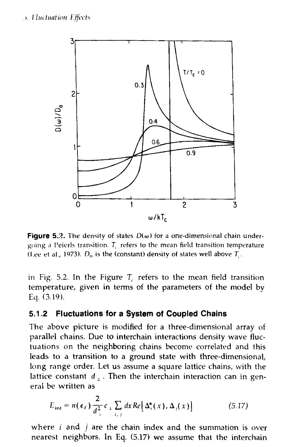
Fluctuation Effects 86
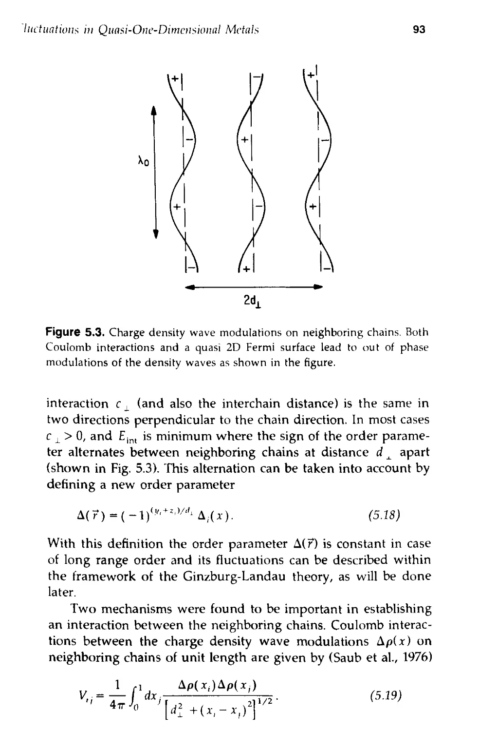
5.1 Fluctuations in Quasi-One-Dimensional Metals 87
5.2 Charge Density Wave Fluctuations in Kli:,MoO-, 101
Collective Excitations 106
6.1 Ginzburg-Landau Theory of Charge Density Wave
Excitations 108
6.2 Excitations of the Spin Density Wave Ground State 124
6.3 Experiments on Charge Density Waves: Neutron
and Raman Scattering 127
d.4 Experiments on Spin Density Waves: AFMR
and Magnetization 132
Commensurability and Near Commensurability
Effects 136
7.1 Models of Commensurability Effects 137
7.2 Experiments: Search for Commensurability Effects
and Solitons 147
8 ¦ The Interaction Between Density Waves
and Impurities 150
8.1 Theories of Density Wave-Impurity Interaction 151
8.2 Experimental Evidence for Finite Correlation
Lengths 158
9B The Electrodynamics of Density Waves 164
9.1 The Electrodynamics of Density Waves 165
9.2 Frequency Dependent Conductivity of Charge
Density Waves 174
9.3 Frequency Dependent Conductivity of Spin
Density Waves 179
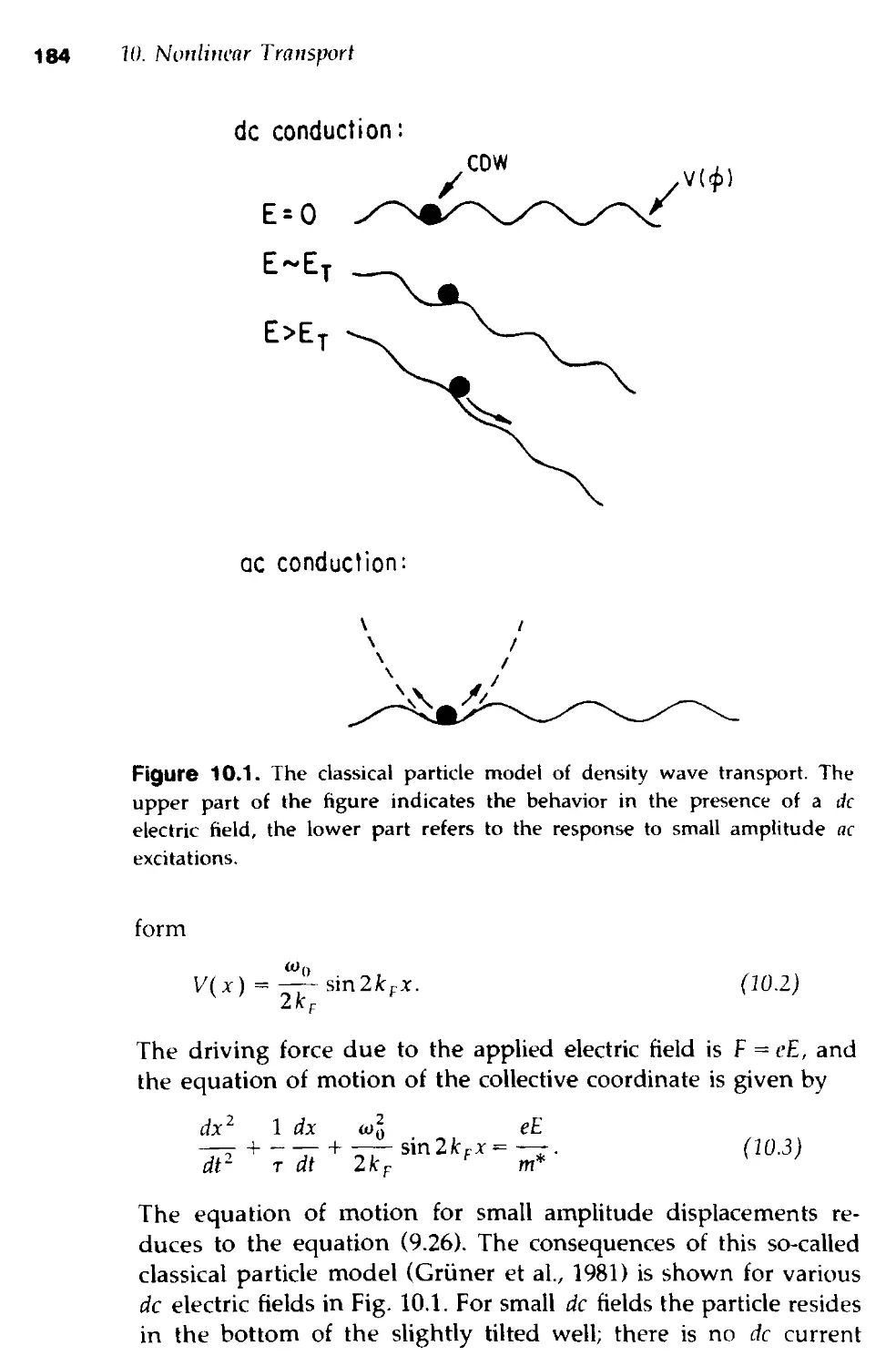
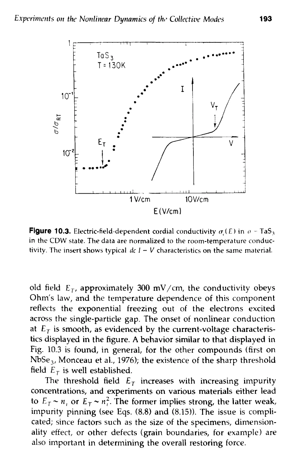
10 ¦ Nonlinear Transport 182
10.1 Models of Density Wave Transport 183
10.2 Experiments on the Nonlinear Dynamics
of the Collective Modes 192

Contents
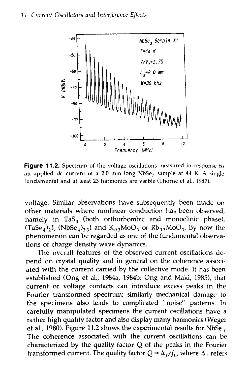
11 ¦ Current Oscillations and Interference Effects
in Driven Charge Density Wave Condensates
(Reprinted in part from Progress in Low
Temperature Physics, vol. XII. Ed.: D.F. Brewer,
Elsevier Publishers, B.V. 1989). 198
11.1 Introduction 198
11.2 Current Oscillations 200
11.3 Interference Phenomena 212
11.4 Conclusions 239
References 244
Appendix: Some Books, Conference Proceedings,
and Review Papers. 252
Index 254

Notation I cgi'iui
(r cordial conductivity
<r( differential conductivity
(j) time averaged current density per chain
fn current oscillation frequency
1 n spectral density of harmonics
Ca' Q, elastic constants related to change of amplitude and
phase of order parameter

Preface
Uensity waves are broken symmetry states of metals, brought
about by electron-phonon or by electron-electron interactions.
The ground states are the coherent superposition of electron-hole
pairs, and, as the name implies, the charge density or spin density
is not uniform but displays a periodic spatial variation. The
former is called the charge density wave (CDW), the latter the
spin density wave (SDW) state of metals.
Charge density waves were first discussed by Frohlich in 1954
and by Peierls in 1955; spin density wave states were postulated
by Overhauser in 1962. It was recognized early that highly
anisotropic band structures are important in leading to these
ground states. Not surprisingly, experimental evidence for these
ground states was found much later, when materials with a linear
chain structure and metallic properties were discovered and in-
investigated. Several groups of both organic and inorganic materials
are now standard examples of density wave ground states; some
members of these groups have been investigated in detail by a
wide array of experimental techniques.
These notes give a fairly elementary, unsophisticated, and
sometimes oversimplified discussion of the field. They reflect an
experimentalist view; there is an emphasis on the close relation
between theory and experiment—an important aspect of the
field. The notes are based on lectures I gave at the Eidgenossische
Technische Hochschule, Zurich in 1989 and subsequently at the
University of California, Los Angeles in 1991; in both occasions to
an audience including graduate and undergraduate students.
Because density waves arise in their simplest form in highly
anisotropic (so-called quasi-one-dimensional materials) some fun-
fundamental aspects of the low dimensional electron gas will be
discussed first. Chapter 2 focuses on the materials, on the various
groups of so-called linear chain compounds. This is followed by a
xix

Ihrlinv
discussion of the mean field theory of CDW and SDW ground
states and the basic experimental observations in Chapters 3 and
4, Because of the low dimensionality, fluctuation effects are im-
important, and the phase transition is different from what is pre-
predicted by mean field theory. The nature of the phase transitions
and fluctuations are discussed in Chapter 5; followed in Chapter
6 by a survey of the collective excitations called phasons, ampli-
tudons, and magnons. Chapter 7 deals with the interaction be-
between the ground states and the underlying lattice, and Chapter
8 with the interaction between density waves and impurities. This
is followed by a discussion of electrodynamics and nonlinear
transport phenomena in Chapters 9 and 10. One of the most
spectacular observations in the field is the detection of current
oscillations, and various interference phenomena which occur
when both dc and ac driving fields are amplified. A recent
review, adopted in part from Progress in Low Temperature Physics
concludes these notes.
The phase transitions and essential features of the ground
states are discussed by using second quantization formalism.
While the various density wave states, together with the super-
superconducting ground state, can be discussed using a simple Hamil-
tonian with a q dependent interaction potential V(<j) between the
electrons, a traditional approach will be followed here: the charge
density wave state is described starting from the Frohlich Hamil-
tonian of electron-phonon interactions, while the spin density
wave state will be discussed by treating the electron-electron
interactions within the framework of the Hubbard model. Fluctu-
Fluctuation effects and elementary excitations will be described within
the framework of Ginzburg-Landau theory, and the interaction
between density waves and the underlying lattice together with
density wave-impurity interactions will also be discussed using
this approach.
Several aspects of the ground states, phase transitions, and
various excitations are similar to those of the superconducting
state, and consequently extensive use will be made of expressions
which have been worked out for BCS superconductors. These
expressions will not be derived, but will merely be adopted from
the literature. The same applies for the discussion of magnetic
excitations which occur in the spin density wave state; which are
similar to spin wave excitations well known for antiferromagnets.

Various topics, such as the microscopic description of the interac-
interaction of the collective modes with impurities, or some aspects of
nonlinear transport, require a discussion which goes beyond the
framework of these notes. In these cases only a short summary of
the pertinent results will be given.
The field is relatively new, and is by no means a closed
chapter of solid state physics. Consequently, many of the issues
have not been completely resolved (this is particularly true for
spin density waves) and parts of these notes reflect this "un-
"unfinished" aspect of the field. Several topics will not be covered by
these notes. Density waves which arise in higher dimensions,
such as the two-dimensional charge density waves observed in a
certain group of materials, called dichalcogenides, and spin den-
density waves in chromium and in its alloys, lie outside the scope of
these notes. Also, the focus is on the simplest case of density
waves: on the periodic modulations of the charge or spin density
with a period which is incommensurate to the underlying lattice.
Somewhat more complicated density waves, which arise in mate-
materials which have two conducting chains—with the material tetra-
thiafulvalene-tetracyanoquinodimethane (TTF-TCNQ) the best
known example—will not be discussed. The interplay between
density waves and superconductivity, so-called field-induced spin
density waves, and other topics, though very interesting in their
own right, will also not be covered by these notes.
1 am grateful to several colleagues, in particular to Stuart
Brown, Steven Kivelson, George Kriza, Kazumi Maki, Attila
Virosztek, and Wolfgang Wonneberger who read and commented
upon the various chapters. My students, Steve Donovan, Yong
Kim, and Andrew Schwartz were kind enough to take the time
and correct many of the mistakes in the early versions of these
notes. The first draft was typed by Renee Wellin and the final
version by Stella Lozano. The figures were drawn by Jackie
Payne. Their help is highly appreciated.
And of course my thanks to Dani, Dora, and Maria—for just
being around.
Los Angeles, 1994

The One-Dimensional
Electron Gas
1
Deine Zauber binden Wieder
Was die Mode streng geteilt;
Fashion's laws, indeed may sever,
But thy magic joins again;
—Friedrich Schiller Hymn of joy
IVIost of the information in subsequent chapters is based on
observations made on materials which have a highly anisotropic
crystal and electronic structures. These types of materials are
usually called "quasi-one-dimensional" or "low-dimensional".
The notion refers both to the crystal and to the electronic struc-
structure, but it also indicates that concepts characteristic of phenom-
phenomena which occur in one dimension may often apply.
The reduction of phase space from three dimensions CD) to
one dimension (ID) has several important consequences. Both
interaction effects and random potentials have a more profound
effect in one than in higher dimensions and fluctuations are also
more important. Also, because of the simple Fermi surface in one
dimension, the interaction between electrons can be expressed in
terms of two coupling constants, one for q = 0 and one for
q = 2kr; leading to simple phase diagrams for the occurrence of
the various broken symmetry ground states which arise as a
consequence of these interactions.
The Response Function of the One-Dimensional
Electron Gas
The Fermi surface of a one-dimensional electron gas is simple: it
consists of two points, one at +kF and one at —kf, for an

1 The One-Dwwn*ional Electron Can
extremely anisotropic metal, two sheets, a distance of 2/cf apart.
The dispersion relation for a ID free electron gas is given by
f(k) = h2k2/2m, and the Fermi energy by
where N(, is the total number of electrons, L is the length of the
ID chain, and mc is the free electron mass.
The Fermi wavevector is
N07T
k,=~r = N,TT 02)
where N(. is the number of electrons per unit length and per spin
direction. The density of states for one spin direction is
L /m,\1/2 L
»U) = -r hr =-7- 0-3)
irk \ 2e / nhv
where the velocity v is given by the relation mt,v = hk.
The particular topology of the Fermi surface leads to a re-
response to an external perturbation which is dramatically different
from that obtained in higher dimensions. The response of an
electron gas to a time independent potential
4>(r)= (<t>(q)e"i ''dq A.4)
is usually treated within the framework of linear response theory
(see, for example, Kittel, 1963). The rearrangement of the charge
density, expressed in terms of an induced charge
pind(r)=/plnd(q)e^r'dq- A.5)
is related to 4>(r) through
d 0-6)
where *(<f), the so-called Lindhard response function, is given in
d dimensions by
J Bn) ^k~ek + q
where fk=f(ek) is the Fermi function. For a three-dimensiona

The Response Function of the One-Dimensional Electron Gas
q=2kF+l
V ±VF8k'
A
hole
Figure 1.1. The dispersion relation for a free electron gas. The linear
dispersion e — €T — ±i>(-(Jt —Jtj.) is used to evaluate the response function,
Eq. A.10).
spherical Fermi surface a straightforward calculation gives
= ~e2n(€F)
1 +
1-x2
Ix
¦In
l+x
l-x
A.8)
where n(eF) is the density of states at the Fermi level per spin
direction, and x = q/2kr *(<p, as given by Eq. A.8), decreases
with increasing q and the derivative has a logarithmic singularity
at q = 2kF.
The situation is different for a one-dimensional electron gas.
For wavevectors near 2ky, x(q) can be evaluated by assuming a
linear dispersion relation around the Fermi energy ef, as shown
in Fig. 1.1,
ek-eF = hor(k-kr). A.9)
The integral in Eq. A.7) can readily be evaluated near 2k, leading
to
*(<?) =
-In
+ 2kF
q-lkf
= -e2n(ef)ln
2kF
q-2kr
A.10)
In contrast to a 3D electron gas, the response function in one
dimension diverges at q = 2kr. For small q values, *(q) is given
by the Thomas-Fermi approximation, x(q)= —e2n(e,). The re-
response function, evaluated for all q values, is displayed in Fig. 1.2,
where for completeness ^(^) is also shown for a two- and a
three-dimensional electron gas. The fact that #(q) diverges for
q = 2kF in the one-dimensional case has several important conse-
consequences. Equation A.6) implies that an external perturbation
leads to a divergent charge redistribution; this suggests, through

J. The One-Dimensional Electron Gas
Figure 1.2. Wavevector dependent Lindhard response function for a one-,
two-, and three-dimensional free electron gas . t zero temperature.
self-consistency, that at T = 0 the electron gas itself is unstable
with respect to the formation of a periodically varying electron
charge or electron spin density. The period is related to kF by
The divergence of the response function at q = 2kF is due to
t le particular topology of the Fermi surface, sometimes called
perfect nesting. Looking at Eq. A.7), the most significant contribu-
contributions to the integral come from pairs of states — one full, one
empty — which differ by q — 2kF and have the same energy, thus
giving a divergent contribution to ^(i;). However, in higher
dimensions the number of such states is significantly reduced, as
shown in Fig. 1.3 leading to the removal of the singularity at
q = 2kF. The quasi-one-dimensional character of the Fermi surface
can be modeled by including a dispersion in the direction perpen-
perpendicular to the direction along which the response function was
evaluated. The dispersion relation
e(k)=eu + lta cos kxa + 2th cos kvb A.12)
where a and b are the lattice constants in the x and y directions

The Response Function of the One-Dimensional Electron Gas
V
Figure 1.3. Fermi surface topology for a ID and 2D free electron gas. The
arrows indicate pairs of states, one full and one empty, differing by the
wavevector q = 2kr.
respectively, leads to a two-dimensional band structure. For /„ a>
tb, and again using a linear dispersion in the x direction this
dispersion relation reduces close to the Fermi energy to
vF8k - 2tb cos kyb
A.13)
with Sk = k- kF. The Fermi surface is determined by the condi-
condition
It
F + —-cos kyb + O(fb2cos2 kyb)
A.14)
which leads to first the order in tb (neglecting the third term in
Eq. A.14)), to a sinusoidal Fermi surface in the kx - k^ plane, as
shown in Fig. 1.4. As for one dimension, we recover a large

1. The One-Dimensional Electron Gas
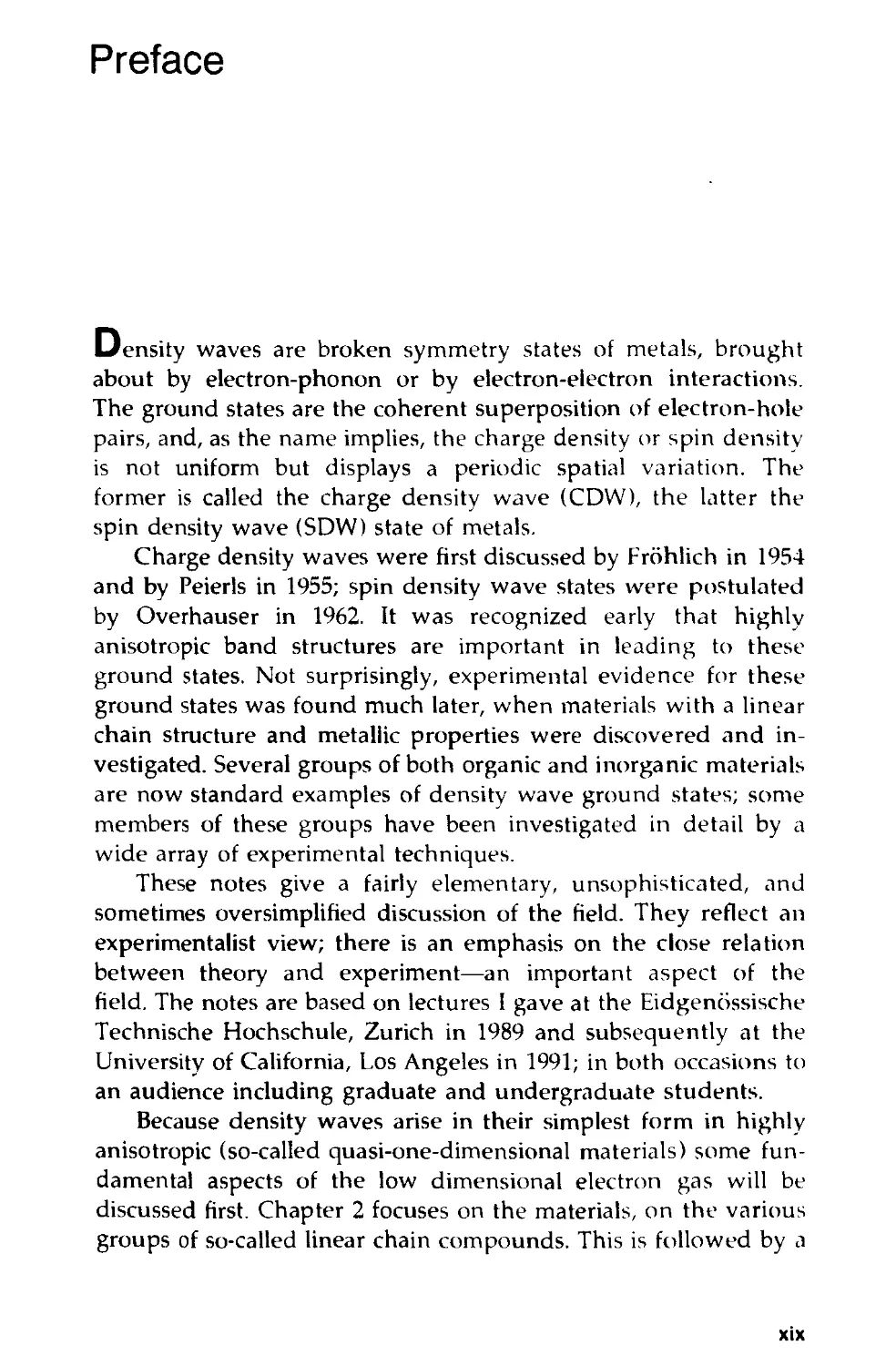
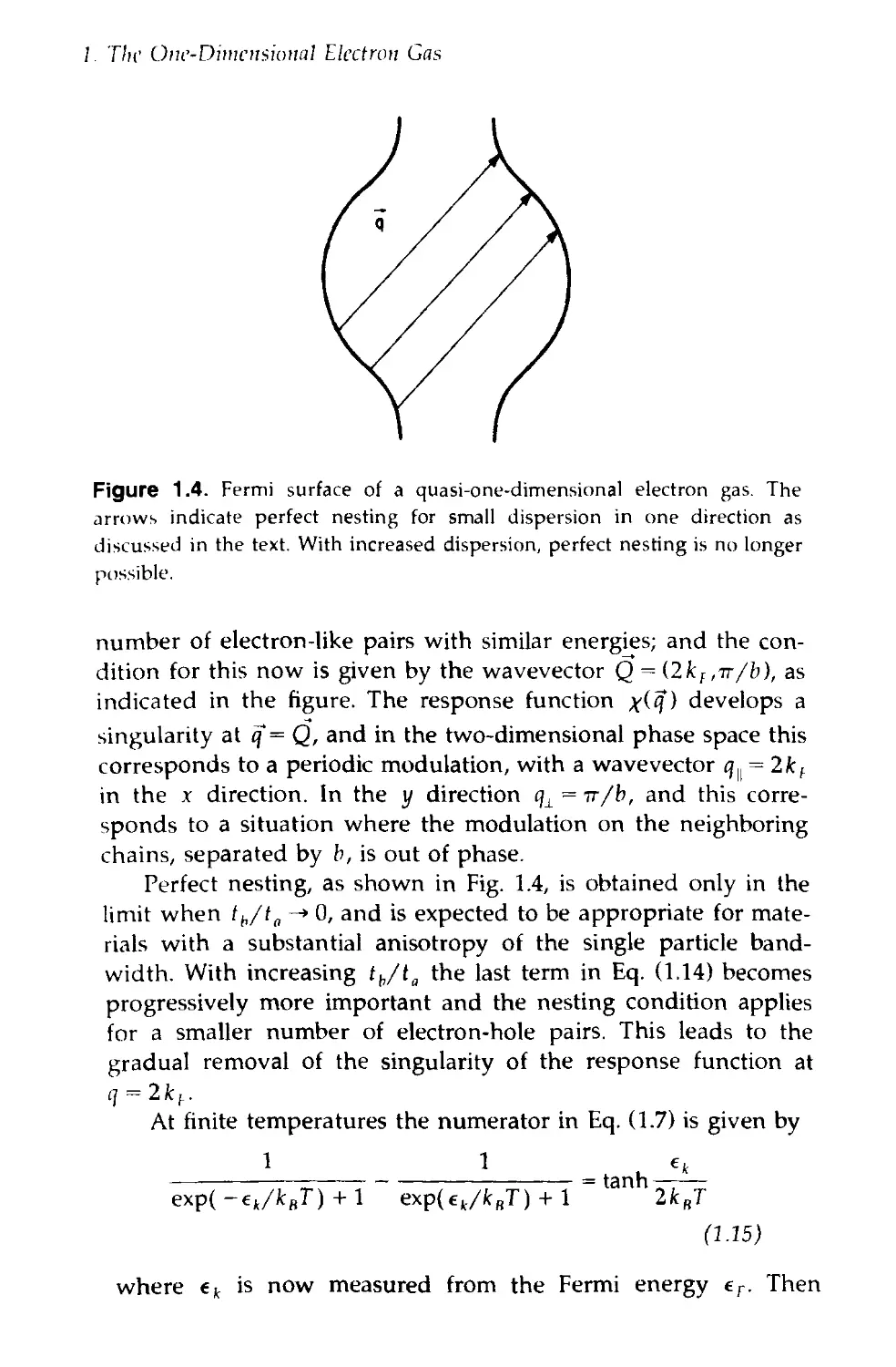
Figure 1.4. Fermi surface of a quasi-one-dimensional electron gas. The
arrows indicate perfect nesting for small dispersion in one direction as
discussed in the text. With increased dispersion, perfect nesting is no longer
possible.
number of electron-like pairs with similar energies; and the con-
condition for this now is given by the wavevector Q = Bkflir/b), as
indicated in the figure. The response function x(<f) develops a
singularity at q = Q, and in the two-dimensional phase space this
corresponds to a periodic modulation, with a wavevector q^ = 2ltf
in the x direction. In the y direction qx = v/b, and this corre-
corresponds to a situation where the modulation on the neighboring
chains, separated by b, is out of phase.
Perfect nesting, as shown in Fig. 1.4, is obtained only in the
limit when th/ta -» 0, and is expected to be appropriate for mate-
materials with a substantial anisotropy of the single particle band-
bandwidth. With increasing th/ta the last term in Eq. A.14) becomes
progressively more important and the nesting condition applies
for a smaller number of electron-hole pairs. This leads to the
gradual removal of the singularity of the response function at
At finite temperatures the numerator in Eq. A.7) is given by
1 1 ek
t
exp( -ek/kj) + 1 exp(e,/fcBT) + 1 t3" UJ
A.15)
where cfc is now measured from the Fermi energy er. Then

"he Response Function of the One-Dimensional Electron
Figure 1.5. The response function of a one-dimensional free electron gas at
various temperatures (after Heeger, 1979).
Eq. A.7) becomes
r tanh x
dx.
B.16)
Here e0 is an arbitrarily chosen cutoff energy which is usually
taken to be equal to the Fermi energy eF, The integral can be
readily evaluated giving
1-14*0
XBkF,T)= -e2n(eF)ln
A.17)

/. Tlw Ouc-Dimt'titional Electron Cris
kt) then has a logarithmic divergence as T —> 0. The response
function can be evaluated for q values different from 2kr and
\(q,T), obtained for various eu/kBT values is displayed in
Fig. 1.5.
1.2 Instabilities in a One-Dimensional Electron Gas:
g-ology
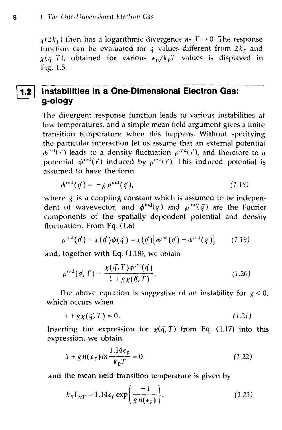
The divergent response function leads to various instabilities at
low temperatures, and a simple mean field argument gives a finite
transition temperature when this happens. Without specifying
the particular interaction let us assume that an external potential
<f>ix'(r) leads to a density fluctuation />m{i('r), and therefore to a
potential 4>"ld(?) induced by plnd(r). This induced potential is
assumed to have the form
*inJ(?)= -,sVnJ(<f), 0.18)
where ^ is a coupling constant which is assumed to be indepen-
independent of wavevector, and (f>md(q) and plmJ(if) are the Fourier
components of the spatially dependent potential and density
fluctuation. From Eq. A.6)
and, together with Eq. A.18), we obtain
PinJ(f,T)-*;* lffT\- 020)
The above equation is suggestive of an instability for % < 0,
which occurs when
1+ <?*(?, T)=0. A21)
Inserting the expression for *(q,T) from Eq. A.17) into this
expression, we obtain
1.14e0
l+?«(€F)fn-—— =0 A.22)
and the mean field transition temperature is given by
1 \
— A23)
fcflTMF=1.14e0expl
l.

Instabilities in a One-Dimensional Electron Gas: g-ologi/ 9
As will be discussed later, the density fluctuation p'nd((f),
reflects the formation of electron-electron or electron-hole pairs,
with the ground state at T = 0 being a coherent superposition of
the various pair states. The nature of the ground state depends
on the electron-electron and electron-phonon interactions, which
can be described by a ^-dependent interaction potential V{q ).
The situation is particularly simple for a one-dimensional
metal where the Fermi surface is two points at ±kf. (Solyom,
1979 and references cited therein; Emery, 1979). Electrons and
holes on the right or left side are denoted by e+ and e_ and by
h+ and h_. With the spin degrees of freedom also included, four
possibilities for pair formation may occur:
e+/ o"f e_, — (r
e+, a; e_,a-
e+, a; h_, u
e+,cr; h_,-(T pairs with q = 2kT
S = l
The development of these states can be discussed using simple
models with a mean field solution giving a finite transition tem-
temperature. However, as will be discussed later, the mean field
solution is not appropriate in one dimension. Solutions of the
models which go beyond the mean field treatment lie outside the
scope of these notes (see, for example, Solyom, 1979). Conse-
Consequently, only the main results will be stated here.
The first two of these states develop in response to interac-
interactions for which q = 0; this is called the particle-particle or Cooper
channel. The resulting ground states are the well known (singlet
or triplet) superconducting states of metals. The last two states,
with a finite total momentum for the pairs, develop as a conse-
consequence of the divergence of the fluctuations at q — 2ky; this is the
particle-hole channel, usually called the Peierls channel. For these
states we find a periodic variation of the charge density or spin
density, and consequently, they are called the charge density
wave and spin density wave ground states. The period Ao = Tr/kv
associated with the spatial variation of the charge or spin density
pairs
with
pairs
pairs
with
total
with
with
total momentum
spin
q = 0
S = 0
S = l
q = 2kr
S = 0

(. The Om'-Dimctwoiml Electron Ga>
Figure 1.6. The phase diagram of the ID electron gas in the second order
scaling approximation showing the most divergent type of fluctuations, for
the coupling constants jj,, #2. For the definition of the coupling constants
and of the various ground states see the text and Solyom, 1979, and
references cited therein.
also leads to a gap in the single particle excitation spectrum at the
Fermi level. For an arbitrary band filling the period is incommen-
incommensurate with the underlying lattice.
In ID the diagrammatic expansion of the Cooper channel
contains contributions from the density fluctuations at q = 2kT,
and the density fluctuations also contain contributions from the
q = 0 fluctuations (Solyom, 1979). Consequently, both the Cooper
and Peierls response functions diverge at the same rate at low
temperatures. Which of these states occurs depends on the de-
detailed nature of electron-phonon and electron-electron interac-
interactions, and in one dimension the interaction can be represented as
the combination of two coupling constants, g-, and g2; which
represent the interactions with momentum transfer of ±2kF and
zero, respectively. The occurrence of these states in the g{-g2
phase space is shown in Fig. 1.6 and this so-called g-ology picture
has been discussed in several reviews. Obviously a strictly one-
dimensional situation cannot occur in real materials even in
compounds with rather highly anisotropic band structure, since

Instabilities in a One-Dimensional Electron Gas: g-olo^y 11
interchain interactions are also of importance. Systems which are
composed of coupled chains have a phase diagram somewhat
different from that shown in Fig. 1.6; but the four different
ground states with features rather similar to those calculated for a
purely one-dimensional band structure are still preserved for
weak interchain coupling.
The various broken symmetry ground states have several
common characteristics which are well known for the extensively
studied superconducting state (see, for example, Schrieffer, 1963;
Tinkham, 1975). For all condensates, the order parameter is com-
complex, and can be written as
A = |A|<?"*. 024)
For the superconducting ground states, gauge symmetry is
broken; the phase is invariant under a gauge transformation. In
contrast, for the density wave ground states, the translational
symmetry is broken. While the time and spatial derivatives play
an important role in the dynamics of the collective modes, the
above difference between the superconducting and density wave
ground states leads naturally to different collective excitations
and also to differences in the coupling of the collective modes to
applied electromagnetic fields. For the density wave ground states
these collective excitations are called phasons and amplitudons,
referring to fluctuations of the phase and amplitude of the con-
condensate. For charge density waves, both occur below the single
particle gap, as will be discussed in Chapter 6. In addition, in the
spin density wave ground state (as in the triplet superconducting
state), the spin rotational symmetry is also broken, leading to
additional collective excitations, similar to those of conventional
antiferromagnets. The features of the various broken symmetry
states are summarized in Table 1.1.
The amplitude |A| is related to (or can be denned as) the
single particle gap. In the case of electron-electron pairing this is
the well known superconducting gap. In case of the density wave
states, the gap occurs at ±kF. In the superconducting state, the
collective mode leads to a supercurrent in response to dc fields. In
the case of density waves, however, the collective mode does not
contribute to the dc conduction (this is due to the interaction
with impurities and lattice imperfections), and the appearance of
a gap in the single particle excitation spectrum at the Fermi level

/. Tlie One-Dimensional Electron Gas
Table 1.1. Various broken symmetry ground states of one-dimen-
one-dimensional metals. The Anderson-Higgs mechanism removes the low
lying exitations in a singlet superconductor.
singlet
superconductor
triplet
superconductor
charge density
wave
spin density wave
Total
Paring Spin
el-el S = 0
el-el S = 1
el-hole S = 0
el-hole S = 1
Total
Momentum
9 = 0
<j = 0
1 = 2Jtr
q = 2k,
Broken
Symmetry
gauge
gauge
translational
translational
Loiv Lying
Collective
Excitations
(Anderson-
Higgs)
low lying
magnetic
excitations?
phasons
amplitudons
phasons
magnons
causes the material to become a semiconductor below the transi-
transition temperature.
The appearance of the single particle gap A also leads to a
finite coherence length ?0, which corresponds to the spatial
dimension of the electron-electron or electron-hole pairs. Crudely
speaking, the pair wavefunctions are the superpositions of one
electron state within the energy region around the Fermi level,
and the corresponding spread of momenta is approximately
B.25)
where vF is the Fermi velocity. This corresponds to a spatial range
of ?0 = (SpI = hvr/b. The correct expression, the BCS coherence
length, is given at zero temperature by (Schrieffer, 1964; Tinkham,
1975)
fc A26)
The temperature dependence of the order parameter and
condensate density have the well known BCS form for all cases;
and the gap is related to the mean field transition temperature,
TMF, through the well known BC3 relation 2|AKT = 0) = 3.52 kgT^,
in the weak coupling limit. The condition when this limit applies
is somewhat different for different ground states, as will be
discussed later.

1.3 Correlations and Fluctuations 13
Correlations and Fluctuations
Because of the reduction of phase space, one-dimensional systems
are unstable against fluctuations. These fluctuations lead to the
absence of long range order at any finite temperature, and for
T # 0 only short range correlations develop. The correlation length
for models which involve the response of the electron gas to
electron-phonon or electron-electron interactions, is related to the
correlation length which characterizes the density fluctuations of
the one-dimensional electron gas. These density fluctuations are
described by the correlation function
;/(€,)<"*' B.27)
where Cf and C are the creation and destruction operators of the
electron density. The spatial dependence is approximately given
by
/C+(F),C@))=exp
\r-r
+ iq- r
A.27a)
where f is the correlation length associated with the density
fluctuations. For a one-dimensional metal, with a linear disper-
dispersion relation ek - eF = hvF(k - kF) as shown in Fig. 1.1,
dk
ielk'x
, dk e"A
(cv).c(o))-/— ggBf|t-t,, + 1
,-,n2,+ l,r/0,, ^ 2g^
/ = u
where /3 = (ItBT), and using Eq. A.27a) the correlation length
nkBT
diverges as the temperature approaches T = 0.
As will be discussed later, at low temperatures the collective
excitations of the density wave states are described by the Hamil-

/. The Otw-Diniensioiml Electron Gas
tonian
^ = A ((V$J d?= (dL'k\<t>k\2k2 A.30)
J J
in dimension d where <j> is the phase of the condensate and A is
the elastic constant associated with the long wavelength deforma-
deformations of the condensate. The thermal expectation value of the
component \4>k\ is
/ k2\<j>k\2\ ,
, k2\<t>k\
id<t>kexp\ —-r
which, after factorization becomes approximately
Let us look at the correlation function which describes the spatial
fluctuations of the phase variable. In the limit when the ampli-
amplitude of the order parameter is close to its T = 0 value, the
correlation function looks like
([]2) A.33)
the term in the exponent,
d''fc(l*4-|2)(pll'r'-lJ A.34)
. d''k ik- . 2
The integral diverges for d < 2, and therefore there is no long
range order at any finite temperature.
The argument advanced here is essentially the same as the
argument for the absence of long range order for a Heisenberg
antiferromagnet, and is due to the existence of low lying, gapless
collective modes. If these excitations develop a gap (and this
would occur for a commensurate density wave, as will be dis-
discussed in Chapter 7) long range order is restored. Arguments,
analogous to those applied for the Ising model (Ziman, 1964)
apply for this latter situation and there is no long range order for
d < 1 at finite temperatures.

Materials
2
Nehdny Anyag
mas-mas tulajdonsdgokkal felruhdzva
Substances, each
blessed with different attributes
—Imre Maciach The Tragedy of Man
A large number of organic and inorganic solids have crystal
structures in which the fundamental structural units form linear
chains. While most of these materials are insulators or semicon-
semiconductors; several groups have partially filled electron bands, and
consequently display metallic behavior at high temperatures.
The greatly different overlap of the electronic wave functions
in the various crystallographic directions leads to strongly
anisotropic, so-called quasi-one-dimensional electron bands dis-
discussed in the previous chapter. This is the prerequisite for the
development of the instabilities at q = 2kh. Among the different
materials which display a variety of phase transitions, only the
simplest examples of density wave formation will be discussed,
where the charge or spin density wave fluctuations develop along
identical chains and, subsequently, the interaction between the
chains leads to a three-dimensional ordered ground state. The
partially filled electron bands, where the number of electrons per
site is not a simple fractional number (eg., 1/2, 1/3, etc.), lead to
density wave instabilities where the period \0 — ir/kr of the
density waves is incommensurate with the underlying lattice (for
which the fundamental period is the lattice constant a). Materials
with two-dimensional band structures (and consequently with 2D
15

2. Materials
density wave ground states) will not be discussed. Materials
which are composed of two or more different metallic chains
(consequently displaying a variety of subtle instabilities) also lie
outside the scope of this discussion.
While probably a coincidence, among the various compounds
with a single conducting chain, inorganic linear chain compounds
have been found to be examples of charge density wave conden-
condensates; while several groups of organic materials have been ob-
observed to develop a spin density wave ground state. In both cases
a broad variety of experiments have been conducted to explore
the normal state properties, with a focus on the parameters which
characterize the single particle electron states, on the anisotropy,
and on the strength of the electron-electron and electron-phonon
interactions.
The crystal structures are in general complex. Several reviews
listed in the Appendix discuss the structural properties of the
various groups of linear chain materials in detail. Therefore only
the basic features of the structural arrangements will be summa-
summarized here, with emphasis on the resulting electronic structure of
these types of materials.
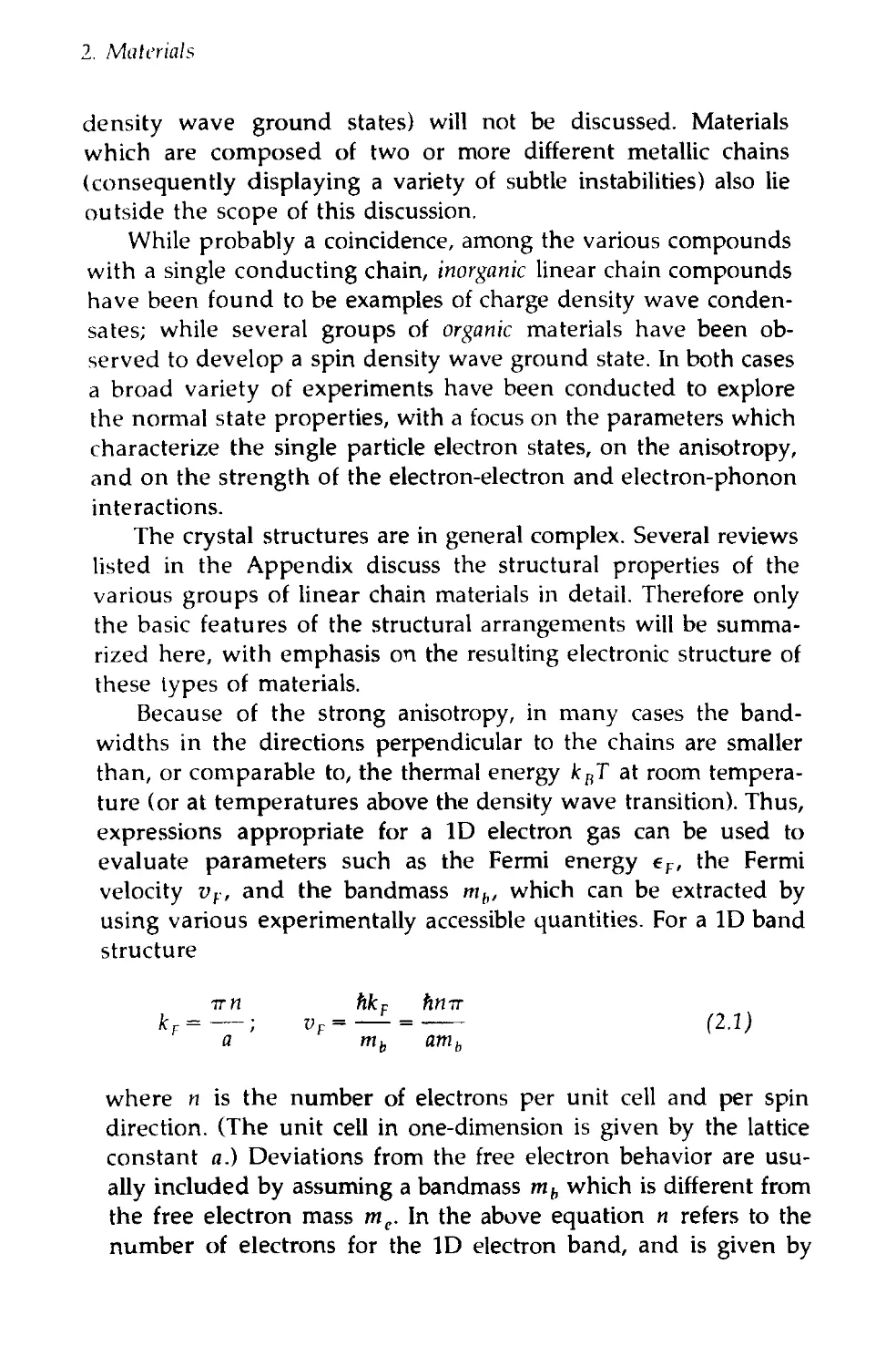
Because of the strong anisotropy, in many cases the band-
widths in the directions perpendicular to the chains are smaller
than, or comparable to, the thermal energy kBT at room tempera-
temperature (or at temperatures above the density wave transition). Thus,
expressions appropriate for a ID electron gas can be used to
evaluate parameters such as the Fermi energy eF, the Fermi
velocity vr, and the bandmass mb, which can be extracted by
using various experimentally accessible quantities. For a ID band
structure
rrn hkF hnv
kF=—; vF=— A.1)
a mb amb
where n is the number of electrons per unit cell and per spin
direction. (The unit cell in one-dimension is given by the lattice
constant a.) Deviations from the free electron behavior are usu-
usually included by assuming a bandmass mh which is different from
the free electron mass mc. In the above equation n refers to the
number of electrons for the ID electron band, and is given by

Materials 17
n = Nea, the total number of electrons per unit volume is given by
n0 = Ncnx, with n± being the number of chains per unit area.
Then, the density of states n(eF) for each spin direction is related
to eF by
N, n
In general, n (or Ne, the number of electrons per unit length) can
be derived from electron counting arguments, as well as from the
measured period Ao = ir/kp of the density wave. If available from
experiments, the plasma frequency
"'I mb
can then be used to evaluate the bandmass. With n and mb
known, Eqs. B.1) and B.2) can be used to determine the Fermi
energy eF.
The magnetic susceptibility
where g is the gyromagnetic factor and fiB the Bohr magneton,
can also be used; together with kr as obtained from the calcu-
calculated band filling or from the period Ao of the measured lattice
distortion, to derive the same parameters. Broadly speaking as
electron-electron interactions lead to an enhancement of the mag-
magnetic susceptibility while (op does not reflect these interactions,
the comparison of the two sets of parameters may also shed light
on the importance of these interactions.
The above equations are based on a nearly free electron
approach; a tight binding description is also often used to extract
parameters such as the Fermi energy eF and Fermi velocity vF
from the measured quantities. The two approaches lead to some-
somewhat different values for the Fermi energy, Fermi velocity, and
density of states. These differences, however, are not essential,
particularly when one is interested only in the gross overall
features of the phase transitions, and in the approximate values of

18 2. Materials
the parameters which characterize the various broken symmetry
ground states.
The expressions in Eqs. B.1) and B.2) which lead to the Fermi
energy and Fermi velocity from measured quantities such as u>p
and x are obviously appropriate only for a strictly ID electron
band, and should consequently be used only for a rather
anisotropic bandwidth. This anisotropy can be estimated by using
the measured anisotropy of the dc electrical conductivity <rik, and
crude arguments (Jerome and Schultz, 1982) lead to
B.5)
vhere i>,n and vr± are the Fermi velocities alonp, and perpendic-
perpendicular to the chain direction. The anisotropy of the optical reflectiv-
reflectivity, in particular the anisotropic plasma frequency (if it exists in
both directions), has also been used to assess the magnitude of
the anisotropy of these materials.
Inorganic Linear Chain Compounds
A variety of inorganic materials have strongly anisotropic crystal,
and consequently strongly anisotropic electronic structures; which
often display various transitions from metallic to nonmetallic
states. Among the many groups of such materials, three have
been explored in detail and these materials are by now well
established examples of the charge density wave ground state.
2.1.1 Mixed Valence Platinum Chain Compounds
Platinum chain complexes are composed of a columnar array of
units which incorporate a chain of Pt atoms with strongly over-
overlapping d orbitals. Although a considerable number of com-
compounds of such structure are known, most of the experiments
have been performed on the material K2Pt(CNLBr(K • 3.2H2O,
usually called simply KCP or Krogmann's salt. The schematic
crystal structure of this material is shown in Fig. 2.1. It consists of
a columnar stacked array of PKCNL units, with a rather short
Pt-Pt separation of 2.894 A along the chain direction. The dis-
distance between the chains in 9.89 A leading to a strongly anisotropic
separation between the Pt atoms in the different directions. The
water molecules form a hydrogen-bonded material between the

Inorganic Linear Chain Compounds 19
CN
Figure 2.1. The crystal structure of the compound K2Pt(CNLBrlu ¦ 3.2H2O,
called KCP, or Krogmann's salt.
CN ligands and the K+ ions provide a cross-link between the
Pt(CNL chains.
The K^+[PKCNL]2~H2O configuration has a full valency Pt2*
and consequently this material would be a semiconductor. The Br
counterions remove electrons from the Pt(CNL unit, and the
resulting fractional charge Pt17(CNL leads to a partially filled
electron band, the prerequisite for metallic behavior.
Indeed, the material is highly conducting at room tempera-
temperature, with a conductivity along the chain direction of cr, - 102il '
cm^1 (Carneiro, 1988). The conductivity is also highly anisotropic,
and the ratio of the conductivities measured along and perpen-
perpendicular to the chains is crj/cr± ~ 105. This anisotropy is also clearly
evident in the optical properties (Bruesh et al., 1975; Geserich,
1988), and the reflectivity measured in the two different directions
is displayed in Fig. 2.2. For Ellc, the optical conductivity is well
described by the usual Drude form
1 - ioit 2ir A — ioit)
{1.6)
with a plasma frequency of oip = 2.9 eV and a relaxation time of
t = 3x105 sec. The band filling of 1.7/2 el = 0.85, obtained
from charge transfer arguments as discussed before, gives a band-

2. Material*
10
reflectivit
uu
50
U
^ ____
-
i V 7
i
Ellc
Jl Elc
1
' ^\
-
-
-
i
\ r
10* 105
optical wave number (cm"')
104
Figure 2.2. The optical conductivity of K,Pt(CNLBr,M ¦ 3.2H:O measured
both parallel and perpendicular to the chain direction at room temperature
(after Geserich, 1988); c refers to the chain direction.
mass of m,,~ 1.0
_. „ _._ ...(. as expected for strongly overlapping Pt
orbitals forming wide conduction bands. This relatively wide
electron band along the chain direction also follows from the
small Pauli susceptibility measured at room temperature or above
(Scott et al., 1979). These magnetic measurements also indicate
that electron-electron interactions do not play an important role
in these materials.
2.1.2 Transition Metalchalcogenides, MX3 and (MX4)nY
Group IV or V transition metals, Nb or Ta, when combined with
chalcogen atoms, S or Se, form a variety of linear chain com-
compounds, several of which have partially filled electron bands and
thus metallic behavior at high temperatures. (Rouxel and
Schlenker, 1989; Meerschaut and Rouxel, 1976).
The basic constituent of the structure is a triangular prism of
MX6 units, with a cross-section close to an isosceles triangle as
shown in Fig. 2.3. The transition metal atom (indicated by the
solid circle in the figure) is located roughly at the center of
the prism. The prisms are stacked on top of each other by sharing
the triangular faces along the b-axis, and the chains are staggered
with respect to each other by half the height of the unit prism.
Therefore, besides the six chalcogen atoms of an MX6 prism, each
transition metal is bonded to two more X atoms from neighbor-

Inorganic Linear Chain Compounds
21
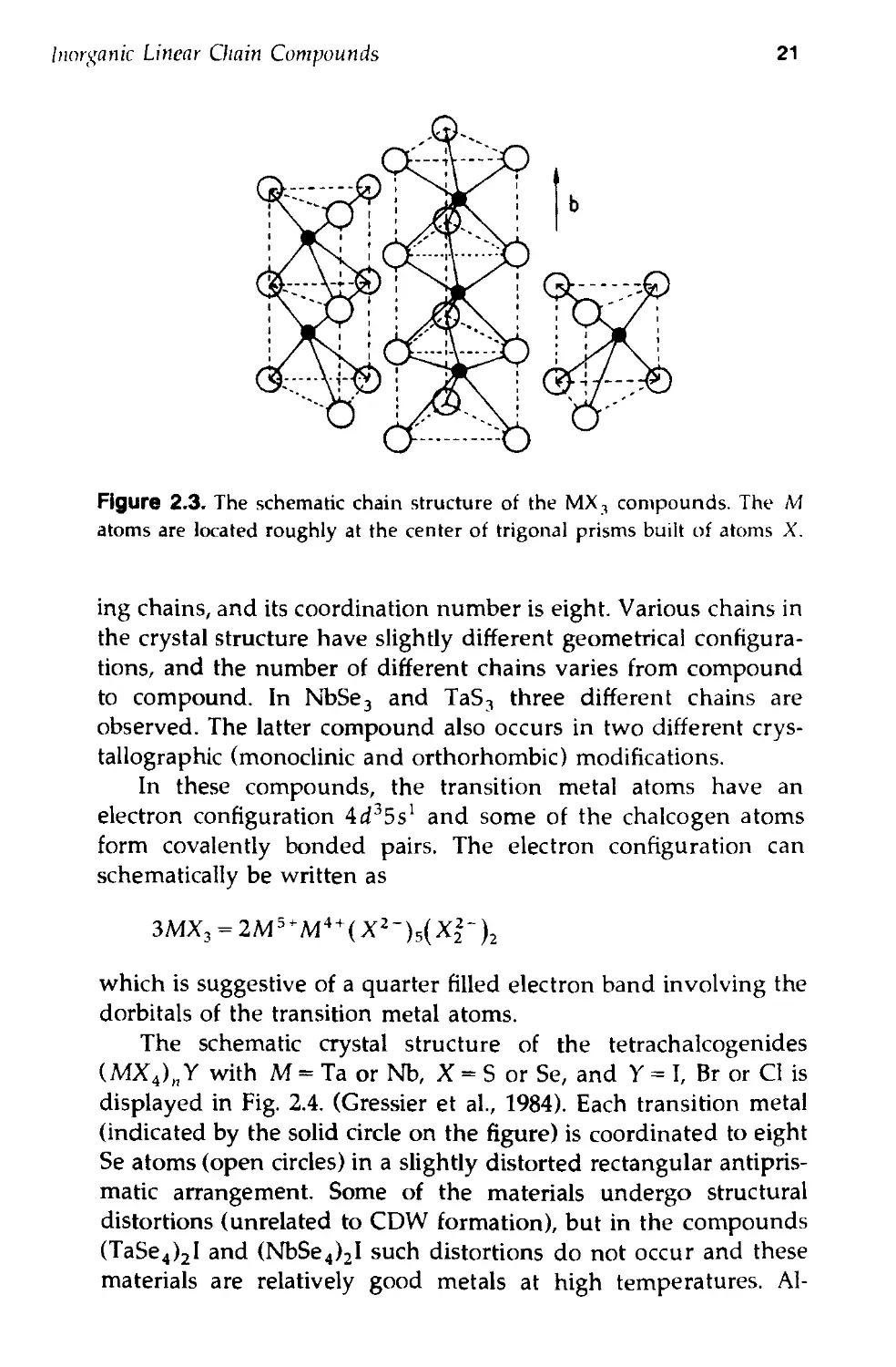
Figure 2.3. The schematic chain structure of the MX, compounds. The M
atoms are located roughly at the center of trigonal prisms built of atoms X.
ing chains, and its coordination number is eight. Various chains in
the crystal structure have slightly different geometrical configura-
configurations, and the number of different chains varies from compound
to compound. In NbSe3 and TaS3 three different chains are
observed. The latter compound also occurs in two different crys-
tallographic (monoclinic and orthorhombic) modifications.
In these compounds, the transition metal atoms have an
electron configuration 4d35s1 and some of the chalcogen atoms
form covalently bonded pairs. The electron configuration can
schematically be written as
which is suggestive of a quarter filled electron band involving the
dorbitals of the transition metal atoms.
The schematic crystal structure of the tetrachalcogenides
(MX4)nY with M = Ta or Nb, X = S or Se, and Y = I, Br or Cl is
displayed in Fig. 2.4. (Gressier et al., 1984). Each transition metal
(indicated by the solid circle on the figure) is coordinated to eight
Se atoms (open circles) in a slightly distorted rectangular antipris-
matic arrangement. Some of the materials undergo structural
distortions (unrelated to CDW formation), but in the compounds
(TaSe4JI and (NbSe4JI such distortions do not occur and these
materials are relatively good metals at high temperatures. Al-

Figure 2.4. The schematic chain structure of the (MX4JY compounds.
though the former compound may be formulated as
Ta4 + Ta3+4[Se2]2~I from charge neutrality arguments, all Ta-Ta
distances are found to be identical C.206 A) along the chain and
the electron band is quarter filled; the same applies to the Nb
compound. The Se atoms lie in planes approximately perpendicu-
perpendicular to the c-axis (which is the chain direction in this case). These
planes (separated by c/4) develop in a helicoidal way along the
oaxis. The chains of TaSe4 are parallel to the c direction and are
well separated by the I atoms. The materials are relatively good
metals along the chain direction with room temperature conduc-
conductivities parallel to the chains, ar on the order of 103-104Q '
cm. The conductivity perpendicular to the chains is 10 to 103
times smaller, suggesting that the anisotropy of the bandwidth is
substantial.
2.1.3 Transition Metal Bronzes
The term bronze is applied to a variety of crystalline phases of the
transition metal oxides. Examples are the ternary molybdenum
oxides of formula A03MoO3, where the alkali metal A can be K,

hwrganic Linear Chain Compounds
23
Figure 2.5. The schematic structure of KinMoO,.
Rj rr T/. They are often referred to as blue bronzes because of
their deep blue color (Schlenker and Dumas, 1986).
The structure of A03MoO3 contains rigid units comprised of
clusters of ten distorted MoOfi octahedra, sharing corners along
the monoclinac b-axis, as illustrated in Fig. 2.5. This corner sharing
provides an easy path for the conduction electrons along the
chain direction. The chains of distorted MoO6 octahedra also
share corners along the [102] direction and form infinite slabs
separated by the alkaline cations.
The band structure, calculated for a slab of Mo10O30 clusters is
fairly complicated (Whangboo and Schneemeyer, 1986), but such
calculations give two overlapping bands at the Fermi level, both
approximately 3/4 filled. This, as will be discussed in Chapter 3, is
in agreement with the lattice distortion observed in the charge
density wave state of the material. The Fermi surface has a
pronounced two-dimensional character in this compound as evi-
evidenced by dc conductivity and optical studies. At room tempera-
temperature, the conductivity measured along the chain direction is
<rb = 3 X 102fl~' cm'1. In the two perpendicular directions the
conductivity is a2a-c = 10ft cm and crla^l =Q5ilx cm.
The crude argument which gives Eq. B.5) then leads to an

2. Material*
Table 2.1 Metallic state parameters of materials with a charge density
wave ground state. The electron density n (not displayed) has been
derived from the band filling and from crystal structure parameters.
When two values are indicated, the upper is derived from the
magnetic susceptibility and the lower from the plasma frequency.
NbSe-,
(ref. 1,5)
K,,,MoO3
(ref. 2,6,8)
(TaSe4Jl
(ref. 3,6,9)
KCP
(ref. 4,5,7)
NbSe,
(ref. 1,5)
K(UMoO3
(ref. 2,6)
(TaSe4JI
(ref. 3,6)
KCP
(ref. 4,5,7)
Band
filing 1
1/4
3/4
0.85
0.85
nUf)
(eV ')
2.3
5.2
3.1
1.9
1.3
14.4
1.0
X
/ b emu \
I cm* '
0.97
0.55
0.12
(eV)
3X10
(ref. 8)
8X10-'
(ref. 9)
(eV)
1.15
2.7
1.2
2.9
'"/,/'",¦
1.8
4.1
1.54
0.94
0.24
2.8
1.0
f
(cV)
0.11
0.048
0.24
0.39
0.68
0.059
0.82
OO7 cm/sec)
1.4
0.65
2.3
3.8
9.9
0.87
5.37
1. H. P. Geserich, et al. Physica 143B, 174 A986).
2. G. Travaglini and P. Wachter, Solid State Comm. 37, 599 A981).
3. H. P. Geserich, et al. Physica 143B, 198 A986).
4. P. Bruesh, et al. Phys. Rev. B12, 219 A975).
5. |. C. Scott, et al. Phys. Rev. B10, 3131 A979).
6. D. Johnston, et al. Solid State Comm. 53, 5 A985).
7. K. Carneiro, et al. Phys. Rev. B13, 4758 A976).
8. J. P. Pouget and P. Comes, In "Charge Density Waves in Solids" Eds. L. P. Gor'kov
and G. Griiner, North Holland 1987.
9. S. Sugai, Physica 143B, 195 A986). H. Fujishita, et al. Physica 143B, 201 A986).

2.2 Organic Linear Chain Compounds 25
anisotropy of the Fermi velocity of approximately 6 and approxi-
approximately 25 for the two perpendicular directions. This has also been
confirmed by optical studies (Travaglini et al., 1981).
The parameters of the single particle bands which occur along
the chain directions are summarized in Table 2.1. In all cases the
strong overlap of the wavefunctions leads to wide bands, with
bandwidths significantly larger than the energy scale which, as
will be discussed in Chapter 3, corresponds to the single particle
gaps associated with the formation of the charge density wave
ground state. The relatively low Pauli susceptibility also indicates
that electron-electron interactions are small in these materials.
Because of the complicated crystal structures, the phonon
spectrum of these materials is also fairly complicated. Which of
the phonon modes couples to the electronic degrees of freedom is
ultimately determined by neutron scattering experiments. The
unrenormalized phonon frequency coBkF) for the wavevector
q = 2kF can be estimated from these experiments, and the various
values are also displayed in Table 2.1.
Organic Linear Chain Compounds
Planar organic molecules often form linear chains with large
overlap of the n orbitals along the chain direction. When com-
combined with counterions or molecules, the resulting charge transfer
salts may have partially filled bands leading to metallic properties.
Some members of three groups of materials, based on the organic
molecules M shown in Fig. 2.6 and having the composition MX2,
also develop a spin density wave ground state at low tempera-
temperatures as established by a wide range of magnetic measurements.
The crystal structure of the material (tetramethyltetrasele-
nafulvaleneJPF6, (TMTSFJPF6, one member of the so-called
Bechgaard salts (Bechgaard et al., 1980), is shown in Fig. 2.7. The
material is built up of segregated stacks of TMTSF and PF6
molecules. The structures of the compounds based on the MDT-
TTF and DMET molecules have the same basic features. All three
molecules shown in Fig. 2.6 are good donors; and when com-
combined with strong acceptors such as PF6 and similar species, a
charge transfer occurs from the M stacks to the X stacks. For
a full charge transfer the M stacks become 3/4 filled. There is a

2. Materials
TMTSF
DMET
MDT-TTF
Figure 2.6. Planar organic acceptor molecules which form metallic charge
transfer salts, and which undergo a transition to a spin density wave ground
state at low temperatures. Me refers to methyl groups and the open ended
lines to H.
significant overlap of electronic wavefunctions on the M stacks,
with practically no overlap along the X stacks; consequently,
band theory predicts metallic behavior along the chains. The
materials which belong to the different groups do indeed show
metallic conduction down to low temperatures, as shown in Fig.
2.8 (Bechgaard et al., 1980). The increase of resistivity at low
temperatures is due to the removal of the Fermi surface upon the
formation of the spin density wave ground state, as will be
discussed in Chapter 4. The optical properties of (TMTSFJPF6 are
that of a Drude metal (Jacobsen et al., 1983), with high reflectivity
R along the chain direction (E\\a), as shown in Fig. 2.8. In
contrast, perpendicular to the chains (E\\b) nonmetallic reflectiv-
reflectivity is observed at high temperatures. From the analysis of the
optical properties the plasma frequencies can be extracted and
these parameters, together with electron concentration, are dis-
displayed in Table 2.2. The magnetic susceptibility is of the Pauli
type (Jerome and Schultz, 1982) and is weakly temperature de-
dependent down to low temperatures where the phase transition
occurs. The parameters wp and x can then be used, together with
the free electron expressions for these parameters, to extract the
parameters which characterize the single particle states, Fermi
velocity vF, Fermi energy eF, and the density of states n(et).

Organic Linear Chain Compounds
27
Figure 2.7. The schematic crystal structure of (tetramethyltetraselenafulva-
leneJPF6, (TMTSFJPF6.

2. Materials
.u
0.8|
0.6
0.4
0.2
0
Y
La,
ft
\E
\
(TMTSFJPF6
T = 300K
la
\
\
6000
frequency (cm"')
1200
Figure 2.8. Optical reflectance of (TMTSFJPF6, measured both parallel and
perpendicular to the chain direction at room temperature; a refers to the
chain direction and b is perpendicular to the chains. (Jacobsen et al., 1982).
The electrical conductivity is also highly anisotropic in these
materials. The dc conductivity <Tdc measured perpendicular to the
chain direction is usually small, indicating a transfer integral less
than kBT, the thermal energy. This then suggests a monmetallic,
hopping type of electrical conduction along these directions. As
discussed, this conclusion is supported by the optical reflectivity
measured perpendicular to the chains. While the reflectivity for
E\\b does not show a well defined plasma edge, such a feature
appears at low temperatures, indicating a crossover to an
anisotropic but three-dimensional band structure, with the band-
bandwidth larger than kBT in both directions. From these studies,

Organic Linear Chain Compounds 29
Table 2.2 Parameters of the metallic state of two materials with a spin
density wave ground state. The electron density has been evaluated
from the band filling and crystal structure parameters.
(TMTSFJPF6
(DMETJAu(CNJ
(TMTSFJPF6
(DMETJAu(CNJ
Band
filling
1/4
1/4
/ cm \
(w— )
\ sec /
0.86
1.0
V
/ emu \
ho"—)
\ cm /
0.58
(ref. 1)
0.51
(ref. 3)
n(e,)
(eV ')
0.25
0.26
0),,
(eV)
2.9
(ref. 2)
mb/mt. (eV)
1.3 6.1 xlO~2
2.4 6.6X10
1. K. Mortensen, et al., Phys. Rev. B25, 3319 A982), D. Jerome and H. Schultz, Adv.
Phys. 32, 299 A982).
2. A Jacobsen, et al., Phys. Rev. B28, 7019 A983).
- K. Kanoda, et al., Phys. Rev. B38, 39 A988).
bandwidths of ?.5 meV and 1 meV are inferred for the two
perpendicular directions, in contrast to the bandwidth along the
TMTSF stacks which is on the order of 0.25 eV (Jerome and
Schultz, 1982).
Members of other groups of organic linear chain compounds
have also been found to develop a spin density wave ground
state. The organic salts, (MDT-TTFJX, where MDT-TTF stands
for rnethilendithio-tetrathiafulvanele (shown in Fig. 2.6) have a
metallic character for various counterions, and one member of the
group, (MDT-TTFJAu(CNJ, has a spin density wave transition
at T = 20K (Nakamura et al., 1990). This material, along with other
members of the group, has a linear chain structure formed by
MDT-TTF stacks with strongly overlapping orbitals in the stack
direction. This then leads to a strongly anisotropic single particle
band.
The molecule dimethylethylenedithio-diselenadithia-fulva-
lene, DMET also forms various charge transfer salts with different
counterions and the composition is (DMETJX (Kikuchi et al.,
1987; Kanoda et al., 1988). Some members of this family are

2. Materials
semiconductors while others remain metals to low temperatures
where they undergo transitions to various broken symmetry
states. In the compound (DMETJ Au(CNJ the ground state is a
spin density wave which develops at T = 20K where a metal-to-
insulator transition occurs with decreasing temperatures.
Optical studies have not been performed on these latter two
groups of compounds, and magnetic susceptibility has only been
measured in a few cases. Consequently, the parameters of the
metallic band can be established only in a few cases and these are
summarized in Table 2.2.

The Charge Density Wave
Transition and Ground State:
Mean Field Theory
and Some Basic Observations
3
Nonchalamment assis, mille couples d'amants
S'y jurent a leur aise une flamme etemclle.
A thousand couples sit in languid poses,
Exchanging pledges of undying love.
—Charles Germain De Saunt-Aubin Sanettc
The charge density wave ground state develops in low-dimen-
low-dimensional metals as a consequence of electron-phono n interactions.
As the name suggests, the resulting ground state consists of a
periodic charge density modulation accompanied by a periodic
lattice distortion, both periods being determined by the Fermi
wavevector kF. Consequently both the electron and phonon spec-
spectra are strongly modified by the formation of the charge density
waves. The phenomenon is usually described by discussing the
behavior of a one-dimensional coupled electron-lattice system,
with the electrons forming a one-dimensional electron gas, and
the ions forming a linear chain. This description is adopted here.
The consequence of the electron-phonon interaction and of
the divergent electronic response at q = 2kF in one dimension is a
strongly renormalized phonon spectrum generally referred to as
the Kohn anomaly (see Woll and Kohn, 1962 and references cited
therein). By virtue of x(i> T) this renormalization is strongly
temperature-dependent, with o>ren 2tf -» 0 at a finite temperature
(within the framework of mean field theory). This identifies a
phase transition to a state where a periodic static lattice distortion
and a periodically varying charge modulation with a wavelength
Ao = n/kF develops.
For a partially filled electron band, the period Ao is incom-
incommensurate with the underlying lattice. The periodically varying
31

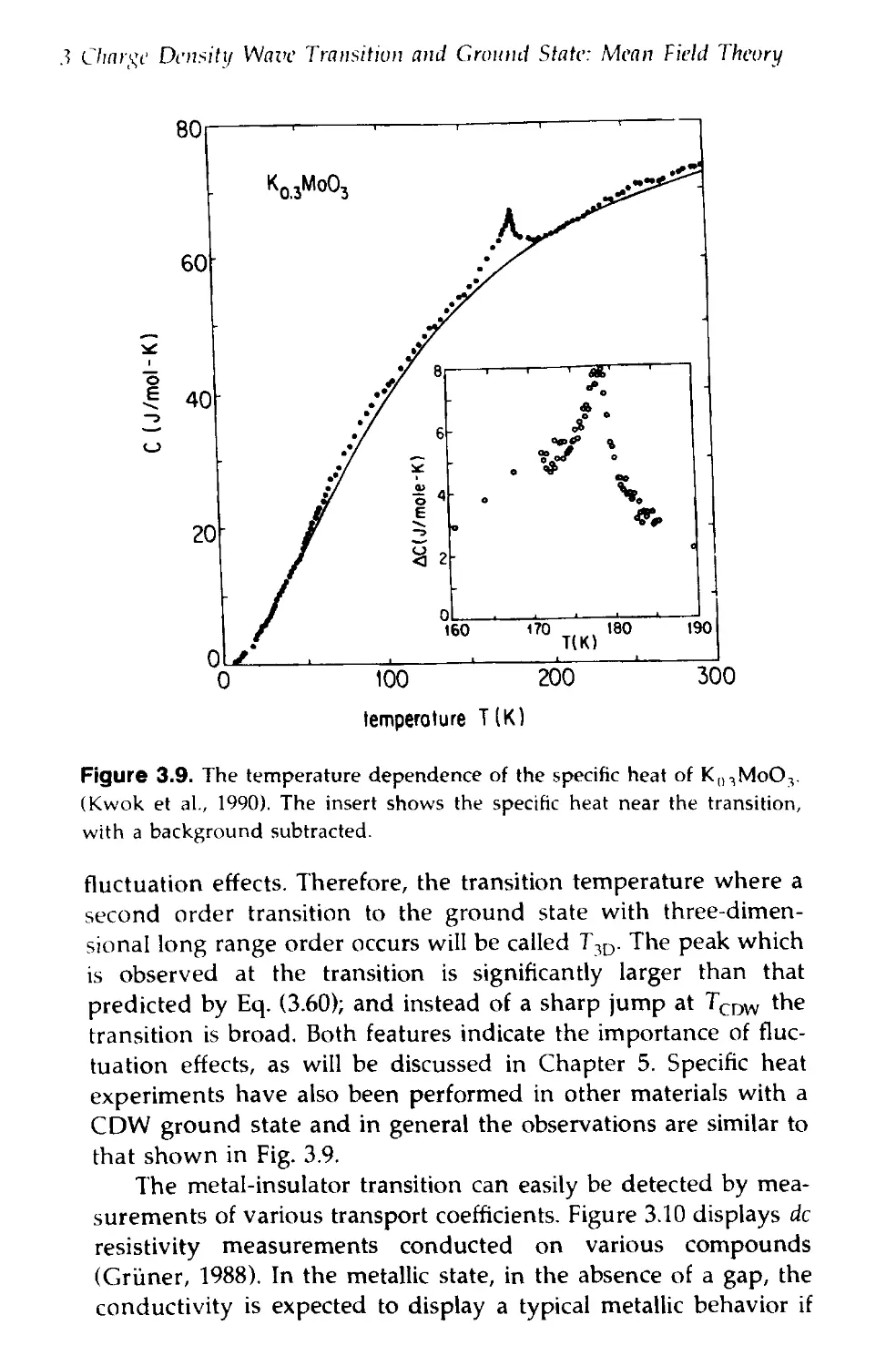
.3 Charge Density Wave Transition and Ground State: Mean Field Theory
lattice distortion leads in turn to a single particle gap at the Fermi
level, turning the material into an insulator. The transition is
generally referred to as the Peierls transition, since this was first
suggested by Peierls A955); the thermodynamics of the ground
state have been worked out by Kuper A955). Independently,
Frcihlich A954) suggested that the ground state can, under the
influence of an applied electric field, carry an electric current.
Hence the state is also often referred to as the Peierls-Frohlich-
Kuper ground state.
In this chapter we first consider the effects of electron-phonon
interactions for a one-dimensional electron gas and describe the
Kohn anomaly for T>T^W, the mean field transition tempera-
temperature. This is followed by a discussion of the state of affairs at
T = 0, described within the framework of a weak coupling theory.
As will be discussed, in the weak coupling limit, where the single
particle gap is much smaller than the Fermi energy er, the
thermodynamics of the phase transition and the temperature
dependence of the order parameter are the same as those of a
BCS superconductor, and extensive use of the expressions worked
out for the superconducting state will be made when finite
temperature effects are discussed.
The most important experimental evidence for these phenom-
phenomena will be discussed next, including observations of the metal-
to-insulator transition which occurs at TCI>VV, the Kohn anomaly
above TCDW, the single particle gap, and the periodic lattice
distortion below the phase transition.
It should be stressed at this point that serious deviations from
the mean field treatment are expected because of the low-dimen-
low-dimensional character of the materials in which the formation of charge
density waves have been observed and also because of the rela-
relatively short coherence lengths which result from the high transi-
transition temperatures. These effects are related to fluctuations of the
order parameter and will be discussed in Chapter 5.
The Kohn Anomaiy and the Peierls Transition:
Mean Field Theory
In order to describe the transition to a charge density wave
ground state let us consider a one-dimensional free electron gas
coupled to the underlying chain of ions through electron-phonon

The Kohn Anomaly and the Peierls Transition: Mean Field Theory 33
coupling. The Hamiltonian for the electron gas is given in second
quantized form as
*"el =!«*«*«
k
where a\ and ak are the creation and annihilation operators for
the electron states with energy ek = h2k2/2m. The formalism is
similar if a tight binding approximation is used, however,
this leads to numerical constants which are somewhat different
from those which follow from the free electron approximation
(AUender et al., 1974). Because spin dependent interactions are
not important in the following discussion, the spin degrees of
freedom are omitted and the density of states n{er) refers to one
spin direction.
The lattice vibrations are described by the Hamiltonian
'vhere Qq and Pq are the normal coordinates and conjugate state
momenta of the ionic motions respectively, a>q are the normal
mode frequencies, and M is the ionic mass. With the notation
1/2
2Mw
" C.3)
\x/z
the Hamiltonian is written as
where b* and bq are the creation and annihilation operators for
phonons characterized by the wavevector q. In terms of these
operators the lattice displacement is given by
1/2
where N is the number of lattice sites per unit length.

3 Charge Oensih/ Wave Transition and Ground State: Menu held Theory
The description of the electron-phonon interaction is usually
referred to as a rigid ion approximation: it is assumed that the
ionic potential V at any point depends only on the distance from
the center of the ion. In second quantized notation
¦*",¦-ph= E aiV(r-/-u)|fc'><iX. C.6)
i,if.i
- V (¦"*' -*x' + u)i/ nt
i.t'.i
where Vk t. is the Fourier transform of the potential of a single
atom V(r), / gives the equilibrium lattice positions, and u is the
displacement from the equilibrium position. For sufficiently small
ionic displacement
C.7)
The Hamiltonian, ¦Wc]_.ph, then has two parts. The first describes
the interaction of the electrons with the underlying ions in their
non-displaced positions. This term transforms the free electron
spectrum into Bloch states, leading to gaps at the Brillouin zone
edge. This term, will be neglected as we are interested in effects
which occur at kr, which is assumed to be away from the
Brillouin zone boundaries. The second term is given by
k, k'.hq
In terms of the phonon creation and annihilation operators, this
interaction term becomes
C-9)
k,k' !
x(k'-
k.q

The Kohn Anomaly and the Peierls Transition: Mean Field Theory 35
where the electron-phonon coupling constant is
h
With all the terms collected, the Hamiltonian, often called the
Frohlich Hamiltonian (Frohlich, 1954), is written as
k q k,q
C.77)
In the case of a ID electron gas, for which the dispersion
relation is described by ek = hvr(k - k,-) = ±vr8k near ±k, (see
Fig. 2.1), (with the energy measured from the Fermi energy eF)
the coupled electron-phonon system is unstable, and this instabil-
instability has fundamental consequences for both the lattice and the
electron gas.
The effect of the electron-phonon interaction on the lattice
vibrations can be described by establishing the equation of motion
of the normal coordinates. For small amplitude displacements
where Qq refers to the second time derivative of the coordinate.
The above equation, utilizing the commutation relations
becomes
where we have assumed that g is independent of q, and
Pq = T.ka\+clak is the qth component of the electronic density.
The second term on the right hand side is an effective force asso-
associated with the lattice dynamics and arises as a consequence
of electron-phonon interactions. The ionic potential
gBMu)q/h) Qq gives, through Eq. A.6), a density fluctuation
Q, C.15)

3 Charge Density Wave Transition and Ground State: Mean Field Tlwory
and with this mean field approximation Eq. C.14) reads
The above equation of motion gives a renormalized phonon
frequency
As discussed in Chapter 1, for a one-dimensional electron gas
x(q,T) has its maximum value at q = 2kF. Consequently, the
reduction, or softening, of the phonon frequencies will be most
significant at these wavevectors. The phonon frequency for q =
2k, becomes
With decreasing temperature, the renormalized phonon fre-
frequency goes to zero and this defines a transition temperature,
when a frozen-in distortion occurs. From Eq. C.18)
where A is the dimensionless electron-phonon coupling constant
S2"(«r)
A=-t — =*'«(«f)- C.20)
Close to the transition temperature a straightforward expansion
gives the following temperature dependence
l CDW
'cdw ;
The phonon dispersion relation a»rcn q, as determined by Eq.
C.17), is shown in Fig, 3.1 at various temperatures above the
mean field transition temperature. This dispersion relation can be
calculated by using the expression for ;f(cj = 2kF,T) as given by
Eq. A.10). The detailed form, as expected, also depends on the
phonon dispersion relation, and in Fig. 3.1 the situation appropri-

77ic Kohn Anomaly and the Peicrls Transition: Mean Field Theory
37
Wfl
Figure 3.1. Acoustic phonon dispersion relation of a one-dimensional metal
at various temperatures above the mean field transition temperature.
ate for the renormalization of an acoustic phonon branch at
various temperatures is displayed.
As discussed earlier, the phase transition is defined by the
temperature where <urcn lkf -» 0 and is due to the strongly diver-
divergent response function of the ID electron gas. The renormaliza-
renormalization of the phonon frequencies also occurs in higher dimensions,
however the reduction of the phonon frequencies is less signifi-
significant. Expressions for \(<\, T) appropriate for a 2D and 3D electron
gas can also be used to evaluate the renormalized phonon fre-
frequencies and these are shown, together with the ID case, in
Fig. 3.2. For the higher dimensions, the temperature dependence
of ^(q,T) is weak, and for small electron-phonon coupling con-
constants <uren remains finite at T = 0 and there is no phase transi-
transition.
Below the phase transition, the renormalized phonon fre-
frequency is zero, indicating a "frozen-in" lattice distortion, that is, a
macroscopically occupied phonon mode with nonvanishing ex-
expectation values (b2kf.) = (bt-2itf)- The order parameter is defined
as
r) + <bUtr>) C.22)

3 Charge Density Wave Transition and Ground State: Menu Field Theory
Figure 3.2. Acoustic phonon dispersion relations of one-, two-, and three-
dimensional metals.
and from Eq. C.5) the lattice displacement is given by
2MMw2ki
1/2
2IAI
-cosBk,x
C.23)
with
1/2
|A|
With this mean field approximation Eq. C.11) becomes
C.24)

The Kolw Anomaly and the Pcicrts Transition: Mean Field Theory 39
where q = ±2kF. As (b2k ) = (b^2t,)< 'he Hamiltonian becomes
*,> C.25)
~*~a\-2k ak(k-2k M + 2^a»2t((&2it| ) •
With the order parameter defined in C.22) the electronic part
becomes
k
C.26)
In the spirit of the nearly free electron approximation we
consider only states near the Fermi level, and states near +kf and
near -Jkf are labelled by the subscripts 1 and 2 respectively. With
this notation and using the dispersion relation ek = hvr{k - kf),
Eq. C.26) becomes
V1;(tfl2,t + |Ak-'V2,tfl1,t]. C.27)
Here and in the following, k is measured relative to the Fermi
wavevector kF. The Hamiltonian can be diagonalized by a canoni-
canonical transformation. We define a new set of operators by
y>,k= Uka,.k- Vk*a2A= Uke-"alik- Vke"KS2a2A
C.28a)
C.28b)
with the constraint that U2k+Vk=\. After some algebra, Eq,
C.27) in terms of yx k and y2 k, becomes
*-L[et(U2k-V?)-2\UUkVk](y\.ky}.k-y\.ky2.k)
+ \2ekUkVk + |A|(li? - V2)](y\,ky2,k + y^y,.,)-
C.29)
The Hamiltonian is diagonalized if the coefficients in front of the

3 Charge Density Wave Transition and Ground State. Mean Field Theory
off-diagonal terms are zero; for example,
2ekUkVk + !A|(U~ - Vf) = 0. C30)
The condition Uf + Vk2 = 1 is satisfied if we choose
j C.31a)
and then C.30) becomes
tan flu = . C.32)
From C.32) and C.31) we obtain
with
Ek-e,+ sign(k - k, )\t,2v}( k - k, f + A"]' '\ C.34)
Upon substitution of the expressions for Uk and Vk, Eq. C.29)
becomes
^^ ha)-,. A2
Instead of the linear dispersion relation ek — ef = twf(k — kF)
appropriate for the metallic state the spectrum of excitations
develops a gap in the charge density wave state, and the disper-
dispersion relation is shown in Fig. 3.3. The density of states is obtained
from the condition
NCDW( E) rfE = N,.(e) de = N,. de C.36)

The Kohn Anomaly and the Peierls Transition: Mean Field Theory
41
Figure 3.3. The dispersion relation for ek (dashed line) and t\ (full line)
near the Fermi wavevectors ±k;.
assuming that the density of states in the metallic state, JV,.(e) = IV,
is independent of the energy. With this assumption
N.,
de
~dE
0
|E|<A
C37)
The density of states diverges as the gap is approached from
below (E < ef) or from above (E > er). The total number of states
is the same in the normal and charge density wave states, and the
increase of NCYm(E) near A is due to the removal of the density
of states within the region of the single particle gap. Both NCDW
and Ne(e), which is assumed to be constant, are shown in Fig. 3.4.
The magnitude of the gap is obtained by minimizing the
energy of Eq. C.35). The opening of the gap leads to the lowering
of the electronic energy, this is given by
C38)

42 3 Charge Density Wave Transition and Ground State: Mean Field Theory
Figure 3.4. The energy dependence of the density of states near ±/c, in the
metallic (dashed line) and in the charge density wave (full line) states.
which after some algebra becomes
*1/2
C.39)
+ A2log-
In the weak coupling limit (ef » A) the expansion of the log term
gives
A
C.40)
The lattice distortion leads to an increase in the elastic energy,

The Kohn Anomaly and the Pcicrls Transition: Mean field Theory 43
given by
li<M(x)>2 C.4V
which, with Eq. C.23), becomes
where A is the dimensionless coupling constant defined in Eq.
C.20). The total energy change is given by the two terms
.A2 , I2e,\ A2
tc = ?,i + Eiau = "U, ) I - y " A2 log — + —
(.3.43)
Straightforward minimization of the total energy leads, for A < < 1,
to
A=2ert>-'/A C.44)
and to the condensation energy
^con = ^normal ~ ^CDW ~ Z ^ ' {3.45)
The positive sign indicates that the CDW ground state has, in ID,
lower energy than the normal state. A comparison with Eq. C.1°)
leads to
2A = 3.52fcflTcMDFw, C.46)
the well known BCS relation between the zero temperature gap
and the transition temperature.
The ground state wave function
\k\<kt
= n (
\k\<kt
where |0> represents the vacuum. The electronic density is
)|*fl> C.48)

3 Charge Density Wave Transition and Ground State: Mean Field Theory
where
Substituting the operators ylk and y2k from Eq. C.28) and using
the relations
straightforward algebra gives
C.52)
where Uk and Vk are given in Fq. C.33). Integration over the
occupied states leads, in the weak coupling limit, to a periodic
charge density variation:
P(*)=P(.h+ > , . cosB/c,.v + <ft) C.52)
where p() is the (constant) electronic density in the metallic state.
The dispersion relation, the electronic density, and the equilib-
equilibrium lattice positions are shown, both above T^w and at 7 = 0 in
Fig. 3.5. (For the purpose of demonstration of what happens, a
half-filled band is shown on the figure. For this special case,
A(, = 2n and the density wave is not incommensurate with the
underlying lattice. These so-called commensurability effects will
be discussed in Chapter 7.) The ground state exhibits a periodic
modulation of the charge density and a lattice distortion (hence
the name charge density wave state) and the single particle
excitations have a gap A at the Fermi level. This turns the
material into an insulator (if the condensate does not contribute
to the electrical conduction) upon the formation of the charge
density wave ground state. The period A(, = n/kr is incommensu-
incommensurate with the underlying lattice for an arbitrary band filling. In
this case, the condensation energy, Eq. C.45), is independent of
the phase variable 0 and this has important consequences both in
terms of the collective excitations and of the response of the
charge density wave to external dc and ac electromagnetic fields.
Commensurability effects which lead to a position-dependent

Ik Kohn Anomaly and the Pewrls Transition: Mean Field Theory
45
(a)
kF=7r/2a
Figure 3.5. The single particle band, electron density, and lattice distortion
in the metallic state above TCDW and in the charge density wave state at
T — 0. The figure is appropriate for a half-filled band.
condensation energy are neglected here; they will be discussed in
Chapter 7. The above discussion of the charge density wave state
has been at temperature 7=0. At finite temperature, thermally
induced transitions across the gap lead to the screening of the
electron-phonon interaction, to the reduction of the energy gain
by the gap, and eventually to a phase transition. This can be
discussed considering Eq. C.17) which reads
C.53)
for wren2t=0. Because of the single particle gap, the response
function ^((|,T) is different from that of a metallic one-dimen-
one-dimensional band. Using arguments similar to those which lead to

3 Charge Density Wave Transition and Ground State: Mean Field Theory
as given by Eq. A.17) we obtain
, *k C.54)
where eu is a cutoff energy. With this response function, Eq. C.18)
reads (by setting (orvn2ki = 0 and using Eq. C.20) for the coupling
constant)
-=ftanh —i- — k~-TJ,, C.55)
the same equation which describes the temperature dependence
of the superconducting gap within the framework of the BCS
theory (see for example, Schrieffer, 1964; Tinkham, 1975). Conse-
Consequently, formulas worked out for superconductors can be used to
describe the temperature dependences of various quantities in
the charge density wave state. The temperature dependences
of the order parameter |A(T)| and the condensate density f(T) are
the same as the temperature dependences which are given by the
BCS theory. The former is determined by Eq. C.55). At tempera-
temperatures well below T<^,FW the temperature variation of |A| is weak,
as only a small number of quasiparticles are excited across the
single particle gap. Close to T^w, where the gap approaches zero
as T -» T^FW from below, Eq. C.19) reduces to
\1/2
= 1.74 1--^ . C.56)
The condensate density depends on the frequency and wavevec-
tor (Rice et al., 1979; Maki and Virosztek, 1990). In the static
(w «: vrq) limit it is given by the relation
\ + A2)~'V2 C.57a)
and in the opposite, so-called dynamic limit (w » vrq)
, ,* tanh(?/2/cB7)
fd(T) =|A|2/ dE w B2 ; . C.57b)
¦'a rE2-A2r/F2

'he Kohn Anomaly and the Peierls Transition: Mean Field Theory
47
.0
Figure 3.6. Temperature dependence of the static and dynamic condensate
density as given by Eqs. C.57a) and C.57b).
As T -> 0, both fs and jd -* 1, and close to the transition tempera-
temperature
/,(T)=2 1-
7-MF
'CDW
C.58)
CDW
The temperature dependences of the two parameters are together
with ACT) and wren(T) displayed in Fig. 3.6 and Fig. 3.7.
The behaviors of the various thermodynamic quantities are
the same as those of a superconductor. The specific heat is
exponentially small at low temperatures, while at TCDVV there is a
finite discontinuity, given by
C.59)
dT

Charge Density Wave Transition and Ground State: Mean Field Theory
Figure 3.7. The temperature dependence of the renormalized phonon
frequency <ori.n 2i,, for T > T«,FW and the temperature dependence of the
magnitude of the single particle gap |A| for T < rc^|w.
leading to
AC = CDVJ \ = 1.438yrTc%,fcJS«(«,) C.60)
in the weak coupling limit. Here ye = 2nz/3n(eF)kjj is the linear
specific heat coefficient of the electron gas and fC) = 1.202 is the
Riemann zeta function.
As usual, the behavior near the transition temperature can be
discussed using the Landau theory of phase transitions. The
functional form of the free energy is chosen to be
+ •••} C.62)
With a = a,(T — TCDW) and b = const, the temperature dependent
order parameter is obtained from the equilibrium condition
This, together with Eq. C.61), leads to |A| = 0 above the transition

The Kohn Anomaly and the Peierls Transition: Mean Field Theory 49
temperature, while for T < '
TI/2 C.62a)
which is identical to Eq. C.56) if
^) -1.74|A(T = 0)|. C.62b)
The specific heat jump at the transition is
which, by comparison to Eq. C.60), leads to the following relation
a 8i
2bTcMDFw 7fC)
From Eqs. C.62a) and C.63a) the coefficients of the Ginzburg-
Landau theory are given in terms of the microscopic parameters
as
T 1
1 CDW ' CDW
and
near the mean field transition temperature.
Above T^y, the minimum of the free energy is at |A| = 0 and
the slope, with respect to the fluctuating order parameter, is
given by
d2F
C.66)
This slope corresponds to a restoring force for the oscillation of
the order parameter, and the oscillation frequency is given, near
tcdw by

50 .3 Charge Density Wave Transition and Ground State: Mean Field Theory
in agreement with the temperature dependence of the frequency
of the soft phonon mode at q = 2kT, which was evaluated above
in Eq. C.21).
Some comments on the relevant cutoff frequency and the
effects of higher dimensionality are in order here. For charge
density waves, the energy gaps develop in response to a static
distortion of the underlying lattice and relaxation effects do not
play a role. Consequently, the entire electron spectrum is influ-
influenced by the electron-phonon interaction and the relevant cutoff
energy is the Fermi energy eF. This is in contrast to the supercon-
superconducting ground state, where retardation of the electron-phonon
interaction is essential and leads in turn to a cutoff frequency on
the cder of wn, the Debye frequency. The difference between
the two energy scales, with eF usually significantly larger than
h(on, leads in general to values of T^,FW which exceed the typical
superconducting transition temperatures.
The singularity of the density of states at the single particle
gap, as given by Eq. C.37), is due to the ID character of the
electronic spectrum. Higher dimensional effects, which can be
described by a quasi-2D or quasi-3D band structure, lead to (along
with a modification of the response function x(<f)) the removal of
these singularities at q = 2/cF, and thus to changes in the elec-
electronic energies upon the formation of the single particle gap
(Huang and Maki, 1989). Consequently, the condition given by
Eq. C.46) is also affected, leading to a single particle gap and a
transition temperature which is different from that which is
appropriate for the strictly ID case.
Single Particle Transitions: Tunneling
and Coherence Factors
The single particle gap and density of states which develop below
Tcdw as a consequence of charge density wave formation are, for
the strictly one-dimensional case, identical to the spectrum of
single particle excitations for the singlet superconductor. Al-
Although the ground states are different; because of this similarity,
the formalism which has been developed for single particle tun-
tunneling in superconductors can be adopted to describe the occur-
occurrence of tunneling in the charge density wave ground state. To

Single Particle Transitions: Tunneling and Coherence Factors 51
date, tunneling has only been observed between a normal metal
and materials with a charge density wave state, therefore expres-
expressions appropriate for this case will be reproduced here. In terms
of the standard semiconductor model (also applied for supercon-
superconductors; see for example Tinkham, 1975), the CDW ground state is
viewed as a one-dimensional semiconductor and the density of
states is given by Eq. C.37). With the normal metal represented by
an energy independent density of states Nc, the tunneling cur-
current is given by
A — J
[/(?)/(? + fV)]d?
C.68)
where Gnn is the tunneling conductance for normal metal to
normal metal tunneling and NCDW(?) is the density of states in
the charge density wave state. As for a superconductor, at T = 0
there is no tunneling current as long as t>|V|<[A|; for nonzero
temperatures an (exponentially) small tunneling current is ex-
expected for voltages less than the single particle gap. The differen-
differential conductance dl/dV is given, in analogy to a superconductor
by
G
n.CDW
dl.
dV
NCDWe\V\
K
C.69)
and is, at temperatures fcB7<|A|, directly proportional to the
density of states.
In addition to normal metal-charge density wave tunneling, it
is expected that other tunneling phenomena, such as charge
density wave-charge density wave tunneling, and phonon struc-
structures may also be observed; and the formalism applied for super-
superconductors may be adopted. This of course does not hold for
tunneling involving coherent pairs, but it has also been suggested
that effects similar to Josephson tunneling may occur as well
(Artemenko and Volkov, 1983).
Single electron transitions, induced by external perturbations
such as electromagnetic radiation, ultrasound, or nuclear relax-
relaxation are determined by coherence factors, in addition to density
of state effects. Such coherence factors arise when the transition
probabilities are calculated. Because the superconducting and

3 Charge Density Wave Transition and Ground State: Mean Field Theory
charge density wave ground states are invariant under different
symmetry operations, the coherence factors will also be different
in the two cases.
We write the external perturbation which acts on the single
particle states as
•*"i= EB^«W= T.Bk^k(a\jk.ahk + a\k.a2k) C.70)
k,k' k,k'
where the electron spin has been neglected. Here Bk^ k are the
matrix elements which connect the usual one-electron states in
normal metals. Each term is independent, and \Bk, k\2 is propor-
proportional to the transition probability.
In the charge density wave state, the transition is written in
terms of the quasiparticle states y as
,t- Vky\k) C.71a)
«2.*'fl2.* = {Vk-y\,f+ Uk.y2A.)(V*yhk+ U*y\ik) C.71b)
= V,Vk*y\ik,y],k-U,Uty{ky2.k
+ VrUiy\irylk+Ul,Vk*y2ik.ylik.
Thus the transitions a\ k-ax k and «2k'fl2 k connect the same quasi-
quasiparticle states. Consequently, the transition probabilities of these
transitions are not independent and the matrix elements must
either be the same, or differ only in sign.
The first two terms on the right hand sides correspond to the
scattering of quasiparticles by the external perturbation, these
processes are important for energies significantly smaller than the
single particle gap. The last two terms correspond to the creation
or annihilation of two quasiparticles and such processes occur if
the frequency of the external perturbation exceeds the gap fre-
frequency a>K = 2A/fi. These processes are shown in Fig. 3.8.
The subscripts 1 and 2 refer to quasiparticles with k> 0 and
k < 0 respectively, and the transition matrix element depends on
whether the external perturbation is symmetric or antisymmetric
when k-*k- 2kF. The former is the case for ultrasonic attenua-
attenuation (case I) as the interaction is between the one electron states
and the scalar deformation potential of the ions. Then the transi-

Single Particle Transitions: Tunneling and Coherence Factors 53
SCATTERING
1 •-! •—
k' k
kF
k'+2kF k
Figure 3.8. Scattering of single particles and creation of pairs of particles in
the CDW state. In the upper part of the figure two scattering processes, both
involving the same change of momentum Ak = k' - k are shown. The energy
associated with these two simultaneous scatterings, ho> •« A. In the lower
part creation of pairs of particles, both with momenta | A It I = It' —It are
shown, these processes are important for tuo > 2A.
tion matrix element is the same for the two transitions. In the case
of electromagnetic absorption (case II) the interaction is through
the term p-A where A is the vector potential, and the reversal of
the momentum p leads to the change of the sign of the interac-
interaction.
In order to see the processes which are involved let us look at
transitions in which the scattering of quasipartides is involved.
For these processes terms like
[UtUk+V*Vk,}y\k,ylk C.72a)
and
[Ut,Uk-VpVk]y\k,yhk C.72b)
arise. The first applies to ultrasonic attenuation, the second to
electromagnetic absorption. From Eq. C.71) the transition matrix
element for the scattering of quasipartides is then given by
(UW ± UV) and the creation or annihilation of pairs of quasipar-
quasipartides by (UU'TVW). The coherence factors are different from
those appropriate for superconductors; the upper and lower signs

3 Charge Density Wave Transition and Ground State: Mean Field Theory
apply for interactions which are either invariant or change sign
with changing the momentum related to the interaction with the
external applied potential.
The calculation of the transition matrix elements proceeds
along the lines worked out for the superconducting ground state,
and we obtain (Tinkham, 1975)
(UU'±VV'J={\l±— j C.73)
for scattering of quasiparticles, while for the creation or destruc-
destruction of pairs of quasiparticles
I. C.74)
The transition rates between energy levels which differ by hu> axe
given by
C.75)
where the + and — signs apply for case I and II coherence
factors respectively.
The evaluation of this integral continues along the lines
which have been worked out for the superconducting case
(Tinkham, 1975 and references cited therein). In the low fre-
frequency limit, the electromagnetic absorption has a temperature
dependence of
a™w , 2 ,,76)
aN l + exp(A//cBT) ¦ '
and sharply decreases with decreasing temperature. The expected
behavior is the same as that of the ultrasonic attenuation in
superconductors. Ultrasonic attenuation, like electromagnetic ab-
absorption for superconductors, is expected to display a maximum
somewhat below T^w; the maximum depends on the excitation
frequency and diverges at T^w as u> -> 0.
In Eq. C.70) the spin degrees of freedom are not included; for
interactions, which involve spin flip processes, case II coherence

}.3 Evidences for Charge Density Wave Transition and Ground State 55
factors occur. Consequently, we expect a maximum in the nuclear
spin lattice relaxation rate somewhat below T$w, in a fashion
which is similar to the Hebel-Slichter peak in conventional super-
superconductors.
Experimental Evidences for the Charge Density Wave
Transition and Ground State
A broad variety of experiments have been conducted on the
various inorganic linear chain materials which were discussed in
Chapter 2 and they have been summarized in various reviews
listed in the Appendix. The second order phase transition which
leads to the charge density wave ground state has been examined
by measurements of various thermodynamic quantities such as
specific heat, thermal expansion, and elastic constants. The transi-
transition to a charge density wave ground state also leads to the
development of a single particle gap at the Fermi level and is
consequently accompanied by a metal-insulator transition. There-
Therefore, the measurement of the various transport coefficients also
gives clear evidence for the phase transition; the magnitude of
the single particle gap can be extracted from these measurements.
Finally, a variety of structural measurements, such as X-ray and
neutron scattering and scanning tunneling microscope experi-
experiments, together with measurements of local properties (by nu-
nuclear magnetic resonance, for example), lead to the examination
of the structural changes which accompany the phase transition.
From these experiments the period and amplitude of the lattice
distortion can also be extracted.
3.3.1 Transition Temperatures
Within the framework of mean field theory, the second order
phase transition leads to a specific heat anomaly at T^pW, with a
jump given by Eq. C.60).
The specific heat measured in K03MoO3 over a broad temper-
temperature range is shown in Fig. 3.9 (Kwok et al., 1990). There is a well
defined anomaly at T= 183 K and this identifies a phase transi-
transition to a three-dimensionally ordered ground state. This tempera-
temperature, as will be discussed in Chapter 5, is different from the mean
field transition temperature T^w as given by Eq. C.19) because of

3 Chnr^e Density Wave Transition and Ground State: Mean Field Theory
80
0 100 200
temperature T(K)
Figure 3.9. The temperature dependence of the specific heat of K,nMoO3.
(Kwok et al., 1990). The insert shows the specific heat near the transition,
with a background subtracted.
fluctuation effects. Therefore, the transition temperature where a
second order transition to the ground state with three-dimen-
three-dimensional long range order occurs will be called T3D. The peak which
is observed at the transition is significantly larger than that
predicted by Eq. C.60); and instead of a sharp jump at TCDW the
transition is broad. Both features indicate the importance of fluc-
fluctuation effects, as will be discussed in Chapter 5. Specific heat
experiments have also been performed in other materials with a
CDW ground state and in general the observations are similar to
that shown in Fig. 3.9.
The metal-insulator transition can easily be detected by mea-
measurements of various transport coefficients. Figure 3.10 displays dc
resistivity measurements conducted on various compounds
(Griiner, 1988). In the metallic state, in the absence of a gap, the
conductivity is expected to display a typical metallic behavior if

'violences for Charge Density Wave Transition and Ground State
57
10 ¦
1/TlK
Figure 3.10. dc conductivity as a function of inverse temperature in some
compounds with a charge density wave ground state (Gruner, 1988). The
dotted line indicates the behavior given by Eq. C.78).
no fluctuation effects are present. In the charge density wave
state, the dc conductivity is described as
aic~ nn(T) C.77)
where n is the mobility and n(T) = n[\ —/S(T)] with /S(T) given
by Eq. C.57). At low temperatures, where |A| is only weakly
temperature dependent the dc conductivity has the following
temperature dependence:
C.78)
and with fi assumed to be temperature independent, the single

.s Charge Density Wave Transition and Ground State: Mean Field Theory
particle gap can be extracted. The measurements of <rlU{T) dis-
displayed in Fig. 3.10 can be described by Eq. C.69) from which
values for the single particle gap can be extracted. Near the
transition, from Eqs. C.48) and C.46),
1.74-n-
\ C.79)
4(T-,n)
and the temperature derivative of the resistivity, pilc = crjr', is
approximately given by
'dT d(l/T) 2MN(.T,2(Tl,,-T) fOr'S'™
C.80)
with dplU/dT ~ 0 above the transition. Consequently, the deriva-
derivative has a cusp singularity at T3D within the framework of mean
field theory. In general, the derivative 41ogpj((T)]/cKl/T) is
plotted, giving A directly for T -> 0, with a singularity at T = TCDW;
a typical example is displayed in Fig. 3.11. Instead of a cusp one
observes a broadened maximum, in agreement with the overall
behavior of the specific heat. Both are the consequence of fluctu-
fluctuations; nevertheless, the transition temperature can clearly be
identified as the temperature when the peak in the derivative
occurs.
The various transition temperatures and also the single parti-
particle gap values, as obtained from resistivity measurements for
some compounds with a CDW ground state, are collected in
Table 3.1. In all cases the value 2A/fcBT3D well exceeds the weak
coupling BCS result of 2A/fcBT3D = 3.52, suggesting that the tran-
transition temperatures are significantly lower than the mean field
transition temperature, T^w.
NbSe3 is different from the materials which show metal-insu-
metal-insulator transitions. Here the phase transition removes only part of
the Fermi surface, and below T3D the material remains a
semimetal. Furthermore, the slightly different chains undergo
phase transitions at different temperatures, called T3D and T3D.
The temperature dependence of the dc resistivity displayed in
Fig. 3.12 (Monceau, 1987) clearly shows the two phase transitions.
Additional evidence for the development of a nonmagnetic,
semiconducting ground state comes from magnetic susceptibility
measurements. In the metallic state, *(T) has the usual Pauli form

ividcnccs far Charge Density Wave Transition and Ground State
59
tO
Figure 3.11. The temperature derivative of the dc resistivity in (TaSe4),I
along the chain direction. The peak identifies the phase transition at T =
263 K.
Table 3.1. Transition temperatures T(, single particle gaps A() (as
obtained from the dc resistivity), A,,;)( (obtained from the optical
conductivity, electron-phonon coupling constant A (Eq. C.44)), and
coherence length ? along the chain direction (Eq. 1.26)) for some
linear chain compounds with a CDW ground state.
KCP
K03MoO3
TaS3
NbSe3
(TaSe4JI
TC(K)
189
183
215
/145
\ 59
263
2AJK)
1400
920
1600
700 w
3000
2Aopl(K)
1700
1400
1800
n/a
2900
A
0.302
0.34
0.65
0.53
0.43
f ,/r = oka)
118
125
40
61
100
(a) tunneling experiments

3 Charge Density Wave Transition and Ground State: Mean Field Theory
100
200
300
T(K)
Figure 3.12. The temperature dependence of the dc resistivity of NbSe-,
Note the increase of />,,, at TC!DW = 149 K and TC?DW = 59 K.
/mole)
E
'o
c
X
20
10
C
T 1
\
\
1
/
/ 1
/ '
/ / /
Jyy
1
KOJMo0
^^
(TaSe4J
/^•Tn
//
/ /
r
i
-i r——
2—
e.
3
4
3 3
5 '
•— o
X t
n
I
¦ ¦
100
i i
~-—
j
u
•
150
t~ r
. ¦
¦
• ¦
¦
¦
#
* ¦ .
200
T(K)
i i
-
¦ •
250
200 400
temperature TlK)
600
Figure 3.13. Temperature dependence of the magnetic susceptibility in
several inorganic linear chain compounds with charge density wave ground
states (Johnston et al., 1985). The arrows indicate the transition temperatures,
and the insert shows the temperature derivative.

3.3 Evidences for Charge Density Wave Transition and Ground State
61
of Eq. B.4), while below T3D (which is proportional to the number
of thermally excited carriers) the temperature dependence is
given by Eq. C.57). At low temperatures, T
exp -
T3D, this reduces to
C.81)
where the weak temperature dependence of the gap well below
T3D has been neglected.
The temperature dependences of the magnetic susceptibility
of various materials are displayed in Fig. 3.13 (Johnston et al.,
1985). The susceptibility is somewhat temperature dependent
even above the transition, which is indicated by the arrows for
the various compounds. This is again due to fluctuations, and as
for the electrical resistivity, the transition temperatures are identi-
identified by evaluating the derivative dx(T)/dti/T). Again, a rounded
transition, such as that shown in the insert of Fig. 3.9, is observed.
3.3.2 The Kohn Anomaly
The phonon dispersion relation and its modification by electron-
phonon interactions has been studied in various compounds by
10
K2Pt(CNLBr33H2O
•° Experiment
Fit T=300*K
0.5
wavenumber q
1.0
w /2c)
Figure 3.14. The phonon dispersion relation, measured above the charge
density wave transition temperature in KCP (after Comes et al., 1975). For
the details of the fit to the experimental results, see the original publication.

^ Charge Density Wnve Transition and Ground State: Menu Field Theory
inelastic neutron scattering. The materials have a complicated
crystal structure and consequently numerous phonon modes oc-
occur. Which of these interacts with the electron states depends on
the electron-phonon coupling constants; the resulting distortions
are difficult to calculate from first principles. In KCP the distortion
involves a modulation of the repeat distances in the chain direc-
direction; in KinMoO3 it is related to the transverse displacement of
some Mo atoms; and in NbSes it is a; ^ociated with an out-of-phase
modulation of the different chains. In Fig. 3.14, the phonon
spectrum is displayed for KCP at a temperature somewhat above
Tvt. The sharp dip, at wavevector q = 0.85ir/n reflects the soften-
softening of the phonon branch and the full line is a fit to the renormal-
i/ed phonon spectrum, including the renormalization of the
phonon frequencies at wavevectors near q = 2kr.
The temperature dependence of o>rt,n 2t , as given by Eq.
C.18), can be examined in detail by approximating the renormal-
1.0
0.5
Koj
* Rb03Mo03
T/T,
CDW
Figure 3.15. The renormalized phonon frequency as the function of tem-
temperature in K(nMoOv The dashed line is the prediction of the mean field
theory, Eq. C.21) (Pouget, 1987).

Evidences for Charge Density Wave Transition and Ground State 63
ized soft mode as a damped harmonic oscillator. Such an ap-
approach leads to a frequency dependent displacement-displace-
displacement-displacement correlation function, which for q - 2k T is given by (Pouget
and Comes, 1989)
SBkF,a>)=kftT- 2V4p2 C.82)
where F2lt( is the damping constant associated with the oscilla-
oscillations of the renormalized phonon frequency. The temperature
dependence of u>rcn 2kf evaluated by fitting the measured scatter-
scattering cross section to Eq. C.82) is given in Fig. 3.15 for two
compounds (Pouget, 1987). Close to TCDW, <orcn 2t has a tempera-
temperature dependence somewhat different from that predicted by mean
field theory, Eq. C.21). This suggests that fluctuations above the
transition are important and will be discussed in Chapter 5.
3.3.3 The Energy Gap for 7 < 7CDW
The dc conductivity measured below the phase transition was
found to be a semiconductor like in most of the materials and
<rdc(T) can be adequately fitted to Eq. C.79). Such fits, at tempera-
temperatures well below the transition temperatures lead to single parti-
particle gaps, as seen through thermal excitations. The gap values
obtained in this manner are collected in Table 3.1. The single
particle gaps have also been studied by optical methods, which all
clearly identify the gap structure. An example is shown in Fig.
3.16 where the frequency dependent conductivity evaluated both
above and below T3D = 183 K is shown. Above the transition the
conductivity is Drude-like at low frequencies with an additional
(most probably) interband transition. In contrast, at T = 5 K the
conductivity is low below about 10"' eV; indicating the appear-
appearance of the single particle gap. The gap, however, can only be
evaluated by a detailed comparison of the measured frequency
dependent conductivity and cr(u>) calculated for the Peierls state.
Such a comparison will be made in Chapter 9. The gap values,
quoted in Table 3.1, have been inferred from optical studies by
performing such a comparison. In the material NbSe3 optical
studies cannot identify the gap structure because of the semi-
metallic character of the material for T < TCDW, and here single
particle tunneling (Ekino and Akimitsu, 1987; Fournel et al., 1986)
has been used to evaluate the gap.

.i C
iar^c Density Wave Transition and Ground State: Mean Field Theory
3000
r. 2000
- 1000-
10
10'* 10"'
photon energy
10°
10'
Figure 3.16. The optical conductivity of KmMoO, measured along the
chain direction both above and well below the charge density wave transi-
transition (Travaglini and Wachter, 1984; Degiorgi et al., 1991).
The measured single particle gaps, together with the Fermi
energies evaluated in Chapter 2, lead by virtue of Eq. C.44) to the
electron-phonon coupling constant A. In all cases A is signifi-
significantly smaller than one, indicating the weak coupling theory, for
which A-«eF/ applies. Consequently, the likely explanation for
the large single particle gaps (when compared with the transition
temperature) is not strong coupling effects; but the fact that
fluctuations due to the quasi-one-dimensional character of the
materials strongly suppress the transition temperatures where the
three-dimensional ordered ground state develops. Imperfect nest-
nesting, however, may also play a role (Huang and Maki, 1989).
The coherence lengths given by Eq. A.26) can also be evalu-
evaluated using the vr values discussed in Chapter 2, together with the
measured single particle gaps. The ?0 values obtained are also
collected in Table 3.1. Because of the large gaps, the coherence
length associated with the CDW state is short, extending only a

Evidences for Charge Density Wave Transition and Ground State 65
few lattice constants. The coherence lengths shown in Table 3.1
are the values along the highly conducting direction. Since ? =
hvF/v&, for an isotropic gap and strongly anisotropic band struc-
structure, the coherence lengths are significantly shorter in the direc-
directions perpendicular to the chains. The band structure anisotropy.
for K03MoO3/ as discussed in Chapter 2, leads to coherence
lengths ?±{2a - c) = 7 A and ?xBa + c) = 1.5 A in the two per-
perpendicular directions. This substantial anisotropy also leads to a
rather small coherence volume
[V?xBfl-c)-^Bfl + c)] ~420 A3 C.83)
indicating that this volume contains only a few electron-hole
pairs. Similar anisotropies have been found for other materials
which develop a charge density wave ground state. Consequently
the coherence lengths perpendicular to the highly conducting
direction are small in these compounds as well.
3.3.4 The Lattice Distortion for T < rCDW
Below the transition a static modulation of the ionic positions
occurs and, for a linear chain of atoms, the positions are given in
the case of long range order by
X,, = na + \u(T)sin(n2kFa +<t>) C.84)
where the amplitude of the distortion Am(T) is determined by Eq.
C.23); it has the same temperature dependence as the order
parameter A. The new periodicity at q = 2/cF leads to new Bragg
peaks, the positions of which give kF directly. The intensities are
related to the displacement Am (Eagen et al., 1975).
In the absence of distortion, the scattering intensity is given
by
I(k)=e-2WY,Hk-Ha*) C.85)
H
where a* = 2v/a, e~2W is the Debye-Waller factor, and H is the
one-dimensional Miller index of reflection. Using Eq. C.84) we
can calculate the nlh order static structure factor S,,(Ha*), and the
scattering intensity
/= E Sn(H)S(k + n2kr-Ha*). C.86)

3 Charge Density Wave Transition and Ground State: Mean field Theory
For a small amplitude lattice distortion the first term gives
C.87)
with A constant, describing the scattering intensity of the Bragg
points. For small Au the second term in the bracket is small, and
the intensity of the Bragg reflections is only slightly modified by
the formation of the periodic lattice distortion. The next term in
Eq. C.86) gives
r(k) =c--2W?<5(/c-Hfl*±2/c,)i(/cAu2). C.88)
H
This describes a set of lattice points with a wavevector given
by k±2k, and with an intensity proportional to Au2, and thus
proportional to the square of the order parameter. Therefore, the
positions of the new peaks, which arise as a consequence of the
new periodicity, lead to the period of the lattice modulation and,
though the relation A0 = fi//cr, to the Fermi wavevector. The
measured intensity of these peaks allows for the evaluation of the
temperature dependence of the order parameter (Pouget and
Comes, 1989 and references cited therein).
For a three-dimensional order which develops in a system of
(weakly) coupled chains the period of the lattice distortion is
given by Q<_dw = Bkl,Ql); where Qx describes the ordering of
the charge density wave modulation on the neighboring chains.
For a system of coupled chains the expression analogous to Eq.
C.88) reads
(k) = e~2WY,s(k- R* ±<?cdw)-J(*Au2) C.89)
where R* is a reciprocal lattice vector. Consequently, the new
superlattice reflection points give 2k, and Q± respectively.
Both X-ray and elastic neutron scattering have been used to
evaluate the wavevector associated with the lattice distortion and
the magnitude of the distortion as the function of temperature
(these have been summarized by Pouget and Comes, 1989; and
Pouget, 1987). The wavevectors associated with the ground state
are collected in Table 3.2, where the first column always refers to
the chain direction and the next two columns to directions per-
perpendicular to the chains. In all cases the period Ao is incommen-
incommensurate with the underlying lattice. Also, in the majority of cases

Evidences for Charge Density Wave Transition and Ground State 67
Table 3.2. Structural distortion parameters for the CDW state of
various compounds. See P. Monceau A985) and references cited
therein.
KCP
K03MoO3
TaS3
NbSe3
(TaSe4JI
Superstructure
qi
0.3
0.71
-0.25
0.24
0.26
0.084
0.5
0.5
0
0.5
0.05
0.5
0.5
0
0.5
0.05
(exp)
0.027
0.05
n/a
n/a
0.09
AumjA)
(Eq. 3.90)
0.049
0.035
—
—
the CDW modulations on the neighboring chains are antiphase.
That is, the maxima of the CDW modulations on one chain are
accompanied by minima on the neighboring chains. The more
complicated structural arrangements such as those which occur in
(TaSe4JI have not been accounted for to date. The temperature
dependence of the lattice distortion is shown for some com-
compounds in Fig. 3.17. In all cases a temperature dependence remi-
reminiscent of the temperature dependence of the order parameter as
given by Eq. C.19) is obtained. The full line on the figure is |A(T)|
as given by the weak coupling BCS theory. The displacement
amplitudes, also obtained from the scattering intensity, are sum-
summarized in Table 3.2. The amplitude is given in terms of the
electron-phonon coupling constant, the unrenormalized phonon
frequency, and the density of states as
2A ¦ •'" C.90)
g
2NMa>7
The parameters which appear on the right hand side have
been evaluated before and are shown in Tables 2.1 and 3.1. The
unrenormalized phonon frequency has been obtained from neu-
neutron scattering experiments and M has been chosen to be the
mass of the basic structural unit (see Table 2.1). Consequently, Am
can be evaluated and the values calculated for the materials on
which the amplitude of the lattice modulation was measured are
also collected in Table 3.2.

3 Charge Density Wave Transition and Ground State: Mean Field Theory
1 .0
CO
c
o
x
T3
0.5
0.0
• ¦» -
A
K0.3M0O3
NbSe3
(ToSe4JI
BCS
-
•
\
0.0
0.5
T/Tp
1.0
Figure 3.17. Temperature dependence of the lattice distortions in K.^MoO-,,
NbSe,, and (TaSe4Jl. The full line is A(T) given by the weak coupling BCS
limit (Griiner, 1988 and references given therein).
The periodic modulation of the charge density leads to a
periodic modulation of electric field gradient at the nuclear sites;
and consequently to changes in the nuclear magnetic resonance
'ine shape. For the charge density wave as given by Eq. C.52), to
first approximation, the resonance frequency at the nuclear site R
R) = Vo + 8v(R) =
x cos
(QC
• R
C.91)
where v{) is the resonance frequency in the absence of the charge
density wave and vx is proportional to the amplitude of the
density wave. The resonance line shape which results from the
distribution of the resonance frequencies can readily be calculated
(Berthier and Segransan, 1987 and references cited therein) and
gives
X( v) = const / — — . C.92)
•'l.-conJ.tVEl'(R)

Evidences for Charge Density Wave Transition and Ground State
69
Figure 3.18. Nuclear magnetic resonance line shapes in Rbu1MoO-, at
several temperatures. The distance between the "wings" of the distribution
is proportional to the amplitude of the density modulation (Berthier and
Segransan, 1987).
For an incommensurate CDW we obtain (Ross et al., 1986; Janossy
et al., 1987)
(r) = const • v
V
1-1 —
"l
-1/2
M<k, C.93)
S(k)=O M>vt C-94)
Typical experiments on Rb^MoOj are shown in Fig. 3.18.
Above the transition the linewidth is determined by interactions
different from the electric field gradient induced distribution, and
below T3D, g(v) can be described by Eq. C.93). The analysis leads
to the temperature dependence of the amplitude of the density
modulation; i.e., the temperature dependence of the order param-
parameter (shown in Fig. 3.19) with the full line is the temperature
dependence of the order parameter as given by the weak cou-
coupling BCS expression. The latter accounts for the experimental
results except close to the transition temperature; where a critical
exponent different from r\ = \ as expected for a mean field

Charge Density Wave Transition and Ground State: Mean Field Theory
1.0
0.8
2 0.6
~ 0.4
0.2
0
¦•¦ — _
Rbo,MoO, *~ ^
¦
i i i
-
\ .
\
\»
\*.
\»
\;
\ -
0.2
0.4
0.6
0.8
1.0
Figure 3.19. Temperature dependence of the amplitude of the density wave
modulation in RbniMoO-, (full circles). The dashed line is the temperature
dependence of the order parameter as given by the weak coupling BCS
theory (BerthuT et al., 1992).
transition (see Eq. C.62a)) is observed. This is most probably due
to fluctuation effects.
Charge density waves have also been observed by scanning
tunneling microscopy in various materials (Slough et al., 1989; Dai
et al., 1991 and references cited therein). These measurements
also give information about the period of the density wave
modulation. The magnitude of the modulation, however, cannot
be extracted from these measurements.

The Spin Density Wave Transition
and Ground State:
Mean Field Theory
and Some Basic Observations
4
... that something is structured is not the essential thing here, but
rather why and how it is structured.
—Vaclav Havel Letters To Olga
I he spin density wave ground state of metals is thought to arise
as a consequence of electron-electron interactions. Questions
about the consequences of this interaction on the Fermi-liquid
state have received considerable interest. There is also a great deal
of literature on the various ground states which develop, and
on the nature of low lying excitations, which occur in one-
dimensional models (see for example, Anderson, 1990). The sim-
simplest possible description of this interaction is given by the follow-
following term in the Hamiltonian
U
I."
= - L «t ak a\,
where U is the on-site Coulomb interaction. Together with the
kinetic energy term, the so-called Hubbard Hamiltonian is given
by
*-ZeA +~ I 4 <>k a\,
k,a ' ' N ki\>tn
D.2)
Many of the important aspects of the one-dimensional Hubbard
71

72 4 The Sjiin Density Wave Transition and Ground State
model (see also Lieb and Wu, 1968), such as spin-charge separa-
separation, etc., will not be discussed here; we will simply assume that
the ID electron gas can be described in terms of a conventional
Fermi liquid with the response functions as discussed in Chapter
1, and confine ourselves to the mean field solution. As mentioned
in the previous chapter this is done by arguing that while fluctu-
fluctuations are important, nevertheless for a system of coupled chains
the ground state is similar to that given by the mean field
solution. (Whether this argument is correct or not remains to be
seen; the experimental results discussed later are in fair agree-
agreement with those obtained from a mean field treatment.) As first
discussed by Overhauser A960,1962) the ground state of Eq. D.2)
is a spin density wave state, and the transition together with the
parameters of the state will be described within the framework of
a mean field theory, with the assumption that U < < er; which is
equivalent to the weak coupling limit for superconductors. The
ground state, as is the case for the CDW state, opens up a gap at
the Fermi level in both spin subbands and, consequently, in the
case of the complete removal of the Fermi surface (such as
expected for a highly anisotropic band structure), a metal insula-
insulator transition results. The ground state also has a well defined
magnetic response, similar to that of an antiferromagnet. Conse-
Consequently, transport and magnetic measurements, together with
local probes which sample the internal magnetic fields at the
nuclear sites, have been used to evaluate the essential characteris-
characteristics of the ground state.
Mean Field Theory of the Spin Density Wave
Transition
The interaction between the electrons with opposite spin, as
given by Eq. D.1), leads to an enhanced response of the electron
gas to an external magnetic field. This response can be simply
described by using the mean field approximation. Assume that we
apply an external magnetic field which varies along the chain
direction as
H(x)-?H,e'«l. D.3)
q
The coupling to this field is described by an extra term in the

Mean Field Theory of the Spin Density Wave Transitio)i 73
Hamiltonian
r=EM,H_, D.4)
1
where Mq is the qth component of the magnetization. We also
assume that the magnetic field is applied to the (arbitrary) z
direction. The spin direction parallel (opposite) to H is denoted
by | ( i )• Then the expectation value of the magnetization is
, (,, t „, i ) ? D.5)
with
where ^0(q) is the wavevector dependent susceptibility in the
absence of Coulomb interactions. The self-consistent equation for
the difference Anq = (nq T) — (n,( i > is then
D.7)
The magnetization from Eqs. D.5) and D.7) is
<M<)= XUxMH<~x"{'q)H-> D8)
2i
and the response is described as that of an electron gas with an
enhanced susceptibility
2m|
For a uniform magnetization, c\ = 0 and with ^i/W = 2/x2B«(er),
we obtain a static susceptibility
DW)
which is enhanced by the well known Stoner factor. For a one-
dimensional electron gas *()(<?) is strongly peaked at q = 2kr, and
the enhancement is most important for perturbations with this

4. The Spin Density Wave Transition and Ground State
wavevector. ^AB/c,,T) is strongly temperature-dependent (see
Eq. A.17)), which leads to a strongly temperature dependent
response, and (with fluctuation effects neglected) to a phase
transition at temperature 7\^vv defined by
UxoBkr,T) 1.14eu
- *°l 2f =Lfw(gr)ln-——^ = 1. D.11a)
This gives
kj#m = 1.14eoexp( - I/A,,), D.11b)
where the dimensionless electron-electron coupling constant is
defined as
A,= l/n(e, ). D.12)
Below T^,w a static, spatially varying magnetization develops. By
introducing the spatially dependent operators
the spin density is given as
D.U)
Z k,k'
Because of the divergent response function at q = 2k,, we assume
that only terms with k' = k ±2k, are important. Thus the above
equation yields the expectation value
We write the expectation value as
S = ISk'*-<n2V( t>--E<«1,,«* + 2*( T> D'37)
k
= -L<fll.i«t+2t, i>= -<«2k, i>
k
assuming that the density modulations have the opposite sign

4.J Mean Field Theory of the Spin Density Wave Transition
75
Figure 4.1. The dispersion relation and charge and spin density wave
modulation for the two spin subbands in the spin density wave ground
state.
(i.e., the same phase 4>) in the two subbands. The situation, where
the phases of the density modulations are different, leads to a
complex spin density wave structure (such as spiral spin density
waves); such states will not be discussed here. From Eq. D.16) we
obtain
<S(jt)>=2|S|cosBJtfjt + <
DA8)
Therefore, the spin density is spatially varying, with a period
\0 = v/kF determined by the Fermi wavevector. There is no
charge density modulation as (n2k ») + {n2k A) does not show
any spatial variation; the situation is displayed in Fig. 4.1.
The magnetic moment /x is given as
2/i»<S> D.19a)

4. The Spin Density Wave Transition and Ground State
and therefore the spatially dependent magnetic moment is
</x(x))=MoCOsB/cfx + <*) D.19b)
where /j.(i = 4/xB]S|. We define a complex order parameter
A = |A|i-"* = l/S D.20)
and use the following approximation for the interaction from Eq.
D.1).
AB = [( A - (A)) + {A)][(B ~ (8)) + (8)} D.21)
= (A)B + (B)A-(A)(B)
where we neglect the higher order terms in(/\-(/\)KB-(B)).
With this approximation the mean field Hamiltonian becomes
(dropping a constant Hartree energy)
2N|A|2
^mi = E e/tfl/t..,"*.., + —jj— D22)
Ae"*(fll + 2lt( ta*,t +a\ + 2kt tak l) + h.c).
k I
The Hamiltonian is similar to Eq. C.26) which describes the
charge density wave ground state, and the procedure for obtain-
obtaining the single particle gap, discussed in the previous chapter, can
be adopted here. Straightforward diagonalization similar to that
done for charge density waves leads to
^ t 2|A|2N
* = L Eky\ ,,yt.,, + -^t— D.23)
k,<r U
with the dispersion relation for the operators yk ir given by
?, = er + sign( k - kF) [ ti2vj( k-krJ + A2]'7' D.24)
for both spin subbands.
The development of the single particle gap leads to a decrease
of the kinetic energy, while the interaction term EM = 2|A|2/L/
(the second term in Eq. D.22)) givjs a positive energy for a finite
magnetization. The equilibrium gap value is obtained from
5?d+ 8?M = 0 D.25)
and straightforward algebra similar to that which led to Eq. C.44)

Mean field Theory of the Spin Density Wave Transition 77
gives
A(T-0)=2eFexp(-l/yr). D.26)
A comparison with Eq. D.11b) leads to the weak coupling BCS
relation 2A = 3.52kBT^W and as for charge density waves, the
ground state energy is given by
?=--nFf)|A|2. D.27)
The temperature dependence of the single particle gap, and also
the amplitude of the spin density wave is given by the weak
coupling BCS expression, and A(T) together with the tempera-
temperature dependent condensate density are given by Eqs. C.55) and
C.57).
Crudely speaking, the SDW ground state can be viewed as
two charge density wave states—one for the "spin up" and one
for the "spin down" subbands as shown in Fig. 4.1, with the
charge density wave modulations given by
CQsBkex
Pi(*) =Po 1 + ——-cosBk!_x + 4> + Tr)
VrKrA,,
D.28a)
D.28b)
The resulting spin density variation p 7(x) - p ^x), given by Eq.
D.18) with |S| = IAIN/17 (see Eq. D.21)), and the resulting charge
density wave variation p T(x) - p ^x) = p() = const are shown in
Fig. 4.1. Both subbands however are tied to the Fermi surface;
which will have important implications for the excitations and for
the dynamics of the SDW ground state.
The above considerations are for an arbitrary spin orientation.
In the case of a continuous spin symmetry the condensate density
can be written as
<S{x)) = 2ScosBkFx + (l,) D.29)
where S = (Sx, Sy, S2). Consequently, both the spin rotational and
the translational symmetries are broken in the spin density wave
state. This will have important consequences on the magnetic
properties of the ground state and on the dynamics of the
collective mode.

4. The Spin Density Wai'c Transition and Ground State
The description of the transition and ground state as given
above is based on a strictly one-dimensional model. The materials
which develop an SDW ground stater however, have significant
transfer integrals perpendicular to the chain directions, and mod-
models for which this so called quasi-one-dimensional character is
included are expected to be more appropriate. Taking into ac-
account the finite bandwidth in the perpendicular directions, the
dispersion relation is given by (Yamaji, 1982, 1983; Huang and
Maki, 1990).
ek = -2f,, cos aki - 2t,, cos bk2 - 2tL cosc/c-, -/* D.30)
where /u, is the chemical potential and t is the transfer integral in
the various directions in the tight binding approximation. For
',, > > U" f, tne condition for nesting
with Q' = Bk,, n/b, n/c) is nearly, bu'. not completely satisfied,
and this leads to deviations from the various expressions which
have been obtained on the basis of strictly one-dimensional mod-
models. The transition temperature Ts^,lw decreases with increasing
transfer integrals perpendicular to the chain direction, and the
transition is completely removed for
,2
A( T = 0) = ~ cos( ak,/tn)sin2( ak,) D.32)
with A(T = 0) given by Eq. D.26). Also, the spin density wave
modulation is given by
S( r) = 2S*cos(Q ¦ r + <*) D.33)
with Q = Bk,-,ir/b,n/c).
The behavior of the order parameter and of the various
thermodynamic quantities can be described near Ts™ w in terms of
the Ginzburg-Landau theory; in a fashion which follows the
description of the charge density wave transition near T^^,.
Consequently, A(T), and AC are also given by Eqs. C.62) and
C.63) in terms of the coefficients a and b of the Ginzburg-Landau
free energy functional.
The evaluation of coherence factors proceeds along the same
lines used for the charge density wave ground state, and the

4.2 Evidences for Spin Density Wave Transition and Ground State 79
resulting transition probabilities, agree with those calculated for
charge density waves. The ultrasonic attenuation reflects the case
II coherence factors, and is expected to display a maximum below
^sdw; while the conductivity is determined by case I coherence,
and is expected to drop sharply below the transition.
Experimental Evidences for the Spin Density Wave
Transition and Ground State
Evidence of transitions to a spin density wave state have been
found in several of the organic linear chain compounds which
were discussed in Chapter 2. Measurements of the various ther-
modynamic quantities have been performed only in a few cases
and the principal observations on the transition have been in the
transport and magnetic properties.
As for charge density waves, the development of the SDW
ground state opens up a gap at the Fermi level, leading to a
metal-insulator transition. The dc resistivity measured on three
compounds which develop SDW ground states is displayed in
Fig. 4.2. In all three cases there is a well denned transition from
metallic to semiconducting behavior; and as for charge density
waves, the transition temperatures, called T3D, are identified
through the measurement of the temperature derivative
dlnp/d(\/T) (see Eq. C.80)). Below T3D, the conductivities are
well described by Eq. C.78), and the single particle gaps, together
with the transition temperatures are collected in Table 4.1. These
values, together with the parameters which characterize the
metallic state above T3D, lead, using Eq. A.26), to ?0 and by virtue
of Eq. D.12), to the coupling constant Ae.
Values of the density of states above the transition, n(er),
have been evaluated from the magnetic susceptibilities measured
above T3D; and the values as given in Table 2.2 lead, using Eqs.
D.11) and D.12), to the Coulomb energies (displayed in Table 4.1),
which are significantly smaller the e F. In all of these compounds
therefore, Coulomb effects lead to an SDW state, in the so-called
weak coupling limit. The measured single particle gaps, together
with the Fermi velocities, also lead to large coherence lengths,
and the zero temperature values (j^ = hvF/irh are given in Table
4.1. As for charge density waves, because of the strongly

4. The Spin Density Wave Transition and Ground State
T{K)
300 10 5 3 2 15
10
0 0.2 0.4 0.6 0.8
Figure 4.2. The temperature dependence of the dc conductivity in various
materials which develop an SDW ground state at low temperatures. The
TMTSF and MDT-TTF salts are semiconducting below T= 11.5 K and 20 K
respectively, the DMET salt remains semimetallic below the transition
(Bechgaard, et al., 1980; Kikuchi et al., 1987; Nakamura et al., 1990).
anisotropic bandwidth in the various crystallographic directions,
the coherence length is also anisotropic. This anisotropy has been
measured only for the (TMTSFJX salts, and with the anisotropic
Fermi velocities, as discussed in Chapter 2 we obtain (L v - 30 A,
while in the z direction Al < c is the lattice constant.
The above values of the single particle gaps and Coulomb
energies also suggest small magnetic moments associated with the
spin density wave state. The amplitude of the SDW modulation
may be written as
Mb
4|A!
IT
D.34)
The values of A and U as evaluated above lead to the reduced

Evidences for Spin Density Wave Transition and Ground State 81
Table 4.1. Parameters of the Spin Density Wave State in various
compounds. Ap refers to the gap as evaluated from the temperature
dependence of the dc resistivity.
(TMTSFJPF6
(MDT-TTFJAu(CNJ
(DMETJAu(CNJ
(TMTSFJPF6
(DMETJAu(CNJ
11.5<"
20B)
20i31
Eq. D.34)
0.01
0.008
2A,(K)
30
NA
200
U(eV)
Eq. D.12)
2.0
2.0
A
Eq.U.ll)
0.26
0.25
320
160
(NMR)
0.08DS)
0.116'
1. D. Jerome and H. Schultz, Adv. Phys. 31. 299 A982).
2. T. Nakamura, et al. Solid State Comm. 75, 583 A990).
3. K. Kikuchi, et al, Jap. J. Appl. Phys. Supp. 26-3, 1369 A987).
4. T. Takahashi, et al. PhySica 143B, 417 A986).
5. J. M. Delrieux, et al. PhySica 143B, 412 A986).
6. K. Kanoda, et al. Phys. Rev. B42, 8678 A990).
7. K. Kanoda, et al. Phys. Rev. B38, 39 A988).
magnetic moments given in Table 4.1. The magnetic properties of
the SDW state have not been calculated using the Hamiltonian
Eq. D.2). It is expected however, that the magnetic response and
the collective excitations are close to those of an antiferromagnet;
with localized spins which are a distance Ao/2 apart and which
correspond to a reduced moment /* and to an effective exchange
constant Jeff. Therefore the Hamiltonian
—) /rffEs;-s;+1-(—) d*?s,vs,\, D35)
Mb/ ,¦ VMs/
—)
Mb
has been used to evaluate the parameters which characterize the
SDW ground state. Here 7eff is the interaction along the chains,
and D* and E* represent the hard- and intermediate-axis
anisotropy energies respectively; the reduced moment is written

4. The Spin Density Wave Transition ami Ground State
as /u/ju,/t. The above Hamiltonian leads to an anisotropic suscepti-
susceptibility, with
at zero temperature; the parallel direction refers to the magnetic
field which is applied parallel to the easy axis along which the
electron spins are aligned in the absence of an external magnetic
field.
The effective exchange constant Jt,,, can be estimated using
the following argument. In the spin density wave ground state
a gap A develops for both spin subbands. However, there is no
gap for spin-flip transitions, i.e., for transitions between the two
spin subbands. In the presence of a magnetic field H, these
subbands are shifted by ±nHH and arguments applied for the
Pauli susceptibility of the metallic state are appropriate. These
lead to Xi^T = 0) = xpau\\(T >Tsnw) and in the absence of
anisotropy effects the susceptibility is unaffected by the SDW
transition. Then
gives
N.
D38)
i,,(elhvFkl.
n(er)
With e, as given in Table 2.2 we expect /cH to be on the order of
1000 K for the various materials.
The anisotropy as implied by Eq. D.36) has been observed in
(TMTSFJX salts, and the susceptibility measured (Mortensen
et al., 1981, 1982) in the AsF6 salt is displayed in Fig. 4.3. The
magnitude of \± leads, using Eq. D.36a), to an effective coupling
constant /cH = 740 K. The Hamiltonian, Eq. D.35), also leads to a
spin-flop field given by
7rBE*/eff)
1/2

vidciices for Spin Density Wave Transition and Ground State
83
o
¦s.
(TMTSFJAsF6
H = 3K Gauss
H lie
H II a
10 20
temperature T(K)
30
Figure 4.3. Temperature dependence of the single crystal spin susceptibility
of (TMTSFJAsF6 in a magnetic field (H = 3kOe) lower than the spin-flop
field. The axis b*, a, and c* are respectively the easy, intermediate, and hard
axis of the SDW state stable below 12 K (Mortensen et al., 1982).
where y is the gyromagnetic ratio. Experiments at various mag-
magnetic fields, again in (TMTSFJX salts (Mortensen et al., 1982),
clearly establish the existence of a spin-flop field, which is on
the order of Hsf=6 kG, from which an anisotropy energy of
? = 3 X 10 5 K has been estimated.
The spatial variation of the spin density as given by
Eq. D.18) leads to a spatial variation of the internal magnetic field
at the nuclear sites given by
8HG) = <ao>H0—cosB0- r
Mb
D.40)

4. Tlic Spin Di'Hsify Wave Transition and Ground State
5 10
temperoture T(K)
15
Figure 4.4. The temperature dependence of the normalized average inter-
internal field at the nuclear sites as measured by nuclear magnetic resonance and
muon spin rotation (Le et al., 199».
in the presence of an external dc magnetic field Hu where (<?„) is
the hyperfine field interaction constant (a quantity which in
general can be estimated). The internal field distribution, which is
a sensitive function of the precise spatial dependence of the spin
density, can be measured by local probes such as nuclear mag-
magnetic resonance (NMR) and muon spin rotation (/nSR). Note that
for a commensurate SDW, the distribution of the local fields at the
nuclear sites is different from the distribution caused by an
incommensurate SDW. Consequently, such studies can establish
the incommensurate character of the density wave, and an elab-
elaborate analysis can also lead to the nesting wavevector, Q =
{Q± , 2kF). This has been done for (TMTSFJPF6, (Andrieux et al,
1981; Takahashi et al., 1986; Delrieux et al., 1981; Creuzet et al.,
1982), leading to an SDW distortion wavevector @.5, 0.24, 0.06) in
units of a*, b*, and c* (with b the chain direction); which is close
to, but distinctively different from, a commensurate period Q =
A/2, 1/4, 0). The period measured along the chain direction is
also near the optimal nesting as arrived at by band structure

42 Evidences for Spin Density Wave Transition and Ground State 85
calculations (Yamaji, 1982, 1983). The incommensurate SDW has
also been established by jiSR studies (Le et al., 1991). The magni-
magnitude of the magnetic field distribution, when measured at various
temperatures, directly gives the temperature dependence of the
order parameter and experimental results obtained both by NMR
and /nSR studies displayed in Fig. 4.4. The full line of the figure is
the order parameter A(T), obtained from the weak coupling BCS
theory. The somewhat stronger temperature dependence ob-
observed near TSDW may be due to the weakly first order nature of
the transition to the spin density wave ground state. The magni-
magnitude of the spin density wave modulation can also be extracted
from the experimental results, leading to /n//nB which is close to
that evaluated from NMR studies. This value is somewhat larger
than the magnetic moment evaluated from the measured single
particle gap and Coulomb interaction energy by using Eqs. D.12),
and D.34).
Magnetic susceptibility and NMR studies have also been con-
conducted in (MDT-TTFJAu(CNJ (Kanoda et al., 1990) and in
(DMETJAu(CNJ (Kanoda et al., 1988). In both cases, the mag-
magnetic properties are similar to those of an antiferromagnet with a
small magnetic moment; and the broadened NMR signal below
T3D clearly establishes that the spin density wave is incommensu-
incommensurate with the underlying lattice.

Fluctuation Effects
5
Whether uv like it or not, whether xve intend it or not, uv are
destined to have an authoritarian order.
—Alexander Solzenitsyn Letters to the Soviet
leaders
As discussed in previous chapters, the mean field solution of
one-dimensional models leads to finite transition temperatures
TMI whire long range order develops. This is an artifact of the
mean field approximation which neglects the role played by
fluctuations of the order parameter. In strongly anisotropic mate-
materials, because of the reduction of the phase space such fluctuation
effects become important; and a strictly one-dimensional system
with short range interactions does not develop long range order
at finite temperatures. Instead, only short range correlations occur
at low temperatures (Landau and Lifschitz, 1958).
Of course, the materials which have been discussed are not
strictly one-dimensional; Coulomb interactions between electrons
on neighboring chains and also one-electron interchain tunneling
lead to coupling of the fluctuations on neighboring chains. Such
coupling leads again to a finite transition temperature, T3D, below
which three-dimensional long range order occurs. For weak inter-
interchain coupling, T3D is significantly smaller than TMF, the tran-
transition temperature given by the mean field approximation.
The region below TMF but above T3D is characterized by one-
dimensional fluctuations which, somewhat above T3D, cross over
to fluctuations which (depending on the anisotropy) have a two-
or three-dimensional character. In addition to such effects the
short coherence lengths observed, especially for charge density
waves, also lead to fluctuations near T3D, in much the same way
86

Fluctuations in Quasi-Onc-Diincnsiunal Metals 87
that fluctuations arise in superconductors with short coherence
lengths (Ginzburg, 1960).
Rigorous solutions for the behavior of the ID chain with
correlations which lead to a complex order parameter and also for
the effects of interchain coupling are not available. The various
approaches (Scalapino et al., 1975; Schultz, 1987), while leading to
the same overall qualitative picture, give different expressions for
the various characteristic temperatures and for the detailed tem-
temperature dependences of the experimentally accessible quantities.
Here only a simplified description of the state of affairs is given,
often referring to results which go well beyond the scope of these
notes. The description which follows is appropriate for a set of
weakly coupled chains where the mean field transition tempera-
temperature is significantly higher than the temperature where three-
dimensional long range order develops. This approach is appro-
appropriate for highly anisotropic materials; while for compounds for
which the anisotropy of the electronic band structure is not large
a different approach based on fluctuation theories in conventional
three-dimensional solids (extended to anisotropic systems) may
be more appropriate. Such an approach is summarized by Schultz
A987).
Experimental evidence for fluctuation effects has been found
in a variety of materials in which charge or spin density wave
ground states occur at low temperatures. Our understanding of
fluctuations which precede the charge density wave transition are
more complete, due partly to the observable structural changes
which accompany such transitions; but also due to the availability
of large single crystals on which the experiments can be per-
performed. The most detailed structural, optical, and thermodynamic
experiments have been conducted on K03MoO3, a material which
undergoes a CDW transition at T = 183 K. Consequently, experi-
experiments on this compound will mainly be discussed and contrasted
with the various models of fluctuations.
Fluctuations in Quasi-One-Dimensional Metais
5.1.1 Fluctuations for a One-Dimensional Chain
For a one-dimensional chain which is described by the Frohlich
Hamiltonian Eq. C.11) or by the Hubbard Hamiltonian, Eq. D.1),

88
>. Fluctuation Effects
the order parameter is complex; and therefore when describing
the temperature dependence of the correlation length, both the
amplitude and phase fluctuations of the order parameter must be
included. These fluctuations can be described by the Ginzburg-
Landau functional, which for a one-dimensional chain is given as
F = F@) + n(eF) fdx
d\
EA)
where A is the complex order parameter.
The mean field description of the density wave transition was
discussed in Chapters 3 and 4 in terms of the Landau theory;
where the last term, representing the spatial fluctuations of the
complex order parameter, is neglected. The shape of the free
energy functional for a complex order parameter is shown in
Fig. 5.1. At temperatures T> TMF, with the mean field transition
temperature as given by Eqs. C.19) and D.11b) for charge and
spin density waves respectively; the amplitude of the order pa-
parameter fluctuates near |A| = 0. The amplitude fluctuations are
progressively removed as the temperature decreases, and at tem-
temperatures well below TMF, the amplitude of the order parameter
Figure 5.1. The free energy functional for a complex order parameter for
T>TMT (a) and for T<TMT (b).

Fluctuations in Quasi-One-Dimensional Metals 89
is close to its 1 = 0 value; and the phase of the order parameter
rotates in the bottom of the potential well of F(A), as shown in
Fig. 5.1. In this limit, the fluctuation of the order parameter is
approximately given by
|d|0<e"*(r))=|A0|e-5<*2<I)> E.2)
where |A|o is the magnitude of the gap at T = 0. For density
waves the uniform phase <t> = const corresponds to a frozen in
lattice distortion with a wavevector q = 2kF, and the spatial
fluctuations of the phase are given in terms of the Fourier compo-
components as
D>\x))= ? (<^>'<''^')l=E(^y<'\ E.3)
q-Zk, if
The energy associated with each component $,,. is approximately
given by n(er)82(e) = n(eF)[hvFq']z for a one-dimensional band.
From the equipartition theorem
E.4)
which, together with E.3), gives
E.5)
where we have replaced the summation with an integral over the
Brillouin zone, and have used n(ef) = (TrhvT)~'.
The integral on the right hand side diverges, and conse-
consequently, the order parameter as given by Eq. E.2) has a vanishing
expectation value at finite temperatures; hence there is no long
range order.
The correlation function of the complex order parameter is
given in this limit by
The spatial dependence of the phase is given by the terms of the
Fourier components
With the previous estimate of the energy associated with the

/i. fluctuation Effects
fluctuating q component, we have
q> irkj
2>*.
E.8)
and consequently,
(A*(x),A@))=|d|,l^!^!fi'l = f j?, E.9)
with the phase-phase correlation length
tiv,
which is the same as that obtained in Chapter 1 for the density
fluctuations of the ID electron gas. All this is appropriate well
below TMI where amplitude fluctuations can be neglected, and
cinly phase fluctuations are important. At high temperatures,
where the fluctuations of the amplitude are important, the corre-
correlation length is somewhat different and is given by (Lee, Rice, and
Anderson, 1973)
where fC) is the third order zeta function. Consequently, the
correlation length displays an approximate \/T dependence (see
Scalapino et al., 1975) at all temperatures with a change of the
prefactor near TM1.
The progressive development of density wave fluctuations is
accompanied by corresponding changes in the phonon and elec-
electron densities of states. The susceptibility, which is related to the
order parameter fluctuations, is defined as
f() E.11)
and by virtue of the fluctuation dissipation theorem the static
correlation function is given by
E.12)
For charge density waves, the order parameter is related to

Fluctuations in Quasi-Oiw-Dimcnsional Metals 91
(or can be defined as) the periodic lattice distortion, and from Eq.
C.23)
S(q) = —/"(Aw(.v), bu(o))e"t* dx. E.13)
For spin density wave correlations, the order parameter is the
staggered magnetization, and using Eq. D.20)
f{S) E.14)
The fluctuations of the charge density wave order parameter can
be examined by X-ray or neutron scattering. As there is no lattice
distortion related to the development of spin density wave corre-
correlations, they can be studied only through magnetic neutron
scattering. The scattering intensity is given by
l(k) = cmZi{k ~ H,- d±2k,)S(q) E.15)
it
where d = d^, d ± represents the lattice points, and dn and d± are
the lattice constants parallel and perpendicular to the chains, and
H() is the Miller index of reflection. From Eq. E.11)
[ T]"y dx EU)
< IA12> f,,,/n
where a is the lattice constant along the chain direction. This
then, through Eqs. E.12) and E.13) leads to a broadened scatter-
scattering peak, with a width determined by ? 1D.
Long range order also leads to a well defined single particle
gap, with a square root singularity at the gap which is character-
characterized of a one-dimensional density of states as discussed in Chap-
Chapter 3. Short range correlations lead instead to a pseudogap, with a
suppressed density of states below the gap energy; the decrease
of D(e) for e < |A| becomes more pronounced for large correlation
length. Die) has been calculated by Lee, Rice, and Anderson
A974) for a ID Frohlich Hamiltonian, and the results are shown

w/kTr
Figure 5.:?. The density of states D(u>) for a one-dimensional chain under-
undergoing a Peierls transition. T( refers to the mean field transition temperature
(lee et al., 1973). D,, is the (constant) density of states well above T .
in Fig. 5.2. In the Figure T, refers to the mean field transition
temperature, given in terms of the parameters of the model by
Eq. C.19).
5.1.2 Fluctuations for a System of Coupled Chains
The above picture is modified for a three-dimensional array of
parallel chains. Due to interchain interactions density wave fluc-
fluctuations on the neighboring chains become correlated and this
leads to a transition to a ground state with three-dimensional,
long range order. Let us assume a square lattice chains, with the
lattice constant d x . Then the interchain interaction can in gen-
general be written as
E.17)
where i and j are the chain index and the summation is over
nearest neighbors. In Eq. E.17) we assume that the interchain

luctuations in Qiwsi-One-Dimcnsional Metals
93
L\
2d,
Figure 5.3. Charge density wave modulations on neighboring chains. Both
Coulomb interactions and a quasi 2D Fermi surface lead to out of phase
modulations of the density waves as shown in the figure.
interaction c ± (and also the interchain distance) is the same in
two directions perpendicular to the chain direction. In most cases
c _,_ > 0, and Eim is minimum where the sign of the order parame-
parameter alternates between neighboring chains at distance d ^ apart
(shown in Fig. 5.3). This alternation can be taken into account by
defining a new order parameter
AG) - ( -\)<fl'+2i>/''L A.^x). E.18)
With this definition the order parameter A(?) is constant in case
of long range order and its fluctuations can be described within
the framework of the Ginzburg-Landau theory, as will be done
later.
Two mechanisms were found to be important in establishing
an interaction between the neighboring chains. Coulomb interac-
interactions between the charge density wave modulations Ap(x) on
neighboring chains of unit length are given by (Saub et al., 1976)
1/2-
E.19)

5. fluctuation Effect*
In terms of the phase difference 4> = (h, — <t>, of the density charge
wave modulations on the neighboring chains,
/2k,
cos </ I
du cos2 u
where u = 2k,(Xj- x ) and Ap is the amplitude of the charge
density modulations. The interaction energy has a minimum
when </> = v/2. As Ap is proportional to A«(e,), the coefficient cL
which appears in Eq. E.17) is given by
1 , l/2t 1 dll COS2 U
S™ [u2+Bk,dS'\'2'
This type of coupling is probably dominant for charge density
waves. However, there is no interaction arising from Coulomb
effects for spin density waves; as there is no charge density wave
modulation. Single particle tunneling between the chains also
leads to ordering of density wave modulations on neighboring
chains. This may be important both for charge and for spin
density waves. The consequence of interchain tunneling is a
two-dimensional (or quasi-three-dimensional) band structure,
with a dispersion relation given by Eq. A.12). The optimal nesting
condition, discussed in Chapter 1, leads to alternating phase of
the density modulations on the neighboring chains; which can be
represented by an interchain coupling, the magnitude of which is
given by (Horowitz et al., 1975).
E.22)
where c is the Ginzburg-Landau coefficient defined in Eq. E.1).
For f, as defined in Eq. E.17) the wave vector dependent
coupling constant is given by
ci(<?.1) = ^-E<.'"'A =^cos(??1rf1). E.23)
z ( z
This interchain coupling acts as an effective field, which tends to
stabilize an ordered phase, with density wave modulation in
opposite phase on neighboring chains. As usual the problem can
be discussed within the framework of the mean field theory.

Fluctuations in Quasi-O>ie-Dime>isio>ial Metals 95
The susceptibility, ^(^y, qx) can be written in the mean field
approximation as
where Z is the number of nearest neighbors. The divergence of
^(tjirqx) defines a mean field transition temperature T,D of the
system of coupled chains, which is then given by
0 E.25)
As discussed earlier, the temperature dependence of ?,D and %\n
have not been evaluated for a complex order parameter and the
behavior is known only well below and well above 7Mt. T3D can
therefore be evaluated only for certain assumptions on the tem-
temperature dependence of the coherence length. For weak inter-
interchain coupling the behavior well below TMK is important. Then
the amplitude of the order parameter is close to its T = 0 value,
and interchain coupling leads to an adjustment of the phase of
the density wave modulations on the neighboring chains. The
transition temperature can then be estimated using the following
simple argument. Correlations over the coherence length f,D(T)
are coupled due to interchain interactions, and the energy gain
due to such phase adjustment is on the order of
AEX =Zf, nFf)|A(T=0)|2fm(r). E.26)
This leads to a transition temperature T3D which, in the spirit of
the mean field approximation, is approximately given by
kJ3n*bE±. E.27)
By virtue of Eq. E.10a) we obtain
2] E.28)
in the limit where T3D ¦« TMF and only phase fluctuations play an
important role. The same transition temperature is obtained using
Eq. E.25), with ?1D as given by Eq. E.16).
In the case where the fluctuations of the amplitude are impor-
important and Eq. E.10b) applies, the same relation, with a prefactor
different from tt~\ is obtained. The transition temperature, T3D,
where three-dimensional order develops is, for a small interchain

,'i. Hnctuatioii Effects
coupling c±, significantly smaller than TMF as given by Eq. C.19);
and the transition temperature approaches zero for vanishing
interchain coupling, as expected.
Having evaluated the mean field transition temperature where
3D order develops; the behavior near T3D can be discussed using
the Ginzburg-Landau functional, and Eq. E.4) together with the
interchain coupling term, Eq. E.17), becomes
1 . .
E.29)
rfA 2
¦c!K A(r)|
where c* = c\d2, and V± is the gradient with respect to the
transverse spatial variables. The spatially varying order parameter
is written as
A(x) = ?Ateltl E.30)
and, in terms of At, F is given by
2 h V
V ) i—i k' k 2 ^-* ^i ^2 fcT k,+k2-^ \ -^ /
with
dn =o + ck2y+c^(k2v + kj). E32)
If we neglect the last term in Eq. E.31), the correlation function of
the order parameter is given by
1
(A*(r),A(o)) = — jdk{^k\2)e'k'. E33)
From the fluctuation-dissipation theorem (note that here we as-
assume that in 3D there is a phase transition, and ak is finite)
kpT
(|AJ2) = E.34)
ak
and with Eq. E.32) the integral in Eq. E.33) can be evaluated in

Fluctuations iti Quasi-Onc-Dimcnshmal Metals 97
three dimensions leading to
\21
Til
E.35)
with the two correlation lengths
E36a)
• E36b)
In the spirit of the Gaussian approximation we assume that near
T3D, a = o'(T - T3D), and therefore
c 1/2
-j (T-T3D)-1/2. E37a)
(T-T^»/2- E37b)
Thus, both the on-chain and perpendicular correlation lengths
diverge at T3D, and the square root behavior of the coherence
length is typical of the Ginzburg-Landau treatment in the Gauss-
Gaussian approximation of the fluctuations, where the last term in
Eq. E.31) is neglected. Near T3D both g^ and f± are large, and fx
exceeds d± , the distance between the chains. In this region, the
fluctuations have a three-dimensional character, with fluctuations
on neighboring chains strongly coupled. With increasing temper-
temperature g± decreases, and at high temperatures it becomes smaller
than d± . In this temperature regime fluctuations on neighboring
chains are decoupled and have a one-dimensional character.
From E.37b) this crossover from 3D to ID fluctuations happens
when
E-38)

I liictunhou
MF
Figure 5.4. The temperature dependence of the correlation lengths parallel
and perpendicular to the chains. The temperature dependence of the corre-
correlation length of a ID chain (given by Eqs. E.10a) and E.10b) at low and at
high temperatures) is also shown. The interchain lattice constant, i/i , is also
indicated. TM] is the mean field transition temperature, and there is a ID to
3D crossover for fluctuations at T*.
This then defines a crossover temperature
d2 a
T* = 7\
E.39)
The temperature dependences of ^ and ?, are displayed in
Fig. 5.4, together with f1D given by Eqs. E.9) and E.10) well
below and well above TMF.
The picture which emerges from the above analysis is as
follows. At temperatures near TMF, the system of coupled chains
does not undergo a phase transition; instead correlations build up
along the chains with the correlation length given by Eq. E.10).
Because the 2kr fluctuations on the neighboring chains are not
correlated the scattering intensity l(k) is essentially that of a ID
chain: the scattering cross section is that of parallel lines at a
distance 2fc, from the Bragg diffraction spots. The situation,
appropriate for a two-dimensional array of chains is shown in
Fig. 5.5. Below approximately T*, correlations among the fluctua-

./ Fluctuation* in Quasi-Onc-Dimcnsional Metals
99
RECIPROCAL SPACE
o
o
o
X;
o
2A
o
I. I •
o o -L
2kF 2kF
REAL SPACE
Tmf
{«
'3D
"AAA/'¦ A_A;' '"' /'¦
AP^AI AAA
Figure 5.5. Fluctuations in a system of coupled chains in the ID and 3D
fluctuation regime and the corresponding long range correlations below T1D.
The main features of the diffraction pattern are also displayed in the dif-
different temperature regions.

5. I'luctuntian Effects
tions on neighboring chains develop, and the correlation function
is given by Eq. E.35). After some algebra the susceptibility
E.40)
Because of the onset of 3D correlations (but absence of long range
order) the scattering intensity I(k) is that of a diffuse spot, with
positions given by the 2fcF periodicity. The width of the spots is
given by ?., and ?L in the directions parallel and perpendicular to
the chains, as indicated in Fig. 5.5. With decreasing temperature
the spot size progressively decreases due to the increasing corre-
correlation length. At T = T3D long range order develops resulting in
Bragg spots of (ideally) zero width and temperature dependent
intensity as discussed in Chapter 3.
With additional fluctuation effects neglected, the behavior of
the transition to the ordered ground state is mean-field-like. The
short coherence lengths, in particular in the case of charge den-
density wave transitions, however, suggest that critical fluctuations
may be important. The temperature region AT where such fluc-
fluctuations are of importance, is given by (Ginzburg, 1960)
E.41)
where AC is the measured specific heat anomaly at T3D and f()|l
and ?()i are the zero temperature coherence lengths as defined by
Eq. A.26). Within this temperature region the temperature depen-
dependence of the various thermodynamic quantities is different from
that which would follow from the mean field treatment. The
temperature dependence of the correlation length is given by
r'~(T-T3O)' E.42)
where the exponent depends on the dimensionality of the fluc-
fluctuations. For three dimensions, and for a complex order parame-
parameter, the exponent v = 0.67 (Dietrich, 1976). The exponent v is
different from y = l/2, which is appropriate for a mean field
transition. This leads to a structure factor and to thermodynamic

5.2 Charge Density Wave Fluctuations in KojMoO, -toi
quantities which have a temperature dependence distinctly dif-
different from those which are given by the mean field approxima-
approximation.
Charge Density Wave Fluctuations in Ko 3MoO3
The linear chain compound K^MoC^ undergoes a metal-insula-
metal-insulator transition at T3D = 183 K, and various experiments discussed
in Chapter 3 give clear evidence for a charge density wave
ground state below the temperature where long range order
develops. Because of the availability of large single crystals, a
wide range of transport, thermodynamic, and scattering experi-
experiments have been performed at temperatures above T3D, and the
important role of fluctuations has been established.
The single particle gap is A = 700 K at T = 0 (see Table 3.1),
and this value, together with the weak coupling expression of the
mean field transition temperature 2A = 3.5kBT^W, leads to
T(~dvv = 330 K; well above the temperature where long range
order due to the coupling between the neighboring chains devel-
develops. There is therefore a large critical region where fluctuation
effects are expected to be important.
These fluctuations have been examined in detail by neutron
scattering measurements of the structure factor S(q). Scans in
different directions, when analyzed in terms of Eqs. E.12) and
E.40), lead at room temperature (i.e., somewhat below T^w but
well above T3D), to a behavior close to that shown in the upper
half of Fig. 5.5. The correlation length along the chains is f ^ =
20 A, exceeding the lattice constant, while in the directions per-
perpendicular to the chains tj± <d± ; and consequently the fluctua-
fluctuations on the neighboring chains are decoupled. The correlation
lengths increase with decreasing temperature and at T* ~ 200 K,
fx measured for both directions perpendicular to the chains
exceeds dx. Therefore at approximately this temperature a smooth
transition to the region with 3D fluctuations occurs. The tempera-
temperature dependence of the inverse coherence length, measured in
the various crystallographic directions (parallel to the chains and
in the two perpendicular directions), is shown in Fig. 5.6. The full
line, which gives an appropriate representation of the experimen-
experimental results of Eq. E.42) with v = 0.68; is in excellent agreement
with that expected for the D = 3, n = 2 universality class for a

5. fluctuation Effects
0.25
0.15
0.05
N
-
-
o-Kd.3M°O3
v -- 0.67
II 2o*-c*/
/
i
i
I
1
^^
.—•-
1
^120%
..—
1
1
t "
c*
lib* _
200
240 280
T(K)
Figure 5.6. Temperature dependences of the inverse correlation lengths,
measured in K,nMoO1 in three different directions. The full line is Eq. E.42),
near Tw with v = 2/3. (Pouget, 1989; Pouget and Comes, 1989 and refer-
references cited therein). The mean field result is v = 1/2.
transition to an ordered state characterized by a com-
complex order parameter. These experiments suggest that the Ginz-
burg critical region is large and AT is on the order of 20 K. This is
not unreasonable, since the measured specific heat anomaly of
AC = 3.6 J(mole KK l and the coherence volume ^.$L\^t^ =
420 A3 (Girault et al., 1989), indeed give A7 = 20 K. While the
above discussion leads to well defined temperature ranges when
one- or three-dimensional fluctuations occur, the actual state of
affairs is certainly more complicated, as a description in terms of
an isotropic interchain coupling cL is an oversimplification and
the interchain coupling is different in the two crystallographic
directions perpendicular to the chain direction. Consequently, a
more detailed comparison between theory and experiment is not
justified.
Fluctuation effects also lead to pronounced changes in the
density of single particle electron states, and the gradual opening
of the pseudogap has been inferred from the magnetic suscepti-
susceptibility and optical properties. The susceptibility ^-(T) displayed
in Fig. 5.7, first slowly decreases with decreasing temperature in

.1.2 Charge Density Wave Fluctuaticuis in Kt, ,/VloO,
103
1.00
T/T,
Figure 5.7. The temperature dependence of the magnetic susceptibility in
KojMoO, and other compounds with CDW ground states. (Johnston et al.,
1985). The full line is the result of a model calculation based on the theory of
Lee et al. A973).
the region near T^w where the fluctuations of the amplitude
are important. The 3D transition temperatures are displayed in
Table 3.1. Then using 2A (also given in Table 3.1) with Eq. C.46)
to evaluate TMF gives the T^d/Tmp ratios 0,4; 0,6; and 0,26 for
TaS3, K03MoO3, and (TaSe4JI. The rapid decrease somewhat
above T3D is due to the more pronounced development of the
pseudogap, with phase fluctuations of primary importance. The
full line on the figure is the result of a model calculation, based on
the theory of Lee, Rice, and Anderson A973), which also leads to
the density of states as shown in Fig. 5.2.
The gradual opening of the pseudogap has been directly
confirmed by optical studies (Degiorgi and Griiner, 1992,
Gorshunov et al., to be published), and the optical conductivity,
measured at two different temperatures above T3D, is shown in
Fig. 5.8. The conductivity is depressed in the range between 100
and 103 cm; indicating a pseudogap with decreasing tempera-
temperatures, in full qualitative agreement with theory, worked out by

>. Fluctuation Effect*
104
s
10
10
K0.3Mo03
I
.Elbl V\
Elb
—*• DC Values
a Cavity Perturbation :
• Fabry-Perot C00 K) :
¦¦¦¦ Fit C00 K)
— Fit B00 K) «.,
E'l :
10

10°
101 102 103 104
Frequency (cm)
105
Figure 5.8. Optical conductivity measured at two different temperatures
above Tin = 180 K in K(, ,MoO-, both parallel and perpendicular to the chain
direction b. The notation "Fit" refers to the Kramers-Kronig type analysis of
the reflectivity (Corshunov et al., to be published).
Lee, Rice, and Anderson A973). There is, however, a narrow peak
near to = 0 along the chain direction, which becomes progres-
progressively more pronounced as T3D is approached from above. This
most likely is due to the fluctuating CDW segments which con-
contribute to the conductivity. A detailed theory however, is not
available to date.
The various thermodynamic quantities, such as specific heat,
thermal expansion, and elastic properties are dominated, in the
temperature range well above T3D, by the (temperature depen-
dependent) contributions due to the underlying lattice. Consequently,
such experiments do not give information on low-dimensional
fluctuation effects. These quantities, however, have been explored
at temperatures near T3D and they give clear evidence for critical
fluctuations and for deviations from the mean field approxima-
approximation. The specific heat (Kwok and Brown, 1989; Kwok et al., 1990),
thermal expansion (Hauser et al., 1991), and elastic properties

Charge Density Wave Fluctuations in Ko ,MoO, 105
(Aronowitz et al., 1990) all show significant deviations from the
mean field behavior and are suggestive of a critical region of
significant magnitude. The detailed behavior near T3D depends
on the available degrees of freedom and on dimensionality. As
the charge density wave has two degrees of freedom, amplitude
and phase, it belongs to the same universality class as the XY
model. This analogy has also been widely used to analyze the
various experimental results near the transition temperature, and
some of the critical exponents have also been extracted (Aronowitz
et al., 1990).

Collective Excitations
6
... not from any one thing in particular but from myriad of voices
comprising a chorus of promise.
—Czeslaw Milosz The Issa valley
The excitations of the density wave states which are related to
the spatially and time-dependent order parameter Mr, t) are
difficult to describe within the framework of a microscopic de-
description, and therefore are usually treated by using the time-
dependent Ginzburg-Landau theory in the long wavelength limit.
As expected for a complex order parameter, both phase and
amplitude excitations occur. To the first order the modes are
decoupled and represent independent oscillations of the ampli-
amplitude and phase of the order parameter.
In the q = 0 limit the phase excitation corresponds to the
translational motion of the undistorted condensate. For an incom-
incommensurate density wave such translational motion does not
change the condensation energy, and consequently the frequency
of the phase mode is
«*(<? = 0) = 0. F.1)
Such translational motion, nevertheless, involves ionic motions in
the case of charge density waves. This leads to an enhanced
kinetic energy and hence to a large effective mass. Mass enhance-
enhancement does not occur for spin density waves which do not couple
to the underlying lattice.
In the q — 0 limit, the frequency of the oscillations of the
amplitude mode is the same as the gap frequency for spin density
106

:\ Collective Excitations 107
waves. For a charge density wave ground state fluctuations of the
single particle gap 8A with a frequency (x>A also lead to fluctua-
fluctuations of the ionic positions 5(Au). This in turn leads to an
oscillation frequency different from A/ft. In the q = 0 limit, a 5A
change of the gap gives a change of the condensation energy
5>!(eF)EAJ; while the kinetic energy associated with the ionic
displacements is given by \MNeo}%cj = 0){8(AuJ} where An is the
atomic displacement. Therefore
{} F.2)
and
n(eF)EAJ
0,2@ = 0)= -^. F.3)
Assuming that 5(A«)/A« = 5A/A, and using Eqs. C.20) and
C.23), we obtain
<o^(<? = 0)=A1/2<o2ti. F.4)
Generally w2ki < A and A < 1 for most materials with a charge
density wave ground state; the amplitude mode frequency is well
below the continuum of single particle excitations. Both modes
are shown in the <j = 0 limit in Fig. 6.1. The oscillations of the
phase involve the displacement of electronic charge distributions
with respect to the ionic positions; and consequently this mode is
optically active. Such displacements do not occur for amplitude
fluctuations and therefore the amplitude mode is expected to be
Raman active.
In this chapter we first discuss these collective excitations for a
one-dimensional chain with a charge density wave ground state
and derive the dispersion relation of the excitations in terms of
the parameters of the Ginzburg-Landau theory. These parameters
can be related to the underlying microscopic theory in certain
limiting cases. Consequently the dispersion relations can then be
described in terms of the parameters of the microscopic theory.
The excitations of the spin density wave ground state are
more complex, as both charge and spin degrees of freedom are
important. The former are similar to excitations of the charge
density wave state. The spin excitations are to some extent similar
to excitations of an antiferromagnet; with the dispersion relation

108
6. Collective Excitations
pit)
Phase
Amplitude
j. -
Figure 6.1. Amplitude {A) and phase ((/>) excitations of the charge density
wave state in the q = 0 limit. Changes of both the charge density and ionic
displacements are indicated. The upper part of the figure shows the charge
density and the atomic positions in the metallic state.
determined by the parameters, such as the effective exchange
constant ]ett, and effective magnetic moment fx.
Ginzburg-Landau Theory of Charge Density Wave
Excitations
We write the free energy of a one-dimensional chain as
F = F@) +
alAI2 + b|A|4
F.5)
+ c
dA
~dx
c/A
Hi
_"fctt— The third term on the right hand side describes the energy
associated with the spatial variation; the last term represents the
kinetic energy, due the temporal fluctuations of the order param-
- f-
Pr
' We assume that the time and spatially dependent order
parameter can be written as
A(x,f) = [lAI + S^Ok*'". F,6)

6.1 Ginzburg-Landau Theory of Charge Density Wave Excitations 109
Here |A| is the magnitude of the spatial and temporal averaged
gap, 8(x, t) describes the fluctuation of the amplitude of the order
parameter, and 4>(x,t) refers to phase fluctuations. Within the
framework of this approximation, two modes, an amplitude mode
and a phase mode, represent the long wavelength excitations of
the condensate. Expanding the expression of the free energy for
small 5 and $> we obtain
, [ , Id8\2
F = F@) + n(eF)J dx a|A|2 + a82 + c — F.7a)
Id8J
\3t
cl? +rfUr
The Lagrangian density which corresponds to the free energy
is given by
and the equations of motion for the amplitude and phase fluctu-
fluctuations are determined by the Lagrange equation
d? <9 3Jzf 33" d^
=0 F.8a)
d<i> dt dcf,, d : d<t><
and
=0, F.8b)
98 dt 35, dx d8x
where the subscripts refer to the time and spatial derivatives of $
and 5. Then with Eq. F.7) we obtain
d2* dz4>
d—r-c-^=0 F.9a)
dt~ dxz
d28 d2S
d—r ~ c—t + 2a8* = 0. F.9b)
dtL dx1
We seek the wave-like solutions for the amplitude and phase
mode
uA = uA/l""-^) F.10a)

6. Collective Excitations
Where the displacement u can be parallel or perpendicular to the
direction of the wave propagation. The former represents a longi-
longitudinal mode, the latter a transverse mode. The dispersion rela-
relations for the amplitude and phase oscillations are given by
/ c \'/2
cojq) = — q F.11a)
\ d)
and
-2a
!/2
The excitations of the phase and amplitude modes are usually
referred to as phasons and amplitudons, respectively. The param-
parameters of the Ginzburg-Lanuau free energy can be derived in terms
of the microscopic description of the charge density wave ground
state, by calculating the spatial and temporal fluctuations using an
appropriate decoupling procedure. Instead of such general treat-
treatment, only the long wavelength fluctuations which are associated
with variations of the phase will be discussed; in the limit where
the order parameter is close to its 7 = 0 value. Then the spatial
and temporal fluctuations of the order parameter are given to the
first order as
Jd<t>\2
IAI U) <
Such an approach is appropriate well below TMF where the
amplitude and phase of the order parameter can clearly be
distinguished. Assume a smooth local variation of the phase,
with d(f>/dx constant over many CDW wavelengths. This, by
virtue of 2dkx = 8<t>, leads to a change of the wavevector by
5k = \d<fr/dx sign(/c) at the two sides of the Fermi surface. There-
Therefore, there is a shift of the single particle gap from ±kF to
±(kr+ jd<t>/dx) as shown in Fig. 6.2a. If the gap follows the
spatial fluctuations and is constrained to be at the Fermi level, the
electronic density must be changed, and this is described by
1 dcf>
P(*)=Po+--rr- F.U)
IT UX

Ymzburg-Lnndau Theory of Charge Density Wave Excitations
111
a)
b)
¦k—!±
F 2vFh dt
2vFh dt
Figure 6.2. The displaced Fermi surface and the dispersion election in
the case of a position- and a time-dependent phase. The states are filled up
to the Fermi level, ± \kt + {(d<t>(x)/dx)] in (a) and up to ±[*.'(±
(l/2i>, h)(d(b/dt)] in (b). The dotted lines refer to the Fermi surface with a
position- and time-independent phase, and are at the positions ±k: in both
figures.
The energy associated with the spatially uniform phase is the
energy difference between the state with and without the forma-
formation of the gap. At T = 0 this is simply the condensation energy
? = ^»(e,)A2, and consequently,
a=-{. F.14)
The energy related to the fluctuations of the phase is the diffei-

112 6. Collective Excitations
ence between the change of energy due to these fluctuations
without the gap and with the single particle gap. As the conden-
condensation energy is independent of the position of the gap in k
space, fluctuations do not change this energy. The change of the
energy for the configuration without the gap is given at zero
temperature, using the linear dispersion relation de = ±hvFdk
by
[dx \ Jo 2tt 2ir \ dx j J
where the factor of 4 accounts for the two sides of the Fermi
surface and for the two spin directions. By virtue of n(eF) =
Nc/tikFvF = (vtivF)~\ Eq. F.15) reduces to
This, together with Eqs. F.5) and F.7), gives
h2vj
F17a)
In terms of the coherence length f 0 = hvr/Tr\&\,
c=— & F.17b)
ID
The consequences of the temporal variations of the phase can
be described similarly. Assuming a translational motion of the
undistorted condensate, the drift velocity vd is given in terms of
the time varying phase by
1 di>
"--2*;*- FA8)
As a consequence, inversion symmetry in k space is broken, as
shown in Fig. 6.2, and the gap, if tied to the moving condensate,
appears at
1 dcfr
±kF+8k=±kF+—-~ F.19)
JdVF ut
as h8k = mvlj. In the presence of a condensate moving with a
velocity vd the dispersion relation is derived as follows (Boriak

Ginzburg-Landau Theory of Charge Density Wave Excitations 113
and Overhauser, 1977; Schulz, 1977). We write the momentum in
the moving reference frame as
hk = hk+ m»l(
and then the dispersion relation in the moving reference frame is
related to the dispersion relation in the laboratory frame as
e(k) = i(k) + mvvd + \mv\. F.20)
Following Eq. C.34) the dispersion relation in the moving refer-
reference frame may be written as
e(k) = + [h2vj(k - irf + A2)'7 F.22)
and the dispersion relation in the laboratory frame is given
(neglecting the last term in Eq. F.20)) as
c(E)= ±(h2vj[k-kF) +A2) F.22X1)
where we have used the relation v =
As ? - fcr = (Jt - kr) + mvd, we obtain the following dispersion
relation
e(k) = ±(h2vj(k -kf~ mvdJ + A2)'/2 F.22b)
mVfV^k- kF - mVj)
which is shown in Fig. 6.2b.
It is easy to see that e(±kF) and therefore the energy gap
remains unchanged, and all the modifications occur away from
the (displaced) Fermi surface. The electric current density which
is related to the displaced Fermi see,
= /^ + m!'« J dk = c(jtf + mVi) _ e(kf. _ mv) = o. F.23)

114 6. Collective Excitations
The moving condensate, however leads to an electric current
e d<t>
;r,w = N,.«,,= --— F.24)
as N, = 2kF/w.
The excess energy associated with the time dependent phase
is evaluated using the same argument which has been used to
evaluate the elastic energy. In the absence of the gap the change
of the energy is given by
The kinetic energy term as given by Eq. F.21) represents the
change of the total electronic energy and does not include the
kinetic energy of the ions which exhibit an oscillating motion for
a time-dependent phase. This energy leads to an enhancement of
the dynamical mass, which can be estimated as follows: for a
charge density wave moving with a uniform drift velocity vti the
total energy is given by
1 1 ,
?k = -mvj+ -M(oj/\u) , F.26)
Zi Zi
where M is the ionic mass, Am is the atomic displacement, and w
is the angular frequency of the ionic oscillations. Here w and vd
are related through a> = 2i7Vd/Ku, and consequently
4ir2/m2 M \ 1
1 ~m*v], F.27)
where m* is called the effective mass. With A() = Tr/fcf, and
Am = A/^ojit, we obtain
^"^^ F.28)
which, with k} = 2meF/h2 and Nc = 2«(ef)ef (both appropriate
for a one-dimensional band) and with A = gn(eF) leads to
m* 4 A2
+ AfiV

jinzburg-Landau Theory of Charge Density Wave Excitations 115
The total kinetic energy is then given by
n(eF) m* I d<j> \2
1 (b.30)
4 m \ dt I
and consequently, using Eq. F.12),
1 m*
d=. (b.3l)
4 m|A|2
The arguments which lead to Eq. F.25) apply in the u> -* 0, q -» 0
limit. At finite frequencies and wavevector (Virosztek and Maki,
1993)
m* m*< to = 0, a = 0) I 2 / a> \2 2 / v, a
m m 3 I2A1 3 I2A
(b32)
at zero temperature, the expression is appropriate in the a>, v, q
< < A limit. This frequency and wavevector dependence then
modifies the dispersion relation of the amplitude and phase
mode.
By inserting the appropriate expressions for the Ginzburg-
Landau parameters into Eq. F.11) the dispersion relation for the
phase excitations is given at zero temperature by
where c4 is called the phason velocity. The amplitude mode
frequency, with a = \ and Eq. F.11a), is
toA = \l/2io2ki F34)
at q = 0. This is the same as Eq. F.4). Eq. F.11b) together with the
wavevector-dependent effective mass, given by Eq. F.32) gives
(Lee, Rice, and Anderson, 1979)
for long wavelength fluctuations. The dispersion relations of the

6. Collective Excitations
Figure 6.3. The dispersion relation of the phase and amplitude mode near
q = 0 for a charge density wave ground state.
phase and amplitude modes are displayed in Fig. 6.3, and the two
modes are sketched in Fig. 6.4 for .i finite wavevector q.
The above arguments apply at zero temperature; the tempera-
temperature dependence of the Ginzburg-Landau parameters a, c, and d
are determined by the temperature dependence of the gap |A(T)|
and of the condensate density /0(T). With these included, the
free energy reads (Fukuyama and Lee, 1978; Brazoskii and
Phase
Amplitude
Figure 6.4. Phase and amplitude excitations with a finite wavevector q.
Only the charge density is indicated on the figure, there are corresponding
modifications in the atomic positions.

Ginzburg-Landau Theory oj Charge Density Wave Excitations 117
Dzyaloshimskii, 1976)
1
4
= F(O) + -n(eF)f(T)fdx F3b)
-2|A|2
n dx m \ dt
At finite temperatures both u)A and c^ are determined by the
temperature dependence of A(T) and /(T). The former is deter-
determined by Eq. C.55) and the latter by Eq. C.58). For the frequency
of the phase excitations for small wavelengths (wA» v,q) the
dynamic limit applies, and
reduces to
1.55 / T \1/4
>/2
j CDW
close to the transition temperature TCDW. The temperature depen-
dependence of the phase and amplitude mode are displayed in Fig. 6.5.
The temperature dependence of the effective mass, which
determines the temperature dependence of the .phase velocity,
m*(T) 4A2(T) 1
~ = 1+*HF) (b39)
is also determined both by the temperature dependent single
particle gap and by the temperature dependent condensate den-
density as c,], < vr the static limit is appropriate. By inserting the
appropriate expressions for A(T) and /,(T), we obtain
m*(T)
= 1.51 (b.40)
m*(T =
close to the transition temperature. The frequency of the ampli-
amplitude fluctuations approaches zero as T -> T^w, while the velocity
of the phase fluctuations remains finite as T ^

118
6. Collective Excilnlions
'cow
Figure 6.5. Temperature dependence of the frequency of the phase and
amplitude modes, u>A(q = 0) and ui^q = 0).
The above analysis applies in the absence of long-range
Coulomb forces. Consequently the amplitude and phase mode
dispersion relations are appropriate only for transverse modes,
which do not involve the redistribution of electronic charges due
to fluctuations, or for longitudinal modes where Coulomb interac-
interactions are screened by uncondensed electrons; i.e., at temperatures
close to Tc^w.
At zero temperature, with no screening by quasiparticles, the
long range Coulomb interactions become important, and this
leads to a gap in the phason spectrum for longitudinal excitations
as first pointed out by Anderson and Higgs (Anderson, 1984). The
argument which leads to the gap frequency is analogous to the
argument which leads to the plasma frequency in metals. A
density wave displacement Am relative to the underlying ionic
background leads to a polarization
F.4-1)
which gives rise to an electric field
4ttP
E= -
F.42;
where c0 is the background dielectric constant due to single
particle excitations across the semiconducting gap. The equation

",inzburg-Landau Theory of Charge Density Wave Excitations 119
FA3)
of motion for the condensate is
m*
and this
"V
where
®'~
defines a
/ m \^2
\ m* j
V ''
characteristic
-1/2
1/2
then
frequency
(b.45)
is the plasma frequency of the metallic state above Tn,w. The
dielectric constant is given by
for a one-dimensional semiconductor with a gap A, and conse-
consequently
3A
by virtue of Eq. F-30).
In the case of screening by the thermally excited quasi-
particles the problem becomes somewhat complicated, and the
frequency and damping constant associated with the phase exci-
excitations depend on factors like the Thomas-Fermi wavevector q{),
the diffusion content Dqp of the quasiparticles, and whether the
static or dynamic limit {co^vFcj) applies. Broadly speaking fluc-
fluctuations with q < qn are screened, while no screening occurs for
q > qiv The Thomas-Fermi wavevector has been evaluated (Maki
and Virosztek, 1992), and its temperature dependence is given by
^oyv'd-/,)'72. (b.48)
where to is the plasma frequency and /, is the static condensate
density. With such screening included, the following dispersion
relation is obtained for the longitudinal phase mode (Lee and

120
6. Collective Excitations
Fukayama, 1978; Kurihara, 1980; Barisic, 1985; Nakane and Takada,
1987)
2
m*
F.49)
which for the two limits reduces (in the static limit) to
« %
F.50a)
F.50b)
with c() =(»//»"*) vF. The dispersion relation given Sy the
above equations is sketched in Fig. 6.6 at a temperature somewhat
below TCDW. Due to quasiparticle damping, the mode also be-
becomes diffusive near q = 0 and strongly damped for finite q
values in the region near q{) and below.
The situation is analogous to that which occurs for supercon-
superconductors, and to that known as the Carlson-Goldman mode A973,
1975). At long wavelengths the condensate current is compen-
compensated by the quasiparticle current and the mode remains acoustic;
Figure 6.6. The dispersion relations of the phase mode at finite temperature
in the presence of Coulomb effects and quasiparticle screening. The screen-
screening wavevector q0 is defined in the text. The mode becomes diffusive near
q = 0, and is strongly damped for q < q0.

Ginzburg-Landau Theory of Charge Density Wave Excitations 121
for q > q() the condensate and quasiparticle currents oscillate in
phase and are therefore subjected to Coulomb forces. As the
quasiparticle density is strongly temperature dependent, m^ also
has a strong temperature dependence (Nakane and Takada, 1985;
Maki and Virosztek, 1990). Obviously, Coulomb effects do not
play a role for the transverse modes; they remain acoustic in the
entire temperature range. Similarly the amplitude mode remains
unaffected by long range Coulomb effects.
In three dimensions, the fluctuations of all three spatial coor-
coordinates contribute to the free energy and the elastic term reads
1 A , I dA\2
2r2 /
dA\
nFF)*IAr /dM-^-J dx F.51)
with the on-chain Fermi velocity vF »vh/vF. With the coher-
coherence length ? = hvr/irA proportional to the Fermi velocity, Eq.
F.51) is usually written as
F.52)
Where vF refers to the Fermi velocity along the chain direction.
This leads to different dispersion relations for CDW fluctuations
in the different directions, and
c** = 13r I vfa Parallel
vF q perpendicular.
The three amplitude modes have the same frequency at q = 0, but
because of the different Fermi velocities, they display different q
dependences for oscillations involving amplitude modes in the
three different directions, as implied by Eq. F.36).

6. Collective Excitations
The excitations of the amplitude and phase also contribute to
the various thermodynamic quantities. At low temperatures, be-
because of the gap in the excitation spectrum, the contribution from
amplitude excitations is small. The excitations of the phase can be
described using the formalism applied to acoustic phonons. We
write the Hamiltonian density <%*, corresponding to the free
energy Eq. F.5), as
2 d<f>\2
where v is the momentum density. The mass density p is given
bv
P =
n(er) m*
F.55)
2 m
We express <t>(x) and tt(x) in terms of the variables Q'k and P'k as
ir(x)=L-lY,P;,eu'x F.56b)
'i
by using periodic boundary conditions over the length L. Then
the Hamiltonian becomes
F.57)
1 / r* ' ' 'I
which, by using the transformation
, 1/2
fO1-, F-58a)
,-l/^D- ' '
1/2
becomes
The dispersion relation, Eq. F.34), is given in terms of c and the

Ginzburg-Landau Theory of Charge Density Wave Excitations 123
mass density as w^ = Bc/p)l/"q, which, as has been shown
earlier, is 10^ = c^q where c^ is the phase velocity.
The calculation of the low temperature specific heat follows
the calculation of the specific heat due to phonons, and in the
Debye approximation we obtain
F.60)
where n is the total number of modes per unit length; for a CDW
period of AA this is given by n = A,7'. The cutoff wavevector qmax
is given by the relation
(bbl)
where the factor TCDW/TF is due to the fact that a significant
fraction of the lattice entropy has been removed at the phase
transition. The Debye temperature then is
1 [ ) |j
4tt/ '\m*
F.62)
Ir case of isotropic phason and phonon dispersion relations,
the relative contributions of the two types of excitation to the
specific heat is given by
^ , F.63;
n<t> I v
Or
The number of phonon modes per unit volume is proportional to
a 3 with a the lattice constant, and therefore n<tl/nph = (a/AY.
With a typical sound velocity co~ 5 X 105 cm/sec, and a typical
phase velocity c^ = vF(tn/m*)l/1 = 105 cm/sec, the two contribu-
contributions are of the same order of magnitude.
The above arguments apply for an isotropic phase excitation
spectrum. In the case of an anisotropic dispersion relation such as

124 6. Collective Excitations
that given by Eq. F.52), the specific heat is modified and is given
by
at low temperatures. As ?y,?2 ^^^ a significant enhancement of
the specific heat is expected due to anisotropy effects at low
temperatures.
Excitations of the Spin Density Wave Ground State
Because of the magnetic character of the SDW ground state, the
excitations are different from the excitations which occur for the
CDW ground state. With both spin and charge degrees of free-
freedom available, various types of amplitude and phase excitations
may occur.
We write the time dependence of the phase fluctuations in
the two subbands as 8(j> T = e" and 8^ =e"uf+*i Similarly, the
amplitude fluctuations are given by 8A T = elu>t and 8A i = eIMt+*.
An arbitrary phase (j> leads, in both cases, to a periodic modula-
modulation of the charge density, such excitations however, are energeti-
energetically not favored. To see what happens, consider the cases for
which (j> = 0 or (j> = tt/2; the various possibilities are shown in
Fig. 6.7 in the q = 0 limit.
The top part of the figure indicates the displacement of both
CDW modulations in the same direction {<}> = 0) and this leads in
turn to the displacement of the spin density wave modulation
without leading to an oscillating charge density wave component.
The excitation is analogous to the phase excitations discussed for
charge density waves. The next two parts of the figure describe
two different excitations, both related to the change of the ampli-
amplitudes of the density wave modulations in the two subbands. The
first represents the amplitude fluctuations for which <j> = ir. This
however should lead to a charge density wave component of the
order parameter and is consequently not allowed. The amplitude
fluctuations may also occur in phase, and this leads to no charge
redistribution but a change of the amplitude of the spin density
wave modulation. This excitation corresponds to the amplitude
mode as discussed earlier. The fourth possibility—charge density
wave modulations, oscillating in opposite phase with 4> =

Excitations of the Spin Density Wave Ground State
125
<; /^-^.
c)
Figure 6.7. The amplitude and phase excitations of the spin density wave
state in the q = 0 limit. The full lines represent the charge density wave
modulation in the two subbands; the dashed lines represent the various
amplitude and phase modes.
tt—would also lead to an oscillating charge density wave compo-
component, and is thus forbidden.
This picture which follows from the above considerations for
the charge excitations is similar to that described for charge
density waves, with some modifications. The phase and ampli-
amplitude excitations are analogous to those given by Eqs. F.34) and
F.35) with two important differences. First, because the SDW
modulation is not coupled to the lattice, the effective mass is the
same as the bandmass, m* =mb, and consequently
o>4, = vrq. F.65)
Second, instead of Eq. F.35), the frequency of the amplitude
mode at q = 0 is given using a = \ and d = l/4A2 (Psaltakis,
1984), by
.1/2
F.66)
The amplitude mode therefore is expected to occur above the gap

6. Collective Excitations
frequency, merging with the continuum of single particle excita-
excitations. This leads to the damping of the amplitude mode, similar
to the damping of the amplitude mode of a superconductor
(Littlewood and Varma, 1982).
Coulomb interactions modify the dispersion relations through
the renormalized density of states due to these interactions. In the
weak coupling limit this renormalization is given by the Stoner
enhancement factor
n(e,) = n"(e,)(\-Un"(el)) ' F.67)
which, through Eq. F.21), translates into an enhanced kinetic
energy. Consequently, the renormalized phason velocity is given
by
l.(=u'/(l + L/n"(er)). F.68)
The above expressions are appropriate in the weak coupling limit;
a crossover from weak to strong coupling has been discussed by
Shrieffer et al. A989).
Next we turn to spin excitations. In the absence of spin-orbit
and dipole-dipole interactions, the spin degrees of freedom have
full rotational symmetry, this leads to excitations which are those
of a ID Heisenberg antiferromagnet. These excitations are de-
described by the Hamiltonian in Eq. D.35) which accounts for the
static magnetic properties of the SDW ground state. Conse-
Consequently, results which have been obtained for antiferromagnets
can be adapted to describe the magnetic excitations of the spin
density wave ground state.
In the absence of magnetic anisotropy fields, the equation of
motion
h-r-(S) = u\(S)xHJ F.69)
at >¦ '
leads to the dispersion relation (Kittel, 1963) for the two magnon
branches
ws = 2/l,ffoq-2/cffy^ F.70)
The effective coupling constant /ctf is given in terms of the
parameter s of the metallic state by Eq. D.38). This then leads to
the dispersion relation
u>s = v,q. F.71)

.3 Experiments on Charge Density Waves: Neutron and Rmimn Scattering 127
Coulomb interactions and an enhanced density of states as given
by Eq. F.56) lead, through n(.eF) *={vtw,)~\ to a decrease of the
Ferini velocity and therefore the dispersion relation reads as
u>^vi;.(\-Unn(er))q F.72)
in the case of Coulomb interactions.
Spin orbit and dipole-dipole interactions remove the rota-
rotational symmetry of the magnetic excitations and lead to an energy
gap in the spin wave excitation spectrum. The gap and the
dispersion relation depend sensitively on the orientation of the
external magnetic field with respect to the preferred axis of
magnetization. For anisotropy constants D* and E* the spin
wave spectrum has two branches, and for zero magnetic field, in
the q = 0 limit
tiW+ = — (D*+ ?•)/,.„ (b.73)
Mb
hW = — 2E*/,l(. F.74)
The magnetic field dependence of the resonant frequencies can
also be calculated for various directions of the magnetic field
(Torrance et al., 1982).
jjatj Experiments on Charge Density Waves: Neutron and
Raman Scattering
Both the phase and amplitude mode dispersion relations can be
examined using inelastic neutron scattering. Phase excitations
lead to the displacement of the electronic charge density, and
consequently the phase mode is optically active. The electrody-
electrodynamics of the ground state will be discussed in Chapter 9. No
charge fluctuation occurs for amplitude fluctuations, therefore the
amplitude mode is Raman active. Both types of optical experi-
experiments have been extensively used to explore the excitations of the
CDW ground state.
The phase mode has been measured in K(KMoO3 by in-
inelastic neutron scattering at temperatures somewhat below Tcnw
(Pouget et al., 1991; Escribe-Filippini et al., 1987). The constant
frequency scans together with the acoustic mode dispersion rela-
relation are displayed in Fig. 6.8. The linear dispersion observed is in
full agreement with Eq. F.7) and gives a phase velocity of i,,, =

6. Collective Excitations
K MOO
03 3
-/-/60/40/«
.Q15 -0LB -005 0 005 O» GL15 T| (I1,*,) O.5t|
Figure 6.8. Constant frequency scans (left side) and dispersion (right side)
of the phase mode branch of K,,3MoO3 and T- 175 K. The slope gives a
phason velocity v^ = 3.3 ± 0.5 X 105 cm/sec in the chain direction (Escribe-
Filippini et al., 1987).
3.3 X 10? cm/sec. This, together with the Fermi velocity as given
in Table 2.1 results in a mass enhancement m*/m = 100.
The mass enhancement can also be calculated using Eq. F.25).
The single particle gap 2A = 1400 K, together with A and wlk
gives m*/m = 600, in good agreement with the results obtained
from the measurement of the phase velocity. The temperature
dependence of c^ has also been examined (Hennion et al., 1992)
and was found to increase with decreasing temperature in accor-
accordance with what is expected from the increased role of Coulomb

xperiments on Charge Density Waves: Neutron and Raman Scattering 129
120 160
temperature T(K)
200
Figure 6.9. Temperature dependence of the phason velocity measured in
K(KMoO, by neutron scattering (Hennion et al., 1992). The full line is ihe
temperature dependence calculated by taking Coulomb effects into account
(Maki and Virosztek, 1992; Maki and Griiner, 1991).
interactions as the thermally excited electrons are progressively
removed. Fig. 6.9 shows c^, measured at different temperatures.
The full line is calculated by evaluating the temperature depen-
dependence of the phase velocity due to Coulomb effects at finite
temperatures (Maki and Griiner, 1991; Maki and Virosztek, 1992).
The phason velocity was also found to be anisotropic, with
the velocities measured perpendicular to the chain direction sig-
significantly smaller than the phason velocity along the chains. This
anisotropy is in broad agreement with the anisotropic band struc-
structure of Kn3MoO3 and with the anisotropy of the coherence
length. One also finds that the frequency of the mode remains
finite as q -> 0, and this gap can be explained as the pinning of
the phase mode by impurities; such pinning acts as a restoring
force, shifting the phase oscillation frequency to a finite value as
q->0.
The amplitude mode has been measured in several com-
compounds both by neutron and by Raman scattering (Travaglini
et al., 1983). The Raman spectrum, obtained at various tempera-
temperatures on KojMoO-, is shown in Fig. 6.10 (Travaglini et al., 1983).

6. Collective Excitations
20 30 40 50 60 70 80
frequency shift (cm)
Figure 6.10. Raman spectrum of K^MoO, in the charge density wave state
(Travaglini et al., 1983).
The mode, is analyzed in terms of a harmonic oscillator fit
'(w) = —" 7"i i F-75)
where &>A is the oscillator frequency, F is the damping constant,
and /3(a>), is the Bose-Einstein factor. Fits to Eq. F.75) are also
displayed in the figure. As expected the intensity of the mode
approaches zero at the phase transition, and F increases as the
temperature increases.
The frequency of the amplitude mode, toA = 1.7 THz at T -» 0,
is comparable to the frequency of the unrenormalized phonon

'xperiments on Charge Density Waves: Neutron and Raman Scattering 131
T(K)
Figure 6.11. Temperature dependence of the amplitude mode frequency in
K01MoOv The dotted line is an extrapolation, assuming wj, - (T™\w - T)
(Travaglini et al., 1983; Pouget and Comes, 1989).
mode aJt) = 1.5 THz. This then, through o)=A!/2w2t would
imply that A is close to number 1 in broad agreement with the d
value arrived at in Chapter 3. The frequency decreases with
increasing temperature, in qualitative agreement with what fol-
follows from the temperature dependent gap A(T) and condensate
density f(T). The temperature dependence a>A(q = 0, T) is shown
in Fig. 6.11 where measurements using both neutron (Pouget et
al., 1991) and Raman scattering (Travaglini et al., 1983) are in-
included. The full line is a fit to Eq. F.38) with Tc^w = 320 K, well
above the transition temperature of T3D=180 K. This, as dis-
discussed in the previous chapter, is due to fluctuation effects which
reduce the transition where 3D order develops with respect to
the mean field transition temperature.
The amplitude mode frequencies at T = 0 measured in vari-
various compounds with a charge density wave ground state are
collected in Table 6.1; together with the values calculated using
Eq. F.35), the electron-phonon coupling constants A, and the
unrenormalized phonon frequencies co2k as given in Tables 2.1
and 3.1. The effective mass values, measured by using neutron
scattering or optical methods, together with the calculated values
using Eq. F.25), are also displayed.

132 6. Collective Excitations
Table 6.1. Amplitude mode frequencies and effective masses for
various materials. The effective mass is calculated using the values of
A and a>A given in this Table and in Table 3.1
ioA(exp) ioA(Eq. 6.35) m*/m m*/m
(eV) (eV) (exp) (Eq. 6.29)
KCP 4.0-5.0 x 10(ref. 1) 4.4 X10 1000 (ref. 1) 660~
K03MoO3 5.2xlO~3(ref. 2) 2.0 X10 300 (ref. 4) 260
(TaSe4JI 9.4 X103 104 (ref. 5)
1. K. Carneiro, in Electronic Properties of Inorganic Quasi-One-Dimensional Com-
Compounds, ed. by P. Monceau (Reidel, Dordrecht, 1985), Pt. 2 and references therein.
2. G. Travaglini, 1. Morke, and P. Wachter, Solid State Comm. 45, 289 A983). J. P.
Pouget et al. Phys. Ser. T25, 58 A989).
3. S. Sugai, S. Kurihara and M. Sato, Physica 143B, 195 A986), T. Sekine et al. Solid
State Comm. 53, 767 A985).
4. C. Escribe-Filippini, Synthet. Met. 19, 931 A987).
5. T. W. Kim et al. Phys. Rev. B43, 6315 A991).
It is expected that these excitations are accessible by thermal
fluctuations and contribute to the various thermodynamic quanti-
quantities. Because of the gap in the dispersion relation, contributions to
the entropy from amplitude fluctuations are likely to be small. As
discussed earlier, due to the linear dispersion relation, phase
fluctuations lead to a specific heat which is proportional to T3 at
low temperatures where these fluctuations have a three-dimen-
three-dimensional character. The strong anisotropy, however, may lead to a
crossover to temperature regions where the character of these
fluctuations is one- or two-dimensional. This in turn leads to
temperature dependences different from the 3D case. A detailed
analysis of the measured specific heat in various compounds has
not been performed to date.
Experiments on Spin Density Waves: AFMR
and Magnetization
The phase and amplitude modes which are related to charge
excitations of the SDW state have not been measured, and neu-
neutron or Raman scattering studies of these materials have not been
performed to date. Optical conductivity measurements, which
couple to q = 0 phase excitations, are discussed in Chapter 9.

experiments on Spin Density Waves: AFMR and Magnetization
133
-^: 12.47 kOe
H* (kOe)
0 4 8 12 16
Figure 6.12. Observed resonance fields (circles) vs. temperature in
(TMTSFJPF6 for H along the hard axis, which give the temperature depen-
dependence of a> + , see Eq. F.73) (Torrance et al., 1982).
The spin excitations have been examined in various materials
through measurements of antiferromagnetic resonance. These ex-
experiments add little to our understanding of the SDW state, but
give clear evidence that Eq. D.35) is an appropriate starting point
in describing the magnetic properties of the ground state. The
experiments, in general, are conducted at a fixed measurement
frequency, while the magnetic field and/or temperature is varied.
The resonance frequencies measured as a function of temperature
are shown in Fig. 6.12. A comparison with calculated values gives
a rough estimate of m/Mb = 0-l» m agreement with NMR and /xSR
studies (Torrance et al., 1982) discussed in Chapter 4.
As for the case of antiferromagnets, the thermally induced
magnetic excitations also determine the temperature dependence
of the magnetization. The magnetic susceptibility and antiferro-
antiferromagnetic resonance experiments can consistently be described in
terms of an effective Heisenberg Hamiltonian, Eq. D.35), which
can also be used to evaluate the temperature dependence of the

134 6. Collective Excitations
magnetization, M(T). As expected, the reduced dimensionality of
the materials which develop an SDW ground state also has a
pronounced influence on the number of thermally excited
magnons. Because of the quasi-two-dimensional band structure,
models which include a two-dimensional dispersion relation and
phase space have been used to account for experiments (Uemura
et al., 1992).
For weakly coupled Heisenberg chains, keeping only the gap
A,, associated with the larger antiferromagnetic resonance fre-
frequency (o+, the dispersion relation in two dimensions is given by
(Kittel, 1963)
io(k) =uie[A2o + k*x2 + 2a(l - cos kvy)f/2 F.76)
where cu(, = 2 /cff(/u.//LiB) and we assume that the dispersion in the
third direction can be neglected. Here a = leff/J ± ,where ] ± is an
effective perpendicular coupling constant, "he gap in the magnon
excitation spectrum given by Eqs. F.73) and F.74) is &>,.A() and we
have kept only one gap for the sake of simplicity. The dispersion
in the third direction is also neglected because of the small
bandwidth in that direction.
The above dispersion relation has a different character at high
and low frequencies. For a>2 — a>2M2Q^> aw2, co(q) is nearly inde-
independent of q and the density of states is that of a ID magnon
spectrum given by
1 w/co2.
P( «»)-—- ; TT75- F.77)
For w2 - (o2A2it ¦« aw2 the dispersion relation can be expanded in
terms of kMy and
w(k) =aic{A2a + k2x2+ak2yy2f/2. F.78)
Consequently, the density of states in this limit is
An approximate form of the density of states, appropriate for
both limits is given by
1 tu/<oj
p(w) = ¦ r-r. F.80)
4T[G?)tf ]1/2

xperiments on Spin Density Waves: AFMR and Magnetization
135
o
1.02
1.00
0.98
0.96
0.94
0.92
0.90
r^^ r"--,^Bcs
-
-i——i—
gap
¦J spin
-
wave
s ¦
0 1
Temperature (K)
Figure 6.13. Temperature dependence of the magnetization MIT) of
(TMTSFJPFh as measured by muon spin rotation. The full line is Eq. F.81'
with parameters given in the text (Le et al, 1993),
The magnetization is given at temperature T by (Kittel, 1963)
»,, p(«)
do)
M(T) =
1 1/2
exp
h<o
-
with the cutoff frequency defined as
2'
(b.81)
F.82)
The magnetization calculated from Eq. F.81) with the parameters
established earlier is shown in Fig. 6.13, together with the magne-
magnetization as measured by muon spin rotation. At low temperatures,
the temperature dependence is clearly determined by magnons
and single particle excitations do not play an important role.
Close to TSDW both collective and single particle excitations may
be important; but which of these determines the temperature
dependence of the internal field remains to be seen.

7
Commensurability and Near
Commensurability Effects
Let us draw up the whole account in terms if easily commensurable.
—Jean Jacques Rousseau Social Contract
In the previous chapters we have discussed the phase transitions
which lead to incommensurate charge and spin density wave
ground states, and the various observations on these states. The
periodic underlying lattice with period given by the lattice con-
constant a has been neglected, and its coupling to the periodic
charge and spin density wave modulation (with period Ao = ir/k,)
has been ignored. As a result, the ground state is translationally
invariant; the ground state energy and the single particle gap are
independent of the phase variable 4>. Also the collective excita-
excitations related to the phase remain gapless (in the absence of
Coulomb interaction as discussed in Chapter 6). This is all valid
for relatively weak lattice potentials, such as those expected here.
It is anticipated that the effect of the underlying lattice period-
periodicity can be ignored as long as the period of the charge or spin
density wave modulation is rather different from the wavelength
Ao. However, if the two periods are commensurate, i.e.,
N
A,,= -« G.1)
where N and M are integers, or are nearly commensurate (with
Eq. G.1) close to being obeyed) the interaction between the two
periodicities becomes important. This then has several important
consequences. The ground state energy becomes a periodic func-
function of the phase variable <f>, and the phase excitations develop a
gap in the q -* 0 limit. Because of the quasiperiodic dependence
of the ground state on the phase, various nonlinear excitations
136

'.] Models of Commensurability Effects 137
occur; the most common of these, soliton solutions, have been
thoroughly explored. The situation is somewhat different near
commensurability, where the density wave can distort itself in
order to develop commensurate regions, separated by discom-
mensurations.
These effects can be described by representing the lattice by
the interaction term
Jf'= V,,{l-cos(M4>)} G.2)
where, for simplicity, we assume that in Eq. G.1) N = l. The
potential Vo can be derived from a microscopic theory using weak
coupling arguments and it decreases with an increasing degree of
commensurability M. Having established the magnitude of V()/
the term given above can be added to the Lagrangian, which has
been used before; and the excitations of the system can be
described within the framework of the Ginzburg-Landau theory.
This approach will be taken here.
Whether such commensurability effects can be seen in the
materials which have been discussed before remains to be seen.
Structural studies conducted in several materials, as well as elec-
electron counting arguments; suggest that at least some of the com-
compounds are commensurate or close to commensurability. In these
cases A(, = 4fl. As will be discussed, for such higher order com-
commensurability the potential Vo is small, and consequently the
energy associated with the periodic variation of the phase is also
small and can be easily overshadowed by other effects such as
interactions with impurity potentials. Nonlinear excitations have
also been searched for by a variety of optical experiments; clear
evidence for such states, however, has not Deen found.
Models of Commensurability Effects
As discussed in Chapters 3 and 4, the condensation energy was
found to be independent of the phase variable <f>. The reason for
this is that by approximating the dispersion of the electron gas by
the expression ek - ef = hvr(k — kF) the underlying lattice period-
periodicity is ignored. From Eq. C.27) the equation of motion, is
' K '¦ 2A G.3)

7. Cvmmensurability and Near Commensurability Effects
where only states on the left and right hand side of the Fermi
surface are included. The new dispersion relation is obtained
from
Ek-ek
¦¦ 0 G.4)
giving Ek = ±(e2 + A2I/2 as in Eq. C.34). Here we have assumed
that states near -t-/cF couple to states near -k, (and vice versa).
As usual, the periodic lattice also leads to a mixture of states
which differ by ±2kF, ±4/cF, •••; however, it is assumed that
only the first term is important as the other states (except those
included in Eq. G.3)) are far from the Fermi energy. In the case of
commensurate density wave, however, this is not the case, and
the situation is illustrated in Fig. 7.1 for a half rilled and for a
one-third rilled band. The former corresponds to A0 = 2a the
latter to Ao = 3a. In the case of the half rilled band a2 k_2k is
equivalent to alrk and the equation of motion is (neglecting for
the moment that a half rilled band is a special case, and the order
parameter is real)
Eka2 k= -eka2ik + le-"l'ahk+ be'*aiik
giving
E/c= ±(e? + 4A2cos24>I/2= + {e2 + 2A2(l
G.6)
The dispersion relation now depends on the phase 4>, and so
does the single particle gap which has a maximum when 4> = 0,
here
A = 2eFe-1/2\ G.7)
For <f> = ir/2, there is no single particle gap. For <t> = 0
Ek= ±(e2 + 4A2I/2 G.8)
and the condensation energy (see Eq. C.40)) is
»(eF)-2A2
: G.9)

Models, of Commensurability Effects 139
using Eq. G.7). In general, the phase dependent electronic energy
can be written as
n(e,)A2
Ed= cos2(/>. G.70)
A
All this can be generalized to higher order commensurabil-
commensurability. The potential as given by Eq. G.1) connects electrons and
holes with +kt in two different ways. There is a direct scattering
from -kr to +kt as shown in Fig. 7.1. Alternatively, M-l
repeated scatterings each involving —2kF leads to the wavevec-
tor 2k,(M - 1). By symmetry however, this is equivalent to a
scattering involving + 2kF and therefore leads to the same final
state. The process involves scattering into states which are far
removed from ef, and this then leads to a reduction of the
potential V,,. For a commensurability M one obtains
Ek = + \e2 + 2A2 + ^-5 cos M4>\ {7.11)
where D is a cutoff energy, assumed to be on the order of the
bandwidth or the Fermi energy (Lee, Rice, and Anderson, 1974).
For M = 2 we recover Eq. G.8). Integrating over the occupied
states leads to the commensurability energy
H(e, )A/A\
t\,,mm= [p] cosMrf. G.12)
which reduces to Eq. G.10) in the M = 2 case.
Having established the phase dependent condensation en-
energy, this term can be added to the Lagrangian which describes
the time and spatial dependence of the phase fluctuations, which
were discussed in Chapter 6. The free energy, from Eq. F.36), is
given at T = 0 by (with amplitude fluctuations neglected here)
^) G.73)
1 m*
—-.jwf—
M- m

140 7. Connncnsurability and Near Cornntensurability Effects
Figure 7.1. The dispersion relation for a half filled (top part) and one-third
filled (bottom part) electron band. The scattering involving the wavevectnr
2k, and the scatterings (one in the half filled band and two in the one-third
rilled band case) which lead to +k, -2v/a are indicated on the figure by
the arrows.
with the notation
4M2 mA2/i\M"'2
tup
G.24)
A m* \ D ,
The Lagrange equation, Eq. F.8a), gives the following equation of

\Aodels of Commcnsurability Effects
141
motion
m d24> ujj
G.15)
the well-known Sine-Gordon equation.
First we look at the small amplitude displacements of the
undistorted density wave around the equilibrium position. Then
the potential is
1 d2V
2 dx2
G.16)
Assuming that the time and spatially dependent phase is given by
<f> = <t> exp[i(cot - qx)] we obtain the following dispersion relation
1/2
M
1/2
GJ7)
where we have used the expression of the phase velocity given
by Eq. F.33). In contrast to Eq. F.33) where the phase excitations
are gapless the periodic potential leads to a gap in the excitation
spectrum, and the dispersion relation is shown in Fig. 7.2.
For arbitiary distortions of the phase, the solution M4>(x, t) =
s(?) is obtained by performing the Galilean transformation f -»
Figure 7.2. The phason dispersion relation for a commensurate (full line)
and incommensurate (dashed line) density wave. The dispersion relations
are given by Eqs. G.17) and F.33).

142
7. Commensurability and Near Commcnsurability Effects
t' -- t and x —» ? = x — ut. Then the integration with respect to
gives
-(c;-m2)I —I = - —cos(s) + const G.28)
where we have the relations d/dt= -u(d/d?) and d/dx =
Choosing the constant, c = mf/M we obtain
ds 4wF/Ml/2
and the integration gives
Ms f
tan| —| =exp{ ±
~u2)
1/2
Therefore,
~
G.20)
G.22)
1/2
The above solution describes a phase charge of 2tt/M over the
region which has the size of approximately d = vf/co,:, m/m*, as
shown in Fig. 7.3. This so-called soliton is invariant under the
transformation x — ut, and consequently, propagating solutions
with a constant velocity u leave the shape of the solution un-
unchanged. The energy associated with the soliton can be obtained
by inserting the solution <)Ax, t) as given by Eq. G.21) into the free
energy Eq. G.13), and after some algebra we obtain
4 / m*
Mel
The creation of a soliton leads to a change of phase by 2tt/M
going (say) from the left hand to the right hand side of the
soliton. As there is 2e charge associated with a density wave

iudels oj Commensurability Effects
143
b)
Figure 7.3. a) A density wave with a local distortion, as given by Eq. G.21)
(full line). The dashed line indicates the undistorted density wave, b) The
spatial dependence of the phase cj>.
period Ao (which corresponds to a phase tt/2), a soliton excita-
excitation corresponds to a charge
2e
G.23)
Obviously, solitons with a change of phase by 2nn/M, where n
is an integer, can also be created, and the excitations correspond
to an effective charge 2en/M. In general, we can show that the
charge associated with any local configuration leading to the
change of phase is given by
G.24)
Until now we have considered only one electron band, ne-
neglecting the spin degrees of freedom. Consequently, only charged
excitations can be created by creating a local distortion of the
phase <j>(x, t). Let us now assume that the charge density wave is
formed by two bands, one with spin up and one with spin down.

144
7. Commcnsurability and Near Commcnsurability Effects
Figure 7.4. a) A charge density wave with different local distortions in the
spin up (full line) and spin down (dashed line) subbands. b) The change of
the phase in the different subbands is different, leading to a spin density
modulation (T - i), as shown.
A soli ton excitation <f>(x,t) which is the same in both spin sub-
subbands returns our previous results and only charge excitations
with charge
; 2tt/M occur. However, the form of the local-
localized excitation can be different in the two subbands, generally
leading to both charge and spin excitations. A simple example of
such excitation (which may occur in response to an impurity
potential) is shown in Fig. 7.4; where the curve shows the two
soliton excitations of the two subbands, and the lower curve
correfDonds to the difference of the two charge excitations in the
two subbands, i.e., a localized spin excitation.
The counting rule, Eq. G.24), can be generalized by defining
the following phases
G.25)
In terms of <t> and 9,
e- =
S.=
G.26)

\Aodcls of Commensurability Effects 145
For the excitation, such as that shown in Fig. 7.4, $(oo) = <?( - oo)
and therefore the change associated with the excitation is zero.
However, the phase change is different in the two subbands, and
0(°°) — 0( —oo) = 2it. This leads to a spin S = 1/2 which is associ-
associated with the excitation. The above also suggests that for arbitrary
phases fractional changes and fractional spins may be created, the
notion of a fractional spin however is not universally accepted
(see, for example, Horowitz A989)).
The periodic lattice potential also leads to important, but
somewhat different, effects when the density wave is not entirely,
but only nearly, commensurate with the underlying lattice. For a
commensurate and undistorted density wave the phase is con-
constant. For a nearly commensurate density wave, in contrast, the
local phase varies slowly with position and this variation is
described as
<t>, = <t>0 + qx G.17)
where q accounts for the deviation from commensurability and is
written as
<?=-^(Mfl-A,,). G.28)
The free energy is then written as
wl m*
+ -?—cos(M*) .
M m
The solution is a periodic array of solitons, separated by
regions where the density wave is commensurate with the under-
underlying lattice. The situation is sketched in Fig. 7.5 where the linear
variation of 4>i corresponds to an incommensurate density wave.
The distance between the solitons, /s, follows from the simple
consideration of the phase which must advance at the same rate
for the soliton lattice as for the incommensurate density wave.
As each soliton advances in phase by 2tt/M, the number of
solitons over a distance x is n = qx/Bw/M), and the distance

7. Commcnsurability and Near Commensurability Effects
Figure 7.5. Variation of the local phase, 4>f, for an incommensurate charge
density wave (dotted line); and for a density wave which, due to interaction
with the lattice, has commensurate regions, separated by discommensura-
tions (full line). The distance between the solitons of with d is (t.
between them is
/s-=-=--J. G.30)
Rather near to commensurability, q <k 1, the distance between
solitons is significantly larger than their width. In this limit <j>(x, t)
for each individual soliton is given by Eq. G.22) and their interac-
interaction can be neglected.
Assuming the incommensurate density wave having zero
energy (except of course the condensation energy), the energy of
the soliton lattice is given by two terms. The first is the commen-
commensurability energy, which over the distance fs is f^Ecomm. The
second term, given by ?s, is the one associated with the solitons.
Consequently, the total energy (per soliton) is
F =/ F + F G M)
tot sol ' "-)*¦/
-2v n(et) m* 4 / m* \1/z
= — = n <oi + -—~t|—-I ho>r
Ma-\0 4M2 m f irM21 m I f
which after some algebra and using the expression for o>r be-
becomes
n(eF)^^\^ 4
A1/2 \d) +w
G.31)

\2 Experiments: Search for Commensurability Effects and Solitons 147
For a small deviation for commensurability Ma — Ao is small, the
first term dominates, and the soliton lattice is stable. With increas-
increasing Ma-A()/ a transition to an incommensurate density wave
occurs. The approximate condition for this is given by ^Ecomm =
?s. For M = 4 this leads to
4A
G33)
where Econd = jn(cf)A2 is the condensation energy.
This crude argument neglects the (repulsive) interaction be-
between solitons. This will become increasingly important as their
separation becomes comparable to their spatial extension, which
occurs near the soliton lattice-incommensurate DW transition. A
sharp phase transition to an ordered state is not expected to occur
in such a strictly one-dimensional system and arguments dis-
discussed in Chapter 5 also apply here. Interchain interactions,
mediated either by Coulomb effects or by interchain tunneling
alter this picture dramatically. Due to such interchain interactions
we expect soliton arrays perpendicular to the chain direction,
with the formation of such ordered structures leading to a phase
transition from a 3D incommensurate density wave state to a 3D
soliton lattice (or other discommensuration lattice) state.
In discussing the effects caused by the underlying periodic
lattice potential we have assumed that the amplitude of the
density wave is constant; consequently only variations of the
phase variable have been considered. The nonlinear excitations
are then called phase-solitons. Nonlinear excitations due to local
changes of amplitude also occur, and such so-called amplitude
solitons have also been widely discussed in the literature (see, for
example, Bak and Pokrovsky, 1981 and references cited therein).
Experiments: Search for Commensurability Effects and
Solitons
In several materials which have a charge or spin density wave
ground state, the period of the density wave is commensurate or
nearly commensurate with the underlying lattice. The wavevector
is usually temperature dependent, and a typical dependence is
shown for K03MoO3 in Fig 7.6. In this case the value \ — q = a'
refers to the wavevector which appears in the CDW modulation

7. Commensurability and Near Commcnsurability Effects
~ 0.73 -
100 200
T(K)
300
Figure 7.6. Temperature dependence of the charge density wavevector in
Kn1M(.Ov The notation used gives a CDW period A,, = 4rt (i.e., a four times
commensurability) for 1 - q,, = 0.75. After J. P Pouget and R. Comes A989).
which has the form of cos(q'x + <f>), and thus at low temperatures
the period is close to four times the lattice constant. The situation
is similar for TaS, and also in NbSe3. In (TMTSFJPF6 the spin
density wave is commensurate along the conducting chains, with
A i, = 4«, and most probably this is the case for the other members
of this group of materials.
Because of this, commensurability and near commensurability
effects have been searched for in these materials; clear evidence
for these effects, such as a gap in the phason excitation spectrum
or nonlinear excitations at energies below the single particle gap,
have not been found.
The most likely reason for this is that at or near commensura-
commensurability the pinning potential is small. For a typical material, such as
K03MoO3, for which A = 700 K, m*/m = 400 and A = 0.5 (see
Chapter 3) the pinning energy from Eq. G.14)
hco, =2x 10-2A = 10":teV,

Experiments: Search for Commcnsurability Effects and Solitons 149
is fairly small. As will be discussed in Chapter 8, the interaction of
density waves with impurities also leads to a pinning of the
collective mode, and the relevant energy is larger than that given
above. Consequently, it is likely that impurity rather than com-
mensurability effects are responsible for the finite frequencies
observed for q -»0 in various materials. This has been directly
confirmed by experiments conducted on alloys of various materi-
materials. The soliton energy for the same set of parameters as used
before is
4 /m*\1/2
4 /m*
s=- —
w \ m
which is somewhat smaller than the single particle gap. The
spatial extension of the soliton
for vr = 107 cm/sec. These excitations, which involve the change
of the phase of the collective mode, are expected to be optically
active, and they have been searched for by a variety of optical
probes without success. It has also been proposed \\\a\ solitons
contribute to the frequency and electric field dependent conduc-
conductivity (Horowitz and Trullinger, 1984), however experimental evi-
evidence for such contributions has not yet been found.

The Interaction Between
Density Waves and Impurities
8
...it is difficult to reconcile the interests of the conflicting sides.
—Mikhail Gorbachev Perestroika
Impurities which are distributed at random in the crystal have a
profound influence on both the static and dynamic properties of
density waves. Isoelectronic impurities (if they do not lead to a
local lattice-distortion) do not couple to density waves while the
electrostatic impurity potential V(T—R,) of the nonisoelectronic
impurities leads to changes of both the amplitude and phase of
the condensate near the impurity site Rr These changes have
been discussed in terms of microscopic models, and the resulting
spatial dependence of the charge and spin distribution has been
evaluated. For small impurity potentials the amplitude of the
density waves is only weakly modified, while for strong impuri-
impurities (which can be represented by electrostatic potentials larger
than the single particle gap) the amplitude collapses near Rt
leading to bound states. The spatial extension of these states is on
the order of the coherence length ?, at zero temperature. For
distances |F— K,| > ? the influence of impurities can be described
in terms of an interaction where the impurity potential couples
directly to the phase <j> of the condensate and the amplitude
remains unaffected. The problem of many impurities distributed
at random can be then treated within the framework of the
Ginzburg-Landau description (Fukuyama and Lee, 1978; Lee and
Rice, 1979).
Impurity potentials which couple directly to the phase (j> of
the condensate, destroy long-range order (Imry and Ma, 1975;
150

8.1 Theories of Density Wave-Impurity Interaction 151
Sham and Patton, 1976; Efetov and Larkin, 1977) and lead to a
finite phase-phase correlation length Lo. The length scale de-
depends on the strength of the impurity potentials, on the impurity
concentration, and on the properties of the density waves. The
absence of long range order, and the appearance of many
metastable states has been confirmed by a variety of structural,
thermodynamic and electric measurements.
Theories of Density Wave-Impurity Interaction
The usual treatment of the problem deals with impurity effects at
low temperatures where temperature induced fluctuations as well
as quantum fluctuations of the collective mode are neglected. The
Hamiltonian which describes the interaction is given withi'i the
framework of the Ginsburg-Landau theory by (see Eq. F.36))
¦T= '2 fdr(V<t>) +-Vimp(<f>) (8.1)
where anisotropy effects due to the anisotropic band structure are
neglected. These can be included by renormalizing the length
scales in the different orientations, as was done in Chapter 6. The
first term is the normal elastic energy (see Eq. F.51)) and the
second describes the interaction between the collective mode and
impurities. The approach is appropriate for long wavelength
deformations; short wavelength modifications of the phase on the
length scale L < f„ = fct^/VA cannot be discussed with the frame-
framework of this description.
The mechanism which leads to an interaction between charge
density waves and impurities is shown in Fig. 8.1. The impurity
potential V(x) = V{) 5G"-R,) at R induces a charge density
oscillation with period \n = Tr/kF (the well known Friedel oscilla-
oscillation) which is phase-matched to the density wave at position Rr
For small impurity potentials this interaction can simply be writ-
written as
v.n
= /dfV(r- R,)Picos(q/? + *(?,)) (8.2)
where p, is the amplitude of the charge density wave modula-
modulation. Obviously this is appropriate only if the impurity potential
does not lead to modification of the amplitude of the collective

152
S. The Interaction Between Density Waves and Impurities
region of mismatch
A
spin polarization
^Friedel oscillation
SDW
0
Figure 8.1. The local density distribution around a nonmagnetic impurity
for a CDW and a SDW ground state (Tutto and Zawadowski, 1985).
mode. This only occurs if Va is small. If Va is comparable to or
larger than the single particle gap, bound impurity states may
occur. These have been discussed in detail by Tiitto and Zawa-
Zawadowski A985).
In the case of spin density waves, the situation is different. In
the first order, charged impurities do not interact with the ground
state. However, in second order the interaction between the
impurity and the two subbands (both with a modulation of the
charge density) is different (Fig. 8.1), leading to an interaction
energy given by
Vmp(<l>) = f d?V(r- R,)Plcos(Qr- R,
(83)

Theories of Density Wave-Impurity Interaction 153
WWVAAAAAAAAA
Figure 8.2. Strong and weak impurity pinning in one dimension. The phase
is fully adjusted at each impurity for strong pinning; for weak pinning such
phase adjustment occurs over a characteristic distance L(l.
Here p, represents the charge density wave modulations in the
two spin subbands; as discussed in Chapter 4 these are displaced
by <f> = tt with respect to each other.
In Eq. (8.1) the first term favors a uniform phase, <t> = const,
with distortions leading to an increase of the elastic energy due to
the internal deformation of the collective mode. The second term
however, favors local distortions of the phase so that <j> is ad-
adjusted to the impurity potential, thus decreasing the electrostatic
interaction energy as given by Eqs. (8.2) and (8.3).
The various situations which may occur can easily be seen for
a one-dimensional density wave interacting with randomly posi-
positioned impurities, such as that shown in Fig. 8.2. For an attractive
potential at site R,, the phase </>(K,) = 0 leads to the maximum
charge density at the impurity site and if this happens, the
potential energy gain with respect to the potential experienced by
the undisturbed density wave with random phase 4>(R,) at the
impurity positions is approximately given by
This adjustment however, would lead to an increased elastic
energy, and from Eq. (8.1) this is approximately given by
Vel'tlVr('77>) =ter"'' (85)
where <(> is the average distance between the impurities.

8. The Interaction Between Density Waves and Impurities
Consequently, the ratio
K-i hvrn,
tells us whether the impurity-density wave interaction or the
elastic term is more important. The situation where Vpot:» Vcl is
called strong impurity pinning (the term pinning refers to the fact
that the collective mode is "pinned" to the underlying lattice
through the interaction with impurities); the case V^, •« Ve| rep-
represents weak impurity pinning.
For both cases long range phase coherence is lost. For large
distances we can write
((t>(r),<t>@)) = e~'/L" (8.7)
with L(, the so called phase-phase correlation length.
For ?»1, the potential energy term dominates and the total
energy of the coupled collective mode and impurity is given by
Em = VtiPin,. (8.8)
As the phase is completely adjusted to the impurity positions at
every impurity site, the average phase coherence length Lo = { is
the average distance between impurities.
The case for e < 1 is more interesting and in this limit scaling
arguments can be used to evaluate the total energy and the
phase-phase coherence length. In contrast to what happens for
strong impurity potentials, expect the phase to adjust to many
randomly positioned impurities with a length scale over which
the phase varies by one wavelength significantly exceeding the
average distance between impurities. The situation is shown in
Fig. 8.3. Assuming that the length scale over which such adjust-
adjustment occurs is Lo, in d dimensions the volume is Lf,, and
statistical arguments lead to an overall decrease of the potential
energy
Epl,,= -VuPl(I>,I/2LG"= -VVX'V72. (8-9)
per volume.

lieories of Density Wave-Impurity Interaction
155
Figure 8.3. The weak impurity pinning in two dimensions. The full circle
represents a region of undistorted density wave, the broken circle represents
the density wave which is adjusted to optimize the interaction with the
impurity potentials.
The change of the elastic energy, associated with such adjust-
adjustment, comes from the gradient term in Eq. (8.1), and is given by
hvf
($.10)
The total energy corresponding to the volume L^ is
?h)t = ?rot
and by minimizing with respect to Lo we obtain
— ( -<<'/2>-l
-3 _
—
(8.1!)
(8.12)
or
\hvr
(8.13)

8. The Interaction Between Density Waves and Impurities
Thus, the characteristic length Lo is finite in any dimension d < 4,
and there is no long-range order. In three dimensions, Eq. (8.13)
gives
(hv,f
L, = 5— (8.U)
° C/4JV2?k '
and the characteristic length is inversely proportional to the
impurity concentration. From Eq. (8.7) th^ total energy gain per
unit volume
'"«
is proportional to the square of the impurity concentration. The
total energy per phase coherent volume is then given by Et<)t.
The above arguments can easily be generalized to an
anisotropic band-structure, which we describe in terms of the
anisotropic coherence length f, which is proportional to the
Fermi velocity, see Eq. F.17). Then the elastic term of the free
energy reads
(8.16)
With dy' = (?v/?x) dx and dz' = (fz/f v) dz Eq. (8.16) becomes
with dr' = dx' dy' dz'. The volume which is evaluated becomes
V = Lrf(fyf2/f2) instead of l{. With this rescaling, Eq. (8.10)
becomes
Erfert,2)!) (8.18)
and the potential energy, from (8.9) becomes
l n\^<\ (8.19)

Theories of Density Wave-Impurity Interaction 157
Minimization of the total energy then gives a characteristic length
(8.20)
and a total pinning energy
(8.21)
The characteristic phase-phase correlation length along the chain
direction is Lo, and in the perpendicular directions is given by
(8.22)
Some numerical ¦ estimates of the characteristic lengths and
total energies per domain are in order here. The impurity poten-
potential cannot greatly exceed the single particle gap, and therefore
V() = 5xl0~2eV for a typical charge density wave gap. The
amplitude of the CDW modulation p, = 1(T2 for vF = 107 cm/sec,
leads to e - 10"' (see Eq. (8.6)) for c = 1000 ppm. For this impu-
impurity concentration the weak impurity pinning limit applies. With
the above parameters, the phase-phase correlation length is Lo =
3 X 10 3 cm along the chain direction, and significantly smaller
perpendicular to the chains. The total energy per phase coherent
volume from Eq. (8.21) is, for an anisotropy ?v/?v~10~' and
f2/?A ~ 10~2, on the order of 0.1 eV, significantly exceeding the
thermal energy kBT well below the transition. Because of the
smaller gap values, Lo is larger and ?tot is smaller for materials
with a spin density wave ground state.
The scaling arguments which lead to a finite correlation length
for d < 4 are based on the assumption that phase excitations are
gapless and can be described by the first term in Eq. (8.1). As
discussed in Chapter 6, Coulomb interactions have a profound
influence on the longitudinal fluctuations, while leaving the
transverse modes unchanged. The consequence of this is that the
collective mode can adjust to impurity potentials only through
deformations which involve transverse distortions. Arguments

158 8. The Interaction Between Density Waves and Impurities
similar to those advanced above lead to a critical dimension d = 3.
Consequently, in the presence of Coulomb interactions, impuri-
impurities do not destroy the long range order in the 3D ordered
density wave state. The situation is somewhat more complicated
at finite temperatures where screening due to normal electrons is
important. This leads to a characteristic Thomas-Fermi wavevec-
tor q{) = 4ve2nqp/T, with nqp a thermally excited quasiparticle
density. This then defines a length scalp Lqp - q^ \ and phase
fluctuations remain gapless for length scales which exceed L .
Consequently, the scaling arguments which lead to Eqs. (8.19)
and (8.15) are valid as long as Lo> Lqp, but are expected to be
significantly modified where Lo as given by these equations is
smaller than the Thomas-Fermi screening length.
S.2 Experimental Evidence for Finite Correlation Lengths
Although the theory outlined earlier has often been used to
describe various experimental findings, many complications may
arise. These complications are most probably responsible for the
diversity of observations. The collective mode can be described as
an anisotropic elastic medium only in the limit where the coher-
coherence length f significantly exceeds the lattice constants both
parallel and perpendicular to the chains. While this may occur for
some materials, such as NbSe3, in the majority of cases ? < d at
least for one direction. If this happens, the problem will likely
resemble a weakly coupled system of layers, with E,ot and L(,
given for each by the two-dimensional variant of the Ginzburg-
Landau theory. This may lead to concentration dependences
different from those given before.
The phase-phase correlation length Lo is usually long, a crude
estimate gives Lo of a few microns to millimeters in relatively
pure specimens. Lo is somewhat smaller in directions perpendicu-
perpendicular to the chains due to anisotropy effects. These length scales are
comparable to the dimensions of the specimens, and in the limit
of Lo > Lspecimen the low wavelength deformations of the collec-
collective mode are removed. This again modifies the concentration
dependence of the characteristic energies and length scales and
also suggests that some experimental findings may depend on the
dimensions of the specimens investigated. Additional effects may

Experimental Evidence for Finite Correlation Lengths 159
be caused by surface effects, which may also contribute to ?tot in
certain cases.
The absence of long-range order, as suggested by the theories
discussed above, has several important effects on the static and
dynamic properties of density waves. The finite phase-phase
coherence length leads to the broadening of the X-ray diffraction
lines which occur as a consequence of the charge density wave.
Similar phenomena are implied for spin-density waves. In this
case the structure factor for magnetic scattering would be modi-
modified. High resolution X-ray studies on materials in which impuri-
impurities have been introduced by alloying or irradiation have been
conducted in a few cases, and the absence of long range order is
well established (Forro et al., 1983; Girault et al., 1988; Tamegai et
al., 1987; DeLand et al., 1991; Sweetland et al., 1990).
The finite coherence length leads to broadening of the X-ray
diffraction peaks, and the satellite peak profiles corresponding to
the CDW wavevector Q can be written as
() T
{k-Q} +r2
The half-width r = l/L0, and therefore gives the phase-phase
correlation length Lo directly. The X-ray intensity profile can be
examined in different crystallographic directions, allowing for the
measurement of the correlation lengths in different orientations.
Such studies have been performed on alloys of NbSe3 (Sweetland
et al., 1990), and of K03MoO3 (DeLand et al., 1991). In both cases
the coherence length was found to be anisotropic, with the
anisotropy as expected for the anisotropic band structure. The
concentration dependence of the width (referred to as full width
at half maximum, FWHM) is displayed in Fig 8.4 for three orienta-
orientations. The measured width is strongly anisotropic due to the
anisotropic correlation length. The concentration dependence is
found to be
in clear contrast to the consequences of weak impurity pinning
which predicts that Lo is inversely proportional to the impurity

8. The Interaction Between Density Waves and Impurities
10'
Id3
id3
id3
¦ Blue Bronze (a) 2a*-
'¦ I5K
• o CDW width
• • Lattice width
¦ ¦ Deconvoluted width ^
—Resolution o^^^
J -i
,, i ,
(b) || 5 +2c
o
"o 1
¦? ..1
(c)||b*
¦i ~*
t
\
11 1
1 1 1 1 . 1 11 .
1 1 1 1 1 1 t 1
-
-
1 "
-
o ~
* ,*:
"Pure" 10

,-2
10
Defect Concentration (at. %)
10
.-I
Figure 8.4. CDW satellite peak widths, widths of nearby lattice peaks, and
deconvoluted widths versus defect concentration in K|KMoOv Widths are
given as full widths at half maximum (FWHM). The CDW and lattice peaks
are: (a) E,0.75,-2.5) and D,0,-2), (b) C, - 0.25,1.5) and B,0,1), and
(c) A,2.75, -0.5) and @,2,0). The resolution is shown as a dashed line (after
DeLand, Mozurkewich, and Chapman, 1991).

Experimental Evidence for Finite Correlation Lengths 161
concentration see (Eq. (8.20)). This disagreement between theory
and experiment is not understood at present.
The disorder and the finite coherence length also lead to a
distribution of energy levels for the various pinned density wave
configurations, with thermally induced transitions between those
configurations. This leads to a low temperature specific heat
which is similar to that observed in various glasses and disor-
disordered systems (Biljakovich et al., 1986; Brown et al., 1988). For
transitions between different configurations differing by an en-
energy e, the specific heat is given by the expression
which, for a broad distribution of energy levels up to a cutoff
energy e0, gives, for kBT <k c(),
Cv=NukBT (826)
where No is the density of energy levels per unit energy. The low
temperature specific heat, measured in various materials with a
CDW ground state, is indeed large, and can approximately be
described by Eq. (8.26). The experimental results are displayed in
Fig. 8.5 together with a prototype glass, vitreous silicon. While
these experiments clearly point to the disordered, glassy behavior
of the condensate, which is pinned by randomly positioned
impurities, no attempt has been made to relate the observed
anomalies to the fundamental parameters of the problem, such as
the phase-phase correlation length or the average pinning en-
energy.
A more significant consequence of impurity-density wave
interactions is the pinning of the collective modes to the underly-
underlying lattice. Due to this interaction charge and spin density waves
cannot move freely in the lattice; but assume a well defined
equilibrium position which is determined by the spatial distribu-
distribution of impurities. A displacement out of this equilibrium position
leads to a change in the collective mode-impurity interaction
energy. For a rigid displacement of the collective mode, this is
given by
E=-fc(x-x,,J (827)
where x0 refers to the equilibrium position and k is a resk ring

8. The Interaction Between Density Waves and Impurities
_20
XL
5
2
1
0.5
0.2
TaS3
** '. 'ej>-'
^'- 1 toO
".* • •°°
NbSe3
- /
" (TaSecJ
¦ i i
oo 8
7
•-vitreous
1 ^
0.3MoO3
o
°° 1
/
&
SiO2
0.22
&
/" 0 O
1 1
!
c
T o ° ° *^
3*° °
>-*T0.50 .
!
A
1-2.r i
/ T0.73
_
111,1
0.1
0.2
0.5
T(K) 2
Figure 8.5. Residual specific heat of various materials in the CDW state. The
phonon and nuclear hyperfine contributions to the specific heat have been
subtracted from the data (after Biljakovich et al., 1989).
force. The latter can be estimated using the following crude
argument. A rigid displacement of the (distorted) mode by roughly
half the wavelength, Ao/2, leads to a change in the impurity-
collective mode interaction, and this change is on the order of the
total pinning energy. Consequently,
(8.28;

Experimental Evidence for Finite Correlation Lengths 163
with Etot given by Eq. (8.8) or (8.15) for strong and weak impurity
pinning. The restoring force therefore is given by
4E..,t
k^——. (8.29)
Upon the influence of an applied ac field, the collective mode
does not move freely. Due to the finite restoring force the oscilla-
oscillator frequency of the collective mode shifts from zero to a finite
frequency. This frequency is well below the gap frequency o>l( =
A/ft for small impurity concentrations. Also, for small k a small dc
electric field can induce a translational motion of the condensate,
leading to sliding charge or spin density waves. These will be
discussed in Chapters 10 and 11.

IThe Electrodynamics
of Density Waves
9
Darkness with eyes open.
Light with eyes open.
Liglit with eyes shut.
The dial of life.
—Milan Kundera Immortality
Doth charge and spin density wave condensates couple to
electromagnetic fields and the fluctuations of the phase <j> of
the ground states lead to fluctuations of the electric current. In
the absence of pinning due to impurities and lattice defects, the
translational motion of the condensates will lead to a conductivity
at zero frequency which, in the absence of damping, will also
result in an infinite conductivity. This possibility was first raised
by Frihlich A954). In addition to such effects related to the
dynamics of the condensate, carrier excitations across the single
particle gap lead to electromagnetic absorption, with an onset
frequency of o>, = 2A//i for the absorption process. These fea-
features are similar to those which are observed in superconductors;
there are, however, several important differences which lead to
electrodynamic properties fundamentally different from those of
the superconducting ground state.
To the first order, the interaction of the collective modes and
impurities can be represented as a restoring force k, leading to a
collective mode contribution to the conductivity at finite fre-
frequency, which is approximately given by wn = (k/m*)[/2. The
interaction of the collective modes with lattice vibrations and
imperfections leads also to damping and therefore to a finite
spectral width of the collective mode resonances. Furthermore,
164

9.1 The Electrodynamics of Density Waves 165
the dynamics of the internal deformations of the collective modes
will lead to long time or low frequency relaxational modes, with a
frequency dependent response similar to those observed in glasses
and strongly disordered solids.
These aspects are well understood for charge density waves
where extensive optical experiments clearly identified the single
particle excitations and the contribution of collective mode reso-
resonances. The state of affairs is less clear for spin density waves,
where major disagreement between theory and experiment re-
remains.
9.1
The Electrodynamics of Density Waves
As in a superconductor, the phase <j>{x, t) plays an important role
in the dynamics of the collective modes. The q = 0 phase mode
corresponds to the translational motion of the condensed elec-
electrons, with the ions oscillating about their equilibrium positions.
A rigid displacement of the density wave leads to an electric
current, and the current density per chain jDW= ~"[)wt>l'i/ =
-nnwe(.dx/dt). With <j> = 2krx and two electrons per density
wave period A,, = ir/kf,
e d<t>
77 at
A compression of the wave leads to a change of the electronic
density, and therefore
e d<b
"l,w=--T- (9-2)
TT dX
at zero temperature. The cross derivatives of the above equations
lead to the continuity equation
+
dx dt
- 0. (93)
The relation that connects the electric current and condensate
density to the time and spatial derivative of the phase <j>(x,t) of
the condensate is different from the relations that are appropriate

9. Electrodynamics of Density Waves
for a superconductor,
d<t> d<j>
v = ih— and u = ih— (9.4)
" dx dt
where p< and /j. are the momentum and chemical potential,
respectively.
The applied electric potential eE couples to the gradient of
the phase, and the potential energy density is given by
cEx d($>
H,--— —. (9.5)
rr dx
Here (and also later in this chapter and in Chapter 10) the electric
field ? is applied along the chain direction.
The energy related to the spatial and temporal fluctuations of
the phase has been derived in Chapter 6. From Eq. F.7), the
Lagrangian density (including the potential energy due to the
applied electric field, and neglecting amplitude fluctuations), is
given by
d<j>\2 ld<t>\2 eEx d<t>
HE)=d\ — \ -c — -.
Ll ' dt \ dx tt dx
(9.6)
The Lagrangian equation
ay a ay a ay
n (9 7)
ad> at ad>, ax a4>x
with d>, = a<j)/at and $, =dd>/ax then gives the equation of
motion,
d2d> ft d2d> 2kFc
in the presence of an ac electric field E(a>, k) = E0e'Uo1 ~kx\ The
frequency and wavevector dependent conductivity <rmn( k, to) then
is given by
i(k,(o) m
E(fc,«) m* u2_hD™k2
m~
Because of the short coherence lengths, nonlocal effects are not

The Electrodynamics 0} Density Waves 167
important and the k dependence can be neglected. Then
/'(&>) m iw2.
where at2 = 4nne2/m is the plasma frequency. The real part
Re{«W*>)}~^«ji8(«) (9.U)
has a Dirac delta singularity at <o = 0, with an oscillator strength
nne2
}
(9.12)
The imaginary part is obtained using the Kramer-Kronig relation
{}I
(9.13)
Because of the gap, the contribution from single particle
excitations is expected to be similar to that of a semiconductor
with a well defined absorption edge of energy ftai = 2A. In the
absence of the contribution from the collective mode, the optical
conductivity coming from band-to-band transitions is given by
ne2
a¦(*,)--_(/(„)-!) (9.14)
where, for a one-dimensional semiconductor, (Wooten 1972)
, 2A2/? 2A2
(9.15)
where E2 = E2 + A2, Ek = ek - eF, and y = A - 4A2//j2w2I/2. Be-
Because of the E~1/2 singularity of the density of states in one
dimension, <rsp(at) has a singularity at the gap frequency at^. The
low frequency dielectric constant is
4TrIm{o-} 1 (hat,,J
(o 6 A2
The collective mode contribution to the conductivity modifies the

9. Electrodynamics of Density Waves
oscillator strength in (9.14) and is given by (Lee, Rice, and
Anderson, 1979)
f((O) /(CO)
and the conductivity reads
(T ( d> ) = —
/aim
-1
(9.18J
For at = 0, the Kramers-Kronig relation leads to Eq. (9.11) and
the frequency dependent response is also modified at energies
tico > A. In Fig. 9.1, Re{o-(o>)} is shown for various values of the
effective mass. The mass enhancement, m*/m ~ 100, is a typical
value for materials with a CDW ground state (this will lead to a
curve similar to that shown in Fig. 9.1); for SDW's the effective
mass is expected to be equal to the band mass. This difference
leads also to different spectral weights associated with the single
particle and collective mode contributions to the optical conduc-
conductivity.
The relative weights of the collective mode and single particle
contributions are determined by sum rule arguments. The total
contribution to the sum rule
(9.19)
is the same as the sum rule which is given in the metallic state
ne2r nne2
f Re{*m}(co)dco = f—r r—do,= - . (9.20)
A) •* mb(l -ftTr ) 2mh
Here the integrals include all contributions to a which come from
a band with bandmass mh. In the density wave state collective
mode contribution (see Eq. (9.12)) is

Tie Electrodynamics of Density Waves
169
lnterbond Conductivity
o) m/m*=0
b) m/m*=1/6
Figure 9.1. The frequency dependence of the conductivity ReWm)} for
m*/m = x and m*/m = 6 (Lee et al., 1974).
while the single particle exc^ations give the contribution
wne
2m,
,p2
2m*
wne
2m,,
(9.22)
For a large effective mass, m* /mh» 1, nearly all of the contri-
contribution to the total spectral weight come from single particle
excitations, while for m*/m,, = 1 all the spectral weight is associ-
associated with the collective mode, with no contribution to the optical

170 9. Electrodynamics of Density Waves
conductivity from single particle excitations. The former is appro-
appropriate for charge density waves, while the latter is valid for spin
density wave transport.
The above arguments are appropriate in the clean limit,
1/t •« A, which is equivalent to the condition ? •« / where / is
the mean free path. The response for the opposite case, the
so-called dirty limit ? » / has not been calculated. It is expected,
however, that arguments advanced for superconductors (Tink-
ham, 1975) also apply for density wave ground states. As for
superconductors, the collective mode contribution to the spectral
weight is given by the difference
with (rji <o)given by Eq. (9.19). This difference is approximately
the area given by
(9.24)
in the dirty limit. Consequently, the spectral weight due to the
collective mode contribution is reduced and an empirical form
similar to Pippard's expression to the penetration depth (Pippard,
1953),
7^ = 1 + ^ (9-25>
Icon aI
can be anticipated, with a a numerical factor on the order of one.
In the above equation /°oll is the spectral weight of the collective
mode in the clean limit.
For a perfect crystal, and for an incommensurate density
wave, the collective mode contribution occurs at uj = 0 due to the
translational invariance of the ground state. As has been dis-
discussed in Chapter 8, this translational invariance is broken and
the collective modes are tied to the underlying lattice due to
interactions with impurities. To the first order this can be de-
described by a restoring force k = u>\m*. The interaction between
the collective mode and the lattice imperfections, impurities, etc.,
may also lead to a finite relaxation time t*. With these effects the

The Electrodynamics of Density Waves 171
equation of motion becomes
d <h 1 dd> , ne
_| _|_ 2, __ Fit) (9 26)
leading in the presence of an ac electric field E(f) = E0(a>)<?""', to
2 * 2 / *
Re(<WaA}=^ ^- (9.27a)
(a)?, - <02)a>
V °2 ' (9.27b)
2J 2
The collective mode contribution to <r(u>) now appears at finite
frequencies, and both Re{o-(o>)} and e(a>) = 4irJm0-(o>)/fc> are
shown in Fig. 9.2. There are several characteristic frequencies
which are given by the maxima of Re{o-(o>)} and the zeros of the
dielectric constant Re{e(a>)}. The collective mode contribution,
Eq. (9.27), leads to a maximum and to a zero crossing for Re (r(a>)
and for Im <r(a>) at o>(). For u <sc w(, the dielectric constant is given
by
4 True
where the second and third terms on the right hand side repre-
represent the collective and single particle contributions to the dielec-
dielectric constant. A second zero crossing occurs at
/ 4irw2
= I — (9.29)
I
the plasma frequency of the collective mode, and in the region
(o* <w < A//i the dielectric constant is
(9.30)
The second maximum of Re{o-(o>)} at 2 A represents the single
particle transitions, and Re{e(a>)} has a crossover from negative to
positive values at the plasma frequency oi;, = (ivne2/m,,I/2.
For m* - mb, which is expected for a spin-density wave
ground state, single particle excitations do not contribute to the

9. Electrodynamics of Density Waves
Figure 9.2. The frequency dependence of the optical conductivity Re{G-(<o)}
and dielectric constant Re{f(<o)) for m*/m = 3> 1. The pinning frequency
<u(l < A, and 1/t* = <o0. The various characteristic frequencies are discussed
in the text.
optical conductivity, the collective mode contribution appears at
a) = oj,), and
477-ne2
(9.31)
with a zero crossing at the plasma frequency iop.
The effect of impurities described by an average restoring
force k is a gross oversimplification since it neglects the dynamics
of the local deformations of the collective modes. The types of
processes which have been neglected are shown in Fig. 9.3. The
top displays an undistorted density wave, with a period A,, =
v/kF, and a constant phase <j>. In the presence of impurities the
collective mode is distorted and adjusted to maximize the energy
gain due to interaction with the impurity potential; a distorted

The Electrodynamics of Density Waves 173
Figure 9.3. The dynamics of the internal deformations of density waves.
The top part of the figure is the undistorted density wave; the middle part
shows the mode distorted due to interaction with impurities (full circles);
and the bottom part displays the rearrangement of the internal distortion by
displacing the density wave by period over the impurity as indicated by the
arrow. The process leads to an internal polarization.
density wave is shown in the middle section of the figure. A
low-lying excitation, which involves the dynamics of the internal
deformations, is shown at the bottom of Fig. 9.3; here a density
wave segment has been displaced by A,,, leading to a stretched
density wave to the left and to a compressed density wave to the
right of the impurity. The local deformation leads to an internal
polarization by virtue of the displaced charge which accompanies
the stretched or compressed density wave. This polarization is
given by
d<t>(T)
P(r)=4ire—~-. (9.32)
dv
Such effects have been described as a broad superposition of
Debye-type relaxation processes, and various phenomenological
expressions have been proposed to account for the low frequency
and long time behavior of the electrical response. Among these,
the so-called Cole-Cole expression (see for example, Ngai, 1979
and references cited therein)
with a < 1. and with e0, and t0 an "average" dielectric constant

174 9. Electrodynamics of Density Waves
and relaxation time is frequently used to describe the so called
"glassy" behavior of a variety of random systems. While these
descriptions offer little insight into the microscopic details of the
density wave dynamics, they are useful in establishing that the
response is due to a broad distribution of relaxation times and/or
frequencies. The local deformations, as shown in Fig. 9.3, lead to a
spatially inhomogeneous local field 5E(k, <o) and the relation
between the two quantities is given by
Sj(k,(n) = ?>(*;, k',a))8E(k',<o). (9.34)
w
Because of the local fluctuations of the internal field, the experi-
experimentally measured conductivity o-(oj) which relates the spatial
averages 8E(o)) and 8j(a)) through the expressions
Sj(w) =,r(w)8E(w) (935)
cannot be expressed as (cr{k, k', oj)) = a(k, w)8k k, and a more
sophisticated treatment which includes the k dependence of
the electric field fluctuations is required. This complicated issue
has received considerable attention recently (Littlewood, 1987;
Wonneberger, 1991).
Impurities also lead to changes in the single particle excitation
spectrum, in much the same way that impurities lead to bound
states in conventional semiconductors (Tutto and Zawadowski,
1985; Zawadowski, 1987.
\9M\ Frequency Dependent Conductivity of Charge Density
Waves
The electrical conductivity has been investigated over a broad
spectral range in various materials and Rerr(aj) is shown in
Fig. 9.4 (Griiner, 1988) for some of the compounds in their charge
density wave state. For clarity, phonon modes observed in the far
infrared spatial range are omitted from the figure. The strong rise
at frequencies approximately 1014sec~' is due to single particle
excitations across the gap. The arrows on the figures indicate the
gap values which are obtained from the temperature dependence
of the low field dc conductivity in the charge density wave state.
The resonance which is observed in the microwave spectral range
is due to the pinned collective mode with the resonance shifted to
finite frequencies due to the interaction with impurities. This has

12 frequency Dependent Conductivity of Charge Density Waves
175
XKX*'
o
o
O
O
c
0
0
X*
X*
x NbSe,
v
X XX
XXX X XXX X'
(ToSe4JI
f Ko,3MoO3
KCP
108
1010 1012
frequency (Hz)
10 u
Figure 9.4. Frequency dependent conductivity measured in several com-
compounds in their charge density wave state (Grijner, 1988). The arrow indi-
indicates the gap measured by tunneling for NbSe,.
been directly confirmed by frequency dependent conductivity
studies conducted in alloys (Kim et al., 1991) where increasing
impurity concentrations lead to increasing pinning frequencies
a>ly The finite width of the collective mode resonances is due to
damping effects, which to date have not been addressed by
theory.

176
9. Electrodynamics of Density Waves
10
Figure 9.5. The measured effective mass values versus the measured single
particle gaps for materials with a charge density wave ground state. The full
line is Eq. F.25) with A = 0.5 and o»2lf = 50 K.
Spectral weight arguments discussed in Section 9.1 can be
used to evaluate the effective mass of the condensates. We have
evaluated m*/m by describing the resonance with Eq. (9.27). The
effective mass is given by Eq. F.25) in terms of the single particle
gap A, the dimensionless electron-phonon coupling constant A,
and the unrenormalized phonon frequency to\kt. For the materi-
materials investigated, A is somewhat less than one, while o)\k is on the
order of 5 X 10  eV and the variation of the mass enhancement
from material to material is mainly due to differences in the
magnitude of the single particle gaps. This is clearly shown in
Fig 9.5 where the effective mass values are plotted as functions of
the measured gap values. The full line on the figure is Eq. F.25)
with A = 0.5 and to2kf as given above.
The single particle contribution to the optical conductivity is
described by Eq. (9.18); the expression leads to a square root

requency Dependent Conductivity of Charge Density Waves
177
Ka3MoO3
T=300K
T=4.EK
Eq (9.18)
I02
frequency (cm"
Figure 9.6. Measured and calculated optical conductivity for K(nMoO, in
the charge density wave state. The conductivity measured above the charge
density wave transition is also shown.
divergence of Re a(w) for large effective mass at oo^ = 2A/ft. This
feature is clearly evident from the data shown in Fig. 9.4. The
optical conductivity measured on K03MoO3 (Degiorgi et al., 1991)
is compared with a(w) as given by Eq. (9.18) in Fig. 9.6, where the
conductivity measured above the CDW transition is also shown.
Several aspects of the single particle response are evident on the
figure. The spectral weight of the single particle excitations at
T = 4.2 K is (within the experimental error) the same as the
spectral weight associated with the Drude response above the
transition. As expected, due to the large effective mass the contri-
contribution of the collective mode to the total spectral weight is small
(see Eqs. (9.21) and (9.22)). The measured conductivity <rU) also
has a well defined peak reminiscent of the singularity which is
given by Eq. (9.15). The broadened peak (in contrast to the sharp
feature expected) may reflect the anisotropy of the single particle

178
9. Electrodynamics of Density Waves
I
E
u
"r'
UCtlVlt
¦o
c
o
o
10*
103
102
1 01
100
10-1
10-2
in-3
-
A
7/
(TMTSFJPF6
T=2K
i i i
A
A
/
/
\
K0.3M0O3
j
T=40K
I I 1
/
>\
\
-
-
101 102 103 10* 105 106 107 108 108101010H
Frequency (sec~i)
Figure 9.7. The conductivity of K03MoO3 and of (TMTSFJPF6 at low
frequencies. The broad tail is due to the internal modes in both materials.
The full and dotted lines are a guide to the eye.
gap but may also be due to impurities which are expected to
remove the singularity and also introduce states in the gap.
The low frequency response has also been investigated in
detail and the behavior is displayed in Fig. 9.7 in one of the
compounds with a CDW ground state, K03MoO3 (Degiorgi
et al., 1991). The resonance which occurs at ion/2v = 100 GHz is
due to the oscillations of the collective mode around the pinned
equilibrium position, and to a first approximation, the resonance
can be described by Eq. (9.27). The low frequency tail of the
spectrum is due to the dynamics of the internal deformations of
the collective mode, and the behavior has been described by the
Cole-Cole expression, Eq. (9.33), or its modified variants. A theory
which takes the local fluctuations of the condensate into account
(Wonneberger, 1991 and references cited therein), can account for
the collective mode dynamics in detail, with only a few free
parameters.

9.3 Frequency Dependent Conductivity of Spin Density Waves 179
The previous discussion of the single particle and collective
mode contributions to the conductivity neglected the interaction
between the ground state and optical phonons which occurs at
frequencies to,,. Such an interaction has several important conse-
consequences and leads to modifications of the phonon contributions
to a (&)) both as far as their spectral intensity and polarization are
concerned. The reason for this is that the oscillation of the ionic
positions at frequency tom leads, through a coupling to the charge
density wave modulation, to oscillations of the condensate. Such
oscillations can be described by the oscillations of the phase, with
frequency ft),,. The polarization of the mode is then parallel to the
wavevector of the charge density wave. For a spectrum of optical
phonons at frequencies &>„ and coupled to the CDW with a
dimensionless coupling constant A,,, the optical conductivity is
given by (Rice, 1976)
/ hiD
at) -/@) - —-
iti>mb ' \ 2A
(9.36)
The first two terms describe the optical conductivity of a one-
dimensional semiconductor. The last term is similar to the renor-
malization of /(&>), as discussed earlier for the zero frequency
collective mode. Here however, D^w) is due to coupling to the
phonon modes. The propagator DJ.ii)) describes the set of optical
phason modes and this, by virtue of Eq. (9.36), leads to maxima in
Re{o-(ft))} at frequencies close to ion. The spectral weight of these
modes is determined by the coupling constants A,,, and due to
the conservation of the total spectral weight, the spectral weight
of the single particle excitations is reduced. The theory was first
applied (Rice, 1976) to the CDW state of the organic conductor
TEA(TCNQJ, and recently to the charge density wave state of
K03MoO3 (Degiorgi et al., 1991).
Frequency Dependent Conductivity of Spin Density
Waves
The frequency dependent response of spin density waves is
expected to be fundamentally different from the frequency de-
dependent conductivity observed in the charge density wave state.
Because the effective mass m* is the same as the band mass, all

180 9. Electrodynamics of Density Waves
¦

\
(TMTSFJ PF6
20K
a I0K
o 5K
• 2K
10"
10
frequency (cm'
Figure 9.8. The frequency dependent conductivity in (TMTSFJPF6 at
several temperatures. Above TSDVV = 11.5 K the low frequency conductivity is
that of a Drude metal; below TSDVV the low frequency peak is due to the
pinned mode.
the spectral weight is expected to be associated with the collective
mode, with single particle excitations not contributing to <r(oj) in
the clean limit; this limit is appropriate in (TMTSFJX salts which
have been investigated in detail. The frequency dependent con-
conductivity measured in (TMTSFJPF6 (Quinlivan et al., 1991;
Donovan et al., 1992), shown in Fig. 9.8; is in clear disagreement
with the models of spin density wave dynamics discussed in
Section 9.1. As for charge density waves, we recover a resonance
in the microwave spectral range; the most likely explanation of
which is that this resonance is the pinned spin density wave
mode. The pinning frequency, 10n = 3 GHz, is smaller than the
single particle gap A. The increase of Re{o-(oj)) in the far infrared
spectral range is not due to single particle excitations; the feature

Frequency Dependent Conductivity of Spin Density Waves 181
has also been observed above the transition temperature at 11.5 K.
The resonance which occurs at frequencies near wo/2ir = 3 GHz
has a small weakly temperature dependent spectral weight
(Donovan et al., 1992) and is approximately two orders of magni-
magnitude smaller than the spectral weight which would correspond to
an effective mass equal to the band mass mh. This gross disagree-
disagreement between theory and experiment is unaccounted for at
present.
The dynamics of the internal deformations of the collective
mode have also been examined and, as for charge density waves,
a low frequency tail develops as a consequence of these deforma-
deformations. This is shown in Fig. 9.7 where Re{o-(oj)) measured in the
spin density wave state of (TMTSFJPF6 is compared with
Re{o-(ci))} measured in the charge density wave state of Ka3MoO3.
Theories derived for the low frequency dynamics of charge den-
density wave states (Littlewood, 1987; Wonneberger, 1991) are also
expected to give a good account of the experimental state for the
spin density wave response.

Nonlinear Transport
10
Ac megis utnak inAul, mint akit szdrny emel
s hiaba hivja drok, maradni ugysc mer
as if picked up by wings, moving along again
and tliough the ditch is calling, dares not long to remain
—Miklos Radnoti Forced March
In the charge and spin density state the dc electrical conductivity
adc is that of a semiconductor, with the temperature dependence
determined by carriers excited across the (temperature depen-
dependent) single-particle gap. As discussed in the previous chapter,
electrons which form the charge or spin density wave condensate
do not participate in the conduction process for small dc electric
fields. The reason for this is the interaction between the conden-
condensate and impurities and other lattice irregularities. This interaction
shifts the oscillator strength associated with the collective modes
to finite frequencies, with no contribution to the Ac conductivity.
The small characteristic frequencies which describe the oscilla-
oscillations of the collective mode about the pinned equilibrium posi-
positions are suggestive of weak restoring forces. It can be anticipated
that small Ac electric fields applied along the direction where the
incommensurate density wave is developed can therefore induce
a translational notion of the condensate; this phenomenon is
called sliding density wave transport.
As was discussed previously, the dynamics of internal defor-
deformations play an important role in the frequency dependent
response. It is therefore expected that such effects are also impor-
important for the dc nonlinear dynamics of the driven collective modes.
182

10.1 Models of Density Wave Transport 183
However, a highly oversimplified model—essentially an exten-
extension of the harmonic oscillator approach used to describe the ac
response—reproduces many of the essential features of the exper-
experimental findings on the nonlinear transport process. As expected,
the model is not capable of accounting for many observations
which are related to the dynamics of the internal deformations.
These have been treated by various approaches (see, for example,
Littlewood, 1989 and references cited therein).
There is a vast amount of literature on the subject, which has
been summarized in several reviews listed in the Appendix. We
also find a broad variety of nonlinear effects, depending on the
nature of the pinning boundaries (whether pinning is due to a
dense set of weak impurity potentials or to a single grain bound-
boundary, for example), the size of the specimens (which can be la-ger
or smaller than the phase-phase correlation length Lo discussed
in the previous chapter), or temperature—just to mention a few
important variables. Therefore it is expected that no single model
will account for the variety of observations.
Models of Density Wave Transport
A simple description of nonlinear transport due to moving den-
density wave condensates neglects the internal dynamics of the mode
and treats the dynamics of the rigid condensate, neglecting finite
temperature fluctuation effects. It is assumed that the overall
effect of the impurities can be described by an impurity potential
V which pins the density wave to the underlying lattice; this then
leads to an equilibrium density wave position at x = 0 where the
density wave rests at the bottom of the potential well. Because of
the intrinsic periodicity of the charge or spin density wave, the
interaction energy which results from the interaction between
impurities and the collective mode is written as
»'= VcosBkrx + d>) A0.1)
where the interaction potential is a simple periodic function of
the displacement x. Neglecting quantum and finite temperature
effects, the problem is then that of a classical particle moving in a
one-dimensional periodic potential, which is assumed to have the

184
10. Nonlinear Transport
dc conduction:
cow
ac conduction:
Figure 10.1. The classical particle model of density wave transport. The
upper part of the figure indicates the behavior in the presence of a dc
electric field, the lower part refers to the response to small amplitude ac
excitations.
form
V(x) = ——• sm2krx.
2k
A0.2)
The driving force due to the applied electric field is F = eE, and
the equation of motion of the collective coordinate is given by
dx2
Ht2
1 dx
__
t dt
eE
(W.3)
The equation of motion for small amplitude displacements re-
reduces to the equation (9.26). The consequences of this so-called
classical particle model (Griiner et al., 1981) is shown for various
dc electric fields in Fig. 10.1. For small dc fields the particle resides
in the bottom of the slightly tilted well; there is no dc current

Models of Density Waiv Transport 185
which would correspond to the translational motion. There is
however a finite displacement which corresponds to a finite
polarization P. With the increase of the dc field there is a well
defined threshold field ?T, where the particle starts to roll down
in the staircase potential. The condition for this is
2m* ul
from which the threshold field is given by
m*u>l
ET=—^. 00.5)
2-irne
For small velocities the inertial term can be neglected and the
equation of motion reads
1 dx eE (o20
= - sin2fcrx. (lO.b)
t dt m* 2kr F
The time dependent displacement is given by the equation
-I*"—* T -fdf-t. A0.7)
Ct tt)f,
___sin2M
The integral can be evaluated and the time dependent displace-
displacement is determined by the equation
eE 0 \
" 2kT tan2
il/2 p- 2
m* / I2fcrI m* 2k'
A0.8)
In the limit of large electric fields ? » ?T, eE/m* » a),2,/2fc, and
therefore
2
¦^ tan"'(tan-\ = fr H0-^

10. Nonlinear Transport
which gives
eEr
and consequently a dc current
dx(t)
nczr
dt m*
The dc conductivity
E.
A0.10)
A0.U)
,= — A0.12)
is independent of electric field in this high field limit, it's value is
determined by damping effects. At intermediate electric fields
Eq. A0.8) represents a time dependent displacement, resulting in
a time-dependent current. The time average is given by
{tan'Uy tany))t = y
and consequently
2
cE\2
2kF
x
- ) =Tf
A0.U)
A0.14)
where (v) refers to the time averaged, dc displacement
- E2rf\ A0.15)
t'T
m*
The current
d{x)
dt
ne t
<F2 -
A0.16)
is a strongly nonlinear function of the applied dc electric field.
Because of this nonlinearity, two conductivities can be defined
0>
1/2
G0.17)

Models of Density Wave Transport
187
<x
Figure 10.2. Cordial (rr( = < j) /E) and differential (<r, = rf< ;) /rff) conductiv-
conductivity which follows from the classical particle model.
the cordial, and
-1/2
(WAS)
the differential conductivity. Both are shown in Fig. 10.2 as the
function of applied dc electric field.
The equation of motion also leads to a time-dependent cur-
current, due to the acceleration and deceleration as the particle
moves down in the staircase potential. The fundamental fre-
frequency corresponds to the displacement of the particle by one
period \a = Tr/kf—2/n with n the number of electrons per unit
length. The time average velocity is (V) = A0/()/ and the time
averaged current density per chain is given by
ne\{)fn, A0.19)
and consequently,
</>//.. = 2e A0-20)
i.e., the frequency of the oscillations is proportional to the time

188 10. Nonlinear Transport
averaged current density. This also follows from the equation of
motion which gives a fundamental frequency of the periodic
component of the time dependent displacement x(t),
The time dependence of the velocity is non-sinusoidal and this
leads to harmonics in the spectral density /(w) of the Fourier
transformed current. A straightforward calculation gives (see, for
example, Griiner and Zettl, 1985 and references cited therein)
/„ ~(<*2-l) a-(«2-l)'/2] cos n I/if +-+ sin ' crj
A0.22)
where a — E/Er, and n - 1,2,3
The substitution 0 = x leads to the dimensionless form
d2t)/dt2+ Vd0/dt + sin0 = E/E, A023)
where V = ((o{)t) ', ET = (\ll/2n){m*io2]/c)l and time t is mea-
measured in units of <o(l '. Equation A0.23) is formally identical to the
equation which describes the behavior of resistive shunted
Josephson junctions (see, for example, Barone and Paterno, 1982)
d24> d<t>
-jy +G— + sin * = ///, A024)
whero <!> is the phase difference across the junction, / is the
current through the junction; and G = (RC<o() ', where R and C
are the resistance and capacitance of the junction, and o>,=
2clt/Cg. /; is the dc critical Josephson current, and time is
measured in units of u>\T1. This analogy suggests a close formal
correspondence between phenomena observed in Josephson
junctions and in materials displaying CDW transport. For exam-
example, the current oscillations described by Eq. A0.20) correspond to
the ac Josephson effect while the threshold field Er corresponds
to the critical current /,. This analogy has been extensively used
to analyze a variety of interference experiments in the presence of
combined dc and ac electric fields (Griiner, 1988 and references
cited therein). Equation A0.23) is also analogous to the equation
describing other systems; for example, a damped pendulum in a
gravitational field or a phase-locked loop configuration of a volt-

Models of Density Wave Transport 189
age controlled oscillator. The equations of motion for these dif-
different systems are summarized in Table 10.1.
The model, which neglects the dynamics of the internal defor-
deformations of the collective mode, is expected to be appropriate only
under circumstances where these deformations play a secondary
role; this may happen in specimens with dimensions comparable
to or smaller than the phase-phase correlation length discussed in
Chapter 8. Since in the majority of specimens investigated this
correlation length is of the order of microns for pure specimens, a
full treatment of the dynamics of internal modes is required.
In the first approximation we assume that the amplitude of
the density wave is constant, and only the phase is locally
distorted around the impurities. Then interaction between the
collective mode and impurities is given by Eq. G.1); the full
equation of motion, which takes this interaction into considera-
consideration reads
+ d2rf>(r) J<t>(r) /,--,,
dt2 dt
= 2kreE A0.25)
where R, (describing the impurity positions) is a random variable.
The treatment of the nonlinear dynamics of this driven system is
complex, and various approaches have been taken to discuss the
nonlinear response in certain limits; they have been the subject of
several reviews (Littlewood 1990, and references cited therein).
Due to this complexity, computer simulations have been exten-
extensively employed and compared with the experimental results. An
alternate approach (see, for example, Narayan and Fisher, 1992;
Myers and Sethna, 1993) treats the problem of depinning as a
critical phenomenon which leads to scaling forms for the re-
response and correlation functions near the threshold field ET. The
exponents which determine the electric field dependence of the
various parameters are somewhat different from those which
follow from the single particle model.
This model of density wave transport applies to a situation
where pinning by weak, randomly distributed impurities plays an
important role. Under these circumstances the amplitude of the
collective mode is not influenced by the impurity potentials. The
dynamics are governed by the dynamics of the phase variable

Table 10.1. Correspondence between the motion of pendulum under gravitation, the Josephson equation
and the classical model of CDW Transport.
CDW
Josephson Junctions
Pendulum
applied field E
mass m*
damping coeff. 1/t
threshold field Er
periodic potential Qx
dc current Jd(.
capacitance C
conductance 1/R
maximum Josephson current l-t
phase difference <t>
applied torque t,,
moment of inertia M,
damping coeff. Df
maximum torque due to gravity
angle from vertical 6
d2x
It2
d2e
It2
\dx u>l
1
rdt 0
e?
—
m
h d2<t>
C
2e
h 1 d<t>
dt2 2e R dt
h t t
L.j = —C—x- H V I sin 4>
"' 2e dt2 2e R dt
d2d dd
t. = M, —^- + D. 1- mvl sin 0
° ' dt2 ' dt s
de
P— + sinfl =
dt
ET
d2d> dd> 1
—7? +G-TT +sin<* = —
dt2
dt

Models of Density Wave Transport 191
<t>G). In the case of macroscopic defects, such as dislocations or
grain boundaries (or even the boundaries associated with con-
contacts), a different model should apply. At such presumably strong
pinning centers the translational motion of the condensate under
the influence of the dc electric field may lead to a transient,
periodic collapse of the amplitude of the density wave. This in
turn, leads to a 2n phase slip which relieves the elastic strain that
accumulates due to the applied electric field. The Ginzburg-
Landau expansion which also includes the amplitude fluctuations
is given by (Gor'kov 1977)
The energy due to the applied electric field, %\ is given by Eq.
(9.5). The gradient energy is given by
*r\ = / dr{CA(V\A\J + C( V<?J} (W.27)
where CA and C^ refer to the elastic constants, related to the
change of the amplitude and phase of the order parameter. The
energy associated with small amplitude fluctuations by
|A|J A028)
where |A| is the time average order parameter, and a is a con-
constant. The impurity term is given by Eqs. (8.2) or (8.3).
The equation of motion, schematically written as
1 <M SJT
= 00.29)
t dt 8A
is complicated, even for rather simple potentials, such as the
plane boundary at a current or voltage contact. In this case, the
strain accumulated at the boundary due to the applied electric
field is periodically relieved due to phase slip processes; with
every phase slip leading to an advancement of the density wave
by the period An. The role of phase slips, and consequently the
current carried by the condensate, is determined by the elastic
constants CA and C^, by the relaxation time t, and by the applied
electric field E. The model also leads to a well defined threshold
field where phase slips start to occur; current oscillations and
nonlinear current-voltage characteristics are also a natural conse-
consequence of the equation of motion.

192 T.O. Nonlinear Transport
Experiments on the Nonlinear Dynamics
of the Collective Modes
A broad variety of experiments have been conducted to establish
the essential features of the nonlinear conduction caused by the
driven collective modes. These include measurement of the dc
current-voltage characteristics, response to the system to com-
combined dc and ac electric fields and evaluation of the spectral
response, and fluctuations of the nonlinear current. Several re-
review papers and Conference Proceedings listed at the end of the
book in the Appendix deal with this subject, and therefore only a
.short summary will be given here.
Depending on factors like the size of the specimens, impurity
concentration, and the presence (or absence) of extended defects
such as grain boundaries; a variety of phenomena have been
observed. The reason for this is that the dynamics of the collective
mode depend sensitively on the nature of pinning provided by
the various potentials V{7) which break the translational in vari-
variance of the collective modes. In small specimens, with dimensions
comparable to the phase-phase correlation length L(), the dynam-
dynamics of the internal deformations do not play a significant role; and
the classical particle model is a good first approximation. For such
sample dimensions, pinning by the surface of the specimens may
also be important. In specimens where pinning is dominated by
weak impurities, the dynamics are governed by Eq. A0.25) and
the full treatment of internal deformations is required. In materi-
materials where pinning is principally due to one strong pinning center,
the dynamics of both amplitude and phase fluctuations must be
considered with phase slips and amplitude collapse at the pin-
pinning site dominating the dynamics of the collective mode. These
different conditions lead to different current voltage characteris-
characteristics, which are also influenced by the (temperature dependent)
screening provided by the normal carriers which are excited
across the single particle gap. Not surprisingly, therefore, a broad
variety of observations have been studied under different condi-
conditions.
The dc conductivity, defined as j/E where j is the total
current density and E is the applied electric field, is shown in
orthorhombic TaS3 in Fig. 10.3. The observation is typical of that
found below TCDW in relatively large specimens. Below a thresh-

Experiments on the Nonlinear Dynamics of thr Collective Modes
193
10"-
1CT-
: r- ¦¦ i i i | ; ¦ -;—
: T=130K .•••'**
I
_ •
y -
V
1 V/cm
lOV/cm
E(V/cm)
Figure 10.3. Electric-field-dependent cordial conductivity <r,(?) in o - TaS,
in the CDW state. The data are normalized to the room-temperature conduc-
conductivity. The insert shows typical dc 1 - V characteristics on the same material.
old field E7, approximately 300 mV/cm, the conductivity obeys
Ohm's law, and the temperature dependence of this component
reflects the exponential freezing out of the electrons excited
across the single-particle gap. The onset of nonlinear conduction
at ?r is smooth, as evidenced by the current-voltage characteris-
characteristics displayed in the figure. A behavior similar to that displayed in
Fig. 10.3 is found, in general, for the other compounds (first on
NbSe3, Monceau et al., 1976); the existence of the sharp threshold
field ET is well established.
The threshold field ET increases with increasing impurity
concentrations, and experiments on various materials either lead
to Er~ n, or ?r ~ n2,. The former implies strong, the latter weak,
impurity pinning (see Eqs. (8.8) and (8.15)). The issue is compli-
complicated; since factors such as the size of the specimens, dimension-
dimensionality effect, or other defects (grain boundaries, for example) are
also important in determining the overall restoring force.

10. Nonlinear Transport
The behavior shown in the figure can be described in terms of
a two-fluid model involving electrons excited across the gap and
electrons in the collective mode. The former has an Ohmic contri-
contribution, the latter a nonlinear response. The total current can be
written as
'„„ = /„ + 'cow (W30)
where the subscripts n and CDW refer to current carried by the
uncondensed and condensed electrons. The validity of such a
two-fluid description has recently been demonstrated by generat-
generating nonlinear current-voltage characteristics in an open circuit
configuration (/„„ = 0), where the voltage was generated through
the thermoelectric effect (Beyermann et al., 1986).
Equation A0.30) implies a two-band model where the normal
electrons and electrons in the CDW condensate provide separate
and independent channels for the conduction process. While this
description suggests a collective transport carried by the CDW
when electric fields exceed threshold, other transport measure-
measurements performed in the nonlinear conductivity region provide
direct evidence that the current at high fields is carried by a
ground-state condensate (Griiner, 1988). The onset of nonlinear
dc transport also leads to changes in other transport coefficients
such as Hall effect and thermoelectric power. These have been
analyzed in terms of the Onsager relations, which were extended
for the nonlinear transport region. Although changes in various
thermodynamic properties (such as the elastic contents) have
been investigated, a microscopic theory of these effects is not
available to date.
The fact that the charge-density wave contributes to the dc
current for E > ET rather than being destroyed, has been estab-
established by performing X-ray experiments in the nonlinear conduc-
conduction region (Fleming et al., 1978). The superlattice reflections were
found to be independent of the applied electric field, even well
into the nonlinear conduction region. The observation demon-
demonstrates that the charge-density wave amplitude remains un-
unchanged, and the condensate executes a translational motion in
the presence of an applied electric field. The most direct evidence
for moving charge-density waves comes from NMR experiments.
Transitions to the CDW state have profound influence on the
NMR spectrum, mainly due to the inhomogeneous broadening
caused by the charge-density wave modulation through quad-

Experiments on the Nonlinear Dynamics of the Collective Modes
195
>
e
150
sample current (jj.A)
Figure 10.4. Current-voltage characteristics observed in NbSe, at two dif-
different temperatures (Zettl and Griiner, 1982). The behavior i> due to ex-
extended defects, such as gain boundaries in the specimen.
rupole effects. The NMR line shape in the presence of uniform
CDW velocity has been worked out in detail as a function of the
velocity v. The solution leads to a motional narrowing and the
appearance of a central line at the unperturbed-perturbed Larmor
frequency. Experiments on NbSe3 (Ross et al., 1986) and
Rb^MoO-, (Nomura et al., 1986; Segranson et al., 1986) clearly
established the motional narrowing associated with moving
charge-density waves. A detailed analysis and the evaluation of
CDW velocity require calculation of NMR line shapes. When this
is done, the current is found to be caused by the translational
motion of the condensate.
In several cases, the onset of nonlinear conduction is accom-
accompanied by switching from the pinned to the current carrying
state, and the behavior observed first in NbSe-, (Zettl and Griiner,
1982) is shown in Fig. 10.4. Experiments employing contacts
which are moved to different positions along the conducting
directions have established that this behavior is due to extended

10. Nonlinear Transport
defects, such as grain boundaries or dislocations; and the posi-
positions where the current-voltage characteristics, such as those
shown in Fig. 10.4 are generated, have been located. The behavior
is most likely due to the dynamics of the amplitude fluctuations,
with the order parameter which executes a phase slip at the
pinning center playing an important role. For a description of the
phenomenon, both phase and amplitude degrees of freedom
must be included. This has been done by applying Eq. A0.29) to a
simple situation, such as one pinning center. Observations can be
accounted for by such simple models.
At low temperatures, with the freeze-out of uncondensed
electrons, long range Coulomb interactions become important.
These remove the dynamics of internal deformations of the col-
collective mode. This then leads to nonlinear transport due to the
translational motion of the rigid condensate; a typical current-
voltage characteristic is shown in Fig. 10.5. The sharp threshold
field ET is again determined by impurities. The differential con-
conductivity dl/dE is enormous, and whether it is limited by intrinsic
effects or factors like contact effects has not yet been established.
With the electrical conduction both nonlinear and frequency
dependent, a broad variety of experiments can be performed in
the presence of both dc and ac applied fields
? = ?,,, +Eai coswf. A031)
Both the resulting dc and ac current can be observed. Experi-
Experiments with small ac electric fields in general are straightforward
to account for, in this limit the perturbative treatment of the
nonlinear dynamics in terms of the ac drive is more appropriate.
Such experiments, which include rectification and harmonic mix-
mixing can be described using the (experimentally established) fre-
frequency dependent and dc nonlinear characteristics (Griiner, 1988).
The responses to large amplitude ac drives, such as depinning by
ac fields are more complicated. Here qualitative arguments
(Griiner et al., 1981) have been used to account for the experi-
experimental findings.
The observations on spin density waves are similar to those
made on charge density waves (Griiner, 1993, and references
cited therein). In materials like (TMTSFJPF6, a sharp threshold
field ?r is observed (Tomic et al., 1989), the magnitude of which
is determined by the impurity concentration. Switching and hys-

Experiments on the Nonlinear Dynamics of the Collective Modes
197
10"
10"
10"
10"'-
-5-4 -3-2-1
1 ! I
-i H*—^
12 3 4 5V(V)
-10-
-10"'
-io-4
-10"
Figure 10.5. Current-voltage characteristics observed in Kn,MoO, at low
temperatures where screening by the uncondensed electrons is absent. The
full line is a guide to the eye.
teresis effects, similar to those shown in Fig. 10.4, have also been
found (Griiner, 1994 and references cited therein), presumably
also due to pinning by extended defects such as grain boundaries.
At low tempertures a different type of current-voltage characteris-
characteristic has been observed (Mihaly et al., 1992; Griiner, 1994). The
results are suggestive of a tunneling process, which is different
from single particle Zener tunneling; and which occurs at a
significantly lower characteristic field than the fields which result
from Zener tunneling across the gap.

Current Oscillations
and Interference Effects
in Driven Charge Density
Wave Condensates
11
e io pari di lei,
picciol passo con picciol sequitando...
] level with her,
accompanying the little steps with mine...
—Dante Alighieri Purgatorium
11.1 Introduction
With the response of the collective modes applied to both fre-
frequency and field dependent electric fields and also because of the
periodic time dependent current in the nonlinear conductivity
region, a broad variety of experiments, involving the application
of dc and ac drives can be performed. These experiments can be
classified as follows:
1. Frequency and electric field dependent conductivity
where the time average current (y@> is measured in the presence
of dc or small amplitude ac drives. The dc conductivity is defined
as (Tjc = (jit)) /Edc where Edc is the applied electric field; and the
small amplitude ac response is characterized by irm. = Re{o-(<o)) +
i Im{G(a))l, where Re{a(<o)) and Im{a(<o)} are the real and imagi-
imaginary components of the conductivity. Here it is assumed that
linear response theory is appropriate, and the response to a
sinusoidal ac drive Eac = Eo sin a>t is also sinusoidal, with no
higher harmonics. Because the dc response is nonlinear, it is
obvious that this is not valid for arbitrary ac fields, and nonlinear
ac effects may occur for finite fields. These experiments serve as
198

11.1 Introduction 199
tests of the various models leading to predictions concerning the
dc and ac response of charge density waves. The ac response can
also be used to evaluate the fundamental parameters of the
problem, such as the effective mass m*, the pinning frequency o>u,
and damping constant 1/t. Frequency dependent conductivity
studies have been performed over a rather broad frequency
range, from audio to sub-millimeter wave frequencies. By now
the a) dependent response of the pinned mode is fully explored
in many materials. Similarly, the dc conductivity has been ex-
explored in detail and compared with various theories. Experiments
performed at finite fields and frequencies have also been con-
conducted. The nonlinear ac response has been examined in detail in
various materials. Such studies are supplemented by the measure-
measurements of rectification and harmonic mixing performed over a
broad range of frequencies and applied dc and ac fields. These
studies will not be summarized here; it should be mentioned,
however, that (perhaps not surprisingly) models which account
for the dc and small amplitude ac response are successful in
describing the response in finite fields and frequencies, as well as
in the piesence of simultaneous ac and dc excitations.
2. Spectral response in the current carrying state. In the
nonlinear conductivity region, the spectral features of the current
include large amplitude broad band noise and current oscillations
(often called narrow band noise, NBN), with a fundamental given
by Eq. A0.20) and several harmonics /„ = «/,, with slowly decay-
decaying intensity. The current oscillations have a finite spectral width
and also display temporal fluctuations which can be studied by
examining the time dependence of the Fourier transformed
current. The origin of the current oscillations has been studied
by using imaginative lead configurations for current and voltage
contacts and also by employing thermal gradients to break up
the coherence which leads to current oscillations. The observa-
observation of current oscillations is suggestive of significant coherence
throughout the specimens, and it is expected that the range of
current-current correlations </(f,0), jit,7)) is comparable to the
dimensions of the samples. The finite widths associated with the
current oscillations (when viewed by employing a spectrum ana-
analyzer which detects the Fourier transformed current) and broad
band noise cannot be explained in terms of external noise repre-

200 11. Current Oscillators and Interference Effects
senting the dynamics of the internal degrees of freedom within
the condensate.
3. Interference experiments where both dc and ac fields are
applied, and where either the dc of the ac response is measured.
Many of the observations are similar to those made on Josephson
junctions, but the relevant frequencies for CDW dynamics are in
the radiofrequency rather than the microwave spectral range.
Features of mode locking between the intrinsic current oscilla-
oscillations and the externally applied ac field are closely related to the
features of the current oscillations; additional effects, such as
synchronization and coherence enhancement by external drives,
can also be investigated by the joint application of dc and ac
drives. Also, in contrast to microwave signals, waveforms other
than sinusoidal can be applied at radio frequencies; these can be
used to examine phenomena such as transitions from the pinned
to the current carrying state in detail.
This chapter focuses on current oscillations and interference
phenomena in an attempt to give an overview of progress in the
field, and to summarize the open experimental and theoretical
questions.
11.2 Current Oscillations
11.2.1 General Features
The current-voltage characteristics, and cordial conductivity
(w> = (;')/? of TaS-, is displayed in Fig. 10.3. The term (j) refers
to the time average dc current measured in the presence of an
applied constant voltage, or to the applied dc current—depend-
current—depending on whether constant current or constant voltage configura-
configuration is used to measure the current voltage characteristics. (In
principle, the current-voltage characteristics can be different de-
depending on whether a constant current or constant voltage con-
configuration is employed. This difference, however, has not been
studied in detail.) In the nonlinear conductivity region, the cur-
current has, in addition to the dc, an oscillating component most
conveniently studied by monitoring the Fourier transformed cur-
current. Whether an oscillating current or oscillating voltage is mea-
measured depends on the external conditions, both of which have

Zurrent Oscillatio
201
-40
-60
I
_ -60
9
i -40'
J -60
O
in
-50
-70
T-47 6K
»» li« ^ VA
k
i 1 i
10)
^ r
aXa
(dl
Mt
0 04 08 It 16 20
FREQUENCY IMHll
Figure 11.1. Fourier transform of the time dependent current in NbSe3 for
various applied currents. Narrow band "noise" results if the current exceeds
the threshold value for nonlinear conduction. Currents and dc voltages are
(a) / = 270 /jlA,V = 5.81 mV (b) / = 219 /j. A, V = 5.05 mV
(c) / = 154 /xA, V = 4.07mV (d) / = 123 /j. A, V = 3.40 mV
(e) / = V= .0
The sample cross-sectional area A = 136 /^m: (Fleming and Grimes, 1979).
been observed. In the following, however, I refer to the phe-
phenomenon as current oscillation or "narrow band noise" (NBN);
the latter is the traditional notation used. The first observation by
Fleming and Grimes A979) in NbSe3 is shown in Fig. 11.1. A
substantial broad band noise (BBN) accompanies the nonlinear
conduction, and a superimposed narrow band "noise", with a
fundamental and several harmonics is also observed. The
spectrum moves to higher frequencies with increasing applied

7 7. Current Oscillators and Interference Effects
•so
-60
-70
-SO
-90
NbSe3
T'44
v/vT*
H'30
Sample fi
K
1.75
0 mm
kHz
4 6
Frequency (MHz]
Figure 11.2. Spectrum of the voltage oscillations measured in response to
an applied dc current of a 2.0 mm long NbSe, sample at 44 K. A single
fundamental and at least 23 harmonics are visible (Thome et al., 1987).
voltage. Similar observations have subsequently been made on
other materials where nonlinear conduction has been observed,
namely in TaS3 (both orthorhombic and monoclinic phase),
(TaSe4JI, (NbSe4K3I and K03MoO3 or Rb03MoOv By now the
phenomenon can be regarded as one of the fundamental observa-
observations of charge density wave dynamics.
The overall features of the observed current oscillations de-
depend on crystal quality and in general on the coherence associ
ated with the current carried by the collective mode. It has been
established (Ong et al., 1984a, 1984b; Ong and Maki, 1985), that
cun-ent or voltage contacts can introduce excess peaks in the
Fourier transformed spectrum; similarly mechanical damage to
the specimens also leads to complicated "noise" patterns. In
carefully manipulated specimens the current oscillations have a
rather high quality factor and also display many harmonics (Weger
et al., 1980). Figure 11.2 shows the experimental results for NbSe3.
The coherence associated with the current oscillations can be
characterized by the quality factor Q of the peaks in the Fourier
transformed current. The quality factor Q = Af//0, where ?if refers

Current Oscillations 203
to the width of the fundamental, was found to approach 105, in
contrast to Q ~ 4 observed in Fig. 11.1.
As a general rule materials, where the electronic structure is
more anisotropic, and consequently, the coherence perpendicular
to the chain direction is less well defined, show broader current
oscillation peaks; which are also less prominent for specimens
with larger cross sections (Mozurkewich et al., 1983). These effects
however, have not been investigated in detail. There is also a
broadly defined correlation between the width of the narrow
band noise and the amplitude of the broad band noise: in materi-
materials and in specimens of the same material with smaller broad
band noise amplitude the Q of the Fourier transformed current
peaks is larger. At one end of this spectrum, NbSe3 has rather
small broad band noise and high Q for the current oscillations in
both CDW states; while K03MoO3 and (TaSe4JI both have large
broad band noise at current oscillations with small quality factors.
TaS3 represents an intermediate case (Griiner, 1988). The quality
of the crystals and of the voltage and current contacts can also be
important (Beauchene et al., 1986) since macroscopic defects can
lead to spurious velocity distributions in the specimens, while
irregular contacts can lead to inhomogeneous current distribu-
distributions.
Current oscillations have also been studied in the time do-
domain by recording the time dependence of the current or voltage
following a pulse excitation. Such experiments were performed in
NbSe3 (Fleming, 1983; Bardeen et al., 1982), and current oscilla-
oscillations have been subsequently observed in TaS3 and K03MoO3
(Fleming et al., 1986). The observation of oscillations in the time
domain differs from studies employing Fourier transforms in
several aspects. First, for a finite Q of the oscillations a dephasing
is expected, with a time dependent amplitude Aj(/) given by
with t ~ Q '. Such a gradual decrease of the oscillation ampli-
amplitude has been observed in all materials, with a more dramatic
decrease for oscillation with smaller Q values (Parilla and Zettl,
1985 and references cited therein; Fleming et al., 1985; Thome
et al., 1987c). Because of the fluctuating oscillation frequency, the

11. Current Oscillators and Interference Effects
time dependence of the oscillation amplitude most probably rep-
represents the dephasing of the various CDW domains, which are
phase locked at the start of the applied pulse. Transient oscilla-
oscillations, induced by the sudden transition from the pinned to the
current carrying state can also accompany the leading edge of the
applied pulse. These transients have the fundamental oscillation
frequency; the amplitude, however, is greatly enhanced over the
steady state oscillation amplitude observed in the Fourier trans-
transform current under dc current or dc voltage drive conditions.
Pulses of finite length of the order of few oscillation periods can
also lead to mode locking, which will be discussed at length in
Section 11.3. The observations can then be regarded as a form of
interference and locking phenomena which are the consequences
of competing periodicities; here the inverse frequency of the
oscillations and the duration of the applied pulse.
11.2.2 Current-Frequency Relation
The frequency of the oscillations is approximately proportional to
the current carried by the CDW (Monceau et al., 1980), and
subsequently it has also been shown that the ratio of the current
to the frequency varies with temperature, approximately as the
number of condensed electron nCDW (Bardeen et al., 1982).
Fig. 11.3 shows the linear relation between /CDW and /„ in a wide
frequency range for a pure NbSe3 specimen (Bardeen et al., 1982);
with the ratio /cdw//o as a function of T in the insert. Normaliz-
Normalizing the CDW current for one chain, the above observations can be
described as
icDW CDw(T) . .
T"ewr=o) (n2)
where )Cdw refers to the current per chain carried by the conden-
condensate. While the precise value of the constant c in Eq. A1.2) is still
debated it is between 1 and 2 for a broad range of materials. For
NbSe3, TaS3 (both orthorhombic and monoclinic form) and for
(TaSe3JI, early experiments (Monceau et al., 1983) were sugges-
suggestive of /Cdw//o = e> indicating that the fundamental periodicity is
related to a displacement of the collective mode by a half wave-
wavelength A/2. There are, however, several ambiguities in the analy-
analysis. In NbSe3 only part of the conduction electrons are condensed

Current Oscillations
205
40
30
5 20
10
1
T=42K
f
1 *\ ;
*8 °
T(K) J
3 , 20 «0, 60
50
100
150
Figure 11.3. Relation between the CDW current and fundamental oscilla-
oscillation frequency in NbSe3. The inset shows
(Bardeen et al., 1982).
'cdw//i> versus temperature
into the collective mode, and the relation /Cdw//o depends on
the assumed number of condensed electrons. Similar problems
arise in monoclinic TaS3. The definition of the fundamental is
complicated in (TaSe4Jl where occasionally the second harmonic
has a larger intensity than the fundamental. In orthorhombic
TaS3, the current-frequency relation in general is nonlinear due
to the distribution of currents caused by the filamentary nature of
the specimens. Using a mode locking technique to improve the
coherence, the measured current-frequency relation in or-
orthorhombic TaS3 leads to (Brown and Griiner, 1985)
'CDW
IT
= B±0.1)e;
A1.3)
the above value was subsequently confirmed in an independent
study which also employs mode locking (Latyshev et al., 1986).
Careful NMR experiments on K03MoO3 specimens (Segransan
et al., 1986) utilizing motional narrowing effects also lead to a
relation /CDW//0 = A.9 + 0.1)e in close agreement with the find-
findings on orthorhombic TaS3.

11. Current Oscillators and Interference Effects
The above relation between the current and oscillation fre-
frequency is related to the fundamental periodicity associated with
the phase 4> (Monceau et al., 1980). The CDW current, described
in terms of drift velocity vd of the (rigidly moving) condensate is
given by jCDW = ncevd. Associating the fundamental frequency
with a CDW displacement by one period, f0 = vd/k0 this then
leads to
A1.4)
in
and with A() = 7r//cF and nc = 2k?/Tr, Eq. A1.2) with a constant
c = 2 is recovered. Alternatively, the fundamental frequency can
be related to the energy difference A? between the two sides of
the displaced Fermi. With
SE/Sk
AE2 (n5>
AE = hf() and /CDW = ncevd also leads to Eq. A1.2) with c = 2. The
strictly linear relation between jcvw and /,, as shown in Fig. 11.3,
also suggests that the CDW velocity is constant throughout the
specimen. Indeed )Cdw is proportional to f0 over a broad range
of currents and frequencies only in high quality materials. In
materials where other, independent evidence suggests that disor-
disorder plays an important role, deviations from the linear relation
between jCDW and /0 are observed (likely related to finite veloc-
velocity-velocity correlation lengths) (Brown and Griiner, 1985).
The amplitude of the oscillating current increases with in-
increasing collective mode current and appears to saturate in the
high electric field limit (Weger et al., 1982; Mozurkewich and
Griiner, 1983). This has been studied in detail in NbSe3, and the
amplitude of the oscillating current is displayed in Fig. 11.4 as a
function of oscillation frequency. In experiments where the oscil-
oscillation amplitude was measured up to /0 = 700 MHz (Weger et al.,
1982; Thome et al., 1986a), the oscillation amplitude was found to
saturate in the large velocity limit.
11.2.3 Size Effects and Fluctuation Phenomena
The current oscillations are suggestive of translational motion of
the condensate in a periodic potential. Considerable effort has
been made to gain information on the origin of the pinning by

Current Oscillations
207
40
 ' i ' "*—?¦
• • • • 1
• • I
ooo ,
00/ «'
a A,,
t
4 -
20 40 60 BO 100 120
(MH;I
Figure 11.4. Amplitude of the fundamental oscillation in NbSe, at 42.5 K,
vs. oscillation frequency. The amplitude is plotted both as a voltage AV,
(solid symbols, left-hand scale) and as an equivalent current density A;\
(open symbols, right-hand scale). The inset shows a typical spectrum. The
dotted line follows from the equation of motion Eq. A0.3) (Mozurkewich and
Griiner, 1983).
measuring the oscillation amplitude as a function of sample
volume; as well as under nonequilibrium conditions such as those
provided by temperature gradients applied to the specimens.
Although all experiments indicate that the current oscillations
disappear in the thermodynamic limit (Mozurkewich and Griiner,
1983) several questions remain, mainly centered around the de-
detailed mechanisms of pinning and the mechanism of oscillating
current generation.
Experiments performed both in NbSe3 (Mozurkewich and
Griiner, 1983) and in (TaSe4JI (Mozurkewich et al., 1984) speci-
specimens with different lengths and cross sectional areas are in
agreement with a volume dependence of the relative oscillation
amplitude
const,
1/2
01.6)
where fl is the volume of the specimen. The results can be
understood by postulating that the specimens are composed of
domains of size L3 where the current is coherent, but the currents
in different domains oscillate with random phase. In this case, the

11. Current Oscillators and Interference Effects
oscilla.ion amplitude is given by
^7cdw _
]CDYJ
(U7)
where A;(, is the oscillation amplitude expected for a coherent
(single domain) response. The latter can be estimated by assum-
assuming simple models (to be discussed later) and then L3 ~ O.lfim3 as
an appropriate lower limit of the domain volume is obtained in
NbSe3 and in (TaSe4JI. The macroscopic domain size is most
probably related to the Fukuyama-Lee-Rice (see Lee and Rice,
1979) coherence length discussed before. As discussed earlier
Eq. (8.20) leads, with reasonable values for the impurity potential
charge, density wave amplitude, impurity concentration, and
Fermi velocity, to Lu = lOO/u along the chain direction. For an
anisotropic band structure, the coherence length is also anisotropic
(Lee and Rice 1979), and in the directions perpendicular to the
chains the phase-phase correlation length LL is given by
L± =— L|(. (U.8)
A typical anisotropy of vF^/vF L ~ 30 leads to L L - 0.3 fim and to
a domain size V = LOL2X of about 1 fim3, in broad agreement with
the experimental results. A different set of experiments (Ong and
Maki, 1985; Ong et al., 1984), performed on NbSe3 however,
indicates that for long specimens, the oscillation amplitude is
independent of (, the length of the specimens. This observation
was used to argue that the oscillating current is generated at the
contacts and not at the bulk (see also Jing and Ong, 1986).
Subsequent experiments (Jing and Ong, 1986) where a length
dependent oscillation amplitude was recovered, were also used to
establish the range of phase coherence, and in NbSe3 the experi-
experimental results are suggestive of Lo ~ 200 /t. The difference be-
between the two sets of experiments may reflect the difference in
contact configurations, impurity concentration, etc. The issue was
further investigated by Brown and Mihaly A985) who employed
a sliding, nonperturbative contact configuration to measure the
noise amplitude in different sections of the specimens investi-
investigated. The observations are consistent with independent domains
oscillating with the same frequency, but with random phase, as

. Current Oscillations 209
suggested by Eq. A1.6). In several specimens evidence was also
found for sudden jumps in the oscillation amplitude when the
contacts were moved along the specimens, indicating oscillating
current generation by macroscopic defects such as grain bound-
boundaries within the specimens.
Several studies have been made to determine whether the
oscillating current is generated in the bulk or at the contacts by
applying a temperature difference between the two ends of the
specimens. The argument for conducting such experiments is
simple: with the two contacts at different local temperatures Tx
and T2, they are expected to generate oscillations at different
frequencies; each of which corresponds to the local temperature.
Narrow band noise generated in the bulk, however, may be
smeared by a temperature gradient; or alternately split into sev-
several frequencies each corresponding to a velocity coherent do-
domain. The first experiments (Zettl and Griiner, 1984, 1985) on
small NbSe3 specimens did not reveal any splitting of the funda-
fundamental oscillation, which was also determined by the average
temperature (T, + T2)/2 of the specimen. The result is indicative
of velocity coherence, comparable to the length I ~\ mm of the
specimen. In subsequent experiments (Ong et al., 1985; Verma
and Ong, 1984), however, a splitting was found and this was
taken as evidence for current generation at the contacts. Several
groups (Brown et al., 1985a; Lyding et al., 1986) later showed that
by increasing the temperature gradient, further splittings can be
induced, demonstrating that the various oscillation frequencies
cannot be associated with contacts alone. In Fig. 11.5, the observa-
observations made by Lyding et al. A986) are shown. A fundamental
observed at / = 1.1 MHz for AT = 0 is split into several peaks with
increasing temperature gradient. The width of the peaks is ap-
approximately the same as that of the peak for AT = 0, suggesting
that the sample is broken up by the application of a temperature
gradient into velocity coherent regions. The minimum velocity
coherence estimated from the number of peaks and the sample
length is of the order of 100 fim, in qualitative agreement with
the conclusions of earlier studies.
The current oscillations, such as displayed in Figs. 11.1 and
11.2, have large temporal fluctuations both in position and ampli-
amplitude. The time scale of the fluctuations is significantly larger than
the inverse fundamental frequency, and is typically on the scale

210
11. Current Oscillators and Interference Effects
NbSe
o.i
0.5 0.9 1.3 1.7 J.I
f (MHZJ
Figure 11.5. Splitting of the fundamental NBN peak for the upper Peierls
transition of NbSe, as a function of applied thermal gradient. The gradient is
opened around an average temperature of 115.7 K and the sample length is
0.89 mm (Lyding et al., 1986).
of microseconds. The phenomenon was first studied by Brown
et al. A985b) and investigated in detail by Link and Mozurkewich
A988) and by Bhattacharya et al. A987).
The probability densities of the noise voltages follow a Gauss-
Gaussian distribution, suggesting that the current oscillations have
many of the characteristics of Gaussian noise; and cannot be
regarded as a coherent signal over a substantial period of time
(Link and Mozurkewich, 1988). This is demonstrated in Fig. 11.6
where the probability distribution of the NBN voltages obtained
for repeated scales of approximately 1 m is displayed. The full
line is a Gaussian distribution with a width <r = 3.3 [iV. The
distribution reflects the underlying probability density in the
recorded oscillation amplitudes which are far enough removed
from each other to be uncorrelated. This is appropriate for long
sampling periods with strongly correlated oscillations expected
for sampling with short time differences. A crossover from such
coherent to Gaussian noise was also studied, and the typical time
for the crossover is on the order of 10 jisec for NbSe3. Sim-
Similar experiments have not been performed in other materials,

Current Oscillations
211
Figure 11.6. Histograms of voltages of narrow band noise in NbSev The
solid line represents the best fit Gaussian with a = 3.3 nV (Link and
Mozurkewich, 1988).
although temporal fluctuations of the oscillation amplitudes have
been widely observed.
11.2.4 Broad Band Noise
The Fourier transformed spectra, such as displayed in Fig. 11.1,
also have a significant broad band component, with an effective
noise temperature corresponding to several thousand degrees of
Kelvin (Richard et al, 1982; Zettl and Gruner, 1983). The ampli-
amplitude of the noise is inversely proportional to the square root of
the volume, fT1/2 (Richard et al., 1982), and the observation is
suggestive of broad band noise generation in the bulk. In pure
NbSe3 specimens, however (Thome et al., 1986b), the noise ampli-
amplitude could clearly be related to the presence of macroscopic
inhomogeneities (such as breaks in the specimens). This suggests
that the broad band noise is generated at macroscopic boundaries
such as grain boundary or breaks within the specimens. The issue
here is similar to that raised in connection with the current
oscillations; the most probable situation is that in general both
macroscopic defects and impurities contribute to the broad noise
since both lead to the disruption of the phase <f> of the conden-
condensate. Clearly, detailed experiments on alloys with different impu-
impurity concentrations are required to clarify this point.
The spectral dependence can be described with a characteris-
characteristic <o"a behavior with a < 1 (Battacharya et al., 1985; Maeda et al.,
1983, 1985) reminiscent of 1// noise widely observed under

212 11. Current Oscillators and Interference Effects
different circumstances in various current carrying conditions.
The observed field, frequency, and temperature dependence of
the broad band noise is inconsistent with a generalized form of
the Nyquist noise (Maeda et al., 1983) and the following model
has been proposed (Bhattacharya, 1985). For constant current,
fluctuations of the threshold voltage VT within the specimens
(assuming that ET depends on the position) lead to fluctuations
of the cordial resistance R = V/I and the noise voltage is given by
— J(SVT2(a»)> (U.9)
It is also assumed that SR/8VT is proportional to SV/SVT, i.e., R
is a function of V - Vr only, and that both quantities are inde-
independent of the frequency. (The latter is valid well below the
pinning frequency w().) Detailed measurements performed on
TaS3 indeed are in agreement with Eq. A1.9). The volume depen-
dependence of the noise indicates that it is an incoherent addition of
fluctuations generated in coherent volumes, given by L3. If the
fluctuation of the effective pinning force 8E7 is proportional to
ET, then
E2L?
)) ^S() (U10)
where Sim) is the spectral weight function, jS(co)da) = 1, and A
is the cross section of the specimens. Eq. A1.10) is a consequence
of the assumption that the number of independent entities gener-
generating the broad band noise is given by fl/L3. An analysis of the
experimental results leads to Lj,~ 1 fim3 in TaS3, in broad agree-
agreement with coherent volumes estimated from the volume depen-
dependence of the current oscillations in NbSe3 and in (TaSe4Jl
(Mozurkewich and Griiner, 1983; Mozurkewich et al., 1983).
Interference Phenomena
The nonlinear current-voltage characteristics and the observation
of intrinsic current oscillations are suggestive of a variety of
interference effects which may arise in the presence of combined
ac and dc fields. In the case of Josephson junctions the phe-
phenomenon was used by Shapiro A963) to demonstrate the exis-
existence of the ac Josephson effect and consequently many of the

Interference Phenomena 213
(formally similar) observations in driven charge density wave
systems are also called "Shapiro phenomena."
Harmonic mode locking was first observed by Monceau et al.
A980). The observation was used to explore the relation between
the oscillation frequency and time averaged current. The experi-
experiments were extended to explore the formal analog between CDW
dynamics and observations made on Josephson junctions, includ-
including the characteristic Bessel function dependence of the interfer-
interference features on the drive amplitudes (Zettl and Griiner, 1984).
Subharmonic mode locking (Brown et al., 1984) has also been
explored in detail together with incoherent effects, coherence
enhancement (Sherwin and Zettl, 1985) and spatio-temporal ef-
effects (Bhattacharya et al., 1987). In contrast to Josephson junctions
where the characteristic frequency is in the microwave spectral
range, here rf frequencies are important, and consequently,
waveforms different from a sinusoidal drive can be employed
(Brown et al., 1986a, b).
11.3.1 Harmonic Mode Locking
Interference effects were first detected by Monceau and cowork-
ers A980) in NbSe3 subjected to dc and ac applied fields. The
differential resistance dV/dl measured in the nonlinear conduc-
conductivity region with an ac field of varying frequency is shown in
Fig. 11.7, for various current levels. Steps in the direct I-V curves
correspond to peaks in the derivative; they occur when the
fundamental frequency of the current oscillations (or its harmon-
harmonics) coincides with the applied frequency. Although the spectrum
of the interference peaks is complicated because of spurious
effects (introduced most probably by inhomogeneous carrier in-
injection at electrical contacts) a fundamental and several harmon-
harmonics, such as those labeled by 4F2, 8F2, and 12F2 in the upper part
of the figure, are evident. Spectra such as those shown in the
figure were used to establish the linear current-frequency rela-
relations discussed earlier.
In carefully selected pure specimens, interference effects are
also evident in direct I-V curves, such as that shown for NbSe, in
Fig. 11.8 (Zettl and Griiner, 1984). The excitation applied to the
sample had the form V= Vcd+ Vac cos(wf) with w/2ir = 100 MHz.
For Vai. — 0, a smooth, nonlinear I-V curve is observed with a
well-defined threshold voltage VT where the conductivity starts
to be nonlinear. At higher values of Vac, well-defined steps, which

214
11. Current Oscillators and Interference Effects
V (MHz)
Figure 11.7. Differential resistance dV/dl in NbSe3 observed by sweeping
the frequency of the rf current, for a constant dc current. The various sets of
interference peaks are labelled by Fu F2, F3, and F4 dc current (Monceau
et al., 1980).
we shall index with an integer n, appear in the nonlinear region.
The step height SV, as defined in the figure, in general first
increases with increasing Vac and then decreases. The position of
the n = \ step (identified in the figure) corresponds to a dc
current ldc which, in the absence of ac fields, yields an intrinsic
oscillation of frequency fx = 100 MHz = w/2tt. This has been

Interference Phenomena
215
established by measuring the oscillation frequency directly. We
should also note the presence of harmonic steps corresponding to
n = 2 (where / = 200 MHz) and smaller subharmonic steps corre-
corresponding to n = \ (where fx = 50 MHz). The steps are thus
clearly an interference effect between the intrinsic current oscilla-
oscillation and the externally applied rf excitation.
Similar experiments have been performed on TaS3 (Brown
and Griiner, 1985) and also on K03MoO3 (Fleming and
Schneemeyer, 1986). For both materials the current oscillations are
in general smaller and have a significantly larger spectral width.
These features are also evident in the interference patterns, shown
for TaS3 in Fig. 11.9.
The definition of the step height is straightforward, and
is indicated in Fig. 11.8; its dependence on the ac amplitude
-too o
dc currem <I>
Figure 11.8. Shapiro steps in the dc I-V traces for NbSe3 when rf field is
applied at frequency io/Itt = 100 MHz and amplitude Vai.. The step height
SV is defined in the figure. No Shapiro steps are observed for VIU = 0, while
the maximum step height is at approximately V0l = 100 mV. The arrow
indicates the dc current which yields a fundamental noise frequency /, =
100 MHz. The step index is n (Zettl and Gruner, 1984).

11. Current Oscillators and Interference Effects
1200
.800-
400-
(a) No rf
(b) 175 V rf
15MHz
2/3 1/3 1/3 2/3
T200 ' Hoo ' t ' ioo"
sample voltage (mV)
200
Figure 11.9. Differential resistance vs. dc sample voltage: (a) with no rf and,
(b) in the presence of 2.75 Vrf at 15 MHz. The peaks in the derivative
correspond to steps in the direct I-V curve (Brown and Griiner, 1985).
is shown in Fig. 11.10. These can be analyzed by employing
the formal correspondence between the equation of motion of
the classical particle model and that of the resistively shunted
Josephson junction. For the latter the step height 5/ for the «lh
step can be obtained by explicitly solving Eq. A0.3). In the high
frequency limit (&> » 2el,R/lh), computer simulations (see, for
example, Lindelof, 1981) and analytic approximations (Clark and
Lindelof, 1976; Fack and Kose, 1971) show that the height of the
nlh step is
A1.11)
where /„ is the Bessel function of order n. The critical current I,
depends on the applied ac current as
The corresponding equations for a CDW system are, by direct

Interference Phenomena
217
200 400 600
OC ompliludt V, (mV)
Figure 11.10. Step height 5 V versus ac amplitude V{U for Shapiro steps in
NbSe,. The rf frequency is 210 MHz and the step index is n = 1. The solid
line is the prediction of the classical model, Eq. A0.3), with parameters
<oIt/2tt - 80 MHz. V1 = 24 mV, a = 0.17 (Zettl and Gruner, 1984).
analogy to Eqs. A1.11) and A1.12)
and
with Vcff given by
(U.H)
<oVT(u=0)
A1.15)
The above equations are appropriate in the high frequency
limit for a strongly damped system where the capacitive term (for
the Josephson junction case) or the inertial terms (for the CDW
case) can be neglected. Equation A1.13) predicts that the maxi-
maximum step height SVmax depends only on the maximum value of
/„ and is thus independent of frequency to. In the low-frequency
limit, still neglecting the junction capacitance or CDW inertia;
computer calculations (Lindelof, 1981) lead to solutions for the
step heights in the I-V characteristics which closely resemble

11. Current Oscillators and Interference Effects
Bessel functions. In this low-frequency limit the maximum step
height 8VmM is a strong function of frequency a>.
Equations A1.13)-A1.15) are appropriate for a coherent re-
response in the current-carrying state. If we assume that (due to
either a distribution of the parameters which represent the CDW
response or inhomogeneities such as phase boundaries, etc.) only
a fraction a of the sample responds collectively to the external
field. Then phenomenologically Eq. A1.13) becomes
<5V = 2aVT(a> = O)|/,,(Vclf)|, A1.16)
while Eq. A1.14) remains unchanged. In general, a can be both
frequency and voltage dependent, reflecting different amounts of
coherence under different circumstances.
The parameters a>0 and t which determine VM can be derived
from the low frequency ac response, or alternatively, a fit to the
data (such as shown in Fig. 11.10), can be used to calculate these
parameters. The full line in Fig. 11.10, is Eq. A1.15) with <o^t =
503 MHz and a = 0.17. The former agrees well with <oAt calcu-
calculated directly from the frequency dependent response and the
value of a indicates a highly coherent response (Zettl and Griiner,
1984).
The formalism also leads to a reduction of the threshold field
which follows an oscillatory behavior (Lindelof, 1981), which was
not observed in early experiments. Subsequent measurements on
extremely well-defined specimens (Latyshev et al., 1987; Thome
et al., 1987b), however, clearly recovered the oscillatory behavior
of VT, as shown in Fig. 11.11.
Interference effects are also evident in the ac response mea-
measured in the nonlinear conductivity region. Fig. 11.12 shows the
real and imaginary parts of the complex conductivity, Re{aaL((o)}
and lm{aac(m)}, as a function of applied dc bias, measured at
o)/2tt=3.2 MHz. It is evident that neither the real nor the
imaginary part of the frequency-dependent response is strongly
affected by an applied dc voltage as long as Vdc < VT. However,
for VJc > VT, Re{<rac} measured at 3.2 MHz, strongly increases and
the ac dielectric constant e, related to the ac conductivity by
4-Tr/mfcr.Jo)))
e(w) = ;/ A1.17)
it)
strongly decreases for increasing Vdc. The dielectric constant ap-

Interference Phenomena
219
VT,mV VT,mV
200
400 Vrt,mV
Figure 11.11. The dc threshold voltage versus ac amplitude for several
applied ac frequencies. The period of the oscillations with ac amplitude is
roughly proportional to the ac frequency. The solid lines are curves calcu-
calculated by using Eq. A1.14) (Latyshev et al., 1987).
proaches zero for large dc drive showing that there is no ap-
appreciable out-of-phase component; Re{o-flf(a>)}, on the other hand,
approaches the high-frequency limit obtained from the frequency
dependence of the small amplitude ac response (observed for the
pinned charge density wave).
In addition to the overall behavior described above, Figs.
11.12a and 11.12b also show that for NbSe, both Re[ajio)} and
e(a>) have sharp anomalies for well-defined values of Vlh in the
nonlinear conductivity region. Specifically, Re a-a< shows "steps"
to higher conductivity values at Vrfl.= 1.6, 2.3, and 3.3 mV. At
these same values of Vdc, e shows well-defined inductive dips
(Zettl and Griiner, 1984; Fleming et al., 1985). The ac response has
not been calculated using the Josephson equation; but arguments

11. Current Oscillators and Interference Effects
B
4
:
?
- n
^ t
•*¦¦•*¦¦*
\
V
-
¦ 1
1 ' T —I
T-«K
«i/2t = J2MHi
1.2 MM.
\ | t.tumi
I
7 (a) .
5 4 5
dc bios voiioqe (mv)
-
3
b
b
§
|
E
1
18
H
10
NbSe3
T=42K
u/Zw-
v-
E,
| i
X 9 UUi 6 4Mh
32MH, J
1 j*^
o
/
(b)
lie bioi volloijt (mVI
Figure 11.12. Real and imaginary part of the ac conductivity ir(iu) and
dielectric constant e(w) measured at (o/2v = 3.2 MH^ as a function of
applied dc bias voltage. The threshold field is indicated by an arrow (Zettl
and Griiner, 1984).

Interference Phenomena
221
similar to those used in nonlinear circuit theory can be applied to
account for the observations (Zettl and Griiner, 1984).
11.3.2 Subharmonic Mode Locking
Interference phenomena have also been observed whenever
f/ext= if a f°r <? an integer, but not equal to one (Brown et al.,
1985). These are called the subharmonic Shapiro steps, and a rich
array of such steps is shown in Fig. 11.13, again observed in
NbSe3. A few of the p/q values are identified in the figure; these
were made by plotting JCDW versus o>exl and checking that the
steps were p/q times that for the fundamental. In general, fea-
features with small p and q are more conspicuous and are both taller
and wider. A complete mode locking would correspond to a
plateau in dV/dl at the same level as the differential resistance
below threshold. This can be understood as follows. The steps are
regions of locking between the internal and applied frequencies
when p/L,xt - qfint is sufficiently small. If locking within such
30
NbSe
-20 -10 0 10 20
somple voltage V (mV)
Figure 11.13. Differential resistance of NbSe3 with and without an applied
rf voltage Vrl. The numbers indicate the various subharmonic steps (Brown
et al., 1984).

\1. Current Oscillators and Interference Effects
regions is complete, the CDW velocity becomes fixed by /L,xl and
does not respond to changes in the applied dc voltage. Hence
dV/dl rises to the linear resistance Ro, which is solely due to the
uncondensed electrons. This situation holds if the CDW velocity
is coherent throughout the specimen. In reality the velocity co-
coherence length must be finite, and /inl may vary spatially. If the
variation of /inl is larger than the width of the region over which
locking can occur, locking will be incomplete, and dV/dl will rise
to level less than Ro. Observations under such circumstances are
called interference "features." Therefore, the height of dV/dl is
expected to correlate to the degree of synchronization across the
sample. The completeness of synchronization depends on various
factors such as sample dimensions, ac amplitude, and frequency;
and in Fig. 11.14, subharmonic peaks several of which display
complete mode locking, are shown (Hall and Zettl, 1984). While
complete mode locking is observed only for a few subharmonic
interference peaks in Fig. 11.14; in subsequent experiments per-
performed in carefully treated NbSe3 specimens, up to 150 subhar-
subharmonic steps between the threshold field and the \ harrronic step
have been observed (Thome et al., 1988).
•15 0
bias current (uA)
15
NbSej
T=42K
ill
boon
i
LdJli
n
If
1/1
. 1
Jli
I
MA)
4
to
i
i
p.
6
Figure 11.14. Mode locked Shapiro steps in NbSe,. Over the mode locked
region, dV/dl is independent of dc bias. The inset shows the subharmonic
structure in detail, with corresponding p/s values (Hall and Zettl, 1984).

nterference Phenomena
223
.a- 1/2
f V2
NbSe3
f=25MHz
Circle map
k=1
0.5
n
1.0
Figure 11.15. Widths of interference peaks for a NbSes sample and for the
circle map, with p/q marked on the vertical axis (Brown et al., 1986).
The detailed dependence of the subharmonic steps on the ac
amplitude and frequency was also investigated, and characteristic
experimental results are displayed in Fig. 11.15. Similarly to the
Shapiro step corresponding to the fundamental (see Fig. 11.10),
subharmonic Shapiro steps also display a characteristic Bessel
function behavior, and in general have an amplitude which is
reduced when compared to the fundamental Shapiro step. Al-
Although it is anticipated that an analysis in terms of Eq. A0.3) will
provide an adequate explanation of the experimental results dis-
displayed in Fig. 11.15, such analysis has not been performed to
date.

11. Current Oscillators and Interference Effects
The appearance of subharmonic mode locking has generated
wide interest, mainly because within the framework of the classi-
classical particle model such as described by Eq. A0.3) no subharmonics
are expected for an overdamped response (Waldram and Wu,
1982; Renne and Poulder, 1974; Alstrom et al., 1984). Several
rather different explanations have been advanced to account for
the subharmonic mode locking, emphasizing the importance of
internal degrees of freedom; assuming a nonsinusoidal potential
or making the ad hoc assumption that inertia effects are impor-
important in the current carrying state.
In this latter case the time development of the phase 8 is
described by a return map (Bak et al., 1984; Alstrom et al., 1984)
where I/O is a "strobing rate" at which (-) is measured A1 =
fi/fdrive 's a convenient choice for ac driven systems). The reduc-
reduction of the relevant coordinates provides the motivation for the
study of simple maps and their relation to complicated dynami-
dynamical systems. This idea has often been applied successfully for
Rayleigh-Bernard instabilities in fluids.
The widths of the subharmonic steps, shown in Fig. 11.13, can
be analyzed analogously to that done for the circle map, where
universal scaling properties have been conjectured for the quasi-
periodic route to chaos (Bak, 1983; Bak et al., 1984; Azbel and Bak,
1984). The circle map is a one-dimensional map with the follow-
following rule for the phase
("),, + 1 =/((">„) + 11- ( K/27i-)sinB7re,,), A1.19)
and is considered a classic problem of competing periodicities,
one coming from the phase space variable @, is defined module
1) and the other from fi. For any value of K < 1 the interactions
of the map may converge to a limit cycle such that 0,,+1J = p + (-)„
for a nonzero interval fi (indicating a p/q subharmonic). When
K = 1 every rational i\ will result in this kind of trajectory, and
the plateaus form a staircase structure such as shown in Fig. 11.16.
The staircase is said to be complete if the number of steps in an
interval / of width greater than a discrimination level r obeys
l-S(r)
N(r) = — r'D, D<\, A1.10)
where S(r) is the sum of the step widths that are greater than r.

Interference Phenomena
225
1000
A/f)
Figure 11.16. Experimental determination of the dimensionality D (see Eq
A1.20)).
The exponent D defines the (fractal) dimension of the staircase.
For K < 1 the staircase is not complete and D = 1. At criticality
(K = l), D = 0.87 was calculated (Bak et al., 1984) and a similar
value was found by analog simulations (Yeh et al., 1984), while
for K > 1 the staircase structure breaks down and the motion is
chaotic. A staircase, derived from differential resistance curves
similar to that presented in Fig. 11.12, is also shown in Fig. 11.16.
For both the circle map and NbSe3 system, the smallest steps have
been left out of the figure, but the two staircase structures are
qualitatively similar, and in both cases the steps are in general
larger for smaller q values.
The experimental results displayed in Fig. 11.12 have been
used to evaluate the fractal dimension D (Brown et al., 1984). The
construction N(r) versus \/r is shown in Fig. 11.17, leading to
D = 0.91 ± 0.03 in surprisingly good agreement with calculated
values, and to those obtained from analog simulations. There are,
however, several problems with such analysis. First, a complete
staircase, D < 1 is expected only if the parameters of the system
are measured at the phase boundary of the chaotic regime, i.e.,
for a well defined Vac value. Experimental evaluations of D can
also be limited by finite (instrumental or intrinsic) noise levels,

11. Current Oscillators and Interference Effects
U.JU
0.25
^ 0.20
^ 0.15
%
g 0.10
0.05
0.00
/
/
- U
NbSe} Sample #1
A T=l2i K
/ A 5 MHz
/ \
/ \
/ \
\
\
\
"\ \ A
p/q:
+ 1/1
x 1/2
o 1/3
* 1/4
2 1/5
10
15
SO
Figure 11.17. Widths of selected steps in the dc I-V characteristic versus
peak ac amplitude for the applied ac frequency of 5 MHz. The period of the
oscillations with ac amplitude varies as 1/q for the p/q step. The solid lines
are guides to the eye (Thome et al., 1987b).
smearing out the smaller steps. Also, computer studies of the sine
circle map (Yeh et al., 1984), indicate that D ~ 0.9 can be obtained
over a finite range of the parameter K <, 1 if the smaller steps are
not considered in the evaluation. This may occur for the CDW
system as well. The good agreement between the fractal dimen-
dimension, observed experimentally, and calculated on the basis of
simple equations of motion, is most probably fortuitous, and
cannot be regarded as evidence for a transition to chaos in the
driven nonlinear system.
An alternative, conceptually simple explanation for the sub-
harmonic steps has been advanced by Bardeen (see Thome et al.,
1986). The argument is based on a sinusoidal potential and em-
employes arguments used originally by Shapiro A963) to account for
the steps in the Josephson junctions irradiated by microwave
fields. The theorem that no subharmonics are expected in the
overdamped response holds only for a sinusoidal potential which
does not have higher harmonic Fourier components. Any other

Interference Phenomena 227
potential gives both harmonic and subharmonic locking, and
consequently the observations are not surprising. The approach
which is used to calculate the magnitude of the interference
regions is the following (Thorne et al., 1986, 1987a). The current
carried by the collective mode is given by equation
<t>dr3
and the time dependence of the average phase is, in the presence
of applied ac and dc fields
dt '' ext
where u>d is the drift frequency a>d = va/\Q and A is proportional
to the amplitude of the applied ac current. The time dependence
of the phase then is
e(f)-«df+(-)sin(«ex,t)+e0. (H-22)
This pinning potential can be Fourier expanded
2 t"j ''
where a = 1 for a periodicity given by the wavelength Ao. After
some algebra
^-^x cos[(pco - qco0)t + qa60
A1.14)
where /(, is the Bessel function of order p.
The conditions of phase locking depend on the equations of
motion for the collective mode, but in general phase locking
occurs if the time average pinning energy in the locked state is
smaller than in the unlocked state. Without locking the time
average pinning energy {VF)), = aa/2, and for po>L,x, = qud an
additional polarization energy
q
is obtained. The polarization energy is less than zero for a range

11. Current Oscillators and Interference Effects
of 60 - 0m < 0O < 0m and 0m determines the width of the step.
V{B) as given by Eq. A1.24) has been used to evaluate 0m for
different p and q values. As expected, both the harmonics and
the subharmonics display a characteristic Bessel function behavior
in broad agreement with the experimental results. The period of
the oscillations with ac amplitude A varies linearly with fre-
frequency and inversely with q also in agreement with the observa-
observations as indicated in Fig. 11.17. In general, the agreement between
experiment and theory is satisfactory for a broad range of applied
ac frequencies and amplitudes (Thome et al., 1987b). A similar
agreement would, however, be obtained by any potential which
has the same periodicity as that of Eq. E.14) and has smooth
minima separated by cusps.
A rather different concept has been developed by Tua and
Ruvalds A985), by Littlewood A986), and by Matsukawa A987) by
extending the models which incorporate the internal degrees of
freedom (discussed in the previous section), to account for the
interference phenomena observed. Both conclude that the inter-
internal degrees of freedom lead to subharmonic mode locking even
under circumstances where single degree of freedom dynamics
lead only to locking corresponding to harmonic frequencies. The
classical dynamics of coupled domains has been used by Tua and
Zawadowski A984) to account for the current-voltage characteris-
characteristics and for the finite size effects associated with the current
oscillations. The extension of the model to combined dc and ac
drives (Tua and Ruvalds, 1985) leads to subharmonic steps, and to
an apparent complete Devil's staircase. The overall amplitudes of
the subharmonics agree well with the experiments. The calcula-
calculations also lead to a subharmonic structure which depends only
slightly on the drive conditions, with no critical values dividing
complete and incomplete staircase behavior; in striking agree-
agreement with the experimental observations. The amplitude of the
steps was found to decrease with the increasing number of
domains, and the steps disappear in the thermodynamic limit.
This feature of the results is in clear contrast with the hydrody-
namic treatment of Sneddon et al. A982) which predicts that
(while the current oscillations are a finite size effect) interference
peaks are recovered in the thermodynamic limit. The origin of
this disagreement is not fully understood.

Interference Phenomena 229
The model where the internal degrees of freedom are incor-
incorporated following the Fukuyama-Lee-Rice model (Fukuyama and
Lee, 1978; Lee and Rice, 1979) has also been used to study the
response of charge density waves to a combination of dc and ac
drives (Coppersmith and Littlewood, 1986). As discussed earlier,
second order perturbation treatment in the hydrodynamic limit
(Sneddon et al., 1982) leads to interference effects involving the
fundamental and higher harmonics. Higher order pertur-
perturbation theory leads to interference features (Coppersmith and
Littlewood, 1985a, b), i.e., sharp peaks in the dl/dV curves; but
not full mode locking with plateaus as displayed in Fig. 11.14.
Complete mode locking is recovered by numerical simulations on
finite size systems where the advance of the average phase (<t>) is
monitored. The results of the calculations, which display ad-
advances A</>/2tt corresponding to various mode lockings p/q, are
shown in Fig. 11.18. The detailed waveform near mode locking
has also been calculated by Coppersmith and Littlewood. The
overall tendency of the experimental results, which are suggestive
of so-called interference "features" (i.e., not complete mode lock-
locking) at high frequencies, and complete mode locking with well
defined plateaus in dV/dl curves at low frequencies (Brown and
Griiner, unpublished); is well reproduced by calculations which
take the dynamics of internal degrees of freedom explicitly into
account. Interference curves, calculated on the basis of single
degree of freedom classical dynamics (called GZC) model (see Eq.
D.2)) and on the basis of the Fukuyama-Lee-Rice model are
shown in Fig. 11.19, together with experimental curves, shown as
the full line. The absence of well defined "wings" in experimental
and numerical simulations based on the FLR model are taken as
evidence of the dynamics of the internal mode. Both harmonic
and subharmonic mode locking are also recovered by perturba-
tional analysis of the Fukuyama-Lee-Rice model in the presence
of combined ac and dc electric fields (Matsukawa, 1987). The
model leads to clear anomalies in the current-voltage characteris-
characteristics. Whenever nq = mp, complete mode locking such as shown in
Fig. 11.14, for example, has not been recovered. Although the
reason for this is not clear at present, it may be related to the
deficiencies of the model itself (Bardeen, 1988), or to the break-
breakdown of the perturbation theory. The conclusion has been sharply

230
11. Current Oscillators and Interference Effects
< CM
Ooffl 002
.Of
HSSBOHt
U= 4
F = 16
a 55 IMPURITIES
Q 25 IMPURITIES
o 10 IMPURITIES
0.5
Figure 11.18. Number of wavelengths moved per pulse (A<t>Jv versus the
pulse duration fon with a fixed ?on = 16 for two systems with U =¦ 4; one
with 55 degrees of freedom and the other with 10. Locking is demonstrated
because (A<4Jtt is always a rational fraction. The calculation is based on the
Fukuyama-Lee-Rice model (Coppersmith and Littlewood 1986).

Interference Phenomena
I.Or
0.8
<D
isi
¦§ 0.6
E
o
c
^ 0.4
0.2
0
231
\'
!/
Experiment
FLR model
GZC model
voltage (mV)
4 6
voltage (mV)
Figure 11.19. Differential resistance dV/dl plotted versus dc voltage V,,
near the first harmonic feature Q.v — &>AC for NbSe3 with ac frequency
a>ac - 25 MHz and ac voltage amplitude V, ~ 50 and 75 mV. The sample's
threshold voltage VT ~ 2 mV. Also plotted are theoretical fits using the
Fukuyama-Lee-Rice deformable model (dotted line) and the Gruner-Zawa-
dowski-Chaikih one degree of freedom result (dashed line). The tops of the
peaks are not calculated for FLR because the perturbation theory breaks
down when the change in dV/d\ is large (Coppersmith and Littlewood,
1986).
criticized recently by Thorne et al. A987), who argued that com-
complete mode locking can also be obtained at high frequencies, in
apparent disagreement with the classical descriptions of charge
density wave dynamics.
The disagreement between the various experimental results
most probably reflects the difference in the degree of coherence
in the materials investigated. As a rule, in small and pure speci-
specimens, where the phase-phase coherence length may exceed the
dimensions of the samples; a highly coherent response, with

77. Current Oscillators and Interference Effects
pronounced complete mode locking is observed even at high
frequencies. In contrast, samples with less coherence display
complete mode locking only at low frequencies. This difference,
and the crossover between the two behaviors, has not yet been
investigated in detail.
11.3.3 Nonsinusoidal and Pulse Drives
In the majority of cases, interference effects have been investi-
investigated by applying a sinusoidal ac field E(a>) = ?0sin(a)extO of
various amplitude and frequency. Most of the relevant theories
have also been worked out for this particular case, mainly because
all experiments on Josephson junctions involving microwave fields
have been conducted under such circumstances (Lindelof, 1971).
In the radiofrequency spectral range various periodic waveforms
can be applied, and this has been used (Brown et al., 1986) to
further investigate the various aspects of mode locking. For a
periodic square wave drive which oscillates between two values,
?, and E2, the former for a time interval f,, the latter for t2, the
fundamental period is t = tl + t2. The terms tlr t2, Ei, and ?2 can
independently be varied leading to a variety of conditions under
which the dynamics of the collective mode can be investigated.
The difference between a sinusoidal drive and pulse drive,
the latter with t, = t2, is shown in Fig. 11.20. The sharp spikes in
the upper part of the figure correspond to the fundamental
interference peaks, with the p/q = \ subharmonics also evident
on the figure. The amplitude of the interference peaks is approxi-
approximately constant for the sinusoidal drive for small dc voltages, and
starts to decrease when \Edc — Eac\ < \ET\, i.e., when the system is
not driven back to the pinned configuration during the experi-
experiment. In contrast, the steps are suppressed near zero dc bias for
the square wave drive, in the interval where the ac drive ampli-
amplitude is large enough that the applied field drives the system from
above threshold to above threshold (with opposite polarity) with-
without allowing it to relax to the pinned configuration. As with the
sinusoidal drive, the interference peaks are again suppressed at
large Edc, for which \Edc - Eac\ < ET. The above difference be-
between the results for a sinusoidal and a square wave drive is
clearly due to the fact that a finite time in the pinned state is
required to observe substantial interference effects. While the
overall features of Fig. 11.20 can be reproduced by computer

233
-5
0 5
sample voltage (mV)
Figure 11.20. Differential resistance curves for (a) sinusoidal ac drive and
(b) square wave drive for the same amplitude (Brown et al.,
1986a, b).
simulations using only single degree of freedom dynamics (Brown
et al., 1986a), experiments can also be conducted by varying tq;
the characteristic time spent below Er, with ?2 > ?T applied for
time f2 varied. Such experiments point to the importance of
internal degrees of freedom in the dynamics of the collective
mode. The measured step height is shown in Fig. 11.21 as a
function of the time f, spent below threshold. As expected, the
step height approaches zero as /, (called f_ in the figure) gets
shorter and saturates in the long time (t, > *>) limit. For short
times the step height 8V can be described by the expression
8V~ VT
A126)
where t0 is the characteristic relaxation time of the system. For an
overdamped classical particle to = &>oT. In the long t2 limit simple
arguments (Brown et al., 1986a, b), based on the classical particle
model lead to a step height

11. Current Oscillators and Interference Effects
0.4,
1,0.2
1
4 Tt=2.0/is
Simulation, r=o.25ns
¦ I
2.0 4.0
t.(MS)
6.0
Figure 11.21. Step height amplitude vs. waiting time (. The dashed line is a
fit to the simulation based on the classical particle model (Brown et al.,
1986a, b).
Computer simulations, with /, =0.25 fis, obtained by fitting the
observed o> dependent response to Eq. A1.27), lead to the dotted
line in Fig. 11.21. The difference between the observed step height
and that which follows from the classical particle model is signif-
significant, and is most probably a consequence of the dynamics of the
internal degrees of freedom (Brown et al., 1986).
A different type of interference effect is called, in general,
" pulse duration memory." The notion of pulse duration memory
effect refers to the observation which is shown in Fig. 11.22
K03MoO3 (Fleming and Schneemeyer, 1986). Square wave volt-
voltage pulses which drive the system from the pinned to the current
carrying state lead to transient current oscillations with frequen-
frequencies given by Eq. A1.2). The amplitude of the oscillations gradu-
gradually decreases with increasing time, and for t -» » the magnitudes
of the oscillations correspond to those which are measured under
dc conditions by detecting the Fourier transformed current. This
can be thought of as the consequence of gradual dephasing of the
current oscillations which start with the same phase but which
have slightly different frequencies depending on the local cur-
currents within the specimen. At the end of the pulse, there is a
sharp upward cusp in the observed current, which occurs for a
broad range of pulse durations /„. The cusp suggests that the
system adjusts itself to the pulse duration in such a way that its
velocity is always rising as the pulse ends. Apparently, the system

Interference Phenomena
235
time(ps)
Figure 11.22. Current oscillations in response to a square-wave driving field
of about 10?r (inset) in K0,MoO3 at 45 K. The data was obtained in a
current driven configuration and has been inverted; however the current
oscillations are also clearly observed in a voltage-driven configuration. These
oscillations have also been reproduced by numerical simulations for a one-
dimensional system with many degrees of freedom (Fleming and
Schneemeyer, 1986).
"remembers" the length of preceding pulses, hence the name
"pulse duration memory effect." The upward cusp, as shown in
Fig. 11.22, is not observed for single pulses, although the current
oscillations are evident.
Clearly a single particle description does not account for this
finding as the current is determined by the derivative of :he
potential at the position of the particle at the end of each pulse.

11. Current Oscillators and Interference Effects
This can be either negative or positive, depending on t(). Conse-
Consequently, the current at the end of each pulse is expected to be a
sensitive function of the pulse duration. It has been proposed
(Coppersmith and Littlewood, 1986) that the pulse duration mem-
memory effect is a consequence of the internal degrees of freedom,
where a large number of metastable states and a negative feed-
feedback mechanism play a crucial role. A simplified one-dimensional
version of the equation of motion, Eq. A0.25), has been examined
numerically where a sequence of square wave pulses of length t{)
is applied; with the time toff between pulses long enough for the
system to relax to its appropriate metastable state between the
applied pulses. The same model also leads to the subharmonic
mode locking discussed earlier. The calculated response wave-
waveforms closely resemble those observed by experiment and this is
taken as evidence for the importance of internal degrees of
freedom in the dynamics. A further elaboration of the model
suggests that when the system with infinite degrees of freedom is
subjected to identical repeated pulses, it attempts to reach a state
for which further pulses do not induce further changes. The fixed
point is the least stable, and the pulse duration memory effect is
the system's signature of being on the verge of its region of
stability.
11.3.4 Fluctuations and Coherence Enhancement
Fluctuation effects associated with the current oscillations, dis-
discussed in Section 11.2, are suggestive of coupled domains of size
L' which oscillate at approximately the same frequency /,,=j/2e
with random phase. The Gaussian distribution of the voltages of
the narrow band noise shown in Fig. 11.6, is suggestive of in-
independent phase dynamics for the various domains. The mode-
locking phenomena discussed earlier can be understood on the
basis of the dynamics of a single degree of freedom system;
however, the volume dependence of the current oscillation am-
amplitudes suggest that the internal degrees of freedom, and the
finite size effects are important (Mozurkewich and Griiner, 1983).
Also, interference experiments performed for relatively small ac
drives give mode locking smaller than that expected for a single
degree of freedom dynamics, and this has been interpreted as
partial mode locking (Zettl and Griiner, 1984). The reason for this
is again most probably the absence of complete phase coherence

Interference Phenomena
237
throughout the specimens. It is then expected that phase synchro-
synchronization by the applied ac field leads also to the reduction of
incoherent phenomena, such as the broad band noise, or the
narrow band noise fluctuations observed in the current carry-
carrying state. These have been investigated recently in detail
(Bhattacharya et al., 1987; Sherwin and Zettl, 1985). The broad
band noise spectrum is significantly reduced during mode lock-
locking, with a total noise power reduced to that comparable to that
observed in the pinned CDW state (Sherwin and Zettl, 1985). This
most probably is related to the freeze-out of the internal degrees
of freedom, and may signal the enhancement of the dynamic
coherence length which characterized the current-current correla-
correlations. Such an effect has been recovered by a perturbational
analysis of the Fukuyama-Lee-Rice model in the presence of
combined dc and ac drives (Matsukawa, 1987). The reduction is
most probably the consequence of phase synchronization be-
between the various domains. This reduces the dynamics to that of
a single domain with no fluctuations and consequently no broad
band noise. The noise reduction depends on the applied ac
amplitude, as shown in Fig. 11.23; where the total measured noise
power is plotted as a function of ac current in this current-driven
experimental arrangement. The gradual reduction of the noise
power is suggestive of a gradual phase homogenization, and a
3
\
1.0
0.8
0.8
0.4
0.2
>
-
-
|
0
T
i
i
-1
"io-1
—i—i—i i i 111—
•
I , I 1 r 1 i 1
1
"—i 1—i 1 1 i m
NbSe3 
T-48K
Urf/eir>eW<2
-
1 "
•
1
Figure 11.23. Total broad band noise amplitude vs. amplitude of an applied
rf current in NbSe3. Intense rf field suppresses the noise by homogenizing
the CDW phase (Sherwin and Zettl, 1985).

11. Current Oscillators and Interference Effects
complete phase homogenization is achieved for ac drive ampli-
amplitudes which are typically about one order of magnitude larger
than those which are required for complete mode-locking.
Fluctuations of the current oscillations are also influenced by
the mode-locking, and both the amplitude and frequency fluctu-
fluctuations are reduced. The system synchronized at the p/q = \
subharmonic steps displays amplitude fluctuation reductions at
short time scales, but may fluctuate between various mode locked
states (characterized by different oscillation amplitudes) over a
large time interval. No amplitude fluctuation reduction has been
observed in a more detailed experiment (Bhattacharya et al., 1987)
but the frequency distribution of the current oscillations was
eliminated by mode-locking. The phenomenon is shown in Fig.
11.24. The upper part of the figure shows the fluctuations of the
1.4 1.5 1.6 1.7
PEAK FREQUENCY(MHz)
4 Or—r—i 1 ¦ . ¦ i ¦ -r-
LOCKED
BARE
V,
0 4 8 12
PEAK AMPLITUDE (arb.units)
Figure 11.24. Histogram of the temporal fluctuation in frequency (a) and
amplitude (b) of a "bare" NBN A^ = 0) and a locked NBN (p/q = 1/2 at
o> = 3 MHz). Results represent 500 scans of each case. In (b) the two
histograms are shifted arbitrarily for clarity (Bhattacharya et al., 1987).

11.4 Conclusions 239
NBN in position and amplitude without the application of ac
drive. When synchronization occurs, the NBN peak frequency
does not fluctuate, but the amplitude fluctuation is unchanged.
The absence of frequency distribution implies that at mode lock-
locking all temporal fluctuations of the oscillation frequency are
quenched, i.e., the velocity degrees of freedom are eliminated.
Coherence enhancement and fluctuation suppression, such as
observed in driven charge density wave systems, probably repre-
represent the most interesting consequences of nonlinear dynamics of
many degree of freedom systems. Some aspects of this phe-
phenomenon, such as subharmonic mode-locking, under circum-
circumstances where a single degree of freedom system would not lead
to subharmonic locking, have been explored. It remains to be seen
whether or not the essential aspects of coherence can be ac-
accounted for.
Conclusions
The current oscillation phenomena which occur in driven charge
density wave systems in the nonlinear conductivity region and
associated interference effects in the presence of dc and ac drives
are clear manifestations of a new type of collective transport
phenomenon, carried by an electron-hole condensate. The linear
relation between the time average current and oscillation fre-
frequency reflect the fundamental 2kF periodicity associated with
the electron hole condensate, and the mere existence of current
oscillations in macroscopic specimens is suggestive of macroscopic
length scales involved. The collective mode is characterized by an
amplitude and phase; and the length scales are related to the
phase-phase correlation length, determined by the impurity con-
concentration and the parameters of the collective mode. The highly
coherent response clearly demonstrates that they are comparable
to the dimensions of the specimens investigated.
In spite of a broad variety of experiments performed in both
the time and frequency domains and conducted by employing
various combinations of ac and dc drive amplitudes, frequencies
and waveforms, several unresolved questions remain. The linear
relation between the time average currents and oscillation fre-
frequency is by now well confirmed in all materials which display

11. Current Oscillators and Interference Effects
CDW transport phenomena; there is however, considerable un-
uncertainty concerning the numerical factors involved. Experiments
on TaS3 suggest that simple arguments advanced in Section 11.2.2
are correct and the oscillation is related to the advancement of the
phase by 2it, corresponding to the displacement of the collective
mode by one wavelength. Careful experiments in other struc-
structurally simple model compounds, such as (TaSe4JI and K.n3MoO3
would be highly desirable. The relation, given by Eq. A1.2) holds
also only at T = 0, and experiments on NbSe3 indicate that the
ratio ;'//,, is proportional to the number of condensed electrons.
In contrast, in TaS3 the ratio was found to be only weakly
temperature dependent (Brown and Griiner, 1985). Further exper-
experiments, in particular the transition temperature near Tp, are
needed to clarify whether the proposed relation
P- (U28)
w(T=°)
is appropriate.
Considerable controversy exists concerning the spectral width
of the current oscillations, and the related broad band noise.
Broadly speaking, larger spectral widths are accompanied by
larger broad band noise amplitudes suggesting that the two types
of incoherent effects are strongly related; and that both are
determined by the relative magnitudes of the phase-phase corre-
correlation length and dimensions of the specimens. One particular
model (Bhattacharya et al., 1987) relates the broad band noise
amplitude to the spatial and temporal fluctuations of the CDW
current, through the relations (SV2) = (S12)RN; where RN is the
resistance due to the normal electrons. Fluctuations in CDW
velocity also lead to fluctuations in the oscillation frequency
explaining the above overall correlation. Studies of the broad
band noise amplitude performed on TaS3 and NbSe3 as a func-
function of the dimensions of the specimens indicate that it is a bulk
effect and that noise generation is due to randomly positioned
impurities. In contrast, studies on rather pure NbSe3 specimens
indicate that macroscopic defects, such as grain boundaries, are
the main source of broad band noise. Macroscopic defects, and
also random impurities, have also been suggested as the source
of the current oscillations. The most probable explanation for the
variety of findings is that in general, both impurities and

Conclusions 241
extended boundaries (such as grain boundaries, contacts, etc.)
contribute to the noise generation (both broad band and narrow
band); but more detailed studies in alloys, or in irradiated speci-
specimens where the concentration of pinning centers is systematically
varied, are called for to settle this issue.
Fluctuation effects, and clear evidence that the current oscilla-
oscillations disappear in the thermodynamic, infinite volume limit,
demonstrate that descriptions of CDW dynamics within the
framework of single degree of freedom models is not appropriate.
Various experiments however, suggest that the dynamics of the
collective mode are characterized by macroscopic length scales.
The static phase-phase correlation length (called the Fukuyama-
Lee length) L,, is, for typical impurity concentrations and CDW
parameters, on the order of 10-100 ^m along the chain directions
and one or two orders of magnitude smaller perpendicular to the
chains. This leads to a typical "domain" size of 10' 2 [im — 1 |im
in broad agreement with estimates of the phase-phase correlation
length on the basis of the length dependent threshold field
(Monceau et al., 1986; Gill, 1982; Zettl and Griiner, 1984; Borodin
et al., 1986), current oscillation amplitudes (Mozurkewich and
Griiner, 1983), and broad band noise (Bhattacharya et al., 1985;
Richard et al., 1982) implying that the static and dynamic aspects
of the problem are characterized by the same length scale (except
perhaps near threshold, see Fisher, 1985). As L() is expected to be
inversely proportional to the impurity concentration, similar ex-
experiments on alloys would be of great importance.
Interference effects confirm many of the conclusions which
have been reached on the basis of the current oscillation studies
alone, but also emphasize the formal similarity between the
Josephson phenomena and nonlinear CDW transport. While for
small amplitude ac drives fluctuation effects, volume depen-
dependences for interference effects, and current oscillations go hand in
hand; large amplitude ac drives also lead to phase homogeniza-
tion, and to interference effects which survive the passage to the
thermodynamic limit. Whether or not this corresponds to the
conclusions arrived at on the basis of the hydrodynamic treat-
treatment of the CDW dynamics (Sneddon et al., 1988) remains to be
seen.
Considerable theoretical activity, generated by the observa-
observation of subharmonic interference peaks, led to several fundamen-

242 II. Current Oscillators and Interference Effects
tally different proposals on the origin of subharmonic locking.
Early analysis indicated that the concept of Devil's staircase be-
behavior tied to inertial effects may be appropriate. This possibility
is now considered unlikely; two remaining suggestions, nonsinu-
soidal pinning potential and internal degrees of freedom, are able
to explain a broad variety of interference features and mode
locking. Most probably, both are important as there is no a priori
reason why the pinning potential should be sinusoidal; and there
is also a broad variety of independent experimental evidence for
the importance of the dynamics of the internal modes of the
condensate. The former effect may be more dominant for small
specimens where pinning by boundaries such as the surface of
the specimens and contacts are important; while the latter may
dominate for larger and impure materials where pinning is due to
randomly distributed impurities. While the experiments led to
several interesting theoretical questions; such as why internal
degrees of freedom dynamics mimics many effects which are also
the consequence of inertial dynamics, or the concept of minimally
stable states; the hope that driven charge density waves can be
appropriate model systems for general questions concerning non-
nonlinear dynamics now appears to be remote. This is mainly because
both randomly distributed pinning centers (which lead to a
broadly defined localization problem) and extended pinning cen-
centers (leading to essentially a boundary problem) are, in general,
equally important and cannot be easily separated.
Several issues related to the dynamics of charge density
waves have not been discussed in this chapter. In particular, the
charge density wave dynamics of specimens which display a
so-called "switching" behavior (Zettl and Griiner, 1983; Hall et al.,
1986) has not been mentioned. The phenomenon arises as the
consequence of macroscopic defects which lead to dynamics simi-
similar to those observed in coupled Josephson junctions (Inoui and
Doniach, 1987). Several observations concerning transitions to
chaos have also not been discussed and I refer to a recent review
(Zettl and Griiner, 1986), which covers this type of experiment.
Mode-locking phenomena also occur in the elastic properties
(Bourne et al., 1986), a not too surprising observation given the
fact that the CDW can be regarded as a coupled electron-phonon
system, and the earlier observations on nonlinear elastic proper-
properties.

Conclusions 243
Several models, with interesting dynamical properties have
not been discussed. Among them, the dynamics of Frenkel-
Kontorova type models have been studied in detail (Sneddon,
1984a; Coppersmith and Littlewood, 1985a, b), and have displayed
many of the features which are the consequence of models where
random impurity pinning is explicitly taken into account. Such
models also lead to a broad variety of interference effects in the
presence of combined dc and ac electric fields, as discussed
earlier.

References
Chapter 1
Heeger, A.J., 1979, in Highly Conducting One-Dimensional Solids, edited by
]. Devreese et al. (Plenum Press; New York, London).
Kittel, C, 1963, Quantum Theory of Solids (John Wiley and Sons, New York).
Schrieffer, J.R., 1964, Theory of Superconductivity (W.A. Benjamin, Inc., New
York).
Solyom, ]., 1979, Adv. Phys. 28, 201.
Emery, V., 1979, in Highly Conducting One-Dimensional Solids, edited by
J. Devreese e* al. (Plenum Press; New York, London).
Tinkham, M, 1975, Introduction to Superconductivity (McCraw Hill, New
York).
Ziman, I.M., 1964. Principles of the Theory of Solids, (Cambridge University
Press; Cambridge, London, New York and Melbourne).
Chapter 2
Bechgaard, K. et al., 1980, Solid State Comm. 33, 1119.
Bruesh, H. et al., 1975, Phys. Rev. B12, 219.
Carneiro, K., 1985, Electronic Properties of Inorganic Quasi-One-Dimensional
Compounds, edited by P. Monceau (D. Reidel Publ. Co.; Dordrecht,
Boston).
Geserich, H.P., 1985, Electronic Properties of Inorganic Quasi-One-Dimensional
Compounds, edited by P. Monceau (D. Reidel Publ. Co.; Dordrecht,
Boston).
Gressier, P. et al., 1984, Inorg. Chem. 23, 1221.
Jacobsen, C.S., D.B. Tanner and K. Bechgaard, 1983, /. Phys. Colloq. 46, 21.
Jerome, D. and H. Schultz, 1982, Adv. Phys. 32, 299.
Kikuchi, K. et al., 1987, jap. ]. Appl. Phys. 26, Suppl. 26-3, 1369.
Kanoda, K. et al., 1988, Phys. Rev. B38, 39.
Nakamura, T. et al., 1990, Solid State Comm. 75, 583.
Meerchant, A. and J. Rouxel, 1986, in Crystal Chemistry and Properties of
Materials with Quasi-One-Dimensional Structures, edited by J. Rouxel
(D. Reidel Publ. Co.; Dordrecht, Boston), p. 205.
244

•rences 245
Rouxel, ]. and C. Schenker, 1989, in Charge Density Waves in Solids, edited by
L.P. Gor'kov and G. Griiner, "Modern Problems in Condensed Matter
Sciences" (North Holland; Amsterdam, Oxford, New York, Tokyo).
Schlenker, C. and J. Dumas, 1986, in Crystal Chemistry and Properties of
Materials with Quasi-One-Dimensional Structures, edited by J. Rouxel
(D. Reidel Publ. Co.; Dordrecht, Boston).
Travaglini, G. et al., 1981, Solid State Comm. 37, 599.
Whangboo, M.H. and L. Schneemeyer, 1986, Inorg. Chem. 25, 2424.
Chapter 3
Allender, D., J.W. Bray and ]. Bardeen, 1974, Phys. Rev. B9, 119.
Artemenko, S.N. and A.F. Volkov, 1983, Pisma Zh. Eksp. Tear Fiz. 17, 310.
Berthier, C. and P. Segranson, 1987, in Low Dimensional Conductors and
Superconductors, edited by D. Jerome and L.G. Caron (Plenum Press,
New York).
Berthier, C. et al., 1992, in Nuclear Spectroscopy on CDW Systems, edited
by T. Butz and A. Lerf (Kluwer Academic Publ., Dordrecht, Boston,
London).
Comes, R. et al., 1975, Phys. Stat. So/. B71, 171.
Dai, Z., G. Slough and R.V. Coleman, Phys. Rev. Lett, fib, 1318 A991) and
references cited therein.
Eagen, C.F., S.A. Werner and R.B. Saillant, 1975, Phys. Rev. B12, 2036.
Ekino, T. and J. Akimishu, 1987, Jap. /. Appl. Phys. 26, Suppl. 625.
Fournel, A. et al., 1986, Phys. Rev. Lett. 57, 2199.
Frolich, H., 1954, Proc. Roy. Soc. London Ser. A223, 296.
Gruner, G., 1988, Rev. Mod. Phys. 60, 1129.
Huang, X. and Maki, K. 1989, Phys. Rev. B40, 2575.
Janossy, A., C. Berthier and P. Segransan, 1987, Phys. Scr. 19B, 578.
Johnston, D.C., M. Maki and G. Gruner, 1985, Solid State Comm. 53, 5.
Johnston, D.C., 1984, Phys. Rev. Lett. 52, 2049.
Kuper, C.G., 1955, Proc. R. Soc. A227, 214.
Kwok, R. et al., 1990, Phys. Rev. Lett. 65, 365.
Maki, K. and A. Virosztek., 1990, /. Magn. Magn. Mat. 90, 758.
Monceau, P., 1985, in Electronic Properties of Inorganic Quasi-One-Dimensional
Compounds, edited by P. Monceau (D. Reidel Publ. Co.; Dordrecht,
Boston).
Peierls, R.E., 1955, Quantum Theory of Solids (Oxford University Press, New
York).
Pouget, J.P. and R. Comes, 1989, in Charge Density Waves in Solids, edited by
L.P. Gor'kov and G. Gruner (North Holland; Amsterdam, Oxford, New
York, Tokyo).
Pouget, J.P., 1987, in Low Dimensional Conductors and Superconductors, NATO
AS1 No. B155, edited by D. Jerome and L.G. Caron (Plenum Press, New
York), 1987.
Rice, T.M., P.A. Lee and M.C. Cross, 1979, Phys. Rev. B20, 1345.
Ross, J.H., Z. Wang and C. Schlichter, 1986, Phys. Rev. Lett. 56, 663.

246 References
Schrieffer, J.R., 1964, Theory of Superconductivity (Benjamin, Inc.; New York,
Amsterdam).
Slough, C.G. et al., 1989, Phys. Rev. B39, 5496.
Tinkham, M, 1975, Introduction to Superconductivity (R.E. Krieger, New York).
Woll, E.J. and W. Kohn, 1962, Phys. Rev. 126, 1693.
Chapter 4
Anderson, P.W., 1990, in Current Trends in Condensed Matter, Particle Physics,
and Cosmology, edited by J. Pati et al. (World Scientific; Singapore, New
Jersey, London, Hong Kong).
Andrieux, A. et al., 1981, /. Phys. Lett. 42, L87.
Bechgaard, K. et al., 1980, Solid State Comm. 33, 1119.
Creuzet, F. et al., 1982, /. Phys. Lett. 43, L755.
Delrieux, J.M. et al., 1986, Physica 143D, 412.
Huang, X. and K. Maki, 1990, Phys. Rev. B42, 6498.
Kanoda, K. et al., 1988, Phys. Rev. B38, 39.
Ibid., 1990, B42, 8678.
Kikuchi, K. et al., 1987, lap. /. Appl. Phys. 26, Suppl. 26-3, 1369.
Le, L.P. et al., 1991, Europhys. Lett. 15, 547.
Mortensen, K. et al., 1981, Phys. Rev. Lett. 46, 1234; ibid., 1982, B25, 3319.
Nakamura, T. et al., 1990, Solid State Comm. 75, 583.
Overhauser, A.W., 1960, P/iys. Rev. Lett. 4, 462.
Overhauser, A.W., 1962, Phys. Rev. 128, 1437.
Takahashi, T. et al., 1986, /. Phys. Site. Japan 55, 1364.
Yamaji, ). 1982, /. Phys. Soc. japan 5, 2787; ibid., 1983, 52, 1369.
Chapter 5
Aronowitz, J.A., P. Goldbart and G. Mozurkewich, 1990, Phys. Rev. Lett. 64,
2799.
Degiorgi, L. and G. Griiner 1992, de Physique 2, 253
Dietrich, W., 1976, Adv. Phys. 25, 615.
Ginzburg, V.L., 1960, S. Phys. Sol. State 2, 1824.
Girault, S. et al., 1988, Phys. Rev. B38, 7980.
Gorshunov, B.P. et al., (to be published).
Hauser, M.R. et al., 1991, Phys. Rev. B43, 8105.
Horowitz, B. et al., 1975, Phys. Rev. B12, 3174.
Johnston, D.C., M. Maki and G. Griiner, 1985, Solid State Comm. 53, 5.
Kwok, R. and S.E. Brown, 1989, Phys. Rev. Lett. 63, 895.
Kwok, R., S.E. Brown and G. Griiner, 1990, Phys. Rev. Lett. 65, 365.
Landau, L.D. and EM. Lifschitz, 1959, Statistical Physics (Pergamon Press,
London).
Lee, P.A., T.M. Rice and P.W. Anderson, 1973, Phys. Rev. Lett. 31, 462.

Tenet's 247
Pouget, J.P., 1989, in Lore Dimensional Electronic Properties of Molybdenum
Bronzes and Oxides, edited by C. Schlenker (Kluver Academic Publ.).
Pouget, J.P. and R. Conies, 1989, in Charge Density Waves in Solids, edited by
L.P. Gor'kov and G. Griiner (North Holland; Amsterdam, Oxford, New
York, Tokyo).
Scalapino, D.J., Y. Imry and P. Pincus, 1975, Phys. Rev. Bll, 2042.
Schulz, H.J., 1987, in Low Dimensional Conductors and Superconductors, edited
by E.D. Jerome and H.G. Caron (NATO AS1, Plenum Press, New York).
Soub, K. et al., 1976, Phys. Lett. A56, 302.
Chapter 6
Anderson, P.W., 1984, Basic Notions in Condensed Matter Physics (Benjamin-
Cummings, Redwood City, CA).
Barisic, S., 1985, Electronic Properties of Materials with Quasi-One-Dii, >cnswnal
Structures, edited by P. Monceau (D. Reidel Publ. Co., Dordrecht,
Boston).
Boriak, S. and A.W. Overhauser, 1977, Phys. Rei>. B16, 5206.
Brazovskii, S. and I.E. Dzyaloshihskii, 1976, Sou. Phys. JETP 44, 1233.
Carlson, R.V. and A.M. Goldman, 1973, Phys. Rev. Lett. 32, 880; ibid., 1975,
34, 11.
Escribe-Filippini, C. et al., 1987, Synth. Met. 19, 931.
Fukuyama, H. and P.A. Lee, 1978, Phys. Rev. B17, 535.
Kittel, C, 1963, Quantum Theory of Solids (John Wiley and Sons, New York).
Kurihara, Y., 1980, /. Phys. Soc. japan 49, 852.
Le, L.P. et al., 1993, Phys. Rev. B. (in press).
Lee, P.A. and H. Fukuyama, 1978, Phys. Rev. B17, 542.
Lee, P.A., T.M. Rice and P.W. Anderson, 1974, Solid State Camm. 14, 703.
Littlewood, P.B. and CM. Varma, 1982, Phys. Rev. B26, 4883.
Maki, K. and G. Griiner, 1991, Phys. Rev. Lett. 66, 789.
Maki, K. and A. Virosztek, 1990, /. Magn. Magn. Mat. 90, 758.
Maki, K. and A. Virosztek, 1992, Phys. Rev. Lett. 69, 3265.
Nakane, Y. and S. Takada, 1985, /. Phys. Soc. japan 54, 977.
Pouget, J.P. et al., 1992, Phys. Rev. Lett. 68, 2374.
Pouget, P. and R. Comes, 1989, in Charge Density Waves in Solids, edited by
L.P. Gor'kov and G. Griiner, "Modern Problems in Condensed Matter
Sciences" (North Holland; Amsterdam, Oxford, New York, Tokyo).
Psaltakis, G.C., 1987, Solid State Comm. 51, 535.
Schrieffer, J.R., X.G. Wen and S.C. Zhang, 1989, Phys. Rev. B39, 11663.
Schultz, H.J., 1977, Thesis, University of Hamburg (unpublished).
Torrance, J.B. et al, 1982, Phys. Rev. Lett. 49, 881.
Travaglini, G. et al., 1983, Solid State Comm. 45, 289.
Virosztek, A. and K. Maki, 1993, Phys. Rev. 8 (in press).

248 References
Chapter 7
Bak, Per and V.L. Pokrovsky, 1981, Phys. Rev. Lett. 47, 958.
Bishop, A.R., J.A. Krumansl and S.E. Trullinger, 1990, Physica ID.
Bra/.ovskii, S., 1989, in Charge Density Waves m Solids, edited by L.P. Gor'kov
and G. Griiner "Modern Problems in Condensed Matter Sciences"
(North Holland; Amsterdam, Oxford, New York, Tokyo).
Horowitz, B., 1986, in Solitons, eds: S. Trullinger et al, "Modern Problems in
Condensed Matter Sciences" (North Holland; Amsterdam, Oxford,
New York, Tokyo).
Lee, PA., T.M. Rice and P.W. Anderson, 1979, So/;<f State Comm. 14, 703.
Maki, K. in Ueetromc Properties of Inorganic Quasi-One-Dimenshmnl Gmi/iom/i/s,
edited by P. Monceau (D. Reidel Publ. Co., Dordrecht, Boston).
Pouget, P. and R. Comes, 1989, in Charge Density Waves in Solids, edited by
L.P. Gor'kov and G. Griiner (North Holland; Amsterdam, Oxford, New
York, Tokyo).
Rice, M.J. et al., 1976, Phys. Rev. Lett. 36, 342.
Su, W.P. and J.R. Schrieffer, 1981, Phys. Rev. Lett. 46, 738.
Chapter 8
Biljakovich, K. et al., 1981, Phys. Rev. Lett. 57, 1907.
Biljakovich, K., J.C. Lasjammias and P. Moncoau, 1989, S;/nf/i. Met. 29, F289.
Brown, S.E. et al., 1988, Phys. Rev. B37, 6551.
DeLand, S.M., G. Mozurkewich and L.D. Chapman, 1991, P/;i/s. Rev. Lett. 66,
2026.
Efetov, K.B. and A.I. Larkin, 1977, Zh. Eksp. Tear. Fiz. 72, 7350.
Forro, L. et al., 1983, Phys. Rev. B27, 7600.
Fukuyama, H. and P.A.Lee, 1978, Phys. Rev. B17, 535.
Girault, S. et al., 1988, Phys. Rev. B38^ 7980.
lmry, 1. and S.K. Ma, 1975, Phys. Rev. Lett. 35, 1399.
Lee, P.A. and T.M. Rice, 1979, Phys. Rev. B19, 3970.
Sham, L.J. and B.R. Patton, 1976,"Phys. Rev. B13, 2151.
Sweetland, E. et al., 1990, Phys. Rev. Lett. 75, 3165.
Tamagai, T., K. Tsutsumi and S. Kagoshima, 1987, Synth. Met. 19, 923.
Tiitto, 1. and A. Zawadowski, 1985, Phys. Rev. Lett. B32, 2449.
Chapter 9
Degiorgi, L. et al., 1991, Phys. Rev. B44, 7808.
Donovan, S. et al. Phys. Rev. (to be published).
Frolich, H., 1954, Pro'c. R. Soc. London Ser. A223, 296.
Griiner, G., 1988, Mod. Phys. 60, 1129 (and references).
Lee, P.A., T.M. Rice and P.W. Anderson, 1974, Solid State Comm. 14
Kim, T.W. et al., 1991, Phys. Rev. B43, 6315.
Littlewood, P.B., 1987, Phys. Rei'. B36, 3108.
Ngai, K.L., 1979, Comments Solid State Phys. 9, 127.

renccs 249
Pippard, A.B., 1953, Proc. R. Soc. London Ser. A216, 547.
Quinlivan, D. et al., 1990, Phys. Rev. Lett. 65, 1816.
Rice, M.J., 1976, Phys. Rev. Lett. 37, 36.
Tutto, I. and A. Zawadowski, 1985, Phys. Rev. Lett. 32, 2449.
Wonneberger, W., 1991, Synth. Met. 41, 3793 (and references cited therein).
Wooten, F., 1972, Optical Properties of Solids (Academic Press).
Zawadowski, A., 1987, Synth. Met. 29, F469.
Chapter 10
Barone, A. and G. Paterno, 1982, Physics and Applications of the losephson Effect
(John Wiley and Sons, New York).
Beyermann, W.P., L. Mihaly and G. Gruner, 1986, Phys. Rev. Lett. 56, 1489.
Fleming, R.M. et al., 1978, Phys. Rev. B18, 5560.
Gor'kov, L.P., 1977, IETP Lett. 25, 358.
Gruner, G., 1988, Rei>. Mod. Phys. 60, 1129.
Gruner, G., 1994, Rev. Mod. Phys. January issue.
Gruner, G., A. Zawadowski and P.M. Chaikin, 1981, Phys. Riv. Lett. 46, 511.
Gruner, G., W.C. Clark and A.M. Portis, 1981, Phys. Rev. B24, 3641.
Gruner, G. and A. Zettl, 1985, Physics Rep. 119, 117.
Littlewood, P.B., 1989, in Charge Density Waves in Solids, edited by L.P.
Gor'kov and G. Gruner (North Holland; Amsterdam, Oxford, New
York, Tokyo).
Mihaly, G. et al., 1991, Phys. Rev. Lett. 66, 1806.
Mihaly, G. et al., 1988, Phys. Rev. B37, 1097.
Monceau, P. et al., 1976, Phys. Rev. Lett. 37, 6902.
Myers, C.R. and J.P. Sethna, 1993, Phys. Rev. B47, 11171.
Narayan, O. and D.S. Fisher, 1992, Phys. Rev. B46, 11520.
Nomura, K., 1986, Physica, B143, 117.
Ross, J.H., Z. Wang and C Slichter, 1986, Phys. Rev. Lett. 56, 663.
Segranson, P. et al., 1986, Phys. Rev. Lett. 56, 1854.
Tomic, S. et al., 1989, Phys. Rev. Lett. 62, 462.
Zettl, A. and G. Gruner, 1982, Phys. Rev. B26, 2298.
Chapter 11
Alstrom, P., M.H. Jensen and M.T. Levinsen, 1984, Phys. Rev. Lett. A103, 171.
Azbel, M.Ya. and Per Bak, 1984, Phys. Rev. B30, 3722.
Bak, Per, 1983, in Proc. Int. Symp. on Nonlinear Transport in Inorganic-Quasi-
One-Dimensional Conductors (Sapporo, Japan) (unpublished).
Bak, Per, T. Bohr, M.H. Jensen and R.V. Christianson, 1984, Solid State Ceinim.
51, 231.
Bardeen, J., E. Ben-Jacob, A. Zettl and G. Gruner, 1982, Phys. Rev. Lett. 49,
493.
Beauchene, P., J. Dumas, A. Janossy, J. Marcus and C. Schlenker, 1986,
Physka B143, 126.

References
Bhattacharya, S., J.I'. Stokes, M. Robbins and R.A. Klemm, 1985, Phys. Rev.
Lett. 54 2453.
Bhattacharya, S., J.P. Stokes, M.J. Higgins and R.A. Klemm, 1987, Phys. Rev.
Lett. 59, 1849.
Borodin, D.V., F.Ya. Nad', Ya.S. Savitskaya and S.V. Zaitsev-Zotov, 1986,
Physica B143, 73.
Bourne, L.C., M.S. Sherwin and A. Zettl, 1986, Phys. Rev. Lett. 56, 1952.
Brown, S.E. and C. Gruner, 1985, Phys. Rev. B31, 8302.
Brown, S.E. and L. Mihaly, 1985, Phys. Rev. Lett. 55, 742.
Brown, S.E., G. Mozurkewich and G. Gruner, 198i, Phys. Rev. Lett. 52, 2277.
Brown, S.E., G. Mozurkewich and G. Gruner, 1985a, Solid State Comm. 54, 23.
Brown, S.E., A. Janossy and G. Gruner, 1985b, Phys. Rev. B31, 6869.
Brown, S.E., G. Gruner and L. Mihaly, 1986a, Solid State Comm. 57, 165.
Brown, S.E., L. Mihaly and G. Gruner, 1986b, Physica D23, 169.
Clark, T.D. and P.E. Lindelof, 1976, Phys. Rev. Lett. 37, 368.
Coppersmith, S.N. and P.B. Littlewood, 1985a, Phys. Rev. B31, 4049.
Coppersmith, S.N. and P.B. Littlewood, 1985b, in Proc. Int. Con>. on Charge
Density Waves in Solids, Lecture Notes in Physics, Vol. 217, edited by
]. Solyom and Gy. Hutiray, Springer Verlag, Berlin, p. 236.
Coppersmith, S.N. and P.B. Littlewood, 1986, Phys. Rev. Lett. 57, 1927.
Fack, H. and V. Kose, 1971, /. Appl. Phys. 42, 320.
Fisher, D., 1985, "hys. Rev. B31, 1396.
Fleming, R.M., 1983, Solid State Comm. 43, 169.
Fleming, R.M. and Grimes, C.C., 1979, Phys. Rev. Lett. 42,1423.
Fleming, R.M. and L.F. Schneemeyer, 1986, Phys. Rev. B33, 2930.
Fleming, R.M., L.F. Schneemeyer and R.J. Cava, 1985, Phys. Rev. B31, 1181.
Fukuyama, H. and P.A. Lee, 1978, Phys. Rev. B17, 535.
Gill, J.C., 1982, Solid State Comm. 44, 1041.
Gruner, G., 1988, Rev. Mod. Phys. 60, 1129.
Hall, R.P. and A. Zettl, 1984, Phys. Rev. B30, 2279.
Hall, R.P., M.F. Hundley and A. Zettl, 1986, Physica B143, 152.
lnoue, M. and S. Doniach, 1987, Phys. Rev. B33, 6244.
Jing, T.W. and N.P. Ong, 1986, Phys. Rev. B33, 5841.
Latyshev, Yu.l., V.E. Minakova, Ya.S. Santikaya and V.V. Frolov, 1986, Phys-
Physica B143, 155.
Latyshev, Yu.l., V.E. Minakova and Ya.A. Zhanov, 1987, Pis'ma v Zs. Ekso.
and Tear. Fiz. 46, 31.
Lee, P.A. and T.M. Rice, 1979, Phys. Rev. B19, 3970.
Lindelof, P.E., 1981, Rep. Prog. Phys. 44, 949.
Link, G.L. and G. Mozurkewich, 1988, Solid State Comm. 65, 15.
Littlewood, P.B., 1986, Phys. Rev. B33, 6694.
Lyding, J.W., J.S. Hubacek, G. Gammic and R.E. Thome, 1986, Phys. Rev. B33,
4341.
Maeda, A.N., Naito and S. Tanaka, 1983, Solid State Comm. 47 1001.
Maeda, A.N., Naito and S. Tanaka, 1985, /. Phys. Soc. Japan 54, 1912.
Matsukawa, H., 1987, /. Phys. Soc. Japan 56, 1522.

renccs 251
Monceau, P., J. Richard and M. Renard, 1980, Phys. Rev. Lett. 45, 43.
Monceau, P., M. Renard, J. Richard, M.C. Saint-Lager, H. Salva and Z.Z.
Wang, 1983, Phys. Rev. B28, 1646.
Monceau, P., M. Renard, J. Richard and M.C. Saint-Lager, 1986, Physica B143,
64.
Mozurkewich, G. and G. Griiner, 1983, Phys. Rev. Lett. 51, 2206.
Mozurkewich, G., M. Maki and G. Griiner, 1983, Solid State Comm. 48, 453.
Ong, N.P. and K. Maki, 1985, Phys. Rev. B32, 6582.
Ong, N.P., G. Verma and K. Maki, 1984a, Phys. Rev. Lett. 52, 663.
Ong, N.P., C.B. Kalem and J.C. Eckert, 1984b, Phys. Rev. B30, 2902.
Parrilla, P. and A. Zettl, 1985, Phys. Rev. B32, 8427.
Renne, M.J. and D. Poulder, 1974, Rev. Phys. Appl. 9, 25.
Richard, J., P. Monceau, H. Papoulas and M. Renard, 1982, /. Phys. C15, 7157.
Segransan, P., A. Janossy, C. Berthier, J. Marcus and P. Boutaud, 1986, Phys.
Rev. Lett. 56, 1954.
Shapiro, S., 1963, Phys. Rev. Lett. 11, 80.
Sherwin, M.S., and A. Zettl, 1985, Phys. Rev. B32, 5536.
Sneddon, L., 1984, Phys. Rev. Lett. 52, 65.
Sneddon, L., M. Cross and D. Fisher, 1982, Phys. Rev. Lett. 49, 292.
Thome, R.E., W.G. Lyons, J.M. Miller, J.W. Lyding and J.R. Tucker, 1986a,
Phys. Rev. B34, 5988.
Thorne, R.E., J.R. Tucker, J. Bardeen, S.E. Brown and G. Griiner, 1986b, Phys.
Rev. B33, 7342.
Thorne, R.E., W.G. Lyons, J.W. Lyding, J.R. Tucker and J. Bardeen, 1987a,
Phys. Rev. B35, 6360.
Thorne, R.E., J.R. Tucker and J. Bardeen, 1987b, Phys. Rev. Lett. 58, 828.
Thorne, R.E., J.S, Hubacek, W.G. Lyons, J.W. Lyding and J.R. Tucker, 1988,
Phys. Rn>. B37, 10055.
Tua, P.F. and J. Ruvalds, 1985, Solid State Comm. 54, 471.
Tua, P.F. and Z. Zawadowski, 1984, Solid State Comm. 49, 19.
Verma, G. and N.P. Ong, 1984, Phys. Rev. B30, 2928.
Waldram, J.R. and R.H. Wu, 1982, /. Low Temp. Phys. 47, 363.
Weger, M., G. Griiner and W.G. Clark, 1980, Solid State Comm. 35, 243.
Weger, M., G. Griiner and W.G. Clark, 1982, Solid State Comm. 44, 1179.
Yeh, W.J., Da-Run He and Y.H. Kao, 1984, Phys. Rev. Lett. 52, 480.
Zettl, A. and G. Griiner, 1983, Solid State Comm. 46, 501,
Zettl, A. and G. Griiner, 1984, Phys. Rev. B29, 755.
Zettl, A. and G. Griiner, 1986, Comments Cotid. Matter Phys. 12, 265.
Zettl, A., M.B. Kaiser and G. Griiner, 1985, Solid State Comm. 53, 649.

Appendix
Some books,
conference proceedings,
and review papers
Books
Devreese, J.T. et al., editors, 1979, Highly Conducting One-Dimensional Solids
(Plenum Press, New York).
Gor'kov, L.P. and G. Griiner, editors, 1989, Charge Density Waves in Solids,
in Modern Problems in Condensed Matter Sciences, edited by V.M.
Agranovich and A.A. Maradudin (North Holland; Amsterdam, Oxford,
New York, Tokyo).
Kagoshima, S., H. Nagasawa and T. Sambongi, 1988, One-Dimensional Conduc-
Conductors, Spring Series in Solid-State Sciences 72 (Springer-Verlag; Berlin).
P. Monceau, editor, 1985, Electronic Properties of Inorganic Quasi-Onc-Dimen-
sional Compounds (D. Reidel Publ. Co., Dordrecht, Boston).
]. Rouxel, editor, 1986, Crystal Chemistry and Properties of Materials with
Quasi-One-Dimensional Structures (D. Reidel Publ. Co.; Dordrecht,
Boston).
Conference Proceedings
Alcacer, L., editor, 1979, The Physics and Chemistry of Low-Dimensional Solids
(D. Reidel Publ. Co., Dordrecht, Boston).
Barisic, S. et al., editors, 1978, "Quasi-One-Dimensional Conductors", Lecture
Notes in Physics (Springer-Verlag; Berlin).
Bernasconi, ]., editor, 1981, Physics in One Dimension (Springer-Verlag, Berlin,
Heidelberg).
Gutiray, Gy. and ]. Solyom, editors, 1985, "Charge Density Waves in Solids,"
Lecture Notes in Physics (Springer-Verlag, Berlin).
Jerome, D. and L.G. Caron, editors, 1987, Low-Dimensional Conductors and
Superconductors (NATO ASI Plenum Press, Nt v York).
Keller, H.J., editor, 1974, Low-Dimensional Cooperative Phenomena (NATO ASI
Plenum Press, New York).
"Yamada Conference on One-Dimensional Conductors, Lake Kawasaki,"
1986, Physica B. International Conference on Synthetic Low-Dimensional
Conductors and Superconductors, ]. Phys. (France) 44-C3.
252

cndix 253
Review Papers
Berlinski, A.J., 1976, "One-dimensional metals and charge density wave
effects," Contemp. Phys. 17, 331.
Dieterich, W., 1976, "Ginzburg-Landau, theory of phase transitions in pseudo
one-dimensional systems," Adv. Phys.. 25, 615.
Griiner, G., 1988, "The dynamics of charge density waves," Rev. of Mod.
Phys. 60, 1129.
Griiner. G., 1994, "The dynamics of spin density waves," Rev. of Mod. Phys.
January issue.
Griiner, G. and K. Maki, 1991, "The dynamics of spin density waves," Comm.
in Cond. Mat. Phys. 15, 145.
Griiner, G. and A. Zettl, 1985, "Charge density wave conduction: a novel
collective transport phenomenon in solids," Phys. Rep. 119, 117.
Horowitz, B., 1986, "Solitons in charge and spin density wave systems in
'solitons'," edited by S.E. Trullinger et al., Modern Problems in Condensed
Matter Sciences Series, 17 (North Holland, Amsterdam).
Jerome, D. and H. Schulz, 1982, "Organic conductors and superconductors,"
Adv. Phys. 31, 299.
Krive, I.V., A.S. Rozhovskii and I.O. Kulik, 1986, "Mechanism of nonlinear
conductivity and electrodynamics of one-dimensional conductors in
the Peierls insulator state," Soviet ]. of Low Temp. Phys. 12, 635.
Solyom, )., 1979, "The Fermi gas model of one-dimensional conductors,"
Adv. Phys. 28, 201.
Toombs, G.A., 1978, "Quasi-one-dimensional conductors," Phi/s. Rep. 40,
1981.

Index
amplitude
excitations, 107, 108, 115, 116, 124, 125
fluctuations, 88, 127, 166
mode, 106, 107, 109, 118, 121, 125, 129,
132
soliton, 147
amplitudons, 11
Anderson-Higgs mechanism, 118
anisotropy energy, 81
antiferromagnet, 72, 85, 107, 126
antiferromagnetic resonance, 133
BCS
relation, 12,43
theory, 46, 67, 85
broad band noise. Sec noise, broad band
broken symmetry ground states, 11
Carlson-Goldman mode, 120
charge density wave, 11, 18, 40, 45, 70, 86,
107
amplitude of, 194
commensurate, 136, 141
ground state, 31
modulation, 31, 67, 70, 194
nearly commensurate, 136, 141
classical particle model, 184, 192, 224, 233
circle map, 224
clean limit, 170
coherence
factors, 50, 51, 53, 78
length, 12, 32, 64, 79, 86, 90, 95, 100,
112, 121, 166
Cole-Cole expression, 173, 178
collective mode, 11, 14, 164, 169, 239
equation of motion of, 185
-impurity interaction, 161, 183, 189
pinning of, 174
resonances, 175
internal deformation of, 181
commensurability
effects, 44, 137
energy, 146
commensurate density wave. So' density
wave, commensurate
condensate
density, 12,46,47, 77, 111, 116, 119
translational motion of, 195, 196
condensation energy, 43, 107, 112, 137,
138, 147
conductivity
anisotropy, 19
cordial, 187
lie, 23, 28,57, 63, 182
differential, 187
Drude, 19
nonlinear, 182
optical, 104, 167, 168, 169-70, 172, 176,
179
continuity equation, 165
Cooper channel, 9
correlation length, 13, 97, 98, 101
phase-phase, 13, 97, 98, 101, 140, 182,
192, 231
Coulomb interaction. Sit interaction,
Coulomb
255

256
Index
coupling
electron-electron, 10, 16, 74
electron-phonon, 16, 32, 43, 46, 62, 67,
176
exchange, 126
interchain, 87, 94, 95
critical
exponent, 69
fluctuations, 100, 104
region, 101, 104
crossover
dimensional, 97
temperature, 98
current
-current correlation, 199, 237
density, 187
-frequency relation, 204
Fourier transformed, 200
oscillation, 188, 191, 206, 208, 209, 235,
236, 241
time average of, 198
-voltage characteristics, 191, 192, 196,
200, 228
cutoff frequency, 50
damping (of the collective mode), 164, 175
Debye
approximation, 123
relaxation, 173
density fluctuation, 9, 13
density of states
single particle, 2, 41, 90
phonon, 90
density wave
commensurate, 138, 141, 146
deformation, 173
displacement, 173
nearly commensurate, 147
polarization, 173
sliding, 182
transport, 184
dielectric constant, 118, 167, 171
differential conductivity. See conductivity,
differential
differential resitivity. Sit resistivity,
differential
dirty limit, 170
discommensuration, 137, 146
dispersion relation, 140, 141
amplitude mode, 110, 125
phase mode, 110, 121
phonon, 36, 37, 38, 61
quasiparticle, 40, 76, 138
single particle, 44, 78
(DMETJAu(CNJ, 29, 30, 81, 85
(DMETJX, 29
Drude
model, 19
response, 177
conductivity. Sec conductivity, Drude
easy axis, 82
elastic constants, 55
electric
current density, 113
field gradient, 68
electromagnetic absorption, 53, 54
electron-electron interactions. Sit
interactions, electron-electron
electron-phonon interactions. Sit
interactions, electron-phonon
electron-hole pairs, 6
equipartition theorem, 89
exchange constant, 82, 108
excitation
nonlinear, 136, 137
collective, 13,81, 107
excitation spectrum
single particle, 10, 171
collective mode, 11
Fermi
liquid, 72
surface, 5, 9, 72
energy, 26, 39
fluctuations, 13, 87, 99
of the order parameter, 110
temporal, 199
fluctuation-dissipation theorem, 90, 96
fractal dimension, 225
free energy, 49, 109
Frenkel-Kontorova model, 243
Frohlich-Hamiltonian, 35, 87, 91
Fukuyama-Lee-Rice model, 208, 229

Index
257
gap
energy, 11, 50, 63, 115, 137
frequency, 118, 125
single particle, 32, 41, 45, 50, 55, 64, 77,
79, 107, 177, 178, 181
superconducting, 11
gauge symmetry, 11
Gaussian
approximation, 97
noise. See noise, Gaussian
Ginzburg critical region, 102
Ginzburg-Landau
expansion, 191
free energy, 78, 110
functional, 96
parameters, 115, 116
theory, 49, 88, 93, 97, 107, 108, 137, 150
g-ology picture, 10
ground state
energy, 77
wave function, 43
harmonic mixing, 196, 199
Hebel-SIichter peak, 55
Heisenberg
antiferromagnet, 14
Hamiltonian, 133
Hubbard-Hamiltonian, 71, 87
impurity, 170, 172
pinning, 154, 193
potential, 150, 172
incommensurate
density wave, 9, 15, 44, 66, 69, 141, 170
interaction
Coulomb, 71, 79, 85, 86, 93, 118, 121,
126, 127, 128-29
electron-electron, 17, 20, 31, 71
electron-phonon, 34, 35, 50
interchain, 92, 147
internal magnetic field, 83, 84
interchain interactions. See interaction,
interchain
interference
effects, 218, 232, 239
experiments, 200, 236
peaks, 223, 232
Josephson
tunneling, 51
junction, 188, 212, 217, 226, 232, 241
KCP, 24, 59, 61, 62, 67, 132
Kll3MoO3, 24, 55, 56, 59, 62, 64, 65, 67, 68,
87, 101, 127, 128, 129, 131, 132,
177, 178, 179, 181, 215, 240
K2Pt(CNLBr0,-3.2H,O, 18, 19
Kohn anomaly, 31, 32, 61
Lagrangian density, 109, 166
Lagrange equation, 109
Landau, theory, 48, 88
free energy, 48
lattice
distortion, 17, 23, 32, 37, 42, 55, 65, 66,
89
modulation, 66
vibrations, 33
linear response theory, 2
Lindhard response function, 2, 7, 74
local deformation (of the collective mode),
174
longitudinal mode, 110
long range order, 14, 65, 86, 87, 92
magnetic
excitations, 133
moment, 75, 81
response, 8]
susceptibility, 17, 26, 60, 61, 133
magnetization, 73, 135
staggered, 91
magnon
excitation spectrum, 134
disperion relation, 126
mass
band, 16
effective, 117, 131
enhancement, 128, 168
(MDT-TTFJAu(CNJ, 81, 85
(MDT-TTFJX, 29
mean field
approximation, 38, 72, 86, 95
solution; 72, 86
theory, 32, 72
transtition temperature, 9K

258
Index
metal insulator tran .ition, 72
mode locking, 205, 213, 221, 229, 230
muon spin rotation, 84, 85, 135
narrow band noise. See noise, narrow
band
nearly commensurate, 136
density wave. See density wave, nearly
commensurate
NbSe,, 24, 58, 59, 60, 62, 63, 67, 195, 204,
207, 217, 237, 240
nesting (of the Fermi surface), 4, 5, 84, 94
neutron scattering, 55, 56, 91, 101
noise
broad band, 211, 212, 237, 240
Gaussian, 210
1/f, 211
narrow band, 201, 209
nuclear
magnetic resonance, 68, 69, 85
spin lattice relaxation rate, 55
One-dimensional electron gas, 16, 18, 35
order parameter, 11, 37, 39, 46, 49, 65, 66,
67, 75, 78, 85, 87, 88, 101, 106, 108
Organic linear chain compounds, 25
optical conductivity. Sec conductivity,
optical
Pauli susceptibility, 20
Peierls, channel, 9
transition, 32
Peierls-Frohlich-Kuper ground state, 32
periodic
charge density, 44
lattice distortion, 91
phase
coherence, 154
diagram, 11
excitation, 108, 116, 117, 124, 125, 127,
141
fluctuations of, 90, 109, 166
locking, 227
mode, 106, 109, 115, 118, 127, 165
oscillations of, 179
-phase correlation length, 90, 154, 161
slip, 191
soliton, 147
synchronization, 237
transition, 37, 45
velocity, 128
phason, 11
velocity, 115, 129
phonon
dispersion relation. See dispersion
relation, phonons
frequency, 25, 36, 62, 67
pinning, 164
energy, 161, 162
frequency, 172, 180
plasma frequency
single particle, 17, 18, 24, 119
collective mode, 171
pseudogap, 91, 103
quasiparticle, 46
annihilation of, 53
creation of, 53
scattering of, 53
Raman scattering, 129, 131, 132
Rb03MoOv 69, 70, 195
rectification, 1%, 197
reflectivity, 26, 28
relaxation time, 70
resistivity
dc, 56, 58, 59, 79, 80
differential, 222
response function, 1, 5, 7
restoring force, 163, 164, 172
scaling, 154
scattering intensity, 65
semiconductor model, 51
Shapiro steps, 212, 217, 223
Sine-Gordon equation, 141
single particle
excitations, 107
gap. See gap, single particle
sliding, 163
soliton, 142, 143
energy, 149
lattice, 146, 147
specific heat, 47, 49, 55, 58, 104, 123, 12<1
161, 162

Index
259
spectral weight, 170, 176, 181
spin density, 74
spin density wave, 11, 71, 81
fluctuations, 15
ground state, 16, 25, 29, 78, 107
modulation, 75, 80
state, 81
spin excitations, 107, 126, 133
spin flip
transitions, 82
processes, 54
spin orbit interaction, 127
spin subbands, 72
spin wave, 127
staggered magnetization Sec
magnetization, staggered
Stoner enhancement factor, 73, 126
structure factor, 100, 101
sum rule,168
susceptibility, 73, 90, 100
(TaSe4JI, 24, 59, 67, 68, 132, 204, 207, 240
TaS3, 59, 67, 204, 215, 240
TEA(TCNQJ, 179
tetrachalcogenides, 21
thermal
expansion, 55, 104
fluctuations, 132
Thomas-Fermi
approximation, 3
wavevector, 119
threshold field, 185, 189, 218
(TMTSFJPF6, 25, 27, 28, 29, 81, 84, 135,
178, 180, 181, 196
(TMTSFJX, 80, 82, 83
transition metal
bronzes, 22
chalcogenides, 20
transition temperatures, 64, 69, 86
translational symmetry, 11
transverse mode, 110
tunneling, 50, 63, 94
conductance, 51
current, 51
microscope, 55
Zener, 197
two fluid model, 197
ultrasonic attenuation, 52, 53, 54, 79
weak coupling
limit, 48, 126
theory, 32
x-ray scattering, 55, 66, 91
XY model, 105
Zener tunneling. See tunneling, Zener