Second Order Parabolic
ifferential Equations

Second Order Parabolic
ifferential Equations
Gary M. Ueberman
Iowa State University
YJ? World Scientific
NEW JERSEY • LONDON • SINGAPORE • BEIJING • SHANGHAI • HONGKONG • TAIPEI • CHENNAI

Published by
World Scientific Publishing Co. Pte. Ltd.
5 Toh Tuck Link, Singapore 596224
USA office: 27 Warren Street, Suite 401-402, Hackensack, NJ 07601
UK office: 57 Shelton Street, Covent Garden, London WC2H 9HE
British Library Cataloguing-in-Publication Data
A catalogue record for this book is available from the British Library.
First published 1996
Reprinted 1998,2005
SECOND ORDER PARABOLIC DIFFERENTIAL EQUATIONS
Copyright © 1996 by World Scientific Publishing Co. Pte. Ltd.
All rights reserved. This book, or parts thereof, may not be reproduced in any form or by any means,
electronic or mechanical, including photocopying, recording or any information storage and retrieval
system now known or to be invented, without written permission from the Publisher.
For photocopying of material in this volume, please pay a copying fee through the Copyright Clearance
Center, Inc., 222 Rosewood Drive, Danvers, MA 01923, USA. In this case permission to photocopy
is not required from the publisher.
ISBN 981-02-2883-X
Printed in Singapore.

PREFACE
My goal in writing this book was to create a companion volume to
"Elliptic Partial Differential Equations of Second Order" by David Gilbarg and Neil
S. Trudinger. Like that book, this one is an essentially self-contained
exposition of the theory of second order parabolic (instead of elliptic) partial
differential equations of second order, with emphasis on the theory of certain initial-
boundary value problems in bounded space-time domains. In addition to the
Cauchy-Dirichlet problem, which is the parabolic analog of the Dirichlet
problem, I also study oblique derivative problems. Preparatory material on such topics
as functional analysis and harmonic analysis is included to make the book
accessible to a large audience. (Dave and Neil, I hope I succeeded.)
This book would not be possible without the help of many people. First and
foremost are David Gilbarg, my Ph.D. advisor, who started me on the road to a
priori estimates; Neil Trudinger, whose continued encouragment, collaboration,
and invitations to the Centre for Mathematics and its Applications (in fact, several
chapters of this book were written at the C. M. A.) kept me going; and Howard
Levine, who showed me the glory of parabolic equations. Next, but just as
important, are my family: my parents, Alvin and Tillie Lieberman, without whom
I would not have been possible; and my wife, Linda Lewis Lieberman, and my
step-children, Ben and Jenny Lewis, who joined me during the writing of this
book. Without Linda, Ben, and Jenny, the project may have been completed more
quickly, but definitely not more pleasantly. Without Olga Ladyzhenskaya and
Nina Ural'tseva, the whole field of a priori estimates would be much smaller; I
thank them for their pioneering work, continued advances, and constant
inspiration. I also thank Cliff Bergman, Jan Nyhus, Ruth deBoer, and Mike Fletcher for
their invaluable assistance with and education on Af^S-T^i and LSTeX. Russell
Brown and Wei Hu were my collaborators on the material in Section 6.1, and it
was their prodding that led to a useful version of the results therein.
I also thank my editors at World Scientific over the years: J. G. Xu, Lam Poh
Fong, and Chow Mun Zing.
There were many others who provided encouragement and advice. In
particular, Suncica Canic, Emmanuele DiBenedetto, Nicola Garofalo, Nina Ivochkina,
Nikolai Krylov, Paul Sacks, Mikhail Safonov, and Michael Smiley deserve special

vi PREFACE
mention. My final thanks are to all those people who gave me advice through the
years and who shared their work with me.
July, 1996
Ames, Iowa USA
Gary M. Lieberman

PREFACE TO REVISED EDITION
In this edition are several, relatively minor changes. I have tried to correct
all the typographical errors from the first edition. (There is an errata sheet at
www.public.iastate.eduriieb/book/errata.pdf.) I have rewritten Section 2 on the
strong maximum principle to show more clearly its connection with the weak
Harnack inequality. In addition, Chapter VII has been rewritten to take advantage
of the recent work of Lihe Wang (based on ideas of Luis Caffarelli) concerning
the proof of the Calderon-Zygmund estimates. Although this method takes a few
more steps, it is closer conceptually to the method used here to prove Schauder
estimates. In converting to MJhX, I have adjusted spacing (and sometimes wording)
to eliminate the nasty overfull messages. Finally, I have added some references
and exercises to keep up with the current state of affairs.
June, 2005
Ames, Iowa USA
Gary M. Lieberman

CONTENTS
PREFACE v
PREFACE TO REVISED EDITION vii
Chapter! INTRODUCTION 1
1. Outline of this book 1
2. Further remarks 4
3. Notation 5
Chapter II. MAXIMUM PRINCIPLES 7
Introduction 7
1. The weak maximum principle 7
2. The strong maximum principle 10
3. A priori estimates 14
Notes 18
Exercises 18
Chapter III. INTRODUCTION TO THE THEORY OF WEAK
SOLUTIONS 21
Introduction 21
1. The theory of weak derivatives 22
2. The method of continuity 29
3. Problems in small balls 30
4. Global existence and the Perron process 36
Notes 41
Exercises 42
Chapter IV. HOLDER ESTIMATES 45
Introduction 45
1. Holder continuity 46
2. Campanato spaces 49
3. Interior estimates 51
4. Estimates near a flat boundary 61
5. Regularized distance 71

x CONTENTS
6. Intermediate Schauder estimates 74
7. Curved boundaries and nonzero boundary data 75
8. Two special mixed problems 79
Notes 82
Exercises 84
Chapter V. EXISTENCE, UNIQUENESS AND REGULARITY OF
SOLUTIONS 87
Introduction 87
1. Uniqueness of solutions 87
2. The Cauchy-Dirichlet problem with bounded coefficients 89
3. The Cauchy-Dirichlet problem with unbounded coefficients 94
4. The oblique derivative problem 95
Notes 97
Exercises 98
Chapter VI. FURTHER THEORY OF WEAK SOLUTIONS 101
Introduction 101
1. Notation and basic results 101
2. Differentiability of weak solutions 108
3. Sobolev inequalities 109
4. Poincare's inequality 114
5. Global boundedness 116
6. Local estimates 121
7. Consequences of the local estimates 129
8. Boundary estimates 132
9. More Sobolev-type inequalities 135
10. Conormal problems 137
11. A special mixed problem 140
12. Solvability in Holder spaces 141
13. The parabolic DeGiorgi classes 143
Notes 150
Exercises 153
Chapter VII. STRONG SOLUTIONS 155
Introduction 155
1. Maximum principles 155
2. Basic results from harmonic analysis 159
3. LP estimates for constant coefficient divergence structure equations 165
4. Interior LP estimates for solutions of nondivergence form constant
coefficient equations 173
5. An interpolation inequality 174
6. Interior LP estimates 175

CONTENTS xi
7. Boundary and global estimates 177
2 1
8. Wp' estimates for the oblique derivative problem 183
9. The local maximum principle 185
10. The weak Harnack inequality 186
11. Boundary estimates 192
Notes 197
Exercises 200
Chapter VIIL FIXED POINT THEOREMS AND THEIR APPLICATIONS 203
Introduction 203
1. The Schauder fixed point theorem 205
2. Applications of the Schauder theorem 206
3. A theorem of Caristi and its applications 208
Notes 216
Exercises 218
Chapter IX. COMPARISON AND MAXIMUM PRINCIPLES 219
Introduction 219
1. Comparison principles 219
2. Maximum estimates 220
3. Comparison principles for divergence form operators 221
4. The maximum principle for divergence form operators 222
Notes 226
Exercises 227
Chapter X. BOUNDARY GRADIENT ESTIMATES 231
Introduction 231
1. The boundary gradient estimate in general domains 233
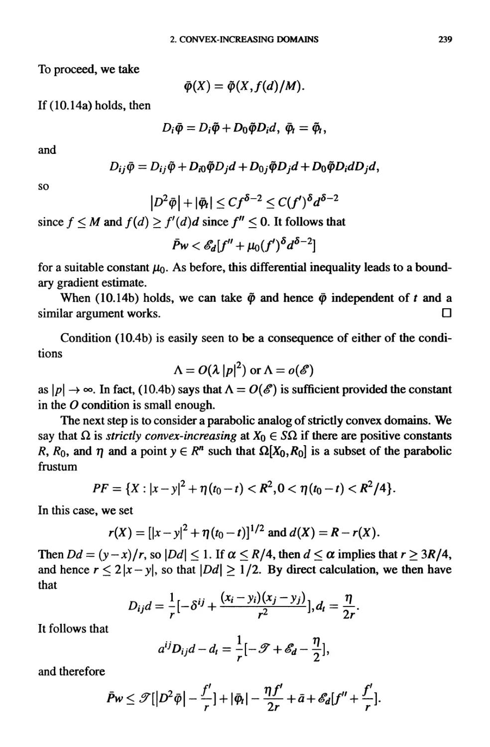
2. Convex-increasing domains 238
3. The spatial distance function 241
4. Curvature conditions 243
5. Nonexistence results 248
6. The case of one space dimension 253
7. Continuity estimates 254
Notes 254
Exercises 257
Chapter XI. GLOBAL AND LOCAL GRADIENT BOUNDS 259
Introduction 259
1. Global gradient bounds for general equations 259
2. Examples 264
3. Local gradient bounds 266
4. The Sobolev theorem of Michael and Simon 271

xii CONTENTS
5. Estimates for equations in divergence form 275
6. The case of one space dimension 289
7. A gradient bound for an intermediate situation 292
Notes 295
Exercises 297
Chapter XII. HOLDER GRADIENT ESTIMATES AND EXISTENCE
THEOREMS 301
Introduction 301
1. Interior estimates for equations in divergence form 301
2. Equations in one space dimension 302
3. Interior estimates for equations in general form 303
4. Boundary estimates 305
5. Improved results for nondivergence equations 309
6. Selected existence results 313
Notes 318
Exercises 320
Chapter XIII. THE OBLIQUE DERIVATIVE PROBLEM FOR
QUASILINEAR PARABOLIC EQUATIONS 321
Introduction 321
1. Maximum estimates 322
2. Gradient estimates for the conormal problem 326
3. Gradient bounds for uniformly parabolic problems in general form 341
4. The Holder gradient estimate for the conormal problem 346
5. Nonlinear boundary conditions with linear equations 347
6. The Holder gradient estimate for quasilinear equations 351
7. Existence theorems 355
Notes 357
Exercises 359
Chapter XIV. FULLY NONLINEAR EQUATIONS I. INTRODUCTION 361
Introduction 361
1. Comparison and maximum principles 363
2. Simple uniformly parabolic equations 365
3. Higher regularity of solutions 371
4. The Cauchy-Dirichlet problem 372
5. Boundary second derivative estimates 375
6. The oblique derivative problem 378
7. The case of one space dimension 381
Notes 382
Exercises
384

CONTENTS
Chapter XV. FULLY NONLINEAR EQUATIONS II. HESSIAN
EQUATIONS
Introduction
1. General results for Hessian equations
2. Estimates on solutions
3. Existence of solutions
4. Properties of symmetric polynomials
5. The parabolic analog of the Monge-Ampere equation
Notes
Exercises
Bibliography
385
385
386
388
400
401
407
414
420
421
Index
445

CHAPTER I
INTRODUCTION
1. Outline of this book
In Chapter II, we prove maximum principles for general, linear parabolic
operators:
Pu= —ut+ alJDtjU + blD[U + cu,
where we use the summation convention and notation discussed in Section 1.3.
Under weak hypotheses on the coefficients of this operator (specifically, that the
matrix (alj) be positive semidefinite and that c be bounded from above), the
inequalities Pu > 0 in Q. and u < 0 on ???l (the parabolic boundary of Q.) imply
that u < 0 in Q.. Nirenberg's strong maximum principle implies that either u < 0
or « e 0 on a suitable subset of ?1 provided the conditions on the coefficients
are strengthened only slightly. Also, maximum estimates for solutions of various
initial-boundary value problems are examined.
Chapter III introduces the notion of weak solution for the problem
-ut+ Di(aljDju) = / in &,u = (p on ?*&
when a1-* is a constant, positive definite matrix and / and (p are sufficiently smooth.
Unlike most discussions of this problem, we deal with noncylindrical domains
directly. In particular, we show that this problem is solvable in sufficiently small
space-time balls. General properties of weak solutions and weak derivatives are
studied also. From the theory in balls, we derive an existence theorem in a wide
class of domains via a version of the Perron process.
The key to our study of linear equations is the Schauder-type estimates in
Chapter IV. These estimates relate the norms of solutions of initial-boundary
value problems for these equations to the norms of the known quantities in the
problems. Specifically, the norms are parabolic Holder norms, which can be
considered as bounds on fractional derivatives of the functions. The main estimates
were first proved by Barrar [13,14] and Friedman [87,88] using a representation
formula for solutions of the inhomogeneous heat equation. Our proof is based on
Campanato's approach [41] and does not use any representation formulae, but it
does need the existence result of Chapter III. The estimates of Chapter IV are
used in Chapter V to prove the existence, uniqueness, and regularity of solutions
l

2
I. INTRODUCTION
for various initial-boundary value problems under several different hypotheses on
the regularity of the data.
Chapter VI contains a further investigation of weak solutions. The class of
equations involved is much larger than that considered in Chapter III and the
definition of weak solution must be appropriately expanded. The first part of the
chapter is concerned with existence, uniqueness, and regularity questions for weak
solutions in suitable spaces. The second part covers the pointwise properties of
weak solutions, in particular the (Holder) continuity of these solutions. These
properties are proved via estimates of the solutions in terms of weak information
on the data of the problem; such estimates are an important part of our study of
nonlinear equations.
Our study of linear equations is completed in Chapter VII, which is devoted
to strong solutions of parabolic equations. These are functions having weak
derivatives in LP for some p > 1 and satisfying the equation only almost everywhere.
We obtain Schauder-type estimates in Lp and pointwise estimates for strong
solutions which are analogous to the estimates in Chapter VI for weak solutions. We
also prove a boundary Holder estimate for the normal derivative of a solution of
the Cauchy-Dirichlet problem in terms of pointwise estimates of the coefficients
of the equation. This estimate, originally proved by Krylov [170], is an important
element in the nonlinear theory.
We begin our study of nonlinear equations in Chapter VIII, which introduces
two fixed point theorems. The first one, due to Schauder [287], is an infinite
dimensional version of the Brouwer fixed point theorem in W1 and is useful for
studying the Cauchy-Dirichlet problem for quasilinear equations. The second
method, due to Lieberman [202,206], is a variant of a fixed point theorem of
Kirk and Caristi [158] related to the contraction mapping principle and is useful
for studying nonlinear oblique derivative problems with quasilinear equations and
fully nonlinear equations (with either Cauchy-Dirichlet data or oblique derivative
data). Our point of view on existence is generally to prove local existence first
(that is, existence for a small time interval) and then global existence. Such an
approach is especially important in blow-up theory. Local existence is often proved
using relatively simple a priori estimates, but these estimates are the key to the
global existence theory. The Cauchy-Dirichlet problem and the oblique derivative
problem are considered separately.
The a priori estimates for the Cauchy-Dirichlet problem fall naturally into
four basic types:
A) the maximum of the absolute value of the solution,
B) the maximum of the length of the gradient on the parabolic boundary,
C) the maximum of the length of the gradient in the domain,
D) a Holder norm for the gradient.

1. OUTLINE OF THIS BOOK
3
These estimates are the topics of Chapters IX, X, XI, and XII, respectively, and
each presupposes the preceding ones.
Chapter IX applies the maximum principle of Chapter II and the maximum
estimates of Chapter VI to get pointwise bounds on the solution. In this chapter,
we also generate some comparison principles which are important for other, later
estimates.
Chapter X is devoted to a boundary gradient bound, which turns out to be the
key estimate in the existence theory. We develop parabolic analogs of the Serrin
curvature conditions for elliptic equations [290], which relate the geometry of the
boundary to the structure of the differential equation. As in [290], we also show
that these conditions are necessary to solve the problem with arbitrary data. All
results are based on the comparison principle.
The gradient estimate is the topic of Chapter XI. The basis for proving such
an estimate goes back to Bernstein [17]: show that the square of the length of the
gradient of the solution satisfies a suitable differential inequality. Unlike Chapters
IX and X, this chapter uses quite detailed structure conditions, and often a change
of dependent variable is useful.
Chapter XII applies the Holder estimates of Chapters VI and VII to the
gradient of the solution. Assuming that a bound is known for the gradient of the
solution, we prove the Holder estimates under very weak assumptions on the equation
in question. The chapter finishes with some examples which illustrate the various
structure conditions.
The oblique derivative problem is examined in Chapter XHI. Since the
techniques are so similar to those for the Cauchy-Dirichlet problem, many proofs in
this chapter are sketched or omitted. An interesting feature of our study of the
oblique derivative problem is that we are not restricted to the conormal problem.
For example, with the heat equation — ut + Am = /(X), we may use the capillarity
boundary condition A -f \Du\2)l/2Du • y+ y(X) = 0, where Du denotes the
gradient of u and y is the interior spatial normal. If /, iff and the domain are smooth
enough, we shall show that this problem has a solution for any smooth enough
initial data (satisfying a certain compatibility condition) provided iff satisfies the
necessary condition for a smooth solution: |^| < 1-
In Chapter XIV, we consider a simple class of fully nonlinear equations,
modeled on the parabolic Bellman equation:
-*+ mf{? dj{X)Diju} = 0,
where (alJ) is a uniformly bounded, uniformly smooth family of uniformly
positive definite matrices. Such equations were first studied systematically by Evans
and Lenhart [79] and Krylov [169,170]. The hypotheses of these authors are
successfully weakened here by using simplifications due to Safonov [282,284].

4
I. INTRODUCTION
Finally, Chapter XV looks at a class of nonuniformly parabolic fully
nonlinear equations, modeled on the parabolic Monge-Ampere equation:
-utdetD2u = y/(X,w,Dw).
Elliptic versions of this equation and its generalizations were first studied by Caf-
farelli, Nirenberg, and Spruck [33-35] and Ivochkina [122-127]. Based on their
work, we prove estimates and existence results for the parabolic equations. Our
choice of parabolic Monge-Ampere equation was first identified by Krylov [167]
as a suitable parabolic version of the equation detD2w = y, and the corresponding
generalizations were recognized by Reye [281] as worthy of study. Other
parabolic Monge-Ampere equations and their generalizations are discussed briefly.
The most noteworthy is that of Ivochkina and Ladyzhenskaya:
-ut + (detD2u)l/n = \j/.
This equation and its variants are studied in [47,130,131,133,134,242,338].
2. Further remarks
Although the notes in this book may seem quite extensive, we have really
only scratched the surface of the subject of parabolic equations. An examination
of any recent issue of Mathematical Reviews shows several dozen articles each
month. Even restricting attention to single, nondegenerate equations of second
order (as we have here) leaves a staggering number of articles to read and
assimilate. A complete bibliography would be much longer than this book and it would
be obsolete before it appeared in print. Alternative sources of material which is
directly relevant to the issues raised here are [68,115,172,183,193,271,276,278].
There are also a number of subjects not covered in this book. Some of them
are systems of parabolic equations and equations of higher order (see [4,183]),
degenerate equations ([63]), and probabilistic aspects of parabolic equations ([69,
172]).
In an effort to keep this book at a manageable size, I have given a single point
of view for most topics; for example, the Schauder estimates of Chapter IV are
proved using the Campanato method, which reappears in the nonlinear theory
(although an alternative proof could be given using methods developed in Chapter
XIV). Many other proofs of these estimates are known; in fact, an entire book
could be written just on the various means of proving them. Similarly, we have
emphasized Moser iteration to prove most estimates for weak solutions; deGiorgi
iteration is also an appropriate and frequently used technique, but it appears only
briefly in Section VI. 13. As a result of this single point of view, experts will
certainly find a favorite technique missing. For example, I have avoided use of
representation of solutions via Green's function and its cousin, potential
representations. In addition, the method of viscosity solutions does not appear here.

3. NOTATION
5
3. Notation
In this book, we adopt the following conventions. First we use X = (x,t) to
denote a point in En+1 with n > 1; x will always be a point in Rn. We also write
Y = (y,s). Superscripts will be used to denote coordinates, so x — (jc1,. ••¦*")•
Norms on En and Rn+l are given by
f(x02J and\X\=max{\x\Ml/2}>
respectively. A basic set of interest to us is the cylinder
Q(X0,R) = Q(R) = {Xe En+1 : \X-X0\ < R,t < to).
We also use the ball
B(x0,R) = {x?Rn: \x-x0\ < R}.
We generally follow tensor notation. As previously indicated, superscripts
denote coordinates of points in Rn. Also, subscripts denote differentiation with
respect to x. In particular,
du d2u
DiU=^-rDuu:
dx1' lJ d*dxJ
for u a sufficiently smooth function and i and j integers between 1 and n, inclusive.
We also write Du for the vector (D\ w,..., Dnu) and D2u for the matrix (Dtju). On
the other hand, we write ut (or occasionally Dtu) for du/dt. In addition, we follow
the summation convention that any term with a repeated index i is summed over
i = 1 to n. For example,
n
biDiu=Y*biDiu'
i=\
To be formally correct, we should demand (as was the case in this example) that
one occurrence of the index be a superscript and the other be a subscript, but we
shall abuse this aspect of the summation convention when convenient.
A word of warning about superscripts and subscripts is also in order. Both
will be used as generic indices and to indicate differentiation with respect to other
variables. In addition, superscripts will also be used to indicate exponentiation. It
should be clear from the context which meaning is intended.
We use Q, to denote a bounded domain in En+1, that is, ?1 is an open connected
subset of Rn+l, so for any Xo G ?2, there is a positive number/? such that the space-
time ball {X : |jc - jco| +(t — toJ < R2} is a subset of Q.. For a fixed number /o,
we write Ob (to) for the set of all points (.Mo) in ?1, and we define y(Xo) to be the
unit inner normal to CO (to) at Xo provided co(to) is not empty. We also write I(?l)
for the set of all t such that co(t) is nonempty. Since ?1 is connected, I(?l) will
be an open interval. As usual, d?l denotes the topological boundary of ?1. The
parabolic boundary g*?l will be defined in Chapter II.

6
I. INTRODUCTION
We also use |ft| to denote the Lebesgue measure of the set ft, and we define
diamft = supfljc — y\ : X,Y in ft}, so diamft is not the usual diameter of a set.
When ft is a cylinder ft = (O x (a,&), then diamft is the usual diameter of the
cross-section fi), but if ft is noncylindiical, diamft may be strictly larger than the
diameter of any cross-section G)(t).

CHAPTER II
MAXIMUM PRINCIPLES
Introduction
An important tool in the theory of second order parabolic equations is the
maximum principle, which asserts that the maximum of a solution to a
homogeneous linear parabolic equation in a domain must occur on the boundary of that
domain. In fact, this maximum must occur on a special subset of the
boundary, called the parabolic boundary. The strong maximum principle asserts that
the solution is constant (at least in a suitable subdomain) if the maximum occurs
anywhere other than on the parabolic boundary. The maximum principle is used
to prove uniqueness results for various boundary value problems, L°° bounds for
solutions and their derivatives, and various continuity estimates as well.
1. The weak maximum principle
As noted in Chapter I, we consider linear operators L defined by
Lu = aij{X)Duu + bi(X)Diu 4- c(X)u - ut B.1)
in an (n + 1)-dimensional domain SI. We assume that L is weakly parabolic. In
other words,
cfj(X)&Sj > 0 for all § e M" and all XeSl. B.2)
We also write & for ?0", the trace of the matrix (a'i).
For a domain SI C Rn+1, we define the parabolic boundary &SI to be the
set of all points Xq ? dSl such that for any e > 0, the cylinder Q(Xo,?) contains
points not in SI. In the special case that SI = D x @,T) for some Del" and
T > 0, ??Sl is the union of the sets BSi-Dx {0} (which is the bottom of SI),
SSI = dDx @, T) (which is the side of SI), and CS1 = dDx {0} (which is the
corner of SI). These sets (and their analogs for more general domains) will play
an important role in the theory of initial-boundary value problems.
The simplest version of the maximum principle is the following.
Lemma2.1. Ifu€C2>l(Sl\^Sl)nC°{Sl), ifLu>0inft\@>Slandif u <0
on &SI, then u<0in SI.
PROOF. Suppose, to the contrary, that u > 0 somewhere in SI. Let t* = inf{r:
u(x,t) > 0 for some X E SI}. By continuity and the assumption that u < 0 on
7

8
II. MAXIMUM PRINCIPLES
&>?ly there is X* = (**,**) e(i\« such that u(X*) = 0. Since w(-,f*)
attains its maximum at jc*, we have Du(X*) = 0, and hence Lu(X*) = -ut(X*) +
fl'->(X*)D,7w(X*). Since we also have u,(X*) > 0 and D2u(X*) < 0, it follows that
Lu(X*) < 0, contradicting Lu > 0. Therefore u < 0 in Q.. D
Since oblique derivative boundary conditions will play an important role in
this book, we formulate a further version of this maximum principle which also
pertains to oblique derivative boundary conditions. For Xo G ???l, we say that an
(n + l)-vector J3 points into ?1 if j3n+1 < 0 and there is a positive constant ? such
that Xo + h/5 G ?1 if 0 < h < e. For such a /?, if the function u is continuous at Xo
and k is a constant, we say that J3 • du(Xo) <kif
r M(X0 + /i/3)-w(X0) ^7
hmsup — ^ —- < k,
and/J-<?w(X0)>A:if
limiafu(Xo + hP)-u(Xo)>
h-+o+ h ~
where we write du for the full space-time gradient (Du,ut) of u. Since these
inequalities are just the appropriate inequalities on the directional derivates of u
at Xo, it follows that J3 • dw(Xo) = k if and only if the corresponding directional
derivative du/dfl exists and is equal to k at Xo. Analogous to our operator L is the
boundary operator M defined by
Mu = p-du + l50u B.3)
for some vector field J3 such that j3(Xo) points into Q, at Xo for each Xo G &&
and scalar function j3°. Inequalities on Mu are defined in the obvious way. In
particular, we have u < 0 is equivalent to Mu > 0 if we choose j3 = 0 and /3° = -1.
With these conventions, we have the following extension of Lemma 2.1.
Lemma 2.2. If u e C2'l(Q.\ @>Cl) nC°(Q), ifLu>0 in Q.\0>Q. and if
Mu>0on &Q., then u<0in ?l.
PROOF. This time, we note that if X* G <^ft, then Mu(X*) < 0. ?
With a little more structure on the coefficients of L and M, we can relax the
smoothness hypotheses on u.
Lemma 2.3. Suppose that there is a positive constant k such that
c<kin?l B.4a)
J3° < 0 on &?l. B.4b)
Ifu G C2'1 (ft) D C°(S), */Lm > 0 m ?1 and ifMu >0on &?l, then u<0in ?1.

1. THE WEAK MAXIMUM PRINCIPLE
9
PROOF. Set v = e^k+l^u, so that Lv = <H*+1)'Lw+ (jfc+ l)v > (jfc + l)v and
Mv = e-^+V'Mu - (*+ l)j3n+1v > -(Jt + l)j3n+1v. If v has a positive maximum
atsomeXG &Q.,thenMv(X) < j3°(X)v(X) <0<
-(/:+l)j3,I+1(^)v(X),contradicting our boundary condition for v. If v has a positive maximum at some X G ?1,
then v,(X) = 0,Dv(X) = 0, D2v(X) isnonpositivedefinite, andc(X)v(X) < kv(X),
so Lv(X) < kv(X) < (k+ l)v(X). Hence v cannot have a positive maximum in ?1.
It follows that if v has a positive maximum, it must occur on d?l \ {P?l, say
at Xo. In this case, set t% — t§ — 1//, ?l( = {X € ?1: t < f,-}, and M, = supa. v.
If i is sufficiently large so that ?li is non-empty and M/ > 0, choose jc; so that
v(Xj) — Mi, noting from the first case that v cannot have a positive maximum in
?li U ?*?li. Then v(X;) -> v(Xo), so there is a convergent subsequence (X^)) and
v(XI-(y-)) -» v(Xo) as y -» oo. Using X* to denote the limit of the sequence (X;(y)),
we have v(X*) = v(Xo), so X* G d?l\ &?l. But then, there is a positive € such
that Q(X*,e) c ?2 and hence there is an integer j such that v(X,(y)) = M^ with
X/(;) G Q(X*,e). We then have v,(X/G)) > 0, Dv(Xi(j)) = 0, D2v(X/W) is
nonpositive definite, and cv(X^) < fcv(X,(;)). As before, these conditions show that the
restriction of v to ?1^ cannot attain a positive maximum at X^. Therefore v < 0,
and hence u < 0 in ?1. ?
More generally, we can get an upper bound on u over ?1 from a lower bound
on Mu just over ^?1.
THEOREM 2.4. Suppose u G C2'1^) nC°(iQ) for some ?1 with t>0in ?1,
and suppose conditions B.2) and B.4) hold. IfLu >0in?l and ifMu > J3°4> on
^?1 for some nonnegative constant®, then u(X) < e^® for all X G ?1.
Proof. Set v = u — eh® and apply Lemma 2.3 to v, noting that eh > 1 on
&>?l. D
Crucial tools in the remainder of this book are the following comparison
principle and uniqueness result.
COROLLARY 2.5. Suppose u and v are in C2>l(?l) CiC°(?l) and conditions
B.4a,b) hold. IfLu > Lv in ?1 and ifMu > Mv on &>?l, then u<v in ?1. If
Lu = Lv in ?1, and ifMu = Mv on 3*?l, then u = v in ?1.
PROOF. The inequality follows by applying Lemma 2.3 to u — v, and the
equality is then clear. ?
By taking j3 = 0 and J3° = -1, we have that Lu > (=)Lv in ?1 and u < (=)v
on ???l implies u < (=)v in ?1.
As we shall see in the next section, determining the set of points at which
u can attain a nonnegative maximum is quite delicate. Related to this issue is
the question of continuous attainment of boundary values for solutions of various
boundary value problems. We shall address this issue further in the next chapter.

10
II. MAXIMUM PRINCIPLES
2. The strong maximum principle
For most applications to the first initial-boundary value problem (in which the
values of the solution are prescribed on the parabolic boundary of the domain), the
weak maximum principle from Theorem 2.4 (with j3 = 0 and J3° = -1) suffices;
however, it is often useful to know that the maximum can't occur inside ?1 unless
the solution is constant on a suitable set. We shall prove this result via an a priori
estimate that plays a critical role in our discussion of the weak Harnack inequality
from Section VII. 10.
Lemma 2.6. Let a andR be positive constants and set
Q = {Xe En+1 : |jc| < R, -aR2 < t < 0}. B.5)
Suppose there are positive constants A, A, Ai, and A2 such that
aij^j > A |§ |2 for all ^f, B.6a)
ST < A, B.6b)
|*|<Ai, B.6c)
\c\ < A2 B.6d)
in Q, and suppose that Lu<0 and u>0in Q. Let h and e be positive constants
with e < 1, and suppose that
u>hon {\x\ < ?R,t = -aR2}. B.7)
Then there is a positive constant K, determined only by a, A, A, andA\R + A2R2,
such that
u > ?K- on {\x\ < R/2,t = 0}. B.8)
Proof. Set
(I — pi)
Vo- g J{t + aR2) + e2R2, v^i=max{v/0-W2,0},
and y = \l/2%q for some q > 2 to be chosen. Then y G C2'1 (Q) for
Q={Xe Mw+1 : \x\2 < Wi-ccR2 <t<0},
and
in Q. Now we set
Fi = - + 8A + 4AH-4Ai/?-f A2R2
a
and E, = 1/^1 /yb- Noting that 0 < y/b < R2 and 0 < e < 1, we see that
Lxi/>xi/l0-q[{l~?2)q^2-F^ + S?i}.

2. THE STRONG MAXIMUM PRINCIPLE 11
By choosing
we see that Ly > 0 in Q.
Now we note that
y(jc, -aR2) = (e2R2 - \x\2J{e2R2)-q < (eR)~2^4 B.9)
if (jc, -aR2) G 3?Q. Now set v = h(eRJ(*-*y. Since y(X) = 0 if X G ^2 and
t > -aR2, we infer from B.7) and B.9) that v < w on ^Q. Applying Corollary
2.5 then yields v <u'mQ and hence
k(jc,0) > h{sRJq-4xif > ^?2q~4 B.10)
for |jc| < R/2 because
\f/(Xj0) = (R2 - \x\2JR~2q > ^-R~2^4 B.11)
16
if |jc| < R/2. For K = 2q - 4, B.10) easily implies B.8). ?
We are now ready to state and prove the strong maximum principle. For
Xo G Q., we define S(Xo) to be the set of all X\ G ?1 \ <^^ such that there is a
continuous function g: [0,1] -+ ?1\ ???l such that g@) = Xq, g(l) — X\ and the
f-component of g is nonincreasing.
Theorem 2.7. Suppose conditions B.6a-d) hold in ?1 and c < 0 in ?1. If
Lu>0 in ?1 and u(Xo) = max^w > Ofor some Xo G ?1 \ &?l, then u = u(Xq) in
S(Xo).
PROOF. Set M = max^w. As a first step, we show that, if Y G ?1 \ &?l, if r
is chosen so that Q(Y, 3r) C ?1, and if there is a Y\ G 2G, r) such that mGi ) < M,
then «(y) < M. to prove this implication, we assume without loss of generality
that v = 0 and s = 0. Then we set R = 2r,a = -s\/R2, zndh=(M- u(Y\))/2.
Because u is continuous, there is a constant e G @,1) such that A/ — u(X) >hif
\x\ < eR and t = -aR2. Then Lemma 2.6 applied to M — u gives M — w(y) >
?K/i/2 and hence u(Y) < M.
We now prove the contrapositive of this theorem. In other words, we show
that if u(X\) < M for some X\ G S(Xq), then u(X0) < M. To this end, we let g be
the function in the definition of S(Xo) and we define
S = {a e [0,1] :u(g(o))<M}.
Our goal is to show that S = [0,1]. Clearly, 5 is a relatively open subset of [0,1]
which is non-empty. Hence, we only have to show that S is closed, so let <7o G S.
Then there is a positive constant r so that <2(g(obM3r) C ?1 and also there is a
point 7 G So \ ??Qo such that u(Y) < Af, where Qo — Q(g(oo),r). Since w is
continuous, there is a point Y e Qo with «(yb) < M, and, from the first part of

12
II. MAXIMUM PRINCIPLES
the proof of this theorem, we infer that u(g(oo)) < M. Hence S is closed and the
contrapositive is proved. ?
Related to the strong maximum principle is the so-called boundary point
lemma, which loosely states that at a boundary maximum of a non-constant
solution, the inner normal derivative must be strictly negative. In fact, the geometry of
the domain near a boundary maximum also plays a role.
LEMMA 2.8. Suppose there are positive constants tj, A, A, Ai, A2, and R
such that conditions B.6a-d) hold in the lower parabolic frustum
PF = PF(R,riJ) = {X :\x-y\2 + T]2(s-t) < R2,t < s} B.12)
for some Y G R"+1. Suppose also that u G C2'1 (PF) with Lu>0 in PF and that
there is X\ = (x\,s) with \x\ — y\ — R such that
u(Xi) > u(X)forallX G PF B.13a)
u(Xi) > u(X)forallXe PF with \x-y\<^, B.13b)
c(X)u(Xx) < 0 for all X G PF. B.13c)
If v = C; - x\)/1y - x\ I and J3 = (v, 0), then ]3 • du(X\) < 0 in the sense defined
in Section II. 1, and u<u(X\) in PF.
PROOF. Setr = r(X) = (|jc-;y|2 + 7]2(.y-f)I/2, define
P={XePF:\x-y\>*},
and note that &>P = Si U52 for S\ = {r = R,t < s} and S2 = {\x - y\ = \R,t < s}.
For a a positive constant to be chosen, we consider the function v = exp(—ar2) -
exp(—aR2). Then a simple calculation shows that
Lv = e-a^[4a2aij(xi-yi)(xj-yj)-a{2& + 2b'{x-y) + 7i2)
+ c{\-e-a(R2-^))
> e~arl [a2XR2 - aBA + 2AXR + tj2) - A2]
in P. We now set
A0=A + Ai/? + A2/?2. B.14)
(This constant will be useful later in this chapter.) Choosing a = g/R2 with g
sufficiently large (depending only on (r\2 + Ao)/A), we can make Lv > 0 in P.
Now u — u(X\) < 0 on S\9 and u — u(X\) < 0 on S2. Hence there is a positive
constant e such that u — u(X\) < — e on S2. Since 0 < v < 1 in P and v = 0 on S\,
it follows that
L(u - u(Xx) + ev) > -cu(Xi) > 0 in P,
u-u(Xi) + ev<0 on&P.

2. THE STRONG MAXIMUM PRINCIPLE
13
The weak maximum principle Lemma 2.3 implies that u - u(X\) < -ev in P9 so
u < u{X\) in P, and then evaluating the directional derivative at Xi yields
P'MX\) < -ev-Dv(Xi) = -2aeexp(-ctr(XiJ/R2)\xi -y\.
Since this last expression is negative, we are done. ?
More generally, we have
i:„..,n(X)-n(*i) ^
hmsuP—TZ ^-|— < °>
as long as t < s and the angle (in Mn+1) between X — Xi and v is bounded above
away from 7r/2. Obviously, the lemma remains true if we assume that Lu > 0 in
?1 and conditions B.13a,b,c) hold with ?1 in place of PF for any domain ?1 such
that PF is a subset of ?1. In fact, the assumption of the existence of an interior
parabolic frustum can be relaxed, but some geometric condition on the domain is
needed. Note that B.13c) follows from any of the three conditions: c = 0 in PF,
u{Xx) = 0, or c < 0 and u{Xx) > 0.
From Lemma 2.8 we can infer uniqueness and comparison theorems for the
oblique derivative problem. To facilitate their statements, we introduce some
further terminology. We say that ?1 satisfies an interior paraboloid condition at Xo
if there is a point Y G Mn+1 and a constant R such that the parabolic frustum
PF defined by B.12) is a subset of ?1 and {X0} = &(PF) D &?l. If ?1
satisfies an interior paraboloid condition at Xo, we say that a vector J5 G Mw+1 points
strongly into ?1 at Xo E &?l if there is a positive ? such that Xo 4- hf} G PF for
all h G @,e). Also, we define B?l to be the set of all points Xo G &?l such that
there is a positive R with Q{(x0,t0 + R2),R) C?l,C?l = (Mfl &?i) \B?l, and
S?l=&>?l\(B?lUC?l).
THEOREM 2.9. Suppose conditions B.6a-d) hold in ?1 and c < 0 in ?1, and
suppose that ?1 satisfies an interior paraboloid condition at each point of SSI.
Suppose also that j3 is a vector field such that j3 (Xi) points strongly into SI at X\
for each X\ G S?l and j3° < 0 on S?l. Then if
Lu>Lvin?l B.15a)
Mu>MvonS?l B.15b)
u<vonB?lUC?l, B.15c)
then u < v in ?1. Moreover for any f G C(?l), any \j/ G C(S?1) and any (p G
C(B?l\JC?l), there is at most one solution of the initial-boundary value problem
Lu = fin?l, B.16a)
Mu = y/onS?l, B.16b)
u = (ponB?lUC?l. B.16c)

14
II. MAXIMUM PRINCIPLES
PROOF. To see that u < v in Gl if B.15) holds, we note that u — v can only
attain a positive maximum on SO., say at X\. From Lemma 2.8, M(u — v) < J3°(w -
v) < 0 at X\ while the boundary condition implies that M(u — v) > 0. Hence u < v.
The uniqueness of solutions of B.16) follows immediately from this comparison
principle. ?
In fact, we shall see in Chapter V that Theorem 2.9 is valid also if c and j3° are
only assumed to be bounded from above provided we strengthen the hypotheses
on SO. and M just a little. Of course if c < 0 and J3° < 0, then the conclusion of
Theorem 2.9 follows immediately from Corollary 2.5.
3. A priori estimates
The maximum principle also provides simple pointwise bounds for solutions
of the equation Lu = f in a large variety of domains. Because so little information
about the coefficients is used, these estimates are very useful in studying nonlinear
equations. For simplicity, we write a+ = max{a,0} and a~ = max{— a,0} for any
real number (or real-valued function) a.
THEOREM 2.10. Suppose conditions B.2) and B.4a) are satisfied in some
domain ?1 such that I(?l) C @, T) for some T > 0, and suppose that u G C°(&) fl
C2'1 (a). IfLu > f in Q, then
supw < e(*+1)r(supM+ + sup/-). B.17)
If Lu = f in ?1, then
sup|M|<^+1)r(sup |m| + sup|/|). B.18)
PROOF. Suppose first that Lu > f, and set v = exp((& 4- l)r) and
F = (supu+ + sup/-).
Because
Lv = -(*+ 1)*(*+1>' + ce<*+1>' < -1
in Q, it follows that
L(u -Fv)>- sup/" + F > 0 in ft,
m - Fv < supn+ - F < 0 on «^ft,
so the maximum principle implies that u — Fv < 0 in CI. Hence B.17) is proved.
If Lu = /, we prove B.18) by applying B.17) to u and — u. D
As an alternative to Theorem 2.10, we can give an estimate for u which is
independent of T if c < 0.

3. A PRIORI ESTIMATES
15
THEOREM 2.11. Suppose conditions B.6a,c) hold, suppose c<Oinft and
suppose there is a positive constant R such that \x\ < Rfor any XEfi. If Lu > /,
then
supw < supw+ + C(Ai/A,/?)sup(/~/A). B.19)
IfLu = /, then
sup|w| < sup|w| + C(Ai/A,fl)sup(|/|/A). B.20)
Proof. Set v = e2aR - ea^+R) for a = 1 + Ai/A. Then
Lv = -(aV1 + abl)ea^^ + cv < -a(aA - Ai) < -A
in ?1 Hence, for F = sup(/~/A), we have L(u — sup^n w+ — Fv) >0'mCl and
w - sup^ft «+ - Fv < 0 on «^&. The maximum principle then implies B.19), and
B.20) is proved in a similar fashion. D
It is also possible to prove various modulus of continuity estimates for
solutions of linear equations. Here we give two simple examples which will prove
useful in later chapters.
THEOREM 2.12. Suppose conditions B.6a-d) are satisfied in a domain Q let
Xo € t??l and suppose there is a parabolic frustum PF of the form B.12) with r\ =
1 for some Y e En+1 andR >0such that?FnQ.= {X0}. //wG^^nC2'1^)
15 a solution ofLu = / inQ., u = q>on &?lfor some <p € C2>1 (Q.) and f G C°(&),
then there is a constant K determined only by A, A, Ai, A2, «, andR such that
\u{X)-u(Xo)\<Kexp((k+l)t0)(F + <P)\X-X0\ B.21)
for anyX eQ. with t = t0, where F = sup|/| and ® = sup\D2<p\ + \<pt\ + \Dq>\ +
|9|.
PROOF. Define r by r2 = \x - y\2 + (t0 - r), define v by
v(*,f) = cxp(-aR2) - exp(-ar2) + 4(f0 - t)/R2,
for a a positive constant to be chosen, and set Q* = ?1 C\ {to — R2 < t < to}. From
the same calculation as in the proof of Lemma 2.8, we see that Lv < — 1 in ?1* if
a = g/R2 with g taken sufficiently large, determined by Ao/A, n.
Next, we observe that Lq> < K\<P in ?2* for some constant K\ determined by
A, Ai, A2, and n, and we set F\ = exp((fc + 1 )t0)[F + A 4- KxL>]. It follows that
L(u-q>-Fiv)>0'mQ.*.
Now on Q. fi {t = ro — R2}, we have v > 4, and Theorem 2.10 implies that u < F\,
so that
u-<p-Fiv<0on&Q*.

16
II. MAXIMUM PRINCIPLES
The maximum principle now implies that u — (p < F\ v on ?lo = ^ f) {t — to}, and
a similar argument gives u — q>> -F\v on ?2o- Hence, for X = (;t,fo) ? ^o with
|jc — jco | <R, we have
\u(X) - u(X0)\ = \u(X) - <p(Xo)\ < \u(X) - (p(X)\ + \<p(X) - cp(X0)\
<®\x-xo\+Fiv(x,t0)
< ( 4> + sup Fi |Dv(x, t0)| J |jc - x0\
\ \x-xo\<R J
<{® + 4F1aR)\x-x0\.
On the other hand, if X 6 &o and |jc — jc0| > R, then \u(X)-u(X0)\ < 2F\ <
2(Fi/R) |jc —jcoI- Therefore B.21) holds with K = 1 +4aKiR+B/R). D
In fact the proof of Theorem 2.12 shows that B.21) holds as long as X = (x,t)
with t < to, and it is possible to prove B.21) for t > to as well. (See Theorem
3.26.) It will be more useful, though, to use this theorem in its present form,
which implies an estimate for \Du(Xo)\ (if this derivative exists). We shall see in
later chapters that an interior modulus of continuity estimate is also valid, but this
result is much deeper. On the other hand, given an interior modulus of continuity
estimate with respect to jc, the following maximum principle argument of Gilding
provides an interior modulus of continuity estimate with respect to t.
THEOREM 2.13. Suppose conditions B.2) and B.6b,c) hold in
R2
Q = {\x-x0\ <R}x (n,fi + —), B.22)
4Ao
with c = 0 in Q and Ao = A 4- h\R, for some point (jco,fi) G Ew+1 and some
positive constant R, and let u€C2,1 (Q) solve Lu — f in Q. If there is a constant
CO such that
\u{x,t) - u{xo,t)\ <@ B.23)
for all xeW1 with \x - jco| < R, then
2R2
\u(xo,t) -u(xo,ti)\ < 2(D+ —-sup|/|. B.24)
A0 q
Proof. Set
5= sup \u(xo,t) - u(xo,t\)\
/1</</!+/?2/DAo)
and define
v± = (sup\f\^^)(t-tl) + ^\x^xo\2-h@±{u-u(xo,h))-

3. A PRIORI ESTIMATES
17
A simple calculation shows that
Lyt = -svp\f\-^$r + jpf + jpb-{x-xo)±f<0
in Q while
v±>-jp\x-x0\2 + CQ±(u-u(x0A))
on @>Q. We have v±(x,t\) > (D±{u{x,t\) - u(xo,t\)) > 0 by B.23), and, if
\x — jco| =R, we have
v±(x,t) >s + (Q±(u(X) - u(x0,ti))
= s + co±(u(X) - u(xo,t)) ± (w(;co,r) - u(xo,t\)) > 0.
It follows that v± > 0 on @>Q. We now apply the maximum principle to v± on
Q to see that v± > 0 on Q. Evaluating this inequality at x — xq and taking the
supremum over all t gives
irl 2sA(k R2
^<(sup|/| + ^/)—-fco,
and a simple rearrangement of this inequality yields B.24). ?
Theorem 2.13 is easily extended to cylinders of arbitrary heights and to
operators with c ^ 0.
COROLLARY 2.14. Suppose, in Theorem 2.13, that c ^ 0 and that
Q = {\x-x0\ < R} x (tut\ +hR2) B.25)
for some positive constant h. Then
R2
\u(x0,t)-u(x0A)\ < B + 4AAo)(fi)+ —sup[H + |/|]). B.26)
A0 Q
Proof. Define Lo by Lou = Lu — cu. Then u satisfies the hypotheses of
the corollary with c = 0 and / replaced by / — cm. Hence it suffices to prove the
result with c = 0. In this case, if h < l/DAo), the proof of Theorem 2.13 gives the
desired result. Otherwise, we partition the cylinder into k subcylinders of the form
Qi; = {\x - xq I < R} x (t(, f,-+1) with i = 1,..., k for k the smallest integer greater
than or equal to /*Ao. Applying Theorem 2.13 in each cylinder and summing the
resulting inequalities gives B.26). ?
Typically, Corollary 2.14 is applied to a problem in which a modulus of
continuity with respect to x is known. In particular, suppose that a gradient bound is
known, that is, \Du\ < K in some cylinder {|jc — x$\ < p} x (t\,t\ + hp2) for some
positive h and p. If t2 G (t\,t\ +hp2), then we take R = [{t2~h)/h]l/2 to see that
|w(^,fe)-«(^^i)|<CB*: + sup|/|)|r2-ri|1/2. B.27)

18
n. MAXIMUM PRINCIPLES
In other words, u is Holder continuous with exponent \ with respect to t. We
shall use a more sophisticated version of this estimate in later chapters. Two
improvements are that we consider also behavior near the parabolic boundary and
that we shall use an integrated form of our equation and estimates.
Notes
One of the most important differences between our discussion of the weak
maximum principle and the usual ones (see, for example, [89, Chapter 2] or
[193, Section 3.2]) is that we only assume u to be a solution of the equation in
CI. Generally, authors assume u to be a solution in CI \ &CI, which allows some
simplifications of the arguments. In addition, for linear equations with smooth
coefficients, a solution of the equation in CI is also a solution in the larger set (see
Chapters IV and V), but many applications are easier with the stronger version of
the maximum principle proved here.
The strong maximum principle for parabolic equations is due to Nirenberg
[270], who adapted the proof of Hopf's strong maximum principle for elliptic
equations. Our approach to the strong maximum principle is based on [235,
Corollary 7.3], which is quite different from Nirenberg's or the one in [115]. Lemma
2.6 is due to Krylov and Safonov [180, Lemma 1.3], but the application to the
strong maximum principle first appears in [235]. The ideas in the proof also apply
to oblique derivative problems (see [235] and also Exercise 2.8).
Theorem 2.13 is taken from Gilding's paper [102], which is based on earlier
work of Kruzhkov [164]. Our statement is slightly different, but the proof is the
same.
Further discussion of the maximum principle can be found in the book of
Protter and Weinberger [278, Chapter 3].
Exercises
2.1 Show that if (a'J) is a nonnegative definite matrix and (fe,-y) is a nonpos-
itive definite matrix, then the sum aljbjj is nonpositive.
2.2 Let ?1 be a bounded domain in En+1 and let a be a relatively open subset
of SCI. Prove that the problem
Lu = / in Cl,Mu = \jf on o,u = <p on &CI \ a
has at most one solution provided c < 0, j3° < 0, CI satisfies an interior
paraboloid condition at every point of a, and J8 points strongly into CI
at every point of a.
23 (Degenerate parabolic equations) Suppose that L is given by
Lu = -r(X)ut + aij(X)Duu + bi(X)Diu + c(X)u

EXERCISES
19
with r > 0 and (alJ) satisfying
a^(XMj>X(Xm\2.
If also r + A > 0 in ft \ <0*ft and there are constants k and K such that
c <kr and \b\ < KX in ft \ <0*ft, prove that the maximum principle
(Theorem 2.4) is still valid. Also prove analogs of Theorems 2.10 and
2.11 for such an operator.
2.4 State and prove analogs of Theorems 2.10 and 2.11 if the boundary
condition is given in terms of Mw rather than u.
2.5 (Integro-differential equations I) Let ft C Rn+1, let (?,./#, 7r) be a o-
finite measure space, and let j: ft x Z -> Rn \ {0} and 71 : ft x E -» E be
functions such that X + j(X,%) G ?2 for any (X,§) G ft x I and 71 > 0.
Define the integral operator J by
jrM(x) = jT[ii^ + ^,§),0-«W]7i(X,§)^ B.28)
Suppose also that L and M satisfy B.2) and B.4). Show that if u G
C2'1 (ft) fl C(ft) satisfies Lu + J^w > 0 in ft, Mm > 0 on ^ft, then w < 0
in ft. Show also that if Lu + Ju — f in ft, Mu = \\f on ^ft, then
\u\ < C(sup l/l -f sup I y\) in ft. (Hint: Imitate the proof of Lemma 2.3,
noting that Ju < 0 at a maximum point. See [95].)
2.6 (Integro-differential equations II) Let a be a bounded function on ft and
define J by
Ju(X) = / u(x,t)g(x,t) dx. B.29)
If L and M satisfy B.2) and B.4) and u G C2'1 (ft) flC(ft) satisfies Lu +
Ju > 0 in ft, Mu > 0 on ^*ft, then w < 0 in ft. Show also that if
Lu + Ju — f in ft, Mm = \f/ on ^ft, then |w| < C(sup |/| + sup 1y/|) in
ft. (Hint: Use Exercise 2.5 and Gronwall's inequality.)
2.7 Show that Lemma 2.8 is true if the lower parabolic frustum is replaced
by a region of the form {|*-;y|1+a + r\2(s -1) < Rl+a,t < s}. (See
[150,208].)
2.8 (Oblique derivative problems in nonsmooth domains [235, Section 7])
We say that ft satisfies an interior parabolic cone condition at Xo G <0*ft
if there are positive constants /?, (Qo, and COo and a unit vector yG W1 such
that every X G Q(Xq,R) such that
Y'{x-xo)<(Oo[\x-xo\2-\r'(x-xo)\2]l/2 + (Oi\t-t0\l/2
is also in ft. By rotating the axes, we may assume that / — 0, y" = 1,
and Xo = 0, so we have
{X G G@,*) :x" < coo\xf\ + <0i|f|1/2} C ft.

II. MAXIMUM PRINCIPLES
We also assume that there are constants jX\ > 0 and e ? @,1) such that
\P'\ < li\Pn on SQ.nQ@,R) andthat (QoVi < l-?.
(a) Show that there are constants A and a,\ such that, if x^[ satisfies
4> (A-ai)cooR
and if COo and C0\ are sufficiently small, then
G(jc) = |jtf + |;t"-jc7|2
satisfies
pDG<?4A—pn
on SO. nQ(R), where
Q(R) = {XG Rn+l : G(X) <l,-aR2 <t <0}
and a is sufficiently small.
(b) Suppose Q. satisfies an interior parabolic cone condition at a point
Xo G SO. and that /J has modulus of obliqueness 5 at Xo. Assuming that
a, cao, and Ofy are sufficiently small, show that Lemma 2.6 remains true
for Q = ?)(/?) D & if Mm < 0 on SCI. (Hint: use G(x) in place of |jc|2.)
(c) Prove a corresponding strong maximum principle and uniqueness
theorem for the oblique derivative problem under these hypotheses.
Note that we obtain, in place of the boundary point lemma, a related
result (called the Lemma on the Inner Derivative by Nadirashvili [263];
see also [152]), which states that, in every neighborhood of a maximum
point, there is a point at which the directional derivative j3 • Du is strictly
negative. In this way, we can relax the smoothness assumption on the
boundary but then we don't have the precise pointwise behavior of the
derivative at the maximum point. A more careful analysis (as in [235])
shows that the smallness conditions on a, coq and @\ can be removed.

CHAPTER III
INTRODUCTION TO THE THEORY OF WEAK
SOLUTIONS
Introduction
In studying parabolic equations, it is sometimes useful to have a notion of
solution that allows for functions which are not as smooth as those considered in
Chapter II. In this chapter, we start to develop this notion for equations of the
special form
-ut + aijDuu = f, C.1)
where (a1-*) is a constant, positive definite matrix. (A more complete discussion of
the theory, which applies to equations with variable coefficients, is given in
Chapter VI.) In fact, our hypotheses are enough to guarantee that the weak solutions
considered here are actually C2'1 (and therefore solutions in the sense of Chapter
II), but it will be very convenient to use weak solutions in developing the
existence theory which is completed in the next two chapters. To motivate the notion
of weak solution, we observe that if u solves C.1) in the cylinder Q = Q(Xo,R)
and if ? G C1 (Q) with ?(X) = 0 if \x - xo\ = R, then an integration by parts gives
I (k, C + c?sDjuD? - fQ dX = 0. C.2)
Q
We shall use C.2) as the basis of our definition of a weak solution because it
makes sense as long as u has continuous x and t derivatives and u is bounded. In
fact, we shall want to make sense of C.2) when the derivatives are only L2, not
necessarily defined everywhere. To emphasize the nature of this definition, we
also write C.1) as
-ut + Di{aijDju)=f C.1)'
Note that we could also integrate by parts with respect to t; however, the resulting
theory is more involved and we defer its discussion to Chapter VI.
The basic theory of these weak derivatives is given in Section III. 1. The
functional analysis used to derive our existence results appears in Section III.2.
Section III.3 contains applications to weak solutions of simple elliptic and parabolic
equations in small balls. Section III.4 is concerned with the solution of parabolic
equations in more general domains.
21

22
III. INTRODUCTION TO THE THEORY OF WEAK SOLUTIONS
1. The theory of weak derivatives
Before studying weak derivatives of general functions, we discuss some
standard properties of the LP spaces. For notational convenience, we consider
functions defined in a subset of RN; the dimension N will represent either n or n +1.
The first property we discuss is a special approximation of LP functions by
smooth ones. To this end, let (p be a nonnegative C1 (RN) function with <p(z) = 0
if \z\ > 1 and
J<p(z)dz=L
Two examples are q>\ and (fc defined by
(Pi(z) = *i(A0(l - \z?)\9i{z) = *2(#)exp(_—)
for \z\ < 1 and (p\(z) = (pi{z) = 0 for \z\ > 1. The constants k\(N) and feW are
chosen to give an integral of 1. (Note that q>\ is C1 but not C2 while (pi is C°°.) We
define the mollification u(x\ r) of u G L/^R^) by
m(*;t) = j u(x->cy)<p(y)dy, C.3)
R*
and observe that u(x;0) = m(jc). If w G L!(ft) for some measurable subset ?1 of
E^, we can define u(x\ t) for all (*, t) G E^+1 via C.3) provided we extend u to
be zero outside of ?1. If u is continuous on ?1 (or equivalently, if u is uniformly
continuous on ?1), we can extend it to all of E^ by Exercise 3.1. More generally,
we can define u(x;t) for u G ^/ocO^) if ^ is open, x G ?1, and |t| < dist(x,d?l). If
w is in an appropriate space, then w(-; r) ->• m as T -» 0 in that space. For example,
if w is continuous, then the convergence is uniform. More precisely, we have the
following result.
Lemma 3.1. If?l is open, andue C°(?l), then u{-\x)^uasx-^0 uniformly
on compact subsets ofCL IfuE C°(&), then the convergence is uniform in ?1.
Proof. Let ?1\ be a bounded open subset of ?1 with h = dist(?l\,d?l) > 0.
If |t| < h andx G ?l\, then
\u(x;r) - u{x)\ = \j [u(x- xy) - u(x)]<p(y)dy
<f\*(*
¦zy)-u(x)\q>(y)dy
< sup \u(x -z) — u(x)|.
\Z\<\T\
Since u is uniformly continuous on ?1\, it follows that this supremum tends to
zero (as T —> 0) uniformly with respect to x G ?l\. A similar argument applies if
u€C°(?i) after extension to all of RN. D

1. THE THEORY OF WEAK DERIVATIVES
23
When ue LP, the convergence takes place in LP.
Lemma 3.2. Ifue Lploc(Q) for 1 < p < oo then w(-;t) -> u as % -» 0 in
LP\?l\) for any ?l\ as in the proof of Lemma 3.1. lfu? LP {Q) for 1 < p < ©o, then
m(-;t) -+uasz ^OinLp(Q.) and\u{'\x)\p < \u\p.
PROOF. With h as before and |t| < h, we have
\p
&\ fli
dx
j \u(x;x) - u(x)\p dx = j\j[u(x-Ty) - u(x)](p(y)dy
<jj\u{x-xy)-u{x)\p<p{y)dydx
\u(x - xy) - u(x)\p (p(y) dxdy
< sup / \u(x — z) — u(x)\p dx
\Z\<\T\J
= //'
by Holder's inequality and Fubini's theorem. Since LP functions are continuous
with respect to translation, this supremum tends to zero as t -» 0, and the first part
of the lemma is proved.
For the second part, we extend u to an LP(RN) function and argue as before
to deduce the estimate on the Z/ norms. D
Now we define weak derivatives. For any multi-index a, and any functions u
and v in ?^(?2), we say that v = Dau and we call v the weak a-derivative of u if
Uvdx={-l)a luDa^dx
CI Cl
for all ? e Cq(?1). We leave it to the reader to show (in Exercise 3.2) that there is
no more than one function V satisfying this definition. Another useful observation
is that the weak derivative of the mollification is the same as the mollification of
the weak derivative.
Lemma 3.3. Let u € L] (Q), let a be a multi-index, and suppose that the
weak derivative Dau = v exists. Lf(peC^y then
Dau{x\x) = v{x\i). C.4)

24
III. INTRODUCTION TO THE THEORY OF WEAK SOLUTIONS
PROOF. By direct calculation, we have
Dau(x;T) =Da (Ju(x-Ty)(p(y)dy)
= Da (T-NJu(z)q>((x + z)/T)dz)
= (-\)\<*\t-\<*\-» Ju(z)Da(p((x + z)/T)dz
= *~N [v(z)(p((x + z)/i;)dz = v(jc;t).
D
Next, we show that a function is weakly differentiable if and only if it can be
suitably approximated. To state this result precisely, we define
Q/i = {dist(jc,d?2) > h]
for h < diamft. We note that if ?1 is bounded, then for any h < \ diam^, there is
a function ^ G C°°(?l) with support in ?2/, and ?/, = 1 in Q.2h• (See Exercise 3.3.)
THEOREM 3.4. Let u and v be in Llloc(Q.) and let a be a multi-index. Then
v — Dau if and only if there is a sequence (um) C C°°(?2) such that um—> u and
Daum-+vinL\0C{Q).
PROOF. If v = Dau, then the sequence is given by um = d/mw(-; l//w), where
C,i/m is the function corresponding to ?l\/m described above. Conversely, if the
approximating sequence (wm) is given, then an integration by parts gives
(-1I°! fumDa^dx= JDaum^dx.
Sending m —»°o gives
(_l)l«l fuDaCdx= jv^dx
and therefore v = Dau. ?
Theorem 3.4 also implies that the product rule D((uv) = wD/v -f vDju holds
provided u, v, wv, and uD{v + vD,-w are all in L^. Moreover if «is locally Lipschitz
in the direction ej parallel to the jc7-axis, then Dju exists and is in Lj^. (See
Exercise 3.4.) Furthermore, the difference quotients of a weakly differentiable
function converge to the appropriate derivative.
Lemma 3.5. IfDjU exists, then
' u(x + hei) — u(x)
lim
h->0
f u{x + hei) — u(x) >,, x , f„ * ,
/ — j- —?(x)dx= / Diu^dx C.5)

1. THE THEORY OF WEAK DERIVATIVES
25
for all C € CL IfDtu G LP (ti) for some p>\, then
u(x + hei) — u(x)
p&h
<\DMP.
Moreover, if there is a constant K such that
\u(x + hei) — u(x)
<K
C.6)
C.7)
r&h
for all (sufficiently small) h, then D[U G LP and
\DiU\p < K. C.8)
PROOF. To prove C.5), we suppose h is so small that ? has support in ^2/1
and define the operators A± by A±v(jc) = (v(x±hei) — v(x))/h. It follows that
/ A+ uC,dx = — uA C,dx.
The right side of this equation converges to — fuD^dx because u G L*(supp?)
and this integral is just fDtu^dx.
To prove C.6), we note that
f \A+u\p dx = lim f |A+w(jc;t)|p dx
r I rl \p
= lim / / Diu(x + thei\r) dt\ dx
-c-+oJnh\Jo I
<limsup/ / \Diu{x + thei\t)\pdtdx
= lim sup / / \Dju(x + thef, t)\p dxdt
T_>o Jo Jah
<[[ \Diu(x + thei)\pdxdt< [ \D(u\pdx.
Jo Jcih Jo.
(Here, we used Lemma 3.2 in proving the second to the last inequality.)
Finally, if C.7) holds, we fix f G Cq and H such that the support of f is
contained in ?Ih- By the weak compactness of bounded sets in LP(Q,h), there is
a function v G LP(Q.h) and a sequence (hj) such that hj —> 0 as j —> 00 such that
lim / Aju?dx= / v?dx,
where Ayw(jc) = (u(x + hjet) - u(x))/hj. On the other hand, we have
lim f Aju?dx= lim- f u^X~kj^ ~ ^ dx= - f uD&dz.
j-+
Exercise 3.5 shows that v = Dxu.
D

26
III. INTRODUCTION TO THE THEORY OF WEAK SOLUTIONS
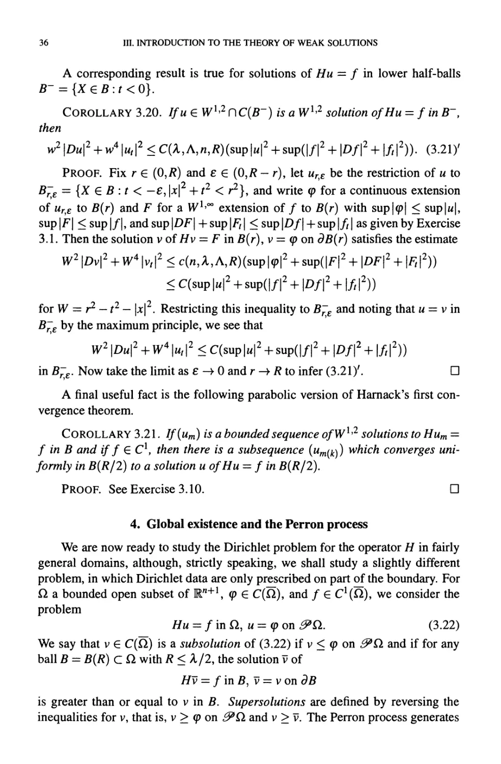
We can also prove a chain rule for weakly differentiable functions.
LEMMA 3.6. Iff e Cl(R), f e L°°(R), and u andDxu are in L\oc{Q), then
Di(f o u) exists and D((f o w) = f(u)DiU.
Proof. Let (um) be a sequence of smooth functions such that um-+ u and
DiUm -» DiU in ?^(?2), and let M be a nonnegative constant such that |/'| < M.
Then, for all sufficiently small positive h,
lim / \f(um)-f(u)\dx< lim / M\um-u\dx = 0,
and
/ \f(um)DiUm-f(u)Diu\dx
<[ \f'(um)\\Dium-Diu\dx+ [ \f(um)-f(u)\\Diu\dx.
Next, we have
/ \f(um)\\DiUm-Diu\dx<M[ \DiUm-Diu\dx->0
JClh JClh
as m —> oo. Since
|/(««)-/(ii)||A«i|<2Af|Aii|,
and \f{um) — f'(u)\ |D,-w| converges to zero almost everywhere in ?}/,, it follows
that
Jah
as well. Hence f(um) -+ f(u) and A(/° um) = f(um)DiUm -> f'(u)DjU in L^.
It follows from Theorem 3.4 that f(u) is differentiable and D/(/ o«) = f(u)DiU.
D
In fact, Lemma 3.6 remains valid as long as / is just globally Lipschitz (see
[348, Section 2.1]) in which case f exists almost everywhere because Lipschitz
functions are absolutely continuous. For our purposes we only need to consider a
special class of Lipschitz, non-C1 functions.
Lemma 3.7. IfDtu exists, then so does DiU+, and
D'«+ = (o'" '"»? .39.)
10 ifu < 0,
fo ifu>0
Diu~ = { J - C.9b)
\DjU ifu<0,
I |/(k*)-/(«) | |D,-«| <k-X)
JClh

1. THE THEORY OF WEAK DERIVATIVES
27
and
Dt\u\ = <
[ —D[U ifu < 0.
Proof. To prove C.9a), define f? by
,,x j(z2 + ?2y/2-? ifz>0
MZ) = H ifz<0.
D[U ifu>0
0 z/w^O C.9c)
/ Mu)DiZdx=-[ Cf2f'"dx
Ja Ju>o} (uz + ?zI/2'
It follows from Lemma 3.6 that
I{u>0} * (u2 + E2I/2 '
for any ? G Cq(Q), and we can send e to zero on both sides of this equation to
obtain
/ u^D^dx-- I t^Dtudx.
Ja J{u>o}
Hence we have proved C.9a). The other two results now follow because u~ =
-(-w)+ and \u\ — u+ 4- u~. D
COROLLARY 3.8. IfDiu exists, then D\u — 0 almost everywhere on {u = c}
for any constant c.
Proof. ApplyC.9c)tow-c. D
We also need the following weak compactness result for bounded subsets of
Wl >?(&), where we define Wk>p(Cl) (k a positive integer and p G [1,°°]) to be the
set of all functions u such that Dau?Lp for any multi-index a with \a\ <k. (By
definition, Dau = u when |a| = 0.) A norm on WkiP is given by
\ i/p
\\a\<kJn J
LEMMA 3.9. If(um) is a bounded sequence in WlyP(Q.) with 1 < p < <*>, then
there is a function u G Wl>p and a subsequence (um^) such that um^ —> u weakly
in Wl>p.
PROOF. The weak compactness of LP implies that there are functions w,
vi,..., vn and a subsequence (wm(*)) such that um^ —> u and A«m(&) -» v,- weakly
in LP. The weak convergence of these subsequences guarantees that Dtu = v,-. ?
It will be useful to have a concept of boundary values for W1'2 functions. We
define W0' to be the closure in the W1,2 norm of C^ (or, equivalently, Cq), and
we say that u = (p on dQ. for (p G W1,2 if w - <p G WA,2

28
III. INTRODUCTION TO THE THEORY OF WEAK SOLUTIONS
We close this section with Poincare's inequality. Further discussion of this
inequality appears in Exercise 3.6 and Section VI.4.
LEMMA 3.10. Suppose u G W^2{Ci) and diamCl < 2R for some positive R.
Then
f u2dx<R2 f \Du\2dx. C.10)
J?l JO.
Proof. Suppose first that ueC^ and [jc1 | < R for x G CI. Then
u(x) = [$-RDiu{t,x\...,xN)dt ifxUO
\fRDiu(t,x2,...,xN)dt ifjc1 >0.
Now square this equation, divide by R2 and integrate with respect to xl from — R
to 0. Using y as an abbreviation for (jc2, • • •,jc^), we see that
2
J
\Du{t,x')\ dt= / \Du(x)\2dxl.
-R J—R
Adding the corresponding inequality obtained by integrating for positive jc1 yields
/ u(xJdxl<R2[ \Du(x)\2dxl.
J-R J-R
If we now integrate this inequality with respect to x! and recall that u and D\u
vanish outside CI, we infer C.10) for any u €Cq. The result for general u€W0'
now follows by approximation. D
The proof of this lemma gives a more general result, which we will use to
study strong solutions in Chapter VII.
Corollary 3.11. Suppose u e Wl>2(Cl) with u = 0 on some subset a of
dCl. Suppose also that there are R > 0 and a unit vector j3 such that, for every
xe CI, there are r G @,7?) andxo G (J with x = xo + rf5 andx-\-pp G CI for every
pG @,r). Then C.10) holds.

2. THE METHOD OF CONTINUITY
29
2. The method of continuity
To prove the existence of solutions to various linear boundary value problems,
we use some simple functional analysis. This section discusses the relevant facts.
A map T from a metric space (X,p) to itself is called a contraction map if
there is a constant 6 G @,1) such that p(Tx,Ty) < 9p(x,y) for all x and y in
X. We say that T has a fixed point x G X if Tx = x. Our first result asserts the
existence of a fixed point for contraction maps in complete metric spaces.
THEOREM 3.12. A contraction map T on a complete metric space (X,p) has
a unique fixed point.
PROOF. Choose jco G X and define a sequence (jc,) inductively by Xi+\ = 7jc,\
If k> mare positive integers, then
m m
p{xk,xm)< ? p(xi-uxi)= ? pfr'-Vr'-1*!)
< L 0'_1p(^O^l) < T3gP(*0,*l).
i=&+1
Since this last expression tends to zero as k -> oo, it follows that (jc,) is a Cauchy
sequence and hence has a limit jc. Moreover, p(x,Tx) = limp(;t;,;t;+i) = 0, so jc
is a fixed point. Finally if y is another fixed point, then
p{x,y)=p(TxJy)<0p{x,y),
which implies that jc = y. ?
If ^i and ^2 are two normed linear spaces, a map r : ^ —» ^ is bounded if
its norm \T\ denned by
m=supl^
xen \x\
jc^O
is finite. A linear map is continuous if and only if it is bounded. Our next theorem,
known as the method of continuity, asserts that two suitably related bounded linear
maps are either both invertible or both non-invertible.
THEOREM 3.13. Let 88 be a Banach space, let Y be a normed linear space,
and let Lq and L\ be two bounded linear maps from 88 into V. For h G [0,1],
define Lh = hL\ + A — h)Lo, and suppose there is a constant C such that
\x\#<C\Lhx\r C.11)
for all h G [0,1]. Then Lq is invertible if and only ifL\ is invertible.
PROOF. Note first that L/, is injective for all h, so we need only prove the
surjectivity of the appropriate maps. Denote by S the set of all h G [0,1] such

30
III. INTRODUCTION TO THE THEORY OF WEAK SOLUTIONS
that Lh is surjective and suppose that S is nonempty. Choose s G S, fix v G ^, let
h G [0,1], and define T : @ -> & by
7* = L5-1v + (/i-^Z^Lo -LOjc.
A straightforward calculation shows that jc is a fixed point for T if and only if
LhX — v. In addition,
\Tx-Ty\ = \(h-s)L;\L0-Ll)(x-y)\<\h-S\±\l4-Ll\\x-rt
for all x and y in 8$. It follows that T is a contraction for \h-s\ < 5 = i\u-l I *
and then T has a unique fixed point for \h — s\<8 and 0 < h < 1 by Theorem
3.12. It follows that h G 5 for any such h and hence that S = [0,1]. D
3. Problems in small balls
We now introduce a fixed positive definite matrix (alj) with constant entries
and eigenvalues bounded by the positive constants X and A. In other words,
A |4|2 <*%¦!,• <A|||2
for all t; G W1. For nonnegative constants ? and 7], we define the operator L?)T? by
Le^u = Dt{aljDju) + {eut)t -T]ut,
which we consider on the ball B = B(R) = {\x\2 + |f |2 < /?2}. We say that u is a
Wl '2 solution of the problem
Le^u = f in #, u = (pondB C.12)
if w G W1'2^), m-96 W01,2(?) and
faijDjuDii; + euti;t + riutCdX= f fC,dX C.12)'
for all ? G Co(?), wnere we suppress the set of integration B. We call ? a tof
function. Note that if w is a IV1*2 solution of C.12), then C.12)' holds for all
f G Wq1'2. Moreover, for any ? G CqE), we have
faijDjuDi?dX = - fuaijDijCdX,
so that there is no loss of generality in assuming that (alJ) is a symmetric matrix.
(As we shall see later, such an assertion need not be true if (alJ) is not a
constant matrix.) Our first step is to show that C.12) has a unique solution for all
appropriate / and (p.
LEMMA 3.14. Suppose that ? > 0. Iff G L2 and (p G W1'2, then C.12) has a
unique W1,2 solution.

3. PROBLEMS IN SMALL BALLS
31
Proof. If u solves C.12), we note that v = u — cp solves
Le,11v = gmB,vew?>2(B) C.13)
for g = f -Le^(p. Conversely if v solves C.13) with this choice of g, then u =
v-h (p solves C.12). Hence it suffices to show that C.13) is uniquely solvable for
any g ?L2.
We first consider the special case that 7] = 0. In this case, we define an inner
product on Wq1, by
(w,z> = [aijDjwDiZ + ?wtztdX. C.14)
Since W^2 is a Hilbert space with respect to this metric, we can define a bounded
1 2
linear functional F on W0' by
Hz) = jgzdX.
1 2
The Riesz representation theorem then gives a unique v € WQ' such that F(z) =
(v,z), which is the unique solution of C.13) in this case.
We now use the method of continuity to solve C.13) for 77 > 0. To this
end, we use llll to denote the norm associated with the inner product (,), and we
define Jfh — ^e,hr] for h ? [0,1]. By what was already proved, we know that ^
is invertible and that «??o and j??i are bounded. If ^w = g, we can use the test
function w to see that
||w||2 = faijDiwDjW + ?w?dX = hr\ fwwtdX+ fwgdX.
But /wwtdX = / \{w2)tdX = 0, so
IM|2< [wgdX<0 [w2dX + ^- Ig2dX
for any G > 0. Now Poincare's inequality gives
f w2dX <R2 [\Dw\2 + w2dX <R2 (j + ^\\\w\\2,
so choosing 0 small enough gives ||w||2 < C||g||2, and therefore j?fo and JSf\ satisfy
the hypotheses of Theorem 3.13. Therefore -??/, is invertible for all h ? [0,1], and
the invertibility of ??\ is equivalent to the solvability of C.13). D
Let us note here that the argument presented in Lemma 3.14 is easily modified
to handle any bounded domain Q. in place of B.
Next, we need a simple version of the maximum principle for these operators.

32 III. INTRODUCTION TO THE THEORY OF WEAK SOLUTIONS
Lemma 3.15. Let <p G C°(B) n W2>2(B) satisfy the inequality <p<M ondB
for some constant M. IfuEW1,2 satisfies
0 > [[aijDjuDiV + ?utvt - rjvw,] ,dX C.15)
for all vGCq and ifu — (p G W0' , then u<M in B.
PROOF. As already noted, we can take as test function v in C.15) any
function in W0' . We take v = (u — M)+ and note that v G W^ by Exercise 3.7. It
follows that
0 > / [aljDjuDtv + eutvt - r\vut]dX.
Since vut = \(y2)t, we have
0 > f[aijDjuDiV + eutvt] dX.
The integrand here is nonnegative and hence it must be zero. Therefore Dv = 0
and vt = 0, and then Exercise 3.8 implies that v is a constant, which must be
zero. ?
For simplicity, we shall write Le^u > 0 in B if C.15) is satisfied.
We now use Lemma 3.15 to prove an important a priori estimate on solutions
of C.12) for sufficiently regular data. Some of the steps in deriving this estimate
will reappear in the quasilinear theory.
Lemma 3.16. Suppose that <p G C2{B), f € Wl>°°(B), and e e @,1], and let
4> and F be constants such that
|^9l<^|^29| + l9/| + l^l<^ l/l + |?>/l + |//|<AF. C.16)
IfR < A/2 and r\ G [0,1], then any W1,2 solution of C.12) satisfies the estimate
\Du\ + \ut\<C{n,X,K,R)(& + F). C.17)
PROOF. Define w(X) -R2- \x\2 -12 and write L for Le^ and B for B(R).
Then
Lw = -2ST -2e + 2r]t < -Ink + 2t)R < -2nX + 2R < -X
and
\L(p\ <{2nh + ? + T])<$><k\X<S>
inB, where^i = BnA-\-2)/X. Hence, v— {u — (p) — (k\<&+F)wsatisfiesLv>0in
B and v < 0 on dB, so v < 0 in B by Lemma 3.15. Therefore u — (p< (k\<& + F)w,
and a similar argument gives — (u- (p) < (k\& + F)w, so \u-(p\< (k\& + F)w.

3. PROBLEMS IN SMALL BALLS
33
From this inequality, we can derive a boundary Lipschitz estimate. For X G B and
Y G SB and ||X - Y\\ = (|jc - v|2 -f (f - sJI/2, we have
|«(X) - u{Y)\ = \u(X) - <p(Y)\ < \u(X) - <p(X)\ + \<p(X) - cp(Y)\
<(ki<Z> + F)w{X) + 2<P\\X-Y\\
<2[{kiR+l)& + FR]\\X-Y\\.
Hence, setting K = 2[(k\R + 1 )<*>+ Ffl], we have
|w(X + t)-w(X)|<#||t|| C.18)
for any vector % G En+1 and any X G dBXi where Bx = {Y G ? : Y + r G ?}, such
that #T is nonempty.
We use C.18) to prove the interior estimate. Fix r so that Bx is nonempty and
define v±(X) = ±(w(X + t) - w(X)) - tf ||r|| - F ||r|| w(X). A simple calculation
shows that Lv± > 0 in Bx and v± < 0 on d#T, so v^" < 0 in Bx. Hence
KX + T)-M(X)|<(^ + F/?2)||T||
for all X G ?T. Then Lemma 3.5 implies that \Du\ + \ut \ < K+FR2, which implies
C.17). ?
Now we specialize to 7] = 1 and send ? —> 0, noting that the estimates derived
in Lemma 3.16 are independent of ?. For simplicity, we set H = Lo,i, which is
just the heat operator when alJ = 8lJ.
Theorem 3.17. If(p G C2(B), f G Wl>°°(B), and R < A/2, then there is a
unique Wl>2 solution u of
Hu = finB,u = (p on dB. C.19)
Moreover, u G Wly°° and C.17) holds.
Proof. Let u? be the unique W1,2 solution of
L?^\ue = f in B, ue = (p on dB
given by Lemma 3.14. Then Lemma 3.16 implies that the family (u?)o<e<\ is
uniformly bounded and equicontinuous, so there is a uniformly convergent sequence
(Me(m))» we write u for the limit of this sequence. By Lemma 3.16, this limit is
also Lipschitz, satisfying C.17), and hence u G W1'2. In addition, for any ? G Cq,
we have
jue(m)D& + e(m)Me(m),/Ci + Me(m),/C]^
= - fu<-(m)WJDijC, + e(m)?, -QdX.

34 III. INTRODUCTION TO THE THEORY OF WEAK SOLUTIONS
Now we send m -> °° and use the uniform boundedness of the sequence (we(m)) to
see that
ff^dX = - [u[aiJDij? - QdX = f[aiJDjuD^ + utQdX.
Hence u solves C.19), and the theorem is proved. D
For further existence results, we study the interior regularity of solutions of
C.19). It is important for the present considerations that these estimates not
depend on the C2 estimates for <p, and we only need to consider the case / = 0. A
key element is the function w from Lemma 3.16.
Lemma 3.18. If u is a bounded W1,2 solution of Hu = 0, then u is a
solution. If\u\<M inB, then
w2\Du\2 + w4\ut\2 < CM2. C.20)
Proof. Fix % e (-R/2,R/2) and set v{X) = u(X; r). For r € (R/2,R- |r|),
we have v e C°°(B(r)) and hence, for ? E Co(#(r)), we have
[aijDjvDi?dX= f [ aijDju(X -rY)(p(Y) dYD&(X)dX
J JB(r) JW+l
= ([ aijDju(X)(p(Y)Dii;(X + TY)dY ,dX
JBJRn+l
= f aijDjuDi^dX,
Jb
where we have used the abbreviation ?t = — ?(•; r). Similarly,
JvtCdX = Jutt;rdX,
so Hv = 0 in B(R — |t|) in the weak sense. It follows that Hv = 0 in the classical
sense as well. (See Exercise 3.9.)
To prove C.20), we use an idea that goes back to Bernstein [16], namely that
|Dv|2 is a subsolution of a certain differential inequality. We implement this idea
by defining W = r2 - \x\2 -12 with R/2 < r < R - \z\ and computing
H{W2 \Dv\2) = H(W2) \Dv\2 + 2[aijDijkv - Dkvt]DkvW2
+ 2aijDikvDjkvW2 + 4aijDikvDkvDj(W2).
Now we note that
H(W2) = 2WH(W) + 2aijDiWDjW > 2WH(W) = -A3TW + 4tW
and that alWijkv — Dkvt = 0. A simple application of Cauchy's inequality now
gives us
H(W2\Dv\2) > -d(A,n,/?)|Dv|2.
In addition,
H(v2) = 2vHv + 2aijDivDjV > 2X |Dv|2,

3. PROBLEMS IN SMALL BALLS 35
so we can apply the maximum principle to W2 \Dv\2 + (C\ /A)v2 in Br to find that
W2\Dv\2<^M2.
A
Choosing suitable constants Ci and C3, we can then apply the maximum principle
to W4 \D2v\2 + C2W2 \Dv\2 + C3v2 and obtain
W4|D2v|2<C(Ci/A,C2,C3)M2.
Hence from the differential equation Hv = 0, we also obtain
W4|v/|2<C(C1/A,C2,C3)M2.
In a similar fashion, we can derive local L°° bounds for any derivative of v. Sending
T -> 0 gives the corresponding bounds for the derivatives of u. Hence
W2\Du\2 + W4\ut\2<CM2,
with C independent of r. Sending r -»R completes the proof. ?
In fact, such an estimate also holds for the inhomogeneous equation Hu — f.
To prove this statement, we first define a slightly more general concept than the
W1,2 solutions already considered. We say that u is a continuous weak solution of
C.12) if 9 G C°(?), u € W^(B)nC°{B), u satisfies C.12)' for all ? G C$(B), and
u = <p on dB.
Theorem 3.19. Ifcpe C°E), / e Wl>°°(B), andR< A/2, then there is a
unique continuous weak solution u of C.19). In addition,
w2|DW|2 + w>,|2<C(^ C.21)
PROOF. Let (<pm) be a sequence of C2 functions converging uniformly to <p
and write um for the solution of Hum = / in B, um = (pm on dB. Then H(um —
ujc) = 0 in B and um — u^ — (fm — <pk on dB for any m and k. Hence the sequence
(um) is uniformly Cauchy on dB, so the maximum principle implies that it is also
uniformly Cauchy in B. Applying Lemma 3.16 to um — u^ shows that Dum —
Duk and «m?/ - u^t tend uniformly to zero on compact subsets of B, so the limit
function u is a weak solution of C.19), which is unique by Corollary 2.5 since the
difference of any two solutions is a classical solution of Lu = 0 in B, u = 0 on
&>B.
To prove C.21), we write v for the solution of Hv = 0 in B, v = (p on dB given
by the first part of the proof. Then Lemma 3.18 and the maximum principle imply
that
w2|Dv|2 + w4|v/|2<C(sup|<p|J.
Since H(u - v) = / in B and u — v = 0 on dB, it follows from Theorem 3.17 that
w2|D(M-v)|2 + w4|(w-v)/|2<|D(M-v)|2 + |(M-v)/|2<CF2.
Combining these two inequalities gives C.21). D

36
III. INTRODUCTION TO THE THEORY OF WEAK SOLUTIONS
A corresponding result is true for solutions of Hu = / in lower half-balls
B~ = {XeB:t<0}.
Corollary 3.20. Ifu G W1'2 nC(r) is a W1'2 solution ofHu = f in B~,
then
vv2|DM|2 + w4|M/|2<^ C.21)'
PROOF. Fix r G @,R) and e G @,R - r), let wr,e be the restriction of u to
B~? = {X G B : t < — ?, |jc| +12 < r2}, and write <p for a continuous extension
of wr,e to B(r) and F for a W1'00 extension of / to B(r) with sup|<p| < sup|w|,
sup \F\ < sup |/|, and sup \DF\ + sup \Ft \ < sup \Df\ -f sup |//1 as given by Exercise
3.1. Then the solution v of Hv = F in #(r), v = 9 on d#(r) satisfies the estimate
W2|Dv|2 + W4|v/|2<c(n,A,A,/?)(sup|<p|2-hsup(|F|2 + |DF|2 + |F/|2))
^CCsupl^ + supd/^ + lD/p + l/,!2))
for W = r2 -12 — \x\2. Restricting this inequality to B~e and noting that u = v in
B~? by the maximum principle, we see that
W2 |Z>u|2 + W4 K|2 < C(sup|i«l2 + sup(|/|2 + |Z>/|2 + |/,|2))
in B~?. Now take the limit as ? -> 0 and r -> R to infer C.21)'. ?
A final useful fact is the following parabolic version of Harnack's first
convergence theorem.
Corollary 3.21. If(um) is a bounded sequence ofW1,2 solutions to Hum =
f in B and if f G C1, then there is a subsequence (um^) which converges
uniformly in B(R/2) to a solution u ofHu = f in B(R/2).
PROOF. See Exercise 3.10. ?
4. Global existence and the Perron process
We are now ready to study the Dirichlet problem for the operator H in fairly
general domains, although, strictly speaking, we shall study a slightly different
problem, in which Dirichlet data are only prescribed on part of the boundary. For
?1 a bounded open subset of Mn+1, <p G C(&), and / G Cl(?i), we consider the
problem
Hu = f in ft, u = (p on 3??l. C.22)
We say that v G C(Q.) is a subsolution of C.22) if v < (p on ?PGl and if for any
ball B = B(R) C Q. with R < A/2, the solution v of
Hv — f in B, v = v on dB
is greater than or equal to v in B. Supersolutions are defined by reversing the
inequalities for v, that is, v > (p on ??Q, and v > v. The Perron process generates

4. GLOBAL EXISTENCE AND THE PERRON PROCESS
37
a solution as the supremum of all subsolutions. To see that this object really is a
solution, we verify certain properties of subsolutions and supersolutions. The first
is a comparison theorem based on the strong maximum principle Theorem 2.7.
LEMMA 3.22. Ifw is a supersolution and v is a subsolution, then w>vin ?1.
Proof. If not, then g = v - w has a positive maximum value achieved at
some point in ?1 \ &?l. By the same argument as in Lemma 2.3, we see that there
is a point X0 G ?1 and a positive R < A/2 such that B = B(X0,R) C ?1, g(X0) =
? > 0 and g(X) < ? if X € B* = BD {t < t0}. Writing G = v- w- ?, we have
HG — 0 in ZT, G < 0 on ??B*, and G(Xo) > 0, so the strong maximum principle
gives G = 0 in B*. It follows that v — w = ? on 0>B*, and hence, since we can
take R arbitrarily small, that v — w = e in {|jc —jco| < r,f = fy} for some small r.
Hence C'(Xo), the subset of C(Xq) on which v — w = ?, is open in C(Xo). Since it
is obviously closed, it must be C(Xo). But then v — w — ? at some point in <^?2,
which contradicts the assumption that v < w on &?l. ?
Next, from a subsolution v and a ball B C ?1 with R < X/2, we construct a
new subsolution V, called the lift ofv, as follows: V = v in ?2 \ B and V = v in B.
To show that V is a subsolution, let B{r) be another ball in ?1 with r < A/2, and
let vi solve
#vi = / in B(r), v\ = V on d?(r),
Since V > v, it follows that vi > v in fl(r). Then vi > v = V on B(r) n ^^ and, by
definition, vi = V on dB(r)C\B. Therefore vi > V on <9(#n?(r)), so the
maximum principle gives vi > V in Z?n#(r). Since vi > v in B(r), we also have vi > V
in 5(r) \5 and hence vi > V in ?(r). In addition if vi and V2 are subsolutions,
then so is V3 = max{vi,V2} because V3 > vi > vi and V3 > V2 > v2-
We now construct our solution by the Perron process. If we use S to denote
the set of all subsolutions of C.22), we define u by
u(X) = supv(X). C.23)
ves
Our next step is to show that this expression gives a solution of the differential
equation.
THEOREM 3.23. The function u defined by C.23) is a solution of the equation
Hu — f in ?1.
PROOF. Note first that vo = -(sup |/|)r - sup |cp| is a subsolution, so u is
defined for all X E ?1 and is bounded from below. In addition, - vo is a supersolution,
so u is also bounded from above. To see that Hu — f, we fix Y G ?1 and R < A/2 so
that B(Y, R) C ?1, and choose a sequence (vm) of subsolutions such that vm (yi) -»
u(Y\) as k -» 00 for Y\ = (y,s + R/8). Next, define wm = max{vm,vo}, and let
Wm be the lift of wm relative to the ball B(Y1R). Because vm < wm < Wm < u, it
follows that Wm(Y\) ->• u(Y\). Hence Corollary 3.20 gives a subsequence (Wm^)

38
III. INTRODUCTION TO THE THEORY OF WEAK SOLUTIONS
which converges uniformly in B(Y,R/2) to a solution w of Hw — f in B(Y,R/2)
with w(Y\) = u(Y\). If >2 is any point in B(Y,R/$)y choose the sequence (vJn ) so
that vL1)(y2) -» u(Y2) and define wj}} = max{wm,vi!)} sowffpi) -> wW^) and
Wm (^2) —> w^'(y2) . Taking a convergent subsequence, we have a function vt^1)
with HwW = / in B(Y,R/4)9 w™ > w and wW^) = vt^). It follows from the
strong maximum principle that w = w^ in B(Y,R/S). Since y2 was arbitary, it
follows that w = « in B(Y,R/8). Hence w is a solution of //m = / in a neighborhood
of any point in ft, and therefore //w = / in ft. ?
Of course, the gradient bound, Theorem 3.19, gives a modulus of continuity
at each point of ft, and Corollary 3.20 shows that
u(X0) = lim u{X)
X->Xq
t<to
xeo.
exists for any Xo G <9ft \ <^ft. If Xo G <9ft \ <^ft and if there is a positive ? such
that B(Xo,e) n <^ft = 0, then the existence of u(X) for any X G ?(X0,?) n dft
implies that w(X) -» w(Xo) as X -> Xo and X G ft, so u is continuous at such a
point. On the other hand, if Xo G <9ft \ «^ft and there is a sequence (X*) in <^ft
with X* ->> Xo, it is possible to give boundary data (p on <0*ft so that the Perron
solution from Theorem 3.23 is discontinuous at Xo- For simplicity, we assume that
/ = 0. If/? is chosen so that Q(Xq,R) C ft, then the closure of Q(X0,R/2) and
<^ft are disjoint and hence there is a continuous function (p which vanishes on
^ftfl{r < to} and <p = 1 on g*Q.nQ(Xo,R/2). The maximum principle implies
that m(Xo) = 0, but lim* <p(X*) = 1, so u does not take on the prescribed boundary
value at Xo. For this reason, we assume that for any Xo G dft \ ^ft, there is a
positive e such that B(X0, e) n <^ft = 0.
Continuity of the Perron solution at points of <^ft is not automatically
guaranteed. When the solution is continuous at such a point, we can use the maximum
principle to prove this continuity. The conditions guaranteeing continuity are
geometric in nature and, as in the case for elliptic equations, are tied to so-called
barrier functions. Because of the special role of the time variable for parabolic
equations, we shall find it convenient to introduce some intermediate notions first.
We say that a continuous function g, defined on ft, is a global barrier at Xo G i^ft
(for the operator H) if g is nonnegative and vanishes only at Xo and if for any
B C ft with R < A/2, the solution h of
Hh = 0'mB,h = gondB C.24)
satisfies the inequality h<g'mB.
We say that Xo G «^ft is a regular point for H if the Perron solution of C.22)
is continuous at Xo for any f EC1 and q> €C®. The next lemma shows that the
existence of a global barrier at a point is equivalent to that point being regular.

4. GLOBAL EXISTENCE AND THE PERRON PROCESS
39
LEMMA 3.24. Xq is a regular point for H if and only if there is a global
barrier at Xq.
Proof. If Xo is regular, use g to denote the Perron solution of Hg = — 1 in
jQ, g = \X — Xq\ on 2??l and note that v = 0 is a subsolution, so that g is nonneg-
ative. Lemma 3.18 shows that g G C2,1 (CI) (because H(g — t)=0) so the strong
maximum principle shows that g > 0 in ?1 \ {Xo}.
Conversely, if g is a barrier, set K = sup |/| and choose ? > 0. Since <p is
continuous, there are positive constants 5 and k such that
\<p(X) - (p(X0)\ +K\t -f0| < ? for \X -X0\ < 5,
\<p(X) - <p(Xo)\ + K\t-t0\ < kg(X) for \X-X0\ > 8.
We set
v± = q>(Xo)±(K[t-to} + e + kg),
and note that
v±(X) = <p(X) + [<p(Xo)-(p(X)]±(K[t-t0} + e + kg).
Then, for X G {|X-X0| < 8} D ^a we have v+(X) > (p(X) + *g(X) > p(X),
and for X G {|X -X0| > 8} D <^a we have v+(X) > <p(X) + ? > (p(X). In
addition, if B C Q. (with /? < A/2), let h0 solve
///i0 = / in B,ho = v+ on <9#
let /ii solve
#/ii = 0in?,/*i = gondB,
and set h = h0- <p(X0) - K[t -10] - ?. Then
Hh = f + K > 0 in B, h = kg on dB,
so the maximum principle and the linearity of// imply that h<kh\< kg in B(R)
and hence Hq < v+ in B(R). Therefore v+ is a supersolution. It follows that u < v+
in ?2, so
limsupw(X) < limsupv+(X) = <p(Xo) + ?•
x->x0 x->Xo
Similarly v~ is a subsolution, so
liminfw(X) > liminfv~(X) = <p(Xo) - ?.
X-*Xo X—>Xq
Since € is arbitrary, it follows that
(p(Xo) < liminfw(X) < limsupw(X) < <p(Xo),
and therefore limx->x0 w(X) — <P(^o)- In other words, u is continuous at Xq. ?

40
III. INTRODUCTION TO THE THEORY OF WEAK SOLUTIONS
The barrier concept is actually a local one. Writing H[Xo,r] = Q.C\B(Xo,r),
we call W a two-sided local barrier (to distinguish it from the one, defined below,
for earlier time) if W is a nonnegative, continuous function on ?l[Xo, r]) for some
positive r vanishing only at Xq such that for any B(R) C (?lC\B(Xo, r)) with R <
A/2, the solution h of
Hh = 0 in B(R), h = W on dB{R)
is less than or equal to W in B(R).
From W, we construct a global barrier rather easily. First, set A = B(Xo, r) \
B(Xo, r/2) and m = inf^ W, and define
_ fmin{W,m} mQnB(X0,r)
g~~[m inft\?(X0,r).
Since m is positive, we need only verify that h < g if h solves C.24). By the
maximum principle, if h solves C.24), then h < m, so if h — g has a positive
maximum M at some X\, then g(Xi) = W(X\) < m and ||Xi — Xo || < r. Hence there
is a ball ?* = B(p, Xi) such that B* CB(X0,r)nB, and there is X2 € ^B* n {r < 11}
with (h-W)(X2) < M. If hi solves
Hhx = 0 in J?*,/zi =Won <??*,
then (/i- Ai)(Xi) > (*- W)(Xi) = (h-g)(X{)=M because W is a two-sided
local barrier. Now, on dB*, we have h — h\ —h — W <h — g <M, so h — h\ <M
in B* by the maximum principle. Since (h — h\)(X\) = M, the strong maximum
principle implies that h-h\ = (h- W)(X\) in B* D {t < t\} which contradicts
{h — h\)(X2) < M. Hence /i < ^ and therefore g is a global barrier.
More significantly, the conditions for a local barrier only need to be satisfied
for t < to. Now we define ?l~ [Xo, r] — B~ (Xo, r) n Q., and we call w a local barrier
from earlier time if w is a nonnegative, continuous function in ?l~ [,Xo, r] for some
positive r vanishing only at Xo such that for any B~ = B~ (R) C B~ (Xo, r) C\ ?1 with
R < A/2, the solution /i of ///i = 0 in B~, h = w on &B~~ is less than or equal to
w\nB~'.
For brevity (and to conform with standard usage), we shall say local barrier
when we mean local barrier from earlier time. To show that existence of a local
barrier implies that of a global barrier, we first prove an existence result for circular
cylinders.
Lemma 3.25. Let R and T be positive numbers, let Y e W+X,_and set Q, =
{\x - y\ < R} x (s - T, s). Then for any f G C1 E) and any (p e C°(ft), there is a
unique, continuous solution of C.22).
Proof. From Theorem 3.23, Lemma 3.24 and the remarks following
Theorem 3.23 and Lemma 3.24, it follows that we need only construct a two-sided
local barrier at each point X0 ? 3*0.. If to = s - 7, then w = |jc - jc0|2 4- 8A(f - fn)

NOTES
41
is a two-sided local barrier. If to > s — T, we set x\ = — y + 2jco- Then the n-
dimensional spheres {\x — x\ \ = R} and {\x — y| = R) are tangent at xo, and hence
g = -exp(-y[(x-xlJ + (t-toJ]) + exp(-YR2)
is a two-sided local barrier at Xo for a suitable positive y. ?
We can now show the equivalence of regularity of a boundary point and the
existence of a local barrier.
THEOREM 3.26. Xo is regular if and only if there is a local barrier at Xo.
PROOF. If Xo is regular, then there is a global barrier and hence a local barrier.
If w is a local barrier, we construct a two-sided local barrier W. Set Q =
{\x — xo\ < r,to < t < to + r}, and let u>o be a nonnegative continuous function on
IR"+1 which agrees with w on (o(to) and vanishes only at Xo. (Such a function
exists by virtue of Exercise 3.1.) Then write w\ for the solution of Hw\ = 0 in Q,
w\ (X) = wo on &Q. It is easy to check that W defined by
w(x) = C{x) if^'°
v ; ywx(X) ift>t0
gives a two-sided local barrier. ?
We close this chapter with an easy example of a local barrier. Let ?1 be a
domain and let Xo G tP?l. Define the parabolic frustum (as in Lemma 2.8 but
with 77 = 1)
PF(R,Y) = {\x-y\2 + (s-t)<R2,t<s}1
and suppose that for some choice of R and Y with s = to, we have PF(R, Y) n ?1 =
{X0}. If r is defined by r(X) = \x - x0\2 + t0-t, then
w=-exp(-ar2)+exp(-~aR2)+4(to-t)/R + ?(\x-x0\2 + \t-to\2)
is a local barrier provided a is sufficiently large and ? is sufficiently small
(depending only on A, A, n, and R).
Notes
The theory of weak derivatives given in this chapter is standard in the theory
of partial differential equations. Our exposition is based on that in [101, Chapter
7]. More detailed discussion of weak derivatives can be found in [348, Chapter 2]
and [68, Chapter 4].
On the other hand, our approach to the existence of weak solutions is quite
different from the usual one. The discussion in Sections Section III.2 and III.3
comes from [228]. The underlying philosophy of what we have called the Perron
process is quite simple: first one shows local existence and then global existence
of solutions. Alternative detailed descriptions of this process can be found in [69].
The key new observation here for local solvability is the gradient bound of Lemma

42 III. INTRODUCTION TO THE THEORY OF WEAK SOLUTIONS
3.16. Classical approaches [89, Section 4.8] prove local solvability in cylinders.
For example, in the Galerkin method, one shows local solvability for boundary
values in some finite-dimensional space and then uses an approximation
argument to obtain arbitrary boundary values; such an approach is extremely useful
for numerical solutions of such equations. Alternatively, one can use the Green's
function for the heat equation in a rectangular parallelepiped (see Exercises 1-13
of [89, Chapter 4]) to show local solvability. The Green's function approach has
the disadvantage that one must verify that an appropriate infinite series of
functions converges.
Our local solvability result for L?jT? is based on the existence of weak
solutions of elliptic operators in [101, Chapter 8]. The special form of the operators
considered here leads to considerable technical simplification.
Our use of local solvability in balls has another advantage over other
methods: The inference of global solvability from local solvability in arbitrary domains
is simplified because we can consider only continuous subsolutions, rather than
upper semicontinuous ones. The role of semicontinuity is demonstrated in, e.g.,
[112, Section 6] or [212, Section 8].
We also note that a necessary and sufficient geometric condition for the
regularity of a boundary point was proved by Evans and Gariepy [77]. We refer the
reader to that work for a detailed history of this problem.
Exercises
3.1 Show that any function u which is continuous on a compact set K in
RN can be extended to a uniformly continuous function on all of E^
with the same modulus of continuity and range. Specifically, if there is
a function co which is continuous, subadditive, and increasing on [0,°o)
with 0)@) = 0 such that
\u(x) — u(y)\ < co(\x-y\) for all x,y in K,
then there is a function U e C(RN) with U = u on K, mint/ = minw,
maxt/ = maxw, and
\U(x) - U(y)\ < co(\x-y\) for all x,y in RN.
3.2 Show that there is at most one weak a-derivative v for a given function
u.
3.3 Let ?1 be an open set and let h< j diam?L Show that there is a function
?/, € C°°(Q.) with support in ?lh and ^ = 1 in &2h-
3.4 Let u be a function defined on some domain Q. and let K be a positive
constant. Show that \u(x + hei) - i#(jc)| < K \h\ for all x G JQ and h G R
such that x + het eClif and only if D,w 6 L°° and |D,-k| < K.

EXERCISES
43
3.5 Let u G ?^(?2), and suppose that for all sufficiently small positive //,
there is a function v# G l) (?2#) such that
/ vn?dx=— uD[C,dx
ix
Jci„ ' Jq.h
for all ? G Cg (&//). Show that the weak derivative D(U exists in ?1 and
thatD,w = vh in ?Ih>
3.6 Prove the following generalization of Poincare's inequality. Let G be a
continuous, convex, increasing function on [0,°°), let R > 0, and let ?2
be a domain with diam?2 < 2R. If u G Cg (?2), then
/."(^HiO*10*-
i 9
3.7 Show that the function v in Lemma 3.15 is in W0' .
3.8 Show that a weakly differentiable function which has all first order
derivatives equal to zero is constant.
3.9 Prove that any C2'1 weak solution of Hu = 0 is a classical solution.
(Note that it follows from Lemma 3.18 that any bounded weak solution
is a classical solution.)
3.10 Prove Corollary 3.21.
3.11 We define a tusk to be a set of the form
2
{X:t0-T<t<t0A[x-xo\- {t0 -1) l'zxx < R2{t0 -1)}
for positive constants R and 7\ and points Xq G Mn+1, and x\ G W1. We
say that ?1 satisfies an exterior tusk condition at Xq G ^Q. if there is
a tusk whose closure intersects Q. only at Xo. Construct a local barrier
at any point Xo at which ?1 satisfies an exterior tusk condition. (See
[72,221].)
3.12 Show that the theory of this chapter can be reproduced without the
restriction R < A/2 if we replace the ball B(R) by the scaled ellipsoid
E(*) = {x:M2 + x^</?2j.

CHAPTER IV
HOLDER ESTIMATES
Introduction
In this chapter, we prove a large number of estimates for solutions of
parabolic equations under various hypotheses. Some of these estimates apply to weak
solutions of equations in divergence form and others to classical solutions of
equations not necessarily in divergence form. Although some of the critical estimates
are on integral norms of the solutions and their derivatives, our primary concern
is with pointwise behavior of these functions. Specifically, we study their
moduli of continuity, and the appropriate class of moduli is the Holder class
introduced in Section IV. 1. To connect the Holder moduli of continuity to the theory
of weak solutions developed in Chapter III, we define the Campanato spaces in
Section IV.2 and we explore the relation between Campanato and Holder spaces.
Interior estimates for smooth solutions of parabolic equations (in divergence and
non-divergence form) are given in Section IV.3. We prove boundary estimates in a
neighborhood of a flat boundary portion with zero boundary data in Section IV.4.
In order to deal with curved boundaries and nonzero data, and to study an
intermediate regularity situation which is important to our considerations for nonlinear
equations, we introduce a parabolic regularized distance in Section IV.5. This
regularized distance is used in Section IV.6 to derive estimates in certain weighted
Holder spaces (and for equations with possibly unbounded coefficients) with flat
boundaries and zero boundary data. Curved boundaries and nonzero data are the
subject of Section IV.7.
An important element of our approach is a simple existence theory, which is
based on the existence results from Chapter III. Other approaches to these
estimates, most of which do not rely on existence theory, are discussed in the Notes
to this chapter. In addition, there are two significant connections made throughout
this chapter. First, we use estimates for equations in divergence form to infer
estimates for equations in nondivergence form. Also, we use estimates for equations
with Dirichlet boundary data to infer estimates for equations with oblique
derivative data and, conversely, we use estimates for equations with oblique derivative
data as the basis for estimates with Dirichlet data.
45

46
IV. HOLDER ESTIMATES
1. Holder continuity
For a e @,1], we say that a function / defined on ?1 C Rn~*~l is Holder
continuous atXo with exponent a if the quantity
M - qnn !/(*)-/(*o)l (dU
[f\aX0 = SUP —nf—71a— D-l)
is finite. If the quantity defined by D.1) is finite for a = 1, we also say that / is
Lipschitz at Xo. Clearly if / is Holder continuous at a point, it is continuous there.
If the semi-norm
l/kn = sup [f\aiXo
Xoen
is finite, we say that / is uniformly Holder continuous in ?1, and if / is uniformly
Holder continuous on any ?1' with compact closure in ?1, we say that / is locally
Holder continuous in ?1. Since functions are Lipschitz at any point of
differentiability, we see that Holder continuity can be thought of as a sort of fractional
differentiability. In addition, our definition is in accord with the basic rule from
the heat equation that "two jc-derivatives are equivalent to one f-derivative"
because the exponents with respect to x in the definition of [/] are twice those with
respect to t. This equivalence makes the definition of higher order Holder semi-
norms slightly more complicated than in the elliptic case. First, for j3 G @,2], we
define
'|/fa,Q-/(Xb)|
and
(f)fi&= sup(/)^^0.
Xoeci
Then, for any a > 0, we write a = k + a, where k is a nonnegative integer and
a G @,1], and we define
(f)a;Cl= ? (DgDlf)a+i,
IP 1+27=*-1
[f]a&= ? [DPxDJf]ai
1M1+2/=*
I/Uq= E sup to"/| + [/]* + </>*•
\P\+2j<k ' '
It is easy to verify that |-|fl defines a norm on Ha(?l) = {/: \f\a < °°} which
makes Ha(?l) a Banach space. Moreover, the inclusion of the term (f)a in the
definition of \f\a (and the corresponding term in other norms) is really
superfluous since it is generally true that (f)a < C\f\0 + [f]a. See Corollary 4.10 and
Exercise 4.1 for details. The reason for including this term in the definition is that
/ G Ha if and only if, for each Xq G ?1, there is a polynomial P(X;Xq) such that
(/)^-«p{iTJM:^^n\W

1. HOLDER CONTINUITY 47
\P(X;Xo) -f(X)\ < C\X-Xo\a. This characterization, which is studied in more
detail in Chapters XII and XIV, is the basis for proving some sharp regularity
results for nonlinear equations.
Certain weighted norms will also be useful. To define these norms, we write
d for the function defined by
d(X0) = inf{|X -Xq\ : X e 3?>Cl and t < t0}
and we set d(X,Y) = min{d(X),d(Y)}. For simplicity of notation, we define
Wo = [/]$ = osc/,|/|0 = 1/15 = sup |/|.
a a
If b > 0, we define
and if b < 0, we define
\f\W = sup db\f\,
l4fc) = (diami2)*sup|/|.
If a > 0 and a + b > 0, we define
[fp= sup ? d(x,rr»l ——5
X/Kin?J|p|+2;=/t l*-*|
(/><*> = sup ? </(x,y)a+61
1+a
x—y
and if a + & < 0, we define [/]i ' and (/)! ' by replacing d(X, Y) with diam?L We
also define |/|* = |/|? , and note that (using the obvious definitions) //? and Ha
are also Banach spaces. Further weighted spaces will be defined as needed.
A key element in our analysis is an interpolation inequality for Holder spaces.
We first demonstrate some special cases of this inequality.
Lemma 4.1. LetO<a<P < 1 and c e @,1). Then
M;a+(i-^<(M*a)a(M^I"<T D.2a)
WUfl-a^tW^'tW;I"' D.2b)
\Du\{0l) < 5([ii]0)a/A+a)(Mo + MI+aI/A+a). D.2c)

48 IV. HOLDER ESTIMATES
Proof. Set UT = [u]* for i > 0, and write d for d(X,Y). Then
|u(X) - u(Y)\ = |u(X) - u(Y)f \u(X) - u{Y)\l-°
< (d-aUa \X - Y\a)G{d^Up \X - Yf)l-C.
If we multiply both sides of this inequality by {d/\X-Y\)aa+^x~o) and then
take the supremum over all X ^ Y in Cl9 we obtain D.2a). A similar argument
gives D.2b).
To prove D.2c), fix X\ G CI and let e G @, ^] be a constant to be further
specified. Then take x2 so that x\ -X2 is parallel to the vector Du(X\) and \x\ —xi\ =
?d(X\); it follows that X2 = (*2>*i) G CI. By the mean value theorem, there is x3
on the line segment between x\ and X2 (so X3 = (x3,t\) G CI as well) such that
Du(X3) • (jci - jc2) = u(Xi) - u(X2).
Also, from our choice of X2, we have
x\-x2
\Du(Xi)\=Du(Xi).
\xi-x2\
< Du(X3) • t^-^j + \Du(X3)-Du(Xx)\.
\X\ —X2\
Now our choice of X3 gives
\Du(Xx)\ < U{X.1) U(\2) + |Dk(X3) -DW(X0
|Xi — X2\
erf(X0 wl+0rf(Xi>*3I+0"
Since d{X\) >2\x\ -jc2|, it follows that d(X\) > 2\x\ -jc3|, and hence \d(X\) <
d(XuX3) < d(Xi). Therefore, we have
Now we multiply this inequality by d(X\) and take the supremum over all Xi G CI.
If U0/Ul+a < 2-", we choose e = (Uo/Ui+a)l/{l+a) and note that 21+a < 4
to infer D.2c). On the other hand, if Uo/U\+a > 2~1_a, we choose e = \. Then
\Du\P < 2t/0a/A+a)[[/01/A+a) + uW+a)\.
The proof is completed by noting that ap + bp < 2(a + b)p if 0, b, and p are
nonnegative with p < 1. D
From the elements given in Lemma 4.1, we can infer a general interpolation
inequality which is crucial to our derivation of the Holder estimates.

2. CAMPANATO SPACES
49
PROPOSITION 4.2. LetO<a<b and let a e @,1). Then there is a constant
C determined only by b such that
\<a+{i-o)t><C(KnK)l-°. D.4)
PROOF. If b < 1, the result is clear from Lemma 4.1. We consider several
cases if 1 < b < 2. For simplicity, we write RHS for C(\uQa(\u\l)l-a, % for
aa + A - o)b, and Ur for \u\*r.
Suppose first that a > 1. In this case, we estimate all quantities involving Du
by an easy modification of D.2a) and then use D.2b) to estimate the term (w)*.
Next we suppose that a — 0. If r = 1, we use Lemma 4.1 to infer that |Z)m|q +
(u)\ < RHS. To see that [u]\ < RHSy we fix X! / X2 in ft. If also |Xi -X2\ >
^(XbX2),then
i«(x,) - M(x2)i < 2i/o < ^mI-*!^
¦x2\
d(XuX2y
If, instead, |Xi -X2\ < \d(XuX2), then
KXi)-ii(X2)|<KXi)-ii(jC2,r1)| + K*2,'i)-"(*2)|
<
lr. .(l) , / \*1 \X\-X2\
because ^(Xi,X2) < d(xi,t\) < 2d(X\,X2) if JC3 is on the line segment joining x\
and x2. Combining these inequalities gives D.4) in this case. If T < 1, we note
that
ur < cu?u{-x < cuS(ulb/bu^b-l)/b)l-T = cu$ulb-G.
If r > 1, then we proceed as in the case T < 1 except that we interpolate UT
between U\ and U^ and then estimate U\ in terms of Uo and U\y.
Next, we suppose that 0<fl<l.lfr=l,we imitate the proof of D.3) using
|w(Xi) - u{X2)\ < Ua(\Xi -X2\ jd)a to find that
d(Xx)\Du{Xx)\<^a+AUbeb-\
The choice ? = mm{{Ua/Ub)l^b-a\\} gives \Du\^] < CU^{Ub)l-° and then
D.4) follows as in the case a = 0. If T < 1, we proceed as in the case a = 0, and
T < 1. The case T > 1 is obtained by combining the cases a—\ and T = 1.
When b > 2, we proceed by induction from our previous cases. ?
2. Campanato spaces
The Holder spaces of the previous section are defined in terms of pointwise
properties of their member functions. Surprisingly, an equivalent definition can be
given by integral properties of these functions. In this section, we prove a weak
version of this equivalence which is useful for applications to parabolic equations.

50 IV. HOLDER ESTIMATES
For X0 G ft, R > 0, andw G L1 (ft), we write ft[X0,#] = ?inQ{Xo,R), and we
define the mean value {w}x0yR by
{w}™=wU\LMwdx-
For # > 0, we define the Campanato space J?l>q(Q,) to be the set of all functions
w G L1 (ft) such that there is a constant Wq for which
L
\w-{w}YAdX<Wqr* D.5)
for all 7 G ft. It is easy to check that j?f ^ consists only of constant functions
if q > n + 4. Moreover, for any constant L, if we omit the domain of integration
ft[Y, r] from all integrals, we have
[\w-{w}Y,r\ dX< f\w-L\dX+ [\{w}Y,r-L\dX.
Since / |{w}y,r - L\ dX = |/(w - L) dX|, it follows that
/ |w - {w}»| dX<2 f\w-L\dX D.6)
and therefore D.5) is true if and only if there are constants L and C such that
\w-L\dX<Crq D.5/
/i
for all Y G ft and all r > 0. The equivalence between Holder spaces and
Campanato spaces is proved quite simply in one direction. If 0 < a < 1, then it is
easy to check that Ha C Jf 1'n+2+a. In the other direction, we first prove a slightly
weaker result.
LEMMA 4.3. Let f G Ll (<2(Xo, 2R)) and suppose there are positive constants
a<\ andH along with a function g defined on Q(Xq,2R) x @,R) such that
L
|/(X) -g(Y,r)\dX< #r"+2+a D.7)
for any Y G Q(Xo,R) and any r G @,/?). Then there is a constant c(n, a) such that
[f]a;Q(Xo,R)<cH. D.8)
Proof. Write Q{r) for <2(X0, r). Let (peC1 (Rn) and rj G C1 (R) be nonneg-
ative functions with
/ <p(x)dx= / T](s)ds =
JRn JR
and <p(x) = 0 if |x| > 1, r)(s) = 0 if s ? @,1). We use K and L to denote the
maximum of \D(p\ and |r}'|, respectively. For G,t) G <2(#) x @,/?), we define
FG,t)=/ [ f(y + Tz,s-t2o)(p(z)ri(G)dzdG D.9)

3. INTERIOR ESTIMATES
51
and note that
Fy{Y,T) = -\ I f f{y + %z,s-x2<j)D<p(z)r]{o)dzdG.
Since jD(p(z) dz = 0, we also have
/ / g(Y,T)D<p(zM°)dzdG = 0
JRnJR
and hence
|Fy(y,T)| <l-ff \f(y + Tz,s-T2o)-g(Y,T)\\D(p(z)\Tl(G)dodz
^T f I \tty + ^S-T20)-g(Y,T)\Tl@)d0dz
1 J\z\<lJR
= -?&[, \f(X)-g(Y^)\r1((s-t)/T2)dX
<HKLxa~l
because 0 < T] < L. Similarly, |F5(y,r)| < HKLxa~2 and \Fx(Y,x)\ <(n + K +
2 + 2L)//Ta.
Now, fix Y and Y{ in Q(fl) and set T = |7 - Yl |. If e G @, t), then
|F(y,e)-F(y1,e)|<|F(r,e)-F(y)T)| + |F(y,T)-F();1,5,T)|
+ |F(y1,5,T)-F(y1,t)| + |F(y1,T)-F(y1,e)|
<{n + K+2 + 2L)H f pa~x dp
+ KLH>ca-1 \y -yx\+ HKLza-2\s - s{\
+ (n + K + 2 + 2L)H f pa~l dp
<C(n,K,L,a)HTa.
Therefore F is uniformly Holder continuous. Since F(-,e) -> / in L1 as € -> 0,
and since we can choose <p and 77 so that # depends only on n and L < 3, we find
that / is also Holder and D.8) is satisfied. ?
3. Interior estimates
To prove our Holder estimates, we start with a sharper version of Lemma
3.18.
LEMMA 4.4. Let (AlJ) be a constant matrix and suppose there are positive
constants A and X such that
A\^\2>Aij^^>X\^\2 D.10)

52 IV. HOLDER ESTIMATES
for all § G Wl. Let ubeaW12 solution of
ut = Di(AijDju) in Q(R) D.11)
with \u\ < M in Q(R) for some constant M. Then there is a constant C(n,X, A)
such that
osc u<C^M D.12)
CM ~ R
forr?@,R).
Proof. From Lemma 3.18, we know that u G C°° so each component of Du
is a solution of D.11). Now we set
S(X) = (R2-\x-x0\2y(R2-{to-t))+.
Since f < fl4, |D?| < 2/?3, and |D2?| < C7?2, it follows that
L(?2|Dw|2) > -Ci{n,X,A)R6\Du\2.
As in Lemma 3.18, we deduce that
?2 |Du|2 < C\M2R6/Bl) D.13)
Since D.12) is clear for r > R/2, we now suppose that r < R/2. Then ? > fi4/8
in Q(r) so |Dw| < CM/R in Q(r). Then B.27) implies that
\u(xo,t0) - u(x0,t)\ < C(M/R)r
for any t G (to - r2,to). Combining this inequality with D.13) gives D.12). ?
Next, we use Lemma 4.4 to prove an integral estimate for solutions of D.11).
Lemma 4.5. If(Aij) satsifies D.10) and if u is a W1'2 solution of D.11), then
there is a constant C determined only by n, A, and A such that
[ u2dX<c(~X+ f u2dX D.14a)
Jq(p) \RJ Jq(r)
^^^ |^ — {w}^,^!2 ^/J^ < ^C^)"^4^^ I" — {"}^o,,r|2^^ D.14b)
for all pe @,/?).
Proof. From the proof of Lemma 3.18, we see that u G C°°(Q(R))9 so U =
Mo!eW2) is finite* Now take Xl e Q(RW with ^(*iI+'z/2K*i)l > U/29 and
write d for d(X\). For 6 G @,1/4) to be chosen, Lemma 4.4 implies that
osc u < CO sup u < CO \u(Xi)\ < C06d~l-n/2U.
Q(Xu6d) Q(Xud/2)
Now take 0 = 1/4A + Co) and note that
\u(X)\>\u(Xi)\- osc u>l\u(Xi)\
Q{Xu0d) ~ 4

3. INTERIOR ESTIMATES
53
for X e Q{XX, dd). It follows that
U2<4dn+2^-{ inf \u\J
<W~n-2 [ u2dX<cf u2dX.
JQ(xudd) Jq(r)
Hence if p < /?/4, we have
/
<c(P-)n+2U2<c(P-)n+2j u2dX.
~ \R) - \RJ Jq(R)
u2 < Cpn+2 sup u2 < Cpn+2 sup u2
JQ(P) Q(P) Q(R/*)
i n+2 - / O \ n+2
)Q(R)
If p > R/4, then D.14a) is clear.
To prove D.14b), we assume that p < R/% since otherwise the inequality is
clear. In this case, Lemma 4.4 and D.14a) (with u — {u}y,r in place of u) imply
that
sup \Du\ <CR~2 sup \u — {u}yr\2
Q(R/4) Q(R/2)
<CR-n~2 f \u-{u}YR\2dX.
Jq(r)
JQ(R)
Now B.27) implies that
sup \u — {«}y,p| < Cp2 sup \Du\2
Q(p) ' Q(R/4)
because QBp) C Q(R/4). The proof is completed by noting that
/ \u - {«}y,p|2 dX < C(n)pn+2 sup |w - {w}r,p|2
JQ(P) ' Q{p)
and combining these inequalities. ?
Note that, as an intermediate result, we have shown that
sup u2 < CR-n~2 I u2
Q(R/2) JQ(R)
•2dX
for solutions of D.11). In Chapter VI, we shall prove a similar estimate for weak
solutions to a much larger class of equations.
Another important element in our estimates is the following iteration lemma.
Lemma 4.6. Let CO and o be increasing functions on an interval @,/?o] and
suppose there are positive constants a, 8, and T with T < 1 and 8 < a such that
r5o(r)<s-5o(s) ifO<s<r<R0 D.15a)

54
IV. HOLDER ESTIMATES
and
co(rr) < raG)(r) + o{r) if 0 < r < R0. D.15b)
Then there is a constant C = C(ct, 5, t) such that
(o(r)<C[(^j a)(i?o) + a(r)]. D.16)
PROOF. Since D.16) is obvious for r > t/?o, we assume that 0 < r < tRo and
write fc for the smallest integer such that TkRo > r. By induction, D.15a,b) imply
that
k
@{r) < ©(t*J?o) < ^aco(R0) + t ? T(a-5^(x(T*/?o).
7=0
This finite sum is a finite geometric series, which we can estimate by the infinite
series. Hence
coir) < S°co(Ro) + ?g?.
In addition, TkRo < rjx < Rq, so
cr(^/?o)<CT(r/T)<T-CT(r).
These last two inequalities give D.16) for C = max{r~a, /_ a}. D
In practice, one of two other conditions is used to infer D.15b) for increasing
functions CO and <7. If there are constants K and j3 with j8 > 5 for which
co(rr) < Kzpco(r) + a{r) D.15)'
for all sufficiently small T, then D.15b) holds with any a G E, j3) and t chosen
so that A't^ < ra. Alternatively, if there are constants r and e in @,1) for which
fi>(rr) < eco(r) + cr(r), D.15)"
then D.15b) holds with a = logT?.
The estimates of Lemma 4.5 form the basis of Campanato's approach to
Holder regularity. We illustrate their use with a simple estimate for an inhomoge-
neous equation with constant coefficients:
-ut+Di(AiJDju)=Difi D.17)
for some vector function /. By this equation, we mean that
fut^AijDi^DjU-fiDi^dX = 0
for all CG Cg.

3. INTERIOR ESTIMATES
55
THEOREM 4.7. Suppose u is a continuous "weak solution of D.17) in some
cylinder Q(Y,2R) with A^ satisfying D.10) and [f]a\Q(Y,2R) < F for some positive
constants Ff A, and A. Then
P»]a,Q(YyR) < C(n,(X,?L,A)(R-n-2-2(X f \Du\2 dX + F2I!2. D.18)
PROOF. Fix X! G Q(Y,R) and r G @,/?), write Q(r) for Q(X\, r), and let v be
the solution of
-v, + Di{AijDjv) = 0in Q(r),v = won ^Q(r)
given by Lemma 3.25. Since Lemma 3.25 only shows that Dv G /^(^(r)), our
next step is to show that Dv G L2(Q(r)). For this, we set w = u — v, and for ? > 0,
we use (w — ?)+ as test function in the equations for u and v. Subtracting these
equations and noting that ffl(X\)Di(w - e)+ dX = 0, we find that
J[(w - ?)+w, + a'Wiiw - e)+Djw) dX = f[f - /'(Xi)]D/(w - e)+ <ff.
Now we observe that (w — e)+wt — \[(w — e)+]2/, so
[(w-e)+wtdX=\[ [(w-ey]2dx>0,
and D((w — e)+Dj\v = D,-(w — e)+D/(w — ?)+, so Schwarz's inequality implies
that
[\D{w-e)+\2dX<C f\f-f{Xx)\2dX<CF2rn+2+2a.
Now we send e -> 0, noting that the uniform L2 bound on D(w — e)+ shows that
?>w+ G L2 and
y|Z)w+|2^<CFV+2+2a.
A similar argument applies to Dw~ and hence
/ \Dw\2 dX < CFV+2+2a. D.19a)
In particular, Dv G L2(Q(r)). Next, Lemma 4.4 applied to each component of Dv
gives
f \Dv-{Dv}p\2dX<c[^)n+ [ \Dv-{Dv}r\2dX. D.19b)
It follows that
f \Du-{Dv}p\2dX<c(^-)n+ f \Du - {Dv}r\2 dX
J (Apr ' KrJ JQ(r)
+ CF2rn+2+2a,

56
IV. HOLDER ESTIMATES
and therefore @ and G defined by
co(r) = f \Du- {Dv}r\2 dX, a(r) = CFrn+2+2a
jQ{r)
satisfy D.15a) and D.15)' with j3 = n -1-4 and 5 = n + 2 + 2a. Hence Lemma 4.6
gives
f \Du - {Dv}r\2 dX < C[{R-n-2-2a [ \Du\2 dX + fV+2+2
jQ(r) JQ(R)
because JQ(R) \{Dv}R\2 dX < fQ^ \Dv\2 dX < C JQ(R) \Du\2 dX, and Lemma 4.3
completes the proof. ?
As we shall see in Chapter VI, it is possible to show D.19a) directly, so the
approximating functions (w =p e)± are not really necessary to this proof.
It is possible to derive all of our Holder estimates from Theorem 4.7 via
suitable interpolation inequalities and perturbation arguments in small cylinders. We
shall take a slightly different view and modify the method of proof in that theorem.
Although we cannot avoid the interpolation inequalities entirely, we can eliminate
the use of more complicated ones than Proposition 4.2. We also use a weighted
Morrey space Af ^ for p > 1, 5 G [0, n + 2], and b>n + 2 — 8, which is the set of
all iieL/ocOQ) such that
|M|W - sup (r-'d(Y)**'-»-2 f \u\" dx)
p' Yen \ JQ(Y,r) J
is finite.
THEOREM 4.8. Let CI be a domain in Rn+l, and let a" G //«0), bl G H$\
^€Af1(J+1+afc0€Mi2+1+o satisfy
A |?|2 < d>Z?j < A|«I2, [aijP < A D.20a)
ftfa <B, D.20b)
lk1lS+i+a<^Jk°llS+i+a<^ D.20c)
for some positive constants A, B, c\, c^y OC < 1, A, and A. Let f be a vector-valued
function in //« and let g G M\ n+\+a such that
\ft]<FA\s\\Z+x+a<G D.21)
for constants F and G.IfuE Hf+a is a weak solution of
-ii/ + Di(aijDjU + VDiu) + c'D/w -f- c°w = D,-/'" + g D.22)

3. INTERIOR ESTIMATES
57
in ?1, then there is a constant C determined only by A, B, c\, C2, n, a, A, and A
such that
Mt+a <C(Mo + F + G). D.23)
PROOF. Suppose first that the coefficients b\ c\ and c° all vanish. Then fix
Y e Q. and r < \d(Y), and let v solve
-v, + Di(aij(Y)Djv) = 0 in Q(Y,r), v = u on &Q{Y,r).
As in Theorem 4.7, we can show that Dv G L2{Q{Y,r)) and that D.19b) holds.
Hence we only need to estimate the L2(Q(r)) norm of D(u — v). By using the
test function w = u — v in the equations for u and v, we obtain from Schwarz's
inequality and the arguments from Theorem 4.7 that
/|DH2^<c[(^JV+^p|DMP + FV(^J+2a
/r\ i+o
+ Gr*supME)
To continue, we define
Ul+a = Ml+a, ?/i = |Dii|^ , t/tt = ?/l+a + («)I+a,
and note that
|w(X)|<|W(X)-DM(y).(x-y)K|v(X)-DM(y).(x-v)|.
Moreover, V defined by V(X) =v — Du(Y) -(x — y) satisfies the same equation as
v, so V obeys the maximum principle. Hence we have \w\ < 2Ua(r/d)l+a and
J \Dw\2 dX < C[Uf + F2 + GUaV Q ^.
From this inequality and the arguments of Theorem 4.7, we infer that
Wa,W4) < C[^2 + F2 + Gf/a]J""
and then (by taking the supremum over all 7Efl) that
tfl+a < C[Ui + F + (Gt/aI/2]. D.24)
(As in Proposition 4.2, we only need to consider the case \X — Y\ < ^d(X,Y).)
To estimate (w)J+a in terms of U\+a, we fix Y G CI and r < \d(Y), and then
define r\(x) = co(r2 - |* —y\2)+ with co chosen so that HtjH! = 1, and
U(t) = f [u(X)-Du(Y) • (y-x)]71(x)dx.
JB(r)

\u(Y)-U(s)\ + \u(y,t)-U(t)\<CUl+a^)a^.
58 IV. HOLDER ESTIMATES
If s - r2 < t < s, we also have
U(s)-U{t)- I [u(x,s)-u(x,t)]r]dx
JB(r)
= f[aij{X)-aij{Y))Dju{X)DiT]{x)dX
-f Jaij(Y)[Dju(X)-Dju{Y)]Diri(x)dX
+ j[f\X)-f\Y)]DiT}(x)dX + jg{X)i}{x)dX
and therefore
\U(s)-U(t)\<C(nJa)^y^[AU1+AU^a + F + G].
Now we note that
\u(y,t) - u(Y)\ < \u(y,t) - U(t)\ + \U(t) - U(s)\ + \u(Y) - U(s)\,
and use the mean value theorem to infer that
T\a 1
<d) d'
The combination of these estimates with the one for \U(t) - U(s)\ implies that
if \t — s\x'2 < r < d/2. Taking the supremum over all Y in Q. and suitable r gives
(")l+a<C(Ul+a + F + G).
We next use this inequality along with D.24) and Schwarz's inequality to
infer that
K+a<C(|D41}+F + G),
and then D.23) follows via D.2c).
For nonzero b\ c\ and c°, we set (pl = f + blu and r = g + c°u -f clD[U. Then
kt,)<^+l"t1)|"lo+l^lSI)Ma.
\\r\G+i+a<G + ci\Du\%) + c2\u\0,
and u solves — ut +Di(alWju) = Di(pl + T, so we can apply what we have just
proved to infer that
\u\\+a<C(\u\0 + F + G)+C([uya + [u}\).
Using the interpolation inequality now gives D.23). ?

3. INTERIOR ESTIMATES
59
It is possible to improve inequality D.23) by displaying the explicit
dependence on the norms of the coefficients. Specifically, we have
\u\l+a<C(n,a,?L,A){K\u\0 + F + G)
with
K=[l+A + cl}V+aVa + (\bi\{J))i+a+c2 + [l>)a)-
Moreover the assumption that \u\\+a is finite can be relaxed to just \u\l being
finite; see Exercise 4.12. If b* and c1 are in ^2^+2a, ai^ ^ c^ dRd g are in ^2^i+2a»
then this statement is clear from the proof of Theorem 4.8. The utility of our
hypotheses will be made clear in Section IV.6.
Estimates for classical solutions of nondivergence structure equations now
follow from the estimate for weak solutions of divergence structure equations.
Theorem 4.9. Let CI be a bounded domain in Rw+1, and let aij E //«0) and
bl eHa satisfy D.20a,b) for some positive constants A, B, X, and A. Let c ? //« '
satisfy
\c\(^<cx D.25)
for some constant c\, and let f E //« . //mG #2+a '5 a so^u^on °f
-ut + aijDijU + VDiu + cu = f D.26)
in CI, then there is a constant C determined only by A, B, c\, n, X, and A such that
l"l2+a<C(|«|0+l/lL2))- D-27)
PROOF. As in Theorem 4.8, we may assume that b' = 0 and that c = 0. Then
we fix Y E CI and r < d/4. We also fix T E @,r) and write U = w(-,t) and
f\ = /(•, t), where m(-, t) and /(•, t) are the mollifications of u and /, respectively.
Defining the operator L by Lw = — wt + alJDij\v and defining the function /2 by
/2(*)= / F^w-fl^x-TyoiD^x-Tyi)^)^!,
we have that LU = f\+ fz in 2G, r) and (by taking <p smooth enough) that U E
C°°. Hence uk = At?/ is a weak solution of the equation
-(uk)t+Di(&(Y)Djuk)=Difi
in Q(r) for
/*' = 5tt[(^(y) -amJ{X))DmjU + fx + /2].

60
IV. HOLDER ESTIMATES
A direct calculation gives constants K\(\u\2+a,ci,A,d,n,r) and /^(n) such that
I/2I < Kxxa and |D2t/| < K2 \D2u\{2) (r/dJ+2a in Q(r) and therefore
/ \D2U-{D2U}p\2dX<c(-\ f \D2U - {D2U}r\2 dX
JQ(pY ' \PJ JQ(rY '
+ C{F+\D1u\fy[^f+2a + CKxXar»+2
Sending x —? 0 gives
/ \D2u-{D2u}pfdX<c(-\ [ \D2u-{D2u}r\2dX
Jq(PV ' \PJ JQ(rV '
which implies that
\Du\^+a<C(\D2uf2)+F),
and the differential equation yields
\ut\^<C(\D2u^+F).
The proof is completed by combining these inequalities with interpolation and the
definitions of the norms. ?
From this theorem, we conclude (as mentioned in Section IV. 1) that the term
(u)i+a *s superfluous in the definition of the norm for #|+cr
Corollary 4.10. Ifu e H^for some a e @,1), then
M5+a <C(n,a)(\u\0+\D2u\{^\ut\^). D.28)
Proof. Define / = —ut + Aw. Then a direct calculation gives
\f\W<C(n)(\D2u\B) + \u,\V),
so D.28) follows from Theorem 4.9. ?
More generally, one can show that if u G C2'1 with D2u and ut in //« , then
u € #2+a anc* D-28) holds. If u is merely continuous with [u}*2 and |w|0 finite, then
u ? HI with \u\*2 < C{n){[u)\ + |w|0). Similar results are true for u G H^ if a > 2
and a -f b > 0. The proof of these results is left to the reader in Exercises 4.2-4.4.

4. ESTIMATES NEAR A FLAT BOUNDARY
61
4. Estimates near a flat boundary
The ideas already discussed also give estimates of solutions of linear
parabolic equations with various boundary conditions. In this section, we consider
these estimates in the special case that the boundary lies in a hyperplane of the
form {*" = 0}. General (sufficiently smooth) curved boundaries are considered in
Section IV.7.
First, we need to modify our notation appropriately. For Y G En+1 and R > 0,
we use Q+{Y1R) and Q° (Y,R) to denote the set of points X in Q(Y,R) for which
jc" > 0 and xn = 0, respectively. We can then prove a boundary version of Lemma
4.3.
LEMMA 4.11. Let X0 G Rn+l with x% = 0,letfe Ll {Q+ (X0,2R)). If there
are positive constants a < 1 andH and a function g defined on Q°(Xq,R) x @,R)
such that
[ \f- g(Y,r)\dX< tfr*+2+« D.29)
JQ+{Y,r)
for all Y G Q°(X0,R) and all r<R. Then
[f]a^(Xo,R)<C(n,a)H. D.30)
If also g can be defined on Q+(X0,R/2) x @,/?) so that D.7) holds for all Y G
<2+(X0,/?/2) and all r < \d, where d = yn, then
[f]a;Q+(X0,R/2)<C(n,a)H. D.31)
Proof. If D.29) holds, then we define F via D.9) with (p(z) = 0 for f < 0.
The argument of Lemma 4.3 applies unchanged to give D.30).
If also D.7) holds, it follows that \Fy\ + \FX\ + t\Fs\ < CHxa~x for 0 < T <
\yn. To estimate [/]«, we estimate \f(Y\) - f(Y2)\ for Y\ and Y2 in Q+. There are
three cases to consider.
If \Y\ - Yz\ < \ minlyp)^}, men Lemma 4.3 implies that
\f(Yl)-f(Y2)\<CH\Yl-Y2\a. D.32)
If yi > 0 = y2 , yl2 = y\ for i < n and si = s2, we set x — \y{ and yf =
(yl,...,yJ-1).Sincey, = (yJ,...,y5-1)fwehave
1/G0 ~f(Y2)\ < \F(YU0) -F(Yux)| + \F{Yux)-F(Y2,0)|
\ tx I I f1
/ Fx(Yx,o)do\ + \\ (Fn + Fx){y',2ox1sUGx)dG
\Jo \Jo
<CHxa.
Now we note that x — \ \Y\ - Y2\ to infer D.32) in this case.
Finally, if \YX -Y2\>\ min{//,^}, we set Y'k = (y|,... ,fi-lAsk). Then
\m )-m)\< \m) - / W) I+1/W) - /(^) I+\m) - /(y2) |.

62
IV. HOLDER ESTIMATES
We estimate the first and last terms on the right side of this inequality via the
second case in this proof and the second term via the first case to obtain
l/(ri)-/(r2)|<^
Since \Y{ - Y[\ < \Y\ - Y2\ and |yi - Y2\ > ± max^y^} by the triangle inequality,
we have D.32) in this case as well. ?
Our next step is an analog of Lemma 4.4 near the boundary.
Lemma 4.12. Let ube a weak solution of
ut = Di(AijDju) in Q+(R), u = 0on Q°(R), D.33)
and suppose that \u\ < M in Q*(R) for some nonnegative constant M. If Ali
satisfies D.10), then there is a constant C determined only by n, X, and A such
that
osc u < CM- D.34a)
2+(P) " R
sup \Du\<CM/R D.34b)
Q+(R/2)
forallp?@,R).
Proof. Define v by
V{X) - R 2& +A &
for A a positive constant to be chosen. Then Lv < 0 in Q~*~(R) if A < A/BnA+1).
In addition v > 0 on Q°(R)9 and v(*,f) > A if t = -R2 or |jc| = R. The maximum
principle implies that ±u < (M/A)v in Q+{R) and a direct calculation shows that
v < A + 2A)p/R in 2+(p), which proves D.34a).
To prove our gradient bound, we fix X G Q?{R/2) and set p = jc". Then
D.13) applied to u — u(X) gives
\Du(X)\<Cp-1 osc u.
If p > 7?/4, we immediately infer that
M
\Du{X)\<C-. D.35)
If p < R/4, then we set X' = (jc1 ,... ,jcn_1,0,f). Since
Q(X,p/2) C e+(^,3p/2) C Q+(X',R/2) C Q+(R),
we can use D.34a) (in Q+(X',jR/2)) to infer that
\Du(X)\ <Cp~x- osc w,
1 V J]~ H RQ+(X',R/2)

4. ESTIMATES NEAR A FLAT BOUNDARY 63
so D.35) holds also in this case. Taking the supremum over all X € Q+(R/2) gives
D.34b). D
Using the same argument as in Lemma 4.5 in g+ gives the following estimate.
Lemma 4.13. IfuisaW1*2 solution of D.33), then
r \ 1+4
jQ+(r) ~ ' ' ' ' \R/ JQ+(R)
for all re @,R).
f u2dX<C(n,?i1A)(-)n^ f u2dX D.36)
JQ+lr) \R' JQ+(R)
Lemma 4.13 can be applied to any tangential difference quotient of u, and
hence by taking limits, to any derivative DjU with i < n. For the corresponding
estimate on Dnu, we use another application of Lemmata 4.12 and 4.13.
LEMMA 4.14. Suppose that u is a weak solution of D.33) with D.10) holding.
Then
sup \DDnu\<CR~2 sup \u-{Dnu}Rx?\ D.37a)
Q+(R/\2) Q+(R/2)
and
f \Dnu - {Dnu}r\2 dX<C (^V+4 f \Dnu - {Dnu}R\2 dX. D.37b)
JQ+(r) \R/ JQ+{R)
Proof. Note that we can mollify with respect to t only and then ut will be
continuous. Next, set U = u — {Dhu}r^ and note that DDnu = DDnU, ut = Ut.
Since U also satisfies D.33), we may apply Lemma 4.12 to D;w and infer that
sup \DijU\<CR-1 sup \DiU\<CR~2 sup \U\
Q+W&) Q+(R/4) Q+(R/2)
for i < n and j < n.
Since ut -> 0 as jc71 —> 0, the differential equation gives
limsup|DnnM(X)| <C7T2 sup \U\
X^X' Q+(R/2)
uniformly for X1 G Q°(/?/8). Now set ? = (/?2-64|jc-jc0|2)+(/?2-64(r0-r))+
and apply the maximum principle to ?4 \Dnnu\2 + k\C,2R6 \DU\2 + k2Rl2U2 for
suitable constants k\ and k2 to infer that
\DmU\ < CR~2 sup U
Q+(R/2)
in Q+{R/\2). Combining these estimates gives D.37a).
To deduce D.37b), we first note that
sup \U\<- sup \D„U\
Q+(R/2) L Q+(R/2)
and then follow the same reasoning as in Lemma 4.5. ?

64
IV. HOLDER ESTIMATES
Our next step involves a slightly different set of weighted norms. First we
write d(X) = dist(X, 9Q\ Q°). Then we define H^+UQo as in Section IV. 1, and
we write h?\q+ U Q°) for the set of functions with finite norm H^i+Uw). We
will generally suppress the expression Q+ U Q° from the notation since there will
be no chance of confusion with the notation in the previous section. It is easy to
see that the interpolation inequality Proposition 4.2 is also true for these norms.
The only modification is in the proof of D.2c). In case the choice of X2 given
there is not in <2+, we take xi so that X2 —x\ is parallel to Du(X\). Using this
interpolation inequality allows us to derive a boundary version of Theorem 4.8.
Theorem 4.15. LetR>0 and let alJ 6 H{a\ V € H$\ c' e M{^n+l+a> and
c° E M\ l+i+a satisfy D.20) for some positive constants A, B, c\, C2, A, and A.
Let f be a vector-valued function in H& ' and let g be a scalar-valued function in
B)
M\ „+i+a satisfying D.21) for constants F and G. Ifu G Hl+a solves D.33), then
there is a constantC(A,B,c\,C2,n,X,A) such that D.23) holds.
PROOF. We proceed as in Theorem 4.7. First, fix X\ e Q° and R > 0, and let
v solve
-v, + Di(AijDjv) = 0 in 0+, v = w on ^Q+
for ?+ = e+(r,X0. If we set F0 = F + UX + (GUa)l/2, then
f \Diu\2dX<c(^)n+4 f \Diu\2dX + CF^l(r-J+2a
JQ+{P) ~ \rJ JQ+{r) \dJ
for i < n by applying D.36) to D/v and
\Dnu-{Dnu}p\2dX
/n\AH-4 r /r\2+2a
?CG) JQ+{r)\DnU-{Dnu}r^X+CF^(-)
by applying D.37b) to Dnv. Using these estimates, we find from Lemma 4.6 and
Corollary 4.10 that U\+a < CFq. To estimate {u)\+a, we modify the definition of
tj by setting 7](x) = c0(r2 — 9|jc — Vi|2)+ where vi = (v1,...,/~1,r/2). D
The proof of the boundary version of Theorem 4.9 turns out to be somewhat
more complicated. Our approach to this result involves the oblique derivative
problem, in which some directional derivative is prescribed on SO,, in a suitable
domain ?1. To this end, let (A1-7') be a constant matrix satisfying D.10), and let j3
be a constant vector satisfying
Pn>X,\P'\<liZ D.38)
/.

4. ESTIMATES NEAR A FLAT BOUNDARY 65
for positive constants % and fi. We fix the constant p, e (m/A + jU2I/2,1), and,
for R > 0 and X^ G R"+1 with jtg = 0, we set
x0 = (xl...1x%-\-jlR,to)
and we write L+(X0,R) and lP(X0,R) for the subsets of g(X0,/?) on which jc" >
0 and x" = 0, respectively. We also define g(Xq,R) = &L+(Xq,R)\IP(X0,R).
When the point Xo is clear from context, we omit it from the notation. We say that
u€Cl (?+(/?) Ul°(/?))nC°(?+(/?)) is a solution of
-w, + Di(AijDju) = / in L+, D.39a)
J3 Dm = i/^on ?°, w = <p on a D.39b)
if w is a weak solution of D.39a) which satisfies D.39b) pointwise. For brevity,
we define operators L and M by Lu = — ut + Di{Al^Dju) and Mm = j8 • Du.
We first show that D.39) is uniquely solvable in a suitable space by virtue
of appropriate estimates. To this end, we define d\{X) = R— |jc —jco|, d2(X) —
(t- t0 + R2)l/2, andd = min{di,d2}. Thus, d(X) = dist(X,<r).
Lemma 4.16. Suppose that u solves D.39) with (p = 0 anJ r/zaf f/zere are
positive constants a, F and G with a < 1 swc/z zTzaf
|/| < FJa in I+, | yr| < *Wa_1 on 1°. D.40)
77zen there is a constant C(a, A, jU,ju) swc/z f/ztff
|w|<C(F+ ?)</" ml+. D.41)
PROOF. Set r = |jc-x0|, wi = (/? - r2/R)a, and w2 = rf" • Then Lwi <
4(a- l)aArff~2 andMwi < -c(jj,,p,)axd^~l by direct calculation. In addition,
Lw2 = -(a/2)d%-1 and Mw2 = 0.
If we define w by
F *? 2
W = (— r—r- + — )w\ + — (F + G)w2,
v4(l-a)aA 2ac(jU,iu)/ or
it follows that Lw < / in L+, Mw < %? on L°, and w > 0 on a. The comparison
principle implies that w > u in ?+, and hence
w<C(a,M)(F + ?)(^* + d2a).
Next we apply the comparison principle to u and C(F + xP)wi in {di < d{\ and to
w and C(F + xP)w2 in {d2 < rfi} to see that u < C(F + *F)da. Arguing similarly
with -w gives D.41). D
Note that c(]U,/2) = ju(l - /I2I/2 - /i, so the constant C in D.41) depends
only on a lower bound for fi.
Next we prove a Holder estimate in appropriate weighted spaces. Here, we
define |-|j^ as in Section IV. 1 with d defined as above.

66 IV. HOLDER ESTIMATES
LEMMA 4.17. Under the hypotheses of Lemma 4.16, iff G //«2 a) and y/ e
H\l+aa)> then
|"|^«} < C(«5Ju,A^XiriL2"^ + IV^ir^)- D-42)
PROOF. We abbreviate H = |/|?~a) + Mh^- From Lemma 4.16 and the
definitions of the norms, we have \u\ < CHda. To estimate the derivatives of u
near L°, we set v = Mu - y/, and note that Lv = D^f - A^Dj\\f) in Z+, v = 0
on 1°. Now fix Xi e Z°(R) and r < \d{Xx\ and set G+(r) = TL+{Xj!vr). Then
we use the proof of Theorem 4.15 to infer that
f \Dkv\2 dX < C(H2 + d-n+2-2a [ \Dkv\2 dXy+2+2ad~*
jQ+(r) JQ+(d/2)
fork<n and
f \Dnv-{Dnv}r\2dX
jQ+(r)
<C(H2 + d-n+2-2aJ+ \Dnv-{Dnv}d/2\2dXy-2+2ad-\
To estimate the integrals on the right sides of these inequalities, we first multiply
the differential equation for v by TLv for the usual cut-off function rj and then
integrate by parts. Writing B+ = {x: \x - (x,1, —ju)| < 1,jc" > 0} and 0+ = Q+(d),
we find that
/ v2T]4dx+f J]*\Dv\2dX<C(d-2 f TJv2dX + H2dn-2+2a)
JB+xfa] JQ+ ~ JQ+
<C(d~2 f T]2\Du\2dX + H2dn-2+2a).
JQ+
We now estimate the integral of tj2 \Du\2 by multiplying the differential equation
for u by 7]2u. An integration by parts yields
If r]2u2dx= f 7i2(AijDuu + f) + 27iritu2dX.
2JB+x{ti} JQ+
Next, we define the matrix (BlJ) by
[ AlJ for i <n, j <n
Bij = I Annpj/pn for i = nj<n
[A™*A*-A^filfi" for i <nj = n.

4. ESTIMATES NEAR A FLAT BOUNDARY
67
Since the difference between (A'-7") and (BlJ) is an anti-symmetric matrix, it
follows that A'WijU = B'JDijU, and hence an integration by parts yields
J r]2uAijDijudX = - f l^B^DjuDjt] + J]2BijDiuDjudX
- f T}2u(AnnIPn)gdj<!dt.
It follows by simple rearrangement that
f TJ\Du\2dX<CH2dn+2a.
JQ+
Hence
and therefore
/ T]4\Dv\2dX<CH2dn-2+2a
JQ+
M&^ffl. D.43)
Now we use the partial differential equation Lu = / on Z°. Defining
61 . Bj BlBj
rlJ — AlJ — AnJ— AmH I Am H H
L ~A A p" * P»+A Q3«J'
Bf = {Ani+Ain)/pn - Annj37(j3'1J
for i,7 < n, we see that AijDijU = CijDijU + ffDiV - tf D,-y. In addition for any
vector ? 6 W1'1, we have &?*# = A^E'S' for the vector S = (?, - j3 • § /J3n). It
follows that w satisfies the uniformly parabolic equation — ut -f OW^u — f\ on ?°
for /i = / - VDtv + ?'AV> ^d D43) implies that |/i |?~0a) < CH. It follows by
applying Theorem 4.9 to w on E° that |D*i<| j^g) < CH for it = 1,... n - 1. Now,
fix ke {l,...,n- 1}, set A*(X) -Dku{xl,...jii"xfi,i) and define h> = D*w-
A*. It follows that Lw = DiE*(/ - /*)) in E+, w = 0 on Z°, where f*(X) =
f(x*,...,x?~l,0,t). Hence D.43) holds for v = w as well. Using the original
differential equation to estimate ut yields D.42). ?
From this estimate, we infer our first uniqueness and existence theorem for
problem D.39).
PROPOSITION 4.18. Under the hypotheses of Lemma 4.17, there is a unique
#2+a solution u of D.39) with (p = 0. This solution satisfies the estimate D.42).
Proof. Suppose first that Aij = Sij and j3' = 5". If also \jf = 0 and (p ^ 0,
we obtain a solution by extending / and (p as even functions of V1 and solving the
Dirichlet problem Lu = f in ?(/?) and u = (p on d?(/?), where Z(/?) is the set of

68 IV. HOLDER ESTIMATES
all X such that X or {x!, -jc" , f) is in ?+ (/?) U IP (R). If ^ ^ 0 is a #2+a function
and (p = 0, we define ?/ by
t/(X)=/ V{pt>y,t)dy,
Jo
and then use the previous case to solve Lv = f — LU in Z+, A/v = 0 on E°, v = - ?/
on a. It follows that u = v + U solves D.39) with p = 0. If y ^ 0 is only #j+~a),
we can approximate y/ by //2+a functions with uniformly bounded H\+? norms,
and then D.42) implies the solvability with the correct estimate.
For general A'J and j3, we use the method of continuity to infer the conclusion
of this proposition. ?
Proposition 4.18 leads to another useful existence result.
COROLLARY 4.19. Iff = 0, \j/ = 0 and (p is merely continuous, then there is
a unique solution of D.39).
Proof. Extend (p to all of Mn+1 as a continuous function and then
approximate uniformly on E+ by smooth functions <pm. If vm solves
Lvm = -L(pm in Z+, Mvm — M(pm on E°, vm = 0 on <7,
then um — vm-\-(pm solves
Lum — 0 in Z+, Mum = 0 on L°, um = <pm on <7.
The maximum principle implies that the sequence (um) converges uniformly to
some limit function u and Lemma 4.17 implies that this sequence also converges
in #2+a > so u satisfies D.42) and is the unique solution of D.39). D
It is now straightforward to infer the usual estimates needed to prove Holder
estimates.
Lemma 4.20. Let ubea weak solution ofLu - 0 in Z+ (/?), Mu = 0on lP(R).
Then
f u2dX<C(n,X,h)(-X f u2dX D.44a)
f+ \u - Mrl2 dX < C(/i, A, A) (^)"+4/+ I" ~ i»U2 dX D.44b)
for all re @,/?).
Proof. With f as in Lemma 4.4, it's easy to check that
k<n K

4. ESTIMATES NEAR A FLAT BOUNDARY 69
satisfies Lv > 0 in Z+ for a suitable positive constant C. Moreover, because Mv =
2M?/? on ?°, we also have Mv > 0 on ?°. It follows from the maximum principle
that supL+ v < supa v < CMq/R2 for Mq = sup\u\. Now we write
\Dnu\ =
p.Du-Y,PkDku
k<n
lpn<\P'Du\lx + [l\D'u\
to see that D.13) holds in this case. Next, we imitate the proof of Theorem 2.13,
noting that Mv± < 0 on Z°, to obtain \u(X) - u(X0)\ < C{M0/R)r if X e Q(Xq,R)
as in Lemma 4.4. The proof is completed as in Lemma 4.5. ?
We are now in a position to prove boundary estimates for the oblique
derivative problem.
Theorem 4.21. Letue H\+a be a weak solution of D.22) in Q+ and
P'Du + p°u = \i/ D.45)
on Q° with coefficients satisfying D.20), D.38), and
\P\a<Bi,\P°\l*)<B2. D.46)
If also D.21) holds and ifl^ < ^X, then
HI+a<C(Ho + F + G + V). D.47)
PROOF. Fix Y0 G Q°, choose r < jlR, set X0 = Cy^-jUr,^), and set jS0 =
J8(X0) and \j/0 = V(Xo). If v is the solution of D.39) with A*'' = aij(X0), J3 replaced
by A), / = 0, y = 0, and <p replaced by u - V^o(A)' (¦* ~*o))/1j3o|2, then Lemma
4.20, applied to D^v for fc < n, gives
[ \D'v-{D'v}o\1 dX<c(P-Y*4 f \D'v-{D'v}r\2 dX,
h+(p)] Fl ~ \rJ Jz+(r)' '
and Lemma 4.13 applied to jSo • Dv gives
f \fcrDv\2dX<c(?-)n+4 [ \Po-Dv\2dX.
(X) + Vo(/3o • (x -xo))/ |J30|2, we can i
the weak forms of the equations for vi and u to obtain
For vi (X) = v(X) + V^oCA) • (x - xq))/ |J3q|2, we can use u — v\ as test function in
/ \Du-Dvx\2 dX <C{F2 ^-GUa + U^ + ^UXY ^
and hence
k«+4
/ \D'u-{D'vAp\2 dX<c(^Y+ I \D'u-{D'vi}r\2dX
Jz+(p)] F| ~ \r/ Jz+(r){ '
<-> o / r \ 2+2°
+ C(F2 + GUa + Ut + mUxy (-J

70
IV. HOLDER ESTIMATES
f \Po Du-Vol2dX<c(?-Y*4 [ \Po-Du-Vol2 dX
Jz+ip) \r/ h+(r)
and
/L+(p)" ~ \r) Jz+(r)'
^ ^ / r \ 2+2a
+ CPS(F2 + GUa + U? + VUl)r» (-)
Now we set h(r) = (q> - f% ¦ {I?u}r)lfi$ and note that
A) • du=psd„u+& • {d'm},+js' • (zyM - {zy«}r).
It follows that
|Dn«-A(p)|2dX
L
X+(P)
n+4
<C(^)"+ ^+ r\Dnu-h(r)\2+\D'u-{D'u}r\2dX
+ C(F2 + G?/a + I/f + Wi)i» (-J
From these estimates, we see that
|D«|^ <C(F + G + ?+IDk^).
Combining this estimate with the interior estimates already proved via Lemma
4.11 gives the desired result. D
It is now a simple matter to prove //2+a boundary regularity with Dirichlet
boundary conditions.
Theorem 4.22. Let ue H^a solve D.26) in Q+ and suppose that u = 0
on Q°. If dK bl, c and f satisfy conditions D.20a,b) and D.25), then there is a
constant C determined only by A, B, c\, ny X, and A such that D.27) holds.
PROOF. As before, we estimate |D*i*| j_,i0 for k < n by using the boundary
condition ?>*w = 0 on Q°. To estimate the same norm for v = Dnu, we note that
pDv = honQ° for j8* = (a** + a"*), pn = ann, and h = / - bnDnu. Theorem
4.21 gives the desired estimate on v. D
For the oblique derivative problem, we obtain the boundary analog of
Theorem 4.9 by similar reasoning.
THEOREM 4.23. Let u € H|+tt satisfy D.26) in Q+ and D.45) on g°.
Suppose that alJ, b\ and c satisfy D.20a,b) and D.25), and that j8 and j3° satisfy
D.38) and
\(i\[lla<BiX,\Pi?la<BoX. D.48)
Then there is a constant C determined only by A, B, Bo, B\, c\, n, X, and A such
that
M2+« < C(Mo + l/lL2) + \?&a IX + \9\Ua)- D-49)

5. REGULARIZED DISTANCE
71
PROOF. Now we use Lemma 4.20 to estimate D*w, Theorem 4.15 to estimate
j3 • Du and then the algebra from Theorem 4.21 to infer the appropriate estimate
on Du. D
5. Regularized distance
To deal with curved boundaries and non-zero Dirichlet boundary data, and
to discuss the intermediate Schauder theory, we now introduce a regularized
distance, that is, a function which is comparable in size to the parabolic distance
to &?l and smooth inside ?1. In this section we prove the existence of such a
function and examine some of its properties.
To define regularized distance, let ?1 C Mn+1 and define d in all of ?1* =
W1 x I(?i) as follows. First we define
d0(X)= min \X-Y\
and then
U(x) ifxen
v J \-do(X) ifX$a.
We then say that p eC2>1 (?1* \ 9>G) r\H\ (SI*) is a regularized distance for ?1 if
there are positive constants R\ and R2 such that R\ < p/d < R2 on ?1* \ &?l. We
shall not consider regularized distances for arbitrary domains ?1, but only a special
class of domains and we shall work locally. To distinguish between cylinders in
spaces of different dimension, we write (? for cylinders in W and Q for cylinders
in Rn+l. Now let Xo G S?l and suppose that there are positive constants A and
5, a coordinate system Y with origin at Xo and a function / G H\(Q'DS)) with
\f\x < A such that
?1DQD8) = {Ye QDS):yn > f(yf,s)}.
For (p and J] as in the proof of Lemma 4.3, we define L = 4(A2 -hiI/2 and K =
J\r\'(a)\dc. We then set
It is easy to check that F € C2(Q.* x (E\ {0}) and that \Fr\ < x < 2' and hence
|F(y,T,) -F(Y,r2)\ < l- |t, - T2|. D.50a)
Another simple calculation gives
\F(Yi, T) - F(Y2, T)| < ^ |l-i - y2| • D.50b)

72 IV. HOLDER ESTIMATES
It follows that F(y,0) > 0, F(y, 45) < 25, and F{Y,t) - t is strictly increasing
with respect to T G @,45) for any Y G CI n 2D5). Hence for any Y G flfl Q„D5),
there is a unique number T G @,45) such that T = F(y, t). We denote this T by
p(Y). From D.50), we have
|p(ri) -p(y2)| < |F(yi,p(yO) -F(y2,p(yo)|
+ |F(y2,p(y1))-F(y2,p(y2))|
<^m-r2| + ^|p(y1)-p(y2)|.
Therefore |p(yi) -p(y2)| < L|7i — y2|/2, so p G #i. More calculation shows
that \Fy\ < L/2 and that \FS\ + \Fyy\ + |FTT| < CL/t, and so
|Dp|<^and|D2p| + |p/|<C^.
In addition, if we define g{Y) =y"~ /(/,*), we have g(Y) -p{Y) = F(y,0) -
F(Y,p(Y)) so \g-p\ < \p and therefore
1 3
-2P<g<~2P.
All that is left to show that p is a regularized distance is that g is comparable to d.
Forthis, wefixy G^nCD5),setyi = (y',f{y',s),s) (sothatyi G &Q.\ and use
Z to denote the point on 0>Q. such that d(Y) = \Z-Y\. Then J(y) <\Y-Y\\ =
g(Y) and g(Y)=g(Y)-g(Z) < (\+A)\Y-Z\ = A+A)d(y). It follows that
1 3
p <d< -p,
so p is a regularized distance in ?lC\QnDS). Moreover, we have DnF — 1, so that
OnP = ^Fx>\. D.51)
If, in addition, f eH\+a for some a G @,1] with |/| l+a < Aa, then it follows
that \Fyy\ + \FS\ + |FTT| + |FyT| < CAaTa_1 and therefore
IPsl + l^pl^CAaT^Mpl^^CAa.
Also we note that the change of variables ?,' — /, a = 5, <^n = p(Y) is a
one-to-one map from Q. D 2B5) onto a set of the form
{0 < $n < h{J;\(J), |§'| < 25,-452 < a < 0}
with/z>c(A)D52-|?'|2).
We have two tasks remaining in this section: to describe appropriate weighted
norms, and to discuss the behavior of these norms under the change of variables
just described.
To define these norms, we set Q = Q+@,/?) for a fixed constant R. Then,
we take numbers a > 0 and b > —a and write a — k -f a with k a nonnegative

5. REGULARIZED DISTANCE
73
integer and a G @,1], We then define |-|j^ as in Section IV. 1 with d replaced by
x11 and diam?2 replaced by R. A simple modification of the proof of Proposition
4.2 shows that whenever c > a > 0, d > b > —a and a G @,1), there is a constant
K determined only by c such that
Ift^t:^ < WI^HI/l^I-*- D-52)
Our next step is an extension lemma to convert arbitrary boundary and initial
data to zero data. To simplify the statement of our extension lemma, we introduce
some notation. Fix R > 0 and write a and j3 for the subsets of ^Q+(R) on which
x*1 = 0 or t = -R2, respectively and set @ = cxUj8. We also write V(t) (t G @,1])
for the set of functions defined on Q+ which vanish for |jc| > tR.
Lemma 4.24. Let a > b > 0 and 0 < z < t' < 1, and suppose that u G
Hb(co) fl V(t). Ifb < 1, then there is a function U G H^~b>) C\ V(t') such that
U -u onco, D.53a)
and there is a constant C(«, T, t') such that
\utb)<C\u\b. D.53b)
Ifb>\ and if there are functions Uj G Hb-j(a) and v* G H^^kiP) for aM non-
negative integers j <b and k < b/2 such that
limDf 11/(^,0,0 = X\mDjnvk{x',?,,ti) D.54)
/or all xf with \x!\ < R, then there is a function U G Ha~ satisfying
DjnU = uj on (T, ?>*[/ = vkonp, D.55a)
am/
|?/|<-6> < C(a, t,tO[I>,|6_,. + I>I»-2*]- D.55b)
j *
Proof. Suppose first that b < 1. Then we may assume that w(-, 0) G H^W1)
by considering the even extension of w and defining wto be zero outside { |jc| < /?}.)
Now we set
Ux{X)=j u(x-txl2-^-0)<p{y)dy
for (p a mollifier. A simple calculation shows that
|[/l''(x)l = 27 |/[m(^~'1/2?3^'0) -<*)W<P(y))dy
<c\u\ht<»-w.

74 IV. HOLDER ESTIMATES
Similar reasoning shows that
D^DJUx I < C|i4f(H0l-2;)/2 for |j3| > o or7 > 0,
so \Uili~ 5: C\u\b- Next we define u2 — u-lJ\ on jS and extend «2 to {;c" = 0}
to be zero where |jc| > R and as an even function of t. We then set
U2(X)= f f u2(x!-**-?-:At-WJ-±-)<p(y'Ms)dy'ds.
Again we find that \U2\(~b) < C\u\b. If 7] € qf(Q(ifR)) with rj = 1 in Q{xR))9 it
follows that U defined by U(X) = 7](X)[Ui (X) + U2(X) - U2(x,0)] is the desired
function.
If 1 < b < 2, we only need to find a function U4 G //i~ such that U4 = 0 on
CO and D„(/4 = v on a for v G //^_i(cr). Such a function is constructed by letting
t/5 G H^J^ satisfy ?/5 = v on (O and taking U4=xnU5.
The case & > 2 is proved similarly. D
6. Intermediate Schauder estimates
In this section, we consider estimates for solutions of the equation D.26) in
an intermediate situation. We allow the functions bl, c, and / to blow up as jc" or t
approaches 0, but we still prove good estimates on u and its first spatial derivatives
near the boundary. Our first estimate is for solutions of D.26) satisfying a Dirichlet
boundary condition.
Proposition 4.25. Let ue H^L{Q?{R)) n V(i) for some constants 8 e
A,2), a G @,1), T G @,1), andR > 0, and suppose u is a solution of D.26) with
u = 0on Q°. If D.20a) holds, if
\bt~5)<B,\c\t5)<ci D.56)
for some constants A, B, andc\ and if there is a continuous increasing function ?
with ?@) = 0 such that
\&(X)-ct\Y)\ < a\X-Y\/R) D.57)
for all X and Y in Q+, then there is a constant C(A,B, ci, n, 5, A, A, ?) such that
\4^<C(\u\0 + \f\{t5))' D-58)
Proof. Define
g(X) = [a*f(Xi) - cfJ(X)]Duu(X) - bi(X)Diu(X) - c(X)u(X)+f{X),
extend g and u to be zero for t < 0 or |jc| > R and let X\ G Q°. It follows that u is a
weak solution of —ut + Di{ali(X\)Dju) = g in Q+(r,X\) for any r < R. Moreover,
/ \g(X)\dX<C^+5(^n+Ul+F)

7. CURVED BOUNDARIES AND NONZERO BOUNDARY DATA
75
for F = |/|?~6), UX = \Du\{0l-5) +141-5), and I/2 = \D2u\f~6). Then the proof
of Theorem 4.15 shows that Us < Cf(?)I/2 + C(C/i +F) for Us = \u\{fS\ and the
proof of Theorem 4.9 gives us Ui < CUs • Hence
?/«<CC(^)?/« + C(I/i+F),
and therefore, by taking r//? small enough, ?/5 < C(t/i + F). Then D.52) gives
Us < C(\u\0 + F) and the proof of Theorem 4.9 is easily modified to give |«l2+a <
C(U$ -f F). Combining these final two estimates gives D.58). ?
Similar reasoning (with Theorem 4.21 in place of Theorem 4.15) gives the
corresponding estimate for the oblique derivative problem.
Proposition 4.26. Let u e H^5J(Q+(R))nv{r) for some constants o G
A,2), a € @,1), T e @,1), and R > 0, and suppose u is a solution of D.26)
with plD(U + J3°m = y on @. Suppose also that D.20a) and D.56) hold for some
constants A, B, and c\ and that there is a continuous increasing function ? with
?@) =0 such that D.57) is satisfied for all X and Y in g+- If also there is a
constant B\ such that
\F\s-M?X-x<XBu D-59)
then there is a constantC(A,B,B\,c\,n,8,X,A,Q such that
i«4;2 <c(M0+i/iL2-5)+iv'i5-,). D.60)
7. Curved boundaries and nonzero boundary data
From the estimates of the previous sections in this chapter, we can prove
analogous results for solutions of the various initial-boundary value problems.
This section is devoted to this final part of the program. Since the proofs rely
on the invariance of certain relations between norms under a change of variables,
our first step is to define a suitable class of domains in which such a change of
variables can be used to transform to the simple situations previously considered.
For 8 > 1, we say that &Q. e H5 if BQ. C {t = t*} for some r* and if there
is ? > 0 such that for any Xq G SCI, there are a function / € Hs(Q'(e,0)) and a
coordinate system Y centered at X such that
QDQ(ey0) = {Ye Q(?,0):yn>f(yflS)}
in this coordinate system. Using the regularized distance p constructed in
Section IV.5, we define the change of variables 4>(X) = (y',p(X),s) which maps
Q. fi N onto Q" (e) H {t > to - r*} for some parabolic neighborhood N of Xo. A
simple calculation shows that
H-5) + \^t5)<C(a,5,\f\5,e),

76
IV. HOLDER ESTIMATES
and therefore
\u\P KC^SAfls^u**-1^ <C2(a,S,\f\5,e)\u\W
for any u with compact support in Q.HN and constants a and b satisfying a > 0,
b > max{—a, —8}. Hence if &Q. G H§, we can define Ha for this range of a and
b locally: We introduce a partition of unity (Xi) subordinate to the finite cover of
Q by sets of the form ?1 C\N and a single set So on which d > e/2, and write Xo for
the function supported on So- If we define ||u||^ = ? | U/w) ° 3*/-1 ll + \Xou\a, it
follows that || || and || are equivalent norms.
To see the effect of this change of variables on the differential equation and
boundary conditions, we first suppose that ???l € //2+a- We write Y = 4>(X) and
defining v(Y) = u{X) and dt = d/dyl. Then (since f = s), we have
mi = v5 + ykdkv, Diu = Dtykdkv,
Duu = DiykDjymdkrnv + Dijykdkv,
and hence
-ut + a^Dj/ii -f i'D/M + cu = - vs + A^djy v + #d/v + Cv,
where
Ai\Y)=akm{X)DkyiDmyi,
B'(Y) = ate(X)D,my + bk(X)Dky -y', C(Y) = c(X).
It follows that the hypotheses of Theorem 4.22 are invariant under an //2+a change
of variables.
For equations in divergence form, we have
- ut + Di(aijDjU + #w) + c'Diu + c°u = - vs + di(AijdjV + tfv) + Cd/v + C°v
for
A'"'" = a^DtfDmyi, Bl = bkDky\
C = ckDkyl-dUdkiD^Drf-h C° = c°-bmdk(Dmyk).
Therefore the hypotheses of Theorem 4.15 are invariant under an H^ change
of variables.
From this change of variables, we infer the following global estimates. We
also define the Morrey space Mp>5 to be the set of all functions u? H\ with finite
norm
\i/p
\\u\\pj= sup (r~5 J \u\*dx)
p" yen V Mr,r] )
r<diamft

7. CURVED BOUNDARIES AND NONZERO BOUNDARY DATA
77
THEOREM 4.27. Let u G #i+a be a weak solution of D.22) in some domain
Q, with &?l G //i+a and suppose that u = (p on &?lfor some (p G H\+a(Q)-
Suppose also that alj and bl are in Ha, and that cl and c° are in M1'n+1+a with
WJ\a<A,\V\a<B, D.61a)
|M|<ci D.61b)
for j = 0,... ,n. Suppose also that the first inequality in D.20a) holds. Iff?Ha
and geMl'n+l+a, then
Ml+a < C(A,/?,ci,n,A,A,ft)(|ii|0 + \f\a + ||s||M+1+a + |<p|1+a). D-62>
PROOF. By considering u — q> in place of w, we may assume <p = 0 on ???l.
If we set F = \f\ and G = ||g||, then for each Xo G ???l, there is a parabolic
neighborhood N such that
<C{\u\0 + F + G),
where T = N(~\ ??&, by Theorem 4.15. Hence, there is a e = e(X0) < 1 such that
Q.[2e,X0] n Q. is a subset of N, so that
e1+aHi+a.m<C(\u\0 + F + G).
We now cover <^?2 by a finite number of cylinders g(X,-,e(X,-)) and set a =
|min,?(X/). It follows that ?1 can be covered by a finite number of cylinders
Q(Xha) with
<C(|M|0 + F + G),
and hence
|DM(x)-z)M(r)|<c(|M|0+F+G)|x-y|a
as long as \X — Y\<o. A similar argument yields
\u(x,t)-u(x,s)\<C(\u\0 + F + G)\t-s\{l+a)/2
for all (jc, r) and (jc,,s) in Q. with r - a2 < s < t. In addition, we have
\Du\0<C(\u\0 + F + G),
and D.62) follows from these three inequalities. ?
For equations in nondivergence form, a similar argument gives the following
result.
THEOREM 4.28. Let u G #2+a be a solution of D.26) in ?1 and u — (p on
??Q. with ??Cl G Hi+a and (p G H\+a(Q.). Suppose also that a'i, b\ and c are in
Ha with ali and bl satisfying D.61a) and c satisfying \c\a < c\. If f G Ha, then
C(A,B,c,,n,A,A,a)(|«|0+|/|o + |9|2+o). D.63)

78
IV. HOLDER ESTIMATES
Note that under the hypotheses of this theorem, <p and / satisfy a
compatibility condition because ut is prescribed in two different ways along CO..
For the case of a cylindrical domain ?1 = D x @,T), if the data are u = (p on
3D x @,7) and w(-,0) = \j/ on D, the condition is just that <p = y and <ft =
aVDijiif + btDjiif + cxif-f on <??> x {0}. For a general domain with //2+a
boundary, if m = (p on SQ and u = y on ?&, then the condition is <p = y/ and
* " T^-aDP D(P = fl''D</V+ (V-rJraDiP^iV+cy-f
\Dp\ \Dp\
on CQ, where p is a regularized distance to the boundary. Note that <pt - r^hiDp'
Dtp can be written as v • (D<p, (pt) for some (n + 1)-dimensional vector v which is
tangent to SO., hence the compatibility condition is independent of the choice of
extension of (p. It is also easily checked that ptj \Dp\ and Dp/ \Dp\ are
independent of the choice of regularized distance, since they are just components of the
n -f 1-dimensional normal vector to S?l. Equivalently, if (p is given on all of &QI,
the compatibility condition can be written as
-(pt + aijDtj(p + blDi<p + c(p = f
on CO., where <p is extended into Q. as an #2+a function , and this condition is
independent of the particular extension.
We also obtain estimates for the intermediate case.
Theorem 4.29. Let 1 < 8 < 2 and suppose &Q. ? H8. Letue H^ be a
solution of D.26) and u — <p on ?*Q, with aij, bl and c satisfying D.20a), D.56)
and
\aV(X)-<fl(Y)\<S{\X-Y\) D.64)
for some continuous increasing function ? with ?@) = 0. If\fya~ ' < F, then
there is a constant C determined only by A, B,c\, n} 8, ?, A, A, and CI such that
\4la<C(\u\o + F+\<P\S)- D-65)
Proof. Again, we may assume that <p = 0. Then we use the partition of
unity (xi) from the definition of ||-||. Then w, = Xiu satisfies the equation Lui — f
with
fi = Xif + (akjDkjXi + bkDkXi)u + 2akjDkXiDju.
It follows that
\4l5a<C(\u\0 + F^\Du\^)
and then D.52) gives D.65). ?
Analogous reasoning also gives us global estimates for the oblique derivative
problem, in which the condition u = (p on &?l is replaced by
u = (p on B?l, P'Dtu + J3°m = y on Sft. D.66)

8. TWO SPECIAL MIXED PROBLEMS
79
We recall that the boundary condition in D.66) is oblique if there is a positive
constant x sucn mat
PY>XonSa. D.67)
THEOREM 4.30. Suppose that, in the hypotheses of Theorem 4.27, the
condition u = (p on &Q. is replaced by D.66) and that D.67) holds for some positive
X- Suppose also that condition D.59) holds with 5 = 1 + a. If\\lf\a< X^ and
H1+fl<C(A>B,Bi,ci,c2,/i,a,AJA,0)(Ho + /r + G + 1P + *). D.68)
THEOREM 4.31. Suppose that, in the hypotheses of Theorem 4.28, the
condition u— <p on &Q. is replaced by D.66) and that D.67) holds for some positive
* #iJ&li+a + IA+a ^BM Ml+a <&> ™d\<p\2+a < 4>, then
H2+0<C(AJfi,/?1,c1,C2,/i,a,A,A,fl)(Mo + ^ + 1P + *)- D-69)
THEOREM 4.32. Suppose that, in the hypotheses of Theorem 4.30, the
condition u — (p is replaced by D.66) and that D.67) holds for some positive X- V
condition D.59) holds and if\y\$_\ < X^ and M$ < 3>, then
|«fca)<C(A,B,B1,ft,ci,/i,a,A>A,fl)(|ii|0 + F + * + *). D.70)
8. Two special mixed problems
We now examine two problems in which a Dirichlet condition is prescribed
on part of SO. and an oblique derivative condition is prescribed on the rest of SO..
Rather than develop a full theory of such problems, we only look at two particular
such problems.
First, for j3 a vector-valued function satisfying D.38), R > 0 and p, as in
Section IV.4, we look at
-ut + aijDtjU = / in ?+, D.71a)
J3 • Du = y on ?°, u = <p on a, D.71b)
which is just D.39) when a'J and J3 are constants. If a'i, J3, /, if/, and <p are
smooth enough, the methods of Section IV.4 show that this problem has a unique
solution. Here we are concerned with the smoothness of u near a0, the subset of
a on which jc" = 0 and t > 0.
LEMMA 4.33. Let u be a solution of D.71) with J3 and ij/ in Ha(?°) and
(p e H\+a(o)for some a G @,1). Suppose also that there are positive constants
B, F, X, A, x?, and 4> such that
A|§|2<fl^.<A|§|2, D.72a)
\f\<XFda~\ D.72b)
\fi\a < B*i Ma < VZ, l9li+fl < *, D.72c)

80
IV. HOLDER ESTIMATES
where d(X) = dist(X,SL+). Then there are constants (Xo(rc,A/A,,jU,ju) > 0 and
C(B,n,R, A, A, jl, jl), and a vector-valued function v such that a < (Xq implies that
\u(X)-(p(Xl)-v(Xl)-(x^xl)\<^\x-xl\l+a[F + ^ + ^] D.73)
for any X\ G <J°.
PROOF. First, we note that D.73) implies that u is differentiable at any X\ G
a0 and that v(Xi) = Du(X\). Moreover, there is a unique vector v(X\) such that
p(Xi) • v(Xi) = yr(Xi) and v(Xi) • t(Xi) = Dp(Xi) • t(Xi) for any vector t(X{)
tangential to IP at X\. In addition v G Ha(o°) with |v|1+0 < OP. Specifically,
writing y* for the unit inner normal to ?+, we have v = D(p + VbT* for some
function V0 € Ho(a0) with |V0|a < OF.
Next, we note that Vq can be extended as an Ha function to all of <r+, the
closure of the subset of 5?+ on which jc" > 0 and t > 0, so that Vb = D<P • 7*
wherever f = 0. Then Lemma 4.24 gives a function ?/ such that U — (p and D?/ •
y* = V0 on <7+. By considering u — U in place of m, we may assume that (p = 0 on
ct+ and that y = 0 on a0.
Now, we fix Xi G O and rotate and translate the (jc7,/) coordinates so that
X\ is the origin and the tangent plane to <7+ at X\ has the equation [cos Oo]xl +
[sin fyjjc'* = 0 for 0o = arccos/l. Setting
r = [(x1J + (^J]1/2,0 = arctan^/jc1)
(these are just polar coordinates in the xljc"-plane), we introduce the function vvi =
r1+a/@) with / G C2[0,fy)] to be further specified. A direct calculation shows
that there is a symmetric 2x2 matrix-valued function (b1*) such that
Lwi = ra-1[bn(l + af)+2bnaf' + b22(f" + (l + a)f)]
in Z+ and
Mw = ra [A + a) plf + Pnf\
on Z°. Now we choose 6\ G (fy),arctan^i) and set S = 0\/0q and
/@)=cos((l + SH-0i).
Then / is increasing and /@) = cos 0i > 0, so / is bounded from below by a
positive constant. In addition,
Lw\ < ra_1A
and
2a— + (a - 8)cosQq
A
Mw\ <ra?cos0i[(l+a)jU-tan0i],
so there are constants (Xq and Q determined only by n, A/A, /i, and jl such that
Lwi < -C0Xra-1 and wi > C0ra+1 in E+, Mw < -C0?ra on Z°.

8. TWO SPECIAL MIXED PROBLEMS
81
We also define
W2-(^I+a,W3-(/?2-|x-Xo|2I+a,
and
F
w = A\(m + F)w\ h>2 — A2FW3,
with A\ and A2 positive constants to be chosen. Since
Lw3 >C(jQ,/?)aA(/?2-|jc-jc0|2)a~1-C(n,/?,A/A),
we can choose first A2 and then A\ so that Lw < Lu and w > 0 in ?+. Since also
Mu>2 < 0, we can increase Ai so that Mw < Mu on E°, and then the maximum
principle gives u < w in Z+. Similarly, — u < w, and then D.73) follows easily. ?
Next, we assume that j3 is a constant vector satisfying D.38) and we take p,
as in Section IV.4. Now, for Xq G Rn+l with jcg = 0, and positive numbers r < R,
we write X[ and X^ for elements of Mrt+1 with rf =x% = 0 and t\ = f2 = 'o such
that |jcq - jci I = R (recall that ^ = -jlR) and
*o-*'i = (i-?)te-*o)-
We then set
L+(X0;R,r)=L+(XuR)nL+(X2,R),
I?(X0'M =I?(XUR)DI?(X2,R),
G(XoM = ^L-f(X1;/?)r)\Z0(X0;/?,r)?
cr*(Ab;^,r) = a(Xi,^)na(X2>i?).
The arguments leading to Proposition 4.18 then imply that there is a unique
solution of D.39) with 0 = 0. In trying to prove higher regularity of the solution, we
note that the condition <j> = 0 implies that Du = 0 on <7*, so we would generally
need
lim w(X) = 0.
x->x*
xez°
For our applications, this condition will be trivially satisfied by taking y/ = 0 as
well. We then have the following analog of Lemma 4.33.
LEMMA 4.34. Let ubea solution of D.39) with j3 constant, y = 0, and (p =
0. Suppose also that there are positive constants F, X, and A such that D.72a,b)
hold with d(X) = dist(X,SL+). Then there are constants Oo(nyA/X,n,jl) > 0
and C(w, R, r, A, A, fi, p.) such that a < Oq implies that
\u{X)\<-\x-xx\l+aF D.74)
for any X\ G<J°UC7*.

82
IV. HOLDER ESTIMATES
PROOF. First, we argue as in Lemma 4.33 that D.74) holds for X\ G o° and
then a similar argument applies for X\ € G* once we note that w\ > 0 rather than
Mw{ < -C0lra. ?
Notes
The Campanato spaces used in this chapter are parabolic versions of spaces
introduced by Campanato [39] for the study of elliptic equations [40]; the
parabolic versions are a special case of a more general concept due to DaPrato [59].
Campanato also used the parabolic versions of these spaces to study parabolic
equations [41]. Our proofs of the estimates in this chapter are simplifications
of his. The mollification proof that Holder and Campanato spaces are
equivalent given here is based on the proof by Trudinger [311] (see Section 3.1 there).
It is quite different from the original proof of DaPrato [59], who used an
iteration scheme to estimate the mean values of the function and then a variant of the
Lebesgue differentiation theorem to infer that these mean value estimates imply
the corresponding ones for the function itself.
The estimates in Lemma 4.5 are a crucial part of the Campanato space
approach. His proof of these estimates is based on the Sobolev imbedding theorem,
which we shall visit in Chapter VI. Our proof is completely different and comes
from the author's work [229,230], which seems to be the first time such an
approach was used although it is similar to DiBenedetto's proof of intrinsic Harnack
inequalities from Holder estimates for solutions of degenerate parabolic equations
[62].
The proof of Theorem 4.7 (and the proofs of all estimates for inhomoge-
neous equations with variable coefficients from the corresponding ones for
homogeneous equations with constant coefficients) is essentially Campanato's except
for some technical details. Our boundary estimates and the use of hypothesis
D.20b) come from [229]. A somewhat stronger hypothesis for the term g appears
in [343]. In fact, Holder estimates of this type are usually proved directly for
equations in general form. Theorem 4.9 was first proved by Ciliberto [54] for the
case n = 1 and extended to arbitrary dimensions by Barrar [13,14].
Boundary estimates for the Cauchy-Dirichlet problem were proved by
Ciliberto [54] (n = 1), who considered only cylindrical domains, and by Friedman [87]
(n > 1), who considered arbitrary domains with //2+a boundary. Estimates for the
oblique derivative problem were first given by Kamynin and Maslennikova [155].
Regularized distance was introduced (in an elliptic setting) by Calderon and
Zygmund [38, Lemma 3.2] via a very different construction; see also [268]. We
have followed [208], in which both a regularized distance and a parabolic
regularized distance were given. The extension lemma, Lemma 4.24, is adapted from
[100].
Our notation and results on intermediate Schauder theory, taken from [213],
are modeled on the corresponding elliptic results of Gilbarg and Hormander [100].

NOTES
83
Our study of the oblique derivative problem, starting after Theorem 4.15, comes
from [207]. Earlier related results for parabolic equations are due to Kamynin
[143-145,147,148] and Kriiger [162] although these authors did not consider the
parameters a and b to be independent. It should be noted that the regularity of
&?l can be further relaxed without affecting the regularity of the solution. If
&>?l € Hu then the solution is in H^~e for some 0 G @,1) (see [221,236]) and
Theorem 4.30 is also true for &Q. E H\+a (see [221,236] and, for the elliptic case
only, [286]).
The estimate for the mixed problem in Section IV. 8 is essentially due to Az-
zam and Kreyszig [11, Lemma 1], who assumed a more general geometric
configuration but a more restrictive set of conditions for alj and j3, specifically that
j3' = aljYj. Our proof is a slight modification of theirs; more general mixed
problems are studied in [222].
There are many different methods for deriving the Holder estimates.
Representation of solutions via Green's functions was the original technique, used
in [13,14,54,87,88,213,296]. The Campanato approach was used in [41,229].
More recently, Safonov [282] has proved the Schauder estimates using the Har-
nack inequality of Krylov and Safonov [180]; we shall discuss this approach in
Chapter XIV. Trudinger [311] has used mollification to prove Schauder estimates
for elliptic equations, and that technique is easily modified to deal with parabolic
equations. Brandt [24] and Knerr [159] used the maximum principle and some
clever comparison functions to obtain Schauder type estimates. Using the theory
of viscosity solutions, Wang [333,334] has given a still different proof.
Many of these Holder estimates (with continuity in space and time for the
derivatives) remain true even when the coefficients of the equation have no
assumed continuity in time. Complete details of this situation can be found in
[24,73,159,229] and the references therein. In the exercises, we consider some of
the extensions, which use essentially the proofs given in the text but require some
additional existence theorems.
On the other hand, the results of this chapter generally fail if the Holder
modulus of continuity is replaced by an arbitrary one. The sharp condition on the
modulus of continuity is that it be Dini. If the coefficients al\ b\ c, and / are
continuous with modulus of continuity CO satisfying
/ ——ds <oo
Jo s
for some positive constant 5 and if there is a constant a G @,1) such that s~aco(s)
is a decreasing function of s, then ut and D2u are continuous with modulus of
continuity @\ defined by
coi(o) = / —^-ds.
Jo s

84
IV. HOLDER ESTIMATES
The proof of this fact (see [251,252,297]) shows that
\D2u - {D2u}r\ dX < C^2@{r),
i
JQ(
so there is an isomorphism with respect to the Campanato-Dini norms. Some
related results (for equations in divergence form) appear in [32].
Furthermore, the Dirichlet and oblique derivative boundary conditions can be
replaced by other ones. For example, the Ventsell' boundary condition, in which
a combination of second tangential derivatives and first tangential and normal
derivatives is prescribed on Sft, was studied by Apushkinskaya and Nazarov [6].
There is also a large literature on nonlocal boundary conditions. We refer to [142,
149] for a discussion of some nonlocal boundary conditions and to [233] for a
discussion of periodic solutions.
Exercises
4.1 Prove Corollary 4.10 without invoking any estimates for solutions of
parabolic differential equations.
4.2 Show that if u G C2'1 and if the right side of D.28) is finite, then so is
the left side, and hence u G #2+cr
4.3 Show that if u is continuous with [life + \u\0 finite then mE//2* with
K<C([u]*2 + \u\0).
4.4 Prove an analog of Exercise 4.2 with Ha in place of //2+ce provided
a + b > 0 and a is not an integer. What regularity of <^ft is needed for
these results?
4.5 Prove the analogs of Theorems 4.9, 4.28, and 4.31 for #*+«.
Specifically, show the following estimates.
(a) Suppose that a1* G Hj^.a9 V € H^a9 c G H$a. If Lu = f with
/€//?>„, then
B)
H^2+a<C(|ii|o+l/li+;a)
(b) Suppose that a1*, b\ and c are in //*+«, 2?€l G //*+2+a> and <P €
Hk+i+a- If Lm = / in ft and u — q> on <^ft, then
M*+2+a ^ C(Mo + l9l*+2+a + l/lik+o)-
(c) Suppose L, /, and ft are as in part (b), PJ (j > 0) and Xjf are in
Hk+i+a, and (p G /4+2+a(#^)- If Lu = f in ft, Mu = y/ on 5ft, and
u = <p on 5ft with / G //*+<*> men
< C(|k|0+ Mt+2+a + IV^U+i+a + l/lt+o)-

EXERCISES
85
4.6 Suppose that A'-7 in Theorem 4.7 depends on t (but not on x) and that /
satisfies the weaker condition
\f{x,t) -/(*i, 01 <F\x-xx\°
for all (x,t) and (x\,t) ? Q(Y,2R). Assuming the existence of the
solution v, show that D.18) still holds.
4.7 Suppose that fi is a Radon measure defined on Q. such that
ii{Q(Y,r))<G,*(r/d(Y))l+a
for all Y e ?1 and r < \d{Y). Hue H^a is a weak solution of
-ut + Di{aijDijU + fe'w) + c'D/w 4- c°w = ?>,•/'' 4-^-h/l,
that is,
/ (ut-c0u-g)C + (ctjDjU + biu-fi)Di?dX= f ?>d\i
Jo. Jq.
for all ? G qj and if the coefficients satisfy D.20) and D.25), then D.23)
holds. (Compare with [231,280].)
4.8 Let (E,^#,7r) be a cr-finite measure space, and let j, j\, and J? be as
in Exercise 2.5. Suppose also that there are constants C3 and Jq and a
nonnegative function jo e Ll (E) such that
Ui(-,«)la<^.U(-^)l«<>0«), D.75a)
jMS)dK<J0. D.75b)
If m satisfies Lm + J^w = / in ft, w = <p on <^?2, show D.63) holds with
C depending also on C3,7, and To-
4.9 If J is defined by B.29) for a G Ha, show that D.63) holds with C
depending also on \j\\a.
4.10 Let 3f : Ha -* Ha (or, more generally, 3? : Ha -> Ha with 0 < a <
2 -I- a) be a bounded operator. Show that if u e Hi+a is a solution of
Lu + -??w = / in ?1, u = 9 on <0*&, then D.63) holds with C depending
also on the norm of J?. As special cases, infer the results of Exercises
4.8 and 4.9.
4.11 State and prove suitable forms of Exercise 4.10 for divergence
structure equations, oblique derivative boundary conditions, and
intermediate spaces.
4.12 Show that Theorem 4.8 remains true if u E H\. (Hint: first show that
|k|i+5 is finite for 5 = a/2, then for 5 = a[l — 2~k] for any positive
integer k. Finally show that the estimate on \u\*l+s is independent of 5.)

CHAPTER V
EXISTENCE, UNIQUENESS AND REGULARITY
OF SOLUTIONS
Introduction
In this chapter, we show the unique solvability of various initial-boundary
value problems, and we investigate the smoothness of their solutions. We only
consider problems with nondivergence structure differential equations; the theory
for divergence structure equations is the topic of Chapter VI. Because of the
important connection between existence and uniqueness of solutions, we begin
with the uniqueness theorems in Section V.l. Existence for the Cauchy-Dirichlet
problem is covered by Sections V.2 (for equations with bounded coefficients) and
V.3 (for unbounded coefficients). The oblique derivative problem is the topic for
Section V.4, including bounded and unbounded coefficients.
1. Uniqueness of solutions
Our first results are for the Cauchy-Dirichlet problem, in which the solution
is prescribed on all of &Q, and the operator L is given by
Lu = — ut + alJDijU + blu + cu. E.1)
When the coefficient c is bounded from above, Corollary 2.5 implies that there is
at most one solution of E.1) with boundary data u = (p on &Q. for any continuous
<p. When the coefficients are unbounded as in Theorem 4.29, we need to assume
also that &?l G H5 for some 5 G A,2).
LEMMA 5.1. Let &Q, G H$ for some S G A,2) and suppose there are positive
constants B, c\, X, and A such that
aij^j > A HI2, er< A, E.2a)
|fc'| < Bds~2, c < ad5'2 E.2b)
in fi, where d is given by d(X) = dist(X, ^Q). Ifu € C(Q) nC2'1 (Q.) is a solution
ofLu = f in SI, u — <p on &CI, then there is a constant C{B,c\, S,X,A,n,Q.) such
that
\u\Q<C(\f\t5) + \<P\o)- E3)
87

88 V. EXISTENCE, UNIQUENESS AND REGULARITY OF SOLUTIONS
Proof. Let p be a regularized distance for ?1, let R = supp, and choose
a e @, S - 1). Then wi = Rl+a - pl+a satisfies
Lwi = A + a)papt - A + a)apa~laijDipDjp
- A + a)\pa(cfJDup + fc'Ap)] + c(/?1+a - p1+a)
< -A + a)aApa_1 |Dp|2 + Cd5'2.
It follows from D.51) that there is a positive constant ?q such that |Dp| > 1/2
on the set {d < t/2,d < ?&}, and therefore there are positive constants C\ and
77 such that, for all sufficiently small ?, we have Lw\ < —r\da~x wherever d <
mm{txl2,?] and Lw\ < C\d5~2 elsewhere. Similarly, for W2 = t^l+a^2 and ?
sufficiently small, we have Lw2 < —t]da~l wherever d — txl2 < ? and Lu>2 <
C\d5~2 elsewhere. (There is no loss of generality in taking the same C\ and rj
here.)
With k a positive constant to be determined, we set W3 = ekt[w\ + w?\. It
follows that
Lwi<ekt[-7] + Cxe8-a-l\da-1
wherever d < ? and
Lw3<ekt[-k + Cl?5-2]
wherever d > ?. We now take ? sufficiently small so that C\?5~a~l < 7]/2 and
then k = C\ ?5~2 + Tjea_1 to infer that
Lw3<-%da-l<-THds-2
in ?1 for some positive Tji, which we may take to be less than one.
Finally, set F = |<p|0 + \/\{q~5\ Then, for any 6 > 0, we see that w = @ +
2F/tji)w3 satisfies L(±«) > Lw in & and ±w < w on ^ft. From Lemma 2.1, we
infer that ±u < w in ii. Sending 0 -» 0 in this inequality yields
F
\uL < 2—supw3
for any 77 > 0, and hence E.3) holds with C - 2{Fjr\\) sup W3. D
COROLLARY 5.2. Suppose that L and ?1 are as in Lemma 5.1. IfLu = Lv in
?1 and u = v on ???l, then u — vin ?1.
For the oblique derivative problem, we use a similar argument to prove an L°°
bound and uniqueness. Here the operator M is defined by Mu — j3 • Du + /3°w.
We shall guarantee that jS points into ?1 by assuming that ???l G H$ for some
Se A,2) and that
P'Y>X E.4)
for some positive constant %, where y(Xq) is the unit inner normal to the boundary
of ?l(t0) = {x e Rn : (jt,r0) G ?1} at X0.

2. THE CAUCHY-DIRICHLET PROBLEM WITH BOUNDED COEFFICIENTS 89
Lemma 5.3. Let &?l G H§ for some 5 € A,2), and suppose that u G C(ft) n
C2,l(?l) is a solution of Lu = f in ?1, Mu = \j/ on S?l, and u = (p on BQ.. If
conditions E.2) and E.4) hold and ifP° < ciX on SCI, then
\"\o<C(\9\o + \Y\o/Z + \f\tS)) E-5)
with C depending on B, c\, c% n, 8, A A, and?l.
PROOF. Suppose first that j3° < —% on SO.. With w^ as in the proof of
Lemma 5.1, we have Mw$ < —C$x on SQ. for some positive constant C4 because
Dp = 7 on SO.. Therefore L(±u) > Lw in ?1, M(±u) > Mw on SO. and ±u < w
on B?l for
y> = Mo + fa I9I0+l/lo2_5) + \w\J(ca)]m,
and hence E.5) holds in this case.
For the general case of J3° < c2X, we define set K = c2 + 1, T = J3° - Kp • 7,
and v = e7^ w. It follows that jS'D/v + Tv = y on 5H and that r < -%. In addition,
v satisfies a differential equation with coefficients satisfying E.2), so we can apply
the previous case of this theorem to v and hence infer E.5) again. D
COROLLARY 5.4. Suppose L, My and Q. are as in Lemma 5.3. IfLu — Lv in
?1, Mu = Mv on SO., and u — v on B?l, then u — v in ?l.
2. The Cauchy-Dirichlet problem with bounded coefficients
Now we prove that the Cauchy-Dirichlet problem (that is, the problem in
which the solution is prescribed on &Q) has a unique solution when the
coefficients of the differential operator are in Ha by adapting the arguments from
Chapter III. The key element is the solvability of the Dirichlet problem in a space-
time ball. We shall prove this solvability for variable coefficients after proving the
corresponding result for cylinders. We start with a basic existence result.
Lemma 5.5. Let R, T, a, and 8 be positive constants with a, 5 < 1. Let
X0 G Rn+l, and set Q. = {|jc- jc0| < R,t0 - T < t < t0}. Suppose that aij = SiJ,
and bl and c are zero. Then for any f G H& ~ , there is a unique continuous weak
solution of
Lu = finQ.,u = 0 on &Q. E.6)
Moreover, u G H^J and there is a constant C determined only by n, R, T, a, and
8 such that
\»\?$<C\f\{tS)- E-7)
Proof. Suppose first that / G Cl(?i). Then there is a unique solution u of
E.6) by Lemma 3.25. Using mollification and Theorem 4.9, we find that u G
C2'1^). Now we set F = |/|^ ', and define functions w\ and w2 by
wx{X) = (R2- \x-x0\2M, w2(X) = (t-to + TM'2.

90
V. EXISTENCE, UNIQUENESS AND REGULARITY OF SOLUTIONS
A simple calculation shows that there are positive constants c\ and C2 such that
w = c\ w\ + C2W2 satisfies Lw < —ds~2 in Q. and hence \u\ < CFw in ?1. Next, we
define
Q{ = {X e ?l:\x-x0\ < ^R,{t -t0 + TI'2 > d},
?l2 = {Xe?l:(t-t0 + T)l/2<R-\x-xo\},
a3 = {Xea:(t-t0 + T)l/2>R-\x-x0\,\x-xo\>^R}.
It follows that \u\ < CFd6 in ft3 and on ^ft,- for 1 = 1,2. On Q.u we have
/?J < wi < 2Rd9 so applying the maximum principle to ±u+Cwt gives |w| < CFd5
in ?2, for 1 = 1,2. Hence |w| < CFd5 in ?1 and then Theorem 4.9 gives E.7).
Next, we suppose only that / G Ha. A simple mollification argument shows
that there is a sequence (/m) from C1^) such that fm -» / and |/m|a <
C|/|^~ \ If um denotes the solution of E.6) corresponding to /m, we see that
E.7) holds for each um (with the norm of / on the right side). The maximum
princple along with the uniform convergence of the sequence (fm) shows that the
sequence (um) converges uniformly in fit to a limit function u which must be the
unique solution of E.6) and which satisfies E.7).
For arbitrary / G Ha~ , we set fm — (sgn/) min{|/| ,m}. Since each fm is
in Ha with the //« ~ ' norms uniformly bounded, we see that each um satisfies
E.7). Hence, for any e > 0, there is do > 0 such that \um\ < e on {d < do} for all
m. Furthermore, there is a positive integer J such that fm = f on {d > do} for all
m>J. The maximum principle implies that \um — Uk\ < ? on {d > do} if m,k > J
and hence (um) converges uniformly to the solution u of E.6) and that u satisfies
E.7). ?
The method of continuity allows us to extend Lemma 5.5 to arbitrary
operators with smooth coefficients in cylinders.
Theorem 5.6. Let R and T be positive numbers, let Xo G Ert+1, and set
Q. = {|jc — xo\ < R,to — T < t < to}. Let (a1-*) be a matrix-valued function, let
(bl) be a vector-valued function and let c be a scalar-valued function on CI and
suppose that (a1-7), V and c are in Ha for some a € @,1) satisfying E.2a) and
WJ\a<A, \V\a<B,\c\a<cu E.8)
for positive constants A, B, c\, A and A. If 8 G @,1) and f G Ha ~ \ then there
is a unique solution u G C2,1(I2) nC°(^) of E.6), where L is defined by E.1).
Moreover, u G #2+a » and (^-7) holds with C determined only by A, B, c\, n, R, T,
X, and A.

2. THE CAUCHY-DIRICHLET PROBLEM WITH BOUNDED COEFFICIENTS
91
PROOF. With w\ and vt>2 as before, we find that there are positive constants
k\, &2, ?3, and Ro such that
T ^ \-kxd8-2 ifR0<r<R,d = R-r
I kid0 z otherwise,
and
if r < R0 or d = (t - t0 + TI/2
Lu>2 <
otherwise.
It follows that there are positive constants ?3 and ?4 such that w — k^w\ + k^W2
satisfies Lw < —d5~2 in ?1. The proof of Lemma 5.5 now shows that E.7) holds
for any solution of E.6), and then the method of continuity implies the unique
solvability of E.6) for all such / by virtue of E.6) and Lemma 5.5. ?
Next, we prove unique solvability for the Dirichlet problem in balls.
Theorem 5.7. Let B = {|x-*o|2 + \t-10\2 < R2}, and let L be defined by
E.1). Suppose also that R is so small that
2/? + 2sup|fc|/? + #2supc+ < X. E.9)
Then for any f G Ha(B), there is a unique solution ofLu = f in B, u = 0 on dB.
Proof. For eg @,1), set
B? = Bn{\t-t0\<(\ -e)R],
G = {M<l,0<j<2(l-e)*},
and define a map from Be to Q by
y=(R2-\t-t0\2)l/2(x-X0),S = t-t0+(l ~?)R.
Since this map is smooth, we can define an operator Le in Q by L?v(Y) = Lu(X),
where v(Y) = u(X). Defining also ge(Y) = /(X), we see that there is a unique
solution ve of Leve = ge in Q, v? = 0 on &Q. It follows that the corresponding
ue (defined by ue(X) = ve(Y)) satisfies Lue = / in Be, ue = 0on &Be.
Now set W = R2 - \x-x0\2 -\t-10\2. Then 0 < W < R2 in B, so
LW = 2(t-t0)-2&- 2i,y - 4] -h cW
< 2/?-2A + 2sup|^|/?-h/?2supc+ < -A
in B. From the maximum principle, we have \ue\ < (sup |/| /X)W in Be, so there is
a uniform pointwise bound on u?. In addition, for any fixed rj G @,1) and any ? G
@,rj), we have |we| < 2r)/?2(sup|/|)/A on {t -10 = -A - 7])R}. Applying the
maximum principle to ue — u^ on a fixed B^ with ? and ? in @, tj), we conclude
that the family (ue) is uniformly Cauchy on By as ? ->• 0. It follows that this
family has a limit u which is continuous in B. Moreover, according to Theorem
5.6, each ve is in H^J for any 5 G @,1). Hence ue G //|+aEe) and we can

92
V. EXISTENCE, UNIQUENESS AND REGULARITY OF SOLUTIONS
apply Theorem 4.9 to infer that the limit function is in this space and hence is the
unique solution of Lu = f in /?, u — 0 on dB. ?
To show the existence of solutions to Lu — f with arbitrary continuous
boundary values in a ball, we follow the proof of Theorem 3.19.
COROLLARY 5.8. IfL, B and f are as in Theorem 5.7, then for any
continuous cp, there is a unique solution ofLu — f in B, u = (p on dB.
Proof. If <p is smooth, we set g — f — L(p and write v for the solution of
Lv = g in /?, v — 0 on dB, and then u = v + <p is the desired solution. In general,
we approximate q> by a sequence of smooth functions (<pm) and use the maximum
principle along with Theorem 4.9 to conclude that the corresponding sequence
(um) converges uniformly to the solution. ?
To study the Cauchy-Dirichlet problem in an arbitrary domain, we follow
Section III.4. Let / G //«, let (p G C°(JQ), and define the operator L by E.1) with
coefficients in Ha- Suppose that c < 0. We then say that v G C(?l) is a subsolution
of
Lu = f in ft, u = (p on &>?l E.10)
if v < (p on ???l and if, whenever/? is so small that 2R(l + sup |?|) < A and Bc?l,
the solution v of Lv = / in B, v = v on dB is greater than or equal to v in B. We
then write S for the set of all subsolutions of E.10) and define u by
u(X) = supv(X). E.11)
ves
The argument used to prove Theorem 3.23 then implies the following theorem
provided we use the Schauder-type estimates of Theorem 4.9 in place of Theorem
3.19. (The hypothesis c < 0 is used to apply the strong maximum principle.)
THEOREM 5.9. Ifu is given by E.11), then u G //|+a andLu = fin?i\ 2??l.
The study of boundary behavior is analogous to that in Chapter III. For X\ G
En+1 and R > 0, we write B(R) for the space-time ball B(XUR) and B'(R) for
the set of all X G B(R) with t <tu and we set Q,-[XUR] = Q.f]B-(R). We then
say that w is a local barrier at Xo G ^Q. (from earlier time) if there is a positive
constant r such that w is nonnegative and continuous in ?l~[Xo,/?], w vanishes only
atX0, and, for all B{R) C Omega~[X0,r] with 2R(\ +sup|fc|) < A, the solution h
of
Lh = -1 in B~{R),h = won 9>BT{R)
is greater than or equal to w in B~ (R). As before, the existence of a local barrier
implies that u is continuous atXo-
THEOREM 5.10. Ifu is defined by E.11), if(p is continuous at Xo, and if there
is a local barrier at Xq, then u is continuous at Xq and u(Xq) = (p(Xo).

2. THE CAUCHY-DIRICHLET PROBLEM WITH BOUNDED COEFFICIENTS 93
Note that if there is a parabolic frustum PF = {\x - y\2 + (t0-t) <R2,t <t0}
such that PF n Q. = {Xo} (see the last page of Chapter III), then a barrier exists.
In particular, if &>Q. € H2, then the u given by E.11) is a C2'1 (?2) nC(ft) solution
of E.10).
It is also a simple matter to relax the condition c < 0 to c < k for some positive
constant k. If we define L*, A, and % by
Likv = Lv-ftv,/ik(X)=«-fa/(X),%(X) = ^-to9(X),
then there is a unique solution u^ to L^m* = fk in ?2 and w* = </>* on <^H. A simple
calculation shows that u(X) = ehUk(X) solves E.10).
For fy+a boundary data, smoothness up to the boundary is an easy
consequence of regularity results for a simpler problem. Suppose that Q, = Q+(Xo,R)
for some Xo with jcg = 0, suppose that (p G C(^?i), and that p G fy+aiQ0)- Our
first step is to show that u is smooth up to Q° for the special operator Lq> defined
by Lqv = — V/ + SlWijV.
Lemma 5.11. Suppose Lqu = f in g+, u = (p on 3?Q+ with (p G C(J2),
/ G //«(Q+), and(p = 0 on Q°. Then u G //2*+aB+ U G°).
PROOF. Extend w, / and (p as odd functions of jc" to all of Q(Xo,/?)> and let v
be the solution of L$v = f in Q, v = (p on ?PQ. The maximum principle applied
to w(X) = v(X) - v(y, -jc71,?) shows that v is odd, so v = 0 on Q°. Hence u and
v solve the same boundary value problem so u = v. Since v G //|+a(Q), we have
the desired regularity for u. ?
Next, we prove Hj+J(Q+ U Q°) estimates with zero boundary data ond =
&Q+\Q°.
LEMMA 5.12. If Lqu = f in Q+ andu- (p on &Q+ with (p G H^, f G Ha,
and (p = 0 onG, then u G H^-a and
Mk2 <C(n,/?,a,5)(|/|a-f|(p|(;5J). E.12)
PROOF. The barrier of Lemma 5.5 shows that \u\ < C(\f\a + IpI^M5 in
Q+, and then the proof of Lemma 5.5 gives E.12). ?
By reasoning as in Theorem 5.6, we infer the existence of solutions to E.10)
in case Q. = Q+ which are smooth up to Q° if (p is smooth on Q°. By the
uniqueness theorem, these solutions are the same as the ones given by the Perron process,
but the proof here does not assume the existence of a solution.
THEOREM 5.13. Suppose (p G C(Q+) n//|+a(g°) and f e Ha. Then there
is a unique C(?l) OC2'1 solution of E.10) for Q. = Q+ and L given by E.1).
Moreover, u G H^+ a, and
\u\*2+a<C(A,B,Ci,n,R,a,8,X,A)(\f\a + \(p\*2+a). E.13)

94
V. EXISTENCE, UNIQUENESS AND REGULARITY OF SOLUTIONS
Proof. Suppose first that (p = 0 and fix 5 € @,1). Then we can proceed
as before to infer that any solution u G #2+a obeys the estimate E.7). From this
estimate and the existence of solutions for L = Lq, the method of continuity shows
that there is a unique solution u G Z^+a w*m M = 0 on &Q+ for any / G //« .
Now suppose that (p G H^-J - If v is the solution of Lv = / — L(p in <2+, v = 0 on
??Q+ given by the method of continuity, then u = v + (p solves E.10). For general
<p, we proceed by approximation. D
An alternative approach is to show that there is a solution of Lu = f in B*,
u = (p on dB* for 5* = {X G ?(/?): jc" > 0} and then imitate the proof of Theorem
5.10 to show that there is a solution of E.10) in //2+a- We shall use this approach
in Section V.4 to study the oblique derivative problem.
We close this section by proving that the solution of E.10) is globally smooth
if the data are smooth and if the compatibility condition from Section IV .7 is
imposed.
THEOREM 5.14. Suppose &CI G //2+a> <p € #2+a> and f G Ha for some
a G @,1). If the coefficients ofL satisfy E.2a) and E.8), then there is a unique
solution u G C(S) HC2'1 (CI) of E.10). If also L(p = f on CC1, then u G H2+a and
W\2+a<C{A,B,cx,n,a,0){\f\a + \(p\2+a). E.14)
Proof. The existence and uniqueness of the solution follow from the
remarks after Theorem 5.10. To prove E.14), we use Theorems 4.28 and 2.10 to
infer that it suffices to show that u G //2+a- We prove this regularity locally in a
neighborhood of an arbitrary point Xo of CI. For Xo G CI \ &Cl9 the smoothness
follows from Theorem 5.9, and for Xo G SCI, it follows from Theorem 5.13 and a
simple change of variables.
To study the cases Xo G BCi and Xo G CC1, we first use Lemma 4.24 along
with a partition of unity and a change of variables to see that (p can be taken so
that L<p = f on BCI U CC1. Hence, after subtracting (p from u, we may assume that
<p = 0 and that / = 0 on BCI. With this assumption, we first suppose that Xo G BCI
and take r so small that Q{2r, (*o,fo + r2)) H {t > to} C CI. We can then extend m,
/, and the coefficients ofL to all of Q Br) = Q((^o^o + ^2),2r) to be independent
of t for t < to; in particular u(X) = f(X) = 0 for t < to. Theorem 5.10 gives a
unique solution v of Lv = / in Q{2r), v = u on ??QBr) and uniqueness implies
that u — v. Theorem 5.10 then implies that u G Z/2+a(QM)> which is the desired
regularity. For Xo G CC1, we imitate the above argument with Theorem 5.13 in
place of Theorem 5.10. D
3. The Cauchy-Dirichlet problem with unbounded coefficients
If the coefficients of the equation are unbounded as in Section IV.6, we prove
existence of suitably smooth solutions via an approximation argument. Suppose

4. THE OBLIQUE DERIVATIVE PROBLEM
95
that the coefficients of L satisfy the conditions E.2a) and
kt0)<^<2~5)<*.l42-5)<<i E-15)
for some constants A, B, c\, a,and 5 with 0<a<l<5<2, and suppose that
there is a continuous increasing function ? with ?@) = 0 such that
\aiJ(X)-aiJ(Y)\<a\X-Y\) E.16)
for all X and Y in ?1. Suppose also that &Q. G H5 and q> G H5(??Q), and write p
for a regularized distance in ?1. For e > 0, we define ?l(e) = {XG(l:p>?,r>
e2}. Extend (p to an //2+a function and write ue for the solution of Lue = / in
&(e), we = 9 on <0*?2(e). From the results of the previous section, ue G H2+a(K)
for any compact subset K of Q.(e) \ CQ.(e). Since ve = ue — (p solves Lve = g
in n(e), ve = 0 on ^^(e) for the bounded function g = f — L(p, it follows that
Ive| < C(e)t in Q(e) and hence ve G #2+^ (^(e))- From Theorem 4.29, we obtain
a uniform estimate on |we|2+a > which depends on \u?\0, but this norm is estimated
via Lemma 5.1. An application of the maximum principle shows that ue -> u
uniformly as ? —> 0, and hence we have proved the following theorem.
THEOREM 5.15. Suppose conditions E.2a), E.15), and E.16) are satisfied
for some a G @,1) and 5 € A,2). If &>?l G H5, f G h?~6\ and (p G H8, then
there is a unique solution of E.10), which is in #2+0 • ^n addition, there is a
constantC(A,B,c\,n,X,A, Q such that
Mi5<C(\f\{tS) + \V\s)- E-17)
4. The oblique derivative problem
Existence of solutions to the oblique derivative problem is proved by
appropriate modification of the Perron arguments, especially the proof of Theorem 3.19.
The major difference is in the proof of local existence. For R > 0 and T G @,1) to
be chosen, we set Jto = @,..., 0, — xR) and
?+ = {X G Mn+1 : |jc-jc0|2 + f2 < R2^ > 0,/ > 0}.
We then write ?, a, and E° for the subsets of <9?+ on which t = 0, |jc — xo\2 +12 =
R2}, and jc" = 0, respectively, and we consider the boundary value problem
Lw = /in?+, Mu=\i/onE°, u = (ponaUZ, E.18)
where M is defined by B.3) for some ]5 which points into Ql. We suppose that
j3° < 0 and that there is a nonnegative constant ji such that |J3'| < jUj3". Noting
that d(X,a) = {R2-t2)ll2 - \x- jc0|, we see that W = R2 - \x- x0\2 -12 satisfies
the inequalities p.Rd < W < 2Rd and
MW < 2/3"/?(-/i +ji(l -?2I/2) < -C(p)PnR

96 V. EXISTENCE, UNIQUENESS AND REGULARITY OF SOLUTIONS
provided ft > ju/(l + jU2I/2. Hence, if we take w\ = W5 and vt>2 = 0, we can
imitate the proof of Lemma 5.5 to obtain the following result.
LEMMA 5.16. Let a and 8 be constants in @,1). /// G H{a~5)(E+ U?°)
and \f/ G //j+~6\e°), then there is a unique solution u of E.18) with L = Lq and
(p = 0. Moreover, u G #2+a » aw^
l4;5a> <C(/?,a,5,n)Ju)(|/lL2-5) + |^|A1+"«))- E19>
The reasoning which leads to Corollary 5.8 then gives the following existence
theorem.
COROLLARY 5.17. Suppose L and R satisfy the hypotheses of Corollary 5.8
andM is defined by B.3) with J3° < 0 and |j3'| < ju j3n. Suppose also that
\PJ\1+a<Ba E-20)
for j = 0,...,n. Then for all f G Ha, \\f G H\+a, and (pEC° (E+), there is a unique
solution u of E.18). Moreover, u G H^+a and tnere i>s a constant C determined
only by A, B, B\, c\, n, R, and a such that
Wl+a<C(\f\a + \V\x+alX + \<P\o)- E-21)
To remove the restriction that c and j3° be nonpositive, we proceed as in the
remarks after Theorem 5.10 except that now we define
Lm,*v = Lv - m(ain + ani)DiV + (lm2annmbn - k)v,
^m,kv — Mv — mf5nv,
fmjk = exp(-fa - m^)/, Wn,* = exp(-^r - nv?) y/,
<Pm,A: = CXp(—kt — AWJCW)(p.
By first choosing m > sup(j3°/j3n)+ and then k sufficiently large, and finally R
small enough, we see that E.18) is solvable in this case as well. A suitable //2+a
change of variables then gives local solvability in some neighborhood of any point
on SQ.UCQ,. Now the proof of Theorem 5.14 establishes the following existence
result for the oblique derivative problem.
Theorem 5.18. Let Clbe a domain with 3*0. G H2+afor some a G @,1),
let the coefficients of L be in Ha and let the coefficients of M be in H\+a and
suppose conditions E.2a), E.4), E.8), E.20) and
\P\<liP'Y, E.22)
are satisfied. Then for any f G Ha, iff G H\+a and (p G C(BQ.UC?l), there
is a unique solution of Lu — f in ?1, Mu = \f/ on SO., u = (p on BQ.. If also
q> G //2+a(#^) and M(p — \\f on C?i, then u G Hi+a and there is a constant C
determined only by A, B, B\, c\, n, R, a, andQ. such that
H2+a < C(\f\a + Mi+o 1% + \<P\2+a)- <5-23)

NOTES
97
Finally, a straightforward approximation argument gives the corresponding
result for the oblique derivative problem with intermediate regularity assumptions.
Theorem 5.19. Let ??Q G H5for some S G A,2), suppose that the
coefficients ofL satisfy the hypotheses of Theorem 5.14y and that the coefficients ofM
satisfy E.4), E.22) and \&\s_x < Bx%for y = 0,... ,/l /// € H(^'5\ \j/G H5_h
and (p G C(BQ U CO.), then there is a unique solution ofLu = f in Q, Mu = Xj/ on
SQ, u = (p on BQ,. If also (p G H§(BQ) andMcp = y/ on CQ, then u G H^J and
there is a constant C determined only by A, B, B\, c\, n, R, a, 8, and Q such that
\4~+5a <C(\f\2+a] + \V\s-l/X + \<P\S). E.24)
Notes
The uniqueness theorems in Section V.l are taken from [212] although the
proofs are not. Existence, uniqueness, and regularity for the Cauchy-Dirichlet
problem with bounded coefficients are standard (see [89, Theorem 3.7; 183,
Theorem IV.5.2]), especially Theorems 5.10 and 5.14. Our proof is based on ideas of
Michael [255] and van der Hoek [112]. The proof of regularity near BQ and CQ
in Theorem 5.14 are taken from [230]. Theorem 5.15, in a slightly different form,
first appears in [212, Theorem 11.3]; see also [162, Satz V.4].
Theorem 5.18 was first proved by Kamynin and Maslennikova [155] as an
offhand remark (see note 2 of that work). The discussion of this result in [89,
Chapter 5] is rather cursory; in particular, that work does not give an existence
result for//2-|-a solutions. The corresponding result in [183, Theorem 5.2] is more
detailed. The intermediate Schauder theory of Theorem 5.19 comes from [212].
In fact, the hypotheses on the coefficients can be further relaxed (see [89, Theorem
5.2]; the elliptic analogs of these results are in [236, Section 6] and they are easily
extended to the parabolic setting) yielding a continuous solution of the initial-
boundary value problem which satisfies the boundary condition only in the sense
defined prior to Lemma 2.2. In fact, if 2?Q G H\, then a complete theory can still
be developed which yields H\+$ solutions for some 6 > 0 (see [221,236]).
Construction of suitable barriers [11,222] gives corresponding results in
suitable weighted spaces for the mixed boundary problem, in which oblique derivative
data are prescribed on part of SQ and Dirichlet data are prescribed elsewhere. In
particular, Lemma 5.16 and Corollary 5.17 are valid for jx — 0 provided 5 is taken
sufficiently small depending on \i. Some of these results will be important in our
study of nonlinear problems, but we shall prove them only in E+ as in Lemma
4.16.
There are a large number of alternative proofs of the existence results in this
chapter. Their applicability is limited only by the specific nature of the solution
sought. For example, the original method of Fourier (separation of variables) can
be used if the coefficients are time-independent, if the domain is cylindrical, and

98
V. EXISTENCE, UNIQUENESS AND REGULARITY OF SOLUTIONS
if one is familiar with the theory of eigenvalue problems for the associated
elliptic operator. Variations on Galerkin's method are also applicable under suitable
hypotheses, but the coefficients may depend on time and the domain need not be
cylindrical. As a special case of Galerkin's method, we mention the finite element
method, which consists of subdividing ft into small subdomains and
approximating the problem by a finite dimensional one. Details of these alternative methods
can be found in Sections 111.14, ffl.15,111.16,111.17,111.18, and IV.16 of [183] or
in Sections 3, 4, 6, 7, 8, and 9 of [115].
Exercises
5.1 Suppose that (L, Jt', 7r), j, j\ and J are as in Exercise 4.6. Suppose also
that «^ft, <p, L and/ satisfy the hypotheses of Theorem 5.14. Show that
the problem Lu + J^u — f in ft, u = (p on <^ft has a unique solution
u e H2+a-
5.2 If J is replaced by «Sf as in Exercise 4.7, show that the result of Exercise
5.1 is still true.
5.3 Extend Exercise 5.2 to problems with oblique derivative boundary
conditions and also to equations as in Theorem 5.15.
5.4 (See [160]) Let P be the operator defined on C2'1 by
Pu = -ut + aij(Xy u,Du)DtjU + a(X,u,Du)
and suppose the matrix (a1-*) is positive definite on ft x R x Rn. Suppose
also that there is a constant a e @,1) such that ??Q e H\+a and alj and
a are in H\+a(K) for any bounded subset K of Q. x R x Rny and define
the operator J which maps #2+a t0 itse^ hy u = Jv if u solves the
linear initial-boundary value problem
-ut + aij(X,0,0)DijU = f(X) in ft, u = 0 on ^ft,
where
f(X) = [a'7(X,0,0) -^(X,v,Dv)]D/7v-«(X,v,Z)v).
(a) Show that there are constant C\ and C2 determined only by ft, a'7,
and a such that |v|2+a < C2 implies
i i(-l-a)^^ I .(-1-a) . 1^
Wl+a <Cllvl2 +2 2*
(b) Infer that there is a positive constant ?q (determined by the same
quantities as were C\ and C2) such that J maps Ji(E) into itself for
e < ?b> where JZ{e) is the set of all v G H^X~a) with Ivl^""' < C2.
(c) Show also that there are positive constants ?\ and 0 with 0 < 1 such
that \Jv\ - Jv2\ < 6 \v\ — v2\ for vi and v2 in J({?) if e < E\.

EXERCISES
99
(d) Use the contraction mapping theorem to conclude that the problem
Pu = 0 in ?2(e), u = 0 on &?l{e) is solvable for e sufficiently small.
(e) Generalize this result to nonzero initial-boundary conditions.
5.5 Repeat Exercise 5.4 with the zero boundary condition replaced by the
nonlinear boundary condition G(X,u,Du) = 0 on SO. subject to the
conditions Gp • y > 0 on SO. x R x R", G G H2+a (K) for any bounded subset
KofSQxRx Rn, and G(X, 0,0) = 0 on Ol How should this last
condition be modified for nonzero initial data?

CHAPTER VI
FURTHER THEORY OF WEAK SOLUTIONS
Introduction
In Chapter III, we introduced the notion of weak solutions by multiplying the
differential equation by a test function, integrating the resultant equation and then
integrating by parts. For the purposes of that chapter, it suffices to consider weak
solutions which have weak derivatives with respect to t. In fact, the solutions
of the equations appearing in that chapter are classical by virtue of the results
in Chapters IV and V. In this chapter, we study equations in divergence form
which have only bounded measurable coefficients. There is no reason to expect
such equations to have solutions with bounded derivatives with respect to space or
time, and therefore we need a notion of solution which is somewhat weaker than
those previously given.
We begin in Section VI. 1 by defining weak solutions and showing that the
Cauchy-Dirichlet problem always has a unique weak solution. Section VI.2
studies the higher differentiability of weak solutions, in particular the existence of
second spatial derivatives for weak solution of equations with suitable smooth
coefficients. We then prove some integral inequalities, valid for arbitrary functions,
in Sections VI.3 and VI.4. These inequalities are used in Sections VI.5-VI.8 to
study some important qualitative properties of weak solutions which are crucial to
our study of nonlinear parabolic equations. The oblique derivative problem is the
subject of Sections VI.9 and VI. 10, and Section VI. 11 discusses a mixed
boundary value problem which is needed in Chapter VII. Existence of weak solutions
to various initial-boundary value problems is described in Section VI. 12 and an
alternative approach to the qualitative properties, based on DeGiorgi's method, is
given in Section VI. 13.
1. Notation and basic results
The basic space in which we seek solutions is V, the set of all u € L2(Q.) such
that Du e L2(a), w(-,f) E L2(co(t)) for all t e /(&), and the norm on V defined by
\\u\\l= [ \Du\2dX+ sup f u2dx
J& t€l{Q)J<»(t)
101

102
VI. FURTHER THEORY OF WEAK SOLUTIONS
is finite. We write Cj^ for the set of all functions in C1 (Q) which vanish on SO. and
Vq for the closure of C^» in the norm of V. For /' and g in L2(Q.) and q> G L2(BQ),
we then say that u is a weak solution of
Lu = Dif+gin ?l,u = 0onSQ.,u = <pon BQ. F.1)
if u G Vb and
/ uvdx— I uvtdX
J<o{x) Ja{x)
in(T)
= / -vg + fDivdX+ I (pvdx
for all v G Cjp and almost all T G /(^). An easy approximation argument shows
that we may take v G W^ (Q), that is, v is the limit in Wl>2 of C^, functions.
The key to studying weak solutions in a cylinder is the Steklov average v/, of
a function v for a nonzero constant A, defined by
1 rt+h
1 p+n
vh(X) = -j v(x,s)ds
For h > 0 this expression gives an average of v over later times, and for h < 0 it
gives an average over earlier times. In a cylinder Q. = to x @,7), the proofs of
Lemmata 3.2 and 3.3 show that vh -> v in //(fl) x @, 7 - 8)) if v e Lp and that
Dvh -> Dv in LP((D x @,7 - 5)) if Due IS provided 0 < 5 < 7 and A -> 0+. In
addition, if v G Vq, then v^ —»v in Vo(co x @,7 — 5)) with the same restrictions on
5 and h. (If h -* 0", we replace 0) x @,7 - 5) by (O x E,7).)
We are now ready to prove our basic estimate in cylinders.
THEOREM 6.1. Let ?1 = (O x @,7) /or some OCR" an d wme T>0and let
ubea solution of F.1) with f and g G L2(Q) and (p G L2(BQ). Ifaij, b\ c{ and
c° are in L°° and if there are positive constants A, A, andA\ such that
al/>A|$|2 F-2a)
for all | el",
|ay|<AA, F.2b)
p(ll*'-<) + T^A?' F-2c)
f/*en fAere w a constant C determined only by X, A\, and n such that
ll"llv<CeCT(||/'||2 + ||5||2 + ||<p||2). F.3)

1. NOTATION AND BASIC RESULTS 103
PROOF. Let % G @, T) and h G @, T - t). Suppose that 77 G W^2(@ x @, T -
h)) with T](X) = 0 if t = 0 or t = 7 - A, and set v = 7]_/„ u> = 7],. A simple
calculation shows that vt — w-h and hence
/ uvtdX = - / / w(X) / w(x,s)dsdtdx
Jo hJcoJo Jt-h
= - / u(X)w(x,s)dtdsdx
h Jay J-h Js
= f uh{X)w(X)dX
Jo
because w(x,s) = 0 for s < 0 and s> T -h. Therefore integration by parts yields
/ uvtdX — - I UhtT)dX.
Jo Jo
(Here u^ means the derivative with respect to t of u^) It follows that
/ (aijDju + Vu - f)hDir\ dX = f (c'D/ii + c°w - g)hr\ dX
Jo Jo
- I u^dX
Jo
for any 77 G W^ which vanishes for t > T — h.
Our next step is to show that this identity remains true if 77 is replaced by
"fcX@> where #(f) = 0 if t > T and #(/) = 1 if t < T. To this end, we fix A: a
sufficiently large integer and write Zk for the continuous function which is linear
on the intervals @,1/?) and (t— 1/?,t), is zero on the intervals (—°°,0) and
(t,oo) and is one on A/&, T — l/k). Since 77* = u^Zk is an admissible test function,
we can take the limit as k —> <*> to infer that
/ (aijDjU + #w + f)hDiUh dX= [ (c'D/w + c°w - g W JX
- / UhtuhdX,
where ^(r) = CO x @, T). Now we can integrate with respect to t and infer that
/ uhtuhdX = - uh{XJdx-- I uh(XJdx.
With this evaluation, we can send h -> 0 to conclude that
- f u2dx+ [ (aijDiU + Vu + fyDtudX
= [ (ciDiu + c®u-g)udX+- I (p2dx.
Jo{z) 2 J bo
F.4)

104
VI. FURTHER THEORY OF WEAK SOLUTIONS
Now F.2) implies that
f u2dx+ [ \Du\2dX<C([[\f\2 + g2]dX+ [ u2dx+f (p2dx).
J(o(x) JCl(T) ~ J CI Ja(x) JB&
If we set H(t) = /w(t) u2 dx and K = C[\\f\\l + \\g\\l + \\<p\\l], we can rewrite this
inequality as
H(r)<C f H(t)dt + K,
Jo
so GronwalFs inequality implies that
foXH(t)dt<^-l),
and hence (||m||vJ < (C + eCT)K, which implies F.3). D
Note that Theorem 6.1 remains valid if we replace |c°| by (c°)+ in F.2c).
Moreover, the dependence of the estimate in F.3) on T can be eliminated if an
additional condition is assumed, namely,
t (V-&)DiV + 2c*vdX<0
Jo.
for almost all T G @, T) and all nonnegative v G C^ provided we replace ||g||2 by
the norm
Ww-jf (//"') "!*-
It's now simple to obtain an existence and uniqueness result for cylindrical
domains.
Theorem 6.2. If the coefficients ofL, /', g, and q> satisfy the hypotheses of
Theorem 6.1t then there is a unique solution u of F.1) for any domain (O C W.
PROOF. Let (fm) and (gm) be sequences of C2 functions which converge to
f and g, respectively, in I?{?1) and let (a'm), (blm), (clm), and (cm) be sequences
of C2 functions which are uniformly bounded and which converge almost
everywhere to al\ b\ c\ and c°, respectively. By using a mollification, we see that the
approximations can be chosen to satisfiy the hypotheses of Theorem 6.1
(including F.2a)) for all m. Now we define the operator Lm on C2'1 by
L^ = _W/ + aUDijW + (D.(afi) + bm + <JjDiW + (D.yw + Cm)w,
and use p to denote a regularized distance for (O. By Sard's theorem, there is a
sequence (em) tending to zero such that Dp never vanishes on {p = em}. Hence if
we define (Om = {p > em}, then dcdmEfy and there is a unique classical solution
Wmof
Lmum = A/m + ?m in ftm, Mm = 0 on &>?lm<>u = (pm on BQm, F.5)

1. NOTATION AND BASIC RESULTS
105
where ftm = (Om x @,T) by virtue of Theorem 5.6 and (q>m) is a sequence of
H2(co) functions which vanish for p < 2em. Since um G //i+« for any a G @,1),
it follows that wm is a weak solution of F.5), that is,
-um4 + Di{al^DjUm + blmu) + c^D/m + c°w = D,-/^ + gm
um = (pm on ?ftm, and wm G Vb(^m). Inequality F.3) implies that ||wm|lv(nm)
is uniformly bounded and hence there is a subsequence (wm(*)) which converges
weakly in V to a limit function m. It's easy to check that u is a weak solution of
F.1). Theorem 6.1 implies that u satisfies F.3) and that u is the unique solution.
?
For noncylindrical domains, we use a somewhat different approach. In such
domains, w/, is not an appropriate test function because it may not vanish on Sft.
Several techniques have been developed to study weak solutions in noncylindrical
domains (see the Notes to this chapter) but only one gives the results of Theorems
6.1 and 6.2 (with the same regularity assumptions on the coefficients of the
problem) under a weak regularity hypotheses on &Q.. The basis of the proof is the
following version of Hardy's inequality.
LEMMA 6.3. Suppose ?P?l G H\ and u G Vq. Then there is a constant C
determined only by Q such that
L&dx^cbDuUx- F6)
PROOF. First suppose that u G C^. Let Xo G SO. and choose a parabolic
neighborhood TV of Xo and a coordinate system centered at Xo such that S?lC\N
is the graph of a function / G H\ {Q!{8)) for some positive 5. We then introduce
coordinates Y by the equations
y,-x,,/-p(x),
where p is the regularized distance on ft. By decresaing 8 or Af as necessary, we
may assume that ft C\N is the same as Q+ = Q*{S) in y-coordinates. It follows
that
/ (^JdX<cf (^JdY.
Now the one-dimensional Hardy's inequality (Exercise 6.1) shows that
for any R > 0, in particular for R = E - \Y'\2)ll2. With this choice for R, we
integrate this inequality over Q'(8) to infer that
( (-) dY<lf 1^1 dY<cf \Du\2dX.

106
VI. FURTHER THEORY OF WEAK SOLUTIONS
An easy covering argument using the compactness of SO. U CO. show that
.2
[ (^) dX<c[ \Du\2dX.
J{d<8\ \dJ J{d<8\
l{d<8} \tf/ J{d<8}
Next, we infer from Poincare's inequality that
/ (^-) dX < S~2 f u2dX <C f \Du\2 dX,
J{d>8} W/ J a J a
and F.6) follows by combining these last inequalities.
For arbitrary u e Vo> the result follows by approximation. ?
We are now ready to prove the analog of Theorem 6.1 in H\ domains. The
idea of the proof is to work locally in the y-coordinates of Lemma 6.3 and then
follow the proof of Theorem 6.1 in those coordinates. Lemma 6.3 will be used to
verify that the appropriate functions are integrable.
Theorem 6.4. Let g*?l e H\ and let u be a solution of F.1) with f and
g e L2(Q) and (p G L2(BQ). IfaiJ, b\ cl and c° are in L°° and if there are positive
constants A, A, and K\ such that conditions F.2a,b,c) are satisfied, then there is
a constant C determined only by X, A, Ai, and n such that F.3) holds.
PROOF. Fix Xq, 5, N and Y as in the proof of Lemma 6.3. Then the Jacobian
determinant det(dX/dY) - l/Dnp and yt = ys + {dy/dyi)pt for y eCl. To
simplify notation, we write Q for <2+E), ©A) = #+@,5) x {-S2} and fi>B) =
?+@,5) x {0}. Then, with A" = akmDkylDmy^ Bl = bkDky\ C = ckDkyy Fl =
fkDky\ and d, = d/dy1, we have
( uys—dY + [ udny-^-dY- [ (Aijdiu + Biu-Fi)diy-—dY
Jq Dnp Jq Dnp Jq Dnp
+ [ (CdiU + c0u-g)\p-l—dY
Jq Dnp
= / u?t:—dy- / uw——dy
J@(\) Dnp J(oB) Dnp
for any \\f € Cl^(NC\Q,). By virtue of Hardy's inequality, we can relax the
regularity on \\f. We define the norm
\\Y\\i=(Jsiw\2+\Dv\2+d2\vl\2dx^ .
and we suppose that yns in the closure of CXg>(NC\Q) with respect to this norm. As
in Theorem 6.1, we replace y by y/L/, with h < 82/2 and reduce the time interval
of integration to (-52H-/i,-/z). Writing Q(h) for?+E) x (-52 + /i,-/i), we see
that
Ih= f u(xif-n)s-±-dY = -[ Vs (-?-) dY.
jQ{h) Dnp JQ(h) \DnpJh

1. NOTATION AND BASIC RESULTS
107
Now we set
u
with ? e Clg>(Nr\Q) to be further specified. Then, we can integrate by parts to
see that
+ it.,-**,**" *LM**
Now we set f = 77 Dnp with 77 € C^(yVnft) to infer that
2 7@A) Z?„P ' 27«i,B) A,P
Using this information in the weak form of the differential equation implies that
\ u2ri——dy-l u2ri——dy
2A>B) Dnp ' 2 70,A) 'Dnp
- f (Aijdtu + Blu - F^ddur]) — dY
JQ Dnp
+ [[(CdjU + c0u-g)uTl]-}—dY = I,
JQ D„p
where
7=4/ ndniu^dY- I u^Jt-dY
lJq Dnp Jq Dnp
~ 5 / u27]s~dY+ \ [ u2J] (-}-) dY.
2JQ Dnp 2Jq l\DnpJs
Integrating the first integral in the definition of / by parts, we see that
7=1 J u2S(Y)dY
with
K' n\'D„p) nlDnp Dnp '\DnpJs
Since d„ = 7rrD„, it follows that S(Y) = -X],lDnp. Therefore, back in the X-
coordinates, we have
- / riu2dx+ f {aijDju + biu + f^DfarfidX
2 Jq(x) Ja(x)
- \ (ciDiu + c°u-g)(uri)dX+ / (p2rjdx.
Jq(z) Jbq

108
VI. FURTHER THEORY OF WEAK SOLUTIONS
Now we take a suitable partition of unity on CI to infer that F.4) holds, and then
the proof is exactly like that of Theorem 6.1. ?
Of course the remarks after Theorem 6.1 apply equally well when ???l G H\.
The proof of Theorem 6.2 is easily adapted to the noncylindrical setting to
yield the following existence and uniqueness result.
THEOREM 6.5. If the coefficients ofL, f, g, and (p satisfy the hypotheses of
Theorem 6.1, then there is a unique solution u of F.1) for any Q. with ???l G H\.
2. Differentiability of weak solutions
The remainder of this chapter is a consideration of improved regularity of
weak solutions. Later sections will discuss pointwise properties of weak solutions
(such as boundedness, Holder continuity, and a strong maximum principle), but
for now we give conditions under which u has weak derivatives D2u and ut.
Theorem 6.6. Let ube a weak solution ofLu = f with f G L2, and suppose
the coefficients ofL satisfy F.2) and
\\D<JJ\l+\\Bb!\l<K F.2)'
for some nonnegative constant K. Then for any Clr CC ?1, we have D2u and ut are
in L2(Qf). In addition, there is a constant C depending only on dist(Q,',d?i), K,
X, A, Ai, n, and T such that
V^Aif* + Nkar ^ c(WDuh +11/112)- F-7)
PROOF. Set g = (b* + &)Dtu + (DtV + c°)u- /, so that we can write the
equation as — ut + Di(alWju) = g. The idea now is to differentiate this equation
with respect to x. Since this differentiation is not really permitted, we use a slightly
different approach. Fix Xo G ?1' and R < \d(X$,dQ). Then for m G {l,...,n}
and h G @,/?/2), set u{X) = u(X) — u(x + hem,t). Using the obvious version of
this notation, we have that — ut + Dj(aiWju) = g and a'WjU = alWjU + al<i(x +
hem,t)Djii. Writing /' = a'WjU allows us to write
-ut+Di((tJDjQ + fi)=g.
Now we use the test function T]2u in the weak form of this equation, where 7] G
C2(Q) is supported in QBR) with 0 < 7) < 1 and u is a Steklov average of u. As
in the proof of Theorem 6.1, we infer that
/ y\Du\2dX<cf [|/'|2 + |f|2 + |M-|2]dX,
livide this inequality by h and send h -+ 0. It follows tl
f ?]2 \DDmu\2 dX<C f [\Du\2 + |/|2] dX.
J0BR) JOBR)

3. SOBOLEV INEQUALITIES 109
By taking 7] to be an element of a suitable partition of unity in Q!, we find that
/ \D2u\2dX <C [ [\Du\2 + \f\2]dX.
J a' Jo.
To show that ut is in L2, we mollify u and note that, for T < \ dist(?2',dn), the
mollified function v = w(-, t) satisfies the equation
-v, = [Di(aijDjU + #w) + c'A-w + c°w - /](X, t)
in Q.f and we can estimate the 1?{QI) norm of right side of this equation by the
right side of F.7). ?
Note that it is a simple matter to replace the term ||?>«||2 by ||w||2 in the right
side of F.7). In addition, it follows by induction that if a1-7', b\ and /' have bounded
spatial derivatives of order less than or equal to some positive integer &, and if c\
c° and g have bounded spatial derivatives of order less than or equal to k — 1, then
the solution u has spatial derivatives of all orders less than or equal to k + 2 in Lf^
and ut has k spatial derivatives in Lj^. A similar argument gives higher regularity
with respect to / corresponding to regularity in t of the coefficients.
3. Sobolev inequalities
For further estimates on weak solutions, we return to the theory of weak
derivatives to investigate additional properties. The basic result is the Sobolev
imbedding theorem.
Theorem 6.7. Ifu e W^P(Rn) with \<p<n, then u e U(Rn) for q =
np/(n- p) and
\\u\\q<C(n,p)\\Du\\p. F.8)
Proof. We first suppose that uECq and p = 1, so q = n/(n — 1). By
induction on n, we shall show that
\Hnnn-l)<U\\Diu\\\,H. F-9)

110
VI. FURTHER THEORY OF WEAK SOLUTIONS
For n = 2, we have
fu2(x)dx = J fu2(x\x2)dxldx2
< I I max|w(f1,jc2)|max|M(^1,r2)l dxldx2
= max f\u(t\x2)\dx2rmLX f \u(x\t2)\ dx1
tleRJ ' ' t2eRJ ' '
< ([Di\u(t\j?)\dtl±A (JD2\u{x\t2)\dxxdt2\
=niMi,
which is just F.9).
For n > 2, we set t = {x!,t") and q=(n— \)/{n — 2). Then we have
f\u\n/{n-1)(x)dx< f f[max\u(t)\i/(n-1]]\u(x)\ dx'dx"
<j(fma\u{f)\dA ( f \u(x)\q dx>\ dx"
= (fnaa.\u(t)\dA f(f\u{x)\qdA dx"
a\ l/(n-l) ,n-l / r \ l/("-l)
Dn \u{t)\ dx'dt") J J] l J D, \u(x)\ dx'\ dx"
<TTIID«II1/("_1)
i=l
which is, again, F.9). We now use the geometric-arithmetic mean inequality to
infer F.8) for u E Cq with C—\jn when /? = 1. A simple approximation argument
shows that the inequality holds for arbitrary mGW1,1.
When p > 1, we set v = ur for r = (np — p)/{n — p) and q = p/(p — 1).
Applying F.8) to v then yields
a\ (»-!)/» i /• r /•
v*/("-i)^ j < i / |Dv| <k= ://-i |Dm| dx
-n(l^g(rl)dX) q([\Du\Pdx)
r / r \ (p-^Ip / r \l/p
= -{hn,{n~l)dx) U \Du\pdx) .

3. SOBOLEV INEQUALITIES 111
By rearrangement, we have
a, \ (n-P)lnP r / r \xlp
^n-lUx) <^ll\Du\pdx) ,
which is just F.8) once we note that rnj[n —\)~q, ?
When p> n, elements of Wl,p have Holder continuous representatives.
THEOREM 6.8. Ifu e Wl>p(Rn)forp > n, then u e Hafor a = 1 -n/p, and
[u}a<C(n,p)\\Du\\p. F.10)
PROOF. We first observe that, for MGf^we have
/ \Du\dx<C{n)\\Du\\pr»-"IP
JB(r) P
for any r > 0. Hence, if w(-; t) is a mollification of w, and we set U = ||^«|L, then
|Dii(jr,T)| <f, \Du(x-ry)\\<p(y)\ dy < C(n)Ux-n'P,
and
M*;t)| < / , i \Du(x- xy) • -y\ \<p{y)\ dy < C(n)Ux-nlp.
The required estimates follows from these two via integration as in Lemma 4.3:
Set T = |jc — y\ to see that
\u(x) - u(y)\ < \u(x;0) - u(x;t)\ + \u(x;<c) - u(y;r)\ + \u(y;<u) - u(y;0)\
<CU f s~n/p ds + CU \x - v| T~n/p + CU [ s~n/p ds
Jo Jo
= C(n,p)U\x-y\a,
which is F.10). ?
The case p = n is more delicate (except for n = 1, in which case IV1'1 (R) is
imbedded in C°), and we leave the details to Exercise 6.3.
It is also possible to derive estimates like Sobolev's in parabolic domains.
These estimates will form the basis for our pointwise estimates of solutions of
parabolic equations.
THEOREM 6.9. Ifu e V0for some cylinder Q = Q{R), then
f |M|2(n+2)/n dX < C(n) max ( f \u(x,t)\2 dx) f \Du\2 dX. F.11)
Jq tei(Q) \Jb{r) ) Jq

112 VI. FURTHER THEORY OF WEAK SOLUTIONS
Proof. Suppose first that n — 1. Then for any t E /(G), we have
fu6dx < max|M(-,0|4 ( u2dx < f \D(u4)\ dx fu2dx
= 4 f\u\3\Du\dx fu2dx
<4[ [u6dxj ( fu2dx\ ( f \Du\2dx\
by integration and Holder's inequality.
On the other hand, for n > 1, there is a constant C (determined only by n)
such that
l/» / , \ (n-\)/n
Ju2W»dx< (ju2dx\ n(fu2^l^n-lUx
<c(ju2dx\ * (f\u\{n+2)ln\Du\dx
,c(/^,)""(/^./v,)(/|D„p^
by the Sobolev imbedding theorem, and Holder's inequality. Rearranging these
two inequalities gives, for any n > 1,
2/n
[ \u(x,t)\2{n+2)/n dx < c(fu2{x,t)dx\ f\Du(x,t)\2 dx
< C (max / u2(x,s)dx\ / \Du{x,t)\2 dx.
The proof is completed by integrating this inequality with respect to t. D
More generally, an analogous weighted estimate is true.
Corollary 6.10. Let u € V0(Q) andX e L°°(Q). LetN = 2 ifn = 1, N > 2,
ifn = 2, andN = n ifn > 2. Then
2/N
n/N , , xWN F-12)
J u2^lNXdX < C{N) (max J u2XN'2(x,s)dx\
,[jQ\Du\2dx)nl\ju2dx)
Proof. For n = 1, we have
/ u4Xdx < (maxw2) / u2Xdx
a\ f r \1/2/ r \1/2 F*13)
u2Xdx) I / \Du\2dx\ f u2dx)

3. SOBOLEV INEQUALITIES 113
by integration and Holder's inequality. For n = 2, Holder's inequality gives
/ n 2/7V , x 1-2/N
and another application of Holder's inequalities yields
fiPW-Qdx < (Ju^-^N-2Ux) (fu2dx)
The first integral on the right side of this inequality is estimated via the Sobolev
imbedding theorem and Holder's inequality as in Theorem 6.9. In this way, we
find that
/ - x 1-2/N / x 1-2/N / \2/iV
(Ju2N/(N-2)d\ <C(ju2dx\ U\Du\2dx\ ,
and hence
/ ^2/N ( N2/W/ X 1-2/N F.14)
<c(ju2XN'2dx) U\Du\2dx) (ju2dx)
Finally, for n > 2, we have
2/n / x 1-2//I
ju2^l"dx< (fu2Xn'2dx\ * (ju2n«n-2Ux\
<C(n) (fu2Xn/2dx} (f\Du\2dx\
F.15)
by Holder's inequality and the Sobolev imbedding theorem (with p = 2). The
proof is completed from the appropriate choice of F.13), F.14), or F.15) as in
Theorem 6.9. ?
In later chapters, we shall need LP versions of Theorem 6.9 and Corollary
6.10. For the statement, we define Vq(&) to be the closure of Cl^,(Q.) in the norm
\Mvp = ll^llp + ^JIHIpjfliM-
Theorem 6.11. Let u e Vjf (Q) for some p > 1. Then
f \u\p{n+p)/n dX < C{n,p) ("max / \u{x,s)\pdx\ f \Du\pdX. F.16a)

114 VI. FURTHER THEORY OF WEAK SOLUTIONS
Moreover, for any nonnegative X ? L°°(Q), ifN = pforn =1,N> pfor \<n<p,
and N = nfor n> p, then
\P/N
F.16b)
f \u\p(n+p)InXdX < C(n,p) (max / \u(x,s)\pX(x,sf'pdx}
*{iQwdxj'\iQw'dx)
PROOF. Inequality F.16a) is proved in the same way as Theorem 6.9. For
F.16b), we follow the proof of Corollary 6.10, with the case n = 1 as in that
corollary, n > p as in case n > 2 and 1 < n < p as in case n = 2. D
4. Poincare's inequality
In Chapter HI, we saw how to estimate the LP norm of a WQ 'p function in
terms of the LP norm of its gradient. In this section, we prove a similar
estimate for WltP functions without assuming that they vanish on d?l. Instead, we
normalize them by subtracting a suitable constant. Such estimates are related to
those in Lemma 4.3, and they play a crucial role in our study of the weak Harnack
inequality in Section VI.6.
Our first result is a weighted version of Poincare's inequality, which will be
used directly in Section VI.6 to prove the weak Harnack inequality. It will also be
the basis of our further investigation of Poincare's inequality with various mean
values.
Lemma 6.12. Let f] be a nonnegative, continuous function in W1 with
compact support E and JZ7J = 1, suppose that the sets {rj > k} are convex for k <
supr], andsetR = diamT.. IfueWl>pforsomep€ [1,°°) ondifL — fwqdx, then
[\u-L\pr)dx<C(n)(sup7])Rn+p f\Du\pr)dx. F.17)
PROOF. By direct calculation and Holder's inequality, we have
J\u-L\pT]dx = j\j[u(x)-u{y)]T)(y)dy?r]dx
<ff\u(x)-u(y)\pr1(x)r1(y)dydx.
Hence we need only estimate the right side of this inequality in terms of the right
side of F.17). To this end, we choose two points x ^ y in the support of 7). Since
\x — y\ <R, we have
\u(x)-u(y)\p=\[l Du(x + s(y-x))-(y-x)dJ
<Rp f \Du(x + s(y-x)\pds
Jo
F.18)

4. POINCARE'S INEQUALITY 115
by Jensen's inequality. Because min5G[0 i}rf(x + s[x — y]) = min{7] (jt), 77 (y)} and
this minimum is positive, it follows that
Kx) - «y)\> < R"[ |DM(^))|^(^))^min{T?(;)t?(y)}
for x(s) = x+s[x — y], and hence
\u(x)-u(y)\pn(x)n(y) < (supTj)*' f \Du(x(s))\Pn(x(s))ds.
JO
Now we fix z 6 Mw and set y = x -f z. Integrating this inequality with respect to x
then implies that
J \u(x) - u(x + z)|/777(jc)tj(x + z)dx
<\ri\oRP f f \Du(x + sz)\pr](x + sz)dsdx.
We now simplify the integral on the right side of this inequality:
/ / \Du(x + sz)\pri(x + sz)dsdx
= \Du(x + sz)\pr((x + sz)dxds
JO JRn
= [ f \Du(w)\pT](w)dwds
Jo JRn
= J\Du(x)\pr1(x)dx,
and therefore
[\u(x)-u(x + z)\pr\(x)i](x + z)dx< (sup r])Rp f \Du(x)\p r](x)dx.
Finally, we observe that r\(x)i](x-f z) —0 if |z| > R, so we can integrate this
inequality over the set on which \z\ <Rto obtain
[ f\u(x)-u(y)\pri(x)ri(y)dxdy < C(n)Rn (sup T])RP I \Du(x)\pr)(x)dx.
The proof is completed by combining this inequality with F.18). ?
To continue our investigation, we now show that the mean value L in F.17)
can be replaced by the weighted average of u with respect to any suitable L°°
weight.
LEMMA 6.13. Let Q be a domain in Rn, let r] be a nonnegative continuous
function in Q., and suppose f E L°°(Q.) with f^fr] dx— 1. If u 6 LP(Q) and if
Uf = fa ufr\ dx, then
[ \u-uf\PT]dx<2psup\f\mf f \u-L\pT]dx. F.19)

116
VI. FURTHER THEORY OF WEAK SOLUTIONS
Proof. From the triangle inequality, we have that
(f \u-uf\pr\dx\ < (f \u-L\pT]dx\ + (f \L-uf\pi\dx\
for any LEi. But
C I C \p
/ \L-uf\P7idx=\L-uf\p= \ (L-u)frjdx\
< f \u-L\pfr]dx<sup\f\ f \u-L\pridx
JO. JQ.
by Holder's inequality and the conditions on /. Combining these two inequalities
with the inequality 1 < sup |/| and taking the infimum on L gives F.19). ?
From the preceding two lemmata, we infer a Poincare inequality for balls
using general mean values.
PROPOSITION 6.14. Let u e Wl>p(B) and suppose f e L°°(B), where B is a
ball with radius R. Then there is a constant C determined only by n and p such
that
[ \u-uf\pdx< CRpsup |/| / IDiiI' dx, F.20)
where Uf = \Cl\~l J^ufdx.
PROOF. Let (g*) be a sequence of continuous functions supported in B which
increase to 1 in B. (For example gk = [(l — \x\2/R2)+]xfk.) By using
8k
Jgkdx
in place of 7] in Lemma 6.12 and sending k —> oo, we infer that
inf [ \u-L\pdx<C(n1p)Rp f \Du\p dx.
leRJb ~ Jb
Combining this inequality with Lemma 6.13 gives F.20). D
We shall use Proposition 6.14 with p = 1 in giving an alternative proof of the
weak Harnack inequality in Section VI. 13.
5. Global boundedness
We now show that weak solutions of Lu — D,-/1 -f g which are bounded on
3*Q. are also bounded in Q. if / and g are bounded. An important element of our
proof is that the linearity of the operator L is not the relevant structure; instead we
use a growth condition in a nonlinear setting. To illustrate these conditions, we
write Lu = Djf1 + g as
-ut +divA(X,w,Dw) +B(X,u,Du) = 0, F.21)

5. GLOBAL BOUNDEDNESS
117
where
A\X,z,p) = aiJ(X)Pj + bi(X)z-fi(X),
B(X,z,p) = ci(X)pi + c°(X)z-g(X).
We then say that u is a weak subsolution (supersolution, solution) of F.21) in ?1
if u € V and if
/ uvdx— I uvdx
+ / [DivAi{X,u,Du)-vB{X,u,Du)-vtu]dxdt
Ja(x)
<(>,=H
for all nonnegative v ? C^ and almost all T € /(&). (In order to simplify our
statements, we assume that I(?l) = @,7) for some positive T.) To see what structure
conditions are satisfied by A and B, we first use F.2a) and Schwarz's inequality to
see that
p.A(X,z,p)>^\p\2-±(\bz\2 + \f\2).
(Here we use \b\ to denote the Euclidean length of the vector (fc1,...,^), etc.)
Assuming now that / and g are bounded, we infer that there is a constant k such
that
l/l + 1*1 < «*.
From F.2c), it then follows that
p-A(X,z,p) > \ \p\2 - (A? + 1)A |z|2 F.22a)
zB(X,z,p) < jb|2 + 4(A?+l)A|z|2 F.22b)
as long as |z| > k. From these structure conditions, we can infer a bound for u in
terms of boundary information. We start by considering the case of a subsolution
which is nonpositive on ???!.
We also need a suitable definition of boundary inequalities. We say that u ? V
satisfies the inequality u < K on ??Q. if (u — K)+ € Vb and u < K almost
everywhere on B?l. We also define u > K on &?l if -u < -K on g??l.
Theorem 6.15. Let A and B satisfy F.22a,b)/or \z\ > k, and suppose u is a
weak subsolution of F.21) with u < 0 on g??l. If ?1 is a cylinder or if &?l ? H\,
then
supw < C(n,Ai,X) \\u\\2 + 2k. F.23)

118 VI. FURTHER THEORY OF WEAK SOLUTIONS
Proof. Suppose first that u e W1'2 and take v = j(u) for ; a C1 (R) function
with bounded derivative such that j(s) — 0 for s < k. If we define the function J
by
J{s)=fj{o)dGy
Jo
then we have
0> / / -utv + Dv'A(X,u,Du)-vB(X,u,Du)dxdt
Jo Jsi(t)
= [ J(u)dx+ [ [ f(u)Du-A-j(u)Bdxdt.
Jaix) Jo Jsiit)
JQ(t) JO J?1A)
Using F.22), we find that
-f
Ia(x) ' ' 2 Jo Ja(t)
0> [ J(u)dx+-f f [f(u)-j(u)/Bu)}\Du\2dX
Jq.(t) 2, Jo JQ(t)
-A(A? + l)f / [j'(u)u + 4j(u)}\u\dX.
Jo Jciit)
F.24)
By imitating the argument involving Steklov averages from Theorem 6.1,.we see
that F.24) holds for any weak subsolution u with u < 0 on ???l.
To continue, we take j to have the form j(s) = x(s)(s ~ ?)+ f°r some C1
function % satisfying
0<*^-*)
for some constant k\ (and also such that / is uniformly bounded) and all s > k.
Then, for s > k,
J{s) = j\{<y){a-k)da
= \x(s)(s-kJ-y\'(o)(a-kJda
>\x(s)(s-kJ-^J\(o)(<7-k)da,
and hence, after some rearrangement,
J^^j^xMs-kJ.
Since % is increasing, we also have
j'(s)-j(s)/Bs)>l-X(s).

5. GLOBAL BOUNDEDNESS 119
Using these estimates in F.24), we find that
/ X(u)(u-kJdx+ f X(u)\Du\2dX
< C(n,A,Ai)(l + hJ f X(u)u2dX.
JCIM
F.26)
We first take
|min{s,Z}(l-*)+]'
for positive constants Z and q at our disposal. It follows from F.26) that
/min{M,Z}«M2(l--)«+2<?c
Jo u
< C(n,q,X,Ai) fmm{u,Z}9u2(l - -)"dX
Jz u
<C[f min{M,Z}«M2(l - -)i+2dX
Jz u
+ fmm{u,Z}ik2(l--)idX],
where we have abbreviated a = {X G G)(t) : u(X) > k} and ? = {X G ?2(t) :
u(X) > k}. We now use Gronwall's inequality to infer that
/min{M,Z}9+2(l - -)i+2dX < /min{M,Z}V(l - -)"+2dX
Jz u Jz u
<Ck2 f mm{u,Z}q(\--)qdX,
Jz u
and hence Young's inequality implies that
/min{w,Z}*+2(l - -)q+2dX < C\Q\kq+2.
Jz u
Sending Z -»«> gives
/ {u+Y+2dX < C{q)kq+2 F.27)
Jci
for any positive q. A similar argument shows that F.26) remains valid for arbitrary
X satisfying F.25) since all the integrals are finite.
Now we fix q > 1 and define x(s) = s2q~2[(l - |)+]("+2)<?-"-2. Since %
satisfies F.25), we infer from F.26) that
f M2,A _ *)(n+2)«-i,?fa+ f M2<7-2A _ *)(»+2)^i.-2 |D|||2 dx
Ja u Jz u
<Cq2 [u2i(l--)(n+2^-n-2dX.
Jz u

120 VI. FURTHER THEORY OF WEAK SOLUTIONS
Now we set h = (u%\ - ?)+](»+2te-*)i/2 and note that
\Dh\2 < C(n)q2u2^2[(l - *)+](»+%-'»-2 (Dlf|2
Therefore we have
max f h2dx+ f \Dh\2 dX < Cq4 [ u2q{{\ - -)+]("+2)*~"~2dX,
and the Sobolev imbedding theorem implies that
(ju2Kq[(l-^}K^2^-Kndx)
< Cq4 f u2q[{\ - -)+](»+2)<i-»-2dX
Jo, u
for K = (n + 2)/n. We now rewrite this inequality by setting w = w2(l - k/u)n+2
and dfi = A - kju)~n~1dX to see that
w^jU) < C1/^4^ f / Wdn) . F.28)
We now iterate this inequality for q = 1, k:, fc2,..., and write I(q) for the Lq(d\i)
norm of w. It follows from F.28) and induction that
j
n
m=l
/(*0 < n(CK4m)fl(m)/(l) =Cb^K°^I(\)
for a(m) = KT~2m,
b(j) = ? 4fl(/n), and a(y) = ? 2ma(m).
m=\ m=\
Since &(y) and GG) are partial sums of convergent series, it follows that b(j) <
C(n) and c{j) < C(n), and therefore /(k*-7) < CI (I) for any positive integer j.
From Exercise 6.4, we have that lirn/-_>0o/(K,-/') = supE w, and hence
supw < C f u2{\ - -)n+2[{\ - -)+Yn-2dX,
1 Jo. u u
or
supM2[(l - -)+]w+2 <C f u2dX.
a u Jo.
The desired inequality follows from this one by considering separately the cases
supw < 2k and supw > 2k. D
Note that F.27) gives an estimate of IMl2;{M>*}» wmcn is enough to estimate
supw in terms of the data of the problem. Moreover, this pointwise estimate holds
if we only assume a nonnegative upper bound for u on ???l.

6. LOCAL ESTIMATES
121
COROLLARY 6.16. If in the hypotheses of Theorem 6.15, we assume that
u<M on f^GlforsomenonnegativeconstantM, then
supw<C(fi,A,Ai,|fl|,r)(Af + Jk). F.29)
Proof. Follow the proof of Theorem 6.15 with A-(M + k)/u)+ in place
of(l-fc/w)+. D
In fact, the global L°° bound in Corollary 6.16 remains valid if the coefficients
of the linear equation (and their counterparts in the quasilinear one) are in the
spaces LP'q = LP([0,T]\Lq(?l(t))) for a suitable range of p and q\ see Exercise
6.5.
6. Local estimates
By modifying the iteration scheme used in the previous section, we can study
the local behavior of weak solutions of linear equations also. For this study, a
slightly different version of the structure conditions is useful. We note also that
\M < (I \aijPj\2)l/2 + 1*1 kl + l/l- Then if |z| > XkR for some constants k and R,
and if
l/l < A*, 1*1 <**/*,
we have
,..>^-a2a(MJ,
\A\<nA\p\+Al2/2X^,
zB<^\p\2 + 4A2x(^j
for A2 = (Ai/?+ lJ, which will imply our local supremum estimate.
THEOREM 6.17. Let A and B satisfy F.30) for \z\ > kR andX e QBR). If
u is a subsolution of F.21) in QBR), then for any m > 0, there is a constant
C(m,n, A,A,A2) such that
sup u < C
QW
PROOF. We now let 77 e Clp(QBR)) and take ^ € C1 @,°o) with x(s) = 0 if
s < kR and %' uniformly bounded. By using the test function v = r\2%(u) (u — kR)+
F.30a)
F.30b)
F.30c)
R
-n-2
I yrdx)
JQBR) J
\/m
+ kR\
F.31)

122
VI. FURTHER THEORY OF WEAK SOLUTIONS
and conditions F.30a,b,c) as in Theorem 6.15, we infer that
sup f x(u)ri2[(u-kR)+]2dx+ f x{u)\Du\2T]2dX
x JBBR)x{x} JQ{2R)
< C(h + lJ / xM^CL + Wt + \Dtl\2)dX
JQ{2R) Rz
provided % satisfies F.25). (The argument in Theorem 6.15 is easily modified to
remove the assumption that x' is bounded.)
Next, we define
H'-SO ('-^)+'
and take 7]2 = ^~n and #(*) = sfl-2va«-n for a = (n + 2)/m and v = f A - f)+
to find that
up f uqvaq~ndx + f uq-2\Du\2va<t-n-2t;2dX
x JBBR)x{x} JQBR)
<Cq2R'2 f uivaq-n-2dX.
JQ12R)
IQ{2R)
Now we apply the Sobolev imbedding theorem with h2 = uqvaq~n and set w =
wva, d\i = [flf(l - kR/u)]-n~2dX to see again that F.28) holds with ? = {X €
GBJ?):v(X)>0}.
We iterate as before but with q — mKj for 7 a sufficiently large integer to infer
that
supw<C(m)( J Wdn)
The proof is completed by noting that
/ 'v^dfiK f (u+)mdX
JL JQ{2R)
and that supz w > Csupgn^ u provided supg/^\ u > 2kR. D
In our further development of local properties of weak solutions, we use the
following variant of our nonlinear structure conditions: For z > 0, we set z = z+kR
and we suppose that
p-A(X,z,p) > ^\p\2-2A2X^ F.32a)
\A{X,z,p)\<A\p\+Al2/2X^ F.32b)
&>-eX\p\2-^& F.32c)

6. LOCAL ESTIMATES
123
for any ? G @,1) and z > 0. We also use a special geometric situation. Fix Y G ?1
and/? > 0 such that Q(RJ) C ?1, and define 0(/?) = Q((y,s-4R2),R). Our weak
Harnack inequality can now be stated as follows.
THEOREM 6.18. Let A and B satisfy F.32), and suppose that u G V is a
supersolution of F.21) which is nonnegative in QDR). Then for any a G [1,1 +
2/n), there is a constant C(n,A, A, A2,cr) such that
(R-n~2 f uGdX) <C('mfu + kR). F.33)
V Jb(r) J ~ Q(R)
A key idea of the proof of this theorem is a restatement of F.33) in terms of
the functional 3> defined for real numbers p and subsets ? of Q. by
•oM-imL"*I"-
This expression is defined for any Z with positive measure and any p G M\ {0}.
For p > 1, it is the normalized LP norm of u over the set E, and, according to
Exercise 6.4, it can be extended as a continuous function of p G [—°o,°o] by setting
4>(-oo??) = infw,4>(oo,Z) = supw,
*@,I)=exp(|ljfliiM?/X).
Suppressing the dependence of 3> on E temporarily, we can write F.33) as 4>(c7) <
C4>(—oo) whereas F.31) can be written as 4>(«>) < <J>(a). The crucial difference
in the proof here comes from "jumping over zero", that is, comparing 4> for a
positive argument with <J> for a negative argument. In fact the proof proceeds
essentially in three steps: First 4>(a) < C<&(p) for any p G @, a), then there is a
positive p such that 3>(p) < C4>@), and finally <?@) < C4>(-oo). (In fact, as is
suggested by the form of 4>@), we estimate various quantities involving In w for
several of these steps.)
The first step (estimating 3>(ct) in terms of 3>(p)) is quite straightforward.
LEMMA 6.19. For any a G [1,1+ 2/n) and any p G @,1] there is a constant
C, determined only by ny X, A, A2, p, and a such that
[R-n-2 f aadX] <C[R-n-2 [ updX) . F.34)
V JQ(R) J \ JQCR/2) J
PROOF. Use the test function ii~qr]aq~n with q G @,1) and a > 0 to be
further specified and 7] a nonnegative cut-off function supported in Q = QBR). By

124
VI. FURTHER THEORY OF WEAK SOLUTIONS
taking ? = e(q) sufficiently small, we find that
[ i]aq-nul-qdx+ [ y\aq-nu-q-x |Dw|2 dX
JBBR)x{x} JQ
<C(q)R~2 f T]aq-n-2Ul-UX,
Jo
sup
T JbBR)x{x)
and hence, from the Sobolev imbedding theorem,
U-n-2 f u<l^J]aKq-n-2dx\ < CR-n~2 f ul-qriaq-n-2dX
for K = 1 + 2/n. If <7 = Kjp for some positive integer j, we take q = 1 - Klp
for i = 0,... J — 1 and obtain F.34) after a finite iteration of this inequality. If
&p < c < K-J+lp for some positive integer j, we infer F.34) by finite iteration
along with Holder's inequality provided a is taken sufficiently large. ?
The next step (estimating 4>(p) in terms of <I>@)) is more complicated,
requiring an additional iteration scheme.
Lemma 6.20. There are positive constants p ? @,1) and C (both determined
only by n, X, A, and A2) such that
(R-n-2 f (±)Pdx)' P < Cexp (jr»-2 / \ta+(l)]lt2dx) F.35)
for any positive constant K.
Proof. Set v = \n+(ii/K) and, for constants q > 2, a to be chosen, set T =
Dq)q~l. We then use the test function r\aq~n(Y + vq~l)/u and note that Young's
inequality gives qvq~2 < \(vq~l + T) and Tv < vq + {4q)q. It follows from the
structure conditions F.32) that
sup f vq7laq-ndx + q2 f vq-2\Dv\2T]aq-ndX
T JBBR)x{x} JQ
<Cq2R-2 f vqT]aq-n-2dX + C{4q)q+2R-2 j ^q-n~2dX.
JQ JQ
For dp. = (r\R)~n~2dX, the Sobolev imbedding theorem then yields a constant c\
such that
^j(yr\a)KU^j K < crflJWdn + Dq)"}.
We rewrite this inequality as
I(Kq)<c\/^"[I{q)+4q]

6. LOCAL ESTIMATES 125
with I(m) = (J(v7]a)m JjuI^, noting this inequality holds also for q G [\,2] by
Holder's inequality. Induction then gives
where
/(»
•jq) < (c,q2)a^Kb^[I(q)+4qli K1},
i=0
a(j)
b{j)-
l± -
2 v -
X>'<
i=0
" ^ JC— 1'
•'<?-U
~ 4 k:- 1
and
Noting also that
we see that
I(KJq)<C2(q)[I(q) + KJq]
for any # > \ and positive integer j.
Now let m be a positive integer and choose q G [\, f) and 7 a positive integer
such that m = K^q. Noting that C2(q) is uniformly bounded on this interval, we
consider two cases. If q = ^, we have I(m) < C2[I{\) + m]9 while if q > ^, we
have/(m) < C2[I{q)+m] and
/(<?) </(f ^/(jI-* < [^(/(^^/(iI^ <c?(/(i)+2)
for some J3 G @,1). It follows from these two cases that
I(m)<c3[I(±)+m],
and therefore (after choosing a appropriately),
R-n-2 j vmdx < cm^R-n-2 f VV>dXf + m]m.
jQCR/2) JQBR)
We now fix J3 G @, \je) and set p = j3/c4. Multiplying both sides of this
inequality by pm/m\i summing on m and then using Exercise 6.6 leads to the estimate
R-n~2 f exp(pvWX < Cexp(/r"-2 / v1/2dX).
jQCR/2) ~ JQBR)
Finally, we note that exp(pv) = (|)p if u > K,
f (f\PdX<C(n)#*2,
JQCR/2)n{u<K} \KJ
and that exp(w) > 1 if w > 0. ?

126
VI. FURTHER THEORY OF WEAK SOLUTIONS
The next step is to choose K in such a way that the right side of F.35) can be
estimated.
LEMMA 6.21. Let r](x) = co(l - |jc — y|2/(9/?2))H", where cq is chosen so
that f^nTJdx= 1. For
K = Qxp(f rj2lnwJjc), F.36)
JBCR)x{s}
we have
f 0n+ ^)l/2dX < C{n,X,A,\2)Rn+2. F.37)
JQ{2R) K
Proof. Set v = \n(u/K) and
V(t) = / 7Jvdx,
JBCR)x{t}
noting that V(s) = 0. If u is strictly positive and u G W1,2, then
< f2 [ ^(IDnA-^lDuA + QBVjdX
Jtx JBCR) U U
for t2>t\, and a simple Steklov averaging argument shows that
V(ti)-V(t2)< f2 f -{2Dt]A-r^\DuA^uB])dX
~ Jtx JbCR) u ul
for an arbitrary subsolution u. Using the structure conditions, we find that
V(ti) - V(t2) + j/7 V2 \Dv\2 dX < CRT2 f2 f \dX,
4 Jh JBCR) Jtx JBCR)
and then Poincare's inequality (Lemma 6.12) implies that
V(h)-V(t2) + ClR-2 T f r]2\v-V(t)\2dX <c2Rn-2(t2-ti)
Jtx JBCR)
for constants c\ and c2 determined by n, A, A, and A2.
If V is differentiable, the proof can be completed fairly directly. We set w =
v + c2R~2(t - s) and W(t) = V(t) + c2R~2(t - s) to infer that there is a constant
C3 such that
w(fi)-w(f2)+§ r / (w-w(t)Jdx<o
RZ Jtx JBBR)
(because r]2 > C(n) in BBR)). For fi > 0 and t G (s - 4/?2,s), we write Qm@
for the set of all points x G BBR) such that w(x,t) > ju. Then W(t) < 0 for
rGE-4/?2,5), sow- W(/) > jU — W(/) > 0 in Qn(t), and hence
W(f.) - Wfc) + ill ? |e„(r)| (M - W(f)Jdt < 0.

6. LOCAL ESTIMATES
127
Now divide by t2 —1\ and take the limit as t\ -> t2, thus obtaining
-W'(r)(M-lV(r))-2 + i|i|eM(r)|<0.
This inequality can now be integrated from s — 4R2 to s. The result is that
1 1 1
>
H~H-W(s) n-W(s-4&)
CA fS (o-38)
>^Js4R2\Q^t)\dt = c4\{XeQBR):w(X)>fi}\/\Q\
because W(s) = 0. Simple integration shows that
/ wxl2dX = \rii-xl1\{X&Qi2R):w{X)>ii}\d^
J{X€Q:w(X)>l} 2Jl
<^[^'2dn=C\Q\.
We easily infer F.37) from this estimate because (v+I/2 <wl'2 + 2cl2,2ifw>l
and (V+I/2 < l+2cl2/2 if w < 1.
If V is not differentiable, we derive F.38) in a slightly different manner. By
hypothesis, V is continuous, so, for a given positive constant ?, there is a positive
5 such that \t -12\ < 8 implies \V(t) - V(t2)\ < e. In particular, if t2 <t\ + 89 then
V(h)-V(t2) + cxR-2 f2 [ 7]2\v-V(t2)\2dX
Jh JBCR)
If we now define
and
then we obtain
Jtl JBCR)
<{c2 + e2cx)Rn-1{tl-t2).
w = v + [c2 + ?2ci]R~2(t - s)
W(t) = V(t) + [c2 + e2Cl]R-2(t-s),
W(tx)-W{t2) t c4 [<2
¦+±r\QM*<o,
(M-^(r2)J 1214
and hence, because W is increasing,
?4 [*,n ()>. W(t2)-W(ty) 1 1__
Qk ' MU| ~ (n-w(t2))^-w(tl)) ti-w(t2) ii-winy
We now take 5i < 5 so that 4R2 is an integer multiple of 8\, say 4R2 = kS\, and set
t2 = s H- (j;+ 1) 5i and t\ — s -f 7 61 for 7 between 0 and k—l. Adding the resultant
inequalities gives F.38) and then we repeat the previous argument. (Note that
by taking the limit as ? ->• 0, we can infer the results with the same constants as
before.) D
The estimates for 4>(p) with p < 0 are proved similarly.

128
VI. FURTHER THEORY OF WEAK SOLUTIONS
LEMMA 6.22. Let 7) be as in Lemma 6.21. For
K = exp ( / r]2\nudx J , F.36)'
\JBCR)x{s-4R2} )
we have
[ (In" ^)l/2dX < C{n,X,A2)Rn+2. F.37)'
JQBR) A
Proof. With v as in Lemma 6.21, we define
w = v + c2R~2(t - s + 4R2),W(t) = V(t) + c2R-2(t - s + 4R2),
and we write gju@ for tne set of a11 x € BBR) such that w(*>0 < M- Then W > 0
and W(s — 4R2) = 0, so, in place of F.38), we infer that
-I> 1
H~H-W(s) n-W(s-4R2)
>j±lS_4R2\Qfl(t)\dt = c4\{XeQBR):w(X)>Li}\/\Q\.
From this inequality, we proceed as in Lemma 6.21. ?
Lemma 6.23. For any positive K, we have
supln(AVw) < C (r-"-2 [ [ln+(-)]!/2dx] . F.39)
Q(R) \ JQBR) " /
PROOF. With v = ln+(A'/M), we use the test function r]aq~nvq~x/u and
imitate the proof of Lemma 6.19. D
Proof of Theorem 6.18. We apply Lemmata 6.19, 6.20, and 6.21 with
Q((y,s - 4R2), r) in place of Q(Y, r) to infer that
1/G
[R-n-2 f uadX) <CK
for K given by F.36)'. Then Lemmata 6.22 and 6.23 show that
CK < inf u
~Q(R)
for this same choice of K. Combining these two inequalities gives F.34). ?
A stronger form of Theorem 6.18 is sometimes useful in applications. It is
proved by a straightforward modification of the proof of that theorem.
Corollary 6.24. Let F.32) hold and suppose that w E V is a nonnegative
supersolution of F.21) in Q. Then for any positive constants Oi, i = 1,2,3,4 and
any a E [1,1 +2/n), there is a constant C(n,A,A,A2,0/,c) such that, ifY\ and

7. CONSEQUENCES OF THE LOCAL ESTIMATES 129
Y2 are points in Q with s{ - (Ox + 0>$)R2 > s2 and Q{YX, @i + %)/?) U Q(Y2, @2 +
fy)R) C Q, then
[R-n-2f ucdX] <C( inf u + kR). F.33)'
V JQVifoR) J QPiAR)
As in Section VI.5, all of the results in this section remain valid provided the
functions b\ c\ c°, /', and g lie in appropriate Lp,q spaces. See Exercise 6.5.
7. Consequences of the local estimates
Theorems 6.17 and 6.18 imply many useful pointwise properties of weak
solutions of parabolic equations. In this section, we discuss a few of them.
The first property is the strong maximum principle for weak subsolutions.
Theorem 6.25. Let L satisfy F.2) and
-VDiV + JvdXKO F.40)
L
JO.
for all nonnegative v G C^, and let u G V satisfy Lu > 0 in ?1. If there is a
cylinder Q = Q(Xq,R) CC ?1 such that supg u = supn u > 0, then u is constant in
S(Xo), the set of all points Xx G ^ \ &?l such that there is a continuous function
T: [0,1] -> Q\ && such that r@) = Xq, T(l) = X\, and the t-component ofT is
nonincreasing.
PROOF. We apply Corollary 6.24 toM-w, where M = supftu. It follows
that
/.
(M-u)dX < Cmf(M-u) = 0
for any cylinder Q(Y, r) CQ with s < to, and hence that u = M in Q. The chaining
argument in Theorem 2.7 completes the proof. ?
From the strong maximum principle, we also infer the weak maximum
principle.
COROLLARY 6.26. Let L satisfy F.2) and F.40), and letueV satisfy Lu>0
in ?1. Then sup^ u < sup^ u.
From Theorems 6.17 and Theorem 6.18, we also conclude a parabolic analog
of Harnack's inequality for harmonic functions.
THEOREM 6.27. Let L satisfy F.2). IfuEV satisfies Lu = 0 and is
nonnegative in QDR), then sup0^/2)U ^ ^m^Q{R)u-
In general, it is not possible to estimate the supremum of u over a cylinder Q
in terms of its infimum over the same cylinder. See Exercise 6.7.
A further consequence of the weak Harnack inequality for positive superso-
lutions is the Holder continuity of weak solutions of parabolic equations. This

130
VI. FURTHER THEORY OF WEAK SOLUTIONS
result, first proved by Nash, opened up the theory of quasilinear parabolic
equations in more than one space dimension.
THEOREM 6.28. Let L satisfy conditions F.2), and let u^V be a bounded
solution of Lu = ?>//' +g in Q(R). If f and g are bounded, then u is Holder
continuous. Specifically, if\u\ < M0 in Q(R), andM0 \b\ +1/| < kh M0 \c°\ +\g\ <
&2 in Q(Ro)> then there are positive constants C and a determined only by n, X,
A, and A2 such that
osc u < C
Q(r) "
( —) osc u + for + kor2
\RJ o(r)
F.41)
forO<r<R.
PROOF. Without loss of generality, we may assume that r < R/4. Then we
define
M\ = supi/,M4 = sup u,m\ = inf w,AW4 = inf u.
Q(r) QDr) Q(r) Q(r)
Then
L(M4 -11) = Di(MAV - f) + (M4c° - g),
L{u -1114) = Di{f - m4#) + (g-m4c°).
Since M4 — U and u — m4 are nonnegative in GDr), we may apply the weak Har-
nack inequality to these functions to see that
r~n-2 f (M4 -u)dX< Cx [(Af4 - Mi) + At],
Je(r)
r~n-2 f (u- #114) dX < Ci [(mi - m4) + kr]
Je(r)
for k — k\-\-k2r. Adding these inequalities yields
M4 — m4<C\ (M4 — m4 + m\—M\+ 2kr),
and then, for ? = 1 - 1/Q and co(p) — oscQ^ u, we see that co(r) < ecoDr) + 2kr.
This inequality is just D.15)", so Lemma 4.6 gives the desired result. D
From Exercise 6.5, we see that the coefficients of L can lie in the Lebesgue
spaces LM for suitable p and q. In fact, we can prove Holder continuity of weak
solutions even if the coefficients lie only in a suitable Morrey space, Mp>q, defined
to be the set of all functions u G L1 with finite norm
||«||M= sup (r-if \u\»dx)
Q(r)ca\ JQ(r) J

7. CONSEQUENCES OF THE LOCAL ESTIMATES 131
Theorem 6.29. Let aiJ satisfy F.2a,b), let S G @,1), suppose thatb1 andf
are in M2>n+25, c' € M2'", andc0 andg are in Af1,/I+5, and let ubea weak solution
ofLu = Dif1 + g in Q(R). Then there are constants a and So determined only by
n, X, and A such that, for any 0 < a with 0 <8, ifu G Hq, if
B = RS \\b\\2A+2S .Co = RS ||c°||lin+5 F.42a)
and if there is ro > 0 such that
L
Ic'l dXKeor" F.42b)
Q(Xs)] '
for r < min{ro,t/(X)} and all X G Q, then
Me <C(B)Co,n,ro,A,A,0)(|M|o + /?5(||/||2(n+25 + ||g||M+5). F.43)
Proof. Let Me = [u]*e and set Mq = sup \u\. Since
we assume without loss of generality that bl = 0 and c° = 0. We also assume that
F.42b) holds with Sq < 1 and ro given. To estimate Me, fix Xo G Q(R) and take
r < mm{\d(Xo),ro}. If v solves
-vt+Di(aijDjv) = 0in 2(X0,r),v-«on ^0(Xo,r).
then Theorem 6.28 (along with the argument from Lemma 4.5) implies that there
are constants a and C\ determined only by n, A, and A such that
/ k-WP|2^<C1(^)'1+2+2a/ \v-{v}r\2dX F.44)
JQ{py ' yrJ JQ(r)
for p <r, where here Q(p) — <2(Xo,p) and Q(r) = Q(Xo,r). Then we use the test
function w — u — v in the weak forms of the equations for u and v to see that
f \Dw\2dX= [ \Du-Dv\2dX
JQ{r) JQ{r)
<C [ [fDiW+ (ciDiu + g)w]dX,
jQ(r)
>Q{r)
and therefore, setting F = ||/||2|W+2$ and G = ||g||M+5,
/ \Dw\2dX<C [\f\2dX + Csupw [ Ic'D/wl + |g| dX
jQ(r) J JQ(rI
< CF2^28
+ Csupw^V^/" \Du\2 dXI'2 + Gr"*8}.

132
VI. FURTHER THEORY OF WEAK SOLUTIONS
To estimate the integral of |Dw|2, we take ? to be our usual cut-off function in
QBr) which is bounded away from zero on Q(r), and we set U = u — {u}r. By
taking the test function C^U in the equation for w, we find that
/ \Du\2dX<C f aijDiuDjU^2dX
JQ{r) JQBr)
<cf IfDtusl + igulfdx
+ c/ \JDiuU\t?dX
JQBr) ' '
+ C f aijDjuUD?t; + U2tttdX.
JQBr)
IQ{2r)
Since \U\< 2Me(r/d)e, it follows that
f \Du\2 dX < CMed^KG + Fy+^+Med-6^26].
jQ(r)
it is easy to check that |w| < CMg(r/dN', and hence
/ \Dw\2 dX < C[(F + G) V+25 + 4/2(Med-e) V+2*].
>e Poincare's inequality to see that
/ w2dX < C[(F + G) V+2+25 + ?o1/2(M0<T*) V+2+2*]
JQ{r)
s inequality to F.44) gives
/ \u-{v}p\2dX<c(^)n+2+2a f \u-{v}r\2dX
Jq(pI ' ^rJ Joir)
Adding this inequality to F.44) gives
rp\n+2+2a
jQ(p)' ^r| ~ \r) jQ(r)'
+ C[(F + GJJ25~2e + ^/2(M0?/"eJ]^+2+2e
and therefore
Me<C[el0/2Me + (F + G)R5}
because d <R. From this estimate, we infer F.43) by simple algebra. D
8. Boundary estimates
It is possible to define inequalities for functions in V near &?i which allow us
to extend our previous results, which were valid in the interior of Q,, to a
neighborhood of an arbitrary point in &?l. If A is a subset of 3*Q., we define C^, (Q. \ A)
to be the set of all functions in C1 (CI) which vanish on g??l \ A. We then say that
u < 0 on A if w+ is the limit in V of a sequence of C}p(?l \ A) functions. If u is
continuous, this definition is equivalent to the usual pointwise one. We then define
u < M on A, for a constant M, to mean that u — M < 0 on A and u > M to mean

8. BOUNDARY ESTIMATES
133
that M — u < 0 on A. We also define inf^ u to be the least upper bound of all
numbers M such that u > M on A and supA u is the greatest lower bound of all M such
that u < M on A. To simplify our notation, we also define ?2[y,/?] = ?1H Q(Y,R)
and &>?l[Y,R] = ^?lf]Q{Y,R) for R > 0 and Y G Ew+1, and we supress Y from
the notation when it is clear from the context. With these definitions, we have the
following analogs of Theorems 6.17 and 6.18.
THEOREM 6.30. Suppose L, fl and g satisfy the hypotheses of Theorem 6.17
and that u is a weak solution ofLu > Dif1 + g in ?1. Let Y G En+1, let R > 0 and
set M — sup^Qp/?]M+- tf& is a cylinder or if ?P?l G H\, then for any m > 0, there
is a constant C(n, A, A, A.2,m) such that
supw < C[(R~n~2 [ (w+)mdX ) + A# + iW]. F.45)
a[*] LV -tap*] /
Proof. Replace Mby M + kR in the proof of Theorem 6.17. ?
THEOREM 6.31. Suppose L, fl and g are as in Theorem 6.18 and suppose
that u is a weak solution ofLu < Dif1 + g in ?1. Let Y 6 Rn+l and R > 0, and
suppose that u>0in ?1[4R]. For m — inf^p/q u, set
um(X) = lM{u{X)>m} ^^ F.46)
\m otherwise.
If ?1 is as in Theorem 6.30, then for any c G [1,1 +2/n), there is a constant
C(n, A, A, A2, cr) such that
(R-n-if (Um)°dX) <C(mfum + kR). F.47)
V JB(R) J Q(R)
Proof. First, we set u — um + kR. In the proof of Lemma 6.19, we use the
test function
{Q-«-(m + kR)-«)Tia«-n
with 0 < q < 1 to infer F.34) again for um.
Next, in the proof of Lemma 6.20, we set v = [ln(u/K) - (u/(m + kR))]+ and
use the test function
v J \u m + kR)
1aq—n
yv x J \u m + kR)
We then obtain
V JQmm\K) v\m + kRJ J
<Cexp(/?-"-2 f (v+)V2dX).
JQBR)

134
VI. FURTHER THEORY OF WEAK SOLUTIONS
Since 0 < u < m + kR, it follows that 1/e < exp(—u/(m + kR)) < 1, and hence
F.35) is valid in this case as well.
Analogous reasoning to that in Lemmata 6.21-6.23 now implies F.47). D
Continuity of weak solutions up to &Q. does not follow directly from
Theorem 6.31 without some geometric restriction on Q.. We shall use a simple one,
known merely as condition (A). We say that Q, satisfies condition (A) at Xo G ???l
if there are positive constants A < 1 and R such that
A\Q(Xo,r)\<\?l[X0,r]\ F.48)
for 0 < r < R. It is easy to check that Q. satisfies condition (A) at each point of
THEOREM 6.32. Let U f and g be as in Theorem 6.28, let Q. be as in
Theorem 6.30, and suppose that Q. satisfies condition (A) at Xq G &?l. Then
there are constants C and a determined only by A, n, X, A, and A2 such that if
a is an increasing function with T_5o*(t) decreasing in T for some 8 < a and
osc&Q[r] u < a(r)> tnen
r-)\
forO<r<R.
oscu <C((^-) oscu + kir + k2r2 + o(r)) F.49)
>[r] V/C/ Q[R]
PROOF. Without loss of generality, we have r < R/4. With
M0 = sup|u|,
Cl[R]
Mi = sup u, mi = inf u
Ci[ir] "["I
fori = 1,4, and
m = inf m,
&a[R]
we see from Theorem 6.31 that
^^^r(M4-M)M4-m^<C(M4-Mi-f/:r).
and, we have
On the other hand, we have
so that
A -A){M4-M) < C{M4-Mi +kr).
A similar argument gives
A — A)(m — m4) < C(m\ — m^ + kr).

9. MORE SOBOLEV-TYPE INEQUALITIES
135
Adding these estimates and rearranging the resultant inequality leads to
M\—m\ < y(M4 — AW4) +kr + M — m.
The desired result follows from this inequality by virtue of Lemma 4.6. ?
In particular, if the restriction of u to 2??l is continuous at Xo, then u is
continuous at Xo. Moreover, if u is Holder continuous and if the constants in condition
(A) can be taken independent of the point Xo, then u is Holder continuous in Q..
To simplify the notation, we say that CI satisfies condition (A) on a subset A of
??Q. if there are positive constants A and R such that F.48) holds for all 0 < r < R
and all X0 G A.
THEOREM 6.33. Let Abe a subset of tPQ. and suppose that ?1 satisfies
condition (A) on A. Under the hypotheses of Theorem 6.32, if there are positive
constants K and j3 such that
osc u<KrP F.50)
&?l[Y,r]
for any Y G A, then for any compact subset L ofQ. U A, there are positive constants
a(n,A,A) an^C(n,j3,e,A,A,A2,dist(Z,^a\A)) such that
\u\e.L<C(\u\0 + K + k) F.51)
for 6 <min{a,/3}.
PROOF. The boundary Holder estimate of Theorem 6.32 and the interior
Holder estimate of Theorem 6.28 are combined as in Lemma 4.11. ?
9. More Sobolev-type inequalities
For the conormal problem in the next section, we shall use extensions of the
results in Section VI.4 to functions which need not vanish on d?l with ?1 a subset
of Rn. The first such result is a simple extension theorem.
Lemma 6.34. Let\<p<ooy and suppose thatue Wl>p(B+(R)) with u(x) =
0 j/|jc| = R, then the function u, defined by
U^,**) ifx»>0
u(x) = < , , F.52)
KJ \u(xf,-xn) ifx"<0
isinW^p(B(R))and
llD^l^ll^l^^dlDt/II^IHg. F.53)
PROOF. If u G C1, then u G W^°° and \Du(x)\ = \Du(x!', |jc"|)| for x G B{R).
Hence F.53) holds (as an equality) in this case. The general result follows by an
easy approximation argument. D
The next step is a general Sobolev inequality.

136 VI. FURTHER THEORY OF WEAK SOLUTIONS
Theorem 6.35. Let dQ. G C0'1. Ifu G Wl>p(Q) for some p G [l,/i), then
there is a constant C(n, p) such that
\HnPKn-P)<Ci\\Du\\p + M\P)- F-54)
PROOF. Let (?2,-) be a finite open cover of Q. such that if ?2/ meets d?lf then
?li D Q. can be mapped by a C0,1 homeomorphism onto B+(R) for some R with
(9Qn&, mapped onto EP(R). If (tj,-) is a partition of unity subordinate to this
cover, then
\\W\\np/(n-p) < \\m*\\*p/(n-p) < ^M^Mp < C(||D(f||I«)||p + \\T]iU\\p)
by Lemma 6.34 and the Sobolev imbedding theorem. The desired result now
follows by adding these inequalities. ?
Our next estimate relates boundary integrals to interior ones.
LEMMA 6.36. IfdQ. G C0'1 and if u G Wl>l(Q), then there is a constant C{Q)
such that
f \u\ds<c[ \u\ + \Du\dx. F.55)
PROOF. Let (tj,) be a partition of unity as in Theorem 6.35. If rj,- is supported
in a small neighborhood Jf of a point xq G dil such that there is a Lipschitz
homeomorphism /: B+ (R) -+ Jf D Q. with f(B°) = Jf n d&, then, for w, = T];w,
we have
/ N * = A k-(/(y))l 0 + |o/(y)|2),/2rfy < c f ]«(/&))] dy'
= Cf iMMdy<c[\Dul\dx
Jb+ dy1 J a
<C [ \u\ + \Du\ dx.
Summing on i gives F.55). ?
For our local estimates, it is useful to have a sharper version of the results in
Theorem 6.35 and Lemma 6.36.
THEOREM 6.37. Let xq G d?l and suppose that there are positive constants
R and K and a function f G H\ (B'(R,xq)) such that \Df\ < K and
Q[xo,R] = K >/(*'), |jc-jc0| </?}, F.56)
Then, for any p G [1, n), there are constants C\ (K,n, p) and Ci {K, n) such that
\Mnp,(n-p)<Cl\\Du\\p F.54)'
for any u G Wq'p(B(R) nU) and
f \u\ds<C2 [ \Du\dx F.55)'

10. CONORMAL PROBLEMS
137
foranyueWQA(B(R)nQ.).
Proof. For both inequalities, we define v(jc) = w^jc" — /(jc7)) and note
thatv = 0on{x* = /(y)+Ji$ + (J^^
f{j!) + 4 + (R2 - \xf-x,0\2I'2}) for F.54)' while v G ^({O < jc71 < ftf) +
4 + G?2 - |^ - jc^I2I/2}) for F.55)'. From Lemma 6.34 applied to v and then
the Sobolev imbedding theorem applied to v, we infer F.54)', and integration by
parts yields F.55)'. ?
10. Conormal problems
We now examine weak solutions of Lu — Dxf + g subject to the boundary
condition Jtu — if/ on 5ft, where J( is defined by
J(u = (aiJDjU + Vu - /% + b°u
for a scalar function b°, where y is the inner normal to 5ft, and ft = (O x @, T)
for some domain fflGl" with <9g) G C01 and some constant T > 0. The weak
formulation of Lw = D,-/' + g in ft, ^w = \}/ on 5ft, w = <p on 5ft is that
f [-uvt + (fl^'D.-ii + tfii - /•')D/v- (c*DiUC0u -g)v]dX
= / (fc°w + y/)v<i.s<if + / (pvdx
JSQ Jo)@)
for all v G C^ft) which vanish on (o(T). It follows from Lemma 6.36 that the
integral over 5ft is defined for all u and v in V.
Some comments are in order concerning this oblique derivative problem.
First, the use of cylindrical domains is not essential to the theory, but noncylin-
drical domains cannot be handled in a simple fashion for the following reason. In
deriving our integral identity, we need to integrate by parts to obtain
/ utr\dX-- \ wr\t+ / ur\Tdo,
Jo. Jq Jda
where da denotes surface measure on <9ft and T is the /-component of the space-
time normal to the surface 5ft. Now let us assume that 7] has support in a small
neighborhood of a point in <9ft, which we take to be the origin and that, in the
support of i), we can write ft as the graph of the inequality jc" > g(jcV) for some
(smooth) function g. Then
da = (l + \D>g\2 + g2)V2dx'dt,r = gt/(l + \D'g\2+gt)V2.
Therefore
/ wqrdG = / ut]gtdx'dt.
As this last integral is only defined if gt G L°° (or if ut\ and gt are suitably related),
the appropriate boundary regularity for a noncylindrical conormal theory would

138
VI. FURTHER THEORY OF WEAK SOLUTIONS
not be one of our Ha spaces. For this reason, we shall investigate the conormal
problem only in cylindrical domains. In addition, we note that none of the terms
alWjUYi, b'uYi, -fji has an intrinsic meaning on SCI, nor does their sum, because
they are all restrictions to SO. of L2(C1) functions. Hence the boundary condition
can only be defined via the integral identity. Of course if the functions in the
problem are all sufficiently smooth, the integral formulation agrees with the pointwise
one.
The results proved (in previous sections) for the Cauchy-Dirichlet problem
all have analogs for the conormal problems which are proved by similar methods.
Theorem 6.38. IfueV isa weak solution ofLu = D,-/' + g in Q., Jtu - y
on SO. with u = (p on BQl, then
IMIv < CeCT(\\f\\2 + \\g\\2 + \\?\\2 + ||<p||2). F.57)
Proof. By approximating as in Theorem 6.1, we see that
/ u2dx+ f \Du\2dX<C(F2+ [ u2dX+ [ u2dsdt)
for F = ||/||2 + \\g\\2 + IIVII2 + IMb- Lemma 6.36 and Cauchy's inequality then
imply that
/ u2dsdt<C{\ + -) [ u2dX + Ce[ \Du\2 dX
JsCl(r) ? JSI(T) JSl(x)
for any e > 0. By taking ? sufficiently small, we have
/ u2dx+ f \Du\2 dX <CF2 +C [ u2dX,
J(Ox{x} JL JL
and F.57) follows by Gronwall's inequality. D
THEOREM 6.39. If(p e L2((o) and if the coefficients ofL and J( are bounded,
then there is a unique solution ofLu — Djf1 + g in ?1, Mu — y on S?l, u — (p on
B?l.
PROOF. We proceed as in Theorem 6.2 with Theorem 5.18 in place of
Theorem 5.6, noting that we can approximate so that the approximations to (p and \\f
are zero near CO.. ?
For the pointwise estimates, we use the structure from Sections VI.5 and VI.6,
noting that the boundary condition J(u — \j/ can be written as
A(X,w,?>w)-y+?(;c,w) =0 F.58)
for ^(X.z) = b°u - ip. The structure for ? is then that
W,z)<(A! + l)|z|2 F.59)
for |z| > &, which corresponds to | \jf\ < kX and b° < A2X. Then our global bound-
edness result takes the following form.

10. CONORMAL PROBLEMS 139
Theorem 6.40. Let A, By and^ satisfy F.22) and F.59) for \z\ > k. Ifu G V
is a weak subsolution of F.21), F.58) with u<M on B?l, then
supu<C(n,X,Ai)(M + k). F.60)
n
PROOF. Following the proof of Theorem 6.15, we first obtain F.26) with an
additional term of
C(l+kx) [X f xM{u-k)dsdt
J0 Jdco
on the right side. Now we use Lemma 6.36, Cauchy's inequality, and F.25) to
infer that
/ [u-k)xds < C{\ + -)A +^iJ / Xu2dx + Ce [ x\Du\2 dx.
Jdco ? JQ Jo.
It follows that
/ X(u)(u-kJdx+[ X(u)\Du\2dX
< C(m,A,Ai)A -f fciK / x{u)u2dX
and the proof of Theorem 6.15 is easily modified to use this inequality in place of
F.26). ?
Local estimates are proved by using the same test function arguments as in
Section VI.6 and estimating the boundary integrals as in Theorem 6.40.
THEOREM 6.41. Let A, B and m satisfy F.30) and F.59) for \z\ > kR and
X e Q[2R]. Ifu is a subsolution of F.21), F.58) in ?2[2R], then for any m > 0,
there is a constant C(m,n,X, A, A2) such that
sup u < C
AM
(R~n~2 [ {u+)mdX)l'm + kR
Jq\2R\
JC1[2R]
Theorem 6.42. Let A and B satisfy F.32), let ? satisfy
F.61)
W,z)>-A2A^, F.59)'
and suppose that u €V is a supersolution of F.21), F.58) which is nonnegative
in Q.[4R\. Then for any o G [1,1+ 2/n), there is a constant C(n, A,A,A2,<7,?2)
such that
(R~n~2 f uGdX) <C('mfu + kR). F.62)
V Je{R)nci J n{R]
We also have a strong maximum principle and a weak maximum principle for
the conormal derivative problem.

140
VI. FURTHER THEORY OF WEAK SOLUTIONS
THEOREM 6.43. Let L satisfy F.2) and suppose F.40) is satisfied for all
nonnegative v E C1 (?1). Suppose also that b° < 0, and letueV satisfy Lu>0 in
?1 and Jtu >0on SCI. If there is a point Xq € ?1 \ B?l such that
limsupw = supw > 0, F.63)
then u is constant in S(Xq), the set of all points X\ € ?1 \ g?Cl such that there is
a continuous functions T: [0,1] -> U\ ?*?l such that T@) = X0, T(l) = X\, and
the t-component ofT is nonincreasing. In any case, supft u < supBft w+.
In addition, the obvious analog of the Harnack inequality, Theorem 6.27,
holds for solutions of the conormal problem. We leave its statement to the reader.
Of primary importance to the quasilinear theory is the following Holder estimate.
THEOREM 6.44. Let L satisfy conditions F.2), and let ube a bounded weak
solution ofLu = Difl+g in ?1[R], Jtu = \\fon S?l[R]. Iff, g, and y are bounded,
then u is Holder continuous. Specifically, if \u\ < Afo, Mo(|&| + \c°\) + |/| < k\,
and \g\ < Jc2 in ?1[R] and ifMo \b°\ < ^2 on S?1[R], then there are positive constants
C and a determined only by n, X, A, and A2 such that
osc u < C
n[r] -
(-) oscu + k\r + k2r2
\Rs q[r]
F.64)
for0<r<R.
As in the previous sections, the boundedness of the coefficients of the
differential equation can be relaxed considerably.
11. A special mixed problem
All of our results have analogs for mixed boundary value problems. For our
applications, we only need to examine a simple mixed boundary value problem
for weak solutions. In particular, following the notation of Section IV.8, we use
Z+ to denote either I^(Xq,R) or ?+(Xo;/?,r). For a constant matrix (a1-7*), we
define the operators Lo and Mo by
Lou=-ut+Di(aijDju)
in ?+ and
J(ou = anjDjU
on L°. Writing CG for the set of all C1 (?1) functions which vanish on cr, we define
Vm to be the closure in V of Cc. We then say that u e Vm is a weak solution of
Lou = Dif in ?1, J(ou = fn on ?+, u = 0 on <J, F.65)
fora = ?+,if
J uvdx + / [-uv, + (aijDju - f)Div] dX = 0

12. SOLVABILITY IN HOLDER SPACES
141
for all v G C^. Here we make explicit use of the observation that / G L2 does not
have a trace on ?°. It's then easy to verify the energy estimate.
Theorem 6.45. Ifu€Vmisa weak solution of F.65) and if(alj) satisfies
F.2a), then
IMIv<^||/||2- F.66)
From Lemma 4.34, it follows that F.65) has a weak solution (which is in
H\+a for some a > 0) if /' G C2 and then the usual approximation argument
gives our existence result.
THEOREM 6.46. For any f G L2, there is a unique weak solution of F.65).
Finally, we have the following local maximum principle.
Theorem 6.47. Let aij satisfy F.2a,b). //mEW1,2^) satisfies Low > 0 in
Q[2R], JZ$u>0onT? [2R], andu<0 on a[2R], then there is a constant C(n, X, A)
such that
sup u < CIR-"-2 J (w+J dX) . F.67)
ci[r) \ Mm J
12. Solvability in Holder spaces
In Chapter V, we proved the existence of solutions for initial-boundary value
problems when the differential equation is in nondivergence form under exactly
the hypotheses that led to estimates in one of the spaces //2+a or H^J (with
a G @,1) and 5 € A,2)) in Chapter IV. Chapter IV also contained estimates for
solutions of initial-boundary value problems when the differential equation is in
divergence form, but there were no corresponding existence results in Chapter V.
The main reason for this lack is that the solutions of these problems need not be in
W1,2, which was the only space available there for weak solutions. In this section,
we prove the existence of weak solutions to those problems not already covered
in Chapter V.
We begin by noting that the proofs of the theorems in Chapter IV, which were
given for W1,2 weak solutions, are also valid for weak solutions. In all cases, the
proofs are either the same or simpler.
Next, we recall the hypotheses under which estimates were proved in Chapter
IV. For a G @,1) and a given domain ?2, we assume that a1* and b are in Ha and
that cj G MljW+1+a for j = 0,... ,n. We also suppose that
[^a + Wa + H^lll^l+a^^ <6-68>
for some nonnegative constant Ai. We then have the following existence,
uniqueness, and regularity theorem.

142
VI. FURTHER THEORY OF WEAK SOLUTIONS
THEOREM 6.48. Suppose &0 G H\+a and that the coefficients ofL satisfy
conditions F.2a,b) and F.68). Then for any (p G #i+a, / G Ha andg G Ml>n+l+a,
there is a unique H\ weak solution ofLu = Dtfl+g in O,u = (pon &O. Moreover,
u G //i+« and
H1+0<C(n,a,A,A,Ai,0)(|9|1+0 + |/|0 + ||g||lf^1+0). F.69)
Proof. We first note from Exercise 4.12 that ueH\ implies u?H\+a.
To prove F.69), we assume without loss of generality that 1@.) = @, T) for
some T > 0 and we set F = |<p|1+a + |/|a + ||*||1|ll+1+0 and v = u - (p. Then
Theorem 4.8 in O(e) gives a constant C\ such that
lvln-a;n(e)<Cl[lvlo;n(e)+F]
for any e G @, T), and hence
Ml;a(e)<Q[|v|0;Q(e)+^]-
Since v = 0 on &O, it follows that |v|0.n/e) < eMj.^g), and therefore, if eC\ <
1A
lvlo;n(e)<2[F+lvlo;n(e)]?
so lvlo;n(e) ^ F f°r ?Ci ^ 1/2- With this choice of ?, we have
Ml+a;n(e) < C2F-
Now we set JL(k) — 0((k+ l)e) \ &(&?) and apply this same argument in L(k) to
see that
<C2[F +
for k > 1. Since E(l) = 0(e), a finite induction gives F.69).
Existence now follows from the same argument as in Theorem 6.2 and
uniqueness is an immediate consequence of F.69). D
For oblique derivative problems, the same arguments apply and we infer the
following result.
THEOREM 6.49. Suppose L and O are as in Theorem 6.48, and let J3° and
P> be Ha(SO) functions with J3 y>% on SO and |j5|a + |j8°|a < B\Xforsome
positive constant B\. Then for any (p G H\+a> Y€Ha, / G //« andg G Af1,n+1+a,
there is a unique H\ weak solution ofLu = D(fl + g in O, fl Du + J3°w — \\f on
SO, and u — (p on BO. Moreover, u G H\+a and
|n|1+a < C(Bun,a,A,A,A!,fl)(|9|1+a + \v\a + \f\a + ||slli,„+,+a). F.69/

13. THE PARABOLIC DEGIORGI CLASSES
143
13. The parabolic DeGiorgi classes
The local estimates of Section VI.6 can be proved without using the Moser
iteration scheme. In its place, we use an adaptation of DeGiorgi's original proof
of local boundedness and Holder continuity for solutions of elliptic equations.
Before denning the parabolic DeGiorgi classes PDG^, we introduce some
notation for this section only. First, we define the cylinder
Q(r,K,T) = {X : \x-y\ <R,s<t <s + tR2}.
(Note that cylinders with a parameter t are different from cylinders elsewhere
in this book, so Q{Y,R, 1) is not the same as Q{Y,R).) Next, if u G Ll(?l) and
e(y,rt,T)Cfl, we define
^/) = {* € Q(Y,R,x): ±(u-k)(X)> 0}.
Similarly, we write
Att(X) = iXe Q(Y>R): ±("-*)(*) > °1-
When Y is clear from the context, we shall not include it in our notation. Then the
parabolic DeGiorgi class PDG+ is the subset of all u G V(Q) for which there are
positive constants ? < ^ anc^ a» an(^ an increasing function % sucn that
sup / \{u-k)+]2dx + f \D(u-k)+\2dX
s-R2<t<sJB(oR)x{t} JQ(oR)x
< an \2P2 I \{u-k)+\2dX F.70a)
+ a[x(RJ + R-(n+2)e?]\A+iR
l+e-2/(/i+2)
for all a G @,1), all * > 0 and all Q(R) = Q(Y,R) c &. We define PDG~
somewhat differently. It is the subset of all u G V(?l) for which there are positive
constants ? < ^ anc^ a> anc^an increasing function % such that
sup /" [(u-k)~]2dx+ f \D(u-k)-\2dX
s-GR2<t<sJB(cR)x{t} JQ(oR)
< «7T—^T^ / \{u-k)-\2dX F.70b)
iafeW^r^2'^]
'Amm
,l+e-2/(/i+2)

144
VI. FURTHER THEORY OF WEAK SOLUTIONS
for all G e @,1), all fc > 0 and all Q(R) = Q(Y,R) C CI and also
sup / [{u-k)~]2dx< f [(u-k)-]2dx
s<t<s+xR2 JB(GR)x{t) JB(cR)x{s}
+ an * f \{u-k)-\2dX F.70c)
A-gJR2Jq(r^)]K '
+ a[x(RJ + R-{n+2)ek2]
AKR,t\
il+e-2/(n+2)
for all a e @,1), all k > 0 and all Q(R, r) = Q(Y,R, t) C ft.
Now we show that weak subsolutions of Lu — D\fl + g are in PDG+ ft\bl\ ,
lc'|2> lc°l> I/'!2' and 1*1 ^ in L* with * > (* + 2)/2. Let C e C^(eW) with
C = 1 in Q(gR), and |D?|2 +1&| < C[(l - a)/?] andO < ? < 1 in Q(R), and use
the test function ?2[w — k]+. Some simple rearrangement along with the Sobolev
inequality shows that F.70a) holds with
z,x(R) = \\fK+R{n+2)e/2\\g\\0,
n + 2 q~K~~' "•'«"
and a determined only by n, q, A, A, and
^+2)?/2[||^l|2g + lk'l|29] + /?("+2I|c0||9.
Similarly, supersolutions satisfy F.70b). The proof of F.70c) is similar except
that ? is taken as a function of x only.
We start by proving a local maximum principle.
Theorem 6.50. Ifu e PDG±(Q(r))f then
sup u± < C(/i,a) ([r-n~2 f (w±JdX]lf2 + X(r)An+2^2) . F.71)
Q(r/2) \ JQ{r) J
PROOF. Without loss of generality, we assume that u ? PDG+ and we
abbreviate Q~{R) to Q(R). For K a positive constant to be further specified and any
positive integer N, we set
kN = A-2~N)K, RN = A +2-")r/2,
Rn = (RN + RN+i)/2, pN = 2~N~3r.
Since RN-RN = pN, we can find functions ?# ? Cl&> (Q(Rn)) such that ?# = 1 on
Q(RN) with 0 < fiv < 1 and |Dfr| < 2"+3r in g(i?^). Writing A (AT) = A+ ^,

13. THE PARABOLIC DEGIORGI CLASSES 145
AN = |A(A0|, Qn = Q(Rn), Qn = (?(**). and v = ?N(u - *n+i)+, we have
/ [(w-^+i)+]2^< / v2dX
<cfsup/¦ v2^+/ |Dv|2 dxV^/("+2)
<c(\ f |M-^+1|2rfX + r-(»+2)^X+e/("+2)N|4/("+2)
\PnJMn) J
<C(J_ f \(u-kNy\2dX + r-("+^K24+e'2/iH+2))A2J{n+2)
provided ^ > XR^2)e/2. Let us also suppose that
K2>r-n-2f (M-fJJX
and set
YN = K~2r-n-2 [ [(u-kN)+}2dX.
JQn
It is simple to check that YN < 70 for all N and that AN < CANfn+2YN. Because
Yq< 1, we infer that
YN+l < C\6NYxN+e.
Settinga(N) = [(l + e)N-1]/e andb(N) = A +e)N, we see by a simple induction
argument that
YN < (yWx^W-^/eybiN)
and hence Yn -> 0 as Af ->• «»if
y0<cb = cr1/ei6-1/e2.
Now we take
^ = max{^+2^^/l + ^Vr-w-2y, (a+J</x) }
to conclude that y# -» 0 from which F.71) follows easily. ?
Note that only inequality F.70b) is needed for the supersolution case of
Theorem 6.50.
The complete proof of the weak Harnack inequality for nonnegative functions
in PG~ requires a large amount of theory which we defer to Chapter VII, so we
shall only sketch the proof; however, with the tools already presented, we can
prove a Holder estimate for weak solutions of F.21). The key to both results is
the following estimate.

146
VI. FURTHER THEORY OF WEAK SOLUTIONS
LEMMA 6.51. Suppose u G PDG (Q) is nonnegative in Q(Xo, r, r) C ?1 and
setu — u-\- %r(n+2)el2. If there are positive constants \i < 1 and K such that
\{x G B(r): u(x,t0) <K}\<^i \B(r)\, F.72)
then for every ?, G (M1/2>1) and b G (ju/(^2,1), there is a constant 0 G @,1)
determined only by b, n, a, ?, ?, and \i such that
\{x G B(r) : u(x,t0) < A - S)K}\ < b\B(r)\, F.73a)
for
t0<t + min{T, eyr2. F.73b)
Proof. If K < xAn+2)?/2, then F.72) and F.73a) hold with \i = b = 0 so
we may assume that K > x^n+2^2. Let r\ - min{r, 0} and k = K - xAn+2^2.
We abbreviate A = A^r and Q = (>(r, tj). Then, for t satisfying F.73b), we infer
from F.70c) that
/ \(K-u)+\2dx< f \(K-u)+\2dx
JB(or)x{t}] ' JB(r)x{t0}] '
+ (l4jv/j<A:-a»+l2"
+ 2ar-(w+2)eA:2|A|1+e-2/(n+2)
for any a G @,1).
Using F.72) and direct calculation to estimate the terms in this inequality, we
see that
\{xeB(r):u(X)>(l-^)K}\e
< \B(r)\ fr + -^-5 + 2a01"e+2/(w+2) + A - ex")].
We now take a < 1 close enough to 1 that \i + A — <jn) < fc<!;2, and then 0 small
enough that
li + /ia0x,-f2a01-?+2^+2) + A - a") < bt;2
A-aJ v y -
to complete the proof. ?
Lemma 6.51 says that if u is bounded from below by a given constant on a
fixed fraction of B(r) x {to}, then u is bounded from below by some other constant
on a fixed fraction of B(r) x {t} provided t is close enough to to. Our next step is
to show that we can bound u from below by some constant on a prescribed fraction
of 2+(r, t) for T sufficiently small.

13. THE PARABOLIC DEGIORGI CLASSES 147
Lemma 6.52. Let u, u, ju, 0, and ?, be as in Lemma 6.51 and setb = (l +
H/$2)/2. //e((^o^o-3rjr2),2r,rj) c ?1 for some r) e (O,min{0,T}], then for
any v G @,1), there is a positive integer G determined only by n, a, ?, \iy t;, 6,
and v such that
\{X e Q{r,r\): u(X) < A -E,)aK}\ < v\Q{r,r))\. F.74)
Proof. With a to be determined, we have
|{;c € B(r): u(x,t0) < A - ^K}\ < \{x G B(r) : u(x,t0) < K}\
<H\B(r)\
for i = 0,..., a — 1, so Lemma 6.51 implies that
\{xeB(r) :u(x,t0) < A -!;)i+1K}\ <b\B(r)\.
To continue, we fix i and set
((i-?)'*-(i-!),'+,? if*> (i-4)'*
(i-$yK-a if(i-$yK>a>(i-?)i+iK
.0 if«<(i-4),+1
v= <
and
/(x) = | \{xeB(r)Ux)=o}\ ifv(X)-0
[0 otherwise
for t satisfying to < t < to + r]r2. Then Proposition 6.14 applied in B(r) x {t} with
p = 1 implies that
/ vdx < C(n,b)r f \Du\ dx,
JB(r)x{t} JAi(t)\Ai+l(t)
where A,-(f) denotes the subset of B(R) x {t} on which u < A - ?)lK. We then
integrate this inequality with respect to t and write A(i) for the subset of Q(r, tj)
on which u < A - Z)lK. Estimating the integral of v from below as in Lemma
6.51, we find that
§A - ZYK\A(i+ 1)| < C(n,b)r [ \Du\ dX
JA{i)\A(i+\)
< Cr (jj^ \Du\2 dX^J l (|A(i)| - |A(i + 1)|I/2.
To estimate the integral of \Du\2, we use F.70b) with G = 1/2. Since
C(/i, T})^2, we infer that
§A - §)'AT|A(i+ 1)| < C(l - ^^r^+^OACOl - |A(i + l)!]1/2.
Now we set A,- = r_/l~2 |A(i)| and rewrite this inequality as
A2+l <C(«,a,e,^rj)[AI-A/+i].
'^,2r,7]
<

148
VI. FURTHER THEORY OF WEAK SOLUTIONS
If we now add these inequalities for i from 1 to cr and note that A/+i > Ac+\9
Aq < 1 and Aa+i > 0, we conclude that &A^+l < C and therefore
\{X e Q{r,ri): u < (l-S)aK}\ < Ca~^2\Q(r,n)\ < v|C(r,i?)|
provided o is sufficiently large. ?
Our next step is to show that if u is bounded from below on a large enough
fraction of Q(r, t), then u is bounded from below on all of <2(r/2, r).
Lemma 6.53. Suppose u ? PDG~(Q(r1z)) is nonnegative with x < ^. Then
there is a constant jx ? @,1) determined only by n, a, e, and T such that if
\{X ? Q(r,T) : u < K}\ < ft \Q(r,r)\ F.75)
for some K > 0, then u > K/2 on Q((y,s + Tr2/4),r/2,r). Moreover, p. is an
increasing function oft.
PROOF. Fix Z ? Q* = 2(^^ + ^/4)^/2^) and apply Theorem 6.50 in
Q(Z,rr) to infer that
SCIiflj55i/fl>-«>+i2,Dtl
since g(Z,Tr) C 2*- Now we note that (K- w)+ < /sT and that |Q(rr)| = xn |g*|.
Therefore
#-w(Z)< sup {K-u)<CT-nl2iLXI2K.
Q(Z,rr/2)
The proof is completed by choosing jQ so small that Cr""/2/!1/2 < 1/4. D
From these results, we infer the following estimate, which leads easily to a
Holder estimate.
Proposition 6.54. Suppose u is a weak solution of F.21) with 0<u<M
in Q(y,/?, t). then there are positive constants Co, (fa, and ?o with ?o < 1 such that
T < 0O and M > c0^r(n+2)?/2 imply that either
%oM<u<M F.76a)
or
0<w<(l-?o)M F.76b)
in B(R/4) x {s+ jf t/?2,s + t/?2).

13. THE PARABOLIC DEGIORGI CLASSES
149
PROOF. Without loss of generality, we may assume that cq > 4 and that
{xee(/?,T):«<|}
<\\Q{R,*)\-
Then there is a t\ in the interval (s,s + \tR2) such that
M
{x?B{R):u{x,h)<-}
<tW)\
because, otherwise,
Mil M
{X e Q(R,t) : u < -} > \{X g Q(R,r) : i< < -}
-/
*/
S+T/?2 I ^f
\{x€B(R) :u(x,t)< —}
A
¦s+2t/?2/3
{xeB(R):Q(x,t)<j}
dt
>\tR2\\B(R)\ = \\Q(R,t)\.
Now for K = M/4, ju = 3/4, § = 5/8, and b = A+ li/$2)/2, take 6b to be the
constant 6 from Lemma 6.51. Then use v = jii, the corresponding constant from
Lemma 6.53, in Lemma 6.52 to infer that u > A - ?)aM/2 in B(R/4) x(s +
j^tR2,s + tR1). This inequality then gives F.76a) with cq = max{16,4/(l -
§nand&=l-(l-§)ff/4. D
It is a simple matter to infer Theorem 6.28 from this result. First, Proposition
6.54 applied to u — ming(/f)T) u gives
osc u<C[(?-Y osc u + XP{n+2)el2]
Ho.x) ~ l\RJ OiR.x)
Q(PS)
for some a > 0. Then we note that Q[r) C Q(r/T,T) and Q(K,t) C Q(#) for
r<T/?.
To prove the weak Harnack inequality for elements of PDG~, we need the
following proposition which compares minima of u on different sets.
Proposition 6.55. Suppose that u e PDG~{Q) and that u is nonnegative
in some <2Dr, t) C Q.. Suppose also that w > K on B(r) x {s} for some positive
constant K. With \L = 1 -4"n, % = A + Hl/2)/2, andb = A +/x/§2)/2, to 0 be
the constant from Lemma 6.51 and suppose that T < 6. Then there is a constant
So ? @,1) determined only by n, a, ? and % such that u > 8qK in BBr) x(s,s +
2%r2).

150
VI. FURTHER THEORY OF WEAK SOLUTIONS
PROOF. Let jx be the constant from Lemma 6.53 and take a from Lemma
6.52 corresponding to v = p.. Then Proposition 6.54 implies that
\{XeQDr,r):u<(l-^)aK}\<fi\QDr,z)\,
and then Lemma 6.53 gives the desired inequality with Sq = A — %)G/2. ?
From this lemma we infer the basic estimate for functions in PDG~.
PROPOSITION 6.56. Suppose u G PDG~(Q) is nonnegative in B(r) x [0, ai]
for some positive GC\ such that B(r) x [0, ai] C Q. and that u>Aon B(Sr) x {s}
for some A > 0 and 8 G @,1/2). Then for any Oq G @,0C\), there are positive
constants C\ and k determined only by n, a, (Xq, ct\, and e such that
a>CiSKAon B(r/2) x [j + o^r2, j+ air2]. F.77)
PROOF. Let k be the positive integer such that 2~k < 8 < 2l~k and choose
T] < 0, the constant from Lemma 6.51, so that t = 16A -4_/:)t)/3 < Ofo. Then
set to = s and r0 = 2~kr and define r,-, U, and A/ inductively by the expressions
rxf = 2r,-_i, txf = r,--i -frjr2, A,- = inf m.
From Proposition 6.55, we have that A/ > 5dA,-_i and hence, since r^ = r/2 and
tk — s + Tr2, it follows that
inf M=Ait>^A>5,cA
5(r/2)x{5+Tr2}
forK: = lnFb)/ln(l/2).
Next Proposition 6.55 implies that u > 8KA in ?(r/2) x [j + rr2^, jH- Tr2].
A simple induction argument shows that u > 8™SKA in B(r/2) x [s + mrr2/2,s +
min{ai, (m + l)r/2}r2] for any positive integer m. The proof is completed by
choosing m so that mT/2 < GC\ < (m + 1)t/2 and setting C\=8q. D
As we shall see in Chapter VII, Lemma 6.53 and Proposition 6.56 imply that
u satisfies the weak Harnack inequality,
(R-n~2 J u°dx] ° < C[ inf u + XR{n+2)e/2]
V Jew J ~ Q(R)
for some positive c, provided u is nonnegative in QDR).
Notes
The theory of weak solutions of parabolic equations originates in the Hilbert
space approach pioneered by Hilbert [111] and Lebesgue [195] for Laplace's
equation in the early 1900's. The theory was more fully developed by many
authors, especially Friedrichs [90] and Garding [91]. An important distinction
between the elliptic and parabolic theories is that, although the space Vq in which

NOTES
151
solutions lie is a Hilbert space, additional structure of the problem is used
because the Riesz representation theorem is not applicable. (But see [302, Chapter
IV] for a Hilbert space approach in cylindrical domains.) Our approach to the
Cauchy-Dirichlet problem (existence and uniqueness of solutions and higher
regularity) is taken from Ladyzhenskaya and Ural'tseva's work [183]. In particular,
Theorem 6.1 and the discussion in Section VI.2 are taken from [183, Chapter III].
The proof of Theorem 6.2 is based on our existence result from Chapter V, but
otherwise it is close to that of the corresponding theorem in [183]. Lemma 6.3
and Theorem 6.4 come from the work of Brown, Hu, and Lieberman [25] which
extended Theorem 6.1 to H\ noncylindrical domains under the same hypotheses
on the coefficients. Alternative approaches to weak solutions in noncylindrical
domains can be found in [42] or [344]. Note also that Theorem 6.1 is true for
arbitrary domains if u E W1'2 or if u is continuous up to &?l. In fact, all the
results in this chapter are true under these somewhat different hypotheses. It is
in this context that the hypothesis of condition (A) is most useful. References to
the corresponding elliptic results, which are proved by very similar methods, can
be found in [101]. In fact, our hypotheses can be weakened somewhat further.
Petrushko [277] showed that it is possible to define weak solutions in cylindrical
domains with H\+a boundary if the boundary data are only in LP for some p > 1,
and Lewis and Murray [198] develop a theory of weak solutions (with L2
boundary data) in domains which satisfy a condition slightly weaker that &Q. € H\. In
both cases, more delicate arguments are needed.
Our proof of the Sobolev imbedding theorem, Theorem 6.7, is also taken
from [183, pp. 63-65]. A more detailed study of this imbedding theorem,
including imbeddings of Wk>p(?l) in Lq{L) for lower-dimensional subsets ? of Q., can be
found in the books [2,78,258,260,348]. Theorem 6.8 is due to Morrey [259], but
is usually derived from a potential representation. The proof given here is based
on the one in [311]. Theorem 6.9 is also from [183] (it's equation C.2) of Chapter
III in the special case q — r — 2(n + 2)/«), and is a simple consequence of the
Gagliardo-Nirenberg multiplicative Sobolev-type inequalities from [93].
Corollary 6.10 comes from [232, Lemma 1.3].
The discussion of Poincare's inequality is based on the basic estimate Lemma
6.12, which was proved in [262, Lemma 3] only for p — 2, as a preliminary step
for the Harnack inequality. As we see here, the same proof works for any p. The
usual proofs of Poincare's inequality proceed either via a potential representation
(see, e.g., [101, G.45)]) or by a contradiction argument using the compactness of
the imbedding of Wl>p in Lp (see, e.g., [348, Section 4.2]). Our Lemma 6.13 is
based on [19, Lemma 2].
Our discussion of boundedness of solutions (Theorems 6.15 and 6.17) is
based on [304, Theorem 1.3], which uses a slightly different test function
similar to the one used in Lemma 6.19. This work, in turn, is based on the Moser
iteration scheme [261]. These pointwise bounds on solutions were first proved by

152
VI. FURTHER THEORY OF WEAK SOLUTIONS
a different iteration scheme ([60,183]), which we discuss more thoroughly in
connection with Section VI. 13. The weak Harnack inequality Theorem 6.18 is also
due to Moser [262] (as a simple consequence of Equation C.10) and Theorem 4.1
in that paper) for linear parabolic equations and Trudinger [304, Theorem 1.2] for
quasilinear equations. It should be noted, however, that Trudinger was the first to
recognize the significance of the weak Harnack inequality even though it was an
easy consequence of previously known results. The proof presented here differs
from those cited as it is based on an alternative method developed by Trudinger
[306, Section 4] to deal with more general classes of degenerate elliptic equations.
Although that reference promised a forthcoming discussion of the parabolic case,
this book marks the first published application of the technique to parabolic
equations.
The weak maximum principle, Corollary 6.26, is well-known, but the present
form of the strong maximum principle, Theorem 6.25 seems to be new. The
Holder continuity of solutions, Theorem 6.28, is originally due to Nash [264],
who assumed that only the coefficients a1-7 were non-zero. An alternative proof
of Holder continuity was given by DeGiorgi [60] for elliptic equations, and this
proof was generalized to parabolic equations by Ladyzhenskaya and Ural'tseva
[184, Section 1-4]; they allow lower order terms. Several other proofs of this
important result are known. It has been noted many times that the lower terms may
be in certain Morrey spaces. The first such observation is in [304, Theorem 5.1],
and a fairly thorough development of the Morrey space theory is given in [343].
Our interest in such weak regularity hypotheses comes from a simplified version
of regularity for weak solutions of quasilinear equations (see [223] as a response to
[64], and [231] as a response to [280]). A weak Harnack inequality was proved in
[231] for quasilinear elliptic equations with coefficients in suitable Morrey spaces
(analogous to the ones given here) based on the Sobolev-type imbedding
theorem of Adams [1]; the parabolic version of this Sobolev-type theorem is not yet
known. Still, it has been shown that weak solutions of linear parabolic equations
are bounded and satisfy a weak Harnack inequality under even weaker conditions
on the coefficients [300,346].
The boundary estimates of Section VI.9 are contained in [304, Section 4]
and the Holder estimate is [183, Theorem III.10.1]. The results in Section VI. 10
are simple variants of the corresponding results for the Cauchy-Dirichlet
problem. Weaker conditions on &Q. which imply continuity of the solution (for the
Cauchy-Dirichlet problem) up to the parabolic boundary are discussed in, e.g.,
[94].
The existence and regularity in Holder spaces from Section VI. 12 is a
straightforward extension of the results for elliptic equations given in [ 101, Section 8.11]
and improves the results in Section III. 11 of [183] slightly.
Section VI. 13 is a modern version of ideas going back to DeGiorgi [60]. In
that work, he showed that weak solutions of linear elliptic equations in divergence

EXERCISES
153
form, without lower order terms, were bounded and Holder continuous. His ideas
were extended to linear parabolic equations with lower order terms and to quasi-
linear parabolic equations by Ladyzhenskaya and Ural'tseva in [184]. They also
pointed out that the maximum estimates were valid for functions in either class
PDG+ or PDG~, which they called 21 and <8, respectively, and that the Holder
estimate holds if ±u are both in PDG~. DiBenedetto and Trudinger [65] showed
that nonnegative functions in the elliptic DeGiorgi class, which corresponds to su-
persolutions of elliptic equations, satisfy a weak Harnack inequality. In addition
to some basic test function arguments, the key to their result is a measure theoretic
lemma of Krylov and Safonov [180], which we shall revisit in Chapter VII. The
results in Section VI. 13 are taken from [328], in which Wang proves a weak
Harnack inequality for functions in the space PDG~. The intermediate steps which
we have reproduced here, in slightly different form, follow fairly closely some
of the steps used in [64] to prove Holder continuity of solutions to degenerate
parabolic equations. An important difference is that DiBenedetto and Friedman
prove an extra inequality which implies that 9 = 1 in Lemma 6.51. Results on
functions in the DeGiorgi classes are applicable to problems other than parabolic
equations. The most important of these is the parabolic Q-minima introduced by
Wieser [342]. (See also [331].)
Exercises
6.1 Prove Hardy's inequality: If / E Ll (R) and F is defined by
*¦(*) = - ['fit)*,
x Jo
then
\\F\\P<C(p)\\f\\P
forp> 1.
6.2 Define LP* (SI) to be the set of all functions ueL1 (SI) such that
IMIM= sup [f (f MxWdx)9]
is finite.
(a) Show that
\Mp4<C(n,p,q)\\u\\v
fora\\ueV0if{- + %>l
(b) Show that the results in Section VI. 1 hold under the weaker
coefficient hypotheses
|fc|2,c°inL™, (c'feL™
with \ + TP < l>4 > "A 5 + # = 1, and Q > 1.

154
VI. FURTHER THEORY OF WEAK SOLUTIONS
63 For a domain AC 1", we say that u G BMO if the quantity
R-" f \u-{u}R\dX
Jb{r)
is uniformly bounded for all R > 0 such that B(R) C Gl, and the supre-
mum of this quantity is called the BMO seminorm of u. Show that
Wl>n(Q.) is continuously imbedded in BMO.
6.4 Let (X, */#, ju) be an arbitrary measure space, and for p G R\ {0}, define
IHIp = (jTHp^I/p.
(a) Show that if u G ?P(X) for all p > po, then lim^oo \\u\\p^ exists if
and only if u G L°°(X), in which case HmH^ = limp_>oo \\u\\p.
(b) Show that if u is ju-measurable and positive in X and if \\u\\p is finite
for p < —po, then limp_>_oo ||m||p exists if and only if inf |w| > 0, in which
case the limit equals the infimum.
(c) Show that if ju(X) = 1, if u ^ 0 almost everywhere in X, and if
limp.+o ||«||p exists, then this limit is exp(/xln|i/| dju).
6.5 Show that a result like Theorem 6.17 remains valid if the hypotheses on
b\c\ and c° are relaxed to those in Exercise 6.2(c) and (f1J and g are
in LP'q. Prove a corresponding result for Theorem 6.18.
6.6 Show that if J3 < l/e, then there is a constant C(j3) such that
h «i -
for all w > 0. (Hint: Use the ratio test to show that the series converges
for all w, and then consider the formal derivative of the series.)
6.7 Give an example of a nonnegative solution u of the heat equation in
QDR) such that infg^ u = 0 and sup^^j u > 0.

CHAPTER VII
STRONG SOLUTIONS
Introduction
So far, we have considered two kinds of solutions of parabolic equations: A
weak solution, which is only once weakly differentiable with respect to x, and a
classical solution, which is twice continuously differentiable with respect to x and
once continuously differentiable with respect to t. In addition, weak solutions are
only defined if the equation can be written in divergence form. In this chapter,
we consider an intermediate regularity situation in which solutions have weak
derivatives Dw, D2u and ut. When these derivatives are in LP for some p > 1,
2 1
we say that u G Wp' . Such functions are then possible solutions for equations in
2 1
nondivergence form. In other words, we define the operator L on W{' by
Lu = -ut 4- aijDijU + blD{u + cu. G.1)
Assuming suitable regularity of the coefficients of L, for example, their member-
2 1
ship in L°°, we say that u is a strong solution of Lu = f if u G Wl' and the equation
is satisfied almost everywhere. (As mentioned in the introduction, we shall not
consider other situations with still weaker regularity hypotheses on the solution,
such as viscosity solutions which are merely continuous, or mild solutions, which
are in L1.)
Two strands run through this chapter. First is a theory of strong solutions in
Wp'1 similar to the Schauder theory of Chapters IV and V, which is the focus of
Sections VII.4-VII.8. The second is the development of maximum principles (in
Section VII. 1) and local properties of strong solutions (in Sections VII.9-VII.il)
analogous to those in Chapters II, III, and VI.
1. Maximum principles
We start with an extension of the classical maximum principle to strong
solutions. To state and prove this extension, we introduce some useful notation.
Writing 9 - det(a^), we note that ^* - ^/fa+i) is well-defined. We also define
the upper contact set E(u) of u to be the set of all X G ?1 \ ???l such that there is
^ G Rn with
u(X) + ?;.(y-x)>u(Y)
155

156
VII. STRONG SOLUTIONS
for all Y e ?1 with s < t. If |jc| < R in Q. and ft) > 0, we write ?+(«) for the
subset of E(u) on which u > 0 and (R + ft)) |? | < w(X) - <^ • jc < sup w+/2. To
deal directly with oblique derivative problems and Dirichlet boundary data, we
suppose also that J3 is an inward pointing vector field on &Q. with |j3| < ft) and
pn+i _ q^ an(j we define ^ by ^M = —u + fl Du. We then have the following
maximum principle which extends Theorem 2.10.
THEOREM 7.1. LetLu>f in Clfor some function u e W^ loc{Cl) D C°{Q).
Suppose that \x\ < R and 0 < t < T for (x,t) ? ?1, and define
So = |l*/^CU+(„)+* + A> G-2a)
IfP —0 on BQ, and ifc<k in ?lfor some nonnegative constant k, then there is a
constant c\ (n) such that
supu < ekT(mV(J!u)- + d<(n+1) ||//iT ||n+1.?+(tt)). G.2b)
The proof of Theorem 7.1 is accomplished by first proving some related
results under stronger hypotheses on u. We also write E+(u\ 6) (with 6 E @,1]) for
the subset of E(u) on which u > 0 and
^±^\^<u(X)-^x<l-supu+.
Note that ?+(w; 0) C ?+(w; 1) = E+(u).
Lemma 7.2. Suppose ?1, R and T are as in Theorem 7.1 and let 6 G @,1]. If
u e C2(Q.) D C°(ft) and if Jtu >0on @>?l, then
supu < C(n) (^r^Y H ( / \utdctD2u\ dX)l'^x\ G.3)
PROOF. Define the function <S>: Q. -> En+1 by 3>(X) = (Du,u-xDu). Then
if ij<n
D(Ut if i <nj = n+I
—xkDjicu if i = n+\J<n
( ut — xkDjcut if i = j = n + 1.
By simple row operations (adding jc* times the k-th row to the last row for k =
1,..., n), we find that the determinant of ?>4> is the same as the determinant of the
matrix F with entries given by
if i,j<n
if i<n,j = n+I
ifi = n+\J<n
{ut ifi = 7 = /i+l,
D/O7 = {
FU=<
(DijU
DiUt
0

1. MAXIMUM PRINCIPLES
157
and the determinant of this matrix is easily computed to be w,det?>2w. It follows
that
/ \utdetD2u\dX> [ \dZ = |3>(?+(w;0))|. G.4)
JE+(u,0) ' ' J<P{E+(u;0)) ' '
Now let M = supw and suppose that w(X0) = M. Then write E for the set of
all S = (?,/*) in Mn+1 such that
^l«K»<f.
and, for SGl, define p(y) = ? y + /i. By hypothesis, p > 0 in ?1 and hence /? > u
on ZK2. In addition, p(Xo) < u(Xq)9 so there is a point yi G ?1 with si < fo such that
p(Yx) = u(Yi) mdp(Y) > u(Y) if j < *i. If fi G ^fl, then j3 -D(ii-p)(yi) < 0,
so
/7(yo = M(yo < p-Du(Yi) < p .Dp(yo < j8b|§|.
Since p(yi) = § -;yi +A > A-/?|§|, it follows that/i < (/? + #)) |§|, which
contradicts the assumption S G ?, so ^ E ?2 \ «0*?2. Therefore, if y E ?2 and 5 < s\, we
have
and hence Y\ E ?+(w). Moreover, it is easy to check that <&(Yi) = S and hence
IC 4>(?+(w)). It follows that
i^M)i>H%(ji+^;;;f+foK
We then infer G.3) from this inequality and G.4). ?
The next step is to show that Lemma 7.2 remains valid under the regularity
hypotheses of Theorem 7.1.
PROPOSITION 7.3. Lemma 7.2 is true if the hypothesis u E C2(Q) nC°(iQ) is
relaxed tou€ W^xloc n C°(S).
PROOF. Suppose first that ^w > 0 on &>?l. If X E ?+(w;0) and X E <^ft,
then there is § with |§ | < k(X) - § • x such that w(X) + § • (jc - v) > u(Y) for
y = h/5+x and 5 = f provided /i > 0 is sufficiently small. It then follows that
/3-D«(X) <§•/*< ft |S|.
From the boundary condition, u{X) < j3o |? |, but X E ?+(w; 6) implies that
«(x)>(K+A>)|?| + $-*>A>l$|.
From this contradiction, we infer that there is a positive constant ? such that
d*(X) = dist(X, &>Q) > e if X E ?+(w; 0).
Now, let («fc) be a sequence of C2 functions converging to u in W^^fl
{J* > e/2}) and let rj be a nonnegative C2(&) function such that tj(X) = 0 if

158
VII. STRONG SOLUTIONS
d*(X) < e/2 and T](X) = 1 if d*(X) > e. Finally, set uk = t]uk + A - r))u. By
invoking G.4) for each w*, we reduce the proof to showing that
/ kdetD2w| dX > limsup / |w*,detD2MJ dX. G.5)
JE+(u,e) ' ' k JE+{uk\0) ' ' '
Now we let G be an arbitrary open set in Rn+l with E+(w; 0) C G and J* > ? in
G. We claim that E+(u,k\ 6) C G for all sufficiently large /:. Otherwise, there is a
subsequence (u^j)) and a sequence of points (Xj) G ?+(wjtG); 0) \ G. Since Q is
compact, we may assume that Xj -> X G ?1 and clearly X # &?l. Now let ?,j be a
vector from the definition of Xj G ^(m^j; 0) and note that \?,j\ < supuk^/BR)
so that the sequence (?7) is also uniformly bounded, and, again, we may assume
that this sequence converges to some vector ?,. If Y G ?1 and s < t, then
Uku) 00 < ukU) (xj)+tj - (y ~ xj) •
Taking the limit as j -> oo gives that X G ?+(w; 0), which contradicts the
assumption that each Xj is not in G and hence X ^ G.
Therefore, we have
/ \utdctD2u\dX> limsup / |w*,/detD2M*| d*-
Since G is an arbitrary open set with E+{u\ 6) C G and E+(u,k\ 6) C G, G.5)
follows immediately, and hence so does the conclusion of this proposition if Jtu > 0
on ??Q.. To extend to the case that Mu > 0 on ???l, we apply the proposition to
u-l/k and note that E+(u-l/fr,0) C E+{u;9). ?
We are now ready to prove Theorem 7.1 by making a suitable change of
dependent variable and a good choice for g.
Proof of Theorem 7.1. We set
—let —let -4-
w = e u — supe w ,
and E = E+{w\Q) for some 6 G @,1] to be determined. Since 0 < e~h < 1,
we have —wt + al*DijW > —f~ — \b\ \Dw\ on E and w < 0 on <^Q. From the
differential equation, we find that
wt-cfJDuw f~ + \b\\Dw\
(n+l)#* ~ (n+l)#*
on?.
Now we note that w(jc, t) > w(x, s) for all X G E and s < t and hence w, > 0
a.e. on ?". Moreover,
w(jc,r)-f <^ •/*> w{x + h,t) andw(jc,r)-<!; /i> w(jc-/i,f)
for all X G ? and all sufficiently small vectors h, so
2w(jc, r) > w(jc + h, t) + w(jc - fc, r).

2. BASIC RESULTS FROM HARMONIC ANALYSIS
159
Now let us choose h = r\H for some unit vector H. Since
w(x + h, t) + w(jc -h,t)- 2w>(jc, r)
converges weakly to the linear combination of derivatives D[jwH1W , it follows
that D2u> < 0 a.e. in E. Since (detAdetflI/^*1) < (traceA#)/(/i+1) for any (w +
1) x (n 4-1) positive semidefinite matrices A and 5, it follows that wt — alWjjW >
{n+\)9* |w,detD2w|1/(n+1) on E. Furthermore, \Dw\ < M0/(tf +ft) on E, so
Proposition 7.3 implies that
//? + flh\',/(,l+1) / OBn \lttn+V
M < C(n) ^±^j ll/WUi^w) +C(») (^J M
because ?+(u>; 0) C ?+(w) C E+(u). We now take
0 = ^min{lJBC(n))-»-l}
to infer G.2b). D
An immediate consequence of Theorem 7.1 is a general comparison theorem.
Corollary 7.4. Suppose b/@* G L"+l and c<kina bounded domain ft.
Suppose also that J3 is an inward pointing vector field which is bounded on <0*ft.
Ifue W^j loc fl C°(ft) satisfies the inequalities Lu>0 in ft, J(u > 0 on 2??l,
then u<0in ft.
Proof. For 5 > 0, set u5 = u - ehS. Then
Lu8 = ehLu - 8ceh + k8eh > 0
in ft and J(u§ — J(u + Seh > 5 on <^ft, assuming without loss of generality that
0 < /in ft. From the proof of Theorem 7.1, we see that b/@* G Ln+l (E+(us)) and
hence Theorem 7.1 implies that u§ < 0 in ft. The proof is completed by sending
S->0. D
2. Basic results from harmonic analysis
In this section, we prove some results from harmonic analysis that will be
useful in our proof of the LP estimates and for studying local properties of strong
solutions as well. Our first step is to examine a parabolic version of the Calderon-
Zygmund decomposition in a cube.
For this purpose, we consider a cube ATo = { |jc* — jcq| < R,\t — to\ < T} for
some point Xo and positive constants R and 7\ and we suppose that / G L1 (Ko) is
nonnegative and that T is a positive constant with

160 VII. STRONG SOLUTIONS
We divide Ko into 2n+1 congruent subcubes with disjoint interiors
^1,1, •• 3^l,2«+2
so that
Kij = {ft-Ajl < m, \t - tij\ < T/4}
for some X\j 6 Kq. Each subcube K such that
f{X)dX<x\K\
L
is subdivided the same way and this process is repeated indefinitely, creating at
the m-th step a finite set of cubes A"mji,..., Km^m). We write y for the set of all
subcubes K obtained by this division such that
/.
f(X)dX>r9
K
and for each K G 5?* we write K for the subcube whose subdivision gives K. Since
\K\ l\K\ = 2n+2, it follows that
T<r^fKf(X)dX<2n+2T
\K\,
for any K G S?. We now define B = \JKeyK, and G - K0\B. The following
variant of the Lebesgue differentiation theorem is now used.
Lemma 7.5. Let f eLl (Kq) be nonnegative, and for each X G Ko, let Km(X)
be the cube obtained at the m-th step of the Calderdn-Zygmund decomposition
such thatX G Km(X), and set
\Km(X)\JKm(x)
Thenfm^finLl(K0).
PROOF. Let pm{X) denote the center of Km(X) and set am(X) =X + am(X).
Then
/ \f{X)-MX)\dX=f \f(X)--r±-f f(Y + am(X))dY\dX
JKq JKq I \**m\ JKm |
^\hl I W)-f(Y + °m(X))\dXdY,
I Am I J Km JKq
where Km is the cube with the same dimensions as Km(X) centered at the origin.
Now fix e > 0 and choose g G C(Ko) such that HZ-gHj < e. Since X +
Y + pm(X) and X are in the same cube Km(X)9 it follows by continuity that
\g(X) - g(X + Y + pm(X)) | < e/3 for all sufficiently large m, independent of the
choice of X. For such an m, we easily see that ||/ — fm\\x < e, and hence fm-+ f
inL1. ?

2. BASIC RESULTS FROM HARMONIC ANALYSIS
161
From this lemma, we see that / < T a.e. in G. In addition, if we define
B = \JK^yK, it follows that
jj(X)dX<x\B\.
J B
In particular, if / is the characteristic function of some set T, then
|r| = |rn5| <t|5|. G.7)
Our next preliminary step is the following lemma on the distribution function
H{h,f) of a function / defined by
li(h,f) = \{X:f(X)>h}\.
When the function / is understood, we write ju(ft) instead of \i{h,f).
LEMMA 7.6. If f € LP(Q.) is nonnegative for some open set ?1 and some
p>\, then
H{h)<h~P f fPdX, G.8)
Ja
and
f fpdX = p I"hp-x\i(h)dh. G.9)
Ja Jo
PROOF. To prove G.8), we note that
V{h)hp< f fpdX< f fpdX.
J{f>h} Jo.
For G.9), we use Fubini's theorem to infer that
r r rf(x)p r rW)
/ fpdX= / / dhdX= / / psp~ldsdX
Jo. J a Jo J a Jo
= rpsp~l [ dXds = p [ sp-ln(s)ds.
JO J{f>s} JO
A change of dummy variable gives G.9). D
From these preliminaries (some of which we shall use directly in our study of
strong solutions), we now derive a special case of the well-known Marcinkiewicz
interpolation theorem.
THEOREM 7.7. Let 1 < q < °° and let J be a linear operator which maps
functions in Lq(Q.) -f L°°(?2) to measurable functions for some open set Q.. If there
are constants Jq and J* such that
M(M/)<(^)9, G.10a)
Pf\L<j„\\f\L, G.iob)

162 VII. STRONG SOLUTIONS
then J is a linear operator from LP to itself for all p 6 (q, «>) and
\\Jf\\P<C{p,ql)AIP^r'),q\\f\\P- G-11)
Proof. For each h > 0, we take s = h/CJ00), and define
/l(x) = (/(x) ifl^x)l>s'
10 otherwise,
and f2 - f - /i. Then \\Jf2\L < V3 and therefore
'2Jq\\m^q
Vi{h,Jf)<n{hl2,Jfx)
< (vmw
Hence
/ \Jf\P dX < pBJq)" fhT1^ f l/l" dX)dh
Ja Jo J{\f\>*}
= pBJ9)<CJ„y-<> [\f\»dX,
which is G.11). D
We now prove a parabolic variant of the Vitali covering lemma. It will be
useful to introduce the centered cylinders:
C(X0,R) = {XeRn: \x-x0\ < R, \t-t0\ < R/2}.
We call R the radius of C(Xq,R).
Lemma 7.8. Let A be a bounded subset ofW1^1 and let ^ be a covering of
A by centered cylinders with bounded radius. Then there is a sequence (C(X,-,/?,•))
of disjoint centered cylinders from *? such that
Ac\JC(Xh5Ri). G.12)
i
Proof. Choose C\ = C{X\,R\) in ^ so that
R\ > ~ sup{R: R is the radius of some Cg^7}.
Then we define Q = C(Xic,Rk) inductively so that Q n C,? = 0 for i < k and
Rk > x sup{/?: R is the radius of some CG^t},
where ^ denote the set of all C € ^ which are disjoint from C\,..., Q_i.
Next, we fix a point X € A and let C(Y, r) be an element of ^ with X ? C(Y, r).
If the sequence (Q) is infinite, we note that the union of the Q has finite measure.
It follows that ? |Q| < °° and hence Rk -» 0 as fc -» «>. Therefore there is a last
positive integer A: such that Rk > r/2. If the sequence is finite, then this statement is
immediate. If C(Y, r) nC(X/,/?,-) = 0 for all i < k, then we contradict our definition

2. BASIC RESULTS FROM HARMONIC ANALYSIS 163
of Rk and hence C(y,r) nC(X/,/?,) is nonempty for some i < k. With this i fixed
and Y\ € C(y,r) nC(X/,/?/), we have
\x-Xi\ < \x-y\ + \y-yx\ + \yi -Xi\ < r+r+ /?, < 5/?,
and, similarly \t — f,| < E/2)/?/. Therefore, X G C(X/,5/?/), which immediately
implies G.12). D
Next, we introduce the parabolic version of the Hardy-Littlewood maximal
function. If v € L1 (En+1), we set
Mv(X) = sup—^/, MY)\dY.
r>0\C(X,r)\Jc(x,r)
If v € l) (Q.) for some measurable subset Q, of M,I+1, we define v by
,(x) (v(x) ifxeo,
v ; |0 ifX^ft,
and we define M^v = M(v).
Lemma 7.9. /fv € Ll (K"+1), then for any a>0,we have
c/t+2
|{X:Mv(X)>«}|<—||v||,. G.13)
/f v € LP for some p > 1, tfien
||Mv||p<C(n,p)||v||p. G.14)
Proof. For a > 0, set
?a = {* : Mv(X) > a}.
Then for every X €Ea, there is a positive r(X) such that
/ |v|JX>a|C(X,r(X))|.
yC(X,r(X))
Lemma 7.8 now gives a sequence (X,-) in Ea such that C(X„ r(X,)) HC(X7, r(X/)) =
0 if / ^ j and
?|C(X(,r(X,))|>5-n-2|?a|.
I
If we set Q — C(X/, r(X/)) as before, we have
l|v||i> / |v|JX>a|UC/|
= «LlQ|>5-"-2a|?a|.
Rearranging this inequality gives G.13).
Next, we observe that G.14) is immediate with C—\ when p = oo. An
application of Theorem 7.7 completes the proof. D

164
VII. STRONG SOLUTIONS
From this lemma, we readily infer the parabolic analog of the Lebesgue
differentiation theorem.
Corollary 7.10. Ifv e L^R"*1), then
v(X) = lim, * x, / v(Y)dY G.15)
for almost all X. Therefore \v\ < Mv a.e.
Proof. Set
\C(X,r)\Jc(x,r)
Then the argument of Lemma 7.5 shows that linv^o ||V(-,r) — v||i = 0 and hence
there is a sequence (r#) such that r* —> 0 and V (-,*>) —> v almost everywhere.
Therefore, it suffices to show that \imr^oV(',r) exists almost everywhere. To
show the existence of this limit, we define v and v by
v = limsupV(-,r), v = liminfV(-,r).
Now, let ? > 0 and rj > 0 be arbitrary and let h be a uniformly continuous
function such that ||v - h\\\ < r]?/B • 5W+1). Then ~h = h and hence for w = v - h,
we have 0<v — v = w — w. Lemma 7.9 implies that
5n+2
|{w-w>?}|<2—|Mli<f?,
and hence
|{v-v>e}| <rj.
Since 7) is arbitrary, it follows that | {v — v > e} | = 0 for all ? > 0 and hence v = v
except on a set of measure zero. D
We are now ready to prove a further variant of the Vitali lemma.
Lemma 7.11. Let 0 < ? < 1, let p > 0, let X0 e Rn+l, and let A and B be
subsets ofQ(Xo,p) such that A C B and \A\ < e|Q(Xo,p)|. Suppose also that, for
every X G Q@,p) and every r e @,p) such that \AC\C(X,r)\ > e\C(X,r)\, we
have C(X,r) fl Q(X0,p) C B. Then
|A|<20"+28|B|. G.16)
Proof. First, by applying Corollary 7.10 to Xa> we see that, for almost all
X €A, there is a number r(X) G @,2p) such that
|AnC(X,r(X))| = e|C(X,r(X))|
and
\ADC(X,r)\<?\C(X,r)\

3. LP ESTIMATES FOR CONSTANT COEFFICIENT DIVERGENCE STRUCTURE EQUATIONS 165
for all r > r(X). Then Lemma 7.8 gives a sequence (X,) (possibly finite) such that
C(Xhr(Xi)) n C(Xj,r(Xj)) =9ifi?j and
Ace(Xo,p)n|JC(X*,5r(X,)).
I
For simplicity, we now set Q = C(X;,r(X/)) and 5Q = C(X;,5r(X,)). Then
|An5C/|<e|5C/|-5n+2e|C/|.
In addition, because X/ G Q(Xo,p) and r(X/) < 2p, we have
|C;|<4w+2|c,ne(Xo,P)|.
It follows that
\A\ =
\J(ArMQ)
<?|An5Q|
<5"+2e?|C-| <20w+2?^|C/nG(x0,p)|
= 20n+2e
(J(Qne(x0,p))
<20"+2e|fl|.
3. Z/7 estimates for constant coefficient divergence structure equations
As a preliminary step, we prove LP estimates for first derivatives of solutions
of divergence structure equations in analogy with the situation in Section IV.3.
Our first step is a measure-theoretic estimate for the maximal functions of these
derivatives. (Note that, strictly speaking, the maximal function in Proposition 7.12
should be replaced by Mn and similarly throughout the section, but we leave it to
the reader to check that this change is immaterial to the proofs.)
Proposition 7.12. Let X and A be positive constants and let (A1-7) be a
constant matrix such that
A|^|2<A%^<A|^|2 G.17)
for all ? G W1. Let X0 G Rn+K letR>0 and set Q. = Q(Xq,6R). Suppose u is a
weak solution of the equation
-ut + Di(AijDju) = Dtf in Q. G.18)
for some f G L2(Q.). Suppose also that X\ G ?1 and r G @,7?) are chosen so that
Q(Xi,6r) C ?1. Then there are positive constants M(A,A,w) and 5(?,A,A,n)
such that, if
{Y G Q(Xur) : M|/|2G) < S20*, M(|D«|2)(y) < 02} ^ 0
G.19)

166
Vn. STRONG SOLUTIONS
for some 0 > 0, then
\{X € Q(Xur) : M(\Du\2) > 62M2}\ < e\Q(Xur)\. G.20)
PROOF. First, let Y0 be a point in Q(Xur) so that M|/|2(y0) < 8202 and
M(|DM|2)(y0) < 02. Then
^r-, f \Du\2dX < 62
and
fi^IFr),l+2 7c(yo,6r)nn
o^Fr)»+2 yC(r0,6r)nn
Next, we set
f* ^min^ +2r,f0}, X* = (xut*),
and we write Qk (k > 0) for Q{X*,kr). It follows that Q4 C C(y0,6r) OQ. Since
|g4| = (OnDr)n+2f we therefore have
L
\Du\2dX<2n+z0z\Qt\.
Qa
Now let w solve
-w, + Di(AijDjw) = Dtf in 04, w = 0 on ^G4, G.21)
and set h = w — w. It follows from the comments following Theorem 6.1 that there
is a constant c\ (determined only by A, A, and n) such that
/ \Dw\2dX<Clf \f\2dX<2^2ClS2e2\Q4l
JQa JQa
and hence
/ \Dh\2dX<lf [\Dw\2 + \Du\2]dX <2n+*{\+ciH2\QA\.
JQa JQa
Since Lh = 0 in Q4, it follows (from Theorem 6.6 and Lemma 3.18) that Djh is a
weak solution of the equation L(Dih) = 0 for 1 = 1,..., n. Hence we can apply the
local maximum principle (Theorem 6.17) in Q(X,r) for each X € Q3 to infer that
sup\Dh\2 < M092 G.22)
for some Mo, determined only by A, A, and n.
Now we apply Lemma 7.9 (specifically G.13)) to conclude that
5-n-2a|{X € Q(Xur): Mq3\Dw\2 >Ct}\< [ \Dw\2dX
JQz
<2n+2c,52e2|G4l
= 8n+2c15202|e(X,,r)|

3. LP ESTIMATES FOR CONSTANT COEFFICIENT DIVERGENCE STRUCTURE EQUATIONS 167
for any a > 0. In particular, for a = 02, we have
\{X G Q(Xur) : Mq3\Dw\2 > 02}\ < 40"+2c1S2|G(X1,r)|.
Next, we note that \Du\2 < 2\Dw\2 + 2M002 in Q3. Suppose that Y G Q{X\, r)
is a point such that Mq3\Dw\2(Y) < 02. For p < 2r, we have CG,p) flQ C Q3
and hence
—±—-f \Du\2dX<2MQ3\Dw\2(Y) + 2M092<BM0 + 2)92.
\CKY,P)\ Jc{Y,p)nci
For p > 2r, we have C(Y,p) C C(y0,2p) and hence
, * Xl / |DM|2 JX < —-L— /* |DM|2JX < 2n+202.
|C(K,p)| 7c(r,p)na' ' " |CG,p)| V0,2P)nn' '
For M = max{2(n+2)/2, BAf0 + 2I/2}, it follows that Mq3 \Dw\2(Y) < 02 implies
M\Du\2{Y) < M262. Therefore
{X G Q(Xur) : M|Dw|2 > M202} C {X G G(Xi,r) : Mq3\Dw\2 > 02},
and hence
\{X G fi(Xi,r) : M|DM|2 > M262}\ < 4ff^2MQ82\Q(Xur)\.
The estimate G.20) now follows by taking S = e/(l + 40"+2MoI/2. D
Next, we draw some useful conclusions about the measure of various sets.
Corollary 7.13. Let A, A, (Aij), X0, R, u and f be as in Proposition 7.12.
Let ? > 0, let M and 8 be the constants from Proposition 7.12, and set E\ = 20n+2?.
If 0 is a positive constant such that
\{M\Du\2 > 02M2}\ < e\Q{Xo,R)\, G.23)
then
\{M\Du\2 > 62M2}\ < e,|{M|D«|2 > 62}\
G 24a)
+ ?,|{M|/|2>5202}|,
|{M|Dk|2 > a202M2}| < e,|{M|DM|2 > a202}|
+ e1|{M|/|2>a202S2}| (?'24b)
for any a > 1, and
|{M|Dm|2 > 62M2j}\ < e/|{M|DM|2 > 02}|
j G 24c)
+ Yte\\{M\f\2>e2M2U-»S2}\
1=1
for any positive integer j, where {Mg > h) denotes the subset of Q(Xo,R) on
which Mg > hfor g— \Du\2 org= \f\2.

168
VII. STRONG SOLUTIONS
PROOF. First, we set A = {M\Du\2 > 62M2} and B = {M\Du\2 > 02} U
{M|/|2 > 0282}. It's easy to check that the hypotheses of Lemma 7.11 are
satisfied by using the contrapositive of Proposition 7.12 to check that \A r\C(X,r)\ >
e\C(X,r)\ implies that C(X,r)D Q(X0,R) C B. Then G.24a) is just G.16).
Next, we apply G.24a) with ad replacing 0 to infer G.24b), and then G.24c)
follows from G.24b) by induction, using a = 1, M,..., MJ'. D
We are now in a position to prove the basic LP estimate for p > 2.
Proposition 7.14. Letp>2,letX and A be positive constants, let (Aij) be
a constant matrix satisfying (J.11) for all ? G W1, and let u G W22,1(e(X0,36/?))
satisfy G.18) with some f G LP(Q(Xq, 36/?)) for some X0eQ.andR> 0. Then
u€Wp' (Q(XojR)) and there is a constant C, determined only by A, A, and n such
that
\\D"\\PtQfwt) ^ C (ll/IUe(*o,36*) + \\u\\P,Q(Xo,36R)) • G.25)
PROOF. For M the constant from Proposition 7.12, set
1 • Ji 11
? = t nun < 1, ——r^— >
and let 5 be the corresponding constant from Proposition 7.12. We also set
F = \\f\\p,Q(Xo&R)+R~ llMIUe(*o,36/?)
and note that
\\fhQWKR) +R-l\\»hQ(Xo,36R) < CWFlfiP-Wtol
We now take tj G C1 (Q(X0,36/?)) a function which vanishes on ?*Q(X0l 36/?) and
is identically one on Q(Xo,6R) such that |Dtj| < 2//? and \rit\ < 4/R2 and we use
tj2m as test function in the weak form of the differential equation for u with and u
a suitable Steklov average of u. As in the proof of Theorem 6.1, we infer that
V>4nw^ < ciF|Q(Xo,*)|(''-2)/Bp)
for some c\ determined only by A, A, and n. In addition, we see from G.13) that
there is a constant C2(A, A,n) such that
|{X e Q(X0,R): M\Du\2 > 62M2}\ < CJ^f-T—F2\Q(X0,R)\
for any 9 > 0. In particular, if we choose
e= C2F ?-V2
M/?(«+2)/P '
we obtain G.23).

3. LP ESTIMATES FOR CONSTANT COEFFICIENT DIVERGENCE STRUCTURE EQUATIONS 169
Next, we set / = IIMlDiil2!!^,^,*), so
/ = p [°°oP-l\{M\Du\2 > a2}\dc
Jo
< 0PMP\Q(X0,R)\+p r aP-l\{M\Du\2 > a2}\da.
Jqm
Now
p / gP~1\{M\Du\2 > c2}\da= Yp ap-l\{M\Du\2 > o2}\do,
JOM p?i JdMJ
and
p / . oP~l\{M\Du\2 > o2}\do < dPM^P\{M\Du\2 > 02M2J}\.
Applying Corollary 7.13 yields
I<ePMP(\Q(X0,R)\+h+I2)
for
Ix = Y,MJPe{\{M\Du\2 > 02M2}\
and
I2 = ?m^^?{|{M/2 >M2^5202}\.
7=1 i=l
Our choice for ? immediately implies that
h < \Q{XoM
while we can rewrite
h = f,e\Mipf^M^P\{Mf2>M2^82e2}\
oo oo
= Lei'Hp ? MJP\{Mf2 > M2J82B2}\
i'=l j=0
oo
< ?MJp\{Mf2 > M2J8262}\
j=0
< \{Mf2 > S262}\ +MP f^'-'^KM/2 > M2J3202}\.
7=1

170
VII. STRONG SOLUTIONS
From the integral test for convergence, we infer that
fM^-l^\{Mf2>M2J8262}\<MP raP-l\{Mf2 > o25262}\do
= MP f
Jo
MfP.dx
Q(Xo,6R) (S0)P
<c(n,p)Mp [ -4—dX.
~ V '" JoiXoAR) (S0)p
Combining all these inequalities and using Corollary 7.10 shows that
/ \Du\pdX <C(X,A,n,p)F
Jq(Xo,R)
as desired. ?
In order to manage the case p < 2, we want to prove our first variant of
Proposition 7.12. As a preliminary step, we prove an estimate which generalizes
Lemma 4.12.
LEMMA 7.15. Let X and A be positive constants and let (AlJ) be a constant
matrix satisfying G.17) for all ? G Rn. Let X0 G Mn+1 with x% = 0,letR> 0, and
set ?1 = Q(X0,R). Let re @,/?), letX\ G ?*?l, and suppose that h satisfies
Lh = 0 in ?l[Xi, r], h = 0 on &>?l[Xx, r], G.26)
and \h\ < M in ?l[X\, r] for some nonnegative constant M. Then there is a constant
C, determined only by n> A, and A such that
osc h<CM^- A.27a)
G[*i,r] r
for all p G @, r) and
sup \Dh\<CM/R. G.27b)
Cl[Xur/2]
PROOF. Note first that we can extend h to be zero for t < to - R2. Now rotate
axes so that the positive Jt"-axis is parallel to jco — x\. Then the argument in Lemma
4.12 yields G.27a). In conjunction with the local gradient estimate D.12), we then
obtain G.27b). D
We are now ready to modify Proposition 7.12.
PROPOSITION 7.16. Let X and A be positive constants and let (AlJ) be a
constant matrix satisfying A.17) for all % G W. Let X0 G Mn+1, letR>0 and set
Q — Q(Xo,6R). Suppose u is a weak solution of
-ut + Di(AijDju) = Dif in Q.,u = 0on &Q.. G.28)

3. LP ESTIMATES FOR CONSTANT COEFFICIENT DIVERGENCE STRUCTURE EQUATIONS 171
Finally, let X\ G Q. and r G @,/?). Then there are positive constants M(A, A,n)
andS(e,X1A,n) such that, if
{Y G Q(Xur)na : M|/|2(y) < S202, M(\Du\2)(Y) < 02} ^ 0 G.29)
for some 6 > 0, then
\{X G Q(Xur) HO.: M(|Dw|2) > 02M2}| < e\Q{Xur)\. G.30)
Proof. If d(X\) > 4r, then the argument of Proposition 7.12 can be used
without change.
If d(X\) < 4r, we first note that there is a constant c\(n) such that there are
points Y\,...,Yk in ^anQ(Xu6r), Yk+U...,Ym in Q.DQ(Xu6r) withm < c\(n)
such that
k
^?l^Q{Xur)c{JQ{Yi/-),
7-1 6
? m
"nG(x,,r)c[jQ(i;^)u (J G(^-fr),
A straightforward modification of the proof of Proposition 7.12 shows that there
are constants M\ and C2, determined only by A, A, and n such that
\{X G Q(Yj, -f- : M|DM|2 > M?02}| < c2S2rn+2 G.31)
c\{n)
for j > k.
If i < A:, then we define
f* = min{r! + ^,f0}, X* = (y/,r*),
and we write Qj for Q(X*Jr/6) flQ. We now note that there a constant C3,
determined only by n such that
^+2
C3
for 7 G [1,6]. It follows that
<ie,i<^+2
f |DM|2</X<c(nHV+2.
•/fid
/Q4
With w solving G.21) and h = u — w,we infer as before that
[ |Dw|2rfX<ceV+2

172
VII. STRONG SOLUTIONS
for some c determined only by A, A, and n. The proof of Lemma 3.10 shows that
JQa
and then Theorem 6.17 gives
sup \h\ < cr.
07/2
Lemma 7.15 then implies G.22). Hence there are constants Mi and c* (determined
by A, A, and n) such that
\{X e Q(Yh^)na: M\Du\2 > M%02}\ < crf2^2 G.32)
6
for i < k. Summing G.31) and G.32) over / and j gives
\{X e fi(Xi,r)nfl : \Du\2 > M202}\ < c5S2\Q(Xur)\
for M = max{Afi, M2 } and the proof is completed as before. D
We then obtain the following estimate for weak solutions of the Cauchy-
Dirichlet problem in a cylinder. Because our theory of weak solutions is not
applicable to G.28) if p < 2, we work only with solutions that are known to have
more smoothness. As we shall see, this form of the estimate is adequate for our
purposes.
Proposition 7.17. Let X and A be positive constants and let (Alj) be a
constant matrix satisfying G.17) for all % e W1. LetX0 € M"+1, letR>0 and set
?1 = (?(Xo, 6R). Let ube a weak solution of (J.2%) for some f G L°°. Then for any
p > I, there is a constant C, determined only by n> A, A, and p such that
\\Du\\p<C\\f\\p. G.33)
PROOF. If p > 2, we follow the proof of Proposition 7.14 with Proposition
7.16 in place of Proposition 7.12.
If p < 2, we set g = \Du\p~2Du and note that g € L°° with \\g\\q = ||Dn||p.
Then we take v to be the solution of the adjoint problem:
v, + Dj(AijDiv) = Djgj in ?1, v = 0 on SO. U (B(x0,6R) x {r0}).
By making the transformation T = to — t, we see that this is equivalent to a Cauchy-
Dirichlet problem and hence \\Dv\\q < C\\g\\q by the case p > 2. Now extend v and
g to be zero in B(xo,6R) x @,1) and let v^ and gh be their Steklov averages for
h e @,1). It follows that vh is a W1'2 solution of
vhj + Dj(AijDiVh) = Djg{ in ?1, vh = 0 on SO. U (B(x0,6R) x {r0})
and therefore
JDiUglhdX = JuvKt-DjuAijDiVhdX.

4. LP ESTIMATES FOR CONSTANT COEFFICIENT EQUATIONS 173
But using Vh as a test function in the weak version of G.28) gives
[uvhj-DiVhAijDjudX = IDtVhfdX.
It follows that
JDiujhdX = JDivhfdX.
Since Dvh -» Dv and gh -> g in Lq, it follows that
J \Du\"dX = JDiUg'dX = JDrfdX < \\Dv\\q\\f\\p < C||DM||^||/||p.
Simple rearrangement completes the proof. ?
4. Interior LP estimates for solutions of nondivergence form constant
coefficient equations
We now prove the basic LP estimates for solutions of simple equations with
constant coefficients. These estimates are parabolic analogs of the Calderon-
Zygmund estimates for elliptic equations. We start with an LP version of Theorem
4.9 in which we abbreviate
l|g|lM = llslUe(xo,/?)-
Proposition 7.18. Let R>0, letX0 e En+1, let p > 1, and let (Aij) be a
constant matrix satisfying G.17). Let u€Wp' (Q(Xq,2R)) and set f — Lu. Then
there is a constant C(n,p,X, A) such that
lD2Mlp,/f+ll"'IU^C(ll/IU2« + ^1IP«||A2« + /?-2||«||p,2R). G.34)
Proof. Let (um) be a sequence of C2'1 functions which converge to u in
Wp' , and let rj be a nonnegative C2(Q(Xo,2R)) function which vanishes, along
with its spatial gradient, on ^Q(Xq,2R). We may take 7] so that |rj/| + |D2rj| +
R~l\Dri | < C(n)R~2. Then we set vm = r\um. It follows that vm = 0 and Dvm = 0
on &>Q(Xq,2R) and that Lvm = fm for
fm = r]Lum - umL7] +AijDiUmDjr] +AijDir]DjUm.
Then each component DkVm is a weak solution of
-wt+Di(AijDjw) = Dif in Q(X0,36R), w = 0 on &>Q(X0,36R)
for /' = 8ikfm. It follows from Proposition 7.17 that
l|OVm||p<C||/m||p
and the differential equation implies that
IK,,||p<c||/m||p.

174
VII. STRONG SOLUTIONS
The properties of rj now imply G.34) with um in place of u and Lum in place of/.
Since um —> u in Wp' , it follows that the corresponding norms converge and that
Lum-+f'mLP. D
5. An interpolation inequality
In order to study equations with nonconstant coefficients, we use an LP analog
of the interpolation inequality Proposition 4.2. As a first step, we prove it in E".
LEMMA 7.19. Letue W2'p(Rn) for some p > 1. Then, for any ? > 0, we
have
\\Du\\p<e\\b1u\\p + 36^\\u\\p. G.35)
Proof. We start by proving G.35) in the one dimensional case. Let v ?
C^(E), fix a e E, set b = a + 6/2, and choose x\ e (a,a + e/6) and x2 G (b -
e/6,&). Then the mean value theorem implies that there is x-$ with x\ < X3 < x2
and
|v'M =
v(xi)-v(x2)
X\-X2
<^(|v(*i)| + |vte)|),
and therefore
|v'W|<7(|v(^l)| + |v(^2)|)+r|v"M|^
c Ja
for any x G {a,b). Integrating this inequality with respect to x\ and x2 now gives
pb Qfi rb
|v'W|</ \v"(y)\dy + ? \v(y)\dy.
Ja c Ja
From Holder's inequality, we infer that
iv'wr<2p[(|)p^|V»M|^y+^y??|vW|p^
Integration with respect to x then yields
Jab\v'(x)\pdy<e" jahy(y)\"dy+(^y fa\v{y)\pdy.
If we then subdivide E into intervals of length e/2 with disjoint interiors and add
the resultant inequalities, we find that
f\v\x)\pdx<erf\v'\y)\pdy+(jp)PJ\v(y)\i>dy.
For the higher dimensional case, we apply this inequality to u considered as
a function of the single variable jc1 and then integrate over the other coordinates.
In this way, we obtain
JlDMPdxKePjlDiiulPdy+^y J\u\pdy

6. INTERIOR If ESTIMATES 175
for any uECq. By approximation, this inequality is also valid for u G W2,p. We
then obtain G.35) by adding with respect to i and applying Minkowski's
inequality. ?
In our applications, we need a version of this inequality in bounded domains.
LEMMA 7.20. Let u G W2>p(@) for some p > 1 and some (OCW1 with d?l G
C1'1. Then, for any ?> 0, we have
\\Du\\p<e\\^u\\p + ^^\\u\\p. G.36)
PROOF. It suffices to extend u to a function u € W2>p(Rn) with compact
support so that
||D2«||p < C[||D2«||p + \\Du\\p + ||«y, P||, < C\\u\\p.
As in Theorem 6.35, we may assume that u G W2*P(B+{R)) with u(x) = 0 and
Du — 0 if |jc| = R. It's straightforward to check (as in Lemma 6.34) that
a(x)=i<x) if^>0,
U{X) \ -3ii(y,-x»)+ 4u(jt,-\j?) ifjc71 >0
has all these properties. D
COROLLARY 7.21. Suppose CO = B(R) or B+(R) for some R > 0. If u G
W2>p(@) for some p > 1, then
||D«||p<e||D2M||p + ^|H|p. G.37)
PROOF. If (O = B(R), then we use a scaling argument to infer that the constant
in G.37) is independent of R. If (O = B+(R), we use the extension argument of
Lemma 7.20 to extend u to a W2>P(B(R)) function u. and then apply the inequality
toil. ?
6. Interior Z/ estimates
We now derive interior LP estimates for the derivatives ut and D2u when u is
a strong solution of a second order parabolic equation. The basic idea is to use a
perturbation argument like that in Chapter IV.
Theorem 7.22. Let?lC Rn+l he a domain, let u G W%j?(a)nLP(Q) for
some p > 2. Define the operator L by G.1) and suppose that the coefficients

176
VII. STRONG SOLUTIONS
satisfy
A|?|2<«'74.S,'<A|||2, G.38a)
|A*(X)| < B/d(X), \c(X)\ < Cl/d(XJ, G.38b)
\a?J(X)-J(Y)\<<»(?zll) G.38c)
for some positive constants X, A, B, and c\ and a positive, continuous, increasing
function @ with 6)@) = 0. Then, for any subdomain Q! with d(Q!, ??Q) > e,
there is a constant C determined only by X, A, B, c\, ?, and (O such that
\\d24p& +1WU' < C(||I«||PfQ + \\u\\p#). G.39)
PROOF. Fix X0 € &' and define Lo = aiJ(X0)Dij - Dt and / = Lu. For 5 €
@,1/2) to be chosen, set R = Sd(Xo), let rj be a cut-off function supported in
Q(R,Xq), and let v = rju. Then, by direct calculation,
Lqv = (a/y"(X0) - aij)DijV + (Ltj)i* + Tj/ 4-2aijDiuDj7) - j][blDiU + cu}.
Then Proposition 7.18 (applied to v) implies that
ll^vll^QGJ^lD^ + Cll/llpSupT]
+ C\\Du\\pjmn[^- + sap\DT\\]
+ CNIp[^ + sup|D277|+sup|77,|].
Now we take 5 so that C\ (o{5) < \. For a € (j, 1), we take tj so that
0 < TJ < 1 in Q(R),
tj = 1 mQ(oR),ri = OinQ(R)\Q(l±Z-R),
With this choice for 7], we have
I^IU* ^ C(H/IU + (TT^ HP»llp,(l+a)*/2+A_^ H«M.
where we use the subscript p, r to indicate the Lp(Q(r)) norm.
For any nonnegative integer k, we now define the seminorm
[u]k= sup (l-a)kRk\\Dku
0<a<l »'
With this definition, our estimate can be written as
Up
p,cR
"]2<C2(tf2||/||. + [«], + [«]o).

7. BOUNDARY AND GLOBAL ESTIMATES
177
To eliminate the term [u]\ from the right side of this inequality, we note that, for
any 6 > 0, there is a a@) such that
[u)i<{l-a{0))R\\Du\\pMe)R + 0.
Hence
Ml < ^r(l -mJR2\\D2u\\pMe)R + C\\u\\pMf)) + 0
<^[uh + C[u]0 + e
by Lemma 7.19 and the definition of the seminorms. Therefore, after sending 6
to zero, we find that
Mi+ [«]2<c(*2||/||p+[«]<>).
It follows that
R2P24P,R/2+R\\Du\\pji/2<c(.\\f\\P + \MP)-
If we now cover SI' by a finite number of cylinders of the form Q(8d(Xo),Xo),
we obtain the estimate on D2u. The estimate on ut follows from this estimate by
taking the differential equation into account. ?
7. Boundary and global estimates
In order to derive estimates near the parabolic boundary of a domain, we first
consider the case of a flat boundary portion. The key new step is a boundary
version of Proposition 7.12. To this end, we recall that Q+(Xo,R) is the set of all
xeQ{X0,R) with;c/I>0.
PROPOSITION 7.23. Let A and A be positive constants and let (A1-*) be a
constant matrix satisfying G.17) for all E, G W1. Let Xq G Rn+l with jtg = 0, let
R > 0, and set SI = Q+(Xo,R). Suppose u is a weak solution of G.28). Finally,
letX\ G SI, let r G @,R), and let E > 0. Then there are constants Af (A, A,/i) and
5(e, A,A,n) such that G.29) for some 6 > 0 implies G.30).
PROOF. Replace Lemma 3.10 by Corollary 3.11 in the proof of Proposition
7.16, and note that Lemma 7.15 remains true if we replace Q by Q+. ?
Proposition 7.24. Proposition 7.17 is valid for SI = Q+(X0,6R).
Proof. The result follows from Proposition 7.23 using the arguments in
Proposition 7.17. ?
2 1
As in Theorem 4.22, in order to obtain boundary Wp' estimates, we also need
a result on the oblique derivative problem. In this case, the geometry is somewhat
more complicated because we only have existence results in domains of the type
I+ from Section IV.8.

178
VE. STRONG SOLUTIONS
We start by recalling some notation. First, we assume that j3 is a constant
vector and that there is a nonnegative constant \i such that
\P'\<lipn- G.40)
We then fix the constant p. G (m/A + M2I/2,1)> an<*> for R > 0 and X? G Rn+l
with jcg = 0, we set
and we write L+(Xq,R) and E°(X0,/?) for the subsets of Q(X0,R) on which x" >
0 and jc* = 0, respectively. We also define a(XQ,R) = ^?+(X0,/?) \?0(X0,/?).
Moreover, with this Xq fixed and X[ G En+1 with \x!x - jc0| = R and jc? = 0, we
define
X2 = X1-f(l-^)(X1-X0),
and
?+(Xi;tf,r) =?+(Xo,fl)nE+(X2,*),
?°(Xi;/?,r) =E0(Xo,/?)nE0(X2,/?),
a(Xi;/?,r) = ^?+(X0;^r)\?0(Xi;/?,r).
We then have our final version of Proposition 7.12,
Proposition 7.25. Let X and A be positive constants and let (Aij) be a
constant matrix satisfying G.11) for all E, G H". Let X0 G Mn+1, letR>0 and set
Q. = ?+(Xo,6/?). Suppose u is a weak solution of
Lu = Dif in ft, u = 0 on o(X0y6R), pDu = gon ?°(X0,6/?) G.41)
for g = Pnfn/Annt and let X\ G Q. and r G @, R). Then there are positive constants
Af(A,A,n,/X,/i) and 5(e,A,A,n,^,/l) such that A.29) for some 0 > 0 implies
G.30).
PROOF. This time, we cover Q(X\,r) by sets of four types: E+(l/;/?,r/)
with ^ g ?°(Xo,/?)ncr(x0,/?), E+(*i,n) with y, g ?°(x0,/?), e(Ji,n)nn with
yi G <r(Xo,/?), and Q(#,rj). The important geometric facts here are that sets of
the second type do not intersect a(Xo,/?), sets of the third type do not intersect
?°(Xo,/?), and sets of the fourth type do not intersect SO..
We observe that u satisfies
-ut + Di(AijDju) = Dif in n, AnjDjU = f on ?°(X0,/?)
for the matrix (Alj) given by
{Aij for ij<n,
Annpj/pn for i = nj < n,
Ain +Ani-Annpi/lin for i < nj = n.

7. BOUNDARY AND GLOBAL ESTIMATES
179
(See the proof of Lemma 4.17.) Moreover, this matrix satisfies the inequalities
G.17) with X and A replaced by suitable constants determined by A, A, and p.
For sets of the first or second type, when we estimate Dh, we use the proof
of Lemma 4.20 to obtain D.13) in our current version of Lemma 4.12. For the L2
estimates in sets of the first type, we invoke Theorems 6.45, 6.46, 6.47 in place
of Theorems 6.1, 6.2, and 6.17, respectively. For sets of the second type, we use
Theorems 6.45,6.46, and 6.41.
Finally, estimates in sets of the third or fourth type follow the exact reasoning
of Proposition 7.16. ?
We then obtain an U estimate for Du if u solves the appropriate mixed
boundary value problem.
Proposition 7.26. Let X and A be positive constants and let (AlJ) be a
constant matrix satisfying G.17) for all t; € Rn. Let Xo € Rn+l, letR>0 and set
Q. — ?+(Xo,6/?). Then, for any f E L°°(Q.), there is a unique weak solution u of
G.41). Moreover, for any p > 1,
\\Du\\p<C(n,X,A,p,ii)\\f\\p. G.42)
PROOF. For p > 2, we argue as before with Proposition 7.25 in place of
Proposition 7.12. For p < 2, we modify the duality argument only a little. With
(A*-7) as in Proposition 7.25, we take v to be the solution of
-v, + Dj(AijDiv) = Djgj in Q, v = 0 on <T, AjnDjv = 0 on ?°.
D
In order to apply our results, we also need a special cut-off function.
LEMMA 7.27. Let p. be a nonnegative constant and let ji bea constant vector
such that |j3'| < jUj3n. Then, for any R > 0, there is a nonnegative function ? ?
C2^(QBR)) with support in QCR/2) such that ? < 1 and R\D?\ + R2\D2?\ +
R%\ < C(n,/x) in QBR), ? = 1 in Q(R), andP'D? = 0 on Q°{2R).
PROOF. Let g € C2([0,1]) with g@) = 0, g'@) = 1, and 0 < ISpg < 1 on
[0,1], Also, let h G C2([0,oo) be decreasing with h = 1 in [0,1/3) and h = 0 in
[1/2, oo). We then define G on BBR) by
and we take
ax)=hoG{x)h(-^j.
From Cauchy's inequality, we have
¦|2 <; M2
l^o^l^UQ

180
VII. STRONG SOLUTIONS
which implies the statement about the support of ?, the estimate ? < 1, the
estimates on the derivatives of ?, and the fact that ? = 1 in Q{R). A simple calculation
(using g@) = 0 and g'@) = 1) leads to J3 • D? = 0 on Q°. D
2 1
From this result, we can infer a local boundary Wp' estimate.
Proposition 7.28. Let R > 0, let X0 e En+1 with x" = 0, ant/ for u e
WpA (Q+(X0,2R)) for some p> lwithu = 0onQ°(X0,R). Let (A*J) be a constant
matrix satisfying G.17) and set f = Lu. Then G.34) is valid.
PROOF. First, let ? be the function from Lemma 7.27 corresponding to jS
defined by
k_ Unk+Akn if k<n,
P ~{Ann if* = n.
We argue as in Proposition 7.18 (but with Proposition 7.24 in place of Proposition
7.17) to obtain Lp estimates for D/yw with i + j < In. Then we observe that w =
Dn(?u) satisfies Lw = A/' in Q+(X0,2R) and J3 • Dw = /n on 0°(Xo,2/?) with
Working in Z+(X0,ciR) for ci large enough that Q+{X$,2R) C I+(X0,ci/?) gives
the L^ estimate for D(nu for / < n. As in Proposition 7.18 (with Proposition 7.26
in place of Proposition 7.17), the LP estimate for all the second derivatives implies
the same estimate for ut. ?
Regularity near BQ. is also straightforward using the notation
QT(X0,r) =B(Xo,r) x @,r),||g||M,r = \\g\\PtQT{Xo*)-
PROPOSITION 7.29. LetR > 0, letT > 0, letX0e W1*1 withx" = 0, letp > 1,
and let u G W^1 (?+ (X0,2R) x @, T)) wiYA u = 0on B°{X0,2R) x @,7). Let (AlJ)
be a constant matrix satisfying G.17) and set f = Lu. Then there is a constant C,
determined only by ny p, X, A, n and T/R2 such that
\\d24p,r,t + INUr <c(\\f\\PM) + irl ||D"IUr) • G.43)
PROOF. We first assume that T < R2. Then, if we extend u and / to be
zero for t < 0, it follows that u G Wp' (Q(Xq,2R)) and hence we obtain the
estimates for D2u and ut in Lp(Q(Xo1R)). But these norms are the same as the
LP(QT(X0,R) norms. If R2 < T < 2R2, we note that QT(X0,R) is the union of
Q(Xq,R) and QT_R2(Xo,R) and the extension argument gives the LP estimates in
each of these subcylinders. A similar decomposition (but also invoking the
estimates from Proposition 7.28 directly) gives the general result. D
The arguments of Proposition 7.18 are easily modified to obtain an estimate
when a homogeneous Dirichlet boundary condition is prescribed on part of SO..

7. BOUNDARY AND GLOBAL ESTIMATES
181
The only complication is that the change of variables used to transform a portion
of SO. into a flat boundary must preserve the continuity hypothesis for alK For this
preservation, we use H\+a domains for suitable a. Thus, we have the following
result.
Theorem 7.30. Let p>\ and a e @,1) such that p(\ - a) < 1. Let CI c
En+1, with an H\+a boundary portion A C SQ, and suppose L is defined by G.1)
with coefficients satisfying G.38a) and
\V\<B,\c\<cu G.44a)
\aiJ(X)-aij{Y)\ < @(\X-Y\). G.44b)
If u G Wp' and u = 0 on A, then, for any ? > 0 and any subdomain Q,f with
dist(?2', 3*?l \ A) > e, there is a constant C such that G.39) holds.
PROOF. The only thing that needs to be checked is the behavior of the terms
associated with the change of variables which transforms A to a subset of Eq+1.
In particular (referring back to Section IV.7), we note that the troublesome terms
are of the form VkDkU with \V\ < c(jc")a_1. Note that we may assume that u is
supported in Q(R) for some R > 0.
To estimate
j{^a-^\Du\pdX,
we first perform the integration with respect to jc", suppressing the other variables
from the notation, and noting that Du(R) = 0:
[R(*»)rta-V\Du\pdjf< I*(jp)*"-^df sup \Du(r)\p
JO JO 0<r<R
= C(p)RpaRl-p sup \Du(r)\p
0<r<R
<CRpaRl-p(f \DnDu{jf)\djf)p
Jo
<CRpa [ \DnDu{x»)\p dxT
Jo
since Du(R) = 0. It follows that
f^y(cc-l) |Dm|P dx < CRPa j |D2M|P dx
?
When the boundary portion A is all of SCI and we also assume that u = 0 on
B?ly we can prove a better estimate.

182
VII. STRONG SOLUTIONS
Corollary 7.31. Let a and p be as in Theorem 7.30. If &Cl G H\+a, and
u G Wpyl is a solution ofLu — f in CI, u = 0on &Cl, then
||02«|P + !kllP<C||/llp. G.45)
Proof. From Theorem 7.30, it suffices to show that we can estimate ||m|| in
terms of ||/|L. For this estimate, we note that the function v defined by
v(x) U*) if*€a
is in Wx'p. It is easy to see that
IHIp = IMIp,lkllp = IK||p.
Moreover,
J \v(x,x)\"dx= [ f ^\u(X)fdxdt
Jr" Jo JRn dt
= f J p\u{X)rX\ut{X)\dX.
JO JRn
We now estimate this last integral using Holder's inequality and then note that
f J \ut{X)\"dX<C{f j \u(X)\PdX + \\f\\»p).
JO JRn JO JRn y
Hence V(t) = JRn |v(jc,x)\p dx satisfies the inequality
v(T)<c(jfv@* + ||/||?).
Hence Gronwall's inequality gives a bound for V, and therefore
\\u\\p = {j%{t)dt)'IP<C\\f\\p.
From this inequality and G.34), we infer G.45). ?
From this estimate, we can infer an existence and uniqueness theorem
analogous to Theorem 5.14.
Theorem 7.32. Suppose CI C Ew+1 with &Cl G H2, and let L, p, and a be
as in Theorem 7.30. Then for any (p G Wp' and any f G LP (CI), there is a unique
solution ofLu = / in CI, u = (p on &Cl. Moreover, u satisfies the estimate
IMI^+IIDiillp+l^^+lkllp^ccii/i^+iivllp+ll^llp+ll^lp+llwllp).
G.46)

8. W^ ESTIMATES FOR THE OBLIQUE DERIVATIVE PROBLEM 183
PROOF. If u is a solution of Lu = f in ?2, u = (p on &?l, then v = u — <p is
a solution of Lv = g in ?1, v = 0 on <0*?2 for g = f — Lq> and conversely, given v
a solution of this problem, u = v + <p is a solution of the original one. To solve
the problem for v, first mollify the coefficients of L and mollify g. This
mollified problem has a unique solution by Theorem 5.15 for b < 2 — l/p, and then
Corollary 7.31 gives uniform estimates on the approximating problems.
Extracting a suitable subsequence gives a solution and then Corollary 7.31 shows that
this solution is unique. ?
2 1
8. Wp' estimates for the oblique derivative problem
When the Dirichlet condition on SO. is replaced by an oblique derivative
condition, the considerations of the previous section need only a minor modification.
The only serious technical difficulty is connected with the extension of nonzero
boundary data. For zero data and operators with constant coefficients, we have a
simple variant of Proposition 7.28.
PROPOSITION 7.33. LetR>0, let X0 G W1 with xn = 0, let P be a constant
vector with (in > 0, and let u e WpA (Q+(X0,R)) satisfy j3Du = 0on Q°(X0,R).
Let Aiy be a constant matrix satisfying G.17) and set f — Lu. If \i is a constant
such that |/3'| < jU, then there is a constant C, determined only by n, X, A, ji such
that G.34) holds.
Proof. With ? from Lemma 7.27, we first apply Proposition 7.26 to w =
Dj(^u) if j < n and note that Lw = Dif with fn = 0 on <2°, and then we apply
Proposition 7.24 to j3 • D(?u). ?
Our next step is an extension lemma for functions defined on W\. x @, T).
Lemma 7.34. Let B\ i = 0,...,n be functions in Ha(M% x @,T)) and let
u e WpA (W+ x @, T)) with u = 0onW^x {0} and support in Q(R,Xq) for some
positive R and some X0 G Eg x @,7). If p(\ - a) < 1 and i/ff (X0) = Ofor all
2 1
i > 0, then there are functions z\ andzi in Wp' such that
Zl = Z2 = 0 on Eg x @,7), G.47a)
Dnz\ = ? BlDiU and Dnz2 = B°u on%x @, T), G.47b)
i>0
IkwIU-l- l^^ill^ < C7(#i,/^,«a^«)i«tt(||^2«||J,-+- II^IU). G.47c)
lk/||p+||D2z2||p<C(n,/7,a,|5\)(l+/?«)||DM||p. G.47d)
Proof. Extend each Bl as an Z/^- function. With <p and r\ as in Lemma
4.3, we then define z\ by
^(X)-^^^^^^-^^^-^)^)^^)!]^)^,

184 VII. STRONG SOLUTIONS
with the index m running from 1 to n. It's easy to check that z\ = 0 and Dnz\ —
BmDmu on Eg x @,T), so we only need to estimate the higher derivatives.
Suppressing the argument of the functions involved and writing dj for djdy\ we have
Duzi = (DijBV + DjBmSin + 8jnDiBm) j Dmu(pr] dY
-DiB JDmu[dj<pT) + 8jndk{yk<p) - 28jn<w']dY
- Bm JDmiu[dj(pr) + 8jndk(/q>) - 28^7]'}dY.
+ >
+ J
Using our estimates on B and its derivatives along with Tonelli's theorem, we
find that
[\D2zi\pdX<CRPa f\D2u\pdX + cj{j?)p(a-V\Du\pdX.
To illustrate the derivation, we look at
1= f \DiBm f Dmudj(pr)dY\ dX.
JRn++l I 7BA) I
From our estimates on B and its derivatives and the assumed bounds on d(p and
tj, we have
<c[ {jfY^-V [ \Du\PdYdX
- jRn++^ 7BA)'
(by Holder's inequality)
= C[ f (x")P^^\Du(x-^,t-(xnJs)\PdXdY.
JQ(i) Jr?1 2
Next we note that ^x" < x" - ijc"/1 < \xn, so
< cfRnJx» - ?f)«a-»\Du(x- ^,t- (x*Js)\PdX
= C f (xn)P^a-i)\Du(x,t)\PdX.
Since |<2A)| = C(n), it follows that
I<cf{xn)P^a-^\Du\pdX,
and the other terms in this representation of z\ are estimated similarly.

9. THE LOCAL MAXIMUM PRINCIPLE
185
SO
Recalling the estimate in the proof of Theorem 7.30, we conclude that
\\^\\p<CR"\\D\\\p.
To estimate zi)(, we note that
zu=x"ffpjDmu(prjdY
+ Bmjul[2dm(p71 + S^idjtfv) -2<p(sn)'}dY,
lkl,,||p<C/?a(||D2«||p + ||Mr||p).
The same arguments work for the derivatives of zi except that we take g — B°u
and note that 15° | < C. D
From these preliminaries, we can prove the analog of Theorem 7.30 for the
oblique derivative problem.
THEOREM 7.35. Suppose ?1, A, p, a, andL are as in Theorem 7.30. Let J3 be
a vector field defined on A such that j3 • y > 0 on A, and let J3° be a scalar function
defined on A. Iff} and J3° are in Ha(A), then for any f € LP and ueWp' such
that Lu — f in ?1 and j3 • Du + /3°w = 0 on A, there is a constant C, determined
alsobya, |j8|a, |/3i|a 0ndmin|j3'|/j3-y, such that A39) is valid. IfA = S?l, then
G.45) holds.
PROOF. Fix Xo G A, choose R as before, and transform A locally to a flat
boundary portion. In the transformed variables, apply Lemma 7.34 to Bl = /3* -
Pl(Xo) for i > 0, B° = J3°, and u replaced by r\u. Then w = T]u- (z\ + zi) is a
solution of -wt +AiJDijw - F in E!J. x @,T), J3(X0) -Dw = 0 on Eg x @,7),
w = 0 on W+ x {0} for a suitable F and w has support in the cylinder Q(R,Xq),
Hence we infer an estimate on w and its derivatives from Proposition 7.33. The
perturbation argument of Theorem 7.22 then yields the desired estimate for u. D
Note that we can also study the nonhomogeneous problem
Lu = f'm?l,Mu=\i/ on S?l, u = (p on B?l
provided there is a function <po€Wp' such that M<po — y on SO, and <po = (p on
5H. See the notes for a discussion of this compatibility condition.
9. The local maximum principle
We now return to the study of strong solutions without any continuity
hypotheses on the highest order coefficients. We shall prove analogs of the results

186
VII. STRONG SOLUTIONS
in Chapter VI. In this section, we show that a local maximum estimate for a sub-
solution can be obtained in terms of an LP estimate. For this estimate, we assume
that there are constants B, Co, Ao, Ai, and ji such that
Ai <A<Ao, A<juA, G.48a)
\b\<BX, c<c0X. G.48b)
Our estimate then takes the following form.
Theorem 7.36. Ifue W2?x satisfies Lu>f in Q{R) with the coefficients
ofL satisfying G.48), then for any p > 0 and p 6 @,1), there is a constant C
determined only by p, Ao, Ai, ji, p, and BR + cqR2 such that
sup u < C
Q(pR)
(R-n~2 f (u+ydX)VP + Rn^V ||/||n+1
G.49)
Proof. Let ? = A - |jc|2 /tf2)+(l + f/#2)+, and for q > 2 to be chosen, set
T] = ?^, We define P by Pv — — vt -f alWijV and set v = T]w. A direct calculation
yields
Pv = r]f-r] (b'DiU + cu) + uPr] + 2aijDiuDjT].
Since \Du\ < \Dv\/r\ + |v||Dtj|/tj and \Dv\ < v/(R-\x\) on ?+(v), we have
\Du\ < 2A +tf)v/(/?7I+1/<?) on E+(v) and hence
>f-Cv?-2R-2®*.
Therefore, Theorem 7.1 implies that
supv < c[/^+1> H/IU +^/(^d-2 ||vc-2||w+1].
Moreover, v?~2 = u2^vl~2^ and n/(« + 1) - 2 = -(n + 2)/(n + 1), so
\ 1/A+1)"
supv < C
F + (supvI-2^ f/?-71-2 / (u+Jln+W« dX )
\ Jq(r) J
for F = /?"/("+!) ||/||n+1. If p < n + 1, we take # = 2(/i + 1)//? and then G.49)
follows from Young's inequality. For p > n + 1, we take # = 2 and then use
Holder's inequality. D
10. The weak Harnack inequality
For our analog of Theorem 6.18, we recall the definition of ©(/?). For Y 6
a and R > 0 so that Q{Y,R) C ft, we set 0(/?) = Q((y, J - 4/?2),/?). With this
definition, we have the following weak Harnack inequality. We also recall the

10. THE WEAK HARNACK INEQUALITY
187
definition of the Morrey space Mp>q as the set of all functions u in IP with finite
norm
||ii||m= sup (r-*[ \u\'dx) ?.
FH r<diamn\ JQ{r) J
THEOREM 7.37. Ifu€ W^x is nonnegative in QDR) and satisfies the
inequality Lu<f in QDR)for some L with coefficients satisfying G.48a),
\\b/M\„+i,i<B> G-48b)'
and c = 0, then there are positive constants C, B\, and p determined only by By n,
Ao, Ai, and jl such that B <B\ implies
(r-"-2 I updx] < C{ inf u + RnHn+V H/ll ). G.50)
V Mr) J Q(R)
As with the proof of Theorem 6.18, we proceed in several stages. Unlike the
situation in that previous theorem, the function w = — \og(u + k) is not needed
here, and we do not estimate the analogs of LP norms with p running from — ©o to
some positive number. Instead, we use some pointwise estimates for u based on
the size of the set on which u is large. Our first lemma shows that if u is large on
most of Q, then u is large on all of a smaller cylinder. To simply notation, we set
* = /?»/("+'> 11/11^ ,« = « + *.
LEMMA 7.38. There are constants jSo and ? determined only by n, Ao, and
Ai such that ifB<Po,r<R, and
\{xeQ{x(
),r):fi>/i}|<e|e(r)| G.51)
for some h>k, then
inf 5>Ci(n,Ao,Ai)/i. G.52)
Q(r/2) ~
Proof. Set
v = h
" l*-*o|2"
r2
-u,Q* = {XeQ(X0lr):u>h}
and compute
Lv = -Lu - hr~2[& + 1 + V{pi - 4)]
so that
^/(w+1Ml^v/^*ll„+i,(r<cifc+c[C1/(',+1J+A,]/i
for some C(n,Ao,Ai) provided j3o < 1. Since v < 0 on &Q*, it follows from
Theorem 7.1 that
suPv<a+c[C1/(rt+1)+A)]^
Q*

188 VII. STRONG SOLUTIONS
Now take ^/(i+i) + fo < \/{AC) to see that
Ck+-h>v> -h-u
4 ~ ~ 2
on Q(r/2). A simple rearrangement gives G.52) with Ci = 1/B + 2C). ?
The next step is a comparison theorem, which states that if u is large on a ball
for some fixed time, then there is a lower bound for u at a given later time on any
concentric ball.
LEMMA 7.39. Let (Xq, GC\, and e be positive constants with Oq < Gt\ and ? <
1/2, and suppose that Lu>f in Q{R). Let r be so small that B(r) x (-r2, (ai -
l)*) C Q(R). Then there are positive constants C2(«,Ao,ju)> j3i(«,Ao, Ai,e), and
K(n,ao, ai,Ao,Ai,jU) such that if ?r"/(n+1) < j3i and
u>Aon {\x\ <er,t = -r2} G.53)
for some positive constant A, then
u > C2eKA on {\x\ < r/2,t = (a - ljr2} G.54)
for any a € [«o,ai].
Proof. Fix a € [ab, «i] and set
and t/J = V^Vo"^ for some # > 2 to be chosen. As in Lemma 2.6, we have -yt +
aljDijXj/ > 0 in 2 if ^ is sufficiently large (determined only by n, Ob, ai, Ao, Ai,
and jU). With this choice of q, we also have
Ly > VDiy = -4yi Yb"**'* ^ ~41*1 r{trJ~2q.
In addition, the proof of Lemma 2.6 gives
y(x,-r2)<(?r)-2«+4 G.55a)
if |*| < r and
9r-2«+4
</,(*,(«_ 1)^)> —— G.55b)
if |jc| < r/2. Now set v = u -A(?rJ?"V and Q = B{r) x (-r2, (a - ljr2). Since
\jf(X) = 0 for |jc| = r, we infer from G.53) and G.55a) that v > 0 on &Q. Applying
Theorem 7.1 to v then yields v > -Ck — Cj5\Ae~2 in Q and hence
?2q-4
u>A[(erJq-4\i/-Cpie-2]-Ck>A— Ck
for |jc| < r/2 and t — (a— l)r2 by G.55b) provided j3i is small enough. For
K = 2q - 4 and C2 = 1 /B + 2C), this inequality is just G.54). D

10. THE WEAK HARNACK INEQUALITY
189
Our next step is a measure-theoretic lemma of Krylov and Safonov. To state
this lemma, we first give some definitions. For any Xq G Rn+l and R > 0, we write
K(Xo,R) for the cube {X : max/ \xl' -jc^| <R,0<t-t0< R2}. With X0 and R
fixed, we abbreviate Kq = K(Xo,R). For 7] G @,3/4) to be further specified and
any cube K(X\, r) C #o, we then define
ATi(Xi,r)=iSbn{max|jc,"-JC,i| < 3r,-3r2 < f-*i < 4r2}
and
A^2(Xi,r) = {maxlV — x\\ < 3r,max|*' — xl0\ < r,
r2<r-r1<(l + -)r2}.
Next, for § G @,1) and T C tf0, we define G* = G*(r, ?,) to be the family of all
subcubes K of K0 such that |imr| > § |JT| and set Yt = UKeG*Ki for i = 1,2.
Lemma 7.40. Lef r c Ab. r/ien
|r\yi|=0, G.56a)
|r| < § |?b| /mp//^ |r| < § |7i |, G.56b)
|yi|<(i + rj)|y2|. G.56c)
PROOF. If |r| > § |^0|, then 7i = K0 (by using # = Kq), which gives G.56a)
in this case. Of course, G.56b) is vacuously true.
If |r| < § |ATo|, then we use the Calderon-Zygmund decomposition from
Section VII.2 with x = %. If K(Xi ,r)ey, then K C Kx (XY, r), so B C 7i and hence
G.56a,b) follow from G.7).
To prove G.56c), we first fix an x such that the set I{x) = {t: (x,t) G I2} is
nonempty. Since I(x) is an open subset of E, we can write it as a union of disjoint
open intervals Im = (fm,Tm) and each Im is a union of (not necessarily disjoint)
open intervals
Jm,k = (W + 4,/b W + A + — )rj^t),
each one corresponding to some #2. If we set
/w,* = (W - 3rm^,rm^ -h4rmjt),/^ = U./^,
with the union taken over all k for which there is an Im^ then
{t:(x,t)eYlUY2}CU(FmUlm)-
By construction, we have
W + d,* > 'm and tmjk + A + -)r^ < rm,

190
VII. STRONG SOLUTIONS
and therefore J^k C (tm - Tj(Tm - fm), Tm) because rj < 3/4. It follows that Im U
/^ C (rm - 77 (rm - rm), Tm), and hence
|{r:(x,r)GyiUy2}|<EA + ?7)(^-r-)=:A + TJ)l/WI-
If we now write %\ and X2 to denote the characteristic functions of Y\ and I2,
respectively, we have that
/ X\(*,t)dt < A + 77) / *2(*,0^
for any jc. (If /(jc) is nonempty, this is what we have just proved since Y\ C Y\ U Y2.
If/(jc) is empty then ?1 (jc,f) = 0 for all t.) Integrating this inequality with respect
to x and using Fubini's theorem give G.56c). ?
We are now ready to prove Theorem 7.37.
Proof of Theorem 7.37. For simplicity, let X0 = 0 and set
Z?i=min{ft,ft(ii,^),Ai,l/12)}.
We then take E, — ?, the constant from Lemma 7.38, 77 — ^m\n{\^~ll2 — 1}
and, for a fixed h > k, we set
r = r(h) = {XeK0:u>h}.
Now write G*(h) for G*(r(A),§) and fix X! and r such that K(Xur) e G*{h).
Then, for
K'(Xur) = {max Ijc* —jc\ I < r/2,*i + -r2 < f < fi + r2},
i 4
we have infKt u > C\h by Lemma 7.38. With e = ^, Ofo = \, (X\ = 1 + 4/7], and
A = Ci/z in Lemma 7.39, we infer that u > C^h in K2 for C3 depending on Q, C2
and *c.
Suppose that |r| < § |tfb|, and set 7 = C3/2. Then |yi | > |r| /? from Lemma
7.40 and we have just shown that u > yh on Y2. Therefore
|r(rft)l<r1/4|r(A)|
implies that
|y2n0|<<r1/4|r(/OI,
and hence
|i-2\0|>(i-41/4)r1/2|r(/i)|,
in which case there is a cube K(X\,r) G G*(/i) such that the intersection of #2
with
{t > A - $l/4)$-l/2\T(h)\r-n -3R2}
has positive measure. It follows that
fl+r2 + lr2>A_ §1/4^-1/2 \T(h)\r-n-3R2,

10. THE WEAK HARNACK INEQUALITY 191
and, because K G G*, t\ + r2 < -3/?2, so
Since u > yh on ?2, we have that u > yh on ?(jci , r) x {—3R2/4} and then Lemma
7.39 with r = # and ? = r/DR) gives
on Q(R). Hence
fi(« - \Rn+2 J
under all these hypotheses.
We summarize the three possibilities for any value of h.
(l) |r(Vr)l<r1/4|rWI,
B) \r(h)\<C5(mfQu/hyRn+2,
C) |r(A)|>§|*b|,
where q < (n + 2)/k is chosen so that *f > t,1//4. Using these three possibilities,
we now obtain an estimate for |r(/i)| for any h > 0. To this end, we choose
h0 > 0 such that |r(/i0)| < ? |#o| and |r(y/i0)| > ? |ATo|. Note that infGw > Cxho
by Lemma 7.38. Next, we set h\ = infqu/C\ and, for any positive integer m,
define
a = C5Rn+\pm = llWy*)! A = max{fr, a}.
Note that fri < C/?n+2, and an easy induction shows that J3m < C/^JT-1-2. Now we
fix h > ho, and we write m for the positive integer such that Y^hi >h> y^m~l^h\.
It follows that
|r(A)| < Cy*<w-1>#,+2 < C (jY^2-
For p € @,g), we infer that
rV"-1 |r(A)| rfA < CRn+2h\ f hP'x-qdh = CRn+2hpv
Jh\ Jh\
and so we have
VjX<C7?"+2/i?
/
0
This inequality implies G.50) because of the definition of h\. ?
From Theorem 7.37, we infer a Holder estimate by the same argument as in
Theorem 6.28.

192
VII. STRONG SOLUTIONS
Corollary 7.41. If Lu — f and the coefficients of L satisfy G.48a) and
G.48)', then
osc
Q(R)
Furthermore, Theorems 7.36 and 7.37 lead directly to a parabolic Harnack
inequality.
Corollary 7.42. IfLu = 0 and u > 0, then
sup u < C inf w. G.58)
0(/?/2) G(*)
11. Boundary estimates
The local maximum principle Theorem 7.36 is easily extended to the case
when the cylinder intersects the parabolic boundary of the domain. To state the
results more easily, for a fixed point Xo, and any number r, we define ?l[r] =
Q(r) n ?1, with a similar definition for &>Cl[r].
THEOREM 7.43. Let u e W^x satisfy Lu>f in Q.andu<0on &>Q[2R]. If
the coefficients ofL satisfy G.48), then, for any /? > 0, there is a constant C(BR +
coR2,n,Xo,Ll) such that
sup u < C
Cl[R]
(R-n~2[ y)PdX)VP + R»^\\f\\n+l
Ja\2R\
G.59)
PROOF. With rj and v as in the proof of Theorem 7.36, we have v < 0 on
?*Q.[2R], so we can imitate the proof of that theorem provided we take E+(v)
with respect to Q[2R]. D
The weak Harnack inequality at the boundary is slightly more complicated.
THEOREM 7.44. Let Lu < f in ?1, u>0 in ?1[4R] and set m = inf^a[4/?] u
and
iinf{w,/w} in?l
; ^ G-60>
m outside LI.
If the coefficients ofL satisfy G.48a) and G.48b)' with c = 0, then there are
positive constants C, B\, and p determined only by n, Ao, X\, and \i such that B <B\
implies
(ir"-2jT <rfX),/'<C(mf«m + ^»+,)||/||l,+1). G.61)
PROOF. Replace u by um in the proof of Theorem 7.37. ?
Boundary modulus of continuity estimates then follow as in Chapter VI.

11. BOUNDARY ESTIMATES
193
COROLLARY 7.45. Let Lu — f in Q, and suppose that Q. satisfies condition
(A) at Xq G ??&. Then there are constants C and a determined only by A, n, Ao,
Ao, jU, and B such that if G is an increasing function with t~5<t(t) a decreasing
function of x for some 8 < a and osc^Q[r] u < G(r), then
™cM<C((?)ao^ G.62)
forO<r<R.
Another useful boundary estimate is one for the oscillation of the normal
derivative proved by Krylov. To state this estimate, we introduce the following
sets:
G(p,R) = {|y | < /?,0 < x" < pR, -R2<t< 0}
G'(p,R) = {\x' | < /?, pR < x" < 2pR, -R2<t< 0}
for positive constants p and R. We also assume for the moment that L has no lower
order terms. In other words,
Lu = — ut 4- alJDijU, G.63a)
and there are positive constants X and A such that
max^ < A,aiJ^j > X |?|2. G.63b)
LEMMA 7.46. Suppose that L has the form G.63) in Q+ with u>0in Q+.
Suppose also that Lu < XF\(xnM~l for some nonnegative constant F\ and S G
@,1). Ifp = X/B + Bn + 4)A) and lOr2 < R2, then
inf ^ <4 inf ^ + |(prMF!. G.64)
&(p,2r) xJ1 ~ G(p,r) X* 5 ^ '
Proof. Set A = infa^^r) n/jc" and
w2 = i[Bpr)M^)V,
n A
W = U—AJT+ —W\ +F\W2>
A simple calculation shows that Lw < 0 in G(p, 2r). Moreover, because w = u on
{x* = 0}, w > -Ay? +Awi/4 on {t = -4r2}, w > u-Ax" +Aw\/4on {|jc7| = 2r},
and w > u —Ay/1 on {y/1 = 2pr}, we infer that w > 0 on ^G(p, 2r). The maximum
principle implies that w > 0 in G(p,2r) and hence in G(p,r). Since w>i < 3^
in G(p,r), it follows that w > [A/4 - 2(Fi/S)(prM]jc" in G(p,r). Dividing this
inequality by y/1 gives G.64). ?

194
VII. STRONG SOLUTIONS
From this estimate and the weak Harnack inequality, we infer an oscillation
estimate for w/jc".
Lemma 7.47. Suppose that there are positive constants F\, K, and 8 G @,1)
such that
\Lu\ < AFi(jc"M-1 ^ Q+, G.65a)
\u\<KjfinQ+. G.65b)
If p is the same as in Lemma 7.46, then there are positive constants 0 and C
determined only by n, 8, A, and A such that
osc — <c(^) [ osc — +Fi/?5] G.66)
for all re @,R).
PROOF. Without loss of generality, we may assume that 10r2 < R2. We
define
• f U TLA U
mi— mi —Mi— sup —
Gipjr)*1 G(p,ir)^
fori= 1,4 and then set
?={|jc'| <r,pr<:f < -pr,-4r2 <f <-2r2},
2L' = G'(p,2r),
I" = {\x'\ < 2r, X-pr<^ < pr, -r2<t<0}.
If we apply the weak Harnack inequality to u — m2Xn in ?' and note that jf/r
is trapped between p and 2p in ?', we obtain
(-^-f(u-m2J(n)pdXj <C(mf(u-m2xn) + rl+5Fl)
u - ¦ j5*
<Cr(inf(--m2) + rdF1)
and then Lemma 7.46 gives
Up
(M UU ~ m2Xn>>PdX) ^ Crtmi - m2 + ^F^'
ng with M2x" — u yields
Similar reasoning with M2xn — u yields
Up
Adding these inequalities gives
(M2 — m2)r < Cr[m\ —m2 + M2 — M\-\- rF\]

11. BOUNDARY ESTIMATES
195
because
{[(w + v)PdX)l/P <C(p)[(f wPdX)VP + {[v?dX)l'P
for any nonnegative functions w and v. The desired estimate now follows after
some elementary algebra by virtue of Lemma 4.5. D
Since u/x" tends to Dnu as jc" tends to zero, this lemma gives an estimate
on the oscillation of the normal derivative on Q° in terms of known quantities.
We shall leave the details of this estimate to a later chapter, in the context of
quasilinear equations.
We can also prove versions of the local maximum principle and the weak
Harnack inequality near the boundary when the Dirichlet boundary condition is
replaced by an oblique derivative condition.
Theorem 7.48. Suppose u € W^x (?+) satisfies Lu>f in g+, and Jtu >
—xi,Pn on Q°. IfL satisfies (IAS) and if there are constants \i and V such that
\P'\<liPn, J3°<vj3", G.67)
then, for any p > 0, there is a constant C determined by BR + cqR2, n, py Ao, ju,
and vR such that
sup u < C[(R-n~2 [ (u+)pdx) +rt"/("+1) ||//0*||n+i + ?/?]. G.68)
Q(R/2) \ JQ J
Proof. Define
and note that, on the set {jc" = 0, tj (X) > 0}, we have 1^1 < 3tR and hence
Bn 2 Bn
^ n ' R 9/lR2^ ~ 3r
Now set v — C,qu for q > 3vR + 3 to be chosen and define J(§ by
^0w = j3Dvv+(j3°-^)w.
Then
H 3R ~ R
and JVqv > -^pn on Q°. As in Theorem 7.36, we also have Pv>t]f- -?%i@*
in Q+ provided q is sufficiently large, depending only on vR and n. Then the
maximum principle, Theorem 7.1, gives
supv < C[F + RV+ (supvI/^^- / (u+J(n+lV<*dX)lttn+V]
\Q\Jq

196 VII. STRONG SOLUTIONS
for F = RnKn+l) ll/ll^j, and G.68) follows from this inequality as before. D
From an Hi change of variables, we obtain the same result in smooth
domains.
Corollary 7.49. Suppose that &Q. e H2 and that u e W^x satisfies Lu >
f in Q[2R]9 Jtu > —^j3w on SQ[2R]y andu<0 on BQ.[2R]. IfL has the form
G.63) and if there are constants \i and v such that
\P-iP- 7)y| < M/5 • 7,0° < vp • y, G.67)'
then, for any p > 0, there is a constant C determined by BR + c$R2, n, p, Ao, jU,
vR, and D. such that
sup u < C[(V"~2 f {u+Ydx\ +fln/(n+1) H/ll ! +VR]. G.68V
Q[R/2] \ J&[R] /
A weak Harnack inequality completely analogous to the one in Theorem 7.37
can be proved in #2 domains. For our applications to quasilinear problems, we
present here a slightly different version for //i+s domains.
PROPOSITION 7.50. Let &Q. e Hx+5 for some 8 e @,1), and suppose that
u ? Wn2+1|toc n C(S) satisfies Lu < f in Q., J(u < ?/? • y on SO.. Suppose also
that (alJ) satisfies G.63b), that there are nonnegative constants B andF such that
\b\ < XBd5~x and \f\ < lFdd~l in ?1, where d is the distance to SO,, and that
c = 0 and j5° = 0.Ifu>0in ?l[4R] for some R such that B?l[4R] is empty, and if
R is sufficiently small (determined only by B, 8, and Q), then there are constants
C and p determined only by Bf n, p, Xo, Ao, jU, x, and vR such that
[R-n-2 [ updx) <C(infw + F/?1+5 + ?/?5), G.69)
V Je(x*yR) J ~ n[/?]
where d{X*) > R andX% e C1[2R).
PROOF. We note that G.69) follows, via an H^ ' change of variables and
a covering argument, from the estimate
l/p
<C( inf u + FRl+5 + ^R), A.69)'
(HuPdX)
G(p,/?/2)
with p suitably chosen and
? = {|jt'| < R,pR < jc" < 2pR, -4R2 < t < -3R2}.
The weak Harnack inequality Theorem 7.37 implies that
(jljjVdx) P<C((?inff)M + /?«/("+1)||//^||„+1+^) G.70)

NOTES 197
for p < A/B+ Bn + 4)A), so we are left with estimating the infimum in this
inequality. To this end, we set
A = inf u,
G>(p,R)
„ /jc»\2 x* m2
W3 = 5(TT5jfBpJ?),+S-(jt"I+^
w = w — A -f — vt>i + *Ph>2 H- F0W3
with F0 = 2F + 2lF + 2A?/r1(l + 1/p). Then we have
/?/?^ 1
LM;<Fo[__5]<0
in G(p,#) provided BR5 < 8/2, J(w < 0 on G\p,R) provided p < 1/2/x, and
w > 0 on 3PG(fi,R) \ G'(p,/?), so Corollary 7.4 implies that w > 0 in G(p,tf) and
hence in G(p,/?/2). Since p < \, it follows that
4 5 5
in G(p,R) and G.69)' follows by combining this inequality with G.70) if BR3 <
5/40. D
The usual Holder estimate follows immediately from Proposition 7.50.
Corollary 7.51. Let u e Wn2|\j/oc(?2) ncE) satisfy Lu = f in Q., \JKu\ <
?/? • 7 on SO.. IfL and M are as in Proposition 7.50, then there are constants C
and a determined only by B, n, Xq, Ao, jU, X, and ?1 such that
oscM<c(^>)a(oscw + /?? + /?1+5F) G.71)
for any R>0 such that BQ. [4R] is empty, and r<R.
We leave to the reader the easy variation of this corollary in which ??2[4/?] is
nonempty and u is Holder continuous on BQ..
Notes
The maximum principle Theorem 7.1 (in the special case j3 = 0) is due to
Krylov [167] (see also [168] and note that the coefficient b is required to be
bounded in these works; Tso [316] showed that b G Ln+1 is allowable) and is
based on the corresponding elliptic results of Aleksandrov, Bakel'man and Pucci

198
VU. STRONG SOLUTIONS
[3,12,279]. Our proof is modelled on a different method, used by Tso [316],
and the modifications for oblique boundary conditions come from work of Lions,
Trudinger, and Urbas [240, Theorem 2.1] and the author [218, Lemma 1.1]. The
idea of introducing the parameter 6 comes from [234] (see Lemmata 3.1 and 5.1
there). An alternative approach, which is much more geometric, is given in [266].
A slightly different version of Theorem 7.1 with general j3 appears in [267,
Theorem 1]. Further variations are given in [7, Theorem 2.1; 28; 234]. In another
direction, Crandall, Fok, Kocan, and Switch [56, Theorem 0.2] showed that u can
be estimated in terms of ||/||p for some p < n +1 if b is bounded and the estimate
and the number p are allowed to depend on the maximum and minimum
eigenvalues of (a1-7"). In addition, Escauriaza [75] showed that, if there is a function
/* depending only on x such that |/(jt,f)| < /*(*) f°r almost all X and if Q. is a
cylinder, then the maximum of u can be estimated in terms of ||/*||n-
The Calderon-Zygmund decomposition was first used by these two authors
to study singular integral operators [37]. The parabolic version given here is
a simple modification of the description from [101, Section 9.2]. Our proof of
the Marcinkiewicz interpolation theorem [249] is taken from [101, Theorem 9.8],
which comes, in turn, from [299, Section 1.4]. Our presentation of the Vitali type
lemma (Lemma 7.8) also comes from [299] in which it is pointed out that Lemma
7.8 is only similar to the actual Vitali covering lemma. The second Vitali type
lemma (Lemma 7.11) is [335, Theorem 3].
Solonnikov [296] first proved the LP estimates for parabolic equations and a
large class of higher order systems as well. By invoking a suitable integral
representation for solutions of constant coefficients equations, he was able to avoid
the interpolation theorems altogether. He also proved Lemma 7.34 via a different
representation for z\ and zi- In addition, his more careful study of trace
theorems (further developed by Weidemaier [340]) leads to better results concerning
nonhomogeneous boundary data; in particular, he states exact compatibility
conditions for these problems. Other integral representations can be used, leading
to a weak Ll estimate, in which case only the Marcinkiewicz interpolation
theorem is used. The details for elliptic equations are in [101, Theorem 9.9]. Our
proof for constant coefficient parabolic equations is based on Wang's geometric
approach [335] although our extension to variable coefficients follows the elliptic
case in [101, Theorem 9.11]. In addition, Wang only considered interior estimates
in [335], so this proof for the boundary estimates appears in print for the first time.
A different but related method, which gives the interior estimate if p is sufficiently
large, was developed for elliptic equations by Caffarelli [30, Theorem 1], and
extended to parabolic equations by Wang [333, Section 5]. This method applies to
a large class of nonlinear equations as well, and it also shows that the hypothesis
of continuity for the coefficient matrix (a1*) can be weakened. We refer also to

NOTES
199
[8,23,237,253,275,294,295,341] for more detail on the LP estimates and Mor-
rey space estimates with discontinuous alJ'. Further variations on the LP estimates
which involve anisotropic norms can be found in [177-179].
We also point out that our boundary assumption (that ??Q. ? H\+a) can be
modified in various ways. In [183, Section IV.9], the coefficients bl and c are
allowed to lie in Lq and with
q > min{/7,n + 2}, q > max{p,n + 2},
, . zi + 2. , w + 2.
4 > min{p, -^-h 4 > max{/7, -y}-
Hence, we may assume that dQ, eWq' . Further weakening of the boundary
regularity appears in [27].
Krylov and Safonov [180] proved the Harnack and Holder estimates in
Section VII. 10; some of their ideas were inspired by earlier work of Landis [192] on
elliptic equations with special structure; the argument of Landis was carried out
for parabolic equations by Glagoleva [104]. The weak Harnack inequality and
local maximum principle were proved by Gruber [105, Theorems 2.1 and 3.1] using
probability methods as well as ideas of Trudinger [308] which were inspired by
[180]. Our proof of the local maximum principle and weak Harnack inequality
is taken from Reye's unpublished thesis [281], which uses many of the ideas in
[308]. Reye's main contribution is our Lemma 7.39 which simplifies a number of
comparisons. In fact, the details of our proof relating to the Morrey space
hypothesis on b come from [190], which has a version of our Lemma 7.39 as well. Dong
[68, Theorem X.7] made further modifications in the proof which are useful for
considering certain nonuniformly parabolic equations. We also note that Wang
and Liu [330] proved the boundary estimates Theorems 7.28 and 7.29, along with
Corollary 7.30.
The normal derivative estimates in Lemmata 7.46 and 7.47 were originally
proved by Krylov [170, Theorem 4.2] using different means. He studied the ratio
u/x" by introducing four new variables y1,..., v4 and defining a new function
v{xi ^iyi /r) = "(*1.-,*-1,?ti(y'J)
It can be shown that v satisfies a degenerate parabolic equation and that the
boundary {x" = 0} is converted to an interior singular set for the equation. Moreover,
v satisfies a certain Harnack inequality. Caffarelli suggested a simplification of
this approach, namely to estimate the quantity u—AyH1 rather than ujx*. The
details of Caffarelli's idea were first published by Kazdan [157, Theorem 4.28] (and
attributed there to Caffarelli); in particular, a two-sided Harnack inequality was
used and a somewhat different comparison function. Our use of the weak
Harnack inequality is closer in spirit to Krylov's original proof and was first used by
the present author [210, Lemmata 4.2 and 4.3]. (This works was written at the

200
VII. STRONG SOLUTIONS
same time as [157], and Caffarelli's suggestion (but not the details) is the basis
for the boundary Holder gradient estimates there. However, I was unaware of
[157] until quite recently.) In [191, Lemma 5.5], Ladyzhenskaya and Ural'tseva
prove a version of Lemma 7.47 under slightly different hypotheses: L has the form
G.1) with b G Lq for q > n + 2 and c = 0, and f ELq. More recently, Apushkin-
skaya and Nazarov [7, Lemma 4.5] have proved such results with b — b\Jrb2 and
/ = /j + /2, where b\ and f\ are in Lq and |^| and I/2I are bounded by Cd8~l.
Our proofs of the local maximum principle and weak Harnack inequality for
oblique derivative conditions are simple variants of the corresponding elliptic
results given in [218; 238, Section 2]. Holder estimates for parabolic oblique
derivative problems have also been stated and proved by Dong [67] and Nazarov [265].
An alternative approach, which gives the local maximum principle and weak
Harnack inequality for parabolic oblique derivative problems in Lipschitz domains, is
given in [235, Section 7].
Exercises
7.1 Show that Theorem 7.1 is valid for the operator Lu = — rut + aljDtjU +
VDiU + cu if we defined* = [det^r]1/^1).
7.2 Show that Theorem 7.1 is valid for the boundary operator
J?u = J3 • Du + j3rt+1w, + j3°w
provided (/3, J8W+1) is inward pointing and J3n+1 < 0.
7.3 Prove that the Marcinkiewicz interpolation theorem can be generalized
to allow differing exponents and measure spaces for the domain and
range of J. Specifically, letl<^<r<©o, l<^<f<oo, and let
Q. and ?lr be arbitrary measurable sets, let J be a linear operator from
LqC\Lr(Q.) to LqC\Lr(?l')> and suppose that there are constants J\ and
J2 such that
„(M/)<(^kM, „<*,,/)< (J^A)'
for all / G LqC\Lr(Q.). Show that J extends as a bounded linear from
Lp(?l) to IJ(Q.') for any p and p such that
1_ a \-a 1 _ a 1 -a
p q r p q f
for some a G @,1).
Also give the bound for the norm of J in terms of J\ and J2, and examine
the case when r or f is infinite.
7.4 Show that Theorems 7.22, 7.30, 7.32, and 7.35 hold if aij is only
uniformly continuous with respect to x and measurable with respect to t.

EXERCISES
201
(Hint: First show that Propositions 7.28 and 7.33 hold if AlJ depends
only on t.)
7.5 Use Lemma 7.47 to show that the hypothesis of continuity D.57) on
(alJ') in Proposition 4.25 can be replaced by a smallness condition on a.
7.6 Show that the Wp' estimates hold if bl and c are in suitable Lqd spaces.
How are n, p, q and q' related?

CHAPTER VIII
FIXED POINT THEOREMS AND THEIR
APPLICATIONS
Introduction
In previous chapters, we saw that the existence, uniqueness, and regularity of
solutions to linear initial-boundary value problems could be derived from certain
a priori estimates. This chapter lays the groundwork for a corresponding study
of nonlinear problems. Primarily, we consider the functional analytic aspect of
these equations, and we prove some general solvability results, which reduce the
question of existence of solutions to the establishment of a priori estimates. While
the method of continuity suffices for linear problems, its application to nonlinear
problems is not without difficulties. The most important for our investigation has
to do with regularity hypotheses. As we saw in Exercise 5.4, this method assumes
that the coefficients of the differential equation have Holder continuous
derivatives with respect to the u and Du variables to prove the solvability of the Cauchy-
Dirichlet problem in #2+a- On the other hand, the linear theory then implies that
this solution is in //3+^ioc f°r some j3. Although this higher regularity
hypothesis can be removed by approximation arguments, it is very convenient to have a
method which can deal with this regularity issue directly. For the oblique
derivative problem, it does not seem possible to handle this regularity issue directly, but
the technique we develop for such problem has other important applications.
In comparison with the existence program developed in [183], the present one
emphasizes the connection of solutions on the entire domain in question (called
global solutions) with solutions only on some small subset of the domain (called
local solutions). A motivating example is the well-studied, semilinear problem:
-ut+Au + up = 0inQ.,
u = 0 on SCI, u = mo on BQ.,
where p > 1. If ?1 = co x @, T) and if uq is a suitable nonnegative function, it is
well-known [197] that there is a positive constant Too (determined by «o and ©)
such that this problem has a solution only for T < Too and that u is unbounded
as T -> Too. In addition, for many of the problems considered in this book, the
solution can fail to exist for any prescribed positive T.
203

204
VIII. FIXED POINT THEOREMS AND THEIR APPLICATIONS
We study two types of fixed point theorems in this chapter. The first is an
infinite-dimensional version of the Brouwer fixed point theorem, which states that
any continuous map of a closed bounded convex set in Rn to itself has a fixed
point. The second is a variant of a theorem due to Cacciopoli. Alternative fixed
point theorems which have been used for studying nonlinear parabolic equations
are discussed in the Notes to this chapter.
In Chapters VIII through XIII, we are concerned with problems with quasi-
linear equations, that is, equations of the form Pu = 0, where the operator P is
defined on C2'1 (ft) for some domain ft C Mn+l by
Pu = -ut + aij(X,u,Du)DijU + a(X,u,Du). (8.1)
The coefficients a'-7" and a are assumed to defined for all values of their arguments.
Specifically, alJ(X,z,p) and a(X,z,p) are defined for all (X,z,p) 6Ax1x1".
Before discussing the functional analysis, we present here some definitions
which will be used in the next six chapters. We say that P is parabolic in a subset
y of ft x R x Rn if the coefficient matrix alJ(X,z,p) is positive definite for all
(X,z,/?) e 5?, and we use A and A to denote the smallest and largest eigenvalues
of the matrix (aiy). Hence
A(X,z,/0 |«I2 < cV(X9z,p)tej < A(X,z,p) \S\2 (8.2)
for all § € Rn, and P is parabolic in 5? if A > 0 on 5?. If the ratio A/A is
uniformly bounded on <y, we say that P is uniformly parabolic on 5?. Two particular
forms for 5? are of special significance here. If S? — ft x R x Rn, we say that P
is parabolic (uniformly parabolic) in ft, and if S? = {(X,z,/?) : z = u(X),p =
Du(X)} for some C1 function m, we say that P is parabolic {uniformly parabolic)
atw.
An important scalar function is the Bernstein <? function, defined by
?{X,z,p)=aV(X,z,p)PiPj- (8.3)
Clearly A |/?|2 < <f < A |/?|2, and a key element in the existence theory is the
placement of ? in this range. For example, if
aiJ(X,z,p) = 8ii--™^1 (8.4)
1 + H
then A = 1/A + \p\2), A = 1, and g = |/?|2/A + |/?|2) = A |/?|2. On the other
hand, if
aV(X,z,p) = [5°' + P,-^]/(l + |p|2), (8.5)
then A = 1/A +1/?|2), A = 1, and <? = |/?|2 = A|/?|2. As we shall see, the
operators corresponding to these two different choices of alj give rise to very different
existence theories even though they have the same maximum and minimum
eigenvalues.

1. THE SCHAUDER FIXED POINT THEOREM
205
Corresponding to a parabolic operator P, there is an elliptic operator E defined
by
Eu = alJ(X,u,Du)Diju + a(X,uiDu).
(Strictly speaking, E is a family of operators indexed by f, but we shall not worry
about this technical distinction.) We call this operator the elliptic part of P. Given
two parabolic operators Pi and Pz, we say that their elliptic parts are equivalent
if there is a (positive) function g defined onftxlxl" such that al{ — ga% and
a\ — gai- Although equivalent elliptic operators give rise to the same elliptic
theory, we shall also see that the corresponding parabolic operators may have
very different properties.
Finally, we say that P is of divergence form if there are a differentiable vector
field A and a scalar function B defined on ?1 x E x Rn such that
Pw = -ut+ di\ A(X,u,Du)+B(X,u,Du).
Such operators occupy a special place in the quasilinear theory because it is
possible to define weak solutions and use the theory of Chapter VI in suitably modified
form.
1. The Schauder fixed point theorem
Our extension of the Brouwer fixed point theorem replaces the convex subset
of W1 by a suitable analog in a Banach space.
THEOREM 8.1. Let y be a compact, convex subset of a Banach space $
and let J be a continuous map of y into itself Then J has a fixed point.
Proof. For a positive integer &, let (Bi)^ be a finite collection of balls of
radius l/k covering y. We write jc, for the center of B[ and y^ for the convex
hull of the points jq,..., jc#. (Note that, in fact, the family of balls and the points
involved will be different for different values of k.) Then we define a mapping
Ik : y -> yk by
^^L^distfcJ^B,)*,
kX llidist(x, y\Bt) '
It is easily seen that 4 is continuous and that
\V*-A\ < aiyxf^\B0||^-x||
Ll^{x,y\Bt) '
for any x G 5? because the i-th summand in the numerator or denominator is zero
whenever ||jc,- — jc|| > l/k. Since 5?^ is homeomorphic to a closed ball in RN, it
follows that Jk, the restriction of 4 °J to ^, has a fixed pointy. The compactness
of y implies that there is a convergent subsequence {yk(m)) with
\\yk(m) ~Jyk(m)\\ = Pk{m)yk(m) -^(m)|| < 1 AH
by virtue of A). It follows that x — lim^(m) is a fixed point of J. D

206
VIII. FIXED POINT THEOREMS AND THEIR APPLICATIONS
2. Applications of the Schauder theorem
Theorem 8.1 leads rather easily to a local existence theorem for quasilinear
equations under very weak hypotheses on the coefficients. In addition, suitable
estimates lead to global existence. To state the local theorem, we need a few
hypotheses. For P defined by (8.1), we suppose that the coefficients are smooth
and parabolic in a certain sense, namely, for any bounded subset X of Q. x E x R",
we suppose that there is a positive constant Xjr such that
^\^\2<^(X,z,p)^j (8.6a)
for any (X,z,p) G / and any ^Gln. The appropriate smoothness of the
coefficients is determined by the linear theory. The maps X -» alJ(X,u,Du) and
X —> a(X,u,Du) should be Holder continuous if u is smooth enough. This
requirement is met if there is a G @,1) such that
aij and a are in Ha(X) (8.6b)
for any bounded subset Jf of Q. x R x W1. When the coefficients are independent
of u and Du, the linear theory provides a unique H^J solution of the Cauchy-
Dirichlet problem for any 5 € A,2) when the boundary data are smooth enough.
If also the boundary data are //2+a and the compatibility condition is satisfied, the
solution is //2+a. The same results are true for quasilinear problems if CI is small
enough in the time direction. We shall prove an equivalent statement in a fixed
domain Q. and study the problem in a smaller domain Q.? defined by
Q.e = {Xe?l:t<t0 + ?},
where we assume that BCl C {t — to}.
Theorem 8.2. Suppose &Q, G H$ and q> G Hd(@>?l) for some 8 G A,2).
Then there is a positive constant € such that the problem
Pu = 0 in Q.e, u = (p on &>Q.e, (8.7)
has a solution u G Hj~^a\ If g*?l G //2+a and (p G //2+a and ifP(p = 0 on C?l,
then u G //2+a-
Proof. Let 0 G A,5), set Mo = 1 -f \q>\g, and for e > 0 to be chosen, set
y = {veHe(Qe):\v\e<Mo}.
We then define the map J: 5? -> He by u = Jv if
-ut +aiJ(X, v,Dv)Duu + a(X, v,Dv) = 0 in ?l?, u = (p on <^ft?,
noting that, for each v, this problem has a unique solution in //^lafe-i) ^y
Theorem 5.15 and
I«Ii<H«<ch<;;(9_1)<c(Wo).

2. APPLICATIONS OF THE SCHAUDER THEOREM
207
It follows that |ii - (p\ < Ce in Q.? and then |w - <p\e < CeE~e^s by interpolation.
Therefore \u\e < Mo if ? is sufficiently small, and hence J maps ^ into itself for
such an ?. Since 5? is a convex, compact subset of//i, it follows that J has a fixed
point w, which is clearly in #2+a(e-i) anc^nence s^ves (8.7). Theorem 5.15 now
shows that u G #2+a •
Under the additional hypotheses made at the end of the statement of this
theorem, we use Theorem 5.14 to conclude first that u G #2+aE-i) an(^ then tnat
ueH1+a- ?
Note that Theorem 8.2 makes no assertion about the uniqueness of the
solution. We shall prove a uniqueness theorem in Chapter IX. More significant is the
question of global existence, which is closely tied to the establishment of a
priori estimates in the following five chapters. Our next theorem demonstrates this
connection.
THEOREM 8.3. Suppose that ?1, <p, and P are as in Theorem 8.2. If there
is a constant M$ (independent of e) such that any solution u of (8.7) obeys the
estimate
\u\8<Ms, (8.8)
then there is a solution ofPu = 0 in ?1, u = <p on &?l.
Proof. Write {to,t\) for 1(d), and let ?q be the largest number in [0,fi -
fo] such that (8.7) has a solution for e < ?b- Theorem 8.2 shows that ?o > 0.
We show by contradiction that ?q = t\ — to. If not, then let (?,) be an increasing
sequence of positive numbers with e, -^ ?o» and denote by ux the solution of (8.7)
with e = ?|. Condition (8.8) along with the Arzela-Ascoli theorem provides a
uniformly convergent subsequence, which we also denote by (n,-), with limit u.
By interpolation, we see that Mj -> u in H\~^l for T G @,1). In particular, if
T > max{ ^, 2+^ }»we see that u,- -> u and Du\ —> Du uniformly in CI and u^ -> ut
and D2U{ -> D2u uniformly in any cylinder Q with Q C Q.. Therefore u solves
(8.7) with e = ?o and then Theorem 8.2 can be used to solve
Pu* = 0 in ?l*,u* = <p on SO\m* = u on ??T,
where ?2* = {X G ?2: to + $> < t < to + ?b + *]} for some 7] > 0. It is easy to check
that w defined by
|M(x) ifxeo^
v ' \u*(x) ifxea*
is a solution of (8.7) with ? > ?o> contradicting the definition of ?o. ?
The proof of estimate (8.8) proceeds in four steps. Chapter IX deals with an
estimate of the maximum of the solution w, the maximum of the gradient on the
parabolic boundary appears in Chapter X, the gradient is estimated over the entire

208
VIII. FIXED POINT THEOREMS AND THEIR APPLICATIONS
domain in Chapter XI, and Chapter XII presents a Holder gradient estimate. As we
shall see, different structure conditions are needed to infer the various estimates.
To illustrate the basic ideas, we consider the simple problem
-ut + divA(Du) = 0 in Q,u = (p on ??Q.,
when Q. = B{0,R) x @, T) and A G #2,ioc(^n)>and V e H2+a- We also assume that
(pt = 0 on SCI. By writing the differential equation in the form -ut + alJ(X)DjjU =
Owith
dA*
<fl(X) = j-{Du(X)),
we infer from the maximum principle that sup |w| < sup |<p|. Next, for k a positive
constant to be chosen, we define
h±(X)=k[R2-\x\2]±(p(X).
A simple calculation gives
-hf -h c/JDijh* = 2&k ± aijDij(p < 0
provided k > sup |/J<p|. With this choice ofk, the maximum principle gives h+ >
u> —h~ because this inequality is easily checked on &CI. In this way, we obtain
the boundary gradient estimate for u.
To prove the global gradient estimate and the Holder gradient estimate, we
note that v = v* — D^u satisfies the differential equation -vt + Di(aljDjv) — 0 for
k = 1,... ,n. The boundary gradient estimate implies that |v*| < C on &>?l for
each k so the maximum principle Corollary 6.26 gives the same bound for |vjt|
in Q.. For the Holder estimate, we first use Lemma 7.47 (after a flattening of the
boundary) to u — (p to infer that Dnu is Holder continuous on ??Q.. (See Chapter
XII on the details of this argument near CO..) Then the Holder estimate Theorem
6.28 gives a Holder estimate for Du in ?i. Therefore, under these hypotheses,
there is a solution of our Cauchy-Dirichlet problem u G Hj^_J for any 5 € A,2)
and a e @,1). If div A (Dp) = 0 on dB@,R), then u G //2+a.
3. A theorem of Caristi and its applications
For the oblique derivative problem with fully nonlinear boundary condition,
the method of the previous section is no longer applicable. There is no simple
analog of the map J from Lemma 8.2, which introduced a linear problem whose
solvability is known to us. Instead, we solve a different although related linear
problem for the oblique derivative problem. We also use a fixed point theorem,
but its connection to the original initial-boundary value problem is not so
straightforward, and the map considered in the fixed point theorem is not necessarily
compact. We start with the following theorem of J. Caristi.

3. A THEOREM OF CARISTI AND ITS APPLICATIONS
209
LEMMA 8.4. Let (V,p) be a complete metric space and let g be a map from
V to itself. If there is a lower semicontinuous function (p : V -* [0, oo) such that
P(v,g(v))<9(v)-9fe(v)) (8.9)
for any v G V, then g has a fixed point.
Proof. Choose uq G V such that
(p(u0)<mf<p+-,
and define un and Sn inductively as follows. Given un, we set
Sn = {weV: <p(w) < (p(un) - -pK,w)},
and then choose un+\ € Sn so that
(p(un+i)-mf(p < -{<p(un)-mf<p).
Since we always have un€ Sn, this procedure generates a sequence of points (un).
If there is an n such that Sn = {un}, then we have um = un for m > n and hence
(un) is Cauchy. On the other hand, if Sn contains points other than un for every n,
then (un) is an infinite sequence. In this case, from the definition of Sni we have
-p(wM,Mw+l) < <p(un)—(p(un+i),
and then the triangle inequality yields
2pK,"m) < <p(un) ~ <p(um) (8.10)
as long as n < m. Since the sequence ((p(un)) is decreasing and bounded from
below, it follows that (p(un) tends to a limit L and hence (un) is Cauchy. The
completeness of V implies that (un) has a limit, which we denote by v. The lower
semicontinuity of (p implies that
p(v)<L<9(tt„)<infp + -.
Next, we observe that Sn+\ C Sn since w G Srt+i implies that
-p(un,w) < -p(un,un+i) + -p(un+uw)
< [<P(*n) ~ 9(«»+l)] + [<PK+0 - 9(w)]
= <p{Un) - (PM
and therefore w G Sn.

210
VID. FIXED POINT THEOREMS AND THEIR APPLICATIONS
By taking the limit as m -» «> in (8.10), we see that v G C\Sn. Conversely if
w e C\Sn, then
-pK,w) < q>(un) - <p(w) < <p(un) - inf <p.
By construction,
<p(un) - inf <p < -[<p("n-i) - inf <p],
and, because Sn-\ C Sn-2, we have
<pK) - inf <p < -[<p(un-i) - inf <p).
An easy induction argument leads to the inequality p(un,w) < 2l~n. Sending
n —> oo shows that w = v.
On the other hand, if w ^ v, then there is a positive integer N such that
<p(w)>pK)--p(M„,w)
for all n > N. Sending n -> <» implies that (p(w) >L- ^p(v, w). Since L > <p(v),
it follows that
9(w)><p(v)--p(v,w).
(If w = v, this inequality is immediate.) In particular, if w = g(v), we infer that
<P(g(v)) > <p(v) - ^p(v,g(v)) and hence ^p(v,g(v)) > <p(v) - (p(g(v)). From
(8.9), it follows that \p(v,g(v)) > p(v,g(v)) and therefore p(v,g(v)) = 0, so v
is the desired fixed point. ?
To apply this theorem, we first note the following useful calculation.
LEMMA 8.5. Let U be a (nonempty) metric space, let 38 be a Banach space
and let J:U -» 38. IfJU is a closed subset of 88 and if for every u€U, there are
a point u\ €U and a number e 6 @,1) such that
||yMl-(i-?)yM||<|||yM||, (8.11)
then 0 € JU.
PROOF. For v e JU, choose u e J~l{v) and define g by g(v) = Ju\. To show
that g has a fixed point, we use the triangle inequality twice. First, we note that
\\Jui -Ju\\-e\\Ju\\ < \\Jui - A -e)Ju\\
to infer from (8.11) that
||/m-/n||<y INI-
Then we note that
||y«,||-(i-e)||yM||<||y«1-(i-e)yM||

3. A THEOREM OF CARISTI AND ITS APPLICATIONS
211
and conclude that
P«ill<(i-f)INI-
Combining these inequalities yields
||yWl-yM||<3(|H|-ll^ill),
and setting (p(u) = 3 ||v||, we see that p(v,g(v)) < p(v) - <p(g(v)). Then Lemma
8.4 shows that g has a fixed point vq. From (8.11), we have that
^llvoll = li^(vo) - A -^)v0)|| < | Hvoll,
so v0 = 0. Since v0 G JU, it follows that OeJU. D
In using Lemma 8.5, we need a simple condition which implies (8.11). For
our purposes, such a condition is most conveniently stated in terms of the Gateaux
variation of a function. Let J be a map from a subset U of one Banach space 8&\
to another Banach space 38. For a fixed ueU and y/ G 38\ such that u + e(p eU
for all sufficiently small e, we define the Gateaux variation Ju(v) of 7 at w in the
direction of y by
Ju{xi/) = hm- ^
?-»o e
provided this limit exists. In general, this limit may exist only for certain choices
of u and \j/. Suppose now that for u G U, there is a \jf G U such that Ju(v) exists
and
Ju(\lf)+Ju = 0. (8.12)
then 0 G JU. By the definition of the Gateaux variation, there is an ? > 0 such that
Then (8.12) gives
\\[j(u + exif)-Ju}-eJu(x,f)\\<^\\Ju\\.
\\[J(u + exif)-Ju] + eJu\\<^\\Ju\\,
which is just (8.11) with u\ =u + E\f/.
Our next step is to calculate the Gateaux variation for the operators appearing
in the oblique derivative problem.
Lemma 8.6. Define P by (8.1) and N by
Nu = b(X,u,Du) (8.13)
for some function b. Suppose that there is an a G @,1) such that ???l G //2+a
and
alj,alJ,alji,a,az, andap are in //a(J^), (8.14a)
b,bz, and bp are in //i+a(E) (8.14b)

212
VIII. FIXED POINT THEOREMS AND THEIR APPLICATIONS
for any compact subsets JXf and Z ofQ, x K x Wl and SQ,xRx W1, respectively.
Let 6 G @, a) and define J: H2+e -> He(Q,) x Hi+0(SQ) by Ju = (Pu,Nu). Then
the Gateaux variation of J exists and we have Ju(}ff)=. (Pu(\i/),Nu(\ff)) with Pu{y)
andNu(\j/) defined by
Pu{y) = -V/ +cfjDUY+ (a'JDijU + ap) DyA + (cfi/DijU + az)yr, (8.15a)
Nu(\i/) = bp-D\l/ + bz\i/, (8.15b)
where alJ, a, b and their derivatives are all evaluated at (X, u,Du).
PROOF. By virtue of the continuity of the derivatives, it is easy to see that
the difference quotients in the definition of the Gateaux variation converge point-
wise to the appropriate limits. It is also elementary to verify that the difference
quotients are uniformly bounded in the H2+a(Q.) x Hi+a(SQ,) norm, so the
interpolation inequality Proposition 4.2 shows the convergence in the Holder spaces
with exponent 6. D
In this case, equation (8.12) is a linear parabolic differential equation with
a linear boundary condition, and the boundary condition is oblique if, for every
compact subset I of SO. x E x W1, there is a positive constant Xl such that
bP-7>Xz. (8.16)
In studying the problem
Pu = 0 in Q., Nu = 0 on SO., u = (p on BQ,, (8.17)
we need to have N(p = 0 on CX2 if we want to consider solutions with continuous
spatial gradient. Theorem 5.18 then gives a unique solution if/ ? #2+a of the
boundary value problem
pu(\j/) = -pM in a, Nu{y) = -Nil on Sft, y/ = 0 on BQ.. (8.18)
More generally, if u G H2+q for 0 G @, a), then \\f is in H2+q.
It is often convenient to deal only with functions that satisfy the boundary
condition. For the Cauchy-Dirichlet problem, it was simple to restrict our attention
in this way. For the oblique derivative problem, we use the preceding observation
to do so.
LEMMA 8.7. Let P, N, Q. and (p be as in Lemma 8.6 with N(p = 0 on CO.,
and set
U = {ue H2+o(ty :Nu = 0onSQ.,u = (pon BCl}. (8.19)
For any u€U, there are a positive ?G @,1) and a function u\ G U such that
\Pul-(l^e)Pu\d<^\Pu\e. (8.20)

3. A THEOREM OF CARISTI AND ITS APPLICATIONS
213
PROOF. For u G U, let y be the solution of (8.18), define J as in Lemma 8.6,
and for tj > 0 to be chosen, take ? G @,1) such that
\\{J(u + ?y)-Ju)-?ju{y)\\<T)?\\Ju\\,
so \\J(u + e\if) - A -e)Ju\\ < r\e\\Ju\\. For simplicity, we write q for ||/w|| =
\Pu\Q. Then we have
\N{u + ?y)\x+Q<r)eq. (8.21)
Now set
Z={(X,z,p):XeSa,\z-u(X)\<\xif\0,\p-Du(X)\<2^\Dyr\0}
and suppose 7] < XlIq- Then
±b(X,u + e\i/,D(u + eyr) ± -^y) > ±b(X,u + ?y,D(u + ey)) + 2?7e4 > °
by (8.21), so the implicit function theorem gives a function / G H\+q(S?1) such
that |/| < 2r)?qlXz and
*(X,K + ?V^(K + evO+/7) = 0
on SX2. Since ^ = 0on BQ. and Afw = 0, we can use Lemma 4.24 to construct
a function \\f\ with \f/\ = 0 on <^H and Di/^i = /y on S?2. In addition, we have
I2+0 < ci (^) l/l l+e- We men talce Mi - u + eV + Vi for suitably chosen 7]
and the corresponding ?. Since mi G U, we need only verify (8.20).
For this verification, we estimate |/|i+0. First we set g — N(u -f ?1/0 and
we work locally, so that we may assume that we are working on the hyperplane
{jt* = 0}. By differentiating the equations for Nu and N(u -f ?\f/), we obtain
BDkf = FDutiu + ?\l/)+ p°Dk(u + evO - AtS,
where
B = bn(X,u + eyf,D(u + e\if)+fY),
^^b\X,u^?\\f,D{u + ?\if))-b\X,u + ?\if,D{u-V?\if)-Vfy),
J3° = bz(X,u + ?\i/,D(u + ?\i/)) - bz(X,u + ?yA,D(w + evO + //)>
and bl,...,bn denote the components of the vector bp. It follows that |I>/|0 <
cr\?q and then that \Df\e < cr\?q. A similar difference quotient argument gives
(/)i+e < cr]?q and then |/|1+e < c1,r\?q. Therefore, IVib+a ^ cic2*??#, and
then a simple calculation based on our choice of ? and \j/ gives (8.20). ?
With this observation, it is a simple matter to prove an existence theorem for
the oblique derivative problem.

214
Vni. FIXED POINT THEOREMS AND THEIR APPLICATIONS
THEOREM 8.8. Suppose P, N, and Q. are as in Lemma 8.6 with conditions
(8.6a) and (8.16) satisfied. Let 0 G @,a) and q> G H2+a{BO) with Nq> = 0 on
CXI If for any u G //2+e(?2) with u — (p on B?l, the estimate
M2+e <C(P,N,n,\q>\2+9,\Pu\e) (8.22)
holds, then there is a solution u G #2+0 of (8.17).
PROOF. We take U as in Lemma 8.7, SS — Hq (?1), and J = P. From Lemmata
8.6 and 8.7 and the remarks immediately preceding this theorem, we need only
show that JU is closed. Let (vm) be a sequence in JU which converges, say to
v, in SS. For each m choose wm G U so that Jwm = vm. Since (Jwm) is bounded,
it follows from (8.22) that (wm) is bounded in U and hence the Arzela-Ascoli
theorem implies that there is a subsequence (wm^) which converges in C2'1. It is
straightforward to check that the limit function w is also in U and that Jw — v and
hence JU is closed. D
In fact, if <p G //2+a, we expect the solution of (8.17) to lie in //2+a. Our
next result not only shows this to be the case but also that the //2+a norm of the
solution of (8.17) can be estimated in terms of a lower norm.
THEOREM 8.9. Define P by (8.1) and N by (8.13) and suppose that conditions
(8.6) and (8.16) hold. Suppose also that b G H\+a(Z) for any bounded subset L
of SO. x E x En, that &€l G //2+a and that (p G //2+a (#?2) satisfies the condition
N(p = 0on C?l. Suppose u G C2'1 (Q) with Pu G H2+a> Nu G //i+a> and u = (pon
B?l. Then u G //2+a and
M2+a < C(P,N,?l, |<p|2+a > Mi+fi, l^la > IHi+« >«) (8-23)
/brtwy 5 G @,1].
Proof. We prove the estimate via local considerations. If Q! CC ClUBQ
then the linear theory shows that we can estimate |«|2+a5 & m terms of the
quantities on the right side of (8.21). If ?1' is a small neighborhood of a point Xo G SCI
with ?2 H BQ. empty, then by a simple change of variables, we may assume that u
satisfies Pu = 0 in Q+ (R) and Nu = 0on Q°(R) for some positive R. If k — 1,..., n,
then w — DkU solves the linear boundary value problem — wt +Di(AlJDjW + fl) =
0 in 2+(fl), p-Dw= yon Q°(R) with
^ = ^[0]>j8=6p[0]l
f = S*V»[X] - *H0])D;mM(X) + fl[X] - fl[0])],
V = (bP[0] ~ bp[X])- Dw(X) - bz[X]Dku(X) - bk[X],
where we have used a^[0] and alJ[X] as shorthand for alJ@,u@),Du@)) and
alJ(X,u,Du)9 respectively (and similarly for a, bp, etc.). By imitating the proofs
of Theorems 4.9 and 4.22, we see that |?>jfc"|i+aS ^/ < C for k < n. For k =
n, we solve the boundary condition b(X,u,Du) = 0 for Dnu to obtain Dnu =

3. A THEOREM OF CARISTI AND ITS APPLICATIONS
215
b*(X,u,D'u) for some H\+a function b*. The estimate for D^u then implies that
Dnu G Hl+e(Q°(R)) for 0 = «52, so Dnu G Hl+e(Q+(R/2)) and \Dnu\x+e < C.
It follows that \Du\l+e?l, < C, and a similar argument works in a neighborhood
of CO.. As in Theorems 4.9 and 4.22, we conclude that |w|2+0 < C for 6 = aS2.
In particular, \u\2 < C, so we can repeat the argument with 5 = 1 to conclude that
M2+a < C- D
Combining this regularity estimate with the results of Theorem 8.8 gives the
following analog of Theorem 8.3 for the oblique derivative problem.
Corollary 8.10. Let P, N, <p, and Q. be as in Theorem 8.8. IfU is nonempty
and if there are positive constants 0 < a and 5 < 1 such that
\u\l+5 <C(P,N,a,\<p\2+0,\Pu\e) (8.22)'
for all u€U, then there is a solution u G #2+0 of (8.17). Moreover, if(p€ H2+C0
then this solution is in Hi+a.
The direct application of this theorem to a typical quasilinear equation with
nonlinear boundary condition is complicated by the details of the estimates even
if the operators P and Af have a simple form; on the other hand, the verification
that U is nonempty will be trivial. For this reason, we shall investigate a slightly
different problem which will be useful in our complete study of oblique derivative
problems in Chapter XIII. We begin by recalling the following definitions from
Chapter IV. For positive constants R and jl with p, < 1 and X0 G Mn+1 with
jcg = -p>R, we define
Z+ = {X G Q(Xo,R) :xn>0},I? = {Xe Q(X0,R) : *" = 0},
and we write a for &Z+ \ iP.
THEOREM 8.11. Suppose that (a1*) is a positive definite matrix-valued
function with a(J G H3(T,+), and let f G //?~a)B:+ UL°), <p G H^(L+UlP), and
g G //3+0j/oc(R'1") for some constants a and 0 in @,1). Suppose also that
\Dg\ < jU. //A > ju/(l +M2I/2> then there is a unique solution u G #3+" °f
-ut + aijDijU = f in ?+, (8.24a)
Dnu - g(D'u) = OonT?,u = <pono. (8.24b)
PROOF. From Lemma 4.16, we immediately infer a bound for sup|w — <p|.
Then Corollary 7.51 gives local Holder bounds for D'u on L+. The boundary
condition then gives the corresponding bound for Dnu on Z°, and this bound on L+
follows from Corollary 7.45. From the explicit form of these estimates, we infer
that \Duys ~a) < C for some 5 > 0. Applying the linear theory (as in Theorem
8.9), we see that |wl3^_a^ 5* ^ *uid the existence of a solution follows from the
argument in Corollary 8.10. ?

216
VIII. FIXED POINT THEOREMS AND THEIR APPLICATIONS
Note that a simple approximation argument then gives this theorem if we only
assume that g G //i+a,ioc-
We close by showing that when we have an initial function which satisfies the
boundary condition on CO., then we can find a function satisfying the boundary
condition on SO. and equal to the given initial function more simply.
THEOREM 8.12. Let &>& G H2+a> let N have the form (8.13) with b G Hx+a
and suppose thatN is oblique. Suppose that (p G //2+a satisfies N(p = 0on CXI If
there is a positive constant H\ such that
±b(X,<p,D(p±LiiY)>0, (8.25)
then there is a function g G //2+a such that Ng = 0on SQ. and g = (p on 0*0..
PROOF. Now we use (8.25) and the obliqueness of N to infer from the
implicit function theorem that there is a (unique) function g\ G //i+a such that g\ = 0
on B?l and b(X,(p,D(p + g\y) — 0 on SO.. Lemma 4.24 completes the proof. ?
As an example to illustrate Theorem 8.12, we suppose that we have a vector-
valued function A and a scalar function y such that
b(X,z,p)=A(X,z,p)-y+yr(X,z),
and that there are positive constants M2i [i2 and JU3 with
p.A(X,z,p)>V2\p\\A(X,z,p)\,
p-A(X,z,p)>(\+to)\p\MX,z)\
for \p\ > M2. Then, for M > M2 a constant to be further specified, we have
±b(X,(p,D(p±My) = ±Y-A±\i/
= ±-(D<p±MY).A-r^-A±xi,
>P-A(\p\ \D(p\ 1 \
~ \p\ \M M\i2 I+113J'
where we have suppressed the arguments (X, (p,D(p±My) from A and (X, (p) from
\j/, and we have written p = Dcp ± My and noted that \p\ > M > M2. By choosing
M sufficiently large, we can make the expression in parentheses positive, thus
obtaining (8.25).
Notes
In the early days A950-1964), existence of solutions for nonlinear initial-
boundary value problems was usually proved on an ad hoc basis. See [153,154]
and the discussion in the introduction of [271]. (It should be noted that at the time
of [271], the word quasilinear was generally applied to equations in which alJ was
independent of Dm.) As indicated in the introduction to this chapter, local
existence theorems are crucial to blow-up results (see [197]). Typically the equations

NOTES
217
are semilinear, so the contraction mapping principle can be used to good effect
here. Another approach, similar to that described in Exercise 5.4, was laid out in
[165,166] for local solutions of the Cauchy problem. (See, especially [166, Teo-
rema4].)
Schauder proved his fixed point theorem (our Theorem 8.1) in [287] and used
it in [288] to study nonlinear equations. For quasilinear elliptic equations, a more
general result is needed to prove existence of solutions. This result is a special
case of the Leray-Schauder fixed point theorem [196], and it is used in many other
works, such as [183], to study the Cauchy-Dirichlet problem. Our local existence
theorem, Theorem 8.2, or at least the form for //2+a solutions, is a commonly
known folk theorem, but does not seem to be explicitly formulated or proved
elsewhere.
The Leray-Schauder theorem has a major drawback in its application to the
Cauchy-Dirichlet problem for general quasilinear parabolic equations. To use this
theorem, one must introduce a family of related Cauchy-Dirichlet problems and,
if the solution is to lie in #2+a> the compatibility condition Pep = 0 on CO, must
be satisfied for the entire family of problems. This compatibility condition is easy
to deal with for simple equations, but these conditions are difficult to verify for
the general class of equations which we wish to study. This difficulty was first
noted by Edmunds and Peletier [71] (see the remarks preceding Theorems 2 and
15 of that work). In the 1970's, Ivanov [117] (see the remark preceding Theorem
0.1) proposed a method to avoid this compatibility condition via global Wp'1 and
interior #2+a estimates for linear equations. Ten years later, I was able to show
that the LP Schauder theory could be avoided by the introduction of weighted
Holder spaces [210] (see Section 5 of that work). The local existence method
presented here sidesteps the compatibility issue because it does not introduce any
additional nonlinear problems.
Caristi's fixed point theorem (our Lemma 8.4) was proved by him in [44,
Theorem 2.1'] as part of a program concerning mappings satisfying inwardness
conditions. The proof given here is adapted from that given by Ekeland [74,
Theorem Ibis], who noticed its connection to variational problems; this connection
is clear from Ekeland's proof and from our modification. The major difference
between Ekeland's proof and ours is that we give a direct proof of the inequality
(p(w) > <p(v) - \p{v, w). Lemma 8.5 comes from [158], The remainder of
Section VIII.3 is based on [202,206] with two exceptions: Theorem 8.9, which is a
more careful reworking of [215, Theorem 2], and Theorem 8.11, which was new
in the first edition of this book. An alternative approach to the nonlinear oblique
derivative problem is provided by a nonlinear version of the method of continuity;
see [101, Section 17.2]. This alternative method has some technical advantages in
its application since one only needs estimates for a family of problems Pu — ePy/
for a fixed function y' satisfying the initial conditions and ? ranging from 1 down

218
VIII. FIXED POINT THEOREMS AND THEIR APPLICATIONS
to 0; however, the method itself uses the Frechet derivative of a map rather than
the Gateaux variation and requires some smoothness of the derivative.
Besides the methods already mentioned, there are several other approaches
to the existence of solutions of nonlinear problems. The most common one is
nonlinear semigroup theory ([4,246]) which emphasizes various regularity aspects
of the solution. In particular, Amann's approach [4] is mostly useful for systems
of equations, and the strong estimates for solutions of nonlinear equations do not
generally have analogs for systems.
Exercises
8.1 Suppose that a1* and a are operators mapping Hi+a§ to Ha for some
fixed a e @,1) and 8 E @,1]. Prove existence theorems corresponding
to Theorems 8.2 and 8.3 for the operator
Qu = aiJ[u]DijU + a[u].
8.2 Prove a local existence theorem similar to Theorem 8.2 when
conditions (8.6a,b) hold for X consisting of all (X,z,p) in a neighborhood
of(X,<p,Z><p).

CHAPTER IX
COMPARISON AND MAXIMUM PRINCIPLES
Introduction
The first step in our existence program is an estimate on the maximum of
the solution of the Cauchy-Dirichlet problem. Our estimates will be proved by
modifying the ideas in Chapters II, VI, and VII for estimating solutions of linear
equations. In addition, we prove comparison principles which will be important
for the estimates in later chapters.
1. Comparison principles
We recall that Corollary 2.5 says that if Lu > Lv in SI and if u < v on ??Sl,
then u < v in SI. The main result of this section is that we have the same result for
quasilinear operators under suitable hypotheses.
THEOREM 9.1. Let P be the quasilinear operator defined by
Pu^-Ut + ^iX^^D^DtjU + aiX.u^Du). (9.1)
Suppose that alJ is independent ofz and that there is an increasing positive
constant k such thata(X, z, p) + k(M)z is a decreasing function ofz on Six [—M, M] x
W1 for any M > 0. If u and v are functions in C2^(S1\ &Q) DC (SI) such that
Pu > Pv in SI \ g?Sl and u<v on &Q. and ifP is parabolic with respect to u or
v, then u<vin Q..
PROOF. Let M — maxjsup \u\,sup |v|}, and set w — (u — v)eXt for X a
constant at our disposal, so w < 0 on &?l. In addition, at a positive maximum Xo of
w, we have Du — Dv, D2(u — v) < 0, and (u — v)t > — X[u — v — e]. For simplicity,
we set R = (Xq,u(Xq),Du(Xo)) and S = {Xo,v(X0),Du(X0)) and then note that
0 < Pu{X0) - Pv{X0) = aij(R)Du(u - v) + [a(R) - a(S)} - (u - v),
<(Jfc(M) + A)[n-v].
Hence, for X < —k(M)9 w cannot have an interior positive maximum, so w < 0,
which implies that u - v < 0 in SI. D
The argument in Lemma 2.3 allows us to reduce the size of the set on which
u and v are C2'1 further.
219

220
IX. COMPARISON AND MAXIMUM PRINCIPLES
Corollary 9.2. The result of Theorem 9.1 remains true ifu and v are only
inC2^{Q)nc{a).
We also infer the uniqueness of solutions to the Cauchy-Dirichlet problem in
this case.
Corollary 9.3. Suppose that P is as in Theorem 9.1 and that u and v are
in C2'1 (?1) fl C(S). IfPu = Pv in ?1 and ifu = von &?l, then u = vin ?1.
For comparison purposes, it is also useful to have the following quasilinear
version of Lemma 2.1.
LEMMA 9.4. Suppose that u and v are in C2'1 (ft \ &>?l) fl C(Q) and that P
is parabolic at u or at v. IfPu> Pv in ?1 \ &?l and ifu<von ???l, then u < v
in ?1.
PROOF. As in Lemma 2.1, we assume that there is a point Xo in ?1\ &?l
such that u = v at X0 and u < v at X if t < r0. Writing R = (Xq, w(Xo),Du{X0)) and
w = u — v, and noting that Du(Xo) = Dv(Xo), we see that
0 < Pu{X0) -Pv(Xo) = -w,(Xo) + cfJ(R)Dijw(Xo).
Since w, > 0 and D2w is nonnegative at Xo. This inequality cannot occur and
hence u < v. ?
2. Maximum estimates
We also have a quasilinear version of the estimate in Theorem 2.10.
Theorem 9.5. Let u e C2>l(Q.) nC(Q,), let P be parabolic at u in ?1, and
suppose that there are constants k and b\ such that
za{X,z,0)<kz2 + bi. (9.2)
IfPu >0in?l and ifI(Q) = @, T), then
supu < e(*+1O(supu+ + b\/2). (9.3)
PROOF. For A = — k — 1, let X be a point in ?1 at which v = eXtu attains a
positive maximum. If X G ???l or if v < 0, we are done, so we may assume that
X e?l. At X, we have
0 < — ut + aljDnu + a< —ut + ku-\
~ J ~ u
= -e-Xtvt + {k + X)u + —<(k + X)u+ —
= -u-\ .
u

3. COMPARISON PRINCIPLES FOR DIVERGENCE FORM OPERATORS 221
1/2
At a maximum, we must have u<b^ . From these observations, we easily infer
(9.3). ?
For our existence theory, Theorem 9.5 suffices; however, for studying large-
time behavior of solutions, it is useful to have maximum estimates which do not
depend on T. Our next theorem gives an example of such an estimate which shows
how the quantity S can be used.
THEOREM 9.6. Let P be parabolic and suppose that there are nonnegative
constants p.\ and \L2 such that
a(X,z,p)s&kz Hi\p\ + li2 (q 4v
*{X*p) ~ \p\2 ' { }
IfPu > 0 in a then
supw < supw+ + C(jUi,diamQ)ji2- (9.5)
Proof. Define P by
Pv = -vt + aij(X,u,Dv)DijV + a(X,u,Dv),
and suppose without loss of generality that 0 < xl <R = diam?2 in ?1. Similarly
to the case in Theorem 2.11, we set
v = ii2{eaR -eaxi) + sup w+
for a = jUi H-1 and we suppose first that \ii > 0. In ?1+ = {u > 0}, we have
Pv= -p.2a2au{X,u,Dv)eaxl +a(X,u,Dv)
eaxl u -ax1
<-e ?(X^Dv)[\-^-e—- ]<0
by (9.4) and the definition of &. Since Pu = Pu > 0 in Q., Theorem 9.1 gives
u < v in ?1 and then (9.5) follows immediately. For \i2 — 0 we just take the limit
as \i2 -> 0. ?
Other versions of estimates which do not depend on T are given in Exercises
9.1 through 9.3.
3. Comparison principles for divergence form operators
Now we suppose that the operator P is in divergence form,
Pu- -ut+ divA(X,u,Du)+B(X,u,Du).
A comparison principle holds for weak subsolutions and supersolutions even if we
relax the regularity hypotheses on the coefficients A and B and on the functions u

222
IX. COMPARISON AND MAXIMUM PRINCIPLES
and v. As in Chapter VI, we say that Pu > 0 in Q. if A(X,u,Du) and B(X,u,Du)
are defined and locally integrable in Q, and if
L
[A{X,u,Du) Dt}-B(X,u,Du)ri - wt]t)dX < 0
a
for all nonnegative t] e C^ which vanish on B?l. Similarly, we say that Pu > Pv in
Q, if A(X,w,Dw), A(X,v,Dv), B(X,u,Du) and B(X,v,Dv) are defined and locally
integrable in Q. and if
L
(A(X,u,Du) DT] -B(X,u,Du)ri - ut]t)dX
< f (A(X,v,Dv) Dr\ -B(X,v,Dv)r\ - vr\t)dX
for all nonnegative 7] € C^ which vanish on BQ.. We then infer the following
comparison principle.
Theorem 9.7. Suppose that A and B are continuously differentiable with
respect to z and p and that the matrix (AlJ) = (dA'/dpj) is positive definite. Ifu
and v are C1 (Q.) functions such that Pu > Pv in Q. and u<v on &Q,, then u<v
in CI.
PROOF. From the definition of Pu > Pv9 we have
0< f (A(X,u,Du)-A(X,v,Dv))'Dr]dX
+ / (B(X,u,Du) -B(X,v,Dv))r] + («- v)tj,dX
for any nonnegative 7] E C^. From the mean value theorem, we can rewrite this
inequality as
0 < / [aij{X)Djw + bi{X)w)Di7] - (c/(X)D/w + c°(X)w)rj -wrftdX,
Jo.
where w = (u — v)+ and the functions alj, b\ cl and c° are uniformly bounded.
Since the matrix (a'-i) is also uniformly positive definite, we infer from Corollary
6.16 that w < 0 in Q, as required. Alternatively, we can imitate the proof of F.27)
for q = 0 to infer that w < 0. ?
4. The maximum principle for divergence form operators
An L°° estimate for solutions of equations in divergence form is quite simple
and general. The first step, analogous to that in Theorem 6.15 for linear equations
is a bound on the maximum of the solution in terms of a suitable LP norm.

4. THE MAXIMUM PRINCIPLE FOR DIVERGENCE FORM OPERATORS
223
THEOREM 9.8. Suppose that there are positive constants ao, a\, bo, b\t m >
1, and M such that A and B satisfy the conditions
p-A(X,z,p)>a0\p\-al\z\m,
zB(X,z,p) <bo{P'A(X,z,p))+ + bx\z\m
for all z>M. IfPu >QinQ. and ifu<Mon &Q., then
supw < 2M + C / (h+jOh-OO"-!) dX
for some constant C determined only by ao, a\, bo, b\, m, and n.
PROOF. For q > max{ 1, 2bo — 2n} we use the test function
I (n+ \)q-n
K)+
u
q+nm-n-1
We then define
v = (q + nm-n-l)(l J + [(n+ \)q-n} —,
and note that
Dr] = v
K)+
(n+l)(q-l)
\q+nm—n—2
Du,
and we define
U= [Usq+nm-n-l
Jm
K)+
(n+ \)q~n
ds.
(9.6a)
(9.6b)
(9.7)
If we also write a(t) and L(f), for the subsets of co(t) and Cl(t), respectively, on
which u> M, then we can write the integral form of Pu > 0 as
/ Udx+ f Du-Au<*+nm-n-2 (l - -) vdX
Ja(r) Jz(x) \ U )
< f uBu^nm~n-2 (l - -)
h{x) \ u )
M\(n+l)(q-l)
(n+l)q-n
dX.
If we also define x(s) = si+nm-n-l(l - M/s)(n+^q~n, then a simple calculation
shows that x satisfies F.25) with k\ = Bmn + 2)q and hence that U > x(u)(u ~

224
IX. COMPARISON AND MAXIMUM PRINCIPLES
M)/(Bmn + 3)q). Our choice of q implies that bo(\ — M/u) < v/2 and therefore
sup / u^nm-n A - — } dx
T JC(X) \ U J
+ / \Du\ u^nm~n-2 A - - J vdX (9.8)
<Clq2 ju«+™-n-2+m(\-^\ dX
with ci a constant determined by the same quantities as C and ? the subset of ?1
on which u> M. We now apply Theorem 6.8 with f] in place of w and u}ln in
place of A. Since TV = n for p — 1, it follows that
(j w«Kd^\ < Clc2(n)q3 JYfld\L,
where K = l + l/n,
w = u(l-^\ , and JjU = ^-"-2+m f i - ^ </*.
Iteration now gives (9.7). D
Since \p\r > \p\ - 1 for r > 1, we see that the maximum of u can be estimated
if the structure condition (9.6a) is modified to
P'A(X,z,p)>a0\p\r-al\z\m. (9.6a)'
If m = 1, this theorem gives a bound on supw directly. To estimate the integral
of M(rt+1)(m_1) when m > 1, we need some further restrictions on our structure. At
first, we suppose that r = 1 and m = 2 (which includes the cases r > 1 and m < 2.)
THEOREM 9.9. Suppose that there are positive constants ao, a\y bo, b\, and
M such that A and B satisfy conditions (9.6a,b) with m = 2 whenever \z\ >M. If
Pu>0 in Cl, ifu <M on 3??l, and ifq>\+ b& then
L
(u+)qdX<CM« (9.9)
n
for some constant C determined only by ao, a\, bo, b\, n, q, T, and \Q.\.
Proof. Now we use the test function
ri = (u^-l-M^-l)+sgnu.
In place of (9.7), we find, after eliminating the integral involving Du, that
f »l-^dx<C{q)f f u\u^-M^)dX.
Ja(x) q 2 ~ kh'Jq Ja(t) K '

4. THE MAXIMUM PRINCIPLE FOR DIVERGENCE FORM OPERATORS
225
Simple rearrangement along with Young's inequality yields
[ uqdx<C[fX f uqdX + M%
Ja{x) JO Ja(t)
and Gronwall's inequality (along with some simple algebra) completes the proof.
?
These two theorems immediately give a two-sided estimate for solutions,
which we record here for future use.
Corollary 9.10. Suppose P satisfies conditions (9.6a,b) with m = 2. If
Pu = 0 in Q. and \u\ <M on &>?l, then \u\ < C(M+Mn+l) in Q with Cdetermined
by the same quantities as in Theorem 9.9
If r > 2 in (9.6a)', then we can improve the integral estimate in Theorem 9.9.
THEOREM 9.11. Suppose that there are positive constants ao, a\, bo, b\,
m>2, and M such that A and B satisfy the conditions
p-A(X,z,p) > a0 \p\m - ax \z\m, (9.10a)
zB(X,z,p)<bo(p-A(X,z,p))+ + bl\z\m (9.10b)
for all z>M. IfPu >0in?l and ifu <M on &?l, and ifq>\+ bo, then there are
constants C determined only by ao, a\, bo, b\, m, n, T, and \?l\ and fio determined
only by ao, q, and diam?2 such that a\+b\ <?q implies (9.9).
Proof. In analogy with the proof of Theorem 9.9, we use the test function
<p = (^-'"+1-M^-m+1)+.
This time we eliminate the integral over <t(t) to infer that
/ uq-m\Du\mdX<cx I uqdX
for c\ = (qa\ + b\)/ao. If we now set h—{uq — Mq)+, then we have
/ \Dh\dX = q f uq~l\Du\dX
Ja Jz
0 \ (m-l)/m f \ 1/m
<**) (/E„«-iD«r«)
<qc\/m f uqdX.
On the other hand, Poincare's inequality implies that
[ hdX<disimQ, f \Dh\ dX,
and therefore
A - (diama)tfc{/m) / uqdX < \Q\Mq.

226
IX. COMPARISON AND MAXIMUM PRINCIPLES
If (diamCl)qc\/m < 1/2, then this inequality implies (9.8). D
If we weaken the growth condition on B with respect to z, we can improve the
growth somewhat with respect to p.
THEOREM 9.12. Suppose that there are positive constants ao, a\, bo, b\, and
M such that A and B satisfy the conditions
p-A(X1z,p)>a0\p\-au (9.6a)"
sgnzB{X1z1p)<b0P'A{X,z1p) + b1 (9.6b)"
for all z> M. If Pu > 0 in Q. and u < M on @>?l, then there is a constant C
determined only by ao, a\, bo,b\, M, n, and ?1 such that u<Cin CI.
Proof. Let k = bo and set v = eku. For
A*{X,z,p)=kzA(X,^,?),
r(X,z,p)=fe^(X,^,|)-^.A(X,^,g)],
we see that -vt +divA*(X,v,Dv) +B*(X,v,Dv) > 0 in Q, and v < M* = exp(fcM)
on &Q.. An easy calculation shows that p • A* > ao \p\ — a\kz2 and zB < kb\z2 for
z > M*, provided M > 0. Then Corollary 9.10 gives an estimate on v, and hence
on w. ?
Note that the constants a\ and b\ can be replaced by nonnegative functions in
suitable Lq>r spaces. We leave the details to the reader in Exercise 9.7.
Notes
The maximum principles for quasilinear equations in nondivergence form are
easy extensions of those for linear equations. (See the discussion, or lack thereof,
in [101,183].) Exercise 9.3, taken from [290], relies more on the quasilinear
structure.
Estimates for quasilinear equations in divergence form take better advantage
of the nonlinear structure of the equation. Ladyzhenskaya and Ural'tseva [183,
Section V.2] prove a priori estimates under the conditions
p-A>aoH2-a,kr,zB<fooH2+*iNm.
If m = 2, they obtain a bound on the maximum of the solution in terms of the
constants and a bound on <p; if m > 2, this bound depends also on an integral
norm of u. Such results also follow from ours. In fact, they allow the coefficients
a\ and b\ to lie in suitable LM spaces. Aronson and Serrin [10] obtained an a
priori bound under the structure
p-A>a0 \p\m - a, \z\m ,zB<b0 \p\m + bx \z\m

EXERCISES
227
assuming that Q. = ft) x @, T) with @ having sufficiently small measure (if m >
2). Such an estimate follows by a simple variation of our proof. The estimates
in Theorem 9.8 and 9.9 were first noted by me [204] in the special case m = 2
although they are very similar to [183, Theorem V.2.2].
Theorem 9.12 was first proved by Vespri [327] in slightly different form. He
assumed that
P'A>a0\p\m-<p(X), \B\<b0\p\m + <p(X)
with (p €Lq for some q > (n + m)/n. Orsina and Porzio [274, Theorem 4.1] also
proved such a bound under slightly different assumptions:
A(X,z,p) =A(X,z,P)+f(X), B(X,z,p)=b(X,z,p)+H{X,z,p)
where
A-P><*\p\M,zl><-ao\z\m,\H\<c(X) + bo\p\m
for some positive constants a, Oq, and bo and nonnegative functions / G L°°,r
for r > (n + m)/(m — 1) and c G L°°'q with q as before. Their proofs differ from
ours in certain minor technical details (primarily concerning the cases m > 2 and
m<2) and in the use of deGiorgi iteration rather than Moser iteration. Any of
these techniques can be used to prove a maximum bound under any of these sets
of hypotheses.
It is also possible to consider non-power growth in the structure conditions.
The techniques developed in [226] for elliptic equations are easily modified to
cover the parabolic case; such an extension was done in [243, Theorem 3.1].
All the estimates in this chapter are valid for arbitrary bounded domains,
although the size of the domain may affect the estimate quantitatively. On the other
hand, some estimates are only valid if the domain is sufficiently small in the time-
direction. For example, if we consider the blow-up problem
—ut + Am = um in ?l,u = 0 on SCl,u = <pon B?l,
with I(Q.) C @,T), then v = [(T - t)(m - i)]-i/(*-0 is a supersolution of the
equation which is infinite when t = T. If also sup|<p| < [(m- \)T]~l^m~l\ then
the comparison principle gives an upper bound for u, and a lower bound is proved
similarly. Hence the maximum bound for u ties together the size of 1(D) and the
size of (p.
Exercises
9.1 Show that Theorem 9.6 holds if we replace (9.3) by
a(X,z,p)sgnz ^ „ , ,
9.2 Suppose we replace (9.3) by the condition
a(X,z,p)sgnz <h(X)
(n+lH*(X,z,p)-*(p)

228 IX. COMPARISON AND MAXIMUM PRINCIPLES
for some nonnegative functions h € Ln+l(Q) and g € tf?}(Rn). Set
R = diam?2 and suppose that
/ h(X)n+l dX< T [ g{p)n+l dpdh.
JQ. J0 J{\p\<h/2R}
(Note that the integral on the right side of this inequality could be
infinite.) If u G W^{ (Q) and Pu > 0 in a, show that
supw < sup w+ + C,
where C is determined by g, h, and diamQ.
9.3 Suppose there are positive numbers L, M, and R such that diam?2 < R
and
a{X,z,p)sgnz< -
for \z\ > M and \p\ >L.lfPu>0 in ft, show that
sup u < max{M, sup w+ } + 2LR.
9.4 Show that the estimate (9.2) in Theorem 9.5 can be sharpened to
/ b \1/2
supw < imVrmax{supw+, ( ) }.
9.5 Show that if condition (9.1) is replaced by
za(X,z,0)<*(|z|)|z| + fei
in Theorem 9.5 with some increasing positive function <?> defined on
[0, oo) such that
- d% = °°
F
JO
Jo 3>(r)
then
sr - sf9_I (^maxo,9(S^upM+),9 ((Hko))})'
where (p is defined by
fs 1
Jo 3>(r)
(Hint: As in [183], find a differential equation satisfied by the function
v = (p(u). See also [55].)
9.6 If (9.6a) is replaced by
P-A>0oM2-0ikl2
for \z\ > M in Corollary 9.10, show that u < CM.

EXERCISES
229
9.7 Show that the results in Section IX.4 remain true provided the constants
a\ and b\ are replaced by nonnegative functions in suitable Lq'r spaces.
Determine the appropriate values of q and r.

CHAPTER X
BOUNDARY GRADIENT ESTIMATES
Introduction
We now turn to the estimate of the gradient of a solution of the
initial-boundary value problem
Pu = 0 in ?1, u = (p on &?l A0.1)
on SO.. (Note that Du = D(p on JK2.) As we shall see, this estimate is the
crucial one for the current state of the existence theory in the following sense. This
chapter presents a number of sets of conditions under which such an estimate is
possible, and examples will be given to show that a solution need not exist if any
of the conditions are violated. For example, we shall give two conditions for the
solvability of the prescribed mean curvature problem, that is, A0.1) with
PU = -Ut + dlV o-TTT-
(l + |DM|2)i/2
One of these is a geometric condition on 2??l and the other is a restriction on the
boundary data (p. If the geometric condition is violated, then there are choices of (p
(satisfying the previously mentioned restriction) such that A0.1) has no solution.
Similarly if the geometric condition is satisfied, then there are choices of (p which
do not satisfy this restriction and for which there is no solution of A0.1).
In fact, rather than bound \Du\ directly, we shall estimate the quantity
\u(X)-u(Y)\
Mi = sup —\^~v\—•
Yen
Under natural assumption on P, ?1, and <p, we shall bound [u]\. When Du € C(?2),
it is easy to check that \Du\ < [u]\ on S?l.
Our method of proof is based on the maximum principle. First we introduce
an auxiliary operator P9 defined by
Pw = -w, +aiJ(X,Dw)DijW + a(X,w,Dw) A0.2)
with alJ and a satisfying
aij(X,Du) = aij(X,u,Du), d(X,u,Du) = a(X,u,Du),
231

232
X. BOUNDARY GRADIENT ESTIMATES
and d(X, •,/?) is a Lipschitz function. In particular, dlJ(X,p) = alJ(X,u(X),p)9 but
some freedom in the exact definition of a will be essential to the development of
this method.
To prove our estimate on [u]'v we first look in a parabolic neighborhood N
of a point Xo € SQ., that is there is a positive R such that Q(Xq,R) C N. For
convenience, we set M — sup|w — <p|. If there are functions w± G C(NC\Q) D
C2'1 (TV flH) such that
±Pw±<0 in Am ft, A0.3a)
w+><p>w" on ND&Q, A0.3b)
w+ -M > <p(X0) >w~ +M on^Wflft, A0.3c)
w±(X0) = <p(Xo), A0.3d)
then the comparison principle Corollary 9.2 implies that
vv+ > u> w~ in Nf)Q.
If there are constants L* such that
w+(Y)-w+{Xq) . w-(Xq)-W-(Y)
\Y-xQ\ ~L ' |y-x0| ~L
for all y G NO?2 with 5 = t0, then
r.. |M(x0)-M(y)| f . m,
Mi;x0 = sup ' \r y ;I < max{L+,L", -}.
Yen lAo-^| ^o
S<t0
We shall see that, under fairly general conditions, the numbers L* and Ro can be
taken independent of Xo and hence this estimate yields an a priori bound for [u][.
To facilitate our discussion, we discuss some of the technical details here. For
simplicity, we only consider the supersolution w+, which we henceforth denote by
w. The comparison functions w will all have the form
w=$ + f(d),
where <p is a suitable function such that <p(Xo) = <p(Xo), / is a C2 function of one
variable which is increasing and concave, and d is essentially the distance to a
suitable comparison surface. Our choice of d will always satisfy d e C2'1 (NDQ.)9
and then
Pw = aijDij$ - <p, 4- f"aijDidDjd4- f'[dijDijd - dt] + a.
Most of our effort will be concentrated on showing that Pw < 0. Since /' > 0
and /" < 0, this can be accomplished if d'WidDjd is large and positive or if
d'Wijd - dt is large and negative. The exact meaning of large in this context will
become clear from our later discussion.
For our estimates, it is useful to introduce the quantity
gd = aijDidDjd

1. THE BOUNDARY GRADIENT ESTIMATE IN GENERAL DOMAINS
233
and to note that
g = (f'J?d + 2f'aijDidDj(p + aijD^Dj^ < 2(fJgd + 2A \D(p\2. A0.4a)
Therefore, if
4A|D<p|2 <<?, A0.4b)
then
<?<4(/'J<%. A0.4c)
1. The boundary gradient estimate in general domains
To demonstrate the application of the ideas mentioned in the introduction,
we consider a simple geometric situation in which we can prove our estimate.
Suppose first that for some point Xo of SCI, there are a positive number R and a
point yGM" such that \xq - y\ — R and the infinite cylinder
Q={XeRn+l :\x-y\<R,t<t0}
does not intersect ?1. For brevity, we say that ?1 satisfies an exterior infinite
cylinder condition at Xq. In this case, we take d(x) = \x-y\-R, and note that
Dd = [x-y]/\x-y\, dt = 0 and
Dijd=\x-y\-3[\x-y\2Sij-(xi-yi)(xj-yj)}.
Suppose now that u is a solution of A0.1) with 9G//2. We then define
P by A0.2) with d(X,z,p) = a(X,u(X),p) and we take <p = (p. For a a positive
constant at our disposal, we take N={R<\x — y\ <R + a}, in which case A0.3b)
and A0.3d) are immediate. Then, since \Dd\ = l'mN, we have
\Dw\ = \f'Dd + D(p\<f, + \D(P\<2f,J
\Dw\>f'-\D(p\>l-f
provided /' > 2sup|Z)<p|. For our structure conditions, we assume that there are
positive constants po and fi such that
|p|A, \,a<\ig A0.5)
f°r \p\ > Po- From this assumption, it follows that
4AW2<8^|DHA<8Ati^<r,

234
X. BOUNDARY GRADIENT ESTIMATES
and hence A0.4b) holds if/' > 8sup \D<p\2 /ju. It then follows that
Pw < A |D>| + \% | + a + f"Sd + /'A/ |x - y\
2(\D2<p\ + |ft|) 1
/' /?
+ f"t
1
forA*o = B|<p|2 + l + i)M-
To continue, we solve the differential equation
/" + Mo(/'J = 0
to see that
f(d) = — ln(l + ^</), f(d)= ,
for &i a constant at our disposal. It follows that f(a) = M (and hence that A0.3c)
holds) if ^a = e^°M - 1, in which case
If k\ is sufficiently small (and positive), we have
/' > 2sup|D<p|, /' > 8sup|D<p|2/M, /' > 2po,
and hence vv+ = w satisfies A0.3a-d). By following a similar argument for w~,
we infer the following pointwise boundary gradient estimate.
Lemma 10.1. Suppose that u is a solution of A0.1) with (p G #2 and that Q.
satisfies an exterior infinite cylinder condition at Xo G SO. with radius R. Suppose
also that there are positive constants po and \i such that
|/?|A+1 + \a\<\ig A0.6)
for \p\ > po- Then there is a constant C determined only by \(p\2, po> M andR such
that
[*]iXo<C. A0.7)
If?l satisfies an exterior infinite cylinder condition at every point ofS?l with radius
R, and if A0.6) holds, then
Mi < C A0.7)'
with the same constant C as in A0.7).
It is not difficult to see that the quantity |<p|2 can be replaced by a slightly
different expression, namely, |<p*|2> where (p* = (p on SO., and (p* > (p on B?l. In
particular, the estimate does not require any information on |<p|2.Bq.
More significantly, we can obtain a boundary gradient estimate under weaker
regularity hypotheses on the exterior surface, which was {\x-y\= R,t < to} in

1. THE BOUNDARY GRADIENT ESTIMATE IN GENERAL DOMAINS
235
Lemma 10.1, and on the boundary data (p. In addition, the exterior surface need
not be cylindrical.
First, to define <p, we use the following extension lemma.
LEMMA 10.2. Let (p G C(QBR)), let M_> oscip, and set Q = Q(R). Then
there is a function q> which is continuous onQx [0,1] and in C°°(Q x @,1)) such
that
<p(X0,0) = <p(X0), A0.8a)
9(-,0)>(pm?, A0.8b)
<p = (p(x0) + Mon&Qx [0,1], A0.8c)
<P - <p(Xo) <MonQx[0,1]. A0.8d)
Suppose also that (p G H5(QBR)) for some S G A,2] and write <p for (f>(X,x°).
Then
-\Do$\+ma* \D#\<C(n)
K \<i<n
M , ,
A0.8e)
and there is a constant 4>o iM, n, R, 8, \ <p | s) such that
E \DiM+m<®o(x0M-2. (io.8f)
ij=0
PROOF. Let y/ e C2(Rn x (—°°,to)) be a nonnegative function which
vanishes outside Q(R/2) with V^(^o) = max \j/ = 1. We then define
<p*(X) = cp(XMX) + [cp(X0) +M][1 - ?{X)].
Next, we let ? G C°°(En+1) be a nonnegative function with L1 norm equal to 1
with ?(y) = 0 if s < 0, s > R2/4 or \y\ > R/2. The appropriate choice for <p is
then
<p(X,x°) =J(p*(x-yx0,t-s(x°JK(Y)dY.
Then A0.8a-f) are easy to check provided \D\jf\ < 4//?, \D2y\ + \yt\ < C(n)/R2
and similar inequalities for the same derivatives of ?. As shown in Chapter IV,
these inequalities can be satisfied by functions satisfying the other hypotheses.
D
A useful variant occurs when we have stronger information on the f-regularity
of 9.
PROPOSITION 10.3. Let (p G C(QBR)), let M > osc(p, set Q = Q(R), and
suppose that there is a nonnegative constant Oi such that
<p(x,t)-q>(x,t0)<*i[to-t] A0.9)

236
X. BOUNDARY GRADIENT ESTIMATES
for allxe B(x0i2R). Then there is a function q> G C(Q x [0,1]) nC°°(Q x @,1))
satisfying A0.8a,b) and
<P > <p(Xo) +Mon&Qx [0,1], A0.8c)'
<p - <p(X0) < M + 4>i[r0 -1] in Q x [0,1], A0.8d)'
<p, >-<*>!. A0.10)
Suppose also that q> G H5(QBR)) for some S G A,2] and write § for <p(X,jc°).
Then A0.8e) holds, and there is a constant 3>o(M,n,/?, 5, |<p|5) such that
? \DU(p\<^o(x0M-2. mm
ij=0
Proof. We define
<p*(X) = <p(x,t0)yfa'o) +4>i(f0 -t) + [<p(X0) + 3M][1 - yCMo)].
Then A0.8a,b,e) and A0.8c,d,f)' are easily verified and A0.10) follows since (p* =
-4>i. D
Now, let X0 G Sft and ? G A,2). If there is a function g G Hr(QBR)) such
that g > 0 in Q(/?) n ft, and |Dg| ^ 0 in QBR), and g(X0) = 0, we say that Q.
satisfies an exterior Hr condition at Xo with constants R and G = |g|r + 1/min|Dg|.
(In particular, Q. satisfies an exterior #2 condition at Xo if and only if there is an
exterior paraboloid frustrum at Xo, as in Theorem 2.12.) Now we take d to be the
regularized distance from the set {g = 0} in the cylinder Q(Xq,R). From Chapter
IV, we infer that \D2d\ + \dt\< Cd^~2 in Q(R) nft for some C determined only
by G, n, and R. A boundary gradient estimate for general domains follows, via
Lemma 10.2, under only slightly stronger hypotheses than those of Lemma 10.1.
An interesting element of this particular estimate is that the regularity of the
comparison surface, specifically the coefficient ? there, affects the structure conditions
while the regularity of the boundary values does not.
Theorem 10.4. Let S G A,2] and suppose that u is a solution of A0.1) with
<p G Hg. Let ? G [5,2] and suppose that ?1 satisfies an exterior H^ condition at Xo
with constants R and G. Suppose also that there are positive constants \i and po
such that
|/>|3"?A+ \a\<\iS A0.11)
for \p\ > po and that either
\p\3~; <M<?\ A0.12a)
or
1 < jU<? andg is increasing with respect to t. A0.12b)

1. THE BOUNDARY GRADIENT ESTIMATE IN GENERAL DOMAINS 237
Then there is a constant C determined only by G, ny R, ?, 5, jU, and \(p\$ such that
A0.7) holds. If the conditions hold with uniform constants at every point Xo € S?l,
then A0.7/ holds.
PROOF. We assume without loss of generality that d has been normalized
so that 0 < d < R/2 in Q{R) n ft, and for a e @,R/2] a constant to be further
specified, we take N = {X e Q(X0,R): d(X) < a}.
If A0.12a) holds, then we take <p{X) = (p(X,d). If /' is sufficiently large,
then /' > d so (/'M_C < d5'^ and hence
Pw < [A + 1]d5~2 + a + /"<% 4- /'[A + \]d^2
< Cli<?(f');-3d5-2 + Li<? + f«d + <W)C~2^~2<^
<«[/// + Mo(/)V-2]
with /io = C/x. The differential equation
/"+w(/'M^ = o
is easily solved by
/(rf)=/"[Mo/-I+*5-1]1/(,-5)^
with /: a constant at our disposal. From the change of variables a — s/a, we see
that/(J) = H(d/a;k/a) where
H(w; k) = / [Hog5-1 + k5-1]1/*!-*) </a.
To achieve f(a) = M, we needH(\\k) —M. Since//(l;k) is a monotone
function of the parameter K with//(l;K-) ->0as *<•->> oo and//(l;/c) -» «> as k:->0,
we see that there is a unique positive value k: such that H(\\k) —M. Since
f'(d) = H'{d/a\ fc)/a, it follows that we can make /' sufficiently large by taking
a small enough. Hence A0.3a) holds. We then infer A0.3b) from A0.8b) since
/ > 0; A0.3c) follows from A0.8c) and the equation /(a) = M. Finally, A0.3d)
follows from A0.8a).
If A0.12b) holds, then we take <p(X) = y(XJ(d)/M). Sodt>0 and we
estimate
Pw < [A + l]f5~2 + a + fgd + f'Ad^-2.
Since /" < 0, we have / > fd and hence
PwK&if + Hoif'M^-2}.
From this inequality, we proceed as before. D
By choosing /' large enough, we can guarantee that <p > (p. Hence we can
weaken A0.11) slightly to
|/?|3-fA + sgn(z-<p)fl<jU<?

238
X. BOUNDARY GRADIENT ESTIMATES
whenever \p\ > po- In certain cases, especially when <p = 0, this slightly weaker
condition can be very useful. See the Notes for details.
When <p is independent of f, we can assert a boundary gradient estimate for
cylindrical domains since Proposition 10.3 gives <pt = 0.
Corollary 10.5. Suppose Q, = co x @,T) for some domain ©Gl" and
that Q. satisfies an exterior H^ condition at some Xq G SO.. Suppose u satisfies
A0.1) with <p independent oft. If A0.11) holds, then A0.7) holds at Xq. In
fact, A0.7) holds at (x§,t) for any t G [0,T]. If the conditions hold with uniform
constants at every point Xq G SCI, then A0.7)' holds.
2. Convex-increasing domains
As we have already seen, the relevant aspect of the geometry of CI is not
the regularity of &Cl but rather the shape of an exterior comparison surface. A
natural generalization of the exterior infinite cylinder condition is an exterior half-
space condition which is the parabolic analog of convexity of a domain for elliptic
equations. Specifically, we say that Q. is convex-increasing at Xo G &CI if there are
a constant unit vector v G W1 and a positive constant R such that v • x > 0 whenever
X eQ. and \X—Xq\<R. Clearly, Q. is convex-increasing at any point of BQ.. IfQ.
is convex-increasing at every point of S?l> we say that ?1 is convex-increasing. A
cylindrical domain Q, = (o x @, T) is convex-increasing if and only if (O is convex.
For convex-increasing domains, our structure conditions for a boundary gradient
estimate can be relaxed.
THEOREM 10.6. Suppose Q. is convex-increasing at Xo and that u is a
solution of A0.1) with q> G H§. Suppose also that A0.4b) holds for \p\ > po and
that
A+|a|</i<? A0.13)
for \p\ > p0. If also
\<\ig A0.14a)
or else
?1 is cylindrical and (p is independent oft, A0.14b)
then there is a constant depending only on M, n, R, 8, and |<p|5 such that A0.7)
holds. If the conditions are satisfied for all Xq G S?l with uniform constants, then
A0.7)' holds.
PROOF. In either case, we take d(X) = v • x and note that a'Wtjd - dt — 0.
Since A0.4c) holds, it follows that
Pw < A|D2<p| + |ft| + <%[/" +4M(/'J].

2. CONVEX-INCREASING DOMAINS
239
To proceed, we take
<p{X) = <p(X,f(d)/M).
If A0.14a) holds, then
D/9 = Dtf + DoQDid, % = %,
and
DijQ = Dijip + DiofyDjd + D0jq>Djd + D0q>DidDjd,
so
|?>2<P| + |ft| < Cf6~2 < C(f'Md5-2
since / < M and /(J) > /'(</)<* since /" < 0. It follows that
for a suitable constant jUo- As before, this differential inequality leads to a
boundary gradient estimate.
When A0.14b) holds, we can take 9 and hence 9 independent of t and a
similar argument works. ?
Condition A0.4b) is easily seen to be a consequence of either of the
conditions
A = 0(X\p\2) or A = o{S)
as \p\ ->• 00. In fact, A0.4b) says that A = 0(?) is sufficient provided the constant
in the O condition is small enough.
The next step is to consider a parabolic analog of strictly convex domains. We
say that CI is strictly convex-increasing at Xo G SCI if there are positive constants
R, Ro, and t] and a point y G Rn such that &[Xo,/?o] is a subset of the parabolic
frustum
PF = {X:\x-y\2 + r1(to-t)<R2,0<Ti(to-t)<R2/4}.
In this case, we set
r(X) = [Ijc-yf + rKfo-O]172 and</(X) =*-r(X).
Then Dd = (y-x)/r, so \Dd\ < 1. If a < R/4, then d < a implies that r > 3/?/4,
and hence r < 2|jc — y|, so that \Dd\ > 1/2. By direct calculation, we then have
that
Dijd=Lhdu+(*-y>)(;j-yj\dt = !L.
r rL 2r
It follows that
aiiDijd-d, = ±[-<? + gd-T±),
and therefore
pw<?[\tf$\-?] + \<pl\-T?+a + gd\f'+?:].

240
X. BOUNDARY GRADIENT ESTIMATES
\Dw\ = \f'Dd + D(p\ <f + \D<p\ </'|
and hence
?> ^ + 1**10 + 211*12
We now have several cases to consider for our boundary gradient estimate. In
the first case, we don't need any hypotheses on the size of <f compared to A, |/?|,
orl.
Theorem 10.7. Suppose u is a solution of A0.1) with (p G #2 and suppose
that ?1 is strictly convex-increasing at some Xo € SO, with constants 7] and R. If
ri(t0-t)<R2inQ. A0.15a)
and if there are positive constants R\ > Ry po, and M sucn that
N + («pJ<^ + ^ + M<? A0.15b)
for \p\ > Po> tnen A0.7) holds with C determined only by M, po, R, R\, 7], and jU.
PROOF. Since r < R, we have f'/r > f/R. Moreover,
^fl + fli,
2i?i J
if/' is sufficiently large and hence
/'
by making /' even larger. Since S < 2(/'J<% + 2A \D(p\2, it follows from A0.15)
that
Pw < [2M(/J + fj + /"]<% < W + 3M(/'J]
for /' > /?/jU. As before, this inequality leads to the desired estimate. D
For general H§ boundary values, we need to include conditions of the form
1 + A = 0(?), but we can relax A0.15) a little.
Theorem 10.8. Suppose u is a solution of A0.1) with q> e H§ for some
8 G A,2], and suppose Q. is strictly convex-increasing at Xo with constants R and
77 satisfying A0.15a). Suppose also that conditions A0.4b) and
h<\ig A0.12)'
hold for \p\ > p0. If
M<| + ^T+/^,1</^ A0.15b)'
or if((pJ is finite with
\a\ + (9h<^[% + ?]+HS, d0.15b)"
then A0.7) holds.

3. THE SPATIAL DISTANCE FUNCTION
241
PROOF. In either case, it follows from the argument in Theorem 10.6 that
Pw < Acf8~2 + n<? + ?d\f + y],
and A0.12)' and A0.4b) imply that
P*<*d\f' + M)*#-\
As before, this inequality gives A0.7). ?
Note that Theorems 10.7 and 10.8 are still valid if 77 = 0. In this case, we
obtain a boundary gradient estimate for cylinders with strictly convex cross-section.
Moreover, if we replace the expression \p\ S? jR by \p\ ?? jR\ for some R\ > R in
A0.15b)' or A0.15b)", 'then we can eliminate the hypothesis A0.4b) from
Theorem 10.8.
3. The spatial distance function
For a more careful examination of the boundary gradient estimate, we
introduce another function which is equivalent to the usual parabolic distance d* to SO.
given by
d*{X)= min|X-y|.
Yeso.
We define the spatial distance to SO. by
d(X)= min|X-y|.
s=t
It is easy to check that d and d* are equivalent for ???l ? H\, which is our usual
minimal smoothness assumption on ?1.
Most of our study of d centers on its spatial behavior. Since d(X) is just
the Euclidean distance from (x,t) to do)(f), we begin by examining the distance
function in Rn given by
d(x) = min |jc-y|,
yedco
for an open subset CO of Rn. (Because the one-dimensional situation is much
simpler, we assume in this section that n > 2.) We say that y € d@ is a nearest
point to x if d(x) — \x — y\. If jc and xo are in CI, we take y a nearest point to x to
infer that
d(x0) < \x0-y\ < |*o-*| + |*-y| = \x0-x\ + d(x).
By reversing the roles of jc and jco, we find that
d(x) < \x0-x\ + d(xo)
and therefore d is Lipschitz with Lipschitz constant no more than 1.
Next, fix jc G (O and take y to be a nearest point to jc. For z on the line segment
connecting jc and y, we note that d(z) = \z — y\ and that y is the unique nearest

242
X. BOUNDARY GRADIENT ESTIMATES
point to z because the ball B(x,d(x)) is a subset of @. In particular if d@ G C1,
then z is on the normal to y. Conversely, if there is a ball B(z, r) C (O with yed@
on the boundary of this ball, then y is the unique nearest point to any point in this
ball on the line segment joining y and z.
Now suppose that there is a positive number R such that 0) satisfies an interior
sphere condition with radius R at each point y G d@. If x is a point in (O with
d(x) < /?, let y be a nearest point to x in d@. As in the preceding paragraph, the
nearest point to x is unique. We write T for the subset of Q. on which d < R.
We now define dz(x) = R — \x — z\ and infer by direct calculation (using Taylor's
theorem) that
dz(x+h)+dz(x-h)-2dz{x)>-\h\2/R
as long as \x — z\ < R and \h\ < dz(x). In particular, if y is the unique nearest point
to x in d@ and if z € (O is chosen on the line through x and y so that \z — y\ = /?,
thendz(x) = d(x) whiledz(x±h) > d(x±h) provided \h\ < d(x). Therefore
d{x + h)+d(x-h)-2d(x)>-\h\2/R. A0.16a)
A similar argument shows that
d(x + h)+d{x-h)-2d(x)<\h\2/R A0.16b)
for \h\ < d(x) if @ satisfies an exterior sphere condition of radius R at each point
of d@. From A0.16a,b), we infer that d € H2 and a fortiori that d € C1. The
directional derivative of d in the direction of the line segment from y to x is the
same as that for dz, so this directional derivative is 1. Hence \Dd\ = 1 on d@,
which means that d@ e C1. Therefore D*/(jc) = y(y) for jcGT, where y is the
unique nearest point to x in dfi) and 7 is the inner normal to (O at y.
From the preceding paragraph, it follows that ft) satisfies interior and exterior
sphere conditions with a fixed radius if and only if d@ G fy. If d@ G C2, we
can say even more about d. For a fixed point yo€d(D, we suppose that @ can be
written locally as the graph of the inequality jc" > v^(^) for some C2 function \f/
with D\if@) = 0. Then for any y G dco close enough to yo, we have
*)= {7DW)A) •
^i + |Dy(y)|2
The eigenvalues of the matrix D2 yC^o) are called the principal curvatures of d ft)
at yo and they are written as Kj,..., K„-\. The mean curvature of dm at yo is given
by
If we rotate axes so that the jc'-axis points along the eigenvector corresponding to
jq, we have a principal coordinate system at yo» in which case
*>V(yo) = ^r(yo) = -<&«[*•].

4. CURVATURE CONDITIONS
243
Further, if x G T and if y is the unique nearest point to x, then x = y + y{y)d.
This equation defines a map from dcox @,R) into Rw. To analyze this map, we
introduce a principal coordinate system at yo and write points in d CO near yo as
j = (y, y/(y')). Then the equation
x = (y'My')) + riy'My'))d
defines a map J from B x @,/?) for a suitably small ball B centered at y'0. The
Jacobian matrix of this map is just diag[l - KT/J, 1], so J is a C1 invertible map
provided #Ki < 1 for all /. It follows that (y',d) is a C1 function of x In addition,
D2d(x) = diag
¦«M =,o
A0.17)
in a principal coordinate system centered at v.
The behavior of d as a function of t is easier to describe. If ???l G #2* then
the argument leading to A0.16) shows that d G fy. In particular, dt exists almost
everywhere. If &Q. G C2'1, we fix Xo G fit such that dt(Xo) exists and take yo to
be the nearest point to jco in dco(to). In a principal coordinate system centered at
y0, we haveXo = @,xg,r0) and d(X0) = *g. For / > r0, d(x0,t) < jcg — y@,r), and
therefore
d(xo,t)-d(X0) ^-xir&t)
t-t0 ~ t-t0
Sending t -> ^, we see that dt(Xo) < —1/^/@,ro). A similar argument with / <
ro such that dt(Xo) > — y^@,ro) and therefore dt(Xo) — —\i/t(Xo) in a principal
coordinate system centered at Yq. In general,
dt =
Vi + I^vl2'
wherever ^ exists. Since the right side of this equation is everywhere continuous,
it follows that dt is also continuous. In other words &?l G C2,1 implies that d G
C2'1 near S?l. We write Kb for , ~^ , and we call the n-vector (kq, ..., ?cn_i)
the space-time curvature of SfiL
4. Curvature conditions
In the previous sections, barriers were constructed from the distance function
d in terms of one-sided estimates on all curvatures of the comparison surface. In
this section, we construct barriers when only some of the curvatures are negative.
The basis for these constructions is work of Jenkins and Serrin [141] who
showed that a barrier exists for the elliptic minimal surface equation when the
boundary of the domain has nonpositive mean curvature. Serrin [290] later
developed general analogs of these results, which we expand upon in this section.

244
X. BOUNDARY GRADIENT ESTIMATES
To describe the ideas, we first suppose that Q. = @ x @, T) is cylindrical and
we write H' for the mean curvature of dco. For the parabolic mean curvature
operator, we have
aij _ Sij-ViVj
~ I '
where v = p/yf 1 + \p\2. Taking w = f{d), we see that
&Dijd=(l + (fJ)-1/2
' (f'fDjdDjdDijd
l + (/'J
= (l + (/'J)-1/2Arf
<-(n-l)(l + (/'J)-1/2//',
and §d = A + (/'J)_3/2 by virtue of A0.17). Hence, if (p = 0 and a = 0, then
P^<(l + (f'J)-1/2[-^2-(n-l)f'H'}.
It follows that Pw < 0 if H' > 0, in other words, dco has nonnegative mean
curvature.
Rather than analyze this particular situation in greater detail, we now present
a more general setting. We suppose that there are functions dl, a^, a*, and ao
such that
aiJ(X,u,p)=ai?(X^)A(X,uJp)+aV(X,u,p), A0.18a)
fl(X,z,p) = floo(X,z, ^t) |p| A(X,z,p) + ?io(X,z,p) A0.18b)
\P\
whenever \p\ > po- We use Ao to denote an upper bound for the absolute value of
the eigenvalues of d^ and we set
a(X,p) = \p\Ao(X,u,p) + \a0(X,u,p)\.
Next, for a fixed Xo, we suppose that there is a C2'1 surface 5? such that Xq ? S?,
Q(Xo,R) fl ?2 fl ^ is empty for some R > 0. By decreasing R as needed, we may
also assume that every point in Q(Xq,R) DO. has a unique nearest point in J?'.
For simplicity, we write 2 for g(Xo,#), d for spatial distance to S?9 and y = DJ.
Finally, for Y e Q D Sft, we define
K± = -aH(Y,±y(Y))Dijd(Y).
Under suitable hypotheses, we now obtain a number of boundary gradient
estimates by choosing
a(X,z,p) = floo(X,z, -r-r) |p| A(X,z,p) +ao(X,u,p).
\P\

4. CURVATURE CONDITIONS
245
The first estimate requires very little of the curvatures of y, but it uses the
strongest hypotheses on the coefficients.
THEOREM 10.9. Suppose that u is a solution of A0.1) with (p G H§ for some
8 G A,2]. Fix Xo G SO. and suppose that the coefficients ali and a can be
decomposed according to A0.18), that aoo is decreasing with respect to z, and that there
is a constant K\ such that
\di{X^)-d?{{y,tU2)\ <*i[|*-;y| + |Ci-&|], A0.19a)
Mx,z,Ci)-^((y,'U6)|<^[l*-y| + ICi-&|], A0.1%)
forX G QfliQ, (y,f) G QHSCl, and C,\ and ?2 in Sn~l. Suppose also that conditions
A0.4b) and A0.12)' are satisfied along with either A0.14a) or A0.14b). If also
**(?) > ±aoo(Y,(p(Y),±Y(Y)) A0.20a)
forY eQnSCland
*b < 0, G < \i?, A0.20b)
then A0.7) holds with C determined only by K\, /?o, R, \iy \<?\& and the C2'1 norm
of &.
PROOF. For X G Q n ft, write X* for the nearest point to X on y and Y for
the the point of intersection of the line segment joining X to X* with SO.. (If these
sets intersect in more that one point, take Y to be the closest such point to y.)
Then Dd(Y) = Dd(X) = y(Y)9 and
\Dw-\Dw\ y\ < \Dw-f'y\ + \\Dw\-f\ = \D(p\ + \\Dw\-f\.
Since ||Dw| - f\ < \D$\, it follows that
Dw
\Dw\
-V
<«. A0.21)
Next, we define
*o = ai?(X,^)Dijd(X)+a„(X,w,^),
and note that
f[-d, + aijDijd] +a= -fdt + \Dw\AS0 + (/'- \Dw\)aijDijd
+ \Dw\aiJDijd + a0.

246
X. BOUNDARY GRADIENT ESTIMATES
From A0.19), A0.20), and A0.21), we can estimate
So < a2(X, ^)Dijd(Y) + a„(X,w, |^)
= -K+(Y)+a„(YMY),7(Y))
+ [<&(X, |^j) - JJ(Y, r(Y))}Dud(Y)
Dw
+ [a„(x,w(x), —) -aro(y,(p(y),r(i-))]
<*i[|*-y| +
Dw
[supD2d+l]
\\Dw\
+ [a„(Y,w(X)MY)) -a„(YMY),7(Y))].
Now we note that \x-y\= d(X) - d(Y) < d{X), so
w(X) = <p(X) + f(d) > <p(Y) -C\x-y\+ f(d) > <p(Y)
iff is sufficiently large. Taking A0.21) into account again, we infer that
S0<C/f.
It follows that
/' [-dt + aijDud] + a < CA + Co < CS.
With this estimate, we infer as before that
Pw<[f' + C(fMd5-2}?d,
and then A0.7) follows easily. D
When the inequality in A0.20a) is strict, we can relax the regularity
hypotheses on the coefficients to continuity.
THEOREM 10.10. Suppose that u is a solution of A0.1) with (p e H5 for
some 5 ? A,2]. Fix Xq € SO, and suppose that the coefficients a'J and a can be
decomposed according to A0.18), that aw is decreasing with respect to z, and
that aJL and a*, are uniformly continuous on (QHQ) x S". Suppose also that
conditions A0.4b) and A0.12)' are satisfied along with A0.14a) or A0.14b)). //
also there are positive constants Ro > R\ such that
K±(y) > ±a00(Y,(P(Y),±Y(Y)) + J- A0.20a)'
forY eQHSQ.and
Kb < 0, \p\ afoijd + a0 < M^ + ;"<?, A0.20b)'
^l
then A0.7) holds with C determined only by R, Ro, R\, fl, \(p\5, a modulus of
continuity estimate for alJ and a, and the C2,1 norm of y.

4. CURVATURE CONDITIONS
247
PROOF. Now the uniform modulus of continuity gives a continuous,
increasing function CO with G)@) = 0 such that
«2(*.jj?j)-«ai'.xi'))
<«(c7),
Dw C
a„(X,w(X),j^)-a~(YMY)MY)) < <o{j).
It follows that
provided /' is large enough. Hence
f'[-dt + aijDijd] + a<n<§>,
and the proof is completed in the usual way. ?
The incorporation of Kq into conditions A0.20a) and A0.20a)' would be very
useful, but no such result is known to the author. Also, a comparison surface J?
satisfying the conditions of Theorem 10.9 or 10.10 at every point of SO, exists
if and only if SO, satisfies these conditions. As in the previous sections, we can
replace condition A0.14) by a suitable restriction on (9J in either theorem.
Corollary 10.11. Let u be a solution of A0.1) with (p G H5 for some 8 G
A,2]. Fix Xo G SCI and suppose that the coefficients alJ and a can be decomposed
according to A0.18), and that ?«> is decreasing with respect to z. Suppose also
either
(a) that there is a constant K\ such that A0.19a,b) hold for X eQntl, (y,t) e
QCiSQ,, and ?i and ?> in Sn~\ that A0.20a) holds for Y eQHSQ,, that A0.20b)
holds, and that
(9J < |p| A[^ t <i~(X, 9, ±7)] + ^ A0.22)
or
(b) that there are positive constants /?o > R\ such that A0.20a,b)' hold and that
(9>2<|p|A€b + /i<? A0.22)'
for some positive constant ?0 < l/R\ — 1
/Rolfconditions A0.4b) and A0.12)' hold, then A0.7) holds with C determined only
by K\, po, R, \i, |<p|5, and the C2'1 norm ofy.
Moreover, we can remove the conditions A0.4b) and A0.12)' in Theorem
10.10 and Corollary 10.11(b) if 5 = 2. We refer the reader to Exercise 10.1 for
details.

248
X. BOUNDARY GRADIENT ESTIMATES
5. Nonexistence results
We now show that the conditions outlined in the preceding sections are
essential to the existence theory. Specifically, whenever the geometric conditions
on SQ or the structure conditions on the operator fail to hold, there are choices
of the function <p for which A0.1) has no classical solution. (Note that this
statement does not violate the local existence results of Chapter VIII because we are
specifying the set on which the solution is expected to exist.)
Throughout this section, we adopt the following simplifying conventions.
First, P is as before with <z(X,z,/?) = a(X,u,p). Also, we use Ko, M, J3, and
6 to denote positive constants with j3 = j^q. Finally, we assume without loss of
generality that t = 0 on BQ.
We start with a simple comparison principle.
LEMMA 10.12. Let T be a nonempty, relative open H§ portion of SQ. with
8 > 1, and let u G C{Q) D C2'1 (Q U T) and v G C(Q) D C2'1 (Q). If
Pv < Pu in Q,v>uon @>Q\T, A0.23a)
and if
dv
— = -oo onT, A0.23b)
then v>uin Q.
PROOF. By Corollary 9.2, if u — v has a nonnegative maximum, it must occur
on T, but A0.23b) precludes this possibility. ?
For our applications of Lemma 10.12, we write 5 = diarn^ and we fix
positive constants a and ot\ with a < 5/2. Now fix Xq G SQ and suppose that d\ < to.
We also define
&i = {X eQ:t <to-cti}, Q2 = {X eQ: \x-x0\ >a,t0-ai <t<t0},
and m\ = sup^nj (p. If a < 0 for z > M and \p\ > /?o, we take v = m\ + (e + po)xl
in the maximum principle to infer that
u < max{M,mi + (? + po)S} inQ\
for any e > 0. Sending ? —> 0, we conclude that
u < max{M,/?05} in Qx. A0.24)
Now, for y/ G C2(a, 5) and m G E to be further specified, we take
v(X)=m + \i/(\x-x0\).

5. NONEXISTENCE RESULTS
249
A simple calculation shows that
Pv =
<
<?+¦
V
(V'J \x-xo\
w"
sr-
s
(V)
¦i\2
+ a
~ (VJ
on H* = Q.\ n {u > M} provided y/ < 0. If we suppose that
a<-\p\6<?
for z > M and \p\ > po, then we have
A0.25)
Y"
on Q.*, so the choice
^fe-MV
W{r) = K[{8-af-{r-af]
A0.26)
gives
pv<^r-a)-P[l-^--(KP)e}<0
on Q.* if K is taken sufficiently large. We now set
m2 = sup w,
0»&xn{\x-xo\>a}
and take m = max{M,W2,mi + /?o5}. From A0.24) and Lemma 10.12, with Q.
replaced by ?1* and
T = {Xe?l: \x-x0\ = a,r <r0},
it follows that
supw <max{M,mi + po8,m2} + K8P. A0.27)
n2
In other words, we can estimate the maximum of u on a subset of iQ in terms of a
proper subset of <^?2 when A0.25) holds. From this estimate, we can prove our
first non-existence result.
THEOREM 10.13. Suppose X$ ? S?l and suppose that there are positive
constants R and OL\ and a point y ? Rn with \x — y\ = R such that the cylinder Q =
{\x — y\ < R,to — a\ <t <to} is a subset of?l. If there are positive constants M,
po, Rq, and 6 with Ro < R such that
\p\?
a<-\p\ *¦
Ro
A0.28)
for z> M and \p\ > po, then there is a function <f> € C°° such that A0.1) has no
solution.

250
X. BOUNDARY GRADIENT ESTIMATES
Proof. Set
Q* = {\x-xo\<R-Ro,to-ai<t<t0}na.
From A0.27) with a = R — Ro, we can estimate
mo = sup u
in terms of sup^ay^* (p. Our goal now is to estimate u(Xo) in terms of mo.
To this end, we fix ? E @, a), we define
y(r) = JST[(J? -c)^-(J?-e- r)*], A0.26/
and we consider the function v = mo 4- yf(\x — y\). An easy calculation shows that
Pv < 0 in
G'e = {k-y|<*-e,|jc-jco|</?-/?o^o-ai <r<r0,«(X)>M},
and that dv/dy= -«> on
r^ljc-yl^n^fii,
so w < v in Qg by Lemma 10.12. In particular,
u(x,t0) <m0 + KRP
if\x-y\=R-? and (jc,f0) € <^<2'e. Sending e -> 0, we see that
u(X0)<mo + KRp.
It follows that <p(Xo) = u(Xq) cannot be prescribed arbitrarily. For example, we
can take q> = 0 on g*?l \ ??Q* with <p(X0) sufficiently large. D
Note that, when a\ =to, we can take the function (p to be independent of t.
Hence Corollary 10.5 with ? = 2 is sharp in the sense that <? cannot be replaced
by \pf § with 9 > 0. It is now a simple matter to extend this result to show that
Theorem 10.4 is sharp.
We suppose now that there is a positive constant rjo such that
-r}o + a<-\p\eS>
when z > M and \p\ > po. With \ff given by A0.26) and v = m + y(|* - y\) + W>
we infer that
supw < max{M,mi +po8,m2} + K8P + r}0fo- A0.27/
with mi and rri2 as in A0.27). From this estimate, we can show the non-existence
of solutions to A0.1) under a different set of conditions.

5. NONEXISTENCE RESULTS
251
THEOREM 10.14. Suppose Xo G SCI and suppose that there are positive
constants R and (X\ and a point y eW1 with \x — y\ = R such that the cylinder Q* =
{\x — y\ < R,to — CC\ <t <to} is a subset of CI. If there are positive constants M,
po, /?o> 9> and <I> with Ro<R such that
-<*> + a < - \p\e - ^4—? a < o A0.29)
for z> M and \p\ > po, then there is a function (p G C°° such that A0.1) has no
solution. Moreover, ifa\ = to, then for any 7]o > 0, there is such a function (p with
|<p,|<4> + T7o.
Proof. Let Tjo G @,<S>). Since a < 0, we have
-Ho4-a<^[-<l> + a]<-b|e/2^
if |p| > Po + D>/7]oJ/e. From the proof of A0.27)', we infer that
supw < max{M,mi +po5,m2} + ^50/B+0) + rj0r0.
Writing mo for the right side of this inequality and defining \j/ by A0.26)', we take
v = mo + y(|x - y\) + 4>f to infer that
u(X0)<mo + KRp+<Pt.
As before, this inequality gives the desired result. ?
Hence Theorem 10.4 with A0.12b) is sharp in the sense that ? cannot be
replaced by \p\* § in A0.11) or in A0.12b); the sharpness of this theorem with
A0.12a) is currently unknown. Since CI can be taken convex-increasing, we also
conclude the sharpness of Theorem 10.6 from this result. We leave it to the reader
(Exercise 10.2) to show that Theorems 10.7 and 10.8 are sharp.
Finally, a slight modification of the preceding argument shows that the
curvature conditions of Section X.5 are also sharp.
THEOREM 10.15. Suppose that the coefficients ofP can be decomposed
according to A0.18) with a* independent ofz and a = o(\p\ A) as \p\ ->• «>. If
a<0, <r<|/?|1-0A A0.30)
for z> M and \p\ > po and if
fc-(X0,r(^o)) + floo(Xo,y(Xo)) >0 A0.31)
for some comparison surface y C CI, then there is a function (p GC°° such that
A0.1) has no solution. If CI is cylindrical, then (p can be taken independent oft.

252
X. BOUNDARY GRADIENT ESTIMATES
PROOF. From the first inequality of A0.30), we infer A0.24). With v = m +
y(|jc — *o|), we now have
<\(w'J 2\x-x0\)
in Q.* provided i/ < -21/A+8). Hence, if we take
-1/A+6)
^r(T4)~ -
then Pv < 0 in ?1* and therefore
supw < max{M,mi -f po8,ni2} + \l/(a).
Using the change of variables s = r/a, we have that
y(a) = ayi [—^-lns) </t,
and a simple application of l'Hopital's rule shows that y^(a) -» 0 as a -» 0.
Therefore, for any p > 0, there is an Oq > 0 such that a < «o implies that
supw < max{M,mi + poS,m2} +P-
n2
To proceed, we fix R > 0 and take
v = m+y(R-d(X))
for some function yr to be further specified and a so small that d(X) < R and X
has a unique nearest point on 5? for X G ?lf, which is the connected subset of
{\x-x0\ <a,t0-cti <t<t0}\y
which lies in ?1. For ? > 0 sufficiently small, we write ?2'e for the subset of Q' on
which d > ? and u> M. It follows from A0.31) that there is a positive constant
?q such that
^v = ^^+VfM-^(X1y(X))dijd(X)+a00(X1r(X))] + v^M + «o
in ?2g if /? is small enough and -y/ is large enough. Using the second inequality
of A0.30) and ij/ given by A0.26)', we conclude that Pv < 0 and hence we can
estimate
(p(X0) < max{M,mi +/?o<5,m2} +P + KR&

6. THE CASE OF ONE SPACE DIMENSION
253
for p and R arbitrarily small. D
An easy refinement shows that our restrictions on ((pJ are sharp.
THEOREM 10.16. Suppose that the coefficients ofP can be decomposed
according to A0.18) with aoo independent of z and a — o(\p\K) as \p\ —> °o. If
A0.30) holds for z> M and \p\ > po and if
\p\A[K-(Xo,y(X0))+aoo(X0,Y(X0))} + <P>0 A0.31)'
for some comparison surface y Cft then there is a function (jDEC°° such that
A0.1) has no solution. IfQ. is cylindrical, then for any ? > 0, (p can be taken so
that \(pt\ <<? + ?.
PROOF. In estimating <p(Xo) at the end of the proof of Theorem 10.15, we
take
v = m + \f/(R - d(X)) + 4>r.
?
6. The case of one space dimension
When n — 1, the boundary gradient estimate is much simpler because
equations are now automatically uniformly parabolic. We start by collecting the
necessary estimates.
THEOREM 10.17. Let 1 < 5 < ? < 2 and suppose ilci2 satisfies an exterior
H^ condition atXo ? SCI. Let ube a solution of A0.1) with cp ? H$. If
\a\<iian\p\2 A0.32)
for \p\ > po and if one of the sets of conditions
I < li\p\;~lal\ A0.33a)
1 < jUfl11 \p\2 andg is increasing with respect to t A0.33b)
g is increasing with respect to t and (p is independent oft A0.33c)
is satisfied, then A0.7) holds with C determined only by M, MR, S, and \(p\$.
PROOF. When A0.33a) or A0.33b) holds, we use Theorem 10.4 and when
A0.33c) holds, we use Corollary 10.5. ?
Non-existence proofs are also easier. If there are positive constants T]o and 6
such that
-Tlo + a<-\p\2+6al\ A0.34)
then sending a -» 0 in A0.26)' implies that there are boundary values q> such that
A0.1) has no solution. If a\ =to, then we can choose this (p so that |<p| < Tjo + ?
for any ? > 0. If also a < 0, then A0.34) holds with 7] replaced by any smaller
positive number (and 6 decreased), so we obtain a non-existence result in this case

254
X. BOUNDARY GRADIENT ESTIMATES
with (ft arbitrarily small. If A0.34) holds with 7]o = 0 and (X\ = fy, then we can
take (p to be time-independent.
7. Continuity estimates
If the boundary function (p is merely continuous, then it is possible to prove
a boundary modulus of continuity estimate. To this end, we suppose that (p is
continuous at Xo e SO.. Fix e > 0 and choose 5 > 0 such that |X — Xo| < 8 implies
that \(p{X) - <p(Xo)| < ?. We then define functions p* by
^(X) = (p(Xo)±(e + ^|X-Xo|2).
Then (p* e C2'1 and <p~ < (p < (p+ on g*?l. If P and 9=*= satisfy the hypotheses of
the theorems in our boundary gradient estimates, our barrier constructions provide
a function w, continuous at Xo such that
<p~-w<w<<p+ + w
in some parabolic neighborhood of Xq, and hence u is continuous at Xo. We thus
infer the following continuity estimates.
THEOREM 10.18. Let u be a solution of A0.1) with (p continuous having
modulus of continuity CO. IfP and (p satisfy the hypotheses of Lemma 10.1,
Theorem 10.4, Corollary 10.5, Theorem 10.6, Theorem 10.7, Theorem 10.8, Theorem
10.9, Theorem 10.10, or Corollary 10 J1, then there is a modulus of continuity @*
determined only by @, sup|m|, sup|<p|, P, and ?1 such that
\u(X)-q>(Y)\<a>*(\X-Y\) A0.35)
foranyXeSlandY e &Q..
Note that the restrictions on (9J in Theorems 10.7 and 10.8 and Corollaries
10.5 and 10.11 must be satisfied in this theorem.
Notes
The basic ideas of the boundary gradient estimate go back to Bernstein's
investigation of two-dimensional elliptic problems [17] (see, in particular, Theorem
2 of the second part of [17]). Bernstein's ideas were further developed for the
minimal surface equation by Finn (see the introduction to [83]) and by Gilbarg
[99, Lemma 2] for equations in convex domains. Serrin [290, Sections 7-11]
expanded on the ideas of these and other authors to create a general existence theory
for elliptic equations in an arbitrary number of space dimensions. We refer to
[290] for a more detailed history of the boundary gradient estimate for elliptic
equations.

NOTES
255
Parabolic analogs of these results were discovered by many different people,
but in the special case of cylindrical domains. Ladyzhenskaya and Ural'tseva
studied uniformly parabolic equations in great detail in the early 1960's but they
relegate the boundary gradient estimate to a simple remark that the Bernstein method
for elliptic equations is also applicable to parabolic equations. (See page 271 of
the English translation of [184].) Following some of Serrin's work, Edmunds and
Peletier [71] (see Section 4 for the boundary gradient estimate) examined a slight
but significant generalization of uniformly parabolic equations known as regularly
parabolic equations; they form a subclass of the class of equations we studied in
Section X. 1. At about the same time, Ivanov [117, Section 2] looked at cylindrical
domains with strictly convex cross-sections in analogy with [99]. Then Trudinger
[307] (Theorems 5 through 8 and Corollary 4 are devoted to parabolic equations)
gave a complete analog of the Serrin conditions for a cylindrical domain, with Hi
boundary values; however, unlike the previously mentioned authors, he did not
pursue the sharpness of these conditions. In [210, Section 2], I provided a
complete analog of Serrin's results for cylindrical domains even with H$ boundary
values, including the sharpness of the conditions (in [210, Section 3]). In fact,
the boundary gradient estimates and the non-existence results in that paper (when
specialized to the case 5 = 2) are proved by adding the simplest possible time-
dependence to the elliptic arguments in [290, Section 18] and [101, Section 14.4];
non-existence in the one-dimensional case was first studied by Fillipov [82]. The
extension to 5 < 2 in [210] follows ideas of Giusti [103, Section 3] and
modified by me [200, Chapter II], both for elliptic problems. The investigation of
non-cylindrical domains in this work is new, but all other considerations in this
chapter, in particular the restrictions on (9J come from [210]. Gradient bounds
for linear equations in noncylindrical domains were also proved by Kamynin and
Khimchenko [151, Theorem 1]. In fact, they also relaxed the Holder modulus of
continuity could be relaxed to a Dini modulus, and they showed that a boundary
gradient estimate essentially implies a Dini modulus of continuity for the gradients
of the boundary data (see the corollary to [151, Theorem 2]). The corresponding
result for quasilinear equations depends on a more detailed analysis of the
ordinary differential equation /" 4- h(f) = 0 for general functions h, with zero initial
condition. This analysis was carried in the elliptic case by Serrin [290] (see the
proof of Theorem 8.1) for #2 boundary data and by me [209, Section 2] for C1
boundary data. The modifications needed to apply these results to parabolic
equations are quite straightforward.
The arguments in Section X.3 are a combination of the Appendix of [227]
(for the interior and exterior sphere condition) and [101, Section 14.6] (for the
discussion of curvatures; note that Serrin [290, Section 3] assumed that d@ € C3).
Further information on the C1 nature of the distance function can be found in [245]
and the references therein.

256
X. BOUNDARY GRADIENT ESTIMATES
When the modulus of continuity G) in Theorem 10.18 is a power function
(so that (p is Holder continuous), the same is true for (D* under suitable additional
conditions. For linear equations, this implication was proved by Cannon [43,
Theorem 3] for cylindrical domains and by Kamynin [146, Theorem 2] for noncylin-
drical domains. For quasilinear elliptic equations, it was proved by Arkhipova [9]
and Lieberman [201], and the method used in these papers easily carries over to
parabolic equations.
Although the structure conditions described in this chapter are quite general,
there are several detailed examinations of situations not covered by the results
in this chapter. For example, Tersenov and Tersenov [301] show that the
conditions a = (<?) can be replaced, for uniformly parabolic equations, by an inequality
that allows a to grow arbitrarily in certain p directions provided an appropriate
monotonicity condition is satisfied. Schulz and Williams [289] showed that, in
the elliptic case, when the curvature conditions are violated, additional
hypotheses still lead to boundary continuity estimates. Bell, Friedman, and Lacey [15]
considered the equation — ut + Qxp(ux)uxx = 0 in @,L) x @, T) with zero initial
data and time-dependent boundary data; for such an problem, pointwise bounds
are needed on the boundary data. Fila and Lieberman [81] studied the equation
-u, + uxx + f(ux)=0m @,L) x @,7)
with zero boundary data and nonnegative initial data, assuming that / is nonnega-
tive and f(s)s~2 -> <*> fast enough as s —> «>; the model case being f(s) = es. In this
case, solutions do not exist for all time despite a uniform bound on the solution.
The gradient can only become infinite at x — 0, which it does at some finite time
T. After this time, the solution continues to exist in a generalized sense, satisfying
the equation and boundary condition only at x = L. This sort of generalized
solution has also been studied (for other equations) by Iannelii and Vergara Caffarelli
[114], Lichnewsky and Temam [199], Marcellini and Miller [248], Kawohl and
Kutev [156], and Hayasida and Ikeda [110]. Bertsch, Dal Passo, and Franchi [18]
looked at operators of the form — ut + {f(ux))x, where / is increasing but bounded
from above on E; their main concern is with the behavior near a "top" point of the
domain, such as the north pole of a space-time ball.
In [81], the nonlinearity in the equation fights against the sign of the solution
in a sense which was exploited in the other direction by Crandall, Lions, and
Souganidis [58]. They studied nonnegative solutions of the equation
-ut+Au + g(x,Du) = 0 in (O x @,oo)
when g is nonpositive for large p and g{x,0) > 0. Provided g grows fast enough,
they produce a unique solution which vanishes on dco x @, <*>) and is infinite at t —
0. We investigate some of the properties of solutions of this equation in Exercise
10.3.

EXERCISES
257
Finally, Oliker and Ural'tseva [273] study the equation
-ut + [SiJ - v'yipiju = 0
in a cylindrical domain without the corresponding curvature condition on dCO.
They prescribe a generalized version of the boundary condition u = 0 on SO. and
show that there is a unique solution. Of particular relevance for this chapter is the
boundary gradient estimate from [273, Theorem 2.3], which shows that, after a
sufficiently long time, the solution attains the boundary values continuously and
satisfies a boundary gradient estimate.
Exercises
10.1 Show that we can remove conditions A0.4b) and A0.14) from Theorem
10.10 when 5 = 2.
10.2 Show that Theorems 10.7 and 10.8 are sharp in the sense that ? cannot
be replaced by \p\e g in conditions A0.15b), A0.15b)', and A0.15b)".
In addition R cannot be replaced by a smaller constant in these
conditions, and R\ cannot be smaller than R.
10.3 Consider the initial-boundary value problem
—ut +Au + H(x,Du) — Oin ?l,u = 0 on SQ,,u = (p on B?l,
for&?leH5,(peH8,(p>0inBQ.,and(p = 0onCCl. IfH(x,0) >0for
all x near SO. and H(x,p) < 0 for all x near SO. and all p with \p\ > po,
show that A0.7) holds with C depending only on n, (p and Q.. (Hint:
note that w = 0 is a subsolution.) What happens if the Laplace operator
is replaced by a more general operator (of the form alJ]{Du)Diju)l

CHAPTER XI
GLOBAL AND LOCAL GRADIENT BOUNDS
Introduction
In this chapter, we discuss a priori estimates for the magnitude of the gradient
of a solution of a quasilinear equation in terms of our previous estimates. These
estimates correspond to the third step of our existence program. The method used
here starts by differentiating the equation Pu = 0, and hence the structure
conditions imposed in order to obtain a gradient bound usually involves the derivatives
of the coefficients a'J and a. In the divergence-structure case, some of the
derivative conditions can be relaxed and other structures are used because of the
different type of argument invoked. Again the Bernstein S function will play an
important role in our estimates.
We also prove interior gradient estimates for solutions which do not
necessarily have globally bounded gradient. Such estimates lead to existence theorems
for the Cauchy-Dirichlet problem when the boundary values are only continuous.
They will also reappear in our study of the oblique derivative problem.
1. Global gradient bounds for general equations
In Chapters HI and IV, we obtained gradient bounds for simple equations by
first differentiating the differential equation with respect to jc* for k = 1,..., n9 then
multiplying by D*w, and finally summing over k. In this section, we generalize this
idea. Suppose that u is a C2'1 solution of
-w, + aij(X,u,Du)DijU + a(X,u,Du) =0 A1.1)
in some domain ?1. To simplify the notation, we set
m — inf u, M = supw.
Next we consider a strictly increasing function XjfQ defined on [m,M] and we write
y for the inverse of V'o- Assuming that iff and \jfo are C3 on their domains, we
define u = ybC") and (O = y"/( V02> where yf and its derivatives are evaluated at
u. Then we can rewrite A1.1) as
~ut -I- \l/aijDjjQ +—;(a + 0)<f) = 0. A1.2)
259

260
XI. GLOBAL AND LOCAL GRADIENT BOUNDS
Supposing that Du ? C2,1, we differentiate A1.2) with respect to jc*, multiply by
Dku, and sum on k. If we set v = \Du\2 and v = \Du\2, we thus obtain
0 = - -v, + y,aijDijkuDku
+ aij>rDijtiDrkuDku + ytdJDijUv + allDijuDku
+ — [arDrkuDku + y/tfzv 4- akDku + (o(grDrkuDku + <%v + <ftD*fi)]
where the superscript r denotes differentiation with respect to pr, and the
subscripts z and k denote differentiation with respect to z and **, respectively. To
simplify this equation, we define the operators
8 = Dz + \p\-2p.Dx,8 = p.Dp,
and the vector bo by
br0 = xf/a^DijU + ar + cog"'.
It follows that
0 = - -v, + -aijDuv - aijDikUDjku
+ \/v(co8aij + Saij)DijU+ hr0Drv
A1.3)
0)
—<? + <0Z(<5 - 1)<? + 0)E<f + E - \)a) + Sa
v.
To simplify this expression still further, we assume the existence of a positive
definite matrix-valued function (dj) and a vector-valued function (//) such that
(alJ) can be decomposed as
aV(X,z,p) = aV(X,z,p) + \[Pifj(X,z,p)+Pjfi(X,z,p)}.
A1.4)
We always asume that aj and fj are differentiable with respect to (jc, z, p) • Such
a decomposition is always possible if we take di — a1* and fj = 0 (as we shall do
for uniformly parabolic equations) but, for some equations, a suitable choice of
these functions is crucial to our gradient estimate. With this decomposition, we
can rewrite A1.3) as
0 = - -v, + -aiJDijv+ -brDrv
+ \^v{(o8ali + 8c?i)DijU - aijDikQDjka
A1.5)
+
CO'
-g + GJ(<5 -!)<? + ©($<? + E - l)a) + 5a
v,

1. GLOBAL GRADIENT BOUNDS FOR GENERAL EQUATIONS
261
where
br = br0 + \i/[-fiDiru + (o8fr + E + l)/r].
Now we use Cauchy's inequality to estimate the terms involving second
derivatives of u:
xi/vcoda'jDijU <\KZ\DiA2 + ??(&#'Jfi>2,
and
Since
A* Y, | Ay" | < a'jDucuDjkii,
it follows from A1.5) that
-v, + aijDijV + brDrv + c0gv > 0, A1.6)
where c° — G)'/V* +Aco2 + Bco + C, and the coefficients A, #, and C are given by
A = i (^I^J-*-^-1)<r) - A1-7a)
B=^{8? + {8-\)a), A1.7b)
c=KiE(^J+fa)- AL7c)
We can now describe conditions under which A1.6) provides a global gradient
bound for solutions of A1.1). Suppose there is a function y/ such that c°<? is
bounded above by some nonnegative constant k, at least for X G ?1, z = «(X) and
|/71 > L for some positive constant L. If we now define ?Il = {X G CI: \Du\ > L},
then the weak maximum principle implies that
sup v < ekT sup v,
and hence
sup|Dw|<^r/2
[maxi/r 1
I min y/7 I
max{L,sup|Dw|}.
A1.8)

262 XI. GLOBAL AND LOCAL GRADIENT BOUNDS
In fact, A1.8) continues to hold even if we only assume that u G C2,1. To see why
this is so, we rewrite A1.3) in the weak form
0=-/ vndx-- vr\tdX
2Ja(T) 2Ja(x)
+ J T (j^W^ + n<tJDikuDjku)dX
+ \l (Dj(rf)DiV- (xi/)-2(xi/a*rDjku + G>gr)Drv)ridX
l JQX%\
L
L
[\l/(G)8aij + 8aij)DijQ -G)a + (D2g + —?}vr) dX
aDr(Druvri)dX.
"AM
If we approximate u in C2'1 by a sequence of smooth functions (m*), then this
integral inequality is true with m* replacing u in the arguments of a1-7', ? and all
their derivatives and a replaced by some function tf*(X, u^Du^). By the assumed
C2'1 convergence, we have that ak(X, u^Du^) -» a uniformly in Q. and hence this
integral inequality holds for u G C2, l. It follows that A1.6) holds in the weak form
-v, + Di(aijDjv) + (V - Dj(aij))DiV + cVv > 0,
and then A1.8) follows from the weak maximum principle for weak solutions,
Corollary 6.26.
Next, we examine conditions implying the upper bound for c°?. We first
discuss conditions which guarantee that this quantity is nonpositive, which is
equivalent to the condition c° < 0. To achieve this inequality, we first note that A, B,
and C will be bounded above if and only if the numbers
Aoo,?oo,Go= lim sup A,B,C A1.7)'
bH°°nx[m,Af]
are all finite. Assuming these quantities to be finite, we define % = ® ° V-1 an^
note that c° < 0 for |p| sufficiently large if there is a nonnegative solution of the
Ricatti inequality
Z,+A-Z2 + B-Z + G- + e<0 A1.9)
on the interval [m,M] for some ? > 0. Given a solution of A1.9), we see that
X = (ln0)' for 0 = \j? o y_1 and then
max!// _ max0
miny7 min</>
If Aoo < 0, Coo < 0 or Boo < -2(|AooC0O|I/2, then (at least for ? small enough)
there is a positive constant k which solves A1.9), in which case we have
0(z)=exp(ir(z-m)).

1. GLOBAL GRADIENT BOUNDS FOR GENERAL EQUATIONS
263
If Aoo = 0, ?oo > 0, and Coo > 0, then A1.9) is solved for e = Coo by taking %
to be a solution of the linear ordinary differential equation %' + B<*>X + 2G* = 0.
We find that
X = ^(exp(MM-z)-l)),
Doo
and hence
# = exp(^(M-z) + |p,M"-Z) _ 2~eM»->).
If Aoo > 0,#oo > 0 and Coo = 0, we set
#(z) =exp((Aoo + ?oo+l)(m-z)),
in which case A1.9) holds for e = exp( - (Aoo + Boo + 1) osc u). Hence
e(y4oo+?o«,+l)(m-z)
» = wp(-(A. + IL + l))-
The case A*, > 0, 2?oo = -2(A00CooI/2, Coo > 0 is easily reduced to the
previous case. We leave the details to the reader.
A final useful case is when the oscillation of u is small. In this case, we take
X(z)=4\C~\(M-z)so
<Kz)=exp(-2|Go|(M-zJ)
and suppose that
4oscm< (|AooCoo|+?2)-1/2. A1.10)
Then, for ? = |Go|, a simple calculation yields A1.9). In this case, the gradient
bound will depend also on the oscillation of u. A more careful analysis (see
Exercise 11.1) can be used to increase the upper bound for oscm in A1.10), but this
condition is adequate for our purposes.
We now collect the results of this calculations in the following theorem.
Theorem 11.1. Letue C2'1^) with Du e C(fl) and suppose that Pu = 0
in ?1. Suppose that P is parabolic at u and that the quantities Aoo, Boo, and Coo
defined by A1.7) and (A1.7)') are finite. If either A1.10) holds or
min{Aoo,Coo,^oo-h2|AooCoo|1/2} < 0, A1.11)
then
sup|DM|<ci, A1.12)
a
where c\ is a constant determined only by sup^^ \Du\, Aoo, Boo, Coo, oscm and the
limit behavior in{\\.1)'.
The conditions implying that c°<? is bounded from above are much simpler
to describe.

264
XI. GLOBAL AND LOCAL GRADIENT BOUNDS
Corollary 11.2. Let u e C2'1 (?1) with Du e C(ft) and suppose thatPu = 0
in SLIfP is parabolic at u and if
lim sup C<?<oo, (H.7)"
\p\->°° Clx[m,M]
then A1.12) holds with c\ depending only on sup^ |u|, oscw, T and the limit
behavior in A1.7)".
Proof. Now we can take \j/(z) = z and apply Corollary 2.5. ?
A special case of Corollary 11.2 is when the limit in A1.7)" is negative (or
more generally when C < 0 for large p). In this situation, A1.8) holds with k — 0.
In other words, \Du\ attains its maximum on ??Q..
2. Examples
In this section, we consider some examples of parabolic equations which
illustrate the structure conditions described in the previous section.
2.1. Uniformly parabolic equations. Here we assume that the ratio A/A
of maximum to minimum eigenvalues of the matrix (a1-*) is bounded. We also
suppose that
\a\ + \p\2\8aiJ\ + \Sa\=0(X\p\2), A1.13a)
\8a?j\=o(X),8a<o(X\p\2) A1.13b)
as |/71 —> oo. If we replace A1.13b) by the weaker conditions
\8aij\ = 0(X),Sa<0(X\p\2), A1.13b)'
we have what are sometimes called the natural conditions for the operator P (See
[183, Section VI.3]). If A1.13a,b) hold, then a gradient bound follows from
Theorem 11.1 by taking dl — ali and observing that the conditions give Coo < 0. The
bound depends on sup^ \Du\ and on the limit behavior in A1.13). Alternatively,
if
8a<0(\),\p\\8aij\ = 0{X1'2) A1.14)
as \p\ -> <*>, then we obtain a gradient bound by virtue of Corollary 11.2.
In either case, our gradient bound is actually independent of the maximum
of the ratio A/A; however, for interior gradient bounds and for gradient bounds
under the natural conditions, this ratio will play a key role.

2. EXAMPLES
265
2.2. Prescribed mean curvature equations. Now we consider equations of
the form
u, = A + |Dw|2)t/2(AW- ViVjDijU + nH(X,u)(l + \Du\2I'2),
where v = Du/(\ -f \Du\2I/2 and % E R. If T = 0, then we take
i + l/>l2
and then compute
A-1 + -2-J, * = -A + lf'V
i + H2 bl2
»(l + H2K/2„ , n(l + |p|2)V2
H2 \p\4
If //z < 0, then we have A«> = — 1, Boo = 0, and Coo = nsup\HX\, and we obtain a
gradient bound from the case Ao« < 0 in Theorem 11.1.
Since we always have
\P\
we can obtain a gradient bound from Corollary 11.2 provided one of the following
sets of conditions holds:
A) T<0and//z<0,
B) t<-1,
C) Hz<0.
In cases l and 2, the gradient bound depends on T. When T = 0, this equation
arises in the study of flow by mean curvature; see [113]. Case 2 includes the
equation
Du
(l+^[2)!/2
ut = div ——|r^ 2 i/o + nH(X,u)
when H is Lipschitz with respect to x and z. We shall return to this equation in
Section XI.5.
2.3. A false mean curvature equation. Our final example is the equation
u^giil + lDu^y^iAu + DiuDjuDijU-^nHiX^Xl + lDul2)^2).
As noted in Chapter VIII, the matrix (a/;) for this operator has the same ratio of
maximum to minimum eigenvalues as the previous one. If we take di — g((l +

266 XI. GLOBAL AND LOCAL GRADIENT BOUNDS
\p\2y/2)SlJ, this time we find that
,1- "WPl4 13 2 ¦ S'\P\2
2«2(i + bl2J i + H2 sO + bl2I/2'
C- n A1 | P'H*\
\P\2A + \P\2)^{Z \P\2)'
Hence A*, is finite as long as there are positive constants go and L such that
•Hg'C5)! < 8og(s) for s > L. Under this assumption, which is true if g(s) = sa
for some a eR, Boo = 0 and Co = 0 for any choice of g. Hence Theorem 11.1
gives a gradient bound here, too. In Section XI.5, we shall consider this example
when g(s) = exp(^2), in which case the equation can be written in divergence
form. Gradient bounds will be proved in this case also.
3. Local gradient bounds
To derive gradient bounds which do not depend on the maximum of \Du\
over all of ^Q., we multiply v by a cut-off function 7] and analyze the resultant
equation for w = T]v. We consider several different configurations since each uses
slightly different additional structure conditions.
First, we examine estimates which are local in time and global in space.
Specifically, we assume a known gradient estimate on SO, but not on B?l. Then
we can take 7] to depend only on f, so
Dw = r\Dv,D2w = r\D2v,wt = rjtv + r\vt.
From A1.6), we infer that
-wt + aiJDij\v + brDrw + (c° + C\)?>w > 0
with br and c° as in Section XI. 1 and C\ = ^/(rj^). If we set ?i = t+ and take
7] = f f for some k > 1 to be chosen, then
If we suppose that there are positive constants L\, 6, and /i with 6 < 1 such that
\p\2e<fi? A1.15)
for \p\ >L\, then
Ci^juibv-^maxy/J7*,
and hence C\ < e for any given positive ? on the set where w>L! provided L' is
sufficiently large (determined from y/). From the considerations of Section XI. 1,

3. LOCAL GRADIENT BOUNDS
267
we conclude that
\Du(X)\<C2[l+rlH2e)] A1.16)
under the hypotheses of Theorem 11.1 (along with A1.15)) and q is determined
by L! and the same quantities as was c\. In fact, the form of estimate A1.16) can
be further refined. For this refinement, we set
^^(SllAool-f-^^^^o^^maxil^Ccol1/2,!^!}.
Now we set a = oscu and suppose that the maximum of w occurs at a point for
which \Du\ > K[ii/e]l'BG>>[o/tl/2]l/d . If a > l/a0, then we immediately infer
from A1.16) that
|Z)M(X)|<c2[l + (^I/0]. A1.16)'
On the other hand if a < l/<70, then we have Boo < l/(Kea) and C + C\ <
2/(KecJ, so by imitating the proof of the global gradient bound when A1.10)
holds, we see that c° + C\ < 0 provided
4g<Bjm\_lJ]~1/2
Since the right side of this inequality is exactly 4<J, it follows that w cannot attain
its maximum at a point where \Du\ > K[iLlO]llBe\o/tll2]xle. In addition, the
corresponding function <j> is given by
(z-mJ
0(z)=exp(- ^Qal ),
so the ratio max0/min0 is bounded by a constant independent of <J, and hence
A1.16)' holds in this case also.
For a gradient bound which is local in space, but not in time, we assume that
a gradient bound is already known on B?l but not on SO.. In fact, our method
assumes that Q. contains a cylinder of the form B(R) x @, T). Now we take rj to
depend on x but not on t and we compute
Wt = TJV/,AW= TJD/V + VA'*?,
DijW = 7]DijV + DiJ]DjV -f Dj7]DiV + vDiy rj.

268
XL GLOBAL AND LOCAL GRADIENT BOUNDS
Using these identities in A1.5), we obtain
- rja^DikuDjku + \j/w[(oSalj + SalJ]DijQ
+
+
@{
^1 + co2(8-l)S> +@E^^(8-1)^ +8a
^DiTiDjT] - ^-a^Dijti - —VDiT)
[7]z ' " J ' 2rj J ' 2r7
Next, we set /! = dfj/dpi, and we write bl in the form
V = x/a^DkjU+^flDkW-^flD^
+ (o(8fi + ^i) + (8+l)fi + ai.
Substituting this expression into the previous equation and denning
5i =
Drj
Dn
and
yields
b\ = V - -aijDjT] - vSifi
-wt + aijDuw + b\D(w+ 2(c° + B0(D + Cq)?w > 0
for c° as before, and
+ ^DniSfi + Di) -fi<p) + ^DiX\Dm - ^
Now we suppose that there is a constant 0 € @,1] such that
\p\e+1\<#Jt\ = o({K*I'2),
\p\2eA+\p\e(\<?p\ + \ap\) = 0(<?),
H2e|/p| + br(lE + i)/| + |5/|) = o(^).
Then we take ^2 = 1 — |x —x0|2 /R2 and 77 = ?2/e to obtain
c 1 1
Bo < TT-57?-c0 < c(^2Za + ^TUn )•
A1.17a)
A1.17b)
A1.17c)
Rwe/2'
KR2we Rwe/2'

3. LOCAL GRADIENT BOUNDS
269
As before, these inequalities lead to the estimate
\Du(x0,t)\<c3(l + (^y/6) A1.18)
with C3 determined by the same quantities as c\ and also by the limit behavior in
A1.17) assuming all the hypotheses in Theorem 11.1 are satisfied.
Finally if conditions A1.15) and A1.17) hold in some cylinder QBR), then
we can use rj = (?i C,2J/e to infer that
|^|<c4(l + (^I/0) A1.19)
inG(K).
The next theorem collects our various interior gradient bounds.
Theorem 11.3. Let ue C2>l(Q.) with Pu = 0 in Q. and P parabolic at u.
Suppose that the quantities Aoo, Boo, and Coo defined fry A1 .7) and A1.7)' are finite
and that A1.10) or A1.11) holds.
(a) If also A1.15) holds, then
sup \Du(-,t2)\ < c2[\ + G'l/2]l/e A1-20)
for some c2 determined by sup^anr/l</</2i \Du\, Aoo, Boo, Coo and the limit
behavior in A1.7), A1.7)'.
(b) If also A1.17a,b,c) hold in Q = B(x0,R) x @, T) for some positive R and T,
holds, then A1.18) holds with C3 determined by supBq\Du\, Aoo, Boo, Coo and the
limit behavior in A1.7), A1.7)'.
(c) If also A1.15) an d A1.17a,b,c) hold in QBR), then A1.18) holds with c3
determined by Aoo, Boo, Coo and the limit behavior in A1.7), A1.7)'.
We now see how these conditions pertain to the examples in Section XI.2.
For example (i), we infer a local gradient bound in space if conditions A1.13) and
\p\\aiii\ + \p\-l\ap\=0(X) A1.21)
hold or if A1.14) and A1.21) hold. For a gradient bound which is local in time,
we also require 1 — 0(A). Then A1.15) holds with 0 = 1, and hence so does
A1.19).
If we assume that conditions A1.13a), A1.13b)', and A1.21) hold and if there
are constants Xq and X\ such that Ao < A < X\y then a gradient bound is still valid.
The proof uses the following Holder estimate.
Lemma 11.4. Let u e W^{ {Q(R)) satisfy the inequality
\Lu\<XyQ\Du\2+finQ(R) A1.22)

270 XL GLOBAL AND LOCAL GRADIENT BOUNDS
for some function f G Z/*+1 and some nonnegative constant jUo, where Lu — —utJr
al-*(X)DijU and the matrix (al*i) satisfies the inequalities
A |?|2 <*%•!,-< A |S |2 A1.23)
for some positive constants A and A. Then there are positive constants a and c$
determined only by n, A, A, and /Jq sup \u\ such that
%?)" -cs ©" &7+/?n/(n+1) H'IU«*)> AL24)
for any re @,R).
PROOF. Suppose first that v is nonnegative and satisfies Lv < AjUo \Dv\2 + /
in Q(r). If we set w = A — exp(—]Uov))/jUo, it follows that Lw < / in Q(r) and
then the weak Harnack inequality Theorem 7.38 implies that
Setting M = supv, we have that w < v < exp(jUoM)w in Q(r) and hence
with c now depending also on jJqM. From this estimate, the Holder estimate
follows by the argument of Theorem 6.28. ?
Combining this Holder estimate with our previous gradient bounds, we
conclude the following global gradient bound for uniformly elliptic equations.
THEOREM 11.5. Suppose u G C2jl(^) satisfies A1.1) in Q.. If there are
positive constants L, Ao, and fi such that
|5flV| + |p||^|<AiA, A1.25a)
8a<jiX\p\2, A1.25b)
\p\\ap\ + \a\<iiX\p\2 A1.25c)
Ao<A<A<l/Ao A1.25d)
f°r \p\ > L, then there is a constant c$ determined only by oscm, Ao, and \i such
that for any X G ?2, we have
\Du{X)\<c6(L+°-^f). A1.26)
If also Du e C(fl), then
sup\Du\ < c7(L +sup|Dw|) A1.27)
with c-j depending on oscm, Ao and ji.

4. THE SOBOLEV THEOREM OF MICHAEL AND SIMON
271
In fact, a global gradient bound holds without the assumption of global
continuity for Du; instead, we can use the boundary Lipschitz estimate of Chapter
X along with estimate A1.26) in an imitation of the proof of Theorem 6.33. We
defer the details to Exercise 11.2.
For example (ii), condition A1.15) fails if T < 0, so we cannot prove a local in
time estimate unless 8H < 0 and T > 0. In addition, A1.17b) always fails, so we
cannot prove a local in space gradient estimate using this method. In Section XI.6,
we prove such a local gradient bound for the case T = — 1 by writing the equation
in divergence form.
In example (iii), let us suppose that g(s) = sa for some real number a. Then
A1.15) holds if and only if a > — 4 so this inequality implies local in time
estimates, while A1.17a-c) always hold with 6 — 1, so we always have local in space
estimates.
4. The Sobolev theorem of Michael and Simon
In this section, we prove a Sobolev-type inequality for functions defined
on manifolds in Km which is particularly useful in deriving gradient bounds for
nonuniformly parabolic equations.
Let m and n be integers with 2 < n < m, let U be an open subset of Em and let
M be a subset of U. Let p be a (nonnegative) measure defined on sets of the form
MOB for B a Borel subset of Em, and suppose ix(MC\K) is finite whenever K is
compact. Finally, let (g1*) and JP be, respectively, a symmetric-matrix-valued and
a vector-valued LJ^Af ;rf/x) function, and define the operator 5 by Sth = g'^Djh
for any h G Wl,2(U). Suppose also that
m
?*"(*) = », (ll-28a)
0 <*"(*)«&<!« |2 A1.28b)
for almost all x € M (with respect to the measure n) and all % G Em,
f [8h + hJif]dn=0 A1.29)
for any h E C1 (U) with compact support, and
limsup«^>l A1.30)
for all % € M.
A simple example of U, M, ju, (g1^), and Jif satisfying all these hypotheses
(which is the only one we actually need) is created by considering a function
u G C2(?l) for some open set Q, G W1. We then set m = n +1 and U = ?lxR and
take M to be the graph of u. If we define v = A4- \Du\2I/2 and v = (Du, — l)/v (so
that v is the downward pointing unit normal to Af), then we define g'J = 8ij — v,-v,-

272 XI. GLOBAL AND LOCAL GRADIENT BOUNDS
and jtf — glWijUV/(nv), and p is defined by dp, — vdx. Note that 8 is just
differentiation in the tangent plane to M and Jif is the mean curvature vector of
the graph.
To prove our Sobolev-type inequalities, we begin by examining the growth
rate of the integrals of certain functions.
LEMMA 11.6. Let X eC1 (E) be an increasing function which vanishes on the
negative real axis. For h a nonnegative function in Cl(U) with compact support
and t; €M, define r = r(x) = \x — l;\,
9(p) = / h(x)X(p-r)dp(x), A1.31a)
JM
y(p) = / [\8h(x)\+h(x)\jr(x)\]X(p-r)dn(x). A1.31b)
JM
Then
_d(m)<m. A1.32)
Proof. Set
/=/"$((*,-&)A(p-r)A)</ji,
JM
and write A for X(p — r). Then by direct calculation,
/ = mp{p) + f (-rX'r'^ixi - $)(xj - &) + X(xt- $)8ih)dv
JM
>n(p-p<p' -p \8h\Xdp
JM
by A1.28) and A1.31) since r < p wherever A is nonzero. On the other hand,
A1.29) gives
I=- [ hXUxi - ?,i)Jtf\dp <p jhX \JP\ dp.
JM JM
Combining these estimates and using the definition of \f/ gives n(p — p(p* < py,
and A1.32) is a simple algebraic consequence of this inequality. D
Next we show that the integral of h near a point where it is large can be
estimated in terms of the integrals of \8h\ and h\Jf?\.
LEMMA 11.7. With h as in Lemma 11.6, suppose that h(^) > 1, and define
9(p)= / hdn, A1.33a)
JMnB(^p)
\jr{p)= [ [\8h\ + h\Jt?\]diL, A1.33b)
JMnB($,p)
R = 2(— [ hdp)l/n. A1.34)
(On JM

4. THE S0B0LEV THEOREM OF MICHAEL AND SIMON 273
Then there is p G {0,R) such that
<pDp)<4"/?y/(p). A1.35)
PROOF. With A, <p, and y as in Lemma 11.6 and a G @,/?), we integrate
A1.32) from a to R to obtain
°~n(p(e)<R~n<P(R)+ p-n\i/(p)dp.
Jo
Now for e G @, a), choose X so that A(f) = 1 for t > ?. It follows that
G-nq>(o-?)<R-n<p(R)+ p-n\ff(p)dp.
Jo
Since <J and ? are arbitrary, we can send ? to zero in this inequality and then take
the supremum over a to infer that
rR
sup o~n$(<J)<R~n<p(R)+ p~nij/(p)dp.
0<a<R JO
Let us denote the supremum here by S. If A1.35) is not true for all p G @,/?),
then
/VvWp < ^foRfDP)dp <S- + ±f~s-»<Ks)ds.
Now we note that q>(s) < 2~n(OnRn, so
s~n(p{s)ds < 2-n(OnR/(n- 1),
and hence (after some rearrangement),
S< 2^2""+ ^±-[y)< fife.
This inequality contradicts A1.30) because h(l;) > 1 and hence A1.35) holds. D
We are now ready to prove our Sobolev inequality.
Theorem 11.8. Under the hypotheses A1.28), A1.29), and A1.30) we have
4>*+i
JM c?ln JM
for any nonnegative h€Cl (U) with compact support.
(f hn^n-lU^n-l^n<~ [ (\Sh\ + h\J?\)dn A1.36)
Jm rn:'n Jm
PROOF. Write A for the subset of M on which h > 1, define R by A1.34), and
for i a positive integer, set p, = R2l~l. With q> and w as in Lemma 11.7, define
¦>2/i-lr-' ^ - - '1
A, = {^6A: 9Dp) < 22"-1/?y/(p) for some p G (-p/,P;]},
and note that Lemma 11.7 implies that A — U/>1 A,-.

274 XI. GLOBAL AND LOCAL GRADIENT BOUNDS
Next, define sets Bk inductively as follows. Let B\ be a finite subset of A\
such that
AX C |J B(S,2f>i)
and #(?i,Pi) and #(?2,Pi) are disjoint for distinct points ?1 and ?2 in #1. If
#1,..., Bk-1 are given, we take Bk to be a finite subset of
Ak\UieBk^B{^2pk-\)
such that
^\U^_^(^2ft-i)C (J*($>2P*)>
^Bk
and Z?(?i ,p*) and B{t,2-,Pk) are disjoint for distinct points ?1 and ?2 in #*. It then
follows that #* C Ajt, that
ACU^U^fl^p*),
and that B(^\,pj) and B(^2,Pk) are disjoint if ?1 € Bj and ?2 G /?* are distinct
points. (These points are automatically distinct if j ^ k.) Finally, define
S(k) = UseBkB(S,2pk)XQ = Ug€^(§,Pik).
Hence, for any ? G Zfc, there is p G (^p&9Pib] such that $Dp) < 22n~xRy(p).
Since 9 and iff are both increasing, it follows that
q>{lpk)<2^-xR\if{pk).
If we now sum this inequality over all ? G Bk and then sum the resulting inequality
over k, we see that
li(A) < f hd^<22n~xR f (\8h\ + h\jr\)dii A1.37)
JA JM
because s(k) and s(j) are disjoint if k ^ 7, and /i > 1 on A.
Now, let a and ? be positive constants and let A be an increasing function on
R such that X{s) = 0 if s < -e and A(s) = 1 if s > 0. Replacing fc by X(h - a)
in(l 1.37) and writing Aa for the subset of M on which h>afv/e see that
V(Aa)<4nQhl/n([ Xd\i)xln f (X'\8h\ + X\jr\)dp
JM JM
because X(h — a) = 1 whenever h> a. Now we multiply this inequality by
ai/(*-i) and note that A < 1 on M and A = 0 whenever h < a - e, so
ai/(/i-D( /" xd\i)xln < ( / (/n-e)^71-1^/!I^.
JM JM
ax^n-l)ii{Aa) <4"fi*r1/n( f (h + ?)nttn-V d\i)x>n f (X'\8h\+.X\Jtr\)dn.
JM JM
It follows that

5. ESTIMATES FOR EQUATIONS IN DIVERGENCE FORM 275
Now we integrate this inequality with respect to a and note that
I* X,(h-a)da = \,
Jo
/•oo rh+?
/ X(h-a)da< I lda = h + e.
Jo Jo
Combining all these estimates and using G.9) gives
— / tfH«-lUii < 4nOMl/n (I (A + c)-/^)^
n Jm \Jm J
x f [\8h\ + (h + e)\je\]dvL.
Jm
Now we send € to zero and simplify the resultant inequality, taking into account
that n > 2. D
The proof of Corollary 6.10 then gives the following weighted analog of
Theorem 11.8.
COROLLARY 11.9. Suppose that g is a nonnegative L°°(M) function and let
N>2ifn = 2 andN = nifn> 2. Then
f W+Wgdli < c(N)( [ hY'2dliJlN
Jm Jm (n38)
x ( / {\8h\2 + h2\jr\2)dLi)n/N{ I h2 dv)l-nlN
Jm Jm
for any heC1 (U) with compact support.
5. Estimates for equations in divergence form
When the parabolic equation A1.1) can be written in divergence form, it is
possible to infer gradient bounds by suitably modifying the hypotheses from
Sections XI.l and XI.3. To illustrate this point in a particularly simple case, we
suppose that u is a C2,1 solution of
-w, -hdivA(X,«,Dw) +B(X,u,Du) =0'mCl A1.39)
with Du e C(U). Now define
C[=A[Dku+A}k + B8l
and suppose that there are nonnegative constant J3 and L such that
?|C?|2</U|DM| A1.40)
ii.

276
XL GLOBAL AND LOCAL GRADIENT BOUNDS
for \Du\ > L. By differentiating A1.39) with respect to jc*, multiplying the
resultant equation by D^u and summing on k, we have that v = \Du\ is a weak solution
of the equation
- vt + Dt(aijDjV + 2C[Dku) + 2aijDjkuDiku + 2CkDiku = 0
in {v > L2}, and then Cauchy's inequality gives
-vt + Di(aijDjV + ft'v) + c°v > 0,
where # = 2CkDku/v and c° = A1 |q|2. From A1.40), we infer that |*''| and
c° are bounded by C(j3)A and hence (from Corollary 6.16)
sup|Dw| < C(]3,A,r)max{L,sup|DM|}.
Condition A1.40) allows less smooth coefficients than our previous structure
conditions, but slower growth of them. For example, if A(X,z,p) = p> then Theorem
11.1 requires that \B\ — 0(\p\ ) and some additional hypotheses on the
derivatives of B while A1.40) requires \B\ = 0(\p\) but no additional hypotheses. It is
possible to modify the brief argument just given to include this faster growth (see
[101, Section 15.4; 183, Section V.4]), but we shall expand our considerations to
cover non-uniformly parabolic equations as well.
In order to state our results, we define quantities related to the Sobolev
inequality of the previous section. We suppose that u is a solution ofA1.39) and we
define
v - A + |?>w|2I/2> v = Du/v^J = 8" - VtVj,
H = —gijDijU,du = vdx.
nv
(Note that our definition of v is actually the projection onto W1 of the vector v
from Section XI.4 and similarly for glK In addition, H denotes the scalar mean
curvature rather than the mean curvature vector, so Jf7 = Hv and \3tf>\ < \H\.) For
our first structure condition, we suppose that there are two matrices (Ck) and (Dlk)
such that (Dlk) is differentiable with respect to (x,z,p) (but not necessarily with
respect to t) and
We define
A -vdPj'Dt-dpj'*k-p' dz + dx>>

5. ESTIMATES FOR EQUATIONS IN DIVERGENCE FORM 277
and suppose that there are nonnegative constants j3i and To along with bounded
functions Ao(X,z,p) and jii(X,z,/?) such that
<&% < ftA^V&&I/2, A1.41a)
C[v% < h/$j\A%$})ll2, A1.41b)
vDiVC,- < ftA^ V&0*),/2, (ll-41c)
J^V*<j82A0 A1.41d)
AiJ$rij < (AISfV'VVfcI'2 (H-41e)
for all n x n matrices ?, all «-vectors <^ and 7], and all (X,z,p) G & x R x En such
that z = u(X) and v > To. We also assume that n > 2 in the remainder of this
section.
For this method, it is convenient to introduce two quantities involving second
derivatives of u. They are
<*f2 = v-2AijgkmDikuDjmu^x = v-2AijDivDjv.
Note that ^2 is always positive. In the special case of the prescribed mean
curvature equation , we have A = v and a simple calculation shows that ^2 is just
the sum of the principal curvatures of the graph of u. The quantity S\ is a simple
variant of the Bernstein function <?. We also write Glx and cox(t) for the subsets
of ?1 and (o(t), respectively on which v > T. The first step in proving our gradient
bounds is a simple energy inequality.
Lemma 11.10. Let X be a nonnegative Lipschitz function defined on [to,°°)
and suppose that there are constants T > To and c(%) > 0 such that
°-^~m^] -c{%) A1'42)
for almost all t; G [t,°o). Suppose also that conditions A1.41) hold. Let ? G
C1 E). lfv<xon 3?>?l D supp ?, then
—±j- sup / (v-tJ*C2J*+/ [{l-htf + ftefdndt
<36(l+c(*)) / [A2AoC2-f-Al^C|2 + v|CC/|]Z^^.
A1.43)
PROOF. Fix s G /(&), let T] be a Lipschitz vector-valued function which
vanishes on &Q., and use the test function divrj in the weak form of A1.39). After
integrating by parts, we find that
/ [utDkT]k + (v-lAijDjku + Cik)Dir]k]dX = f (&kr\k + DiJDijurik)dX.

278
XL GLOBAL AND LOCAL GRADIENT BOUNDS
Next, we take r\ — Ov for a nonnegative Lipschitz scalar-valued function 9
vanishing on ^?1. Substituting this choice for T] yields
/ [utDk@vk) + (v-WDjV + C^DiO^X
f e(v-lAijDiku + Ck)DiVkdX
Ms)
f {^kV^D^DijUV^ddX.
Ms) k
Ms)
+
We now note that Dtvk = gmkDimu/v and AijDikuDjku = v2(tf2 + S\). It then
follows from A1.41a,c,d) that
/ uiDk@vk)dX + [ [(v-lAiJDjv + Ckvk)Di0 + l-V20]dX
Ja(s) Ja(s) 2
f [Ux+ltfAotfdX.
J?l(s) ?
Ms) M')
<
M*)
Finally, we choose 6 = (v — t)+^(v)^2. If u € C2'1 and if Dut exists and is
continuous, we have that
- / utDk@vk)dX= f Dkutvk0dX= f vt0dX.
Jn(s) Jci(s) Ms)
Setting
we infer that
-/ u,Dk(dvk)dX = f Z(v);2dx + 2[ Z(v)^dX,
JQ(s) Jco(s) JCl(s)
and an easy approximation argument shows that this identity holds for arbitrary
u € C2'1. As in Theorem 6.15, it follows that
:(v-TJ^(v)<S(v)< I(v-TJ^(v),
2 + 2c(Xy //ww" W-2X

5. ESTIMATES FOR EQUATIONS IN DIVERGENCE FORM
279
JCl(s)
I
/0(f)
Ms)
and therefore (assuming without loss of generality that #(<7) = 0 for a < t)
2 + 2c(X) Ja>{s) JCi(s)
+ /, U2{v-x)XV2dX
<[ C2[\*i+2fiAo](v-t)xdX
J Ms) 1
fCyDiviz + iv-iMdX
)
-2 I [v-WDjvDM + Civ'DiSQxdX
M')
+ [ v>\G$\zdX.
JCl(s)
We then use A1.41 b) and A1.41 e) to estimate the last two integrals in this
inequality, noting that %' > 0- Some slight rearrangement along with Cauchy's inequality
gives
< / j8,2Ao[3vz + 4v(X + (v - x)X')\ dX
+ [ m\DQ2v+\i;Q\v2}zdx.
M*)
If we multiply this inequality by 4 and use the upper bound for %' from A1.42),
the desired result follows by taking the supremum over s. ?
From our energy inequality and the Sobolev inequality, we can now reduce
our pointwise estimate of | Dm | to an integral estimate of a suitable quantity. For
this reduction, we introduce three positive C1[tq,oo) functions w, X and A. The
functions X and A are not to be confused with the maximum and minimum
eigenvalues of the matrix (alj); however, they are connected to these eigenvalues and
this connection will become obvious from our examples. In addition to their
smoothness, the functions w, X and A obey the following monotonicity
properties:
w is increasing, A1.44a)
?~Pw(t;) is a decreasing function of ^, A1.44b)
w($)P(A($)/X($)f/2/$ is an increasing function of §, A1.44c)
?-P(A(?)/X(Z)f/2 is adecreasing function of § A1.44d)

280 XI. GLOBAL AND LOCAL GRADIENT BOUNDS
for some nonnegative constant J3. For simplicity in notation, we also fix Xo € ?1
and p > 0, and define
I(T,p) = {X e Q.: |jc —jc0| < P,> < t0,v(x) > *},
L'(p) = {Xe&>?l: \x-x0\ < p,t < t0},
Qx(fl) = {XeQ\p]:v{X)>T}.
Lemma 11.11. Suppose conditions A1.41) and A1.44) hold, and that
vA(v) (l + (j^) j 8U^j < Aijtej, A L45a)
A0<vA, A<A A1.45b)
jU<vA A1.45c)
on O.^. If also v <% on L'(p)for some T > % then
1--) w<C(n,J3,J3ip)p-"-2 / w(AlXfl2Ad\ldt. A1.46)
Tfa/so v < Ton ?P>Q.[2p] andA> 1, f/ie/z
sup fl--) + w<C(n,j3,/3ip)p-"-2 / w{All)NI2Adiidt. A1.47)
fit(p)V v/ ^OtBp)
PROOF. For # > 1 + p\ use the function
N/2
(A\N'2 \f T\ +
/v
in Lemma 11.10 and note that A1.42) holds with c{%) - C{fi,N)q. Let f = A -
\x - jc0|2 /BpJ)+, and replace ?2 by ?("+2)?-". From A1.43) and A1.45b,c) we
infer that
-L(-;)w(a">^
+f [{\-x-)^2+^]X{v)^N+2^-Ndiidt
< Cqp-2ja A (l - lf+2)(C,-X) {*)m ^-^d»d,
Now we define the function h by
h2 = xx{\-^)\^N+2)"-N.
Since A1.45a) implies that

5. ESTIMATES FOR EQUATIONS IN DIVERGENCE FORM
281
it follows that
\8h\2 < C(n,l3)qx[?it;{N+2)g-N+p~2?Lv(;(N+2^-V].
Moreover, we have vXH2 < C(n)^2, so
sup / h2X-xdiL+ [ (\8h\2 + h2H2)diidt
s Jco(s) JCl
Now apply Corollary 11.9 to estimate the left side of this inequality, and set jc =
(N + 2)/N,
* = w (i - l)N+2 z™M = p-2 (?) m (i - y-2 r»-W.
In this way, we find that
([ wqKdfi\ <Cq2 f wqdfL,
V?(T,2p) / «/E(T,2p)
and our usual iteration leads to
sup w <C wdfi.
I(T,2p) ^(*,2p)
Rewriting this inequality in terms of w, A, and A gives A1.46).
If v < r on &Q.[2p] and A > 1, we repeat the above argument with C,\ =
?A + [t - f0]/p2)+ replacing ?. D
Note that Lemma 11.11 gives a global gradient estimate in terms of a
boundary gradient estimate and an integral estimate. In this case, the estimate can be
written in a somewhat different form, which we present in Exercise 11.3.
When the structure functions w, A and A are all powers of v, Lemma 11.10
gives an estimate of the maximum of v in terms of the integral of some, possibly
large, power of v. Our next estimate reduces this power to a manageable size.
To deal with nonpower functions, we shall assume more generally that there are
nonnegative constants /fe and ft such that
f-j Av<^2W^DuA A1.48)
on Q.xq. Hence we wish to estimate JwqDu-AdX in terms of f Du • AdX for q =
2 + ft. We shall prove this type of estimate for arbitrary q>2. Some additional
structure conditions are needed for this estimate and one of them uses an additional
function ? which is assumed to be positive and decreasing on [to,«>).

282
XL GLOBAL AND LOCAL GRADIENT BOUNDS
LEMMA 11.12. Suppose conditions A1.41a-d) and A1.44a,b) hold and that
v < % on ^Q.. Suppose also that there are nonnegative constants J34 and /?5 and
a positive decreasing function e such that
w\v)A^ < J34(A/^/^I/2(v.AI/2j AL49a)
v|Az| + |A,|<ftDii.A, A1.49b)
fLv<$DuA, A1.49c)
A0v < e(v)w2Du-A, A1.49d)
w\A\<Du-A, A1.49e)
on Q.XQ. Set a = sup, osc^,) u, let q>2, and set E = exp(j35(j). If there is a
constant %\ > T such that
400(j3K7J?Vj342e(Ti)(l +JS^K < 1, A1.50)
then there is a constant C determined only by n, q, j3, jSip, and J34 such that
I wqDuAdX<C[w(i;i)+E-) f DuAdX. (ll.5l)
M*,p) \ pJ M*tp)
If also
v2<p4wDu-A, (ll.52)
then
f wqDu-AdX<C[w{i;i)+E-) f DuAdX. A1.53)
¦/flt(p) V P/ ^rBp)
PROOF. Set u(X) = w(X) — inf^,) w and let ? be as in Lemma 11.11.
Suppressing the set of integration ?(r,2p) on our integrals, we define
/= UqwqDuAdX,
/' = [?qexp(p5u)(l+p5u)(wq-w(i;)q)+Du-AdX.
To estimate /, we integrate /' by parts to obtain
/' = - / wexp(j35w)div [C,q{wq - w(>t)q)+A] dX
= -q fuexp(l55u)t;q-l(wq - w(t)*)+?>C AdX
-q f utxpips^^w^w'Dv-AdX
- f aexp(p5Q)Cq(wq -w(r)q)+ divAdX,
and we write I\, h, and I3 for the three terms on the right side of this equation.

5. ESTIMATES FOR EQUATIONS IN DIVERGENCE FORM 283
First, we have
h<qE- [&-ltf-lw\A\dX
<qE- f{wQq-lDu-AdX
by A1.49e) since |Df| < 1/p.
Using A1.49a) and Cauchy's inequality, we have
h < j (Plq2E2G2^qwq-2^v)ll2^qwqDu-A)ll2dX
< ±I + tiq2E2G2 jW-^gMHldt.
For /3, we first note that
divA = v-lAijDijU + DiuAi +A\,
so A1.49b) gives
h < oE I\wq -w{T)q)+Zqv-xAijDijUdX
+ f p5uexp(P5Q)i;q(wq -w(r)q)Du-AdX.
For the estimate of the first integral here, we note that v > 2t implies that vfl -
w(t)q < 2wq(l - t/v) while v < 2t implies that
< qP— ld?< 2qpwq{\ - t/v).
T Jx
Hence vfl - w(x)q < 2A + pq)\^{\ - t/v), so
gE f ?q(wq - wfrW+v-WDijudX
< 2A+Pq)P4GE jZqwq(\--Yc?2 + ?\)X,2(v.A)xl2dX
<l-I + A{\+PqJp2o2E2 J\qwq-2\(\--^2 + g^d\ldt
by A1.41 e), A1.49c), and A1.49e) because A1.49e) implies that w < v. It follows
that
h < jl+ Jp5uexp(p5a)t;q(wq-w{t)q)Du-AdX
+ 4(\+pqJE2p2G2J t;qwq~2 [(l - I) ^2 + ^] dX.

284 XI. GLOBAL AND LOCAL GRADIENT BOUNDS
Using these estimates for I\,l2, andJ3, we find that
/' < )-!+ f j55ucxp(p5u)(wq -w{x)q)Du-AdX
+ 2qE^?- f(wQ^lDu-AdX
+ 5(l+pqJE2p2c2Jwq-2i;q[[l-^)^2 + ^]dX.
Simple rearrangement, along with the observations that exp(/?5 w) > 1 and 0 < ? <
1, gives
X-l < w{x)q I Du AdX + 2qE^- f(wQq~lDu AdX
+ 5(l+pqJE2p^G2Jwq-^q[^-^^2 + ^]dX.
This last integral is now estimated via Lemma 11.10. If we take %(v) = u^~2,
then A1.42) holds with c{%) = fiq and then A1.43) implies that
/h*~2C'[(i-J)** + ^i] d\idt
< 36A+ $q) J[pfAovwq-2i;q + jlv(wOq-2] dX.
From this inequality and A1.49c,d), we infer that
X-l < w{x)q fDwAdX+lS0E2p^q2pfa2(li-pqKe(x)I
+ C— f(wQq~lDu AdX + C(—} [{wQq-2Du-AdX.
We now replace T by Ti and use Young's inequality to infer from A1.50) that
/ (wQqDu'AdX<c(w(Ti) + —) f DuAdX.
Finally we note that
f (wQqDu-AdX<w(Ti)q [ DuAdX,
Jt.(*12p)\Ht1 ,2p) JL(xt2p)\^i >2p)
and the proof is completed by adding these last two inequalities and recalling that
C> l/2onZ(T,p).
If A1.52) holds, we proceed with ?1 replacing ?. ?
Note that A1.50) holds if ? goes to zero as v —> 00 or if a modulus of
continuity is known for u. In our examples, we shall have reason to consider both
possibilities.

5. ESTIMATES FOR EQUATIONS IN DIVERGENCE FORM 285
Finally, we estimate fDu-AdX. For this estimate, we define
QT(p) = {X € ?1: |jc —jco| < p,t0 -4p2 < t < f0, v(X) > t}.
Lemma 11.13. Suppose that there are constants p(, and fa such that
\Du\ \A\ < p6Du-A, \B\ < faDu A A1.54)
on Q.'cq. Fix Xo G ?1 and p > 0 and suppose that osc^ppi u < M for some nonneg-
ative constant M. Set %i — max{To,4j36M/p} and
A= sup {(B- faDu-A)+ + (Du-A)+ + — |A|1. A1.55)
V<T2 t P )
IfS?l[2p] is empty, then
[ DwAdX <C(n)exp(faM)pn[M2 H-Ap2]. A1.56)
Jq*2(p)
IfSSl[2p] is not empty, suppose that S??l G H\, that u G C(Q.[2p]), and that there
is a function (p G H\ such that u = (pon SQ[2p] with \Dq>\ < 3> and \u-(p\< <&d
in Q\2p], where d denotes distance to S?l. Then
[ DwAdX <C(n)exp(faM)pn[M2 + (A + C(ft)<D2)p2]. A1.56/
JQx2(p)
Proof. Suppose first that S?2[2p] is empty. Let ? be a cut-off function of x
only, and set
m— inf u,(Q = (u — m — M[\ — ?])+,? = cxp(fa(u — m))
GBp)
M
Ai = sup(B-faDu-A)+ + — \A\.
V<T2 P
If we use the test function r\ = Eco, it follows that
J utridX+ [(DuAfa-B)Eco + DcQAEdX = 0.
Now we define
U(*)= / (z-m-M[l-Q)+zxp{fa(z-m))dz
Jm+M[\-C,(x)]
and E0 = txp(faM), so that Ut = utr\ and 0 < U(X) < E$M2. Defining also
A* = E(o{faDu A-B)-EDco• A, we have
/ A*dX< f A*dX
J^ JQBp)\Clr2
- f [U{x,t0-4p2)-U{x^)]dX
JB{xq,2p)
1Xl JQBp)\?lX2
+
lB(xo,2Py
<(OnE0pn[Aip2 + M2].

286
XI. GLOBAL AND LOCAL GRADIENT BOUNDS
Now choose
r • n a \x~xo\ ^
C = min{l,4 -2—}
so that ? = 1 in Q' = Qt2(p)- Since
E(Q(faDuA- ?) > 0, D@ A = DuA+MDt; A > \du-A
on Q1, we have A* > jDu-A on 2' and hence
1 [ Du'AdX<cOnE0pn[Ap2 + M2].
2 J Qf
On the other hand,
/.
Du AdX < (Onpn+2 sup(Du • A)+,
and the proof is completed by adding these two inequalities.
If S?l[2p] is not empty, we replace m by <p(X), noting that we can assume
that \(pt\ < C(?l)®d-1 by Lemma4.24. Then
Ut = utr\ - (pt[u - <p - MA - C)]+exp[j87M(l - Q],
so that Ut>utri— C(?2L>2exp(j37M). We then infer a bound on
L
DuAdX.
Qx2n{u>(p}
Similar arguments with — u replacing u give the corresponding estimate for the set
on which u<(p. ?
Note that the bound on \u — (p\ is essentially the one from Chapter X.
Although it is possible to write a theorem which incorporates our structure
conditions into a single estimate for sup \Du\, we shall see that is more convenient
to use these three lemmata in various combinations to study the examples from
Section XI.3.
First, the mean curvature equation in divergence form can be written as
-ut =divv + Ai//(X,«),
so we have A — v and Ali = glK If we assume that Hz<0 and if we take Ok — 0,
then Dl{ = 0 and A1.41), A1.44), and A1.45) hold with
h> = v,A = — ,A0 = 1,A= -,? = 1,
2v v
]5 = l,i5i=(/isup|/t|I/2.
Hence, if we take lb > 2 sup^ v anc* P = diamft, then Lemma 11.11 gives
supv<C(Ai,p2sup|//,|)[T0 + p"w / vdX].

5. ESTIMATES FOR EQUATIONS IN DIVERGENCE FORM
287
Since 2v > Du A on ?1^, we can use Lemma 11.13 to bound this integral. For
To = Aisup|//|-f 2supv + M,
condition A1.54) holds with ft = 1 and ft = 1/M. Then
A < n sup \H\ + To + M/p,
so we infer that
M2
supv <C(n,p2 sup |//*|)(sup|//| + supv + M+—y).
If we only assume that v is bounded on B?l, then it follows that
M2
sup v < C(n,p2sup|//*|)(sup\H\ + supv + M + —*-),
tf(p) *» P
for g'(p) = {X E ft : |jc —jc0| < p}, as long as p < \d(X0).
In the context of equations in divergence form, uniform parabolicity means
that there are positive constants 0\, • • •, 65, a constant a > — 1, and a decreasing
function ?\ such that
0iv»|§|2 <^6^ < «zv«|§|2,
DuA > 03Va+2- 04,|A| < 05va+1,
vKI + KKI^^eKvI/^^2.
Now conditions A1.41), A1.44), A1.45), A1.48), A1.49) and A1.52) are satisfied
with Dlk = 0,
w = 05v/Be3), A = c(a, 0i)va, A = c@2)va+2, A0 = c(n)ei va+3,
A = e2va+1,e = c(n)e3,05)?i,
J3 = tf,ft = l,j82 = c(ii, ft, fc,ft), ft = Af + 3,ft = c@!,%,%,%),
ft = ei(l),A5 = 65/2%, ft = 1
provided To > max{l,B04/%I^a+2)}. In addition, A > 1, so we infer a
completely local gradient bound in this case provided either ?\ (v) —> 0 as v —> ©o or
else a modulus of continuity is known for w. When a — 0, a Holder estimate
follows by modifying Theorem 6.27 along the lines of Lemma 11.4. (In fact, a
Holder estimate is known for arbitrary a > — 1 although the proof is much more
complicated. We refer to the Notes for a detailed discussion.)
We write the false mean curvature equation in the form
-ut + div(exp(-v2)Dw) +B(X,u,Du) = 0
subject to the condition
|B| < ftv'^exp^v2)

288
XI. GLOBAL AND LOCAL GRADIENT BOUNDS
for some positive constant 9\. Note that the elliptic part of this equation is not
necessarily equivalent to the elliptic part of the equation in example (iii) of
Section XI.2; however, the present method only gives results in this situation. Now
conditions A1.41), A1.44), and A1.45) are satisfied for
w = v,
A = vexp(-v2), A0 = exp(-v2),jQ = v3exp(-v2),A = v2exp(-v2),
j3 = 2tf,ft = e,.
Moreover, A1.48) holds with ft = 2 and ft = 3N + 2, so
supv < C(l + p-n~2 fv3N+2Du-AdX).
This integral cannot be estimated via Lemma 11.12 because, for example, A1.49c)
fails. The following global estimate is then useful.
Lemma 11.14. Suppose conditions A1.41a-d) and A1.49a,b) hold on 0.^
and that A1.44a,b) hold. Suppose also that
AiJZj < ^V'A)lf\Ai^jk)l,\ dl.57a)
Aov<e(v)Dn-A A1.57b)
on GIxq. If q, G, E, and X are as in Lemma 11.12 and if X\ > T is so large that
A1.50) holds, then
f wqDwAdX < 50{w(Ti) + l)q [ Du-AdX. A1.51)'
JC1X JCIX
PROOF. In the proof of Lemma 11.12, take ? = 1 so that I\ = 0. In addition,
we find that
I2<\l+^[wq~2DuAdX.
To estimate /3, we note from A1.57a) that
GE f(wq - w(T)q)+v-lAijDuudX < i/
+144A+ pqKE2$G2tf fwqAQvdX
by using x — w** m Lemma 11.10. Then we estimate this last integral by using
A1.57b) and finish the proof as before. ?
We apply Lemma 11.14 with
? = v-1,ft = 0,ft = l,Ti =max{supv,C(tt,0i)},
so
/v3N+2Du • AdX < C(n,0X)supv3N+2 f DwAdX.

6. THE CASE OF ONE SPACE DIMENSION
289
/'
Now Lemma 11.13 with ft = 1 and Pi = 1 gives
DuAdX < C(«,4>,oscw).
The combination of these three estimates implies the gradient bound.
6. The case of one space dimension
When the number of space dimensions is one, the gradient bound can be
proved by reducing it to a boundary gradient estimate for a problem with two space
dimensions. Such a reduction was exploited by Kruzhkov in [163]. Although the
boundary gradient estimate appears in Chapter X, we reprove it here in a slightly
different fashion in order to bring out the exact form of the dependence of the
estimate on various parameters. In what follows, G will be a domain in the three-
dimensional space {(x,y,t) G E3} such that x > y in G.
Lemma 11.15. Suppose that P is defined on C2'1 (G) by
Pw = -wt + a(x,y,t,Dw)wxx + p(x,y,t,Dw)wyy-ha(x,yJt,Dw) A1.58)
for functions a, J3 and a defined on G x E2 with a and /3 positive and suppose
that there are positive constants bo and b\ such that
a{x,y,t,p) < b0[ct(x,y,t,p)p2l+P{x,y,t,p)pl] A1.59)
for (x,y,t) G G and \px |, \p2\ > bh Ifv G C2'1 (G) HC(G) satisfies Pv>0 in G and
if there are positive constants M\ andL\ such that
v < Mx in G, v < Li [jc - y] on &>G, A1.60)
then
v < exp(boMi)(Li+bi)[x-y] A1.61)
in G.
Proof. Set E = exp(M^i), a = Eb0[Li + b\]9 a = (E- I)/a, and
w(*,;y>0 = —ln(a[x-y] + l),
bo
and use G' to denote the subset of G on which x — y < a. A simple calculation
shows that wx = — wy and that \wx\, \wy\ >L\+b\ in G'. Therefore Pw < 0 in G'.
Moreover, w> (L\ +b\)(x-y) > von <^G'n^Gandw = M> von ^G'\^G,
so the comparison principle implies that w > v in G'. Since w < (L\ + b\)E[x — y]
in G', it follows that A1.61) holds in G'.
In addition, on G \ G', we have
V<Ml<^[X-y] = (Ll+bl)E^\[X-y].
Since s < e? - 1 for5> 0, we see that A1.61) also holds in G\G' and hence in all
ofG. ?

290
XI. GLOBAL AND LOCAL GRADIENT BOUNDS
From Lemma 11.15, we immediately derive the following global gradient
bound.
Theorem 11.16. Suppose P is defined on C2'1 (Q.) by
Pw=-wt+an(X,wiwx)wxx + a(X,w,wx) A1.62)
and that there are positive constants /3o and J3i such that
\a(X,z,p)\<p0an(X,z,p)p2 A1.63)
for \p\ >pi. Ifue C2'1 (CI) fl C(Q) is a solution ofPu = 0inQ and if there are
constants M and Lq such that
\u{x,t)-u{y,t)\<M A1.64a)
for all (x,y,t) such that (jc,r) and (y,t) are in Q. and
\u(x,t)-u(y,t)\<Lo\x-y\ A1.64b)
for all (x,y,t) such that (x,t) G &€l and (y,f) G ft then
sup|Wjc| <exp(A)M)(Lo + j30. A1.65)
n
Proof. For (jc,f) and (y,t) in Q. with jc > y, define
v+(*,y,0 = u(x,t) - w(y,0,
G = {(x,y,t) : x > y, (x,t) and (y,f) are in ft},
«(^,y,r,p) =all(x,t,u(x,t),pi),
P(^y,t,p) = all(y,t,u(y,t),piI
a(x,y,t,p)=a(x,t,u(x,t),pi)-a(y,t,u(y,t),p2).
Then Pv+ > 0 in G, and conditions A1.59) and A1.60) hold with b0 = ft, b\ = ft,
L\ = Lo, and Mi = Af. Hence Lemma 11.15 gives
v+<exp(ftM)[Lo + /3i](*-y).
Sending jc — y to zero gives
Wjc<2exp(jM/)[Lo + /3i],
and the same argument with v+ replaced by — v+ yields the same estimate for
~ux. ?
Since, in the one dimensional case, the ratio A/X is always 1 and hence
bounded, condition A1.63) is exactly the definition of uniform parabolicity. Hence
we have a global gradient bound for what we have previously called uniformly
parabolic equations. In addition, Theorem 11.16 gives a global gradient bound for
the false mean curvature equation (or any of its variants with equivalent elliptic
part).

6. THE CASE OF ONE SPACE DIMENSION 291
On the other hand, for the mean curvature equation , we have all(X,z,p) =
v~3 and a = nH(X,z). Hence A1.63) fails to hold unless H = 0. To cover this
case, we refer the reader to Exercise 11.8.
Local estimates are only somewhat more complicated.
THEOREM 11.17. With Pas in Theorem 11.16, and?l= (-2r,2r) x @,7),
suppose that u satisfies Pu = 0 in ?1, A1.64a) and
\u(x,0)-u(y,0)\<Lo\x-y\ A1.64by
forx andy in (—2r,2r). Then
W < expDj3oM)(Lo + ft +4A#/r) A1.66)
in(-r,r)x@,T).
PROOF. This time, we set p = (x2 4-y2I/2 and
v±(*,y,0 = ±[u(x,t) - u(y,t)] -M [(? - l)+
With the obvious choices for a, K, and a, we see that A1.59) and A1.60) hold
for b\ — P\ -h 4Af /r, and bo, L\, and M\ as in Theorem 11.16. Applying Lemma
11.15 to v* and proceeding as before completes the proof. ?
Hence a gradient bound which is local in space follows under exactly the same
hypotheses as for a global bound. The fully local estimate needs one additional
assumption.
THEOREM 11.18. Suppose P is as in Theorem 11.16 and that there is a
positive constant fa such that
l<P2an(X,z,p)p2 A1.67)
for \p\ > ft. Ifu satisfies Pu = 0 in QBr) and A1.64a), then
\ux\ < 2expDj3oM)exp^Af2/^) (ft + —) A1.68)
in Q{r).
Proof. Now we set
v(x,y,t) = ±[u(x,t) -u(y,t)]-M [(? - l)+] "A/(^ - l)+,
and observe that
a<4Po(aP\ + pPl) + ^<DPo + ^-)(ap21+Pp22)
for \px\,\P2\> Pi +M/r. ?

292
XL GLOBAL AND LOCAL GRADIENT BOUNDS
Note that condition A1.67) is exactly the condition from Chapter X which
allows a boundary gradient estimate for time-dependent boundary data. As
already noted, uniformly parabolic equations satisfy this condition when a > — 2 as
does the false mean curvature equation, but the mean curvature equation does not
satisfy A1.67).
7. A gradient bound for an intermediate situation
It is also possible to prove a gradient bound for problems with equations in
nondivergence form under weaker regularity assumptions than used so far. The
argument is basically a reworking of ideas in Section XI.5, although it can be
described without reference to the details of that section. Unfortunately, a key
structure condition seems to eliminate nonuniformly parabolic equations.
To take advantage of our previous work, we define v, v, gl\ H, and d\L as in
Section XI.5. For a matrix-valued function (a/y) defined on ?1 x R x En, we also
define the following functions:
-ijm_^J__^_ ui-_<Ml_ daJi
dpm dpj ' dz J dxJ '
u dafj da(J ,,
and then we define ^2 and S\ as in Section XI.5.
We then have the following energy estimate.
LEMMA 11.19. Let ? € C^(J2) and let u e C2>l(Q.) solve Pu = 0 in Q..
Suppose that conditions A1.41a,b,c) hold on Q.^ with Dk = v_1c^ and Clk = a8lk and
that A1.41 e) holds. Suppose also that
v*JmCtjtm < Potfi&CjkI,2Wi$ZjI/2, A1.69a)
vb% < fcAy2(voy&lyI/2 A !-69b)
on QLxq. Ifx is a Lipschitz function satisfying
(Po-l)+<X'iv)x{(v~X)<c(x) A1.70)
for v > t and */ T > % then
—^ sup / (v-tfx?dx+[ [(l--)V2 + <?l]xS2dlidt
;32(l+cCf)) / (pfAo^2+ QQ + fi\DQ2)xdndt.
A1.71)
<

7. A GRADIENT BOUND FOR AN INTERMEDIATE SITUATION 293
PROOF. Suppose first that u and Du are in C2'1. If we differentiate the
equation Pu = 0 with respect to jc*, we have
0 = -Dkut + aijDijku + Dk(aij)DijU + Dka
= -{Dku)t + Di(aijDjku + 8lka) + af^DijuD^u + blDiku + c^Dyii
Now multiply this equation by 6vk and integrate by parts to obtain
f-vt0dX+ f[aijDjhu + 5^]D/ v* 0 + [a'7?>;v + a v']D, 0 <ff
+ [[a^DijuDrnV + VDiV + JtDijuV^edX = 0.
Finally, we take 0 = (v - t)+#(v)?2, and estimate the terms as in Lemma 11.10.
?
Note that A1.69a) does not hold for equations with elliptic part equivalent to
that of the mean curvature equation except when the equation can be written in
divergence form. The same is true for the false mean curvature equation. However,
all these conditions are satisfied for uniformly parabolic equations.
From the energy inequality, we infer a local pointwise bound for the gradient
in terms of a suitable integral as in Lemma 11.11.
Lemma 11.20. Suppose P satisfies the hypotheses of Lemma 11.19 and also
conditions A1.44c,d), and A1.45) with w — v.lfu solves Pu = 0 in QBr), then
v, vx+ltf+2 r /A\N/2
sup [1--J v2<Cr~n-2 v2 t AvdX. A1.72)
Q(r) LV x) J JQBr)nCiT \A J
Proof. From the proof of Lemma 11.11, we see that it suffices to check that
the lower bound in A1.70) holds for
^=^y/2w2,-lA_l)(iV+2)(9-l)
with q large enough. But it is simple to see that it holds for q > 1 + J3 + j3o. D
If (X) < ft v^3, we need only estimate the integral of vq for q large. Here
we take explicit advantage of our assumed uniformly parabolic equation.
Specifically, we suppose that there are constants a and J84, and a decreasing function e
such that
va III2 < a'7!/!;, Ao < ?(v)va+3, /I < j34va. A1.73)
We now wish to show that if e goes to zero or if a modulus of continuity is known
for w, then we can estimate the integral of vq. This estimate follows from a simple
modification of the proof of Lemma 11.12.

294
XI. GLOBAL AND LOCAL GRADIENT BOUNDS
Lemma 11.21. Suppose that conditions A1.69), A1.41e), and A1.73) hold.
Suppose also that #>2 + j3 + /3b + a+. If there is a constant X\ > max{2, Tq}
such that e(ti)pfa2q2 < \, then
[ v«dX < C(ti + -)V+2. A1.74)
JQ{r)nax r
Proof. Now we set
/ = J vq^dX,r = f(v«-2 - T*)+?* \Du\2 dX.
We can integrate /' by parts, if we write \Du\ = Du • Dm, to see that
/' = - (q - 2) J vq~3 ^uDu • DvdX
- qf(yq~2 ~ T«-2)+u?!-lDZ • DudX
- /K " ^'^^uDuudX.
The integrals on the right side of this equation are estimate as in Lemma 11.12 to
infer that
/' <^ + C(j34)^(yJ f(vQq-2dX + C(P)^f(vQ^dX
for T = Ti. Since |Dw|2 > 3^/4 for v > 2, it follows that
I (vO««<C(Ti + -)V+2>
and the desired result follows from this one as in Lemma 11.12. D
For uniformly parabolic equations, the conditions are easily verified under the
hypotheses
Va\^\2<ai^j<e1va\^\2,
da1' da"
<&iva-\
| dpm dpj
\dj\ = 0(v«), \afi\ = o(va+i), \a\ = o{va+1).
Hence the assumptions about the derivatives of a, which were used in Sections
XI.2 and XI.3, do not affect the gradient bound. As always, when a modulus of
continuity is known, the little o conditions can be relaxed to big O.

NOTES
295
Notes
The maximum principle method for proving gradient bounds is due to
Bernstein [16,17] and was expanded considerably by Ladyzhenskaya [182] and La-
dyzhenskaya and Ural'tseva [186, Section 6] to yield global and local gradient
bounds for uniformly parabolic equations; the same authors also were able to deal
with some classes of nonuniformly parabolic equations as well in [188,
Theorem 3]. Serrin [291] (see Section 6 for the discussion of parabolic equations)
exploited the decomposition A1.4) to analyze large classes of equations. All these
authors investigated elliptic equations as well, in which case the hypotheses can
be weakened by considering equations equivalent to the original one [187,188] or
by introducing appropriate multiplier functions [291]. As in [101, Sections 15.2
and 15.3], we have followed the argument in [291] and we have weakened the
assumed regularity of the solutions from w E C2'1 and Du E C2'1 to just u E C2'1. It
is clear that this regularity can be further relaxed to u E W2' and Du continuous.
When the gradient bound is local in time and space, then the global regularity
of the solution can be relaxed from global continuity of Du to global continuity of
u along with a boundary Lipschitz modulus of continuity estimate. (See Exercise
11.2). Such a result has been known for quasilinear elliptic equations with simple
structure for some time [305, Theorem 5], but the general result seems to be quite
recent [209, Theorem 4.1] (again, for elliptic equations only).
Other related gradient bounds can be found in [116; 118, Section 2.3; 139,
Section 3] and in the references from page 9 of the English translation of [118].
In addition, Krylov [173,174] has developed an alternative method for proving
gradient bounds, which also applies to a large class of degenerate, fully
nonlinear equations. The Holder estimate Lemma 11.4, proved by Ladyzhenskaya and
Ural'tseva (see [190]) in 1980, resolved a long standing question of the sufficiency
of the natural condition for a gradient bound. As already mentioned in the notes
to Chapter VII, Dong [68, Theorem X.7] proved a Holder estimate for a class
of uniformly parabolic equations with A, approximately equal to 1 + \p\a with
a €@,1).
For divergence structure equations, Ladyzhenskaya and Ural'tseva [185,
Section 4] proved gradient bounds when the operator is uniformly parabolic as
considered here for the entire range a > — 1; they also proved the Holder estimate for
a = 0. DiBenedetto [61, Theorem 1] extended their result to the case a > 0,
and, along with Chen [51, Theorem], he also proved the Holder estimate for
a E (—1,0). (In [50, Theorem 1], they had proved the result for A independent
of time. See also [52, Theorem 2] for an alternative approach to this estimate.)
Our estimate A1.40) is based on work of Trudinger [303, Lemma 5] by way of
[101, Theorem 15.6]. For nonuniformly parabolic equations, the first major step
was taken by Bombieri, DeGiorgi and Miranda [20] in their proof of interior
gradient bounds for the elliptic minimal surface equation in any number of dimensions

296
XI. GLOBAL AND LOCAL GRADIENT BOUNDS
(although Finn [83, Theorem III] had proved such bounds in the two-dimensional
case). Their method depends on an isoperimetric inequality of Federer and
Fleming [80, Remark 6.6] and was adapted to similar parabolic equations by Gerhardt
[96, Section 3] and Ecker [70, Section 3]. The isoperimetric inequality was
refined and modified by Michael and Simon [256, Theorem 2.1] to produce the
Sobolev inequality Theorem 11.8. This inequality was used by Simon [292] to
derive interior gradient bounds for the prescribed mean curvature equation and a
large class of nonuniformly elliptic equations. Simon's bounds were extended to
parabolic equations in [204] under slightly different hypotheses from those given
here. The structure conditions in this book come from [232, Section 5] in which
the weighted inequality Corollary 11.9 first appears.
The case of one space dimension is special. Such problems were
investigated by, for example, Oleinik and Venstell' [272] when a11 is independent of Dm.
Their results were extended to include this dependence by Ladyzhenskaya and
Ural'tseva (see [183, Section VI.6]. In [163], Kruzhkov further extended these
results and we have followed his proofs in Section XI.6 to prove global and local
gradient bounds in very general situations. Since Kruzhkov was concerned with
fully nonlinear equations as well, his hypotheses for quasilinear equations are a
little stronger than the ones given here.
Although the basic idea in Lemma 11.19 of showing that \Du\ is a subsolu-
tion of on equation in divergence form with terms not involving derivatives of a
is well-known from analyses of the Holder gradient estimate as far back as 1963
[186, Sections 3 and 5], it was not applied to the global gradient bound until quite
recently. The application of the idea was first published by Ivanov, Ivochkina, and
Ladyzhenskaya [121] in 1980. We have modified their argument only to make it
conform to the discussion for divergence structure equations. Further relaxation
of the hypotheses, in particular replacement of L°° bounds on coefficients by LP
bounds, can be found in [189].
Unlike the situation for a boundary gradient estimate, the conditions implying
global and interior gradient bounds do not seem to be necessary in any simple
sense for the bounds to hold. In fact, only the recent works [5,98] address the
question of when a solution can fail to exist because a structure condition for the
global gradient bound fails. For the elliptic prescribed mean curvature equation
divv = n//(jt),
Bombieri and Giusti [21, Section 3.3] showed that the condition DH G L°° can be
relaxed only slightly. In particular, they allow v • DH to lie in a slightly larger
space that L°° which includes all LP spaces with finite p and they show that the
equation need not have a Holder continuous solution even if v • DH G LP for all
finite p.
Recently, there has been some interest in gradient estimates for equations
of divergence form when the inhomogeneous grows quickly. Chen, Nakao, and

EXERCISES
297
Ohara [45,46] have shown that, for equations of the form
-ut + div(a(|Dii|)Dii) +g(\Du\) = 0
(for suitable functions a and g, which are essentially power functions), one can
estimate the gradient of the solution even if g grows more rapidly than allowed
by the results in this chapter. In addition, they obtain some estimates which are
almost local in time, only requiring that the initial data have small Lq gradient for
sufficiently large q. Their hypotheses include two conditions that seem
unnecessary in general: they assume that the domain ?1 is a cylinder with cross-section
possessing nonnegative mean curvature, and the boundary values of u are always
assumed to be zero.
Exercises
11.1 By solving the Ricatti equation
X' + Hx2+JX + K = 0
explicitly for constants H > 0, J > -2(HKI/2, and K > 0, show that
this equation has a nonnegative solution on the interval [a,b] (in this
case) if and only if
2 J
a< (HK + AJiy/2 B(tftfI/2
where
((T^I/2arccot(TW72 if-K'<l
21/2 iff = l
F(t)
(^^arccot^^ if,>l.
11.2 Suppose u e C(?l) with Du G C(Q.) and that there are positive constants
Lq and ro and an increasing function F such that
\Du(m<F(^)
whenever Xo G ?1 and r < min{^d(Xo),ro}, and
\u(X)-u(Y)\<Lo\X-Y\
whenever X6(l and Y G SI. Show that \Du\ is uniformly bounded in ?1
and derive an estimate for this bound.
11.3 Suppose that the hypotheses of Lemma 11.11 are satisfied except for
A1.41e) and A1.45c). If v < t on 3?>?l, show that
supfl-^)'71' w<C(n,P,Pi) [ w(AlX)Nl2dfidt.
nT v v/ Jcix

298
XL GLOBAL AND LOCAL GRADIENT BOUNDS
11.4 Show that there is a global gradient bound for equations of the form
A1.39) if there are constants a > — 1 and a < 1 + j^ sucri mat
jfrfiSj > \Pla, \P\ \Az\ + |A,| + \B\ < C\p\*+°
if ii = 0 on ^ft.
11.5 Show that the conclusion of Exercise 11.4 continues to hold if we change
the second inequality to
\p\\Az\ + \Ax\ + \B\=o(\Pri+i"N+V).
11.6 Show that, if we replace A1.41d,e) by
^*v*<j812A0 + ftv
in Lemma 11.15, then we have
—l-r-, sup f (v-TJx?e-0,dx
+ f [(l-l)& + ei\x?e-e,dndt
<32(l+cCt)) / (tfAo?+ &T+fi\DQ2)e-e'xdLidt
for ? depending only on jc, where 0 = 40g(l + c(#)).
11.7 Use Exercise 11.6 to prove an analog of Lemma 11.15 and then infer a
gradient bound for the mean curvature equation if Hz is bounded above.
Prove both a global bound and a bound which is local in space.
11.8 Suppose that, in the hypotheses of Theorem 11.16, the assumption on a
is relaxed to a(X,z,p) = a\(X,z,p)+ci2(X,z) with 01 satisfying A1.65)
and
|<*2,x|< 02,02* < 03
for some nonnegative constants 02 and 03. Show that the following
gradient bound is true:
supH < C@37>xp((l + ?HoM)(Lo + 0i + C(e)ftr),
a
where e > 0, and give expressions for the two constants C(fcT) and
C(?).
11.9 Suppose that A(p) = f(v)p for some function / satisfying the
inequalities
-,<$5><*
/(v)

EXERCISES
299
for some positive constant k. Prove a gradient bound for solutions
ofA1.39)if
1*1 < 0iv2/M, Bz + vBx< 02v/(v), \Bp\ + \Bp-p\ < 03f(v).
(This generalization of the mean curvature problem is discussed in [203,
219,292].)
11.10 Suppose that we take the following generalization of the false mean
curvature equation:
-ut +g((l + \Du\2I/2(Au + DiiiDjuDiju) +a(X,u,Du) = 0.
What hypotheses on g and a guarantee a global gradient bound or a
local gradient bound? In particular, if g(s) = exp(^2), show that \a\ =
o(\Du\g) implies a global bound.

CHAPTER XII
HOLDER GRADIENT ESTIMATES AND
EXISTENCE THEOREMS
Introduction
We are now ready to complete our existence program by establishing interior
and global Holder estimates for the gradient of a solution of the quasilinear
parabolic equation Pu = 0 in bounded domains assuming that the solution in question
and its gradient are bounded. For divergence structure equations, that is, when P
is given by
Pu- -ut + &vA(X,u,Du)+B(X,u,Du), A2.1)
we assume that A is differentiable with respect to the variables (x,z,p) and that
A and B are continuous with respect to all variables. For nondivergence structure
equations, that is, P is given by
Pu = -ut + aij'(X ,u,Du)DijU + a{X,u,Du), A2.2)
we assume that at* is differentiable with respect to (x,z,p) and that a1* and a are
continuous with respect to all variables. In the case of one space dimension, we
can even remove the differentiability hypothesis. The basic tools for the interior
estimates are the Holder and weak Harnack estimates of Chapters VI and VII.
The oscillation estimate Lemma 7.47 for u/x" will be the key to the boundary
estimates.
To illustrate the various structures allowed by the assumptions of the
preceding three chapters and this one, we present a select list of existence theorems in the
last section of this chapter. Included as special cases are the three examples from
Chapter XI: uniformly parabolic equations, the mean curvature equation, and the
false mean curvature equation.
1. Interior estimates for equations in divergence form
Suppose that P has the form A2.1) and that A is differentiable with respect
to (x,z,p). If u e C2,1 satisfies Pu — 0 in ?2, then we showed in Chapter XI that
w = DkU is a weak solution of the equation
-wt+Di(ai*Djw + fk)=0
301

302 XII. HOLDER GRADIENT ESTIMATES AND EXISTENCE THEOREMS
in Q. for k = 1,... ,ai, where
,, dA* A dA* dAl c,
and 5 and the derivatives of A are evaluated at (X,u(X),Du(X)). If an upper
bound is known for \u\ and |Dw|, then the coefficients ali and flk are also bounded.
More exactly, if
\u\ + \Du\<Km?l A2.3)
for some positive constant K, then there are positive constants Xk, A# and Hk such
that
^|«|2<^6^,|^|<Ajr,|/(|<rtr.
It then follows from Theorem 6.28 that w is Holder continuous in CI. We write
this estimate as follows.
THEOREM 12.1. Let ue C2>1 satisfy Pu = 0 in Q. and A2.3), and suppose
P has the form A2.1) with A differentiable with respect to (x,z,p) and A and
B continuous. Then there is a positive constant a(rt,Ajr,Ajr) such that for any
Clf CC?l, we have
[Du]a& < C(n,K,XK,AK,LiK,diam?l)d-a, A2.4)
where d = dist(ft', &Q). In addition,
osc Du<C(n,K,XK,KK)(^\ ( osc Du + iiKR) A2.5)
fi(*b,r) KRJ 0(*o>*)
as long asO<r<R< d(X0).
2. Equations in one space dimension
When the number of space dimensions is one, the Holder gradient estimate is
also quite simple. We note now that w = ux is a weak solution of the equation
-u>, + (all(X,u,ux)wx + a(X,u,ux))x = 0,
and hence as before, w is Holder continuous.
THEOREM 12.2. Suppose that n = 1 and that a*J and a are continuous with
respect to all variables, and let u ? C2,1 be a solution ofPu = 0 m ft C R2
satisfying A2.3). IfXic, Ak and \Ik are constants such that
XK<an{X,z,p)<AK, \a(X,z,p)\<liK A2.6)
for \z\ + |p| < K, then there is a positive constant a(n, Xk, Ar) such that for any
ft' CC ft, we have
[ux]a-tf < C(n,?, A^A^jU^diamft)^", A2.7)
where d = dist(ft', &>Q). In addition, A2.5) holds as long asO<r<R< d(X0).

3. INTERIOR ESTIMATES FOR EQUATIONS IN GENERAL FORM 303
This theorem could also be proved by noting that v(jt,y,f) = u(x,t) — u(y,t)
satisfies a linear parabolic equation and then applying Lemma 7.47 (with x — y in
place of jc71).
3. Interior estimates for equations in general form
Holder gradient estimates for parabolic equations of the general form A2.2)
are proved by showing that certain combinations of the derivatives of the solutions
are subsolutions of linear equations in divergence form. Then we apply the weak
Harnack inequality Theorem 6.18 to these combinations to infer the estimates.
To begin, we recall the definitions
aiim=d<jj ^
dPm dpj '
b=-te-pj-dF'
a dot* da1'
from Chapter XI and conclude that Dku is a weak solution of the equation
-{pku)t +Di(&Dj{Dku) +a8lk) + J**DijuDm(Dku)
+ VDi(Dku) + tfDiju = 0.
In addition, for cu = 2ckPk — 2a8'J, we see that v = |Di#| is a weak solution of
the equation
- v, + Di(aijDjV + 2aDiu) + aijmDijuDmv
+ 6'D/v + cijDuu - 2aijDikuDjku = 0.
Adding these equations, we see that, for any ? > 0 and k = 1,..., n, the
functions
w± = w? = ±Dku + ?v
satisfy
- wf + DiiaVDjw* + fk) + aijmDijuDmw±
+ biDiw± + (±cll + ?cij)DijU - e^DtkuDjkU = 0,
where fk = a[Slk + 2?D,w]. Then Scharwz's inequality implies that
-w? + Ditf'DjW* + fk) > -co \Dw\2 " 8 A2.8)
for
*=i*iV(^)+L|4y|2/(^)+cLl^|2/*r.
cQ = sup\aiJm\2/(eXK) + eXK.

304
XII. HOLDER GRADIENT ESTIMATES AND EXISTENCE THEOREMS
Next, we suppose that Pu = 0 in QDR) and define
W? = sup wf.
BD/?)
Note that W± — w± is a supersolution of the equation corresponding to A2.8). In
order to apply Theorem 6.18, we need to eliminate the quadratic gradient term,
which we do by defining
* = i[l-exp(M(w±-W±))],
M
with ju = 2cq/Xk. For
fk = (»w + l)/i, f= (Mm>+ l)Bc0?(/iJM| + 5),
we then have
-w, + D^DjW + /*) - g < 0,
so the weak Harnack inequality Theorem 6.18 implies that
—^-y / wt/X<ci(n,A^A^)(inf w + F^ + G^/?2),
where F# > sup |/^|, Gk > supg. Assuming that e = r]/K with 0 < 7] < 1 (which
turns out to be trie correct form for our later considerations), we see that
W± - w± < w < cxp(cQK)(W± - w*),
and hence
m\L{w± ~w±) dx - C2{m{w± ~w±)+f«r+g«r2)
for ci = c\ exp(coAT).
To proceed, we note that w? + w^ = lev and hence
W,+ - wt + WT - w7 > osc D*w + 2e[ inf v - v]
in 2D/?). In addition,
Setting
BD/?) BD/?)
> osc Djtw - 2e osc v
BD/?) BD/?)
inf (W* — vt^) = sup w± — sup w± < osc w* — osc
QW BD/?) G(/?) BD/?) Q(R)
w±.
®k(p) = OSC wt + OSC W, ,
Q(p) k Q(p) k
we infer that
osc Dku-2e osc v < c2{(Ok{AR) - (Dk(R)+FKR + GKR2). A2.9)
BD/?) BD/?)

4. BOUNDARY ESTIMATES
305
Finally, we set 0) = Y,k ^k and note that
for any p so that
osc v< KY osc Dm
Q(P) ~ TB(P)
T osc Dku < 0)(p) < 3 V osc D*a A2.10)
* e(p) * e(p)
provided ? < \/{2nK). In particular, for e = \/(\0nK), we obtain after summing
onfc in A2.9) that
coDR) < 3nc2(coDR) - co(R) + FKR + G*/?2).
Now we estimate Fk and Gk as follows: Choose jU# so that
VLK>K[\a>J\ + \a<J\\p\\ + \a\
for |z| + \p\ < K, and note that
Fk < C(c0K)vk,Gk < C(c0K)^l/K.
Hence
coDR) < c3(co{4R) - co(R) + fiKR),
where c?> is determined by n, A#, A#, sup a^ \K, and /XkR/K. As usual, it follows
that
aKr)<C (?)%(*) + «**)
for C and a determined by C3. Invoking A2.10) provides the estimate for Du.
Theorem 12.3. Let u ? C2'1 satisfy Pu = 0 in CI and A2.3), and suppose
P has the form A2.2) with alJ differentiable with respect to (x,z,p) and alj and
a continuous. Then there is a positive constant a determined only by n, Xk, Ak,
sup \alp \K, and /AkR/K such that for any Clf CC CI, we have A2.4). In addition,
A2.5) holds, with C depending also on /1kR/K as long asO<r<R< d(Xo).
4. Boundary estimates
To estimate the Holder norm of the gradient of a solution of Pu — 0 near
2?Cl, we use the boundary estimate Lemma 7.47 and a related result valid near
BC1. The connection between the pointwise behavior of u from Lemma 7.47 and
the behavior of Du from the theorems in this chapter is seen through the following
simple lemma.
LEMMA 12.4. Let u ? C(Q) and suppose Du ? C(Q) for some cylinder Q =
Q(X\,R). Suppose moreover that there are nonnegative constants c\, c2 and a
with a < 1 such that
osc
Q(*o
: Du<ci(-) ( osc Du + c2pa) A2.5)'

306
XD. HOLDER GRADIENT ESTIMATES AND EXISTENCE THEOREMS
whenever r<p and Q(Xq,p) C Q. Then for any LeRn and U G K, we have
sup \Du-L\<C(cun,a)[R-lsup\u(X)-L'X-U\ + c2Ra]. A2.11)
e(x^/2) Q
Proof. Define
v(X) = u(X)-L-x-U
and note that A2.5)' is the same as
: Dv<ci(-| ( osc Dv + c2pa).
osc
It follows that
(Ov]L1)<ci([Dv]|I) + c2JR1+a),
and then the interpolation inequality D.2c) gives
[Ov]L1)<C(c1,a)(|v|0+c2/?1+«)
and
\Dv\^<C(cua)(\v\0 + c2R^a).
In particular, if \X - X0\ < R/2, then
\Dv(X)\ < C(cua)(R-1 |v|0 + c2/?a),
and writing this inequality in terms of w, L and U gives A2.11). ?
From Lemma 12.4 and our interior Holder gradient bounds, we then infer an
estimate near SCI.
THEOREM 12.5. Letue C2*1 fl//i(Q) satisfy Pu = 0in?l, u- q> on SO.,
and suppose that &?l G #i+p, <p G Hi+p for some j3 G @,1] with |<p|lH_p = 4>.
Suppose also that P satisfies the hypotheses of Theorem 12.1, Theorem 12.2 or
Theorem 12.3 uniformly in ?1. Then there are constants C\ and a depending on
n> fa, Ak and also IIkR/K under the assumptions of Theorem 12.3\ such that for
any Xo G SQ we have
osc Du<C[(!-)aK + <Prfi + iiKr] A2.12)
a(Xo,r) ~ l\RJ
1/2
as long asO<r<R<t0' .
PROOF. Without loss of generality, we may assume Xo = 0, ^Q.[Xo,R] =
??°(fl), and Q.[Xq,R] = Q+(R). Then Lemma 7.47 implies that Dnu exists on
Q°(R/2). Let us extend <p (as in that lemma) so that Dn(p = 0 on Q°.
Now we fix r G @,/?/2) and X\ G Q+(r) and we set L = Du(X[) and U =
<p(X[) - L! • x\. We then have
u(X) -Lx-U = [u(X) - <p(X) -Lnx"]
+ WX)^(X/)] + WX')-L'.(,-,1)-9(x;)].

4. BOUNDARY ESTIMATES 307
,0
Since <p 6 Hx+p and Dn(p = 0 on <2U, it follows that
| <p(X) - <p(X') | < CGR*", | p(X') - L' • (x - xo) - <p(X0)] \ < <M#*,
where /?o = x\j2. Then Lemma 7.47 implies that
C[K(^a + <Z>rP+llKr)
u(X)-<p(X)
so that
\u(X)-L'X-U\<CR0[K^y + ^+^Kr].
Applying Lemma 12.4 in Q(X\,Ro) then yields
\Du(Xx)-Du(X[)\ < C[K (?)" + *r* + jU*r]
since we may assume that a from Lemma 7.47 is the same as a from any one of
Theorems 12.1,12.2 and 12.3. Since Lemma 7.47 also implies that
\Du(Xl)-Du@)\ < C[K (?)" + *,* + jfcr],
we infer A2.12). ?
For regularity near B?l, we use the following variation on Lemma 7.47, for
which we define
Q'(R) = {\x\<R,0<t<R2}.
Lemma 12.6. Let Fo, R, A, and j3 be positive constants with j3 < 1. Let
(alJ) be a positive definite matrix defined on Q'{R) with 2T < A, define PbyPw —
-wt+aijDijW, and let (p G //1+? (?(/?)). Suppose that u G C2'1^') satisfies the
conditions \Pu\ < F0f (/3~1)/2 on g' am/ w(-,0) = <p on ?(/?). Then v defined by
v(X) = u(X)-D(p@) x-9@) A2.13)
can &e estimated by
sup |v| < C(A)[(F0 + [D9]p)r1+* + sup |v| (?I+P]. A2.14)
Proof. Set
M— sup |v|,
cm
and define wx = r 0+P)/2, w2 = (|x|2 + 2A/)<1+0)/2, and
w = 2F0W! + (-^ + [Z>9]pJ w2.

308 XII. HOLDER GRADIENT ESTIMATES AND EXISTENCE THEOREMS
A simple calculation shows that Pw < P(±v) in Qf(R) and w > ±v on ??Q'(R),
so the maximum principle implies that w > ±v in Q'{R). Therefore
sup |v| < sup w = 2F0rl+P + A + 2A)A+^/2 ([DcpU + -^ 2r1+^.
Inequality A2.14) now follows easily from this one because A + 2A)A+0)/2 <
1+2A. D
With A2.14) in place of G.66), we follow the proof of Theorem 12.5 to infer
regularity near the initial surface.
Theorem 12.7. Let P satisfy the hypotheses of any of Theorems 12.1, 12.2
or 12.3 uniformly inCinBO,. If also u = q>on B?l, then A2.12) holds for X0 G BQ.
as long asO<r<R< dist(X0,Sft).
Finally, for regularity near a point of CX2, we use the following simple variant
of Lemma 12.6. To simplify notation, we define
Q+(R) = {\x\ <R,0<t< /?V > 0},
Qo(r) = {\x\ <R,0<t</?V = 0}.
Lemma 12.8. Let Fo, R, /?, A, and A be positive constants with j3 < 1. Let
(alJ) be a positive definite matrix defined on Q'{R) with ?f < A and
fl^>A|§|2, A2.15)
define P by Pw — -wt + aijDijWy and let (p G Hi+p(Q+(R)). Suppose that u G
C2^{Q') satisfies the conditions \Pu\ < Fornax^)/2, A^-1} on Q+ andu =
(p on Qo and on B(R) x {0}. Then v defined by A2.13) can be estimated by
sup |v| <C(/J,A)[(F0 + Fi)r1+',+ sup |v| (^V^L A2.14)'
Q+(r) Q+(R) KK/
where F{ = [D(p]p + (<p)i+p.
Proof. We now choose r < R and set
w3 = 2/<1+W2 + irI+P - i (*») 1+0 + ^ ((*»J + 2A/).
Then
w = 2FqW3 + ( R + F\ )w2
satisfies Pw < P(±v) in Q+{R) and w>±von &>Q+(R), so w > ±v in Q+(/?).
It follows that
sup |v|< sup w<i^F0r^+f-^ + F1Vl+2A)AW2ri^)
Q+(r) e+W P \R+P J
which implies A2.14)' as before. ?

5. IMPROVED RESULTS FOR NONDIVERGENCE EQUATIONS
309
Combining Lemma 12.8 with Theorem 12.5 gives the Holder gradient
estimate near C?l.
THEOREM 12.9. Suppose that the hypotheses of one of Theorems 12.1, 12.2
or 12.3 hold uniformly in the intersection of?l with a neighborhood N of a point
X0 E CQ. If&ClClN E H1+j3 andu = (p on &>Q.nN for some (p E Hl+p{^Q.DN),
then A2.12) holds as long asR< dist(X0,?l\N).
Combining Theorems 12.5, 12.7, and 12.9 gives a global Holder gradient
bound.
Theorem 12.10. Suppose P has one of the forms A2.1) or A2.2) in ?1 with
&?l E #i+0- If it has the form A2.1), suppose also that A is continuously differ-
entiable with respect to (jc, z, p). If it has the form A2.2), suppose either that n—\
or that alJ is continuously differentiate with respect to (jc, z, p). lfu E C2'1 PI C(?l)
with Du E L°° satisfies Pu^OinQ., u — (p on &?lfor some (p E #i+p> then there
are positive constants a and C determined only by n, j3, Xk, A#, and diam^ (and
also IJLk/K ifP has the form A2.2) and n > I) such that
[Du}a<C[K+\(p\l+p-hilK}. A2.16)
5. Improved results for nondivergence equations
In fact, the Holder gradient estimate for nondivergence structure equations
is true under weaker conditions on the coefficients than we have already studied.
Here we show how to relax the regularity with respect to x and z. Although this
result does not have any direct relation to the existence questions studied in this
chapter, the argument will prove useful in our study of oblique derivative problems
in Chapter XIII. As was the case forrour estimates for linear equations, we first
study a problem with "frozen" coefficients. In this situation, the coefficient a1-*
will still depend on p.
LEMMA 12.11. Suppose that a1-* is a Lipschitz, matrix-valued function
defined on W1 and that there are positive constants K, X, Ao, and A such that
aij(pMj>m2, A2.17a)
\aij(p)\<A, A2.17b)
|<#(/>)|<Ao */>!<*, A2.17c)
\^(p)\=0if\p\>K. A2.17d)
FixR>0 and set Q = Q(R). Then for any u € C(Q), there is a unique C2>1 (Q) C\
C(Q) of
-v, + aij(Dv)Duv = 0inQ,v = uon &>Q. A2.18)

310
XII. HOLDER GRADIENT ESTIMATES AND EXISTENCE THEOREMS
PROOF. If u e //i+« for some a > 0, then we can use Corollary 9.3 and
Theorems 9.5, 10.4, 11.1, and 12.10 to infer that A2.18) is uniquely solvable.
For arbitrary continuous w, let (um) be a sequence of H\+a functions converging
uniformly to u and use vm to denote the solution of A2.18) with um replacing w.
An easy application of Theorem 9.1 shows that (vm) is uniformly Cauchy in Q.
In addition, A1.22) and Theorem 12.2 imply that (Dvm) is uniformly bounded
in Hp on any Q(r) with r < R, with J3 possibly depending also on r. The linear
theory then implies that (vm) is Cauchy in C2>l(Q(r)) for any r < R. Hence the
limit v = limvm exists pointwise as do Dv, D2v and vt. It is simple to check that v
solves A2.18) and uniqueness follows from Corollary 9.3. ?
Our next step is an alternative characterization of functions with Holder
continuous gradient.
Lemma 12.12. Let u e C(Q(R)) for some R>0 and suppose that there are
positive constants c\ and a with a < 1 such that for any Xo G Q(R/2) and any
r < R/2, there is a vector V(Xo, r) satisfying
\u(X) - u{X0) - V(X0,r) • (jc-jco)I < cxrx+a A2.19)
whenever \X -X0| < r. then Du e Ha(Q(R/2)) and
[^]o,fi(J«/2)<C(ii,a)ci. A2.20)
PROOF. It's easy to check that the mollification u(X, t) satisfies the
inequalities
\Uxx\ + \Uxx\ + M < CciT", \Uxt\ + \U«\ < CcXTa-2.
As in Chapter IV (see, for example, Lemma 4.3), these inequalities give A2.20).
?
From these two preliminary results, we now prove a Holder gradient bound
in small cylinders.
LEMMA 12.13. Let R and K be positive constants, and let (a1-*) be a matrix
valued function defined on Q(R) x {\p\ < K} such that there are positive constants
A, A, and Ao such that A2.15) and
<^<A, \tf\<Ao A2.21)
hold. Suppose that u e C2^{Q{R)) solves -ut -f aij(X,Du)DijU + a(X) = 0 in
Q(R) with \Du\ < K in Q(R). If a is bounded with \a\ < ju in Q{R) for some
nonnegative constant \l, then there are positive constants C, a, and G determined
only by Ky n, X, Ao, and A such that \alj(X,p) — alj(Y,p)\ < g implies
/ r\a
oscDu<C(-) [osc Du + fiR]. A2.22)
Q(r) - v/?y [Q{R) **J

5. IMPROVED RESULTS FOR NONDIVERGENCE EQUATIONS 311
PROOF. The idea here is to prove A2.19) with a suitable constant c\. Hence,
we fix Xo G Q(R), and we set Ro = d(Xo)/2 and M = [Du]*a for a to be determined.
We also choose r<Ro and suppose that V(Xq, r) has been determined.
Next we extend alj to all of Q(R) x W1 so that the hypotheses of Lemma
12.11 hold. First, for each X, we define a Lipschitz extension (AlJ (X, •)) satisfying
\AlJ\ <Aand
^
< Ao, and note that ^{X.p)^ > (A/2) |?|2 for \p\ < K +
(A/2)Ao. Now we define
C(p) = min{l,^2(|p|-iP)+}
and aij = ?X8'J + A - QAij, so that all the hypotheses of Lemma 12.11 hold
with constants determined only by K, A,, Ao, and A. Hence there is a solution v of
-v, + aij(X0jDv)Duv = 0 in Q(X0,r), v = w on ^G(X0,r).
Now we define u by
w(X) = u(X) - u(X0) - V(X0,r) • (jc- jc0),
and we set M = supG(Xo r) w, Q = g(Xo, r/2), and H = M + jir2. Then Corollary
7.45 gives
["]e,G<Cr-etf
for positive constants C and 6 determined only by n, A,, and A. Writing d —
dist(X, «^<2)> we see that there is a function U 6 #2+c?(G) with (/ = "on <^2
and
|tf,| + \D2U\ < Cr~eHde-2, \DU\ < Cr-eHd°-x.
The proof of Lemma 4.16 implies that \u-U\ < CH(j)e and a similar
estimate holds for v = fi -f v — ii. For §o G @,1) to be further specified we set
0 = Q(Xo,(l-8o)r/2). Since
sup|« —v| < osc(« —v) = osc(w —v) < osci/-hoscv
5 5 S S S
for any set S meeting &Q, it follows that
sup \u-v\<C8^[M-h fir2}.
(AC
For 5 € @,1) to be further specified, we take So so small that CSfi < 5/2. Hence
we have
sup|w-v| < -M + CjLir2
(AC 2
with C independent of 5. Now on Q7, we can use A1.24) and Theorem 12.2 to
infer that there are positive constants C(S) and e(8) (depending on 5) so that
[DvYe{SW<C(8).

312
XII. HOLDER GRADIENT ESTIMATES AND EXISTENCE THEOREMS
Now we use the linear theory to infer that
sup|?>2v| < CE)r~2 supv < CE)r-2supi/.
Q Q Q
With this pointwise estimate for D2v, we now prove that u and v are close on Q'.
To this end, we set
c
w = A(t -10) + -M + C/ir2
with A = aC(8)r~2M -f \i. We then have
/>(v + w) = -(vH-w)/ + a/-/'(X,D(v + w))D/7(v + w) + a
= -v, Wy(X,Dv)D/7v + a-A
< [^(X)Dv)-^'(Xo,Z)v)]A7V + M-A
<aCE)r-2M-fjU-A = 0
in Q7. Since A > 0 it follows that u <v + w on ZPQ1 and then the comparison
principle implies that u < v 4- w in Q'. Similarly, u > v - w in Q' and therefore
sup|w-v| < [aC(8) + -]M + Ciir2. A2.23)
G 2
Now we analyze the behavior of Dv in 2- Since A1.24) implies that \Dv\ < C
in <2(Xq, r/4), it follows that there are constants C and J3 (independent of 5) such
that
osc Dv<c[-\ osc Dv
Q(X0,p) \rJ Q(Xo,r/4)
provided p < r/4. Arguing as in Lemma 12.4, we find that
/0\l+P
sup |v-Dv(Xo)-(x-*o)-v(X0)|<C - SUP^
Q(Xo,P) Vr/
Combining this inequality with A2.23) then gives a constant C\ such that
sup \u- Dv(X0) • {x - xo) - w(X0)|
Q(Xo,P)
< [ci (-) ^ + 5 + aC{8)]M + c\i?.
Now we choose a G @,/3) and then take T < \ so that CjTl+^ < ITi+(«+P)/2.
If 5 = Ti+(a+P)/2/4 and c = S/C(8), then, by setting p = rr and V(X0,rr) =

6. SELECTED EXISTENCE RESULTS 313
Dv(X0), we find that
sup \u-u(Xo)-V(X0,/tr)'(x-x0)\
Q(Xo,xr)
<Ti+(a+«/2 sup \u-u(x0)-V(X0,r)-(x-xo)\
Q(*0,r)
In general, we define V(Xq,Ro) = Du(Xo) and then define L(Xq, TkRo)
inductively by the preceding description. Finally if zk+lRo < r < zkRo for some non-
negative integer k, we define V(Xo,r) = V(Xo,T%). The usual iteration scheme
gives
sup \u-u(X0)-V(Xo1r)'(x-xo)\
Q(Xos)
/ r \ 1+a
<C( — ) [ sup \u^u(Xo)-V(Xo,Ro)'(x-xo)\ + nR20]
for K\ = oscq(Rq)Du. This inequality leads to A2.22) by simple algebra and
Lemma 12.12. ?
6. Selected existence results
In this section, we prove the existence of solutions to the Cauchy-Dirichlet
problem for various quasilinear parabolic equations, recalling that Theorems 8.3
and 4.29 show that the existence is an immediate consequence of a Holder estimate
on the gradient and a global bound for u and Du. Rather than attempt to construct
examples showing all possible combinations of our structure conditions, we focus
mainly on the specific examples already discussed in previous chapters.
6.1. Uniformly parabolic equations. Suppose first that P has the
divergence form A2.1) with A G H\+a(K) and B G Ha(K) for any bounded subset
^ofnxlxE". From Corollary 9.10 and Lemmata 11.11, 11.12, and 11.13,
along with Theorems 10.4 and 12.10, we have the following existence result.
THEOREM 12.14. Let &?l e Hl+p and (p e #i+/j for some J3 E @,1).
Suppose that there are nonnegative constants ao, a\, bo, b\y andMo with ao>0 such
that
p-A(X,z,p)>ao\p\2-ax\z\2 A2.24a)
zB(X,z,p) <bo(p-A(X,z,p))+ + b{\z\2 A2.24b)

314 XII. HOLDER GRADIENT ESTIMATES AND EXISTENCE THEOREMS
for \z\ > Mo. Suppose also that there is a positive function X such that alJ =
dAl/dpj satisfies
«%>A(kl)|?|2, A2.25a)
and that
\p\2 \Ap\ + \p\ \AZ\ + |A,| + |B| = 0(\p\2) A2.25b)
as \p\ -* oo. If Ap, Av Ax, and B are Holder continuous with exponent a as
functions 0/(X,z,p), then there is a solution u E #2+a ofPu = Q in ?1, u = (p
on&Cl.
If B is Lipschitz with respect to z and /?, then uniqueness of the solution in
C° OC2'1 follows from Theorem 9.7. In addition, if &Q. E H2+a and (p E H2+a
and if <p satisfies the compatibility condition Pep = 0 on CO., then the linear theory
implies that u E H2+a.
Our existence result is easily generalized to other divergence structure
equations which retain the uniform parabolicity.
THEOREM 12.15. Let &Q. E Hx+p and (p E Hx+p for some j3 E @,1). Sup-
pose that there are nonnegative constants a$, a\, bo, b\, m, m1, andMo with ao>0
and m > max{ 1, m'} such that
p-A(X,z,p) > a0\p\m-ai \Z\™M A2.24a)'
zB(X,z,p) < bo{P-A{X,z,p))+ + h \zr*{2*} A2.24b)'
for \z\ > Mo- Suppose also that there is a positive function A such that ali =
dAl/dpj satisfies
aijtej > A(k|)(l + \p\)m-2\^\2, A2.25a)'
and that
\AP\ = 0(\p\m-2), \p\ \AZ\ + \AX\ + \B\ = o(\p\m) A2.25b)'
as \p\ -± °o. If Ap, Az, Ax, and B are Holder continuous with exponent a as
functions of(X,z,p), then there is a solution u € #2+a ofPu = 0in?l, u = <p
on&Q..
Note that conditions A2.24a,b)' can be weakened in case m>2. According
to Theorem 9.11, we can assume that w! = m as long as a\ and b\ are sufficiently
small. In addition, the term 0(|/?|m) in hypothesis A2.25b)' can be relaxed to
0(\p\m) by the Holder estimates of DiBenedetto [61] for m > 2 and Chen and
DiBenedetto [50,51] for m E A,2).
When P has the form A2.2) with (a1-*) satisfying A2.25a), we use Theorems
9.5, 10.4, 12.10 along with Lemmata 11.20 and 11.21 to infer existence of
solutions to the Cauchy-Dirichlet problem.

6. SELECTED EXISTENCE RESULTS
315
THEOREM 12.16. Let &?l G //i+p and (p G H^p for some j3 G @,1).
Suppose that there are nonnegative constants b\ and k such that
za(X,z,0)<bi\z\2 + k A2.26)
Suppose that (aij) satisfies A2.25a) and that aij G H\ (K) and a G Ha(K) for any
bounded subset Kof?lxRxRn. Suppose finally that
\p\3\$\ + \p\ \<jj\ + \ctj\ + \a\ = 0(\p\2). A2.27)
Then there is a solution in #2+a to Pu = 0 in ?1, u = <p on &?l.
If a is Lipschitz with respect to z and p and if ali is independent of z, then this
solution is unique.
When A2.25a) is replaced by (A2.25a)'), a similar existence result is true.
Theorem 12.17. Let 3*?l G Hx+p and (p G Hx+p for some j3 G @,1).
Suppose that there are nonnegative constants b\ and k such that A2.26) holds.
Suppose that aij G H\ (K) and a G Ha{K) for any bounded subset Kof?lxRxRn,
and that (alJ) satisfies A2.25a)'. Suppose finally that
\4\ = 0{\p\m-\ \P\ 1^1 + K'| + l«l = <>{\p\m). A2.27)'
Then the problem Pu = 0in?l, u— (p on ???l has a solution in #2+a •
When 2 < m < 3, the Holder estimate of Dong [68] allows us to replace the
o(\p\m) term in 12.27' by 0(\p\m).
6.2. Mean curvature equations. When the condition A < CX is dropped
from our hypotheses, the geometry of the domain ?1 plays a major role in the
nature of the existence results. To illustrate this role, we first define
J(u = div(l + \Du\)~l/2Du,
and then consider the operator P given by
Pu = -ii, + A + \Du\2Yl2JZu A2.28)
for a real parameter r. We then have the following theorem for cylindrical
domains.
THEOREM 12.18. Let ?1 = CO x @,7) with dco G C2 and denote by H' the
mean curvature of dco. Then the Cauchy-Dirichlet problem Pu = 0 in ?1, u = cp
on ^?1 with P given by A2.28) is solvable for arbitrary (p G #1+0 if and only
ifx>\ and H' > 0. IfO<T<l,the Cauchy-Dirichlet problem is solvable for
arbitrary (p G Hl+p with % G L°° if and only ifH' > 0. Ifx = 0, then the Cauchy-
Dirichlet problem is solvable for arbitrary (p G H\+p with % G L°° if and only if
sup | <pf | <{n- l)inf//'. Ifx < 0, then the Cauchy-Dirichlet problem is solvable
for arbitrary time-independent (p G #i+/3 if and only ifH' > 0.

316
XII. HOLDER GRADIENT ESTIMATES AND EXISTENCE THEOREMS
PROOF. First, we note from Corollary 9.2 (with v = ±max<p and u replaced
by ±u) that sup \u\ = sup |<p|. When t > 1 or else T < 0 and (p is time-independent,
the boundary gradient estimate follows from Theorem 10.9 by setting
\p\
so k* = — //'. For 0 < T < 1, we use Corollary 10.11. A global gradient bound
and Holder gradient bound follow from Corollary 11.2 and Theorem 12.10.
The sharpness of the conditions was already noted in Section X.5. D
We can go one step further by considering the operator
Pu = -ut + A + \Du\2yl2[J?u + H(X,u)}
with H Lipschitz with respect to x and z9 assuming that there are nonnegative
constants k and b\ such that zH(X,z) < kz2 + b\. From Theorem 10.9 and Corollary
10.11, we see that instead of//' > 0, we must assume
{n-l)H'(X)>\H(X,(p)\ forXeSQ..
Additional hypotheses are needed which depend on T. If T > 1, we assume also
that Hz < 0. If 0 < t < 1, we assume also that Hz < 0, that (<pJ < «>, and that
(n-l)H'(X) > |ff(X,p)| for* G SO..
If r = 0, we assume also that that (9J is finite with
(n- l)inf//' > sup|//(-,<p)| + (<pJ.
Finally, if t < 0, we assume also that (pt = 0.
6.3. False mean curvature equations. For operators of the form
Pu = -ut + A + |DM|2)T/2[AM + D/MDyWA7i/ + //(X,M)(l + |D«|2)l/2] A2.29)
with r a real parameter, we have the following existence result.
Theorem 12.19. Let &Q. e Hl+p and (p e Hx+p, let H e H\(K) for any
compact subset KofClxR, and suppose that there are nonnegative constants k
and b\ such that
zH{X,z)<kz2 + bx. A2.30)
Let P have the form A2.29). Ifx < — 3, we suppose also that Gl is cylindrical. If
T < —4, we suppose further that (p is time-independent. Then there is a solution
u e //2+«_/3) ofPu = 0inCl,u = (pon &>?l.
PROOF. Theorem 9.5 gives the bound on |«|0, and the boundary gradient
estimate follows from Theorem 10.4 if r > -4 and from Corollary 10.5 if % <
-4. A global gradient estimate is always true here because Coo = 0, and a Holder
gradient estimate follows from Theorem 12.10. ?

6. SELECTED EXISTENCE RESULTS
317
For the false mean curvature operator in divergence form
Pu = -ut + div(exp(-(l + \Du\2)Du)) + B(X,u,Du), A2.29)'
we have a corresponding result.
THEOREM 12.20. Let P have the form A2.29)' with B G Ha(K) for any
bounded subset Kof&xRx dRn and let g??l G Hx+p and (p€Hx+p. If
zB(X,z,p) < *oexp(i(l + \p\2)) \p\2 + bx \z\m A2.31)
for \z\ > M and if \B\ — 0(exp(^(l + |?>w|2)) \Du\), then there is a solution u G
H2+a~P) °fPu = 0inQ,u = q>on &?l.
6.4. Equations in convex-increasing domains. When ?1 is strictly convex-
increasing, then Theorems 9.5, 10.7, 12.10 and Corollary 11.2 give an existence
result under suitable structure conditions.
THEOREM 12.21. Suppose ?1 is a strictly convex-increasing domain with
constants R and 7] and &Q. G Hx+p for some j8 G @,1). Suppose condition
A2.7) holds. Let <p G H2, and suppose there are constants k, po, and ju such
that the structure conditions
I«l + (<PJ<2^ + J4f+M^, A2.32)
az + -^-ax<k A2.33)
\p\2 ~
are satisfied for \p\ > po and R\ > R. If also alj is independent ofx and z, then
there is a solution ofPu = 0inCl, u = <p on !PQ. in #2+0 •
6.5. Continuous boundary values. By means of the interior gradient
estimates, some of the existence results can be extended to include boundary values
which are merely continuous. In this case, we approximate 9 by a sequence of
//1+j3 functions (<pm) and use the appropriate estimates to infer that the
corresponding solutions um of Pum = 0 in ?1, um = <pm on &?l converge to a solution
of the limit problem. In particular, once we know that the solutions are uniformly
bounded, Theorem 10.18 guarantees a uniform modulus of continuity up to &Q,.
For uniformly parabolic equations, we use Lemmata 11.19 and 11.20 (if the
equation is in general form) or Lemmata 11.11, 11.12, and 11.13 (if the equation
is in divergence form) to infer the following existence theorem.
Theorem 12.22. Let P satisfy the hypotheses of Theorem 12.14, 12.15,
12.16y or 12.17. Let ft satisfy an exterior H^ condition for some ? G A,2].
Then for any continuous function (p defined on ?P?l, there is a solution u G
C(fl) D C2'1 (ft) ofPu = 0in?l,u = (pon &Q..

318
XII. HOLDER GRADIENT ESTIMATES AND EXISTENCE THEOREMS
For the mean curvature equations, the interior gradient bound is given in terms
of a gradient bound for the initial function, so our existence theorem takes this
condition into account.
THEOREM 12.23. Suppose that the hypotheses of Theorem 12.18 on P and CI
are satisfied. Then the Cauchy-Dirichlet problem Pu = 0 in ?1, u — (p on &?l is
solvable for any (p G C(^Q) such that D(p is bounded on compact subsets ofBQ.
and % satisfies the restrictions of Theorem 12.18.
In the case of the false mean curvature equation, we only have proved
interior gradient estimates when P has the form A2.29), so our existence result only
includes this case.
Theorem 12.24. Suppose that the hypotheses of Theorem 12.19 on P and ?1
are satisfied. Ifx > — 3, then the Cauchy-Dirichlet problem has a solution for any
continuous boundary function (p.lfz<—3, the Cauchy-Dirichlet problem has a
solution if(p is continuous on ???l andD(f> is bounded on compact subsets ofBCl.
6.6. One-dimensional problems. If the number of space dimensions is one,
then the existence result is much more straightforward.
Theorem 12.25. Let 0 < J3 < 1 and 1 + j3 < ? < 2, let ?1 c R2 and suppose
that &?l G Hr. Let (p e Hl+p. If A2.26) holds, if
\a\ = 0(all\p\2), A2.34)
and if one of the sets of conditions
\^0{\p\^xau), A2.35a)
1 = 0(an \p\2) and ?1 is a cylinder A2.35b)
?1 is a cylinder and (p is independent oft A2.35c)
is satisfied, then there is a solution u G H^^ ofPu = 0 in ?1, u — (p on &?l.
Moreover if A2.35a) or A2.35b) holds, then there is a solution u G C2,1 nC(Cl) of
this problem for arbitrary (p G C{&*?1). If A2.35c) holds, then there is a solution
if also (px is bounded on compact subsets ofBQ.
Notes
The basis for our Holder gradient estimates is the Holder estimate of Nash
[264]. The application to parabolic divergence structure equations was first
explicitly noted by Ladyzhenskaya and Ural'tseva [184, Section 5], who also
introduced the functions wf for studying equations in general form [186, Section 2].
Our proof differs from theirs in two respects: We use the weak Harnack inequality
as in [304, Theorem 2.3] (as was also done in [101, Section 13.3]), and we sum the

NOTES
319
estimates for wf rather than introducing a new iteration scheme. This summation
was a key step in the second derivative Holder estimates of Evans [76, Section 4]
and Krylov [169, Theorem 2.1] for fully nonlinear equations, and its application
to Holder gradient estimates comes from [238, Theorem 4.1].
Boundary Holder gradient estimates were first proved by Ladyzhenskaya and
Ural'tseva [185, Section 2; 186, Section 5] under the additional hypothesis that
all coefficients in the equation (whether or not the equation is in divergence form)
were differentiable with respect to (f,z,/?), thus replacing the parabolic equation
by an elliptic equation since this assumption leads to an estimate on ut. The
crucial estimate of Krylov [170, Theorem 4.2] (which we proved in a slightly
different form as Lemma 7.47) shows that this additional hypothesis is not needed.
In [170, Theorem 4.2], Krylov also proves a corresponding result near CO.,
analogous to our Lemma 12.8, by a different argument. Our proof of Lemmata 12.6 and
12.8 comes from work of Cannon [43] on initial regularity for linear equations,
although the iteration scheme is based on more recent work [224, Lemma 2.1]. The
connection between the interior and boundary estimates is based on Lemma 4.11;
a different account of this connection is given in [210, Theorem 4.6]. Note that
the pointwise estimates from Lemmata 12.6 and 12.8 can also be used to infer that
the full gradient is Holder on an appropriate portion of tPQ. and then the proofs of
the interior estimates can be repeated at the boundary with suitable modifications.
Our proof of the Holder gradient estimate for equations in general form with
the coefficients a1-* being differentiable only with respect to p is based on ideas of
Caffarelli [30, Theorem 2] for fully nonlinear elliptic equations. The underlying
principles are the same as for the linear case of Chapter IV, but the implementation
is quite different. Wang [333, Theorem 1.3] gave a proof for viscosity solutions of
fully nonlinear parabolic equations which, when specialized to classical solutions
of quasilinear equations, assume that the coefficients ali are just continuous with
respect to all variables, but this proof seems to have some serious gaps. Trudinger
[315] proves a Holder gradient estimate for viscosity solutions of fully nonlinear
elliptic equations, which, for quasilinear equations, assumes the coefficients a1*
are differentiable with respect to p. Although Lemma 12.13 is not used for the
existence theory for quasilinear equations with Dirichlet boundary conditions, it
will become important for our study of oblique derivative problems in the next
chapter. Applications to fully nonlinear problems will appear in Chapter XIV.
More recently, several authors have investigated the Holder gradient estimate
under weaker assumptions on the regularity of ali with respect to p. Using
techniques developed by Chen [49] for viscosity solutions of elliptic equations, Zhu
[347] showed that if alJ is Holder continuous with exponent j3 > 1/2 (actually
a slightly weaker assumption is made), then a Holder gradient estimate can be
proved in terms of [u]\ and (u)q for some 6 > 1. Bourgoing [22] showed how to

320
XII. HOLDER GRADIENT ESTIMATES AND EXISTENCE THEOREMS
get the (u)q estimate, but only for solutions of the Cauchy problem and the
estimate depends on the regularity of the initial data. However, Han [108, Theorem
1] proved the same estimate as Zhu except without the dependence on (u)e.
Our list of existence theorems is based on the existence theorems in [101,
Sections 15.5 and 15.6] for quasilinear elliptic equations, but it can hardly be
considered exhaustive. Other existence theorems can be found, for example, in [71,
Section 7; 210, Section 5; 307], etc. For uniformly parabolic equations, Ladyzhen-
skaya and Ural'tseva [183, Section V.6; 189, Theorem 1.3] showed that existence
and regularity continue to hold when the boundedness of certain structure
functions is relaxed to their membership in suitable LP,q classes. This work was further
expanded by Apushkinskaya and Nazarov [7] (in which the appropriate estimates
are proved without an explicit existence theorem being given).
Exercises
12.1 Show that Theorem 12.1 holds if, instead of assuming that \Ik is a
constant, we assume that it is a function in the Morrey space M2'n+^
provided a is also allowed to depend on J3. Prove the corresponding version
of Theorem 12.2.
12.2 Show that Theorem 12.3 continues to hold if, instead of assuming that
Hk is bounded, we assume that it is in the Lebesgue space L2q>2r with
l/r + n/2q< 1.
12.3 Show that the hypotheses of Theorem 12.1 can be relaxed along the lines
of Section XII.4. Specifically, if X |^|2 < a^C/Cy, \AP\ < A,
|A(*,f,z,p) -A(v,r,w,p)| < Ai(l + \p\)[\x-y\a + \z- w\%
\B\<A2{l + \p\2)
for positive constants A, A, Ai, and A2, show that there are constants
0(n,A,A) G @,1) andCdetermined also by Ai,A2,diam?2, and a
modulus of continuity estimate for u such that
[Du]o& < Cdist(n',<^ft)-0.
(See [97] and [217].)
12.4 Show that Lemma 12.13 holds if the L°° bound on a in A2.24) is relaxed
to a bound in the Morrey space Mn+1'^ with a depending also on J3.

CHAPTER XIII
THE OBLIQUE DERIVATIVE PROBLEM FOR
QUASILINEAR PARABOLIC EQUATIONS
Introduction
When the Dirichlet boundary condition u — (p on S?l is replaced by a
nonlinear boundary condition b(X,u, Du) = 0 there, many of the previous results remain
true for the resultant initial-boundary value problem, and the proofs are similar
to those for the Dirichlet case. The main differences are in the technical details,
which tend to be significant. On the other hand, the boundary estimates are proved
by modifying the methods used for interior estimates and, consequently, the
geometry of the domain Q. is not as important for such problems. For example, we have
seen that the Cauchy-Dirichlet problem for the parabolic minimal surface
equation,
-K, + div((l + \Du\2)-ll2Du) = 0, A3.1)
is solvable in a smooth cylindrical domain Q, = CO x @, T) for arbitrary Dirichlet
boundary data if and only if the mean curvature of the boundary of @ is nonnega-
tive, and, even then, the boundary data must be independent of t. As we shall see,
with the conormal boundary condition
A + \Du\2)-l/2Du • y+ y(x) = 0,
equation A3.1) is solvable in arbitrary smooth cylindrical domains assuming only
that \\f is sufficiently smooth and
obvious since
(l + |Dw|2)-1/2?>"
| \f/\ < 1. The necessity of this last condition is
|<1.
We prove some basic maximum bounds and comparison principles for
solutions of the general problem
-ut + au(X,u,Du)DijU + a(X,u,Du) = 0 in fl, A3.2a)
fc(X,w,Dw) = 0onS&, u = (p on B?l A3.2b)
in Section XIII. 1, and we always assume the boundary condition to be oblique by
which we mean that the function b is differentiate with respect to p and bp • y > 0
on SO.. These estimates are the analogs of those in Chapter IX. Then
gradient bounds (analogous to those of Chapter XI) for solutions are given in
Sections XIII.2 and XIII.3. In Section XIII.2, we prove them for conormal problems
321

322
XIII. THE QUASILINEAR OBLIQUE DERIVATIVE PROBLEM
in cylindrical domains, that is, for problems in which there is a vector function
A(X,z,p) such that alj(X,z,p) = dA/dp (so that the equation is in divergence
form) and also b(X,z,p) = A(X,z,/?) • y+ \j/{X,z) for some scalar function y,
where y is the inner normal to dco. This structure is analogous to the linear
divergence structure already encountered in Section VI. 10. In Section XIII.3, we prove
a gradient bound for problems in the general form A3.2). Next, Section XIII.4
provides a Holder gradient estimate for conormal problems. For general oblique
problems, we first prove a Holder gradient estimate and some existence theorems
when the equation is linear in Section XIII.5, and then a Holder gradient
estimate for oblique derivative problems with quasilinear equations in Section XIII.6.
Some simple existence theorems are given in Section XIII.7.
1. Maximum estimates
Our first step is an estimate on the maximum of the solution of problem A3.2)
without assuming that it is in conormal form.
THEOREM 13.1. Suppose that bpy>0 and that there are nonnegative
constants Mo and M\ such that
sgnzb(X,z,-sgnzMiY) < 0 A3.3a)
for \z\ > Mo. Suppose also that (ali) > 0 and that there are increasing functions
ao, a\ and Ao such that
sgnza(X,z,p) <flo(|p|)|z|+«i(b|), A3.3b)
A(X,z,/>)<A0(|/?|). A3.3c)
If u is a solution of A3.2) with ?P?l € Hi, then
sup|w| <C(flo,ai,Mb,Afi,sup|9|,Q,Ao). A3.4)
PROOF. We shall only prove an upper bound for u since the lower bound
is proved similarly. In addition, without loss of generality, we may assume that
|<p| < Mo. Since ???l ? Hi, there is a regularized distance function p G Hi C\ C2'1
with Dp = |Dp| y and \ < \Dp\ < 2 on SO.. In addition, \Dp\<2 in CI. With A a
constant to be determined, we now define
v+(X) = exp(-2Mip) +exp(Af) +M0.
Our goal is to show that there cannot be a point Xo such that u — v+ = 0 at Xo and
u — v+ < 0 at X with t < to. By calculation,
Pv+ = -2MiE[-pt+aiJDijp]+4MiEaiJDjpDjp + a-Aexp(At),
where E = exp(-Mip) and alj and a are evaluated at (X, v+,Dv+). Since |Dv+| =
\-2M\EDp\ < 4Mi, we have
Pv+ < Ci(fl0DAfi),fliDAf,),Af1,Afo,AoDAf,),ft) + [aQ{AMx) -A]exp(Af),

1. MAXIMUM ESTIMATES 323
so Pv+ < 0 in ?1 if A > C\ + aoDM\)9 and Xq is not in ii. In addition u - v+ < 0
on the closure of 2?iQ by construction, so Xo is not in the closure of BQ., either.
Finally, on SO,, we have
b(xy,Dv+) = b{xy,-2Mx \Dp\y) < 0
since b is oblique. On the other hand, if Xo G SO., we have u(Xo) = v+(Xo) and
Du(Xo) = Dv+(Xo) + xy for some nonnegative number t, so
fc(X0,v+,Dv+) < b(X0,u,Du) = 0,
and so Xo is not in SO..
It follows that there is no such point Xo and hence u <v+. This inequality
gives A3.4). ?
Maximum estimates for solutions of A3.2) under different hypotheses are
given in Exercises 13.1 and 13.2.
For our estimates for conormal problems, we need the following variant of
Lemma 6.36.
Lemma 13.2. Let co C W1 and suppose that d@ G C2. Then there is a Cl(Q.)
vector field y with \y\ < 1 in @ and y is the unit inner normal to d?l. Moreover, if
— div 7 < Kq for some constant Kq, then
f hds<K0 [ hdx+ [ \Dh\dx A3.5)
JdCJ JO) J CO
for all nonnegative Lipschitz functions h.
Proof. Let p be a C2 regularized distance for @, so Dp G C1 (To) and there
are positive constants 5 and ? such that \Dp\ > 8 for d < ?. Then
Dp
7 (|Dp|2 + p2)l/2
is the desired function. To prove A3.5), we write
/ hds= / hy>yds = - / div(hy)dx
Jd@ Jd@ J@
= - hdivydx- / y-Dhdx
J@ J CO
by the divergence theorem. The proof is completed by noting that — div 7 < Kq
and |y| < 1. ?
From this inequality, we infer a simple Sobolev inequality.
Lemma 13.3. Under the hypotheses of Lemma 13.2, ifX G L°°(a)), then
f hl'+W'Xdx < C(n) (J hXndx\ (f [\Dh\ + Koh]tb\. A3.6)

[h\Dfe\dx= f -dx^> f hda
J J{d<e\ e Jdco
324 XIII. THE QUASILINEAR OBLIQUE DERIVATIVE PROBLEM
PROOF. For e > 0, we define fe {x) = min{ 1, d(x) /e} and note from Theorem
6.11 that
Jjfeh)WnXdx < C(n) UfehX" dx\ " U \D(feh)\ dx\ .
We now estimate
J \D{feh)\dx< j h\Dfe\dx + j fe\Dh\dx.
Since Dfe = Dd/e on {d < e} and Dfe = 0 elsewhere, it follows that
h
1{d<e}
as ? —> 0. Since f? —> 1 as e -> 0, it follows that
lim f\D(f?h)\dx< [\Dh\dx+ f hda,
e->oy J Jdco
and hence
f h(n^'nXdx < C(n) ( [ hXndx) ( [ \Dh\ dx+ f hda) .
J@ \J@ J \J@ Jd@ J
The desired result follow from this estimate by virtue of Lemma 13.2. D
With these preliminary results, we can state the maximum estimate for the
conormal problem in the following way.
Lemma 13.4. Suppose Q. = CO x @,7) for some domain co with dco G C2.
Suppose also that there are positive constants ao, a\, bo, b\, Co andMo with co < 1
such that
p-A(X,z,p)>ao\p\-al\z\\ A3.7a)
zB(X,z,p) <bo{p-A{X,z,p))+ + bx\z\2, A3.7b)
zy(X,z)<aoco\z\ A3.7c)
for \z\> Mo- Suppose also that \(p\< Mo. IfuE H2(?l) is a weak solution of
-ut + divA(X,«,Dm) +B(X,u,Du) = 0 in ?1, A3.8a)
A(X,u,Du) • y+ Y(X,u) = 0on SO., A3.8b)
u = (ponB?l, A3.8c)
then
L
sup|w| <C(ao,aubo,buco,n) f |w|rt+1 dX + 2M, A3.9a)
\u\q dX KCiao^uboM.co^q^M^col A3.9b)
/a
/or M = Mo + cqATq vWf/i Kq as in Lemma 13.2, and q>\.

1. MAXIMUM ESTIMATES
325
PROOF. For q > max{2n, (bo + l)/«o(l — co)}> we use the test function
I (h+ \)q-n
T} =
(-r)+
\urn-2u,
and observe that
Dr\
(-r)+
(IM-I)fo-I)
|«|«+*-29iZ>«,
for
Setting
„=[(„+i),-»]^+(,+„-i)(i-^).
-/;[(
-?y
+1 (»+i)te-i)
iT^-^dT,
L={XeQ.:\u\>M},o = {XeS?l: \u\ >M)
W\(»+»)(H)
we have that
sup / U(x,t)dx + / 1-T-T |W|^+rt^iDM-AJX
0<ktJ(o Jl\ \u\J
<
K'-r) l"r~2"8'*
7.('-h) m"**-***
Next, we use Lemma 13.2 and A3.7c) to estimate the boundary integral:
Jo { \«\)
<a0
\u\qJtn-2uydsdt
t( M\{n+1)iq-l) a.
Avr) i«r"-2?ip«irfx,
+ «oco
noting that cqKq < M. Therefore, if we set h = |tj| and note that #/2 < q\ <
(n-f 1)#, we see that
0</<r
sup [h\u\(x,t)dx+[ \Dh\dX
<t<TJ@ JO.

326
XIII. THE QUASILINEAR OBLIQUE DERIVATIVE PROBLEM
and then Lemma 13.3 with X = \u\ 'n gives us
(fwqKd^ <Cq2fwqdfi,
where
",= A-R)"+1|"u" = A-R)""'M""Jt
Iterating this inequality for different values of q yields A3.9a).
To prove A3.9b)), we use the test function 7] = (\u\q~2 - Mq~2)+u. With
U= A|t|*-2-M*-2)+tJt,
Jm
we have that
f U(x,s)dx<C(aubuq) f f {\u\q~2 - Mq~2)+\u\2 dX
Jco JO J(o
and hence
/ \u(x,s)\qdx<C T / \u(x,t)\qdX + CMq\(o\s.
Jco JO Jco
The desired result follows from this inequality via Gronwall's inequality. D
Condition A3.7c) is not as restrictive as it might first appear. For example, if
P A > f(\p\) - fli \z\2 ,zy < c2 \z\,
for a function / with /(t)/t -> ©o as T -> ©o and an arbitrary constant C2, then
conditions A3.7a,b,c) hold with Co = \ and suitable Mq and a^. In Exercise 13.3,
we shall indicate how to obtain a maximum estimate if zy is superlinear provided
the assumptions on A and B are suitably modified.
2. Gradient estimates for the conormal problem
As it happens, gradient estimates are relatively straightforward for solutions
of the conormal problem once we know the technique for proving interior gradient
bounds for equations in divergence form. There are two new ingredients. The first
is a pair of integral inequalities: a connection among certain boundary and interior
integrals, analogous to Lemma 13.2, and an extension of the Sobolev inequality
Corollary 11.9 to functions which do not necessarily vanish on d@. The second
ingredient is the construction of a function, here called vi, which behaves similarly
to the function v = A + \Du\2I/2 as far as the differential equation is concerned
but which also satisfies a useful boundary condition.
We start with a version of the integration by parts formula, Lemma 13.2,
which uses integration on surfaces. We use all the definitions from Section XI.5
without further comment.

2. GRADIENT ESTIMATES FOR THE CONORMAL PROBLEM 327
Lemma 13.5. Let co be a subset ofW1 with dco G C2 and let h e Hi(co).
Suppose that there is a constant Co < 1 such that \ v • y\ < c$ on dco C\{h> 0}.
Extend y to all of CO as in Lemma 13.2 and suppose — div y is less than or equal to
some constant Kq. Then
[ hvds<—^ [ (\Sh\ + \hH\ + Ko\h\)vdx. A3.10)
J dco 1 — Cq Jco
Proof. We integrate by parts to see that
/ YSihvdx = J (YDth - v • yvlDih)vdx
JcO JcO
= - [ [Di(vf - v • yv(v)]hdx - [ [1 - (v • yJ]hvds.
J@ Jd@
Now we estimate the right side of this equation. First,
Di(vY - v • yv'v) = Diivgiiyj) = vg^D^ + yjDi(vgij)
and
Di(vgij) = Di(vSij - VtDju) = Djv - HDjU - VtDijU = -HDjU.
It follows that
/ hv[\ - (v• yJ]ds = [ fSihdn - f h[gijDiyj + Hv• y]d\i.
Jdco Jco J(o
In fact, this equation holds for any C1 extension of the inner normal field y.
If we choose the one described in the hypotheses of this lemma, then we have
-gijDiyj < Kq and | v • y\ < 1 in co. Since we also have 1 - (v • yJ < 1 - c^ on
dCO, A3.10) follows immediately. D
Next, we have a weighted Sobolev inequality for arbitrary Lipschitz functions
in co.
LEMMA 13.6. Under the hypotheses of Lemma 13.5, there is a constant C
determined only by n and co such that
J h2(N+2)/Ngd^ < c( r h2^l2dll)HN{ f tfdrf-n/N
Jco Jco Jco H^ 11^
x(f\8h\2 + h2H2 + 4h2dfi)^N
Jco
for any nonnegative Lipschitz function h.
PROOF. Define fe(x) as in Lemma 13.3 and apply Corollary 11.9 to feh. The
proof follows that of Lemma 13.3 (with Lemma 13.5 in place of Lemma 13.2)
once we note that 5//e = (gljDjd)/e, so
e\8f?\ = {gVg^DidDjdI'2 < (gVDidDjdI'2 = A - (v-DdJI'2

328
Xm. THE QUASILINEAR OBLIQUE DERIVATIVE PROBLEM
and therefore
[ h\8fe\dLl<- [ (l-(v-DdJ)l'2hvdx-+ f (l-(v-YJ)l/2hvds
J(o € J{d<e} Jdco
as e -> 0. D
It is no longer possible to estimate v directly because it does not satisfy a
useful boundary condition. Instead, we introduce an auxiliary function vi which
behaves similarly to v as far as the differential equation is concerned but which
also satisfies a simple boundary condition. The key to constructing vi is a variant
of the function b which defines the boundary condition. In fact, the construction
does not assume a conormal boundary condition. For simplicity of notation, we
define clJ = SlJ — fyi, where y is the usual extension of the normal field. It is
also useful to introduce the following hypothesis for a function /. We say that / is
k-decreasing for a positive constant k if / is decreasing and f(s)sk is an increasing
function of s.
LEMMA 13.7. Let b be a scalar function in Cl (SO. xRn xR) and suppose
that bpy> 0 whenever b{X,z,p) = 0. Suppose also that there are constants
co G @,1) and po > 1 such that b{X,z,p) = 0 and \p\ > po imply
|p*y|<c0(l + |p|2I/2. A3.12)
Suppose further that there are k-decreasing functions Ekfor k= 1,2, an increasing
function Ao and a nonnegative constant bo such that b(X,z,p) =0 and \p\ > po
imply
\bP(X,z,p)\ < b0bp(X,z,p)'Y, A3.13a)
\bz(X,z,p)\<ei(\p\)\p\bp(X,z,p)-Y, d3.13b)
\bx(X,z,p)\ < e2(\p\) \p\2bp(X,z,P) • y, A3.13c)
\bt{X,z,p)\<AQ(\p\)h(X>*>P)'Y. d3.13d)
Then there is a function beC^QxWxR) with bp G C1 ((ft xinxE)\{l? = 0})
such thatb(X,z,p) = OforX G SO.ifb(X,z,p) =0and\p\ > C(co)po- Moreover,
\<bp-r<\ A3-14)
on SO. x R x Rn, and
|*p|<2(fto+l), A3.15a)
\bz\<C(bo,c0)ei(\p\)\p\ A3.15b)
|^|<C(^o,co)e2(|p|)|p|2 A3.15c)
\bt\ < C(b0,c0)MC(co) \p\) A3.15d)

2. GRADIENT ESTIMATES FOR THE CONORMAL PROBLEM 329
for \p\ > C(cq)pq. Also
\bbpp\<C(b0,co,n), A3.16a)
\bbpt\<C(botc0,n)ei(\p\)\p\, A3.16b)
\'bbpx\ < C(b0,co,n)e(\p\) \p\2. A3.16c)
Moreover, if we define
vi = A+ ciJDiUDjU + rib1I'2 A3.17a)
v\ = -{p-{py)y+n~bbp), (i3.nb)
vi
bkm = ckm + T}fikbm + Lb1™), A3.17C)
for a positive constant r\, then there is a positive constant Tjo determined only by
bo and cq such that f] < T]o implies
b^k^y^t A3.18a)
y<vi<2v, A3.18b)
Vi-P>jifvi>4, A3.18c)
|vi|<2, A3.18d)
where v = A+ |/?|2I/2-
Proof. By the implicit function theorem, for each fixed (X,z) we can write
the equation b(X,z,p) = 0 as
py = g{X,z,p')
P
dg
with p' the vector having components cl*pj. Moreover, as long as \p'\ > po, we
have
dp,\<bo, 03.19a)
\8z\<C{cQ)ex{\it\)\iJ\, A3.19b)
\8x\<C(co)e2(\p,\)\p,\\ A3.19c)
IS/|<Ao(C(c0)|p|), A3.19d)
lsl<C(c0)|//|. A3.19e)
Now we note that the normal field y can be chosen so that \y\ = 1 in a
neighborhood of SS1\ with this extension, we extend g so that conditions A3.19a-e) hold
in this neighborhood (and for \p'\ < po as well with ?\ and ?2 extended to be
constant on @,/?o]) and g = 0 outside this neighborhood. For q> as in Lemma 4.3, we

330 XIII. THE QUASILINEAR OBLIQUE DERIVATIVE PROBLEM
define
*<*.*"*> = LAX^»- 2^fmo)))(piq)dq-
Since \gt\ < 1/2, there is a unique function <&(X,z,p) such that
® = py-g{X,z,p,&).
Following the construction of regularized distance in Section IV.5, we see that
\\p-y-g{x,z,P')\ <|*(x,z,/>)| <2\P-y-g(x,z,p')\ <c(co)(b| + i),
so <J>(X,z,p) = 0 if and only if b(X,z,p) = 0. It is then easy to check that
pl_ 6<!>{X,z,pL
<2(H + 1)
2b0 + 4 + C(c0)\
for any 9 € @,1]. Since ?* is ^-decreasing, we then see that
l|z|<C(c0)ei(H)b|,
\8x\<C(c0)e2(\p\)\p\2,
|l/|<Ao(C(co)H),
\§\<C(c0)\p'\,
where g and its derivatives are evaluated at (X,z,/?',0<I>(X,z,/?)) provided \p\ >
Pq. We now continue our analysis in the neighborhood of SO. on which |y| = 1, as
everything we have asserted is obvious outside this neighborhood.
We then take
b(X,z,p)=p-r-g(X,z,p',0*(X,z,p))
with 0 e @,1/2) to be further specified. From now on, 4> and all its derivatives
are to be evaulated at (X,z,p) and g and its derivatives are to be evaluated at
(X,z,p', 03>) unless otherwise indicated. Since gp • y = 0, we have
Vy=i-e*T<Vy. A3.20)
By differentiation, we have
% = Y-gP{X,z,p',<S>) - 0gx(X,z,p',*)*P,
so ®p • y = 1 - 0?T(X,z,//,<?K>p • y and hence, since 0 G @,1/2), <&P • y G
D/5,4/3). Using this inequality in A3.20) gives A3.14). Similar arguments
giveA3.15a-d).
For the second derivative estimates, we have
hkm = _-km _ Q^rn^-m^k^-^km + Q^tf&ny
We now estimate the terms in this expression. First \g^ | < C/@<I>), \g% | < C for
C = (p,r) and \&p\ < C, |4>p/7| < Cj |4>|, and hence \pbpp\ < C/0. Once 0 has
been chosen, this inequality implies A3.16a), and A3.16b-d) are proved similarly.

2. GRADIENT ESTIMATES FOR THE CONORMAL PROBLEM 331
In addition, g^yk = 0, so |??*mym| < C and \bbkmykym\ < CO. Hence,
\bbkmtem\<c\t;'\2/e+ce\t;-Y\\
and so
**"&&,> |«f(i-c|) + i?|§-y|2(J-ce).
We infer A3.18a) from this inequality by first choosing 0 and then T) sufficiently
small.
Now we write
v? = l+cijDiuDjU + 7ib2 < 1 + |/?'|2A +Ctj) + 2tj |/>-y|2 < 4v2
provided 7) is sufficiently small. Also, if 7] is sufficiently small, we have
V\>1 + \P'\2 + T]\P-Y\2-CT1\P\\P'\
>i + |//|2(i-cn) + fb-7l2>p,
thus proving A3.18b).
Next, we have
Vi-/>=-(|p'| +7)bbP'p),
and
so
vi-p>^(H2(i-ci?) + i?|/'-y|2(i-ce)-ci])>^-^
for 0 and tj sufficiently small, which implies A3.18c). Finally, A3.18d) follows
by noting that
|v1|2 = 4(l4-|/7' + r,^|2)<l(l + 2|p'|2 + 2r,2F|^|2)
vi vi
<^B + 2M2 + 2r]62) = 2
provided rj Bb0 + 2) < 1. ?
The significance of the quantities Vi and bkm is seen by setting
a0 = —T]bbz, at = —[Di{cjk)DjuDku-?T]bbi],
vi vi
ak0 = %z?* + »*], ^ = ¦i(Di(^)Dyii + #/?*4-Sftf]).
Vi Vl
Then
Div\ = v{DijU + a$DiU + cii,

332 XIII. THE QUASILINEAR OBLIQUE DERIVATIVE PROBLEM
and
Di vf = —ti^DimU Avi vf + a%Dtu + a).
Vi Vi
To apply Lemma 13.6 to the conormal problem, we assume that there are
nonnegative constants ft, ft, ft and Tf with ft < 1 such that
(Ll^lj <ft^TO. A3.21a)
|^(X,z)|<ftv-A,|A|<ftv.A A3.21b)
on the subset of SO. where v > t'. Here a1* = dAl/dpj. It is clear that A3.21a) is
just A3.13a) and the assumption of ellipticity for A guarantees that bp • y > 0. To
see that A3.12) holds, we consider the quantity
F0 = (A + yy)-(y-(v-y)v).
Schwarz's inequality implies that
|Fo|<(|A| + M)|y-(v-y)v|,
and a direct calculation gives
l7-(v-r)v|2 = l + (|v|2-2)(v-yJ<l-(v-rJ
because |v| < 1. It then follows from A3.21b) that
N<(ft + j83)A-v(l-(v-rJI/2.
On the other hand, the boundary condition implies that
/ro = -(v-y)(A-v + yv-7)»
so
M>|v-y|A-v(i-ft).
Combining the two estimates for |Fo| and rearranging yields
,v.T|<(ri AZ«! V/2<!
|V11-V (i_ftJ+(ft+j33J;
for v > t'. Hence A3.12) follows from A3.21b).
We are now ready to study the initial-boundary value problem A3.8) when
Q = co x @,T) for some bounded domain co cW1 with dco eC2. The proof
of the gradient bound follows the outline presented in Section XI.5 with suitable
modification. We suppose that there are two matrices (Ck) and (D^) such that (Dlk)
is differentiable with respect to (jc,z,/?) (but not necessarily with respect to t) and
CJ + 4=A<+Al + BS<,
we define
'dpj'^-dpj'^'-^dz + dx>>

2. GRADIENT ESTIMATES FOR THE CONORMAL PROBLEM
333
and we introduce the quantities
tfl=AijbkmDikuDjmu/vvu?,2=AijDivlDjV2/vvu
and we write Q,T, <oT(f), and S?lT to denote the subsets of ?l> (o(t), and S?l,
respectively, on which vi > t. In addition to A3.21a,b), we assume that there are
functions Ao, Ao, ?q, ?\, and ?2* and a nonnegative constant /?4 such that
kM + IVzl<JMo?i,
|AX| + |v^| < i84Aoe2Vi,
\A,\ + \V,\ < tiXoAo(\p\/C(co))/vu
a A-ftJ V/2
V i-(i-ftJ+(ft+ftJ;
A3.22a)
A3.22b)
A3.22c)
where
and C(co) is the constant from A3.15) (here all functions are evaluated at vi rather
than at v) on SCl^ and
Wy'&l,<A%S; A3.23)
on Glxo'> we assume also that ?\ and ?2 are 1-decreasing. Note that for b(X,z,p) =
A(X,z,p) ¦ 7+ W(X,z), conditions A3.22a,b,c) are just A3.13b,c,d).
We introduce the following additional hypotheses on ?2^:
*o < Ao, A < Ao, A3.24a)
A^iVj < (A |S|2I/2(A'^r,,),/2) A3.24b)
A,J$tij < (A M2I/2(^'|,-!,-I/2, A3.24c)
CkV%j < p4K/2(AUMjkI/2> d3.24d)
Cjvil* < j34aJ/2(A'^(&I/2, A3.24e)
Llc*le2M<04Ao, A3.24f)
?iCi/>,S*<MolSI, A3.24g)
v^vf^</34Ai/2(A'^«Cy*I/2, (B.24h)
^vf<j342Ao, A3.241)
M%W < A}/2(A'JttjI'2, A3.24J)
My&V < Aj/2(A'^,I/2, A3.24k)
e|MH2<Ao, A3.241)
e, \p ¦ Az+A| + fi| < # An, A3.24m)
\Dy\ < /54. A3.24n)

334 XIII. THE QUASILINEAR OBLIQUE DERIVATIVE PROBLEM
Finally, we define Dj — D — y{yD) and
gk = Dk\i/+ \i/zDku+ADTyk - %D*,
and we assume that there is a C1 function Ai such that
ftvf<Ai, A3.25a)
(viAiJ + A?</542^)Ao A3.25b)
on SCIxq.
Lemma 13.8. Let % be a nonnegative, Lipschitz function satisfying
0<*'(^~T)<c(;g) A3.26)
for t, > X and T > t§. Let ? € C1^), and suppose that |vi (jc, 0)| < To wherever
C(*,0) is nonzero and that conditions A3.21) - A3.25) are satisfied. Then there
is a constant c\ determined only by n, j3, j3i, ft, and ft such that
sup—^f(Vl-rJx^dx+f[(l-pj^ + ^)X^d^dt
s i+c{X)Joh(s) Jat \ v\J
<c.[l+cU)]2 / [j342AoC2 + |CC,l + M|OC|2]^^*-
A3.27)
Proof. If we use the test function Dk(Qv\) with 6 = 0 wherever vi < Tb»
we find that
/ OtffdX- [ utDk{dv\)dX+ [ [v-xAijDjkuv\ + C[v\]DiOdX
= I Plv\ ~ v\lC[bkj)DijuedX + I \&kv\ - C[a\}edX
J Li J Li
+ / dkCkDiuOdX+ f —AijDjkuv\DiVXQdX
Jo. Jciwi
- [ [v~ xAijDjkuaki + v" lAijDjkDiuak0] 6 dX
J Li
+ I gkv\edodt,
where da denotes surface measure on dco.
From A3.24d) and A3.24h), we have

2. GRADIENT ESTIMATES FOR THE CONORMAL PROBLEM 335
and A3.24f) and A3.24i) imply that &kv\ - Cka\ < 2j3|Ao. Now we write
AijDjkuv\DiVX = (l - ^) [wi^i - AVajDiVx - aoAVDiViDju]
+ ^ [AijDjkuv$Dimuv? + AijDjkuv\ai + a0aijDjk u vf D, w] .
Since
and
77
M < Q34?i |Dw|2, |oo| < Cj34?2 |Dii|
by virtue of A3.22a,b) and A3.24n), it follows that
f —aijDikuvkxDiuOdX < \ f tf?0dX
Jcivvi J 3Jci
Then A3.18a), A3.22a), and A3.24J) imply that
-v-'A^DjkuDm^ < C^j2^I'2,
and A3.22b), A3.24b), and A3.241) imply that
-v-U'^Kflf < CAj^C^2)'/2.
Combining all these estimates and taking 0 = (v\ — t)+??2, we infer that
/ -utDk6dX + \ j (v, -T^frfdX+il- 1) / vtftzfdX
+ J v-xA^Djkuv\DiVx [X + (v, - r)X'K2dX
<-[ CJvfD,v,k + (v, - t)*']C2<«
-if v-WDjtuvtDiKivx - t)*</X
-2 / C{vfD,fCz(vi -T)dX + cf /342Ao(v, - t)^C2^
+ /" AiZC2(vi-T)rfcrdr.
Jsa

336 XIII. THE QUASILINEAR OBLIQUE DERIVATIVE PROBLEM
To proceed, we estimate the boundary integral:
/ AlXt:2(n-r)dG<2[ AlZC2(i--Wcx
Jd@ Jd@ Vi
<cf 5(AaC2(i-f))
J@\ Vl
Jco I V]
+ c/j84AaC2^
Jay
d\i
\H\d\i
by Lemma 13.5. Each of these integrals is estimated by using A3.25b). In this
way, we conclude that
- / M,D*(vf(v1-T)xCVx + ;? /[(l--)S? + ?]viZC2<«
Jn o4 ya vi
<c/[/542AoC2 + A|DC|2]via:^-
Now we estimate the first integral on the left side of this inequality. First,
integration by parts with respect to x and the approximation argument from Lemma
11.10 give
- / i*D*(vf(Vl -T)Z?)dX = f E(vxK2dX-2 f E(vx)^tdX
Ja J(o(t) Jci
- [ i\bbzut{l - -)Z?dX - [ T}Fbt{\ - -)xC2dX
Jsi vi Ja vi
with S defined as in Lemma 11.10. The integrals involving S are estimated as
before.
Next, we note that
ut = v-1AijDiju + [AJA-ii+AJ + fl],
so A3.24m) implies that
/ t\bbzut{\ - -)xt2dX <c[ tfAoxfdvdt
+c[[(\- ^^[izfjifinfdiidt.
Jo. vi
Finally, A3.22c) implies that t]bbt{\ - ^)x?2 < Cp%A0x?2v. Combining all
these estimates and using Cauchy's inequality yields A3.27). ?
From the energy inequality Lemma 13.8 and the Sobolev inequality Lemma
13.6, we infer a pointwise bound just as in Lemma 11.11. As before, we set
fl(r,p) = ?lTn{\x-xo\ < p}
for X0 Eft and p > 0.

2. GRADIENT ESTIMATES FOR THE CONORMAL PROBLEM 337
Lemma 13.9. Let Xq e Q.US&, and let p > 0. Suppose, in addition to the
hypotheses of Lemma 13.8, that there are nonnegative C1 functions w, X, and A
such that
w is increasing, A3.28a)
^~^w(^) is a decreasing function oft, A3.28b)
w(t)p(A(Z)/k(S))N'2/S w on increasing function of?, A3.28c)
and %-p(A($)/X(Z))N/2 is a decreasing function of? A3.28d)
for some nonnegative constant ft If
viA(v,) (l + (^J^-J) *Jttj<AiJtej> A3-29a)
A0 < viA A3.29b)
in Q.(xi2p)for some % > To, then there is a constant ci determined only by n, ft
ft, ft, ft, flfld ftp such that
sup (l - -)~N~2w2 < c2p-n~2 f w2{A/X)N'2Ad^dt. A3.30)
n(r,P)v v/ ^(t,2P)
The right side of A3.30) is estimated in much the same way as the right side
of A1.47).
LEMMA 13.10. LetXo and p be as in Lemma 13.9 and suppose, in addition
to the hypotheses of Lemma 13.8, that A3.28a,b) hold and that
w'A^ <k(AVtej)l'2(v.AI'2, A3.31a)
w\A\<DwA, A3.31b)
A^Qj < ft^&fyO^Cv-AI/2, A3.31c)
jUv<ft2D«A, A3.31d)
sup|i^| <ftmin{|A|,Ao}, A3.31e)
v\Az\ + \Ax\<I56Du-A, A3.32)
A0v<e(v)w2DwA. A3.33)
Set a = sup^sc^pjx^w and E — expj36CT. If q>2, then there are constants
c3 = c3(",tf,ftft,ft,ft) andcA = c4(n,?,ftft,ft,ft,ftp,ft) such that
c3ft2ft2C72?:28(Ti) < 1 A3.34)
for some %\ > T implies that
f wqDu-AdX<cA\w(Tx)+E-) [ DuAdX. A3.35)

338 XIII. THE QUASILINEAR OBLIQUE DERIVATIVE PROBLEM
PROOF. Following the proof of Lemma 11.12, we see that we only need to
estimate the boundary integral If, = /0r Io(s) ds, where
/0(f) = - f Qexp(p5u)(wq -w{x)q)+C,qA • yds.
Jd(Ox{t}
Now we note that Ay= —\jf and set *F = sup | iff] to conclude that
70@ < oEV f (wq - w{T)q)+i;qds
< 2PqGE^ f wq-\\ - —)+;qvds.
~ Jd(Ox{t} Vi
Now we use Lemma 13.5 to estimate this integral. For simplicity, we also use K
to denote any constant determined only by q9 ft ft, ft, and ft and we suppress
the region of integration co(t) n {vi > t}. Then
7o@ < KEVa f (wq-2W + wq~l —\ |5vi | tfdii
+ KE^Gf{wQq-l\8Qvdx
+ KEx?o fwq~l A - — J Htfdii
+ KEVp4o fwq-xC,qvdx.
To proceed, we set
/ = f(wQqDu-Adx,
and we write J\,... ,7* for the four terms on the right side of this inequality. First,
we observe that *? < ft(AoI/2(ft v ¦ AI/2 and W < pw/v\ to see that
A <KE^5G [(w^^lSvx]2/(v\))^2(wqV'A)l/2dii
< KEp5a(fwq-2^2dn)l/2(f)l/2.
Next, we note that \SQ < |D?| to see that
72 < KEfi5- f(wQq-lDu-Adx.
To estimate 73, we recall that XqH2 < Ktf2 so that
73 < KEfca (f™q-2 (l - Pj ^Kqdv\ G'I/2.
Finally,
J4 < KEp5ap4 f(wQq-lDu-Adx.

2. GRADIENT ESTIMATES FOR THE CONORMAL PROBLEM
339
With these estimates, we proceed as in Lemma 11.12. ?
The final bound, on the integral of DuA, follows by another simple
modification of previous arguments. To state this bound more easily, we define
Q(r,T) = {|jc-*o| < r^-Ar2 < t < t0,X G ft,v > t},
K2 = suppl~n\Bpnd(o\,
p>0
where the supremum is also taken over all balls Bp in W1.
Lemma 13.11. Suppose that there are nonnegative constants fa, fa, and To
such that
\B\ < foDu-A,v\A\ < fcDu-A A3.36)
on 2Bp,To). IfM > osc^Bp)u and T2 > max{To,8j3gM/p} and
M
A2 = sup (B-foDwA)+ + (DwA)+ + — |A|, A3.37)
{v<r2} P
then
[ Du-AdX<C{n)exp(faM)pn[M2 + A2p2 + K2Mpsup\\i/\]. A3.38)
JQ(PM)
Proof. Using the test function rj from Lemma 11.13, we find that
/ Du-AdX<C{n)exp(li7M)pn[M2 + Aip2]+C(n) f yr]dodt.
Jq(psi) Jsq(p)
This boundary integral is estimated in the obvious way to infer A3.38). ?
As in Section XI.5, our method provides gradient bounds for the conormal
problem associated with various equations. In all examples, we assume that ?1 =
CO x @,7) for some domain CO CW1 with dco G C2, and we set Y = sup \D2d\y
where d is distance to dco.
2.1. The prescribed mean curvature equation. We first consider problem
A3.8) when A — v, yt — 0, and \j/z — 0. We suppose that there are nonnegative
constants *P < 1, *Pi, flb,..., fl|j such that
IWl<*,%=01|V4|<,P,,
\B\ < 6ov,vBz < 6U\BX\ < 02,\Bp\ + \p-Bp\ < fy/v.

340 XIII. THE QUASILINEAR OBLIQUE DERIVATIVE PROBLEM
Then conditions A3.21)-A3.25) hold with
04 = c(?)[r+?2 + ei + fc + 03],
ei=0,e2 = -,
V
provided lb is sufficiently large (determined only by XF) and Zq > v\ (9). The only
condition that needs any elaboration is A3.21). To prove this condition, we note
that
/ \ 1/2
(l>'7y,J) =Jlr-(v-y)v|<i,
while
aij7i7j = v~l[l - (v-yJ] > [1 -*F2]/v
wherever A • y+ \\f = 0. By choosing
V2 a 1 1 1
w = v1/ ,A= — ,A = —,
vi 2vi
we see that A3.28a,b,c) are valid with j3 = 2, so Lemma 13.9 gives
sup vi < c2p~n~2 [ DuAdX + 2N+2x
an{|^-jco|<p} ynn{|^-^|<2pv1>T}
for any T > To and ci is determined only by n, x?, and fap. Since A3.36) holds
with
07 = 200,08 = 2,
we infer that
T M2
sup vi < c3expBfyMW^ + 1 + \Dq>\0].
nn{|^-jco|<P} P P
A global estimate for \Du\ follows from this inequality by choosing p
appropriately and taking advantage of the interior estimates from Chapter XL By suitably
modifying our arguments, we can also allow y to depend on t and we need not
assume \j/z < 0; see Exercise 13.4 for details.
2.2. Uniformly parabolic equations. Now, we assume that there are non-
negative constants %,..., %, *P, and *Pi such that
fj^*i*

3. GENERAL FORM GRADIENT BOUNDS
341
for all % e Mn,
\AP\ < eu\A\ < &2(l + \Du\2)l/2,DwA > 00\Du\2-03,
v\Az\ + \AA + \B\<04l + \Du\2),\At\<65(l + \Du\3),
\V\<%\Yx\ + \Vz\ + \?i\<^i'
Then conditions A3.21)-A3.25) hold with
j5i = 0i/*,fc = l/2lft = 2ft*,
61=62 = 1,
A0 = Kv\,Xq = min{l,6b}v,Ai = K[^{ +?2 + r]v,/i = ftv,
where # denotes a constant determined only by do, 0\, and ai provided To is
sufficiently large determined only by az, 6q, 63, and x?. Choosing
w = v\,X = rmn{l,(Oo},A = Kv2
gives A3.28) and A3.29) with j3 = N. In addition, A3.31 HI3.34) hold for
provided p is small enough because we have an a priori Holder estimate for u.
Since A3.36) holds with jSy = 204/eo and j38 = 202/%, we conclude that
suplDul^C^eb-.^es^^^^supliihsuplD^^).
We leave to the reader the formulation of a gradient bound for the more general
class of uniformly parabolic operators discussed in Chapter XI.
3. Gradient bounds for uniformly parabolic problems in general form
A gradient bound for solutions of problems in the general form A3.2) requires
additional work because there is no connection between the boundary function b
and the coefficient matrix (a'i). This difficulty can be overcome in several
different ways, which we discuss in the notes. Here we focus on a modification of the
approach from Section XIII.2. The key idea is a suitable extension of the function
b to Q. x R x Rn. To avoid some of the more involved calculations, we shall work
only with uniformly parabolic equations in a domain with a flat boundary portion.
The first step is a suitable version of Lemma 13.6.
Lemma 13.12. Let b be as in Lemma 13.6 with Q°B) in place of SCI. Sup-
pose also that ?\ and?2 are constants and that Ao(\p\) = &3|/>| for some constant
b3. Then there is a function beC1 (?+A) x R x Rn)DC2(Q+(l) xlxEn)\{^ =

342
XIII. THE QUASILINEAR OBLIQUE DERIVATIVE PROBLEM
0}) such that b(X,z,p) = 0 if and only if b(X,z,p) — 0. Moreover, conditions
A3.14), A3.15a-^d), and 13.16a-c) hold. In addition
\t>bzz\<C{b0,co,n)el\p\,
\bbzx\<C(bo,co,n)el?2\p\2,
2\„\2
\bbxjc \<C(bo,co,n)?$\p\
A3.39a)
A3.39b)
A3.39c)
for \p\ > C(co)po- Finally, ifv\, V\, andbkm are defined by A3.17a-c), then there
is positive constant Tio(bo,co,n) such that Tj < rjo implies A3.18a-d).
PROOF. With g chosen as in Lemma 13.6, we define
gpAM = fg<r-*,t,z
where E = (|, ?, it) € R"_1 x R x K"-1,
IHhO + ^ + H2)''2
and L\, L2, L3 are positive constants. Since
W-\\p't
gx
-I
. M/>'ll4
T2-\\P'\\2
?gi<p(Z)dZ
«'«9(S)JS
it follows that
J—gk7tk(p(E)dZ,
'^M+gi.
and hence we can choose Li, L2, and L3 so that |gT| < 1/2. With these constants
fixed, it's easy to see that
ifci^lMI
\i*P\<^\\p'\\
Ce
ill„'ll2
\8«\<^\\P%
\gpr\ < ~,
ii«i<^M3.
ifoi<^IHI2,
\Spp\ < ~,
l*«|<?.

3. GENERAL FORM GRADIENT BOUNDS
343
We now take 4> to be the fixed point of the equation
* = p„-$(X,z,//,«>),
and set
b(X,z,p) =pn-g(X,z,pf,ril®)
with rji a sufficiently smalll, positive constant. Noting that |4>| < c[l + \p\] leads
to A3.14), A3.15), A3.16), and A3.39) just as before.
Next, we calculate
bkm - gkm - r\x [<Pmgk + *#? + 9^gx + Tli***"*™],
and hence \bkm | < C/(rjit). Since g*m = 0 if k = n or m = n, we also have
and A3.17) follows from these inequalities. ?
With this construction, we can now prove a boundary gradient bound.
THEOREM 13.13. Suppose that there are positive constants bo, b\, M, A, A,
Ai, A2, and A3 such that a1-* and a satisfy
«%?,> A1412, d3.40a)
\aij\<A, A3.40b)
\p\2Wj\+\p\Hj\+WJ\<*i\pI <13-40c)
|a|<A2|p|2, A3.40d)
b|2K| + N<A3b|3, A3.40e)
\p\az<A3\p\2 A3.400
\bP\ < b0bn, A3.40g)
\p\2 \bz\ + \p\ \bx\ + \bt\ < bi \p\3b", A3.40h)
for \p\ >M.Letu€ C2>1 (Q+(R) U Q?(R)) satisfy
-u, +aij(X,u,Du)DijU + a(X,u,Du) = 0 in Q+(R), A3.41a)
b(X,u,Du) = 0 onQ°(R) A3.41b)
with R<\. Then there are positive constants 9 and C determined only by bo, b\,
n, X, A, Ai, A2, and A3 such that oscq+^ u<9 implies that
sup \Du\<c\OSCQ+{R)U+m\. A3.42)
Q+(R/4) L R J

344 XIII. THE QUASILINEAR OBLIQUE DERIVATIVE PROBLEM
Proof. Set a — oscg+^jw, p = min{/?/4, a},
I={XG2+(/?/2):/<p},
M-Wh2)'
Mo = sup w, Mi = sup^vf.
For ai and a2 positive constants to be further specified, we define
u* = exp(- -), w = ?v? + aiMiM* + cfcMi v**.
By using Theorem 11.5, we see that
\Du(X)\<c[?+M]
in Q+(R/2), and hence vx" < C\Ma. If we suppose that ai < 1/4 and C\Maaa <
1/4, then ?v2 > ^Mi and ?v2 > |Mi at a maximum point Xo of w.
Suppose first that jcg = 0. Noting that b — 0 and jc" = 0 on g°, we see that
VD(w = vf ft'D/C - 2?(fcz |^"|2 + ftx • ?>'") + —Mi w*p • bp + a2Mi vfcn
>^[-i0|OC|v?-2CFiv?v-c—Afiii*6o + ai2ilfiv]
> bnMxv{-b0-^-bv^^ -4bx + a2).
If we suppose that Mi > (Sa/cciRJ, then C1/2/?v > 2RM\12 > ax/4a at X0. It
follows that w cannot have a maximum on Q° C\ {\Du\ > M} if
a2 = 4bi+3b0—.
a
Note that CiMaa2 < CM[0 + ai] < 1/4 if 0 and ai are small enough.
With this choice for a2, we now determine ai so that the maximum cannot
occur in Q+ D {\Du\ > M}. First, we set
Bk = aij*DijU + ak- ^akjDj^
and we define the operator L = —Dt + a'Wij + BkDk. We then have
Lw = v\Lt; + ?L(v?) + 2cfJDitf)DjZ
+ —Mxu*Lu+%Mxu*g
a a2
+ a2MlxnLv + a2Mi v?n + 2?>Mi anjDjV.

3. GENERAL FORM GRADIENT BOUNDS 345
From the definition of Bk along with conditions A3.40c) and A3.40e), we have
C C\Du\?l* C\D2u\^2
^ - R2 R R\Du\ '
Next, we define the operators &r and So by
Zrf = fz+\p'\~2p'-fx, Sof = fz + p-fx/p-bp,
and we note that
L(v\) = 2 \D'u\2 [&raijDijU + &ra]
4- 2 J2 aijDikuDjku + 2j]bbz[-ut + aijDiju]
k<n
- 2T]bbp • Du[SoaijDijU + Soa]
+ 27] [ffi* + bmbk]aijDikuDjmu - 2rjte,
+ 2tj[a^ (fy + zD7-k)(*,- + bzDtu) +a'-* (*,- + bzDju)bkDiku)
+ 2ribaiJ(bij + Ib^DjU + b$Djku + b^DtuDju)
+ 2ribbk[aij'kDijU + ak]
2
- 7aijDj?[Y, DikuDku + 2Tjfc(S,- + ftzD,-ii -f-6*Daii)].
Taking advantage of our structure conditions, we see that
?(v?)(X0) > -C|Dw|4-hrjA|D2M|2.
Applying similar reasoning, we find that Lu > —C\Du\ — C \D2u\, and Lv >
-C\Du\3 -C\Du\ \D2u\. Since 1/3 < w* < 1 and 1/MXR2 < So?/a2, it follows
(using the form of 0^) that
LW(Xo) >Mxu*?(*-2-^--^4--C4) .
V a2 a a2 J
and hence there cannot be an interior maximum if
ai<±-,a<mM^-2,(^) }•
Finally, if ;cg = p, then Mi < 8?v2 < 8QM2. With these choices for (X\ and
a2» and 6 sufficiently small, it follows that w has a maximum at a point where
\Du\ < M or Mi < (Sa/cciRJ or Mi < 8QM2. In any case, we infer A3.42). ?
Next, we have a Holder estimate for u by modifying Corollary 7.51 along the
lines of Lemma 11.4.

346 XIII. THE QUASILINEAR OBLIQUE DERIVATIVE PROBLEM
LEMMA 13.14. Let a1-* satisfy A3.40a,b)/or some positive constants X and
A, let a satisfy
W<A2[|p|2+l], A3.40d)'
and let b satisfy A3.13a) and
\b(X,z,p')\<Ml + \p'\) A3-43)
for X €Q®(R).lfu solves A3.41), with \u\ < Mo, then there are constants C and
a determined only by b$> n, Mo, R, A), A, A, and A2 such that \u\aQ+fR/2\ < C.
Since our hypotheses on the coefficients are invariant under an H3 change of
variables, we have the following global gradient bound.
Theorem 13.15. Let &Q. G H3. Suppose that ali and a satisfy conditions
A3.40a,b) and A3 AOd)'for all p and conditions A3.40c), A3.40e), and A3.40f)
for \p\ > M. Suppose also that b satisfies A3.13a) and A3.43) for all p and
N<*iblVr, (i3.i3by
\bx\<b2\p\2bp.Y, A3.13c)'
\bt\<b3\p\3bp-y A3.13d)'
for \p\ > M. Ifu G C2'1^) solves A3.2), then
sup|Dw| < C(n,bo,... ,Z?3,A,A,Ao,... ,A4,sup|w|,sup|Z)<p|). A3.44)
?1
4. The Holder gradient estimate for the conormal problem
As we have already proved interior and initial Holder gradient estimates for
equations in divergence form, we only need to estimate the Holder norm of the
gradient near S?l. When &Q. G Hi, this estimate is easy to obtain: We flatten
the boundary locally so that D^u (k < n) solves a linear conormal problem in g+.
Theorem 6.44 gives a Holder estimate for D^u, and then the boundary condition
gives a Holder estimate for Dnu on Q°. Finally, Theorem 6.32 provides the Holder
estimate for Dnu. Thus we have the following result.
THEOREM 13.16. Let?l = (Ox @, T) for some domain (OCRn with d@ G H2
and let (p G H2. Let u G C2'1 (Q) be a solution of A3.7) with A a Cl function of
(jc,z,p), iffaC1 function of(x,z) and A and B uniformly continuous with respect
to (X,z,p) and suppose that there are positive constants AT, Xk, A#, and }Xk such

5. NONLINEAR BOUNDARY CONDITIONS WITH LINEAR EQUATIONS
347
that \u\ + \Du\ < K and
—^j>Xk\^\ A3.45a)
\AP\<AK, A3.45b)
|AZ| + |A,| + |?|<^, A3.45c)
\Vz\ + \Yx\ + \v\<lto A3.45d)
for (X,z,p) with \z\ + \p\ < K, and
\A(x,t,z,p) - A(x,5,z,p)| + |y(*,',z) - Y(x,s,z)\ < iiK\t - s\x/1 A3.46)
for all (x,z,p) edcoxRxW1 with \z\ + \p\ < K and all s and t in @, T). If also
A(X, (p,Dq>) • y+ y(X, q>) =0on CO., A3.47)
then there is a positive constant a = a(K,n,^K^K) such that
\Du\a<C(nM,AK,l*K,\<p\2,n)- A3.48)
5. Nonlinear boundary conditions with linear equations
For problems in the general form A3.2), the ideas already developed will give
a Holder gradient estimate if all coefficients are C1 with respect to all their
arguments and &Q. G #3. Since the existence theory is more complicated if we need to
work with these regularity assumptions, we shall prove a Holder gradient estimate
under weaker assumptions, which are almost minimal for such an estimate.
Our first step is to study the Holder gradient estimate when the problem is
in a simple form. To this end, we recall some definitions from Chapter IV with
a slight change. For R > 0, p, G @,1) and X'0 G Rn+l with jcg = 0, we set x0 =
(xlQ,...,x%-\-p,R,t0) and we write E+(X?,/?) and lP(X^R) for the subsets of
Q(Xq,R) on which xn > 0 and x" = 0, respectively. We also define g(Xo,R) =
<0*?+(Xo//?) \I°(Xq,/?). When the point X'0 is clear from context, we omit it
from the notation.
Lemma 13.17. Let (Alj) be a constant positive definite matrix with
eigenvalues in the interval [A, A], let g G //4}/0C(En_1) with \Dg\ < \i for some nonnegative
constant \it and suppose that p, > ju/(l 4- jU2I/2. Ifv solves
-v, + AiJDijV = 0 in L+ (R), Dnv = g(D'v) on 1°(R), A3.49)
for some Xq and R, then there are constants C and 0 determined only by n, A, A,
and \i such that
osc Dv < c(-) osc Dv A3.50)
I+(r) ~ \R/ Z+(R)
for0<r<R.

348 XIII. THE QUASILINEAR OBLIQUE DERIVATIVE PROBLEM
Proof. For k and j in {l,...,n—1}, we set w = D^u and g7 = dg/dpj
evaluated at E/v. Then w solves
-wt + A^*A7w = 0 in I+ (/?), D„w - gjDjw = 0 on I+ @),
so Corollary 7.51 implies that there are constants C\ and a determined by the
same quantities as C and 6 such that
osc w < C\ ( — ) osc w.
L+(r) ~ \R' L+(R)
Then the boundary condition implies that
V^1 fP\a
osc Dnv < U) osc Div < C [ — 1 osc ?>v.
iP(p) -MfiE+(p) " W e+W
The proof is completed by applying Corollary 7.45 to Dnv and choosing 0 <
a. D
Our next step is to consider more general linear equations.
LEMMA 13.18. Let (a1-*) be a positive definite matrix-valued function with
eigenvalues in the interval [A, A], let a be a scalar-valued function, let g be a
//a(Z+ x En_1) scalar-valued function with \gp\ < fi for some nonnegative
constant/1, and suppose that p, > jU/(l H-jU2I/2. Suppose also that there are positive
constants ao, a, and fi\ such that
\a(X)\<ao(*?)a-1 A3.51)
for all X and Y in L+(X0,R), and
\g(X',pf) - g(Y',p')\ < Mi(l + \P'\) \X' - Y'\a A3.52)
for all X' and Y' in E° and p' eRn~l. Ifu solves
-ut + aijDijU + a = 0 in Z+(Z0,/?), Dnu = g(X',D'u) on T?(X0,R), A3.53)
for some Xo and R, then there are constants C, <7, and 6 determined only by Ao,
n, a, A, A, and p, such thatosc^+^a1^ < a implies
osc Du<C (?-) [ osc Du + aiRa] A3.54)
E+(r) "" \RS L+(R)
for 0 < r < R and a\ — ao + jUi [1 -h sup \Du\].
Proof. We imitate the proof of Lemma 12.13. Fix X[ G Z°(X^R/2). For
each r < R/2, we want to determine a vector V(X{,r) with certain properties. In
addition to an inequality like A2.19), this vector should solve the equation Vn =
g(X[, V1). Hence, we choose r and suppose that V(X[, r) has been determined. We
then define u by
u(X) = u{X) - V(X[,r) • {x-x\) - u(X[),

5. NONLINEAR BOUNDARY CONDITIONS WITH LINEAR EQUATIONS 349
ft(X) = / -^-(X,sDu(X) + A -s)V)ds
JO dp
we abbreviate V(X[,r) to V, and we set b(X',p) = pn-g(X',p'). With /J defined
by
we set Mw = p - Dw and Lw = -w/ + aijDtjW. Setting also y' = g(Xf, V') -
g(X[,V), we see that Lu + a = 0 in ?+(r) and Mm = if/ on ?°(r). Now we
set M0 = supL+(r) |w|, Mi = /Zi(l + |V'|) + a0, and // = M0 +Mir1+a. Since
I Vl <Mi(l + iV'Dr* on E°(r), Corollary 7.51 implies that
["]e,i+(r/2)<Cr-0//.
Hence there is a function ?/ G H^(E+(r/2) UE°(r/2)) with t/ = fi on a(r/2)
and
|?/,| + |D2?/| < Cr-0//de~2, \DU\ < Cr~eHde-x
where d denotes parabolic distance to cr(r/2). Finally, let us set
wi = ^[r1+a - (jt"I+a], h± = ±[u-U] - wx.
Then
?(**) > Cr~eHdd-2 in I+(r/2),
M^ > Cr~dHde-1 on ?+(r/2),
A±<0oncy(r/2),
so the proof of Lemma 4.16 implies that h± < CH (^) , and therefore
u-U\<C[(-j M0 + Mirl+a]
I
As before, we write v for the solution of
-v, + aiJ(Xl)Duv = 0 in ?+(r)
Mv = *(Jf[,Dv) on ?°(r), v = w on &>Z+{r) \?°(r)
and then a similar estimate holds for v — U.
We now take 5 6 @,1) to be further specified and 5o € @,1) so small that
CS0e < 5/2- Setting 2 = E+(r/2) and Q7 = ?+((l - $>)r/2), we infer that
sup|«-v|<-M0 + Mir1+a,
e\c? 2
with C independent of 5. On Q', we infer that there is a positive constant C(8)
(independent of Mi) such that
[Dv]*90<C(8).

350
XIII. THE QUASILINEAR OBLIQUE DERIVATIVE PROBLEM
The linear theory now implies that
\D*v\<C(8)r-l-e(jr)e-lMo.
To estimate \u — v| in @, we define M* by M*w = J3i • Dvv, with
>3i = / ¦^-(X{,jDm-(l-j)Dv)rfj.
Jo dp
We then have that
\L(u- v)| < CMj^)"-1 +CE)M0(Jr-1-?(jcn)e-1 in 2',
|M*(M-v)|<C[l+sup|D/M|]raonI0((l-50)r/2).
If we now set
w2 = -Mx[rl+a - (jc"I+a] -I- ^l^Mor-1-6^1^ - (jt*I+e],
w3 = CjUi [1 + sup I/)'w|]ra[r- *"] 4- sup |u - v|,
(NX
then the maximum principle gives \u — v| < W2 + W3 in Q'. It follows that
|m - v| < [C(S)a + -]M0 + C[Af 1 + sup |D'w|]r1+a.
Now we use Lemma 13.17 to infer that
osc Dv<c(-) osc Dv
I+(p) ~ \rJ E+(r/2)
for 0 < p < r/4. The desired result follows from these last two inequalities as in
Lemma 12.13 after we note that our choice of V guarantees that |V'| < Csup \Du\.
?
If the differential equation is of the form
-ut + aijDijU + VDiu + a = 0,
with aij continuous and \b\ < B(xn)a~l for some constant B, then the form of the
estimate in Lemma 13.18, along with interpolation, gives
\Du\e-x+(R/2) < CE,/i,a,A,A,/x,/Xi,fi))[floH-1 + \u\0.x+{R)].
It then follows via Theorem 8.11 and an approximation argument that the problem
- w, + aijDijU + a = 0 in Q., b(X,Du) = 0 on SO., u = (p on BQ.
(—1—6)
is solvable in H\+a for & G //i+« provided a13 ? //?, tfu is uniformly
continuous in ?1, a G //« » and b(X,D(p) = 0 on CO.. We finally infer a conditional
solvability result for quasilinear equations. As before, we define P and N by
Pu = -ut + aij(X,u,Du)DijU + a(X,u1Du),Nu = b(X,u,Du).

6. THE HOLDER GRADIENT ESTIMATE FOR QUASILINEAR EQUATIONS 351
We also define, for e > 0, ?2e to be the subset of ?1 on which t > ?, assuming
without loss of generality that I(?l) = @, T).
THEOREM 13.19. Let ??Q. G H\+a, and suppose thataij and a are in Ha{K)
for any bounded subset K of Q.xRx Rn, and that (ali) is uniformly positive
definite on each K. Suppose that b G Ha(K*)for any bounded subset K* of SO. x
R x Rn, that b is Lipschitz with respect to p with bp • y bounded away from zero on
each such K*. If there are constants 8 G @,1) and C (independent ofe) such that
any solution ofPu = 0 in ?le, Nu = 0on S?le, u = <p on BQ. satisfies the estimate
lMli+$ < C then there is a solution of A3.2).
PROOF. As in Section VIII. 1, we need only verify local solvability. To this
end, we define J by u = Jv if
-ut + aij(X,v,Dv)DijU + a(X,v,Dv) = 0 in ?le,
b(X,v,Du) = 0 on SQ.e, u = (p on BQ,,
which we have just shown to be well-defined. The estimates just proved can be
used as in Theorem 8.2 to infer local solvability, and then the proof of Theorem
8.3 gives the desired result. ?
In deriving estimates for quasilinear equations, we shall also use the following
existence result for globally smooth solutions.
PROPOSITION 13.20. Suppose that aij and a are in //«(!+(/?)) with the
eigenvalues of(alJ) in the interval [A, A] and suppose that g is as in Lemma 13.18.
(—1—6)
If(p€ Hi+§, then the solution u of A3.53) is in #2+a for some 0 € @? !)•
PROOF. We only need to show that u G H\+q. Near the set on which jc" = 0
and \x — xo\ = /?, we use Lemma 4.33 and then combine this estimate with
Lemmata 12.4, 12.12, and 13.18. ?
6. The Holder gradient estimate for quasilinear equations
The ideas just presented can be modified to give Holder gradient estimates
when the equation is quasilinear. The first step in this modification is an estimate
along with an existence result when the equation and boundary have a simple,
nonlinear form.
LEMMA 13.21. Suppose (a1-*) is a Lipschitz, matrix-valued function defined
on Rn and that there are positive constants Ky A, Xo, and A such that
^{pMj>^\2, A3.55a)
|«y(/>)|<A,|flj/0»)|<Ao A3.55b)

352
XIII. THE QUASILINEAR OBLIQUE DERIVATIVE PROBLEM
for all p eW1 and
\tf(p)\=0if\p\>K. A3.55c)
Suppose also that g is a Lipschitzf scalar-valued function defined on Rn~l such
that
l*(p)l<A, \gP(j>)\<li A3.56a)
forallpeW1'1 and
\gP(p)\=0if\p\>K. A3.56b)
Then there is a positive constant 6 determined only by K, n, A, Ao, and A such
that any solution vGC2,1fl//i A+ (R)) with Dv G C(L+ U ?°) of
-vt + aij(Dv)DijV = 0 m ?+,?>„ v = g(D'v) on E° A3.57)
satisfies the estimate
osc Dv < C(K,n,A,Ao,A, sup |Dv|) (¦?) osc Dv. A3.58)
L+(r) L+{R) \R/ !+(/?)
/« addition, for any continuous function (p, there is a solution of A3.57) with
v = (ponZ+\I?.
Proof. With b and tj as usual, set V = \D'v\2 + rib2, and, for e a positive
constant to be further specified and k = 1,..., n, define
wf = ±Dkv + eV.
A straightforward calculation gives
-w? + aijDuwf < C\Dwf |2 in L+.
We also have anJDjwf = 0 on Z° if k < n, while w± = ±g(D'v) + ?V on E°. If
we now define
fifc(r) = osc wt + osc w7,
L+(r) k L+(r) k
the proof of Theorem 12.3 (with Proposition 7.50 replacing Theorem 6.18) shows
that
osc Dkv-2e osc V < C\[(OkDr) - @k(r)]
I+Dr) I+Dr)
for k < n.
Now we define W* — supL+Dr) wf and infer from Theorem 7.44 (applied to
W±-w±)that
inf (W± - w±) < C2[c0nDr) - <^(r)],
L°Br)

6. THE HOLDER GRADIENT ESTIMATE FOR QUASILINEAR EQUATIONS 353
and direct calculation gives
inf (iy+_w+)+ inf (W--w-)
?°Br) I°Br)
> osc Dnv — 2e osc V— osc Dnu
I+Dr) Z°Br) lPBr)
Using the boundary condition, we find that
osc Dnv < C3 Y osc AfcV
^°Br) *<»*+Dr)
<C3CiV[^Dr)-^(r)] + 2C3e osc V.
w I+Dr)
Combining all these estimates and setting CO = ?<fy, we infer that
Lose D*v-2(/i + C3)e osc V < C[a>Dr)-fi>(rI.
If we now take ? = 1/[10(h + C3) sup V1/2], we have
CODr)<C[coDr)-d)(r)],
and this inequality gives A3.58) in the usual way.
For the existence result, we first assume that u G #1+5 with Dn(p — g{D'(p)
on {X e ???l,t = —R2,^ = 0}. From Proposition 13.20 and the argument in
Theorem 8.2, we infer local existence. The arguments in that proposition along
with the estimate just proved give global existence via the argument in
Theorem 8.3. To reduce the regularity hypothesis on <p, we approximate by smooth
functions (pm satisfying the compatibility condition and note that the
corresponding UmS converge uniformly to some limit function u. The local estimates show
that Dum ->• Du uniformly on compact subsets of ?+ UZ° and that D2um -> D2w,
"m,/ -> "/ uniformly on compact subsets of Z+. ?
From this estimate, we infer a Holder gradient estimate in ?+(/?) ifR is small
enough and alj is continuous with respect to X.
Lemma 13.22. Suppose there are positive constants ao, K, R, a, X, Ao, A,
ji, ji\ such that
^(X,p)^>A|^|2, A3.59a)
\aij(X,P)\ < A, \tf(X,p)\ < Ao, A3.59b)
\a(X)\<a0 A3.59c)
for all (X,p) e Z+(R) x E" with \p\ < K, and
\gAX'P')\<^ \8(X,p')-g(Y,p')\<Hi\X-Y\a A3.60)

354 XIII. THE QUASILINEAR OBLIQUE DERIVATIVE PROBLEM
for all (X,p) G L°(R) x Rn~l. Ifu G C2'1 H//i (!+(/?)) with Du G C(?+ UlP) is a
solution of
-ut+aiJ(X,Du)DijU + a{X) = 0 in ?+, A3.61a)
Dnu - g{X,D'u) =0onlP A3.61b)
with \Du\ < K, then there are positive constants 0 and a determined only by K,
n, a, A, Ao, A, ju, H\ such that
\aiJ(X,p)-aiJ(Y,p)\<G A3.62)
for all (X,Y,p) Gl+xl+xr with \p\ < K implies
f r\e
osc Du<C(K,n,a,X,Xo,A)(-) [ osc Du + a0R + H\Ra]. A3.63)
I+(r) VA/ ?+(/?)
Proof. As before, we use d to denote distance from <^Z+ \ E°. Then we fix
X0 G ?° and define R0 = jd(X0), M = [Du]*a. For r < R0i let v be the solution of
-v, +aij{X0,Dv)Duv = 0 in ?+(r/2),
Dnv-s(X0,^)=0on?°(r/2)
v = u on o(r/2)
given by Proposition 13.20. With V, u, v, and Mo as in Lemma 13.18, and So G
@,1) to be chosen, we set Q = ?+(r/2) and Qf = ?+(A - 8o)r/2). Then for any
5 G @,1), there is So such that
sup \u-v\< SMo + C[a0r2 + jUir1+a]
Then Lemma 13.21 gives a constant e — e(S) such that
|^>2v| < CE)(jcw)e-1r-1-e^f0-
By our choice of V, we know that Mo < Csup \Du\ r and hence
|D2v|<CE)(xw)?-1r-e.
Next, we define the vector & by
b = [^(X,Du)-rf(X,DV)]DljV°U-f*
\Du - Dv\
and the operator L by
Lw = -wt + aiJ(X,Dw)DijW + fe'D/w.
Since |&| < CE)(jc/I)e_1r~e, a simple calculation shows that
\L(u-v)\<C(8)a(jcn)?-lr-l-?Mo + ao.
Similarly, for M* as in Lemma 13.18, we have
\M*(u-v)\<Li\ra.

7. EXISTENCE THEOREMS
355
Now we define / by
f{z)=j\xV^r~^jds
with the constant C\ to be determined. Then
provided C\ X > 1 +CE). It follows that
w = C(8)[a0r + C(8)o + liira]f{xn)
satisfies the inequalities Lw<- \L(u - v)\, M*w < - \M*(u — v)|, so
sup|w- v| < w+ sup |w —v|
0! Q\Q
< [5 + CE)a]Mo + CE)[aor2 + /ii^1+a].
The proof is now the same as for Lemma 12.13 with this inequality in place of
A2.23). D
7. Existence theorems
With our estimates in hand, the existence theorems are easily stated. We shall
only give simple results. Note that we always need a compatibility condition of
the form
b(X, <p,D<p) = 0 on CO.. A3.64)
For the conormal problem, condition A3.64) can be written
A(X, <p,D<p) • y+ y/(X, <p) = 0 on CO.,
and estimates can be proved under suitable combinations of the structure
conditions from Section XIII.2.
Specifically, we have a result for the parabolic capillarity problem.
THEOREM 13.23. Suppose that A = v, that yt = 0, and that \/fz<0 and
suppose that d@ G Hi. Suppose also that there is a positive constant cq < 1 such
thatzy(X,z) < coz,tnat
|B| = 0(|p|), \p\Bz<0(\p\), |*,| = 0A), |*p| + |Vp| = 0(l/|p|) A3.65)
as \p\ -> oo, and that A3.64) holds. If B is Ha with respect to Xt z and p, then
there is a solution u G H^\ a) (for any 5 G @,1)) of A3.8).
For the uniformly parabolic conormal form, the result can be written as
follows.

356 XIII. THE QUASILINEAR OBLIQUE DERIVATIVE PROBLEM
THEOREM 13.24. Suppose that dco G #2, and that conditions A3.7) and
A3.64) hold. Suppose also that there are positive constants 9$<Q\ such that
^|2<|^;<0i|?|2 03.66a)
dpj
and that
\p\\AZ\ + \AX\ + \B\ = 0(\p\2), \A,\ = 0(\p\) A3.66b)
as \p\ —v 00. If B is Ha with respect to X, z and p, then there is a solution u G
Hl~+a8) (for any S in @,1); of A3.8).
Of course, with smoother data, we have smoother solutions. In both theorems,
if B and the derivatives of A are in Ha, \\f is H\+a with respect to X and z, and
9@ G H\+a> then u G #2+a-
Our existence result in general form is also quite easy.
Theorem 13.25. Suppose thataij, a, and b satisfy A3.3), A3.40a,b), and
\P\2 \$\ + \P\ K7'| + K;'| = 0{\p\2), A3.67a)
\p\2 \ap\ + \p\ \az\ + \ax\ = 0(|p|4), A3.67b)
\p\3 \bP\ + \p\21**| + \p\ \bx\ + \bt\ = 0(\p\3bp • y) A3.67c)
as \p\ -> 00. If &?i g H3, then there is a solution u G #2+0" for any a and $ *n
@,1).
The case of one spatial dimension is even easier, since the boundary
condition can be written as ux = g(X,u). Then conditions A3.3a,b,c) give an estimate
on |m|0. For the gradient bound, we proceed as in Section XI.6, writing G\ for
the subset of &G on which neither (jc,f) nor (y,f) is in SCI and G2 = &G\G\.
Then there are positive constants Lo and L\ such that the function v defined there
satisfies the boundary conditions v < C\ \x — y\ on G\ and j3 Dv > -L\ on G2 if
j3 is defined by
f @,1) if (jc, t) G SO. but (y, t) $ SO.
P(x,y,t) = { (-1,0) if (jc,r) i SO, but (y,f) G SO.
[(-1,1) if (jc, t) and (y, t) are both in SQ.
Hence we have a gradient bound if \a\ = 0(an |p|2). Similarly, the Holder
gradient estimate follows if a11 and a are bounded and g is Holder in both arguments.
Hence we obtain a solution of
—ut + a1 * (X,w, I/*) Wxx + a(X, w, w*) = 0 in il,
a* = g(X,u) on S?2, w = <p on ??2
for HcE2 under the hypotheses just outlined.

NOTES
357
Notes
The nonlinear oblique derivative problem for elliptic equations was first
studied in detail by Fiorenza [84-86] who showed how to infer an existence theorem
from suitable estimates. He also proved some of these estimates in certain special
cases. For the uniformly parabolic conormal problem, a version of his existence
program was carried out by Ladyzhenskaya and Ural'tseva [183, Section V.7]
under more restrictive hypotheses than considered here. Their primary additional
assumption is that a1* depends only on X and w, and this hypothesis is made in
order to study the gradient bound more simply; the Holder and gradient Holder
estimates and a pointwise bound for the solution are easy to obtain. Subsequently,
Ural'tseva [318-321] studied a generalization of the elliptic capillary problem:
divA(x,u,Du) +B(x,u,Du) = 0 in ?2,
A(jc, w,Du) • y + \f/(x, u) = 0 on d?l,
when A — dF/dp for some scalar function F which behaves like A + \p\2I/2.
Again, the main point is to estimate the gradient of a solution of such a problem.
Gradient bounds for the elliptic capillary problem were also derived independently
via different methods by Spruck [298] in two space dimensions and by Simon and
Spruck [293] in higher dimensions. Simon and Spruck only proved a bound on
the tangential gradient (suitably extended into Q.) and then used the boundary
condition to infer a bound on the full gradient. In fact, they were able to bound
the tangential gradient when | \j/\ = 1 (which corresponds to an infinite normal
derivative) provided this condition holds on an open subset of d?l. This technique
was used by Gerhardt [96, Section 4] (along with a simple pointwise bound on
ut) to study the parabolic capillary problem. A key step is to note in the special
case that dQ, is the hyperplane x" = 0 that the differential equation allows us to
estimate Dnnu in terms of the other second derivatives.
A combination of Ural'tseva's method and Simon's method for proving
interior gradient bounds [292] was the basis for my work on gradient bounds for the
variational elliptic conormal problem [203]. In that work A = dF/dp for a large
class of functions F. Particular examples are F(p) = A -f \p\ I/2, which is the
capillary problem, F(p) — A + |/?|2)m with m > 1/2, which is uniformly elliptic,
and F(p) = exp(^ \p\ ), which is the false mean curvature problem. At about the
same time [205], I proved a simple existence result for general quasilinear elliptic
oblique derivative problems, including a maximum bound, a gradient bound and
a Holder gradient estimate. Only the gradient bound requires strong hypotheses
on the coefficients. The techniques of this paper were expanded considerably by
Lieberman and Trudinger [238] to obtain estimates for general uniformly elliptic
oblique derivative problems. In addition, [238] is concerned with fully nonlinear
equations, of which quasilinear equations are a special case. Our proof of
Theorem 13.13 is modelled on the proof of [238, Theorem 2.3]. Various other gradient

358
Xm. THE QUASILINEAR OBLIQUE DERIVATIVE PROBLEM
bounds for solutions of the elliptic oblique derivative problem were proved using
the maximum principle by, for example, Korevaar [161, Sections 3 and 4] (the
capillary problem) and Lieberman [216,220] (two classes of non-uniformly
elliptic equations), but a key element of most maximum principle proofs is that the
tangential gradient is estimated by using the equation to estimate Dnnu in terms
of the other second derivatives. An exception is Korevaar's work in which the
variational nature of the boundary condition is used. It was first noted explicitly
in [214, p. 116] that a key step in bounding the full gradient is the existence of a
function H(x,z,p) satisfying the following conditions, at least for large \p\:
A) H(x,z,p) -> oo as p -> oo,
B) Hpp > 0,
C) Hp-Y=0onda.
The first condition implies that a bound on H gives a bound on p, while the last
two imply that H solves a suitable boundary value problem and hence (under
additional structure conditions) H satisfies some sort of maximum principle. In [66],
Dong showed that a function H (denoted by / on [66, page 19]) with these listed
properties can be constructed for any parabolic oblique derivative problem
assuming H has second derivatives with respect to all variables and assuming some mild
growth conditions of various combinations of derivatives of H. It seems, though,
that some of his second derivative conditions are unrealistic (see the introduction
to [323] for details). We have modified Dong's construction as in [219, Lemma
1.4] to avoid any hypotheses on the second derivatives of b. With the modification,
it was shown in [219] that the gradient bounds in [203] hold even without the
variational structure condition. Unfortunately, some of the conditions in [219] (such
as conditions C.8d,f,h)) are not quite correct as stated. We have made the
adjustments here. In addition, we have used the weighted Sobolev inequality Lemma
13.5, following [232, Section 5], to improve the hypotheses on A and B.
An alternative to our approach, in particular our use of the function b, is to
consider the function vi = minjlzywl2 + eb2,?\ \Du\2} for suitable positive
constants e and ?\ provided b is written in the form Du • y— g(X, w,/}7*/). Ural'tseva
[323,324] has used this function to obtain gradient bounds for various quasilin-
ear and fully nonlinear parabolic oblique derivative problems. In particular, [324]
gives a gradient bound like the one in Theorem 13.13 with two improvements: a
need not be differentiable with respect to (x,z,p) and ^Q. need only be in fy.
On the other hand, some assumptions are made about the second derivatives of b.
The method is a refinement of that presented in Section XI.7, but the behavior of
bpp cannot be replaced by that ofbpp. Further refinements of this estimate appear
in [267].
The Holder gradient estimate for conormal problems is due to Ladyzhenskaya
and Ural'tseva. As in Chapter XII, this estimate can be proved under even weaker
hypotheses on the problem; see [217], Exercise 12.3, and Exercise 13.8.

EXERCISES
359
The results in Section XIII.5 are new, but the techniques involved are not. The
estimates are all proved by modifications of ideas already used in Chapter XII.
The Holder gradient estimate for general elliptic oblique derivative problems
was first proved in [205, Lemma 2.4] and this proof was based on the one in
[85, Theorem 5.2] for the Holder continuity of solutions of divergence structure
equations with nonconormal, oblique boundary conditions. Another proof, under
different hypotheses, was given in [238, Theorem 4.1] and this second proof is the
basis for our Holder gradient bound Lemma 13.21 in Section XIII.6. (As in [238],
the proof can be extended to include the full structure on a,J, a, and b provided
these functions are all Lipschitz with respect to jc, z, and p, and HPQ. G H$.) An
important difference between the elliptic and parabolic cases is that [238] first
proves a Holder estimate for D'u and then one for Du • y. As previously noted
for the gradient bound, such an approach is not possible for parabolic equations
without a bound on ut. This difficulty was overcome in [225, Theorem 2] and
the method here is a simpler version of the argument there. Alternative proofs
(under slightly different hypotheses) were given by Dong [66, Theorem 4.5] and
Ural'tseva [323, Theorem 2].
Existence theorems for the parabolic capillary problem were given by Ger-
hardt [96, Theorems 2.5 and 4.5] and for general conormal problems by Lieber-
man [219, Section 7]. Existence theorems for general quasilinear (in fact, even for
fully nonlinear) parabolic equations with oblique boundary conditions were given
by Dong [67, Section 7], Ural'tseva [323, Theorem 6], and Nazarov and Ural'tseva
[267, Section 4]. Our path (via linear equations with nonlinear boundary
conditions) seems to be new.
Exercises
13.1 Prove a maximum estimate for solutions of A3.2) if the conditions
sgnzb(X,z,-zMiY) < 0,
sgnza{X,z,p)<k[\z\ + \p\],
A(X,z,p)<k
are satisfied for |z| > M, where k, M, and M\ are positive constants.
13.2 Show that Theorem 13.1 remains valid if A3.3a) is replaced by
sgnzb(X,z,-zMiY) <0
for |z| > M provided 1(d) is small enough.
13.3 Let m € A,2) and suppose that in Lemma 13.3 conditions A3.6a,c) are
replaced by
p-A(X,z,p)>ao|p|m-ai|z|2,
zy(X,z)<a0c0\z\3~2/m.

360
XIII. THE QUASILINEAR OBLIQUE DERIVATIVE PROBLEM
Show that
supH<C(flo,fli,6o,*i,co,n,in) [ \u\l+{2n/m)-n dX+ 2M,
where M = M0+ (c0^o)m/B"m). Show also that A3.9b) holds. What
happens when m = 2?
13.4 Let m > 2 and suppose that in Lemma 13.3 conditions A3.6a,b,c) are
replaced by
p-A(X,z,p)>ao\p\m-ai\z\m,
zB(X,z,p)<b0p-A(X,z,p)+bl\z\m,
z\ir(X,z)<a0c0\z\m.
Show that there are constants M\ = M\ (Mo,?o,Cb,m) and q = q(m,n)
such that, if M > Mi, then
sup|w|<C f\u\qdX + 2M.
If a\, b\, and Co are small enough, show also that A3.9b) holds.
13.5 Modify the arguments in Section Xffi.2 to estimate the gradient of a
solution of the capillary problem when y depends on x and t.
13.6 State and prove analogs of Lemmata 13.8, 13.9, and 13.10 which are
valid locally in space and in time.
13.7 Suppose that A and B are as in Exercise 11.9. Prove a gradient bound
for solutions of A3.8) if \j/ depends only on x.
13.8 Suppose u is a bounded weak solution of A3.8) and that A and B satisfy
the hypotheses of Exercise 12.3. If also \j/ satisfy the condition
\V(X,z)-Y(Y,")\<H4[\X-Y\a + \z-Wn
prove that u G H\+g for some 0 G @,1). Show that a = 6 if dal/dpj is
a continuous function ofp uniformly on bounded subsets of ?1 x E x W1.
(See [217].)
13.9 Prove the analog of Lemma 11.14 for the conormal problem and then
formulate a corresponding existence result for the conormal problem for
the false mean curvature equation.

CHAPTER XTV
FULLY NONLINEAR EQUATIONS I.
INTRODUCTION
Introduction
In this chapter and the next, we turn our attention to nonlinear equations
which are not necessarily quasilinear. Such an equation can be written in the
form
Pu = P(X,u,Du,D2u, -ut) = 0 A4.1)
for some nonlinear function P defined onr = (lxExInx§'IxE, where §n
denotes the set of all real symmetric nxn matrices. (The utility of taking — ut as
a basic quantity will become apparent in our investigation of Monge-Ampere type
equations in Chapter XV). We shall denote a typical point in T by (X,z,/?,r,T).
When F is differentiable with respect to r and r, we have the following extension
of the definitions in Chapter VIII.
We say that the operator P is parabolic on some subset T\ of T if the matrix
{Pr/Pr) is positive definite, where the subscripts denote differentiation. In
particular Px is not zero on Ti. If equation A4.1) can be solved for ut9 that is, if the
equation can be written as
w, =F(X,w,Dw,D2w), A4.2)
and if A and A denote the maximum and minimum eigenvalues of the matrix
(Fr), respectively, we say that P is uniformly parabolic on T\ if the ratio A/A is
uniformly bounded on Y\.
When P is not differentiable with respect to r or T, we can further extend the
definitions as follows. We say that P is parabolic in T\ if
P(X,z,p,r+ij,T + a)>P(X,z,p,r,T) A4.3)
for any positive definite matrix r], any positive number O", and any (X,z,p, r, t) G
ri. P is uniformly parabolic on F\ if A4.1) can be written in the form A4.2) and
if there are positive functions A and A such that
AtrTj<F(X,z,p,r+Tj)-F(X,z,/?,r)<Atrrj A4.4)
for any (X,z,p,r) such that (X,z,p,r,F(X,z,p,r)) G T\ and any positive definite
matrix 7), where tr r\ denotes the trace of 7] and if the ratio A/A is bounded on Ti.
361

362
XIV. FULLY NONLINEAR EQUATIONS I. INTRODUCTION
(Note that this definition guarantees that F is Lipschitz with respect to r and that,
wherever Fr exists, we can take A and A to be the minimum and maximum
eigenvalues of that matrix.) For any r G §", we define \r\ to be the sum of the absolute
values of its eigenvalues, so \r\ = tr r if and only if r is positive semidefinite.
We also use the following abbreviations for derivatives of /, which are very
useful in our investigation:
FlJ = dF/dru, F1 = dF/dph Ft = dF/dx*.
Also Fz and Ft denote the derivatives with respect to z and t, respectively.
The following examples illustrate some important classes of fully nonlinear
parabolic operators.
0.1. Monge-Ampere type operators. If the operator in A4.1) can be written
as
Pu = (-w,)det(D2w) - y{X,u,Du)
for some positive function V', we say that P is a Monge-Ampere type operator,
in analogy with the Monge-Ampere equation det(D2w) = \ff(x) for functions of
x only. Since iff is positive, the equation will be parabolic only if r is positive
definite and T is positive. Hence, unlike the quasilinear equations studied so far,
this equation must be considered only for functions that are concave with respect
to x and decreasing with respect to /. This example and a generalization are studied
in Chapter XV.
0.2. Pucci extremal operators. For a € @,1/n], let Jfa denote the set of
all linear operators of the form Lu = alWjjU for some constant matrix (a1-*) with
^ = 1 and alJ%?j > a|?|2. Pucci's maximal and minimal operators are then
defined by
Ma[u](x) = sup Lu(x), ma[u](x) = inf Lu(x).
It is clear that Ma and ma are fully nonlinear and satisfy Ma[—u] = —ma[u]. If
Ai(r) and A„(r) denote the maximum and minimum eigenvalues of the matrix r,
then an easy calculation shows that
Ma[u] = aAw + (l -na)X\{D2u),
ma[u] = aAu+(l-na)Xn(D2u)
and hence Ma and ma satisfy A4.4) with X — a and A = 1. (In fact, the
condition & — 1 is a convenient normalization for the corresponding elliptic operators.
Here, it is possible to assume only uniform bounds on the upper and lower
eigenvalues of the matrix (a1-*).) Thus the equations
-K/+A#aM=/(X), -u$+ma[u]=f(X)
are uniformly parabolic although the coefficients are not differentiable with
respect to r.

1. COMPARISON AND MAXIMUM PRINCIPLES 363
0.3. Parabolic Bellman equations. The family j?f« of example (ii) can be
replaced by more general families of linear or quasilinear operators with some
uniform control on their coefficients. When the operators are linear, so that _S? =
(Lv)vGr for some index set V with each Lv linear, the equation
-ii, + inf (Lvii-/v(X))=0 A4.5)
is a parabolic Bellman equation. The solution u is the minimal expected cost for
an optimally controlled diffusion process. If we assume that
Lvu — a'yDijii + blvDiU -f cvu,
then equation A4.5) will be uniformly parabolic provided there are positive
constants Ao and Ao such that
Ao|S|2<<fe<Ao|!|2 A4.6)
for all § € W1 and VGf. We shall also consider the equation
-ii, + infLvw = 0, A4.5)'
when each Lv is a quasilinear operator:
Lvu = ay(X,uyDu)DijU + av(X,u,Du)
and A4.6) holds for suitable positive functions Xq(X,z,p) and Ao(X,z,p).
1. Comparison and maximum principles
The comparison principle of Chapter IX is easily extended to fully nonlinear
equations.
THEOREM 14.1. Suppose that there is a constant K>0 such that
P{X,zuP,r,x-Kzi)<P{X,Z2,p,r,T-Kz2) A4.7)
whenever z\ > Zi and P is parabolic at (X,Zi,p, r,T — Kzi) for i—\ori — 2.lfu
and v are in C2'1 (?2 \ &Q.) n C(fl) with P parabolic at uoratv and ifPu > Pv in
Q.\ ??Q. with u<von <?&, then u < v in ?X
PROOF. Set ii = zxp(—Kt)u and v = exp(—Kt)v. If u > v somewhere in
Q. \ 2??l, then u - v has a positive maximum at some JKo. Now set E = exp(AYo)
and suppress the argument Xo. If P is parabolic at u, we have that
Pu{X0) = P(X0,Eu,EDu,ED2u,-E(ut+Ku))
< P(Xo,Eu,EDv,EI?v,-E(vt+KQ))
because Dv = Du, Ep-u < D2v and iit > v, at Xo. Now A4.7) implies that
P(X0,Eu,EDv,ED2v, - E{vt + Ku))
< P{X0jEv,EDv,ED2v,-E(vt+Kv)),

364 XIV. FULLY NONLINEAR EQUATIONS I. INTRODUCTION
and this inequality gives Pu(Xo) < Pv(Xo) which contradicts the assumed
inequality between Pu and Pv. A similar argument applies when P is parabolic with
respect to v, and hence the theorem is proved. ?
Note that A4.7) is equivalent to the inequality Pz < KPT when P is differen-
tiable. In man) instances, this condition is easy to check directly.
Uniqueness of solutions is an easy consequence of Theorem 14.1.
Corollary 14.2. Suppose that the operator P satisfies condition A4.7)
whenever z\ > Zi and P is parabolic at (X,z,-,p, r,T — Kzi) for i—lori = 2.Ifu
and v are in C2,1 (ft \ &?l) fl C(ft) with P parabolic at uoratv and ifPu = Pv in
ft \ <0*ft with u — von <^ft, thenu — vin ft.
For many applications, an alternative result, analogous to Lemma 2.1, is more
useful because it requires no quantitative monotonicity hypotheses.
THEOREM 14.3. Suppose that u and v are in C2'!(ft \ &?l) HC(ft). IfP is
parabolic with respect to uortov and ifPu > Pv in ft \ <0*ft with u <v on &?l,
then u<v in ft.
PROOF. As in Lemma 2.1, we consider the first time (if any) that u — v. At
such a point, we have
Pu = P(X,v,Dv,D2u, -ut) < Pv
and hence there is no such time. ?
From this comparison principle, we infer the following maximum estimate.
THEOREM 14.4. Suppose that u € C2'1 (ft \ 3>?l) fl C(fl) and that P is
parabolic at u. Suppose also that the equation P(X,z,0,0, t) = 0 can be solved for %
as
T = a(X,z) A4.8a)
for some function a and that there are positive constants k and b\ such that
-za(X,z)<k\z\2 + bx. A4.8b)
IfO<t< TforX e ft, and ifPu = 0 in ft \ <0*ft, then
supw < exp((Jk+ l)T)(supu+ + b\/2). A4.9)
Proof. Set A = sup^n m+ + b\/2 and v = A<?(*+1)'. Then
Pv = P(X,v,0,0,-(/:+l)v).
Since (&+ l)v > —a(X, v), it follows that Pv < 0, and v > u on &?l by
construction, so
Ae(k+\)T >v>u. ?

2. SIMPLE UNIFORMLY PARABOLIC EQUATIONS
365
2. Simple uniformly parabolic equations
In our analysis of fully nonlinear equations, a key role is played by the Holder
estimates for second derivatives. To derive them, we use an auxiliary existence
theorem which relies on Holder second derivative estimates for a simple class of
equations. In this section, we prove the Holder estimates along with the existence
theorem.
Our first step is an algebraic lemma which is crucial to our Holder estimate.
For brevity, we define the tensor product «(8>vof two vectors u and v to be the
matrix with entries given by (u ® v)ij = w/vy.
LEMMA 14.5. Let X and A be positive constants with X < A and use S[X, A]
to denote the set of all positive definite, symmetric nxn matrices A1 J with
eigenvalues in the interval [A, A]. Then there are positive constants X* and A* determined
only by n, X, and A and a finite set of unit vectors F = {v\,..., v#} such that any
matrix A G S[A, A] can be written as
N
A=?pkvk®vk A4.10)
with the numbers j3i,..., J3rt in the interval [X*, A*]. Moreover, F can be chosen to
include any finite set of unit vectors.
Proof. First note that A = ? A^v* ® vh where ?(A) = {vi,..., vn} is an or-
thonormal set of eigenvectors of A with corresponding eigenvalues X\,..., Xn.
Now for any set of vectors E = {v*}, define
so that the collection of all U(L(A)) with A G 5[A,A] forms an open cover of
5[A,A], and hence it has a finite subcover U(T<(A\)),...,U(?(A^)). Now let
r(A, A) = U/I(AI) and note that
vker
with each J3* > 0. It's easy to check that J3* < A. For a lower bound on j3*, we
note that once we have our set of vectors T(X, A), we can set
A=A-X* ? vk®vk,
vker(X/2A)
which will be in S[A/2,A] if A* = X/BN). Then
A=A + A*?vik(8)vik = ?(ft + A*)vik®vik.
A similar consideration shows that we can include any finite set of vectors in our
set {vi,...,v,v}. ?

366
XIV. FULLY NONLINEAR EQUATIONS I. INTRODUCTION
With this algebra in hand, we can now prove a simple Holder estimate for
second derivatives.
Lemma 14.6. Letue C2>x(Q(R))r\H2(Q(R)) satisfy -ut + F(D2u) = 0 in
Q{R). IfF is concave and satisfies the inequality A4.4) with positive constants X
and A. Then there are positive constants a and C determined only by n, X, and A
such that
osc ut + osc D2u < C(n,X,A) (?-) (osc ut + oscD2u) A4.11)
Q(P) Q(P) ~ ^' Q(R) Q(R)
forp<R.
PROOF. First note that, for any h G @,/?) the function
V(X)=V(X;h) = u{x>t)-Uh{x>t-h)
satisfies the equation
-vt+aij(X)Duv = 0
for some matrix (a1*) (depending on h) with eigenvalues in the interval [A,A].
Hence, from Corollary 7.42, there is a constant 5i (n, A, A) G @,1) such that
osc v < 5i osc v.
Q((R-h)/2) Q(R-h)
Sending h -* 0, we find that
osc ut < 8\ osc W/.
Q(R/2) Q(R)
Next, for I; €Rn and h as before, set
uh(X,l;) = ±u(x + h^t) + ^u(x-hl;,t)-u(X).
By the concavity of F, we have
and hence
-(«*)/ +F[i|i(x + A§,f) + \u{x-ht;,t)] -F[u}>0.
Again, there is a matrix (a*-*) G 5[A, A] such that
-(uh)g+efjDijUh>0.
Now, we define HSh = supgE^4) Uh for s — 1,2 and use Theorem 7.37 to infer that
(/r»-2 / (//2,„ - Uhy dxf'p < c(H2,h - Hw).
J&(R/4)

2. SIMPLE UNIFORMLY PARABOLIC EQUATIONS 367
Now we divide this inequality by \h2 and send h to zero. Setting
w(X^)=Diju(X)Z?j,Ms= sup w,
Q(sR/4)
we find that
(R-n-2 f (M2-w)pdX)x'p <C(M2-Mx). A4.12)
J@(R/4)
To complete the proof, we use Lemma 14.5 to obtain a corresponding
inequality for w - mi- First, for any X and Y in Q(R/2), there is a matrix (a'J(X,Y)) G
S[A,L] such that
cfJ[Duu(X) -Diju(X)] = F[u(Y)] - F[u(X)] = ut(X) - ut{Y).
It follows from Lemma 14.5 that there are vectors §i,..., §v and constants X* and
A* determined only by n> A and A such that
Y,Pk(XJ)(w(Y&)-w(X&)) = ui(X)-ui(Y) A4.13)
with Pk G [A*, A*]. Fixing this choice for ^i,...,^, we set
ww=w(.,&),Jlf5W= sup w^k\mik)= inf w<*\
gE/?/4) Q(sR/4)
and
©(ri*/4) = ?M5W -mik) = ?oscw«.
* it
Now we fix an integer j and sum the inequalities A4.12) with ? = ?* over A: ^ 7
to see that
{R-n-2 f Y(M^-wWydX)lIP
< C ?(Aff) - Afi&)) < C((D(R/2) - fi)(/?/4)).
Now, for any Y G B(/?/2) and X G Q(#/2) chosen so that w^ (X) = m%\ we have
j3y(X,y)(wW(y) - wW(X)) > A*(wW(y) -m^),
and, from A4.13),
j5y(x,y)(wO)(y)-»vW(x))
< osc. «, + ? fc(x,y)(w«(x) -w«(y))
G(«/2) *^
<™»<+*L(Mik)-w{k)(Y))-

368
XIV. FULLY NONLINEAR EQUATIONS I. INTRODUCTION
It follows that
{R~n~2 f (wW - m{2j))P dX)xtP < ClcQtiR/2) + (o{R/2) - co(R/4)],
J®(R/4)
where
(Dt(p) = OSCUt.
Q(P)
Now we sum this inequality over all j and sum A4.12) over all k and add the
resulting inequalities to infer that
G)(R/2) < C[@(R/2) - G)(R/4) + 0}(/?/2)]
and therefore
<o(R/4) < b\(o{R/2) + a*(R/2)
with b\ e @,1). Now we set
<r(P) = ®(P) + y3g-fi*(P)
and §3 = max{52,5i} to infer that o(R/4) < 1>3G(R). Simple iteration shows that
<y(p)<c(^)aa(R)
and A4.11) follows immediately from this inequality since we can choose the set
of unit vectors {?y} to include all vectors of the forms ej and (e, + ek)/V2 with
j±k. D
Now we reduce the interior second derivative Holder estimate for equations
with lower order terms to an existence result for an auxiliary problem.
THEOREM 14.7. Let F be defined on?lx§n and suppose that F is concave
with respect to r and that A4.4) holds. Suppose further that there are positive
constants b\y 2?2> and J3 such that
\F(X,r)-F(Y,r)\<\X-Yf[bl+b2\r\] A4.14)
for any r € Sn and any X and Y in CI. Suppose finally that for any Xo G CI,
P ^ d(Xo), and any continuous (p, there is a unique solution v of
-v/ + F(Z0,D2v) = 0 inQ(X0,p), v = <p on &Q(Xo,p). A4.15)
If—ut+ F(X,D2u) = 0 in Q., then there are positive constants a determined only
by n, J3, X and A, and C determined also by bi such that
(">2+a + M2+a<C(H; + 6i). A4.16)
Proof. Fix X0 e H, set d = d(X0), let p < d/2, and let v be the solution of
A4.15) with (p = u. Then there is a matrix-valued function (a1-*) with eigenvalues
in the interval [X, A] such that w = u — v satisfies the equation
-wt+aijDijW = F(X1D2u)-F{X0,D2u).

2. SIMPLE UNIFORMLY PARABOLIC EQUATIONS
369
Defining P by Ph = — ht + aljDijh9 we conclude that
\Pw\<[bl-\-b2\D2u\]pP
in Q(Xo,p). It then follows from the maximum principle that
\u-v\<C(n,X,h)[bx+b2 sup \D2u\]p2+p.
<2(*o,P)
Now we write Pi for the set of all polynomials / of the form
f(X) = Fn+Xt + Fiftx? + Fix1 + F0.
Similarly to the situation in Lemma 12.13, let us assume that we have already
determined a polynomial fp G Pi- From Lemma 14.6 and a simple interpolation
argument, we infer that
[v-fp]*2+e;Q(p)<C\v-fp\o
Therefore if we define fxp (with T to be determined) as the Taylor polynomial of
v centered at Xo, it follows that
sup |v-/Tp|<CT2+e sup |v-/p|.
G(*o,tp) <2(*o,P)
It follows that
sup |w-Ap|<Ct2+0 sup |«-/p|+C[Z>i+Z?2 sup |D2M|]p2+/3.
Q(x0sp) Q(Xo,p) Q(Xo,p)
Choosing r sufficiently small and a < jS, a < 6, we infer A4.16) as in Lemma
12.13. D
In fact, if Fr is continuous with respect to r, then we can take 6 < 1 to be
arbitrary and hence a = j3 in A4.16); see Exercise 14.1.
To complete the proof of our estimates, we need to prove a suitable existence
theorem. We use the exact form of Theorem 14.7 to infer existence of solutions
for A4.15).
LEMMA 14.8. If F is a concave function of r which satisfies A4.4), then
A4.15) is solvable.
PROOF. Suppose first that Fr is Lipschitz continuous with respect to X and r
and that (peHg for some 0 G @,1). For s G [0,1], define
FW(r)=jF(r) + (l-j)Atrr.
The linear theory implies that
-v,+F^(D2v) = 0 in?(Xo,p),v = (p on &Q{X0,p) A4.17)

370
XTV. FULLY NONLINEAR EQUATIONS I. INTRODUCTION
is solvable for s = 0. We shall use the method of continuity to show that it is
solvable for s e [0,1]. So suppose that A4.17) is solvable for some s and let
|a — 5"| (A + A) < ? for some constant ? to be further specified. Then
-ut + FW(D1u)=g(X)
if and only if
-ut + F^XeP-u) = g(X) + [a - s][F(D2u) - AAw].
Now set U = H^°J and & = H%~e) in Lemma 8.5. Therefore, from the
argument in Theorem 8.8 (the assumed smoothness of Fr is needed to obtain the
desired properties of the Gateaux variation), we have existence of a solution to
-Vt+F^itfv) = g{X) in 0, v = <p on &>Q
with Q = Q(Xo,p) and arbitrary g e SS provided we can prove a bound in the U
norm for such a solution in terms of |^|^~e\ First, note that we can write the
differential equation as
-v,+rf'D0-v = F@)+*(X)
for some matrix (a1-7) with eigenvalues in [A, A]. Extending (f> to a function in U,
we infer from a simple modification of Lemma 4.16 that
W-<P\<C[\<p\e + \F@)\ + \g\te))
(—9)
for some C determined only by /i, 0, A, A, and p. Setting N = [ufo+a¦» we infer
from the interior bound of Theorem 14.7 and interpolation that
N<C[\<p\0 + \F(O)\ + \8\%-9) + M}-
If Ce < 1/2, this inequality gives the appropriate estimate for N, so A4.17) has
a solution for arbitrary Hq boundary values and s = <7. By taking uniform limits
of such boundary values, we infer solvability of A4.17) for arbitrary continuous
<p and s = a. It follows that the set of s for which A4.17) has a solution for
arbitrary <p is open. Since Theorem 14.7 gives estimates which are uniform with
respect to s, it follows that this set is also closed. As we have already shown it to be
nonempty, it follows that A4.17) is solvable for any s G [0,1] and, in particular, for
s—\. The Lipschitz smoothness of Fr can be removed by a simple approximation
argument, namely replace F by its mollification since mollification preserves the
properties of F needed to obtain uniform estimates. D
From Theorem 14.7 and Lemma 14.8, we infer the following second
derivative Holder estimate.
COROLLARY 14.9. Let F be concave in r and satisfy A4.4) and A4.14). //
u € #2+a solves —ut 4-F(X,D2w) = 0 in Q with a the constant from Theorem
14.7, then A4.16) holds.

3. HIGHER REGULARITY OF SOLUTIONS
371
From the proof of Lemma 14.8, we also infer the following general existence
result.
THEOREM 14.10. Let F be as in Corollary 14.9. Then there is a constant
fy> G @,1) determined only by n, A, and A such that if ???l G H\+q with 9 G
@,fy)], then —ut + F(X,D2u) = 0 in ?1, u = q> on &Q. has a unique solution
u G C(Q) flC2'1^). In addition u G H%+a for some a G @,1). If(p G H\+e, then
u e H2+a '
PROOF. We only need to prove appropriate bounds if <p G H\+q. In this case,
an easy modification of the boundary gradient estimate in Chapter X shows that
\u — <p\ <Cd and Lemma 7.47 shows that [u — (p]/d is Holder continuous up to
<P?l with exponent 0. Coupling these estimates with the interior estimate of
(—1—9)
Theorem 14.7 (and using interpolation inequalities) gives a bound for |«l2+a •
?
3. Higher regularity of solutions
For our further study of fully nonlinear equations, we show that C2,1 solutions
of such equations are smoother when the function F is sufficiently smooth. The
basic result is quite simple.
Lemma 14.11. Let u G C2'1 be a solution of A4.1). If P G Cl{T), then
Du G Wqfoc for any q > 1. If P G Hi+a(K) for any bound subset K ofT, then
u G Hs+ajoc If also d?l G #3+a and (p G //3+a and if (p satisfies the appropriate
compatibility condition, then u G //3+a.
PROOF. For the local regularity result, we fix a coordinate vector em and, for
ft G K, we set
w(X)=wh(X)=u{X)-u{Xh+h^t).
Then, for 6 G @,1), we define
i*e (X) = 0u{X) + A - 0)u(x + hem,t),
Ye = (X + Qhem,ueiDue,D2uQ,-UQj),
a°(X) = l/ [lpT(Ye)dO,
Jo
aiJ(X) = a°(X)[lpiJ(y0)de,
Jo
bi(x) = a°(x) f1pi(ye)de,
Jo
c(X) = a0(X)f1pzGe)dd,
Jo

372
XIV. FULLY NONLINEAR EQUATIONS I. INTRODUCTION
f(X)=a°(X) f Pm(re)dd,
Jo
where Pij = dP/driJ9 P* = dPjdpu and Pm = dP/dxT1. It follows that w is a
solution of the uniformly parabolic linear equation
- wt + aljDjjW -f blD[W + cw — f
in any cylinder QCC?l provided h < dist(<2, &Q). If P E C1, we can now use the
regularity theory of Chapter VII to infer a bound on w/, in Wq' which is uniform
2 1
in A, and sending A -> 0 gives the Wq' regularity for Du. If P G //i+«, we use the
regularity theory of Chapters IV and V to infer an //2+a(Q) estimate on w/, and
hence on Du.
The boundary regularity result follows by similar arguments. D
This regularity result will be useful in deriving gradient bounds in the next
section and also for deriving second derivative estimates in Chapter XV.
4. The Cauchy-Dirichlet problem
Now we consider equations of the general form
-ut + F{X,u,Du,D2u) = 0 A4.18)
when F is continuously differentiable with respect to (X,z,/?, r) and (F'J) satisfies
the condition
X HI2 < F'J(X,z,p,r)^j < A|||2 A4.19)
for some positive constants A and A. We also assume that there are constants k
and b\ such that
ZF(X,zA0)<k\z\2 + bu A4.20)
so that the maximum of u can be estimated, via Theorem 14.4, in terms of the
maximum of its boundary values. Next, we suppose that there is an increasing
function fi so that
\F(X,z,p,0)\<H(\z\)(\p\2+l). A4.21)
Then there is a matrix (alJ(X,z,p^r)) € 5[A, A] such that
F(XlZ,p,r)-F(X,z,p,0) =oiJrij, A4.22)
and hence Lemma 11.4 provides a local Holder estimate for u. In addition,
Theorem 10.4 gives a boundary gradient estimate provided 2??l ? #1+0, 9 ? #i+e for
some 0 G @,1].
To proceed in our existence program, we next prove estimates for the gradient
of a solution of A4.18). Although these estimates are not immediate consequences
of the corresponding results in previous sections, the method of proof requires
only a slight modification from that for quasilinear equations. We recall that the
operator 5 is defined by 8F = Fz + \p\~2p • Fx.

4. THE CAUCHY-DIRICHLET PROBLEM
373
Theorem 14.12. Suppose that u G C2^(Q) is a bounded solution of A4.18)
in Q — Q(R)- Suppose that F satisfies condition A4.19) and that there are nonr
negative constants M > 1, jUi, and fa such that
\p\\Fp{X,z,p,r)\ <Mi(l/>|2 + |r|), A4.23a)
8F(X,z,p,r)<in(\p\2 + \r\), A4.23b)
|F(X,z,p,0)|</x2|p|2 A4.23c)
for X eQ, z — u(X), and \p\>M.IfFeCl (T), then there are positive constants
C and 7] determined only by n, X, A, fa, and fa such that osc^) u < tj implies
that
sup |Dw|<M + C^^. A4.24)
Q(R/2) R
Proof. From Lemma 14.11, Du G C2'1. With ? as in Theorem 13.13, we set
Mo = supm,Mi = sup?|Dw| .
Q Q
Now for a — oscqu and ai G @, \) to be further specified, set
t/*=exp(M~ 0),w = C\Du\2 + aiMiu*.
Next we define Bl = Fl - ^FijDj?. Applying the operator DkuDk to A4.18) now
yields
Lw = \Du\2Lt; + ?L(\Du\2) + 2FijDi(\Du\2)DjC
+ CtMiu*Lu + ?%M\u*g.
a2
The terms in this expression for Lw are estimated for appropriate r\ and a\ as in
Theorem 13.13. ?
The combination of this interior estimate with our boundary gradient estimate
gives a global gradient estimate.
Theorem 14.13. LetueC2^{Q)nC(Q) be a bounded solution of (WAS)
in ?1 with \u\ < Mo and u = (pon ^Q, and suppose that tP?l G H\+q and (p G H\+q
for some 6 G @,1]. Suppose also that F satisfies conditions A4.19) and A4.21)
and that there are nonnegative constants M > 1, fa, and fa such that conditions
A4.23a,b,c) hold for X G ?1, \z\ < Mo, and \p\ > M. Then there is a positive
constant C determined only by Mo, M, n, X, A, fa, fa, and diamft such that
sup|Dw|<C. A4.25)
a
Next, we consider the Holder gradient estimate. The pointwise boundary
estimate from Lemma 7.47 follows by using the representation A4.22). The interior
estimate is proved by a simple modification of the proof of Theorem 12.3.

374 XIV. FULLY NONLINEAR EQUATIONS I. INTRODUCTION
THEOREM 14.14. Let w G C2'1 solve A4.18) in Q(R) with \Du\ < K and
suppose that there are constants A, A, and jU3 such that
|Fp|<ai3(M + 1), A4.26a)
te| + |F,|</i3(M + l). A4.26b)
If F G C1 (r), then there are constants C and 8 determined only by K, n, X, A, and
jU3 such that
oscDu<c(?) [1+fl2] A4.27)
q(p) " Vi?; L J
forp<R.
PROOF. Since F EC1, Lemma 14.11 implies that Dm G W^^. As in
Theorem 12.3, we define
w = wf = ±Dku + e \Du\2
with e a positive constant to be further specified. Then
- wt + FijDuw + FlDiW - 2e?2
+ 2e \Du\2 8F ± (ftD*w + ft) = 0,
and A4.26) implies that
-w, + F^A7w>C1(^n,A,A,Ai3)(|^w|2 + l).
We now follow the proof of Theorem 12.3 with Theorem 7.37 in place of Theorem
6.18 to infer A4.27). ?
These estimates, along with our existence theorem for simple fully nonlinear
equations, give an existence theorem for the more general equations considered
here.
Theorem 14.15. Let &Q. G Hi+e and (p G #i+e. Suppose that F satisfies
conditions A4.19), A4.20), A4.21), and
|F(X,z,p,r)-F(yjW^,r)|<[|X-y| + |z-H + b-^[*l+feM]-
A4.14)'
Suppose also that F satisfies conditions A4.23a,b) with jj\ and \ii increasing
functions of\z\ and A4.26b) with jU3 an increasing function of\z\ + \p\. If finally
F is concave with respect to r, then there is a unique solution uEC2yl (Q.) C\ C(?l)
of the initial-boundary value problem
-ut+F(X,u,Du,D2u)=0 in?l,u = <p on &Q.. A4.28)
Moreover, u G #1+0 for some 6 > 0.

5. BOUNDARY SECOND DERIVATIVE ESTIMATES
375
PROOF. For 0 sufficiently small and /3 G @,0), define the map J : //1+ig ->
H\+p by w = 7v if w is the solution of
-ut + F(X,v,Dv,D2w) = 0 in Q.,u = (p on &>&
given by Theorem 14.10. Arguing as in Theorem 8.2, we infer small time
existence of a smooth solution to A4.28) and then long time existence provided a
uniform estimate is known for |«|1+0. This estimate was just proved. Uniqueness
follows from Corollary 14.2. D
A simple approximation argument allows us to replace condition A4.19) by
the monotonicity condition A4.4) with constant A and A. Hence this theorem is
applicable to the quasilinear Bellman operator A4.5)' provided the operators Ly
are given by
Ly = dy(X ,u,Du)DjjU + ay(X ,w,Dw),
where the coefficients dy and av are differentiable with respect to X,z,p with
derivatives uniformly bounded (independent of v) on compact subsets of^xlx
W1 and when there are constants A, A, and ju such that the inequalities
A|«|2<^^<A|«|2,
\sdA
\P\
"ip
+
<M,
M,|p|Kp|, 8av<iJ.(l + \p\2)
hold. When the operators Lv are linear, we only need a uniform Holder estimate on
the coefficients since the H\+$ estimates can be derived via interpolation. Further
weakening of these hypotheses is discussed in the Notes. Improved boundary
regularity is the topic of our next section.
5. Boundary second derivative estimates
When the boundary data of the Cauchy-Dirichlet problem for a fully
nonlinear parabolic equation are in //2+a, one expects the solution to have this improved
regularity. For quasilinear equations, this improved regularity is an immediate
consequence of the linear theory. For general fully nonlinear equations, it requires
a little more work.
Since we shall always assume that a Holder estimate is known for u and Du,
the dependence of F on the variables z and p is no longer important. In addition,
our hypotheses will be invariant under an H2+p change of variable with J3 a known
constant in @,1). For these reasons, we consider solutions of
-ii, = F(X,D2u) in Q+(R), u = 0 on Q°(R). A4.29)
Our first estimate is for the case that F depends only on r.

376 XIV. FULLY NONLINEAR EQUATIONS I. INTRODUCTION
LEMMA 14.16. Suppose that Fq is a C2, concave function ofr and satisfies
A|^|2<^'(r)^<A|§|2 A4.30)
for positive constants X and A. Then there are positive constants C\ and a
determined only by ny X and A such that if u G C2'1fl//1*+a(g+) satisfies —ut = Fo(D2u)
in Q+(R) andu = 0 on Q°(R), then
<«>2+a + M2+a<Ci|ii|I+fl, A4.31)
where the norms are weighted with respect to distance from &Q^\ Q°.
PROOF. We first note by taking differences in the directions jc1 ,... ,y1-1 that
DiU osc0+(R)DiU
osc -^-<C—^2 A4.32a)
Q+(R/2) Xn ~ R
UiU / O \a UiU
osc—<C(?) osc — A4.32b)
xn ~ \r) o+(r/2) x"
by elementary barrier arguments and that
DiUsr{P\a D*u
—^r < c t: osc
Q+(P) *" " V#' Q+(R/2)
by Lemma 7.47. Next, we fix h G @,R) and set
/v\- u{x,t)-u{x,t-h2)
Then w = 0 on Q°(R - h) and -wt + aijDuw = 0 in Q°(R - h) for some matrix
(alj) with eigenvalues in the interval [A, A], and hence
sup — < C— D
Q(R/2) X" R
provided h < R/4. It's easy to check that w < CR'1'01 \u\\+a in Q+CR/4), and
hence (by sending x" to zero and using the previous estimate as well) we have
¦i@
\Dnu\\^<C\u\*l+a,
osc^<C/?-2-«p«H*+a. A4.33)
and hence (by arguing as above) w\ = DnutfiX*1) — Dnu(X',0,t) satisfies the es
timate
W\
Next, fix p and X\ such that Q(X\, p) C Q+>let 7} be the usual cutoff function
in this cylinder and set w2 = Tj2uj + Cp~2 \Du - L\2 for constants C and L to be
chosen. A simple calculation shows that
-w2,t + F^Duw2 > 0 in Q(Xup)

5. BOUNDARY SECOND DERIVATIVE ESTIMATES 377
for C chosen appropriately (here is where we use the assumption that Fq G C2) and
determined only by n, X and A. Now choose L = Du{x!x,0,t\) and p = jc^/2 to
infer that
kWI<c sup -—-—L- l-.
{|*'-X{|<xJ,tf,<2x{} *1
From our previous estimates, it follows that ut is bounded up to Q° with
kli)<c|«it+0.
Now we can use Corollary 7.45 (applied to difference quotients) to infer that
k]a2) <C\u\\+a.
In conjunction with A4.32), A4.33), and Theorem 14.7, this inequality gives the
desired regularity and estimates. ?
Note that it is possible to infer the regularity of u up to Q° from the estimates.
See Exercise 14.2 for details.
Next we use this estimate to prove an existence result.
LEMMA 14.17. Suppose that Fo is as in Lemma 14.16, Then, for any (p G
C(Q+) with q> = 0 on Q°, there is a unique solution v G C2'1 nC(Q+) of-ut =
Fq(D2u) in Q+(R), u — (p on &Q+. Moreover, there are positive constants C\
and a determined only by n, X and A such that u G H^^Q^) and, ifFo@) = 0,
then |«|2+a ^ C[9]o> where the norms are weighted with respect to distance from
PROOF. Existence of a unique solution (even without the assumption that
<p = 0 on <2°) follows from Theorem 14.10 and a simple approximation argument.
The regularity result follows from Lemma 14.16. ?
Now we can state a global regularity result.
THEOREM 14.18. Let &Q. e H2+p and (p 6 #2+j3> and suppose that F
satisfies the hypotheses of Theorem 14.15 in ?1. Then there is a unique solution
u G C2>l(a)nC(Q) of A4.28). Moreover, if
-q)t + F(X,(pyD(p,D2(p)=0 onCCl, A4.34)
then u G #2+a for some positive constant a determined only by n, X, A, and /3,
and
M2+a < C(n,A,A,J8,*2,G)(ii + I9I2+/0- A4.35)
Proof. As we have already seen, problem A4.28) is uniquely solvable and
(—1—0)
the solution is in //2+a • Hence we only need to estimate the //2+a norm, which
we do locally. In a neighborhood of a point in Q. \ &CI, this was done in Theorem
14.10, so we only need to consider points in &?l.

378
XIV. FULLY NONLINEAR EQUATIONS I. INTRODUCTION
By subtracting (p from u, we may assume that <p = 0 on g??l. If the point
is in SC19 then a change of variables allows us to restrict our attention to problem
A4.29), and an easy variant of the proof of Theorem 14.7 gives an estimate of
u in the //2+a(<2+(/?/2)) norm. Points in CO. or BQ. are handled as in Theorem
5.14. D
6. The oblique derivative problem
We now consider the oblique derivative problem for fully nonlinear parabolic
equations:
-ut + F{X,u,Du,D2u) = 0 in fl, A4.36a)
b(X,u,Du) = 0 on SO, u = (p on B?l, A4.36b)
where we always assume that b(X, <p,Dq>) = 0 on CO.. We also assume that
Z=bp(X,z,p)'r>OonSa, A4.37)
so that the boundary condition in A4.36) is oblique.
As before, we can write the differential equation in A4.36a) as a quasilinear
equation. Hence, if we assume that there are nonnegative constants Mo and M\
such that
sgnzb(X,z,-sgnzMiY) < 0 A4.38a)
for \z\ > Mo and if there are increasing functions ao,a\ and Ao such that
sgnzF(X,z,/>,0) <ao(\p\)\z\+ai(\p\), A4.38b)
|Fr(X,z,/>,r)|<Ao(|p|) A4.38c)
then Theorem 13.1 gives a pointwise estimate for u. If also F satisfies conditions
A4.19) and A4.21) and if b satisfies the condition
\b{X,z,p')\ < A>Z(X,z,p)(l + \pf\), A4.39)
then Lemma 13.14 provides a Holder estimate for u. A gradient bound then
follows by modifying the proof of Theorem 13.15 along the lines indicated in
Theorem 14.12.
Theorem 14.19. Let ue C2>l(Q) be a solution of A4.36) with \u\ < M0
and \u\a < Ma for some a G @,1). Suppose that 0*0. G H3 and that there are
constants M > I, H\, fa sucn that conditions A4.23a,c) and
^(X,z,/>,r)<Mi(M2 + kl), d4.40a)
\p\\Fx(X,z,p,r)\ </ii(M2 + |r|), A4.40b)

6. THE OBLIQUE DERIVATIVE PROBLEM
379
hold for \p\ > M. Suppose also that there are nonnegative constants bo,... ,&3
such that
\bP\<b*X, A4.41a)
\p\2\bz\ + \p\\bx\ + \bt\<bx\p\*x d4.41b)
for \p\ > M. Then
sup\Du\<C(n^...,b3,PuM1M0jMa,\D<p\,Q.). A4-42)
a
In fact, Theorem 14.19 is true even if we weaken the boundary regularity to
@>?l e fy+e for some ? > 0. We leave the details to the reader in Exercise 14.3.
From the gradient bound, we obtain a Holder gradient estimate by a simple
modification of the arguments leading to Lemma 13.21 and Theorem 14.14.
Theorem 14.20. Let u e C2'1 E) be a solution of A4.36) with \u\ < M0 and
\Du\ < M{. If&Cl e H3 and if conditions A4.26a,b), A4.41a), and
\bt\ + \bx\ + \bz\<biZ, A4.41)'
then A4.27) holds.
Of course, we can relax the regularity of F and b by using the method of
Section XIII.6. The details are left to the reader in Exercise 14.4.
When combined with the known interior //2+a estimates, the results of
Theorems 14.19 and 14.20 are insufficient to infer existence via the theory of Chapter
VIII. One alternative is to imitate the arguments of Chapter XIII by using the
global #1+5 estimate of Exercise 14.4. The alternative we shall use is to prove
a global fy+a estimate under suitable conditions. For this approach, we first use
an idea of Dong [66] (cf. Chapter IV) to obtain the estimate for problems in a
particularly simple form. We recall the following definitions from Section IV.4.
Let R and p be positive constants with p < 1 and let Xq G En+1 with jcg = 0. We
then setX0 = (*J,... ,jcg_1, -pR,t0) and we write Z+(X^R) and lP(X^R) for the
subsets of Q(Xq,R) on which jc" > 0 and jc" = 0, respectively. We also define
(j(X^/?)-^I+(X^/?)\L0(X^/?).
LEMMA 14.21. Let v e C2>1(Z+@,/?)) be a solution of the problem
-v, + F(D2v) = 0 in I+(fl), A4.43a)
Dnv* = J3 D'v-fjSi •*' on lP(R). A4.43b)
Suppose that F is C2, concave and satisfies A4.4) and ]3 and j3i are constant
vectors with J3rt = 0, |J31 < \i and p, > ju/( 1 + p?)l/2. Then there are constants C
and 6 determined only by n, A, A, jU, /i, and sup |j3i | such that
osc D2v+ osc v, <c(-)
Z+(p) E+(p) ~ \RJ
osc D v+ osc v,
!+(/?) Z+{R)
A4.44)

380
XIV. FULLY NONLINEAR EQUATIONS I. INTRODUCTION
forpe@,R).
Proof. Set
w = Dnv-p D'v- j3i -jc' andM= sup |D2v| + |v,|.
Z+(R/2)
Then w = 0 on IP and -wt + FlW(jW = 0 in ?+. From Lemma 7.47, we infer that
WU5;L0K>p) < CM
as long as |Xq| < R/2 and p < R/4 for some 5 determined only by n, X and
A. Then by direct calculation, we have that Dnnv = Dnw + PkDknv, and D*„v =
AfcV — j37^v - J3f = -fiWjkV — j3f on Z°, where 7 and A: go only from 1 to n — 1.
Now on L°, v satisfies the differential equation -vt + F(X,Djv) — 0, where D^v
is the matrix of second derivatives with respect to jc1 ,..., jc71-1 and F(X,r) = F(r)
with
(r,y if i <nj <n
r =\~PkrkJ~lii if i = nj<n
nj |-j8S,--j8{ ifi<n,y = /i
[Alu' + J3*j3mr*m ifi = n,j = n
(with m and A: being summed only up to n — 1). A simple calculation shows that
A|«|2<^y^<A[l+M2]|«|2
and that F is concave with respect to r. From the previously derived Holder
gradient estimate on w and Theorem 14.7, we infer that
M2+0;ZP(A5^/2) ^ CM-
The desired result now follows from this estimate via Lemma 14.16 and a standard
interpolation argument. ?
From this result, we easily infer global #2+0 estimates for solutions of the
fully nonlinear oblique derivative problem.
THEOREM 14.22. Suppose F is as in Theorem 14.7 and b e H\+a(J^) far
any bounded subset J(f of SO. x Rn with &?l G //2+a. Suppose also that there
are positive functions G and jl such that \b\i+a.^ < G(K) and |Zy | < fi(K)bp • y
on Jf = SO. x {p e W1 : \p\ < K} for any positive number K. Let u e C2'1 solve
A4.36a,b), and suppose that b(X,Dq>)=0 on CO.. If\u\x < K and [u]\+e < Ke for
some ? e @,1], then there are constants 6 determined only by n, a, A, A, ju(AT),
and C determined also by b\, Z?2> G(K)y K, Ke, ?, and Q. such that \u\2+q < C.
Proof. Since the result is a local one, we consider first the estimate near a
point of SO,. Without loss of generality, we may assume that u satisfies
-ut + F(X,D2u) = 0 in E+@,1), b(X,Du) = 0 on I°@,1).

7. THE CASE OF ONE SPACE DIMENSION
381
We now define ft = *p@,Dm@)), J3 = ft/fio» and ft = bx@,Du@)). As before,
there is a solution of A4.43) with w = v on a. Since
\Dnu - p • D'w - ft • jc| < G(tf)*1+a + G(tf) |Dw - Dw@) |1+a,
and
\Du-Du@)\l+a <\u\2G(K)Rae
on ?°@,/?), we find that \u-v\< C[\ + |w|2]^ae in ?+@,/?). Following the proof
of Theorem 14.7 gives an estimate for u in //2+e with 6 < ae and then we can
repeat the argument with \u\2 bounded.
Near a point of ?1, we have the desired estimate by Corollary 14.9, and near
points of B?l or GQ, similar arguments apply. ?
Combining all these estimates gives the following existence result.
Theorem 14.23. Let 3*Q. ? H3 and (p ? //2+a- Suppose that F satisfies
conditions A4.4), A4.14)', A4.19), A4.21), and A4.38b,c) and that b satisfies
conditions A4.37), A4.38a), and A4.39). Suppose also that F and b satisfy
conditions A4.40) and A4.41) for \p\ large. If also b ? //i+a(J^) for any bounded
subset X of SO. x R x En, then there is a solution u ? C2'1 nC(S) of A4.36a,b).
Moreover u ? H2+p for some J3 ? @, a).
As we have already pointed out, the smoothness hypothesis on ??Cl can be
relaxed to ^Q, ? //2+a. Existence of solutions under weaker hypotheses is
discussed briefly in the Notes.
7. The case of one space dimension
When there is only one space dimension, the situation is considerably
simpler as we already noted for quasilinear equations. In fact, we can reduce fully
nonlinear equations to suitable quasilinear equations.
Specifically, suppose that there are positive constants ao and a\ such that
a0<Fr<ai A4.45)
and nonnegative constants b\ and k and an increasing function jUo such that
conditions A4.20) and A4.21) hold. By using the representation A4.22) along with
Theorems 14.14, 10.17, 11.16, and 12.10, we obtain global estimates on |w|i_f_©
for H\+a boundary data if u is a solution of the Cauchy-Dirichlet problem —ut +
F(X1u,ux,uxx) = 0in&, u — (p on &?l.
For the second derivative estimate, we suppose that Fo : E -> E is smooth
and satisfies the inequality ao < Fo>r < a\ for positive constants. If v solves -vt +
Fo(vxx) = 0, then w = vx solves —wt +Fo,r(vJQ:)wja: = 0. Then Theorems 11.18 and
12.2 give local H\+q estimates for w and hence H2+e estimates for v. Standard
approximation shows that this estimate is still valid if Fo is only Lipschitz, and
then the argument in Section XIV.3 gives a local Holder estimate for w^ and
hence ut provided F is Holder with respect to X, z, and p. Note that, unlike the

382
XIV. FULLY NONLINEAR EQUATIONS I. INTRODUCTION
situation in higher dimensions, here F need not be concave as a function of r.
Boundary estimates can be proved by imitating Lemma 14.17, assuming as usual
that -(ft + F(X,<p,<px,<Pxx) = 0 onCQ.
We then have the following simple existence theorem.
Theorem 14.24. Let &Q. G H2+a> and let F satisfy conditions A4.19),
A4.20), and A4.45). Suppose also that for any K > 0, there are constants b\ =
b\ (K) and b2 = b2(K) such that A4.14)' holds for X and Y in Q. and \z\ +Jw| +
\p\ + |#| < K- Then, for any (p G H2+a> there is a solution u G C2'1 C\C(Q) of
—ut + F(X ,u,ux,Uxx) = 0in?l, u = (p on &Q.. Moreover, u G H2+q(?1) for some
0 determined only by ao and a\ provided —(pt+F(X,(p,(px, (pxx) =0on CXI
For the oblique derivative problem, we can write the boundary condition in
the form ux = g(X, u). Therefore, in addition to the simplifications noted in
Chapter XIII for the first derivative estimates, we see that the function w mentioned
above satisfies a Dirichlet condition on SO,. We therefore infer the following
result.
THEOREM 14.25. Let Q.CM2 with &Q. G //2+a, and suppose F satisfies
conditions A4.14)', A4.21), A4.38b,c), and A4.45). If there are nonnegative
constants Mo and M\ such that g satisfies the condition
sgnzg(X,z) > -M{ A4.46)
for \z\ > Mq and if g G H\+a(SCl x [~K,K]) for any positive constant K, then for
any (p G //2+aBtf*) with (px = g(X,(p) on CO., there is a solution u G C2^(Q.) n
C(Ql) of—ut + F(X,«, ux, Uxx) = 0 in ?1, ux = g(X,u) on SO., u = (p on B?l.
Moreover, u G H2+q (Q) for some 6 determined only by ao and a\.
Notes
A general study of fully nonlinear parabolic equations was developed by
Kruzhkov [163] for the case of one space dimension, and the results of
Section XIV.7 are based on that work. In the 1970's, Ivanov (see [120]) and Ivochk-
ina [123] studied fully nonlinear elliptic equations in several dimensions. A major
step towards the study of fully nonlinear parabolic equations was the work of
Evans and Lenhart [79] in which the Bellman type equation, example (iii) with
sufficiently smooth coefficients, was studied. The second critical step for this
investigation came in the early 1980's when Evans [76] and Krylov [169]
discovered a C2,a estimate for solutions of Bellman type equations. (Evans only
looked at elliptic equations while Krylov looked at parabolic equations, but their
approaches, discovered independently, are very similar.) Krylov's boundary C1,a
estimate [170] for linear equations led the way for a global C2,a estimate; in fact,
this is the context in which Krylov proved his result.

NOTES
383
Krylov's study of uniformly parabolic equations [170] required stronger
conditions than those used here; he used a one-sided condition on the second
derivatives of P with respect to (jc,z,/?,r) and the first derivative with respect to t and he
used smoother boundary data. Trudinger [309] (in the context of uniformly
elliptic equations) showed that Krylov's conditions could be generalized, but he still
needed some one-sided control on the second derivatives of P. Safonov [282] (see
[283] for a more detailed description of the method) showed that P need only be
Holder with respect to (X, z, p) and Lipschitz and concave (or convex) with respect
to r. In fact, recent work [29,36,345] has come up with some examples of non-
convex elliptic operators for which a C2'a estimate holds. Ivanov [119] showed
that the concavity condition can be relaxed slightly (again, in the elliptic case) to
obtain bounds on the first and second derivatives. The regularity of the boundary
data was relaxed to that in Section XIV.4 (although with the stronger
hypotheses on F) by Krylov [171] and Lieberman [211, Theorem 6]. Our proof of the
interior C2,a estimate is an easy modification of the method recently introduced
by Safonov [285, Sections 4 and 5], although we handle the technicalities of the
existence result differently. Moreover, Safonov assumed a linear Bellman
structure for his equations; the extension to quasilinear structure is straightforward.
The interior gradient bound is proved by variation of the method from Chapter
XI, with details from [238, Section 3]. It can be proved under weaker
hypotheses, namely, without assuming that F is differentiable with respect to x and z by
invoking methods of viscosity solutions; see [315].
Further results on the regularity of solutions of fully nonlinear uniformly
parabolic equations were obtained by Crandall, Kocan, and Switch [57]. They
developed an LP theory for such equations; in particular, they showed that the W2'p
estimates of Wang [333, Section 5] apply to a broader class of equations (which
include some gradient dependence) and they allow p = n + 1. A key ingredient
of the estimates in [57] is the existence result of [56, Theorem 2.1], which gives
the existence of a viscosity solution to the Cauchy-Dirichlet problem in a cylinder
?1 = co x @, T), with CO satisfying an exterior cone condition. Unlike the theory
developed here, the operator F need not be concave with respect to r.
The oblique derivative problem for fully nonlinear elliptic equations was first
studied systematically by Lieberman and Trudinger [238], who showed the key
gradient estimate for such problems. Their global C2'a estimate also assumed the
continuity of Fr, but this hypothesis was shown to be extraneous by Trudinger
[310, Theorem 6]. Dong extended this work to the parabolic case [67], and he
made several important contributions. First, he introduced the function //, which
is more fully discussed in the notes to Chapter XIII. Second, he gave a much
simpler proof of the global C2,a estimate. Ural'tseva [322,323] has also studied
the oblique derivative problem for fully nonlinear parabolic equations. By using
an alternative approach, she relaxed some of Dong's hypotheses; see the Notes
from Chapter XIII for more detail. The regularity of ??Q. can be relaxed to H\+a

384
XIV. FULLY NONLINEAR EQUATIONS I. INTRODUCTION
in Theorem 14.22 by modifying the elliptic argument in [236, Theorem 5.4] (see
Section 6 of that paper and also [286, Theorem 3.3]).
Exercises
14.1 Suppose F in Lemma 14.6 is continuously differentiable with respect to
r. Show that the constant a can be chosen arbitrarily in @,1) provided
C depends also on the modulus of continuity of Fr in A4.11). State and
prove the corresponding result for Theorem 14.7.
14.2 Suppose that Lemma 14.16 has only been proved assuming that u E
^2+cr Use this weaker result to prove Lemma 14.17 and then infer the
full strength of Lemma 14.16.
14.3 Prove Theorem 14.19 if &>Q G H2+e for some e G @,1).
14.4 Set up an existence program for the oblique derivative problem using a
global //i+s estimate (rather than a global #2+a estimate). Also state
and prove the corresponding version of Theorem 14.20.

CHAPTER XV
FULLY NONLINEAR EQUATIONS II. HESSIAN
EQUATIONS
Introduction
In this chapter, we finish our study of fully nonlinear equations by examining
a class of nonuniformly parabolic equations based on the elliptic Monge-Ampere
equation detD2w = f(x). The theory of such equations is roughly analogous to the
theory of nonuniformly parabolic quasilinear equations developed in Chapters X,
XI, XII, and XIII. We note here that a complete theory would encompass various
equations depending on the curvatures of the graph of the solutions, but we shall
not study such equations. A more complete discussion of such equations, with
relevant references, can be found in the Notes to this chapter.
As indicated in Chapter XIV, we consider the parabolic Monge-Ampere
equation
(-ut)detD2u = \i/(X,u,Du)n+l A5.1)
and the Hessian equation
f(X{D2u,-ut)) = y{X,u,Du), A5.2)
where we use A(r, t) to denote the vector of eigenvalues of the matrix f — (J ?) •
As we shall see, our hypotheses on / include the special case /(A) = (n^i) l^n+l\
so equation A5.1) can be considered as a particular example of A5.2). We
separate them because our hypotheses on the inhomogeneous function iff need to be
much stronger for general Hessian equations than for the Monge-Ampere
equation.
In Section XV. 1, we collect some key facts about general Hessian equations,
which will also be important for the Monge-Ampere equation. A key element
of our approach is the assumed existence of what we call strict subsolutions.
Included in Section XV. 1 is a condition which guarantees the existence of these
strict subsolutions. Section XV.2 is concerned with deriving appropriate estimates
on solutions of Hessian equations under suitable hypotheses, and the application
of these estimates to the existence theory is given in Section XV.3. Section XV.5
provides the proof of estimates for the parabolic Monge-Ampere equation under
more general assumptions than those made in Sections XV.2 and XV.3.
385

386
XV. FULLY NONLINEAR EQUATIONS II
1. General results for Hessian equations
Our interest is with initial-boundary value problems of the type
F(D2u,-ut) = y(X,u,Du) in&, A5.3a)
u = (p on &Q, A5.3b)
where F = /o A with / satisfying suitable hypotheses, and &?l and <p are smooth
enough. (We always assume, at least, that &Q, and (p are in #2.) A typical
example for / is /(A) = (YlXi)l^n*l\ so that A5.3a) is just the parabolic Monge-
Ampere equation which is easily seen not to be parabolic at an arbitrary function u
but only at those functions for which each A/ is positive. This strong restriction on
the class of functions for which the equation is parabolic is an important feature
of the equations we now consider. More generally, we wish to study functions /
like Sfc, the elementary symmetric polynomial of degree k, and ratios Sk/Sm with
n+l>A:>m>l.All these cases, and more, are covered by the following set of
hypotheses.
We assume that there is a convex symmetric proper subcone Jf of Ew+1 with
vertex at the origin such that
the positive cone {A,- > 0 : i= l,...,n+ 1} is a subset of X, A5.4a)
Dif>0mjr fori = l,...,n+l, A5.4b)
/ is concave with respect to A in Jf, A5.4c)
limsup/(A) < 0 for all Ao G dJT, A5.4d)
inf w>Vo>0. A5.4e)
(Further structure conditions will be given below.) A function u is called
admissible if X(D2u(X),— ut(X)) e JXf for all X € ?1, and an admissible function u
which satisfies A5.3a,b) is called an admissible solution of A5.3). We show in
Section XV.4 that S* and Sk/Sm can be brought into this framework by taking
/ = Slklk and / = (Sk/Sm)lttk-m\ respectively, with
jtT = Xk = {Sj(X) > 0 for j < k}
in either case.
We collect here some consequences of conditions A5.4b,c) which show their
connection to our previous hypotheses on P.
Lemma 15.1. Suppose that F = foX.Then
(a) the matrices r and Fr commute.
(b) condition A5.4b) implies that dF/dr > 0.
(c) conditions A5.4b,c) imply that F is concave with respect to r.
PROOF. We first note that F is invariant under orthogonal transformations.
In other words, F(UrUT, t) = F(r, t) for any orthogonal matrix U because r and

1. GENERAL RESULTS FOR HESSIAN EQUATIONS
387
UrUT have the same eigenvalues. Hence r and Fr can be simultaneously diago-
nalized, and therefore they commute. Thus (a) is proved.
To prove (b), we rotate the spatial axes so that the coordinate directions are
the eigenvectors of r (and hence of Fr as well). Then r = diag(Ai,..., A„) and
Fr = diag(cpi,..., %) for numbers A/ and 9,-. Since F,J = (df/dXk)(dXk/drij), it
follows that (pi = fk8^> 0. It is clear that Fx > 0.
Finally, to prove (c), we first write the eigenvalues (A,) of fin increasing order
Ai < • • • < An+i, and note the variational characterization of the sum of the first k
eigenvalues:
k k
? A™ = inf{ ? nj&Zl: ?m • §,- = Smj}.
m=\ m=\
It follows that Ej,=i Am is a concave function of r. Since / is a concave function
of A, we can write
#1+1
/(A) = inf{ ? jU7-A, + /io : M = (jUo, jU,) 6 5}
7=1
for some set S on which ju7 > 0 for 7 > 0. Writing /(A) = /M (A) for this sum with
ju G S, let us fix A G J^ and choose p G S so that /(A) = /(A). Now we fix j < k
such that Xj < Xk. Since X is symmetric, it follows that
A* = (Ai,...,A7_i,Ajt,A7+i,...,Ajt_i,A7-,Ajt+i,Ari+i)
is also in J*T. Therefore, since / is symmetric ,
/(A*)>/(A*)=/(A) = /(A),
and hence
0 < /(A*) - /(A) = nj[k - Xj] + jU*[A,- - A*].
Hence ju, > \i^ if A, < A*. Thus we can write
n k n+\
/W = ?(tt-«ik+i)?^+/wi ?*«+«),
&=1 m=l m=l
which implies that / is a concave function of r for each /I G S. It follows that F is
a concave function of r and (c) is proved. ?
As with the prescribed mean curvature equation, we need to impose some
condition on &Q, (similar to the boundary curvature conditions of Chapter X)
for A5.3) to be solvable. Here, instead of an explicit geometric condition, we
use the strict subsolution hypothesis suggested by the investigations of Caffarelli,
Nirenberg, and Spruck, and studied in more detail by Guan [106] and Lijuan Wang
[336]. We say that u is a strict subsolution of A5.3) if u G C2,l(Q) is admissible
and if there is a positive constant 5o such that
F(D2w, -w,) > y(X,u,Du) + So in ft, u = (p on S?l, u < (p on BQ. A5.5)

388
XV. FULLY NONLINEAR EQUATIONS II
A strict subsolution exists if simple geometric and structure conditions are
satisfied. To state them, we use K = (kq, • • •, Kn-i) to denote the space-time curvatures
of S?l as defined in Section X.3.
LEMMA 15.2. Suppose that F = /o X and that conditions A5.4a-d) are
satisfied. Suppose also that there is a positive constant R\ such that (k,R\) G X. If
for any compact subset Kof?lxRxRnx Xy there is a positive constant R2{K)
such that
f(RX) > v(X,Rz,Rp) A5.6)
for any R > R2{K) and any (X,z,/?, A) G K, then there is a strict subsolution of
A5.3).
PROOF. Write d for the distance function to SO., and, for a a positive
constant to be chosen, set v = [exp(—ad) — 1]/<j. If Xq G S?l, then
(D2v, -v,)(Xo) = diag(Ki,..., Kn.x, a, Kb) (X0)
in a principal coordinate system and hence (?>2v, —v,)(Xo) G X for a > R\. With
a now fixed, there is a positive constant e such that (D2v, -v,)(X) G X if v(X) >
-e.
We now choose g to be a convex, C2((—°°,0]) function such that g = — 1 on
(—oo, — e], g' > 0 on (-?,0) and g@) = 0 and we define w — g{v). It follows that
w G C2'1 (?2) and that w — 0 on 5Q. Since g is convex, a simple calculation shows
that X (D2w, -wt)(X) eX if v(X) > -e/2 and that A(ZJw,-w,)(X) G JTu{0}
ifv(X)<-e/2. _
Next, we take ? to be a nonnegative, C2(&) function with support in {v <
—e/4} such that ? = 1 in {v < —e/2}. For positive constants A and ?i to be
chosen, we now define W = E\ ? \X\ +w and u = AW -f <p. Then w = cp on S?2
and, if ?\ is sufficiently small, « < (p on 2K2.
If v(X) < -e/2, then X(D2W,-Wt)(X) G X because ?>2W = D2w + ?Xl
-W, = -w, + ?i, and A(D2w, -wt) G X U {0}. Hence A(D2W + D2<p/A, -W, -
<jty/A) G X provided A is sufficiently large. It follows that X(D2u, —u^) G X in
this case.
On the other hand, if v(X) > -e/2, then \D2w - D2W | < C?\ and |w, - Wt \ <
C?\. Since X(D2w,-wt) G JT, it follows that X(D2W,-Wt) G X if ei is small
enough. As before, it follows that X(D2u, —u^) ? X in this case as well.
With ei now fixed, we can choose A sufficiently large by virtue of A5.6) to
guarantee that u is a strict subsolution. D
2. Estimates on solutions
Now we note that
n+l
? Xt > 0 in X
/=!

2. ESTIMATES ON SOLUTIONS 389
because J*T is a symmetric proper subcone of Rn+1. Hence, if we use u to denote
the solution of
-ut+Au = OmQ,, u = 9 on 0>?l, A5.7)
then Theorem 2.4 gives w < u. On the other hand, if Xjf is continuous, then there is
a positive constant 5i such that
F(D2u,-u,) > y(X,u-6,Du) + 6o/2
for all 0 € @,5i), so Theorem 14.3 implies that u-6 < u for all sufficiently small
9 and hence u < u. We immediately infer a pointwise bound for u as well as a
boundary gradient estimate.
Lemma 15.3. Suppose that f and Jf satisfy conditions A5.4a-c). Suppose
also that &Q, and (f> are in H2 and that there is a strict subsolution of A5.3). Ifu
is an admissible solution of A5.3), then
infw < u < supcp, A5.8a)
sup|Dw| <C(<p,|Dw|0,a). A5.8b)
&>&
Further estimates can be proved under additional hypotheses. We start with a
simple gradient estimate.
LEMMA 15.4. Suppose that the hypotheses of Lemma 15.3 are satisfied along
with A5.4d,e) and that there are nonnegative constants M, fi\, and JLX2 such that
V^+r^-V^-Mibl2, A5.9a)
\p\
P-Yp<Hi\p\2 A5.%)
for \p\ > M. Suppose also that there is a positive constant /X3 such that
fiW > M3 i//(A) > Vo andXt < 0, A5.9c)
and that
lim/(/&)= 00 A5.9d)
/?->oo
for any X G Jf. If \i\ is sufficiently small (determined only by fa, jt/3 and oscu),
and if Du e C2'1, then
sup|Dw| < C(li\,14,2,1*13,oscu,M,sup\Du\). A5.10)
Proof. For g a positive C2(K) function to be further determined, set v =
g(u) \Du\ and define L by
Lw = -FTw, + FijDuw - xfDtw,

390 XV. FULLY NONLINEAR EQUATIONS II
with Fx and Fr evaluated at (D2u,—ut) and \f/p evaluated at (X,u,Du). A direct
calculation gives
Lv = (g" - ^-) \Du\2F^DiuDju + 2F'^C,*
+ g' \Du\2 [F^Diju - FTut - y^Dm] + g \Du\2 [yfz + -^ • yj,
|Dii|
where ?,7 = y/gD;jU + (g'/y/g)DiuDjU. Note that F^^C/fc > 0. Moreover, from
A5.9d), for any X € X, there is a constant R > 1 such that f(RX) - f(X) > 0.
Concavity implies that fi(X)(R — 1)A, > 0 and hence F'WijU — Fxut > 0.
Therefore,
Lv > (*" - ^-) |DW|2F^AiiDyii - SjUl |^"|4 - sVfc \Du\4
6
wherever \Du\ > M.
Suppose now that v attains its maximum at Xq G CI \ ??Q.. Then
0 = Dtv = #' \Du\2 Dtu + 2gDikuDku
at X0, for i = 1,..., n. If also \Du(X0) \ > M, then we set ? = Du(X0)/ \Du(X0) | to
conclude that
Dfr«& = -fHDi«|26,
so § is an eigenvector of the matrix D2u with eigenvalue —g' \Du\ /g, which is
negative if g' > 0. In this case, F^DtuDjU > jU3 \Du\2 (at X0) by A5.9c) and
therefore
Lv(X0) > \Du\2FVDiuDju\gr - ^ -*?¦ -g'^}.
g M3 M3
Now we set k — Ifa/fa, A = 9exp(?osc w), and
g(s) =
A — gk(s—mmu)'
A simple calculation shows that g' > 0 and that
g M3 M3
for this choice of g provided fi\ is small enough. Since v attains its maximum at
Xq, we must have Lv(Xq) < 0, which contradicts what we have just shown. Hence
v attains its maximum either where \Du\ < M or on &?l. In either case, we infer
A5.10). ?
For our estimates on D2w, we use the following upper bound for L(u — w).

2. ESTIMATES ON SOLUTIONS
391
LEMMA 15.5. Suppose that y is convex with respect to p and define the
operator L as in Lemma 15.4. If
Yz(X,z,Du)<cu A5.11)
for all zE R, then there is a positive constant e determined only by u and F such
that
L(w-w)<ci[w-^-e[l+FT + ?F"]. A5.12)
i
Proof. For ?\ a positive constant to be further specified, set
1 ?
v = u-el[-\x\z-t].
Then there is a positive function a with g(?\ ) -> 0 as ?\ -* 0 such that
F(D2v, -v,) > F(D2w, -w,) - a(e\) > y(X, w,Dw) + 5q - cr(ei).
On the other hand, the concavity of F implies that
F(D\ -v,) < F(D2u, -ut) + FijDu(v - M) + Fr{u - v)t
= \l/(X,u,Du)-?i[Fx + Y^F"]-Uu-!i) + VfDi(u-u).
i
If we now combine these two inequalities and use the convexity of y, we find that
Hf(X,u,Du) - <r(ei) + So < yr(X,u,Du) - ?i[FT + JV"] + L(u-«),
i
SO
L{u-u) < a[u- u] + ei[FT + ^F"] + 5o + cr(ei).
The proof is completed by choosing ?\ so small that o(?\) < 5o/2 and then taking
? = min{?i,5o/2}. D
Our next step is to prove second derivative estimates on SO.. To this end, we
fix a point Xo G SO. and rotate the spatial axes so that the jc"-axis is parallel to
Y(Xq) and Xo is the origin. Then we can represent ?1 locally as the supergraph of
a function, that is,
Cl[R] = {Xe Q(R) :x" > g(x',t)} A5.13)
for some function g € H2(Qf(R)) such that Dg@) — 0, and if ???l is smoother,
then so is g. We can now evaluate certain second order derivatives of functions on
the boundary in terms of their boundary values and lower order derivatives. For
example, suppose that v = 0 on &?l. Then we may write v(xfit,g(xf,t)) — 0 for

392 XV. FULLY NONLINEAR EQUATIONS II
(y,r) near the origin. Hence, for i, j < n, we have
0 = -gv{x!,t,g(j!,t)) = DiV + giDnv,
= DijV -f gjDmV + gijDnV + giDnjV + gigjDnnV,
where the derivatives of v and g are evaluated at (xf,t,g(jd,t)) and (jcV)>
respectively. In particular, D//v@) = g//@)Dnv@). In general, if m = (p on <^?2 and
if we assume, without loss of generality that (f> has been extended into ?1 to be
constant along normals, then
D,7w(X0) = Dij(p(X0) - Dnu{X0)gij{Xo)
for /, j < n and hence we can estimate all double tangential derivatives of u on SCI.
To estimate the mixed tangential-normal derivatives, we use Lemma 15.1(a)
to infer that Flhjk = FJkrij and therefore
FijDij {^Dmu - j^Dku) = FikDimu + FkjDjmu + xkFijDijmu
- FimDiku - FmJDjku - jTFijDijku
= /FijDijmu - jTFijDijku
= xk(FrDmut+Dm\i/)-xm(FxDkut+Dk\l/).
It follows that
L^AnW-JC^w)
= Xj^DmU - \i/nDku^-\i/z[xkDmu-xmDku] -\-xk\j/m-xm\j/k,
and hence there is a constant C2 determined only by sup \Du\, CI, and sup |\j/p\ +
|%l + IVfc| such that
where L\w = Lw — c\\v. To continue, we assume that the axes have been rotated
so that D2g@) is diagonal. For a fixed k < n, we take m = n and set
w = Dk(u - (p)+gkk@)[xkDn(u - (p) -j?Dk{u - 9)].
A direct calculation gives
Lx (Dku) = -FxDkut + FijDijku + y^A*" = YzAfe" + V*>
so the triangle inequality implies that
|Liw|<c3[l+FT + ?F"].

2. ESTIMATES ON SOLUTIONS
393
Now we fix R so that the representation A5.13) holds. If A and B are now positive
constants, Lemma 15.5 implies that
Ll(w-A[^\x\2-t]-B[u-u])>0
in Q,[R] provided Be > c3 + A[l + 2{c\R2 + flsup | yp|)].
On &Q,[R], we have Dk(u - (p) = -gkDn(u - (p) and hence
w = Dn{u - <p)[-gk + *tt@)(x* + xngk)}
there. Because ?>2g@) is diagonal, we have
\^\ + \gk-^gkk@)\<C(a)\Xf\2
on &a[R] if <^ft <E H3. It then follows that w < A[\ \x\2 -1] +B[u - u] on &Q[R]
for B > 0 and A > 2C(ft)sup(|Z)w| + \Dq>\). Finally, on ^Q(^) flft, we have
w < c4(sup(|Dii| + |Dp|),fl,i?), so
1 o
w-A[-\x\z-t]-B[u-u] <0
on the parabolic boundary of &[/?] provided A > 2c^R~2. The maximum
principle implies that w < A[\ |*|2 — t]+ B[u - u\ in Q[R] and similar reasoning shows
the corresponding estimate for -w. Hence \w\ < A[\ |jc|2 -1] + #[w — w] in ?2[/?].
Evaluating this inequality atX = @,jc",0) gives
|w>@,jc",0)| <^(^J + ^sup|D(w-w)|j^<c5j^.
Since w@,^,0) = Dk(u - (p)@,jc",0)[1 - gt^O)*"], it follows that
\Dknu@)\<c5 A5.14)
and the mixed derivative estimate is proved.
To prove the double normal estimate, we need the following lemma on
eigenvalues of matrices.
Lemma 15.6. Let r?SN with rNN = 0, and let r1 be the (N -\) x{N-\)
matrix with rj = r,7- for i, j < N. For agE, define
nM) = \a *i = i = N' A5.15)
I r/7 otherwise.
Then there are constants ao, c\, and C2 determined only by N and \r\ such that
\h{r{a))-h(r')\<cxla ifk<N A5.16a)
a < XN(r(a)) <a + c2 A5.16b)
for a > ao, where the eigenvalues ofr1 and r(a) are written in increasing order.

394
XV. FULLY NONLINEAR EQUATIONS II
Proof. We note that
which proves the first inequality in A5.16b). In addition, there are constants K\
and #2 determined only by N and max{|r/; |} such that
rii(a)^<Kx\^ + K2\^\\^\+a\^\2.
Since |?| = 1, it follows from this inequality and Cauchy's inequality that the
second estimate in A5.16b) holds with ci — K\ + K2 + 1.
For A5.16a), we have
It follows that Xk{r(a)) > Ajt(r') - K2/a if a is large enough, and a similar
argument shows that A*(r(a)) < A* (a*7) + K^/a if a is large enough. ?
Next, we observe that if A G JT (with the components not necessarily
written in increasing order), then there is a constant G* (determined by A) such that
(Ai,..., An, g) G Jfc for G > G*. In particular, if we consider a point Xo G SO. and
work in a principal coordinate system there, we can write A' for the eigenvalues
of the matrix
(Pij»]iJ<n 0
V 0 -ut
From Lemma 15.1(b), we see thatF(D2w + cry<g>y, -ut) > F(D2u, -ut) for g > 0.
Moreover, Lemma 15.6 implies that
h(D2u + GY®Y,-ut) < X'k + cx/G,
Xnjr\{D2u^rGy^y,-ut) > g + ci
for some positive constants c\ and c^ (determined by bounds on the full second
derivative matrix) provided g is large enough, say g > G*. For such a <J, there is
a constant ? > 0 such that
f(Xk(D2u + ay® y, -w/) - e, Vh (?>2" + tf7® 7> -*<*)) > ^(?>2w, -"/)•
Hence, for G > max{ci/?,a*} + C3, it follows that /(A',a) > F(D2u,-ut) -
\l/(X,u,Du) and (A',a) G J^ and therefore
R0 = M{g > G0 : /(A',cr) > v(X,M,D«),(A',a) G X for all X G S?l},
with ao a constant to be further specified, is finite. We now define
/00(A) =/(A;,/?o), G(f) =/(A'(r),*o),
so that G is concave and increasing with respect to r.
¦

2. ESTIMATES ON SOLUTIONS
395
Now we define the tangential derivative operator d on SQ by <9,w = Dj\v —
yyWjW. It then follows that DijU — DyudiYj + dij*P f°r hi < n> where Dru =
y-Du.
Now choose Xq G SQ such that
g\ = U{X(D2u, -ut)) - y{X,u,Du)
is minimized (over SQ) at Xo. We fix a principal coordinate system centered at Xq
and write ^l\..., ^n_1) for a set of C2'1 vector fields such that ^(O) = 5/ and
? 0). y = 0 on S?l We now define V,-, Vl7 and %j by
V.-ii = ^Dku^iju = $!;{kJ)DkmuXj = ^WD»».
The boundary condition implies that
Vuu = (Dyu)%j + Vi7<p - (Dr<p)%
and the eigenvalues A{,.-,^_i of the matrix [A7w]/J<n agree with those of
the matrix [V,7w] on g*Q[R] for R so small that A5.13) is valid. Recalling that
Si (Xo) < 8i M for any X e SQ, we have
Y(X)-v(Xo)<MX)-MXo),
where we have suppressed the arguments u, Du, D2u, and — u,. With this same
suppression in force, we infer from the concavity of G that
W(X) - Y(Xo) < GU[DijU(X) -Dtju(Xo)] - Gx[u,(X) - u,(X0)]
= GiJ[Dru(X)%j(X) + Vij<p(X) - Dr<p(X)tfu(X)
- DyU(Xo)tfij(X0) - Vyfl)(Ab) - Dy<p(Xo)%j(X0)}
- Gx[(<p,(X) - <p,(X0)) +DY(u - <p)(X)g(X)
-Dy(u-<p)(Xo)g(Xo)],
where g = -gt/(l + \Dg\2I/2, and GT and G'j are evaluated at Xq. Rearranging
this inequality and setting Go = Gij%j{Xo) + Gtg{X0) - yp ¦ y(X0) then gives
Y(X) - y(Xb) < [Go + WP • Y(Xo)][Dru(X) -DYu(X0)]
+ (?'[Vlj(X) - %j(X0)][DyU{X) - DyU(XQ)]
+ Gx[g{X) - g(Xo)][Dru(X) -Dru(XQ)]
+ &Dj9{Xo)[%j{X) - %j(X0)}
+ GxDy<p(Xo)[g(X)-g(Xo)]
+ G^'[(Vy9 + %jDy<p)(X) - (V<p + %jDy<p)(X0))
+ Gx[((p, - §Dy<p)(X) ~(ft- gDy(p)(X0)}.

396 XV. FULLY NONLINEAR EQUATIONS II
Since \jf is twice differentiable, we can find a vector ?1 and a constant k\
such that
xir(X) - \i/(X0) > YP(Xo) • y(X0)[DYu(X) - Dru(X0)}
+ yl'(x-x0)-kl\X-X0\2
on ^Q[R]. Hence, if we set
H(X,Xq) = GV(Vij{X) -Vu(Xo)) -Gr(g(X) -g{Xo)),
these two inequalities give a vector go and a constant k2 such that
0 < [Go + H(X,X0)][D7u(X) - Dru(Xo)}
+ gO'(x-xo)+k2\X-X0\2.
Now we estimate Go- For this estimate, we note that [^-(Xo)] is the diagonal
matrix with diagonal entries K\ (Xq) ,... Kn-\ (Xo), and that g(Xo) = -gt (Xo) and
hence
Go = ? JQ(Xb)G" " ^t^(Xo) - V/> • 7(^o).
i
If we set v = w — w, then the concavity of G implies that
G(V2w, -«,) - G(V2w, -w,) < GijVuv - GTv,
= [?iQG"+|GT]Drv
= [Go+vvr(*o)pyv>
where G'7 and GT are evaluated at (V2w, -«/). If we also assume that
G(X0)<V(Xo) + 5o/2 A5.17)
and take Go so large (determined by F and w) that
G(V2w,-w,)>F(D2
then
G:(V2m,-m/)-G(V2m,-m/) > v^(Xo,m,Dm)-v^(X0,m,Dm) + 5o/2-
In addition, because w(Xo) = w(Xo) and i/a is convex in /?, we have
y/(X0,w,Z)w) - y(Xo,u,Du) > y'Av(X0) = ?P' 7(*o)?>yv(X0).
It follows that
GoDyv>^,
so Dyv < 0, G0 < 0 and
G < ^
0 - 2Drv(X0)"

2. ESTIMATES ON SOLUTIONS
397
Now we note that \H(X,Xo)\ < k-$ \X — Xo\ for some constant ?3, so
Dru(X) - DYu(X0) <^-'(x-x0)+k4\X- X0\2
for some constant ?4. Using the upper bound for \Dv\, we infer that
Dnu(X) < Dnu(X0) + vi. (x-x0) + k5 \X-X0\2
on &Cl[R] for some constant vector vi and constant scalar ?5. Since Dnu satisfies a
linear inequality \L(Dnu)\ < ?5, an easy barrier argument shows that Dnnu(Xo) <
C. Recalling that — ut + Au > 0 and that ut is bounded on SQ (because ut —
cpt + gtDn(u - <p)), we see that
\Dnnu(X0)\<C
with the constant C determined independent of Rq and (To- If we take Gq large
enough (determined also by C) that /(Aq, Gq) > yt^o) and (Aq, Go) G Jf for A^ =
A'(D2w, — «/)(Xo), it follows that /?o = Ob. Since f > 0, we conclude that there
is a positive constant 8\ (determined by our second derivative bound only at Xo)
such that
/oo(X0)>V^(^o) + 5i.
If A5.17) is false, this inequality is clear with 5i = 5o/2. By the choice of Xo, we
then have /«> > y+ 5i on SO.. It follows that F(D2u + (R\ - Dyyujy® y, -ut) >
F(D2u, — ut) + 5i for some known constant R\, and this inequality (along with our
previous second derivative bounds) implies that
\D2u\<Con&>?l.
Let us collect the results of our calculations.
LEMMA 15.7. Suppose that the hypotheses of Lemma 15.3 are satisfied and
that y is convex with respect to p. Suppose also that &?l G H4 and (p G H4. If
DueC2>{(Q.), then
sup|ZJM|<C(sup|/)M|,|w|2)r2,|9|4,/,^). A5.18)
To derive global bounds for the second derivatives, we consider two slightly
different situations. In the first, we suppose that there is an admissible function
veC2>1 (CI) n C(U) such that
F(D2v, -v,) > y{X,u,Dy) + $), v < u in ft. A5.5)'
If \f/z = 0, then we can take v = u. More generally, if there are constants R G K and
peRn such that F(RX) > v(X,z,/?(p + ;c)) for A = A,..., 1) and \z\ < sup|w|,
we can take v = R[^ \x\2 — t] + vo for a suitable constant vo- We note from the
proof of Lemma 15.5 that there is a positive constant e such that L(u — v) < — e.
Let us now suppose that
Vz>0, Y*<M4 A5.19)

398 XV. FULLY NONLINEAR EQUATIONS II
for some nonnegative constant JU4. Since w = — ut satisfies the equation Lw =
yzw - yt, it follows that
^i(w+—(«-v))<0
wherever w < 0 and therefore
~ut > sup(w — v) — sup(—ut)~.
Since -ut -+• Au > 0 on &SI, it follows that
-w, >Con^n, A5.20)
and this estimate will be needed to give a global bound on the second spatial
derivatives.
To estimate the second derivatives, we fix a unit vector ^ ? W to be further
specified and define
w(X) = Z'^DijuiX).
Since F is jointly concave with respect to r and T, we have
-Fxwt + FijDijw > V&Dijy.
By direct calculation, we have
where & = D^mu^m. Recalling that y is convex in p and setting
c3 = sup [lvfel + |Z>«| |?feI + l^w|21Vfcl]>
c4 = sup[\\i/xp\ + \Du\\\i/zp\],
we infer that
LiW> y/zW-C3-C4\Q.
Now we write M2 for the maximum of w on ?1* = {(X,?) E & x 1R" : |?| = 1},
and we set W = w(X) — A[u — v] with A a positive constant to be chosen. If the
maximum of W over Q,* is attained at (Xo,?), then a simple Lagrange multiplier
argument shows that ? is an eigenvector of D2u(Xq) with corresponding
eigenvalue no larger than M2, so |?| < Mi- It follows that
Li(w>-A[w-v])(Xo) > -C3-c4M2-c4C + A?>0
for A > C(c3,C4,e) + C4M2/C If we assume that
c4<?/Bsup(M-v)), A5.21)
then we obtain an upper bound for w and hence for \D2u\ because — ut + Aw > 0
and we have a lower bound for — ut from A5.20).

2. ESTIMATES ON SOLUTIONS 399
Note that A5.21), in general, requires |y*p| and |yzp\ to be quite small. One
way to achieve this condition is to assume that \j/(X,z,p) = \ff\(X,z) + Vi(p) so
that C4 = 0. Alternatively, we may suppose that iff is strictly convex with respect
to /?, that is, the minimum eigenvalue of the matrix \\fpp is at least some positive
constant, which we may take to be y/b. In this case, we have
?&DU? > -c3 -c4|C| + WoKl2 > ~C
for the vector ? as before. Thus we obtain a global second derivative bound in this
case without the smallness assumption for C4.
Instead of assuming that there is a function v satisfying A5.5)', we now
assume that A5.19) is satisfied and that there is a positive constant ko such that
m > ^m. A5.22)
For A and k positive constants to be further specified, we define
wl(X)=e-kt[-u,+A\Du\2]
and for ? € W with |? | = 1, we define
w(X,§) =Dy«|'4>, w{X^) =e-k'[w+A\Du\2].
Suppose first that sup^ w\ > supnx{|^|=1} w and choose Xo so that w\ (Xo) =
supwi. If k,(X0) < 0, it follows from A5.22) that
Fx(D\-ut)(X0) > C(n)koYo/(-u<{X0)),
and hence, at Xo, we have
ehLw\ = kFxw\ + y/zwi +AyxDu+AFljDikuDjku.
Then
ehLwi > kFt(-ut) -c5(A,sup|Dii|,sup|%|,|V/|) > °
if k > cs/[C(n)ko\i/o] and hence the maximum principle implies that
supw, sup(—ut) < C A5.23)
in this case. Of course, if ut(Xo) > 0, this inequality is obvious. Since — ut + Am >
0, we then infer that
|D2M| + |h/|<C. A5.24)
On the other hand, if supw\ < supw and the maximum of w occurs at a point
(Xo,^) such that w(Xo,^) > 0, we have
pUQZ > C(n)*o?o |CI2
for any C, € R". It follows that
FijDikuDJku > c6(n,k0, ?o) \D2u\

400
XV. FULLY NONLINEAR EQUATIONS II
at Xo and hence
ehLw = kFxw + Lw + L(A \Du\2) > -c7 - c8 \D2u\ + Ac6 \D2u\
with cs independent of A. We now choose A so large that Ac$ — eg > 1 to infer
that|D2u(X0)| < ci which again implies A5.23) and hence A5.24).
The global second derivative bound can also be proved under slightly weaker
hypotheses. We indicate these results in Exercise 15.1.
In addition, we also have a Holder estimate for the second derivatives of u,
which we state in the following form combined with our global second derivative
bounds.
Corollary 15.8. Suppose the hypotheses of Lemma 15.7 are satisfied along
with condition A5.19). Suppose also that \j/ is strictly convex with respect to p,
A5.21) holds or A5.22) holds. IfD2u and ut are in C2'1 and if
F(D2(p,-(pt) = y{X,(p,D(p) on CO., A5.25)
then there are positive constants J3 and C\ determined only by F, the constant C
from A5.18), C2, C3 andc^ (andko if A5.22) holds) such that \u\2+q < C\.
PROOF. Lemma 15.7 along with the preceding remarks gives a bound for
\D2u\ and \ut\ in terms of the indicated quantities. For the Holder estimate, we
use the functions /^ from the proof of Lemma 15.1. Let E denote the image of Q.
under the map (D2u, -ut). Since E is a compact subset of J^, there is a compact
set S* such that f(X) agrees with
/¦(A) =inf{/M(A) :ji6S*}
if X = X{f) for some PGl. Hence \ij is bounded above and below by positive
constants as long as ji € 5* and j > 0. Hence, if we set F* = /* o A, it follows
that u is a solution of F*(D2u,—ut) = \lf(X,u,Du) in ?1. Because of our bounds
on jdj, this differential equation can be written in the form from Chapter XIV, and
hence a Holder estimate follows from Theorem 14.18. D
3. Existence of solutions
To see that our estimates imply the existence of solutions for A5.3), we use
our previous existence theorem for uniformly parabolic equations.
THEOREM 15.9. Let F = fo X, where f is defined on a convex symmetric,
proper subcone J(f ofW+l with vertex at the origin with conditions A5.4a-e),
A5.19), and A5.25) satisfied. Suppose that \f/ is convex with respect to p, that
there is a strict subsolution u, and that there is a function 4> € H2(BCl) such that
<I> = -cpt on CO. and X(D2(p,<&) e Jf. Suppose also that conditions A5.9) hold
with jl\ sufficiently small. Suppose finally that either A5.21) holds, A5.22) holds,
or else \\f is strictly convex with respect to p. If F G Hi, Xj/ G #2, ??&> ? H4,

4. PROPERTIES OF SYMMETRIC POLYNOMIALS
401
and (p G H4, then there is a unique admissible solution u of A5.3). Moreover,
u G H>$+aforany a G @,1).
Proof. Let (p be an arbitrary H4 extension into Q. such that % = —4> on
BQ.. Now choose So > 0 so small that <p is admissible in CI(8q) and then e > 0 so
small that v is admissible on ?l(So) if v G C2'1 and |v — (p\2 < ?. Now take F to be
uniformly parabolic and \[r to be uniformly bounded so that
F(r,T) =F(r,T),^r(X,z,/>) - y(*,*,/>)
for
|r- D2<p| 4- |t + ft| + \p - D<p\ + \z- <p\ < e.
We also assume that ij/x, %, and y/^ are uniformly bounded. From Theorem 14.15,
there is a unique solution u G #1+0 of
F(D2u,-ut) = i(r(X,u,Du) in&Eb),w = (jD on ^fl(db),
and Theorem 14.18 implies that u G #2+a for some positive a.
It follows that there is a positive constant 5 such that
I" " 9l2,nE) <e>
and hence w solves A5.3) in fiE), w = (p on ^?2E) and u is admissible there.
By uniqueness, u is the desired solution in Q,(S). The uniform estimates already
proved in Corollary 15.8 and Lemma 14.11 then imply global solvability because
at each step, we can take O = —ut. ?
4. Properties of symmetric polynomials
In this section, we study the symmetric polynomials
where the sum is over all multiindices / with i(j + 1) > i(j) and A is a vector
in RN. We also study the ratios S^/Sj and other related functions. We start by
defining Ok = Sk/C^) if k > 0 and <7o = 1. To facilitate matters, we recall the
following calculus lemma.
Lemma 15.10. If f is defined by
m
/(*oO = I^~V, A5.26)
7=0
i/co and cm are nonzero, and if all roots x/y of the equation f(x,y) — 0 are real,
then x/y is real for any roots offx(x,y) = 0 and fy(x,y) = 0.

402
XV. FULLY NONLINEAR EQUATIONS II
Proof. For each fixed v, / is a polynomial of degree m'mx and therefore
it has m real roots. By Rolle's theorem, the equation fx(x,y) = 0 has m — 1 real
roots for each fixed y and hence all the roots are real. A similar argument shows
that, for each fixed jc, fy(x, y) = 0 has m — 1 real roots. ?
From this lemma, we can infer the Newton inequalities.
LEMMA 15.11. For any real numbers X\,..., A# and any k>2,
a*(A)a*-2(A)<C*-iW2. A5.27)
PROOF. Suppose first that 0)(A) is nonzero for all j < n. Then we can use
the function / defined by
f(*,y) = Ite+W = I (") oAW-V
in Lemma 15.10. If we differentiate this function k — 2 times with respect to v and
n — k times with respect to jc, we obtain the function
F(x,y) = aJk_2(A)x2 + 2(TJt_1(A)^ + CTJt(A)v2,
and Lemma 15.10 implies (after a simple induction argument) that the roots of
F(x,y) — 0 are real. It follows that 0*-20'* < o^_{ in this case. For the general
case, we note that the set on which Gj ^ 0 for j = 1,..., n is dense in RN. ?
These inequalities lead to the Maclaurin inequalities.
Lemma 15.12. Fix integers k > j > 1. Ifom(X) > Oform < k, then
ok(k)l'k<Gj(k)l's. A5.28)
PROOF. A simple induction argument shows that we only need to prove
A5.28) for k — j + 1. We prove A5.28) in this case by induction on j. If j — 1,
then
02 — Ob 0*2 < G\
by Lemma 15.11, so A5.28) holds. For j > 1, we have by the induction hypothesis
and Lemma 15.11 that
Gj^G(jJ-l)/J < Gj+xGj-x < G).
It follows that
and A5.28) is obtained by simple algebra from this inequality. D
Another set of inequalities is known as the Newton-Maclaurin inequalities.
We prove only two special cases which will be used below.

4. PROPERTIES OF SYMMETRIC POLYNOMIALS
403
Lemma 15.13. Ifk>j are positive integers and ifGm(X) > 0 for m<ky
then
g*W < g;W 05 29)
If also k > j;+ 1, then
/gt-,(A)\
V Oj{X) )
* {iffi) • A530)
Proof. Note that it suffices to prove A5.29) when k-j=l, and in this case
Gk _ GkGk-2 < °*-l _ Oj
<^t-i Ok-iOk-2 Gfe-iGlb-2 <*j-\
by Lemma 15.11.
To prove A5.30), we rewrite the inequality in the form
°k-i>°k °J-
When k — j = 2, this inequality is just Lemma 15.11. Once we have proved it for
j = k - m, we set j = k — (m + 1) and write
OkkZ{ = Ok-iOk-l > 0^-lGj^Gk_x > G^-lGkGj
by the induction hypothesis and A5.29). But this inequality is what we wanted to
prove. ?
We shall also consider the quantities Sjj defined by S/,i(A) = Sj(X^), where
\ = ^* ^* ^ •/ anc* V = 0- These quantities are connected to the symmetric
polynomials by the equation
Sj(X) = Su(X) + XiSj-U(X) A5.31)
for each i. These quantities (with suitable i and j) are positive on ^.
LEMMA 15.14. IfX G J**, then S^{X) > Ofor \<j<k.
Proof. We argue by induction on j. First, Si,,(A) = 1 > 0, so the lemma is
true for 7=1. Now suppose that Sjj > 0 for j = m — 1 with m < k. Then Newton's
inequality and A5.31) give
^m,i — ^m+l,i"m—l,i = Wm+1 — ^i^mj)^m— 1,/*
Since Sm+i > 0 and Sm-\yj > 0, it follows that
and hence
The desired result follows from this inequality because Sm > 0. ?

404 XV. FULLY NONLINEAR EQUATIONS II
Our next step is an algebraic inequality, which is equivalent to the concavity
of the function /(A) = (UT=\ ^I/m-
LEMMA 15.15. Let f\,... ,/m be superadditive functions on some convex set
L and suppose that fi>0onZ. Then (Y\fi)x^m is superadditive.
Proof. First we define P by P(X) = njLi Ay-. Then if a and b are m-tuples
with positive components, we have
(m \xlm
? ajDjP(b) < m I Y[ajDjP(b) I = mP(a)l/mP(b)^-^m
by the arithmetic-geometric mean inequality. It follows that
m
Y[ajDjPl'm(b)<P1/m{a)y
so Pxlm is concave. By homogeneity, we also have that Pxlm is superadditive, that
is
Plfm(a + b) > Pl/m(a)+Pl'm(b).
Now let A and \i be elements of Z and write / for (/i, • • • ,/m). The superad-
ditivity of (Ufi)l/m = Pl,m °f now follows by taking a = /(A) and b = /(/x) in
this inequality. D
We are now ready to prove our concavity result for / = {Sk/Sj)l^k~^. Since
/ is homogeneous of degree one, it suffices to show that / is superadditive.
THEOREM 15.16. Let m and k be positive integers with m<k<N.IfX and
jU are in J?*, then
/ sk(x+n) y/- / Sk(x) yf" (sk(n) y/"
Proof. First, we prove A5.32) when m = 1 by induction on k. If & — 1, then
inequality A5.32) is an obvious equality. For k > 1, we use the homogeneity of
St to infer that
AT
i=l
so A5.31) implies that
(n-k)Sk(X) = f,Sjyi(X). A5.33)
Now we use A5.31) twice to write
*(A) = S*,,(A) + JA-, (A) - A?S*_2?/(A).

4. PROPERTIES OF SYMMETRIC POLYNOMIALS
405
Summing on i and using A5.33) now gives
N
kSk(X)=Sl(X)Sk.l(X)-1?tfSk-2AV- A5.34)
Now we define gk — Sk/Sk-\ and g*,; = S^/S^-i,; to see from A5.31) and
A5.34) that
W^lW-L5 f2y
Next we define
and infer that
1 N (
ft(A,/*)=**(A + ju)-**(*)-?*(m),
A2 | ft? (fr + juJ
+ S*-i,,-(A) jU/ + ?*-i,/(M) A/ + jU/ + ^_i,/(AH-Ju)>/'
By the induction hypothesis and Lemma 15.14, we have that gk-\,i is
superadditive, and therefore for each i (abbreviating gk-\,i to g)
A(+g(A) Hi + g(n) Xt + nt + g(X + ii)
A,2 , Hf (A, + M,J
>
A, + g(A) M. + s(M) A, + M/ + 5W+g(M)
(Atf(M)-ttg(A)J
(A; + 5(A)) (ju/ + *(/*)) (A* + S(A,) + jU, + g(ju,))
>0.
It follows that (pk (A, jU) > 0 and hence A5.32) is proved for m = 1 and any & > 1.
Ifw > 1, we write
n-m
(A)
By the case m = 1, each gk-j+i is superadditive, and Lemma 15.15 completes the
proof of A5.32). ?
We are now ready to show that our structure conditions are satisfied if / =
Theorem 15.17. Conditions A5A), A5.9c,d), and A5.22) holdfor f = Slk/k
and J(f = Jtjc- Moreover, J^ is a convex, proper subcone ofRn+l.

406
XV. FULLY NONLINEAR EQUATIONS II
PROOF. It's easy to check A5.4a,d) hold while A5.4b) follows from Lemma
15.14. Lemma 15.15 and the homogeneity of/ give A5.4c).
Now suppose that A,- < 0. Then // = ^s[ ~ '' S*-i,/, and
Sk-\,i = Sk-\ - Sk-2,ih > S/c-l A5.35)
by A5.31). Therefore
by Maclaurin's inequality and A5.9c) is proved. The homogeneity of Sk implies
A5.9d), and J#* is a proper subset of En+1 because the Maclaurin inequalities
imply that ?Aj > 0 on Jfk. It is a cone because / is homogeneous, and it is
convex because it is a component of the set on which /, a concave function, is
positive.
Finally, we write
Sk = Sk,i + kSk-hi < SlSi] +kSk-i,i < C(n,k) |A|Sjfc_i,,-
to infer A5.22). D
For the Hessian quotient problems, we need to work only a little harder.
Theorem 15.18. Suppose f = (Sk/Sj)l^k'~j>} with k > j. Then conditions
A5.4) and A5.9c,d) are satisfied for X' = Xk.
PROOF. Conditions A5.4a,c,d) are proved just as in Theorem 15.17.
To prove A5.4b), we have
1 fSk\{l-k+j)/{k-j) A
fi-k-j\sj) sy
where
A = Sk-l,iSj - SfcSj-lj
— $k-1 jSjj + MSk-1 jSj-1,/~~ SkjSj-1 j — AiSk-1 jSj _ i }i
= Sk-ijSjj — SkjSj-ij
by A5.31). From the Newton-Maclaurin inequality A5.29)inequalities, we infer
that
Gkj<*j-\,i < Ok-l,i<Jj,l,
so that
( n \ fn\ r n-k+l j ,
A= U-0 (J i°^ff"—r-^TTi01^-1^
^ f n \ fn\ ^ n-k+\ j ,
It follows that/i > c(nJ,k)fl-k+jSk-USj,i/S2j > 0 in Xk.

5. THE PARABOLIC ANALOG OF THE MONGE-AMPERE EQUATION 407
If A, < 0, we use A5.35) to infer that
/.>c(»,M)^J -JJ-.
It then follows from A5.30) that ft > C{n, j, k), so A5.9c) is proved. Again A5.9d)
is an immediate consequence of the homogeneity of /. D
It is a simple matter to write the corresponding existence theorems for these
operators.
COROLLARY 15.19. Let f = s\,k with \<k<n+\andlet 3??l G H4 and
(p G H4. Suppose Xjf G //2,/oc is convex with respect to p with \\fz > 0. Suppose
(p satisfies the compatibility condition A5.25) and Sm{X(p2(p)) > 0 on BClfor
m < k. If there is a strict subsolution of A5.3) and if conditions A5.9a,b) are
satisfied with p.\ sufficiently small, then there is a unique admissible solution of
A5.3).
COROLLARY 15.20. Let f = (Sk/Sj)l^k'^ with 1 < j <k<n+l and let
^Q.eH4 and (p G H4. Suppose \j/ G //2,/oc is convex with respect to p with \j/z > 0.
Suppose (p satisfies the compatibility condition A5.25) and Sm(X(D2(p)) > 0 on
B?lfor m<k. Suppose also that A5.9a,b) hold with ji\ sufficiently small and that
either A5.21) holds or else if/ is strictly convex with respect to p. If there is a strict
subsolution of A5.3), and if there is a function v satisfying A5.5)', then there is a
unique admissible solution of A5.3).
In general, it is not known if these results are true when the hypotheses,
especially the convexity of iff, are relaxed. (Although if the smallest eigenvalue of the
matrix Xj/pp 1S not t0° negative, some existence theorems are known; see Exercise
15.1 and the Notes for details. In addition, condition A5.9b) is actually
superfluous for these operators; see Exercise 15.2.) On the other hand, for k = n + 1 in
Corollary 15.19, we show in the next section that our hypotheses can be weakened
considerably.
5. The parabolic analog of the Monge-Ampere equation
In this section, we look at a special fully nonlinear parabolic equation of the
type considered in Sections XV.2 and XV.3 for which the estimates hold under
weaker hypotheses on the inhomogeneous term \\f. Specifically, we consider the
boundary value problem
-W/detD2!! = \ir{X,u,Du)n+x in ?2, A5.36a)
u = (pon&>Q. A5.36b)
This problem is the special case of A5.3) in which /(A) = (n^/I^'H"^ anc* <W
is just the positive cone {A/ > 0,i = 1,... ,n -f 1}. As in Section XV.2, we can

408 XV. FULLY NONLINEAR EQUATIONS II
estimate \u\0 and \Du\0 #>& if a strict subsolution exists. In addition, since u(-,t)
is convex for any t 6 I(&), it follows that \Du(-,t)\ attains its maximum value
on d?l(t) and hence \Du\0 is estimated in terms of a strict subsolution without
imposing any additional structure conditions on y/\
A key step in our second derivative estimates is the following modification of
the barrier construction in Lemma 15.5.
LEMMA 15.21. Suppose that yr eCl and \Du\ < K. Then there are positive
constants M, So, $i, and 6 such that
Lv>SiA+?f" + Ft) A5.37)
i
in Q[8o], where v = u-u + M\x?\2 - 0[\x!\2 - 2t\ If also 0 G &Q. and if there are
nonnegative constants c\ and C2 such that
x" > -cx in Q{6o], xn<c2 \X'\2 on &a[8o], A5.38)
then there are positive constants 8 < 5o and &z such that
v<-&2 \X'f on ^fl[5], A5.39a)
v < -52 on ?ln&>Q{8). A5.39b)
Proof. We compute
Lv = L(u-u)+MFnn-20(FT + Y,Fii) + 2M\i/p-x-0\i/p-x'
i<n
>(?- 20) (FT + ?F") +MFnn + ?
i
- V\So[0+M] - \i/isup\Du-Du\ +inf[y(X,ii,Dii) - yf(X,u,Du)]
(as in Lemma 15.6), where \j/i = sup |\f/p\. The choice 6 = e/4 yields
Lv > MFm + \e{Fx + ?F") - c3,
1 i
where C3 depends only on y/, c\, and sup|D(w — w)|, provided MSo < 1.
Next, we observe that the minimum eigenvalue of the matrix
@* U)
is f{X)l((n + l)A„_|_i), where A^+i is the largest A,-. It follows that
Lv> xj/q
M e
+
+ 7(^ + 1^)-^
_{n+\)K+\ *f<nk_
Now we use the arithmetic-geometric mean inequality to see that
(«+l)A„+1+4^-C4 ?

5. THE PARABOLIC ANALOG OF THE MONGE-AMPERE EQUATION 409
for c4 = ((n + l)e/4)nHn+V and ? = sup y(X,u,Du). It follows that
Now we take M > 1 so large that c4 VoMlHn+x)/\y -c3> e/4 and then 8q<\/M
to infer A5.37) with Si = c/4.
If A5.38) holds, then we have
v = Ml**!2 - 0[\xf |2 - It] < \MS(ci + c2) - 0] \X'\2
on Pi = 0>Q[8\. Hence A5.39a) holds with 82 = -0/2 if 5 < 8q and MS(ci +
ci) < 0/2. Moreover,
v<[2A/Sc2-0]|xf < -| |X'|2 < -|52
on
p2 = an&Q(8)n{j<n<2c2\x'\2,t = -82}
provided 4c2AfS < 0. Next, on
P3 = ftn &>Q(8) n{x? < 2c2 \X'\2, t > -S2}
we have l^2 + (jc"J = 52, and therefore
52>|y|2(l-2c252)>i|y|2>|xf/4
provided 4c2S2 < 1/2. It follows that v < -f \X'\2 < -f S2 on Fj.
Now note that w -f C5 d is a subsolution for C5 a sufficiently small positive
constant, so Dr(u — w) > C5. Hence there is a positive constant c$ such that u — u <
—C582 on
PA = Q.n&Q(8)n{xn > 2c2 \X'\2}.
It follows that
v<-c682+M\jP\2<-^82
on P4 if MS < ce/2. Combining all these possibilities gives A5.39b) because
an^fQ(8) = PiUP1uP3UP4. ?
Since the differential equation was not used in bounding the double tangential
derivatives, we obtain the estimate |w//| < C on &?L for ij < n just as before. For
the mixed derivatives, we infer A5.14) by using — Av in place of A[^ |jc| — f] +
B[u-u].
The double normal derivative is estimated by modifying the proof of A5.18)
appropriately. First, for Go a positive constant at our disposal, we define Rq by
R0 = inf{G > Go : /(A', g) > yb, (A', <x) € X for all X e SO}.
With this choice for J?o, we define /«, and G as before and set

410
XV. FULLY NONLINEAR EQUATIONS II
If Xo is now the point in SCI at which g\ attains its minimum, we have that
0<[Go + H(X,Xo)][DYu(X)-DYu(Xo))+go-(x-x0) + kl\X-Xo\2
with Go, H, go and k\ as before. If
G(D2u,-ut) < i//b + 5o/2 A5.17)'
and Go is sufficiently large, then
G(V2w,-«,) - G(V2w,-ut) > y(Xo,u,Du) - y0 + So/3 > y0/3
and hence G0 > So/BDrv(X0)). It follows that
Dyu(X) - Dyu(Xo) <^-'(x-x0)+k3\X- X0\2
^o
on &?l[R], and hence that \Dnnu(X0)\ < C. Whether or not A5.17)' holds, by
choosing <7o sufficiently large, we conclude that there is a positive constant 5i
such that
/~(*o)>Vo + Si
and also that R0 = a0. Since /oo(A(r,t)) = [RoYl&!(r,t)]1/("+1), we infer a
positive lower bound for n A/(?>2w, — ut) and hence an upper bound for Dnnu.
Therefore, we obtain a boundary estimate on the second derivatives of u assuming only
that &Q. ? #4, <p E #4 and that there is a strict subsolution.
For a global second derivative estimate, we first define 4>(r) = ?ln(A/(r)) and
*F = (n + 1) In Xj/. Thus, we can write the differential equation as
<P(D\-ut) =V(X,u,Du), A5.40)
and by direct calculation, we have
&J = uij^ijM = -uikujmM = 0,<DTT = -T,
where ul* denote the entries of the inverse matrix of r. Differentiating A5.40)
once with respect to f shows that v = — ut solves the equation
— + uijDuv - VDtv - *Fzv + % = 0.
v J
If A5.19) holds, it follows that
-v, + vuijDijV - vW'DiV - jU4v < 0
wherever v < 0 and then Corollary 2.5 gives a lower bound for v:
v> exp(u4r) inf v.

5. THE PARABOLIC ANALOG OF THE MONGE-AMPERE EQUATION 411
Now we let § G W1 and h G C2(Rn), so that w = exp(h(Du))D^u satisfies
Dp?u
w
Jtt
Dtw lkrx D^fu
w
Jtt
DjjW DiwDjW lkmry ^
-^— = 2J +hkmDikuDjmu
+ h Dijku + — — yz—.
In addition, differentiating the equation A5.40) twice in the direction ?, gives
and hence, after defining the operator Lo by
Lqv = -4>Tv, + <&ljDijV,
we infer that
exp(-A)Low > D^u \h/m^iDikuDjmu + hfcLo(Dku)\
1 A5-41>
If we choose /*(/?) = A \p\ /2 with A a positive constant to be further specified,
we find that
hkm®ijDikuDjmu = AAw,
and the differential equation gives us Lo(D*m) = Afc^-
Next, we suppose that the constant /I2 has been chosen so that
\D9\ + \D2x?\ < jU2 A5.42)
for |z| + |p| < |w|0 + \Du\q, where here the symbol D represents differentiation
with respect to (x,z,p). It follows that
DuuhkLo(Dku) +DppV > -^Vd/w
^ ** w
-c[\ + \D2u\2+A(l + \D2u\)]
for some constant C determined only by n9 /X2, and \Du\0.
The remaining third derivative terms in A5.41) are handled by considering w
as a function of (X,?) on ^ x {|?| = 1}. If G, ?) is a point at which w attains
its maximum on this set, we see that D^u(Y) will be the maximum eigenvalue of

412 XV. FULLY NONLINEAR EQUATIONS II
D2u(Y), and hence 1 /D^u is the minimum eigenvalue of 3>r. Since 4>r is positive
definite, it follows that
-±-^D^uDmu < V^D^uD^u
at (y, ?). We also have Dw(Y) = 0 and Lqw{Y) < 0, and hence
0 > AAuD^u - C(l + \D2u\2 +A(l + \D2u\))
at y. This inequality, with A chosen sufficiently large, gives the desired estimate
on \D2u\. We therefore obtain the following global bounds for solutions of the
parabolic Monge-Ampere equation.
Theorem 15.22. Let u G C2^{?i) be a convex solution of A5.36) in ?1. If
u — (p on ???l with ???l G H4 and (p G H4, if there is a strict subsolution u of
A5.36), and if \p is a positive, C2 function satisfying A5.19) and A5.42), then
\D2u\ < C(fi2,Ai4,W2 A l9l4)- A5-43>
This estimate immediately leads to the following existence theorem.
THEOREM 15.23. Let g??l G H4 and (p G H4. Suppose that y/ is a positive
function defined on?lxRxRn with \\fz < 0, and suppose that \j/ G ^z(^) for any
compact subset K of?l x E x Rn. If the compatibility condition
-p,det?>2<p = \j/(X,(p,D(p)n+l A5.25)'
is satisfied, if (p is convex on B?l, and if there is a strict subsolution of A5.36),
then A5.36) has a unique solution.
In fact, the existence of a strict subsolution can be relaxed considerably if
we strengthen our geometric assumptions on ?1. According to Lemma 15.2, we
have a strict subsolution if ?1 is convex in x and strictly increasing in t provided \f/
grows linearly with sufficiently slow linear growth in z and p. In other words, if/ <
Q + C2{\z\ -f \p\) for some positive constant C\ and a sufficiently small positive
constant C2. By modifying the argument in Lemma 15.2 (see [33]), we can relax
this condition so that C2 is an arbitrary constant, but more is true.
THEOREM 15.24. Suppose that there are positive constants Mo and C2 and
an increasing function g such that
(-ut)det(D2u) <g(\Du\) + C2\u\ A5.44)
wherever X € ?1, u< —Mo and —ut > 0 andD2u > 0. Then
sup(-ii) < C(C2,g(l),sup*T + Af0,Q). A5.45)

5. THE PARABOLIC ANALOG OF THE MONGE-AMPERE EQUATION 413
Proof. Assume without loss of generality that t > 0 in ?1. Then set R =
diam?2 and co = sup^Q u~ + Mo, and define
with K a positive constant to be determined. Since \Dv\ < 1, it follows that
-v,det(D2v) = K2eKtR~n > g(l) + 2C2KeKt > g(\Dv\) + C2 |v|.
provided AT = 1 + c0 + 2(C2 + g(l))#n. Theorem 14.3 implies that v < w in Q. and
the explicit form of co gives A5.45). ?
Since —ut + Am > 0, it follows that u < sup <p, and hence an explicit subsolu-
tion is not needed for an L°° bound on u.
To obtain a boundary gradient estimate, we need only construct a lower
barrier. For this construction, we assume the existence of constants j3 > 0 and ao > 0
and an increasing function ji such that
0 < V(X,z,p)n+x < li(\z\)d(X)» \p\n+2+t A5.46)
for d(X) <ao,ze E, and \p\ > ll(\z\). We also suppose that for any Xo E SO.,
there are constants k and R and a point Y = (y,fo) such that |jto — y| = R and
|jc - y \2 + k(s — t)<R2 for any XeH with f < fo- (In other words, Q. is strictly
convex-increasing.) We then extend q> to ?2 so that D2q> > 0 and — <p, > 0 in ?1,
which is possible by Exercise 15.3, and set p(X) — R2 — \x — y\ — k(s -1) and
w = (p-/opfor/a function to be determined. We suppose first that /' > 0 and
/" < 0 and note that
(-w,)detD2w> (-//)detD2/= -2U[/,,|jc-y|2 + /'](/,r,
and
\l/(XlU,Dw)n+l < 2n+2+V(M)^(/T+2+/J,
where M = sup|«|. If we take /(p) = ^ln(l +Ap) with A and V positive
constants, it follows that /' > 0 and /" < 0. In addition, pf < 1 if v > 1. Let us
choose a so that f(a) = M and suppose that A and v have been chosen so that
a < min{a0/?,/?2/4} and A > ju(M)v[l +Aa]. (Note that 1 + Aa = exp(vM) and
d < p/R.) Then
(-w,)detD2w > kW[AR2/4 - exp(vM)],
y(X,u,Dw)n+l < W[22+^Aju(M)^+2/v],
where W = {f)n2nA/{v{\ +ApJ). If we now take v = 1 +23+Pp(M)Rn/k and
then A sufficiently large, we infer that
(-w,)detD2w> v{X,u,Dw)n+l,
so the maximum principle implies that w < u in a neighborhood of Xo. As before,
this inequality gives a lower bound on Dru(Xo) and the fact that u is subharmonic

414
XV. FULLY NONLINEAR EQUATIONS II
gives an upper bound. Therefore \Du\ is bounded on SO. and hence in Q. because
it is convex with respect to x.
We obtain our second derivative bounds in this case by taking u to satisfy
{-ut)dtW2u> \i/(X,u,Du) + \.
The construction of such a function follows from the proof of Lemma 15.2 since
\f/ is bounded. Combining these results, we infer the following estimates and
existence results.
THEOREM 15.25. Suppose there are positive constants y/b and do and an
increasing function \1 such that
Vo < W(X,z,p) < H(\z\) |p|("+2)/("+1) A5.47)
for d < do. Suppose also that conditions A5.19) and A5.42) hold with C2 and
\i2 increasing functions of |z| 4- |p|. If ?&*& G H4 and (p G H4 and if?l is strictly
convex-increasing, then there is a constant C determined only by ?2, ji, y/b, ]3, C2,
|<p|4, and such that \D2u\ <C in Q. for any admissible solution of A5.36).
THEOREM 15.26. Let ?1, iff, and (p satisfy the hypotheses of Theorem 15.25.
Suppose also that y/ G H2{K) for any compact subset KofQ.xRxRn. If the
compatibility condition A5.25/ is satisfied and ifcp is convex on BCl, then A5.36)
has a unique admissible solution.
If the domain Q. is a cylinder of the form @ x @,T), and if @ is a strictly
convex domain in Rn with sufficiently smooth boundary, then Theorems 15.25
and 15.26 are true provided % is bounded from above by a negative constant and
A5.47) is replaced by the stronger condition
Yo<V(X,z,p)<n(\z\)\p\- A5.47)'
The proof of this fact is left to the reader as Exercise 15.4.
Notes
The approach to parabolic Hessian equations in this chapter is a combination
of ideas from several sources, most of which study elliptic Hessian equations.
Until the 1970's the only elliptic Hessian equation to receive much attention was
the elliptic Monge-Ampere equation in two space dimensions. In the late 1970's
and early 1980's a number of authors considered the Monge-Ampere equation in
higher dimensions, and shortly thereafter more general Hessian equations were
examined. We refer the interested reader to the Notes in Chapter 17 of [101] (and
to [107]) for a more detailed history of the elliptic Monge-Ampere equation.
Our structure conditions A5.4a-e) come from [34] (see, in particular,
conditions B), C), E), and F) of that work) as do Lemmata 15.1 (Section 3 of [34])
and 15.2 (Section 2 of [34]). The maximum bound and boundary gradient
estimate in Lemma 15.3 are immediate; Lijuan Wang [336] and Guan [106] first used

NOTES
415
the existence of a strict subsolution to infer these estimates for solutions of elliptic
equations. The proof of Lemma 15.4 is a simple modification of the corresponding
elliptic results in [336, Section 3.1] while Lemma 15.5 is the parabolic analog of
the corresponding result in [106, Lemma 2.1]. Our proof of double tangential and
mixed tangential-normal second derivative estimates at the boundary is, like the
same results in [281], based on the elliptic results in [33,34]. The original proof of
the double normal derivative estimate (see [33,34,123]) used a barrier argument
to obtain a careful upper bound on the inner normal derivative and then the
equation provides the estimate on the double normal derivative. A key assumption in
these works is that
lim/(Ai,...,^,i?)=oo. A5.48)
Our proof of double normal derivative estimates at the boundary is based on the
results of Trudinger [313, Sections 2 and 3], who showed that such estimates
are possible in the elliptic case without assuming A5.48). Our proof of global
second derivative estimates in the first case (in terms of v) is based on the first
derivative estimates in [106, Section 2]; the observation on strict convexity seems
to be new. Global bounds when A5.22) is valid follow [126, Lemma 2.3], in
which the convexity of \j/ with respect to p is relaxed to the condition
V7C,-0 > -M5VKI2 A5.49)
for a suitably small, positive constant jus; see Exercise 15.1. In addition, Caffarelli,
Nirenberg, and Spruck prove a global C2'a estimate by first using the one-sided
estimates (of Calabi and Nirenberg) on some of the third derivatives of u at the
boundary to infer a two-sided boundary logarithmic modulus of continuity on
all of the second derivatives via a barrier argument due to Caffarelli [33, Lemma
5.1]. There does not seem to be a simple parabolic analog of this result. Caffarelli,
Nirenberg, and Spruck also introduced a division of elliptic Hessian equations into
two types: type 1 equations, for which the positive A; axes are in dJ^, and type
2 equations, for which the positive A,- axes are in J^. The refined analysis in this
chapter is essential for type 1 equations, but, for type 2 equations, the curvature
condition of Lemma 15.2 is always satisfied, and estimates can be obtained more
easily. Note that the Hessian and Hessian quotient equations studied in this chapter
are all of type 1.
Theorem 15.9 is a variation on an old idea, which does not seem to appear
in recent literature. The point of using the local existence theory is to avoid
compatibility conditions as much as possible. In [329] Wang studies the parabolic
Monge-Ampere equation in cylindrical domains but with a fourth order
compatibility condition (to insure that the two different ways of computing utt on CO.
give the same answer). This compatibility condition was removed in [337] but the
solutions obtained there are not necessarily smooth up to &Q..
The results in Section XV.4 come from a variety of sources; we found [109]
and [258] very useful. Although they are mostly well-known by experts in the

416
XV. FULLY NONLINEAR EQUATIONS II
field, there does not seem to be any other one place where all are collected. As the
names suggest, the Newton inequalities A5.27) were first proved by Newton [269]
and the Maclaurin inequalities are due to Maclaurin [247].The Newton-Maclaurin
inequalities, which are straightforward consequences of these other inequalities,
are certainly quite old, but the first reference to them known to this author is
the paper of Trudinger [312]. Lemma 15.14 is a special case of Lemma 8 from
[126]; we have modified the proof from [239, Lemma 2.4] to make it direct rather
than reductio ad absurdum. Lemma 15.15 is due to Minkowski [257] (see also
Theorem 10 in [109]); our proof is based on Garding's proof [92] of the more
general inequality
N
? ajDjP(b) < mP{a)llmP{b)(m-xVm,
which holds whenever P is a polynomial in N variables of degree m with is
hyperbolic with respect to a and b, and a and b lie in the same component of the set on
which P t^ 0. (In particular this inequality holds if P — Sm for any m<N and any
a and b in J^.) Theorem 15.16 was proved for m = 1 by Marcus and Lopes [250]
in 1957, and then for general m (without using the result of Marcus and Lopes)
by McLeod [254] in 1959. We have followed the proof of Marcus and Lopes for
the case m—\ and then that of Bullen and Marcus [26] for the case m > 1. That
/ = Sk' and J(f = Jtk satisfy A5.4a-d) was proved, via slightly different
methods (i.e., Garding's inequality for concavity of / and using the analyticity of /*
to infer A5.4b)) by Caffarelli, Nirenberg, and Spruck. They first noted condition
A5.9c) in [35], and condition A5.22) comes from Ivochkina's work [126].
Theorem 15.18 was proved in [312]. It is useful to notice that A5.22) does not hold for
general Hessian quotient equations; see Exercise 15.5.
The parabolic Monge-Ampere equation was first shown to have classical
solutions by Reye [281], who proved a slightly different version of Theorem 15.26;
he considered noncylindrical domains for which BQ. consists of only one point.
Except for the boundary double normal second derivative estimate, our proof of
the estimates follows his, which in turn follows [33]. Similar results (with \\f
depending only on X) were also proved by G. Wang [329] and G. Wang and W.
Wang [332]. R. H. Wang and G. L. Wang [337] also proved a parabolic version of
Caffarelli's result on interior regularity [31] for the elliptic Monge-Ampere
equation when y/ is Lipschitz with respect to x and t. Chen, Wang, and Lian [48]
further developed the techniques from [337] to study generalized solutions of this
equation.
In 1976, Krylov [167] had proposed three alternatives for the parabolic analog
of the Monge-Ampere equation:
-utdetD2u=\i/l+\ A5.50a)
detD2w = [(k, + y0+]n, A5.50b)

NOTES
417
det(D2w-w,/) = y/*, A5.50c)
in suitable classes of functions. We have followed Reye [281] in using the first
equation as a model. The reason for our choice was elucidated by Krylov in [ 167]:
the quantity (—ut)detD2u appears naturally in the Krylov-Tso parabolic version
of the Bakel'man-Aleksandrov-Pucci maximum principle (see Theorem 7.1 and
the notes to that chapter). In the past ten years, considerable work has been done
on these alternatives and their generalizations to Hessian equations.
First, Wang and Liu [241] looked at a different Hessian version of A5.50a):
-utf{X(D2u)) = y(X)
with \jf > 0 in Q. and Q. a cylindrical domain. They showed existence of
solutions (under appropriate curvature conditions) in the obvious class of admissible
functions (namely, — ut > 0 and X(D2u) in a suitable convex symmetric proper
subconeofE71).
Equation A5.50b), when rewritten as
-ut + (dct(D2u))l,n = \if,
has attracted the most attention. Ivochkina and Ladyzhenskaya [131] showed that
the Cauchy-Dirichlet problem for this equation has an admissible solution (that
is, a convex solution) in a cylindrical domain Q. = (O x @,7) if @ and <p(-,0) are
strictly convex, and if either
1 9
infy+ inf % > -ad2 A5.51a)
or
inf(y+ (j>t) >0, y/and (det(D2<p(-,0)I/n are concave, A5.51b)
where a = max{supQg/,0} and d — diamil. A straightforward maximum
principle argument [131, Theorems 3.1 and 3.2] shows that either of the conditions
in A5.51) implies that ut + \j/ has a positive lower bound and hence detD2M must
be strictly positive. Wang and Wang [338] improved this result by considering
generalized solutions. In this way, they were able to relax the compatibility
conditions but not A5.51). Another variant of this result was given in [47] by relaxing
A5.51).
Ivochkina and Ladyzhenskaya [130] expanded the approach in [131] to
examine the equation
-u,+ [Sk(X(D2u)]i/k = xif.
Now, admissible solutions must have X(D2u) G J^t, and conditions A5.51) are
only modified in that the determinant of D2(p is replaced by [Sjc(X(D2u)] . The
operator [Sjk(A)]1/* was replaced in [134] by a general f(X) with / satisfying
A5.4a-e) and A5.48). Similar results appear in [242].

418
XV. FULLY NONLINEAR EQUATIONS II
A more general class of fully nonlinear operators was introduced by Ivochk-
ina in [128]. They have the form
G(a0(Du)ut + w(X), A(Du)D2uA(Du) -ax(Du)utI + W(X)) = y(X)
for suitable scalar functions G, ao, a\, and w and symmetric matrix-valued
functions A and W. The key assumptions are that ao and a\ are nonnegative with
at least one everywhere positive, and A is positive definite. The special case
G(r,r) = — T+ [Sjt(A(r))] ' leads to the previously discussed Hessian form of
A5.50b), and this general form includes many other equations of interest. As with
the Hessian equations in this chapter, a critical assumption is that this equation is
only parabolic for certain values of ut and D2u\ for this reason, Ivochkina calls the
equation "nontotally parabolic". In [128], the main interest is with showing that
appropriate a priori estimates imply the existence of admissible solutions. These
estimates for uniformly parabolic equations (which means that the eigenvalues of
the matrix
(Gr 0 \
V 0 -GZJ
lie between some fixed positive multiples of some positive function A(r,r) and
that the derivatives of the functions involved can be suitably estimated in terms of
A) are derived in [135,140]. The ideas (but not the estimates) in these papers are
further developed in [129].
In a different direction, G. Wang and W. Wang [332] study a different analog
of the Monge-Ampere equation,
-ut + logdetD2w = y(X,u,Du)\
when \ff is independent of/?, this equation arises in the study of certain eigenvalue
problems for the Monge-Ampere operator; see [317], in which the restricted
parabolic problem is also solved. The corresponding equation for symmetric functions
-ut + \ogSk{X{{D2u)) = y{X,u)
was discussed by X.-J. Wang [339, Appendix A]. Chou and Wang [53] looked at
a variation on this last equation
-ut+f(Sk(?i(D2u))) = xi/(X,u)
with / a strictly increasing, strictly concave function which satisfies the additional
conditions
!txlp \it>\
ur__i,
logr iff<f0,
where p and to are positive constants with p > k. Trudinger and Wang [314,
Section 2] look at
, fskmD2u))\ , x

NOTES
419
Another variation on the class of Hessian equations is the class of curvature
equations in which the eigenvalues of the Hessian matrix are replaced by the
curvatures of the solution surface. At one extreme is the parabolic mean curvature
equation -ut/v + div(Du/v) = H(X,u), where v = A -I- \Du^)xl2, which has
already been studied in Chapter XII. At the other extreme is the parabolic Gauss
curvature equation which can be written as (—ut)detD2u = va(X,m)v/H~2, which
was studied in this chapter. We refer the interested reader to [138] for a
thorough discussion of the elliptic version of such equations. The underlying method
of proof for the estimates is similar to the contents of this chapter, but often a
much more detailed analysis is needed. Moreover, many of the ideas used here
in studying parabolic Hessian equations are based on a consideration of
curvature equations. For example, condition A5.9c) was first considered by Caffarelli,
Nirenberg, and Spruck in their study [35] of elliptic curvature equations, and the
interest in Hessian quotient equations comes from Trudinger's work on elliptic
curvature quotient equations [312,313]. Although it seems natural from the point
of view of this chapter to study the equation /(k*, —ut/v) = \j/(X,u, Du), such
research has not yet been carried out. On the other hand, Ivochkina and Ladyzhen-
skaya [132,133,136,137] have studied the equation -ut +/(*) = Y(X)9 which
is the natural generalization of their parabolic Hessian equations.
A quite different approach to global first and second derivative bounds was
introduced by Krylov. In the series of papers [175,176], he was able to prove
the elliptic version of many of the estimates in this chapter by considering the
equation as a Bellman equation of the form
mf{laii + /a}=0
for a suitable family of linear operators (La). In particular, this approach works
for equations such as
Sk(HD2u))=kfcj(x)Sj(?L(D2u))
j=0
for appropriate coefficient functions c*.
Other classes of fully nonlinear equations have also been studied. Ivanov
[120] looked at a class of nonuniformly elliptic equations which are not
necessarily concave with respect to the r variable. Kutev [181] considered fully nonlinear
elliptic equations from the point of view of rewriting the Serrin curvature
conditions in terms of their nonlinear analogs. Finally, Laptev [194] studied some
nonuniformly parabolic equations in one space dimension.
Finally, we remark that the theory of oblique derivative problems for fully
nonlinear parabolic equations is in its infancy. Urbas [325,326] has shown that

420
XV. FULLY NONLINEAR EQUATIONS II
only in two space dimensions is there a possibility of obtaining second
derivative estimates for solutions of oblique derivative problems for (elliptic) Monge-
Ampere and Hessian equations with nonlinear boundary conditions. In this
situation, the second derivative bounds are still not simple to prove.
Exercises
15.1 Show that Lemmata 15.5 and 15.7 and Corollary 15.8 (if A5.22) holds)
are still valid if we replace the hypothesis of convexity of iff with respect
to p by inequality A5.49) with 11$ sufficiently small.
15.2 Show that condition A5.9b) in Lemma 15.4 can be removed if / is
homogeneous of order 1 and \\f is convex with respect to p. Conclude that
Corollaries 15.19 and 15.20 are valid even if we remove the restriction
A5.9b). (Compare with the gradient bounds in [106] and [336].)
15.3 Suppose that Q. is a strictly convex-increasing domain with ???l 6 Ha
for some a > 2. If (p G Ha(???l) and if (p is strictly convex on B?l, show
that (p can be extended to all of Q. so that D2(p>0 and (pt < 0.
15.4 Verify the remarks following Theorem 15.26.
15.5 Show that A5.22) fails in case n = 1 and / = S2/S\. Show also that the
conditions
lim Tfi(l + X?) = oo in Jtr(8o) = {A G X : /(A) > 6o}
from [106] and
from [244] fail to hold for this example.

Bibliography
[I] D. R. Adams, Traces of potentials arising from translation invariant
operators, Ann. Scuola Norm. Sup. Pisa 25 A971), 203-217.
[2] R. A. Adams, Sobolev Spaces, Academic Press, New York, 1975.
[3] A. D. Aleksandrov, Certain estimates for the Dirichlet problem, Dokl.
Akad. Nauk SSSR134 A960), 1001-1004 (Russian). English transl. in
Soviet Math. DokL 1 A960), 1151-1154.
[4] H. Amann, Linear and Quasilinear Parabolic Problems, Birkhauser, Basel,
1995.
[5] S. Angenent and M. Fila, Interior blow-up in a semilinear parabolic
equation, Differential Integral Equations 9 A996), 865-877.
[6] D. E. Apushkinskaya and A. I. Nazarov, An initial-boundary value problem
with a Venstell' boundary condition for parabolic equations not in
divergence form, Alg. i Anal. 6 A994), no. 6, 1-29 (Russian). English transl. in
St. Petersburg Math. J. 6 A995), 1127-1149.
[7] , Boundary estimates for the first-order derivatives of a solution
to a nondivergent parabolic equation with composite right-hand side and
coefficients of lower-order derivatives, Prob. Mat. Anal. 14 A995), 3-27
(Russian). English transl. in J. Math. Sci. 77 A995), 3257-3276.
[8] O. Arena, Sopra una classe di equazioni paraboliche, Boll. Unione Mat.
Ital. D) 1A969), 9-24.
[9] A. Arkhipova, On the smoothness of the solution of nonuniformly elliptic
equations, Prob. Mat. Anal. 7 A979), 14-25 (Russian). English transl. in
SelectaMath. Sov. 5 A986), 127-136.
[10] D. Aronson and J. Serrin, A maximum principle for nonlinear parabolic
equations, Ann. Scuola Norm. Sup. Pisa 21 A967), 291-305.
[II] A. Azzam and E. Kreyszig, Smoothness of solutions of parabolic equations
in regions with edges, Nagoya Math. J. 84 A981), 159-168.
[12] I. Ya. Bakel'man, Theory of quasilinear elliptic equations, Sibirsk. Mat. Zh.
2A961), 179-186 (Russian).
[13] R. B. Barrar, Some estimates for solutions of linear parabolic equations,
Ph.D. Thesis, University of Michigan, Ann Arbor, MI, 1952.
421

422
BIBLIOGRAPHY
[14] , Some estimates for solutions of parabolic equations, J. Math.
Anal. Appl. 3 A961), 373-397.
[15] J. Bell, A. Friedman, and A. A. Lacey, On solutions to a quasi-linear
diffusion problem from the study of soft tissue, SIAM J. Appl. Math. 51 A991),
484-493.
[16] S. Bernstein, Sur la generalisation du probleme de Dirichlet II, Math. Ann.
69 A910), 82-136.
[17] , Sur les equations du calcul des variations, Ann. Sci. Ecole Norm.
Sup. 29 A912), 431^85.
[18] M. Bertsch, R. Dal Passo, and B. Franchi, A degenerate parabolic equation
in noncylindrical domains, Math. Ann. 294 A992), 551-578.
[19] T. Bhattacharya and F. Leonetti, A new Poincare inequality and its
application to the regularity ofminimizers of integral functionals with nonstandard
growth, Nonlinear Anal. 17 A991), 833-839.
[20] E. Bombieri, E. DeGiorgi, and M. Miranda, Una maggiorazione a
priori relativa alle ipersuperfici minimali non parametriche, Arch. Rational
Mech. Anal. 32 A969), 255-267.
[21] E. Bombieri and E. Giusti, Local estimates for the gradient of non-
parametric surfaces of prescribed mean curvature, Comm. Pure Appl.
Math. 26 A973), 381-394.
[22] M. Bourgoing, C1^ regularity of viscosity solutions via a continuous-
dependence result, Adv. Differential Equations 9 B004), 447-480.
1 2
[23] M. Bramanti and M. C. Cerutti, Wp solvability for the cauchy-dirichlet
problem for parabolic equations with VMO coefficients, Comm. Partial
Differential Equations 18 A993), 1735-1763.
[24] A. Brandt, Interior Schauder estimates for parabolic differential- (or
difference-) equations via the maximum principle, Israel J. Math. 7 A969),
254-262.
[25] R. M. Brown, W. Hu, and G. M. Lieberman, Weak solutions of parabolic
equations in noncylindrical domains, Proc. Amer. Math. Soc. 125 A997),
1785-1792.
[26] P. S. Bullen and M. Marcus, Symmetric means and matrix inequalities,
Proc. Amer. Math. Soc. 12 A961), 285-290.
[27] S.-S. Byun and Lihe Wang, Parabolic equations in Reifenberg domains,
Arch. Rational Mech. Anal. 176 B005), 271-301.
[28] X. Cabre', On the Alexandroff-Bakelmanfucci estimate and the reversed
Holder inequality for solutions of elliptic and parabolic equations, Comm.
Pure Appl. Math. 48 A995), 539-570.
[29] X. Cabre and L. A. Caffarelli, Interior C2,a regularity theory for a class
of nonconvex fully nonlinear elliptic equations, J. Math. Pures Appl. (9) 82
B003),573-612.

BIBLIOGRAPHY
423
[30] L. A. Caffarelli, Interior estimates for fully nonlinear equations, Ann. Math.
130A989), 189-213.
[31] , Interior W2*p estimates for solutions of the Monge-Ampere
equation, Ann. Math. 131 A990), 135-150.
[32] L. A. Caffarelli and C. E. Kenig, Gradient estimates for variable coefficient
parabolic equations and singular perturbation problems, Amer. J. Math.
120 A998), 391-439.
[33] L. A. Caffarelli, L. Nirenberg, and J. Spruck, The Dirichlet problem for
nonlinear second order elliptic equations I. Monge-Ampere equations, Comm.
Pure Appl. Math. 37 A984), 369^02.
[34] , The Dirichlet problem for nonlinear second order elliptic
equations HI. functions of the Hessian, Acta Math. 155 A985), 261-301.
[35] , Nonlinear second order elliptic equations V. the Dirichlet problem
for Weingarten hypersurfaces, Comm. Pure Appl. Math. 41 A988), 47-70.
[36] L. A. Caffarelli and Y. Yuan, A priori estimates for solutions of fully
nonlinear equations with convex level set, Indiana Univ. Math. J. 49 B000),
681-695.
[37] A. P. Calderon and A. Zygmund, On the existence of certain singular
integrals, Acta Math. 88 A952), 85-139.
[38] , Local properties of solutions of elliptic partial differential
equations, Studia Math. 20 A961), 171-225.
[39] S. Campanato, Proprieta di holderianita di alcune classi difunzioni, Ann.
Scuola Norm. Sup. Pisa C) 18 A964), 175-188.
[40] , Equazioni ellittiche del II0 ordine e spazi -??2'*, Ann. Mat. Pura
Appl. D) 69 A965), 321-381.
[41] , Equazioni paraboliche del secondo ordine e spazi J?2'6 (?1,8),
Ann. Mat. Pura Appl. D) 73 A966), 55-102.
[42] P. Cannarsa, G. DaPrato, and J.-P. Zolesio, Evolution equations in non-
cylindrical domains, Atti. Naz. Accad. Lincei Rend. CI. Sci. Fis.Mat. Natur.
(8) 83 A990), 73-77.
[43] J. R. Cannon, Regularity at the boundary for solutions of linear parabolic
differential equations, Ann. Scuola Norm. Sup. Pisa C) 19 A965), 415-
427.
[44] J. Caristi, Fixed point theorems for mappings satisfying inwardness
conditions, Trans. Amer. Math. Soc. 215 A976), 241-251.
[45] C. Chen, M. Nakao, and Y Ohara, Global existence and gradient estimates
for quasilinear parabolic equations of the m-Laplacian type with a strong
perturbation, Adv. Math. Sci. Appl. 10 B000), 225-237.
[46] , Global existence and gradient estimates for a quasilinear
parabolic equation of the mean curvature type with a strong perturbation,
Differential Integral Equations 14 B001), 59-74.

424
BIBLIOGRAPHY
[47] L. Chen and G. Wang, Some remarks on the solution of one type of
parabolic Monge-Ampere equation, Chinese Ann. Math. Ser. A 24 B003), 33-
40 (Chinese). English transl. in Chinese J. Contemp. Math. 24 B003), 35-
44.
[48] L. Chen, G. Wang, and S. Lian, Generalized solution of the first boundary
value problem for parabolic Monge-Ampere equation, J. Partial Differential
Equations 14 B001), 149-162.
[49] Y. Z. Chen, C1'" regularity of viscosity solutions of fully nonlinear elliptic
PDE under natural structure conditions, J. Partial Differential Equations 6
A993), no. 3,193-216.
[50] Y. Z. Chen and E. DiBenedetto, On the local behavior of solutions of
singular parabolic equations, Arch. Rational Mech. Anal. 103 A988), 319-
345.
[51 ] , Holder estimates of solutions of singular parabolic equations with
measurable coefficients, Arch. Rational Mech. Anal. 118 A992), 257-271.
[52] Y. Z. Chen and S. Zhou, A note on three classes of nonlinear parabolic
equations with measurable coefficients, J. Partial Differential Equations 8
A995), 310-320.
[53] K. Chou and X.-J. Wang, A variational theory of the Hessian equation,
Comm. Pure Appl. Math. 54 B001), 1029-1064.
[54] C. Ciliberto, Formule di maggiorazione e teoremi di esistenza per le
soluzioni delle equazioni paraboliche in due variabili, Ricerche Mat. 3
A954), 40-75.
[55] A. Constantin and J. Escher, Global solutions for quasilinear parabolic
problems, J. Evol. Equations 2 B002), 97-111.
[56] M. G. Crandall, P. Fok, M. Kocan, and A. Switch, Remarks on nonlinear
uniformly parabolic equations, Indiana Math. J. 47 A998), 1293-1326.
[57] M. G. Crandall, M. Kocan, and A. Switch, LP-theory for fully nonlinear
uniformly parabolic equations, Comm. Partial Differential Equations 25
B000), 1997-2053.
[58] M. G. Crandall, P.-L. Lions, and P. E. Souganidis, Maximal solutions and
universal bounds for some partial differential equations of evolution, Arch.
Rational Mech. Anal. 105 A989), 163-190.
[59] G. DaPrato, Spazi &(/7,0) {@,8) e low proprieta, Ann. Mat. Pura Appl. D)
69 A965), 383-392.
[60] E. DeGiorgi, Sulla differenziabilitd e Vanaliticita delle estremali degli in-
tegrali multipli regolari, Mem. Accad. Sci. Fis. Mat. Natur. 3 A957), 25-
43.
[61] E. DiBenedetto, On the local behaviour of solutions of degenerate
parabolic equations with measurable coefficients, Ann. Scuola Norm. Sup. Pisa
13 A986), 487-535.

BIBLIOGRAPHY
425
[62] , Intrinsic Harnack type inequalities for solutions of certain
degenerate parabolic equations, Arch. Rational Mech Anal. 100 A988), 129-
147.
[63] .Degenerate Parabolic Equations, Springer-Verlag, Berlin, 1993.
[64] E. DiBenedetto and A. Friedman, Holder estimates for nonlinear parabolic
degenerate equations, J. Reine Angew. Math. 357 A985), 1-22.
[65] E. DiBenedetto and N. S. Trudinger, Harnack inequalities for quasi-minima
of variational integrals, Ann. Inst. H. Poincare Anal. Non Lineaire 1 A984),
295-308.
[66] G. C. Dong, Initial and nonlinear oblique boundary value problems for fully
nonlinear parabolic equations, J. Partial Differential Equations 1 A988),
12-42.
[67] , Holder estimate of quasilinear parabolic equations with nonlinear
oblique derivative boundary condition, J. Partial Differential Equations 3
A990), 49-53.
[68] , Nonlinear Partial Differential Equations of Second Order,
American Mathematical Society, Providence, RI, 1991.
[69] J. L. Doob, Classical Potential Theory and its Probabilistic Counterpart,
Springer-Verlag, Berlin, 1984.
[70] K. Ecker, Estimates for evolutionary surfaces of prescribed mean
curvature, Math. Z. 180 A982), 179-192.
[71] D. Edmunds and L. A. Peletier, Quasilinear parabolic equations, Ann.
Scuola Norm. Sup. Pisa C) 25 A971), 397-421.
[72] E. G. Effros and J. L. Kazdan, On the Dirichlet problem for the heat
equation, Indiana Univ. Math. J. 20 A971), 683-693.
[73] S. D. Eidel'man, On fundamental solutions of parabolic systems II, Mat.
Sb. 53 (95) A961), 73-136 (Russian). English transl. in Amer. Math. Soc.
Transl. B) 41 A964), 49-120.
[74] I. Ekeland, Nonconvex minimization problems, Bull. Amer. Math. Soc. (N.
S.) 1A979), 443-474.
[75] L. Escauriaza, A note on Krylov-Tso's inequality, Proc. Amer. Math. Soc.
115 A992), 1053-1056.
[76] L. C. Evans, Classical solutions of fully nonlinear, convex, second order
elliptic equations, Comm. Pure Appl. Math. 25 A982), 333-363.
[77] L. C. Evans and R. P. Gariepy, Wiener's criterion for the heat equation,
Arch. Rational Mech. Anal. 78 A982), 293-314.
[78] , Measure Theory and Fine Properties of Functions, CRC Press,
Boca Raton, 1992.
[79] L. C. Evans and S. M. Lenhart, The parabolic Bellman equation, Nonlinear
Anal. 5 A982), 765-773.
[80] H. Federer and W. Fleming, Normal and integral currents, Ann. Math. 72
A960), 458-520.

426
BIBLIOGRAPHY
[81] M. Fila and G. M. Lieberman, Derivative blow-up and beyond for quasi-
linear parabolic equations, Differential Integral Equations 7 A994), 811-
821.
[82] A. F Filippov, Conditions for the existence of a solution of a quasi-linear
parabolic equation, Dokl. Akad. Nauk SSSR141 A961), 568-570. English
transl. in Soviet Math. Dokl. 2 A961), 1517-1519.
[83] R. Finn, On equations of minimal surface type, Ann. Math. 60 A954), 397-
416.
[84] R. Fiorenza, Sui problemi di derivata obliqua per le equazioni ellittiche,
Ricerche Mat. 8 A959), 83-110.
[85] , Sulla holderianita della soluzioni deiproblemi de derivata obliqua
regolare del secondo ordine, Ricerche Mat. 14 A965), 102-123.
[86] , Sui problemi di derivata obliqua per le equazioni ellittiche quasi
lineare, Ricerche Mat. 15 A966), 74-108.
[87] A. Friedman, Boundary estimates for second order parabolic equations and
their applications, J. Math. Mech. 7 A958), 771-792.
[88] , Interior estimates for parabolic systems of partial differential
equations, J. Math. Mech. 7 A958), 393-418.
[89] , Partial Differential Equations of Parabolic Type, Prentice-Hall,
Englewood Cliffs, N. J., 1964. Reprinted by Krieger, Malabar, FL, 1983.
[90] K. Friedrichs, On the differentiability of the solutions of linear elliptic
differential equations, Comm. Pure Appl. Math. 6 A953), 299-326.
[91] L. Garding, Dirichlet's problem for linear elliptic partial differential
equations, Math. Scand. 1 A953), 55-72.
[92] , An inequality for hyperbolic polynomials, J. Math. Mech. 8 A959),
957-965.
[93] E. Gagliardo, Problema al contorno per equazioni differentiali lineari di
tipo parabolico in n variabili, Richerche Mat. 5 A956), 239-257.
[94] R. Gariepy and W. P. Ziemer, Thermal capacity and boundary regularity, J.
Differential Equations 45 A982), 374-388.
[95] M. G. Garroni and J. L. Menaldi, Green Functions for Second Order
Parabolic Integro-differential Problems, Longman Scientific and Technical,
Harlow, Essex, 1992.
[96] C. Gerhardt, Evolutionary surfaces of prescribed mean curvature, J.
Differential Equations 36 A980), 139-172.
[97] M. Giaquinta and E. Giusti, Global Cl>a -regularity for second order qua-
silinear elliptic equations in divergence form, J. Reine Angew. Math. 351
A984), 55-65.
[98] Y. Giga, Interior derivative blow-up for quasilinear parabolic equations,
Discrete and Continuous Dynamical Systems 1 A995), 449-461.
[99] D. Gilbarg, Boundary value problems for nonlinear elliptic equations in n
variables, Nonlinear Problems, 1963, pp. 151-159.

BIBLIOGRAPHY
427
100] D. Gilbarg and L. Hormander, Intermediate Schauder estimates, Arch.
Rational Mech. Anal. 74 A980), 297-318.
101] D. Gilbarg and N. S. Trudinger, Elliptic Differential Equations of Second
Order, Springer-Verlag, Berlin, 2001. Reprint of the third edition A998).
102] B. H. Gilding, Holder continuity of solutions of parabolic equations, J.
London Math. Soc. 13 A976), 103-106.
103] E. Giusti, Boundary behavior of nonparametric minimal surfaces, Indiana
U. Math. J. 22 A975), 435-444.
104] R. Ya. Glagoleva, A priori estimate of the Holder norm and the Harnack
inequality for the solution of a second order linear parabolic equation
with discontinuous coefficients, Mat. Sb. (N.S.) 76 A18) A968), 167-185
(Russian). English transl. in Math. USSR-Sb. 5 A968), 159-176.
105] M. Gruber, Harnack inequalities for solutions of general second order
parabolic equations and estimates of their Holder constants, Math. Z. 185
A984), 23-43.
106] B. Guan, The Dirichlet problem for a class of fully nonlinear elliptic
equations, Comm. Partial Differential Equations 19 A994), 399-416.
107] C. E. Gutierrez, The Monge-Ampere Equation, Progress in Nonlinear
Differential Equations and their Applications, vol. 44, Birkhauser, Boston,
2001.
108] G. Han, C1'" regularity of viscosity solutions of fully nonlinear parabolic
PDE under natural structure conditions, J. Partial Differential Equations 12
A999), 1-10.
109] G. H. Hardy, J. E. Littlewood, and G. Polya, Inequalities, Cambridge
University Press, London, 1934.
110] K. Hayasida and Y. Ikeda, Dirichlet problem for evolutionary surfaces of
prescribed mean curvature in a non-convex domain, J. Math. Soc. Japan 56
B004), 1169-1202.
Ill] D. Hilbert, Uberdas Dirichletsche Prinzip, Jber. Deutsch. Math.-Verein. 8
A900), 184-188.
112] J. van der Hoek, Existence via interior estimates for second order parabolic
equations, Proc. Centre Math. Anal. 8 A984), 221-232.
113] G. Huisken, Non-parametric mean curvature evolution with boundary
conditions, J. Differential Equations 77 A989), 369-375.
114] M. Iannelli and G. Vergara Caffarelli, On the boundary value problem for
surfaces of prescribed mean curvature, Sympos. Math. 14 A974), 473-480.
115] A. M. Il'in, A. S. Kalashnikov, and O. A. Oleinik, Second order linear
equations of parabolic type, Uspekhi Mat. Nauk 17 A962), 3-146 (Russian).
English transl. in Russian Math. Surveys 17 A962), 1-143.
116] A. V. Ivanov, Interior estimates of the first derivatives of the solutions
of quasilinear non-uniformly elliptic and non-uniformly parabolic
equations, Zap. Nauchn. Sem. Leningrad. Otdel. Math. Inst. Steklov. (LOMI)

428
BIBLIOGRAPHY
14 A969), 24-74 (Russian). English transl. in Sem. V. A. Sem. Steklov
Math. Inst. Leningrad 14 A971), 9-21.
[117] , The first boundary value problem for second order quasi-linear
parabolic equations, Zap. Nauchn. Sem. Leningrad. Otdel Mat. Inst.
Steklov. (LOMI) 38 A973), 10-32 (Russian). English transl. in J. Soviet
Math. 8 A977), 354-372.
[118] , Quasilinear degenerate and non-uniformly elliptic and parabolic
equations of second order, Trudy Mat. Inst. Steklov. 160 A982), 1-285
(Russian). English transl. in Proc. Steklov Inst. Math. 160 A982), 1-287.
[119] , Second-order nonlinear nonuniformly elliptic equations, Zap.
Nauchn. Sem. Leningrad. Otdel. Mat. Inst. Steklov. (LOMI) 138 A984),
35-64 (Russian). English transl. in J. Soviet Math.32 A986), 448-469.
[120] , On classical solvability of the Dirichlet problem for nonlinear,
nonuniformly elliptic equations, Trudy Mat. Inst. Steklov. 179 A989), 54-
79 (Russian). English transl. in Proc. Steklov Inst. Math. 179 A989), 55-83.
[121] A. V. Ivanov, N. M. Ivochkina, and O. A. Ladyzhenskaya, On a
strengthening of results on the solvability of the Dirichlet problem for uniformly
elliptic equations of second order, Vestnik Leningrad. Univ 1975 A975),
no. 1,61-72 (Russian). English transl. in Vestnik Leningrad Univ. 8 A980),
51-64.
[122] N. M. Ivochkina, The integral method of barrier functions and the Dirichlet
problem for equations with operators of Monge Ampere type, Mat. Sb. 112
A54) A980), 193-206 (Russian). English transl. in Math. USSR- Sb. 40
A981), 179-192.
[123] , A priori estimates of\\u\\^2.^ of convex solutions of the Dirichlet
problem for the MongeAmpere equation, Zap. Nauchn. Sem. Leningrad.
Otdel. Mat. Inst. Steklov. (LOMI) 96 A980), 69-79 (Russian). English
transl. in J. Soviet Math. 21 A983), 689-697.
[124] , Classical solvability of the Dirichlet problem for the
MongeAmpere equation, Zap. Nauchn. Sem. Leningrad. Otdel. Mat. Inst. Steklov.
(LOMI) 131 A983), 72-79 (Russian). English transl. in J. Soviet Math. 30
A985), 2287-2292.
[125] , A description of the stability cones generated by differential
operators of MongeAmpere type, Mat. Sb. 122 A64) A983), 265-275 (Russian).
English transl. in Math. USSR- Sb. 50 A985), 259-268.
[126] , Solution of the Dirichlet problem for some equations of
MongeAmpere type, Mat. Sb. 128 A985), 403^15 (Russian). English transl. in
Math. USSR-Sb. 56 A987), 403^15.
[ 127] , The Dirichlet problem for the curvature equation of order m,
Algebra i Anal. 2 A991), 192-217 (Russian). English transl. in Lenigrad Math.
J. 2 A991), 631-654.

BIBLIOGRAPHY
429
[128] , On the Dirichlet problem for fully nonlinear parabolic equations,
Zap. Nauchn. Sem. S.-Peterburg. Otdel. Mat. Inst. Steklov. (POMI) 233
A996), 101-111, 256 (Russian). English transl. in J. Math. Sci. 93 A999),
698-696.
[129] , On some directions in the development of the theory of second-
order fully nonlinear evolution equations, Proceedings of the St. Petersburg
Mathematical Society, Vol. 8, 2000, pp. 121-151 (Russian). English transl.
in American Mathematical Society Translations, Series 2, Vol. 205 B002),
105-131.
[130] N. M. Ivochkina and O. A. Ladyzhenskaya, On parabolic problems
generated by some symmetric functions of the Hessian, Top. Meth. Nonlinear
Anal. 4 A994), 19-29.
[131] , Parabolic equations generated by symmetric functions of the
eigenvalues of the Hessian or by the principal curvatures of a surface. I.
Parabolic Monge-Ampere equations, Algebra i Analiz 6 A994), no. 3,141—
160 (Russian). English transl. in St. Petersburg Math. J. 6 A995), 575-594.
[132] , Estimation of the second derivatives for surfaces evolving under
the action of their principal curvatures, Topol. Methods Nonlinear Anal. 6
A995), no. 2, 265-282.
[133] , The first initial-boundary value problem for evolution equations
generated by symmetric functions of the principal curvatures, Dokl. Akad.
Nauk 340 A995), 155-157 (Russian). English transl. in Russian Akad Sci.
Dokl. Math. 51 A995), 33-35.
[134] , Flows generated by symmetric functions of the eigenvalues of
the Hessian, Zap. Nauchn. Sem. S.-Peterburg. Otdel. Mat. Inst. Steklov.
(POMI) 221 A995), 127-144, 258 (Russian). English transl. in J. Math.
Sci. 87 A997), 3353-3365.
[135] , Estimates for first-order derivatives for solutions of some classes
of non-totally parabolic equations, Alg. i Anal. 9 A997), no. 6, 109-131
(Russian). English transl. in St. Petersburg Math. J. 9 A998), 1111-1128.
[136] , Estimation of the second derivatives on the boundary for
surfaces evolving under the action of their principal curvatures, Alg. i Anal. 9
A997), no. 2, 30-50 (Russian). English transl. in St. Petersburg Math. J. 9
A998), 199-217.
[137] , On classical solvability of the first initial-boundary value problem
for equations generated by curvatures, Topol. Methods Nonlinear Anal. 11
A998), no. 2, 375-395.
[138] N. M. Ivochkina, M. Lin, and N. S. Trudinger, The Dirichlet problem for
the prescribed curvature quotient equation with general boundary values,
Geometric Analysis and the Calculus of Variations, 1996, pp. 125-141.

430
BIBLIOGRAPHY
[139] N. M. Ivochkina and A. P. Oskolkov, Nonlocal estimates for the first
derivatives of solutions of the first boundary problem for certain classes ofnonuni-
formly elliptic and nonuniformly parabolic equations and systems, Trudy
Mat. Inst. Steklov. 110 A970), 65-101 (Russian). English transl. in Proc.
Steklov Inst. Math. 110 A970), 72-115.
[140] N. M. Ivochkina and S. I. Prokofieva, A priori estimate for the second-order
derivatives of solutions to the Dirichlet problem for fully nonlinear
parabolic equations, Problem. Mat. Anal. 16 A997), 112-133. English transl.
in J. Math. Sci. (New York) 92 A998), 4302-4315.
[141] H. Jenkins and J. Serrin, The Dirichlet problem for the minimal surface
equation in higher dimensions, J. Reine Angew. Math. 229 A968), 170-
187.
[142] L. I. Kamynin, A boundary value problem in the theory of heat
conduction with a nonclassical boundary condition, Zh. Vychisl. Mat. i Mat. Fiz.
4 A962), 1006-1024 (Russian). English transl. in USSR Comput. Math.
Math. Phys. 4 A962), no.6, 33-59.
[143] , On the smoothness of heat potentials I. Heat potentials on a
surface of type Aj?(^2a)/2, Differentsial'nye Uravneniya 1 A965), 799-839
(Russian). English transl. in Differential Equations 1 A965), 613-647.
[144] , On the smoothness of heat potentials III. The special heat potential
P(x,t) of the simple layer on surfaces of type Aj'0'^ J* an^ ^\^f\+a) I2>
Differentsial'nye Uravneniya 2 A966), 1333-1357,1484-1501 (Russian).
English transl. in Differential Equations 2, A966), 690-701, 767-775.
[145] , On the smoothness of heat potentials II. Heat potentials on a
surface of type \^fi+a)/2> Differentsial'nye Uravneniya 2 A966), 647-687
(Russian). English transl. in Differential Equations 2 A966), 337-356.
[146] , The maximum principle and boundary a-estimates of the
solution of the first boundary value problem for a parabolic equation in a
non-cylindrical domain, Zh. Vychisl. Mat. i Mat. Fiz. 7 A967), 551-567
(Russian). English transl. in USSR Comput. Math. Math. Phys. 7 A967),
no. 3,104-127.
[147] , Smoothness of heat potentials VI. The special heat potentials
n j r\ -c j- ^ km+\,a,a/2 , Am+l,l,(l+a)/2 n.rr
P and Q on surfaces of type A2m+1|lf(/1+a)/2 and \m+3^a/{' , Differ-
entsial'nye Uravneniya 4 A968), 1867-1891, 2034-2055 (Russian).
English transl. in Differential Equations 4 A968), 962-974, 1051-1061.
[148] , The smoothness of heat potentials V. The heat potentials U, V,
j Ti/ -c r +i ^ Km+l,a,a/2 , Am+l,l,(l+a)/2 ^.^
and W on surfaces of the type A2m+1I/1+a)/2 and A2m+3,a,a/2 > Dlf"
ferentsial'nye Uravneniya 4 A968), 347-365, 881-895 (Russian). English
transl. in Differential Equations 4 A968), 185-195, 459^65.

BIBLIOGRAPHY
431
[149] , Solution of the boundary-value problem of the fifth kind for
second-order parabolic equations in noncylindrical domains, Sibirsk. Mat.
Zh. 9 A968), 1153-1166 (Russian). English transl. in Siberian Math. J. 9
A968), 859-870.
[150] L. I. Kamynin and B. N. Khimchenko, The principle of the maximum
and boundary Lipschitz bounds for the solution of a second order elliptic-
parabolic equation, Sibirsk. Mat. Zh. 15 A974), 343-367 (Russian).
English transl. in Siberian Math. J. 15 A974), 242-260.
[151] , The maximum principle and local Lipschitz estimates near the
lateral boundary for the solutions of a second order parabolic
equation, Sibirsk. Mat. Zh. 16 A975), 1172-1187 (Russian). English transl. in
Siberian Math. J. 16 A975), 897-909.
[152] , A Nadirashvili-type theorem for a second order parabolic
equation with nonnegative characteristic form, Differentsial'nye Uravneiya
27 A986), 52-66 (Russian). English transl. in Differential Equations 27
A986), 511-523.
[153] L. I. Kamynin and V. N. Maslennikova, The solution of the first
boundary value problem in the large for a quasilinear parabolic equation, Dokl.
Akad. Nauk SSSR137 A961), 1049-1052 (Russian). English transl. in
Soviet Math. Dokl. 2 A962), 405^08.
[154] , The solution of the first boundary value problem for a quasilinear
parabolic equation in a noncylindrical region, Mat. Sb. 57 (99) A962),
241-264 (Russian).
[155] , Boundary estimates of the Schauder type for the solution of the
problem with oblique derivative for a parabolic equation in a
noncylindrical domain, Sibirsk. Mat. Zh. 7 A966), 83-128 (Russian). English transl.
in Siberian Math. J. 7 A966), 65-103.
[156] B. Kawohl and N. Kutev, Global behavior of solutions to a parabolic mean
curvature equation, Differential Integral Equations 8 A995), 1923-1946.
[157] J. L. Kazdan, Prescribing the Curvature of a Riemannian Manifold, CBMS
Regional Conference Series in Mathematics, vol. 57, American
Mathematical Society, 1985.
[158] W. A. Kirk and J. Caristi, Mapping theorems in metric and Banach spaces,
Bull. Acad. Polon. Sci. Ser. Math. Astronom. Phys. 23 A979), 891-894.
[159] B. Knerr, Parabolic interior Schauder estimates by the maximum principle,
Arch. Rational Mech. Anal. 75 A980), 51-58.
[160] H. Koch, On fully nonlinear mixed parabolic problem with oblique
boundary conditions, Universitat Heidelberg, 1995.
[161] N. J. Korevaar, Maximum principle gradient estimates for the capillary
problem, Comm. Partial Differential Equations 13 A988), 1-31.

432
BIBLIOGRAPHY
[162] H. Kriiger, Lineare parabolische Dijferentialgleichungen auf nichtzylin-
drischen Gebieten, Ph.D. Thesis, Universitat Augsburg, Augsburg,
Germany, 1984.
[163] S. N. Kruzhkov, Nonlinear parabolic equations in two independent
variables, Trudy Moskov. Mat. Obshch. 16 A967), 329-346 (Russian). English
transl. in Trans. Moscow Math. Soc. 16 A967), 355-373.
[164] , Remarks concerning the nature of the continuity of solutions of
parabolic equations and some of their applications, Mat. Zametki 6 A969),
97-108 (Russian). English transl. in Math. Notes 6 A969), 517-523.
[165] S. Kruzhkov, A. Castro, and M. Lopez, Mayoraciones de Schaudery teo-
rema de existencia de las soluciones del problema de Cauchy para ecua-
ciones parabolicas lineali y no lineali (I), Cienc. Mat. (Havana) 1 A980),
55-76.
[166] , Mayoraciones de Schauder y teorema de existencia de las
soluciones del problema de Cauchy para ecuaciones parabolicas lineali y no
lineali (II), Cienc. Mat. (Havana) 3 A982), 37-56.
[167] N. V. Krylov, Sequences of convex functions and estimates of the maximum
of the solution of a parabolic equation, Sibirsk. Math. Zh. 17 A976), 290-
303 (Russian). English transl. in Siberian Math. J. 17 A976), 226-236.
[168] , On the maximum principle for nonlinear parabolic and elliptic
equations, Izv. Akad. Nauk SSSR 42 A978), 1050-1062 (Russian). English
transl. in Math. USSR-Izv. 13 A979), 335-347.
[169] , Boundedly inhomogeneous elliptic and parabolic equations, Izv.
Akad. Nauk SSSR 46 A982), 487-523 (Russian). English transl. in Math.
USSR-Izv. 20 A983), 459-493.
[170] , Boundedly inhomogeneous elliptic and parabolic equations in
a domain, Izv. Akad. Nauk SSSR 47 A983), 75-108 (Russian). English
transl. in Math. USSR-Izv. 22 A984), 67-98.
[171] , On estimates for the derivatives of solutions of nonlinear
parabolic equations, Dokl. Akad. Nauk. SSSR 274 A984), 23-26 (Russian).
English transl. in Soviet Math. Dokl. 29, A984), 14-17.
[172] , Nonlinear Elliptic and Parabolic Equations, "Nauka", Moscow,
1985. English transl. D. Reidel, Dordrecht, Holland, 1987.
[ 173] , Barriers for derivatives of solutions of nonlinear elliptic equations
on a surface in Euclidean space, Comm. Partial Differential Equations 19
A994), 1909-1944.
[174] , Weak interior second order derivative estimates for degenerate
nonlinear elliptic equations, Differential Integral Equations 7 A994), 133—
156.
[175] , On the general notion of fully nonlinear elliptic equations, Trans.
Amer. Math. Soc. 347 A995), 857-895.

BIBLIOGRAPHY
433
[176] , A theorem about degenerate elliptic Bellman equations in bounded
domains, Differential Integral Equations 8 A995), 961-980.
[177] , On the Calderdn-Zygmund theorem with applications to parabolic
equations, Algebra i Analiz 13 B001), no. 4,1-25 (Russian). English transL
in St. Petersburg Math. J. 13 B002), 509-526.
[178] , The Calderdn-Zygmund theorem and parabolic equations in
Lp(R,C2+a)-spaces, Ann. Scuola Norm. Sup. Pisa EI B002), 799-820.
[179] , Parabolic equations in Lp spaces with mixed norms, Algebra i
Analiz 14 B002), no. 4, 91-106 (Russian). English transl. in St. Petersburg
Math. J. 14 B003), 603-614.
[180] N. V. Krylov and M. V. Safonov, Certain properties of solutions of
parabolic equations with measurable coefficients, Izv. Akad. Nauk 44 A980),
161-175 (Russian). English transl. in Math. USSR-Izv. 16 A981), 155-164.
[181] N. Kutev, Existence and nonexistence of classical solutions of the Dirich-
let problem for a class of fully nonlinear nonuniformly elliptic equations,
Banach Center Publ. 19 A987), 169-178.
[182] O. A. Ladyzhenskaya, Solution of the first boundary value problem in the
large for quasilinear parabolic equations, Trudy Moskov. Math. Obsc. 7
A958), 149-177 (Russian).
[183] O. A. Ladyzhenskaya, V. A. Solonnikov, and N. N. Ural'tseva, Linear and
Quasilinear Equations of Parabolic Type, Izdat. "Nauka", Moscow, 1967
(Russian). English transl.: American Mathematical Society, Providence R.
I., 1968.
[184] O. A. Ladyzhenskaya and N. N. Ural'tseva, A boundary value problem for
linear and quasilinear parabolic equations, Izv. Akad. Nauk SSSR Ser.
Mat. 26 A962), 5-52 (Russian). English transl. in Amer. Math. Soc. Transl.
B) 47 A965), 217-267.
[185] , A boundary value problem for linear and quasilinear
parabolic equations II, Izv. Akad. Nauk SSSR Ser. Mat. 26 A962), 753-780
(Russian). English transl. in Amer. Math. Soc. Transl. B) 47 A965), 268-
299.
[186] , A boundary value problem for linear and quasilinear
parabolic equations III, Izv. Akad. Nauk SSSR Ser. Mat. 27 A963), 161-240
(Russian). English transl. in Amer. Math. Soc. Transl. B) 56 A966), 103-
192.
[187] , Global estimates of first derivatives of the solutions of quasilinear
elliptic and parabolic equations, Zap. Nauchn. Sem. Leningrad. Otdel. Mat.
Inst. Steklov (LOMI) 14 A969), 127-155 (Russian). English transl. in Sem.
V. A. Steklov Math. Inst. Leningrad 14 A971), 63-77.
[188] , Local estimates for gradients of solutions of non-uniformly elliptic
and parabolic equations, Comm. Pure Appl. Math. 23 A970), 677-703.

434
BIBLIOGRAPHY
[189] , Estimates ofmax\ux\for the solutions of quasilinear elliptic and
parabolic equations of the general form and existence theorems, Zap.
Nauchn. Sem. Leningrad. Otdel. Mat. Inst. Steklov. (LOMI) 138 A984),
90-107 (Russian). English transl. in J. Soviet Math. 32 A986), 486-499.
[190] , Estimates for the Holder constant for functions satisfying a
uniformly elliptic or a uniformly parabolic quasilinear inequality with
unbounded coefficients, Zap. Nauchn. Sem. Leningrad. Otdel Mat. Inst.
Steklov. (LOMI) 147 A985), 72-94 (Russian). English transl. in J. Soviet
Math. 37 A987), 837-851.
[191] , Estimates on the boundary of a domain for the first derivatives
of functions satisfying an elliptic or parabolic inequality, Trudy Mat. Inst.
Steklov. 179 A988), 102-125 (Russian). English transl. in Proc. Steklov
Inst. Math. 179 A989), 109-135.
[192] E. M. Landis, s-capacity and its applications to the study of solutions of a
second-order elliptic equation with discontinuous coefficients, Mat. Sbornik
76 A18) A968), 186-213 (Russian). English transl. in Math. USSR Sb. 5
A968), 177-204.
[193] , Second Order Equations of Elliptic and Parabolic Type, Nauka,
Moscow, 1971 (Russian). English transl. American Mathematical Society,
Providence, R. I., 1998.
[ 194] G. I. Laptev, The first boundary value problem for a second order nonlinear
parabolic equation with one space dimension, Izv. Vyssh. Uchebn. Zaved.
Mat. 32 A988), no. 5, 84-86 (Russian). English transl. in Soviet Math. (Iz.
VUZ) 6 A988), no. 5, 109-112.
[195] H. Lebesgue, Sur le probleme de Dirichlet, Rend. Circ. Mat. Palermo 24
A907), 371-402.
[196] J. Leray and J. Schauder, Topologie et equations fonctionelles, Ann. Sci.
Ecole Norm. Sup. 51 A934), 45-78.
[197] H. A. Levine, The role of critical exponents in blowup theorems, SIAM Rev.
32 A990), 262-288.
[198] J. L. Lewis and M. A. Murray, The method of layer potentials for the heat
equation in time-varying domains, Memoirs Amer. Math. Soc. 114 A995),
1-157.
[199] A. Lichnewsky and R. Temam, Pseudosolutions of the time-dependent
minimal surface problem, J. Differential Equations 30 A978), 340-364.
[200] G. M. Lieberman, The quasilinear Dirichlet problem with decreased
regularity at the boundary, Comm. Partial Differential Equations 6 A981), 437-
497.
[201] , The Dirichlet problem for quasilinear elliptic equations with
Holder continuous boundary values, Arch. Rational Mech. Anal. 79 A982),
305-323.

BIBLIOGRAPHY
435
[202] , Solvability of quasilinear elliptic equations with nonlinear
boundary conditions, Trans. Amer. Math. Soc. 273 A982), 753-765.
[203] , The conormal derivative problem for elliptic equations of
variational type, J. Differential Equations 49 A983), 281-257.
[204] , Interior gradient bounds for non-uniformly parabolic equations,
Indiana Univ. Math. J. 32 A983), 579-601.
[205] , The nonlinear oblique derivative problem for quasilinear elliptic
equations, Nonlinear Anal. 8 A984), 49-65.
[206] , Solvability of quasilinear elliptic equations with nonlinear
boundary conditions. II, J. Funct. Anal. 56 A984), 21Q-219.
[207] , The Perron process applied to oblique derivative problems,
Advances in Math. 55 A985), 161-172.
[208] , Regularized distance and its applications, Pac. J. Math. 117
A985), 329-352.
[209] , The Dirichlet problem for quasilinear elliptic equations with
continuously differentiable boundary data, Comm. Partial Differential
Equations 11 A986), 167-229.
[210] , The first initial-boundary value problem for quasilinear second
order parabolic equations, Ann. Scuola Norm. Sup. Pisa D) 13 A986),
347-387.
[211] , Global regularity of solutions of nonlinear second order elliptic
and parabolic differential equations, Math. Z. 193 A986), 331-346.
[212] , Intermediate Schauder theory for second order parabolic
equations II. Existence, uniqueness, and regularity, J. Differential Equations 63
A986), 32-57.
[213] , Intermediate Schauder theory for second order parabolic
equations I. Estimates, J. Differential Equations 63 A986), 1-31.
[214] , Quasilinear elliptic equations with nonlinear boundary
conditions, Proc. Symp. Pure Math. 45 A986), 113-117.
[215] , Regularity of solutions of nonlinear elliptic boundary value
problems, J. Reine Angew. Math. 369 A986), 1-13.
[216] , Gradient bounds for solutions of nonuniformly elliptic oblique
derivative problems, Nonlinear Anal. 11 A987), 49-61.
[217] , Holder continuity of the gradient of solutions of uniformly
parabolic equations with conormal boundary conditions, Ann. Mat. Pura Appl.
148 A987), 77-99, 397-398.
[218] , Local estimates for subsolutions and supersolutions of oblique
derivative problems for general second order elliptic equations, Trans. Amer.
Math. Soc. 304 A987), 343-353.
[219] , The conormal derivative problem for non-uniformly parabolic
equations, Indiana Univ. Math. J. 37 A988), 23-72.

436
BIBLIOGRAPHY
[220] , Gradient estimates for capillary-type problems via the maximum
principle, Comm. Partial Differential Equations 13 A988), 33-59.
[221] , Intermediate Schauder theory for second order parabolic
equations III The tusk condition, Appl. Anal. 33 A989), 25^3.
[222] , Optimal Holder regularity for mixed boundary value problems, J.
Math. Anal. Appl. 143 A989), 572-586.
[223] , Boundary regularity for solutions of degenerate parabolic
equations, Nonlinear Anal. 14 A990), 501-524.
[224] , Initial regularity for solutions of degenerate parabolic equations,
Nonlinear Anal. 14 A990), 525-536.
[225] , On the Holder gradient estimate for solutions of nonlinear elliptic
and parabolic oblique boundary value problems, Comm. Partial
Differential Equations 15 A990), 515-523.
[226] , The natural generalization of the natural conditions ofLadyzhen-
skaya and Ural'tseva for elliptic equations, Comm. Partial Differential
Equations 16 A991), 311-361.
[227] , The conormal derivative problem for equations of variational type
in nonsmooth domains, Trans. Amer. Math. Soc. 330 A992), 41-67.
[228] , Existence of solutions of the first initial-boundary value problem
for parabolic equations via elliptic regularization, Progress in Partial
Differential Equations: Elliptic and Parabolic Problems, 1992, pp. 193-206.
[229] , Intermediate Schauder theory for second order parabolic
equations IV. Time irregularity and regularity, Differential Integral Equations 5
A992), 1219-1236.
[230] , Boundary and initial regularity for solutions of degenerate
parabolic equations, Nonlinear Anal. 20 A993), 557-569.
[231] , Sharp form of estimates for subsolutions and supersolutions of
quasilinear elliptic equations involving measures, Comm. Partial
Differential Equations 18 A993), 1191-1212.
[232] , Maximum estimates for solutions of degenerate parabolic
equations in divergence form, J. Differential Equations 113 A994), 543-571.
[233] , Time-periodic solutions of linear parabolic differential equations,
Comm. Partial Differential Equations 24 A999), 631-663.
[234] , The maximum principle for equations with composite coefficients,
Electronic J. Differential Equations 2000 B000), 1-17.
[235] , Pointwise estimates for oblique derivative problems in nonsmooth
domains, J. Differential Equations 173 B001), 178-211.
[236] , Higher regularity for nonlinear oblique derivative problems in
nonsmooth domains, Ann. Scuola Norm Sup. Pisa 1 B002), 111-151.
[237] , A mostly elementary proof of Morrey space estimates for elliptic
and parabolic equations with VMO coefficients, J. Funct. Anal. 201 B003),
457-479.

BIBLIOGRAPHY
437
[238] G. M. Lieberman and N. S. Trudinger, Nonlinear oblique boundary value
problems for fully nonlinear elliptic equations, Trans. Amer. Math. Soc.
295 A986), 509-546.
[239] Mi Lin, On the solvability of some curvature quotient equations, Ph.D.
Thesis, Northwestern University, Evanston, Illinois, 1994.
[240] P.-L. Lions, N. S. Trudinger, and J. I. E. Urbas, The Neumann problem
for equations of Monge-Ampere type, Comm. Pure Appl. Math. 39 A986),
539-563.
[241] H. Liu and G. Wang, Some results on evolutionary equations involving
functions of the eigenvalues of the Hessian, Northeast. Math. J. 13 A997), 433-
448.
[242] , The first initial-boundary value problem for complete nonlinear
parabolic equations generated by the eigenvalues of a Hessian matrix, Acta
Sci. Natur. Univ. Jilin. A998), no. 1, 27-36.
[243] S. Li and X. Wang, An upper estimate of solution for a general class of
parabolic equations, J. Partial Differential Equations 13 B000), 289-300.
[244] Y Y Li, Some existence results for fully nonlinear elliptic equations of
Monge-Ampere type, Comm. Pure Appl. Math. 43 A990), 233-271.
[245] Y Y Li and L. Nirenberg, The distance function to the boundary, Finsler
geometry, and the singular set of viscosity solutions of some Hamilton-
Jacobi equations, Comm. Pure Appl. Math. 58 B005), 85-146.
[246] A. Lunardi, Analytic Semigroups and Optimal Regularity in Parabolic
Equations, Birkhauser, Basel, 1995.
[247] C. Maclaurin, A second letter to Martin Folkes, Esq.; concerning the roots
of equations, with the demonstration of other rules in algebra, Phil.
Transactions 36 A729), 59-96.
[248] P. Marcellini and K. Miller, Asymptotic growth for the parabolic equations
of prescribed mean curvature, J. Differential Equations 51 A984), 326-
358.
[249] J. Marcinkiewicz, Sur I'interpolation d'operations, C. R. Acad. Sci. Paris
208A939), 1272-1273.
[250] M. Marcus and L. Lopes, Symmetric functions and Hermitian matrices,
Canad. J. Math. 9 A957), 305-312.
[251] M. I. Matiicuk and S. D. Eidel'man, On parabolic systems with coefficients
satisfying a Dini condition, Dokl. Akad. Nauk SSSR 165 A965), 482^85
(Russian). English transl. in Soviet Math. Dokl. 6 A965), 1451-1464.
[252] , The correctness of the problem of Dirichlet or Neumann for
second-order parabolic equations with coefficients in Dini classes, Ukr.
Mat. Zh. 26 A974), 328-337 (Russian). English transl. in Ukr. Math. J.
26 A974), 269-276.
[253] A. Maugeri, D. K. Palagachev, and L. G. Softova, Elliptic and parabolic
equations with discontinuous coefficients, Wiley-VCH, Berlin, 2000.

438
BIBLIOGRAPHY
[254] J. B. McLeod, On four inequalities in symmetric functions, Proc. Edinburgh
Math. Soc. 11 A959), 211-219.
[255] J. H. Michael, A general theory for linear elliptic partial differential
equations, J. Differential Equations 23 A977), 1-29.
[256] J. H. Michael and L. M. Simon, Sobolev and mean-value inequalities on
generalized submanifolds ofW1, Comm. Pure AppL Math. 26 A973), 361-
379.
[257] H. Minkowski, Geometrie derZahlen, I, Leipzig, 1896.
[258] D. S. Mitrinovic, Analytic Inequalities, Springer-Verlag, Berlin, 1970.
[259] C. B. Morrey Jr, On the solutions of quasi-linear elliptic partial differential
equations, Trans. Amer. Math. Soc. 43 A938), 126-166.
[260] , Multiple Integrals in the Calculus of Variations, Springer-Verlag,
Berlin, 1966.
[261] J. Moser, A new proof of de GiorgVs theorem concerning the regularity
problem for elliptic differential equations, Comm. Pure Appl. Math. 13
A960), 457^168.
[262] , A Harnack inequality for parabolic differential equations, Comm.
Pure Appl. Math. 17 A964), 101-134.
[263] N. Nadirashvili, A lemma on the inner derivative, and the uniqueness of
solutions of the solutions of the second boundary value problem for
second order elliptic equations, Dokl. Akad. Nauk SSSR 261 A981), 804-808
(Russian). English transl. in Soviet Math. Dokl. 24 A981), 598-601.
[264] J. Nash, Continuity of solutions of parabolic and elliptic equations, Amer.
J. Math. 80 A958), 931-954.
[265] A. I. Nazarov, Holder estimates for bounded solutions of problems with
an oblique derivative for parabolic equations of nondivergence structure,
Probl. Math. Anal. 11 A990), 37-46 (Russian). English transl. in J. Soviet
Math. 64 A993), 1247-1252.
[266] A. I. Nazarov and N. N. Ural'tseva, Convex-monotone hulls and an estimate
of the maximum of the solutions of a parabolic equation, Zap. Nauchn.
Sem. Leningrad. Otdel. Mat. Inst. Steklov. (LOMI) 147 A985), 95-109
(Russian). English transl. in J. Soviet Math. 37 A987), 851-859.
[267] , A problem with an oblique derivative for a quasilinear parabolic
equation, Zap. Nauchn. Sem. S.-Petersburg. Otdel. Mat. Inst. Steklov. 200
A992), 118-131 (Russian). English transl. in J. Math. Sci. 77 A995), 1587-
1593.
[268] J. Necas, Sur une methode pour resoudre les equations aux derivees par-
tielles du type elliptiques, voisine de la variationelle, Ann. Scuola Norm.
Sup. Pisa C) 16 A962), 305-326.
[269] I. Newton, Arithmetica universalis: sive de compositione et resolutione
arithmetica liber. [Opera, I.]

BIBLIOGRAPHY
439
[270] L. Nirenberg, A strong maximum principle for parabolic equations, Comm.
Pure Appl. Math. 6 A953), 167-177.
[271] O. A. Oleinik and S. N. Kruzhkov, Quasilinear second-order parabolic
equations with many independent variables, Usp. Mat. Nauk 16 A961),
no. 5, 115-156 (Russian). English transl. in Russian Math. Surveys 16
A961), no. 5, 105-146.
[272] O. A. Oleinik and S. N. Venstell', The first boundary value problem and
cauchy's problem for quasi-linear equations of parabolic type, Mat. Sb. (N.
S.) 41 (83) A957), 105-128 (Russian).
[273] V. Oliker and N. N. Ural'tseva, Evolution of nonparametric surfaces with
speed depending on curvature. II. The mean curvature case, Comm. Pure
Appl. Math. 46 A993), 97-135.
[274] L. Orsina and M. M. Porzio, L°°(Q) estimates and existence of solutions
for some nonlinear parabolic equations, Boll. Un. Mat. Ital. BG)-6 A992),
631-647.
[275] D. K. Palagachev, M. A. Ragusa, andL. G. Softova,
Cauchy-Dirichletproblem in Morrey spaces for parabolic equations with discontinuous
coefficients, Boll. Unione Mat. Ital. Sez. B Artie. Ric. Mat. (8) 6 B003), 667-
683.
[276] C. V. Pao, Nonlinear Parabolic and Elliptic Equations, Plenum, New York,
1992.
[277] I. M. Petrushko, On boundary and initial conditions in J?p, p > 1, of
solutions of parabolic equations, Mat. Sb. 125 A67) A984), 489-521 (Russian).
English transl. in Math. USSR-Sb. 53 A986), 489-522.
[278] M. H. Protter and H. F. Weinberger, Maximum Principles in
Differential Equations, Prentice-Hall, Englewood Cliffs, N. J., 1967. Reprinted by
Springer-Verlag, Berlin, 1984.
[279] C. Pucci, Limitazioni per soluzioni di equazioni ellitiche, Ann. Math. Pura
Appl. D) 74 A966), 15-30.
[280] J. M. Rakotoson and W. P. Ziemer, Local behavior of solutions of
quasilinear elliptic equations with general structure, Trans. Amer. Math. Soc. 319
A990), 747-764.
[281] S. J. Reye, Fully Nonlinear Parabolic Differential Equations of Second
Order, Ph.D. Thesis, Australian National University, Canberra, ACT,
Australia, 1986.
[282] M. V. Safonov, On the classical solvability of Bellman's elliptic equations,
Dokl. Akad. Nauk SSSR 278 A984), 810-813 (Russian). English transl. in
Soviet Math. Dokl. 30 A984), 482-485.
[283] , On the classical solution of nonlinear elliptic equations of second
order, Izv. Akad. Nauk SSSR 52 A988), 1272-1287 (Russian). English
transl. in Math. USSR Izv. 33 A989), 597-612.

440
BIBLIOGRAPHY
[284] , Nonlinear Elliptic Equations of Second Order, Dipartimento di
Matematica Applicata "G. Sansome", Universita degli Studie di Firenza,
1991.
[285] , On the boundary value problems for fully nonlinear elliptic
equations of second order, Technical Report MRR 049-94, Australian National
University, 1994.
[286] , On the oblique derivative problem for second order elliptic
equations, Comm. Partial Differential Equations 20 A995), 1349-1367.
[287] J. Schauder, Der Fixpunktsatz in Funktionalraumen, Studia Math. 2 A930),
171-180.
[288] , Uber das Dirichletsche Problem im GrossenfUr nicht-lineare el-
liptische Differentialgliechungen, Math. Z. 37 A933), 623-634, 768.
[289] F. Schulz and G. Williams, Barriers and existence results for a class of
equations of mean curvature type, Anal. 7 A987), 359-374.
[290] J. Serrin, The problem of Dirichlet for quasilinear elliptic differential
equations with many independent variables, Philos. Trans. Roy. Soc. London
Ser. A 264 A969), 413-496.
[291] , Gradient estimates for solutions of nonlinear elliptic and
parabolic equations, Contributions to Nonlinear Functional Analysis, 1971,
pp. 565-601.
[292] L. M. Simon, Interior gradient bounds for non-uniformly elliptic equations,
Indiana Univ. Math. J. 25 A976), 821-855.
[293] L. M. Simon and J. Spruck, Existence and regularity of a capillary surface
with prescribed contact angle, Arch. Rational Mech. Anal. 61 A976), 19-
34.
[294] L. G. Softova, Oblique derivative problem for parabolic operators with
VMO coefficients, Manuscripta Math. 103 B000), 203-220.
[295] , Parabolic equations with VMO coefficients in Morrey spaces,
Electron. J. Differential Equations 2001 B001), no. 51, 1-25.
[296] V. A. Solonnikov, On boundary value problems for linear parabolic
systems of differential equations of general form, Trudy Mat. Inst. Steklov.
83 A965), 3-163 (Russian). English transl. in Proc. Math. Inst. Steklov 83
A966), 1-184.
[297] E. Sperner Jr., Schauder's existence theorem for cc-Dini continuous data,
Ark. Mat. 19A981), 193-216.
[298] J. Spruck, On the existence of a capillary surface with prescribed contact
angle, Comm. Pure Appl. Math. 28 A975), 189-200.
[299] E. M. Stein, Singular Integrals and Differentiability Properties of
Functions, Princeton University Press, Princeton, N. J., 1970.
[300] K. Sturm, Harnack's inequality for parabolic operators with singular low
order terms, Math. Z. 216 A994), 593-611.

BIBLIOGRAPHY
441
[301] A. Tersenov and A. Tersenov, Global solvability for a class of quasilinear
parabolic problems, Indiana U. Math. J. 50 B004), 1899-1912.
[302] F. Treves, Basic Linear Partial Differential Equations, Academic Press,
New York, 1975.
[303] N. S. Trudinger, Some existence theorems for quasi-linear, non-uniformly
elliptic equations in divergence form, J. Math. Mech. 19 A968/69), 909-
919.
[304] , Pointwise estimates and quasilinear parabolic equations, Comm.
Pure Appl. Math. 21 A968), 205-226.
[305] , Lipschitz continuous solutions of elliptic equations of the form
#/(Du)D2u = 0, Math. Z. 109 A969), 211-216.
[306] , On the regularity of generalized solutions of linear, non-uniformly
elliptic equations, Arch. Rational Mech. Anal. 42 A971), 50-62.
[307] , The boundary gradient estimate for quasilinear elliptic and
parabolic differential equations, Indiana Univ. Math. J. 21 A972), 657-670.
[308] , Local estimates for subsolutions and supersolutions of general
second order elliptic quasilinear equations, Invent. Math 61 A980), 67-
79.
[309] , Fully nonlinear, uniformly elliptic equations under natural
structure conditions, Trans. Amer. Math. Soc. 278 A983), 217-231.
[310] , Boundary value problems for fully nonlinear elliptic equations,
Proc. Centre for Math. Anal. 8 A984), 65-83.
[311] , Lectures on Nonlinear Second Order Elliptic Equations, Nankai
Institute of Mathematics, Tianjin, China, 1985.
[312] , The Dirichlet problem for the prescribed curvature equations,
Arch. Rational Mech. Anal. Ill A990), 153-170.
[313] , On the Dirichlet problem for Hessian equations, Acta Math. 175
A995), 151-164.
[314] N. S. Trudinger and X.-J. Wang, A Poincare inequality for Hessian
integrals, Calc. Var. Partial Differential Equations 6 A998), 313-328.
[315] N. S. Trudinger, Lipschitz lecture notes, per oral communication.
[316] K. Tso, On an Aleksandrov-Bakel'man type maximum principle for second-
order parabolic equations, Comm. Partial Differential Equations 10 A985),
543-553.
[317] , On a real Monge-Ampere functional, Inv. Math. 101 A990), 425-
448.
[318] N. N. Ural'tseva, Nonlinear boundary value problems for equations of
minimal-surface type, Trudy Mat. Inst. Steklov. 116 A971), 217-226
(Russian). English transl. in Proc. Steklov Inst. Math. 116 A971), 227-237.
[319] , Solvability of the capillary problem, Vestnik Leningrad. Univ.
1973 A973), no. 19, 53-64 (Russian). English transl. in Vestnik Leningrad
Univ. 6 A979), 363-375.

442
BIBLIOGRAPHY
[320] , Solvability of the capillary problem II, Vestnik Leningrad. Univ.
1975 A975), no. 1,363-375 (Russian). English transl. in Vestnik Leningrad
Univ. 8 A980), 151-158.
[321] , Estimates for the maxima of the moduli of the gradients for
solutions of capillarity problems, Zap. Nauchn. Sem. Leningrad. Otdel. Mat.
Inst. Steklov. (LOMI) 115 A982), 274-284 (Russian). English transl. in J.
Soviet Math. 28 A985), 806-813.
[322] , Gradient estimates for solutions of nonlinear parabolic oblique
derivative problems, Technical Report 64-89, Australian National
University, 1989.
[323] , A nonlinear problem with an oblique derivative for parabolic
equations, Zap. Nauchn. Sem. Leningrad. Otdel. Mat. Inst. Steklov. (LOMI)
188 A991), 143-158 (Russian). English transl. in J. Math. Sci. 70 A994),
1817-1827.
[324] , Gradient estimates for solutions of nonlinear parabolic oblique
boundary problem, Geometry and Nonlinear Partial Differential Equations,
1992, pp. 119-130.
[325] J. Urbas, The oblique derivative problem for equations of Monge-Ampere
type, Proc. Centre for Math. Anal. 12 A987), 171-195.
[326] , Nonlinear oblique boundary value problems for Hessian equations
in two dimensions, Ann. Inst. H. Poincare Anal. Non Lineaire 12 A995),
507-575.
[327] V. Vespri, L°° estimates for nonlinear parabolic equations with natural
growth conditions, Rend. Sem. Mat. Univ. Padova 90 A993), 1-8.
[328] G. Wang, Harnack inequalities for functions in De Giorgi parabolic class,
Lecture Notes in Math. 1306 A986), 182-201.
[329] , The first boundary value problem for parabolic Monge-Ampere
equation, Northeastern Math. J. 3 A987), 463-478.
[330] G. Wang and F. Liu, The Holder estimate near the boundary for solutions
of general second order parabolic quasilinear equations with measurable
coefficients, Northeast. Math. J. 4 A988), 417-431.
[331] G. Wang and A. X. Sun, WeakHamack inequality for functions from class
&2 and application to parabolic Q-minima, Chinese J. Contemp. Math. 14
A993), no. 1,75-84.
[332] G. Wang and W. Wang, The first boundary value problem for general
parabolic MongeAmpere equation, J. Partial Differential Equations 3 A990),
no. 2, 1-15.
[333] Lihe Wang, On the regularity of fully nonlinear parabolic equations I,
Comm. Pure Appl. Math. 45 A992), 27-76.
[334] , On the regularity theory of fully nonlinear parabolic equations II,
Comm. Pure Appl. Math. 45 A992), 141-178.

BIBLIOGRAPHY
443
[335] , A geometric approach to the Calderon-Zygmund estimates, Acta
Math. Sin, English Ed. 19 B003), 381-396.
[336] Lijuan Wang, The Dirichlet problems for a class of fully nonlinear elliptic
equations relative to the eigenvalues of the Hessian, J. Partial Differential
Equations 5 A992), 53-68.
[337] R. H. Wang and G. Wang, On existence, uniqueness, and regularity of
viscosity solutions for the first initial-boundary value problems to parabolic
Monge-Ampere equation, Northeast. Math. J. 8 A992), 417-446.
[338] , An improvement of a result oflvochkina and Ladyzhenskaya on a
type of parabolic Monge-Ampere equation, Chinese Ann. Math. Ser. B 18
A997), 405^22.
[339] X.-J. Wang, A class of fully nonlinear elliptic equations and related func-
tionals, Indiana Univ. Math. J. 43 A994), 25-53.
[340] P. Weidemaier, On the sharp initial trace of functions with derivatives in
L«@,T;LP(g>)), Boll. Un. Mat. Ital. 9-B A995), 321-338.
[341] , On LP -estimates of optimal type for the parabolic oblique
derivative problem with VMO coefficients, Differential Integral Equations 18
B005), 935-946.
[342] W. Wieser, Parabolic Q-minima and minimal solutions to variational flow,
ManuscriptaMath. 59 A987), 63-107.
[343] H.-M. Yin, &2^-estimates for parabolic equations and applications, J.
Partial Differential Equations 10 A997), 31-44.
[344] J. Yong, Weak solutions of second order parabolic equations in noncylin-
drical domains, J. Partial Differential Equations 2 A989), no. 2, 76-86.
[345] Y. Yuan, A priori estimates for solutions of fully nonlinear special La-
grangian equations, Ann. Inst. H. Poincare Anal. Non Lineaire 18 B001),
261-270.
[346] Q. Zhang, On a parabolic equation with a singular lower order term, Trans.
Amer. Math. Soc. 348 A996), 2811-2844.
[347] N. Zhu, C1+a regularity of viscosity solutions for fully nonlinear parabolic
equations, Nonlinear Anal. 38 A999), 977-994.
[348] W. P. Ziemer, Weakly Differentiable Functions, Springer-Verlag, Berlin,
1989.

Index
barrier, 38
global, 38^0
local, 40
from earlier time, 92, 231-257, 397,
408,413
two-sided, 40
Bellman equations, 363, 375, 382
boundary point lemma, 12
Brouwer fixed point theorem, 204
Calderbn-Zygmund decomposition,
159-161, 189
Campanato space, 49-51
equivalent to Holder space, 50-51, 61-62
Caristi fixed point theorem, 208-210
Cauchy-Dirichlet problem
for fully nonlinear equations, 369-378,
381, 385-420
for linear equations, 36-41, 77-78, 89-95
for quasilinear equations, 219-320
comparison principles, 13, 37, 159, 188,
219-222, 363-364
conormal problems, 137-140, 179, 324-341,
346-347, 355-356
contraction mapping principle, 29
convex-increasing domain, 238-241, 317,
413-414
cube decomposition, see Calderon-Zygmund
decomposition
curvature conditions, 243-247
cylinder condition, 233-234
DeGiorgi class, 143-150
DeGiorgi iteration, 144-145
Dini continuity, 83-84
distance functions
regularized, 71-72
spatial, 241-243
domains
with H\ boundary, 75, 105-108, 241
with H8 boundary, 75-79, 87-89, 95, 97,
243, 306-307, 309, 314-318
duality argument, 172-173
elliptic part of operator, 205
extension of a function, 73-74, 175,
183-185, 235-236, 328-331, 341-343
false mean curvature equation, 265-266,
287-289,316-318
fully nonlinear equation, 361-384
boundary gradient estimate, 389, 413-414
boundary regularity, 375-378, 389
Cauchy-Dirichlet problem, 385^20
global bound, 389,412-413
global solvability, 369-371, 374-375, 377,
381
gradient bound, 408
gradient estimate, 372-373, 378-379,
389-390, 414
Holder gradient estimate, 373-375, 379
Holder second derivative estimate,
365-371,377-378,400
maximum estimate, 364, 378
oblique derivative problem, 378-381
second derivative bounds, 391-400,
409^12,414
uniformly parabolic, 361-363, 365-384
Gateaux variation, 211-212, 370
global solvability, 36-41, 92-93, 95-97,
104-108, 138, 141-142, 182, 185,

446
INDEX
207-208, 213-215, 313-318, 351,
355-356,400-401, 407,412,414
gradient estimates
boundary, 15,62-^3, 170, 231-257,
326-346, 371
global, 32-33, 259-266, 270-271,
275-276,281,286-291
Holder, 55-56, 301-313, 346-355
local, 62-63, 266-269, 277-289, 291-294
Harnack inequality
for strong solutions, 192
for weak solutions, 129
weak, 186-192
Hessian equations, 385-420
Hessian quotient equations, 406-407
H61der
continuity, 46-49
norm, 46-47
weighted, 47
semi-norm, 46
Holder continuity, 129-132, 134-135, 140
#c condition, 236-238, 253-254, 318
integro-differential equations, 19, 85,98
interpolation inequalities, 47-49, 73,
174-175
linear parabolic equations (operators)
classical solutions
Cauchy-Dirichlet problem, 77-78,
87-95
maximum principles, 7-20
oblique derivative problem, 79, 88-89,
95-97
divergence form, see weak solutions
first initial-boundary value problem, see
Cauchy-Dirichlet problem
strong solutions, 155-201
boundary estimates, 177-185
boundary regularity, 192-197
Cauchy-Dirichlet problem, 181-183
global bound, 155-159
Holder estimate, 192
Holder estimates, 197
local bound, 185-186
LP estimates, 173-185
maximum principle, 155-159
oblique derivative problem, 183-185
weak solutions, 21-43, 55-56, 62-67,
101-154
boundary regularity, 132-135
Cauchy-Dirichlet problem, 36-41, 77,
104-108, 141-142
continuous, 35-43, 55-56
global bound, 116-121, 138-139
Holder continuity, 129-132, 134-135,
140
local bound, 121-132
mixed boundary value problem, 65-68,
140-141
oblique derivative problem, 79, 142
local solvability, 30-36, 89-92, 206-207
LP* spaces, 121, 129,130,154, 229
Maclaurin inequalities, 402, 406
Marcinkiewicz interpolation theorem,
161-163
maximal function, 163-172
maximum principles
for fully nonlinear equations, 364
for linear equations
classical solutions, 7-20
strong solutions, 155-159
weak solutions, 129,139-140
for quasilinear equations, 220-226,
322-326
mean curvature, 242-244
mean curvature equation, 231, 244, 265, 277,
286-287, 291-293, 315-316, 318,
339-340
method of continuity, 29-30, 369-370
mixed boundary value problems, 140-141,
179,215-216,351
Monge-Ampere equation, 385, 386,407-414
Morrey space, 130
weighted, 56-58
Moser iteration, 119-120, 122, 143
Mp^ spaces, see Morrey spaces
Newton inequalitites, 402-403
Newton-Maclaurin inequalities, 402-403,
406
nonlinear boundary condition, see oblique
derivative problem
oblique derivative problem
for fully nonlinear equations, 378-381
for linear equations, 8, 13-14
for quasilinear equations, 211-215,
321-360

INDEX
447
parabolic frustum, 12, 13, 15, 19,41, 93,
236, 239
paraboloid condition
interior, 13,18
Perron process, 36-41, 89-93, 95-96
PoincarS's inequality, 28,114-116
Pucci operators, 362
quasilinear parabolic equations, 203-360
boundary regularity, 231-257, 305-309
Cauchy-Dirichlet problem, 206-208
conormal problem, 324-341,346-347,
355-356
global bounds, 220-226,322-326
gradient estimate, 259-299
boundary, 231-257, 326-346
Holder gradient estimate, 301-313,
346-355
maximum principle, 220-226
oblique derivative problem, 211-215,
321-360
weak solutions, 301-302, 324-341,
346-347, 355-356
regular point, 38-41
regularized distance, see distance functions,
regularized
Schauder estimates
boundary, 65-67, 69-71
global, 75-79, 141-142
interior, 56-60
intermediate, 74-75
Schauder fixed point theorem, 205-206
Sobolev imbedding theorem, 109-112
Sobolev inequalities, 109-114,135-137,
271-275
weighted, 112-114, 275,327-328
Steklov average, 102, 108,118,126
strong maximum principle, 129
strong solutions
Cauchy-Dirichlet problem, 181-183
oblique derivative problem, 183-185
subsolution, 92,117
strict, 387-391, 393, 396-397,407,408,
412
supersolution, 117
symmetric function, 386, 387
symmetric polynomials, 401-407
quasilinear, 204, 253, 264, 270-271, 290,
292-294, 313-315, 318, 340-346
Vitali covering lemma, 162-163
Wl'2 solution, 30-41
weak maximum principle, 7-9
weak solutions, 101-154, 221-226
LP estimates, 165-173, 177-179
uniformly parabolic equations