THEORY OF
ANISOTROPIC
PLATES
STRENGTH
STABILITY
VIBRATION
S. A. AMBARTSUMYAN
Edited by
J. E. ASHTON
General Dynamics Corporation
Fort Worth, Texas
Translated from the first Russian Edition by
T. CHERON
Aeronautics Division of the Philco Corporation
Newport Beach, California
a TECHNOMIC publ.cat.on
TECHISTOiMIC Publishing Co., Inc.
750 Summer St., Stamford, Conn. 06901

THEORY OF
ANISOTROPIC
PLATES
Progress in Materials Science Series Volume II
TECHNOMIC Publishing Co., Inc. 1970
750 Summer St., Stamford, Conn. 06901
Publication
Printed in U.S.A.
Library of Congress Catalog Card No. 69-17885

Progress in Materials Science Series . . . Volume II
CONTENTS
Foreword v
Preface vii
Chapter I. Basic Equations of the Theory of
Elasticity of an Anisotropic Body 1
Sec. 1. Preliminary remarks 1
Sec. 2. Stressed and deformed state of a solid
anisotropic body 1
Sec. 3. Finite deformations 4
Sec. 4. Generalized Hooke's law 8
Sec. 5. Transformation of elastic constants due to rotation
of coordinate system 13
Sec. 6. Elastic constants for some anisotropic materials 15
Chapter II. General Theory of Anisotropic Plates 19
Sec. 1. Initial principles and assumptions of the
general theory 19
Sec. 2. Basic equations and identities 20
Sec. 3. Equations of the deformed plate surface and
boundary conditions 28
Sec. 4. Selection of the functions fj(z) 35
Sec. 5. Equation of the deformed plate surface and
boundary conditions (continuation of Sec. 3) 36
Sec. 6. Particular theory 40
Sec. 7. Theory of bending of plates with
cylindrical anisotropy 47
Sec. 8. Geometrically non-linear theories of
anisotropic plates 55
Sec. 9. Theory for the analysis of two-layer
orthotropic plates 69
Sec. 10. Theory for the analysis of multi-layer
orthotropic plates 75
Chapter III. Determination of the State of
Stress and Deformation of Plates 84
Sec. 1. Bending of a plate into a cylindrical surface 84

Sec. 2. Bending of a simply-supported orthotropic
rectangular plate by sinusoidal load 96
Sec. 3. Bending of a simply-supported orthotropic
rectangular plate by arbitrary load 110
Sec. 4. Bending of a rectangular plate with two
supported sides 114
Sec. 5. Bending of a semi-infinite plate by a
load distributed along the edge 124
Sec. 6. Axisymmetric bending of a circular
curvilinear anisotropic plate 130
Sec. 7. Two problems of bending of transversely
isotropic plates in a cylindrical coordinate system 137
Sec. 8. Large deflections of long orthotropic
plates into a cylindrical surface 147
Sec. 9. Large deflections of simply-supported
orthotropic plates 154
Sec. 10. Axisymmetric problem of the bending of
circular transversely isotropic plates in the
presence of large displacements 163
Sec. 11. Thermoelastic problem for orthotropic plates 169
Sec. 12. Bending of a simply-supported two-layer
plate by a sinusoidal load 176
Chapter IV. Some Problems of Vibration
and Stability of Plates 183
Sec. 1. Free vibrations 183
Sec. 2. Static stability of plates 196
Sec. 3. Problems of dynamic stability of plates 213
Sec. 4. Vibration and stability of plates in the
presence of large displacements 223
Sec. 5. Stability of anisotropic plates subjected
to supersonic gas flow 233
Sec. 6. Stability of transversely isotropic non-elastic plates
with consideration of transverse displacements 238

THEORY OF ANISOTROPIC PLATES
(STRENGTH, STABILITY, AND VIBRATION)
S. A. AMBARTSUMYAN
This book is devoted to the development and formulation of an improved
theory of anisotropic plates free from the basic hypothesis of the classical
theory, i.e., from the hypothesis of nondeformable normals. The versions of the
improved theory considered in this book are, in fact, new approaches for the
consideration of the effect of transverse displacements and of normal stresses
with respect to the middle-plate surface. These versions introduce a basic
correction to the classical theory and may be applied in the derivation of the
first correction to the basic stress state of the classical theory. The magnitude of
this correction increases together with the ratio Ej/G^ and may be significant
for highly anisotropic plates.
The book consists of four chapters.
The first chapter presents information from the theory of elasticity of the
anisotropic body which is needed for further presentation of the material. The
second chapter presents two improved theories of anisotropic plates based upon
the principal statements of the theory of elasticity of the anisotropic body.
These theories are based on hypotheses which impose limitations only on
transverse stress-deformation characteristics of the plate. The third chapter
considers numerous problems regarding the determination of stresses and
displacements of different types of anisotropic plates with different forms of
loading. The fourth chapter is devoted to problems of stability and vibration.
Free and forced vibrations, static and dynamic stability, and supersonic flutter
of different types of anisotropic and transversely isotropic plates are considered
here. Numerous examples show that the classical theory of anisotropic plates is
imperfect in many cases and the results obtained using this theory are not always
acceptable in many important applied problems. There are 24 tables, 30 figures
and 98 references in this book.

PREFACE
The problem of strength, stability and vibration of plates has attracted the
attention of researchers for many years.
A wide application of anisotropic materials in modern technology enhanced a
particular interest among researchers regarding the theory of anisotropic plates.
Numerous results obtained in this field were generalized and systematized in an
important and useful monograph by S. G. Lekhnitskii titled "Anisotropic
Plates", which is devoted to the classical theory of anisotropic plates.
The studies conducted during recent years on the theory of shells and plates,
both in the USSR and in foreign countries, are devoted in many instances to the
improvement of theories free from the basic hypothesis of the classical theory,
i.e., from the hypothesis of nondeformable normals. The great interest of re-
researchers toward new and improved theories of shells and plates is caused by the
fact that the classical theory is imperfect and the results obtained in many cases
are not acceptable for many important applied problems. Such problems in-
include, for example, the problem of high frequency vibration, the propagation of
elastic waves, the concentration of stresses, the consideration of plates of moder-
moderate thickness and, of course, the problem of anisotropic plates.
At the present time, despite a number of articles appearing in various
journals, there is not a single book which is devoted entirely to the improved
theories of anisotropic plates. The author of this book hopes that this work will
fill the gap to some extent.
The book is based on studies conducted during recent years by the author
himself and his co-workers. The book is devoted to the development and formu-
formulation of a theory of anisotropic plates which will define more precisely the
principal stress state of the plate. But similar to the classical theory and to other
improved theories of this kind, it does not produce, as a rule, a true picture with
regard to the stress state of the plate near the edge. The author presents two
versions of the improved theory which introduce a basic correction to the
classical theory and may be applied in the derivation of the first, correction in
the principal stress state presented by the classical theory. The extent of this
correction increases together with the ratio Ej/Gi3 and can become significant
for highly anisotropic plates.
The improved theories of anisotropic shells and plates considered in this book
represent, in fact, new methods for accounting for the influences of transverse
shears and normal stresses az. When the problems of bending, stability and
vibration of anisotropic plates are considered, these theories are not the only
ones possible, as there are many approaches which can improve the theories of
VII

shells and plates. Many intensive studies are being conducted as well as many
discussions regarding the derivation of improved theories of plates and shells.
Doubtless this problem will be completely clarified in the near future.
The book consists of four chapters. The first chapter presents necessary in-
information of the theory of elasticity of an anisotropic -body. The second chapter
is devoted to the presentation of two versions of the improved theory of the
bending of anisotropic plates at small and large displacements. The third chapter
considers the numerous problems of the determination of stresses and shears of
different types of anisotropic plates under different types of loading. The fourth
chapter presents the problems of stability and vibration of plates. Free and
forced vibrations, static and dynamic stability, and the supersonic flutter of
anisotropic and transversely isotropic plates are also considered in this chapter.
The problems presented in this book are of interest to designers of all types
of machines, aircraft, ships, and rockets and are of importance in many other
branches of current technology. The book could be used as a valuable informa-
information source for engineers, designers, scientists, graduate students of higher educa-
educational institutions and for other specialists who encounter the theoretical and
applied problems of anisotropic plates in their work.
The author is very grateful to A. L. Gol'denveizer, who read the manuscript
very carefully and contributed many valuable suggestions, and to co-workers D.
V. Peshtmaldzhyan, G. E. Bagdasaryan, V. Ts. Gnuni and A. A. Khachatryan of
the Institute of Mathematics and Mechanics of the Academy of Sciences of
Armenya SSR. They were all helpful during the preparation of the manuscript.
Editor's Note: To minimize errors in the reproduction of the equations in this translation,
the equations from the original Russian text have been used; consequently, certain minor
differences exist between the symbols in the text and in the equations. Generally such
minor differences cause no problem. One possible exception is the lower case Greek theta,
which is used in the two forms в = д.
VIII

CHAPTER I
BASIC EQUATIONS OF THE THEORY OF ELASTICITY OF
AN ANISOTROPIC BODY
1. Preliminary Remarks
This chapter presents all the necessary information from the theory of
elasticity of a solid body which will be used in the succeeding pages.
A detailed presentation of the principal equations and the theory of elasticity
of the anisotropic body and also of the geometrically non-linear theory of
elasticity, on which this chapter is based, is given in the works of S. G.
Lekhnitskii [1] and V. V. Novozhilov [2]. These two monographs are used
frequently in Chapter I of this book. As a rule they are used without additional
references.
2. Stressed and Deformed State of a Solid Anisotropic Body
Let the solid body in Cartesian coordinates x, y, z undergo deformation
because of some applied system of forces. Then any point M of the body with
coordinates x, y, z is displaced. This displacement can be represented by the
following three projections of the displacement vector along the coordinates x,
y,z:
uy = uy(x, y, z),
uz = uz(x, y, z). J
B.1)
These points are referred to below as displacements of the point M.
Displacements ux, uy, uz are assumed to be positive when they are directed
toward positive directions of the corresponding independent variables.
A deformed state of the solid body in the vicinity of the point M is
characterized by six deformation components. Three of these components, ex,
ey, and ez, represent relative elongation along corresponding coordinate
directions x, y, z and the remaining three, exy, eyz, ezx, are shear deformations
which take place on the corresponding coordinate planes, z = constant, x =
constant, and у = constant.
The deformation components ex, ey, . . . , ezx are related to the
displacements ux, uy, uz of the point M by the equations:

Theory of A niso tropic Plates
dux duy duz
dx dz oy
du,, duz dux
duz dux duy
B.2)
dy dx
A stressed state at any point M is characterized by a stress tensor with nine
components, three of which are normal stresses acting along the three mutually
perpendicular directions x, y, z, and the remaining six are tangential stresses
acting in three mutually perpendicular coordinate planes. The tangential stresses
are symmetrical and thus the number of independent stresses is equal to six.
ax, ay, az are normal stresses; their subscripts indicate the direction of the
external normal to that area element to which the given normal stress is related.
rxy = ryx> rxz = rzx> ryz = rzy are tangential stresses. The first subscript
indicates which direction a given tangential stress acts, and the second subscript
indicates the direction of the external normal to that plane on which the given
stress acts.
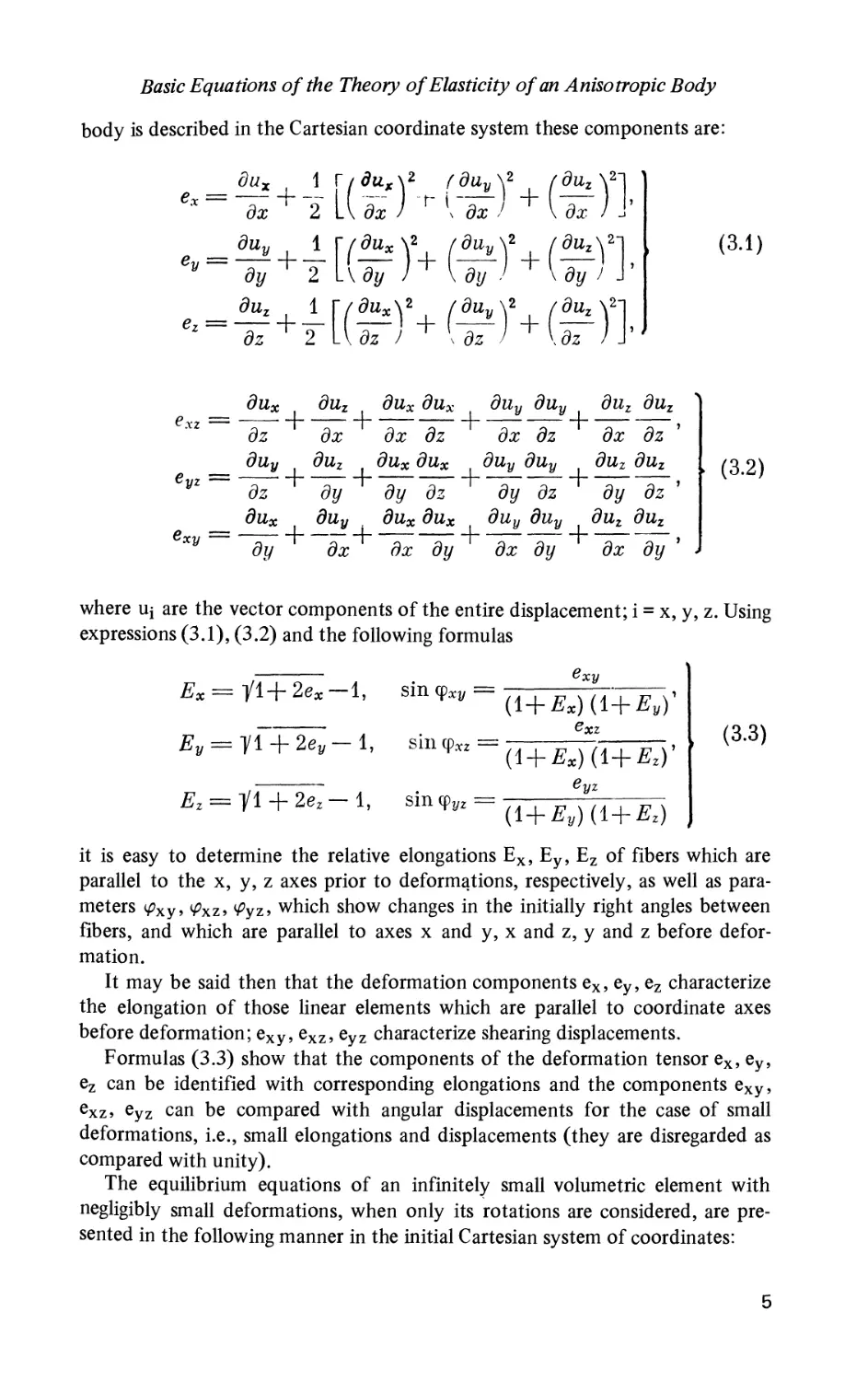
All stresses, both normal and tangential, are positive provided they act along
positive directions of the corresponding external normals while being applied to
an area element with positive external normals (Figure 1).
For a given solid body in equilibrium, the equilibrium conditions in Cartesian
coordinates are represented by the following three differential equations:
дх ду dz
дх ду dz
+
дх ду
dz
B.3)
where Px = Px(x, y, z), Py = Py(x, y, z), Pz = Pz(x, y, z) are projections of the
body force (as related to a unit volume) along the directions x, y, z.
A differential equation of motion of the solid body in the Cartesian system of
coordinates x, y, z is obtained when inertial terms
d2uz
~dt2'
(p is the material density; t is the time) are added into the right hand side of
B.3).

Basic Equations of the Theory of Elasticity of an Aniso tropic Body
tf £ </• 0 jo
r
2
'm
Figure 1.
Figure 2.
Let the solid body be referred to a cylindrical coordinate system г, 0, z, with
the z axis coinciding with the z axis of the Cartesian coordinate system, the
radial coordinate being measured within the plane z = constant from the origin О
of the Cartesian system of coordinates, and the в angle being measured from the
x axis which is assumed to be a polar axis (Figure 2).
Displacements of any point M(r, в z) are presented in the following way in
the cylindrical coordinate system:
Ur = u>r(r, 0, z),
u& = uo(r, 0, я),
Uz = Uz(r, 0, Z),
B.4)
where ur is the displacement in the direction of the radial coordinate r, u@) is
the displacement which is normal to the coordinate plane Orz, i.e., in the direc-
direction of the coordinate в; uz is the displacement in the direction of the
coordinate z.
In the cylindrical coordinate system the deformation components er, e#, ez
represent relative elongation for coordinate directions г, в, z, and e0z, erz, е1в
represent shear deformations within coordinate planes r = constant (within a
plane tangent to the coordinate surface r = constant), в = constant and z =
constant.
The deformation components er, ee,..., е1в are related to displacements ur,
%, uz by the equations:
dur
ez =
duz
диъ 1 диг
dz r d$
duz dur
erz = ~T г ~Z i
dr dz
диг
B.5)

Theory of Anisotropic Plates
A stressed state in the cylindrical system of coordinates is described by a
stress tensor with components ar, r0r, rzr; ов, т1в, rz0; az, rrz, tQz acting on
area elements normal to the coordinate directions г, 0, z respectively. The
symmetry property is expressed here by тв1 = т1в, rzr = rrz, rz0 = r0z.
The equilibrium equations in this case are represented as
dgr 1 0тн> дтГ2 огг-а» д = Q
dr r d§ dz r *
B.6)
where R = R(r, в, z), 0 = G(r, 0, z), Z = Z(r, в, z) are projections of body force
as referred to a unit volume in the coordiante directions r, 0, z.
When the right hand sides of equations B.6) are replaced with inertia terms
dt2' dt2' ' dt2 '
the differential equations of motion of the solid medium in the cylindrical
system of coordinates r, 0, z are obtained.
3. Finite Deformations [ 3 ]
The non-linear theory of elasticity, or as it is often called the theory of finite
deformations, differs significantly from the classical (linear) theory of elasticity
due to certain geometric properties contained within it.
The basic difference is that the theory of finite deformations takes into
account the difference between the geometry of the deformed and the un-
undeformed states.
It is known that the deformed state may be described by different methods in
the theory of finite deformations. The deformed state here is described with the
assumption that the accepted system of coordinates is material and travels with
the body as it undergoes deformation. The (numerical) coordinates of points
under consideration in the undeformed system coincide with coordinates of the
deformed system. For example, if in the system of Cartesian coordinates for the
undeformed state any point M has coordinates x, y, z, then the system of
coordinates in the deformed state becomes curvilinear, generally speaking. How-
However, the curvilinear coordinates of the point M remain unchanged, i.e.,x = x,'y
= y, z*= z (sign ~ indicates the deformed state). This descriptive method of the
deformed state is known as the Lagrangian method.
The tensor components of finite deformations characterize the deformations
in the theory of finite deformations. In the case when the undeformed state of a

Basic Equations of the Theory of Elasticity of an Anisotropic Body
body is described in the Cartesian coordinate system these components are:
ex =
dx 2
dx
n dx '
fy ' 2 Ufy У ' \dy ) f Uy ; У
duz 1 r/^wx\2 /duy\2 /duz^2
Z ~~~ о ' olio / • ' о / • \ n
^2 1 \-\ dz J \ dz / V az
C.1)
duz дих дих duv duv
. _| 1 1
dx dx dz dx dz
duz duz
dx dz
duy duz dux dux duy duy duz duz
dz dy dy dz dy dz dy dz
dux duv дих дих duy duy duz duz
dy dx dx dy dx dy dx dy
C.2)
where Uj are the vector components of the entire displacement; i = x, y, z. Using
expressions C.1), C.2) and the following formulas
Ex = У1+ 2ex —1, sin <pxy =
Ey = yi + 2ey — 1, sin <pxz =
Ex)(l+Ezy
Ez = ]/l + 2ez — 1, sin cpyz =
"yz
C.3)
it is easy to determine the relative elongations Ex, Ey, Ez of fibers which are
parallel to the x, y, z axes prior to deformations, respectively, as well as para-
parameters <pXy, <pxz, <pyz, which show changes in the initially right angles between
fibers, and which are parallel to axes x and у, х and z, у and z before defor-
deformation.
It may be said then that the deformation components ex, ey, ez characterize
the elongation of those linear elements which are parallel to coordinate axes
before deformation; exy, exz, eyz characterize shearing displacements.
Formulas C.3) show that the components of the deformation tensor ex, ey,
ez can be identified with corresponding elongations and the components exy,
exz> eyz can be compared with angular displacements for the case of small
deformations, i.e., small elongations and displacements (they are disregarded as
compared with unity).
The equilibrium equations of an infinitely small volumetric element with
negligibly small deformations, when only its rotations are considered, are pre-
presented in the following manner in the initial Cartesian system of coordinates:

Theory of Anisotropic Plates
dux \ dux t dux
б Г/ дих \
дх L\ дх /
д \(л
V
диь
дх
L дх ду ' \ 5z У J
where ax,.. ., ryz are the stress components along the directions of the local
axes of the curvilinear system of coordinates, which in the case of small defor-
deformations form the axes of the Cartesian system rotated with respect to the initial
axes x, y, z due to deformation; Pj(i = x, y, z) are the components of body
forces along directions of the initial coordinate axes x, y, z.
Let the solid body be related to the cylindrical coordinate system г, в, z (see
Section 2) before deformation. Then the deformation components are:
и, 1 [/дщ>
i (dUr
+ {
дп 2

Basic Equations of the Theory of Elasticity of an Anisotropic Body
(Continued) g i g ,
1 / диъ . \ диъ , 1
т г № дг г
г \ дЪ г 1 дг г дг д® '
1 duz ди® 1
диг \ дщ 1 duz duz
+
г \вь V dz ' 7 до fc>
диг duz диг диг ди® du$ duz duz
dz дг дг dz дг dz dz дг '
C.5;
where, as usual, Uj (i = r, 0, z) are the vector components of the displacement in
the direction of r, 0 z.
The equilibrium equations in the initial cylindrical system of coordinates are:
д г/ , диг*
д \(л
dUr\ .
4 (dUr
(
( i
"~ " d® l г rv l dz
dz L dr
dur\ , 1 / dur \ , dur
dz
duz^
диг\ 1 I дщ \ диг
C.6)

Theory of Anisotropic Plates
In this case ar,. . . , tQz are the stress components along the directions of the
local axes of the curvilinear system of coordinates, which in the case of small
deformations form the axes of the cylindrical coordinate system, which is ro-
rotated with respect to the initial cylindrical coordinate system г, 0, z according to
the rotation obtained as a result of deformation; R, 0, Z are the components of
body forces along directions г, fl, z of the initial coordinate system.
By disregarding all non-linear terms in C.1) — C.6) it is easy to obtain from
them the corresponding equations of the linear theory, i.e., equations B.2) -
B.6).
When corresponding inertial terms are added to the equilibrium equations
C.4) and C.6) the equations of motion of the solid medium in the case of finite
deformations are obtained.
4. Generalized Hooke's Law [4, 5]
This book concerns only those deformations for which the generalized
Hooke's law is valid.
Equations for the generalized Hooke's law for a uniform elastic body can be
expressed in the following way in an arbitrary orthogonal system of coordinates
x, y,z:
eXy =
where aik are the elastic constants (deformation coefficients). In the general case
the number of independent elastic constants is equal to 21 because aik = aki-
The elastic potential for a unit volume element is:
_ 1 2
V = - + ( + + + + ) +
aX + tyz {ai&XzX + aktfxy) + -^ аъьхгх + xaX + flt
D.2)
On the basis of D.1) V can be represented in the following form:
V = ~(oxex + ayey + ozez + xyzeyz + xzxezx + xxyexy). D.3)
z
The strain energy of a whole body is determined by integrating V over the
entire body volume:

Basic Equations of the Theory of Elasticity of an Anisotropic Body
D.4)
If there is symmetry in the internal structure of the anisotropic body mate-
material, then certain elastic symmetry is also present in its elastic properties, i.e.,
there are symmetric directions in the body with respect to which the elastic
properties of the material are identical. When the anisotropic body possesses
such elastic symmetry the equations of the generalized Hooke's law are simpli-
simplified. Below, some important cases of such elastic symmetry are described.
1. One elastic symmetry plane. Let each point of the body have a plane with
any two directions symmetrical with respect to it which are equivalent in
their elastic properties. The equations of the generalized Hooke's law are
then presented as follows, on the assumption that the plane of elastic
symmetry at each point of the body is parallel to the coordinate plane
Oxy:
D.5)
ex =
ez =
eyz =
eXz =
exy =
The number of independent elastic constants a^ in this case is reduced
to thirteen.
Equations D.5) can be represented in terms of engineering constants:
eV —
V21
1 V23 T]2,12
G G +
V31 __ V32 1 , -I-,**
ez — ~Б~ Ох ~Б~ °у "i" ~W~ Oz ~t~ ~n Txv»
_
eyz —
Л
^23,31
Ji31,23
, Л12,2 , T|12,3 , 1
-j —~ Gy -f- —— Gx -f- —— Xxy.
D.6)

Theory of Anisotropic Plates
Here E-, = Ex, E2 = Ey, E3 = Ez are the Young's moduli along principal
elasticity directions x, y, z, respectively; G23 = Gyz, G13 = Gxz, G12 =
Gxy are shear moduli which characterize angular changes between princi-
principal directions у and z, x and z, x and y;^<i2 ~pxy> vi\ =pyx> ^13 =vxz>
^31 = ^zx> ^23 = ^yz> ^32 = ^zy are the Poisson's ratios which characterize
the transverse contraction (expansion) during tension (compression) in
the direction of coordinate axes (the first index shows the direction of
contraction or expansion, the second index indicates the direction of the
acting force); ju23j31 = Му2,гх,Мз1,23 = ^zx,yz are Chentsov coefficients
which characterize the shear strains within planes parallel to the first
referenced coordinate plane which are produced by shear stress parallel to
another coordinate plane (for example, juZXjyz characterizes the shear
strain within the plane parallel to Ozx caused by the stress ryz); 1?121 =
riXy)X, 1?122 = r?Xy,y> t?12j3 = T?XyjZ are the coefficients of the reciprocal
effect of the first kind which characterize shear strains within planes
parallel to the first referenced coordinate plane due to normal stresses
(for example, i?xyx characterizes a shear strain within the plane parallel
to Oxy which was produced by the stress ax); 1?112 = i?xxy, 1?212 *
%,xy> *?3,12 = ^xy are coefficients of the reciprocal effect of the
second kind which characterize elongations in directions parallel to the
first referenced coordinate axis and which are produced by shear stresses.
(For example, i?ZXy characterizes elongation in the Oz direction caused
by the stress rxy).
2. Three planes of elastic symmetry. Let three mutually perpendicular
planes of elastic symmetry pass through each point of a body. By
assuming that these planes are perpendicular to corresponding coordinate
axes x, y, z at each point the following equations of the generalized
Hooke's law are obtained:
ex =
eu = a\2Ox + a22Oy + агзстг, ezx = a$sxzx, I D-7)
ez =
The number of independent elastic constants a^ is nine in this case.
Equations D.7) can also be represented in terms of engineering con-
constants:
_ 1 _Vi2 _^Vl3 g =_Lt
V
V21 V23 _ 1
— ox — — oz, ezx — — r2X,
1 V31 V32 1
е* = — oz — — ox — — Oy, exy = — xxy
& ft & ^
D.8)
10

Basic Equations of the Theory of Elasticity of an Anisotropic Body
The following equalities exist because of the symmetry of equations
D.7).
E2V21 = #ivi2, E3V32 — E2V23, EiVi3 — E3x3i. D.9)
A body which has three mutually perpendicular planes of elastic
symmetry at each point is called the orthotropically anisotropic or ortho-
tropic body.
3. A plane of isotropy. If a plane in which all directions are equivalent with
respect to elastic properties passes through each point of the body, then
the equations of the generalized Hooke's law for a system of coordinates
with the z-axis normal to this plane are:
ex = a\[Ox + а\2ву + а\зО2, eyz =
ey = п\2Ох + ci22<Jy + #13O"Z, exz = a44TXz, > D.10)
ez = а>1з(ох + Oy) + аззО, exy = 2 (аи —
The number of independent elastic constants in this case is five.
Equations D.10) can also be represented in terms of engineering con-
constants as follows:
1 v v' 1
j-, ^x j-, *-> у j-pf ^li "yz \^f
v 1 v' 1
% = — V, Ox
= -- %
xy.
D.11)
G
The following equalities exist because of the symmetry of D.10):
v"Ef = v'E. D.12)
In equations D.11) and D.12) E designates the Young's modulus for
directions within the isotropy plane; G = E/2(l + v) is the shear modulus
for the isotropy plane; E' is the Young's modulus for the direction per-
perpendicular to the plane of isotropy; G' is the shear modulus for planes
normal to the plane of isotropy; v is the Poisson's coefficient which
characterizes the contraction within the plane of isotropy for forces
applied within the same plane; v' is the Poisson's coefficient which charac-
characterizes contraction within the plane of isotropy due to forces in the
direction perpendicular to it; v" is the Poisson's coefficient which charac-
characterizes contraction in the direction perpendicular to the plane of isotropy
due to forces within the plane of isotropy.
11

4.
Theory of Anisotropic Plates
The body with the above elastic properties is called transversely iso-
tropic.
In this case of elastic symmetry the direction perpendicular to the
isotropy plane and all other directions within this plane are principal
directions.
Complete symmetry, the isotropic body. All directions in an isotropic
body are equivalent and any plane passing through any body point is a
plane of elastic symmetry. The equations of the generalized Hooke's law
are:
[ ( + )L
E
1.
exy
D.13)
Here E is Young's modulus; v is the Poisson's coefficient; G = E/2 A + v)
is the shear modulus. There are two independent elastic constants.
Cylindrically anisotropic bodies are also of interest and are discussed in
this book in addition to rectilinearly anisotropic bodies.
A body with cylindrical anisotropy possesses the following elastic
properties. A straight line 7 which is the axis of anisotropy is always
referred to for the case of cylindrical anisotropy (this line may be either
inside or outside of the body). All directions which cross the axis of
anisotropy at right angles are equivalent; all directions which are parallel
to the axis of anisotropy and all directions which are orthogonal to the
first two are correspondingly equivalent.
Equations of the generalized Hooke's law for a body with cylindrical
anisotropy of the general type, in the cylindrical coordinate system г, 0,
z, with the z axis coinciding with the axis of anisotropy, are presented in
the form:
er =
D.14)
The number of independent elastic constants is 21.
Special cases of anisotropy with different types of elastic symmetry
are also possible in the case of cylindrical anisotropy. For example, if
three planes of elastic symmetry are present at each point of the body,
then one of them is normal to the axis of anisotropy, the second passes
through it, and the third is orthogonar to the first two. In this case
12

Basic Equations of the Theory of Elasticity of an Anisotropic Body
equations D.14) will take the form of equations D.7) (witrrtltffefent
indexes for stresses). The body is called orthotropic with cylindrical
anisotropy in this case.
Equations of the type D.7) for the case of cylindrical anisotropy can
also be expressed in terms of engineering constants:
vrz
eo = —- — crr + — o> — -— az, erz = 77—
£Lr &$ tiZ Lrrz
Vzr Vrf 1 1
ez = — — crr — —- сто + -— az, ero = ——
D.15)
where Er, Ee, Ez are Young's moduli for the principal elasticity directions
г, в, z, respectively; G0Z, Grz, Gr0 are shear moduli which characterize
the angular changes between principal directions в and z, r and z, r and в;
vie 5 ^0r> ^rz> ^zr> ^0z> ^ze are Poisson's coefficients (the first index shows
the contraction (expansion) direction, the second index shows the direc-
direction of the acting force).
Equalities analogous to C.9) also exist here because of the symmetry:
= ErVr0, EzVzr = ErVrz, EzViQ = EbXQz. D.16)
In this case the number of independent elastic constants is nine.
Equations of the generalized Hooke's law in the cylindrical coordinate
system can also be presented in a similar way for other cases of elastic
symmetry.
The equations of the generalized Hooke's law are also valid for finite
deformations in the case of small elongations and shearing strains in com-
comparison with unity. The equations of the generalized Hooke's law describe
in this case the linear relation between components of the deformation
tensor ejk and stress components according to the directions of the local
axes of the curvilinear system of coordinates. This relation does not
depend explicitly on Lagrange coordinates. The body is uniform with
respect to curvilinear coordinates, i.e., the body under consideration is
curvilinearly anisotropic. This means that the mechanical properties of
the body material in any local system (axes) of curvilinear coordinates is
described identically. The principal anisotropy axes change directions
from point to point, in accordance to direction changes of axes of the
local system.[6]
5. Transformation of Elastic Constants Due to Rotation of Coordinates [7]
In order to solve certain problems in the theory of elasticity of an anisotropic
13

Theory of Anisotropic Plates
body, it is necessary to know the values of elastic constants for some system of
coordinates x', y', z', when the elastic constants in another system of coordi-
coordinates x, y, z are known.
Consider now a generalized state of plane stress of an anisotropic plate. Let
the plate material have only one plane of elastic symmetry at each point which is
parallel to the coordinate planes Oxy and Ox'y'. Let the coordinate systems (x,
y, z) and (x', y', z') be produced from each other by rotating the system at some
angle <p around the common z-axis.
For this case the following transformation formulas for the elastic constants
are obtained:
an = an cos4 ф + B«i2 + «ее) sin2 ф cos2 ф + «22 sin4 ф +
+ (#16 cos2 ф + «26 sin2 ф) sin 2<pr
, /
0,22 = an sin4 ф + B«i2 + «ее) sin2 ф cos2 ф + Я22 cos4 ф —
— (aie sin2 ф + Яге cos2 (p)s'm 2фv
d\2 = («Ц + «22 — 2«12 — «66 ) Sin2 ф COS2 ф + «12 +
+ — («26 — «к) sin 2ф cos 2qv
«ее = 4 («и + «22 — 2«i2 — «ее) sin2 ф cos2 ф + «ее +
+ 2 («26 — «1б) sin 2ф cos 2qv
[1 1
«22 sin2 ф — «u cos2 ф + — B«i2 + «бб) cos 2ф sin 2ф +
+ «16 cos2 ф (cos2 ф — 3 sin2 ф) + «26 sin2 ф C cos2 ф — sin2 ф),
#26 = I «22 cos2 ф — an sin2 ф — — B«i2 + «бб) cos 2ф sin 2ф -f-
L Z J
+ «i6 sin2 ф C cos2 ф — sin2 ф) + «26 cos2 ф (cos2 ф — 3 sin2 ф).
The following invariant relationships should also be mentioned:
«11 + «22 + 2«i2 = «u + «22 + 2«i2, «66 — 4«J2 = «66 — 4«i2.
In the particular case of an orthotropic plate with principal directions of
elasticity which coincide with the directions of the coordinate axes x and у and
with the principal elastic constants which are known, it is easy to find the elastic
constants of the rotated system of coordinates x'y'z. The following formulas are
available to accomplish this:
/ cos4 ф / 1 2vi \ r r sin4 ф
«11 = — h I 77 77- ) sinz ф cosz ф H ^, E.1)
/ sin4 m /1 2v2
Я22= -ТГ---1
14

Basic Equations of the Theory of Elasticity of an Aniso tropic Body
1/1 2vi\ 1 . ,
j \g - ж)cos 2ф Isin 2ф> E-5)
n2<p- E-6)
Three additional formulas are needed for this special case of an orthotropic
plate:
/ cos2cp sin29
^44 = -7; h-^—, E-0
«55 =
/1 1 \
«45 = ( 77- ) sin ф cos ф. E.9)
There are also the following invariant relationships:
E2 Ei Ei E2 Ei
1=> EЛ0)
G' f E/ G+
In equations E.1) - E.7), the following notation has been used:
Vl2 = v2, V21 = vi, (E\v2 = E2v\), G12 = G. E.11)
This notation will be used for the remainder of the book.
6. Elastic Constants for Some Aniso tropic Materials
Among the many types of existing anisotropic materials only some non-
crystalline materials which are widely used in industry are discussed here. In-
Included in this class of materials are natural wood, rolled metal sheets, concrete,
paper, delta wood, plywood, fabrics, different structural plates, etc. As a first
approximation it is assumed that the materials under consideration are uniform
and orthotropic. The principal directions of elasticity coincide with the coordi-
coordinate lines x, y, z.
15

Theory of Anisotropic Plates
Natural wood. Disregarding the nonuniformity and the curvature of
annual rings, natural wood reveals three planes of elastic symmetry: one
of these, Oyz, is normal to the wood fibers; the second, Oxy, is parallel to
the plane of annual layers, and the third, Oxz, is orthogonal to the first
two.
The numerical values of elastic constants for pine are taken from the
work by A. L. Rabinovich and are [8]:
E1 = 1 • 105 kg/cm2 ; E2 = 0,042 • 105 kg/cm2;
^2 = 0.01; ' G12 = 0.075 • 105 kg/cm2.
2. Delta wood. Delta wood is a layered wood material which is produced by
a hot pressing of the wood stack consisting of a great number of layers
impregnated with resin. Assuming that the x-axis coincides with the
dominant direction of fibers the following numerical values for averaged
elastic constants are available[9]:
Ел = 3.05 • 105 kg/cm2; E2 = 0.467 • 105 kg/cm2;
p2 = 0.02; G12 = 0.22 • 105 kg/cm2.
Plywood. A sheet of plywood is layered and anisotropic. However, as a
first approximation it can be assumed that plywood also represents a
uniform orthotropic material. By assuming that the x-axis coincides with
the direction of the external fibers the following data are available for a
three-layer plywood 1.0-5.0 mm thick[10]:
E, = 1.2 • 105 kg/cm2; E2 = 0.644 • 105 kg/cm2;
v2 = 0.044; G12 = 0.072 • 105 kg/cm2.
4. Glass laminate. Glass laminate is an anisotropic laminated plastic which
consists of glass cloth impregnated with resin. However, it is assumed as a
first approximation that the glass laminate is a uniform anisotropic
material. Assuming that the x-axis coincides with the direction of the
glass cloth basis, the following data are available for the glass laminate C
- 10 mm thick) made of polyester acrylate 911-MS-KhO and the glass
cloth T-, (GOST8481-57)[11]:
16

Basic Equations of the Theory of Elasticity of an Anisotropic Body
E1 = 1.37 • 105 kg/cm2; E2 = 0.9 • 105 kg/cm2;
G12 = 1.22- 105 kg/cm2.
Fiber-glass reinforced plastics. Fiber-glass reinforced plastic AG—4s is an
anisotropic laminated material which consists of oriented glass fibers im-
impregnated with resin. It is usually produced in the form of bands of
different widths by continuous methods. Individual items from this
material are produced by extrusion.
Assuming that the x-axis coincides with the direction of higher rigidity
the data available for this material are[12]:
E, = 2.1 • 105 kg/cm2; E2 = 1.6 • 105 kg/cm2;
v2 = 0.07; G12 = 0.42 • 105 kg/cm2.
6. SVAM. SVAM is an acronym for glass-fiber anisotropic material made of
glass veneer sheets impregnated with resin. For this case we also consider
that we deal with a uniform anisotropic material as a first approximation.
On the assumption that the x-axis coincides with the direction of the
majority of glass fibers the following data are available for SVAM E mm
thick with a ratio of glass fibers 1:5) made of epoxy resin ED-6 and glass
veneer sheets 0.35 - 0.4 mm thick[13]:
E, = 3.05 • 105 kg/cm2; E2 = 1.88 • 105 kg/cm2;
v2 = 0.12; G12 = 0.49 • 105 kg/cm2.
7. Concrete. Concrete acquires anisotropic properties because of the method
with which it is produced and cast. The numerical values of the elastic
moduli of light concrete are[14]:
, = 1J08 • 105 kg/cm2; E2 = 0.81 • 105 kg/cm2.
Paper. In general all types of paper sheets are anisotropic. For example,
values for the semi-Bristol paper produced by the Goznak plant with a
density of 160 g/m2 are[ 15]:
E, =30.1 - 103 kg/cm2; E2 = 22.6 • 103 kg/cm2;
v2 = 0.23; G12 = 9.96 • 103 kg/cm2.
17

Theory of Anisotropic Plates
REFERENCES
1. Lekhnitskii, S. G., Theory of Elasticity of an Anisotropic Body. Gostekhizdat, 1950
2. Novozhilov, V. V., The Theory of Elasticity. Sudpromgiz, 1958
3. Novozhilov, V. V., Fundamentals of the Non-Linear Theory of Elasticity. Gostekhiz-
Gostekhizdat, 1948
4. Lekhnitskii, S. G., See Reference 1, pages 15 - 62
5. Rabinovich, A. L., "Elastic Constants and the Stability of Anisotropic Materials".
Trudy TsAGI, No. 582, 1946
6. Novozhilov, V. V., See Reference 2, pages 145 - 152, 174 - 178
7. Lekhnitskii, S. G., See Reference 1, pages 33 - 48
8. Rabinovich, A. L., See Reference 5, page 15
9. Rabinovich, A. L., See Reference 5, page 15
10. Rabinovich, A. L., "Calculation of Tension, Shear and Bending of Orthotropic Lami-
Laminated Panels". Trudy MAP, No. 675, 1948
11. Arasin, Ya. D., "Glass Laminates Made of Polyester Acrylate Binding Materials". Glass
Laminates and Other Structural Plastics, Oborongiz, 1960
12. Baev, L. V. and Malinin, N. N., "Elasticity and Creep of Glass Laminates AG— 4s".
Plasticheskie massey, No. 7, 1964
13. Ashkenazi, E. K., "Anisotropy of Mechanical Properties of Glass Laminates". Lenin-
Leningrad Center of Scientific and Technological Propaganda, Leningrad, 1961
14. Karapetyan, K. S., "The Effect of Anisotropy on Concrete Creep Deformation". Iz-
vestiya AN Arm SSR, Seriya fizikomatematicheskikh nauk, v. X, No. 6, 1957
15. Chebanov, V. M., "Stability Studies of Thin-Walled Shells With the Use of Paper
Models". Inzhenernyi Sbornik, v. XXII, 1955
18

CHAPTER II
GENERAL THEORY OF ANISOTROPIC PLATES
1. Initial Principles and Assumptions of the General Theory
Consider an anisotropic plate of uniform thickness h. The plate material
obeys the generalized Hooke's law A.4.1) and has only one plane of elastic
symmetry at each point which is parallel to the plate middle plane (plates with a
more general anisotropy are not considered in this book). The middle plane in
this case is equidistant from two parallel planes which form the upper and lower
surfaces of the plate. In addition, for the case of finite plate dimensions, the
plate, in the general case, is also restricted by some cylindrical surface С with
components which, for the undeformed plate, are normal to the plate middle
plane.
Let the plate be loaded by surface forces which cause both in-plane and
bending deformations.
On the assumption that the plate middle plane coincides with the coordinate
plane Oxy and the coordinate z-axis is directed as shown in Figure 3, the general-
generalized Hooke's law for this plate can be represented in the form A.4.5) or A.4.6).
The theory of anisotropic plates suggested here is based on the following
assumptions [1,2, 3,4]:
(a) The displacement uz which is normal to the plate middle plane does not
depend on the z-coordinate;
(b) the shear stresses rxz and ryz or the corresponding deformations exz and
eyz change according to a given law with respect to the plate thickness.
The first assumption, in fact, coincides with the corresponding assumption of
the classical theory[5], while the second is new and allows investigation of the
phenomena related to transverse shear.
19

Theory of Anisotropic Plates
2. Base Equations and Identities
Considering the assumptions (a) and (b) we assume, in fact, that
ez = 0, B.1)
Xxz =
h(z)ff(x,y),
Y+-Y'
h
B.2)
where X+(x, y), Y+(x, y), and X (x, y), Y (x, y), are tangential components of
the force vectors applied to the external plate planes (z = Vih, z = -Vih); <p(x, y)
and ф(х, у) are arbitrary functions of the coordinates x and у which are to be
determined; fj (z) is the function which characterizes the variation of shear
stresses rxz and ryz with respect to the plate thickness. In addition fj (±h/2) = 0
(Figure 4).
Figure 4.
It is not difficult to see from B.2) that tangential stresses rxz and ryz satisfy
the following boundary conditions of the plate:
at z=~ rxz = X+,ryz =Y+
at z= -^
=-Y"
Solving the generalized Hooke's law equations A.4.5) for the stresses ox,oy,
rxz> Tyz> rxy5 one obtains:
ax = Bnex + Bi2ey
oy = B22ey + B
txy = B66exy
Xyz =
— A\oz,
+
B.3)
B.4)
B.5)
B.6)
B.7)
20

General Theory of Anisotropic Plates
where
Q
a12a26-
ai2a6(
011066 — <
Q
2
— «12
Q
Я44
,
@
Q
B.8)
со =
«45
,
—
+
2 2
— «22^16,
«55
CO
2
a45,
Л2 =
B26U23
Using B.1) and the equalities A.2.2)
ez = -^ = 0,
= w(x,y),
B.9)
B.10)
B.11)
B.12)
i.e., just as in classical theory the displacements uz for all points along a given
normal plate element (the elements normal to the plate middle plane) are equal
to the normal displacement w of the cbrresponding point of the middle plane.
From equations A.4.5) and B.2) we have the following formulas for the
transverse shear deformations exz and eyz
eyz = 044/2E)^ + Я45/1 B) Ф + 044 Yi +
where
: #55/1B)9 +
the following
X,
*2
notation is used:
x+-x-
2 '
5X1 + Тг
Yt =
(^44^2 + а45л2),
- («55-^2 + «45^2) ,
Y+—Y-
2 '
B.13)
B.14)
B.15)
B.16)
From equations A.2.2) with consideration for B.12)
dux dw
oz dx
duv
dw
B.17)
21

Theory of Anisotropic Plates
Integration of the expression B.17) with respect to z from zero to z with the
condition that for z = 0, ux = u(x, y) and uy = v(x, y), the following values for
the inplane displacements of any point in the plate are obtained:
Ux= U — Z-
дх
^45^2), B.18)
— v — z- \- 044/02^
o, x-~-. f «45X2), B.19)
where
г г
/и = J /iB)dz, /02 = J h{z)dz, B.20)
о о
u(x, y), and v(x, y) are inplane displacements of the corresponding point of the
middle plane.
Equations B.18) and B.19) show that the inplane displacements ux and uy
of any point of the plate located at a distance z from the middle plane along the
normal have, in the general case, a non-linear dependence on z, which is contrary
to the classical theory of plates.
Substituting values of ux and uy from B.18) and B.19) into A.2.2) we
obtain expressions for the corresponding deformation components:
da d2w dcp dty
ex = z — + «55/01 — + «45/02 7; г
дх дх- ч дх дх
du d2w
ду ду2 ду ду
dXt\ z2 I dY2 0X2
5T- +— («44—? + ^
— + «45T +— («44+ a45-^
ду ду J 2п\ ду . ду
B.22)
ди ди d2w I дф дц) \
вху = ~ Ь ^- — 2Z + /oi ( «55 -г- + «45 — ) +
ду дх дх ду \ ду дх /
/ д^ дур \ Г dXt dYi 1 dY{ t dXi \1
+ /02 ! «44 -~ + «45 -z- ) + Z \ пъъ — h «44 ~7 \~ «45 ~ V ~ )
\ dx dy J L ду dx \ dy dx /J
z2 Г dX2 dY2 (dY2 dX2
dy dx ' V dy ' dx /j
22

General Theory of Aniso tropic Plates
Substituting values of rxz and ryz from B.2) into the third equilibrium
equation A.2.3) in the absence of body forces (Pz = 0), as well as considering
the equalities B.15) and B.16), and integrating with respect to z, the expression
for normal stress oz is obtained:
дх
ду
\ dx
ду I
дХ2
dY2
B.24)
where x(x, y) is the integration constant (with respect to z) and is determined
from conditions on the plate surfaces which are of the following type:
at
h
at , = -_
oz = —
B.25)
The following expression for x(x, y) satisfies these conditions:
+
dtp +
h
as well as the following equation:
where the following notation is used:
2/'
B.28)
Z+-Z~
B.29)
Equation B.27), which is presented in terms of the functions <p and ф, is
obtained as a result of satisfaction of conditions on the surfaces B.25). It is also
considered as the third equation of equilibrium[6]. This will be self-evident from
equations C.3), B.43) and B.47).
Substituting values of ex, ey, exy and az into formulas B.3) — B.5),equa-
B.5),equations are obtained for the principal stresses ох,ау,тху:
23

Theory of Anisotropic Plates
du dv [ du dv \
+ В + Bj— + — I-
+ Вп + Bj— + — I
ox dy \oy dx I
дх* ду* ' 1°дхду
l_ dx
{
/02 I (a45#n + auBie) ~ + (auPi2 + a^B^ + Ai) ^* 1 -
- Лix
z2 Г / 3-X2 дУ2\1
— fiufli + Bi2R2 + 516Й3 + Л! -—- + ^ , B.30)
2hl \ dx dyl\
fiufli + Bi2R2 + 516Й3 + Л! + ^
2hl \ dx dy
dv du / da dv \
Oy = B22-—Ь Bi2 -—h B1Q ( -—[-_-) —
dx2 dxdy/
J02 («44^22 + «45^26 + A2) — + («45 ^12 + ^44^2б) ~^ 1 +
L dy dx J
Г дф дф 1
/oi («45^22 + а55В2б) — + («55^12 + «45^26 + A2) -— —
L аг/ га J
B26Q3 + Л2
dx dy
(^ ^y^ , B.31)
du dy / du dv \
rTy = BiQ —- + -S26 ——h -О66 I -—r — ) —
dx dy \dy dxJ
/ d2w d2w d2w \
~~" z\ Butt + Bw— + 2J566 ) +
\ dxu dy1 dx oy /
+ 2J566 )
dy1 dx oy /
+ /01 Г (Я55#16 + ЯиРы + А3)-^ + («45^26
L га
+ /02 Г (а45516 + а44^бб) ^ + («44^26
L d^:
[
Bi6Q
d-^ + d-^^ ; B.32)
d d / J
24

General Theory of Anisotropic Plates
where the following notation is used:
dXt , 6Yi _ dYi , dXi
Qi = a55 — + a45 —, Q2 = au—+ ai5 — ,
ox ox oy oy
(dYt.dX,
+ ( Ь
dX,
Qz = аЪъ ~ h «44
\ аг/ ox '
B.33)
дХ2
дх
дХ2
«45
0Y2
дх
0Y2
_
0X2
dY2 (dY2 дХ2\
дх \ ди дх /
B.34)
Equations B.2), B.24), B.30) - B.32) are the laws for stress variation
through the plate thickness. However, just as in the classical theory, it is con-
convenient to replace the stresses with statically equivalent stress resultants and
moments acting over small areas of the normal plate cross sections.
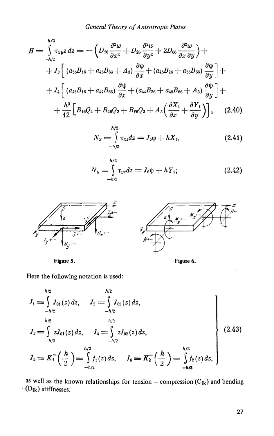
Using basic equilibrium relationships for internal normal and tangential (Tx,
Ту, S = Sxy = SyX) and transverse (Nx, Ny) forces, as well as for bending (Mx,
My) and torque (H = Hxy = Hyx) moments for unit lengths of the middle plane
we obtain (see Figures 5 and 6):*
/1/2
-Л/2
+ h
Г
L
ди
дх +
а^пц
ди
12 ду
ду
*~^Л^ дх~
, (да
/16\ду
■ + (а^В
\-ди\ +
дх 1
12 + «55
1б)¥-
+ a44Bie) -~ + («44^12 + «45^16 +
ox
-2-
oy
B.35)
^Editor's comment: Note the difference between the usual English notation
where Nx, Ny, Nxy designate the normal and tangential inplane stress resultants
(as opposed to Tx, Ty, S used herein) Qx and Qy designate the transverse stress
resultants (as opposed to Nx, Ny used herein) and Mx, My, Mxy designate the
bending and torque moment resultants.
25

Theory of Aniso tropic Plates
Л/2
~ dv „ du „ I du
4dzCnp + C
_m dy dx
h
Г(«44^2 + а^Я* + A2)^ + (ai5Bi2
L dy
Л Г (а45522 + а5ЪВ26) |i + (а55Я12 + «45^26 + At) p-] -
L аг/ ox J
+ ±L [B22R2 + 5,2^! + B26R3 + At(^ + ^\\, B.36)
Л/2
f , du dv „ I du du \
= Xxydz = Cie— + C2e— + Cee( — + -r-) +
_l/2 dx dy \dy dx)
[dw dwl
(ab5Bi6 + а.ьВее + A3) -^- + {акъВ2Ь + а555бв) ~ +
dx dyJ
+ h \ (a,5Bi6 + auB66) p. + (а44526 + а,ъВт + A3) 51 -
L dx dy J
^ + d-Il \1 , B.37)
dx dy / i
) +
o,r r/z = - (Da^2+Di2^
\ d2 dy2
_h/2 * — дУ2 'dxdyj
[dw dw 1
(auBu + ai5Bi6 + At)-?- + (ai5Bi2 + a55Bi6) J- +
+ Л I (ouBu + auBi6) ^ + (а44512 + aaBu + ^i) ^1 +
L ox dy j
(^~ + ^ I, B.38)
/2
My= \
-Л/2
d2w d2w d2w
dx2 ' dxdyl
4- //{ («44^22 + Я45#26 + i42) y1 + (^45^2 4" «44^26) ~^
dwl
2) jL J
A2) j
)], B.39)
26

General Theory of Aniso tropic Plates
Л/2
# =
-Л/2
d2w d2w
5y
' дхду
)
dq> dw~\
A3) -£■ + (ai5B2e + а5ЬВт) j- | +
+ «44^66) -i + (^44^26 + «45^66 + АЯ) -- +
ах ау J
5е6^3 + Л,(^ + ^)]. B-40)
h/2
-h/2
h/2
B.41)
B.42)
-Л/2
4-
Here
the
Л/2
•■■ ur-
Figure 5.
1
f/lb-b-
following notation is used:
= 5 Joi(z)dz,
-h/2
h/2
Л/2
h = j /021
-Л/2
/1/2
) zJoi(z)dz, h = ) zJ02{z)dz,
-h/2 -ft/2
Л/2
Figure 6.
Л/2
, 76 = /ГГ (— ) =
-h/2
-X
B.43)
as well as the known relationships for tension — compression (C^) and bending
(Dik) stiffnesses;
27

Theory of Anisotropic Plates
Cik = hBtk, Dih = -£ Bih. B.44)
Integration of each equation of equilibrium in A.2.3) excluding the presence
of body forces, with respect to z within z = -h/2 to z = h/2 and multiplication of
the first two equations of A.2.3) by z within these same limits excluding again
the body forces, and integrating this result with respect to z within the same
limits, the following five plate differential equilibrium equations, as expressed
with respect to the eight internal stress and moment resultants Mx, My, H, Tx,
Ty, S, Nx, Ny, are obtained:
B.45)
дх ду
£ ^=-y* B.46)
дх
ду
dNx
B.47)
дх ду
^ + Nx~hXu B.48)
^ + NxhXu
дх ду
дМу дН
-~ + -^- = Ny-hYi. B.49)
ду дх v
Surface boundary conditions have been used in the derivation of equations
B.45) - B.49).
3. Equations of the Deformed Plate Surface and Boundary Conditions
It is evident from equations B.35) — B.42) that the internal stress and
moment resultants of the plate are expressed in terms of displacements u, v, w
and functions which arise in the expressions for the transverse shear, </?, ф. These
five functions can be shown to satisfy a system of differential equations of tenth
order.
Substituting the values of the internal stress and moment resultants Tx, Ty, S,
Mx, My, H, Nx, Ny into the equilibrium equations B.45) - B.49) the following
tenth order system of differential equations of the deformed plate are obtained:
La (Cik) и + Li2 (Cik) v + JiLitp +
ду
h2 h2 ( д д
— (L,X2 + Li2Y2) + — (— LikX2 + — L{iY2 J
У C.1)
28

General Theory of Anisotropic Plates
L22 (Cfk) v ~t~ ^12 (Cik) м ~\~ J2L2ty -\- J\L2{ty -f-
Л. д л. д
ду * to
r~v2 + —
= -—(Ьг¥2 + Ь*Х2) + — >
24 12 \5^
LiS(Dik)w — .
h3 Г
= -l2LJ
L23 (Dik) w — JJ^ — J
д
с/л:
д
— Л —
5 1
— L14y4
ду J
/6\|; —
д
—
ду
д
—
дх
.-У2,
C.2)
C.3)
C.4)
C.5)
where the following notations are used for linear operators:
k) = С a —— + 2Ci6 —-—
дх2 дх ду
L2
д2
д2
22
22
C
d2
ду2
д2
66
(С12
дхду
C.6)
Li3(Dik) = Dn-^-
дх3
д3
L23 (Dik) = D22-—
ду3
д3
—
ду3
дх2ду
д3
—-—
ду2 дх
д3
д3
дх ду2
д3
■(Z?12+2ZN6)-^^+z?16-
C.7)
29

+. [«45 (Bi2 + Bee
Theory of Aniso tropic Plates
d2
д2
d2
L2 = («44^22 + «45^26) —
д2
d2
— ,
д2
Li2 =
d2
д2
L2i = (a45522 + «55^26) -j-y
6) + 2a45526]
d2
д2
~дх21 J
C.8)
д д
= A2— -\-Az-.
oy ox
C.9)
_ д д
дх дух
Equations C.1) — C.5) comprise the complete system of five differential
equations with respect to the undetermined functions u, v, w, у,ф. Once these
functions have been obtained and also using the equations from Section 2 of this
chapter it is not difficult to compute basic stresses and internal stress and
moment resultants.
The functions u, v, w, </?, ф should satisfy both the system of differential
equations C.1) —C.5) and the boundary conditions on the cylindrical surface С
which forms the plate edge.
We assume for simplicity that the plate edge passes along the coordinate line
x = 0, i.e., the surface of С represents the plane x = 0.
It is known that the uniform boundary conditions can be written in the
following manner for the case of a three-dimensional problem in the theory of a
thick plate [7, 8]:
(a) free edge
txy
(b) simply-supported edge
= 0,
= 0,
= 0,
т« = 0;
uz = 0,
h2 = 0;
C.10)
C.11)
30

or
General Theory of Anisotropic Plates
(c) rigidly-fixed edge
ux = 0, uy = 0, uz = 0,
ux = 0, xxy = 0, uz = 0.
C.12)
The boundary conditions C.10) — C.12) cannot be fulfilled at each point of
the boundary surface С in the case of arbitrarily selected functions fj(z). Due to
this fact only "relaxed" boundary conditions are considered.
The principle of "relaxed" boundary conditions is justified by the theory
suggested here, by St. Venant's principle, and by the methods used for enforcing
actual boundary conditions.
The theory suggested in this book as well as all other improved theories of the
same ckss[97 Щ^гШ define more accurately the state of stress in the plate only
дt^QrIle_ШsJдn£e_fmnl „the Jbounclary. In other words, tfaey do not produce
jgijable information about the boundary соМШоп^дпД^
frjom the рщпХМ=ШЖ of the three-dmensional ргоЫ
. &eyj>rth£less* it should be emphasized that tljexdo define the principal
sM£JEJit3^^ classical theory[10, 11,12, 13]
On the basis of the above, the "relaxed" boundary conditions of the problem
(for the edge x = 0) to be used in place of C.10) - C.12) are:
(a) free edge. Considering equations B.35) - B.42) and C.10)
h/2
axdz = Tx =
oxz dz =MX = 0,
-h/2
h/2
-h/2
h/2
xxzdz = Nx =
-h/2
xxyz dz = H = 0.
C.13)
(b) Simply-supported edge. Using equations B.12), B.35) - B.40)
and C.11) we have either:
h/2
j axdz =
-h/2
h/2
xxydz
-h/2
h/2
Tx = 0, \ oxz dz = Mx = 0, uz = w = 0,
-h/2
h/2
5 = 0, J xxyz dz = H = 0,
-h/2
C.14)
31

Theory of Anisotropic Plates
or by assuming [14] in C.11) that the condition uy = 0 is satisfied only for z =
±z0 @ < z0 < h/2) we have the following expression from the second line of
C.11):
/i/2 h/2
J oxdz = Tx = 0, jj gxz dz=Mx = Q, uz = w =
-Л/2 -h[2
У +
(Zq)
dw K2
— — +044
д 2
^ + ai5
W<P + 7^- (auY2 + «45^2) = Or
Ki (*„) ,
or
(c) Rigidly-fixed edge. Just as in the case of the simply-supported
edge, we assume that conditions C.12) are fulfilled only for z =
±z0 @ < z0 < h/2) and because of B.12), B.18), B.19) and
C.12):
Ux | z=±zo = 0, Uy\ z==±zo = 0, W = 0,
2
7ГГ
«45^2)
^(auYt + a*
20)'\|? = 0» wz = и; = 0,
«44^2
dw Ki (z0)
ф
^1 (^o)
= 0,
f 0 = 0,
C.15)
^ (zo) , ,
■ + a44 — ф + a45
У 7.7n
The second conditions for a rigidly fixed edge on the basis of the second line
in C.12), proceeding as in preceding cases, are:
dw
(z0) cp
(z0)
)
Ф
20)ф + — («55*2 + «45^2) = 0,
uz = w = 0,
^ (ZO) ,
2z0 T ' "^ 2z0
h/2 h/2
:xydz = 5 = 0, jj xXyZ dz = II = 0.
-"/1/2
C.15')
32

General Theory of Anisotropic Plates
Mixed boundary conditions can also be presented as well as the uniform
boundary conditions C.13) — C.15):
(a) Loaded edge:
TX = T«, Mx = M*, Nx = N*9 S = S\ H=H\ C.16)
where T*x .... , H* are forces (stress resultants) applied to the edge under
consideration; in particular cases some of these stress resultants could equal zero.
(b) Simply-supported edge under the action of stress and moment
resultants:
ТХ=Г, MX=M*, w = Q, S = S\ H = H'; C.17)
(c) Displaced edge:
2 (z0) -ф +
2 '
~
dw
—
dx
dw
(zQ)
2z0
Ф
K2 (z0)
^
w = w
i>+ + v~
2 '
u+ — u-
(z0)
КГ
045*1) =
'7+ — 7;-
2z0
C.18)
where w* is the given normal edge displacement, u+, u , v+, v~ are given inplane
displacements of the edge which correspond to z = ±z0. In particular some of
these specified displacements could equal zero.
О
Figure 7.
Figure 8.
33

Theory of Anisotropic Plates
Many types of plate supports are encountered in actual structures and a
multiplicity of boundary supports for actual plates cannot be represented with
sufficient accuracy with the present mathematical models and boundary condi-
conditions. Due to this fact only a few possible combinations of boundary conditions
have been given here.
In the general case it is assumed that the plate edge is curvilinear and has an
external normal n (Figure 7). Then the internal stress and moment resultants
with respect to the curvilinear edge (Figure 8) can be written as follows:
Tn = Tx sin2 * + Ty cos2 * + 2S sin * cos *,
Snt = 5(sin2* — cos2*) + {Ty — Tx) sin*cos*,
Nn = TV* cos * + Ny sin *,
Mn = Mx sin2 * + My cos2 * + 2# sin * cos *,
Hnt = Я (sin2 * — cos2 *) + (My — Mx) sin * cos *,
For normal and tangential displacement components of any point of the plate
edge within a plane parallel to the middle plane, we have:
un = ux sin * + uy cos *, unt = Uy sin * — ux cos *.
On the basis of the above relationships, the following uniform boundary
conditions for the curvilinear edge of the plate can be stated:
(a)
Tn =
(b)
Tn =
or
Tn--
(c)
Free edge
0, Mn =
= 0,
Simply-supported
0, Mn =
= 0, Mn
Rigidly fixed
= 0,
= 0
edge
Nn
edge
Snt
w
= 0,
= 0,
' = 0,
Snt = 0,
Hnt = 0,
Unt 1 Z=±Zq
Hnt =
= 0;
0; C.19)
0, C.20)
C.20')
a<i|z-±ze = 0, unt\z=s±Z0 = 0, w = 0, C.21)
or
un|z=±Z0 = 0, Snt = 0, tfn, = 0, M7 = 0. C.21')
The mixed boundary conditions for the curvilinear edge may be presented
similarly to conditions C.16) - C.18).
Assuming that a44 = a55 = a45 = 0, A1 = A2 = A = 0, X+ = X~ = Y+ = Y~ = 0
in the equations and formulas given in the second and third sections of this
34

General Theory of Anisotropic Plates
chapter and performing certain necessary transformations, the equations and
identities of the classical theory of anisotropic plates are obtained[15]. These
simplifications will be used below and each time the corresponding equations of
the classical theory of plates will be obtained.
У V
4. Selection of the Functions f j(z)
One of the principal steps in the improved theory of anisotropic plates pre-
presented in the previous sections involves the selection of the functions fi(z).
It is evident from the results of certain researchers[ 16,17] that some in-
inaccuracies which are allowed during the selection of the functions fi(z) do not
have a major influence on the final results as computed at a distance from the
boundaries. Arbitrariness in the logical selection of the functions fj(z) cannot
introduce inadmissible errors into the suggested theory. This is amply illustrated
on appropriate examples in Section 2 of Chapter III and in Section 6 of Chapter
IV.
However, the selection of the functions fi(z) should preferably be based on
the analysis of the shear stress distribution rxz and ryz using the sufficiently
accurate theories of the bending of thick plates[ 18-22]. This analysis shows that
tangential stresses rxz and ryz for the case of thick as well as thin plates have a
parabolic distribution.
It is of interest to note here that in the solution of the plane bending problem
of a strip fixed at one end[23] the shear stress rxz (which varies at the fixed end
according to a complex law) is smoothed out at a distance of h/5 from the fixed
end and at a distance of h/2 the distribution is parabolic.
Following the above discussion and considering that we are interested in this
book in transverse bending of plates and in phenomena related to transverse
bending of plates, it is assumed that
1 / h2 \
f(z) = ft(z)=k(z) = --(--*) . D.1)
From D.1), B.20), B.28) and B.43) we obtain
z / h2 z2\
Jo = ЛI = ЛJ = ~( — —у , Ji — ^2 — 0,
Kt = о.
However, while considering D.1) for f(z), we do not deny the possibility of
selecting other logical distributions for the functions fi(z).
35

Theory of Anisotropic Plates
5. Equation of the Deformed Plate Surface and Boundary Conditions
(Continuation of Section 3)
For the case when the plate is made of an orthotropic material and the
direction of the x, у and z axes coincide with the principal directions of elas-
elasticity the governing equations of the problem are simplified.
Considering equations A.4.7) - A.4.9), the elastic constants of an ortho-
orthotropic material are:
1
«зз = —,
_ i 1
7Г > «22 — -ТГ »
Vl2 V21 V2 Vl
«12 РГ t-T 7-» ^ '
Vi3 V31 \'23 V32
«13 = — "=--7Г,. «23 = — = --- ,
JI3 tLi Ьз Lj2
1
1
1
E.1)
#44 — , «55 = — , «66 — ,
(-JT23 ^13 Cri2
«16 = 0, «26 = 0, a36 = 0, «45 = 0.
Substituting these values of aik into B.8) - B.11), we obtain the coefficients
k and A4:
«22 Ei _ «и Ег
1 — V1V2'
«12
1
«66
A1 =
1 — V4V2 1 — VlV2 '
1
«55
V13 + V2V23
1 — V1V2
Vl = V21, V2 = Vl2,
-S44 = ^23,
«44
_ £1
+ # i2«23 — p;
E
£3 1 — V1V2
V31 V13 + V2V23
V13 1 — V1V2
/?2 V23 + V1V13 V32 V23 +
£3 1 — VlV2 V23 1 — V1V2
A3 = 0,
o = «11«22 — «12.
E.2)
On the assumption that X± = 0, Y± = 0 (the case when the plate is loaded
only by a normally applied force Ъ- is of great practical interest) and consider-
considering D.1), D.2) the following system of differential equations is obtained from
equations C.1) - C.5) for the orthotropic plate:
ох1 оу2
J^- = Axh^-. E.3)
дхду дх v
36

General Theory of Anisotropic Plates
„ d2v d2v д2и dZt
C22 h C66 h (Ci2 + Cee) = A2h , E.4)
ду2 дх2 дхду ду
ду dty 12
ftz ду Ы
^]^=-^fi, E.6)
^l + ^^-^45A E.7;
дхдуJ 12 10 Зг/
For the internal stress and moment resultants, and for the stresses, we obtain
equations corresponding to the system E.3) — E.7) from equations B.35) —
B.41) and B.30)-B.32).
du dv
Tx = Cu — + Ci2 — -hAtZu E.8)
дх ду
dv du
Ty = C22 — + Ci2 hA2Zu E.9)
ду дх
<M0>
„ d!w d2w h2 f ^ d(f „ dty \ h2
Mx = -Du — - Di2 -— + — [atsDu / + auPa-J- ) -777
dx2 ду2 10 \ дх ду 1 10
d2w ^ d2w li2 ( _ 5ib „ dw\ h2
= -£>22 _ - Di2 — + — • a44^22 ^- + a55Z>i2 ■^-)- —
ду2 дх2 10 V ду дх/ 10
E.11)
дхду 10 \ ду
7,3 /,3.
E.12)
E.13)
E.15)
37

Theory of Anisotropic Plates
/ du d2w \ / du d2w \ z / h2 z2\
Gu = Bool —• Z | + В\Л —• Z I + — I IX
"- \ dy dy2) \dx dx2) 2 V 4 3 /
E.16)
+ £* +(
ду dx dxdy 2 \ 4 3
E.17)
Equation E.5) and the values of the elastic constants given at the beginning
of this section were used in the derivation of equations E.3) — E.7) and the
identities E.8)-E.17).
A close examination of C.1) - C.5) and E.3) - E.7) reveals that the
complete system of differential equations C.1) — C.5) can be divided into two
independent systems. These systems are equations E.3), E.4), which represent
some generalized plane problem (which is of no interest to us) and the equations
E.5) - E.7) which represent the problem of transverse bending of the plate.
The general theory of anisotropic plates presented in preceding sections of
this chapter and at the beginning of this section can be somewhat simplified.
Only the transverse bending problem of orthotropic plates will be considered.
As opposed to the basic theory, one additional assumption is used in addition
to the initial assumptions (a) and (b) (see Section 1). Namely, the normal stress
az on areas parallel to the middle plane is considered negligible with respect to
all other stresses.
Formally this assumption is equivalent to A-, = 0, A2 = 0. Using this result
and the equalities E.11) — E.17) we obtain the following expressions for in-
internal moment resultants, transverse stress resultants, and stresses:
d2w
dx2
d2w
dy2
on
Z/V6
iz dx2 '
^2a? ( /г2
° Зж 5у 10
v—{?'•'■
/г2
10
10
-^-O E.18)
dy I
d\b \
^) E.20)
d2w
38

General Theory of Anisotropic Plates
d2w z f h2 z2
+ (
z f h2 z2 \ ( дф d\b \
-( — -—)BJan^+au-^). E.24)
2 V 4 3 V ду дх)
+ ( )BJan^
дх dy 2 V 4 3 V ду
Finally, from equations E.5) — E.7) a complete system of three differential
equations with respect to the three undetermined functions w, у, ф is obtained:
0<p ftp 12
OQ 7 0 r"
2Dee) —^-—Г ^
da; <9z/2 10 L d^2
^ + a44 (ZI2 + Dee) -^ J + _ ф = 0, E.26)
d3w ^ d3w h2 Ф
+ (/? + 2D) auD22 -± +
h3
d3w h2 Г #2Ф
2Dm) —— - — auD22 -±
ду дх2 10 L дг/2
h
-^ = 0. E.27)
We assume that
w=
— j |_ {в№Ри + а44Дбб)
^] ^}Ф, E.28)
ф = (l5 a" iAlZ>66 ^ + (Z>llZ>22Z)l2Z>66 ~ ^S
ГЛ2 Г дъ
К 10 L #£Г
дъ 9 дъ
+ (DD 2DD Dh
ТТЛ +
ду3дх2
39

Theory of Anisotropic Plates
which identically satisfy equations E.26) and E.27). And from E.25) a dif-
differential equation of sixth order with respect to the undetermined function Ф =
Ф(х, у) is then obtained:
12 h2 ( d6 2
7 Т7Г i аььРhDqq —— -f- [^44 {DaD22 — 2Di2DsQ — Di2
h6 10 v dxb
d6
T7T + [M#iiA>2 - 2Z?i2Z>66 -
де д6 Л 144
D6e] —— + a55D22D66 — ^Ф = —- Z2. E.31)
dyk dx2 dyQ ) h6 ;
Thus, the problem of transverse bending of an orthotropic plate is reduced to
the determination of some potential function Ф(х, у) which satisfies the dif-
differential equation E.31) and boundary conditions given in Section 3 of this
Chapter.
Substituting values of w, <p, ф from E.28), E.29) and E.30), respectively,
into E.18) - E.24), it is quite straightforward to represent internal stress and
moment resultants and stresses through the undetermined function Ф. These
formulas are not given here because of their length. In general, it is easy to find
all desired values of these quantities from equations E.18) — E.24) and E.28)
— E.30) when values of the function Ф are known.
A close examination of the derivation of equations E.18) — E.31) shows
that analogous equations for the bending of a plate with a more general (as
opposed to orthotropic) case of anisotropy can be derived from B.30) — B.44)
and C.1) - C.8) if we assume that A, = 0, A2 = 0; A3 = 0.
It can be shown that in this case we are inconsistent in the exlusion of normal
stresses az. The fact is that a correction to the theory of nondeformable nor-
normals, which is introduced by the consideration of stresses az, is approximately
of the same order as the correction which is introduced by the consideration of
transverse shears, and this latter correction is still taken into account when we
assume that A-j = 0, A2 = 0. This inconsistency will not introduce inadmissible
errors in the majority of actual problems, as has been demonstrated before
[24, 25] and will be further shown in this book.
6. Particular Theory [27-29]
An additional theory is presented in this section which is more accurate than
the classical theory of bending of anisotropic plates made of material which has
only one plane of elastic symmetry which is parallel to the plate middle plane.
It is assumed that the plate is acted on by only loads applied normal to the
40

General Theory of Anisotropic Plates
plate middle plane Z± ф 0 (X± = 0, Y± = 0).
This theory is based on the following assumptions:
(a) the displacement uz which is normal to the plate middle plane does
not depend on the z coordinate;
(b) it is considered that for the determination of deformations the shear
stresses rxz, ryz and the normal stress az do not differ from the
corresponding stresses found with the use of the hypothesis of non-
deformable normals, i.e., from the corresponding stresses of the classi-
classical theory of bending of anisotropic plates.
On the basis of hypotheses (a) and (b) we assume the following approximate
relationships:
/ 3 z z3\
ег=0, a2 = Zi+ (----2 —)Z2, F.1)
\ I h n3 /
1 / W \ 1 / /г2 \
Ххг = 1\1 ~ /ф0' T^ = -2VT~~*2/*0' F'2)
where, as is known [30]
<е.з,
1 v~x* ' ~~DU/ дудх2+В{6 дх* J ' F' )
wq is the normal displacement of the corresponding anisotropic plate as found
with the classical theory, i.e., from the differential equation
+ ^
22
and satisfying the corresponding boundary conditions.
Equations B.24) - B.27) as reduced to the classical theory were used here to
determine az. Namely, the equations
yo(zil)-z d<po dfy12
X(x,y)-Zu +
дх ду h3
41

Theory of Anisotropic Plates
as well as the equilibrium conditions on the surface B.25) and the notation
B.29) were used to obtain the result F.1).
Following the usual method (see Section 2) the following expressions are
obtained for the displacement of any point of the plate subjected to bending:
uz = w(x, y), F.5)
dw z / hz z2
»x = - z — + - ^— - —
dw z (h2 z2\
+ ^ j ( + ) F.7)
where w = w(x, y) is the undetermined normal displacement of the middle plane.
From B.3) - B.5) with consideration of A.2.2), F.1), F.5) - F.7) we
obtain for the stresses:
d2w d2w d2w
+ B + 2B
Bit + Bi2 + 2Bi6
ox2 dy2 oxoy
z I h2 z2 \Y
"о (  Г
+
oy
1 (^^ + B(l)
51 (^11^45 + Bi6(lu)
oy ox
—
J
z i
2'
z(b2z
< №
d*w
дуг
z2\["
\D22(X
d2w
1
44 T"
d2w
——
дхду
)
дц>о
-г h
сл:
yj/ J
tjrt/ = —
+ Д«
z / h2 z2 \Г
--( — -—) (Вееаьь + В26а,ь) ^ + (Bmakb + 516a55)
2\ 4 о /L oy ox
—— —
с/г/ J
42

General Theory of Anisotropic Plates
Substituting expressions F.8) - F.10) into B.38) - B.40) we obtain the
following relationships for the bending and twisting moment resultants:
дхг дуг дх ду
h2 Г _ ^Фо ^фо
^16^45) -Т h (-D 12^45 + #16^55) —" '
--^AiZa, F.11)
(d2w d2w дР-w \
Z>22 —2 + />12 -T-, + 2A>6 -r-— )
ду2 дх2 дх ду/
+ — [ (ZW -f- £>26a45) -^?
- -^^2Z2, F.12)
дх ду)
1(J
-J5- - 77тА&. F.13)
c/y J 10
+ (£66a45 + Z?2eau)J 77т
c/a; c/y J 10
Transverse shearing stress resultants can be determined from equations B.48)
and B.49). Substitution of values of the moments F.11) - F.13) into B.48)
and B.49) we have then for these transverse shearing stress resultants:
d3w d3w d3w
дх3 дх1 ду дх ду1 ду3
h2 ( д2
+ Jq | (Dua55 + Оыам) — +
кб(Di2 + Dee) + 2a55Di6]-^— + (£66a55 + D26a,5) -^-}фо
ox oy dy2 )
h2 ( д2 д2
To I(Z?a + D^ + [ (Z) + D) + 2°^
Dm
1-— + Л3-т-), F.14
to ду '
43

[d3w
Theory of Anisotropic Plates
d3w d3w
+3D
[a45 (A2 + Азе
h? ( d2
д2 d2
+ (D + D)
h? ( д2 д2
— {(Dvflu + D26a№) — + [a55 (Di2 + /?) + 2а1>]
^}фо-|(Л2^ + ^^). F.15)
Finally, substituting F.14) and F.15) for Nx and Ny into B.47) a differen-
differential equation of fourth order with respect to one undetermined function is
obtained:
dw dw
Da — + 4ZI6 -—- + 2 (Di2 + 2Dm)
dxk дх3ду д
+ 2 (Di2 + 2Dm)
дх3ду дх2дуг
w dkw h2
+ D Z +
+ D22 Z2 + \ (Diiu55 + Di6a,5)
дхду3 dyk 10 I dx3
i2 + 2D6e) ^
^ +
дх2ду
д3 д3
[«55 (Di2 + 2D66) + З#] + (^ + ^)
TO оЧ OQ
{ (Я + ^) —- + [«45 (Z>12 + 2ZN6) + З^]
ду3
{ (Я22а44 + ^26^45) + [«45 (Z>12 + 2ZN6) + За44^2б] 7^
10 l ду3 ду2дх
[«44 (Z?12 + 2Z)) + З#]
ду дх2
h2 Г д2 д2 д2 1
— —- Ai~— + 2Лз- h^2 Z2. F.16)
10 L дхг дх ду ду~ J
The undetermined function w(x, y) should satisfy not only the differential
equation F.16), for which the left side is the same as the corresponding left side
of the equation of the classical theory, but also the boundary conditions at the
plate edge which, as a rule, have the same form as the boundary conditions of
the classical theory.
Boundary conditions for five principal cases are given below [31]. The edge
for the general case is considered as being curvilinear with normal n and contour
arc s.
44

General Theory of Anisotropic Plates
(a) Free edge
Д/п = 0, Nn + ^=0. F.17)
OS
(b) Simply-supported edge
w = 0, Mn = 0. F.1S)
(c) Rigidly fixed edge
w = 0, »n| z=±z. = 0. F.19)
(d) Loaded edge
Mn = M:, Nn + ^ = NZ. F.20)
OS
(e) Displaced edge
= Un. F.21)
Let us indicate for completeness that the given boundary conditions may be
expanded to some extent (see the examples in the next Section) for this theory.
If the plate under consideration is made of orthotropic material and the
directions of the x, у and z axes coincide with the principal directions of elas-
elasticity, then expressions E.1) and E.2) are valid. Therefore, from F.8) — F.15)
we have the following results for stresses and internal stress and moment resul-
resultants:
(e-22>
&j£hl F-23)
d2w z I h2 z2
+ (
Xxv = -2zBee —— + - ( )( 5^5 -^ + f?66a44 -
дхду 2 \ 4 3 /\ dy d
F.24)
10
Dliab^ + Dl2aJJl), F.25)
10 \ dx dy I
45

Theory of Anisotropic Plates
"To"
D2zaa^ + Di2aJ), F.26)
10 \ dy dx /
<6-27>
F.28)
Finally, from equation F.16) the specialized differential equation for this
problem is obtained:
dw dw дЧп
Du -^ + 2 (Da + Wee) -f^~2 + D22 ^ =
ox* dx2dy2 dyk
h2 Г d3 d3 1
= Z2 + - a55 [Dll — + (Da + Wee) —-J
h2 Г d3 d3
+4^+(Z>+2Z))
^- + Л2^J2- F-30)
In regard to the assumed functions <po(x» У) ^d ^o(x» y)» for tne orthotropic
plate they are
where wq is the normal displacement determined from the solution of the classi-
classical problem, i.e., from the equation
46

General Theory of Anisotropic Plates
l 2г F.зз)
and satisfying the corresponding boundary conditions.
Thus the final expressions for the stress identities and the differential equa-
equation are obtained by substituting values of <po and i//q from F.31) and F.32)
into F.22) - F.29) and F.30). The resulting differential equation
is given here without giving all the cumbersome intermediate equations.
For the given case of the orthotropic plate the boundary conditions remain
unchanged, i.e., the conditions F.17) — F.21) are valid.
It can be noted in conclusion that the equations of the theory suggested here
are in fact equivalent to equations of the first three approximations of the
principal iterational process of A. L. Gol'denveizer [32], which is used to deter-
determine slowly changing states of stress of the plate. Generally speaking, this
process is applied to the entire plate and produces more accurate values of
stresses and displacements at some distance from the line of distortion.
The state of stress near rapid distortions are excluded from consideration in
this particular theory and only the influence on the principal state of stress is
considered, as opposed to the general theory with which it is possible to derive
formally not only the principal state of stress but the boundary stress conditions
as well.
Finally, assuming that A-, = 0 and A2 = 0 in the equations of this section we
obtain all the equations of that improved theory of anisotropic plates which
disregards the effect of the stress oz on the stressed and deformed state of the
plate.
7. Theory of Bending of Plates with Cylindrical Anisotropy
A general and a particular theory of bending of plates with cylindrical aniso-
anisotropy can be obtained in the manner discussed in the preceding sections.
47

Theory of Anisotropic Plates
It is assumed that a plate with cylindrical anisotropy is specially orthotropic
and all radial planes which pass through the axis of anisotropy are planes of
elastic symmetry [33]. In addition, the pole of anisotropy> a point where the
axis of anisotropy intersects the plate middle plane (which is assumed to be
perpendicular to this axis), is the origin of the cylindrical system of coordinates
r0z (see Section 2, Chapter I), and the z-axis is directed along the axis of
anisotropy (Figure 2.).
Finally, we consider the case where fj(z) changes according to a parabolic law
D.1) and the plate is loaded with only normally applied load ЪЦх, в) Ф0,Х± =
0,Y± = 0.
1. General theory. The general theory is derived on the basis of the initial
assumptions (a) and (b) given in Section 1 of this chapter and the basic
equations and identities of the three-dimensional theory of elasticity of
cylindrically anisotropic bodies.
Using assumptions (a) and (b) it is assumed that
ez = 0, G.1)
where <p(r, 0) and ф(т, О) are arbitrary undetermined functions of the
coordinates r, 0.
The method for the derivation of the equations is the same as in
Sections 2 — 5. Therefore, in many instances only results are given with-
without detailed explanations.
Due to assumptions G.1), G.2) and A.2.5) and considering A.4.15)
we obtain for displacements:
u2 = M2(r,fl) = u;(r,0), G.3)
dw z I h2 z2\
ur= u — z — + --(— — — )агф, G.4)
or I \ 4 о /
dw z ,W . . G5)
where w(r, в) is the normal displacement of the middle plane; u = u(r, в)
and v = v(r, в) are the tangential displacements of the middle plane along
coordinates r and в, respectively. On the basis of A.2.5) and using G.3) -
G.5) the following expressions for stresses are obtained, after substituting
the strains er, e#, er# into the generalized Hooke's law A.4.15):
48

Or =
General Theory of Anisotropic Plates
dv и
+
dw
(
2 \ 4
4 <7-e)
G.7)
du dv v
dv v д I 1 dw \
"d~~~ 2¥\7^/
G.8)
where (see A.4.15))
Er
1 _ 1
Brz Grz
Er Vrz +
_
+ VrVr2
EZ 1 —
G.9)
= vr, vr^ = vo.
The last terms in equations G.6) and G.7) appear due to the stress oz
which is determined as before from A.2.6) and the conditions at the
surface B.25).
49

Theory of Anisotropic Plates
Figure 9.
Internal stress and moment resultants (Figure 9.) which are obtained
from the given stresses are:
Fin \
T Г \ Г I "" I \ 7 Л rj
dr
r \ oft
Mr = —Dr Drv& —
ЭГ2 Г\Г
G.10)
G.11)
G.12)
—ф,
—^
G.15)
G.16)
where Dr, De and Cr, Ce are bending stiffnesses and tension-compression
stiffnesses for the directions r and в, respectively; D^ is the torsional
rigidity; Ck is the shear rigidity. These values are expressed in the follow-
following manner:
50

General Theory of Anisotropic Plates
h3 h3 №
Dr=—Br, Д>=—Я*, Dk = ~Bk
Cr ^ hBr, C$ = hBft, Ck = hBk,
= Drvo + 2Z)fe,.
G.17)
and Z-| and Z2 are as given in B.29).
In a manner identical to that used in Section 2, the following system
of differential equations of plate equilibrium for the case X± = 0, Y* = 0,
Z± Ф 0 is obtained from A.2.6), including consideration of the surface
conditions:
дтг l
дг г
Tr -
dS*r
-—-
дг
W= 0,
dNr 1
5a г
dN* 1
iVr = —Л2,
~
G.18)
G.19)
G.20)
G.21)
G.22)
Substituting the values of the internal stress and moment resultants
into the equations of equilibrium, a system of five differential equations
with respect to five undetermined functions is obtained:
/ d2u
\ or1
д2и да
д2и
I dv
дгдЪ
д
—
or
G.23)
dv v
дт г
ди dZ\
=hA2 — , G.24)
51

Theory of Anisotropic Plates
1*|> 12
G25)
I d2w
10 I L dr\dr/ r d№ r
<a, +a.) i-^
Л A A <9
Т2Гф = Л21о22-Л1То^(г22)' G-26)
d3w
(A,
-»„,—*»«*. G.27)
12 T io a*
The boundary conditions do not change, i.e., we have equalities C.19) —
C.21) and the corresponding non-uniform boundary conditions.
2. Particular theory. The particular theory is based on the initial assump-
assumptions (a) and (b) given in Section 6 of this chapter, on the basic equations
and identities of the three-dimensional theory of elasticity, and on some
results of the classical theory of bending of anisotropic plates [34].
The order of derivation of the equations is similar to that given in
Section 6. Therefore, only the final results are given here.
The basic expressions for stresses are:
Or = —
52

General Theory of A niso tropic Plates
z /h? z2\f 1 Л|)„ /Фо
ldw\ z ф ф
G.30)
The bending and torsional moment resultants are:
= —Dr-— — Dr\9-\ 1 )+
dr2 r\ r d®2 Or I
фо \ „ 1 дфо! А
(
r \r
h2 1 dtyo /ф0 5фО\1 /г
L^+M + lJ G'32)
( ) + 77,Ur^+^(f) f G.33)
dr\ rd$/ 10L r^ \ 3r r/J^
The transverse shearing stress resultants are:
[Л1{А1Аш)ъ], G.34)
10 L or r J
53

Theory of Anisotropic Plates
d3w 1 d2w \ 1
/г2
^m_.42i^. G.35)
And finally the basic differential equation of the problem is:
iO \ I \r dr2 dr3 J r2 ddW
/1 ^Фо 1 дуо фо\1 Г 1
+ ^ — --— — — — \- — + ^ flr*-
г3 ^2 г2 дг г3 /J L г
г2 дг дЬ г3 а# /J >
[(Ml^^ + ^ + ^] G.36,
10 L г аг or2 Ho^ J
In all these equations the functions <^o and i//q can be taken as follows:
1 d2 /dw0 wo\
; G.38)
54

General Theory of Anisotropic Plates
where wq is the normal displacement of the corresponding anisotropic
plate as determined from the classical theory, i.e., the solution of the
following differential equation
Л
f1 дтгдЬг
r3 ^r^^2 r2 dr2
+ /)Д^? = ^(^^) G.39)
r6 or
with the corresponding boundary conditions.
All the basic boundary conditions remain unchanged, i.e., we have
F.17)-F.21).
8. Geometrically Non-Linear Theories of Anisotropic Plates
A general and a particular theory are given here for the case that the plate
displacements are of the same size as its thickness h. These theories are applied
to specially orthotropic plates, i.e., plates made of orthotropic material with
principal directions of elasticity coincident with the directions of coordinate
lines.
These theories are presented on the assumption that not only are the elonga-
elongations and shearing deformations small in comparison with unity, but the angles
of rotation of the plate elements are also small with respect to unity [35].
As opposed to the non-linear theory of the very large deflections of plates,
only those non-linear terms are preserved here from the basic equations of the
non-linear theory of elasticity which are due to normal displacement w and its
derivatives. Thus, instead of A.3.1) - A.3.4) we have the following expressions
for the deformations:
_du1, 1 / daz_ \2
6x ~ dx ~2 \dx ) '
duy 1 / daz \2
ey — ~^ г ~ I ~ ) i
dy 2 \ dy 1
duz 1 / duz \2
dz 2 \ dz I
(8.1)
55

Theory of A niso tropic Plates .
дих ды2 duz duz
6xz ~~ 'dz !kc ~dx dz '
diiy duz duz duz
cb о у dy dz
diiy duz dnz
dx dx dy
e*y = —
(8.2)
dy
and the equations of equilibrium without considering body forces are now:
dixz
d / duz
дх\ дх
duz
1
dx dy ' dz
dXxy , dOy , dxyz
dx dy dz
d / du
(8.3)
(8.4)
\ d / duz duz \
' du \ dx du I
duz
о2) = 0. (8.5)
Equations A.3.5) and A.3.6) can be simplified in an analogous manner.
1. General theory [36]. The general theory is based on the basic equations,
(8.1) - (8.5) and the following assumptions:
(a) a normal displacement uz with respect to the middle plane does
not depend on the z coordinate;
(b) shearing stresses txz and ryz or the corresponding deformations
exz and eyz change according to a given function fj(z) through
the plate thickness;
(c) the normal stress oz can be determined from the linearized equa-
equation of equilibrium (see formulas B.24) - B.25) and equation
(8.5)).
For simplicity we considered the case where fj(z) changes according to
a parabolic law D.1), and the plate is loaded only by normally applied
load Z^x, у) Ф 0, X± = 0, Y± = 0.
By accepting assumptions (a), (b) and (c) we assume in fact
duz
—-
= Zl—-( — I — + —4 , (8.6)
(8.7)
56

General Theory of Anisotropic Plates
where <p(x, y) and ф(х9 у) are undetermined functions of the coordinates
x, у and Ъ\ and Z2 are determined from B.29).
From the generalized Hooke's law A.4.7) and using equations (8.7) in
the expressions for transverse shear strains, we obtain:
1 (h% Л l (hZ Л ,
" = 2~VT /а55ф> 6yz = 2\T / п'л^'
(8.8)
On the basis of expressions (8.6) and (8.8) and using (8.1) and (8.2)
we have for displacements:
uz = uz(z,y) = w(x,y),
dw z / h2 z2'
ux = и — z .L I
dx ' 2 V '
dw z
(8.9)
(8.10)
where w = w(x, y), u = u(x, y) and v = v(x, y) are the normal and
tangential displacements of the plate middle plane.
Examination of equations (8.9) and (8.10) shows that the displace-
displacement formulas for uz, ux and uy are identical to the corresponding
formulas of the linear theory of bending of anisotropic plates, i.e., with
formulas B.12), B.18) and B.19).
Substituting values of displacements from (8.9) and (8.10) into the
corresponding expressions (8.1) and (8.2), the following expressions are
obtained
du
dx
du
dy
du
'XV dy
for the
d2w
dx2
" z —о
du
dx
deformations ex, ey
z /h? z2\
' + 2 V 4 s)u
z /h2 z2\
d2w z / Iv
dxdy 2 \ 4
/ ^ф
^ \аьъ ~\- <
\ dy
and exy
^Ф
'55 +
dx
dty
44 Ь
з у
344 dx)
1
2
1
2
1 V
\5x /
U' )'
dw dw
dx dy
(8.11)
Assuming that z = 0 and eliminating displacements u, v, w we obtain
from (8.11) a known equation for the compatibility of the middle plane
[37].
dy2 dxdy dx2
\2 dzw dzw
дх ду i дх2 дуг'
(8.12)
57

Theory of Anisotropic Plates
where
_ du 1 / dw \2 _ dv 1 / dw \2
to 2 \ to / ety 2\dy/
du dv dw dw
у = 1 1 .
dy dx dx dy
(8.13)
From the generalized Hooke's law A.4.7) and using (8.6) and (8.11)
we obtain for the stresses
dw \2
J
du
d2w 1 / dw \21 z I h2 z2
+U) ]+( т - f
2 \ dx
du . dv л d2w . dw dw 1
„ Г du dv
xy = Bqq — [- ——
I du dx
dx dy dx dy J
In a similar manner the internal stress and moment resultants are ob-
obtained:
L
Ой 1 / дш\2
Г do l/div\2~]
L dy 2 \ dy I J
T, =
Г do 1 / dw \2
\^~bi2ldy
\21 . л Г d^ 1 / du;
/ ^a ^г; ^zz; ^zz; \
A- h h -x— — - j
\dy dx dx ay /
1/ dip
~?A !& I ! ' ^дл i dy ' 2 \ ay
J \ C/ t^ >
5 =
(8.17)
(8.18)
(8.19)
58

General Theory of Anisotropic Plates
/г2
10
02w
~дт2~
/
\ пп"
dhv
f
= — ;
л d2w .
ду2
dw
da;
dx dy
h3
^55 ) "
da: /
f 10 A
ф, ^
Jib / dw
1 Ш \dx
h'} / dw
12C)\дх ^
/г3
'~ 12^'
^\
"
(8.21)
(8.22)
(8.23)
It should be remembered that
Z1 = -4^-, Z2 = Z+ + Z- B.29)
Cik = hBik, Dih = —Bih. B.44)
From (8.3) — (8.5) the following plate equilibrium equations with
respect to internal stress and moment resultants are obtained:
+ £0
дх ду
m, , aN, , J/,fc\ a
da; dy dx\ x dx J dy\ dx
dMx dH dMy dH
г- —= A*, ^ b — = Ny. (8.26)
dx dy dy dx
If we assume that
d2F &F dF
^ 5'^V (8'27)
where F = F(x, y) is an undetermined stress function, then equations
(8.24) are satisfied identically and then from (8.17) - (8.19) with con-
consideration of (8.13) we obtain for ex, ey and 7:
59

Theory of Anisotropic Plates
an d2F ai2 d2F
Ex = _ -- + ——- + (an At + ai2A2)Zu
h dy2 h dx2
e =
y
a22
ai262F
+
h dx1 h dyz
d2F
h dx ду '
(8.28)
During the derivation of expressions (8.28) the identities E.1), E.2) and
B.44) were used.
Substituting values of the internal stress and moment resultants from
(8.20) - (8.23) and (8.27) into equations (8.25) and (8.26), and of values
of 6X, €y and 7 from (8.28) into the compatibility equation (8.12) we
obtain
2 +
дх- ду2 дхдудхду dy2 dx2
\2\dx dy
— № + ?*) = - Z2 C8 29)
\2\dx dy)
d3w
+ 2Z)
°3W k2 Г
66) ---r-2- —
dx dy2 10 L
r2 a5bDn+ abj)m^
dx dy2 10 L dxz dy2
04 1 h3 hb I d2w д2\\) \
дуА 12 120 \ dx2 dx dy)
дхду
d3w
h2 Г дЧ)
10 L ^у2
/г3
^ \ +
дхду 1 12
I
+ 2)
/г5
120
— ♦ - i2 — (-т-| + -—J-) = 0, (8.31)
12 120 \^г/2 дхду/
дхду/
/г дх2ду2
ду*
( д2ю
\дхду
\2 52м; <92ы; Г ч 52
I дх2 ду2 L дуг
+ (а22А2 + «12^0 — J Zu (8.32)
Thus, a complete system of four differential equations with respect to
four undetermined functions w(x, y), <p(x, y), i//(x, y) and F(x, y) is
obtained.
The undetermined functions must satisfy the system of differential

General Theory of Anisotropic Plates
equations (8.29) — (8.32) as well as the boundary conditions which,
generally speaking, are of the familiar form C.13) — C.21). Boundary
conditions will be defined more precisely in the next chapter when deal-
dealing with actual problems.
Finally we present the following expressions for the determination of
inplane displacements of points of the middle plane obtained from (8.13)
and (8.28):
w\2 a&F a 62F
/i, (8.33)
ди
дх~~
dv
-~(
2\
ч
dw\2
~а~ ) "г
дх /
•toy
.ду Г
~~h
а-гъ
'Т
d2F
ду1"
d*F
'дх2'
«12
, «12
52/^
"дз?
d*F
ду-
ooA2
When dealing with certain problems it is more convenient to use an-
another system of differential equations in place of (8.29) — (8.32).
When the values of internal stress and moment resultants from (8.17)
— (8.23) are substituted into (8.24) — (8.26), a complete system of five
differential equations with respect to five undetermined functions u, v, w,
</?, ф is obtained:
д2
dx2 ' ^ ^ ' °°' Зд;^ ' °°ау2 ' V - ' "/ дудХду '
+ т— ( Сц —— + Сев т^7 ) == ^i ~,Г~
га \ dx1 dy2 I дх
+ (С12 + Сбб)^^+Св6
дх дх ду ду \ дуг дх2 / ду
h3 (d(f dq\ 3 Г d2w l dw \2 d2w I dw \2]
i2\T+T r~2lCiiw\te) +С22-дТЛ--) r
1 d2w [ dw \2 dw dw d2w
\ d /
Г 1 d2w
L 2 dx2
\ dx / dx dy дх ду
1 d2tv / dw\2l
2 dy2\ dy / J
1 d2tv / dw\2l n г д (dw \ d / dw
dy / J I dx\ dx / dy \ ay
The remaining two equations of this system are not given here because
they are identical to equations (8.30) and (8.31).
The analogous equations for cylindrically orthotropic plates are given
below (see Section 7):
61

Theory of Aniso tropic Plates
For stresses
= вт\
du d2w 1 / dwv
~~dr~~ Z~~dr2 ~2\drJ J
^^+ - + 7-)J , (8.35)
1 d2w 1 dw\ 1 / dw \21
0 / J
ди d2w 1 /dw \2
Г Зу u / 1 d2w 1 dw\ 1 / dw
Lrdft r \r2 d№ r dr ! 2r*\ 50
f 9a 5y i; 5 /dw\ ldwdw}
1Г51Э1 5r г 5r Xrd'&J r dr 50 J
For internal stress and moment resultants:
r 2 \ 5
ди и
Г 1 ди ди v 1 dw дш~\
S*r=Ch\-— + - + _ — _.. (8.40)
Lr 50 dr r r or dft J
- Dr — - Z)rv<> - ( - -— + — ) +
or1 r \r d№ dr I

General Theory of Anisotropic Plates
h1 Г /
10 L \
dw
IT"
dr
1 d\|)
r db
j-AJ-'+l+lll). (Ml,
dw'
(
777
10
^ / ф
D&a> ( — + v' IT )-
\ r dr I
(
120 \ dr
Г d/dw\ /г2 Г 5ф / Зф г|з \Т»
V дг\гд$/ 10 L rflf) \ Зг г 'J'
/г3
(8.42)
(8.43)
(8/i4)
The internal stress resultants Tr, T#, and Sg r can be represented in the
following manner in terms of the undetermined stress function F =
F(r, в):
1 d*F idF
d*F
ldF 1 d*F
r"~^^~7Jr~^- (8-45)
Inplane displacements of points in the middle plane u = u(r, в) and v =
v(r, в) can be determined from the following equations:
du _ 1 / dw \2
^7" ~~~7)
h drz
1 dv и 1 / dw \2 flio / 1
1_ _ = _ _ — ) + _i ( _
r 30 г 2r2\ 30 / /^
«22 d2F
i a/-1-.
(8.46)
Finally, the following system of four differential equations with
respect to four undetermined functions is obtained:
63

d
12 ldr
Theory of Anisotropic Plates
Зг|?1 д Г dw ( 1 32F Si'7 \1
dOJ Or I Or \ r dW dr /J
д V dw / 1 OF 1 32/T \ 1
ieZ_i^l)l+i.(i^^) = _rZ,. (8.47>
r2 d^ г drdti/] dft\r d® dr2 /
д / д2ш\ д I 1 d2w\ / 1 dw 1 d2w
/ 1
\r
г Of}2/ \r ^r r2 d№
г г dfOJ
d3w
ri fi^i r dr d$ I dr2
Обв + 2МХ
ли / 1 З/ 1 di 1 З/ 2 &F \
d2w / 1 dw I d2w\ Г d / 1 dw \12
dr2 \ r dr r2 d№ ) ldr\r дЪ /J
2 3
~-j ^)) Zl = 0. (8.50)
64

General Theory of Anisotropic Plates
The boundary conditions are presented in the usual form, equations
C.19)-C.21).
In the particular case when the effect of oz on the state of stress is not
considered, the basic formulas and principal differential equations may be
obtained from the corresponding formulas and equations by substituting
Ai = 0 and A 2 = 0. In this case the systems of differential equations
(8.29) - (8.32) and (8.47) - (8.50) can be reduced to corresponding
systems of two differential equations with respect to two undetermined
functions. For example, using expressions E.28) — E.30) we satisfy
identically equations (8.30), (8.31) and from (8.29), (8.32) the desired
system of two differential equations with respect to the two undeter-
undetermined functions F(x, y) and Ф(х, у) is obtained. However, this system
will be of ninth order, as opposed to the corresponding eighth order
system of the classical theory.
2. Particular theory [38, 39]. This theory is based on the following
assumptions:
(a) the normal displacement uz with respect to the plate middle plane
does not depend on the z coordinate;
(b) in dealing with deformation it is considered that the shear stresses
rxz and ryz do not differ from the corresponding stresses
determined from the classical theory of bending of orthotropic
plates;
(c) the effect of normal stresses oz is not considered during the deter-
determination of deformations because the stresses oz are considered
to be negligibly small in comparison with the inplane stresses.
If it is desired to account for the effect of az on the deformed and
stressed state of the plate, then the terms with multipliers A1 and A2
from (8.14) - (8.50) should be added to the corresponding formulas and
equations.
By accepting assumptions (a), (b) and (c) we assume in fact that
duz
-r- = 0, (8.51)
oz
Т-*>о, ... - 2U
(8.52)
65

Theory of Anisotropic Plates
where wq is the normal displacement of the corresponding plate as deter-
determined from the classical theory, i.e., from the following system of
equations
дх2ду2
d2w0 02F0 9 dhoQ 02F0 d2w0 d2F0 _
дх2 ~Ъ7у2 дхду'дхду "ду^^дх2" ^'
, , , о 1 d'Fo , 1 dF0
Л дх2ду2 h dyk
/ ^2ш0 \2 d2w0 d2w0 _
~\дх~ду) +~дх^~д^2~~ J
and the corresponding boundary conditions.
In this system of equations Fq(x, y) represents the stress function
which expresses the internal stress resultants of the classical theory in the
following manner:
^у2 Зж2 дхдг/
First we determine the displacements of any point of the plate:
uz = w(x, y), (8.53)
dw z f h2 z2 \
' U-x = —z ~1, 1 XT — («55ф0 + «45^0) , (8.54)
дх 2 \ 4 о '
dw z / h2 z2 \
и = —z —— -)—- —— — -— I (a44\ho + я45фо), (8.55)
ду 2 \ 4 3 J
where w = w(x, y) is the undetermined normal displacement of the plate
middle plane.
For stresses we have
Г да дЧи 1 / dw \21
z i , ( )
Idx дх2 2 \ дх / J
17)- (8'56>
66

. General Theory ofAniso tropic Plates
Гди d*w l/dw\*l
Oy = #22 — — Z -— + ( — ) +
L dy dy2 2 \ dy I J
du d2w 1 / dw \2
у —
dx2 ^ 2\dx
Г du d2
£ —_ z
Lax dx
z (h2 z2
77 ( - - T
2 \4 3
ду
dy dx dx dy dx dy J
2 72 \
Tx =
2
i2
г + r
dy 2
cco\
Ox /
2 \4 3/ \ dy dx I
The internal stress resultants and moments are:
(8.58)
(8.59)
g2w
d'-w
£1 ^jjl/66
d*w
dx dy
/du
\dy
+ 10 V
1 io V
1 Ю д
dv
~дх +
^11^55
^22^44
36 (^53
3w;
3^
3^
3i|}(
dy
Зф
dj)
;
j /7 ■ ■
3\f
44 r?x
/'
).
/•
(8.60)
and from equation (8.26) we obtain the transverse shear resultants:
Nx = -
xdy2]
... 32 З2 \ А2 #2^
■ -77,^55 /)ll -Г-;- + Dee -T~ фО + — ^44 (/>J2 + ^66) -—;— ,
10 x Зх2 ду*) 10 dxdy
N» = —
d3w
1 °o/ 3^/3x2.
Л2 / З2 32 \ h2
a44 Z?22—+ Z?ee— )^o + —«55(^2-
67

Theory of Anisotropic Plates
From the formulas for internal forces (8.59) — (8.61) it is evident that
the correction terms for the classical theory involve only the moment and
transverse shear resultants, while the non-linear terms are present in only
the inplane stress resultants Tx, Ty and S, and these non-linear terms have
the same form as the classical theory.
On the assumption that I
(8.62)
rp rr
дхду'
where, as before, F = F(x, y) is the undetermined stress function which
satisfies the equilibrium equations (8.24), we obtain from (8.59) after
considering (8.13):
aiz
a22
ai2 dF
/г 9ж дг/
(8.63)
From (8.25) with the use of (8.26) to eliminate transverse stress resul-
resultants Nx and Ny we obtain:
дх*
■+2
Лг дг/ дг/2
д
дх
dw
ду \ дх
(8.64)
When values of ex, ey and У from (8.63) are substituted into (8.12)
and the values for the moment and inplane stress resultants from (8.60)
and (8.62) are substituted into the equilibrium equation (8.64), a system
of two differential equations with respect to the two undetermined func-
functions w = w(x, y) and F = F(x, y) is obtained:
[ d'iF 1 d'*F 1 d^F
b(^66 + 2ai2) h #n —
г dxk h дх2 ду2 h dyk
d2w d2w
у d>-w d2w
дхду ) дх2 ду2
дх2 ду2
22"
68

General Theory of A niso tropic Plates
d3
дх2 ду1 дх ду дх ду
10
ы
~10
h% Г д3
—-а44 \D22—-- + (Di2-
10 L ди3
дх ду9-
д3
дудх1
(8.66)
It is evident upon examining (8.65) and (8.66) that equation (8.65) is
completely identical to the corresponding equation of the classical
theory, and the left hand side of equation (8.66) is identical to the
corresponding left hand side of the equations of the classical theory. The
right hand side of equation (8.66) contains a correction to Z2 which can
be easily derived, provided the solution to the classical problem under
consideration is known.
It should be remembered that the boundary conditions in this particu-
particular theory, generally speaking, are the same as the boundary conditions of
the classical theory [40].
The equations of the non-linear particular theory for the case of cylin-
cylindrical anisotropy are not given here because they can be easily derived by
analogy. It is necessary only to remember equations G.30) - G.35) and
(8.35)-(8.50).
9. Theory for the Analysis of Two-Layer Orthotropic Plates [41, 42]
Consider a two-layer orthotropic plate made of two uniform orthotropic
materials. The planes of elastic symmetry of each layer are mutually perpendicu-
perpendicular. One of these planes at each point of every layer is parallel to the external
parallel planes of the plate, and the remaining two are perpendicular to the
coordinate lines x = constant, у = constant.
We assume that the coordinate plane Oxy coincides with the intersection
plane of the layers and is thus also parallel to the external planes of the plate
(Figure 10.).
Figure 10.
69

Theory of Anisotropic Plates
It is also considered that the layers displace together along the intersecting plane
and remain elastic.
The following assumptions are used in this theory of two-layer plates:
(a) a displacement uz in each plate layer which is normal to the plate
middle plane does not depend on the z coordinate;
(b) in the determination of deformation it is considered that shearing
stresses тх^9 Ty^are the same as the corresponding stresses (т£Ь °}
rm'z°) found with the assumption of nondeformable normals for
the entire plate as a whole;
(c) the effect of normal stresses oz is not considered during the deter-
determination of deformation because oz is negligibly small in com-
comparison with the inplane stresses.
Similar assumptions are found in many works [43—47]. Using assumptions
(a), (b) and (c) we assume in fact that
еГ= О, (9.1)
m,0 1 2 _,4 \T>rg
= Ххг — —-^(Om — Z2) Д11
Z L
дх* ' х ' даяду* J
, @.2)
where uq = uq(x, у), vq = vq(x, y), wq = wq(x, у) are tangential and normal
displacements of the intersection plane in the case of classical theory, respec-
respectively; m is the number indicating the layer number. It should be noted that for
the first and second layers when m is used as a superscript on the value under
consideration, we use one or two prime signs instead of m = 1 or m = 2.
Furthermore, in the expressions (~l)m, and only in those expressions, m is
considered as a power.
Examination of (9.2) and (9.3) shows that the determination of tangential
stresses is reduced to the determination of displacements uq, vq and wq. These
displacements are determined from the system of three differential equations
[48,49]:
70

General Theory of Aniso tropic Plates
Ll2 (Cik) v0 — L13 (Kik) w0 - 0,
Ll2(Cik)u0 — l23(Kik)w() = 0,
Z/13 (if *л) Щ — Z/23 (ifift) г;о = ^2,
(9.4)
where the linear operators are defined to be:
д2 д2
L&{Cih) = ^'22 —- + Сбб -т-r
Li2(Cik) = (C12 + Сбб)——" ,
dxdy
Li3(Kik) = Яи ^ ^
ду3
ду дх2
(9.5)
(9.6)
(9.7)
(9.8)
(9.9)
I- (91°)
— + D22—
The following notation is used for the stiffness terms:
Cik =F2Bih +6i Bih) щ (9.11)
Zik = -F;B&-6?B'ih), (9.12)
Dih = -gF2Vfc + б!в!к). (9.13)
For the displacements of any point of the m-th layer of the plate (see
Sections 2 and 6) we have:
uz = w(x,y),
(9.14)
С/.Г
m о
m, 0
n, 0 Z т>о
n, 0 Z3 m> о
~TX2 ,
(9.15)
71

Theory of A niso tropic Plates
where u = u(x, y), v = v(x, y), w = w(x, y) are the undetermined tangential and
normal displacements of the intersection plane of the plate and:
фГ'0 = (^1)^6Гп?Г'°+^хГ0, (9.16)
° = a£ [La
™) v0
771» 0
771 f / 7-) 771 ч
—a55Lis(Bik ) wo;
Li2(B?h
T71, 0
(9.17)
T71 т- / Z~> ^ \ ».« /r\/IQ\
= —auL23(Bik ) w0. (9.18)
It is evident from equations (9.14) and (9.15) that in the case of a one-layer
plate a normal displacement of any point of the m-th layer does not depend on
the z coordinate, while the tangential displacements ux and uy depend non-
linearly on z. The coefficients of the non-linear terms are known values which
are determined from (9.17) and (9.18) on the basis of the theory of laminated
plates, using the hypothesis of nondeformable normals for the entire plate as a
whole.
Examination of (9.1) - (9.3), (9.4), (9.14) - (9.18) shows that the shearing
stresses r^5, Ty1^, normal stress az, and the displacements ux, uy, uz satisfy
boundary conditions on the surface and also the boundary conditions for the
intersection of the two plate layers which are of the following form:
on external planes
at z=-
at z = 62
=-Z-
(9.19)
= 0,
= 0,
o"= Z+;
on the intersection plane at z = 0
lyz,
I H
y = Uy ,
(9.20)
I If
Uz= Uz .
Substituting the values of displacements ux, uy, and uz from (9.14), (9.15)
into A.2.2) we obtain expressions for the principal deformations of the m-th
layer
171
ex =
171 ffl
ev = e2
(9.21)
72

where
General Theory of Anisotropic Plates
da m dv da dv
—, 62=62 = — , a>™=a> = —+ -; (9.22)
d9
2г
m,0
p
ox
O9
m d2w
= ——7 H
ду2
7 H
ду2 ду
дх dy ду дх
1 dC° ™__J_i?
2 dx 2
^m,0
P.771,0 ^m>°
dx /'
1 dXi

т,0
6 % '
дх /
\ (9.23)
(9.24)
(9.25)
Using equations (9.21) — (9.25) and the generalized Hooke's law we obtain
for stresses:
/ 7-)W I 7->W \ I
Z(#llXi + J5i2X2) +
m,0 2 m,0 ^
m0
-T-X2 ), (9-26)
(B22 k2 + Bi2 ki) +
m>o 22 m0 Z3 TO,o
1 -Tt, —xi
^v 2 ~6 /
W|0 22 m0
m,0
(9.27)
(9-28)
73

Theory of Anisotropic Plates
where along with expressions (9.22) — (9.25) we have
d2w
"дх2
. momer
тх
Н =
Х2
ду*
it resultants:
0
= \ а
-б,
0
f /
xdz +
:dz +
j
0
ь
oUz,
ixyZ dz.
d2w
дхду
(9.29)
(9.30)
Substituting the values of stresses from (9.26) - (9.28) into (9.30) for in-
internal stress and moment resultants we obtain:
rp
ly —
s =
Mx =
77
/^ 1
^1161 ~r
C2282 +
Опт-}
D66x +
Cl2S2 +
Cl26i +
K66x +
-Dm-
- .£?12%1 —
KuKi + -£12X2 + Tx,
■KtiKi + Knxi + Tl,
s\
{-k^ + k^+mI,
h -^262 + Ki2e.i + My,
(9.31)
(9.32)
(9.33)
(9.34)
(9.35)
(9.36)
where the correction terms (with stars) which are derived for the classical theory
are:
T: = 4- ^ R" - B'« R>)+4- (^ Rz - В[г R'2),
ox oy
г* д ivtIJ
i у = —- (#22
oy
22 ti2 ) "Г "Г- (^12 #1 — #12
ox
. Ri,fdRi dRt\ ,/dR; 5Да\
Ml = -^(BiiP'i + BnP[) + ^-E>г'
(9.37)
--
с/г/
га
ду
(9.38)
74

General Theory of Anisotropic Plates
R2 R3 A4
j^m От m,0 . Mn)Om vm,0 Om m,0 /пол-
г=Тфг' ""(") T^ ~24Xi f ( ]
T^m Om m,0 , , ч м От -. т,0 От т,0 /Гк /гчч
1 =Тфг* ~"(~) ~§"Ь ~30Хг' ' ( *
The internal stress and moment resultants should satisfy the equilibrium
equations. The equilibrium equations for the laminated plate resemble those of
B.45) — B.49). Eliminating the transverse shear resultants Nx andNy from the
system of five equations, the following three equilibrium equations for the dif-
differential element of the laminated plate are obtained:
dS==
дх ду ду дх
дШ &МУ
+ 2 -—г- + —г-Г" = "~
(9.41)
дх2 дх ду ду2
Substituting the values of internal stress and moment resultants from (9.31)
- (9.36) into (9.41), a complete system of three differential equations with
respect to three undetermined functions u(x, y), v(x, y) and w(x, y) is obtained:
dT*x dS*
+ Lt2(Cik)v-Li3(Kth)w = - — - — 9 (9.42)
dTl dS*
Li2(Cih) a - L23(Kih) w = --^---^~, (9.43)
— L13 (Kih) и — Z/
23
дх ду ду2
The left hand sides of equations (9.42) — (9.44) are of the same form as the
corresponding equations of the classical theory (9.4). Additional terms which
define more precisely the actual solution than the classical theory, are present in
the form of given load terms in the right hand sides of (9.42) - (9.44). (The
additional terms are derived on the basis of classical theory).
The boundary conditions here coincide with the boundary conditions of the
classical theory of laminated plates, i.e., with conditions F.17) — F.21) [50].
However, for the case of the theory suggested here these conditions can be
expanded.
Finally, the theory suggested here for two-layer plates can be easily general-
generalized for three-layer plates [51].
10, Theory for the Analysis of Multi-Layer Orthotropic Plates
Consider a thin multi-layer plate consisting of an odd number Bm + 1) of
75

Theory of Anisotropic Plates
uniform orthotropic layers arranged symmetrically with respect to the plate
middle plane Oxy. These layers are of identical physical and mechanical proper-
properties (Figure 11 .)•
Let the plate be fabricated in such a way that one of the planes of elastic
symmetry is parallel to the middle plane at each point of every layer, and the
remaining two are perpendicular to the coordinate lines x = constant and у =
constant.
It is assumed that all layers remain elastic and do not slip during deformation.
Furthermore, the plate is loaded only with normally applied surface load
Z+ = Z+(x, y), Z- = Z~(x, y) (Figure 4.).
The theory of multi-layer plates is based on the following assumptions:
(a) the displacement uz normal to the middle plane in each plate
layer is independent of the z coordinate;
(b) shearing stresses txz and тД or corresponding deformations exz,
eyZ change according to a given law with respect to the thickness
of each layer.
(c) the effect of normal stresses o\ is disregarded during the deter-
determination of the displacements ux and Uy as well as in determining
stresses ax and o\-
2m
m+2
Figure 11.
On the basis of assumptions (a) and (b), for the i-th layer it is assumed that
approximately
= — = 0, uz=uz(xyy)=
dz
1 A0.1)
x,y), A0.2)
where ip(x, у), ф(х, у) are arbitrary undetermined functions of the x and у
coordinates; f(z) is the function which characterizes changes of the shearing
stresses rxz and ryz with respect to the plate thickness; at the same time f(z) =
76

General Theory of Anisotropic Plates
f(-z), f(h/2) = 0; Aj, Bj are constants which are determined from the boundary
conditions of adjacent layers.
The boundary conditions on the external planes, at the intersection of ad-
adjacent layers, and at the middle plane are represented as follows:
1 ( h\ 2m+i/ h\ i i-i
Xxz ( у 1 = Tr2 \ — — \ = 0, xxz(Ы-i) = %xz
1 / h \ 2m+i / h \ i
Xyz \T/ =Xyz I ~~ "/ xyz^hi-^
A0.3)
i-t) = ux
ux(x,y,z = 0) = и = 0,
uy(x,y,z = 0)= у = 0.
A0.4)
When the boundary conditions at the intersection of adjacent layers and
those on the external planes A0.3) are satisfied, the following formulas are
obtained for the constants Aj and Bj:
= A2m+i = 0, Bi = B2m+i = 0,
2m
= 2 f(hr)
i = m + 1,..., 2m,
= ^2m+2-i, #i = ^2m+2-z, I = 1A2, . . . , m + 1.
A0.5)
Conditions A0.2) which are generalizations of conditions B.2) for the
symmetrically assembled multi-layer plates, were first used by Osternik and Barg
[52] when they considered the theory of bending of multi-layer anisotropic
plates including the effects of transverse shears.
Inverting the generalized Hooke's law equations A.4.5) and considering
assumption (c) the following expressions are obtained for the stresses in each
layer:
Ox =
tXz =
oy =
A0.6)

Theory of Aniso tropic Plates)
where
t
#22
Q, 1 -
вЬ = ^ =
1-v'vf
355 = —Г
а1ь
-644 = —r = G23, -^66 = " =
44
а\л
A0.7)
—ViV2
From A.2.2) on the basis of A0.1), A0.2) and A0.6)
i dux dW 1 г .. . . Лг
^^ га иг Сгг
г диу dW
= +
13
23
13
23
A0.8)
Integration of equations A0.8) with respect to z from zero to z and consider-
considering A0.4) results in the following expressions for u£ and uj,:
г
ux= — z
= — z
—-
ду
where
13
^
A0.9)
Г'- 0,
r=?n-f-i ' ~ 13 3
г-1
23
= 0,
A0.10)
78

General Theory of Anisotropic Plates
, 1 = 1,2, ...,m,
And for Jq
z
/0= $
A0.11)
Substituting values of ux and uy from A0.9) into A.2.2) expressions are
obtained for the strain components
i d2w Г At i . Tup
6x= — 2-Г-,+ /0 + 7T-Z + i?iSlgIlZ --,
5x2 L Gli3 J ^ж
1
L'xy :
23
A0.12)
Substituting the strain values from A0.12) into A0.6) the following ex-
expressions are obtained for stresses:
d2w
13
L (Jo+ ^-z + R\ sign z)9^-, A0.13)
23
Ai
+-^-z + Rl sign z^j£
^
13
Bi_
A0.14)
A0.15)
Internal bending and twisting moment resultants and transverse shear stress
resultants are determined in the usual way [53]:
79

Theory of Aniso tropic Plates
Mx = 2 $
сгГ+1
in
2 ) GxZ dz =
d2w d2w d(p
dx2 dy2 dx
hm + i m hs
My = 2 j a™ z dz + 2 2 j Gvz ^z =
dy
s=l
dy
h ,.
m+i 171
// = 2 J t^+12 dz + 22
0 s—i
Nx=2
^-Db^-Du^ + Pm^ + Pi* — , (Ю.17)
d2 dx2 dy dx
—
dx
dx dy dy
m К
A0.18)
A0.19)
0 s=l hs+i
The coefficients in A0.16) - A0.20) are defined as follows:
(Ю.20)
s=l
1
-hUi) \ ,
s—l
Ay
13
3 ,3 „ /7 2 7 2
13
]•
5.
+1
—^ -
- J
A0.22)
80

General Theory of Anisotropic Plates
г = IGV'h + 2Am+lhm+i + 22 [GtsJio + As(h. - hs+t)],
m
-f-
A0.23)
where
/7 =
/9=
dz, /8 =
f /10= J fdz.
A0.24)
Substituting values of the internal stress and moment resultants from A0.16)
- A0.20) into B.47) - B.49) (X-, = Y-, = 0), a complete system of equations
for transverse bending of multi-layer orthotropic plates is obtained
— f- A2—
ox oy
A0.25)
дх3
d3w
—
ду3
d3w
ду дх2
- pui || - pm £ -
д2 д2
дхду
дхду
= 0, A0.26)
= 0. A0.27)
Comparison of the system of equations A0.25) — A0.27) with the corre-
corresponding system for the one-layer orthotropic plate C.3) — C.5) or E.5) —
E.7) shows that the systems are completely identical except for different con-
constant coefficients. As opposed to one-layer plates, the coefficients in the equa-
equations for the case of multi-layer plates are defined through the use of cumber-
cumbersome formulas A0.21) - A0.23).
Stresses in individual layers of multi-layer plates are of importance for
strength analysis, and are determined from equations A0.2), A0.13) —A0.15).
Finally, the boundary conditions for multi-layer plates can be constructed in
a manner similar to the case of one-layer plates, (see Section 3). However, it
should be remembered that boundary conditions derived in such a way should
be carefully examined in each individual case because the problem of boundary
81

Theory of A niso tropic Plates
conditions, when considering bending of laminated anisotropic plates, including
the effect of transverse shears, requires a cautious approach and supplementary
studies.
When the function of transverse deformations f(z) is selected in the form of a
parabola, i.e., according to formula D.1), the integrals present in A0.11) —
A0.23) are obtained from
~2VT ~3/f /7~~6W 5/
3/f /7~6W 5/f
h
A0.28)
h% 4
ho = — (&s ~ ^s+i) — — (ue
о о
The subsequent chapters of this book consider the solutions of actual prob-
problems for one-layer and two-layer plates. In the case of multi-layer plates the
reader should use the results obtained in this section and apply them appro-
appropriately because the solution procedures for one-layer and multi-layer plates are
the same.
REFERENCES
1. Lekhnitskii, S. G., Anisotropic Plates. Gostekhizdat, 1957
2. Ambartsumyan, S. A., "On the Theory of Bending of Anisotropic Plates". Izv. AN
SSSR. OTN, no. 5, 1958
3. Ambartsumyan, S. A., "On the Theory of Bending of Anisotropic Plates and Sloping
Shells". Prikl Matem. iMekhanika, v. XXIV, no. 2, 1960
4. Ambartsumyan, S. A., Theory of Anisotropic Shells. Fitzmatgiz, 1961
5. See Reference 1, page 26
6. See Reference 4, pages 45 - 47, 309, 312
7. Lur'e, A. I., Space Problems of the Theory of Elasticity. Gostekhizdat, 1955, pages
146 - 250
8. Gol'denveizer, A. L., "Construction of the Approximate Theory of Plate Bending with
the use of Asymptotic Integration of the Equations of the Theory of Elasticity". Prikl.
Matem. iMekhanika, v. XXVI, no. 4, 1962
9. Ibid
10. Ponyatovskii, V. V., "On the Theory of Bending of Anisotropic Plates". Prikl. Matem. i
Mekhanika, v. XXVIII, no. 6, 1964
11. Gol'denveizer, A. L., "On the Theory of Bending of Reissner Plates". Izv. AN SSSR.
OTN, no. 4,1958
12. Nigul, U. K., "An Approximate Consideration of Boundary Effects of the St. Venent
Type in Boundary Problems of Plate Statics". Prikl. Matem. i Mekhanika, v. XXVIII,
no. 1, 1964
13. Kolos, A. V., "Area of Application of Approximate Theories of Bending of Reissner
Plates". Trudy 6-oi Vsesoyuznoi konferentsii po teorii obolochek i plastinok. Izd.
"Nauka", 1966
82

General Theory of Anisotropic Plates
14. Moskalenko, V. N., "Application of Improved Theories of Bending of Plates in the
Problem of Eigen Vibrations". Inzener. Zhurnal, v. 1, no. 3, 1961
15. See Reference 1
16. See Reference 2
17. Moskalenko, V. N., Eigen Oscillations of Elastic Plates Which are Rectangular in Plane.
Thesis, 1963
4^8. Galerkin, B. G., "State of Stress During Bending of Rectangular Plate Derived from the
Theory of Thick Plates and the Theory of Thin Plates". Works, v. I, AN SSR, 1952,
pages 347 - 362
19. Lur'e, A. I., See Reference 7, pages 200 - 218
20. Vlasov, B. F., "Bending of Rectangular Thick Plate". Vestnik MGU, no. 2, 1957
21. Melkonyan, A. P., "Bending of Two-Layer Thick Plate". Izv. AN ArmSSR, Seriya
Fiz.-Matem. Nauk, v. XII, no. 2, 1959
22. Lekhnitskii, S. G., "On the Theory of Anisotropic Thick Plates". Izv. AN SSSR. OTN.
Mekhan. iMashinostr., no. 2, 1959
23. Galfayan, P. O., "Solution of One Mixed Problem of the Theory of Elasticity for a
Rectangle". Izv. AN Arm SSR, Seriya Fiz.-Matem. Nauk. v. XVII, no. 1, 1964
24. Ambartsumyan, S. A., See References 3 and 4
25. Mushtari, Kh. M. and Teregulov, I. G., "The Theory of Slanted Orthotropic Shells of
Average Thickness". Izv. AN SSSR. OTN. Mekhan. iMashinostro., no. 6, 1959
26. Melkonyan, A. P., See Reference 21
27. Ambartsumyan, S. A., "Analysis of Two-Layer Orthotropic Shells". Izv. AN SSSR.
OTN, no. 7, 1957
v!28. Ambartsumyan, S. A., "Two Analysis Methods for Two-Layer Orthotropic Shells". Izv.
An Arm SSR. Seriya Fiz.-Matem. Nauk, v. X, no. 2, 1957
29. Ambartsumyan, S. A., See Reference 4
30. Lekhnitskii, S. G., See Reference 1, page 243
31. Lekhnitskii, S. G., See Reference 1, page 249
32. Gol'denveizer, A. L., See Reference 8, page 38
33. Lekhnitskii, S. G., See Reference 1, pages 276 - 278
34. Lekhnitskii, S. G., See Reference 1, page 59
35. Novozhilov, V. V., Principles of the Nonlinear Theory of Elasticity. Gostekhizdat,
1948, pages 170 - 175
36. Peshtmaldzyan, D. V., "On the Nonlinear Theory of Rectangular Orthotropic Plates".
Izv. AN SSSR. OTN. Mekhan. iMashinostr., no. 5, 1961
37. Vol'mir, A. S., Flexible Plates and Shells. Gostekhizdat, 1956, page 20
38. Ambartsumyan, S. A., "The Nonlinear Theory of Anisotropic Plates". DAN Arm SSR,
v. XXIV, no. 4, 1957
39. Ambartsumyan, S. A. and Peshtmaldzyan, D. V., "On the Nonlinear Theory of Slanted
Orthotropic Shells". Izv. AN Arm SSR. Seriya Fiz.-Matem. Nauk, v. XI, no. 1, 1958
40. Volmir, A. S., See Reference 37, pages 39 - 44
41. Ambartsumyan, S. A., See Reference 38
42. Ambartsumyan, S. A., See Reference 27
43. Epokhin, I. P., "State of Stress in Beams Made of Materials with Different Elastic
Moduli". Trudy LIIPS, no. 5, 1938
44. Melkonyan, A. P., "Axisymmetric Bending of Two-Layer Thick Round Plate". Sb.
Nauch. Trudov Erevanskogo Politekh. Insttituta, no. 20, 1959
45. Melkonyan, A. P., See Reference 21
46. Lekhnitskii, S. G., See Reference 1, pages 260 - 266, 271 - 274
47. Ambartsumyan, S. A., See Reference 4, pages 32 - 34, 45 - 47, 219 - 222
48. Ambartsumyan, S. A., "Analyzing Laminated Orthotropic Plates". Izv. AN Arm SSR,
Fiz-Matem, i Tekhn. Nauki, v. VI, no. 3, 1953
49. Ambartsumyan, S. A., See Reference 4, pages 188 - 204
50. Ambartsumyan, S. A., See Reference 4, pages 43 - 45
51. Khachatryan, A. A., "Analyzing Three-Layer Orthotropic Shells". Izv. AN Arm SSR.
Seriya Fiz.-Matem. Nauk, v. XII, No 5, 1959
52. Osternik, E. S. and Barg, Ya. A., "Industrial Computing Method for Multi-Layer Aniso-
Anisotropic Plates", Trudy konf. Izd. AN Arm SSR, 1964
53. Lekhnitskii, S. G., See Reference 1, pages 260 - 264
83

CHAPTER III
DETERMINATION OF THE STATE OF STRESS
AND DEFORMATION OF PLATES
1. Bending of a Plate Into a Cylindrical Surface
Consider a long rectangular plate with a transverse load which is constant
along the plate length. The plate is uniformly supported along the long sides and
arbitrarily supported along the short sides. The bent surface of the plate in this
case, at a sufficient distance from the short sides, resembles a cylindrical surface.
As is usual [ 1 ] the origin of coordinates is taken on the long side away from
the short sides, and the y-axis is directed along the long side (Figure 12.). We
consider in this case that the functions u, v, w, <p, and ф depend only on the x
coordinate.
Figure 12.
Orthotropic plate. Consider an orthotropic plate with principal directions
of elasticity which coincide with the directions of the coordinate axes x,
y,z.
For internal stress and moment resultants and for stresses we have for
this case, from expressions B.5.8) — B.5.17):
du
—
ax
dx
dv
-т-,
ax
A.1)
84

Determination of the State of Stress and Deformation of Plates
dlw h2 dy h2
Mx Dii——-\- — abbDii— AiZz,
dx1 1U \dx 10
d2w h2 dcp h2
My = — #12 —1 + — «55^12 — — —- A 2Z2,
dx2 10
4x 10
A.2)
Txv =
/ du
\dx
Лох'
d2w\ z /h2
3 /
2 V 4
dtp
dx
dq
A.3)
A.4)
The functions u, v, w, </?, and ^ are determined from the system of
equations B.5.3) - B.5.7) which for this case is:
d?u
Си—- =
dx2
do:
*P_ 12-
A.3)
A.6)
Dl
dsw h2
dx3 10
h3
12
л h2 dZ2
10 dx
A.7)
dx2
A.8)
Examination of equations A.5) — A.8) reveals that here we have in
fact two independent problems. The first is the trivial generalized plane
stress problem which is described by equations A.5), and it is assumed
that the load Ъл and the boundary conditions are such that и = 0, v = 0.
85

Theory of Anisotropic Plates
This problem is not considered here. The second problem is the transverse
bending of the plate with the consideration of transverse shears and nor-
normal stresses oz and it is described by the system of equations A.6) —
A.8) with respect to the three functions w(x), <p(x), and ф(х).
It is assumed that the plate is of thickness h = constant and is bent by
a uniformly distributed load applied in such a way that
z+ = q z- = q
L 2' L 2
so that in the notation B.2.29)
Ъл = 0, Z2 = q = constant A.9)
On the basis of these equalities from A.6) we have for <p\
12 12
ф = -Тз^~ТзС1- (U0)
Substituting values of <p from A.10) into A.7) and considering A.9)
we obtain:
d3w
D + A11)
and from this we obtain for w:
тг-v I I I I / \ \ О \
И^~^4+С1Т 2Т 3<Г 4' ^' '
Finally, from A.8) we can obtain the third function ф:
^ = Cbekx + c6e-hx. A.13)
Here с-i , c6 are integration constants.
The integration constants are determined from the boundary condi-
conditions.
Let the plate of width I be simply-supported along its long sides. Then
the boundary conditions are,B.3.14):
A.14)
at
at
X
X
= 0
= i
w = 0
w = 0
Mx
Mx
= 0
= 0
H = 0
H = 0
86

Determination of the State of Stress and Deformation of Plates
When the boundary conditions A.14) are satisfied, all six integration
constants q are determined. Substituting their values into A.10), A.12)
and A.13) results in
12 / I \
q / z4 хЧ Px \ Г 3a55 A№ I
w = ~(—7 — + -ZT- + -^-H (lx — x*)q. A.16)
Da \24 12 24 / L 5ft 20/>n J
Now the stresses and moment resultants are found from A.2) — A.4)
by substituting these values of <p, ф, and w.
In equation A.16) the first term represents the normal displacement of
the plate which is found with the classical theory, and the second term is
a correction to the first term; the first part of this correction results from
the consideration of transverse shears, and the second, from the consider-
consideration of normal stresses az.
For the deflection of the centerline of the plate, i.e., the line x = 1/2,
we obtain from equation A.16)
where
is the deflection of the centerline of the plate as found in the classical
theory [2].
It is evident from A.16) and A.17) that the results for the normal
displacements obtained from the classical theory, for certain values of the
elastic constants of the plate material and of the relative plate thickness,
could differ significantly from the corresponding values of normal dis-
displacements as obtained from the theory suggested in this book.
Furthermore, on the basis of B.5.2), A.16) and A.17) it is not diffi-
difficult to conclude that the consideration of normal stress oz amounts to a
very small correction. This point is illustrated by the following equation
for the normal displacement of the centerline for the case of an isotropic
plate
24 1 + v A2 24
Wr ~~
87

Theory of Anisotropic Plates
where the second term within the brackets with a coefficient 2 represents
the correction when the transverse shears are considered, and the third
term with coefficient v represents the correction due to normal stresses
oz. In particular, when h/l= 1/4 and v = 0.3 the correction due to oz is
2.6%, while the correction due to transverse shear amounts to 17%.
The above statements are also valid for the other pertinent quantities,
for example for the stresses, which are written as follows:
Qq
3 z
В
и
д
55
Су =
Bi2
h3 Bn
Hiz A I 3 z
\\ \ I h
h3
A.19)
Let one long side of the same plate be fixed (x = 0) and the other long
side (x = i) be free and uniformly loaded by a transverse edge load of
intensity Q.
The boundary conditions in this case upon consideration of B.4.1),
B.3.15) and B.3.13) are
atx = 0
dw
О,
w 1 / h2 z\ \
— + «55 "Г ( — ~ — Ф = 0,
ax Z \ 4 3 /
atx=L NX =
H = 0.
A20)
Considering that Ъл = Z2 = 0 for this problem, we obtain from A.6),
A.7) and A.8), after integration, the following expressions
= c5ekx -f c&e~kx,
2
hz x
Dnw= — a — x3 + C2—
/2 2
+
A.21)
where the Cj represent integration constants.
Using the boundary conditions A.20) and substituting the values of
the integration constants q into A.21), we obtain the solutions for^, \p,
and w:
w =
— О-
(? I хЧ
х /3
A.22)
88

Determination of the State of Stress and Deformation of Plates
The other quantities of interest for this problem can be determined
from A.2) -A.4).
In the expression A.22) for w the first term represents the normal
plate displacement which is found from the classical theory and which
corresponds to the classical boundary conditions (w = 0, 5W = 0).The
second term represents the correction due to the consideration of trans-
transverse shears.
Different variations in the clamping of the plate edges are obtained
when zq is changed from zero to h/2 in the expression for w. For com-
comparison sake the effect on the value of the maximum normal plate
displacement due to three different assumptions for zq are given below.
Assuming that the maximum value of w is obtained as x = L, we have:
where
QL3
wrt =
is the value of the maximum deflection of the plate as found with the
classical theory.
The first variation of clamping. Let zq = h/2, then the boundary condi-
conditions at x = 0 are
dw h*
0 | 0 + о, A.24)
0, г|> 0, +
and for the corresponding wmax:
A.25)
The second variation of clamping. Let
then the boundary conditions at x = 0 are
dw h2
w = 0, a|) = 0, -—— + —
CLX \\j
A.26)
which represent the Reissner boundary conditions [3, 4] in our notation.
For wmax we obtain:
Z^max —
89

Theory of A niso tropic Plates
The third variation of clamping. Let zq = 0, then the boundary condi-
conditions at x = 0 are
dw h2
w = 0, 4> = 0, - —+ —a55<P = 0, A.28)
ax b
which coincides with results obtained previously [5]. For wmax we have:
£) A-29)
55 L£
A comparison of A.25), A.27) and A.29) reveals that they differ very
little. For example, when
B55 V
the maximum difference between the values of wmax is less than 10%.
The difference between the first two values of wmax, which are the most
important variations of clamping, amount to only 4%.
In each actual case it is possible to construct a mathematical model for
the clamping by a corresponding selection of zq , which would represent
the clamping case under consideration. The error in the determination of
the solution at a distance from the place of clamping will be within the
accuracy of the determination of the actual clamping.
From A.22) and A.4) we obtain for stresses
12
ax = z(z — l) — <?, av = v2or3cll rxy = 0. A.30)
The values of wmax and of the stress ax agree with accurate values for the
maximum displacement and normal stress of the isotropic rectangular
cantilevered beam bent by a force Q. The accurate value of the shear
stress rxz (as was expected [6]) starting from some distance from the
clamped boundary (« h/5) is almost identical with the value found in this
book. The variation of this stress along the plate thickness (h) in the
vicinity of the clamped boundary is not equivalent to the parabolic law
accepted here.
During the evaluation of the state of stress at the plate boundary a
careful approach is required not only in the case of the theory of
Kirchhoff plates [7, 8], but also for the theory suggested here which may
be used for the determination of the state of stress and deformation in
the internal region of the plate.
2. A general case of anisotropy. Consider the cylindrical bending of a plate
90

Determination of the State of Stress and Deformation of Plates
for the general case of anisotropy when only one plane of elastic sym-
symmetry (which is parallel to the plate middle plane) is present at each point
of the plate.
Considering the assumptions and identities B.4.1), B.4.2) and dis-
disregarding the stress oz in comparison with other stresses, i.e., assuming
that A-] = A2 = A3 = 0, we obtain the following initial differential
equations from B.3.1) - B.3.4) (assuming also that X± = 0, Y± = 0):
A.31)
T7
dx2
d<p
12
A32)
/г3
h3
where
P{ =
P3 =
P2 = a
= «45^66
A.34)
A.35)
Without considering the plane problem, let us deal now with the trans-
transverse cylindrical bending of the plate on the assumption that u = 0 and v
= 0, i.e., let us solve equations A.32) — A.34) for given boundary and
loading conditions.
In this case from B.2.38) — B.2.42) the stress and moment resultants
are• 7» 7 о
h
Nx = —
12
y
12
A.36)
Mv = — <
d2w
+
dx2 10
dx
dx
1 dx I'
Д
dx
A.37)
where
«44^26,
91

Theory of Aniso tropic Plates
The stresses for this problem as given in B.2.30) - B.2.32) can be
rewritten as follows:
A.38)
dx2 h \ 2 h2 / V dx dx
z2
d2w z F z
dx1 h\2 h2 J\ dx
. Just as in the case of the orthotropic plate we assume
dx i
3dx~
= q=cons\. A.39)
Because of A.39) we obtain from equation A.32) by integration:
Ф= qx + Cu A.40)
Then equations A.33) and A.34) become:
d3w h2
dw h cP\b h3
Dn — Pi = qx Си
dx* 10 dx2 Ч 12 u
When w is eliminated from this system we obtain:
10 Dn t Ь?
where
P =
»Д), k2 = J^Th- (!-42>
Integration of A.41) leads to the solution for the function ф:
ф = C2efc* + c3e-fc* — —" f-— qx — ciV,
Da \n6 /
A.43)
For the determination of the normal displacement w the following dif-
differential equation is then obtained:
d3w h2 h3
Pk2 {k + к
which produces
x3
xz
h2 P2
A.44)
92

Determination of the State of Stress and Deformation of Plates
The integration constants q which are present in A.40), A.43) and
A.44) are determined from the boundary conditions of the problem.
Let the plate be of width L and simply-supported along the long sides;
then the boundary conditions are (see B.3.13)):
x =
: = О, Н = 0;
= 0, Н = 0.
A.45)
By satisfying the boundary conditions six integration constants q are
determined, and when they are substituted into A.40), A.43), and A.44)
we obtain
qxk qlx3 ql3x
3q
240
, i
5hD2
A.47)
All other pertinent quantities for the problem are easily found from
A.36) — A.38) since w, у and ф are known.
Consider now a plate fixed along one long side (x = 0) with the other
long side completely free (x = I), carrying a uniformly distributed trans-
transverse edge load of intensity Q.
The boundary conditions of the problem, B.3.15) and B.3.13), in this
case because of B.4.1) are
at x = 0 w = 0,
dw 1 / h2 l
+(
+ а45ф = 0,
clw I / № Zq \
~~j h T^ f ~1 -X" ! (а55ф + ^45^) = 0,
atx=l Л^х = (?, i¥x. = 0, # = 0.
A.48)
Considering that Z-, = Z2 = 0, and proceeding just as in the preceding
problem we obtain:
<p = Ci, if = c2ekx + сге-кх +
Dnw = — a
h3x3
——
-кх + Ci --
x2
ь—+ c5x + c6
— cze~h*
cze~h*).
93

Theory of Anisotropic Plates
After the integration constants q are determined from A.48) we
obtain the following expressions for <p, ф, and w:
4> = ^Q, A.49)
TDa e*('-*) + e-*('-*) /Z?» ,045X112
* h( + ^^ A5U)
x 0 r^2 / ^16 #45 \ Й44Я55 — #45 / о *0 \ I л
___ ( 1 j_j l_ _ 2 —-1 (? —
i_JLi [z_^._i_z^. и 1 ___f ——— о (\ ъ\)
5hk DH [Da a44 /L efe' J V* V " ;
The product kL usually is greater than one. Because of this fact the
formulas obtained here are somewhat simplified.
As in the previous solutions, the other pertinent quantities may be
determined from equations A.36) - A.38).
3. Particular theory. The problem of the cylindrical bending of a plate for a
more general case of anisotropy is considered here with the use of the
equations of the particular theory presented in the preceding chapter,
Section 6.
The initial equation B.6.16) in this case is
Z() + {P^ + P)A \ } A.52
i =Z2(x) + —{Pt^ + P2Tj)TKAi \
dz4 10 \ dx3 dx3 J 10 dx2
where from B.6.3) and B.6.4) we have for <po and ^0:
d3w0 d3w0
фО=-д11__, ib = _5l6-__) A.53)
and wo is determined from the equation of the classical theory for a plate
bent into the cylindrical surface [9]:
A.54
4)
On the basis of B.6.8) - B.6.13) we have equations A.37) and A.38)
for the stresses and moment resultants in which known values <po and ф$
(as determined from A.5.3)) are introduced instead of у and ф.
94

Determination of the State of Stress and Deformation of Plates
The transverse shear resultants are determined from B.6.14) and
B.6.15):
d^0 dZ2l
dxz dx J
dZ?
A.55)
The solution of the problem utilizing the particular theory follows the
following course. Expressions for <po and фо are found from the solution
of equation A.54) with the use of A.53):
Фо = — -т^ \ Z2dx — —c°iy г^о = —- фо, A.56)
/г3 J h6 13ц
where the integration constant q° does not need to be determined be-
because in all succeeding equations and formulas <p° and \//° are present in
the form of derivatives with respect to x.
When the values of <p° and i//° from A.56) are substituted into A.52)
the following final equation is obtained:
10 L
which differs from the corresponding equation of the classical theory
A.54) only on the right hand side.
A comparison of equation A.57) with the system of equations of the
general theory A.32) - A.34) reveals their principal difference, namely,
that the order of the system A.32) - A.34) is higher than that of equa-
equation A.57) by two orders, i.e., in the case of the general theory the
governing equation of the problem is of the sixth order while equation
A.57) is of fourth order. This is easily seen from expressions A.40) -
A.44) and equation A.57).
In order to demonstrate the method of solution for the case of the
particular theory, we consider cylindrical bending of a plate simply-
supported along its long sides and loaded by a uniformly distributed load
of intensity q.
In this case Z2 = q = constant, and the boundary conditions are of the
type B.6.18):
atx = O ю = 0, MX = L,
atx = L w = 0, Mx = 0 < A58)
95

Theory ofAnisotropic Plates
Substituting the value of Z2 into A.57) reduces the problem to the
solution of the equation
g A.59)
with the boundary conditions A.58), where on the basis of B.6.8), A.37)
and A.56) we have
Solving equation A.59) and determining four integration constants
from the boundary conditions A.58) a final expression for w is obtained:
This expression differs from the corresponding one for w in the general
theory, i.e., from A.46), by the last term in A.46) which appears due to
the consideration of transverse shear.
In the particular case of an orthotropic plate when the principal direc-
directions of elasticity coincide with the principal geometric directions (x =
constant, у = constant), we obtain with the use of A.61) the following
expression for w:
qxk
As could be expected, this expression is identical to that found from the
general theory, namely with A.16), with Aj = 0.
2. Bending of a Simply-Supported Orthotropic Rectangular Plate
Under a Sinusoidal Load
Consider an orthotropic rectangular plate of dimensions a, b, simply-
supported along the entire contour, which is bent by a normally applied load (X
= 0, Y = 0) distributed according to
i ,
. nx . kij
Z2 = q sin — sm —,
a b
B.1)
96

Determination of the State of Stress and Deformation of Plates
where q is the load intensity at the center of the plate (x = a/2, у = b/2). See
Figure 13.
Figure 13.
The system of differential equations for bending of an orthotropic plate
B.5.5) - B.5.7) is in this case
dy 5t|) 12
dx dy h3
nx ny
a b
dx3
dx d'y*
dxdyl ^ 12
h2 я nx . яу
—- — cos — sin — ,
10 a a b
dy3
1^
dy
дхду
T2^
Ь? л . nx
= —qA2 — — sm — cos
10 b a b
B.2)
у
These equations described only the transverse bending of the plate. The com-
complete system of equations for orthotropic plates contains equations B.5.5) -
B.5.7), plus two additional equations B.5.3) and B.5.4), which describe the
plane stress problem of the plate and are not of interest here.
Assuming that
nx m ny
w = /sin — sin—,
a b
nx ny nx ny
Ф = сф cos — sin — , гЬ = Сф sin — cos — ,
a b a b
the boundary conditions of simple supports B.3.14') are satisfied which
case, on the bases of B.4.1) and B.4.2) are
at x = 0, x =
at у = 0, у = b
= 0;
B.3)
in this
B.4)
My = 0, w = 0, ф = 0.
97

Theory of Anisotropic Plates
Substituting the expressions for w, у, and ф from B.3) into the governing
equations B.2), we obtain expressions for the coefficients f, c^, and c^
x Ai Д2 Дг, /о_ч
До До Ао
where the Aj are:
^]{£ + °*£), B-6)
12/ А» А» Г / Л2
A2 / Г А3 я2 /г2 я2
h2 я2 / я2 я2\ /г2
\
At \ («,2 + 2£66) ^- + А, Д}, B.8)
98

Determination of the State of Stress and Deformation of Plates
I2 + 2Dee)^- + Z?22-^-]}, B.9)
Substituting the expressions for the functions w, tp, and \p into B.5.11)—
B.5.17) we obtain
77Г( «55^11Д2 Ь«44^12Аз— + -4lAo) —Sin Sill-— r
10 \ a . b IJ Ao a b
h2 / n я \ "I q nx
— 77Г I «44^22^3 — + CL55Di2&2 \~ A2&0 ) \— Sill Sill
10 \ fe a /JAoa
Я= --2ZN6Ai-T + -T7r/>fee(a55A27 + a44A3- hrcos — C0S~T»
L ab 10 \ 6 a /J Ao a b
qh3 Д2 яо: ny лг д/г3 Аз яо: пу
Nx = — — cos — sin —, Ny = — — sin — cos — ,
12 До a b 12 До a b
[I я2 я2 \
2VBiiT2+£i2t0Ai"
z/A2 22\/„ л я\
о т~Т Яи^нДг 1- a44Bl2A3 — ) —
2\4 3/\ a b /
—• —( — — 2 -— ) A iA0 -т- sin — sin —,
/г\2 Д2/ JAo a b
z l h2 z2
(
z l h2 z2 \/ я я\
— — ( —. 5" ) ( «иВггДз т + а55В12Д2 — ) —
2\4 о/\ о а/
— — ( —— 2— Ы2До -r-sin — sinT"'
h\ 2 h2/ J До a b
99

Theory of Anisotropic Plates
z (h2 z2\/ n я VI q nx ny
+2 (t " т лаиД2 ъ+аиАз a )kcos тcos t •
We consider now some particular cases.
1. Transversely isotropic plate. In the particular case of the transversely
isotropic plate when the isotropy plane at each point of the plate is
parallel to the middle plane, the elastic constants of the plate material on
the basis of A.4.10), A.4.11), B.5.1) and B.5.2) are:
Вц = Z?22 —
E
1-v2 '
Bm = G =
E
B12 =
1-v2 '
Vi3
V23
#55 = 044 = —— , ^13 = ^23= JT = £Г =
Cj xi3 £C
v'£
V'
г7'
tf'(l-v) ■
B.10)
The system of differential equations for bending B.5.5) —B.5.7) will
be in this case:
дх ду h3 '
B.11)
„5 h2 D I d2q> 1 — v д*ф 1 + v d2tb \ fe3
дх 10 G' Xdx2 2 ду2 2 дхду J 12^
_ 5 A2Z? / <?2t|> , 1 — v
D — Aw
d lOG'Xd2 2
1
E' A — v) 10 5x'
+ — =
Aw14
dy lOG'Xdy2 2 6>x2 2 дхду/ 12
7 A-v) 10
10 ty"' ( }
where it was assumed that
52
ду2
B.14)
100

Determination of the State of Stress and Deformation of Plates
The internal stress and moment resultants and the stresses, with the
results B.10), are:
d2w
9X2
д2ш
*<
d2w\
d2wy
if
Л3
V' дхду 12
h3
G / dw
i i
G I dty
■1-
E'(i
h3
dip'
E
-v)
д
-v)
1 Ьх,
io z*
\%
10 "'
B15)
CZ -Z3\ VE 7
\ 2 h h3/ E'(l — v) J'
where, as before,
БТ2' D <О(Г 2Г •
1 — v2 12A — v2)
On the basis of B.10), B.3), and B.5) - B.9) the solution for the
transversely isotropic rectangular plate can be written:
w =
E
a b
101

Theory of Anisotropic Plates
12ba2q . nx ny
/3B + 62) b
where the normal displacement wq is the same as found from the classical
theory for the transverse bending of a plate [10]
12A —v2)aWq nx ny
With these available expressions for the functions w, </?, and ф9 equa-
equations for the moment resultants and stresses are immediately obtained:
a2 b2 I 60A —v) G'\ a I
v'E h2 1 nx ny
_j_ . n sin — sm — ,
£"A — v) 10 J a b
60A—v) G'
v'E h2 "I nx ny
;— — q sin — sin -
V A—v) 10 J a
£J(Bh
120 G \ b
'A-v) 10 "J a b
ny
h3 nx . лг/ /г3 яа; пу
—-Bcos — sin-—, Ny = —Csm — cos —
12 a b 12 a b
3z
32 z3\ v'S 1 . лх
^2
In the particular case of a square plate (a = b) the deflection of the
center of the plate (x = a/2, у = b/2) can be obtained from B.18):
102

Determination of the State of Stress and Deformation of Plates
where ,
Let us now attempt to find a solution for this case with the use of a
theory which disregards the effect of the normal stress oz but includes the
other accepted general assumptions, i.e., with the use of formulas B.5.18)
— B.5.31), which differ from the equations used previously by the
absence of terms with multipliers A^ and A2.
A derivation for the case of a transversely isotropic plate requires the
elimination of terms from the final expressions for the functions <p, ф9
and w which contain the multiplier v'. Then obviously equations B.19)
and B.20) will not change and for normal displacement we have from
B.18):
For deflection of the center of a square plate
Wr =1
It is evident from B.18) - B.23) that, just as before, normal displace-
displacements (as computed with the classical theory) could differ significantly
from corresponding values of normal displacements computed with the
use of the theories suggested in this book for certain values of E/E', G/G',
h/a and h/b.
Tables below present values of the maximum normal displacement of a
square plate at different values of E/E', G/G', for two different ratios of
h/a (h/a = 1/5, 1/10). It was assumed for these calculations that v = 0 and
j/ = 0.25.
h/a = 1/5
E'E'
0,0
1,0
5,0
GIG'
0,0
1,000
0,980
0,901
1.0
1,158
1,138
1,059
2,5
1,395
1,375
1,296
5,0
1,789
1,770
1,691
h/a = 1/10
E/E'
0,0
1,0
5,0
1
0
0
0,0
,000
,995
,975
1
1
1
1,0
,039
,035
,015
G/G'
1
1
1
2,5
,099
,094
,074
1
1
1
5,0
,198
,193
,173
103

Theory of Aniso tropic Plates
The corresponding value of Wq, i.e., the value of the maximum de-
deflection as obtained with the classical theory, was used as a multiplier in
these tables [11]. The first lines in both tables show the results for com-
computations carried out with equation B.23), i.e., for the case when the
effect of normal stress oz is disregarded.
It is easy to see from these results that the classical theory (G/C = 0,
E/E' = 0) produces significant errors for large values of G/G', even for a
comparatively thin plate (h/a =1/5).
The error in the classical theory decreases with the decrease in the
relative plate thickness h*, which for the case of the transversely isotropic
plate is
|[4f}
The above relative plate thickness depends in the general case on both
the geometric and material characteristics of the plate.
By examining equations B.5) - B.9), and B.18) - B.23) and the
tables for normal displacements, it is evident that the correction intro-
introduced into the classical theory by the normal stress oz is insignificant, as a
rule, compared to the correction introduced due to the consideration of
transverse shear [12, 13]. For example, when h/a = 1/5, v = 0.3, this
correction amounts to 3%, while the correction introduced by the con-
consideration of transverse shear reaches 22%.
The system of equations B.11) — B.13) can be reduced to two in-
independent equations after simple manipulations:
-удг, B.25,
^-|ф-=0, B.26)
where Ф = Ф(х, у) is a new undetermined function from which the
functions <p, and ф can be obtained:
Ed 6 / G E \dZ дф 12
Дм; ( 2 v'— 1
(l-\2)dz 5&(l-v) \ G' E' Jdx dy h?
Ed 6 / G E\dZ ЗФ12
\h = Дм; -I 2 — — v' — I — .
A — v2) dy 5/^A — v) \ Gr Ef /dy dx h?
B.28)
With expressions B.27) and B.28) it is easy to derive values for in-
internal moment resultants and stresses, as well as the boundary conditions,
using the usual initial equations.
104

Determination of the State of Stress and Deformation of Plates
In the particular case of an isotropic plate equations B.14) and B.15)
are
A2 2 —v
DAbw = Z AZ,
10 1
10 1 — v
ЛФ- — Ф = 0,
№
-,
12A —v)
These expressions are identical to those obtained by different authors and
by different methods [14-17].
2. Thick plates. The theories suggested here for certain cases of boundary
conditions and loads can be considered as approximate. They are, how-
however, suitable for thick plates. To illustrate this point the maximum de-
deflection of an isotropic plate simply-supported along the entire square
contour (a x a) (h/a = 1/3, v = 0.3) and loaded by the sinusoidal load
B.1) is given. All computations were carried out with equations B.21),
B.23) and with the use of the precise theory of reference [18]. The
results obtained are:
Precise
Theory
3.492
From
B.21)
3.498
From
B.23)
3.692
Classical
Theory
2.270
Looking at this table, it is easy to see that even in the case of such a thick
plate (h/a = 1/3) the theories applied here result in insignificant errors.
So, the formula B.21) gives an error of 0.18%, the formula B.23) -
5.73%. As for the classical theory of thin plates here, as would be ex-
expected, the error approaches 35%.
3. The function f(z). In Section 4 of Chapter II it was indicated that suffi-
sufficient accuracy for the function fj(z) can be obtained with expression
B.4.1), namely:
1 /A2
(
and therefore
/з = Л =
= j2 = o,
h5
120"'
5 6 ' 12'
=0.
B.29)
B.30)
However, as was indicated before, such an expression for the function
f(z), in the general case, only approximately represents the real picture.
105

Theory of Anisotropic Plates
To what extent then will the results change if fi(z) has other distri-
distributions? In order to answer this question, one additional distribution of
fj(z) will be considered.
Let
1 / hk \
f'() U( '(A; B.31)
Z4 lb '
z(hk
then Z4 lb
3 4~420' ]ь~]ъ = К< =4q. A' =0-
In order to compare results for both distributions of f(z) let us return
to the square transversely isotropic plate which is simply-supported along
the entire contour and loaded with the loads B.1). To simplify the calcu-
calculations the case is considered when the effect of oz can be disregarded
(Al=A2=0).
From equations B.3.3) - B.3.5) with the use of B.10) we have for
the transversely isotropic plate
dcp (M> q nx ny
-— + — = — — sin — sin —,
ox oy /5 a b
Eh /52Ф
G'(l2) W
2 ду* + 2дхду
д EJ/, I d2ty 1 — v d2ty 1 -f- v д2ф \
"dy W ~ G7(l -v2) V^2 2 ~д& ~~2~дх~ду) 6^~
Proceeding as before, the boundary conditions B.4) are satisfied with
B.3), and undetermined coefficients А, В and С are found from B.33);
when their values are substituted into B.3) the expressions for the func-
functions w, ip, and ф are obtained:
G J
qa nx . ny
ф = COS Sin , (Z.OO)
2nJ$ a a
^«^f B.36)
t sin
2я/5 a
where for wq
3A —v2)a4^ nx ny
w° = ГБГ? sin — sin-^
^Eh3 a a
106

Determination of the State of Stress and Deformation of Plates
Substituting values of J4 from B.30) and B.32) into equation B.34)
we obtain solutions for the normal displacements w(>) (both distributions
of fl[z))
! + — h*), B-37)
where the relative thickness h* is given as
The ratio
*'=■
(l-v)a2 G'
for different values of h* are tabulated below:
h*
w/w0
w'/w0
0.5
1.100
1.095
1.0
1.200
1.191
2.0
1.400
1.381
5.0
2.000
1.952
10.0
3.000
2.905
6qa nx ny
—— sin — cos —
nh3 a a
— cos'-^, B.38)
20qa nx ny
-sin — cos
a a
— cos^. B.39)
It is evident from this table that both distributions produce almost
identical values of deflections. Even in cases when values of deflections
from the classical theory differ from those obtained with the theory
suggested in this book by 200 - 300%, the distributions of f(z) produce
results for deflections which differ by only 2.5 — 3.0%.
The same conclusion is valid for other pertinent quantities of the plate.
For example, substituting values of J5 from B.30) and B.32) into B.35)
and B.36) leads to expressions for the functions </?(*) and
6qa nx ny
Ф = -—cos — sin —,
nh6 a a
20qa nx ny
ф = cos — sin —, г|э
nh5 a a
Examination of ^@ (analogously of фЩ reveals that in each case
their values differ. This is to be expected because the <p(i) for these
different cases represent different things and they cannot be compared.
(This is obvious when the equations for rxz and ryz are compared, or the
dimension of the corresponding variations of <^(*), are checked.) However,
a substitution of values of w(i), <^@ and ф(*) into the corresponding
equations for displacements B.2.18), B.2.19) or stresses B.2.30) -
B.2.32) indicates that there is complete agreement between values of the
two considered distributions. In any case displacements and stresses for
these two cases differ by not more than normal displacements [19]. For
example, substituting values of ^@ and ф(*) from B.38) and B.39) into
B.2.18) and assuming u = 0, the following inplane displacements are
obtained for the surface points (z = h/2) of the transversely isotropic
plate:
107

Theory of Anisotropic Plates
This proves once more the accuracy of our statement.
It should be said in conclusion that an arbitrary selection of the func-
functions f(z) in the suggested theory does not introduce inadmissible errors
into the "internal" problem of the transverse bending of the plate.
4. Particular Theory. The problem of bending of a simply-supported rectan-
rectangular plate can also be solved with the use of the particular theory
(Chapter II, Section 6). Only the case of the transversely isotropic plate is
considered.
From equalities B.6.29), B.10) and B.6.28) the following governing
differential equation is obtained
V-v'-f)w=7)AZ' B0)
where, as before
nx яц д2 д2
Z = Z2 = qsm — sm-j-, A = — + — . B.41)
а о дх2 ду2
The governing equation of the problem obtained in such a way is
identical, obviously, with the corresponding equation of the general
theory, i.e., with equation B.25). However, as was expected, the second
governing equation of the general theory, namely, B.26), is absent here.
The boundary conditions of simple supports B.6.18) are in this case
at x = 0, x = a;
d*w\ № G (дщ д^
£'A_V) 10
aty = 0,y = b;
60A— v) G'
sb h2
7_[)
E'(i-v) 10 '
108

Determination of the State of Stress and Deformation of Plates
For this problem the boundary conditions can be simplified. We con-
consider that <£o and фо, on the basis of B.6.31), B.6.32) and B.10), are of
the following form:
P° ~~ 1—v2" \~lh?'~ dx ду2 )' *° ~ l^ \ ду3 дудх2 ) '
B.42)
where wq is the solution of the classical equation
AA q . nx , ку
AAwo = —- sin — sin ——
Dab
with simply-supported boundaries. This solution is [20]
Using B.42) and B.43) the boundary conditions of the problem are
at x = 0, x = a;
O2W OZW
aty = 0, y = b;
12(lv)flfeg . лх . Щ
wn = —'— sin — sin —, B.43)
я4£/*3(а2 + &2J а 6 V У
B.44)
ду2 дх2
Thus the solution for the transverse bending of a rectangular plate
simply-supported along the entire contour and loaded by a sinusoidal load
is reduced in the particular theory to the solution of the differential
equation B.40) with the boundary conditions B.44).
Assuming that
nx ли
w = Asm — sin — , B.45)
a b
the boundary conditions B.44) are satisfied, and from the differential
equation B.40) an expression for the undetermined coefficient A is ob-
obtained:
-v2)fl^r n2h2 /1 1\/ С ,Д\]
п^Ек3(а2+Ь2J L 10A—v)\a2b2 Л С £' / J"
B.46)
Substituting the value of A from B.46) into B.45), a final equation
for the normal displacement w is obtained. Inspection of this equation
shows that it is identical to that obtained from the general theory for w,
i.e., with formula B.18). The same is true for other quantities (for
example, <pq and <p; ф$ and ф).
109

Theory of Anisotropic Plates
However, a comparison of the governing equations of the general and
particular theories, as well as the analysis of problems solved in Section 1
of this Chapter, show that solutions obtained from the general and partic-
particular theories are not identical. In some cases the particular theory can
produce a complete solution of the problem which would be identical to
the solution obtained with the general theory. One such problem is this
transverse bending of the plate. In particular, in the case of a transversely
isotropic plate the equality of results found from both theories is verified
by equal satisfaction of equation B.26).
3. Bending of Simply-Supported Orthotropic Rectangular Plate by
Arbitrary Load
A solution for the transverse bending of a simply-supported rectangular plate
by arbitrary normally applied loads (X = 0, Y = 0) can be obtained with the use
of the results from the preceding section.
We consider a rectangular orthotropic plate with principal direction of elas-
elasticity which coincides with the plate edges (Figure 13), simply-supported at all
four sides (x = 0, x = а, у = 0, and у = b) and bent by a load distributed
according to some arbitrary law:
The system of differential equations for this problem will be of the type
B.5.5) — B.5.7) and the applicable boundary conditions are given in B.4).
The boundary conditions B.4) will be satisfied if the solution of the system
B.5.5) — B.5.7) is represented in the form of the following trigonometric series
oo oo
S^ mnx nny
2jfmn sin sin ——,
a b
m=i n=l
oo oo
S^n mnx . nny
2, Цтп COS Sin —— , C.2 )
a b
m=l n=l
S^, # mnx
, /1 ^\b?ri7i Sin COS
a
m=l n=l
In order to determine the unknown coefficients fmn, C^n, C^ mn, the load
function F(x, y) is expanded into a double Fourier series
00 OO
mnx
Z = F(x }= У У " j y /o 34
a b
m=l n=l
where
, a b
4 с с mnx nny
amn=—) ) f(x, y)sin sm-—dxdy. C.4)
о о
110

Determination of the State of Stress and Deformation of Plates
Now the expressions for w, <p, ф, and Z from C.2) and C.3) are substituted
into the system of equations B.5.5) - B.5.7), respectively, with the assumption
that the function F(x, y) can be differentiated once with respect to x or to y.
Comparing coefficients of identical trigonometric functions on the left- and
right-hand sides of the resulting equations, we obtain the coefficients fmn,
, and C^ mn in the following form:
t Almn ~ A2mn _ Азтп
Jmn Q<mn, С'фтп - птп, С-фтп — — Ятп, C.5)
&Qmn
where the Aimn are given as follows:
Л3 Г „ л4то4
nkm2n2 я4гс4 1
2 (Di2 + 2Dm) -jgj- + D22 -^-\
/*2Г/ Я« «2Л2\/П Я^
77Г\ (Dii — + ^66 , „ ) ( М>2 —г^
10 L \ а2 Ь2 I \ Ь2
а2
2т2 п2п2 \ /о оч
)> C.6)
12 Г А6 Д5 Г / д2те2 я2/г2
2п2 п2т2
±D
2т2
я2т
4( )^( ^ + ) Х
/ я2/г2 л2т2 \ 1 1 h2 ( Г ft3 я2т2
/г2
1о
4-(ZI2 + ZN6)--—J), C.7)
111

Theory of Anisotropic Plates
12 nm
12 nm i Лз г я2/п
п = "Л^ ~Vtl2 Г11 ~^
12 д/г
^]}. C.9,
Substituting the resulting values of the functions w, <p, and i// into B.5.11) -
B.5.17) we obtain the moment resultants and stresses:
nm
ЦНY + A2
m=l 7i=l
A2 / Я7П ЯД \1
10 \ * a b Jl
X
йтп . rnnx . /гяу
X sin sm —-—,
Лотп О- О
=l n=l
~~( Л44Д22Д3ШП -7- + а55^12Д2тп h ^гАотп )
10\ b a /J
X
flmn , тяд; . nny
X ■- sm sm ——
Aomn a b
112

Determination of the State of Stress and Deformation of Plates
i ^ ъ ( a n>n A Jtm \ 1 птп тлх илу
+ — Азб a55A2mn -Г- + ДиАзтп ) " COS COS — ,
10 \ b a IJ Aomn a b
- OO OO
iVy=—-2j 2j  flmnSin COS
12m^ln=1Aom» а Ь
x2m2
m=l n=l
z / A2 z2 \ / я/n шг \
—1-7- ^T ) I a55-t>H^2mn Г a>U&12&3mn — ) —
2 \ 4 3 / \ a b /
л lflmn . wta; . пку
m=l n=i
2 / A2 22 \ / я/г ядгг \
— - ( — )[ а^В22^зтп — + аььВ\г&2тп — —
2\4 o/\ о а
— T ( - — 2 —1 Л2Дотп . sin sin — -,
h\2 h2/ JAomn a b
z C о \ а л 1
( — 2 —1 Л2Дотп
h2/ JAomn
z I h2
[~2^6бЛ1тп~^~ +
m=l n=
1
z2 \ ( nn яга \"| amn mnx nn\
) ( CLbb&lmn Г au&Zmn COS COS — -
3 / \ b a '1 Aomn a b
The coefficients amn present in the above expressions depend on the distri-
distribution of the external load F(x, y). For the case of a uniformly distributed load
16g 1
G>mn — Г ?П, П = 17 3, 5 . . .
я2 mn
113

Theory of Anisotropic Plates
amn = 0 for all remaining m and n; q is the load intensity.
For the case of a concentrated force P applied at the point (?,т
4P
amn =
sin
sm
(m,/1=1,2,3,...).
ab a b
The results obtained here can be applied to other problems concerning
simply-supported rectangular plates subjected to various types of loads [21].
4. Bending of Rectangular Plate with Two Supported Sides
It is assumed that the load and boundary conditions are such .that u = v = 0.
Furthermore, the plate is made of transversely isotropic material and the effect
of the normal stress oz on the state of stress and normal displacement w of the
plate are disregarded. A general solution of the transverse bending of the plate
with an arbitrary transverse load is presented on the assumption that the plane
^of isotropy at each point of the plate is parallel to the plate middle plane. Two
opposite sides of the plate are simply-supported and the other two are fixed
arbitrarily [22].
The coordinate system is selected in such a way that the origin of coordinates
is located at the center of a simply-supported side and the y-axis is directed
along this same side, while the x-axis is perpendicular to it (Figure 14).
b/2
Figure 14.
The system of differential equations of bending B.5.25) - B.5.27) because of
B.10) are
hW
°1 , ^_
дх ду
) 1 — v д2
h3 '
1 + v
+
д h2D (д2гЬ
h3
h3
D.1)
114

Determination of the State of Stress and Deformation of Plates
The normal stress oz is disregarded here as compared with other stresses, i.e.,
it has been assumed that A-j = A2 = 0; and Z-j = 0, Z2 = Z = Z(x, y).
From B.5.18) - B.5.24) we have
м« = —.
• dzw
кду2
d2w
d2w \
h2D
\dy
дхду
h3
_ / dzw d2w ■
= —zB( ^r-r + V
\dx2
dy2
2 \ 4
3 /G
dx
Txv = —
d2w z i h2 _ z2 \ G l дц> di\>\
—+ -{—-—}—{— + —
D.2)
D.3)
D.4)
D.5)
D.6)
D.7)
D.8)
Since the plate is simply-supported along two opposite sides (x = 0, x = a),
then from B.3.14) for the simply-supported edges:
at x = 0, x = a
w = 0, Mx = 0, ■$ = 0. D.9)
The solution of the system D.1) will be determined in such a form that the
boundary conditions D.9) are satisfied completely. Namely, it is assumed that
n=i
<P=
71=1
n=l
nnx
a. ,
a
nnx
a
D.10)
115

Theory of Anisotropic Plates
Substituting values of w, у and ф from DЛ0) into D.1) and considering the
external load in the form of the series
where
a
^ —\Z(x, y)sin dxy
n * n
D.11)
D.11')
the following system of ordinary differential equations with respect to the func-
functions Wn, Фп and *n is obtained
20G'
1-v2 A—v
20G'
-o
D.12)
where
D.13)
The solution of a uniform system of equations such as D.12) is sought in the
form:
\¥п = Апе*У, Фп = Впе°Уу Vn = Cne**. D.14)
Substituting D.14) into D.12) and carrying out several manipulations, the
following characteristic equation is obtained:
the roots of which are
20G-
«3,4 = Xn,
«5,6 = ± ©„ = ± |/ Я„2
Eh?
D.16)
116

Determination of the State of Stress and Deformation of Plates
On the basis of D.14) and D.16) the solution of the system of equations
D.12) is
Wn (y) = (Ani + Aniy) eKv + (AnS + Aniy)e-KV +
+ Апье°>пУ + An6e-"nv, D.17)
Ф„ (у) = (Bni + Bn2 y) eKv + (Bn3 + Bnk y) e~Kv +
+ Bnbe«nV + Bn6e-*nV, D.18)
Wn (y) = (Cni + Cn2 у) еКУ + (Cn3 + Cni y)e~Kv +
+ Спъ e«nv + Cne e-°nv, D.19)
where Anj, Bnj and Cnj are eighteen intergration constants which are related by
the following identities because of corresponding equations of the system
D.12):
~ T^
1 — v2
"
п3 ^
1 — V2
П2 = Cnl = 0,
nk ==z Cnk== 0,
=? 0,
== 0;
D.20)
Due to these relationships, only six integration constants remain instead of 18.
These six constants are determined from the boundary conditions along the
edges у = ±b/2.
Considering the identities D.20) for Wn, Фп and ^n, D.17) -DЛ9) can be
rewritten:
Wn = (Ant + yAn2) eKv + (A n3 + yAnk) e-Kv,
фп = -
1 — v2
1 — v2
Using the same notation for all the integration constants (Knj) and deter-
determining a particular solution of the non-uniform system D.12) by the method of
variation of parameters, the following expressions are obtained for these func-
functions:
Wn (y) = Kni sh Xn
+■ Кп
%ny
, D.21)
117

24DJt£
h3
Theory of Anisotropic Plates
(Kn3 ch An у + Knk sh Kny) +
+ -±(Kn6sh<any + Kn,cii<uny) + <l>n(y), D.22)
Лп
n (у) = - -
sh Л„у + /^„4 ch Ky) +
n5 ch юпг/ + Zn6 sh со„г/ + 4V
D.23)
The particular solutions of the non-uniform system D.12) are:
Ф»* (y) = - — (/»iefc»» -
nse^nv + Jnie-Kv)], D.24)
»»), D.25)
where the following notation has been used:
/nl = \e~KvPn{y)dy, /n2
/n3 = J ye-^nvPn (j,) dy, 7n4 = $ yeKvPn (y) dy,
k =
10A-
(i — v)k
D.26)
D.27)
D.28)
Two problems on the bending of rectangular plates subjected to a uniformly
distributed load of intensity Z(x, y) = q = constant are considered below. In this
case using formulas D.11') and D.24) — D.26)
nn
D.29)
Here n can have only odd values (n = 1, 3, 5,...).
1. Plate with entire contour simply-supported. Consider the problem of the
transverse bending of a rectangular plate subjected to a uniformly distri-
distributed load q = constant with the entire contour simply-supported, i.e.,
118

Determination of the State of Stress and Deformation of Plates
along with boundary conditions D.9) we also have
aty = b/2,y=-b/2
w = 0, My = 0,
= 0.
D.30)
The deformed surface of the plate in this case is symmetrical with
respect to the x-axis (Figure 14) and, therefore, functions Фп(у) and
Wn(y) are even and ^n(y) is °dd. Therefore, in expressions D.21) —
D.23) for this problem it should be assumed that
Kn I =
= к„5 = о
Considering these equalities and also D.29) the solution can be
written:
W'n (У)= Kni ch Хпу + KnZy sh Xny +
Фп(у)=
соп„ ,
— An6ch Ып
Wn(y)= ~- &nz sh %ny + Kn6 sh сопг/.
h6
D.31)
From equations D.3) and D.10) and the indicated symmetry of the
deformed plate, the boundary conditions D.30) can be reduced to
Substituting the functions in the form D.31) into these transformed
boundary conditions, we obtain a system of three algebraic equations
with respect to the three integration constants, Kn2, Kn3, Kn6. The
solution of this system results in
qb shan
\,n3ch2an
2g 1
chan
n3 ch an>
— 0,
D.32)
119

Theory of Anisotropic Plates
where
Kb nnb
ttn = __ = __. D.33)
Finally, using equationsD.10), D.31) and D.32) the solution is:
anthan
4^a4 « 1 jT
я5/) гс5 U
я5/) гс5 U. 2chan
n=l3
^^)} sinXnx, D.34)
~ 1 / сЬХпг/ \
2j -TV1 i^ )cosXnxy D.35)
n2 \ ch an /
71 = 1,3,...
D.36)
2j tt
л2/г3 о az2 chan
79=1,3,...
With the expressions for w, <p and ф and equations D.2) - D.8) it is
easy to find expressions for the stresses and moment resultants. For
simplicity we give here only expressions for the derivatives which are
necessary to evaluate these stresses and moment resultants,
namely:
d*w Aqab %t A,n2 f[\ _ an th an + 2 ,_ ,
n Kl 2chan
71 —1,3,...
4 у sh xny
+ 4: у sh xny ] + kxn (i
2chan J V chan
_ пъ vL 2chan
71 —1,3,...
^— ch Хпг/ + -—P—г/вЬХпг/ + ^n2 (l — Xn2 .
clian 2chan J V cnan
sh Ky + тг^- У ch Япу] + АЯп2 A - ^n
dw i&qa ^ К (A ch Kn
Ox n2h3 ril \ ch an
71 = 1,o,...
120

Determination of the State of Stress and Deformation of Plates
дц) A8qa ^ 1 / , . sh;
chan
\cosX x
dx
C0S AnXy
пг ch an
— sm Kf%x.
n2 ch an
In order to evaluate quantitatively the effect of transverse shear on the
plate deflections, the maximum deflection at x = a/2, у = 0 is given below
n-i
an th an + 2
2chan
n-i
77=1,3,...
The second summation in D.37) contains the multiplier к which
characterizes the effect of transverse shear and which is given in D.28).
Assuming that к = 0, an expression for the maximum deflection is ob-
obtained which is equivalent to that obtained with the classical theory [23].
As an example, let us compute the maximum deflection of a square
plate (a = b). From D.37) because of D.28)
l,8145gfe2 1
A —^aZG'J'
D.38)
where wq = 0.00406 qa4/D is the maximum deflection of a square plate
computed from the classical theory.
The table below presents the ratio of the maximum deflection of a
square plate to the corresponding value as found from the classical theory
for different values of the ratios E/G' and h/a with v = 0.3.
h/a
0.1
0.2
E/G'
0.0
1.0
1.0
2.6
1.0518
1.2074
5.0
1.0997
1.3988
10.0
1.1994
1.7976
Here E/G' = 2.6 corresponds to an isotropic plate.
121

Theory of Anisotropic Plates
2. Plate with two opposite edges rigidly-supported. Let a rectangular plate
which is bent by a uniformly distributed load q = constant be rigidly-
supported along the edges у = ±b/2 and simply-supported along the edges
x = 0, x = a (Figure 14).
On the basis of equations B.3.14), B.3.15), B.4.1) and B.4.2) or
B.29), B.30), the boundary conditions of the problem are:
at x = 0, x = a
w = 0, Mx = 0, ф = 0; D.39)
at у = ±b/2
w = 0, Ф = 0, |
D'40)
dy+2G'\4 3 /* '
Just as in the previous problem the deformed surface of the plate is
symmetrical with respect to the x-axis. Consequently the functions
Wn(y), Фп(у) and ^n(y) can be expressed in the form D.31).
From D.3) and D.10) and the indicated symmetry of the deformed
surface of the plate, the boundary conditions D.40) are reduced to
Substituting the expressions for Wn, Фп and ^n from D.31) into these
transformed boundary conditions, a system of three algebraic equations
with respect to the three integration constants, Kn2, Kn3, Kn6, is ob-
obtained.
Upon solving this system we find that
v An2 v jAn3 K _ An6
An2 = -—, An3 = ——■, An6 —> D.41)
An An An
where
(On
An = — Ban + sh 2an) ch pn +
/1 2o2\
— — —- ) (o)n sh an ch pn —- Xn ch an sh pn) ch aUy
4 ohz I
A712 = —-i л n (onchpn(shan + anchan) +
nnD I Xn4
122

Determination of the State of Stress and Deformation of Plates
H {Xn ch an sh pn — (Од sh an ch pn) r ,.
—-1^
n ch p,-
- 2an
sh2an,
conb
Thus, using formulas D.31), D.10) and the integration constants
D.41), the basic solution of the problem is determined. That is, the
functions w, y, and ф and consequently all other quantities of interest
can be determined. However, these formulas are not given here because of
their size. On the basis of these results and passing to the limit (k -> 0) the
corresponding formulas of the classical theory are obtained.
For a quantitative evaluation of the effect of transverse shear on the
plate deflections, an expression for the maximum deflection at x = a/2, у
= 0 will be given, as well as some numerical results:
n-i
D.42)
71 = 1,3,...
Passing to the limit (k -> 0) we have the maximum plate deflection
as obtained with the classical theory:
n-l
2 (sh an + an ch an)
71 = 1,3,...
Г 2(shan + anchanI 4^
L 2an + sh2an J
In the case of a square plate (b = a) from D.43) using only the first
three terms in the series we obtain
w0 = 0.001918 2*!L.
Values of wmax / wq for a square plate at different ratios of E/G', h/a,
and zo/h (see section 2.3) with v = 0.3, are given in the table below.
zo/h
0,5
0,5
h/a
0,1
0
1
1
.0
.0
,0
1
1
EIG'
2,6
,0813
,3239
1
1
5,0
,1569
.6284
Zo/h
0,1
0,1
h
0
0
'a
1
2
0
1
1
,0
0
0
1
E/G'
2,6
.1076
,4217
1
1
5,0
.2057
, 7929
123

Theory of Anisotropic Plates
A comparison of the numerical ratios of deflections for a square plate
with two fixed and two simply-supported edges with the results obtained
for a plate simply-supported along the entire contour (i.e., comparing the
last two tables) shows that the boundary conditions influence consider-
considerably the values of the plate deflection when including transverse shear.
The method of analyzing the transverse bending of a plate with two
simply-supported edges is also completely applicable to an orthotropic
plate. However, in this case the characteristic equation of the type D.15),
generally speaking, cannot be solved in a simple manner. Depending on
the ratios- between the elastic constants of the plate material, different
variations in the roots of the characteristic equation are possible, and,
therefore, different types of solutions of the initial system of equations
are obtained. Nevertheless, procedures introduced in this section remain
unchanged and are valid for any such variation of the solution of the
initial system of equations.
The case of the transversely isotropic plate with transverse bending
may be more simply solved with equations B.25) and B.26) as will be
shown in the next section.
5. Bending of a Semi-Infinite Plate
by a Load Distributed Along the Edge
Consider the transverse bending of a transversely isotropic semi-infinite plate,
the middle plane of which occupies the entire half-plane x > 0, bent by a
bending moment Mx, a twisting moment H, and transverse shear force Nx ap-
applied along the edge x = 0 [24] (Figure 15).
Figure 15.
Let the edge loads be distributed in the following manner:
ny
Mx = Mq sin -
E.1)
124

Determination of the State of Stress and Deformation of Plates
where Mq, Hq and Nq are constants; X is the length between changes in the
direction (sign) of the applied loads along the plate edge at x = 0. It is assumed
that X is sufficiently large in comparison with the plate thickness h.
Let us start with equations B.25) and B.26) which can be expressed in the
following manner because of the absence of external surface load (Z = 0):
E.2)
Дф _ б2Ф = 0; "
where
Substituting values of <p and ф from B.27) and B.28) into B.15), respec-
respectively, we obtain for moment resultants and transverse shear resultants:
d2w 2 d2 2 д2Ф
+ /)Д + E.4)
—- + —/)—-Д^ + -,
ду2 б2 ду2 б2 дхду
d2w 2 д2 2 д2Ф
дх2 б2 дх2 Ь2 дхду
E.5)
H=—D(l — v) -^- — 2~D-?— Л w + Ф - — — , E.6)
V 'дхду б2 дхду б2 дх2 v ;
д дФ
Nx= -D — Л^ + ^г-, E.7)
дх ду
д дФ
Ny = -D — bw- — . E.8)
ду дх
During the derivation of E.4) — E.8) the first equation from E.2) was
frequently used.
The solution of the system of equations E.2) is sought in the form:
w = W(x) sin со/, Ф = Фо(я) cosaz/, E.9)
where
a = ^ E.10)
Substituting expressions E.9) into E.2), the following ordinary differential
equations with respect to W and Ф are obtained:
E' )
125

Theory of Anisotropic Plates
The general solution of the system E.11) is
W(x) = (ci + c2x)e-ax + (c3 -
фо(х) = съе-™х + с6еасол:,
')
where
б2
E.12)
E.13)
Here the q are integration constants which must be determined from the
boundary conditions of the problem. Considering that the moments and stresses
should approach zero as x becomes large, we assume that
= c4 = c6 = 0.
E.14)
Finally, due to E.14), E.12) and E.9) the solution may be written:
w = (c\ + C2x)e~ax sin аг/,
Ф = сье-™х cos ay.
E.15)
E.16)
Thus, the problem under consideration is reduced to the determination of
three integration constants, c-j, c2, c5. These constants are found from the
conditions at the edge x = 0, i.e., from the conditions E.1). Generally speaking,
some of the load conditions E.1) can be replaced by geometric conditions for
the consideration of other boundary value problems.
Particular cases are discussed below.
1. Edge of the semi-infinite plate loaded by forces which change according
to some particular law. On the basis of expressions E.15), E.16), and
also E.4) - E.7), the conditions at the edge x = 0 are
О
б2 Da
Мо
o
—- c5= - —
Da Da
E.17)
It is evident that the determinant of the system E.17) is not zero and,
therefore, definite values of the constants c<|, c2 and c5 can be obtained;
thus the total solution can be explicitly obtained,
126

Determination of the State of Stress and Deformation of Plates
Consider two particular cases.
Case I. Only bending moment Mx acts at the edge x = 0. It is assumed
in this case that Hq = Nq = 0. Then from the system E.17)
M0(l+v) 1
c2 =
2M0
t I
= , E.18)
t+il + t2-)
3+v-4-
The normal displacement w(x, y), is obtained from equality E.15):
4 t Г1
3+v
where wq is the plate deflection as found from the classical theory,
namely ' щ%2 1+v я ^* ny
and t is the relative thickness
E-rw,- E-19)
It is evident that the result of the classical theory is obtained at t = 0.
Expansion of the right-hand side of E.18) into the Maclaurin series
and keeping only the first three terms we obtain
E-20>
The extent of the correction to the classical theory is easily seen from
E.20) to contain t in the first power.
Case II. Only the transverse shear force Nx is acting at the edge x = 0.
It is assumed here that Mq = Hq = 0. Then from the system E.17) we
have
n __ 2N0 A-
— v)a3
Wo 1 + v
oT 3 + v —
127

Theory of Anisotropic Plates
On the basis of equation E.15) the deflection w is
w = —
ny
e-nx/K sjn
-. E.21)
-1-0
When t = 0 the corresponding expression for wq of the classical theory
is derived:
-j-xI f Tsin ^в E22)
Jl(l —v) J A
2. Edge of the semi-infinite plate simply-supported and loaded by a bending
moment Mx. The conditions of simple support are defined in Section 3 of
Chapter II by formulas B.3.14) and B.3.14'). We will attempt to solve
this problem using two variations of the simple support boundary condi-
conditions to see how the theory suggested in this book behaves, in this case,
for these two different assumptions.
Variation I. The boundary conditions B.3.14) for this problem are:
atx = 0
w = 0,
Mx = Mo sin ay,
H = 0.
E.23)
On the basis of E.15) and E.16), as well as equations E.4) and E.6)
the conditions E.23) are
E.24)
Solving the system E.24) for the integration constants cj we obtain
1 + 2 —
l-v+4—
62
128

Determination of the State of Stress and Deformation of Plates
and for the functions w and Ф we have
Mc \ 6 /
(Ь25)
/ a2\
f 1 — v + 4— e-a@X cos ay
Ф = - -° ^ . E.26)
After the determination of these functions and using equations E.4) —
E.8), the moments and transverse shears for the problem can be deter-
determined.
Variation II. Boundary conditions B.3.14') are in this case at x = 0
w = 0, Mx = Mo sin ay, г|з = О. E.27)
On the basis of E.15), E.16), E.4) and B.27), the conditions E.27)
E.28)
are
d = 0, 2ac2 + — c5 = 0,
Mo_
'~ Da
Solving the system E.28) for the integration constants q we have
Mo Mo
a = 0, c2 = ■—, cb = — —,
2Da со
and for functions w and Ф:
w = —- xe~ax sin ay, E.29)
2Da
ф = — — e-aux cos ay E.30)
@
This second variation is completely determined using E.29), E.30)
and E.4)-E.8).
Comparing expressions E.29) and E.30) with E.25) and E.26) we see
that these variations of the simple support differ significantly from each
other and this difference influences the final results. In reality we actually
have here two different boundary conditions. Nevertheless, considering
that the classical conditions of simple supports (conditions for w and M)
are present for both these variations of simple supports, it is consistent at
129

Theory of Anisotropic Plates
this point to combine them under one heading. These boundary condi-
conditions may, however, be represented under different headings as more
information is accumulated in the process of this study. For example,
conditions B.3.14) might continue to be considered as the conditions of
a simply-supported edge, and conditions B.3.14') with the limitation on
ф -might be considered as the conditions of the simply-fixed edge. Thus,
we can say that the theory treated in this book is sensitive to both
variations of simple support. During the analysis of plates with simply-
supported edges it is important to carefully select the corresponding
mathematical model, considering, of course, the actual type of plate con-
conditions which are to be simulated.
6. Axisymmetric Bending of a Circular Curvilinear Aniso tropic Plate
Consider a circular plate of radius a, made of material having cylindrical
anisotropy (Figure 16). The origin of coordinates (г, 0, z) coincides with'the
circular plate center which also represents the pole of anisotropy. The plate is
loaded by a normally applied uniformly distributed load of intensity q in such a
manner that
Z+ = q, Z- = 0 F.1)
and on the basis ofB.2.29) we have
Z, =|-, Z2 = q. F.2)
Accepting further that we have axisymmetrical boundary conditions (with
respect to the axis of anisotropy, i.e., the z-axis) it is not difficult to see that the
deformed middle surface of the plate also represents a surface of revolution with
the rotation taken about the z-axis.
Then from B.7.23) - B.7.27) the following system of differential equations is
obtained:
и qh
130

Determination of the State of Stress and Deformation of Plates
d2v 1 du %v
12
dw h2 V w d
+ \D1D
dr \ dr2 / r dr 10 L r dr \ dr
h3 h2
*♦+!*!: fi+JiLu^o F.7)
Equations F.3) — F.7) together with the boundary conditions constitute a
complete system with respect to five undetermined functions, u(r), v(r), w(r),
ф) and ф(х).
On the basis of B.7.6) — B.7.16) the internal stress and moment resultants
and the stresses are:
/ du d2w \ / и 1 dw
Or=Br(—-Z—)+BrVf>(—Z-—
\dr dr1 I \r r dr
/ и ldw\ I du d?w \
= B1>(--z-— )+B*vr I —-z—- +
\r r dr J \dr dr2 J
F-9)
— + CrV*--hAil F.11)
dr r 2
- + C#vr —-/i42J, F.12)
r dr z
131

Theory of Anisotropic Plates
= -Dr^-Dr^+^Drar(^ + ^)-^Aiq, F.14)
dr2 r dr 10 \ dr r I 10
= -^I^-^Vr^ + ^^arE + Vr^)-^^, F.15)
r dr dr2 10 \r dr / 10
А3 /г3
7Vr=—Ф, #,, = —ф. F.17)
Equations F.3) and F.4) describe the plane problem.
Considering that v = 0 in the center of the axisymmetrically deformed plate
and eliminating a rigid body rotation of the plate with respect to the z-axis
(which is present in the solution of F.4)), we have for the tangential displace-
displacement v;
v = 0. F.18)
Due to F.18) and using F.13) we also have that:
Svr = 0. F.19)
The second equation of the plane problem F.3) can be rearranged to this
form: d?u ldu 2u qh Aj — Аг
dr7dr 1ЪСг
where
*-Ь%-ъ <6-20)
A simple integration of equation F.3) for n Ф 1 gives:
At — A2 qh
The integration constant c2, on the basis of the conditions at the plate center
(u = 0 at r = 0) is equal to zero. Then for the radial displacement we have
The integration constant c-j can be determined from conditions at the plate
edge.
Equation F.5) is easily solved for the function </?:
12 q c3
132

Determination of the State of Stress and Deformation of Plates
The integration constant c3 is equal to zero as can be determined from the
conditions on <p at the plate center. Then for <p we have:
12 q
Ф = -^iГ- F-22)
Substituting this value of у from F.22) into equation F.6), the following
differential equation is obtained for w:
d3w 1 d2w n2 dw qr Г h2 3ar 1 q
F.23)
The solution of equation F.23) for n Ф 1 is
w = c4 + c$rl+n + c6rl~n + btr2 + b2r4, F.24)
where
fo2==: q . F.26)
8(<d-n2)Dr
Due to the fact that the center of the deformed plate has zero slope (at r = 0,
dw/dr = 0) the constant c6 is assumed to be equal to zero.
Thus, the solution for w is:
w = C4 + Csri+n + ь{г2 + b2r\ F.27)
The integration constants c4 and c5 are determined from the conditions at
the plate edge.
Equation F.7) can be represented as follows
where
6ae Dk
It is easy to see that equation F.28) represents the Bessel equation and its
solution can thus be derived with the Bessel function of the first and second
kind of imaginary argument, namely [25]
г|з = c7li(ar) + csKi(ar).
Due to the limitation on ф at the plate center the integration constant c8 is
equal to zero; then for ф we have
ar), F.29)
133

Theory of Anisotropic Plates
The integration constant c7 is determined from the conditions at the plate edge,
just as in all the other cases.
We will have need in this section for the functions and some of their deriva-
derivatives. Below these expressions are given for convenience:
и =
qh(Ai — A2)
—
2Cr(l—n2)
du
—
dr
)
г, — =
d
i
-\
w = c4 -
dw
--=C5(l-}-W)rn + 2bir + ib2r\
Cli
= c5(l + n)rer"-1
12 q (Ц
dr2
1( = cih{o.r), — = c7(-
12681е,
12 q
a/
:(«"•))•
F.30)
F.30)
We now consider particular boundary conditions along the plate contour.
1. Plate with a simply-supported contour. In the case of a simply-supported
plate we have from equations B.3.14) or B.3.20) at r = a
Tr = 0, Mr = 0,
= 0,
w = 0.
F.31)
From equations F.11), F.14), F.16) and considering F.21), F.22),
F.24), F.29) and F.30), the boundary conditions F.31) are easily satis-
satisfied, and as a result we obtain expressions for the integration constants:
qhal~n
C4 =
2a2 Г A\ (re—re2—vo+rev#) + Az B—re—w2-j-v*—rev*)
10A-re2) L
, 3ar(l-»2)
4C-v#)
134

Determination of the State of Stress and Deformation of Plates
= 0.
Substituting these values of the integration constants c<|, c4, c5 and c7*
into the corresponding equations, final expressions for the functions u, w,
and ф are obtained. These expressions are not given here because of the
simplicity of the procedures. However, it should be indicated that ф = 0
for the boundary conditions considered here. Expressions for other perti-
pertinent quantities can easily be derived from F.8) -F.17) by substituting
the solutions for u, v, w, у and ф.
In the particular case of the transversely isotropic plate when the plane
of isotropy of the material at each point is parallel to the plate middle
plane we obtain the following expressions on the basis of B.10) or, more
completely, because of A.4.10), A.4.11), B.5.1), B.5.2), B.7.9),
B.7.17) and F.20):
r = Bo = Br* = Brv + 2Bk =
E
1-v2'
= Vr = v, —_=—._= —
Eh3
F.32)
12A — v2)
On the basis of F.32) and using F.8) — F.17) the stresses, the stress
resultants, and the moment resultants are:
__ E rdu__ &w z /h2 z2\d(pl
~" i--v2V'dr"^Z~d^+ 2G'\~4 ~~ ~3/ ~dr\
rdr+2G'VX
F.33)
135

Theory of Anisotropic Plates
E Г и zdw z (h2
\-Adr Zrfr2+2
F.34)
<e-35)
(б.зв)
1 — v2 г 1 — vz ar Z
Eh3 /d2w vdw\ h2
~Г77 + -~Т~ )~"Л77Т
12A —• v2) \ drz r dr / 10
h2 Eh3 (dq> ф \
\dw
10 12A-'
^)' F-38>
F-39)
The functions u, w, and <p present in F.33) — F.39) are given by F.22)
and the following final results [26]:
F.40)
даЧг- 3 + v^ 5 + vi
64Z>La4 1 + va2 1+vJ
Substituting these values of ^, u and w from F.22), F.40) and F.41),
respectively, into F.33) — F.39), formulas for the stress and moment
resultants and stresses can be easily obtained.
Equation F.41) can also be easily derived from the solutions of F.27)
and F.22) by passage to the limit while considering the values of the
136

Determination of the State of Stress and Deformation of Plates
corresponding constants Ъ{ and q. However, it is simpler to derive equa-
equation F.41) directly from F.23) and the boundary conditions F.31) for
the transversely isotropic plate.
From F.41) the deflection of the center of the plate (r = 0) is:
c ~~ 64/M + vl +5(l-v)E + v)a2LG7~ A + v) /FJi
F.42)
where the first term qa4 E + v)
64 D A + v)
is the deflection of the plate center as computed from the classical theory
[27].
If this problem is solved with the simplified theory which disregards
the effect of normal stress az, then from expressions F.22), F.40) and
F.41) we can obtain, evidently,
Ф==~"^ТГ' u = 0> F-43)
Equations F.33) — F.39) are available to determine the other quantities
of interest using equations F.43) and F.44) and assuming that A = 0. In
this case the deflection of the center of the plate is obtained from F.42)
and F.44):
r 16A + y)*C I
L 5(l-v) E + v)a2G/ J V '
c 64» 1 + v L 5(l-v) E + v)a2G/
This same problem of the bending of a circular plate under a uniformly
distributed load with a simply-supported contour can be solved with the
use of the particular theory. Without mentioning any details it should be
indicated that all the pertinent results obtained in this way are completely
identical with the corresponding formulas derived with the use of the
generalized theory, i.e., the simplified general theory [28] which dis-
disregards the effect of az.
Using the same circular plate it can be shown that the theories sug-
suggested in this book (general and particular) can be applied to the analysis
of thick plates for certain boundary conditions and loads. As an example,
consider the axi-symmetrical bending of a circular isotropic plate simply-
supported along the contour and carrying a uniformly distributed load of
intensity q.
137

Theory of Anisotropic Plates
An accurate solution for the deflection of the plate middle plane leads
to the following expression [29]
qak 5 + v I
64/M + v '
v ;
According to the theory suggested here and using equations F.42) and
F.45) for the isotropic plate (G = G', E = E', v = v') the center deflection
is
5 + v
16
64ZM + vL" ' 5A —v) E +v) а2 Г
and if the effect of az is disregarded
w,
64/M
F.47)
F.48)
5A -v)E + v) a2
Comparing equations F.46) with F.47) and F.48) we see that all of
the equations are identical when Poisson's ratio is equal to zero (y = 0).
Therefore, we need a numerical comparison only in the case when
Poisson's ratio is larger than zero. For example, if we assume that h/a =
1/3 and v = 0.3, we obtain the results shown in the table below.
64D (l+v)
qa4 E+i/)W
From
Accurate
Formula
1.1005
From
F.47)
1.0958
From
F.48)
1.1245
From the
Classical Theory
of Plates
1.0000
2. Plate with a clamped contour. In the case of a plate with a clamped
contour from B.3.15) or B.3.21) we have at r = a because of B.4.1):
и = 0, w = 0, \J) = 0,
dw 1 / h2 zo2 \
dr 2 \ 4 3 /
F.49)
On the basis of F.21), F.22), F.24), F.30) and using the boundary
conditions F.49) we obtain the integration constants:
— A2)
rjl — П
qa2
; C-»)a2 3ar /h2 zo2\
' -n?)Dr + h3 \4 3 )
3ar(l — n)
Ш
2
138

Determination of the State of Stress and Deformation of Plates
lqa>-n Г a2 3ar I h2 *o2\
~ (l + тг)L4(9--^2)Z)r+ ~2h3\~I~T/
_ _3ar (Л2-Л!)/г21
ЮЛ 20A —n2)AJ
Substituting the values of the integration constants c-,, c4, c5 and c7
into the corresponding expressions F.21), F.27),F.29) and F.30), final
expressions are obtained for the functions u, w and ф. The expressions
for these functions as well as for the other pertinent quantities (which can
easily be obtained from F.8) — F.17)) are not given here.
In the particular case of a transversely isotropic plate when the plane
of isotropy of the material is parallel to the plate middle plane, equations
F.32) — F.39) are available for the material constants, the stress and
moment resultants, and the stresses. For the functions present in F.33) —
F.39) we have
и = 0, Ч> = 0, <p=-^-|r, F.50)
During the derivation of F.51) it was assumed that zq = 0, i.e., all vertical
elements of the plate edge adjacent to the middle plane were considered
to be fixed. A detailed analysis of the effect of zq on the plate deflection
can be found in Section 1 of this chapter. It is of interest to notice that
the value of w given in F.51) is identical to the precise solution [30].
The plate with clamped contour can also be solved with the use of
particular theor.y. The results obtained in this case, as expected, would
not differ from those obtained from the general theory [31].
7. Two Problems of Bending of Transversely Isotropic Plates
in a Cylindrical Coordinate System
The system of differential equations B.7.25) - B.7.27) for the case of a
transversely isotropic plate with the plane of isotropy parallel to the middle
plane at each point of the plate can be reduced to two independent differential
equations with respect to two functions w(r, 0) and Ф(г, в) after certain simple
transformations:
DA Aw =Z-kAZ, G.1)
Дф _ б2ф = 0; G.2)
139

Theory of Anisotropic Plates
The following notations are used here
д / д \ d
G.3)
E \ h2 n 10 G'
G.5)
The undetermined function Ф(г, 0) is related to the functions w(r, 0), <p(r, 0)
and i//(r, ^) by these expressions:
From B.7.13) - B.7.16) because of F.32), and using G.3) - G.7), the
internal moment resultants and transverse shear resultants can be written:
, 2D /1 д , I d2 \ 2 a / 1 SO \
62\rdr r2 dW KJ
2
^)*(Z), G.9)
д I 1 dw\ 2D д [1 д
д I 1 dw\ 2D д [1 д 1
дг\ г д® / б2 dr L г д® J
2к д /ldZ
+ ф-^-7Г£--7£7г(-7^
б2 Зг2 б2 дг \ г дд
д 6Z 1 дФ
Nr=-D—(/iw)-k — + -—, G.H)
dr dr r дФ
Id I dZ dO
Wd = -Z)- —(Дш)-Л- —- —. G.12)
г 5§ г д§ дг
140

Determination of the State of Stress and Deformation of Plates
1. Bending of a plate in the shape of a circular sector subjected to a uni-
uniformly distributed load. Let a plate in the shape of a circular sector with
an aperture angle 0q and radius a be subjected to a uniformly distributed
normal load of intensity q (Figure 17).
Figure 17.
Let the plate be simply-supported along the straight edges0=0 and в
= 6q and be completely free along the arc r = a.
The boundary conditions of this problem are given, from B.3.13) and
B.3.14), as:
at в = 0 and в = 0O
w = 0, Ah = 0, <p = 0;
at r = a
G.13)
G.14)
The uniformly distributed load of intensity q can be expanded into the
series:
q = 2 Qn sm
where.the coefficients qn are given as:
О (л
nn
G.15)
G.16)
The solution of the system G.1) and G.2) is sought in the form
Ф(г,0)=2 Фп
G.17)
G.18)
n=0
141

Theory of Anisotropic Plates
It is evident that the boundary conditions G.13) are satisfied identically.
Substituting values of Z = q, w and Ф from G.15), G.17) and G.18),
respectively, into G.1) and G.2) the following equations are obtained
which are needed in order to determine the functions Wn(r) and Фп(г):
00 г
2 |>л
n=i
- ^] sin K^ = 0, G,19)
2 [ДпФп - 62ФП] cos XnO = 0, G.20)
п=0
where
сР 1 d Хп ял
п~ dr1 r dr г2 ' п ~~ до '
On the basis of equations G.19) and G.20) and equating the ex-
expression in square brackets to zero we obtain ordinary differential equa-
equations which have solutions of the form
Wn (r) = cnIA + сп2Л +2
(-1'2'-)- G-22)
к п{Ьг) (п = 0,1,2,...), G.23)
where cnj are integration constants which are found from the boundary
conditions; Ip(x), Kp(x) are Bessel functions of imaginary argument of
the first and second kind [33].
Since we are considering a plate supported at the center (r = 0), then
for any value of n it is necessary that we have:
Cnz = Cni = Спб = 0. G.24)
All remaining intergration constants are determined from the bound-
boundary conditions G.14).
Substituting the expression for w and Ф from G.17) and G.18) into
G.8), G.10), and G.11) and considering the solutions G.22) and G.23),
expressions for Mr, Nr and H are obtained in terms of the integration
constants cni, cn2 and cn5. By requiring that these values of Mr, Nr and
H be equal to zero at r = a, an algebraic system of three equations with
respect to the three integration constants is derived. When this system is
solved with respect to cni, cn2 and cn5 we find that these constants
become zero when n = 0, 2, 4,... while they are determined from the
following formulas when n = 1,3, 5 . ..
142

Determination of the State of Stress and Deformation of Plates
+ 9Я
(Л„ + 2) (Я^— 16)
i2(^« + 2)
2дпа* Г 2 + v(Xn + 2)
l 4) п
(К + 2) (Я„ + 4)
The following notations are used here:
,* k /c, G , E \ }fi. a -l/~i0Gr
rn=d+vH ^ 1 \Kn + *) -7—774— •
Substituting values of cn1, cn2 and cn5 into G.22) and G.23) and
considering G.24) as well as G.17) - G.19) the following expressions are
obtained for the functions w(r, в) and Ф(г, в):
L A ~ V)A
\)
2)
K + 2) (Х„ + 4)
Pn
— {[(l-v)Xn-2(l+v)][ V " -+ ". " .jr-^'M +
*- L(An+^) (Л„+4) £z(A,n-f-<b) J
P Г
+£T~fL
(Ля + 9^n + 4An + 16) — v(An + HAn
C7.25)
143

Theory of Anisotropic Plates
cos
With the available expressions for w and Ф all other pertinent quanti-
quantities can be determined. Final expressions are given below for only the
maximum deflection and the bending moment Me at the point (в = 6q/29
r = a):
П-1
Xn + 2) r;> 1 P» Г Х„2
(Х„ + 4) п_,~^~ xn-ll (kn
2) (Х„ + 4) п_,^ xn-ll (kn + 2) (Хп + 4)
We see from equation G.25) that the first term of the series at 0q =
л/4 (^n = 4n) and at 60 = я/2 (Xn = 2n) and the second term at 60 = Зя/4
(Xn = 4n/3) contain indeterminacies which can be easily found.
Finally, corresponding expressions and formulas are obtained for this
problem similar to those found from the classical theory, by assuming
that h* = 0 and passing to the limit t -> °° [34].
2. Axisymmetric bending of a circular plate subjected to a self-equilibrating
normally applied load. Let a circular transversely isotropic plate of radius
a and thickness h with a free contour be bent by an axisymmetric self-
equilibrating load of the type
Z = qcosar. G.29)
The load Z is self-equilibrating if a satisfies the equation
aa sin aa + cos aa = 1. G.30)
144

Determination of the State of Stress and Deformation of Plates
Due to the symmetry of the problem under consideration the system
of initial equations G.1) and G.2) with consideration of G.29) can be
presented us follows
[sin ar 1
A + /ca2)cos ar + ka I, G.31)
ДоФ - 62Ф = 0, G.32)
where
д * + if «7.33,
dr2 , r ar
Expressions for internal stress and moment resultants are also consider-
considerably simplified. From G.8) — G.12) these are:
Mr = D(l - v) - ^ - (l - ~4~) (DA°W + kV cos ar)> G*34)
r dr \ 62 r dr I
d2w I 2 cP\
Мь = D A - v) —- - A - — — ) (DAow + kq cos ar), G.35)
drL \ oz arz/
*-*-f£. G-36)
Nr=-— (DAoW + kq cos ar)y No = -^. G.37)
dr dr
A general solution of equations G.31) and G.32) is
w = a + c2r2 + сз In ar -+- cif1 In ar -j-
^ cu5ar— ar^inar + F+4/ca2-a2r2O?(r)], G.38)
4£>a4
Ф = с5/о(бг) + c6tfoFr), G.39)
where c-|,... , c6 are integration constants; Io(x), Kq(x) are Bessel func-
functions of imaginary argument of the first and second kind of zero order,
and
С 1 — cos ar
R(r)= ) dr.
By excluding a rigid body displacement and considering that the stress
and moment resultants of the plate should be finite at r -> 0, we assume
that
- 0, сз == 0, c6 - 0. G.40)
145

Theory of Anisotropic Plates
The remaining integration constants, c2, c4 and c5, are determined
from the boundary conditions at the free plate edge which because of
B.3.13) are
at r = a
Л/г = 0, Nr = 0, H = 0. G.41)
Satisfying the boundary conditions G.41) we obtain the integration
constants:
8A + v)Da2
= 0, c5 = 0
G.42)
Substituting expressions G.40) and G.42) into G.38) and G.39) we
obtain the functions w and Ф:
4£>a4 l2(l + v) l
+ E + 4/ca2) cos ar - ar sin ar + F + 4/ca2 - ah2)R(r) j , Ф = 0.
G.43)
With these available expressions for w and Ф it is easy to determine all
other necessary quantities.
In the particular case of an isotropic plate the parameter к is obtained
from G.4):
10A — v)
Substituting this value of к into G.43) the normal displacement w can
+ 5 cos ar— arsinar + F — a2r2)R(
070
+ (8 - 4v) 10("_v) [cos ar + R(r)], G.45)
where the last term with multiplier (84i/) represents a correction to the
classical theory.
This problem for the isotropic plate was solved before [35] with the
use of another more consistent theory [36]. A comparison of our results
with those of A. V. Kolos (after correcting certain inaccuracies in his
work) shows that they differ only in the terms which characterize the
correction to the classical theory. Furthermore, this difference is only in
146

Determination of the State of Stress and Deformation of Plates
the multiplier of the correction term, namely, instead of (84 v) the above
work obtains (8-3 v). This difference is insignificant and disappears al-
altogether at v = 0.
8. Large Deflections of Long Orthotropic Plates into a Cylindrical Surface
Consider a long rectangular orthotropic plate loaded with a transverse uni-
uniformly distributed load applied at the external plate surfaces in the following
manner:
Z+ = ?, Z- = 0,
On the basis of this and according to B.2.29)
(8.1)
(8.2)
Furthermore, let the plate be uniformly supported along the long sides and
arbitrarily supported along the short sides. The bent surface of the plate at a
distance from the short sides will resemble a cylindrical surface. By placing the
origin of coordinates on one of the long sides away from the plate short sides
and directing the x-axis along the long side, we consider that the undetermined
quantities of the problem, w, <p, ф9 and F, are functions of the coordinate у
only. (Figure 18)
The functions w(y), <p(y), ф(у) and F(y) are determined from the system of
differential equations B.8.29) - B.8.32) which in this case because of B.8.27)
and (8.2) is
h3 chb d2w
| ' j ГП ____ /Q Q\
4 0 Л,, * V л,,? ^» \"#"/
d3w
h2
To
A2
h3
'Vl
(8.4
4»
й5
120
dip 12^ 4ОЛ 2'7-2 ^8'5^
Without mentioning details it should be indicated, however, that for a very
long plate (with respect to x) it has been assumed that the force Ty is constant
147

Theory of Anisotropic Plates
for the entire plate area under consideration and the strain ex is zero. Because of
these facts equation B.8.12) and therefore B.8.32) are not considered [37, 38].
From (8.3) and letting Ty = T (here and below the subscript у on Ty is
omitted)
,_-« _«r*S+ei. ,8.e,
h3 h3 ay
where q is the integration constant.
From the second equation of the initial system, i.e., from (8.4), we have for
(8.7)
where c2, c3 are integration constants, and к is defined such that
5A
Finally, from (8.5) with the use of (8.3) to eliminate ф(у), we obtain the
differential equation for w(y):
where
=i_ (88)
D dif D '
+*L*V|. (8.9)
10 #22 / J
Thus, we arrived at the differential equation (8.8) which is solved identically
for given boundary conditions at the long sides of the plate (y = 0, у = b).
A case is discussed below where the effect of the normal stress oz is dis-
disregarded, i.e., in all expressions A-j = A2 = 0.
By introducing dimensionless parameters
the differential equation (8.8) can be rewritten in the form
where
Я.2 = — . (8.12)
Ь2A + т'Г) V ;
148

Determination of the State of Stress and Deformation of Plates
A general solution of equation (8.11) using the conventional notation is
w = ctk sh Xy + cb ch Xy + c6y + Ci —
qy2
IT
(8.13)
where c4,...., c7 are integration constants, and the last term represents a
particular solution corresponding to the right-hand side of equation (8.11).
The integration constants c-,, , c7 are determined, as a rule, from the
boundary conditions. However, considering that the determination of the rela-
relationships between q, T, w, ay,deformed.> is of interest> оп1У tne integration
constants present in (8.13)*are determined. All remaining integration constants
are determined in the same way as described in Section 1 of this chapter.
Two boundary conditions along the long sides of the plate are considered
below.
1. Plate simply-supported along the long sides. The boundary conditions
imposed on w(y) in the case of simple supports are presented in the
following manner on the basis of B.3.14), B.8.21) and (8.6):
aty = 0
w = i
dtw X2 / 1 _D22 \ _
~dy* f\ 7^~ ~ ~T~' ~
0;
at y = b
(8.14)
After the integration constants c4,.... , c7 are determined from the
boundary conditions (8.14) and equation (8.13) we have a solution for
the normal plate displacement which is obtained by substituting their
values back into (8.13):
w = q
p
-i
2T
(8.15)
The line of maximum deflection will be at у = b/2 and this deflection
is determined to be
-1
(8.16)
149

Theory of Anisotropic Plates
The force T is easily found by considering the stationary conditions of
the plate supports. The total relative displacement of the supports, A, is:
(8.17)
From B.8.18) and considering B.8.13) and B.8.27) we obtain for
dv/dy:
dy
22
2\dy
Notice that (8.18) can be obtained directly from B.8.34) if we con-
consider that a22/h is equal to 1/C22 (along the x direction) for the long
strip under study.
Substituting the expression for dv/dy from (8.18) into (8.17) and
considering (8.15) we obtain an expression with which to determine T:
(h
1
T2b*
2
2Kb
L
T
i
4ch2
2
2T
hz№b
%b
Ь 2
Finally, from B.8.15) because of (8.6) and (8.15) the extremal bend-
bending stress (z = ±h/2, у = b/2)is found to be:
min _ ± ^22
abending
(8.20)
By introducing dimensionless quantities for the load (q*), stress (o*),
and maximum deflection (f*)
B22hk
22
h
(8.21)
150

Determination of the State of Stress and Deformation of Plates
We obtain from (8.15), (8.19) and (8.20) the final equations of the prob-
problem:
5Э ОТ*
(8.22)
,8.23)
(8.24)
Let us study now the effect of transverse shear on the deflection of the
centerline and on the bending stresses. For this purpose tables have been
compiled at different values of m* which characterize the influence of
transverse shear and which show the relationships between q*, f* and a*
for this problem.
Because of the transcendental nature of equation (8.23) values of q*
are determined for given values of T*. Using the corresponding values of
T* and q* and also formulas (8.22) and (8.24), the corresponding maxi-
maximum deflections (f*) and maximum bending stresses (a*) are determined.
m* = 0
m*-0,5
T *
c*
a*
g*
a*
0,2
2,275
0,284
1,362
1,724
0.280
1.004
0,4
3,827
0,400
1,902
3,064
0,395
1,461
1,0
8,991
0,631
2.953
7,795
0,623
2 209
3,0
32,61
1,086
4,894
30,49
1,066
3,753
In this table calculations for two values of m* are given. The first case
of m* = 0 represents the classical theory which is indifferent toward
B22/B44.
It is evident from this table that the maximum deflection f * and the
stress resultant at the midplane T* increase, for a constant load, with an
151

Theory of Anisotropic Plates
increase in the shear coefficient, i.e., with a decrease of B44 = G23, when
transverse shears are considered. The classical theory produces too small
values for f * and T* at the same loads. In the case of the maximum
bending stresses, a*, the classical theory produces values that are too
high.
2. Plate clamped along the long sides. Boundary conditions imposed on w(y)
in the case of rigid clamping are obtained from B.3.15) on the as-
assumption that zq = 0, i.e., on the assumption that the vertical elements of
the plate adjacent to the midplane are fixed:
aty = 0
at у = b
dw
dy
dw
~dy + '
h2
a44-
«44 —
= 0,
(8.25)
The boundary conditions (8.25) will be transformed somewhat, and
the undetermined quantity ф(у) will be eliminated from them. Due to the
absence of concentrated forces distributed along the line у = b/2 and also
due to the symmetrical shape of the plate bending with respect to the line
у = b/2 we have
Using conditions (8.26) we obtain for ф(у), from (8.6):
(8.26)
(8.27)
Substituting this expression for ф from (8.27) into (8.25), the bound-
boundary conditions become
aty = 0
dw
dy
(8.28)
dw
~dy 2h
= 0.
152

Determination of the State of Stress and Deformation of Plates
From conditions (8.28) with the use of (8.13) the integration con-
constants c4,... ., c7 are determined. Substitution of these results into
(8.13) produces the solution for w(y):
w = q-
+
Kb
2TKth —
ch M -
Kb
chT
•—1
(8.29)
Next, using the assumption of immovable supports (Д = 0) and by
repeating the method and logical steps of the previous problem, the fol-
following equations are obtained, which determine the relation between the
dimensionless load q*, dimensionless stress resultant of the middle surface
T*, dimensionless maximum deflection f* and dimensionless bending
stress a* (the bending stresses correspond to points (у = 0, z = ±h/2) and
(y = b, z = ±h/2) where they are extremal):
(m"T* + 0,8) KbT*th
(<7*J 0,4
(ГJ т'Т* + 0,8
0,Г
2 mT + 0,8
KW-
9,6
mT + 0,6
*Г + 0,8)sh2
Kb
(т*Г
Kb
, (8.31)
(8.32)
Just as before, some numerical results are given below to show the
influence of transverse shear on the pertinent quantities of the problem.
The bending stresses are determined for z = h/2.
153

Theory of A niso tropic Plates
m*-=0
/и* = 0,5
T*
g*
a*
Q*
a*
1,0
25,82
0,62
10,90
10,77
0,63
2,08
3,0
67,42
1,11
22,64
35,58
1,08
3,27
A comparison of the results obtained shows that they resemble the
case of a simply-supported p]ate. Namely, the classical theory (m* = 0)
for the maximum deflection f* and for mid-plane stress resultants T*
produces values that are too low and values for the maximum bending
stresses a* which are too high. However, the quantitative difference in
results between the classical and improved theories for the case of rigidly
clamped edges is considerably greater than the difference for the case of
simply-supported edges. This indicates that the nature of the boundary
conditions also influences the accuracy of results obtained with the class-
classical theory.
9. Large Deflections of Simply-Supported Orthotropic Plates
Consider the transverse bending of a simply-supported rectangular (a x b)
orthotropic plate loaded by a uniformly distributed load of intensity
(9.1)
It is assumed that the ratio of the sides a/b is within 1 < a/b <2, and the
moduli of elasticity Ex and Ey, generally speaking, differ very little; otherwise,
the approximate solution accepted in this section would not be acceptable [39,
40] (Figure 13).
This problem can be reduced to the solution of the system of equations
B.8.29) - B.8.32) for the load (9.1). The applicable boundary conditions are:
154

Determination of the State of Stress and Deformation of Plates
at x = 0, x = a
w = О, МХ = О, г|> = О, Тх° = О, S = О,
at у = 0, у = b
u> = 0, ДГу = 0, ф = 0, Ту0 = 0, 5 = О,
where
а •>
(9.2)
are the average values of the inplane stress resultants at the corresponding plate
edges.
The first three conditions for simple supports will be satisfied along all plate
edges if we assume for w, у and ф
nx m щ
w = f sin — sm —,
a b
nx ny
Ф = £ф cos — sin —
a b
nx щ
ib = c^ sin — cos —.
a b
(9.3)
Substituting these expressions for w, <p and ф from (9.3) into B.8.30) and
B.8.31) and solving them with respect to the coefficients c^ and c^ we obtain
where
_ АФ
СФ — д h
(9.4)
А6
(9.5)
h3 Г я3
л3
—
3
Я3 1
— Jd
(9.6)
155

h2
r
[U8-
IL
1
1
Dzi/
Theory
1 "
4-5бб4
of Anisotropic Plates
1 Л2 2|
]й44 юя 1
IP 1
2 + 2Аб)/Ьа:
" 1
1 I
2 Pi
1
66 V2
P1P2-
b
1 ~~ 10Я L
# 2 Г Дц/а» + (Дц + 2D<x)/ab2 p2
~ ~ТоЯ L A^/a3 + (Da + 2Dm)/ab2 ~ab
(9.7)
«2
= f -B22 H , p2 =
V CLkU
It is evident that the \\ represent additional terms which originate because of
the consideration of transverse shear and the normal stress az.
Thus the functions <p and ф are now represented in terms of the undeter-
undetermined parameter f. We will also attempt to represent the function F in terms of
this same parameter.
Substituting the expression for w from (9.3) into B.8.32) the following
expression is obtained,after some preliminary manipulations:
Л22 d^F am +2ai2
1
h dx^
, an d^F я4 / 2nx 2ny \
1H = cos h cos )/2
h dx^ h дх2ду2 h dy' 2a2b2\ a ^ b /J
(9.9)
It was assumed during the derivation of (9.9) that q and consequently Z-, are
constant.
A general solution of (9.9), which satisfies boundary conditions (9.2) for T£,
T^ and S, can be presented in the following form (see also B.8.27)) [41]
hf Г 1 / a \2 2nx 1 / b \2 2nyl
Р(^У)=-4^\—(-т)^ + -(-) cos-q . (9.10)
32La22\ b/ а ац\ a I b J
Consequently, the function F(x, y) has also been represented in terms of the
undetermined parameter f. In other words, all three equations of the principal
system, namely, B.8.30), B.8.31) and B.8.3^), for the boundary conditions
156

Determination of the State of Stress and Deformation of Plates
(9.2), have been solved accurately and all of the desired functions are rep-
represented in terms of the parameter f. Only equation B.8.29) remains unused, as
well as the solution for the parameter f.
In order to solve the equation B.8.29) we need the Bubnov-Galerkin equa-
equation
a b
\ \b(x,y) sin — sin —dydx = 0, (9.11)
• J a b
о о
where
d2w d2F d*w d°-F 9 d2w d2F
дхду Я'
(9.12)
Substituting expressions for <p(x, y), i//(x, y), F(x, y) and w(x, y) into (9.11)
and integrating leads us to an equation which relates the deflection coefficient f
to the external load q
+
Ш2Ь2
Thus, the first approximation to the problem has been obtained. It is easy to
find the functions (<р(х, y), ^(x, y), F(x, y) and w(x, y)) with the available value
of f using equations (9.3), (9.4) and (9.10), for different values of q, as weH as
all other quantities of interest.
Following the usual procedures [42], it is possible to derive further approxi-
approximations for the problem under consideration.
It is evident from equation (9.13) that corrections to the classical theory due
to the inclusion of transverse shear and normal stress oz are represented by
(Xq — ^i) / A + ?4))> which depends on the geometry as well as on the ratio of
the elastic constants of the material.
In order to have an idea about the magnitude of the corrections present in
(9.13) the tables below show numerical values of the quantity
a • — 1
-1
for square (a = b) transversely isotropic plates with Poisson's ratios of v = 0.3, v'
= 0.25.
157

Theory of A niso tropic Plates
h/a =
= 1/5
\ E/G'
\
E/E'
0
2
h/a =
\
\
0
0
1/10
\e/g'
\
E/E'
0
2
\
\
,0
,0
1
1
1
1
0,0
,000
,059
0,0
,000
,014
0,
o,
0
0
2,0
852
896
2,0
95S
972
0
0
0
0
5,0
,692
,729
5,0
,902
,914
10,0
0,536
0,556
10,0
0,828
0,832
These tables show that the correction X* for the classical theory (E/G' = 0,
E/E' = 0) is equal to zero. The correction in the case of the improved theory,
which is defined by inclusion of the effects of transverse shear (E/G' Ф 0) and of
the normal stress oz (E/E' Ф 0),%is not zero and may be large for certain ratios of
the elastic constants of the plate material.
Particular theory. The problem of a simply-supported rectangular plate under-
undergoing large deflections may be solved with particular theory [43].
Consider a transversely isotropic plate when the effect of transverse shear is
considered. For this kind of plate on the basis of A.4.10), A.4.11), B.5,1),
B.5.2), and B.10) and using equations B.8.65) and B.8.66), the following
system of governing equations is obtained:
дх*
+ 2
. 2——
дх*ду2
1 t&w d*F
~~D \l№~di/z дхдудхду ' ду
d*w
'dx^Ldy^~
+ -
dxdy
\ Q
дх* J D *
(9.14)
(9.15)
where
Q=q-
ED
7 10V дх*
дх2дуь
(9.16)
158

Determination of the State of Stress and Deformation of Plates
The normal displacement wq is found from the classical theory, i.e., from this
system of equations:
+ 2
%4
Г U2Wq U2Wq / d2lUQ \21
дх2ду2
-h<
дх2 ду2 дх ду дх ду
The boundary conditions of simple support, because of (9.2), B.8.60),
B.8.62) and B.8.52), are
for x = 0, x = a
w = 0,
for у = 0, у = b
и; = 0,
дх2
= 0,
= 0,
= o,
■ = of
d2F
дх ду
d2F
дхду
= 0;
= 0.
(9.19)
Replacing w and F with wq and Fq in (9.19) produces the boundary conditions
of the classical theory.
The first step is to find wq(x, y), i.e., to obtain the solution of the problem in
the classical form.
This may be accomplished by the method of independently selecting approxi-
approximating functions [44] which has been successfully used for the solution of some
problems of the bending of rectangular plates with the consideration of large
deflections [45].
Without considering unnecessary details, a general procedure for obtaining
the classical solution is given below. From equations (9.14), (9.15), (9.17),
(9.18) as well as the boundary conditions (9.19) we see that the method of
solution of the classical equations is also completely acceptable for the improved
theory.
The.solution of the system (9.17) and (9.18) is sought in the form
AOmnUm(x)Vn(y),
7П=1 71 = 1
fomnXm(x)Yn(y),
(9.20)
(9.21)
m=l n=l
159

Theory of Aniso tropic Plates
where Aomn and fomn are undetermined constants; Um(x), Vn(y), Xm(x),
Yn(y) are functions which are selected in such a way that the boundary condi-
conditions (9.19) are satisfied.
Assuming that Um(x),...., Yn(y) are characteristic shapes found as solu-
solutions of the natural vibration of a beam, the functions are
m=l n=l
•Ottiti I Sin Sil
la a
AmX hmX \ # Any
cos — en sin —
a a / J L b
Xny ( Хпу ЬпУУ\
— sh — an cos — ch —- , (9.22)
о \ о о J л
wo = 2j 2j /omn sin sin —-, (9.23)
a b
777=1 П«=1
where
су = (shXj — sin Xj) / (chXj — cos
^j are the roots of the transcendental equation
chXjCOsXj = 1, i.e., Xj = (j+
To determine the constants Aomn a11^ fomn we use the basic principles of
the method of independently selecting the approximating functions, namely,
equation (9.17) is multiplied by the variation of the function F, and equation
(9.18) is multiplied by the variation of the function w. After integrating the
obtained expression over the entire plate area the following system of two
equations is obtained:
a b
loUm(x)Vn(y)dxdy = 0, (9.24)
о о
a b
§WXm(x)Yn(y)dxdy = O, (9.25)
о о
160

Determination of the State of Stress and Deformation of Plates
where
„ [d2w0d2w0 /d2wo\2l
L dx2 dy2 \dxdyJ J
1 / d2w0d2F0 d2w0 d2F0 d*w0 d2F0 \
D \ d2 d2 d d d d d2 d2 J
1 / d2w0d2F0 d2w0 d2F0 d*w0 d2F0
D \ dx2 dy2 dx dy dx dy dy2 dx2
+ 2 +
АЛ=^ + 2 dx2dy2 +dy^'
Using only the first approximation, i.e., by assuming that
^0 = AoU(x) V(y), w0 = f0X(x)Y(y), (9.26)
where
. Kx Xx / Kx ,kx\'
и (x) = sin sh — — a ( cos ch — I,
; a a \ a a /
T// ч • Ky ъХу ( Ку ъКу\
"(У) = sm — sh —- — a ( cos ch — ),
0 b \ 0 0 /
X(x) = sin —, Y(y) = sin—-,
a b
sh X — sin X
=1,01781, Л = 1,50562я,
a
ch л — oos л
the boundary conditions (9.19) are completely satisfied and from (9.24) and
(9.25) we obtain
, ЪЪ&ЕЪ.
°~ 537,2(e-2 + e2) +322,5 ( }
as well as an equation which establishes the relationship between the bending
load q(x, y) and the deflection at the plate center f*o
(^»)sm —sin—
о о
я4 / 1\2 4234
(e + e-iJ +322,5 So;
where
e = —, ь = 4--
a h
Thus, the problem in the classical form is solved.
161

Theory of Anisotropic Plates
Now by examining the principal equations of the improved theory, equations
(9.14) and (9.15) and the boundary conditions (9.19), we see that they are
completely identical in form to the corresponding equations and boundary con-
conditions of the classical theory. Therefore, for the problem under consideration
for the case of the improved theory
Г Xx kx ( Xx Xx\~\
к = A\ sin sh — — a f cos en — X
La a \ a a ) л
^l (9.30)
A
sh^Jcos^ch
b \ b b
а о /г
537,2(^ + ^+322,5'
о а Ь
a2e г r ^ nx w _ ,
— J ) Q(x,y)Sm — sm — dxdy =
0 0
(933)
where for Q(x, y) because of (9.26) and (9.16) we have
их
f0 is determined from (9.28).
Substituting values of Q(x, y) from (9.34) into (9.33) a final equation is
obtained which establishes the relationship between the arbitrary transverse load
q(x, y) and the deflection coefficient f. For the case when the plate is subjected
to a uniformly distributed load of intensity qo, i.e., when q = qo = constant, on
the basis of (9.33) and (9.34) we have
* я8/г2 e6 + 3e4 + 3e2 + 1 E
Я + 1920A — v2Ja2 ^ G'^°
- - (l+r^)'t + !^ ft (9.35)
192A —v2) 537,2A+ 4) + 32252
and to determine fo we have from (9.28)
537,2A
162

Determination of the State of Stress and Deformation of Plates
In these equations along with the notations (9.29) and (9.31) the following is
also used
q =
(9.37)
Eh* '
In the case of a square plate (e = 1) from (9.35) and (9.36) we have
E я«
^1+7щз' (9-38)
The table below shows values of the relative deflection f at different values of
q* and relative thickness h* = Eh2/G'(l - i>2)a2. All calculations were carried
out with equations (9.38) and (9.39) and v = 0.3. The last column shows the
values of fo-
X
20,0
40,0
60,0
1
1
1
0,50
,15
,62
,90
0
1
1
0,20
,92
,38
,69
0
1
1
0,10
,83
,30
,61
0
1
1
0/5
,79
,25
,57
0
1
1
0,00
,76
,22
.53
It is evident from this table that the correction to the classical theory could be
significant for certain types of anisotropy of the plate material.
With values of w(x, y), wq(x, y) and F(x, y) it is easy to determine all other
pertinent quantities for the problem using formulas B.8.56) — B.8.62).
10. Axisymmetric Problems of the Bending of Circular Transversely
Isotropic Plates in the Presence of Large Displacements
Consider the axisymmetric bending of a circular plate of radius a, made of
transversely isotropic material in such a way that the plane of anisotropy of the
material is parallel to the middle plane at each point of the plate (Figure 16).
The vertical elements of the plate edge are rigidly fixed along the circum-
circumference at the mid-plane, but the plate edge can move freely within the mid-
plane. Furthermore, the plate is loaded by a uniformly distributed load in such a
way that
=0, Z2 = g.
A0.1)
163

Theory of Anisotropic Plates
The problem is solved with equations B.8.47) — B.8.50), without consider-
considering the effect of normal stress oz (A-| = 0, A2 = 0), by the method of pertur-
perturbations [46]. The method of perturbations has been previously used for the
solution of the problem under consideration [47].
After the introduction of the dimensionless parameters
г «да4 w
T' q eW w =T
A0.2)
the system of equations B.8.47) -B.8.50) for the problem under consideration
(see A.4.10), A.4.11),B.5.1), B.5.2) and B.10)) takes the following form after
some manipulations
d*w* d?w*
dp3 dp2
1 dw*
P dp
dw* dF*
)
' dp dp
_ 6 d Г1 d fdw" dF*
5 dp L p dp I dp dp
d?F" d*F* 1 dF' 1 (dw*
Q , _ I
dp3 dp2 p dp 2 V dp
A0.3)
On the basis of equations B.3.21) and B.3.19) and assuming that zq = 0, the
boundary conditions are:
atp = 1
h dw*
_—
a dr
о
A0.4)
In addition we have the conditions for the plate center (p = 0) that dw/dr = 0
and Tr is a finite quantity.
During the derivation of the governing system of equations A0.3) the condi-
condition ф = 0 (see Section 6 of this Chapter) was used as well as equation B.8.47)
which for this problem is
d
12 d (dw dF
12
A0.5)
Using equation A0.5) and considering the relationships B.8.45) and A0.4),
and the limiting condition on the function <p(r) at the plate center (r = 0), the
boundary conditions A0.4) are
atp = 1
h'qt
dp
8A -v*)' p dp
A0.6)
164

Determination of the State of Stress and Deformation of Plates
Thus, the problem is reduced to the solution of A0.3) for the boundary
conditions A0.6). A dimensionless deflection of the plate center f = w*@) is
used here as the principal perturbation parameter.
Functions w*(p) and F*(p) as well as the uniformly distributed load q* =
constant are represented as infinite series in powers of f:
q* =
A0.7)
In the expressions for w* and q* terms are omitted with even powers of f and in
the expression for F those with odd powers are omitted because they are other-
otherwise eliminated during the derivation.
Substituting values of w*, F* and q* from A0.7) into A0.3) and comparing
terms with identical powers of f, a system of linear differential equations with
respect to Wj(p) and Fj(p) (i = 1,3, , j = 2, 4,.....) is obtained. In order
to solve the system of differential equations thus obtained, the boundary condi-
conditions A0.6) must also be expanded into a power series in f and then the corre-
corresponding terms of this expansion are taken for each approximation.
Comparing the coefficients of f to the first power the equation for the first
approximation is obtained:
du>i
(la8)
The boundary conditions and conditions at the plate center used with equa-
equation A0.8) are
as well as the equality
wx@) = 1. A0.10)
Solving equation A0.8) for the conditions A0.9) and A0.10), we obtain the
expansion coefficient w-,(p) and the constant ал
. A0.11)
Ц2 [X2 . Ц2
The following notations are used here:
It is easy to observe from A0.11) that we are dealing here with the small
deflection problem. In particular, by assuming that h* = 0 a solution is obtained
which is identical with that for the clamped plate using the classical equations.
165

Theory of Anisotropic Plates
Equating now the coefficients of f2, the equation for the second approxi-
approximation is obtained
ldF, 1 dFt 8 2. „ з , 2 . ..„.„.
— -—— = гСМ'Ор5 — 2цоИР3+М.1Р . A0.13)
p dp2 p2 dp ji-
H
dp3 p dp2 p2 dp
The boundary conditions and the conditions at the plate center are
) =0, (i«) <oo.
p dp I p=1 \p do /P=o
The solution of A0.13) with the conditions A0.14) is
dF2 l[|io2. 2|io|ii B, а з /
т=-^Ьр7—г*'+*
A0.15)
The equation for the third approximation is
dwi dF2
6 drl d fdwi dF2
where
6 drl d fdwi dF2\~\
5 dp Lp dp \ dp dp /J
3 2
— . = I ■ о9 о7 -] о5 —
dp dp (iH 6 м 6 м т 3 м
3 „ 2 2
r3J
A0.17)
The boundary conditions and conditions at the plate center for w3 are
/ dwv \ h*a3 I dws \
=0, (-г*) =-~, (-Т1) =0.A0.18)
\ dp/p==i 8\iQ \ dp /p=o
Considering the condition A0.10) it must be assumed that w3@) = 0.
Solving equation A0.16) with the conditions A0.18) we obtain
3 s
0 5fxofxi
о о
48 г ' 18 '
з
4 \~6
166

Determination of the State of Stress and Deformation of Plates
960
\i0
2
— 5|xi L A0.20)
Or- S ЛЛ 2 in 2
jii ojio Г [Xo llM-oM-i lojioM-i ,
2
The fourth approximation is used to determine F4. The equation for the
fourth approximation is
d3Fi 1 d2/^ 1 dFb 1 dwi dw3
dp3 p dp2 p2 dp p dp dp' V '^}
Substituting values of w-, and w3 from A0.11) andA0.19) and then solving
equation A0.22) with the conditions
=0, (I*«) <-, (Ю.23,
p=i \ p dp / D=o
a final expression for the expansion coefficient F4(p) is obtained, which is not
given here because of its size.
If we use only these four approximations, then the following expression is
obtained for the ratio between the dimensionless deflection f and the load:
aiS + ct3£3 = ?*, A0.24)
where the coefficients a\ are given in A0.11) and A0.20).
For the radial stresses in the middle surface аг* u we obtain, on the basis of
B.8.35) and B.8.45):
at the plate center (p = 0)
^^+t61' A0-25)
167

Theory of Anisotropic Plates
• / h \ 1 + h*or,c @, z) ( 4(ii
A0.26)
at the plate edge (p = 1) (conditionally)
Gr,c(l, Z) = 0,
24A—v)(l —v2) '
A0.27)
L |ioM-30\ 3 3/
60 ' 48
31[Xojii з \ , Заз , coi
~24~+Г
where along with A0.20) and A0.21) we have
4 „ 3 лгл 2 2 3
0J =
I2,8h*
^2
672 ' 120
4 лл З
96
20
18
■+
10
аз(цо — 2щ)
^-. A0.29)
The tables below present computed values for different h* obtained from
equations A0.24) - A0.28). The first rows in these tables (h* = 0) correspond
to the problem as treated by the classical theory
z
A0.30)
\
\
h*
0,
o,
f
\
0
5
0
0
10,0
,307
,605
0
1
20,0
,587
,048
30,0
0,831
1,374
168

Determination of the State of Stress and Deformation of Plates
\
\
h
0
0
\
» \
,0
,5
0
0
10,0
,047
,120
20,0
0,169
0,318
30,0
0,330
0,466
A0.31)
\ q
\
h*
o,
0,
*
\
0
5
10,0
—0,866
—0,803
20
— 1,
-1,
,0
599
095
30,0
0
—0
153
643
A0.32)
We see from these tables that the dimensionless deflection and midplane
stresses increase with h*, as compared with results obtained from the classical
theory. In the case of bending stresses, the classical theory produces values that
are too large.
These remarks are the result of the consideration of only the first four ap-
approximations of the method of perturbations and are valid only for investiga-
investigations of the magnitude of changes of h* and q*.
11. Thermoelastic Problem for Orthotropic Plates
Consider an orthotropic plate in a rectangular Cartesian coordinate system x,
y, z (see Section 5, Chapter II). We assume that the elastic properties of the
material and the coefficients of thermal expansion ал = ax and a2 = ay follow
given functions of temperature over the plate, T(x, y, z).
The general theory of anisotropic plates as well as the generalized theory of
F. Neiman [48, 49] for orthotropic places are used here for the thermoelastic
problem. This problem, with some generalization, was studied in certain other
works [50, 51] and we will follow the course of their presentations.
Because of the absence of external surface loads (X± = Y± = Z± = 0), on the
basis of B.2.24) and considering B.4.1), B.4.2), B.2.27) and B.2.29), it is easy
to see that the normal stress oz is zero. (Here and in succeeding pages, the
problem under consideration will be presented without any additional refer-
references; all necesary details can be found in the works of S. A. Ambartsumyan, S.
M. Durgar'yan, and V. Novatskii.)
169

A1.1)
Theory of Anisotropic Plates
From the generalized Hooke's law we have for stresses
Ox = Вцех + B\2ey + QuT, oy = #22^ + Bi2ex + Q2tT,
fxy == -^бб^ху^ ^xz == Bbb^xzi ^yz ==
where along with B.5.2) we have
Q\t = —(B\\<Xi + ^1202), Q2t == —(B22CL2 + B\2OL{)\ A1.2)
At the same time we should remember that
Bik = Bih(T), T = T(z, y,z), Bik = Bik(x, y,z),
>, ai = ai(x,y,z), QiT *=QiT(x, y, z).
A1.3)
On the basis of A.2.2) because of the assumptions above, and considering
B.2.1), B.2.2), B.2.12), A.4.5) and B.4.1), we have inplane and normal dis-
displacements of any point of the plate:
dw
dw
uz = w,
A1.4)
where
1 { (K \
= -J a44 (— - z*j dz.
A1.5)
Considering B.52) and A1.3)
, y, z), a55 =
, у, z).
A1.6)
Substituting values of ex, ey, and exy from A.2.2) into A1.1) and consider-
considering A1.4) we obtain for the stresses:
ди
ax =
Bi
dv ( d2w d2w\
i2 —- — z ( Вц —— + В!2 —- ) +
дц \ дх2 ди2 /
дх ду \ " дх2 ' '" ду2
ду
ау —
dv
Ту
ди
—
дх
— z
дх
d2w d^w \
1 ду2 12 дх2 )
, A1.7)
^- (фГ0+ Q2TT, (H.8)
170

Determination of the State of Stress and Deformation of Plates
ди ди d2w д д 1
With these expressions for stresses it is not difficult to express the internal
stress and moment resultants in terms of the quantities u, v, </?, and ф.
After certain substitutions and manipulations we obtain:
cin^+ Cm^+ 610, A1.10)
T -Г dV4-r dU К
Ci2itX<p + Сш-^+ Ci2i-^ + в20х A1.11)
ду дх
ду дх/ дхду
дф &}b
вв^ + Свв1-^+Свв«-^, (И.12)
ду дх
A1.13)
52 W
~dxz~
h3
*~ 12~ф
1
du
H~dx~
h3
""IF11
dv
+ Кш,х<р + Ki22>yq + Яш-^-+ Ктр+ Он, A1.14)
d2w d2w ди ди
—-Di2 — + K22 — + Ki2— +
ду2 дх2 ду дх
dtp д(р
+ ^121,хф + #222 — + #121 -Г" + ©21» A1.15)
оу ох
171

Theory of Anisotropic Plates
The different types of stiffnesses are denoted as follows:
/г/2 /i/2 /г/2
d = ^ B{dz, K{ = $ Btz dz, Di = $ B{z2 dz,
-Л/2 -/г/2 -/i/2
-Л/2 -/i/2
/i/2
-A/2 5Г -Л/2 "'
(i= 11,12,22,66; 7=1,2; r=x,y),
/1/2
A1.17)
as well as
6<;-= J QiTTz*dz (i=l,2; /=0,1). A1.18)
-/г/2
Substituting the expressions for the internal stress and moment resultants
A1.10) -A1.16) into the equilibrium equations of the plate element B.2.45) -
B.2.49), the following system of five differential equations with variable coeffi-
coefficients with respect to the five undetermined functions is obtained:
Г d /
Ld^l
Г—^
l dx \
д f
Yx \ 'i2
d2
11 dx2 12
1 д
дх
1— Ь С122, у
ду
ду2
\
) +
-) +
д
ч
ду \
д (
ду \
/ д
V 661д^"
Сбб2 ——Ь
д2
дхду
Г '661,
Сбб2, х
A1.19)
— (са—Л« + Г-
дг/ \ дл:/J Ld^:
„ д
Сев—
дх
ду V дг/2
—(Са—)
ду \ ду /J
д2 \1
172

Determination of the State of Stress and Deformation of Plates
+ I -— ( C222- h C222, у ) +д ( CW h С662, x ) ^ +
Ldy \ ду I ox \ ox /J
A1.20)
£ + £-0. (И.21)
ду2 J ду
дх J ду \ ду J 12
A1.22)
w+
dy
A1.23)
In addition to equations A1.19) - A1.23), we have boundary conditions which
are defined in the usual way (see B.3.13) - B.3.18)).
Cylindrical bending. Consider the problem of cylindrical bending due to
temperature. It is assumed that the boundary conditions and the temperature
changes are such that the plate bends into a cylindrical surface.
The y-axis is directed along the long side of the plate (Figure 12) and the
boundary conditions along the plate edges x = 0, x = I remain unchanged. The
temperature is a function of only the z and x coordinates, T = T(x, z). It can
then be assumed that v = 0, ф = 0 and the remaining quantities of the problem,
u, w, ip are functions of only the independent variable x (see Sections 1 and 8 of
this Chapter). Due to this, the system of differential equations A1.19) - A1.23)
for the cylindrical bending of the plate is
173

Theory of Anisotropic Plates
du\ d t _ d2w \ , d / d
dw\ d / dlw\ d / d \ dQi0
wi —- )— — ( An —- ) + — I bin — + wh, x I Ф = — -3—,
ал: / dx \ dx2 / dx \ dx J dx
A1.24)
A1.25)
d
~dx
Considering identities A1.25), the following expressions are obtained from
A1.24) and A1.26) after some elementary transformations (here СПОП —
i
йгг 1 Г / h3
h3 \
'""^Clll'x"
Du - Л3^ц - AiBio + ^иЭи ] , A1.27)
^
+ A2Kn — ЛзСн - ZuBio + СцВи I, A1.28)
where A1, A2, A3 are integration constants.
It is not difficult to solve equations A1.27) and A1.28) provided the
temperature changes and the functions which represent the dependence of the
elastic and thermoelastic characteristics on temperature are known.
Six integration constants (three from A1.27) and A1.28))and another three
appearing in the course of solution, are present in the expressions for ^, u, and w
and are determined from the boundary conditions along the edges x = 0 and x =
L.
We consider a numerical example [52]. Let the temperature at the lower
plate plane (z = h/2) be changed accordingly in a linear manner from 0° to 400°
C, and at the upper plane (z = —h/2) let the temperature be maintained at 0°
(Figure 19), i.e., we have
at z = h/2
at z = -h/2
A1.29)
174

Determination of the State of Stress and Deformation of Plates
Assuming that
l\hl 2)'
A1.30)
о
- 1
2
Щ
I
Figure 19.
it is easy to see that the temperature function T satisfies both the equation of
thermal conductivity and the conditions A1.29). It is further assumed that
Ex = £A-0,0005Г), Gxz = G'(l-0,0005r),
ai = п2 = a = const, vi = const, v2 = const.
Furthermore, the plate edges are fixed in such a way that
at x = 0, z = 0
Ux — U>z — —— — U,
dx
ux = uz = —— = 0.
dx
A1.31)
A1.32)
Expressions A1.30) - A1.32) are sufficient for the solution of the numerical
example under consideration. Using the quantities A1.30) — A1.32), the basic
formulas A1.2) - A1.5), A1.17) and A1.18) and also equations A1.25),
A1.27) and A1.28) we obtain for the integration constants (after some cumber-
cumbersome manipulation)
337,4
92,59 + 0,1481*'
Eh,
1—0,001163*'
E*
3
0,6365 + 0,2798*'
1—0,001163**
175

Theory of Anisotropic Plates.
where
G'(l-vtv2) I2 '
1 —• V1V2
With the integration constants Aj available, the problem is solved.
From the values of Ai we see that the correction due to transverse shear can
reach a significant size. For example, for the case h* = 0.114 to 1.00 the
correction due in the determination of A2 may reach 5 to 40%.
12. Bending of a Simply-Supported Two-Layer Plate
by a Sinusoidal Load
Consider a rectangular (a x b) simply-supported two-layer E л = 52 = 5) plate
made of transversely isotropic layers (Figures 10,13).
Let the plate be loaded by a normally applied load distributed according to
ж Л г, г, ПХ ПУ
i = 0, Z2 = Z = q sin — sin —,
a b
A2.1)
where q is the intensity of the load at the plate center (x = a/2, у = b/2).
This problem may be solved on the basis of the theory presented in Section 9,
Chapter II.
Let the plate layers have the following properties:
(a) for the first layer (where a prime sign is used instead of m)
Z>11 = П 99 =
nE
1-v2 '
Bi2' = •
nE
nE
1-v2
(b) for the second layer (where two prime signs are used instead of m)
в »-в "- Е я " E
Bli — £>22 = Г , -D12 = V
A2.2)
1 - V2 '
#66 =
E
#55 = #44 = —Вц .
A2.3)
In these expressions the proportionality constants к and n are introduced along
with the usual notations.
Substituting the values of Bik from A2.2) and A2.3) into B.9.11) - B.9.13)
and considering that 5-j = 52 = ^ we obtain for the stiffnesses:
176

Determination of the State of Stress and Deformation of Plates
K. —
—'Сц = С22 =
= A22 ==
1 —v2
-n)
1 —v
; = V0, O66 = — C,
1 — v „
2A-v2) '
= Dn = D22 =
3A —v2) '
A2.4)
Next, for the parameters хь fi <ft we obtain from B.9.16) —B.9.18) on the
basis of B.9.5) -B.9.10),A2.2), and A2.3):
Xl'.o = Xl",o==_/
*/„', 0 *jJr 1 0 Z
Л.2 %2 » /1
д3 д3
\
1
' ° = -6S/. 0
фЛо = 6C/'° -I y/'°
4 »'• °* Ф2"' ° =
A2.5)
A2.6)
A2.7)
Finally, because of A2.5) - A2.7) we have from B.9.39) and B.9.40) for
the parameters Rf and Pf
24
24
. 0
—
15
15
—
24
24
. 0
—
15
15
, 0
A2.8)
A2.9)
From equations A2.5) — A2.9) we see that all the necessary parameters are
functions of the displacements of the classical theory, i.e., uq = uq(x, y), vq =
vq(x, y), wq = wq(x, y), which may be determined from the system of equations
177

Theory of Aniso tropic Plates
B.9.4). Considering B.9.5) - B.9.10) the equations B.9.4) may be written:
д2щ 1 — v д2и0 1 + v d2v0 К / d'sWo d3w0
I r» о о ' гл о о /~i loo »
дх2 ' 2 ^г/2 2 дхду С \ дх3 дх ду2
d2v0 1 — v d2y0 . 1 + v д2щ К / 33M70 ^3^o \
1 1 1 ] == Q
ду2 2 дх2 2 дх ду С \ ду3 дх2 ду )
я „4
К
5%п
5%о
A2.10)
From the system of equations A2.10), by eliminating displacements uq and
i, we have
AAu>o = —. A2.11)
Here
Eb3
+ n2
С 12A-v2) 1+n
A2.12)
A2.13)
Next, using the first two equations of the system A2.10), the parameters
Ri,Pi from A2.6), A2.8) and A2.9) are:
= A; —— Д »Oj
L ox
4
_
ду
A, = k —
/■• = Ь".« = *§-|гА«г.; A2.14)
1 =~ 2x
= — Л, — Ди;п. Д2" = —Л2—-Ди^о, A2.15)
, б4 1 +9п
24 1 + n '
24 1 + п '
178

Determination of the State of Stress and Deformation of Platen
Pi = -Bi 4- Ди7о» Pi" = ~BZ 4~ Ди7о,
ox ox
б5 57 + In
l~ ^40 1 + ra '
2" = —В2 — Aw0,
. б5 7 + 57/г
240 1 + и
1 A2.16)
Substituting the values of Rj and Pj from A2.15) and A2.16) into B.9.37)
and B.9.38) we obtain the correction terms:
5а;2
Ту* = -T
д*
)
дх2/
S=-T(l-v)
д2
дхду
where
— v2
—
ду2
дх2 i
and where
/Ь/
' дхду
Е 7 + И4п + 7га*
A2.17)
A2.18)
A2.19)
1-v2" \ + п 240'
From equations B.9.5) -B.9.10), A2.17) -A2.19) and B.9.42) - B.9.44)
a system of three differential equations with respect to the three displacements
can now be obtained:
d2u l — vd2u
TT+ 0 Я2
дх2 2 ду2
d2v l — vd2v
v д2и
7 я я
2 дхду
+ v д2и \
ду2 2 5х2
/ ^
DAAw — К ( — Дц Н Ау
\3ж
5
%
д
дх
д
ду
5х5г/ /
= Z - MAAAwn.
дх
д
ду
A2.21)
179

Theory of Aniso tropic Plates
From the system A2.21), by eliminating displacements u and v, the following
fourth order differential equation with respect to the function w is obtained:
The value of wq, which is present in A2.22) is determined from A2.11).
The solution of equations A2.11) and A2.22) is sought in the form:
u>o = /osin — sin-—, A2.23)
a b
71X Till
w = /sin-sin-f, A2.24)
а о
The conditions of simple supports B.44) are, evidently, completely satisfied
by A2.23) and A2.24).
Substituting values of w0, w and Z from A2.23),A2.24) andA2.1), respec-
respectively, into A2.11) and A2.22) we have for the coefficients fo and f:
1 + 62n + n2 б2 / я2 , я
When values of f0 and f from A2.25) and A2.26) are substituted into A2.23)
and A2.24), the solutions for wq and w are obtained. Thus, fo is the parameter
which characterizes the classical solution and f characterizes the solution ob-
obtained by the theory suggested here. The second term in parenthesis in A2.26)
is, in fact, a correction to the classical theory which results from consideration
of the phenomena related to transverse shear.
All remaining quantities of interest can be easily found since the expression
for w is known.
The results obtained here agree well with those obtained from a more refined
theory [53].
REFERENCES
1. Lekhnitskii, S. G.,Anisotropic Plates. Gostekhiz4at, 1957, pages 280 - 281
180

Determination of the State of Stress and Deformation of Plates
2. Timoshenko, S. P., Plates and Shells. Gostekhizdat, 1948, page 17
3. Reissner, E., "On the Theory of Bending of Elastic Plates". /. Math, and Phys., v.
XXIII, no. 1, 1944
4. Reissner, E., "On Bending of Elastic Plates". Quart. AppL Math., v. V, no. 1, 1947
5. Ambartsumyan, S. A., Theory of Anisotropic Shells. Fizmatgiz, 1961, page 315
6. Galfayan, P. O., "Solution of a Mixed Problem of the Theory of Elasticity for a
Rectangle". Izv. AN Arm SSR, Seriya Fiz.-Matem. Nauk, v. XVII, no. 1, 1964
7. Aksetyan, O. K. and Vorovich, 1.1., "A State of Stress of Thin Plates". Prikl. Matem. i
Mekh., v. XXVII, no. 6, 1963
8. Gol'denveizer, A. L., "Construction of an Approximate Theory of Plate Bending with
the Use of the Asymptotic Integration of the Equations of the Theory of Elasticity".
Prikl. Matem. i. Mekhan., v. XXVI, no. 4, 1962
9. Lekhnitskii, S. G., Anisotropic Plates. Gostekhizdat, 1957, page 281
10. See Reference 2, page 116
11. See Reference 5, page 335
12. Melkonyan, A. P., "Bending of Two-Layer Thick Plates". Izv. AN Arm SSR, Seriya
Fiz.-Matem. Nauk, v. XII, no. 2, 1959
13. Melkonyan, A. P., "Bending of Three-Layer Thick Plates". Izv. AN Arm SSR, Seriya
Fiz.-Matem. Nauk, v. XV, no. 5, 1962
14. See References 3 and 4
15. Alekseev, S. A., "Bending of Thick Plates". Trudy VVIA im. N. E. Zhukovskogo, no.
312, 1949
16. Green, A. E., "On Reissner's Theory of Bending of Elastic Plates". Quart. ofAppl.
Mathem. v. VII, no. 2, 1949
17. Timoshenko, S. P. and Woinowsky-Krieger, Theory of Plates and Shells. 2nd ed., New
York, McGraw-Hill, 1959
18. Vlasov, B. F., "Bending of Rectangular Thick Plates". VestnikMGU, no. 2, 1957
19. Ambartsumyan, S. A., "On the Theory of Bending of Anisotropic Plates". Izv. AN
SSSR, OTN, no. 5, 1958
20. See Reference 2
21. Kachaturyan, Т. Т., "Slanted Cylindrical Shells". Soobshcheniya Instituta Matem. i
Mekhan. AN Arm SSR, no. 4, 1949
22. Melkonyan, A. P. and Khachatryan, A. A., "Bending of Rectangular Transversely Iso-
tropic Plates". Izv. AN Arm SSR, Seriya Fiz.-Matem. Nauk, v. XVIII, no. 1, 1965
23. See Reference 17, page 136
24. Khachatryan, A. A., "Bending of a Semi-Infinite Plate with a Load Distributed Along
the Edge". Izv. AN Arm SSR, Seriya Fiz.-Matem. Nauk, v. XVIII, no. 2, 1965
25. Gray, A. and Mathews, G. В., Treatise on Bessel Functions and Their Application to
Physics, 2nd ed. Macmillan, 1922
26. See Reference 5, pages 340 - 344
27. See Reference 2, page 67
28. Ambartsumyan, S. A. and Peshtmaldzhyan, D. V., "On the Theory of Orthotropic
Shells and Plates". Izv. AN Arm SSR, Seriya Fiz.-Matem. Nauk, v. XII, no. 1, 1959
29. Love, A. E. H., A Treatise on the Mathematical Theory of Elasticity, 4th ed. New
York, Dover publications, 1944
30. See Reference 17, page 91
31. See Reference 28
32. Khachatryan, A. A., "Some Problems of Bending of Transversely Isotropic Circular
Plates". Izv. AN SSSR, Mekhanika, no. 5, 1965
33. See Reference 25, page 149
34. Galerkin, B. G., Collection, v. II, AN SSSR, 1953
35. Kolos, А. В., "On the Improvement of the Classical Theory of Bending of Circular
Plates". Prikl. Matem. iMekhan., v. XXVI, no. 4, 1962
36. See Reference 8
37. Volmir, A. S., Elastic Plates and Shells. Gostekhizdat, 1956, pages 74 - 76
38. Peshtmaldzhyan, С V., On the Nonlinear Theory of Orthotropic Plates and Shells.
Dissertation, 1964
39. See Reference 37, pages 97 - 98
181

Theory ofAnisotropic Plates ;
40. Peshtmaldzhyan, D. V., "On the Nonlinear Theory of Rectangular Orthotropic Plates".
Izv. ANSSSR. OTN. Mekhan. iMashinostr., no. 5, 1961
41. Ibid.
42. See Reference 37, pages 97-109
43. Ambartsumyan, S. A., "On the Nonlinear Theory of Anisotropic Plates". DAN Arm
SSR, v. XXIV, no. 4, 1957
44. Vlasov, V. Z., General Theory of Shells. Gostekhizdat, 1949, pages 477 - 478
45. Koltunov, M. A., "Bending of Rectangular Plates when Large Deflections Are Con-
Considered". Inzhener Sbornik, v. XIII, 1952
46. Polubarinova-Kochina, P. Ya., "Stability of Plates". Prikl Matem. i Mekhan., v. Ill, no.
1, 1936
47. See Reference 40
48. Ambartsumyan, S. A., 'Temperature Stresses in Laminated Anisotropic Plates". Izv.
AN Arm SSR, v. V, no 6, 1952
49. Novatskii, V., "Problems of Thermoelasticity", ЛЛ^ЗЖ, 1962, pages 228 - 235
50. Durgar'yan, S. M., "On the Thermal Analysis of Orthotropic Plates with the Considera-
Consideration of Transverse Shear". Izv. ANSSSR, OTN, Mekhan. i Mashinostr., no. 6, 1962
51. Ambartsumyan, S. A.* and Durgar'yan, S. M., "Some Thermoelastic Problems of Aniso-
Anisotropic Shells and Plates. Non-Classical Shell Problems". Proceedings of the IASS
Symposium. Amsterdam, Warszawa, 1964
52. See Reference 50
53. See Reference 12
182

CHAPTER IV
SOME PROBLEMS OF VIBRATION AND STABILITY OF PLATES
1. Free Vibrations
This section discusses briefly some problems of transverse vibration of ortho-
tropic and transversely isotropic plates.
Consider a plate in the orthogonal system of coordinates (x, y, z) with axes
coincident with the principal directions of elasticity of the plate material. The
density of the plate material is p.
The plate is loaded by a normally applied load
X+=X~= 0,
Z-), Z2 = Z+ + Z-,
= Y~ = 0, Xi = Yt
A.1)
and for f(z) we take B.4.1), i.e.,
A.2)
The equations of motion A.2.3) can be presented in the following form when
there are no body forces:
dxx
day dx
y dxyZ
d2uz
A.3)
where t is the time.
For this problem from identities B.2.2), B.2.12), B.2.18), B.2.19) because
of A.2) and B.4.2) we have
xyz =
A.4)
183

and
Theory of Anisotropic Plates
uz= w(x,y,t)
dw
—
dw
h2
A.5)
Solving the third equation of the system A.3) and considering A.1) — A.5)
and B.2.25) we obtained for az:
CTz=^-!\4
3 h\ дх
ду
d2w
A.6)
Regarding other stresses, because of B.2.3) - B.2.5), A.2.2), A.5), A.6), as
well as B.5.1) and B.5.2), we have
d2w
d2w
ff,=o,-z4ip —, ov = ay-zAi9-dt%.t _ ....
where the quantities o*x, ay, щ represent corresponding stresses which are deter-
determined without consideration of the inertial terms, i.e., B.5.15), B.5.16) and
B.5.17).
After multiplication of all three equations of A.3) by dz and also the first
two by z dz, and after integration from —h/2 to h/2, five equations of motion
are obtained in terms of internal stress and moment resultants.
ЪТХ dS
dS
d2w
дМх дН
дМу
дН
__^ j yy __ 0
dxdt2
ду
дх
12 dydt2
ра44
120
A.7)
Internal stress resultants Тх (х, у, t), Ty(x, у, t), S(x, у, t), Nx(x, у, t), Ny(x,
у, t) and torque resultant H(x, y, t) are determined from formulas B.5.8) —
B.5.10), B.5.14) and B.5.13); for bending moment resultants Mx(x, y, t),
My(x, y, t) we have
_ Ш d2w _
Mx = Mx-pAi — — , Mv = My-
where Mx and My are determined from B.5.11) and B.5.12).
h'6 d2w
— — , A.8)
184

Some Problems of Vibration and Stability of Plates
Substituting values of internal stress and moment resultants into A.7), equa-
equations of motion in terms of the displacements u(x, y, t), v(x, y, t), w(x, y, t) and
the shear functions <p(x, y, t) and ф(х9 у, t) are obtained;
д2и
d2v
—
ду2
д2и
W
d2v
—
дх2
д2и
d2u
дхду
д2и
-, A.9)
dq> dty 12
дх ду h3
d3w
-p; + (Z?i2 + 2D66)
d3w h2
h2 Г
- —
10 L
a55
ду
12 d2w
Hfdf2
д2
d2v
-—
dt2
, A.10)
A.11)
д2 \
T-r Ф
^г/2 /
дхду.
—
12
120
12
lo
v дх ду I
h5 сРю
mW A12)
1 Л3 Л5 3 /Sib 5ф\
7^ +—^-^2^—— / + / =
дхду л 12 120 ду\ду дх J
h3 d3w
дЧ
where
A'ft =
—
A.14)
Thus we have obtained the equations of motion in terms of the functions u,
v, w, if, ф. Boundary conditions B.3.13) — B.3.18) should be added to these
equations, as well as the initial conditions
att = O
A.15)
where uq, vq, wq ; ui5 vi5 wi5 are, respectively, known components of the
initial displacements and the initial velocity for the point (x, y).
w = wo(x, y),
u = uo(x,y),
v = vo(x,y),
dw
~дГ =
ди
dt
dv
u>i(x,y),
u>i(x,y),
vi(x,y),
185

Theory of Anisotropic Plates
It is easy to detect wave characteristics in the system of equations A.9) —
A.13) after performing a series of transformations. However, this is not shown
here because the wave characteristics of the plate are beyond our interest in the
text to follow. We will be dealing only with the determination of the frequencies
of low-frequency vibrations of the plate which can be found with sufficient
accuracy without a consideration of the rotational inertia [1]. Therefore, all
terms which owe their origin to rotational inertia are omitted from the system of
equations A.9) —A.13) when we deal with actual problems.
As has been indicated by a comparative analysis [2] the improved theories
will produce a satisfactory approximation to the more precise theory for the
first three series of frequencies. The best approximation is obtained from the
theory presented in this book and from the theory of E. Reissner[3].
Some cases of free transverse vibrations of plates are discussed below.
1. Determination of vibration frequency of simply-supported (along the en-
entire contour) rectangular orthotropic plates. The initial system of differ-
differential equations of plate vibrations A.9) — (.1.13) is considerably simpli-
simplified when all terms which account for rotational inertia and normal stress
oz are omitted and only transverse vibrations without inplane dis-
displacements are considered.
After an appropriate elementary transformation we obtain from A.9)
-A.13) [4]
3<p dip 12 у
дх ду h3 g dt2
-|1) Ф + au№ + В-) £У + Ф = 0,
д3 д3 1 h2 Г / д2 д2"
+ {B + 2B)\A (я + Я
h2 Г / д2 д2\
--A аи(я22_ + Явб—W+
10 L \ ду2 дх2/
+ {Bi2 + 2Bm)\wA аи(я22
ду3 дудх2л 10 L \ ду2
^-0, A.16)
to
where 7 is the specific weight of the plate material; g represents the
acceleration of gravity (p = 7/g).
Boundary conditions of simple supports B.3.14') should be added
these equations, which may be presented in the form (Figure 13)
at x = 0, x = a
w = 0, Mx = 0, ф = 0;
at у = 0, у = Ъ
ю = 0, My = 0, ф = 0.

щг
Some Problems of Vibration and Stability of Plates
The solution of the system A.16) is sought in the following form:
. mnx . nny
ix> У, 0 = /sin — sin -— cos
mnx nny
Ф (•£, Уi t) = ^Ф COS Sin —-— COS G)mn J,
mnx .
i|> (ж, г/, t) = c^ cos sin
b
nny
cos (omn£,
A.17)
which satisfies all the conditions of the simple supports along the plate
contour, f, c^, c^ are constants; m and n are whole numbers.
Substituting the expressions for w, \p, ф from A.17) into A.16), the
following system of algebraic equations with respect to the unknown
constants f, c^, c^ is obtained (after some simplifications):
h2 mn
12 a
h2 nn
12 b
n2h2
) — #44
10
га2
—
(B
i2
/га2 1
— J/ -
10
Bm)
ab
A.18)
In order to have non trivial solutions of the system A.18) it is neces-
necessary that the determinant be equal to zero. If the determinant of the
system A.18) is set equal to zero then we obtain the frequencies of
natural vibration of the plate under consideration, expressed in the fol-
following form:
Ob
0
A.19)
where co^n is the frequency of natural vibration of a simply-supported
(along the entire contour) orthotropic rectangular plate as found from the
classical theory [5]. This classical solution can be expressed in the form:
(Omn —
1.20)

Theory of Anisotropic Plates
The term d, which characterizes the correction to the classical theory is
l+B '
1 / YYl2 П2 \
10
riW I m2 , n2 \
10 V a2 b21
г2 . _ и2\/ т2 „ п2\ _ _ m2n2
■ Bee ~rr ) ( Bee —~ -f~ B22 — ) — (-S12 -^- R*^ 2 _
oz / \ a2 b21
x - w
mk m2n2 nk
~^ + B^ (L21)
Thus, о?п1П in A.19) represents the frequency of natural vibration of
the plate as determined with the classical theory, while the second term is
the correction to it due to the consideration of transverse shear.
From A.21) we see that this correction is strongly dependent on not
only the size and elastic characteristics of the plate but also on the
number of half-waves in the x and у directions.
Considering the properties of the coefficients ЕЦк and ay we see from
A.21) that d is a positive value and is always less than unity. Conse-
Consequently, the frequency of interest to us is determined from formula
A.19) and is always lower than the corresponding frequency found with
the classical theory.
In the particular case when the plate is made of a transversely isotropic
material (the plane of isotropy is parallel to the plate middle plane at each
point) on the basis of A.4.10), A.4.11) and B.5.2)
= B22 = B\2 ~f~ 2i?66 = , B12 =
1 — Vz 1 — V2
1 _ V13 V23 V'
г7
й55_а44__, а13 = а23 = ==,
Ai = A2 — al3Eц -f- J5j2) = #23 (B22 -\- J512) = — -—
vi = V2 = v, vi3 = v23 = v'.
188

Some Problems of Vibration and Stability of Plates
Then for vibration frequencies, from A.19) and A.20), we obtain
A.23)
gD i m2
where the following notations are used
D =
E
10b2 G'(l — v2):
Eh3
12A-v2)
a
с = —.
A.25)
It should be remembered that frequencies A.24), or A.23) at h* = 0,
are the result of the classical theory of plates and they have the same
value for isotropic and transversely isotropic plates. This shows the indif-
indifference of the classical theory to changes of the elastic characteristics of
the plate material in directions perpendicular to the plate middle plane.
The Table below shows the frequency change of the plate vibrations vs
the parameter h*. Values of the ratio tomn / co^", which corresponds to
some vibration mode (m, n = 1,2), have been calculated from A.23) for
square (c = 1) plates at different values of the parameter h*.
h *
0,00
0,02
0,03
0,05
0,07
0,10
0,15
0,20
0,25
0,30
1,00
0,9806
0,9713
0,9535
0,9366
0,9129
0,8771
0,8452
0,8165
0,7906
1,00
0,9535
0,9325
0,8944
0,8607
0,8165
0,7559
0,7071
0,6667
0,6325
W2i/Wa20
1,00
0,9285
0,8980
0,8452
0,8006
0,7454
0,6742
0,6232
0,5774
0.5423
It is evident from this Table that the frequency of natural vibrations,
wmn, differs more and more from the corresponding frequencies, co&n,
189

Theory of Anisotropic Plates
found from the classical theory, as the parameter h* increases. This differ-
difference is less prominent for the lowest frequency о;-, л, but becomes more
noticeable for the frequencies of higher modes, a;-, 2 = cj2i , w22) etc.
2. Determination of the vibration frequency of transversely isotropic circu-
circular plates. Equations for the free transverse vibrations of transversely
isotropic circular plates can be obtained if Z in C.7.1) and C.7.2) is
replaced with
where у is the specific weight of the plate material; g is the acceleration of
gravity.
After this substitution the following differential equations are ob-
obtained:
vh d2w
ДДы; —(l —АД) = О, ДФ —62Ф = 0. A.27)
gD dt2
where for D, А, к and 52 we have equations C.7.3), C.7.4), etc., respec-
respectively.
A-±\°(°\+°(±°\\t D= ™
12A~V2)> A28)
10 G' ( * >
The solution of the system of equations A.27) corresponding to the
plate vibration with n nodal parameters is [6]
w (r, ®,t) = W (r) cos rcfl cos со*, 1
ф (r? fyt) = F (r) sin д# cos co^, J
where a; is the circular frequency of natural vibration; n = 0, 1,2,3,...
is the number of waves of the plate middle surface in the circumferential
direction.
Using the necessary information from the work cited above, we sub-
substitute w and Ф from A.29) into A.27). This leads to the following
ordinary differential equations for the determination of W(r) and F(r):
-^со2A-А;ЛпI^ = 0, ^F-62F=0; A.30)
190

Here
Some Problems of Vibration and Stability of Plates.
_ d2 1 d _ n2
An = , „ ~\ ; г •
dr1 r dr r2
A general solution of equations A.30) is
W(r) = c,/n(ar)
F(r) = с5/„(бг)
c3/n(pr)
,,,)
A.31)
A.32)
where Jn, Yn and In, Kn are Bessel functions with real and purely imagin-
imaginary arguments:
yhc»2 yhk(O2
m
yhti»
2gD ) gD
yhka2!1'*
A.33)
and where c1,..., c6 are integration constants.
Let the plate of radius a be of a full circular shape (Figure 16). Because
of this it should be assumed that c2 = c4 = c6 = 0; then on the basis of
A.29) and A.32)
, t) =
Ф(г, О, t)
п(Р^)] COS ДО COS
sin n$ cos cot.
A.34)
The integration constants presented in A.34) can be determined from
conditions at the contour, r = a.
We consider two cases for the plate contour.
Case I. The plate is simply-supported along the contour. The boundary
conditions of the simple supports are
at r = a
w = 0, Mr = 0,
= 0.
A.35)
From equations C.7,7), C.7,8), A.34) and the boundary conditions
A.35) a uniform system of algebraic equations in terms of the integration
constants c-j, c3, c5 is obtained. When the determinant of this system is
set equal to zero, the following transcendental equation is obtained for
the determination of the frequencies of natural vibration of the plate:
191

Theory of Anisotropic Plates
Л1-1
2aopo Г /»-i(Po) . _ /n ]
rr— / ao— + po T . ч -
62n L /„(Po) /n(ao) J
0
Go + po ) H г . — = U, Aжоо)
L о / (Oo) -I
where
t'( \ — ^h:— j \_ nj
A.37)
a0 = aa, p0 = Ka, 60 = 6a,
The following relation between a and 0 exists because of A.33):
^2^2^^ ^ p = —-— (l.oo;
gZ) У1 + /ca2
The frequencies of natural vibration o?nj for each value of n and j(n =
0, 1, 2,...; j = 1, 2,...), using relations A.38), are determined as the
roots of equation A.36) by the following formula:
A.39)
yh yi +
where anj = aonj/aj; aonj is the j-th root of equation A.36) for a fixed
value of n.
A corresponding transcendental equation of the classical theory can be
obtained from A.36). By assuming that к = 0 in A.36) and passing to the
limit 80-+ °° we obtain
2ao A367)
/n(ao) -Mao) 1 —v'
The corresponding frequencies of natural vibration can be determined
from A.39) with к = 0.
The roots of equation A.36) and the corresponding vibration fre-
frequency for some values of the ratio E/G' and h/a have been calculated
from the above formulas and equations on the assumption that E/E' = 0.
The results obtained are presented in the next two Tables. These Tables
show the value of the first two roots aonj (j = 1, 2) in A.36) and
192

Some Problems of Vibration and Stability of Plates
corresponding to them values
CO nj
gD
A.40)
for each of the values n = 0,1, 2. In all calculations it was assumed that v
= 0.3.
The results in these Tables show that the frequencies of natural vibra-
vibrations as calculated while including the effects of transverse shear differ
noticeably from corresponding frequencies found with the classical
theory (E/G' = 0). This difference increases with an increase in the ratio
E/G' and h/a, and it increases for higher n and j.
h/a =
0
1
2
= 1/10
n
,0
,0
,0
«on;
2,222
5,452
3,728
6,963
5,081
8,374
0,0
«n/
4,935
29,720
13,898
48,479
25,613
70,117
«•n;
2,223
5,454
3,730
6,966
5,063
8,377
EjGf
2,6
"nj
4,903
28,559
13,643
45,473
24,746
64,051
5,0
aonj
2.224
5,453
3,731
6,968
5,065
8,380
<*nj
4,879
27,599
13 419
43,143
24,020
59,654
h/a--
0
1
2
-1/5
n
,0
,o
,0
«on;
2,222
5,452
3,728
6,963
5,061
8,374
0,0
<*ni
4,935
29,720
13,898
48,479
25,613
70,117
«on;
2,226
5,461
3,735
6,973
5,069
8,385
E/G'
2,6
4
25
12
38
22
52
"nj
,821
,752
,953
,986
,594
,356
5,0
«on;
2,230
5,467
3,740
6,980
5,076
8,391
"nj
4,722
23,219
12,233
33,855
20,585
44,117
193

Theory of Anisotropic Plates
Case II. The plate is rigidly clamped along the contour. The boundary
conditions in this case on the basis of B.3.15) or B.3.21) are
at r = a
w=0,
dw 1 / h2 zo2\
flr 2G' V 4 3 / v
1 dw , 1 fh2 zo2 \
г дЪ^ 2G'\ 4 3 /v
= 0,
= 0.
A.41)
Here, just as in the general theory, it is assumed that the conditions for
which the tangential displacements ur and щ are equal to zero are satis-
satisfied only along two circumferences z = ±zq @ < zq ^ h/2) of the lateral
plate surface. Following then in the same way as in the case of a simply-
supported plate, a transcendental equation is obtained for the determina-
determination of the frequencies of natural vibration of a clamped plate:
/n-i(ao)
10
/n-i(Po)
= 0. A.42)
Frequencies of natural vibrations,conj, just as in the previous problem, are
determined from A.39) with the use of roots of the transcendental equa-
equation A.42). Assuming that к = 0, and letting 50 -* °°, it is easy to obtain
the corresponding equation of the classical theory:
—/n-i(ao)/n(ao) = 0.
A.42')
Here, as before, the roots of equation A.42) have been computed and
also the corresponding frequencies, for the same numerical values of E/G',
at h/a =1/5 and for two values of the ratio zo/h. The results obtained are
presented in the two Tables below.
194

Some Problems of Vibration and Stability of Plates
h/a = 1/5, zo/h= 1/2
\. E/G'
n ^\^^
0,0
1,0
2,0
0,0
aQnj
3,196
6,306
4,611
7,800
5,906
9,197
10,216
39,771
21,260
60,829
34,877
84,583
2,6
aOnj
3,150
6,127
4,505
7,544
5,733
8,873
9,405
31,403
18,284
44,304
28,027
57,124
5,0
a0nj
3,114
6,023
4,432
7,423
5,634
8,748
8,804
27,059
16,416
37,056
24,364
46,732
]j/a j/^ Zn/h -
\. E/C
n ^^~\^
0,0
1,0
2,0
= 1/1-')
0,0
У
onj
3,196
6,306
4,611
7,800
5,906
9,197
<*„,-
10,216
39,771
21,260
34,877
£4,583
2,6
aonj
3,110
6,013
4,436
7,397
5,632
8,704
%,■
9,213
30,415
17,778
42,914
27,171
55,463
5,0
3t
onj
3,055
5,802
4,32^
7,237
5,490
8,556
8,501
25,935
15,733
35,708
23,370
45,320
It was assumed here that v = 0.3, E/E' = 0.
The results verify the conclusions of the previous problem. The fre-
frequencies of natural vibration of the plate increase with an increase in the
ratio zo/h in the problem under study, provided all other conditions are
equal. This means that with an increase in distance between the clamped
195

Theory of Anisotropic Plates
circumferences of the lateral plate surface the general rigidity of the plate
increases as well as the plate vibration frequency* However, the difference
in frequencies at zq/п = 1/10 and zo/h = 1/2 is insignificant. This once
more verifies the statement made in Section 1 of Chapter HI for the case
of cylindrical bending of a plate with a clamped edge.
2. Static Stability of Plates
In this section the determination of critical load is illustrated on certain
actual examples without presenting all the details of the generally known state-
statements and definitions on which the stability of elastic plates is based [7—9]. In
addition, some formulas are presented which show the effect of transverse shear
and the normal stress oz on values of the critical loads for the stability problems
of orthotropic and transversely isotropic plates.
Let the plate be deformed by forces which act in its middle plane and which
are small enough that the flat shape of the plate is the only possible configura-
configuration in equilibrium, and this equilibrium is stable. If these forces are increased,
the initial flat form of the plate may become unstable and the plate may pass,
under the effect of negligibly small perturbations, to a new stable equilibrium
with a curved middle surface.
The transition of the plate from the initial form of equilibrium into a new
curved form of equilibrium is called the loss of stability. The smallest loads
which cause this transition are called the critical loads.
This description of the occurrence of instability is not complete and is not
rigorous. More rigorous definitions can be found in other works [10] where the
stability of elastic systems are presented on the basis of sufficiently general
concepts.
By assuming that the initial state of stress in the plate involves no moments,
we arrive at a fictitious transverse load of the form
-{Тх"щ + ТуЫ, + 8Н), B.1)
where T^, T^, S° are internal inplane stress resultants of the initial flat state of
the plate; кл ,к2,Т2ие the curvatures and the twist of the plate middle surface in
the curved form of equilibrium for which we have also (see B.2.21) — B.2.23)):
Substituting values of к \, r from B.2) into B.1) we obtain an expression for
a fictitious normally applied load, which appears during the derivation of the
force equilibrium equations. This expression is obtained for a small deviation
from the flat equilibrium shape [11,12].
~ d2w дЧо d2w
д1 д2
дх ду
196

Some Problems of Vibration and Stability of Plates
All other (tangential) components of the fictitious load are neglected in the
problems discussed below.
1. Stability of simply-supported (along the entire contour) orthotropic
rectangular plates.
Consider the stability problem of a simply-supported (along the entire
contour x = 0, x = a and у = 0, у = b) rectangular (a x b) orthotropic
plate which is compressed within its own plane along two principal
directions x and y. These directions are parallel to the plate edges (Figure
20).
ttttttttntn
Рг
Figure 20.
Let the compressive forces have a uniform distribution with intensity p-| in
the x direction, and p2 in the у direction. It is also assumed that their ratio is
constant, i.e., p-i = p, p2 = Xp (X is some constant).
A critical value of the load needs to be determined, pcr = p*, at which the
plate becomes unstable, i.e., at which the flat form of equilibrium ceases to
be stable [13].
The differential equations for plate stability are obtained by generalizing
the initial system of differential equations for transverse (u = 0, v = 0) plate
bending, including the consideration of the effect of transverse shear B.5.25)
— B.5.27) on the plate stability. For this purpose the intensity of the
normally applied load Z2 is understood to be the given fictitious load which
appears because of ^the equilibrium conditions of the adjacent buckled form
of equilibrium, i.e., Z.
As was mentioned before, the plate is in a momentless state prior to the
loss of stability. Therefore, using the initial plane stress state for the internal
stress resultants T°, T°, S° we have
* x Pi
TO
l у
Xp,
= 0.
B.4)
197

Theory of Anisotropic Plates
On the basis of B.3), B.4) and A.14) we obtain from B.5.25) - B.5.27)
the following system of differential equations for the stability of an ortho-
tropic plate including the effect of transverse shear:
h3 / dm d\b \ / d2w . . d2w
/ I j,
12 \ дх ди J
д3 д3 1
Bu —- + (Bi2 + 2Bm) —— w -
дх3 дхду2}
/ д2 „ д2 \
д3 д3 1
Вп — + (Bi2 + 2В6б) ——„ w -
ду3 ду dx2i
h2 Г / д2 д2 \ д2® 1
-77^ а" 522—+ Вк—)уЬ + аьь{Вк + Яве)-—- + г|) = 0.
10 L \ ду2 дх2/ дхду А
(Z.o)
The boundary conditions for simple supports should be added to equa-
equations B.5), which may be presented as follows:
at
at
х = 0
у = 0
X
W
У
W
= а
= 0,
= Ь
= 0,
мх
My
= 0,v
[/ = 0;
? = 0.
The solution of the system B.5) is:
. тлх т пку
(x, y) = /sin sin
a
mnx пку
Ф (*, У) = c<p cos sin
a
ь
B.6)
b
, . mnx пку
(X, у) = Сгр Sin COS
where f, c^, c^ are constants: m and n are whole numbers which show the
number of half-waves of the buckled plate.
Substituting the expressions for w, <p, ф from B.6) into B.5) the following
system of algebraic equations is obtained for the three undetermined con-
constants:
198

Some Problems of Vibration and Stability of Plates
~ 6в^' С* B.7)
n2h2 .„ . „ тпп _
Ei2 + Явв)т
10 an
When the determinant of this system is set equal to zero, we obtain an
expression for the determination of the critical force p*
Pmn =Pmn(i — d), B.8)
where
B-9)
represents the value of the critical load for the plate under consideration as
found from the classical theory of orthotropic plates [14]; d is the correction
to the classical theory which is determined from A.21). The constants f, c^
and c^ remain undetermined in the present linear presentation of the prob-
problem.
As was mentioned in Section 1 above, d is always smaller than unity.
Consequently, the critical forces pmn which are determined from B.8) will
be smaller than the corresponding critical forces found with the classical
theory. Evidently, from all possible values of p^n, the smallest should be
selected, and this will be critical. It is easy to see from B.8) that the value of
the critical load depends on many independent geometric and physical quan-
quantities of the plate and a complete analysis of the critical stability behavior is
difficult in a general case.
Consider the .case when a plate is compressed only in the x direction, i.e.,
Pi = P> P2 = 0- In this case the critical force is determined from B.8) and
B.9) with X = 0. From the above and using A.21) for d the following
expression is obtained with which to determine the critical load:
199

Theory of Anisotropic Plates
1+2Г
where A and В represent the correction when the transverse shear is included.
A and В are determined from A.21).
Thus, formula B.10) can produce the values of Pmn, which correspond to
all possible combinations of m and n (m = 1, 2, 3,... ; n = 1, 2, 3,...). As
was mentioned before, from all these possible values of pmn, the lowest
should be selected. Values of p^n become lowest, obviously, when only one
sinusoidal half-wave is formed in the у direction (which is perpendicular to
the direction of compression) i.e., when n = 1. Now we have only to deter-
determine that value of m at which pm1 (below the subscript 1 is omitted)
obtains its lowest value.
Some numerical results are presented below which were obtained from
formula B.10). For this purpose some of the plate parameters should be
defined concisely.
These notations are used
vi E{ a
~ = k*> 7Г- = А2> f=T, B.11)
V2 Cri2 U
as well as the following, which simplifies calculations and decreases the
number of parameters:
B.12)
Using notations B.11) and B.12) we can obtain from B.10) an expression
for the dimensionless quantity pm b2 / tt2D-| -| which would depend on the
parameters k-|, k2, k3, on the ratio с = a/b, and on the number of half-waves
m, n. The expression obtained is very cumbersome and is not given here,
although it is useful in calculations. With the use of this formula (in fact
B.10)) values of Фт(с) = Pm b2 / тг2 D-, л have been calculated as a function
of с = a/b at m = n = 1, h/b = 0.1 for several values of the parameters kj. The
results are presented in four Tables presented below. In these Tables the
values of Ф(с) found from the classical theory are shown in the columns k3 =
0, while the last two lines present values of с = a/b and corresponding mini-
minimum values of Ф.
200

. = *г = 5,0,
. = 0,3
с
0,35
0,65
0,95
1,25
1,65
1,95
2,25
2,55
с
Фт1п
*-о.о
9,093
3,357
2,194
1,858
1,817
1,929
2,116
2,360
1,5954
1,8000
,з = 2,0
7,682
3,144
2,105
1,799
1,769
1,881
2,066
2,306
1,4820
1,7488
fcj = 5,0
6,241
2,873
1,984
1,716
1,700
1,814
1,995
2,230
1,4629
1,6770
к3= 10,0
4,763
2,516
1,816
1,596
1,598
1,712
1,889
2,115
1,4336
1,5694
= Л2 = 2,0, V! =
с
0,25
0,45
0,75
0,95
1,25
1,45
1,75
2,15
с
(T)min
?С = 0,0
18,241
7,250
4,269
3,7G9
3,631
3,737
4,068
4,738
1,1892
3,6241
Кз = 2,0
13,263
6,335
3,978
3,569
3,481
3,599
3,936
4,601
1,1588
3,4657
к, = 5,0
9,440
5,335
3,610
3,305
3,277
3,411
3,754
4,411
1,1151
3,2469
fcj= Ю,0
6,392
4,234
3,130
2,944
2,986
3,137
3,485
4,126
1,0475
2,9264
= 0,3
с
0,25
0,35
0,55
0,75
1,05
1,25
1,45
1,55
с
fc3 = 0,0
20,545
12,828
8,331
7,323
7,532
8,185
9,101
9,641
0,8409
7,2484
Кз = 2,0
14,915
10,576
7,519
6,826
7,167
7,844
8,763
9,300
0,8036
6,8026
К3 = 5,0
10,570
8,371
6,561
6,196
6,683
7,384
8,301
8,832
0,7489
6,1964
к3= 10,0
7,115
6,212
5,412
5,372
6,008
6,728
7,634
8,151
0,6605
5,3267
201

Theory of Anisotropic Plates
1/5, k2= 1,0, v2 = 0,3
с
0,25
0,35
0,55
0,65
0,85
0,95
1,15
1,25
с
к, = 0,0
20,840
13,304
9,346
9,007
9,525
10,149
11,897
12,981
0,6688
9,0001
15,547
11,239
8,601
8,435
9,087
9,734
11,489
12,565
0,6386
8,4329
fra = 5,0
11,291
9,135
7,691
7,708
8,507
9,177
10,931
11,991
0,5937
7,6577
fr3= 10,0
7,784
6,987
6,552
6,751
7,696
8,385
10,119
11,150
0,5177
6,5377
We see from these Tables that the difference between the values of critical
loads as found from the improved and from the classical theories increases
with an increase in k3. The critical force B.8) found from the theory
presented here is always smaller than the corresponding critical force deter-
determined with the classical theory.
In the particular case when the plate is made of transversely isotropic
material in such a manner that the plane of isotropy is parallel to the plate
middle plane, considering A.22) and assuming that n = 1, from B.10) for
critical forces we have
Pm =
n2D
т
B.13)
where
1+Л*1
E
_ G
iOb2 (l-v2)G"'~ 5A -~V)b2~G''
Eh?
a
с = —-
Z> =
12A-v2)
B.1,
Formula B.13) with h* = 0 produces, evidently, the value of the
critical load as found with the classical representation of the problem. It
should be noted here, however, that the classical theory, since it is indif-
indifferent to the ratio G/G', produces identical values of critical loads for
both isotropic and transversely isotropic plates, provided the modulus of
elasticity within the plane of isotropy in the latter case coincides with the
modulus of elasticity of the isotropic plate. This indicates clearly the
202

Some Problems of Vibration and Stability of Plates
shortcomings of the classical theory.
Let us now analyze formula B.13). For this purpose consider the
following expression which is obtained directly from B.13):
m
It follows from this that at
с = ra)/(l - й*)/A +
the function Фт(с) takes its minimum value
4
ФпИп 77
B.15)
B.1C)
B.17)
which depends only on the relative plate thickness h*.
With formulas B.16) and B.17) it is easy to find the minimum value
of the critical load from B.13) or B.15)
Pmin —
A+/**J
BЛ8)
Just as in the case of classical theory, the minimum value of the critical
load does not depend on the number of half-waves of the curved plate.
However, it exhibits an extensive dependence on h*.
Without giving elementary details let us plot the stability curves for the
transversely isotropic plate for several values of h*. For this purpose we
construct a table of Ф(с) values with m = 1 for four values of h*.
^^\^ h*
0,4
0,5
0,6
0,7
0,8
0,9
1,0
1,1
1,2
1,3
1,4
o,ou
8.410
0.250
5,138
4,531
4,203
4.045
4,000
4.036
4 Л 34
4,282
4.470
0,052в
6,087
4,948
4,286
3,906
3,703
3,619
3,619
3,682
3,7%
3,951
0,1053
4,770
4,095
3,676
3,432
3,310
3,274
3,304
3,385
3,510
0,2100
3,329
3,045
2,862
2,762
2,730
2,750
2,815
2,915
203

Theory of Anisotropic Plates
On the basis of the data in this table it is not difficult to plot stability
curves for all values of m = 1, 2, 3,... From B.15) we see that the
structure of the function Фт(с) is such that when we have a curve at m =
1 then it is easy to plot curves at m = 2, 3,... For this purpose it is
sufficient to keep the ordinates of the curve m = 1 (Ф-i) unchanged and
increase the abscissas by 2, 3,... times, respectively. Curves plotted in
such a way are shown in Figure 21. From B.13), B.15), the table above
and these curves (Figure 21), we see that the critical load is a function of
h*.
5,0
4,0
3.610
3,274
2,730
\
\
X
V->>'-0 h*-O,IO53
vsz_
m=2
m-3
Figure 21.
2. Stability of rectangular transversely isotropic plates with two opposite
sides simply-supported. The equations of stability for the transversely
isotropic plate in the coordinate system x, y, z, because of C.2.25),
C.2.26) and B.3), can be presented as follows
Л2
Q2
DAAw = ( ZV> — + Ty° — + 2S)
x дх2 ду2 дх ду'
) (и; - ЛЛи;),
B.19)
where, as before:
Дф - 62Ф = О,
к =
д2
'дх2'
д2
h2 o_ 10 С
"У 10A —v)' ~~lf~G'
Eh3
12A —v2) '
And for internal moment and transverse stress resultants, on the basis of
C.2.15), C.2.27) and C.2.28), we have
204

Some Problems of Vibration and Stability of Plates
d2w d2w \ 2 d2
Kd2w
dx2
dy2
2 d2 1
62 dy2 J
дх ду
2
б2"
Mv=-.
11=-.
б2 дхду
б2 дх2I
дх ду б2 дх ду
2 <Э2Ф_ 2к
б2 дх2
д дФ dZ
дх ду дх
д дФ dZ
J ~ ~дп^ W' ~дх ди '
B.20)
Let the plate have simply-supported sides (x = 0, x = a) and be com-
compressed by a uniformly distributed load of intensity p (Figure 22). Then
using the initial plane stress state, we have for internal inplane stress
resultants:
T°x = - p, Ту = S° = 0.
B.2П
Substituting Т£, T^ and S° from B.21) into B.19) we obtain the
following stability equations for the plate under consideration [15].
p Г dhv d2 1
AAw + -g- [— - к -^(bw) J = 0, АФ - №Ф = О. B.22)
The boundary conditions of simple support on the two opposite sides
x = 0 and x = a are
at x = 0, x = a
w = 0, Mx = 0, ф = 0
B.23)
205

Theory of Anisotropic Plates
-—»-
1
I/
\
^ Q ^
«■
^
Figure 22.
The solution of B.22) which satisfies the boundary conditions B.23)
is
w = W(y) sin
mnx
a
mnx
a
B.24)
where m is the number of half-waves of the buckled shape along Ox.
Substituting B.24) into B.22) a system of ordinary differential equa-
equations with respect to W(y) and F(y) is obtained:
B.2Г))
dy"
dy2
A general solution of B.25) is
W = c\ sh ay + C2 ch
F = c5 sh сог/ + c6 ch
+ c3 sin p?/ -h c4 cos
B.26)
B.27)
where q represents the integration constants which are determined from
the boundary conditions along the plate sides у = 0 and у = b; and
со = УЛ2 + б2.
B.28)
B.29)
206

Some Problems of Vibration and Stability of Plates
As was mentioned before, the integration constants q, which are
present in B.26) and B.27), are determined from the boundary condi-
conditions along the sides у = 0 and у = b. For example, consider the stability
of a plate when the side у = 0 is simply-supported, and the side у = b is
completely free [16].
The boundary conditions in this case are
aty = 0
w = 0, My = 0, ф - 0;
at у = b
My = 0, N2 = 0, H = 0.
B.30)
When the above boundary conditions are satisfied, a uniform system of
six algebraic equations with respect to the six integration constants q is
obtained. When the determinant of this system is set equal to zero the
following transcendental equation is obtained from which the critical
buckling load may be determined [16]:
- 2A - v)aopo(ao2+ Po
лсо0 = 0, B.31)
where we have the notation
a ab $b ыЬ bb
—, a0 = —, Po = — , wo = —, Oo = — , {1.62)
о л л я n
as well as the dimensionless terms
_ Pb2 , - л'к
B.33)
In equation B.31) а$ and j3q are unknown. With the use of formulas
~T~ A — ^oTl) »
c2 J
B.34)
207

Theory of Anisotropic Plates
these terms (clq and j3q) are expressed in terms of the parameter r?
which involves the compressive load p.
Knowing the ratio of the elastic constants of the material and the
relative plate dimensions it is possible to find from B.31) and B.34) the
corresponding value of 17 for each fixed value of m, and consequently the
value of the critical force:
B-35)
From these results we see that by passing to the limit (k = 0,50 -> °°)
it is easy to obtain the corresponding results of the classical theory.
When the only phenomena which are considered are related to trans-
transverse shear (i.e., when G/G' Ф 0, E/E' = 0) there is the following inter-
interdependence between the parameters kg and 6q:
On the basis of B.36) equation B.31) can be presented in a simplified
form
m2 2 m2
^ / 2 т*ч2Ро+*Г
—- ig яр0 — Po a0 — v —)
P2+ \
/ 2) т*\2^ / 2 т*ч2Р+*Г
ao I Po + v — —- ig яр0 — Po a0 — v —) ig na0
+ 2A - v)aopo(a2o + Ро)^?Шяоз0 = О. B.37)
It is of importance to note that the smallest critical load in this prob-
problem, which corresponds to the smallest positive root of equation B.31) or
B.37), just as in the classical theory, takes place [17] at m = 1, i.e., when
buckling of the plate occurs into one half-wave.
Using the above equations, values of 7? have been calculated for dif-
different ratios of the plate sides с = a/b at different ratios of E/G', E/E' and
for different values of the ratio h/b for m = 1, v = v' = 0.25.
These results [18] show that the value of 7? (and also the critical load)
decreases, for fixed values of the ratio a/b, when the ratio E/G' increases.
208

Some Problems of Vibration and Stability of Plates
\ E/G'
0,8
1,0
1,4
2,0
2,5
3,0
4,0
5,0
0
1,989
1,434
0,952
0,698
0,610
0,563
0,516
0,495
2,5
1,887
1,378
0,923
0,678
0,593
0,547
0,501
0,479
= 1/10
1
1
0
0
0
0
0
0
5,0
,804
,333
,903
,667
,584
,539
,494
,473
1
1
0
0
0
0
0
0
h/b =
2,5
,660
,255
,868
,648
,57Q
,527
,483
,463
= 1,5
1,
1,
o,
o,
o,
o,
o,
o,
5,0
436
128
810
618
547
507
4G7
449
a/b
0,8
1,0
1,4
2,0
2,5
3,0
4,0
5,0
E/G' = 0
E/E' = 0
1,989
1,434
0,952
0,698
0,610
0,563
0,516
0,495
Л/Ь=1/10
E/G' =2,5
E/E' =1,0
1,896
1,382
0,925
0,679
0,594
0,547
0,501
0,480
E/G' = 5,0
E/E'= 2,0
1,820
1,341
0,906
0,668
0,585
0,539
0,494
0,473
h/b =
E/G'= 2,5
e/e' = 1,0
1,687
1,269
0,874
0,650
0,571
0,527
0,484
0,463
= 1/5
£/G' = 5,0
E/E' = 2,0
1,476
1,150
0,819
0,621
0,549
0,509
0,468
0,449
Comparing the corresponding columns we see that the correction
introduced by the consideration of normal stress oz is insignificant as
compared with the correction which occurs when transverse shear is con-
considered.
3. Stability of transversely isotropic circular plates [19]. Consider the stabil-
stability of a circular plate of radius a which is compressed along the circum-
circumference by a uniformly distributed radial force of intensity p (Figure 23).
In this case we obtain (using the plane stress initial state):
= o.
B.38)
Considering B.1) and B.38) the following system of differential equa-
equations for the stability of a transversely isotropic plate in the coordinate
system (z, г, 0) is obtained from C.7.1) and C.7.2):
Дф _
= 0,
B.39)
209

Theory of Anisotropic Plates
Here
A2 G '
It Hi /
дЪ\ г дЪ
_ P
D — kpx
h2
D =
Eh3
12A -v2I
The solution of B.39) is sought in the form:
w(r,ft) = W(r) cosn®,
Ф(г, «■) = F (r) sinnfl,
B.40)
where n = 0, 1,2,....is the number of waves of the plate middle surface
in a circular direction.
Figure 23.
Substituting w and Ф from B.40) into B.39) the following ordinary
differential equations with respect to W(r) and F(r) are obtained:
AnAnW + |jMnW = 0, AnF — 62F = 0, B.41)
where
Л»=-?7 + -ЗГ—?• B-42)
A general solution of B.41) is
W(r) = cjn(\ir) + c2Yn(\ir) + c3rn
F{r) = c5/nFr) + c6#nFr),
Л}
B.43)
210

Some Problems of Vibration and Stability of Plates
where Jn, Yn and In, Kn are Bessel functions of real and purely imaginary
arguments; Ci represent integration constants.
Due to the fact that a full circular plate is considered it should be
assumed that c2 = c4 = c6 = 0 in B.43). Then because of B.40) and
B.43)
w = [c\Yn(\ir) + c3rn]cos ?гО, B.44)
Ф = csln(dr) smnft. B.45)
The integration constants c1? c3 and c5 present in B.44) and B.45)
are determined from conditions at the circumference r = a.
Two ways of supporting the circumference are considered below.
Case I. The plate is simply-supported along the circumference. The
boundary conditions of the simple supports are
at r = a
117 = 0, Mr = 0, ф = 0. B.46)
A uniform system of algebraic equations with respect to c-j, c3 and c5
can be obtained from C.7.7), C.7.8), B.44) and B.45) and from the
boundary conditions B.46). When the determinant of this system is set
equal to zero the following transcendental equation is obtained, from
which the critical load can be determined:
 * пуПпХ
1=0, B.47)
°0
where
_ — k
B.48)
c\ т X
The critical load pn* for each value of n (n = 0, 1, 2,... ) is deter-
determined with the following formula, according to the above
D Uon , B.49)
where juon is the smallest positive root of equation B.47) for a fixed
value of n.
211

Theory of Anisotropic Plates
By setting ко = 0,50 -> ©о it is easy to obtain the corresponding equa-
equations with which to determine the critical load according to the classical
theory.
Case II. The plate is rigidly fixed along the circumference. The bound-
boundary conditions in this case are
at r = a
w = 0,
dw 1 / h2 zo
1 dw . 1
B.50)
Here, just as in the general theory, it is assumed that the zero conditions
of inplane displacements ur and щ are fulfilled only along two circum-
circumferences z = ±zo (CX z < h/2) on the plate lateral surface.
Using the same approach as in the case of a simply-supported plate the
following transcendental equation is obtained for this case
10 Mo /11 zo2
U "
The previous notations are used here.
The critical force pn* for each value of n is determined from B.49),
where jiion is the smallest positive root of equation B.51) for a given
value of n.
When k0 = 0, 50->°°,the corresponding equation of the classical
theory is obtained:
/n+il|io) =0. B.52)
The critical force in this case is determined from B.49) with ко = 0 and
the value of the smallest positive root present in B.49) must be found
from B.52).
It is of interest to note that in the case of the axisymmetric buckled
shape (i.e., at n = 0) the instability determined with equations B.51) and
B.52) are identical. And the difference in critical loads as obtained from
the improved and the classical theories is the result of the correction
present in B.49).
212

Some Problems of Vibration and Stability of Plates
Equations B.47), B.51) and B.49) can be used in calculations of
critical loads for different plate parameters and physical and mechanical
properties.
3. Problems of the Dynamic Stability of Plates
The dynamic stability of orthotropic and transversely isotropic plates are
analyzed in this section including the effects of transverse shear.
General statements and definitions on which the dynamic stability of an
elastic system is based can be found in a monograph by V. V. Bolotin [20]. This
monograph has been used in writing the introductory part of this section.
Dynamic stability problems of plates are located at the junction of two
theories, the theory of vibrations and the theory of static stability of plates.
Let the plate be loaded by alternating forces of low magnitude which act in
the middle plane. In determining ratios between the frequency of appliedload в
and the frequency of the transverse vibrations со, the flat shape of the plate
becomes dynamically unstable, i.e., transverse vibrations of the plate take place
with amplitudes which reach unbounded values.
The alternating load, which may lead to the loss of dynamic stability, is
present as one of the parameters in the equation of perturbed equilibrium. Due
to this fact such a load is called the parametric. Thus, the theory of the dynamic
stability of plates involves the study of transverse vibrations which originate due
to the alternating parametric load acting in the middle plane of the plate.
Just as in the case of static stability, we assume that the initial state of stress
in problems of dynamic stability involves zero moment, Then we arrive at the
concept of a fictitious transverse load
g dt2 дх2 ду2
where the first term represents the normal component of the inertia force (the
inplane components of the inertial forces are omitted here);
T°x = Tx(x,y,t), fy = fy{x,y,t), S° = S»(x,y,t)
are inplane stress resultants of the initial flat state of the plate, and generally
speaking these stress resultants are periodic functions of time. In the problems
considered below the inplane components of the fictitious load are neglected.
With this fictitious load and the system of differential equations of plate
equilibrium (Section 2 of this Chapter), a system of differential equations for
the dynamic stability of a plate can be derived.
Dynamic stability of a simply-supported (along the entire contour) rectangu-
rectangular orthotropic plate [21 ]. Consider the dynamic stability of a simply-supported
rectangular (a x b) orthotropic plate which is loaded by a compressive periodic
213

Theory of Anisotropic Plates
load acting in the principal direction x. Let the intensity of this uniformly
distributed load be p(t). Then because of the flat initial state the following
expression is obtained for the inplane stress resultants:
- I
—\ ^
El
1У
Figure 24.
and for the fictitious transverse load we have
yh d2w
z=~ — -Zjr —
g ot~
d2w
C.2)
C.3)
Substituting Z from C.3) in place of Z2 in equations B.5.25) - B.5.27), the
following system of differential equations for the dynamic stability of an ortho-
tropic plate is obtained, including the effects of transverse shear:
12'
oy
d2w yh d2w
д3 д3 1
— + (Дя + 2Вее) j—— w -
ду3 ду dx2J
C.4)
The boundary conditions of simple supports should be added to equations
C.4):
at x = 0, x = a w = 0, Mx = 0, ф = 0;
at у = 0, у = b w = 0, My = 0, <p = 0.
214

Some Problems of Vibration and Stability of Plates
The solution of C.4) is sought in the form
. . mnx nny J
w(x, y, t) = fmn {t)sm sin — ,
a b
mnx nny '
ф (X, y, t) = фтп (t) COS Sin — ,
a b
t ч mnx nny
^ («, У, t) = Ipmn (t) Sin COS —— ,
a b
C.5)
where fmn(t), <Ann(t) and ^mn@ are some functions of time, which represent
the values of the functions w, <p, ф at the plate center at any time; m and n are
whole numbers. It is possible to satisfy all the conditions of the simple supports
by representing the function w, <p and ф in the form C.5).
Substituting C.5) into C.4) we obtain
тт2т № nm h3 nn yh d^jmn{t)
12 а фтп^ ' 12 £™тп^' g dt2 '
тпЧ m2 n21
Вц — + (В12 + 2Вм)— \fmn(t)-
a L а* Ьг J
я2й2 ran
—-E12 + Bee) — ^mn (t) = 0, C.7)
10 ab
nn6 r w2
-^ + (Bi2 + 2B6ef^ ]fmn (t) -
[я2
a44"i
1U
тип
)—-((>mn(t) = 0. C.8)
When the functions </>mn@ and Фтп@ are eliminated from C.6) with the
use of C.7) and C.8), the following ordinary differential equation of the second
order with respect to fmn (t) is obtained:
+ шД„Г 1 - ^-1 fmn "@ = 0; C.9)
215

Theory of Anisotropic Plates
where comn is the frequency of natural vibration of the plate A.19); pmn is the
value of the critical force when the plate becomes unstable B.10).
In the general case when p(t) is a periodic function of the type
P(t) =Po
where 3(t) is a periodic function with period T:
then equation C.9) is called the Hill equation [22, 23].
In our case when p(t) is a periodic function of a particular type, we have
p(t) = po + pt cos Of, C.10)
where в is the frequency of the compressive load; p(t) is the magnitude of the
exciting force. Equation C.9) can then be presented in the following form after
some elementary transformations:
^P+Qmn A-2A™» COS <>*)/=<), C.11)
Ctt
where £2mn is the frequency of natural vibration of the plate when loaded with a
constant component of the external load (po) and is determined from
mn is a coefficient which is called the excitation coefficient and is of the
form:
Equation C.11) is the Mathieu equation, which has successively increasing
solutions for certain ratios of the coefficients. These solutions occupy a con-
considerable region of the parameters and represent the region of the dynamic
instability of the plate.
The boundaries of the first three regions of dynamic instability for this prob-
problem can be determined with the following approximate equations [24].
The first (principal) instability area:
C.14)
216

Some Problems of Vibration and Stability of Plates
The second instability area:
Г = Qmn]/l+l|i2mn,
•- У^ 2
The third instability area:
C.15)
These equations establish the relationship between the frequency of the com-
pressive force and that of the natural vibration of the plate in the vicinity of the
regions in which the dynamic instabilities are located. The critical frequencies of
the external force are represented here by 0*, corresponding to the boundaries
of the regions of dynamic instability.
From equation C.13) and taking into account pmn, Pq and p-| we see that
the excitation coefficient jiimn is a positive value and cannot exceed 1/2 because
PO + Pt < Pmn
(Otherwise the plate becomes unstable because of the static application of the
load po + Pt). Considering this and equations C.14) — C.16) we see that the
width of the region of dynamic instability rapidly decreases as the number of the
regions increases. The first principal instability region has the greatest width and
from the point of view of practical applications it is of the most interest.
Instability regions are easily plotted in a rectangular system of coordinates
where 0*/2£lmn is plotted on the ordinate and /xmn on the abscissa.
In order to solve the problem of the dynamic instability of a plate it is
necessary to find a point within the plane (jumn, 0*/2£2mn) which would cor-
correspond to a given relationship of the parameters. If this point is outside of the
instability region this means that the initial flat shape of the plate is stable. On
the other hand, if this point is located inside of any instability region, then any
initial transverse deviation of the plate will become limitless with time, i.e., the
flat shape of the plate will be dynamically unstable at a given value of the
frequency of the external load.
Let us consider a case when the constant intensity component of the external
compressive force po is zero [25], i.e.,
p(t) = pt cos Ы, C.17)
217

Theory of Anisotropic Plates
Then equation C.11) is
d2fmn
~dF
where
-- 2|lmn COS
pt
= 0,
2P\
C.18)
C.19)
In this case the boundaries of the first three instability regions are obtained
from C.14)-C.16) as
± \imn;
C.20)
nn |/ 1 +-N, ♦• = сотпУГ-г^; C.21)
2
1V —
u
C.22)
Let us rewrite equations C.20) - C.22) by considering A.19) and B.8).
First of all, for the excitation coefficients jiimn because of B.8) and C.19) we
obtain
Pt
2p<> (i — d)'
or
C.23)
where for the excitation coefficient, Mmn> without considering the trans-
transverse shear, we would have!
Pt
C.24)
Furthermore, considering A.19) and C.24) expressions are obtained from
C.20) — C.22) for the boundaries of the instability regions
/„0 \2
C.25)
C.26)
218

Some Problems of Vibration and Stability of Plates
. 2 „
9 ОС/
C.27^
Thus, with equations C.25) — C.27) the boundaries of the first three in-
instability regions of the orthotropic plate can be determined. A distinctive charac-
characteristic of these equations is the fact that they are constructed in terms of the
results of the classical theory of plates w° n, ju° n with the correction d due to
transverse shear A.21) taken into account. Evidently when d = 0 the results will
correspond to those of the classical theory.
Considering that £imn < 1/2 it is easy to find from C.23) the limiting value of
the excitation coefficient /i^n:
n, lim
and this value is evidently lower than that of jiimn for which
, lim ~ 2
These results are sufficient for a successful construction of the instability
regions of the orthotropic plate under consideration.
The four tables below present the results obtained with formulas C.25) —
C.28) for a square (a = b) orthotropic plate when only one half-wave is formed
in the directions x and y, i.e., when m = 1, n = 1. These tables present the ratio
6*/2oo^ as a function of the excitation coefficient у§л for рл = 0.3 and
different values of the kj (к-, = ЪЛ1Ъ2 = J>iA>2*> k2 = Ei/^12> ^з = Ei/G-i3 =
E2/G23)..
= 2,0, A:2 =
Ax
0,0
0,1
0,2
0,3
0,4
0,475
Region I
0,974
0,922
0,866
0,806
0,741
0,689
0,974
1,024
1,072
1,118
1,162
1,193
Region II
0,487
0,482
0,465
0,436
0,391
0,344
0,487
0,488
0,491
0,495
0,501
0,507
Region HI
0,325
0,322
0,314
0,295
0,256
0,194
0,325
0,323
0,318
0,311
0,302
0,294
219

Theory of Anisotropic Plates
«4
0,0
0,1
0,2
0,3
0,4
0,441
Region I
0,939
0,88r>
0,826
0,763
0,695
0,664
0,939
0,991
1,040
1,087
1,132
1,150
Region II
0,470
0,464
0,445
0,412
0,360
0,332
0,470
0,471
0,474
0,479
0,486
0,489
Region III
0,313
0,311
0,301
0,278
0,228
0,187
0,313
0,311
0,306
0,298
0,288
0,284
/c1==5,0, k2= 5,0, A:3 = 2,
«4
0,0
0,1
0,2
0,3
0,4
0,481
Region
0,980
0,928
0,872
0,813
0,749
0,693
I
0,980
1,030
1,077
1,123
1,167
1,201
Region
0,490
0,485
0,468
0,440
0,396
0,347
II
0,490
0,491
0,494
0,498
0,504
0,510
Region
0,327
0,325
0,316
0,298
0,260
0,195
III
0,327
0,325
0,320
0,313
0,304
0,296
•4
0,0
0,1
0,2
0,3
0,4
0,454
Region
0,953
0,899
0,842
Q,78O
0,713
0,674
I
0,953
1,004
1,053
1,099
1,144
1,167
Region II
0,477
0,471
0,453
0,421
0,373
0,337
0,477
0,478
0,480
0,485
0,492
0,496
Region
0,318
0,315
0,306
0,285
0,239
0,190
III
0,
0,
0,
0,
0,
0,
318
316
310
303
294
288
220

Some Problems of Vibration and Stability of Plates
The last lines of these tables give the highest and lowest values of the ratio
Q*/2<jj°^ for all three instability regions at the corresponding limiting values of
Mi°i lim (which are presented at the end of the first column in each table). Using
these numerical results it is easy to construct the first three instability regions
for the dynamic stability problem for certain plate materials.
Consider now the case when the plate is made of transversely isotropic
material in such a manner that the plane of isotropy at each point is parallel to
the middle plane of the plate. Then because of A.22) we obtain from A.21)
C.30)
where h* and с are defined in B.14).
From C.25) - C.28) and C.30) it is not difficult to derive equations which
can be used to determine the boundaries of the dynamic instability regions of a
transversely isotropic plate. In particular, for a square plate (a = b, с = 1) when
only one half-wave is formed in the x and у directions, i.e., when m = 1 and n =
1, the following expressions for the ratio 0*/2co° of each of the first three
instability regions are obtained from C.25) — C.27) (subscripts 1" are
omitted):
_*.=iу l i i+2h'
2co° 2 ' 1 + 2h* ^ 3
2ш° 3
and from C.24) and C.28) we have
C.32)
C33)
Assuming that h* = 0 in these formulas the known results of the classical
theory are obtained.
Results obtained from C.31) - C.34) are given in the three tables below.
Values of 0*/2co° are given as functions of ц° for certain values of h*.
221

Theory of Anisotropic Plates
0,0
0,10
0,20
0,30
0,40
0,50
Region I
1,00
0,949
0,894
0,837
0,775
0,707
1,00
1,M9
1,095
1,140
1,183
1,225
Region II
0,50
0,495
0,479
0,453
0,412
0,354
0,50
0,501
0,503
u,507
0,51.°,
0,520
Regior
0,333
0,331
0,324
0,307
0,273
0,199
l III
0,333
0,332
0,327
0,321
0,312
0,302
/г* = 0,10
1-»°
0,0
0,10
0,20
0,30
0,40
5/12
Region
0,913
0,85G
0,796
0,730
0,658
0,616
I
0,913
0,966
1,017
1,065
1,111
1,H8
Region
0,456
0,450
0,429
0,393
0,335
0,308
II
0,4Db
0,4b»
0,^bx
0,467
0,474
0,475
Region
0,304
0,301
tf,2<H
0,264
0,201
0,182
III
0,304
0,302
0,296
0,288
0,278
0,276
*=0,20
0,0
0,10
0,20
0,30
5/14
Region
0,845
0,784
0,717
0,644
0,598
I
0,845
0,902
0,956
1,007
1,035
Region
0,423
0,414
0,388
0,340
0,299
II
0,423
0,424
0,428
0,435
0,440
Region
0,282
0,278
0,263
0,223
0,168
III
0,282
0,27Э
0,272
0,262
0,255
The last lines of these tables give the limiting values of Ц°цт and the corre-
corresponding values of 0*/2co°.
The first Table corresponds to the classical theory. Figure 25 shows the
regions of dynamic instability of the plate under consideration at h* = 0.0 and
h* = 0.2. These areas were constructed on the basis of the numerical results
given in the first and the third tables.
222

Some Problems of Vibration and Stability of Plates
Figure 25.
Examination of Figure 25 and the tables and equations of this Section reveals
that with an increase in the parameter k3 or h* the instability regions calculated
from C.25) - C.27) or from C.31) - C.33) differ more and more from the
corresponding regions as determined with the classical theory (k3 = 0 or h* = 0).
This difference is explained by the fact that an increase in k3 or h* leads to a
decrease in 0*/2co° and of /x°. In fact we find here a narrowing of the plate
instability region.
4. Vibration and Stability of Plates
in the Presence of Large Displacements
The problems of free and forced vibrations and of static and dynamic in-
instability of a rectangular (a x b) orthotropic plate, which is simply-supported
along the entire contour, are considered in this Section including the possibility
of large displacements (Figure 13 and 20). The influence of the normal stress oz,
rotational inertia, and inplane components of the inertial force are disregarded.
Similar problems for a three-layer plate have been studied before [26]. The
material in this section is presented as in this previous work [26].
1. Post-critical state and parametric vibration of plates. Let the plate be
subjected to the action of uniformly distributed compressive forces of
intensity p-,(t) and p2(t) within the xy plane (Figure 26).
223

Theory of Aniso tropic Plates
/77Г/7Ш7777
Figure 26.
Furthermore, a linear decay of the plate vibration takes place with a
decay coefficient e. Then, considering an initial flat state for the plate, we
obtain for the "fictitious" transverse load (see equations B.1), B.3),
C.2) and C.3)):
d-w
dw о dw
Z= -ph~- + Tx—
d dz
ду1
,od2w
х~дх2'
dw
Hi'
D.1)
where p is the material density; p = y/g, T^ = —Pi(t), T^ =—Рг@.
The governing system of differential equations is derived from B.8.29)
- B.8.32) with Z2 = Z, A, = A2 = 0:
/ _J_ l _ I j _| 9
d2w
d2w d-F dho o*F
+ ■
dx dy dxdij dy2 dx1
d2w d2w _ , dw
tr = 0' D-2)
d3w d3w
В и -— + {В а + 25вв)т-т-,
дх3 Ох ду2
Вц «9
h2 Г Вц «92ф
~ ТО L ~В^~дх~^
, D.3)
^
- ^ + BatВбе f'l 1 -f t = 0, D.4)
44 га- /э5- dy dx J
224

ai2 dF
Some Problems of Vibration and Stability of Plates
to + 2a12 54F . ati d'-F
h
h dxf
_(«*)• + ££_ a D.5,
\ дхду ' дхг дуг
We let the stress function F(x, y, t), normal displacement w(x, y, t)
and the transverse shear functions <p(x, y, t), i//(x, y, t) be represented as
F = Fmn (t) sin Xnx sin \лту,
W — fmn {t) Sin XnX Sin [1тУ,
Ф = фтп@ COS^n^ Sin [imy,
i|) = г|)тп (t) sin Xnx cos \xmy,
where
mt ran
a m b
D.6)
D.7)
are undetermined functions of time.
The conditions of simple supports, which can be presented as follows, are
identically satisfied:
at x = 0, x = a
_ - - ^L- b
at у = 0, у = b
Q
d2F r v x
w = 0, Mv = 0, <p = 0, = 0д \ — dx = 0.
Sa;2 ^ дхду
Substituting the expressions for the functions w, <p, i// from B.6) into
D.2) and D.3) the functions ^mn(t) and ^mn(t) can be easily repre-
represented in terms of the function fmn(t):
фтп —
D.8)
where
, ri.2mn —
Q2P11-Q1R21
= DiiXn + (D12
n[im, Q2 = DayL + (Di2 + 2Z>e6) 1„|лт,
225

Theory of Anisotropic Plates
Ы /B22 о В* Л h*
till = — I -=- [im + -=— An I + — ,
lZl) \ Z>44 i>44 / 12
When the expressions for w and F from D.6) are substituted into D.5)
and the method of Bubnov-Galerkin is applied, then for Fmn(t) we have
p = _
dab
Thus, using the last three equations of the governing system of dif-
differential equations we have represented Fmn, ymn and фтп with the use
of equations D.8) and D.9), in terms of the function f(t).
Only one equation, D.2), and the one undetermined function f(t)
remain. Equation D.2) is solved by the Bubnov-Galerkin method. In the
process of deriving an equation of the type C.9.11) where
дер дя|) \ d*w 02F
д д J д2 д
h /дер дя|) \ dw 0F
12 V дх ду J дх2 ду2
— 2
12 V дх ду J дх2 ду2 ду2 дх2
d2w d2F d2w d2w d2w dw
and equations D.6), D.8), D.9) are available for </>, ф, F and w, the
following nonlinear differential equation with variable coefficients is ob-
obtained in terms of fmn(t):
P P
* lmn * 2mn
tL + 2efL + ^п[1-Ш-М1 ]fmn + amnfL = 0|
D.10)
where
2 Фтп * Фтп • Фтп //лл.
С0тп = —— , р1тп = -—— , р2тп=—— , D.11)
а 512 ^
_ А3 , df
Фтп —7о"(^Г1тп^п "Ь ^2тп|1т), fmn = —- D.13)
1^ at
226

Some Problems of Vibration and Stability of Plates
Comparison of equation D.11) with A.19) and B.8) shows that comn
is the linear value of the frequency of natural vibration, and p*mn and
P2mn are the critical value of the forces p-| and p2 acting independently.
From equation D.10) it is easy to establish that the correction due to
transverse shear in C.9.13) is present only in the linear term. On the
other hand, the coefficient amn does not depend on the plate transverse
shear properties.
When the elements which characterize dynamic processes are elimi-
eliminated from D.10) and using the assumption that fmn, p-| and p2 do not
depend on time, then we have
(P — Pmn)fmn — amnfmn = 0, D.14)
which describes the post-critical behavior of a plate subjected to a load of
the type p-! = p, p2 = kp. The following notations have been used here:
• _ Фтп
РтП л О I 7 о »
+ ix
n J^e + 2ai2) X^
If we consider that the plate deflection fmn is not zero after the plate
becomes unstable (as a result of the critical load Pmn)> then from D.14)
we have
p = /w + aL/2; D.16)
This expression shows a relationship between the load and the plate
deflection in the post-critical state (p > pJnn)*
As is known from Section 2 of this Chapter, critical forces р^п as
determined including the consideration of transverse shear are always
smaller than the corresponding critical forces found from the classical
theory. On the other hand, the consideration of transverse shear does not
introduce any changes into the coefficient of the linear term in D.14).
Thus it is not difficult to see from D.16) that the post-critical state of the
plate, when transverse shear is taken into account, is achieved with a force
which is smaller than the corresponding force found from the classical
theory.
Assuming that
Pi (t) = рог + Pu cos Ы (i = 1, 2), D.17)
we obtain from D.10) an equation for the nonlinear parametrically ex-
excited vibration of the plate
227

Theory of Anisotropic Plates
fmn -h 2e/mn + Qmn A ~ 2[lmn COS W)fmn + amnfmn = 0, D.18)
where
_ oi/W PoaP.n, ^ DЛ9)
mni1 mn2
* . •
PltPmn2 T~ P2tPmni .. ««.
rmnlr ?ип2 *^01^ mn2 ^02^ m?il
are the frequency £2mn and excitation coefficient Mmn of the plate sub-
subjected to constant external forces acting within the midplane. Equation
D.18) in terms of its harmonic approximation is [27]'.
f(t) = a sin —- + b cos — ; D.21)
It is known that three solutions of this type exist. One of them corre-
corresponds to the flat plate shape, the second is unstable, and the third one
(steady-state bending vibrations) is
=0. D.22,
Because of D.22) we obtain the amplitude of vibration in the presence
of the principal parametric resonance
Boundaries of the regions of the principal parametric resonance, i.e.,
the first region of dynamic instability, are determined in the usual way
with the use of C.14), which in this case is
= 4QL (l =F ]Aimn ^-) • D.24)
mn
In the case of a conservative problem (e = 0) from D.23) and D.24)
we obtain
»п = -^—[^-(СпП (иJ = 4Й™»AТМ. D.25)
228

Some Problems of Vibration and Stability of Plates
respectively.
Thus, the consideration of the effect of transverse shear, while lower-
lowering considerably the frequency of natural vibration, does not change the
value of the coefficient amn. Therefore, the value of the critical fre-
frequencies of the principal parametric resonance decrease, and the ampli-
amplitude-frequency characteristics c^n — 02 displace in a parallel manner to
lower frequencies.
A numerical example is given below. Let the transversely isotropic
square plate (a = b), for which h* = 0.024тг2 (see A.25)), be loaded in
such a way that poi = P02 = Pt2 = 0, Pti = 0.4422 p^ni ап(* ^et & be
vibrated only by identical sinusoidal half-waves (m = n = 1).
On the basis of the above, from D.19) and D.20) while considering
A.23), A.24), B.13) and C.24), we obtain for Q2 and yt (indexes m = 1
and n = 1 are omitted):
(Q0J = (со0J, ix° = 0,1500,
Q2 = 0,6785((o0J, [i = 0,2211,
where just as before, the values found with the classical theory are desig-
designated by zeros. Furthermore, by designating with "+" and "—" subscripts
the upper and lower boundaries of the instability regions, we have from
D.25)
(fl°J2 = 3,400(со0J, @°J = 4,600(cd0J,
(O2 = 2,114(oHJ, (О*,J = 3,314(cd0J.
The first line represents frequencies as found from the classical theory.
Amplitudes of the established resonance vibrations within the region
of the principal parametric resonance from D.25) are
3a(ClJ = 02 - 3,400(о0J,
This example illustrates sufficiently the effect of transverse shear.
2. Problems of transverse vibrations. Let the plate be subjected to the action
of a normally applied load distributed according to q(x, y, t) (Figure 26).
Let the vibrations follow a linear decay with decay coefficient e. Then the
governing system of differential equations for the nonlinear vibrations of
the orthotropic plate can be written:
229

Theory of Anisotropic Plates
h3 /ftp д$ \ d2w d2F d2w d2F d2w d2F
J2\'dx ~dy ) ~дх2~ду2~~ ~дхду дхду Jy2 ~дх2 ~
d2w dw
—-29he — =-q(x,ytt), D.26)
ot* at
d3w d3w
+ (B + 25)
дхду2 10L555 дх
+ -7Г- ТТ + ^t 66/7 I + Ф = 0, D.27)
ду3 ■ * ~ ' "' 3^2. 1OL544 ду2 '
Н — —^ Н 66 —^~ + Ф = О, D.28)
544 дх2 Въъ дхду J
I 7 ^О^О^Т^/
32w; \2 d2wd2w
\дх ду I дх2 ду2
). D.29)
When the functions F(x, y, t), w(x, y, t), <p(x, y, t) and ф(х, у, t) are
assumed in the form D.6), then the conditions of simple supports will be
identically satisfied. By following the same principle as in the previous
problems, relationships for the functions Fmn, <pmn and фтп in the form
of equations D.9) and D.8) are found, and for determining fmn(t), the
following differential equation is obtained
fmn + 2&fmn + COmn/mn + Ctmn/mn = Qmn (t) , D.30)
where along with D.11) — D.13) we have
а Ь
abph
\ \я(х, y,t)sinXnz sin \xmydxdy. D.31)
о
When qmn = 0 and e = 0 in D.30), an equation for the undamped
natural nonlinear vibration of the plate is derived
fmn + COm^/mn + CLmnfmn = 0.
Assuming that
fmn = Cmn COS G>mnt, D.33)
230

Some Problems of Vibration and Stability of Plates
where сУтп is the vibration frequency, and Cmn is the amplitude, then
for the frequency of the natural nonlinear vibration in the first approxi-
approximation [28] we have
~ 2 2 3
G)mn = U>mn "h "Г (
D.34)
It is evident from D.34) that with an increase in vibration amplitude
(Cmn) the frequency of nonlinear vibration increases. On the other hand,
as was shown before, including the effects of transverse shear leads to a
decrease in the frequency of natural linear vibrations (comn). It is evident,
therefore, that when phenomena related to transverse shear are taken into
account the frequency of nonlinear natural vibration could be lower than
that determined neglecting the effects of transverse shear (Figure 27).
(*$)
OJi
Figure 27.
Figure 27 shows the amplitude-frequency relationship for nonlinear
natural vibration of a transversely isotropic square plate (a = b) at m = n =
1 for two values of h* = 0.024тг2 and h* = 0, i.e., with and without
consideration of transverse shear.
Assuming that qmn(t) = qmn cos 0t in D.30) an equation for forced
vibrations is obtained:
fmn +
+ tomnfmn + CLmnfmn = Яти COS №.
D.35)
Equations of the type D.35) have been sufficiently studied before
[29]. In this book we follow the principles presented in the literature
[30].
Assume that we are in the vicinity of the usual resonance, i.e.,
D.36)
where 5mn is a small value.
231

Theory of Anisotropic Plates
A relationship between the amplitude Cmn of forced vibration and the
frequency of the external force qmn(t) in the vicinity of the. usual
resonance is, in terms of a linear approximation,
2
gmn
4oJ
D.37)
When the nonlinearity is taken into account in the first approximation
then D.34) is obtained and from it we have
За
mn r 2
8@
D.38)
In accordance with this the following equation is obtained when comn
is replaced with c3mn in D.37)
,2 | ( 3Omn
Omn ~ '
OCOmn
2
Qmn
4co2
D.39)
Equation D.39) is cubic with respect to C^n. Starting with a definite
value of qmn, namely,
64comne3
D.40)
equation D.39) has three real roots defining a positive frequency region.
The boundary of this region is determined by the condition dCmn/d5mn
= °°,or
Л2,2 О 0mnr2 ,
Omn + &г — -^ Umn ^mn "T
С0т?
o4 to
D.41)
When equation D.41) and D.39) are solved simultaneously, points С
and D of the resonant curve D.39) are found (Figure 28).
Figure 28.
232

Some Problems of Vibration and Stability of Plates
The section CD corresponds to unstable plate vibrations. At point С the
amplitude breaks and it drops to point E. The amplitude jumps to point В
during the reverse process.
It should be also noted that the nonlinearity does not influence the
maximum value of the amplitude of the established vibrations which is
^ D.42)
Finally, since the frequency of natural linear vibration comn decreases
when transverse shear is considered, the phenomenon of resonance starts
considerably earlier, as compared with the classical case, and the maxi-
maximum value of the amplitude of established vibration will increase con-
considerably.
5. Stability of Anisotropic Plates Subjected to Supersonic Gas Flow
In this Section the stability problem of an infinite anisotropic plate subjected
to supersonic gas flow on one side is considered. The direction of flow is along
the x axis with a non-perturbed velocity U.
Let the plate material obey the generalized Hooke's law and have one plane
of elastic symmetry which is parallel to the plate middle plane at each plate
point.
It is assumed that the gas pressure p on the plate surface can be calculated
from the approximate formula of "piston theory" [31 ].
2*
/ , x — 1 г
where p^ is the pressure of non-perturbed gas flow; v is the normal component
of velocity of the plate surface; a^ is the velocity of sound for non-perturbed
flow; 7c is the poly tropic exponent.
The transverse load Z(x, y, t) (which must be substituted for Z2) from the
governing system of differential equations B.3.1) - B.3.5) is found to be com-
composed of the inertial forces, damping forces and aerodynamic pressure and can
be presented in the following way [32].
2*(*!*!) E.2)
r dt2 k dt (too \ dt д
where p is the material density; e is the damping factor. The last term in this
equation represents the additional pressure obtained by expanding E.1) into a
series. It was assumed in this case that
dw dw .
v = _ + (/ — (d.3)
dt dx
233

Theory of Anisotropic Plates
The governing system of differential equations for determining the stability
of an anisotropic plate which is subjected to supersonic gas flow can be obtained
from B.3.1) - B.3.5) when u = v = 0; A, = A2 = A3 = 0; Xi = Y{ = 0; Ъл = 0
and transverse shear of the plate are taken into account. In the derivation of this
system of equations B.4.1), B.4.2) and E.2) were considered. After some
elementary transformations the following system of differential equations for
this problem is obtained:
h3 (dw d\b \ d2w dw кр^ / dw dw
12 \ dx dy / dt dt #oo ^ dt dx ,>
Lis(Dik)w-To(Liy + L^) + -^<P = O,
h2 h3
L/23(Dik) W — — (/>2"Ф ~Ь ^21ф) H ^ == 0,
E.4)
where B.3.7) and B.3.8) define the linear operators L.
Let an infinite number of waves with half-wave lengths Xx and Xy be formed
in the x and у directions of the plate, respectively.
Then the solution of E.4) is [33].
E.5)
W =
where Vj represent complex coefficients; со is the number of vibrations of the
streamlined plate; r = n/Xx and s = тг/ \ are wave numbers. Here i = \/— 1
Substituting the expressions for <p, ф, w from E.5) into E.4) a uniform
system of three algebraic equations with respect to the three unknowns Vj is
obtained. When the determinant of this system is set equal to zero the following
characteristic equation is obtained:
со2 — to Be + \i) + ir\iU — Q2 = 0, E.6)
where
<5-8)
Also, п2 is the square of the natural frequency of transverse vibration of the
plate in a vacuum. Furthermore:
234

Some Problems of Vibration and Stability of Plates
— [Dus* + 3D№rs2 _|_ (Da + 2Д») r4 +
Dmr*]| (assPu + auPa) r2 + [ak& (Di2 + Аи) + 2а56£>1
5 1 h2
+ (аиАи + auD№) s2 + - Л ]- — [D^t* +
+ (Di2 + 2Z>66) rs2 + £>26S3] { («45^22 + «55^26)
—
10
r2 + [aa {Di2 + Z?ee) + 2а45#1б] rs
/j2
+ (a45Ai6 + «44^26) S2} - — [Dut* +
+ {DU + 2Z>66) ™2 + Z>26S3] {(«44^22 +
-
—
-
5
[а45 {Di2 + £>бб) + 2я44^2б] rs + (аЛ + а45^1б) г2 + - h
r2 + [a44 (/?
[a55 (D, 2 + Dm) + 2а45Аб] rs + {al5D6e + «
From equation E.6) we have for the frequency of vibration of the plate
1
со = —[iBe + ц)± y4Q2 — Air\iU — Be -f~ M<J]-
2
On the basis of E.5) it is easy to establish that if the imaginary part of со, i.e.,
=- [Be+ |i)± ]/ j- X
235

Theory of Anisotropic Plates
is positive, then non-perturbed motion of the plate is stable for small pertur-
perturbations. Thus, for the velocity of non-perturbed flow for which the plate motion
is stable, we obtain from the condition Im со>0
tf <-^-(l + — ), E.11)
where the second term represents the constructive damping.
For the critical velocity from E.11) we have
Ucr =iL(i+?iy E.12)
As was mentioned before (Section 1 of this Chapter) consideration of the
phenomenon related to transverse shear results in a decrease in the frequency of
the free plate vibrations £2. Therefore, on the basis of E.12) it can be said that
the consideration of transverse shear also decreases the value of the critical
velocity Ucr at which a loss of stability of the non-perturbed plate motion is
possible.
Plates made of orthotropic materials in such a way that the principal elas-
elasticity directions of the plate material do not coincide with the principal geo-
geometric directions, i.e., do not coincide with directions x = constant and у =
constant, are of great interest.
Let the plate be made of orthotropic material in such a manner that one of its
planes of elastic symmetry is parallel to the plate middle plane and two other
principal directions of elasticity form an angle <p with the principal geometric
directions (x and y) at each point of the plate.
Furthermore, let the elastic constants of the material in the principal
directions of elasticity, i.e., at <p = 0, be known and be designated in the usual
way but with primes, namely, Bjk and ajk.
Then on the basis of A.5.1) - A.5.9) and B.2.8) - B.2.11) the following
expressions are obtained for the elastic constants present in the coefficients Cj:
Вц = Bu cos4 ф + 2 (B'l2 + 2fiee) sin2 <p cos2 <p + B22 sin4 ф,
B22 = ВГц sin4 ф + 2{B[2 + 2B66) sin2 <p cos2 <p + B& cos4 cp,
В и = B[2 + [Bu + В'22 - 2 (i4 + 2S«) ] sin2 Ф cos* ф,
Bee = BeQ + [В[± + B22 - 2 (B[2 + 2Bm) ] sin2 cp cos- cp,
#16 = -z [Br2z sin2 ф — -Bu cos2 <p + (J3i2+2J?6e) cos 2q>] sin 2<p,
2
1
2*
#26 — -r [#22 cos2 <p — B'u sin2 ф — (#12+2#бб) cos 2q>] sin 2<p,
236

Some Problems of Vibration and Stability of Plates
#44 = «44 COS2 ф + #55 Sill2 ф, #55 = #44 Sill2 ф + #55 COS2 ф,
#45 = (#4^ — #55) Sill ф COS ф.
Examination of the expressions for Bjk and ajk as well as formulas E.8) and
E.12) shows that the critical velocity Ucr depends considerably on the orienta-
orientation of the principal elasticity directions of the plate material and is a periodic
function of the orientation angle <p.
Those values of the half-wave lengths Xx and Xy are of greatest interest in the
vicinity of which the critical velocity achieves its minimum value for a given
orientation angle <p and given elastic properties of the plate material. These
values are determined from the following system of nonlinear algebraic equa-
equations:
aur
= o,
■=0.
E.13)
It is clear that the system of equations E.13) in the general case is cumber-
cumbersome and can be solved only by numerical methods.
In order to illustrate the influence of transverse shear and the orientation
angle <р the stability solution for the infinite orthotropic plate with non-
coinciding principal geometric and elasticity directions is given for the case when
the plate is subjected to supersonic gas flow in the direction of the x axis.
Let B22 = 11Вц = 1 IB; Вт 2 = 0;B66 = 0.5B, a55 = 5a44 = 5a; Xy =°° or s =
0.
Three cases of Ba = к are considered, namely, к = 0 (classical theory), к = 8.0
and к = 10.0 (two cases when transverse shear are accounted for) at different
orientation angles <p.
Figure 29 shows a graphical representation of the values U* = Ucr ph/Dr2(l
20 40 60 80 W0 120 140 ISO
Figure 29.
237

Theory of Anisotropic Plates
Examination of the curves in this figure shows that the critical value of the
velocity of the gas flow decreases considerably when the transverse shear is
considered. However, by varying the orientation of the principal directions of
elasticity of the plate material it is possible to increase the critical velocity of the
gas flow.
6. Stability of Transversely Isotropic Non-Elastic Plates
with Consideration of Transverse Shear [34]
Consider the problem of buckling of a non-elastic plate under conditions of
continuous loading when the transverse deformations of the plate are con-
considered. This problem is solved with the theory of plastic flow [35]. Similar
problems have been studied before [36] but without the consideration of trans-
transverse shear.
While considering the basic principles of the theory of plastic flow, the
author's improved theory (at кл = A2 = 0) uses the hypothesis of a continuous
loading [37—39] according to which the bending of the plate is possible as the
load increases insuring loading on all points of the plate.
Let an initially flat state be realized in a plate which undergoes deformation
beyond the limits of elasticity:
Ox = — p,
ov = —
ixy = r.
F.1)
During buckling the stresses in a plate increase by negligibly small amounts
дох, доу, 5rxy, 5rxz, 5ryz. At the same time the deformation components
undergo correspondingly small increases. In the general case for the plate under
consideration we have [40]
-p),
' G
F.2)
And also
2T2 dT'
= ~ gy [Bp - q) 6ox + Bq - p) 6ay -
F-3)
238

Some Problems of Vibration and Stability of Plates
where Ф(Т) is the stress intensity which is a function of T and which is charac-
characteristic of a given material and which does not depend on the type of stress state.
On the basis of F.3) and F.2) we obtain
Ebex = Au6gx
ЕЪеу =
E6exy = у
E6exz = А$$6тХ2, Ebeyz = Ац
where the following notations are used
An = 1+ b{2p - q)\ A22 = 1 + flBg - pJ
E E
6r
F(T)
F.4)
Ai6= —
18 T "
When F.4) is solved with respect to the stress increments we obtain
F.5)
F.6)
Here
F.7)
Q
E
E
п{
E
:"Q(
= -—(А12А26 — A22Ai6), 626 = — (^4i2^i6 — Ац
ГЛ Л
66
2 2
.2 . 2A\2A 16^26 — ^411-426 — -^22^416
— A12H
А ее
F.8)
With the assumption that X± = Y± = 0 and f,(z) = f2(z) = f(z) we obtain for
shear stresses, from B.2.2)
. У),
239

Theory of Anisotropic Plates
Because of F.7) we have for transverse strain increments
1
6exz =
п
1
y), Seyz =
#44
x, y), F.9)
where <p(x» y) and ф(х, у) are functions which characterize infinitely small
increases of the transverse strains. (Remember that during the initial flat state
tXz = ^yz = 0, <p = ф = 0.)
From B.2.18) and B.2.19), and on the basis of the above conditions, ex-
expressions are derived for shear displacements of the buckled plate with the
additional assumption that X{ = Y{ = 0, J01 = J02 = 0 and a45 = 0 (transversely
isotropic plate):
dw Jn
ox аъъ
dy au
F.10)
where u° = u°(x, y); v° = v°(x, y) are inplane displacements of points of the
middle plane which correspond to the flat plane state of stress F.1); 5u = 5u(x,y);
5v = 5v(x, y), w = w(x, y) are the increases in the inplane and normal
displacements of points of the plate middle surface during buckling; Jq- ff(z)dz,
i.e., defined as in B.2.20). 4
On the basis of F.10) and A.2.2) for the strain increases ex, ey and exy
during buckling we have
дби d2w , /о дер
бех = z 1 —,
дх дх2 пъъ дх
дби d2w Jq dib
беу = z 1 ,
ду ду2 аи ду
дби дби d2w
оеху = — I—- 2z л —
ду дх дх ду
+,.(±.±+±2.).
\ а55 ду аи дх ! *
F.И)
Thus, we now have values of all the strain increments, F.9) and F.11).
Substituting the strain increments F.11) into F.7) we.obtain the stress in-
increments:
240

Some Problems of Vibration and Stability of Plates
d2w d2w d2w
+b + 2b
== — zl i
—(
дх2 ду2 дх ду
f Ьц Зф &12 Зф Ь\% Зф 6i6 3\b \
—т-н—ь~н—"з~н—т~)+
\ пъъ их uia оу пьъ oy Q>kk ох /
dbu dbv / дби d6v \
+ Ьц——Ь &12—-—h but — 1 — ),
дх ду \ ду дх '
d2w d2w d2w \
22 ду2 12 дх2 26 3^ Зу /
/о ( ~^"Г" + ~^"^ + ~Т~ + ~^"^) +
\ «44 3?/ «55 О1^ ^44 О1^ ^55 ^?/ /
36*;' dbu /dbv d6u\
A00 "™^"™™™^ I IJАО " I \JOf\ I I I e
cty 3a: \ Зя Зг/ /
32г^ . , d2w . л, 32г^ \
- 1
dw
— - + 2b
д2
I г_ j |_ I |_, I —I—
V 255ЗЛ: «44 dy «55 dy a44 dx I
+ bi6 —— + Ьгб-тгт + Ы -^-- +
ЗбУ / дби dbv \
-Т- + Ьбб( -7 Г" -^— )
З З З /
In the same way as B.2.38) - B.2.42) it is not difficult to calculate the
increments of moments and transverse stress resultants
А3 /, 32u; 32ш ог^ 32u; \
с?12 1~ ^■"'|С '
( 6ц + 612 + 2616
12 \ Зх2 ^г/2 дхду1
дх ду / «44 \ ду дх
2 (
dy dx/ «55 \ dx dy IJ
241

Theory of Anisotropic Plates
h3
^ дхду '
dx dy
= 7ф,
ду2
Ту'' и*»Э~хП'
v2 = M\
F.14)
F.15)
where, as usual,B.2.43),
+ЛУ2
+Л/2
= J zJ0(z)dz, /5= ^ f(z)dz.
F.16)
-/7/2
The equilibrium equations of the differential element of the plate after
buckling are of the following form (see B.2.47) - B.2.49) and B.3))
d8H _
dx dy
. d6N2 . „
dbH
dx
F.17)
dx dy ' dx2 dy2
where T^, T^ and S° are the inplane stress resultants of the initial flat state, i.e.,
Tx = -ph; T£ = -qh; S° = rh.
Substituting the expressions for the stress and moment resultant increments
from F.12) - F.15) into F.17) we obtain
дф dib h [ d2w d2w
dx dy h V Ox2 dy*
J
d3w
"dx3
1
d3w
~dy3
d3w
dxdy2
d2w d2w
dy2 dxdy J '
d3w d3w
'дхЧ)у~+ 26^""~
F.18)
12
d2q>
dxdy
' dx dy dy'
dy2
-^.]\ + ^h<p = 0, F.19)
dy2 1) h3
dx2dy
( bZ2 "Г—- + 2&26
d3w d3w
—~+ bie-—
dxdy2 dx3
dx dy
+ "б
dx2!
+
242

Some Problems of Vibration and Stability of Plates
12
This system of equations represents the stability of a non-elastic plate.
The system of equations F.18) — F.20) can be reduced to one equation of
sixth order by introducing the function Ф(х, у). Assuming that
w =
Я55 Я44/ 0s2 \a55 пи' дхду
«55 /^У2 ^44^55
Ф===Т71-
' F-22)
«55
. F-23)
4, F.24)
= &22&66 — &26, С26 =
F.25)
equations F.19) and F.20) are identically satisfied. And from F.18) a single
differential equation governing the stability of a non-elastic transversely iso-
tropic plate is derived, which accounts for transverse shear:
243

Theory of Anisotropic Plates
д*ф
+ 46»—— +
дхЧу v ' 'дх2ду2 дхду*
#4Ф /з Г си д^Ф Ciq д*Ф / с 12 Сц\
+ Ья——Г —Т1 +2~T1F+(— + —)
О у /5 L Д44 OX C44 ОХ°Оу \ пц Л55
4-2( -—4-—-
^44 «55/
■+
F.26)
Examination of the system of equations F.18) — F.20) and F.26) shows
that externally they resemble the equations of the theory of elastic anisotropic
plates.
The stability of a compressed strip made of non-elastic material. Let a long
rectangular strip be simply-supported along two long sides (x = 0, x = X) and
subjected to compression by a uniformly distributed (along the same sides) load
of intensity p(q = 0, r = 0). The strip is of such a length that a cylindrical
buckled shape is realized. (Figure 30).
Figure 30.
From the system of equations F.18) — F.20) or from F.26) it is easy to
derive the stability equation for the simply-supported strip:
dkw
u J3
F.27)
244

Some Problems of Vibration and Stability of Plates
Assuming that
F.28)
where f is a constant; m = 1, 2, 3,...., we satisfy the conditions of the simple
supports for the strip C.1.14), and for critical load we obtain
P—Ou—--
The coefficients b-, л and a55, from F.29) and because of F.5) - F.8) and
the initial conditions of the problem, are
1 — v2 + Ьрг(Ъ — 4v)
The value of в according to F.6), just as in an analogous problem [41], is
determined from the conditions of simple stretching (compressing) of the plate
material stretched within the plane of isotropy. In the case of a simple
stretching, when it is assumed that ex = f(ax) and considering that the plastic
deformation during stretching does not depend on the loading method and is
only a function of stress intensities, i.e., A = Ф(Т), this expression is obtained
after some simple transformations
where E is the modulus of elasticity within the plane of isotropy; Eq is the local
or tangent modulus also within the plane of isotropy. (Remember that G' is the
shear modulus within the planes Ozx and Ozy).
In order to calculate the ratio J3/J5 we assume that
i.e., taking into account B.4.1) we derive on the basis of B.2.20) and F.16)
Substituting values of в and J3/J5 into F.29) we obtain for the critical load
K[l+K^ F.3.)
245

Theory of Anisotropic Plates
where
о m2n2 D ^ Eh3
D
I2 A' 12A —v2)'
4A -v';
Here p^ is the value of the critical load for the elastic strip which was deter-
determined without the consideration of transverse shear.
In particular, disregarding the correction due to transverse shear, i.e., the
value
m2n2 № E
a. critical load is obtained which is the same as that found with the classical
theory, namely:
Pl* = p^K. F.34)
Just as in Subsection 3 of Section 2, Chapter III, a few words should be said
about the function f(z). It is known from many studies [42] that the distribu-
distribution of shear stress rxz on yielding areas of the material degenerates into a
triangular shape. Due to this fact a question is raised regarding the acceptability
of the parabolic law B.4.1) for the distibution of shear stresses in the case of a
non-elastic plate. Assume that
f(z) = a - Ba/h)z sign z.
Then with B.2.20) and F.16) we obtain J3/J5 = 10h2/96. The value of J3/J5,
as was expected, for this limiting case differs insignificantly (~ 4%) from the
value of J3/J5 for the parabolic distribution. Considering that J3/J5 is the cor-
correction coefficient originating on account of the consideration^ of transverse
shear, we can repeat once more that the arbitrariness in the logical selection of
the function f(z) cannot introduce inadmissible errors into the stability problem
of non-elastic plates when transverse shear is considered.
Let us consider one last numerical example. It is easy to note from F.32) and
F.33) that the correction to the classical theory depends on the number of
half-waves m, the relative plate thickness h/L, and the material properties of the
plate material, E, Eq, G', v, and could differ markedly from zero.
Let
v О К П — q n
246

Some Problems of Vibration and Stability of Plates
Then
h* = 0,138 m = 1; h* = 0,552 m = 2.
From this we see the significance of the correction A3—55%) which enters
into the value of the critical load for the stability problem of a non-elastic
transversely isotropic plate when transverse shear is considered.
The influence of transverse shear could be still larger because the coefficient
K, which depends on the shape of the curve e* = f(a), can exceed unity (in this
example К = 0.875), and the principal material ratio which characterizes the
phenomenon related to transverse shear (E/C), can exceed 3.
REFERENCES
1. Timoshenko, S.P., Vibration Problems in Engineering. Van Nostrand, 1955.
2. Moskalenko, V. N., "Application of the Improved Theories of Plate Bending to Prob-
Problems of Natural Vibration". Inzhen. Zhurnal, v. 1, no. 3, 1961
3. Reissner, E., "On the Theory of Bending of Elastic Plates". /. Math. Phys., v. 23, 1944
4. Ambartsumyan, S. A. and Khachatryan, A. A., "On Stability and Vibration of Aniso-
tropic Plates". Izv. AN SSSR Otdel. Tekhn. Nauk. Mekhan. iMashinostr., no. 1, 1960
5. Lekhnitskii, S. G.,Aniso tropic Plates. Gostekhizdat, 1957, pages 368 - 371
6. Melkonyan, A. P. and Khachatryan, A. A., "On Vibration of Transversely Isotropic
Circular Plates". Izv. AN Arm SSR Mekhanika, v. 19, no. 3, 1966
7. Timoshenko, S. P., Strength of Materials. Van Nostrand, 1955-56
8. Lekhnitskii, S. G., See Reference 5, pages 380 - 386
9. Vol'mir, A. S., Stability of Elastic Systems. Fizmatgiz, 1963
10. Bolotin, V. V., Non conservative Problems in the Theory of Elastic Stability. Fizmatgiz,
1961
11. Lekhnitskii, S. G., See Reference 5, pages 253 - 257, 380 - 386
12. Vol'mir, A. S., See Reference 9
13. Ambartsumyan, S. A. and Khachatryan, A. A., See Reference 4, page 202
14. Lekhnitskii, S. G., See Reference 5, pages 387^- 399
15. Melkonyan, A. P. and Khachatryan, A. A.j'bn the Stability of Rectangular Trans-
Transversely Isotropic Plates". Prikl. Mekhan. AN Ukr. SSR, v. 2, no. 2, 1966
16. Ibid
17. Timoshenko, S. P., See Reference 7, pages 345 - 357
18. Melkonyan, A. P. and Khachatryan, A. A., See Reference 15
19. Melkonyan, A. P. and Khachatryan, A. A., "On the Stability of Transversely Isotropic
Circular Plates". Izv. AN Arm SSR Mekhanika, v. 19, no. 2, 1966
20. Bolotin, V. V., Dynamic Stability of Elastic Systems. Gostekhizdat, 1956
21. Ambartsumyan, S. A. and Khachatryan, A. A., See Reference 4
22. M'Lachlan, N. W., Theory and Application ofMathieu Functions. Oxford, 1947
23. Bolotin, V. V., See Reference 20, pages 20 - 48
24. Ibid
25. Ambartsumyan, S. A. and Khachatryan, A. A., See Reference 4
26. Ambartsumyan, S. A. and Gnuni, V. Ts., "On Forced Vibrations and Dynamic Stabil-
Stability of Three-Layer Orthotropic Plates". Izv. AN SSSR Otd. Tekhn. Nauk, Mekh. i
Mashinostr., no. 3,1961
27. Bolotin, V. V., See Reference 20, pages 115 - 125, 561 - 562
28. Ibid, pp. 100-106
29. Landau, L. D. and Lifshits, E. M.,Mekhanika, 1958
247

Theory of Anisotropic Plates
30. Ambartsumyan, S. A. and Gnuni, V. Ts., See Reference 26
31. Il'yushin, A. A., "The Law of Cross Sections at High Supersonic Velocities". Prikl
Matem. iMekhan., v. 20, no. 6,1956
32. Bolotin, V. V., See Reference 20, pages 250 - 257
33. Bargasaryan, G. E., "Stability of Anisotropic Laminated Cylindrical Shells in Super-
Supersonic Gas Flow". Dokl. AN Arm SSR, v. 39, no. 5, 1964
34. Ambartsumyan, S. A., "On the Stability of Non-Elastic Plates when Transverse Shear Is
Considered". Prikl Matem. iMekhan., v. 27, no. 4,1963
35. Kachanov, L. M., Fundamentals of the Theory of Elasticity. Gostekhizdat, 1956
36. Ibid, pages 290 - 297
37. Ibid
38. Shanley, F. R., "Inelastic Column Theory". /. Aeronaut. Sci., v. 14, no. 5, 1947
39. Rabotnov, Yu. N. and Shesterikov, S. A., "Stability of Rods and Plates Under Condi-
Conditions of Creep". Prikl. Matem. iMekhan., v. 21, no. 3, 1957
40. Kachanov, L. M., See Reference 35
41. Ibid, pages 290 - 297
42. Filin, A. P., "Determination of Forces in Indeterminate Systems in the Presence of a
Non-Linear Dependence Between Stresses and Deformations". Trudy LIIVT, v. 25,
1958
248