570/^03 \r.:?>■'<-:.b
Theory of
Hydrodynamic Lubrication
OSCAR PINKUS, M.M.E.
Technical Research Group, Inc.
Syosset, A\Y.
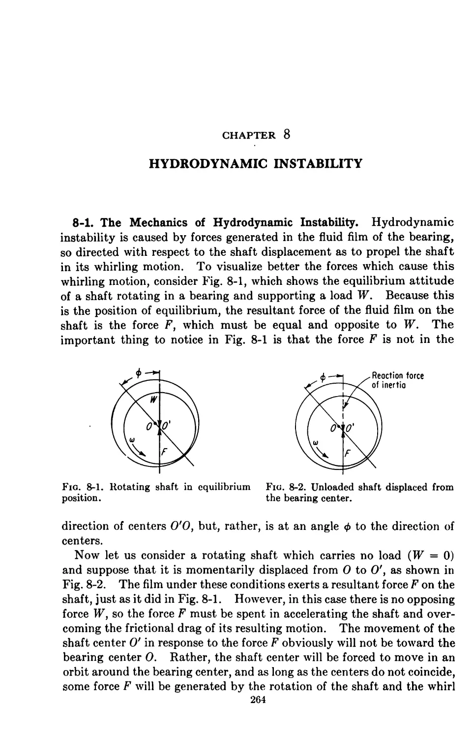
BENO STERNLICHT, PH.D.
Consulting Engineer, General Engineering Laboratory
General Electric Co.
McGRAW-HILL BOOK COMPANY, INC.
New York Toronto London
1901

Engin. Library
1
THEORY OF HYDRODYNAMIC LUBRICATION
Copyright © 1961 by the McGraw-Hill Book Company, Inc. Printed
in the United States of America. All rights reserved. This book, or
parts thereof, may not be reproduced in any form without permission
of the publishers. Library of Congress Catalog Card Number: 60-14450.
50050
THE MAPLE PRESS COMPANY, YORK, PA.

PREFACE
For a number of years it has been apparent that a need exists for a book
on the theory of hydrodynamic lubrication. In response to this need,
the Hydrodynamic Research Technical Committee of the Lubrication
Division of the American Society of Mechanical Engineers, under the
chairmanship of Beno Sternlicht, recommended the writing of this book.
The book was written in equal partnership by both authors and with
the Committee’s intentions as a guide.
We have accordingly attempted to offer here a unified treatment of
hydrodynamic lubrication. We have aimed at three objectives. By the
application of the general principles of fluid flow to the circumstances of
bearing operation, we have stated the differential equations of lubrica¬
tion, including energy and elasticity considerations. We have then pre¬
sented techniques of solving these equations either analytically or by
means of analogue and digital computers. And lastly, we have given
exact or approximate solutions of the differential equations involved
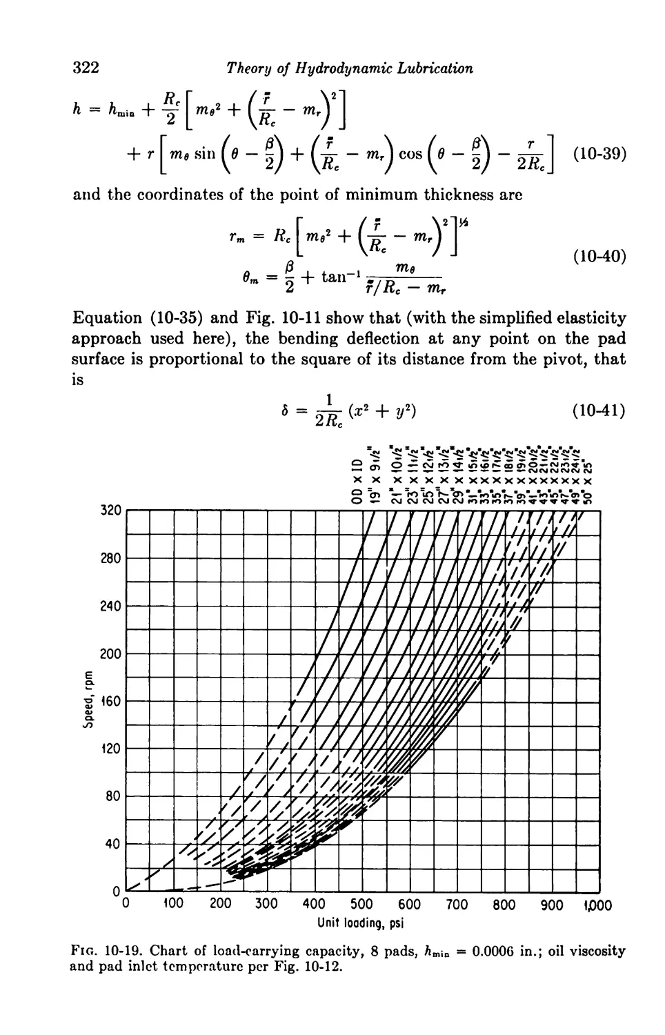
which provide a basis for the design and the solution of specific bearing
problems.
The presentation of lubrication theory and the solution of bearing
problems involve a good deal of mathematics. We have, however,
used no more than a minimum of space for discussing the mathematics
involved. This was done advisedly. We have used mathematics as a
tool for the presentation of lubrication theory and have devoted our main
effort to the presentation. We have for the same reasons omitted many
of the intermediate steps whenever we considered the mathematical
operations to be sufficiently straightforward or standard. We have,
however, been careful to state the assumptions and simplifications
underlying the final expressions.
The subject matter can be broken up into several groups. Chapter 1
lays the mathematical foundations of the material and derives the
differential equations of lubrication in their most general form. Chapter
2 deals with simple configurations which are a part of or constitute models
of bearings and bearing systems. Chapters 3 to 13 deal specifically with
bearings. Perhaps the inclusion of hydrostatic bearings may seem
inconsistent with the title of the book; however, both functionally and

vi
Preface
mathematically, hydrostatic bearings are closely linked to the general
subject of hydrodynamic lubrication.
The chapter on the Extension of the Classical Theory is an attempt to
remove some of the restrictions inherent in the Reynolds equation with
the object of finding solutions applicable to such subjects as thick film
lubrication and parallel sliders, subjects for which the Reynolds equation
collapses or does not hold. Chapter 15 is the only one dealing with
experiments. This chapter is intended, not to offer a record of test data,
but rather to portray through experimental evidence the validity of the
basic propositions of hydrodynamic lubrication.
This book draws its material from many sources as well as the authors’
published and unpublished work. We have avoided using proper names
except where they are a part of the technical vocabulary. Each chapter
is followed by a list of sources, and we have used the term “sources”
deliberately to emphasize that the particular chapter is derived from
them. The listings at the end of each chapter constitute the acknowledg¬
ment due to the individual contributions. We have not offered a list of
references, for the material is too extensive; bibliographies can be found
elsewhere.
The authors wish to express their appreciation to the Research Tech¬
nical Committee of the Lubrication Division of the ASME for its sponsor¬
ship and interest and to the General Electric Company for the use of its
facilities in preparing this book.
0.	Pinkus
B. Sternlicht

CONTENTS
Preface	 v
Nomenclature	xii
1. Basic Differential Equations	 1
1-1. The Navier-Stokes Equations	 1
1-2. The Generalized Reynolds Equation	 5
1-3. Flow and Shear Equations	12
1-4. Derivation of Energy Equation	14
1-5. Equation of State	22
2. Hydrodynamics of Simple Configurations	24
General Equations of Motion for Compressible	Fluids	24
2-1. The Theoretical Equation for Laminar Flow	25
2-2. The Empirical Equation for Turbulent Flow	25
Flow through Narrow Slots	27
2-3. Isothermal Flow	27
Constant-area Slot	27
Diverging Width	27
Diverging Depth	28
2-4. Flow through Orifices in Scries	28
Incompressible Flow	31
2-5. Flow between Parallel Walls	31
2-6. Circumferential Flow between Concentric Cylinders	32
2-7. Axial Flow in Cylinders	34
Concentric Cylinders	34
Flow through Eccentric Cylinders	35
3. Incompressible Lubrication; One-dimensional	Bearings	37
The Real Bearing	37
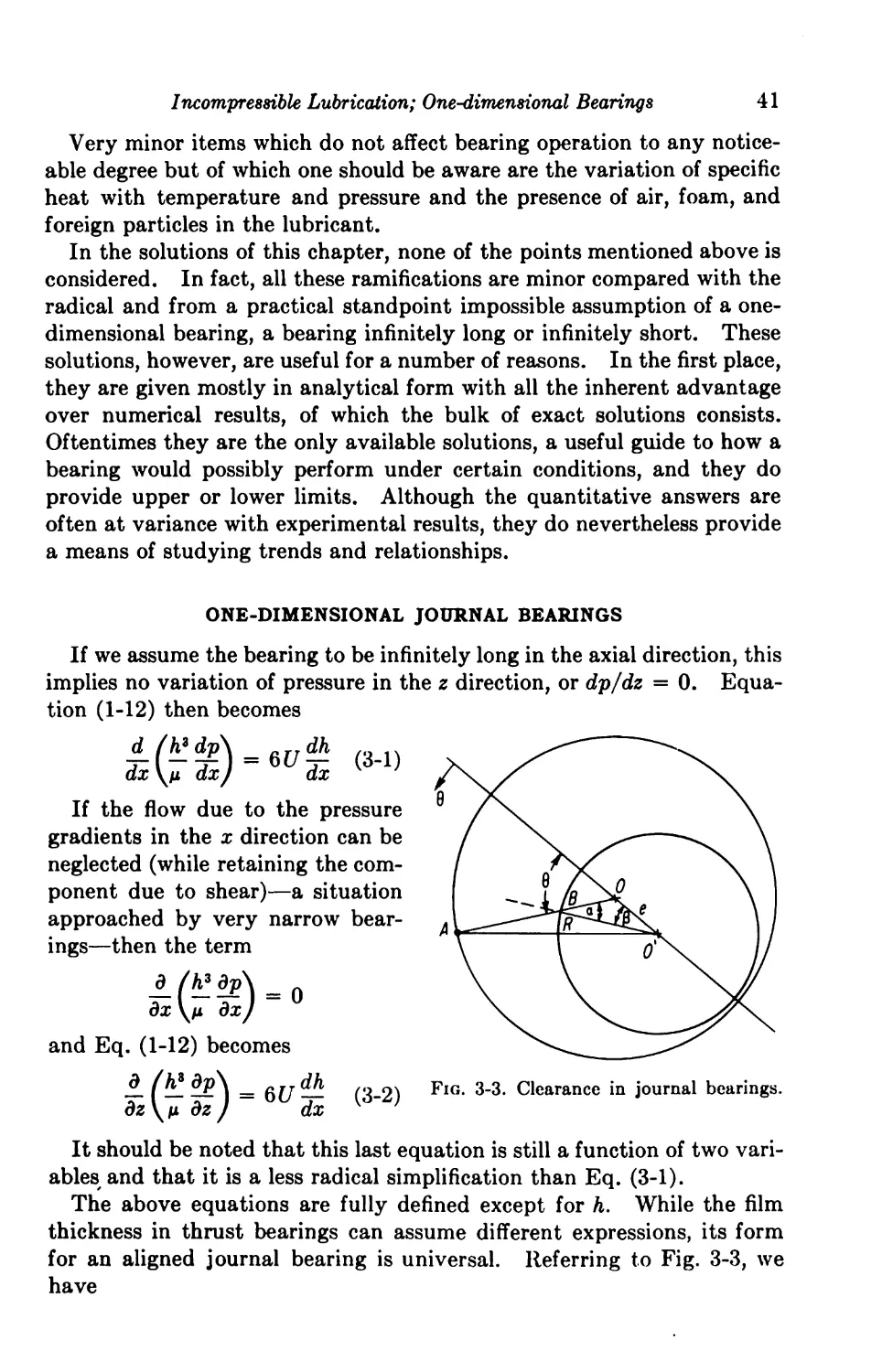
One-dimensional Journal Bearings	41
3-1. Infinitely Long Bearing	42
3-2. Infinitely Short Bearing	48
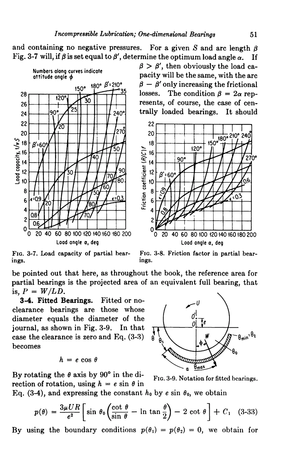
3-3. Partial Bearings	50
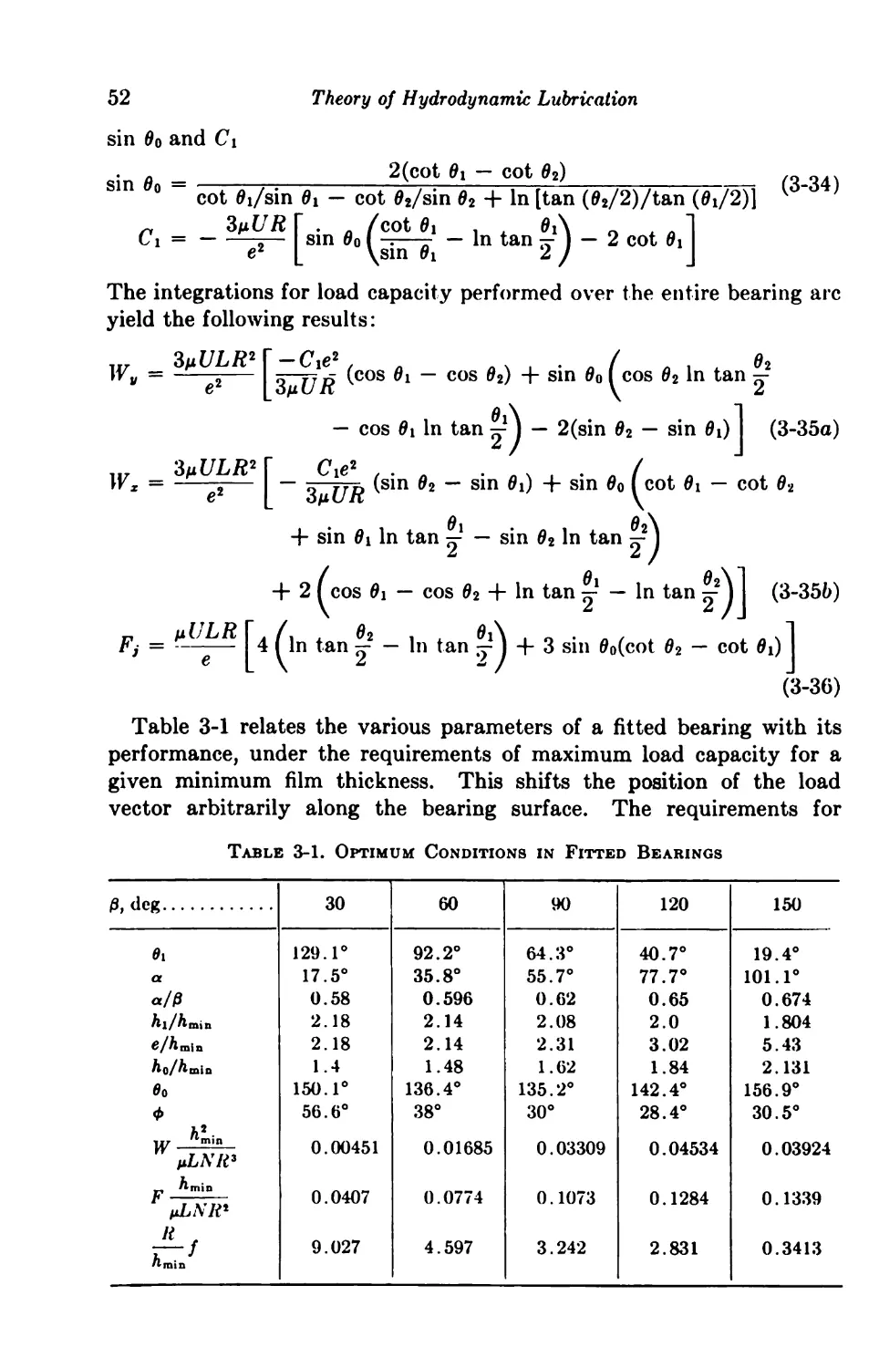
3-4. Fitted Bearings	51
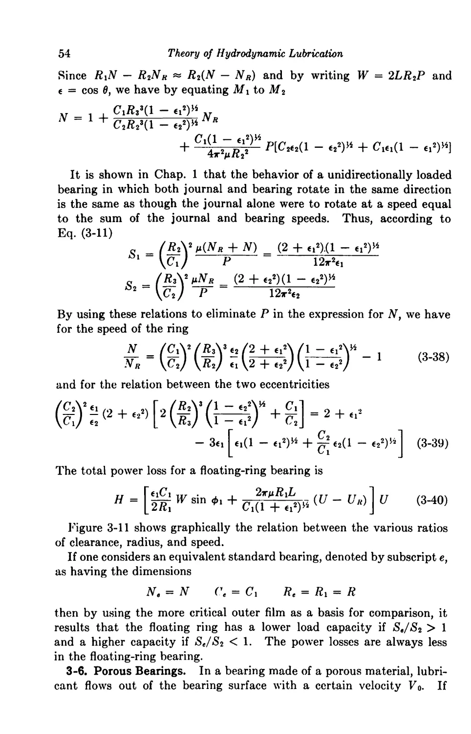
3-5. Floating-ring Bearings	53
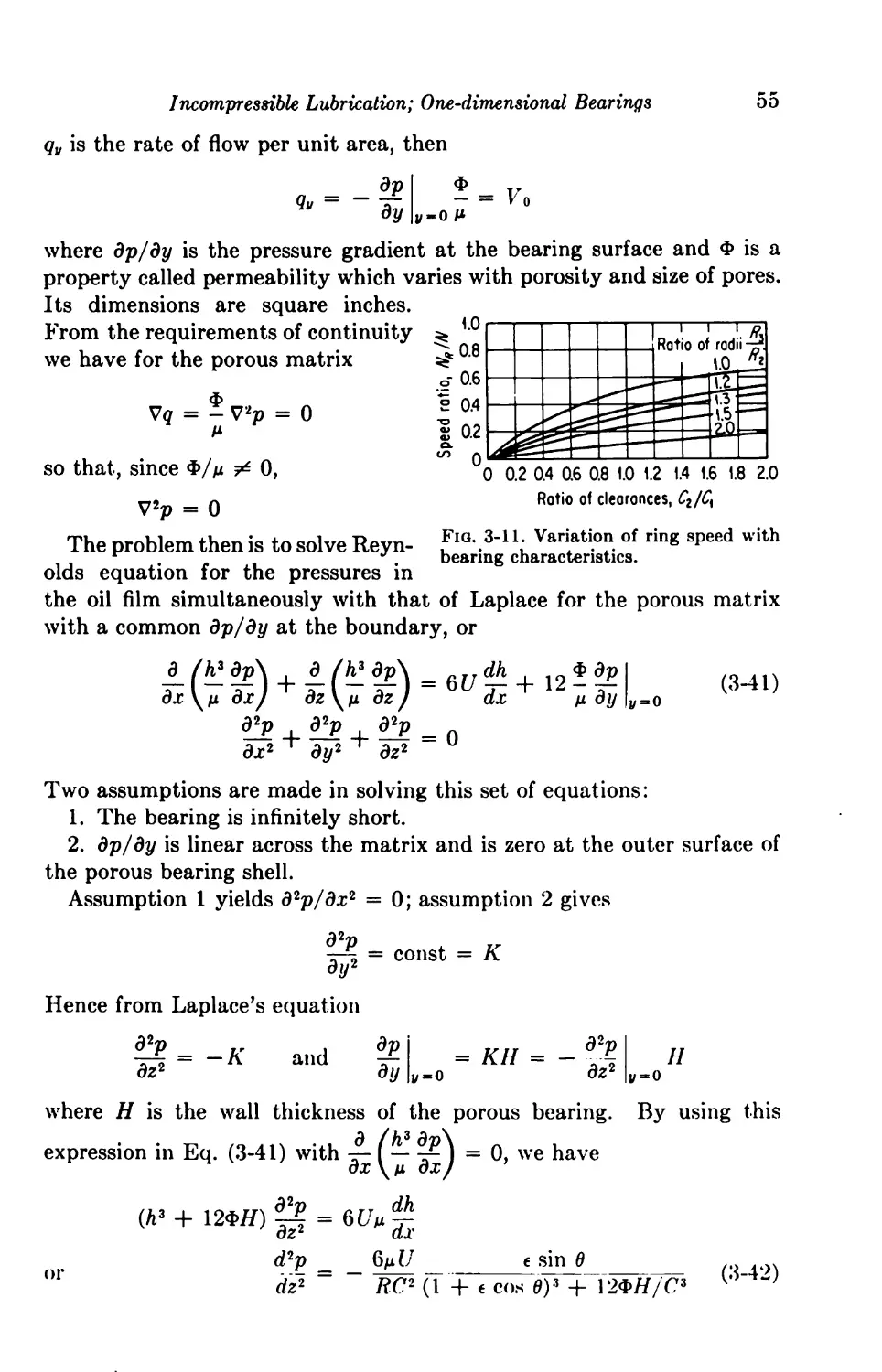
3-6. Porous Bearings	54
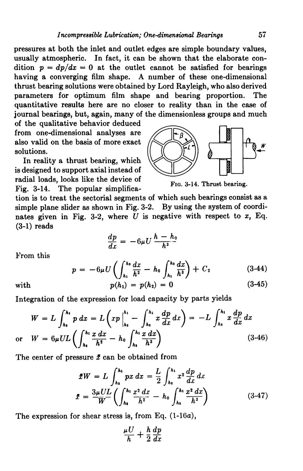
One-dimensional Thrust Bearings	56
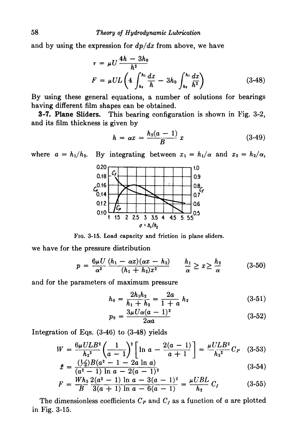
3-7. Plane Sliders	58
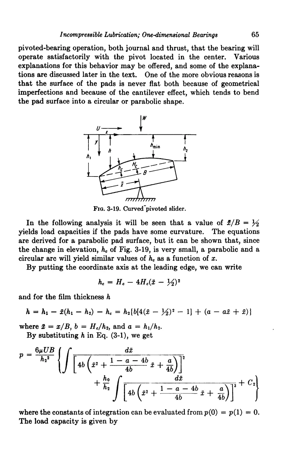
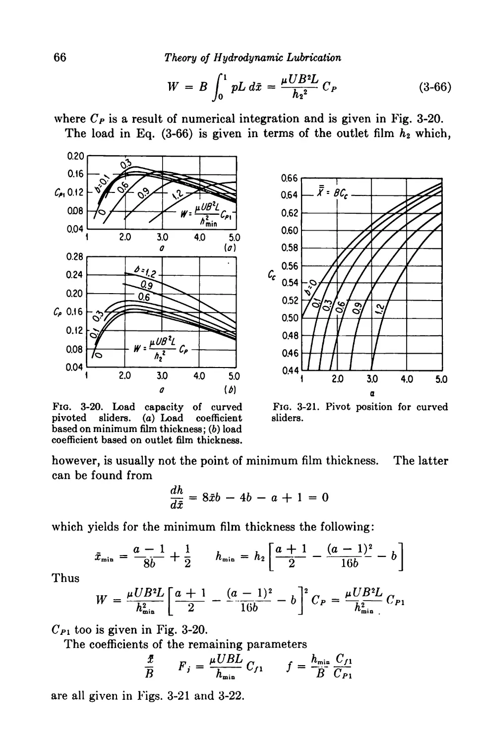
3-8. Curved Sliders	 59
vii

viii	Contents
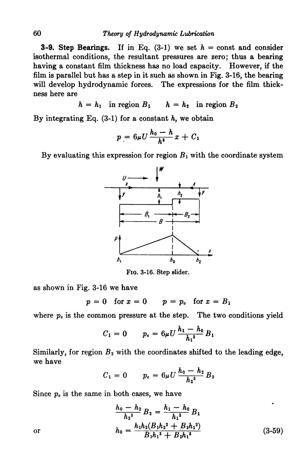
3-9. Step Bearings	60
3-10. Composite Bearings	62
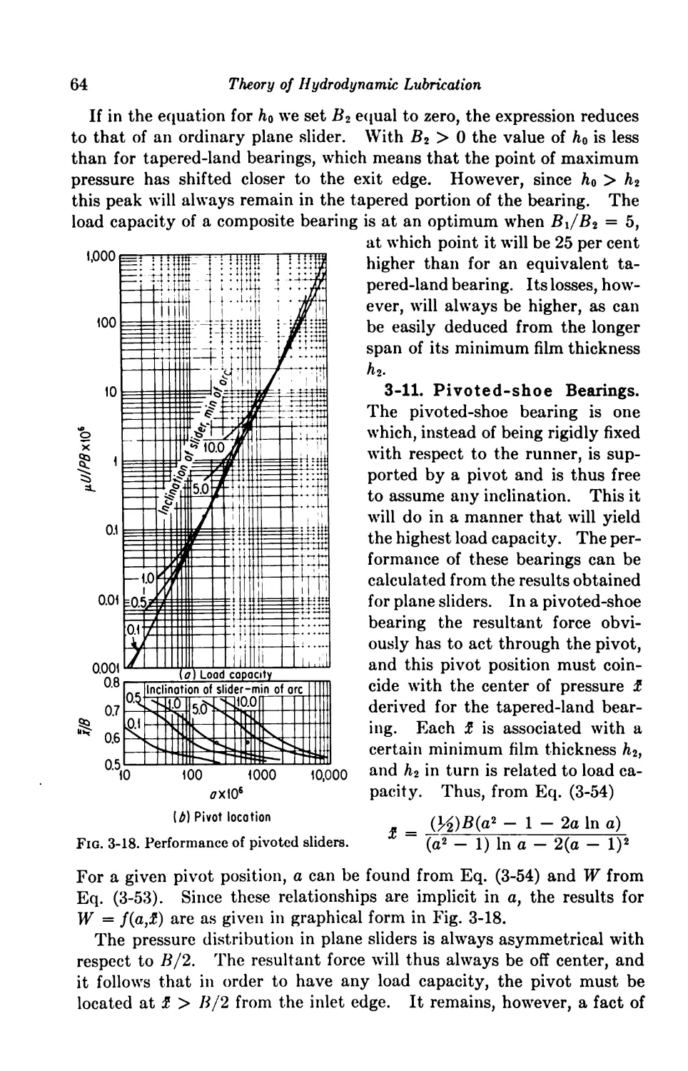
3-11. Pivoted-shoe Bearings	64
4.	Incompressible Lubrication; Finite Bearings	68
Finite Journal Bearings	68
Analytical Methods	69
4-1. Journal Bearing with Axial Feeding	71
4-2. Journal Bearing with Circumferential Feeding	75
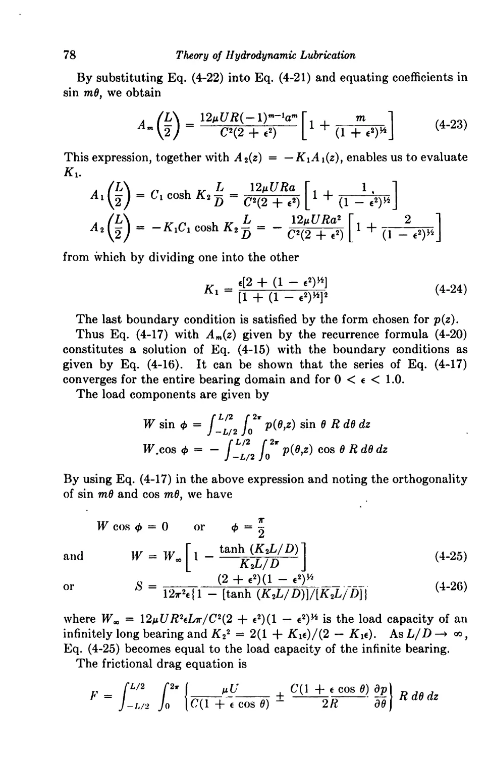
Numerical Methods	79
4-3. Digital Computers	79
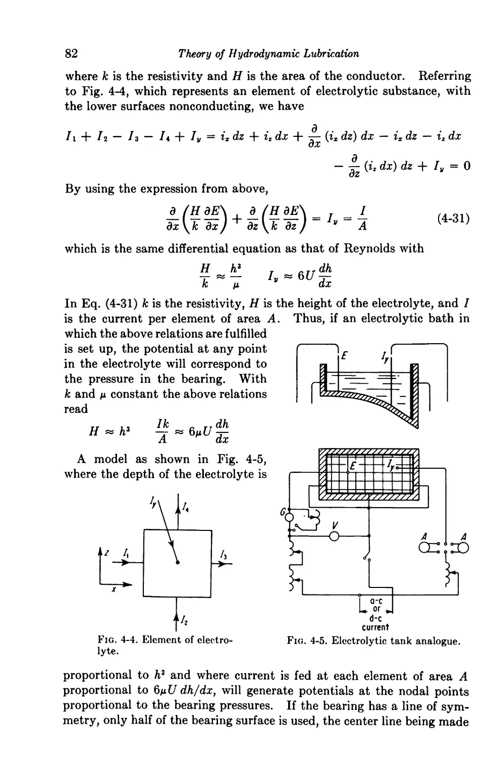
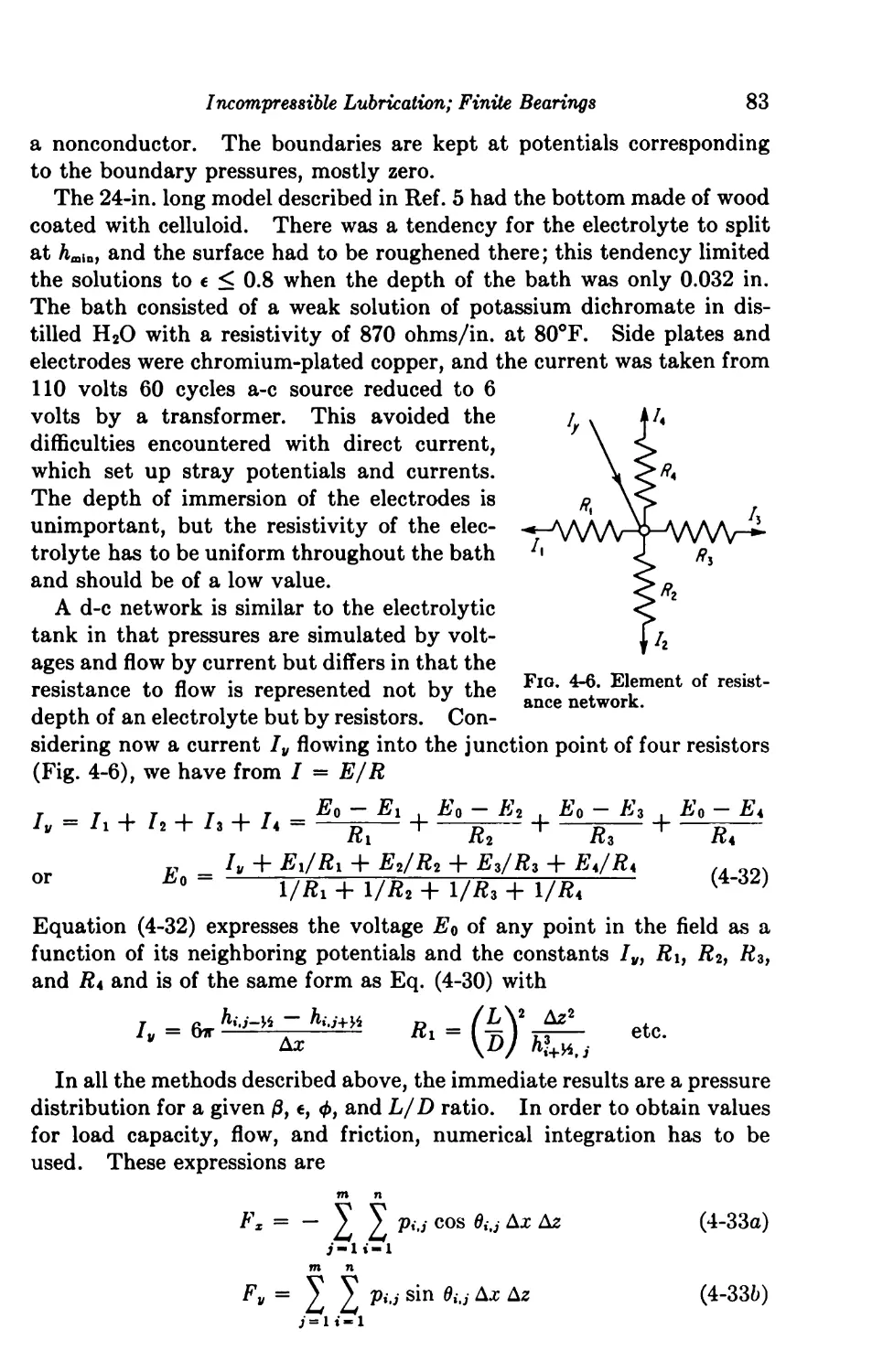
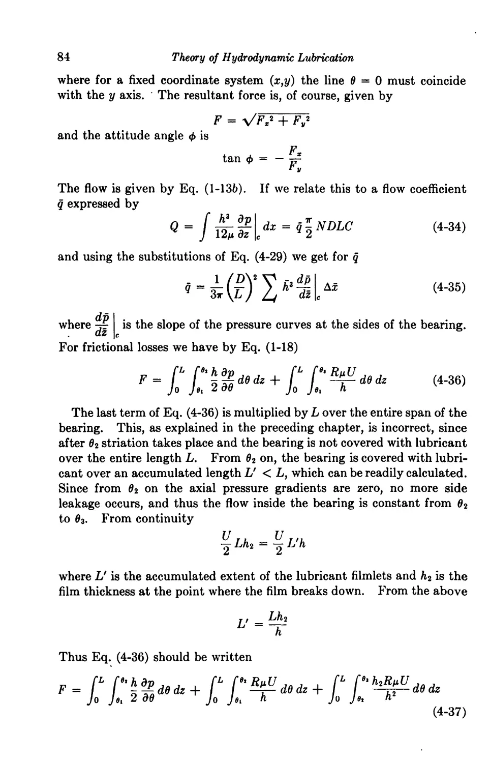
4-4. Electrical Analogues	81
Journal Bearing Solutions	85
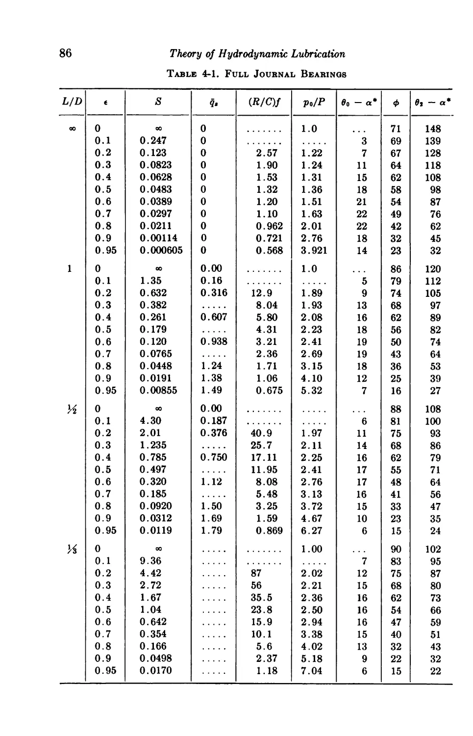
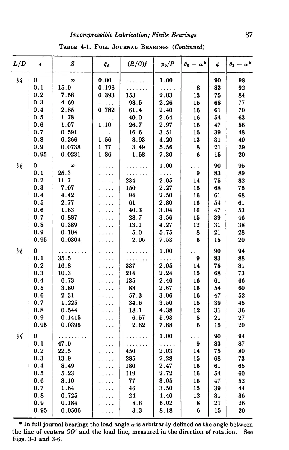
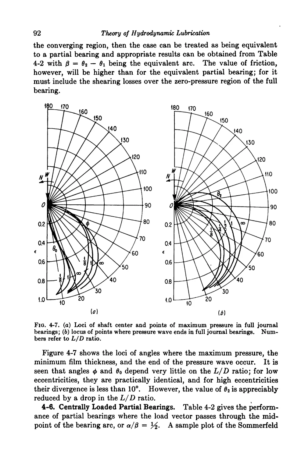
4-5. Full Journal Bearings	85
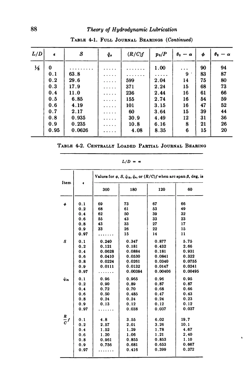
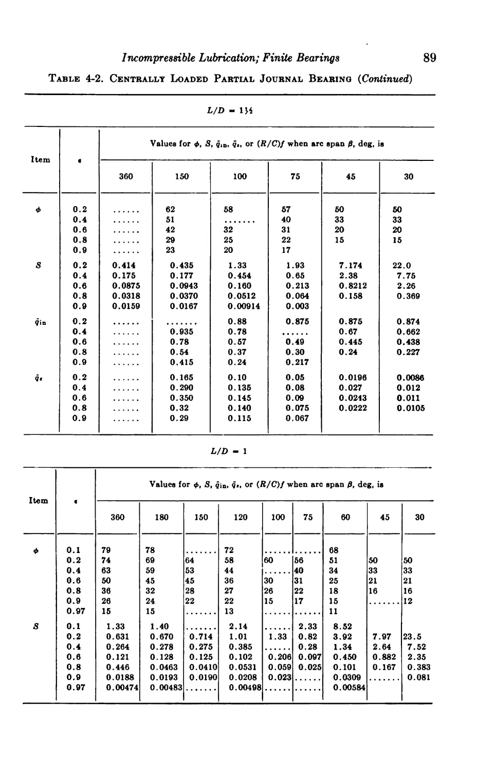
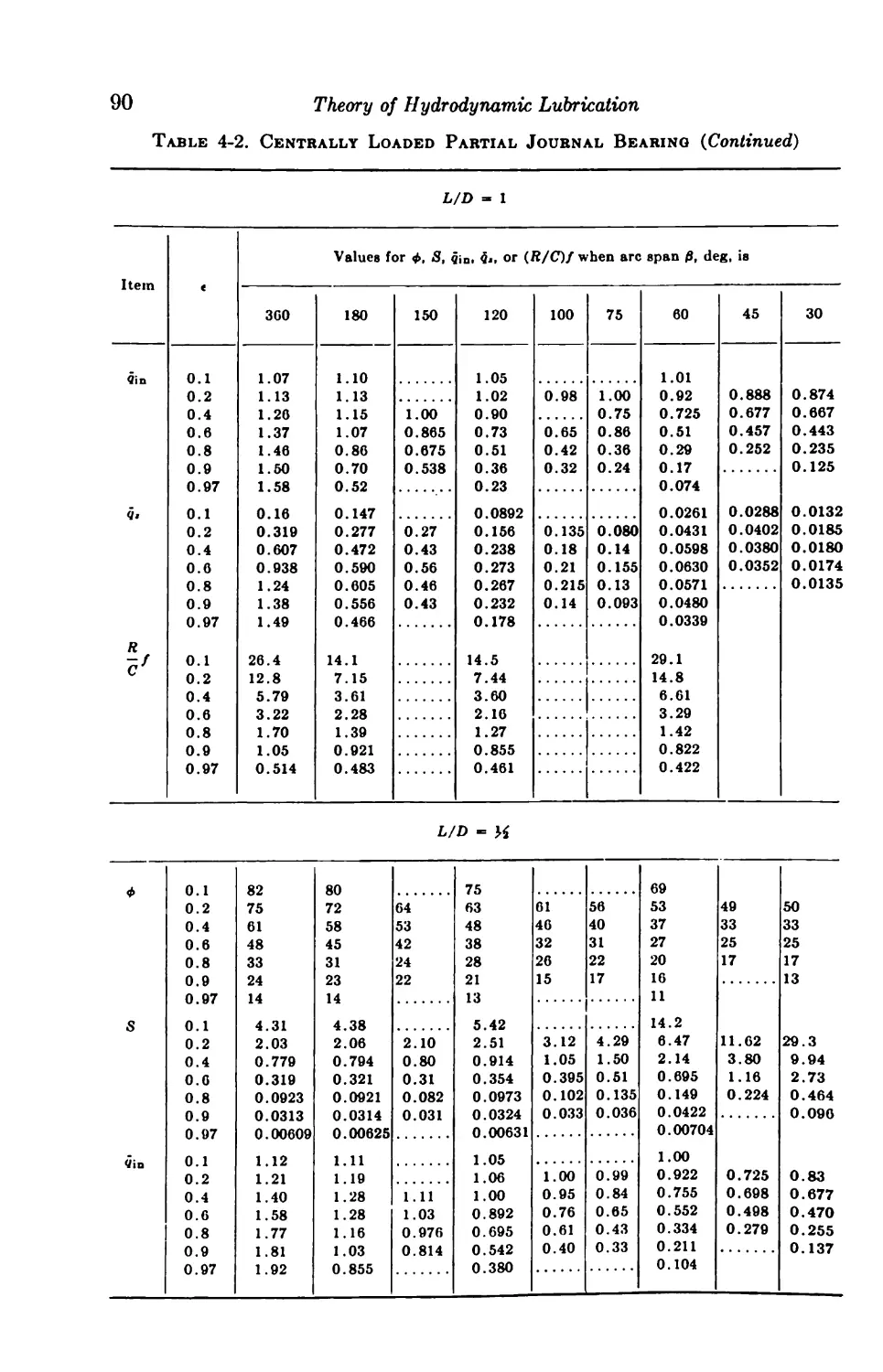
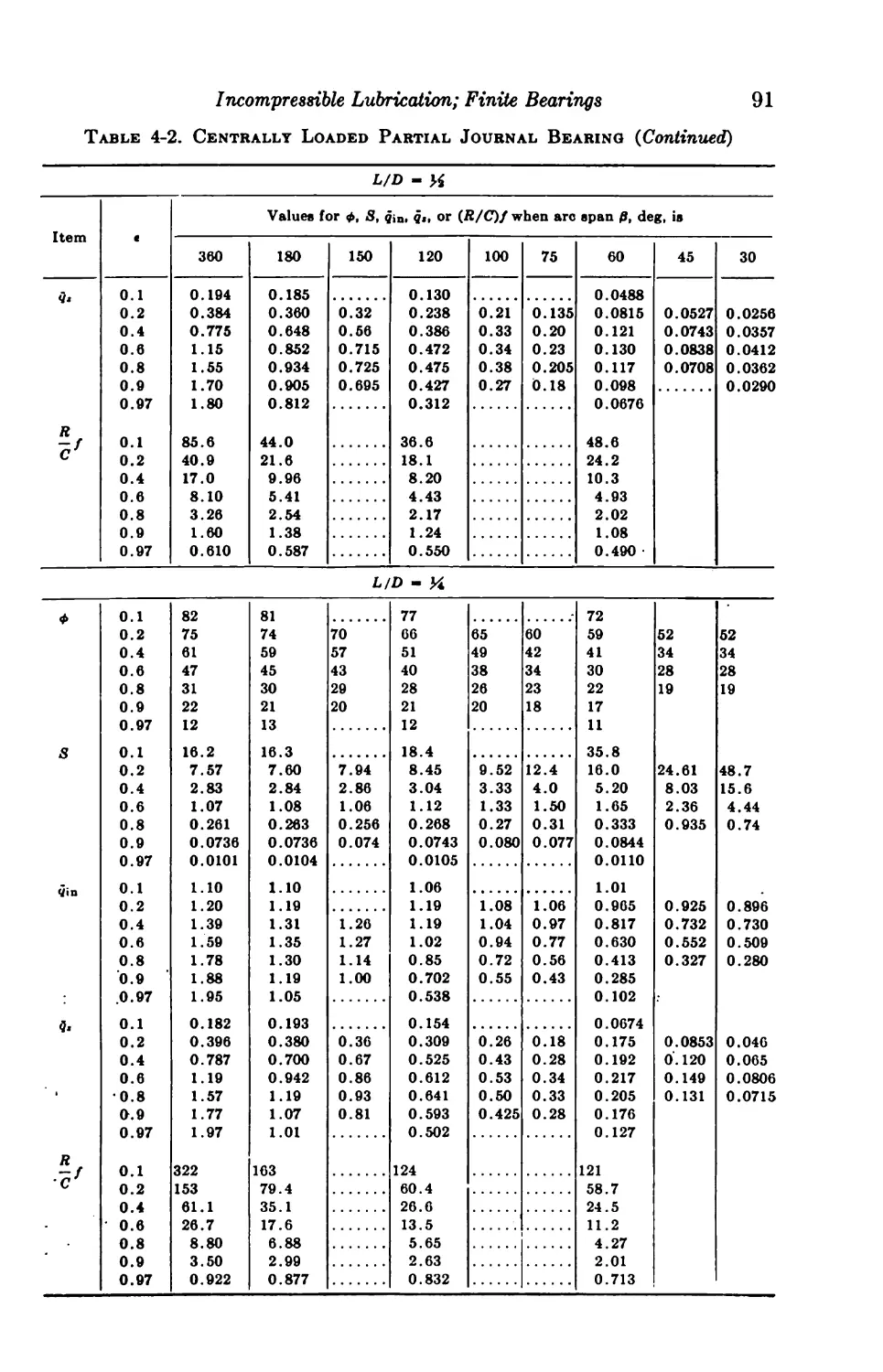
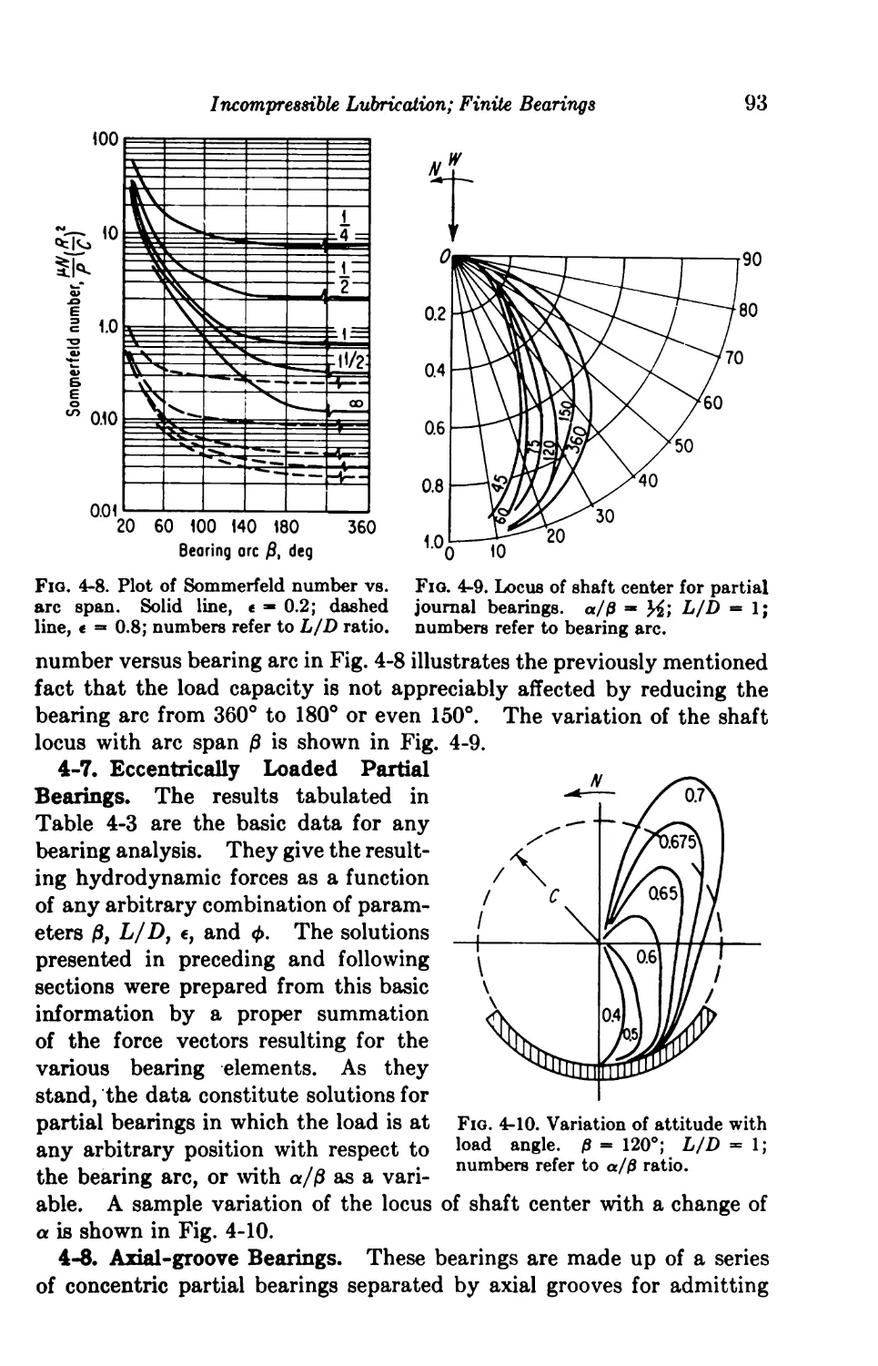
4-6. Centrally Loaded Partial Bearings	92
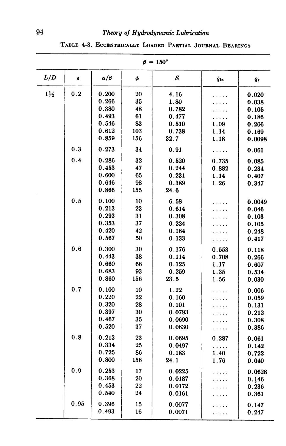
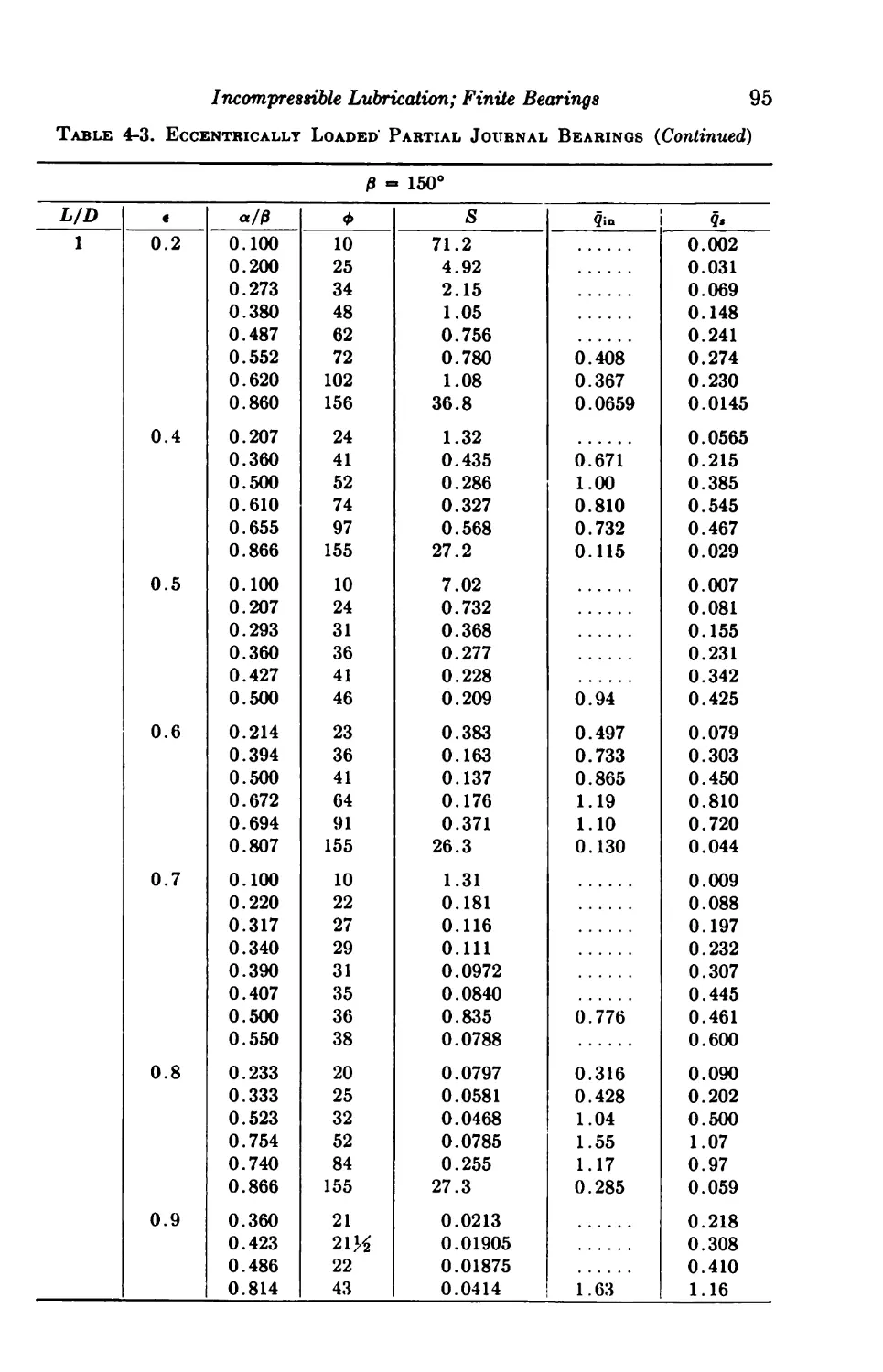
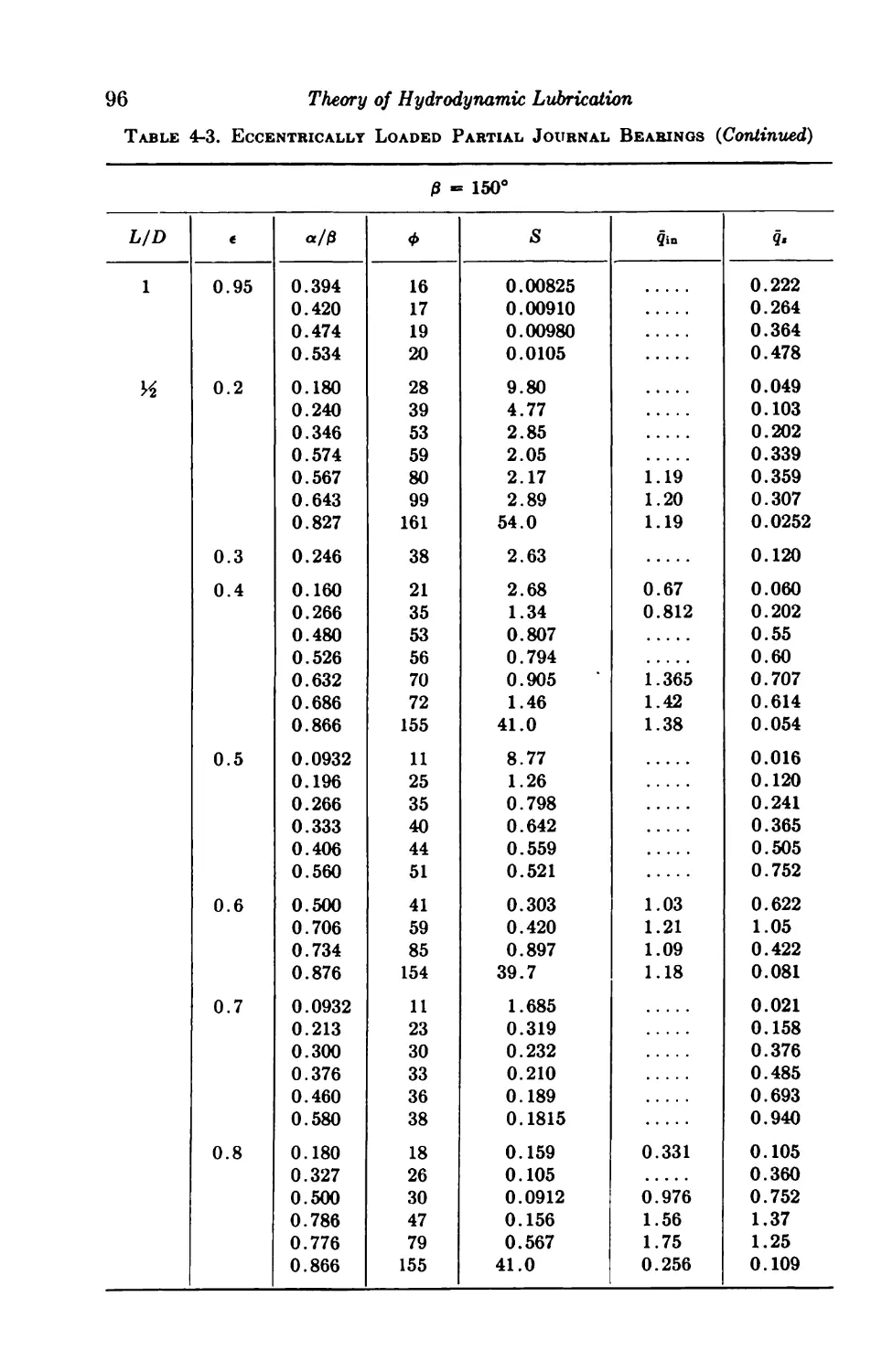
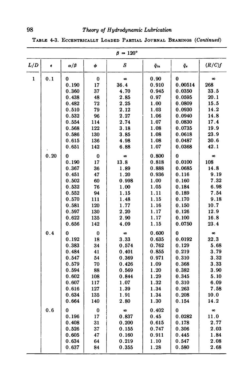
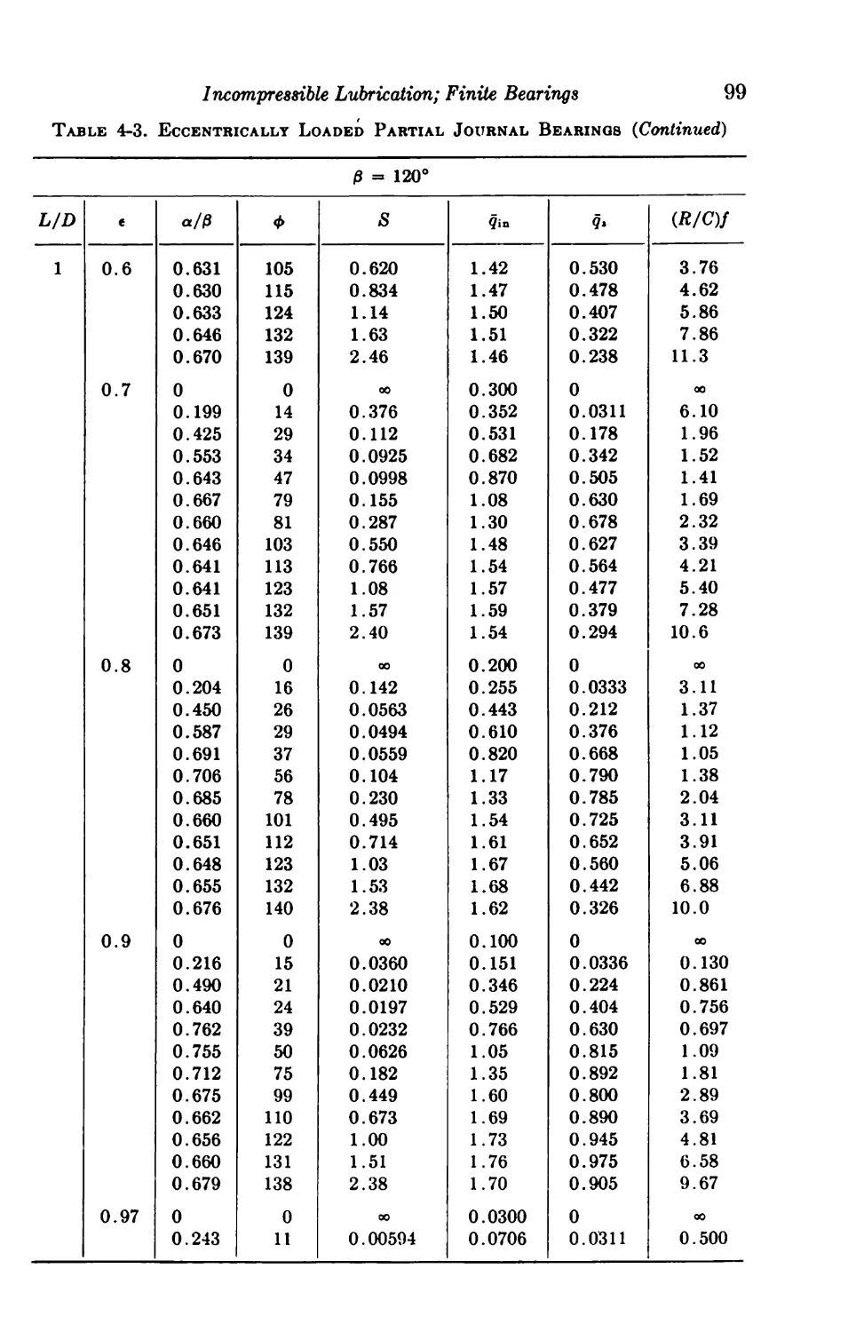
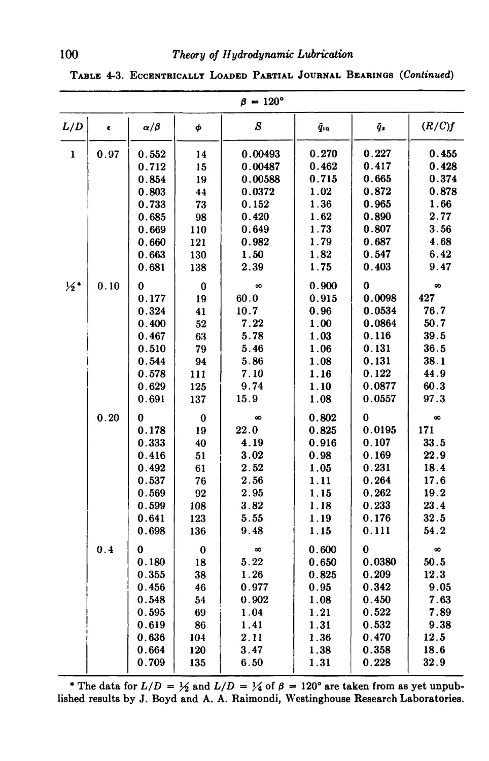
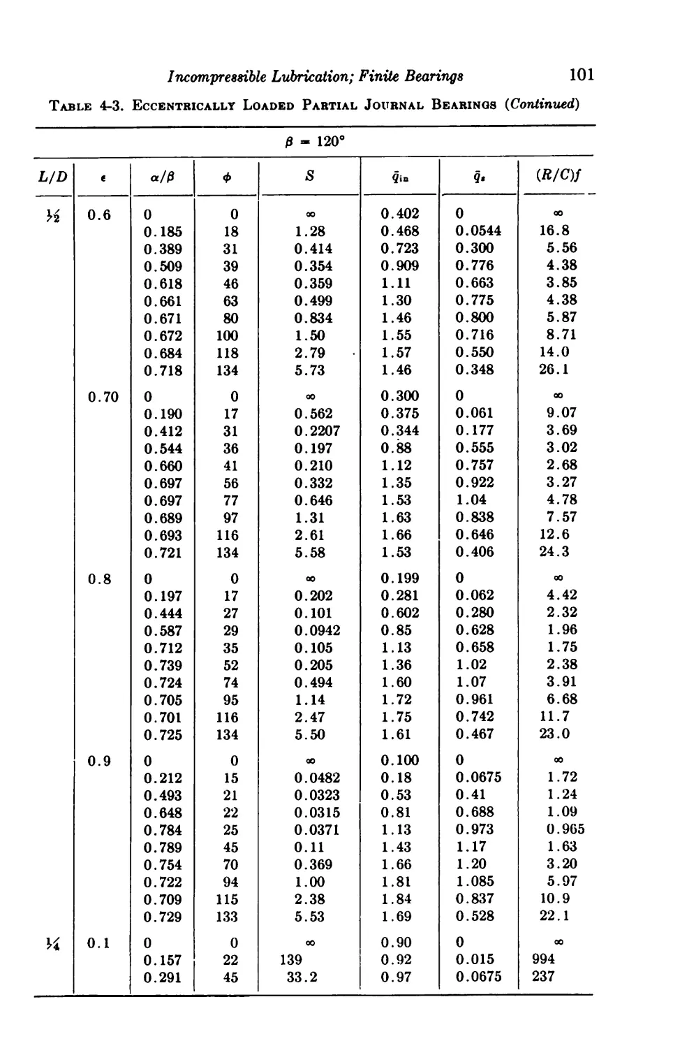
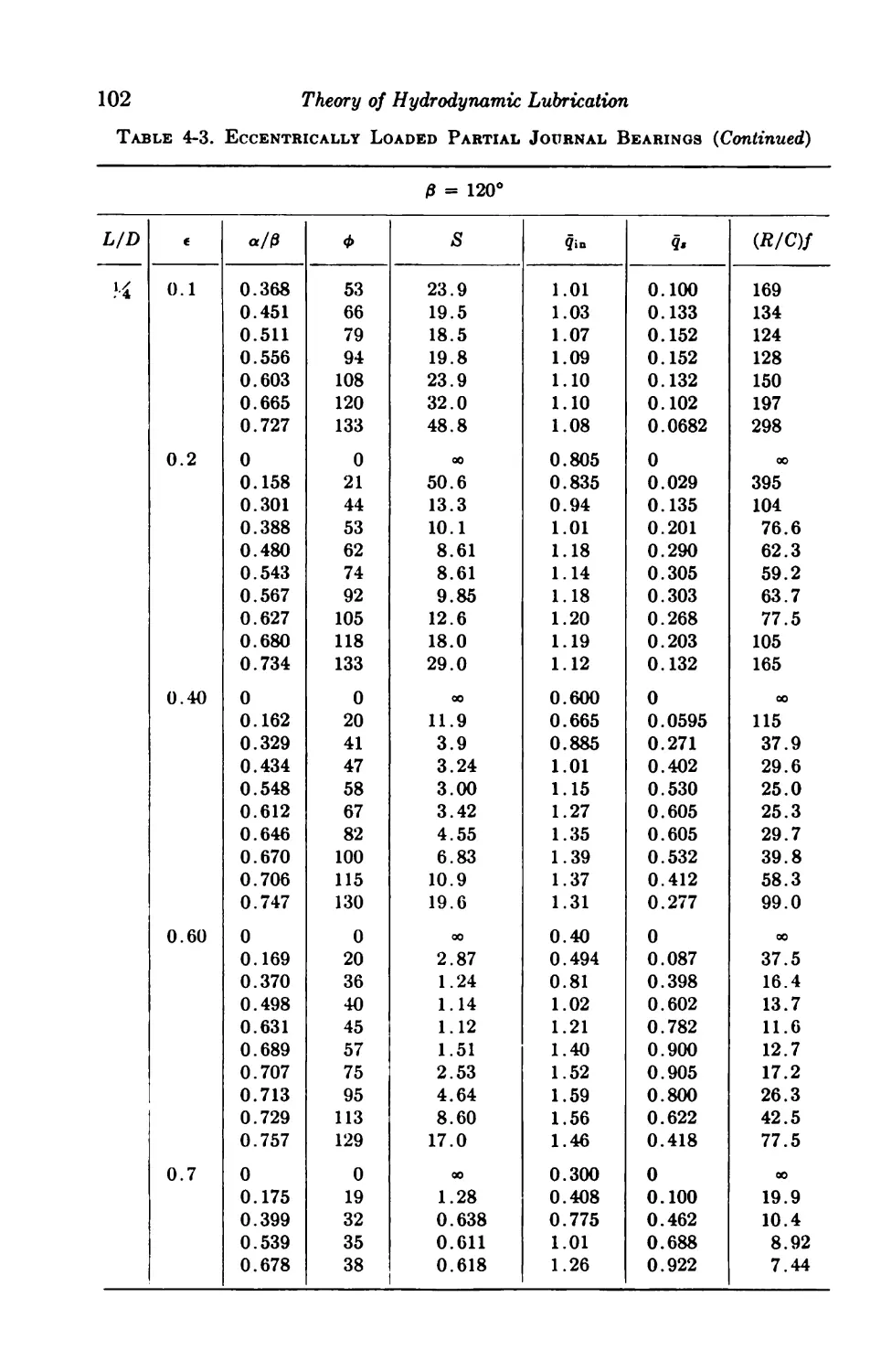
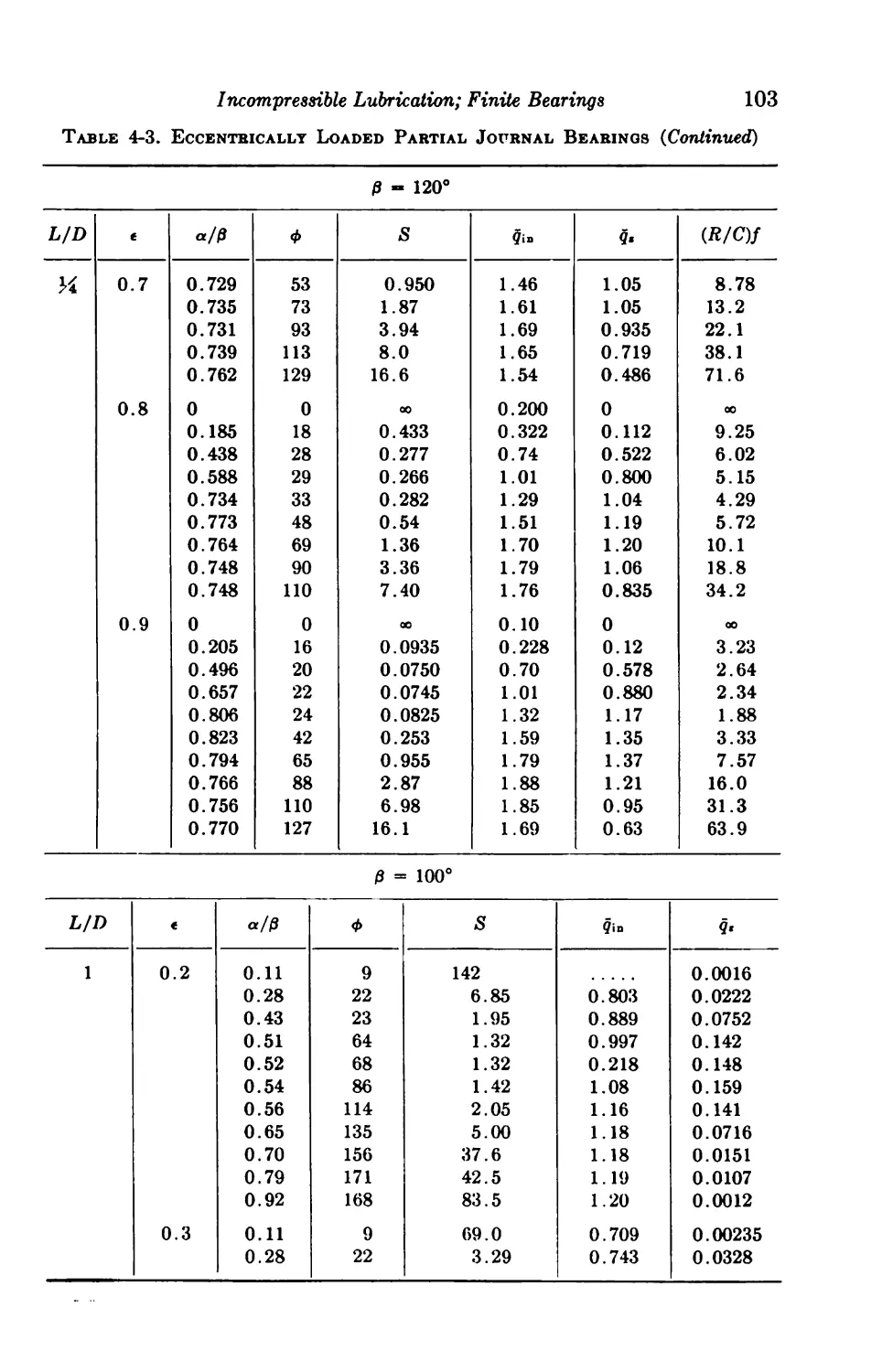
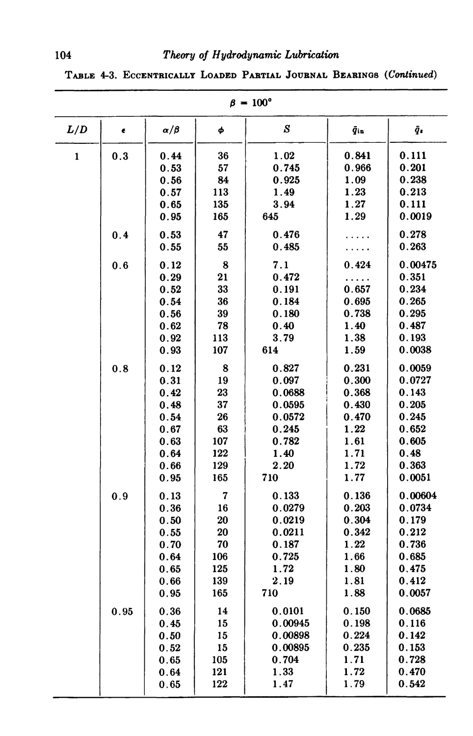
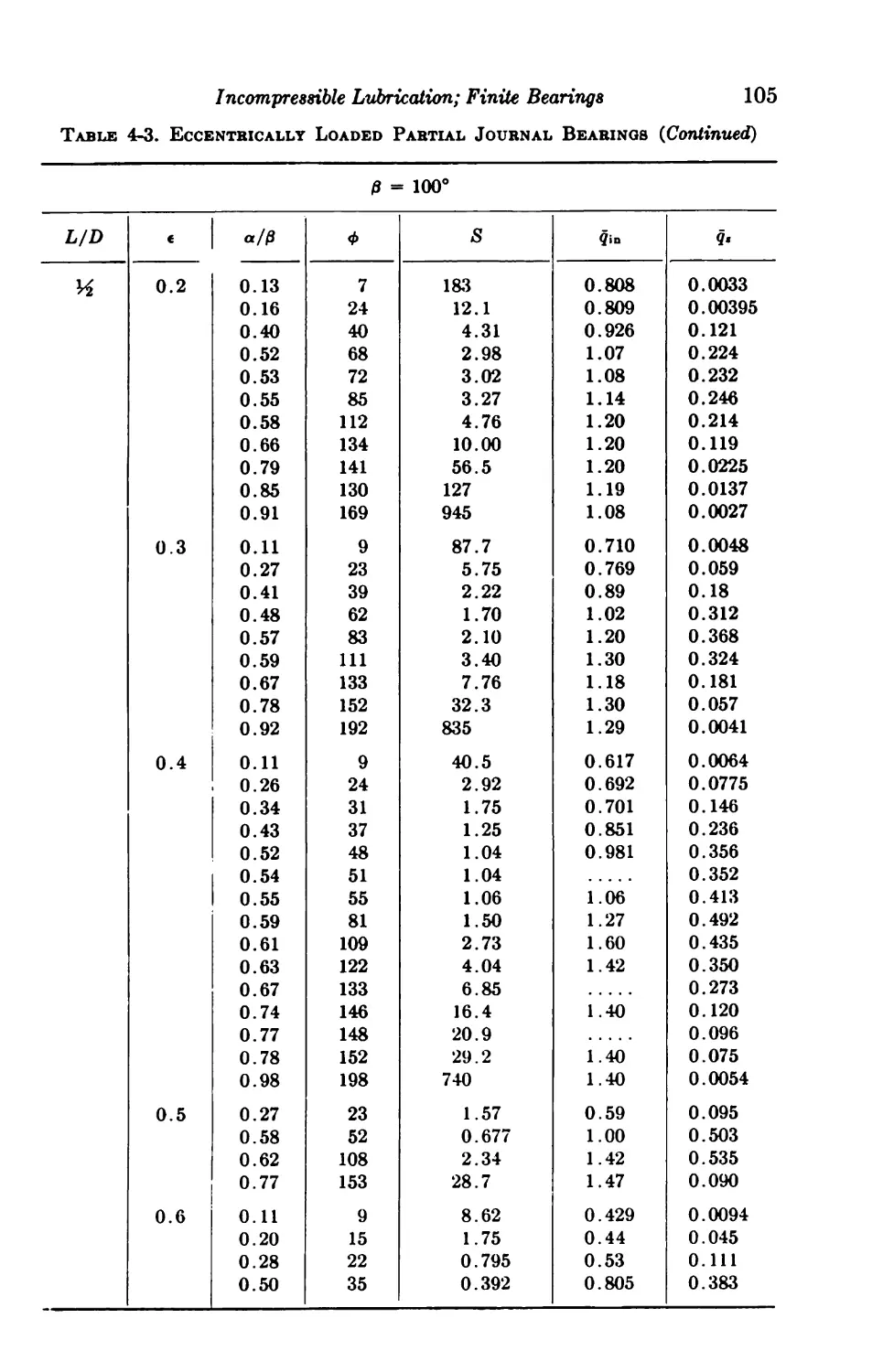
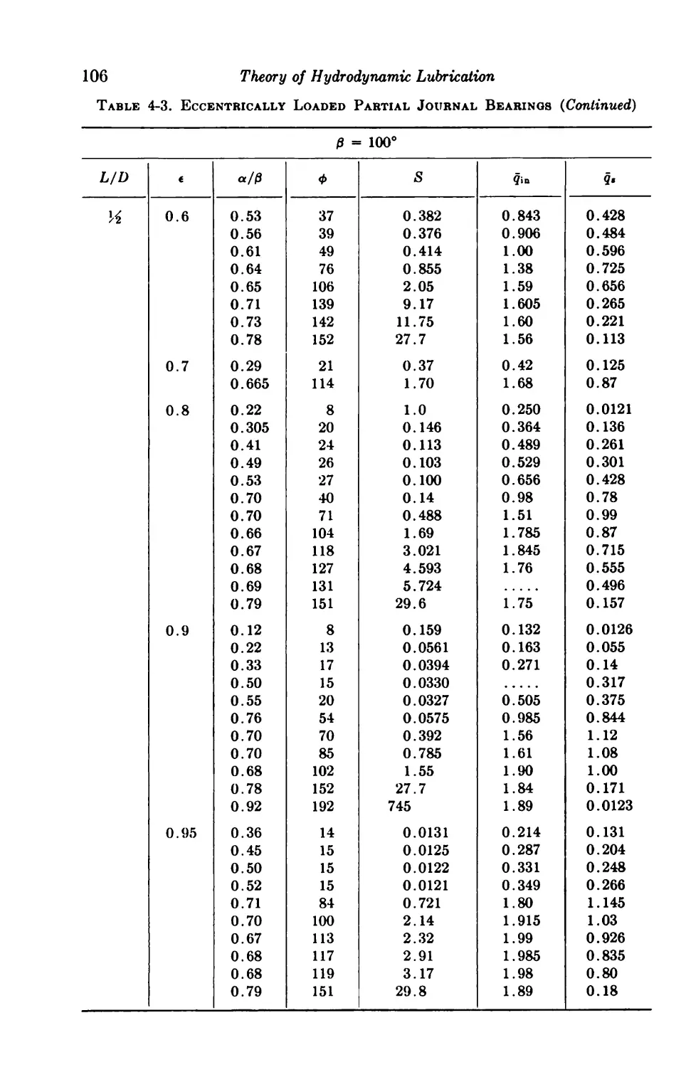
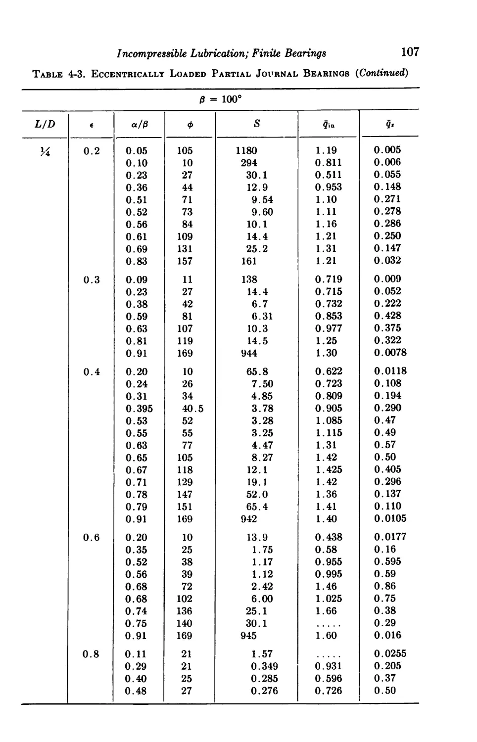
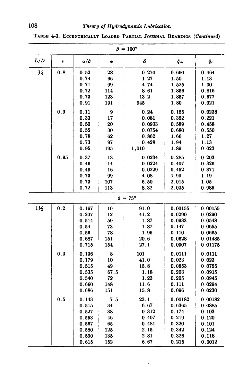
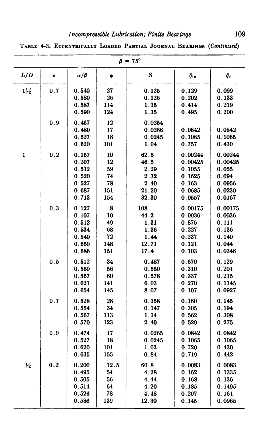
4-7. Eccentrically Loaded Partial Bearings	93
4-8. Axial-groove Bearings	93
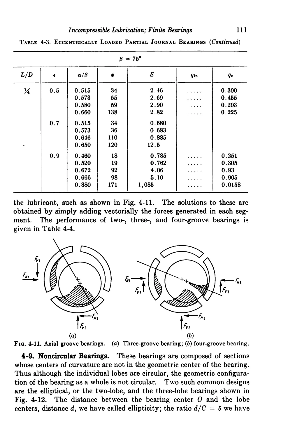
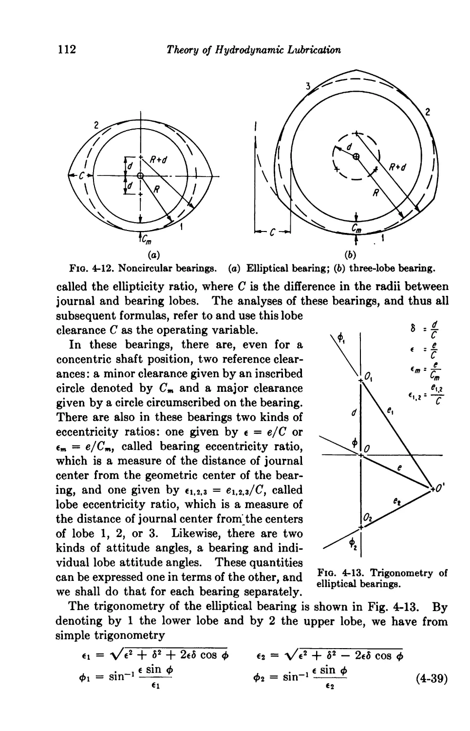
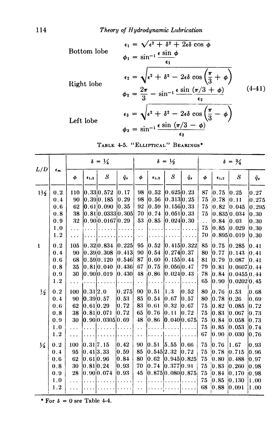
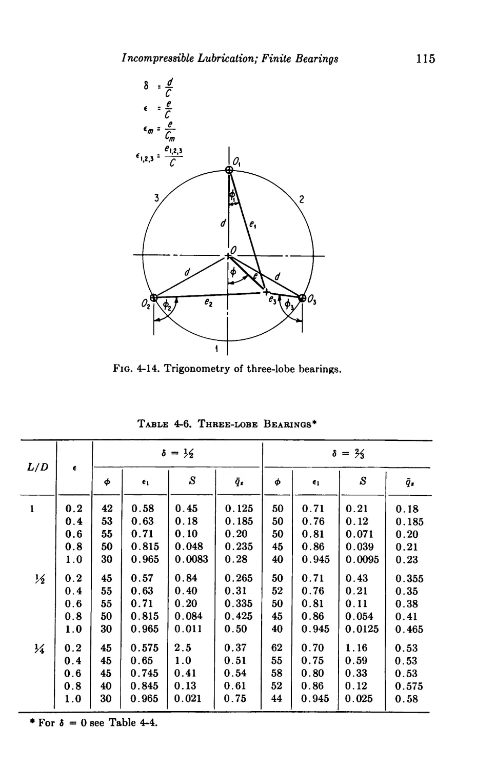
4-9. Noncircular Bearings	Ill
Finite Thrust Bearings	116
Analytical Solutions	116
4-10. The Step Bearing	118
4-11. Slider with Exponential Film Shape	'	122
Numerical Solutions	124
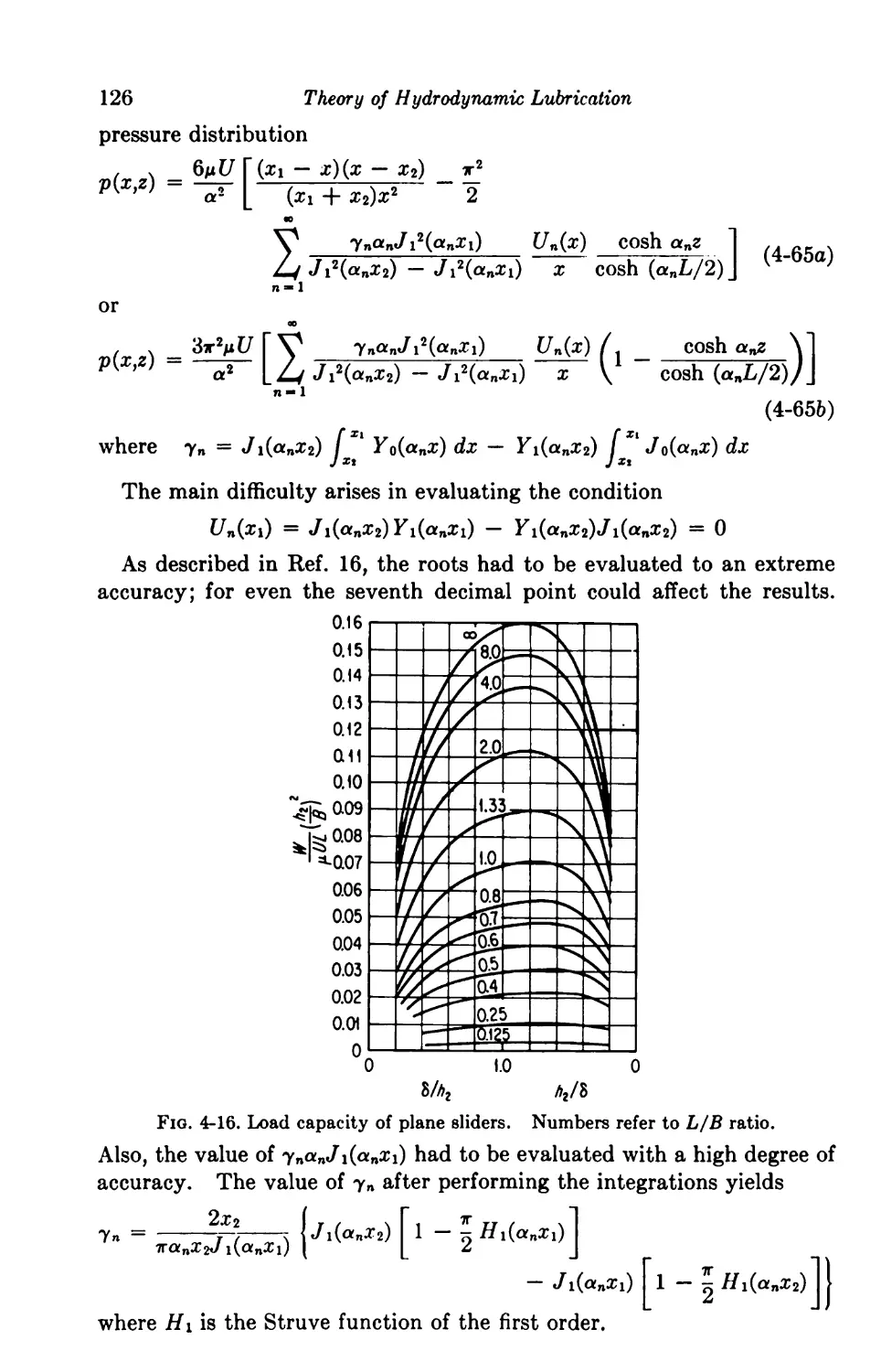
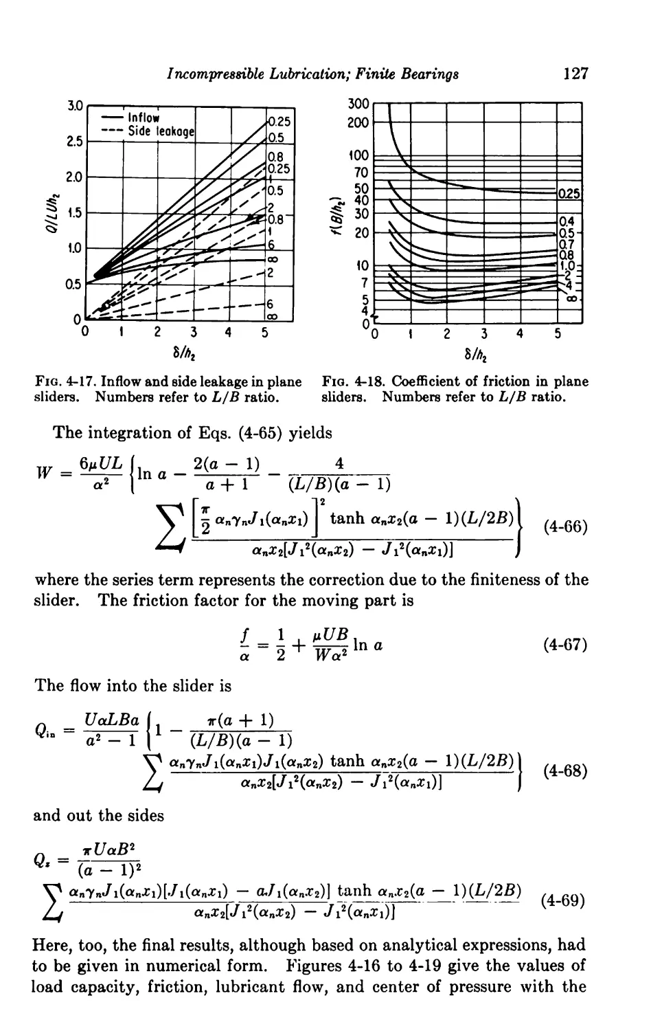
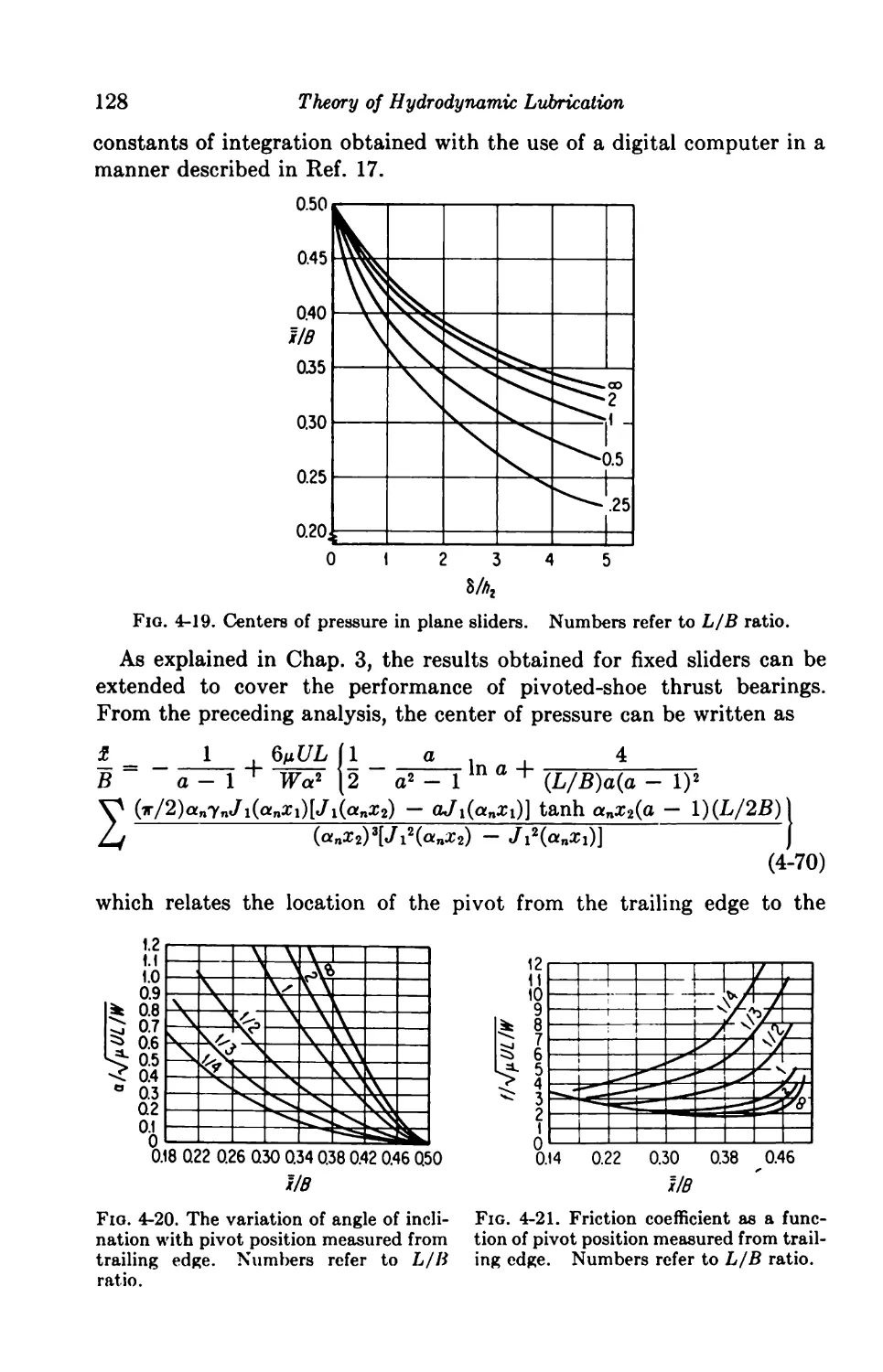
4-12. Slider Bearing; Semianalytical Methods	124
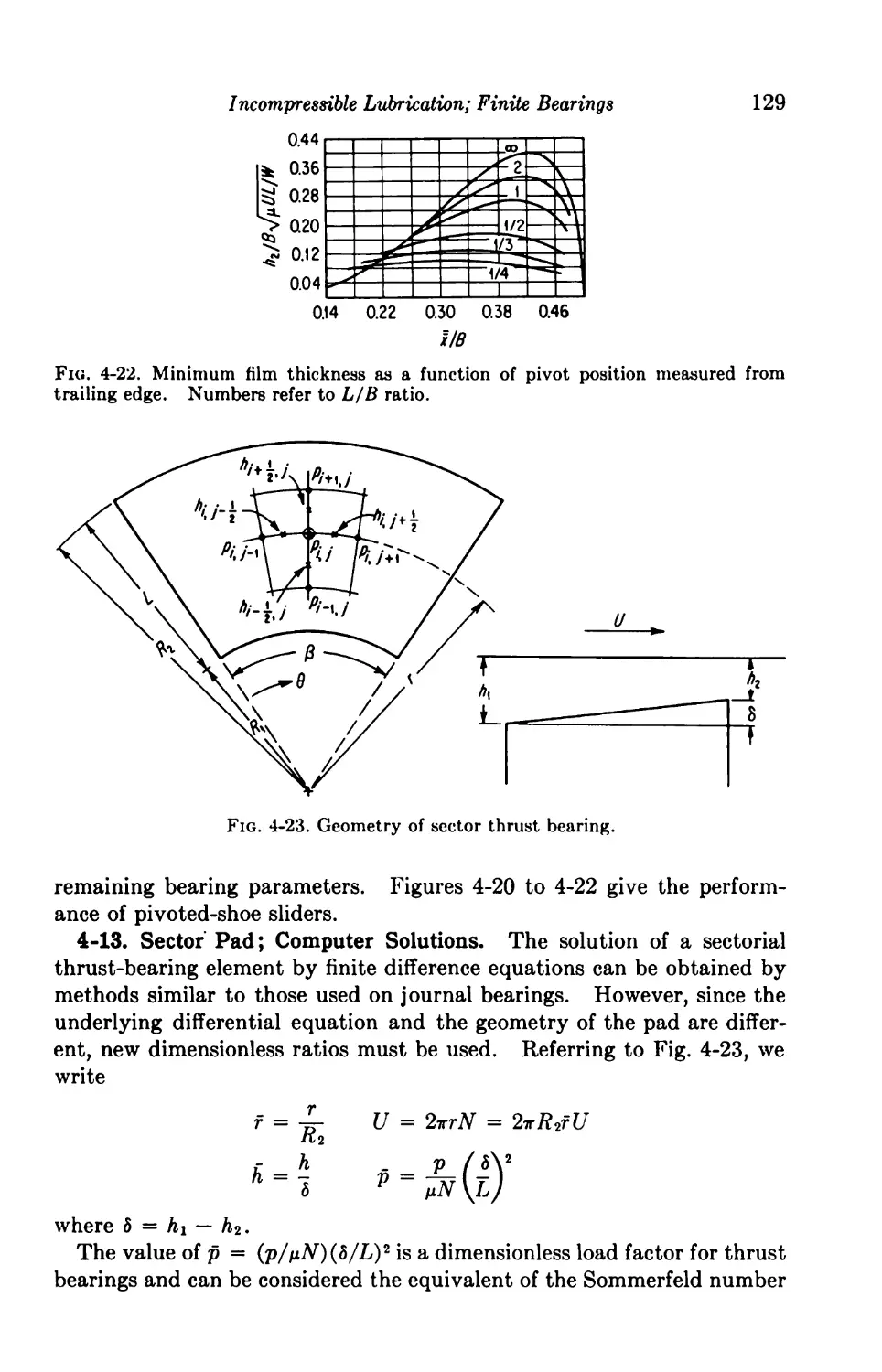
4-13. Sector Pad; Computer Solution	129
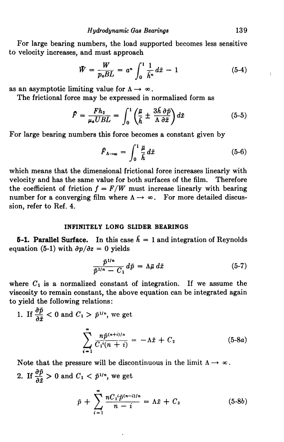
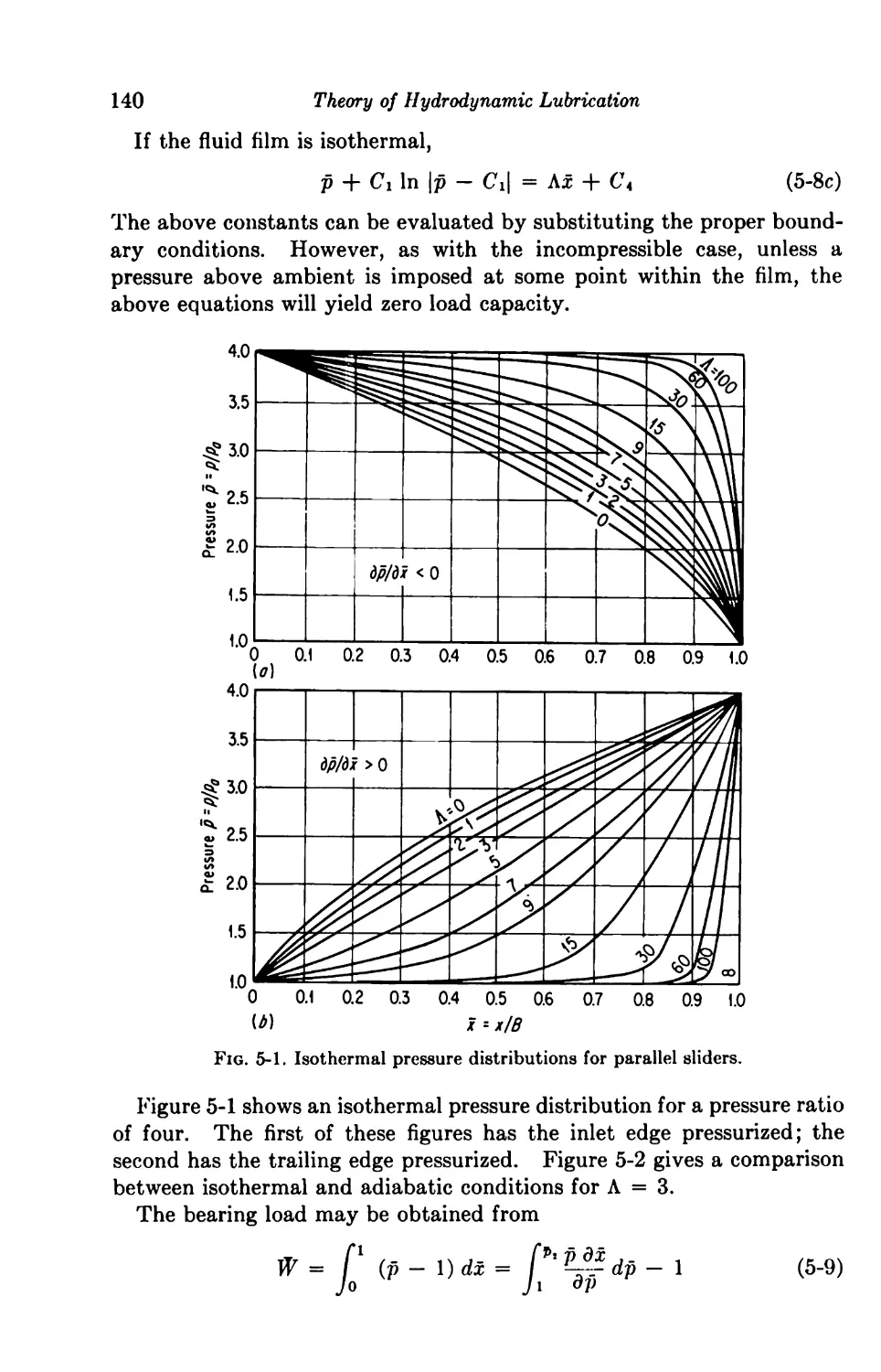
6.	Hydrodynamic Gas Bearings	136
General Considerations	136
Limiting Characteristics	138
Infinitely Long Slider Bearings	139
5-1. Parallel Surface	139
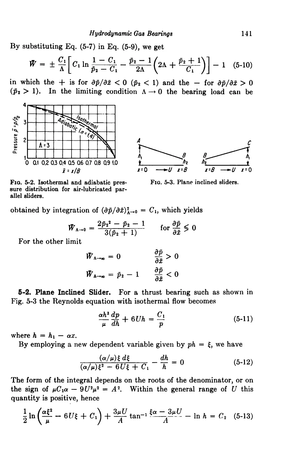
5-2. Plane Inclined Slider	141
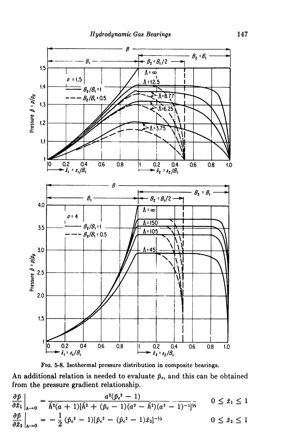
5-3. Composite Slider	145
5-4. Step Slider	148
5-5. Convergent-Divergent Slider	149
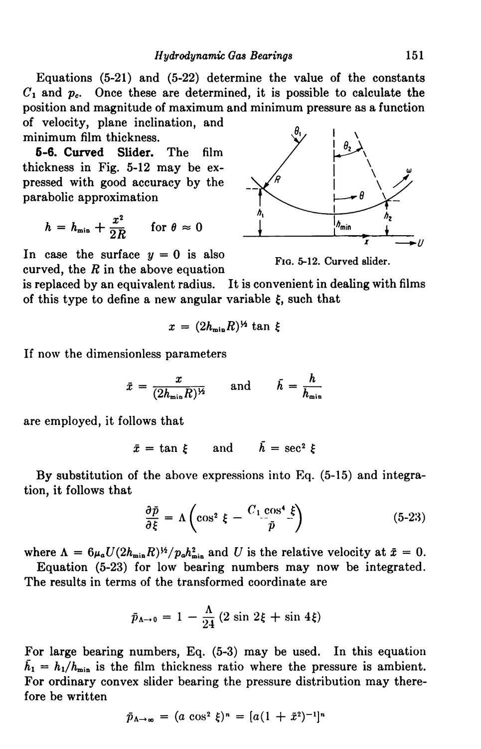
5-6. Curved Slider	151
Finite Slider Bearings	152
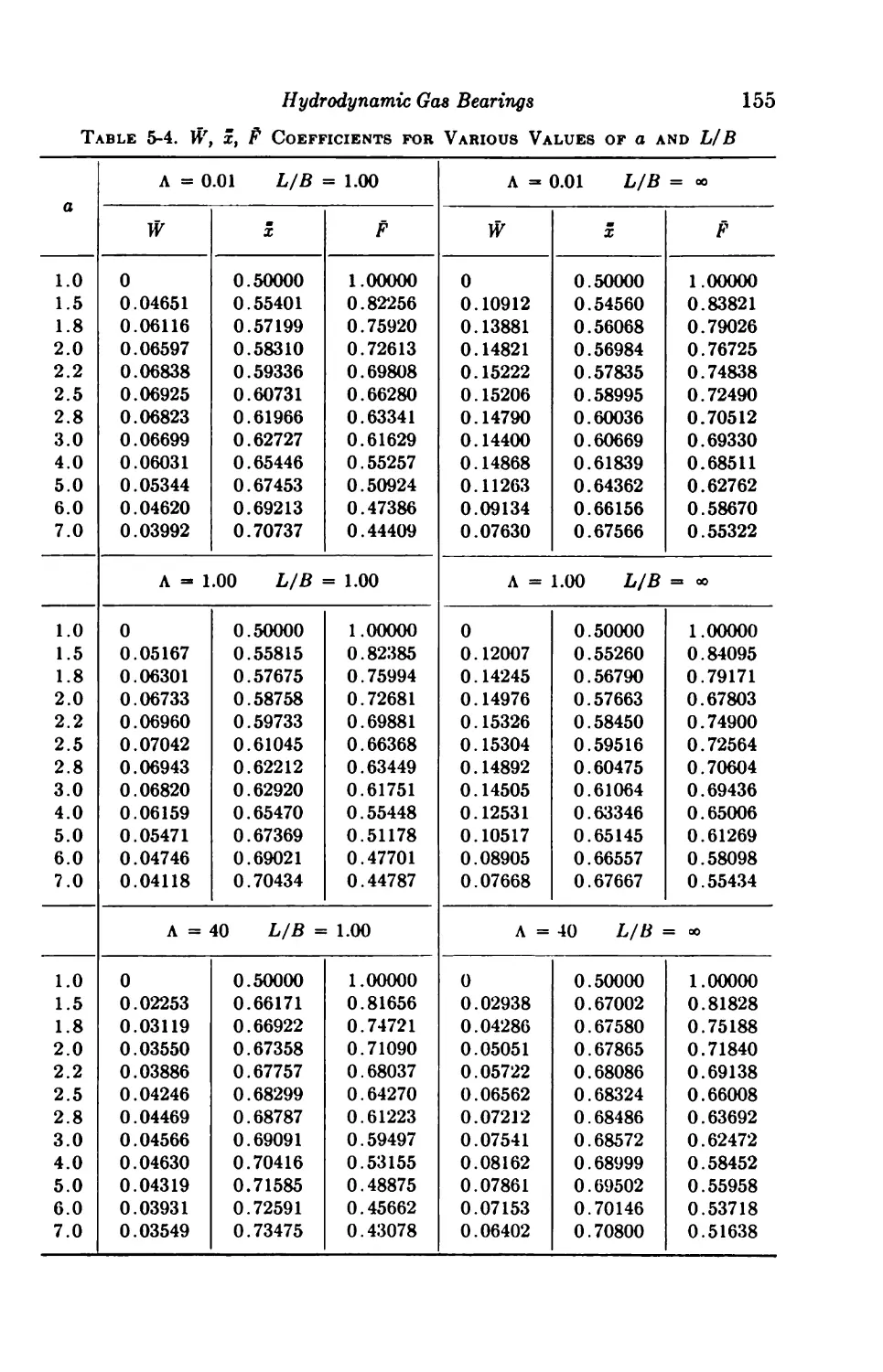
5-7. Plane Inclined Slider	152
Infinitely Long Journal Bearings	152
5-8. Journal Bearing with	Inertia	Considered	152
5-9. Journal Bearing with	Inertia	Neglected	157
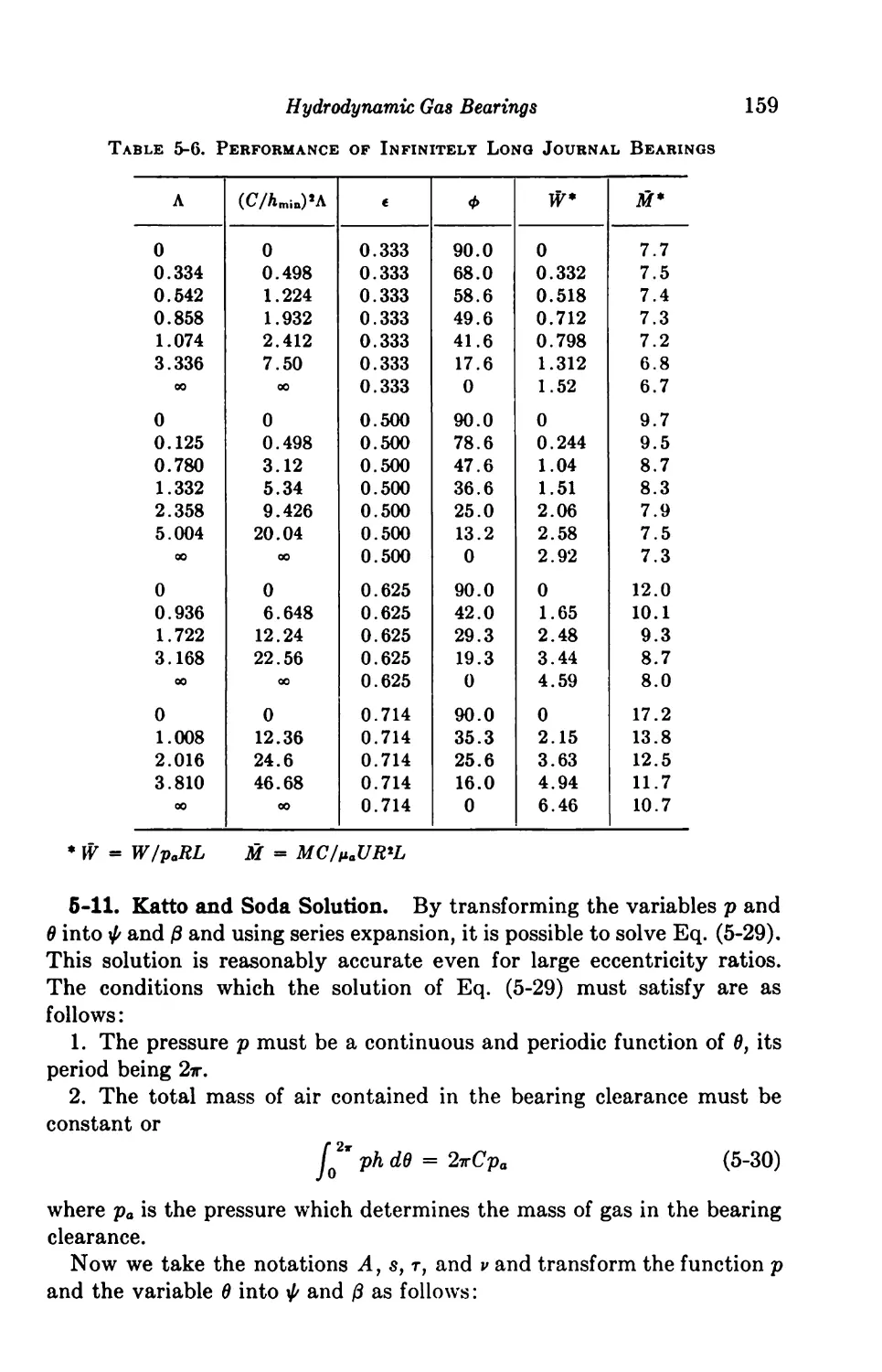
f5-10.	Numerical	Solution	158
*5-11.	Katto and	Soda Solution	159
Finite Journal Bearings	163
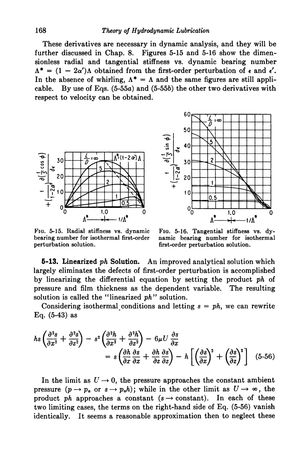
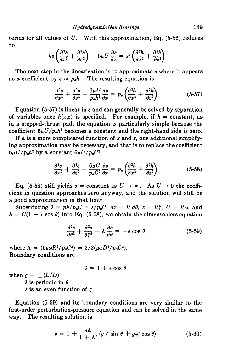
5-12. Perturbation Solution	163
5-13.	Linearized	ph Solution	168
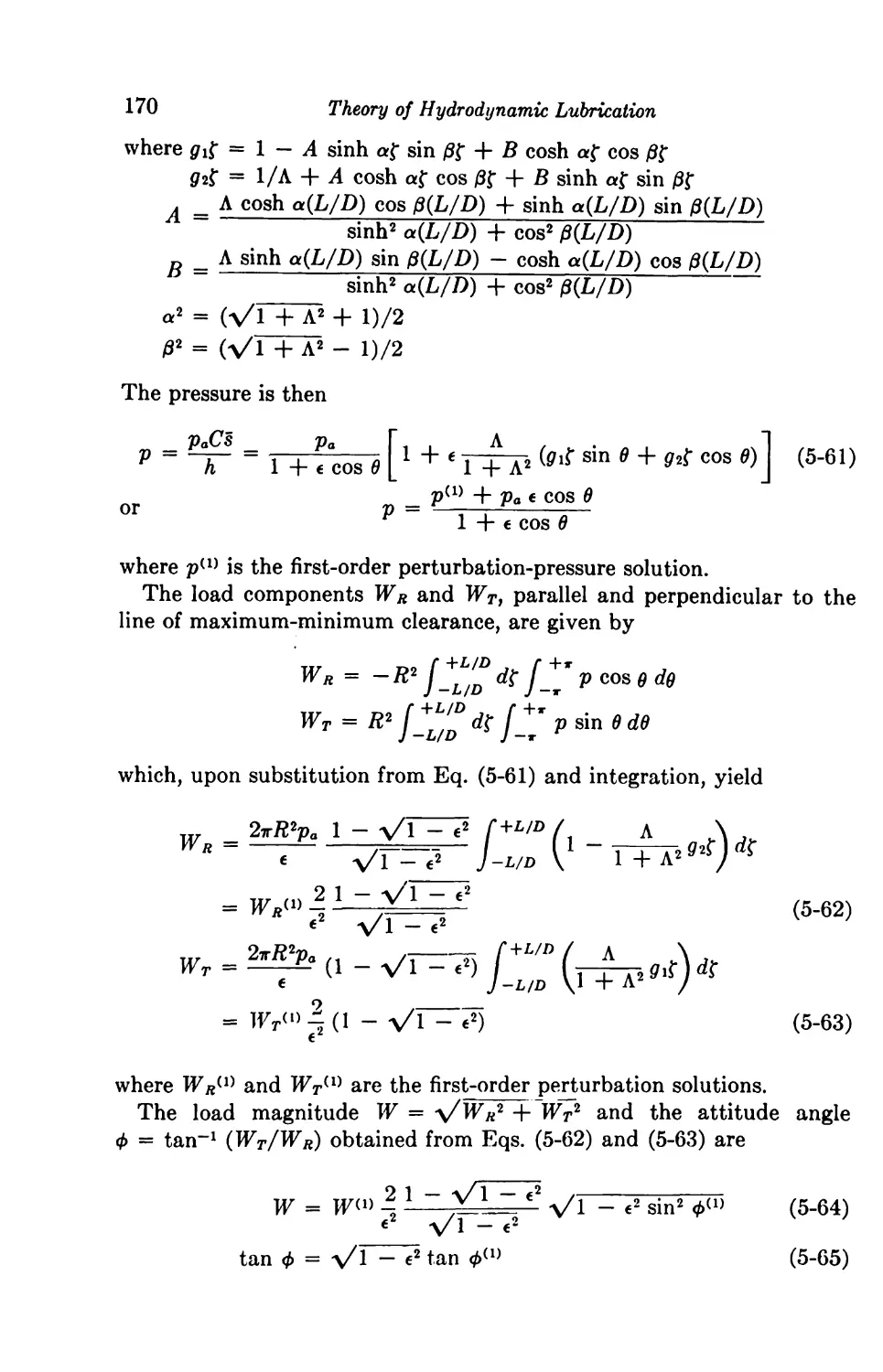
5-14.	Numerical	Solution	171
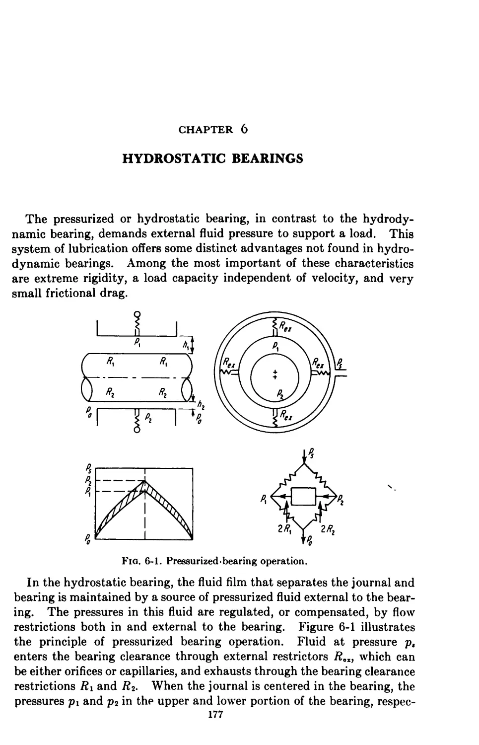
6.	Hydrostatic Bearings	177
Plain Journal Bearings	178

Contents	ix
6-1.	Incompressible Lubrication	178
Laminar Feeding	178
Turbulent Feeding	182
Rotational Considerations	187
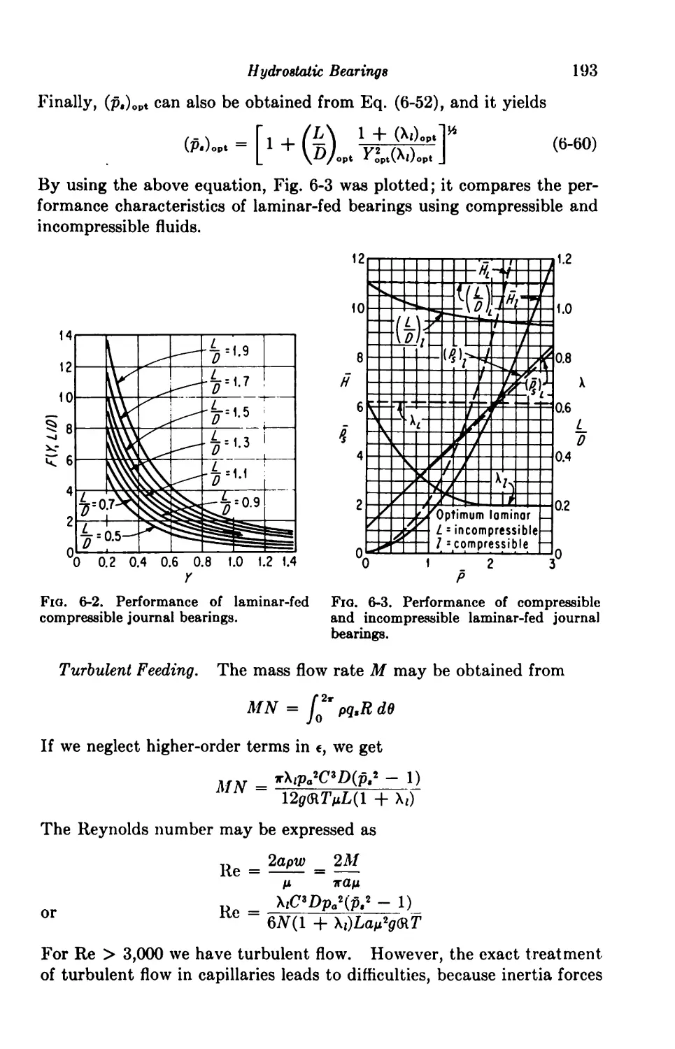
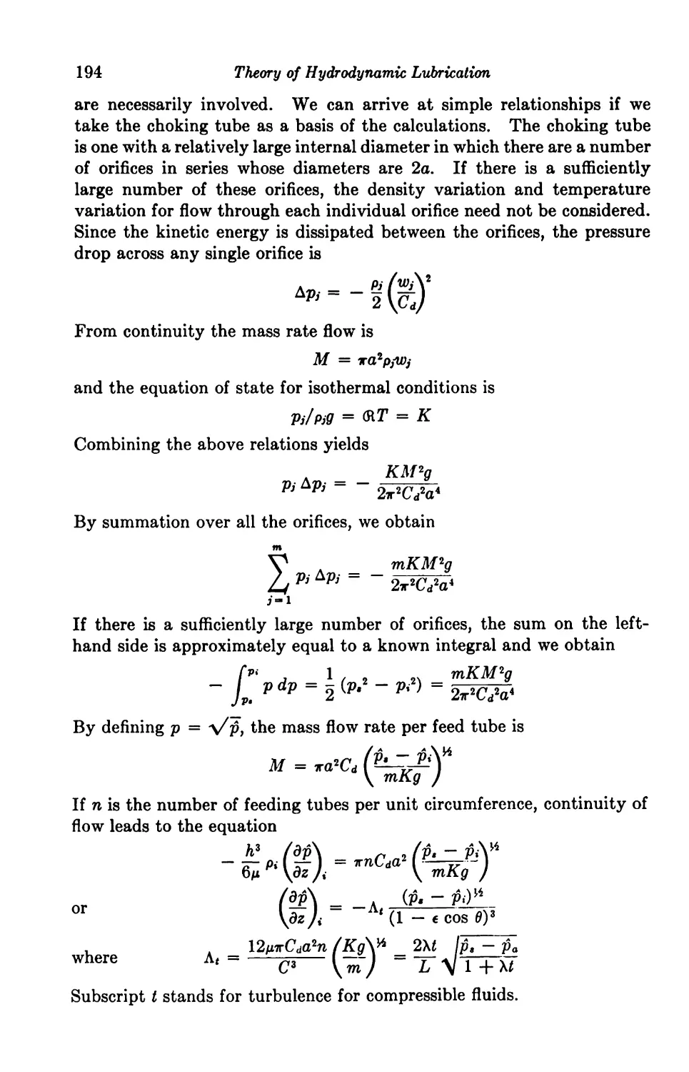
6-2. Compressible Lubrication	190
Laminar Feeding	190
Turbulent Feeding	193
Static and Dynamic Characteristics of Gas	Journal Bearings ....	196
Step Thrust Bearing	200
Isothermal Operation	200
6-3. Compressible Lubrication	200
6-4. Incompressible Lubrication	203
Adiabatic Operation	204
6-5. Incompressible Lubrication	205
6-6. Compressible Lubrication	206
Self-excited Vibrations in Gas-lubricated Step Thrust Bearing ....	207
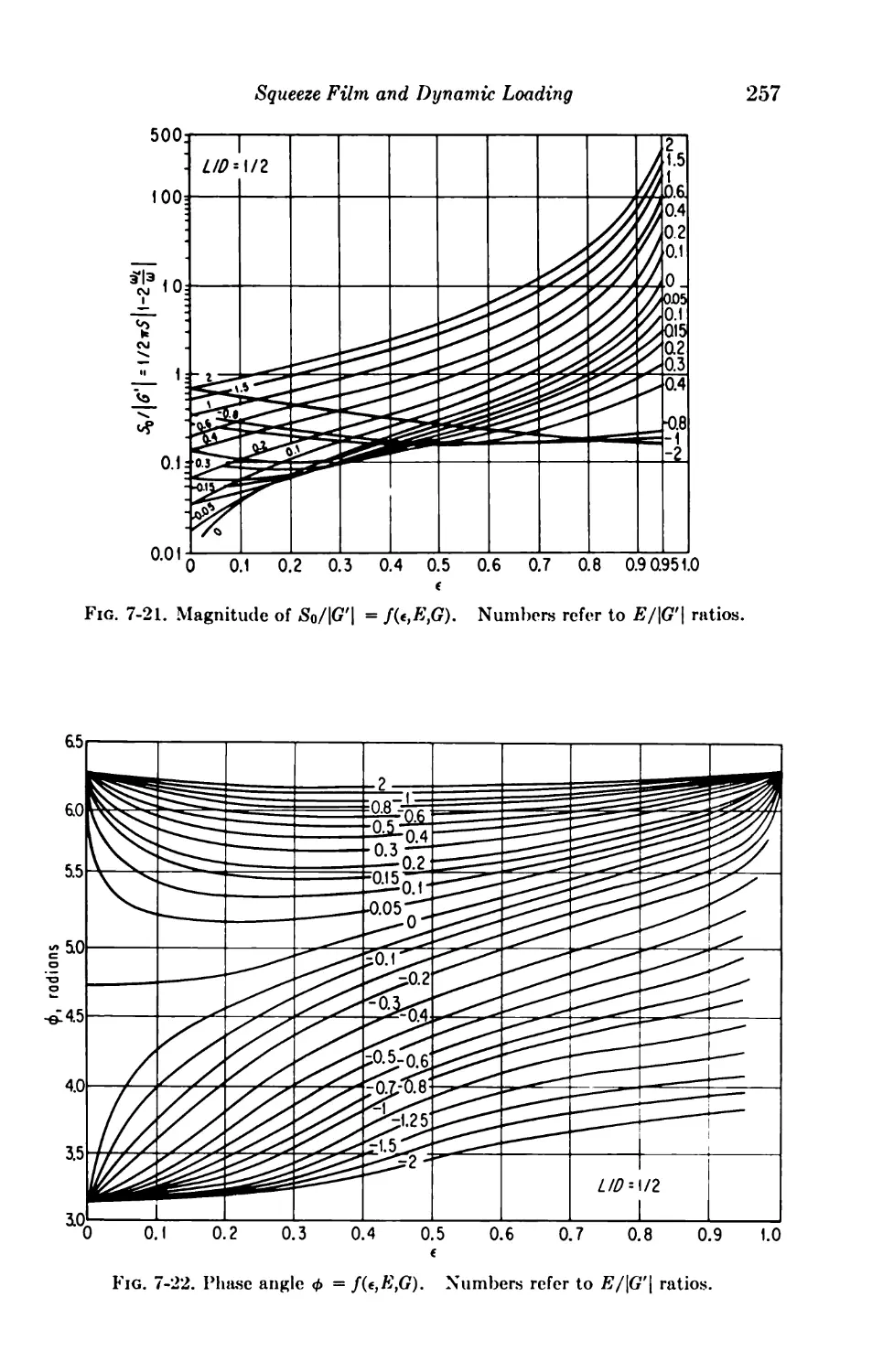
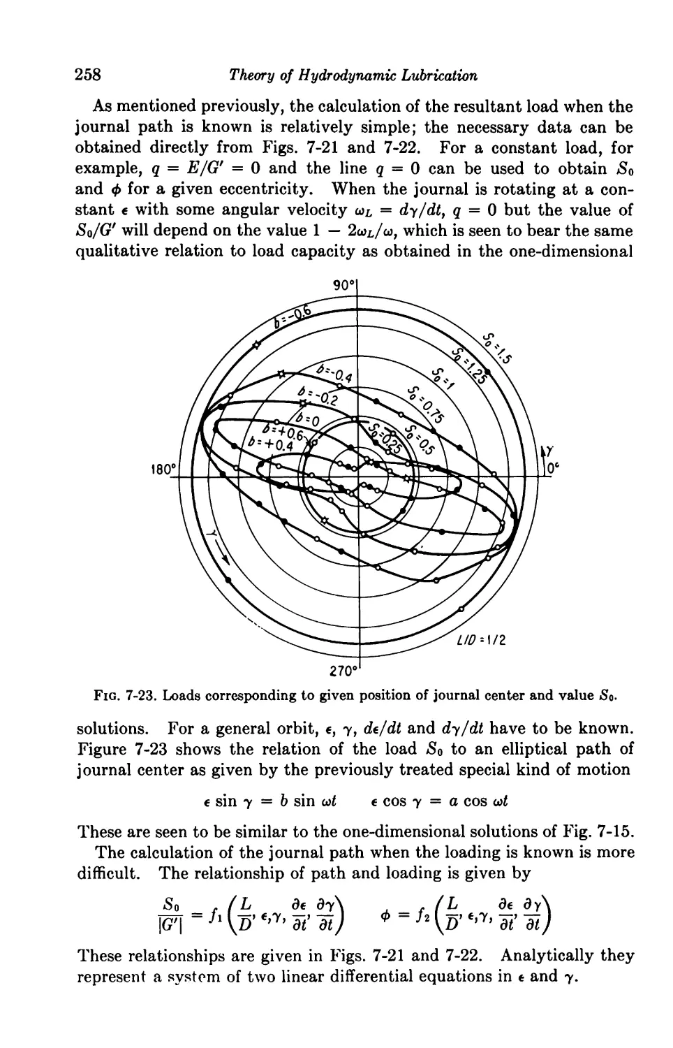
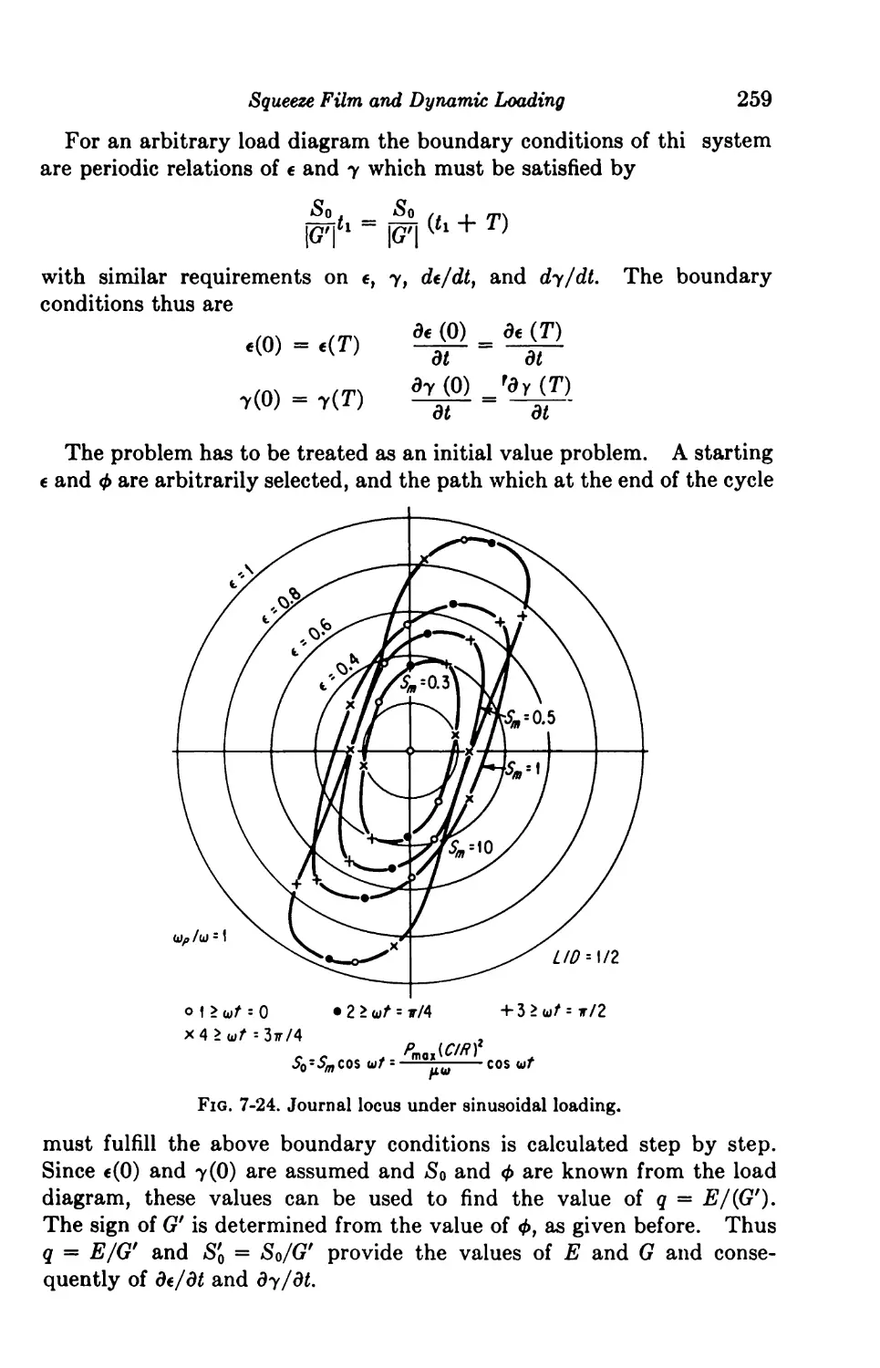
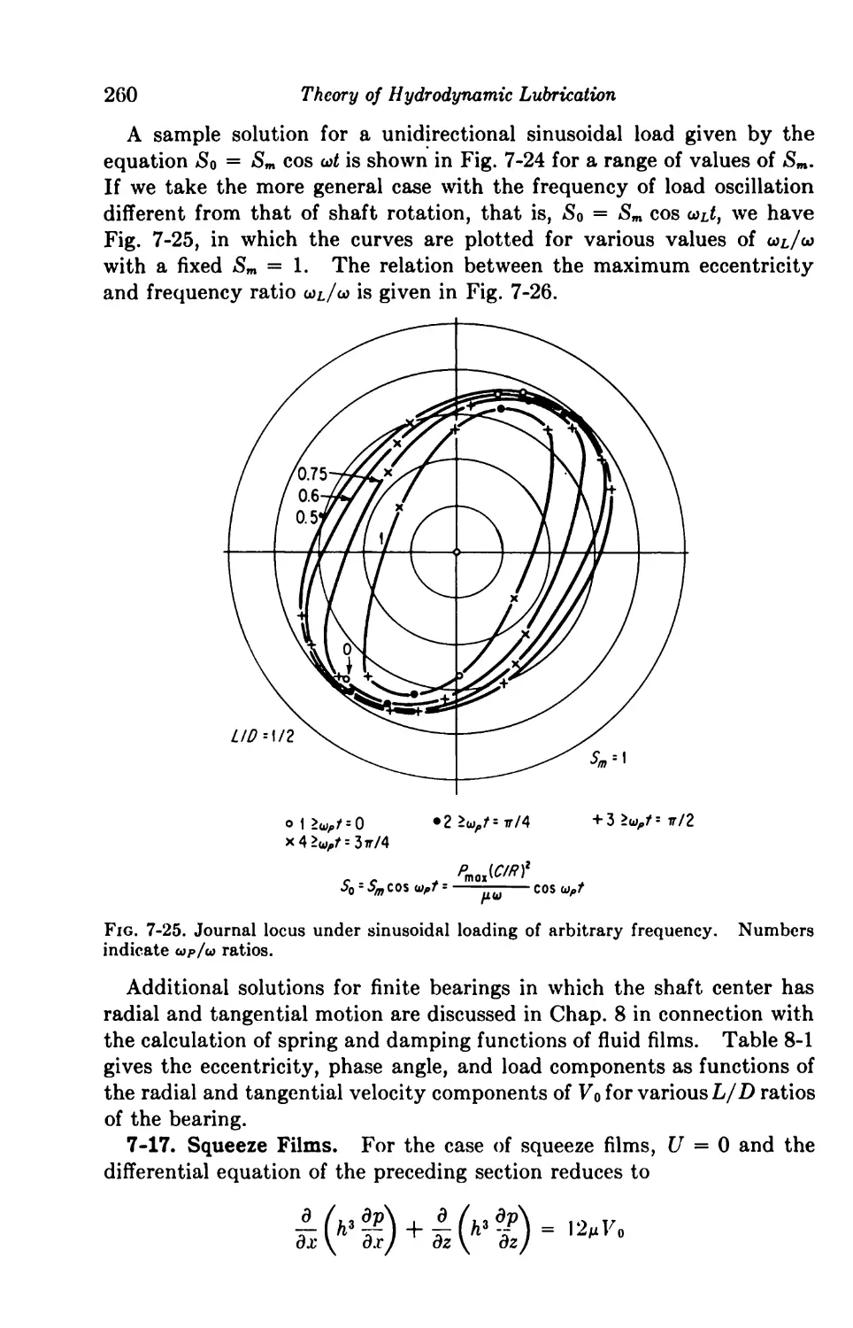
7. Squeeze Film and Dynamic Loading	213
Dynamically Loaded Bearings	213
The Reynolds Equation for Dynamic Loading	214
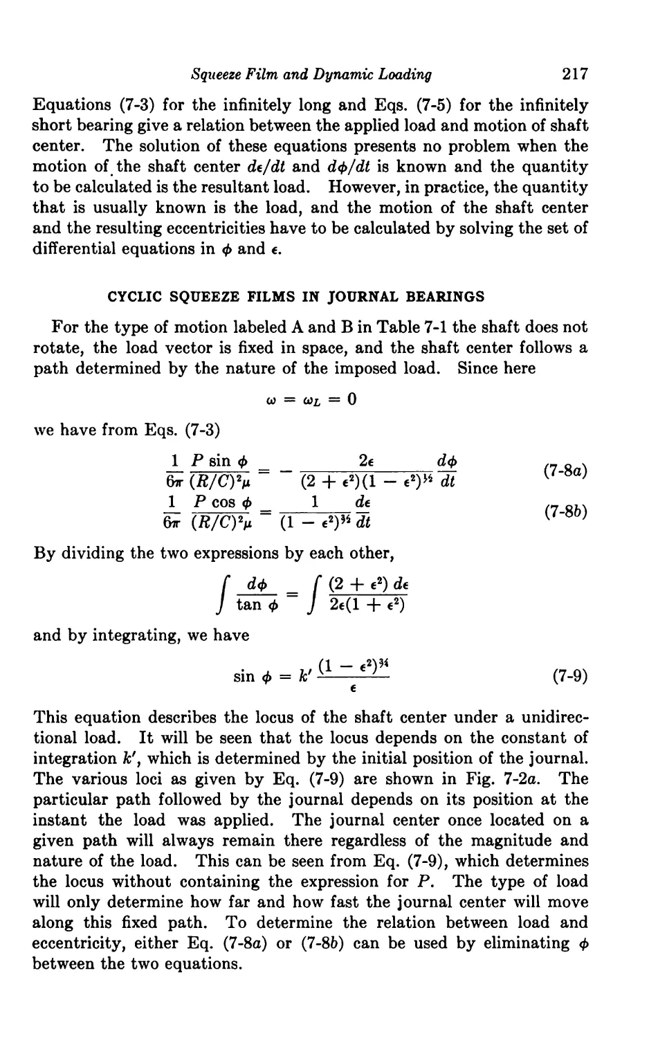
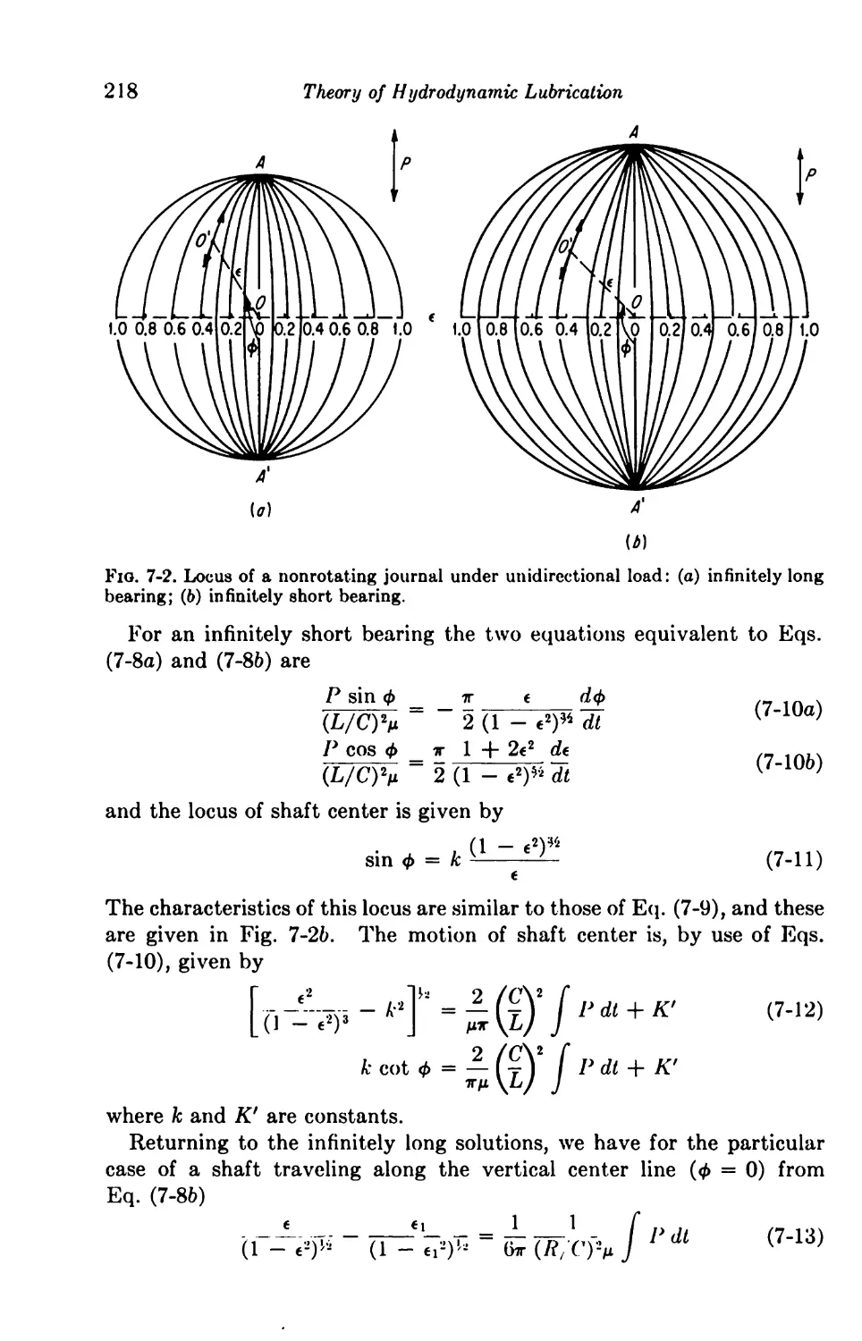
Cyclic Squeeze Films in Journal Bearings	217
7-1. Constant Loads	219
7-2. Alternating Loads	219
7-3. Rotating Loads	219
Noncyclic Squeeze Films	220
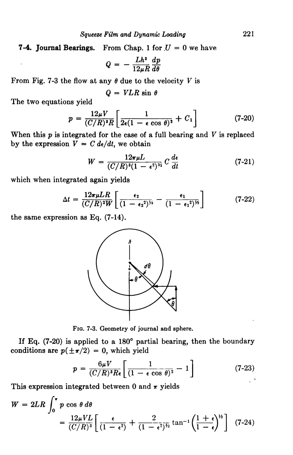
7-4.	Journal Bearings	221
7-5.	Spherical Bearings	222
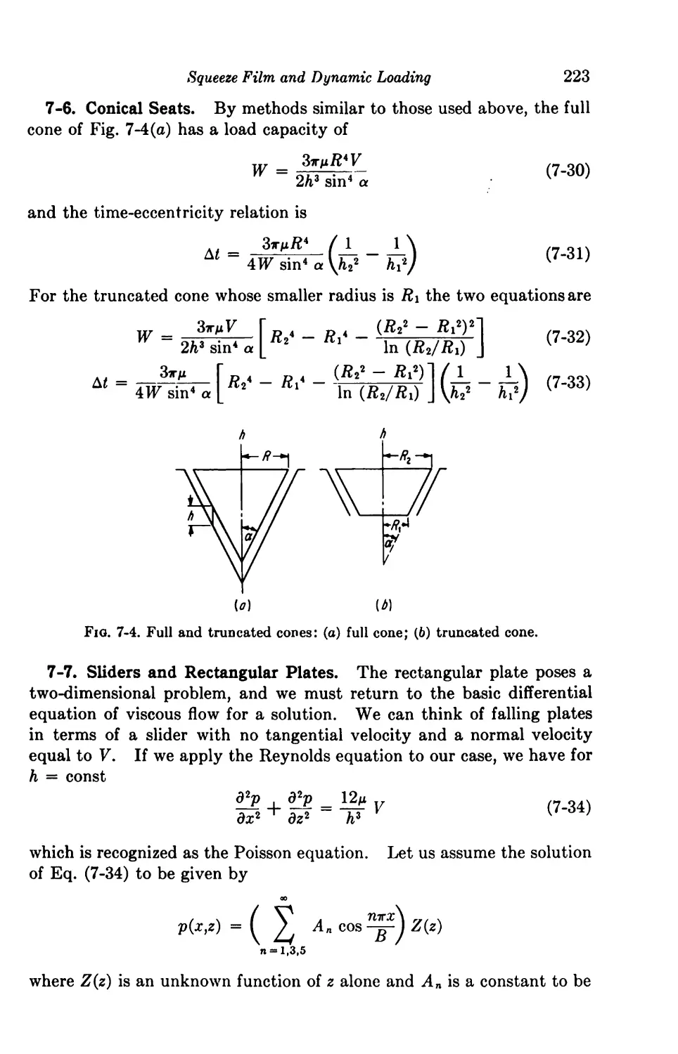
7-6.	Conical Seats	223
7-7.	Sliders and Rectangular Plates	223
7-8.	Elliptical and Circular Plates	225
7-9.	Miscellaneous Configurations	226
Dynamic Loading of Journal Bearings	227
7-10.	Constant Unidirectional Loads	227
7-11.	Variable Unidirectional Loads	229
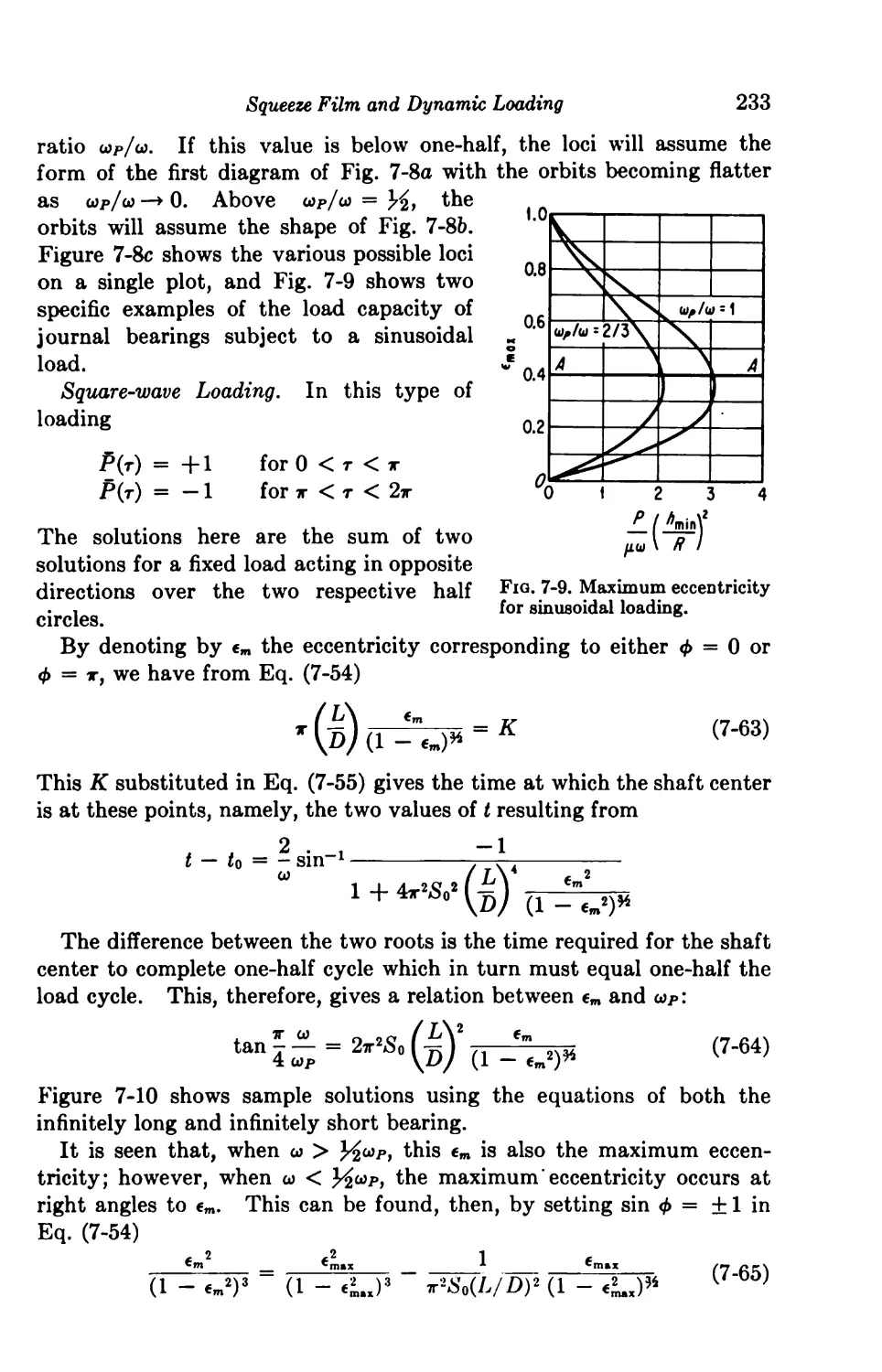
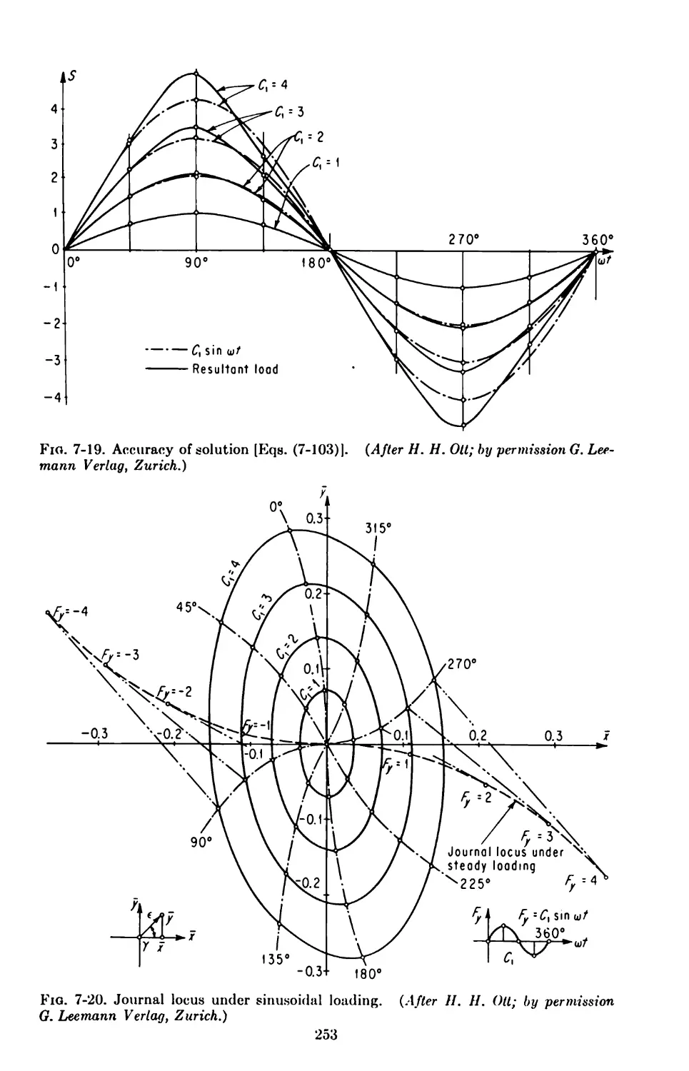
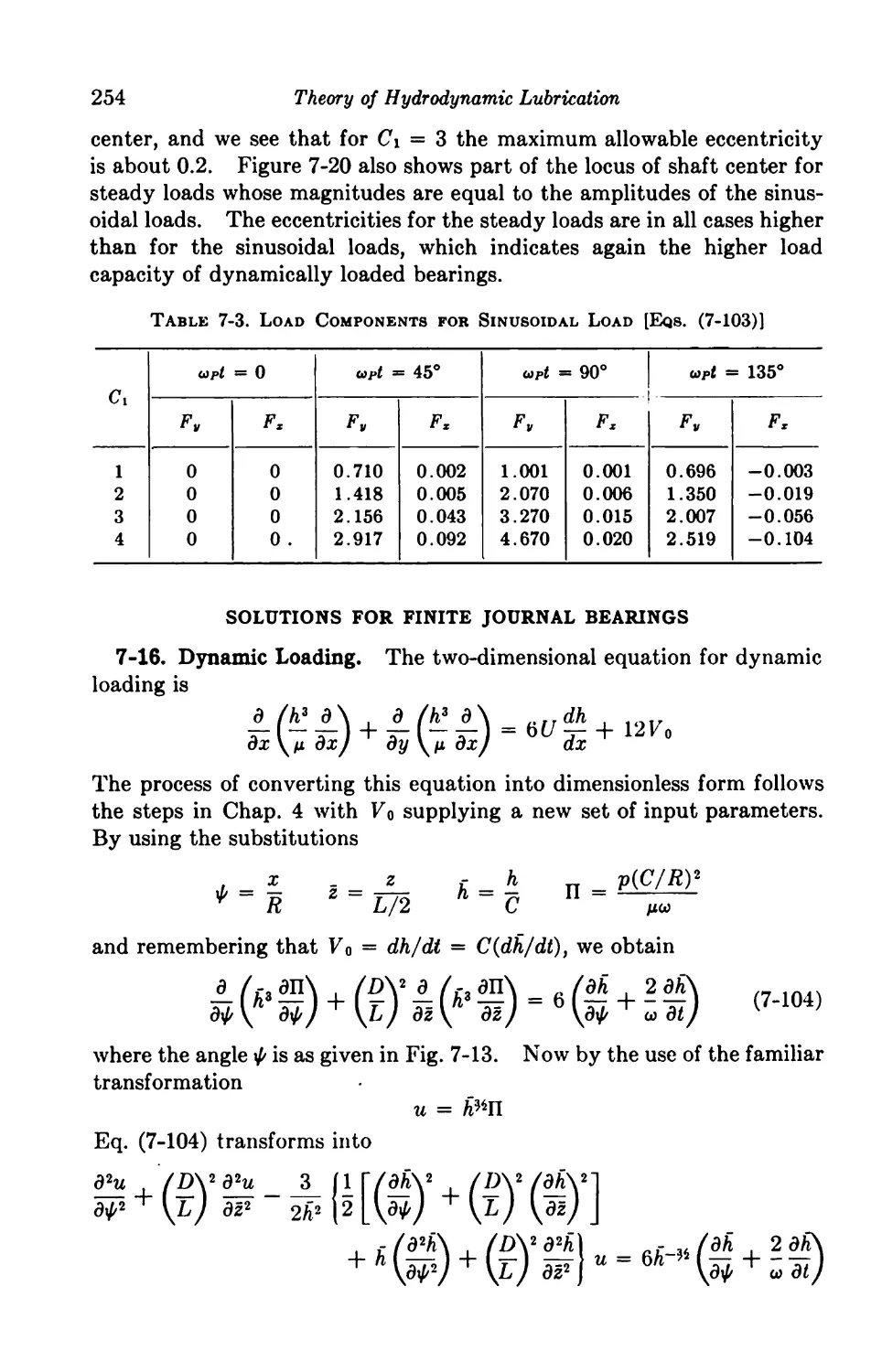
Sinusoidal Loading	231
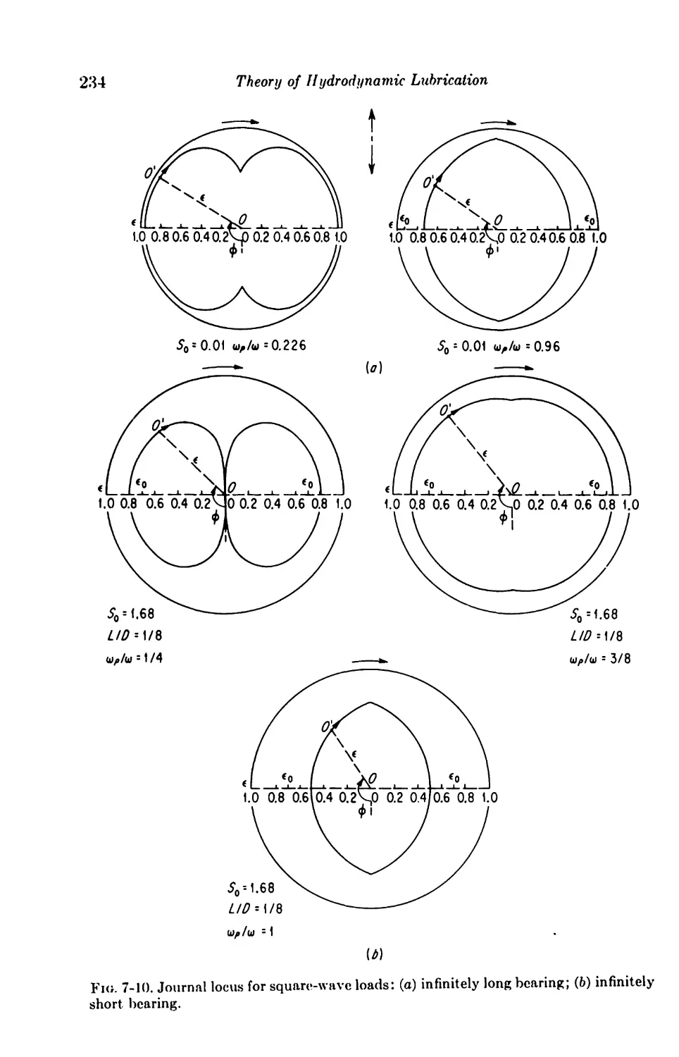
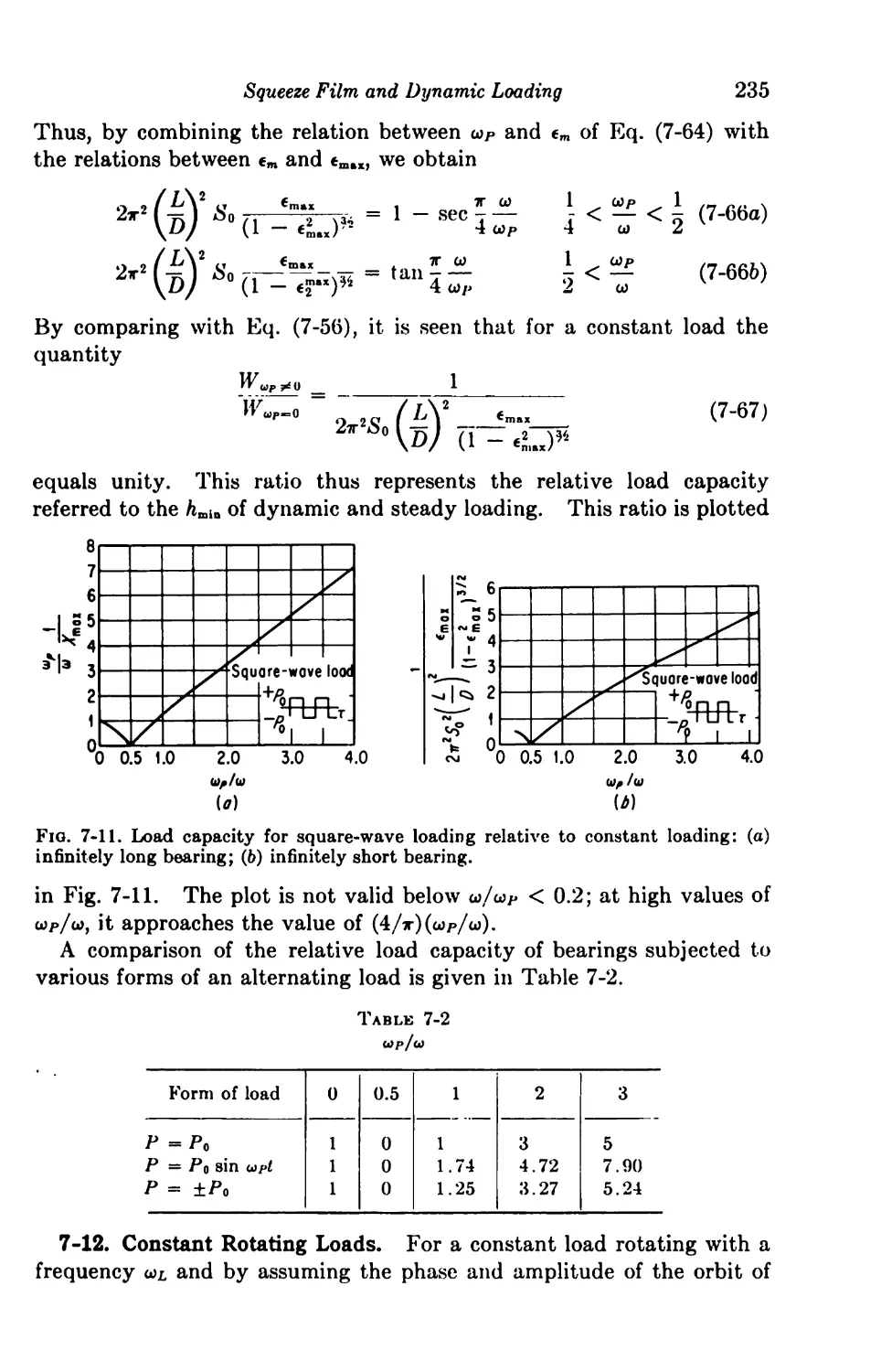
Square-wave Loading	233
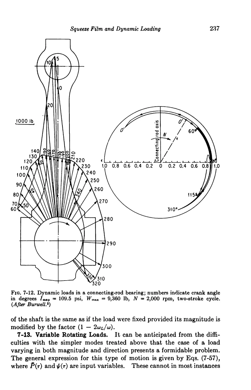
7-12.	Constant Rotating Loads	235
7-13.	Variable Rotating Loads	237
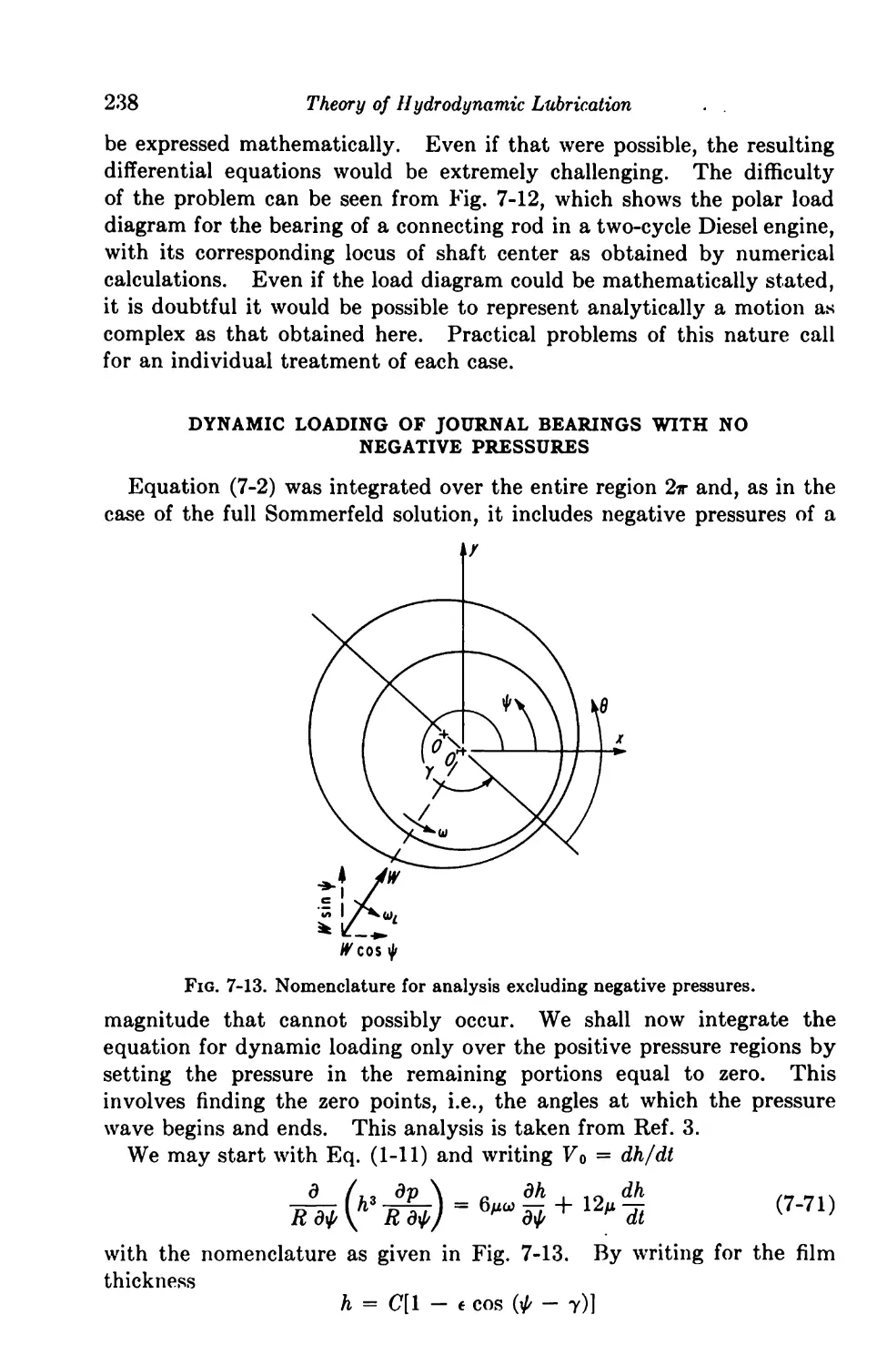
Dynamic Loading of Journal Bearings with No Negative Pressures.	238
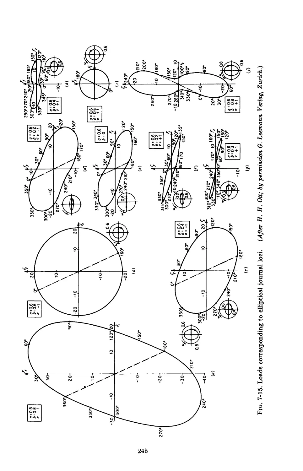
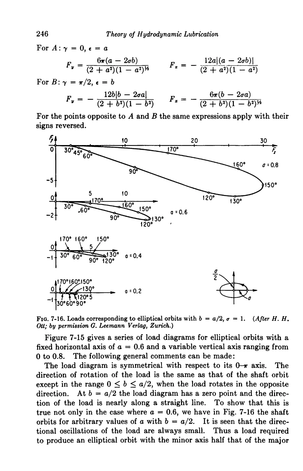
7-14.	Solutions for Prescribed Loci	242
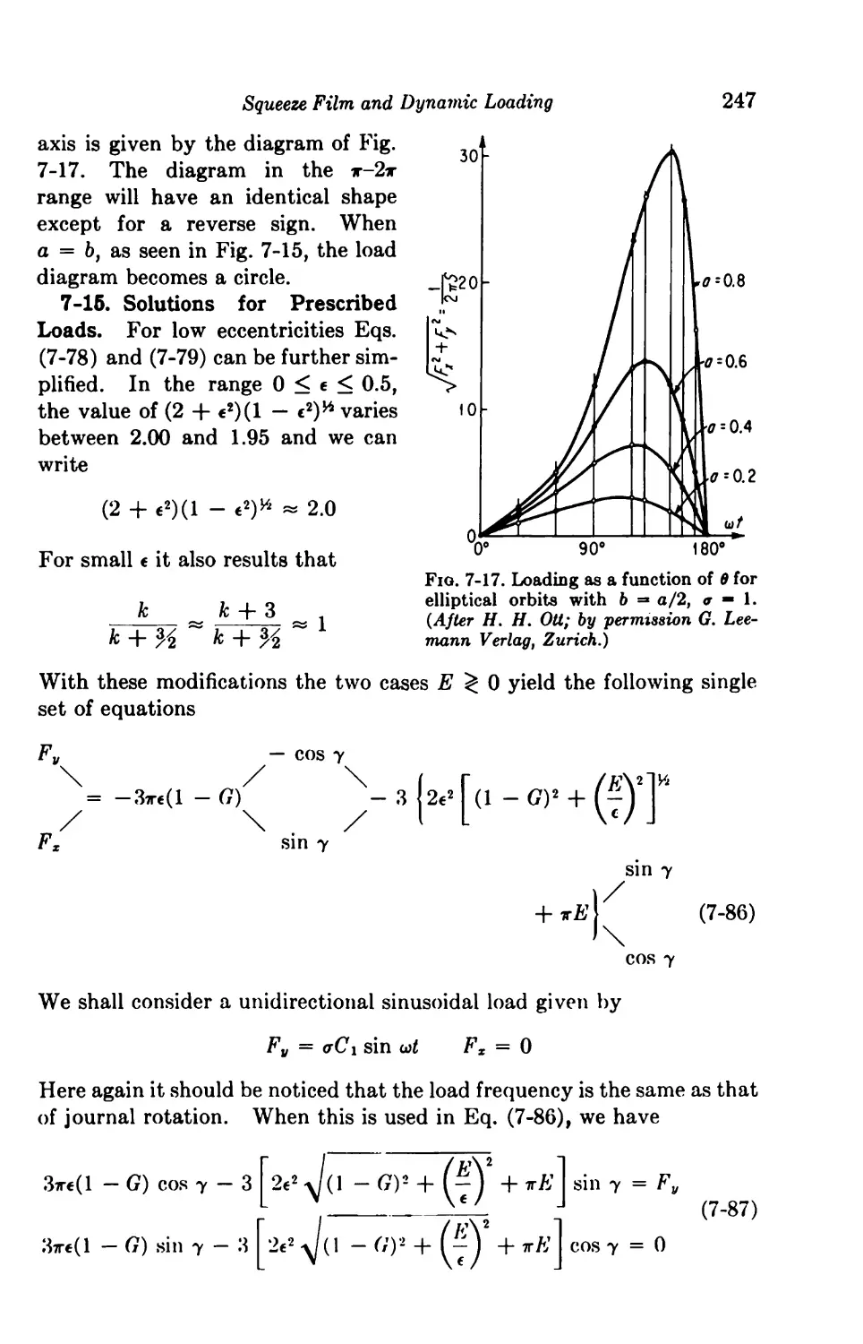
7t15.	Solutions for Prescribed Loads	247
Solutions for Finite Journal Bearings	254
7-16. Dynamic Loading	254
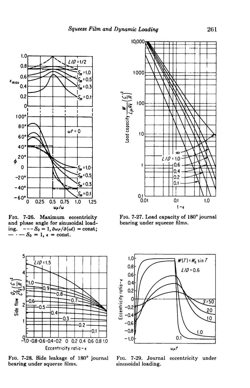
7-17. Squeeze Films	260
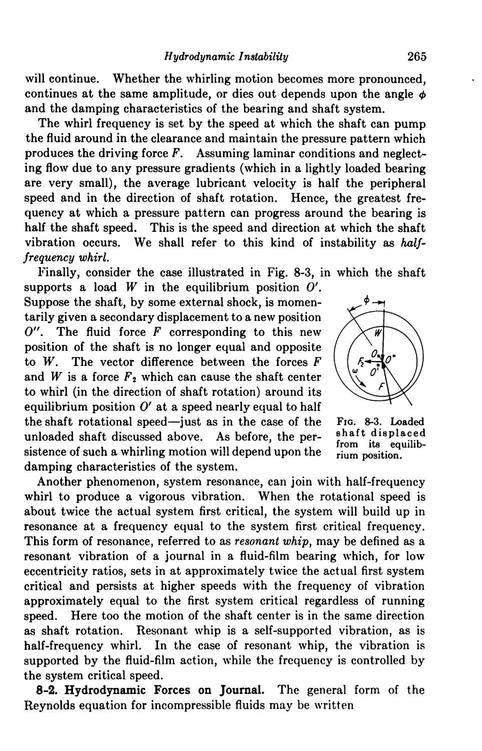
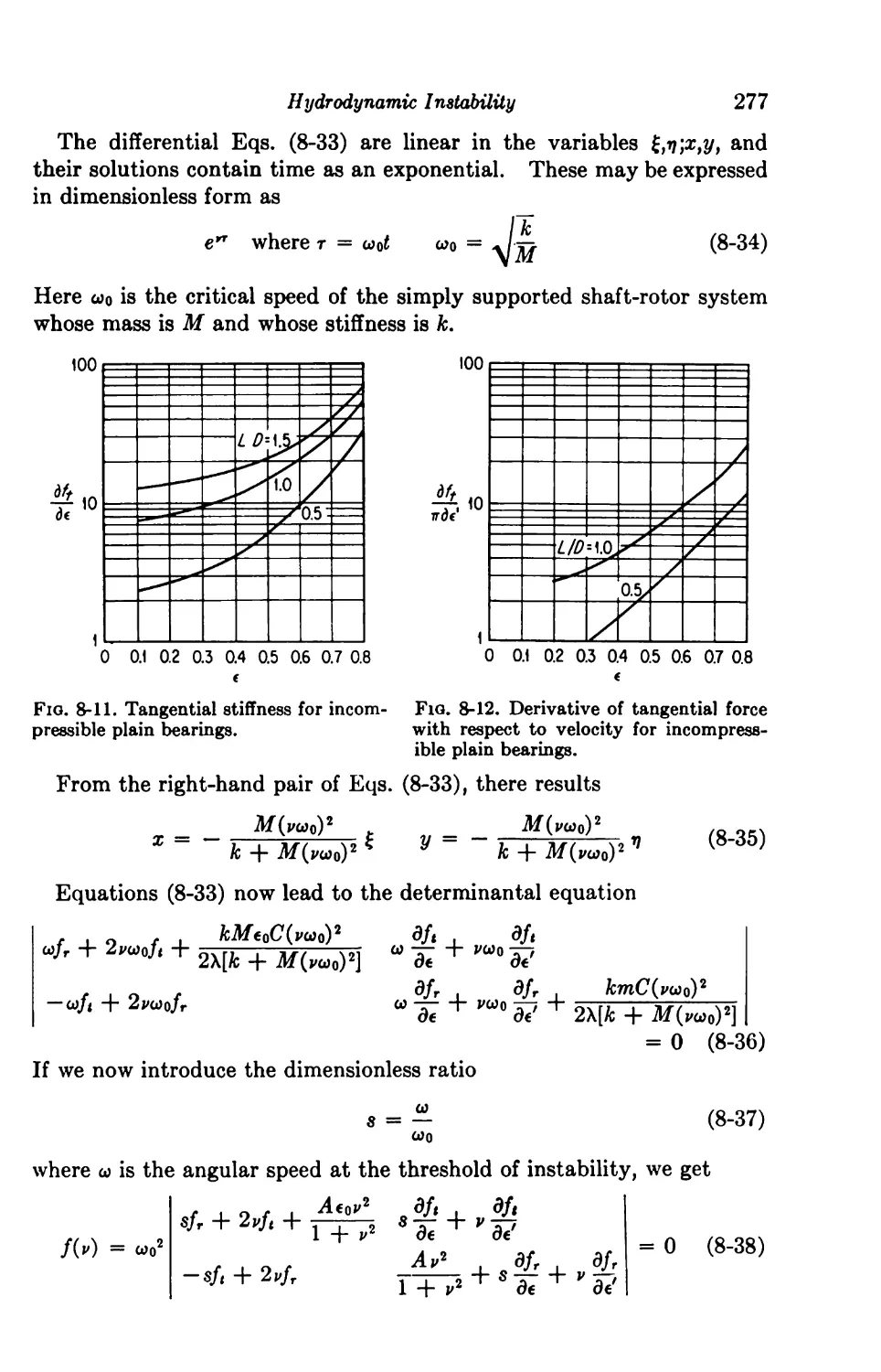
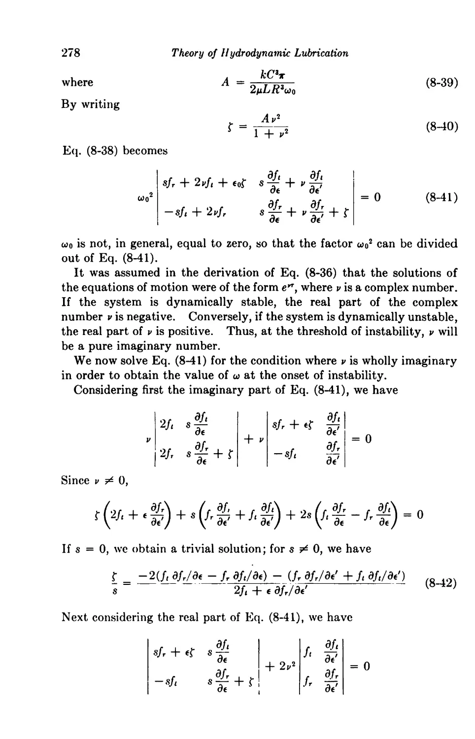
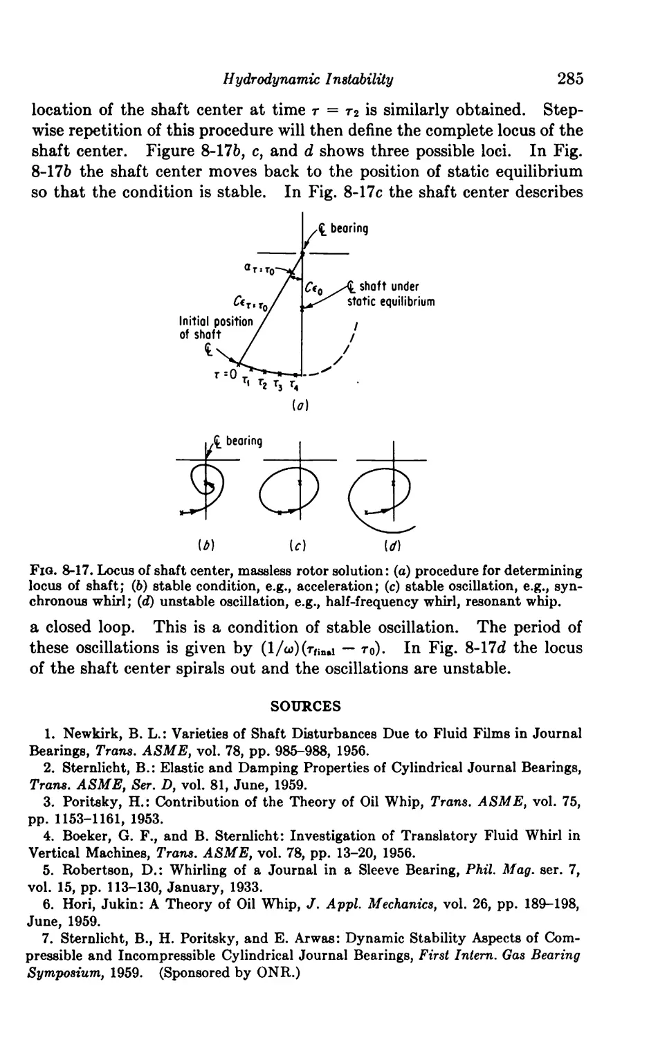
8. Hydrodynamic Instability	264
8-1.	The Mechanics of Hydrodynamic Instability	264
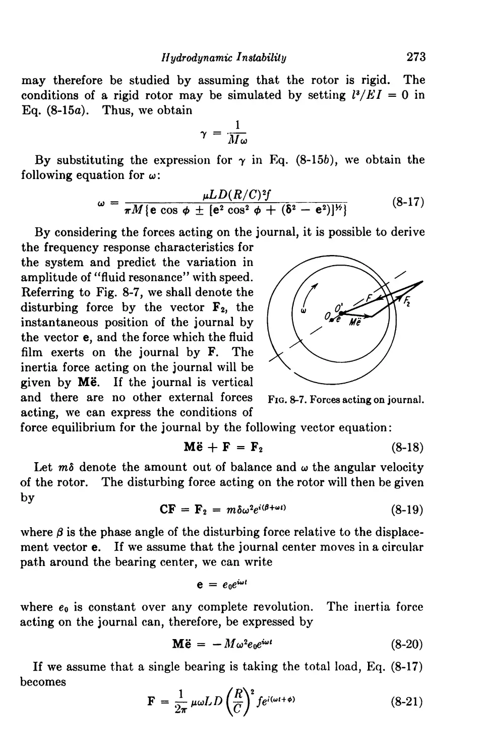
8-2.	Hydrodynamic Forces on Journal	265
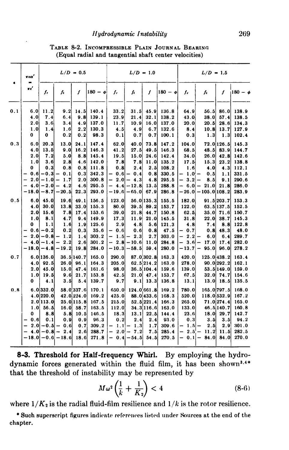
8-3.	Threshold for Half-frequency Whirl	269
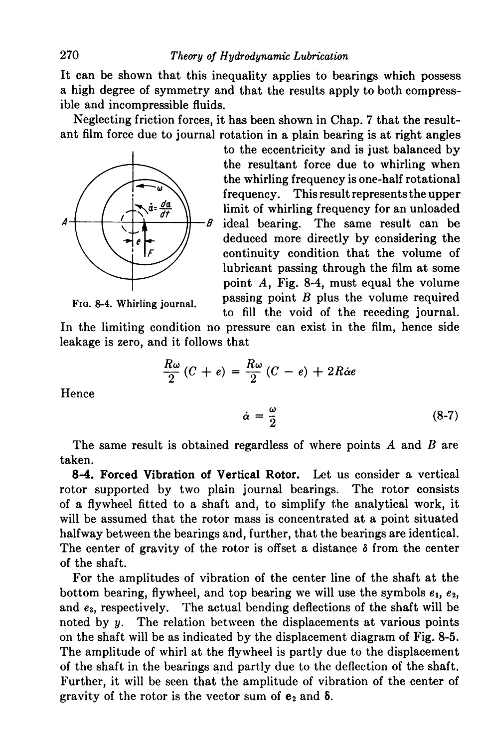
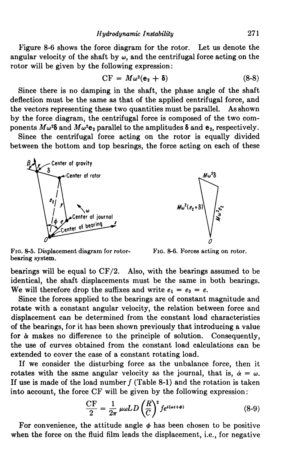
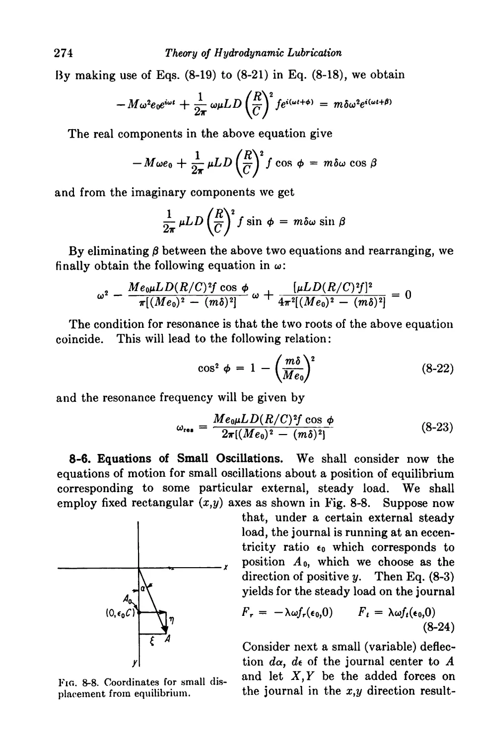
8-4.	Forced Vibration of Vertical Rotor	270
8-5.	Fluid-film and Rotor Resonance	272

X
Contents
8-6. Equations of Small Oscillations	274
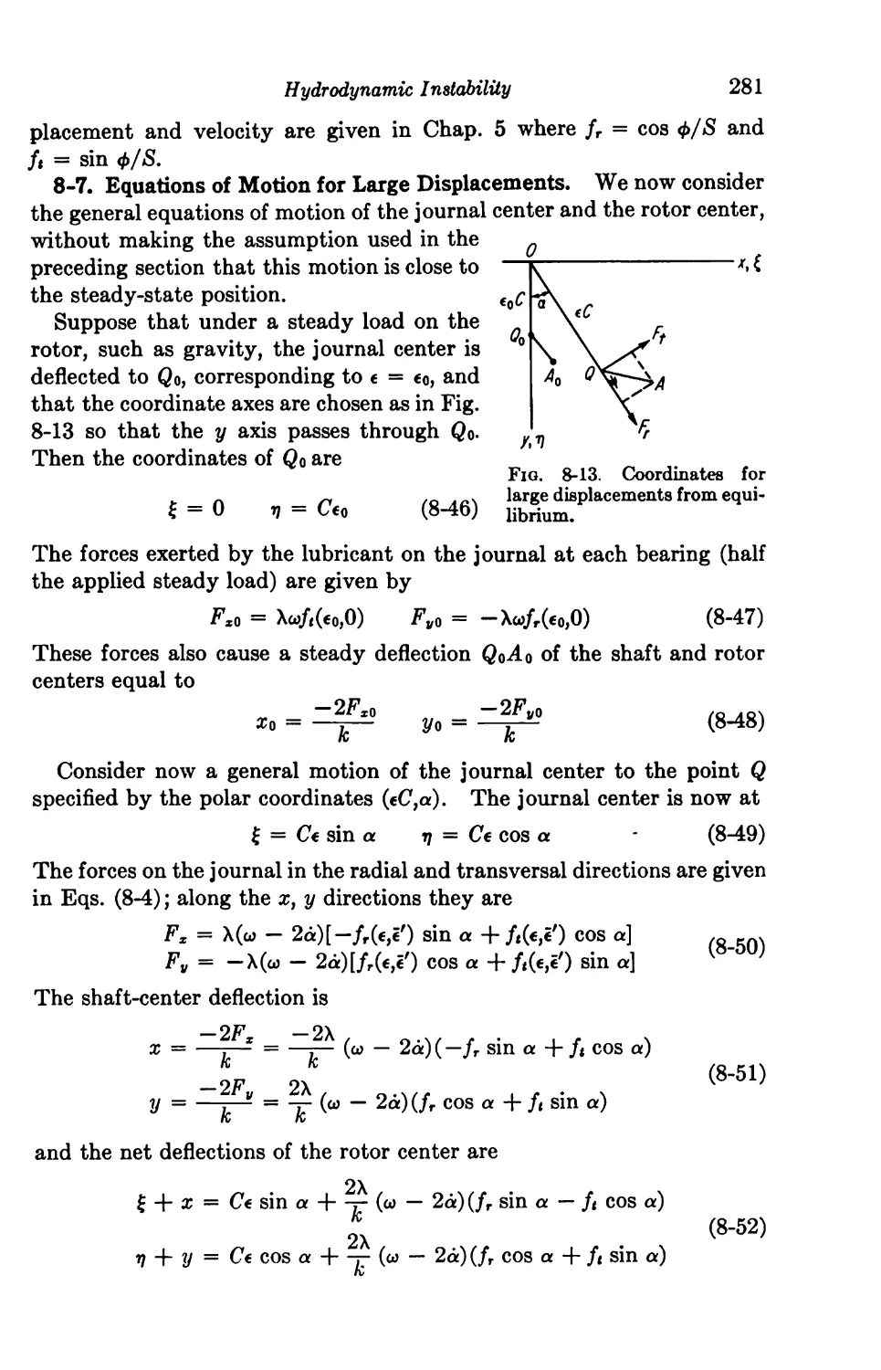
8-7. Equations of Motion for Large Displacements	281
9.	Adiabatic Solutions	286
Introduction	286
The Thermal Wedge	288
One-dimensional Solutions	292
9-1. Parallel Slider with p = f(T), p = f(p,T)	292
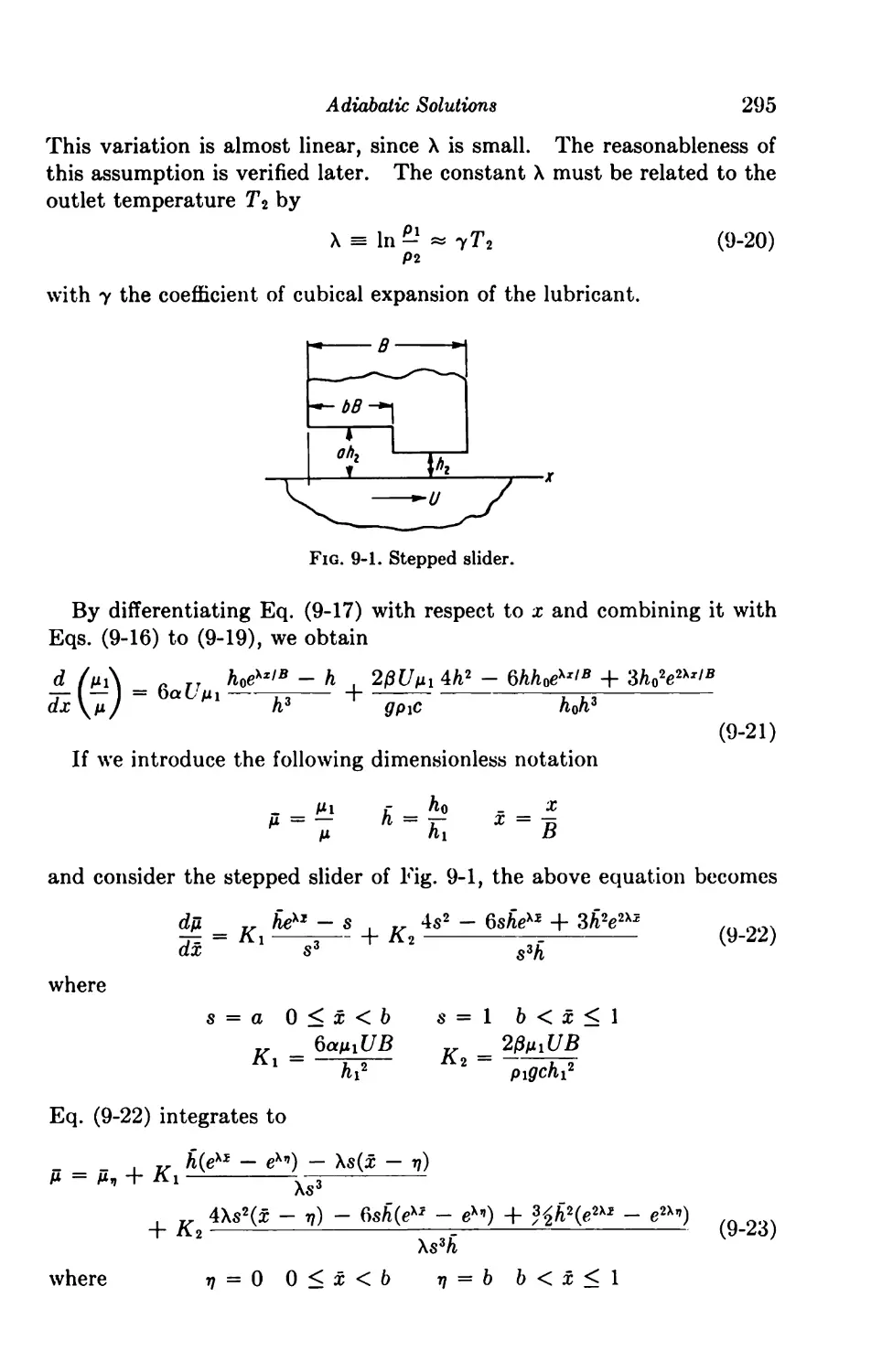
9-2. Step Slider with p = f(x), p = f(p,T)	294
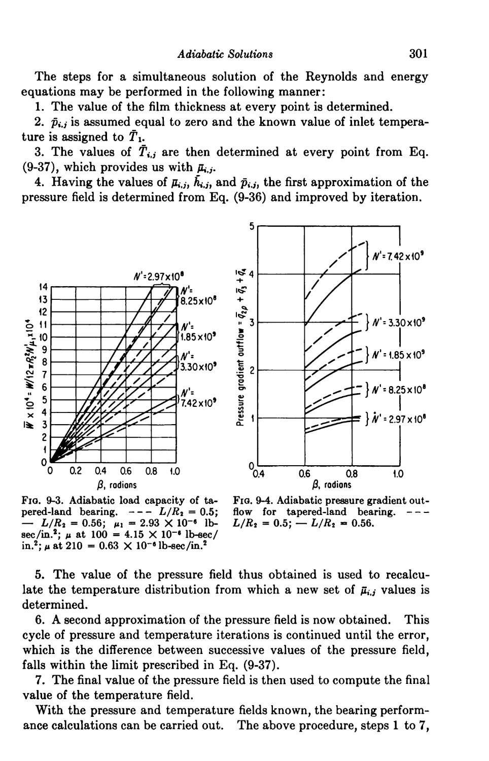
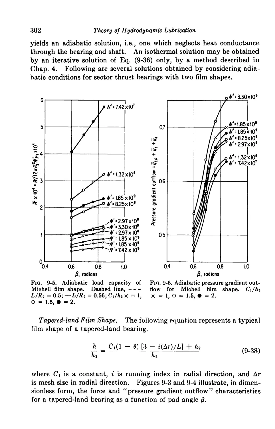
9-3. Exponential Slider with p = f(p,T)	297
Finite Solutions	298
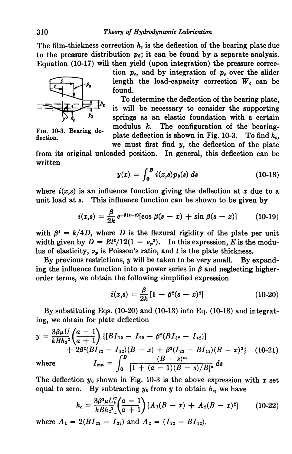
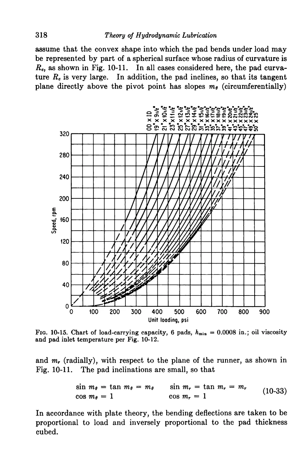
10. Elasticity Considerations	306
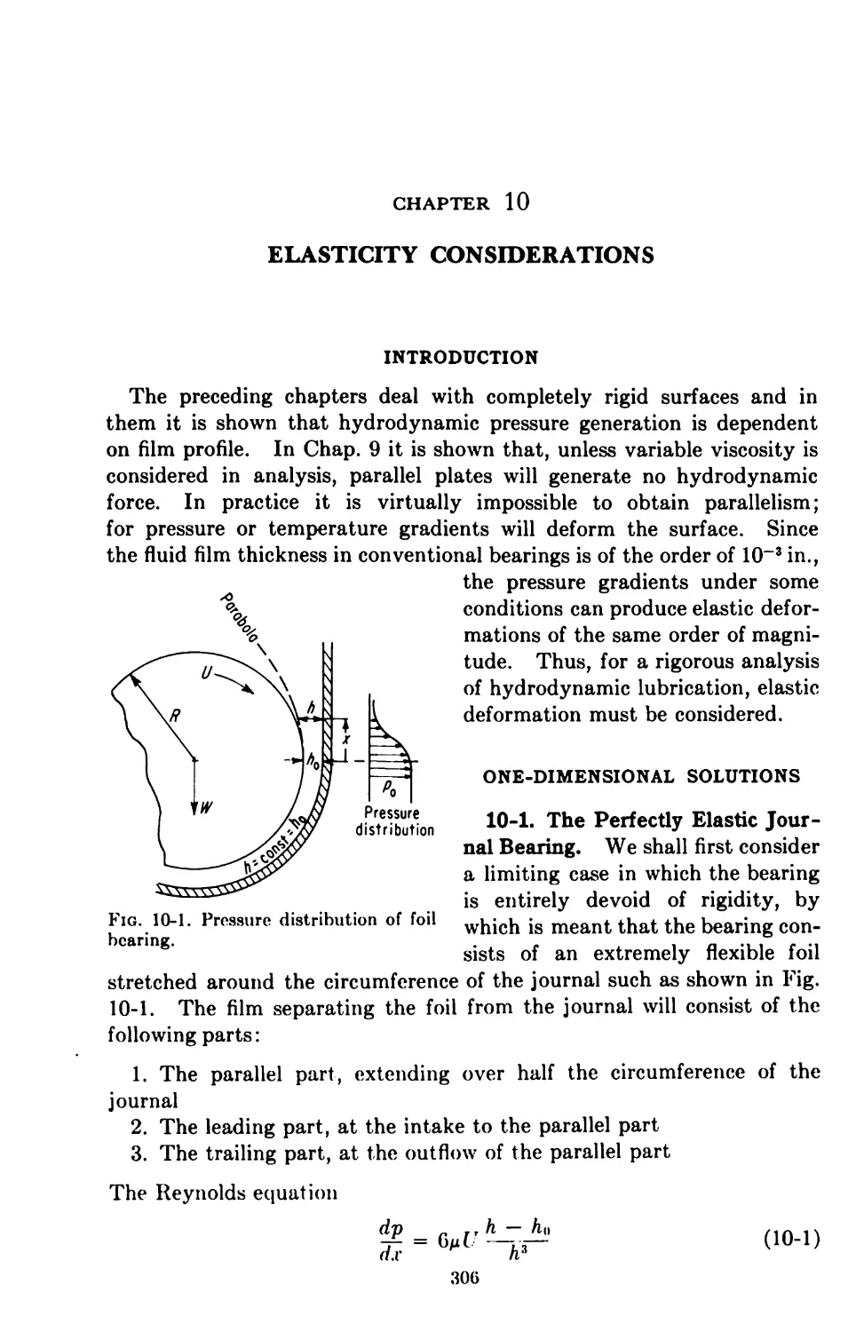
Introduction	306
One-dimensional Solutions	306
10-1. The Perfectly Elastic Journal Bearing	306
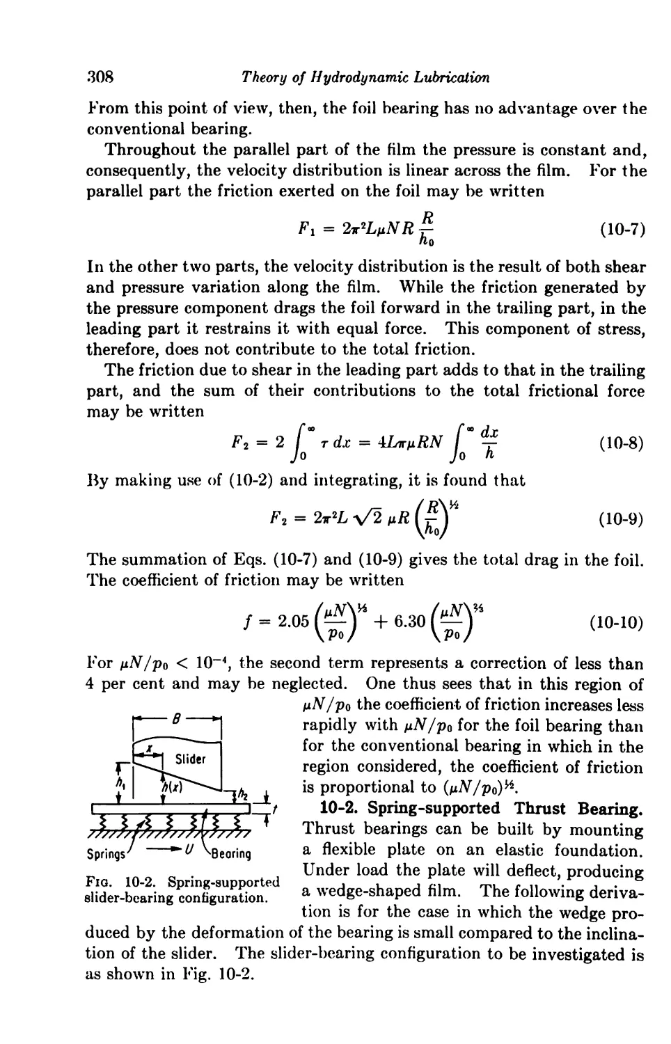
10-2. Spring-supported Thrust Bearing	308
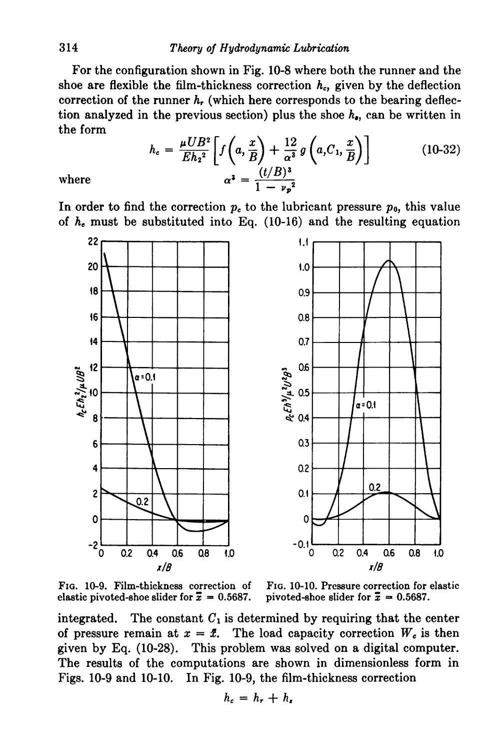
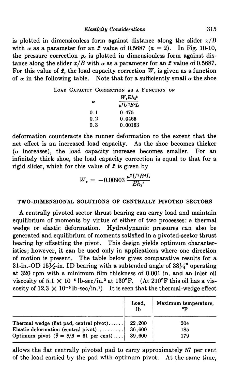
10-3. Pivoted Shoe with Elastic Deformation	313
Two-dimensional Solutions of Centrally Pivoted Sectors	315
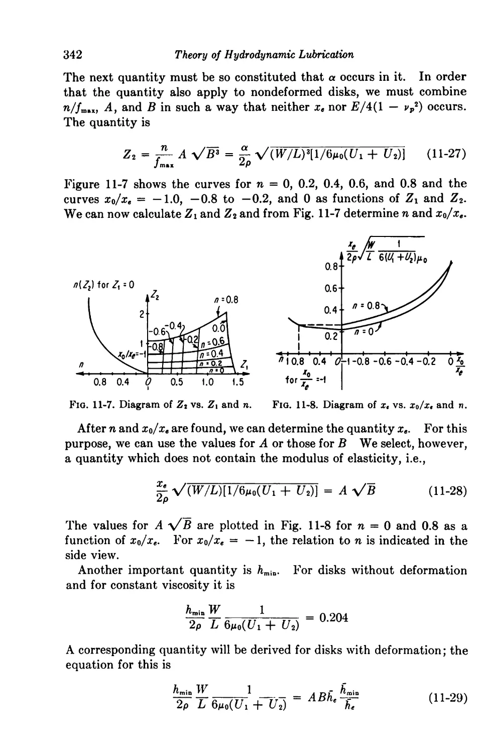
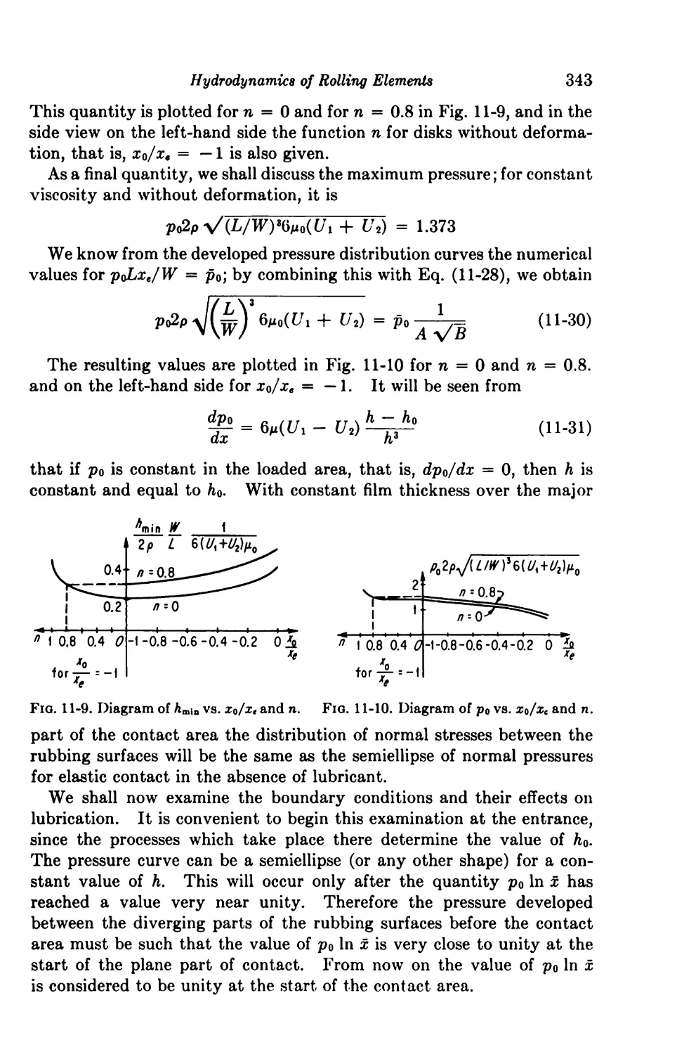
11. Hydrodynamics of Rolling Elements	328
General Remarks	328
Fluid Film with Rigid Surfaces	329
11-1. Solutions with Constant Viscosity	329
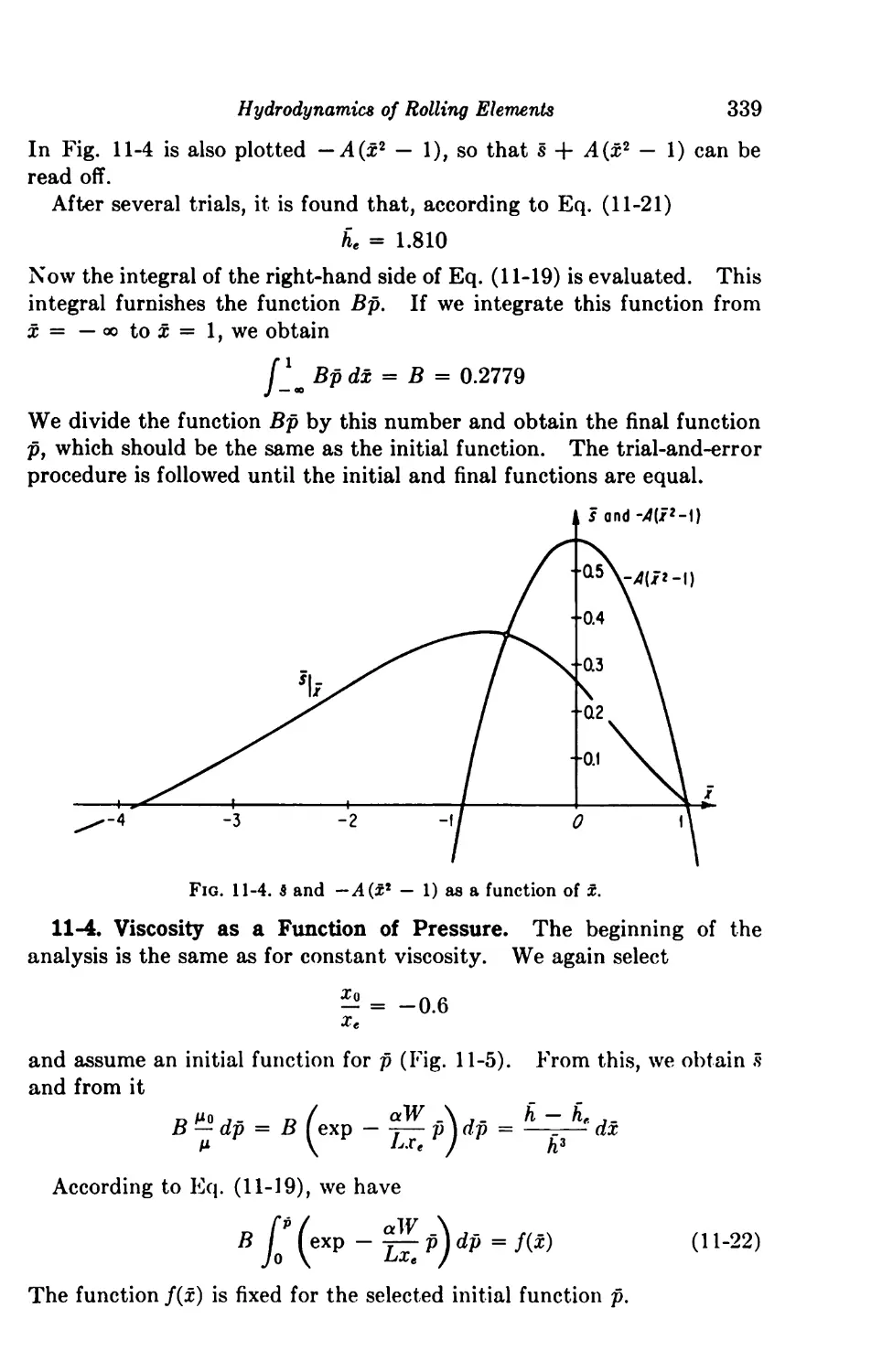
11-2. Viscosity as a Function of Pressure	335
Fluid Film with Elastic Deformation	336
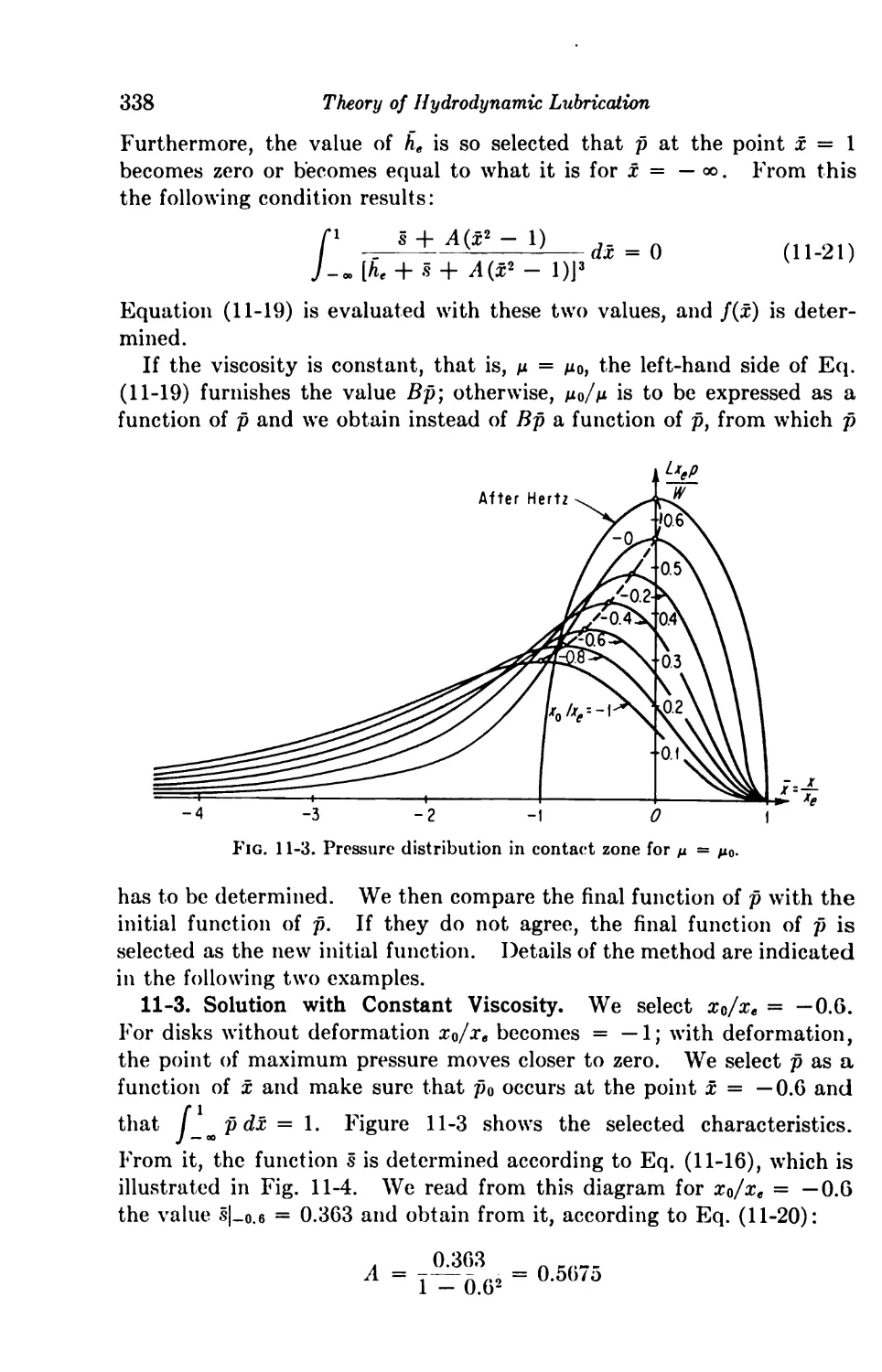
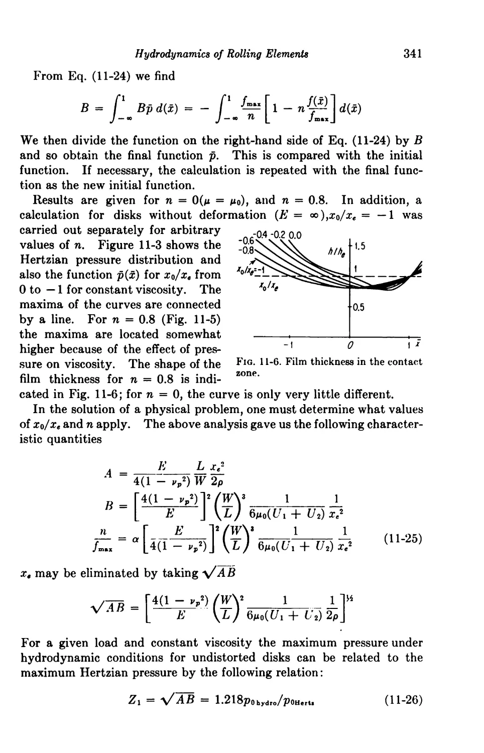
11-3. Solution with Constant Viscosity	338
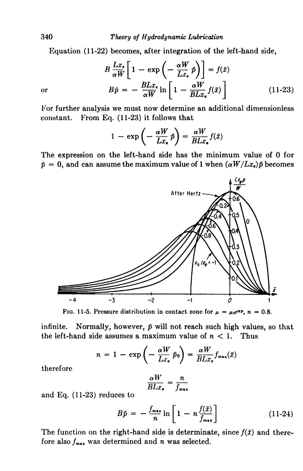
11-4. Viscosity as a Function of Pressure	339
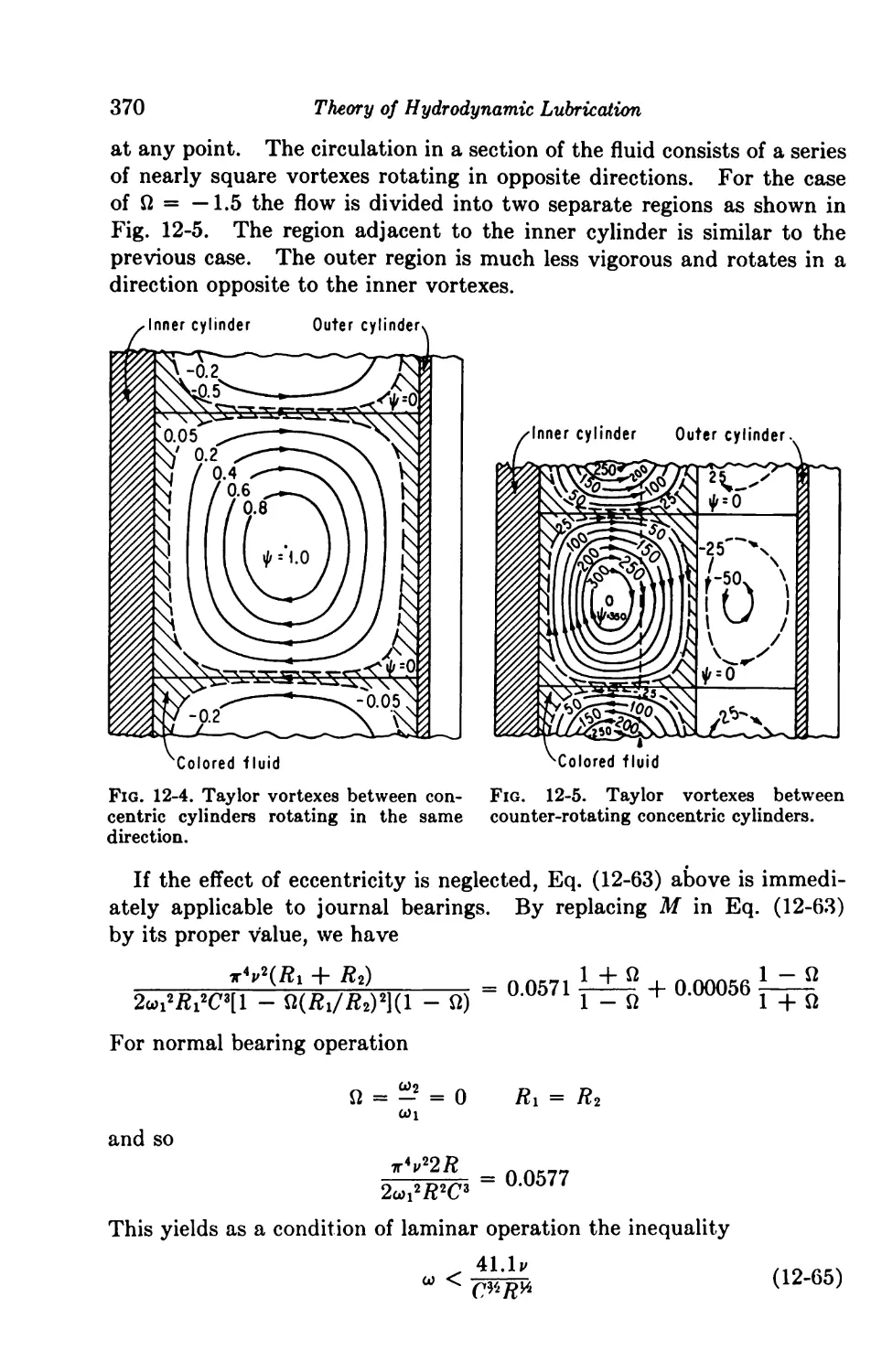
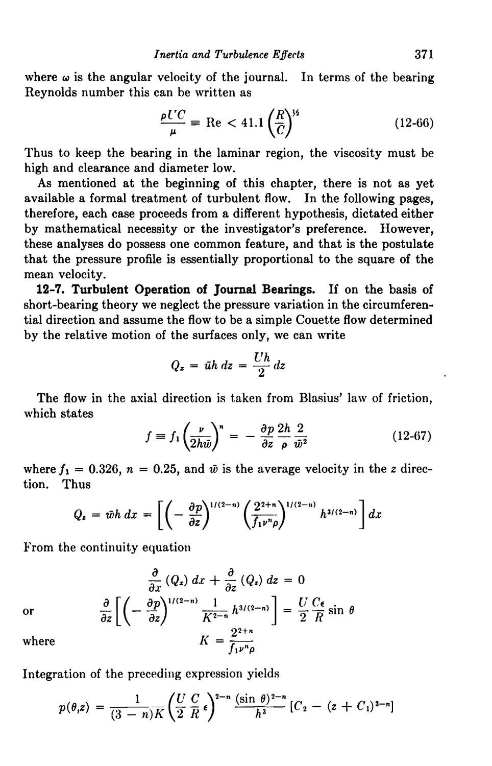
12. Inertia and Turbulence Effects	351
Introduction	351
Effects of Fluid Inertia	352
Significance of Inertia Terms	352
Iteration Method	354
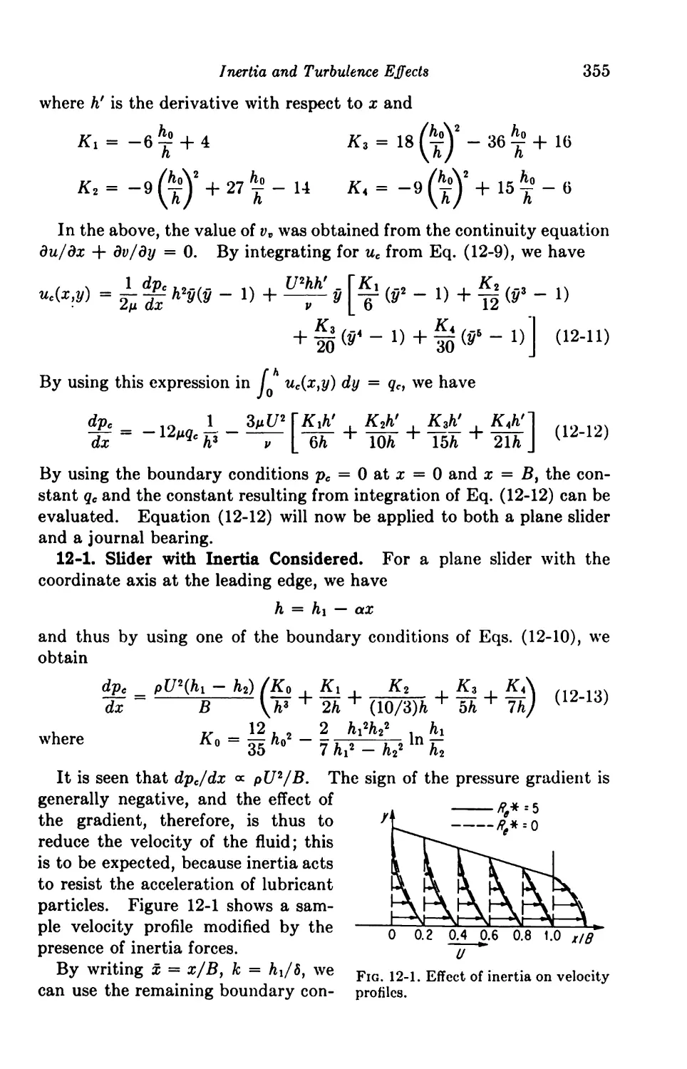
12-1. Slider with Inertia Considered	355
12-2. Journal Bearing with Inertia Considered	357
Method of Averaged Inertia	360
12-3. Squeeze Films	362
12-4. Journal Bearing	362
12-5. Slider Bearing	364
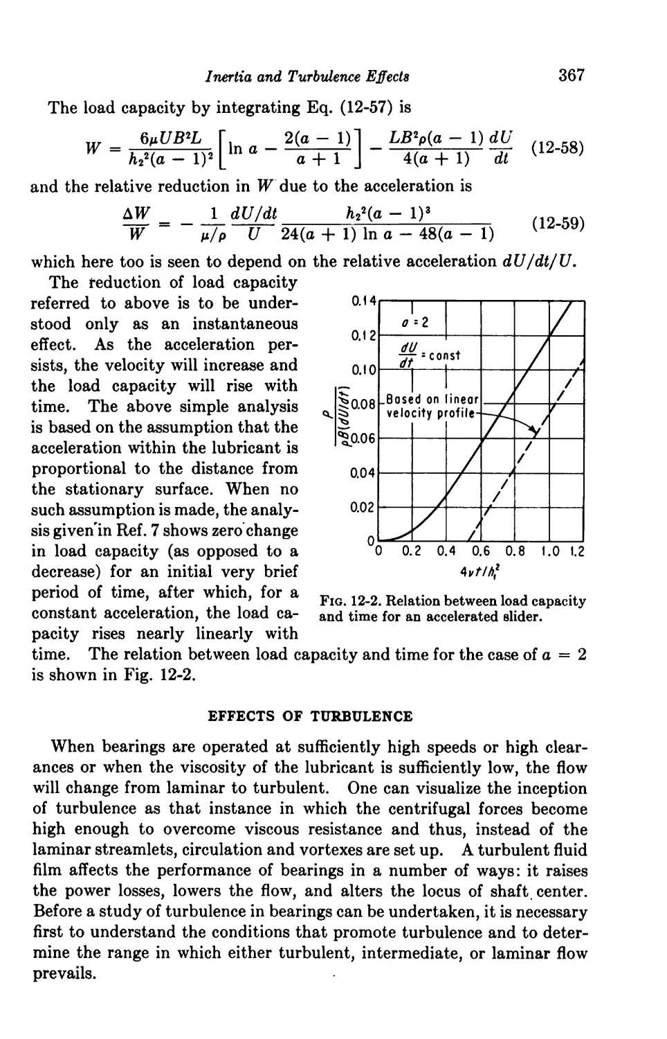
Acceleration Effects in Bearings	365
Effects of Turbulence	367
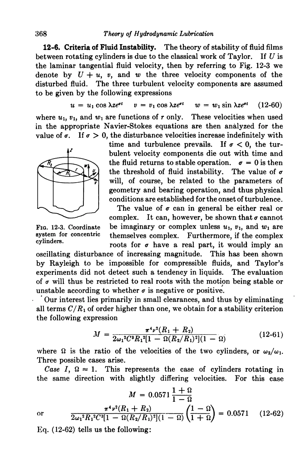
12-6. Criteria of Fluid Instability	368
12-7. Turbulent Operation of Journal Bearings	371
12-8. Turbulent Operation of Slider Bearings	373
13. Non-Newtonian Fluids	380
General Remarks	380
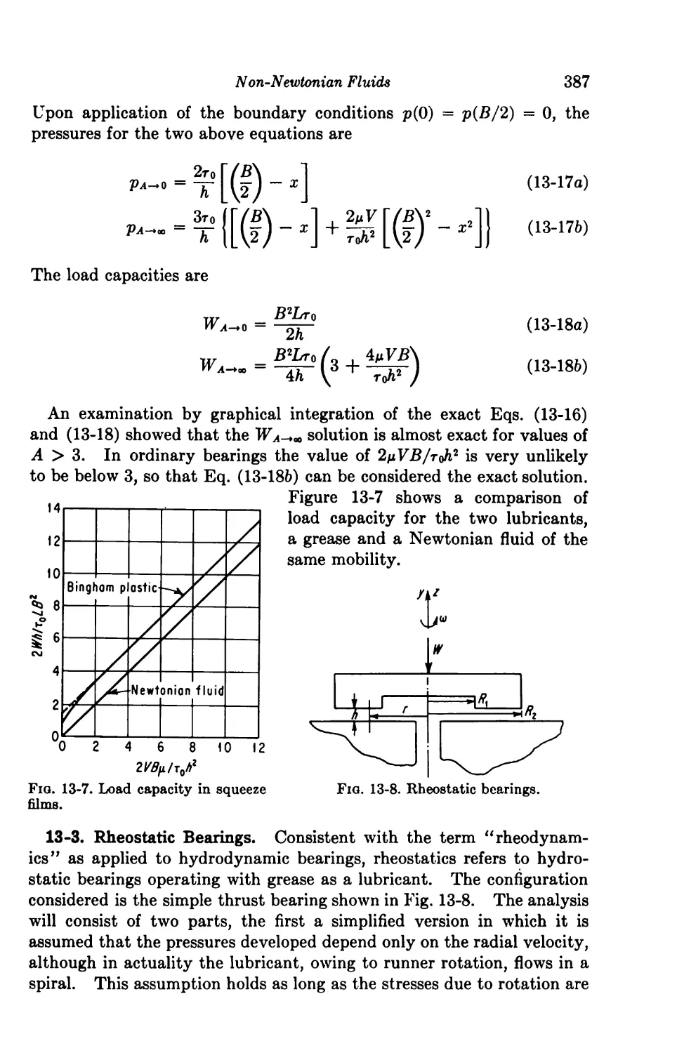
Bingham Plastics (Greases) as Lubricants	381
13-1. Rheodynamic Bearings	381
13-2. Squeeze Films	385

Contents	xi
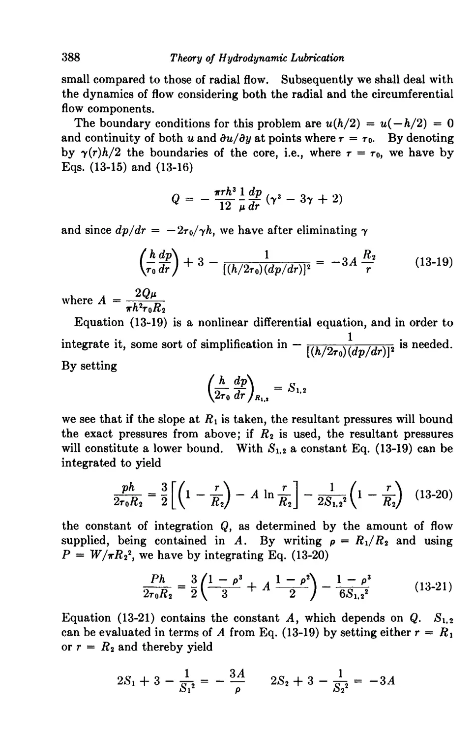
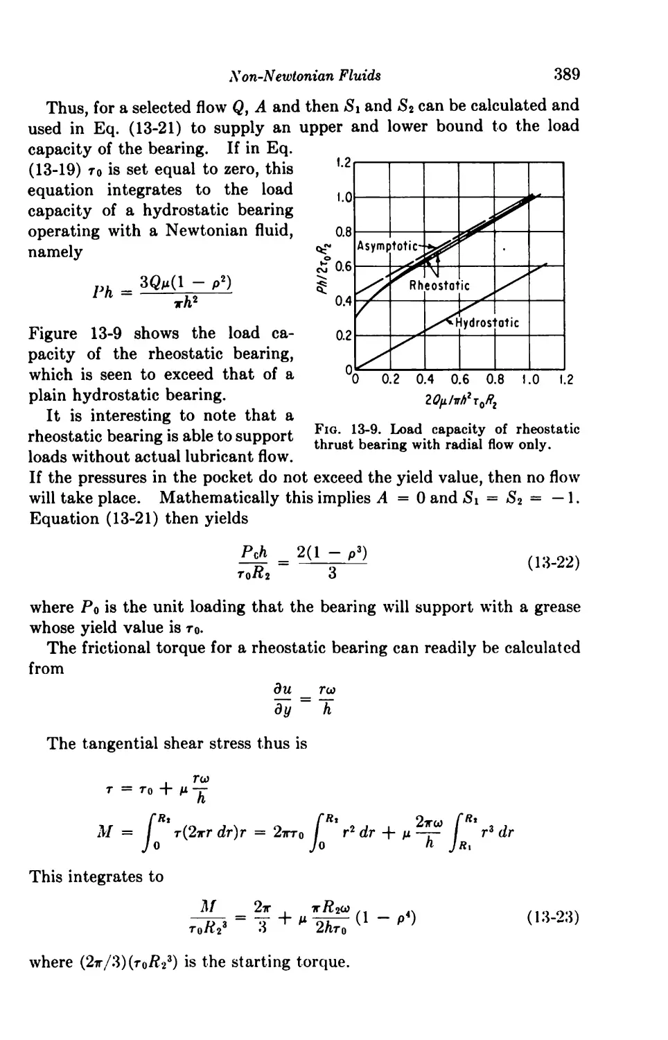
13-3. Rheostatic Bearings	387
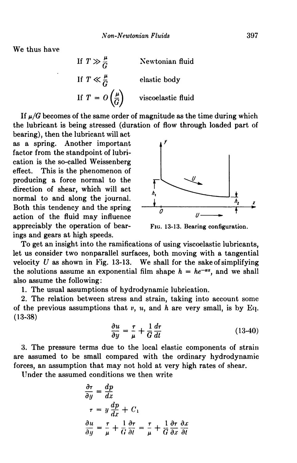
Viscoelastic Lubricants	396
14.	Extension of the Classical Theory	403
The Restrictions of Lubrication Theory	403
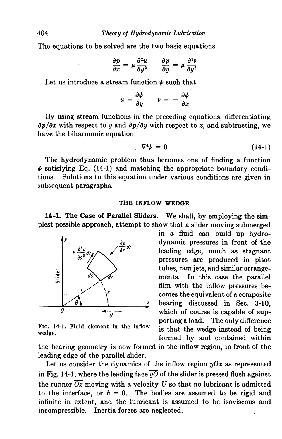
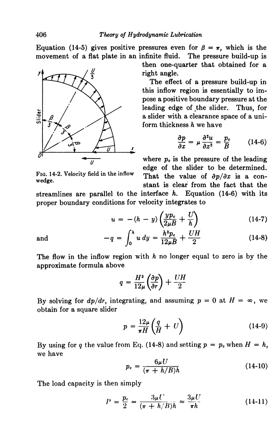
The Inflow	Wedge	404
14-1. The	Case of Parallel Sliders	404
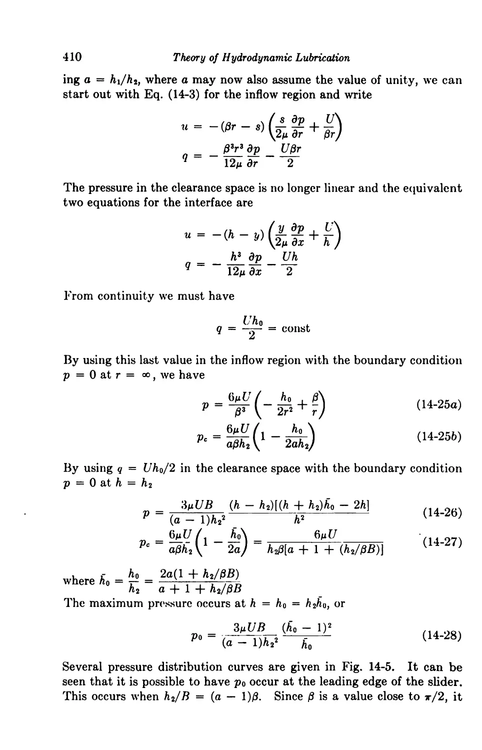
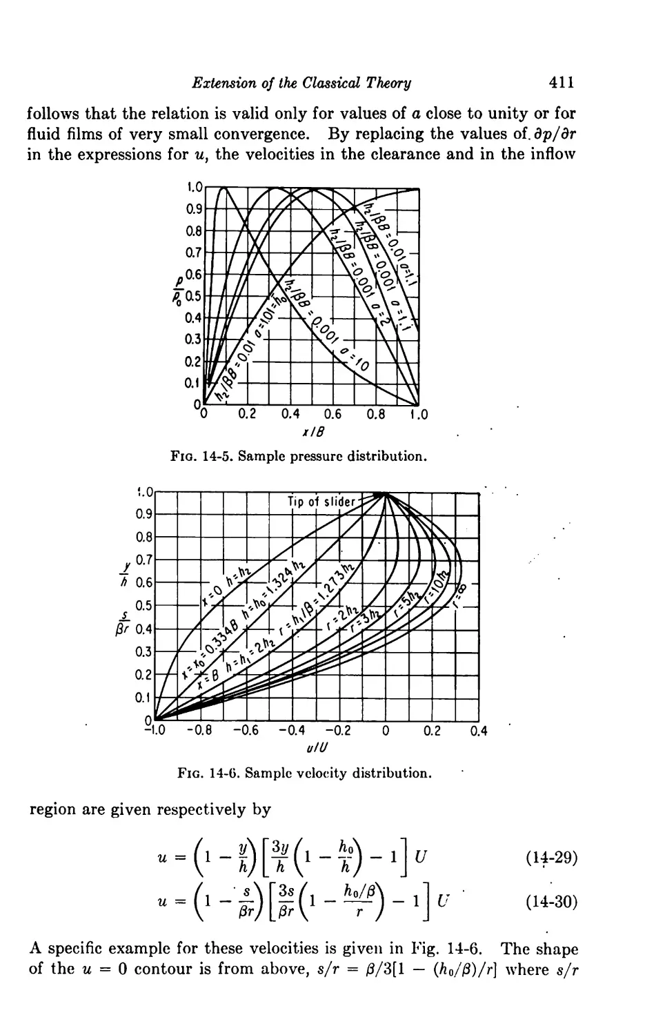
14-2. The	General Case of Plane Sliders	409
Variations across the Fluid Film	416
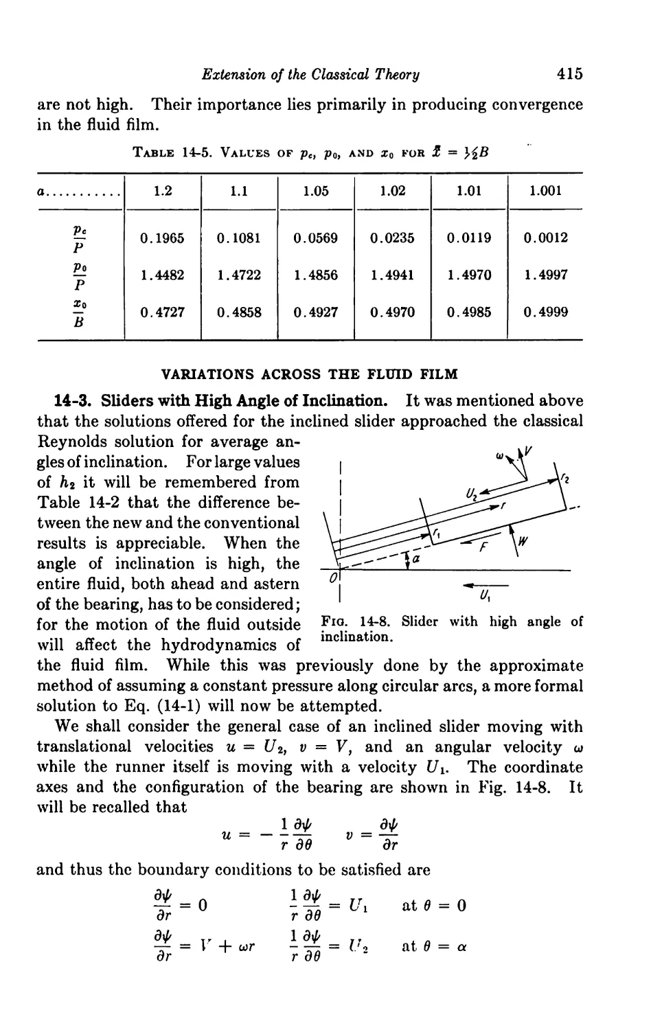
14-3. Sliders with High Angle of Inclination	415
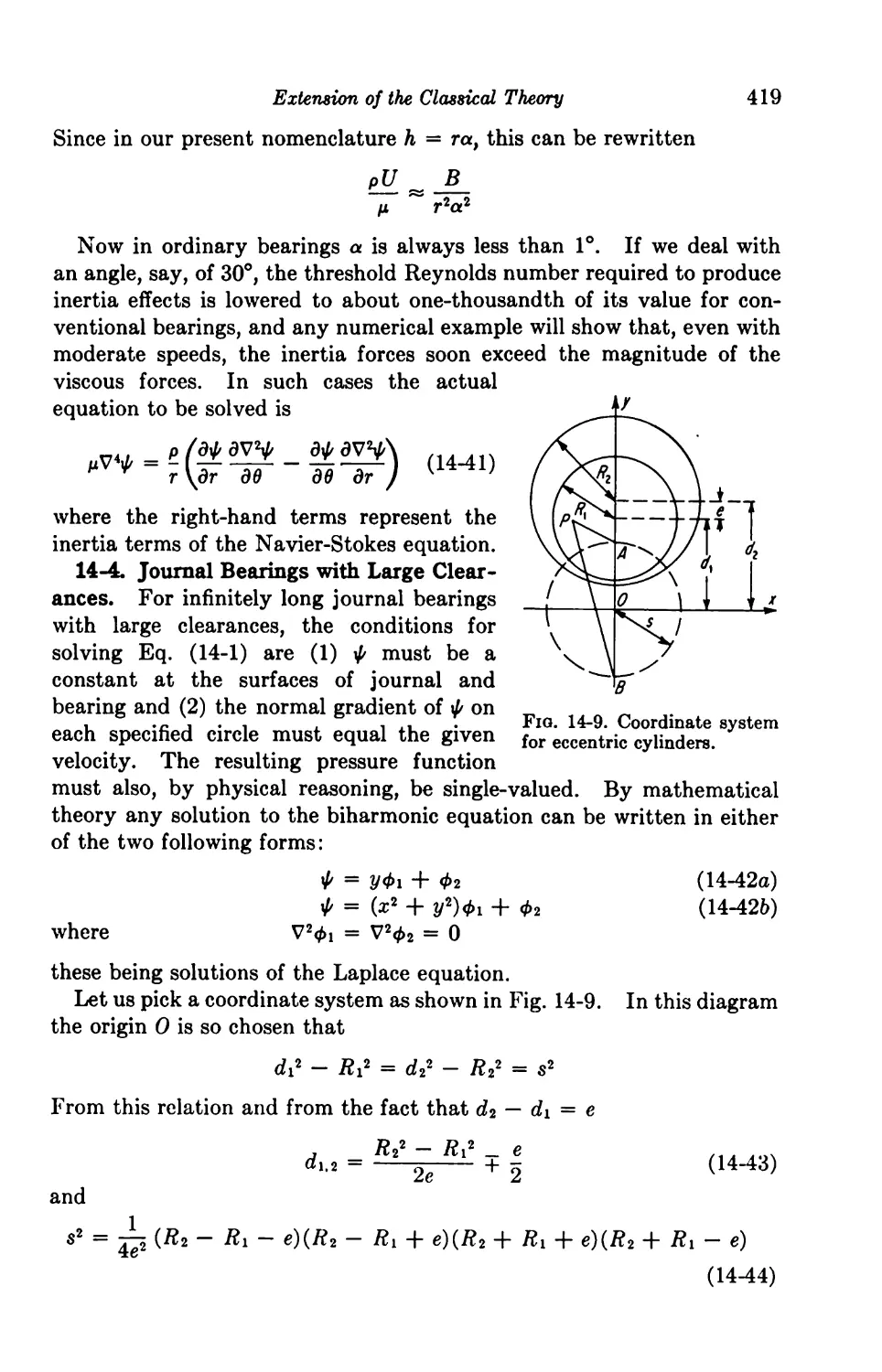
14-4. Journal Bearings with Large Clearances	419
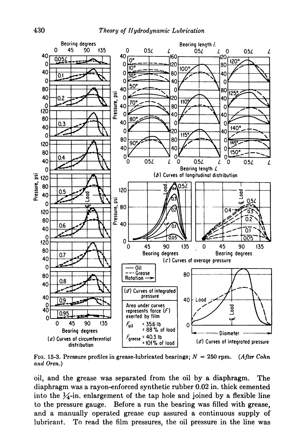
16. Experimental Evidence	426
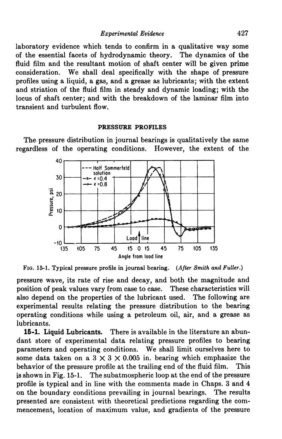
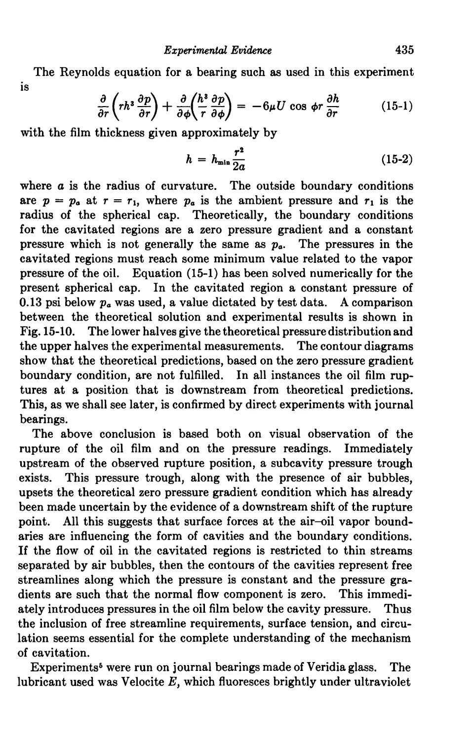
Pressure Profiles	427
15-1. Liquid Lubricants	427
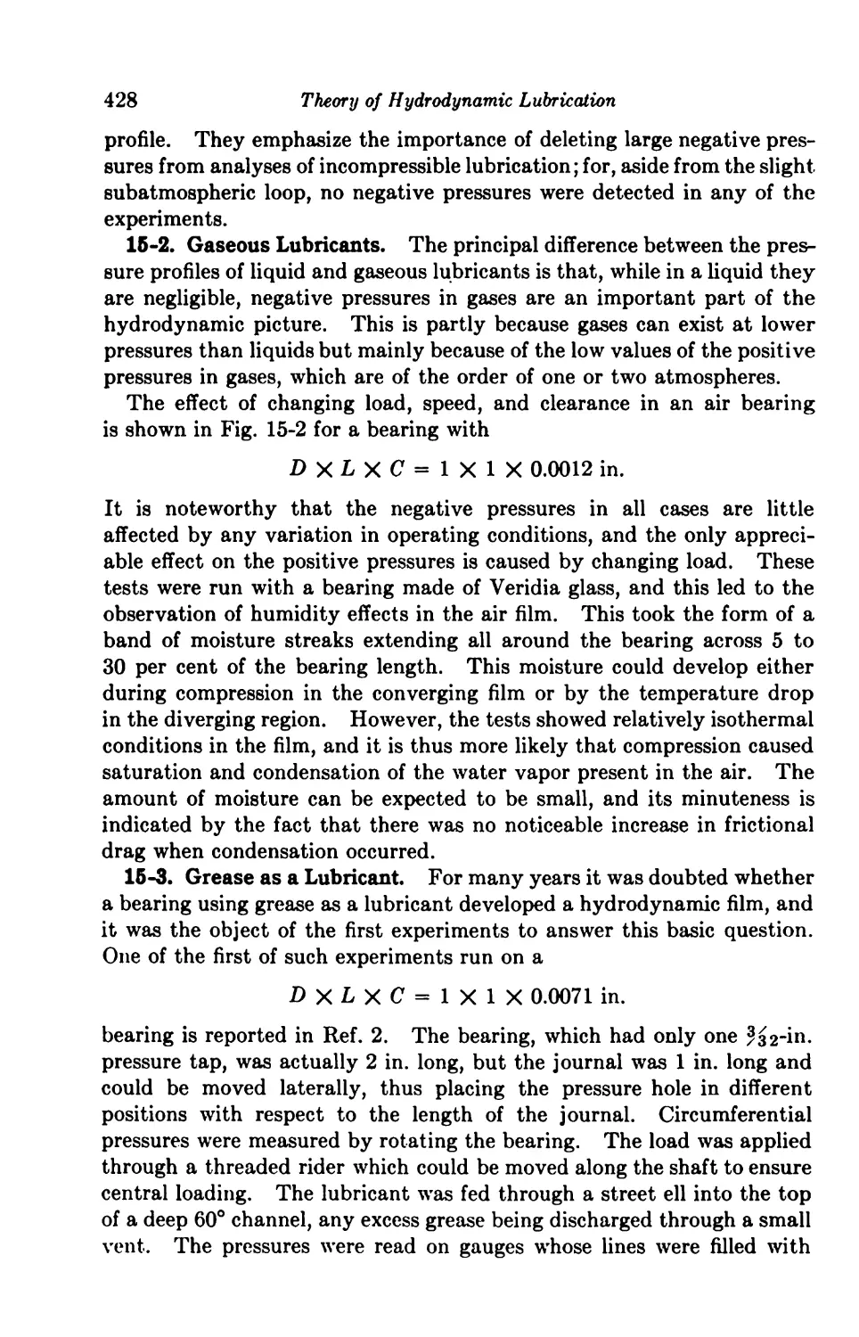
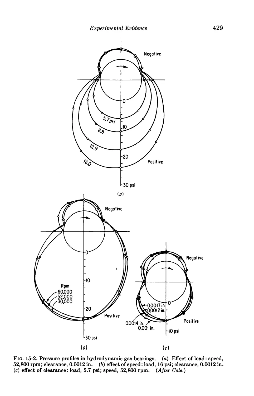
15-2. Gaseous Lubricants	428
15-3. Grease as a Lubricant	428
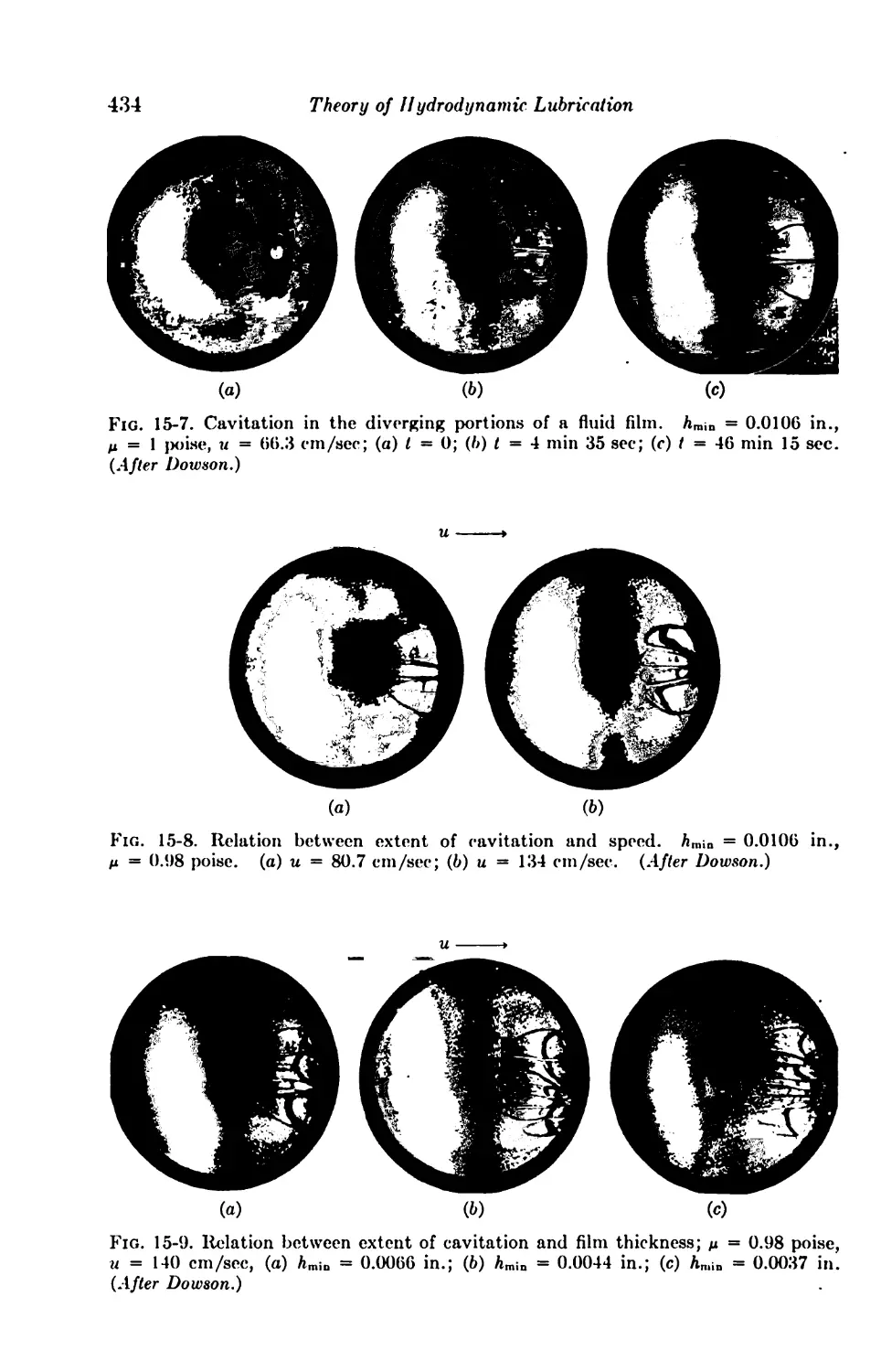
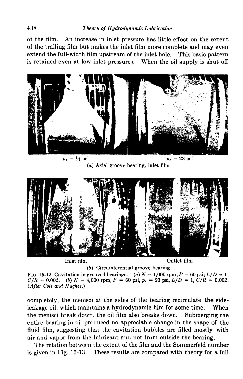
The Fluid Film; Cavitation	432
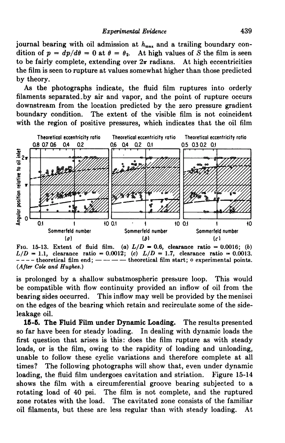
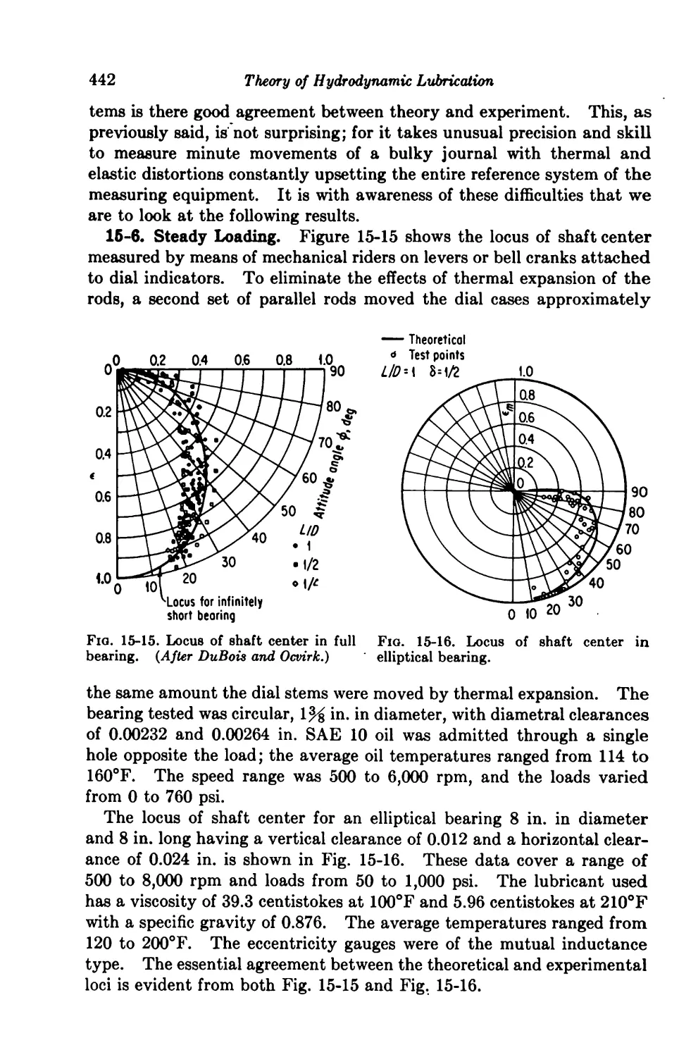
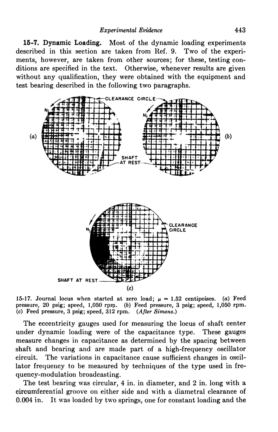
15-4. The	Fluid Film under Steady Loading	433
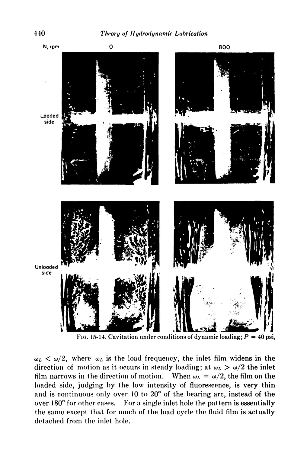
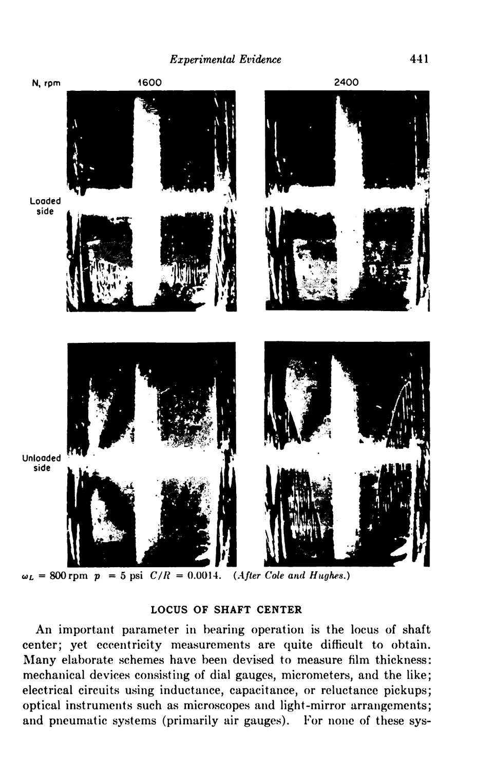
15-5. The	Fluid Film under Dynamic Loading	439
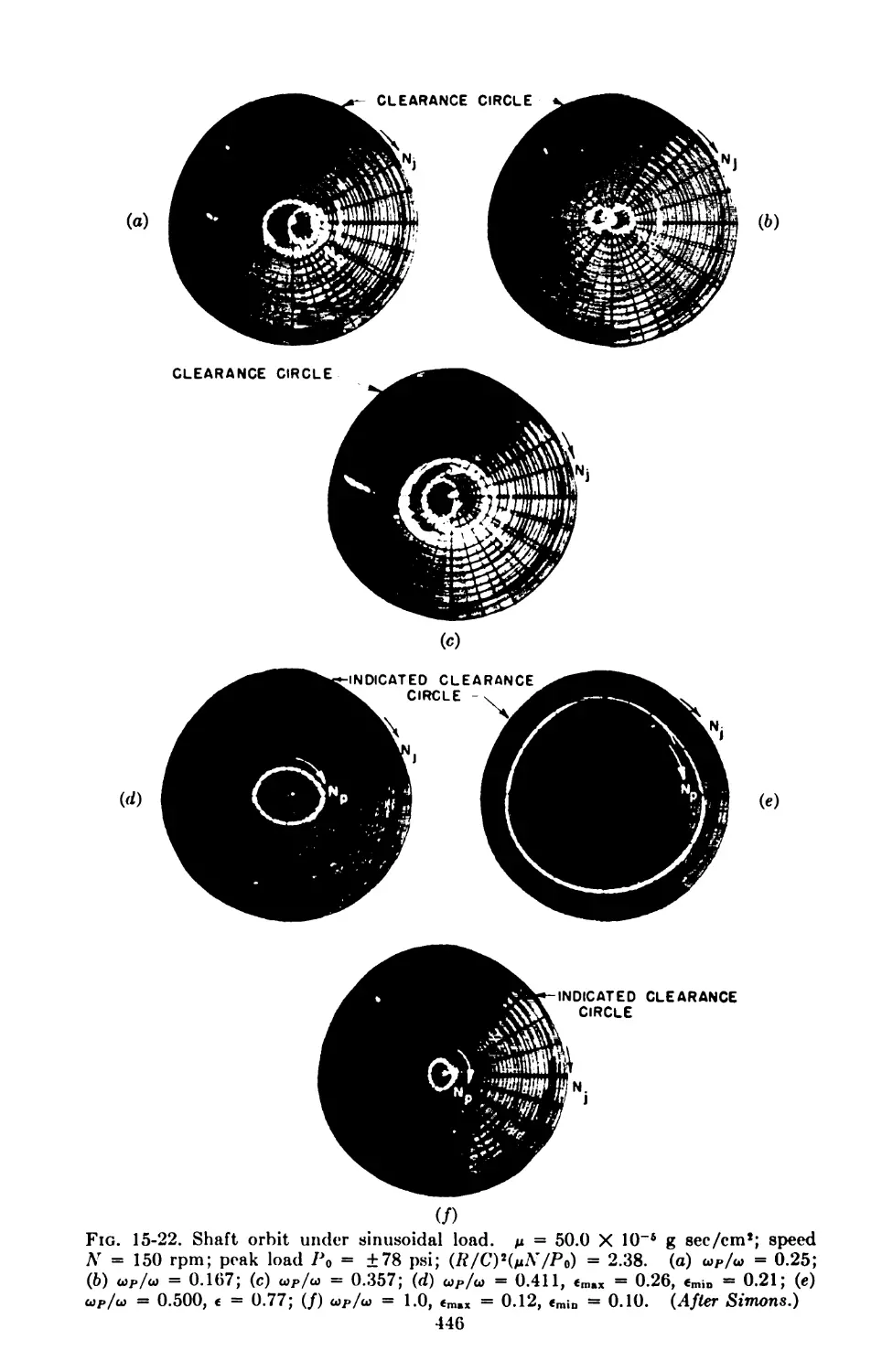
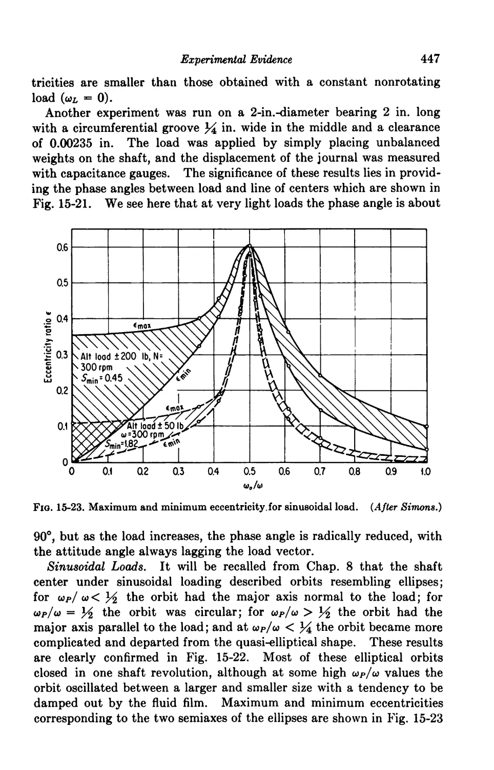
Locus of Shaft Center	441
15-6. Steady Loading	442
15-7. Dynamic Loading	443
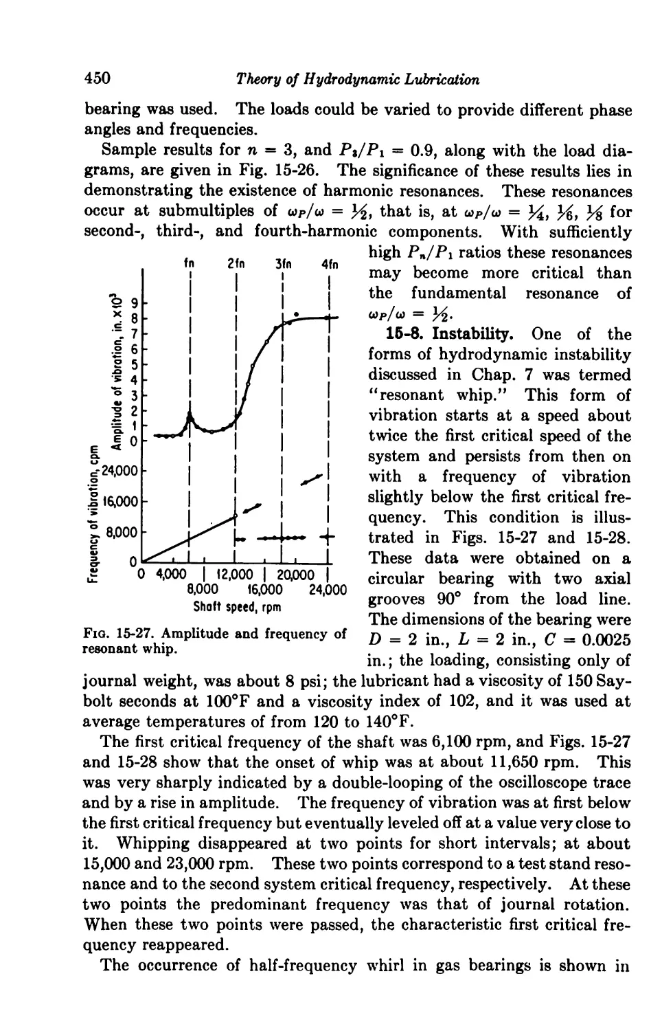
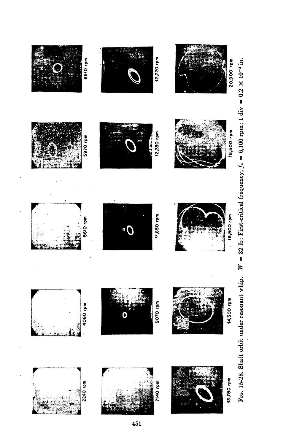
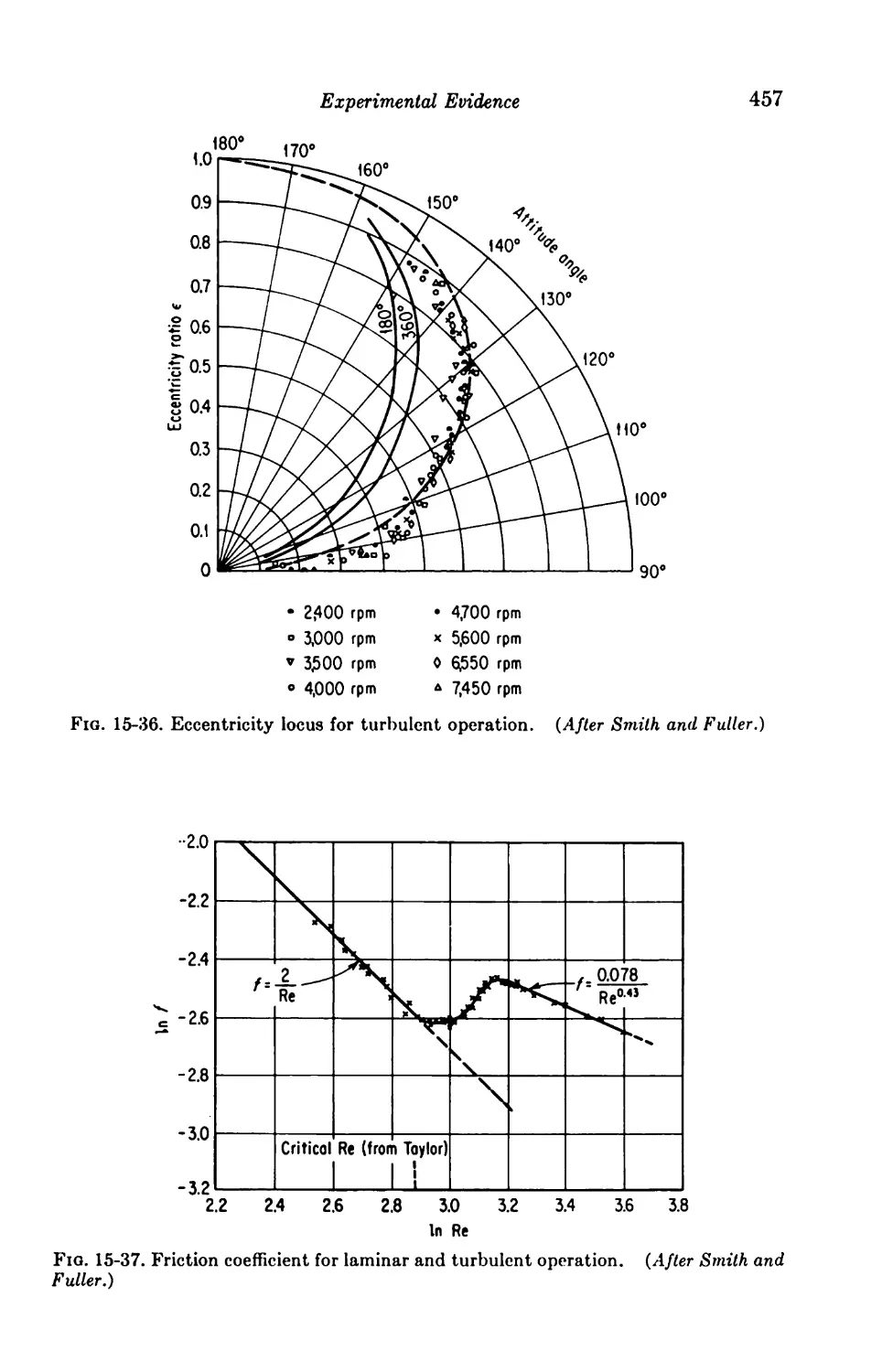
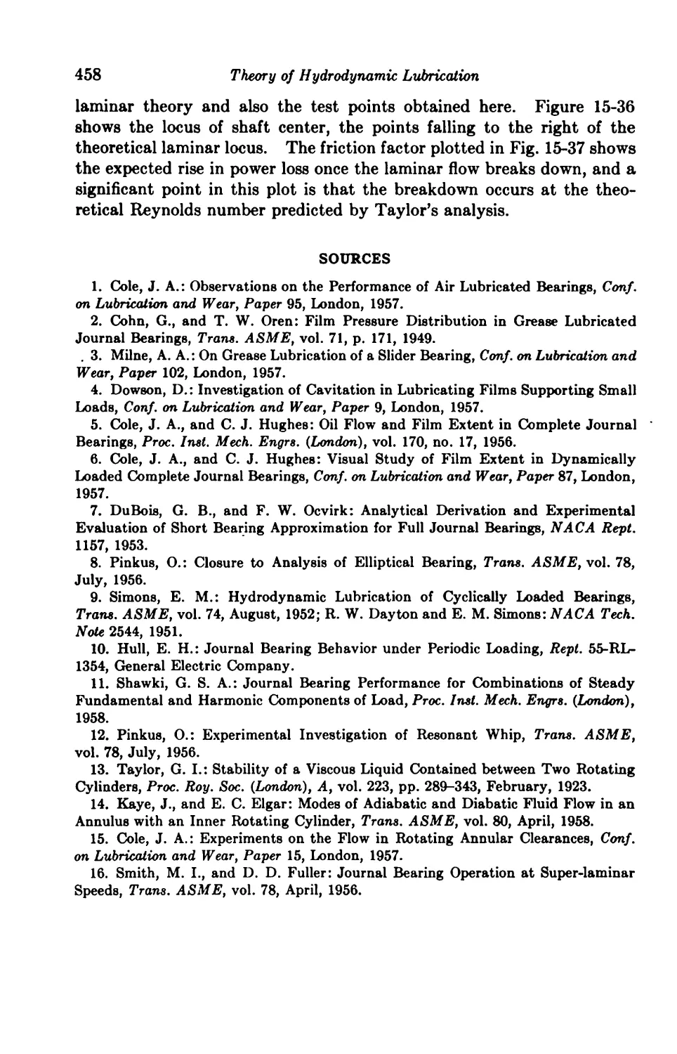
15-8. Instability	450
Turbulence	452
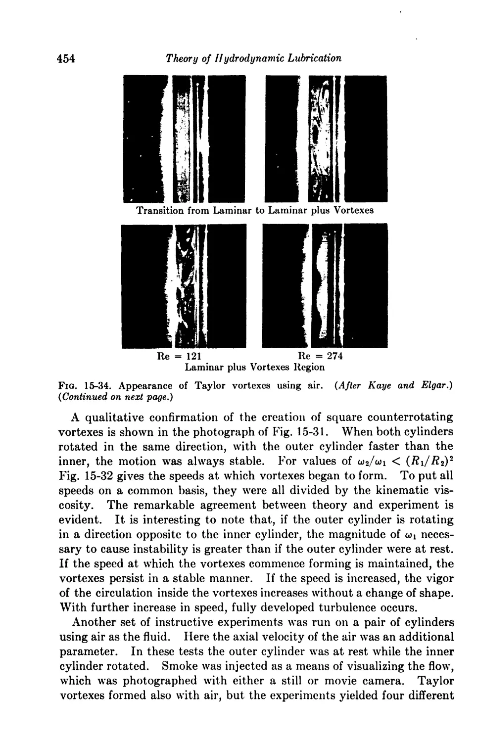
15-9. Breakdown of Laminar Flow	452
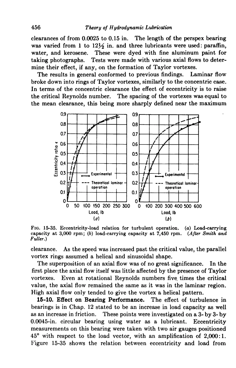
15-10. Effect on Bearing Performance	456
A’ame Index	459
Subject Index	461

NOMENCLATURE
Unless otherwise specified, the following symbols are used in the text:
B
breadth, width (parallel to direction of motion)
C
radial clearance
D
diameter
E
energy, Young’s modulus
F
frictional force, force
G
weight flow rate
H
power, work rate
I
moment of inertia
J
mechanical equivalent of heat
K
spring constant
L
bearing length (normal to direction of motion)
M
mass, moment
N
revolutions per unit time
P
unit loading = W/LD
Q
volume flow rate
R
bearing radius
(R
perfect-gas constant
Re
Reynolds number
S
Sommerfeld number = (i*N/P)(R/C)2
T
temperature
U
linear velocity
V
velocity, volume
W
load
a
ratio of inlet to outlet film thickness
b
damping coefficient
c
specific heat
e
eccentricity
f
coefficient of friction, dimensionless force = l/S
9
constant of gravitational acceleration
h
film thickness
k
ratio of specific heats, thermal conductivity, spring constant
m
mass
xii

Nomenclature
xiii
n	polytropic constant
p	pressure
q	heat flow rate, volume flow rate per unit length
q	dimensionless flow coefficient = Q/tRCNL
t	time
u,v,w	linear velocity components
2	center of pressure
x,?/,z	rectangular coordinates
a	dimensionless taper, load	angle
0	angular span of bearing	arc or sector
6	amount of taper = (h\	— h2), ellipticity ratio
€	eccentricity ratio = e/C
A	bearing number = §nUB/pahl or (6fjLO)/pa)(R/C)2
M	absolute viscosity
v	kinematic viscosity
p	density
r	shear stress
<p	attitude angle
o)	angular velocity
Subscripts
H	horizontal
L	laminar, load
P	load
R	radial
T	tangential, turbulent
V	vertical, volume
a	ambient
b	bearing
c	common, critical
j	journal
1	laminar
r	radial
s	slider, supply
t	tangential, turbulent
avg	average
max	maximum
min	minimum
opt	optimum
red	reduced
0	pertains to point of maximum pressure

Nomenclature
beginning, inlet
end, outlet
Superscripts
dimensionless (x = x/B)
first derivative with respect to time
second derivative with respect to time
third derivative with respect to time

CHAPTER 1
BASIC DIFFERENTIAL EQUATIONS
The study of hydrodynamic lubrication is, from a mathematical stand¬
point, the study of a particular form of the Navier-Stokes equations.
This particular differential equation was formulated by Osborne Reynolds
in 1886 in the wake of a classical experiment by Beauchamp Tower in
which the formation of a thin fluid film was for the first time observed
and understood to be the basic mechanism of hydrodynamic lubrication.
This Reynolds equation can be deduced either from the Navier-Stokes
equations or from first principles, provided, of course, that the same
assumptions are used in both methods. The Reynolds equation contains
viscosity, density, and film thickness as parameters. These parameters
both determine and depend on the temperature and pressure fields and
on the elastic behavior of the bearing surfaces. Thus, to get a complete
and accurate representation of the hydrodynamics of the lubricating film,
it is oftentimes necessary to consider simultaneously the Reynolds equa¬
tion, the energy equation, the elasticity equation, and the equation of
state. This chapter deals with the mathematical formulation of these
equations and serves as a basis for the solution of bearing problems in
subsequent chapters. We shall first derive, in as simple a manner as
possible, the Navier-Stokes equations and subsequently reduce them to
the Reynolds equation, thereby showing the restrictions and assumptions
inherent in the equations used in the solution of lubrication problems.
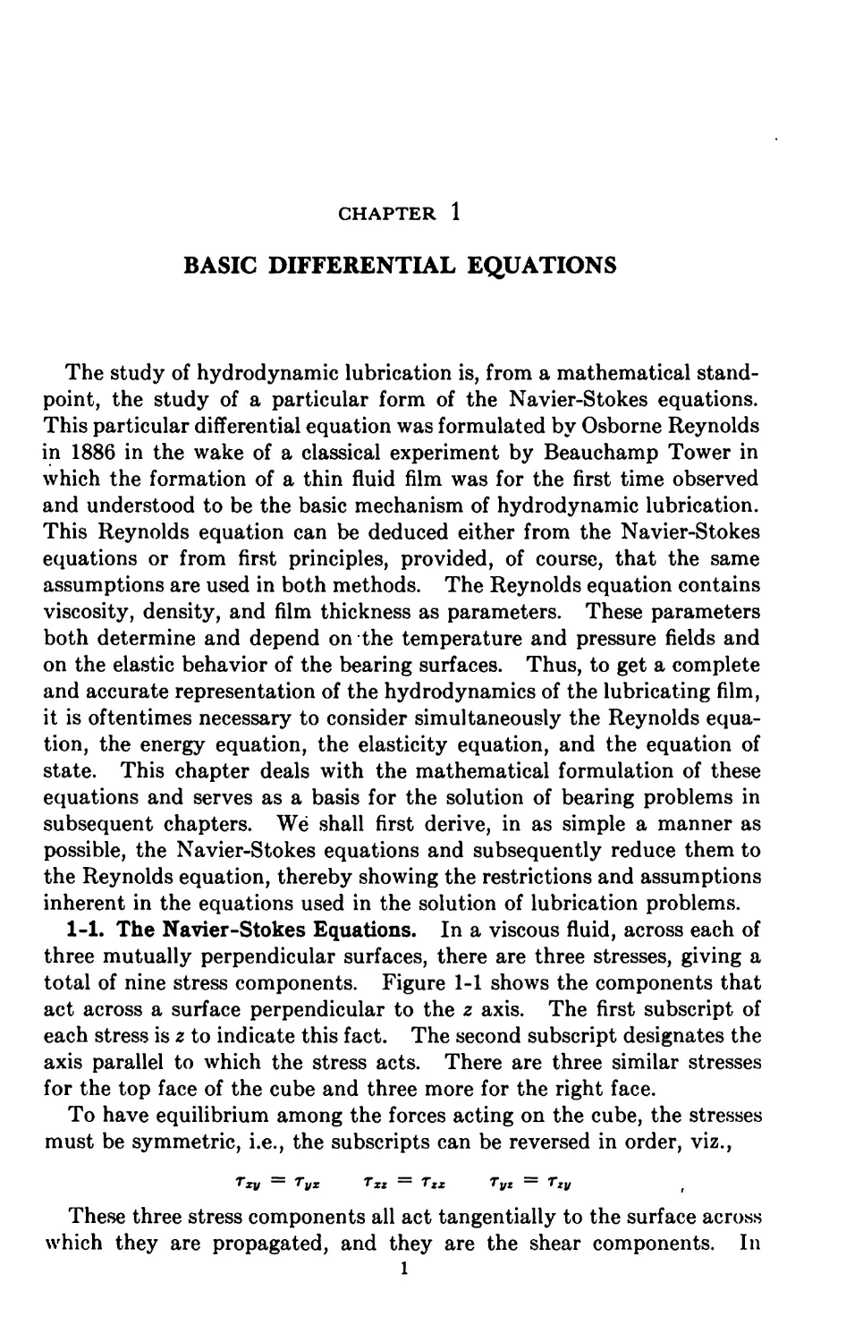
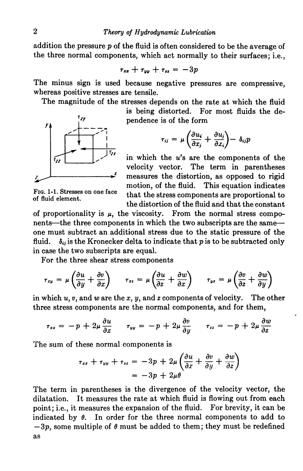
1-1. The Navier-Stokes Equations. In a viscous fluid, across each of
three mutually perpendicular surfaces, there are three stresses, giving a
total of nine stress components. Figure 1-1 shows the components that
act across a surface perpendicular to the z axis. The first subscript of
each stress is z to indicate this fact. The second subscript designates the
axis parallel to which the stress acts. There are three similar stresses
for the top face of the cube and three more for the right face.
To have equilibrium among the forces acting on the cube, the stresses
must be symmetric, i.e., the subscripts can be reversed in order, viz.,
Txy ~ Tyx	Txz ~ Tzx	TyZ — TZy	(
These three stress components all act tangentially to the surface across
which they are propagated, and they are the shear components. In

2
Theory of Hydrodynamic Lubrication
addition the pressure p of the fluid is often considered to be the average of
the three normal components, which act normally to their surfaces; i.e.,
TXX + Tyy + TtZ = — 3 P
The minus sign is used because negative pressures are compressive,
whereas positive stresses are tensile.
The magnitude of the stresses depends on the rate at which the fluid
is being distorted. For most fluids the de¬
pendence is of the form
(dui . duA
to, + dxj~ iiiV
in which the u1 s are the components of the
velocity vector. The term in parentheses
measures the distortion, as opposed to rigid
motion, of the fluid. This equation indicates
that the stress components are proportional to
the distortion of the fluid and that the constant
of proportionality is y, the viscosity. From the normal stress compo¬
nents—the three components in which the two subscripts are the same—
one must subtract an additional stress due to the static pressure of the
fluid. 8ij is the Kronecker delta to indicate that p is to be subtracted only
in case the two subscripts are equal.
For the three shear stress components
(du . dv\	(du	.	dw\	(dv	, dw\
=	-,	+	Tx)	=	+	T"~M^ + 5ir;
in which u} v, and w are the x, y, and z components of velocity. The other
three stress components are the normal components, and for them,
i o du	.	o	dv	.	o	dw
rxx=-p + 2»-^ ryw=-p + 2„-	T„=-p + 2» —
The sum of these normal components is
r„ + r„ + r„ = -3p + 2, (g + g + g)
= —3p 4- 2yd
The term in parentheses is the divergence of the velocity vector, the
dilatation. It measures the rate at which fluid is flowing out from each
point; i.e., it measures the expansion of the fluid. For brevity, it can be
indicated by 6. In order for the three normal components to add to
— 3p, some multiple of 0 must be added to them; they must be redefined
as
Fig. 1-1. Stresses on one face
of fluid element.

Basic Differential Equations
3
<rx = — p -f X0 + 2/z — au — — p + X0 + 2/i —
(Tz = — p + X0 + 2/i-T-
The coefficient of 0 is X, at present an undetermined quantity. The sum
of these normal components is —3p provided that
Some fluids have a “volume viscosity” that measures their resistance to
volume changes, just as conventional viscosity measures the resistance
to flow. In the case of a fluid with a volume viscosity, X + is not
zero. For the time being, both X and p can be retained in the equations;
subsequently the volume viscosity can be assumed to be zero and X can
be expressed in terms of p.
The three components of acceleration of the fluid are the three total
derivatives Du/dt, Dv/dtf and Dw/dt. The mass of an element of fluid
with dimensions dx, dy, and dz is p dx dy dz; thus the components of the
force required to accelerate the element are
Total derivatives of the velocity components are calculated by treating
the velocity as a function of x} y, z, and t in which x, y, and z are them¬
selves functions of t.
The partial derivatives of x} y, and z with respect to time are, of course,
the velocity components w, v, and w. The total time derivative measures
the change in velocity of one particle of fluid as it moves about in space;
the partial time derivative measures the change in velocity of whatever
particles of fluid occupy one particular location.
The forces needed to accelerate the element of fluid are supplied by an
external force field, perhaps gravity, and by pressure or stress gradients
within the fluid. If the components of the external force field per unit
mass are X, Y, and Z, these forces are equal to Xp dx dy dz, Ypdxdy dz,
Zp dx dy dz.
The forces due to the stress gradients must be added to the external
force. Three stresses tend to move the element in the x direction.
X =
p dx dy dz p-^dx dy dz p dx dy dz
Du diL fir. fin fin Ha. fiz du
dt

Theory of Hydrodynamic Lubrication
Thus, a change in tXV) for example, across the cube and through a distance
dy. is
drXi
dy
dy
This stress acts on the face of a cube with area dx dz and produces a
force:
Force = dy dx dz
dy
There are similar expressions for rIX and rxz. When these stress-gradient
forces are added to the external force and the common factor dx dy dz
is eliminated,
Du
dt
v- i d(Tx . drxu drxz
pX +	+	~dy	+
Also, there are similar expressions for the stress gradients that tend to
move the element in the y and z directions:
V	_L dT*u	I d<Tu	,	dr^
p dT	= pl	+	+ lij	+	Tz
Dw	dr„	dr„z	d(Tz
PW	= pz	+ ^	+ ~	+
dx
dy
dz
In case the volume viscosity X + %p is zero, X can be written in terms
of p, and we have after replacing m by their proper expressions
Du	dp	d	i
dx
dy
"W - pY-?,+§j\r
; .+£
•y-rf-g + sl-
+1
[2»? 2fc + *+^')l|
dx S\dx dy dz J J)
(du dlA] d \ (Sw duN]
dv _ 2 (du dv_ dw\ 1)
dij ~ 3 \di + d7j “*■ dz)J)
p(I+S!)]+£[m(S+£)]
dw _ 2 (du dv	)
~dz ~ 3 V^r + dy +
(dw .	d	f (dv dwAl
^ + 3^J + ^K*+-WJ
(l-la)
(1-16)
(1-lc)
which are the general Navier-Stokes equations. Equations (1-1) con¬
tain the four unknowns u, v, w, and p. A fourth equation is supplied
by the continuity equation:

Basic Differential Equations
5
where m accounts for the presence of sources and sinks. With no sources
or sinks present and with the state of the lubricant independent of time,
the continuity equation reads
+ dl^l = o	(1-2	a)
dx dy dz
Equations (1-1) and (1-2) contain the density and viscosity as variable
parameters. Thus in order to define fully the problem, functional rela¬
tionships for p and y must be available in the form
p = p(p,T) y = y(p,T)
In cylindrical coordinates, the’ Navier-Stokes equations read
/ Du uv\  	  1	dp 1	| r 2 dw _ 2/1 drv 1 du
P \ dt r )	r	dd r dQ (M [r ^0 \r dr r dB
+ £)]|+'l['‘0S+5)]'+f,['OS
<>-"0
(Dv u2\ D dp . d \ \ ndv	2/1 drv . 1 du . dw\l)
=	+	^	Hr^	+	ra5	+ai-JJj
+
I AT /I*? 4_ On _ A\1 , d_
r dd	\r dd + dr r ) J + dz
+ 7
(dv . ditAl
+ «F/J
dv	1 du	vl /t	t n
Tr-ree-'r\ <Me)
d ( dw 2(\drv	I du	dw\l|
. l a r /dv ,	,	i	a	r (\aw , au\]
+ r 7r [Mr	+*)\ + 7 ae |_p ae + Tz)\ (M/)
Dw	dp
p-W = z~al +
with the continuity equation given by
d(pu)	a(prv)	d(pw)	=	ol
ae	dr	dz
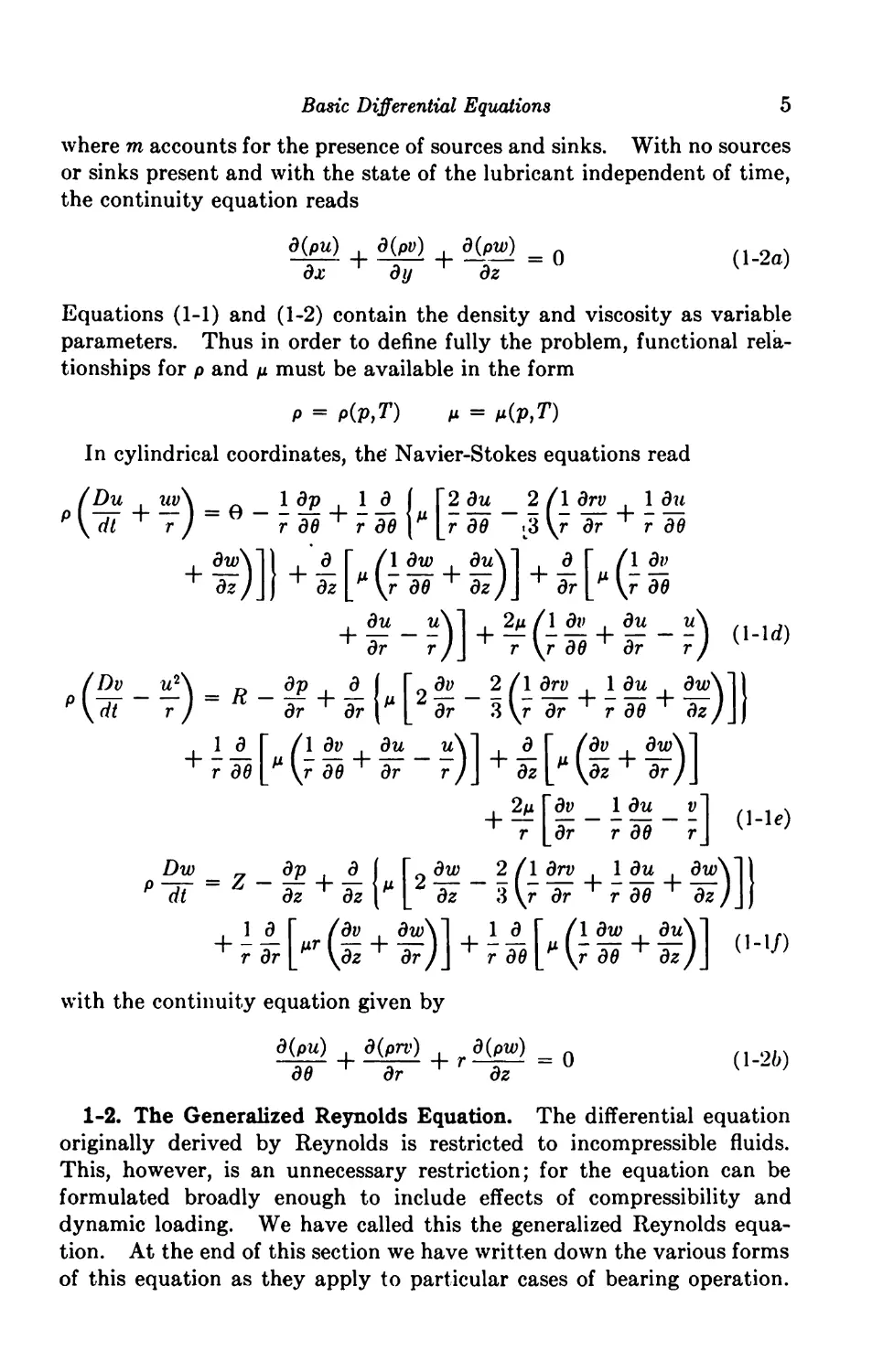
1-2. The Generalized Reynolds Equation. The differential equation
originally derived by Reynolds is restricted to incompressible fluids.
This, however, is an unnecessary restriction; for the equation can be
formulated broadly enough to include effects of compressibility and
dynamic loading. We have called this the generalized Reynolds equa¬
tion. At the end of this section we have written down the various forms
of this equation as they apply to particular cases of bearing operation.

6
Theory of Hydrodynamic Lubrication
The assumptions involved in reducing Eqs. (1-1) to the Reynolds equa¬
tion are, referring to the fluid film of Fig. 1-2, as follows:
1. The height of the fluid film y is very small compared to the span and
length x, z. This permits us to ignore the curvature of the fluid film,
such as in the case of journal bearings, and to replace rotational by trans¬
lational velocities.
2. No variation of pressure across the fluid film. Thus
? = °
dy
3. The flow is laminar; no vortex flow and no turbulence occur any¬
where in the film.
4. No external forces act on the film. Thus
X = Y = Z = 0
5. Fluid inertia is small compared to the viscous shear. These inertia
forces consist of acceleration of the fluid, centrifugal forces acting in
curved films, and fluid gravity. Thus
Du _ Dv _ Dw _ „
dt dt dt
6.	No slip at the bearing surfaces.
Fio. 1-2. The fluid film.	7-	Compared	with	the	two	veloc-
ity gradients du/dy and dw/dy, all
other velocity gradients are considered negligible. Since u and, to a
lesser degree, w are the predominant velocities and y is a dimension much
smaller than either x or z, the above assumption is valid. The two
velocity gradients du/dy and dw/dy can be considered shears, while all
others are acceleration terms, and the simplification is also in line with
assumption 5. Thus any derivatives of terms other than du/dy and
dw/dy will be of a much higher order and negligible. We can thus omit
all derivatives with the exception of d2u/dy2 and d2w/dy2.
Assumptions 1 to 7 used in Eqs. (1-1) yield
1 dp _ d2u
iai-w	(	}
1 dp _ d2W	.
-pTz~W	(	36)
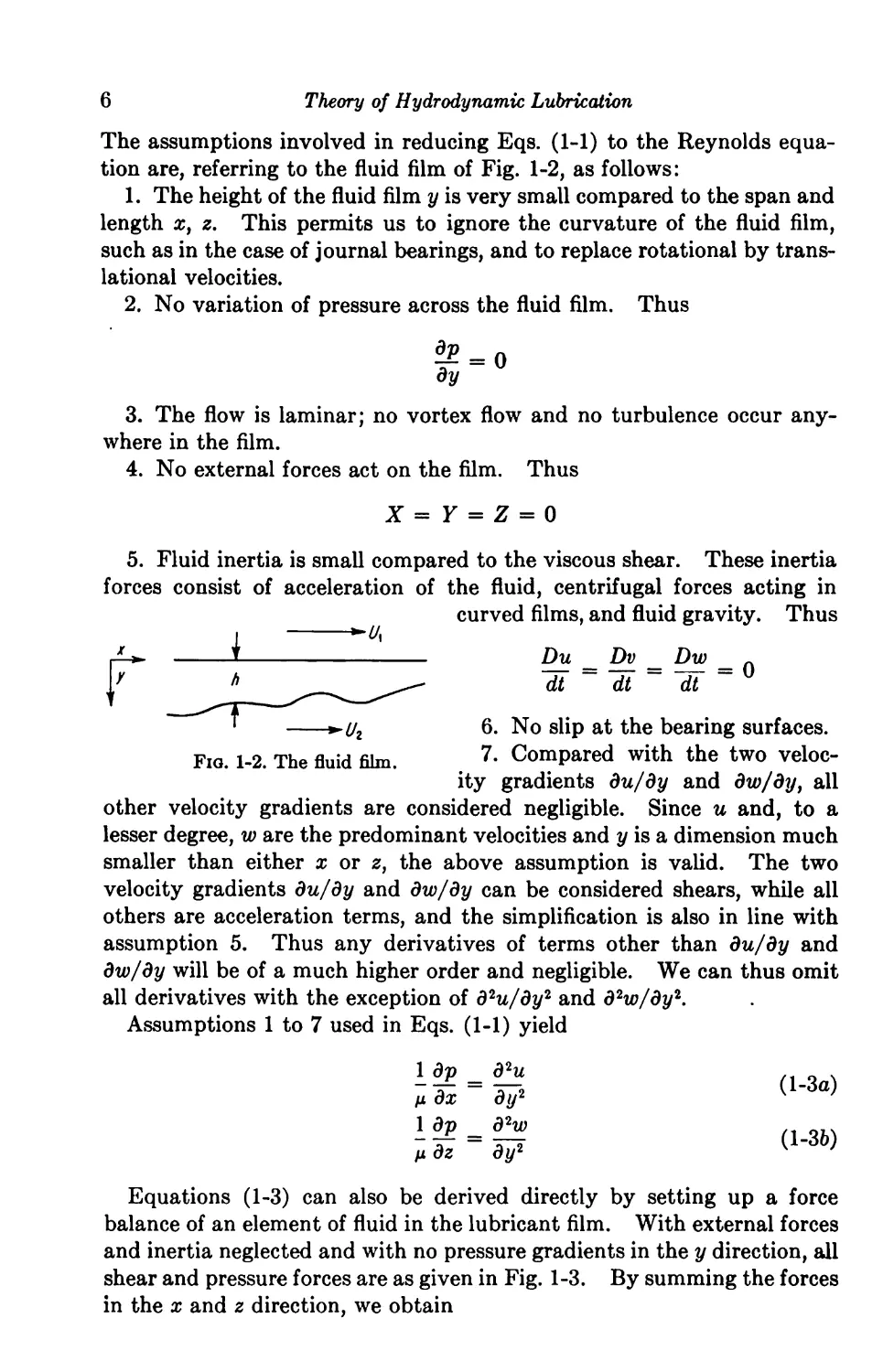
Equations (1-3) can also be derived directly by setting up a force
balance of an element of fluid in the lubricant film. With external forces
and inertia neglected and with no pressure gradients in the y direction, all
shear and pressure forces are as given in Fig. 1-3. By summing the forces
in the x and z direction, we obtain

Basic Differential Equations	7
^r* + ^ dz'j dx dy — tx dx dy + (rx + ^ dy^j dx dz — r* dx dz
+ (p-licdx)dydz-(p + lZdx)dydz = 0
H- ^ drr^ dy dz — tm dy dz + ^rf + ^ dy^j dx dz — r* dx dz
+ (p~ I2dz)dxdy ~ {v + \idz)dxdy = 0
By canceling like terms and simplifying,
drx	drx _ dp
dy	dz	dx
dr* . drz _ dp
dy dx dz
We now introduce the assumption of a Newtonian lubricant, i.e., a
fluid in which the shear stress is proportional to the rate of shear, or
du
T* = 11 dy
dw
tz = y-r~
dy
(l-4a)
(1-46)
It will be recalled that this assumption was made in deriving the
Navier-Stokes equations, and it was thus unnecessary to introduce it in
dXr
(i> + -jjdy)dxdz
{rx+ — dz)dxdy
1/
i,d,dy
~~J
/
/ •«-
T:dydz
2Txdx^y(iz
r/dxdz	Txdxdz	1
/
¥{p-t^d!)dxdy
(r!^^dy)dydi
(j) Forces in / direction	{t>)	Forces	in	/	direction
Fig. 1-3. Forces acting on a fluid element.
deriving Eqs. (1-3). Here, however, starting from a basic momentum
equation, we must rely on expressions (1-4) to provide us with a relation
between velocity and stress. Physically, assumption (1-4) implies that
the viscosity is independent of the rate of shear, a phenomenon which
is not true of all fluids. By using (1-4) in the preceding equation, we
obtain
d2u d2u _ 1 dp
dy2	dy dz	y	dx
d2w	d2yy	_	1	dp
dy2	dy dz	y	dz

8	Theory	of Hydrodynamic Lubrication
Now, by making use of assumption 7, the second terms on the left-hand
side drop out and we have Eqs. (l-3a) and (1-36) derived above:
d2u I dp	n o i
lWal
d^ = -f	[1-36]
dy- y dz
By integrating Eq. (l-3a) twice with the boundary conditions,
u — U\ at y = 0 u — L\ at y = h
we have	u = ^ y{y - h) + h -^-y- Ux + | Ui	(l-5a)
By integrating Eq. (1-36) with the boundary conditions,
w = 0 at y — 0 and at y = h
which implies a motion of the bearing surfaces only in the x direction, we
have
w = TMy(y~h)	(1'56)
Equations (1-5) give the velocity profile in the fluid film as affected
by the viscosity y, film shape 6, surface velocities Ux and U2, and the
pressure gradients.
We now make use of the continuity equation (1-2). The equation can
be written
d(pv) _	d(pu)	d(pw)
dy	dx	dz
By replacing u and w by their values from Eqs. (1-5), we have
By integrating with respect to y with the conditions v = V at y = 0 and
v = 0 at y = 6, we have
pF = f0ki[-,ty{y-h)](lu + fo y(y~h)]dy]
~/0 hp\^irUi + lUi\du
The upper limit h in the last equation is a function of the coordinates xy z.
By making use of the relation

Basic Differential Equations	9
fh(a) d	d	fh<a>	dh(a)
Jo dad}J = da Jo f('J'a) d,J ~ ma)'a]
we can perform the integration before differentiating to obtain
+ £(^Y|
2 [dx \6y dx/	dz\bydz/]
IT ld(f'r2+f/l)	,	(1J	JJ	X	d(ph)	1
“ 2 [* di + {Ul ~ Ui) ~dx~J
+ 6p6— (Ux + U2) ■+■ 12pF (l-6a)
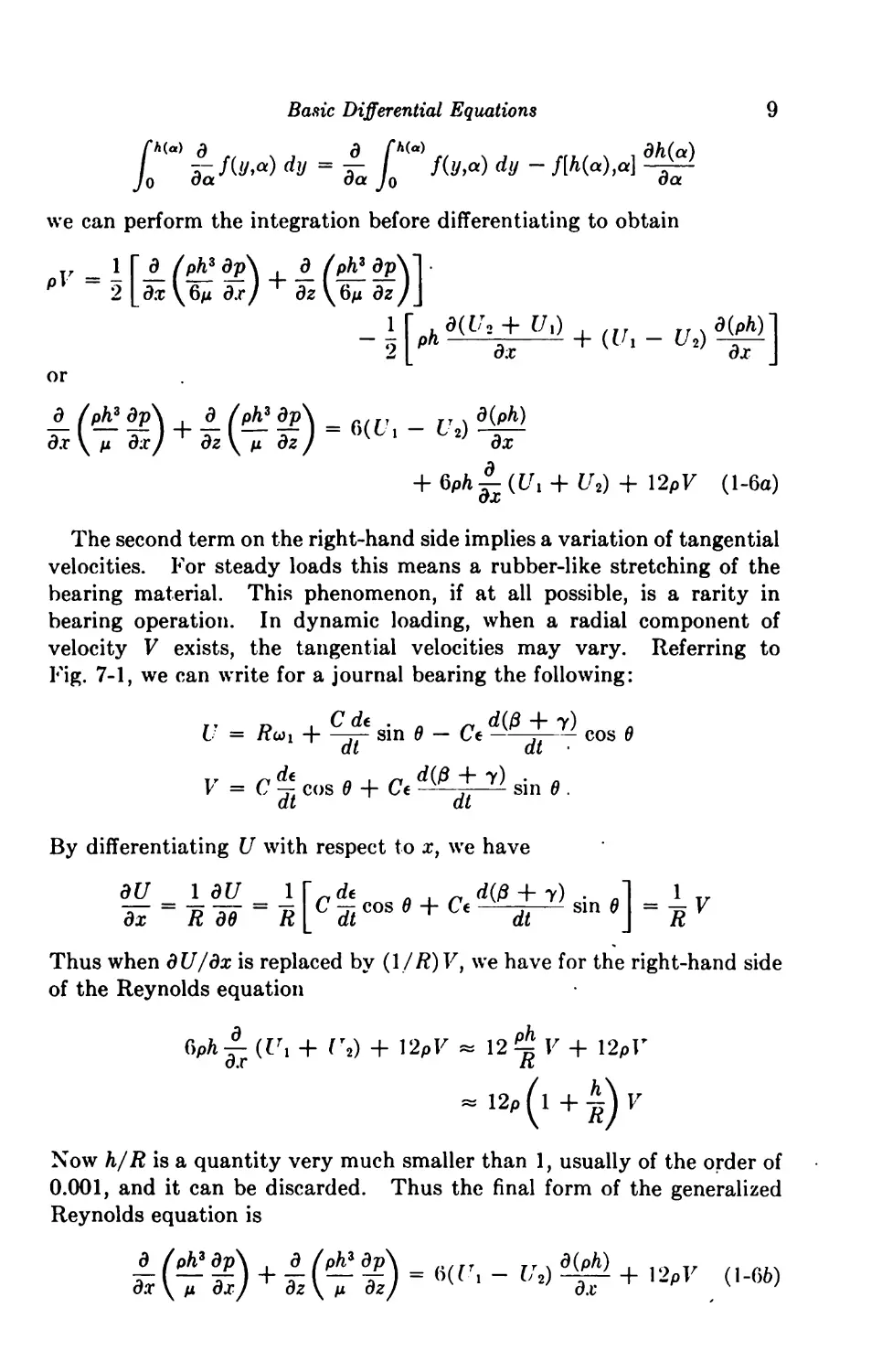
The second term on the right-hand side implies a variation of tangential
velocities. For steady loads this means a rubber-like stretching of the
bearing material.	This phenomenon, if at all possible,	is a rarity	in
bearing operation.	In dynamic loading, when a	radial	component	of
velocity V exists,	the tangential velocities may	vary.	Referring	to
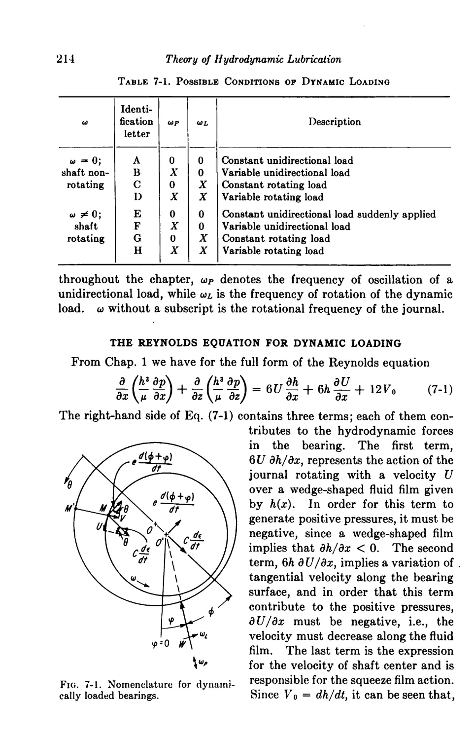
Fig. 7-1, we can write for a journal bearing the following:
U = Rwi + —rp s*n 0 — Ce —1^	— cos 0
at	at
Tr	~ de n . ~ d((3 -f- y) .	_
V = C -r cos 0 + Cc --	—- sin 0	.
at	at
By differentiating U with respect to x, we have
dU = IBU
dx R d0
1 T„de n „ d(fi + y) • J 1
= R[CdtC0S6 + C(—di~Sm *] = *
Thus when dU/dx is replaced by (1 /R)Vt we have for the right-hand side
of the Reynolds equation
Ciph (tri + r2) + VlpV « 12 ^ V + 12pV
ox	It
- 12p(l+4V
Now h/R is a quantity very much smaller than 1, usually of the order of
0.001, and it can be discarded. Thus the final form of the generalized
Reynolds equation is
d(ph)
dx

10
Theory of Hydrodynamic Lubrication
The first right-hand term 6(t/i — U2) d(ph)/dx, is obviously the contri¬
bution of the bearing velocities along the oil film, while the term 12pV
is due to the relative velocity of bearing surfaces in a direction normal
to the fluid film. It is of interest to note that the effect of the term
6(C71 — U2) d(ph)/dx depends on whether the bearing surfaces have trans¬
lational or angular velocities. For a thrust slider if Ui — U2, the first
right-hand term of Eq. (1-66) disappears and—since in the absence of
any normal movement of bearing surfaces, V = 0—such a bearing has
zero load capacity; conversely, if Ui = — U2, the load capacity is doubled.
However, in a journal bearing if Ui = t/2, the first right-hand term dis¬
appears, but the angular motion of the two surfaces introduces both
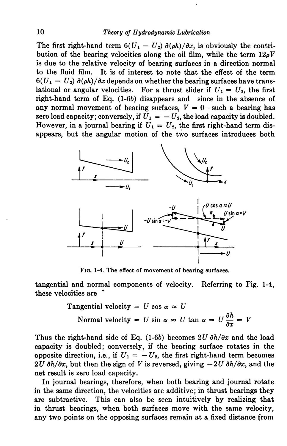
Fiq. 1-4. The effect of movement of bearing surfaces.
tangential and normal components of velocity. Referring to Fig. 1-4,
these velocities are
Tangential velocity = U cos a « U
dh
Normal velocity = U sin a « U tan a = U — = V
ox
Thus the right-hand side of Eq. (1-66) becomes 2 U dh/dx and the load
capacity is doubled; conversely, if the bearing surface rotates in the
opposite direction, i.e., if Ui = —1/2, the first right-hand term becomes
2U dh/dx, but then the sign of V is reversed, giving —2U dh/dx, and the
net result is zero load capacity.
In journal bearings, therefore, when both bearing and journal rotate
in the same direction, the velocities are additive; in thrust bearings they
are subtractive. This can also be seen intuitively by realizing that
in thrust bearings, when both surfaces move with the same velocity,
any two points on the opposing surfaces remain at a fixed distance from

Basic Differential Equations
11
each other; in a journal bearing any two points on journal and bearing will
approach each other at a rate depending on how fast both of the surfaces
move. However, it can be shown that, if the center of curvature of the
journal bearing surface does not coincide with the center of rotation,
counterrotation at identical speeds will produce hydrodynamic forces.
Thus bearings with a noncircular cross section will yield a load capacity
even under the above conditions7.
Equation (1-66) holds for both compressible and incompressible lubri¬
cants. By setting p = const, the Reynolds equation for incompressible
fluids is obtained:
£(7!)+ £(7	+
In Eq. (1-66) the viscosity p is still treated as a variable, being a
function of both the x and z coordinates. The film thickness h, too, is
general enough and can be a function of both coordinates.
Equations (1-66) and (1-7) are nonhomogeneous partial differential
equations of two variables. They are difficult equations to solve, and the
degree of complexity depends on the form of the parametric functions p,
p, and h and on the boundary conditions. Even for the simplest case of
p = p = const and V = 0 when Eq/ (1-66) reduces to
+ <‘-8>
closed solutions are difficult to obtain. Some successful attempts in
solving Eq. (1-8) for simple functions h(x) and numerical solutions for the
more complicated cases are treated in later chapters.
In cylindrical coordinates using the substitutions
x — r cos 0 and z = r sin 0
the generalized Reynolds equation becomes
IC? %) +; f. (f 8) - «v' - v* ™	<■-»)
In deriving Eq. (1-66) we have used the boundary conditions in a
manner such that V represents the resultant normal velocity regardless
of what is instrumental in producing this radial motion. In thrust
bearings, the velocity V can come only from the actual normal movement
of the sliding surfaces. However, in journal bearings, as we have seen
above, a normal relative velocity can come from two sources: from the
rotational velocity of the sliding surfaces and also from any actual motion
of journal center. It is convenient to have V represent only the radial
velocity that results from the motion of shaft center, and we shall thus

12
Theory of Hydrodynamic Lubrication
rewrite Eq. (1-66) for journal bearings in the following manner:
In most practical cases, the bearing is stationary and only the runner
in thrust bearings and the shaft in journal bearings are moving. In that
case, Eqs. (1-10) and (1-66) reduce to
which is the same for both thrust and journal bearings with U the sliding
velocity of either runner or journal. For steady loading (Fo = 0) and
incompressible lubricants (p = const) Eq. (1-11) becomes
which is the most commonly encountered form of the Reynolds equation.
1-3. Flow and Shear Equations. Several important expressions have
been formulated in the process of deriving the Reynolds equation. These
are the flow and shear equations of lubrication. It was pointed out that
Eqs. (1-5)
represent the velocity components of the lubricant in the x and z directions.
These equations, when integrated between the two bearing surfaces,
provide the lubricant flow at any given section:
where F0 now represents the motion of journal center.
(1-12)
/:[
These integrations yield
h3 dp	h
V2fx dx	2
hz dp
12p dz
(l-13a)
(1-136)
The flow in the z direction will be positive or negative depending on the

Basic Differential Equations
13
sign of the pressure gradients. The flow in the x direction is made up of
two components: the pressure flow (h3/\2n)(dp/dx) and the shear flow
h(Ui + U2)/2. Its direction will depend on both the magnitude of
Ui and Ui and the sign of dp/dx.
In polar coordinates Eqs. (1-13) are
_ h3 dp , r(o»i -f- o)i)h
qe	\2ritdB H 2	~
_ __ h3 dp
^r	12n dr
The shear stress from the definition of a Newtonian fluid as given by
Eqs. (1-4) is
du	dw
By differentiating Eqs. (1-5) with respect to y, we have
Ti = IS(2i/ _ h)+i{U* ~Ui) (1*14a)
The value of the shear stress depends on y, and the sections of interest
are the two bearing surfaces. Thus at the surface moving with velocity
U i we have y = 0 and
T*= + Ul) (1'15a)
Thus
_ _ h dp
2 dz
Tz = ~ T^TT-	(1-155)
At the surface moving with velocity U2 we have y = h and
+ !"'•	(|-10“>
'• = \1	<-'-m
Since the total force is given by integrating r over the bearing surface,
we have
F = JJV dA
Since Fz	=	JfrzdA	is at right angles to the	displacement of the	bearing
surfaces,	the	total	drag exerted by the moving	bearing	surface at y = 0

14
Theory of Hydrodynamic Lubrication
dx
dz
(1-17)
or y = h is given by
IN
In polar coordinates the above equation is by expressing Eq. (1-17)
in terms of torque rather than force,
M
h dp	y.r(o)2	— o)
± 2r ae +
r2 dd dr
(1-18)
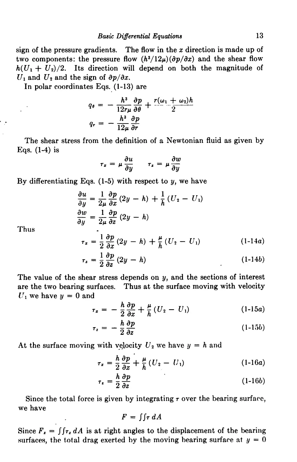
1-4. Derivation of Energy Equation. In rigorous bearing analysis the
variation of viscosity with temperature must be considered. As the fluid
is sheared, work is being done on it and there is a temperature rise which
in turn reduces the viscosity of incompressible fluids and raises the
viscosity of compressible fluids. This variation of viscosity must be
Fig. 1-5. Incremental volumes.
included in the solution of Reynolds equation. Likewise, from the stand¬
point of heat transfer and thermal distortion, it is desirable to determine
the temperature gradients that exist in the bearing. This section deals
with the derivation of energy relations which describe the temperature
variation in the fluid film.
It is desirable to have the modified energy equation in such a form
that all variations with y are integrated “out of the picture,” some¬
what analogous to the form of the Reynolds equation. There are two
approaches in deriving the modified energy equation: one is to sum ener¬
gies on an incremental control volume of finite height h, as in Fig. l-5a;
the second is to sum energies on an incremental control volume of
incremental height, as in Fig. 1-56, and then integrate over the height h.
Since there is some confusion over what constitutes mechanical energy
for a bounded finite-height incremental volume, the second of the two
approaches will be used. However, care must be exercised in integrating
the boundaries having slope. If certain terms are neglected in the
integrand, an erroneous partial differential equation will result.

Basic Differential Equations
15
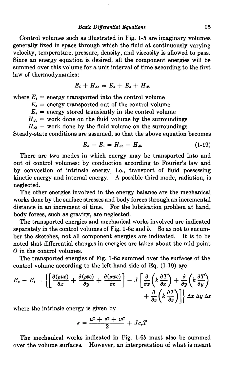
Control volumes such as illustrated in Fig. 1-5 are imaginary volumes
generally fixed in space through which the fluid at continuously varying
velocity, temperature, pressure, density, and viscosity is allowed to pass.
Since an energy equation is desired, all the component energies will be
summed over this volume for a unit interval of time according to the first
law of thermodynamics:
Ei + Hdo — E, + E0 + Ha,
where Ei = energy transported into the control volume
E0 = energy transported out of the control volume
E, — energy stored transiently in the control volume
Hdo ~ work done on the fluid volume by the surroundings
Hdb = work done by the fluid volume on the surroundings
Steady-state conditions are assumed, so that the above equation becomes
E0 — Ei = Hdo — Hdb	(1-19)
There are two modes in which energy may be transported into and
out of control volumes: by conduction according to Fourier’s law and
by convection of intrinsic energy, i.e., transport of fluid possessing
kinetic energy and internal energy. A possible third mode, radiation, is
neglected.
The other energies involved in the energy balance are the mechanical
works done by the surface stresses and body forces through an incremental
distance in an increment of time. For the lubrication problem at hand,
body forces, such as gravity, are neglected.
The transported energies and mechanical works involved are indicated
separately in the control volumes of Fig. l-6a and 6. So as not to encum¬
ber the sketches, not all component energies are indicated. It is to be
noted that differential changes in energies are taken about the mid-point
0 in the control volumes.
The transported energies of Fig. l-6a summed over the surfaces of the
control volume according to the left-hand side of Eq. (1-19) are
*• - * - (pfc*+:V+“E*] -' [£(*£)■+ «(*S)
where the intrinsic energy is given by
e = *±4±^ + Jc.T
The mechanical works indicated in Fig. 1-66 must also be summed
over the volume surfaces. However, an interpretation of what is meant

16
Theory of Hydrodynamic Lubrication
by work done on and work done by a volume in terms of the surface
stresses and fluid velocity is first needed. All the works done by the
fluid volume are on the upstream surfaces of the control volume, i.e.,
where the velocity components are in the opposite direction to the stress
dog A/
E--q dA
etc
do/ A/ dir A/
°> + 17 ~'*+77T
dT/X A/ dr/ A/
T"+iJ/ T’*'+IrT
. du A/
„JjLki7 >
it 2	\/
dr A/
d<rr A/ dK A/
U)
Fig. 1-6. Control volumes, (a) Transported energies; (b) mechanical energies.
components. With this viewpoint in mind, the right-hand side of Eq.
1-19 becomes
d
HJo	Hdb — (llOz “f" tJTU*	"f"
dy
d\ ,
(UT
V<7 y -j- WT zy)
a,) j Ax Ay Az
By equating the expressions for E and H according to Eq. (1-19),
+ ^ {utxz -j- xnuz + W0z]
|~d(pue)	d(pve) d(pwe)
[ dx
dy
dz

Basic Differential Equations
and by rearranging some of the terms.
17
[*S-S+-£]-'[£(*SK(*S)+£(*S)]
-*(£+»+£)+*(£+&+&)
(&+1+b)+('• B+- S+S)+- (w+ S)
(I+Ij)+'"(b + £) <■-“>
+ “Tyi
where the first parenthesis term of Eq. (l-20a) reduces to its stated
form because of the continuity equation
d(pu) d(pv) d(pw) _
dx ^ dy ^ dz
The equilibrium equations of fluid flow for steady-state conditions
(dv/dt = 0) and zero body force are given by the expressions preceding
Eqs. (1-1), namely
/ dll	du	:	du\	dox	drzy
p{UYx +	Vd-y	+ WYz)	= -dI	+ ^
( dv .	dv	. di>\	drux
p\UTx + Vd-y + Wdi) = l>x
( dw	dw	dw\	drtz	drty	,	do-
p\udl +	vdj	+wdl)	= aT	+ ^	+	aF
dTx-
dz
i doy . dryx
^ dy ^ dz
The substitution of the expressions for o and r into the last three equa¬
tions yielded for us previously the Navier-Stokes equations. Substitut¬
ing the last three equations and equations for o and r into Eq. (1-206)
yields
( de . de . de\ . I" d /, dT\ . d (, dT\ . d /. dT\ 1
p\uTx + vd-y + wTz) ~ ,/[aiV+ 9v\ dy) + d’z\!fe
= P
(u d[{u2 + v2 + w2)/2]	v d[(u2	+ »2_±w2)/2]
dx
d[(u* + ;
dy
^	dz	j	p\dx^	dy	^	dz
From e = (u2 + v2 + w2)/2 + JcvT we have
jp r u +v ^p.+w a(c’7’)
dx
dy
dz
1 , [du di>
dw
+ ~dz
+ (1-21)

18
Theory of Hydrodynamic Lubrication
where
- * [* (£)‘+’ (£)'+*(£)■- i (£+S+£)'
. (du	dv\2 .	(dv . dw\2 . fdw dw\2l
+	+	^ +	+ ^ + a?jJ
It is to be noted that only a d{cvT)/dt need be added within the first
bracket of Eq. (1-21) to make the energy equation applicable also to tran¬
sient states, subject only to the limitation that the flow be laminar.
The first	bracket	term in Eq. (1-21) is the	convection of internal energy
of the fluid.	The	second bracket	term is	the rate of work done by a
differential volume of fluid in expansion against the surrounding pressure.
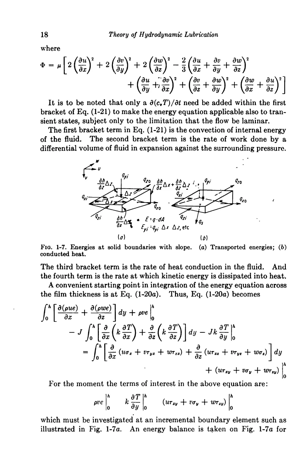
fro dh.	dh -a
Fig. 1-7. Energies at solid boundaries with slope, (a) Transported energies; (6)
conducted heat.
The third bracket term is the rate of heat conduction in the fluid. And
the fourth term is the rate at which kinetic energy is dissipated into heat.
A convenient starting point in integration of the energy equation across
the film thickness is at Eq. (l-20a). Thus, Eq. (l-20a) becomes
/:[
d(pue) d(pwe) 1 ,	|A
=/:[
d	d
(iKTz + VTvx + WTZX) -f- ~ (UT
-1- VTyx + w<Tt) dy
“1“ (WTXy “I- V(Ty -f" WTZy)
For the moment the terms of interest in the above equation are:
pve
kd-T
dy
(UTzy + V<Ty + WTzy)
which must be investigated at an incremental boundary element such as
illustrated in Fig. l-7a. An energy balance is taken on Fig. l-7a for

the first term
which becomes
+ pwe +
Basic Differential Equations
(Axo “1“ fozo AZ| Kyi Ezi)h = 0
dh (Az)2
dz 2
d(pwe) dh Ax ^ dh A^\ A   du (At)2
19
d(pu«) “If aA	dh Az]
pue + ~&rAx\ [aiAx + TzT\ * ~pue
. "1 f dh At . dh "I	du	(At)2
A2J [d5T + ^A2JAx-pwa5 —
dz | | dx 2	1	dz |	1	dx 2
— pve Ax Az = 0
where average incremental heights have been used, and hence
dh
dh
pve
= pue —
h dx
h
= pweTz
In lubrication problems, the boundaries are usually such that
and thus
u = w =0
I h !a
pve\ =0
If the fluid has intrinsic energy at this boundary, then v ^ = 0; this
may be verified by a mass balance of the same form as used above. At
the zero-slope boundary
pve = 0
The heat conduction term may be evaluated from Fig. 1-76 as
- Kt{T - Tw) (1-22)
dy
_ dTdh
dx dx
, , dTdh
+ k-r- —
h dz dz
where the approximation,
Jr.o V1 + (^) V1 + (S) -
has been made. Tw is the stator-plate temperature, which may or may
not be a function of x and z, and K\ is the heat transfer coefficient at the
fluid-solid interface. If the runner has the same temperature distribu¬
tion as the stator plate, then
dT
k
dy
K2{T - Tw)
The surface mechanical works are
(UTXy + V(Ty -I- WTzy) = 0
(UTXy -{- V(Jy -j“ WTzy) 0	TXJ

20
Theory of Hydrodynamic Lubrication
since u = v = w = Ow = U, and v = w =0.
\h |/» \h	|o	’	|o |o
Substitution of the above equations into the integrated form of Eq.
(l-20a) yields
jl [	+	hI""> ] d> - J /„' [k (‘ H) +1 (* S) ] *•
-j(t££+ti£i£)l+K’<T-T->
~ Jo	^U(Tz	VTyX	^UTlZ	^	~~	^Txv o
(l-23a)
where Kt = Ki + K2. Carrying out the same operation as in Eqs.
(l-20a) and (1-206) gives for the right-hand side of (l-23a):
Right-hand side
iide = p ju
d[(u2 + v2 + w2)/2]
dx
+ v d[(u2 + v2 + w2)/2] + ^ d[(u2 + v2 + w2)/2] |
dy	dz	|
fh	(du	dw\	,	fh ( d [	(du dv\
-Jo p(di+^)dy-Jo |MapK^ + ^/.
.	d (	di/\	dp	2d (du	dv dw\
L	^	3 ^ M (to	+ ^ + Tz)
+ W Fy [" (If + %)]) dy + lo *" ^ - C/T- lo (U236)
where
*" - - [*(£)'■+2 (£)'-l(s + r» + S) (I + S)
/dw diA2 I I ^ _L (Urn ■	^1
^ds: dx ,/ * ^ + dx/ dx + \dl/ + dz) dz\
+ 1
And now making the approximation that since the film thickness
h <$C B, L, then v « 0 and T, p j* f(y). In addition, then p and p are inde¬
pendent of y. Hence the first integral in Eq. (l-23a) may be reduced,
since the continuity equation becomes
d(pu) d(pw) = 0
dx
dz
and
* =	+	Jc.T
Also, the second integral in Eq. (l-23a) may be integrated directly.
The first integral in Eq. (1-236) will cancel (for v = 0) a like integral
on the left-hand side of Eq. (l-23a). With these approximations, equa¬
tion (l-23a) reduces to

Basic Differential Equations	21
+ K,(T-T.)\ --, £(£ + %) i,
-' f; (■ w+• ®o* - ‘u 11.+r ■" v-2w
where
,, f0 /du\2	(dw\2	2 (du	dw\2	(du dw\2l . OA,*
* =m[2U/ +2w _n^ + */ +U+^jj (U24b)
which cannot be deduced from Eq. (1-21) by stating v « 0.
The next step in the reduction of Eq. (l-24a) is the neglect of any
terms of insignificant size. Dealing first with terms of a mechanical
nature, one of the expansion terms is by requirements of continuity,
du n / p dp\
pei = 0{u7^)
Hence the ratio of one of the largest viscosity terms to the expansion
term is
pu d2u/dy2
p du/dx
W pw)
which is approximately equal to 1 X 103. By taking a similar ratio
with one of the terms in Eq. (1-246),
uu d2u/dy2 _ n /£2\
2u(du/dx)2	\h2)
which is nearly equal to 2 X 107. It might be noted that
°(M/o*uSdi/)=0(^SL)
Substitution of the relations for the velocity as given by Eqs. (1-5)
U =	-	yh)	+	U
w =	^(y* - yh)
(‘-D
into Eq. (l-24a) and using the above approximations yields
([(pVh	h> dp\ d(c,T)	h3 dpd(c,T)~\
tL\ 2	12k dx) dx	12v dz dz J
-[l(tk^) + i(hk^}} + K^T-T->)

22
Theory of Hydrodynamic Lubrication
For ordinary lubricants, the characteristic values of the parameters
are such that conduction is a minor mode of heat transfer. Further,
the heat transfer coefficient at the fluid boundaries as reported in Ref. 5
is very small. Since it is expected that the fluid temperature rise through
a bearing will not be large, the specific heat of the fluid will essentially be
constant. With the above-mentioned fluid parameter characteristics,
Eq. (1-25) becomes
r ttt . l. T/i W dp\dT	h2	dp dT~] _ \2nU> \, ,	/t4
(inUdx)dx (i/it/ dz dz J h ( + 12M2t/2
[(g)’ + ©II <■*>
Equation (1-26) states that all of the heat generated within the fluid
because of viscosity is carried away by the mass transfer of the fluid
and that no heat is gained or lost through the bearing surfaces.
Equation (1-26) can be made more convenient for numerical work by
reducing it to nondimensional form. By setting x = x/B, z = z/Bt
h = h/B, /z = m/mi, p = p/pi, V = pB/GmU, T = TpiJcvB/pJJ, where B
is a representative length in the x direction, Eq. (1-26) becomes
-h(i _	_	M3	dp	ar	=	9 m 11 , 3h4 r/ap\2	/dpV])
a dxjdx a dz dz a I P L\d*/ \di) J)
(l-27a)
Likewise, the Reynolds equation becomes
1-5. Equation of State. In Eq. (1-26), m is a known function of p and T
and h a known function of x and z. One more equation is needed because
there are three unknowns (p, p, and T), and it is provided by the equation
of state given by
pv = (5iT	(1-28)
For lubrication with a gas, the assumption that the gas obeys the perfect-
gas law will be adequate. Since p and f are quantities of practical
importance, the procedure might be to eliminate p from (l-27a) and
(1-275) by the substitution p — 1/6(n — 1 )pT. For lubrication with a
liquid film the choice of an equation of state is more difficult. Even for
simple liquids the equations proposed are modified van der Waals type of
considerable algebraic complexity, so that their introduction into Eqs.
(1-27) would increase the complications to such an extent that the solution
would probably be a major computing operation.
If it be sufficiently accurate to ignore the variation of p, /z, etc., with
temperature, or if the variation with temperature can be replaced by a

Basic Differential Equations
23
variation, known a priori, with x and z, then Eq. (1-276) becomes an
equation for p only. The solution thus obtained can be inserted into
Eq. (l-27a), which then becomes an equation in T only. This situation,
which also arises in other branches of applied mechanics, enables the
equations to be solved successively instead of simultaneously, but only
in the order (1-276) to (l-27a). However, as soon as it becomes necessary
to take variation with temperature into account, the equations become
interlocked and must be solved simultaneously.
SOURCES
1. Reynolds, O.: On the Theory of Lubrication and its Application to Mr. Beau¬
champ Tower’s Experiments, Phil. Trans. Roy. Soc., London, vol. 177, part 1, 1886.
2. Weilder, S. E.: Data Folder DF-54-AD-7, General Electric Company.
3. Goldstein, S.: “Modern Developments in Fluid Dynamics,” vols. I and II,
Oxford University Press, New York, 1950.
4. Vogelpohl, G.: Heat Transfer in a Bearing from the Lubricant to the Gliding
Surfaces, VDI-Forschungsheft, July-August, ed. B, vol. 16, no. 425, pp. 1-26, 1949.
5. Cope, W. F.: The .Hydrodynamic Theory of Film Lubrication, Proc. Roy. Soc.
(London), A, vol. 197, p. 201, 1949.
6. Sternlicht, B.: Energy and Reynolds Considerations in Thrust-bearing Analysis,
Proceedings of the Conference on Lubrication and Wear, I.M.E., 1957, pp. 28-38.
7. Pinkus, O.: “Counterrotating Journal Bearings,” General Electric Internal
Publication R60MSD322.

CHAPTER 2
HYDRODYNAMICS OF SIMPLE CONFIGURATIONS
It is not the purpose of this chapter to deal with any general problems,
nor even with any specific branch of fluid flow. The subjects were chosen
solely on the basis of whatever relation they may have to the study of
bearings, be it as actual components of lubrication systems or as an
idealization of a complex bearing geometry. Thus capillary tubes and
orifices are an integral part of hydrostatic bearings, and their character¬
istics must be known before the performance of such bearings can be
calculated; and the study of flow in concentric and eccentric cylinders is
applicable to journal bearings and may throw some light on the flow of
lubricant in the clearance space.
GENERAL EQUATIONS OF MOTION FOR COMPRESSIBLE FLUIDS
The three forces affecting the flow of a gas in a slot are the pressure
force, the viscous force, and the force required to accelerate or decelerate
the fluid. If the depth of the slot is very small and the viscous and
pressure forces are very large in comparison to the inertia force, then the
viscous force can be equated to the pressure force. For laminar flow
this results in a simple theoretical equation relating pressure distribution,
temperature, mass flow, and slot geometry. For turbulent flow use is
made of the concept of resistance X, where
* = \7~~T~	(2-1)
Mpul,
t being the “skin friction” per unit of surface area in contact with the fluid
and wmvg the spatial mass velocity. The relationship between X and the
Reynolds number Re, based on the hydraulic mean depth for turbulent
flow, is given empirically by Blausius1-* as
X - °*079	(2 2^
Xr - Ri«	(2'2)
and this value can be used to develop an equation corresponding to that
* Such superscript figures indicate references listed under Sources at the end of the
chapter.
‘24

Hydrodynamics of Simple Configurations
25
obtained theoretically for laminar flow. The assumptions made in the
derivation of the flow equations are the same in both cases. The force
required to accelerate or decelerate the fluid is assumed to be negligible;
the pressure distribution over any cross section is assumed to be constant;
and the temperature of the gas as it flows along the slot is assumed to be
constant or a known function.
2-1. The Theoretical Equation for Laminar Flow. With the condi¬
tions as stated above, we can start with Eq. (l-5a). For the flow of a
fluid between stationary walls we have Ui = U2 = 0, and Eq. (l-5a)
becomes
— hy dp
u =
2/x dx
giving a parabolic velocity profile.
The mean velocity at any cross section is
Wav
1 [h A
= hJoUdy=-
dx 12/x
(2-3)
(2-4)
If the width of the slot is denoted by 6, where 6 is a function of x, the
weight flow along the slot is then
given by
G = pgbhua,
— _ &P
^ 12/i dx
from which we obtain
dp = _ 12 pG
dx	gpbh3
and by substituting in this equation
the value gp = p/<HT, we obtain
p dp =
12/i(R TG
bh3
dx (2-5)
Fig. 2-1. Elementary volume between
two plates.
If T, b} and h are known functions
of x, this equation can be integrated and the theoretical pressure distri¬
bution so obtained.
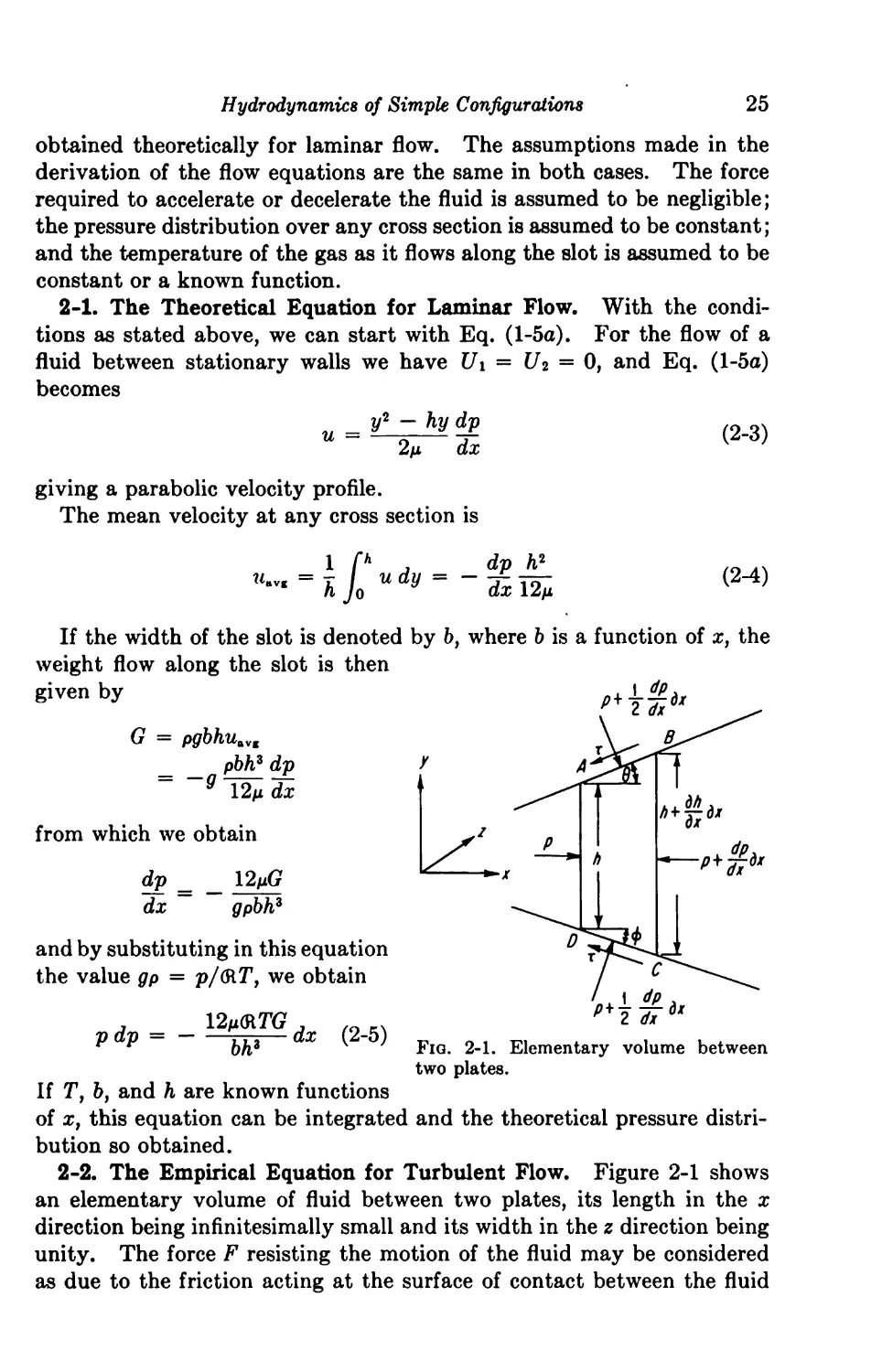
2-2. The Empirical Equation for Turbulent Flow. Figure 2-1 shows
an elementary volume of fluid between two plates, its length in the x
direction being infinitesimally small and its width in the z direction being
unity. The force F resisting the motion of the fluid may be considered
as due to the friction acting at the surface of contact between the fluid

26	Theory	of Hydrodynamic Lubrication
and the wall. If the skin friction per unit area of wetted surface be
denoted by r, then
Fi = rAB cos 6 + rDC cos <f>
that is	Fi = 2r dx
The pressure force acting in the direction of motion is given by
^2 = M	^ dx^j (AB sin 0 + CD sin <f>)
~(P + tx dx)(h+Txdx)
= pk + (p + \txdx) Txdx - (P + txdx) (h + Txdx)
which, neglecting second-order terms, reduces to
F2 = -h^dx
dx
By equating the two forces Fi and F2, we have
dp _ _ 2r
dx	h
By substituting Eq. (2-1) we get
~ = - —(2-6)
dx	h
The coefficient X is dependent on the Reynolds number Re. For laminar
flow the value of Xl is
x =24
L Re
On substituting \L in Eq. (2-6), we have
dp _ _ 24 uJVJ = 24 __GP_
dx Rep h Re g2pb2hz
where	Re =
p gbp
dp _	12 pG
Hence
dx bhzpg
, \2p(RTG ,	fo
or	pdp=	bW~dx	(2‘7)
which is the same as Eq. (2-5).
To obtain the corresponding equation for turbulent flow, we substitute
in Eq. (2-6) the value \t

Hydrodynamics of Simple Configurations
27
0.079 G2
dx Re* h	Re*	g2Pb2h3
0.067m*G*
hW'pg*
,	0.067m*(RTO*	,	0,
pdp = Piy—(2'8)
FLOW THROUGH NARROW SLOTS
The general equations (2-7) and (2-8) can be integrated if b, h, and T
are known as functions of x. We shall now apply these equations to
various specific cases.
2-3. Isothermal Flow. Constant Area Slot. For a constant area we
have h = const and b = const, and integration of (2-7) gives for steady
laminar flow
2	2	24n&TG .	.	fo	m
Pi2 -	 gp—	(*2	-	*i)	(2-9)
On integrating Eq. (2-8), we obtain for turbulent flow
0.133„*(RTO»(*. - X,)
P> “ P2 = pwp 	(	)
Diverging Width. Let us denote the rate of width divergence by
b — ax. Then if the frictional effect of the two side walls is neglected,
the flow is analogous to the radial flow between two circular flat plates
of constant film thickness, and by symmetry the pressure at any given
radius is constant. Provided, therefore, that the divergence is small, the
pressure in any plane perpendicular to the axis is approximately constant,
and Eqs. (2-7) and (2-8) may be applied. By substituting in these
equations b = ax, we obtain for laminar flow
,	12 p(RTG dx
pdp =	u
ahz x
which when integrated becomes
2	2	24M(Rrci	x2	/011N
(2'n)
and for turbulent flow
,	0.067m*<R7’G*	dx
pdp ^
which when integrated becomes
\Xi« Xi’V
.	0.178x xi
P* P2 ct/'h3gii I •*••*	)	(2-12)

28
Theory of Hydrodynamic Lubrication
Diverging Depth. Let us here denote by h = fix (b = const) the
divergence of slot depth. Because the divergence of the two plane sur¬
faces is very small, the component of velocity perpendicular to the axis
of the slot must also be very small, and the pressure distribution over any
cross section is, therefore, assumed to be constant.
For laminar flow, substitution of h = fix in Eq. (2-7) yields
,	12	dx
Vdp
and, when integrated, this becomes
Pi2 - p2
W3 \Xi2 X22
By the same substitution in Eq. (2-8), we have for turbulent flow
0M7n*(RTGK dx
(2-13)
p dp = —
which when integrated gives
blip SgK
t 0.067MM<nrow / 1	1\	/01,,
Pl -w ~ &)	( }
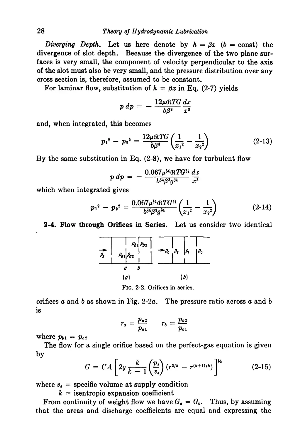
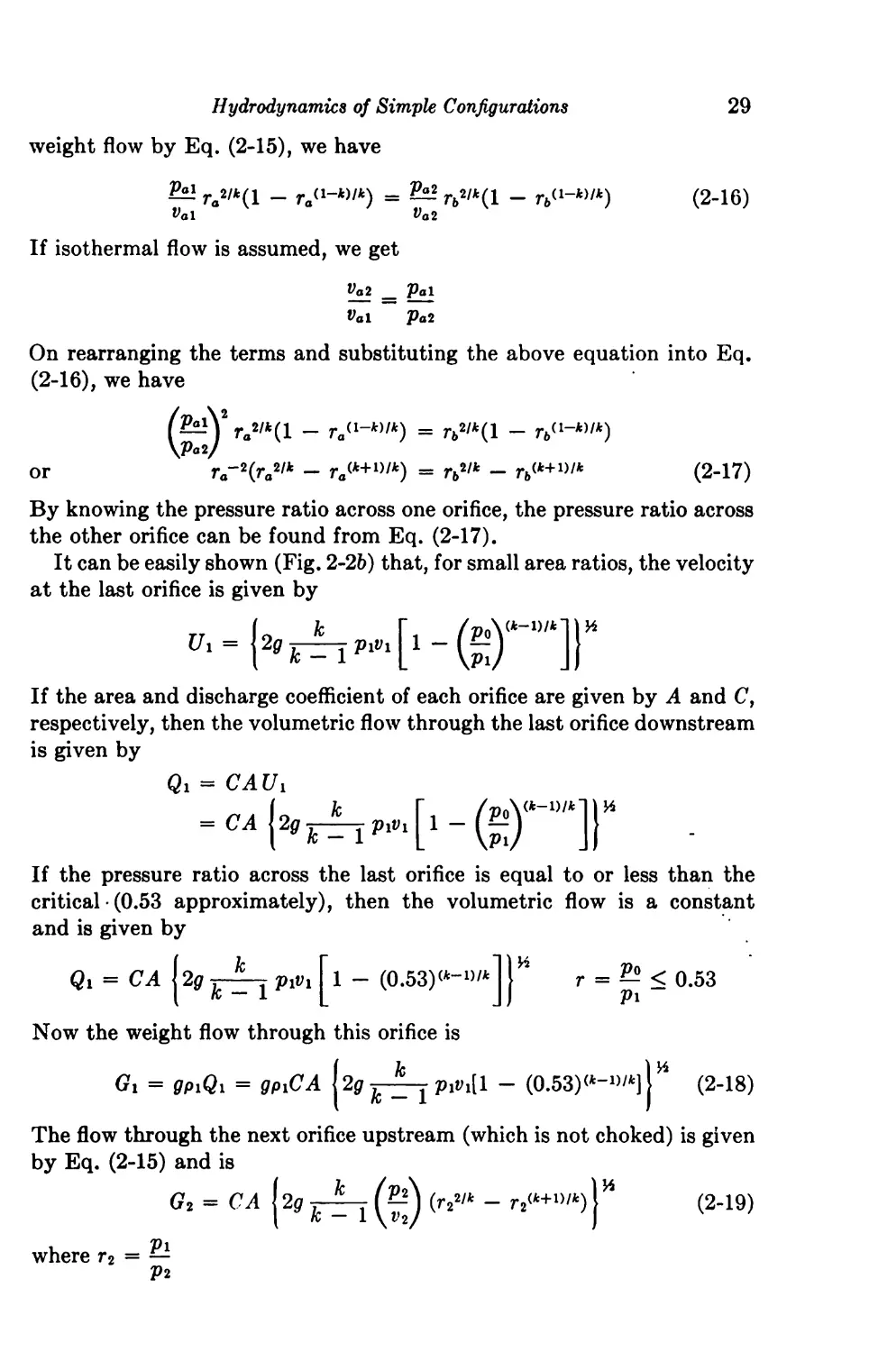
2-4. Flow through Orifices in Series. Let us consider two identical
i ft,
Pbi | |
T
Po^ai |
1 \h
1 ..I Lj
Ps
1
Pb
o b
(<7)	\b\
Fig. 2-2. Orifices in series.
orifices a and b as shown in Fig. 2-2o. The pressure ratio across a and b
is
„ _ Pal ^ _ Pb2
ra	Tb
Pal	Pb1
where pb i = pa 2
The flow for a single orifice based on the perfect-gas equation is given
by
G = CA [2g	(^j (r2/* -	j*	(2-15)
where vt — specific volume at supply condition
k = isentropic expansion coefficient
From continuity of weight flow we have Ga = Gb. Thus, by assuming
that the areas and discharge coefficients are equal and expressing the

Hydrodynamics of Simple Configurations
weight flow by Eq. (2-15), we have
TaW{ 1 -	ris/*(i	_	rt<i-*)/*)
Val	Va2
(2-16)
29
If isothermal flow is assumed, we get
Vg2 _ Pal
Va\ Pa2
On rearranging the terms and substituting the above equation into Eq.
(2-16), we have
By knowing the pressure ratio across one orifice, the pressure ratio across
the other orifice can be found from Eq. (2-17).
It can be easily shown (Fig. 2-26) that, for small area ratios, the velocity
at the last orifice is given by
If the area and discharge coefficient of each orifice are given by A and C,
respectively, then the volumetric flow through the last orifice downstream
is given by
If the pressure ratio across the last orifice is equal to or less than the
critical • (0.53 approximately), then the volumetric flow is a constant
and is given by
The flow through the next orifice upstream (which is not choked) is given
by Eq. (2-15) and is
or
Qi = CAUi
Qi = CA lig ptf! T1 -	Jh	r	=	2?	<	0.53
Gi = gpiQi = gpiCA 2g	-	(0.53)<*-»'*]|H	(2-18)

30
Theory of Hydrodynamic Lubrication
If we equate the weight flows through the orifices and still assume
that the areas and discharge coefficients are equal, then
[ 1 - (0.53)(t-l)/‘l	=	^ (r22'* - r2<*+>«‘)
Vl L	J	v2
Assuming again that pv = constant, the above equation reduces to
r2_2(r22/* - r2«+l)lk)	=	1 - (O.W'~»lk	(2-20)
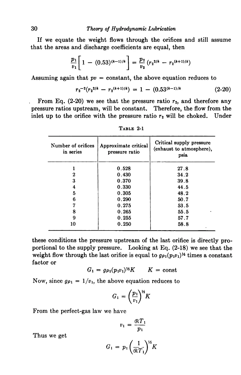
From Eq. (2-20) we see that the	pressure ratio r2, and therefore	any
pressure ratios upstream, will be constant. Therefore, the flow from the
inlet up to the orifice with the pressure ratio r2 will be choked. Under
Table 2-1
Number of orifices
in series
Approximate critical
pressure ratio
Critical supply pressure
(exhaust to atmosphere),
psia
1
0.528
27.8
2
0.430
34.2
3
0.370
39.8
4
0.330
44.5
5
0.305
48.2
6
0.290
50.7
7
0.275
53.5
8
0.265
55.5
9
0.255
57.7
10
0.250
58.8
these conditions the pressure upstream of the last orifice is directly pro¬
portional to the supply pressure. Looking at Eq. (2-18) we see that the
weight flow through the last orifice is equal to gpi(piVi)** times a constant
factor or
Gi — gpi(piVi)^K K - const
Now, since gpi = \/v\, the above equation reduces to
«■ - {v)“K
From the perfect-gas law we have
=
pi
Thus we get
a - ”• (irrl)"x

Hydrodynamics of Simple Configurations
31
Since pv = const, GiT = const and we have
G\ = piKi	K i	= const
We have already deduced that pi/p, = const; therefore, the equation
above becomes
G\ = p,K2 — < critical volume K2 = const
P*
and we see that the weight flow through a series of orifices with the
exhaust orifice flow choked is directly proportional to the supply pressure,
provided that the discharge pressure is constant.
For a discharge to the atmosphere, the critical pressure ratio and
critical pressures are given in Table 2-1.
INCOMPRESSIBLE FLOW
2-6. Flow between Parallel Walls. The simple case of laminar flow
of an incompressible fluid between two parallel surfaces of infinite extent
is given by Eq. (l-5a). By placing the coordinate axis y — 0 at the center
of the film, i.e., at h/2, and setting U2 = 0, we obtain
-?(• + *!)-si [>-*©']
For the case U = 0, that is, when both surfaces are at rest, Eq. (2-21)
gives a parabolic velocity profile; for dp/dx = 0 and U ^ 0 the velocity
profile is linear. For the general case the velocity profile is made up of
both contributions, and, depending on the value of dp/dx, the profile
may be convex or concave, or it may even reverse itself. The point
at which flow will occur in a direction opposite to U can be calculated
by letting du/dy = 0 at the stationary wall. The result is that, for
dp/dx > 2 Up/h2, the flow will reverse itself over certain values of y.
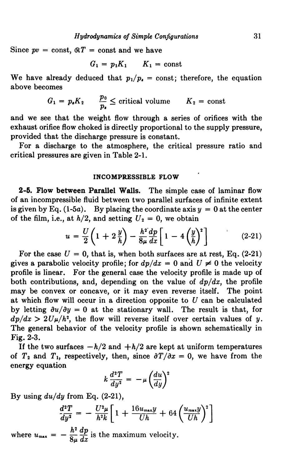
The general behavior of the velocity profile is shown schematically in
Fig. 2-3.
If the two surfaces —h/2 and +h/2 are kept at uniform temperatures
of T2 and 7\, respectively, then, since dT/dx = 0, we have from the
energy equation
. d2T	(du\2
dy1	M \dy)
By using du/dy from Eq. (2-21),
d*T	_	IPp [	16umtkXy	(twyVl
'dy2	h2k L	Uh ^	\ Uh ) J
where umAX = —	^	is the maximum velocity.
8p dx

32	Theory	of	Hydrodynamic Lubrication
The solution of the above equation is
= t, + (p-
- T
2 . fiUUn
3 k
1 + 2
fiUum
3 k
The temperature gradient is
dT = Ti - T2 , 2mUum
dy	h	3kh
[i+80D1+tHi _ i6©'
IS
2hk I \h)
(2-22)
+ 16
um
~U \h)
, 128wL
3 U2 \h
(2-23)
and depending upon whether the first right-hand term of (2-23) is greater
or smaller than the remaining two terms, heat will either flow into or out
of the upper wall.
T->0
dx
du I
dy I
> o
± = o
dp
dx
dx
dx
du
= 0
1 h
£1 >°
dy | h
du
dy
dy |
1 *
2
2
2
< 0
> 0
2-6. Circumferential Flow between Concentric Cylinders. The lam¬
inar flow between concentric cylinders extending to infinity in the axial
direction yields from physical considerations
u '= u(r) v = w — 0 p = p(r)
When these considerations are used in the Navier-Stokes equations, the
following two differential equations are obtained
dr2 ^ dr \r)
pu2 _ dp
r dr
(2-24 a)
(2-24 b)

Hydrodynamics of Simple Configurations	33
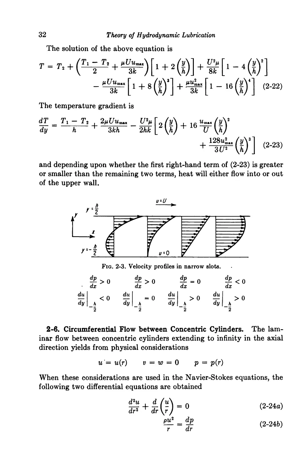
By using the boundary conditions of Fig. 2-4, we obtain by integration
of Eq. (2-24a)
U =	[r(u>2ft22	-	Ulft,2) -	(«2	- «,)]	(2-25)
and for the pressure distribution from Eqs. (2-25) and (2-246)
* = PI + (g,»-B1y[W -
— 2i?l2/?22(&>2 — <*>i) (o^fi^2 — Wj/?12) In
til
2.
where pi is the pressure at Ri.
-W«i« fi2‘(«. - »,)* ^ f i)] (2-:
26)
Fig. 2-4. Notation for concentric cylinders.
If the inner cylinder is kept at rest, the moment of the fluid on a length
L of the outer cylinder is
M 2 = 2ttR22Lt2 — 2tR'?Lp,t
«GD
or	Af, = 4irL	“2	(2-27)
This last equation can be used to determine m by merely measuring the
moment M2.
When only one cylinder rotates in an infinite fluid, we have for o>2 = 0,
T — oo
/?l200l
w =
r
Af = ^tcpLR\2<j)i
The energy equation for our case is
H / dT\ = _ m /dw _ w\*
r dr \ dr / A; \dr r /

34	Theory	of	Hydrodynamic	Lubrication
which gives the following temperature distribution
T—T I M ^i4^24(o>i —	2)2/	1	1\
1_1"/b (RJ-RfY \RS r2/
T T fl Rl4R24(d)l-U)2)2 ( 1	l\
l2^k (RS-RW \RS	RS),	r
In Rt/Rx	Ri	(2“28)
2-7. Axial Flow in Cylinders. Concentric Cylinders. The differential
equation for the axial flow of fluid in an annular space is
+	<2'29>
By using the boundary conditions of w	= 0 at Ri and	R2i	where	Ri and	R2
are	the	inner	and	outer radii,	the velocity profile	in	an	annular	slot
becomes
+	(2-M>
By integrating w between Ri and R2, the flow becomes
«-*■•>[*1’-ft’-ETIGTO]	<M1>
By setting	Ri	=	0 in	Eq. (2-30), which	gives the	flow in annular slot, we
obtain	the	flow of a	liquid in a circular	cylinder.	The velocity	profile is
given by
(2-32>
1 2
w-“"i»TzR>
The velocity profile is parabolical, therefore
1		 1 dp p 2
W.v, - 2	W,„	gM dz Ri
The volume flow is given by
Q = RS - ^	(2-33)
The energy equation is given by
. /d2T , 1 dT\	/dw\2
\dr2 r dr) M \dr)
so that for a temperature of T2 at R2 and at r = 0 we have
T-Tt+ (Ti _ T,) [ 1 -	(2-34)

Hydrodynamics of Simple Configurations
35
Equation (2-33) is useful in the calculation of the performance of inter¬
nally pressurized bearings where lubricant is admitted through a series of
capillary tubes.
Flow through Eccentric Cylinders. If the cylinders are not concen¬
tric, the slot height h is a function of 6 and is given by the equation
C(1 + c cos 6) (Chap. 3). If we are allowed to simulate the case of
eccentric cylinders by two nonparallel developed surfaces, then the
velocity from Eq. (1-56) is given by
and now is a function of both coordinates. The flow is, by integrating w,
For c = 0, the above equation reduces to (1-56).
The exact analytical treatment of flow in eccentric cylinders is compli¬
cated. It represents a two-dimensional problem which is described by
Poisson’s equation
where w — 0 at the boundaries. A partial solution of this problem is
given in Ref. 5, where the velocity profile is expressed in series form by
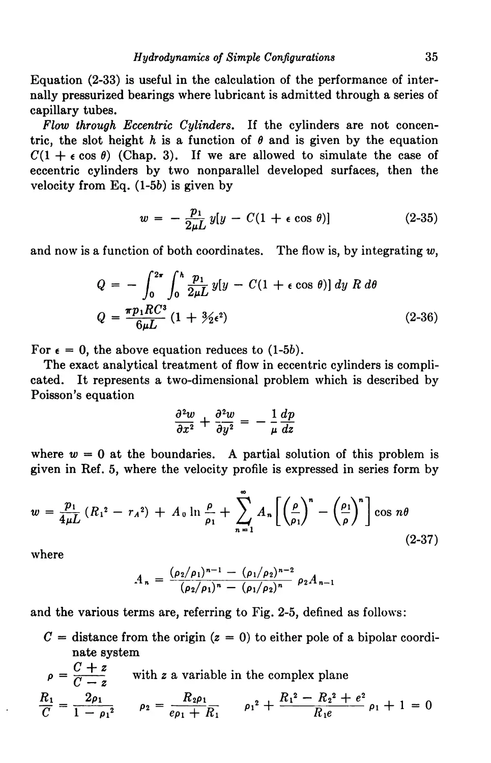
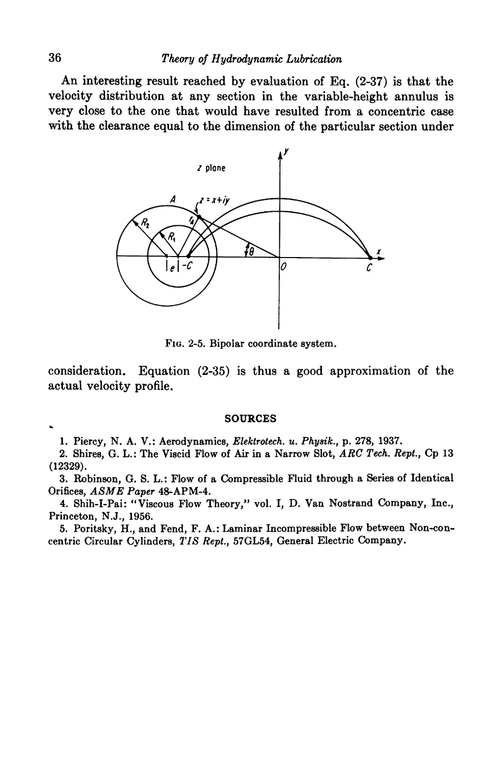
and the various terms are, referring to Fig. 2-5, defined as follows:
C = distance from the origin (z = 0) to either pole of a bipolar coordi¬
nate system
w = - ^ y[y - C(1 + € cos 0)]
(2-35)
Q =	(1	+	««*)
(2-36)
d2w	dhv	_ I dp
dx2	dy2	p dz
(2-37)
where
C + z
p = q~zt~z	2	a	variable	in	the	complex	plane

36
Theory of Hydrodynamic Lubrication
An interesting result reached by evaluation of Eq. (2-37) is that the
velocity distribution at any section in the variable-height annulus is
very close to the one that would have resulted from a concentric case
with the clearance equal to the dimension of the particular section under
consideration. Equation (2-35) is thus a good approximation of the
actual velocity profile.
SOURCES
1. Piercy, N. A. V.: Aerodynamics, Elektrotech. u. Physik., p. 278, 1937.
2. Shires, G. L.: The Viscid Flow of Air in a Narrow Slot, ARC Tech. Rept., Cp 13
(12329).
3. Robinson, G. S. L.: Flow of a Compressible Fluid through a Series of Identical
Orifices, ASME Paper 48-APM-4.
4. Shih-I-Pai: “Viscous Flow Theory,” vol. I, D. Van Nostrand Company, Inc.,
Princeton, N.J., 1956.
5. Poritsky, H., and Fend, F. A.: Laminar Incompressible Flow between Non-con-
centric Circular Cylinders, TIS Repl., 57GL54, General Electric Company.

CHAPTER 3
INCOMPRESSIBLE LUBRICATION;
ONE-DIMENSIONAL BEARINGS
With the exception of Chap. 6 we shall be dealing throughout this book
with hydrodynamic lubrication. By “hydrodynamic lubrication” we
mean a process in which two surfaces, moving at some relative velocity
with respect to each other, are separated by a fluid film in which forces
are generated by virtue of that relative motion only. As in all other
problems in engineering, the solutions on the following pages are based
on certain assumptions, and in order to appreciate the degree of applica¬
bility of these results, a realistic picture of bearing operation will first be
given.
THE REAL BEARING
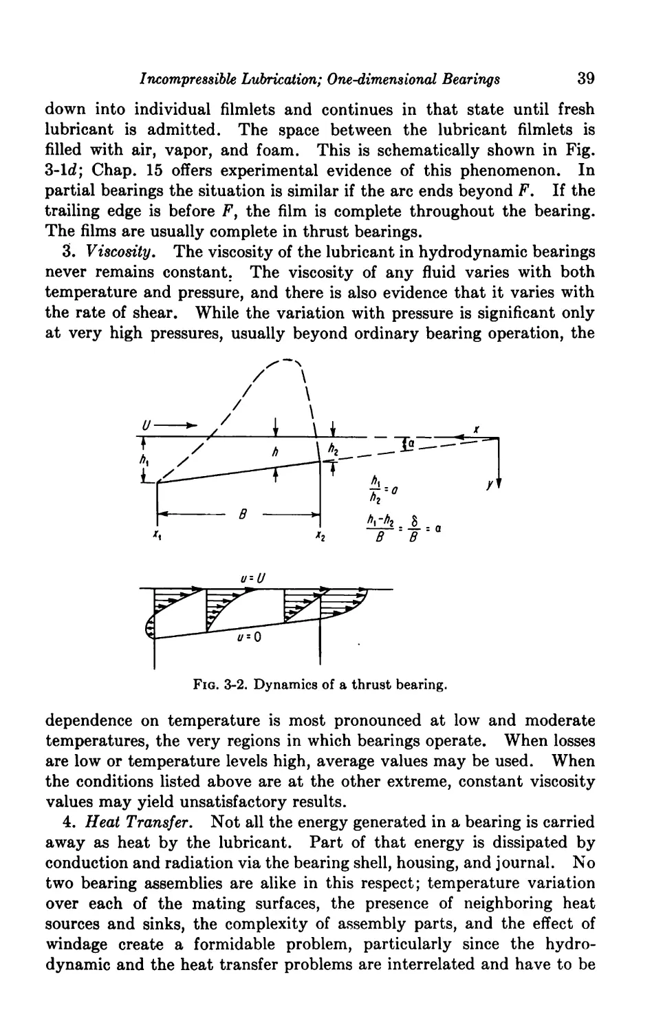
Figure 3-1 shows a journal bearing operating with an external load W
and speed (7. Under the physical conditions imposed, the journal will
run at some eccentricity e, the region below the line of centers 00' form¬
ing a converging and the region above 00' a diverging space. From A
to D the lubricant is being pumped by the journal into an ever-decreasing
space with the result of building up high pressures in the fluid. The
eccentricity e and the magnitude and distribution of these pressures will
be such as to yield a resultant force equal and vectorially opposite to W.
In the process the fluid is being continuously squeezed out the ends of
the bearing, and this side leakage, plus any conduction and radiation
that may exist, carries away the heat generated by the rotating journal.
New lubricant is being delivered at point B to replenish the amount lost
by side leakage. The hydrodynamics of thrust bearings are essentially
represented by Fig. 3-2.
Available bearing solutions even in their elementary form satisfy the
basic requirements of continuity and momentum and express the per¬
formance of bearings as a function of load, speed, viscosity, and bearing
dimensions. However, there are other significant features which are often
disregarded either because of incomplete knowledge or because of mathe¬
matical difficulties. Together with the basic theory they constitute the
physical reality of journal and thrust bearings. These features are:
37

38
Theory of Hydrodynamic Lubrication
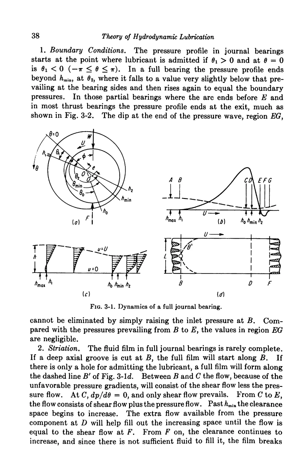
1.	Boundary Conditions. The pressure profile in journal bearings
starts at the point where lubricant is admitted if 0i > 0 and at 0 = 0
is 0i < 0 ( —ir < 0 < ir). In a full bearing the pressure profile ends
beyond hmiD, at 02, where it falls to a value very slightly below that pre¬
vailing at the bearing sides and then rises again to equal the boundary
pressures. In those partial bearings where the arc ends before E and
in most thrust bearings the pressure profile ends at the exit, much as
shown in Fig. 3-2. The dip at the end of the pressure wave, region EG}
Fig. 3-1. Dynamics of a full journal bearing.
cannot be eliminated by simply raising the inlet pressure at B. Com¬
pared with the pressures prevailing from B to E, the values in region EG
are negligible.
2.	Striation. The fluid film in full journal bearings is rarely complete.
If a deep axial groove is cut at B, the full film will start along B. If
there is only a hole for admitting the lubricant, a full film will form along
the dashed line B' of Fig. 3-Id. Between B and C the flow, because of the
unfavorable pressure gradients, will consist of the shear flow less the pres¬
sure flow. At C, dp/dd = 0, and only shear flow prevails. From C to E,
the flow consists of shear flow plus the pressure flow. Past hmin the clearance
space begins to increase. The extra flow available from the pressure
component at D will help fill out the increasing space until the flow is
equal to the shear flow at F. From F on, the clearance continues to
increase, and since there is not sufficient fluid to fill it, the film breaks

Incompressible Lubrication; One-dimensional Bearings	39
down into individual filmlets and continues in that state until fresh
lubricant is admitted. The space between the lubricant filmlets is
filled with air, vapor, and foam. This is schematically shown in Fig.
3-1 d; Chap. 15 offers experimental evidence of this phenomenon. In
partial bearings the situation is similar if the arc ends beyond F. If the
trailing edge is before F, the film is complete throughout the bearing.
The films are usually complete in thrust bearings.
3.	Viscosity. The viscosity of the lubricant in hydrodynamic bearings
never remains constant. The viscosity of any fluid varies with both
temperature and pressure, and there is also evidence that it varies with
the rate of shear. While the variation with pressure is significant only
at very high pressures, usually beyond ordinary bearing operation, the
u~-U
Fig. 3-2. Dynamics of a thrust bearing.
dependence on temperature is most pronounced at low and moderate
temperatures, the very regions in which bearings operate. When losses
are low or temperature levels high, average values may be used. When
the conditions listed above are at the other extreme, constant viscosity
values may yield unsatisfactory results.
4.	Heat Transfer. Not all the energy generated in a bearing is carried
away as heat by the lubricant. Part of that energy is dissipated by
conduction and radiation via the bearing shell, housing, and journal. No
two bearing assemblies are alike in this respect; temperature variation
over each of the mating surfaces, the presence of neighboring heat
sources and sinks, the complexity of assembly parts, and the effect of
windage create a formidable problem, particularly since the hydro-
dynamic and the heat transfer problems are interrelated and have to be

40
Theory of Hydrodynamic Lubrication
treated simultaneously. Usually, the smaller the bearing and the lower
the shear losses the higher the percentage heat lost to the surroundings.
5.	End Effects. This subject is still unexplored, but a multitude of
experimental data on lubricant flow which refuse to conform to theoretical
predictions can be explained only by the effects to be mentioned. These
include phenomena such as surface tension at the sides of the bearing,
the formation of a meniscus, and the sealing effect that such a meniscus
has on the free flow of lubricant out of a bearing. This sealing mecha¬
nism causes the lubricant to flow backward along the sides of the bearing,
i.e., in a direction opposite to journal rotation, and to reenter the bearing
in the low-pressure region to be recirculated. Another phenomenon is
the possible formation of a vena contracta around the annular outlet.
These and perhaps other effects make the side leakage usually less than
that predicted from theory.
The points listed above are all major and general phenomena associ¬
ated with hydrodynamic bearings using incompressible fluids. Some
points that assume significance only in certain ranges of operation are:
a. Elastic Deformation. Under heavy loading and depending on its
structure and assembly, the bearing surface will deform. This in effect
will produce a different film shape with a drastic change in bearing
performance.
b. Turbulence. The Reynolds equation is based on the assumption of
laminar flow. High linear speeds, large clearances, and low viscosities
will cause turbulence with a resulting rise in power loss, a drop in lubri¬
cant flow, and a shift in the locus of shaft center.
c. Thermal Expansion. When bearings undergo appreciable tempera¬
ture changes, when journal and bearing materials have radically different
coefficients of thermal expansion, or when journal and bearing are forced
to expand against each other, the clearances will not retain their original
shape and dimension, and the performance of the bearing will be affected.
d. Surface Roughness. When bearings are operated at very low values
of hmin, the inherent surface roughness of all materials may have an effect,
since the roughness may be of the same order of magnitude as the mini¬
mum clearance. This may not only change the shape of the oil film but
carry the operation into a mixed boundary region where the require¬
ments of hydrodynamic lubrication are no more than partially fulfilled.
e. Unbalance. Most journals will have some residual unbalance.
With unbalance the journal center is not confined to a point but moves
along some locus. Thus, the steady state is replaced by dynamic
conditions.
/. Misalignment. Slight amounts of misalignment are inherent in all
journal bearing assemblies. When the degree of misalignment becomes
excessive, it is necessary to take this effect into consideration.

Incompressible Lubrication; One-dimensional Bearings	41
Very minor items which do not affect bearing operation to any notice¬
able degree but of which one should be aware are the variation of specific
heat with temperature and pressure and the presence of air, foam, and
foreign particles in the lubricant.
In the solutions of this chapter, none of the points mentioned above is
considered. In fact, all these ramifications are minor compared with the
radical and from a practical standpoint impossible assumption of a one¬
dimensional bearing, a bearing infinitely long or infinitely short. These
solutions, however, are useful for a number of reasons. In the first place,
they are given mostly in analytical form with all the inherent advantage
over numerical results, of which the bulk of exact solutions consists.
Oftentimes they are the only available solutions, a useful guide to how a
bearing would possibly perform under certain conditions, and they do
provide upper or lower limits. Although the quantitative answers are
often at variance with experimental results, they do nevertheless provide
a means of studying trends and relationships.
ONE-DIMENSIONAL JOURNAL BEARINGS
If we assume the bearing to be infinitely long in the axial direction, this
implies no variation of pressure in the z direction, or dp/dz = 0. Equa¬
tion (1-12) then becomes
(3-1)
dx \p dx)	dx
If the flow due to the pressure
gradients in the x direction can be
neglected (while retaining the com¬
ponent due to shear)—a situation
approached by very narrow bear¬
ings—then the term
£C-‘2)-°
and Eq. (1-12) becomes
dz\p dz )	dx
(3-2)
It should be noted that this last equation is still a function of two vari¬
ables and that it is a less radical simplification than Eq. (3-1).
The above equations are fully defined except for h. While the film
thickness in thrust bearings can assume different expressions, its form
for an aligned journal bearing is universal. Referring to Fig. 3-3, we
have

42	Theory	of	Hydrodynamic	Lubrication
OB _ R _ R _ e
sin 0	sin (7r — 0) sin 0	sin a
P = 0- a = 6- sin-1 sin 0^
OS =	^	sin	|^0	—	sin-1	^	sin	0^j	=	R2	—	e2	sin2	0	—	e	cos	0
h = (S + C) - OB
= C + e cos 0 + R — \/#2 — sin2 0 « C + e cos 0
or	h = C(1 «+• e cos 0)	(3-3)
3-1. Infinitely Long Bearing. The earliest solution of the infinitely
long full journal bearing is due to Sommerfeld, who by use of an adroit
substitution succeeded in integrating Eq. (3-1). When x is replaced
by the angular coordinate 0, that is, when x = Rd, and it is remembered
that n is constant, Eq. (3-1) becomes
WR%	(3-4)
de\ de)
By integrating once with respect to 0
dp
de ~
6 nURh
+ Ci
h3
II
^3 1^3
0, so Ci
II
1^3
6 nURh
— ho
h3
At some h = ho,
Ann	h 	 2i	-
(3-5)
where h is given by Eq. (3-3) and ho is still to be determined. From
Eq. (3-5) the pressure is given by
_ 6nUR	\ f dd	h0	f	d$ 1	r
P C2	Li (1	+ e cos 6)1	C J	(1 + « cos 0)3J	+ 2
To integrate the above, let
1 *>
11	n	1	—
1 -f € cos 0 = ,
1 — c cos ^
...	.	COS	\p	—	€
from which	cos	0	—
1 — e cos
By using sin2 0 + cos2 0 = 1, we have
(1 — t2)Yi sin \j/
sin 0 =
1 — c cos \J/
and by differentiating one of the terms above
(l-€2)^#

Incompressible Lubrication; One-dimensional Bearings
43
The boundaries 0 = 0 and 0 = transform into the same boundaries
in the ^ coordinate, and thus the boundary conditions are
p — pa at \f/ = 0
p( 0) = p(2t)
(3-6)
By evaluating the integrals resulting from the above substitutions, we
have
/
de
(i +1 cos ey
_ r n -1 cos a» a -€%«
J V 1 - €2 J 1 — 6 CO" *#‘
and
Thus
/
d0
€ COS ^
d\p
= (1 _V)W (* - 2t sin^ + e-J +J8in2^
_ /* /1 — € COS A2 *
(1 + € COS 0)2 “ J V l - €2	/
(1 - w*
ho
= n~ 4 sin
®(a) =
C2 [ (1 - «2)*	C(1
h 0 _
- «2)« V
2e sin \p
c2 sin 2^ j
4- C 2
By using the first boundary condition
of Eq. (3-6), we have
C2= pa
By using the second, we get
2C(1 - €2)
ho —
2 + €2
(3-7)
and thus the expression for the pres¬
sure distribution becomes, by revert¬
ing to the original coordinate,
P = Pa +
6pURe (2-f« cos 0) sin 0
C2 (2 + €2)(l + 6COS0)2
(3-8)
Fig. 3-4. Pressure distribution in¬
cluding negative regions.
where pa is the pressure at 0 = 0. This can be evaluated from the condi¬
tions at B, where a given inlet pressure pi corresponds to a given angle 0i.
If the inlet hole is at 0i = 0, then of course pa is the value of inlet pressure.
Equation (3-8) yields regions of high negative pressures such as shown
in Fig. 3-4. The magnitude of these negative pressures will depend
both on the position of 0i and on the magnitude of p\. In any case, the

44	Theory	of	Hydrodynamic	Lubrication
pressure distribution resulting from Eq. (3-8) is always antisymmetrical
about 0 — t and p = pa.	- "• {
The vertical load component is/by integrating the pressure over the
bearing surface given by
W sin <*. = jf" LR de p sin 6
By integration by parts,
W sin <f> = LR £ — p cos 6	—	j	^ cos 0 dd j
and, by using from Eq. (3-5), we have
dd
cos 6^d$
du
. J 6^LUR2[h0 f2' cos 9 de	f2
wsm* = —c^[c]0 (i + (cosey ~ Jo
2r cos 6 dd
(1 + C cos 0)2J
These can be reduced to the same integrals used in evaluating the pressure
distribution by writing
cos Q _	1/c	  1	/€
(1 4- c cos 0)z	(1	+ € cos 0)2	(1	+ c cos 0)3
,	_	cos	0	_	1/c	1/c
an	(1	4~	c	cos	0)2	(1	+ « cos 0)2	1	4" c cos 0
Thus
-«») f2r ^
C2 \ 24- €2 > (1 4- € cos 0)3
d0
: COS 0 |
w ^	6nULR* (2(1 - c2) f2*	dd
W sm <f> = —	j	v	'	1
_ f 2(1 — t2)	]	[*	de	[»	dfl
L 2 + «* J Jo (i + * cos ey Jo i +1<
The only new integral to appear is the last one, and its value is
de _ i
/
1 4- € cos 0	y/\	—	e2
By following the same procedure used for evaluating the pressures, we
obtain
1V sin	6	-	(3	„x
w sin	<t>	~	(2-|-	e2)(i	_ t2)W	^
To find	the	attitude angle,	we	must	look	for	the load component at
right angles to	W sin	<t>, or
W cos <j> = j^'LRde p cos 0

Incompressible Lubrication; One-dimensional Bearings	45
Upon integration by parts,
W cos <t> = LR sin 0	— j sin 6 ~ dd j = — LR sin 6 ^ dd
By use once again of the Sommerfeld substitutions,
^ GpULR*\ ho (	#	c2	. , A .	1	.1 I2'
W COS <t> = Ci	i)	(cos	j, - 2- Sill2 + J— COS |o
and	W	cos <f> = 0
or, since W ^ 0,	<f>	=	^	(3-10)
and the displacement of the shaft is always at right angles to W sin <f>.
Moreover, since there is no load component at right angles to W sin 4>,
W sin <f> = W is the total resultant load. This unrealistic result is a
consequence of including the negative pressures in the integration for
load capacity. Thus we can rewrite Eq. (3-9) as
_pN/R\_
p Vcj "
(2 + e2)(l - t2)»	.
12rt	W'11)
and the Sommerfeld number is seen to be a function of c only.
The shear stress at the journal is, from Eq. (l-16a), given by
—	.	h	dp
Tx ~ h + 2R d§
and the frictional force on the journal is
de
Fj = j*’r,LR de = -LR J*' j-
+ € COS d
M /02'( 1 + ec°s e^de\
By using for the integrals the expressions derived above
F - i tt # 4x(l + 2c2)
Fj pLL c (2 + €2)(1 _ e2jW
The friction factor defined as / = F/W is then
f-h-9. I + 2i!	(3-13)
W ~ R 3f	W)
At the bearing surface, by Eq. (l-15a),

46
Theory of Hydrodynamic Lubrication
The difference in the journal and bearing torques is balanced by the
external load IT, which exerts a moment through its eccentricity e or
RFj = RFb + We
(3-14)
The friction in a concentric journal bearing when e = dp/dO = 0 is often
referred to as Petroff’s equation and is given simply from Eq. (3-12) by
2 thULR/C,
The foregoing analysis yields quantitative results that are far afield
from any actual bearing performance. They are also qualitatively in
error; for, as mentioned previously, negative pressures of the same order
as the positive pressures could not possibly be maintained and the locus
of shaft center is never a straight horizon¬
tal line.
The major shortcomings of the foregoing
analysis can be eliminated by imposing a
more realistic boundary condition at the
trailing end of the pressure wave. These
boundary conditions are discussed in
greater detail in Chap. 4. Suffice it to
say here that no negative pressures are
allowed and the requirement is imposed that, at the point where the pres¬
sure wave falls to zero, line E, the pressure gradient too becomes zero, as
shown in Fig. 3-5. Thus the boundary conditions imposed are:
vq CTmin
Fig. 3-5. Pressure distribution ex
eluding negative regions.
p = 0
dp _
dd ~
p = 0
= 0
at 6 = 0
at d = d2
at 6 — d2
(3-15)
Since Eq. (3-1) is a second-order differential equation, it cannot in
general satisfy more than two boundary conditions. It will be shown,
however, that the last two conditions of Eq. (3-15) are a special case of a
more general single condition and that the solution based on Eq. (3-15)
is only one of a family of possible solutions. Let the last two boundary
conditions at 02 be written as the single condition
D =
P kd9
then, by integrating the Reynolds equation, we obtain
QnUR[ f9 dd , „ f9 dd
• V =
Writing
C2
—-7^—3T2 + Ci je> , r.i-	+	Ci
[	(1	+	4	cos	9)
-/: *
(1 + € cos 6)n
(i + € cos ey
  i_
1 + € COS 02

Incompressible Lubrication; One-dimensional Bearings	47
the constants C1 and C2 are evaluated by using p = 0 at 0i and
P = fcgf atfl2
n	h + kg2	n _uglh-9ih
tl ~	h + kg*	°2	k h + kg*
The expressions for p and dp/de then become
6mI/K
P C2
f* de _ It + kg* [•
Je, (1 + < cos BY h + kga Je,
de
(1 + € cos 6
9*1.
dp	1		 /2 "h kg
d0 C2 [(* + € cos 0)2	^3 + kg3 (1 + e cos 0)3J
Since e < 1, 7n > 0, and g > 0, the denominators never vanish. Thus
the conditions for p = 0 and dp/dd = 0 at 0 = 02 are for p = 0
k(g2h - gzI2) =0 or %2(/3 - ^/2) = 0
for5? = 0
0(/2 + kg2) = /3 + kg3	or /3 - fif/2
It follows then that, to have p = 0, we need either
k = 0
d0
or
/**« d0	/'®I
/	/i _i_	—zr2	= (1 + * cos 02) /
Jet (1 + € cos 0)2	J9l
(1 + c cos 0)3
Thus if the later condition holds, both p and dp/dd are zero for any value
of k including k = 0, which corresponds to our particular boundary
conditions.
By again employing Sommerfeld’s substitutions and using the first two
boundary conditions of Eq. (3-15), we obtain for the pressure distribution
6 nUR	I,	.	(2 + «2)^ — 4e sin \J/ -J- e2 sin $ cos yp ]
P = C*( 1 - «»)* T " *	*	2[1	+	e	COS	{h	-	r)\	)
(3-16)
where cos ^ = € + cos 0^ an^ ^ corresponds to 02. By using the last
1 *i € COS tt
condition, namely, p = 0 at ^ = ^2, we obtain from Eq. (3-16)
€[sin (^2 — t) cos — x) — ^2] + 2[^2 cos (^2 — x)
- sin (*2 - tt)] = 0	(3-17)
which determines ^2 and thus 02. Equation (3-16) with ^2 determined by
Eq. (3-17) gives a pressure profile satisfying all the conditions of Eq. (3-15).

48
Theory of Hydrodynamic Lubrication
For the two load components, by writing ^ = ^2 —
a.,,,
(1 - «2)(1 + t COS^'j)
W sin <b = WW/WW* cos # ~ sin #)	.	.
►V sin </>	(1	_	+	{	cog	(6 19)
3nUL(R/cr r ««(i + cos
(1 - «2)*(1 + t cos f'2) [	1	- e2
+ 4(^2 cos i/'i — sin ^2)21	(3-20)
2(1 — <2)^(sin ^2 — *p2 cos ^2)
«(1 + cos
i.„„ ^	c	r	vam	^2	Y2	WO	Y2J	/o m\
tan <f> —	.//\2	 (3_21)
(«)/=^± + _^!s_	(322)
The use of conditions (3-15) resulted in the elimination of the region of
negative pressures and the derivation of a journal locus, Eq. (3-21),
which conforms with experimental evidence. Numerical results of Eqs.
(3-20) to (3-^2) are given in Table 4-1, where they are tabulated together
with the solutions of finite bearings.
3-2. Infinitely Short Bearing. Equation (3-2) has been written down
as applying to infinitely narrow bearings. Since for aligned journals
h = f(x) alone, we can integrate this equation by treating h as a constant.
Thus
QnUdh z2
h3 dx 2
_ uflu an z- r r
V = TT + C'z + C*
By using the boundary conditions p = 0 at +L/2
**•■> - W- (t - *■) ir-r^'w <3-23>
This pressure distribution is parabolic in z and antisymmetrical about
6 — nr and p = 0; that is, the region of negative pressures is identical to
that of positive pressures. Here the problem of negative pressures is
dealt with simply by deleting the region t < 0 < 2tt where the negative
pressures occur. (This, of course, can also be done for the infinitely long
bearing, and results of such an integration are given in Chaps. 7 and 12.)
By summing forces only over the interval 0 < 0 < tt:
c sin 0 cos 0 ,
ad
Wx = —2 f f p cos 0 R d0 dz = —	[	n	,
jo Jo	2c2 jo (i +«cos ey
o [' fL/2	a	T>	Ja	j	nUL*	[*	€	sin2 0
Wy = 2 \	/	p	sin	0	R	dd	dz	  /	y—-	-r-	d0
Jo Jo	2c2	jo (i + € cos ey
By again using the Sommerfeld substitution and integrating,

Incompressible Lubrication; One-dimensional Bearings	49
(3'24a)
W‘ = !^W^W>	(3-246)
The total load capacity is then given by
pUL3	e
4C2 (1 - €2)
^	,t	-	.M	I'**1	-	‘2)	+	16‘2]»	(3-24c)
T (§)’ ’ s (I)’ -	.■)'	+	I6.'jw <«-25>
This last expression is seen to be independent of bearing diameter.
The effect of diameter is felt through the value of Cy which is usually a
function of bearing diameter. The attitude angle is given by
tan 0 = ^	^ ~	(3-26)
Since there is no pressure-induced shear,
_pU
T h
and	F	=	J*' M £ LR de	=	(3-27)
with the friction coefficient given by
— f	—	2t2£	(o og\
CJ	“	(1 - €2)^	(	}
The lubricant flow out the sides of the bearing is, by Eq. (1-136),
f'RVdp
Qz~ Jo 12m dz
d6 = eULC	(3-29)
±L/2
The parameters at the point of maximum pressure are
1 - (1 + 24e2)>*
COS do =
4e
ho = j [5 - (1 + 24*2)»]	(3-30)
_ _3pUL2 c sin 0O	/b oi\
P° 4RC* (1 + t cos fio)3	1	'
This treatment yields a fair approximation to the performance of narrow
bearings at low eccentricities and, by the simplicity and compactness of
its mathematics, constitutes a useful tool in the analysis of lubrication
problems.

50
Theory of Hydrodynamic Lubrication
3-3. Partial Bearings. By definition any bearing having an arc less
than 2t is a partial bearing; in practice, however, the criterion is usually
an arc less than 180°. The analysis of partial bearings, as evident from
Fig. 3-6, is made more difficult by the appearance of two new independent
parameters, the load angle a and the arc span 0. Most available solu¬
tions are similar to the Sommerfeld
solutions for a full bearing and in¬
clude negative pressures. We shall,
however, restrict ourselves to bound¬
ary conditions similar to those of Eq.
(3-15), namely:
V = Pi
dp n
v = Te =0
at 0 = 0i
at 0 = 02
p >	0 in the region 0i < 0 < 02
p =	0 at 0 > 02
Although the methods and the equa¬
tions involved are similar to those of
full bearings,	the	actual	calculations are	laborious and the final expres¬
sions are long	and	cumbersome.	For this	reason, the results will be given
in graphical form.
If in Eq. (3-5) the limits of integration are kept general, then
P = Pi +
6/tiUR
feh- h0
Je, hz
or after performing the integrations in the same manner as before
V = Pi + rf‘
6 pUR
C2(l -62)* {[(1	<2)	c(1 + 2)](*	^
- £e(l - «2) - ^T-°j (sin - sin f,)
- (sin 2^ - sin 2^i)
(3-32)
where \p is the angle from Sommerfeld’s substitution and h0 is to be
evaluated from the boundary conditions at 02. Equation (3-32) was
evaluated by numerical integration for low eccentricities and by the use
of the mathematical expression for high eccentricities. The results are
extracts from families of solutions and represent points of maximum load
capacity, a condition at which all bearings tend to operate. Figures 3-7
and 3-8 present performance of partial bearings with the load vector
located at any arbitrary position with respect to the bearing boundaries

Incompressible Lubrication; One-dimensional Bearings	51
and containing no negative pressures. For a given S and arc length 0
Fig. 3-7 will, if 0 is set equal to 0', determine the optimum load angle a. If
0 > 0', then obviously the load ca-
Numbers along curves indicote
attitude angle <f>
150°
180° >3 = 210°
pacity will be the same, with the arc
0 — 0' only increasing the frictional
losses. The condition 0 = 2a rep¬
resents, of course, the case of cen¬
trally loaded bearings. It should
22 r
0 20 40 60 80 100 120 140160 180 200
Load angle a, deg
Fig. 3-7. Load capacity of partial bear¬
ings.
0 20 40 60 80100 120140160180 200
Load angle a, deg
Fig. 3-8. Friction factor in partial bear¬
ings.
be pointed out that here, as throughout the book, the reference area for
partial bearings is the projected area of an equivalent full bearing, that
is, P = W/LD.
3-4. Fitted Bearings. Fitted or no-
clearance bearings are those whose
diameter equals the diameter of the
journal, as shown in Fig. 3-9. In that
case the clearance is zero and Eq. (3-3)
becomes
h = e cos 0
Fig. 3-9. Notation for fitted bearings.
By rotating the 0 axis by 90° in the di¬
rection of rotation, using h = e sin 0 in
Eq. (3-4), and expressing the constant ho by e sin 0O, we obtain
p(9) =	j^sin	0o	- In tan - 2 cot 0 j + <7,
By using the boundary conditions p(0i) = p(0o) = 0, we obtain for
(3-33)

52	Theory	of	Hydrodynamic	Lubrication
sin 0O and Ci
2(cot fli — cot 02)
Q 	 1/1	  1/	V2J	/Q
Sin 0 cot 0i/sin 0i — cot 02/sin 02 + In [tan (02/2)/tan (0i/2)]
n	3nU R

[8in 00 (s§4l “ln tan I1) "2 cot *i]
The integrations for load capacity performed over the entire bearing arc
yield the following results:
SnULR2 T -Cie2 ,	.	i	•	n	(	n	i	,	02
Wy — 	^	 SjHJR	^C0S	—	cos	2' sm 0 I cos 2	2
— cos 0i ln tan —^ — 2(sin 02 — sin 0i) j (3-35a)
Wx =	(s^n	^2	sin	^0	+	sin	0O	^cot	0i	— cot 02
0 0 \
+ sin 0i ln tan ^ — sin 02 ln tan
+ 2 ^cos 0i — cos 02 + ln tan ~ — ln tan ^ j (3-356)
j^4 ^ln tan |-2 — ln tan ^ + 3 sin 0o(cot 02 — cot 0i) j
e
(3-30)
Table 3-1 relates the various parameters of a fitted bearing with its
performance, under the requirements of maximum load capacity for a
given minimum film thickness. This shifts the position of the load
vector arbitrarily along the bearing surface. The requirements for
Table 3-1. Optimum Conditions in Fitted Bearings
0, deg
30
60
90
120
150
0i
129.1°
92.2°
64.3°
40.7°
19.4°
a
17.5°
35.8°
55.7°
77.7°
101.1°
a/P
0.58
0.596
0.62
0.65
0.674
hi/hmia
2.18
2.14
2.08
2.0
1.804
c/hm\a
2.18
2.14
2.31
3.02
5.43
h{)/hmia
1.4
1.48
1.62
1.84
2.131
0o
150.1°
136.4°
135.2°
142.4°
156.9°
4>
i J
56.6°
38°
30°
28.4°
30.5°
w
uLNIt*
0.00451
0.01685
0.03309
0.04534
0.03924
_ ^min
0.0407
0.0774
0.1073
0.1284
0.1339
uLNR1
At
9.027
4.597
3.242
2.831
0.3413
” min

Incompressible Lubrication; One-dimensional Bearings
53
minimum friction in the bearing are very close to those of Table 3-1. It
should be noted that in fitted bearings the minimum film thickness is
always at the outlet end.
3-5. Floating-ring Bearings. This
kind of bearing has a thin ring float¬
ing freely between journal and bear¬
ing as shown in Fig. 3-10. The pur¬
pose of the ring is to reduce the shear
losses by decreasing the relative speed
between the mating surfaces. Since
the losses vary as the square of the
speed but vary only linearly with
area, the rotation of the ring will
always result in some reduction in
drag, if all other parameters remain
unaffected.
It is clear that for equilibrium the
sum of the two moments M i and M 2
acting on the floating ring must be zero. The expression for the drag
is given by Eq. (3-12), which will be rewritten for our purposes in the
following manner:
Fig. 3-10. Floating-ring bearing.
nULR 4x(l + 2e2)
C (2 + «2)(1 —
4tvLRU [	2
C [(l-€2)“
2t nULR .
(2 + €2)(1 - €2)*J
(yjruLUe2
Cy/T=7* ^C(2 + e2)(l -e2)»
By multiplying and dividing the last term by (R/C)( 1/e) and recalling
the expression for W sin <t> given by Eq. (3-9), we have
„	2TpULR	.	cC	w	.
* ~	C(1 - t2)»	+	2R	n *
By a similar procedure the drag on a bearing is
„	2rgXJLR	eC	lir	.
6 “	C( 1 - £2)*	2R	Sln
We thus have for the two moments
(3-37)
M, = -
^^L(RXN - R2Nr)
Cl( 1 - €!2)*
4ir2nRzzLN R
^sin + Wi

54	Theory	of	Hydrodynamic	Lubrication
Since R\N — R2Nr « R2(N — Nr) and by writing W = 2LR2P and
€ = cos 6, we have by equating Mi to M2
„ _ . 1	- <.2)»	v
^ - 1 + C2fl23(l - ‘22)k
+ P[C2t2(1 “ <s2)W + Cltl(1 -
It is shown in Chap. 1 that the behavior of a unidirectionally loaded
bearing in which both journal and bearing rotate in the same direction
is the same as though the journal alone were to rotate at a speed equal
to the sum of the journal and bearing speeds. Thus, according to
Eq. (3-11)
_ fRi\*n(NR + N) _ (2 + €l’).(l - €1*)K
P	12t26i
s2 =	-(2+€22)(i -ef,)*
12t262
By using these relations to eliminate P in the expression for N, we have
for the speed of the ring
and for the relation between the two eccentricities
- 3*i [e,(l - c,*)» + £-2 «2(1 - <2*)» j (3-39)
The total power loss for a floating-ring bearing is
" - [m; w”n*• *cfift)*<-u-v*\u <3-"»
Figure 3-11 shows graphically the relation between the various ratios
of clearance, radius, and speed.
If one considers an equivalent standard bearing, denoted by subscript e,
as having the dimensions
Ne = N (\ = Cl Re = Ri = R
then by using the more critical outer film as a basis for comparison, it
results that the floating ring has a lower load capacity if Se/S2 > 1
and a higher capacity if Se/S2 < 1. The power losses are always less
in the floating-ring bearing.
3-6. Porous Bearings. In a bearing made of a porous material, lubri¬
cant flows out of the bearing surface with a certain velocity VQ. If

Incompressible Lubrication; One-dimensional Bearings
qy is the rate of flow per unit area, then
oo
dp
q«=-Ty
- = V0
v-o M
where dp/dy is the pressure gradient at the bearing surface and $ is a
property called permeability which varies with porosity and size of pores.
Its dimensions are square inches.
From the requirements of continuity
we have for the porous matrix
Vq = * V‘p = 0
so that., since ^ 0,	”o	0.2	0.4	06	0.8	1.0	1.2	1.4 1.6 1.8 2.0
y2p = q	Rotio	°f	cleoronces,	Ct/Ct
The problem then is to solve Reyn-	J'10-.3'1Var‘atiof.of	rin« 8Peed with
r	,	.	bearing characteristics,
olds equation for the pressures m
the oil film simultaneously with that	of Laplace for the porous	matrix
with a common dp/dy at the boundary, or
*(»%)+* (V^\ = wdh 2*0j> I	(3-41)
dx\v dx/ dz\u dz)	dx	m	dy	|y=o
d2p d2p	d*p	_
3x2 ^ dy2	dz2
Two assumptions are made in solving this set of equations:
1. The bearing is infinitely short.
2. dp/dy is linear across the matrix and is zero at the outer surface of
the porous bearing shell.
Assumption 1 yields d2p/dx2 = 0; assumption 2 gives
d2p
dy2
Hence from Laplace’s equation
= const = K
d2p _
dz2
= -K
and
dp
dy
KH = -£?l
dz2
H
y = 0	OZ	|y-0
where H is the wall thickness of the porous bearing. By using this
expression in Eq. (3-41) with ^ ^	=	0,	we	have
(A. +
or
d2p _
dz2
6m U
e sin Q
RC2 (1 + € cos ey + 12$>H/C
r-TTii (8-42)

56
Theory of Hydrodynamic Lubrication
Equation (3-42) solved and integrated for the resultant load along the
line of centers yields
W§ =M^V11±_*
2C2 ^ 6A.2
111
[fc2 -
fc(l
fc2 - k( 1 + €) + (1 + «2)]
*) + (!- <)2	(1	+	*:	+ «)* J
(! + *-«)
+	(tan-	-	‘I	-	tan-	P-^	-	-UP
th? y/'& ( L fcV3 V3j	L	*:V3	vUJ/
(3-43)
where k* = V2’t>H/C3.
Figure 3-12 gives a comparison of the relative load capacities of porous
Fig. 3-12. Load capacity of porous Fig. 3-13. Friction factor for porous
bearings.	bearings.
and solid bearings both based on the short-bearing approximation. The
coefficient of friction as given by
-/ =
n j
2ir2<S
1
+ o sin
CJ ' H -s/l - e ' 2
is plotted in Fig. 3-13 as a function of il, the relative load capacity of the
porous and solid bearings.
ONE-DIMENSIONAL THRUST BEARINGS
The analysis of thrust bearings is made somewhat easier by the simplic¬
ity of the expressions for film thickness and by the less complicated bound¬
ary conditions. In most thrust bearings the film is nondiverging and
continuous and the problem of negative pressures does not arise. The

Incompressible Lubrication; One-dimensional Bearings
57
pressures at both the inlet and outlet edges are simple boundary values,
usually atmospheric. In fact, it can be shown that the elaborate con¬
dition p = dp/dx = 0 at the outlet cannot be satisfied for bearings
having a converging film shape. A number of these one-dimensional
thrust bearing solutions were obtained by Lord Rayleigh, who also derived
parameters for optimum film shape and bearing proportion. The
quantitative results here are no closer to reality than in the case of
journal bearings, but, again, many of the dimensionless groups and much
of the qualitative behavior deduced
from one-dimensional analyses are
also valid on the basis of more exact
solutions.
In reality a thrust bearing, which
is designed to support axial instead of
radial loads, looks like the device of
Fig. 3-14. The popular simplifica¬
tion is to treat the sectorial segments of which such bearings consist as a
simple plane slider as shown in Fig. 3-2. By using the system of coordi¬
nates given in Fig. 3-2, where U is negative with respect to x, Eq.
(3-1) reads
6S|
Fig. 3-14. Thrust bearing.
<£ = -wh-
ax
— ho
h3
From this
with	p(hi)	= p(h2) = 0
Integration of the expression for load capacity by parts yields
W-L^pto-L („ i;; - /;
o, w-toVL(J*’-£
The center of pressure 1 can be obtained from
The expression for shear stress is, from Eq. (l-16a),
nU , h dp
h 2 dx
(3-44)
(3-45)
(3-46)
■dx
(3-47)

58	Theory	of	Hydrodynamic	Lubrication
and by using the expression for dp/dx from above, we have
, 4h — Sho
h2
'■-'“(‘/Tt -“•£'!)	(3-48)
By using these general equations, a number of solutions for bearings
having different film shapes can be obtained.
3-7. Plane Sliders. This bearing configuration is shown in Fig. 3-2,
and its film thickness is given by
,	h2{a	—	1)
h = ax = ——~	  x
Jt>
(3-49)
where a = h\/h2. By integrating between X\ = hi/a and x2 = h2/af
0.20
0.18
Cf
.0.16
Lp
0.14
0.12
0.10
/'
1.0
0.9
0.8.
0.7
0.6
0.5
1 1.5 2 2.5 3 3.5 4 4.5 5 5.5
a - hjht
Fig. 3-15. Load capacity and friction in plane sliders.
we have for the pressure distribution
V =
_ 6fiU (hi — ax)(ax — h2)
(hi + h2)x2
h-l > x> -2
and for the parameters of maximum pressure
t   2hih2   2d t
0 ” hi + h2 ~ T+~a k2
3nUa(a - l)2
2aa
Integration of Eqs. (3-46) to (3-48) yields
V o =
^ - tt1’ (rh)' ['” * - 2-r^r] - ~cPc'
(^)B(a2 — 1 — 2a ln a)
(a2 — 1) ln a — 2(a — l)2
=	2(a2 - 1) ln a - 3(a - l)2
ixUBL
(3-50)
(3-51)
(3-52)
(3-53)
(3-54)
(3-55)
B 3(a + 1) ln a — 6(a — 1) h2
The dimensionless coefficients Cp and Cf as a function of a are plotted
in Fig. 3-15.

Incompressible Lubrication; One-dimensional Bearings	59
By setting in Eq. (3-53) dW/da = 0, the value of a for maximum load
capacity is obtained, and its value is5 a = 2.2. This is also evidenced
from Fig. 3-15. Based on a = 2.2, the values of the other quantities are
W = 0.1602	ho = 1.37hi F = 4.7 ^
h>2	Jo
If the bearing is made up of a series of tapered-land segments, each
segment being equal to B/n, while the total breadth is B, then
which means that the bearing load capacity is (1/n) times smaller than
that of an equivalent unbroken surface. This, of course, assumes that
the taper over each segment B/n is equal to a.
3-8. Curved Sliders. If h = mxni then the value for the resultant
load is
_	6pULB* I"(3n - 1 )(a-2+1'" - 1 )(a-3+2'" - 1)	a~2+2'" - I]
V(a1/n - l)2 L (2n - l)(a“*+l'")(3n - 2)	2(n - 1) J
(3-57)
By setting n = 2, that is, by using a parabolic surface and calculating
its load capacity for the optimum value of a, which is 2.3, we have
W = 0.163
If the film thickness is expressed exponentially, h = e?x, then by perform¬
ing the rather easy integration, we obtain
t\r _ 3uUL Ta2 — 1	/3(a2	—	a3)B~\
(0ah2)2 [	6	■*" a3 - 1 J
or since = ln a,
<->
For an a = 2.3, W assumes a maximum value of
W = 0.165
h 2
The similarity between the load capacity for all these various bearings
underlines the important fact that, once hi and h2 are fixed, the exact
shape of the oil film is not of great importance. This conclusion is
reached on the basis of two-dimensional analysis also.

60
Theory of Hydrodynamic Lubrication
3-9. Step Bearings. If in Eq. (3-1) we set h = const and consider
isothermal conditions, the resultant pressures are zero; thus a bearing
having a constant film thickness has no load capacity. However, if the
film is parallel but has a step in it such as shown in Fig. 3-16, the bearing
will develop hydrodynamic forces. The expressions for the film thick¬
ness here are
By evaluating this expression for region Bi with the coordinate system
Fig. 3-16. Step slider,
as shown in Fig. 3-16 we have
p = 0 for x — 0 V — Vo for x = Bi
where pe is the common pressure at the step. The two conditions yield
Similarly, for region B2 with the coordinates shifted to the leading edge,
we have
h = hi in region Bi h = h2 in region B2
By integrating Eq. (3-1) for a constant h, we obtain
p = &pU^^x + Ci
B
Ci = 0 pc = 6pU^~^Bi
C» = 0
Since pc is the same in both cases, we have
or
(3-59)

Incompressible Lubrication; One-dimensional Bearings	61
and the pressure profile is
h2(Bih2* -j- B2hi*)
P(I) " Ti?-
/ \	6pU
P(I) - T?
1	B,A,»	+	S2/n8
hi{Bih2* -f- B2hi*)
B1A2* -I- B2hi*
- 1
x	for region £1	(3-60a)
x	for region £2	(3-606)
which reduces to zero if hi — h2 or if B1 or £2 = 0. It is apparent from
Eq. (3-1) by setting h equal to hi or h2 that the pressure gradient is dis¬
continuous at the step.
The load capacity is
„ = wt + w. =	[*'xdx	+	W(h>-h2)L f*>xdx
hi*	Jo	h2*	Jo
w	3pULBiB2B(hi — h2)	(	.
w	B557(3'61)
By writing £1 = £ — £2 and a = hi/h2j Eq. (3-61) can be rewritten
_ 3pULBB2(B - B2)(a - 1)
(Bja* + B — B2)h2i
To find the optimum B2 and a we set
dW n	,	dW	n
aF2 = 0	and	3a
The first relation yields
dW _ 3pULB(a — 1)
dB2	W
[*(£20* +	B -	£2)(£ - 2£2) - £2(£ - £2)(a3 - I)]	_	n
L	(£2^ + £- £2)3	J	"	U
and, to satisfy this,
£2 - 2££2 + B22 _ /£ — £2V
V )
£22
or	£	=	£2(a*	+ 1)
The second relation yields
dIF _ 3pULBB2(B - £2) I"£2a3 + £ - £2 - (a - l)3£2a2]
da	W	[	(£*a* + £ - £2)2	J
which yields
£ =	B
2	2a3	-	3a2	+	1

62	Theory	of	Hydrodynamic	Lubrication
By using the expression for B from above,
B2 =
£2(a* + 1)
or
2a3 - 3a2 + 1
(a - l)(4a2 - 8a + 1) = 0
One root is a = 1 and the other one is
a = 1 + V% = 1-866
The optimum value of B\/Bi is then
§! = o2(2a - 3) = 2.549
r>2
With these optimum parameters, the performance of the step bearing is
w 0.2052Mt/L£2
h2*
B
= 0.4262
/ = 4.091 ^
It can be shown by the use of calcu¬
lus of variation that a stepped film is
the optimum film shape for a slider
bearing. This is true also for the
more general case when the viscosity
of the lubricant is considered to be a
function of pressure.
3-10. Composite Bearings. The bearing termed “composite” is
made up of a combination of tapered- and flat-land bearings, as shown in
Fig. 3-17. Its film function is
h = ax for region B\
Fig. 3-17. Composite slider.
h = h2 for region B2
For region B2i taking the exit edge as the origin, we have for boundary
conditions
p = 0 at x = 0 p = pc at x = B2
with the common pressure pe given by
Pc = 6/i t/f? 2
For Bi, writing a in terms of the taper hi — h2f
>	hi	—	h2

Incompressible Lubrication; One-dimensional Bearings	63
and by rewriting the expression p = f(x) into p = }{h)
dp _ dp dh _ h\ — h2 dp
dx dhdx Bi dh
we have	dp_^UBl(ha	1\
dh	hi_htyh3 h,j
and upon integration
„ru\ SpUBifl h0\ n
rW = h^h2{h-2h*) + C2
The boundary conditions for this equation are:
p	=	p< =	6hUB2	at	A =	A2
hi
p	=	0	at	h =	hi
By using these two conditions, we obtain
p = 6»U |b2 (^-t	-	^	^	-	2^-^	j	J
(3-62)
i.	_	2hih2(Bihi + B2hi)
0	(A,	+ A2)[B,A2 + 2B2A,V(Ai + A*)]	(	)
It should be noted that the expression for pc is a function of the local h
alone, and thus p will be continuous at the boundary.
The total load is given by
■dh
ri2
fB*	fhl	B	i
W = / Lpdx — / Lp
yo	fti — a2
_ 6Ml/LB!2 (B2 /B2	\ /A + 1	1	A + 1\
A2* (B,VBi	/Vfc + 2	2 7* + 2/
-rh + i[^-m]| <"*>
where k = ^-=A2	7	=	r>7	^/B')kik	+	D
2(Bi/Bi)(k+ 1)2+ (k + 2)
With, --.</($-1)
[(& - k) {; •"+j; (3 w - c) H
l'“i2i:[3<,-’>rT5-2]-<h'
_,[M-
A: + 2
+ 1) 6_
A* —|— 2
(3-65)

64
Theory of Hydrodynamic Lubrication
If in the equation for ho we set B2 equal to zero, the expression reduces
to that of an ordinary plane slider. With B2 > 0 the value of ho is less
than for tapered-land bearings, which means that the point of maximum
pressure has shifted closer to the exit edge. However, since ho > h2
this peak will always remain in the tapered portion of the bearing. The
load capacity of a composite bearing is at an optimum when Bi/B2 = 5,
at which point it will be 25 per cent
higher than for an equivalent ta¬
pered-land bearing. Its losses, how¬
ever, will always be higher, as can
be easily deduced from the longer
span of its minimum film thickness
h2.
3-11. Pivoted-shoe Bearings.
The pivoted-shoe bearing is one
which, instead of being rigidly fixed
with respect to the runner, is sup¬
ported by a pivot and is thus free
to assume any inclination. This it
will do in a manner that will yield
the highest load capacity. The per¬
formance of these bearings can be
calculated from the results obtained
for plane sliders. I n a pivoted-shoe
bearing the resultant force obvi¬
ously has to act through the pivot,
and this pivot position must coin¬
cide with the center of pressure £
derived for the tapered-land bear¬
ing. Each £ is associated with a
certain minimum film thickness h2,
and h2 in turn is related to load ca¬
pacity. Thus, from Eq. (3-54)
[6) Pivot locotion
Fig. 3-18. Performance of pivoted sliders.
(H)#(a2 - 1 - 2a ln a)
(a2 - 1) ln a - 2(a - l)2
For a given pivot position, a can be found from Eq. (3-54) and W from
Eq. (3-53). Since these relationships are implicit in a, the results for
W = /(a,£) are as given in graphical form in Fig. 3-18.
The pressure distribution in plane sliders is always asymmetrical with
respect to B/2. The resultant force will thus always be off center, and
it follows that in order to have any load capacity, the pivot must be
located at £ > B/2 from the inlet edge. It remains, however, a fact of

Incompressible Lubrication; One-dimensional Bearings
65
pivoted-bearing operation, both journal and thrust, that the bearing will
operate satisfactorily with the pivot located in the center. Various
explanations for this behavior may be offered, and some of the explana¬
tions are discussed later in the text. One of the more obvious reasons is
that the surface of the pads is never flat both because of geometrical
imperfections and because of the cantilever effect, which tends to bend
the pad surface into a circular or parabolic shape.
Fig. 3-19. Curved pivoted slider.
In the following analysis it will be seen that a value of £/£ = %
yields load capacities if the pads have some curvature. The equations
are derived for a parabolic pad surface, but it can be shown that, since
the change in elevation, hc of Fig. 3-19, is very small, a parabolic and a
circular arc will yield similar values of hc as a function of x.
By putting the coordinate axis at the leading edge, we can write
he = hc — 4//c(* - y2y
and for the film thickness h
h = hi — x(hi — h2) — hc = h2{b[4:(x — %)2 — 1] + (a — ax + x))
where £ = x/B, b = He/h2, and a = hi/h2.
By substituting h in Eq. (3-1), we get
where the constants of integration can be evaluated from p(0) = p(l) = 0.
The load capacity is given by

66
Theory of Hydrodynamic Lubrication
W = B P pLdx = m^2L Ci.
yo	/i	2
(3-66)
where Cp is a result of numerical integration and is given in Fig. 3-20.
The load in Eq. (3-66) is given in terms of the outlet film h2 which,
0.66
Fig. 3-20. Load capacity of curved
pivoted sliders. (a) Load coefficient
based on minimum film thickness; (b) load
coefficient based on outlet film thickness.
Fig. 3-21. Pivot position for curved
sliders.
however, is usually not the point of minimum film thickness. The latter
can be found from
^ = 8x6 - 46 - a + 1 =0
dx
which yields for the minimum film thickness the following:
- ®_-j m1 h ~h rfL+j _	- d2 _ j
8b + 2	2	[	2	1C6 J
»UB2L[a+\	(a- l)2	.I’	nUB*L	_
[-2	m~~b\	Cp = -hi~Cpi
Thus
W =
hi
Cpi too is given in Fig. 3-20.
The coefficients of the remaining parameters
£	p nUBLn
B	Fi ~ -J— Cfl
hm\n C f 1
f _ ,vmin	i
3 ■ ~B C7i
are all given in Figs. 3-21 and 3-22.

Incompressible Lubrication; One-dimensional Bearings	67
This analysis is an example of thrust bearings where negative pressures
do occur. From hmin on, the clearance diverges and, depending on the
value of He and other parameters, larger or smaller regions of negative
pressure may appear. The integrations above did not exclude them,
and thus the combination of pad curvature and negative pressures com¬
bined to give pivot positions on either side of the pad center.
Over the range of f/B from 0.5 to 0.6 the optimum value for Hc/hmia is
about 0.35. For this value of He/hmin the optimum pivot position is
f/B = 0.55, and this yields a 10 per cent increase in load capacity as
compared to an optimum flat-land pivoted bearing.
Fig. 3-22. Friction in curved pivoted sliders.
An additional advantage of this type of a bearing is the ease of starting;
for even at rest a converging wedge exists between runner and leading
half of the pad. Thus upon inception of motion, hydrodynamic pressures
build up much faster than between flat surfaces.
SOURCES
1. Sommerfeld, A.: Zur hydrodynamischen Theorie der Schmiermittelreibung,
Z. Math. u. Physik, vol. 60, p. 97, 1904.
2. Sedney, R., A. Chames, and E. Saibel: The Reynolds Lubrication Equation with
Smooth Outflow, Proc. First Natl. Congr. Appl. Mech.
3. Cameron, A., and Mrs. L. Wood: The Full Journal Bearing, Proc. Inst. Mech.
Engrs. (London), vol. 161, p. 59, 1949.
4. Du Bo is, G. B., and F. W. Ocvirk: Analytical Derivation and Experimental
Evaluation of Short Bearing Approximation for Full Journal Bearings, NACA Rept.
1157, 1953.
5. Lee, J. C.: Analysis of Partial Journal Bearings under Steady Load, ASME
Paper 55-LUB-l, October, 1955.
6. Kingsbury, A.: Optimum Conditions in Journal Bearings, ASME Paper RP-54-7,
1931.
7. Morgan, T. V., and A. Cameron: Mechanism of Lubrication in Porous Metal
Bearings, Conf. on Lubrication and Wear, Paper 89, London, 1957.
8. Rayleigh, Lord: Notes on the Theory of Lubrication, Phil. Mag. vol. 35, no. 1,
1918.
9. Abramovitz, S.: Theory for a Slider Bearing with a Convex Pad Surface; Side
Flow Neglected, J. Franklin Inst., vol. 259, no. 3, 1955.
10. Shaw, M. C., and E. F. Macks: “Analysis and Lubrication of Bearings,”
McGraw-Hill Book Company, Inc., New York, 1949.

Basic Differential Equations
15
Control volumes such as illustrated in Fig. 1-5 are imaginary volumes
generally fixed in space through which the fluid at continuously varying
velocity, temperature, pressure, density, and viscosity is allowed to pass.
Since an energy equation is desired, all the component energies will be
summed over this volume for a unit interval of time according to the first
law of thermodynamics:
Ei + Hdo — E, + E0 + Hdb
where Ei = energy transported into the control volume
E0 = energy transported out of the control volume
E, — energy stored transiently in the control volume
Hdo ~ work done on the fluid volume by the surroundings
Hdb = work done by the fluid volume on the surroundings
Steady-state conditions are assumed, so that the above equation becomes
E0 — Ei = Hdo — Hdb	(1-19)
There are two modes in which energy may be transported into and
out of control volumes: by conduction according to Fourier’s law and
by convection of intrinsic energy, i.e., transport of fluid possessing
kinetic energy and internal energy. A possible third mode, radiation, is
neglected.
The other energies involved in the energy balance are the mechanical
works done by the surface stresses and body forces through an incremental
distance in an increment of time. For the lubrication problem at hand,
body forces, such as gravity, are neglected.
The transported energies and mechanical works involved are indicated
separately in the control volumes of Fig. l-6a and 6. So as not to encum¬
ber the sketches, not all component energies are indicated. It is to be
noted that differential changes in energies are taken about the mid-point
0 in the control volumes.
The transported energies of Fig. l-6a summed over the surfaces of the
control volume according to the left-hand side of Eq. (1-19) are
*• - * - (pfc*+:V+“E*] -' [£(*£)■+ «(*S)
where the intrinsic energy is given by
e = *±4±^ + Jc.T
The mechanical works indicated in Fig. 1-66 must also be summed
over the volume surfaces. However, an interpretation of what is meant

16
Theory of Hydrodynamic Lubrication
by work done on and work done by a volume in terms of the surface
stresses and fluid velocity is first needed. All the works done by the
fluid volume are on the upstream surfaces of the control volume, i.e.,
where the velocity components are in the opposite direction to the stress
dog A/
E--q dA
etc
do/ A/ dir A/
°> + 17 ~'*+77T
dT/X A/ dr/ A/
T"+iJ/ T’*'+IrT
. du A/
„JjLki7 >
it 2	\/
dr A/
d<rr A/ dK A/
U)
Fig. 1-6. Control volumes, (a) Transported energies; (b) mechanical energies.
components. With this viewpoint in mind, the right-hand side of Eq.
1-19 becomes
d
HJo	Hdb — (llOz “f" tJTU*	"f"
dy
d\ ,
(UT
V<7y -j- WTZy)
a,) j Ax Ay Az
By equating the expressions for E and H according to Eq. (1-19),
+ ^ {utxz -j- vrUi + W0z]
|~d(pue)	d(pve) d(pwe)
[ dx
dy
dz

Basic Differential Equations
and by rearranging some of the terms.
17
[*S-S+-£]-'[£(*SK(*S)+£(*S)]
-*(£+»+£)+*(£+&+&)
(&+1+b)+('• B+- S+S)+- (w+ S)
(I+Ij)+'"(b + £) <■-“>
+ “Tyi
where the first parenthesis term of Eq. (l-20a) reduces to its stated
form because of the continuity equation
d(pu) d(pv) d(pw) _
dx ^ dy ^ dz
The equilibrium equations of fluid flow for steady-state conditions
(dv/dt = 0) and zero body force are given by the expressions preceding
Eqs. (1-1), namely
/ dll	du	:	du\	dox	drzy
p{UYx +	Vd-y	+ WYz)	= -dI	+ ^
( dv .	dv	. di>\	drux
p\UTx + Vd-y + Wdi) = l>x
( dw	dw	dw\	drtz	drty	,	do-
p\udl +	vdj	+wdl)	= aT	+ ^	+	aF
dTx-
dz
i doy . dryx
^ dy ^ dz
The substitution of the expressions for o and r into the last three equa¬
tions yielded for us previously the Navier-Stokes equations. Substitut¬
ing the last three equations and equations for o and r into Eq. (1-206)
yields
( de . de . de\ . I" d /, dT\ . d (, dT\ . d /. dT\ 1
p\uTx + vd-y + wTz) ~ ,/[aiV+ 9v\ dy) + d’z\!fe
= P
(u d[{u2 + v2 + w2)/2]	v d[(u2	+ »2_±w2)/2]
dx
d[(u* + ;
dy
^	dz	j	p\dx^	dy	^	dz
From e = (u2 + v2 + w2)/2 + JcvT we have
jp r u +v ^p.+w a(c’7’)
dx
dy
dz
1 , [du di>
dw
+ ~dz
+ (1-21)

18
Theory of Hydrodynamic Lubrication
where
- * [* (£)‘+’ (£)'+*(£)■- i (£+S+£)'
. (du	dv\2 .	(dv . dw\2 . fdw dw\2l
+	+	^ +	+ ^ + a?jJ
It is to be noted that only a d{cvT)/dt need be added within the first
bracket of Eq. (1-21) to make the energy equation applicable also to tran¬
sient states, subject only to the limitation that the flow be laminar.
The first	bracket	term in Eq. (1-21) is the	convection of internal energy
of the fluid.	The	second bracket	term is	the rate of work done by a
differential volume of fluid in expansion against the surrounding pressure.
fro dhdh -f.
Fig. 1-7. Energies at solid boundaries with slope, (a) Transported energies; (6)
conducted heat.
The third bracket term is the rate of heat conduction in the fluid. And
the fourth term is the rate at which kinetic energy is dissipated into heat.
A convenient starting point in integration of the energy equation across
the film thickness is at Eq. (l-20a). Thus, Eq. (l-20a) becomes
/:[
d(pue) d(pwe) 1 ,	|A
=/:[
d	d
(iKTz + VTvx + WTZX) -f- ~ (UT
-1- VTyx + w<Tt) dy
“1“ (WTXy “I- V(Ty -f" WTZy)
For the moment the terms of interest in the above equation are:
pve
kd-T
dy
(UTzy + V<Ty + WTzy)
which must be investigated at an incremental boundary element such as
illustrated in Fig. l-7a. An energy balance is taken on Fig. l-7a for

the first term
which becomes
+ pwe +
Basic Differential Equations
(Axo “1“ fozo AZ| Kyi Ezi)h = 0
dh (Az)2
~dz 2
d(pwe) A_~| \dh Ax dh A ] A   du (Ax)2
19
d(pu«) “If aA	d6 Az]
pue + ~&rAx\ [aiAx + TzT\ * ~pue
. 1 [ dh Ax . dh . 1 .	du	(Ax)2
Az\ [d5T + ^A2JAx-pwa5 —
dz | | dx 2	1	dz |	1	dx 2
— pve Ax Az = 0
where average incremental heights have been used, and hence
dh
dh
pve
= pue —
h dx
h
= pWe~dz
In lubrication problems, the boundaries are usually such that
and thus
u = w =0
I h |A
pve\ =0
If the fluid has intrinsic energy at this boundary, then v ^ = 0; this
may be verified by a mass balance of the same form as used above. At
the zero-slope boundary
pve = 0
The heat conduction term may be evaluated from Fig. 1-76 as
- K,(T - 7V)	(1-22)
dy
_ dTdh
dx dx
, , dTdh
+ k-r- —
h dz dz
where the approximation,
Jr.o V1 + (^) V1 + (S) -
has been made. Tw is the stator-plate temperature, which may or may
not be a function of x and z, and K\ is the heat transfer coefficient at the
fluid-solid interface. If the runner has the same temperature distribu¬
tion as the stator plate, then
dT
k
dy
K2(T - Tw)
The surface mechanical works are
(urxy + V(Ty -I- WTzy) = 0
(UTXy -{” V(Jy -j“ WTZy) 0	TXJ

20
Theory of Hydrodynamic Lubrication
since u = v = w = Ow = U, and v = w =0.
\h |/» \h	|o	’	|o |o
Substitution of the above equations into the integrated form of Eq.
(l-20a) yields
jl [	+	hI""> ] d> - J /„' [k (‘ H) +1 (* S) ] *•
-j(t££+ti£i£)l+K’<T-T->
~ Jo	^U(Tz	VTyX	^UTlZ	^	~~	^Txv o
(l-23a)
where Kt = Ki + K2. Carrying out the same operation as in Eqs.
(l-20a) and (1-206) gives for the right-hand side of (l-23a):
Right-hand side
iide = p ju
d[(u2 + v2 + w2)/2]
dx
+ v d[(u2 + v2 + w2)/2] + ^ d[(u2 + v2 + w2)/2] |
dy	dz	|
fh	(du	dw\	,	fh ( d [	(du dv\
-Jo p(di+^)dy-Jo |MapK^ + ^/.
.	d (	di/\	dp	2d (du	dv dw\
L	^	3 ^ M (to	+ ^ + Tz)
+ W Fy [" (If + %)]) dy + lo *" ^ - C/T- lo (U236)
where
*" - - [*(£)'■+2 (£)'-l(s + r» + S) (I + S)
/dw diA2 I I ^ _L (Urn ■	^1
^ds: dx ,/ * ^ + dx/ dx + \dl/ + dz) dz\
+ 1
And now making the approximation that since the film thickness
h <$C B, L, then v « 0 and T, p j* f(y). In addition, then p and p are inde¬
pendent of y. Hence the first integral in Eq. (l-23a) may be reduced,
since the continuity equation becomes
d(pu) d(pw) = 0
dx
dz
and
* =	+	Jc.T
Also, the second integral in Eq. (l-23a) may be integrated directly.
The first integral in Eq. (1-236) will cancel (for v = 0) a like integral
on the left-hand side of Eq. (l-23a). With these approximations, equa¬
tion (l-23a) reduces to

Basic Differential Equations	21
+ K,(T-T.)\ --, £(£ + %) i,
-' f; (■ w+• ®o* - ‘u 11.+r ■" v-2w
where
,, f0 /du\2	(dw\2	2 (du	dw\2	(du dw\2l . OA,*
* =m[2U/ +2w _n^ + */ +U+^jj (U24b)
which cannot be deduced from Eq. (1-21) by stating v « 0.
The next step in the reduction of Eq. (l-24a) is the neglect of any
terms of insignificant size. Dealing first with terms of a mechanical
nature, one of the expansion terms is by requirements of continuity,
du n / p dp\
pei = 0{u7^)
Hence the ratio of one of the largest viscosity terms to the expansion
term is
pu d2u/dy2
p du/dx
W pw)
which is approximately equal to 1 X 103. By taking a similar ratio
with one of the terms in Eq. (1-246),
uu d2u/dy2 _ n /£2\
2u(du/dx)2	\h2)
which is nearly equal to 2 X 107. It might be noted that
°(M/o*uSdi/)=0(^SL)
Substitution of the relations for the velocity as given by Eqs. (1-5)
U =	-	yh)	+	U
w =	^(y* - yh)
(‘-D
into Eq. (l-24a) and using the above approximations yields
([(pVh	h> dp\ d(c,T)	h3 dpd(c,T)~\
tL\ 2	12k dx) dx	12v dz dz J
-[l(tk^) + i(hk^}} + K^T-T->)

22
Theory of Hydrodynamic Lubrication
For ordinary lubricants, the characteristic values of the parameters
are such that conduction is a minor mode of heat transfer. Further,
the heat transfer coefficient at the fluid boundaries as reported in Ref. 5
is very small. Since it is expected that the fluid temperature rise through
a bearing will not be large, the specific heat of the fluid will essentially be
constant. With the above-mentioned fluid parameter characteristics,
Eq. (1-25) becomes
r ttt . l. T/i W dp\dT	h2	dp dT~] _ \2nU> \, ,	/t4
(inUdx)dx (i/it/ dz dz J h ( + 12M2t/2
[(g)’ + ©II <■*>
Equation (1-26) states that all of the heat generated within the fluid
because of viscosity is carried away by the mass transfer of the fluid
and that no heat is gained or lost through the bearing surfaces.
Equation (1-26) can be made more convenient for numerical work by
reducing it to nondimensional form. By setting x = x/B, z = z/Bt
h = h/B, /z = m/mi, p = p/pi, V = pB/GmU, T = TpiJcvB/pJJ, where B
is a representative length in the x direction, Eq. (1-26) becomes
-h(i _	_	M3	dp	ar	=	9 m 11 , 3h4 r/ap\2	/dpV])
a dxjdx a dz dz a I P L\d*/ \di) J)
(l-27a)
Likewise, the Reynolds equation becomes
1-5. Equation of State. In Eq. (1-26), m is a known function of p and T
and h a known function of x and z. One more equation is needed because
there are three unknowns (p, p, and T), and it is provided by the equation
of state given by
pv = (5iT	(1-28)
For lubrication with a gas, the assumption that the gas obeys the perfect-
gas law will be adequate. Since p and f are quantities of practical
importance, the procedure might be to eliminate p from (l-27a) and
(1-275) by the substitution p — 1/6(n — 1 )pT. For lubrication with a
liquid film the choice of an equation of state is more difficult. Even for
simple liquids the equations proposed are modified van der Waals type of
considerable algebraic complexity, so that their introduction into Eqs.
(1-27) would increase the complications to such an extent that the solution
would probably be a major computing operation.
If it be sufficiently accurate to ignore the variation of p, /z, etc., with
temperature, or if the variation with temperature can be replaced by a

Basic Differential Equations
23
variation, known a priori, with x and z, then Eq. (1-276) becomes an
equation for p only. The solution thus obtained can be inserted into
Eq. (l-27a), which then becomes an equation in T only. This situation,
which also arises in other branches of applied mechanics, enables the
equations to be solved successively instead of simultaneously, but only
in the order (1-276) to (l-27a). However, as soon as it becomes necessary
to take variation with temperature into account, the equations become
interlocked and must be solved simultaneously.
SOURCES
1. Reynolds, O.: On the Theory of Lubrication and its Application to Mr. Beau¬
champ Tower’s Experiments, Phil. Trans. Roy. Soc., London, vol. 177, part 1, 1886.
2. Weilder, S. E.: Data Folder DF-54-AD-7, General Electric Company.
3. Goldstein, S.: “Modern Developments in Fluid Dynamics,” vols. I and II,
Oxford University Press, New York, 1950.
4. Vogelpohl, G.: Heat Transfer in a Bearing from the Lubricant to the Gliding
Surfaces, VDI-Forschungsheft, July-August, ed. B, vol. 16, no. 425, pp. 1-26, 1949.
5. Cope, W. F.: The .Hydrodynamic Theory of Film Lubrication, Proc. Roy. Soc.
(London), A, vol. 197, p. 201, 1949.
6. Sternlicht, B.: Energy and Reynolds Considerations in Thrust-bearing Analysis,
Proceedings of the Conference on Lubrication and Wear, I.M.E., 1957, pp. 28-38.
7. Pinkus, O.: “Counterrotating Journal Bearings,” General Electric Internal
Publication R60MSD322.

CHAPTER 2
HYDRODYNAMICS OF SIMPLE CONFIGURATIONS
It is not the purpose of this chapter to deal with any general problems,
nor even with any specific branch of fluid flow. The subjects were chosen
solely on the basis of whatever relation they may have to the study of
bearings, be it as actual components of lubrication systems or as an
idealization of a complex bearing geometry. Thus capillary tubes and
orifices are an integral part of hydrostatic bearings, and their character¬
istics must be known before the performance of such bearings can be
calculated; and the study of flow in concentric and eccentric cylinders is
applicable to journal bearings and may throw some light on the flow of
lubricant in the clearance space.
GENERAL EQUATIONS OF MOTION FOR COMPRESSIBLE FLUIDS
The three forces affecting the flow of a gas in a slot are the pressure
force, the viscous force, and the force required to accelerate or decelerate
the fluid. If the depth of the slot is very small and the viscous and
pressure forces are very large in comparison to the inertia force, then the
viscous force can be equated to the pressure force. For laminar flow
this results in a simple theoretical equation relating pressure distribution,
temperature, mass flow, and slot geometry. For turbulent flow use is
made of the concept of resistance X, where
* = \7~~T~	(2-1)
Mpul,
t being the “skin friction” per unit of surface area in contact with the fluid
and wmvg the spatial mass velocity. The relationship between X and the
Reynolds number Re, based on the hydraulic mean depth for turbulent
flow, is given empirically by Blausius1-* as
X - °*079	(2 2^
Xr - Ri«	(2'2)
and this value can be used to develop an equation corresponding to that
* Such superscript figures indicate references listed under Sources at the end of the
chapter.
‘24

Hydrodynamics of Simple Configurations
25
obtained theoretically for laminar flow. The assumptions made in the
derivation of the flow equations are the same in both cases. The force
required to accelerate or decelerate the fluid is assumed to be negligible;
the pressure distribution over any cross section is assumed to be constant;
and the temperature of the gas as it flows along the slot is assumed to be
constant or a known function.
2-1. The Theoretical Equation for Laminar Flow. With the condi¬
tions as stated above, we can start with Eq. (l-5a). For the flow of a
fluid between stationary walls we have Ui = U2 = 0, and Eq. (l-5a)
becomes
— hy dp
u =
2/x dx
giving a parabolic velocity profile.
The mean velocity at any cross section is
Wav
1 [h A
= hJoUdy=-
dx 12/x
(2-3)
(2-4)
If the width of the slot is denoted by 6, where 6 is a function of x, the
weight flow along the slot is then
given by
G = pgbhua,
— _ &P
^ 12/i dx
from which we obtain
dp = _ 12 pG
dx	gpbh3
and by substituting in this equation
the value gp = p/<HT, we obtain
pdp =
12/i(R TG
bh3
dx (2-5)
Fig. 2-1. Elementary volume between
two plates.
If T, b} and h are known functions
of x, this equation can be integrated and the theoretical pressure distri¬
bution so obtained.
2-2. The Empirical Equation for Turbulent Flow. Figure 2-1 shows
an elementary volume of fluid between two plates, its length in the x
direction being infinitesimally small and its width in the z direction being
unity. The force F resisting the motion of the fluid may be considered
as due to the friction acting at the surface of contact between the fluid

26	Theory	of Hydrodynamic Lubrication
and the wall. If the skin friction per unit area of wetted surface be
denoted by r, then
Fi = rAB cos 6 + rDC cos <f>
that is	Fi = 2r dx
The pressure force acting in the direction of motion is given by
^2 = M	^ dx^j (AB sin 0 + CD sin <f>)
~(P + tx dx)(h+Txdx)
= pk + (p + \txdx) Txdx - (P + txdx) (h + Txdx)
which, neglecting second-order terms, reduces to
F2 = -h^dx
dx
By equating the two forces Fi and F2, we have
dp _ _ 2r
dx	h
By substituting Eq. (2-1) we get
~ = - —(2-6)
dx	h
The coefficient X is dependent on the Reynolds number Re. For laminar
flow the value of Xl is
x =24
L Re
On substituting \L in Eq. (2-6), we have
dp _ _ 24 uJVJ = 24 __GP_
dx Rep h Re g2pb2hz
where	Re =
p gbp
dp _	12 pG
Hence
dx bhzpg
, \2p(RTG ,	fo
or	pdp	  (2‘7)
which is the same as Eq. (2-5).
To obtain the corresponding equation for turbulent flow, we substitute
in Eq. (2-6) the value \t

Hydrodynamics of Simple Configurations
27
0.079 G2
dx Re* h	Re*	g2Pb2h3
0.067m*G*
hW'pg*
,	0.067m*(RTO*	,	0,
pdp = Piy—(2'8)
FLOW THROUGH NARROW SLOTS
The general equations (2-7) and (2-8) can be integrated if b, h, and T
are known as functions of x. We shall now apply these equations to
various specific cases.
2-3. Isothermal Flow. Constant Area Slot. For a constant area we
have h = const and b = const, and integration of (2-7) gives for steady
laminar flow
2	2	24n&TG .	.	fo	m
Pi2 -	 gp—	(*2	-	*i)	(2-9)
On integrating Eq. (2-8), we obtain for turbulent flow
0.133„*(RTO»(*. - X,)
P> “ P2 = pwp 	(	)
Diverging Width. Let us denote the rate of width divergence by
b — ax. Then if the frictional effect of the two side walls is neglected,
the flow is analogous to the radial flow between two circular flat plates
of constant film thickness, and by symmetry the pressure at any given
radius is constant. Provided, therefore, that the divergence is small, the
pressure in any plane perpendicular to the axis is approximately constant,
and Eqs. (2-7) and (2-8) may be applied. By substituting in these
equations b = ax, we obtain for laminar flow
,	12 »<RTG dx
pdp —	t-
ahz x
which when integrated becomes
2	2	24M(Rrci	x2	/011N
(2'n)
and for turbulent flow
,	0.067m*<R7’G*	dx
pdp ^
which when integrated becomes
\Xi« Xi’V
.	0.178x xi
P* P2 ct/'h3gii I •*••*	)	(2-12)

28
Theory of Hydrodynamic Lubrication
Diverging Depth. Let us here denote by h = fix (b = const) the
divergence of slot depth. Because the divergence of the two plane sur¬
faces is very small, the component of velocity perpendicular to the axis
of the slot must also be very small, and the pressure distribution over any
cross section is, therefore, assumed to be constant.
For laminar flow, substitution of h = fix in Eq. (2-7) yields
,	12	dx
Vdp
and, when integrated, this becomes
Pi2 - p2
W3 \Xi2 X22
By the same substitution in Eq. (2-8), we have for turbulent flow
0M7n*(RTGK dx
(2-13)
p dp = —
which when integrated gives
blip SgK
t 0.067MM<nrow / 1	1\	/01,,
Pl -w ~ &)	( }
2-4. Flow through Orifices in Series. Let us consider two identical
i ft,
Pbi | |
T
Po^ai |
1 \h
1 ..I Lj
Ps
1
Pb
o b
(<7)	\b\
Fig. 2-2. Orifices in series.
orifices a and b as shown in Fig. 2-2o. The pressure ratio across a and b
is
„ _ Pal ^ _ Pb2
ra	Tb
Pal	Pb1
where pb i = pa 2
The flow for a single orifice based on the perfect-gas equation is given
by
G = CA [2g	(^j (r2/* -	j*	(2-15)
where vt — specific volume at supply condition
k = isentropic expansion coefficient
From continuity of weight flow we have Ga = Gb. Thus, by assuming
that the areas and discharge coefficients are equal and expressing the

Hydrodynamics of Simple Configurations
weight flow by Eq. (2-15), we have
TaW{ 1 -	ris/*(i	_	rt<i-*)/*)
Val	Va2
(2-16)
29
If isothermal flow is assumed, we get
Vg2 _ Pal
Va\ Pa2
On rearranging the terms and substituting the above equation into Eq.
(2-16), we have
By knowing the pressure ratio across one orifice, the pressure ratio across
the other orifice can be found from Eq. (2-17).
It can be easily shown (Fig. 2-26) that, for small area ratios, the velocity
at the last orifice is given by
If the area and discharge coefficient of each orifice are given by A and C,
respectively, then the volumetric flow through the last orifice downstream
is given by
If the pressure ratio across the last orifice is equal to or less than the
critical • (0.53 approximately), then the volumetric flow is a constant
and is given by
The flow through the next orifice upstream (which is not choked) is given
by Eq. (2-15) and is
or
Qi = CAUi
Qi = CA lig ptf! T1 -	Jh	r	=	2?	<	0.53
Gi = gpiQi = gpiCA 2g	-	(0.53)<*-»'*]|H	(2-18)

30
Theory of Hydrodynamic Lubrication
If we equate the weight flows through the orifices and still assume
that the areas and discharge coefficients are equal, then
[ 1 - (0.53)(t-l)/‘l	=	^ (r22'* - r2<*+>«‘)
Vl L	J	v2
Assuming again that pv = constant, the above equation reduces to
r2_2(r22/* - r2«+l)lk)	=	1 - (O.W'~»lk	(2-20)
From Eq. (2-20) we see that the	pressure ratio r2, and therefore	any
pressure ratios upstream, will be constant. Therefore, the flow from the
inlet up to the orifice with the pressure ratio r2 will be choked. Under
Table 2-1
Number of orifices
in series
Approximate critical
pressure ratio
Critical supply pressure
(exhaust to atmosphere),
psia
1
0.528
27.8
2
0.430
34.2
3
0.370
39.8
4
0.330
44.5
5
0.305
48.2
6
0.290
50.7
7
0.275
53.5
8
0.265
55.5
9
0.255
57.7
10
0.250
58.8
these conditions the pressure upstream of the last orifice is directly pro¬
portional to the supply pressure. Looking at Eq. (2-18) we see that the
weight flow through the last orifice is equal to gpi(piVi)** times a constant
factor or
Gi — gpi(piVi)^K K - const
Now, since gpi = \/v\, the above equation reduces to
«■ - {v)“K
From the perfect-gas law we have
=
pi
Thus we get
a - ”• (irrl)"x

Hydrodynamics of Simple Configurations
31
Since pv = const, GiT = const and we have
G\ = piKi	K i	= const
We have already deduced that pi/p, = const; therefore, the equation
above becomes
G\ = p,K2 — < critical volume K2 = const
P*
and we see that the weight flow through a series of orifices with the
exhaust orifice flow choked is directly proportional to the supply pressure,
provided that the discharge pressure is constant.
For a discharge to the atmosphere, the critical pressure ratio and
critical pressures are given in Table 2-1.
INCOMPRESSIBLE FLOW
2-6. Flow between Parallel Walls. The simple case of laminar flow
of an incompressible fluid between two parallel surfaces of infinite extent
is given by Eq. (l-5a). By placing the coordinate axis y — 0 at the center
of the film, i.e., at h/2, and setting U2 = 0, we obtain
-?(• + *!)-si [>-*©']
For the case U = 0, that is, when both surfaces are at rest, Eq. (2-21)
gives a parabolic velocity profile; for dp/dx = 0 and U ^ 0 the velocity
profile is linear. For the general case the velocity profile is made up of
both contributions, and, depending on the value of dp/dx, the profile
may be convex or concave, or it may even reverse itself. The point
at which flow will occur in a direction opposite to U can be calculated
by letting du/dy = 0 at the stationary wall. The result is that, for
dp/dx > 2 Up/h2, the flow will reverse itself over certain values of y.
The general behavior of the velocity profile is shown schematically in
Fig. 2-3.
If the two surfaces —h/2 and +h/2 are kept at uniform temperatures
of T2 and T\, respectively, then, since dT/dx = 0, we have from the
energy equation
. d2T	(du\
dy1	M \dy)
By using du/dy from Eq. (2-21),
d*T	_	IPp [	16umtkXy	(twyVl
'dy2	h2k L	Uh ^	\ Uh J J
where umAX = —	^	is the maximum velocity.
8p dx

32	Theory	of	Hydrodynamic Lubrication
The solution of the above equation is
= t, + (p-
- T
2 . fiUUn
3 k
1 + 2
fiUum
3 k
The temperature gradient is
dT = Ti - T2 , 2mUum
dy	h	3kh
[i+80D1+tHi _ i6©'
IS
2hk I \h)
(2-22)
+ 16
um
~U \h)
, 128wL
3 U2 \h
(2-23)
and depending upon whether the first right-hand term of (2-23) is greater
or smaller than the remaining two terms, heat will either flow into or out
of the upper wall.
T->0
dx
du I
dy I
> o
± = o
dp
dx
dx
dx
du
= 0
1 h
£1 >°
dy | h
du
dy
dy |
1 *
2
2
2
< 0
> 0
2-6. Circumferential Flow between Concentric Cylinders. The lam¬
inar flow between concentric cylinders extending to infinity in the axial
direction yields from physical considerations
u '= u(r) v = w — 0 p = p(r)
When these considerations are used in the Navier-Stokes equations, the
following two differential equations are obtained
dr2 ^ dr \r)
pu2 _ dp
r dr
(2-24 a)
(2-24 b)

Hydrodynamics of Simple Configurations	33
By using the boundary conditions of Fig. 2-4, we obtain by integration
of Eq. (2-24a)
U =	[r(u>2ft22	-	Ulft,2) -	(«2	- «,)]	(2-25)
and for the pressure distribution from Eqs. (2-25) and (2-246)
* = PI + (g,»-B1y[W -
— 2i?l2/?22(&>2 — <*>i) (o^fi^2 — Wj/?12) In
til
2.
where pi is the pressure at Ri.
-W«i« fi2‘(«. - »,)* ^ f i)] (2-:
26)
Fig. 2-4. Notation for concentric cylinders.
If the inner cylinder is kept at rest, the moment of the fluid on a length
L of the outer cylinder is
M 2 = 2ttR22Lt2 — 2tR'?Lp,t
«GD
or	Af, = 4irL	“2	(2-27)
This last equation can be used to determine m by merely measuring the
moment M2.
When only one cylinder rotates in an infinite fluid, we have for o>2 = 0,
T — oo
/?l200l
w =
r
Af = ^tcpLR\2<j)i
The energy equation for our case is
H / dT\ = _ m /dw _ w\*
r dr \ dr / A; \dr r /

34	Theory	of	Hydrodynamic	Lubrication
which gives the following temperature distribution
T—T I M ^i4^24(o>i —	2)2/	1	1\
1_1"/b (RJ-RfY \RS r2/
T T fl Rl4R24(d)l-U)2)2 ( 1	l\
l2^k (RS-RW \RS	RS),	r
ln Rt/Rx	Ri	(2“28)
2-7. Axial Flow in Cylinders. Concentric Cylinders. The differential
equation for the axial flow of fluid in an annular space is
+	<2'29>
By using the boundary conditions of w	= 0 at Ri and	R2i	where	Ri and	R2
are	the	inner	and	outer radii,	the velocity profile	in	an	annular	slot
becomes
+	(2-M>
By integrating w between Ri and R2, the flow becomes
«-*■•>[*1’-ft’-ETIGTO]	<M1>
By setting	Ri	=	0 in	Eq. (2-30), which	gives the	flow in annular slot, we
obtain	the	flow of a	liquid in a circular	cylinder.	The velocity	profile is
given by
(2-32>
1 2
w-“"i»TzR>
The velocity profile is parabolical, therefore
1		 1 dp p 2
W.v, - 2	W,„	gM dz Ri
The volume flow is given by
Q = RS - ^	(2-33)
The energy equation is given by
. /d2T , 1 dT\	/dw\2
\dr2 r dr) M \dr)
so that for a temperature of T2 at R2 and at r = 0 we have
T-Tt+ (Ti _ T,) [ 1 -	(2-34)

Hydrodynamics of Simple Configurations
35
Equation (2-33) is useful in the calculation of the performance of inter¬
nally pressurized bearings where lubricant is admitted through a series of
capillary tubes.
Flow through Eccentric Cylinders. If the cylinders are not concen¬
tric, the slot height h is a function of 6 and is given by the equation
C(1 + c cos 6) (Chap. 3). If we are allowed to simulate the case of
eccentric cylinders by two nonparallel developed surfaces, then the
velocity from Eq. (1-56) is given by
and now is a function of both coordinates. The flow is, by integrating w,
For c = 0, the above equation reduces to (1-56).
The exact analytical treatment of flow in eccentric cylinders is compli¬
cated. It represents a two-dimensional problem which is described by
Poisson’s equation
where w — 0 at the boundaries. A partial solution of this problem is
given in Ref. 5, where the velocity profile is expressed in series form by
and the various terms are, referring to Fig. 2-5, defined as follows:
C = distance from the origin (z = 0) to either pole of a bipolar coordi¬
nate system
w = - ^ y[y - C(1 + € cos 0)]
(2-35)
Q =	(1	+	««*)
(2-36)
d2w	dhv	_ I dp
dx2	dy2	p dz
(2-37)
where
C + z
p = q~zt~z	2	a	variable	in	the	complex	plane

36
Theory of Hydrodynamic Lubrication
An interesting result reached by evaluation of Eq. (2-37) is that the
velocity distribution at any section in the variable-height annulus is
very close to the one that would have resulted from a concentric case
with the clearance equal to the dimension of the particular section under
consideration. Equation (2-35) is thus a good approximation of the
actual velocity profile.
SOURCES
1. Piercy, N. A. V.: Aerodynamics, Elektrotech. u. Physik., p. 278, 1937.
2. Shires, G. L.: The Viscid Flow of Air in a Narrow Slot, ARC Tech. Rept., Cp 13
(12329).
3. Robinson, G. S. L.: Flow of a Compressible Fluid through a Series of Identical
Orifices, ASME Paper 48-APM-4.
4. Shih-I-Pai: “Viscous Flow Theory,” vol. I, D. Van Nostrand Company, Inc.,
Princeton, N.J., 1956.
5. Poritsky, H., and Fend, F. A.: Laminar Incompressible Flow between Non-con-
centric Circular Cylinders, TIS Repl., 57GL54, General Electric Company.

CHAPTER 3
INCOMPRESSIBLE LUBRICATION;
ONE-DIMENSIONAL BEARINGS
With the exception of Chap. 6 we shall be dealing throughout this book
with hydrodynamic lubrication. By “hydrodynamic lubrication” we
mean a process in which two surfaces, moving at some relative velocity
with respect to each other, are separated by a fluid film in which forces
are generated by virtue of that relative motion only. As in all other
problems in engineering, the solutions on the following pages are based
on certain assumptions, and in order to appreciate the degree of applica¬
bility of these results, a realistic picture of bearing operation will first be
given.
THE REAL BEARING
Figure 3-1 shows a journal bearing operating with an external load W
and speed (7. Under the physical conditions imposed, the journal will
run at some eccentricity e, the region below the line of centers 00' form¬
ing a converging and the region above 00' a diverging space. From A
to D the lubricant is being pumped by the journal into an ever-decreasing
space with the result of building up high pressures in the fluid. The
eccentricity e and the magnitude and distribution of these pressures will
be such as to yield a resultant force equal and vectorially opposite to W.
In the process the fluid is being continuously squeezed out the ends of
the bearing, and this side leakage, plus any conduction and radiation
that may exist, carries away the heat generated by the rotating journal.
New lubricant is being delivered at point B to replenish the amount lost
by side leakage. The hydrodynamics of thrust bearings are essentially
represented by Fig. 3-2.
Available bearing solutions even in their elementary form satisfy the
basic requirements of continuity and momentum and express the per¬
formance of bearings as a function of load, speed, viscosity, and bearing
dimensions. However, there are other significant features which are often
disregarded either because of incomplete knowledge or because of mathe¬
matical difficulties. Together with the basic theory they constitute the
physical reality of journal and thrust bearings. These features are:
37

38
Theory of Hydrodynamic Lubrication
1.	Boundary Conditions. The pressure profile in journal bearings
starts at the point where lubricant is admitted if 0i > 0 and at 0 = 0
is 0i < 0 ( —ir < 0 < ir). In a full bearing the pressure profile ends
beyond hmiD, at 02, where it falls to a value very slightly below that pre¬
vailing at the bearing sides and then rises again to equal the boundary
pressures. In those partial bearings where the arc ends before E and
in most thrust bearings the pressure profile ends at the exit, much as
shown in Fig. 3-2. The dip at the end of the pressure wave, region EG}
Fig. 3-1. Dynamics of a full journal bearing.
cannot be eliminated by simply raising the inlet pressure at B. Com¬
pared with the pressures prevailing from B to E, the values in region EG
are negligible.
2.	Striation. The fluid film in full journal bearings is rarely complete.
If a deep axial groove is cut at B, the full film will start along B. If
there is only a hole for admitting the lubricant, a full film will form along
the dashed line B' of Fig. 3-Id. Between B and C the flow, because of the
unfavorable pressure gradients, will consist of the shear flow less the pres¬
sure flow. At C, dp/dd = 0, and only shear flow prevails. From C to E,
the flow consists of shear flow plus the pressure flow. Past hmin the clearance
space begins to increase. The extra flow available from the pressure
component at D will help fill out the increasing space until the flow is
equal to the shear flow at F. From F on, the clearance continues to
increase, and since there is not sufficient fluid to fill it, the film breaks

Incompressible Lubrication; One-dimensional Bearings	39
down into individual filmlets and continues in that state until fresh
lubricant is admitted. The space between the lubricant filmlets is
filled with air, vapor, and foam. This is schematically shown in Fig.
3-1 d; Chap. 15 offers experimental evidence of this phenomenon. In
partial bearings the situation is similar if the arc ends beyond F. If the
trailing edge is before F, the film is complete throughout the bearing.
The films are usually complete in thrust bearings.
3.	Viscosity. The viscosity of the lubricant in hydrodynamic bearings
never remains constant. The viscosity of any fluid varies with both
temperature and pressure, and there is also evidence that it varies with
the rate of shear. While the variation with pressure is significant only
at very high pressures, usually beyond ordinary bearing operation, the
u~-U
Fig. 3-2. Dynamics of a thrust bearing.
dependence on temperature is most pronounced at low and moderate
temperatures, the very regions in which bearings operate. When losses
are low or temperature levels high, average values may be used. When
the conditions listed above are at the other extreme, constant viscosity
values may yield unsatisfactory results.
4.	Heat Transfer. Not all the energy generated in a bearing is carried
away as heat by the lubricant. Part of that energy is dissipated by
conduction and radiation via the bearing shell, housing, and journal. No
two bearing assemblies are alike in this respect; temperature variation
over each of the mating surfaces, the presence of neighboring heat
sources and sinks, the complexity of assembly parts, and the effect of
windage create a formidable problem, particularly since the hydro-
dynamic and the heat transfer problems are interrelated and have to be

40
Theory of Hydrodynamic Lubrication
treated simultaneously. Usually, the smaller the bearing and the lower
the shear losses the higher the percentage heat lost to the surroundings.
5.	End Effects. This subject is still unexplored, but a multitude of
experimental data on lubricant flow which refuse to conform to theoretical
predictions can be explained only by the effects to be mentioned. These
include phenomena such as surface tension at the sides of the bearing,
the formation of a meniscus, and the sealing effect that such a meniscus
has on the free flow of lubricant out of a bearing. This sealing mecha¬
nism causes the lubricant to flow backward along the sides of the bearing,
i.e., in a direction opposite to journal rotation, and to reenter the bearing
in the low-pressure region to be recirculated. Another phenomenon is
the possible formation of a vena contracta around the annular outlet.
These and perhaps other effects make the side leakage usually less than
that predicted from theory.
The points listed above are all major and general phenomena associ¬
ated with hydrodynamic bearings using incompressible fluids. Some
points that assume significance only in certain ranges of operation are:
a. Elastic Deformation. Under heavy loading and depending on its
structure and assembly, the bearing surface will deform. This in effect
will produce a different film shape with a drastic change in bearing
performance.
b. Turbulence. The Reynolds equation is based on the assumption of
laminar flow. High linear speeds, large clearances, and low viscosities
will cause turbulence with a resulting rise in power loss, a drop in lubri¬
cant flow, and a shift in the locus of shaft center.
c. Thermal Expansion. When bearings undergo appreciable tempera¬
ture changes, when journal and bearing materials have radically different
coefficients of thermal expansion, or when journal and bearing are forced
to expand against each other, the clearances will not retain their original
shape and dimension, and the performance of the bearing will be affected.
d. Surface Roughness. When bearings are operated at very low values
of hmin, the inherent surface roughness of all materials may have an effect,
since the roughness may be of the same order of magnitude as the mini¬
mum clearance. This may not only change the shape of the oil film but
carry the operation into a mixed boundary region where the require¬
ments of hydrodynamic lubrication are no more than partially fulfilled.
e. Unbalance. Most journals will have some residual unbalance.
With unbalance the journal center is not confined to a point but moves
along some locus. Thus, the steady state is replaced by dynamic
conditions.
/. Misalignment. Slight amounts of misalignment are inherent in all
journal bearing assemblies. When the degree of misalignment becomes
excessive, it is necessary to take this effect into consideration.

Incompressible Lubrication; One-dimensional Bearings	41
Very minor items which do not affect bearing operation to any notice¬
able degree but of which one should be aware are the variation of specific
heat with temperature and pressure and the presence of air, foam, and
foreign particles in the lubricant.
In the solutions of this chapter, none of the points mentioned above is
considered. In fact, all these ramifications are minor compared with the
radical and from a practical standpoint impossible assumption of a one¬
dimensional bearing, a bearing infinitely long or infinitely short. These
solutions, however, are useful for a number of reasons. In the first place,
they are given mostly in analytical form with all the inherent advantage
over numerical results, of which the bulk of exact solutions consists.
Oftentimes they are the only available solutions, a useful guide to how a
bearing would possibly perform under certain conditions, and they do
provide upper or lower limits. Although the quantitative answers are
often at variance with experimental results, they do nevertheless provide
a means of studying trends and relationships.
ONE-DIMENSIONAL JOURNAL BEARINGS
If we assume the bearing to be infinitely long in the axial direction, this
implies no variation of pressure in the z direction, or dp/dz = 0. Equa¬
tion (1-12) then becomes
(3-1)
dx \p dx)	dx
If the flow due to the pressure
gradients in the x direction can be
neglected (while retaining the com¬
ponent due to shear)—a situation
approached by very narrow bear¬
ings—then the term
£C-‘2)-°
and Eq. (1-12) becomes
dz\p dz )	dx
(3-2)
It should be noted that this last equation is still a function of two vari¬
ables and that it is a less radical simplification than Eq. (3-1).
The above equations are fully defined except for h. While the film
thickness in thrust bearings can assume different expressions, its form
for an aligned journal bearing is universal. Referring to Fig. 3-3, we
have

42	Theory	of	Hydrodynamic	Lubrication
OB _ R _ R _ e
sin 0	sin (7r — 0) sin 0	sin a
P = 0- a = 6- sin-1 sin 0^
OS =	^	sin	|^0	—	sin-1	^	sin	0^j	=	R2	—	e2	sin2	0	—	e	cos	0
h = (S + C) - OB
= C + e cos 0 + R — \/#2 — sin2 0 « C + e cos 0
or	h = C(1 «+• e cos 0)	(3-3)
3-1. Infinitely Long Bearing. The earliest solution of the infinitely
long full journal bearing is due to Sommerfeld, who by use of an adroit
substitution succeeded in integrating Eq. (3-1). When x is replaced
by the angular coordinate 0, that is, when x = Rd, and it is remembered
that n is constant, Eq. (3-1) becomes
WR%	(3-4)
de\ de)
By integrating once with respect to 0
dp
de ~
6 nURh
+ Ci
h3
II
^3 1^3
0, so Ci
II
1^3
6 nURh
— ho
h3
At some h = ho,
Ann	h 	 2i	-
(3-5)
where h is given by Eq. (3-3) and ho is still to be determined. From
Eq. (3-5) the pressure is given by
_ 6nUR	\ f dd	h0	f	d$ 1	r
P C2	Li (1	+ e cos 6)1	C J	(1 + « cos 0)3J	+ 2
To integrate the above, let
1 *>
11	n	1	—
1 -f € cos 0 = ,
1 — c cos ^
...	.	COS	\p	—	€
from which	cos	0	—
1 — e cos
By using sin2 0 + cos2 0 = 1, we have
(1 — t2)Yi sin \j/
sin 0 =
1 — c cos \J/
and by differentiating one of the terms above
(l-€2)^#

Incompressible Lubrication; One-dimensional Bearings
43
The boundaries 0 = 0 and 0 = transform into the same boundaries
in the ^ coordinate, and thus the boundary conditions are
p — pa at \f/ = 0
p( 0) = p(2t)
(3-6)
By evaluating the integrals resulting from the above substitutions, we
have
/
de
(i +1 cos ey
_ r n -1 cos a» a -€%«
J V 1 - €2 J 1 — 6 CO" *#‘
and
Thus
/
d0
€ COS ^
d\p
= (1 _V)W (* - 2t sin^ + e-J +J8in2^
_ /* /1 — € COS A2 *
(1 + € COS 0)2 “ J V l - €2	/
(1 - w*
ho
= n~ 4 sin
®(a) =
C2 [ (1 - «2)*	C(1
h 0 _
- «2)« V
2e sin \p
c2 sin 2^ j
4- C 2
By using the first boundary condition
of Eq. (3-6), we have
C2= pa
By using the second, we get
2C(1 - €2)
ho —
2 + €2
(3-7)
and thus the expression for the pres¬
sure distribution becomes, by revert¬
ing to the original coordinate,
P = Pa +
6pURe (2-f« cos 0) sin 0
C2 (2 + €2)(l + 6COS0)2
(3-8)
Fig. 3-4. Pressure distribution in¬
cluding negative regions.
where pa is the pressure at 0 = 0. This can be evaluated from the condi¬
tions at B, where a given inlet pressure pi corresponds to a given angle 0i.
If the inlet hole is at 0i = 0, then of course pa is the value of inlet pressure.
Equation (3-8) yields regions of high negative pressures such as shown
in Fig. 3-4. The magnitude of these negative pressures will depend
both on the position of 0i and on the magnitude of p\. In any case, the

44	Theory	of	Hydrodynamic	Lubrication
pressure distribution resulting from Eq. (3-8) is always antisymmetrical
about 0 — t and p = pa.	- "• {
The vertical load component is/by integrating the pressure over the
bearing surface given by
W sin <*. = jf" LR de p sin 6
By integration by parts,
W sin <f> = LR £ — p cos 6	—	j	^ cos 0 dd j
and, by using from Eq. (3-5), we have
dd
cos 6^d$
du
. J 6^LUR2[h0 f2' cos 9 de	f2
wsm* = —c^[c]0 (i + (cos ey ~ Jo
2r cos 6 dd
(1 + C cos 0)2J
These can be reduced to the same integrals used in evaluating the pressure
distribution by writing
cos Q _	1/c	  1	/€
(1 4- c cos 0)z	(1	+ € cos 0)2	(1	+ C cos 0)3
,	_	cos	0	_	1/c	1/c
an	(1	4~	c	cos	0)2	(1	+ « cos 0)2	1	4" c cos 0
Thus
-«») f2r ^
C2 \ 24- €2 > (1 4- € cos 0)3
d0
: COS 0 |
w ^	6nULR* (2(1 - c2) f2*	dd
W sm <f> = —	j	v	'	1
_ f 2(1 — t2)	]	[*	de	[»	dfl
L 2 + «* J Jo (i + * cos ey Jo i +1<
The only new integral to appear is the last one, and its value is
de _ i
/
1 4- € cos 0	y/\	—	e2
By following the same procedure used for evaluating the pressures, we
obtain
1V sin	6	-	(3	„x
w sin	<t>	~	(2-|- e2)(i	_	t2)H	^
To find	the	attitude angle,	we	must	look	for	the load component at
right angles to	W sin	<t>, or
W cos <j> = j^'LRde p cos 0

Incompressible Lubrication; One-dimensional Bearings	45
Upon integration by parts,
W cos <t> = LR sin 0	— j sin 6 ~ dd j = — LR sin 6 ^ dd
By use once again of the Sommerfeld substitutions,
^ GpULR*\ ho (	#	c2	. , A .	1	.1 I2'
W COS <t> = Ci	i)	(cos	j, - 2- Sill2 + J— COS |o
and	W	cos <f> = 0
or, since W ^ 0,	<f>	=	^	(3-10)
and the displacement of the shaft is always at right angles to W sin <f>.
Moreover, since there is no load component at right angles to W sin 4>,
W sin <f> = W is the total resultant load. This unrealistic result is a
consequence of including the negative pressures in the integration for
load capacity. Thus we can rewrite Eq. (3-9) as
_pN/R\_
p Vcj "
(2 + e2)(l - t2)»	.
12rt	W'11)
and the Sommerfeld number is seen to be a function of c only.
The shear stress at the journal is, from Eq. (l-16a), given by
—	.	h	dp
Tx ~ h + 2R d§
and the frictional force on the journal is
de
Fj = j*’r,LR de = -LR J*' j-
+ € COS d
M /02'( 1 + ec°s e^de\
By using for the integrals the expressions derived above
F - i tt # 4x(l + 2c2)
Fj pLL c (2 + €2)(1 _ e2jW
The friction factor defined as / = F/W is then
f-h-9. I + 2i!	(3-13)
W ~ R 3f	W)
At the bearing surface, by Eq. (l-15a),

46
Theory of Hydrodynamic Lubrication
The difference in the journal and bearing torques is balanced by the
external load IT, which exerts a moment through its eccentricity e or
RFj = RFb + We
(3-14)
The friction in a concentric journal bearing when e = dp/dd = 0 is often
referred to as Petroff’s equation and is given simply from Eq. (3-12) by
2 thULR/C,
The foregoing analysis yields quantitative results that are far afield
from any actual bearing performance. They are also qualitatively in
error; for, as mentioned previously, negative pressures of the same order
as the positive pressures could not possibly be maintained and the locus
of shaft center is never a straight horizon¬
tal line.
The major shortcomings of the foregoing
analysis can be eliminated by imposing a
more realistic boundary condition at the
trailing end of the pressure wave. These
boundary conditions are discussed in
greater detail in Chap. 4. Suffice it to
say here that no negative pressures are
allowed and the requirement is imposed that, at the point where the pres¬
sure wave falls to zero, line E, the pressure gradient too becomes zero, as
shown in Fig. 3-5. Thus the boundary conditions imposed are:
vq CTmin
Fig. 3-5. Pressure distribution ex
eluding negative regions.
p = 0
dp _
dd ~
p = 0
= 0
at 6 = 0
at Q = 62
at 6 — d2
(3-15)
Since Eq. (3-1) is a second-order differential equation, it cannot in
general satisfy more than two boundary conditions. It will be shown,
however, that the last two conditions of Eq. (3-15) are a special case of a
more general single condition and that the solution based on Eq. (3-15)
is only one of a family of possible solutions. Let the last two boundary
conditions at 62 be written as the single condition
D =
P kd9
then, by integrating the Reynolds equation, we obtain
QnUR[ f9 dd , „ f9 dd
• V =
Writing
C2
—-7^—3T2 + Ci je> , r.i-	+	Ci
[	(1	+	4	cos	9)
-/: *
(1 + € cos d)n
(i + € cos dy
  1_
1 + € COS 02

Incompressible Lubrication; One-dimensional Bearings	47
the constants C1 and C2 are evaluated by using p = 0 at 0i and
P = fcgf atfl2
n	h + kg2	n _uglh-9ih
tl ~ h + kg*	k	h	+	kg*
The expressions for p and dp/de then become
6mI/K
P C2
f* de _ h + kg2 [•
Je, (1 + « cos 0)2 h + kg3 Je,
d6
(1 + € cos 6
9*1.
dp	1		 /2 "h kg
d0 C2 [(* + € cos 0)2	^3 + kg3 (1 + e cos 0)3J
Since e < 1, 7n > 0, and g > 0, the denominators never vanish. Thus
the conditions for p = 0 and dp/dd = 0 at 6 — 62 are for p = 0
k(g2h - gzI2) =0 or kg2{Iz - gh) = 0
for5? = 0
g(h + kg2) = /3 + kg3 or /3 - fif/2
It follows then that, to have p = 0, we need either
k = 0
d0
or
/**« d0	/'®I
/	/i _i_		zr2	= (1 + * cos 02) /
Jet (1 + € cos 0)2	J9l
(1 + c cos 0)3
Thus if the later condition holds, both p and dp/dd are zero for any value
of k including k = 0, which corresponds to our particular boundary
conditions.
By again employing Sommerfeld’s substitutions and using the first two
boundary conditions of Eq. (3-15), we obtain for the pressure distribution
6 nUR	I,	.	(2 + «2)^ — 4e sin \J/ -J- e2 sin	$ cos yp ]
P = C2(l - e2)* r - ‘ 81,1 *	2[1+«C06(»,-T)1	)
(3-16)
where cos ^ = € + cos 0^ an^ ^ corresponds to 02. By using the last
J. *i € COS tt
condition, namely, p = 0 at ^ = ^2, we obtain from Eq. (3-16)
€[sin (^2 — t) cos	— x) — ^2] + 2[^2 cos (^2 — x)
- sin (*2 - tt)] = 0	(3-17)
which determines ^2 and thus 02. Equation (3-16) with ^2 determined by
Eq. (3-17) gives a pressure profile satisfying all the conditions of Eq. (3-15).

48
Theory of Hydrodynamic Lubrication
For the two load components, by writing ^ = ^2 —
a.,,,
(1 - «2)(1 + t COS^'j)
W sin <b = WW/WW* cos # ~ sin #)	.	.
►V sin </>	(1	_	+	{	cog	(6 19)
3nUL(R/cr r ««(i + cos
(1 - «2)*(1 + t cos f'2) [	1	- e2
+ 4(^2 cos i/'i — sin ^2)21	(3-20)
2(1 — <2)^(sin ^2 — *p2 cos ^2)
«(1 + cos
i.„„ ^	c	r	vam	^2	Y2	WO	Y2J	/o m\
tan <f> —	.//\2	 (3_21)
(«)/=^± + _^!s_	(322)
The use of conditions (3-15) resulted in the elimination of the region of
negative pressures and the derivation of a journal locus, Eq. (3-21),
which conforms with experimental evidence. Numerical results of Eqs.
(3-20) to (3-^2) are given in Table 4-1, where they are tabulated together
with the solutions of finite bearings.
3-2. Infinitely Short Bearing. Equation (3-2) has been written down
as applying to infinitely narrow bearings. Since for aligned journals
h = f(x) alone, we can integrate this equation by treating h as a constant.
Thus
QnUdh z2
h3 dx 2
_ uflu an z- r r
V = TT + C'z + C*
By using the boundary conditions p = 0 at +L/2
**•■> - W- (t - *■) ir-r^'w <3-23>
This pressure distribution is parabolic in z and antisymmetrical about
6 — nr and p = 0; that is, the region of negative pressures is identical to
that of positive pressures. Here the problem of negative pressures is
dealt with simply by deleting the region t < 0 < 2tt where the negative
pressures occur. (This, of course, can also be done for the infinitely long
bearing, and results of such an integration are given in Chaps. 7 and 12.)
By summing forces only over the interval 0 < 0 < tt:
c sin 0 cos 0 ,
ad
Wx = —2 f f p cos 0 R d0 dz = —	[	n	,
jo Jo	2c2 jo (i +«cos ey
o [' fL/2	a	T>	Ja	j	nUL*	[*	€	sin2 0
Wy = 2 \	/	p	sin	0	R	d0	dz	  /	y—-	-r-	d0
Jo Jo	2c2	jo (i + € cos ey
By again using the Sommerfeld substitution and integrating,

Incompressible Lubrication; One-dimensional Bearings	49
(3'24a)
W‘ = !^W^W>	(3-246)
The total load capacity is then given by
pUL3	e
4C2 (1 - €2)
^	,t	-	.M	I'**1	-	‘2)	+	16‘2]»	(3-24c)
T (§)’ ’ s (I)’ -	.■)'	+	I6.'jw <«-25>
This last expression is seen to be independent of bearing diameter.
The effect of diameter is felt through the value of Cy which is usually a
function of bearing diameter. The attitude angle is given by
tan 0 = ^	^ ~	(3-26)
Since there is no pressure-induced shear,
_pU
T h
and	F	=	J*' M £ LR de	=	(3-27)
with the friction coefficient given by
— f	—	2t2£	(o og\
CJ	“	(1 - €2)^	(	}
The lubricant flow out the sides of the bearing is, by Eq. (1-136),
f'RVdp
Qz~ Jo 12m dz
d6 = eULC	(3-29)
±L/2
The parameters at the point of maximum pressure are
1 - (1 + 24e2)>*
COS 00 =
4e
ho = j [5 - (1 + 24*2)»]	(3-30)
_ _3pUL2 c sin 0O	/b oi\
P° 4RC* (1 + t cos fio)3	1	'
This treatment yields a fair approximation to the performance of narrow
bearings at low eccentricities and, by the simplicity and compactness of
its mathematics, constitutes a useful tool in the analysis of lubrication
problems.

50
Theory of Hydrodynamic Lubrication
3-3. Partial Bearings. By definition any bearing having an arc less
than 2t is a partial bearing; in practice, however, the criterion is usually
an arc less than 180°. The analysis of partial bearings, as evident from
Fig. 3-6, is made more difficult by the appearance of two new independent
parameters, the load angle a and the arc span 0. Most available solu¬
tions are similar to the Sommerfeld
solutions for a full bearing and in¬
clude negative pressures. We shall,
however, restrict ourselves to bound¬
ary conditions similar to those of Eq.
(3-15), namely:
V = Pi
dp n
v = Te =0
at 0 = 0i
at 0 = 02
p >	0 in the region 0i < 0 < 02
p =	0 at 0 > 02
Although the methods and the equa¬
tions involved are similar to those of
full bearings,	the	actual	calculations are	laborious and the final expres¬
sions are long	and	cumbersome.	For this	reason, the results will be given
in graphical form.
If in Eq. (3-5) the limits of integration are kept general, then
P = Pi +
6/tiUR
feh- h0
Je, hz
or after performing the integrations in the same manner as before
V = Pi + rf‘
6 pUR
C2(l -62)* {[(1	<2)	c(1 + 2)](*	^
- £e(l - «2) - ^T-°j (sin - sin f,)
- (sin 2^ - sin 2^i)
(3-32)
where \p is the angle from Sommerfeld’s substitution and h0 is to be
evaluated from the boundary conditions at 02. Equation (3-32) was
evaluated by numerical integration for low eccentricities and by the use
of the mathematical expression for high eccentricities. The results are
extracts from families of solutions and represent points of maximum load
capacity, a condition at which all bearings tend to operate. Figures 3-7
and 3-8 present performance of partial bearings with the load vector
located at any arbitrary position with respect to the bearing boundaries

Incompressible Lubrication; One-dimensional Bearings	51
and containing no negative pressures. For a given S and arc length 0
Fig. 3-7 will, if 0 is set equal to 0', determine the optimum load angle a. If
0 > 0', then obviously the load ca-
Numbers along curves indicote
attitude angle <f>
150°
180° >3 = 210°
pacity will be the same, with the arc
0 — 0' only increasing the frictional
losses. The condition 0 = 2a rep¬
resents, of course, the case of cen¬
trally loaded bearings. It should
22 r
0 20 40 60 80 100 120 140160 180 200
Load angle a, deg
Fig. 3-7. Load capacity of partial bear¬
ings.
0 20 40 60 80100 120140160180 200
Load angle a, deg
Fig. 3-8. Friction factor in partial bear¬
ings.
be pointed out that here, as throughout the book, the reference area for
partial bearings is the projected area of an equivalent full bearing, that
is, P = W/LD.
3-4. Fitted Bearings. Fitted or no-
clearance bearings are those whose
diameter equals the diameter of the
journal, as shown in Fig. 3-9. In that
case the clearance is zero and Eq. (3-3)
becomes
h = e cos 0
Fig. 3-9. Notation for fitted bearings.
By rotating the 0 axis by 90° in the di¬
rection of rotation, using h = e sin 0 in
Eq. (3-4), and expressing the constant ho by e sin 0O, we obtain
p(9) =	j^sin	0o	- In tan - 2 cot 0 j + <7,
By using the boundary conditions p(0i) = p(0o) = 0, we obtain for
(3-33)

52	Theory	of	Hydrodynamic	Lubrication
sin 0O and Ci
2(cot fli — cot 02)
Q 	 1/1	  1/	V2J	/Q
Sin 0 cot 0i/sin 0i — cot 02/sin 02 + ln [tan (02/2)/tan (0i/2)]
n	3nU R

[8in 00 (s§4l “ln tan I1) "2 cot *i]
The integrations for load capacity performed over the entire bearing arc
yield the following results:
SnULR2 T -Cie2 ,	.	i	•	n	(	n	i	,	02
Wy — 	^	 SjHJR	^C0S	—	cos	2' sm 0 I cos 2	2
— cos 0i ln tan —^ — 2(sin 02 — sin 0i) j (3-35a)
Wx =	(s^n	^2	sin	^0	+	sin	0O	^cot	0i	— cot 02
0 0 \
+ sin 0i ln tan ^ — sin 02 ln tan
+ 2 ^cos 0i — cos 02 + ln tan ~ — ln tan ^ j (3-356)
j^4 ^ln tan |-2 — ln tan ^ + 3 sin 0o(cot 02 — cot 0i) j
e
(3-30)
Table 3-1 relates the various parameters of a fitted bearing with its
performance, under the requirements of maximum load capacity for a
given minimum film thickness. This shifts the position of the load
vector arbitrarily along the bearing surface. The requirements for
Table 3-1. Optimum Conditions in Fitted Bearings
0, deg
30
60
90
120
150
0i
129.1°
92.2°
64.3°
40.7°
19.4°
a
17.5°
35.8°
55.7°
77.7°
101.1°
a/P
0.58
0.596
0.62
0.65
0.674
hi/hmia
2.18
2.14
2.08
2.0
1.804
c/hm\a
2.18
2.14
2.31
3.02
5.43
h{)/hmia
1.4
1.48
1.62
1.84
2.131
0o
150.1°
136.4°
135.2°
142.4°
156.9°
4>
i J
56.6°
38°
30°
28.4°
30.5°
w
uLNIt*
0.00451
0.01685
0.03309
0.04534
0.03924
_ ^min
0.0407
0.0774
0.1073
0.1284
0.1339
uLNR1
At
9.027
4.597
3.242
2.831
0.3413
” min

Incompressible Lubrication; One-dimensional Bearings
53
minimum friction in the bearing are very close to those of Table 3-1. It
should be noted that in fitted bearings the minimum film thickness is
always at the outlet end.
3-5. Floating-ring Bearings. This
kind of bearing has a thin ring float¬
ing freely between journal and bear¬
ing as shown in Fig. 3-10. The pur¬
pose of the ring is to reduce the shear
losses by decreasing the relative speed
between the mating surfaces. Since
the losses vary as the square of the
speed but vary only linearly with
area, the rotation of the ring will
always result in some reduction in
drag, if all other parameters remain
unaffected.
It is clear that for equilibrium the
sum of the two moments M i and M 2
acting on the floating ring must be zero. The expression for the drag
is given by Eq. (3-12), which will be rewritten for our purposes in the
following manner:
Fig. 3-10. Floating-ring bearing.
nULR 4x(l + 2e2)
C (2 + «2)(1 —
4tvLRU [	2
C [(l-€2)“
2t nULR .
(2 + €2)(1 - €2)*J
(yjruLUe2
Cy/T=7* ^C(2 + e2)(l -e2)»
By multiplying and dividing the last term by (R/C)( 1/e) and recalling
the expression for W sin <t> given by Eq. (3-9), we have
„	2TpULR	.	cC	w	.
* ~	C(1 - t2)»	+	2R	n *
By a similar procedure the drag on a bearing is
„	2rgXJLR	eC	lir	.
6 “	C( 1 - £2)*	2R	Sln
We thus have for the two moments
(3-37)
M, = -
^^L(RXN - R2Nr)
Cl( 1 - €!2)*
4ir2nRzzLN R
^sin + Wi

54	Theory	of	Hydrodynamic	Lubrication
Since R\N — R2Nr « R2(N — Nr) and by writing W = 2LR2P and
€ = cos 6, we have by equating Mi to M2
„ _ . 1	- <.2)»	v
^ - 1 + C2fl23(l - ‘22)k
+ P[C2t2(1 “ <s2)W + Cltl(1 -
It is shown in Chap. 1 that the behavior of a unidirectionally loaded
bearing in which both journal and bearing rotate in the same direction
is the same as though the journal alone were to rotate at a speed equal
to the sum of the journal and bearing speeds. Thus, according to
Eq. (3-11)
_ fRi\*n(NR + N) _ (2 + €l’).(l - €1*)K
P	12t26i
s2 =	-(2+€22)(i -ef,)*
12t262
By using these relations to eliminate P in the expression for N, we have
for the speed of the ring
and for the relation between the two eccentricities
- 3*i [e,(l - c,*)» + £-2 «2(1 - <2*)» j (3-39)
The total power loss for a floating-ring bearing is
" - [m; w”n*• *cfift)*<-u-v*\u <3-"»
Figure 3-11 shows graphically the relation between the various ratios
of clearance, radius, and speed.
If one considers an equivalent standard bearing, denoted by subscript e,
as having the dimensions
Ne = N (\ = Cl Re = Ri = R
then by using the more critical outer film as a basis for comparison, it
results that the floating ring has a lower load capacity if Se/S2 > 1
and a higher capacity if Se/S2 < 1. The power losses are always less
in the floating-ring bearing.
3-6. Porous Bearings. In a bearing made of a porous material, lubri¬
cant flows out of the bearing surface with a certain velocity VQ. If

Incompressible Lubrication; One-dimensional Bearings
qy is the rate of flow per unit area, then
oo
dp
q«=-Ty
- = V0
v-o M
where dp/dy is the pressure gradient at the bearing surface and $ is a
property called permeability which varies with porosity and size of pores.
Its dimensions are square inches.
From the requirements of continuity
we have for the porous matrix
Vq = * V‘p = 0
so that., since ^ 0,	”o	0.2	0.4	06	0.8	1.0	1.2	1.4 1.6 1.8 2.0
y2p = q	Rotio	°f	cleoronces,	Ct/Ct
The problem then is to solve Reyn-	J'10-.3'1Var‘atiof.of	rin« 8Peed with
r	,	.	bearing characteristics,
olds equation for the pressures m
the oil film simultaneously with that	of Laplace for the porous	matrix
with a common dp/dy at the boundary, or
*(»%)+* (V^\ = wdh 2*0j> I	(3-41)
dx\v dx/ dz\u dz)	dx	m	dy	|y=o
d2p d2p	d*p	_
3x2 ^ dy2	dz2
Two assumptions are made in solving this set of equations:
1. The bearing is infinitely short.
2. dp/dy is linear across the matrix and is zero at the outer surface of
the porous bearing shell.
Assumption 1 yields d2p/dx2 = 0; assumption 2 gives
d2p
dy2
Hence from Laplace’s equation
= const = K
d2p _
dz2
= -K
and
dp
dy
KH = -£?l
dz2
H
y = 0	OZ	|y-0
where H is the wall thickness of the porous bearing. By using this
expression in Eq. (3-41) with ^ ^	=	0,	we	have
(A. +
or
d2p _
dz2
6m U
e sin Q
RC2 (1 + € cos ey + 12$>H/C
r-TTii (8-42)

56
Theory of Hydrodynamic Lubrication
Equation (3-42) solved and integrated for the resultant load along the
line of centers yields
W§ =M^V11±_*
2C2 ^ 6A.2
111
[fc2 -
fc(l
fc2 - k( 1 + €) + (1 + «2)]
*) + (!- <)2	(1	+	*:	+ «)* J
(! + *-«)
+	(tan-	-	‘I	-	tan-	P-^	-	-UP
th? y/'& ( L fcV3 V3j	L	*:V3	vUJ/
(3-43)
where k* = V2’t>H/C3.
Figure 3-12 gives a comparison of the relative load capacities of porous
Fig. 3-12. Load capacity of porous Fig. 3-13. Friction factor for porous
bearings.	bearings.
and solid bearings both based on the short-bearing approximation. The
coefficient of friction as given by
-/ =
n j
2ir2<S
1
+ o sin
CJ ' H -s/l - e ' 2
is plotted in Fig. 3-13 as a function of il, the relative load capacity of the
porous and solid bearings.
ONE-DIMENSIONAL THRUST BEARINGS
The analysis of thrust bearings is made somewhat easier by the simplic¬
ity of the expressions for film thickness and by the less complicated bound¬
ary conditions. In most thrust bearings the film is nondiverging and
continuous and the problem of negative pressures does not arise. The

Incompressible Lubrication; One-dimensional Bearings
57
pressures at both the inlet and outlet edges are simple boundary values,
usually atmospheric. In fact, it can be shown that the elaborate con¬
dition p = dp/dx = 0 at the outlet cannot be satisfied for bearings
having a converging film shape. A number of these one-dimensional
thrust bearing solutions were obtained by Lord Rayleigh, who also derived
parameters for optimum film shape and bearing proportion. The
quantitative results here are no closer to reality than in the case of
journal bearings, but, again, many of the dimensionless groups and much
of the qualitative behavior deduced
from one-dimensional analyses are
also valid on the basis of more exact
solutions.
In reality a thrust bearing, which
is designed to support axial instead of
radial loads, looks like the device of
Fig. 3-14. The popular simplifica¬
tion is to treat the sectorial segments of which such bearings consist as a
simple plane slider as shown in Fig. 3-2. By using the system of coordi¬
nates given in Fig. 3-2, where U is negative with respect to x, Eq.
(3-1) reads
6S|
Fig. 3-14. Thrust bearing.
<£ = -wh-
ax
— ho
h3
From this
with	p(hi)	= p(h2) = 0
Integration of the expression for load capacity by parts yields
W-L^pto-L („ i;; - /;
o, w-toVL(J*’-£
The center of pressure 1 can be obtained from
The expression for shear stress is, from Eq. (l-16a),
nU , h dp
h 2 dx
(3-44)
(3-45)
(3-46)
■dx
(3-47)

58	Theory	of	Hydrodynamic	Lubrication
and by using the expression for dp/dx from above, we have
, 4h — Sho
h2
'■-'“(‘/Tt -“•£'!)	(3-48)
By using these general equations, a number of solutions for bearings
having different film shapes can be obtained.
3-7. Plane Sliders. This bearing configuration is shown in Fig. 3-2,
and its film thickness is given by
,	h2{a	—	1)
h = ax = ——~	  x
Jt>
(3-49)
where a = h\/h2. By integrating between X\ = hi/a and x2 = h2/af
0.20
0.18
Cf
.0.16
Lp
0.14
0.12
0.10
/'
1.0
0.9
0.8.
Cf
0.7
0.6
.0.5
1 1.5 2 2.5 3 3.5 4 4.5 5 5.5
a - hjht
Fig. 3-15. Load capacity and friction in plane sliders.
we have for the pressure distribution
V =
_ 6fiU (hi — ax)(ax — h2)
(hi + h2)x2
h-l > x> -2
and for the parameters of maximum pressure
t   2hih2   2d t
0 ” hi + h2 ~ T+~a k2
3nUa(a - l)2
2aa
Integration of Eqs. (3-46) to (3-48) yields
V o =
^ - tt1’ (rh)' ['” * - 2-r^r] - ~cPc'
(^)B(a2 — 1 — 2a ln a)
(a2 — 1) ln a — 2(a — l)2
=	2(a2 - 1) ln a - 3(a - l)2
ixUBL
(3-50)
(3-51)
(3-52)
(3-53)
(3-54)
(3-55)
B 3(a + 1) ln a — 6(a — 1) h2
The dimensionless coefficients Cp and Cf as a function of a are plotted
in Fig. 3-15.

Incompressible Lubrication; One-dimensional Bearings	59
By setting in Eq. (3-53) dW/da = 0, the value of a for maximum load
capacity is obtained, and its value is5 a = 2.2. This is also evidenced
from Fig. 3-15. Based on a = 2.2, the values of the other quantities are
W = 0.1602	ho = 1.37hi F = 4.7 ^
h>2	Jo
If the bearing is made up of a series of tapered-land segments, each
segment being equal to B/n, while the total breadth is B, then
which means that the bearing load capacity is (1/n) times smaller than
that of an equivalent unbroken surface. This, of course, assumes that
the taper over each segment B/n is equal to a.
3-8. Curved Sliders. If h = mxni then the value for the resultant
load is
_	6pULB* I"(3n - 1 )(a-2+1'" - 1 )(a-3+2'" - 1)	a~2+2'" - I]
V(a1/n - l)2 L (2n - l)(a“*+l'")(3n - 2)	2(n - 1) J
(3-57)
By setting n = 2, that is, by using a parabolic surface and calculating
its load capacity for the optimum value of a, which is 2.3, we have
W = 0.163
If the film thickness is expressed exponentially, h = e?x, then by perform¬
ing the rather easy integration, we obtain
t\r _ 3uUL Ta2 — 1	/3(a2	—	a3)B~\
(0ah2)2 [	6	■*" a3 - 1 J
or since = ln a,
<->
For an a = 2.3, W assumes a maximum value of
W = 0.165
h 2
The similarity between the load capacity for all these various bearings
underlines the important fact that, once hi and h2 are fixed, the exact
shape of the oil film is not of great importance. This conclusion is
reached on the basis of two-dimensional analysis also.

60
Theory of Hydrodynamic Lubrication
3-9. Step Bearings. If in Eq. (3-1) we set h = const and consider
isothermal conditions, the resultant pressures are zero; thus a bearing
having a constant film thickness has no load capacity. However, if the
film is parallel but has a step in it such as shown in Fig. 3-16, the bearing
will develop hydrodynamic forces. The expressions for the film thick¬
ness here are
By evaluating this expression for region Bi with the coordinate system
Fig. 3-16. Step slider,
as shown in Fig. 3-16 we have
p = 0 for x — 0 V — Vo for x = Bi
where pe is the common pressure at the step. The two conditions yield
Similarly, for region B2 with the coordinates shifted to the leading edge,
we have
h = hi in region Bi h = h2 in region B2
By integrating Eq. (3-1) for a constant h, we obtain
p = &pU^^x + Ci
B
Ci = 0 pc = 6pU^~^Bi
C» = 0
Since pc is the same in both cases, we have
or
(3-59)

Incompressible Lubrication; One-dimensional Bearings	61
and the pressure profile is
h2(Bih2* -j- B2hi*)
P(I) " Ti?-
/ \	6pU
P(I) - T?
1	B,A,»	+	S2/n8
hi{Bih2* -f- B2hi*)
B1A2* -I- B2hi*
- 1
x	for region £1	(3-60a)
x	for region £2	(3-606)
which reduces to zero if hi — h2 or if B1 or £2 = 0. It is apparent from
Eq. (3-1) by setting h equal to hi or h2 that the pressure gradient is dis¬
continuous at the step.
The load capacity is
„ = wt + w. =	[*'xdx	+	W(h>-h2)L f*>xdx
hi*	Jo	h2*	Jo
w	3pULBiB2B(hi — h2)	(	.
w	B557(3'61)
By writing £1 = £ — £2 and a = hi/h2j Eq. (3-61) can be rewritten
_ 3pULBB2(B - B2)(a - 1)
(Bja* + B — B2)h2i
To find the optimum B2 and a we set
dW n	,	dW	n
aF2 = 0	and	3a
The first relation yields
dW _ 3pULB(a — 1)
dB2	W
[*(£20* +	B -	£2)(£ - 2£2) - £2(£ - £2)(a3 - I)]	_	n
L	(£2^ + £- £2)3	J	"	U
and, to satisfy this,
£2 - 2££2 + B22 _ /£ — £2V
V )
£22
or	£	=	£2(a*	+ 1)
The second relation yields
dIF _ 3pULBB2(B - £2) I"£2a3 + £ - £2 - (a - l)3£2a2]
da	W	[	(£*a* + £ - £2)2	J
which yields
£ =	B
2	2a3	-	3a2	+	1

62	Theory	of	Hydrodynamic	Lubrication
By using the expression for B from above,
B2 =
£2(a* + 1)
or
2a3 - 3a2 + 1
(a - l)(4a2 - 8a + 1) = 0
One root is a = 1 and the other one is
a = 1 + V% = 1-866
The optimum value of B\/Bi is then
§! = o2(2a - 3) = 2.549
r>2
With these optimum parameters, the performance of the step bearing is
w 0.2052Mt/L£2
h2*
B
= 0.4262
/ = 4.091 ^
It can be shown by the use of calcu¬
lus of variation that a stepped film is
the optimum film shape for a slider
bearing. This is true also for the
more general case when the viscosity
of the lubricant is considered to be a
function of pressure.
3-10. Composite Bearings. The bearing termed “composite” is
made up of a combination of tapered- and flat-land bearings, as shown in
Fig. 3-17. Its film function is
h = ax for region B\
Fig. 3-17. Composite slider.
h = h2 for region B2
For region B2i taking the exit edge as the origin, we have for boundary
conditions
p = 0 at x = 0 p = pc at x = B2
with the common pressure pe given by
Pc = 6/i t/f? 2
For Bi, writing a in terms of the taper hi — h2f
>	hi	—	h2

Incompressible Lubrication; One-dimensional Bearings	63
and by rewriting the expression p = f(x) into p = }{h)
dp _ dp dh _ h\ — h2 dp
dx dhdx Bi dh
we have	dp_^UBl(ha	1\
dh	hi_htyh3 h,j
and upon integration
„ru\ SpUBifl h0\ n
rW = h^h2{h-2h*) + C2
The boundary conditions for this equation are:
p	=	p< =	6hUB2	at	A =	A2
hi
p	=	0	at	h =	hi
By using these two conditions, we obtain
p = 6»U |b2 (^-t	-	^	^	-	2^-^	j	J
(3-62)
i.	_	2hih2(Bihi + B2hi)
0	(A,	+ A2)[B,A2 + 2B2A,V(Ai + A*)]	(	)
It should be noted that the expression for pc is a function of the local h
alone, and thus p will be continuous at the boundary.
The total load is given by
■dh
ri2
fB*	fhl	B	i
W = / Lpdx — / Lp
yo	fti — a2
_ 6Ml/LB!2 (B2 /B2	\ /A + 1	1	A + 1\
A2* (B,VBi	/Vfc + 2	2 7* + 2/
-rh + i[^-m]| <"*>
where k = ^-=A2	7	=	r>7	^/B')kik	+	D
2(Bi/Bi)(k+ 1)2+ (k + 2)
With, --.</($-1)
[(& - k) {; •"+j; (3 w - c) H
l'“i2i:[3<,-’>rT5-2]-<h'
_,[M-
A: + 2
+ 1) 6_
A* —|— 2
(3-65)

64
Theory of Hydrodynamic Lubrication
If in the equation for ho we set B2 equal to zero, the expression reduces
to that of an ordinary plane slider. With B2 > 0 the value of ho is less
than for tapered-land bearings, which means that the point of maximum
pressure has shifted closer to the exit edge. However, since ho > h2
this peak will always remain in the tapered portion of the bearing. The
load capacity of a composite bearing is at an optimum when Bi/B2 = 5,
at which point it will be 25 per cent
higher than for an equivalent ta¬
pered-land bearing. Its losses, how¬
ever, will always be higher, as can
be easily deduced from the longer
span of its minimum film thickness
h2.
3-11. Pivoted-shoe Bearings.
The pivoted-shoe bearing is one
which, instead of being rigidly fixed
with respect to the runner, is sup¬
ported by a pivot and is thus free
to assume any inclination. This it
will do in a manner that will yield
the highest load capacity. The per¬
formance of these bearings can be
calculated from the results obtained
for plane sliders. I n a pivoted-shoe
bearing the resultant force obvi¬
ously has to act through the pivot,
and this pivot position must coin¬
cide with the center of pressure £
derived for the tapered-land bear¬
ing. Each £ is associated with a
certain minimum film thickness h2,
and h2 in turn is related to load ca¬
pacity. Thus, from Eq. (3-54)
[6) Pivot locotion
Fig. 3-18. Performance of pivoted sliders.
(H)#(a2 - 1 - 2a ln a)
(a2 - 1) ln a - 2(a - l)2
For a given pivot position, a can be found from Eq. (3-54) and W from
Eq. (3-53). Since these relationships are implicit in a, the results for
W = /(a,£) are as given in graphical form in Fig. 3-18.
The pressure distribution in plane sliders is always asymmetrical with
respect to B/2. The resultant force will thus always be off center, and
it follows that in order to have any load capacity, the pivot must be
located at £ > B/2 from the inlet edge. It remains, however, a fact of

Incompressible Lubrication; One-dimensional Bearings
65
pivoted-bearing operation, both journal and thrust, that the bearing will
operate satisfactorily with the pivot located in the center. Various
explanations for this behavior may be offered, and some of the explana¬
tions are discussed later in the text. One of the more obvious reasons is
that the surface of the pads is never flat both because of geometrical
imperfections and because of the cantilever effect, which tends to bend
the pad surface into a circular or parabolic shape.
Fig. 3-19. Curved pivoted slider.
In the following analysis it will be seen that a value of £/£ = %
yields load capacities if the pads have some curvature. The equations
are derived for a parabolic pad surface, but it can be shown that, since
the change in elevation, hc of Fig. 3-19, is very small, a parabolic and a
circular arc will yield similar values of hc as a function of x.
By putting the coordinate axis at the leading edge, we can write
he = hc — 4//c(* - y2y
and for the film thickness h
h = hi — x(hi — h2) — hc = h2{b[4:(x — %)2 — 1] + (a — ax + x))
where £ = x/B, b = He/h2, and a = hi/h2.
By substituting h in Eq. (3-1), we get
where the constants of integration can be evaluated from p(0) = p(l) = 0.
The load capacity is given by

66
Theory of Hydrodynamic Lubrication
W = B P pLdx = m^2L Ci.
yo	/i	2
(3-66)
where Cp is a result of numerical integration and is given in Fig. 3-20.
The load in Eq. (3-66) is given in terms of the outlet film h2 which,
0.66
Fig. 3-20. Load capacity of curved
pivoted sliders. (a) Load coefficient
based on minimum film thickness; (b) load
coefficient based on outlet film thickness.
Fig. 3-21. Pivot position for curved
sliders.
however, is usually not the point of minimum film thickness. The latter
can be found from
^ = 8x6 - 46 - a + 1 =0
dx
which yields for the minimum film thickness the following:
- ®_-j m1 h ~h rfL+j _	- d2 _ j
8b + 2	2	[	2	1C6 J
»UB2L[a+\	(a- l)2	.I’	nUB*L	_
[-2	m~~b\	Cp = -hi~Cpi
Thus
W =
hi
Cpi too is given in Fig. 3-20.
The coefficients of the remaining parameters
£	p nUBLn
B	Fi ~ -J— Cfl
hm\n C f 1
f _ ,vmin	i
3 ■ ~B C7i
are all given in Figs. 3-21 and 3-22.

Incompressible Lubrication; One-dimensional Bearings	67
This analysis is an example of thrust bearings where negative pressures
do occur. From hmin on, the clearance diverges and, depending on the
value of He and other parameters, larger or smaller regions of negative
pressure may appear. The integrations above did not exclude them,
and thus the combination of pad curvature and negative pressures com¬
bined to give pivot positions on either side of the pad center.
Over the range of f/B from 0.5 to 0.6 the optimum value for Hc/hmia is
about 0.35. For this value of He/hmin the optimum pivot position is
f/B = 0.55, and this yields a 10 per cent increase in load capacity as
compared to an optimum flat-land pivoted bearing.
Fig. 3-22. Friction in curved pivoted sliders.
An additional advantage of this type of a bearing is the ease of starting;
for even at rest a converging wedge exists between runner and leading
half of the pad. Thus upon inception of motion, hydrodynamic pressures
build up much faster than between flat surfaces.
SOURCES
1. Sommerfeld, A.: Zur hydrodynamischen Theorie der Schmiermittelreibung,
Z. Math. u. Physik, vol. 60, p. 97, 1904.
2. Sedney, R., A. Chames, and E. Saibel: The Reynolds Lubrication Equation with
Smooth Outflow, Proc. First Natl. Congr. Appl. Mech.
3. Cameron, A., and Mrs. L. Wood: The Full Journal Bearing, Proc. Inst. Mech.
Engrs. (London), vol. 161, p. 59, 1949.
4. Du Bo is, G. B., and F. W. Ocvirk: Analytical Derivation and Experimental
Evaluation of Short Bearing Approximation for Full Journal Bearings, NACA Rept.
1157, 1953.
5. Lee, J. C.: Analysis of Partial Journal Bearings under Steady Load, ASME
Paper 55-LUB-l, October, 1955.
6. Kingsbury, A.: Optimum Conditions in Journal Bearings, ASME Paper RP-54-7,
1931.
7. Morgan, T. V., and A. Cameron: Mechanism of Lubrication in Porous Metal
Bearings, Conf. on Lubrication and Wear, Paper 89, London, 1957.
8. Rayleigh, Lord: Notes on the Theory of Lubrication, Phil. Mag. vol. 35, no. 1,
1918.
9. Abramovitz, S.: Theory for a Slider Bearing with a Convex Pad Surface; Side
Flow Neglected, J. Franklin Inst., vol. 259, no. 3, 1955.
10. Shaw, M. C., and E. F. Macks: “Analysis and Lubrication of Bearings,”
McGraw-Hill Book Company, Inc., New York, 1949.

CHAPTER 4
INCOMPRESSIBLE LUBRICATION; FINITE BEARINGS
The various analyses of journal and thrust bearings presented in the
preceding chapter are applicable to either infinitely long or infinitely short
bearings and are based on the Reynolds equation with one of its pressure
derivatives equated to zero. The value of these solutions lies primarily
in the fact that they are given in analytical form, that they indicate
trends, and that they often establish upper or lower limits to bearing
performance. However, for an accurate and correct representation of
the finite bearing, we must return to Chap. 1 and start with the full
Reynolds equation as given by its various forms (1-6) to (1-12). The
present chapter is intended to treat the full two-dimensional Reynolds
equation. Owing to the difficulty of obtaining analytical solutions, a
substantial portion of this chapter will be devoted to numerical methods
applicable to the solution of bearing problems. The results given in the
various tables are based primarily on these numerical solutions.
FINITE JOURNAL BEARINGS
The difficulty in obtaining satisfactory solutions of journal bearings lies
not only in solving but also in defining adequately the boundary condi¬
tions of Eq. (1-12). The lubricant can be admitted to a bearing at any
angle, and the deeper this angle lies in the converging film the more
pronounced is its effect on the resulting pressure distribution. The
lubricant is not always admitted at atmospheric, or zero, pressure but
may have any value. The situation at the trailing end of the pressure
profile is illustrated in Fig. 3-1. In finite bearings this is further compli¬
cated by the fact that the points C, Ef F, and G do not, generally, lie on a
straight line across the bearing. These points form curves that are con¬
vex in the direction of motion, and the pressure profiles near the bearing
sides may not have the negative pressure loop at all. Also, line B,
depending on the mode of lubrication, may not be a straight line.
The manner in which the trailing boundary conditions are treated
in the literature falls into three general categories.
68

Incompressible Lubrication; Finite Bearings
69
1. p = 0 at	the physical end of the	surface.*	For	a	full	bearing	this
will be at 0 =	0i + 2x and for a partial	bearing	at 0	—	0*.	This	condi¬
tion, curve 1 of Fig. 4-1, yields negative pressures over extensive portions
of the bearing.
2. Same conditions as (1), but the negative pressure region is then dis¬
carded and p = 0 is set wherever the analysis yielded negative values
(curve 2). If the leading boundary
condition in a full bearing is p = 0
at 0 — 0, this	approach yields p — 0
over the range x < 0 < 2x.
3. p = 0 for all 0 > 02 and dp/dd = 0
at 6 = 02 (curve 3). This condition
requires that the pressure and pressure
gradient be zero at 02.
All of the above conditions disregard
the negative dip EFG. This simpli¬
fication is permissible, for the negative
pressure loop is quite insignificant.
Boundary condition 1 yields results
that are at variance with all available
experience, and any calculations based
on this assumption are at best of only
academic interest. Condition 2 is more realistic, although quantitatively
still in error. The* retained positive pressures are substantially reduced
both'in angular extent and in magnitude as compared to the pressure
distribution obtained by the exclusion of negative values. Condition 3
yields results that compare favorably with practice.
Analytical Methods
The following general treatment will point out some of the possibilities
and complexities in dealing with the Reynolds equation. The nonhomo-
geneous, linear differential equation can be easily transformed into dimen¬
sionless form with the inverse of the local Sommerfeld number replacing
the dependent variable p. It can be modified to give greater accu¬
racy around the region of maximum pressure where the gradients are
steep. In general the approach to obtaining a solution is to assume the
existence of a homogeneous and a particular solution, the latter being the
solution of the infinitely long bearing. The homogeneous solution, if
obtained, would represent the correction factor to the infinite case.
Although the homogeneous equation can in turn be expressed as a product
* Throughout the book, whenever we say zero pressure, we mean ambient or
atmospheric pressure.
Fig. 4-1. Boundary conditions in jour¬
nal bearings.

70	Theory of Hydrodynamic Lubrication
of two functions of d alone and z alone, it is this homogeneous equation
that presents the stumbling block to analytical solutions.
Let us in Eq. (1-12) use the substitutions
-	2	h	p(C/R)2	m
x = Re 2 = 779 h = j; V =  	0	=	  =1
L/2	C	ixu)
then we obtain
£(*«)+(?)■*(*■«)-S <«>
Since the variation of the pressure gradients is most pronounced
around p0, greater accuracy will be obtained if the curves are flattened in
that neighborhood. Remembering that h is at a minimum near p0, this
can be accomplished by writing
p — hap
For an aligned shaft, h = f(d) alone; thus
d*p,
de2 "r
/D\*d*p ,3-2 adhdp	a |\0 s/dftV , r d’fil .
(l) d + -(-+wjp
The first derivative of p can be eliminated by choosing a = % and
remembering that d2h/dd2 = 1 — h
£2 /cv
de2 VL/
g + a(9)p = 6(9)
with a(0) and b(d) corresponding to the appropriate terms in Eq. (4-2).
The original boundary condition of p = 0 at the start of the pressure
wave and at the sides of the bearing also holds for p. Since
p = h^p h 7* 0
p disappears simultaneously with p. From the expression
de 2 dep + de
it follows that the condition p = dp/dd = 0 also implies dp/dd = 0.
Thus, the boundary conditions are identical for both p and p.
The solution of Eq. (4-2) can be assumed to have the form
= Q(e>2) + pW
(4-3)

Incompressible Lubrication; Finite Bearings
71
where p(6) is the solution of the infinitely long bearing and q(d,z) is the
solution of the homogeneous part of Eq. (4-2)
d*q
3$2 ‘r
Equation (4-4) can be carried further by representing q(d,z) as a product
of two single-variable functions
q(e,z) = e(e)Z(z)	(4-5)
By using this in Eq. (4-4) and transposing the variables, we have
where X is a constant. This yields two differential equations of single
variables
0" - (A [(§)* + 2h(l -«)]+*} © = 0	(4-6a)
z"+ (b)2 xz = 0	(4’66)
These last equations are not readily solvable. It should also be remem¬
bered that the pressure distribution is not the final goal but that the
function p(0,z) and its derivatives must also be integrable before it can
yield useful expressions for load capacity, flow, and bearing friction.
In the following analyses we shall apply the above outlined general
procedure to the solution of two specific bearing problems with two differ¬
ent boundary conditions, that of an axially and that of a circumferentially
lubricated journal bearing. Like the Sommerfeld solution in Chap. 3,
these too are based on a full and continuous fluid film.
4-1. Journal Bearing with Axial Feeding. For analytical purposes
there is no need to nondimensionalize the Reynolds equation, and we can
proceed with the form given by Eq. (1-12). This equation with h
expressed in terms of 0 gives
^[(l + «C06*)'g]+^[(l+.cw*)'fjf] = -^‘sinO
(4-7)
where z = z/R.
The boundary conditions corresponding to those used in the Sommer¬
feld solution for the infinitely long bearing are
ap(-x,2) _ dp(r,S) /	^4'8^
de	36

72	Theory of Hydrodynamic Lubrication
For the solution to Eq. (4-7) we write the form	given	by	Eq.	(4-3),
namely,
p(0,z) = q(6, z) + p(0)
where p(0) is the particular solution to Eq. (4-7) and	represents	the solu¬
tion to the infinitely long bearing as given by
. v _ 6pURt (2 + € cos 0) sin 0
"" C2(2 + c2)	(1	+ € cos 0)2
and q{0}z) is the solution to the homogeneous equation
h [(1+*cos •>* 3]+1 [(1+£ cos fl)* 8] =0 (4-9)
The boundary conditions for Eq. (4-9) are
q(—r,l) = q(r,2)	q(e,~	=	-p(0)
8(-x,*) _	g(,t+L\_pW
ae ae
Now by writing
q(0tz) = 0(0)Z(z)
we obtain by substitution into Eq. (4-9) the following two differential
equations:
d2e	3c	sin 0	d0	,	A	{A lnN
— 1	i	n	+ XO = 0	(4-10)
d02	1	+	c cos	0 d0
g-XZ =	0	(4-11)
From Sturm-Liouville theory it can be shown that Eq. (4-10) with the
given boundary conditions has a set of real nonnegative eigenvalues
X,. The solution to Eq. (4-11) is then
Zi = Ai cosh \/\{ z H- Bi sinh \/xt z X, ^ 0
Z o = A0 + Bqz	\i	= 0
The solution to Eq. (4-10) can be found by using the substitution
0
u = sin2 -
which transforms Eq. (4-10) into
-!)(«-	+	[4«* - (4 + l)u +
- X (u -	6	=	0	(4-12a)

Incompressible Lubrication; Finite Bearings	73
This equation is of the form of Heun's equation which in standard nomen¬
clature reads
z(z — 1 )(z — a) -f {(at + 0 + l)^2 — [at+ 04-1 — 5 + a(y + 5)]z
+ or) ^	- o)y = o (4-126)
where	a,	g,	a,	0,	7, and 5 are arbitrary constants.	If the singularities
at 0, 1,	a,	and	«>	are regular, and with exponents 0	and 1 — 7 at z = 0,
the two solutions to Eq. (4-126) for noninteger 7 are
y = F(a, g; a, 0, y, i; z)
y = zl->F{a, gt; a — y + 1, 0 — y + 1, 2 — y, S; z)
with
_ a&9 + (1 “ 7)[(« + 0) + b(a — 1) 4- (1 — 7)]
91	(«	-	7	+	l)tf	-7+1)
where the Heun function is given by
F(a, g; a, 0, y, S; z) = 1 + £ C,z"
1
with the following recurrence relations
07C1 = 0(00
2a*y(7 + l)Cs = (aft/)2 + [(« + 0 4~ 1 “ b) + (7 4“ 5)a]at00 — ayat0
a(n + l)(y -h w)C,h-i = [(a + 0 + n — 6)n + an(7 + S + n — 1)
+ «0p]C'n — [(n- — l)(a + 0 + n — 1) + a0]Cn-i
It can be shown that the Heun function is convergent for all \z\ < \a\
if |a| > 1.
Now by comparing Eq. (4-12a) with the standard form of Heun’s
equation, we have
a = ^	9 = L5T a> 0 =	± 0 + 4X)*] t-H *-H
and since e < 1, we have a > 1 and the Heun functions are convergent
for all $.
The general solution of the homogeneous equation then by analogy
with the Heun relations is
so
q(fi,S) = QoZo + ^ (A.,- cosh \A< z + sinh \/Xi z)(CiFi + ZW<)
(4-13)

74	Theory of Hydrodynamic Lubrication
where
p „ Tl + < 1 + *. 3 + (9 + 4X,)M 3 - (9 + 4X,)*4 1 1.	«1
Fi = F [-IT ~2T’	2	’	2	2’	2’	Sln	2J
* -(*I)'[&«>| J;*■ I]
Z0 = A o “h
0o = Co “I- Do j (1 -|- c cos 0)“3 dd
= Co + 2>. |(^^i tan-	tan	|]
€ sin 6	3c	sin
in 0 J
L + c cos 0) J
2(1 - c2)(l + € cos ey 2(1 - c2)2(l
and Aij Bif C„ and D» are constants.
Since q(d, z) is an even function in z, we have
Bo = Bi = 0
Since p(0) is an odd function of 0, q(0,z) will also by the last two
boundary conditions be an odd function of 0. In addition, F, and Hi are
respectively even and odd functions of 0. This implies
Co = Ci = 0
From the first two boundary conditions we have
Do /; (1 + c cos 0)”3 dd = 0	and DiHi(d)	=0
and since the integral is different from zero and also D, ^ 0, we have
D0 = 0 and	Hi{ir) = 0
The solution thus becomes after absorbing D, into At-
00
p(d,z) = p(d) + ^ Ai cosh y/\izHi(\i\6)	(4-14)
» = i
where X, are the roots of
* ri + c _ 4 + (9 + 4X)* 4 - (9 + 4X)W 3 1,1	„
F 019	2—'	2	’	2’	2	J	=
The remaining constant Ai can be evaluated by noting that i/,(0) is
orthogonal with respect to (1 + c cos 0)3 over the interval (—that is
(1 + € cos d)3Hi(6)Hj(d) dd = 0 for i j* j

Incompressible Lubrication; Finite Bearings
75
By multiplying Eq. (4-14) at z = L/D by (1 + c cos 0)3i/,(0) and inte¬
grating over (—7r,ir), we get
[* (1 -f c cos 0)3p(0)//,(0) dd
= 	J	-*•
cosh [a/>w (L/D)}	(1 + € cos e)3Hi\e) de
Equation (4-14) is an expression for the pressure distribution in full
journal bearings. Like its equivalent one-dimensional solution p(0), it
(1)	includes negative pressures, (2) is antisymmetrical about 6 — tt, and
(3), if integrated over 2v for load capacity, would yield a shaft locus at
right angles to the resultant load.
4-2. Journal Bearing with Circumferential Feeding. The differential
equation used for the preceding analysis applies here also. With z
replaced by its dimensional quantities, Eq. (4-7) reads
A[(i + tcoe*)*g] + **![(l + .co8 9)* |f] =
(4-15)
For a journal bearing lubricated through a circumferential groove the
boundary conditions are
p(0,z) = p(2ir,z)	p	= 0	(4-16)
t (0,z) = Ye (2^) P (*,-§) = P.
where p, is the supply pressure of the lubricant.
We assume the solution to consist of three parts: p(0), that is, the
solution to an infinitely long bearing; q(6,z), the solution to the homo¬
geneous equation; and p(z), which is due to the supply pressure p,.
This last term is usually small and can in most cases be neglected. Thus
for the solution of Eq. (4-15) we have
. v	6pURe(2 + e cos 0) sin 0 V . M .	,	(\	z\
p{e’z) = C»(2+ <*)(!+< cos 0)* " 2/ 4"(2) Sln m9 + P‘ (2 " l)
m — 1
(4-17)
where the form of q(B.z) is assumed to be given by the second right-hand
term of Eq. (4-17).
The first and third terms of the right-hand side of Eq. (4-17) satisfy
the Reynolds equation. The second term can be made to satisfy Eq.
(4-15) by inserting it into the differential equation and equating all the
coefficients in sin md to zero. From this equation the following recur-

76	Theory of Hydrodynamic Lubrication
rence formula for Am(z) is obtained:
2(Z)2 - l)Ai(z) + «(D* + 2) A,(2) = 0	(4-18a)
and in general
2(Z>2 — m2)Am(z) + €(D2 — m2 — m + 2)Am_i(z)
+ €(Z>2 - m2 + m + 2)Am+l(z) = 0	(4-186)
where D2 = ft2 ^-5
dz2
We shall assume that in Eq. (4-18a) A 2(2) is related to A 1(2) by a
constant — K\, that is
A 2(2) = -KxAi(z)
with Ki a positive constant to be determined. We thus have for Eq.
(4-18a)
[(2 - K*)D* - 2(1 + K^A^z) =0 or (D2 - K^A^z) = 0
,hereK,.-2a±|j)
The solution to the differential equations above is straightforward and
consists of terms in cosh (K&/R) and sinh (K&/R). Since the homo¬
geneous solution must be even in z, we discard the sinh (K&/R) term
and write
Ai{z) = Ci cosh ^	(4-19)
and also	A2(z) = — KiCi cosh
The A2(z), At(z), . . . , Am+1 terms are thus given by
2(2)2 _ 4)^(2) + t(£>* _ 4)A1(z) + tD2A2(z) = 0
2(2)2 _ 9)4,(z) + e(2)2 - 10)A2(z) -f «(2)2 - 4)A,(z) = 0
(2)2 - m2 + m + 2)Am+l(z) = - j (D* - m*)Am(z)
— (D‘ — m2 — m + 2)Am.i(z)	(4-20)
Thus, for example, A3(z) and -44(2) are given by
- (“' - >) (¥) * cosh ** + C,

Incompressible Lubrication; Finite Bearings	77
Equation (4-20) is a second-order differential equation for Am+i(z),
and there will always be two new arbitrary constants to satisfy the
boundary conditions.
We shall now apply the boundary conditions of equation (4-16). First,
it will be noticed that Eq. (4-17) by its formulation satisfies the first
and second boundary conditions. By applying the third boundary con¬
dition, we have
00
6fiURt(2 + t cos 6)	. a V , /A • a « ,, o,s
e»(2 + ,»)(l + «cosg)»sin 9 - 2, A- W 8in me = 0 (4-21)
m — 1
To make the two terms equal to each other, it is necessary to expand the
first term, p(0), into a Fourier series. By recalling the useful relation
f+ 2aTos90 + a2 = 5}	sin	m6
1
we shall transform p(0) into a corresponding form, rewriting it as
/n\ — SpUR \ e	,	e	~\	.	a
VW ej(2 + t!) [i + e cos 9 + (1 + e cos 0)2J Sm
We thus have with - = a
6	Z	a
00
tsin9	20 sin 9	=	o V ia- sin me
1 + t cos 6	1	+	2a cos 6 + a2 Lj
1
By differentiating the last equation with respect to €,
00
/ c sin 0	\	_	sin	0	_	V'	(	—	l)m~!am	sin	md
de \1 + c cos e) ~ (1 + e cos 0)2 ~~ M	e	\/l	—	e2
1
By combining the last two expressions, we obtain the Fourier series for
p(0) as
*	oo
P(9) = C»(2t+^) X (-1)““‘a" [l + (l -S)»\ sin m6 (4'22)
1
where a =	€.
i + Vi-s

78	Theory	of	Hydrodynamic Lubrication
By substituting Eq. (4-22) into Eq. (4-21) and equating coefficients in
sin md, we obtain
(L\ _ 12iiUR(— 1)—'a" [	m	]	,	23)
" (2) _	C2(2	+ t2) [ + (1 + «2)WJ	(	'
This expression, together with A2(z) = — KiAi(z), enables us to evaluate
^'(2) “ c' COsh KlD ~ C'-(2 + «’) f1 + (1 - »“)»]
A.fy - -K,C, co.li K,i - -	[l + ji-^]
from which by dividing one into the other
K\ —	^	~	(4-24)
Kl ~ [1 + (1 - e2)*]2	{	}
The last boundary condition is satisfied by the form chosen for p(z).
Thus Eq. (4-17) with Am(z) given by the recurrence formula (4-20)
constitutes a solution of Eq. (4-15) with the boundary conditions as
given by Eq. (4-16). It can be shown that the series of Eq. (4-17)
converges for the entire bearing domain and for 0 < e < 1.0.
The load components are given by
W sin <f> = jy*/2 f*r p(0,z) sin 6 R dd dz
TT.cos <f> = — jy*/2 JqW p(0>z) cos BRdddz
By using Eq. (4-17) in the above expression and noting the orthogonality
of sin md and cos ra0, we have
W cos 0 = 0 or $
and	W-W.[	^
S = (2 + «»)(! - «»)»
127r2e{ 1 - [tanh (K2L/D))/[K2L/D\\	K	}
where = \2yU RhLnr/C2{2 + €2)(1 — e2)^ is the load capacity of an
infinitely long bearing and K22 = 2(1 -f- Kie)/{2 — Kit). As L/D—> <*>,
Eq. (4-25) becomes equal to the load capacity of the infinite bearing.
The frictional drag equation is

Incompressible Lubrication; Finite Bearings
79
By integrating the first term directly and the second term by parts, we
obtain
„	2rcpURL	^ Ct CL'2 f2'	.
C(1 - e2)W ± 2R J-L/2 Jo p( sm eRdedz
The integral above is the expression for load capacity evaluated
previously, and thus in terms of the coefficient of friction the drag is given
as
— / =	*2	h	i	(4-27)
C J 6e{ 1 — [tanh (KJj/D))/[KJj/D]) “2	^	''
The oil flow out of the z — L/2 end of the bearing is by Eq. (1-136)
f2* h3 dp
Q‘	jo	12m	dz
R dd
L
2
which integrates to
a	+	H-)	(4.M)
This analysis duplicates the results obtained for the infinitely long
bearing in that the negative pressures are a mirror image of the positive
pressures and the locus of the shaft center is a straight line at right angles
to the applied load. It is of interest to note that Eq. (4-28) is the same
as Eq. (2-36), i.e., it consists only of the flow contributed by the supply
pressure pB. The pressure gradients being the same and opposite over
0 to x and x to 2x, there is no contribution of flow owing to the finiteness
of the bearing.
Numerical Methods
The nonanalytical methods employed for the solution of the Reynolds
equation range over the entire field of numerical analyses. They include
ordinary mathematical relaxation, electrolytic tank models, d-c ana¬
logues, and digital computers. The following paragraphs deal with some
of the techniques employed; this is followed by a tabulation of the avail¬
able results.
4-3. Digital Computers. By using the substitutions
x	z
X=D	Z=L
c _ h	-	_ V (C\
2 C	P	nN\Rj
we have for the dimensionless Reynolds equation

80
Theory of Hydrodynamic Lubrication
12	3/
7+1,/
hi /-i
4;/-,
/>/.!
?•/
A/
A/
4-.,
Fig. 4-2. Grid element for computer solutions.
Referring to Fig. 4-2, we have in finite increments for the three terms
of the above equation
1%3	P*. 3+1	V'	i	_	jU3
Ax	iJ-
Pi.i — Pi, 3-1
* Ax
Ax
^3 Pi+l.j Pi.j   ^3	P*'./	Pi-l.i
Az
•-H.i A2
Az
d/l   /it, /+V£	j—Yi
dx	Ax
from which we have by solving for pitj
n /&». i-H ~	I	(D\ r L3 Pi+l.) I L3
‘	\L/	L	<+M,i Az2 + AZ2 J
Ax
+
P.-./ =
ft 3	P*> 3+1 i ^ 3 PiJ-l
“i.i+H Ax2 ^	Ax2
/D\2 M+Vi,i +	hi	j
\L/ Az2	'+‘
i+H "b M
Ax2
(4-30)
which is of the form
Pi,i = «o + aip»+i.; + CL2Pi-\,j + «3 P«.y+i + a*Pi,i-1

Incompressible Lubrication; Finite Bearings
81
with a0, ai, a2, a3, and a4 given constants for each point (i,j) of the mesh
and the pressure p,., a function of these constants and the four surrounding
pressure. For n X m points in the mesh there will be n X m simul¬
taneous equations which can be solved either in matrix form or by an
iteration process.
If the latter is used, the iterative process is repeated until an error
smaller than the prescribed value A is reached. The error is defined by
i-it-i
< A
11
y-it-i
9/16
3/4 3/4 3/4 3/4	3/4
3/4
3/4
3/4
9/16
9/16
where k is the number of iterations performed.
The allowable error A has to be kept to very small values, in the order
of small fractions of 1 per cent, to obtain good accuracy. The individual
pressures can, of course, differ from iteration to iteration by an amount
larger than A.
The pressure distribution is not much affected by the density of the
grid, but it affects the numerical integration for load capacity. There
are two ways of improving the accu¬
racy of the load capacity with a given
number of points: one is to fit in
additional pressure points and then
perform the ordinary step integration;
the other is to perform trapezoidal
integration. The latter method can
be shown to be achieved if the ordi¬
nary integration is used but by assign¬
ing to each boundary point a multi¬
plying factor of % and to each corner
point a multiplying factor of %6 as shown in Fig. 4-3.
points remain at their original value.
Of course, Eq. (4-30) can also be used for ordinary mathematical
relaxation by using the various techniques described in works on numer¬
ical analysis.
4-4. Electrical Analogues. The basic fact upon which the electrolytic
tank and d-c analogue methods are based is that the differential equation
governing the relation between electric potential and current is the same
as for pressure and fluid flow. In general the flow of current in the x and
z directions can be written as
3/4 3/4 3/4 3/4 3/4
3/4
3/4
3/4
9/16
Fig. 4-3. Multiplying factor for trape¬
zoidal integration.
All internal
. _ HdE
u k dx
HdE
k dz

82
Theory of Hydrodynamic Lubrication
where k is the resistivity and H is the area of the conductor. Referring
to Fig. 4-4, which represents an element of electrolytic substance, with
the lower surfaces nonconducting, we have
q
11 4- h — 13 — I a + Iv = ix dz + iz dx + — (ix dz) dx — ix dz — iz dx
ox
Q
— — (iz dx) dz + Iy = 0
dz
By using the expression from above,
A (K + A (K =	= L
dx\k dx) dz\kdz) y A
which is the same differential equation as that of Reynolds with
(4-31)
6 V
dh
dx
In Eq. (4-31) k is the resistivity, H is the height of the electrolyte, and I
is the current per element of area A. Thus, if an electrolytic bath in
which the above relations are fulfilled
is set up, the potential at any point
in the electrolyte will correspond to
the pressure in the bearing. With
k and y. constant the above relations
read
H « h*
Ik a it dh
A~&liUTx
A model as shown in Fig. 4-5,
where the depth of the electrolyte is
lyte.
Fig. 4-5. Electrolytic tank analogue.
proportional to hz and where current is fed at each element of area A
proportional to 6yU dh/dx, will generate potentials at the nodal points
proportional to the bearing pressures. If the bearing has a line of sym¬
metry, only half of the bearing surface is used, the center line being made

Incompressible Lubrication; Finite Bearings
83
a nonconductor. The boundaries are kept at potentials corresponding
to the boundary pressures, mostly zero.
The 24-in. long model described in Ref. 5 had the bottom made of wood
coated with celluloid. There was a tendency for the electrolyte to split
at hmin, and the surface had to be roughened there; this tendency limited
the solutions to e < 0.8 when the depth of the bath was only 0.032 in.
The bath consisted of a weak solution of potassium dichromate in dis¬
tilled H20 with a resistivity of 870 ohms/in. at 80°F. Side plates and
electrodes were chromium-plated copper, and the current was taken from
110 volts 60 cycles a-c source reduced to 6
volts by a transformer. This avoided the
difficulties encountered with direct current,
which set up stray potentials and currents.
The depth of immersion of the electrodes is
unimportant, but the resistivity of the elec¬
trolyte has to be uniform throughout the bath
and should be of a low value.
A d-c network is similar to the electrolytic
tank in that pressures are simulated by volt¬
ages and flow by current but differs in that the
resistance to flow is represented not by the
depth of an electrolyte but by resistors. Con¬
sidering now a current Iv flowing into the junction point of four resistors
(Fig. 4-6), we have from I — E/R
E0
Fig. 4-6. Element of resist¬
ance network.
Iv = 11 + It. + Iz + Ia —
or	E	0	=
Ei Eq — Ei E0
R1	R2 1 Rz
Iy -f- E1/R1 -b E2/R2 + Ez/Rz -b Ea/Ra
Ez Eq - Ea
Ra
(4-32)
1/Rl + l//?2 + l/#3 “H 1/R\
Equation (4-32) expresses the voltage E0 of any point in the field as a
function of its neighboring potentials and the constants IV) Ri, R2, Rz,
and Ra and is of the same form as Eq. (4-30) with
_ fhj'j+M
Ax
Iv = 6ir
Ri
_ /L V Az2
~ \d) h^j
etc.
In all the methods described above, the immediate results are a pressure
distribution for a given 0, e, </>, and L/D ratio. In order to obtain values
for load capacity, flow, and friction, numerical integration has to be
used. These expressions are
Ex = — ^ Y Pi.j cos 6itj Ax Az
i-it-i
m n
Ft = ^ ^ pi,j sin $i,j Ax Az
(4-33 o)
(4-336)
j = 1 f -1

84
Theory of Hydrodynamic Lubrication
where for a fixed coordinate system (x,y) the line 0 = 0 must coincide
with the y axis. The resultant force is, of course, given by
The flow is given by Eq. (1-136). If we relate this to a flow coefficient
q expressed by
The last term of Eq. (4-36) is multiplied by L over the entire span of the
bearing. This, as explained in the preceding chapter, is incorrect, since
after 02 striation takes place and the bearing is not covered with lubricant
over the entire length L. From 02 on, the bearing is covered with lubri¬
cant over an accumulated length L' < L, which can be readily calculated.
Since from 02 on the axial pressure gradients are zero, no more side
leakage occurs, and thus the flow inside the bearing is constant from 02
to 03. From continuity
where V is the accumulated extent of the lubricant filmlets and h2 is the
F = y/Fx2 + Fv2
and the attitude angle 4> is
tan <f> — - tt
1/
(4-34)
and using the substitutions of Eq. (4-29) we get for q
(4-35)
da
where ~ is the slope of the pressure curves at the sides of the bearing.
For frictional losses we have by Eq. (1-18)
^ IJh
film thickness at the point where the film breaks down. From the above
Thus Eq. (4-36) should be written

Incompressible Lvbrication; Finite Bearings
85
In the following section, values of S, e, qiu, q„ and / will be tabu¬
lated for a number of bearing designs. These results when used in the
expressions
will provide values of load capacity, minimum film thickness, flow, and
friction as functions of bearing operating conditions and geometry.
Tables 4-1 to 4-6 present the basic solutions of journal bearings
obtained mostly on digital computers. These include full (ungrooved),
partial, axial groove, and noncircular bearings, the latter being made up
of several nonconcentric circular lobes. No separate results are given
for bearings with circumferential grooving, for these grooves essentially
convert such a bearing into two or more bearings of reduced L/D ratios,
and solutions to these can be obtained from the results given. The
boundary conditions upon which the solutions are based are essentially
those described under assumption 3 at the opening of the chapter, i.e.,
as given by Eq. (3-15). Any other particular design, such as grooved
bearings with eccentric loading or multiple-lobe bearings with unequal
lobes, can be evaluated by the use of the fundamental solutions presented.
A vast number of significant curves and cross plots can be drawn from the
assembled material; only a few of these will be presented in the following
brief discussions.
4-5. Full Journal Bearings. The data for full bearings are given in
Table 4-1, and, according to the boundary conditions of Eq. (3-15), con¬
tain p = 0 at 0 = 0. This is not always the case with full journal bear¬
ings; for the lubricant can be admitted at any angle 0i. In fact, even
if the admission point were located at 0 = 0 for some given operating
condition, it would not remain at 0 = 0 for any other operating condition,
since the 0 = 0 line shifts with each change of <f>. However, in practice
this 0i is usually not very far from the 0 = 0 line, and a full bearing is
not very sensitive to shifts even of the order of ±20°. This can be
verified from the data of Table 4-2, where the performance of 180° bearing
is seen to differ little from a full 360° bearing. If 0i is moved deep into
= C( 1 - €)
Qi. = q^NDLC
Q. = q, | NDLC
F = fW
(4-38)
JOURNAL BEARING SOLUTIONS

86	Theory	of	Hydrodynamic Lubrication
Table 4-1. Full Journal Bearings
L/D
€
S
Qb
CR/Of
Po/P
0o - a*
0, - a*
00
0
00
0
1.0
71
148
0.1
0.247
0
3
69
139
0.2
0.123
0
2.57
1.22
7
67
128
0.3
0.0823
0
1.90
1.24
11
64
118
0.4
0.0628
0
1.53
1.31
15
62
108
0.5
0.0483
0
1.32
1.36
18
58
98
0.6
0.0389
0
1.20
1.51
21
54
87
0.7
0.0297
0
1.10
1.63
22
49
76
0.8
0.0211
0
0.962
2.01
22
42
62
0.9
0.00114
0
0.721
2.76
18
32
45
0.95
0.000605
0
0.568
3.921
14
23
32
1
0
00
0.00
1.0
86
120
0.1
1.35
0.16
5
79
112
0.2
0.632
0.316
12.9
1.89
9
74
105
0.3
0.382
8.04
1.93
13
68
97
0.4
0.261
0.607
5.80
2.08
16
62
89
0.5
0.179
4.31
2.23
18
56
82
0.6
0.120
0.938
3.21
2.41
19
50
74
0.7
0.0765
2.36
2.69
19
43
64
0.8
0.0448
1.24
1.71
3.15
18
36
53
0.9
0.0191
1.38
1.06
4.10
12
25
39
0.95
0.00855
1.49
0.675
5.32
7
16
27
X
0
oo
0.00
88
108
0.1
4.30
0.187
6
81
100
0.2
2.01
0.376
40.9
1.97
11
75
93
0.3
1.235
25.7
2.11
14
68
86
0.4
0.785
0.750
17.11
2.25
16
62
79
0.5
0.497
11.95
2.41
17
55
71
0.6
0.320
1.12
8.08
2.76
17
48
64
0.7
0.185
5.48
3.13
16
41
56
0.8
0.0920
1.50
3.25
3.72
15
33
47
0.9
0.0312
1.69
1.59
4.67
10
23
35
0.95
0.0119
1.79
0.869
6.27
6
15
24
Vs
0
00
1.00
90
102
0.1
9.36
7
83
95
0.2
4.42
87
2.02
12
75
87
0.3
2.72
56
2.21
15
68
80
0.4
1.67
35.5
2.36
16
62
73
0.5
1.04
23.8
2.50
16
54
66
0.6
0.642
15.9
2.94
16
47
59
0.7
0.354
10.1
3.38
15
40
51
0.8
0.166
5.6
4.02
13
32
43
0.9
0.0498
2.37
5.18
9
22
32
0.95
0.0170
1.18
7.04
6
15
22

Incompressible Lubrication; Finite Bearings
Table 4-1. Full Journal Bearings (Continued)
87
L/D
e
S
9*
(R/C)f
Po/P
do — a*
02 - a*
X
0
00
0.00
1.00
90
98
0.1
15.9
0.196
8
83
92
0.2
7.58
0.393
153
2.03
13
75
84
0.3
4.69
98.5
2.26
15
68
77
0.4
2.85
0.782
61.4
2.40
16
61
70
0.5
1.78
40.0
2.64
16
54
63
0.6
1.07
1.10
26.7
2.97
16
47
56
0.7
0.591
16.6
3.51
15
39
48
0.8
0.266
1.56
8.93
4.20
13
31
40
0.9
0.0738
1.77
3.49
5.56
8
21
29
0.95
0.0231
1.86
1.58
7.30
6
15
20
X
0
00
1.00
90
95
0.1
25.3
9
83
89
0.2
11.7
234
2.05
14
75
82
0.3
7.07
150
2.27
15
68
75
0.4
4.42
94
2.50
16
61
68
0.5
2.77
61
2.80
16
54
61
0.6
1.63
40.3
3.04
16
47
53
0.7
0.887
28.7
3.56
15
39
46
0.8
0.389
13.1
4.27
12
31
38
0.9
0.104
5.0
5.75
8
21
28
0.95
0.0304
2.06
7.53
6
15
20
X
0
1.00
90
94
0.1
35.5
9
83
88
0.2
16.8
337
2.05
14
75
81
0.3
10.3
214
2.24
15
68
73
0.4
6.73
135
2.46
16
61
66
0.5
3.80
88
2.67
16
54
60
0.6
2.31
57.3
3.06
16
47
52
0.7
1.225
34.6
3.50
15
39
45
0.8
0.544
18.1
4.38
12
31
36
0.9
0.1415
6.57
5.93
8
21
27
0.95
0.0395
2.62
7.88
6
15
20
X
0
1.00
90
94
0.1
47.0
9
83
87
0.2
22.5
450
2.03
14
75
80
0.3
13.9
285
2.28
15
68
73
0.4
8.49
180
2.47
16
61
65
0.5
5.23
119
2.72
16
54
60
0.6
3.10
77
3.05
16
47
52
0.7
1.64
46
3.50
15
39
44
0.8
0.725
24
4.40
12
31
36
0.9
0.184
8.6
6.02
8
21
26
0.95
0.0506
3.3
8.18
6
15
20
* In full journal bearings the load angle a is arbitrarily defined as the angle between
the line of centers 00' and the load line, measured in the direction of rotation. See
Figs. 3-1 and 3-6.

88	Theory	of	Hydrodynamic	Lubrication
Table 4-1. Full Journal Bearings (Continued)
L/D
€
S
CR/C)f
Po/P
00—01
4>
02 — Ot
H
0
1.00
90
94
0.1
63.8
9
83
87
0.2
29.6
599
2.04
14
75
80
0.3
17.9
371
2.24
15
68
73
0.4
11.0
236
2.44
16
61
66
0.5
6.85
155
2.74
16
54
59
0.6
4.19
101
3.15
16
47
52
0.7
2.17
60
3.64
15
39
44
0.8
0.935
30.9
4.49
12
31
36
0.9
0.235
10.8
6.16
8
21
26
0.95
0.0626
4.08
8.35
6
15
20
Table 4-2. Centrally Loaded Partial Journal Bearing
L/D
Item
ft
c'
0.1
0.2
0.4
0.6
0.8
0.9
0.97
0.1
0.2
0.4
0.6
0.8
0.9
0.97
0.1
0.2
0.4
0.6
0.8
0.9
0.97
0.1
0.2
0.4
0.6
0.8
0.9
0.97
Values for <f>, S, vin. Q*, or (ft/C)/when arc Bpan 0, deg, is
360
0.240
0.121
0.0628
0.0410
0.0224
0.0111
0.96
0.90
0.72
0.50
0.24
0.13
4.8
2.57
1.52
1.20
0.961
0.756
180
73
61
50
43
33
26
15
0.347
0.181
0.0884
0.0530
0.0261
0.0132
0.00384
0.965
0.89
0.70
0.485
0.24
0.12
0.038
3.55
2.01
1.29
1.06
0.855
0.681
0.416
120
0.877
0.432
0.181
0.0841
0.0340
0.0147
0.00406
0.96
0.87
0.68
0.47
0.24
0.12
0.037
6.02
3.26
1.78
1.21
0.853
0.653
0.399
60
49
32
23
17
15
11
5.75
2.66
0.931
0.322
0.0755
0.0241
0.00495
0.95
0.87
0.66
0.43
0.23
0.12
0.037
19.7
10.1
4.67
2.40
1.10
0.667
0.372

Incompressible Lubrication; Finite Bearings	89
Table 4-2. Centrally Loaded Partial Journal Bearing (Continued)
l/d - n*
Item
«
Values for 4>, 8, g,a, <z*. or (R/C)f when arc span 0, deg, is
360
150
100
75
45
30
*
0.2
62
58
57
50
50
0.4
51

40
33
33
0.6
42
32
31
20
20
0.8
29
25
22
15
15
0.9
23
20
17
5
0.2
0.414
0.435
1.33
1.93
7.174
22.0
0.4
0.175
0.177
0.454
0.65
2.38
7.75
0.6
0.0875
0.0943
0.160
0.213
0.8212
2.26
0.8
0.0318
0.0370
0.0512
0.064
0.158
0.369
0.9
0.0159
0.0167
0.00914
0.003
7in
0.2
0.88
0.875
0.875
0.874
0.4
0.935
0.78
0.67
0.662
0.6
0.78
0.57
0.49
0.445
0.438
0.8
0.54
0.37
0.30
0.24
0.227
0.9
0.415
0.24
0.217
g*
0.2
0.165
0.10
0.05
0.0196
0.0086
0.4
0.290
0.135
0.08
0.027
0.012
0.6
0.350
0.145
0.09
0.0213
0.011
0.8
0.32
0.140
0.075
0.0222
0.0105
0.9
0.29
0.115
0.067
L/D - 1
Item
0.1
0.2
0.4
0.6
0.8
0.9
0.97
0.1
0.2
0.4
0.6
0.8
0.9
0.97
Values for <p, 8, gin, g*, or (R/C)f when arc span 0, deg, is
360	180	150	120	100	75	60	45	30
79
74
63
50
36
26
15
1.33
0.631
0.264
0.121
0.446
0.0188
0.00474
78
69
59
45
32
24
15
1.40
0.670
0.278
0.128
0.0463
0.0193
0.00483
0.714
0.275
0.125
0.0410
0.0190
72
58
44
36
27
22
13
2.14
1.01
0.385
0.102
0.0531
0.0208
0.00498
1.33
0.206
0.059
0.023
2.33
0.82
0.28
0.097
0.025
68
51
34
25
18
15
11
8.52
3.92
1.34
0.450
0.101
0.0309
0.00584
7.97
2.64
0.882
0.167
23.5
7.52
2.35
0.383
0.081

90	Theory	of	Hydrodynamic	Lubrication
Table 4-2. Centrally Loaded Partial Journal Bearing (Continued)
L/D * l
Item
Values for 4>, S, $in, it, or (R/Of when arc span fi, deg, is
360
180
150
120
100
75
60
45
30
0.1
1.07
1.10
1.05
1.01
0.2
1.13
1.13
1.02
0.98
1.00
0.92
0.888
0.874
0.4
1.26
1.15
1.00
0.90
0.75
0.725
0.677
0.667
0.6
1.37
1.07
0.865
0.73
0.65
0.86
0.51
0.457
0.443
0.8
1.46
0.86
0.675
0.51
0.42
0.36
0.29
0.252
0.235
0.9
1.60
0.70
0.538
0.36
0.32
0.24
0.17
0.125
0.97
1.58
0.52
0.23
0.074
it
0.1
0.16
0.147
0.0892
0.0261
0.0288
0.0132
0.2
0.319
0.277
0.27
0.156
0.135
0.080
0.0431
0.0402
0.0185
0.4
0.607
0.472
0.43
0.238
0.18
0.14
0.0598
0.0380
0.0180
0.0
0.938
0.590
0.56
0.273
0.21
0.155
0.0630
0.0352
0.0174
0.8
1.24
0.605
0.46
0.267
0.215
0.13
0.0571
0.0135
0.9
1.38
0.556
0.43
0.232
0.14
0.093
0.0480
0.97
1.49
0.466
0.178
0.0339
R
-f
0.1
26.4
14.1
14.5
29.1
cJ
0.2
12.8
7.15
7.44
1
14.8
0.4
5.79
3.61
3.60
::::::::::::
6.61
0.6
3.22
2.28
2.10
i
3.29
0.8
1.70
1.39
1.27
1.42
0.9
1.05
0.921
0.855
0.822
0.97
0.514
0.483
0.461
0.422
L/D - M
0.1
0.2
82
75
80
75
69
72
64
63
61
56
53
49
50
0.4
61
58
53
48
46
40
37
33
33
0.6
48
45
42
38
32
31
27
25
25
0.8
33
31
24
28
26
22
20
17
17
0.9
0.97
0.1
0.2
24
14
4.31
2.03
23
14
4.38
2.06
22
21
13
5.42
2.51
15
17
1
16
11
14.2
13
2.10
3.12
4.29
6.47
11.62
29.3
0.4
0.779
0.794
0.80
0.914
1.05
1.50
2.14
3.80
9.94
0.0
0.319
0.321
0.31
0.354
0.395
0.51
0.695
1.16
2.73
0.8
0.0923
0.0921
0.082
0.0973
0.102
0.135
0.149
0.224
0.464
0.9
0.97
0.1
0.2
0.0313
0.00609
1.12
1.21
0.0314
0.00625
1.11
1.19
0.031
0.0324
0.00631
1.05
1.06
0.033
0.036
0.0422
0.00704
1.00
0.090
1.00
0.99
0.922
0.725
0.83
0.4
1.40
1.28
1.11
1.00
0.95
0.84
0.755
0.698
0.677
0.6
1.58
1.28
1.03
0.892
0.76
0.65
0.552
0.498
0.470
0.8
1.77
1.16
0.976
0.695
0.61
0.43
0.334
0.279
0.255
0.9
0.97
1.81
1.92
1.03
0.855
0.814
0.542
0.380
0.40
0.33
0.211
0.104
0.137

Incompressible Lubrication; Finite Bearings	91
Table 4-2. Centrally Loaded Partial Journal Bearing (Continued)
Item
0.1
0.2
0.4
0.6
0.8
0.0
0.97
0.1
0.2
0.4
0.6
0.8
0.9
0.97
360
0.194
0.384
0.775
1.15
1.55
1.70
1.80
85.6
40.9
17.0
8.10
3.26
1.60
0.610
L/D - «
Values for S, gin. ?«. or (R/C)f when aro span fi, deg, is
180
0.185
0.360
0.648
0.852
0.934
0.905
0.812
44.0
21.6
9.96
5.41
2.54
1.38
0.587
150
0.32
0.56
0.715
0.725
0.695
120
0.130
0.238
0.386
0.472
0.475
0.427
0.312
36.6
18.1
8.20
4.43
2.17
1.24
0.550
100	75
0.21
0.33
0.34
0.38
0.27
0.135
0.20
0.23
0.205
0.18
60
0.0488
0.0815
0.121
0.130
0.117
0.098
0.0676
48.6
24.2
10.3
4.93
2.02
1.08
0.490
0.0527
0.0743
0.0838
0.0708
30
0.0256
0.0357
0.0412
0.0362
0.0290
L/D - K
0.1
82
81
77
72
0.2
75
74
70
66
65
60
59
52
52
0.4
61
59
57
51
49
42
41
34
34
0.6
47
45
43
40
38
34
30
28
28
0.8
31
30
29
28
26
23
22
19
19
0.9
22
21
20
21
20
18
17
0.97
12
13
12
11
s
0.1
16.2
16.3
18.4
35.8
0.2
7.57
7.60
7.94
8.45
9.52
12.4
16.0
24.61
48.7
0.4
2.83
2.84
2.86
3.04
3.33
4.0
5.20
8.03
15.6
0.6
1.07
1.08
1.06
1.12
1.33
1.50
1.65
2.36
4.44
0.8
0.261
0.263
0.256
0.268
0.27
0.31
0.333
0.935
0.74
0.9
0.0736
0.0736
0.074
0.0743
0.080
0.077
0.0844
0.97
0.0101
0.0104
0.0105
0.0110
_
0.1
1.10
1.10
1.06
1.01
0.2
1.20
1.19
1.19
1.08
1.06
0.965
0.925
0.896
0.4
1.39
1.31
1.26
1.19
1.04
0.97
0.817
0.732
0.730
0.6
1.59
1.35
1.27
1.02
0.94
0.77
0.630
0.552
0.509
0.8
1.78
1.30
1.14
0.85
0.72
0.56
0.413
0.327
0.280
0.9
1.88
1.19
1.00
0.702
0.55
0.43
0.285
.0.97
1.95
1.05
0.538
0.102
dm
0.1
0.182
0.193
0.154
0.0674
VI
0.2
0.396
0.380
0.36
0.309
0.26
0.18
0.175
0.0853
0.046
0.4
0.787
0.700
0.67
0.525
0.43
0.28
0.192
0.120
0.065
0.6
1.19
0.942
0.86
0.612
0.53
0.34
0.217
0.149
0.0806
1
0.8
1.57
1.19
0.93
0.641
0.50
0.33
0.205
0.131
0.0715
G.9
1.77
1.07
0.81
0.593
0.425
0.28
0.176
0.97
1.97
1.01
0.502
0.127
R
— /
0.1
322
163
124
121
■cf
0.2
153
79.4
60.4
58.7
0.4
61.1
35.1
26.6
24.5
• 0.6
26.7
17.6
13.5
11.2
0.8
8.80
6.88
5.65
4.27
0.9
3.50
2.99
2.63
2.01
0.97
0.922
0.877
0.832
0.713

92
Theory of Hydrodynamic Lubrication
the converging region, then the case can be treated as being equivalent
to a partial bearing and appropriate results can be obtained from Table
4-2 with 0 = $2 — di being the equivalent arc. The value of friction,
however, will be higher than for the equivalent partial bearing; for it
must include the shearing losses over the zero-pressure region of the full
bearing.
M	id)
Fig. 4-7. (a) Loci of shaft center and points of maximum pressure in full journal
bearings; (6) locus of points where pressure wave ends in full journal bearings. Num¬
bers refer to L/D ratio.
Figure 4-7 shows the loci of angles where the maximum pressure, the
minimum film thickness, and the end of the pressure wave occur. It is
seen that angles <f> and 0O depend very little on the L/D ratio; for low
eccentricities, they are practically identical, and for high eccentricities
their divergence is less than 10°. However, the value of 02 is appreciably
reduced by a drop in the L/D ratio.
4-6. Centrally Loaded Partial Bearings. Table 4-2 gives the perform¬
ance of partial bearings where the load vector passes through the mid¬
point of the bearing arc, or a/(3 = A sample plot of the Sommerfeld

Incompressible Lubrication; Finite Bearings	93
<00
V
E
2 1.0
-o
B
E
” 0.10
0.01,
Bearing arc 0, deg	,	v/0	10
Fig. 4-8. Plot of Sommerfeld number vs.	Fig. 4-9. Locus of shaft center for partial
arc span. Solid line, e — 0.2; dashed	journal bearings, a/t3 =* L/D = 1;
line, € =* 0.8; numbers refer to L/D ratio,	numbers refer to bearing arc.
number versus bearing arc in Fig. 4-8 illustrates the previously mentioned
fact that the load capacity is not appreciably affected by reducing the
bearing arc from 360° to 180° or even 150°. The variation of the shaft
locus with arc span 0 is shown in Fig. 4-9.
4-7. Eccentrically Loaded Partial
Bearings. The results tabulated in
Table 4-3 are the basic data for any
bearing analysis. They give the result¬
ing hydrodynamic forces as a function
of any arbitrary combination of param¬
eters 0, L/ Df €, and </>. The solutions
presented in preceding and following
sections were prepared from this basic
information by a proper summation
of the force vectors resulting for the
various bearing elements. As they
stand, the data constitute solutions for
partial bearings in which the load is at
any arbitrary position with respect to
the bearing arc, or with a/0 as a vari¬
able. A sample variation of the locus of shaft center with a change of
a is shown in Fig. 4-10.
4-8. Axial-groove Bearings. These bearings are made up of a series
of concentric partial bearings separated by axial grooves for admitting
Fig. 4-10. Variation of attitude with
load angle. 0 = 120°; L/D = 1;
numbers refer to a/0 ratio.

94	Theory	of	Hydrodynamic	Lubrication
Table 4-3. Eccentrically Loaded Partial Journal Bearings
0 = 150°
L/D
(
a/0
<t>
S
9in
l X
0.2
0.200
20
4.16
0.020
0.266
35
1.80
0.038
0.380
48
0.782
0.105
0.493
61
0.477
0.186
0.546
83
0.510
1.09
0.206
0.612
103
0.738
1.14
0.169
0.859
156
32.7
1.18
0.0098
0.3
0.273
34
0.91
0.061
0.4
0.286
32
0.520
0.735
0.085
0.453
47
0.244
0.882
0.234
0.600
65
0.231
1.14
0.407
0.646
98
0.389
1.26
0.347
0.866
155
24.6
0.5
0.100
10
6.58
0.0049
0.213
23
0.614
0.046
0.293
31
0.308
0.103
0.353
37
0.224
0.105
0.420
42
0.164
0.248
0.567
50
0.133
0.417
0.6
0.300
30
0.176
0.553
0.118
0.443
38
0.114
0.708
0.266
0.660
66
0.125
1.17
0.607
0.683
93
0.259
1.35
0.534
0.860
156
23.5
1.56
0.030
0.7
0.100
10
1.22
0.006
0.220
22
0.160
0.059
0.320
28
0.101
0.131
0.397
30
0.0793
0.212
0.467
35
0.0690
0.308
0.520
37
0.0630
0.386
0.8
0.213
23
0.0695
0.287
0.061
0.334
25
0.0497
0.142
0.725
86
0.183
1.40
0.722
0.800
156
24.1
1.76
0.040
0.9
0.253
17
0.0225
0.0628
0.368
20
0.0187
0.146
0.453
22
0.0172
0.236
0.540
24
0.0161
0.361
0.95
0.396
15
0.0077
0.147
0.493
16
0.0071
0.247

Incompressible Lubrication; Finite Bearings	95
Table 4-3. Eccentrically Loaded Partial Journal Bearings (Continued)
0 = 150°
L/D
e
«/0
*
S
Qin 1
<7*
1
0.2
0.100
10
71.2
0.002
0.200
25
4.92
0.031
0.273
34
2.15
0.069
0.380
48
1.05
0.148
0.487
62
0.756
0.241
0.552
72
0.780
0.408
0.274
0.620
102
1.08
0.367
0.230
0.860
156
36.8
0.0659
0.0145
0.4
0.207
24
1.32
0.0565
0.360
41
0.435
0.671
0.215
0.500
52
0.286
1.00
0.385
0.610
74
0.327
0.810
0.545
0.655
97
0.568
0.732
0.467
0.866
155
27.2
0.115
0.029
0.5
0.100
10
7.02
0.007
0.207
24
0.732
0.081
0.293
31
0.368
0.155
0.360
36
0.277
0.231
0.427
41
0.228
0.342
0.500
46
0.209
0.94
0.425
0.6
0.214
23
0.383
0.497
0.079
0.394
36
0.163
0.733
0.303
0.500
41
0.137
0.865
0.450
0.672
64
0.176
1.19
0.810
0.694
91
0.371
1.10
0.720
0.807
155
26.3
0.130
0.044
0.7
0.100
10
1.31
0.009
0.220
22
0.181
0.088
0.317
27
0.116
0.197
0.340
29
0.111
0.232
0.390
31
0.0972
0.307
0.407
35
0.0840
0.445
0.500
36
0.835
0.776
0.461
0.550
38
0.0788
0.600
0.8
0.233
20
0.0797
0.316
0.090
0.333
25
0.0581
0.428
0.202
0.523
32
0.0468
1.04
0.500
0.754
52
0.0785
1.55
1.07
0.740
84
0.255
1.17
0.97
0.866
155
27.3
0.285
0.059
0.9
0.360
21
0.0213
0.218
0.423
21H
0.01905
0.308
0.486
22
0.01875
0.410
0.814
43
0.0414
1.63
1.16

96	Theory	of Hydrodynamic Lubrication
Table 4-3. Eccentrically Loaded Partial Journal Bearings 0Continued)
0 -= 150°
LID
€
a/0
0
S
qm
q*
1
0.95
0.394
16
0.00825
0.222
0.420
17
0.00910
0.264
0.474
19
0.00980
0.364
0.534
20
0.0105
0.478
0.2
0.180
28
9.80
0.049
0.240
39
4.77
0.103
0.346
53
2.85
0.202
0.574
59
2.05
0.339
0.567
80
2.17
1.19
0.359
0.643
99
2.89
1.20
0.307
0.827
161
54.0
1.19
0.0252
0.3
0.246
38
2.63
0.120
0.4
0.160
21
2.68
0.67
0.060
0.266
35
1.34
0.812
0.202
0.480
53
0.807
0.55
0.526
56
0.794
0.60
0.632
70
0.905
1.365
0.707
0.686
72
1.46
1.42
0.614
0.866
155
41.0
1.38
0.054
0.5
0.0932
11
8.77
0.016
0.196
25
1.26
0.120
0.266
35
0.798
0.241
0.333
40
0.642
0.365
0.406
44
0.559
0.505
0.560
51
0.521
0.752
0.6
0.500
41
0.303
1.03
0.622
0.706
59
0.420
1.21
1.05
0.734
85
0.897
1.09
0.422
0.876
154
39.7
1.18
0.081
0.7
0.0932
11
1.685
0.021
0.213
23
0.319
0.158
0.300
30
0.232
0.376
0.376
33
0.210
0.485
0.460
36
0.189
0.693
0.580
38
0.1815
0.940
0.8
0.180
18
0.159
0.331
0.105
0.327
26
0.105
0.360
0.500
30
0.0912
0.976
0.752
0.786
47
0.156
1.56
1.37
0.776
79
0.567
1.75
1.25
0.866
155
41.0
0.256
0.109

Incompressible Lubrication; Finite Bearings	97
Table 4-3. Eccentrically Loaded Partial Journal Bearings (Continued)
jS = 150°
L/D
(
a//3
S
Qxa
9*
0.9
0.253
17
0.0226
0.063
0.306
20
0.0321
0.386 *
0.460
21
0.0307
0.588
0.540
24
0.0161
0.362
0.814
43
0.0417
1.15
0.95
0.334
15
0.01135
0.402
0.500
15
0.01065
0.618
x
0.2
0.156
31
25.1
0.068
0.220
42
15.3
0.125
0.326
56
9.62
0.243
0.453
67
8.00
0.335
'
0.500
70
7.75
0.360
0.580
78
7.70
1.21
0.398
0.670
95
9.80
1.22
0.346
0.870
155
115
1.19
0.042
0.4
0.173
29
6.40
0.136
0.240
39
4.18
0.256
0.370
49
3.09
0.482
0.480
63
2.84
0.680
0.653
67
3.03
1.42
0.795
0.720
87
4.07
1.44
0.687
0.873
154
87.0
1.40
0.086
0.6
0.187
27
1.74
0.201
0.273
34
1.265
0.388
0.426
41
1.075
0.730
0.487
47
1.065
0.882
0.735
55
1.27
1.61
1.16
0.767
80
2.70
1.67
1.03
0.8
0.0866
12
0.954
0.04
0.220
22
0.319
0.257
0.326
26
0.277
0.496
0.506
29
0.257
0.947
0.830
42
0.398
1.66
1.40
0.820
73
1.51
1.85
1.34
0.875
154
86.0
1.80
0.173
0.9
0.100
10
0.154
0.042
0.246
18
0.0836
0.271
0.370
19.5
0.0788
0.515
0.526
21
0.0720
0.983
0.870
35
0.159
1.90
1.74

98	Theory	of Hydrodynamic Lubrication
Table 4-3. Eccentrically Loaded Partial Journal Bearings (Continued)
0 = 120°
e
a/0
<f>
S
Qin
g*
CR/C)S
0.1
0
0
00
0.90
0
oo
0.190
17
36.4
0.910
0.00514
268
0.360
37
4.70
0.945
0.0350
33.5
0.438
48
2.85
0.97
0.0595
20.1
0.482
72
2.25
1.00
0.0809
15.5
0.510
79
2.12
1.03
0.0930
14.2
0.532
96
2.27
1.06
0.0940
14.8
0.554
114
2.74
1.07
0.0830
17.4
0.568
122
3.18
1.08
0.0735
19.9
0.586
130
3.85
1.08
0.0618
23.9
0.615
136
4.98
1.08
0.0487
30.6
0.651
142
6.88
1.07
0.0368
42.1
0.20
0
0
00
0.800
0
oo
0.190
17
13.8
0.818
0.0100
108
0.367
36
1.89
0.888
0.0685
14.8
0.451
47
1.20
0.936
0.116
9.19
0.502
60
0.998
1.00
0.160
7.32
0.532
76
1.00
1.05
0.184
6.98
0.552
94
1.15
1.11
0.189
7.54
0.570
111
1.48
1.15
0.170
9.18
0.581
120
1.77
1.16
0.150
10.7
0.597
130
2.20
1.17
0.126
12.9
0.622
135
2.90
1.17
0.100
16.8
0.656
142
4.09
1.15
0.0750
23.4
0.4
0
0
00
0.600
0
oo
0.192
18
3.33
0.635
0.0192
32.3
0.383
34
0.574
0.762
0.129
5.68
0.484
41
0.401
0.855
0.219
3.79
0.547
54
0.369
0.971
0.310
3.32
0.579
70
0.426
1.09
0.368
3.33
0.594
88
0.569
1.20
0.382
3.90
0.602
108
0.844
1.29
0.345
5.10
0.607
117
1.07
1.32
0.310
6.09
0.616
127
1.39
1.34
0.263
7.58
0.634
135
1.91
1.34
0.208
10.0
0.664
140
2.80
1.30
0.154
14.2
0.6
0
0
oo
0.402
0
00
0.196
17
0.837
0.45
0.0282
11.0
0.408
31
0.200
0.615
0.178
2.77
0.526
37
0.155
0.747
0.306
2.03
0.605
47
0.160
0.911
0.445
1.84
0.634
64
0.219
1.10
0.547
2.08
0.637
84
0.355
1.28
0.580
2.68

Incompressible Lubrication; Finite Bearings	99
Table 4-3. Eccentrically Loaded Partial Journal Bearings (Continued)
0 = 120°
t
a/0
*
S
Qin
(R/C)f
0.6
0.631
105
0.620
1.42
0.530
3.76
0.630
115
0.834
1.47
0.478
4.62
0.633
124
1.14
1.50
0.407
5.86
0.646
132
1.63
1.51
0.322
7.86
0.670
139
2.46
1.46
0.238
11.3
0.7
0
0
oo
0.300
0
00
0.199
14
0.376
0.352
0.0311
6.10
0.425
29
0.112
0.531
0.178
1.96
0.553
34
0.0925
0.682
0.342
1.52
0.643
47
0.0998
0.870
0.505
1.41
0.667
79
0.155
1.08
0.630
1.69
0.660
81
0.287
1.30
0.678
2.32
0.646
103
0.550
1.48
0.627
3.39
0.641
113
0.766
1.54
0.564
4.21
0.641
123
1.08
1.57
0.477
5.40
0.651
132
1.57
1.59
0.379
7.28
0.673
139
2.40
1.54
0.294
10.6
0.8
0
0
00
0.200
0
oo
0.204
16
0.142
0.255
0.0333
3.11
0.450
26
0.0563
0.443
0.212
1.37
0.587
29
0.0494
0.610
0.376
1.12
0.691
37
0.0559
0.820
0.668
1.05
0.706
56
0.104
1.17
0.790
1.38
0.685
78
0.230
1.33
0.785
2.04
0.660
101
0.495
1.54
0.725
3.11
0.651
112
0.714
1.61
0.652
3.91
0.648
123
1.03
1.67
0.560
5.06
0.655
132
1.53
1.68
0.442
6.88
0.676
140
2.38
1.62
0.326
10.0
0.9
0
0
OO
0.100
0
oo
0.216
15
0.0360
0.151
0.0336
0.130
0.490
21
0.0210
0.346
0.224
0.861
0.640
24
0.0197
0.529
0.404
0.756
0.762
39
0.0232
0.766
0.630
0.697
0.755
50
0.0626
1.05
0.815
1.09
0.712
75
0.182
1.35
0.892
1.81
0.675
99
0.449
1.60
0.800
2.89
0.662
110
0.673
1.69
0.890
3.69
0.656
122
1.00
1.73
0.945
4.81
0.660
131
1.51
1.76
0.975
6.58
0.679
138
2.38
1.70
0.905
9.67
0.97
0
0
00
0.0300
0
00
0.243
11
0.00594
0.0706
0.0311
0.500

100	Theory	of Hydrodynamic Lubrication
Table 4-3. Eccentrically Loaded Partial Journal Bearings (Continued)
0 - 120°
L/D
€
a/0
4>
S
9>n
(R/C)f
1
0.97
0.552
14
0.00493
0.270
0.227
0.455
0.712
15
0.00487
0.462
0.417
0.428
0.854
19
0.00588
0.715
0.665
0.374
0.803
44
0.0372
1.02
0.872
0.878
0.733
73
0.152
1.36
0.965
1.66
0.685
98
0.420
1.62
0.890
2.77
0.669
110
0.649
1.73
0.807
3.56
0.660
121
0.982
1.79
0.687
4.68
0.663
130
1.50
1.82
0.547
6.42
0.681
138
2.39
1.75
0.403
9.47
'A*
0.10
0
0
00
0.900
0
00
0.177
19
60.0
0.915
0.0098
427
0.324
41
10.7
0.96
0.0534
76.7
0.400
52
7.22
1.00
0.0864
50.7
i
0.467
63
5.78
1.03
0.116
39.5
1
0.510
79
5.46
1.06
0.131
36.5
i
0.544
94
5.86
1.08
0.131
38.1
0.578
111
7.10
1.16
0.122
44.9
0.629
125
9.74
1.10
0.0877
60.3
0.691
137
15.9
1.08
0.0557
97.3
0.20
0
0
00
0.802
0
00
0.178
19
22.0
0.825
0.0195
171
0.333
40
4.19
0.916
0.107
33.5
0.416
51
3.02
0.98
0.169
22.9
0.492
61
2.52
1.05
0.231
18.4
0.537
76
2.56
1.11
0.264
17.6
0.569
92
2.95
1.15
0.262
19.2
0.599
108
3.82
1.18
0.233
23.4
0.641
123
5.55
1.19
0.176
32.5
0.698
136
9.48
1.15
0.111
54.2
0.4
0
0
00
0.600
0
00
0.180
18
i 5.22
0.650
0.0380
50.5
0.355
38
| 1.26
0.825
0.209
12.3
0.456
46
0.977
0.95
0.342
9.05
0.548
54 1
0.902
1.08
0.450
7.63
0.595
69
1.04
1.21
0.522
7.89
0.619
86
1.41
1.31
0.532
9.38
i
i
0.636
104
2.11
1.36
0.470
12.5
0.664
120
3.47
1.38
0.358
18.6
0.709
135
6.50
1.31
0.228
32.9
* The data for L/D = % and L/D = Y\ of 0 = 120° are taken from as yet unpub¬
lished results by J. Boyd and A. A. Raimondi, Westinghouse Research Laboratories.

Incompressible Lubrication; Finite Bearings	101
Table 4-3. Eccentrically Loaded Partial Journal Bearings (Continued)
0 - 120°
L/D
€
a/0
4>
S
9io
9*
(R/C)f
X
0.6
0
0
00
0.402
0
00
0.185
18
1.28
0.468
0.0544
16.8
0.389
31
0.414
0.723
0.300
5.56
0.509
39
0.354
0.909
0.776
4.38
0.618
46
0.359
1.11
0.663
3.85
0.661
63
0.499
1.30
0.775
4.38
0.671
80
0.834
1.46
0.800
5.87
0.672
100
1.50
1.55
0.716
8.71
0.684
118
2.79
1.57
0.550
14.0
0.718
134
5.73
1.46
0.348
26.1
0.70
0
0
00
0.300
0
00
0.190
17
0.562
0.375
0.061
9.07
0.412
31
0.2207
0.344
0.177
3.69
0.544
36
0.197
0.88
0.555
3.02
0.660
41
0.210
1.12
0.757
2.68
0.697
56
0.332
1.35
0.922
3.27
0.697
77
0.646
1.53
1.04
4.78
0.689
97
1.31
1.63
0.838
7.57
0.693
116
2.61
1.66
0.646
12.6
0.721
134
5.58
1.53
0.406
24.3
0.8
0
0
00
0.199
0
00
0.197
17
0.202
0.281
0.062
4.42
0.444
27
0.101
0.602
0.280
2.32
0.587
29
0.0942
0.85
0.628
1.96
0.712
35
0.105
1.13
0.658
1.75
0.739
52
0.205
1.36
1.02
2.38
0.724
74
0.494
1.60
1.07
3.91
0.705
95
1.14
1.72
0.961
6.68
0.701
116
2.47
1.75
0.742
11.7
0.725
134
5.50
1.61
0.467
23.0
0.9
0
0
00
0.100
0
00
0.212
15
0.0482
0.18
0.0675
1.72
0.493
21
0.0323
0.53
0.41
1.24
0.648
22
0.0315
0.81
0.688
1.09
0.784
25
0.0371
1.13
0.973
0.965
0.789
45
0.11
1.43
1.17
1.63
0.754
70
0.369
1.66
1.20
3.20
0.722
94
1.00
1.81
1.085
5.97
0.709
115
2.38
1.84
0.837
10.9
0.729
133
5.53
1.69
0.528
22.1
X
0.1
0
0
00
0.90
0
00
0.157
22
139
0.92
0.015
994
0.291
45
33.2
0.97
0.0675
237

102	Theory	of Hydrodynamic Lubrication
Table 4-3. Eccentrically Loaded Partial Journal Bearings (Continued)
0 = 120°
L/D
e
a/(3
<t>
S
Qin
(R/C)f
hi
0.1
0.368
53
23.9
1.01
0.100
169
0.451
66
19.5
1.03
0.133
134
0.511
79
18.5
1.07
0.152
124
0.556
94
19.8
1.09
0.152
128
0.603
108
23.9
1.10
0.132
150
0.665
120
32.0
1.10
0.102
197
0.727
133
48.8
1.08
0.0682
298
0.2
0
0
00
0.805
0
00
0.158
21
50.6
0.835
0.029
395
0.301
44
13.3
0.94
0.135
104
0.388
53
10.1
1.01
0.201
76.6
0.480
62
8.61
1.18
0.290
62.3
0.543
74
8.61
1.14
0.305
59.2
0.567
92
9.85
1.18
0.303
63.7
0.627
105
12.6
1.20
0.268
77.5
0.680
118
18.0
1.19
0.203
105
0.734
133
29.0
1.12
0.132
165
0.40
0
0
OO
0.600
0
00
0.162
20
11.9
0.665
0.0595
115
0.329
41
3.9
0.885
0.271
37.9
0.434
47
3.24
1.01
0.402
29.6
0.548
58
3.00
1.15
0.530
25.0
0.612
67
3.42
1.27
0.605
25.3
0.646
82
4.55
1.35
0.605
29.7
0.670
100
6.83
1.39
0.532
39.8
0.706
115
10.9
1.37
0.412
58.3
0.747
130
19.6
1.31
0.277
99.0
0.60
0
0
OO
0.40
0
00
0.169
20
2.87
0.494
0.087
37.5
0.370
36
1.24
0.81
0.398
16.4
0.498
40
1.14
1.02
0.602
13.7
0.631
45
1.12
1.21
0.782
11.6
0.689
57
1.51
1.40
0.900
12.7
0.707
75
2.53
1.52
0.905
17.2
0.713
95
4.64
1.59
0.800
26.3
0.729
113
8.60
1.56
0.622
42.5
0.757
129
17.0
1.46
0.418
77.5
0.7
0
0
oo
0.300
0
oo
0.175
19
1.28
0.408
0.100
19.9
0.399
32
0.638
0.775
0.462
10.4
0.539
35
0.611
1.01
0.688
8.92
0.678
38
1
0.618
1
1.26
0.922
7.44

Incompressible Lubrication; Finite Bearings	103
Table 4-3. Eccentrically Loaded Partial Journal Bearings (Continued)
0 - 120°
L/D
t
a/0
<t>
S
Qia
{R/C)f
H
0.7
0.729
53
0.950
1.46
1.05
8.78
0.735
73
1.87
1.61
1.05
13.2
0.731
93
3.94
1.69
0.935
22.1
0.739
113
8.0
1.65
0.719
38.1
0.762
129
16.6
1.54
0.486
71.6
0.8
0
0
oo
0.200
0
00
0.185
18
0.433
0.322
0.112
9.25
0.438
28
0.277
0.74
0.522
6.02
0.588
29
0.266
1.01
0.800
5.15
0.734
33
0.282
1.29
1.04
4.29
0.773
48
0.54
1.51
1.19
5.72
0.764
69
1.36
1.70
1.20
10.1
0.748
90
3.36
1.79
1.06
18.8
0.748
110
7.40
1.76
0.835
34.2
0.9
0
0
00
0.10
0
00
0.205
16
0.0935
0.228
0.12
3.23
0.496
20
0.0750
0.70
0.578
2.64
0.657
22
0.0745
1.01
0.880
2.34
0.806
24
0.0825
1.32
1.17
1.88
0.823
42
0.253
1.59
1.35
3.33
0.794
65
0.955
1.79
1.37
7.57
0.766
88
2.87
1.88
1.21
16.0
0.756
110
6.98
1.85
0.95
31.3
0.770
127
16.1
1.69
0.63
63.9
0 = 100°
L/D
<
a/0
<t>
S
q\n
9*
1
0.2
0.11
9
142
0.0016
0.28
22
6.85
0.803
0.0222
0.43
23
1.95
0.889
0.0752
0.51
64
1.32
0.997
0.142
0.52
68
1.32
0.218
0.148
0.54
86
1.42
1.08
0.159
0.56
114
2.05
1.16
0.141
0.65
135
5.00
1.18
0.0716
0.70
156
37.6
1.18
0.0151
0.79
171
42.5
1.19
0.0107
0.92
168
83.5
1.20
0.0012
0.3
0.11
9
69.0
0.709
0.00235
0.28
22
3.29
0.743
0.0328

104	Theory	of Hydrodynamic Lubrication
Table 4-3. Eccentrically Loaded Partial Journal Bearings (Continued)
0 - 100°
L/D
e
a/0
S
0in
g«
1
0.3
0.44
36
1.02
0.841
0.111
0.53
57
0.745
0.966
0.201
0.56
84
0.925
1.09
0.238
0.57
113
1.49
1.23
0.213
0.65
135
3.94
1.27
0.111
0.95
165
645
1.29
0.0019
0.4
0.53
47
0.476
0.278
0.55
55
0.485
0.263
0.6
0.12
8
7.1
0.424
0.00475
0.29
21
0.472
0.351
0.52
33
0.191
0.657
0.234
0.54
36
0.184
0.695
0.265
0.56
39
0.180
0.738
0.295
0.62
78
0.40
1.40
0.487
0.92
113
3.79
1.38
0.193
0.93
107
614
1.59
0.0038
0.8
0.12
8
0.827
0.231
0.0059
0.31
19
0.097
0.300
0.0727
0.42
23
0.0688
0.368
0.143
0.48
37
0.0595
0.430
0.205
0.54
26
0.0572
0.470
0.245
0.67
63
0.245
1.22
0.652
0.63
107
0.782
1.61
0.605
0.64
122
1.40
1.71
0.48
0.66
129
2.20
1.72
0.363
0.95
165
710
1.77
0.0051
0.9
0.13
7
0.133
0.136
0.00604
0.36
16
0.0279
0.203
0.0734
0.50
20
0.0219
0.304
0.179
0.55
20
0.0211
0.342
0.212
0.70
70
0.187
1.22
0.736
0.64
106
0.725
1.66
0.685
0.65
125
1.72
1.80
0.475
0.66
139
2.19
1.81
0.412
0.95
165
710
1.88
0.0057
0.95
0.36
14
0.0101
0.150
0.0685
0.45
15
0.00945
0.198
0.116
0.50
15
0.00898
0.224
0.142
0.52
15
0.00895
0.235
0.153
0.65
105
0.704
1.71
0.728
0.64
121
1.33
1.72
0.470
0.65
122
1.47
1.79
0.542

Incompressible Lubrication; Finite Bearings	105
Table 4-3. Eccentrically Loaded Partial Journal Bearings (Continued)
0 = 100°
L/D
M
0.2
0.3
0.4
0.5
0.6
«/0
0.13
0.16
0.40
0.52
0.53
0.55
0.58
0.66
0.79
0.85
0.91
0.11
0.27
0.41
0.48
0.57
0.59
0.67
0.78
0.92
0.11
0.26
0.34
0.43
0.52
0.54
0.55
0.59
0.61
0.63
0.67
0.74
0.77
0.78
0.98
0.27
0.58
0.62
0.77
0.11
0.20
0.28
0.50
0
7
24
40
68
72
85
112
134
141
130
169
9
23
39
62
83
111
133
152
192
9
24
31
37
48
51
55
81
109
122
133
146
148
152
198
23
52
108
153
9
15
22
35
183
12.1
4.31
2.98
3.02
3.27
4.76
10.00
56.5
127
945
87.7
5.75
2.22
1.70
2.10
3.40
7.76
32.3
835
40.5
2.92
1.75
1.25
1.04
1.04
1.06
1.50
2.73
4.04
6.85
16.4
20.9
29.2
740
1.57
0.677
2.34
28.7
8.62
1.75
0.795
0.392
gin
0.808
0.809
0.926
1.07
1.08
1.14
1.20
1.20
1.20
1.19
1.08
0.710
0.769
0.89
1.02
1.20
1.30
1.18
1.30
1.29
0.617
0.692
0.701
0.851
0.981
1.06
1.27
1.60
1.42
1.40
1.40
1.40
0.59
1.00
1.42
1.47
0.429
0.44
0.53
0.805
g«
0.0033
0.00395
0.121
0.224
0.232
0.246
0.214
0.119
0.0225
0.0137
0.0027
0.0048
0.059
0.18
0.312
0.368
0.324
0.181
0.057
0.0041
0.0064
0.0775
0.146
0.236
0.356
0.352
0.413
0.492
0.435
0.350
0.273
0.120
0.096
0.075
0.0054
0.095
0.503
0.535
0.090
0.0094
0.045
0.111
0.383

106	Theory	of Hydrodynamic Lubrication
Table 4-3. Eccentrically Loaded Partial Journal Bearings (Continued)
0 = 100°
L/D
e
a/0
S
q\n
9*
H
0.6
0.53
37
0.382
0.843
0.428
0.56
39
0.376
0.906
0.484
0.61
49
0.414
1.00
0.596
0.64
76
0.855
1.38
0.725
0.65
106
2.05
1.59
0.656
0.71
139
9.17
1.605
0.265
0.73
142
11.75
1.60
0.221
0.78
152
27.7
1.56
0.113
0.7
0.29
21
0.37
0.42
0.125
0.665
114
1.70
1.68
0.87
0.8
0.22
8
1.0
0.250
0.0121
0.305
20
0.146
0.364
0.136
0.41
24
0.113
0.489
0.261
0.49
26
0.103
0.529
0.301
0.53
27
0.100
0.656
0.428
0.70
40
0.14
0.98
0.78
0.70
71
0.488
1.51
0.99
0.66
104
1.69
1.785
0.87
0.67
118
3.021
1.845
0.715
0.68
127
4.593
1.76
0.555
0.69
131
5.724
0.496
0.79
151
29.6
1.75
0.157
0.9
0.12
8
0.159
0.132
0.0126
0.22
13
0.0561
0.163
0.055
0.33
17
0.0394
0.271
0.14
0.50
15
0.0330
0.317
0.55
20
0.0327
0.505
0.375
0.76
54
0.0575
0.985
0.844
0.70
70
0.392
1.56
1.12
0.70
85
0.785
1.61
1.08
0.68
102
1.55
1.90
1.00
0.78
152
27.7
1.84
0.171
0.92
192
745
1.89
0.0123
0.95
0.36
14
0.0131
0.214
0.131
0.45
15
0.0125
0.287
0.204
0.50
15
0.0122
0.331
0.248
0.52
15
0.0121
0.349
0.266
0.71
84
0.721
1.80
1.145
0.70
100
2.14
1.915
1.03
0.67
113
2.32
1.99
0.926
0.68
117
2.91
1.985
0.835
0.68
119
3.17
1.98
0.80
0.79
151
29.8
1.89
0.18

Incompressible Lubrication; Finite Bearings	107
Table 4-3. Eccentrically Loaded Partial Journal Bearings (Continued)
0 = 100°
LID
t
a/0
<t>
S
<?« n
9*
H
0.2
0.05
105
1180
1.19
0.005
0.10
10
294
0.811
0.006
0.23
27
30.1
0.511
0.055
0.36
44
12.9
0.953
0.148
0.51
71
9.54
1.10
0.271
0.52
73
9.60
1.11
0.278
0.56
84
10.1
1.16
0.286
0.61
109
14.4
1.21
0.250
0.69
131
25.2
1.31
0.147
0.83
157
161
1.21
0.032
0.3
0.09
11
138
0.719
0.009
0.23
27
14.4
0.715
0.052
0.38
42
6.7
0.732
0.222
0.59
81
6.31
0.853
0.428
0.63
107
10.3
0.977
0.375
0.81
119
14.5
1.25
0.322
0.91
169
944
1.30
0.0078
0.4
0.20
10
65.8
0.622
0.0118
0.24
26
7.50
0.723
0.108
0.31
34
4.85
0.809
0.194
0.395
40.5
3.78
0.905
0.290
0.53
52
3.28
1.085
0.47
0.55
55
3.25
1.115
0.49
0.63
77
4.47
1.31
0.57
0.65
105
8.27
1.42
0.50
0.67
118
12.1
1.425
0.405
0.71
129
19.1
1.42
0.296
0.78
147
52.0
1.36
0.137
0.79
151
65.4
1.41
0.110
0.91
169
942
1.40
0.0105
0.6
0.20
10
13.9
0.438
0.0177
0.35
25
1.75
0.58
0.16
0.52
38
1.17
0.955
0.595
0.56
39
1.12
0.995
0.59
0.68
72
2.42
1.46
0.86
0.68
102
6.00
1.025
0.75
0.74
136
25.1
1.66
0.38
0.75
140
30.1
0.29
0.91
169
945
1.60
0.016
0.8
0.11
21
1.57
0.0255
0.29
21
0.349
0.931
0.205
0.40
25
0.285
0.596
0.37
0.48
27
0.276
0.726
0.50

108	Theory	of Hydrodynamic Lubrication
Table 4-3. Eccentrically Loaded Partial Journal Bearings (Continued)
0 - 100°
L/D
€
a/0
<t>
S
j
qin
I
i
H
0.8
0.52
28
0.270
0.690
0.464
0.74
66
1.27
1.50
1.13
0.71
99
4.74
1.525
1.00
0.72
114
8.61
1.856
0.816
0.73
123
13.2
1.857
0.677
0.91
191
945
1.80
0.021
0.9
0.11
9
0.24
0.155
0.0238
0.33
17
0.081
0.352
0.221
0.50
20
0.0933
0.589
0.458
0.55
30
0.0754
0.680
0.550
0.78
62
0.862
1.66
1.27
0.73
97
0.428
1.94
1.13
0.95
195
1,010
1.89
0.023
0.95
0.37
13
0.0234
0.285
0.203
0.46
14
0.0224
0.407
0.326
0.49
16
0.0229
0.452
0.371
0.73
99
4.08
1.99
1.19
0.73
107
6.50
2.015
1.05
0.72
113
8.32
2.035 j
| 0.985
0 = 75°
IK
0.2
0.167
10
91.0
0.00155
0.00155
0.207
12
41.2
0.0290
0.0290
0.514
59
1.87
0.0933
0.0548
0.54
73
1.87
0.147
0.0655
0.56
78
1.95
0.110
0.0665
0.687
151
20.6
0.0628
0.01485
0.715
154
27.1
0.0907
0.01175
0.3
0.136
8
101
0.0111
0.0111
0.179
10
41.0
0.023
0.023
0.515
49
15.8
0.0853
0.0755
0.535
67.5
1.18
0.203
0.0915
0.540
72
1.23
0.205
0.0945
0.660
148
11.6
0.111
0.0294
0.686
151
15.8
0.096
0.0230
0.5
0.143
7.5
23.1
0.00182
0.00182
0.515
34
6.67
0.6365
0.0885
0.527
38
0.312
0.174
0.103
0.553
46
0.407
0.219
0.120
0.567
65
0.481
0.320
0.101
0.580
125
2.15
0.342
0.124
0.590
135
2.81
0.326
0.118
0.615
152
6.67
0.215
0.0012

Incompressible Lubrication; Finite Bearings	109
Table 4-3. Eccentrically Loaded Partial Journal Bearings (Continued)
P - 75°
L/D
€
a/P
4>
S
3in
9*
IK
0.7
0.540
27
0.125
0.129
0.099
0.580
26
0.126
0.202
0.133
0.587
114
1.35
0.414
0.219
0.590
124
1.35
0.495
0.200
0.9
0.467
12
0.0254
0.480
17
0.0266
0.0842
0.0842
0.527
18
0.0245
0.1065
0.1065
0.620
101
1.04
0.757
0.430
1
0.2
0.167
10
62.5
0.00244
0.00244
0.207
12
46.5
0.00425
0.00425
0.512
59
2.29
0.1055
0.055
0.520
74
2.32
0.1625
0.094
0.527
78
2.40
0.163
0.0956
0.687
151
21.20
0.0685
0.0230
0.713
154
32.30
0.0557
0.0167
0.3
0.127
8
108
0.00175
0.00175
0.107
10
44.2
0.0036
0.0036
0.512
49
1.31
0.875
0.111
0.534
68
1.36
0.227
0.136
0.540
72
1.44
0.237
0.140
0.660
148
12.71
0.121
0.044
0.686
151
17.4
0.103
0.0346
0.5
0.512
34
0.487
0.670
0.129
0.560
56
0.550
0.310
0.201
0.567
60
0.578
0.337
0.215
0.621
141
6.03
0.270
0.1145
0.654
145
8.07
0.107
0.0927
0.7
0.528
28
0.158
0.160
0.145
0.554
34
0.147
0.305
0.194
0.567
113
1.14
0.562
0.308
0.570
123
2.40
0.529
0.275
0.9
0.474
17
0.0265
0.0842
0.0842
0.527
18
0.0245
0.1065
0.1065
0.620
101
1.03
0.720
0.430
0.635
155
0.84
0.719
0.442
K
0.2
0.200
12.5
60.8
0.0083
0.0083
0.495
54
4.28
0.162
0.1335
0.505
56
4.44
0.168
0.136
0.514
64
4.20
0.185
0.1495
0.526
78
4.48
0.207
0.161
0.586
139
12.30
0.145
0.0965

110	Theory	of Hydrodynamic Lubrication
Table 4-3. Eccentrically Loaded Partial Journal Bearings (Continued)
0 = 75°
L/D
e
«/0
<t>
S
9>n
9*
Vi
0.2
0.640
145
15.80
0.109
0.0666
0.727
153
44.20
0.064
0.0324
0.3
0.126
8
131
0.0034
0.0034
0.140
12
62.1
0.0067
0.0066
0.515
49
2.47
0.204
0.184
0.541
67
2.64
0.279
0.223
0.548
72
2.90
0.281
0.222
0.70
90
28.2
0.061
0.676
147
21.7
0.132
0.076
0.5
0.515
34
0.890
0.242
0.221
0.535
43
0.895
0.295
0.269
0.560
51
0.935
0.324
0.320
0.575
60
1.065
0.398
0.359
0.606
137
8.25
0.354
0.239
0.654
145
12.2
0.284
0.178
0.7
0.527
28
0.273
0.253
0.245
0.560
30
0.260
0.314
0.292
0.580
36
0.272
0.360
0.328
0.620
111
3.26
0.507
0.500
0.615
117
3.90
0.647
0.476
0.615
122
4.85
0.600
0.430
0.9
0.475
17
0.0365
0.161
0.161
0.581
19
0.0342
0.439
0.248
0.648
94
1.50
0.942
0.736
0.654
104
2.46
0.662
0.915
174
3,090
0.00414
0.00414
M
0.2
0.154
11
211
0.0082
0.180
14
123
0.0135
0.500
60
12.4
0.184
0.527
73
12.3
0.206
0.530
78
12.6
0.209
0.714
149
77.0
0.061
0.741
152
99.0
0.0487
0.3
0.126
8
202
0.0062
0.154
11
95
0.0123
0.500
50
6.95
0.243
0.540
67
7.15
0.298
0.547
72
7.50
0.307
0.694
146
50.2
0.113
0.714
149
63.4
0.092

Incompressible Lubrication; Finite Bearings	111
Table 4-3. Eccentrically Loaded Partial Journal Bearings (Continued)
0 = 75°
L/D
«/0
4
S
?in
9*
H
0.5
0.515
34
2.46
0.300
0.573
55
2.69
0.455
0.580
59
2.90
0.203
0.660
138
2.82
0.225
0.7
0.515
34
0.680
0.573
36
0.683
0.646
110
0.885
•
0.650
120
12.5
0.9
0.460
18
0.785
0.251
0.520
19
0.762
0.305
0.672
92
4.06
0.93
0.666
98
5.10
0.905
0.880
171
1,085
0.0158
the lubricant, such as shown in Fig. 4-11. The solutions to these are
obtained by simply adding vectorially the forces generated in each seg¬
ment. The performance of two-, three-, and four-groove bearings is
given in Table 4-4.
Fig. 4-11. Axial groove bearings, (a) Three-groove bearing; (6) four-groove bearing.
4-9. Noncircular Bearings. These bearings are composed of sections
whose centers of curvature are not in the geometric center of the bearing.
Thus although the individual lobes are circular, the geometric configura¬
tion of the bearing as a whole is not circular. Two such common designs
are the elliptical, or the two-lobe, and the three-lobe bearings shown in
Fig. 4-12. The distance between the bearing center 0 and the lobe
centers, distance d, we have called ellipticity; the ratio d/C = 8 we have

112
Theory of Hydrodynamic Lubrication
Fig. 4-12. Noncircular bearings, (a) Elliptical bearing; (b) three-lobe bearing.
called the ellipticity ratio, where C is the difference in the radii between
journal and bearing lobes. The analyses of these bearings, and thus all
subsequent formulas, refer to and use this lobe
clearance C as the operating variable.
In these bearings, there are, even for a
concentric shaft position, two reference clear¬
ances : a minor clearance given by an inscribed
circle denoted by Cm and a major clearance
given by a circle circumscribed on the bearing.
There are also in these bearings two kinds of
eccentricity ratios: one given by c = e/C or
€m = e/Cm, called bearing eccentricity ratio,
which is a measure of the distance of journal
center from the geometric center of the bear¬
ing, and one given by €1,2,3 = eit2,3/C, called
lobe eccentricity ratio, which is a measure of
the distance of journal center from the centers
of lobe 1, 2, or 3. Likewise, there are two
kinds of attitude angles, a bearing and indi¬
vidual lobe attitude angles. These quantities
can be expressed one in terms of the other, and
we shall do that for each bearing separately.
The trigonometry of the elliptical bearing is shown in Fig. 4-13. By
denoting by 1 the lower lobe and by 2 the upper lobe, we have from
simple trigonometry
€1 = x^e2 S2 -f- 2(8 cos <t>
c sin <f>
€1
Fig. 4-13. Trigonometry of
elliptical bearings.
= sin-
€2 = \/e2 + 82 — 2(8 cos <f>
.	.	€ sin <f>
4> 2 = sin-1 -
€2
(4-39)

Incompressible Lubrication; Finite Bearings
113
Table 4-5 gives the performance of elliptical bearings for three elliptic-
ity ratios, 5 = J4, 5 = H, and 6 = The case of 6 = 0 corresponds
to a circular axial-groove bearing; 5 = 1 is the limiting case of a no-clear¬
ance bearing. In this table we have tabulated the larger of the two
lobe eccentricity ratios, for this is the parameter that provides the value
of the minimum film thickness
= C( 1 - €ltl)	(4-40)
It is of interest to note that the journal under loading may actually
travel upward, a result of the high initial convergence of the film. Thus,
in Table 4-5 whenever the bearing attitude angle 0 is more than 90°, the
lobe eccentricity ratio to be used in Eq. (4-40) is actually c2; for the mini¬
mum film thickness will occur in the upper lobe.
Table 4-4. Axial Groove Bearings*
L/D
e
Two-groove
Three-groove
Four-groove
<t>
8
9*
S
*
S
IX
0.2
62
0.435
0.165
67
0.99
0.11
80
1.9
0.081
0.4
51
0.179
0.290
49
0.37
0.205
72
0.71
0.16
0.6
42
0.0943
0.350
36
0.15
0.29
49
0.245
0.29
0.8
29
0.037
0.320
27
0.05
0.39
25
0.259
0.38
0.9
23
0.0167
0.290
20
0.019
0.40
18
0.0222
0.37
1
0.2
64
0.714
0.27
69
1.33
0.16
79
2.04
0.12
0.4
53
0.275
0.43
50
0.48
0.30
72
0.87
0.6
45
0.125
0.56
37
0.187
0.425
49
0.30
0.39
0.8
28
0.041
0.46
26
0.059
0.51
25
0.07
0.51
0.9
22
0.019
0.43
20
0.022
0.66
19
0.025
0.53
X
0.2
64
2.10
0.32
72
3.00
0.245
80
4.23
0.20
0.4
53
0.80
0.56
54
1.06
0.47
72
1.7
0.42
0.6
42
0.31
0.715
39
0.385
0.68
49
0.55
0.67
0.8
24
0.082
0.725
27
0.103
0.92
25
0.11
0.84
0.9
22
0.031
0.695
20
0.033
1.04
19
0.035
0.90
X
0.2
70
7.94
0.36
74
9.61
0.30
79
11.6
0.272
0.4
57
2.86
0.67
56
3.30
0.625
72
4.5
0.56
0.6
43
1.06
0.86
41
1.17
0.90
49
1.3
0.89
0.8
27
0.256
0.93
28
0.27
1.17
25
0.23
1.15
0.9
20
0.074
0.87
20
0.0735
1.29
19
0.073
1.22
* For ungrooved bearing see Table 4-1.
The trigonometry of the three-lobe bearing is shown in Fig. 4-14. The
relations between bearing and lobe attitudes are, by referring to the
figure,

114
Bottom lobe
Right lobe
Left lobe
Theory of Hydrodynamic Lubrication
€1 = \/e2 + 52 + 2e5 cos </>
<f>i = sin'
€l
€2
-V
(i + *)
^	«	sill	(t/3	+	<#>)
02	 sin
O	€2
(4-41)
c3 = yjt
<f> 3 = sin
2 + 52 — 2*5 cos — (fr'j
l e sin (tt/3 — 0)
Table 4-5. “Elliptical” Bearings*
L/D
Ui
H
5 = K
5 = H
Cm
<t>
Cl.2
S
9*
<t>
Cl,2
S
Q*
<t>
Cl,2
S
Qt
0.2
110
0.33
0.572
0.17
98
0.52
0.625
0.23
87
0.75
0.25
0.27
0.4
90
0.39 0.185
0.29
98
0.56
0.313
0.25
75
0.78
0.11
0.275
0.6
62
0.61
0.090
0.35
92
0.59
0.156
0.33
75
0.82
0.045
0.295
0.8
38
0.81
0.0333
0.305
70
0.74
0.051
0.33
75
0.835'0.034
0.30
0.9
32
0.90
0.0167
0.29
53
0.85
0.024
0.30
0.84
0.03
0.30
1.0
75
0.85
0.029
0.30
1.2
70
0.895
0.019
0.30
0.2
105
0.32
0.834
0.225
95
0.52
0.415
0.322
85
0.75
0.285
0.41
0.4
90
0.39
0.308
0.413
90
0.54
0.274
0.37
80
0.77
0.143
0.41
0.6
68
0.59
0.120
0.546
87
0.60
0.155
0.44
81
0.79
0.087
0.41
0.8
35
0.81
0.040
0.436
67
0.75
0.056
0.47
79
0.81
0.0607
0.44
0.9
30
0.90
0.019
0.430
48
0.86
0.024
0.43
78
0.84
0.0455,0.44
1.2
65
0.90
0.0202
0.45
0.2
100
0.31
2.0
0.275
90
0.51
1.3
0.52
80
0.76
0.53
0.68
0.4
90
0.39
0.57
0.53
85
0.54
0.67
0.57
80
0.78
0.26
0.69
0.6
62
0.61
0.29
0.72
83
0.61
0.32
0.67
75
0.82
0.085
0.72
0.8
38
0.81
0.071
0.72
65
0.76
0.11
0.72
75
0.83
0.067
0.73
0.9
30
0.90
0.0305
0.69
48
0.86
0.040
0.675
75
0.84
0.058
0.73
1.0
75
0.85
0.053
0.74
1.2
67
0.90
0.030
0.76
0.2
100
0.31
7.15
0.42
90
0.51
5.55
0.66
75
0.76
1.67
0.93
0.4
95
0.41
3.33
0.59
85
0.545
2.32
0.72
75
0.78
0.715
0.96
0.6
62
0.61
0.96
0.84
80
0.62
0.945
0.825
75
0.80
0.488
0.97
0.8
30
0.81
0.24
0.93
70
0.74
0.377
0.91
75
0.83
0.260
0.98
0.9
28
0.90
0.074
0.93
45
0.875
0.080
0.875
75
0.84
0.170
0.98
1.0
75
0.85
0.130
1.00
1.2
68
0.88
0.091
1.00
|
1
1
5 = %
* For 5=0 see Table 4-4.

Incompressible Lubrication; Finite Bearings	115
Table 4-6. Three-lobe Bearings*
L/D
€
5
- lA
8
= H
4>
s
Qi
<t>
<i
S
Qi
1
0.2
42
0.58
0.45
0.125
50
0.71
0.21
0.18
0.4
53
0.63
0.18
0.185
50
0.76
0.12
0.185
0.6
55
0.71
0.10
0.20
50
0.81
0.071
0.20
0.8
50
0.815
0.048
0.235
45
0.86
0.039
0.21
1.0
30
0.965
0.0083
0.28
40
0.945
0.0095
0.23
M
0.2
45
0.57
0.84
0.265
50
0.71
0.43
0.355
0.4
55
0.63
0.40
0.31
52
0.76
0.21
0.35
0.6
55
0.71
0.20
0.335
50
0.81
0.11
0.38
0.8
50
0.815
0.084
0.425
45
0.86
0.054
0.41
1.0
30
0.965
0.011
0.50
40
0.945
0.0125
0.465
H
0.2
45
0.575
2.5
0.37
62
0.70
1.16
0.53
0.4
45
0.65
1.0
0.51
55
0.75
0.59
0.53
0.6
45
0.745
0.41
0.54
58
0.80
0.33
0.53
0.8
40
0.845
0.13
0.61
52
0.86
0.12
0.575
1.0
30
0.965
0.021
0.75
44
0.945
0.025
0.58
* For 5=0 see Table 4-4.

116
Theory of Hydrodynamic Lubrication
Here too the basic clearance to be used in all formulas is C, the lobe
clearance and the minimum film thickness is determined by the value of
«i given in Table 4-6.
The analyses for both of these bearings were conducted by fixing a
bearing attitude angle 4> and eccentricity ratio c, calculating the various
lobe attitudes by use of Eq. (4-39) or Eq. (4-41) and then obtaining the
vertical and horizontal force components for each lobe from Table 4-3.
A solution was obtained for 2Fx = 0, and then 2Fy provided the load
capacity. The flow coefficient was obtained by summing the individual
values for all lobes.
FINITE THRUST BEARINGS
Analytical Solutions
As mentioned in Chap. 3, the analysis of thrust bearings is made easier
by the simplicity of the expressions for film shape and by the simple
boundary conditions
p( 0)
= p(£) = p(|) = p(-^) = 0
We may, as in the case of journal bearings, attempt to obtain an exact
solution of the Reynolds equation for a simple slider. By writing h = ax
for the film shape, we have from Eq. (1-12)
S+IS+S-S-o <«2>
The solution of Eq. (4-42) is assumed to be of the form
= y«.(s)8in«
Zv nx
1,3,5
the odd integers being due to symmetry in the z direction. By setting
the length of the slider as it (the span being taken as a multiple of 7r), and
since
1,3,5
7 for all 0 < z < 7T
4	—	—
we can rewrite Eq. (4-42) into

Incompressible Lubrication; Finite Bearings	117
By setting £ = nx and —!= k
iraL
00
dp Bp V A dw»	™n\ •
aI = na? = nZV{^_Fj8inn2
1
^ sin rw:
i
d2p V' n2tt>n •
a? “ ” 2/ T~sin 712
the differentiation of the series term by term being permissible because
p(0) = p(r) = 0. By making all the coefficients of sin nz equal to zero,
we have
B2wn 1 Bwn	(	1 \	_k	f
d£2	£	d£	\	£2/	£2	(4-43)
The homogeneous part of Eq. (4-43) is in the form of Bessel equations,
and the nonhomogeneous part can be written as a series of £. Thus the
complete solution of Eq. (4-43) is made up of
wn = AnIi(£) + BnKi(£) 4- (C 4- Z)£ 4- E%2 4- * • *)
and u>n = A'nIl(Q 4- B'uKt(t) 4- (C 4- D^~l 4- E^~2 + • • •)
where h and K\ are the Bessel functions of the first and second kind.
With the coefficients C, Z), E, . . . determined, the two series above
become
wn = AnIx(£) 4- BnKi(£) — k ^1 4- -|- 4- 7^7-32 + 7 . 52 32 + ' '
= A'nI,(£) 4- B'nKi(i) - k(f2 + 3 £"4 -b 5 • 32£"6 4- 7 • 52 32£~8
4_	.	.	.)
Thus the solution of Eq. (4-43) can be written as follows:
For small nx
oo
p(x,z) =	|a./,(iw)	+ BnK^nx)
24/it/ [. . (nx)2	(nx)4	(nx)«	1)
%+7W+	J) (4’44a)
For large nx
oo
p(x,z) = J S-^ (^/.(nx) + B'nK\(nx)
24/.t/ f, ,	3	,	5-32 ,	7 • 52 32	,	H
xa2(na;)2 [	(nx)2	(nx)4	(nx)6	J!
d2p 2 d^p =	2	y/l	B2wn	2	dww	2u>,
ax2 n a£2	71	Z/\£	a£2	£2	a£	£3

118
Theory of Hydrodynamic Lubrication
The coefficients An and Bn must be determined from p(0) = p(x) = 0
for all values of z. This is done by making the terms in the bracket,
which is independent of z, zero. However, their evaluation by analytical
means is not easily obtained. The solution of these equations by numerical
means is given later in the text.
4-10. The Step Bearing. A complete analytical solution of the step
bearing can be obtained by essentially solving Laplace’s equation with
one nonzero boundary condition. For the plane slider the film thickness
is given by h = const, and Eq. (1-12) transforms into that of Laplace
A solution of the following form is assumed:
oo
1,3,5
1,3,5
with boundary conditions (see Fig. 3-16)
p(0,z) = p(x, 0) = p(x,L) = 0 and
1,3,5
From the first two boundary conditions
An = Cn = 0
From the last condition we have
1,3.5
1,3,5
from which
sinh (mrBi/L)
sinh (mrBi/L)
1,3,5
An identical analysis for region I yields

Incompressible Lubrication; Finite Bearings
To evaluate pn, the requirement of continuity is imposed:
119
Uhi	hi3_ dp
~2~ + 12pdx
— -hi _i_ hih hz
-Bi ” ~T + I2ii di
Bt
dp
dx
dp
dx
2mr
TVn
1,3,5
00
2 me
Al mrB2 . mrz
coth —7— sin
L	Jj
Al_ mrBi . mrz
coth —j— sin -j-
When these expressions are used in the flow equations,
a	mrBi , , ,	mrB2\ .	mrz
3 coth —■=— 4- hS coth 1 si
1,3,5
since
-j— + h2z coth	sin	^	=	fyU(hi	-	h2)
-y
- hi) — sin ^
Z-/	mr	L
1,3,5
00
2
1,3,5
4	.	mrz
— sin —=- = 1
mr L
The above relation thus yields the value of pn:
24nUL(hi - h2)
Pn =
nV[hi3 coth (mrBi/L) + h2z coth (mrB2/L)]
Thus Eq. (4-45) with the value of pn as given above provides the pres¬
sure distribution. The load capacity after proper integration is
oo
iv — 48mlJLz{hj — h2) V _1 tanh (mrBi/2L) + tanh (mrB2/2L)
7r4	Lj n4 h\z coth (mrBi/L) + h2z coth (mrB2/i
1.3.5
i/L)
(4-46)
The frictional force is
F = nUL
(Bi B2\ 2UUIJ(hi - h2y
\ki V	7T3
00
X n’t*?
1
1.3.5
coth (mrBi/L) + h2z coth (mrB2/L)\
(4-47)

120	Theory	of	Hydrodynamic	Lubrication
Flow in at the leading edge is
^ UhiL 4:ULhi2(hi - h2)
Qi	=	 -t
«
n2 sinh (nrBi/L) [hi2 coth {mrBi/L) + A23 coth (mcB2/Li)]
1,3,5
Flow out at the trailing edge is
„ UhJj . 4ULh22(hi - h2)
Q*	- — +	?
00
^ n2 sinh {mcB2/L) [hi2 coth (mrBi/L) + /i23 coth (mrBi/L)]
1.3,5
The side leakage is then
Qz = Qi - Q2
For a sectorial step bearing with d1 and d2 replacing B1 and B2 Laplace’s
equation is
a2p	1	d2p	1	dp	_
dr2	r2	dd2	r	dr
By using	r	=	Rxep
r	= Ri	for	p	=	0
r	= R2	for	p	=	p2	= I11 ~
Hi
the equation above becomes
*2. 4.	=	n
dp2 ^ dd2
The solutions to this equation are thus identical with those for a rec¬
tangular shape and are for region II
oo
/ ax V Pn • ln (r/Ri) . , mrO
= A -:-u	sin	T^/p-rp-x	sinh	i
Li sinh [mrd2/ln {R2/Ri)\ ln (R2/Ri) In (rt2/fli)
(4-50a)
and for region I
oo
, flv _	V	•	7l1r	ln (r/^l) • U
nr, }	Z/	sinh [ftjr^/ln (ft,/Si) 1 Sm "In («2/fl,) S1" ln (ft2/fl,)
(4-506)
The expression for flow is given by
. _ rco/i. h2 dp _ uRieph h2 dp
1 ~ T" + l2pr dd ” —2	+	dd

Incompressible Lubrication; Finite Bearings	121
and by equating the two regions I and II, we have
oo
yK — pn (hi* coth + h23 coth	sjn VUE = 6pwfti2e2p(/ti — hi)
p2	\	p2	P2 / pi
i
By expansion of e2p into a Fourier series we obtain
oo	oo
e2p — V Kn sin = V F — f e2p sin dpi sin 7—
L^i	pi LJ I pi Jo	pi	J	pi
n — 1	1
00
S2mc[(— l)n+1e2p* + 1] • nxp
{nx)2 + (2p2)2 sin 7T
i
By solving for pn, we have
\2pRJ<* ln (R2/Ri)[(-l)”+'(R2/Ri)2 + mi ~ hi)
Pn { {nx)2 + [2 ln (Ri/Ri)}2\[hY coth [nxdi/ln {Ri/Ri)]
+ h2* coth [71x62/In (R1/R1)]}
The total load capacity is
n- 1
tanh	+	tanh	nr9'
ln {Rt/RxY ' v"“" ln WRQ3	}
hi* coth j—- -N -f- h23 coth nT^2
ln (R2/R1) '	'	In	(R2/R1)
The torque required is
(,„iy i
\ (-1 )»+w+ft.j 1
L (mr)2 + [2 In («S//?,)]2J
1.3,5
1
hi3 COth y>y-r;-,-T + A.8 COth nT®2
In {Rt/RO '	‘	ln	(Rt/R,)
(4-52)
Flow becomes
Qi =	_ 2a> (ln A,3(A, - ^2)(«22 - tf,*)
X {(wr)2 -I- [2 ln (^/fti)]2) sinh, _ .	.
n-1,3,5	In	{Ri/	Rl)
—	(4-53)
rnrdi
hY coth p^-~T + h2* coth .—1
L	ln (R2/R1)	In (/?2//?i)J

122
Theory of Hydrodynamic Lubrication
Q* =	^	+	2«ln(^-2)	*,»(*,	-	*,)(*,*	-	«.2)
1
X ((n*)2 + [2 In (Rt/Rx)]2) sinh Y*?
n-1.3.5	In	{tl2/ Kl)
[*‘*coth EM + w coth in (X/fio] (4‘54)
4-11. Slider with Exponential Film Shape. As is evidenced from pre¬
ceding paragraphs, the attainment of exact solutions to the Reynolds equa¬
tion is not easy even for simple configurations. However, as will be
apparent from the following analysis, considerable simplification is
introduced by expressing the film thickness by an exponential function.
Its use can be justified by the fact that the performance of thrust bearings
at constant viscosity is influenced very noticeably by the values of hi
and h2 and much less by the actual film shape between the inlet and
outlet ends. Mathematically, the simplification introduced by an expo¬
nential function is that of eliminating the variable coefficients in the
two differential equations resulting from the homogeneous part of the
assumed solution. By writing h = c&x Eq. (1-12) can be written as
3+S+»g-2^«-”'	<««
The solution is assumed to be of the form p(x,z) = p(x) + q(x,z), and
we have for the homogeneous equation
0 + *!+»£S-°
with the	boundary conditions now p(x) + q(x,z) = 0 on	the edges	of	the
bearing.	By	multiplying p(x) by e3bx and setting p(0)	=	p(B)	=	0,	we
have for the particular solution
, v 3mU \e~2bB - e-*>* , 1 - <r2W* _36x	2.	"I
P(I) = -PT [ 1 -	+	1 - e~»‘ 6	"	e \	(4~57)
which is a solution to the infinitely wide slider with an exponential
clearance.
The homogeneous equation yields two differential equations
Z" - \2Z = 0
X" + 3 bX' + A2X = 0
and the solutions to these two equations are of the form
Z(z) = E cosh Az + F sinh Az
X(x) = e~3bxl2(C cos nx + D sin nx)
where n = \/\2 — (36/2)2 is a constant to be evaluated.

Incompressible Lubrication; Finite Bearings
123
Since we set p(0) = p(B) — 0, we have for boundary conditions of
q(x,z) the following:
Using q = 0 for x = 0 yields C = 0, and symmetry in z yields F = 0.
This gives the homogeneous solution
q(xyz) = 2(jne-36z/2 sin nx cosh \z
From q(B) = 0, excluding the trivial case Gn = 0, we have
The remaining boundary condition necessary to evaluate Gm is
along z = L/2 for all x. By equating the two expressions, with z set
equal to L/2, multiplying both sides by sin (kirx/B)} integrating from
x — 0 to x = By and making use of the orthogonality properties, we have
for Gm the following:
r _	6/z U (mir/B)
m	Bc2b\2 cosh XL/2
l(\ _ e-26B)[(_1)mg-36B/2 _ 1 ] -|_ (g-2 bB _	_	1)me-36B/2	_	!]
| 1 -
or
m = 1, 2, 3, . . .
q(x,z) = -p(x)
The final solution is thus
^ cosh \z + p(x)
(4-58)
m — 1
where p(x) is given by Eq. (4-57).
The load capacity is, upon integration of Eq. (4-58),

124
Theory of Hydrodynamic Lubrication
The friction is given by
F = &k Ue-** - l) + 9(1 ~ e'tbB^]
cb |_ 1	l) + 4(1 -	e-•**) J
00
+ c ^ Gm	[«-»*/*(- 1)”‘ - 1] sinh ^ (4-60)
m — 1
The flow into the bearing is
n 4 - Se~bB - e-*bB T TT bB , c3e36*'2 V Gm(-l)mrrnr/B . , L\
Q“ - - 4(1 -	UUe	+ “67" 2/ X Smh - 2
(4-61)
and the side leakage
00
n c3	/wwA eZbB,2{ — l)m — 1 . ,XL
Q‘ = 6^ 2/ W  X Sinh ~2~	(4*62)
The centroid is
m* 1
X4 LV '	J)J	1	c263	I	4
[e-»*(36£ + 1) - 1](1 - e~2bB) b2B2(e~2bB - e~*bB)
9(1 - e~zbB)	+	2(1 - e~zbB)
(4-63)
Figure 4-15 has some of the above results plotted for L/B = oo, 1, and
These results differ from the solutions obtained for a slider with
h = ax by less than 2 per cent. This reaffirms the previously expressed
view that, once the ratio h\/h2 is fixed, the intermediate shape of the film
is of no great significance.
Numerical Solutions
4-12. Slider Bearing; Semianalytical Methods. The analytical ex¬
pression for pressure given by Eqs. (4-44) was arrived at by expanding
both p and 6nU/aW in a Fourier series in z. This necessitates a new
numerical evaluation of the power or Laurent series each time the value
of nU/a2 is changed. This can be avoided by following the previous
procedure of representing the solution as the sum of p(x), the solution for
L/B = oo, and q(x,z), the solution to the homogeneous equation.
Thus

Incompressible Lubrication; Finite Bearings	125
where the first right-hand term is clearly the particular solution identical
with Eq. (3-50) and satisfies the boundary conditions p(x 1) = p(x2) = 0.
t/2
>1
-CO
e:
l
i
i !
1
	r—
/
, 1
I
h'
/
1
/
/
V/
7
0	20	40	60	80
pULtfW
Fig. 4-15. Performance of exponential sliders. Numbers refer to L/B ratio.
The homogeneous part is then written
(4-M)
n-1
where	Un(x)	=	Ji(anx2)Yi(anx)	-	Yi(anx2)Ji(anx)
Ji and Y\ being first-order Bessel functions of the first and second kind,
respectively. Hyperbolic instead of trigonometric functions are used to
improve the convergence of the results.
The boundary conditions for Eq. (4-64) are
q(xlfz) = q(x2,z) = 0
q(x'i) = q(x’~i) = p(x)
which will be satisfied if
Un(x) =0 at x = Xi and x = .r2
n tt //»\  	x)(x2 x)
» n( ) " ~(xi + X2)x
By using these relationships to evaluate the constants and making use
of the orthogonality properties of the involved functions, we have for the

126
Theory of Hydrodynamic Lubrication
or
"Y n&nJ	U	\
pressure distribution
,	, _ 6\iV \ (x, - x)(x - x2) t2
pM - -pr [	(*,	+ l2)x2	- 2
•0
7n^n«fl^(^n^l)	Un(x)	COSh OLnZ "j , .	.
L/ J12(«„X2) - Jl2(«nXi)	COSh (anL/2) J
n-1
n(s) /	_	COSh	ttng \1
x \ cosh (anL/2)/J
(4-656)
where = </i(a„x2) /	T0(a„x)	dx	-	Ti(a„x2) / '‘ Jo(anx) dx
J XI	J Xl
The main difficulty arises in evaluating the condition
t/„(xi) = J i(otnx2)Yi(anXi) — Y i(anx2)J i(anx2) = 0
As described in Ref. 16, the roots had to be evaluated to an extreme
accuracy; for even the seventh decimal point could affect the results.
0.16
v(xt) =^fV
n — 1
0 1.0 0
8 /hz	V	8
Fig. 4-16. Load capacity of plane sliders. Numbers refer to L/B ratio.
Also, the value of ynotnJ i(«„xi) had to be evaluated with a high degree of
accuracy. The value of yn after performing the integrations yields
- Jx{aai) [l -^//.(a„x2)]J
where Hi is the Struve function of the first order.

Incompressible Lubrication; Finite Bearings
127
3.0
2.5 ■
2.0 ■
€
1.5 ■
1.0 -
0.5 -
°0
	Inflow
— Side leokoge
0.25
0.5
/'
0.8
0.25
,/6
%
0.5
2
0.8
1
e
/ s —
00
2
A
	—


6
CO
2	3
l/ht
Fig. 4-17. Inflow and side leakage in plane	Fig. 4-18. Coefficient of friction in plane
sliders. Numbers refer to L/B ratio.	sliders. Numbers refer to L/B ratio.
The integration of Eqs. (4-65) yields
	4
« + 1	(1 /«)(•> - 1)
^ ^ anynJi(anXi) j
-W	anx2\JtHt
tanh anx2(a — l)(L/2B)\
(4-66)
<xnx2[J i2(ocnx2) — J i2(a„Xi)]
where the series term represents the correction due to the finiteness of the
slider. The friction factor for the moving part is
/ _ 1 , pUB,
a	2 + Wot*	®
(4-67)
The flow into the slider is
UaLBa (, ir(a 1)
l -
a2 - 1 |	(L/B)(a	—	1)
SotnynJi(otnXi)Ji(anx2) tanh gnx2(a - 1)(L/2£)|
&nX*hJ T?(ot.nx2) J i2(a„:ri)]	|
(4-68)
and out the sides
icUaB2
(a - l)2
<xnynJi(anXi)[Ji(otnXi) — cul i(anx2)] tanh gnx2(a — \){L/2B)
anX2[J i2(anx2) — J i2(an£i))
(4-69)
Here, too, the final results, although based on analytical expressions, had
to be given in numerical form. Figures 4-16 to 4-19 give the values of
load capacity, friction, lubricant flow, and center of pressure with the

128
Theory of Hydrodynamic Lubrication
constants of integration obtained with the use of a digital computer in a
manner described in Ref. 17.
*/ht
Fig. 4-19. Centers of pressure in plane sliders. Numbers refer to L/B ratio.
As explained in Chap. 3, the results obtained for fixed sliders can be
extended to cover the performance of pivoted-shoe thrust bearings.
From the preceding analysis, the center of pressure can be written as
1
6/xC/L
jl_^n-lna +
a — 1 Wa2 [2 a2 - 1	1	(L/B)a(a - l)2
(ir/2)anynJi(anXi)[Ji(anz2) — aJ\{otnXi)] tanh anX2(a — 1)(L/2R)
(<xnx2)z[Ji2(anx2) - Ji2(anxi)]
(4-70)
which relates the location of the pivot from the trailing edge to the
0.18 Q22 0.26 Q30 0.34 0.38 0.42 0.46 Q50
x/B
x/B
Fio. 4-20. The variation of angle of incli-	Fig. 4-21. Friction coefficient as a func-
nation with pivot position measured from	tion of pivot position measured from trail-
trailing edge. Numbers refer to L/B	ing edge. Numbers refer to L/B ratio,
ratio.

Incompressible Lubrication; Finite Bearings
129
0.44
* 0.36
0.28
> Q20
5: 0.12
0.04
0.14	0.22	0.30	0.38	0.46
i/B
Fici. 4-22. Minimum film thickness as a function of pivot position measured from
trailing edge. Numbers refer to L/B ratio.
remaining bearing parameters. Figures 4-20 to 4-22 give the perform¬
ance of pivoted-shoe sliders.
4-13. Sector Pad; Computer Solutions. The solution of a sectorial
thrust-bearing element by finite difference equations can be obtained by
methods similar to those used on journal bearings. However, since the
underlying differential equation and the geometry of the pad are differ¬
ent, new dimensionless ratios must be used. Referring to Fig. 4-23, we
write
f = i- U = 2-irrN = 2-rRifU
til
where h — hi — h2.
The value of p — (p/nN)(8/L)2 is a dimensionless load factor for thrust
bearings and can be considered the equivalent of the Sommerfeld number

130	Theory	of	Hydrodynamic	Lubrication
for journal bearings. By writing these substitutions in Eq. (1-9), we
have
<«■>
By expressing the derivatives in finite difference form and using them in
Eq. (4-71), we have for any point in the grid,
10—p (^\	h*,i+H	I	£	3	(rp)<+hj I LJ
1 \L) Ad +	~(W' + '-*■* ~WF
i zTs P*.j+1	i	£ 3	Pt.i-i
, _	+ h‘-»» ¥~Ke + T~m
Pi,j	—	:
_L	hj-iiJi-U	i	1	 (£3 . J. ^3	\
(Af)2	+	(Af)2	+	fw Aff 1 *J-M +
(4-72)
and this equation too is of the form
Pi,j = do + CllPi+\.j 0>2Pi-\,j + ttsPtJ+l 4" 0>\Pi,j-\
and for a set of m X n equations, can be solved by methods previously
described.
The film shape assumed for the following solution is that of an uniform
taper in the circumferential direction given by
or in dimensionless form
h = A, + t (l -	(4-73)
* “ 7 + (4 “ |)
The expression for the load capacity is
nt n
=/r iopr d$ dr=low**** Af ^22 ^ (4-74)
The dissipated power is
*hN*R2a
\n2/
j=1 i-i
where j is the term in the brackets.
<4-,s)

Inco?npressible Lubrication; Finite Bearings
131
The flow of lubricant is again defined in terms of the flow coefficient q,
namely,
irNLht
(4-76)
(/?i + Ri) + qnrR2NL6 (4-77)
Ad
Ri.Rt
Af
(4-78)
(4-79)
From above the two flow coefficients q, and qi are
j
- = _L (k\
qi 12t \Rt) A f de
i
Thus the final answers will be given as
The results of the calculations are given in Table 4-7, and some of the
relationships are plotted in Figs. 4-24 to 4-26. When the quantity
Fig. 4-24. Ix)ad capacity of tapered-land thrust bearings.
(iiN/P)(L/8)2 is plotted vs. the angular span 0, there is a minimum in the
curve indicating the optimum number of pads for a given set of condi¬
tions, and these are tabulated in Table 4-8. Table 4-9 gives a comparison
of results for an inclined slider, a slider with exponential film, and for a sector
with a circumferential taper only. Again the closeness of the results
emphasizes the conclusion that, once h\/h2 is fixed, the actual film shape
is of secondary importance.

132
Theory of Hydrodynamic Lubrication
Table 4-7. Performance of Sector Thrust Bearings
L/Rt
hi/6
ft
deg
U
Q\n
Center of
pressure *
j
At Ri
At Ri
6
r
H
1
80
1.423
0.34
0.46
0.87
0.64
0.37
2.44
55
1.108
0.32
0.44
0.84
0.625
0.45
1.685
40
0.947
0.28
0.395
0.81
0.61
0.49
1.26
30
0.870
0.235
0.35
0.75
0.605
0.51
0.95
H
80
0.321
0.35
0.47
0.87
0.71
0.37
3.94
55
0.257
0.32
0.44
0.84
0.69
0.47
2.70
40
0.225
0.28
0.40
0.79
0.67
0.50
2.00
30
0.211
0.24
0.36
0.74
0.66
0.51
1.57
H
80
0.0855
0.35
0.47
0.87
0.78
0.41
5.96
55
0.0714
0.32
0.44
0.83
0.76
0.45
4.25
40
0.0652
0.29
0.41
0.78
0.74
0.505
3.23
30
0.0635
0.245
0.36
0.70
0.73
0.52
2.54
H
80
0.0278
0.36
0.48
0.85
0.83
0.465
8.51
55
0.0247
0.33
0.45
0.81
0.815
0.50
6.23
40
0.0238
0.29
0.41
0.75
0.795
0.51
4.86
30
0.0242
0.25
0.37
0.67
0.78
0.565
3.91
'A
l
80
1.72
0.23
0.405
0.75
0.62
0.48
2.90
55
1.494
0.19
0.36
0.69
0.61
0.51
1.96
40
1.435
0.145
0.31
0.61
0.60
0.53
1.47
30
1.489
0.11
0.26
0.57
0.59
0.55
1.13
A
80
0.402
0.23
0.41
0.74
0.685
0.46
4.72
55
0.3585
0.19
0.33
0.61
0.67
0.52
3.33
40
0.352
0.15
0.31
0.60
0.655
0.53
2.49
30
0.370
0.11
0.26
0.53
0.65
0.55
1.92
A
80
0.1138
0.24
0.42
0.72
0.755
0.48
7.32
55
0.1062
0.20
0.27
0.65
0.735
0.52
5.29
40
0.1080
0.15
0.32
0.56
0.72
0.54
4.065
30
0.1103
0.11
0.27
0.49
0.71
0.56
3.18
%
80
0.0402
0.25
0.42
0.70
0.81
0.50
10.81
55
0.0399
0.20
0.28
0.62
0.78
0.53
8.06
40
0.0423
0.16
0.32
0.53
0.77
0.55
6.30
30
0.0470
0.11
0.27
0.44
0.765
0.57
5.01
n
l
80
2.240
0.12
0.35
0.60
0.61
0.50
3.06
55
2.185
0.082
0.295
0.53
0.60
0.55
2.12
40
2.320
0.052
0.245
0.48
0.59
0.58
1.57
30
2.590
0.033
0.200
0.44
0.59
0.61
1.20

Incompressible Lubrication; Finite Bearings	133
Table 4-7. Performance of Sector Thrust Bearings (Continued)
L/Ri
ht/h
0,
deg
Qia
Center of
pressure*
j
At Rx
At Ri
6
m
r
M
80
0.538
0.13
0.35
0.58
0.67
0.51
5.07
55
0.537
0.084
0.30
0.51
0.66
0.56
3.59
40
0.578
0.0535
0.25
0.45
0.65
0.59
2.70
30
0.653
0.034
0.20
0.40
0.645
0.61
2.07
H
80
0.1598
0.13
0.36
0.56
0.735
0.53
8.00
55
0.1655
0.087
0.30
0.46
0.72
0.57
5.79
40
0.1820
0.055
0.25
0.40
0.71
0.60
4.43
30
0.2085
0.035
0.21
0.36
0.705
0.62
3.46
H
80
0.0599
0.14
0.365
0.53
0.79
0.55
12.07
55
0.0649
0.09
0.31
0.44
0.78
0.58
8.98
40
0.0737
0.056
0.25
0.35
0.765
0.61
6.94
30
0.0861
0.036
0.21
0.29
0.76
0.63
5.47
0 = 6/0 r = (r — R\)/L.
Fig. 4-25
bearings.
Angular span 0, deg
Side flow in tapered-land thrust
40	60	80	100
Angular span 0, deg
Fig. 4-2G. Friction in tapered-land thrust
bearings.

134	Theory	of	Hydrodynamic	Lubrication
Table 4-8. Optimum Geometry in Tapered-land Thrust Bearing
l/r2
hi/8
0, deg
Number of pads
Vs
1
<30
>10
A
<30
>10
H
35
9
A
40
8
A
l
40
8
A
45
7
H
50
6
A
60
5
H
1
50
6
A
60
5
A
80
4
A
>80
4
Table 4-9. Performance of Thrust Bearings with
Various Film Configurations
a
Plane slider*
Exponential sliderf
Sector padf
p _ PL'hS
tiojRi4
2.00
0.0810
0.0819
0.0826
2.50
0.113
0.1137
0.106
2.85
0.135
0.135
0.125
Fhn
F — ■ -
IXOiRi*
2.00
0.66
0.81
0.78
2.50
0.74
0.875
0.825
3.04
0.84
0.95
0.88
* h = ax t h = kxek**	J h = hi + 5(1 - 0/0)
SOURCES
1. Tao, L. N.: On Journal Bearings of Finite Length with Variable Viscosity, J.
Appl. Mechanics, vol. 26, June, 1959.
2. Fedor, J. V.: A Sommerfeld Solution for Finite Journal Bearings with Circum¬
ferential Grooves, Trans. ASME, Series D, June, 1960.
3. Sassenfeld, H., and A. Walter: Journal Bearing Calculations, VDl-Forschungs-
heft (B), vol. 20, no. 441, 1954.
4. Kingsbury, A.: On Problems in the Theory of Fluid Film Lubrication with an
Experimental Method of Solution, ASME Paper APM-53-5, 1930.

Incompressible Lubrication; Finite Bearings
135
5. Needs, S. J.: Effects of Side Leakage in 120° Centrally Supported Journal Bear¬
ings, Trans. ASME, vol. 56, 721, 1934.
6. Pinkus, O.: Analysis of Elliptical Bearings, Trans. ASME, vol. 78, July, 1956.
7. Sternlicht, B., and F. J. Maginnis: Application of Digital Computers to Bearing
Design, Trans. ASME, vol. 79, October, 1957.
8. Pinkus, O.: Solution of Reynolds Equation for Finite Journal Bearings, Trans.
ASME, vol. 80, May, 1958.
9. Raimondi, A. A., and J. Boyd: A Solution for the Finite Journal Bearing and Its
Application to Analysis and Design—III, Trans. ASLE, vol. 1, no. 1, 1958.
10. Raimondi, A. A.: A Theoretical Study of the Effect of Offset Loads on the Per¬
formance of a 120° Partial Bearing, Trans. ASLE, vol. 2, no. 1, 1959.
11. Pinkus, O.: Analysis and Characteristics of the Three-lobe Bearing, Trans.
ASME, Ser. D, vol. 79, March, 1959.
12. Pinkus, O.: Analysis of Journal Bearings with Arbitrary Load Vector, Trans.
ASME, vol. 79, August, 1957.
13. Michell, A. G. M.: The Lubrication of Plane Surfaces, Z. Math. u. Physik,
vol. 132, p. 123, 1905.
14. Archibald, F. R.: A Simple Hydrodynamic Thrust Bearing, Trans. ASME,
vol. 72, May, 1950.
15. Charnes, A., and E. Saibel: On the Solution of the Reynolds Equation for
Slider-bearing Lubrication: The Rectangular Thrust Bearing, Trans. ASME, 1952,
vol. 74, p. 867.
16. Muskat, M., F. Morgan, and M. W. Meres: The Lubrication of Plane Sliders,
J. Appl. Phys., vol. 11, March, 1940.
17. Hays, D. I.: Plane Sliders of Finite Width, Trans. ASLE, vol. 1, no. 2, 1958.
18. Pinkus, O.: Solution of the Tapered-land Sector Thrust Bearing, Trans. ASME,
vol. 80, October, 1958.
19. Pinkus, O.: Solution of Reynolds Equation for Arbitrarily Loaded Journal
Bearings, Joint ASME-ASLE Lubrication Conf., October, 1960.

CHAPTER 5
HYDRODYNAMIC GAS BEARINGS
GENERAL CONSIDERATIONS
Hydrodynamic gas bearings operate on essentially the same principles
as the bearings described in preceding chapters. However, since the
lubricant used is a compressible fluid, a number of divergencies from
incompressible lubrication are introduced. These differences can be
summarized as follows:
1. Pressure Distribution. In an incompressible fluid, a full converging-
diverging film will have pressures greater and less than ambient. How¬
ever, this need not be the case for a compressible film, where the pressure
may always be greater than ambient. The hydrodynamic pressures of
an incompressible film are independent of the ambient pressure. Conse¬
quently, the absolute pressures can be determined by summing the pres¬
sure rise and the ambient pressure. This cannot be done for a compressible
film. The absolute pressure must be used in the Reynolds compress¬
ible equation. The ability of a compressible film to carry a load increases
with the ambient pressure.
2. Variation in Density. Unless the density is treated as a variable,
the results will differ materially from actual bearing performance.
Table 5-1 is an illustration of the kind and degree of such discrepancies.
Table 5-1. Effect of Compressibility on Bearing Characteristics
N, rpm
U, ips
€
230
72.2
0.39
805
252.5
0.1625
1,730
542.5
0.091
Value
Exp.
Theor.
Exp.
Theor.
Exp.
Theor.
Vo - pa, psi
77.7
80.5
43.7
100.0
43.7
117.2
Pmin Pa, psi
- 59.0
- 80.5
- 47.2
-100
- 50.7
-117.2
VO Praia, psi
136.7
161.0
90.9
200.0
94.4
234.4
6o — 180, deg
- 28
- 57
- 43
- 76
- 43
- 82
0inin 180, deg.. . .
51
57
96
76
129
82
0.n»D — 00, deg
79
114
139
152
172
164
136

Hydrodynamic Gas Bearings
137
The theoretical results in Table 5-1 are based on air as an incompressible
fluid at a constant atmospheric density. Several points emerge. The
experimental data indicate that, as the velocity increases, the value of
Po — Pa decreases and approaches a definite limit, that the position of the
maximum pressure is displaced nearer to the point of closest approach,
and that the position of minimum pressure is displaced further from that
point. Only when the bearing number A approaches zero can incompress¬
ible theory be used to predict the behavior of gas bearings.
3. Viscosity. In general, the approach to the analysis of gas bearings
is to assume an isothermal path for the lubricant. This is not too bad
an assumption for moderate speeds, at which the frictional losses are
small and there is only a slight temperature rise. In compressible fluids,
unlike incompressible fluids, the viscosity increases with temperature.
4. Striation and Slip. There is no striation in gas bearings, and this
simplifies considerably the boundary conditions in the analysis. When
the bearing film thickness becomes comparable in magnitude to the
molecular mean free path of the gas, continuum flow theory no longer
holds and “slip flow” occurs. In order to bring the predictions based
on the continuum theory and experimental results into better agreement,
the Reynolds equation must be modified to include slip velocities at
the boundaries. Perturbation methods may then be employed in the
analysis. Examples of cases in which the influence of the molecular
mean free path should be taken into consideration are hydrodynamic
gas bearings operating with very small film thicknesses or at low ambi¬
ent pressures. Analysis indicates that, under these conditions, the
load-carrying capacity decreases as the ratio of the molecular mean
free path to film thickness increases. This decrease is most pronounced
at low speed. For more detail, see Ref. 1.
5. Dimensional Accuracy. This becomes a major item in the operation
of gas bearings for two reasons. One is that the films in gas bearings
are appreciably thinner than the films in incompressible lubrication, and
the minimum film thickness may be of the same order of magnitude as
the surface roughness of the journal and bearing. The other is that any
ellipticity or waviness of the mating surfaces will cause the fluid to
alternately expand and compress with resulting low and high pressures
which distort the pressure profile and flow pattern.
6. Heat Transfer. Because of the drastically lower shear losses, the
amount of heat transfer out of gas bearings is less than in liquid lubricants
and becomes significant only at very high velocities.
While the relative constancy of viscosity and the simpler boundary
conditions tend to simplify the analyses of gas bearings, the introduction
of variable density makes the mathematics considerably more difficult.
In addition, even if perfect-gas relations are used for the fluid, there still

138
Theory of Hydrodynamic Lubrication
remains the problem of choosing a thermodynamic path for the gas.
The simplest path is one of constant temperature, but even then the
solutions for gas bearings tend to be complex, for the differential equa¬
tions become nonlinear.
LIMITING CHARACTERISTICS
By using the perfect-gas relation in Eq. (1-11), the normalized Reynolds
equation can be written as
d (pllnhzdp\ , d (p1/nh3 dp\ _ A dpl,nh
d£ \T“ d2/ d~z \/T” 31/	~d£~	(	'
in which A = §naUB/h\ pa, P = p/pay h = h/h2) P — n/na, x = x/B, and
z = z/B. In journal bearings h2 is replaced by the radial clearance C
and the breadth B by radius R. Equation (5-1) may also be written as
d rfraQ^+W")] £ ffr affi"*1”")] = n + 1 /dpl'nR\
dx[p dx J dz [_ p dz J n \ dx J
and for isothermal conditions the above equation reduces to
d_ A3 ap2\ d_ /h* df \ _ dph
dx dx) + dz dz)	dx	'
Equation	(5-2)	is of the same form as Eq. (4-29) for	incompressible
lubrication.	It is	only necessary to relate p2 and 2ph of the compressible
equation to p and h of the incompressible equation to establish similarity.
Thus incompressible solutions can be modified, by proper substitution, to
apply to compressible cases.
When the bearing number approaches zero, good approximations of the
pressure distribution and bearing load of a compressible film may be
obtained from a solution which assumes the film to be incompressible.
On the other hand, when the load number approaches infinity, the right-
hand side of Eq. (5-1) becomes very large and the solution approaches
that of an infinitely long bearing. It also follows that, for the pressures
to remain finite under these conditions, it is necessary that
d(Pllnh)
dx
Thus, the pressure distribution approaches
=gy	(5-3)
in which a — h\/h2 is the film-thickness ratio where the film pressure is
ambient.

Hydrodynamic Oas Bearings
139
For large bearing numbers, the load supported becomes less sensitive
to velocity increases, and must approach
W =	=	a» fl i-dx - 1	(5-4)
P°BL J0 h"
as an asymptotic limiting value for A —* oo.
The frictional force may be expressed in normalized form as
For large bearing numbers this force becomes a constant given by
Fa-.= r^-dx	(5-6)
Jo h
which means that the dimensional frictional force increases linearly with
velocity and has the same value for both surfaces of the film. Therefore
the coefficient of friction / = F/W must increase linearly with bearing
number for a converging film where A —> ». For more detailed discus¬
sion, refer to Ref. 4.
INFINITELY LONG SLIDER BEARINGS
6-1. Parallel Surface. In this case h — 1 and integration of Reynolds
equation (5-1) with dp/dz = 0 yields
v 1
piM_ e/p = am d£
(5-7)
where C\ is a normalized constant of integration. If we assume the
viscosity to remain constant, the above equation can be integrated again
to yield the following relations:
1.	If ^| < 0 and Ci > p1/n, we get
^ CV(n Hr i)
i- 1
= -Ax + C2	(5-8	a)
Note that the pressure will be discontinuous in the limit A -
dp

140
Theory of Hydrodynamic Lubrication
If the fluid film is isothermal,
p + Ci ln |p — Ci| = Ax + CA	(5-8c)
The above constants can be evaluated by substituting the proper bound¬
ary conditions. However, as with the incompressible case, unless a
pressure above ambient is imposed at some point within the film, the
above equations will yield zero load capacity.
Fig. 5-1. Isothermal pressure distributions for parallel sliders.
Figure 5-1 shows an isothermal pressure distribution for a pressure ratio
of four. The first of these figures has the inlet edge pressurized; the
second has the trailing edge pressurized. Figure 5-2 gives a comparison
between isothermal and adiabatic conditions for A = 3.
The bearing load may be obtained from
(5-9)

Hydrodynamic Gas Bearings
141
By substituting Eq. (5-7) in Eq. (5-9), we get
* - * X h - *3^ (21 + '-T^)] - 1 (5-10)
in which the + is for dp/dx < 0 (p2 < 1) and the - for dp/dx > 0
(p2 > 1). In the limiting condition A —» 0 the bearing load can be
0 ai 0.2 03 0.4 05 06 0.7 0.8 Q9 1.0
x = x/B
Fig. 5-2. Isothermal and adiabatic pres¬
sure distribution for air-lubricated par¬
allel sliders.
x=0	—+U	x--B	x~-B	—	U	jr	=	0
Fig. 5-3. Plane inclined sliders.
obtained by integration of (dp/dx)^-o — Ci, which yields
W -P*~ 1
For the other limit
3(p2 + 1)
for $ 0
dx
IPa-.. = 0
1Pa-« = ?2 - 1
f->°
dx
T- <°
dx
5-2. Plane Inclined Slider. For a thrust bearing such as shown in
Fig. 5-3 the Reynolds equation with isothermal flow becomes
^ + 6Uh = c1
y dh	p
where h = hi — ax.
By employing a new dependent variable given by ph
(a/y)Zdt	dh
(a/v)p -6Ut + Cx h
The form of the integral depends on the roots of the denominator, or on
the sign of yC\a — 9U2y2 — A2. Within the general range of U this
quantity is positive, hence
(5-11)
£, we have
(5-12)

142
Theory of Hydrodynamic Lubrication
Now the boundary conditions are p = pa for x = 0, h = hi and for x = B
h — h2. From these two boundary conditions we can determine C1 and
C2. To find the value and position of maximum pressure, we notice that,
when dp/dx = 0,
6 nUph = Ci
Hence the position x0 of the maximum pressure is given by the equation
hi - axo _ 1 ,	2((V6t/)2
hi 2 ap^h/t/n - GUpahi + Ci
xo having been found, the value of the maximum pressure can be obtained
from Eq. (5-13).
Comparison of these results with the incompressible solutions shows
that compressibility forces the position of maximum pressure closer to the
point of minimum film thickness and decreases somewhat the value of the
maximum pressure. Equations similar to Eqs. (5-13) and (5-14) are
obtained for diverging inclined planes, except that tan-1 is replaced by a
logarithmic form. Here the effect of compressibility is to displace the
position of minimum pressure in the direction of motion and to reduce
the differential between the generated subatmospheric pressures and the
ambient pressure.
Equation (5-13) may be somewhat easier to interpret if it is normalized.
Under isothermal conditions, the viscosity may be considered constant
and the equation describing pressure distribution may then be written as
where Ci is a new integration constant, and it represents the product of
pressure and the film thickness at the point where the maximum pressure
occurs.
The integration of Eq. (5-15) is simplified by expressing h as the
d	d
independent variable. Since (a — 1)	=	—	—> the above equation
may be written as
As before we choose a new dependent variable £ = ph. For the boundary
conditions we set p(0) = 1 and p(l) = p2. Therefore, at the leading
edge x = 0, £ = a, while at the trailing edge x = 1, £ = p2. For the
plane slider bearing, p2 = I. The same methods apply for p2 7* 1.
tan_1 aCi/6U - ZiiU _	~	3mIT
) (5-14)
phs || = A {ph - Ci)
(5-15)

Hydrodynamic Gas Bearings	143
Now, setting	A/a	—	1 =	X, we get
{({« - Af + ACi)"1 di = ^
h
Integration is immediately possible, and it yields
e -	A£ + ACi =	(5-16)
in which	C2	is	a	constant	of integration	and	^(£) assumes values as
follows:
^i(£) = exp- (—	-— tan-1 -——	4—)	for A < 4C\
l[A(4C»-A)]* [A(4Ci - A)]»J
^c(f) = exp 2	for	Ac	=	4Ci
l2f - A - [A(4C, - A)]*]
The load-carrying capacity may be obtained by integration of Eq.
(5-16).
W = (a- I)"1
W = (a- I)-1
A ln a + (A - Ci) lnj^^yjj for A < 4Ci
Ac ln ~~ ~
2 p2 — Ac
- Ac)-1] J
W = (a — I)-1 |a ln a + C, ln	jj	for	A	>	4C:
- ^ [(2a - Ac)-1 - (2p2 - Ae)-1]} for Ae = 4C,
Table 5-2 gives the isothermal load capacity and center of pressure for
infinitely long slider bearings. For bearing numbers approaching zero
the load-carrying capacity may be expressed as
Wa-+ o = A (a2 + l)-»[ln a - 2 (a - 1 )(a + I)"1] - 1
For large bearing numbers with adiabatic conditions the bearing load is
given by
q(qn~1 — 1)
(n - l)(a - 1)
For isothermal conditions
and Fig. 5-4 compares an isothermal and adiabatic pressure distribution
for an inclined slider of infinite width operating with a load number equal
to 400.

144
Theory of Hydrodynamic Lubrication
Table 5-2. Performance of Infinitely Long Sliders under
Isothermal Conditions*
a
A
W/LBp.
X
1.5
0.5
0.01091
0.5456
1.0
0.02172
0.552
5.0
0.0957
0.5861
10.0
0.1486
0.6168
25.0
0.1942
0.6585
2.0
0.5
0.01323
0.5724
1.0
0.02640
0.5761
5.0
0.1234
0.6008
10.0
0.2124
0.6235
30.0
0.3367
0.6705
50.0
0.3639
0.6870
3.0
0.5
0.01232
0.6095
1.0
0.02063
0.6116
5.0
0.1201
0.6264
10.0
0.2252
0.6402
50.0
0.5618
0.6950
4.0
0.5
0.01034
0.6349
1.0
0.02068
0.6364
5.0
0.1023
0.6464
10.0
0.1980
0.6560
25.0
0.4264
0.6756
50.0
0.6424
0.6976
6.0
0.5
0.007241
0.6688
1.0
0.01448
0.6696
5.0
0.07243
0.6753
10.0
0.1435
0.6809
50.0
0.5943
0.7057
100.0
0.9021
0.7255
* After W. A. Gross, IBM Corporation.
ii
a>
Fig. 5-4. Isothermal and adiabatic pressure distribution for air-lubricated plane
inclined slider.
i 1
— a = 9
A
A = 400
■7
f
n - 1
/l:U
/
/
f\
J
v
r
/
* /
V
✓
0 0.1 0.2 0.3 0.4 0.5 0.6 0.7 0.8 0.9 1.0
x - x/B

Hydrodynamic Gas Bearings
145
The first moment may be obtained by evaluation of Eq. (5-16). For
limiting conditions, the center of pressure may be expressed as
f = Co - i -1-6 a(a + 2) ln a - (5a - l)(a - 1)
A~°	1	'	2[(a2 - 1) ln a - 4(a - l)2]
When the bearing number approaches infinity and the gas path is poly¬
tropic, the center of pressure may be expressed by
^ = (a - 1)- a - a^-)(n -2)-V + H(l-a-)]
v ' I	(1 - al~n)(n - l)_lan + 1 - a J
If the film is isothermal, the center of pressure becomes
£a-.oo = a(a - I)"1 - (a - l){2[a(ln a - 1) + I])”1
Figure 5-5 shows the effects of bearing number and film-thickness ratio
upon the center of pressure. Unlike the incompressible solutions, the
Fig. 5-5. Center of pressure for isothermal infinitely long plane inclined sliders.
center of pressure is determined completely not by the film thickness ratio
a but by £ = /(a,A). For pivoted bearings, compressible analysis shows
that a discontinuity may set in, in which a decreasing minimum film is
accompanied by a decreased load capacity. In the case of a crowned
slider, it is possible to have as many as two discontinuities, as shown in
Fig. 5-6. To avoid this condition, it is first necessary to establish the
range of load numbers to which the bearing is subjected and then pick £,
making sure that for each a there will result an increase in W, as shown
in Fig. 5-5 and Table 5-2.
5-3. Composite Slider. There are various combinations which may be
considered composite slider bearings. One such configuration consisting

146
Theory of Hydrodynamic Lubrication
Unstable
\ region
U
B
Fig. 5-6. Load vs. minimum film-thick-
Fig. 5-7. Composite slider.
ness instability.
of an inclined slider and a flat is shown in Fig. 5-7. As discussed in Chap.
3, the bearing can be treated in two parts. Let
The boundary conditions are p(xi = 0) = p(x2 = 1) = 1; also
p(x i = 1) = p(x2 = 0)
The interior pressure pe, as well as the necessary constants for an iso¬
thermal film, may be obtained by utilizing Eqs. (5-8c) and (5-16)
Continuity of mass flow may be used as the fifth equation in order to
solve for the five unknowns
Note that the normalized pressure gradients will not be continuous unless
Bi = B2. Equation (5-15) may be utilized to demonstrate that C\ = C3.
The solution of Eqs. (5-17) is now possible, although very tedious.
Equation (5-2) may be employed to gain an approximate idea of the
limiting pressure distribution. By letting A —> 0 and neglecting z deriva¬
tives, the resulting pressure distributions are
Ai = —^ A	A2 = -77 A and Ai = 	1—
d	a	—	1
a — Aid + A1C1 = CM(P)
pc2 — AiPc + A1C1 = Ctf(l)
Pc + Ci ln \p. - C,| = Ci
(5-17)
1 -|- Ci ln |1 — O3I = Ai	C4
(5-18)
Pa—»o = (pc2 - 1) (j2 - 1) (a2 - 1)-' + l]M
Pa~»0 = [pc2 — (pc2 — 1)^2]^
0 < Xi < 1
0 < X2 < 1

Hydrodynamic Gas Bearings
B
147
0	0.2	0.4	0.6	0.8
—: X\/B{
|l 0.2	0.4	0.6	0.8	1.0
*
0	0.2	0.4	0.6	0.8
1	0.2	0.4	0.6	0.8	1.0
*~*iz*i!B\
Fig. 5-8. Isothermal pressure distribution in composite bearings.
An additional relation is needed to evaluate pc, and this can be obtained
from the pressure gradient relationship.
dp
dxi
dp
dx2
a2(p2 - 1)
A_o h2(a + l)[h2 + (Pc - l)(a2 - h2)(a2 - l)~']»
= - \ (Pc2 - l)[p«2 - (Pc2 -
A—>0	*
0 < x\ < 1
0 < X2 < 1

148
Theory of Hydrodynamic Lubrication
In the ca.se when A —► Eq. i.Voi may be applied. The pressure
gradient is again discontinuous at the inner boundary.
The pressure profile for two different film-thiekness ratios is shown in
Fig. 5-8. Results are shown for length ratios B2 B\ = 0.5 and 1. The
effect on pressure of altering the B+ 'Bi ratio for a fixed B is seen in Fig.
5-9 for which a = 2.33 and A = 26.6. The effect of bearing number
upon isothermal load capacity and center of pressure is illustrated in
Fig. 5-10 for a — 1.5, 2.33, 4, and 9.
5-4. Step Slider. The pressure distribution for the step slider may be
obtained from Eqs. (5-8). By imposing the appropriate boundary con¬
ditions on Eq. (5-8c) we obtain the following system of four equations in
five unknowns:
 	     i
0	0.1	0.2	0.3	0.4	0.5	0.6	0.7	0.8	0.9	1.0
/ = x/B
Fig. 5-9. Pressure distribution for various composite bearings.
1	— Cl In 11	—	Cil	=	C2
pe -f Cl ln I pc	-	Ci|	=	Ai +	C2
pc	C3 ln | pc	—	C3I	—	Ci
1	-|- C3 ln 11	—	C3I	=	Ao +	Ci
(5-19)
where
a — _ ilf — _ _
1 B2 a2 B a2
B\ A2   B\ A
and
Since the continuity of mass must be preserved,
(5-20)
Thus from Eqs. (5-19) and (5-20) the four constants and the pressure
at the step are evaluated. Note that in the leading region of the bearing,

Hydrodynamic Gas Bearings
149
the pressure gradient will monotonically increase, while in the trailing
region it will monotonically decrease. Figure 5-11 shows the pressure
distribution for several B2/Bi ratios.
n
i*
■o
o
* 2
WBS
=9
/
r4
1 ^
1
1	-
r—-

<7=2.;
<7=1.!
V
05^.
1
/
0.5
0
n
0.8 iiw
0.7 £
0.6
1.0
0.8
£
? 0.6
*
^Q4
0	50	100 150 200 250 300 350 400 450 500 oo
(<7)	Bearing	number	A = 6\i0UBlpahf
0.2
*/Js o .


, 1 1
BJBS =0\J\
s
1^
^0.5

<7 = 9
///
//
A
r


~r“r'
r\

IO
AfA'
0.8
0.7 «;
0.6 ?
U)
5	10	15	20	25	30	35	40	45	50
Beoring number A= §\i0UBIp0h}
Fig. 5-10. Isothermal bearing load and center of pressure for inclined-plane and
composite bearings.
6-5. Convergent-Divergent Slider. Let us consider next a converging-
diverging film as shown in Fig. 5-3. The same integral forms are
obtained for sections AB and BC as in the separate cases [refer to Eq.
(5-13)], but whereas the constant C\ had different values in these cases,
it is easily seen that, owing to continuity, C\ must have the same value
for a given velocity in both sections.

150	Theory	of	Hydrodynamic	Lubrication
Fig. 5-11. Isothermal pressure distribution for step bearings.
Let pc be	the pressure at B; then	for the	section AB	we have the
conditions p	= p« at x = 0; p = pc at	x = B.	By substituting these in
Eq.	(5-13) and subtracting, we	obtain
1 .	apa2h\2/y — 6Upahi	+ C\	,	h\
2	ap2h22/m - 6Upch2	+ Ci	hi
+ W (tan-	-	tan-	ap'hi	~	=	0	(5-21)
where 42 =	pCi« — 9U2y2. By treating the equation for	p between B
and C in the	same way, we have
1 .	apa2hi2/ti + QUpghi	— Ci	_ .	hi
2 n otpc2ha2/n + QUpch2 — Ci n hi
3(JlU . (C2 + apa^l + 3/uC)(C2 — apehi — 3/xC) _ _	00.
+ 2C;	(C2	-	apji!	-	3mC)(C2 + ctpAi + ZvU) ~~ K }
where C22 = pCia + 9 U2y.2.

Hydrodynamic Gas Bearings
151
Equations (5-21) and (5-22) determine the value of the constants
Ci and pc. Once these are determined, it is possible to calculate the
position and magnitude of maximum and minimum pressure as a function
of velocity, plane inclination, and
minimum film thickness.
6-6. Curved Slider. The film
thickness in Fig. 5-12 may be ex¬
pressed with good accuracy by the
parabolic approximation
h = ha^ for 6 « 0
In case the surface y = 0 is also
curved, the R in the above equation
is replaced by an equivalent radius. It is convenient in dealing with films
of this type to define a new angular variable £, such that
x = (2hmiuR)H tan £
If now the dimensionless parameters
* = (2	and	*	= h~
are employed, it follows that
x = tan £ and h = sec2 £
By substitution of the above expressions into Eq. (5-15) and integra¬
tion, it follows that
| = a(coS^-C'-C"S‘J)	(5-23)
where A = QpaU(2hminR)^/pahllia and U is the relative velocity at x — 0.
Equation (5-23) for low bearing numbers may now be integrated.
The results in terms of the transformed coordinate are
ps.—+ o = 1 - ^ (2 sin 2£ + sin 4£)
For large bearing numbers, Eq. (5-3) may be used. In this equation
hi = hi/hnin is the film thickness ratio where the pressure is ambient.
For ordinary convex slider bearing the pressure distribution may there¬
fore be written
Fig. 5-12. Curved slider.
pA—>oq = (a cos2 £)" = [a(l + ^2)“1]n

152
Theory of Hydrodynamic Lubrication
FINITE SLIDER BEARINGS
6-7. Plane Inclined Slider. By setting the Reynolds equation in
difference form, it is possible to solve it by numerical methods and obtain
the pressure distribution in the x and z directions in a manner similar
to that outlined in Chap. 4. Tables 5-3 and 5-4 give the dimensionless
coefficients of load, center of pressure, and friction force for various ratios
of inlet to outlet film thickness a, length-to-breadth ratio, and bearing
numbers A for the case of plane inclined sliders under isothermal condi¬
tions. Using these coefficients it is possible to calculate such bearing
characteristics as
Load = W =	W	(where W = f
0	\	A
1
Friction force = F = BL jj r* dx dz = ^2fo^A F
i
jj (p — l)x dx dz
Center of pressure £ =
jj (p - 1) dx dz
o
INFINITELY LONG JOURNAL BEARINGS
6-8. Journal Bearing with Inertia Considered. By adding p Du/dt to
Eq. (l-3a) we get the differential equation which governs steady-state
flow without side leakage and with inertia effects considered, or
d2u dp Du dp ( du du\	.
=	+	p dt =Tx + l,{ua-x + vd-y)	(5'24)
The flow must satisfy the continuity equation which, for a compressible
fluid, is from Eqs. (1-2)
L(pu)+ty{pv) = 0
and which can be expanded to
For a perfect gas
du	dp	dv	dp	n
dx	dx	dy	dy

Hydrodynamic Gas Bearings	153
Table 5-3. W, Z, F Coefficients for Various Values of a and L/B
A =
10 L/B =
0.25
A =
10 L/B -
- 0.40
CL
W
X
P
w
2
F
1.0
0
0.50000
1.00000
0
0.50000
1.00000
1.5
0.00705
0.58987
0.81269
0.01532
0.59445
0.81476
1.8
0.00859
0.61923
0.73817
0.01873
0.61688
0.74222
2.0
0.00917
0.63585
0.69773
0.01996
0.62977
0.70313
2.2
0.00945
0.64749
0.66272
0.02071
0.64125
0.66947
2.5
0.00980
0.66634
0.61821
0.02126
0.65644
0.62680
2.8
0.00994
0.68309
0.58096
0.02137
0.66988
0.59124
3.0
0.00996
0.69311
0.55926
0.02128
0.67816
0.57058
4.0
0.00968
0.72726
0.47662
0.02004
0.70989
0.49216
5.0
0.00921
0.75199
0.42078
0.01827
0.73362
0.43890
6.0
0.00855
0.77289
0.37972
0.01655
0.75163
0.39974
7.0
0.00792
0.78869
0.34808
0.01502
0.76585
0.36938
A =
10 L/B
0.50
A =
10 L/B =
• 0.75
1.0
0
Q.50000
1.00000
0
0.50000
1.00000
1.5
0.02150
0.59864
0.81630
0.03564
0.60591
0.81984
1.8
0.02623
0.61762
0.74523
0.04382
0.61928
0.75226
2.0
0.02792
0.62870
0.70711
0.04672
0.62742
0.71651
2.2
0.02891
0.63872
0.67440
0.04836
0.63489
0.68606
2.5
0.02958
0.65194
0.63305
0.04940
0.64496
0.64791
2.8
0.02965
0.66384
0.59869
0.04933
0.65444
0.61641
3.0
0.02945
0.67121
0.57875
0.04880
0.66042
0.59810
4.0
0.02722
0.70107
0.50293
0.04405
0.68539
0.52817
5.0
0.02447
0.72302
0.45130
0.03885
0.70432
0.48005
6 0
0.02195
0.73983
0.41323
0.03422
0.71944
0.44390
7.0
0.01975
0.75325
0.38357
0.03032
0.73174
0.41528
A =
10 L/B =
= 1.00
A =
10 L/B =
« 1.50
1.0
0
0.50000
1.00000
0
0.50000
1.00000
1.5
0.04630
0.60964
0.82250
0.05938
0.61272
0.82577
1.8
0.05768
0.62006
0.75780
0.07531
0.62044
0.76486
2.0
0.06172
0.62662
0.72401
0.08115
0.62551
0.73372
2.2
0.06401
0.63278
0.69546
0.08448
0.63045
0.70774
2.5
0.06545
0.64118
0.65995
0.08654
0.63734
0.67576
2.8
0.06532
0.64923
0.63080
0.08646
0.64399
0.64982
3.0
0.06452
0.65438
0.61382
0.08533
0.64840
0.63463
4.0
0.05768
0.67642
0.54862
0.07572
0.66775
0.57567
5.0
0.05034
0.69372
0.50305
0.06542
0.68353
0.53320
6.0
0.04393
0.70777
0.46817
0.05651
0.69663
0.49964
7.0
0.03856
0.71945
0.44001
0.04918
i
0.70764
0.47185

154
Theory of Hydrodynamic Lubrication
Table 5-3. W, x, F Coefficients for Various Values of a and L/B
(<Continued)
A =
10 L/B =
2.00
A =
10 L/B =
= 3.00
CL
W
X
F
W
X
F
1.0
0
0.50000
1.00000
0
0.50000
1.00000
1.5
0.06643
0.61390
0.82754
0.07354
0.61486
0.82932
1.8
0.08509
0.62045
0.76877
0.09504
0.62042
0.77275
2.0
0.09205
0.62489
0.73917
0.10321
0.62429
0.74475
2.2
0.09606
0.62929
0.71469
0.10796
0.62824
0.72182
2.5
0.09853
0.63556
0.68475
0.11087
0.63401
0.69401
2.8
0.09851
0.64163
0.66067
0.11094
0.63956
0.67186
3.0
0.09719
0.64574
0.64649
0.10946
0.64341
0.65877
4.0
0.08600
0.66397
0.59110
0.09662
0.66074
0.60702
5.0
0.07398
0.67910
0.55031
0.08279
0.67531
0.56794
6.0
0.06364
0.69175
0.51746
0.07095
0.68759
0.53572
7.0
0.05515
0.70247
0.48978
0.06126
0.69806
0.50811
A =
i—*
o
\
to
II
4.00
A =
10 L/B =
= 5.00
1.0
0
0.50000
1.00000
0
0.50000
1.00000
1.5
0.07706
0.61527
0.83020
0.07911
0.61552
0.83071
1.8
0.09996
0.62040
0.77472
0.10287
0.62039
0.77588
2.0
0.10872
0.62404
0.74751
0.11198
0.62389
0.74914
2.2
0.11384
0.62779
0.72535
0.11732
0.62753
0.72744
2.5
0.11702
0.63332
0.69863
0.12065
0.63293
0.70135
2.8
0.11713
0.63867
0.67743
0.12079
0.63817
0.68072
3.0
0.11558
0.64240
0.66488
0.11920
0.64183
0.66850
4.0
0.10191
0.65932
0.61497
0.10505
0.65853
0.61968
5.0
0.08718
0.67365
0.57673
0.08979
0.67271
0.58194
6.0
0.07459
0.68576
0.54483
0.07675
0.68472
0.55022
7.0
0.06431
0.69610
0.51725
0.06611
0.69499
0.52266
A = 10 L/B =
10.00
A =
10 L/B «
= 00
1.0
0
0.50000
1.00000
0
0.50000
1.00000
1.5
0.08301
0.61597
0.83168
0.08522
0.61625
0.83224
1.8
0.10835
0.62038
0.77807
0.11159
0.62037
0.77937
2.0
0.11818
0.62363
0.75224
0.12188
0.62345
0.75409
2.2
0.12395
0.62706
0.73142
0.12783
0.62678
0.73375
2.5
0.12758
0.63221
0.70655
0.13158
0.63178
0.70954
2.8
0.12779
0.63723
0.68703
0.13208
0.63659
0.69089
3.0
0.12614
0.64077
0.67544
0.13084
0.63979
0.68014
4.0
0.11105
0.65705
0.62867
0.11476
0.65605
0.63423
5.0
0.09476
0.67096
0.59187
0.09781
0.66979
0.59798
6.0
0.08086
0.68278
0.56049
0.08337
0.68148
0.56678
7.0
0.06954
0.69290
0.53294
0.07159
0.69156
0.53910

Hydrodynamic Gas Bearings	155
Table 5-4. W, x, P Coefficients for Various Values of a and L/B
A = 0.01 L/B
= 1.00
A = 0.01 L/B
= 00
o
W
m
X
F
W
X
F
1.0
0
0.50000
1.00000
0
0.50000
1.00000
1.5
0.04651
0.55401
0.82256
0.10912
0.54560
0.83821
1.8
0.06116
0.57199
0.75920
0.13881
0.56068
0.79026
2.0
0.06597
0.58310
0.72613
0.14821
0.56984
0.76725
2.2
0.06838
0.59336
0.69808
0.15222
0.57835
0.74838
2.5
0.06925
0.60731
0.66280
0.15206
0.58995
0.72490
2.8
0.06823
0.61966
0.63341
0.14790
0.60036
0.70512
3.0
0.06699
0.62727
0.61629
0.14400
0.60669
0.69330
4.0
0.06031
0.65446
0.55257
0.14868
0.61839
0.68511
5.0
0.05344
0.67453
0.50924
0.11263
0.64362
0.62762
6.0
0.04620
0.69213
0.47386
0.09134
0.66156
0.58670
7.0
0.03992
0.70737
0.44409
0.07630
0.67566
0.55322
A - 1.00 L/B
= 1.00
A =
1.00 L/B
= 00
1.0
0
0.50000
1.00000
0
0.50000
1.00000
1.5
0.05167
0.55815
0.82385
0.12007
0.55260
0.84095
1.8
0.06301
0.57675
0.75994
0.14245
0.56790
0.79171
2.0
0.06733
0.58758
0.72681
0.14976
0.57663
0.67803
2.2
0.06960
0.59733
0.69881
0.15326
0.58450
0.74900
2.5
0.07042
0.61045
0.66368
0.15304
0.59516
0.72564
2.8
0.06943
0.62212
0.63449
0.14892
0.60475
0.70604
3.0
0.06820
0.62920
0.61751
0.14505
0.61064
0.69436
4.0
0.06159
0.65470
0.55448
0.12531
0.63346
0.65006
5.0
0.05471
0.67369
0.51178
0.10517
0.65145
0.61269
6.0
0.04746
0.69021
0.47701
0.08905
0.66557
0.58098
7.0
0.04118
0.70434
0.44787
0.07668
0.67667
0.55434
A = ■
40 L/B =
= 1.00
A =
40 L/B =
= 00
1.0
0
0.50000
1.00000
0
0.50000
1.00000
1.5
0.02253
0.66171
0.81656
0.02938
0.67002
0.81828
1.8
0.03119
0.66922
0.74721
0.04286
0.67580
0.75188
2.0
0.03550
0.67358
0.71090
0.05051
0.67865
0.71840
2.2
0.03886
0.67757
0.68037
0.05722
0.68086
0.69138
2.5
0.04246
0.68299
0.64270
0.06562
0.68324
0.66008
2.8
0.04469
0.68787
0.61223
0.07212
0.68486
0.63692
3.0
0.04566
0.69091
0.59497
0.07541
0.68572
0.62472
4.0
0.04630
0.70416
0.53155
0.08162
0.68999
0.58452
5.0
0.04319
0.71585
0.48875
0.07861
0.69502
0.55958
6.0
0.03931
0.72591
0.45662
0.07153
0.70146
0.53718
7.0
0.03549
0.73475
0.43078
0.06402
0.70800
0.51638

156
Theory of Hydrodynamic Lubrication
Since T is constant and p varies with x only, we have
^ +	+	= 0	(5-25)
dx dy	p dx
Equations (5-24) and (5-25) must now be solved for pressure. Chapter
12 describes in detail a method of averaging the inertia of the fluid across
the film height by writing
/ du , du\ p fh ( du .	du\
»{UTx + VlTy) = hjo {UTx + VlTy)dy
We thus have by this approach
d2U 1 dp p fh ( du	du\ j	\	/c o
W = vTx + lTh]o \uTx + vTy)dy=Hx) (5-26)
where after the integration is performed the right-hand side is a function
of x only. Integrating Eq. (5-24) twice and evaluating the constants of
integration by the boundary conditions w(0) = U and u(h) = 0 yields
u = f(x)
By substituting this u into Eq. (5-25) and integrating, we obtain
„ = (M-	E\?£dh	_	(y*	_ hy*\ df(x)
\ 2	h2) 2 dx	\3	2	/ 2dx
where Ci	is	an	integration constant which by the	condition	that v(0) = 0
must be zero.	Now by substituting u and v into Eq. (5-26)	we	obtain an
expression for f(x) in terms of its derivative with respect to x. Another
such equation can be obtained by applying the boundary condition
v(h) = 0 in the expression for v. The derivative oif(x) can be eliminated
between these two equations, leaving a single equation in f(x).
Elimination of f(x) between this equation and
^ [h , [Uh f(x)h*l
J0 ^ = p ^ "2	12~ J
where G' is the flow per unit length, leads to the expression
1 dp _ QU	12& =	2p	["9Gft dh
y. dx h2 ph3	\5y(RTg	[p2h3 dx

Hydrodynamic Gas Bearings
157
Upon writing for the film thickness C(1 + « cos 6) and using the substi¬
tutions
- = JL (9X A = G'C(S{T r = R(a
v mw\^/	nR3o)2	y/g&T
the expression for the pressure gradient becomes
dp	6	 12	A	_ 2B2 r pe sin d
dd	(1	+	€	cos	6)2 p(l € cos 0)3	15	|_1 + € cos 6
9A2tsin9 dp(	9A2	18	X]	(5	2S)
p(i + e cos ey T de y T ps(i +«cos ey 1 +«cos e)\ K J
The quantity A in this equation, and the constant which will arise
when the equation is integrated for pressure, can be evaluated by the
pressures specified at the beginning and the end of the bearing arc.
Equation (5-28) is difficult to integrate exactly, but it may be solved
numerically by using the Runge-Kutta method of integration. This gives
rise to a trial-and-error solution wherein the pressure is set equal to
atmospheric at one end of the film (this evaluates the integration con¬
stant) and the value of A is so adjusted that the pressure reduces to
atmospheric at the other end.
5-9. Journal Bearing with Inertia Neglected. The right-hand side of
Eq. (5-28) is a measure of the lubricant inertia. By neglecting these
terms and replacing p and A by their dimensional parameters, we obtain
dy _ §nUR I"i	Ci 1	/c	oq')
de	c2(l + e cos e)2 [	C(i + c cos $)p J	y}
This equation can also be obtained directly from Eq. (1-11) by setting
dp/dz = Vo = 0 and using the isothermal relation p « p. Equation
(5-29) can be integrated numerically by using the Runge-Kutta method.
The bearing arc is divided into a number of segments. To begin the
evaluation, two constants are assumed. These two constants for prac¬
tical purposes are the pressure and its gradient at the beginning of the
first segment. The test of the correctness of these assumed values is (1)
the pressure at d = 0 must be equal to that at 6 = 2t and (2) from con¬
tinuity the total mass of air must be constant or
f** (p - Pa) (1 +	cos 6) dd = 0
The	assumed	values of the constants have to be varied until these condi¬
tions are satisfied.
At high speeds the inertia effect can be significant for gas-lubricated
journal bearings. Table 5-5 compares some results obtained from both

158
Theory of Hydrodynamic Lubrication
Eqs. (5-28) and (5-29) and shows the effects of inertia on the operation
of a partial 180° gas-lubricated journal bearing in laminar flow. (Transi¬
tion occurs at Ne = 300,000 rpm.)
Table 5-5. Effect of Lubricant Inertia on Performance of
Journal Bearings
e
Speed,
rpm
W/L
0
Inertia
considered
Inertia
neglected
Inertia
considered
Inertia
neglected
0.2
25,000
6.65
6.65
32.3
32.0
50,000
8.33
8.65
27.2
26.5
100,000
8.66
9.15
25.7
22.0
150,000
8.66
9.58
26.3 .
20.8
200,000
8.66
9.60
28.0
20.3
0.4
25,000
16.6
16.7
28.0
27.1
50,000
20.0
20.8
24.0
21.8
100,000
21.6
22.9
23.1
18.4
150,000
21.6
23.3
24.5
18.0
200,000
21.2
23.5
26.8
17.5
0.6
25,000
33.3
33.4
23.2
22.0
50,000
40.0
41.7
20.7
17.5
100,000
44.1
46.2
21.2
15.3
150,000
44.3
47.9
23.5
14.5
200,000
43.3
48.8
26.0
14.0
D = 2 in., C/R = 0.001. At 6i = 45° and 0a = 225°, p = pa. 0i = angle
between line of centers and inlet edge.
5-10. Numerical Solution. Harrison8* in his solution assumed a dis¬
continuous linear film variation in which the mean film thickness is the
same as the radial clearance of the journal bearing. He was therefore
able to use the equations for a slider bearing in the journal bearing
analysis. He further assumed the flow to be isothermal. Sheinberg7
applied numerical methods directly to the pressure gradient
Table (5-6) shows results of his computation for attitude angle, load, and
frictional moment.
* Such superscript figures indicate references listed under Sources at the end of the
chapter.

Hydrodynamic Gas Bearings	159
Table 5-6. Performance of Infinitely Long Journal Bearings
A
(C/Amin)*A
t
<t>
W*
Af*
0
0
0.333
90.0
0
7.7
0.334
0.498
0.333
68.0
0.332
7.5
0.542
1.224
0.333
58.6
0.518
7.4
0.858
1.932
0.333
49.6
0.712
7.3
1.074
2.412
0.333
41.6
0.798
7.2
3.336
7.50
0.333
17.6
1.312
6.8
00
00
0.333
0
1.52
6.7
0
0
0.500
90.0
0
9.7
0.125
0.498
0.500
78.6
0.244
9.5
0.780
3.12
0.500
47.6
1.04
8.7
1.332
5.34
0.500
36.6
1.51
8.3
2.358
9.426
0.500
25.0
2.06
7.9
5.004
20.04
0.500
13.2
2.58
7.5
oo
00
0.500
0
2.92
7.3
0
0
0.625
90.0
0
12.0
0.936
6.648
0.625
42.0
1.65
10.1
1.722
12.24
0.625
29.3
2.48
9.3
3.168
22.56
0.625
19.3
3.44
8.7
oo
00
0.625
0
4.59
8.0
0
0
0.714
90.0
0
17.2
1.008
12.36
0.714
35.3
2.15
13.8
2.016
24.6
0.714
25.6
3.63
12.5
3.810
46.68
0.714
16.0
4.94
11.7
oo
00
0.714
0
6.46
10.7
* W = W/VaRL M = MChaUR'L
6-11. Katto and Soda Solution. By transforming the variables p and
0 into ^ and 0 and using series expansion, it is possible to solve Eq. (5-29).
This solution is reasonably accurate even for large eccentricity ratios.
The conditions which the solution of Eq. (5-29) must satisfy are as
follows:
1. The pressure p must be a continuous and periodic function of 0, its
period being 2tt.
2. The total mass of air contained in the bearing clearance must be
constant or
ph dd = 2irCpa	(5-30)
where pa is the pressure which determines the mass of gas in the bearing
clearance.
Now we take the notations A, s, r, and v and transform the function p
and the variable 0 into ^ and /3 as follows:

160
Theory of Hydrodynamic Lubrication
A = 6 nU
s2 = 1 - €2
r = 1 — e cos 0
where r is a function of 0 and v is a constant which is used instead of C\.
By using these notations, we obtain from Eq. (5-29)
3-;(-*)	««»
In this equation \p also must be a continuous and periodic function of 0
with a period of 2*\ If we consider only the case of v > 0, it is clear
from Eq. (5-31) that the sign of d\p/d0 is determined by r < ^, since r
cannot be negative for any value of 0 (e can take only the values between
0 and 1). Accordingly, we can state that the solution of Eq. (5-31) as a
continuous and periodic function of 0 must exist in the region
1 + * ^ ^ 1 - €
Next, we consider the solutions for the particular cases when the
constant v becomes infinitely small or large. In the former case, since
dp/d0 must be finite for any value of 0y we obtain from Eq. (5-31)
lim„_»o yp = t
In the latter case, as v increases to an infinite value, d\p/d0 approaches
zero.
By multiplying Eq. (5-31) by \J/n, (— oo < n < oo), we have
ypn d\p = (T\pn — Thpn~l) d0	(5-32)
and the integral of the left-hand member of this equation between 0 = 0
and 2ir is zero, since \p is a periodic function of 0. We have therefore
Jq2v Tipn d0 = p rVn-1 d0
When we take \p as a constant in this formula, we obtain the following
solution
€2
lim^oo \p = 1+2
Considering that r/\p is always positive, we obtain
cos 0 =
CC i
* AR
€ -f~ COS d
1 -h € cos 6
*
v i(£)

Hydrodynamic Gas Bearings
From this, combined with Eq. (5-31), we have
161
i*k < i
rd&
Now, by rewriting Eq. (5-31), we have
, = 1
* T1 - (v/r)(dtm
which can be expanded as follows:
By disregarding all terms of the second or higher order, we obtain an
approximate solution
* = 1 - i-qjrjicoe|8 + sin 0	(5-33)
The validity of this approximation decreases with an increase in v and e.
However, the magnitude of v appearing in bearing problems is not very
large, so that the error caused by the above approximation is small.
By transforming p, 0, etc. of Eq. (5-30) to our notation, we have
■-j	ycWM)	(5-34)
0 «	v
/.
Now, by multiplying Eq. (5-32) by r_m (m > 0), we have
7.	_ 1 / V _ ^-1\
Tm W v ^rm-l Tm- 2 J
From the transformation between p and \f/ and the magnitude of r it is
seen that the integral of the left-hand member is positive between p = 0
and 2r. Therefore we obtain
[2w jtL ^ f2’ t!ll JR
Jo rm_1 Jo r"-2
and if n = 1, m = 3 in this inequality, we have
r2wj,	f2w 1
/ —2dp> -dp	(5-35)
Jo T Jo r
Moreover, the allowable maximum value for ^ is 1 + e and we have
a + >>/„”? >£*•«’	<M6)
Thus we have finally from Eqs. (5-34) to (5-36) the following inequality:

162
Theory of Hydrodynamic Lubrication
from which it is seen that the magnitude of v appearing in bearing prob¬
lems is of the same order as s{C2pJ AR). Both these values are small
and may be neglected.
Now by converting ^ and 0 in Eq. (5-33) to the original notations,
we can obtain the pressure distribution p as a function of 0, involving
Coefficient of friction (R/C)f
e and v as parameters. The relation between the velocity of the
bearing A — GpU and the parameters e and v is obtained by sub¬
stituting the above pressure into Eq. (5-30). The integral of the above
film pressure must balance the bearing load in both magnitude and
direction. From these conditions we can obtain the relations between
the attitude angle <f>, the mean load P, the velocity of the journal, and
parameters e and v. The moment or the friction coefficient can be easily
calculated in the same way as for the usual bearing problem.

Hydrodynamic Gas Bearings	163
In order to represent the results in dimensionless form, the following
parameters are used:
A — ^ ^	^	-	—	P
~ C2Pa	~	Pa’	P	~	Fa
By using the above notations, we obtain
1 I „2 o2
A =	2	(5-38)
vs2-v2
(5-39)
tan <f> = v	(5-40)
_ _ 1 + v2 ["	€	/	e	+	cos	6	\	tsv	/	sin	0	\1
V ~ s2 + V2 [	1	+	»! \1 + e c°s e) + 1 + r \1 + e cos 0/ J
 	(5-41)
/ _ i * Vi + v2 r« ,	/.	_n1	(za<)'i
C/R 21-s v [3*1 + *^	(	^
In Eq. (5-42) the positive and negative signs represent the coefficient
of friction for the journal and bearing, respectively. The various bearing
solutions are shown in Fig. 5-13.
FINITE JOURNAL BEARINGS
6-12. Perturbation Solution. Another approach to the solution of gas-
lubricated journal bearings is to use perturbation methods to replace the
nonlinear Reynolds equations by an infinite set of linear differential
equations. A sufficient number of these equations are then solved. This
method, like the other gas lubrication approximations, has greatest accu¬
racy for small eccentricities. The value of the solution lies in its com¬
paratively simple form, which enables us to handle general processes for
the lubricating film.
The two-dimensional Reynolds equation for constant loading with
density proportional to plln is from Eq. (1-11)
d_
dx y
■	2)	+	i (r'lnh3 S) = I W'V {5-43)
By use of x = R6} z = z/R} and division by pa1/nC3, Eq. (5-43) becomes
& [©“" ©’ S]+ h [(£)'" ©’ If] = *** i [©“" &]
(5-44)
where	A	=	-	—	(
npa\CJ

164
Theory of Hydrodynamic Lubrication
The partial differential equation (5-44) is nonlinear in p, but a perturba¬
tion solution can be developed if pressure is expressed as a power series of
increasing powers of e:
V = Po + «Pl -f €2p2 -f €3P3 + • • •
By writing h in terms of 6 and using p from above in (5-44), the follow¬
ing set of linear partial differential equations is obtained
W - A + S' " ~lnr' "" *	<	W8*)
S - * %'+S -	"»i [(&)'+(£)’]
+ ( 3 sin 6 - 2A cos 6 - A ^\ ^	(5-45b)
\	Pa/	O0
<?Pl -	+	d2Pl	=	.	.	.	(5-45^
det d$ + dz'1	(5-45c)
The first equation can be solved for pi, which can then be substituted
into the right-hand side of the second equation as a known function.
This	permits	the	second equation to be solved for p2, which in	turn can be
used	to	obtain	the solution for p3. Because the	“driving	functions”
on the right-hand side soon become quite lengthy, the process is, in prac¬
tice, restricted by algebraic complexity to obtaining only one or two terms
beyond p0 in the pressure series. In our case the second-order solution
p2 does not contribute to the bearing load support, so that the load
characteristics can be determined fairly accurately with the first-order
solution pi alone.
The First-order Solution. The first perturbation Eq. (5-45a) is made
homogeneous by the substitution
Pi = Pkoo) + Z(z)e(6)	(5-46)
where Z is a function of z alone, 0 is a function of 6 alone, and Pim is the
corresponding term in the perturbation solution for an infinitely long
bearing, or
Pi(o°) = ^^2 (sin 6 “ A cos	(5-47)
When Eq. (5-46) is substituted into Eq. (5-45a), a homogeneous equa¬
tion in Z and 0 is obtained; it can be solved by separation of variables.
The boundary conditions for our problem are:
1. For pressure continuity pi, and therefore 0, must be periodic in 8:
Pi(z,8) = pi(z, 8 + 2tt)
2. From symmetry ph and therefore Z, must be an even function in z:
= 0 at z = 0
dz

Hydrodynamic Gas Bearings
165
3.	pi must vanish at the ends of the bearing:
pi = 0 at z = ±
By Eqs. (5-46) and (5-47) the third boundary condition can be stated
in the form
z(z= ± £) 9(9) = -plM =	(A	cos	e - sin 0)	(5-48)
Equation (5-48) indicates not only that 0 is periodic in 0 but that it is
made up of first-harmonic terms, sin 0 and cos 0. It can be verified by
substitution that the first-harmonic solution to the homogeneous equa¬
tion in ZQ satisfying the first two boundary conditions is
ZQ = Ci (cosh al cos j31 cos 0 — sinh az sin pi sin 0)
+ C2(cosh az cos pi sin 6 + sinh az sin pi cos 0)	(5-49)
,	.	Vl	+	A*	+ 1
where a2 = —
2
Vl + A2 - 1
2
and Ci and C2 are arbitrary constants which are determined by substitut¬
ing Z(z = L/D)Q(0) from Eq. (5-49) into Eq. (5-48), which expresses
the condition that the pressure be ambient at the ends of the bearing.
Once Ci and C2 are determined, ZQ is completely specified and the final
form of pi is given by
Anpa
1 + A2 |L
Pi =
sinh (aL/D) sin (PL/D) + A cosh (aL/D) cos (PL/D) . , . .
	iinh‘'(aL/D) + cos’ (flL/D)	Smh	**	*
_ cosh (aL/D) cos (pL/D) — A sinh (aL/D) sin (PL/D)
sinh2 (aL/D) + cos2 (pL/D)
cosh az cos pi j sin 0
Tsinh (aL/D) sin (pL/D) + A cosh (aL/D) cos (pL/D)
+ [	sinh ^(aLjD) + cos2~(pL/D) '
cosh al cos pi — A
_ cosh (aL/D) cos (pL/D) — A sinh (aL/D) sin (pL/D)
sinh2 (aL/D) -f cos2 (pL/D)

166
Theory of Hydrodynamic Lubrication
Second-order Solution. Although the second-order solution is too
lengthy to be given here, it is easily shown that the form of p2 will be
P2 = P2(oo>(0) + fi(z) + fz(z) sin 2d + fz(z) cos 26	(5-51)
The functions /i, /2, and /3 are linear combinations of even functions
of z formed from products of trigonometric and hyperbolic functions.
The second-order solution p2(oo) of the infinitely long journal bearing is
of the form
P2(») = Go + d\ sin 26 -f a2 cos 26	(5-52)
The important characteristic of the second-order solution p2 is that it
contains no first harmonics sin 6 and cos 6. This fact, as shown below,
means that p2 does not contribute to the load capacity.
The load on the journal must be equal and opposite to the resultant
pressure force acting on the journal. Components of the load are given
by
WK = — R- J^D dz p p cos 6 dd
WT = R2 [L D dz f2rpsmed$
J -L/D Jo y
It is clear from the d6 integrals that only those terms in p which con¬
tain first harmonics, sin 6 and cos 0, will produce any load. Of the first
three terms in the pressure series only pi contains such terms. Thus
WR ~ —R2 [L/.I*ndz [*V*Pi cos 6 d6
J —L/D JO
WT = R2 fL/,D dz P'tpisin 0 d$
J —L/D JO
By substituting Eq. (5-50) into the above integrals and integrating, we
obtain
WR	A
lrenpaRL 1 + A2
r (« - 0A) sin (2(3L/D) - («A + fl) sinh (2«L/Z))1
L (L/D) Vl + A2 [cosh (2aL/D) + cos (2/3L/Z))] J
Wt ^ A
rrmpaRL 1 + A2
_ (a ~ 0A) sinh (2aL/D) + (arA + |8) sin (2aL/D)~\	R
L (L/D) \/l + A2 [cosh (2aL/D) + cos (2pL/D)] J
Corresponding expressions for an infinite width bearing are obtained by
letting L/D approach infinity in Eqs. (5-53). The resulting limits are
WR oo	A2
irenpaRL 1 + A2
W Too	= A
wenpaRL 1 + A2
(5-54a)
(5-546)

Hydrodynamic Gas Bearings
167
Figure 5-14 shows dimensionless load and attitude angle against bearing
number.
This method of solution applies only to small eccentricity ratio, in
general less than 0.3. The first-order solution implies that the deflection
is directly proportional to the load. This is not true at high eccentricity
ratio. To obtain good approximation to the pressure distribution, addi¬
tional terms should be used in the pressure series.
Fig. 5-14. Isothermal bearing load and attitude angle vs. bearing number for first-
order perturbation solution.
It can be shown that the quasi-steady-state Reynolds equation with
squeeze film velocity terms present can be solved by perturbation tech¬
niques in the same manner as the static-loading case discussed above.
When such an analysis is performed employing first-order perturbation of
€ and e'} the results show that a correspondence relation exists so that
WD = (1 - 2a')Ws
where the subscripts D and S correspond to dynamic and static cases
respectively.
It can further be shown that correspondence relations exist between
the derivatives of force with respect to displacement and velocity, which
are
where e =
A
icdt
da
o)dt
dWR = 	2	/dWr\ = (dWT\
de 1 — 2a' \ de )d \ de )s
-I = _	2	(dW«\	=	o	(*WR\
\	1	—	2ol	y de Jd	\	de	Js
dW
de
(5-55a)
(5-556)

168
Theory of Hydrodynamic Lubrication
These derivatives are necessary in dynamic analysis, and they will be
further discussed in Chap. 8. Figures 5-15 and 5-16 show the dimen¬
sionless radial and tangential stiffness vs. dynamic bearing number
A* = (1 — 2a')A obtained from the first-order perturbation of e and
In the absence of whirling, A* = A and the same figures are still appli¬
cable. By use of Eqs. (5-55a) and (5-55b) the other two derivatives with
respect to velocity can be obtained.
1.0
A*	*4-— 1/A*
Fig. 5-15. Radial stiffness vs. dynamic
bearing number for isothermal first-order
perturbation solution.
Fig. 5-16. Tangential stiffness vs. dy¬
namic bearing number for isothermal
first-order perturbation solution.
5-13. Linearized ph Solution. An improved analytical solution which
largely eliminates the defects of first-order perturbation is accomplished
by linearizing the differential equation by setting the product ph of
pressure and film thickness as the dependent variable. The resulting
solution is called the “linearized ph” solution.
Considering isothermal conditions and letting s = ph, we can rewrite
Eq. (5-43) as
, (dh , d2s\ 2 (d2h , d2h\ a Trds
(dhds , dh ds\	,|" / ds\2 , / dsVl
= 8 (to te + T* ai) - h [ (te) + (ai) J (5-56)
In the limit as U —> 0, the pressure approaches the constant ambient
pressure (p —■► pa or s —> pah); while in the other limit as U —> oo, the
product ph approaches a constant (s —> constant). In each of these
two limiting cases, the terms on the right-hand side of Eq. (5-56) vanish
identically. It seems a reasonable approximation then to neglect these

Hydrodynamic Gas Bearings
169
terms for all values of U. With this approximation, Eq. (5-56) reduces
to
hs(te2 + a?)-6>‘uVx = s (a? + 1?)
The next step in the linearization is to approximate s where it appears
as a coefficient by s « pah. The resulting equation is
dh &s	_	M/ ds	(dVi	<Mi\
dx2 +dz2	pah2 dx	Pa\dx2+	dz2)	(	'
Equation (5-57) is linear in s and can generally be solved by separation
of variables once h(x,z) is specified. For example, if h = constant, as
in a stepped-thrust pad, the equation is particularly simple because the
coefficient 6nU/pJi2 becomes a constant and the right-hand side is zero.
If h is a more complicated function of x and z, one additional simplify¬
ing approximation may be necessary, and that is to replace the coefficient
6nU/pJi2 by a constant 6nU/paC2.
d2s , d2s	6/uU ds	(d2h .	d2h\	(
d^ + 6?-^dx = J,‘\d72+d?)	(5'58)
Eq. (5-58) still yields s = constant as U —> oo. As U —► 0 the coeffi¬
cient in question approaches zero anyway, and the solution will still be
a good approximation in that limit.
Substituting s = ph/paC = s/paC, dx = R dd, z = R{, U = Ray, and
h — C( 1 + € cos 6) into Eq. (5-58), we obtain the dimensonless equation
d2S d2S ds
ap + dr~ATe~ ~£C0S®	(o‘59)
where A = (6/zwR2/paC2) = 3/2(/zo>D2/paC2).
Boundary conditions are
s = 1 + € cos 6
when f = ± (L/D)
s is periodic in 6
s is an even function of f
Equation (5-59) and its boundary conditions are very similar to the
first-order perturbation-pressure equation and can be solved in the same
way. The resulting solution is
s = 1 +	2	(0d*	sin	6	+	9$	cos	e)	(5-60)

170	Theory	of	Hydrodynamic	Lubrication
where gtf = 1 — A sinh af sin 0f +	B cosh af	cos 0f
02f = 1/A A cosh af cos /3f	-f	B	sinh	af	sin 0f
^ _ A cosh a(L/D) cos P(L/D) + sinh a(L/D) sin &{L/D)
sinh2 a(L/D) -f cos2 P(L/D)
^ _ A sinh a (L/D) sin ${L/D) — cosh a(L/D) cos 0(L/D)
sinh2 a(L/D) + cos2 0(L/D)
a2 = (\/r+T2 + l)/2
02 = (Vl + A2 - l)/2
The pressure is then
j __i_	s*n	^	cos	(5-61)
J)aCs	J)a	Tii	A
V h 1 + € cos e L e
or	v = pW + Va ( C0S 9
1 + € COS 0
where p(1) is the first-order perturbation-pressure solution.
The load components Wr and Wt, parallel and perpendicular to the
line of maximum-minimum clearance, are given by
wR = -** jpj* dt ffj p cos e de
Wt = R2	dt	PJ p sin 6 de
which, upon substitution from Eq. (5-61) and integration, yield
_ 2r«*p. 1 - VT=7> [+W (, A \ ^
- T" "VT^T* " J-*/* I1 " T+T**
2 1 - -s/l
vr
= ^<Si-77==T^	(5-62)
wT-	(1 - V. -.-) /“; (i^x, „,r) *
= WTW | (1 - v~?)	(5-63)
where 1T*(1) and IfV0 are the first-order perturbation solutions.
The load magnitude W = y/W R2 + Wt2 and the attitude angle
0 = tan-1 (Wt/Wr) obtained from Eqs.	(5-62) and	(5-63)	are
W = )T<» \ 1 ~	\/l	-	«2	Sin2	4>u>	(5-64)
€ Vl “ €2
tan <f> = Vl c2 tan 0(I)	(5-65)

Hydrodynamic Gas Bearings
171
where and <£(1) are the load magnitude and attitude angle obtained
with the first-order perturbation. For completeness, W(l) and 4>a) are
shown in Fig. 5-14 as functions of the bearing parameter A for various
values of length-to-diameter ratio L/D.
5-14. Numerical Solution. By using numerical methods, results which
are applicable over the complete range of eccentricity ratios are obtained.
With proper grid size and convergence limit, these results are in closer
agreement with experiments than are the previously discussed methods
of analysis.
A+i. /
M	j	n
(hbAj-'j
’(4wty-i, /
A/
piJ ■■	p‘.i"	1
Fig. 5-17. Mesh representation.
For steady loads, the Reynolds equation is by Eq. (1-11)
d_
dx
( hz dp\	d ( h3 dp\
\	dx)	dz \ n dz)
dx
(5-66)
By using the dimensionless parameters
x
P
P = —
Pa
and substituting them in Eq. (5-66), we obtain
d (. h3 dp\ (D\ d / h3 dp\ d(ph)
di\p^Tx) + {L) di[pJTz) = 6T-dx~
(5-67)

172	Theory	of Hydrodynamic Lubrication
Referring to Fig. 5-17, Eq. (5-67) can be written in finite difference
form as follows:
d_
dx
d_
dz
(^lB)	Ky+i ~ fij _ /^*p\	Pi.i ~ Pi.j-1
/_ h3 dp\ = \ m /,,	Ax	\	jl	Jj, j-u	Ax
\ pi dx)	Ax
(fcp\	Pi±hJ_-P}'J _ (^lI)	BiJ ~ Pi-i.J
(- !£ 12\ - V M A+k. j	Az	V	P	Ij-Yx, j	Az
V /Z dz)	Az
d   (p^)t.y+H	(p^)».i—w
ai(p/i)	Ai
The pressure in the center of any grid is
Pi.i =
+ tt;
M(pfe)t-,y-H - (ph)i,j+u] , /^p\ p».i+l , / ^3p\ Pi, j-1
		Ax	\M Ay-m Ax2 \ M / j. j- m Ax2
_L + ^ l +	_L
\ A /i.i+14	\ jl /i.j-y. Ax* \L/ [\ jl /t+w,y Az2
+	_L‘
V M A-^.y Az2
w r/** p.+i.j, A3p\ p»-i.>1
		\L/	LVm	Az2 \fl	Az2	J
+@L,A]
Both the density and viscosity in Eq. (5-68) are functions of temperature
and pressure. The pressure-density relationship is given below:
V_ = /pY
Pa \PaJ
where n may take on values between unity (isothermal) and the ratio of
specific heats (adiabatic). Under isothermal conditions p ~ pand/Z = 1.
Since there is no film-thickness variation in the z direction,
j = ht-Vi, j
and Eq. (5-68) can be written in the following form:
pij = Uo + a\pi+\tj + a2pi,j+i + dzpi-i.j + d\pi,j-\

Hydrodynamic Gas Bearings
173
€ = 0.8
'0.6
1 _,i/ 6tt I
S'WpnLRk
.U^
p7 "
LID--1/2
6 fiu (I?
z~p~\'c
A
0.4
0.2
'0.1
0 0.2 0.4 0.6 0.8 1.0 0.8 0.6 0.4 0.2 0
A 4-	1/A
1/A
Fig. 5-18. Dimensionless force vs. bearing Fig. 5-19. Dimensionless force vs. bearing
number.	number.
1/A
Fig. 5-20. Dimensionless force vs. bearing Fig. 5-21. Dimensionless force vs. bearing
number.	number.
Fig. 5-22. Attitude angle vs. bearing Fig. 5-23. Attitude angle vs. bearing
number.	number.

174
Theory of Hydrodynamic Lubricalion
90
80
-e-70
£.0
° 50
a>
T3
£ 40
5 30
20
10
°0 0.2 0.6 1.0 0.6 0.2 0
A 4* t/A
Fig. 5-24. Attitude angle vs. bearing
number.
2.60
2.40
2.20
2.00
1.80
1.60
UH
1.00
0.80
0.60
0.40
Q20
°0 0.2 0.4 0.6 0.8 1.0 0.8 0.6 0.4 0.2 0
A *1*	1/A
Fig. 5-26. Friction force vs. bearing
number.
Fig. 5-25. Attitude angle vs. bearing
number.
x Computer solution (Ref.12)
° Linearized ph solution (Ref.10)
^ Infinitely long solution (Ref.15)
(end flow corrections(Ref.9)
• First order perturbation solution (Ref.9)
Fig. 5-27. Dimensionless force and atti¬
tude angle vs. bearing number, compari¬
son employing various methods of
analysis.
These equations now can be solved by relaxation, iteration, or matrix
methods, and the result similar to the work in Chap. 4 yields a complete
pressure profile in both x and z directions.
Figures 5-18 to 5-26 give results obtained using a digital computer for
the solution of isothermal gas bearings. Figure 5-27 compares results
obtained by first-order perturbation, linearized ph, and iterative pro¬
cedure. The linearized ph gives an improvement over the first-order
perturbation. Figures 5-28 to 5-31 give results of radial and tangential
stiffness and damping vs. eccentricity ratio for several values of L/D and

Hydrodynamic Gas Bearings
175
Fig. 5-28. Radial stiffness vs. eccentricity
ratio.
Fig. 5-30. Radial force derivative with
respect to velocity vs. eccentricity ratio.
e' =“ dt/ta dt
Fig. 5-29. Tangential stiffness vs. eccen¬
tricity ratio.
'■o
I
30|- D
20
4 = 2
■S^l.5*
A A = 0.5
o A= 1
-
- = 1.5-
k- f -
0	0.2	0.4	0.6	0.8	1.0
€
Fig. 5-31. Tangential force derivative
with respect to velocity vs. eccentricity
ratio, e' = dt/u dt
compressibility number A. These
analysis and are discussed in Chap.
functions are necessary for dynamic
8.
SOURCES
1. Burgdorfer, A.: The Influence of the Molecular Mean Free Path on the Per¬
formance of Hydrodynamic Gas Lubricated Bearings, Trans. ASME Ser. D, vol. 81,
March, 1959.
2. Constantinescu, V. N.: Consideratii Asupra Calculului Lagerelor de Alungire
Infmita Lubrificate cu Gaze, Compuse din Suprafete Plane (Methods for Calculating
Characteristics of Plane Surfaces and Lubricated by Gas), Studii Se Cercetari de
Mecanica Aplicata, vol. 7, no. 3, 1956.

176
Theory of Hydrodynamic Lubrication
3. Harrison, W. J.: The Hydrodynamical Theory of Lubrication with Special
Reference to Air as a Lubricant, Trans. Cambridge Phil. Soc., vol. 22, no. Ill, p. 39,
1913.
4. Gross, W. A.: Compressible Lubrication of Infinitely Long Slider and Journal
Bearings, IBM Notes, June, 1958.
5. Brody, S.: Solution of Reynolds Equation for a Plain Slider Bearing of Finite
Width with an Isothermal Gas Flow, ASLE Paper 60AM5A-4.
6. Osterle, J. F., and W. J. Hughes: High Speed Effects in Pneumodynamic Journal
Bearing Lubrication, Applied Scientific Reseach, Section A, vol. 7, 1958.
7. Sheinberg, S. I.: Gas Lubricated Journal Bearings, Izvest. Akad. Nauk, S.S.S.R.,
vol. 3, pp. 107-204, 1953.
8. Katto, Y., and N. Soda: Proc. Second Japan. Natl. Congr. Appl. Mech., 1952.
9. Ausman, J. S.: The Finite Gas-lubricated Journal Bearing, Conf. on Lubrication
and Wear, Paper 22, London, 1957.
10. Ausman, J. S.: An Improved Analytical Solution for Self-Acting Gas-Lubri¬
cated Journal Bearings of Finite Length, ASME Paper 60-LUB-9.
11. Sternlicht, B., and R. C. Elwell: Theoretical and Experimental Analysis of
Hydrodynamic Gas Lubricated Journal Bearings, Trans. ASME, vol. 80, June, 1958.
12. Sternlicht, B.: Gas Lubricated Cylindrical Journal Bearings of Finite Length,
Part I, Static Loading, Aug. 15, 1960, ONR Report, Contract No. NONR 2844(00).
13. Sternlicht, B.: Gas Lubricated Cylindrical Journal Bearings of Finite Length,
Part II, Dynamic Loading, Sept. 14, 1960, ONR Report, Contract No. NONR
2844(00).
14. Raimondi, A. A.: A Numerical Solution for the Gas-lubricated Full Journal
Bearing of Finite Length, ASLE Paper 60LC-14.
15. Elrod, H. G., and A. Burgdorfer: Refinement of the Theory of Gas Lubricated
Journal Bearings of Infinite Length, Proc. First Intern. Symposium on Gas Lubricated
Journal Bearings, Washington, D.C., October, 1959.

CHAPTER 6
HYDROSTATIC BEARINGS
The pressurized or hydrostatic bearing, in contrast to the hydrody¬
namic bearing, demands external fluid pressure to support a load. This
system of lubrication offers some distinct advantages not found in hydro-
dynamic bearings. Among the most important of these characteristics
are extreme rigidity, a load capacity independent of velocity, and very
small frictional drag.
Fig. 6-1. Pressurized bearing operation.
In the hydrostatic bearing, the fluid film that separates the journal and
bearing is maintained by a source of pressurized fluid external to the bear¬
ing. The pressures in this fluid are regulated, or compensated, by flow
restrictions both in and external to the bearing. Figure 6-1 illustrates
the principle of pressurized bearing operation. Fluid at pressure p,
enters the bearing clearance through external restrictors R9X, which can
be either orifices or capillaries, and exhausts through the bearing clearance
restrictions Ri and Ri. When the journal is centered in the bearing, the
pressures pi and pi in the upper and lower portion of the bearing, respec-
177

178
Theory of Hydrodynamic Lubrication
tively, are equal and no net force is exerted on the journal. However,
when the shaft is deflected to increase the clearance hi, the restrictions
Ri and R2 decrease and increase, respectively, thus causing pi to decrease
and p% to increase. This action may be visualized with the aid of the
electrical bridge shown in Fig. 6-1. A net force, proportional to the
shaded area in the pressure distribution diagram, acts to oppose shaft
deflection. Thus, the bearing load-carrying capacity is a function of
the rate of change of pressure with clearance.
Although the frictional losses in the hydrostatic bearing are quite low,
the total power required for the operation of hydrostatic systems may be
very high, because considerable power is required for pressurizing the
fluid. Thus efficient design requires optimization of the supply flow
relative to the load-carrying capacity.
Both laminar and turbulent flows are considered, and, as will be seen
later, from the standpoint of power requirements it is preferable to
maintain turbulent flow in the restrictors. Consideration is given to
both compressible and incompressible lubricants, and conditions for
stable operation with compressible fluids are presented. The assump¬
tions made are that pressure drop from the recess to the bearing periphery
is linear and that, for small deviations from equilibrium, this type of
pressure distribution is maintained.
In the presence of relative motion between the two surfaces a combina¬
tion of hydrodynamic-hydrostatic lubrication results. The effect is to
raise slightly the load-carrying capacity.
PLAIN JOURNAL BEARINGS
6-1. Incompressible Lubrication. Laminar Feeding. For the non¬
rotating bearing the pressure distribution may be expressed by setting
U = 0 in Eq. (1-12) as
(6-la)
or
d/p	d/p	3 dhdp
dz2	dx2	h dx dx
4. ~ _ rr = 0
(6-1 b)
By writing x = R6 and h = C(1 — € cos 6), we have
3 dh _ 3e sin (x/R)
h dx C[1 — e cos (x/R)]
The boundary conditions for this problem are
p = Pa	when	z	=	±	—
p = pi(x)	when z — 0

Hydrostatic Bearings	179
where subscript i represents inlet to the bearing clearance and
where q	is	the	flow per unit length.	If the fluid enters	the	bearing
through	a	laminar feeding tube, the pressure drop in	the	tube	may be
written as
P. - P> =	(6-2a)
where I is the length and a the radius of the feeding tube. Let N be
the number of feeding tubes; then the number of feeding tubes per unit
length in circumferential direction is n = N/2irR and the above equation
becomes
= wip,~Pi)
Thus from continuity
Ta*n (	\	h*	(dP\	ta	on
9“ = W(p‘-pi)	= "sfej,	(6-26)
By substituting the film-thickness expression in Eqs. (6-2), we have
3 ira4n(pt — pj)
4C3/[1 - c cos {x/R)Y
(6-3)
This equation represents the inlet boundary conditions into the bearing.
Since dp/dx —► 0 as c —> 0, for small c, dp/dx is of the same order of
magnitude as e. This means that (3/h) (dh/dx) (dp/dx) is of the order
c2 for c 1.0, which allows Eq. (6-16) to be written as
3+S- *«'•»
By separating variables in Eq. (6-4), we have
p = X(x)Z(z)
which yields two ordinary differential equations
H + K.X.°	g-K.Z-0
where if is a constant. This gives p(x,z) as
(6-4)

180	Theory	of	Hydrodynamic	Lubrication
sin (jx/R) having been disposed of on the basis that pressure distribution
must show axial symmetry.
Since e cos (x/R)	1.0, we can use in Eq. (6-3) the binomial expansion
m	1—Tip vf3 = 1 4" 3c cos "d 4“ 6 (c cos -5j 4~ • • •
[1 — «cos (x/R))z	R \ RJ
Thus the boundary condition given in Eq. (6-3) is to a very good approxi¬
mation
(!j). = -Ai ^1 + 3e cos-|) (p. - Pi)	(6-6)
where only the first-order, or linear, terms in c have been retained and
_ 3to4n
L " ~icn
Applying boundary conditions to the plus z half of the bearing gives
C.--S* B, = — AjeiLIR
so that Eq. (6-5) becomes
00
p(x,z) = Pa + Cl (z - 7j) + A> COS'! {e’‘IK ~ e,<L"‘)/fi)	(6‘7)
3 = 1
From which
Pi = pa - Ci ^ 4- ^ Ay cosJ~ (1 - e’LIR)
3 = 1
(6-80)
and (S). = + 2 ^	(i)	^
j-1
From Eqs. (6-85), (6-6), and (6-8a) we obtain
00
c\ + J A, cos! (!) (1 + e*!«) = -A,. (1 + 3« cos |)
3 = 1
00
[p. - [p. -	2	A>	cos! (1 “ e'L/ft)])	(6-0)
3=1
from which
r - - A^(P« ~ ?«)
14“ AlL/'2,
4 _	3A	lR(p,	—	Pa)e
/1	1	a	/	7oui	i	'/./«'	i	i
(l + A,.L/2)[1 + eL'R + ALR{eLIR - 1)]

Hydrostatic Bearings	181
and, neglecting higher-order terms of e, A2, A3, . . . , Aj = 0. Upon
substitution of these constants into Eq. (6-7), the pressure distribution
becomes
p(x,z) pa +	(2	*)
3Atft(p. - p.Mcos (x/ft)(e"« - e<L-'»'*)]
(1 + AtL/2)[l + eL'R + ALR{eL'R - 1)]
for e 1.0
The load-carrying capacity is
(6-10)
W = 2 JqL/2 J2r p cos OR dd dz
By using Eq. (6-10) and integrating, we obtain
w = forAlR\v* ~ p0)[cosh (L/2R) - l]c	.	.
(1 + AlL/2)[cosh (L/2R) + ALR sinh (L/2R)]
p _ W _ ZirALR*(p. - Pa)[cosh (L/2R) - l]e
0r	LD	L(	1	+ AtL/2)[cosh (L/2ft) + At* sinh (L/2ft)j
The power required to pump the fluid through the feeding line into the
bearing is
h = (p.~ p„) j\„Rde = -(P. - po) /o2'£(g)(ft^
From Eq. (6-86) in which the constant C\ is substituted we have for the
pressure gradient
(£), - - tTxim + X ^ C“^/R)l1 + «"■> (6-12)
i-i
The expression for film thickness may be expanded to
h3 = c3(i - € cos ey = c3[i - 36 cos e + • • •]
The product of the last two equations integrated with respect to 0 over
the interval 0 to 2x and with terms of order «2 and higher neglected yields
_ rRALC3(p. - pa)3
Hl ~ 3m(1 + AlL/2) '	(6_13)
in which it should be noted that H is independent of t for small values of
(. Eliminating p, — p0 between Eqs. (6-11) and (6-13) gives
4 C2P2(L\
L 27*pt3\2R)
2 (1 + At L/2) [cosh (L/2 ft) + At ft sinh (L/2 ft)]2
Atft[cosh (L/2ft) - l]2
(6-14)

182	Theory	of	Hydrodynamic	Lubrication
Minimizing H with respect to Al reveals
A _ J_ JTi	I	*L/R	1*
2L tanh (L/2 fl) J
Equation (6-15a) can be rewritten as
f1	,	8L/D	f	_ j
(Na*\	_	L	tanh	(L/D)\
\ 1C* /0p»	1.5L/L
By letting the minimum pumping power for an arbitrary L/D ratio be
defined as the reduced power, we have
H - Hl
«red —
(6-15a)
(6-156)
Cip*
108 TM€2
= kU + (l+ 8V*> Y\
D I V tanh L/D) j
(4(L/D)	cosh	(L/D) + [(l +	~	l] sinh (L/D))*
[(' +	-	•]	(t/B)	-	1J=
(6-16)
By taking the derivative of HT9d with respect to the L/D ratio, we obtain
a minimum value Hrtd of 721 at L/D = 1.1. At this point Eq. (6-16)
yields
ftp*
^ = 2.15^-	(6-17)
Solving Eq. (6-11) for L/D = 1.1 yields
(p. - P«)op. = 2.43^	(6-18)
The shear stress by Eq. (l-15a) is
/du\	( U 1	dp ,\
Since for small e, dp/dx is of the same order of magnitude as €, the fric¬
tional forces are	given	by
,	,	2tthRLU	lft,
Txdxdz =	~—	(6-19)
CL/2 f:
= 2/o Jo
Turbulent Feeding. The Reynolds number for a capillary can be
defined as
Re = 2 apw = 2 Qp
jl	7T	a/X

Hydrostatic Bearings	183
where a is the radius of the feeder and w the average velocity.
Since for laminar flow
Q = C»Ai,(p. - p.)
v 6/*n(l + AtL/2)
the Reynolds number becomes
(6-m>
For the minimum power loss, the above reduces to
C*pP
Re = 0.56
eNap2
If Re < 2,320, laminar flow is maintained; if Re > 3,000, turbulent flow
is experienced. Turbulent flow can be achieved in one of two ways:
for turbulent pipe flow, at Reynolds number greater than 3,000 the pres¬
sure drop is given by
fl 2
Va-Vi = -pW*
where/is the pipe friction factor. The volumetric flow rate is thus given
by
Q =	(V«	” Pi)
For series orifice flow the pressure drop across an orifice is given by
pw2
Pi - Pi± i - 2C?
where C* is the discharge coefficient which is generally in the neighborhood
of 0.63. For m orifices in series
P. - Pi = Tjjjj and Q = wa*Cd y]^(P> ~ P.)
It has been shown that
so that, neglecting terms containing higher orders of e, we obtain
(1), = ~At 0 +3e cos i) v?‘ ~ p*
where subscript T stands for turbulence under incompressible condition.

184	Theory	of	Hydrodynamic	Lubrication
Thus for turbulent flow in a pipe
12 ira2pn Ya
' v/£
and in an orifice
Let
By using the previous boundary conditions, we obtain for the integration
constants
/nr __  	Pa)
(L/2)(1 + Xr)
	3cXr	(p$	—	pa)

2(1 4- \t)[(L/D) cosh (L/D) 4- 3^Xr sinh (L/D)]eLlD
and as before Ai} Ai} . . . , Aj = 0. By substituting these constants
into Eq. (6-7), we get
	3<Xr(e‘!R -	-	p.) cos (x/R)	 .	.
2eL'®(l + \t)[{L/D) cosh (L/D) + (Xr/2) sinh (L/D)J K	’
Now, by comparing this result with the result previously obtained for
laminar feeding where Xl = AlL/2, we have
i Mp.-p.)
P P° +	1	+	XL
M)
3e\L(e*lR — e{L~t),R)(pt — pa) cos (a/fl)
2ei'"(l + Xl)[(L/D) cosh (L/D) + Xl sinh (L/D)]	(6'23)
The last expression differs only in form by the coefficient of sinh (L/D),
which is 0.5X7-	for	turbulent flow and Xl for	laminar	flow. The dimen¬
sionless	quantities	Xt- and	\L have, however,	different	values.
For laminar flow
37r a*Ln	f .
Xl =	(6-24)
For turbulent capillary flow
<«*>

Hydrostatic Bearings	185
For series orifice flow
^ mC«P(p.
The load-carrying capacity is obtained by integrating Eq. (6-22):
p		3irXr[cosh (L/D) - l](p, - p„)i	 .	.
2L/D(l + \t)[(L/D) cosh (L/D) + y2\T sinh	(L/D))	y	>
By defining
p = — V. = &
Pa€	Pa
we get for turbulent feeding
5 =  	3?rXr[cosh	(L/D)	-	1	\(p,	-	1)	 .
(2L/D)(1 + \t)[(L/D) cosh (L/D) + sinh (L/D)}	°
and for laminar feeding
p = 	3TXL[cosh	(L/D)	-	l](p,	-	1)	__
(2L/D)(1 + \l)[(L/D) cosh (L/D) + \L sinh	(L/D)j	V	;
The power necessary to pump the fluid through the bearing is
H = (p. - Pa) f/'q„Rde
where for turbulent feeding the flow per unit circumferential length is
q- = fr (xttt) (1 +3t cos ~
JJ ttC3D ( Xt \ (	^
HT = ^L\yyXr) {P‘-V°y
so that
Let the dimensionless power be defined by
f{T =	_ Tr\TD(p, — l)2
C*p o2	3L(1 + \T)
then elimination of p8 — 1 between Eq. (6-28) and the last expression
yields
Q	_ 4 P*L(\T	+	1 ){(L/D) cosh (L/D)	+	y2\T sinh (L/D)Y
T	27ir	CXr[cosh	(L/D)	-	I]2.	^	J
As	a comparison the	dimensionless power	for	laminar feeding	is
0	_ 4 P2L(\i	+	1 )[(L/D) cosh (L/D)	+	\L sinh (L/Z))]2
L 27ir	DXl[cosh (L/D) - I]2	(	'5U)

186	Theory of Hydrodynamic Lubrication
Minimizing S with respect to X, that is, setting dH/d\ = 0, gives the
optimum values for X:
f'T opt
= i (Ti + m ?_i|
4 j [	£>	tanh	(L/ D) J ‘j
Xl"pt = ijl1 + DtoHhWZT)] " *}
Insertion of these values in Eqs. (6-29) and (6-30) yields
l([1 + P t>nh «,/P)] +3|(sC“hS
+n[i+i> jt/p)r-ii“"b^p)'
|[‘+ Dtafwcif - 1)(cosh B -')
(6-31)
B |[' + P imMI/Pl]* + 3I(b I°*h^
J ([> + PtenhV/Dir-1!”111*^)
IP   ^ p2	4
Hl ~ 27iP “
If1 + -mJh(L7D)T ~1 |(cosh i-1)
(6-32)
Evaluation of above equations gives the following optimum parameters
104 #rmi„ = 1.45P2
(IL=
0=^ ^ = 1.10 ffL^ = 2.15P2	(6-33)
(XT).!. = 0.934 (P*)rop, = 1 + 1.725P
(Xz.),,p» = 0.615	=	1	+	2.43P
From this information it can be shown that for turbulent capillary flow
/oW\ =0Q2p
V/^w.P.
and for turbulent orifice flow
/.WWN ,0Mp
\ mC«ppa /opt
while for laminar flow
/ aAN\

Hydrostatic Bearings
187
Rotational Considerations. The velocity components in a fluid film
were derived in Chap. 1 as
17 o -1) - s is ^ ^
If we find the average value of the velocity through the fluid film and
combine the two equations into one vector v, we get
1 tt	h2 _
T =	2	12m
and for the continuity equation
V • (hv) = 0
Under isothermal conditions the above equations yield
U(Vh) - ~ (Vh) . (Vp) - Jji Ap = 0
If the z axis is taken as a line generating the cylindrical journal surface,
taking into account that dh/dz = 0, the last equation gives
dh ^Wdhdp	+ ^P\	/6_34)
dx 2m dx dx + 6m	\dz*	+ dx7	{	’
We will	limit ourselves	to the	case where the	eccentricity ratio	is small
and second or	higher powers of	e can	be disregarded.	Thus Eq.	(6-34)
becomes
Cell . x — Xo Ch . X — Xodp	C3 (d2p . d2p\
2rn^- = ssm"irari2i^ + ¥‘) (6-35)
where xo = R<f>. However, as explained previously, dp/dx is of the order
of magnitude of «, and we have
d2p , d2p _ 6fiU	x - xo	,n
dx2 + dz2 'RC2 *	R	(	^
One boundary condition is z — L/2, p — pa; the other boundary con¬
dition follows from the consideration that the quantity of lubricant
that flows through the capillaries is the same as that leaving the bearing.
This latter condition leads to
37r a4n	p,	—	pi
4/C3 [1 — e cos (x — Xo)/R\z

188
Theory of Hydrodynamic Lubrication
To solve for p in Eq. (6-36), we assume the solution is of the form
p = X(x)Z(e) + A sin
By substituting the above expression into Eq. (6-36), we get
Here K2 must be a positive constant because X must be a periodic func¬
tion with a fundamental period of 2tR. The individual values of K
are therefore K = j/R (j = 1, 2, . . . , n). Lastly, since Ciz -f C2 rep¬
resents a specific integral of the homogeneous differential equation, the
result will be of the form
V = P. + c* + c2 + £ (Au*<* + At,e~’,IR) cos j
i-i
+ £	+	B2ie-“'*)	sin j	^	tR	sin	(6-37)
>- 1
If we substitute the two boundary conditions and disregard terms
containing the second or higher power of e, we get
An = A2j- = 0	j	=	2,	3,	.	.	.	,	n
B\j = Bn = 0	j	=	2,	3,	.	.	.	,	n
n ^ _ MP*	Pa)	//»	oq\
2 ~ "T+r	(6_38)
r _ A(p, - Pa)
2	1	+	X
	3A(p,	—	pa)e-LIDe
Aw —
2[(L/D) cosh {L/D) + <r\ sinh {L/D)]{ 1 + X)
4	=	 3X(p,	—	pa)eLlDe
*21	2[(L/Z>)	cosh	{L/D)	+	a\ sinh {L/D)]{ 1 + X)
6pUR[L/D + a\{ 1 - e~L,D)]e
Bn =
C22[{L/D) cosh {L/D) + *A sinh {L/D)]
6nUR[L/D + <r\{eLiD - l)]e
“ C22[(L/Z>) cosh {L/D) + (tX sinh {L/D)]
X above is defined by Eq. (6-24) for laminar flow and Eq. (6-25o) for
turbulent flow, while <j is unity for laminar flow and 0.5 for turbulent flow.
By substituting these equations in Eq. (6-37), the pressure distribution
can be evaluated.

Hydrostatic Bearings	189
To determine the shearing stress distribution across the journal surface,
we start with the fundamental equation (l-15a):
T = _ * *2 _ £ t;
*	2	dx	h
By substituting constants from Eqs. (6-38), we get
r* = — ^ ^1 + e cos —+ A2ie~*IR) sin X—^X°
- (Bne-'s + Bne-i«) cos	+ ^(R cos L^°] j (6-39)
In order to determine the position of the journal with respect to the
bearing, we must introduce the equilibrium requirements for the journal.
The only inertia force acting is that due to gravity. Therefore the follow¬
ing equilibrium conditions are applicable:
W = 2R j^/2 dz f2* p cos Odd -+• 2 R j^/2 dz j2* ts sin 0 dB	(6-40a)
r l/2 r 2w	r l/2 r2w
0 = — / dz / p cos 0 dd + / dz / rx cos 0 d0	(6-405)
These two equations yield two relationships for the two unknowns e and
<f> that will establish the position for the journal. Neglecting all terms
of order of C/R and integrating Eq. (6-40a) yields
P = eE(cos <f> + 7 U sin <£)	(6-41)
whprp F - 	3T\[cosh	(L/D)	- l](p. - pa)
2(X + 1 )(L/D)[(L/D) cosh (L/D) + *A sinh (L/D)\
2
^ C2(pt — Pa)
(1 + X){cosh (L/D)[(L/D)2 - 2<rA] + (L/D) sinh (L/D)(a\ - 1) + 2<rA|
X[cosh (L/D) — 1]
If we substitute in this the optimum values for laminar and turbulent
inlet flow, we get
E = paP
Rn
C^aP
Ryi
nw, = 2.04	(6-42)
Eq. (6-406) yields
yT t = 1.08
r°p‘	C'pJ>
cos <t> =	,	*■	—	sin	$	=	2^.—=	(6-43)
Vl +	Vl	+ y2U*
The position of journal center can now be obtained from Eqs. (6-41) and
(6-43).

190	Theory	of Hydrodynamic Lubrication
For a stationary journal 0 = 0, U = 0, so that the center of the
journal is exactly below the center of the bearing. As U increases, 0 also
increases. For the limiting case of U = oo, 0 = 90°. To find the shaft
locus for different values of U, we will set up a coordinate system { and
rj, such that
£ = e sin 0 r\ — e cos 0
If we eliminate the parameter U from Eqs. (6-41) and (6-43) by using the
new coordinates, we get
*■4-3)'-(0)*
This is the equation of a circle with its center on the rj axis and
radius = (3)
This passes through the center 0 of the bearing, but only reaches it for
U = oo.	If e0 is the amount by which the center	of the journal is lowered
for U =	0, we must have e0 = PC/E, or
e0 _	2 P (1 + \)[(L/D) cosh (L/D)	+	<rX	sinh (L/D))	(	.	.
C ~	3t p, - pa	X[cosh (L/D)	-	1]
The friction torque can be obtained from the shearing stress distribution
equation (6-39). We get
M* = 2 (2* [Ln R2tx dedz = - ~(6-46)
6-2. Compressible Lubrication. Laminar Feeding. The Reynolds
equation for compressible, laminar flow is given by Eq. (1-66). By using
the perfect-gas relation for isothermal flow, p/pg = const, and since
V = Ui = U2 = 0, we have
h3lz(PJz) + Tx(ph3f/) = 0	(6-47)
This equation when expanded becomes
1 r/apV -I- (^1Y1 -i- (^P	4-	( sin (x/R) 1 dp = .
V L \^x)	\^z) J \dx*	l — c COS (x//2)J J dx
As we did previously, we set tdp/dx ~ 0 and we have
j[(!?MS)’MB+20=»	Ml
* Refers to frictional torque.

Hydrostatic Bearings	191
We may now define a new dependent variable p such that
p = Vp
which allows Eq. (6-48) to be written as
3+S=°	^
which is the same differential equation as for the incompressible case.
If we put pa = pa2j the first boundary condition of our problem reads:
for z =	L/2	(from	capillary exit to gap) p — pa.	This is	again	the same
condition	as	for	incompressible flow, with pa replaced by	p.	Therefore,
Eq. (6-23) is a solution to Eq. (6-49), except that p is replaced by p.
Thus
* = * +	-	ft)
V Pa+ 1 + X,
(-?)
	3e\i(e'lR - e(L~‘)lR)(p, - pa) cos (x/R)	.	.
2eLiD(l + \i)[(L/D) cosh (L/D) + X, sinh (L/D)}	^~OV}
By substitution of the relation between p and p, Eq.	(6-50) may	be
written (neglecting higher-order terms in c) as
„ _ „ T1 4- hp.2 - HP.2 - l)2g/Ll*
° L 1 + Xi J
3X/€(p#2 — \)(e*,R — eiL~t)IR) cos 6	\
|	4e*'*[l + p.2h - (p.2 - l)X,2z/L]	I
[	[(L/D)	cosh	(L/D)	+	\i	sinh	(L/D)]J
(6-51)
If we carry out the integration, the load capacity is
p _ 	3yXf6p0(p<2	—	1)
4 L Vf+ h eL‘D[(L/D) cosh (L/D) + X, sinh (L/D)}
1/2	(eVr-M)IB	_	e*//2)	dz
0 [1 + \ip.2 - HP.2 - 1)2*/Lp*
s:
(6-52)
This equation may be integrated by using the transform
_ \(L/D)[\ + \ip2 - HP.2 - D2*/L]|»
I	HP.2-i)	J
This integral can be resolved into the Gaussian error integrals
4>(z) = —= f e~1' dt and xf/(z) — f e+fl dt
VnJo	Jo

192	Theory	of Hydrodynamic Lubrication
both of which are tabulated. Thus from Eq. (6-52) we get
e-r'MVY* + L/D) - *(F)]
b_3t(	-	(Vx/2)eH*>(V(Y' + L/D)	- 4>(F)]I
4Y |	(L/D)	cosh	(L/D)	+ X, sinh (L/D)	j	( l
The isothermal pumping power required is
H =	gp q,R d$
PQ Pa JO
Neglecting higher-order terms in «, the laminar pumping power is given by
U _ *'Xip.sC',(p,8 - 1) ln p.	,a K<n
Hl L/D^(i + X|)	(6‘54)
In dimensionless form this may be written as
a _ r X,D(p.2 - 1) ln p.	,	,
Hl ~ 6 —L(TTT,)		(6	)
In terms of Y the above equation reads
Hi	= I^ln[l	+	+	Xl)	]	(6-556)
If for	brevity we put	Eq. (6-53)	into	the form
F (r-	b)	-	m I*"” [*	- 'H
- ^ er’ [* (^jF2 + 75) - *(F)]J	(6-56)
then Eq. (6-53) can be written as
p =	F(Y,L/D)
cosh (L/D) + \,D/L sinh (L/D)	y 1
By eliminating X/ between Eq. (6-556) and the last expression, we obtain
a _	,n r J	p	sinh	(L/D)	_L_ "I
'	12 F2 [ F2 F(Y, L/D) — P cosh (L/D) L>Y2 J
Figure 6-2 shows a plot of F(Y, L/D) against Y for various values of L/D.
(Xdopt can be obtained also from Eq. (6-57), and it takes the following
form:
©.
AN - I u \	(L/D)opt]	- P cosh (L/D)opX ,fi
(M^-ln)^	P	sinh	(L/D),	'	(	)

Hydrostatic Bearings	193
Finally, (p,)opt can also be obtained from Eq. (6-52), and it yields
».). p, = [ 1 + (s)opl VJ	]	(6-60)
By using	the	above equation, Fig. 6-3 was plotted; it	compares	the per¬
formance	characteristics of laminar-fed bearings	using compressible and
incompressible fluids.
0	0.2	0.4	0.6	0.8	1.0	1.2	1.4
r
Fia.	6-2.	Performance	of laminar-fed	Fig.	6-3.	Performance	of	compressible
compressible	journal	bearings.	and incompressible	laminar-fed	journal
bearings.
Turbulent Feeding. The mass flow rate M may be obtained from
MN = J*’ pq.R d9
If we neglect higher-order terms in e, we get
MN = tX'P<.*<?3-P(P.2 - 1)
12?<R7VL(1 + X,)
The Reynolds number may be expressed as
He	—	^aPw _ 2 A/
M	Tray,
Re = J&DPW --1)-
6iV(l + \,)La^g(SlT
For Re > 3,000 we have turbulent flow. However, the exact treatment
of turbulent flow in capillaries leads to difficulties, because inertia forces

194
Theory of Hydrodynamic Lubrication
are necessarily involved. We can arrive at simple relationships if we
take the choking tube as a basis of the calculations. The choking tube
is one with a relatively large internal diameter in which there are a number
of orifices in series whose diameters are 2a. If there is a sufficiently
large number of these orifices, the density variation and temperature
variation for flow through each individual orifice need not be considered.
Since the kinetic energy is dissipated between the orifices, the pressure
drop across any single orifice is
Aft
From continuity the mass rate flow is
M — ra2p/Wj
and the equation of state for isothermal conditions is
Vi/PiQ = (RT = K
Combining the above relations yields
„ A_ _ KM2g
Pi Vi 2ir2CVo4
By summation over all the orifices, we obtain
mKM2g
t ft A Vi =
If there is a sufficiently large number of orifices, the sum on the left-
hand side is approximately equal to a known integral and we obtain
‘ V dv = - (v 2 - v 2) = mKM- g-
pdp	2 (P.	p.)	2w*C/at
By defining p = \/p, the mass flow rate per feed tube is
If n is the number of feeding tubes per unit circumference, continuity of
flow leads to the equation
-ip‘(s).=^a2(^r
(d/\ =
\dz )i	(1	—	€	cos
— Vi) ^
cos 6y
- Pa
,	.	12\nrCdd2n (Kg\54	2\t	lpa
where	A,	^ ^T+ M
Subscript t stands for turbulence for compressible fluids.

Hydrostatic Bearings	195
By using the boundary conditions p = p« at z = L/2, the solution for
the pressure distribution has the same form as in the laminar-feeding case,
namely, Eq. (6-51)
„ _ „ r 1 + M.2 ~ HP.2 ~ l)2g/L"|*
p p° L i + J
(	3X«<(p,2	- l)(e'/s - e{L~‘)IR) cos 6	)
j 4eL/D[l + p.2X, - (p.2 - l)X,2z/L]	}	(6-61)
{	((L/D)	cosh	(L/D)	+	(X,/2)	sinh	(L/D)]J
By defining the mean bearing pressure in a manner	analogous to the
laminar feeding case and by integrating Eq. (6-61), we	have
le-y'lHVWTL/D) - *(F)J
p = *1 j	-	^	+	L/D)	-	*(y)JJ (6.62)
(	(L/D)	cosh (L/D) + sinh (L/D)
In terms of parameter F the above equation becomes
p _   nr, W)		(6.63)
cosh (L/D) + (X,/2L)D sinh (L/D)	V ’
where
F(Y, L/D) = fg je- [* (^F2 + £) - *(F)]
- ^>k,KVf2+5)-$(f)]|
The dimensionless pumping power is analogous to Eq. (6-556)
[1 + (L/Zx,K2+Xl-]	(6'64)
T
I2F2 J
By eliminating X* from Eq. (6-64) and (6-63), we obtain an expression
analogous to Eq. (6-58):
fj   t i [~ I	P sinh (L/D)	L 11
‘	12F2 ln [2F2F{Y, L/D) - P cosh (L/D) + DF2 + 1J (6‘65)
For a given value of the quantity P we can find a minimum for with
respect to the variables Y and L/D. In this way the values of (L/D)opi
and Fopt are obtained as functions of P; the related values of Hmi1x are also
obtained. (X<)opt then follows from Eq. (6-62):
_o/-\ F(Fopt, (L/D)opt) - P cosh (L/ D)opt (Q
P sinh (L/D)0

196
Theory of Hydrodynamic Lubrication
12
10
(i\
	r
u
"1—7"
-
n)
Tf
i L
ii:
tzi
V
-
£ V
-4-
rrxl
\t _
— i
o!,..
7 A
_L
h n~
—h-
s
s —
>£
/
f- L
- Ht-
r**
W'\
-S-
T
-l
^up'
T- i
fimum turbulent
incompressible
:ompressible
t = <
1.2
L
D
Optimum power
'Turbulent
T - incompressible^
t - compressible
Lominor
Fig. 6-4. Performance of compressible	Fig. 6-5. Optimum pumping power re-
and incompressible turbulent-fed bear- quirements in journal bearings.
ings.
Figure 6-4 compares the bearing performance characteristics of the com¬
pressible and incompressible turbulent-fed bearing; Fig. 6-5 compares
dimensionless pumping power for the various cases studied. The fric¬
tion force is similar for all four cases and is expressed by Eq. (6-19).
STATIC AND DYNAMIC CHARACTERISTICS OF
GAS JOURNAL BEARINGS
The dynamic analysis of journal bearings can be considerably simplified
if we replace each symmetrical portion of the journal bearing by an
equivalent thrust segment and neglect
A.M.*	crossflow as shown in Fig. 6-6. A
m further simplification is that the pres-
-^C+e sure gradients are linear. With these
simplifications the change in force on
the full bearing AF is related to the
change in force in the model AF0 by
the equation
-* Lp -*•
-I 	-
\
AF = ki AF0
(6-68)
Fig. 6-6. Simplified model of a pres¬
surized journal bearing.
where the constant ki normally is
equal to one-half the number of lubri¬
cant inlets in the bearing. If the

Hydrostatic Bearings
197
actual pressure distribution in the pad is replaced by a constant circum¬
ferential pressure and a linearly decreasing axial pressure, the change in
pad force AF0 as a function of change in pad pressure Ap0 is found to be
Af o = 6(L + Lp> Ap„	(6-69)
and the corresponding shaft force is
Af = k, b(L Ap0 = A. Apa	(6-70)
where Ae	is	an	effective	area over which Ap0 is assumed to act.
The flow	into and out	of the pad is controlled by the combined valving
action of the inlet and the clearance-space restrictions. If we assume that
the eccentricity is small, the incremental-flow relations for the equivalent
pad can be written in the form
AM,
M,
AM,
ria _ f c dMjA e	/Poi dM{1\ Ap0
\MidCjC \MidpoJpoi	U}
out 	 / ^	£	|	/Poi ^^fout\ Apo	/p
"	\Mi dC JC* \M> dpQ J poi
M,
where p0i	and	Mi	are	respectively	pocket	pressure	and	the	mass	flow
through	the	pad	when	e	= 0.	For simplicity Eqs.	(6-71)	and	(6-72)	are
written in the form
A Min	,	e	Apo
-M7 = hlc~a^
AM.,,	u	e , _	Ap0
-M~ = h'C + a^
The quantities «i, a2, &i, and 62 are effective valve parameters for the
bearing. The net flow into the pad is
AMia —- AM0Ut	\	£	/	i	^	Apo	(p
 —	 =	_	52)	_	_	(ai	+	a2)	—	(6-73)
The conservation of mass requires that the net mass flow rate into the pad
equal the rate of change of mass inside the pad
M in — Mout —
dM,md
dt
d
dt
d
dt
PoLpbpA + PobLp(C + e) + f6(L- LP)(C + e)j
po [V, + b(L + hp) (C + «) j J	(6-74)

198	Theory of Hydrodynamic Lubrication
where po is the pocket density and Vp is the pocket volume. By lineariza¬
tion of Eq. (6-74) for small changes from the steady-state conditions
e = 0, po = poi and dpQ/dt = 0 yields
A M{n — A Mout =
p«hl*Lr)% + \ v> + HLtLp)c]ii (6_75)
Since the	changes	occurring in fluid properties inside the pad are small and
are likely	to	be	rapid in comparison with thermal lags, we can assume an
isentropic relation between p and p. Thus
^-° = k ^	(6-76)
Poi	Poi
Combining Eqs. (6-70), (6-73), (6-75), and (6-76) gives us
= ” i jl [-(L +2Ly)CM‘] + (62 - 60 j (6-77)
Equation (6-77) can be rewritten in the form
(6-78)
where kd is the dynamic spring stiffness:
A F
kd = - —	(6-79a)
e
k, is the static spring stiffness:
\bz — bi
, _ Atp,/poi\l
‘ C \p.) i
' 0L\ -|- 0,2
n is the lead time constant:
Poib(L + Lp)CMi
(6-79 b)
(6-80 b)
'■ -	2«, -Ij ■ '
t2 is the lag time constant:
[Vp + b(L + Lp)C/2]poiMi
k{(L\ -f" CL2)
Therefore, the dynamic-force-displacement relationship for a pressur¬
ized bearing is equivalent to a static spring stiffness with a lead or lag.
When the bearing is deflected very slowly, equilibrium flows and
pressure distributions are achieved in the clearance spaces, and the
restoring force depends on the static stiffness kf. When the bearing is

Hydrostatic Bearings
199
deflected very rapidly, no appreciable flow can enter or leave the clearance
space, and a restoring force occurs because of compression or expansion
of the essentially trapped fluid film. The latter force depends on the
compressibility of the film and is determined from the quantity k9(ri/r2).
If a steady sinusoidal displacement of amplitude Y and frequency «
is impressed on a bearing, then, in complex notation, the amplitude of the
resulting force Fb is given by
Fb = kj^1 + | Y
103T2 + 1
juT2 +
If r2 > ri, as shown in Fig. 6-7, force FB lags displacement F. Then,
since one component of the force is 180° out of phase with the velocity
vector jo)Yf negative damping exists
for any frequency w. Consequently,
without external damping the system
is unstable for r2 > ri. Conversely,
if n > r2, the bearing is positively
damped and stable. Thus the dy¬
namic spring constant in a stable bear¬
ing must be larger at high frequencies
than at low frequencies. The magni¬
tude of n/r2 gives an indication of the
amount of inherent positive damping
in bearing.
Effective negative
damping
Fig. 6-7. Vector diagram of force and
displacement for compensated gas
bearing.
From Eq. (6-80a) and (6-806) the condition for stability is
T1
r2
k(ai + a2)
1
2Vv
+ 1
> 1
(6-81)
(6-82)
62 — 6i
_6(L + L0)C
Combining Eqs. (6-70) and (6-796) gives us
KC = kib(L + Lp) /poA b2 - 6t
p.	2	\p./ai-|-a2
The last two equations provide a basis for evaluating a bearing configura¬
tion required for stable operation.
Since the value k{ai + a2)/(62 — 6i) is normally near unity, Eq. (6-81)
indicates that the volume of any pocket bearing must not be of a higher
order of magnitude than the clearance space volume and that the smaller
the pool the more stable the bearing.
If two bearings having an equal number of inlet regions, equal sizes,
and equal values of inlet pressure ratio are considered, Eq. (6-82) gives
(^•/pocfcet 	 V	I	1 _J_ ‘-‘P \	^0
(k.) pocket   3 I i
Xk.)i o. “2V	2/

200
Theory of Hydrodynamic Lubrication
where IC stands for inherently compensated bearings. For practical
bearing design Lp/L can vary from approximately one-half to zero. Thus
the ratio above varies from 1.5 to approximately 2.25. From Eq. (6-81)
(r 1 /T2) pocket
(6-84)
(n/rt)l0 S[2Vp/b(L + LP)C + 1]
The pocket bearing is seen to have a higher spring constant, but in
general it has lower stability properties.
STEP THRUST BEARING
Isothermal Operation
6-3. Compressible Lubrication. In a simple hydrostatic bearing, as
shown in Fig. 6-8 the gas is introduced at the center of the pad and is
distributed out at a radius Ro by means of grooves or reliefs. By Eq.
(2-4) we have
n _ h32irr dp
{J ~ ~
From continuity under isothermal conditions we get pQ = p0Qo = const,
which reduces the above equation to
n Po _ 2trh3 dp
Qo p ~ •	12m	di
By separating the variables and integrating, we get

Hydrostatic Bearings	201
Now	when r =	R,	p	= pa and therefore
po \ TArpo R 0/
By rewriting and substituting Q0 from above, we get
r - •" [1" tww' (|n r <°-85)
or	—	T)2 — t71n2 — 71 2>i (r/flo)
0F	PO	P - (PO Pa ) ln (jR/flo)
If we assume a constant pressure over the recess, we can then calculate
the load
W	=	TrpoRo2 — irpaR2 + J 2*r dr p
2t j	pr	dr	=	2tt J p0 ^1 — Ciln^-^ r dr
By using the probability integral Je~zt dx and by making the substitutions
1 - C, ln (r/fi.) = ^
= gl/C,6—x*/2
R0
d (jr^j = -e~lic’xe~x'n- dx
it is possible to integrate the above expressions.
The limits of integration are
when	-X-	=	1
K o
x “ Vcj_ “
when i = fo x = VA_21ni = ^
Therefore
2t I* pr dr = — 7rp0/2o2e2/Cl V^Ci J & x2e~x* d£
and, by integration by parts,
IV -	(1 - 6 jg +	[*«-'	- / «-• *
The load is thus expressed in terms of the error function.
(6-86)

202
Theory of Hydrodynamic Lvbrication
Evaluation of Eq. (6-85) from R0 to R indicates that the pressure is
nearly linear. Thus it is possible to simplify Eq. (6-86) by assuming
linearity and integrating the pressure over the area over which it acts.
We then have
This equation shows that, when all other parameters are fixed, the hydro¬
static force is a function only of the entrance gauge pressure po — pa.
Thus a change in entrance pressure is required for every change in applied
load. To be practical, the pad must be self-regulating; i.e., the hydro¬
static force must increase with load. To satisfy this requirement, it is
necessary to introduce a restrictor into the gas supply. Such a restrictor
could be an orifice or a capillary.
When an orifice is used to restrict the flow, the velocity of the gas
upstream is negligible as compared to that at the throat of the orifice.
The following relation is true:
where po/p. is greater than critical, and
where po/p. is less than critical; subscript c refers to critical pressure ratio.
The use of two separate equations may be avoided if it is remem¬
bered that the expression (po/p«)1/n[l — (po/p«)(n_1)/n]H remains con¬
stant for all ratios of po/p* less than critical. Since the flow through
the orifice must be equal to that through the pad, we get from continuity
considerations:
(po2 - pa*)*h*	/2g	fp»Yn	Ti	-	/M(n-1)/TT
12ln (R/Ro) y/T~M 71-1) W L W J
P = PO - Pa
0 < r < #o
Ro < r < R
and
or
(6-87)
or
h* =

Hydrostatic Bearings	203
6-4.	Incompressible	Lubrication. For	viscous	fluid	flow	in	the flat-
step bearing	it	is	easily shown that the	pressure	distribution may be
expressed by
V	- p. = (p. - p.)	(6-89)
The load-carrying capacity of the bearing then is given by
TJ7 _ ^(PO “ Pa)(R2 — Ro2)
2 In (R/Ro)
and the flow may be expressed by
(6-90)
o = (po - P°)*hz	(6.on
W 6m ln (fi/fto)	(	'
Under the influence of centrifugal force and squeeze film, Eqs. (6-89),
(6-90), and (6-91) become
rMW + c. [„•-«.) + <*■ - «.■) **£]
(6-89a)
w - l<*’ - "•’>	-«.[<*•+	*•■>	-	t^'])
(6-90a)
q   ir^3 ["/_	\	i	ft	/pz	p 2\	6pr^h In (R/Rq)~\
Q - 6^mr7Ro) [(p0 ” Va) + C'(R ~Ro) v J
(6-9 la)
where	C>	=|(t	+	¥)
The total energy loss of the step bearing is made up of two parts: the
pumping loss and the viscous friction. The pumping loss may be
obtained by the use of Eqs. (6-89) and (6-91). Assuming a linear veloc¬
ity gradient, the viscous torque is
dv
dM* = 2irpcor3 ^
ri
M* = Ifil (RA “ R°A)	(6"92)
There exists an optimum film thickness that will produce a minimum
power loss, for both the friction and pumping losses are functions of film
thickness.
* Refers to friction torque.

204
Theory of Hydrodynamic Lubrication
Adiabatic Operation
If we consider adiabatic flow, the energy equation in addition to the
momentum and continuity equations must be satisfied. A proper vis-
cosity-temperature relationship must then be used, and for compressible
fluids also an equation of state.
By neglecting compressibility and inertia effects, making use of radial
symmetry, and also neglecting velocities and velocity gradients in the
radial and tangential direction in comparison to the changes of velocity
in the y direction, we obtain for both compressible and incompressible
flow the relations
The energy equation, neglecting work of expansion and assuming constant
temperature across the film, becomes
dp _ yd2w
Tr~
(0-93)
The mass flow from continuity is
2rrpw dy
By using the boundary conditions
y — 0	w — 0	u — 0
y = h	w = 0	u = ro)
in the first two relations, we obtain for the velocity
(6-94)
(6-95)
(6-96)
By combining Eqs. (6-96) and (6-94), we get
Trprh* dp
~ ~fyT dr
(6-97)
By combining Eqs. (6-93), (6-95), and (6-96) and integrating over an
annular cross section, we get

Hydrostatic Bearings	205
Equations (6-97) and (6-98), together with a temperature-viscosity rela¬
tionship, must be solved for pressure and temperature. In addition, for
compressible fluids the equation of state must be used:
V = 9P&T
6-5. Incompressible Lubrication. From Eq. (6-98), it is evident that
heat generated by tangential motion is much greater than that generated
by radial motion. Therefore the energy equation reduces to
,, dT	2ro>Vr3	,a qq\
gCv ~dr = —h—	^	^
Assuming the viscosity-temperature relationship
M = pve-w-To)	(6-100)
the temperature distribution becomes
By substituting this expression into Eq. (6-100) and then into Eq. (6-97),
we obtain the pressure as a function of radius:
6mo M	.	-4
p — Po =  t	r-	In
“•'('-InSM *•* [smw. <r‘" R,,) + *]
(6-102)
Next we want to evaluate M by using the boundary conditions p = pa,
r = R:
6mo M	.	R4
Pa ~ Po = 	t—-——	v- In
“'*(?nFS7 -■)	+
(6-103)
M can be calculated from Eq. (6-103) and substituted into Eqs. (6-101)
and (6-102) to give the temperature and pressure distribution as a func¬
tion of radius. The total load capacity is obtained by integrating the
pressure over the disk:
W = 27r [* rp dr + Tr(Ro2pQ — R2pa)
J no

206
Theory of IIydrodynamie Lubrication
This can be expressed as
W = tR2(po — pa) +	In	ft	—	2ft02	ln	ft0
- (ft2 - fto2)(l + 2 ln ft,)] - - 'B	[(ft2 •%/Ai + Ci)
4Ci2 VAi
ln (ft2 y/Ai + Ci) - Jfto2 VAi + Ci) In (ft02 V^i + C.)
+ (ft2 V^4i - Ci) ln (ft2	- Ci)
- (ft„2 VTi - Ci) ln (ft»2	-	C,) -	2 -v/Al (ft2	- ft,2)]	(6-104)
The frictional torque may be found by integrating the shear stress over
the surface of the rotating disk and is given by
6-6. Compressible Lubrication.. In the case of compressible lubrica¬
tion, by comparing the two right-hand terms of Eq. (6-98) for low and
moderate velocities, it is seen that the second term is the larger. Conse¬
quently, the energy equation may be written as
The variation of viscosity with temperature may be represented by
By assuming that the pressure distribution under adiabatic conditions is
similar to the isothermal case and varies nearly linearly with radius, we
obtain
dp = po - p. = K
dr ft - ft0
By combining Eq. (6-106) with the above equation and integrating, we
obtain
By rewriting Eq. (6-101) and substituting the new equation for p and
integrating, we obtain a more accurate expression for pressure distribu¬
tion than by assuming that it is isothermal.
* Refers to frictional torque and not mass flow.
where
(6-105)
(6-106)
m = mo[1 + y(T — To)]
(6-107)
T - To
y
1

Hydrostatic Bearings	207
If yDiRo2 < 1 the pressure distribution is given by
P°2^ P* = (1 - yDiRo2) ln-^ + ^ (r2 - ft.2)
- (yT„ — 1) |l — VI + yDt(r* - ft.2)
+ Vl - VW In	~	?*>»«»	+	Vl	+	yDi(r + ft.)]
r(Vl - y£>iR»2 + 1)	I
(6-109o)
If yDiRo2 > 1
P°\~ pi = (1 - yDiRo2) In-g; + ^	+ ««2)
- (7T. - 1) [l - Vl + yDi(r2 - ft.2) + VyDiRo2 - 1
sec_I r yjyDiRo2'- 1 " V7£>.fto2 - 1 sec-1 ft. yjyDiyRito_ j ]
where	E	=
(6-1096)
fiGiMgpo
irh*y
n ir/i’tf2
i-'i =
Qp0Mgcv
The frictional torque given by
Jl/* =	f*r3	Vl + Diyir2 - ft.2) dr
n Jro
integrates to
jl/* = 15-^-g;j. ([■V»i(3ft2 + 2fto2) - 2][1 + 7/>i(ft2 - fto2)l«
- (5/)i7fto2 - 2)}	(6-110)
SELF-EXCITED VIBRATIONS IN GAS-LUBRICATED STEP
THRUST BEARING
This section deals with the problem of self-excited vibration in step
thrust bearings using compressible fluids. The stability analysis is based
on a number of simplifying assumptions:
1. At equilibrium the recess area is subjected to a uniform pressure p0
and the pressure drop from the edge of the recess to the bearing periphery
is linear.
2. For small deviations from the equilibrium point, this type of pres¬
sure distribution is preserved.

208	Theory	of	Hydrodynamic Lubrication
3. Changes in gas density are due	primarily to	pressure variations;
therefore, the relationship p/p = g(RTo	is considered	to hold.
4. External damping may be neglected.
5. The motion is purely vertical.
Based on the assumptions made and referring to Fig. 6-8, the pressure
in the annulus can be written as
P.. = Pr - (Pr -	Pa) ^ T=T	(6-111)
it — /to
The equation of motion using linear pressure gradients is
m,A = 2r (J/ pr dr - J* p	r dr)	(6-112)
r 2R3 - Ro3 - 3ft2/Sol	r,,	,
=		3(R~Ro) J = ^
where /S.2 = /S2	3(R	_ Rt)
A€ = icRS
mi = mass of the upper plate
Referring to the Fig. 6-9, it is noted that the mass flow into the bearing
depends on the recess pressure only, whereas the outflow is a function
of the recess pressure, as well as the annular height.
Fig. 6-9. Rates of change of mass flow about equilibrium point.

Hydrostatic Bearings	209
For small deviations from the equilibrium point (p and H) there are
corresponding variations in inflow and outflow which, to a first degree
of approximation, can be written respectively as
(dM'\
Mn = Vd£) / = -“p
,, (dMA >(dMz\	(6'1U)
Mn = \~w)ap + {~w)«H = 0P +eH
where M is rate of mass flow and H = h — ho variation in film thickness.
The time rate of change of the bearing gas mass content then becomes
M = Mn - M22 = -(a + fi)p - BH	(6-114)
where	a,	0,	and 0 are all positive.
The gas mass m2 contained between the bearing surfaces is
m2 = 2x {J0*° (A + h)prr dr + f* hpar dr j	(6-115)
where	A	is	the recess depth. By assuming pr = pr/g6iTo	and making
use of Eq. (6-111), we obtain
pa	If	,	x	r	-	Ro	]
p“ ff(R2’o g&To [pr (Pr ^ R - «oJ
By substituting this into Eq. (6-115), integrating between the limits, and
simplifying, we obtain
m2 = -~~jr [hprAe + AprvRo2 + hpa{vR2 - Ae)]	(6-116)
The time rate of change of the bearing gas content M2 is evidently equal
to the difference between inflow and outflow M and corresponds to the
time rates of small deviations from the equilibrium point (p and H).
',+<w,7)
where, by differentiation of Eq. (6-116)

210
Theory of Hydrodynamic Lubrication
From Eqs. (6-114) and (6-117) we have
qp + sH + (a + 0)p + 6H = 0	(6-119)
and from Eq. (6-112)
^ - mi
p~t.h
p =	(6-120)
By elimination of p and p between Eqs. (6-119) and (6-120), the following
differential equation is obtained:
H +	H + — H + —H = 0	(6-121)
q	m\q	m\	q
Equation (6-121) is of the form
H + C2H + CXH + CoH = 0	(6-122)
where all coefficients C are positive. Applying Routh’s stability criteria
to Eq. (6-122), the following inequality must be satisfied in order to
achieve stability
CiCt > Co	(6-123)
Therefore a stability criterion is given by the inequality
> -	(6-124)
$ s
A study of Fig. 6-9 indicates that a high ratio of a + 0/0 corresponds
to large values of the recess pressure po and small values of the annulus
height ho (where the subscript 0 pertains to equilibrium conditions).
For a given supply pressure p,f a favorable condition results if the maxi¬
mum possible load is being supported within the safety limits of a mini¬
mum annular height h0. Under those conditions the ratio of a/6 has a
large value, though, unavoidably, 0 is small. Equation (6-118) shows
that the value of q/s is proportional to the recess depth A and the annulus
height ho and inversely proportional to the recess pressure p0. It can
thus be noted that the values of po and h0 have an opposite effect on the
magnitude of the ratios forming the two sides of the inequality (6-124).
It is also apparent from Eq. (6-118) that the recess, which represents
the bulk of the gas storage capacity, should have a minimum depth A
in order to achieve stability. Referring to Fig. 6-10, it is evident that the
magnitude	of	a depends on the manner in	which	the	gas	is	supplied to the
bearing.	The	three	values	of a shown	correspond	to	three	different
conditions when gas is fed through a small nozzle «i, a larger nozzle a2,
or a capillary ae. In each case, the load is the same, since the recess
pressure p0 (but not the supply pressure p,) and annular height hQ remain

Hydrostatic Bearings
211
Recess pressure P
Lorge-diom nozzle (2) Smoll-diom nozzle(1) Capillary (C)
EE	E
ct2> a, > ac
Fig. 6-10. Comparison of magnitude of the coefficient a.
unchanged. The analysis shows that the recess depth has to be smallest
with the capillary-fed bearing in order to achieve stability. Deeper
recesses are possible for bearings with large orifices.
For evaluation purposes of the recess depth the following two equations
may be written:
\R») [ p„r,(l - r22) J vl LW Jl I>(1 -
(k -I- 1 ^r,(*+i)/Jt _ 9r,2/ifc“|	\
+	-	n)»~J	- V > A for ri > 0528 (f,-125)
for (n < 0.528)	(0-126)
where a„ = cross-sectional area of nozzle
„ /2gk(RTY 12m In (R/Ro)
K = \T=t) 	5?
Ki = 0.532<RT» 12m ln

212
Theory of Hydrodynamic Lubrication
SOURCES
1. Heinrich, G.: Uber Stromungslager, Maschinenbau u. Warmewirtsch., Wien, jg.
4, Heft 11, s. 176-179, 1949.
2. Heinrich, G.: Das zylindrische Stromungslager, Maschinenbau u. Warme¬
wirtsch., Wien, jg. 5, Heft 8, s. 136-143, 1950.
3. Heinrich, G.: Das Stromungs-Spurlager, Maschinenbau u. Warmewirtsch.,
Wien, jg. 6, s. 57-60, 78-87, 1951.
4. Heinrich, G.: The Aerodynamic Bearing, Part I: Laminar Flow, Maschinenbau
u.	Warmewirtsch., Wien, jg. 7, Heft 7, 8, s. 117-120, 129-135, 1952.
5. Richardson, H. H.: Static and Dynamic Characteristics of Compensated Gas
Bearings, ASME Paper 57-A-138.
6. Weber, R. R.: The Analysis and Design of Hydrodynamic Gas Bearings, North
Am. Rept. AL 699, 1949.
7. Hughes, W. F., and J. F. Osterle: Temperature Effects in Hydrodynamic Thrust
Bearing Lubrication, ASME Paper 55-LUB-ll.
8. Licht, L., D. D. Fuller, and B. Sternlicht: Self-excited Vibrations of an Air-
Lubricated Thrust Bearing, Trans. ASME, vol. 80, 1958.
9. Fuller, D. D.: Hydrostatic Lubrication, Machine Design, June-September, 1947.

CHAPTER 7
SQUEEZE FILM AND DYNAMIC LOADING
DYNAMICALLY LOADED BEARINGS
The preceding chapters have dealt with bearings subjected to a con¬
stant, unidirectional load. The parameters involved were considered
to be independent of time and fixed with respect to a point in the bearing.
The result was that for each set of conditions there was a corresponding
position of journal or thrust runner which remained unchanged as long
as the original conditions were maintained. However, in actual practice,
it is likely that some of the parameters will be time-dependent functions
and, as a result, the locus of the journal center will be some path other
than a point. This applies particularly to the load which frequently
varies in magnitude, direction, or both. The pressures in the fluid film
and the position of journal center will thus undergo fluctuations com¬
patible with the variations in the applied load.
Dynamically loaded bearings may be divided into two classifications:
that of squeeze films and that of dynamic films. The first category
refers to cases in which the journal does not rotate about its center;
rather, the journal center moves, under an imposed load, along some path.
If this motion is not cyclic, i.e., if the shaft center moves indefinitely
toward larger eccentricities, we deal with the subject of falling bodies,
which is concerned with the time it takes two surfaces separated by a fluid
film to approach each other over a certain distance. It will be seen
later that it is not necessary to have journal rotation in order to produce
hydrodynamic forces in the lubricant.
The other group refers to cases in which there is journal rotation about
the journal center. The hydrodynamic forces here will consist of the
contribution made by the progression of shaft center and that due to the
rotation of the journal about its own center. It should not, however,
be construed that these two components are algebraically additive; the
resultant forces and displacements are of a much more complicated
nature.
Since the shaft may or may not rotate, and since the load may vary
in both magnitude and direction, there are eight different conditions of
dynamic loading, and these are listed in Table 7-1. In this table, as
213

214	Theory	of	Hydrodynamic	Lubrication
Table 7-1. Possible Conditions op Dynamic Loading
U)
Identi¬
fication
letter
up
OIL
Description
w = 0;
A
0
0
Constant unidirectional load
shaft non¬
B
X
0
Variable unidirectional load
rotating
C
0
X
Constant rotating load
D
X
X
Variable rotating load
(a ^ 0;
E
0
0
Constant unidirectional load suddenly applied
shaft
F
X
0
Variable unidirectional load
rotating
G
0
X
Constant rotating load
H
X
X
Variable rotating load
throughout the chapter, coP denotes the frequency of oscillation of a
unidirectional load, while col is the frequency of rotation of the dynamic
load. a> without a subscript is the rotational frequency of the journal.
THE REYNOLDS EQUATION FOR DYNAMIC LOADING
From Chap. 1 we have for the full form of the Reynolds equation
+ + + av‘
The right-hand side of Eq. (7-1) contains three terms; each of them con¬
tributes to the hydrodynamic forces
in the bearing. The first term,
6 U dh/dx, represents the action of the
journal rotating with a velocity U
over a wedge-shaped fluid film given
by h(x). In order for this term to
generate positive pressures, it must be
negative, since a wedge-shaped film
implies that dh/dx < 0. The second
term, 6hdU/dx, implies a variation of
tangential velocity along the bearing
surface, and in order that this term
contribute to the positive pressures,
dU/dx must be negative, i.e., the
velocity must decrease along the fluid
film. The last term is the expression
for the velocity of shaft center and is
responsible for the squeeze film action.
Since \\ = dh/dt, it can be seen that,
Fig. 7-1. Nomenclature for dynami¬
cally loaded bearings.

Squeeze Film and Dynamic Loading
215
when Vo acts in the same direction as the applied load, the film will decrease
(dh/dl < 0) and the velocity will contribute to the load capacity.
If the bearing is fixed, the shaft center will have instantaneous radial
and tangential velocities. Referring these velocities to the vertical line
<P = 0 of Fig. 7-1, they will be C de/dt, and e d(<p + <f>)/dt. Any point M
on the surface of the shaft at angular position 6 will have tangential and
normal velocities relative to M' on the surface of the bearing. These veloc¬
ities are made up of the components of the velocity of shaft center relative
to the bearing center plus the velocity of the surface of the shaft Rio
about its own center. Thus
U = Rio + C ~ sin 6 — Ce 77-^- cos 0
at	at
r„ = C^coe« + C«^+*) sin*
at	at
The infinitely long bearing is from above described by
dx \u dx)	dx	dx
By using the expressions for U and F0 from above and considering that
(C/R) <K 2 and (e/R) « 2 cos $ and that
2Ce d{v + sin 6 = -2 ^±-*) ^
at	at	dd
we obtain
T,(‘‘IS) - «•*’ [(" - ,2~ - 2$) S + 20 J, “ *]
By integrating between 0 and 2tt with the conditions that
p(0) = p(2t) = p'a
we obtain
_ a (R\2 | 2 + e cos Q (	0	0	d<f>\	e	.	Q
p p0-6/z^cj j(l	€ C()S	2^	-	dt)	2 +	€2
.fir —1	1— 1—)	(7-2)
^	+	€ COS e)2	(l+€)2Jd*j	K	'
where iol = d<p/dt is the frequency of rotation of the applied load. In
the expression above, the term (ioL + d<f>/dt)e sin 6/(2 + e2) represents
the contribution of the tangential motion of shaft center, the terms in
de/dt its radial motion. If ioL = d<t>/dt = de/dt = 0, Eq. (7-2) reduces
to the Sommerfeld solution.

216
Theory of Hydrodynamic Lubrication
Equation (7-2) integrated along and at right angles to the line of centers
yields
Sin* -	*	X( 2«L-2d-£)	(7-3«)
12irsS (2 + f2)(l - a \	L	dt
COS 0	(	1	de
(7-3 b)
12t2S	(1 - €2)^ 0) dt
where Eq. (7-3a) is the load capacity due to the wedge action and Eq.
(7-36) is the load capacity due to the squeeze film. This set of equations
provides a relation between e and <t>, the phase angle between load and
line of centers. In these equations, £, a>, and can be functions of time.
This may make the integration of Eqs. (7-3) difficult but when accom¬
plished these equations would, through the relation between e and <f>,
yield the cyclic locus of shaft center as well as the instantaneous resultant
hydrodynamic force. Through a relation between the applied load and
the minimum film thickness of the shafts orbit, a comparison with the
performance of steady-state bearings is possible.
By using the previous expressions for the radial and tangential velocity
in the equation for the infinitely short bearing which is given by
Zn/TTdh .udU OT/\/2	L2\
p~p‘ = ¥\uTx + hfc+2Vj\z ~T)
we have, by again neglecting terms of order higher than C/R
[i (“ -**L-2 sin 6 - § cos *]	(7-4)
where pa is the ambient pressure. By integrating over 2t with
p( 0) = p(2ir) = v(±^J = p*
we have
~ (d) 2(1 -«*)*«(“	2wt 2 dt) (7'5o)
cos 0	/L\2 1 -f 2e2 1 de	(n cn
4^S -(d)	(1	(7-56)
From Eq. (3-22) the instantaneous friction coefficients are
R f	, € .	2ir2S
Cf=	±2 S1P»+(1 _.»)»	(7-8)
and the average power consumption over a period of h — t\ is
2 R2L f1'

Squeeze Film and Dynamic Loading	217
Equations (7-3) for the infinitely long and Eqs. (7-5) for the infinitely
short bearing give a relation between the applied load and motion of shaft
center. The solution of these equations presents no problem when the
motion of the shaft center de/dt and d<j>/dt is known and the quantity
to be calculated is the resultant load. However, in practice, the quantity
that is usually known is the load, and the motion of the shaft center
and the resulting eccentricities have to be calculated by solving the set of
differential equations in </> and e.
CYCLIC SQUEEZE FILMS IN JOURNAL BEARINGS
For the type of motion labeled A and B in Table 7-1 the shaft does not
rotate, the load vector is fixed in space, and the shaft center follows a
path determined by the nature of the imposed load. Since here
O) = COL = 0
we have from Eqs. (7-3)
1 P sin <f>	2e	d<f>
6t(jB/0*m	(2	+	e2)(l	-	e2)*	dt
1 P cos <f>	1	de
for {R/CYii ~ (1 - c2)** dt
By dividing the two expressions by each other,
(2 + e2) de
(7-8a)
(7-8 b)
[ d<f> = fi
J tan <*> J
2«(1 + €2;
and by integrating, we have
sin <t> = k'(1 ~ <2)*	(7-9)
This equation describes the locus of the shaft center under a unidirec¬
tional load. It will be seen that the locus depends on the constant of
integration fc', which is determined by the initial position of the journal.
The various loci as given by Eq. (7-9) are shown in Fig. 7-2a. The
particular path followed by the journal depends on its position at the
instant the load was applied. The journal center once located on a
given path will always remain there regardless of the magnitude and
nature of the load. This can be seen from Eq. (7-9), which determines
the locus without containing the expression for P. The type of load
will only determine how far and how fast the journal center will move
along this fixed path. To determine the relation between load and
eccentricity, either Eq. (7-8a) or (7-8b) can be used by eliminating <f>
between the two equations.

218
Theory of Hydrodynamic Lubrication
io)
Fig. 7-2. Locus of a non rotating journal under unidirectional load: (a) infinitely long
bearing; (6) infinitely short bearing.
For an infinitely short bearing the two equations equivalent to Eqs.
(7-8a) and (7-86) are
P sin </>	7re	d<f>
(L/C)V 2 (1 - e2)* dt
P cos </> r 1 + 2e2 de
(L/C)v “ 2 (1 - e2)» It
and the locus of shaft center is given by
sin $ = k 	—
(7-10a)
(7-106)
(7-11)
The characteristics of this locus are similar to those of Eq. (7-9), and these
are given in Fig. 7-26. The motion of shaft center is, by use of Eqs.
(7-10), given by
+ (7‘l2)
k cot 0 = 7- (^j J l>dt + K'
where k and Kf are constants.
Returning to the infinitely long solutions, we have for the particular
case of a shaft traveling along the vertical center line (<f> = 0) from
Eq. (7-86)
d
- ‘ ..n- - 7"j (‘ ..,n. = / 777 !.,,-, [ Pdt	(7-13)
- e~)	(1	- erp-	for (R, ( )’n J

Squeeze Film and Dynamic Loading
219
This expression provides a relation between load and eccentricity, and
its exact form depends on P.
7-1. Constant Loads (Type A of Table 7-1). If P = const, Eq. (7-13)
yields
(i - «*)» “ (i - «i2)» = &T(ft/C)V(< “ ll)	(7'14)
Equation (7-14) determines the time it takes a journal to drop a distance
e — €i when subjected to a constant load P. This subject is discussed in
more detail in the section on falling bodies.
7-2. Alternating Loads (Type B of Table 7-1). If the load is given by
P = Po sin copt
where Po is the maximum amplitude and wj> the frequency of oscillation,
and using c = €i at (apt = r/2, we have from Eq. (7-13)
€	<i	cos	(apt	(n	.
-	(7-15)
(1 - e2)*	(1	- ei)*	\2ttW
where	*s'	=	(?)2£f„
Equation (7-15) describes	a periodic motion which is	not neces¬
sarily symmetrical about	ei.	If «i	= 0, the oscillation is	symmetrical
about the bearing center	and the	maximum eccentricity	is given by
setting cos caPt = 1 or
 -™x	 =	 -	—	(7-16)
(1 -	\2t2S'	0)
The displacement as seen from Eq. (7-15) is always lagging the load
vector by x/2.
For square-wave loading
P = +Po for the first half cycle w/(aP
P = —Po for the second half cycle
Since the displacement lags the load vector by tt/2, the maximum eccen¬
tricity will occur one-fourth cycle later, i.e., at tt/2(aP. By use of «i = 0
at t = 0, Eq. (7-15) yields at t = t/2cop
^max	1
(1 - *L.)M	24ir<S''	(7‘17)
7-3. Rotating Loads (Type C of Table 7-1). In a symmetrical bearing
with the load constant and rotating at a uniform frequency, it is reason¬
able to expect a fixed relation between load vector and displacement as

220	Theory	of	Hydrodynamic	Lubrication
well as a constant eccentricity. Although this cannot be proved a priori,
it is assumed here that for this type of motion
_ d# _ de _ n
dt dt
and thus by Eq. (7-3)
P sin <t>	 €	,
6r(ff/C)V (2 + 0(1 - €2)* ^ L)
P COS <f>
\2ir\R/C¥n
These two equations yield
= 0
P.-12,, (*)■ „ (2 + ,,;(l . ,,)W	(MS)
Equation (7-18) gives the load carried by a nonrotating journal subject
to a constant load rotating at an angular velocity wz,. This expression is
similar to the expression for a steady load carried by a journal rotating
at w = except for the sign, which indicates that the two resultants are
always 180° out of phase.
When the equations for the infinitely short bearing are used, the load
capacity is
(*)’©' <r^r»	<™»
and <f> = t/2. The comments made about the infinitely long solution
apply also to this last expression.
NONCYCLIC SQUEEZE FILMS
This section is concerned with the time it takes two bodies separated
by a thin fluid film to approach each other over a certain distance when
one of them is subjected to a velocity V. The velocity V is usually
imparted by a load W which will be considered throughout this treat¬
ment as constant in magnitude and direction and symmetrically placed
with respect to the boundaries of the system. One such expression is
given by Eq. (7-14), which determines the time it takes a journal in a
full sleeve bearing to travel the distance e — «i. This expression was
developed from the basic equations, (7-8). The various geometries con¬
sidered here can be analyzed much more simply by equating the flow as
predicted by Eqs. (1-13) to that which results from the displacement of
the configurations involved.

Squeeze Film and Dynamic Loading	221
7-4. Journal Bearings. From Chap. 1 for JJ = 0 we have
D _	Lhz dp
Q ~	12nR dd
From Fig. 7-3 the flow at any 6 due to the velocity V is
Q = VLR sin 6
The two equations yield
p = (c/R)'R [>(1 -«cos	ey + Cl]	(7'20)
When this p is integrated for the case of a full bearing and V is replaced
by the expression V = C de/dt, we obtain
W — 12t/xL	„d*	(7-21)
W ~ (C/R)\ 1 - e2)^	° dt	U Zl)
which when integrated again yields
_ _12irpLR T €2	_	€l	1	(7-22)
”	(C/R)*W [(1 - <22)*	(1 -	U '
the same expression as Eq. (7-14).
If Eq. (7-20) is applied to a 180° partial bearing, then the boundary
conditions are p(±x/2) = 0, which yield
H (C/R)*Re
This expression integrated between 0 and ir yields
W = 2LR (' p cos 6dd
(7-2S>
/ v 1

222	Theory	of	Hydrodynamic	Lubrication
By replacing V by C de/dt and integrating, we obtain
* j  24uLR T €2	/	1	+	e*Y4	  1	A + €i\^l
l(i-'«,«)>*tan v-«iV (i-*i2)“	v-«i/J
(7-25)
7-5. Spherical Bearings. The configuration considered here is that
of a hemispherical seat which, owing to symmetry, has a cross section
identical to that of Fig. 7-3. For a sphere the amount of fluid passing a
conical element of surface is according to Eqs. (1-13)
Q _ (2tcR sin 0)C3(1 — e cos 0)3 dp
Q	12pR dd
The displacement of the fluid at any point in the seat is
Q = tVR2 sin2 0
The two equations yield a relationship
,	_	6nV sin 0 dd
V ~ (C/R)*R( 1 - € cos 0)3
which when integrated with p(±ir/2) = 0 gives.us
v = {c/R)*Rt [(i - ecos ey ~ *]	(7_26)
The equation for load capacity of a hemisphere is
W = 2tR2 f;/2 p sin 0 cos 0 dd
W = WfRY [i3 ln (1 _ €) + ^0^1) ” 2e]	(7‘27)
This equation integrated for e and t gives
3*nR2 r«2-€l i+tl2. . N 1 +«*21_	si
(C/R,yw[ t,ei +	«,2	(	l}	(22	(	€2)J
(7-28)
By similar methods it can be shown that for a spherical seat of a span
equal to 2a the time-eccentricity relationship is given by
from which
A t=
tm puw f (l + -V)ln 1		f1	+ —2Vn rr —
(C/RyW \\	c22/	1	— €2 cos a \	d2/	1 + ei cos a
sin2 a	sin2	a	(1 l\	1

Squeeze Film and Dynamic Loading
223
7-6. Conical Seats. By methods similar to those used above, the full
cone of Fig. 7-4 (a) has a load capacity of
W =
(7-30)
2hz	sin4 a
and the time-eccentricity relation is
At =	(A - A)	(7-31)
4 IF sin4 a	\h22 h\l)
For the truncated	cone whose smaller	radius is R\ the two equations are
W =
SttvlV
At =
2h3 sin
3 Try.
*a[Ri Rl ln («,/«,) J
4IP sin4 a
R2
R i4
In (R2/Ri)
(R22 -
ln (R2/R
0 J W hx*)
(7-32)
(7-33)
(4)
Fig. 7-4. Full and truncated cones: (a) full cone; (6) truncated cone.
7-7. Sliders and Rectangular Plates. The rectangular plate poses a
two-dimensional problem, and we must return to the basic differential
equation of viscous flow for a solution. We can think of falling plates
in terms of a slider with no tangential velocity and a normal velocity
equal to V. If we apply the Reynolds equation to our case, we have for
h = const
d2p d2p	12m	v
dx2^ dz2	hz
(7-34)
which is recognized as the Poisson equation. Let us assume the solution
of Eq. (7-34) to be given by
oo
p(-v) = ( ^ a. cos ^)z(z)
n = 1,3,5
where Z(z) is an unknown function of z alone and An is a constant to be

224	Theory	of Hydrodynamic Lubrication
determined. Then after substituting this solution into Eq. (7-34), we
obtain
oo	oo
21 nxY a nrx ?{ \ i X' a nTX d2Z(z)	12/u T/
(b) A» cos T Z(-z) + L, A" cos ~B~ W = T>- F
n-1,3,5	1,3,5
Since
i- j
mrx
- cos
n-773.5
we can write
oo	oo
(mr\ . rvKX rjf , .	. mcx d2Z{z)
- b vb) a-™~bz^ + 2/ A*cos-B^y
 IOC	 IOC
00
4^2	-J-
n-1,3,5	n-1,3,5
4 12m F
1,3,5
which is satisfied if
. <PZb) /t»Y .	_48„V(-1)<-W*
“5?“ _ U) a"z(z) ~ TV —n—	(7'35)
Expression (7-35) is an ordinary linear differential equation with a homo¬
geneous and particular solution given by
rjf \ D • U nirZ . n	48mB2F	(—l)(n-1)/2	« ocv
Z(z) — Bn sinh --g	|-	Cn cosh ^	7r3/i3	nzA	(7-36)
Thus the general solution to Eq. (7-34) is
p(x,z) =	^ An cos ^ sinh ™ + Cn cosh
n-1,3,5
AQ.. D2T7 (	1\r«-l)/2l
(7-37)
48mB2F (-1)(»-d/*J
irzhz nzA
One of the terms above can be eliminated by the requirements of sym¬
metry in the z direction, or Bn = 0. From the boundary conditions
p = 0 at z = ± ^
we must have for all x
n , mcL 48MR2F(-l)(n-1)/2 n
Cn cosh 2B ^hl n,A^
0r	C	=	—	(— l)(n-l)/2 	\
°	"	irzhznzAn	K } cosh (mrL/2B)

Squeeze Film and Dynamic Loading	225
which when substituted into Eq. (7-37) and simplified yields for the pres¬
sure distribution
v(x£, _48mB»P V (-!)<-)/»[ cosh(n«/g)
P(’ ’ T*h> Li n3 [cosh (nwL/2B) J B
n-1,3,5
(7-38)
The total load by integrating Eq. (7-38) yields
w=2ii p{x’z) dx dz=2 tanh § - £)
n-1,3,5
(7-39)
By writing F = d/i/cft and integrating Eq. (7-39) for a relation between
2 and h, we have
2 (£-£-*«)] <M»>
n-1,3,5
7-8. Elliptical and Circular Plates. The differential equation (7-34)
used above applies also to any other arbitrary configuration. For an
elliptical plate the boundary conditions are
x2	z2
p = 0 on - + - = 1
and we thus have for an immediate solution
p(x,z) = Cl(g + g- i)	(7-41)
where a, b are the major and minor semiaxes of the ellipse. Equation
(7-41) satisfies the boundary conditions, and all that remains is to satisfy
the nonhomogeneous terms of Eq. (7-34). By using Eq. (7-41) in the
Poisson equation, we have
or (l + 1\- 12"F
2ti(? + 5y ~~v~
from which
r	6 uVa2b2
1	h3(a*	+	b*)
Thus the pressure distribution is

226
Theory of Hydrodynamic Lubrication
The load capacity is, by integrating Eq. (7-42)
b r ay/\ — t'/b*
(7-43)
By writing V = -rr and integrating, we have
ti - h =
2 (a2 + b2)W
3TMa363
(7-44)
Circular plates are a special case of the above expressions and can be
calculated by setting a = b = r. Thus, for the h-t relation we get
7-9. Miscellaneous Configurations. By methods similar to those
described above or by transplanting analogous solutions from problems in
torsion where the differential equation is also that of Poisson, results for
other shapes of falling plates can be extracted. Some of these are given
below.
1.	Circular rings of inner radius ri and outer radius r2:
By setting r\ = 0 in Eqs. (7-47) and (7-48), the solution of a full sector
of radius r is readily obtained.
h -
2.	Circular sector of angle /S and bounded by radii r\ and r2:
n-1,3,5
n0 [4 — (nx//3)2]2	r22nT//3	—	ri2nr//5
2 x	1	(r2	2+nWfl	—	ri2+nWfl)
]	(7-47)
4»2(2 - nvl&y
r24 - r,4
(7-48)

Squeeze Film and Dynamic Loading
227
3. A circle of radius a, a portion of which has been cut out by another
full circle of radius 6, as shown in Fig. 7-5:
If b = 0, the above equations reduce to those given for a full circle.
7-10. Constant Unidirectional Loads. In steady-state hydrodynamics
a constant nonrotating load yields journal attitudes which are fixed with
respect to the bearing. However, if the more general approach of an
arbitrary initial shaft position is taken, then the resultant solution is
one of the shaft center moving in a cyclic orbit. The locus will depend
on the applied load and initial shaft position and will have as its pole
the steady-state eccentricity corresponding to the applied load.
Physically, this shaft behavior corresponds to the free oscillation of an
undamped system in which the shaft, under the impact of a suddenly
applied load, first overshoots its proper attitude and then is forced back
to its original position by the excessive hydrodynamic forces resulting
from an eccentricity which is too high for the applied load. Thus the
journal, although subject to a constant unidirectional load, will continue
in an orbit around its theoretical eccentricity. Only if the initial shaft
position corresponds to the magnitude of the applied load will the orbit
be a point. The above phenomenon is a result of a hypothetical system
devoid of all damping. In practice, damping will soon bring the shaft
to a steady-state position in accordance with the solutions of Chap. 3.
However, these undamped oscillations play a part in the various forms
of hydrodynamic instability discussed in Chap. 8.
Fig. 7-5. Section of a circular plate.
DYNAMIC LOADING OF JOURNAL BEARINGS

228	Theory	of	Hydrodynamic	Lubrication
This case, therefore, corresponds to condition E in Table 7-1, and from
Eqs. (7-3) by setting o>l = 0, we have
(2 + 0(1
/	2	d<t>\ _ sin <f>
- €2)*\	0)dt)	~	127r2£
1	de/dt __ cos <t>
(1 - €2)*	12*2S
With d<f>/dt = de/dt = 0, these two equations yield the steady Sommer¬
feld solutions
e°	1	J	-	T	(7-51)
(2 + «o2)(l - to2) 12t2S
TC
2
where e0 is now the pole of the general orbit traveled by the shaft center.
This orbit is obtained by eliminating dt between the two equations above
J'*
sconst
S = 0.0214
it)
Fig. 7-6. Journal locus under a constant load suddenly applied: (a) infinitely long
hearing; (6) infinitely short bearing.
and integrating the resulting expression in e and <t>. The result of the
integration is
sin <f> =
12* 2S
5«(1 - €2)”
+ K
(1 - €2)**
(7-52)
which gives the cyclic locus of shaft center. This locus depends on the
value of the constant K, which is determined by the initial position of shaft
center. Equation (7-52) represents a family of curves with one extreme
being a point locus as given by Eq. (7-51) and the other a circle of radius
C corresponding to an initial shaft position of e = 1. A sample solution
for the case of a pole of e0 = 0.7 is given in Fig. 7-6a.

Squeeze Film and Dynamic Loading	229
The periodicity of this motion is given from the starting equations by
1 — d<t>/dt/u. The ratio of vibration frequency to the rotational speed is
d<f>/dt  1 T -i	s*n </>/12t2£	]	m	KO>k
co ~ 2 L c/(2 + e2)(l - e2)^ J {7'b6)
which is seen to depend on the instantaneous position of the shaft center
as well as on the pole of the orbit. When this expression is examined
for the particular case of e = 1, the average value of (d<f>/dt)/co is always
one-half. For all orbits that have c < 1 but enclose the bearing center
and for all very small orbits, this ratio is less than one-half. Thus, in
general, the frequency of shaft oscillation is always slightly below one-half
of shaft speed.
For an infinitely short bearing, the same conditions yield from Eqs.
(7-5)
2(1 - «*)» (*	~	a	J 4r*(L/D)!S
1 + 2e2 de/dt cos
(1 + €2)W ~u~ “ 4t2(L/D)2S
By elimination of dt between the two equations and integration,
(7-54)
This yields a family of curves similar to that obtained from the infinitely
long solution; an example is given in Fig. 7-6b. By using the expression
of Eq. (7-54), we can obtain from the preceding equation the motion of
shaft center in terms of e and K as a parameter. This yields
d<f>/dt\ __ sin <f>
2’‘ (d)‘ «■ <riW. - [:1 + 4',K'S’ (s)T “ -
(t - to)
2
+ |^1 + 2ir*K2S2 (^
(7-55)
The frequency of shaft motion is from the term sin At seen to equal
or exactly one-half of journal rotation. The pole for each orbit is
given by setting d<j>/dt = de/dt = 0 or
S-2'*(b)’(T^7)»	W
7-11. Variable Unidirectional Loads. For the case in which the fre¬
quency of both the applied load and journal rotation may vary let us
define by

‘230	Theory	of	Hydrodynamic Lubrication
a — angular displacement of journal
\p — angular displacement of load
P = PoP(wpt) = PaP(r), where P0 is the maximum load amplitude
and o)p its frequency
f = (! J = tan (sin_1 f)
0" (cy i\
From the above, w = da/dt and cop = d\p/dt. By assuming that is in
most cases related to w/> by a multiple of its frequency, we have from
Eqs. (7-3)
f ~t~ t y ^p ^ r / \	\	oil   P(r) sin <f>
2 + 3f2 f « rfr ^t)	2^t)	(	)
03p dt _ P(t) cos <£
o) dr 12tt2*S’o
(7-57 b)
A plot of [(1 + T2)/(2 + 3{*2)]$* vs. t will show that, beginning with
t > 0.7 or € > 0.58, the expression [(1 + f2)/(2 + 3f2)]f can be approxi¬
mated by a straight line, the deviation there being no more than 1% per
cent. Thus, except for lightly loaded bearings, [(1 + $*2)/(2 + St2)]t
can be replaced by at 4- 6, where a and b are constants. Writing now
.r = 12tt25o — (at + b)
(j)
we have from Eqs. (7-57)
X (a -	-	2*)	=	P(t)	sin	«	-	~ = P(t) cos <t>
ar	a	dr
These last equations give x (that is, e) and <f> as functions of r = upt.
For our case the load is unidirectional, thus d\p/dt = 0, and the equations
become
- *^) = P(T) sin *	(7'58a)
- ~ = p(r) cos 4>	(7-586)
a ar
The solutions of these equations will, of course, depend on the form of
loading P(r). In the equation above the value of which should be
used as a basis of comparison of dynamic and steady-state loading is
given by

Squeeze Film and Dynamic Loading
231
A similar approach to the infinitely short bearing yields equations
corresponding to those of Eqs. (7-57) in the form
{wp d . . .	.	.	„ . _ P(t) sin <f>
2 u dr l“(T)	“^(t)	01	4ir2(L/ £>)2So
cop d£ _ P(t) COS
co dr 47T2(L/Z))2£o
(7-60o)
(7-606)
where £ = t/{\ — e2)*-.
If we write
the two equations become
x' — (<* — 2\j/ — 2<f>) = P(r) sin <f>	2	=	P(r) cos <f>
ar	ar
and with d\p/dt = 0
•c'(J-2S) = PWsin^ (7-61“)
dr'
2 —■ = p(r) cos 0	(7-616)
Equations (7-61) have the advantage of not containing the approxi¬
mation of a linearized £ which restricts the infinitely long solution to
moderate and heavy loads (c > 0.55). We shall now use the developed
relations to examine some of the more common modes of variable uni¬
directional loading.
Sinusoidal Loading
P(r) = sin a)pt
If the journal speed is constant, we have from Eqs. (7-58) da/dr = co/cop,
and thus
x — 2	=	sin	r	sin	<f>	(7-62a)
~~r~ s*n r C()S ^	(7-626)
a dr
These equations cannot be easily solved; they contain two integration
constants which, because of the cyclic nature of loading, must be so
chosen that the path closes after a complete cycle in r. The solutions
must be obtained by numerical methods involving a trial-and-error pro¬
cedure. The calculations are summarized in Eig. 7-7, where the ordinate
gives the	ratio	of	xm%x	and	thus	cmmx of a sinusoidally	loaded	bearing to
that of a steady-state	bearing in	terms of the frequency	ratio cop/w. The

232
Theory of Hydrodynamic Lubrication
7
6
J5
n 4
SI3
z
/
z
z
0 0.5 1.0
2.0
Vplu
3.0	4.0
Fig. 7-7. Load capacity for sinusoidal
loads relative to constant loading.
curve has not been calculated for values
up/u < and its behavior there is
uncertain. At w?/« = 0 the ratio is
simply the steady-state solution. At
up/w = the load capacity is zero.
As the load frequency up rises, the load
capacity also rises, and as up/u—» oo
the ratio (up/u)/xm„ approaches the
line 3up/u.
The locus of shaft center changes
its form depending upon the frequency
[o)
(6)
(0
Fig. 7-8. Journal locus for sinusoidal loading: (a) infinitely long bearing; (b) infinitely
short bearing; (c) general appearance of journal locus under sinusoidal loading.

Squeeze Film and Dynamic Loading
233
ratio cop/co.	If this value is below one-half,	the	loci	will	assume	the
form of the	first diagram of Fig. 7-8a with the	orbits	becoming	flatter
as cop/co —> 0. Above wp/w = the
orbits will assume the shape of Fig. 7-86.
Figure 7-8c	shows the various possible loci
on a single	plot, and Fig. 7-9 shows two
specific examples of the load capacity of
journal bearings subject to a sinusoidal
load.
Square-wave Loading. In this type of
loading
Hr) = +1
P(r) = -1
for 0 < r < t
for t < r < 2t
The solutions here are the sum of two
solutions for a fixed load acting in opposite
directions over the two respective half
circles.
By denoting by «m the eccentricity corresponding to either </> = 0 or
<f> = t, we have from Eq. (7-54)
Fig. 7-9. Maximum eccentricity
for sinusoidal loading.
D (1 - O*
= K
(7-63)
This K substituted in Eq. (7-55) gives the time at which the shaft center
is at these points, namely, the two values of t resulting from
t — to — - sin-1 -
co
-1
1 + 4t2S02
(-Y—*
\DJ (1 -
The difference between the two roots is the time required for the shaft
center to complete one-half cycle which in turn must equal one-half the
load cycle. This, therefore, gives a relation between em and cop:
tan^ = 2^o(^),(r^
(7-64)
Figure 7-10 shows sample solutions using the equations of both the
infinitely long and infinitely short bearing.
It is seen that, when co > J^cop, this em is also the maximum eccen¬
tricity; however, when co <	the	maximum	eccentricity occurs at
right angles to em. This can be found, then, by setting sin <f> = ± 1 in
Eq. (7-54)
1
(1 - eJY (I - eLJ3 t*Sq(L/D)* (1 - €L,)*
(7-65)

234	Theory	of	Hydrodynamic	Lubrication
(o)
w/»/w = 1/4	   u)p/u)	=	3/8
U)
Fig. 7-10. Journal locus for square-wave loads: (a) infinitely long bearing; (b) infinitely
short bearing.

Squeeze Film and Dynamic Loading
235
Thus, by combining the relation between coP and €m of Eq. (7-64) with
we obtain
the relations between cm and
'LV
2v2
(1 -
(	,T	^max
W ° (1 -
i	T	“
pr* = 1 “ sec 3 —
)'■	4	up
7T O)
= tan- —
)92	4	w/>
\ < i (7-66a)
4	a>	Z
i < —	(7-666)
Z	a)
By comparing with Eq. (7-56), it is seen that for a constant load the
quantity
up ^ 0   1
w~
2**S0 (q) (1 jTjJ*
(7-67)
equals unity. This ratio thus represents the relative load capacity
referred to the hmla of dynamic and steady loading. This ratio is plotted
8
7
6
?5
■*4
3
2
1
CL
-L
>
Squ
uie wuve iuuc
p°\ i
\
/
0 0.5 1.0
2.0
dip/d)
io)
3.0
4.0
^ 6
S 5
~ E
r4
—r3
. | ^ 2
~— 1
£	°0	0.5	1.0
^Squore-wove load
t 1 1
>
2.0
uip ha
(b)
3.0
4.0
Fig. 7-11. Load capacity for square-wave loading relative to constant loading: (a)
infinitely long bearing; (6) infinitely short bearing.
in Fig. 7-11. The plot is not valid below u/up < 0.2; at high values of
wp/w, it approaches the value of (4/t)(o>p/w).
A comparison of the relative load capacity of bearings subjected to
various forms of an alternating load is given in Table 7-2.
Table 7-2
<t)p/u)
Form of load
0
0.5
1
2
3
F =P0
1
0
1
3
5
P = Po sin (apt
1
0
1.74
4.72
7.90
II
H-
1
0
1/25
3.27
5.24
7-12. Constant Rotating Loads. For a constant load rotating with a
frequency wl and by assuming the phase and amplitude of the orbit of

236
Theory of Hydrodynamic Lubrication
shaft center to be constant, we have from Eqs. (7-3)
(2 + (2)(1 - e2)* (* ~ 2	=	±	('7'68)
<t> = ±x/2
Equation (7-68) can also be obtained by adding algebraically the load
capacity for a nonrotating journal with a load rotating at a frequency
ujl as given in Eq. (7-18) to the load capacity of a journal rotating at w
with a nonrotating constant load as given by Eq. (7-51). The two load
capacities are 180° out of phase, and an algebraic addition yields the
resultant load capacity.
The resultant of Eq. (7-68) is seen to depend on the value of 1 —
2col/w, being 1 at o>z,/a> = 0 (steady-state solution), becoming zero at
wl = and then rising continuously with a further rise in oil.
The special case of a)L = when the shaft center will progress in
an orbit with no resultant hydrodynamic force is the theoretical back¬
ground for the experimental fact that a very lightly loaded journal is
subject to severe vibration whose frequency is about one-half that of the
journal speed. The progression of the shaft center is in the same direc¬
tion as the rotation of the journal. The phase angle between the load
and line of center is theoretically tt/2.
To determine the nature of the orbit of vibration, we can for a moment
discard the assumption of de/dt = d<f>/dt = 0. Then from Eqs. (7-3) we
have
sin <f>
(2 + *2)(1	-	t2)* V	w	"	dt)
1	1 de	cos <f>
(1	-	€2)*	a) dt	~	12ir2£
and, by eliminating	dt	between the two	equations	and integrating, we
obtain
.	,	12x2S(l - 2«l/«) , ^ (1 - €2)*4
Sln * = 5t(l — t2)**	+ K —	(7'69)
This	last	equation is similar in form to Eq. (7-52) except	for	the term
1 —	2a)l/o).	The orbits thus will be identical with those of Fig. 7-6 except
that they will be related to the line of centers, which is itself in motion.
The orbits relative to the bearing will be quite complicated and will in
general not be a closed path.
For the infinitely short bearing a similar treatment yields
»in . , _ K, » - <■)“
Both the infinitely short and infinitely long solutions show that the line
of centers is always at right angles to the load and that the eccentricity

Squeeze Film and Dynamic Loading	237
Fig. 7-12. Dynamic loads in a connecting-rod bearing; numbers indicate crank angle
in degrees /map = 109.5 psi, Wm»x = 9,360 lb, N = 2,000 rpm, two-stroke cycle.
(After Burwell.1)
of the shaft is the same as if the load were fixed provided its magnitude is
modified by the factor (1 — 2u3L/o)).
7-13. Variable Rotating Loads. It can be anticipated from the diffi¬
culties with the simpler modes treated above that the case of a load
varying in both magnitude and direction presents a formidable problem.
The general expression for this type of motion is given by Eqs. (7-57),
where P(r) and ^(r) are input variables. These cannot in most instances

238
Theory of Hydrodynamic Lubrication
be expressed mathematically. Even if that were possible, the resulting
differential equations would be extremely challenging. The difficulty
of the problem can be seen from Fig. 7-12, which shows the polar load
diagram for the bearing of a connecting rod in a two-cycle Diesel engine,
with its corresponding locus of shaft center as obtained by numerical
calculations. Even if the load diagram could be mathematically stated,
it is doubtful it would be possible to represent analytically a motion as
complex as that obtained here. Practical problems of this nature call
for an individual treatment of each case.
DYNAMIC LOADING OF JOURNAL BEARINGS WITH NO
NEGATIVE PRESSURES
Equation (7-2) was integrated over the entire region 2?r and, as in the
case of the full Sommerfeld solution, it includes negative pressures of a
Fig. 7-13. Nomenclature for analysis excluding negative pressures.
magnitude that cannot possibly occur. We shall now integrate the
equation for dynamic loading only over the positive pressure regions by
setting the pressure in the remaining portions equal to zero. This
involves finding the zero points, i.e., the angles at which the pressure
wave begins and ends. This analysis is taken from Ref. 3.
We may start with Eq. (1-11) and writing Vo = dh/dt
with the nomenclature as given in Fig. 7-13. By writing for the film
thickness
h = C[ 1 — c cos (\p — 7)]

^	•	•	Squeeze Film and Dynamic Loading	239
we have
(C[R]_ jjj _ t cos ^	fL?	_|_	3[J	_	t	cos	_	7)]2e	s;n	_	y)
6/uo>	(	d\J/2	d\f/
- e sin - 7) - ^ [- cos - 7)] ^ - € sin - 7) ^	=0
By use of
_ p(C/R)2	F=*dl r = 2rfy
/XO)	J	03	dt	03	dt
the equation above can be rewritten as
— 7) - g(l - 0)
[1 — e cos (^ — 1
= 0 (7-72)
d2n	3c sin — 7) dn „ E cos — 7) — c(l — G) sin (\J/ — 7)
d\p2 1 — c cos (\J/ — 7) d\p	[1	—	e	cos	(\p — 7)]3
By using the substitutions
\j/ — 7 = 0 n =
and noting that
(1 — c cos 0)2
an	_ an	a2n	_ a2n
e+	“ de	du2 “ de2
we have in terms of the new variables u and 0
d2U	du
(1 — € cos 0) -rTz — e sin 0 — — 2c(cos 6)u = 6[c(l — G) sin 0 — E cos 0J
dd	dd
(7-73)
Assume a solution of the form
u(d) = Ci sin 0 + C2 sin 20 + C3 cos 0 -f- C4 cos 20
By replacing	w,	w',	and	w" in	Eq.	(7-73)	and equating the	coefficients of
like terms on	the	right-	and left-hand	sides of Eq. (7-73),	we evaluate	the
constants to give
12«(1 - G) . a . 3c2(1 - G) sin 20 . VIE
UW = 2+«» Sm 9 + 2~+«»  +	C0S 9
ME oa
cos 20
2 -f- €
or, by replacing u(d) by its original expression,
n = p(c/R)* =  	1	[-12«(1 - G) sin e
no) (1 — c cos 0)2(2 + c2)
+ 3c2(l - G) sin 20 + 12# cos 0 - 3eE cos 20]	(7-74)
The constant of integration in obtaining Eq. (7-74) was set equal to zero
on the requirement that p(0) = p(7r) =0 for the steady-state case.

240	Theory of Hydrodynamic Lubrication
As was stated in the beginning, the pressures are to be integrated only
over the positive region. This requires the knowledge of the zero points
of Eq. (7-74), i.e., the angles 0i and 02 at which the pressure is zero.
For stationary loads these angles were assumed to be 0 and t; for a vari¬
able load they are time-dependent functions.
The zero points can be obtained by writing
= pjC/R)1 = u =
ficj (1 — e cos 0)2
or u = 0. By writing out u from above, we have
— 12e(l — G) sin 0 + 3«2(1 — G) sin 20 + 12E cos 6 — 3eE cos 26 = 0
With q = (1 — G)/E the above reads
—4eq sin 6 + e2q sin 20 + 4 cos 6 — c cos 26 = 0	(7-75)
An examination of Eq. (7-75) will show that in general for E = 0, 6 = it
will always lie between the two zero points 0i and 02. For E > 0, the
pressures are positive around 0 = 0 or hmin. For E < 0 the pressures are
positive around 0 = t. Equation (7-75) can be rewritten as
qt(4 sin 0 — e sin 20) — (4 cos 6 — e cos 20) = 0
By expressing the double argument in terms of single-argument functions,
we have
2(qe sin 0 — cos 0)(2 — « cos 0) — e = 0
The simplification now introduced is that c cos 0 is small as compared to 2,
and we have
qe sin 0 — cos 0 — ^ = 0
By using the substitutions
2 tan 0/2	.	1 - tan2 0/2
sin 0 = -———' /rt cos 0 = ^-
1 + tan2 0/2	1 + tan2 0/2
we obtain the quadratic equation
(i - j) tan* | + 2qt tan | - ^1 +	=	0
where the roots are
4	0	_	—	qt	±	y/q2€2 + 1 — e2/16
tan 2	r^/4

Squeeze Film and Dynamic Loading	241
By neglecting c2/16 and rearranging the terms, we obtain for the two zero
points 0i and 02
tan 9-f = ± 6 (l +	hF	?]	(7-76)
which as seen are spaced tt radians apart.
We are now to integrate the pressures from 0i to 02 for horizontal and
vertical components along the coordinate axis of Fig. 7-13. These are
given by
Wv = — f pty) sin yj/LR d\fr
J Qi
Wx = — f p{yp) cos yf/LR dyj/
J 0i
From
Pit) =	and	t	=	0 + y
we also have
p- -	-1 wkp jttm	““ <* + ’)" - 5MW-F-	(7’77“>
p- -	-1 wm Sn<,)	c“ +7)" ’ s sot '"•	(7-77t)
where Fx and Fy represent the respective integrals or, with the sum of the
angles expanded, are given by
Fv — —/II(0)(sin	0 cos y + cos 0 sin 7) dd
Fx = —/II(0)(cos	0 cos 7 — sin 0 sin 7) dd
The evaluation of these integrals involves a good deal of mathematical
manipulation, and for their details the reader is referred to Ref. 3. The
result of these integrations is for E > 0 given by

242
Theory of Hydrodynamic Lubrication
and for H < 0
Fy	— cos 7
\	,	x/
6irt(l - G)	(	k	\
(2 + «2) (1 — .*)«V* + h)
/	\
Fx	sin 7
sin 7
+ (2 + t2)(l - «2)W(1 - (■) [4fc<2 “ (2 + <2)lr k +	(7‘79)
COS 7
where	k	=	(1 -	[(4^)’	+	^
By setting E = G = 0, the above equations can be reduced to the stand¬
ard Sommerfeld solution for a 0 — t positive pressure wave, or
F =	6rfe	 F =	12«2	n	ROx
v (2 + €2)(1 - t2)^	1	(2	+	c2)(l - e2)	W	;
and the attitude angle is
<t> = arctan -■	* jy*	(7-81)
As mentioned above, the analytically simpler technique of treating
Eqs. (7-78) and (7-79) is to find the form of loading W = W(t) cor¬
responding to a given locus e = «(£) and y = 7(0, and our main interest
in the following section will be concentrated on an analysis of sinusoidal
and elliptical orbits.
7-14. Solutions for Prescribed Loci. 1. Circular Locus of Uniform
Velocity. If the locus is circular, e = const, and if the velocity of travel
of shaft center is uniform, 7 = cot and dy/dt = const = co. We thus
have
E=0	0=2—
CO
F»	—	cos	cot
_ (1 _ 2 —) G,rf '
Fx	sin	cot
sin cot
~ | (l “ 2 T?) |	 -	(7-82)
(2 + €«)(1 - **)\
COS cot

Squeeze Film and Dynamic Loading
243
or for the resultant load capacity
D	V	I	O	I	6€[7T2	—	€2(tT2	—	4)P*	(n _ .
M \C) I" ^ (2 + <2)(1 - «2)	^	^
Again, as in all previous analyses, the load capacity is zero when
Wi = Hco.
2. Unidirectional Sinusoidal Locus. Let the equation of the locus be
given by
€ = 6o H“ a sin wpt
where the motion takes place along a straight line with y equal to either
0 or x. From these conditions we have
2
E = - aoip cos copt G = 0
a)
With y equal to either zero or 7r, sin y = 0 and Eqs. (7-78) and (7-79)
become for E > 0
fore / k + 3 \
(2 + ,*)(i - «*)>* yFTJi)008 7	,7
3# l,,,	k	+	31	(	}
(2 + «2)(1 -	[	+	( + ‘ )lr k + % J cos 7
and for E < 0
Ei	&7T6	/ k	\
Fw ~ (2 +	.*)(1 - .*)» (fc +	C0S 7
f--(2+.w-.■)*■ [4fa!-<2 + ■’>*thi]cos 1y (7-85)
Two specific examples in which wp = w are given in Fig. 7-14. The
diagrams represent the instantaneous resultant hydrodynamic forces and
thus the external loading required to produce a sinusoidal motion of
shaft center given	by either e = 0.6	sin wt or e	=	0.3	+	0.3 sin	wt.	It
should	be noted that the frequency of	the marked orbit	is that	of	journal
rotation. The angular values marked on the diagram of the load vector
when substituted in the expression for e will yield the corresponding
position of shaft center.
3. Elliptical Orbits. The parametric equations of an ellipse are
c sin y — ab sin wt
€ cos y = a cos wt

244
Theory of Hydrodynamic Lubrication
where a and b are respectively the major and minor semiaxes and a is
± 1. Here too the load frequency is assumed to be that of shaft rotation.
The ellipse, of course, is nothing more than a simultaneous sinusoidal
motion in two directions, and we can distinguish two cases: those in
which the orbit progresses either in the same direction as the load or in
Fig. 7-14. Loading corresponding to sinusoidal journal locus: (a) force diagram for a
journal locus e = 0.6 sin a>t; (b) force diagram for a journal locus « = 0.3 + 0.3 sin w/.
(After H. H. Oil; by permission of G. Leemann Verlag, Zurich.)
the opposite direction. By assigning to <r the value of either +1 or — 1,
this can be taken into account in a single expression. From the expres¬
sions for c and y given above by noting that
b	1	dy b o)
tan y = a - tan ut	~	~
a	cos2	y	dt	a	cos2	a>t
we have
L, /k2	sin	2u)t	n	2ah	t2	+	2oab
h = (62 — a2)	 G	=	a	—	-	q	=
€2	(b2	—	a2)c	sin	2wt
These can now be used in Eqs. (7-78) and (7-79) to obtain the vertical and
horizontal load components for the respective positions of the shaft center
as given by the various values of u>t. The loads for the apexes A and B
can be easily obtained from Eq. (7-82) by setting

245
Fig. 7-15. Loads corresponding to elliptical journal loci.	(After H. H. Oil; by permission G. Leemann Verlag, Zurich.)

246	Theory of Hydrodynamic Lubrication
For A: y = 0, e = a
p _ for (a — 2ab)
y (2 + a2)(l -a2)*
For B: y = t/2, e = b
Fv= -
12b\b — 2oa\
Fx = -
12a|(a - 2ab)\
(2 + a2)(l - a2)
6ir(6 — 2<ra)
(2 + 52)(1 — 62) X x (2 + 52)(1 - 62)*
For the points opposite to A and B the same expressions apply with their
signs reversed.
-1
170° 160°	150°
0 =o.4
u 90° 120°
-I
170° 16(£150°
Vffe
1121
120° 5
30° 60° 90°
a=0.2
Fig. 7-16. Loads corresponding to elliptical orbits with b = a/2, <r = 1.	(After H. H.
Ott; 6j/ 'permission G. Leemann Verlag, Zurich.)
Figure 7-15 gives a series of load diagrams for elliptical orbits with a
fixed horizontal axis of a = 0.6 and a variable vertical axis ranging from
0 to 0.8. The following general comments can be made:
The load diagram is symmetrical with respect to its 0-tt axis. The
direction of rotation of the load is the same as that of the shaft orbit
except in the range 0 < b < a/2, when the load rotates in the opposite
direction. At b = a/2 the load diagram has a zero point and the direc¬
tion of the load is nearly along a straight line. To show that this is
true not only in the case where a — 0.6, we have in Fig. 7-16 the shaft
orbits for arbitrary values of a with b == a/2. It is seen that the direc¬
tional oscillations of the load are always small. Thus a load required
to produce an elliptical orbit with the minor axis half that of the major

Squeeze Film and Dynamic Loading
247
axis is given by the diagram of Fig.
7-17. The diagram in the x-2x
range will have an identical shape
except for a reverse sign. When
a = 6, as seen in Fig. 7-15, the load
diagram becomes a circle.
7-15. Solutions for Prescribed
Loads. For low eccentricities Eqs.
(7-78) and (7-79) can be further sim¬
plified. In the range 0 < e < 0.5,
the value of (2 -J- «2)(1 — c2)* varies
between 2.00 and 1.95 and we can
write
(2 + €2)(1 - t2)* « 2.0
For small«it also results that
k k + 3
k + H k + y2
1
Fig. 7-17. Loading as a function of $ for
elliptical orbits with b =* a/2, o — 1.
{After H. H. Ott; by 'permission G. Lee-
mann Verlag, Zurich.)
With these modifications the two cases E ^ 0 yield the following single
set of equations
\
— cos y
= — 3ire(l — G)
\
F,
\ /
sin y
- 3 2e2
[<■-
Gy + (‘i
\/
k
sin 7
(7-86)
cos 7
We shall consider a unidirectional sinusoidal load given by
Fy = aCi sin ut Fx = 0
Here again it should be noticed that the load frequency is the same as that
of journal rotation. When this is used in Eq. (7-86), we have
sin 7
3t«(1 - G) cos 7 - 3 |k yjd - or- + (^) + ttA’J s:
- 3 [k yjd - GY + (£j + irE j cos 7 = 0
(7-87)
3tt€(1 — G) sin 7

248	Theory	of	Hydrodynamic	Lubrication
These two equations can be solved for G and E to give
G = 1 — Fj,~S r E = - F‘ 7 ±	(7-88)
Sice	ott	3tt2
where 4e2 was ignored against the value of it2.
We shall now revert from the polar coordinates c, y to the cartesian
system. By setting x = x/C and y = y/C, we have
€2 = x2 -J- y2 tan y = j T = wt
and from the definitions of G and E
r _ 2 dy _ _0gdx_ ,0xdy
U co dt	e2	dT e2 dT
2 de_ xdx	ydy
h	a>dt	e dT € dT
By replacing E and	G	by the values given in Eq.	(7-88), we	obtain
2*	+	2y & = -yFo - \ (i*	+ yWo\
.	.	(7-89)
-21/g + 2xg= (** + fl*) -
where Fo = Fv/3t
By solving Eqs. (7-89) for the first derivatives, we obtain
-y-2x\Fo\	2^	= x-^y\F,\-Fo	(7-90)
where Fo =	<r(Ci/3ir) sin T = <rCo sin T.	As a first approximation we
neglect	the	terms	containing Fo and, by	writing x/3?r = x0, y/3t = y0,
we have from Eq. (7-90)
2 g? = -yt 2 ^|° = x„ - „c. sin T	(7-91)
By differentiating the	first equation and using it in the second,	we obtain
4	+ Xo = aCo sin T
The solution of this equation is, by substitution of xo = B sin T} easily
seen to be
Xo = — livCo sin T
and from (7-91)
yo = %crC0 cos	T	(7-92)
which are the equations of an ellipse with b = a/2.

Squeeze Film and Dynamic Loading	249
We now proceed to refine solution Eq. (7-92) by writing
x = xo + xoi y = 2/0 + 2/oi
where xoi and yoi are now the new unknowns. When x and y are placed
in (7-90) with x0 and yo as given by Eq. (7-92), we obtain
2 w =	~m	~ \|Fol(Xo + Xoi)	2 w	= Xo1 _	\|fo|(2/0	+ yoi)
By proceeding as above, i.e., ignoring the terms (2/x)FoXoi and
(2/t)Fo2/oi, we obtain for approximate solutions denoted by xx and yi
2 S? = ~Vl ~ \|Fo|xo 2	=	Xl “ \ |Fo|2/0	(7'93)
This set of linear nonhomogeneous equations does not differ essentially
from Eq. (7-91) and can be easily solved. We can now proceed with a
further refinement by writing
Xoi = Xl + Xn	2/01 = 2/1 + 2/11
and these are now inserted in the set preceding Eq. (7-93) to yield
2	=	— 2/11	— ~ |Fo|(xi + Xu)	2	= Xu —	- |Fo|(2/1	H~ 2/11)
This is	a set of	equations analogous to Eq.	(7-93).	We continue by
writing
£11 = x2 + x2i 2/11 = 2/2 + 2/21
and, ignoring the terms (2/x)FoXn and (2/x)F02/n, we obtain
S	2 '	(7-94)
2A' = x*-l^'
which is a set identical with Eq. (7-93). We can continue in that manner
for any arbitrary number of steps, and the set of equations to solve will
always be of this form:
o	2	1»•» 1
2 ~77fi ~ -Ui ko|xt_i
f , ’	(»)
The solution of any of these sets of equations is accomplished by differ¬
entiating the first equation with respect to T} solving for dyi/dT, and using

250
Theory of Hydrodynamic Lubrication
the solution in the second equation. The resulting single equation is then
of the form
where F0 has been replaced by its proper value.
Equation (7-96) is essentially the differential equation for forced vibra¬
tion with no damping in the system. Since the solutions will always be
in the form of the particular solution k sin T and since x0 and yo have a
period of 2t, all subsequent solutions will likewise have a period of 2*.
The right-hand side of Eq. (7-96) can be written in terms of a Fourier
series, so that
The expressions above can be shown to be rapidly converging series, and
accurate results are obtained if no more than two indices are taken, i = 0
and i = l. For i = 0, x0 and yo are given by Eq. (7-92). For i = 1 we
have, by considering the right-hand side of Eq. (7-96) with x0 and y0
replaced by their proper values, the following:
d2r-	2	4	d
+	=	t	Co|sin	T|^-1	—	7r	0	<TT(|sin T\Xi-l) (7‘96)
4 -T^1 + *» = / Ain cos nT + Bin sin nT
n «■ 1
and thus the solution to this equation must be of the form
tl
From Eqs. (7-97), then, we obtain

Squeeze Film and Dynamic Loading
251
The total solution then is
oo
x = xo + xi = —licCo sin T + ^ <rC02 ^	cos	nT
1,3,5
(7-98)
2/ ^ T , IB ,2V	2n2	+	1
y = l/o + yi = /3<tCo COS 7 +	u	^	2
3n(n* - 4)(4n2 - 1)
sin nT
1.3.5
The expressions above are rapidly converging series, and good accuracy
is obtained if only three terms of the series are retained. With these
approximations the equations above become
X = -HffC'o sin T - ^,<rCV cos T + -^<rC02 cos 3T
97T2	1	/	07r2
y = %<rC„ cos T — <rCo2 sin 1' +	<rCV	sin	371
97T2	1,0/07T2
(7-99)
The first terms on the right-hand side of Eqs. (7-99) can be seen to repre¬
sent the equations of an ellipse. The remaining terms represent the
Fig. 7-18. Accuracy of solution (Eqs. (7-99)).	(After H. H. Ott; by permission G. Lee-
mann Verlag, Zurich.)
extent of “distortion” of this ellipse. They are sufficiently small, at
least for small e, to retain for the locus of a shaft subject to a sinusoidal
load the essential features of an elliptical orbit. A check can be made
on the extent of validity of solution (7-99) by putting the orbit as given by
x and y into Eqs. (7-78) and (7-79) and recalculating the resultant Fx and
Fy. For complete accuracy we must have Fx = 0 and Fy = Ci sin cot.
Figure 7-18 shows the extent of deviation due to the assumption made
at the beginning of this paragraph. Solution (7-99) seems to be restricted
to Ci < 1.5, which corresponds to an eccentricity no larger than 0.1.

252
Theory of Hydrodynamic Lubrication
To improve upon this rather narrow restriction, we shall return to
Eqs. (7-78) and (7-79), which carry no restriction on the magnitude of e,
but we shall retain the simplification (2 -f- c2)(l — €2) « 2.00. This is
valid for eccentricities up to 0.5. The resulting two equations are then
for E > 0.
ri	cos	y
K	y	\
T.	.	/
\	-	/fc	+ 3\'	'	3£
y+ h)	2d	-.»)
sin 7
sin 7
l
4 kS + (2 + ««)x	(7-100)
A: + 3
+ y2j
\
COS 7
and for E < 0
„	-	cos	7
“	/
)- -3"(I -	(iT«)
F‘	\in	7
sin 7
+ 2(r?lii[4h,-(2 + <,»'iTTs]	<7-101>
COS 7
We shall assume a solution of the form
x	= —\ioCo sin T + k&Co2 cos T + k2oCo2 cos 3T	.
y	= 2/z<jcq cos T + kzoCo2 sin T + hoCo2 sin 3T	U-UW;
where A;i, k2} fa, and fa are to be determined from the conditions that
Fx = 0 and Fv = oC\ sin T. These solutions, owing to the complexity
of Eqs.	(7-101) and (7-102), were obtained by numerical means	with the
calculations	carried out at four locations: T = 0°, 45°, 90°,	and 135°.
With the constants evaluated, solutions (7-102) read
x = -^oCo sin T - 0.2868(rCo2 cos T + 0.0195aC02 cos 3T
y = 2\£ac0 cos T - 0.3920(rCo2 sin T + 0.0861<rCV sin 3T U
Table 7-3 gives the values of Fx and Fy as obtained from Eqs. (7-100) and
(7-101), and Fig. 7-19 gives an evaluation of the accuracy involved. It
seems that the use of Eqs. (7-100) and (7-101) extended the validity
of our solutions to Ci < 3. Figure 7-20 gives the resulting locus of shaft

Fig. 7-19. Accuracy of solution [Eqs. (7-103)]. (After H. H. Ott; by permission G. Lee-
mann Verlag, Zurich.)
Fig. 7-20. Journal locus under sinusoidal loading. (After //. H. Ott; by permission
G. Leemann Verlag, Zurich.)
253

254
Theory of Hydrodynamic Lubrication
center, and we see that for C\ = 3 the maximum allowable eccentricity
is about 0.2. Figure 7-20 also shows part of the locus of shaft center for
steady loads whose magnitudes are equal to the amplitudes of the sinus¬
oidal loads. The eccentricities for the steady loads are in all cases higher
than for the sinusoidal loads, which indicates again the higher load
capacity of dynamically loaded bearings.
Table 7-3. Load Components for Sinusoidal Load [Eqs. (7-103)1
cx
copt
= 0
<opt = 45°
(opt =
H
cO
o
0
(opt =
1
= 135°
Fy
Fx
Fy
Fx
Fy
Fx
Fy
Fx
1
0
0
0.710
0.002
1.001
0.001
0.696
-0.003
2
0
0
1.418
0.005
2.070
0.006
1.350
-0.019
3
0
0
2.156
0.043
3.270
0.015
2.007
-0.056
4
0
0 .
2.917
0.092
4.670
0.020
2.519
-0.104
SOLUTIONS FOR FINITE JOURNAL BEARINGS
7-16. Dynamic Loading. The two-dimensional equation for dynamic
loading is
r (~ Pi + 7r(-f) = (iUT+ 12Ko
dx \n dx) dy\y. dx)	dx
The process of converting this equation into dimensionless form follows
the steps in Chap. 4 with V0 supplying a new set of input parameters.
By using the substitutions
.	*	,	*	ch	p(C/Ry
*=/e z = Z72	h c n-—^~
and remembering that V0 = dh/dt = C(dh/dt), we obtain
where the angle ^ is as given in Fig. 7-13. Now by the use of the familiar
transformation
u = h* n
Eq. (7-104) transforms into
dH	,(DY &u _	J_ jl [MV	, (D\* /dh\]
dr	+	\l) dV	2h2 \2 my	\L/ \d~z) J

Squeeze Film and Dynamic Loading
255
If the angular coordinate is rewritten as 0 = (\j/ — y) and the expression
for h = 1 — € cos 0 is written out, the basic differential equation becomes
S+(?)2 S+a(e’°u - b{9'i)	(7*io5)
with
^ r€2(sin2 0 — 2 cos2 0) + 2e cos 0]
4(1 — € cos 0)2
H6,t) =	(6C0S t« sin 8(1 -G) - E cos 9]
where	E	=	- ^ and G = - ^
. (a at	a) at
Although the resulting differential equation u =	is	a	function
of three variables, the coordinate of time appears only in connection with
the parameters E and (7, and thus Eq. (7-105) can be solved only for 0
and z. When the path is known, c and y and their derivatives are known,
and the pressures arid resultant load can be calculated. This, as pointed
out before, is the easier approach, but one that is the reverse of practical
situations when the loading is known and the locus of shaft center must be
obtained from the differential equation. The boundary conditions are
p(^) = p(*,-t;) = 0
p(8hz) = 0
»<»•■« - -0
where 0i and 02 are the angles corresponding to the beginning and end of
the pressure wave. However, such boundary conditions present formi¬
dable difficulties, and the simplification is made that the pressure profile
starts and ends at 0 and 7r, respectively. The four boundary conditions
thus are
p(0,L/2) = p(0,-L/2) = p(0,2) = p(ir,z) = 0
In terms of the variable u these boundary conditions become
w(0,l) = u(0f — 1) = u(0,z) = u(tt,z) = 0
Differential equation (7-105) with all its terms written out reads
d2u
602
+ (r)2 S - 4(i - f cos ey [t’(sin2 e - 2 cos2 e) + 2< cos e]u
= J 6 -rru r€ sin 0^1-- ^	cos	(7_106)
(1 — € COS 0) J L	\	03	dt)	03	dt	J

256
Theory of Hydrodynamic Lubrication
This is a linear differential equation and thus the results of the different
terms of the right-hand side of Eq. (7-106) can be superimposed. The
right-hand side consists of three terms:
6h~^e sin 0, which is the contribution of the journal rotating about its
center with an angular velocity w
2 dy
— 6h~V- ~jt sin 0, which is the term due to the tangential velocity of
co dt
journal center
— 6/H* - ^ cos 0, which is the term due to the radial velocity of journal
o) dt
center
Upon combining the terms in sin 0, we are left with two principal terms:
6fi-#(l - (?) sin 0 = 6h-»G' sin 0	(?'	= (1 - (?)
and	—6hr^E cos 0
The general solutions can now be obtained by obtaining results for E and
(?' separately and then superimposing these special solutions. The force
components in dimensionless form are
Fx = J*	Jj II cos 0 dd dz
Fy = J*	Jj II sin 0 dd dz
with the range of integration extending only over p > 0. The resultant
load capacity and the phase angle <£, that is, the angle between the line
of centers and the resultant instantaneous load, is
So
K?'|
where Fx = — (
li - V(iSi)'+(iSi)’	<7-107>
fJLO) \R
The sign of (?' is determined by the value of <f> as follows:
0 <	<t>	<TT	(?'	<	0
7T <	<f>	< 2tt	G'	>	0	(7-108)
<f>	= TVK	G'	—	0
The above equations were solved for the case of L/D = H by means of
mathematical relaxation. The results relating So to the eccentricity and
phase angle with q = E/(G') as a parameter are given in Figs. 7-21 and
7-22.

radians
Squeeze Film and Dynamic Loading
257
Fig. 7-21. Magnitude of So/IG'I = /(«,#,G). Numbers refer to E/\G'\ ratios.
Fig. 7-22. Phase angle <j> = /(«,/£,(/). Numbers refer to E/\G'\ ratios.

258
Theory of Hydrodynamic Lubrication
As mentioned previously, the calculation of the resultant load when the
journal path is known is relatively simple; the necessary data can be
obtained directly from Figs. 7-21 and 7-22. For a constant load, for
example, q = E/G' = 0 and the line 5 = 0 can be used to obtain So
and <t> for a given eccentricity. When the journal is rotating at a con¬
stant e with some angular velocity coL = dy/dt, q = 0 but the value of
Sq/G' will depend on the value 1 — 2wl/w, which is seen to bear the same
qualitative relation to load capacity as obtained in the one-dimensional
Fig. 7-23. Loads corresponding to given position of journal center and value So.
solutions. For a general orbit, e, y, de/dt and dy/dt have to be known.
Figure 7-23 shows the relation of the load So to an elliptical path of
journal center as given by the previously treated special kind of motion
c sin y = 6 sin cot e cos y = a cos cot
These are seen to be similar to the one-dimensional solutions of Fig. 7-15.
The calculation of the journal path when the loading is known is more
difficult. The relationship of path and loading is given by
\G'\ fl VD’ c’7’ dt’ dt) * f2 V/)’ ^ dt’ dt)
These relationships are given in Figs. 7-21 and 7-22. Analytically they
represent a system of two linear differential equations in e and y.

Squeeze Film and Dynamic Loading
259
For an arbitrary load diagram the boundary conditions of thi system
are periodic relations of e and y which must be satisfied by
= + T)
with similar requirements on ef y, de/dt> and dy/dt. The boundary
conditions thus are
de (0) _ de (T)
<(0) = e(T)
7(0) = y(T)
dt	dt
dy (0) _fdy (T)
dt	dt
The problem has to be treated as an initial value problem. A starting
e and <t> are arbitrarily selected, and the path which at the end of the cycle
x4>wf--3W4	,
P^W> COS ut
Fig. 7-24. Journal locus under sinusoidal loading.
must fulfill the above boundary conditions is calculated step by step.
Since €(0) and 7(0) are assumed and <S0 and <t> are known from the load
diagram, these values can be used to find the value of q = E/(G').
The sign of G' is determined from the value of <f>, as given before. Thus
q = E/G' and S'0 = So/G' provide the values of E and G and conse¬
quently of de/dt and dy/dt.

260
Theory of Hydrodynamic Lubrication
A sample solution for a unidirectional sinusoidal load given by the
equation So = Sm cos mt is shown in Fig. 7-24 for a range of values of Sm.
If we take the more general case with the frequency of load oscillation
different from that of shaft rotation, that is, So = Sm cos out, we have
Fig. 7-25, in which the curves are plotted for various values of o>l/«
with a fixed Sm = 1. The relation between the maximum eccentricity
and frequency ratio wl/g) is given in Fig. 7-26.
o 1 >(jjpt = 0	*2	tu)ptz	tt/4	+3	luipi-	ir/Z
x 4 Ivpt- 3tt/4
Jo * Sm MS "<•' =	—	COS Wft
Fig. 7-25. Journal locus under sinusoidal loading of arbitrary frequency. Numbers
indicate «/>/w ratios.
Additional solutions for finite bearings in which the shaft center has
radial and tangential motion are discussed in Chap. 8 in connection with
the calculation of spring and damping functions of fluid films. Table 8-1
gives the eccentricity, phase angle, and load components as functions of
the radial and tangential velocity components of Fo for various L/D ratios
of the bearing.
7-17. Squeeze Films. For the case of squeeze films, U = 0 and the
differential equation of the preceding section reduces to
!(*•!)+!(“ 2)

Squeeze FUrn and Dynamic Loading
201
40e
-40‘
-60°
\
Uit -
0
A
^—
C • 4 A
V
\l
Sr 0.5
pS*=0.3
1
\
^•0.1
0.25 0.5 0.75 1.0	1.25
Uip/di
Fig. 7-26. Maximum eccentricity
and phase angle for sinusoidal load¬
ing.  So = 1, du>p/d((U) = const;
—	So = 1, « = const.
Fig. 7-27. Load capacity of 180° journal
bearing under squeeze films.
Eccentricity rahc-*
Fig. 7-28. Side leakage of 180° journal
bearing under squeeze films.
Fig. 7-29. Journal eccentricity under
sinusoidal loading.

262
Theory of Hydrodynamic Lubrication
We shall consider the case of a 180° journal bearing with the journal
traveling along the line of centers. By considering both positive and
negative eccentricities, the solution for the 180° bearing can be made
applicable to a full bearing, since the latter is made up of two 180° arcs,
Fig. 7-30. Maximum eccentricity under Fig. 7-31. Power loss under sinusoidal
sinusoidal loading.
loading.
one arc subject to a positive and the other to a negative journal dis¬
placement. Under these conditions the above equation becomes
de
where e = Equation (7-109) is worked out6 by assuming a solution
of the form
7rz
sin n -j- cos md
and evaluating the coefficients on a digital computer.
Figures 7-27 and 7-28 give the resultant hydrodynamic forces and side
leakage as a function of journal velocity and eccentricity. Figures 7-29
to 7-33 give relations for a sinusoidal mode of loading
W(o)Pl) = Wo sin wpt
The flows for the sinusoidal loading are to be understood as time averages
for the complete cycle. The total flow Qin includes both the side leak-

Squeeze Film and Dynamic Loading
263
age and the flow out the axial ends of the 180° arc due to the pressure
gradients. The power loss H too is the average for the cycle, and in the
<0 I Cfc;
tu
CVJ I
0.1
0.01
0.001
-
= sin T
-
Z/Z? = 0.1 /
0.2/
0.4/
L	1	1—1—
0.6 y
1.0X
		i	i	i i
0.1
&
10 20
fiutp / R \2
2VP0
Fiq. 7-32. Average side flow under sinus¬
oidal loading.
3
PO
<o
s 0.1
*
0.01
' Z/ZM.O
W[T)--
IV0 sin T
0.6
0.4
: 0.2

‘ 0.1
-
	1	1	L_l_
—i—i	i_i_
. i__ _. i ii
0.01
0.1
10
H-up /ft_\2/ L
ZttPACiVD
Fig. 7-33. Average total flow under
sinusoidal loading.
absence of journal rotation is due to the oscillation of the journal in the
oil film as given by
where T = apt.
SOURCES
1. Archibald, F.: Load Capacity and Time Relations for Squeeze Films, Trans.
ASME, vol. 78, pp. 24-35, January, 1956.
2. Burwell, J. T.: The Calculated Performance of Dynamically Loaded Sleeve
Bearings, J. Appl. Mechanics, vol. 69, pp. A231-A245, 1947; vol. 71, pp. 358-360,1949.
3. Ott, H. H.: “ Zylindrische Gleitlager bei instationarer Belastung,” Verlag A. G.
Leemann, Zurich, 1948.
4. Hahn, H. W.: Dynamically Loaded Journal Bearings of Finite Length, Conf. on
Lubrication and Wear, Paper 55, London, 1957.
5. Swift, H. W.: Fluctuating Loads in Sleeve Bearings, J. Inst. Civil Engrs. {Lon¬
don), vol. 5, p. 161, 1937.
6. Hays, D. F.: “Squeeze Films: A Finite Journal Bearing with a Fluctuating
Load,” General Motors Corp., 1960.

CHAPTER 8
HYDRODYNAMIC INSTABILITY
8-1. The Mechanics of Hydrodynamic Instability. Hydrodynamic
instability is caused by forces generated in the fluid film of the bearing,
so directed with respect to the shaft displacement as to propel the shaft
in its whirling motion. To visualize better the forces which cause this
whirling motion, consider Fig. 8-1, which shows the equilibrium attitude
of a shaft rotating in a bearing and supporting a load W. Because this
is the position of equilibrium, the resultant force of the fluid film on the
shaft is the force F, which must be equal and opposite to W. The
important thing to notice in Fig. 8-1 is that the force F is not in the
Fig. 8-1. Rotating shaft in equilibrium Fig. 8-2. Unloaded shaft displaced from
position.	the bearing center.
direction of centers O'O, but, rather, is at an angle <f> to the direction of
centers.
Now let us consider a rotating shaft which carries no load (W = 0)
and suppose that it is momentarily displaced from 0 to O', as shown in
Fig. 8-2. The film under these conditions exerts a resultant force F on the
shaft, just as it did in Fig. 8-1. However, in this case there is no opposing
force W, so the force F must be spent in accelerating the shaft and over¬
coming the frictional drag of its resulting motion. The movement of the
shaft center O' in response to the force F obviously will not be toward the
bearing center 0. Rather, the shaft center will be forced to move in an
orbit around the bearing center, and as long as the centers do not coincide,
some force F will be generated by the rotation of the shaft and the whirl
264

Hydrodynamic Instability
265
will continue. Whether the whirling motion becomes more pronounced,
continues at the same amplitude, or dies out depends upon the angle <f>
and the damping characteristics of the bearing and shaft system.
The whirl frequency is set by the speed at which the shaft can pump
the fluid around in the clearance and maintain the pressure pattern which
produces the driving force F. Assuming laminar conditions and neglect¬
ing flow due to any pressure gradients (which in a lightly loaded bearing
are very small), the average lubricant velocity is half the peripheral
speed and in the direction of shaft rotation. Hence, the greatest fre¬
quency at which a pressure pattern can progress around the bearing is
half the shaft speed. This is the speed and direction at which the shaft
vibration occurs. We shall refer to this kind of instability as half¬
frequency whirl.
Finally, consider the case illustrated in Fig. 8-3, in which the shaft
supports a load W in the equilibrium position O'.
Suppose the shaft, by some external shock, is momen¬
tarily given a secondary displacement to a new position
0". The fluid force F corresponding to this new
position of the shaft is no longer equal and opposite
to W. The vector difference between the forces F
and IF is a force F2 which can cause the shaft center
to whirl (in the direction of shaft rotation) around its
equilibrium position O' at a speed nearly equal to half
the shaft rotational speed—just as in the case of the
unloaded shaft discussed above. As before, the per¬
sistence of such a whirling motion will depend upon the
damping characteristics of the system.
Another phenomenon, system resonance, can join with half-frequency
whirl to produce a vigorous vibration. When the rotational speed is
about twice the actual system first critical, the system will build up in
resonance at a frequency equal to the system first critical frequency.
This form of resonance, referred to as resonant whip, may be defined as a
resonant vibration of a journal in a fluid-film bearing which, for low
eccentricity ratios, sets in at approximately twice the actual first system
critical and persists at higher speeds with the frequency of vibration
approximately equal to the first system critical regardless of running
speed. Here too the motion of the shaft center is in the same direction
as shaft rotation. Resonant whip is a self-supported vibration, as is
half-frequency whirl. In the case of resonant whip, the vibration is
supported by the fluid-film action, while the frequency is controlled by
the system critical speed.
8-2. Hydrodynamic Forces on Journal. The general form of the
Reynolds equation for incompressible fluids may be written
Fig. 8-3. Loaded
shaft displaced
from its equilib¬
rium position.

266
Theory of Hydrodynamic Lubrication
d_
dd
£(1 -1- € cos 6)
] + ft’A[(i + ,cose),xg]
[u> — 2a) sin 6 -f- 2e cos 6]	(8-1)
Here the journal speed is a>, and the velocity components of the shaft cen¬
ter in the radial and tangential directions are Vr (= Ci) and Vt (= Cea).
As explained in Chaps. 3 and 4, Eq. (8-1) is subject to the following
boundary conditions:
Solution of Eq. (8-1) yields the pressure distribution in the bearing
side B, one obtains the resultant force which the fluid film exerts on the
journal, and thus one may evaluate Fr,Fh the components of the force in
the radial and in the tangential directions.
These components can be expressed in the following form:
The negative sign in the first equation is due to the fact that Fr is
measured positive in the direction of increasing e, while (at least for Vt
— 0) the dimensionless radial force actually turns out to point in the
direction opposing the radial displacement.
The right-hand side of Eq. (8-1) is linear in w, a, and i and can be put
in the alternative form
It would appear that the linearity of the Reynolds equation in U, Vr,
Vt should lead to the conclusion that the equation can be integrated
separately for a stationary center (with Vr = Vt = 0), then for a radial
velocity Vr of the center (with U = 0, Vt = 0), finally for a tangential
velocity Vt (with U = 0, Vr = 0), and the pressures (and hence also the
forces Fri Ft) superposed to obtain the joint effect of Uf Vr, Vt. These
conclusions, however, are vitiated by the nonlinear requirement that
p = 0 over the area where cavitation occurs
Sp
anc* aa = 0 on boundary B of the cavitation area
outside of B (p = 0 inside of B). By integration of the pressures out-
(8-2)
6*i	—	(eCU	—	2RVt) sin 6 + 2RVr cos 6]

Hydrodynamic Instability
267
p > 0 and the fact that the cavitation curve B will, in general, change
in a manner depending on all three velocities, U, Vr, and Vt.
Nevertheless, an examination of the right-hand side of the Reynolds
equation shows that at least U and Vt enter in the form
(eCU - 2RVt) sin 6
or in the equivalent form (w — 2d) sin 0. If Eq. (8-1) is integrated for a
given L/D and the forces Fr, Ft in Eqs. (8-2) are evaluated for Vt = 0,
the equations reduce to the following form:
Fr = -\ufrM Ft = X0*f|(€,O	(8-3)
where /r, /< are dimensionless measures of the radial and tangential forces
and are functions of the eccentricity ratio e and e'. The latter is a dimen¬
sionless measure of the rate of change of eccentricity:
' = Jl = 1 yr
* o> dt it 2CN
while Xu has dimensions of force, X being defined by
. _ uLR (R\ _ SF
A —
IT
For nonzero Vt or d	the forces may be derived from	the solutions	for the
case where Vt = 0.	It is only necessary to replace	U in Eqs.	(8-2)	by
U - 2~ = Rw - 2a
Ce
or to replace w by w(l — 2a'), where a! = d/w = RVt/tCU.
This requires also that the dimensionless parameter e' be divided by
(1 — 2a'). Hence,	for Vt ^ 0, the fluid film forces	become
Fr = -X«(l - 2a')/r(€,«')	,	.
Ft = X«(l - 2a')/t(e,e')	^
where	I' = ,—(8-5)
1 — la
Numerical integrations of Eq. (8-1) have been carried out for plain
journal bearings. The resulting dimensionless forces fT and ft of Eq. (8-3)
are given in Tables 1 and 2 as functions of e, e' and L/D. The results
extend the available solutions of statically loaded plain journal bearings
given in Chap. 4 to the dynamic cases by including the additional param¬
eter c' in the analysis.

Table 8-1. Incompressible Plain Journal Bearing, L/D = 1
(No tangential shaft center velocity)
Nomencloture
-fr e
a>
-K,
+ft S'
u
O' ~lf
, O
.E
F + ^
^ 3
z3(-
<
re'
fr
ft
/
180 — <t>
0.1
2.0
10.0
0.090
10.0
179.5
1.5
7.30
0.089
7.30
179.3
1.0
4.80
0.088
4.80
179.0
0.5
2.25
0.087
2.25
177.8
0
0.001
0.075
0.075
91.0
-1.0
- 5.00
0.067
5.00
0.8
-2.0
-10.00
0.065
10.00
0.4
0.3
2.0
20.0
3.10
1 20.2
171.2
1.5
15.0
3.08
j 15.3
168.4
1.0
10.0
3.00
1 10.5
163.3
0.5
5.00
2.96
i 5.81
149.4
0
0.798
2.43
! 2.56
108.2
-1.0
- 2.50
1.75
3.05
35.0
-2.0
- 5.50
1.69
5.75
17.1
0.5
2.0
40.00
7.30
40.7
169.7
1.5
29.50
6.80
30.3
167.0
1.0
19.50
6.45
20.5
161.7
0.5
10.50
5.70
12.0
151.5
0
2.90
4.77
5.58
121.3
-1.0
- 1.55
2.66
1 3.08
59.8
-2.0
- 3.90
2.48
4.63
32.4
0.7
2.0
102
15.0
103.3
171.6
1.5
80.0
14.5
81.4
169.7
1.0
52.0
13.7
53.9
165.2
0.5
27.0
12.0
30.1
156.0
0
9.67
9.08
13.3
136.8
-0.5
1.60
5.75
5.97
105.5
-1.0
- 1.00
3.80
3.93
75.3
-1.5
- 1.85
3.24
3.73
60.3
-2.0
- 2.98
3.06
| 3.33
45.7
0.05
2.0
2,000
70.0
2,000
178.0
1.5
1,495
69.0
1,496
177.4
1.0
1,000
67.0
1,002
176.2
0.5
545
58.0
548
173.9
0
112
38.0
118
161.3
-0.5
13.0
13.5
19.4
133.9
-1.0
3.5
6.50 !
7.38
118.3
208

Hydrodynamic Instability	2(59
Table 8-2. Incompressible Plain Journal Bearing
(Equal radial and tangential shaft center velocities)
Tta
L/D
- 0.5
L/D
- 1.0
L/D - 1.5
fr
ft
/
180-0
fr
ft
/
180-0
fr
ft
i
/
180-0
6.0
11.2
0.2
14.5
140.4
33.2
31.5
45.0
136.8
64.0
56.5
86.0
138.0
4.0
7.4
6.4
0.8
130.1
23.0
21.4
32.1
138.2
43.0
38.0
57.4
138.5
2.0
3.6
3.4
4.0
137.0
11.7
10.0
16.0
137.0
20.0
20.5
28.6
134.3
1.0
1.4
1.6
2.2
130.3
4.5
4.0
6.7
132.6
8.4
10.8
13.7
127.0
0
0
0.2
0.2
08.3
0.1
0.7
0.7
100.1
0.3
1.3
1.3
102.4
6.0
20.3
13.0
24.1
147.4
62.0
40.0
73.8
147.2
104.0
72.0
126.5
145.3
4.0
13.6
0.0
16.2
146.3
41.2
27.5
40.5
146.3
68.5
48.5
83.0
144.7
2.0
7.2
5.0
8.8
145.4
10.5
15.0
24.6
142.4
34.0
26.0
42.8
142.6
1.0
3.6
2.8
4.6
142.0
7.8
7.8
11.0
135.2
17.5
15.3
23.2
138.8
0
0.3
0.8
0.8
111.8
0.8
2.4
2.5
108.2
1.6
4.0
4.3
112.1
- 0.6
-0.3
- 0.1
0.3
342.3
- 0.6
- 0.4
0.8
330.5
- 1.0
- 0.5
1.1
331.5
- 2.0
-1.0
- 1.7
2.0
300.8
- 2.0
- 4.3
4.8
205.5
- 3.2
- 8.5
0.1
200.6
- 4.0
-2.0
- 4.2
4.6
205.5
- 4.4
-12.8
13.5
288.8
- 6.0
- 21.0
21.8
286.0
-18.0
-8.7
-20.5
22.3
203.0
-10.6
-65.0
67.0
286.8
-26.0
-105.0
108.2
283.0
6.0
45.0
10.6
40.1
156.5
123.0
56.0
135.3
155.5
182.0
01.5
203.7
153.3
4.0
30.0
13.8
33.0
155.3
80.0
30.5
80.2
153.7
122.0
63.5
137.5
152.5
2.0
15.6
7.8
17.4
153.6
30.0
21.8
44.7
150.8
62.5
35.0
71.6
150.7
1.0
8.1
4.7
0.4
140.0
17.3
11.0
21.0
145.5
31.8
22.0
38.7
145.3
0
1.1
1.6
1.0
125.6
2.0
4.8
5.6
121.3
4.8
7.4
8.8
122.8
- 0.6
-0.2
0.2
0.3
35.6
- 0.6
0.6
0.8
47.5
- 0.7
0.8
48.3
48.0
- 2.0
-0.8
- 1.2
1.4
303.2
- 1.5
- 2.3
2.7
303.0
- 2.2
- 6.0
6.4
280.7
- 4.0
-1.4
- 2.2
2.6
301.2
- 2.8
-10.6
11.0
284.8
- 3.6
- 17.0
17.4
282.0
-18.0
-4.8
-10.2
10.8
284.0
-10.3
-58.5
50.4
280.0
-13.7
- 05.0
06.0
278.2
6.0
136.0
36.5
140.7
165.0
200.0
87.0
302.8
163.3
420.0
125.0
438.2
163.4
4.0
02.5
26.0
06.1
164.3
205.0
62.5
214.2
163.0
278.0
00.0
202.2
162.1
2.0
45.0
15.0
47.4
161.6
08.0
36.5
104.4
150.6
130.0
53.5
140.0
150.0
1.0
10.5
0.6
21.7
153.8
42.5
21.0
47.4
153.7
67.5
32.0
74.7
154.6
0
4.1
3.5
5.4
130.7
0.7
0.1
13.3
136.8
13.1
13.0
18.5
135.5
6.0
332.0
58.0
337.6
170.1
650.0
124.0
661.8
160.2
780.0
165.0
707.5
168.0
4.0
220.0
42.0
224.0
160.2
425.0
88.0
433.6
168.3
520.0
118.0
532.0
167.2
2.0
113.0
25.0
115.8
167.5
215.0
52.5
221.4
166.3
265.0
71.0
274.4
165.0
1.0
56.5
16.0
58.7
163.5
112.0
34.3
116.6
163.0
133.0
46.5
140.7
160.8
0
8.8
5.8
10.5
146.5
18.3
13.1
22.5
144.4
23.6
18.0
20.7
142.7
- 0.6
0.1
0.0
0.0
06.3
0.2
2.4
2.4
03.0
0.3
3.5
3.5
04.2
- 2.0
-0.5
- 0.6
0.7
300.2
- 1.1
- 1.3
1.7
300.6
- 1.5
- 2.5
2.0
301.0
- 4.0
-0.8
- 2.4
2.6
288.7
- 2.0
- 7.2
7.5
285.4
- 2.5
- 11.2
11.5
282.5
-18.0
-0.6
-18.6
18.6
271.8
- 0.4
-54.5
54.5
270.5
- 0.1
- 84.0
84.0
270.0
8-3. Threshold for Half-frequency Whirl. By employing the hydro-
dynamic forces generated within the fluid film, it has been shown8 4*
that the threshold of instability may be represented by
M“'(i + /k)<4	<8J”
where 1/K2 is the radial fluid-film resilience and l/k is the rotor resilience.
* Such superscript figures indicate references listed under Sources at the end of the
chapter.

270
Theory of Hydrodynamic Lubrication
It can be shown that this inequality applies to bearings which possess
a high degree of symmetry and that the results apply to both compress¬
ible and incompressible fluids.
Neglecting friction forces, it has been shown in Chap. 7 that the result¬
ant film force due to journal rotation in a plain bearing is at right angles
In the limiting condition no pressure can exist in the film, hence side
leakage is zero, and it follows that
The same result is obtained regardless of where points A and B are
taken.
8-4. Forced Vibration of Vertical Rotor. Let us consider a vertical
rotor supported by two plain journal bearings. The rotor consists
of a flywheel fitted to a shaft and, to simplify the analytical work, it
will be assumed that the rotor mass is concentrated at a point situated
halfway between the bearings and, further, that the bearings are identical.
The center of gravity of the rotor is offset a distance S from the center
of the shaft.
For the amplitudes of vibration of the center line of the shaft at the
bottom bearing, flywheel, and top bearing we will use the symbols eiy e2,
and 63, respectively. The actual bending deflections of the shaft will be
noted by y. The relation between the displacements at various points
on the shaft will be as indicated by the displacement diagram of Fig. 8-5.
The amplitude of whirl at the flywheel is partly due to the displacement
of the shaft in the bearings and partly due to the deflection of the shaft.
Further, it will be seen that the amplitude of vibration of the center of
gravity of the rotor is the vector sum of e2 and 8.
to the eccentricity and is just balanced by
the resultant force due to whirling when
the whirling frequency is one-half rotational
frequency. This result represents the upper
limit of whirling frequency for an unloaded
Fig. 8-4. Whirling journal.
B ideal bearing. The same result can be
deduced more directly by considering the
continuity condition that the volume of
lubricant passing through the film at some
point A} Fig. 8-4, must equal the volume
passing point B plus the volume required
to fill the void of the receding journal.
Hence
a
2
(8-7)

Hydrodynamic Instability
271
Figure 8-6 shows the force diagram for the rotor. Let us denote the
angular velocity of the shaft by w, and the centrifugal force acting on the
rotor will be given by the following expression:
CF = Mu}2(e2 + 8)	(8-8)
Since there is no damping in the shaft, the phase angle of the shaft
deflection must be the same as that of the applied centrifugal force, and
the vectors representing these two quantities must be parallel. As shown
by the force diagram, the centrifugal force is composed of the two com¬
ponents Mo)2B and Mw2e2 parallel to the amplitudes 8 and e2, respectively.
Since the centrifugal force acting on the rotor is equally divided
between the bottom and top bearings, the force acting on each of these
Mdi18
Md2(£2+8)\ Ic
0
Fig. 8-6. Forces acting on rotor.
bearings will be equal to CF/2. Also, with the bearings assumed to be
identical, the shaft displacements must be the same in both bearings.
We will therefore drop the suffixes and write e\ = e2 = e.
Since the forces applied to the bearings are of constant magnitude and
rotate with a constant angular velocity, the relation between force and
displacement can be determined from the constant load characteristics
of the bearings, for it has been shown previously that introducing a value
for U makes no difference to the principle of solution. Consequently,
the use of curves obtained from the constant load calculations can be
extended to cover the case of a constant rotating load.
If we consider the disturbing force as the unbalance force, then it
rotates with the same angular velocity as the journal, that is, a = w.
If use is made of the load number / (Table 8-1) and the rotation is taken
into account, the force CF will be given by the following expression:
? = i^LD©2/ei<“,+*>	(8'9)
For convenience, the attitude angle <f> has been chosen to be positive
when the force on the fluid film leads the displacement, i.e., for negative
Fig. 8-5. Displacement diagram for rotor-
bearing system.

272	Theory of Hydrodynamic Lubrication
load numbers. Here, / and 0 are a function of the eccentricity ratio e as
given in Table 8-1.
Let us introduce the symbol @ for the phase angle difference between
vectors 8 and e2 -f 8 as shown in Fig. 8-5. By resolving the displacement
vectors in the x and y direction, we arrive at the following two equations:
e sin 0 = 8 sin P	(8-10)
8 + e2 = e cos </> -f 8 cos p + y	(8-11)
The deflection of the shaft is obtained from simple beam theory and
is given by
_CFZ3
y 48 EI	(	^
If use is made of Eqs. (8-8), (8-9), and (8-12), Eq. (8-11) can now be
written as
«.♦ + ««»«	(8-13)
The unknown p can be eliminated between Eqs. (8-10) and (8-13), and
as a result we obtain the following relation between the frequency and the
amplitude of synchronous whirl:
(?)v(i - A))'-- b “ (?Mk - A)
e cos 0 + e2 = 82	(8-14)
For a further study it will be convenient to introduce in the above
equation a new variable defined by
_	1	I*03	/O	1C	\
7 Mo, 48 EI	(8-15a)
This leads to a simple quadratic equation, the solution of which is
7 = JUlT) \r) cos * ± cos2 ^	“	e2)]M!	(8-156)
By making use of Table 8-1 and the above equation, values can be
found for 7 as a function of any eccentricity e.
The frequency w is defined in terms of y by Eqs. (8-15). By rearranging
and solving for a>, we get the following formula:
CO —	—
^4(^-7+w]”	<»-*>
8-5. Fluid-film and Rotor Resonance. Fluid-film resonance is a con¬
sequence of the quasi-elastic properties of the oil film. The phenomenon

Hydrodynamic Instability
273
may therefore be studied by assuming that the rotor is rigid. The
conditions of a rigid rotor may be simulated by setting l*/EI = 0 in
Eq. (8-15a). Thus, we obtain
7 = in.
By substituting the expression for y in Eq. (8-156), we obtain the
following equation for w:
= 	nLD(R/C)2f
“ tM{e cos <t> ± [e2 cos2 <*> + (82 - e2))»)	(	’
By considering the forces acting on the journal, it is possible to derive
the frequency response characteristics for
the system and predict the variation in
amplitude of “fluid resonance” with speed.
Referring to Fig. 8-7, we shall denote the
disturbing force by the vector F2, the
instantaneous position of the journal by
the vector e, and the force which the fluid
film exerts on the journal by F. The
inertia force acting on the journal will be
given by Me. If the journal is vertical
and there are no other external forces
acting, we can express the conditions of
force equilibrium for the journal by the following vector equation:
Me + F = F2	(8-18)
Let md denote the amount out of balance and w the angular velocity
of the rotor. The disturbing force acting on the rotor will then be given
by
CF = F2 =	(8-19)
where 0 is the phase angle of the disturbing force relative to the displace¬
ment vector e. If we assume that the journal center moves in a circular
path around the bearing center, we can write
e = eoe™1
where eo is constant over any complete revolution. The inertia force
acting on the journal can, therefore, be expressed by
Me = -Jl/c^eoe*1	(8-20)
If we assume that a single bearing is taking the total load, Eq. (8-17)
becomes
F = MwLD (*)’ /e;<",+«	(8-21)

274
Theory of Hydrodynamic Lubrication
By making use of Eqs. (8-19) to (8-21) in Eq. (8-18), we obtain
— Mo>2eoeiut + ^ wfiLD (Jj'j fen»t+*) = m6<a2eilat+fi)
The real components in the above equation give
2
/ cos <f> = mdu cos (3
and from the imaginary components we get
2
/ sin 0 = mbu sin /3
— Mo>e0 -1-	yLD f ^
h*D(§,
By eliminating 0 between the above two equations and rearranging, we
finally obtain the following equation in a>:
[vLDiR/CyfY
, Me0iiLD(R/Cyf cos <t>
*	tr[(Me,)2 - (m5)2]	"	"h
4tr2[(Me0)2 - (md)2
= 0
The condition for resonance is that the two roots of the above equation
coincide. This will lead to the following relation:
cos2 0
= i - (
\Me,
and the resonance frequency will be given by
_ MeofxLD(R/C)2f cos 0
- 2*l(Me,y - (mb)2]
(8-22)
(8-23)
8-6. Equations of Small Oscillations. We shall consider now the
equations of	motion for	small	oscillations about a position of equilibrium
corresponding	to	some	particular external,	steady load. We shall
employ fixed rectangular (x,y) axes as shown in Fig. 8-8. Suppose now
that, under a certain external steady
load, the journal is running at an eccen¬
tricity ratio	co which corresponds to
position Ao,	which we choose as the
direction of positive y. Then Eq. (8-3)
yields for the steady load on the journal
Pr — —ho)fr(e 0,0)	Ft = Aco/*(*0,0)
(8-24)
Consider next a small (variable) deflec¬
tion da, dt of the journal center to A
Fig. 8-8. Coordinates for small dis- and let X’Y b® the added forces on
placement from equilibrium.	the	journal in the x,y direction result-

Hydrodynamic Instability
275
ing from this displacement. From Eq. (8-3) owing to changes in magni¬
tude of Fr, Ft we obtain (since co is constant)
dFr = X
dFt = X
2 da/, -
— 2 daf, + w
de +
H]
H]
(8-25)
df	df	df df
where fr, ft,	-A	-/-*»	^7> ^7	are evaluated at € = €0, e' = 0. These forces
de	de	de de
contribute directly to X,Y, respectively. In addition, there are also
contributions to X and Y due to the directional changes da given by
Fr da = — Xcofr da	—Ft da = — Xo>/* da
where /r, ft are also evaluated at eQ, 0. Hence
X = X
— oj da fr — 2dof, + 00 de + ^
-u> cfa/, + 2dafr - u d» + |£ JJ
(8-26)
(8-27)
Since /r, are positive and increasing functions of € as well as c', both
frjft and the various derivatives dfr/de, dfr/de' are positive.
Let the components of the displacement A0A along the x,y direction
be (Fig. 8-8) and let a be measured from the y axis. Then for small
£, rj, and a there results from Fig. 8-8
Eqs. (8-27) yield
X =
V
da =
C
eoO
_ de _
V
dd =
t
CO
Cco
" e0C
(dA _
2/if
71 -L
dft V
€()C
€0 C
c
de'
dfr
V
dfr if
€0 C ^
€qC
de
c
de' C
(8-28)
(8-29)
Now suppose that a rotor consisting of a single disk is symmetrically
mounted on a shaft which is carried in two similar and symmetrically
placed bearings. Let k be the shaft stiffness constant. We assume
that the deflections of the shaft in each bearing, both for the steady load
deflection e0 and for small further deflections, are symmetrical about
the middle plane of the rotor and that steady load and the added forces
X, Y on each journal are equal. The shaft segment to the left of the rotor
has the forces X, Y0 + Y exerted by the lubricant on its journal and must

276
Theory of Hydrodynamic Lubrication
have an equal and opposite force exerted on it by the rotor mass (which
also exerts a similar force on the shaft segment to the right). Thus the
shaft center deflects relative to the journal centers an amount
x = —
2X
giving rise to a net displacement of the rotor center
z + £ y + v
(8-30)
(8-31)
We suppose that the steady force —2F0 is an external load on the rotor
(gravity). The remaining forces, 2X and 2Y, assuming that the rotor
100
dfr
ifde
10
UD'-yo.T*
z
%
Fig. 8-9. Radial stiffness for incompress¬
ible plain bearings.
0 0.1 0.2 0.3 0.4 0.5 Q6 0.7 0.8
e
Fig. 8-10. Derivative of radial force with
respect to velocity for incompressible
plain bearings.
(8-32)
is balanced, can only be used up as “inertia forces.” Hence
2X =	Mix	+	£) =	-kx
2 Y =	M(y	+	ri) =	-ky
and,	by substituting from Eqs. (8-29)	we get
y _	x (	^	r\	dft	rj\	M ..	kx
x -x{-7JJ--^c + -dTc + d?c) = ^(-x + t) = ~2
V - \ ( vf'S _l 2fr$ ** dfr v dfr A M (a _l	ky
Y -	+ IX - ~dT C - Me) = -2iy + r,) - - T
Here the functions fr)ft and their derivatives with respect to	«,e'	are
all evaluated at the equilibrium eccentricity ratio, and for «' = 0.	They
are given in Figs. 8-9 to 8-12 for the incompressible cases.
(8-33)

Hydrodynamic Instability
277
The differential Eqs. (8-33) are linear in the variables ^frj;xfyf and
their solutions contain time as an exponential. These may be expressed
in dimensionless form as
err where r = coot
0)0
= /-
y/M
(8-34)
Here wo is the critical speed of the simply supported shaft-rotor system
whose mass is M and whose stiffness is k.
Fig. 8-11. Tangential stiffness for incom- Fig. 8-12. Derivative of tangential force
pressible plain bearings.	with	respect to velocity for incompress¬
ible plain bearings.
From the right-hand pair of Eqs. (8-33), there results
M(v wo)2	  M(v	wo)2
x = —
k + M{vmY *	9	k	+	M(vw„)2''
Equations (8-33) now lead to the determinantal equation
kMeoC(vo)o)2
V = -
(8-35)
0)fr + 2vO)0ft +
— uft + 2 VO) ofr
dft ,	dft
2x[fc + M(^o)2] “	+	at'
dfr ,	dfr ,	kmC(v Wo)2
" at + ,'"0 at' + 2\[k + MOwo)2]
If we now introduce the dimensionless ratio
w
s = —
wo
= 0 (8-36)
(8-37)
where w is the angular speed at the threshold of instability, we get
Atov2
/M = wo2
Sfr + 2 Vft +
— sft + 2 vfr
1 + *2 at at'
Av1 | dfr j dfr
at'
= 0	(8-38)

278
where
By writing
Theory of Hydrodynamic Lubrication
kC**
A =
r =
2/zL/?3wo
Av2
1 -i-
Eq. (8-38) becomes
Wo
sfr + 2j//* + e0r S~dt^r v
— s/l + 2 k/,	+	f
= 0
(8-39)
(8-40)
(8-41)
wo is not, in general, equal to zero, so that the factor w02 can be divided
out of Eq. (8-41).
It was assumed in the derivation of Eq. (8-36) that the solutions of
the equations of motion were of the form err, where v is a complex number.
If the system is dynamically stable, the real part of the complex
number v is negative. Conversely, if the system is dynamically unstable,
the real part of v is positive. Thus, at the threshold of instability, v will
be a pure imaginary number.
We now solve Eq. (8-41) for the condition where v is wholly imaginary
in order to obtain the value of w at the onset of instability.
Considering first the imaginary part of Eq. (8-41), we have
2/,
•s
+ *
sfr +
dft
de'
2/r
-sft
dfr
de'
2/, «^ + f -«/<
Since v ^ 0,
f (2/- + fS) +	+/,S)+ 2s(f:^~fri)= 0
If s = 0, we obtain a trivial solution; for s ^ 0, we have
£ = -2(/« a/,/3* ~/,a/«/a«) - (/, a/,/«V + /, a/,/a*')
s	2/, + e dfr/dt'
(8-42)
Next considering the real part of Eq. (8-41), we have

Hydrodynamic Instability	279
Therefore
('• t.+<• f)+«(>■+• t)+f+2-’ ('• i? - *») - °
Again, for s ^ 0, we have
_ -«(f/s)2 - a + ‘ a/,/*)(r/*) - (A a/,/3. + a/,/a.)	}
W	2(/| df,/dt - fr df,/d('\
From Eq. (8-40) we have
(>2 - Av1 + f = 0
Once again, for s ^ 0, we can write
„	-4(,/s)2± VM(„/sj2]2 - 4(f/«)*(*/«)*
,. itmuw	 (tM4)
The speed a> at which instability starts to occur is now defined, since
O) = SO)q.
The above defined speed at which instability sets in is, in general,
different from the critical speed of the shaft-rotor-bearing system. For
a symmetrical, two-bearing system the critical speed may be calculated
as follows:
a.	Shaft	stiffness	=	k
b. Lubricant film stiffness =	= ^wRiR/C) df
de	ttC	dt
_ sk df
“2ATt
The critical speed of the system is then
2 =	1	=	kJ_M_
■"'"G'+i-s/ao'
(“if),= {dpIr+ATs)	(8_45)
or
where subscript r refers to radial stiffness.
The dimensionless number A [defined in Eq. (8-39)], is a function of
bearing geometry, shaft stiffness, and fluid viscosity. Calculations for

280
Theory of Hydrodynamic Lubrication
the threshold of instability in which A was varied from 0.1 to 100 for
0.1 < c < 0.8 and L/D = 0.5 and 1 were performed. The values of
fr, fh d/r/d«, dft/de, dfr/de', and dft/de' were obtained from the solution
of the dimensionless Reynolds equation. These are given in Table 8-1
and Figs. 8-9 to 8-12. By introducing these values into Eqs. (8-39),
(8-42), (8-44), and (8-45), we obtain the results of Table 8-3. The results
Table 8-3. Threshold of Instability for Symmetrical Rotor Supported
by Plain Journal Bearings
L/D
€
A
r
s
(*/«)*
1 V
i s
s
(w<7*)r
<0
too
(«C*)r
H
0.2
0.1
- 0.9429
-0.1411
0.3756
2.6096
0.9852
2.6488
0.5
0.1
- 3.1968
-0.1252
0.3538
2.8104
0.9974
2.8177
0.8
0.1
-13.4452
-0.05543
0.2354
4.2438
0.9998
4.2446
H
0.2
100.0
- 0.9429
-0.1411
0.3756
0.06678
0.02910
2.2948
0.5
100.0
- 3.1968
-0.1252
0.3538
0.2533
0.1315
1.9262
0.8
100.0
-13.4452
-0.05543
0.2354
1.9267
0.7751
2.4857
l
0.2
0.1
- 2.6761
-0.1377
0.37
2.6763
0.9948
2.6903
0.3
0.1
- 4.324
-0.1338
0.37
2.7224
0.9971
2.7303
0.7
0.1
-18.484
-0.0846
0.29
3.4179
0.9998
3.4186
0.8
0.1
-29.2005
-0.04898
0.22
4.5169
0.9999
4.5173
l
0.2
100.0
- 2.6761
-0.1377
0.37
0.1951
0.0834
2.3420
0.3
100.0
- 4.324
-0.1338
0.37
0.3198
0.1390
2.300
0.7
100.0
-18.483
-0.0846
0.29
1.6553
0.7000
2.3647
0.8
100.0
-29.2005
-0.04898
0.22
3.1199
0.8998
3.4675
indicate that, while for low eccentricity ratios instability sets in at approx¬
imately twice the critical speed, this number increases with an increase in
eccentricity ratio. Thus, the onset of instability for eccentricity ratios
of 0.8 is about four times the critical speed. This conclusion agrees
with observations which show that stability increases with an increase
in eccentricity ratio and also that instability may occur even at high
eccentricity ratios.
The number (1 /i)(v/s) shown in Table 8-3 (where i = y/ — l) repre¬
sents the ratio of the frequency of the oscillation of the shaft center
to the running frequency of the shaft, calculated at the onset of instabil¬
ity. Note that this ratio is always below 0.5 and is independent of the
magnitude of A.
The analysis described above is equally applicable to compressible and
incompressible fluids. It requires only that the force and gradients be
evaluated in each case from the applicable Reynolds equation. For the
compressible fluids the forces and their derivatives with respect to dis-

Hydrodynamic Instability
281
placement and velocity are given in Chap. 5 where fr = cos <f>/S and
ft = sin 4/S.
8-7. Equations of Motion for Large Displacements. We now consider
the general equations of motion of the journal center and the rotor center,
without making the assumption used in the
preceding section that this motion is close to
the steady-state position.
Suppose that under a steady load on the
rotor, such as gravity, the journal center is
deflected to Qo, corresponding to c = €o, and
that the coordinate axes are chosen as in Fig.
8-13 so that the y axis passes through Qo.
Then the coordinates of Qo are
i = o
= Ce o
Fig. 8-13. Coordinates for
/o ac\ large displacements from equi-
(8-46) Hbrium.
The forces exerted by the lubricant on the journal at each bearing (half
the applied steady load) are given by
Fx o = Xw/<(€o,0) Fvo = — Xco/r(€ o,0)	(8-47)
These forces also cause a steady deflection QoAq of the shaft and rotor
centers equal to
(8-48)
Xo =
—2FX(
~k~	= k
Consider now a general motion of the journal center to the point Q
specified by the polar coordinates (eC,a). The journal center is now at
£ = C* sin a rj = Ce cos a	*	(8-49)
The forces on the journal in the radial and transversal directions are given
in Eqs. (8-4); along the x, y directions they are
Fx = X(w — 2a)[— /r(€,c') sin a + /<(€,e') cos a]
Fv = — X(w — 2d)[/r(€,c') cos a +/*(c,e') sin a]
The shaft-center deflection is
-2 Fx	— 2X
k
—2F„i
(8-50)
y =
k
— 2F,
(co — 2a) (—fr sin a + /* cos a)
2X
(8-51)
- = (co — 2a) (fr cos a + ft sin a)
and the net deflections of the rotor center are

282	Theory	of	Hydrodynamic Lubrication
By subtracting the steady force components equation (8-47) from Eqs.
(8-50) we obtain
Fz - Fz0 = -Aa>/<(e0,0) + A(a> - 2d)(-/r sin a + ft cos a)
Fv — Fyo = Aw/r(«o,0) — A(a> — 2a) (fr cos a + ft sin a)
These forces can only be used up in producing acceleration of the rotor
mass. Thus,
y (* + £') = F. - F,„	^(y + f,) =F„- F„o	(8-54)
or more explicitly,
+	[(o’	- 2a)(—/, sin a + f, cos or)]
,, n,,MCd* .	.
= «/i(to,0) + 2x^2 (« Sln “)
(8-55)
,, MC d2 ,	,
=	w/r(«0,0)	-	JJjj	(« C0S «)
If we consider the case of a massless rotor, the terms involving M can
be deleted from Eqs. (8-55), which then reduce to
^1 - ^ l—M*,*') sin a + /i(e,e') cos a] = ft(eo,0)
^1 - ^ [/r(M') cos a + /«(€,€') sin a] = fr(e0,0)
(8-56)
These are differential equations from which a, e can be solved as func¬
tions of €, a. The steady-state solution is given by e = e0, a = 0. Equa¬
tions (8-56) may be transformed by multiplying first by (— sin a, cos a)
and adding, and then by (cos a, sin a) and adding. There results
(l - —)/r(M') = -/t(*o,0) sin a + /r(co,0) cos a
/	2a\	(8_57)
fl -	=	/*(«o,0) COS Q! + /r(eo,0) sin a
From Fig. 8-14 we have the following
/(«,*') = V7?Tf?
yp = tan-1 ^
Jr
fr=f cos \p ft = / sin \p
fo and are the values of / and yp at the positions of equilibrium, or
fo = /(e0|0)	=	^(co,0)

//ydrodynamic Instability
283
Fig. 8-14. Representation of resultant force.
By	taking	the	square	root	of	the sum of squares of	Eqs.	(8-57)	and their
ratio,	one obtains	the	following equivalent form for	these	equations:
(* "	=f°	(8-58)
tan \f/ = tan (a + ^0)
Hence
\f/ = a +	(8-59)
Let t = vt; then Eqs. (8-58) can be replaced by
(1 -	2= /(«o,0) = fo	(8-00)
By	means	of	plots	of / and	\p in the e — I plane,	such	as those	of Figs.
8-15 and	8-16,	the	locus	of	a shaft center	initially	displaced	from its
equilibrium position (e0,^o) to some other position («,^) can be obtained
numerically.
The equations required for finding this locus and a description of the
procedure follow: From Eq. (8-59) we have
a = \f/ — \f/ o	(8-01)
and from Eq. (8-60) we have
= 3 - \j	(8-C2)
For a small dimensionless time increment Ar = r„+i — r„ we can write
€T-rn + | ~	+ *T—Tn At	(8-63)
and	«r=rB+l « otr=Tn	+ oj-r, Ar	(8-64)
Now,	consider a	shaft center whose	static equilibrium	position	is (€0,0)
and let	it	be	displaced	to a position	(€T=To, aT-T0)	at	the	instant	r = r0.
Its locus can then be traced as follows (see Fig. 8-17):

284
Theory of Hydrodynamic Lubrication
-2.4
0.1 0.2 0.3 0.4 0.5 0.6 0.7
0.1 0.2 0.3 0.4 Q5 0.6 0.7
Fig. 8-15. Contour lines of / in « — i'
plane (L/D = 1).
Fig. 8-16. Contour lines of f in e — i
plane {L/D = 1).
1. From Figs. 8-15 and 8-16 obtain the dimensionless force fo and the
angle which correspond to the position of static equilibrium (e = co,
i' = 0).
2.	From Eq. (8-61)	calculate \l/T-r0 =	+	Or-r0-
3.	Locate the point	(€rDT0,^r_r0) in Fig.	8-16 and hence	read	off i'_To.
4.	Locate the point	(eT-T„eT^0) in Fig.	8-15 and read	off /T^0.
5.	By means of Eq.	(8-62) calculate
2	2	/o
6. For a small time increment Ar = n — ro, calculate from Eq. (8-64)
T,	Otr—To ~F T0 Ar
7. From Eq. (8-61) calculate
$0 "F Otrmi^i
8. From Eq. (8-5) obtain
= [e'd - 2<*')U,
9. From Eq. (8-63) calculate
^T-rri	—To ~F ^f-»T0 At
The new location of the shaft center (€T_T„aT^l) is now defined. The
procedure is repeated for a new time interval Ar = n — ri, and the

Hydrodynamic Instability
285
location of the shaft center at time r = 7-2 is similarly obtained. Step¬
wise repetition of this procedure will then define the complete locus of the
shaft center. Figure 8-176, c, and d shows three possible loci. In Fig.
8-176 the shaft center moves back to the position of static equilibrium
so that the condition is stable. In Fig. 8-17c the shaft center describes
.(£ bearing
9 O
a
id)
ic)
id)
Fig. 8-17. Locus of shaft center, massless rotor solution: (a) procedure for determining
locus of shaft; (6) stable condition, e.g., acceleration; (c) stable oscillation, e.g., syn¬
chronous whirl; (d) unstable oscillation, e.g., half-frequency whirl, resonant whip.
a closed loop. This is a condition of stable oscillation. The period of
these oscillations is given by (l/co)(rfinai — r0). In Fig. 8-17d the locus
of the shaft center spirals out and the oscillations are unstable.
SOURCES
1. Newkirk, B. L.: Varieties of Shaft Disturbances Due to Fluid Films in Journal
Bearings, Trans. ASME, vol. 78, pp. 985-988, 1956.
2. Sternlicht, B.: Elastic and Damping Properties of Cylindrical Journal Bearings,
Trans. ASME, Ser. D, vol. 81, June, 1959.
3. Poritsky, H.: Contribution of the Theory of Oil Whip, Trans. ASME, vol. 75,
pp. 1153-1161, 1953.
4. Boeker, G. F., and B. Sternlicht: Investigation of Translatory Fluid Whirl in
Vertical Machines, Trans. ASME, vol. 78, pp. 13-20, 1956.
5. Robertson, D.: Whirling of a Journal in a Sleeve Bearing, Phil. Mag. ser. 7,
vol. 15, pp. 113-130, January, 1933.
6. Hori, Jukin: A Theory of Oil Whip, J. Appl. Mechanics, vol. 26, pp. 189-198,
June, 1959.
7. Sternlicht, B., H. Poritsky, and E. Arwas: Dynamic Stability Aspects of Com¬
pressible and Incompressible Cylindrical Journal Bearings, First Intern. Gas Bearing
Symposium, 1959. (Sponsored by ONR.)

CHAPTER 9
ADIABATIC SOLUTIONS
INTRODUCTION
In the preceding chapters dealing with hydrodynamic bearings it was
assumed that isothermal conditions prevail. Yet while the fluid is
being sheared, work is done on it, which raises the lubricant temperature.
In the case of incompressible fluids this means a lowering of the fluid
viscosity; the reverse is true in compressible fluid lubrication. The
conservation of energy principle requires that the internal energy stored
in the lubricant be equal to the work done on the lubricant by the viscous
forces less the heat conducted away from it. Isothermal flow implies
that all the work done on the lubricant is conducted away as heat.
However, in most cases almost all of the work done on the lubricant
is stored in it as internal energy; that is, the flow is essentially adiabatic.
The actual process will lie somewhere between the isothermal and adia¬
batic conditions, and it is thus appropriate to establish both limits. This
chapter deals with the latter thermodynamic path.
Energy considerations in lubrication are important, for they affect
the load-carrying capacity, the film thickness, and all other performance
characteristics of the bearing. Satisfactory operation of bearings
depends to a very large extent on maximum bearing temperature from
the standpoint of material choice; it also depends on thermal gradients
which in turn influence the bearing distortion and thus film profile.
It becomes evident that only through the simultaneous solution of the
Reynolds and energy equations can we obtain such parameters as maxi¬
mum temperature and an accurate minimum film thickness, the two
parameters which are generally employed as criteria for bearing failure.
One of the difficulties encountered in dealing with energy relations
stems from the fact that there are no exact analytical expressions for
viscosity as a function of temperature and pressure. Numerous empirical
expressions of m = f(p,T) have been developed, and some of them are
given below.
If the lubricant viscosity at a pressure pi and a temperature Ti is
represented by /ui, the viscosity at an arbitrary pressure p and tempera¬
ture T can be represented by
280

Adiabatic Solutions
287
(P - Pi) + A
T Ar a T i + a
1
(9-la)
This equation has a theoretical basis in the kinetic theory of liquids
besides being verifiable experimentally over a useful range. The pressure
and temperature scales can be so chosen that pi and Ti are both zero.
Equation (9-la) then reduces to
The temperature rise likely to be encountered in practical problems is
small enough that for most lubricants the second term in the above equa¬
tion is nearly linear in T. Therefore an approximation to the above
equation is the widely used expression
Where the pressure and temperature range is large, the following
expression is often used:
Where viscosity is only a function of temperature, Eq. (9-Id) or (9-lc)
is used:
where a, 0, and y are constants whose values differ in the above five
expressions.
The density of most lubricating oils varies linearly with temperature,
decreasing about 2 per cent for a 50°F temperature rise. It may be
readily checked that for a reasonable temperature range the following
formulas are very close approximations to this relationship.
where pi is the density of the lubricant at 7\. The lubricant enthalpy
is given by
p = pi^e
(9-16)
(9-lc)
7
(9-Id)
i + arf+ ar
(9-lc)
p = Pie~XT
p = Pl[l + a(T - T\)\
(9-2 a)
(9-26)
(9-3a)
In the developments that follow in this chapter the internal energy is
assumed to be independent of pressure and linearly related to tempera¬

288
Theory of Hydrodynamic Lubrication
ture. The internal energy equation is then
6 = 6\ cT
(9-36)
where e\ is the internal energy of the lubricant at some Ti and c is the
specific heat.
Since the energy equation (1-26) developed in Chap. 1 is used exten¬
sively throughout this chapter, it is for convenience rewritten below in
slightly different form:
For compressible fluids an additional term + \2h(dp/dt) appears on the
right-hand side of Eq. (9-6). For infinitely long bearings the above
equation reduces to
The mechanism of film formation due to changes in film temperature
will be presented by investigating the one-dimensional thrust bearings
because the question of film divergence does not arise, and the boundary
conditions can be stated in simple form. By employing the dimensionless
parameters
For infinitely long bearings the above equation reduces to
Likewise the Reynolds equation (1-66) is given as
= 6(1/, - Vt) L (ph) + 12pV (9-6)
(9-7)
These equations are employed throughout this chapter.
THE THERMAL WEDGE
Ml
- _ pB rp _ TpgcB
P	1	...rr
9
P = -
Pi
6mi U	mi	U
Equations (9-5) and (9-7) can be reduced to
IK '-j©]-°	<«•>

Adiabatic Solutions
289
These can be integrated to give
dx frh* H 2 ^	4	V	M	/	J
= -?■ (l -	(9-96)
dx h*\ ph)
where Poho is the constant of integration.
Now for successful lubrication the pressure must rise to a maximum and
fall again, that is, dp/dx must vanish at some point in the film. The
equation shows that evanescence of dp/dx cannot be achieved by varia¬
tion of p alone, since viscosity is a monotonic function, but that it can be
achieved by suitable decrease of p> of h, or of their product. Quali¬
tatively, the effect is the same for variation of p or of h, but quantitatively
it will be different, since l/h2 occurs outside the bracket. A decrease of
h will produce a greater total change in dp/dx, so varying h is likely to be
more effective than varying p. If p and h both vary in such a way that
ph is always >pohoj then again film lubrication is impossible. Now, the
pressure in a bearing increases manyfold but the temperature increases
only a fewfold, so that:
1. For a gas p( p/T) will increase. So it seems unlikely that it will be
possible to run parallel face bearings with gas as a lubricant, and it will
be noticed that in general the variation of h will have to be considerable
to counterbalance the increase in p.
2. For a liquid the increase of p with p is usually small compared with
its decrease with T, and the over-all variation of p may prove sufficient
in some cases for successful film lubrication of parallel face bearings.
Since for all real fluids p and p increase or decrease together, an increase
of pressure inhibits the formation of a film and the only useful variation
of p is the decrease with temperature.
The boundary conditions are
x = 0, p = 0, T = Th p = p = 1;	x	= 1, p =	0
and the variation of h, p, and p is given by
E-'-O-TT1) ' - 1 - MT - n "(0
where h\y /i2, A, and are known a priori. With an assumed pohoj Eq.
(9-9a) can be integrated immediately to give the dependence of T on x.
From this relationship the dependence of p and p on f can be replaced
by a dependence on x, so that Eq. (9-9b) becomes	integrable.	If	the
assumed poho is correct, then p will vanish for x =	1;	if it does	not, then
another value of poho is taken and the process is repeated as often as is
necessary to make p vanish for x = 1 to the required order of accuracy.

290	Theory	of	Hydrodynamic	Lubrication
Table 9-1. Hydrodynamic Equations of the Geometric and Thermal Wedges
Equations
Geometric wedge
— = - (\ -
dx ~ h>\	h)
dT=±\l _*h_o
dx h0h [	2	h	4\h)
Thermal wedge
dp = J_ (.	_	po\
dx h.* \	p /
= AT.	_	:lb	+ ?fiLY
dx h2* [	2 p	4 \ p /
Boundary
conditions
x = 0, h = h\, p = 0, T = T\
x = ], h = h2, p = 0, T = T2
x = 0, p = 1, p = 0, T = f,
x = 1, p = p2, p = 0, T = f,
Definition of a
hjL.
MH
Law of vari¬
ation
h = ah
p = 1 -
(a - l)x
h0 or po
:2ah2/(a + 1)
(a — l)/a ln c
(£, — h)(h — h2)
(a2 - \)(h/h*j~
[-T
(1 - P)
In (1 /P)
ln a
p
(a
6 f	2(a	-	1)1
\a — 1 In a)
AT
o(a + 1)i
2	In	a	—	3
6 <^’-4
a(ln a)2
Load criterion
Drag criterion
F =
load per unit area
vxU/B
frictional drag per unit area (h
~B
ftp*
nxU/B
dx
rp,	.	A	temperature	rise	through	bearing	,	-	_
Temperature criterion AT = 	-		 k22 = (T2 — Tx)ho*
uxU/gpxcB
Solutions obtained from Eqs. (9-9) cannot, of course, pretend to repre¬
sent all that goes on in an actual bearing. Besides any approximation
involved in the assumptions which lead to Eqs. (9-8), the simplest pos¬
sible equation of state is used, and the law of viscosity variation selected
is a compromise between the actual viscosity variation and an expression

Adiabatic Solutions
291
Table 9-2. Effect of the Geometric and Thermal Wedges on the
Performance of Plane Sliders
a
ht/B
a
0
... ..p ....
F
F/P
AT
10"»
0
0
47 X 10"3
0.95
20
1.81
'%
lO"8
0
-1.5
32 X lO"3
0.63
20
1.18
10-»
0
-3
24 X 10“3
0.48
20
0.91
1.25
10"3
0
0
88 X 10"3
0.90
10
1.63
1.27
10"3
10“3
0
95 X 10"3
0.90
9.5
1.65
1.25
10"3
0
-1.5
61 X 10"3
0.61
10
1.09
1.26
10“3
10"3
-1.5
64 X 10"3
0.61
9.6
1.10
1.25
10“3
0
-3
48 X 10-3
0.48
10
0.84
1.26
10"3
10-3
-3
49 X 10"3
0.48
9.6
0.85
1.5
10~3
0
0
131 X 10"3
0.84
6.4
1.41
1.5
10"3
0
-1.5
95 X 10"3
0.60
6.3
0.98
1.5
10“3
0
-3
75 X lO"3
0.47
6.3
0.77
1.75
10"3
0
0
151 X 10"3
0.80
5.3
1.26
1.76
10~3
0
0
154 X 10~3
0.80
5.2
1.27
1.75
10"3
0
-1.5
112 X 10~3
0.58
5.2
0.89
1.76
10"3
10"3
-1.5
115 X 10"3
0.58
5.1
0.90
1.75
10"3
0
-3
92 X lO"3
0.47
5.1
0.71
2
10~3
0
0
159 X 10"3
0.77
4.9
1.16
2
10~3
0
-1.5
122 X 10“3
0.57
4.7
0.84
2.01
10“3
10~3
-1.5
123 X 10"’
0.57
4.7
0.84
2
10”3
0
-3
101 X 10"3
0.47
4.6
0.67
1.02
10"3
10"3
0
11 X 10~3
1.00
92
2.02
1.01
10"3
10“3
-1.5
4 X 10~3
0.64
147
1.29
1.01
10“3
10"3
-3
3 X 10"3
0.48
196
0.97
1.06
6.32 X 10~*
10'3
0
28 X 10“3
1.00
36
2.06
1.02
-v/40 X 10"4
10"3
-1.5
6 X 10"3
0.47
79
0.95
1.02
V^O X 10"4
10"3
-3
3 X 10-3
0.32
120
0.64
1.13
4.47 X 10"4
10"3
0
60 X 10“3
1.00
16.7
2.13
1.04
y/20 X 10"4
10~3
-1.5
7 X 10-3
0.35
52
0.72
1.02
y/20 X 10"4
10"3
-3
3 X 10-3
0.22
88
0.44
1.33
3.16 X 10"4
10'3
0
142 X 10“3
1.00
7.0
2.35
1.06
V10 X 10"4
10"3
-1.5
7 X 10-3
0.26
36
0.53
1.03
Vio X 10“4
10"3
-3
2 X 10"3
0.15
67
0.30
a is the coefficient of cubical expansion of the oil with temperature:
p = p,U + a(T - TO]
0 is the index of T in a power-law variation of viscosity with temperature:
a is the ratio of inlet to minimum wedge thickness
_ h
° ~ h, + 1 - A' AT
where K is written for ap\UB/gpxch22

292
Theory of Hydrodynamic Lubrication
that is analytically simple. Nevertheless, useful information can be
obtained or inferred from a set of solutions with h%9 h2j A, and 0 selected
to cover the range of variation actually encountered in practice.
Let us consider solutions of Eq. (9-96) for the two simple cases, namely,
h a linear function of x, the pure geometric wedge, and p a linear function
of Tf the pure thermal wedge. The results are given in Table 9-1, where
because of its complexity the solution of the energy equation is not given.
This solution does, however, show that, for constant viscosity and light
loads at any rate, T is approximately a linear function of x. The analysis
can thus be considerably simplified by replacing the Unear dependence
of p on T by a linear dependence of p on 5; accordingly, the formulas
for the thermal wedge in the table have been derived for p « x.
The definition of a also requires clarification when both geometric and
thermal wedges are present. The preceding discussion shows that l/p2
plays the same part for the thermal wedge as h\/h2 does for the geometric.
The simplest procedure is to define a as the ratio
From this definition the value of a has been calculated. The solutions
of Eqs. (9-9) under the conditions stated above are given in Table 9-2.
9-1. Parallel SUder with p = f(T) and p = f(p,T). The Reynolds
equation (9-7) and the energy equation (9-5) with the density, viscosity,
and internal energy given by Eqs. (9-2a), (9-16), and (9-36), respectively,
represent a system of simultaneous equations in pressure and temperature
as the two unknowns.
Equation (9-7) after integration becomes
Inlet film thickness
“Effective film thickness” at point of closest approach
Thus, when both geometrical and thermal wedges are present,
h2 P2
Ki	A(T2-Ti)
h2 1 - A(T2 - fi)
hi	(A/h22)AT
h2 1 - (A/h22) AT
ONE-DIMENSIONAL SOLUTIONS
(9-10)

Adiabatic Solutions
293
Upon substitution of Eq. (9-10) and the expression for internal energy
into the energy equation (9-5) and rearrangement, there results
idra 2 U
p dx h2cpog
From the density equation (9-2a) we can write
— = eX(r_T,) = 1 + X(T -	T„)	+ %	(T - To)2	+ • •	•
P	*
In all cases of practical importance,	only the	first two terms of	this series
need be considered, so that Eqs. (9-10) and (9-11) reduce to
1 dp _	6U./rp	,	IdT _	2U
— -j— —	,	2	^ (T	^ o) and -■ ~j —
p dx	hr	p	dx	h2cpog
respectively.
Upon introduction of viscosity equation (9-16) into the above two
equations and rearrangement, there results, respectively,
d(-e~“P) =	-	To)	(9-12)
dx h2cpog
The pressures usually encountered in parallel-surface slider bearing
lubrication are such that their variation is small. If eap is replaced by ki,
a constant, Eq. (9-13) can be readily integrated, yielding the following
temperature equation:
T = ^ln (1 + kjex) with Jfc =	(9-14)
p	n£cpog
where it has been noted that T = 0 when x = 0. Upon substitution of
this temperature equation into Eq. (9-12) and integration, there results
the following pressure equation
where it has been noted that p = po when x = xq.
If ki is set equal to unity, the minimum value of eap, the temperature
distribution given by Eq. (9-14), will bound the actual temperature
distribution from below. Since pressure varies directly with viscosity
and viscosity varies inversely with temperature, the pressure distribution
given by Eq. (9-15) for this value of ki will bound the actual pressure
distribution from above. If k\ is now set equal to eapo, the temperature
distribution given by Eq. (9-14) will bound the actual temperature

294
Theory of Hydrodynamic Lubrication
distribution from above. The pressure distribution given by Eq. (9-15)
for this value of k\ will bound the actual pressure distribution from below.
Thus, in this way, close upper and lower bounds can be established for
the pressure and temperature in the oil film.
The three quantities x0, po, and T0 are still unknown, but since Eq.
(9-14) relates T and x, there are really only two unknowns. There
are two boundary conditions available for the determination of these
unknowns, namely, p = 0 when x = 0 and x = B. By eliminating x
between Eqs. (9-14) and (9-15), we have
e-ao-p.) = I + 3aXcpoff e„p^T _ To)2	(9_16)
2k i
For both this equation and the boundary conditions to be satisfied, it i£
easily seen that it is necessary for AT, the temperature rise from inlet to
outlet, to be twice T0. With this relationship Eq. (9-14), when solved
for AT, yields the following equation for T0:
T° = ^ln (1 + k\k&)
The above equation is implicit in T0, since T0 is contained in k.
Once T0 is known, Eq. (9-14) written in the form
provides the value of x0. Equation (9-16) applied to either end of the
slider yields
ZaXcpig
2ki
With T0, xo, and p0 known, the temperature and pressure equations (9-14)
and (9-15) are now complete.
9-2. Step Slider with p = /(x), /u = /(p,T). Starting with the Reynolds
equation (9-7) and integrating it leads to
(9-17)
where h0 is the constant of integration. Upon substitution of the above
equation into the energy equation (9-5) there results
f-7JMr.[4»’-67*J‘ + 3(>)1	(W8)
We shall	employ Eq. (9-16) for viscosity variation and assume	that the
density	varies exponentially with distance along the slider;	that	is
p = pjg-xr/B	(9_19)

Adiabatic Solutions
295
This variation is almost linear, since X is small. The reasonableness of
this assumption is verified later. The constant X must be related to the
outlet temperature T2 by
X S ln ^ = 7^2	(9-20)
P2
with y the coefficient of cubical expansion of the lubricant.
By differentiating Eq. (9-17) with respect to x and combining it with
Eqs. (9-16) to (9-19), we obtain
d /mi\	r „ hoe*z,B -	h ,	4/i2	-	m0e^B	+	3/i0Vx"*
_ [ _) = 6a Ufx i ^	 +
dx\nj	/j,3	1	gpiC	h0h3
If we introduce the following dimensionless notation
(9-21)
Pi r
M —	h
n	n	i
and consider the stepped slider of Fig. 9-1, the above equation becomes
(9-22)
d/Z „ heu — s „ 4s2 — 6s/ieXI + 3h*e2Xx
-jr = /Vl  o h A2 	"7
dx	s3	^
where
6a/xi UB
K2 =
Eq. (9-22) integrates to
n = fir, + K:
X(eXi — ex,J) — Xs(x — 77)
Xs3
where
, 4Xs2(x - v) -	-	ex”)	+	V2h2(e^	- e2X”) ,n oox
+ K2 (9'23)
77 = 0 0 < x < 6	7}	- b b < x < 1

296	Theory	of Hydrodynamic Lubrication
Note	that ft = 1.	If the	fact	that the pressure and temperature	are
continuous at the	step is	taken	into account, we have that	ft	=	ft
where subscript h corresponds to position x = b.
Upon replacing the exponentials in Eq. (9-23) by their power-series
expansions and retaining only terms in the first power of X (since X is
quite small), there results
£ = m -|- Xd,(x2 —	ri2)	with m — ft + c,(z — rj)
,	„ h	— s	v 4s2 — 6s/i + 3h2
where	c,	= K\ —5	h K2	=
S3	s*h
J	TS	1	f	3)
d'~ Kl2? + K*	?
Note that m is the value of fl when density variation is neglected and that
ft = mi + \djb2 where subscript 0 corresponds to boundary condition
*7 = 0.
Equation (9-17) for the stepped slider can now be rewritten as
dp _ 6mi UB s h (1 -f- \x)
dx hi2 53[m + Xd,(z2 — 172)]
Equation (9-24) must be integrated with respect to x to determine the
pressure distribution. The constant h is determined by the condition
that the pressure vanish at the inlet and outlet ends of the slider and be
continuous at the step. With this value of h, the pressure distribution
may be integrated with respect to x to determine the load capacity.
The temperature rise through the bearing may then be calculated and the
constant X adjusted to satisfy Eq. (9-20). This direct procedure is
tedious and quite time-consuming. A relatively simple iteration pro¬
cedure for finding the load capacity is described below; the first step of the
procedure proves to be sufficient for almost all cases.
If the density variation is neglected (that is, X is taken as zero), it is
apparent that, since there is no f4 density-wedge/* the resulting load
capacity will bound the actual load capacity from below. For this case
Eq. (9-23) becomes
dp _ 6niUB s — h
dx hi2 s3m
By integrating the above equation with respect to x, we obtain

Adiabatic Solutions
297
The condition that the pressure be continuous at the step requires that
a — h .	1	—	h. mi
—:— ln mi = ln —
a3co	Cb	m2
The constant h can be determined from the above equation. Integrat¬
ing Eqs. (9-25) with respect to x yields for the load capacity
w _ GmULB*
-	[mi ln ^ + (mi - m2)l
Cb i mi	J
(9-26)
Thus, if the geometrical configuration of the slider (£,a,6), the operat¬
ing conditions (hi,U), and the lubricant properties (/z,a,7,pi,c) are known,
Eq. (9-26) gives a lower bound to the load once h is determined.
From the definition of ra2 it follows that the temperature experienced
by the lubricant in flowing adiabatically through the stepped slider
bearing is to a first approximation given by
T2 = - ln m2
y
If the temperature as given by the above equation is substituted
into Eq. (9-20) to determine a X, a second approximation to the load
capacity can be obtained by substituting this value of X into Eq. (9-24),
integrating this equation to obtain the pressure distribution, determining
h by requiring continuity of pressure at the step, and with this h integrat¬
ing the pressure distribution for the load capacity. If greater accuracy
is desired, the cycle of operations can be repeated.
9-3. Exponential Slider with n = f(p,T). The Reynolds equation
(9-7) integrated and rearranged reduces to
s-wo-*)
By substitution of Eq. (9-27) into the energy equation (9-5), there results
dT	2 nU
dx gpcho2
If we let h0/h = h and assume the film thickness to vary with distance
along the slider according to the equation h = hie~bx, Eqs. (9-27) and
(9-28) become
5?-§?«■-*>	<9-29>
and	~	(3£2	- Qh + 4)	(9-30)
dh bgpcho
respectively.

298
Theory of IIydrodynamic Lubrication
Upon introducing the viscosity equation (9-16) into Eqs. (9-29) and
(9-30), we obtain
= &ua^fi_ 1}
Mi	dh	bh<?
and	-	e-“»	=	2t/^ (3/i2 - 6h + 4)
mi dh bgpcho
The sum of the above two equations is recognized as (d/dh)p~l. There¬
fore the reciprocal of viscosity at any point in the film is given by
r* d(iu-*)
dh
This leads to
f
■dh
+ u? [(" + £)	-	*'•>	-1 (“ +1) <S’ - S''>
+ «(*-«,)]	(9-31)
By substituting Eq. (9-31) into Eqs. (9-29) and (9-30), we obtain the
following pressure and temperature distribution equations:
6/xiU h( 1 - h) dh
T-
k1
bhj h, 1 + (2niU/bhj) Y
(9-32)
(9-33)
bgpcho2 Jhl 1 + (2piU/bh02)Y
where Y is the expression within the brackets in Eq. (9-31).
One boundary condition has not yet been used, namely, p = O.when
h = hi. From this condition h0 can be determined, thus making the
pressure and temperature equations complete. Since the integrand in
Eq. (9-32) contains a cubic h in the denominator, it is impractical to
determine ho explicitly, and a trial-and-error process will prove more
convenient. Once h0 is known, the integrations indicated by Eqs. (9-32)
and (9-33) can be carried out to give the pressure and temperature at
any point in the film.
FINITE SOLUTIONS
The energy and momentum equation developed in Chap. 1 is rewritten
in polar coordinates to give
+;s[(^+£)*(- £8+?)]--(£8+*?) <»*>

Adiabatic Solutions
To put the above equation in dimensionless form, let
299
r =
Ri
h2 6
A = —
mi
P =
12tt.VVi
T = KT
where
where K =
gPCyJ
Substituting the above dimensionless parameter in Eq. (9-34) gives us
T + V N frfc ?P\ , j>_ A* dp\ _ _2 Ai
f2 [ df\ji df) d5\pde) d9\
+	a(-f	+	P)	+	(-*1 dl + A d(-T + P>
\ p df) df	\	jifi	de ) de
= h	(9-35)
desk
The first part of Eq. (9-35) is identically equal to zero and is the Reynolds
equation. The remainder of Eq. (9-35) is the energy equation (1-26) in
polar coordinates. Next, the dimensionless Reynolds and energy equa¬
tions can be transformed into a set of difference equations (refer to
Chap. 4) as follows:
(?
Pt+i. A
Af2 y
+ (tI
Af2 / ^
A3|
li.
Pt.y+A
y+>4 Ad2 /
( rhz
ir^3
\ 1 .
/£3|
i ) —
It
H—_-
t-Bl> M 1
VM It.y+w
+ ~_
rp
It. Ad2
i.
(9-36)
rhe
	A2	/	’	V Ad /
/rfr I rh* \ J /£* I fi* I \
|t + M*. j M i — Vz.j/ Af2 vAl«,j + W fp\i,j-Yi) Ad2
energy equation in dimensionless form reduces to
Air2 . h* / dp V i /dpVI — /fr fr3 dp\ dT /t3 dp df
3^	|A^/	VV	J	V	pf2 dd/ dd M df df
herring to Fig. 9-2, the above equation reduces to a difference equation:
2	_j_*L3|	-	ft.i-A2 |	+ ft-i.A2l
■« *LlV 2fA* )	2Af )\_
= [a I — — I (f>i i+' ~	/r..j+1 — tA
L L- ^l,A 2A9 /J V 2 A §	/
A I /ft+l. j ~ P<-1. A /r,+ l. j ~ 7*1-1. A
~H,A '2Af A 2	/

300
Theory of Hydrodynamic Lubrication
Fig. 9-2. Indices used in pressure and temperature calculations.
Solving next for fit gives
;2'
Ti.j+i =
2A0 [T'! + *!| I CP<-^ - P
Wu g I.J
2 f Ae
a* l //>.+1
+
M l.j
_	I (T.	A]
ij	pr2 lt.j V 2 Ad	/ J
r+i.y	~t~	Pt-i. A /Tj+i'j	ft-i,A
2 Af / \	2 Af /
L-l _ il I /Pi.i+1 - P.-.y-iM
li.y	Mr4A 2 AS	)\
[■
+
'_£.| (*».-
ij Mr- |itj \
t ~ Pt. y-A 1 y-i
2 Ad / J 2 Ad
k; pr2 I*,;
1 ~
2 Ad )\
(9-37)

Adiabatic Solutions
301
The steps for a simultaneous solution of the Reynolds and energy
equations may be performed in the following manner:
1. The value of the film thickness at every point is determined.
2. pi,j is assumed equal to zero and the known value of inlet tempera¬
ture is assigned to T\.
3. The values of 7\,y are then determined at every point from Eq.
(9-37), which provides us with ft,,.
4. Having the values of ft,,-, /i*-.,-, and ft.,-, the first approximation of the
pressure field is determined from Eq. (9-36) and improved by iteration.
0.4	0.6	0.8
ft rodions
Fio. 9-3. Adiabatic load capacity of ta-
pered-land bearing. L/R% = 0.5;
— L/Ri = 0.56;	-	2.93	X	10"®	lb-
sec/in.2; n at 100 = 4.15 X 10“* lb-eec/
in.2; n at 210 = 0.63 X 10"® lb-sec/in.2
0.6 0.8
ft rodions
Fig. 9-4. Adiabatic pressure gradient out¬
flow for tapered-land bearing.
L/Rt = 0.5; — L/Rt - 0.56.
5. The value of the pressure field thus obtained is used to recalcu¬
late the temperature distribution from which a new set of ft,,- values is
determined.
6. A second approximation of the pressure field is now obtained. This
cycle of pressure and temperature iterations is continued until the error,
which is the difference between successive values of the pressure field,
falls within the limit prescribed in Eq. (9-37).
7. The final value of the pressure field is then used to compute the final
value of the temperature field.
With the pressure and temperature fields known, the bearing perform¬
ance calculations can be carried out. The above procedure, steps 1 to 7,

302
Theory of Hydrodynamic LvJbricalion
yields an adiabatic solution, i.e., one which neglects heat conductance
through the bearing and shaft. An isothermal solution may be obtained
by an iterative solution of Eq. (9-36) only, by a method described in
Chap. 4. Following are several solutions obtained by considering adia¬
batic conditions for sector thrust bearings with two film shapes.
Fig. 9-5. Adiabatic load capacity of
Michell film shape. Dashed line,
L/Rt = 0.5; —L/R« = 0.56; C,/A* x = 1,
O = 1.5, • = 2.
j9, rodions
Fig. 9-6. Adiabatic pressure gradient out¬
flow for Michell film shape. C\/h»
x = 1, O = 1.5, • = 2.
Tapered-land Film Shape. The following equation represents a typical
film shape of a tapered-land bearing.
A = Ci(l^»)J3 - t(Ar)/L] + hi
hi	hi
where Ci is a constant, i is running index in radial direction, and Ar
is mesh size in radial direction. Figures 9-3 and 9-4 illustrate, in dimen¬
sionless form, the force and “pressure gradient outflow” characteristics
for a tapered-land bearing as a function of pad angle 0.

Adiabatic Solutions
303
Michell Film, Shape. The film shape often referred to as a Michell
bearing may be expressed in dimensionless form by
A = 1 + £> (1 - 9)
fl 2	H>2
(9-39)
where C\ = 5.
Figures 9-5 and 9-6 illustrate in dimensionless form the force and pres¬
sure gradient outflow characteristics of a Michell bearing as a function
of pad angle. Table 9-3 shows the dimensionless “pressure gradient
Table 9-3. Power Loss in Adiabatic Thrust Bearings
h-t, in.
Tapered-land:
0.0010
0.0015
0.0020
0.0030
0.0050
Michell:
0.0010
0.0020
0.0050
0.0010
0.0020
0.0050
0.0010
0.0050
in.
0.0030
0.0030
0.0030
0.0030
0.0030
0.0010
0.0020
0.0050
0.0015
0.0030
0.0075
0.0020
0.0100
(hpip + Aps + hi) X 10*
L/Ri = 0.5168
L/Rt = 0.5000
0 = 0.69 0 = 0.76
1.88
2.18
2.40
2.55
2.52
0.93
1.55
2.20
1.77
2.79
3.81
2.65
5.45
2.15
2.52
2.80
3.05
3.10
1.88
2.72
2.00
3.38
4.53
3.13
6.50
0 = 0.84
2.30
2.75
3.02
3.32
3.38
2.00
2.97
2.18
3.60
4.81
3.29
7.17
2.47
2.96
3.26
3.59
3.66
2.14
3.21
2.33
3.88
5.48
3.55
7.77
horsepower” loss as a function of bearing geometry for
Pi = 2.93 X 10-8 lb-sec/in.2
The total dimensionless flow out of a bearing is
where
Q = Q 2» + Q2p	Qz	Q4
231Q
and
7	60a-	NRiLh,
while the total dimensionless horsepower loss is
2 Rt
where
hp = hpiV -J- hp2P + hp$ -f- hp4
^	(horsepower)	=	q	AT
(9-40)
(9-41)

304
Theory of Hydrodynamic Lubrication
Figure 9-7 is included, for it compares the load-carrying capacity,
using several methods of analysis, for the tapered-land and Michell
bearings, respectively. With isothermal assumptions, the two bearing
profiles carry approximately the same load. With adiabatic assump¬
tions, the tapered load bearing is somewhat better. Even though the
isothermal solutions employed average lubricant viscosity in their calcu-
1 1 1
-O.OO6V-7 0.000”
-0.(
)06"'—
Jom
3"
1
Pi
y 8=1/^
k
UfrZ/fT'
1
y 8=5/6
1
0	0.001	0.002 0.003 0.004 0.005 0.006
hlt in.
[a) Tapered land film shape
• Isothermal (exponential solution ref. 5)
pa¥g - 2.04 x 10'6 lb sec/in.2
o Isothermal (iterative solution ref.7)
/i^ = 2.04 x 10“6 lb sec/in.2
+ Adiabatic (iterative solution ref.7)
/*, = 2.93 x 10“6lb sec/in.2
x Adiabatic (iterative solution ret.7)
Mixing in the groove
0	0.001	0.002 0.003 0.004 0.005 0.006
in.
(£) Michell film shape
• Isothermal (exponential solution ref. 5;
V-avg12.04 xl0"6lb sec/in.2
+ Isothermal (Michell solution ref. 6)
pa¥g-- 2.04 x 10~61b sec/in.2
o Isothermal (iterative solution ref.7)
P\ - 2.93 x 10"6 lb sec/in.2
x Adiabatic (iterative solution ref. 7 )
Mixing in the groove
a Experimental (ret.5)
/?= 0.69 radians; /?2 = 11.12 in.; Z//?2 = 0.5618; 8 pads; /V = 3600 rev/min
Fig. 9-7. Comparative load-carrying capacity.
lations, they give optimistic results and should be used with caution.
The adiabatic results agree much closer with practice. This is especially
true when mixing in the groove, of the inlet and the hot carry-over oil
from the preceding pad, is considered in the analysis.
SOURCES
1. Cope, W. E.: The Hydrodynamical Theory of Film Lubrication, Proc. Roy. Soc.}
London, A, vol. 197, p. 201, 1949.
2. Cameron, A., and W. L. Wood: Parallel Surface Thrust Bearing, Proc. Sixth
Intern. Congr. Appl. Mechanics, 1946.

Adiabatic Solutions
305
3. Osterle, F., A. Charnes, and E. Saibel: On the Solution of Reynolds Equation for
Slider Bearing Lubrication. VI: The Parallel Surface Slider-Bearing without Side
Leakage, Trans. ASME, vol. 75, p. 1133, 1953.
4. Osterle, F., A. Charnes, and E. Saibel: On the Solution of the Reynolds Equation
for Slider Bearing Lubrication. IX, Trans. ASME, vol. 77, pp. 1185-1187, 1955.
5. Sternlicht, B., and H. J. Sneck: A Numerical Solution of Reynolds Equation,
Lubrication Eng., vol. 13, no. 8, p. 459, 1957.
6. Michell, A. G. M.: The Lubrication of Plain Surface, Z. Math. Physik, Bd. 50,
pp. 123-137, 1904.
7. Sternlicht, B.: Energy and Reynolds Considerations in Thrust Bearing Analysis,
Conf. on Lubrication and Wear, London, 1957.

CHAPTER 10
ELASTICITY CONSIDERATIONS
INTRODUCTION
The preceding chapters deal with completely rigid surfaces and in
them it is shown that hydrodynamic pressure generation is dependent
on film profile. In Chap. 9 it is shown that, unless variable viscosity is
considered in analysis, parallel plates will generate no hydrodynamic
force. In practice it is virtually impossible to obtain parallelism;
for pressure or temperature gradients will deform the surface. Since
the fluid film thickness in conventional bearings is of the order of 10~3 in.,
the pressure gradients under some
conditions can produce elastic defor¬
mations of the same order of magni¬
tude. Thus, for a rigorous analysis
of hydrodynamic lubrication, elastic
deformation must be considered.
ONE-DIMENSIONAL SOLUTIONS
10-1. The Perfectly Elastic Jour¬
nal Bearing. We shall first consider
a limiting case in which the bearing
is entirely devoid of rigidity, by
which is meant that the bearing con¬
sists of an extremely flexible foil
stretched around the circumference of the journal such as shown in Fig.
10-1. The film separating the foil from the journal will consist of the
following parts:
1. The parallel part, extending over half the circumference of the
journal
2. The leading part, at the intake to the parallel part
3. The trailing part, at the outflow of the parallel part
The Reynolds equation
^ = G nUh—~	(10-1)
dx	h*
306
Fig. 10-1. Pressure distribution of foil
bearing.

Elasticity Considerations
307
is valid for all three parts of the film. For the parallel film, h — ho and
consequently dp/dx = 0; hence, the pressure is constant. For sufficiently
low values of ho, say, for ho/R < 10-2, the pressures are generated mainly
in the region immediately before the beginning of the parallel film, and the
wedge formed between a plane surface and a cylinder may be replaced
by a parabolic wedge. Thus
Equation (10-1) can be integrated by setting x2/2Rho = tan2 It is
then found that
where p0 represents the specific pressure, which may be written po = s/R
(s = tension in foil).
For the purpose of comparing the operational reliability of the foil
bearing with that of the conventional bearing, the value of hmin for a rigid
bearing with film thickness as given by Eq. (10-2) is
where 1/r = l/R — 1/(R + C) « C/R2 (if C/R, the clearance ratio,
is sufficiently small). Thus Eq. (10-5) becomes
Equations (10-4) and (10-6) enable us to compare the minimum film
thickness of the two bearings at high loads. To this end the ratio
ho/hmia is determined, and it is found that
(10-2)
~ !sin4*)+Ci (io-3)
By using the boundary conditions
p = 0 for x = oo or \p = t/2
and	p	=	po	for	x = 0 or ^ = 0
and substituting them into Eq. (10-3), we get
(10-4)
hmin 2AbLnU
r	W
(10-5)
(10-6)
It follows that for a clearance ratio C/R of, say, 10-3 the foil bear¬
ing gives greater film thickness than the classical bearing when 10VN/po
< 0.024, which is below the acceptable limits of safe bearing operation.

308
Theory of Hydrodynamic Lubrication
From this point of view, then, the foil hearing has no advantage over the
conventional bearing.
Throughout the parallel part of the film the pressure is constant and,
consequently, the velocity distribution is linear across the film. For the
parallel part the friction exerted on the foil may be written
In the other two parts, the velocity distribution is the result of both shear
the pressure component drags the foil forward in the trailing part, in the
leading part it restrains it with equal force. This component of stress,
therefore, does not contribute to the total friction.
The friction due to shear in the leading part adds to that in the trailing
part, and the sum of their contributions to the total frictional force
may be written
The summation of Eqs. (10-7) and (10-9) gives the total drag in the foil.
The coefficient of friction may be written
For yN/p0 < 10-4, the second term represents a correction of less than
4 per cent and may be neglected. One thus sees that in this region of
yN/po the coefficient of friction increases less
rapidly with yN/p0 for the foil bearing than
duced by the deformation of the bearing is small compared to the inclina¬
tion of the slider. The slider-bearing configuration to be investigated is
as shown in Fig. 10-2.
Fj = 2v*L»NR ^
h o
(10-7)
and pressure variation along the film. While the friction generated by
(10-8)
By making use of (10-2) and integrating, it is found that
(10-9)
(10-10)
Springs'	^Bearing
Bearing a flexible plate on an elastic foundation.
ZI1 /	10-2.	Spring-supported Thrust Bearing.
^7	Thrust bearings can be built by mounting
for the conventional bearing in which in the
region considered, the coefficient of friction
is proportional to (yN/p0)**.
Under load the plate will deflect, producing
a wedge-shaped film. The following deriva¬
tion is for the case in which the wedge pro-

Elasticity Considerations
309
Even the one-dimensional Eq. (10-1) is difficult to solve, since the film
thickness is now a function of pressure. A solution will be obtained by
starting with the solution for a rigid bearing and then computing a
“correction.” This correction will be small, since we are restricting
ourselves to the case in which the effect of plate deformation is small.
The Rigid-bearing Case. For a slider bearing with the bearing rigid
the film-thickness variation is given by
ho = ^2 £l “b (a, — 1) —g—j	(10-11)
The zero subscript will be used to denote the fact that the bearing is being
considered rigid. For this case, Eq. (10-1) takes the form
t?-O'" («?"»)	(UM2)
where hoo is a constant of integration and is integrated to give
OyUB (a - 1\	(x/B)(I - x/B)
P" ht* Vo + 1/ [1 + (a - 1)(1 - x/B)r- (1(M3)
In this equation the integration constants have been evaluated by the
conditions that p = 0 at x = 0 and x = B. From Chap. 3
hoo = hz	(10-14)
and the load capacity is
nr _6nULB2 1	/,	^,<1-1^	/1rt1fN
0	fe22	(o-l)2V	o+l/	(10-15)
The Flexible-bearing Case. Now, for the slider bearing with a flexible-
bearing plate, we will write h = h0 + he, p = p0 + pc, and W = W0 + Wet
where he, pc, and We are small quantities which account for the flexibility
of the bearing. By substituting these expressions into Eq. (10-1),
taking account of the smallness of the corrections, and subtracting off Eq.
(10-12), we are left with
TT [*•(-* + 3 £)-*■•]	(1<M<i>
where hco is constant of integration for the correction
By substituting Eqs. (10-11) and (10-14) into Eq. (10-16), we obtain
dpc _	6nU	1
di ~	W [1	+	(a -	1 )(B	-	x)/B\*
|-2 + 6	^	p^a irj)-(7j—“j/jj j "	(10-17)

310
Theory of Hydrodynamic Lubrication
The film-thickness correction hc is the deflection of the bearing plate due
to the pressure distribution p0; it can be found by a separate analysis.
Equation (10-17) will then yield (upon integration) the pressure correc¬
tion pei and by integration of pe over the slider
1^* ^	^	length	the	load-capacity correction Wc can be
found.
—=—-	To determine the deflection of the bearing plate,
it be necessary to consider the supporting
/o springs as an elastic foundation with a certain
„	, modulus k. The configuration of the bearing-
Fig. 10-3. Bearing de-	.	®
flection.	plate deflection is shown m Fig. 10-3. To find hCf
we must first find y, the deflection of the plate
from its original unloaded position. In general, this deflection can be
written
y(x) = Jf i(x,s)p0(s) ds	(10-18)
where i(x,s) is an influence function giving the deflection at x due to a
unit load at s. This influence function can be shown to be given by
i(x,s) = e-^-^cos 0(s — x) -f- sin 0(s — x)]	(10-19)
with = fc/4D, where D is the flexural rigidity of the plate per unit
width given by D — Et*/12(1 — vp2). In this expression, E is the modu¬
lus of elasticity, vp is Poisson’s ratio, and t is the plate thickness.
By previous restrictions, y will be taken to be very small. By expand¬
ing the influence function into a power series in 0 and neglecting higher-
order terms, we obtain the following simplified expression
*(»,*) = ^ [i - 02(s - z)2]	(10-20)
By substituting Eqs. (10-20) and (10-13) into Eq. (10-18) and integrat¬
ing, we obtain for plate deflection
»- HcKm)l|B'" -
+ 2/3*(B/„ - In){B - x) + /32(/22 - BIn){B - *)*}	(10-21)
[1 + (a — 1)(B — s)/B]n
The deflection y0 shown in Fig. 10-3 is the above expression with x set
equal to zero. By subtracting t/0 from y to obtain hCf we have
K = lMB ~x) + MB ~x)2] (10-22)
where Ai = 2(BI22 — ^32) and A2 = (I22 — Bin).

Elasticity Considerations	311
Thus the film-thickness correction has been determined. It now
remains to substitute this into Eq. (10-17) and integrate to obtain the
pressure correction. When this is carried out, we obtain
36 v2pU2a2{a	7	r	r ,
Pc kB2hit (a + 1)J	/i3Jo3)
— CAi	(/03J14 — IuJ03) + 2A2(/o3-/23 ~ liiJos)
- 6A2 (I03Ju - /2</o3)j	(10-23)
where the J*s are indefinite integrals defined by
-JC
(B — x)m	,
[l + (a- l)(B-x)/B]»ax
The new integration constant and hc0 have been evaluated by the bound¬
ary conditions that pe = 0 at x = 0 and x = B.
From Eq. (10-13) the dimensionless pressure distribution for a bearing
is given by
<10•24,
1	-	Poh22	,	_	B — x
where	p	0 = —j-g	and	x — —g—
The dimensionless load capacity from Eq. (10-15) reduces to
^•-5Ar.(ln“-2jTi)	(ll>-25>
.here
If the elasticity of the bearing is taken into account, the correction to the
film thickness is given by
po(s) ln
where	hc	=
— X
heEh22
ds	(10-26)
fxUB2
By substituting this into Eq. (10-17), we obtain the form
dpc _ a hc{-2 + 6a/(a + 1)[1 + (a - l)x]} - hc0 /in 0>7N
dx	[1	+	(a - l)x]2	( °	}
where	v =
wnere	Vt

312
Theory of Hydrodynamic Lubrication
m/B
0.11
§ 0.10
^ 0.09
0.08
r
\
/
\
/
r
\
1.00 1.50 2.00 2.50 3.00 3.50
o
Fig. 10-4. Film-thickness correction along Fig. 10-5. Maximum film-thickness cor-
the slider.
reotion.
Fig. 10-6. Pressure distribution in plane	Fig. 10-7. Load capacity of clastic slider
sliders, (a) Rigid surface; (/>) elastic	bearings, (a) Rigid surface; (b) elastic
surface correction.	surface correction.

Elasticity Considerations
313
By integrating first for the pressure correction and then for load capacity,
we obtain
WcEhS
n2U2LB*
(10-28)
Note that in this dimensionless form the load capacity and load capacity
corrections depend only on a. The above
equations are evaluated and plotted in
Figs. 10-4 to 10-7.
10-3. Pivoted Shoe with Elastic Defor¬
mation. For the pivoted-shoe bearing
shown in Fig. 10-8, where the shoe is con¬
sidered a flexible plate, the shoe deflection
correction h. will not be zero, and its value
will now be calculated. It will be noted
that h, is simply the plate deflection meas-
Fig. 10-8. Nomenclature
pivoted-shoe bearing.
for
ured vertically upward and due to po given by the familiar equation
(10-29)
(Ph.
dx2
M
D
where D is flexural rigidity, as defined previously, and M is the bending
moment at x given by
M = L /; p0(x — s) ds
M
Since
and
p o =
L /; p0(x — s) ds — lF0(x — f)	£	<	x	<	B
fifiUB (a - 1\	(x/B)(I - x/B)
V* +V
(10-30)
f [1 -f- (a — 1)(1 -x/B)\2
1I7 GnULB2	1	/	a — l\
M « = —n— 7	I In	a — 2	——r )
h22 (a	-	1)2\	a + 1/
the expression for flexural rigidity can be integrated directly for h. and
written in the functional form
h. =
nUB*
I)h22
(10-31)
where, in order to compare the rigid-slider case with the flexible shoe
case on the basis of the same minimum film thickness, the deflection of the
slider at a; = B is set equal to zero. One integration constant Ci remains;
it is determined by the condition that the center of pressure remain at
x = £ when the influence of the flexibility of the shoe and runner on the
pressure distribution is taken into account.

314
Theory of Hydrodynamic Lubrication
For the configuration shown in Fig. 10-8 where both the runner and the
shoe are flexible the film-thickness correction hCf given by the deflection
correction of the runner hT (which here corresponds to the bearing deflec¬
tion analyzed in the previous section) plus the shoe h9, can be written in
the form
nUB2\
he =
Eh2
where
[f(a’£) + %g(a’Ci’i)}
_ (il/B)>
(10-32)
1
In order to find the correction pe to the lubricant pressure p0, this value
of he must be substituted into Eq. (10-16) and the resulting equation
Fig. 10-9. Film-thickness correction of
elastic pivoted-shoe slider for x = 0.5687.
Fig. 10-10. Pressure correction for elastic
pivoted-shoe slider for x = 0.5687.
integrated. The constant Ci is determined by requiring that the center
of pressure remain at x = £. The load capacity correction We is then
given by Eq. (10-28). This problem was solved on a digital computer.
The results of the computations are shown in dimensionless form in
Figs. 10-9 and 10-10. In Fig. 10-9, the film-thickness correction
hc — hr h8

Elasticity Considerations
315
is plotted in dimensionless form against distance along the slider x/B
with a as a parameter for an £ value of 0.5687 (a = 2). In Fig. 10-10,
the pressure	correction	pe	is plotted	in dimensionless	form	against	dis¬
tance	along	the slider x/B	with	a as a	parameter for an	£	value	of 0.5687.
For this value of £, the load capacity correction Wc is given as a function
of a in the following table. Note that for a sufficiently small a the shoe
Load Capacity Correction as a Function of
WeEh2>
n*U*B*L
0.1	0.475
0.2	0.0465
0.3	0.00163
deformation counteracts the runner deformation to the extent that the
net effect is an increased load capacity. As the shoe becomes thicker
(a increases), the load capacity increase becomes smaller. For an
infinitely thick shoe, the load capacity correction is equal to that for a
rigid slider, which for this value of £ is given by
W.- -0.00903
TWO-DIMENSIONAL SOLUTIONS OF CENTRALLY PIVOTED SECTORS
A centrally pivoted sector thrust bearing can carry load and maintain
equilibrium of moments by virtue of either of two processes: a thermal
wedge or elastic deformation. Hydrodynamic pressures can also be
generated and equilibrium of moments satisfied in a pivoted-sector thrust
bearing by offsetting the pivot. This design yields optimum character¬
istics; however, it can be used only in applications where one direction
of motion is present. The table below gives comparative results for a
31-in.-OD 153^-in. ID bearing with a subtended angle of 38J4° operating
at 320 rpm with a minimum film thickness of 0.001 in. and an inlet oil
viscosity of 5.1 X 10-6 lb-sec/in.2 at 130°F. (At 210°F this oil has a vis¬
cosity of 12.3 X 10~6 lb-sec/in.2) It is seen that the thermal-wedge effect
Load,
lb
Maximum temperature,
°F
Thermal wedge (flat pad, central pivot)
22,200
204
Elastic deformation (central pivot)
36,600
185
Optimum pivot (0 = 0//3 =61 per cent)
39,600
179
allows the flat centrally pivoted pad to carry approximately 57 per cent
of the load carried by the pad with optimum pivot. At the same time,

316
Theory of Hydrodynamic Lubrication
the maximum temperature reached with the flat centrally pivoted pads
is 25°F higher than that reached in the pad with optimum pivot. How¬
ever, experience suggests that the difference in performance between
central and optimum pivot location is not so severe. By considering a
simplified elasticity solution which allows pad deformation to be approxi¬
mated and included in the analysis, the results between theory and
Fig. 10-11. Coordinate system of sector thrust bearing with radial and tangential
deformation.
170
u_
°«r 160
3
I 150
o.
? 140
c
1 130
a»
| 120
o
110,
—-

y
Point!
;reter
to test
1 result
s cone
lucted
—
by three different investigators Ret.5
Tr- 115°F,
fi at 100°F = 12.5x10'6lb sec/in.2
ft at 210°F = 1.15 x 10"6lb sec/in.2
0	100	200	300	400 500 600 700 800 900 1,000 1,100 1,200
Unit loading, psi
Fig. 10-12. Groove mixing temperature vs. unit loading.
practice compare more realistically. By comparing the elastically
deformed pad, we see that it is capable of carrying approximately 92 per
cent of the load and that its maximum temperature is only 6°F higher
than that of the flat pad with optimum pivot.
The analysis presented here employs numerical methods for the simul¬
taneous solution of the Reynolds, energy, and elasticity equations. In
Chap. 9 the simultaneous solution of the first two equations was
discussed; thus, here only the added factors will be considered. We

Elasticity Considerations
317
200 400 600 800 IjOOO V200 1,400
Unit loading, psi
Fig. 10-13. Chart of maximum and average temperatures; oil viscosity and pad inlet
temperature per Fig. 10-12.
Fig. 10-14. Chart of load-carrying capacity, G pads, hmin = 0.0010 in.; oil viscosity
and pad inlet temperature per Fig. 10-12.

318
Theory of Hydrodynamic Lubrication
assume that the convex shape into which the pad bends under load may
be represented by part of a spherical surface whose radius of curvature is
Ref as shown in Fig. 10-11. In all cases considered here, the pad curva¬
ture Re is very large. In addition, the pad inclines, so that its tangent
plane directly above the pivot point has slopes me (circumferentially)
Unit loading, psi
Fig. 10-15. Chart of load-carrying capacity, 6 pads, hmiu = 0.0008 in.; oil viscosity
and pad inlet temperature per Fig. 10-12.
and	mr	(radially),	with respect to	the plane of the	runner,	as shown	in
Fig.	10-11.	The pad inclinations are	small, so that
sin me	— tan me — me	sin mr = tan	mr	—	mr	w
cos me	= 1	cos mr = 1
In accordance with plate theory, the bending deflections are taken to be
proportional to load and inversely proportional to the pad thickness
cubed.

Elasticity Considerations
319
Fig. 10-16. Chart of load-carrying capacity, 6 pads, hmin = 0.0006 in.; oil viscosity
and pad inlet temperature per Fig. 10-12.
Let the film thickness at a reference point (xa,ya) on the pad surface
be ha. The film thickness at any other point (x,y) can then be written
h = ha - mt(x - x„) + mr(y - y«) + Rc ^1 - X° ^2Va ^ '
-(‘-ttT] (,0-34)
Since Re is very large, powers of the ratio r2/Rc2 are neglected. Equation
(10-34) then becomes
h = ha — me(x - x.) + m,(y - ya) + {x* + y,)	+ y‘]	(10-35)
This equation can be converted from the x,y coordinate system to the
r,d coordinate system of Fig. 10-11 by means of the relations

(10-36)
320	Theory	of	Hydrodynamic	Lubrication
y = r cos ^0 -	0 - f cos ^0 - ^
The general equation for the film shape in	polar coordinates	is	then
h = ha + m91 ra sin ^0O — ^ -	r sin ^0 — 0 j - mr | r0 cos	^0a	-	^
— r cos ^0 — 0 j -f-	[r2 — ra2 — 2rr cos (0 — 0)
+ 2rar cos (0a - 0]	(10-37)
Equation (10-37) can also be used to describe the film shape for flat
pads. In such cases, Rc is infinite, thus eliminating the fourth term
on the right-hand side of the equation.
a4S
XX X X X xxxxx xxxxxxxx
Unit loading, psi
Fig. 10-17. Chart of load-carrying capacity, 8 pads, hmin = 0.0010 in.; oil viscosity
and pad inlet temperature per Fig. 10-12.

Elasticity Considerations
321
Unit loading, psi
Fig. 10-18. Chart of load-carrying capacity, 8 pads, hmin = 0.0008 in.; oil viscosity
and pad inlet temperature per Fig. 10-12.
For cases in which loads are light and the bending deflections are small,
it is convenient to use as reference the point at the inside radius and trail¬
ing edge of the pad. Equation (10-37) then becomes
h = hi + me (R — L) sin ^ — r sin ^0 — ^ j
— mr[(R — L) cosf - r cos (<> - §)] + ~
|V — (R — L)2 + 2(11 - L)r cos ~ - 2rr cos (e -	(10-38)
For cases in which the loads are large and the bending deflections are of
the order of the minimum film thickness, the point of minimum film
thickness may fall within the pad boundary. It is then more convenient
to use this point as reference. Equation (10-37) then becomes

322
Theory of Hydrodynamic Lubrication
h =	^	j
+ r [«, sin («-§) + (ic ~ *,) cos («-§)- ggj (10-39)
and the coordinates of the point of minimum thickness are
Tm = Rc j m,2 +	j
0	,	z	.	Ttl)
6m - 2 + tail f/R' _ ^
(10-40)
Equation (10-35) and Fig. 10-11 show that (with the simplified elasticity
approach used here), the bending deflection at any point on the pad
surface is proportional to the square of its distance from the pivot, that
is
1
5 = 2WC +
(10-41)
Unit loading, psi
Fig. 10-19. Chart of load-carrying capacity, 8 pads, hmia = 0.0006 in.; oil viscosity
and pad inlet temperature per Fig. 10-12.

Elasticity Considerations
323
Unit loading, psi
Fig. 10-20. Chart of load-carrying capacity, 10 pads, hmln = 0.0010 in.; oil viscosity
and pad inlet temperature per Fig. 10-12.
The value of the bending coefficient 1/2Re was obtained by calculating
the deflection at the rim of an equivalent circular plate, point-supported
at the center of its lower face and carrying a conically distributed load
on its upper face. A circular plate was used because a closed solution
for its bending deflections is available.8-* A conical load distribution was
selected because sinusoidal and parabolic pressure distributions yield
essentially similar results and because the ratio of peak to average pres¬
sure (3:1) is similar to that in an actual bearing pad.
By integrating Eq. (57) of Ref. 8 for a steel circular plate (radius a
and thickness ^vg) under the loading and support described above, the
deflection at the rim is found to be
Wa2
8 = 0.225	(10-42)
* Such superscript figures indicate references listed under Sources at the end of the
chapter.

324
Theory of Hydrodynamic Lubrication
Unit loading, psi
Fig. 10-21. Chart of load-carrying capacity, 10 pads, hmin = 0.0008 in.; oil viscosity
and pad inlet temperature per Fig. 10-12.
From Eqs. (10-41) and (10-42), the relation between the bending coeffi¬
cient and the pad load is
1	W
2 Rc	0 225 tl'E
(10-43)
At each operating point, the pad deformation has to be related to the
pad load in accordance with Eq. (10-43). The film shape which depends
on this deformation and on the inclinations of the pad has to be such
that the resulting center of pressure passes through the pivot. Finally,
the inlet boundary temperature has to be related to the unit loading in
accordance with Fig. 10-12. In order to meet these requirements, the
following trial-and-error procedure has to be used:
1. For the bearing geometry being studied, select a value of minimum
film thickness.
2. Estimate the corresponding unit load and hence the inlet tempera¬
ture Ti and the bending coefficient 1/2Rc.

Elasticity Considerations
325
3. Select values of radial and tangential inclinations (me and mr,
respectively).
4. Introduce the above as input data and obtain the corresponding
solution.
5. Determine the coordinates of the center of pressure and the actual
unit load (and hence the actual inlet temperature and bending coefficient).
Check whether these agree with the estimated values within the following
prescribed error	limits. In the results presented later, the following
accuracies were imposed:
a	ITw, - ru < 2°F
b
c	!(?%)«,... - f%I < 0.5%
d	|(0%)«.„.i - S%\ < 0.5%
(iL... - GklJ ^2 x ,o-6 in - (io-44)
"•s ^ ^
in 5 s oo
Unit loading, psi
Fig. 10-22. Chart of load-carrying capacity, 10 pads,
and pad inlot temperature per Fig. 10-12.
hmin = 0.000(> in.; oil viscosity

326
Theory of Hydrodynamic Lubrication
If any of the conditions a to d of Eq. (10-44) are not satisfied, steps 2 to 5
must be repeated until all errors are within the specified limits. Figures
10-13 to 10-24 give computer results for bearing sizes ranging from 19
to 50 in. in diameter. These bearings are all geometrically similar, with
the following properties:
£- = 0.5
It 2
^ = 0.154 f% = 6% = 50
"D W U	 VJ.icrx	,	/0	—	V	/0	—	w
It 2	It	2
with 15 per cent of the bearing surface taken up by oil inlet grooves.
20
10
r 5
D
; 2
1
0.5
0.2
6 pod (0=51°)
8 pad IP = 38.25°)
10 pad (P = 30.6°) \
UJ	I	I	I	I	I	1	I
0.02 0.05 0.1 0.2	0.5	1	-
/*ovg ^ovg
PB
X 106
Fig. 10-23. Chart of hydrodynamic oil
flow per pad. Average film temperature
per Fig. 10-13.
Fig. 10-24. Chart of horsepower loss per
pad. Average film temperatures per
Fig. 10-13.
When the oil-film temperatures are plotted, it is seen that both the
maximum and average temperatures are, with good accuracy, functions
only of the unit load, number of shoes, and pad inlet temperature. This
allows the maximum and average temperature to be represented on a
single chart (Fig. 10-13). The accuracy of this chart, up to T— = 235°F,
is ±5°F. Above T^ = 235°F, the accuracy is ± 10°F.
Numerical methods for evaluation of pressure gradients are not too
accurate. Thus errors as high as 20 per cent may exist in flow and horse¬
power results plotted in Figs. 10-23 and 10-24, respectively.
SOURCES
1. Blok, H., and J. J. van Rosaus: The “Foil Bearing”: A New Departure in Hydro-
dynamic Lubrication, Delft Publication 140, Dec. 18, 1952.
2. Osterle, F., and E. Saibel: The Spring Supported Thrust Bearing, Trans. AS ME,
vol. 79, February, 1957.
3. Osterle, F., and E. Saibel: The Effect of Bearing Deformation in Slider Bearing
Lubrication, Trans. ASLE, vol. 1, no. 1, 1958.

Elasticity Considerations
327
4. Osterle, F., and E. Saibel: Surface Deformation in Hydrodynamic Slider Bearing
Problems and Their Effect on Pressure Development, Conf. on Lubrication and Wear,
Paper 35, London, 1952.
5. Sternlicht, B., and E. Arwas: Propeller Shaft Thrust Bearing Analysis, Phase I,
Bur. of Ships, U.S. Navy, 1959, TIS 59 GL 81, General Electric Company.
6. Sternlicht, B., J. C. Reid, and E. B. Arwas: Performance of Elastic, Centrally
Pivoted, Thrust-bearing Pads, Part I, ASME Paper 60-LUB-10.
7. Sternlicht, B., G. K. Carter, and E. B. Arwas: Adiabatic Analysis of Elastic,
Centrally Pivoted, Sector, Thrust-bearing Pads, ASME Paper 60-WA-104.
8. Timoshenko, S., and S. Woinowsky-Krieger: “Theory of Plates and Shells,”
2d ed., McGraw-Hill Book Co., Inc., New York, 1940.

CHAPTER 11
HYDRODYNAMICS OF ROLLING ELEMENTS
GENERAL REMARKS
One of the more complex problems in the field of lubrication is that of
gear teeth and rolling-element bearings. This problem involves not only
the theories of elasticity and hydrodynamics but also the consideration
of such effects as heat transfer, relaxation time, compressibility, and the
variation of viscosity with pressure, temperature, and rate of shear.
Knowledge in some of these areas is very meager, particularly as regards
the effect of shear on viscosity under high pressure and the relaxation
time of lubricants. The subject of lubricating rolling elements will be
discussed beginning with very simple cases and progressively increasing
the complexity of the discussion as the effects of the individual factors
are brought in. Thus we shall consider first a case which deals entirely
with hydrodynamic theory and neglects heat
transfer, compressibility, and elastic effects.
The theory of lubrication as developed by
Osborne Reynolds for bearings appears to be
equally applicable to the lubrication of high¬
speed gears and rolling-element bearings. The
absence of wear must be attributed to the
presence of a fluid film between the meshing
surfaces. Because the contact zone between
the teeth of a gear is very narrow, there is no
appreciable fluid flow parallel to the line of
contact;	the	entire	flow	takes place in the direction of motion. Thus we
can apply	one-dimensional analysis to the treatment of gears, whereas in
considering bearings a two-dimensional analysis is more applicable.
In the case of the usual type of teeth found in gears, the motion of the
teeth relative to each other is primarily that of rolling, the slip being only
a fraction of the roll. A simple modification of the conventional solu¬
tions is applicable to this case. Suppose that in Fig. 11-1 there is a
roller of radius R revolving with a surface speed U, and that at a short
distance below the roller there is a plane surface moving with the same
speed. If the roller and plane are covered with fluid, they will drag
328
Fig. 11-1. Hydrodynamics of
cylinder and plane surface.

Hydrodynamics of Rolling Elements
329
this fluid along, crowding it into the constantly narrowing space. The
result is that a pressure is developed in the fluid. As will be demonstrated
later, this pressure may attain extremely high values, although it is
confined to a very narrow band.
FLUID FILM WITH RIGID SURFACES
11-1. Solutions with Constant Viscosity. For conditions of pure roll¬
ing found at the gear pitch line, the theory is the same as for a roller
bearing without slip. Since end leakage is neglected, the equation for
the pressure gradient is, from Chap. 1,
g = 6	(11-1)
The film of a roller above a flat plate may be expressed by
(2R — h + hmiB)(h - hmin) = x2
If we neglect the square of h — hmin, which is very small in the neighbor¬
hood of the point of contact, the above equation gives
h = A"‘" (* + 2Rh~)	(ll'2)
Substituting Eq. (11-2) in Eq. (11-1) and integrating, we get
p = 3m(£/i + U2)	sec2	*°)	+	*	+	sin	*	cos
— sec2 Xo sin x cos3 xj
where Xo corresponds to h0. The above equation can also be written in
the following form
p = UV2Rh~\ x	sin 2x	tr
12m	1.2	~4	4
r (‘ix 3ir sin 2x sin 4x\l
ClV8-l6 + -ir +^i2~)\ (11'3)
where Ci is an integration constant, Ui = L\ = U, and
tan x = x/y/2Rhmin
To determine Ci, we note that, when the pinion tooth begins to engage
the rack tooth, the pressure is zero when x is zero. From the pressure
generation standpoint this is an unfavorable condition as compared to
the case represented by Fig. 11-1, where the region of pressure extends also

A 0
330	Theory	of	Hydrodynamic Lubrication
to the left of OE. Taking it as one possible case, however, we note that,
when x = 0, x is also zero, so that putting p = 0 in Eq. (11-3) with this
value for x gives Ci = %. We then get
V	U	(20. , iy . ^ U(2Rhmia)»<t>
ih'-inL	12 (sm2x + ^sin4x)“ —35:—
The minus sign appears because, as shown in Fig. 11-1, U is directed
toward negative x. The above function is evaluated
in Table 11-1.
If % > Ci > 1, we obtain a curve of the general
type shown in Fig. 11-2. Here the curve cuts the x
axis to the left of the origin, at point B an<£ again at A.
Frofilefor	max^mum	pressures	are	attained when points B
r	and	A	coincide.	The	curve	then touches the x axis
without cutting it. The distance of this point of contact from O is given
by the relation
tan x = —r—— = -0.47517
V2Rhm>.
and the value of Ci is 1.2258. If we denote this curve by \f/, then the
pressure at any point is given by
V = ¥^V2Rh~t
Values of are given in the fourth column of Table 11-1.
If we take C\ as unity, we obtain
1	U	\Z2Rhmia (it _ , sin 4x
12m P A*,.	8
(7r	_ , sin 4x\
2-‘ + —)
The curve thus expressed has a point of inflexion when x = 0. While
this curve does not correspond to any practical lubrication case, if we
denote
1 Ar _ sin 4x\	.
8 \2 _ X 4 / =
8
then every possible pressure curve (subject to the condition that the
pressure is zero at infinity) may be expressed as
j= ~	^2Rh~	[(1	-	y)6	+	y<t>]
For the curve which we have denoted by \f/, y has the value 0.67725.
Values of 0 are given in the third column of Table 11-1.

Hydrodynamics of Rolling Elements
Table 11-1. Pressure Distribution Functions
a
-si
a
>
-0.5
-0.4
-0.3
-0.2
-0.1
0.0
0.1
0.2
0.3
0.4
0.5
0.6
0.7
0.8
0.9
1.0
1.5
2.0
2.5
3
4
5
6
7
8
9
10
H2
ii
•O-
-0.10667
-0.09908
-0.08417
-0.06163
-0.03266
0.00000
0.03266
0.06163
0.08417
0.09908
0.10667
0.10813
0.10510
0.09915
0.09158
0.08333
0.04734
0.02667
0.01585
0.01000
0.00589
0.00246
0.00146
0.00093
0.00063
0.00045
0.00028
•H
.5
*35
+
I
k l<N
<-< 100
II
0.22431
0.21270
0.20406
0.19883
0.19668
0.19635
0.19602
0.19387
0.18864
0.18000
0.16839
0.15474
0.14011
0.12540
0.11129
0.09818
0.05132
0.02796
0.01635
0.01022
0.00467
0.00223
0.00147
0.00094
0.00063
0.00045
0.00033
•B-
LO
CO
a
■«
S
>
d
v
JG
O
0.000155
0.00154
0.00885
0.02244
0.04135
0.06337
0.08538
0.10430
0.11788
0.12519
0.12658
0.12317
0.11639
0.10762
0.09794
0.08812
0.04862
0.02708
0.01601
0.01007
0.00549
0.00239
0.00146
0.00936
0.00632
0.00445
0.00029

332	Theory of Hydrodynamic Lubrication
The total area of 0 between x = 0 and x = + <» is easily obtained; it is
equal to y/2Rhmin/4i. Similarly, the integral of <f> between the same limits
is y/2Rhmiu/Qf while the value of ^ between x = — y/2Rhmitk X 0.47517
and x = oo is 0.2040 y/2Rhmin, or a little over y/2Rhmtn/5. With this
latter curve the load carried with a given thickness of oil film is a maxi¬
mum. This total load is
L [' pdx = - X2^~L V2Rh~ y/2Rh~. X 0.2040
J-x	nmxa
= -4.896 ^RL	(11-4)
The maximum pressure is attained when
.r„ = 0.47517 y/2Rh~,
and its value is
Po = 1.521 -rj— ^2Rh~
^min
These expressions apply to a pinion gearing with a rack. If, however,
the pinion meshes with a gear, we must replace R by p, where
I = _L+_L
p R\ Ri
In this expression R\ denotes the radius of curvature of the pinion tooth
and Ri denotes that of the gear tooth. The work done on both acting
surfaces is
dH = 2UnL ^ I dx
dy |o
12I/VL r 1	Cx
dx
hm, „ [1 + xy2Rh„in	(1 + x*/2Rh„t.)
which when integrated yields
(11-5)
The following boundary conditions such as may be found in a cam and
cam follower are next considered
u(x, 0) = l't	u(x,h) = L'i
v(x,0) = Vt	v(x,h) = V,
The Reynolds equation (l-6a) without side leakage becomes
1 d/h°dp\_ d	-	f/2)	I	,r
i2d^\Jdl) “ ~dJ-[ J + '1_ u

Hydrodynamics of Rolling Elements
333
The cam profile can be approximated by a parabola. The oil-film
thickness is then expressed by Eq. (11-2). If the follower does not move
in the xz plane, and if the surface velocity of the cam is U, then
U2 = 0 Ui = U
= 0
For these boundary values, the above equation can be integrated to
give
,f,Ln ■3'	_	2)	+	»v2B)*^+1“ (se: + sir.)
[fc, + .V2R + (£)“ "c“" vfa] +
in which C1 and C2 are unknown constants of integration. The value of
hmin is also unknown. These quantities will next be evaluated. If the
velocity U is positive, the cam and oil are moving across the follower
from the negative x direction to the positive x direction. Thus the oil
in the negative x direction has not yet passed between the cam and
follower, and, if sufficiently far away, the oil is at atmospheric pressure.
Consequently,
lim p(x) = 0
X—► — 00
For the conditions to be met, the constant C2 must be
and Eq. (ll-6a) becomes
PM - 3, (j-1 -	+	.i/jsji	+	!'	(ar + 4l—)
+V/2* + (£)“ (1+ vit)] <n-IIW
As the oil is carried by the cam through the narrow space between the
cam and follower, the pressure rises to a maximum and then decreases.
Eventually, after the oil passes the region of minimum film thickness, the
pressure drops to zero, but cavitation prevents it from becoming negative.
Consequently, for some value xe which corresponds to the end of pressure
zone,
and the pressure remains zero for all larger values of x. These boundary
conditions cannot be used to evaluate the remaining unknown constants

334	Theory	of	Hydrodynamic	Lubrication
Ci and /tmin explicitly. However, Ci can be replaced by a function of the
unknown xe, since
dp _ 3yUx2/R + 12/zCi	. ..
dx~ (hmiu + x*/2Ry	KLL"n
must vanish for x — xe\ that is,
n - Ux'~
1	4	R
Equation (11-66) then becomes
_	3yUx (hmln + x.*/2R)	3yU (	3x«2 \ [	*
26mln (6min + z2/2fl)2 ^ 4/imin V 2hmiaR) + x2/2R
+ (E)"(i + “ct“vfa)]
The pressure p(x) given by Eq. (11-8) meets the condition that |dp/dx|*#
is zero. If a new variable xa is defined by
-	Xe
Xa —
V2 hml.R
the additional condition that p(xe) itself vanishes can be reduced to
— xa — 3xaz + (1 — 3xa2)(l + xa2) ^ + arctan xa^ = 0
The only real root is
Xa = - j-*'— = 0.475130	(11-9)
V2haiaR
Both xe and haln are unknown, but if either one is somehow evaluated and
the other one is determined from it by Eq. (11-9), then p(xe) is zero.
Another condition can be imposed to determine hmia: the pressure must
be able to support the force W between the cam and follower. Thus, if
L is the length of the contact between the cam and follower, then
W = L p" p(x) dx
in which p(x) is given by Eq. (11-8). Upon integration,
j1^1 ~20)
[l +	(2	+	arctan	V2^r)]}
Equation (11-9) can be used to evaluate xe/\/2hmiaR. Then
ij/ _ 3yURL
~2hZT

Hydrodynamics of Rolling Elements
335
Equation (11-7) implies that +xe and —xe are the only finite zeros of
dp/dx. Since dp/dx is negative between x« and —xe and positive else¬
where, p(x) is a maximum for whichever value of +xe and — xe is nega¬
tive, and p{x) is a minimum for whichever value is positive. The
maximum is p(—xe) because Eq. (11-9) shows that +xe is positive.
From Eq. (11-8)
/   \ = 3fxUXe	1	3pU [* _ 3xe2 1 [	Xe
Xe) 2hmin hmiD + x*/2 R 4/tmin L • 2hm^R\ |>min + x*/2 R
(r—)^ (arctan	—	-)1
\hminj \ \/2hminR 2/J
Equations (11-8) and (11-10) can be used to eliminate xe and hmin:
WH
Po = p( X*) = 0.280879	(11~11)
11-2. Viscosity as a Function of Pressure. If the variation of viscosity
with pressure is represented by the form p = poeap, then
UM2,
The right-hand side of Eq. (11-3) will be the same; the left-hand side will
be 1 — e~ap/a instead of p
-*P = 3(t/i + C/2)Mo	(11-13)
®	“'min
(1 + % sec2 xo) + x + sin x cos ^ H sec2 x0 sin x cos3 x j
and 1 — e~apo = 0.76mo«(C/i + t/2)
We see that po will be infinite when the right-hand side goes to unity.
The total load W is again J^Lpdx, and when po~* <*>, W is still
finite though about two and a half times the value corresponding to the
p = po case. If the speed is increased, the maximum pressure cannot
rise (because it is already infinite), but the peak, instead of being infinite
over an infinitely small area, becomes infinite over a finite area. Thus
the film thickness hmla must increase (assuming a and mo are constant).
Hence the disks become oil-borne whatever the load. This accounts
for the observation that the friction-speed curve is independent of load;
i.e., the drop from mixed friction to full fluid friction is independent of
load and dependent only on speed.
The obvious criticism of this analysis is that an infinite pressure will
produce a number of other phenomena neglected in this simple treatment:

336
Theory of Hydrodynamic Lubrication
an infinite pressure will cause infinite viscosity, and at that point infinite
heat generation, which will reduce mo and a; and the disks will deform
and alter the shape of the oil film, which in turn will change the pressure
curve.
FLUID FILM WITH ELASTIC DEFORMATION
We next combine the hydrodynamic theory with the theory of elastic¬
ity for two conditions: constant viscosity mo and a viscosity given by
m = Moeap. When the disks are not deformed, the film thickness is
h = he +
2P
where subscript e corresponds to the end of the lubricant pressure zone.
As a result of deformation, the displacements Si and s2 at the boundary
points of the disks must be added. Since the pressure is important only
adjacent to the narrowest point of the gap, we replace the disks by half
planes in the calculation of Si or s2. In the case of a half plane4* the
displacements s of the boundary points for a given perpendicular load W
are determined by the equation
E - -	««	-	»(2' - »i rh * (1 M4>
If we select a pressure distribution p as a function of x, we can then
determine ds/dx and, from it, by further integration, s. The change
of the gap becomes then s9 = Si + s2 = 2s. The resulting force due to
pressure p for the disk length L becomes
W
By employing the dimensionless parameters p = p(L.re/!F), x = x/xe, we
obtain p as a function of x:
We also define Xo/xe as the point at which po is to occur. Then, Eq.
(11-14) becomes
(11-15)
* Such superscript figures indicate references listed under Sources at the end of the
chapter.

Hydrodynamics of Rolling Elements	337
and
E
4(1 - O W
f* I 1
J, = /	- -
Jl \ IT
By means of the two integrations, we obtain s as a function of x; the
second integration constant is so selected that x = 1, also for the end of the
lubricant pressure se = 0.
The film thickness with deformation then becomes
T^ — T ^
h = he + s, H	»—-
2p
which in dimensionless form may be written as
£ = £. + *+ A(x2 - 1)	(11-17)
E L L , _ E L xe2
where	h	4^_Vt>2)wh	A	4(1	—	v2)	W	2p
The equation for pressure in the lubricating film is
dp = 6 lx(Ul +
At the point x = — <» and x = xe, p is zero. At the point x0, where
h = ho = hej p = po.
The hydrodynamic equation for the dimensionless quantities reads
With h according to Eq. (11-17) we have
B fP — dp = fZ	+		dx = /(x)	(11-19)
> M	./—[/l,	+	s	+	X(x*- 1)|3
The displacement function s is therefore determined. The values A and
he have to be chosen. The value A is so selected that dp at the pre¬
determined point Xo/xe becomes zero. From this it follows that for this
point

338
Theory of Hydrodynamic Lubrication
Furthermore, the value of he is so selected that p at the point x = 1
becomes zero or becomes equal to what it is for x = — oo. From this
the following condition results:
/.
s -f A(x2 — 1)
-oo [he + S + A(x2 - 1)]:
dx = 0
(11-21)
Equation (11-19) is evaluated with these two values, and f(x) is deter¬
mined.
If the viscosity is constant, that is, y = mo, the left-hand side of Eq.
(11-19) furnishes the value Bp] otherwise, mo/m is to be expressed as a
function of p and we obtain instead of Bp a function of p, from which p
has to be determined. We then compare the final function of p with the
initial function of p. If they do not agree, the final function of p is
selected as the new initial function. Details of the method are indicated
in the following two examples.
11-3. Solution with Constant Viscosity. We select x0/xe = —0.6.
For disks without deformation xQ/xe becomes = — 1; with deformation,
the point of maximum pressure moves closer to zero. We select p as a
function of x and make sure that pQ occurs at the point x = —0.6 and
that f^goPdx = 1- Figure 11-3 shows the selected characteristics.
From it, the function s is determined according to Eq. (11-16), which is
illustrated in Fig. 11-4. We read from this diagram for x0/xe = —0.6
the value s|_0.e = 0.363 and obtain from it, according to Eq. (11-20):

Hydrodynamics of Rolling Elements
339
In Fig. 11-4 is also plotted —A(x2 — 1), so that 5 + A(x2 — 1) can be
read off.
After several trials, it is found that, according to Eq. (11-21)
he = 1.810
Now the integral of the right-hand side of Eq. (11-19) is evaluated. This
integral furnishes the function Bp. If we integrate this function from
x = — oo to x = 1, we obtain
jl_m Bpdx = B = 0.2779
We divide the function Bp by this number and obtain the final function
p, which should be the same as the initial function. The trial-and-error
procedure is followed until the initial and final functions are equal.
11-4. Viscosity as a Function of Pressure. The beginning of the
analysis is the same as for constant viscosity. We again select
^ = -0.6
Xe
and assume an initial function for p (Fig. 11-5). From this, we obtain 5
and from it
B^dp = B (exp -^pyp = lL^rdi
According to Eq. (11-19), we have
B j* (exp - g p) dp = f(x)	(11-22)
The function f(x) is fixed for the selected initial function p.

340	Theory	of	Hydrodynamic Lubrication
Equation (11-22) becomes, after integration of the left-hand side,
B^w[1~exp{-iS'p)] =m
(11-23)
For further analysis we must now determine an additional dimensionless
constant. From Eq. (11-23) it follows that
-	/ aW \ aW
1 -exp {- u.p) = bu.s{x)
The expression on the left-hand side has the minimum value of 0 for
p = 0, and can assume the maximum value of 1 when (aW/Lxe)p becomes
Fio. 11-5. Pressure distribution in contact zone for n = p0ca*», n = 0.8.
infinite. Normally, however, p will not reach such high values, so that
the left-hand side assumes a maximum value of n <	1.	Thus
t	/ aW _\ aW f	...
n = 1 " exp (- IF.Po) = blfMx)
therefore
a\V _ n
BLXe /mix
and Eq. (11-23) reduces to
-.ffi!]	(,,.24)
The function on the right-hand side is determinate,	since f(x)	and there¬
fore also /mfcX was determined and n was selected.

Hydrodynamics of Rolling Elements
341
From Eq. (11-24) we find
«-	-	-/'.%[i -.£■;]«<*>
We then divide the function on the right-hand side of Eq. (11-24) by B
and so obtain the final function p. This is compared with the initial
function. If necessary, the calculation is repeated with the final func¬
tion as the new initial function.
Results are given for n = 0(/x = mo), and n = 0.8. In addition, a
calculation for disks without deformation (E = °o),x0/xe = — 1 was
carried out separately for arbitrary
values of n. Figure 11-3 shows the
Hertzian pressure distribution and
also the function p(x) for xQ/xe from
0 to — 1 for constant viscosity. The
maxima of the curves are connected
by a line. For n = 0.8 (Fig. 11-5)
the maxima are located somewhat
higher because of the effect of pres¬
sure	on	viscosity.	The	shape of the
film	thickness	for	n —	0.8 is indi¬
cated in Fig. 11-6; for n = 0, the curve is only very little different.
In the solution of a physical problem, one must determine what values
of xo/xe and n apply. The above analysis gave us the following character¬
istic quantities
4	£ kil
4(1	- >v2) W 2p
d = r 4(1 - »p*)i2 (w\* i i
[ E \ \LJ 6Mo(t/. +
n [	E	VfW
/-., " Ua-V)JU
x, may be eliminated by taking y/A B
^/tb = r4(1 - ^	1	_	it*
[	E	\LJ 6m.(I/i+
For a given load and constant viscosity the maximum pressure under
hydrodynamic conditions for undistorted disks can be related to the
maximum Hertzian pressure by the following relation:
1
1
6/Xo(f/l "f* Ui) Xe2
(11-25)
Fig. 11-6. Film thickness in the contact
Z\ — \/AB — 1.218p0hydro/p<)Hert.
(11-26)

342
Theory of Hydrodynamic Lubrication
The next quantity must be so constituted that a occurs in it. In order
that the quantity also apply to nondeformed disks, we must combine
and B in such a way that neither xe nor E/4(1 — vp2) occurs.
The quantity is
Z2 = A a/B5 = £ ViW/DWMUt + u,)\	(11-27)
J max	"P
Figure 11-7 shows the curves for n = 0, 0.2, 0.4, 0.6, and 0.8 and the
curves x0/xe — —1.0, —0.8 to —0.2, and 0 as functions of Zi and Z2.
We can now calculate Zj and Z2 and from Fig. 11-7 determine n and xQ/xe.
After n and xQ/xe are found, we can determine the quantity xe. For this
purpose, we can use the values for A or those for B We select, however,
a quantity which does not contain the modulus of elasticity, i.e.,
g VCW7L)[l/6w(tfi + Ut)] = A VB	(11-28)
The values for A y/B are plotted in Fig. 11-8 for n = 0 and 0.8 as a
function of xQ/xe. For x0/xe = —1, the relation to n is indicated in the
side view.
Another important quantity is hmia. For disks without deformation
and for constant viscosity it is
—TOi? —	?:	 =	o	204
2p L 6Mo(t/i + Ut)
A corresponding quantity will be derived for disks with deformation; the
equation for this is

Hydrodynamics of Rolling Elements
343
This quantity is plotted for n = 0 and for n = 0.8 in Fig. 11-9, and in the
side view on the left-hand side the function n for disks without deforma¬
tion, that is, xo/xe = — 1 is also given.
As a final quantity, we shall discuss the maximum pressure; for constant
viscosity and without deformation, it is
p«2p	+	Ut)	=	1.373
We know from the developed pressure distribution curves the numerical
values for poLxJW = po] by combining this with Eq. (11-28), we obtain
Po2p	+ Ui) = Po	(11-30)
The resulting values are plotted in Fig. 11-10 for n = 0 and n = 0.8.
and on the left-hand side for x0/xe = — 1. It will be seen from
J = 6M(/i - Uo)	(11-31)
that if po is constant in the loaded area, that is, dpo/dx = 0, then h is
constant and equal to ho. With constant film thickness over the major
An in W	1
Fig. 11-9. Diagram of hmia vs. x0/xe and n. Fig. 11-10. Diagram of p0 vs. xq/xc and n.
part of the contact area the distribution of normal stresses between the
rubbing surfaces will be the same as the semiellipse of normal pressures
for elastic contact in the absence of lubricant.
We shall now examine the boundary conditions and their effects on
lubrication. It is convenient to begin this examination at the entrance,
since the processes which take place there determine the value of ho.
The pressure curve can be a semiellipse (or any other shape) for a con¬
stant value of h. This will occur only after the quantity p0 In x has
reached a value very near unity. Therefore the pressure developed
between the diverging parts of the rubbing surfaces before the contact
area must be such that the value of pQ ln x is very close to unity at the
start of the plane part of contact. From now on the value of p0 ln x
is considered to be unity at the start of the contact area.

344	Theory of Hydrodynamic Lubrication
According to Ref. 8, with dry friction the shape of the gap between
rubbing surfaces	outside	the	contact area	is	given	by	the	following
expression,	which	is	applicable for the initial	contact	of	two surfaces at
the point.
•'(*) = -%W(Vl + vt)
fe (i _ .__f!	l4l	\ _ 		_	d<t>		_	(11-3*2')
Jo \	l>2	+	<(>	a2	+	4>)y/(at+	*)(6«	+	*)<*>
where c is the positive root of the equation
x2	v2
1 y =	1	(11-33)
b2 + c a2 c
and a and b are the semiaxes of the contact ellipse; W is the load corre¬
sponding to the volume of the semiellipsoid of pressure, that is, W = %tt
abpo, and v = (1 — vp2)/tE.
By substituting this value of W in Eq. (11-32), we obtain
$'(x) =  ^2?	_J_ „j)
N i--*	v' V d* N
J0\	b2	+ 4, a2 + <t>) V\/(l +	<t>/a2)(b2	+
Proceeding to the case	of	linear contact, we must	insert o	= » in
Eqs. (11-33) and (11-32) and take into account that for this case
W
J- = liltb-pa
Ry these means we obtain
>! \	W I J- \	(	**	\	d*
~	+	"■>	i. - i- —*) viPTm
and by setting x = x/b,	<£	=	4>/b2, we obtain
s (x) = 7- («1 + V2) /	( ,	I 7 - 1 )	,-^-====
Ij Jo V1 + <t>	/V<*>(i	+	<*>)
= ^ (ki + Vi) lxy/x2 - 1 - ln (i + Vx2 - 1)] (11-34)
The following expression applies for the half width of the area of contact
6 = 2 VWfa + Vi)p/L	(11-35)
where p is the effective radius.

Hydrodynamics of Rolling Elements	345
In what follows it will be more convenient to measure the thickness of
the lubricant layer in units of
Lh
V =
W(v i + l/2)
(ll-36o)
Thus we must change variables from h and x to 17 and x. It follows that
in the presence of a lubricant we have
v' =
Vo =
Ls'
W(Vl + w2)
Lho
s = s' + ho	v = v' + Vo
= 2[i Vi2 — 1 — \n {x + y/x2 — 1)]	(11-366)
W(v, + Vt)
Equation (11-31) now takes the form:
(ll-36c)
t+v’>V7W‘
or, with the new variables,
dpo 0 /Tr - jT x 17'	L2
dx 6,ll(t/1 +bi) (,' + *)» ir2(u, + v,)»
Upon integrating this last expression within the limits from x = — 00 to
x = —1, we find
6mi(Ui + U 2)
dx (11-37)
The integral in this expression is a function of 170. This function is
denoted by 2(170) and may be determined by numerical integration; the
relationship between 2(170) and 170 is given in Table 11-2.
Table 11-2
0.1
0.2
0.5
1.0
2.0
5.0
Accurate values 2(170)
2.33
0.902
0.258
0.0986
0.0372
0.00982
0.0986 ijo-1-*71
2.34
0.901
0.254
0.0986
0.0380
0.0108
It develops that over the interval of change of 170 which is of practical
importance the function 2(170) can be represented very accurately by the
equation
2(170) = 0.0986170-1*376	(11-38)
as may be seen from the above table. It follows from the above that
1

346
Theory of Hydrodynamic Lubrication
By substituting in Eq. (11-37) the relationships (11-35), (ll-36c),
(11-38), and (11-39), we finally obtain
h0 = 1.13
[n(Ui + U5
ln a]0.727p0.364
[(TT/L)(w1 + U2)]0-0»1
(11-40)
The mean thickness of the lubricant film at contact is determined from
this expression by means of the external parameters, namely, the load per
unit width of contact line; the elastic constants i>i and v2f of the rubbing
bodies their effective radius p, and their speeds of movement Ui and U2;
and, finally, the values m and a. It follows from the foregoing that for
small values of Ui — U2 these last
two parameters are the ordinary
viscosity of the lubricant at atmos¬
pheric pressure and the piezo-coeffi-
cient of viscosity, both at the tem¬
perature of the rubbing bodies.
Note that ho is very slightly de¬
pendent on W and vi -f- v2. Equa¬
tion (11-40) is fundamental for
calculations in practical cases with
elastic rubbing surfaces.
The lubricant film develops both
pressures and shear stresses. On
the surfaces of the disks without
deformation, the pressures are so
directed that they pass through
the center of the disks. Consequently, their resultant forces W also pass
through the centers. On the x axis, they go through the point
Fig. 11-11. Frictional forces in disks.
* = Jl'.*?***/ Jl'. vdx
In this case, £ is negative. The two forces W have, therefore, no
common line of action, refer to Fig. 11-1 la.
On the surfaces of the disks, in addition to the pressures, there are
shear stresses which we combine into the tangential forces Fi and F2,
which are not necessarily equal. We assume
Fi = F, + Fd
and
F2 = F, — Fd
In these equations F, depends on Ui + U2 and Fd depends on U\ — U2.
If now the forces W acting on the disks are combined with the con¬
siderably lower forces F* (Fig. 11-1 la), their directions change. The new
resultants W have now a common line of action and with opposite direc-

Hydrodynamics of Rolling Elements
347
tions. From this follows the relation
W | 2 p
If we divide the height of the gap h in half, the points of bisection
lie on a middle arc of the radius Rd, with 1 /Rd = %(\/Ri — l/R2).
The common line of action passes through the center of this arc.	Calcu¬
lated with respect to the centers of the disks, the torques are
— fW	— fW
M[ = F.Ri = -sF- Ri and ATJ = FtR2 = R*
Zp	Zp
We can also use £ to determine M[ and M'2.
In addition to the determined resultants with a common line of action,
we have yet to add the forces +Fd and — Fd. This changes the direction
of the line of action, as indicated in Fig. 11-116. The torques resulting
from +Fd and —Fd become
M[f = FdRx and M" = -FdR2
Therefore the torques for both rollers become
A/,	= (F. + F„)ft, =	ft, + Fdft,
A/>	= (F. - Fd)Ri =	ft* - ftrfft*
Zp
We now define as friction coefficients
/ _	 I	^	{	= ^2  	 EjL	(11 _ai
Jl WRi 2p^W j2 WR2	2 p	W K }
In the	cylindrical	mid-plane there	occur	only the pressures	and	the
shear	stresses	that	depend on U\ —	U2.	The pressures	furnish	the
resultant W through the centers of the middle arc; the shear stresses
furnish the forces ±Fd. In order to determine fi and /2, we therefore
start from this plane.
For the deformed disks the pressures no longer pass through the disk
centers. We divide the film thickness in the ratio of the displacements
Si:s2. Since we have assumed the same modulus of elasticity for both
disks, we have Si = s2 and we have to divide the widths of the gap in
half. The middle arc placed through these bisecting points remains
unchanged during the deformation. We, therefore, obtain in the respec¬
tive cylindrical planes the same conditions as on the disks without
deformation: first the forces W through the center of this middle arc
and then the tangential force +Fd for disk 1 and — Fd for disk 2. We can
then determine from the torque at the disk centers the friction coefficients
according to Eq. (11-41).

348	Theory of Hydrodynamic Lubrication
We can now start with the calculation. From the developed diagrams
p{x), we find
£ =	xp dx j J*'" pdx = xe	xp d(x) j p dx	=	xe	^	xp dx
and with x0 from Eq. (11-28):
& [t	=	a vs /- - **di
There are, furthermore, the shear stresses rd	=	p[(Ui	—	Ui)/h) depend¬
ing on U\ — U2' With the equation
(aW \	.	(otW \	1
M = MO*-' = M. exp ^ P) and	exp	^	pj	=	t
according to Eq. (11-22), it becomes
fx*	EL	fl	1
^ = j- X*L dx =	1	-	(n/Z/^D
+
s + A(x2 - I)
In this way, we obtain for the friction coefficients
* y]z^uUu\) - ~A /_.ip di
U. - U2 1 _ /•• 	I
U1 + (;2 (') v7B	1 — nf/fm„ho + s	+	.4 (i2 —	1)
and	/2 S 6Mu!+ u2) = ~AVF /_. Xp di
dx
Ui - Ui 1 f1	1
r __
Ui+ UiQ y/B J1 - nif/f^h0 + s + 4(i2 - 1)
dx (11-42)
The right-hand side terms of the above two equations are plotted in
Fig. 11-12 for n = 0 and n = 0.8 as a function of zo/x, and on the left-
hand side they are plotted as a function of n for xq/x€ = — 1.
For a good approximation, a simplified relation that may be used to
determine the coefficient of friction is given by
f vUUt - (/*)
^mlnPO
Note that the minimum film thickness and maximum pressure must
be known and that the coefficient of fluid friction increases rapidly as
Ui — Ui increases and may eventually exceed the coefficient of dry
friction. According to some theories, dry friction takes place in the

Hydrodynamics of Rolling Elements
349
presence of a mono- or bimolecular layer of fluid. It would appear, there¬
fore, that when the coefficient of fluid friction exceeds that for dry fric¬
tion, there must be a breakdown of the lubricant layer. This break
might be of a brittle or even plastic nature, but it does not follow New¬
tonian laws of fluid flow; furthermore, it would be limited to the region
of particularly high pressures and would not affect our fundamental
solution. We shall consider that in the presence of such breakdowns, the
coefficient of friction would be equal or about equal to the coefficient of dry
friction. In this case, we obtain good qualitative agreement between
calculated values of friction and practical results.
l 1.5
/? = 0.8
1 r —7—z~z—7—dx
| 0.5-
1
-it 1 i i i
	n = 0.8
* 1 Q8 0.4 0
for-jr* = -1
*e
-i-d.8-a6-a4-a2 6*£
Fig. 11-12. Graphical representation of the right-hand terms of Eq. (11-42).
It has been shown that both viscosity variation with pressure and
deformation of rolling surfaces have important effects on lubrication.
An example will show these effects more clearly. The particular case
considered in Ref. 6 is that of contact between two rollers that have
curvatures of 1.475 in.-1 and roll together with a mean velocity of 206 ips
under an applied load of 3,000 lb per inch of width. The rollers have a
Young’s modulus of 30 X 10* psi and a Poisson’s ratio of 0.3. The
lubricant has a viscosity m = noeap, where mo = 0.65 X 10“* lb sec/in.2
and a = 7.143 X 10“5 in.2/lb.
Table 11-3
Surfaces rigid
Surfaces deformable
Lubricant isoviscous 0* = mo)
Zimin = 3.74 X 10“8 in.
W = 3,000 lb/in.
Amm = 1.84 X 10-fl in.
W = 3,000 lb/in.
Lubricant viscosity varies
(m = MoCap)
hmin = 2.62 X 10"6 in.
W = 477 lb/in.
Amin = 4 X 10-6 in.
W = 3,000 lb/in.
Lubricant isoviscous (/x = /xo)
hm\n = 4 X 10-6 in.
W = 28.0 lb/in.
Amin = 4 X 10"8 in.
W - 47.8 lb/in.
Lubricant viscosity varies
(/x = /xoeap)
hmin = 4 X 10“6 in.
W = 40 lb/in.
A0 = 4 X 10-# in.
W = 3,000 lb/in.

350	Theory	of	Hydrodynamic	Lubrication
It appears, then, that for heavily loaded bearings it is almost essential
to permit both the shape and the viscosity to vary.
SOURCES
1. Martin, H. M.: The Lubrication of Gear Teeth, Engineering, vol. 102, p. 119,
1916.
2. Cameron, A.: Hydrodynamic Lubrication of Rotating Disks in Pure Sliding: A
New Type of Oil Film Formation, J. Inst. Petrol., vol. 37, p. 471, 1951.
3. Weber, C., and Saalfeld, K.: Z. Angew. Math. u. Mech., vol. 34, no. 1/2, pp. 54-64,
1954.
4. Weber, C.: Boundary Deformation of a Half Plane by a Perpendicular Load,
Z. angew. Math. u. Mech., vol. 30, no. 8/9, pp. 240-242, 1950.
5. Dorr, J.: Schmiermitteldruck und Randverformung des Rollenlagers, Ingr.-
Arch., vol. 22, pp. 171-193, 1954.
6. Poritsky, H.: First ASLE Natl. Symposium on Fundamentals of Friction and
Lubrication in Engineering, September, 1952.
7. Grubin, A. N.: Investigation of Contact of Machine Components, Tsentral.
Nauk. Issledovatel. Inst. Tekhnol. i Mashinostroen., vol. 30, 1949.
8. Shchedrov, U.S.: On the Molecular Theory of Friction, Zhur. Tekh. Fiz., vol. 17,
no. 5, 1947.
9. Davies, R.: Hydrodynamic Lubrication of a Cam and a Cam Follower Lubri¬
cation. Engineering, vol. 11, p. 37, 1955.
10. Sternlicht, B., P. Lewis, and P. Flynn: Theory of Lubrication of Rolling Con¬
tacts. ASME Paper 60-WA-286.

CHAPTER 12
INERTIA AND TURBULENCE EFFECTS
INTRODUCTION
Two of the assumptions underlying the derivation of the Reynolds
equation are that the inertia forces of the lubricant are negligible and
that the flow is laminar, assumptions 5 and 3 of Chap. 1. The familiar
Reynolds number of fluid dynamics, given by pUD/p, expresses the ratio
of the inertia forces to the viscous forces; in bearings a similar Reynolds
number can be formulated by writing Re = pUh/p} where h is some
representative film thickness. When this Reynolds number becomes
sufficiently high, the two assumptions referred to above no longer hold.
The inertia forces become of the same order of magnitude as the shearing
forces, and laminar flow may give way to a turbulent or semiturbulent
state. Under these conditions, the Reynolds equation as formulated in
Chap. 1 no longer represents the true state of the lubricant, and we must
return to the basic Eqs. (1-1) for a new approach to the problem.
Inertia effects can be accounted for by including those terms of the
Navier-Stokes equations which were originally dropped because of our
assumption of negligible inertia. While the inclusion of these terms,
the total derivatives Du/dt, Dv/dt, and Dw/dt, may complicate consider¬
ably the differential equations, there is at least no fundamental obstacle
in the treatment of the subject. With the problem of turbulence, how¬
ever, there is a basic question of approach which merely reflects the
general state of this branch of science. No definitive theory regarding
turbulent flow as yet exists, and thus our solutions too will be based on
differing hypotheses.
It will be seen in the following pages that the contribution of inertia
to the hydrodynamic forces in bearings is small. At very high speeds
inertia effects may begin to have some influence, but then the motion
of the lubricant becomes turbulent and our laminar equations, even
though including the effect of inertia, no longer hold. The problem then
must be solved on the basis of turbulent flow. Thus one can perhaps
visualize three broad ranges of bearing operation: a lower region in which
only viscous forces are of importance, a narrow intermediate range in
which laminar flow prevails with both viscous and inertia forces present,
and an upper region in which turbulent conditions prevail.
351

352
Theory of Hydrodynamic Lubrication
EFFECTS OF FLUID INERTIA
Significance of Inertia Terms
Before proceeding with finding explicit solutions, let us first examine
the hydrodynamic equations and determine at what stage the inertia
forces merit attention. By rewriting Eqs. (1-1) for incompressible fluids
and by making use of the continuity relation, we have
(12-la)
(12-16)
(12-lc)
By nondimensionalizing the above equations by writing
du .	u du	,	du , uv
vd7 + 7ee+wTz+T
dv	,	u dv	,	dv	u2
dr	r dd	dz	r
dw ,	u dw ,	dw
vTr+7ae+wTz
-Ifp + afvtv + lto-A
prdd p\	r2 dd r2)
p dr p V	r2 r2dB)
-If + Uv'-w
p dz p
where
dr2	r dr
r2 de2 + dz2
r _ u	w
r ~ R U ~	W	~ hu
_ z _ _ v	p
2 ~h v ~ Th> p ~ KTfop
and considering only the (r,0) plane, we have for the first two equations of
(12-1)
_ du . U du t _	du	.	UV	_	_	1 dp	M r d^U	.	\	du	.	1 d2U
V df	f d$	W	dz	f	f dd	pR2co [_df2	f df	f2 dd2
. /R\2 d2u 2 dv ul /10 0 v
+ {h) eF+T>Te~T>J (12'2a)
_	u2	_	__	dp	p d^v	JL	dv ,	_1	d*v
f	df	pR2u) [df2	f	df	f2	dd2
is <i2-2w
_ dv , u dv ,	_	dv
H— — -}- w —
dr r dd dz
Since (r,d) is the plane of bearing surface, z is in the direction of film
thickness. By nondimensionalizing z and w in terms of h instead of R,
we have made all velocity terms, as well as their first and second deriva¬
tives, of the same order. The relative magnitudes of the terms in Eq.
(12-2) are thus given by their coefficients, the variables all being of order
one. Since (R/h)2 is a very large number compared to one, the order of
magnitude being 1,000,000:1, we can write for Eqs. (12-2)

Inertia and Turbulence Effects
353
_ du . u du . _ du . uv 1 dp . p d2u /in 0 N
vaf+fM+wai + 7 =	+	(12'3a)
_dv . u dv .	.	dv	u2	dp	p	d2v	. M
,,a? + FF9 + ",al-7= "a?+	(12‘36)
The left-hand sides of Eqs. (12-3) contain all inertia terms; the last terms
on the right-hand sides represent the viscous forces. Thus the inertia
terms will be of the same order of magnitude as the viscous forces when
their coefficients (the terms themselves being of the same order) are equal
to the coefficients of d2u/dz2 and d2v/dz2J or
pwh2
This can be rewritten as
eM m eEh. m Re = *	t	(i2-4)
MM	ri
which gives the magnitudes of speed, bearing size, and viscosity necessary
to produce noticeable inertia effects in hydrodynamic bearings. This,
however, does not mean that the contribution of inertia to the load
capacity, or to any other bearing characteristic, is of the same order as the
shearing forces. In fact, it will be seen later that, even when bearings
operate in the range given by Eq. (12-4), the contribution of the inertia
forces to the dynamics of bearings is still very small.
For one-dimensional bearings the equation governing the flow of lubri¬
cant with inertia effects included is from Eqs. (1-1) given by
Du	_	dp	.	d2u
p dt	dx	p dy2
(du du	du\	dp	d2u	/10
>(u+uai + 9»i)~-te + 'lW' (12‘5)
If only steady-state conditions are considered, du/dt = 0, and we have
/ du du\ dp d2u	, n
f,\urx	+ vTy)=	-ix + liw*	(12'6)
Equation (12-6) contains all the assumptions leading up to Eqs. (1-3)
minus that	of	negligible inertia. The	expression — dp/dx	+	p	d2u/dy2f
instead of being equated to	zero as in Eqs. (1-3), is set equal	to	the	inertia
forces of the lubricant.
The exact solution of Eq. (12-6) is not simple. Two methods of
approach will be formulated below, one an iteration process and the other
a method based on averaged inertia across the fluid film. Both are
justified on the basis that the contribution of inertia to the total hydro-
dynamic forces is relatively small.

354
Theory of Hydrodynamic Lubrication
Iteration Method
Basically, this method consists of the following: the fluid velocities
are first calculated with the inertia forces neglected, i.e., as a first approx¬
imation taking u and v as given by Eqs. (1-5) and the continuity equation
and using them in the inertia terms of Eq. (12-6). Thus the left-hand side
of Eq. (12-6) becomes a known function of x and y and the remaining
unknowns are p and u on the right-hand side. Thus denoting by the
subscript v the inertialess solutions, we have
( duv duv\ dp d2u	/io7\
p{U’te+V’^-y)=-TX + ltW	(12'7)
where	u = uv + uc p = pv + pc	(12-8)
uc and pc above are the correction terms due to inertia, and u and p
without subscripts are the solutions for a bearing in which both viscous
and inertia forces are present. If a further refinement is desired, the
values of u and v can later be substituted into the left-hand side of
Eq. (12-6) and a new set of u and p values obtained. By putting Eqs.
(12-8) into Eq. (12-7) we have, since —dpv/dx -f- yd2uv/dy2 = 0, the
equation
P
( duv	duv\ dpc	d2ue
n + v’-*j) = ~ di + liw	(12-9)
M = F{x,y)
which in functional form is simply
d2uc
dy5
and can be solved for known sets of boundary conditions. The usual
boundary conditions are
u = U at y = 0 p = pa at x = 0
u = 0 at y = h p = pa at x = B
where B is the bearing span. These conditions yield for the correction
variables
uc = 0	at y = 0 and y = h	n2-10>)
pc = 0	at x = 0 and x = B
It also follows, since j* u(x,ij) dy = const, that
JQh uc{x,y) dy = qc = const
By writing y = y/h and referring to Chap. 3 for the expressions for an
inertialess bearing, we have for the inertia terms
«. § + *. ^	™ [K,y + K,r + K,r + K<p]

Inertia and Turbulence Effects
355
where h' is the derivative with respect to x and
Ki=- 6^ + 4	Kz	=	18	-	36^°	+	16
K2 = ~9 (x)2 + 27 7? " 14	=	“9	(l)2	+	15 J ~ 6
In the above, the value of vv was obtained from the continuity equation
du/dx dv/dy = 0. By integrating for uc from Eq. (12-9), we have
Mx,y) = ^ ^ htyiy - 1) + y ^ (y* - 1) + ^ (y3 - 1)
+ §(r-D+f|(y6-l)] (12-U)
By using this expression in f* uc(x,y) dy = <jn we have
dPc	1	3mC72 T Kih1 Kzh' Kzhf	K<h']
-di ~ - 12m'¥--r[-W+m+T5h + 2ih\ (12-12)
By using the boundary conditions pc = 0 at x = 0 and x = B, the con¬
stant qe and the constant resulting from integration of Eq. (12-12) can be
evaluated. Equation (12-12) will now be applied to both a plane slider
and a journal bearing.
12-1. Slider with Inertia Considered. For a plane slider with the
coordinate axis at the leading edge, we have
h = hi — ax
and thus by using one of the boundary conditions of Eqs. (12-10), we
obtain
dVc _ pU2(hi - h2) (Ko Ki K2 Kz KA
dx	B	\h* ~h	2 h* (10/3)h ^	bh lh) K
,	„	12 , ,	2	. hi
where	*0	=	_ Ao« _	_____ in_
It is seen that dpc/dx pU2/B. The sign of the pressure gradient is
generally negative, and the effect of
the gradient, therefore, is thus to
reduce the velocity of the fluid; this
is to be expected, because inertia acts
to resist the acceleration of lubricant
particles. Figure 12-1 shows a sam¬
ple velocity profile modified by the
presence of inertia forces.
By writing x = x/B, k = A./*, we Fig ^ Effect of inertia on velocity
can use the remaining boundary con- profiles.

356
Theory of Hydrodynamic Lubrication
dition to integrate Eq. (12-13) and thus
*<■> -[{[ - (r^)’1
(‘ - T=~m)+ fln r=V4 <12-14)
3k —
35 2k
It is seen that pc PJJ2 and that it is independent of the inclination of the
slider or film height but depends only on the ratio hi/8. The value of
this pc is always positive, thus adding to the total load capacity; its shape
is similar to pv. By writing for a modified Reynolds number
Re* = ^	(12-15)
we have for the total pressure
p(x) = pv + pe = (pv + Re* pc)	(12-16)
6^2 x(l  ^c)
where pv = 2k — 1 (k — x)2 *S so^u^on ^or a s^^er without inertia
and pc is the expression given in the brackets of Eq. (12-14). By inte¬
grating for load capacity, we have
W. = LB // pc(x) dx
=	He* We = pU'BLWc
hi
,	t77	1	6	k2	—	k	1 k2 — k, k	/10
where	W<	~ 7	35	(2k	- l)2	5	2k^~l	F^l	(	)
The total load capacity is
w = W, + We =	(W. + Re* We)	(12-18)
where	Wv	=	0/c2	(hi
Values for Wv and Wc are given in Table 12-1. At Re* values of 5, the
correction is of the order of 10 per cent. The curve We has a maximum
at k — 1.65 which compares with a maximum at k = 1.85 for Wv. The
location of the resultant load through the slider is essentially unaffected
by the inertia term.
For friction
dn.

Inertia and Turbulence Effects	357
Table 12-1. Inertia Effects in Thrust Bearings
k =
hi
hi — hi
1.0
1.1
1.2
1.3
1.4
1.5
1.6
1.7
1.8
1.9
2.0
2.5
3.0
Wv
00
5.330
3.130
2.190
1.680
1.330
1.110
0.940
0.818
0.719
0.634
0.405
0.302
0
We
0.1429
0.0857
0.0588
0.0449
0.0349
0.0283
0.0237
0.0198
0.0167
0.0142
0.0123
0.0069
0.0044
0
F,
5.050
3.460
2.760
2.348
2.095
1.920
1.789
1.685
1.604
1.543
1.360
1.272
1
Fe
-0.0286
0.0097
0.0287
0.0384
0.0431
0.0452
0.0462
0.0458
0.0451
0.0441
0.0428
0.0368
0.0316
0
0.820
0.948
1.105
1.260
1.400
1.572
1.730
1.901
2.080
2.260
2.440
3.360
4.290
•0.0148
■0.0105
0.0066
0.0029
0.0003
0.0026
0.0045
0.0063
0.0074
0.0082
0.0099
0.0095
and upon integration
r,(£) dx =	Re*	Fc	=	PU*htLFc
h i
or
F =	(P,	+	Re*	Fc)
ki
Fc = ^
18 fc - 1
where
^ 1
35 k
35 (2k - l)2
and the coefficient of friction is
(12-19)
(12-20)
(12-21)
/ = ^ =/,(! + Re* /.)
where
/ = *ji -
Je f9 wv
(12-22)
and
_ hi J_ (2 ln [k/(k - 1)] - 3/(2k - 1)
Jv B 3k
ln [k/(k - 1)] - 2/(2k - 1)
Values of FV) PCf fvy and fe are given in Table 12-1. In general the friction
is increased except at very low values of k.
12-2. Journal Bearing with Inertia Considered. For the inertialess
component of the final solutions, we shall here employ the so-called half-
Sommerfeld expressions, i.e., bearing characteristics based on integrations
over the range 0-tt, with the negative pressure of the region t-2tt set
equal to zero. These expressions are from previous considerations
(Chaps. 3 and 7).

358	Theory	of	Hydrodynamic	Lubrication
nUR _	,	_	6c	(2	+ € cos 6) sin 0
Pv = -^Pv where p. = ^ ~ (f+t cos 9)*
1	12t*2	1	.	67T2C
tt COS 4>v = 71 ,wo ,	57 TT Sin <f>v =
S, "	(1	- C2)(2 + €2) *Sr	(1	-	62)^(2 + €2)
T /l - €2\^
tan <f>v =	|f—LJ	(12-23)
„	_	*	,	fr	2t	1	+	2«2
* C	"	re	q _ C2)M»	2	+	«2
/ =	where f = (1 +	~
Jv RSJV wnere^2(1 _ ^ + ^
The expression for the correction pressure gradient is similar to that of
Eq. (12-13):
dVc	\A	h'(Kx	,	,A'3_lAA]
~dd = pl	[F3 ”	¥	\ 2~	+ To73 + T + tJJ	(12“24)
with
4 [36	€	2	€	1	1	, 1+el
" [ 5	(2 +	e2)3	5	(2	+ €2)2	3	2 +	c2 1 - ej
and h, of course, given	by h =	C(1	e	cos 0).	The pressure	correction
after integration is
Pc = ~ Re** pc = PU*p.	(12-25)
where
.	216	e (h	/2\	12	€	//,	I3\
Ve 35 (2 + e2)2 y7r	2 )	35	2	+	<2 \t	2 )
_2lnl/i+lln 1+.
7 X t 7	1	+	<	cos
— «2)w sin 9
2 + t2 1 + f cos 9
« (1 — «2),c' sin 9
2	2	+	«2	(1	+	« cos ey-
r  	!	 Li	e	i 1
2	[1	+	X	tun2 (9/2)]2	1	-I-	X	tan2	(9/2)	^
j = ,	1_	 x	=	Ijtj
3	1	+	X tan2 (9/2)	1	+	t
and Re** has been redefined as
25 (I)’	(12-20)

Inertia and Turbulence Effects	359
Thus the total pressure in a journal bearing with both viscous and inertia
terms considered is
p =	(?• + Re** ?•)	(12-27>
In general,	the correction pe is positive except at	low eccentricities and
high values of 0, when it becomes negative. For the two load com¬
ponents, we have
cos <f> = J- cos <f>v + Re**	(12-28)
where after	integration of Eq. (12-27)
1	432	c(l + €2)*	/0_	. 24\ 1 €(1 - €2)^
-(27' + v)i1
irSd 35ir (2 -j- «2)3	\	tt / 35 (2 + €2)2
3tT (1 — €2)* - (1 - €2) . IT 1 — (1 — €2)*
+ 35	€(2	+	c2)	+	7	e
4 (1	c2)l*	^	1	4~	€	(12-29)
7ir (2 + €2) 1 1 - €	(12
and	4	sin	0	=	4"	s*n	<£*>	+	Re**	—
/S	Sv	7tSc2
where
1	324	c2	18	e2	(j	1	2
7rSc2	35	(2 + e2)3	+ 5	(2 + e2)2	35	2 +	e2 + 7
_ 1	1 - 62	1+J
5 6(2 + 62)	1 - €
The total load capacity by neglecting terms of higher order is
with
1 _ (1/SV) sin <f>v (\/irSc2) + (1 /7T<Sp) cos <f>v (1/^ci)
irSc	1JSl
The new attitude angle is
<t> = <f>v + Re** 0C	(12-31)
„.u	 j.	(!/&„)	COS (f>v (1/mSU) - (l/iSr) sin 4>v (1/tt*Sci)
where 04	(Ijsj>
Values	for all	the	dimensionless	constants	are	given in Table	12-2. It
can be	seen	that the	effect of	the	inertia	forces on the total load	capacity
and attitude angle of a journal bearing is quite small.

360	Theory	of	Hydrodynamic	Lubrication
The correction factor for friction is
Fc =	Re**Fc	=	pU'-LCFc	(12-32)
,	* I-108 1 - e2 18 1 - e2 2 1
6	e * [ 35 (2 + f2)3	35	2	+	e2	35j
and the friction coefficient
/ = /»(! + Re**/c)	(12-33)
with	/.	=	'•	-	m.
F. 1/S,
This correction coefficient fe is quite small and for t > 0.5 becomes nega¬
tive The correction friction force Fe becomes negative at € > 0.7.
Table 12-2. Inertia Effects in Journal Bearings
e
1
“5" cos <t>v
Top
1/t Set
;ksin +'
1/x5c2
l/*Sv
1 /*Sc
<t>*> deg
<t>c, deg
0
0
0
0
0
0
0
90
0
0.1
0.0603
-0.0075
0.9425
0.0003
0.945
-0.0002
86.34
0.46
0.2
0.2451
-0.0107
1.8861
0.0019
1.902
0.0005
82.67
0.33
0.3
0.5679
-0.0138
2.8361
0.0069
2.893
0.0041
78.68
0.26
0.4
1.0582
-0.0125
3.8087
0.0183
3.954
0.0169
74.47
0.22
0.5
1.7778
-0.0055
4.8369
0.0377
5.154
0.0334
69.82
0.19
0.6
2.8602
0.0104
5.9903
0.0669
6.638
0.0648
64.48
0.17
0.7
4.6303
0.0387
7.4206
0.1061
8.748
0.1105
58.04
0.16
0.8
8.0808
0.0847
9.5200
0.1545
12.490
0.1726
49.67
0.16
0.85
11.4760
0.1216
11.2741
0.1820
16.090
0.2142
44.49
0.15
0.9
18.2056
0.1626
13.8500
0.2118
22.880
0.2576
37.26
0.15
0.95
38.2694
0.2288
19.7583
0.2452
43.070
0.3158
27.31
0.15
1.0
00
0.4488
oo
0.2857
oo
0.3700
0
0.15
Method of Averaged Inertia
Since the inertia forces are small and the fluid film is very> thin, a
reasonable approach is to average out the inertia effects across the film.
We can thus rewrite Eq. (12-6) in the following manner:
fl fh I du du\ , \ dp d2u	noo4\
~^+M^ ( 3 )
The left-hand side of Eq. (12-34) after integration is a function of x
alone, and the expression can thus be integrated for y in the manner of
previous solutions. By writing
p fh ( du . du\
35). (“S + Vj

Inertia and Turbvlence Effects
361
we have from Eq. (12-34)
0 = /(*>	(12-35)
It will be recalled that this approach was used in Chap. 5 to obtain
an expression for the pressure in gas bearings, and Eq. (5-28) is based on
Eq. (12-34). No explicit solutions of Eq. (5-28) were possible because
of the variable density which made the equations nonlinear. However,
here, for incompressible fluids, it is possible to directly integrate Eq.
(12-34) and obtain solutions for both thrust and journal bearings.
By integrating Eq. (12-35), we obtain
u = }4f(x)y2 + Ci(x)y + C2(x)
By using the continuity equation du/dx + dv/dy = 0, we have
v = - f&dy
or	v	=	-	+	C[(x) £ + C'2(x)j/] + C,(z)
where the primes denote differentiation with respect to x. The boundary
conditions in general are
u = 0	v = 0	at y = 0
u = U	v = V	at y = h
When the first three conditions are used in the expressions for u and t>,
we have
u = \f(.x){y'-hy)+^	(12-36)
> = - (J/W + i [x - l/Wh] I)	(12-37)
We can now use the remaining boundary condition v = V at y = h in
Eq. (12-37) to obtain the value of f(x) and finally of dp/dx. These
expressions are
/(x) -»/,*+ «/«,(?) + £	-	(12-38)
g-«K») + p[-JlW'-£vWK + il/*f
-	+	±f(x)Uhk' + ^/’(z)^']	(12-39)
Equation (12-39) can be evaluated when (7, V, and the function h are
given. This expression will now be applied to thrust and journal bear-

362
Theory of Hydrodynamic Lubrication
ings starting with the simple case of squeeze film action between two
plates.
12-3. Squeeze Films. Considering two infinitely long parallel plates
of span B approaching each other with a relative velocity F, we have
(7 = 0 h! = 0 V = const
and so from Eq. (12-39)
2-('+¥)*>
Since	/(x)=g	f	yrfx	+ g-^ + g
we have	p(x) = J* (m +	+	£f)	dx
The integration yields
p(x) = (m +	x)	(12-40)
Equation (12-40) differs from the standard solutions given in Chap. 7
by the supplementary term phV/5 in the parentheses, which does not
depend on the viscosity but which contains the density. The total
correction is seen to be proportional to the square of the approach velocity
V2; its magnitude will not be large owing to the value of h, which is of an
order much lower than all other terms in Eq. (12-40).
12-4. Journal Bearing. For ordinary bearing operation, expression
(12-39) can be somewhat simplified. Under conditions of steady loading
and constant linear velocity, we have F = 0 and U' = 0, and Eq. (12-39)
becomes
t - ««*>+<•
[sL'(j)+	+	TS™*'*']
Returning to expression (12-38), we have after integration for our
conditions
,, .	6 Uh , C\
/(x)	UT + ¥
which can be rewritten as
/(x) = ~ (ht - h)	(12-42)
where hx is the film thickness which, according to Eq. (12-35), makes
d2u/dy2 = 0 and is essentially an integration constant. When Eq.
(12-42) is used in Eq. (12-41) we obtain
dp 6 yV
- = — {hx-h) +
30h [ \/i/
(12-43)

Inertia and Turbulence Effects	363
The first right-hand term of Eq. (12-43) is seen to be similar to Eq.
(3-5); the remaining term is that due to inertia forces. If we write
pC2	_	pUC2 __ Re /C\
P	6nUR	6pft	6 \R/
the expression for the pressure gradient becomes
dp (hx - h)C2
dd	hz
ai(S)Ki)’-4
(12-44)
By writing pv for the Re =	0 case, i.e., with the inertia	terms	neglected,
we have for the solution of	Eq. (12-44)
p = pv	+ \pe hx = h0 + \he
By substituting these last expressions into Eq. (12-44)	and	neglecting
small quantities, we have
dpv _ (h0 - h)C2
dd	h3
dpc hcC2
The values of pv and h0 are the known Sommerfeld solutions:
_ _ e sin 6(2 + e cos S) L _	1	— c2
p' ~ (2 + e2)(i + e cos ey 0 ”	2	+ «2
By using the same Sommerfeld substitutions and the proper boundary
conditions on pe, we obtain
he r 2 + e2 , e -f cos 6
Pc = ~nT\ ini —77— cos"1
C(1 - e2)>* I 2	1	+	€	cos 6
«(1 — e2)**(€2 — 3e cos 0 — 4)
+	2(i	+«cos ey sin
in e j
, 3/1 - «2Yr 1	1	1	,	2	1	+	t
+ 5 \2 +	«7 [(1 + «)2	(1 + t cos 0)2J	+	15	1 + « cos e	(12’45)
u	i, _ 4(?(i -<2)* r 6*	11	1 + ‘i
where	hc 5,(2 +	e2) [(2 + «2)2	3	1 - t J
The ratio	of	the pressures	obtained from	the purely viscous	and	the
viscous-inertia solutions is given by
-?■ = 1 + x —
p.	p.
or, by using the proper relations
p=l+ile^	(12.46)
Pr	6	Rpv

364
Theory of Hydrodynamic Lubrication
For an eccentricity ratio of 0.2 the value of pc/6pp, which is a function
of c and 8 only, ranges from 0.009 at 8 = 30° to —0.01 at 0 = 150°.
Now, from the criterion for turbulence given in the second part of this
chapter, the maximum value of Re at which laminar flow still prevails is
Re = 41.1 (R/C)M. Thus Eq. (12-46) can be written
(p.)-..	1	+	6p.	411	(ft)
By using a representative value of 0.001 for C/R we get for a maximum
possible correction
41.1	= 0.01 • 41.1/VpOO = 1.3 per cent
which, as previously mentioned, is relatively small.
12-6. Slider Bearing. By using for the slider film thickness the expo¬
nential function
h = hmtor-*IB
where r = hmiu/hh and writing
T = —	ft — ^°lin	X	—	in	hmia p
B P 6nUB	A 6nB	6B K
we get for the pressure gradient from Eq. (12-43)
(12-47,
By proceeding as above with a solution that consists of pv and a correc¬
tion pe due to inertia, we have
dpv _ (h0 — ft) ft*,u
	jjf2
dx	h8
dpc_hchlia lnrf ApV I
dx /i3	30 [ \h) J
The two equations integrated with p = 0 at x = 0 and x — \ yield
1/1 - r32	1	-	r22\
r V1 - r3 1 - r2 J
/I - r2\2 .	,	2	ln r/_	1	-	r”\
(l - r3) ?,+	15 V 1 - r3)
.	27^/1-^’	(12‘48)
Pc =
40
By writing for the load capacity

Inertia and Turbulence Effects	365
we have after integrating pv and pe
(\ - r-^i i -
b = r2 - 1 I	3 ln	r _	2	ln r I
2 In r \ 1 — r8	1—	r2/
b _ 27 In r/1 - rJV . . ln r f\ o 1 - (r3 ~ l)/(3 ln r)]
P‘ ~ "lo- \T=7>) p' + 16 L	T^75	J
and the ratio of the load capacities is
(12-49)
T, = l + K^B£= l+KjgRe (12-5°)
where K is the ratio of Pc/Pv and is given by
„ _ 27 ln r /l - r2V
40 V “ r7
_ „ 1 - (r3 - l)/(3 ln r)
i	^	^	1	/10C1\
+ 15(r2 - 1) 1 - (r3 - l)/(3 ln r) 1 - (r2 - l)/(2'Inr)	(12'51)
1 - r3	1	-	r2
which is seen to be a function of r only. Here again by numerical
examples it can be shown that even at high linear speeds the inertia
effects on load capacity are of the order of 1 per cent or less.
ACCELERATION EFFECTS IN BEARINGS
Tangential acceleration of journal or thrust runner always occurs in
starting and stopping of engines, and some machine components such as
piston rings or spur gears experience a cyclic sequence of acceleration and
deceleration. The following is a simplified examination of the effects
such accelerations have on the performance of bearings. We shall in
Eq. (12-5)	ignore	the inertia of the lubricant and	consider	only the	inertia
term	due	to	the	unsteady linear	velocity	of the	bearing	surface.	Thus
the equation we shall consider is
du dp d2u
pTt =	-d-x +	^W*	(12'52)
When this is integrated with the ordinary boundary conditions, we obtain
d£-wk-^-lw
which is an equation identical with (3-5) except for the acceleration term

366	Theory	of	Hydrodynamic	Lubrication
pdU
2
yields
6pUR € sin 0(2 + e cos 0)
V - Va =
2 dt	integrated	over	2ir with p = pa at 0 = 0, Eq. (12-53)
C2 (1+6 cos 0)2(2 + €2)
6 sin 0(e2 — 4 — 3c cos 0)(1 — e2)>* dt/
+ '	2(l+e	cos	0)2(2	+	c2)	p	df
+ COS’
/ cos 6 + « \ pR dU	pR dU a	/10
(r+tco8f»j^-	dT®	(12'54)
The last three terms of Eq. (12-54) are the contribution of the accelera¬
tion term to the bearing pressures. These tend to reduce the magnitude
of p. The reduction increases with the value of the acceleration.
As in the steady-state case, the term W cos <f> yields zero, indicating a
locus at right angles to the load. For the load capacity then with
sin <f> = 1
f2w	2r	f2w fo
W = L I p sin 0R d0 = — RLp cos 0	+ RL / cos 0 d0
Jo	o	Jo	d0
which when integrated results in
2-KhpR'LN	v2tR*Lp	dN
5C2(2 + c2)(l - 62)*	10(2	+	c2)	dt
The percentage decrease in load capacity due to an acceleration dN/dt is
from Eq. (12-55)
AW _	1	dN/dt	C2(l -	€2)*
W	p/p N	4
which shows that the reduction is proportional to the relative accelera¬
tion dN/dt/N.
For slider bearings with a film given by the equation
h = h2(a — ax + x)
where x = we have
£>
dp = 6 pUB I" 1	Ci		1	pB	dU	n2KfiN
dx hi2 [(a — ax + x)2	h2(a — ax +	x)3J	2	dt
By use of the boundary condition p(0) = p(l) = 0, the integrated pres¬
sure is
6pUB	x(a - 1)(1 - x)
P{X) h22 (a + l)(o - ax + x)2
+ 2{J - 1) It [(o -	ax + xY +	~	+	^ ]	(12'57)
The second right-hand term is always negative, thus a positive accelera¬
tion will yield lower pressures than for steady-state conditions.

Inertia and Turbulence Effects
367
The load capacity by integrating Eq. (12-57) is
<«•>
and the relative reduction in TT due to the acceleration is
ATT	1 dU/dt	hf(a ~ l)3	n2	.
TT	m/p U 24(a	+ 1) ln a - 48(a - 1)
which here too is seen to depend on the relative acceleration dU/dt/U.
The reduction of load capacity
referred to above is to be under¬
stood only as an instantaneous
effect. As the acceleration per¬
sists, the velocity will increase and
the load capacity will rise with
time. The above simple analysis
is based on the assumption that the
acceleration within the lubricant is
proportional to the distance from
the stationary surface. When no
such assumption is made, the analy¬
sis given'in Ref. 7 shows zero change
in load capacity (as opposed to a
decrease) for an initial very brief
period of time, after which, for a
constant acceleration, the load ca¬
pacity rises nearly linearly with
time. The relation between load capacity and time for the case of a = 2
is shown in Fig. 12-2.
EFFECTS OF TURBULENCE
When bearings are operated at sufficiently high speeds or high clear¬
ances or when the viscosity of the lubricant is sufficiently low, the flow
will change from laminar to turbulent. One can visualize the inception
of turbulence as that instance in which the centrifugal forces become
high enough to overcome viscous resistance and thus, instead of the
laminar streamlets, circulation and vortexes are set up. A turbulent fluid
film affects the performance of bearings in a number of ways: it raises
the power losses, lowers the flow, and alters the locus of shaft center.
Before a study of turbulence in bearings can be undertaken, it is necessary
first to understand the conditions that promote turbulence and to deter¬
mine the range in which either turbulent, intermediate, or laminar flow
prevails.
4 vt/hf
Fig. 12-2. Relation between load capacity
and time for an accelerated slider.

368
Theory of Hydrodynamic Lubrication
12-6. Criteria of Fluid Instability. The theory of stability of fluid films
between rotating cylinders is due to the classical work of Taylor. If U is
the laminar tangential fluid velocity, then by referring to Fig. 12-3 we
denote by U + uf v, and w the three velocity components of the
disturbed fluid. The three turbulent velocity components are assumed
to be given by the following expressions
u — U\ cos \zeai v = Vi cos \zeai w = W\ sin Xze** (12-60)
where wi, v\, and Wi are functions of r only. These velocities when used
in the appropriate Navier-Stokes equations are then analyzed for the
value of <r. If <r > 0, the disturbance velocities increase indefinitely with
time and turbulence prevails. If <r < 0, the tur¬
bulent velocity components die out with time and
the fluid returns to stable operation, a = 0 is then
the threshold of fluid instability. The value of a
will, of course, be related to the parameters of
geometry and bearing operation, and thus physical
conditions are established for the onset of turbulence.
The value of a can in general be either real or
complex. It can, however, be shown that a cannot
be imaginary or complex unless u\, Vi, and W\ are
themselves complex. Furthermore, if the complex
roots for a have a real part, it would imply an
oscillating disturbance of increasing magnitude. This has been shown
by Rayleigh to be impossible for compressible fluids, and Taylor’s
experiments did not detect such a tendency in liquids. The evaluation
of <r will thus be restricted to real roots with the motion being stable or
unstable according to whether <r is negative or positive.
* Our interest lies primarily in small clearances, and thus by eliminating
all terms C/R\oi order higher than one, we obtain for a stability criterion
the following expression
Fig. 12-3. Coordinate
system for concentric
cylinders.
M =
ir*p2(Ri 4" Rz)
(12-61)
2a>12C8#i2[l - fl(fl2/fli)2](l - 0)
where 12 is the ratio of the velocities of the two cylinders, or w2/a>i.
Three possible cases arise.
Case /, 12 « 1. This represents the case of cylinders rotating in
the same direction with slightly differing velocities. For this case
1+12
M = 0.0571
1 - 12
or
7TAV2{R\
+ &)
2a>i2fli2C3[l - 12(tf2/fli)2](l
Eq. (12-62) tells us the following:
(i+i) ‘ 0 0571

Inertia and Turbulence Effects
369
1. If w2/wi < (/?i/#2)2, the motion is unstable for any value of an higher
than that obtained from Eq. (12-62).
2. If w2/a>i > (#i/#2)2, the motion is always stable (c*>i is imaginary).
Lord Rayleigh’s criterion for the stability of inviscid fluids agrees
with statement 2. For part 1, Rayleigh's criterion was that the fluid will
be unstable at all speeds, while here instability will set in only above an
given by Eq. (12-62). The type of instability formed is periodic along
the length of the cylinder with a wavelength almost equal to the dia¬
metral clearance, or 2t/\ = 2C.
Case I Ij 0 < 12 < 1. This case covers any velocities of the two
cylinders, provided the two rotate in the same direction. Two groups
of solutions arise: (1) C/Ri « 0. This is the case applicable to bear¬
ings where the clearance is negligible compared to the diameter. The
solutions here are only slightly different from those given for case I, the
correction being of the order of 1 per cent. The value of M is here given
by
M = 0.0571+ 0.00056	(12-63)
1 \l	1	"j"
(2) If (C/Ri) is not negligible, the value of M is
M = 0.0571 (i±? - 0.0652 §-) + 0.00056 (i±| - 0.652 £)"*
(12-64)
Case IIIj 12 < 0. When the cylinders rotated in opposite directions,
the relevant equations could not be solved explicitly. Two specific
cases were computed and gave the following results
Ri, cm
Ri> cm
ft
XC/t
M
3.80
4.035
-1.50
1.73
0.00134
3.55
4.035
-1.347
1.73
0.00134
To sum up, the values of M given above with M defined by Eq. (12-61)
set up quantitative criteria for the onset of instability. In general, when
the inner cylinder is stationary, the flow is always stable; when the inner
cylinder rotates, instability will set in at some definite speed. This
is not yet full turbulent flow. At this point, orderly vortexes are formed,
and while these persist, we have an intermediate state. Only when these
vortexes break up into an apparently random pattern do we enter the
fully turbulent region. These vortexes can be mapped by a study of the
fluid streamlines.
For the case when 12 « 1 and C/Ri « 0 the streamlines are given in
Fig. 12-4. Their spacing gives an estimate of the velocity of the fluid

370
Theory of Hydrodynamic Lubrication
at any point. The circulation in a section of the fluid consists of a series
of nearly square vortexes rotating in opposite directions. For the case
of 12 = —1.5 the flow is divided into two separate regions as shown in
Fig. 12-5. The region adjacent to the inner cylinder is similar to the
previous case. The outer region is much less vigorous and rotates in a
direction opposite to the inner vortexes.
I neiAr ^ulin^Ar
Hnfar /*u tin War
'Inner cylinder Outer cylinder
'Colored 'fluid
Fig. 12-4. Taylor vortexes between con¬
centric cylinders rotating in the same
direction.
Colored fluid
Fig. 12-5. Taylor vortexes between
counter-rotating concentric cylinders.
If the effect of eccentricity is neglected, Eq. (12-63) above is immedi¬
ately applicable to journal bearings. By replacing M in Eq. (12-63)
by its proper value, we have
xV(fti + Rt)
2u)i2Ri2C3[l - U(Ri/R*)*\(l - 12)
For normal bearing operation
= 0.0571	+	0.00056	1	12
1 - 12
1 + 12
and so
Q = ss = 0
0>1
-V2 R
Ri = R\
= 0.0577
2«i 2R2C3
This yields as a condition of laminar operation the inequality
41.1*
w <
C*R»
(12-65)

Inertia and Turbulence Effects
371
where w is the angular velocity of the journal. In terms of the bearing
Reynolds number this can be written as
Thus to keep the bearing in the laminar region, the viscosity must be
high and clearance and diameter low.
As mentioned at the beginning of this chapter, there is not as yet
available a formal treatment of turbulent flow. In the following pages,
therefore, each case proceeds from a different hypothesis, dictated either
by mathematical necessity or the investigator’s preference. However,
these analyses do possess one common feature, and that is the postulate
that the pressure profile is essentially proportional to the square of the
mean velocity.
12-7. Turbulent Operation of Journal Bearings. If on the basis of
short-bearing theory we neglect the pressure variation in the circumferen¬
tial direction and assume the flow to be a simple Couette flow determined
by the relative motion of the surfaces only, we can write
The flow in the axial direction is taken from Blasius’ law of friction,
which states
where/i = 0.326, n = 0.25, and w is the average velocity in the z direc¬
tion. Thus
(12-66)
Qz = uhdz = -g- dz
(12-67)
From the continuity equation
^ («.) dx +	(0.)	dz
= 0
or
d_
dz
where
K fivnP
22+"
Integration of the preceding expression yields
/n \	1	(U	C	\2_n	(sin	6)2~n	[ri	.	n	.
p(0,z) - (3 _ n)K \2 Re) h3 ^ 2	^	+	^	^

372	Theory of Hydrodynamic Lubrication
By use of the boundary conditions
^ = 0 at z = 0 p = 0 at z = ^
v(ez) =   I /j/V-w_L J*sin eY~n. lYA3- - *3-l
(3 - n)K\2R) Cl+n (1 + « cos d)8 [\2)	J
(12-68)
In integrating expression (12-68) for the two load components use is
made of the following formula:
•/; <«*»+• c°s *)-* de=^ ?(T+W)F	^ *+b (j
where T(x) is the gamma function and F(a}b; c; a:) is the hypergeometric
function. For the hypergeometric function we can also write
F [I Mr: *+ (rr^y] = (1 + z'yF{t’1 ~s + s +	z2)
The integrated load components then are
w	A	1 wc*v-n(L\~n 1
PVl	I)l~n	K 4-n \2j C3
B \ (UCe)2-" (L\~» \
y	I)l~n	K 4 - n \2J C
(12-69)
with
C3
3 — n
A	/-	3« r 2	/5 0 6 - n 2\
^	-r=7i * (2’2; —5e)
2
4-n
2
The resultant load capacity is
P = (UCt)2 /L\4 "
r LI)'-»K(4 - n)C*\2j K ^	;
With Re = CU/v,
(R\ (kYn Re,-. = >«(* ~ ") I 	(12-70)
P \c) \d) Kt	/lire2-'1	(A2 + B*)*	(lZ iU>
The attitude angle is of course given by
<f> = arctan-^	(12-71)

Inertia and Turbulence Effects
373
It will be seen that here in addition to the Sommerfeld number and the
L/D ratio, the Reynolds number is also a parameter; i.e., the attitude
of the shaft is determined by the dimensionless grouping
3-n
Re*-" = /(«)
For laminar flow n — 1, and thus this grouping will be reduced to the
standard form obtained in Chap. 3. For laminar flow K = 96 and then
2	4	6	8 10 12 14 16 18
10 20 30 40 50 60 70 80 90
4 0 80 1 20160 200 240280 320
5U/0)2 75tf*°75
1.0
0.8
0.6
f
0.4
0.2
0.
A*
= 2,000
L-4,000
*"6,000
10,000
20.000
M
ion
i/nor
_
i r
0 0.1 0.2 0.3 0.4 0.5 0.6 0.7 0.8 0.9 1.0
SU/O)2
Fig. 12-6. Load capacity of journal bear¬
ings under turbulent conditions.
Fig. 12-7. Locus of journal center
under turbulent conditions: A,
turbulent; B, laminar; semi¬
circle.
A = 2/(1 - c2)2, B = (tt/2)(1 - e2)-* and Eqs. (12-68) to (12-71) will
reduce to those of laminar flow. Figures 12-6 and 12-7 show the charac¬
teristics of turbulent flow as a function of the grouping 5(L/Z))2*76 Re0-76.
As before, it is seen that turbulence in the fluid film causes an increase in
load capacity. The position of shaft center, however, as seen from Fig.
12-7, is to the right of the laminar locus yielding higher values of <f> for a
given eccentricity.
12-8. Turbulent Operation of Slider Bearings. For the study of slider
bearings we shall employ the principles of Prandtl’s mixing length theory.
This concept introduces a length similar to the mean free path in the
kinetic theory of gases such that a certain quantity of the turbulent flow
is assumed to be preserved throughout this mixing length. By represent-

374
Theory of Hydrodynamic Lubrication
ing by a bar mean values and by subscripts the turbulent fluctuations,
we have
u = u + Ui w = w W\
v = v + vi p = p + pi
The Navier-Stokes equations for incompressible fluids and one-dimen¬
sional bearings are from Eqs. (1-1)
/ du	du\	dp
+	=	~di + ,lVu
( dv	dv\	dp	_2
p{UYx + Vry)=-Ty + >iV2v
where V2 is the Laplacian operator. When the expressions for the
turbulent velocities are introduced in the above equations and averaged,
these equations become
ci-	d2U d2U	,	d*v	dH
s,nce	aZ^W'	and	«W
dUi2 , diiiVi „ dUiVi
~~z and —— « ——
dx	dx	dy
d2u d2v	dUi2	dU\Vi _
paF = p^ = p^F = p-yr = °
(.du ... diZ\	dp d ( du	_ _ \
(uTx + vij)--Tx + ai\!lai-'m'v')
(.dv dv\	dp	d ( dv A
p{u^ + VTy)= -Ty + aTj^Vy-^)
— _L — — 0
dx + dy “
By calling the mixing length I and assuming that the transferable fluid
quantity q is a function of y only, we can write for the fluctuating value
of q over the length I
l«i| = q(v +1) - g(y)
By expansion of q(y + I) in a Taylor series,
we can write
and we have
(12-72)

Inertia and Turbulence	Effects	375
which for	very	small	values of	I gives
The momentum of	flow will	here be	considered the transferable quan¬
tity, and we write
M =	(12-73)
The fluctuating velocities u\ and Vi may be related to the mean velocities
by use of the mixing length I. Since dv/dx <C du/dy, we can write
= -pivv'=p^gy
or more appropriately, since du/dy can change sign
r = pi2
fy <12-74>
du
dy
Two more assumptions are made. One is that the turbulent friction
is much larger than laminar friction, and thus p d2u/dy2 = 0; the second
is that, by analogy to pipe flow, we can write for the slider
pi2 = k2y(h - y)	(12-75)
where k is an experimental constant. With the expressions of r and I
used in the first of Eqs. (12-72) we have
(. du	du\	dp d [72	.	du\du'\	/10
p{UK+VTy)= -fx+TV[ky{y-h) Ty\Ty\ (12'76)
By making y an order 8 and du/dx an order 1, we have for Eq. (12-76)
the following orders of magnitude
\ dx	dy)	dx	dy \_	\dy\dy\
8	8	L	8	8	J
The left-hand side is thus seen to be of an order much lower than the
right-hand side and is here neglected. Thus we have
which is the pressure equation for turbulent flow in bearings. Here
dp/dx is written in place of dp/dx on the assumption that v and V\ are
small and that consequently there is no pressure variation across the

376	Theory	of	Hydrodynamic Lubrication
film. By integration of Eq. (12-77),
- »> (fj)* = C'W - fx y
If we omit the small region of back flow, then du/dx is always negative,
and by writing dp/dx = p, we obtain
(12'78)
Since y(h — y) > 0, we must also have C\ — py > 0. Equation (12-78)
can be used in its given form, for it can be shown that, if the region of
back flow is omitted, the equation retains its form, i.e., has a negative
sign for regions of both positive and negative pressure gradients.
By making the substitution
i =si"2 f
we can write the integral of Eq. (12-78) as
“ = - 2~nr IX1 ~ Ssin2 0 dt + Cl
Since the term {ph/C/) sin2 f < 1, we can expand the integrand into
(i _g1 -	l.l.^sinu+ • • •
and, taking only the first two terms of the expression,
-fe--')***
The integration, with y/h substituted back for sin2 yields
* - -2-# [(■ - w) J + k	<12-™
By using the boundary conditions
u = V at y = 0 u = 0 at y = h
we obtain
k*U*
C'-u c,= 2t2
[(* + mr*p) + {1+wm*) ]
The flow as given by q = j* u dy is
« = Uh -	{(l	-	$)	foh	sin-	^	dy	+	4g-1 Vu(h-y)dy

Inertia and Turbulence Effects	377
Since
sin-1 dy = | and	y/y(h	-	y)	dy	=	|	h-
'-"-tI'-II	«,2-80)
From continuity requirements dq/dx = 0, and so
which upon integration yields
5h + C, = ^ (l + ~ pj!
where	C3 is an	integration constant. By squaring	and	rearranging the
above,	expression,	and remembering that p = dp/dx, we	have
dp kHJ2
dx T2
By remembering that h = h2[a — (a — 1 )x/B) and using the boundary
conditions of p = 0 at x = 0 and x = B, we integrate Eq. (12-81) for
the mean turbulent pressure and obtain
k2U2B | , /, a — 1 _\ ■	x(\	—	tx) \ MO QON
P =	t)	\r	In	(1	-	—	-	xj	+	.	(-—-	D^p)	d2-82)
Tr2h2a2{a
where x = 4s
r = 24a2
a(a - l)C,(r, + 10a/i2)
S	'	h22
t = (L=-l\l
a [	2(C3	+	10a/i2)J
The load capacity by integrating (12-82) between 0 and B is given by
nr _ k2U2LB2(a + 1)	,	,	,	a -	0,JX
w = "h^T-TyvW \m + "ln a + !hi)	(12'8,})
where m = ———— r + st
a -hi
s(2at — a + 1) + (a — l)2r
n =	    —
a~ — 1

378
Theory of Hydrodynamic Lubrication
The equivalent pressure and load capacity equations for laminar flow
are from Chap. 3
6/zUB(a - 1) x(l - x)
P h22(a + 1) [a — (a — l)x]2
6pULB2 /,	0	a	- 1\
w = hxa- irVna-2v+i)
The frictional force in the slider is, by integrating the shear stress in the
viscous sublayer,
* t (B n i &U2L p/1Q , 6C3 . C/\ ,
Jo ~ 2ir* Jo V h + 2h*)
„	kHPBL	f„_ .	.	36/i2’a	+	C,1	,
y“T»fc1(a-'l)L3C,lna+	4h2a	(a	~ 1}J	(12^}
with the corresponding drag in the laminar flow given by
h2(a - 1) L	a	+ 1 J
Because of the original assumption of nd2u/dy2 = 0, the turbulent
equations for pressure and load are independent of viscosity. Instead,
they depend on fc2, which has the dimensions of density and is an experi¬
mental quantity. Even for low values of k2 the load capacity of turbu¬
lent flow is higher than that of laminar flow. A numerical example for
B = 2, U = 2,500, h = 0.002, a = 2, M = 0.145, and Re = 2,410 would
yield the following values:
k
W/L
Po
H/L
0
2.30 X 10*
1.81 X 10*
0.212
0.01
3.30 X 10*
3.08 X 104
3.93 X 10
0.1
3.30 X 10«
3.08 X 10®
3.93 X 10®
1.0
3.30 X 10®
3.08 X 10®
3.93 X 10®
SOURCES
1. Brand, R. S.: Inertia Forces in Lubricating Films, Trans. ASME, vol. 77, p. 363,
1955.
2. Kahlert, W.: Der Einfluss Der Tragheitskrafte bei der hydrodynamischen
Schmiermitteltheorie, Ingenr.-Arch., Band XVI, 1948, pp. 321-342.
3. Slezkin, N. A., andJ3. M. Targ: The Generalized Equations of Reynolds, Compl.
rend. acad. sci. U.R.S.S., vol. LIV, no. 3, 1946.
4. Osterle, F., and E. Saibel: On the Effect of Lubricant Inertia in Hydrodynamic
Lubrication, Z. Angew. Math. u. Phys., vol. 6, p. 334, 1955.
5. Osterle, F., Y. T. Chou, and E. A. Saibel: The Effect of Lubricant Inertia in
Journal Bearing Lubrication, ASME Paper 57-APM-37.

Inertia and Turbulence Effects
379
6. Ladanyi, D. J.: Effects of Temporal Tangential Bearing Acceleration on Per¬
formance Characteristics of Slider and Journal Bearings, NACA Tech. Note 1730,1948.
7. Lyman, F. A., and E. A. Saibel: Transient Lubrication of an Accelerated Infinite
Slider Bearing, ASME-ASLE Joint Lubrication Conf., Boston, 1960.
8. Taylor, G. I.: Stability of a Viscous Liquid Contained between Two Rotating
Cylinders, Phil. Trans. Roy. Soc. London, ser. A, vol. 223, pp. 289-343, 1923.
9. Tao, L. N.: A Theory of Lubrication in Short Journal Bearings with Turbulent
Flow, Trans. ASME, vol. 80, November, 1958.
10. Chou, Y. T., and E. Saibel: The Effect of Turbulence on Slider Bearing Lubri¬
cation, Trans. ASME, Ser. E, vol. 81, March, 1959.
11 MlLAOl - CftlTiCA^

CHAPTER 13
NON-NEWTONIAN FLUIDS
GENERAL REMARKS
The Reynolds equation as originally derived and as applied in the
preceding chapters dealt with Newtonian fluids. However, Newtonian
fluids are not the only possible lubricants, and non-Newtonian fluids,
particularly greases, have their applications. The use of these fluids
brings us back to the beginnings of lubrication theory, namely, to the
relation between shear stress and strain. To obtain an expression for the
study of rheodynamic lubrication, the Reynolds equation has to be
reworked to take account of the peculiar viscosity properties of non-
Newtonian lubricants. This new form of Reynolds equation should
essentially allow for a local variation of viscosity across the oil film. Thus
Newtonian fluids having a constant viscosity across the fluid film are
only a special	case	of this more general family of lubricants.
From	the	basic	equation of flow dp/dx = dr/dy we have with	p	a
function of x only:
T = y (2) + Ci
Let us define the flow properties of the lubricant in general form as
fy = 'M
then by substitution for r and integration
U =	Jo F [* (to) + Cl] dy + C*	(13'1}
9 =	fo {fo" F [9 (to) + Cl] dy + C’| dy
where C\ and C2 are constants depending on the velocities at the bearing
surfaces and q = const at all sections of the film. The results of these
integrations depend, of course, on the functional form F(r).
380

Non-Newtonian Fluids
381
If we deal with a Newtonian fluid, the shear stress is constant and
F(r) = I = J*
n dy
,nd ,,3'2)
which is the basis of the Reynolds equation. If the shear stress is (as
per example in greases) given by
F(r) = - + k
then the same expression (13-2) is obtained. However, the effective
viscosity governing pressure generation is not the absolute viscosity based
on the mean rate of shear but rather is based on the mean slope of the
flow curve at the particular section of the film.
In general when F(t) is some arbitrary function, neither the viscosity
based on the mean rate of shear across the film nor the mean slope of the
flow curve is applicable, and Eqs. (13-1) must be properly integrated.
BINGHAM PLASTICS (GREASES) AS LUBRICANTS
13-1. Rheodynamic Bearings. Grease is a common lubricant in roll¬
ing-element bearings, and it is also occasionally used in hydrodynamic
bearings. The basic properties of a grease can be described in terms of a
Bingham plastic. Both Bingham plastics and Newtonian fluids show a
linear relation between shear stress and shear rate. The distinguishing
feature of the two is that Bingham plastics have a yield value in shear.
This value must be exceeded before flow takes place. Therefore, in
those parts of the film where the shear stress does not exceed the yield
value, stagnant portions of the lubricant, called cores, will be formed.
Actually, owing to their soap-sponge structure, greases are both thixo-
tropic (the property of coagulating when at rest and of becoming fluid
when stressed) and elastic, and various greases approximate a Bingham
plastic in varying degrees.
Mathematically, the characteristics of greases can be written down as
r=±ro + M^	(13-3)
dy
where r0 is the yield value, a quantity equal to zero in Newtonian flu¬
ids. This relation yields dp/dx = /x d2u/dy2f an equation similar to
that of Newtonian hydrodynamics except that this equation holds not
throughout the entire rheodynamic film, but only in those regions where
du/dy j* 0. By denoting by ha and hb the lower and upper limits of the

382	Theory of Hydrodynamic Lubrication
stagnant cores and then considering the equilibrium of an element of the
core, we obtain
g (h„ - K) = ±2rc	(13-4)
By applying these equations to a slider bearing with the runner moving
at velocity U and the core at some intermediate velocity ue and by inte¬
grating (13-2) for the three separate regions, we obtain
“=	~~M{K~v)2 + ^~T^)y~ U	0<y <K	(13-5a)
u =	— uc	ha<y<hb	(13-56)
1 dp (h + hb y2 hhb\ h — y ,	.	.	,
M=	~nrx{— y~ 2 -^)-u‘h=hb	h^y^h	<13-5c>
The volume flow across any section must remain constant, thus
L
\dy = q=- ^g (V + (h- hby\	+	h„)
(13-6)
At the boundaries of the core, at ha and hb, the velocity gradients must be
zero. Hence, by differentiating Eqs. (13-5) and equating the derivatives
to zero, we obtain:
J_ dp _ uc — U
2fi dx ha2
I dp _ Uc
2y. dx	(h,	— hb)2
(13-7 a)
(13-76)
By elimination of uc between the two,
1 dp	2	U
u dx (h — hb)2 — ha2
and from Eq. (13-4)
(13-8)
,	_ pU(hb ha)	/io n\
±ro	" (h-hby - Ka2	(13'9)
Equations (13-7) and (13-9) are sufficient to determine ha, hb and uc.
The additional parameter here is r0.
It follows from Eq. (13-8) that, if \dp/dx\ < 2pU/h2, both ha and hb
are unreal	and	there	will be	no cores formed.	For	this	condition the
velocity gradient is	nowhere zero across the film	and	Eq.	(13-6)	reduces
to
= _	_	Eh
q 12/i dx 2
the ordinary Reynolds expression. If ha and hb are real, two cases arise.
In the inlet region dp/dx < 0, and if t0/m is large enough, then it is pos¬

Non-Newtonian Fluids
383
sible to make the upper boundary of core adhere to the bearing, that is,
hb = h. At the outlet edge dp/dx > 0 and there, with a sufficiently low
value of to/m, it is possible to obtain ha = 0, and the core will be formed
adjacent to the runner. If ha = 0,
then ue = U and the flow equation
becomes from Eqs. (13-6) and (13-7)
q = - | (2* + h„)
If hb = h, uc = 0 and then
U j,
9- - 3 A.
There will thus be three regions
in the bearing: an inlet region with
hb = h and ha = const; an inter¬
mediate region with no core, and
an outlet region with ha = 0 and
h = const — 2h. These regions are
shown in Fig. 13-1.
It is, of course, possible for the
values of to/m to be such that the
core touches neither the bearing nor
runner surfaces. In that case, the
cores will be detached and moving
within the'lubricant at* the same velocity ue.
cases is more complicated.
For a plane slider where the film is given by
A = fc,[l+(a-l)
we have by integrating Eqs. (13-7) with the boundary conditions
p( 0) = p(B) = 0
the following relation for the inlet core:
i,   j,	3a
ha — h 2	,
1 -j- a
[b)
Fig. 13-1. Formation of cores in slider
bearings, (o) Detached cores; (6) at¬
tached cores.
The treatment of these
(13-10)
which shows that the extent of the core is proportional to the minimum
film thickness. Since ha must always be less than h\ or ah2} a real value
of ha is obtained only if a > 2. The condition a > 2 is essentially the
requirement for reverse flow in a slider bearing, and this, of course, never
occurs with grease lubrication. Thus a bearing with an inlet-outlet film

384
Theory of Hydrodynamic Lubrication
thickness less than 2 will always operate without core formation. The
condition for complete core formation may be shown to be given by the
inequality
Toh2 ^ (a - 2) (a + 1)
nU ~	a
(13-11)
The integration of Eqs. (13-6) and (13-7) for the pressure distribution
and then for the load capacity yields
W =
2 yUB'L
(r=Tp(31»2 -§i„? -? + n) <13-12>
The frictional drag calculated from the tangential stresses at y = 0 gives
for the total drag
2 yUB
F — L
^l(2ln2 + Iln|-f + 2i)\	03-13)
Figures 13-2 to 13-4 give these relations in graphical form; they show
an increase in both load capacity and
frictional drag of the rheodynamic
bearing over one with a Newtonian
fluid. Detached cores would tend
to reduce somewhat the load ca¬
pacity and appreciably reduce the
friction, although in all cases they
would still be higher than in an
ordinary bearing. This increase in
load capacity is due to the throttling action of the cores, which essentially
produce much flatter and smaller clearances.
In journal bearings, as in the case of a slider bearing, cores are formed
in the regions of maximum and minimum clearance, as shown in Fig.
13-5. The more or less uniform clearance created by the cores will tend
Fig. 13-2
bearings.
Load capacity of slider
co -
C\J
k. I
t/fi
18
' 9
-10
* 9
.1
'9
VO
28
9
&
/'<6
 V A
Newtonian fluid
10
Fig. 13-3. Friction in slider bearings.

Non-Newtonian Fluid8
385
to give a pressure profile with a constant, instead of a concave, slope and
a higher load capacity.
0	2	4	6	8	10
o *
Fig. 13-4. Friction coefficient in slider bearings.
Fig. 13-5. Formation of
cores in journal bearings.
Fig. 13-6. Formation of cores in
squeeze films.
13-2. Squeeze Films. Starting with Eq. (13-2), we can write for the
sheared and unsheared regions
d2u _ 1 dp
dy
— —r-	for Irl > ro
fx dx
^ = 0
dy2
(13-14)
for Irl < r0
At the core surfaces where |r| = r0 there is no shear and we can define
these surfaces by
y = y(x)h/2
where 7(3) is symmetrical with respect to y, as shown in Fig. 13-6. We
shall consider the squeeze-film effects of a slider moving only normally to

386
Theory of Hydrodynamic Lubrication
the bearing surface, and thus the conditions to be met by Eq. (13-14) are
those of u = 0 at both surfaces. Also, the velocity and velocity gradients
must be continuous along the y = y(x)h/2 surfaces.
Considering first the sheared region, we can integrate the first of
Eqs. (13-14) by applying the no-slip conditions at y = ±h/2. Then by
replacing y by y(x)h/2, we can integrate again for u and Q to obtain
<2 = -^£(i-^(2+^) (13-15)
The flow can also be obtained from the velocity relation
|0.vi
dx
which when integrated for Q = 0 at x = 0 (since there is no flow there
due to symmetry) gives us
Q = LVx
By equating the two expressions for flow, we have
(.-.w+
Considering next the flow in the core to which the second of Eqs.
(13-14) applies, we have from dp/dx = dr/dy for r = to at y = y(x)h
the following:
dp _ _ ro — (—rc)
dx	yh
By eliminating y between the last two expressions, we have
h dp/dx	1	_	\2nVx	.	.
to ^	[(A/2r0) (dp/dx)]2	r,h2	U j
which is the basic equation governing the pressure distribution.
Two limiting cases will be considered: those in which A = 2\kVB/r^h1
is very small or very large. For very small values of A, Eq. (13-16)
becomes
h dp/dx_	.
2ro
For very large values of A} Eq. (13-16) becomes
hdp/dxA-* , 0 _ \2yVx
ro	to/i2

Non-Newtonian Fluids
387
Upon application of the boundary conditions p(0) = p{B/2) = 0, the
pressures for the two above equations are
2ro
Pa~ o = T
(|) - *]	(13-17a)
- T {[(#) - '] + SP [(I)’ - '•]]
The load capacities are
WA-> o =
Wa-~ =
B2Ln
2 h
*W3 + W»)
4 h
(13-18a)
(13-186)
An examination by graphical integration of the exact Eqs. (13-16)
and (13-18) showed that the WA-*» solution is almost exact for values of
A > 3. In ordinary bearings the value of 2fiVB/roh2 is very unlikely
to be below 3, so that Eq. (13-186) can be considered the exact solution.
Figure 13-7 shows a comparison of
load capacity for the two lubricants,
a grease and a Newtonian fluid of the
same mobility.
14
12
10
<*! 8
/
/
'/
Bingt
iom pi
lostic
~y
A
'/
/
V
/
Newt
onion
fluid
Y
I
0	2	4	6	8	(0	12
ZVB\kh„hl
Fig. 13-7. Load capacity in squeeze
films.
13-3. Rheostatic Bearings. Consistent with the term “rheodynam-
ics” as applied to hydrodynamic bearings, rheostatics refers to hydro¬
static bearings operating with grease as a lubricant. The configuration
considered is the simple thrust bearing shown in Fig. 13-8. The analysis
will consist of two parts, the first a simplified version in which it is
assumed that the pressures developed depend only on the radial velocity,
although in actuality the lubricant, owing to runner rotation, flows in a
spiral. This assumption holds as long as the stresses due to rotation are

388
Theory of Hydrodynamic Lubrication
small compared to those of radial flow. Subsequently we shall deal with
the dynamics of flow considering both the radial and the circumferential
flow components.
The boundary conditions for this problem are u(h/2) = u( — h/2) = 0
and continuity of both u and du/dy at points where r = r0. By denoting
by y(r)h/2 the boundaries of the core, i.e., where r = r0, we have by
Eqs. (13-15) and (13-16)
0--T5-1;! <’•-* + *>
and since dp/dr — —2T0/yh, we have after eliminating y
(r0 df) + 3 “ [(A/2t,)(dp/dr)]* = ~3A "F	{13"19)
where A =
irh2ToR2
Equation (13-19) is a nonlinear differential equation, and in order to
integrate it, some sort of simplification in — [(h/2r ){dp/dr)]2 1S nee(*e(**
By setting
( h dp\
\2ro Tr)RlA ~ ^
we see that if the slope at Ri is taken, the resultant pressures will bound
the exact pressures from above; if R2 is used, the resultant pressures
will constitute a lower bound. With £1,2 a constant Eq. (13-19) can be
integrated to yield
Ph _ “ I . .	I	A	1«	‘	I	-	I	,	■	1	/,o	20)
2t qR2
2[(1	**)	"41n«J	281.1*	{l	«2)	(13'"
the constant of integration Q, as determined by the amount of flow
supplied, being contained in A. By writing p = R\/R2 and using
P — W/tR22, we have by integrating Eq. (13-20)
Equation (13-21) contains the constant A, which depends on Q. Si,2
can be evaluated in terms of A from Eq. (13-19) by setting either r = Ri
or r = R2 and thereby yield

Xon-Newtonian Fluids
389
Thus, for a selected flow Q, A and then Si and S2 can be calculated and
used in Eq. (13-21) to supply an upper and lower bound to the load
capacity of the bearing. If in Eq.
(13-19) to is set equal to zero, this
equation integrates to the load
capacity of a hydrostatic bearing
operating with a Newtonian fluid,
namely
Ph =
3Qm(1 ~ P2)
ich2
Figure 13-9 shows the load ca¬
pacity of the rheostatic bearing,
which is seen to exceed that of a
plain hydrostatic bearing.
It is interesting to note that a
rheostatic bearing is able to support
loads without actual lubricant flow.
1.2
Fig. 13-9. Load capacity of rheostatic
thrust bearing with radial flow only.
If the pressures in the pocket do not exceed the yield value, then no flow
will take place. Mathematically this implies A = 0 and Si = S2 = — 1.
Equation (13-21) then yields
Poh
TqR2
2(1 - p3)
(13-22)
where Po is the unit loading that the bearing will support with a grease
whose yield value is to.
The frictional torque for a rheostatic bearing can readily be calculated
from
du _ ro)
dy ~ h
The tangential shear stress thus is
1 ro)
T =r» + MT
/Rt	fRt
t(2tct dr)r = 2tttq I
This integrates to
r2 dr + p I r3 dr
P
TO
M 2r tR2o ,	.
= tt + m or— (1 - P4)
R23	3	'	"	2/ito
(13-23)
where (2tt/3)(t0/?23) is the starting torque.

390
Theory of Hydrodynamic Lubrication
In considering both radial and circumferential flow, the first question
that must be answered is what combination of stresses is required to
cause the grease to flow. This question is not yet adequately settled.
Here the yield value will be taken to be the root mean square of the
maximum shear stresses acting on three mutually perpendicular planes.
This quantity, the invariant of the reduced stresses, gives in cylindrical
coordinates
where the Sij terms are the reduced stresses and the a terms are the fluid
stresses. Flow will then occur only if J2 exceeds a certain critical value.
the condition that the ratios of deformation rates must equal the ratios
of the reduced stresses. By denoting by the components of deforma¬
tion rate, we have
which is a generalized form of the relation given at the beginning of the
j 2 = H(«rr2 + See2 + S«2) + Or# + O>02 + VtO2
The formulation of a stress-deformation rate relation must also satisfy
1 y/ J i — ro
y/J2 > To
V J2 < To
d.. = /2m y/jt
atJ — V
X0
(13-24)
chapter for Bingham plastics. The stress-strain equations in cylindrical
coordinates are
[%<Trr ~ %((T0e + V,z)]
[%Oee — M(*rr + O]
M(°Vr + <Jee)]
(13-25)
The sum of the first three equations gives the continuity equation

Non-Newtonian Fluids
391
The force equations with the three inertia terms neglected yield
d<rrr	1 d<rre	, do- rz	,	&rr	06$ _ q
dr ■*" r dd dz ^ r
d^ + -dj£+ *-¥ + — = 0	(13-27)
dr r dd dz r
d<Trx .	1^ d<Tx$	.	dozx	.	(Trt   ~
~dr	rdd	dz	r —
A solution of the problem of Fig. 13-8	has to	satisfy Eqs. (13-26) and
(13-27).
Proceeding from the physical fact that the flow of the lubricant is
determined primarily by the rotation of the runner, we shall assume
that Ji is influenced mainly by the circumferential shear stress. The
problem	is	thus solved for rotation alone. Then to the	obtained veloci¬
ties and	pressures	we add the contribution resulting	from	radial flow.
This will be done by perturbation methods.
Considering the tangential flow only, we have for the configuration of
Fig. 13-8
z	. rco
u =	ru	-	<jte	=	r0 +	M	-jr
v =	w	= 0 srr	=	See =	szt = <r„ = <rre = 0
By adding the radial flow and expressing the above terms in somewhat
different form, we have
Vibiz	2	,	V mi.	V max
v = -5— Vl	u	=	ro)	-r	+	u	1	w	=	Wi
K20)	fo	ti 200	K203
VtDMX	V	m»x	Vmtx
$rr = "n ^rr 1	S$e	=	S&81	Szz	~	$zzl
it 2W	it	2(i)	it
Vm*x	I	r(t)	.	i'max	Vmmx
<Tr6 ~ d— <7rei	^9	“	TO	+	M	T <?z61 T*	0x61	Ort	—	-5— Orzl
lt2W	fo	Xl2C*)
where Vm*, is the maximum radial velocity and subscript 1 denotes the
perturbations on the corresponding quantities. In all these equations
By using the last expressions in the equation for the invariant J2, we
have
J2 = (T» + * t) + (to + mt)
which gives Eq. (13-24) the form
w.. - J-V2i To  	1	I”	1	I	MmxxTo&zlH	"J ..n OQ\
a<’ = %. -JIT ~ ^ L l+T*h/nro, + 7e2«(ro + ,mo//t)2J l

392	Theory	of	Hydrodynamic	Lubrication
Assuming that Ui, that is, the contribution of the radial flow to the
circumferential velocity, is zero, we have, by using Eq. (13-28) in Eqs.
(13-25) to (13-27), the following:
IF = i (r+ r[%a"' ~ 1AW,n +
7 = i (l +r!fc/„r«) {%atn ~ H(arr' + °",)l
1 = % (rrrkvi)[%a-1 ~ MKrl + <79,,)1
i dm = 1 /	1	\
dz dr u \1 + Toh/yru/ zrl
<r,e i = 0
0*«i = 0
Id, . , dwi n
- 3- {rvi) + — = 0
r dr	dz
dflVrl dffui fffd o~$$i   q
dr dz	r
du>
dz
dy
(13-29)
dcrrti
+ — = 0
dr dz r
By eliminating the unknowns tt>i, <rrri, <rm, <r«i, and <r„i, we obtain the
following equation for t>i:
d4i>i 0	d4^i	d4vi	2 d*vi 2 d3t>i	3 d*i?i	2 d2i>i	3 d^
dz4 +	dr2 dz2	+ dr4	+ r dr3	+ r dr dz2	r2 dr2	r2 dz2	r3 dr
1 d2i>i 5 diij 5	\	,
The homogeneous solution of Eq. (13-30) satisfies the boundary con¬
dition Di = 0 at z = ± h/2, so we write for the particular solution the
expression
. Toh
H
fxroo
c,
where Ci is a constant and t>n is a function to be determined. By intro¬
ducing this expression for Vi into Eq. (13-30) and retaining only first-order
terms of Toh/uru	(roh/yro) <K	1),	we get
d^Vii , 2	d4Vn	,	d4*>n , 2	dh>u	,	2 d3yn _ _3 d2vn _	2^	d2vn
dz4 dr2 dz2 dr4 r dr3 r dr dz2 r2 dr2 r2 dz2
, 3	dvn	3	_	2C\
+ ?	d7	“	74	Pn	"	7^

Non-Newtonian Fluids	393
By representing tin by a power series of the form
«o
= 2 /*«»*
*- -2
and remembering that, since z is here in the direction of the film thickness
(z/r 1), we get
+
°lfzi > n i . lA 16C» ( z* . Dzi . n
- f(I2 + *** + *)- — (360 + 12 +^*+c)
and for t>i
Pl_£!(,._V/4)+^§[(g + &* + £)
_S(sio + :S"f^ + G)+ ‘ ' ']
From the condition V\ = 0 at z = ±h/2 we reduce the number of con¬
stants by two, which yields
(<•-1)-?)+•]
t’l
r I
16
360r2
The condition Wi = 0 at z = 0 due to symmetry and wx = 0 at ±h/2
can be used in the continuity equation
Id. . dwi
r dr	~dz	=
to obtain D and F which become
D = — — F =	9h*
40	16 • 40 • 35
When h/r terms of order higher than one are dropped, the expression for
Vi becomes
(13-31)
The remaining constant Ci can be expressed in terms of flow into the
bearing. Since the integrated bearing flow must equal the input flow,
we have
r h/2	v fh/2
Q - 4r / rvdz = 4tt	rvx	dz
J0	iV2« Jo

394	Theory	of	Hydrodynamic	Lubrication
which yields
p _   3 Q R20)
1	7r/l3 i>m»x
Finally
■ra[I_ 4(*)’]) “”2)
From the first three equations of set (13-29) and by using the boundary
conditions for the pressure
(Trr = 7>o at r = R2
we obtain for the radial pressure distribution
(1M3>
The pressure at which the lubricant must be admitted is obtained simply
by setting r = R\, which gives us
P.. = Pa + ^ [hi ^ (|i - 1)]	(13-34)
where pa is the atmospheric pressure and p,a the absolute supply pressure.
The total load capacity is given by
W = — f * azi(2irr) dr — TRi2<rtt — ttR22<tTt — — 2irf pr dr
JR1	r««i	JR1
— ir(Ri2pta — Ri2pa)
which upon integration gives
6nQ IR22 — Ri
W =
yR2o)	|_	V*V	2	\ti2/	2jj
k3 \	2
The torque required is
M = 2tt {R,<r,<r*dr
J R1
which gives
-^[iO-wO + ireO-®)]
These equations rewritten yield
W (ir/2)[(l - RS/RS) - (2Tgh/pRiw) (2flt2/R22 - dRj/Rj + 1)]
ln (R2/R1) + (rJi/nR#»XRt/Ri — 1)
(13-35)

Non-Newtonian Fluids
395
3.0
2.5
2.0
‘ 1.0
0.5
0
0.02 0.04 0.06 0.08
r0/f/2fiF2U)
0.1
20
18
Wi
16
= 0.8
14
£1?'2
= 0.6
Ml" 10
ti*8
= 0.4
6
4
=0.2
0
= 0.01
C
0,
Fio. 13-10. Load capacity for rheostatic
thrust bearings.
where p, is the gauge inlet pressure.
Mh
0.04 0.06 0.08
T0/t/2fiR2(o
Fig. 13-11. Pumping-power requirements
for rheostatic thrust bearings.
For the torque
2mo)R24 t [4 (X R2*) + 3 2m«2«(1	/f23)j	(13'36)
and the power required to feed the lubricant is
5W-T['4l + ^;(t-■)]"'	{,M7)
These equations reduce to those of ordinary hydrostatic bearings when
to is set equal to zero.
Figures 13-10 to 13-12 are plots of the last three equations.
Contrary to the conclusions
reached for the bearing with radial
flow only, the load capacity of grease
is less than that of Newtonian fluids.
The higher the value of ro, the lower
the load capacity. The frictional
drag is, as before, higher for a rheo¬
static bearing and is almost a linear
function of r0.
The assumption made in the analy¬
sis to the effect that v^/R^w <3C 1
imposes the qualification that the
circumferential stresses be high com¬
pared to all other remaining stresses.
By a review of the order of magnitude of the stresses and reduced stresses
involved, it can be shown that this condition implies
Fig. 13-12. Torque requirements for
rheostatic thrust bearings.
n 9	In	^2Y
p‘	W~lnRi)

396	Theory	of	Hydrodynamic	Lubrication
Since h is usually very small and w high, the condition is true in most
rotating bearings.
VISCOELASTIC LUBRICANTS
A viscoelastic	fluid	is	one	that	exhibits	properties	of	both	a	viscous
fluid and	an	elastic	body.	All	liquids	are	to	a	degree	viscoelastic;	the
prominence of the elastic behavior depends on the rate of shear. If a
liquid is stressed rapidly enough, it will show an elastic response to stress,
and thus the duration of stress becomes a parameter in describing the
properties of such fluids. Assuming linear behavior, we can say that the
total distortion of an element of fluid is the sum of the elastic deformation
and viscous flow or
1	1
5	+	r-
(i	M
where G is the shear modulus and r the applied stress. The last term in
the above equation is the rate of flow, and we must think in terms of rate
of flow because its value depends on the duration of stress r. Thus we
must talk of rates of deformation, and the above equation should be
written as
ar-r + si	(,3‘38)
If an element of fluid is rapidly deformed and then constrained in its
deformed shape, the internal flow gradually relaxes the stress. Under
these conditions we eventually have db/dt = 0 and Eq. (13-38) becomes
1— 4- I - n
G dt + „ T
which integrates to
r = roe-^	(13-39)
The last	expression	tells	us that the stress	relaxes	exponentially with
time. After	a time	interval equal to n/G, r will have	decayed to	(l/e)r0,
where r0 is the original stress. \l/G is called the “relaxation time.” If
the stress acts over a time interval T, then the deformation is given by
Elastic deformation = ^
Flow deformation = - T
The two terms can be compared to each other as

Non-Newtonian Fluids
397
We thus have
If T » £
If T « £
Newtonian fluid
elastic body
If T = 0
viscoelastic fluid
If n/G becomes of the same order of magnitude as the time during which
the lubricant is being stressed (duration of flow through loaded part of
bearing), then the lubricant will act
as a spring. Another important	iy
factor from the standpoint of lubri¬
cation is the so-called Weissenberg
effect. This is the phenomenon of
producing a force normal to the	i-k,.
direction of shear, which will act	J
normal to and along the journal.
Both this tendency and the spring 	^	►
action of the fluid may influence	u
appreciably the operation of bear- Fig. 13-13. Bearing configuration,
ings and gears at high speeds.
To get an insight into the ramifications of using viscoelastic lubricants,
let us consider two nonparallel surfaces, both moving with a tangential
velocity U as shown in Fig. 13-13. We shall for the sake of simplifying
the solutions assume an exponential film shape h = he~ax, and we shall
also assume the following:
1. The usual assumptions of hydrodynamic lubrication.
2. The relation between stress and strain, taking into account some
of the previous assumptions that v, uf and h are very small, is by Eq.
3.	The pressure terms due to the local elastic components of strain
are assumed to be small compared with the ordinary hydrodynamic
forces, an assumption that may not hold at very high rates of shear.
Under the assumed conditions we then write
(13-38)
(13-40)

398	Theory	of	Hydrodynamic Lubrication
Since for the configuration of Fig. 13-13 the inlet-outlet film thickness
is not much larger than one and both surfaces move with a velocity U,
it can be assumed that the velocity of the fluid dx/dt = U and thus
<iwi>
Upon substitution for r of its value in terms of dp/dx
du
dy
integration
1 ( dV , ^ \ , U ( dtp , dC A
= »(ydx + c')+G\yd£+*;)
u = yl(i^ + lL^\ + v(c1+udc\
2 dx + G dx1) + V Vm G dx) ^
and the use of boundary conditions u = (0) = u(h) = U, the expression
for u becomes
-"+i<«-*>ei+ss)	<>«*>
By integrating for q = fu dy, we obtain
JJh hz /I dp U d2p\	,	. .
9= Uh ~ ni^Tx + a w)	(13^J)
or as a differential equation
S
If l/G in the above expression is set equal to zero, the equation reduces to
the familiar one-dimensional Reynolds equation.
The integration of Eq. (13-44) with h = h\e~ax is straightforward and
yields
- r Mr .-fix l2W $e*az m 12^u Pe2ax
p(x) Cj + C,e	3a(3a	+	^	2a(2a + ^	(13-45)
where @B = GB/Uy is a measure of the ratio of the transit time B/U
to the relaxation time y/G and Cz and C< are the constants of integration.
p dx gives
w - l [c,B + £ (, - «-») - “a
(13-46
The frictional drag on the plane y = 0 is given by F = J — Ijt | Q dx
or after proper integration
F = L [— (1 — e~pB) - l2-q ^22 ~ ^	~	^	1	(13-47)
[ 0	hi2 4“(2<* + 0) hi 2*(<* + 0) J

Non-Newtonian Fluids
399
which also contains two arbitrary constants Ci and q. The two constants
in Eq. (13-46) can be determined from the boundary conditions p(0) and
p(B), but the other two depend on the state of the fluid at the moment of
entry. Physically it means that the moving planes subject the lubricant
to shear even before it enters the clearance space. If the shearing is
slow as compared to the relaxation time, the lubricant will enter the bear¬
ing in a partially relaxed state. If the shear is rapid, the lubricant will
enter the bearing unrelaxed and receive a suddenly applied rate of shear.
The two extremes of lubricant entry are:
1. Fully relaxed, that is, r/y = du/dy, which would be applicable to
Newtonian fluids
2. Unstressed, that is, r — 0, which is more applicable to cases where the
transit time B/U is comparable to the relaxation time
The actual state of the fluid probably lies somewhere between the two
extremes. Considering case 1 first, we have
t du
- = — at x — 0
dy
This from r = y ^ + Ci gives
du 1 / dp n \
dy y V dx 7
which when used in the equation following Eq. (13-44) gives
U( d2p,dC1\ _ n
G y dx2 dx )
or since this applies to all the fluid at the inlet
tE =	= n
dx2 dx u
The full set of four boundary conditions is thus given by
p = S = 7E = 0 at x = 0
p = 0	at	x	=	B
which when used in Eqs. (13-44) to (13-47) yields
12m U 0
Cz =
W 2a(2a + 0)
(a2 - 1)(02 - 9a2) - (a3 - 1)(02 - 4a2) - 5a2(l
02(a3 - 1) + 9a2(l - e-»B)
12MU	af} 9(a2 - 1) - 4(as - 1)
hi2 2 (2a + 0) 02(a3 - 1) + 9a2(1 - e~»B)
- 3 Tlh 3a + 0 02(a2 - 1) + 4a2(1 - <r»*)
9	2	1 2a + 0 02(a3 - 1) + 9a2(l - e~BB)
„	12^9 ot	12 uU
Cb —	» o•	^	1
hx2 2ot (5 hi 2(a + 0)

400	Theory	of	IIydrodynamic Lubrication
These values inserted in Eqs. (13-46) and (13-47) yield
w ^ nULB2 16&i ln a[(a2 - 1 )(kl2 - 9) - (a3 - l)^2 - 4) - 5fc2]
(13-48)
(13-49)
h22	\	a2	(In2	a)	(2 + IfciP^a* - 1) + 9k2]
k2[27(a2 - 1)(2 + fcO - 8(a3 - 1)(3 + kx)] + fc^a2 - l)(a3 - 1)
“l"	a2 (In2 a)(2 + fci)[/ci2(a3 - 1) + 9A;2]
_ 3/it/LB (4(2 + ki)2[ki2(a* - 1) + 9k2][kx2(a - 1) - k2]
2h2	{ a(ln a)fci(l + kx)(2 + fci)2[fci2(a3 - 1) + 9/c2]
3(3 + *0(1 + ki)[k\2(a2 - 1) - ^k2][kx2(a2 - 1) + 4fc2]
a(ln a)fci(l + kx)(2 + fcOWfa* - 1) + 0/c2]
where k\ = - —	^	and	k2 = I — e~&B
a	Ujxa
If the lubricant is assumed to be unstressed outside the bearing, then
by writing r = 0 at x = 0
,i+c..o
or since this condition applies at any y
Tx + Cl = 0
and the four boundary conditions are
p =	g^	=	Ci	=	0	at x = 0
p =	0	at	x = B
which gives for the values of the integration constants
0
3 ft,2 2a(2a + 0)
(a2 -	l)(3a	+	0)	-	(a3 - l)(2a +	0)	+ a(l - e~fB)
0(a3	-	1) - 3a(l -	<r«B)
„	YZnU	0	3(a2	-	1) - 2(a3 - 1)
t 4 =	—
ft,2 2(2a	+ 0) 0(a3	-	1) -	3a(l - «"«)
,	=	3	...	3a	+ 00(a2 - 1)	-	2a(l	-	e-W)
q	2	1	2a	+ 0 0(o3 - 1)	-	3a(l	-	e~BB)
r	_	12nU	0	129m	0
^ ft, 2(a + 0) ft,2 2(2a + 0)
The load capacity and friction are then given by
|6ft,
^ WAIn*
_ nULB2	(6ft,	ln	a((o2 - 1)(3 + ft,) - (a3 - 1)(2 + ft,)	+	ft.)
ft22	\	a2(ln2 a)(2 + fc,)[fc,(a3 - 1) - 3fc2]
2[4(o3	-	1)(3	+ ft,) - 9(a2 - 1)(2 + ft,)) + fc,2(a2 -	l)(a3 - 1)1
a2(ln2 a)(2 + fc,)[ft,(o3 - 1) - 3fc2]	j
(13-50)

X on-Newtonian Fluids
401
F = Z»ULB
4(2 + kiyikfa* -	1)	- 3fc2Pi(<* - 1) + k2)
2h2	[ a(ln a)( 1 + *i)(2	+	*i)2[*i(«8 - 1) - 3k2)
3(3	+	fei)(l + ki)[ki(a2 -	1)	+ 2fe,p1(o« - 1) - 2k2]\
a(ln a)(l + ki)(2 +	ki)2[ki(a* — 1) — 3A;2]	j
(13-51)
In all expressions above the ratio pB = (B/U)/(n/G) is the ratio of
transit time to the relaxation time. When pBy> 1, the equations for
W and F reduce to the ordinary equations of hydrodynamic lubrication:
lim
SB-* *
lim
SB-* oo
W =
nULB*
h22
F = nULB
In2
3
h2 2a ln
<‘«2>
-4^]
A comparison of load capacity and friction values for lubrication with
Newtonian and viscoelastic fluids is given in Figs. 13-14 and 13-15.
_ 0.4
*5 0.3
•>0.2
^0.1
%

Newtonio
n fluid
1 I
y*
V
1	0.5	10	100	500
Rotio of transit time to reloxotion time
Fio. 13-14. Load capacity of bearings
using viscoelastic lubricants; a = 2.	(A)
The lubricant is assumed to enter the
bearing in an unstressed condition. (B)
The lubricant is assumed to be fully
relaxed at the moment of entry.
1.2
1.0
^ 0.8
|'0.6
S~0.4
0.2
V
-
Xs
Newtonior
i fluid \
0.5
10
100	500
Ratio of transit time to relaxation time
Fia. 13-15. Friction in bearings using
viscoelastic lubricants; a = 2.	(j4) The
lubricant is assumed to enter the bearing
in an unstressed condition. (B) The
lubricant is assumed to be fully relaxed
at the moment of entry.
It can be seen when @B is low, say, up to 10, the load capacity is much
lower and the drag much higher for a viscoelastic fluid. Since cases 1
and 2 are the two extremes and the actual fluids are somewhat between
the two, it follows that the elasticity of a lubricant decreases sharply
the load capacity of bearings.
SOURCES
1. Milne, A. A.: A Theory of Grease Lubrication of a Slider Bearing, Proc. Second
Intern. Congr. of Rheology, 1958.
2. Milne, A. A.: A Theory of Rheodynamic Lubrication, Kolloid Z.y Band 139,
Heft 1/2, p. 6, 1954.

402
Theory of Hydrodynamic Lubrication
3. Osterle, F., A. Charnes, and F. Saibel:	Rheodynamic	Squeeze	Film, Lubrication
Eng., vol. 12, no. 1, pp. 33-36, 1958.
4. Osterle, F., and E. Saibel: The Rheostatic Thrust Bearing, ASME Paper
55-LUB-6.
5. Slibar, A., and P. R. Paslay: On the Theory of Grease Lubricated Thrust Bear¬
ings, ASME Paper 56-LUB-l.
6. Milne, A. A.: Theory of Rheodynamic	Lubrication	for a	Maxwell	Liquid,	Conf.
on Lubrication and Wear, Paper 41, London,	1957.

CHAPTER 14
EXTENSION OF THE CLASSICAL THEORY
THE RESTRICTIONS OF LUBRICATION THEORY
The Reynolds equation and the theory based on it represent the basic
mechanism of hydrodynamic lubrication. The equation rests on the
various assumptions stated in Chap. 1, most of which stem from the
physical fact that the height of the fluid film is very small compared
with the axial and longitudinal dimensions of the film. As a conse¬
quence, it is the practice to neglect all hydrodynamic variations across
the fluid film. It is also the practice of conventional analysis to confine
the region of investigation to the actual bearing clearance, since, as seen
above, the Reynolds equation is valid only for such thin films. It is
usually assumed that at the edges of the bearing, the pressures are the
static values of the surrounding atmosphere, and the hydrodynamics
of the problem are confined strictly to the interface between the two
mating surfaces. Both of the above assumptions will now be removed.
We shall try to generalize the Reynolds equation by allowing the exist¬
ence of fluid films of any arbitrary thickness. We shall also, wherever
applicable, extend our field of interest and try to take into account any
hydrodynamic effects in the fluid surrounding the actual bearing. This
extension of the classical theory should accomplish several things. In
the first place it will extend the applicability of our equations to such
devices as sliders with high tapers, cylinders with relatively high clear¬
ances, piston rings, electric brushes, and many other similar configura¬
tions. Secondly, this may help explain one of the puzzling phenomena
of hydrodynamic lubrication, namely, the successful operation of parallel
sliders and centrally pivoted pads, both of which should by conventional
theory (neglecting pad deformation and thermal effects) have no load
capacity. By removing the restriction of a very thin film and by con¬
sidering the hydrodynamics of the fluid at the bearing ends, we can extend
the validity of the hydrodynamic equations to both parallel and highly
divergent fluid films, the two extremes at which the classical Reynolds
equation collapses and fails to provide solutions.
Even for infinitely long bearings, the problem becomes two-dimen¬
sional; for all quantities will now vary along and across the fluid film.
403

404
Theory of Hydrodynamic Lubrication
The equations to be solved are the two basic equations
dp _ d/u	dp _ d/v
dx	M dy2	dy	M dy2
Let us introduce a stream function ^ such that
d\p	dyp
u = ~ v = — -r1-
dy	dx
By using stream functions in the preceding equations, differentiating
dp/dx with respect to y and dp/dy with respect to x, and subtracting, we
have the biharmonic equation
. VV = 0	(14-1)
The hydrodynamic problem thus becomes one of finding a function
\p satisfying Eq. (14-1) and matching the appropriate boundary condi¬
tions. Solutions to this equation under various conditions are given in
subsequent paragraphs.
THE INFLOW WEDGE
14-1. The Case of Parallel Sliders. We shall, by employing the sim¬
plest possible approach, attempt to show that a slider moving submerged
in a fluid can build up hydro-
dynamic pressures in front of the
leading edge, much as stagnant
pressures are produced in pitot
tubes, ram jets, and similar arrange¬
ments. In this case the parallel
film with the inflow pressures be¬
comes the equivalent of a composite
bearing discussed in Sec. 3-10,
which of course is capable of sup¬
porting a load. The only difference
is that the wedge instead of being
formed by and contained within
the bearing geometry is now formed in the inflow region, in front of the
leading edge of the parallel slider.
Let us consider the dynamics of the inflow region yOx as represented
in Fig. 14-1, where the leading face yO of the slider is pressed flush against
the runner Ox moving with a velocity U so that no lubricant is admitted
to the interface, or h — 0. The bodies are assumed to be rigid and
infinite in extent, and the lubricant is assumed to be isoviscous and
incompressible. Inertia forces are neglected.
Fig. 14-1. Fluid element in the inflow
wedge.

Extension of the Classical Theory
405
Because of the geometry of the corner yOx, a certain symmetry about
the origin 0 is expected. For a first approximation let it be assumed
that the flow is purely radial, and we shall call this approach the polar
approximation.	It	follows	immediately	that,	since	there	is	no flow
in the	angular	direction,	all	0	= const lines are also isobars.	It	further
follows that there are no tangential stresses in the 0 direction and that
the force equilibrium equation is simply
dp d2u	(	.
dr - *1?	(14'2)
where ds = r dd. Since for a constant radius the pressure is independent
of 0, it follows that it is also independent of s. Thus for r = const, dp/dr
is also independent of s and we can integrate Eq. (14-2) along a constant r.
By using the boundary conditions
u — U at s = 0 u = 0 at s = H = rfi
with 0 the angle between runner and front of slider, we obtain
»-<«-•) (it+»)	<■«>
The total flow across any surface r = const must be zero, since there is
no loss of fluid past the origin, and thus
[”	,	Hz	dp
« = j0 uds = 12^37
Hence
dp _	6mU _	6yU
df ~	~	w*
(14-4)
By using the condition p = 0 at r = oo, we can integrate Eq. (14-4)
for the pressure distribution
P(r) = ^	(14-5)
By putting the expression for dp/dr into Eq. (14-3), we obtain for /3 = tt/2
It is seen that u = 0 at ?r/2, which is the boundary, and also at 0 = ir/6,
which indicates a reversal of flow in this plane as shown in Fig. 14-2.
from this last equation occurs at 7r/3, and its value is 17/3. In
general, for any value of P we have
u = 0 at 0/3	um„	= - at 20/3

406
Theory of Hydrodynamic Lubrication
Equation (14-5) gives positive pressures even for (3 — tc, which is the
movement of a flat plate in an infinite fluid. The pressure build-up is
then one-quarter that obtained for a
right angle.
The effect of a pressure build-up in
this inflow region is essentially to im¬
pose a positive boundary pressure at the
leading edge of^the slider. Thus, for
a slider with a clearance space of a uni¬
form thickness h we have
dp _
dx	M dx2
d2u _ pc
~ B
(14-6)
where pe is the pressure of the leading
edge of the slider to be determined.
That the value of dp/dx is a con¬
stant is clear from the fact that the
streamlines are parallel to the interface h. Equation (14-6) with its
proper boundary conditions for velocity integrates to
Fig. 14-2. Velocity field in the inflow
wedge.
and
fh , ft'p. , UH
~q = Jo udy = WB + ^~
(14-7)
(14-8)
The flow in the inflow region with h no longer equal to zero is by the
approximate formula above
IJH
2
Hz (dp\ , UI
q I2n \dr) + 2
By solving for dp/dr, integrating, and assuming p = 0 at H = oo, we
obtain for a square slider
(14-9)
By using for q the value from Eq. (14-8) and setting p = pe when H = h,
we have
6m U
Pe (ir + h/B)h
The load capacity is then simply
/> = £?= :*Mf
2
Or + k/Ii)h
irh
(14-10)
(14-11)

Extension of the Classical Theory	407
For an arbitrary angle the relation between h and P is
The stress near the moving surface is
du |	yUv — 2h/B yU	,1A 10X
T=-^U = T7+W“T	(14'13)
The total drag is then
F = L t dx = BLt
Hence the coefficient of friction is in general
“4-M>
By a similar treatment on the trailing side it is easy to show that the
trailing boundary pressure is given by
Pi ~ (i^b)2 p‘	(14'15)
which is a small value.
The above problem can also be solved without the restricting assump¬
tion of polar symmetry. This can be done by superimposing the solu¬
tions to the following two problems: (1) Find the pressure distribution
in a sector-shaped inflow zone with one moving boundary and no leakage.
(2) Find the pressures in a similar sector with all boundaries stationary
but with a point sink of strength q = Uh/2 at the apex.
The two stream functions satisfying the biharmonic equation VV = 0
for cases 1 and 2 are
Ur
=	02 _ sin2 p I9 sin P sin (0 ” e) “ 0(P ” 6) sin 0] (14-16a)
_	2g[sin (0 - 26) + 26 cos 0]	,
+*	~	2 cos 0(2/3 - sin 2/3) - sin* 0	(14'16b)
From m =	-	and v = — ~
r	dd	dr
Ul = 42 _ dni “ fS‘n ^Sin (P ~ 0) ~ 6 COS (0 - 0)]
U_
p2 — sin2 P
+ p[sin	0	—	(p	—	8) cos 0]}	(14-17a)
«i = 02	_^in;	^ (6 sin 0	sin (0 -	0) - 0(0	- 6)	sin	6}	(14-18a)
8q	(	sin 6 sin	(0 — 6)	)
r	(sin30 - 2 cos 0(20 - sin 20))	(14-176)
vt = 0	(14-186)

408
Theory of Hydrodynamic Lubrication
When Eqs. (14-16) are used in Eq. (14-3) and integrated, we have
= 02 -^2 0 [0 sin 0 — sin /? sin (/3 - 6)]	(14-19a)
_	0 sin 20 + sin 2(/3 - 0)	. iqm
nq	1 - cos 20 - 0 sin 2/3	1	;
For 0 = 1
~f[j ~ IL 4 ^ s^n ® — cos	(14-20a)
= -2 sin 20	(14-206)
nq
Equations (14-19) and (14-20) are now seen to be dependent on both
6 and r. pi gives values that are generally lower than those given by
Eq. (14-5), although the maximum pi which occurs at 0 = 57J^° is
somewhat higher than the value given by Eq. (14-5). The points at
which Ui = 0 occur at 31° for /3 = ir/2 and at 64° for 0 = tt. The
corresponding values for the polar approximation are 30 and 60°.
To get the load capacity of a parallel film, we must now add pi and p2
at the entrance. This can be done in either of two ways. By setting
directly	6	=	t/2 and r = h, we obtain	from Eqs.	(14-20)
and so	for	a	linear pressure distribution in the film
P = y2Vc and h = 1.07 ^	(14-22)
If, however, we average pi and p2 over 0
(Pi A = 	8	/	Pir2\	=	_	4
\M U/»vt *(* - 2)	\	nq /avg	7T
P.v. = (p. + p2)...=^(^f-f)
For r = h and q = Uh/2 we have
4/2	1 \y.U
Ve ir\x - 2	2/ h
(14-2:1)
The load capacity then is
=	h	=	n	7Q
P = VzVc h = 0.79	(14-24)
The values of h obtained from both Eq. (14-22) and Eq. (14-24) are seen
to be not too far from the value of 0.955y.U/P given by Eq. (14-11).

Extension of the Classical Theory
409
The results contain two significant features: First, because of the linear
pressure distribution over the slider from pe at the leading edge down to
near zero at the trailing edge, the resultant load acts through a line
located at x = B/3 from the leading edge. This means that an external
load applied in the center of the slider would cause the slider to tilt
and thus produce a hydrodynamic wedge. This may throw some light
on the operation of lightly loaded or very rigid centrally pivoted tilting
pad bearings and on the success with parallel plate sliders in general.
The other novel result is the nature of the coefficient of friction, which
for a square slider is nearly t/3, or greater than unity. This is a very
high value, and it suggests that high friction is not always an indication
of the onset of boundary lubrication. It is also noteworthy that the
coefficient of friction is independent of load, speed, or viscosity.
Fig. 14-3. Experimental streamlines in	Fig. 14-4. Inclined slider with inflow
the inflow wedge.	wedge.
Experiments1* yielded the flow pattern given in Fig. 14-3. The flow
of lubricant into the clearance space essentially came from the region
underneath the ^ = 0 line. This streamline starts at the tip of the
slider and tends asymptotically toward the runner surface. It is
highly pressurized, and it may thus be considered an extension of the
hydrodynamic film. The u = 0 line too originates at the tip of the
slider and then tends asymptotically toward the 6 = 30° line measured
from the origin (0,0) and merging with the tt/6 radius at a distance of
about 10h from the origin. The liquid contained between ^ = 0 and
u = 0 lines begins by moving inwardly, crosses the u = 0 line, and then
flows outward in the region above u = 0. Above u = 0 all streamlines
issue from the leading tip of the slider; below u = 0 they are an extension
of the streamlines in the film.
14-2. The General Case of Plane Sliders. In the experiments men¬
tioned above the flow pattern was observed to remain the same even when
the sliding was not parallel. Thus the treatment employed above can be
extended to include inclined sliders. By referring to Fig. 14-4 and writ-
* Such superscript figures indicate references listed under Sources at the end of the
chapter.

410
Theory of Hydrodynamic Lubrication
ing a = h\/h2, where a may now also assume the value of unity, we can
start out with Eq. (14-3) for the inflow region and write
« = +
- _ A37*3
9 “	12/i	dr	~2~
The pressure in the clearance space is no longer linear and the equivalent
two equations for the interface are
= _	_	Mh
9	12/i	dx	2
From continuity we must have
Uh
q = —= const
By using this last value in the inflow region with the boundary condition
p = 0 at r = *, we have
P‘ = ^ShX'	~ 2oii)	(14-256)
By using q = Uh0/2 in the clearance	space with the boundary condition
p = 0 at h = h2
3*UB (h - h2)[(h + h2)h0 - 2/i]
p ~ (T-~Dh? ~	P	 (14'2b)
=	(\	_		m 97i
Pc a0ht\	2 a)	h$[a + 1 + (kt/0B)]
,	ho 2a(l + ho/0B)
where h„ = -^ = —-	, t ,-'
h2 a 1 ”f" h2/(3B
The maximum pressure occurs at h = ho = A 2^0, or
3/.t/fl	(Ao-1)2
p° =	-T—	(14‘28)
Several pressure distribution curves are given in Fig. 14-5. It can be
seen that it is possible to have p0 occur at the leading edge of the slider.
This occurs when h2/R = (a — 1)0. Since 0 is a value close to tt/2, it

Extension of the Classical Theory
411
follows that the relation is valid only for values of a close to unity or for
fluid films of very small convergence. By replacing the values of. dp/dr
in the expressions for u, the velocities in the clearance and in the inflow
x/B
Fio. 14-5. Sample pressure distribution.
Fig. 14-0. Sample velocity distribution,
region are given respectively by
“-(‘-!)[t(1-i)-1]'/	W-29)
'	(U-301
A specific	example for these velocities is given in Fig.	14-6.	The shape
of the u	=	0 contour is from above, s/r = (3/3[1 — (h0/p)/r\ where s/r

412
Theory of Hydrodynamic Lubrication
is the angle which the vector radius r from O' to a point along the u = 0
line makes with the moving plane (Fig. 14-4). When r —» oo, s/r —> 0/3
in accordance with previous conclusions.
By integrating Eq. (14-26) between hi and h2, we obtain the load
capacity as
Table 14-1 gives the value of P for a range of values of a with h2/0B as a
parameter which is seen to have a maximum at about a = 2. The load
capacity is given there as a ratio of Pa*i/Pa-i where
P 1 = ML
0-1 hp(2 + h/pB)
Table 14-2 gives the ratio of load capacities as obtained from this analysis
and from the conventional Reynolds equation as given in Chap. 3.
For the normal range of values of a the discrepancy between this theory
Table 14-1. Ratio of Load Capacity of Inclined to Parallel Sliders
a
h2/pB \
1
1.01
1.1
1.5
2.0
2.5
3.0
4.0
0.02
1
1.17
2.45
5.38
6.24
6.13
5.73
4.83
0.002
1
2.64
15.4
44.7
53.9
53.4
50.1
42.6
Table 14-2. Ratio of Load Capacity of Sliders Based on Eq. (14-31) to
That Obtained from Conventional Theory
\
h2/pB \
1
1.001
1.01
1.1
2.0
3.0
0.02
00
60.5
6.78
1.69
1.17
1.15
0.002
00
7.00
1.57
1.07
1.02
1.02
and the conventional theory is high only at large values of h2/B, usually
beyond the range of actual bearing operation. For a value of 0 around
ir/2 and small values of h2/Bf solution (14-31) approaches that of classical
analysis. This, however, is not true at very small convergencies of the
film. In this region the classical theory tends to a zero load capacity,
while here the load capacity is positive even at a = 1.

Extension of the Classical Theory	413
1 fB
The center of pressure is from / XP dx given by
t>Lr Jo
% — 2(^o + 2a)(ln a)/(a — 1) — (3 — a)hp — 2(a -f 1) (14.32)
4(a — l)[(ln a)/(a — 1) + (a — l)h0/2a — 1]
Table 14-3 gives some values of £ from this and the classical theory.
Table 14-3. Centers of Pressure for ht/pB » 0.002
a
x/B
1.0
1.01
1.1
1.5
2.0
2.5
3.0
4.0
New theory
Conventional theory
0.333
0.500
0.438
0.501
0.496
0.510
0.537
0.566
0.569
0.587
0.605
0.608
0.630
0.633
The tangential stress on the underface of the slider is as shown in
Fig. 14-7:
— _ I — A 3^o\
T "	k~\ ~ ~2h)
and	F	= L [B rdx =	(jh	_	JB-5L)	(14-33)
Jo	h2 \ 2a a — 1/
The coefficient of friction on the slider is / = (F + F')/W, where F' is
Fig. 14-7. Friction forces in inclined slider.
the tangential component of the applied load. From Eqs. (14-31) and
(14-33) we thus have
/ =
(2 ln o)/3(a - 1) + ho/2 - 1
(In a)/(a - l)2 + h„/2a - l/(a - 1) B
For the runner the coefficient of friction is
. _ 4/it U / ln a _ 3/?q\
Ph2 \a — 1	4a/
(14-34)
(14-35)

414	Theory of Hydrodynamic Lubrication
A special case of interest is the centrally loaded slider. By replacing
h0 by its proper value in Eq. (14-32), we obtain the relation
ht =	2[q2 + 2a - £(a2 - 1)] ln a - (a - 1)[5a + 1 -4£(a - 1)]
PB (a — 1)[2f{a — 1)(a — 2) — a2 + 4a + 1] — 2[2a — £(a — 1)] ln a
(14-36)
The first pertinent comment about this expression is that the two
terms in the numerator are nearly equal to each other, which emphasizes
the strong influence of minute distortions in the shape of the fluid film.
By combining Eq. (14-36) with the expressions obtained above for the case
of a square slider and central loading, that is, p = ir/2 and £ = we
obtain from both analytical and graphical correlations the following
qualitative results:
a - 1 =	=	Cef a =	=	C,P
Table 14-4 gives some numerical examples, the important result again
being that central loading produces a definite slider inclination. This
Table 14-4. Centrally Loaded Sliders
03=ir/2)
a
1.2
1.1
1.05
1.02
1.01
1.001
W/uLU
918
6,168
44,860
660,000
5,173,000
5,077,000,000
B/ht
104
367
1,369
8,197
32,310
3,188,000
f
0.11
0.06
0.03
0.01
0.006
0.0006
a
2-10"’
3 10-*
4-10-6
2 10"6
3-10“7
3 10~10
cx
0.90659
0.91695
0.92192
0.92481
0.92575
0.92659
Ci
0.86147
0.83983
0.82070-
0.80645
0.80123
0.79633
c3
1.02586
1.04490
1.05987
1.07087
1.07490
1.07869
C<
1.07741
1.09120
1.10384
1.11356
1.11718
1.12319
Cs
1.94372
1.83394
1.77662
1.74136
1.72946
1.71868
C 6
1.89472
1.75513
1.67626
1.62612
1.60894
1.59330
C7
1.76216
1.68162
1.63793
1.61042
1.60104
1.59250
(\
1.63224
1.47409
1.37571
1.31138
1.28913
1.26879
action is a result of the presence of pc at the leading edge. From Eq.
(14-27) for £ = we have
2i = A (\ _ hi\ (vLL\ h
P ap\ 2 a)\PBJB
and some numerical values are given in Table 14-5. It can be seen that
the actual values of pC} and thus their contribution to the load capacity,

Extension of the Classical Theory
415
are not high. Their importance lies primarily in producing convergence
in the fluid film.
Table 14-5. Values of pe, p0, and x0 for £ =
VARIATIONS ACROSS THE FLUID FILM
14-3. Sliders with High Angle of Inclination. It was mentioned above
that the solutions offered for the inclined slider approached the classical
Reynolds solution for average an¬
gles of inclination. For large values
of hi it will be remembered from
Table 14-2 that the difference be¬
tween the new and the conventional
results is appreciable. When the
angle of inclination is high, the
entire fluid, both ahead and astern
of the bearing, has to be considered;
for the motion of the fluid outside
will affect the hydrodynamics of
the fluid film. While this was previously done by the approximate
method of assuming a constant pressure along circular arcs, a more formal
solution to Eq. (14-1) will now be attempted.
We shall consider the general case of an inclined slider moving with
translational velocities u = C/2, v = V, and an angular velocity cj
while the runner itself is moving with a velocity Ui. The coordinate
axes and the configuration of the bearing are shown in Fig. 14-8. It
will be recalled that
= _	=	Hi.
U r dd V ~ dr
Fig. 14-8. Slider with
inclination.
high angle of
and thus the boundary conditions to be satisfied are
d\f/ ^	1	d\I/	rr , n

416	Theory of Hydrodynamic Lubrication
A stream function	satisfying Vty	= 0 can be written as
^(r,0)	=	(A	+	B6	+ C cos 20 +	D sin 20)
+ r(E sin 6 +	Fd cos 0 + GO sin 0)
+ r\H	+ 70 + J cos 20 -f 7C sin 20)	(14-37)
and the values of the constants satisfying the boundary conditions are
Ci (sin a — 2a cos a)
A =
B =
C =
D =
„	t/1«2 + (/20c sin a — V(a cos a -J- a)
it, =
2 (sin a — a cos a)
2Ci cos a
2 (sin a — a cos a)
Ci sin a
2 (sin a — a cos a)
Ci cos a
2 (sin a — a cos a)
in a
2 — sin2 a
p _ — U1 sin2 a — Uyot sin a + V(a cos a + sin a)
a2 — sin2 a
q _ Ci(sin a cos a — a) + Ui{a cos a — sin a) + Va sin a
a2 — sin2 a
jj	u)	sin	a
bi =
4 (sin
a — a
COS
a)
— 0) cos
a
2 (sin
a — a
cos
a)
-o) sin
a
4 (sin
a — a
cos
a)
o) cos a
4(sin
a — a
cos
a)
/ =
J =
A =
where Ci is an arbitrary constant constituting the flux per unit length
of radial distance from the origin 0.
The pressure gradient along a radius is given by Ref. 6 as
dp _	l du\
Tr~ r 00 \dr r r~dOj
=	( — C sin 20 + D cos 20) + ^ (F cos 0 + G sin 0) — ^ 7
which upon integration yields

Extension of the Classical Theory	417
Assuming that the boundary conditions are zero at the leading and trail¬
ing edges, that is
p = 0 at 0 = (a,ri) and 0 = (a,r2)
and, by writing r2/ri = n, we obtain for the two	constants of	integration:
C2 = — r-l— (F cos a + G sin a) + 4ui (in	r,	+	■	,	In
ri 1 + n	y	n4 - I /
~ sin a — a cos a f nri	~	0 nVi* r .
Ci = 	 —: (F cos a + G sin a) — 2	^ / ln n
cos a [n 4- 1	n2	—	1
and thus the pressure along the slider at 0 = a	is
p(r) = 2„(F cos a + G sin a) I ^ - 1 +
+4'‘/[A(i-¥)lnn-ln^] (i4-38)
By integrating Eq. (14-38) between ri and r2, we obtain for the load
capacity
2 !L=_j)
-(-^[(n-D-^inn]
The shearing stress as given by Ref. 6 is
(dv v . 1 du)\
T', = ,l{d-r--T + -rde)
= ^ (C cos 20 + Z) sin 20)	—	(F	sin	0 — G cos 0)
r	r
4- 4/u(,/ cos 20 4- A sin 20)
Along the plane 0 — a between ri and r2 the total drag is from
F = L J" Tre dr
given by
P = — % (F cos a 4- G sin
D
a) An n —

418
Theory of Hydrodynamic Lubrication
Upon substitution of the values of the constants, the equations for the
load capacity and drag become
p _ 2/z T U\ot sin a + U2 sin2 a — V(a + sin a cos a) 1
B [	a2	— sin2 a	J
cos« [(»_!)__?» J
\	tt	+	1/	B	sin	a	—	a	cos	a	[	n	+	1	J
(14-39)
F = 2yL
+ 2/aL
Lri(a cos a — sin a) + l^Csin a cos a — a) + F sin
cr — sin* a
in2 a] .
    ln n
Uia sin a + U2 sin2 a — U(a + sin « cos a)~| sin a (n — l\
a2 — sin2 a	J	cos	a	\n	+ 1/
+ nu,Ln 	^5-2	[	(n - 1)	  ln	n1 (14-40)
sin a — a cos a [	n	+	1	J
When the angle a is small, the pressure gradient becomes the same
for both planes and the resulting load capacity becomes equal to that of
classical theory, namely,
~2e-(v
Ba2 \ 1
+ u,
-?)[-
tt -f
6/ucor
~Ba*
By comparing the conventional solution with the expression given in
Eq. (14-39), it can be shown that the discrepancy is of the order of a2
and that even at angles as high as 30° the difference between the two
solutions is of the order of only 1 per cent. While this, of course, indi¬
cates that for hydrodynamic bearings, the Reynolds assumption is quite
adequate, the present results are of importance in the lubrication of disks,
gears, and other machine elements that have a high angle of inclination.
The approximate analysis based on the polar approximation, i.e., Eqs.
(14-31) and (14-36), is adequate even for angles higher than 30°, the error
again being of the order of a2. The results of the polar approximation
begin to diverge from the present results when angles of the order of 7r/2
are approached.
In applying Eqs. (14-39) and (14-40), it should be borne in mind that
inertia forces were not taken into account and that these are not negligible
for films of high convergence. From Eq. (12-4) inertia forces become
of the same order as the viscous forces when
Uh B
p M ~ h

Extension of the Classical Theory
419
Since in our present nomenclature h — rat this can be rewritten
Now in ordinary bearings a is always less than 1°. If we deal with
an angle, say, of 30°, the threshold Reynolds number required to produce
inertia effects is lowered to about one-thousandth of its value for con¬
ventional bearings, and any numerical example will show that, even with
moderate speeds, the inertia forces soon exceed the magnitude of the
viscous forces. In such cases the actual
eauation to be solved is	h?
constant at the surfaces of journal and	^“1f
bearing and (2) the normal gradient of 0 on _
v	,	,	,	,,	Fig.	14-9.	Coordinate	system
each specified circle must equal the given for eccentric cyiinder8.
velocity. The resulting pressure function
must also, by physical reasoning, be single-valued. By mathematical
theory any solution to the biharmonic equation can be written in either
of the two following forms:
these being solutions of the Laplace equation.
Let us pick a coordinate system as shown in Fig. 14-9. In this diagram
the origin 0 is so chosen that
pU B
-— « —-—
where
0 = y4> i + 02
0 = (x2 + y2)<t> i + 02
V201 = V202 = 0
(14-42o)
(14-426)
di2 - Ri2 = d22 - R22 = s2
From this relation and from the fact that d2 — di = e
(14-43)
and
s2 — ^2 (^2 — R\ — e)(R2 — Ri + e)(R2 + ~b e)(R2 Ri — e)
(14-44)

420
Theory of Hydrodynamic Lubrication
Points A and B equidistant from 0 are made the origins for the logarith¬
mic potential taken as a solution of Eqs. (14-42):
<*> = C In =
AP
The curves on which <f> is constant are circles which include the journal
and bearing. For any arbitrary circle of radius r and distance d from the
origin to the center of the circle we have d2 — r2 = s2 and
d«5)
This form of 0, together with its derivatives, can be used to produce a
large number of solutions of Eq. (14-1). Of these we shall use only
those that are linear in y on either limit circle and which are single¬
valued. This yields
= A ln *! + jS + y!! + B	+	C	y)
x2 + (s - y)2 x2 + (s + y)2 x2 + (s - y)2
+ Dy + £(** + „* + s’) + Fy ln g-^±-g| (14-16)
or in (d,y) coordinates
*(d,{/) = A ln + B	+	c	2^-Zl)	+	°y	+	i’2	dy
+ Fy In	(14-47)
where A, B, C, D, E, and F are constants to be determined. These six
constants have to be evaluated from the condition of ^ = const on either
circle and also cty/dri = const. The first gives df/di/ = 0 for both circles
and thus provides two boundary conditions, drp/dn provides four bound¬
ary conditions, two by setting all the coefficients containing the term l/y
equal to zero and two by equating the remaining coefficients to the surface
velocities of the two circles, Ricoi and R&)2. When this is done, the values
of the six constants are:
A =	“	s2)K
B = (di + s)(d2 + 8)K
C = (dt - s)(d2 - s)K
di ln [(d2 + s)/(d2 - s)] - d2 ln [(di + s)/(di - s)]
- 2s(R22 - Rx2)/(R22 + Rx2)
D =
(Ri2 + Ri2) In {(di + s)(d2 - s)/(di - s)(d2 + s)] - 4se
Ri2R22(Ui/Ri - U2/R2)
(RiUi + R2U2) -
(Ri2 + R*2)e

Extension of the Classical Theory	421
lA In [(di + s)(d2 - s)/(dl - s)(d2 + s)](RiUi + RtUt)
(RS + RS) In [(di + s)(d2 - s)/(dl - s)(d2 + «)] - 4se
p _	e{R\Ui -1- R2U2)
(RI2 + R22) In [(di + s)(d2 - «)/(€<! - «)(d, + «)] - 4sc
with
2(rfi* - di2)(flif/i + R2U2)
K =
(fli2 + R22)l(RI2 + /?22) In [(d! + 8)(di - s)/(d 1 - *)(d2 + «)]
— 4se]
, fli2fl22(E/i/fli ~ U2/R2)
s(R\2 + R22){d2 — di)
From the conjugate relationship between the streamlines and the pressure
lines VY + i( 1/m)p = /(£ + **/) we obtain for the pressure distribution
1	_   p s(* + y) _ ^ *(« - y) _ E* 4ss
M	2/2(d	H-	«)2	2/2(d	- «) y(d2 - s2)
To calculate the forces, the stress tensor of the two-dimensional field
has to be first obtained. The tensors are given by
o dY
<Tzx = —p — 2 ii
dx dy
dY
dx dy
rm= -p + 2/» T—3-	(14-49)
/av av\
^	di/2/
These can be evaluated simply from Eqs. (14-47) and (14-48) to yield
1	-	i	>1 s*(2rf2/ - d2 - s2) R x[2y2 + (s - 3d)y - 2sd]
n 011	y2{d>	-	s2)2	y\d	+	s)3
„ x[2?/2 — (s + 3d)y + 2sd]	sx(2dy	-	3d’	+	s2)
i/2(d - s)3	j/2(rf2	-	s2)2
1 -	_	.	.	sx(2di/ - d2 — s2) , D x[2y* + (3s - d)y + 2s2]
m'"	y2(rf2	— s2)2	y2(d + s)3
x[2^2 - (3s + d)y + 2s2] sj-(2rf^ - d2 - s2)
y2(d - s)3	^	j/(d2	-	s2")2
1	.	.	s[ —2dy2 + (3d2 + s2)y - 2ds2]
!/2(d2 — s2)2
-2i/3 + 2(2d - s)i/2 + (3ds - 2s2 - d2)i/ + s2(d - s)
+	j/2(d + s)3
—2?/3 + 2(2d + s)i/2 - (3ds + 2s2 + d2)y + s2(d + s)
j/2(d - s)3
, tc, s[ — 2dy2 + 4d2(/ - d(d2 + s2)]
+ 4 f	;f}i

422	Theory	of	Hydrodynamic	Lubrication
The equations for the components of force acting upon a circle of
parameter d are
wz = L<j) ^<r« p + <Tly	dl
] Vu = L(f(*„;+<rnV-Zj)<ll
These equations when integrated for the forces acting on the journal yield
Fy = 0 Fx = W = FStcuL
By replacing the constant F by its explicit value, we obtain for the load
w =	SryLejRiUi	+ R2U2)	 /14
(Ri2 + R22) In [(di + s)(d2 - s)/(dl - s)(d2 + s)] - 4se v
where di, d2, and s are given by Eqs. (14-43) and (14-44). The torque
taken as acting through the center of a circle with the parameter d is
M = Lr j) |V„ - „„)	dl
= S*tiL(A + Fd)	(14-51)
For the journal the torque is then Mj = SrnL(A + Fdi) and for the bear¬
ing Mb = 87rtiL(A + Fd2)} the difference between the two being
8TnLF(d2 - di) = We
The journal torque represented as a coefficient of friction from
. _ M/r
J W
yields
_ Rt^dxdi - s2) {(RS + R22) ln [(dt + s)(d2 - s)/(dl - s)(d2 - s)] - 4se]
J	2Rise2(Ri2 + R22)
+ ft!2 + ft22 (14‘52)
The above equations can be easily examined for the two extreme
positions of the inner cylinder, the condition of e = 1, and the concentric
case. For e = 1 we have s = 0, and since d = r and e = C, the equa¬
tion for the potential becomes
*{r,y) = ^ [Rtffr - ft2) + ft2(/2(r - ft,)](r - ft,)(r - ft2)
The pressure is given by
2nRitRi1 x f.„	...	/I 2	2	2	\	Ux	L\~\

Extension of the Classical Theory
423
which is seen to have singularities at y = r = 0 and will yield infinite
values for load capacity and torque. For the concentric case
di « d2 — oo
e — d\ — di — 0, and the potential is given by
f, ,	1 R2U2 - RiU, , . RSR^Ux/Ri + U2/R2)_
*(r) ~ 2 ft* - ft* r +		,nr
The pressures here are zero. The only stress is that due to shear, which
yields a torque equal to
2yRl*R2*(U1/Rl + U2/R2)
M = —2irL
R 22 — Ri
Figure 14-10 shows the streamlines at e = 3^ for a specific case of
R2/R1 = %, It is seen that a circulation is set up in the diverging portions
Fio. 14-10. Streamlines between eccentric
cylinders.
Fig. 14-11. Isobars between eccentric
cylinders.
of the bearing with a direction opposite to the direction of rotation of the
inner cylinder. The pressure distribution for the case of « = is shown
in Fig. 14-11. First, it will be noted that here too the pressure distribu¬
tion is antisymmetrical about the line of centers, with negative pressures
equal to their positive counterparts. Also, the pressure variation across
the film is seen to be small even for large clearances, a thing that was
a priori assumed in the Reynolds equation. Figures 14-12 and 14-13
show the load capacity and coefficient of friction calculated by these
and the conventional formulas by using in the Sommerfeld equation an
aintermediate’; radius of 7.

424
Theory of Hydrodynamic Lubrication
When the above equations are applied to bearings, further simplifica¬
tions in the basic results of Eqs. (14-48) to (14-52) are possible. Since
in bearings Ri « Ri} we have from (14-43) and (14-44)
dx
— = - s = - (C2 - e2)« = - (1 - «2)W
e €	e	c
and the pressure distribution becomes for t/2 = 0
6neR (7(2 — € cos 0) sin 0
V =
c\2 + «2)(i - € cos ey
where 0 is measured from hmin. This is the same as the standard Sommer¬
feld solution. Likewise, the load capacity and friction coefficient as
80
60
5l40
20
1
1
II
7
/
/
/
//
f
/
/ ,
V
/
e/C
0 Q25 0.50 0.75 1.0
€
Fig. 14-12. Load capacity of journal Fig. 14-13. Friction coefficient for
bearings. 	Solutions	from	Eq.	journal	bearings.	  Solutions
(14-50) for Rt/Ri = %.	Som-	from	present	analysis	for	Rt/Ri	=	%;
merfeld solution for R = 7.
Sommerfeld solution for R = 7.
given by Eqs. (14-50) and (14-51) reduce under these conditions to the
familiar expressions
W =
12 tvUL(R/C)U
(2 + €2)(1 - €2)*
1 (C\ 1 + 2cs
3	3\R)	«
SOURCES
1. Lewicki, W.: Theory of Hydrodynamic Lubrication in Parallel Sliding, Engineer,
vol. 200, pp. 930-941, Dec. 30, 1955.
2. Lewicki, W.: Hydrodynamic Lubrication of Piston Rings and Commutator
Brushes, Engineer, vol. 203, Jan. 18 and 25, 1957.

Extension of the Classical Theory
425
3. Milne, A. A.: A Contribution to the Theory of Hydrodynamic Lubrication,
Wear, vol. 1, no. 1, 1957.
4. Wannier, G. H.: A Contribution to the Hydrodynamics of Lubrication, J. Appl.
Math., vol. VIII, pp. 1-32, April, 1950.
5. Blok, H.: Discussion to (1), Engineer, vol. 202, p. 336, 1956.
6. Lamb, H.: “Hydrodynamics,” 6th ed., p. 579, Cambridge University Press,
Cambridge, 1932.

CHAPTER 15
EXPERIMENTAL EVIDENCE
Despite the abundance of test data, significant experiments on bearings
are rare. The reasons for this lie both in the quality of the available
experimental results and in the nature of the subject. The most common
technical fault is that of not keeping the bearing variables isolated during
testing. It is therefore difficult to obtain a correlation between perform¬
ance and a given parameter or to arrive at a basis for making comparisons
and deducing trends. While this is oftentimes due to the incorrect and
careless ways of the experimenter, much of it is a consequence of the
nature of bearing operation. Each test bearing and each experiment
involves many variables which must be carefully controlled. The clear¬
ances in journal and the tapers in thrust bearings are very minute dimen¬
sions, and the problem of machining, maintaining, and duplicating such
dimensions at times becomes an art. The difficulties in obtaining perfect
alignment introduce into all tests a degree of bearing misalignment, and
residual 'unbalance tends to degenerate all steady-state tests into some
form of dynamic loading. Some additional inevitable complications in
bearing tests are heat transfer to the surroundings, thermal and elastic
distortion of bearing and machine parts, and variations in ambient
conditions.
These complications could perhaps be minimized or accounted for; the
factor which makes experiments on bearings particularly difficult is that
of lubricant viscosity. The complications introduced by this parameter
into the theory of lubrication have been discussed in preceding pages.
Its ramifications in the experimental field are no less troublesome. It is
almost impossible to vary a parameter during testing without simul¬
taneously varying the viscosity field of the lubricant. The only possible
escape from this difficulty would be to use a fluid whose viscosity is
not affected by temperature, pressure, or rate of shear. Such a lubri¬
cant, however, does not exist.
It is, therefore, not surprising that reliable experiments on bearing
behavior are both difficult and scarce. Even if such material were
available, it would be impossible, nor would it be our intention, to present
it in a single chapter such as this. What we propose is to offer some
426

Experimental Evidence
427
laboratory evidence which tends to confirm in a qualitative way some
of the essential facets of hydrodynamic theory. The dynamics of the
fluid film and the resultant motion of shaft center will be given prime
consideration. We shall deal specifically with the shape of pressure
profiles using a liquid, a gas, and a grease as lubricants; with the extent
and striation of the fluid film in steady and dynamic loading; with the
locus of shaft center; and with the breakdown of the laminar film into
transient and turbulent flow.
PRESSURE PROFILES
The pressure distribution in journal bearings is qualitatively the same
regardless of the operating conditions. However, the extent of the
135	105	75	45	15 0 15	45	75	105	135
Angle from lood line
Fig. 15-1. Typical pressure profile in journal bearing. (After Smith and Fuller.)
pressure wave, its rate of rise and decay, and both the magnitude and
position of peak values vary from case to case. These characteristics will
also depend on the properties of the lubricant used. The following are
experimental results relating the pressure distribution to the bearing
operating conditions while using a petroleum oil, air, and a grease as
lubricants.
15-1. Liquid Lubricants. There is available in the literature an abun¬
dant store of experimental data relating pressure profiles to bearing
parameters and operating conditions. We shall limit ourselves here to
some data taken on a 3 X 3 X 0.005 in. bearing which emphasize the
behavior of the pressure profile at the trailing end of the fluid film. This
is shown in Fig. 15-1. The subatmospheric loop at the end of the pressure
profile is typical and in line with the comments made in Chaps. 3 and 4
on the boundary conditions prevailing in journal bearings. The results
presented are consistent with theoretical predictions regarding the com¬
mencement, location of maximum value, and gradients of the pressure

428
Theory of Hydrodynamic Lubrication
profile. They emphasize the importance of deleting large negative pres¬
sures from analyses of incompressible lubrication; for, aside from the slight
subatmospheric loop, no negative pressures were detected in any of the
experiments.
15-2. Gaseous Lubricants. The principal difference between the pres¬
sure profiles of liquid and gaseous lubricants is that, while in a liquid they
are negligible, negative pressures in gases are an important part of the
hydrodynamic picture. This is partly because gases can exist at lower
pressures than liquids but mainly because of the low values of the positive
pressures in gases, which are of the order of one or two atmospheres.
The effect of changing load, speed, and clearance in an air bearing
is shown in Fig. 15-2 for a bearing with
DXLXC = 1 X 1 X 0.0012 in.
It is noteworthy that the negative pressures in all cases are little
affected by any variation in operating conditions, and the only appreci¬
able effect on the positive pressures is caused by changing load. These
tests were run with a bearing made of Veridia glass, and this led to the
observation of humidity effects in the air film. This took the form of a
band of moisture streaks extending all around the bearing across 5 to
30 per cent of the bearing length. This moisture could develop either
during compression in the converging film or by the temperature drop
in the diverging region. However, the tests showed relatively isothermal
conditions in the film, and it is thus more likely that compression caused
saturation and condensation of the water vapor present in the air. The
amount of moisture can be expected to be small, and its minuteness is
indicated by the fact that there was no noticeable increase in frictional
drag when condensation occurred.
15-3. Grease as a Lubricant. For many years it was doubted whether
a bearing using grease as a lubricant developed a hydrodynamic film, and
it was the object of the first experiments to answer this basic question.
One of the first of such experiments run on a
DXLXC = 1 X 1 X 0.0071 in.
bearing is reported in Ref. 2. The bearing, which had only one J32-in.
pressure tap, was actually 2 in. long, but the journal was 1 in. long and
could be moved laterally, thus placing the pressure hole in different
positions with respect to the length of the journal. Circumferential
pressures were measured by rotating the bearing. The load was applied
through a threaded rider which could be moved along the shaft to ensure
central loading. The lubricant was fed through a street ell into the top
of a deep 60° channel, any excess grease being discharged through a small
vent. The pressures were read on gauges whose lines were filled with

Experimental Evidence
429
Negative
0 / / \
1
J I I
V —
J /
V ^5^
s' r
-20 y
. Positive
-30 psi
Negative
Positive
30 psi
id)
If)
Fio. 15-2. Pressure profiles in hydrodynamic gas bearings, (a) Effect of load: speed,
52,800 rpm; clearance, 0.0012 in. (6) effect of speed: load, 16 psi; clearance, 0.0012 in.
(c) effect of clearance: load, 5.7 psi; speed, 52,800 rpm. (After Cole.)

430
Theory of Hydrodynamic Lubrication
Beoring degrees
0	45	90	135
0.5Z
Bearing length /.
0°
i
—— 1
10°
50° _
✓T _
	"N
—j
o
t o
\
1
A
80V^
\
9C
0.5 L
120°^"
/-'
V
r
<25^-
Z.—
140 V-
—„
■ N ■
\
V
150V-

0.5 L L 0	0.5	L	L 0
Beoring length L
Kb) Curves of longitudinal distribution
0.5 L
I
^ Looc
\\<=>
\A"
'o.?\
V
4
d
—
“oT^
0.05
w
45	90	135
Bearing degrees
45	90	135
Beoring degrees
— Oil
— Grease
Rotation —3
[c) Curves of overage pressure
[d) Curves of integrated
pressure
0	45	90	135
Bearing degrees
(o) Curves of circumferential
distribution
Area under curves
represents force (/")
exerted by film
/"j,	=35.6	lb
= 88 % of lood
^grease = ^0.3 ^
= 101% of lood
80
40
...
H
■ Loaa s* /
' /1
^ \
1 NOv
*-«— Diameter
[d) Curves of integrated pressure
Fig. 15-3. Pressure profiles in grease-lubricated bearings; N = 250 rpm. {After Cohn
and Oren.)
oil, and the grease was separated from the oil by a diaphragm. The
diaphragm was a rayon-enforced synthetic rubber 0.02 in. thick cemented
into the J^-in. enlargement of the tap hole and joined by a flexible line
to the pressure gauge. Before a run the bearing was filled with grease,
and a manually operated grease cup assured a continuous supply of
lubricant. To read the film pressures, the oil pressure in the line was

Experimental Evidence
431
raised to about 10 psi below the expected film pressure. When the
grease exceeded the back pressure, the gauges read the correct film
pressures.
Transverse pressures were taken at 11 positions, 0.1 in. apart in general
and 0.05 in. apart at the edges. The number of circumferential pressures
varied according to the steepness of the pressure profiles. The properties
of the grease and of an oil used for comparative purposes are given in
Table 15-1. Figure 15-3 gives test results which clearly show the hydro-
dynamic nature of grease lubrication. The pressure profiles are flatter
and extend over a wider arc than an oil film, which can be attributed to
the higher resistance of grease to side leakage.
Table 15-1. Properties of Test Lubricants
NLGI No. 2 Grade Ball and Roller-bearing Grease
Calcium and sodium soap, per cent	 15
Mineral oil, per cent	 85
Penetration at 77°F (ASTM),	worked	 268
unworked	 256
Dropping point, °F	 296
Values of extracted mineral oil:
Kinematic viscosity, centistokes, at 100°F	 52.8
at	210°F	 6.59
Specific gravity at 60/60°F	 0.9094
Pour point, °F	 20
300 SS V Paraffin Oil
Kinematic viscosity, centistokes, at 100°F	 52.7
at	210°F	 6.54
Specific gravity at 60/60°F	 0.8973
A visual confirmation of the existence of cores, the unsheared regions
discussed in Chap. 13, is provided by Ref. 3. Visualization of flow was
achieved in a slider by dispersing bronze powder in the grease, and the
motion was then observed through a microscope. The traveling micro¬
scope attached to the runner permitted measurement of the vertical posi¬
tion, and by differential focusing on individual particles the movement of
the particles at various proportionate depths across the film could be ob¬
served. Stops were provided to permit unit horizontal displacement of the
runner, and the relative linear and angular displacement of individual par¬
ticles was measured on the eyepiece graticules. Figures 15-4 and 15-5 give
the basic test results. Since velocity profiles are theoretically a function
only of the L/B and hi/h2 ratios, the results given here hold for any values
of viscosity or absolute velocity. From theory for h\/h2 < 2 there is no
reverse flow and the velocity gradients never become zero. Thus the
behavior of grease is similar to that of oil, and this is illustrated in Figs.
15-4 and 15-5. For hi/h2 > 2 the oil film shows regions of reversed flow,

432
Theory of Hydrodynamic Lubrication
Fig. 15-4. Displacement profile in oil-
lubricated slider bearing, (a) Inlet/out¬
let film-thickness ratio a = 2; (b) inlet/
outlet film-thickness ratio a = 4; (c)
inlet/outlet film-thickness ratio a = 6.
		Theoretical profiles; + + 4- ex¬
perimental observations. (After Milne.)
(c)
Fig. 15-5. Displacement profile in grease-
lubricated slider bearing, (a) Inlet/out¬
let film thickness ratio a =2; (6) inlet/
outlet film-thickness ratio a * 4; (c)
inlet/outlet film-thickness ratio a = 6.
		Theoretical profiles; + + + ex¬
perimental observations. (After Milne.)
whereas the grease in these regions remains unsheared and forms stagnant
cores.
THE FLUID FILM; CAVITATION
The angular extent of a fluid film in a journal bearing has been in the
past the subject of considerable speculation, and its precise limits are
still not definitely established. Many analyses assumed, as some still
do, a complete film around a journal bearing. Since this assumption
violated physical reality, a convenient alternative was to assume a full

Experimental Evidence
433
film throughout, and no film beyond, the converging region. Then,
based on the requirements of continuity and the fact that liquids cannot
endure negative stress, a refined boundary condition was established by
requiring that both pressure and pressure gradient vanish at the end of the
film. Further complications and greater obscurity prevailed when
dynamic loading and hydrodynamic instability were treated. We now
know that the limits of a fluid film cannot be precisely established without
simultaneously considering the phenomena of cavitation and striation.
These two phenomena upset all attempts at
arriving at a neat rational boundary condition
of the fluid film, and they convert the region
past the hydrodynamic film into a complex
system of lubricant, vapor, and air. It is about
these regions that we shall try to learn from
available experiments.
15-4. The Fluid Film under Steady Loading.
It is perhaps instructive to begin with a general
demonstration of the mechanism of cavitation
as it may occur in bearings. A 6-in. steel ring
38 in. in outside diameter was run between two
perspex spherical caps having a 19.75-in. radius
of curvature, as shown in Fig. 15-6. One of
the caps had axial pressure taps, and by rotating the cap, pressure read¬
ings could be taken anywhere on the surface. Photographs of the fluid
film were taken through the other cap. Both caps were submerged in oil.
When the ring was rotated at constant speed, air bubbles were drawn
into the divergent clearance from the oil bath. Initially these united into
a single bubble such as shown in Fig. 15-7. As the bubble increased in
size, it divided into two bubbles separated by a thin film of	oil.	Finally,
an equilibrium was reached and no further air bubbles were	seen entering
the clearance space. The time taken to reach equilibrium depended on
the viscosity, minimum film thickness, and speed. Figure 15-8 shows
the effect of speed on the size of the cavity. The variation of the fully
developed cavity with film thickness is shown in Fig. 15-9.
In the fully developed regions the two outer air bubbles were generally
much wider than the inner bubbles. The outer air bubbles were con¬
stantly being swept to the rear of the cavitated regions where they
reunited with the central air bubbles. The central air bubbles then so
divided that the number of bubbles was constant for a particular set of
conditions. At any given hmin the number of air bubbles increased with
speed and viscosity, and for a given p the number of air bubbles increased
with a decrease of hmia.
i:
Level of oil
Bross cop
o
Perspex cop
Fig. 15-6. Cavitation ap¬
paratus.

434	Theory	of	IIydrodynamic Lubrication
(a)	(6)	(c)
Fig. 15-7. Cavitation in the diverging portions of a fluid film. hmxn = 0.0106 in.,
n = 1 poise, u = 66.3 em/see; (a) I = 0; (/>) t = 4 min 35 sec; (c) t = 46 min 15 sec.
(After Dowson.)
Fig. 15-9. Relation between extent of cavitation and film thickness; n = 0.98 poise,
u = 140 cm/sec, (a) hmia = 0.0066 in.; (b) hmiU = 0.0044 in.; (c) Amin = 0.0037 in.
(After Dowson.)

Experimental Evidence
435
The Reynolds equation for a bearing such as used in this experiment
Tr (rA* t) + m	S) =	~&liU C0S *r £	(15‘1)
with the film thickness given approximately by
* -	(15-2)
where a is the radius of curvature. The outside boundary conditions
are p = pa at r = rh where pa is the ambient pressure and r\ is the
radius of the spherical cap. Theoretically, the boundary conditions
for the cavitated regions are a zero pressure gradient and a constant
pressure which is not generally the same as pa. The pressures in the
cavitated regions must reach some minimum value related to the vapor
pressure of the oil. Equation (15-1) has been solved numerically for the
present	spherical cap. In the cavitated	region a constant	pressure of
0.13 psi	below pa was used, a value	dictated by test data. A	comparison
between the theoretical solution and experimental results is shown in
Fig. 15-10. The lower halves give the theoretical pressure distribution and
the upper halves the experimental measurements. The contour diagrams
show that the theoretical predictions, based on the zero pressure gradient
boundary condition, are not fulfilled. In all instances the oil film rup¬
tures at a position that is downstream from theoretical predictions.
This, as we shall see later, is confirmed by direct experiments with journal
bearings.
The above conclusion is based both on visual observation of the
rupture of the oil film and on the pressure readings. Immediately
upstream of the observed rupture position, a subcavity pressure trough
exists. This pressure trough, along with the presence of air bubbles,
upsets the theoretical zero pressure gradient condition which has already
been made uncertain by the evidence of a downstream shift of the rupture
point. All this suggests that surface forces at the air-oil vapor bound¬
aries are influencing the form of cavities and the boundary conditions.
If the flow of oil in the cavitated regions is restricted to thin streams
separated by air bubbles, then the contours of the cavities represent free
streamlines along which the pressure is constant and the pressure gra¬
dients are such that the normal flow component is zero. This immedi¬
ately introduces pressures in the oil film below the cavity pressure. Thus
the inclusion of free streamline requirements, surface tension, and circu¬
lation seems essential for the complete understanding of the mechanism
of cavitation.
Experiments6 were run on journal bearings made of Veridia glass. The
lubricant used was Velocite E, which fluoresces brightly under ultraviolet

436
Theory of Hydrodynamic Lubrication
Fig. 15-10.	Contours of (p//xo>)	X 10-3 over a spherical	cap.
1. hiaia	=	0.0106	in.	(a)	Experimental:	/xo>	= 3.05	g/cm	sec*;	(6)	Theoretical:
/xo) = 3.142 g/cm sec*.
2. hm\n	=	0.0106	in.	(a)	Experimental:	/xo>	= 0.3	g/cm	sec*;	(b)	Theoretical:
/xo) * 9.425 g/cm sec*.
3. Amin	=0.0106	in.	(a)	Experimental:	/xo>	= 6.3	g/cm	sec*;	(6)	Theoretical
/xo) = 6.283 g/cm sec*.
4. Amin = 0.0027 in. (a) Experimental : /xo> = 4.41 g/cm sec*; (6) Theoretical
/xo) = 4.41 g/cm sec*. (After Dowson.)

Experimental Evidence
437
light. Both sides of the glass bearing were photographed simultaneously
by using two cameras and an electronic-flash light source. To evaluate
the angular limits of the oil film on the photographs, a scale was prepared
by photographing an engraved shaft fitted inside the bearing with the
clearance space filled with oil. The test bearings were loaded by means
of cables and weights. Bearings tested were 0.984 in. in diameter with
Fig. 15-11. Cavitation as a function of the Sommerfeld number. Inlot film: (a)
S = 3.00; X = 1,500 rpm, P = 10	psi, pt =	0 psi, L/D = 1, C/D	= 0.0012.	(b)
S = 0.15; X = 1,500 rpm, P = 65	psi, pt = 3 psi, L/D = 1, C/I) =	0.002. Outlet
film:	(c) S = 0.10; .V = 1,500	rpm, P	= 105 psi, p.= 3 psi, L/D	= 1,
C/D = 0.002.	(d) S = 0.02; X =	500 rpm,	P = 100 psi, p. = 25	psi, L/D	= 1,
C/D = 0.0028.	(After Cole and Hughes.)
widths of 1, and 1 l/i in-; clearances were 0.001 and 0.002 in. Bearings
with a single hole and with axial and circumferential grooves were tested,
all grooving being 0.05 in. deep and located opposite the load.
The qualitative behavior of the fluid film is shown in Figs. 15-11 to
15-13. Under light load, S > 10, the fluid film is complete. At S = 0.0
the film ruptures at the end. With a single oil hole the inlet film begins
to neck down even before the trailing end ruptures. At low speeds
the film pattern is steady, but at high speeds the filmlets fluctuate
laterally and eventually combine with the incoming oil on the inlet side

438
Theory of Hydrodynamic Lubrication
of the film. An increase in inlet pressure has little effect on the extent
of the trailing film but makes the inlet film more complete and may even
extend the full-width film upstream of the inlet hole. This basic pattern
is retained even at low inlet pressures. When the oil supply is shut off
P« = H psi	P.	=	23	psi
(a) Axial groove hearing, inlet film
Inlet film	Outlet	film
(6) Circumferential groove bearing
Fig. 15-12. Cavitation in grooved bearings, (a) N = 1,000 rpm; P = 60 psi; L/D = 1;
C/R = 0.002.	(6) N = 4,000 rpm, P = 60 psi, p. = 23 psi, L/D = 1, C/R = 0.002.
(After Cole and Hughes.)
completely, the menisci at the sides of the bearing recirculate the side-
leakage oil, which maintains a hydrodynamic film for some time. When
the menisci break down, the oil film also breaks down. Submerging the
entire bearing in oil produced no appreciable change in the shape of the
fluid film, suggesting that the cavitation bubbles are filled mostly with
air and vapor from the lubricant and not from outside the bearing.
The relation between the extent of the film and the Sommerfeld number
is given in Fig. 15-13. These results are compared with theory for a full

Experimental Evidence
439
journal bearing with oil admission at hmmx and a trailing boundary con¬
dition of p = dp/dd = 0 at 0 = 62. At high values of S the film is seen
to be fairly complete, extending over 2v radians. At high eccentricities
the film is seen to rupture at values somewhat higher than those predicted
by theory.
As the photographs indicate, the fluid film ruptures into orderly
filaments separated.by air and vapor, and the point of rupture occurs
downstream from the location predicted by the zero pressure gradient
boundary condition. The extent of the visible film is not coincident
with the region of positive pressures, which indicates that the oil film
z2*
'o
£
2
o
S »
§
2.
o
| 0
0.1 1 10 0.1 1 10 0.1 1 10
Sommerfeld number	Sommerfeld	number	Sommerfeld	number
(o)	(6)	(c)
Fig. 15-13. Extent of fluid film, (a) L/D - 0.6, clearance ratio = 0.0016; (6)
L/D = 1.1, clearance ratio = 0.0012; (c) L/D = 1.7, clearance ratio = 0.0013.
 theoretical film end;	theoretical	film	start; o experimental points.
(After Cole and Hughes.)
is prolonged by a shallow subatmospheric pressure loop. This would
be compatible with flow continuity provided an inflow of oil from the
bearing sides occurred. This inflow may well be provided by the menisci
on the edges of the bearing which retain and recirculate some of the side-
leakage oil.
15-5. The Fluid Film under Dynamic Loading. The results presented
so far have been for steady loading. In dealing with dynamic loads the
first question that arises is this: does the film rupture as with steady
loads, or is the film, owing to the rapidity of loading and unloading,
unable to follow these cyclic variations and therefore complete at all
times? The following photographs will show that, even under dynamic
loading, the fluid film undergoes cavitation and striation. Figure 15-14
shows the film with a circumferential groove bearing subjected to a
rotating load of 40 psi. The film is not complete, and the ruptured
zone rotates with the load. The cavitated zone consists of the familiar
oil filaments, but these are less regular than with steady loading. At
Theoretical eccentricity ratio Theoretical eccentricity ratio Theoretical eccentricity ratio

440	Theory	of	//ydrodynaviic Lubrication
N, rpm	0	800
Fig. 15-14. Cavitation under conditions of dynamic loading; P = 40 psi,
03l < «/2, where w: is the load frequency, the inlet film widens in the
direction of motion as it occurs in steady loading; at a>l > w/2 the inlet
film narrows in the direction of motion. When ool = co/2, the film on the
loaded side, judging by the low intensity of fluorescence, is very thin
and is continuous only over 10 to 20° of the bearing arc, instead of the
over 180° for other cases. For a single inlet hole the pattern is essentially
the same except that for much of the load cycle the fluid film is actually
detached from the inlet hole.

Experimental Evidence	441
N, rpm	1600	2400
LOCUS OF SHAFT CENTER
An important parameter in bearing operation is the locus of shaft
center; yet eccentricity measurements are quite difficult to obtain.
Many elaborate schemes have been devised to measure film thickness:
mechanical devices consisting of dial gauges, micrometers, and the like;
electrical circuits using inductance, capacitance, or reluctance pickups;
optical instruments such as microscopes and light-mirror arrangements;
and pneumatic systems (primarily air gauges). For none of these sys¬

442
Theory of Hydrodynamic Lubrication
tems is there good agreement between theory and experiment. This, as
previously said, is not surprising; for it takes unusual precision and skill
to measure minute movements of a bulky journal with thermal and
elastic distortions constantly upsetting the entire reference system of the
measuring equipment. It is with awareness of these difficulties that we
are to look at the following results.
15-6. Steady Loading. Figure 15-15 shows the locus of shaft center
measured by means of mechanical riders on levers or bell cranks attached
to dial indicators. To eliminate the effects of thermal expansion of the
rods, a second set of parallel rods moved the dial cases approximately
— Theoretical
LUIU3 IUI llll llll ICI j	———
short beoring	0	10	^
Fig. 15-15. Locus of shaft center in full Fig. 15-16. Locus of shaft center in
bearing. {After DuBois and Ocvirk.) ' elliptical bearing.
the same amount the dial stems were moved by thermal expansion. The
bearing tested was circular, 1% in. in diameter, with diametral clearances
of 0.00232 and 0.00264 in. SAE 10 oil was admitted through a single
hole opposite the load; the average oil temperatures ranged from 114 to
160°F. The speed range was 500 to 6,000 rpm, and the loads varied
from 0 to 760 psi.
The locus of shaft center for an elliptical bearing 8 in. in diameter
and 8 in. long having a vertical clearance of 0.012 and a horizontal clear¬
ance of 0.024 in. is shown in Fig. 15-16. These data cover a range of
500 to 8,000 rpm and loads from 50 to 1,000 psi. The lubricant used
has a viscosity of 39.3 centistokes at 100°F and 5.96 centistokes at 210°F
with a specific gravity of 0.876. The average temperatures ranged from
120 to 200°F. The eccentricity gauges were of the mutual inductance
type. The essential agreement between the theoretical and experimental
loci is evident from both Fig. 15-15 and Fig. 15-16.

Experimental Evidence
443
16-7. Dynamic Loading. Most of the dynamic loading experiments
described in this section are taken from Ref. 9. Two of the experi¬
ments, however, are taken from other sources; for these, testing con¬
ditions are specified in the text. Otherwise, whenever results are given
without any qualification, they were obtained with the equipment and
test bearing described in the following two paragraphs.
15-17. Journal locus when started at zero load; n = 1.52 centipoises. (a) Feed
pressure, 20 psig; speed, 1,050 rpip. (b) Feed pressure, 3 psig; speed, 1,050 rpm.
(c) Feed pressure, 3 psig; speed, 312 rpm. (After Simons.)
The eccentricity gauges used for measuring the locus of shaft center
under dynamic loading were of the capacitance type. These gauges
measure changes in capacitance as determined by the spacing between
shaft and bearing and are made part of a high-frequency oscillator
circuit. The variations in capacitance cause sufficient changes in oscil¬
lator frequency to be measured by techniques of the type used in fre-
quency-modulation broadcasting.
The test bearing was circular, 4 in. in diameter, and 2 in. long with a
circumferential groove on either side and with a diametral clearance of
0.004 in. It was loaded by two springs, one for constant loading and the
(a)
SHAFT AT I

444
Theory of Hydrodynamic Lubrication
Fig. 15-18. Journal locus when started at 50-psi load. Sommerfeld number at
equilibrium = 0.752. (After Simons.)
CLEARANCE CIRCLE
FULL-LOAD
EQUILIBRIUM
POSITION—■
—NO-LOAD
EQUILIBRIUM
POSITION
(a)
(b)
CLEARANCE CIRCLE
"FULL-LOAD
EQUILIBRIUM
POSITION
NO-LOAD
EQUILIBRIUM /
POSITION '
(c)	(d)
Fig. 15-19. Shaft locus under various supply pressures. = 20.0 X 10-6 g sec/cm2;
speed, GOO rpm; upward load, zero to 50 psi, gradually applied; Sm\n = 0.529.	(a)
Flood lubrication, = 0.49; (b) 5-psig feed pressure, «max = 0.45; (c) 10-psig feed
pressure, (mH = 0.45; (d) 20-psig feed pressure, «,n»x = 0.39. (After Simons.)

Experimental Evidence
445
other actuated by a cam which produced sinusoidal loading. A rotating
constant load could be imposed via a bell crank, one arm of which was
attached to the load bearing and the other to the loading spring.
Noncyclic Variations in Load and Speed. Figure 15-17 shows the
path traveled by the journal center when started under zero load;
Fig. 15-18 shows the path of the same journal when started under a load
of 50 psi. In both cases the journal settled down to a fixed position in a
matter of seconds. The time required to reach equilibrium varied; more
rapid damping was obtained with high loads, high speeds, and low vis¬
cosity. Figure 15-18 is particularly instructive because it offers a graph¬
ically vivid verification of the locus of shaft center under steady loading.
The path indicated was exactly retraced when the speed was slowly
reduced and brought to zero. The
lack of a spiraling movement here
as opposed to the no-load conditions
of Fig. 15-17 is to be noted.
Figure 15-19 shows the motion
of shaft center at constant speed
with a slowly rising load. The shaft
moves for a while along a line nor¬
mal to the load, which corresponds
0.9
© 0.7
\ 0.5
:| 0.3
C
O)
» 0.1
0
\y
i
0 0.2 0.4 0.6 0.8 1.0 1.2
Frequency of lood opplicotion
Frequency of spindle rotation
1.4 1.6
(i)Lju
Fio. 15-20. Eccentricity ratio for con¬
stant rotating load. (After Simons.)
Totallood, lb
Fig. 15-21. Journal attitude for
wl/w = 1. (After Hull.)
to very light loading with perhaps a symmetrical positive and negative
pressure field. When the load increases and film rupture occurs, the
journal begins to move in the direction of the load.
Rotating Constant Load. For all load frequencies higher than one-
quarter shaft speed, or for col > co/4, the shaft, when subject to a con¬
stant rotating load, describes a circular orbit. The radii of these orbits,
which also represent eccentricities, are plotted in Fig. 15-20. The peak
at u)L = co/2 is another indication of bearing instability at load fre¬
quencies equal to one-half journal rotation. When col = co, the eccen-

CLEARANCE CIRCLE
(rf)
INOICATED CLEARANCE
CIRCLE
(e)
INOICATED CLEARANCE
CIRCLE
Fig. 15-22. Shaft orbit under sinusoidal load, m = 50.0 X 10-6 g sec/cm*; speed
N = 150 rpm; peak load I\ = ±78 psi; (R/C)H»K/Po) = 2.38.	(a) u>P/o> = 0.25;
(6) top/u> = 0.167; (c) wp/w = 0.357; (d) wp/u = 0.411,	=	0.26,	cmin	=	0.21;	(e)
up/u) = 0.500, « = 0.77; (/) wp/u = 1.0, «mBX = 0.12, «miD = 0.10. (After Simons.)
446

Experimental Evidence
447
tricities are smaller than those obtained with a constant nonrotating
load (o>l = 0).
Another experiment was run on a 2-in.-diameter bearing 2 in. long
with a circumferential groove 34 in. wide in the middle and a clearance
of 0.00235 in. The load was applied by simply placing unbalanced
weights on the shaft, and the displacement of the journal was measured
with capacitance gauges. The significance of these results lies in provid¬
ing the phase angles between load and line of centers which are shown in
Fig. 15-21. We see here that at very light loads the phase angle is about
Fig. 15-23. Maximum and minimum eccentricity, for sinusoidal load. (After Simons.)
90°, but as the load increases, the phase angle is radically reduced, with
the attitude angle always lagging the load vector.
Sinusoidal Loads. It will be recalled from Chap. 8 that the shaft
center under sinusoidal loading described orbits resembling ellipses;
for wp/ a>< 34 orbit had the major axis normal to the load; for
o)p/o) — 34 the orbit was circular; for wp/w > 34 the orbit had the
major axis parallel to the load; and at cop/u < 34 the orbit became more
complicated and departed from the quasi-elliptical shape. These results
are clearly confirmed in Fig. 15-22. Most of these elliptical orbits
closed in one shaft revolution, although at some high wp/w values the
orbit oscillated between a larger and smaller size with a tendency to be
damped out by the fluid film. Maximum and minimum eccentricities
corresponding to the two semiaxes of the ellipses are shown in Fig. 15-23

448
Theory of IIydrodynamic Lubrication
and again the resonant behavior at cop/co = is apparent. At suffi¬
ciently high values of cop/co the maximum eccentricities are, as in the
case of a rotating load, smaller than for an equivalent constant load.
This figure also indicates that at a>/>/w = the effect of load on the
1.0
0.9
0.8
0.7
W
0
1 0.6
f 05
I 0.4
U
LU
0.3
0.2
0.1
0
0	0.4 0.8 1.2	1.6	20 2.4 2.8 3.2 3.6 4.0 4.4 4.8 5.2 5.4 6.0 6.4 6.8 7.2
/mo* u
Fig. 15-24. Eccentricity for sinusoidal loading with wp/« = }£.	(After Simons.)
eccentricity is small. However, both viscosity and speed as shown in
Fig. 15-24 have a definite effect on the eccentricity. Higher viscosities,
and, to a greater degree, higher fre¬
quencies (of both load and shaft)
have a definite damping effect.
Sinusoidal Load with Super¬
imposed Constant Rotating Load.
This load combination consisted of
± 18.75-psi sinusoidal load with
(op/(o = % and a constant’ load
rotating at shaft frequency, or
(oijio = 1. The sinusoidal load was
maintained at the same value while
various magnitudes of the con¬
stant rotating load were super¬
imposed on it. Figure 15-25 gives the results. The noteworthy point
here is that the maximum eccentricity is less than that for a sinusoidal
load alone; also, the larger the imposed rotating load the thicker the oil
film.
1.0
o 0.8
| 0.6
;| 0.4
C
<L>
3 0.2
0
0	5 10 15 20 25 30 35 40 45
Superimposed rotating load, psi ot
frequency of shaft rotation
Fig. 15-25. Maximum eccentricity for
combination oscillating and rotating load.
(After Simons.)
Mill UJI
_ Alternating lood, i 18.75 psi, applied!,
at one-half frequency of shoft rotation
- Shoft speed, 150 rpm	—
Lubricant, soe 10 oil, 85°F, 40psig
— feed pressure 		—

Experimental Evidence
449
PjPx= 0.9
upfa
Fig. 15-26. for sinusoidal loading with third harmonics. (After Shawki.)
Sinusoidal Load with Superimposed Higher Harmonics. The wave¬
forms imposed in these tests were in the general form of
P = Pi sin a)pt + Pn sin nupt + ^
which represents a combination of fundamental and harmonic load com¬
ponents. For this series of tests a D X L X C = 4 X 6 X 0.0064 in.

450
Theory of Hydrodynamic Lubrication
= 24,000 -
bearing was used. The loads could be varied to provide different phase
angles and frequencies.
Sample results for n — 3, and P%/P\ = 0.9, along with the load dia¬
grams, are given in Fig. 15-26. The significance of these results lies in
demonstrating the existence of harmonic resonances. These resonances
occur at submultiples of w/»/w = J^, that is, at wp/w = H, % f°r
second-, third-, and fourth-harmonic components. With sufficiently
high Pn/Pi ratios these resonances
may become more critical than
the fundamental resonance of
(Op/it) = 3^.
15-8. Instability. One of the
forms of hydrodynamic instability
discussed in Chap. 7 was termed
“resonant whip.” This form of
vibration starts at a speed about
twice the first critical speed of the
system and persists from then on
with a frequency of vibration
slightly below the first critical fre¬
quency. This condition is illus¬
trated in Figs. 15-27 and 15-28.
These data were obtained on a
circular bearing with two axial
grooves 90° from the load line.
The dimensions of the bearing were
D = 2 in., L — 2 in., C = 0.0025
in.; the loading, consisting only of
journal weight, was about 8 psi; the lubricant had a viscosity of 150 Say-
bolt seconds at 100°F and a viscosity index of 102, and it was used at
average temperatures of from 120 to 140°F.
The first critical frequency of the shaft was 6,100 rpm, and Figs. 15-27
and 15-28 show that the onset of whip was at about 11,650 rpm. This
was very sharply indicated by a double-looping of the oscilloscope trace
and by a rise in amplitude. The frequency of vibration was at first below
the first critical frequency but eventually leveled off at a value very close to
it. Whipping disappeared at two points for short intervals; at about
15,000 and 23,000 rpm. These two points correspond to a test stand reso¬
nance and to the second system critical frequency, respectively. At these
two points the predominant frequency was that of journal rotation.
When these two points were passed, the characteristic first critical fre¬
quency reappeared.
The occurrence of half-frequency whirl in gas bearings is shown in
4,000 | 12,000 | 20,000 |
8,000	16,000	24,000
Shoft speed, rpm
Fio. 15-27. Amplitude and frequency of
resonant whip.

451

452
Theory of Hydrodynamic Lubrication
Fig. 15-29. The effects of speed and load, as well as the presence of holes,
on the onset and intensity of instability are clearly indicated by the incep¬
tion and relative magnitude of the orbits of vibration.
(a)	(6)	(c)
Fig. 15-29. Half-frequency whirl in hydrodynamic air bearings.
D XL XC = 3.5 X 3.5 X 0.002 in. pa = 14.7 psi
(a) No hole: P = 2 psi; last stable operation, 6,600 rpm; smallest loop, 6,720 rpm;
largest loop, 7,320 rpm. (6) 0.035-in. hole on top: P = 2 psi + 60 psig external
pressure in hole; last stable operation, 13,860 rpm; smallest loop, 14,250 rpm; largest
loop, 15,250 rpm; (c) 0.035-in. hole on top: N = 8,000 rpm; P = 2 psi + external
pressure in hole; last stable operation, 10 psig; smallest loop, 6 psig; largest loop,
0 psig. (After L. W. Winn, General Electric Company.)
e 1.200
Q.
U
| 800
>*
U
c
§* 400
0
1 0
Fig. 15-30. Half-frequency whirl and resonant whip.
The occurrence of both half-frequency whirl and resonant whip is
shown in Fig. 15-30. At speeds below twice the first system critical, the
shaft is driven by a half-frequency vibration, while at speeds higher than
twice the first critical the shaft is governed by the resonance of the system.
400	800
1,200 1,600 2,000
Shaft speed, rpm
2,400 2,800
TURBULENCE
15-9 Breakdown of Laminar Flow. Taylor’s analysis of fluid stability
between two concentric cylinders was accompanied by a series of metic-

Experimental Evidence
453
Fig. 15-31. Appearance of Taylor vortexes. (After Taylor.)
-2,200
1,000
■2,000 -1,600
•1,200
-800	-400
u2/v
400
800
Fig. 15-32. Comparison between observed and calculated speeds at which instability
first appears. (After Taylor.)
2,000
Adiabatic flow
vertical annulus
Width
Mean radius
0.307
1,000 :
500 -
. w Turbulent flow
LammarX plus vortexes
flow a *
Laminar flow
plus vortexes
2P00
1,500
ipoo
5001-
Laminar XV
flow
Adiabatic flow,
horizontal annulus
Width =Q198
Mean radius
Turbulent flow
plus vortexes
flow
vortexes
100	200	300 400 500 600 700
Taylor's number
low	^Laminar
/ VL plus vor*
 ,	,	L
100 200 300 400
• 1 1
Toylor s number wfttCi/v
500
(b)
(a) Wide annulus; (6) narrow annulus.
(a)
Fig. 15-33. Four instability regimes for air.
{After Kaye and Elgar.)
ulous experiments. The tests were run with 90-cm-long cylinders;
the inner cylinder was made of steel, and the outer cylinder, with a
radius of 4.035 cm, was made of glass. For the inner radius, values of
3.55 and 3.80 cm were used. The fluid used was deaerated water. To
trace the fluid streamlines, six radial holes were drilled in the inner
cylinder; through them eosin mixed with either ammonia or alcohol to
approximate the density of water was injected.

454
Theory of IIydrodynamic Lubrication
Transition from Laminar to Laminar plus Vortexes
Re = 121	Re	=	274
Laminar plus Vortexes Region
Fio. 15-34. Appearance of Taylor vortexes using air. (After Kaye and Elgar.)
(Continued on next page.)
A qualitative confirmation of the creation of square counterrotating
vortexes is shown in the photograph of Fig. 15-31. When both cylinders
rotated in the same direction, with the outer cylinder faster than the
inner, the motion was always stable. For values of cd2/«i < (Ri/R2)2
Fig. 15-32 gives the speeds at which vortexes began to form. To put all
speeds on a common basis, they were all divided by the kinematic vis¬
cosity. The remarkable agreement between theory and experiment is
evident. It is interesting to note that, if the outer cylinder is rotating
in a direction opposite to the inner cylinder, the magnitude of au neces¬
sary to cause instability is greater than if the outer cylinder were at rest.
If the speed at which the vortexes commence forming is maintained, the
vortexes persist in a stable manner. If the speed is increased, the vigor
of the circulation inside the vortexes increases without a change of shape.
With further increase in speed, fully developed turbulence occurs.
Another set of instructive experiments was run on a pair of cylinders
using air as the fluid. Here the axial velocity of the air was an additional
parameter. In these tests the outer cylinder was at rest while the inner
cylinder rotated. Smoke was injected as a means of visualizing the flow,
which was photographed with either a still or movie camera. Taylor
vortexes formed also with air, but the experiments yielded four different

Experimental Evidence	455
Laminar	Vortexes	begin	to	form
Vortexes almost formed	Vortexes	formed
Transition from Laminar to Laminar plus Vortexes
Vortexes almost formed	Vortexes	formed
Transition from Laminar plus Vortexes to Turbulent plus Vortexes
Fig. 15-34 {continued). Appearance of Taylor vortexes using air. Reynolds num¬
ber = 0. {After Kaye and Elgar.)
flow regions. These regions are shown in Fig. 15-33 as a function of the
Taylor number anRKC**/V and the Reynolds number 2 VC/v. In a sim¬
plified manner the Taylor number can be replaced by the speed of
rotation and the Reynolds number by the axial velocity of the air. The
appearance of the fluid film in these various regions is shown in the
photographs of Fig. 15-34.
If the cylinders run eccentrically, the onset and pattern of the Taylor
vortexes seem to remain, qualitatively at least, the same. This was
observed in a series of tests run on a l-in.-diameter bearing with radial

456
Theory of Hydrodynamic Lubrication
clearances of from 0.0025 to 0.15 in. The length of the perspex bearing
was varied from 1 to 12}^ in. and three lubricants were used: paraffin,
water, and kerosene. These were dyed with fine aluminum paint for
taking photographs. Tests were made with various axial flows to deter¬
mine their effect, if any, on the formation of Taylor vortexes.
The results in general conformed to previous findings. Laminar flow
broke down into rings of Taylor vortexes, similarly to the concentric case.
In terms of the concentric clearance the effect of eccentricity is to raise
the critical Reynolds number. The spacing of the vortexes was equal to
the mean clearance, this being more sharply defined near the maximum
X
/
/
/
/
* j
/
i
/
t,
!
perimc
eoreti
erotic
t
—
—•
— Th
op
ntal
col loi
in
minor-
f
50 100 150 200 250 300
Load, lb
U)
100 200 300 400 500 600
Load, lb
M
Fig. 15-35. Eccentricity-load relation for turbulent operation, (a) Load-carrying
capacity at 3,000 rpm; (6) load-carrying capacity at 7,450 rpm. (After Smith and
Fuller.)
clearance. As the speed was increased past the critical value, the parallel
vortex rings assumed a helical and sinusoidal shape.
The superposition of an axial flow was of no great significance. In the
first place the axial flow itself was little affected by the presence of Taylor
vortexes. Even at rotational Reynolds numbers five times the critical
value, the axial flow remained the same as it was in the laminar region.
High axial flow only tended to give the vortex a helical pattern.
15-10. Effect on Bearing Performance. The effect of turbulence in
bearings is in Chap. 12 stated to be an increase in load capacity as well
as an increase in friction. These points were investigated on a 3- by 3- by
0.0045-in. circular bearing using water as a lubricant. Eccentricity
measurements on this bearing were taken with two air gauges positioned
45° with respect to the load vector, with an amplification of 2,000:1.
Figure 15-35 shows the relation between eccentricity and load from

Experimental Evidence
457
2,400 rpm
3.000 rpm
3£00 rpm
4.000 rpm
• 4,700 rpm
x 5,600 rpm
0 6£50 rpm
A 7,450 rpm
Fig. 15-36. Eccentricity locus for turbulent operation. (After Smith and Fuller.)
•2.0
-2.2
-2.4
5 "26
-2.8
-3.0
-3.2
2.2	2.4	2.6	2.8	3.0	3.2	3.4	3.6	3.8
In Re
Fig. 15-37. Friction coefficient for laminar and turbulent operation.	(After Smith and
Fuller.)

458
Theory of Hydrodynamic Lubrication
laminar theory and also the test points obtained here. Figure 15-36
shows the locus of shaft center, the points falling to the right of the
theoretical laminar locus. The friction factor plotted in Fig. 15-37 shows
the expected rise in power loss once the laminar flow breaks down, and a
significant point in this plot is that the breakdown occurs at the theo¬
retical Reynolds number predicted by Taylor’s analysis.
SOURCES
1. Cole, J. A.: Observations on the Performance of Air Lubricated Bearings, Conf.
on Lubrication and Wear, Paper 95, London, 1957.
2. Cohn, G., and T. W. Oren: Film Pressure Distribution in Grease Lubricated
Journal Bearings, Trans. ASME, vol. 71, p. 171, 1949.
. 3. Milne, A. A.: On Grease Lubrication of a Slider Bearing, Conf. on Lubrication and
Wear, Paper 102, London, 1957.
4. Dowson, D.: Investigation of Cavitation in Lubricating Films Supporting Small
Loads, Conf. on Lubrication and Wear, Paper 9, London, 1957.
5. Cole, J. A., and C. J. Hughes: Oil Flow and Film Extent in Complete Journal '
Bearings, Proc. Inst. Mech. Engrs. {London), vol. 170, no. 17, 1956.
6. Cole, J. A., and C. J. Hughes: Visual Study of Film Extent in Dynamically
Loaded Complete Journal Bearings, Conf. on Lubrication and Wear, Paper 87, London,
1957.
7. DuBois, G. B., and F. W. Ocvirk: Analytical Derivation and Experimental
Evaluation of Short Bearing Approximation for Full Journal Bearings, NACA Rept.
1157, 1953.
8. Pinkus, O.: Closure to Analysis of Elliptical Bearing, Trans. ASME, vol. 78,
July, 1956.
9. Simons, E. M.: Hydrodynamic Lubrication of Cyclically Loaded Bearings,
Trans. ASME, vol. 74, August, 1952; R. W. Dayton and E. M. Simons: NACA Tech.
Note 2544, 1951.
10. Hull, E. H.: Journal Bearing Behavior under Periodic Loading, Rept. 55-RL-
1354, General Electric Company.
11. Shawki, G. S. A.: Journal Bearing Performance for Combinations of Steady
Fundamental and Harmonic Components of Load, Proc. Inst. Mech. Engrs. {London),
1958.
12. Pinkus, O.: Experimental Investigation of Resonant Whip, Trans. ASME,
vol. 78, July, 1956.
13. Taylor, G. I.: Stability of a Viscous Liquid Contained between Two Rotating
Cylinders, Proc. Roy. Soc. {London), A, vol. 223, pp. 289-343, February, 1923.
14. Kaye, J., and E. C. Elgar: Modes of Adiabatic and Diabatic Fluid Flow in an
Annulus with an Inner Rotating Cylinder, Trans. ASME, vol. 80, April, 1958.
15. Cole, J. A.: Experiments on the Flow in Rotating Annular Clearances, Conf.
on Lubrication and Wear, Paper 15, London, 1957.
16. Smith, M. I., and D. D. Fuller: Journal Bearing Operation at Super-laminar
Speeds, Trans. ASME, vol. 78, April, 1956.

NAME INDEX
Abramovitz, S., 67
Archibald, F. R., 135, 263
Arwas, E., 285, 327
Ausman, J. S., 176
Blok, H., 326, 425
Boeker, G. F., 285
Boyd, J., 100n., 135
Brand, R. S., 378
Brody, S., 176
Burgdorfer, A., 175, 176
Burwell, J. T., 263
Cameron, A., 67, 304, 350
Carter, G. K., 327
Charnes, A., 67, 135, 305, 402
Chou, Y. T., 378, 379
Cohn, G., 458
Cole, J. A., 458
Constantinescu, V. N., 175
Cope, W. F., 23, 304
Hahn, H. W., 263
Harrison, W. J., 176
Hays, D. I., 135, 263
Heinrich, G., 212
Hori, Jukin, 285
Hughes, C. J., 458
Hughes, W. J., 176, 212
Hull, E. H., 458
Kahlert, W., 378
Katto, Y., 176
Kaye, J., 458
Kingsbury, A., 67, 134
Ladanyi, D. J., 379
Lamb, H., 425
Lee, J. C., 67
Lewicki, W., 424
Lewis, P., 350
Licht, L., 212
Lyman, F. A., 379
Davies, R., 350
Dayton, R. W., 458
Dorr, J., 350
Dowson, D., 458
DuBois, G. B., 67, 458
Elgar, E. C., 458
Elrod, H. G., 176
Elwell, R. C., 176
Macks, E. F., 67
Maginnis, F. J., 135
Martin, H. M., 350
Meres, M. W., 135
Michell, A. G. M., 135, 305
Milne, A. A., 401, 402, 425, 458
Morgan, F., 135
Morgan, T. V., 67
Muskat, M., 135
Fedor, J. V., 134
Fend, F. A., 36
Flynn, P., 350
Fuller, D. D., 212, 458
Goldstein, S., 23
Gross, W. A., 176
Grubin, A. N., 350
459
Needs, S. J., 135
Newkirk, B. L., 285
Ocvirk, F. W., 67, 458
Oren, T. W., 458
Osterle, J. F., 176, 212, 305, 326, 327, 378,
402
Ott, H. H., 263

460
Theory of //ydrodynamic Lubrication
Pai-Shih-I, 3G
Paslay, P. R., 402
Piercy, N. A. W., 30
Pinkus, (>., 23, 135, 458
Poritsky, H., 36, 285, 350
Raimondi, A. A., 100n., 135, 170
Rayleigh, Lord, 67
Reid, J. C., 327
Reynolds, O., 23
Richardson, H. H., 212
Robertson, D., 285
Robinson, G. S. L., 36
Rosaus, J. J. van, 326
Saalfeld, K., 350
Saibel, E., 67, 135, 305, 326, 327, 378, 370,
402
Sassenfeld, H., 134
Sedney, R., 67
Shaw, M. C.. 67
Shawki, G. S. A., 458
Shchedrov, U. S., 350
Sheinberg, S. I., 176
Shires, G. L., 36
Simons, E. M., 458
Slezkin, N. A., 378
Slibar, A., 402
Smith, M. I., 458
Sneck, H. J., 305
Soda, N., 176
Sommerfeld, A., 67
Sternlicht, B., 23, 135, 176, 212, 285, 305,
327, 350
Swift, H. W., 263
Tao, L. N., 134, 379
Targ, S. M., 378
Taylor, G. I., 379, 458
Timoshenko, S., 327
Tower, Beauchamp, 1
Vogelpohl, G., 23
Walter, A., 134
Wannier, G. H., 425
Weber, C., 350
Weber, R. R., 212
Weilder, S. E, 23
Woinowsky-Krieger, S., 327
Wood, W. L., 67, 304

SUBJECT INDEX
Acceleration effects, 365-367
Adiabatic solution, comparison with iso¬
thermal, 304
Air hammer, 207-211
Axial groove bearings, 111, 113
Bearing number, 138, 163
Bending moment, 313
Biharmonic equation, form of, 404, 407
solution to, 407, 416, 419-420
Bingham plastic, 381
Blasius friction coefficient, 24, 371
Boundary conditions, half Sommerfeld,
48, 242, 357
in journal bearings, actual, 38, 432-435
Sommerfeld, 38, 71
theoretical, 68-69
in thrust bearings, 56-57
zero pressure and pressure gradient, 46,
50, 69
Cam and follower, 332-335
Capillaries, laminar flow in, 179
turbulent compressible, 193
turbulent incompressible, 183
Cavitation, under dynamic loading, 440-
441
in spherical cap, 433-436
under steady load, 38, 437-439
width of streamlets, 84
Center of pressure, 57
Centrifugal force, 271
Circulation in journal bearing, 423
Circumferential groove bearing, 75-79, 85
Composite slider, gas, 145-149
with incompressible lubrication, 62
Compressibility number (see Bearing
number)
Computer methods, 79-81, 129-131, 171—
172, 299-301, 324-326
Conjugates, 421
Continuity equation, for compressible
fluids, 5
for incompressible fluids, 390
with sources and sinks, 4
Convergence indicator, 81
Cores, criterion for occurrence, 431-432
experimental, 431-432
in journal bearings, 384-385
in thrust bearings, 382-384
Critical speed, of rigid rotor, 277, 280
of rotor-bearing system, 279, 280
Curved slider, 59
gas, 151
pivoted, 65-67
Damping functions, for hydrodynamic
(self-acting) gas bearings, 167, 175
for hydrostatic (externally pressurized)
gas bearings, 199
for incompressible lubricants, 276-277
D-C analogues, 83
Density of oils, 287
Dilatation, 2
Dynamic loading, definition of, 213
equation of, 214
experimental, 445-449
finite solutions, 257, 268-269
kinds of, 213-214
load components, 216
power consumption, 216
pressure distribution, 215-216
velocity components, 214-215, 256-266
zero pressure points of, 241
Eccentricity gages, capacitance, 443
mechanical, 442
mutual inductance, 442
Elastic body, 397
Elastic deformation, comparative results,
315
effect of, 40, 306
Electrolytic tank, 82
Elliptical bearings, 111-114
Ellipticity, 111
ratio, 111-112
Energy, internal, 288
intrinsic, 15
mechanical, 16
transported, 15-16

462
Theory of Hydrodynamic Lubrication
Energy equation, approach to, 14
with conduction neglected, 22
iD dimensionless form, 22
general form of, 21
in nonintegrated form, 17-18
for thrust bearings, 204-206
Enthalpy, 287
Equation of state, 22-23
Experiments on bearings, availability of,
426
difficulties with, 426
film thickness, 441-442
flow visualization, 453, 454
with grease, 428, 431
Exponential sliders, adiabatic solution,
297-298
with incompressible lubricant, 122-124
with inertia included, 364-365
with viscoelastic lubricant, 397-401
Extent of film (see Cavitation)
Falling bodies, circular plates, 226
in conical seats, 223
definition of, 213, 220
elliptical plates, 225
flat plates, 223-225
journals in bearings, 219-222
in spherical seats, 222
Feeding of lubricant, point of, 85, 92
Film thickness equations, effect on thrust
bearings, 122, 124, 131, 134
in exponential sliders, 122
in fitted bearings, 52
in journal bearings, 41-42
in Michell sliders, 130, 303
in parabolic sliders, 65, 151, 307
in pivoted shoes, 319-322 '
in plane sliders, 58
in tapered land bearings, 302
Finite journal bearings, axial groove, 111-
113
circumferential groove, 75-79, 85
for dynamic loading, 257, 268-269
elliptical bearing, 111-114
partial bearings, 81-111
360° compressible, 163-175
360° incompressible, 71-79, 85-88
three-lobe bearings, 111-116
Finite thrust bearings, with deformation,
313-326
exponential, 122-124
Michell, 129-134
plane compressible, 152-154
plane incompressible, 125-129
step, 118-122
Fitted bearings, 51-53
Flexural rigidity, 310, 313
Floating-ring bearing, 53-55
Flow of fluids, compressible, constant
area slot, 27
in diverging slots, 27-28
through orifices, 28-31 .
general expressions, 12, 84
incompressible, parallel walls, 31-32
between concentric cylinder, 32-35
between eccentric cylinder, 35-36
Fluid film forces, for any velocity, 284
for equal radial and tangential veloc¬
ities, 269
general expression, 266
for large displacements, 281
for radial velocity only, 268
for small displacements, 275
Foil bearing, 306-308
Fourier series, 116, 119
Frequency of vibration, rotor-bearing
system, 280
theoretical limit, 270
Friction, skin, 24, 26
Frictional force, general expression, 13-14
Full journal bearings, with circumferen¬
tial feeding, 75-79, 85
finite analytical solution, 71-75
finite numerical solution, 85-88
infinitely long, 42-48
infinitely short, 48-49
with large clearance, 419-424
load angle in, 87
Gas journal bearings, finite analytical
solutions, 163-171
finite numerical solutions, 173-175
infinitely long, 152, 156-163, 166
Gas sliders, finite, 152-154
infinitely long, 141-145, 155
Gaussian error integrals, 191
Gears, 329-332
Geometric wedge, 290-292
Grease, properties, 431
yield value, 381, 390
Grease lubrication effect, on hydrody¬
namic bearings, 384-385
on hydrostatic bearings, 389, 394-395
on Reynolds equation, 380
on squeeze films, 387
Half-frequency whirl, definition of, 265
experiments, 450, 452
(See also Instability)
Half Sommerfeld solutions, 48-49, 242,
357-358

Subject Index
463
Harmonic resonances, 449-450
Heat transfer, 39, 137-138
Hertz pressure distribution, 338, 340
Heun’s equation, 73-74
Humidity effect in gas bearings, 428
Hydrodynamic lubrication, definition of,
37
differential equation of, 9
history of, 1
ranges of, 351
Hydrostatic lubrication, advantages of,
177
assumptions of, 178
definition of, 177
effect of rotation on, 178, 187-190
principles of, 177-178
stability of, 199-200, 210-211
Hypergeometric function, 372
Inertia, averaged, 152-157, 360-364
effect on bearings, 351, 353
terms in Navier-Stokes equations, 353
Inflow wedge, equivalence of, 404
importance of, 403
streamlines in, 409
Instability, causes of, 264
equation of, 266
experiments, 450-452
frequency of, 265, 270
kinds of, 265
locus of, 284-285
mechanism of, 264
threshold of, 269
Internal energy, 288
Invariant, 390
Iteration method, 354
Katto and Soda solution, 159-163
Kingsbury bearings (see Pivoted-shoe
bearings)
Laplace equation, operator, 374
in polar coordinate, 120-121
in rectangular coordinate, 55, 118-119
solution of, 179-181
Lead and lag time, 198
Load angle, in full bearings, 87
in partial bearings, 50
Locus of end of pressure profile, 92
Locus of maximum pressures, 92
Locus of shaft center, in elliptical bear¬
ings, 442
in full bearings, 92, 442
in partial bearings, 93
on starting, 443-444
under turbulent conditions, 457
at various inlet pressures, 444
Meniscus, 438
Michell bearing, 303
Misalignment, 40
Mixing in the groove, effect of, 304
temperatures, 316
Navier-Stokes equations, in cylindrical
coordinates, 5
for incompressible fluids, 352
for incompressible and one-dimensional
bearings, 374
in rectangular coordinates, 4
Newtonian fluid, 7
Non-Newtonian fluids, 380, 390, 396-397
Normal stresses, in Navier-Stokes equa¬
tions, 2
in Reynolds equation, 7
Number of pads, optimum of, 134
Oil whip (see Resonant whip)
Orbits of journal, circular, 242-243
elliptical, 243-247, 257-259
under sinusoidal load, 232, 253, 259-
261
under square wave load, 234
under suddenly applied load, 228
in two-cycle engine, 237
under unidirectional load, 218
Orifices, flow through single, 202
in series, 183, 194
Parallel plate bearings, adiabatic, 289,
292-294
gas, 139-141
with inflow wedge, 404-415
Partial journal bearings, centrally loaded,
88-91
eccentrically loaded, 94-111
infinitely long, 50-51
locus of shaft center, 93
Perfect gas equation, 22
Permeability in bearings, 55
Perturbation methods, 163-168, 391-394
Petroff’s equation, 46, 56
Phase angle, for arbitrary loads, 284
for constant rotating loads, 271
Pinion and gear, 332
Pinion and rack, 329-332
Pivoted-shoe bearings, effect of mixing in
groove, 316
with elastic deformation, 313-326
finite, 128-129
infinitely long, 64-67
temperatures in, 317

464
Theory of Hydrodynamic Lubrication
Plane sliders, with acceleration, 366-367
finite, 125-129
grease-lubricated, 381-385
with high angle of inclination, 415-419
with inertia, 355-357
infinitely long, 5S-59
with inflow wedge, 309-415
under turbulent condition, 373-378
Poisson’s equation, 35, 187-188, 223-225
Poisson’s ratio, 310
Polar approximation, 405
Porous bearings, 54-56
Power loss including striation, 84
Prandtl’s mixing length, 373
Pressure profile, end of, 92
experimental, 427, 429-430
in journal bearings, 38, 46
in thrust bearings, 39
Probability integral, 201
Pumping power requirement in hydro¬
static bearings, laminar compres¬
sible, 192, 193
laminar incompressible, 181-182, 193
turbulent compressible, 195-196
turbulent incompressible, 185-186, 193
Rayleigh’s criterion, 368-369
Reduced stresses, 390
Relaxation time, 396
Resilence, 269
Resistance coefficient, for laminar flow,
26
for turbulent flow, 24
Resonant whip, definition of, 265
experimental, 450-452
frequency of, 265
Reynolds equation, for compressible
fluids, 163, 171
in cylindrical coordinates, 11, 130-134
in dimensionless form, 22, 70-80
for dynamic loading, 214, 238, 254, 255,
266
generalized form, 9
for incompressible fluids, 11
linearity of, 256, 266
in ph coordinates, 138, 168
for spherical slider, 435
for squeeze films, 262
techniques of solution, analytical, 69-
78, 116-117
computer, 79-81, 129-131, 171-172,
299-301, 324-326
d-c analogue, 83
electrolytic tank, 82
semianalytical, 124-128
underlying assumptions of, 6, 403
Reynolds number, 351
for axial flow, 455
in bearings, 351,.371
in capillaries, 182-183
expression for, 353
Rheodynamic lubrication, 380
Rheostatic bearings, 387
Rolling elements, boundary conditions,
330, 333
center of pressure, 347
comparative results, 349
with dry friction, 344, 349
effect of viscosity variation, 335
equation of, 329, 332
film thickness, 341
hydrodynamics of, 328
pressure distribution in, 338, 340
torques, 347
Rotating bearing, effect on boundary con¬
dition, 8
effect on performance, 10-11, 54
Rotating constant load, with journal ro¬
tation, 235-236
with no journal rotation, 219-220
Rotors, amplitude of vibration, 272
inertia force for, 273, 276
unbalance of, 271
Routh’s stability criteria, 210
Shear modulus, 396
Shear stresses, in Navier-Stokes equa¬
tions, 1-4
in Reynolds equations, 7
Sinusoidal loading, finite solutions, with
rotation, 259-260
without rotation, 260-263
half Sommerfeld solution, 247-254
Sommerfeld solutions, with rotation,
231-233
without rotation, 219
Slip, 137
Sommerfeld boundary condition (see
Boundary conditions)
Sommerfeld number, 45, 85
Sommerfeld solutions, 42-45, 75, 79, 424
as Fourier series, 77
Sommerfeld substitution, 42
Specific pressure, 307
Spherical seat, 222
Spring function, in gas films, 168, 175, 198
for incompressible films, 276-277, 279
Spring-supported bearing, 308-313
Square-wave loading, with journal rota¬
tion, 233-235
without journal rotation, 219

Subject Index
465
Squeeze films, definition of, 213
equation of, 216
in gas bearings, 167
with grease lubrication, 385-387
with inertia included, 362
kinds of, 214
(See also Dynamic loading; Falling
bodies)
Stable oscillation, 285
Static equilibrium, 285
Step bearing, adiabatic, 294-297
gas, 148-149
hydrostatic, 200-207
incompressible, 60-62, 118-122
stability of, 207-211
Stream functions, 404, 407, 415
Stress tensor, 421
Striation (see Cavitation)
Surface tension, 435
Tapered-land bearings, 129-134
Taylor number, 455
Taylor vortexes, appearance of, 370
criteria for onset, 368-379
in bearings, 370-371
experimental, 453-455
Temperature distribution, between con¬
centric cylinders, 34
in exponential sliders, 298
in hydrostatic bearings, 205-206
between parallel walls, 32
Thermal wedge, 288-292
Three-lobe bearings, 111-116
Threshold of instability, for bearing-rotor
system, 278, 280
for fluid film resonance, 274
Thrust bearings, actual geometry of, 57
boundary conditions, 57, 116
effect of film shape, 31, 59, 134
Thrust bearings, elastic effects, 312, 314-
315
hydrodynamics of, 39
temperature effects, 286-304
Thixotropy, 381
Tilting-pad bearing (see Pivoted-shoe
bearings)
Time derivatives, 3
Trapezoidal integration, 81
Turbulence, in capillaries, 184
effect, on bearings, 40, 351, 373
in slider bearings, 378
experimental, 452-458
in orifices, 183, 186, 193-194
in series, 185
threshold of, 368-369
in bearings, 370-371
velocity components, 368
Unbalance, 40
Unstable oscillation, 285
Velocity components, 34-35
Vibration (see Dynamic loading; Insta¬
bility)
Viscoelastic fluids, definition of, 396
effect on bearings, 401
equation for, 396
state of, 399
Viscosity, of air and liquids, 137
difficulties with, 286, 426
effect of, 286
expressions for, 287
mathematical definition of, 1,7
Volume viscosity, 3
Wedge action, 216
Weissenberg effect, 397
Whirl (see Half-frequency whirl)

UNIVERSITY OF MICHIGAN
9015 03525 28: