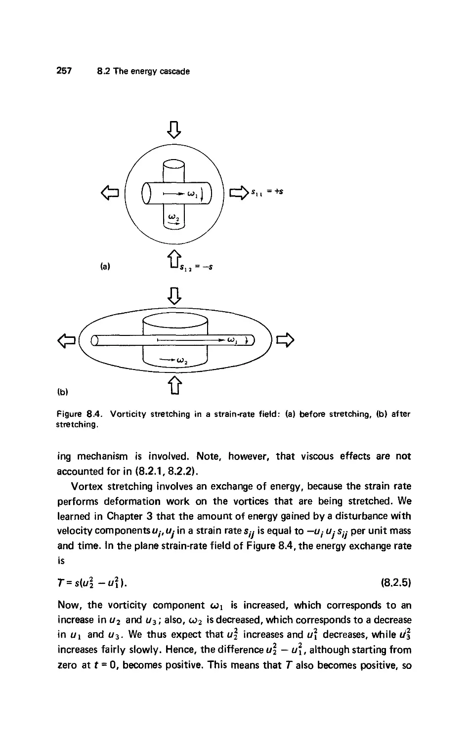
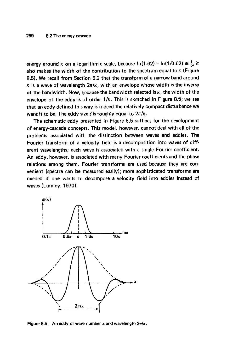
/


Автор: Tennekes H. Lumley J.L.
Теги: mathematics geometry higher mathematics cambridge university press course in turbulence
Год: 1972


Текст
A FIRST COURSE IN TURBULENCE
H. Tennekes and J. L. Lumley
A Fust Course inTurbulence
Ш
The MIT Press
Cambridge, Massachusetts, and London, England
Copyright © 1972 by
The Massachusetts Institute of Technology
This book was designed by the MIT Press Design Department.
It was set in IBM Univers Medium,
printed and bound by Kingsport Press
in the United States of America.
All rights reserved. No part of this book may be reproduced
in any form or by any means, electronic or mechanical, including
photocopying, recording, or by any information storage and
retrieval system, without permission in writing from the publisher.
ISBN 0 262 20019 8 (hardcover)
Library of Congress catalog card number: 77—165072
CONTENTS
Preface xi
Brief guide on the use of symbols xiii
1.
INTRODUCTION 1
1.1
The nature of turbulence 1
Irregularity 1. Diffusivity 2. Large Reynolds numbers 2. Three-dimensional
vorticity fluctuations 2. Dissipation 3. Continuum 3. Turbulent flows are
flows 3.
1.2
Methods of analysis 4
Dimensional analysis 5. Asymptotic invariance 5. Local invariance 6.
1.3
The origin of turbulence 7
1.4
Diffusivity of turbulence 8
Diffusion in a problem with an imposed length scale 8. Eddy diffusivity 10.
Diffusion in a problem with an imposed time scale 11.
1.5
Length scales in turbulent flows 14
Laminar boundary layers 14. Diffusive and convective length scales 15.
Turbulent boundary layers 16. Laminar and turbulent friction 17. Small
scales in turbulence 19. An inviscid estimate for the dissipation rate 20.
Scale relations 21. Molecular and turbulent scales 23.
1.6
Outline of the material 24
2.
TURBULENT TRANSPORT OF MOMENTUM AND HEAT 27
2.1
The Reynolds equations 27
The Reynolds decomposition 28. Correlated variables 29. Equations for the
mean flow 30. The Reynolds stress 32. Turbulent transport of heat 33.
Contents
2.2
Elements of the kinetic theory of gases 34
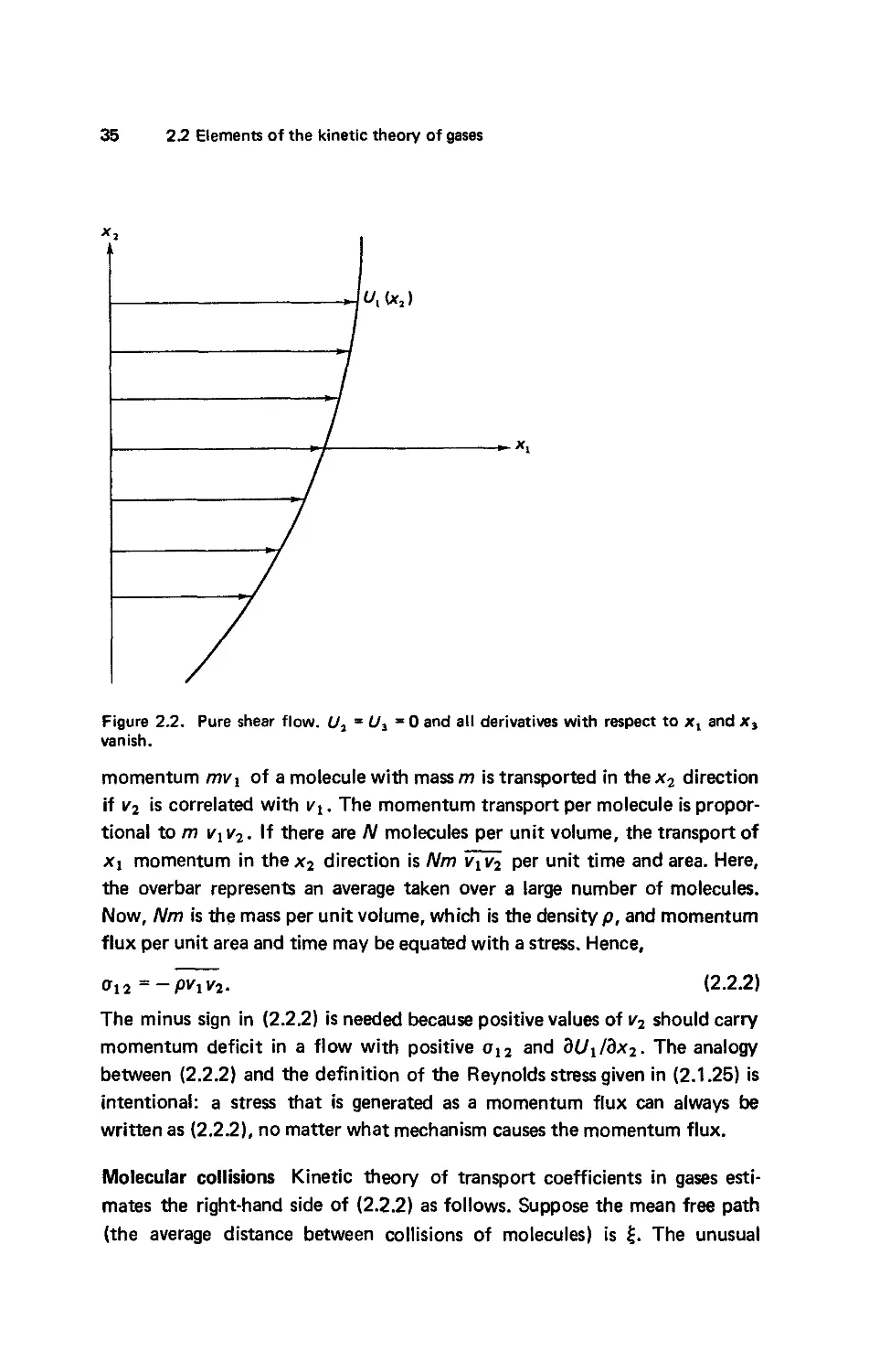
Pure shear flow 34. Molecular collisions 35. Characteristic times and
lengths 38. The correlation between v, and v2 38. Thermal diffusivity 39.
2.3
Estimates of the Reynolds stress 40
Reynolds stress and vortex stretching 40. The mixing-length model 42. The
length-scale problem 44. A neglected transport term 45. The mixing length
as an integral scale 45. The gradient-transport fallacy 47. Further esti-
estimates 49. Recapitulation 49.
2.4
Turbulent heat transfer 50
Reynolds'analogy 51. The mixing-length model 51.
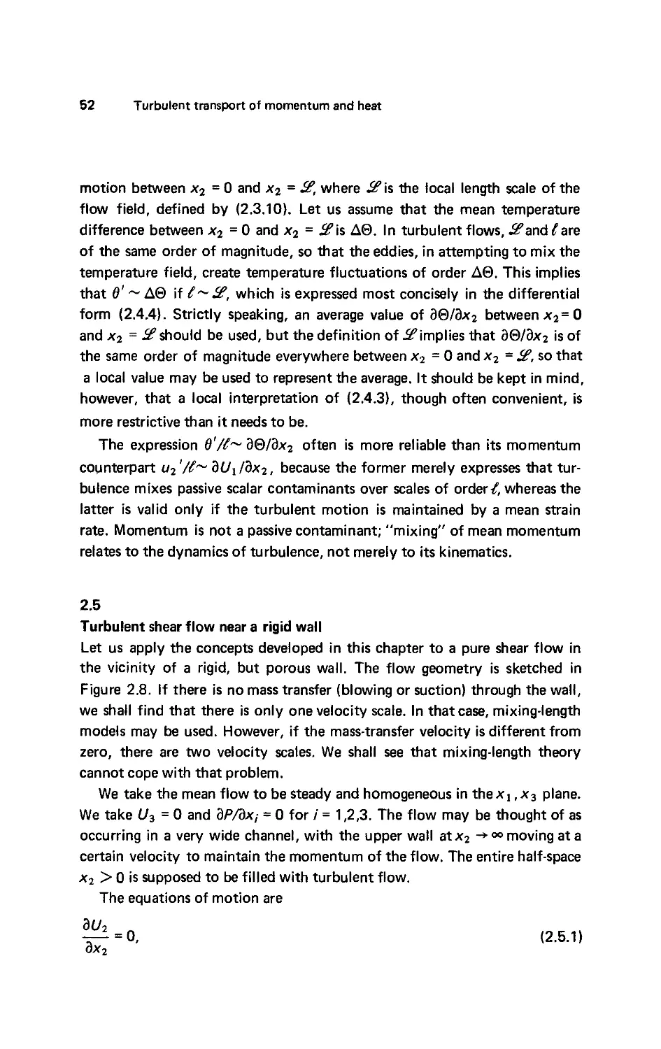
2.5
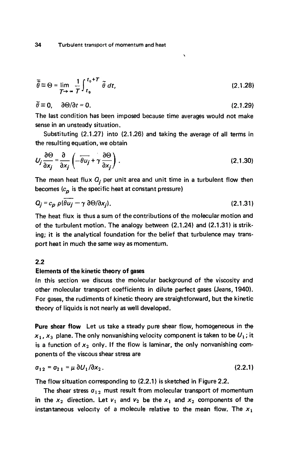
Turbulent shear flow near a rigid wall 52
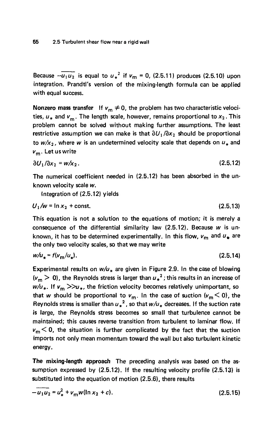
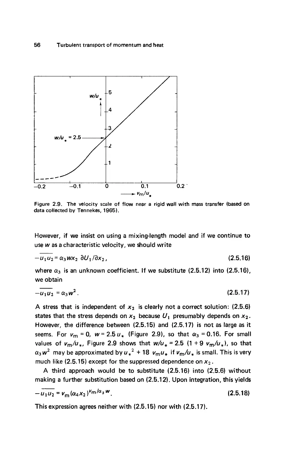
A flow with constant stress 54. Nonzero mass transfer 55. The mixing-length
approach 55. The limitations of mixing-length theory 57.
3.
THE DYNAMICS OF TURBULENCE 59
3.1
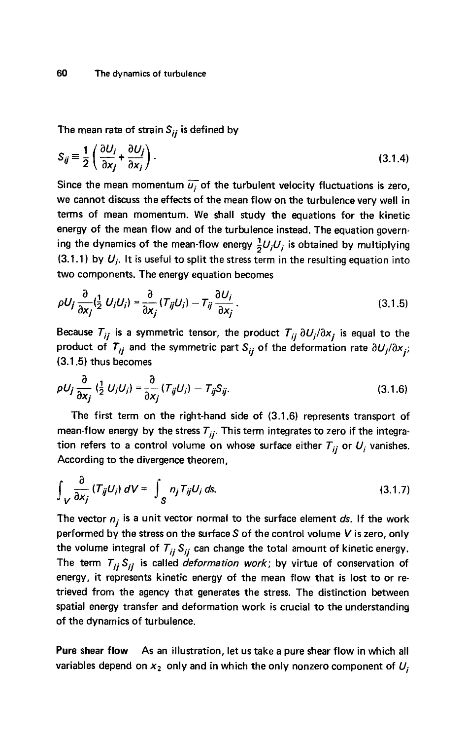
Kinetic energy of the mean flow 59
Pure shear flow 60. The effects of viscosity 62.
3.2
Kinetic energy of the turbulence 63
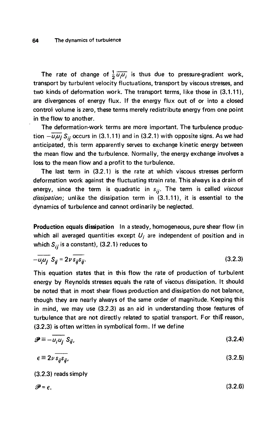
Production equals dissipation 64. Taylor microscale 65. Scale relations 67.
Spectral energy transfer 68. Further estimates 69. Wind-tunnel turbu-
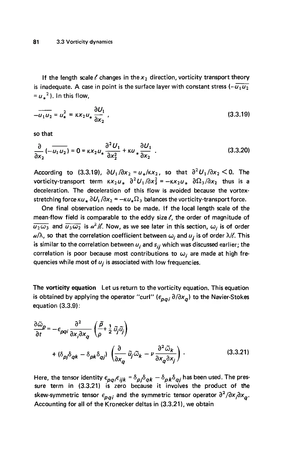
turbulence 70. Pure shear flow 74.
3.3
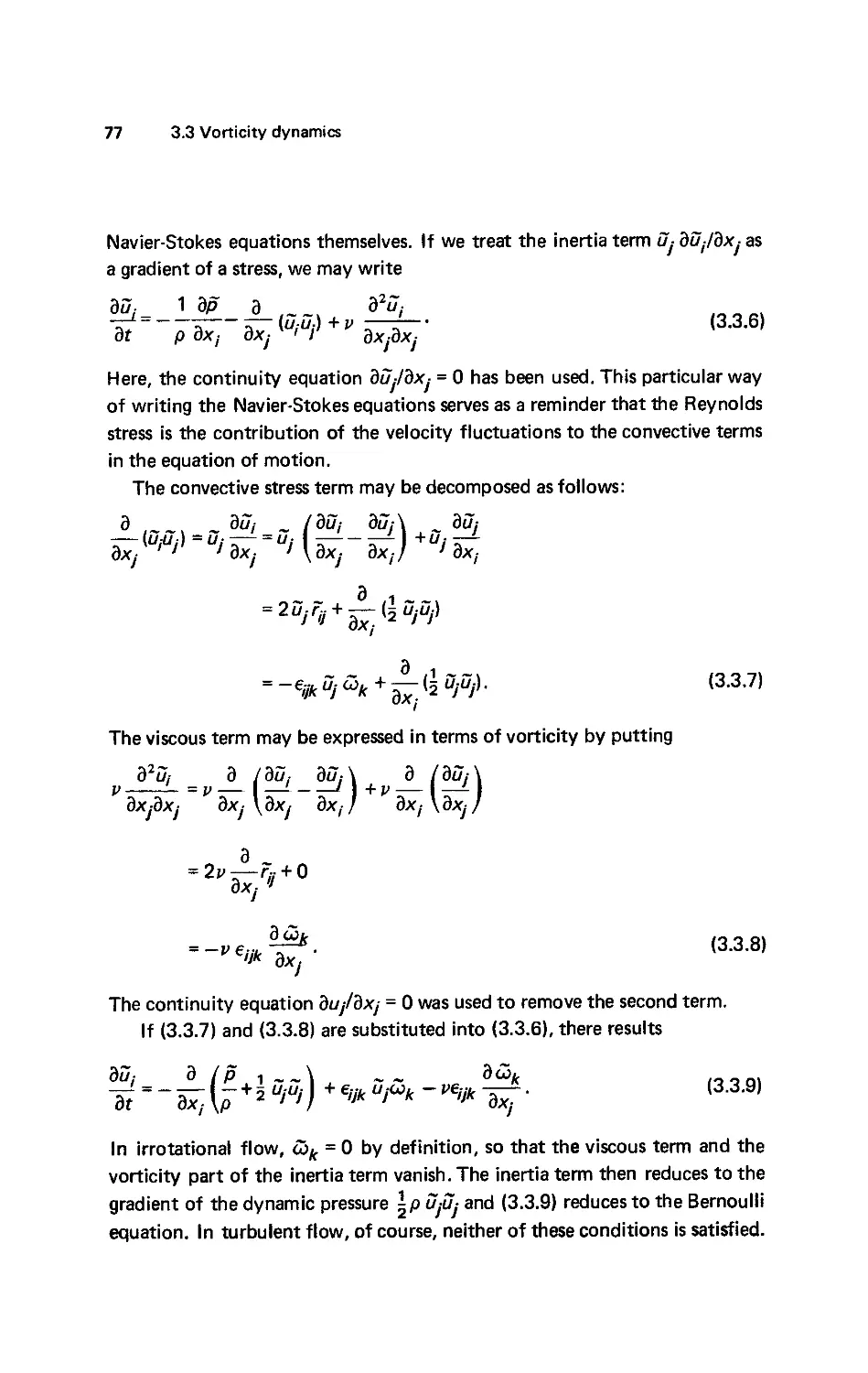
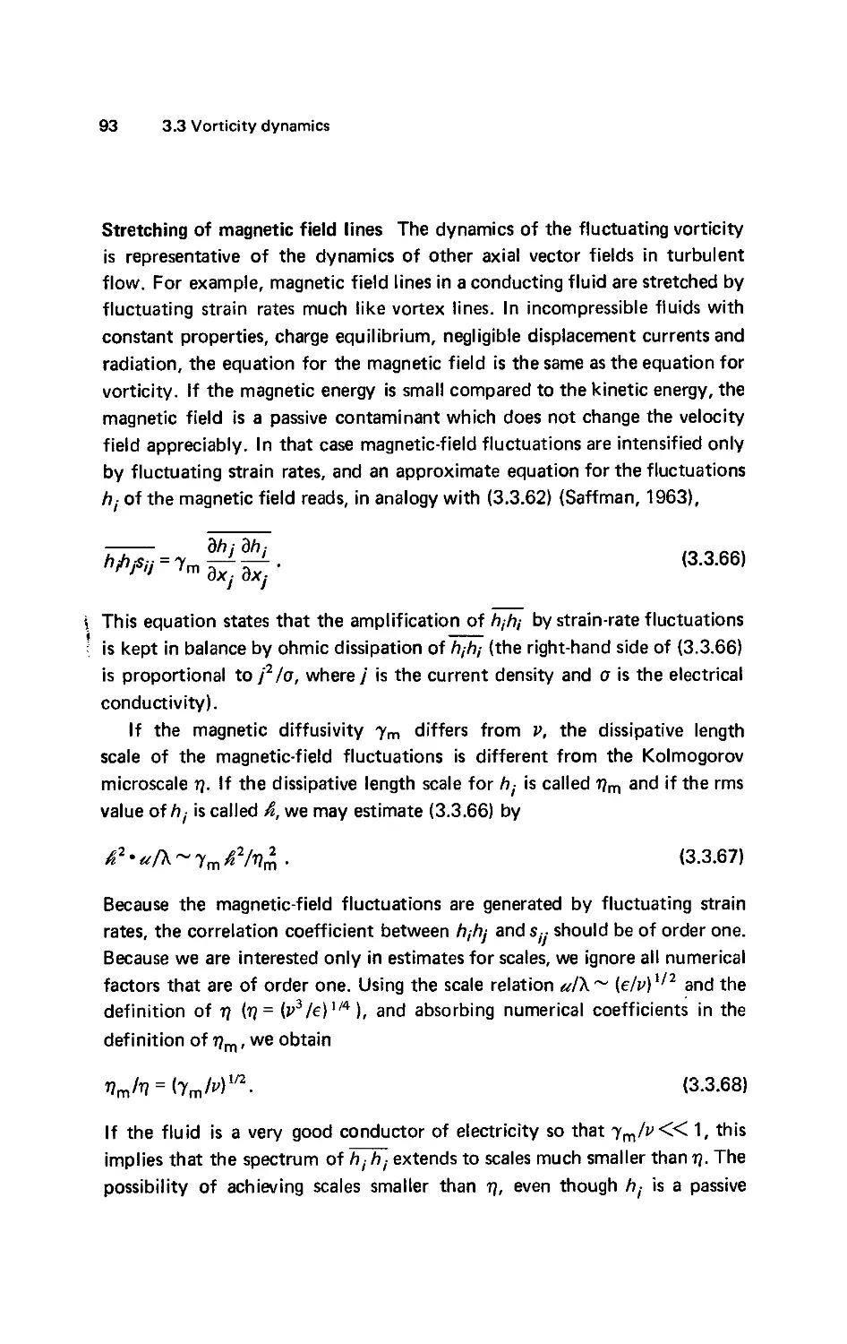
Vorticity dynamics 75
Vorticity vector and rotation tensor 76. Vortex terms in the equations of
motion 76. Reynolds stress and vorticity 78. The vorticity equation 81.
Vorticity in turbulent flows 84. Two-dimensional mean flow 85. The
dynamics of П,-П/ 86. The equation for «/«/ 86. Turbulence is rota-
rotational 87. An approximate vorticity budget 88. Multiple length scales 92.
Stretching of magnetic field lines 93.
vii Contents
3.4
The dynamics of temperature fluctuations 95
Microscales in the temperature field 95. Buoyant convection 97. Richardson
numbers 98. Buoyancy time scale 99. Monin-Oboukhov length 100. Convec-
Convection in the atmospheric boundary layer 100.
4.
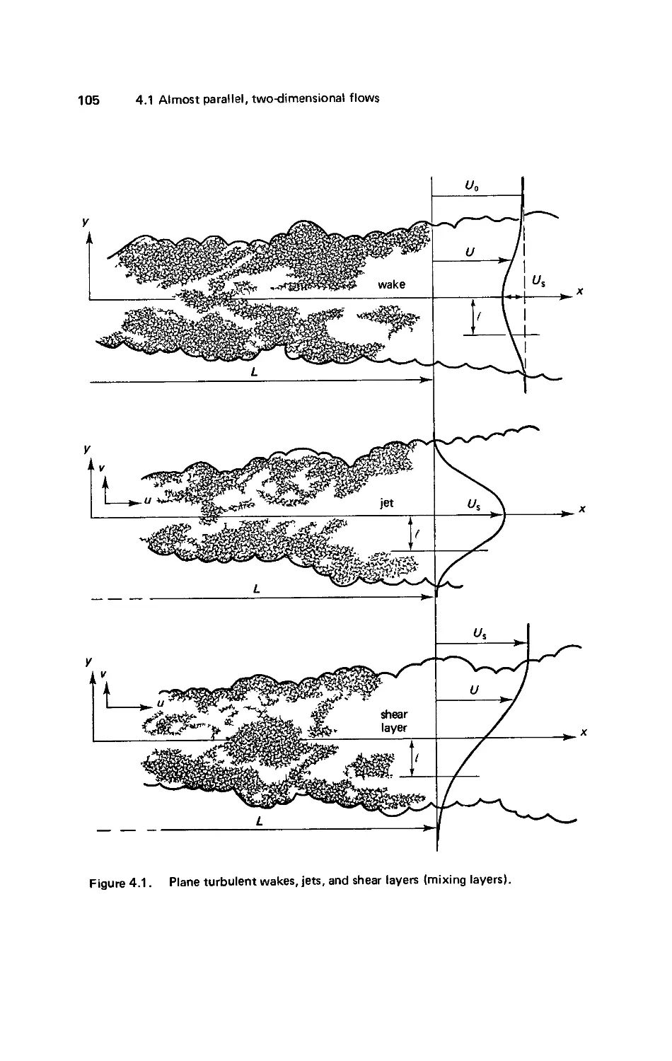
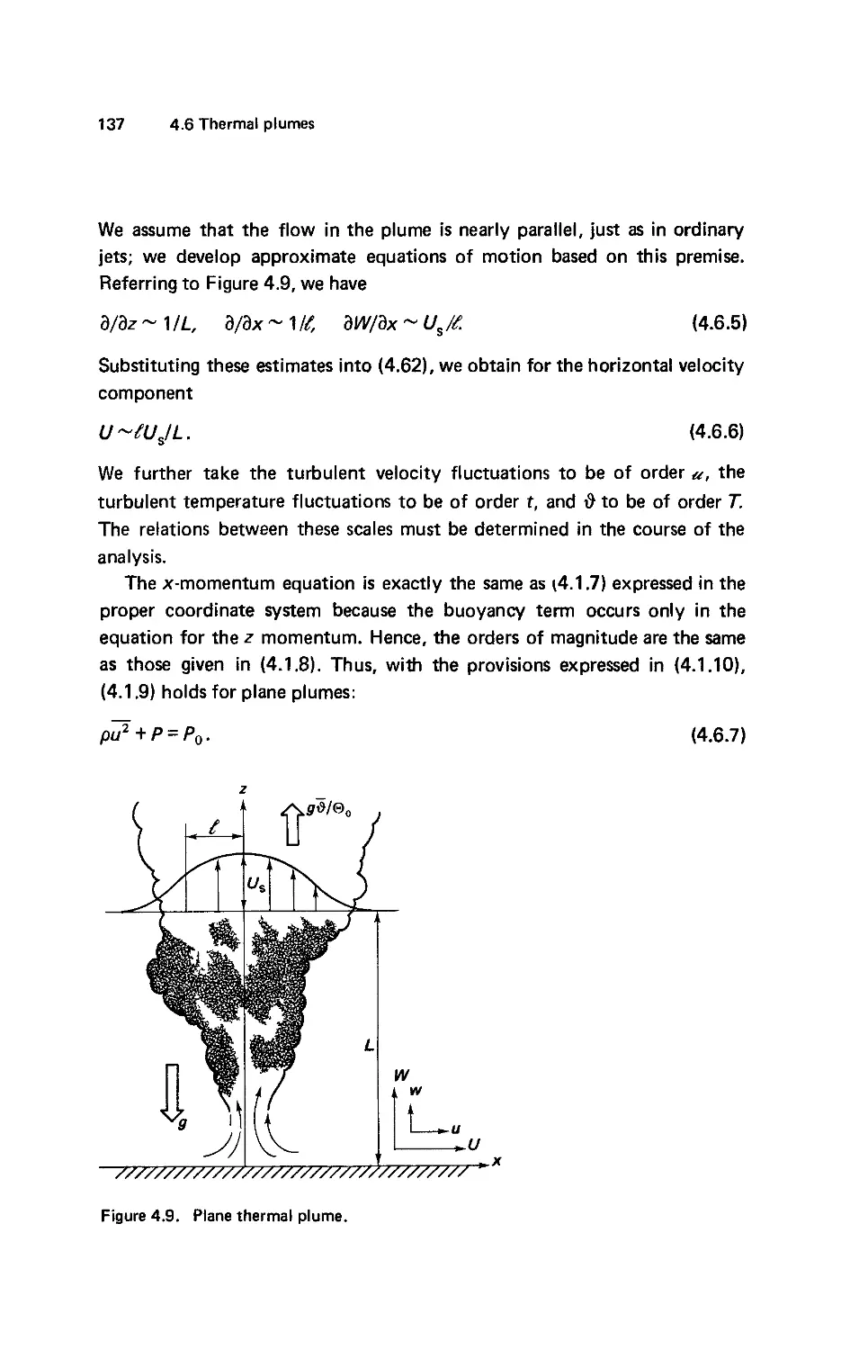
BOUNDARY-FREE SHEAR FLOWS 104
4.1
Almost parallel, two-dimensional flows 104
Plane flows 104. The cross-stream momentum equation 106. The streamwise
momentum equation 108. Turbulent wakes 109. Turbulent jets and mixing
layers 110. The momentum integral 111. Momentum thickness 112.
4.2
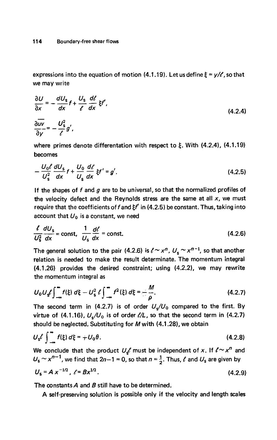
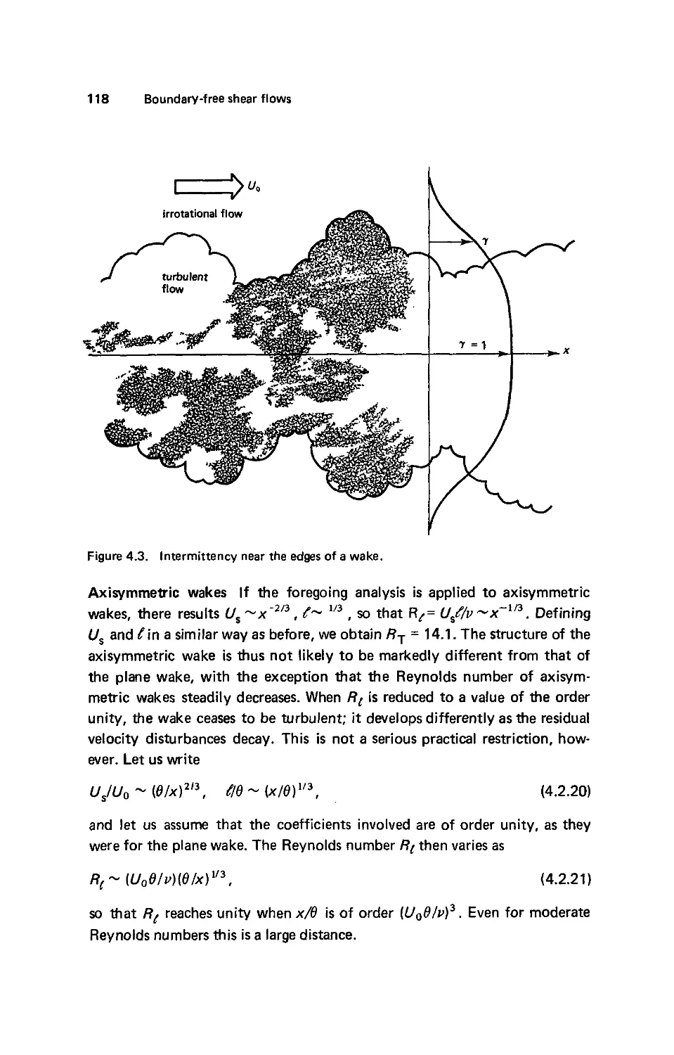
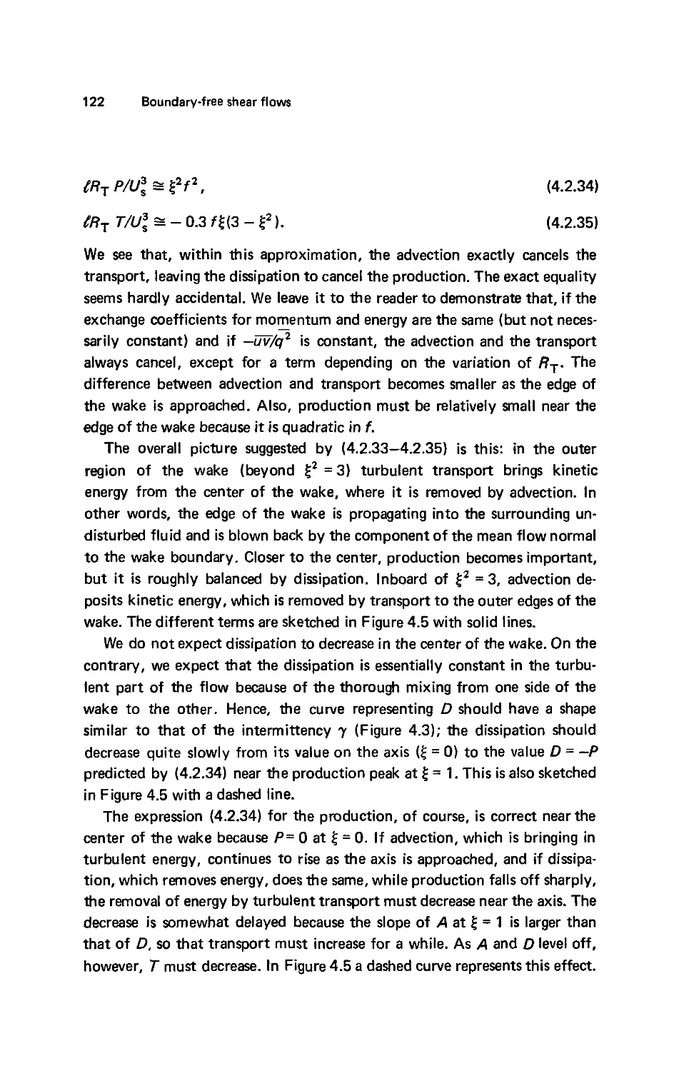
Turbulent wakes 113
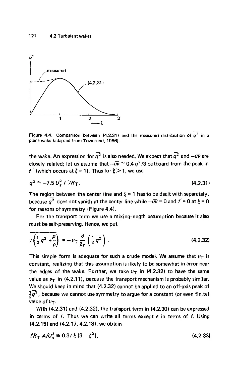
Self-preservation 113. The mean-velocity profile 115. Axisymmetric
wakes 118. Scale relations 119. The turbulent energy budget 120.
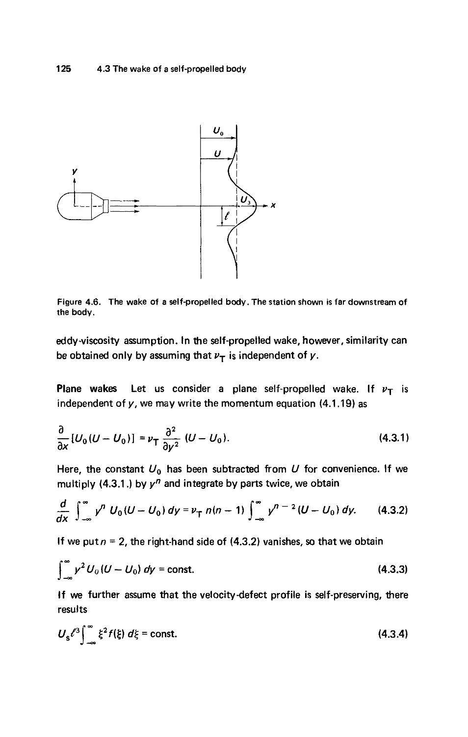
4.3
The wake of a self-propelled body 124
Plane wakes 125. Axisymmetric wakes 127.
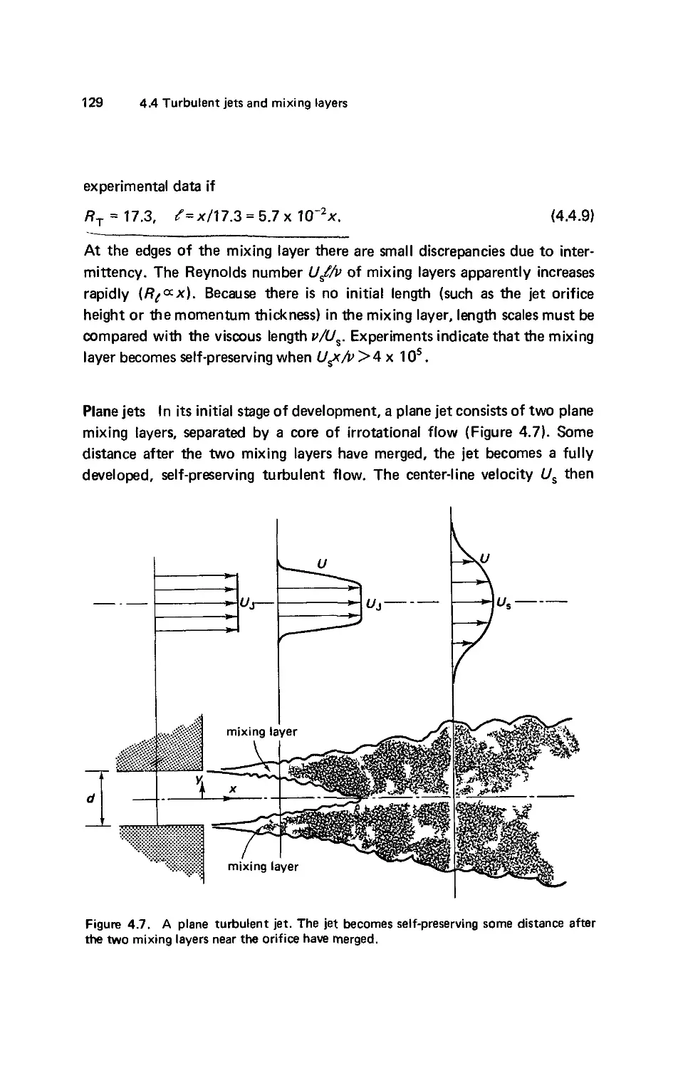
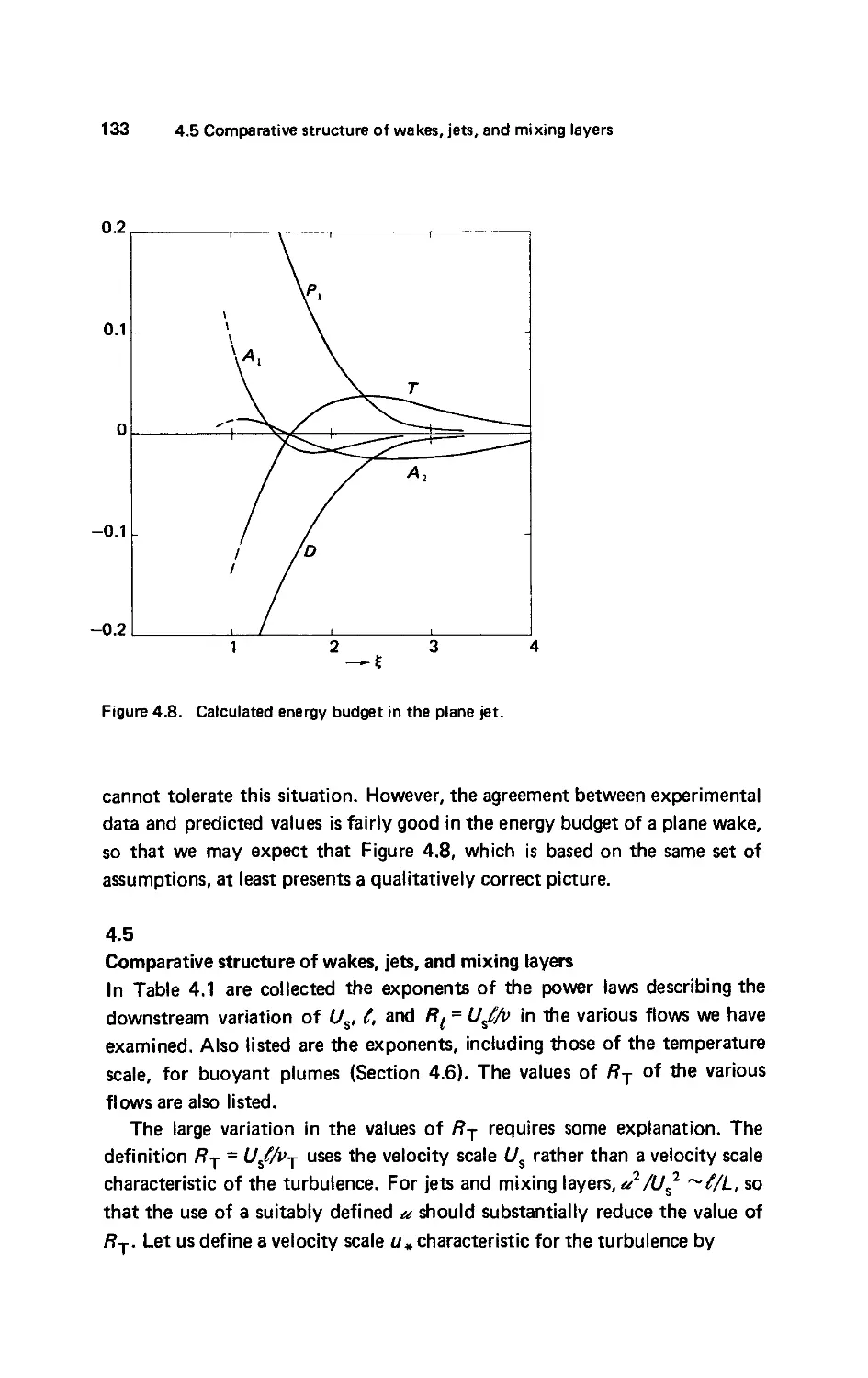
4.4
Turbulent jets and mixing layers 127
Mixing layers 128. Plane jets 129. The energy budget in a plane jet 131.
4.5
Comparative structure of wakes, jets, and mixing layers 133
4.6
Thermal plumes 135
Two-dimensional plumes 136. Self-preservation 141. The heat-flux inte-
integral 142. Further results 142.
5.
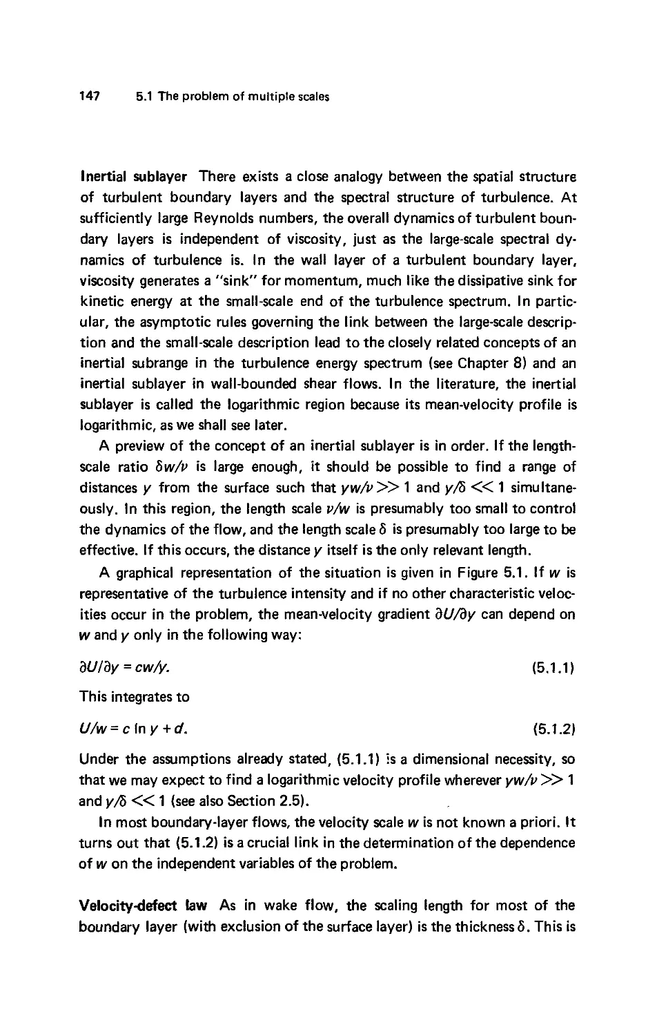
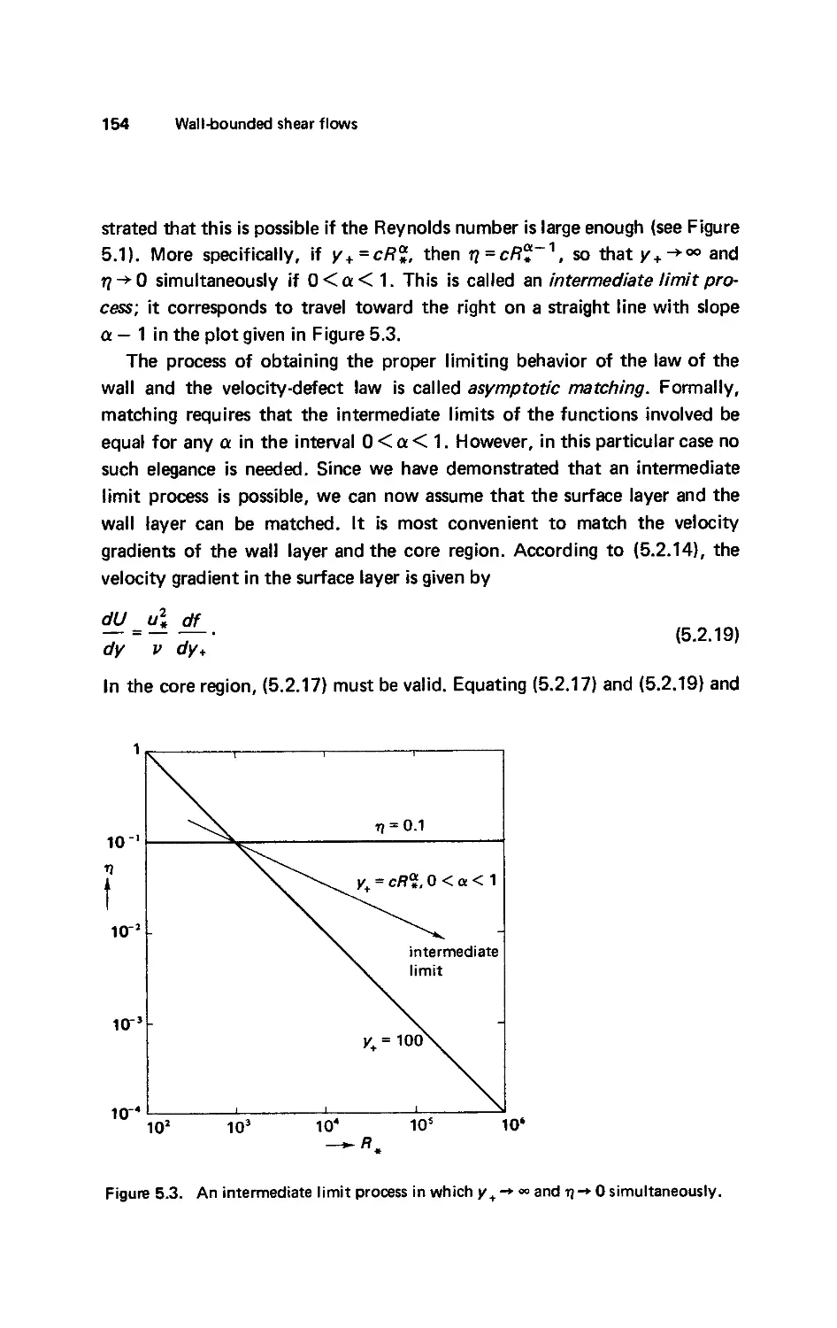
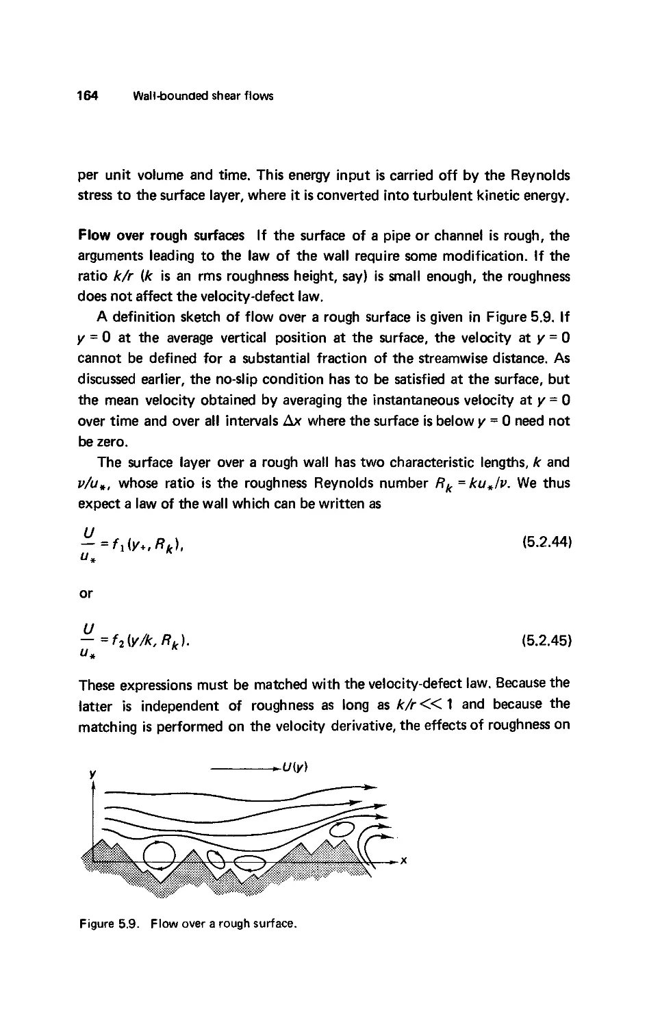
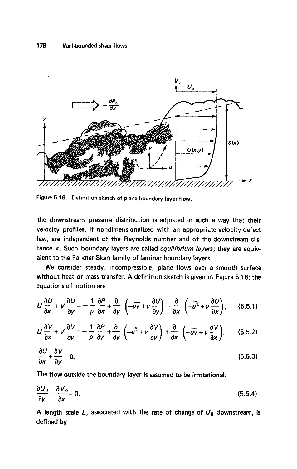
WALL-BOUNDED SHEAR FLOWS 146
5.1
The problem of multiple scales 146
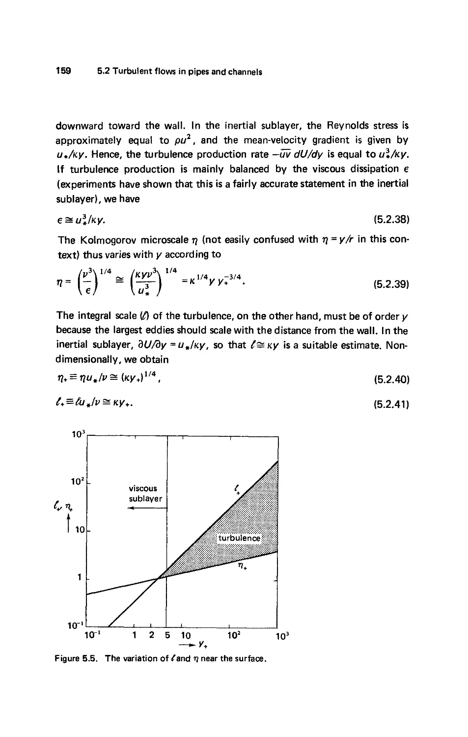
Inertial sublayer 147. Velocity-defect law 147.
viii Contents
5.2
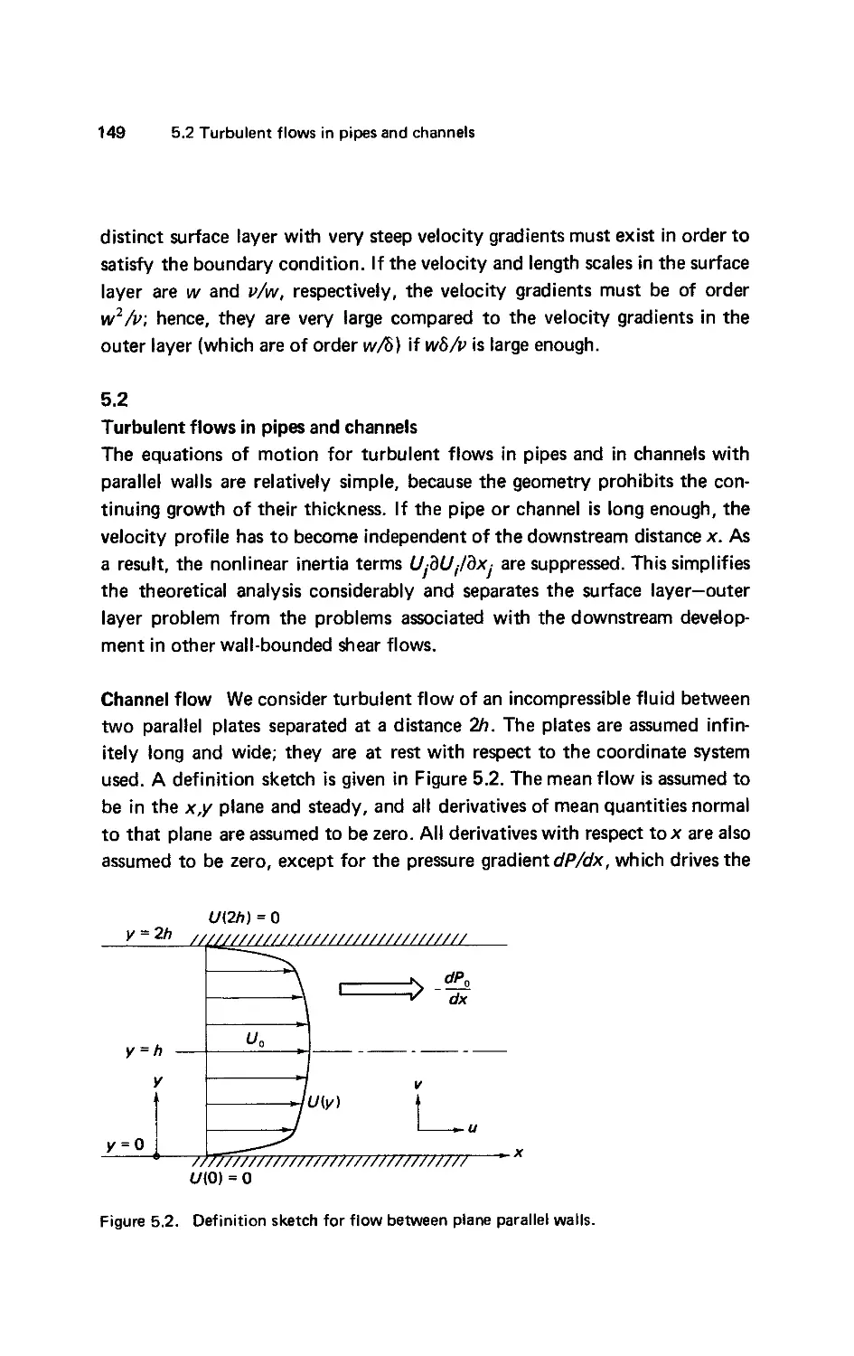
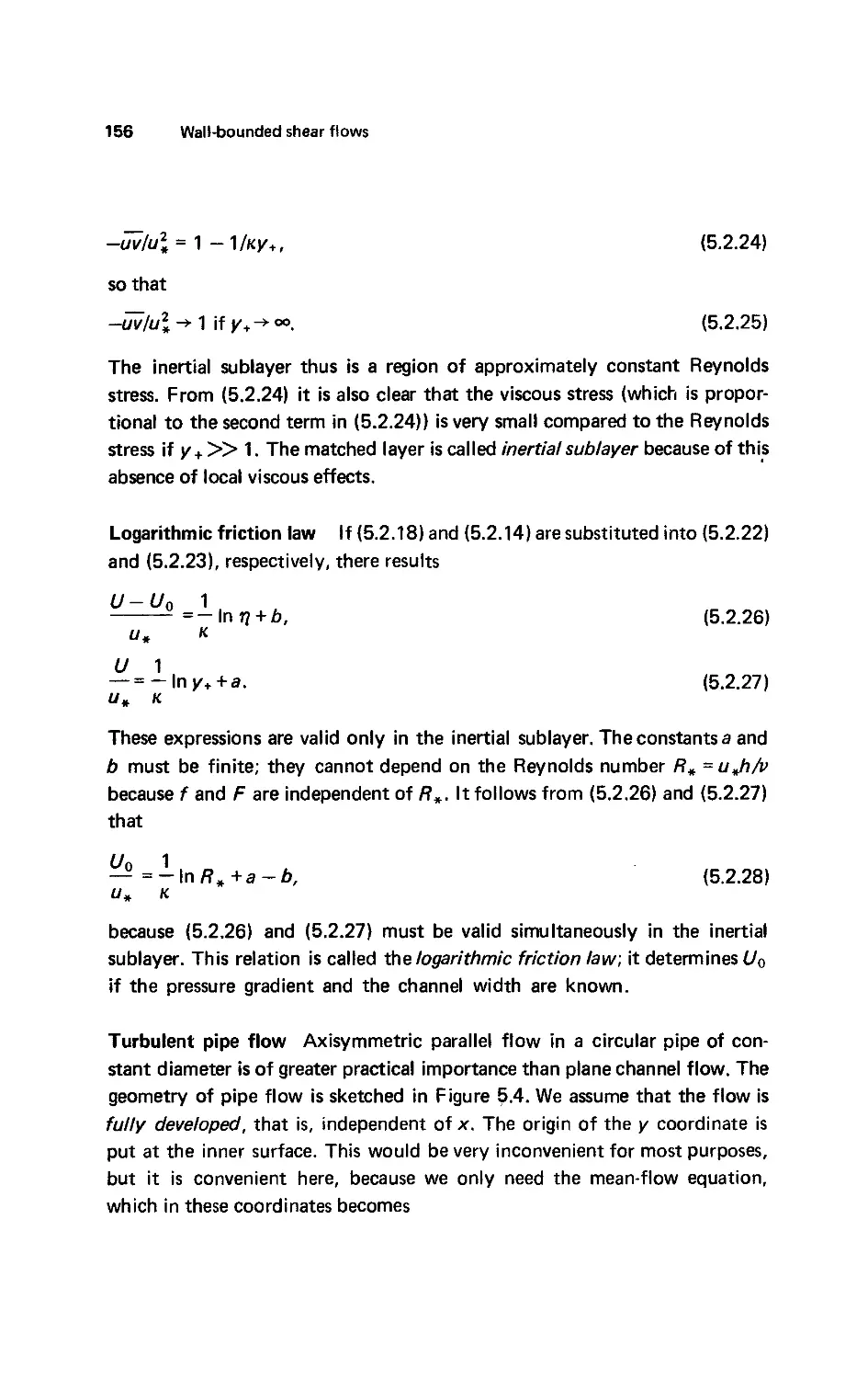
Turbulent flows in pipes and channels 149
Channel flow 149. The surface layer on a smooth wall 152. The core
region 153. Inertial sublayer 153. Logarithmic friction law 156. Turbulent
pipe flow 156. Experimental data on pipe flow 157. The viscous sub-
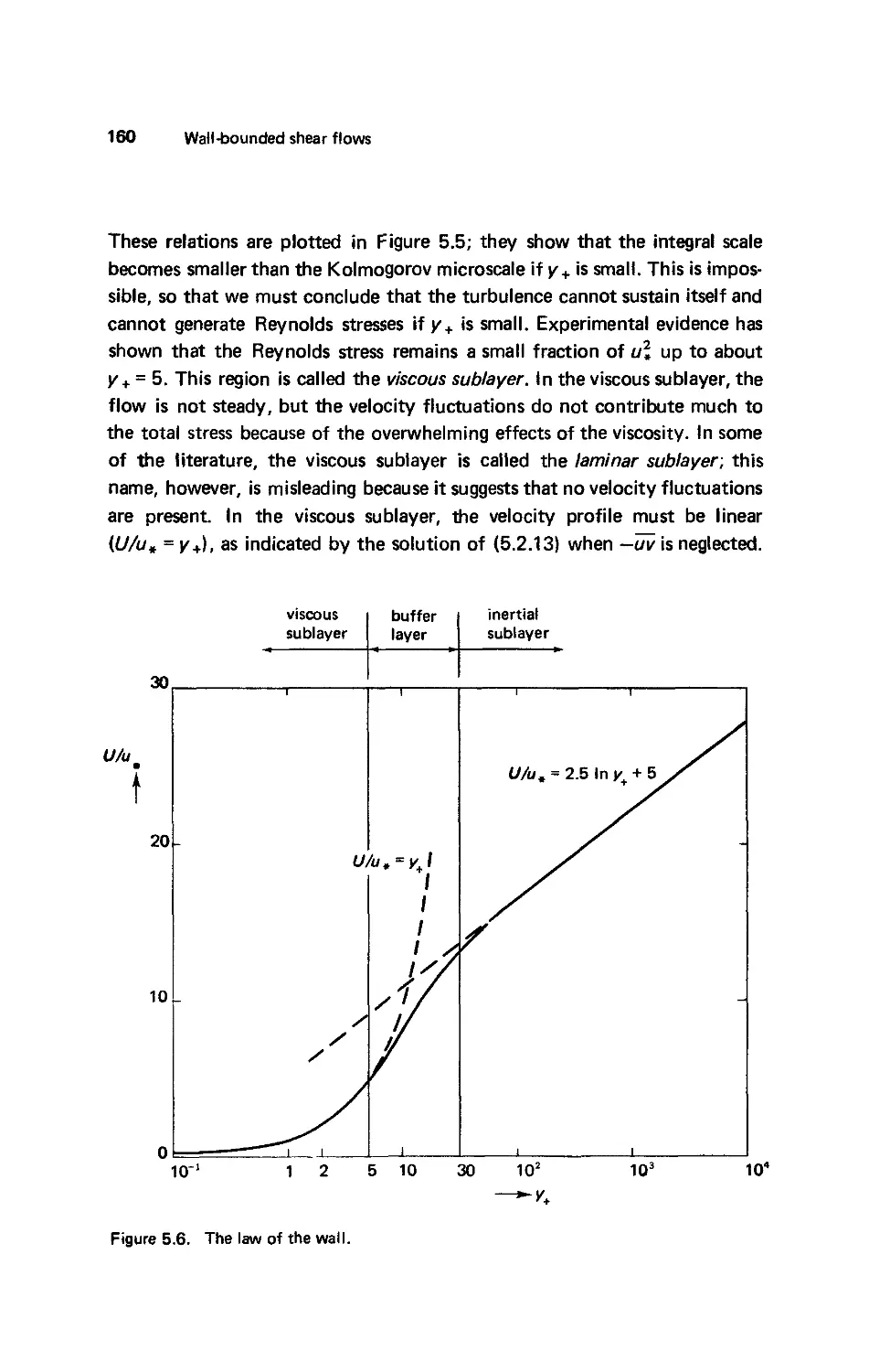
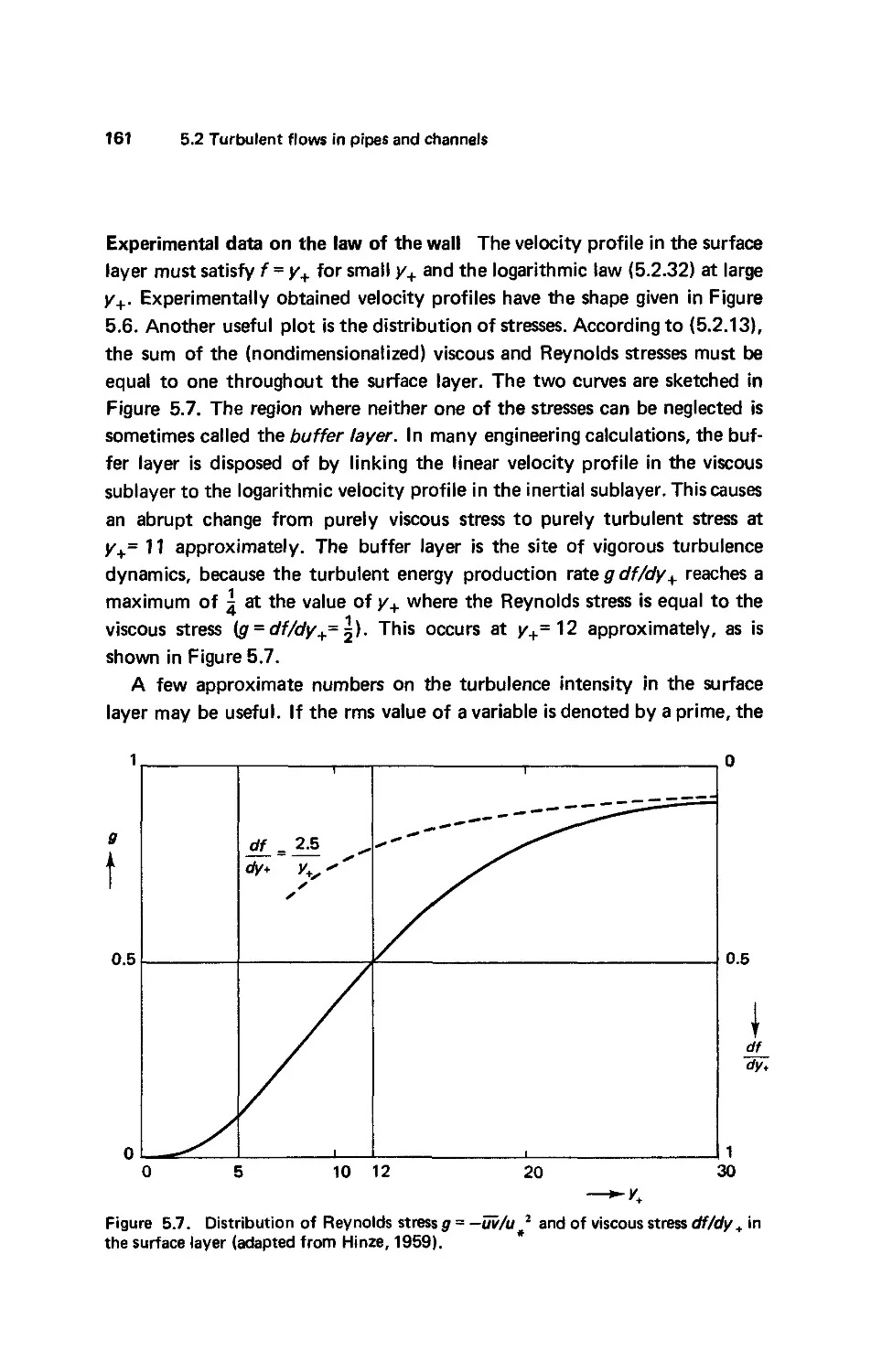
sublayer 158. Experimental data on the law of the wall 161. Experimental data
on the velocity-defect law 162. The flow of energy 163. Flow over rough
surfaces 164.
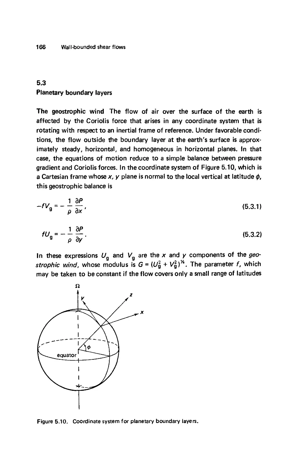
5.3
Planetary boundary layers 166
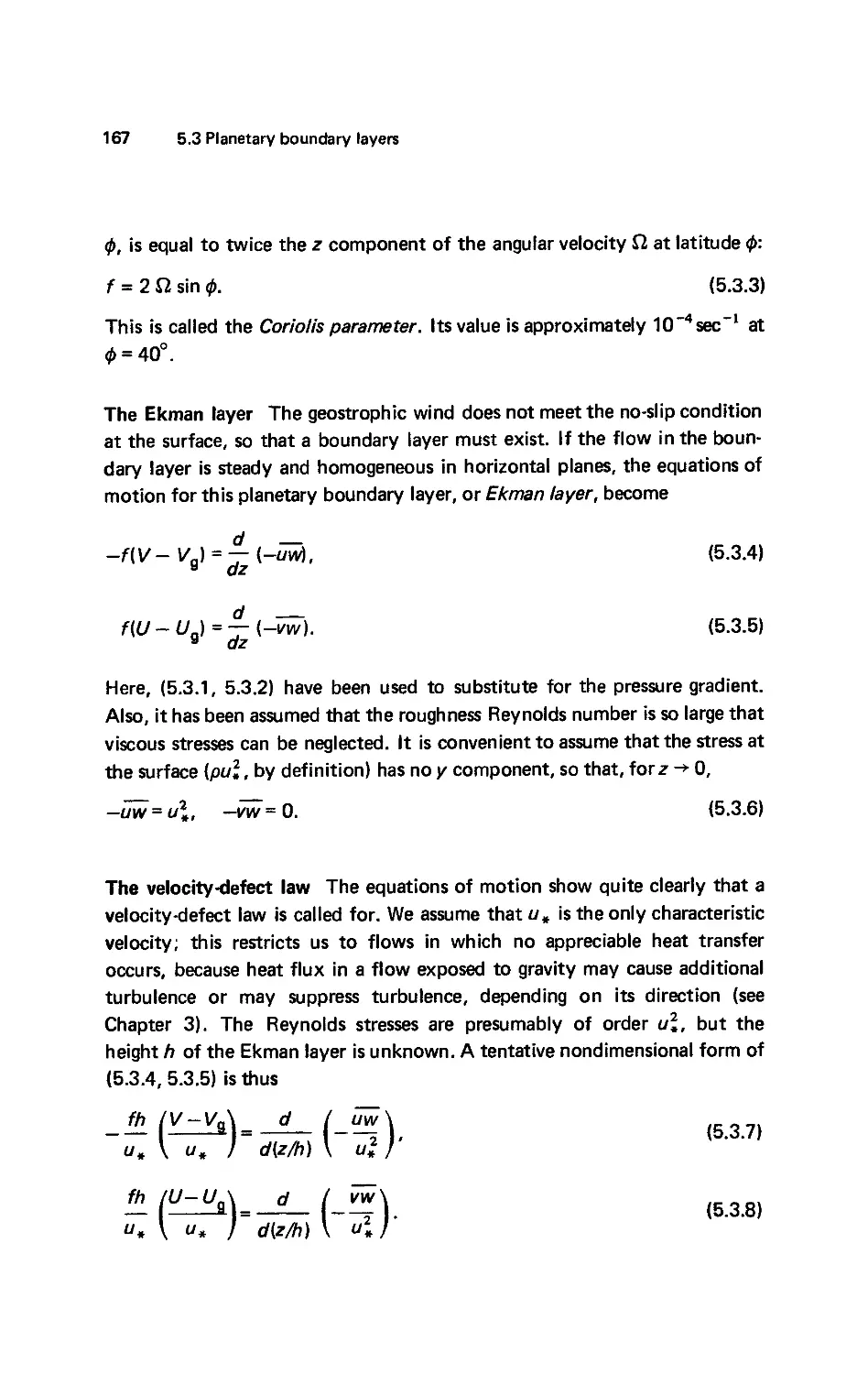
The geostrophic wind 166. The Ekman layer 167. The velocity-defect
law 167. The surface layer 168. The logarithmic wind profile 169. Ekman
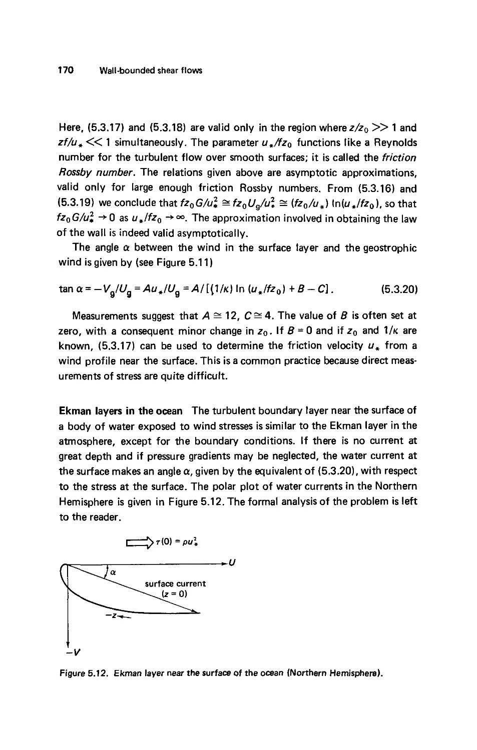
layers in the ocean 170.
5.4
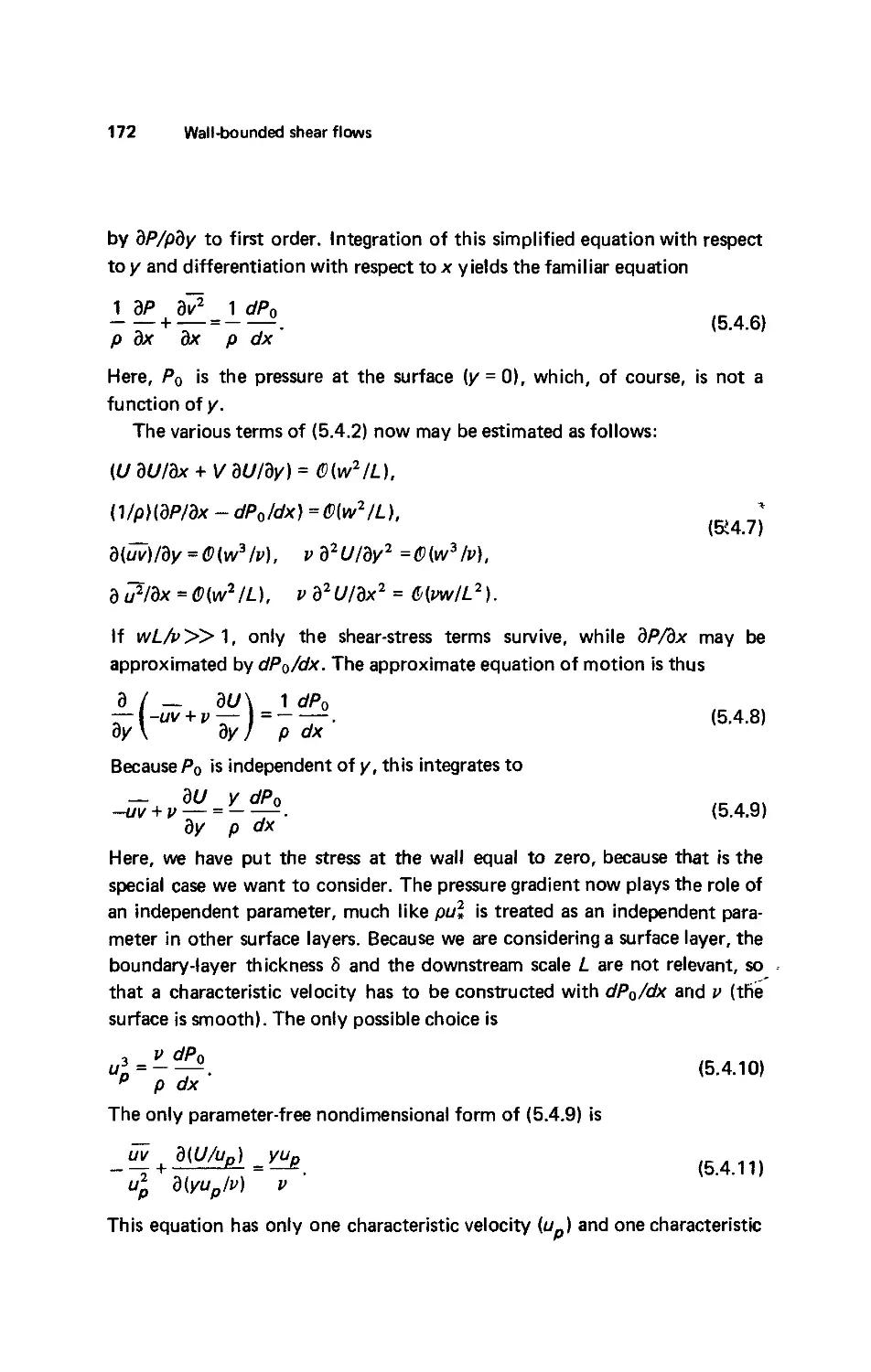
The effects of a pressure gradient on the flow in surface layers 171
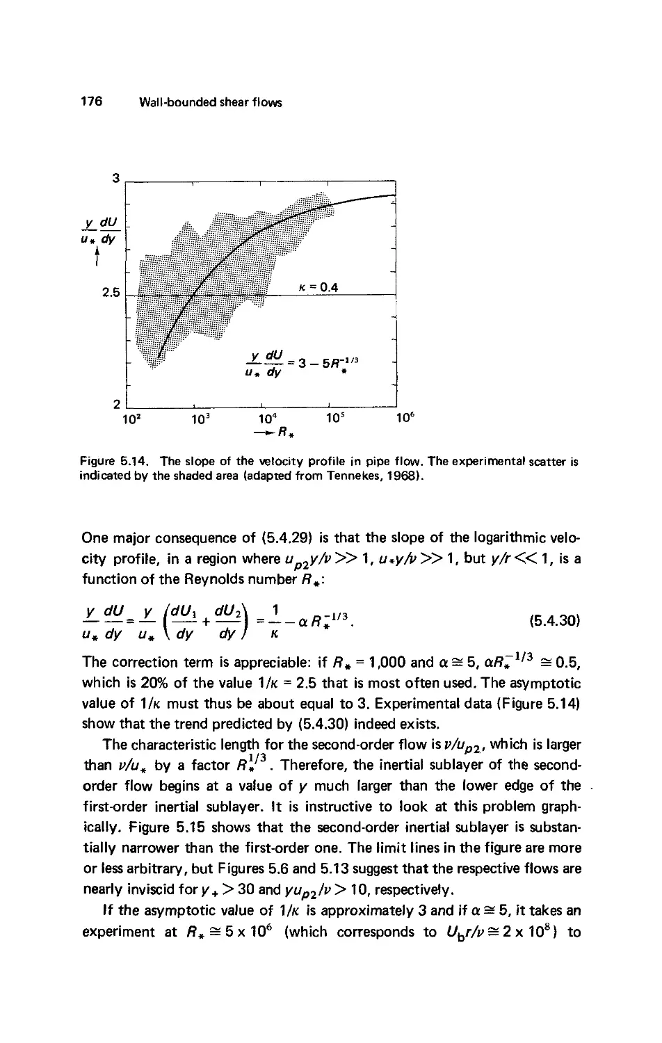
A second-order correction to pipe flow 174. The slope of the logarithmic
velocity profile 175.
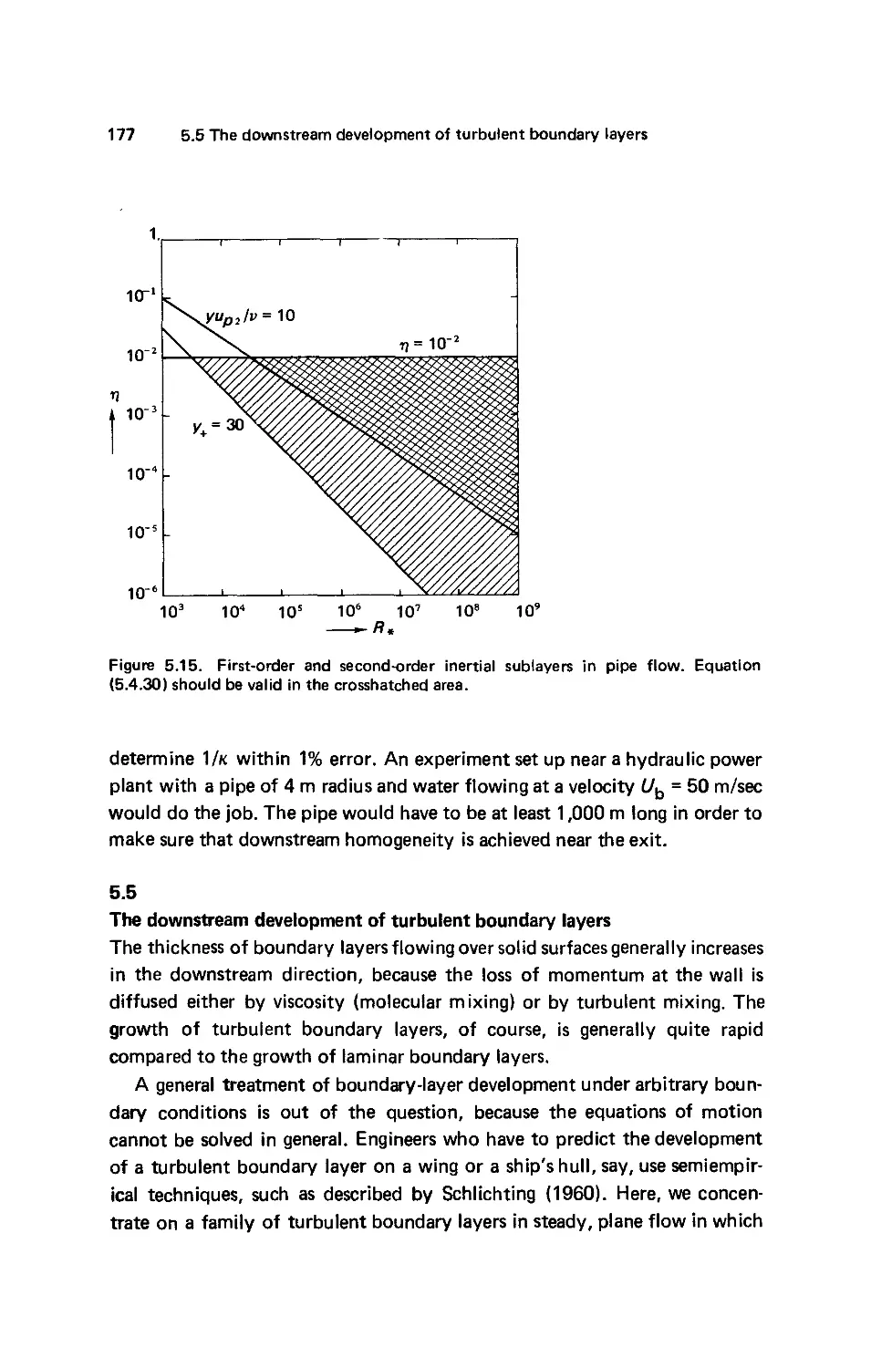
5.5
The downstream development of turbulent boundary layers 177
The potential flow 179. The pressure inside the boundary layer 181. The
boundary-layer equation 182. Equilibrium flow 184. The flow in the wall
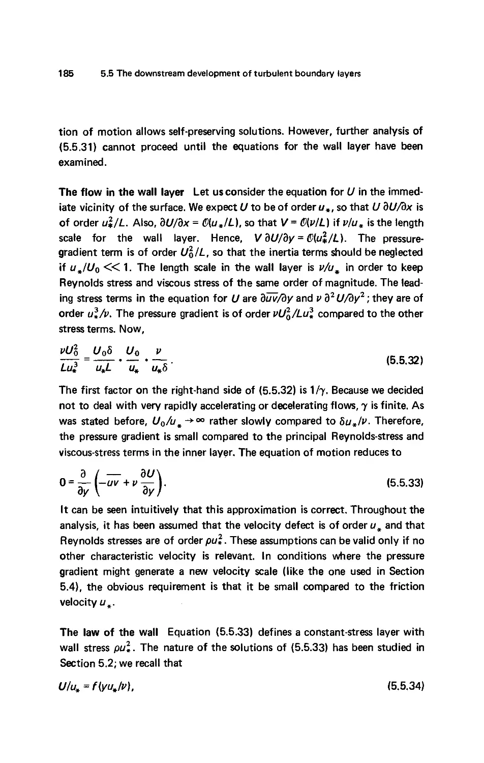
layer 185. The law of the wall 185. The logarithmic friction law 186. The
pressure-gradient parameter 186. Free-stream velocity distributions 188.
Boundary layers in zero pressure gradient 190. Transport of scalar contam-
contaminants 194.
6.
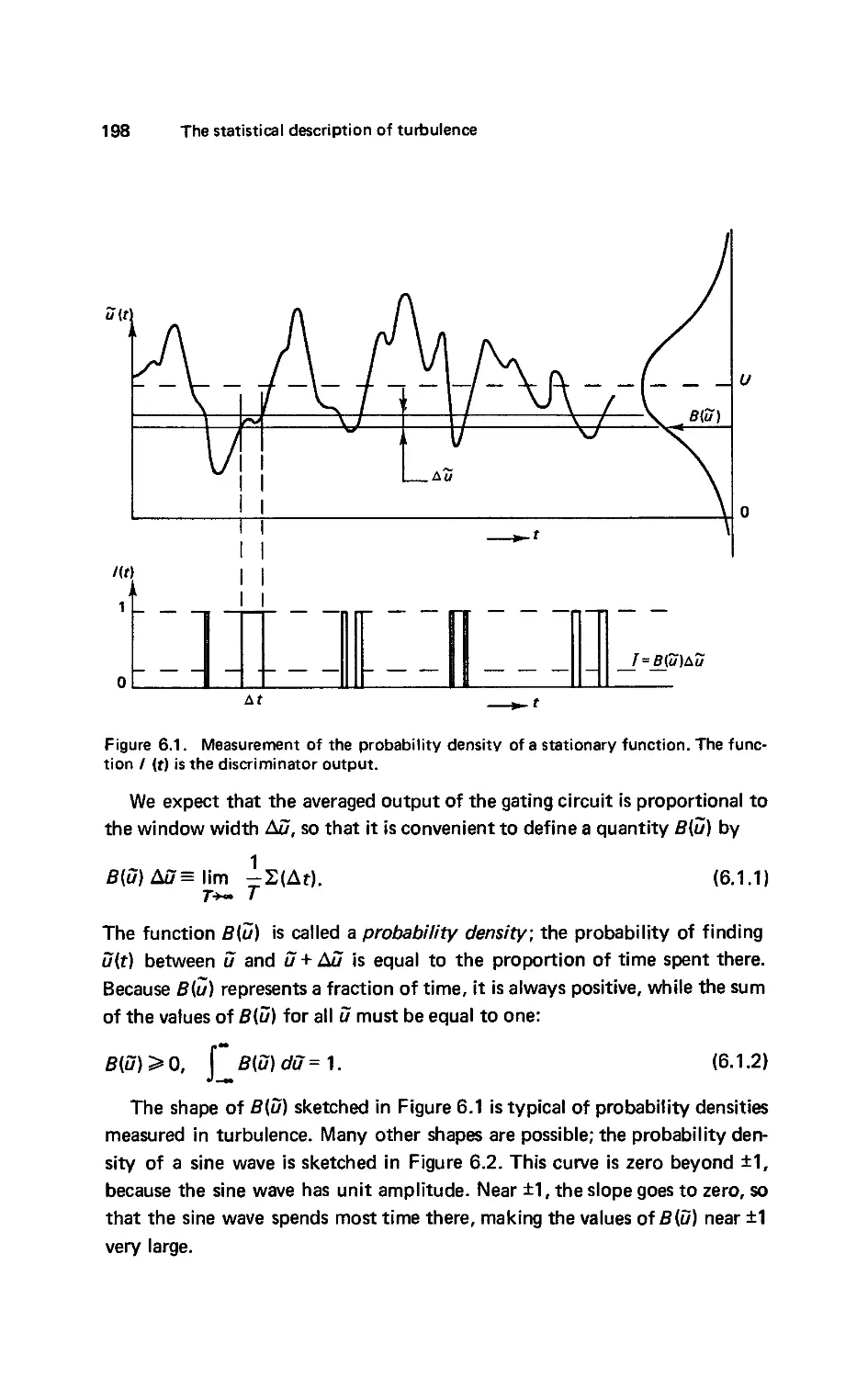
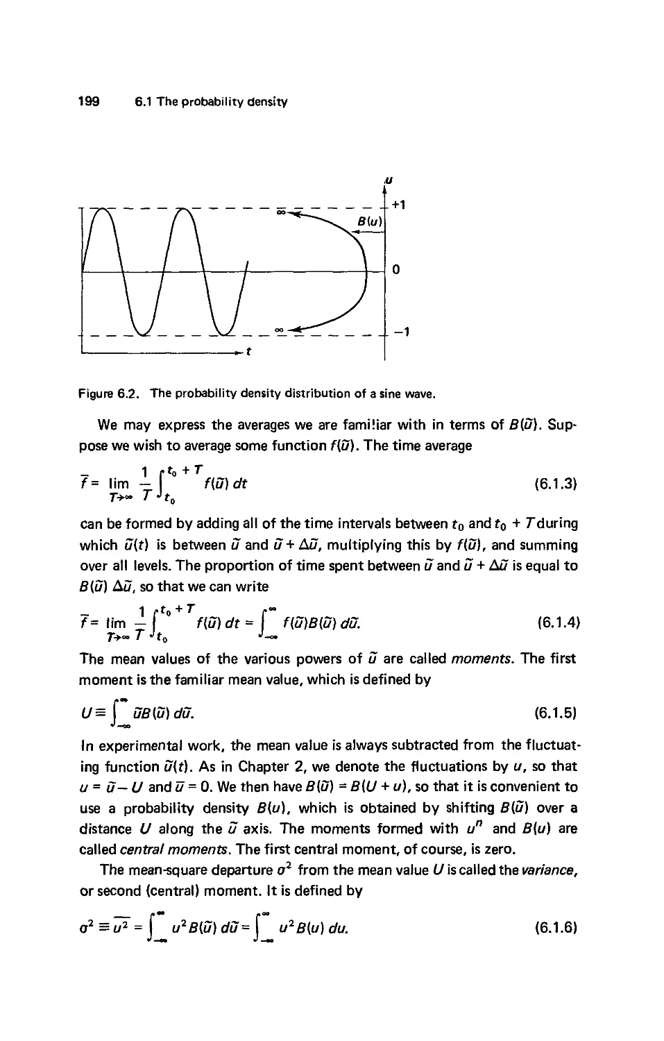
THE STATISTICAL DESCRIPTION OF TURBULENCE 197
6.1
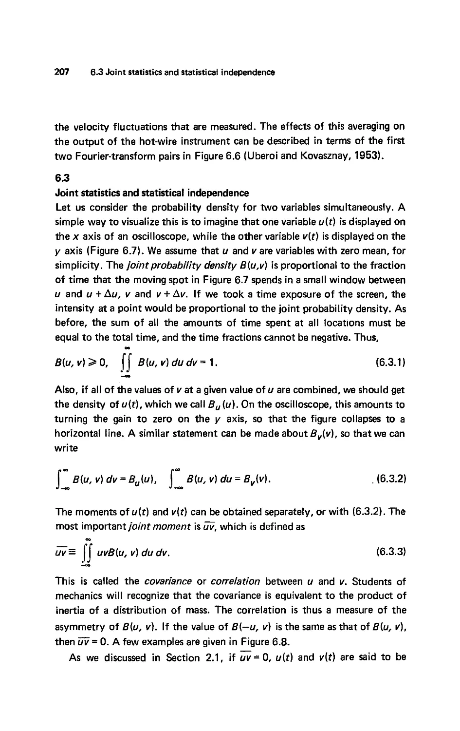
The probability density 197
6.2
Fourier transforms and characteristic functions 201
The effects of spikes and discontinuities 203. Parseval's relation 205.
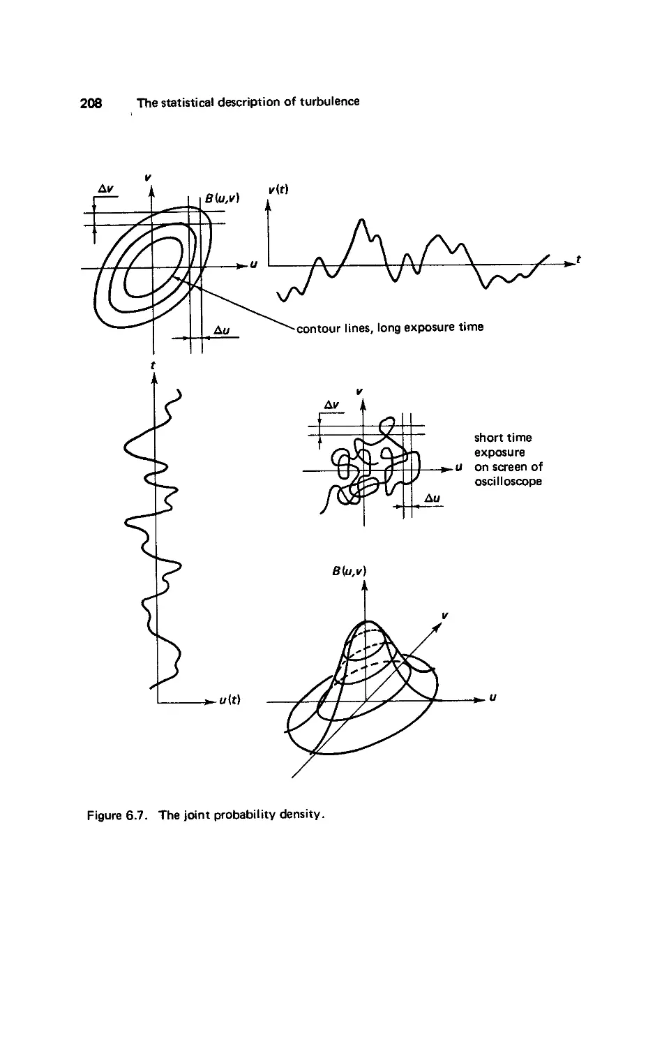
6.3
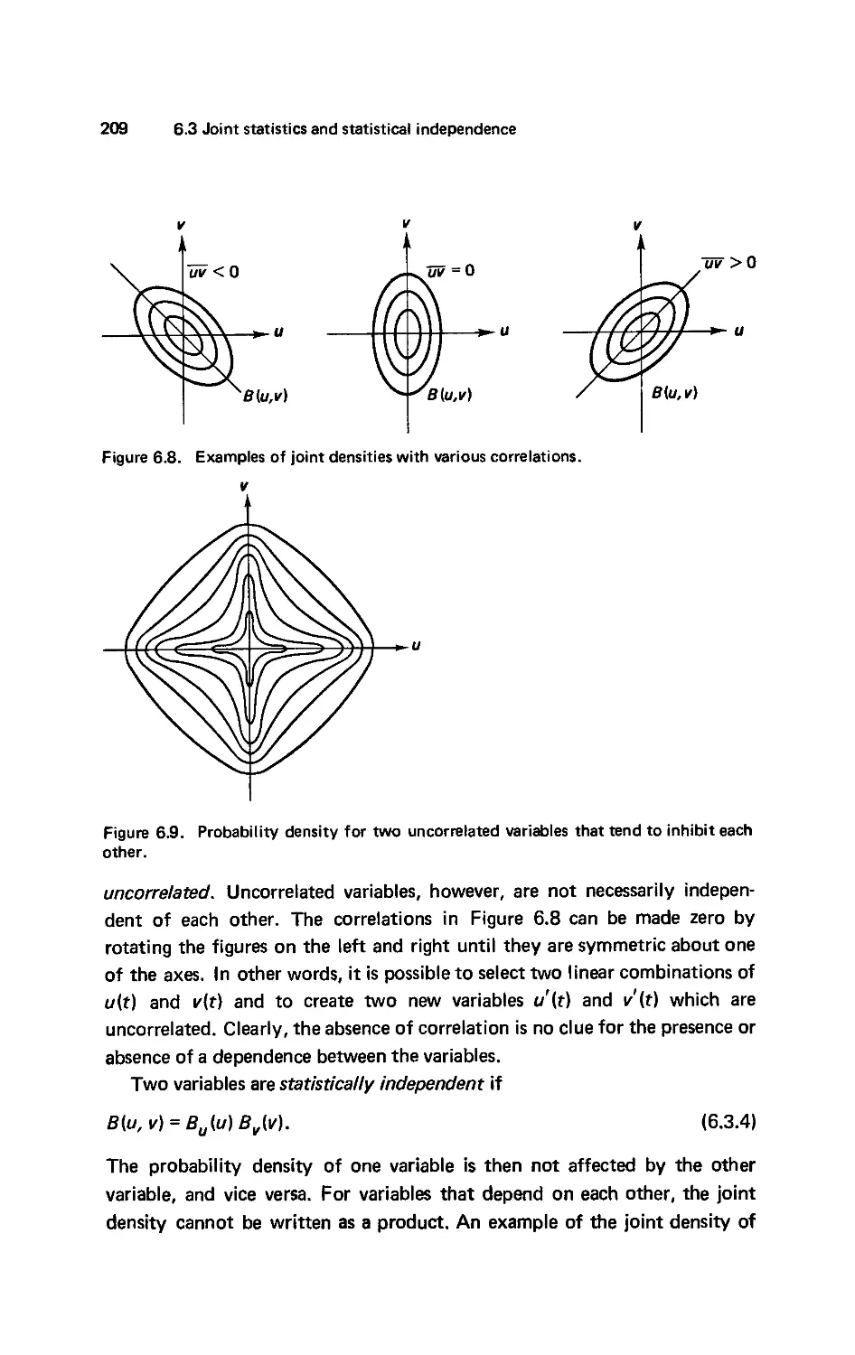
Joint statistics and statistical independence 207
ix Contents
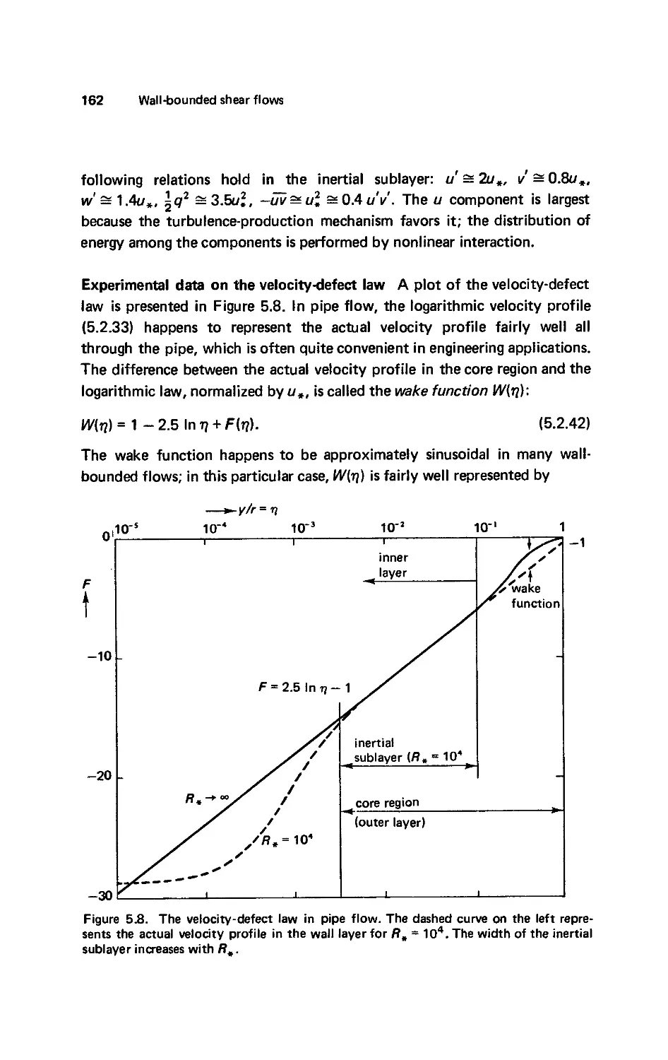
6.4
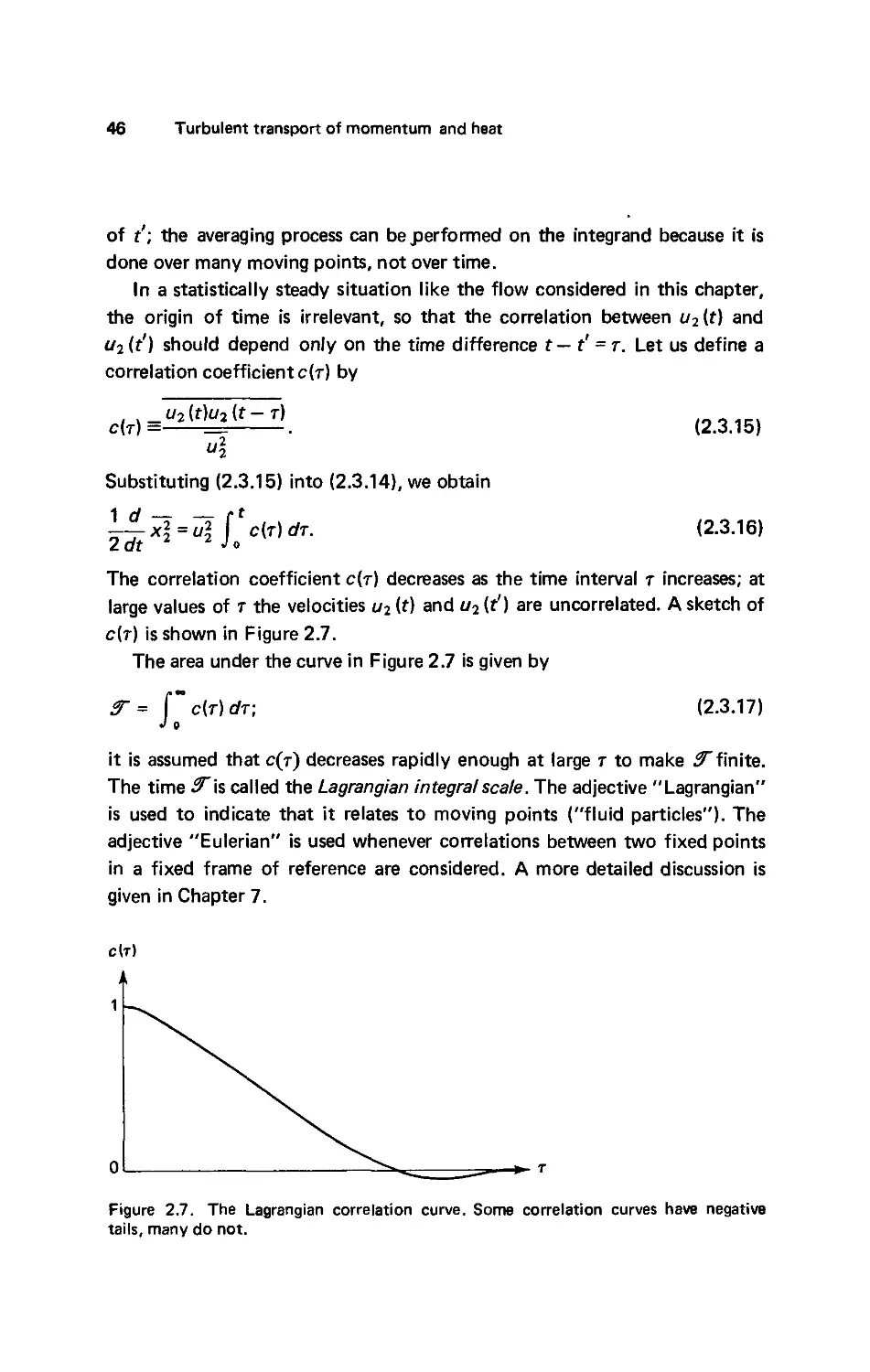
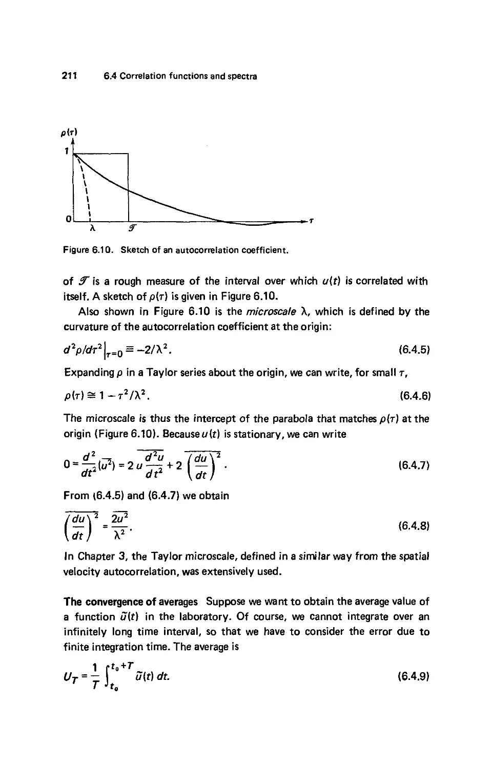
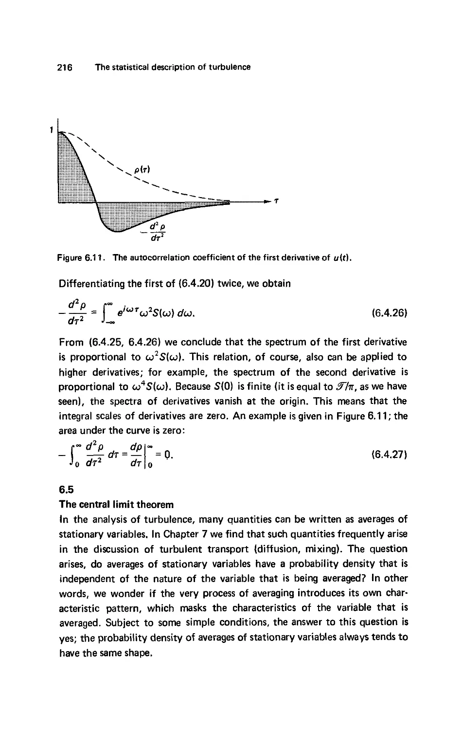
Correlation functions and spectra 210
The convergence of averages 211. Ergodicity 212. The Fourier transform of
р(т) 214.
6.5
The central limit theorem 216
The statistics of integrals 218. A generalization of the theorem 220. More
statistics of integrals 220.
7.
TURBULENT TRANSPORT 223
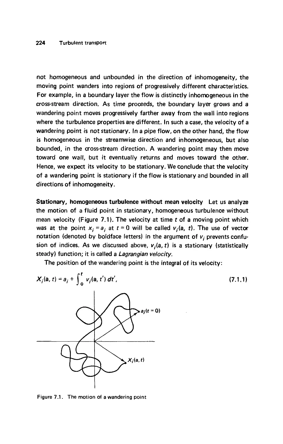
7.1
Transport in stationary, homogeneous turbulence 223
Stationarity 223. Stationary, homogeneous turbulence without mean veloc-
velocity 224. The probability density of the Lagrangian velocity 226. The
Lagrangian integral scale 229. The diffusion equation 230.
7.2
Transport in shear flows 230
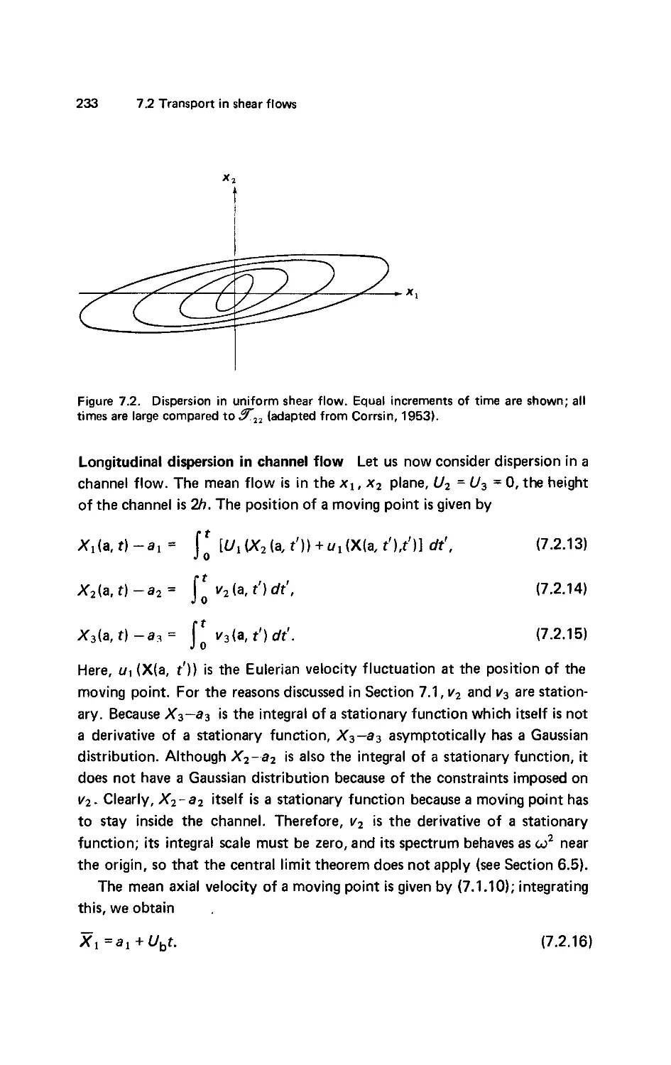
Uniform shear flow 230. Joint statistics 232. Longitudinal dispersion in
channel flow 233. Bulk velocity measurements in pipes 235.
7.3
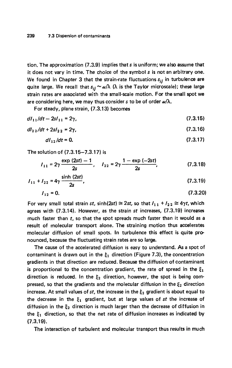
Dispersion of contaminants 235
The concentration distribution 235. The effects of molecular transport 237.
The effect of pure, steady strain 238. Transport at large scales 241.
7.4
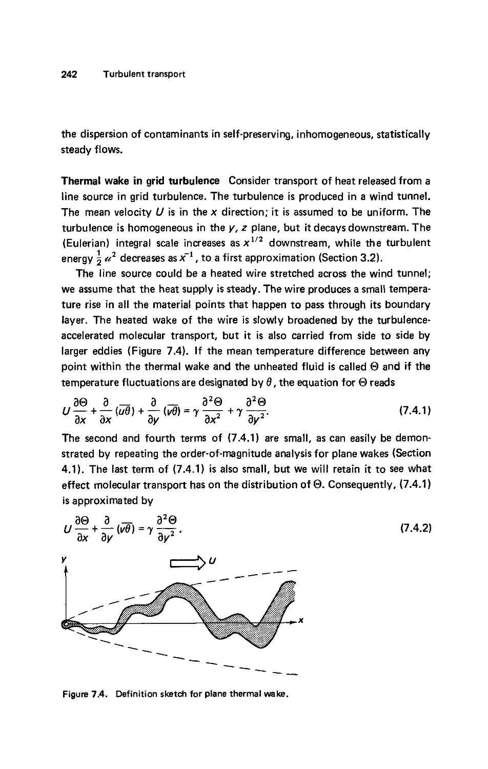
Turbulent transport in evolving flows 241
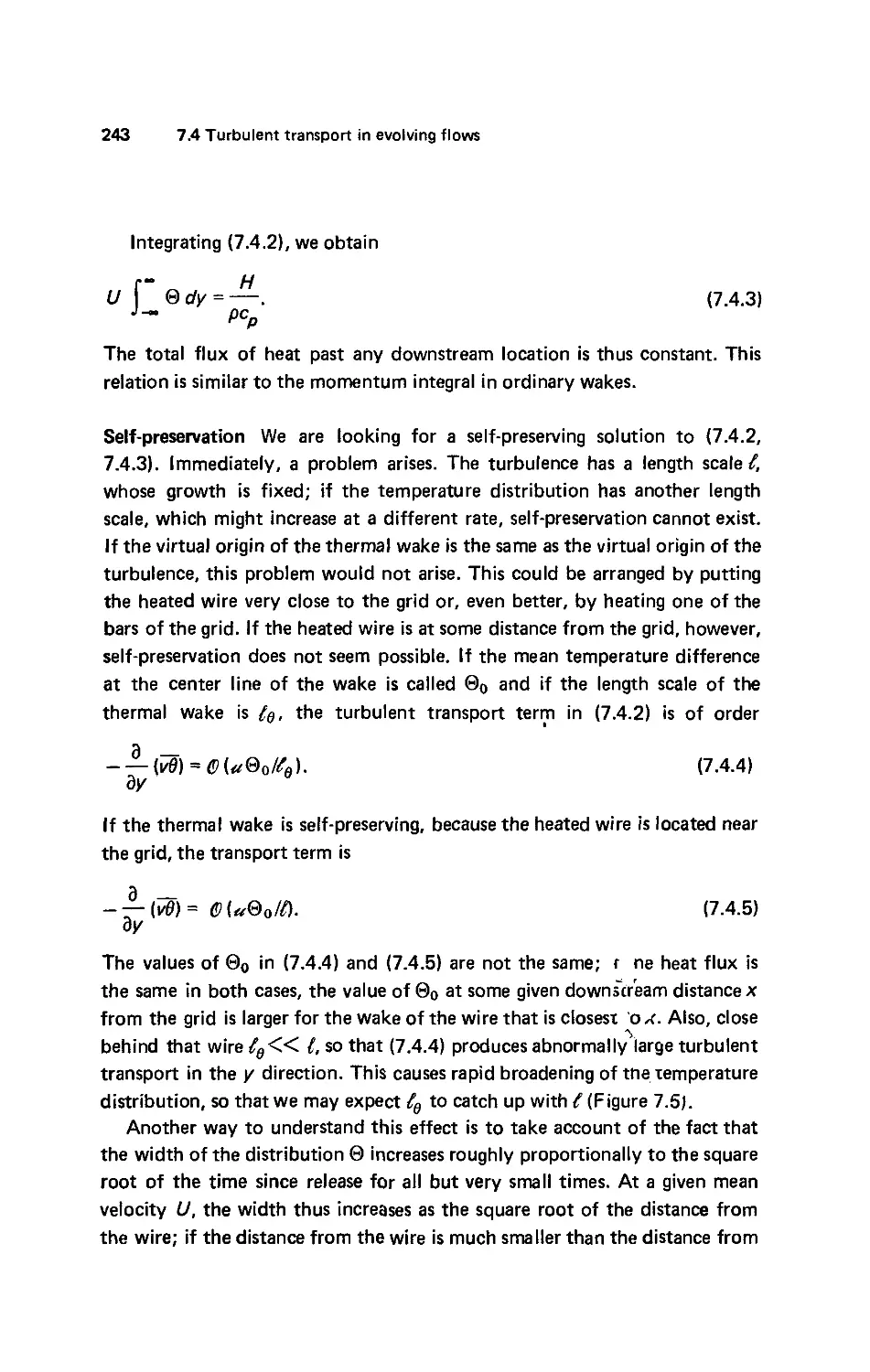
Thermal wake in grid turbulence 242. Self-preservation 243. Dispersion rela-
relative to the decaying turbulence 245. The Gaussian distribution 246. Disper-
Dispersion in shear flows 246.
8.
SPECTRAL DYNAMICS 248
8.1
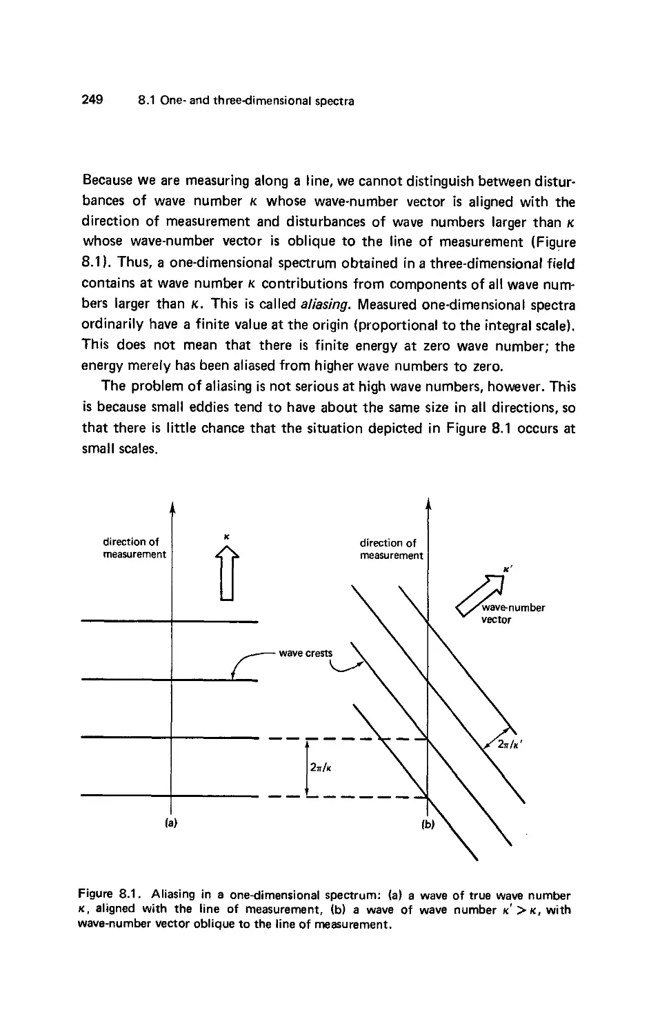
One- and three-dimensional spectra 248
Aliasing in one-dimensional spectra 248. The three-dimensional spec-
spectrum 250. The correlation tensor and its Fourier transform 250. Two
Contents
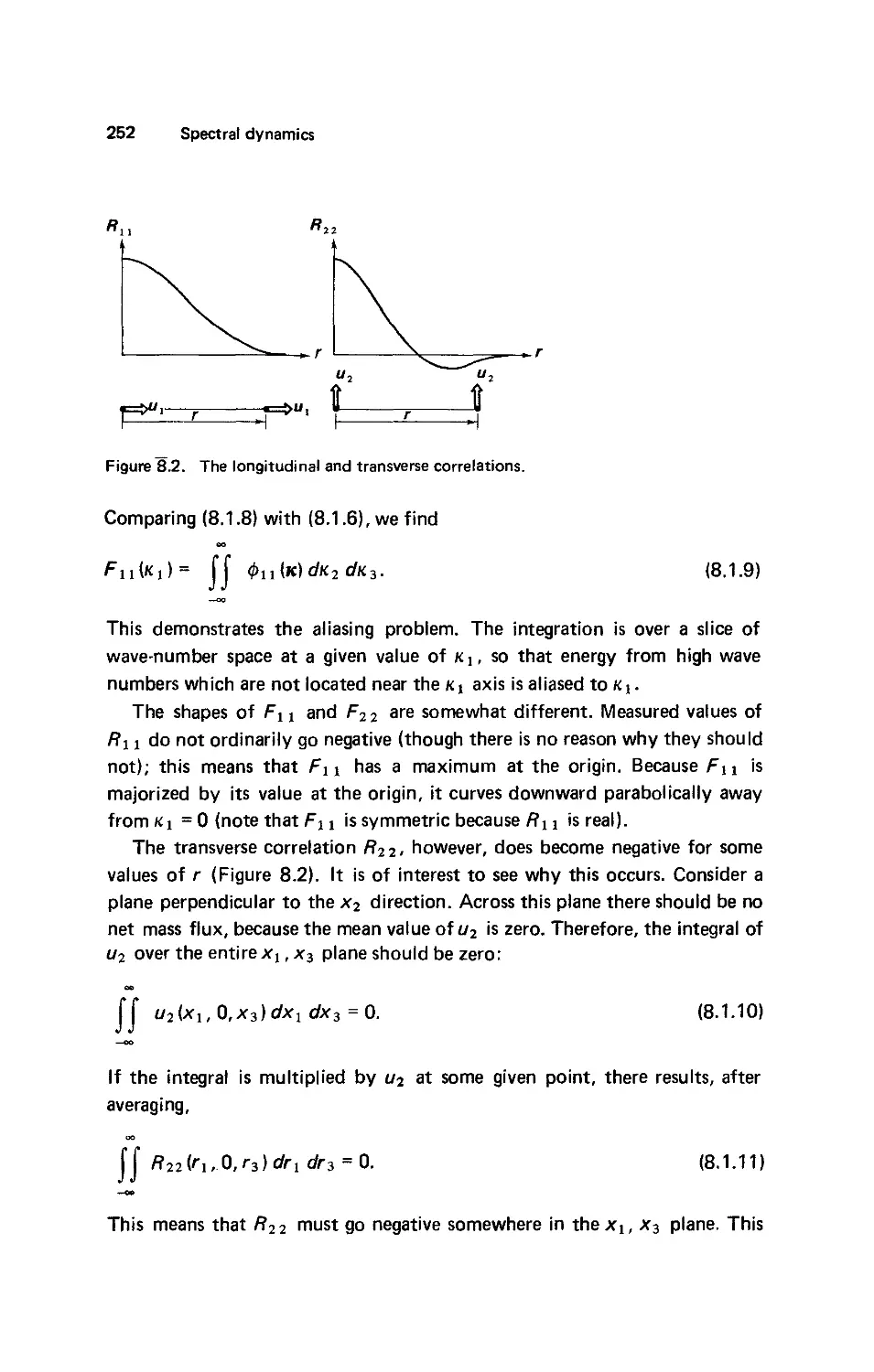
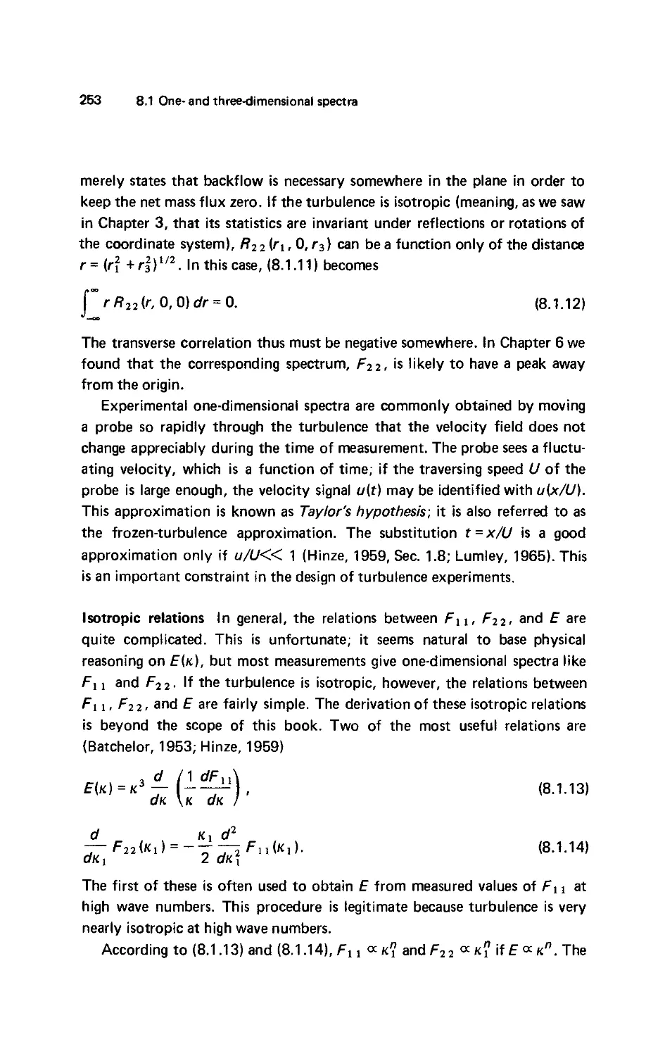
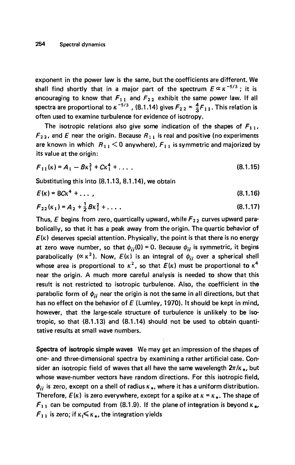
common one-dimensional spectra 251. Isotropic relations 253. Spectra of
isotropic simple waves 254.
8.2
The energy cascade 256
Spectral energy transfer 258. A simple eddy 258. The energy cascade 260.
8.3
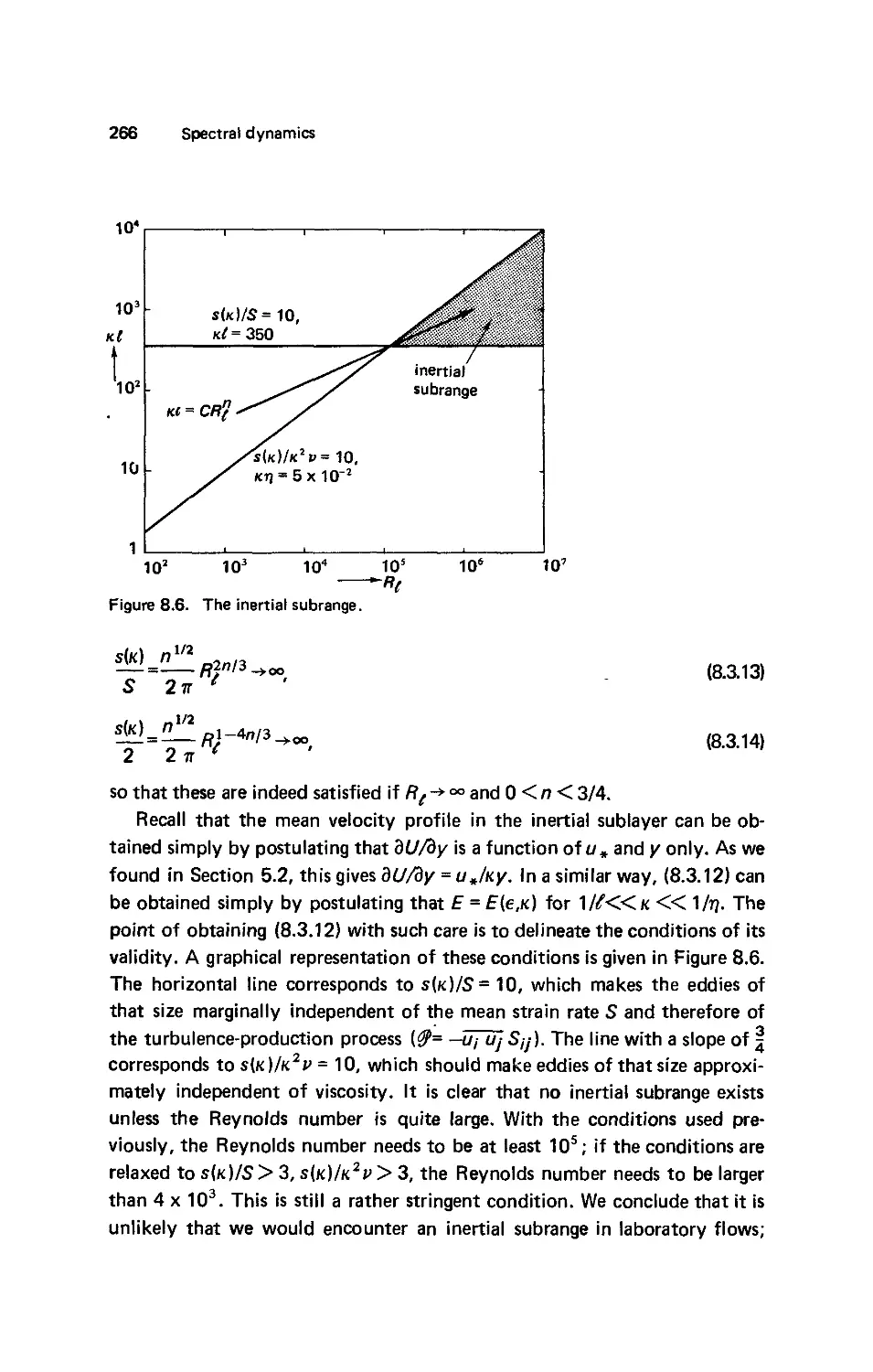
The spectrum of turbulence 262
The spectrum in the equilibrium range 262. The large-scale spectrum 264.
The inertial subrange 264.
8.4
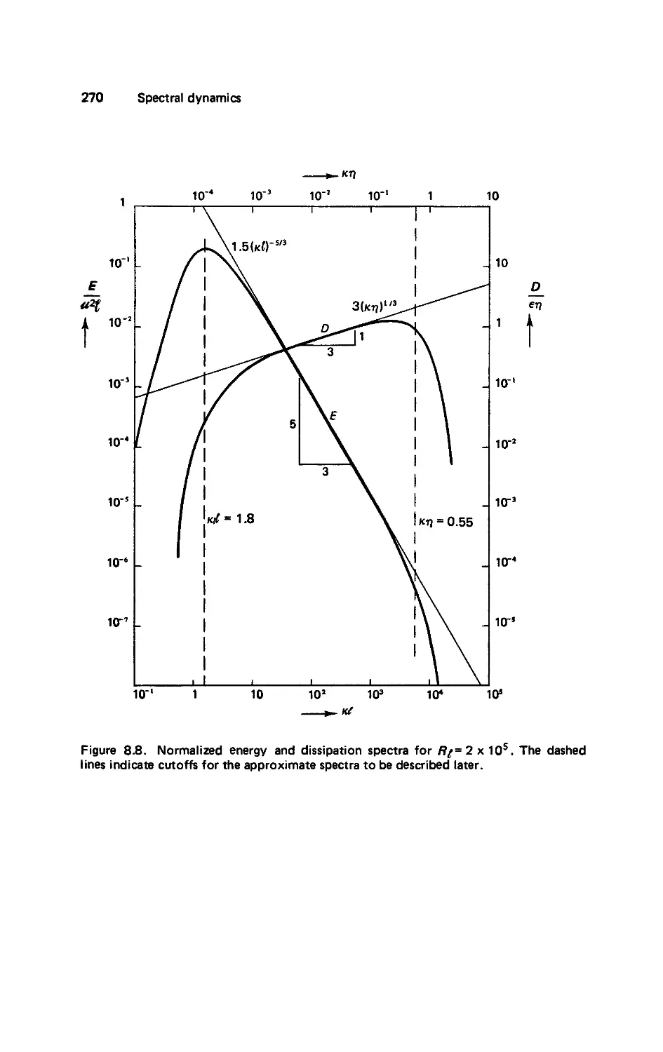
The effects of production and dissipation 267
The effect of dissipation 269. The effect of production 271. Approximate
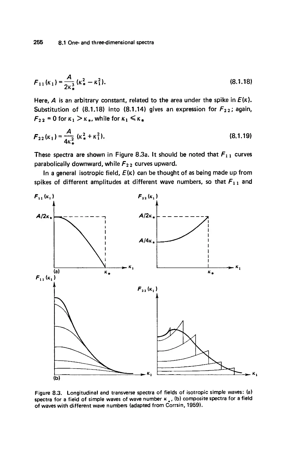
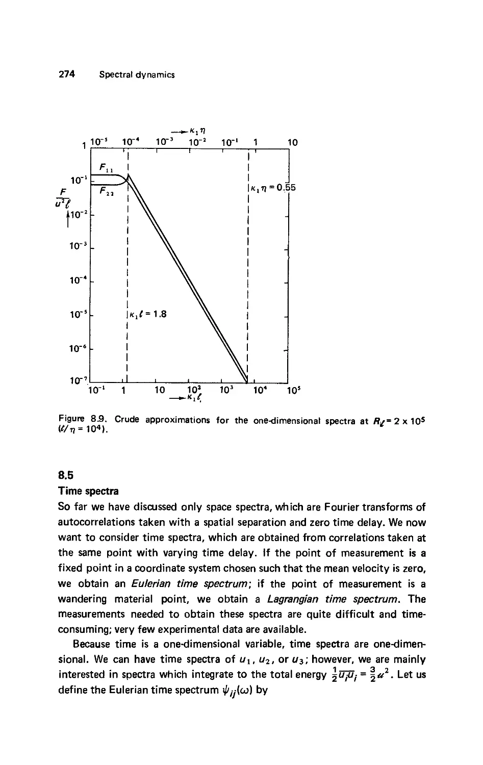
spectra for large Reynolds numbers 272.
8.5
Time spectra 274
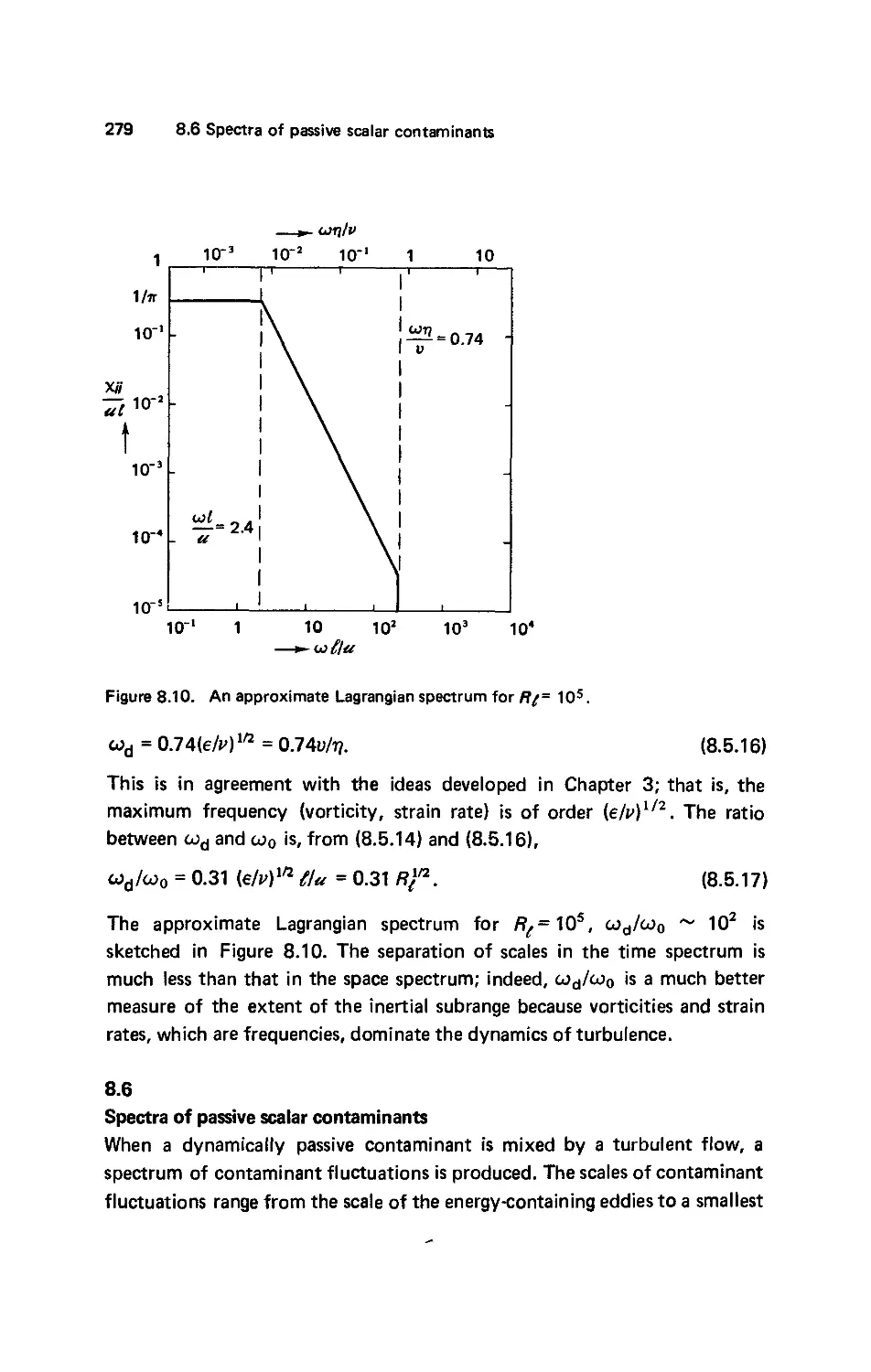
The inertial subrange 277. The Lagrangian integral time scale 277. An
approximate Lagrangian spectrum 278.
8.6
Spectra of passive scalar contaminants 279
One- and three-dimensional spectra 280. The cascade in the temperature
spectrum 281. Spectra in the equilibrium range 282. The inertial-diffusive
subrange 283. The viscous-convective subrange 284. The viscous-diffusive
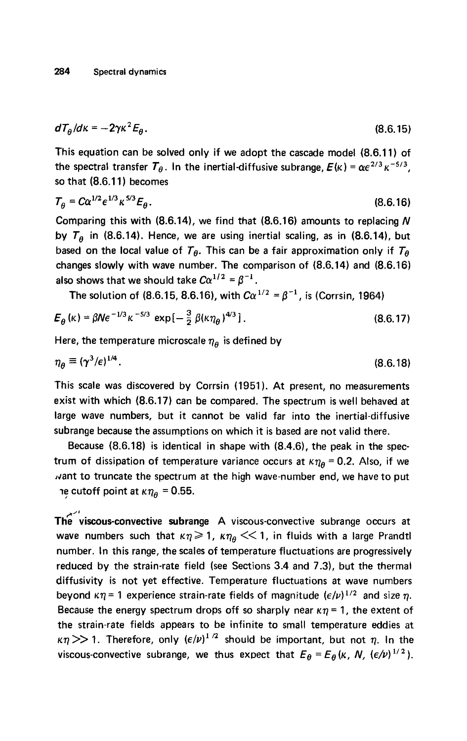
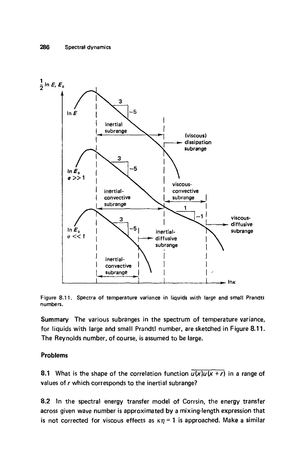
subrange 285. Summary 286.
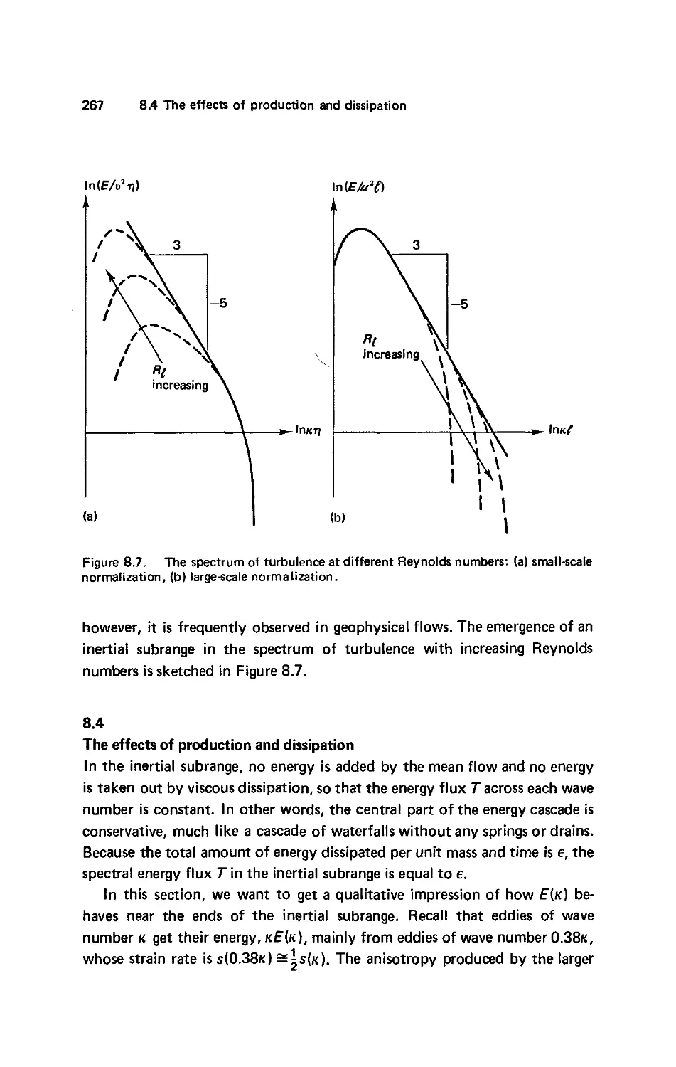
Bibliography and references 288
Index 295
PREFACE
In the customary description of turbulence, there are always more unknowns
than equations. This is called the closure problem; at present, the gap can be
closed only with models and estimates based on intuition and experience. For
a newcomer to turbulence, there is yet another closure problem: several
dozen introductory texts in general fluid dynamics exist, but the gap between
these and the monographs and advanced texts in turbulence is wide. This
book is designed to bridge the second closure problem by introducing the
reader to the tools that must be used to bridge the first.
A basic tool of turbulence theory is dimensional analysis; it is always used
in conjunction with an appeal to the idea that turbulent flows should be
independent of the Reynolds number if they are scaled properly. These tools
are sufficient for a first study of most problems in turbulence; those requiring
sophisticated mathematics have been avoided wherever possible. Of course,
dimensional reasoning is incapable of actually solving the equations governing
turbulent flows. A direct attack on this problem, however, is beyond the scope
of this book because it requires advanced statistics and Fourier analysis. Also,
even the most sophisticated studies, so far, have met with relatively little
success. The purpose of this book is to introduce its readers to turbulence; it
is neither a research monograph nor an advanced text.
Some understanding of viscous-flow and boundary-layer theory is a pre-
prerequisite for a successful study of much of the material presented here. On
the other hand, we assume that the reader is not familiar with stochastic
processes and Fourier transforms. Because the Reynolds stress is a second-
rank tensor, the use of tensor notation could not be avoided; however, very
little tensor analysis is needed to understand elementary operations on the
equations of motion in Cartesian coordinate systems.
We use most of the material in this book in an introductory turbulence
course for college seniors and first-year graduate students. We feel that this
book can also serve as a supplementary text for courses in general fluid
dynamics. We have attempted to avoid a bias toward any specific discipline,
in the hope that the material will be useful for meteorologists, oceanographers,
and astrophysicists, as well as for aerospace, mechanical, chemical, and pollu-
pollution control engineers.
The scope of this book did not permit us to describe the experimental
methods used in turbulence research. Also, because this is an introduction to
xii Preface
turbulence, we have not attempted to give an exhaustive list of references.
The bibliography lists the books devoted to turbulence as well as some major
papers. The most comprehensive of the recent books is Monin and Yaglom's
Statistical Fluid Mechanics (Monin and Yaglom, 1971); it contains a complete
bibliography of the current journal literature.
The manuscript was read by Dr. S. Corrsin and Dr. J. A. B. Wills; they
offered many valuable comments. Miss Constance Hazuda typed several drafts
and the final manuscript. A preliminary set of lecture notes was compiled in
1967 by Mr. A. S. Chaplin. Several generations of students contributed to the
development of the presentation of the material. While writing this book, the
authors received research support from the Atmospheric Sciences Section,
National Science Foundation, under grants GA-1019 and GA-18109.
HT
JLL
June 1970
BRIEF GUIDE ON THE USE OF SYMBOLS
The theory of turbulence contains many, often crude, approximations. Many
relations (except the equations of motion and their formal consequences)
therefore do not really permit the use of the equality sign. We adopt the
following usage. If the error involved in writing an equation is smaller than
about 30%, we use the approximate equality sign s. For crude approxima-
approximations the symbol ~ is employed. This generally means that the nondimen-
nondimensional coefficient that would make the relation an equation is not greater
than 5 and not smaller than 1/5. If the value of the coefficient is of interest
(for example, if the theory is to be compared with experimental data or if a
statement about the coefficient is in order), the equality sign is used and the
coefficient is entered explicitly. If the problem discussed is the selection of
the dominant terms in an equation of motion, the order symbol 0, which
does not make any commitment on the value of the coefficient, is employed.
After the dominant terms have been selected, the equality sign is used in the
resulting simplified equation, with the understanding that the error involved
can be made arbitrarily small by increasing the parameter in the problem
(often a Reynolds number) without limit. We do not claim that we have been
completely consistent, but in most cases the meaning of the symbols is made
clear in the text.
Though it may sometimes seem confusing, this usage serves as a continuing
reminder that relatively few accurate statements can be made about a turbu-
turbulent flow without recourse to experimental evidence on that flow. If one has
to study a flow for which no data are available, all one can do is to find the
characteristic parameters (velocity, length, time, and other scales) and to
make crude (say within a factor of two) estimates of the properties of the
flow. This is no mean accomplishment; it allows one to design an experiment
in a sensible way and to select the appropriate nondimensional form in which
the experimental data should be presented.
1
INTRODUCTION
Most flows occurring in nature and in engineering applications are turbulent.
The boundary layer in the earth's atmosphere is turbulent (except possibly in
very stable conditions); jet streams in the upper troposphere are turbulent;
cumulus clouds are in turbulent motion. The water currents below the surface
of the oceans are turbulent,; the Gulf Stream is a turbulent wall-jet kind of
flow. The photosphere of the sun and the photospheres of similar stars are in
turbulent motion; interstellar gas clouds (gaseous nebulae) are turbulent; the
wake of the earth in the solar wind is presumably a turbulent wake. Boundary
layers growing on aircraft wings are turbulent. Most combustion processes
involve turbulence and often even depend on it; the flow of natural gas and
oil in pipelines is turbulent. Chemical engineers use turbulence to mix and
homogenize fluid mixtures and to accelerate chemical reaction rates in liquids
or gases. The flow of water in rivers and canals is turbulent; the wakes of
ships, cars, submarines, and aircraft are in turbulent motion. The study
of turbulence clearly is an interdisciplinary activity, which has a very
wide range of applications. In fluid dynamics laminar flow is the exception,
not the rule: one must have small dimensions and high viscosities to
encounter laminar flow. The flow of lubricating oil in a bearing is a typical
example.
Many turbulent flows can be observed easily; watching cumulus clouds or
the plume of a smokestack is not time wasted for a student of turbulence.
In the classroom, some of the films produced by the National Committee
for Fluid Dynamics Films (for example, Stewart, 1969) may be used to
advantage.
1.1
The nature of turbulence
Everyone who, at one time or another, has observed the efflux from a smoke-
smokestack has some idea about the nature of turbulent flow. However, it is very
difficult to give a precise definition of turbulence. All one can do is list
some of the characteristics of turbulent flows.
Irregularity One characteristic is the irregularity, or randomness, of all
turbulent flows. This makes a deterministic approach to turbulence problems
impossible; instead, one relies on statistical methods.
Introduction
Diffusivity The diffusivity of turbulence, which causes rapid mixing and
increased rates of momentum, heat, and mass transfer, is another important
feature of all turbulent flows. If a flow pattern looks random but does not
exhibit spreading of velocity fluctuations through the surrounding fluid, it is
surely not turbulent. The contrails of a jet aircraft are a case in point: exclud-
excluding the turbulent region just behind the aircraft, the contrails have a very
nearly constant diameter for several miles. Such a flow is not turbulent, even
though it was turbulent when it was generated. The diffusivity of turbulence is
the single most important feature as far as applications are concerned: it
prevents boundary-layer separation on airfoils at large (but nottoo large) angles
of attack, it increases heat transfer rates in machinery of all kinds, it is the source
of the resistance of flow in pipelines, and it increases momentum transfer
between winds and ocean currents.
Large Reynolds numbers Turbulent flows always occur at high Reynolds
numbers. Turbulence often originates as an instability of laminar flows if the
Reynolds number becomes too large. The instabilities are related to the inter-
interaction of viscous terms and nonlinear inertia terms in the equations of mo-
motion. This interaction is very complex: the mathematics of nonlinear partial
differential equations has not been developed to a point where general solu-
solutions can be given. Randomness and nonlinearity combine to make the equa-
equations of turbulence nearly intractable; turbulence theory suffers from the
absence of sufficiently powerful mathematical methods. This lack of tools
makes all theoretical approaches to problems in turbulence trial-and-error
affairs. Nonlinear concepts and mathematical tools have to be developed
along the way; one cannot rely on the equations alone to obtain answers to
problems. This situation makes turbulence research both frustrating and
challenging: it is one of the principal unsolved problems in physics today.
Three-dimensional vorticity fluctuations Turbulence is rotational and three
dimensional. Turbulence is characterized by high levels of fluctuating vor-
vorticity. For this reason, vorticity dynamics plays an essential role in the des-
description of turbulent flows. The random vorticity fluctuations that char-
characterize turbulence could not maintain themselves if the velocity fluctuations
were two dimensional, since an important vorticity-maintenance mechanism
known as vortex stretching is absent in two-dimensional flow. Flows that are
substantially two dimensional, such as the cyclones in the atmosphere which
1.1 The nature of turbulence
determine the weather, are not turbulence themselves, even though their char-
characteristics may be influenced strongly by small-scale turbulence (generated
somewhere by shear or buoyancy), which interacts with the large-scale flow.
In summary, turbulent flows always exhibit high levels of fluctuating vor-,
ticity. For example, random waves on the surface of oceans are not in turbu-
turbulent motion since they are essentially irrotational.
Dissipation Turbulent flows are always dissipative. Viscous shear stresses
perform deformation work which increases the internal energy of the fluid at
the expense of kinetic energy of the turbulence. Turbulence needs a continu-
continuous supply of energy to make up for these viscous losses. If no energy is
supplied, turbulence decays rapidly. Random motions, such as gravity waves
in planetary atmospheres and random sound waves (acoustic noise), have
insignificant viscous losses and, therefore, are not turbulent. In other words,
the major distinction between random waves and turbulence is that waves are
essentially nondissipative (though they often are dispersive), while turbulence
is essentially dissipative.
Continuum Turbulence is a continuum phenomenon, governed by the equa-
equations of fluid mechanics. Even the smallest scales occurring in a turbulent
flow are ordinarily far larger than any molecular length scale. We return to
this point in Section 1.5.
Turbulent flows are flows Turbulence is not a feature of fluids but of fluid
flows. Most of the dynamics of turbulence is the same in all fluids, whether
they are liquids or gases, if the Reynolds number of the turbulence is large
enough; the major characteristics of turbulent flows are not controlled by the
molecular properties of the fluid in which the turbulence occurs. Since the
equations of motion are nonlinear, each individual flow pattern has certain
unique characteristics that are associated with its initial and boundary condi-
conditions. No general solution to the Navier-Stokes equations is known; conse-
consequently, no general solutions to problems in turbulent flow are available.
Since every flow is different, it follows that every turbulent flow is different,
even though all turbulent flows have many characteristics in common.
Students of turbulence, of course, disregard the uniqueness of any particular
turbulent flow and concentrate on the discovery and formulation of laws that
describe entire classes or families of turbulent flows.
Introduction
The characteristics of turbulence depend on its environment. Because of
this, turbulence theory does not attempt to deal with all kinds and types of
flows in a general way. Instead, theoreticians concentrate on families of flows
with fairly simple boundary conditions, like boundary layers, jets, and wakes.
1.2
Methods of analysis
Turbulent flows have been investigated for more than a century, but, as was
remarked earlier, no general approach to the solution of problems in turbu-
turbulence exists. The equations of motion have been analyzed in great detail,
but it is still next to impossible to make accurate quantitative predictions
without relying heavily on empirical data. Statistical studies of the equations
of motion always lead to a situation in which there are more unknowns than
equations. This is called the closure problem of turbulence theory: one has to
make (very often ad hoc) assumptions to make the number of equations
equal to the number of unknowns. Efforts to construct viable formal pertur-
perturbation schemes have not been very successful so far. The success of attempts
to solve problems in turbulence depends strongly on the inspiration involved
in making the crucial assumption.
This book has been designed to get this point across. In turbulence, the
equations do not give the entire story. One must be willing to use (and
capable of using) simple physical concepts based on experience to bridge the
gap between the equations and actual flows. We do not want to imply that
the equations are of little use; we merely want to make it unmistakably clear
that turbulence needs spirited inventors just as badly as dedicated analysts.
We recognize that this is a very specific, and possibly biased, point of view. It
is possible that at some time in the future, someone will succeed in developing
a completely formal theory of turbulence. However, we believe that there is a
far better chance of developing a physical model of turbulence in the spirit of
the Rutherford model of the atom. The model need not be complete, but it
would be very useful. The real challenge, it seems to us, is that no adequate
model of turbulence exists today.
Turbulence theory is limited in the same way that general fluid dynamics
would be if the Stokes relation between stress and rate of strain in Newtonian
fluids were unknown. This illustration is not arbitrary: one approach to tur-
turbulence theory is to postulate a relation between stress and rate of strain that
involves a turbulence-generated "viscosity," which then supposedly plays a
12 Methods of analysis
role similar to that of molecular viscosity in laminar flows. This approach is
based on a superficial resemblance between the way molecular motions trans-
transfer momentum and heat and the way in which turbulent velocity fluctuations
transfer these quantities. Phenomenological concepts like "eddy viscosity"
(to replace molecular viscosity) and "mixing length" (in analogy with the
mean free path in the kinetic theory of gases) were developed by Taylor,
Prandtl, and others. These concepts are studied in detail in Chapter 2.
Molecular viscosity is a property of flu ids; turbulence is a characteristic of
flows. Therefore, the use of an eddy viscosity to represent the effects of
turbulence on a flow is liable to be misleading. However, current research
seems to indicate that, in simple flows, we may, for analytical reasons, speak
of a turbulent fluid rather than of a turbulent flow. Turbulent "fluids,"
however, are non-Newtonian: they exhibit viscoelasticity and suffer memory
effects. In favorable circumstances, the memory is fading in time, so that one
may be able to develop a semilocal theory relating the mean stress to the
mean rate of strain.
Phenomenological theories of turbulence make crucial assumptions at a
fairly early stage in the analysis. In recent years, a group of theoreticians
(Kraichnan, Edwards, Orszag, Meecham, and others) have developed very
formal and sophisticated statistical theories of turbulence, in the hope of
finding a formalism that does not need ad hoc assumptions (see Orszag,
1971). So far, however, rather arbitrary postulates are needed in these
theories, too. The mathematical complexity of this work is so overwhelming
that a discussion of it has to be left out of this book.
Dimensional analysis One of the most powerful tools in the study of turbu-
turbulent flows is dimensional analysis. In many circumstances it is possible to
argue that some aspect of the structure of turbulence depends only on a few
independent variables or parameters. If such a situation prevails, dimensional
methods often dictate the relation between the dependent and independent
variables, which results in a solution that is known except for a numerical
coefficient. The outstanding example of this is the form of the spectrum of
turbulent kinetic energy in what is called the "inertial subrange."
Asymptotic invariance Another frequently used approach is to exploit some
of the asymptotic properties of turbulent flows. Turbulent flows are char-
characterized by very high Reynolds numbers; it seems reasonable to require that
Introduction
any proposed descriptions of turbulence should behave properly in the limit as
the Reynolds number approaches infinity. This is often a very powerful con-
constraint, which makes fairly specific results possible. The development of the
theory of turbulent boundary layers (Chapter 5) is a case in point. The limit
process involved in an asymptotic approach is related to vanishingly small
effects of the molecular viscosity. Turbulent flows tend to be almost indepen-
independent of the viscosity (with the exception of the very smallest scales of mo-
motion); the asymptotic behavior leads to such concepts as "Reynolds-number
similarity" (asymptotic invariance).
Local invariance Associated with, but distinct from, asymptotic invariance is
the concept of "self-preservation" or local invariance. In simple flow geom-
geometries, the characteristics of the turbulent motion at some point in time and
space appear to be controlled mainly by the immediate environment. The
time and length scales of the flow may vary slowly downstream, but, if the
turbulence time scales are small enough to permit adjustment to the gradually
changing environment, it is often possible to assume that the turbulence is
dynamically similar everywhere if nondimensionalized with local length and
time scales. For example, the turbulence intensity in a wake is of order
б Ьи/Ьу, where б is the local width of the wake and Ы1/Ьу is the average
mean-velocity gradient across the wake.
Because turbulence consists of fairly large fluctuations governed by non-
nonlinear equations, one may expect a behavior like that exhibited by simple
nonlinear systems with limit cycles. Such behavior should be largely indepen-
independent of initial conditions; the characteristics of the limit cycle should depend
only on the dynamics of the system and the constraints imposed on it. In the
same way, one expects that the structure of turbulence in a given class of
shear flows might be in some state of dynamical equilibrium in which local
inputs of energy should approximately balance local losses. If the energy
transfer mechanisms in turbulence are sufficiently rapid, so that effects of
past events do not dominate the dynamics, one may expect that this limit-
cycle type of equilibrium is governed mainly by local parameters such as scale
lengths and times. Simple dimensional methods and similarity arguments can
be very useful in this kind of situation. Because one may want to look for
local scaling laws (both in the spatial and the spectral domain), the problem
of finding appropriate length and time scales becomes an important one.
Indeed, scaling laws are at the heart of turbulence research.
1.3 The origin of turbulence
1.3
The origin of turbulence
In flows which are originally laminar, turbulence arises from instabilities at
large Reynolds numbers. Laminar pipe flow becomes turbulent at a Reynolds
number (based on mean velocity and diameter) in the neighborhood of 2,000
unless great care is taken to avoid creating small disturbances that might
trigger transition from laminar to turbulent flow. Boundary layers in zero
pressure gradient become unstable at a Reynolds number U8*/v = 600
approximately F* is the displacement thickness, U is the free-stream velo-
velocity, and v is the kinematic viscosity). Free shear flows, such as the flow in a
mixing layer, become unstable at very low Reynolds numbers because of an
inviscid instability mechanism that does not operate in boundary-layer and
pipe flow. Early stages of transition can easily be seen in the smoke rising
from a cigarette.
On the other hand, turbulence cannot maintain itself but depends on its
environment to obtain energy. A common source of energy for turbulent
velocity fluctuations is shear in the mean flow; other sources, such as buoy-
buoyancy, exist too. Turbulent flows are generally shear flows. If turbulence
arrives in an environment where there is no shear or other maintenance mech-
mechanism, it decays: the Reynolds number decreases and the flow tends to
become laminar again. The classic example is turbulence produced by a grid
in uniform flow in a wind tunnel.
Another way to make a turbulent flow laminar or to prevent a laminar
flow from becoming turbulent is to provide for a mechanism that consumes
turbulent kinetic energy. This situation prevails in turbulent flows with
imposed magnetic fields at low magnetic Reynolds numbers and in atmos-
atmospheric flows with a stable density stratification, to cite two examples.
Mathematically, the details of transition from laminar to turbulent flow
are rather poorly understood. Much of the theory of instabilities in laminar
flows is linearized theory, valid for very small disturbances; it cannot deal
with the large fluctuation levels in turbulent flow. On the other hand, almost
all of the theory of turbulent flow is asymptotic theory, fairly accurate at
very high Reynolds numbers but inaccurate and incomplete for Reynolds
numbers at which the turbulence cannot maintain itself. A noteworthy excep-
exception is the theory of the late stage of decay of wind-tunnel turbulence
(Batchelor, 1953).
Experiments have shown that transition is commonly initiated by a pri-
Introduction
тагу instability mechanism, which in simple cases is two dimensional. The
primary instability produces secondary motions, which are generally three
dimensional and become unstable themselves. A sequence of this nature gen-
generates intense localized three-dimensional disturbances (turbulent "spots"),
which arise at random positions at random times. These spots grow rapidly
and merge with each other when they become large and numerous to form a
field of developed turbulent flow. In other cases, turbulence originates from
an instability that causes vortices which subsequently become unstable. Many
wake flows become turbulent in this way.
1.4
Diffusivity of turbulence
The outstanding characteristic of turbulent motion is its ability to transport
or mix momentum, kinetic energy, and contaminants such as heat, particles,
and moisture. The rates of transfer and mixing are several orders of magni-
magnitude greater than the rates due to molecular diffusion: the heat transfer and
combustion rates of turbulent combustion in an incinerator are orders of
magnitude larger than the corresponding rates in the laminar flame of a
candle.
Diffusion in a problem with an imposed length scale Contrasting laminar and
turbulent diffusion rates is a useful exercise not only for getting acquainted
with turbulence but also for recognizing the multifaceted role of the Rey-
Reynolds number. Suppose one has a room (with a characteristic linear dimension
L) in which a heating element (radiator) is installed. If there is no air motion
in the room, heat has to be distributed by molecular diffusion. This process is
governed by the diffusion equation (в is the temperature; 7 is the thermal
diffusivity, assumed to be constant):
ьв ъ2е
- = ?—. d-4.1)
Of OX-OXj
We are not looking for a specific solution of A.4.1) with a given set of
boundary conditions. Instead, we want to discover the gross consequences of
A.4.1) with the simple tools of dimensional analysis. Dimensionally, A.4.1)
may be interpreted as
Д0 Д0
-~7T7, A.4.2)
1.4 Diffusivity of turbulence
where Ав is a characteristic temperature difference. From A.4.2), we obtain
Tm~^, A.4.3)
which relates the time scale 7~m of the molecular diffusion to the independent
parameters L and 7. If the characteristic linear dimension L (the length scale)
of the room is 5 m, the time scale Tm of this diffusion process is of the order
of 106 sec (more than 100 h). In this estimate the value of 7 for air at room
temperature and pressure has been used G = 0.20 cm2/sec). We conclude that
molecular diffusion is rather ineffective in distributing heat through a room.
On the other hand, even fairly weak motions, such as those generated by
small density differences (buoyancy), can disperse heat through the room
quickly. Suppose that the turbulent motion of the air in the room may also
be characterized by the length scale L (that is, motions are present of scales
< L). This is a fair assumption, since large-scale motions are most effective in
distributing heat and since the largest possible scales of motion can be no
larger than the size of the room. We also need a characteristic velocity и (this
и may be thought of as an rms amplitude of the velocity fluctuations in the
room). For flow with a length scale L and a velocity scale u, the characteristic
time is
Г~-. d-4.4)
и
Apparently, Tx can be determined only if и can be estimated. Suppose the
radiator heats the air in its vicinity by Ав degrees Kelvin. This causes a
buoyant acceleration дАв/в, which is of order 0.3 m/sec2 if Ав - 10°K.
This acceleration probably occurs only near the surface of the radiator. If it
has a height h = 0.1 m, the kinetic energy of the air above the radiator is
дпАв/в, which is of order 0.03 (m/secJ per unit mass. This corresponds to a
velocity of 17 cm/sec. Much of the kinetic energy, however, is lost because of
the stable vertical temperature gradient in the room (the air near the ceiling
tends to be hotter than the air near the floor). A characteristic velocity и of
order 5 cm/sec may be a reasonable average throughout the room. With
и = 5 cm/sec and L = 5 m, Tt becomes 100 sec, or about 2 min. Of course, we
still have to rely on molecular diffusion to even out small-scale irregularities
in the temperature distribution. However, the turbulence generates eddies as
small as about 1 cm (this estimate can be obtained with simple equations
10 Introduction
based on the dissipation of kinetic energy; those are discussed in Section 1.5).
The temperature gradients associated with these small eddies are smeared out
by molecular diffusion in a time of order^2/7 (see Section 7.3), which is only a
few seconds if t= 1 cm.
Diffusion by random motion apparently is very rapid compared to
molecular diffusion. The ratio of the turbulent time scale Tt to the molecular
time scale Tm is the inverse of the Peclet number:
Tt L у у
Tm и L2 uL
Since for gases the heat conductivity у is of the same order of magnitude as
the kinematic viscosity v (for air vly = 0.73; this ratio is known as the Prandtl
number), and since we are discussing only orders of magnitude, we may write
without compromise,
7"t v 1
In our example, the Reynolds number Я is about 15,000.
This exercise shows that the Reynolds number of a turbulent flow may be
interpreted as a ratio of a turbulence time scale to a molecular time scale that
would prevail in the absence of turbulence in a problem with the same length
scale. This point of view is often more reliable than thinking of Я as a ratio of
inertia terms to viscous terms in the governing equations. The latter point of
view tends to be misleading because at high Reynolds numbers viscous and
other diffusion effects tend to operate on smaller length scales than inertia
effects.
Eddy diffusivity Since the equations governing turbulent flow are very
complicated, it is tempting to treat the diffusive nature of turbulence by
means of a properly chosen effective diffusivity. In doing so, the idea of
trying to understand the turbulence itself is partly discarded. If we use an
effective diffusivity, we tend to treat turbulence as a property of a fluid
rather than as a property of a flow. Conceptually, this is a very dangerous
approach. However, it often makes the mathematics a good deal easier.
If the effects of turbulence could be represented by a simple, constant
scalar diffusivity, one should be able to write for the diffusion of heat by
turbulent motions,
11 1.4 Diffusivity of turbulence
30 Ь2в
9f dxfiX
in which К is the representative diffusivity (often called "eddy" diffusivity
but sometimes called the "exchange coefficient" for heat). In order to make
this equation at least a crude representation of reality, one must insist that the
value of К be chosen such that the time scale of the hypothetical turbulent
diffusion process is equal to that of the actual mixing process. The time scale
associated with A.4.7) is roughly
L2
T~—, A.4.8)
К
and the actual time scale is 7"t, given by A.4.4). Equating Г with 7"t, one finds
K~uL. A.4.9)
It should be noted that this is a dimensional estimate, which cannot predict
the numerical values of coefficients that may be needed. Expressions like
A.4.9), with experimentally determined coefficients, are used frequently in
practical applications.
The eddy diffusivity (or viscosity) К may be compared with the kinematic
viscosity v and the thermal conductivity 7:
К К uL
-a = Д. A.4.10)
У v v
One concludes that this particular Reynolds number may also be interpreted
as a ratio of apparent (or turbulent) viscosity to molecular viscosity. A note
of warning is in order, though. In most flow problems, many different length
scales exist, so that the interpretation of Reynolds numbers based on these
length scales may not always be as straightforward as in the example used
here.
It cannot be stressed too strongly that the eddy diffusivity К is an artifice
which may or may not represent the effects of turbulence faithfully. We
investigate this question carefully in Chapter 2.
Diffusion in a problem with an imposed time scale As another example of
the diffusivity of turbulence, we look at boundary layers in the atmosphere.
The boundary layer in the atmosphere is exposed to the rotation of the earth.
12 Introduction
In a rotating frame of reference, flows are accelerated by the Coriolis force,
which is twice the vector product of the flow velocity and the rotation rate.
If the angular velocity of the frame of reference is f/2, it follows that atmos-
atmospheric flows have an imposed time scale of order 1/^. At a latitude of 40
degrees, the value of f for a Cartesian coordinate system whose z axis is
parallel to the local vertical is about 10~4 sec (f is called the Coriolis
parameter).
If the boundary layer in the atmosphere were laminar, it would be
governed by a diffusion equation like A.4.1), so that its length and time
scales would be related by
L2m~vT. A.4.11)
With v = 0.15 cm2 sec and Т=Г1 = 104 sec, this gives Lm = 40 cm.
In reality, however, the atmospheric boundary layer is nearly always
turbulent; a typical thickness is about 103 m A km). One can obtain some
appreciation for this by replacing v by К in A.4.11) and substituting for К
with A.4.9). This yields
Lx~uT, A.4.12)
which, of course, merely rephrases A.4.4). In turbulent boundary-layer
flows, the characteristic velocity of the turbulence is typically about ^ of
the mean wind speed. For a wind speed of 10m/sec, we thus estimate that
u~0.3m/sec. With 7" = 1/f= 104 sec, A.4.12) then yields Z_t~3x10³m
C km), which is indeed of the same order as the observed thickness.
From a somewhat different point of view, we may argue that turbulent
eddies with a characteristic velocity u, exposed to a Coriolis acceleration
which imposes a time scale Mf, must have a size (length scale) of order u/f. It
should be noted that we can equate eddy size and boundary-layer thickness
only because in most turbulent flows the larger eddies seem to have sizes
comparable to the characteristic size of the flow in a direction normal to the
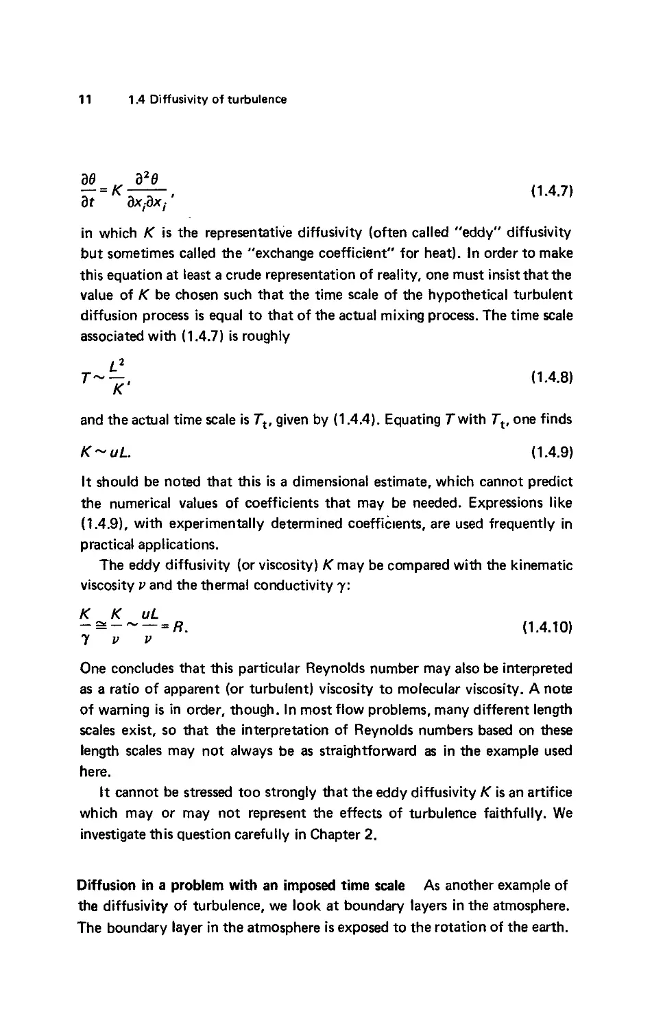
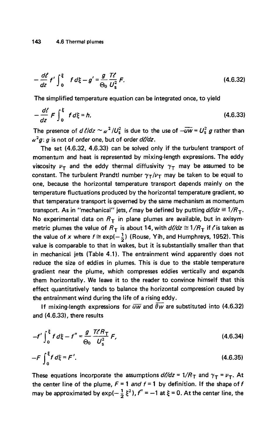
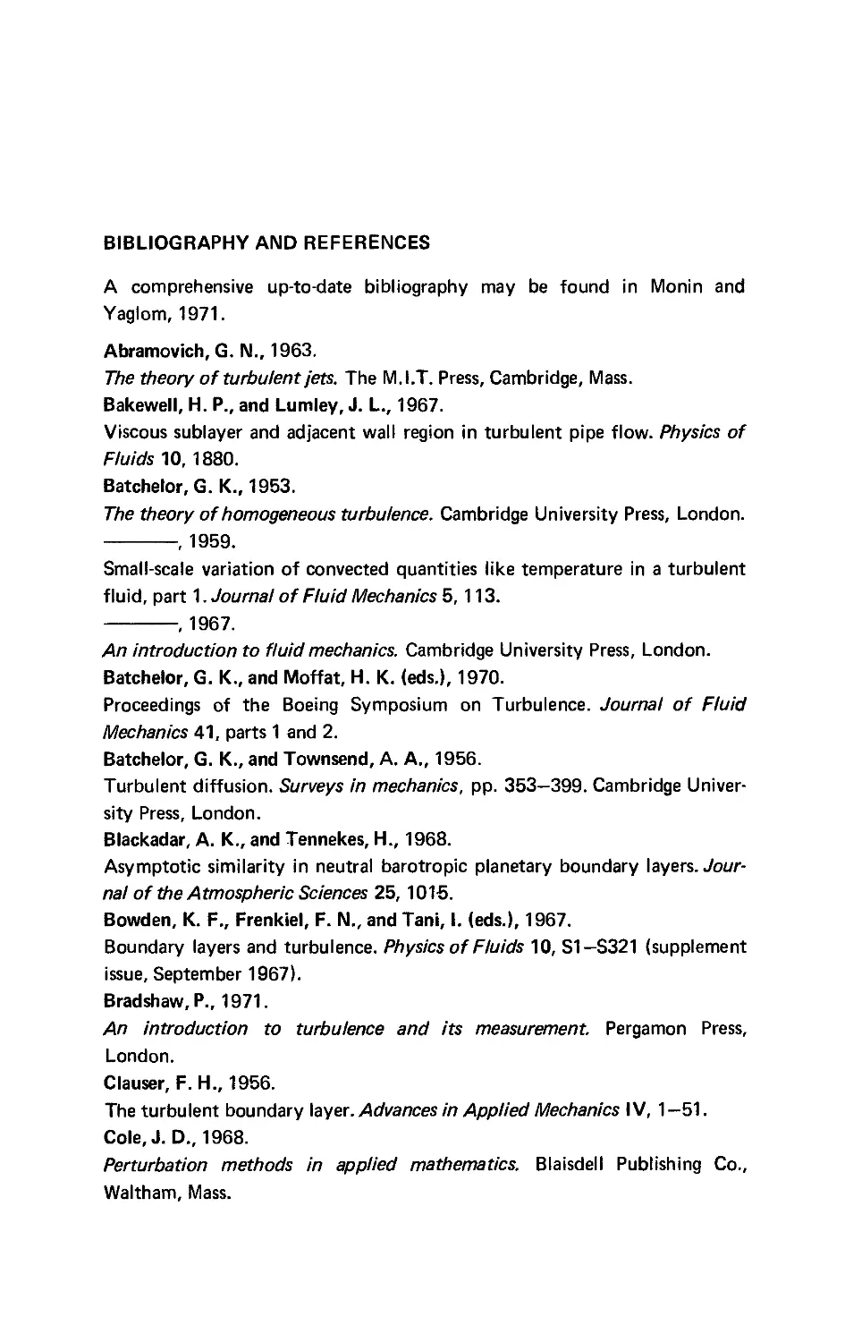
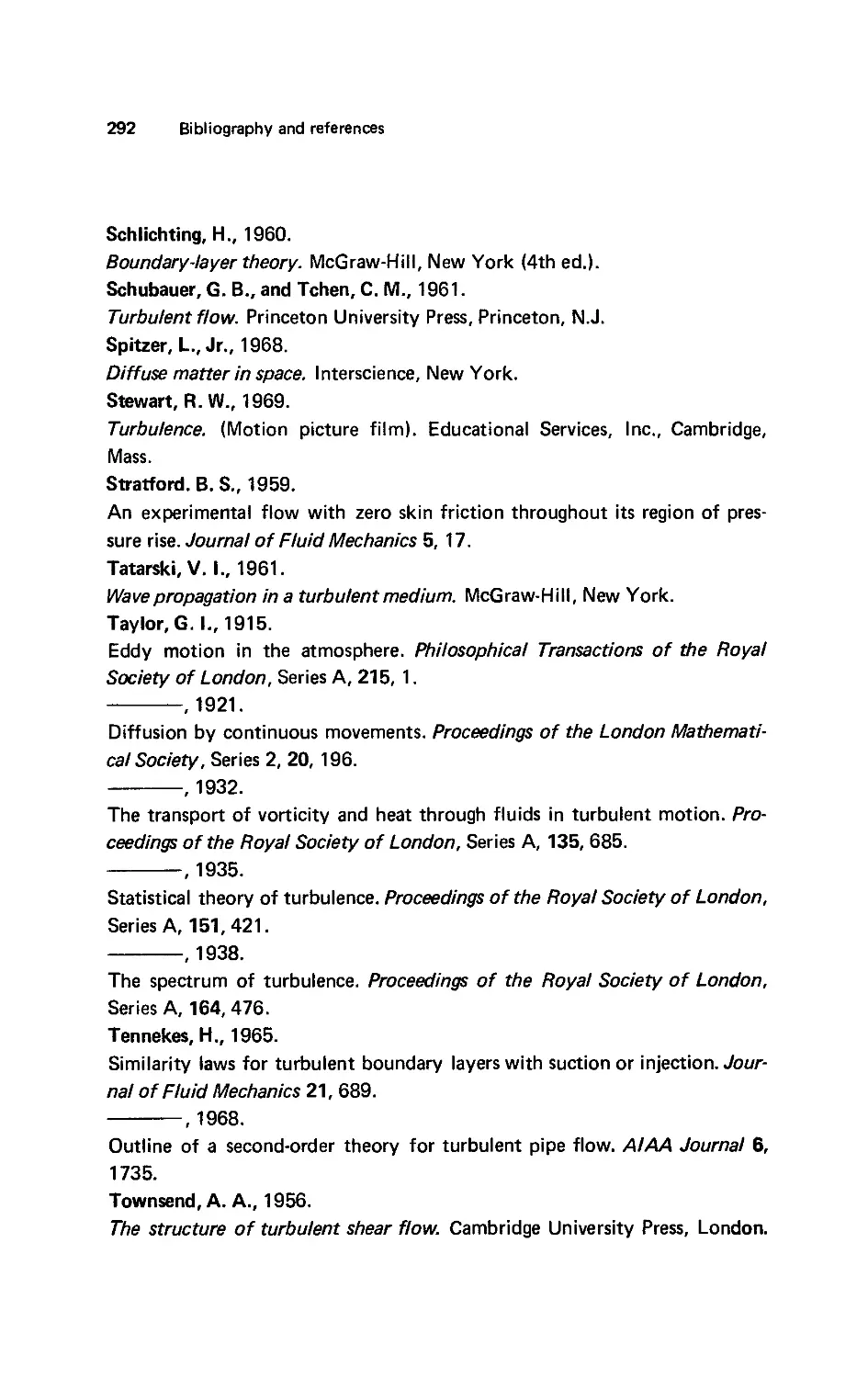
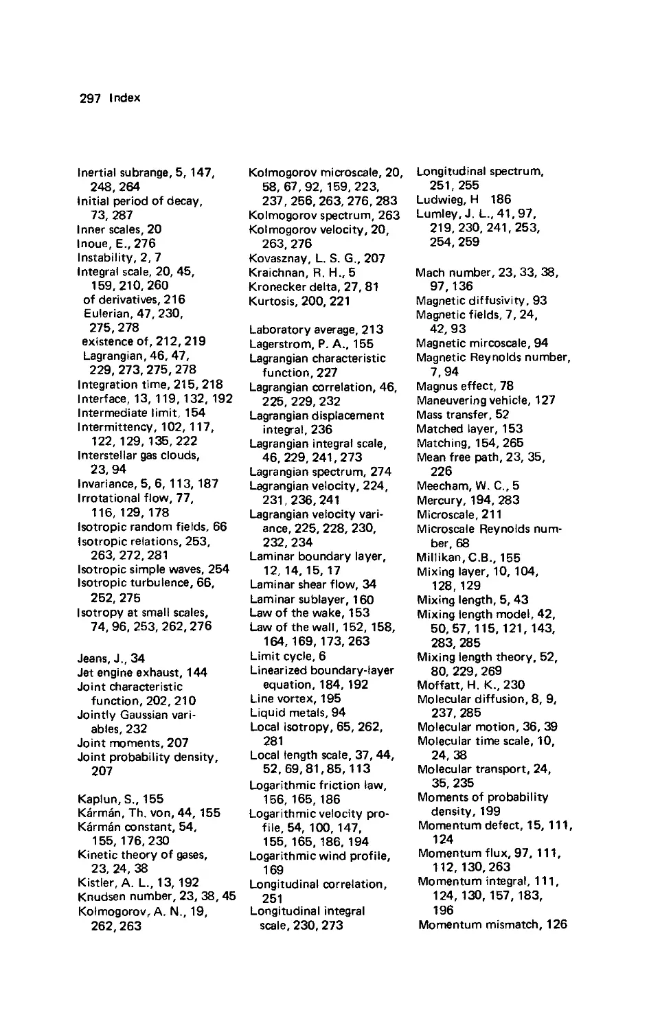
mean flow field (Figure 1.1). In estimates of diffusion or mixing, the large
eddies are relevant because they perform most of the mixing (К ~ u/increases
with eddy size).
Arguments of this nature are often supplemented by experiments to
determine the numerical coefficient in formulas like A.4.12), because this
coefficient cannot be found by dimensional reasoning. In the case of the
atmospheric boundary layer,
13
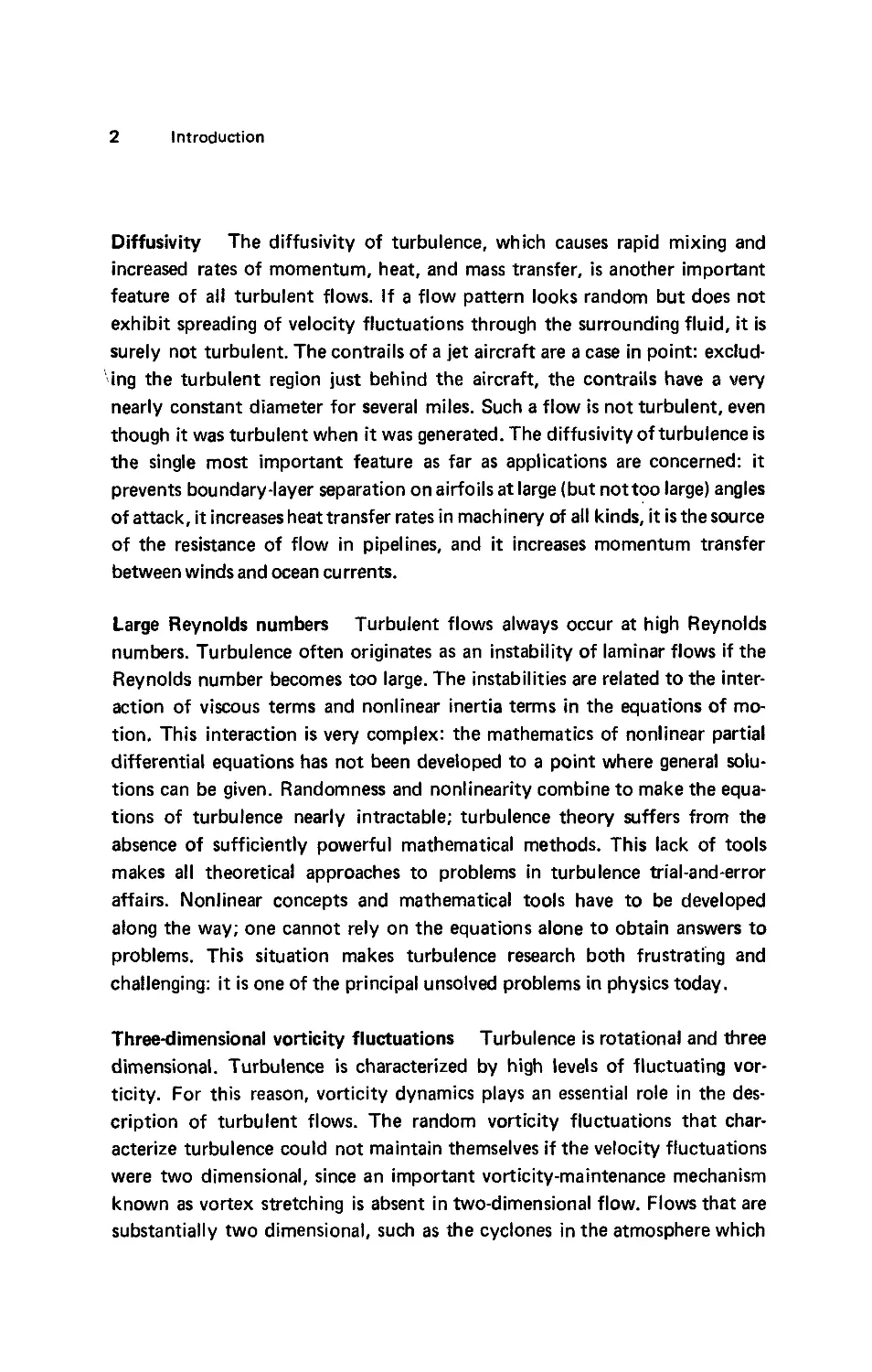
1.4 Diffusivity of turbulence
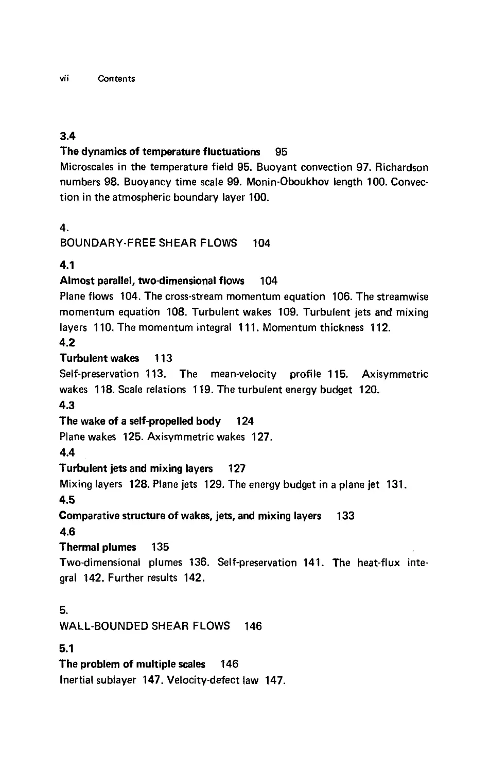
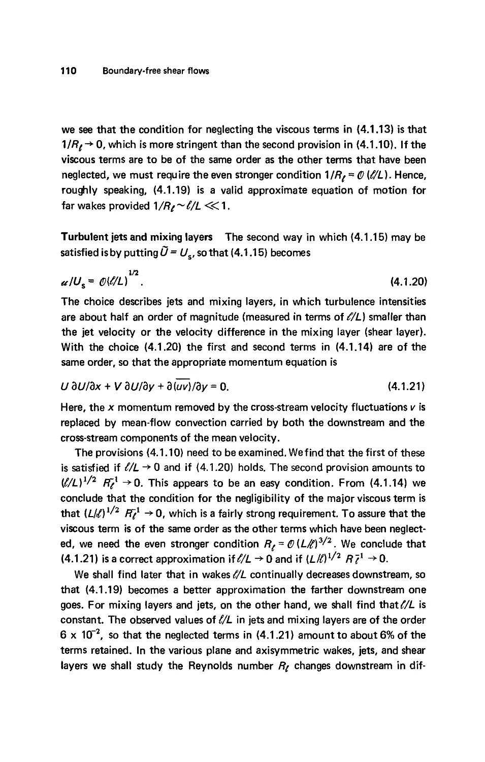
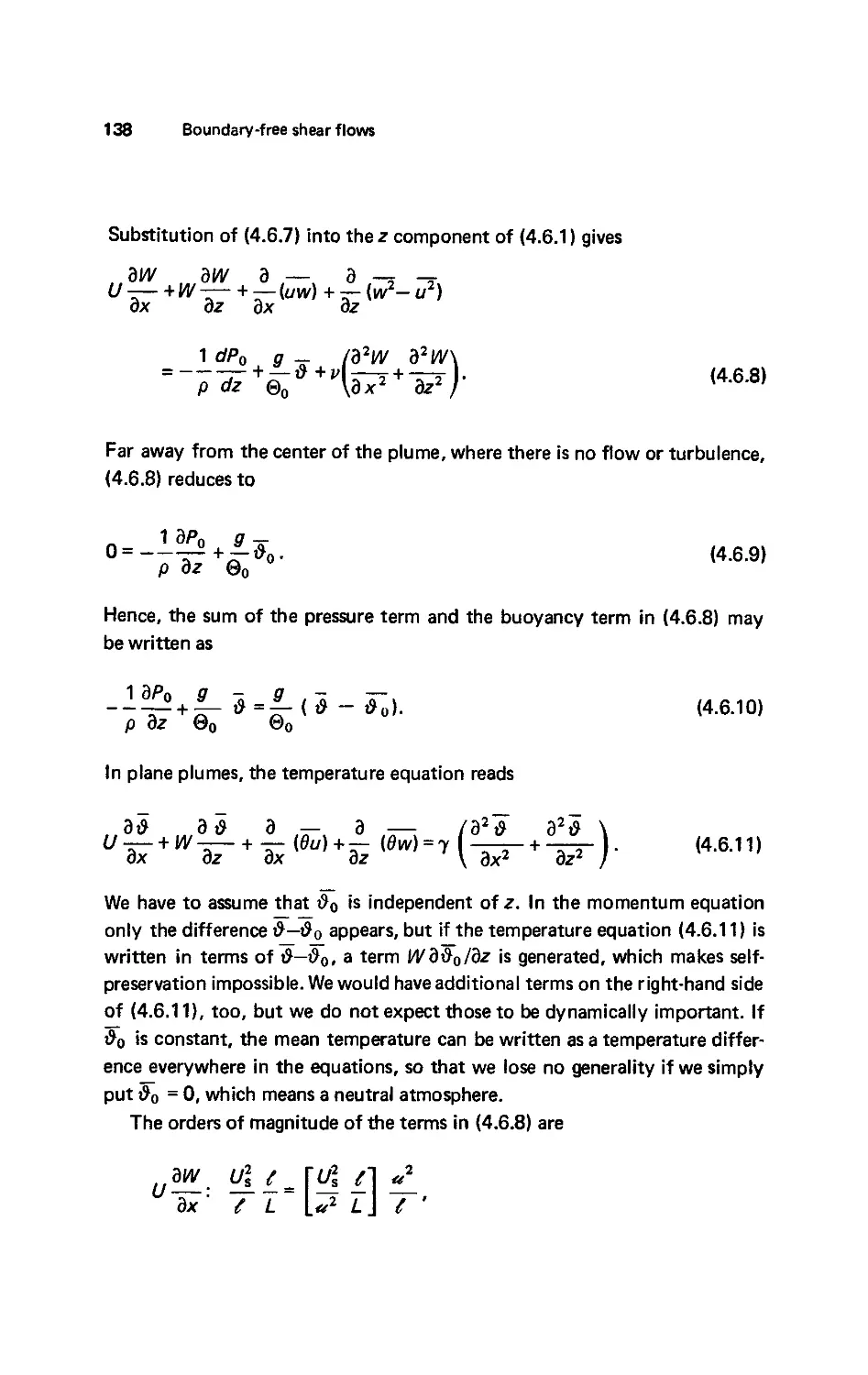
Figure 1.1. Large eddies in a turbulent boundary layer. The flow above the boundary
layer has a velocity I/; the eddies have velocities u. The largest eddy size it) is comparable
to the boundary-layer thickness (Lt). The interface between the turbulence and the flow
above the boundary layer is quite sharp (Corrsin and Kistler, 1954).
Lx = \ulf A.4.13)
would give very close agreement between "theory" and experimental evi-
evidence.
Using A.4.11), A.4.12), and T = Mf, we find the ratio between the
thicknesses of the laminar and turbulent atmospheric boundary layers to be
1/2
A.4.14)
Lm f\v) \fu)
_ о 1/2
This is the square root of the Reynolds number associated with the turbulent
boundary layer in the atmosphere, since u/f is proportional to the actual
length scale Lt. In this example, the Reynolds number Я is clearly associated
with the ratio of the turbulent and molecular diffusion length scales:
turbulent flow penetrates much deeper into the atmosphere than laminar
flow. In our example, Я ~ 107.
The results obtained here concerning the different aspects of the Reynolds
number may be summarized by stating that in flows with imposed length
scales the Reynolds number is proportional to the ratio of time scales, while
in flows with imposed time scales the Reynolds number is proportional to the
square of a ratio of length scales. Since the Reynolds numbers of most flows
are large, these relations clearly show that turbulence is a far more effective
diffusion agent than molecular motion.
14 Introduction
The examples discussed here are rather crude because only a single length
or time scale has been taken into account. Most turbulent flows are far more
complicated; this introduction would not be complete without a look at
turbulence as a multiple length-scale problem.
1.5
Length scales in turbulent flows
The fluid dynamics of flows at high Reynolds numbers is characterized by the
existence of several length scales, some of which assume very specific roles in
the description and analysis of flows. In turbulent flows a wide range of
length scales exists, bounded from above by the dimensions of the flow field
and bounded from below by the diffusive action of molecular viscosity.
Incidentally, this is the reason why spectral analysis of turbulent motion is
useful.
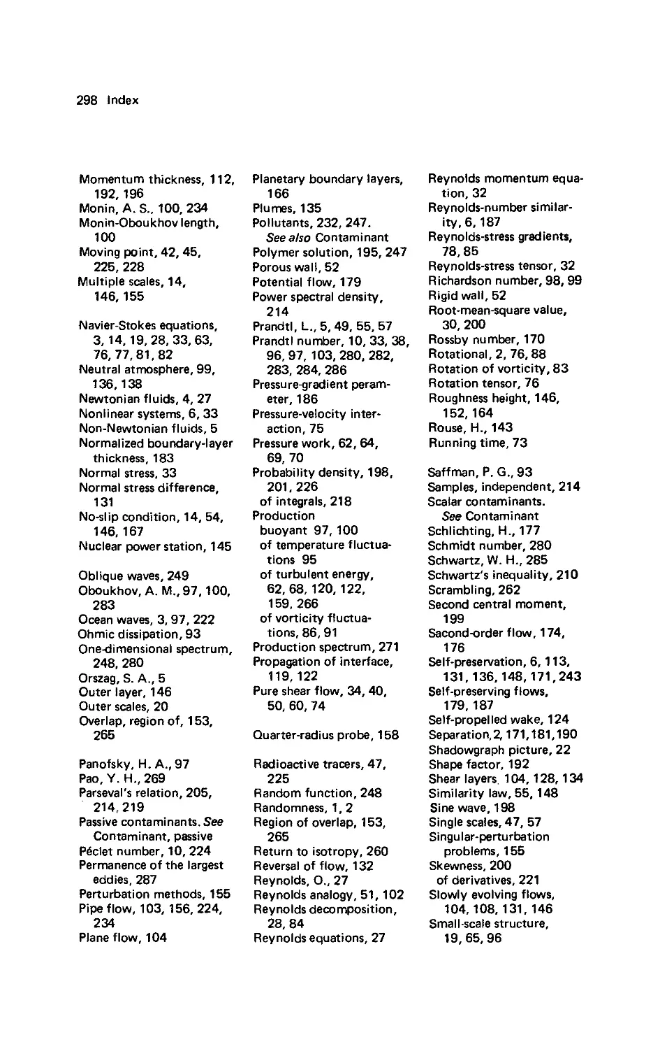
Laminar boundary layers Let us take a look at the problem of multiple
scales in laminar shear flows. For steady flow of an incompressible fluid with
constant viscosity, the Navier-Stokes equations are
^ Ъи, _ 1 Эр | ^ Э2ц- A51)
1 Эх, р Эх,- ЭхуЭху'
One would be tempted to estimate the inertia terms as U2/L (U being a
characteristic velocity and L a characteristic length) and to estimate the
viscous terms as vil/L2. The ratio of these terms is UL/v = R, indicating that
viscous terms should become negligible at large Reynolds numbers. However,
boundary conditions or initial conditions may make it impossible to neglect
viscous terms everywhere in the flow field. For example, a boundary layer has
to exist in the flow along a solid surface to satisfy the no-slip condition. This
can be understood by allowing for the possibility that viscous effects may be
associated with small length scales. The viscous terms can survive at high
Reynolds numbers only by choosing a new length scale ^such that the viscous
terms are of the same order of magnitude as the inertia terms. Formally,
U2IL~vU/t2. A.5.2)
The viscous length t is thus related to the scale L of the flow field as
/ / v V2
f~(- -„-». (,.5.3,
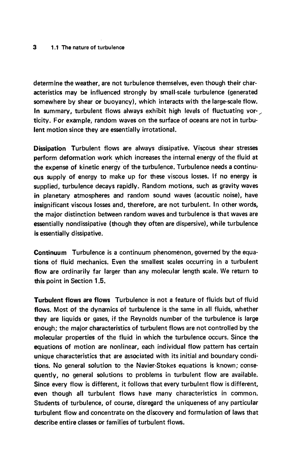
15
1.5 Length scales in turbulent flows
The viscous length ( is a transverse length scale: it represents the width
(thickness) of the boundary layer, because it relates to the molecular
diffusion of momentum deficit across the flow, away from the surface.
Molecular diffusion along the flow, of course, is negligible compared to the
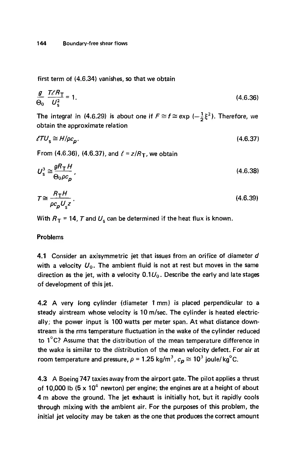
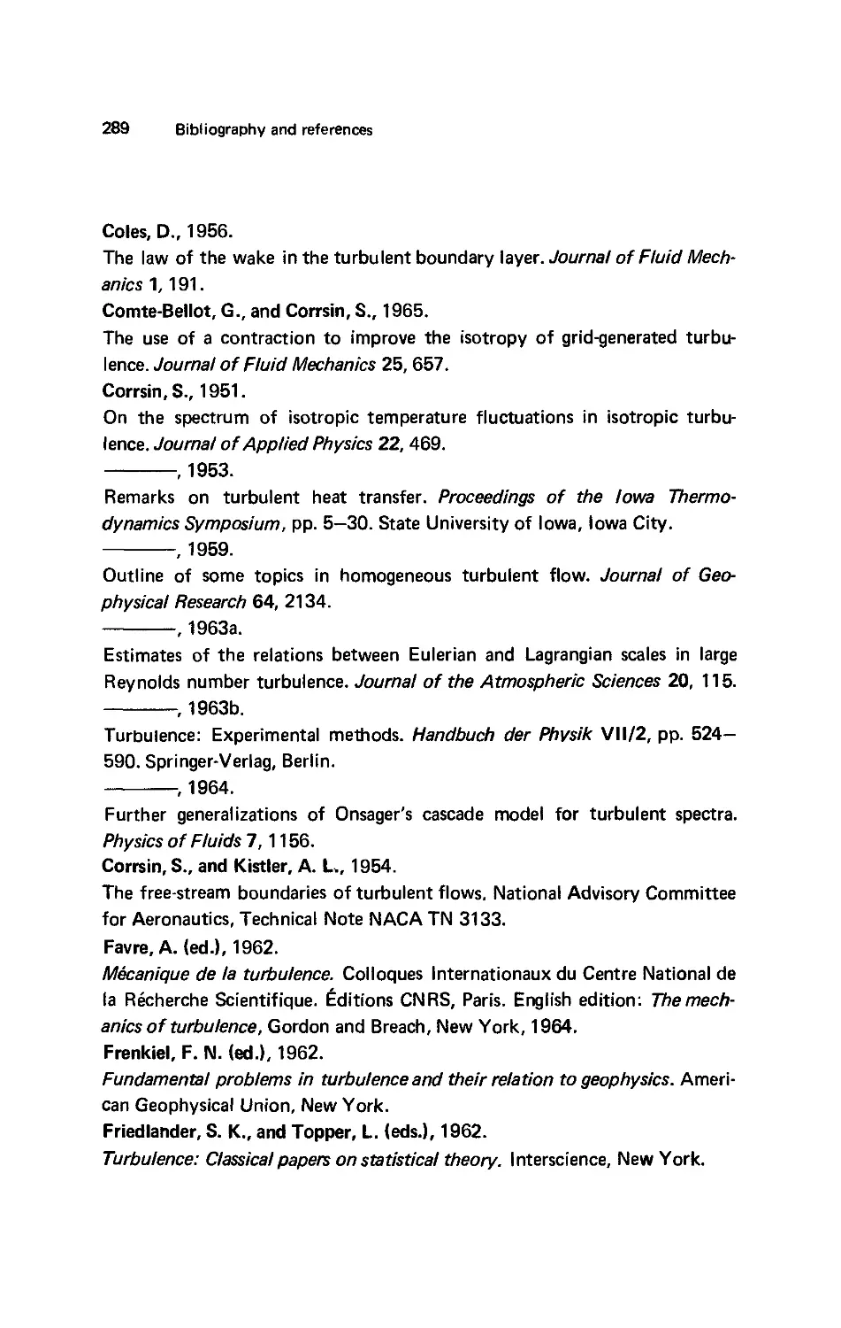
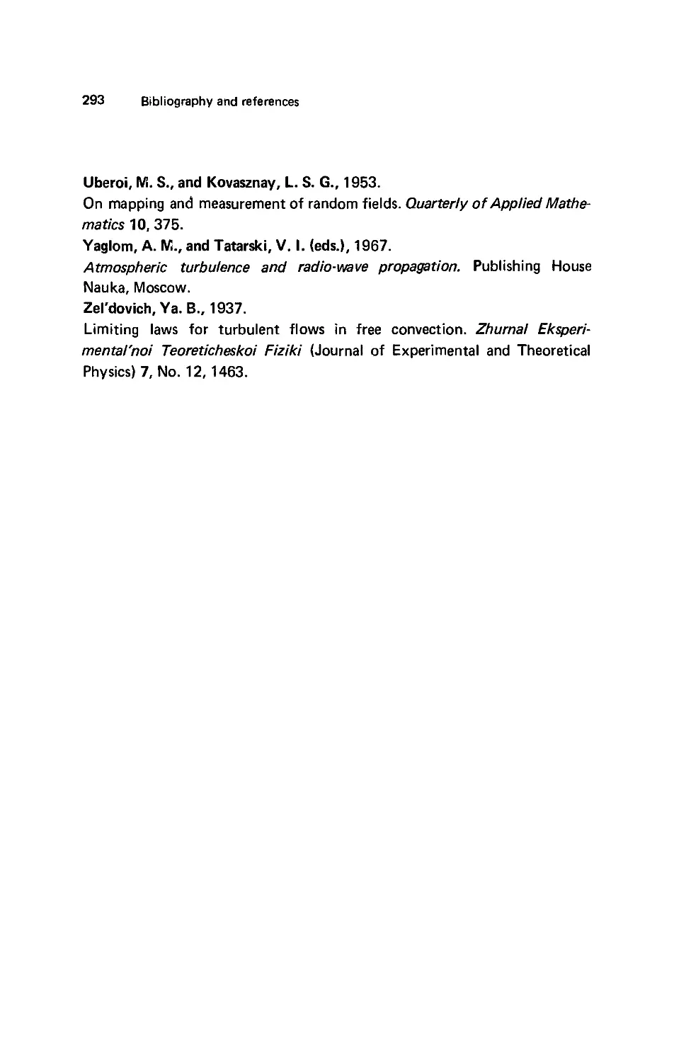
downstream transport of momentum by the flow itself. Figure 1.2 illustrates
this situation.
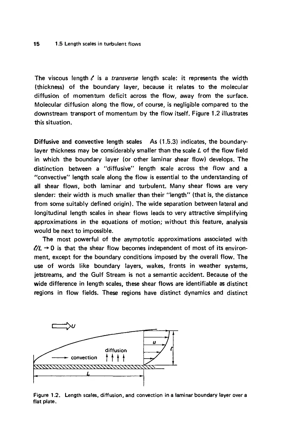
Diffusive and convective length scales As A.5.3) indicates, the boundary-
layer thickness may be considerably smaller than the scale L of the flow field
in which the boundary layer (or other laminar shear flow) develops. The
distinction between a "diffusive" length scale across the flow and a
"convective" length scale along the flow is essential to the understanding of
all shear flows, both laminar and turbulent. Many shear flows are very
slender: their width is much smaller than their "length" (that is, the distance
from some suitably defined origin). The wide separation between lateral and
longitudinal length scales in shear flows leads to very attractive simplifying
approximations in the equations of motion; without this feature, analysis
would be next to impossible.
The most powerful of the asymptotic approximations associated with
t/L -* 0 is that the shear flow becomes independent of most of its environ-
environment, except for the boundary conditions imposed by the overall flow. The
use of words like boundary layers, wakes, fronts in weather systems,
jetstreams, and the Gulf Stream is not a semantic accident. Because of the
wide difference in length scales, these shear flows are identifiable as distinct
regions in flow fields. These regions have distinct dynamics and distinct
diffusion
convection f f f
Figure 1.2. Length scales, diffusion, and convection in a laminar boundary layer over a
flat plate.
16
Introduction
characteristics; they are governed by specific equations of motion, which, in
the asymptotic approximation ?/L+ 0, may be substantially simpler than the
equations governing other parts of the flow field.
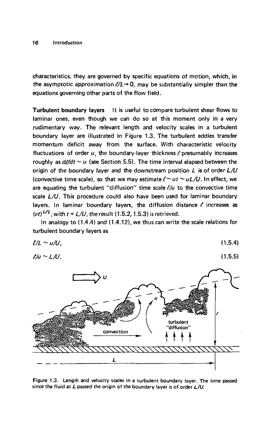
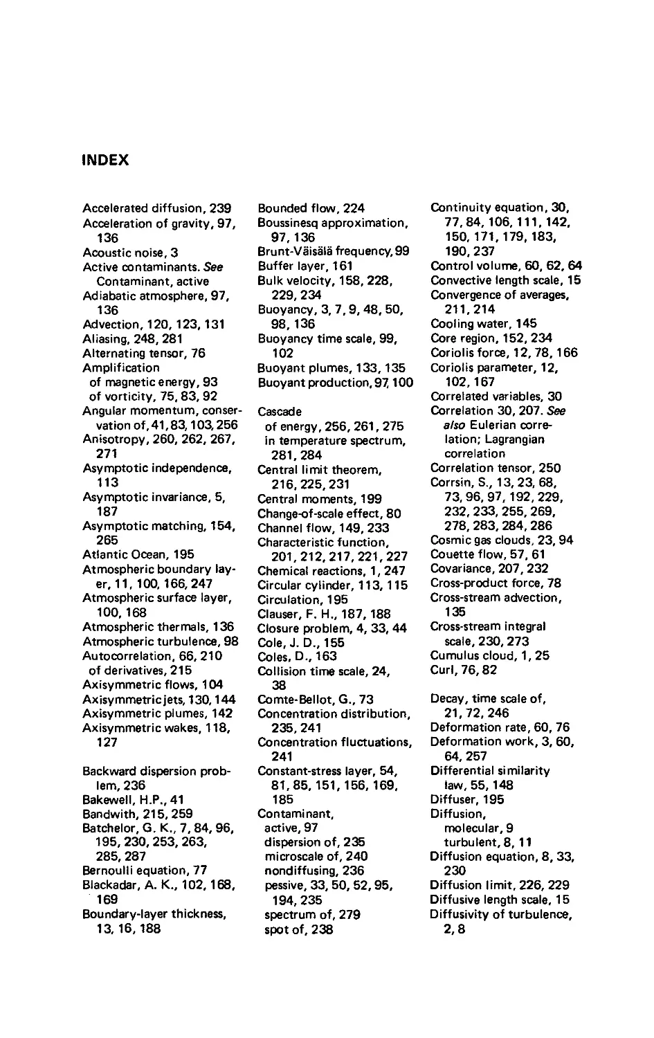
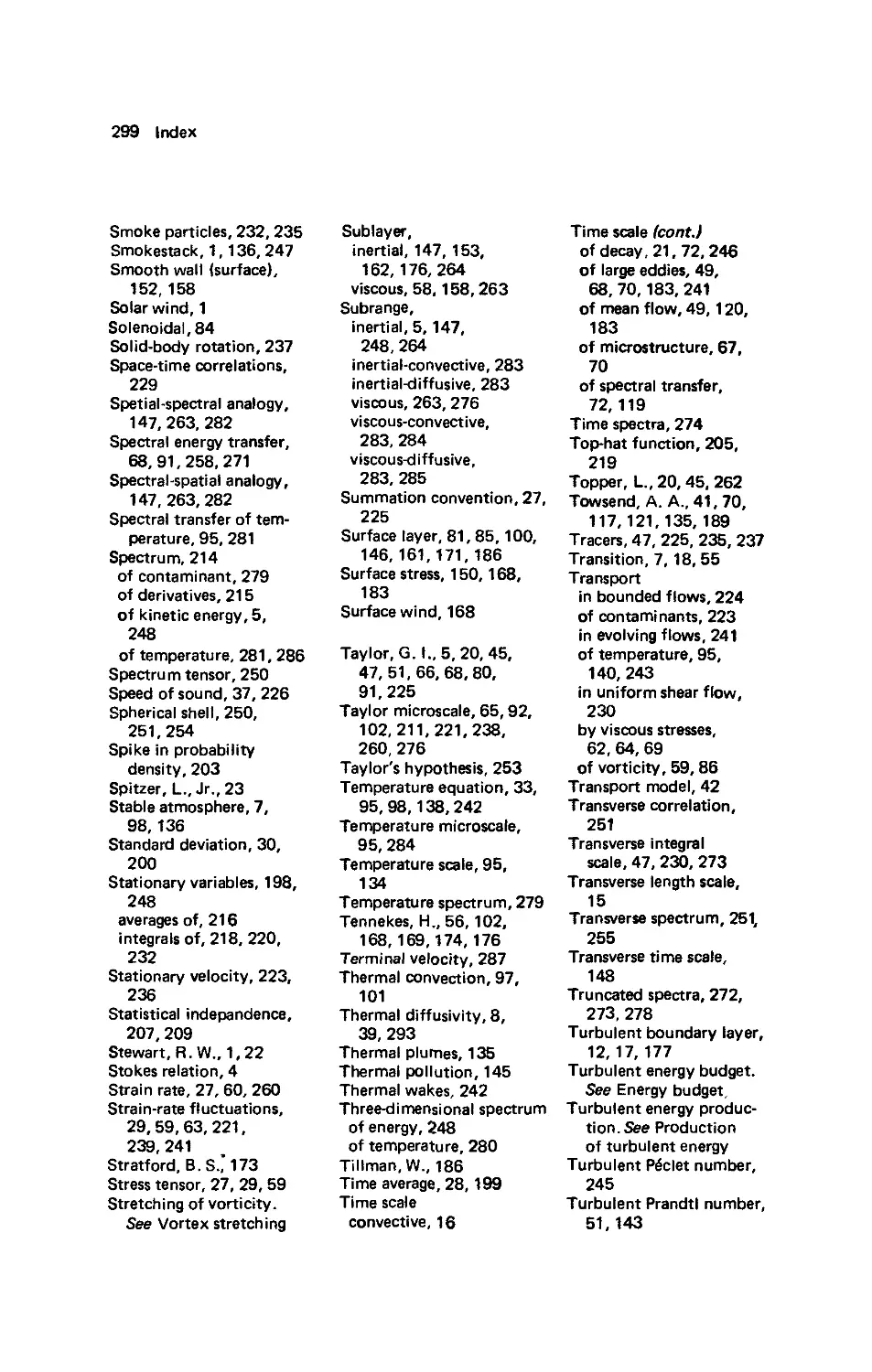
Turbulent boundary layers It is useful to compare turbulent shear flows to
laminar ones, even though we can do so at this moment only in a very
rudimentary way. The relevant length and velocity scales in a turbulent
boundary layer are illustrated in Figure 1.3. The turbulent eddies transfer
momentum deficit away from the surface. With characteristic velocity
fluctuations of order u, the boundary-layer thickness /presumably increases
roughly as d{/dt~ и (see Section 5.5). The time interval elapsed between the
origin of the boundary layer and the downstream position L is of order L/U
(convective time scale), so that we may estimate (~ ut ~ uL/U. In effect, we
are equating the turbulent "diffusion" time scale t/u to the convective time
scale L/U. This procedure could also have been used for laminar boundary
layers. In laminar boundary layers, the diffusion distance <f increases as
(vtI/г; with t = L/U, the result A.5.2,1.5.3) is retrieved.
In analogy to A.4.4) and A.4.12), we thus can write the scale relations for
turbulent boundary layers as
t/L ~ u/U,
(/и ~ L/U.
A.5.4)
A.5.5)
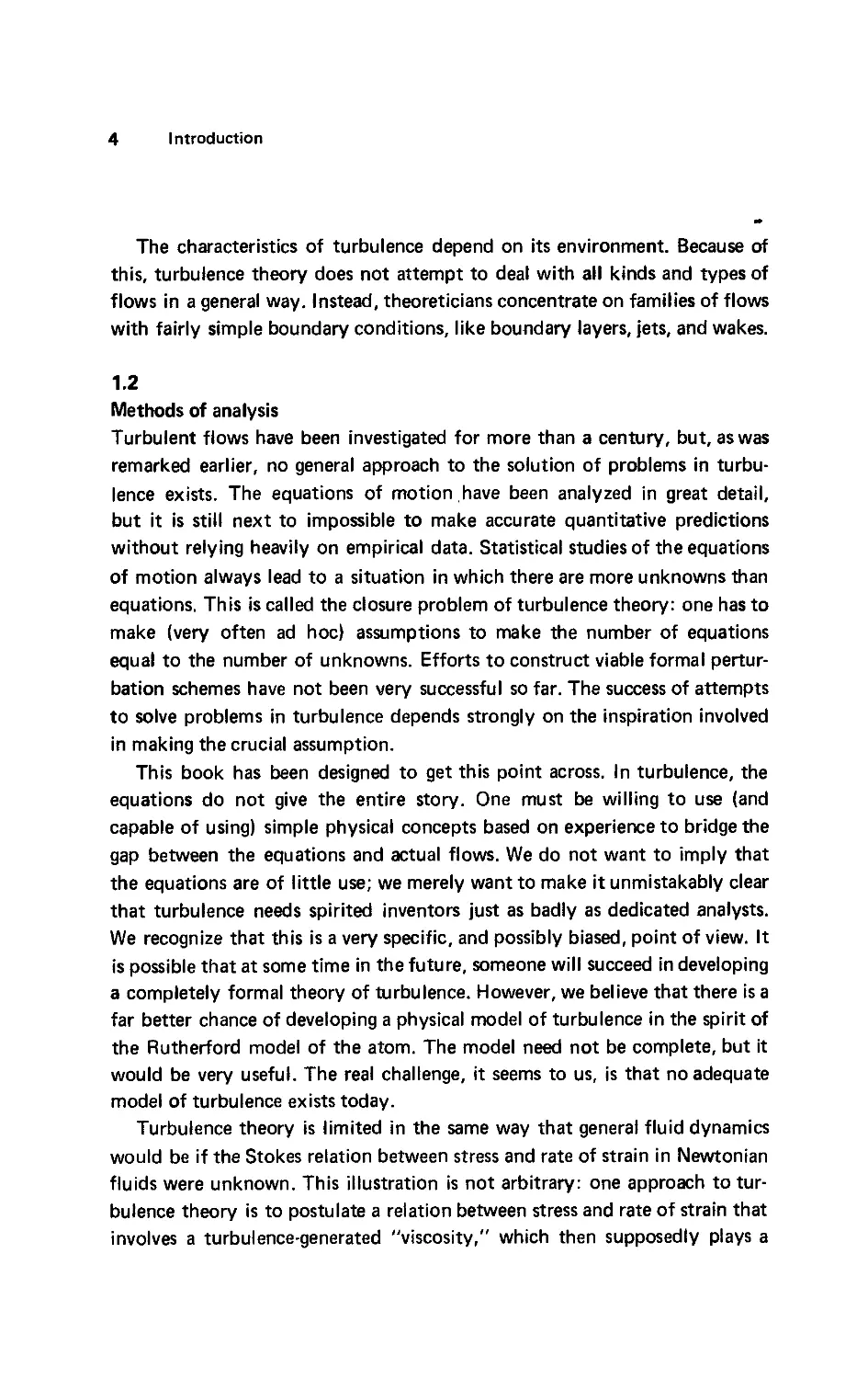
\\
Figure 1.3. Length and velocity scales in a turbulent boundary layer. The time passed
since the fluid at L passed the origin of the boundary layer is of order L/U.
17 1.5 Length scales in turbulent flows
These relations merely relate characteristic lengths and velocities; they should
not be used as formulas to compute the rate of spreading of a turbulent
boundary layer. The relation between the time scales, A.5.5), rephrases the
fundamental assumption we implicitly encountered earlier, that is, that in a
situation with an imposed external flow the turbulence, being part of the
flow, must have a time scale commensurate with the time scale of the flow. As
we will see later, this assumption conflicts with eddy-viscosity concepts.
Fortunately, not all of the turbulence has such a large time scale: the small
eddies in turbulence have very short time scales, which tend to make them
statistically independent of the mean flow.
Laminar and turbulent friction If we compare A.5.3) and A.5.4) and
introduce experimental data, which suggest that u/U is of the order of 10
over a wide range of Reynolds numbers, we again get some appreciation for
the relatively rapid growth of turbulent shear flows. This rapid growth should
correspond to a larger drag coefficient.
For a steady laminar boundary layer in two-dimensional flow on a plate
with length L, the drag D per unit span is equal to the total rate of loss of
momentum. Estimating the momentum loss as pU2(, where if is a boundary-
layer thickness at the end of the plate, we may put
D~pUH. A.5.6)
The drag coefficient (or friction coefficient) cd is defined by
A.5.7)
Substituting A.5.6) into A.5.7) and using the relation for t/L given by
A.5.3), we obtain
cd~2f = 2fl-1/2. A.5.8)
L
For a turbulent boundary layer, on the other hand, the mass flow deficit
at the end of the plate is proportional to put (see Chapter 5), so that the rate
of loss of momentum is proportional to (puC)U. Consequently,
D~puUt. A.5.9)
18
Introduction
The drag coefficient then becomes, if we use the definition A.5.7) and the
scale relation A.5.4),
2
A.5.10)
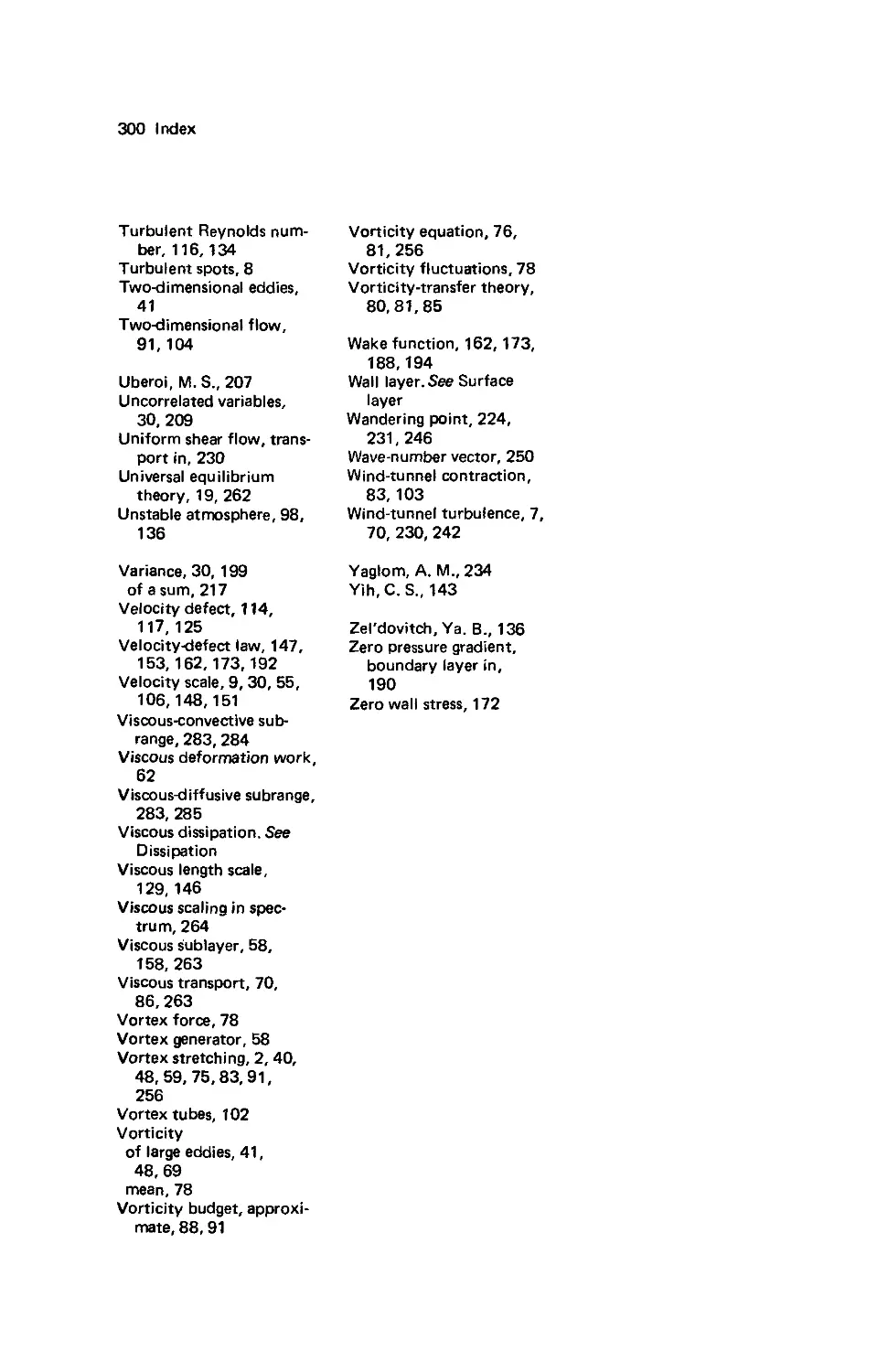
Experimental evidence shows that the turbulence level u/U varies very slowly
with Reynolds number, so that the drag coefficient of a turbulent boundary
layer, given by A.5.10), should be very much greater than the drag
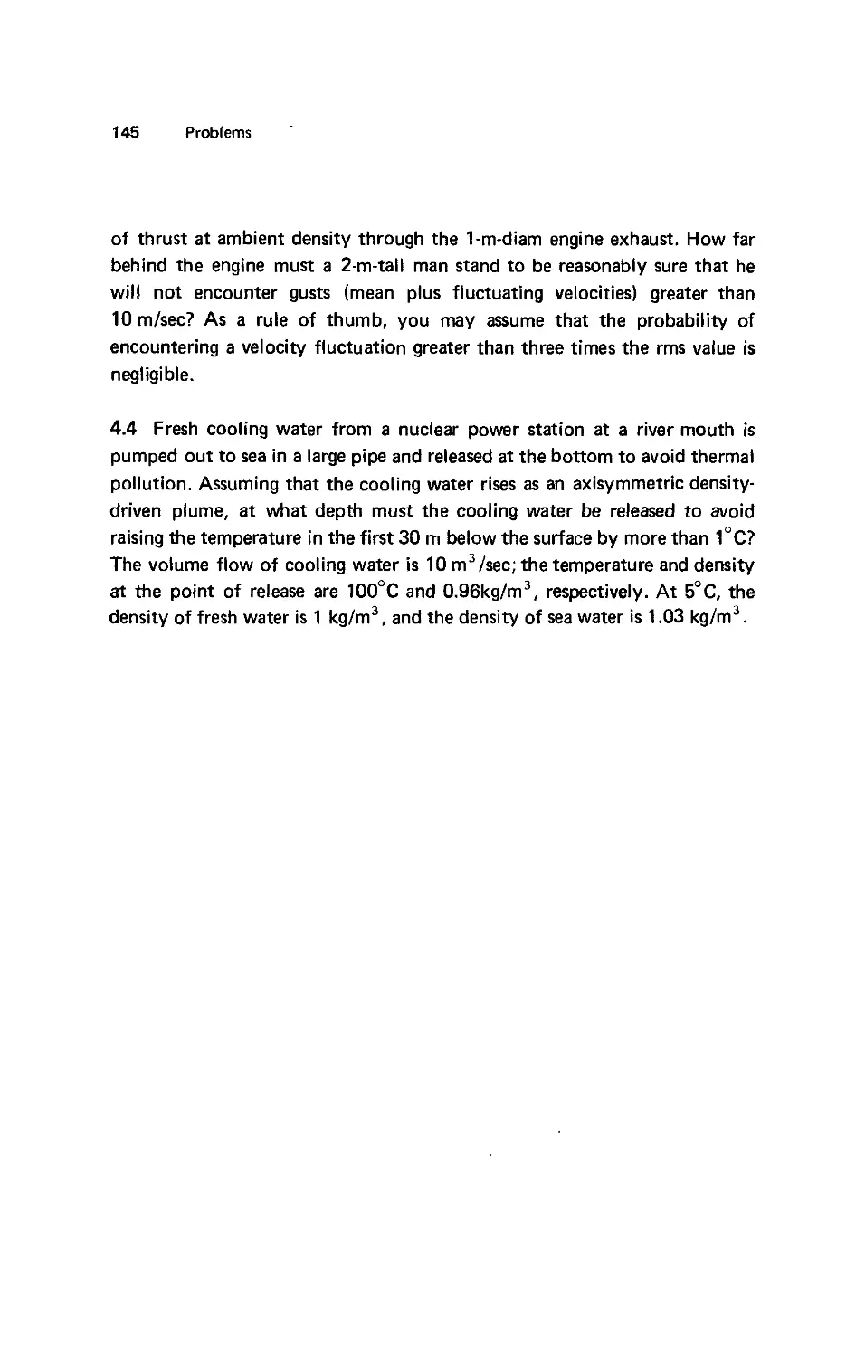
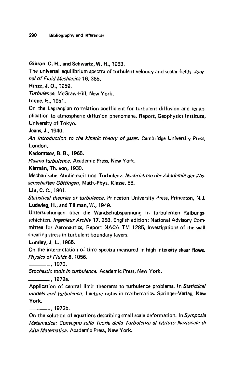
coefficient of a laminar boundary layer A.5.8). Figure 1.4 illustrates this
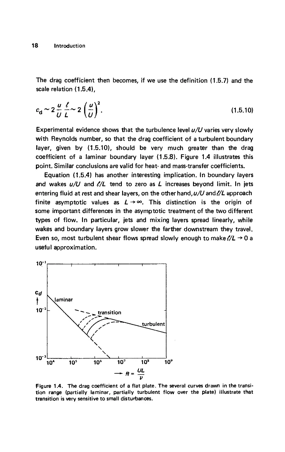
point. Similar conclusions are valid for heat- and mass-transfer coefficients.
Equation A.5.4) has another interesting implication. In boundary layers
and wakes u/U and t/L tend to zero as L increases beyond limit. In jets
entering fluid at rest and shear layers, on the other hand, u/U and t/L approach
finite asymptotic values as L-*<*>. This distinction is the origin of
some important differences in the asymptotic treatment of the two different
types of flow. In particular, jets and mixing layers spread linearly, while
wakes and boundary layers grow slower the farther downstream they travel.
Even so, most turbulent shear flows spread slowly enough to make<!7Z. ~* 0 a
useful approximation.
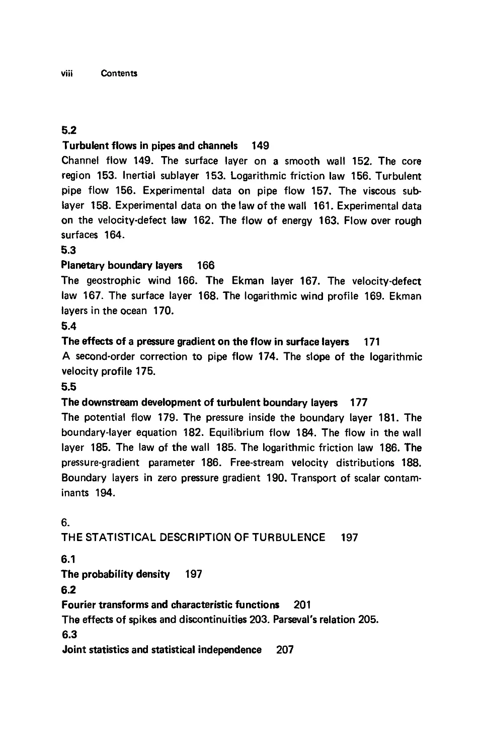
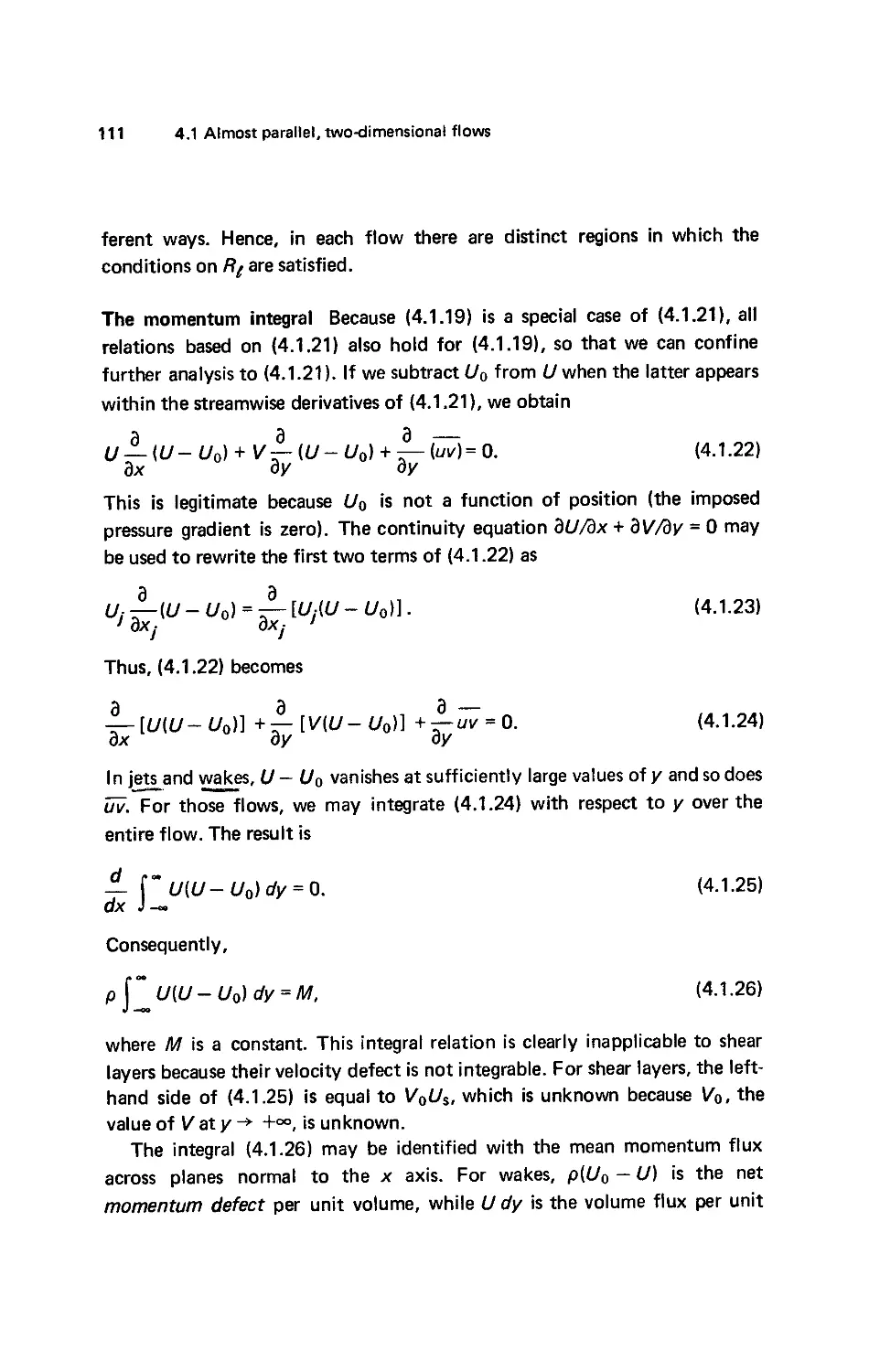
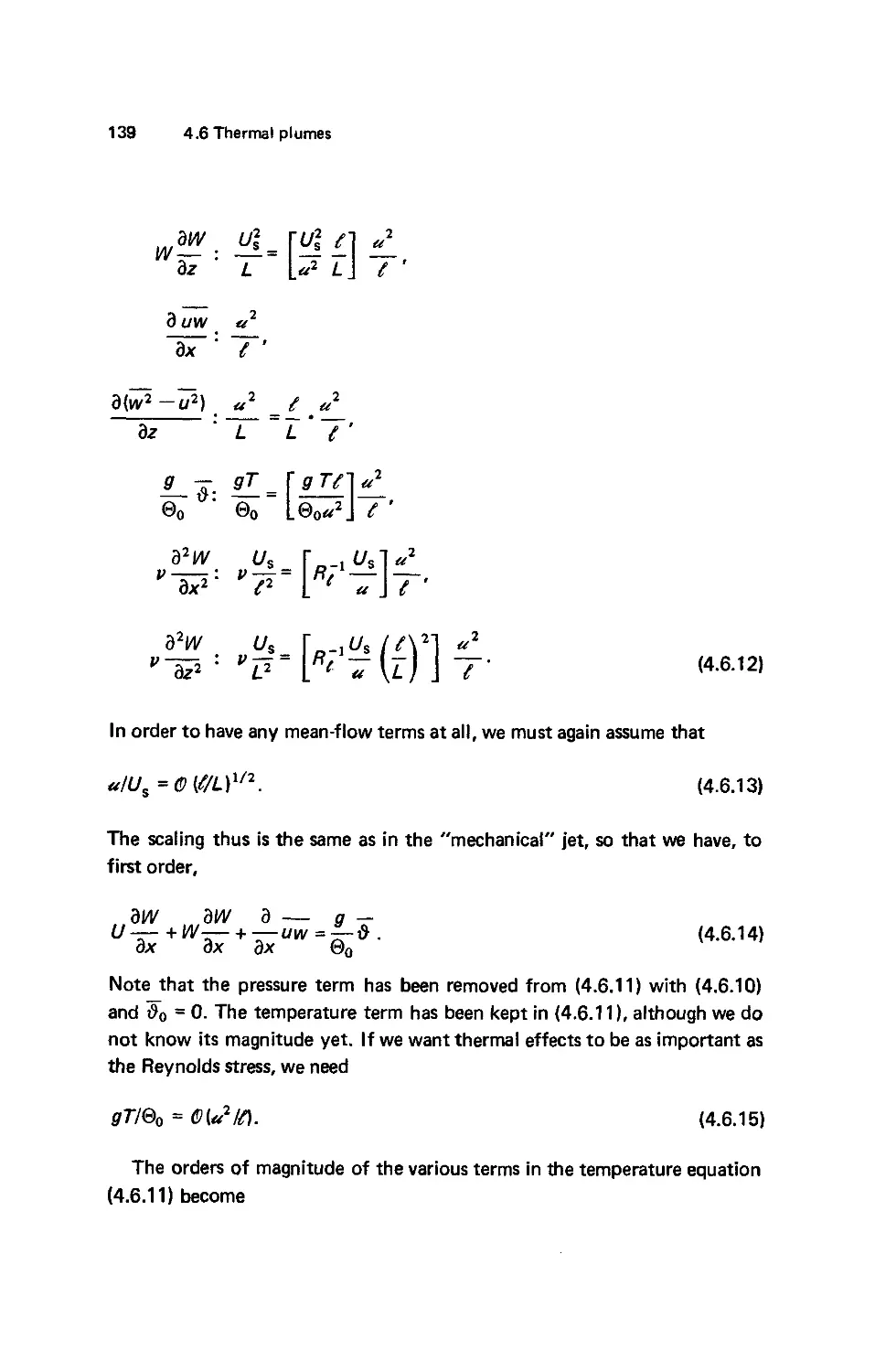
10-
Figure 1.4. The drag coefficient of a flat plate. The several curves drawn in the transi-
transition range (partially laminar, partially turbulent flow over the plate) illustrate that
transition is very sensitive to small disturbances.
19 1.5 Length scales in turbulent flows
Small scales in turbulence So far only the largest eddy sizes in turbulent
flows have been considered, because the large eddies do most of the transport
of momentum and contaminants. We have suggested that large eddies are as
big as the width of the flow and that the latter is the relevant length scale in
the analysis of the interaction of the turbulence with the mean flow. For
some of the other aspects of the dynamics of turbulence, however, other
length scales are needed.
We shall attempt to find the smallest length scales in turbulent flows. At
very small length scales, viscosity can be effective in smoothing out velocity
fluctuations. The generation of small-scale fluctuations is due to the nonlinear
terms in the equations of motion; the viscous terms prevent the generation of
infinitely small scales of motion by dissipating small-scale energy into heat.
This is characteristic of a small parameter like v (more properly 1/Я) with a
singular behavior. One might expect that at large Reynolds numbers the
relative magnitude of viscosity is so small that viscous effects in a flow tend
to become vanishingly small. The nonlinear terms in the Navier-Stokes
equation counteract this threat by generating motion at scales small enough
to be affected by viscosity. The smallest scale of motion automatically adjusts
itself to the value of the viscosity. There seems to be no way of doing away
with viscosity: as soon as the scale of the flow field becomes so large that
viscosity effects could conceivably be neglected, the flow creates small-scale
motion, thus keeping viscosity effects (in particular dissipation rates) at a
finite level.
Since small-scale motions tend to have small time scales, one may assume
that these motions are statistically independent of the relatively slow
large-scale turbulence and of the mean flow. If this assumption makes sense,
the small-scale motion should depend only on the rate at which it is supplied
with energy by the large-scale motion and on the kinematic viscosity. It is fair
to assume that the rate of energy supply should be equal to the rate of
dissipation, because the net rate of change of small-scale energy is related to
the time scale of the flow as a whole. The net rate of change, therefore,
should be small compared to the rate at which energy is dissipated. This is the
basis for what is called Kolmogorov's universal equilibrium theory of the
small-scale structure (Chapter 8).
This discussion suggests that the parameters governing the small-scale
motion include at least the dissipation rate per unit mass e (m2 sec'3) and the
20 Introduction
kinematic viscosity v (m2 sec '). With these parameters, one can form length,
time, and velocity scales as follows:
7?=(^/e)i/4( т=(„/еI/2( у=(„€)>/4. A.5.11)
These scales are referred to as the Kolmogorov microscales of length, time,
and velocity (see Friedlander and Topper, 1962). In the Russian literature,
these scales are called "inner" scales.
The Reynolds number formed with r\ and v is equal to one
Vv/v=1, A.5.12)
which illustrates that the small-scale motion is quite viscous and that the
viscous dissipation adjusts itself to the energy supply by adjusting length
scales.
An inviscid estimate for the dissipation rate One can form an impression of
the differences between the large-scale and small-scale aspects of turbulence if
the dissipation rate e can be related to the length and velocity scales of the
large-scale turbulence. A plausible assumption is to take the rate at which large
eddies supply energy to small eddies to be proportional to the reciprocal of
the time scale of the large eddies. The amount of kinetic energy per unit mass
in the large-scale turbulence is proportional to u2; the rate of transfer of
energy is assumed to be proportional to u/f, where if represents the size of the
largest eddies or the width of the flow. We shall see later that Prelates to the
"integral" scales of turbulence, which can be measured by statistical methods.
To avoid confusion, we identify { from here on as the "integral scale,"
leaving a more precise definition for Chapter 2. Russian scientists speak of
"outer" scales rather than of integral scales.
The rate of energy supply to the small-scale eddies is thus of order
u2 'u/f=u3/? This energy is dissipated at a rate e, which should be equal to
the supply rate. Hence (Taylor, 1935),
е~иъ1(, A.5.13)
which states that viscous dissipation of energy can be estimated from the
large-scale dynamics, which do not involve viscosity. In this sense, dissipation
again is clearly seen as a passive process in the sense that it proceeds at a rate
dictated by the inviscid inertial behavior of the large eddies.
The estimate A.5.13) should not be passed over lightly. It is one of the
21 1.5 Length scales in turbulent flows
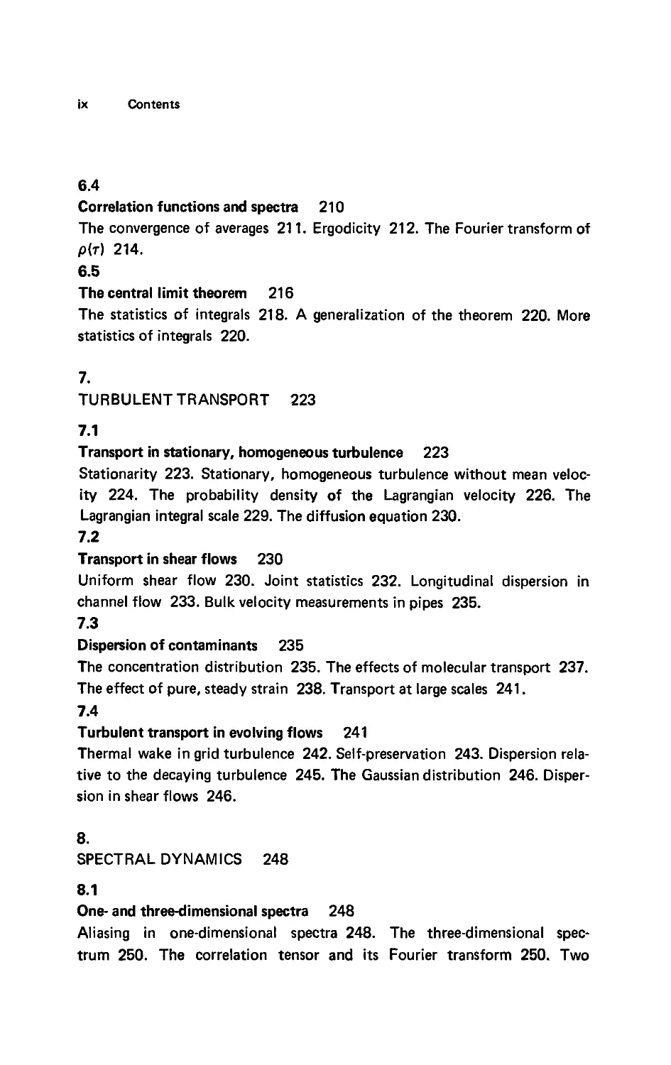
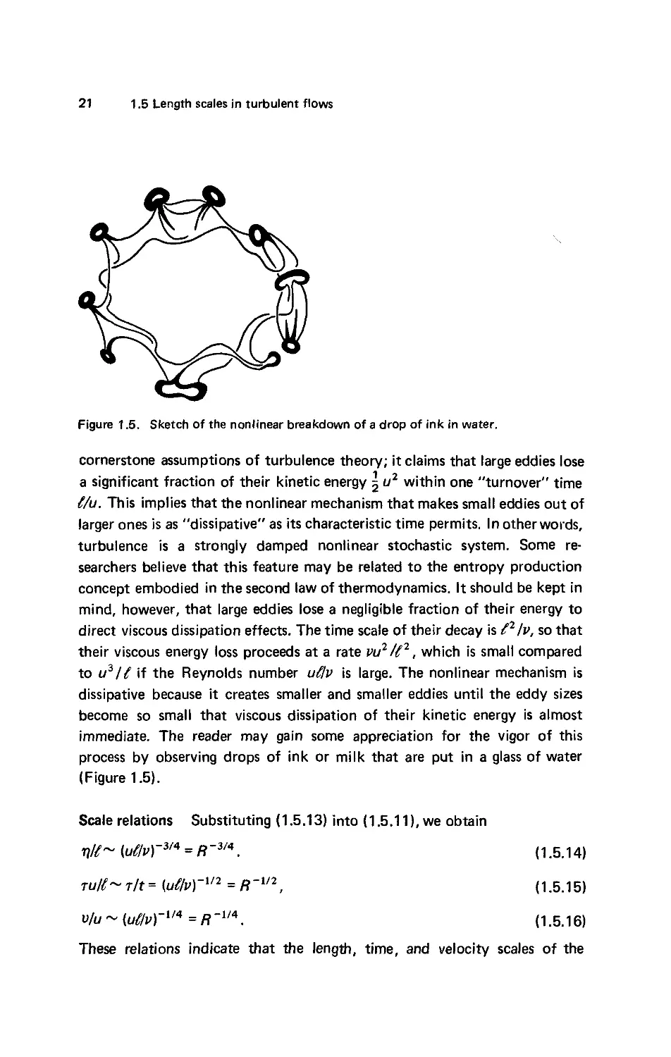
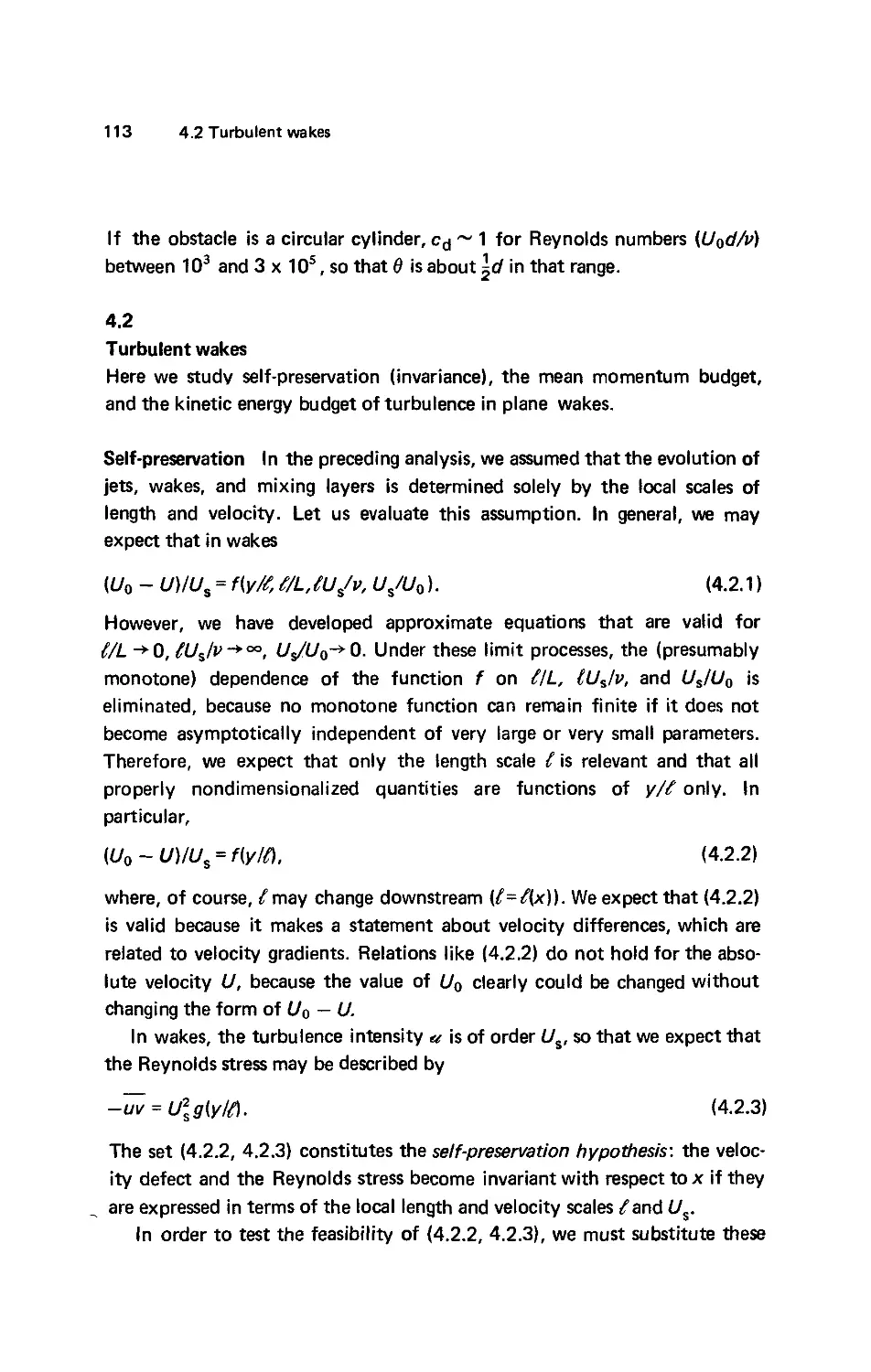
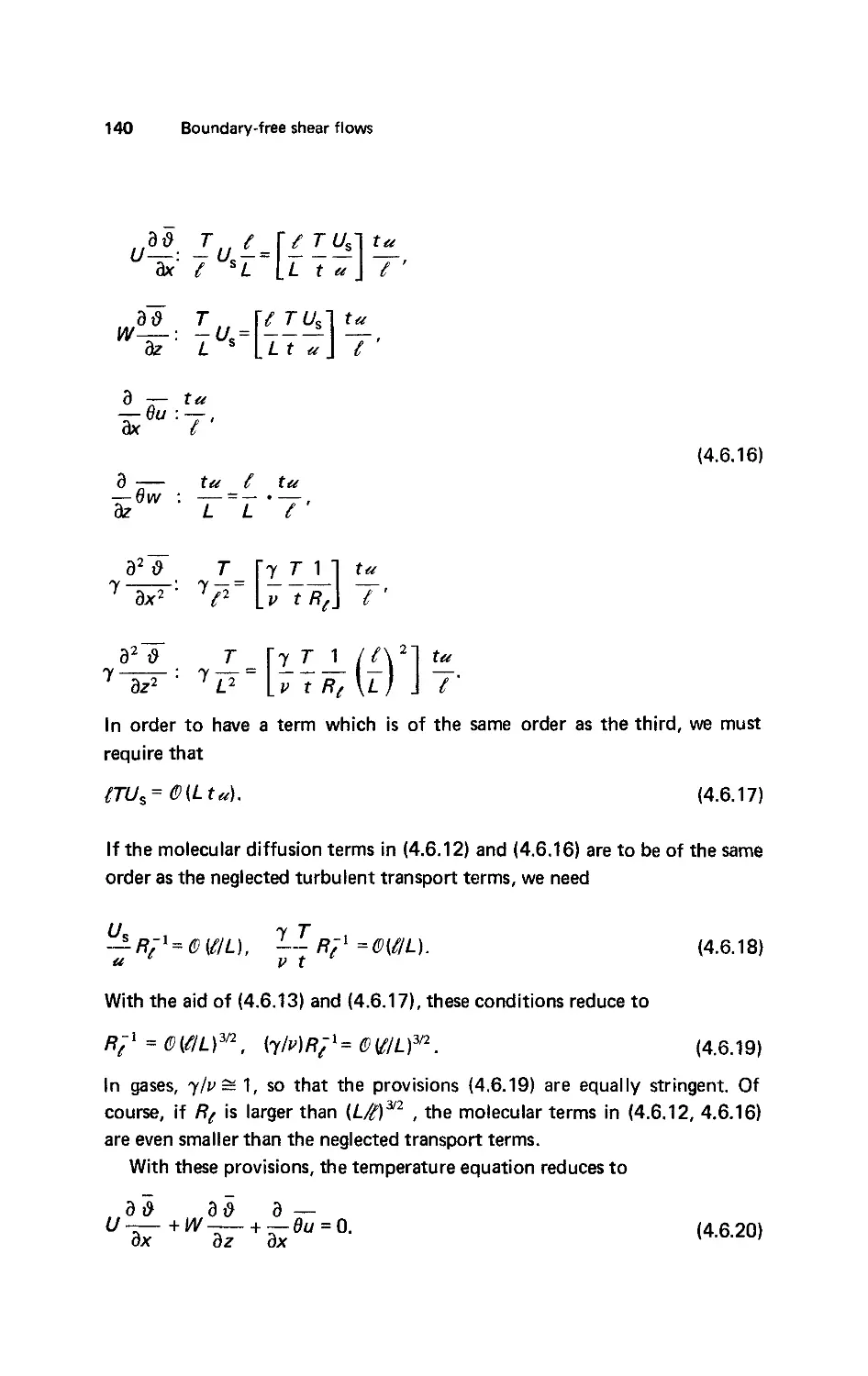
Figure 1.5. Sketch of the nonlinear breakdown of a drop of ink in water.
cornerstone assumptions of turbulence theory; it claims that large eddies lose
a significant fraction of their kinetic energy \ u2 within one "turnover" time
t/u. This implies that the nonlinear mechanism that makes small eddies out of
larger ones is as "dissipative" as its characteristic time permits. In other words,
turbulence is a strongly damped nonlinear stochastic system. Some re-
researchers believe that this feature may be related to the entropy production
concept embodied in the second law of thermodynamics. It should be kept in
mind, however, that large eddies lose a negligible fraction of their energy to
direct viscous dissipation effects. The time scale of their decay is t2 Iv, so that
their viscous energy loss proceeds at a rate vu2 It2, which is small compared
to u3It if the Reynolds number u?lv is large. The nonlinear mechanism is
dissipative because it creates smaller and smaller eddies until the eddy sizes
become so small that viscous dissipation of their kinetic energy is almost
immediate. The reader may gain some appreciation for the vigor of this
process by observing drops of ink or milk that are put in a glass of water
(Figure 1.5).
Scale relations Substituting A.5.13) into A.5.11), we obtain
r\l(~ Ku(lvYva> = R ~3/4. A.5.14)
Tul(~Tlt= Ы/vr1'2 = H'V2, A.5.15)
v/u ~ (uflv)~U4 = R~u*. A.5.16)
These relations indicate that the length, time, and velocity scales of the
22
Introduction
smallest eddies are very much smaller than those of the largest eddies. The
separation in scales widens as the Reynolds number increases, so that one
may suspect that the statistical independence and the dynamical equilibrium
state of the small-scale structure of turbulence will be most evident at very
large Reynolds numbers.
The main difference between two turbulent flows with different Reynolds
numbers but with the same integral scale is the size of the smallest eddies: a
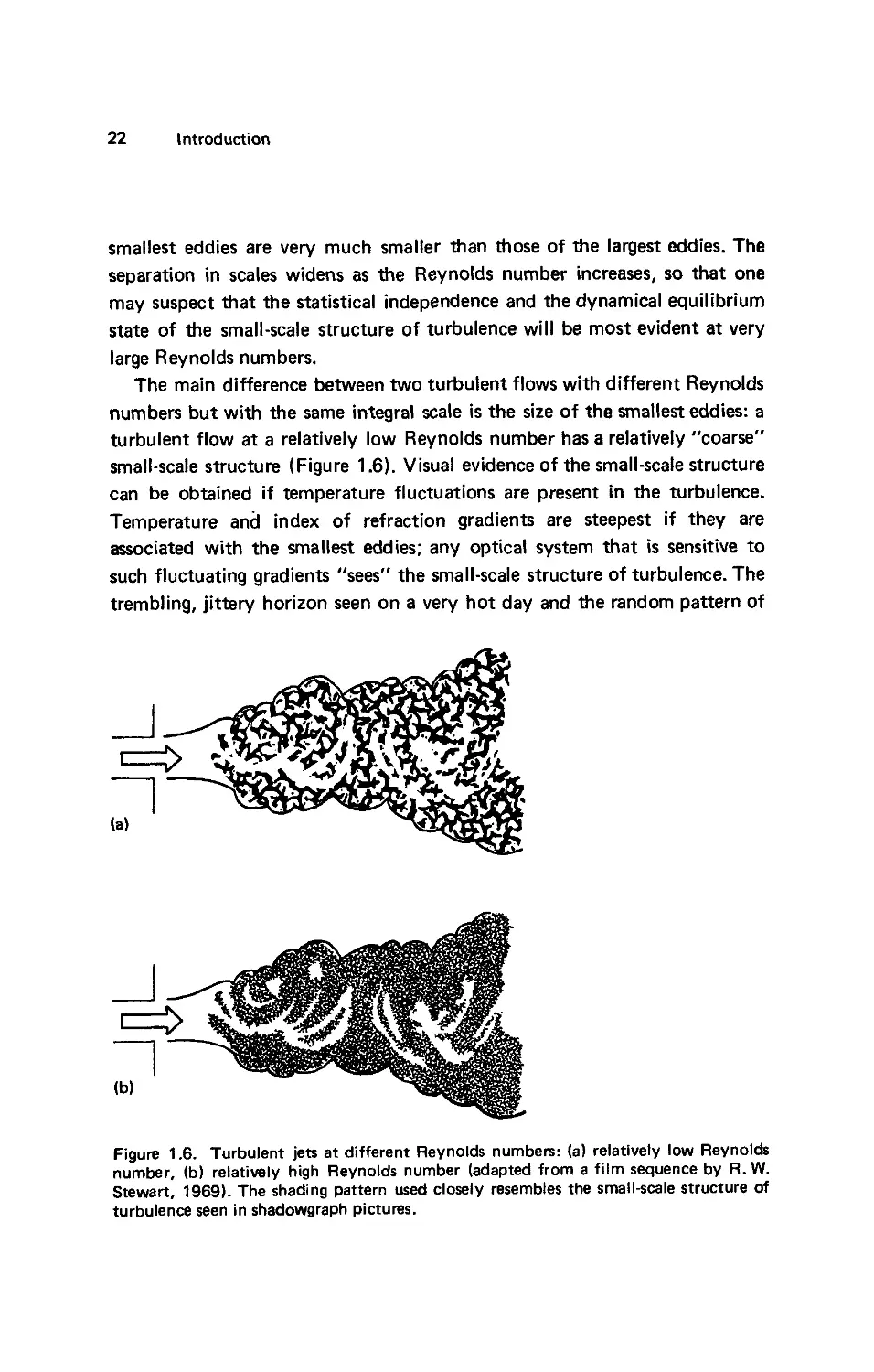
turbulent flow at a relatively low Reynolds number has a relatively "coarse"
small-scale structure (Figure 1.6). Visual evidence of the small-scale structure
can be obtained if temperature fluctuations are present in the turbulence.
Temperature and index of refraction gradients are steepest if they are
associated with the smallest eddies; any optical system that is sensitive to
such fluctuating gradients "sees" the small-scale structure of turbulence. The
trembling, jittery horizon seen on a very hot day and the random pattern of
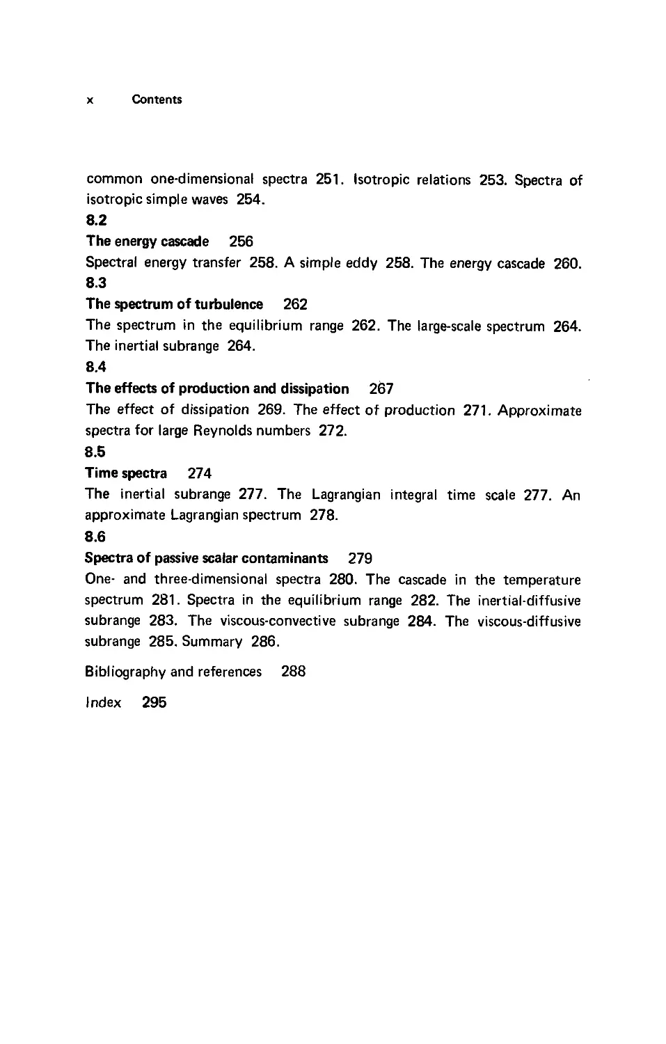
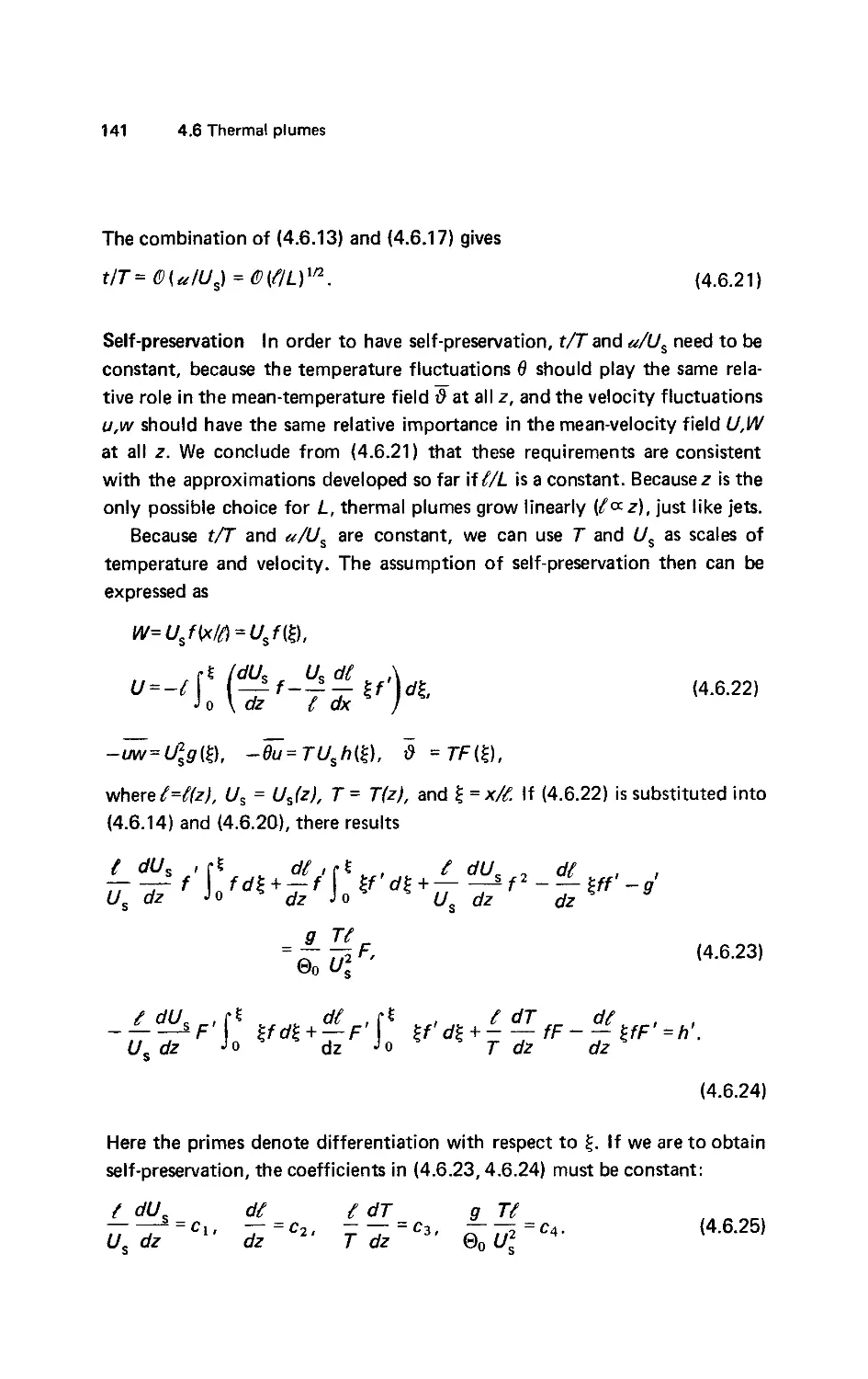
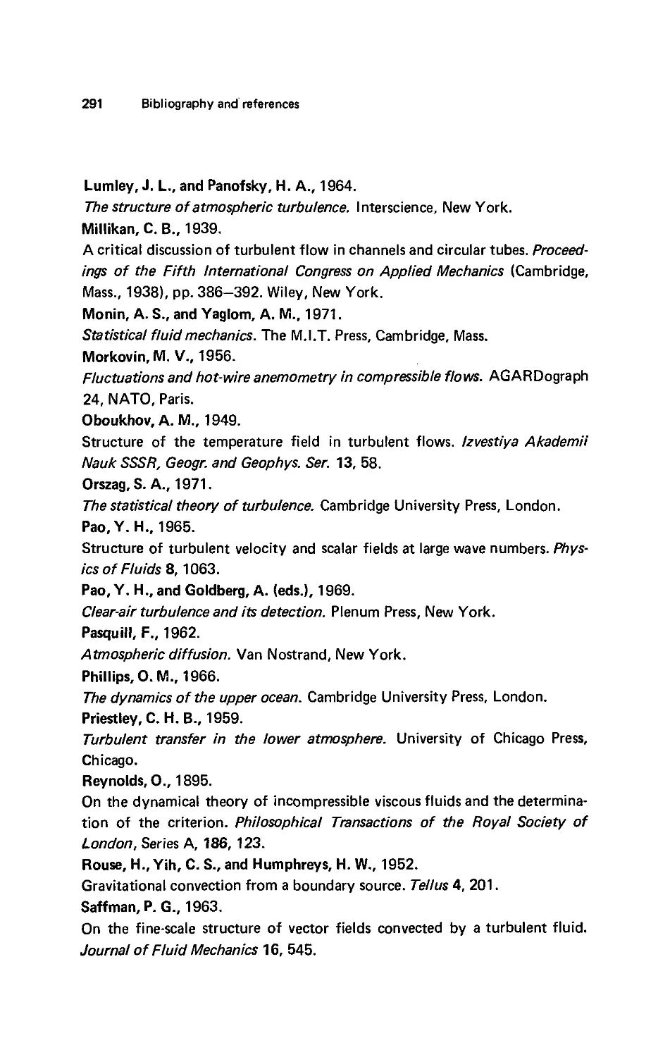
(a)
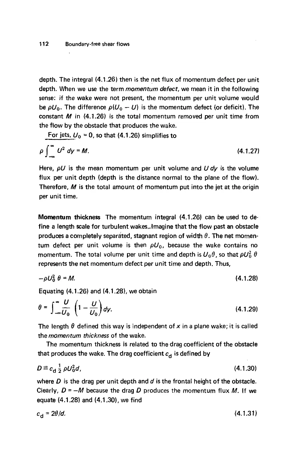
(b)
Figure 1.6. Turbulent jets at different Reynolds numbers: (a) relatively low Reynolds
number, (b) relatively high Reynolds number (adapted from a film sequence by R. W.
Stewart, 1969). The shading pattern used closely resembles the small-scale structure of
turbulence seen in shadowgraph pictures.
23 1.5 Length scales in turbulent flows
light and dark seen on the wall next to a heating element in sunlight are good
illustrations.
Vorticity has the dimensions of a frequency (sec). The vorticity of the
small-scale eddies should be proportional to the reciprocal of the time scale r.
From A.5.15) we conclude that the vorticity of the small-scale eddies is very
much larger than that of the large-scale motion. On the other hand, A.5.16)
indicates that the small-scale energy is small compared to the large-scale
energy. This is typical of all turbulence: most of the energy is associated with
large-scale motions, most of the vorticity is associated with small-scale
motions.
Molecular and turbulent scales The Kolmogorov length and time scales are
the smallest scales occurring in turbulent motion. At this point, it is
convenient to demonstrate that most turbulent flows are indeed continuum
phenomena. The Kolmogorov scales of length and time decrease with
increasing dissipation rates. High dissipation rates are associated with large
values of u. In gases, large values of и are more likely to occur than in liquids.
Therefore, it is sufficient to show that in gases the smallest turbulent scales of
motion are normally very much larger than molecular scales of motion. The
relevant molecular length scale is the mean free path %. The velocity scale of
molecular motion in a gas is proportional to the speed of sound a in the gas.
Kinetic theory of gases shows that the product a% is proportional to
the kinematic viscosity of the gas:
v~a%. A.5.17)
The ratio of the mean free path % to the Kolmogorov length scale t\ (this
might be called a microstructure Knudsen number) becomes (Corrsin, 1959)
?Л}~М/Я1/4, A.5.18)
where we have used A.5.14) and A.5.17). In A.5.18) the turbulence
Reynolds number Я = ut/v and the turbulence Mach number M = и/a are used
as independent variables. It is seen that turbulence might interfere with
molecular motion at high Mach numbers and low Reynolds numbers. This
kind of situation is unlikely to occur, because M is seldom large, but A is
typically very large. A pertinent illustration is the situation in gaseous nebulae
(cosmic gas clouds) (Spitzer, 1968). In clouds that consist mainly of neutral
24 Introduction
hydrogen, the turbulent (viach number is of order 10 (и ~ 10 km/sec,
a~ 1 km/sec), while the Reynolds number is of order 107 (t~ 1017 m,
| ~ 1011 m). With A.5.18), we compute that |/т? ~ 1/6. In this extreme case,
it seems doubtful that the smallest eddies perceive a continuum. In clouds
that consist mainly of ionized hydrogen, temperatures are quite high,
increasing a to about 10 km/sec and decreasing M to about 1. The mean free
path % remains roughly the same (the density in ionized clouds is not
appreciably different from that in neutral clouds), so that R reduces to about
106. In this case, ?Л?~з^, which may be small enough for the smallest
eddies to operate in a continuum.
The ratio of the time scale r to the collision time scale ?/a associated with
molecular motion is, in terms of R and M,
ral%~RinM-2. A.5.19)
For M = 10 and R = 107, the smallest time scale of turbulence is 32 times as
large as the collision time scale of the gas molecules; for M = 1 and R = 106
the ratio is 1000. It should be recognized that in ionized gases other length
and time scales are associated with the motion of the microscopic particles
and with the several other dynamical processes (radiation, cosmic rays,
magnetic fields) that may be present, so that rj may not always be a relevant
length scale.
Because the smallest time scales in turbulent motion tend to be much
larger than molecular time scales, the motion of the gas molecules is in
approximate statistical equilibrium, so that molecular transport effects may
indeed be represented by transport coefficients such as viscosity and heat
conductivity. These representations would become invalid if the departures
from equilibrium were large; the case %lt\ ~1 та/| ~ 32 would probably re-
require treatment with the methods of statistical mechanics.
1.6
Outline of the material
The bird's-eye view of turbulence dynamics given in the preceding sections
sets the stage for a brief outline of this book. In Chapter 2, we deal with
eddy-viscosity and mixing-length theories. The dimensional framework of
these theories is useful in the analysis of typical shear flows. In Chapter 3, the
energy and vorticity equations of turbulent flow are derived. In Chapter 4,
some free shear flows like wakes and jets are discussed. In Chapter 5,
25 Problems
boundary layers are analyzed. To prepare a formal basis for the study of
diffusion and spectral dynamics, an introduction to statistics is given in
Chapter 6. In Chapter 7, turbulent diffusion and mixing are studied.
The study of the spatial dynamics of turbulent flows precedes that of the
spectral dynamics. There exist many similarities and analogies between spatial
and spectral dynamics of turbulence. Also, spatial dynamics can be visualized
more easily by those new to the subject. Once some of the subtle features of
turbulent shear flow are understood, the dynamics of turbulence in wave-
number space should not be too perplexing. Spectral dynamics is studied in
Chapter 8.
Problems
1.1 Estimate the energy dissipation rate in a cumulus cloud, both per unit
mass and for the entire cloud. Base your estimates on velocity and length
scales typical of cumulus clouds. Compute the total dissipation rate in
kilowatts. Also estimate the Kolmogorov microscale rj. Use p = 1.25 kg/m3
andi>= 15 x 10~6 m2/sec.
1.2 A cubical box of volume L3 is filled with fluid in turbulent motion. No
source of energy is present, so that the turbulence decays. Because the
turbulence is confined to the box, its length scale may be assumed to be equal
to L at all times. Derive an expression for the decay of the kinetic energy
|u2 as a function of time. As the turbulence decays, its Reynolds number
decreases. If the Reynolds number uL/v becomes smaller than 10, say, the
inviscid estimate e=u3/L should be replaced by an estimate of the type
e = cvu2/L2, because the weak eddies remaining at low Reynolds numbers
lose their energy directly to viscous dissipation. Compute с by requiring that
the dissipation rate is continuous at uL/v =10. Derive an expression tor the
decay of the kinetic energy when uL/v< 10 (this is called the "final" period
of decay). If L = 1 m, v= 15 x 10~6 m2 /sec and и = 1 m/sec at time Г = 0, how
long does it take before the turbulence enters the final period of decay?
Assume that the effects of the walls of the box on the decay of the turbu-
turbulence may be ignored. Can you support this assumption in any way?
1.3 The large eddies in a turbulent flow have a length scale/, a velocity
scale v(fl = u, and a time scale tl?) =t/u. The smallest eddies have a length
26 Introduction
scale 7j, a velocity scale v, and a time scale т. Estimate the characteristic
velocity v(r) and the characteristic time t{r) of eddies of size r, where r is any
length in the range ц<г<{. Do this by assuming that v(r) and t(r) are
determined by e and r only. Show that your results agree with the known
velocity and time scales at г ={ and л = r). The energy spectrum of turbulence
is a plot of Е(к) = к v2 (к), where к = 1/л is the "wave number" associated
with eddies of size r. Find an expression for Е{к) and compare your result
with the data in Chapter 8.
1.4 An airplane with a hot-wire anemometer mounted on its wing tip is to
fly through the turbulent boundary layer of the atmosphere at a speed of
50 m/sec. The velocity fluctuations in the atmosphere are of order 0.5 m/sec,
the length scale of the large eddies is about 100 m. The hot-wire anemometer
is to be designed so that it will register the motion of the smallest eddies.
What is the highest frequency the anemometer will encounter? What should
the length of the hot-wire sensor be? If the noise in the electronic circuitry is
expressed in terms of equivalent turbulence intensity, what is the permissible
noise level?
2
TURBULENT TRANSPORT OF MOMENTUM AND HEAT
Turbulence consists of random velocity fluctuations, so that it must be
treated with statistical methods. The statistical analysis does not need to be
sophisticated at this stage; a simple decomposition of all quantities into mean
values and fluctuations with zero mean will suffice for the next few chapters.
We shall find that turbulent velocity fluctuations can generate large momen-
momentum fluxes between different parts of a flow. A momentum flux can be
thought of as a stress; turbulent momentum fluxes are commonly called
Reynolds stresses. The momentum exchange mechanism superficially resem-
resembles molecular transport of momentum. The latter gives rise to the viscosity
of a fluid; by analogy, the turbulent momentum exchange is often repre-
represented by an eddy viscosity. This analogy will be explored in great detail.
2.1
The Reynolds equations
In turbulence, a description of the flow at all points in time and space is not
feasible. Instead, following Reynolds A895), we develop equations governing
mean quantities, such as the mean velocity. The equations of motion of an
incompressible fluid are
3<7- _ 9G- 1 3 _
dt 'bxj pdxj "
Щ
—*=(). B.1.2)
дх,.
Here, dj, is the stress tensor. Repeated indices in any term indicate a summa-
summation over all three values of the index; a tilde denotes the instantaneous value
at (Xj, t) of a variable on which no Reynolds decomposition into a mean value
and fluctuations (see next section) has been performed.
If the fluid is Newtonian, the stress tensor a,-.- is given by
B.1.3)
In B.1.3), bjj is the Kronecker delta, which is equal to one if / =j and zero
otherwise; p is the hydrodynamic pressure and ц is the dynamic viscosity
(which will be assumed to be constant). The rate of strain s}.- is defined by
28 Turbulent transport of momentum and heat
If B.1.3) is substituted into B.1.1) and if the continuity equation B.1.2) is
invoked, the Navier-Stokes equations are obtained:
9"; 9t7,- 1 dp 92<7,-
—J-+U1—*- = --—+v '- . B.1.5)
9r 'dxj pbx, bXjbxj
Here, v is the kinematic viscosity (v = ц/р).
The Reynolds decomposition The velocity <7,- is decomposed into a mean
flow Uj and velocity fluctuations U/, such that
B.1.6)
We interpret Ut as a time average, defined by
fo + T
Uj= Mm- j ' Ujdt. B.1.7)
Time averages (mean values) of fluctuations (which are denoted by lowercase
letters) and of their derivatives, products, and other combinations are
denoted by an overbar. The mean value of a fluctuating quantity itself is zero
by definition; for example,
U7=lim-f
° {u,-Uj)dt=ia. B.1.8)
The use of time averages corresponds to the typical laboratory situation, in
which measurements are taken at fixed locations in a statistically steady, but
often inhomogeneous, flow field. In an inhomogeneous flow, a time average
like U/ is a function of position, so that the use of a spatial average would be
inappropriate for most purposes. For a time average to make sense, the
integrals in B.1.7) and B.1.8) have to be independent of Го. In other words,
the mean flow has to be steady:
^ = 0. B.1.9)
of
Without this constraint B.1.7) and B.1.8) would be meaningless. The averag-
averaging time T needed to measure mean values depends on the accuracy desired;
this problem is discussed in Section 6.4.
The mean value of a spatial derivative of a variable is equal to the corre-
corresponding spatial derivative of the mean value of that variable; for example.
29 2.1 The Reynolds equations
^ B.1.10)
bxj bXj bXj dxj
These operations can be performed because averaging is carried out by
integrating over a long period of time, which commutes with differentiation
with respect to another independent variable.
The pressure p and the stress d/.- are also decomposed into mean and
fluctuating components. Again, capital letters are used for mean values and
lowercase letters for fluctuations with zero mean. Specifically,
p=P + p, p = 0, B.1.11)
Like Uj, P and S,-- are independent of time. The mean stress tensor S^.- is
given by
//цЩ B-1-13)
and the stress fluctuations O/.are given by
a# = -p8tf + 2»xs/y. B.1.14)
Here, the mean strain rate Sy and the strain-rate fluctuations Sj, are defined
by
1 IbU: bU:\ 1 Ibu ЪиЛ ,01<0
The commutation between averaging and spatial differentiation involved here
is based on B.1.10).
Correlated variables Averages of products are computed in the following
way:
= UjUj + UjUj. B1.16)
The terms consisting of a product of a mean value and a fluctuation vanish if
they are averaged, because the mean value is a mere coefficient as far as the
averaging is concerned, and the average of a fluctuating quantity is zero.
30 Turbulent transport of momentum and heat
If UjUJ^O, Uj and Uj are said to be correlated; if u,u- = 0, the two are
uncorrelated. Figure 2.1 illustrates the concept of correlated fluctuating
variables. A measure for the degree of correlation between the two variables
Uj and Uj is obtained by dividing JljUJby the square root of the product of the
variances u2 and uj; this gives a correlation coefficient c«, which is defined
by
c^^./iuj ¦~u~fI'2, B.1.17)
with the understanding that the summation convention does not apply in this
case. If Cjj = ±1, the correlation is said to be perfect. Each variable, of course,
is perfectly correlated with itself (саа = 1 if / =/ = a).
The square root of a variance is called a standard deviation or root-mean-
square (rms) amplitude; it is denoted by a prime (for example, u/ = (u2I^2).
A characteristic velocity, or "velocity scale," of turbulence at some down-
downstream position in a boundary layer might be defined as the mean rms
velocity taken across the boundary layer at that position; in this way velocity
scales used in dimensional analysis could be given a precise definition when-
whenever desired.
Equations for the mean flow If we apply the decomposition rule B.1.6) to
the continuity equation B.1.2), we obtain
If the average of all terms in this equation is taken, the last term vanishes
because of B.1.8, 2.1.10). Hence, the mean flow is incompressible:
dUi/dxi = 0. B.1.19)
Subtracting B.1.19) from B.1.18), we find that the turbulent velocity fluctu-
fluctuations are also incompressible:
bUjlbXj = 0. B.1.20)
The equations of motion for the mean flow Uj are obtained by substitut-
substituting B.1.6) and B.1.12) into B.1.1) and taking the average of all terms in the
resulting equation. This yields, if all rules on averaging are observed (in partic-
particular, recall that bUjlbt = 0),
31 2.1 The Reynolds equations
-*-1
Figure 2.1. Correlated and uncorrelated fluctuations. The_fluctuating variable a has the
same sign as the variableb for most Of the time;mistakesab >0.The variablec, on the
other hand, is uncorrelated with a and_6, so that ac = 0 and be = 0 (note that ab Ф 0,
ac ^Odoes not necessarily imply that be ^)
32 Turbulent transport of momentum and heat
With
1 Э
P a*/ *
use1 of the continuity equation
fluctuations, we
7^
'Эх,-
0
=эх7Uyt
may write
B.1.21)
B.1.20) for the turbulent velocity
B.1.22)
This term is analogous to the convection term Uj ЭЦ/Эху; it represents the
mean transport of fluctuating momentum by turbulent velocity fluctuations.
If Uj and U: were uncorrelated, there would be no turbulent momentum
transfer. Experience shows that momentum transfer is a key feature of turbu-
turbulent motion; the term B.1.22) of B.1.21) is not likely to be zero. Mean
transport of fluctuating momentum may change the momentum of the mean
flow, as B.1.21) shows. The term B.1.22) thus exchanges momentum
between the turbulence and the mean flow, even though the mean momen-
momentum of the turbulent velocity fluctuations is zero {рй~; = 0).
Because momentum flux is related to a force by Newton's second law, the
turbulent transport term B.1.22) may be thought of as the "divergence" of a
stress. Because of the Reynolds decomposition, the turbulent motion can be
perceived as an agency that produces stresses in the mean flow. For this
reason, B.1.21, 2.1.22) are rearranged, so that all stresses can be put to-
together. This yields the Reynolds momentum equation:
B-1-23)
If we recall that 2=.. is given by B.1.13), the total mean stress Ту in a
turbulent flow may be written as
Ту = 2,y - pUjUj = -P bjj + 2ц S/j - pUjUj. B.1.24)
The Reynolds stress The contribution of the turbulent motion to the mean
stress tensor is designated by the symbol r,y:
Tjj = -pUiUj- B.1.25)
In honor of the original developer of this part of the theory, т,у is called the
Reynolds stress tensor. The Reynolds stress is symmetric: т,у = Ту,, as can be
33 2.1 The Reynolds equations
seen by inspection of B.1.25). The diagonal components of тц are normal
stresses (pressures); their values are pu\, pu\, and p<v|. In many flows, these
normal stresses contribute little to the transport of mean momentum. The
off-diagonal components of Tj.- are shear stresses; they play a dominant role in
the theory of mean momentum transfer by turbulent motion.
The decomposition of the flow into a mean flow and turbulent velocity
fluctuations has isolated the effects of fluctuations on the mean flow. How-
However, the equations for the mean flow B.1.23, 2.1.24) contain the nine
components of r/y- (of which only six are independent of each other) as
unknowns additional to P and the three components of Ur This illustrates the
closure problem of turbulence. Indeed, if one obtains additional equations for
Tj: from the original Navier-Stokes equations, unknowns like UjUjUj are gen-
generated by the nonlinear inertia terms. This problem is characteristic of all
nonlinear stochastic systems.
This is a frustrating prospect. Therefore, many investigators have attemp-
attempted to guess at a relation between r/y- and S/y-. This is a tempting approach
because the function of the Reynolds stress in the equations of motion seems
to be similar to that of the viscous stress 2/uS,y. We investigate the nature of
possible relations between r/y- and S/y- in Section 2.3; before this is done, some
background material on the viscous stress is given in Section 2.2.
Turbulent transport of heat Turbulence transports passive contaminants
such as heat, chemical species, and particles in much the same way as momen-
momentum. For later use, we develop the equation governing heat transfer in turbu-
turbulent flow of a constant-density fluid. The density is approximately constant if
temperature differences remain relatively small, if gravity-induced density
stratification may be neglected, and if the Mach number of the flow is small.
The starting point is the diffusion equation for heat in a flow:
or oxj oxjOXj
The thermal diffusivity у is assumed to be constant; its dimensions are
m2sec"J. The ratio vly is called the Prandtl number.
The temperature 9 at (x/V t) is decomposed in a mean value 0 and tem-
temperature fluctuations 0, such that
0=G + 0, B.1.27)
34 Turbulent transport of momentum and heat
9 = G= lim -J ddt, B.1.28)
0 = 0, 9©/9f = O. B.1.29)
The last condition has been imposed because time averages would not make
sense in an unsteady situation.
Substituting B.1.27) into B.1.26) and taking the average of all terms in
the resulting equation, we obtain
3G Э
5(/ ) B.1.30)
Xy OXj \ ' OX J
The mean heat flux Qj per unit area and unit time in a turbulent flow then
becomes (cp is the specific heat at constant pressure)
Qj = cp p(8uj - у Эе/Эху). B.1.31)
The heat flux is thus a sum of the contributions of the molecular motion and
of the turbulent motion. The analogy between B.1.24) and B.1.31) is strik-
striking; it is the analytical foundation for the belief that turbulence may trans-
transport heat in much the same way as momentum.
2.2
Elements of the kinetic theory of gases
In this section we discuss the molecular background of the viscosity and
other molecular transport coefficients in dilute perfect gases (Jeans, 1940).
For gases, the rudiments of kinetic theory are straightforward, but the kinetic
theory of liquids is not nearly as well developed.
Pure shear flow Let us take a steady pure shear flow, homogeneous in the
Xi, x3 plane. The only nonvanishing velocity component is taken to be U\; it
is a function of x2 only. If the flow is laminar, the only nonvanishing com-
components of the viscous shear stress are
о12=о21=цди1/дх2. B.2.1)
The flow situation corresponding to B.2.1) is sketched in Figure 2.2.
The shear stress ai2 must result from molecular transport of momentum
in the x2 direction. Let vt and v2 be the xx and x2 components of the
instantaneous velocity of a molecule relative to the mean flow. The xx
35 22 Elements of the kinetic theory of gases
Figure 2.2. Pure shear flow. U2 = 6/3 = 0 and all derivatives with respect to x, and x3
vanish.
momentum mvx of a molecule with mass m is transported in the x2 direction
if v2 is correlated with i^. The momentum transport per molecule is propor-
proportional to m vxv2. If there are N molecules per unit volume, the transport of
Xj momentum in the x2 direction is Nm viv2 per unit time and area. Here,
the overbar represents an average taken over a large number of molecules.
Now, Nm is the mass per unit volume, which is the density p, and momentum
flux per unit area and time may be equated with a stress. Hence,
B.2.2)
The minus sign in B.2.2) is needed because positive values of v2 should carry
momentum deficit in a flow with positive o12 and Ы/\1Ъх2. The analogy
between B.2.2) and the definition of the Reynolds stress given in B.1.25) is
intentional: a stress that is generated as a momentum flux can always be
written as B.2.2), no matter what mechanism causes the momentum flux.
Molecular collisions Kinetic theory of transport coefficients in gases esti-
estimates the right-hand side of B.2.2) as follows. Suppose the mean free path
(the average distance between collisions of molecules) is %. The unusual
36
Turbulent transport of momentum and heat
notation is selected because X has to be reserved for one of the length scales
occurring in turbulence. On the average, a molecule coming from x2 = —%
collides with another molecule at the reference level (x2 = 0). This process is
illustrated in Figure 2.3. If we assume that because of this collision the
molecule coming from below adjusts its momentum in the xx direction to
that of its new environment, it has to absorb an amount of momentum equal to
B.2.3)
The quantity M is equal to the amount of momentum lost by the environ-
environment at x2 =0, because the upward-traveling molecule carries a momentum
deficit with respect to the mean momentum x2 = 0.
The right-hand side of B.2.3) may be expanded in a Taylor series. This
yields
* Ьх2 2"- Ъх\
The second and higher terms in the expansion may be neglected if
дхг
Ъх\
B.2.4)
B.2.5)
Figure 2.3. Molecular motion in a shear flow.
37 2.2 Elements of the kinetic theory of gases
A local length scale <fof the flow Ux {x2) is defined as
Э?Л/Эх2 _ B_2>6)
Hence, B.2.5) may be written as
t»\%. B.2.7)
For air at room temperature and density, % = 7 x 10~6 cm, so that for almost
all flows the condition B.2.7) is indeed satisfied. This implies that B.2.4)
may be approximated by
M = m%bUJbx2. B.2.8)
In this simplified model, the quantity ? bU\lbx2 is the part of vx that is
correlated with v2, apart from a minus sign needed due to the sign convention
for a12. The number of collisions occurring at the reference level x2 = 0 per
unit area and time may be estimated as Na, where N again is the number of
molecules per unit volume and a is the speed of sound (which is a good
representative for the rms molecular velocity). If the momentum transfer per
collision is M, the momentum transfer per unit area and time must be propor-
proportional to MNa. Using B.2.8), we thus can write
a, 2 = oMNa = oNma% bUx /dx2. B.2.9)
Here, a is an unknown coefficient, which should be of order one. In air at
ordinary temperatures and pressure, a is approximately =-; we shall use this
з
anu (леээшс, u is afj^jiuAiniaLciy
value for convenience.
Because Nm = p, B.2.10) becomes
0i2 = \pa% bUxlbx2. B.2.10)
If we compare this with B.2.1) and use ц - pv, we obtain
v = \al B.2.11)
The Reynolds number formed with these variables is
aJ=- B.2.12)
v 2"
That this Reynolds number turns out to be of the order one is no accident,
because the viscosity is defined on the basis of molecular motion with
38 Turbulent transport of momentum and heat
velocity scale a and length scale ?. The Reynolds number B.2.12), however, is
not a dynamically significant number because at length scales of order % the
gas is not a continuum. For air at room temperature and pressure, % =
7 x 1СГ8 m, a = 3.4 x 10² m/sec, so that v = 15 x 10~6 m2/sec. It should be
noted that elementary kinetic theory as given here cannot predict ratios of
diffusivities (such as Prandtl number v/y).
Characteristic times and lengths The ratio of % to the local length scale I of
the flow is called the Knudsen number K. With B.2.12), we obtain
i;_3 V _3U V _3M
*~7~2~аТ~2а~7/Г27?- BZ13)
The Knudsen number is thus proportional to the ratio of the Mach number M
and the Reynolds number R. In most flows M«R, so that the condition
B.2.7) is easily satisfied.
The Knudsen number is a ratio of length scales. The time scales involved in
molecular transport of momentum are of interest, too. The molecular time
scale is the time interval %la between collisions; this is typically of the order
of 10~10 sec. The time scale of the flow is the reciprocal of the velocity
gradient Ы)\1Ьхг. If the velocity gradient is 104 sec, corresponding to
quite rapid shearing, the time scale of the flow is 10~4 sec. It is seen that
changes in the flow are slow compared to the time scale representing molec-
molecular motion. This suggests that the thermal motion of the molecules should
not be disturbed very much by the flow: molecules collide many thousands
of times before the flow has advanced appreciably.
The correlation between vt and v2 For future reference, it is useful to
obtain some idea of how well the molecular velocity components V\ and v-i
are correlated. The part of V\ correlated with v2 is proportional to
%Ы)\1Ьхг, as shown by B.2.8). Taking representative values for a rapid
shearing flow in air (? = 7x 10"8 m, bUxlbx2 = 104 sec), we find that
% Ы)х1Ьхг = 7 x 10~4 m/sec. A correlation coefficient с between i^ and v2
may be defined as
B.2.14)
Here, v2' is the rms value of thex2 component of the molecular velocity. As
39 22 Elements of the kinetic theory of gases
a comparison of B.2.14) and B.1.17) shows, we have used vx' = v2'. If we
use the results previously given, we may estimate that
(Z2,5)
Since v2' is of the same order of magnitude as the speed of sound a, which is
3.4 x 10² m/sec for air at room conditions, we find that с is approximately
2 x 10~6, indicating that vt and v2 are very poorly correlated. If dUi/dx2 is
estimated as lilt, we find that the correlation coefficient is of the order of
M2/R, a parameter which indeed tends to be extremely small in most flows.
We may conclude that the state of the gas is hardly disturbed by molecular
momentum transfer. In other words, the dynamical equilibrium of the
thermal motion of the molecules in shear flow of gases is, to a very close
approximation, the same as the equilibrium state in a gas at rest. This implies
that shear flow is not likely to upset the equation of state of the gas, unless
M2/R is large.
In anticipation of results that are obtained in Section 2.3, we note that the
correlation coefficient of turbulent velocity fluctuations, defined in a manner
similar to B.2.14), is not small in turbulent shear flow. Consequently, the
"state" of the turbulence is not independent of the mean flow field; on the
contrary, the interaction between the mean flow and the turbulence tends to
be quite strong.
Thermal diffusivity Molecular transport of scalar quantities is similar to the
transport of momentum. The heat transfer rate is given by the second term of
B.1.31); in the model flow used here, the only nonvanishing component is
Q2 = - pcpy Эе/Эх2 • B.2.16)
In terms of molecular parameters, this is
Q2 =-0.93cpPa$№dx2. B.2.17)
In this equation we have used B.2.11) and p/7 = 0.73 (air at room condi-
conditions). The thermal diffusivity is larger than the diffusivity for momentum
because molecules that travel faster than average carry more thermal energy
with them and make more collisions per unit time. Energetic molecules thus
do more than a proportional share in transporting heat.
40
Turbulent transport of momentum and heat
2.3
Estimates of the Reynolds stress
We have seen that molecular transport can be interpreted fairly easily in terms
of the parameters of molecular motion. It is very tempting to apply a similar
heuristic treatment to turbulent transport. We again use a pure shear flow as a
basis for our discussion. This flow is illustrated in Figure 2.4. Using B.1.25)
and B.1.31), we find the rates of turbulent momentum transfer and heat
transfer to be
T12=-pu1u2l B.3.1)
H2 =рсрвп2. B.3.2)
The symbol H2 is used to avoid confusion with the total rate of heat transfer
Reynolds stress and vortex stretching Let us consider the Reynolds stress
only. The existence of a Reynolds stress requires that the velocity fluctua-
fluctuations ux and u2 be correlated. In a shear flow with bUilbx2 >0, negative
values of ux should occur more frequently than positive ones when u2 is
positive, and vice versa. This is a rather intricate problem: the energy of the
eddies has to be maintained by the shear flow, because they are continuously
losing energy to smaller eddies. Molecules do not depend on the flow for their
energy because the collisions between molecules are elastic. Eddies, on the
Figure 2.4. Turbulent pure shear flow. The mean velocity is steady: U2 = U3 = 0 and
I/, = l/, (хг). The instantaneous streamline pattern sketched refers to a coordinate
system that moves with a velocity I/, @).
41 2.3 Estimates of the Reynolds stress
other hand, need shear to maintain their energy; the most powerful eddies
thus are those that can absorb energy from the shear flow more effectively
than others. Evidence (for example, Townsend, 1956, Bakewell and Lumley,
1967) suggests that the eddies that are more effective than most in maintain-
maintaining the desired correlation between Ui and u2 and in extracting energy from
the mean flow are vortices whose principal axis is roughly aligned with that of
the mean strain rate. Such eddies are illustrated in Figure 2.5. The energy
transfer mechanism for eddies of this kind is believed to be associated with
vortex stretching: as the eddies in Figure 2.5 are being strained by the shear,
conservation of angular momentum tends to maintain the good correlation
between ut and u2, thus allowing (as we discuss in more detail in Chapter 3)
efficient energy transfer.
The interaction between eddies and the mean flow described here is essen-
essentially three dimensional. Two-dimensional eddies (velocity fluctuations with-
without a component normal to thexi,x2 plane) may on occasion have appre-
appreciable Reynolds stress, but the mean shear tends to rotate and strain them in
such a way that they would lose their capacity for extracting energy from the
mean flow rather quickly.
These considerations suggest that a simple transport theory patterned after
kinetic theory of gases is at best a very crude representation of reality. The
dynamic interaction between the mean flow and the turbulence is too strong
Figure 2.5. Three-dimensional eddies (vortices with vorticity u>) being stretched by the
rate of strain S. The fluctuating velocity has strong components in the plane normal to
the vorticity vector. Note that the shape of these eddies may differ widely from flow to
flow.
42 Turbulent transport of momentum and heat
to allow for a simple transport model. Also, a more detailed analysis of the
energy and vorticity dynamics of the eddies (Chapter 3) is essential to the
understanding of turbulence.
It should be noted that this discussion applies only to shear flows. If
eddies receive energy in other ways (from buoyancy or a magnetic field, say),
the picture may be entirely different.
The mixing-length model An estimate for the turbulent momentum flux can
be obtained by analyzing the random motion of moving points ("fluid
particles") in a turbulent shear flow. A formal treatment of the statistics of
the motion of wandering points is given in Chapter 7; the less rigorous
analysis presented here is more than adequate for a first look at turbulent
transport.
Suppose a moving point starts from a level x2 = 0 (see Figure 2.6) at time
t = 0. Its Xi momentum per unit volume is puv @,0), where u\ @,0) stands
for the instantaneous velocity at x2 = 0, t = 0. If we assume that the moving
point does not lose its momentum as it travels upward, it has a momentum
deficit AM = pux (x2, t) — pHi @, 0) when it passes an arbitrary level x2 at
time f. Using the Reynolds decomposition of velocities, we can write the
momentum deficit as
= p[U1(x2)-Ul@)] +p[u1(x2,t)-u1@,0)]. B.3.3)
If the contribution of the turbulence to the momentum deficit can be
neglected and if the difference Ui(x2) — Ui@) may be approximated by
Figure 2.6. Transport of momentum by turbulent motion.
43 2.3 Estimates of the Reynolds stress
x2 bU\lbx2, where the gradient is taken atx2 = 0, AM may be approximated
by
AM = px2 dUi/dx2. B.3.4)
The volume transported per unit area and unit time in the x2 direction is O2 of
the moving point. Now, u2 = dx2/dt, so that the average momentum flux at
x2 = 0 may be written as
T12=5p-^ — (xl). B.3.5)
ax2 dt
The overbar here denotes an average over all moving points that start from
x2 = 0.
The dispersion rate d(x\ )ldt may be written as (see also Section 7.1)
B.3.6)
If the fluid at any point did not continually exchange momentum with its
environment, u2 would remain constant for any given moving point, and
x2u2 would continue to increase in time asx2 increased. This is not realistic;
instead, we expect that the correlation between u2 andx2 of a moving point
decreases as the distance traveled increases. If we assume that u2 and x2
become essentially uncorrelated at values of x2 comparable to some trans-
transverse length scale {(see Figure 2.6), we may estimate thatx2u2 is of order
u2'f. Here, u2 is the rms velocity in the x2 direction; the dispersion length
scale { is called the mixing length. Of course, this very estimate of x2u2
implies that momentum is not conserved when the moving point travels in the
x2 direction, so that this estimate makes the expression for the momentum
deficit AM given in B.3.4) very dubious, to say the least.
With 2x2u2 = 2ciu2 V, B.3.5) becomes
т12=с1ри2Пи1/дх2. B.3.7)
The numerical coefficient ci is unknown.
We define the eddy viscosity Pj (or turbulent exchange coefficient for
momentum), in analogy with B.2.1), by the equation
Ui/bx2. B.3.8)
44 Turbulent transport of momentum and heat
Comparing B.3.7) and B.3.8), we find that the eddy viscosity is given by
v1=cxuil B.3.9)
If the mixing length / and the velocity u2 were known everywhere in the
flow field and if the mixing-length model were accurate, the closure problem
would be solved. The unknown Reynolds stress would be related to known
variables and to the mean velocity gradient, making a solution of the equa-
equations of motion possible. However, the situation is not quite that simple.
Even if we were willing to accept B.3.7) as a model, u2' and /are not
properties of the fluid but properties of the flow. This implies that u2 and/
may vary throughout the flow field, making the eddy viscosity variable, depen-
dependent on the position in the flow. This is not a very promising prospect.
Consequently, applications of B.3.7) are usually restricted to flows for which
it can be argued that u2' is approximately constant (at least in the cross-
stream direction) and for which / is either constant or depends in a simple
way on the geometry of the shear flow concerned.
In reality, turbulence consists of fluctuating motion in a broad spectrum
of length scales. However, in view of the way /occurs in B.2.7), one may
argue that large eddies contribute more to the momentum transfer than small
eddies. The mixing-length model therefore favors large-scale motions; for
simplicity, / may be taken to be proportional to the size of the larger eddies.
The length-scale problem The approximations involved in the estimate
B.3.4) of the momentum deficit carried by a moving point need to be
carefully considered. Because the distance over which momentum is trans-
transported is of order/, the approximation B.3.4) of B.3.3) should be accurate
over transverse distances of order/. Let us define a local length scale i?of the
mean flow by (von Karman, 1930)
B.3.10)
b2UJbx\'
The approximation U\ (x2) — Ux @) = x2 dUl/dx2 for all values of x2 of
order/is valid only if
&»\t. B.3.11)
In turbulent flows, however, the largest eddies tend to have sizes comparable
to the width of the flow, as we have seen in Chapter 1. Consequently, / is
45 2.3 Estimates of the Reynolds stress
usually of the same order as the local length scaled?. This makes the "turbu-
"turbulent Knudsen number" A3?of order one. Note that both /and .5?are trans-
transverse length scales: they are associated with thex2 direction, which is normal
to the mean flow.
We have to conclude that the truncation of the Taylor series expansion
involved in B.3.4) is not justified. Therefore, a gradient-transport model,
which links the stress to the rate of strain at the same point in time and space,
cannot be used for turbulent flow. It should be emphasized again that turbu-
turbulence is an irreducible part of the flow, not a mere property of the fluid.
Turbulence interacts strongly with its environment; the "state" of turbulence
depends strongly on the flow in which it finds itself.
A neglected transport term The approximation B.3.4) to the momentum
deficit AM given by B.3.3) neglected the contribution p[u1{x2,t) —
Ui @, 0)]. Let us call this p Aux. The momentum flux associated with this
term is p u2'Aui, where the overbar again denotes an average over many
moving points. The velocity difference Aul should be very small for trans-
transverse distances small compared to I, but it could be appreciable for values of
x2 of order {, so that there is no a priori reason why this term can be
neglected. However, in view of all of the other dubious assumptions involved
in the mixing-length model, it does not seem useful to pursue this issue.
The mixing length as an integral scale In the derivation of B.3.7), we used
1 d
\ clu2't. B.3.12)
x\
2 dt
It is worthwhile to investigate how /could be defined. For this purpose,
consider how the value of x2 increases as the moving point travels away from
the reference level x2 = 0. We can write
x2(t)= u2(t')dt'. B.3.13)
* 0
This implies that B.3.12) may be written as (Taylor, 1921; see Friedlander
and Topper, 1962)
WZr*l= С u2(t)u2(t') dt'. B.3.14)
2 dt J 0
The velocity u2 (t) can be taken inside the integral because it is independent
46 Turbulent transport of momentum and heat
of t'; the averaging process can be performed on the integrand because it is
done over many moving points, not over time.
In a statistically steady situation like the flow considered in this chapter,
the origin of time is irrelevant, so that the correlation between u2 (t) and
u2(t1) should depend only on the time difference t—t' = r. Let us define a
correlation coefficient с(т) by
Substituting B.3.15) into B.3.14), we obtain
I— Ц = Ц f*c[T)dr. B.3.16)
The correlation coefficient с{т) decreases as the time interval r increases; at
large values of r the velocities u2 (t) and u2 (t') are uncorrelated. A sketch of
c(t) is shown in Figure 2.7.
The area under the curve in Figure 2.7 is given by
= f
J t>
c(r)err; B.3.17)
it is assumed that c(r) decreases rapidly enough at large r to make ^"finite.
The time ^is called the Lagrangian integral scale. The adjective "Lagrangian"
is used to indicate that it relates to moving points ("fluid particles"). The
adjective "Eulerian" is used whenever correlations between two fixed points
in a fixed frame of reference are considered. A more detailed discussion is
given in Chapter 7.
с It)
Figure 2.7. The Lagrangian correlation curve. Some correlation curves have negative
tails, many do not.
47 2.3 Estimates of the Reynolds stress
Moving fluid loses its capability of transporting momentum when the
correlation between x2 and u2 becomes zero. The time interval t involved in
B.3.16) should thus be large enough to make c(t) zero. The dispersion rate
then becomes (see also Section 7.1)
\^ B.3.18)
If we define (Taylor, 1921) a Lagrangian integral length scaled by
L B.3.19)
we can write B.3.18) as
?f)
?f) U2 B.3.20)
2 at
The time scale 5" is hard to determine experimentally, because it requires
that the motion of many tagged fluid particles be followed, say with
photographic or radioactive tracer methods. In most turbulent flows, how-
however, the length scale (L is believed to be comparable to the transverse
Eulerian integral scale t, which is defined by
B.3.21)
The averaging process used in B.3.21) is performed over a long period of
time, with a fixed transverse separation x2 and zero time delay between the
two velocities. Experimental determination of/is relatively simple.
If li_ and /are of the same order of magnitude, we thus may estimate x2u2
'? where^is defined by B.3.21) (see also Sections 7.1 and 8.5).
The gradient-transport fallacy The mixing-length model has been discussed
in great detail because of its ubiquitous use in much of turbulence theory. Let
us now demonstrate that B.3.7) is merely a dimensional necessity in a turbu-
turbulent shear flow dominated by a single velocity scale u2 and a single length
scale I.
The correlation coefficientCi 2 between ut andu2 is defined as
B.3.22)
Hence, we may write
Ti2=-ci2puiu2. B.3.23)
In all turbulent flows, ut' and u2' are of the same order of magnitude so that
48 Turbulent transport of momentum and heat
B.3.23) may be written as
r,i = c2p(u2J. B.3.24)
In turbulent flows driven by shear, the unknown coefficients ci2 and c2 are
always of order one: ut and u2 are well correlated in eddies that can absorb
energy from the mean flow by vortex stretching (Figure 2.5). Note, however,
that in turbulence maintained in other ways, say by buoyancy, c12 and c2
may be quite small.
The eddies involved in momentum transfer have characteristic vorticities
of order u2'/f; they maintain their vorticity because of their interaction with
the mean shear bUilbx2. Let us write
и2'/6=сгдих/дх2, B.3.25)
so that c3 is a nondimensional coefficient. If the straining of eddies is the
effective mechanism that Figure 2.5 suggests it is, c3 should be of order one.
In effect, we are merely saying that the characteristic time of eddies (t/u2)
and the characteristic time of the mean flow (dUx/dx2)~l should be of the
same order if no other characteristic times or lengths are present, because
turbulence is the fluctuating part of the flow. In particular, it is implied that I
and the differential length scale .5?defined in B.3.10) are of the same order
and that the mixing length is of the same order as the length scale of large
eddies. The statement about time scales made here may be transposed into a
statement about vorticities or strain rates if so desired: if c3~ 1, B.3.25)
states that the vorticity found in the larger eddies is of the same order as the
vorticity of the mean flow, and that the respective strain rates are also com-
comparable.
If we use B.3.25) to substitute for one of the u2 occurring in B.3.24), we
find
bx2, B.3.26)
which, of course, is equivalent to B.3.7). We see that we can relate the stress
at x2 = 0 to the mean velocity gradient at x2 = 0 because the correlation
between ut and u2 is good and because the time-scale ratio is of order one.
No conservation of momentum needs to be assumed; the mean-velocity
gradient Ы)\1Ьх2 atx2 =0 may be used because it is a convenient representa-
representative of bililbx2 throughout an environment of scaled. Indeed, B.3.16) is
only one member of a class of expressions
, dU,
0)~put
—
|xa | </), B.3.27)
49 2.3 Estimates of the Reynolds stress
all of which are implied by B.3.24) and B.3.25). The localized estimate
B.3.26) merely is the most convenient member of this class. In other words,
we may treat the local stress as if it were determined by the local rate of
strain because there is only one characteristic length and one characteristic
time. In short, B.3.26) is a dimensional necessity that does not imply
conservation of momentum or "localness" of the mechanism that produces
the stress; B.3.26) should not be mistaken for a gradient-transport postulate.
Further estimates Comparing B.3.23) and B.3.26), we see that the part of
Uy that is correlated with u2 is of order tbUylbx2. If the correlation between
u\ and u2 is good and if и у' and u2' are of the same order, we may write
T12 -
8X2
Эх2
B.3.28)
In B.3.28), c4 is a coefficient of order one; the modulus of dUi/dx2 is used
to make r12 switch signs with dUi/dx2. This expression is the one originally
proposed by Prandtl (see Hinze, 1959).
The eddy viscosity is of order u2 'I. The ratio of the Reynolds stress to the
viscous stress is thus
T'2 ^Tl^ = Cl% B.3.29)
HdUl/dx2 v ' v -'"'•
This substantiates one of the results obtained in Chapter 1: the Reynolds
number u2t/v of the turbulent eddies may be interpreted as a ratio of
diffusivities. In most flows, R( is very large, which implies that the Reynolds
stress is much larger than the viscous stress. In other words, turbulent trans-
transport of momentum tends to be much more effective than molecular trans-
transport. If this is the case, the viscous terms in the equations for the mean flow
may be neglected. The dependence of the mean flow on the Reynolds
number is thus small, except in regions where I and v/u2 are of the same
order of magnitude.
Recapitulation We have found that, in a shear flow with one characteristic
velocity and one characteristic length, the time scale of the turbulence is
proportional to the time scale of the mean flow. Under certain circumstances,
t/u2 may be as small as one-tenth of the reciprocal of bU\lbx2, but the
general conclusion must be that turbulence in a shear flow cannot possibly be
in a state of equilibrium which is independent of the flow field involved. The
turbulence is continually trying to adjust to its environment, without ever
SO Turbulent transport of momentum and heat
succeeding. This conclusion is substantiated by the good correlation between
U\ andu2- I" all turbulent shearflows \—UiU2\ ~0.4t/i'u2'; the value of 0.4
should be contrasted to the correlation coefficient for molecular motion,
which was seen to be of order 10~6. A theory for the Reynolds stress thus
cannot be patterned after the kinetic theory of gases; the mixing-length
model must be rejected, even though a mixing-length expression like B.3.26)
makes good dimensional sense in a situation where only one length scale and
only one time scale are relevant.
In situations where more than one characteristic length and time are
involved, the problem of the relation between stress and rate of strain gener-
generally becomes nearly intractable. If, for instance, the turbulence is mainly
generated by buoyancy (as in an atmospheric boundary layer with an un-
unstable temperature gradient), there is no need for the vorticity bUilbx2 of
the mean flow to be of order t/2'/I, so that nothing can be said a priori about
the value of the coefficient cx in B.3.7). Problems such as this require a very
careful study of the kinetic energy budget of turbulent motion.
In the model problem considered in this chapter, downstream variation in
the flow was suppressed by virtue of the assumption that U\ is only a func-
function of x2. In most flows, however, downstream changes do occur, introduc-
introducing time scales such as the reciprocal of 9l/1/3x1 and length scales such as
the distance X\ from some suitably defined origin. These parameters would
have to be taken into account were it not for the fact that in many flows of
practical interest
^^. ,«Xl. B.3.30)
dxi dx2
If these inequalities hold almost everywhere in the flow, the downstream
changes in the flow field are slow compared to the time scale of the turbu-
turbulence, so that the turbulence may be in approximate equilibrium with respect
to its environment at all values of the downstream distance Xi. This concept
is vital to the theory of turbulent shear flows (Chapters 4 and 5).
2.4
Turbulent heat transfer
Passive contaminants are transported by turbulent motions in much the same
way as momentum. The transfer of heat in the pure shear flow considered in
this chapter is a good example. We assume here that the heat flux does not
cause significant buoyancy effects.
51 2.4 Turbulent heat transfer
Reynolds' analogy The vertical heat flux H2 is given by B.3.2):
H2 =рсри2в.
An eddy diffusivity for heat, jj, is defined by
H2=- pcpjy Эв/Эх2. B.4.1)
This is a mere definition, which does not assume anything about the nature of
7-p In most turbulent flows, the "turbulent Prandtl number" р-г/7-г is close
to one: turbulence transports heat just as rapidly as momentum (Hinze,
1959). Recall that T\ г may be expressed as B.3.8):
If v-yly-y is equal to one, heat and momentum transfer are related by
H2 = _ Э0/Эх2
ODTl2 billlbx2 "
B.4.2)
This is called Reynolds'analogy: It is used to estimate the turbulent heat flux
if the stress and the mean velocity and temperature fields are known. The
analogy avoids an explicit statement on the magnitudes of the eddy diffusivi-
ties for heat and momentum, so that it can be applied even if Vj and jj
cannot be determined.
The mixing-length model Mixing-length theory (Taylor, 1915) estimates the
heat flux as
H2 = -pcpcsu2 t Эв/Эх2, B.4.3)
where c5 is a coefficient of order one. The mixing-length model of turbulent
heat transfer is not as misleading as the model of momentum transfer, be-
because the temperature of a fluid particle is more nearly conserved than its
momentum. Even so, B.4.3), like its stress counterpart, does not need to be
defended with a mixing-length model in order to justify its use in situations
with a single characteristic length and velocity. If the correlation between u2
and в is good and if
в'1{~Ъ<д1Ъх2, B.4.4)
the heat transfer can be expressed as B.4.3).
The assertion B.4.4) may be understood as follows. Consider turbulent
52 Turbulent transport of momentum and heat
motion between x2 = 0 and x2 - &, where Z?\% the local length scale of the
flow field, defined by B.3.10). Let us assume that the mean temperature
difference between x2 = 0 and x2 = &\s A®. In turbulent flows, ?Cand ?are
of the same order of magnitude, so that the eddies, in attempting to mix the
temperature field, create temperature fluctuations of order Д0. This implies
that в' ~ Д0 if (~ S?, which is expressed most concisely in the differential
form B.4.4). Strictly speaking, an average value of Э0/Эх2 between x2=0
and x2 = if should be used, but the definition of if implies that Э0/Эх2 is of
the same order of magnitude everywhere between x2 = 0 andx2 = S?, so that
a local value may be used to represent the average. It should be kept in mind,
however, that a local interpretation of B.4.3), though often convenient, is
more restrictive than it needs to be.
The expression 6'/?~Ъ@1Ъх2 often is more reliable than its momentum
counterpart u2'/f~ bUxlbx2l because the former merely expresses that tur-
turbulence mixes passive scalar contaminants over scales of order/, whereas the
latter is valid only if the turbulent motion is maintained by a mean strain
rate. Momentum is not a passive contaminant; "mixing" of mean momentum
relates to the dynamics of turbulence, not merely to its kinematics.
2.5
Turbulent shear flow near a rigid wall
Let us apply the concepts developed in this chapter to a pure shear flow in
the vicinity of a rigid, but porous wall. The flow geometry is sketched in
Figure 2.8. If there is no mass transfer (blowing or suction) through the wall,
we shall find that there is only one velocity scale. In that case, mixing-length
models may be used. However, if the mass-transfer velocity is different from
zero, there are two velocity scales. We shall see that mixing-length theory
cannot cope with that problem.
We take the mean flow to be steady and homogeneous in the*! ,x3 plane.
We take U3 = 0 and ЬР/bXj = 0 for / = 1,2,3. The flow may be thought of as
occurring in a very wide channel, with the upper wall atx2 -*• °° moving at a
certain velocity to maintain the momentum of the flow. The entire half-space
x2 > 0 is supposed to be filled with turbulent flow.
The equations of motion are
bil2
^ = 0, B.5.1)
Э
53
2.5 Turbulent shear flow near a rigid wall
J
7
Figure 2.8. Turbulent flow near a rigid surface with mass transfer. The surface is at rest
«/, (O)=O).
Ьх2
'» _ T
— — — I ¦
12-
B.5.2)
Equation B.5.1) can be solved at once; because U2 has to be independent of
Xi by virtue of downstream homogeneity, U2 is uniform:
U2 = vm. B.5.3)
The mass-transfer velocity vm is independent of x\ and x2, but it does not
need to be zero as in the flow considered in Section 2.3.
With B.5.3), B.5.2) can be integrated to yield
pvm Ux =
B.5.4)
The boundary condition Ut @) = 0 is implied in B.5.4). Let us define a
friction velocity и by
T12@)=pul.
B.5.5)
If the analysis is restricted to values of x2 where x2U\lv» 1, the viscous
contribution to the total shear stress 7"i 2 should be negligible, so that we may
write
B.5.6)
54 Turbulent transport of momentum and heat
A flow with constant stress If vm = 0, the Reynolds stress — U\U2 is equal to
u»2 at all values of x2 for which viscous effects are negligible. A flow of this
kind is called a constant-stress layer; it also occurs close to the wall in most
turbulent boundary layers (Chapter 5). Assuming that u\ and u2 are well
correlated, we conclude that u2 must be independent of x2 and proportional
to u,. The scale relation B.3.25) between the vorticity of the turbulence and
the vorticity of the mean flow becomes
uJt^QLi bUilbXi, B.5.7)
in which «i is a coefficient of order one.
The rigid wall constrains the turbulent motion in the sense that transport
of momentum downward from some level x2 is restricted to distances smaller
than x2 itself. If no length scales are imposed on this flow, the only dimen-
sionally correct choice for<f is
<=<x2x2. B.5.8)
A comprehensive study of the implications of B.5.8) is deferred until Chap-
Chapter 5. With B.5.8), B.5.7) becomes
dUJdx2 =u#/kx2, B.5.9)
which readily integrates to
— = I|nx2+ const. B.5.10)
The coefficient к is known as the constant of von Karman (Karman constant,
for short). Experiments have shown that к is approximately equal to 0.4
(Hinze, 1959).
The additive constant in B.5.10) is presumably determined by the no-slip
condition {Ui =0 at x2 =0). However, this condition cannot be enforced
because B.5.10) is not valid at values of x2 which are so small that the
Reynolds numberx2 UiIv is of order unity.
In this flow without mass transfer through the surface, mixing-length
models can be used because there is only one length scale (x2) and one
velocity, scale (u»), so that no ambiguity can arise. Specifically, B.3.7) be-
becomes
Ы1\1Ъх2. B.5.11)
55 2.5 Turbulent shear flow near a rigid wall
Because —U\U2 is equal to t/,2 if vm = 0, B.5.11) produces B.5.10) upon
integration. Prandtl's version of the mixing-length formula can be applied
with equal success.
Nonzero mass transfer If vm Ф 0, the problem has two characteristic veloci-
velocities, u» and vm. The length scale, however, remains proportional tox2. This
problem cannot be solved without making further assumptions. The least
restrictive assumption we can make is that bU\lbx2 should be proportional
to w/x2, where w is an undetermined velocity scale that depends on u* and
vm. Let us write
bUJbx2=w/x2. B.5.12)
The numerical coefficient needed in B.5.12) has been absorbed in the un-
unknown velocity scale w.
Integration of B.5.12) yields
U1/w = In x2 + const. B.5.13)
This equation is not a solution to the equations of motion; it is merely a
consequence of the differential similarity law B.5.12). Because w is un-
unknown, it has to be determined experimentally. In this flow, vm and ищ are
the only two velocity scales, so that we may write
w/ut=f(vm/uj. B.5.14)
Experimental results on w/u* are given in Figure 2.9. In the case of blowing
(vm > 0), the Reynolds stress is larger than u,2; this results in an increase of
w/u». If vm »u», the friction velocity becomes relatively unimportant, so
that w should be proportional to vm. In the case of suction {vm< 0), the
Reynolds stress is smaller than t/»2, so that w/u* decreases. If the suction rate
is large, the Reynolds stress becomes so small that turbulence cannot be
maintained; this causes reverse transition from turbulent to laminar flow. If
vm< 0, the situation is further complicated by the fact that the suction
imports not only mean momentum toward the wall but also turbulent kinetic
energy.
The mixing-length approach The preceding analysis was based on the as-
assumption expressed by B.5.12). If the resulting velocity profile B.5.13) is
substituted into the equation of motion B.5.6), there results
B.5.15)
56
Turbulent transport of momentum and heat
-0.2
Figure 2.9. The velocity scale of flow near a rigid wall with mass transfer (based on
data collected by Tennekes, 1965).
However, if we insist on using a mixing-length model and if we continue to
use w as a characteristic velocity, we should write
dUi/dx2,
B.5.16)
where a3 is an unknown coefficient. If we substitute B.5.12) into B.5.16),
we obtain
=a3w
B.5,17)
A stress that is independent of x2 is clearly not a correct solution: B.5.6)
states that the stress depends on x2 because l/t presumably depends on x2-
However, the difference between B.5.15) and B.5.17) is not as large as it
seems. For vm = 0, w=2.5u» (Figure 2.9), so that a3 =0.16. For small
values of vm/u*, Figure 2.9 shows that w/u* = 2.5 A+9 I'm/"*). so that
a3w2 may be approximated by t/*2 +18 vmu* if vm/u* is small. This is very
much like B.5.15) except for the suppressed dependence on x2.
A third approach would be to substitute B.5.16) into B.5.6) without
making a further substitution based on B.5.12). Upon integration, this yields
B.5.18)
This expression agrees neither with B.5.15) nor with B.5.17).
57 Problems
A fourth approach would be to use B.5.12) to remove w from the mixing-
length formula B.5.16). This results in Prandtl's version of the mixing-length
formula; after integration of the equation of motion B.5.6) there results
-uiu2 = lag vm(\nа6хг)]2. B.5.19)
The corresponding velocity profile is obtained by substitution of B.5.19)
into B.5.6). The proponents of B.5.19) claim that it agrees with their experi-
experimental data. However, B.5.19) contains two adjustable coefficients (a5 and
a6), both of which may depend on vm/u^. Like B.5.15), B.5.17), and
B.5.18), B.5.19) is not a solution to the equations of motion.
The limitations of mixing-length theory At this point it has become abun-
abundantly clear that mixing-length models are incapable of describing turbulent
flows containing more than one characteristic velocity with any degree of
consistency. None of the versions that were tried gives a clear picture of the
roles of the two velocity scales; the effects of vm/u* on the integration
constants remain altogether unresolved. Let us recall that mixing-length ex-
expressions can be understood as the combination of a statement about the
stress (-uiu2 ~w2) and a statement about the mean-velocity gradient
(bU\lbxi ~w/x2)- These statements do not give rise to inconsistencies if
there is only one characteristic velocity, but they cannot be used to obtain
solutions to the equations of motion if there are two or more characteristic
velocities that contribute to w in unknown ways. In other words, mixing-
length theory is useless because it cannot predict anything substantial; it is
often confusing because no two versions of it can be made to agree with each
other. Mixing-length and eddy-viscosity models should be used only to gener-
generate analytical expressions for the Reynolds stress and the mean-velocity pro-
profile if those are desired for curve-fitting purposes in turbulent flows character-
characterized by a single length scale and a single velocity scale. The use of mixing-
length theory in turbulent flows whose scaling laws are not known before-
beforehand should be avoided.
Problems
2.1 Consider a fully developed turbulent Couette flow in a channel between
two infinitely long and wide parallel plane walls. The distance between the
walls is 2/7, the lower wall is at rest and the upper wall moves with a velocity
Uq in its own plane. Assume that the flow consists of two wall layers (Section
58 Turbulent transport of momentum and heat
2.5) which match at the center line of the channel. Find an expression for the
friction coefficient at the lower wall (cf = 2t/*2/L/c2, where Uc is the mean
velocity at the center line) in terms of an appropriate Reynolds number.
Estimate the additive constant in the logarithmic velocity profile B.5.10) by
assuming that near the walls there exist "viscous sublayers" in which the
Reynolds number is so small that the Reynolds stress is negligible. The thick-
thickness of these sublayers is equal to 10j>/u,. Sketch the velocity profile in the
channel.
2.2 Experimental evidence obtained in pipe flow (Hinze, 1959) suggests that
a more accurate representation of the velocity profile in turbulent Couette
flow is obtained if it is assumed that the eddy viscosity is nowhere larger than
0.07/ш». Repeat the analysis of Problem 2.1 on this basis.
2.3 A certain amount of hot fluid is released in a turbulent flow with charac-
characteristic velocity и and characteristic length t. The temperature of the patch is
higher than the ambient temperature, but the density difference and the
effects of buoyancy may be neglected. Estimate the rate of spreading of the
patch of hot fluid and the rate at which the maximum temperature difference
decreases. Assume that the size of the patch at the time of release is much
smaller than I and much larger than the Kolmogorov microscale 17. The use of
an eddy diffusivity is appropriate, but the choice of the velocity and length
scales that are needed to form an eddy diffusivity requires careful thought, in
particular as long as the size of the patch remains smaller than the length scale
t. In this context, a review of Problem 1.3 will be helpful.
2.4 A vortex generator in the shape of a low aspect-ratio wing is located on
the wing of a Boeing 707. The height of the vortex generator is comparable to
the thickness of the turbulent boundary layer over the wing. Give a qualita-
qualitative description of the effect of the vortex generator on the momentum
transfer in the boundary layer.
3
THE DYNAMICS OF TURBULENCE
In Chapter 2, we studied the effects of the turbulent velocity fluctuations on
the mean flow. We now turn to the other side of the issue. Two major
questions arise. First, how is the kinetic energy of the turbulence maintained?
Second, why are vorticity and vortex stretching so important to the study of
turbulence? To help answer these questions, we shall proceed as follows. We
first derive equations for the kinetic energy of the mean flow and that of the
turbulence. We shall see that turbulence extracts energy from the mean flow
at large scales and that this gain is approximately balanced by viscous dissipa-
dissipation of energy at very small scales. Realizing that dissipation of energy at
small scales occurs only if there exists a dynamical mechanism that transfers
energy from large scales to small scales, we then turn to a study of vorticity.
In order to gain an appreciation of the role of vorticity fluctuations, we first
analyze how they are involved in the generation of Reynolds stresses. It turns
out to be convenient to associate the Reynolds shear stress with transport and
stretching of vorticity. With the understanding obtained that way, the vorti-
vorticity equations can be studied. We shall discover that energy is transferred to
small scales by vortex stretching and that the dissipation rate of energy is
proportional to the mean-square vorticity fluctuations if the Reynolds num-
number is large enough. The analysis of the interaction between the vorticity and
the strain rate demonstrates the dynamical role of strain-rate fluctuations;
this gives us the opportunity to discuss some other problems in which the
strain-rate fluctuations play a role.
3.1
Kinetic energy of the mean flow
We found in Section 2.1 that the equations of motion for steady mean flow
in an incompressible fluid are
= 0. C.1.2)
The stress tensor Тц is
Тц = -РЬц + 2;uS,y -p и/ц. C.1.3)
60 The dynamics of turbulence
The mean rate of strain S/.- is defined by
Since the mean momentum U7of the turbulent velocity fluctuations is zero,
we cannot discuss the effects of the mean flow on the turbulence very well in
terms of mean momentum. We shall study the equations for the kinetic
energy of the mean flow and of the turbulence instead. The equation govern-
governing the dynamics of the mean-flow energy \iljUj is obtained by multiplying
C.1.1) by Uj. It is useful to split the stress term in the resulting equation into
two components. The energy equation becomes
Because ТГ) is a symmetric tensor, the product 7",y bUjlbx- is equal to the
product of Tjj and the symmetric part S,y of the deformation rate ди,/дх-,
C.1.5) thus becomes
pUj Ъх~- ^ UiUi) = ъх~-(TijUi) ~ TijSiJ- Ct 1 -6>
The first term on the right-hand side of C.1.6) represents transport of
mean-flow energy by the stress 7~;y. This term integrates to zero if the integra-
integration refers to a control volume on whose surface either Ту. or U, vanishes.
According to the divergence theorem,
f ir(TiJUl)dV= f njTijUfds. C.1.7)
J у OXj J s
The vector п.- is a unit vector normal to the surface element cfe. If the work
performed by the stress on the surface S of the control volume V is zero, only
the volume integral of Ту S;y can change the total amount of kinetic energy.
The term T/jS,-.- is called deformation work; by virtue of conservation of
energy, it represents kinetic energy of the mean flow that is lost to or re-
retrieved from the agency that generates the stress. The distinction between
spatial energy transfer and deformation work is crucial to the understanding
of the dynamics of turbulence.
Pure shear flow As an illustration, let us take a pure shear flow in which all
variables depend on x2 only and in which the only nonzero component of U/
61
3.1 Kinetic energy of the mean flow
is Ux. For this turbulent Couette flow, which is sketched in Figure 3.1, the
energy equation reads
0 = ^-G-12(У1)-7-12^1 . C.1.8)
0*2 0*2
Figure 3.1 illustrates that the rate of work done by the stresses per unit
volume is equal to the first term in C.1.8). The average value of the stress is
7"i2; the work done by the average stress is equal to the second term in
C.1.8). Because the left-hand side of C.1.8) is zero,the work 9G"! 2U\)lbx2
performed by the stresses does not result in a change of the kinetic energy of
this flow; instead, it is all traded for deformation work. This is consistent
with C.1.8), because this equation implies that 7".. is constant. A constant
stress field does not accelerate a flow; the tendency to change \UjU-, by
9G2t/i)/9x2 is balanced exactly by the deformation work 72 bUx/bx2.
Work is performed, but \UjUj does not change. We expect that deformation
work generally will be an input term for the energy of the agency that
generates the stress and that the kinetic energy \UjUj will decrease because of
the deformation work unless this loss is balanced by a net input of energy.
However, no specific conclusions can be made without a study of the indivi-
individual contributions of the various stresses to the deformation work.
The deformation work is caused by the stresses that contribute to Тц.
Substitution of C.1.3) into 7";yS,y yields
lij=2vLSijSij-pi
C.1.9)
Дх,
/ Ax,
T12
U, @)
Figure 3.1. Stresses on a small volume element in a pure shear flow.
62 The dynamics of turbulence
The contribution of the pressure to deformation work in an incompressible
fluid is zero:
-PS/jSij = -PS,;- = -P -r-' = 0. C.1.10)
OX/
The contribution of viscous stresses to the deformation work is always
negative; consequently, viscous deformation work always represents a loss of
kinetic energy. For this reason, the term 2/x S,yS,y is called viscous dissipation.
Note that the dissipation is related to the strain rate, not to the vorticity (the
vorticity is related to the skew-symmetric part of bUj/bxj).
The contribution of Reynolds stresses to the deformation work is also
dissipative in most flows: negative values of u,Uj tend to occur in situations
with positive S,-:, as we have seen in Chapter 2. Positive values of U/Uj S,y can
occur in unusual situations; even then the region in which ujUj S,y >0 is a
small fraction of the entire flow. Since turbulent stresses perform the de-
deformation work, the kinetic energy of the turbulence benefits from this work.
For this reason —p up.- S,y is known as turbulent energy production.
The effects of viscosity If C.1.3) is substituted into C.1.5), the energy
equation for the mean flow becomes
i]i] jSij. C.1.11)
The first three terms on the right-hand side of C.1.11) are called pressure
work, transport of mean-flow energy by viscous stresses, and transport of
mean-flow energy by Reynolds stresses, respectively. The word "transport"
refers to the integral property expressed by C.1.7): if UJVl is zero on the
surface of a control volume, the first three terms of C.1.11) can only re-
redistribute energy inside the control volume.
In most flows the two viscous terms in C.1.11) are negligible. This can be
demonstrated easily by invoking the scale relation bUjbXj ~ tt/t ({is an
integral scale) and the stress estimate —UjUj ~«2 which were developed in
Chapter 2. Of course, these relations are valid only if the turbulence is charac-
characterized by и and /'and if no other characteristic scales are present. We define
the representative velocity « by
63 3.2 Kinetic energy of the turbulence
S^IujUj. C.1.12)
With Sjj ~и/( and —UjUj ~u , turbulence production is estimated as
'ujuj C.1.13)
in the same way, energy transport by turbulent motion is estimated as
-u,uj Ui = C2 аЮ/Sfj. C.1.14)
In most simple shear flows, the undetermined coefficients Сц and C2 are of
order one. Comparing C.1.13) and C.1.14) with the corresponding viscous
terms C.1.11), we see that the turbulence terms arsui/v times as large as the
viscous terms. This Reynolds number tends to be very large (except in situa-
situations very close to smooth surfaces), so that the viscous terms in C.1.11) can
ordinarily be neglected. This conclusion again illustrates that the gross struc-
structure of turbulent flows tends to be virtually independent of viscosity. Vis-
Viscosity makes itself felt only indirectly.
Although the equation for the energy of the mean flow is helpful in
obtaining additional insight into the dynamics of turbulent motion, it does
not contain any more information than the momentum equation for the
mean flow since the former is obtained from the latter by mere manipulation.
3.2
Kinetic energy of the turbulence
The equation governing the mean kinetic energy | u~ju~J of the turbulent velo-
velocity fluctuations is obtained by multiplying the Navier-Stokes equations
B.1.1) by и,, taking the time average of all terms, and subtracting C.1.11),
which governs the kinetic energy of the mean flow. This is a fairly tedious
exercise, which is left to the reader. The final equation, the turbulent energy
budget, reads
4pjf^. C.2.1)
The quantity s,y is the fluctuating rate of strain, defined by
1 (bu; bui\
^2(Ц + Ц)- <3-2-2>
64 The dynamics of turbulence
The rate of change of \upt is thus due to pressure-gradient work,
transport by turbulent velocity fluctuations, transport by viscous stresses, and
two kinds of deformation work. The transport terms, like those in C.1.11),
are divergences of energy flux. If the energy flux out of or into a closed
control volume is zero, these terms merely redistribute energy from one point
in the flow to another.
The deformation-work terms are more important. The turbulence produc-
production -u;Uj Sjj occurs in C.1.11) and in C.2.1) with opposite signs. As we had
anticipated, this term apparently serves to exchange kinetic energy between
the mean flow and the turbulence. Normally, the energy exchange involves a
loss to the mean flow and a profit to the turbulence.
The last term in C.2.1) is the rate at which viscous stresses perform
deformation work against the fluctuating strain rate. This always is a drain of
energy, since the term is quadratic in s,y. The term is called viscous
dissipation; unlike the dissipation term in C.1.11), it is essential to the
dynamics of turbulence and cannot ordinarily be neglected.
Production equals dissipation In a steady, homogeneous, pure shear flow (in
which all averaged quantities except U, are independent of position and in
which Sjj is a constant), C.2.1) reduces to
jjijyy. C.2.3)
This equation states that in this flow the rate of production of turbulent
energy by Reynolds stresses equals the rate of viscous dissipation. It should
be noted that in most shear flows production and dissipation do not balance,
though they are nearly always of the same order of magnitude. Keeping this
in mind, we may use C.2.3) as an aid in understanding those features of
turbulence that are not directly related to spatial transport. For this reason,
C.2.3) is often written in symbolical form. If we define
P^-liJujSg, C.2.4)
e=2vs~js~jl C.2.5)
C.2.3) reads simply
^»=e. C.2.6)
65 3.2 Kinetic energy of the turbulence
In order to interpret C.2.6), we again employ the scale relation S,y ~a/e
and the stress estimate -UjUj ~«2, keeping in mind that these estimates are
valid only in shear-generated turbulence with one length scale and one
velocity scale.
With this provision, we use C.1.13) as an estimate for the Reynolds stress.
The energy budget C.2.3) becomes
/7 // /У/У" \o.4t..//
Since the Reynolds number«^ is generally very large, we conclude that
^ »S^-. C.2.8)
The fluctuating strain rate s;y is thus very much larger than the mean rate of
strain Sjj when the Reynolds number is large. Since strain rates have the
dimension of sec, this implies that the eddies contributing most to the
dissipation of energy have very small convective time scales compared to the
time scale of the flow. This suggests that there should be very little direct
interaction between the strain-rate fluctuations and the mean flow if the
Reynolds number is large. In other words, S,y ands,y do not interact strongly,
because they are not tuned to the same frequency band. Therefore, the
small-scale structure of turbulence tends to be independent of any orientation
effects introduced by the mean shear, so that all averages relating to the small
eddies do not change under rotations or reflections of the coordinate system.
If this is the case, the small-scale structure is called isotropic (Figure 3.2).
Isotropy at small scales is called local isotropy (see Chapter 8).
Taylor microscale The preceding considerations suggest that any length scale
involved in estimates of s,y must be verv much smaller than I if a balance
between production and dissipation is to be obtained. The situation is similar
to the one in laminar boundary-layer theory (Section 1.5). In laminar
boundary layers, we had to select the thickness S in such a way that the
essential viscous term in the equation of motion could be retained; this
yielded Ь/L ~ ft/2 A.5.3). Here, we should be able to proceed in a similar
way. The dissipation of energy is proportional to sjjs~-; this consists of several
terms like (Ъи/Ъх-г, most of which cannot be measured conveniently.
However, as we mentioned, the small-scale structure of turbulence tends to be
66
The dynamics of turbulence
щ
Ш
га«5
55
Еж
Ц
т
ш
1
Щ
1
р
ш
1
Ш
Ж
ЙР
¦ё
Ж
ш
Як
Р
р
¦я
i
i
i
Ям
Й
ш
ш
Ж!
1
1
I
1
(Ь)
(с)
Figure 3.2. The shading pattern used in this book: (a) was selected because it is an
isotropic random field, like the small-scale structure of turbulence. The other patterns,
(b) and (c), have preferred directions; they are not isotropic.
isotropic. In isotropic turbulence, the dissipation rate is equal to
e = 2vslisii = 15i> (buxlbxi J. C.2.9)
The derivation of C.2.9) is not given here; it involves bookkeeping with terms
like Ot/i/9*iJ that contribute tos,y s,y (Hinze, 1959). The coefficient 15 in
C.2.9) is considerably larger than one because so many components are
involved. In many flows, {Ъиi/dxiJ can be measured relatively easily.
Let us define a new length scale X by
Cui/3xiJ =u\l\2 =«2/X2. C.2.10)
The length scale X is called the Taylor microscale in honor of G. I. Taylor
who first defined C.2.10). The Taylor microscale is also associated with the
curvature of spatial velocity autocorrelations; this is discussed in Section 6A
The substitution u\ =«2can be made because in isotropic turbulence u\ = u\
- u\, so that a2, which was defined as 1U/U,-, is equal to uf. Since the
small-scale structure of turbulence at large Reynolds numbers is always
approximately isotropic (see Section 8.3), we use
67 22 Kinetic energy of the turbulence
e=15v«2/\2, C.2.11)
with Л defined by C.2.10), as a convenient estimate of e.
A relation between X and ^can be obtained from the simplified energy
budget C.2.3). If S,-.- is of order«/<fand if -up-, is of order €?, we obtain
C.2.12)
The ratio X/iHs then given by
Tl /1C\1/2 / t\ — 1/2 /1E\1/2
Л /15\ / ul\ /15\ ...
7=Ы (т) "Ы "' C-13)
In C.2.12, 3.2.13), A is an undetermined constant, which is presumably of
order one. Because in all turbulent flows R( » 1, the Taylor microscale X is
always much smaller than the integral scale I. Again we see that dissipation of
energy is due to the small eddies of turbulence.
Scale relations The Taylor microscale X is not the smallest length scale
occurring in turbulence. The smallest scale is the Kolmogorov microscale t],
which was introduced in Chapter 1:
q=(i>3/eI/4. C.2.14)
The difference between X and tj can be understood if we return to the
definition C.2.7) and the estimate C.2.11) of the dissipation rate e. The
strain-rate fluctuations Sj.- have the dimension of a frequency (sec); the
definition of e thus defines a time scale associated with the dissipative
structure of turbulence. Calling this time scale т, we find that
. C.2.15)
This time scale is identical to the one discovered by elementary considera-
considerations in Chapter 1. This is no coincidence. The dimensions of s,y are such that
the length scale X was found by taking a as a velocity scale. There is no
physical reason at all for this choice of characteristic velocity; the only scale
that can be determined unambiguously is the time scale т. The Taylor
microscale should thus be used only in the combination C.2.11):
ul\ = 0.26 r~l = 0.26 Ш1'2. C.2.16)
68 The dynamics of turbulence
The Taylor microscale is thus not a characteristic length of the strain-rate
field and does not represent any group of eddy sizes in which dissipative
effects are strong. It is not a dissipation scale, because it is defined with the
assistance of a velocity scale which is not relevant for the dissipative eddies.
Even so, X is used frequently because the estimate s;y~«/X is often
convenient. For future use, expressions relating (, X, and 17 are given:
/?7/2= —/?^\ C.2.17)
255 \1/4 1/4 1/4 1/2
R( =15 Rx . C.2.18)
The undetermined constant A is the same as the one used in C.2.12) and
C.2.13). The parameter Rx is the microscale Reynolds number, which is
defined by
Rx = u\lv. C.2.19)
This Reynolds number may be interpreted as the ratio of the large-eddy time
scale t/u (which is proportional to X2/v by virtue of C.2.13)) and the time
scale \lu of the strain-rate fluctuations (Corrsin, 1959).
Spectral energy transfer The energy exchange between the mean flow and
the turbulence is governed by the dynamics of the large eddies. This is clear
from C.2.7): large eddies contribute most to the turbulence production^
because 0* increases with eddy size. The energy extracted by the turbulence
from the mean flow thus enters the turbulence mainly at scales comparable to
the integral scale t.
The viscous dissipation of turbulent energy, on the other hand, occurs
mainly at scales comparable to the Kolmogorov microscale 17. As we found in
Chapter 1, this implies that the internal dynamics of turbulence must transfer
energy from large scales to small scales. All of the available experimental
evidence suggests that this spectral energy transfer proceeds at a rate dictated
by the energy of the large eddies (which is of order u1) and their time scale
(which is of order t/o\. Thus, the dissipation rate may always be estimated as
e=A«3lt, C.2.20)
provided there exists only one characteristic length ( (Taylor, 1935). The
69 3.2 Kinetic energy of the turbulence
estimate C.2.20) is independent of the presence of turbulence production;
C.2.12) is thus a valid statement about the dissipation rate even if production
and dissipation do not balance.
Of course, turbulence can maintain itself only if it receives a continuous
supply of energy. If —U/U- S/j is the only production term and if e is estimated
with C.2.20), the approximate balance between & and e which occurs in
many turbulent shear flows may be written as
—ни ^ ~ Л yy3 If И 9 911
This equation needs careful interpretation. It states that 2? must be of order
иъ1( if 0>=e and if e is estimated by C.2.20). This is distinct from the
original interpretation of C.2.12), which stated that ^must be of order иг'/(
because —ut-uj is of order a2 and S,-.- is of order a/t, so that e must be of order
аъ/{ if 0>=e. This discrepancy arises because the estimate —u/Uj ~ a2 was
introduced in Chapter 2 as an empirical statement without theoretical
justification. This estimate now receives support from C.2.21). With e of
order аъIt because spectral energy transfer is of that order and with S;.- of
order alt because the vorticity of the large eddies is maintained by the vor-
ticity and the strain rate of the mean flow, we conclude from C.2.21) that
—UjU: has to be of order a2 if a balance between 0> and e, however approx-
approximate, is to be obtained. Conversely, C.2.21) states that a good correlation
between t/, and uj can be obtained only if S/j and alt occur in the same range
of frequencies.
Further estimates The orders of magnitude of the other terms of the original
energy budget C.2.1) need to be established. We shall use s,y~WX and ~K/t~
R{112 wherever needed.
The pressure-work term in C.2.1) is estimated as
9 /1~X * C.2.22)
because the pressure fluctuations p should be of order pu2 and because the
local length scale of the flow, which determines the gradients of averaged
quantities, should be of the same order as the large-eddy size/.
Mean transport of turbulent energy by turbulent motion is estimated as
70 The dynamics of turbulence
It is tempting to estimate transport by viscous stresses in the following way:
This estimate, however, is too large because it assumes that uf and Sy are well
correlated. This is not likely because the time scale of the eddies contributing
most to Sjj is much smaller than the time scale of the eddies contributing
most to и,. The problem can easily be resolved by substituting the definition
C.2.2) of s^ into C.2.24) and employing Эи,/Эх,- = О:
2 Э2
Э Э2 , Э
() (I )
Э Э , Э
2v — (u/Sg) = v —-— (I ujUj) + v —— u,u,. C.2.25)
Both terms on the right-hand side of C.2.25) are of order v<? If1, so that the
correct estimate for the viscous transport term is
Ъц^-'Т-Т*?' C-2-26)
Comparing C.2.24) and C.2.26), we see that the correlation coefficient
between u-t and s/y- must be of order R^.112. The time scale of the large eddies
is of ordert/« and the time scale of the dissipative eddies is of order X/«. The
ratio of these time scales is X/^ which is of order Rf112 by virtue of C.2.17).
The correlation coefficient thus scales with the ratio of the time scales
involved. One might say that u-t and Sy cannot interact strongly at large
Reynolds numbers because they are not tuned to the same frequency range.
The estimates C.2.22) through C.2.26) show that only the viscous
transport of turbulent energy can be neglected if the Reynolds number is
large. The other transport terms are of the same order of magnitude as the
production and dissipation rates, so that they need to be retained in most
flows. The pressure-work term is sometimes neglected, partly because it
cannot be measured and partly becausep tends to be rather poorly correlated
with Uj, except near a wall (Townsend, 1956). A possible explanation is that
the pressure is a weighted integral of ufj-., so that its fluctuations tend to have
scales that are larger than those of the velocity fluctuations.
Wind-tunnel turbulence As an application of the equations and estimates
developed here, we discuss the decay of nearly homogeneous turbulence in a
low-speed wind tunnel. Wind-tunnel turbulence is commonly generated by a
71
3.2 Kinetic energy of the turbulence
grid or screen in a uniform flow without shear. The flow geometry is illus-
illustrated in Figure 3.3. If S,y is zero, there is no turbulence production. The
turbulence should then decay through viscous dissipation. This serves as a
reminder that the approximation & ~ e is not always relevant.
If the frame of reference is chosen such that U\ (a constant) is the only
nonzero component of the mean velocity, the energy budget C.2.1) becomes
C.2.27)
It has been assumed that the Reynolds number R( is so large that the viscous
transport term can be neglected. The orders of magnitude of the various
terms in C.2.27) may be estimated as follows:
,
C.2.28)
Ut = constant
grid
Figure 3.3. Geometry of wind-tunnel turbulence. The mean flow velocity Ul is
independent of x,, but«2 decreases downstream because of viscous dissipation.
72 The dynamics of turbulence
C-2>29>
C.2.30)
The distance X! is measured from a virtual origin which is presumably in the
immediate vicinity of the turbulence-producing grid. The downstream dis-
distance Xi is the appropriate length scale in the estimate of the downstream
decay of \up-t and и^(р/р +1ujUj): the integral scale/ is not a measure for
the downstream inhomogeneity of the turbulence and no characteristic length
in the downstream direction is imposed, so that 9/9xi can scale only with Xi
itself. More specifically, if a2 ~x\ then Ъи2/dxx~aa2/x\, so that
In grid turbulence, the velocity fluctuations are small: и « U. The
turbulent transport terms in C.2.27) then should be negligible compared to
the transport by the mean flow, so that the energy equation reduces to
Э ,
tfir (\ujUi) = -e. C.2.31)
3xj
The dimensional estimates C.2.28) and C.2.30) suggest that
< j = Call C.2.32)
which states that the time scale of the flow (in this case the "age" X\/U\ of
the mean flow, which is equal to the running time on the clock of an observer
moving with the mean flow) is of the same order as the time scale of the
turbulence.
We would like to determine how ( and и change downstream. Equation
C.2.32) gives only one relation between f and и in terms of Xi and U\, so
that another relation is needed to solve this problem. Such a relation can be
obtained as follows. The time scale of energy transfer from the large eddies to
the small eddies is r ~l\u. The time scale associated with the decay of the
large eddies themselves is T~t2Iv (based on a simple diffusion estimate like
those used in Chapter 1). The ratio of these time scales is
Tfr~tulv, C.2.33)
which suggests that at large values of R( =?u/v the large eddies are affected
73 3.2 Kinetic energy of the turbulence
very little by direct dissipation. We now assume that these time scales, to-
together with the running time X\/U\, are the only independent variables of the
problem. This is a fair assumption, since this flow has no time scales imposed
from outside. A relation between the independent and dependent variables
should exist; in nondimensional form it may be written as
Since Т/т is proportional to tdlv, this can be rewritten
Now, the only way in which utcan be a function of ul(\% by requiring 1
be a constant. This is supported by the fact that the argument of g should be
a constant, as predicted by C.2.32). Hence, wind-tunnel turbulence in its
initial period of decay (where R(» 1) should have an approximately con-
constant Reynolds number. Keeping in mind that Rt should be independent of
xu we find from C.2.32)
1— _«--•¦:*. C236)
3
U
(R{vI12. C.2.37)
The constants # are undetermined. Because R( is a constant, the ratios/Л
and ?/t\ are constant by virtue of C.2.17, 3.2.18). Hence A. and 1? also are
proportional toxi ll2.
We conclude that the turbulent energy decays as xf1, while all length
scales grow as Xi1^2. These results are expected to be rather crude approxi-
approximations, because they are based on the assumption that only a small number
of nondimensional groups is relevant. Experimental evidence indicates that
the predicted exponents are within 30% of the observed values (Comte-Bellot
and Corrsin, 1965). More realistic results can be obtained by spectral analysis
(Problem 8.3).
At large distances from the grid, the turbulence decays much faster than
indicated in the preceding analysis. The final period of decay, as this is called,
74 The dynamics of turbulence
cannot be understood with simple dimensional estimates, since the asymp-
asymptotic behavior of the largest eddies (much larger than/, but with little energy)
is very complicated. The largest eddies are the ones that survive in the end;
spectral analysis (Problem 8.4) is needed to resolve their decay.
Pure shear flow The energy budget of steady pure shear flow is also of
interest if only because it relates to the situation discussed in Chapter 2. We
adopt the notation used in that chapter: Ux = Ui (x2). U2 = U3 = 0,
Uj д/dxj = 0, 9/9xi = 9/9x3 = 0. In this flow, the only nonzero component
of bUjlbxj is di/1/dx2, so that the only nonzero components of S,j are Si2
andS21, both of which are equal to |9?/i/9x2. The turbulence production
then is —~ЩЩ S12 —u2u\ S21 = —U\U2 bilxlbx2. If the Reynolds number
is large, the energy budget C.2.1) reads
0 = ~uiu2- — - u2p + \ UjUjU2 -e.
Эх2 дх2\р I
C.2.38)
/
All of these terms are of order a3 If; the viscous-transport term, which is much
smaller C.2.26), has been neglected.
The main features of the energy budget have already been discussed. In
this simple geometry, it is worthwhile to compare C.2.38) with the equations
for the kinetic energy of the three velocity components individually. These
equations are obtained in the same way as the equation for \uJTf, if viscous
transport is neglected and if the Reynolds number is so large that_the cHs_-
sipative structure can be assumed to be isotropic, the equations for \u\, -u2
and ^u\ are, respectively,
' , C.2.39)
2 р 9xi 6x
2
0= 0 +-p^--^- {plp + iul)u2 -\e, C.2.40)
p 9x2 9x2
0= о +lp^_A.(ill|lla) _ie> C.2.41)
p 9x3 9x2 ^
The sum of these three equations equals C.2.38), as it should. Note that
because of incompressibility
х 9u2 ди3 Ъи, ,„.,.
p—-+/? — +p 7—=p—= 0. C.2.42)
OX ox 9x 9x
OX] ox2 9x3 9xy-
75 3.3 Vorticity dynamics
Comparing C.2.38) with C.2.39-3.2.41), we seejhat the entire produc-
production of kinetic energy occurs in the equation for \u\ C.2.39) and that the
equations for ^и2 and it/f have no production terms. The u2 and 1/3 com-
components must thus receive their energy from the pressure interaction terms
listed in C.2.42). The transport terms in C.2.39-3.2.41) could import
energy from elsewhere, but that would not explain how the u2 and u$ com-
components can have energy at all: | u\ and ^u\ have to be generated somehow.
Because the sum of the pressure terms is equal to zero, by C.2.42), the
pressure terms exchange energy between components, without changing the
total amount of energy. Also, if ^u2 and \u\ are to maintain themselves,
notwithstanding dissipative losses, p Ъиг/Ъх2 and p Ьиъ/Ъхг must be posi-
positive, so that p bu\lbxi must be negative. This, of course, can шхиг only if
the turbulence is not isotropic. Indeed, in most shear flows ^uj is roughly
twice as large as ^и2 anc' \u\- m summary: thet/j component has more
energy than the other components because it receives all of the production of
kinetic energy; the transfer of energy to the other components is performed
by nonlinear pressure-velocity interactions.
3.3
Vorticity dynamics
All turbulent flows are characterized by high levels of fluctuating vorticity.
This is the feature that distinguishes turbulence from other random fluid
motions like ocean waves and atmospheric gravity waves. Therefore, we have
to make a careful study of the role of vorticity fluctuations in the dynamics
of turbulence.
Recalling from Section 2.3 that Reynolds stresses may be associated
with eddies whose vorticity is roughly aligned with the mean strain rate, we
first show that the turbulence terms in the equations for the mean flow are
associated with transport and stretching of vorticity. We then turn to a study
of the vorticity equation. We shall find that vorticity can indeed be ampli-
amplified by line stretching due to the strain rate. The equation for the mean
vorticity in a turbulent shear flow also will be explored; the interactions
between velocity and vorticity fluctuations again include both transport and
stretching.
Because the scale of eddies that are stretched by a strain rate decreases, the
energy transfer from large eddies to small eddies may be considered in terms
of vortex stretching. We shall study the mean-square vorticity fluctuations
76 The dynamics of turbulence
,- in detail. The ultimate energy transfer, the dissipation of kinetic energy
into heat, will turn out to be approximately equal to v 00,00,- if the Reynolds
number is large. In summary, this section attempts to explain what we mean
when we say that turbulence is rotational and dissipative.
Vorticity vector and rotation tensor The vorticity is the curl of the velocity
vector:
This relation shows that со, is related to the deformation rate dDj/dxj. The
deformation rate can be split up into a symmetric and a skew-symmetric part:
^-*, + V '3.3.2,
The strain rate s}.- has been introduced before. The skew-symmetric tensor 7ц
is called the rotation tensor; it is defined by
эх,.
C.3.3)
Since the alternating tensor et-jk in the definition of c5,- is a skew-symmetric
tensor (it is +1 if /, /, к are in cyclic order, -1 if /,/, к are in anticyclic order,
0 if any two of /, /, к are equal), the vorticity vector is related only to the
skew-symmetric part of дп/fdxj:
S/ = *цк7к1- C-3-4)
Conversely, with some tensor algebra it is found that
Ъ~-л*Чк*к- <3-3-5»
The one-to-one relation between the vorticity vector and the rotation tensor
is due to the fact that 7ц has only three independent components which, if so
desired, may be represented as the components of the axial vector со,-.
Vortex terms in the equations of motion The vorticity equation is obtained
by taking the curl of the Navier-Stokes equations. Before we perform this
operation, we want to look at the way in which vorticity appears in the
77 3.3 Vorticity dynamics
Navier-Stokes equations themselves. If we treat the inertia term п.- 9t/;/9x.- as
a gradient of a stress, we may write
Ъй, 1 Ър э Ьгй-.
-*ш-7ьГЦ®Ф+"ърГ1' C-3-6)
Here, the continuity equation ди.-/дх, = 0 has been used. This particular way
of writing the Navier-Stokes equations serves as a reminder that the Reynolds
stress is the contribution of the velocity fluctuations to the convective terms
in the equation of motion.
The convective stress term may be decomposed as follows:
OX/
= — €j.k и: cok + — (j UjUj). C.3.7)
The viscous term may be expressed in terms of vorticity by putting
Э2 .
dxy \dxy Эх,-,
„ 3 ~
= -ve J?. C.3.8)
4* bXj
The continuity equation duj/bxj = 0 was used to remove the second term.
If C.3.7) and C.3.8) are substituted into C.3.6), there results
In irrotational flow, S>k = 0 by definition, so that the viscous term and the
vorticity part of the inertia term vanish. The inertia term then reduces to the
gradient of the dynamic pressure \puf>j and C.3.9) reduces to the Bernoulli
equation. In turbulent flow, of course, neither of these conditions is satisfied.
78
The dynamics of turbulence
Figure 3.4. The vorticity-velocity cross product generates the body forces (per unit
mass) f, and f2.
The cross-product term е,.к й-. &>k is crucial to turbulence theory. It is
analogous to the CorioMs force 2 e,jk Dj йк' that would appear in the equation
of motion if the coordinate system were rotating with an angular velocity Uk
(the factor 2 is absent from the vorticity term because СЬк is twice the angular
velocity of a small fluid element). The vortex term is also related to the lift
force (Magnus effect) experienced by a vortex line exposed to a velocity й.-. А
graphical interpretation of the "vortex force" may be helpful. In the equation
for u\, the term €/.-к й:Сзк becomes u2 ?3 — U3 co2. Figure 3.4 illustrates
the geometry involved.
Reynolds stress and vorticity In turbulent flow, cross-product forces arise
both from Uj bUj/dxj and from d{UjUj)/dXj. The instantaneous vorticity со,- is
decomposed into a mean vorticity ?2,- and vorticity fluctuations cj;-:
€},¦ = &,¦+ 03,,
C.3.10)
If we assume that the flow is steady in the mean, so that we can use time
averages, the equation for the mean velocity U, may be written as
C.3.11)
Clearly, Reynolds-stress gradients contain both a dynamic-pressure gradient
and an interaction term between the vorticity fluctuations and the velocity
79 3.3 Vorticity dynamics
fluctuations. In many turbulent flows the contribution of the turbulence to
the dynamic pressure is insignificant because \ujuj«\UjUj- The dynamic
significance of the Reynolds stress is then associated mainly with the inter-
interaction between velocity and vorticity. For a closer look at this interaction, let
us consider a two-dimensional mean flow in which U\ » U2,U3 = О, and in
which downstream derivatives of mean quantities are small compared to
cross-stream derivatives (9/9xi <<9/9x2). This corresponds to most
boundary-layer and wake flows (see Chapters 4 and 5). Under these condi-
conditions, the only nonzero component of ?2,- is Q,3 = bU2/bxx — bili/bx2.
Because U2 «Ui and 9/9xi « Э/Эх2, the vorticity component fl3 is
approximately equal to -Ы1\1Ъх2.
In the equation for U\ the vorticity cross-product terms associated with the
mean flow are U2Q,3 and — U3Q,2. The first of these is equal to
—U2 bUilbx2 + U2 Ъи21Ъх\, the second is zero because U3 =0, Q,2 =0.
Also, -b(\UjUj)lbxi is equal to -Ux dUJdxx -U2 bU2/dxi in this flow;
the small term U2 dU2/bxi cancels the same term generated by U2Q,3. If we
neglect the viscous term and the contribution of the turbulence to the
dynamic pressure, the equation for Ux may be written as
C.3.12)
Comparing B.1.23) and C.3.12) and observing that duj/dxi
« b(uiU2)/dx2, we find that the vortex terms represent the cross-stream
derivative of the Reynolds shear stress —uxu2:
g
—— (—и i u2) — u2 CO3 — u3co2. C.3.13)
0X2
This result can be obtained also by substituting cj3 = du2/dxi — dui/dx2 and
co2 =dui/dx3 —bu3/bx\ into u2co3 — u3co2 and neglecting all terms that
can be written as gradients of dynamic pressures.
Some understanding of the turbulent vorticity terms in C.3.13) may be
obtained by employing the estimate
-Ulu2~ a{bUJbx2. C.3.14)
If a is approximately independent of x2 (this is true for many turbulent shear
flows), the Reynolds-stress gradient becomes
80 The dynamics of turbulence
Ы bUy
C.3.15)
(uxu2)u{ + a.
Ьх2 Ъх\ дх2 Ъх2
Of course, C.3.15) needs to be viewed with considerable reservation because
C.3.14) is a scaling law, not an equation. Because bU\lbx2 = —Я3 approx-
approximately, C.3.15) may be written as
9 Э?23 Ы
(Ulu2) ~al апъ. C.3.16)
0X2 0X2 0X2
Let us now consider u2co^ and u3co2. In the flow treated here, the only
nonzero component of ?2;- is Q,3. If vorticity can be transported in the x2
direction by u2 in the same way as momentum is transported, we should be
able to write
Эх2. C.3.17)
The adoption of this expression constitutes a mixing-length theory of vor-
vorticity transfer (Taylor, 1932). Of course, C.3.17) does not need to be the
same as the first term on the right-hand side of C.3.16), because the numer-
numerical coefficients involved, which have been omitted from C.3.16) and
C.3.17), are not necessarily equal. However, it is clear that the other term,
U3CJ2, cannot be represented by an expression like C.3.17) because ?22 = 0.
From a comparison of C.3.13) and C.3.16) we conclude that the nature of
1/3CJ2 is associated with a change-of-scale effect:
«пъ^. C-3.18)
The term u3cj2 may be called a vortex-stretching force, since it is associated
with the change of size of eddies with vorticity of order ?23 (see also the
discussion following C.3.35)).
The relative contributions of и2и>з and ujco^ to 9(-t/1t/2)/9x2 appar-
apparently depend on the kind of flow considered. If the length scale t is approx-
approximately constant across the flow, the vortex-stretch ing force C.3.18) should
be negligible; the Reynolds-stress gradient may then be interpreted as vor-
vorticity transport, which should scale according to C.3.17). This may explain
why vorticity transport theory has had some success in the description of
turbulent wakes and jets: in those flows, the length scale is roughly constant
in the cross-stream direction.
81 3.3 Vorticity dynamics
If the length scale if changes in thex2 direction, vorticity transport theory
is inadequate. A case in point is the surface layer with constant stress (-UiU2
- uJ'). In this flow,
, — , C.3.19)
OX2
so that
(
7\l/
= 0 = кх2и,-т-± + ки, —!! . C.3.20)
ox2 0x5 ox2
According to C.3.19), biljbx2 = uJkx2, so that Э2?/!/Эх2<0. The
vorticity-transport term кх2и* b2Uilbx\ = — кх2и* ЪО,$1Ъхг thus is a
deceleration. The deceleration of this flow is avoided because the vortex-
stretching force ki/* di/1/dx2 = — ки*?1з balances the vorticity-transport force.
One final observation needs to be made. If the local length scale of the
mean-flow field is comparable to the eddy size if, the order of magnitude of
о2шз and и3аз2 is u1It, Now, as we see later in this section, со,- is of order
ufK, so that the correlation coefficient between со,- and u, is of order \lt. This
is similar to the correlation between u, and s,y which was discussed earlier; the
correlation is poor because most contributions to со,- are made at high fre-
frequencies while most of uj is associated with low frequencies.
The vorticity equation Let us return to the vorticity equation. This equation
is obtained by applying the operator "curl" (epq/ d/dxq) to the Navier-Stokes
equation C.3.9):
Эг »' Эх,Эх„
C.3.21)
Here, the tensor identity epQieijk = Spj-8qk - Spjt5a/ has been used- The Pres"
sure term in C.3.21) is zero because it involves the product of the
skew-symmetric tensor ep ¦ and the symmetric tensor operator Э2/Эх,Эх .
Accounting for all of the Kronecker deltas in C.3.21), we obtain
82 The dynamics of turbulence
^кйк^и[Щ+рЬ^- . C.3.22)
bt K dxk k bxk dxp \ Ъхк } ЪхкЪхк
The first of the viscous terms in C.3.22) is zero because vorticity has zero
divergence (the divergence of the curl of a vector is zero):
C.3.23)
Ъхк ljk bXjbxk
The final form of the vorticity equation is (changing p to / and the dummy
index к to/ for convenience)
Т^ + ^Г-^/Г^ГТ^' 3.3.24
9f > dxj ' bxj dXjdXj
In keeping with the form of the Navier-Stokes equations introduced in
Chapter 2, C.3.24) is valid for an incompressible constant-property fluid.
Before we interpret the first term on the right-hand side of C.3.24), we want
to show that the skew-symmetric part 7ц of 9u,/9xy does not contribute to it.
For this purpose, 9t7,/9xy is split up into 7ц and s,y, such that
bu;
C-3-25)
Because of the definition of 7r the second term in C.3.25) becomes
^jnr-\eijk^fik- C-3-26)
Since/ and к are dummy indices they may be interchanged to yield
-1 eijk "/"* = - \ eikj Zfik ¦ C.3.27)
Again interchanging the indices / and к in elkj, we obtain a change in sign
because eijk is skew-symmetric. Hence, we find
-1 eijk ?jjuk = | eiJk ojjdk. C.3.28)
This can be true only if this term is zero. Consequently, only the term in s},-
survives in C.3.25). The vorticity equation then may be written as
9п/ ^ Щ „ _ 92co/
-r— +U-. — = со .-s, ¦ + v _ . . C.3.29)
bt ' bxj ' '' dxjdxj
83
3.3 Vorticity dynamics
The term со.- 5}.- represents amplification and rotation of the vorticity vector
by the strain rate. In the context of this section, the turning of vortex axes by
the strain rate is of minor importance; we shall concentrate on the com-
components of ajysw that represent vortex stretching.
Vorticity apparently can be amplified by stretching of present vorticity by
the strain rates,-,-. On the other hand, vorticity is decreased in an environment
where squeezing (s}y < 0) occurs.
This "source" or "sink" for vorticity is the most interesting term of the
vorticity equation. It is essential to recognize that the term does not occur in
two-dimensional flow. Suppose a flow is entirely in thexi,x2 plane. Then
coi and <22 are zero, so that the only nonzero vorticity component is c53.
The. vortex-stretch ing term then becomes co3s,-3. However, in a two-dimen-
two-dimensional flow only ?i 2 (=521), Si i, and s22 can be different from zero. A two-
dimensional flow cannot turn or stretch the vorticity vector.
A simple illustration of vortex stretching is the accelerated flow in a wind-
tunnel contraction. Here (Figure 3.5) ?ц is positive, so that ?22 and s33
must be negative to satisfy the continuity equation (s};- = 0). In this kind of
flow, cji is increased by vortex stretching, while co2 and c53 are attenuated.
The change of vorticity by vortex stretching is a consequence of the con-
conservation of angular mdmentum. The angular momentum of a material
Figure 3.5. Vortex stretching in a wind-tunnel contraction. As the flow speeds up from
left to right, the vorticity component u, is amplified because angular momentum has to
be conserved.
84 The dynamics of turbulence
volume element would remain constant if viscous effects were absent; if the
fluid element is stretched so that its cross-sectional area and moment of
inertia become smaller, the component of the angular velocity in the direc-
direction of the stretching must increase in order to conserve angular momentum.
Vortex stretching always involves a change of length scale, as Figure 3.5
illustrates. For a full account of vorticity kinematics, readers should consult
general texts in fluid dynamics (for example, Batchelor, 1967).
Vorticity in turbulent flows In turbulent flow, the vorticity is decomposed
into a mean vorticity ?2,- and vorticity fluctuations со,- according to C.3.10).
After substituting C.3.10) and the corresponding Reynolds decompositions
for Dj and I/.- into C.3.29) and taking the average of all terms in the equation,
we obtain
dXj ' bXj ' " ''I bXjbXj
The mean flow has been assumed to be steady.
From C.3.10) and C.3.23) we conclude that both the mean vorticity and
the fluctuating vorticity are solenoidal (that is, divergenceless):
^=0, p-0. C.3.31)
Эх,- Эх,-
With the second equation in C.3.31) and the continuity equation Эи,/Эх,- = 0,
the turbulence terms in C.3.30) can be rearranged as follows:
Эсо,- _ Э
C.3.32)
cjjS/j = coy —- = — (cOjUj). C.3.33)
The term given in C.3.32) is clearly analogous to the Reynolds-stress term
in the equation for Uj, it is due to mean transport of со,- through its inter-
interaction with fluctuating velocities uf in the direction of the gradients Э/Эх-.
This term, of course, changes the mean vorticity only if t/y-co,- changes in the x,-
direction. Properly speaking, C.3.32) is a transport "divergence."
85 3.3 Vorticity dynamics
The term given in C.3.33) is the gain (or loss) of mean vorticity caused by
the stretching and rotation of fluctuating vorticity components by fluctuating
strain rates.
Two-dimensional mean flow In a flow with U3 = 0, Sl\ = O2 = 0, Э/Эх3 = О,
and ЫЪх\ «Э/Эхг (whose equation of motion was discussed earlier), the
major turbulence terms in the equation for ?23 are
Эсоз "
и,-— =г— Цмз), C.3.34)
' Эх,- Эх2
Э
— {u3u>2)- C.3.35)
OX2
The products иг^г and U3CO2 are related to the Reynolds-stress gradient by
C.3.13); U2W3 was interpreted as a body force arising from transport of со3
by u-2 in a field with a mean gradient Э?23/Эх2, whereasU3CO2 was interpre-
interpreted as a body force associated with the change of size of eddies in a flow field
with a varying length scale. The vortex-stretching nature of 03CJ2 is con-
confirmed by C.3.35). The cross-stream gradients of these body forces are
sources or sinks for mean vorticity. In a surface layer with constant stress, the
mean vorticity Q,3 is constant along streamlines; from C.3.17, 3.3.34) and
C.3.18, 3.3.35) we may conclude that ?23 is maintained because the gain of
mean vorticity due to a net transport surplus is balanced by the loss of mean
vorticity due to the transfer of vorticity to the turbulence by vortex stretch-
stretching. A more comprehensive interpretation of C.3.34) and C.3.35) becomes
extremely involved. Even if C.3.17) and C.3.18) are adopted as crude
models of и2шз and иъы2, respectively, it would be presumptuous to dif-
differentiate these equations in order to obtain models for C.3.34, 3.3.35),
because that would amount to differentiating the Reynolds-stress scaling law
C.3.14) twice. In vorticity-transfer theory, of course, the term соду is ig-
ignored and the transport term C.3.34) is scaled on basis of C.3.17).
In the discussion following C.3.20) we found that u2co3 and U3OJ2 both
are of order J1 It. The cross-stream gradients (Э/Эх2) should scale with the
local length scale of the mean flow, which is comparable to t{ in flows without
multiple scales. Therefore, C.3.34) and C.3.35) are of order «2//2.
86 The dynamics of turbulence
The dynamics of ?2,12,- An equation for the square of the mean vorticity is
needed because the interaction between mean and fluctuating vorticities can
be studied only in terms of fi,-$2;. and co^cj/. Multiplying C.3.30) by ?2,- and
rearranging terms, we find
9 /1 о о - 9 9fi/
i dxj 2 bxj ' ' ' ' bXj
+ n, Zw,+v ¦?-— (\ ap,) -v^^L. C.3.36)
1 '' bXbX * ' ' bx bX
The first term on the right-hand side of C.3.36) is the transport of fi;-Si#-
by turbulent vorticity-velocity interactions. This term is equivalent to the
turbulent transport term of UjUh. The second term on the right-hand side of
C.3.36) is like the turbulence-production term in the energy equation. We
may call it gradient production of cj/CJ/, in anticipation of the occurrence of
the same term (with opposite sign) in the equation for cj/Cjy. The third term
is stretching or shrinking of mean vorticity by the mean strain rate. The
fourth term is amplification or attenuation of fl,-fl;- caused by the stretching
of fluctuating vorticity components by fluctuating strain rates. The fifth term
is viscous transport of Ц.$2;., and the sixth is viscous dissipation of Q.p.r
The mean vorticity fl;- is of order alt. Because oi/Uj ~ */2It and
coy Sjj ~u2lt2, the viscous terms in C.3.36) are of order U3/«f3) (vlui), and all
the other terms are of order аг1(г. Generally speaking, therefore, only the
viscous terms can be neglected. In a two-dimensional flow in thexi, x2 plane
the only nonzero component of fl;- is Q,3. At large Reynolds numbers,
C.3.36) may then be approximated by
Э 1 Э Э?2Ч
U: -— A П3П3) = - — (П3 "/) + UjU>3 — + ^з "ySsy • C.3.37)
' ЭХ • OX: ' ' OX: ' '
( П3П3) (П3 "/) + UjU>3
ЭХ • OX: ' ' OX:
The stretching term Q,jQ,jSl- is zero in two-dimensional flow. If the flow
involves no change of length scale, the last term of C.3.37) may be neglected
(see the discussion following C.3.35)).
The equation for c^co, The equation of the mean-square vorticity fluctua-
fluctuations is obtained by a procedure exactly similar to the one followed for the
equation of the turbulent kinetic energy. We leave the algebra as an exercise
for the reader; the final result is, if the flow is steady in the mean,
87 3.3 Vorticity dynamics
Э •¦ дП,- 1 Э
_ Э I 9w;- Эсо/
+ aJ "К +рь^Г^ "^ "" 9^7 I*} • {3-3-38)
The first term on the right-hand side of C.3.38) is the gradient production
of <*),<*),¦. This term exchanges vorticity between u,-co,- and ?2,-?2,- in the same
way as turbulent energy production {—UjUjS/j) exchanges energy between
UjUj and UjUJ.
The second term is the transport of mean-square turbulent vorticity by
turbulent velocity fluctuations. This term is analogous to the transport term
d(UjUjUj)/dXj in the equation for UJuj.
The third term is the production of mean-square turbulent vorticity by
turbulent stretching of turbulent vorticity. We shall soon see that this is one
of the dominant terms in the equation for
The fourth term is the production (or removal, as the case may be) of
turbulent vorticity caused by the stretching (or squeezing) of vorticity fluc-
fluctuations by the mean rate of strain S,y.
The fifth term is a mixed production term. It occurs in the equation for
Sift/ with the same sign. Evidently, the stretching of fluctuating vorticity by
strain-rate fluctuations produces fl/fl; and cj/cj,- at the same rate.
The sixth and seventh terms on the right-hand side of C.3.38) are viscous
transport and dissipation of cojojj, respectively.
Turbulence is rotational The equation for со;со,- looks nearly intractable.
However, if the Reynolds number is large, a very simple approximate form of
C.3.38) can be obtained, because strain-rate fluctuations are much larger
than the mean strain rate and vorticity fluctuations are much larger than the
mean vorticity:
Sift = 0 (u/\J. S,jS,j =OMtf, C.3.39)
a3jU,= 0 («A)a, ПД- =0MO2. C.3.40)
As before, <S stands for "order of magnitude." The estimates for s,j, 5/y, and
SI/ were obtained earlier; we have to prove that the first of C.3.40) is a valid
88 The dynamics of turbulence
statement before we can proceed. Some tensor algebra applied to the defini-
definitions of S/j, Гц, and со,- yields
"/"/ = 2 rijrij- C.3.41)
Vtf " WU = Э2<"/^> /Эх/Эх/- C.3.42)
Now, s,yS,y is of order *2/X2, but the right-hand side of C.3.42) is of order
u2l(:2. Consequently, at large Reynolds numbers C.3.42) is approximated by
sijsiJ-rijr'T <3-3-43>
Substituting this into C.3.41), we find
«,-a;,. S2s/ys/y. C.3.44)
From this we conclude that со,- is of order «A, just like s/;-. This proves that
the first of C.3.40) is a valid statement if the Reynolds number is large
enough. Turbulence indeed is rotational, with large vorticity fluctuations.
The strain-rate fluctuations are associated with viscous dissipation of tur-
turbulent energy. We recall that the dissipation rate e is defined by
ujj. C.3.45)
Because of C.3.44), this may be rewritten as
e s v со/со/. C.3.46)
This relation shows that dissipation of energy is also associated with vorticity
fluctuations. This is a useful result, but it should be kept in mind that a causal
relation exists only between the strain-rate fluctuations and the dissipation
rate. Indeed, C.3.44) states merely that in flows with high Reynolds numbers
the symmetric and skew-symmetric parts of the deformation-rate tensor have
about the same mean-square value.
An approximate vorticity budget The estimates C.3.39) and C.3.40) should
enable us to simplify the vorticity budget C.3.38) appreciably. However,
many of the terms in C.3.38) contain mixed products like cj/Uj and coys,y,
which have to be estimated with care because they are nonzero due to the
distorting effect of the mean strain rate S,y. From C.3.13) we concluded
before that
89 3.3 Vorticity dynamics
UjUj= С(«2/Л; C.3.47)
from C.3.13) and C.3.33) we concluded that
п^у~ = 0U2/<f2). C.3.48)
We also need the orders of magnitude of ы,-<о,- and of t/чо/Ы,-. The diagonal
components of w^y are of order «2/\2, but the off-diagonal components are
different from zero only in response to a mean strain rate. The mean strain
rate S/j is of order alt so that it can only weakly affect the vorticity structure
whose characteristic frequency is a/X. Therefore, we expect that the effect of
Sfj should be proportional to the time-scale ratio (\la)l(?la) = X/t:
The coefficients a and Ьц should be of order one. The discount for the
time-scale ratio \lt applied here is analogous to the discount needed in U/W.-.
The term ш;-шу Sy in C.3.38) becomes
2
"/"/ SU = tf \aSii + b'i JSH+---)- <3-3-50>
Because 5/7 = 0 as a result of incompressibility, and 6« S/, ~ alt, we find that
C.3.51)
The transport term 9(u-cj/cj;)/9x- may be written as
Э I)
— иыы: = u,— (cj/cj/) . C.3.52)
bxj ' ' ' ' dxj ' '
This term does not depend on the mean strain rate but on inhomogeneity in
the distribution of mean square vorticity. If we assume that turbulent motion
is an effective "mixer" of vorticity, u- should be well correlated with the
gradients of oJJcJj, so that
With the results obtained above, most of the terms of C.3.38) can be
estimated. We obtain
90 The dynamics of turbulence
«»*«
C.3.60)
C-3-61>
In the stretching term C.3.60), no prorating with XAf is necessary, because co-
cooperates on the same time scale as s,y. The viscous dissipation term C.3.61)
has been left undecided, since we expect dissipation of vorticity to occur
mainly at length scales smaller than X. In the viscous diffusion term C.3.56),
the relation ?2/X2 ~atlv has been used. In the transport term C.3.59), the
operator Ujblbxj has been estimated as all; that choice is consistent with the
estimates used in the equations for the mean flow and the turbulent kinetic
energy (see 3.2.28,3.2.31, 3.2.32).
The expressions C.3.54) through C.3.60) have been arranged in increasing
order of magnitude. If the Reynolds number is large, all of the terms C.3.54)
through C.3.59) are smaller than the turbulent stretching term C.3.60) by at
least a factor of \lt, which is of order RJm. Therefore, at sufficiently high
91 3.3 Vorticity dynamics
Reynolds numbers the turbulent vorticity budget C.3.38) may be approxi-
approximated as (Taylor, 1938)
дсодсо-
r1*-1 • C-3-62)
The budget of mean-square vorticity fluctuations is thus approximately
independent of the structure of the mean flow. Turbulent vorticity fluctua-
fluctuations, unlike turbulent velocity fluctuations, do not need the continued pres-
presence of a source term associated with the mean flow field. Of course, in the
absence of a source of energy, turbulent vorticity fluctuations will decay, too.
Also, the rate of change of uyHj, as represented by C.3.59), is small com-
compared to the rate at which turbulent vortex stretching occurs. In Chapter 8
it will be shown that these conclusions lead to the concept of an equilibrium
spectrum of turbulence at small scales.
The right-hand side of C.3.62) is quadratic in dojj/dxj, so that it is always
positive. Hence, the left-hand side is positive, too. This implies that, on the
average, there js more turbulent vortex stretching than vortex squeezing:
vortex stretching transfers turbulent vorticity (and the energy associated with
it) from large-scale fluctuations to small-scale fluctuations. In this way turbu-
turbulence obtains the broad energy spectrum that is observed experimentally, and
in this way the very smallest eddies (which suffer rapid viscous decay) are
continually being supplied with new energy. The approximate vorticity
budget C.3.62) is just as essential to understanding turbulence dynamics as
the approximate energy budget C.2.6). The relationship between these two
budgets, incidentally, is a close one: viscous dissipation of vorticity prevents
vorticity production (ZJjcoJsJj) from increasing W/W,- without limit, while vis-
viscous dissipation of energy (which is proportional to Wyco,-) prevents the ener-
energy production (—UjUjSjj) from increasing uju~; without limit. Vortex stretching
makes c^cj,- as large as viscosity will permit; at large Reynolds numbers the
mean-square strain-rate fluctuations keep pace, so that the turbulent energy is
subject to rapid dissipation.
Two points need to be emphasized. First, in two-dimensional "turbulence"
there is no vortex stretching, so that the vorticity budget C.3.62) is irrelevant
in that case. This implies that the spectral energy-transfer concepts developed
here do not apply to two-dimensional stochastic flow fields.
92 The dynamics of turbulence
Second, vorticity amplification is a result of the kinematics of turbulence.
As an example, take a situation in which the principal axes of the instanta-
instantaneous strain rate are aligned with the coordinate system, so that s/;- has only
diagonal components {su, s22, and s33). Let us assume for simplicity that
S22 =s33, so that, by virtue of continuity, Si i = -2s22. The term co,coyS;y
becomes, if we also assume that co2 ~ со2,
2 ¦ 2 2 i 2 2 \ /о о л-i
COi St 1 т CO 7 So i ' CO3SQ ч = Si 1 \ CO1 — CO2 / • (JawiQj)
If $i 1 >0, со2 is amplified (see Figure 3.4), but со2 and со2 are attenuated
because s22 and s33 are negative. Thus, со? -col tends to become positive if
Si 1 is positive. Again, if si 1 < 0, со? decreases, but col and со?, increase, so
that со? -col < 0. making the stretching term positive again.
Multiple length scales If the vorticity gradients Эсо/Эху in C.3.62) were
estimated as <//X2, the dissipation term would be smaller than the stretching
term. However, X is not the proper length scale for estimates of со,- and a is
not the proper velocity scale; all we know is that the ratio al\ is the order of
magnitude of со,-. Clearly, we need a new length scale. Calling it 5, using
C.3.60), and requiring that the two sides of C.3.62) have the same order of
magnitude, we obtain
C.3.64)
The ratio 6A becomes
8A= 0(|>/«АIЯ = GiRim). C.3.65)
Comparing this with C.2.18), we see that 5 is proportional to the Kolmo-
gorov microscale т?. The Kolmogorov microscale thus has a role in the turbu-
turbulent vorticity budget which is comparable to the role of the Taylor microscale
in the turbulent energy budget. Since vortex stretching is the only known
spectral energy-transfer mechanism, t] is the smallest length scale possible: the
dynamics of (Эсоу/ЭхJ would not lead to a length scale smaller than т?.
Since the vorticity budget is approximately independent of the structure
of the mean flow, vorticity dynamics can be studied more easily in the
wave-number (spectral) domain than in the spatial domain. This subject,
therefore, is taken up again in Chapter 8.
93 3.3 Vorticity dynamics
Stretching of magnetic field lines The dynamics of the fluctuating vorticity
is representative of the dynamics of other axial vector fields in turbulent
flow. For example, magnetic field lines in a conducting fluid are stretched by
fluctuating strain rates much like vortex lines. In incompressible fluids with
constant properties, charge equilibrium, negligible displacement currents and
radiation, the equation for the magnetic field is the same as the equation for
vorticity. If the magnetic energy is small compared to the kinetic energy, the
magnetic field is a passive contaminant which does not change the velocity
field appreciably. In that case magnetic-field fluctuations are intensified only
by fluctuating strain rates, and an approximate equation for the fluctuations
hj of the magnetic field reads, in analogy with C.3.62) (Saffman, 1963),
\ This equation states that the amplification of h;h; by strain-rate fluctuations
; is kept in balance by ohmic dissipation of h,h; (the right-hand side of C.3.66)
is proportional to j2la, where; is the current density and a is the electrical
conductivity).
If the magnetic diffusivity ym differs from v, the dissipative length
scale of the magnetic-field fluctuations is different from the Kolmogorov
microscale tj. If the dissipative length scale for ht is called T?m and if the rms
value of hj is called A, we may estimate C.3.66) by
Л2-«/\~утЛ2/г)?. C.3.67)
Because the magnetic-field fluctuations are generated by fluctuating strain
rates, the correlation coefficient between Л/Лу and sf- should be of order one.
Because we are interested only in estimates for scales, we ignore all numerical
factors that are of order one. Using the scale relation a/\~ (e/vI/2 and the
definition of т? A7= (i>3/eI/4), and absorbing numerical coefficients in the
definition of r?m, we obtain
Vmh = (yji>)m- C.3.68)
If the fluid is a very good conductor of electricity so that ym/v« 1, this
implies that the spectrum of Л,- Л,- extends to scales much smaller than 17. The
possibility of achieving scales smaller than 17, even though hj is a passive
94
The dynamics of turbulence
contaminant, arises because the strain rate stretches the magnetic field into
thin filaments if the magnetic diffusivity is small. The scale-reducing effect of
the strain rate proceeds until it is checked by the magnetic diffusivity (see
Figure 3.6). This effect is similar to that observed in mixing paint of different
colors. The diffusivity of pigment is quite small relative to the kinematic
viscosity of paint; it takes long, patient stirring before the filaments of dif-
different color have become so thin and so close together that the molecular
diffusivity of pigment can homogenize the mixture.
In interstellar gas clouds consisting mainly of ionized hydrogen, ym/v may
be as small as 10~s, so that the smallest magnetic eddies are quite small
compared to т?. In liquid metals and electrolytes, on the other hand, ym/v »
1, so that the smallest magnetic eddies are large compared to t]. If this is the
case, the estimate s/y-~ (e/v)il2 has to be revised, because the strain rate at
scales comparable to the magnetic microscale r?m is smaller than (e/uI12 if
т?т » т?. In other words, the viscosity cannot be used as a scaling parameter
at scales large compared to т?. The only alternative is to construct a strain rate
from e and r?m; this yields s;y ~ elj3 т?т~2/3 (see also Section 8.6). If we use
this instead of «A in C.3.67), we obtain
=ly3/e)
\3/4
C.3.69)
A note of warning is in order, because there may be no magnetic eddies at all
if ym/v is large enough. In mercury, 7m/f = 7 x 10⁶, so that the magnetic
Reynolds number Rm = *?/ym is less than one if R = ed/v < 7 x 10⁶. If Rm <
1, the generation of magnetic-field fluctuations is prevented by the magnetic
diffusivity, much as turbulent motion cannot exist if /?< 1. In that case.
(a)
Figure 3.6. A magnetic eddy (a) of scale tj is stretched by the strain rate into a thin
filament (b). If 7m «v, the gradients in magnetic field intensity can become quite
steep (the dashed lines represent surfaces of constant h).
95 3.4 The dynamics of temperature fluctuations
there can be only a mean magnetic field, which affects the velocity turbu-
turbulence if it is strong enough.
3.4
The dynamics of temperature fluctuations
The equations governing turbulent fluctuations of vectors (such asvorticity)
are complicated because vectors interact with a flow field in a variety of
ways. However, scalar contaminants (such as temperature) are governed by
fairly simple equations, as we have seen in Chapter 2. We shall discuss the
dynamics of temperature fluctuations in an incompressible turbulent flow as
an example of the dynamics of all other passive scalar contaminants.
The equation governing the dynamics of в2 in a steady flow is obtained in
exactly the same way as the equations for U/U/ and cojuj. The result is
The rate of change of в2 is thus controlled by turbulent and molecular
transport of в2 (the first two terms on the right-hand side of the equation),
by gradient production (which is like the production term of turbulent
kinetic energy), and by molecular dissipation G is the thermal diffusivity). In
a steady homogeneous shear flow, C.4.1) reduces to
Э0 Э0 Ъв
— шу——, C.4.2)
' dxj dxj QXj
which states that gradient production of в2 is balanced by the molecular
"smearing" of temperature fluctuations.
If there is only one temperature scale and one length scale, 0uy- is of order
в'и and Эв/Эх.- is of order Q'It {в' is the rms temperature fluctuation). The
left-hand side of C.4.2) is then of order 02«/Л which is consistent with the
idea that spectral transfer of temperature fluctuations toward the dissipative
range of eddy sizes should proceed at a rate dictated by the characteristic
time of large eddies {t/u) and the amount of в2 that is involved.
Microscales in the temperature field The right-hand side of C.4.2) requires
the introduction of a Taylor microscale for the temperature fluctuations. Let
us define
<з.4.з>
96 The dynamics of turbulence
The coefficient 2 in C.4.3) is a normalization factor, which brings C.4.3)
into agreement with the expressions used in the literature (see also Chapter 6).
If the small-scale structure of the temperature field is isotropic, (90/8xiJ =
(Э0/Эх2J = (Э0/Эх3J, so that the right-hand side of C.4.2) becomes
30 30 в2
7— — =67vT C.4.4)
An estimate for Х<? is obtained by requiring that both sides of C.4.2) have the
same order of magnitude. Recalling that -dUjd®/dxj ~ 02*r//(as discussed
previously) and that (<f/XJ ~ul/v, we find
Xe/\=C(y/u)ln. C.4.5)
The constant С is of order one (Corrsin, 1951).
The Taylor microscale for temperature, Xe, is an artificial length scale, just
like X. If we want to determine the dissipative eddy size of the temperature
field, we have to consult the equation governing temperature gradients. In
analogy with C.3.62) and C.3.66), the equation for (Э0/Эху)(Э0/Эху) may
be approximated by (Corrsin, 1953)
30 Э0 Э20 д2в
г— г— su = у -—— -—— . C.4.6)
Эх,- bxj '' bXjbXj bXjbXj
If у < v, most of the dissipation of temperature-gradient fluctuations
occurs at scales smaller than т?, so that the temperature field is exposed to the
entire spectrum of strain-rate fluctuations. Consequently, the proper estimate
for S/j is (e/vI/2 in this case. In analogy with C.3.68), the temperature
microscale r\e is then given by (Batchelor, 1959; see also Section 8.6)
- C.4.7)
If the thermal diffusivity у and the kinematic viscosity и are approximately
equal (as in gases), temperature fluctuations extend to scales as small as 77. In
liquids, the microscales may be different. For water, the Prandtl number v/y
is about 7, so that temperature fluctuations extend to scales almost 3 times as
small as 77. The creation of very small temperature eddies in a fluid with a
large Prandtl number is due to the straining effect illustrated in Figure 3.6.
If y>v, so that the Prandtl number is smaller than one, т?е is larger than
17. In this case, even the very smallest temperature eddies are not exposed to
the entire spectrum of strain-rate fluctuations. If y»v, the effective value
97 3.4 The dynamics of temperature fluctuations
of the strain rate must be independent of v. This leads to s,y ~ e1'3 т?е~2/3; in
analogy with C.3.69), the temperature microscale becomes (Oboukhov,
1949; Corrsin, 1951; see also Section 8.6)
Щ = <73/eI/4, T?e/T? = Ш3'4 ¦ C.4.8)
This estimate applies to liquid metals and electrolytes, in which the Prandtl
number is small (for mercury, v/y = 0.028).
Buoyant convection One interesting group of problems arises when tempera-
temperature is not a passive but an active contaminant which can contribute to the
generation of velocity fluctuations. The case we have in mind is thermal
convection in gases exposed to a gravity field. Temperature fluctuations cause
density fluctuations in a gas at essentially constant pressure (that is, very low
Mach number). The density fluctuations cause a fluctuating body force gjp'/p
{g/ is the vector acceleration of gravity, p' is the density fluctuation, and p is
the mean density). In the Boussinesq approximation, the fluctuating body
force is written as -g.&/®0, where @0 is the mean temperature of an
adiabatic atmosphere and # is the difference between the actual temperature
and 0O ¦ The adiabatic temperature @0 changes in the direction of the gravity
vector in response to the gravity-induced pressure gradient, but the length
scale involved is large, so that 0O may be treated as a constant in many
problems (Lumley and Panofsky, 1964).
The temperature difference d is decomposed into a mean value # and
fluctuations 0@ = 0). If U-. = 0, the fluctuating body force performs work at a
mean rate -fly 0Uy/@o. This work, called buoyant production, must be added
as a source term in the budget of turbulent kinetic energy. The heat flux
Сррви.- then assumes a dual role, because it occurs in production terms for
both |u^and02.
In a flow that is steady and homogeneous in the*i ,x2 plane and in which
the only nonzero components of Uf andfly are \J\ = U\ (x3) andg3 = —g (it is
consistent with geophysical practice to take the x3 direction vertically
upwards), the heat and momentum fluxespcp Qu3 and рпТпз are constant if
molecular transport of & and Ux in thex3 direction can be neglected. The
equations for \ujUj and 0^ reduce to
dUi g~ 3 U 1 \ Ьи-.Ъи; nv
--? — u3e---Uuiuiu3 +-pu3) -V-J--J-, C.4.9)
9x3 ©o ox3Y I oxd
1 \ Ьи-.Ъи;
P I oxjdxj
98 The dynamics of turbulence
Ъ& Э л-т- Э0 Э0
8—-—(le2u3)-y1—1—. C.4.10)
* Ьх г ax dx
In these equations the terms representing transport of kinetic energy and
temperature variance by molecular motion have been neglected because they
are ordinarily very small. The mean temperature gradient 3d/9x3 is equal to
the actual temperature gradient minus the gravity-induced temperature
gradient д&0/дх3 = -g/cp which would exist in a flow without heat transfer
(the set b®0/dx3 =-g/cp, A/p0) dP0/dx3=-g, P0/p0=R@0 defines a
perfect-gas atmosphere in which the entropy is constant).
The two equations C.4.9, 3.4.10) are used in the study of atmospheric
turbulence. The outstanding feature of these equations, of course, is the
buoyant production of kinetic energy. Apparently, there exist situations in
which turbulence need not be maintained by shear stresses because it can be
maintained by fluctuating buoyancy forces. Turbulence driven by body
forces is not nearly as well understood as turbulence driven by shear stresses;
for example, no satisfactory theory of atmospheric turbulence in unstable
conditions (Э#/Эх3 < О) exists.
Richardson numbers Some of the parameters governing C.4.9,3.4.10) need
to be introduced. The most obvious one is the ratio of buoyant production to
stress production of turbulent kinetic energy. This parameter is called the flux
Richardson number, it is defined as
„ - 9
If the heat transfer is upward (и3в > О), the value of #f is negative because
U\U3 < 0 if bU\lbx3 >0. As C.4.9) indicates, the production of turbulent
kinetic energy is increased in this case. Upward heat flux generally corres-
corresponds to Ъ&/Ьхъ <0; this is called an unstable atmosphere. If the heat trans-
transfer is downward (вп1< 0), Rf>0, and the buoyant-production term
becomes negative, indicating that kinetic energy is lost. Negative values of
6u3 generally correspond to positive values of Э#/Эх3; this is called stable
stratification. If a positive /?f becomes large enough, it leads to complete
suppression of all turbulence.
99 3.4 The dynamics of temperature fluctuations
If we define an eddy viscosity and an eddy conductivity by
VjbUi/dx3, * C.4.12)
-виз =УтМ/дх3, C.4.13)
the flux Richardson number may be written as
утд дЪ/дх3
Я'-^Щ/ет- (ЗА14)
Apart from the "exchange" coefficients Vj and yr, this expression contains
variables that can be measured with relative ease. This suggests that a dif-
different parameter, the gradient Richardson number, should be useful:
g ъЪ/Ьх3
u~k in, /a V <3-4-15>
8 Э (Ъи/ЬхГ
If Vj and 7T are approximately the same (which may be a very unreliable
assumption if the absolute value of Rf is not small), the parameters fif and /?g
are approximately the same, too. Observations have shown that turbulence
cannot be maintained if fif > 0.2 approximately.
Buoyancy time scale The group (g/©o)9#/8x3 in C.4.15) has dimensions
sec. If Э#/Эх3 > О (stable conditions), we define
=Nl; C.4.16)
if Ьд/Ьх3 < О (unstable conditions), we define
= 7?2. C.4.17)
The parameter /Vb is called the Brunt-Vaisala frequency; it is the frequency of
gravity waves in a stable atmosphere. In an unstable atmosphere, gravity
waves are unstable and break up into turbulence. Therefore, if b&/dx3 < 0 we
use the buoyancy time scale Tb. In sunny weather, Tb is typically of the
order of a few minutes; more strongly unstable_conditions correspond to
smaller values of Tb. In a neutral atmosphere (Э#/Эх3 =0), the time scale
7"ь "* °°, and the frequency Nb = 0.
The mean wind gradient dUi/dx3 has the dimensions sec. If we define
dUjbx3=T;\ C.4.18)
100 The dynamics of turbulence
we obtain
Яд = (Л/ЬГ8J, (ЪЪ/Ъх3 > 0), C.4.19)
/?9 = -G-s /TbJ, №/dx3 < 0). C.4.20)
We conclude that the gradient Richardson number is the square of a ratio of
time scales.
Monin-Oboukhov length In the surface layer of the atmosphere (which may
extend up to several tens of meters above the surface), different parameters
are important, so that the Richardson number is arranged in a different way.
We assume that the wind profile is logarithmic: d(JJdx3 = uJkx3 (see
Section 2.3). The Reynolds stress —p U\U3 is constant; it is put equal to
pu\ (u, is the friction velocity). The flux Richardson number then reads
кдх3ви3
Rf = ~eou 3 ' C.4.21)
The heat flux H = pco ШГЪ; if we define a length L by
C.4.22)
we obtain
Rf=x3/L. C.4.23)
The length L is known as the Monin-Oboukhov length scale. Monin and
Oboukhov have successfully used x3/L as the basic independent variable for
the description of the surface layer, both in stable and unstable conditions.
The absolute value of L is seldom less than 10 m, so that the conditions in the
lowest meter of the atmosphere are approximately neutral, except when the
wind speed is very low.
Convection in the atmospheric boundary layer As an illustration of the com-
complexity of the problems caused by buoyant production of turbulence, let us
consider atmospheric boundary layers in unstable conditions (Э#/Эх3 < 0).
In the surface layer of these boundary layers the absolute value of Rf is small,
but at heights above 50 m, say, we may expect production by Reynolds
stresses to be very small compared to buoyant production if the upward heat
flux is appreciable (sunny afternoon weather). Also, the turbulence outside
101 3.4 The dynamics of temperature fluctuations
the surface layer is thoroughly mixed by the thermal convection, so that
transport terms in the energy budget C.4.9) should be small. An approximate
energy budget for the turbulence above the surface layer then reads
i-0^3^. C.4.24)
©o bXj bxj
Let us assume that в and u3 are well correlated, so that виъ ~ tw if the rms
values of в and i/3 are represented by f and w. In turbulence with velocity
scale w and length scale h, the dissipation rate is of order w3/h (h scales with
the height of the atmospheric boundary layer). Substituting the estimates
виъ ~ tw and e~ ws/h into C.4.24), we obtain
w2~gth/&0. C.4.25)
This estimate states that a buoyant acceleration of order gt/®0, acting over a
distance h, produces kinetic energy of order gth/@o.
If the heat flux pc 0u3 throughout the boundary layer is of the same
order as the heat flux in the surface layer, виг can be written in terms of the
Monin-Oboukhov length L defined in C.4.22) (note that the Monin-
Oboukhov length is defined on basis of the surface heat flux). This yields
вп~3 ~ wt ©o u^lgL. C.4.26)
Substituting for Г with C.4.26) in C.4.25), we obtain
(w/u,J~{-h/LJ/3. C.4.27)
As the heat flux increases, the value of — L (L<0 if 6u3 >0) decreases. A
value of —L representative of strong convection is -L = 10 m; the height/? is
of the order of 1,000 m. We conclude from C.4.27) that the kinetic energy
|w2 of the turbulence above the surface layer becomes large compared to ul
if the upward heat flux is large (in the absence of heat transfer, w ~ u,). This
implies that the correlation between ux and u3 is small under these condi-
conditions, because u^ ~ w, u3 ~ w, but u~JF3 ~ u». Turbulent eddies created by
buoyancy forces apparently cause relatively little momentum transfer. This
undermines the foundation on which eddy-viscosity and mixing-length ex-
expressions are based, so that they cannot be used in a complicated problem
like this.
In a flow with temperature fluctuations of order f and with a length scale
102 The dynamics of turbulence
h, the mean temperature gradient дд/дх2 is at most of order t/h if the
thermal convection keeps the temperature field mixed. Thus, the buoyancy
time scale 7"b defined in C.4.17) may be estimated as
Tb~{gt/@0h)'1'2. C.4.28)
Substituting for Г with C.4.26,3.4.27), we obtain
Ть~ф/и»Н-Ш1/3. C.4.29)
The height h of the boundary layer often is of order ujf, where f is the
Coriolis parameter (Blackadar and Tennekes, 1968). If this is the case,
C.4.29) becomes
Tbf~(-L/h)y\ C.4.30)
Clearly, the problem of buoyant convection is one with two time scales, that
is, Tb and f'1, which may differ by an order of magnitude if — L and h differ
by a few orders of magnitude. As we have seen before, most problems in
turbulence theory that involve more than one dynamically significant time or
length scale are so complicated that no comprehensive solution is possible at
the present state of the art.
Buoyancy-generated eddies cause relatively little momentum transport,
but they are quite effective in transporting heat. In other words, the ratio of
the turbulent diffusivities for heat and momentum is much larger than one, so
that Reynolds' analogy (Section 2.4) does not apply.
Problems
3.1 Estimate the characteristic velocity of eddies whose size is equal to the
Taylor microscale X (see Problem 1.3). Use this estimate to show that eddies
of this size contribute very little to the total dissipation rate.
3.2 Experimental evidence suggests that the dissipation rate is not evenly
distributed over the volume occupied by a turbulent flow. The distribution of
the dissipation rate appears to be intermittent, with large dissipation rates
occupying a small volume fraction. Make a model of this phenomenon by
assuming that all of the dissipation occurs in thin vortex tubes (diameter т?,
characteristic velocity и = [ \ujuj\ l^2). What is the volume fraction occupied
103 Problems
by these tubes? Verify if the approximate vorticity budget C.3.62) indeed
holds for these vortex tubes.
3.3 A qualitative estimate of the effect of a wind-tunnel contraction (Figure
3.5) on turbulent motion can be obtained by assuming that the angular
momentum of eddies does not change through the contraction. Let the con-
contraction ratio, which is equal to the ratio of the mean velocity behind the
contraction to that in front of the contraction, be equal to с Show that the
velocity fluctuations associated with an "eddy" aligned with the mean flow
(as in Figure 3.5) increase by a factor cxl2 and that those associated with an
eddy perpendicular to the mean flow decrease by a factor c. Compute the
effect of the contraction on the relative turbulence intensity u/U. Estimate
the effect of the contraction on the rate of decay of velocity fluctuations. Is
it feasible to design a contraction such that the evolution of turbulent velo-
velocity fluctuations during the contraction can be ignored?
3.4 A fully developed turbulent pipe flow of fluid with a Prandtl number
equal to one is being cooled by the addition of a small volume of slightly
cooler fluid over a cross section. Estimate the initial temperature fluctuation
level. How many pipe diameters downstream are required before the tempera-
temperature fluctuations have decayed to 1% of the initial level? For the purpose of
this calculation, it may be assumed that the mean velocity in the pipe is
approximately independent of position. Also, an estimate for the dissipation
rate e is needed; it can be obtained from momentum and energy integrals for
pipe flow. For a prescribed decrease in mean temperature in the pipe, should
one increase the volume flow of coolant and reduce the temperature differ-
difference or vice versa in order to reduce the temperature fluctuations?
4
BOUNDARY-FREE SHEAR FLOWS
Turbulent shear flows that occur in nature and in engineering are usually
evolving that is, in the flow direction the structure of the flow is changing.
This change is sometimes due to external influences, such as pressure or
temperature gradients, and sometimes due only to evolutionary influences
inherent within the turbulence. At the present time, very few evolving flows
are well understood; those evolving because of external influences are particu-
particularly difficult to understand, unless the variation of the external influence
happens to match in some way the flow's own evolutionary tendencies. In
Section 5.5 we encounter an example of such a flow. Here we shall limit
ourselves to flows evolving under the influence of their own evolutionary
tendencies. Even this class of flows is not generally understood; we shall
further restrict the discussion to two-dimensional flows whose evolution is
slow and whose dynamics is not affected by the presence of a solid surface.
4.1
Almost parallel, two-dimensional flows
There are two types of two-dimensional flows, the so-called plane flows and
the axisymmetric flows. In both, the mean velocity field is entirely confined
to planes. In the plane flows, mean flow in planes parallel to a given plane is
identical; in the axisymmetric flows, mean flow in planes through the axis of
symmetry is identical. We analyze in detail the plane flows (for algebraic
simplicity) and give the results for the axisymmetric flows.
Plane flows Let us consider flows whose principal mean-velocity com-
component is in the x direction, which are confined to the x,y plane, and which
evolve slowly in the* direction. Thus,
Ui={U,V,0}, Ь/Ьх«Ь/Ьу nearly everywhere. D.1.1)
The classical flows falling within this class are wakes, jets, and shear layers
(Figure 4.1). For these flows it is possible to simplify the equations of motion
by discarding many terms that are small. To identify these terms, we must
determine in what order the terms vanish as these flows become more and
more nearly parallel. Slightly more complicated flows, such as jets flowing
into a moving medium, are not treated here; they can be analyzed in the same
way as the flows in Figure 4.1.
105 4.1 Almost parallel, two-dimensional flows
Figure 4.1. Plane turbulent wakes, jets, and shear layers (mixing layers).
106 Boundary-free shear flows
Examining Figure 4.1, we can identify two velocity scales in the wake and
one in the jet and the shear layer. In the wake, there is a scale Uo for the
velocity of the mean flow in the x direction; in all of these flows there is a
scale Us for the cross-stream variation of the mean velocity component in the
x direction. Let us define Us as the maximum value of \U0-U\. In wakes
US<^.UO far from the obstacle, while in jets and shear layers Uo = 0. Hence,
in far wakes U = Uo + (U-Uo)= Ci{U0 + Us) = G(U0), while in jets and shear
layers U = 0 (Us) (as before, 0 stands for "order of magnitude"). For
convenience we use U = & @), where 0 = Uo for wakes and 0 = Us for jets
and shear layers.
If we agree to define a cross-stream scale i as the distance from the center
line at which U— Uo is about ^Us (a more precise selection is made later), we
can write
s. D.1.2)
We designate the scale of change in the x direction by A, so that
dU/дх = <S(UJL). D.1.3)
In addition to the velocity and length scales just defined, we need a velocity
scale for the turbulence. Let us use the symbol u, so that
2 ^=0(«2), v* = &U*2). D.1.4)
The magnitude of a relative to Us is determined later. Finally, we need a scale
for the cross-stream component V of the mean velocity. This scale can be
determined from the mean equation of continuity:
bU/bx + bV/by = 0. D.1.5)
Because bLllbx ~ U%/L, we need bVlby ~ U</L in order to balance D.1.5).
On the other hand, cross-stream length scales are proportional to /, so that
dV/ду ~ VII. Equating these two estimates, we obtain
l/= ®(Ust/L). D.1.6)
The cross-stream momentum equation We are now in a position to examine
the equations of motion in the limit as (/L ->• 0, that is, as the flow becomes
parallel. Let us first look at the equation for V, which governs the mean
momentum in the cross-stieam direction. This equation is
107 4.1 Almost parallel, two-dimensional flows
9 ,-, 1ЭЯ /9V 9V\
by рду \Ъх* byi I
Ьх by Ъх by рду \Ъх* by
Expressing each term of D.1.7) in the scales introduced earlier, we may
identify their orders of magnitude as follows:
Ъх' L L [a a [l ) J ( '
9 — «2 I «2
— (uv) : _= — .— ,
bx L L {
Э - u2 u2
. 7
рЪу'
92V vUc
Ъ2 V vU»
Unless u2l@u^i -*Q as fast as (Ш2, the first, second, and third terms of
D.1.7) are negligible relative to 8v2/3/. If the Reynolds number^fy = uffv is
large enough, the viscous terms are also negligible compared to 9v2/9y. There
must be at least one term of the same order as bv1 /by in order to balance the
equation; inspection of D.1.8) shows that only the pressure term can do this.
Thus we obtain the following approximate form of D.1.7):
D.1.9)
This approximation is valid only if
°-Ши0. U'f'Uo D.1.101
in the limit as f/L -»¦ 0; the conditions D.1.10) need to be imposed to assure
108 Boundary-free shear flows
the negligibility of the first two and the last two terms of D.1.7). We shall later
show that D.1.10) is always satisfied, provided that Re is sufficiently large.
Integration of D.1.9) is straightforward; it yields
P/p + v*=P0/p. D.1.11)
Here, Po is the pressure outside the turbulent part of the flow field (y -> ±°°).
Equation D.1.11) holds for all narrow, slowly evolving flows. We will assume
that the imposed downstream pressure gradient дР0/дх = 0. If Po were to
vary in the x direction we could not state without hesitation that all deriv-
derivatives in the downstream direction scale with L, since the variation of Po
might introduce another scale.
We need the derivative of D.1.11) with respect to*. Because дР0/дх = 0,
we obtain
A/p) дР/дх + Ь?/дх = 0. D.1.12)
The streamwise momentum equation The equation for U, which governs
the downstream component of mean momentum, reads
Ьх by Ьх Ъу \Ъ2 bi I
Here, D.1.12) has been used to substitute for дР/дх. Using the scales already
introduced, we estimate the orders of magnitude of the terms of D.1.13) as
by L t \\u
/~2 ~2\ ^ f *2
(u2 -v2 : — = ,
L L I
Э — a2 u2
(uv): _=1._ D.1.14)
2',
~ ' L2 \u
,92^ V(/I =
'эк2: p =[«'/?J /• '
109 4.1 Almost parallel, two-dimensional flows
If we assume that R{ is sufficiently large, we can make the viscous terms
as small as desired. In the limit as ?/L -*0, the third term of D.1.13) is also
negligible. In order to balance the equation, at least one other term of the
same order as 9(uv)/9y is needed. Of the remaining terms, the first is the
largest because 0 > Us. Thus, we must require that
0A); D.1.15)
а и L
that is, this nondimensional group must remain bounded as t/L -*¦ 0.
Turbulent wakes There are two ways in which D.1.15) can be satisfied. If,
as one possible choice, we take&IU% = 0A), D.1.15) requires that
alO=GWL). D.1.16)
This situation occurs in far wakes. Far wakes have turbulence intensities of
the order of the velocity defect; both of these are small relative to the mean
velocity. As a wake evolves downstream and as l/L becomes smaller, WU
keeps pace with it.
With u = <9{US) and D.1.16), the second term in D.1.13, 4.1.14) is neg-
negligible relative to the first, so that the momentum equation for turbulent
wakes far from an obstacle reduces to
U bUlbx + ЭЫ)/Ьу = 0. D.1.17)
We can make one further simplification. For wakes, 0 = U0 and «~ U%l so
that we may write, by virtue of D.1.16),
(U-UoWUo = <P(US/UO) = &ШЦ. D.1.18)
This implies that the undifferentiated U occurring in D.1.17) may be replaced
by Uo. Thus, D.1.17) may be approximated by
Uo bUlbx + bjfjv)lbv = 0. D.1.19)
This equation states that the net momentum flux due to the cross-stream
velocity fluctuations v is replaced by x momentum carried by the mean flow
in the streamwise direction.
Returning to the provisions expressed in D.1.10), we see that the first is
satisfied if t/L -*0 and if D.1.16) holds. The second provision is satisfied as
long as t/KRtL) ¦* 0. This condition can be met easily. If we examine D.1.14),
110 Boundary-free shear flows
we see that the condition for neglecting the viscous terms in D.1.13) is that
1/fy-*0, which is more stringent than the second provision in D.1.10). If the
viscous terms are to be of the same order as the other terms that have been
neglected, we must require the even stronger condition MR( = 6 (ffL). Hence,
roughly speaking, D.1.19) is a valid approximate equation of motion for
far wakes provided \/Ri~t/L
Turbulent jets and mixing layers The second way in which D.1.15) may be
satisfied is by putting 0 = Us, so that D.1.15) becomes
1/2
*/Us= ®{<?/L) . D.1.20)
The choice describes jets and mixing layers, in which turbulence intensities
are about half an order of magnitude (measured in terms of tf/L) smaller than
the jet velocity or the velocity difference in the mixing layer (shear layer).
With the choice D.1.20) the first and second terms in D.1.14) are of the
same order, so that the appropriate momentum equation is
U bUlbx + V ЪЩЪу + Э(п7)/Э/ = 0. D.1.21)
Here, the x momentum removed by the cross-stream velocity fluctuations v is
replaced by mean-flow convection carried by both the downstream and the
cross-stream components of the mean velocity.
The provisions D.1.10) need to be examined. Wefind that the first of these
is satisfied if t/L -> 0 and if D.1.20) holds. The second provision amounts to
(t/LI/2 R}1 -+0. This appears to be an easy condition. From D.1.14) we
conclude that the condition for the negligibility of the major viscous term is
that (ШI/2 R~(X -*¦ 0, which is a fairly strong requirement. To assure that the
viscous term is of the same order as the other terms which have been neglect-
neglected, we need the even stronger condition Rc = <S(L/t)^2. We conclude that
D.1.21) is a correct approximation \U/L -*0and if [LitI/2 Rt1 -*0.
We shall find later that in wakes t/L continually decreases downstream, so
that D.1.19) becomes a better approximation the farther downstream one
goes. For mixing layers and jets, on the other hand, we shall find that t/L is
constant. The observed values of t/L in jets and mixing layers are of the order
6 x 10~2, so that the neglected terms in D.1.21) amount to about 6% of the
terms retained. In the various plane and axisymmetric wakes, jets, and shear
layers we shall study the Reynolds number R[ changes downstream in dif-
111 4.1 Almost parallel, two-dimensional flows
ferent ways. Hence, in each flow there are distinct regions in which the
conditions on R( are satisfied.
The momentum integral Because D.1.19) is a special case of D.1.21), all
relations based on D.1.21) also hold for D.1.19), so that we can confine
further analysis to D.1.21). If we subtract Uo from U when the latter appears
within the streamwise derivatives of D.1.21), we obtain
э а а —
U — (U- Uo) + V — (U- Uo) + — (uv)=O. D.1.22)
Эх by dy
This is legitimate because l/0 is not a function of position (the imposed
pressure gradient is zero). The continuity equation bU/bx + bV/by = 0 may
be used to rewrite the first two terms of D.1.22) as
Uj — Ш -U0) = i— lUAU - Uo)]. D.1.23)
1 dx dx I
Thus, D.1.22) becomes
э а а —
— lU(U-Uo)] +—[V(U-U0)] +—uv = O. D.1.24)
Эх by by
In jets^and wakes, U — Uo vanishes at sufficiently large values of у and so does
Uv. For those flows, we may integrate D.1.24) with respect to у over the
entire flow. The result is
%- Г U(U-Uo)dy = 0. D.1.25)
ax i-o.
Consequently,
U{U - Uo) dy = M, D.1.26)
where M is a constant. This integral relation is clearly inapplicable to shear
layers because their velocity defect is not integrable. For shear layers, the left-
hand side of D.1.25) is equal to VoUs, which is unknown because Vo, the
value of V at у -*¦ +°°, is unknown.
The integral D.1.26) may be identified with the mean momentum flux
across planes normal to the x axis. For wakes, p[Uo — U) is the net
momentum defect per unit volume, while U dy is the volume flux per unit
112 Boundary-free shear flows
depth. The integral D.1.26) then is the net flux of momentum defect per unit
depth. When we use the term momentum defect, we mean it in the following
sense: if the wake were not present, the momentum per unit volume would
be pUo- The difference p(U0 — U) is the momentum defect (or deficit). The
constant M in D.1.26) is the total momentum removed per unit time from
the flow by the obstacle that produces the wake.
For jets, Uo = 0, so that D.1.26) simplifies to
U2dy = M. D.1.27)
Here, pU is the mean momentum per unit volume and U dy is the volume
flux per unit depth (depth is the distance normal to the plane of the flow).
Therefore, M is the total amount of momentum put into the jet at the origin
per unit time.
Momentum thickness The momentum integral D.1.26) can be used to de-
define a length scale for turbulent wakes..Imagine that the flow past an obstacle
produces a completely separated, stagnant region of width в. The net momen-
momentum defect per unit volume is then pUo, because the wake contains no
momentum. The total volume per unit time and depth is U06, so that pU% в
represents the net momentum defect per unit time and depth. Thus,
-pUld=M. D.1.28)
Equating D.1.26) and D.1.28), we obtain
The length в defined this way is independent of x in a plane wake; it is called
the momentum thickness of the wake.
The momentum thickness is related to the drag coefficient of the obstacle
that produces the wake. The drag coefficient cd is defined by
D = cu\pU\d, D.1.30)
where D is the drag per unit depth and d is the frontal height of the obstacle.
Clearly, D = -M because the drag D produces the momentum flux M. If we
equate D.1.28) and D.1.30), we find
D.1.31)
113 4.2 Turbulent wakes
If the obstacle is a circular cylinder, c^ ~ 1 for Reynolds numbers (Uod/v)
between 103 and 3 x 10⁵, so that 0 is about \d in that range.
4.2
Turbulent wakes
Here we study self-preservation (invariance), the mean momentum budget,
and the kinetic energy budget of turbulence in plane wakes.
Self-preservation In the preceding analysis, we assumed that the evolution of
jets, wakes, and mixing layers is determined solely by the local scales of
length and velocity. Let us evaluate this assumption. In general, we may
expect that in wakes
(uQ - u)/us = f{y#. e/t,eu%'v, us/uQ). D.2.1)
However, we have developed approximate equations that are valid for
t/L -+0, fUjv-^-^, Us/Uo^-O. Under these limit processes, the (presumably
monotone) dependence of the function f on tIL, lUJv, and Us/U0 is
eliminated, because no monotone function can remain finite if it does not
become asymptotically independent of very large or very small parameters.
Therefore, we expect that only the length scale t is relevant and that all
properly nondimensionalized quantities are functions of y/? only. In
particular,
(UQ ~ U)lUt = fiy/Л. D.2.2)
where, of course, t may change downstream Kl=(W\. We expect that D.2.2)
is valid because it makes a statement about velocity differences, which are
related to velocity gradients. Relations like D.2.2) do not hold for the abso-
absolute velocity U, because the value of Uo clearly could be changed without
changing the form of Uo — U.
In wakes, the turbulence intensity a is of order Us, so that we expect that
the Reynolds stress may be described by
-w = Wsg(yM. D.2.3)
The set D.2.2, 4.2.3) constitutes the self-preservation hypothesis: the veloc-
velocity defect and the Reynolds stress become invariant with respect to x if they
are expressed in terms of the local length and velocity scales {and U%.
In order to test the feasibility of D.2.2, 4.2.3), we must substitute these
114 Boundary-free shear flows
expressions into the equation of motion D.1.19). Let us define ? = y//,sothat
we may write
Эх dx ? dx D24)
bw U\ ,
-r—=--r9.
by {
where primes denote differentation with respect to %. With D.2.4), D.1.19)
becomes
If the shapes of f and g are to be universal, so that the normalized profiles of
the velocity defect and the Reynolds stress are the same at all x, we must
require that the coefficients of/and %f in D.2.5) be constant. Thus, taking into
account that l/0 is a constant, we need
t dUs 1 dt
Tfi-г1^ const, — — = const. D.2.6)
1Д dx Us dx
The general solution to the pair D.2.6) is^~x", Us~xn~1, so that another
relation is needed to make the result determinate. The momentum integral
D.1.26) provides the desired constraint; using D.2.2), we may rewrite
the momentum integral as
4 an я то ПЛ
f(%)d%-U\(\ f2 (?)</? = --. D.2.7)
-~ j — p
The second term in D.2.7) is of order Us/Uq compared to the first. By
virtue of D.1.16), Us/U0 is of order t/L, so that the second term in D.2.7)
should be neglected. Substituting for M with D.1.28), we obtain
U/ $"__№(%-+U0B. D.2.8)
We conclude that the product U/ must be independent of x. If ?~x" and
Us ~x"~1, we find that 2n—1 = 0, so that n-\- Thus, ( and Us are given by
Us=Ax~m, (=Bxm. D.2.9)
The constants A and В still have to be determined.
A self-preserving solution is possible only if the velocity and length scales
115 4.2 Turbulent wakes
behave as stated in D.2.9). Of course, the fact that such a solution is possible
does not guarantee that it occurs in nature. In many problems, possible
solutions are not observed because they are not stable and change to a diff-
different form when disturbed. We need experimental evidence to determine
whether or not the solution D.3.9) indeed occurs. Experiments with plane
turbulent wakes of circular cylinders have shown that the development of С
and Us is well described by D.2.9) beyond about 80 cylinder diameters. Also,
measured mean-velocity profiles agree with D.2.2) beyond x = 80c/. However,
turbulence intensities and shear stresses do not exhibit self-preservation much
before x = 200c/. In most turbulent flows the mean velocity profile reaches
equilibrium long before the turbulence does. Generally, the more complicated
the statistical quantity, the longer it takes to reach self-preservation. For
example, v3 and v4 take longer to reach self-preservation than v2. However,
all measured quantities in wakes are fully self-preserving beyond x/d = 500.
The mean-velocity profile If we substitute D.2.9) into D.2.5), we obtain
lW + f)=g'. D.2.10)
In order to proceed, we need a relation between fandg. If we define an eddy
viscosity vj by —uv = Vy bU/by, we can state, by virtue of D.2.2, 4.2.3),
j j D.2.11)
Thus, we expect Vj/U/ to be some function of y/t. Now, <7/f' is a symmetric
function, so that Uj is approximately constant near the wake center line.
Also, from physical intuition, we expect the turbulence in the wake to be
thoroughly mixed, so that the scales of length and velocity should not be
functions of the distance from the center line. This again suggests that Vj
may be constant.
It should be noted that D.2.11) is a consequence of the existence of the
single velocity scale U% and the two length scales у and (. Therefore, D.2.11) is
a consequence of self-preservation; it should not be construed as support for a
mixing-length model. The assumption that vT is constant is equivalent to
assuming that one of the length scales (namely y) is not relevant to Vj.
Because both g and f' have a zero at the center line, there is some question
whether Vj remains finite as y-*0. This problem is resolved with I'Hopital's
rule, which states that the limit of g/f as у -*¦ 0 is equal to the limit of g'/f".
The latter is finite at у = 0.
116 Boundary-free shear flows
With these provisions, we proceed on the assumption that vT is constant:
= 1 /ffT = -g/f'. D.2.12)
The parameter /?T = U//vT is called the turbulent Reynolds number; we
need experimental data to determine its value. We should keep in mind that
D.2.12) is likely to be valid only near the center line of the wake (because of
symmetry); we should expect errors near the edges of the wake.
If we substitute D.2.12) into D.2.10), we obtain
u($f'+f) + f" = 0, D.2.13)
in which
\j D.2.14)
The solution of D.2.13) is
/:=exp(-Ja|2). D.2.15)
In accordance with the definition Us = max (Uo— U), we have f@) = 1. We still
have not defined ^precisely; a convenient definition is to take a; =1 so that
f = exp (-|) = 0.6 at | = 1 (y =i). The normalized momentum integral then
becomes "
f ni)d% = Btt)m. D.2.16)
The observed value of Ят, with U% and /as previously defined, is 12.5.
Substitution of D.2.16) into D.2.8) and of D.2.14) (with a = 1)jnto D.2.9)
then gives, with some algebra,
s , D.2.17)
/f/0=O.252(x/0)i/2. D.2.18)
It should be noted that the Reynolds number defined by Us and I is constant:
U/lv = QAUoeiv. D.2.19)
Thus, once turbulent, a plane wake remains turbulent.
The decay laws D.2.17) and D.2.18) are similar to those for plane
laminar wakes. This is because the momentum deficit, which is proportional
to U%i', is independent of x, so that both the Reynolds number Us?/v and
the turbulent Reynolds number U//vj are constant.
117 4.2 Turbulent wakes
Figure 4.2. The velocity-defect profile of a plane turbulent wake (after Townsend,
1956).
The velocity profile D.2.15) is in excellent agreement with the observed
velocity profiles in wakes for all values of ? less than 1.3. For larger values of
%, D.2.15) has the correct shape, but it predicts somewhat larger values off
than are observed (see Figure 4.2). The deviation is never larger than 5% of U%.
Because the predicted velocity profile D.2.15) approaches the free-stream
velocity Uo slightly more gradually than the observations indicate, the value
of vT appropriate for the center of the flow is evidently too large near the
edges. A glance at Figure 4.3 makes the main reason for this clear. Within the
turbulent part of the flow, average scales of velocity and length do not vary
with cross-stream position, because there is thorough mixing from side to
side. Here, a constant value of i>T would be appropriate. Near the edges,
however, a point at a fixed distance у spends only a fraction of its time in the
turbulent flow. When the point is in the irrotational flow, the Reynolds stress
is zero so that the net momentum transport should be multiplied by the
relative fraction of time the point is in the turbulent fluid. This fraction is
called the intermittency y; the variation of у is sketched in Figure 4.3. Thus,
an expression like i>T= yi>jc (where vJC is the value appropriate to the center
of the wake) would be a better estimate. Indeed, if a velocity profile is
computed on this basis, it is found to fit the experimental data extremely
well. For many purposes, however, D.2.15) is sufficiently accurate.
118 Boundary-free shear flows
Figure 4.3. Intermittency near the edges of a wake.
Axisymmetric wakes If the foregoing analysis is applied to axisymmetric
wakes, there results Us ~x/3, t~ ш , so that R,= U//v ~x~xri. Defining
U% and (\n a similar way as before, we obtain /?T = 14.1. The structure of the
axisymmetric wake is thus not likely to be markedly different from that of
the plane wake, with the exception that the Reynolds number of axisym-
axisymmetric wakes steadily decreases. When R( is reduced to a value of the order
unity, the wake ceases to be turbulent; it develops differently as the residual
velocity disturbances decay. This is not a serious practical restriction, how-
however. Let us write
UJUo ~ @Mm, W ~ (х/вIП,
D.2.20)
and let us assume that the coefficients involved are of order unity, as they
were for the plane wake. The Reynolds number R{ then varies as
Rl~(Uoeiv){6lx)xn,
D.2.21)
so that R( reaches unity when x/6 is of order (U06/i>K. Even for moderate
Reynolds numbers this is a large distance.
119 4.2 Turbulent wakes
Scale relations With D.2.17,4.2.18), we are in a position to examine quanti-
quantitatively some of the scale relations in plane wakes. With the help of D.2.3)
and D.2.12), we may write
-^=-U\f IRj. D.2.22)
The Reynolds stress attains a maximum when ? = 1, as differentiation of
D.2.15) (with a = 1) shows. This yields
(-~^/U\ )max = (R2- e) ~m = 0.05. D.2.23)
If the correlation coefficient between и and v is taken to be about 0.4, as it is
in most shear flows (see Section 2.2), we obtain as an estimate for the rms
velocity fluctuation aW2 = | пд s u2 = v2):
« a (O.OBUl /0.4)m = 0.35t/s. D.2.24)
The rate at which the wake propagates into the surrounding fluid can be
defined as dt/dt = Uo dt/dx, which, with D.2.18) and D.2.19), becomes
dt/dt = Uo dt/dx s 0.08 Us. D.2.25)
In a self-preserving flow we expect that all velocities are proportional to U%,
so that D.2.24) and D.2.25) are not surprising results. However, the values of
the coefficients are interesting. The interface in Figure 4.3 propagates into
the surrounding irrotational medium because it is contorted by the turbu-
turbulent eddies. The contortion of the interface is caused by eddies of all scales;
on the smallest scales, viscosity acts to propagate vorticity into the irrota-
irrotational fluid. The net rate of propagation (or entrapment, as it is most often
called), however, is controlled by the speed at which the contortions with the
largest scales move into the surrounding fluid. Evidently, the largest eddies
have a characteristic velocity roughly 0.08/0.35 a 23% of that of the rms
velocity fluctuation u. This is supported by direct measurements; the
large eddies contributing most to the entrainment are fairly weak, but have
dimensions as large as the flow permits. They are substantially larger than the
eddies that contain most of the energy.
A look at time scales is also instructive. A time scale fp characteristic of
the turbulence is given by the total energy | u^ij over the rate of production
-uvbU/Ъу (the latter roughly equals the dissipation rate e). With Uj<jj = 3#2
and —ш = 0Аи2, fp becomes
120 Boundary-free shear flows
\utu; 3.75 {
tp= —'.' = rr^- D.2.26)
4 —uv oUloy Usf
The minimum value of fp is reached at the maximum of f', which occurs at
| = 1. We obtain
fp = 6.2 0UV D.2.27)
On the other hand, a time scale characteristic of the development (the down-
downstream change) of the wake is fd = (/(dl/dt), which becomes, on substitution
of D.2.25),
td = Hidi/dt) as 12.5 tlUv D.2.28)
Hence, the ratio of time scales is about 2:
td/tp = 2. D.2.29)
The time scale of transfer of energy to small eddies apparently is only about
half the time scale of flow development. Clearly, the turbulence can never be
in equilibrium because it never has time to adjust to its changing environ-
environment. The structure of turbulence in wakes can be self-preserving only be-
because the time scale of the turbulence and that of the flow keep pace with
each other as the wake moves downstream.
The turbulent energy budget The equation for the kinetic energy of the
turbulence, in an approximation which is consistent with the momentum
equation D.1.19), reads
0 = -U0—(\q'*)-uv — -—v[\q*+-\ -e. D.2.30)
Эх г by by Y Р/
Here, q2 = UJTj is twice the kinetic energy per unit mass. The first term of
D.2.30) is convection of \q2 by the mean flow. This term is called advection
in order to distinguish between it and thermal convection. The second term is
production, the third is transport by turbulent motion, and the last is dissipa-
dissipation. We designate these terms by the letters A, P, T, and D.
With a few approximations, the distributions of the terms in D.2.30)
across the plane wake can be computed. We retain the approximation
—uv = — Us2 f'/Rj, which is known to be slightly in error toward the edges of
121 4.2 Turbulent wakes
Figure 4.4. Comparison between D.2.31) and the measured distribution of q1 in a
plane wake (adapted from Townsend, 1956).
the wake. An expression for q2 is also needed. We expect that q2 and -uv are
closely related; let us assume that — uv = 0.4 q2 /3 outboard from the peak in
f' (which occurs at | = 1). Thus for ? > 1, we use
TfZi-l.bUlf'/Rj. D.2.31)
The region between the center line and % = 1 has to be dealt with separately,
because q2 does not vanish at the center line while — uv = 0 and f = 0 at ? = 0
for reasons of symmetry (Figure 4.4).
For the transport term we use a mixing-length assumption because it also
must be self-preserving. Hence, we put
This simple form is adequate for such a crude model. We assume that vj is
constant, realizing that this assumption is likely to be somewhat in error near
the edges of the wake. Further, we take u-y in D.2.32) to have the same
value as vj in D.2.11), because the transport mechanism is probably similar.
We should keep in mind that D.2.32) cannot be applied to an off-axis peak of
\q2, because we cannot use symmetry to argue for a constant (or even finite)
value of Vj.
With D.2.31) and D.2.32), the transport term in D.2.30) can be expressed
in terms of f. Thus we can write all terms except e in terms of f. Using
D.2.15) and D.2.17, 4.2.18), we obtain
-?), D.2.33)
122 Boundary-free shear flows
^^f2, D.2.34)
<7?T T/U\ a - 0.3 f?C - f). D.2.35)
We see that, within this approximation, the advection exactly cancels the
transport, leaving the dissipation to cancel the production. The exact equality
seems hardly accidental. We leave it to the reader to demonstrate that, if the
exchange coefficients for momentum and energy are the same (but not neces-
necessarily constant) and if —uV/q2 is constant, the advection and the transport
always cancel, except for a term depending on the variation of Дт. The
difference between advection and transport becomes smaller as the edge of
the wake is approached. Also, production must be relatively small near the
edge of the wake because it is quadratic in f.
The overall picture suggested by D.2.33-4.2.35) is this: in the outer
region of the wake (beyond ?2 = 3) turbulent transport brings kinetic
energy from the center of the wake, where it is removed by advection. In
other words, the edge of the wake is propagating into the surrounding un-
undisturbed fluid and is blown back by the component of the mean flow normal
to the wake boundary. Closer to the center, production becomes important,
but it is roughly balanced by dissipation. Inboard of ?2 = 3, advection de-
deposits kinetic energy, which is removed by transport to the outer edges of the
wake. The different terms are sketched in Figure 4.5 with solid lines.
We do not expect dissipation to decrease in the center of the wake. On the
contrary, we expect that the dissipation is essentially constant in the turbu-
turbulent part of the flow because of the thorough mixing from one side of the
wake to the other. Hence, the curve representing D should have a shape
similar to that of the intermittency у (Figure 4.3); the dissipation should
decrease quite slowly from its value on the axis (| = 0) to the value D = —P
predicted by D.2.34) near the production peak at % = 1. This is also sketched
in Figure 4.5 with a dashed line.
The expression D.2.34) for the production, of course, is correct near the
center of the wake because P= 0 at ? = 0. If advection, which is bringing in
turbulent energy, continues to rise as the axis is approached, and if dissipa-
dissipation, which removes energy, does the same, while production falls off sharply,
the removal of energy by turbulent transport must decrease near the axis. The
decrease is somewhat delayed because the slope of A at ? = 1 is larger than
that of D, so that transport must increase for a while. As A and D level off,
however, T must decrease. In Figure 4.5 a dashed curve represents this effect.
123
42 Turbulent wakes
0.6
0.4
0.2
0
-0.2
-0.4
-0.6
ч
\
\
\
У
/ / А
Figure 4.5. The turbulent energy budget of a wake. The solid lines are based on
D.2.33—4.2.35); the dashed lines are extrapolations described in the text.
In the central part of the wake, therefore, the mean-flow transport (advec-
(advection) deposits turbulent energy, some of which is dissipated locally and some
of which is transported toward the outer part of the wake. Most of the energy
transported to the outer part of the wake comes from just inboard of the
production peak. As an aside, we note that near the center line, gradient-
transport (mixing-length) concepts are very poor: there is almost no energy
gradient, 3(|qr2)/6y, and what little there is has the wrong sign. The energy
flux is locally uphill.
The predicted energy budget presented in Figure 4.5 is in good qualitative
agreement with the available experimental data. However, the predicted
values of advection and transport near the edge of the wake are too small by a
factor of about 2. As we saw before, the measured velocity profile in wakes
decreases more rapidly than the f calculated on basis of a constant eddy
viscosity. Hence, the gradient of the actual / is larger than the gradient of the
f that has been used in these predictions D.2.15). If the measured velocity
124 Boundary-free shear flows
profile is used to calculate the advection term, it increases substantially and
matches the experimental data. As we have seen, T keeps pace with A, in-
independent of what curve is used for f, so that the use of the measured falso
brings T in close agreement with the data. In effect, the predictions
D.2.33-4.2.35) should be modified for the effects of intermittency.
The fact that the dissipation decreases as fast as production near the edge
of the wake is a little surprising. If D ~аъ/{, we would expect that О would
be proportional to (fK/2/. Actually, the dissipation decreases as P, which is
proportional to (fJ. The explanation must be that the length scale increases
as (f'T1/2 near the outer edge. This seems realistic; as we have noted before,
the eddies responsible for contorting the interface between the wake and the
irrotational fluid are of larger scale.
4.3
The wake of a self-propelled body
In order to find the behavior of the length and velocity scales in self-preserv-
self-preserving wakes, we were forced to make use of the momentum integral. In a very
important practical case, that of a self-propelled body, the momentum in-
integral vanishes. Through its propulsor (propellor, jet engine) a self-propelled
body traveling at constant speed adds just enough momentum to cancel the
momentum loss due to its drag, so that the wake contains no net momentum
deficit. We assume that the body does not operate near an interface of two
media, so that no wave drag is involved. Figure 4.6 illustrates this situation.
The integral D.2.8) vanishes identically and the value of n in t~xn,
Us~xn~i remains undetermined.
It is not possible to resolve this problem without making the assumption
that uT is constant from the beginning of the analysis. In view of the more
complex structure of a self-propelled wake, with the secondary extrema of U
on either side of the center line, this assumption is even more questionable
than it was in the wake with nonzero momentum. For example, at the center
line we have — uv = 0 and ЪШЪу = 0, so that their ratio is constant because of
symmetry. At the secondary extrema, however, symmetry arguments are not
applicable, so that there is no reason to expect that —Ш is zero where
Ъи/Ъу = О. All results based on a constant value of vr thus have a qualitative
significance only. It is particularly important to recognize that the existence
of similarity in wakes with finite momentum defect does not depend on the
125 4.3 The wake of a self-propelled body
Figure 4.6. The wake of a self-propelled body. The station shown is far downstream of
the body.
eddy-viscosity assumption. In the self-propelled wake, however, similarity can
be obtained only by assuming that vT is independent of /.
Plane wakes Let us consider a plane self-propelled wake. If uT is
independent of/, we may write the momentum equation D.1.19) as
— [UoiU-Uo)] =vTzfj(U-
D.3.1)
Here, the constant UQ has been subtracted from U for convenience. If we
multiply D.3.1.) by /" and integrate by parts twice, we obtain
— f" y" U0{U-U0)dy = vTn{n-'\) Г у" ~ 2 (U - Uo) dy. D.3.2)
dx J— J —
If we put n = 2, the right-hand side of D.3.2) vanishes, so that we obtain
j" y2 Uo [U - Uo) dy = const. D.3.3)
If we further assume that the velocity-defect profile is self-preserving, there
results
= const.
D.3.4)
126 Boundary-free shear flows
Because self-preservation of the equations of motion requires that ?~x",
Us ~ xn~l D.2.6), we obtain Зл + n — 1 = 0 or n = \. Hence,
Us = Ax'314, /= Bx m, D.3.5)
where A and В are undetermined coefficients. The decay of U% is thus
substantially faster than in the wake with finite momentum.
If we substitute D.3.5) and D.2.12) into D.2.5), we obtain
aCf+$f) + f" = 0, D.3.6)
where a = U0B Rj/4A. The solution to D.3.6) is
D.3.7)
Here, /has been defined by selecting a= 1, as before. The velocity profile
D.3.7) is qualitatively similar to the one sketched in Figure 4.6. No informa-
information on the value of R7 in self-propelled wakes is available, although it is not
likely to be much different from the value of RT in ordinary wakes.
From an experimental point of view, it is of interest to ask what would
happen if both the self-propelled and the finite-momentum wakes were simul-
simultaneously present. Imagine that a slight inaccuracy has been made in satisfy-
satisfying the condition of self-propulsion (zero momentum deficit). The wake then
consists of
D.3.8)
These are the first two terms of a general expansion that could be used for
any wake profile (a Gram-Charlier expansion). Substitution of D.3.8) and
D.2.12) in the equation of motion D.2.5) gives, by equating like powers of %,
in, a*x-in, 6<x/'2. D.3.9)
This rather surprising result claims that the presence of a nonzero momentum
integral dominates the growth of the length scale and forces quite rapid decay
of the self-propelled component of the wake. Consider an attempt to produce
a self-propelled wake in the laboratory. If we achieve self-propulsion to the
extent Thatb/a = 102 atone body diameter (the momentum mismatch then is
1%), it takes only 102 body diameters downstream before the self-propelled
component is overshadowed by the momentum-deficit component. This may
127 4.4 Turbulent jets and mixing layers
explain why no data on self-preserving, self-propelled wakes are available. The
Reynolds number of the self-propelled component of the plane, "mixed"
wake varies as x'1, so that this component quickly ceases to be turbulent as
it progresses downstream.
Axisymmetric wakes In the case of the axisymmetric wake of a self-pro-
self-propelled body, an analysis similar to that just presented gives Us<xx~4/S,
{a.xl/s, so that R(ax~3/S. In the case of a "mixed" wake with self-pro-
self-propelled and finite-momentum components, the development of the length
scale is again forced by the momentum defect, so that l&x 1/3. The momen-
momentum-defect component then decays as x~2/3 and the self-propelled
component decays as x~Vi. Again, the Reynolds number of the self-propelled
component varies as x ~l.
The fact that the self-propelled wake decays so much faster than the wake
with finite momentum defect has some interesting implications. A maneuver-
maneuvering aircraft or submarine, which is accelerating or decelerating at times, leaves
behind it a momentum-defect jet or wake when it is changing speed and a
self-propelled wake when it is not. The latter decays much more rapidly.
After some time, only the patches of wake representing changes of speed
survive.
4.4
Turbulent jets and mixing layers
In jets and mixing layers there are two velocity scales, a and U%l which are
related by «г/U\ = Ш/Ц as given in D.1.20). It is clear that«/t/s needs to
be constant in order to achieve self-preservation. The turbulence must retain
the same relative importance as the jet develops; if the relative magnitudes of
the turbulence and the mean flow are constantly changing, the flow cannot
possibly be self-preserving. Because л2/Ц2 = (9(tfL), a consequence o\tt/U%
being constant is that ?/L must be constant. Since L is a downstream length
scale, we expect that in mixing layers and jets/<*x. If t/L is constant, the
approximations obtained in Section 4.1 do not improve as x increases. Ex-
Experiments indicate that f/L = 6 x 10~2, as was remarked earlier.
Because и is proportional to U%, either one can be used as a scaling velo-
velocity. Let us use U%, so that we can write
D.4.1)
128 Boundary-free shear flows
f^??t#W ,4.4.2,
dx { dx )
D.4.3)
S S D.4.4)
Here, as before, primes denote differentiation with respect to %; % - 0 at the
center line. We must bear in mind that Этах^!-' instead, we have
If we substitute D.4.1 -4.4.3) into D.1.21), we obtain
{ dUs di . t dUs , ft , ь df , fJ ,
— ~f - — %ff -— —1f \ fdS + — f'\ %f'd% = g. D.4.5)
Us dx dx Us dx •> о dx Jo
Self-preservation can be obtained only if we require
d{ e dUs 1Яй„
— = A, - = B, D.4.6)
dx Us dx
where A and В are constants. The first of these is not a surprise, because we
already knew that L ~ x and that t/L must be constant. The second condition
in D.4.6) can be satisfied by any power law Us<xxn, including n = 0.
Mixing layers In a mixing layer, the velocity difference Us is imposed
(Figure 4.1) by the external flow. If Us is constant, D.4.5) reduces to
TP d^3 D.4.7)
dx Jo
With the eddy-viscosity assumption D.2.12), this becomes
Я-r-f'f1 fd% = f". D.4.8)
T dx Jo
Here, of course, RT is taken to be constant. It is not possible to obtain a
solution of D.4.8) in closed form. However, for the scale relations this is
irrelevant. Let us define ( by taking /?T di/dx = 1, so that all adjustable con-
constants in D.4.8) are absorbed by<f. This corresponds to the normalization
used in wakes. The profile predicted by D.4.8) is in fair agreement with
129
4.4 Turbulent jets and mixing layers
experimental data if
/?T = 17.3, <f = x/17.3 = 5.7 x Ю'2х.
D.4.9)
At the edges of the mixing layer there are small discrepancies due to inter-
mittency. The Reynolds number U//p of mixing layers apparently increases
rapidly (/?^«x). Because there is no initial length (such as the jet orifice
height or the momentum thickness) in the mixing layer, length scales must be
compared with the viscous length v/U%. Experiments indicate that the mixing
layer becomes self-preserving when U^/v > 4 x 10s.
Plane jets In its initial stage of development, a plane jet consists of two plane
mixing layers, separated by a core of irrotational flow (Figure 4.7). Some
distance after the two mixing layers have merged, the jet becomes a fully
developed, self-preserving turbulent flow. The center-line velocity Us then
Figure 4.7. A plane turbulent jet. The jet becomes self-preserving some distance after
the two mixing layers near the orifice have merged.
130 Boundary-free shear flows
varies as x" (пФО), and a momentum integral is needed to determine the
power /?. If the velocity profile is self-preserving, the momentum integral
D.1.27) becomes
dy = U\^" fiQdt'Uld. D.4.10)
where Uj is the initial jet velocity and d is the orifice height (Figure 4.7). We
conclude that 2n+1=0or/? = — ^in order to make the momentum flux in the
jet constant. Thus we obtain, for large enough values of x/d,
U%/U^C(x/dyxn, D.4.11)
while (- Ax, as given by D.4.6). The Reynolds number Rt= U/A> increases
asx1/7', so that the viscous terms become smaller and smaller asx increases.
With the use of the eddy-viscosity assumption, D.4.5) becomes
|4А1а
If we define ( again by taking dt/dx = 2//?T (as in the other cases, this corres-
corresponds to/ =e~m at?= 1), we can solve D.4.12) to obtain
f = sech2(?2/2I/2. D.4.13)
This fits the experimental data very well, except near the edges of the jet, if
we take
t= 0.078x, Rjj25Jj_ Us/Uj = 2J(d/x)m. D.4.14)
Compared with the wake, the value of /?T in jets is surprisingly large. The
value of /?-|- in the mixing layer D.4.9) is intermediate between those of the
jet and the wake, because the mixing layer is jet I ike on one side and wakelike
on the other.
Not much experimental information is available on plane jets. Measured
mean-velocity profiles appear to be self-preserving beyond about five orifice
heights (x/d>5).
The ajosyjTimetncjet can be approached in the samewav. We obtain
/?T = 32. D.4.15)
The Reynolds number U/A> is constant in axisymmetric jets. No measure-
measurements have been made beyond 40 orifice diameters. The mean-velocity pro-
131 4.4 Turbulent jets and mixing layers
file appears to be self-preserving beyond about x/d = 8, while the turbulence
quantities are still evolving at 40 diameters.
The energy budget in a plane jet If the analysis of Section 4.1 is applied to
the turbulent energy budget in a plane jet, we find that to lowest order
production balances dissipation. This is too crude; if we want to take advec-
tion and transport into account, we have to include terms that are of order
in and^/Z. compared to the leading terms. The full equation reads
Ъу
-i-l(W+p/p)v]-e. D.4.16)
by
We designate the terms by A x, A2, Pi, P2, Т, and D. With the same approxi-
approximations as made in Section 4.2, we can obtain expressions for Alr A2, Pi,
and T. The only term that presents a problem \sP2, which is a production
term caused by normal-stress differences. On grounds of self-preservation we
expect that K, defined by
^-V^KV+7), D.4.17)
is a function of | = ///only. The energy in the и component differs from that
in the v component because the major production term Pi feeds energy into
u2, so that the energy must leak into v2 by inertial interaction. The value of
the difference depends on the ratio of the supply rate to the leakage rate; this
ratio may be expected to be constant because the two rates are determined
by the same turbulence dynamics. Hence, we assume that К is not a function
of position. Clearly, К is less than unity. If we use D.2.31), D.4.17), and the
approximate relation u2 + v2 = \q2, we can also express P2 in terms of f.
Even near the edge of the jet (? > 3), we still have y/x « 1. Therefore,
we do not violate the assumption of a slow evolution, and D.1.16) remains
valid. Approximate expressions for the terms in D.4.16) near the edge of the
jet (?> 1) are, if we use the mean velocity profile D.4.13),
RjtPi/Ul =2f2, D.4.18)
RTSP2/Ul=0.28Kf2, D.4.19)
R T?A i/Ul = -0.58?f2, D.4.20)
132 Boundary-free shear flows
RytA2/Ul = ~0.41f, D.4.21)
RTn/U I =0.41f. D.4.22)
The dissipation D again can be found by difference. From D.4.18—4.4.22) it
is clear that Р\,Рг, and A t all are proportional to f2, so that near the edge of
the jet they become negligible long before A2 and T, which are proportional
to f. As in wakes, we find that A 2 and Г have the same numerical coefficient;
it can be shown that this is valid for any f if uv/q2 is constant and if the
transport term can be represented by a gradient-transport expression like
D.2.32). Thus, the energy carried by transport from the center of the jet is
removed by the second advection term, A2 ¦
Physically, what is happening is this: near the outer edge of the jet, only
one component of the mean velocity, V, is nonzero; it approaches a constant
value in the plane jet, thus entraining the fluid surrounding the jet. Because
the average boundary of the jet is stationary, turbulent energy must be trans-
transported into the "entrainment wind" at just that speed which keeps the aver-
average position of the interface stationary. This result is essentially independent
of the assumptions embodied in D.4.18—4.4.22). Because/42 and Г balance,
dissipation plays no role. Note that/It plays no dominant role here, contrary
to the situation in wakes.
Closer to the center line of the jet, the energy budget becomes more
complicated. Calculated distributions of the terms in D.4.16), based on the
same approximations that were used for wakes, are presented in Figure 4.8.
The mean velocity profile D.4.13) was used; the second production term
(Pi) has not been plotted because it is never larger than —0.003 if К in
D.4.17) is 0.4. The plot shows that A2 and T balance in the far edge of the
jet, as we discussed earlier. Somewhat closer to the center line, the sum of Ay
and A2 approximately balances T while P and D balance each other, as in
wakes. Close to the center line, A2 becomes negligible and Ay reverses sign.
Also, P\ must decrease to zero at ? = 0 because f' = 0 there, and D levels out
near the center line. The energy budget in the center region thus may be
expected to be similar to that in the wake (Figure 4.5).
Unfortunately, there are almost no measurements with which this analysis
can be compared. Near the edge of a jet, the mean velocity is small, so that
the turbulence level, measured as a fraction of the mean velocity, reaches very
high values, and reversal of the flow becomes a frequent occurrence. The
instruments customarily used to measure turbulence (hot-wire anemometers)
133
4.5 Comparative structure of wakes, jets, and mixing layers
0.2
0.1
0
-0.1
-0.2
\
\
\
V'
\
-A.
i
\
У^
/d
-
7"
A,
-
2 3
Figure 4.8. Calculated energy budget in the plane jet.
cannot tolerate this situation. However, the agreement between experimental
data and predicted values is fairly good in the energy budget of a plane wake,
so that we may expect that Figure 4.8, which is based on the same set of
assumptions, at least presents a qualitatively correct picture.
4.5
Comparative structure of wakes, jets, and mixing layers
In Table 4.1 are collected the exponents of the power laws describing the
downstream variation of Us, C, and R( = U//i> in the various flows we have
examined. Also listed are the exponents, including those of the temperature
scale, for buoyant plumes (Section 4.6). The values of Rr of the various
flows are also listed.
The large variation in the values of Rj requires some explanation. The
definition /?T = U//Pj uses the velocity scale Us rather than a velocity scale
characteristic of the turbulence. For jets and mixing layers, «2/Ц2 ~f/L, so
that the use of a suitably defined и should substantially reduce the value of
Rj. Let us define a velocity scale u» characteristic for the turbulence by
134 Boundary-free shear fI ows
Table 4.1. Powers of x describing the downstream variation of Us, I, R{, and the tem-
temperature scale 7" of free shear flows. Also listed are the values of Rr and ut(Jvj; these
parameters are independent of position.
Plane wake
Self-propelled plane wake
Axisymmetric wake
Self-propelled
axisymmetric wake
Mixing layer
Plane jet
Axisymmetric jet
Plane plume
Axisymmetric plume
Powers of x for
Us
-1/2
-3/4
-2/3
-4/5
0
-1/2
-1
0
-1/3
I
1/2
1/4
1/3
1/5
1
1
1
1
1
*t
0
-1/2
-1/3
-3/5
1
1/2
0
1
2/3
7"
—
-
—
_
-
—
-
-1
-5/3
12.5
?
14.1
?
17.3
25.7
32
?
14
ujjvy
2.75
?
2.92
?
4.00
4.18
4.78
7
2.9
_ u1
u\ =max(-uv)=-^max{f'). D.5.1)
The maximum value of f is, of course, different in each case we have dis-
discussed. Also, the definition of /varies somewhat from case to case. It would
be preferable to use a length scale A such that U%/?* is the same fraction of
the maximum of dU/ду; a convenient number is em , because that is the
inverse of the maximum slope for plane and axisymmetric wakes. Thus,
max(^ = ^-s max(f') = ^ e-v*, D.5.2)
which yields
f/S.*eU2wax{f'). D.5.3)
A more meaningful turbulent Reynolds number, which allows us to com-
compare all of the boundary-free shear flows on an equal footing, can now be
defined as
135 4.6 Thermal plumes
The value of max(f) can be computed from the mean-velocity profile of each
flow. If these numbers are substituted into D.5.4), the values of U*&/vj
given in Table 4.1 are obtained.
The values of uJ*lv-^ clearly separate into two groups, wakes on the one
hand, jets and mixing layers on the other hand. Within each group the varia-
variations in u*t*lv-y are probably not significant, although there seems to be a
consistent tendency for axisymmetric flows to have higher values than plane
flows.
The difference between the two groups of flows requires explanation.
The only quantity in u*f*/vj which is open to question is L: it is related in a
uniform way to the slope of the mean-velocity profile, but we do not know
how it is related to the length scale of the turbulent eddies. Suppose that the
cross-stream scales of eddies which contribute to the momentum transport in
jets and mixing layers are smaller than they are in wakes. We expect
that the eddy viscosity Vj ~udv where /t is a turbulence length scale. The
value of u+?*lvj would then be effectively equal to ?*ltx. In order to explain
the observed difference, the value of t,lt\ in jets and mixing layers needs to
be about 1.5 times the value in wakes. How can we explain this?
The one important way in which jets and mixing layers differ from wakes
is that the cross-stream advection term VbU/Ьу is of the same order as
U Ы1/Ъх in jets and mixing layers, while the former is negligible compared to
the latter in wakes. In jets and mixing layers, therefore, as much momentum
is carried by the transverse flow as by the downstream flow. The transverse
flow has a strain rate (BV/ду) associated with it, which tends to compress
eddies in the cross-stream direction. This may explain why these eddies tend
to have smaller length scales than those in wakes. In fact, a crude calculation
(Townsend, 1956) indicates that the expected compression factor is about
1.5. This is in agreement with observations on the intermittency у in
axisymmetric jets. The region over which у decreases from one to zero in jets
is much narrower than that in wakes, implying that the large eddies, which
are responsible for contorting the interface, are indeed relatively small.
4.6
Thermal plumes
In a medium that expands on heating, a body that is hotter than its surround-
surroundings produces an upward jet of heated fluid which is driven by the density
difference. The most familiar example is the plume from a cigarette in a quiet
136 Boundary-free shear flows
room. Atmospheric thermals rising over a surface feature of high temperature
and plumes from smokestacks are other common examples. Also, if liquid of
a certain density is poured into a liquid of lower density, it forms an upside-
down density-driven plume. These flows can be analyzed in the same way as
wakes and jets by employing the concept of self-preservation (Zel'dovitch,
1937). In the atmospheric examples we will study, we have to assume that
the environment is neutrally stable. The stability plays the role of a stream-
wise pressure gradient; no self-preserving solutions can be expected if the
stability is an arbitrary function of height.
We restrict the analysis to thermal plumes in the atmosphere, in which
density differences are created by temperature differences. We use the Bous-
sinesq approximation to the equations of motion, which was introduced in
Section 3.4. We recall that in the Boussinesq approximation, the buoyancy
term -gp'/p\s replaced by gd/@0, where 0O is the temperature of the adiabatic
atmosphere and & is the difference between the actual temperature and 0O.
The temperature difference i? is decomposed into a mean value i? and temper-
temperature fluctuations в {в =0). If d = 0, the atmosphere is neutrally stable. If d
increases upward, the atmosphere is stable; if it decreases upward, the atmo-
atmosphere is unstable.
The Mach number of these plumes is presumed to be low, so that the
continuity equation retains its customary form. If the acceleration of gravity
points toward the negative x3 direction, the equations of mean motion and
mean temperature difference are
bU: Э 1 ЪР Ъги. g -
(/,¦-! + - UiJ:= — +У. ' + — &S:,, D.6.1)
1 dxj bXj > p Эх, ЭхуЭху ©о
^ = 0, D.6.2)
Э# Э — д2д
U.— + — да, = у —— • D.6.3)
' oxj axj ' oXjOXj
Two-dimensional plumes Let us consider two-dimensional plumes driven by
a line source of heat (Figure 4.9). We take the z axis to be vertically upward.
The line source is assumed to be parallel to the у axis, so that
V = 0, Э/Эу=0. D.6.4)
137
4.6 Thermal plumes
We assume that the flow in the plume is nearly parallel, just as in ordinary
jets; we develop approximate equations of motion based on this premise.
Referring to Figure 4.9, we have
Ъ/bz ~ 11L, Э/Эх ~ 11t, bW/Ъх ~ U. /if.
D.6.5)
Substituting these estimates into D.62), we obtain for the horizontal velocity
component
U~MJL.
D.6.6)
We further take the turbulent velocity fluctuations to be of order a, the
turbulent temperature fluctuations to be of order f, and Ь to be of order T.
The relations between these scales must be determined in the course of the
analysis.
The x-momentum equation is exactly the same as D.1.7) expressed in the
proper coordinate system because the buoyancy term occurs only in the
equation for the z momentum. Hence, the orders of magnitude are the same
as those given in D.1.8). Thus, with the provisions expressed in D.1.10),
D.1.9) holds for plane plumes:
pu2+P = P0. D.6.7)
Figure 4.9. Plane thermal plume.
138 Boundary-free shear flows
Substitution of D.6.7) into the z component of D.6.1) gives
ЫА/ bW Э Э
Эх Ъг Эх Ъг
dP0 g - fiW \
V++) <4-6-8)
Far away from the center of the plume, where there is no flow or turbulence,
D.6.8) reduces to
0 = -1^+^0. D.6.9,
p oz 0O
Hence, the sum of the pressure term and the buoyancy term in D.6.8, may
be written as
-JLZJi + I— 1?=-^- ( i? - t?0,- D.6.10,
In plane plumes, the temperature equation reads
Ov О v О О /и v О v \
Эх Ъг Эх Ъг \ Эх2 Ъг2 )'
We have to assume that &0 is independent of г. In the momentum equation
only the difference t?—1?0 appears, but if the temperature equation D.6.11) is
written in terms of t>—#0, a term \А/Ъ#01Ъг is generated, which makes self-
preservation impossible. We would have additional terms on the right-hand side
of D.6.11), too, but we do not expect those to be dynamically important. If
#o is constant, the mean temperature can be written as a temperature differ-
difference everywhere in the equations, so that we lose no generality if we simply
put t?0 = 0, which means a neutral atmosphere.
The orders of magnitude of the terms in D.6.8) are
Ъх ' t L
139 4.6 Thermal plumes
bz L U2 L\ t
buw a2
~h~x~' T'
2
d(w2-U2) a =
dz L L
J. ?L
©0 ©0 L ©0«
"IT2 : vU=r< T\I) J T' D-6-12»
In order to have any mean-flow terms at all, we must again assume that
a/Us = Ф WL)U2. D.6.13)
The scaling thus is the same as in the "mechanical" jet, so that we have, to
first order,
bW bW Э — a —
U—+W— + —uw=— д. D.6.14)
ax ox Ъх 0О
Note that the pressure term has been removed from D.6.11) with D.6.10)
and i?o = 0. The temperature term has been kept in D.6.11), although we do
not know its magnitude yet. If we want thermal effects to be as important as
the Reynolds stress, we need
flf770o = <9{«2/fl- D.6.15)
The orders of magnitude of the various terms in the temperature equation
D.6.11) become
140 Boundary-free shear flows
иъ1- 1ие-Л^т-иЛ1-
Ы t sl [l t и \ e '
t u\ ( '
3 — t/г
D.6.16)
7 T 1 "I tu
\
2Т т_ = Гт_т;_1_ /A2] ta_
fcr: JU~ ulW( [if J 7"
In order to have a term which is of the same order as the third, we must
require that
lTUs=@(Lt«). D.6.17)
If the molecular diffusion terms in D.6.12) and D.6.16) are to be of the same
order as the neglected turbulent transport terms, we need
— Rf^eWL), —Rf^dUffL). D.6.18)
With the aid of D.6.13) and D.6.17), these conditions reduce to
. D.6.19)
In gases, y/v= 1, so that the provisions D.6.19) are equally stringent. Of
course, if Re is larger than (L$)m , the molecular terms in D.6.12, 4.6.16)
are even smaller than the neglected transport terms.
With these provisions, the temperature equation reduces to
ъЪ ъЪ э —
141 4.6 Thermal plumes
The combination of D.6.13) and D.6.17) gives
tlT=<B(^IUs) = <!)(flL)m. D.6.21)
Self-preservation In order to have self-preservation, f/Tand u/U% need to be
constant, because the temperature fluctuations в should play the same rela-
relative role in the mean-temperature field i? at all z, and the velocity fluctuations
u,w should have the same relative importance in the mean-velocity field U,W
at all z. We conclude from D.6.21) that these requirements are consistent
with the approximations developed so far if t/L is a constant. Because z is the
only possible choice for L, thermal plumes grow linearly (f^z), just like jets.
Because t/T and u/U% are constant, we can use T and U% as scales of
temperature and velocity. The assumption of self-preservation then can be
expressed as
Ъ =
where t=t(z), Us = Us(z), T = T(z), and % =x/l If D.6.22) is substituted into
D.6.14) and D.6.20), there results
& 75^ D-6.23)
% dz Jo dz Jo т dz dz
D.6.24)
Here the primes denote differentiation with respect to %. If we are to obtain
self-preservation, the coefficients in D.6.23,4.6.24) must be constant:
77 w =Cl1 ~7=c*- т^Г=Сг< <=T77i=c4- D.6.25)
U% dz dz T dz ©o ill
142 Boundary-free shear flows
We clearly need linear growth of the plume; that is, { = c2z. The first and
third relations in D.6.25) only state that Us and T must be powers of z. If
Us<xn" and T<*zm, the fourth relation in D.6.25) gives m + 1 = 2/7, so that
Us = Azn, T=Bz2n~'1. D.6.26)
We obviously need a constraint similar to a momentum integral. However,
momentum is not conserved in a plume because the potential energy repre-
represented by the buoyancy is being converted into kinetic energy, so that the
momentum is continually increasing. Instead, an integral related to the
amount of heat added per unit time is constant.
The heat-flux integral Let us take D.6.20) and rewrite it, with the help of
the continuity equation, as
^(»U)+^ $W) +^~(вд) = 0. D.6.27)
дх bz dx
This may be integrated with respect to x, which yields
?
dx = const = — D.6.28)
The constant may be identified as H/pcp, where H is the total heat flux in the
plume, because pcp i? is the amount of heat per unit volume and Wdx is the
volume flux per unit depth. Substituting the first and last of D.6.22) into
D.6.28), we obtain
ITU. Г fFd? = —. D.6.29)
Therefore, with D.6.26) and t=c2z, we find
Us = const, T=Bz~l. D.6.30)
If exactly the same reasoning is applied to axisymmetric plumes, we obtain
?<xz, Us*z-in, Г<хг/3. D.6.31)
Further results Let us return to the equations for the plane plume. Because
dUs/dz = 0 by virtue of D.6.30), several terms in D.6.23) and D.6.24) are
zero. With a little manipulation, the equation of motion reduces to
143 4.6 Thermal plumes
dz- , • -, » л ..... D.6.32)
The simplified temperature equation can be integrated once, to yield
dt
f\ fd% = h. D.6.33)
dz Jo
The presence of dlldz ~«гIU\ is due to the use of —Uw = Uj g rather than
a2g: g is not of order one, but of order d(/dz.
The set D.6.32, 4.6.33) can be solved only if the turbulent transport of
momentum and heat is represented by mixing-length expressions. The eddy
viscosity Vj and the eddy thermal diffusivity 7T may be assumed to be
constant. The turbulent Prandtl number "tjlv-y may be taken to be equal to
one, because the horizontal temperature transport depends mainly on the
temperature fluctuations produced by the horizontal temperature gradient, so
that temperature transport is governed by the same mechanism as momentum
transport. As in "mechanical" jets, /may be defined by putting df/dz = 1/Rj.
No experimental data on RT in plane plumes are available, but in axisym-
metric plumes the value of /?T is about 14, with dt/dz = 1//?T if f is taken as
the value of x where f=exp(—|) (Rouse, Yin, and Humphreys, 1952). This
value is comparable to that in wakes, but it is substantially smaller than that
in mechanical jets (Table 4.1). The entrainment wind apparently does not
reduce the size of eddies in plumes. This is due to the stable temperature
gradient near the plume, which compresses eddies vertically and expands
them horizontally. We leave it to the reader to convince himself that this
effect quantitatively tends to balance the horizontal compression caused by
the entrainment wind during the life of a rising eddy.
If mixing-length expressions for mv and 8w are substituted into D.6.32)
and D.6.33), there results
D.6.з4)
D.6.35)
U\
These equations incorporate the assumptions dt/dz = 1/Rj and 7T = Vj. At
the center line of the plume, F = 1 and f = 1 by definition. If the shape off
may be approximated by exp(— | ?2), f" = — 1 at % = 0. At the center line, the
144 Boundary-free shear flows
first term of D.6.34) vanishes, so that we obtain
The integral in D.6.29) is about one if Fsf^exp (—\%2)- Therefore, we
obtain the approximate relation
?TU%^H!(>cp. D.6.37)
From D.6.36), D.6.37), and ? = z/Rr, we obtain
D.6.38)
D.6.39)
With /?T = 14, Tand Us can be determined if the heat flux is known.
Problems
4.1 Consider an axisymmetric jet that issues from an orifice of diameter d
with a velocity Uq. The ambient fluid is not at rest but moves in the same
direction as the jet, with a velocity 0.1 LV Describe the early and late stages
of development of this jet.
4.2 A very long cylinder (diameter 1 mm) is placed perpendicular to a
steady airstream whose velocity is 10 m/sec. The cylinder is heated electric-
electrically; the power input is 100 watts per meter span. At what distance down-
downstream is the rms temperature fluctuation in the wake of the cylinder reduced
to 1°C? Assume that the distribution of the mean temperature difference in
the wake is similar to the distribution of the mean velocity defect. For air at
room temperature and pressure.p = 1.25 kg/m3, cp = 103 joule/kg°C.
4.3 A Boeing 747 taxies away from the airport gate. The pilot applies a thrust
of 10,000 Ib E x 104 newton) per engine; the engines are at a height of about
4 m above the ground. The jet exhaust is initially hot, but it rapidly cools
through mixing with the ambient air. For the purposes of this problem, the
initial jet velocity may be taken as the one that produces the correct amount
145 Problems
of thrust at ambient density through the 1-m-diam engine exhaust. How far
behind the engine must a 2-m-tall man stand to be reasonably sure that he
will not encounter gusts (mean plus fluctuating velocities) greater than
10 m/sec? As a rule of thumb, you may assume that the probability of
encountering a velocity fluctuation greater than three times the rms value is
negligible.
4.4 Fresh cooling water from a nuclear power station at a river mouth is
pumped out to sea in a large pipe and released at the bottom to avoid thermal
pollution. Assuming that the cooling water rises as an axisymmetric density-
driven plume, at what depth must the cooling water be released to avoid
raising the temperature in the first 30 m below the surface by more than 1°C?
The volume flow of cooling water is 10 m3/sec; the temperature and density
at the point of release are 100°C and 0.96kg/m3, respectively. At 5°C, the
density of fresh water is 1 kg/m3, and the density of sea water is 1.03 kg/m3.
5
WALL-BOUNDED SHEAR FLOWS
Boundary-layer flows are more complicated than flows in free shear layers
because the presence of a solid wall imposes constraints that are absent in
wakes and jets. The most obvious constraint is that the viscosity of the fluid,
no matter how small it is, enforces the no-slip condition: the velocity of the
fluid at a solid surface must be equal to the velocity of the surface. This
viscous constraint gives rise to a viscosity-dominated characteristic length,
which is of order v/w if w is characteristic of the level of turbulent velocity
fluctuations. At large Reynolds numbers, the boundary-layer thickness 5 is
much larger than v/w, so that we have to deal with two different length scales
simultaneously. This problem will be thoroughly discussed for turbulent flow
in channels and pipes. After the consequences of the presence of more than
one length scale are fully understood, turbulent boundary layers in the atmos-
atmosphere and turbulent boundary layers in pressure gradients will be studied.
5.1
The problem of multiple scales
It is instructive to take a preliminary look at the problem of multiple scales.
We do so in a qualitative way, leaving the analytical details for Section 5.2.
The solid wall may be smooth or rough, so that we have a small viscous length
v/w or a characteristic height к of the roughness elements in addition to the
boundary-layer thickness 5. Because 5 is generally much larger than v/w
and/or k, we expect that the latter do not influence the entire flow. Instead,
we expect that these small length scales control the dynamics of the flow
only in some narrow region in the immediate vicinity of the surface. This
region, called the wall layer or surface layer, has an asymptotic behavior in
the limit as 8w/v-*°° or 8/k-*°°, which is quite distinct from the overall
development of the boundary layer. Therefore, we must treat boundary
layers in a piecemeal fashion by first dealing with the surface layer and the
rest of the flow (which is called the outer layer) separately and then reconcil-
reconciling these partial descriptions with appropriate asymptotic methods.
As in boundary-free shear flows, a comprehensive analysis of boundary-
layer flows can be performed only if the downstream evolution is slow. If L is
a streamwise length scale, we need to require that Ь/L « 1 in order to make
sure that only the local scales 5, v/w, and w are relevant in the dimensional
analysis.
147 5.1 The problem of multiple scales
Inertial sublayer There exists a close analogy between the spatial structure
of turbulent boundary layers and the spectral structure of turbulence. At
sufficiently large Reynolds numbers, the overall dynamics of turbulent boun-
boundary layers is independent of viscosity, just as the large-scale spectral dy-
dynamics of turbulence is. In the wall layer of a turbulent boundary layer,
viscosity generates a "sink" for momentum, much like the dissipative sink for
kinetic energy at the small-scale end of the turbulence spectrum. In partic-
particular, the asymptotic rules governing the link between the large-scale descrip-
description and the small-scale description lead to the closely related concepts of an
inertial subrange in the turbulence energy spectrum (see Chapter 8) and an
inertial sublayer in wall-bounded shear flows. In the literature, the inertial
sublayer is called the logarithmic region because its mean-velocity profile is
logarithmic, as we shall see later.
A preview of the concept of an inertial sublayer is in order. If the length-
scale ratio Ъуя/v is large enough, it should be possible to find a range of
distances у from the surface such that yw/v» 1 and y/8 « 1 simultane-
simultaneously. In this region, the length scale v/w is presumably too small to control
the dynamics of the flow, and the length scale б is presumably too large to be
effective. If this occurs, the distance у itself is the only relevant length.
A graphical representation of the situation is given in Figure 5.1. If w is
representative of the turbulence intensity and if no other characteristic veloc-
velocities occur in the problem, the mean-velocity gradient bU/Ьу can depend on
w and у only in the following way:
bUlby=cw/y. E.1.1)
This integrates to
U/w = с In у + d. E.1.2)
Under the assumptions already stated, E.1.1) is a dimensional necessity, so
that we may expect to find a logarithmic velocity profile wherever yw/v » 1
and y/8 « 1 (see also Section 2.5).
In most boundary-layer flows, the velocity scale w is not known a priori. It
turns out that E.1.2) is a crucial link in the determination of the dependence
of w on the independent variables of the problem.
Velocity-defect law As in wake flow, the scaling length for most of the
boundary layer (with exclusion of the surface layer) is the thickness 6. This is
148
Wall-bounded shear flows
10--
y/b
10"
io-3
\
у/ь
-
1 ¦
/w/v = 100
= 0.01 \
\
/
inner /
layer
outer
layer
inertial
sublayer
\
102
103
10"
10s
106
Figure 5.1. An inertial sublayer can exist only if the Reynolds number is large enough.
For illustrative purposes, yw/v » 1 and y/S « 1 have been interpreted as yw/v > 100,
y/b < 0.01. For many practical applications, the limits do not need to be as strict as this.
the appropriate length because the large eddies in the flow have sizes compar-
comparable to 5. If the turbulence in a boundary layer is driven by Reynolds stresses,
the mean-velocity gradient dU/ду, which is the reciprocal of a "transverse"
time scale for the mean flow, has to be of order w/8 if w is the scaling
velocity for the Reynolds stress. This argument does not apply to the flow
near the surface, because the length scale is different there. The differential
similarity law
= (w/8)f(y/8)
E.1.3)
thus has to be integrated from outside the boundary layer toward the wall in
order to obtain a similarity law for U. The result is
U-Uo = -
f(y/8) dy = wF(ylb),
E.1.4)
where Uo is the velocity outside the boundary layer. We find later in this
chapter that self-preservation can be obtained only if w/U0 « 1. However, a
velocity defect (Uo - U) of order w can never meet the no-slip condition
Uo — U = Uo at the surface if w/U0 « 1. This indicates that a dynamically
149
5.2 Turbulent flows in pipes and channels
distinct surface layer with very steep velocity gradients must exist in order to
satisfy the boundary condition. If the velocity and length scales in the surface
layer are w and v/w, respectively, the velocity gradients must be of order
w2/v; hence, they are very large compared to the velocity gradients in the
outer layer (which are of order w/8) if wd/v is large enough.
5.2
Turbulent flows in pipes and channels
The equations of motion for turbulent flows in pipes and in channels with
parallel walls are relatively simple, because the geometry prohibits the con-
continuing growth of their thickness. If the pipe or channel is long enough, the
velocity profile has to become independent of the downstream distance x. As
a result, the nonlinear inertia terms UjdUj/dXj are suppressed. This simplifies
the theoretical analysis considerably and separates the surface layer—outer
layer problem from the problems associated with the downstream develop-
development in other wall-bounded shear flows.
Channel flow We consider turbulent flow of an incompressible fluid between
two parallel plates separated at a distance 2Л. The plates are assumed infin-
infinitely long and wide; they are at rest with respect to the coordinate system
used. A definition sketch is given in Figure 5.2. The mean flow is assumed to
be in the x,y plane and steady, and all derivatives of mean quantities normal
to that plane are assumed to be zero. All derivatives with respect tox are also
assumed to be zero, except for the pressure gradient dP/dx, which drives the
у = 2Л
UBh) = 0
//////////////////////////у/
Uty)
7777777777777777777777777777/
U@) = 0
Figure 5.2. Definition sketch for flow between plane parallel walls.
ISO Wall-bounded shear flows
flow against the shear stresses at the two walls. The continuity equation
requires that the у component of the mean velocity is zero everywhere if it is
zero at both walls.
The relevant equations of motion for the mean flow are
1 bP d — d2U
p bx dy dy2
1 ЪР d -,
0=--— - — P. E.2.2,
p by dy
Integration of E.2.2) yields
P/p + v2 =P0/p, E.2.3)
where Po is a function of x only. Because v2 is independent of x (by assump-
assumption), дР/дх is equal to dP0/dx. Both of these gradients should be indepen-
independent of x to avoid streamwise acceleration of the flow. Therefore, E.2.1) can
be integrated from у = 0 upward, to yield
0=-~ d-^-^+v^--u\. E.2.4)
p dx dy
As in Section 2.5, the stress at the surface has been defined as pu\; the
velocity u» is called the friction velocity. The turbulent velocity fluctuations
have to satisfy the no-slip condition, so that the Reynolds stress is zero at the
surface. The surface stress is thus purely viscous stress.
At the center of the channel [y =h), the shear stress (-puv + y. dil/dy)
must be zero for reasons of symmetry. Hence, if у = h, E.2.4) reads
h dP0
u\= -^ ¦ E.2.5)
In this problem the shear stress at the wall is determined by the pressure
gradient and the width of the channel only, which is one reason why this flow
is less complicated than others.
If we use E.2.5) to substitute for dPQ/dx in E.2.4), we obtain
— dU . ( y\
-uv + v — = u\u 1. E.2.6)
Contemplating possible nondimensional forms of E.2.6), we conclude that
u\ is the proper scaling factor for —uv because we expect the viscous stress
151 5.2 Turbulent flows in pipes and channels
to be small at large Reynolds numbers. Also, the experience gained in the
study of wakes suggests that bil/by should be scaled with ujh, because the
turbulent scales of velocity and length presumably are u, and h. Thus, we
should write
^-1-f «5.2.7,
h
If the Reynolds number ff, =ujh/v is large, this particular nondimensional
form suppresses the viscous stress. Because the stress at the surface is purely
viscous, E.2.7) cannot be valid near the wall in the limit as ff» -*°°. In the
immediate vicinity of the wall, therefore, another nondimensional form of
E.2.6) must be found; it should be selected in such a way that the viscous
term does not become small at large Reynolds numbers. From E.2.7) we
conclude that this can be done by absorbing /?* in the scale for у. The
resulting equation is
uv cHU/uJ _ v yu*
~2+ ~7, Г» ' ~ Z— — ¦ E.2.8)
u\ dtyujv) Ьи* v
It is clear that this nondimensionalization tends to suppress the change of
stress in the у direction if R* =ujhlv -*¦ °°.
For convenience, let us define
y^ = yujv, n = y/h. E.2.9,
Equations E.2.7) and E.2.8) then can be written as
E.2.10)
uv d I U\ _.
- —+— — = 1-ff* Y+- E.2.11)
u\ dy+ \u»/
We are looking for asymptotic solutions of these equations in the limit as
Я» -><». From E.2.10, 5.2.11) it is evident that these solutions depend on
our point of view: for all but very small values of r? we expect the viscous
stress to be negligibly small, and at finite values of y+ (which correspond to
very small values of tj) we expect that viscous stresses are important and that
the total stress is approximately constant. The region of viscous effects must
152 Wall-bounded shear flows
be confined to the immediate vicinity of the wall, since only there can we
expect the local Reynolds numbers Uy/v and y+ to be so small that turbu-
turbulence cannot sustain itself.
In the limit as fl»->°°, but with т? remaining of order one, E.2.10) re-
reduces to
-UvAil = 1-ri. E.2.12)
This equation cannot represent conditions as r? -»• 0, which corresponds to
finite values of y+. We call the part of the flow governed by E.2.12) the core
region (the name "outer layer" is not appropriate in channel flow).
In the limit as fl»-*00, but with y+ remaining of order one, E.2.11)
becomes
E.Л13)
u; d(yujv)
This equation cannot represent reality if y+ ->°°, which corresponds to finite
values of r?. The part of the flow governed by E.2.13) is called the surface
layer.
The surface layer on a smooth wall We now restrict ourselves momentarily
to flow over smooth surfaces, so that the roughness height к does not occur
as an additional parameter. The flow in the surface layer is governed by
E.2.13), which is free of explicit dependence on parameters. If the surface is
smooth, no additional parameters occur in the boundary conditions on
E.2.13), so that we may expect the solution of E.2.13) to be
* = Пу.), E.2.14)
-uf/ul=g[y+). E.2.15)
These relations are called the law of the wall. The only boundary conditions
that the system E.2.13, 5.2.14, 5.2.15) needs to satisfy at this point are
f{0) = 0,0@) = 0. The similarity expressions E.2.14, 5.2.15) may not be valid
if y+->¦ °°, unless that limit is approached rather carefully. The shapes of / and
g have been determined experimentally, but we prefer not to discuss the
experimental evidence before we have taken a look at the other side of the
coin.
153 5.2 Turbulent flows in pipes and channels
The core region In the core region, all we have is a statement, E.2.12), on
the Reynolds stress. The momentum equation thus gives no explicit informa-
information on U itself. Let us look at an equation in which (/does occur explicitly.
Such an equation is the turbulent energy budget, which in this channel-flow
geometry is
-Uv — =e + — [-vp + lcTv]- E.2.16)
dy dy \p )
In E.2.16), e stands for the viscous dissipation of the turbulent kinetic
energy -q2; viscous transport of lq2 has been neglected (see Chapter 3).
Referring back to E.2.12), we see that the Reynolds stress — uv is of order
u\ for all finite values of x\. Since the turbulent energy is generated by this
stress, we expect q2 and p/p to be of order u\, too. We have seen before
that the large eddies in turbulent flows scale with the cross-stream dimensions
for the flow. Hence, the terms on the right-hand side of E.2.16) must be of
order ul/h. Since the Reynolds stress is of order u\, we conclude that
dU/dy is of order ujh. If we stay well above the surface layer, so that no
other characteristic lengths can complicate the picture, we can state without
any loss of generality that
dy h dr\
with the understanding that dF/dr), which is the derivative of some unknown
function F, is of order one. Because h is not an appropriate length scale near
the surface, E.2.17) has to be integrated from the center of the channel
(tj = 1) toward the wall. This results in
(U-U0)/u* = F(r)), E.2.18)
where Uo is the mean velocity at the center of the channel. We see that the
appropriate similarity law for the core region is a velocity-defect law. Of
course, E.2.18) is not applicable as 77 -*¦ 0.
Inertial sublayer A two-layer description as developed here requires special
attention in the region where the two descriptions merge into each other. The
existence of a region of overlap or matched layer is possible only if the limits
y+ ->°° and 77 -»• 0 can be taken simultaneously. In Section 5.1 it was demon-
154
Wall-bounded shear flows
strated that this is possible if the Reynolds number is large enough (see Figure
5.1). More specifically, if
cR", then i7 = cff?~1, so that
and
r?-*0 simultaneously if Q<a< 1. This is called an intermediate limit pro-
process; it corresponds to travel toward the right on a straight line with slope
a — 1 in the plot given in Figure 5.3.
The process of obtaining the proper limiting behavior of the law of the
wall and the velocity-defect law is called asymptotic matching. Formally,
matching requires that the intermediate limits of the functions involved be
equal for any a in the interval 0 < a < 1. However, in this particular case no
such elegance is needed. Since we have demonstrated that an intermediate
limit process is possible, we can now assume that the surface layer and the
wall layer can be matched. It is most convenient to match the velocity
gradients of the wall layer and the core region. According to E.2.14), the
velocity gradient in the surface layer is given by
E.2.19)
dU = ul df_
dy v dyt
In the core region, E.2.17) must be valid. Equating E.2.17) and E.2.19) and
кг4
Figure 5.3. An intermediate limit process in which y+-*°°and tj-*O simultaneously.
155 5.2 Turbulent flows in pipes and channels
keeping in mind that we are considering some limit process in which y +
and rj -*¦ 0 simultaneously, we obtain
u*dF u\ df
T T = ~ T~ ¦ E.2.20)
h dr\ v dy*
On multiplication by y/u*, this becomes
dF df 1
П — = Kt—=-• (Ъ2.2\)
dr) dy+ к
The left-hand side of E.2.21) can be a function only of tj and the right-hand
side can be a function only of y+, because neither F nor f depends on any
parameters. Thus, in the inertial sublayer both sides of E.2.21) must be equal
to the same universal constant. If the constant is denoted by 1/к, E.2.21) can
be integrated to yield
F(r))= — In tj + const, „ E.2.22)
к
f (k+) = - In k+ + const. E.2.23)
к
Both of these are valid only if r?« 1 and y+ » 1.
The chain of arguments leading to E.2.22, 5.2.23) was developed by Clark
6. Millikan, who presented it at the Fifth International Congress of Applied
Mechanics (Millikan, 1939). At that time, the formal theory of singular-
perturbation problems was unknown; not until the decade 1950—1960 was a
rational theory of multiple length-scale problems developed by Kaplun,
Lagerstrom, Cole, and others (see Cole, 1968). The constant к in E.2.22,
5.2.23) is called von Karman's constant, because Th. von Karman was one of
the first to derive the logarithmic velocity profile from similarity arguments
(von Karman, 1930).
The logarithmic velocity profile in the inertial sublayer is one of the major
landmarks in turbulence theory. With analytical tools of a rather general
nature a very specific result has been obtained, even though the equations of
motion cannot be solved in general.
In this flow, matching of the Reynolds stress is straightforward. According
to E.2.12), -Uv/ul -M if t?-»0. According to E.2.13) and E.2.21), for
156 Wall-bounded shear flows
u-
и
u*
U _
и*
1
к
0
In
1
к
У*+а.
E.2.24)
so that
-Uv/ul -y 1 if к+ -»• °°. E.2.25)
The inertial sublayer thus is a region of approximately constant Reynolds
stress. From E.2.24) it is also clear that the viscous stress (which is propor-
proportional to the second term in E.2.24)) is very small compared to the Reynolds
stress if y + » 1. The matched layer is called inertial sublayer because of this
absence of local viscous effects.
Logarithmic friction law If E.2.18) and E.2.14) are substituted into E.2.22)
and E.2.23), respectively, there results
E.2.26)
E.2.27)
These expressions are valid only in the inertial sublayer. The constants a and
b must be finite; they cannot depend on the Reynolds number /?* = uJiA>
because f and F are independent of ff». It follows from E.2.26) and E.2.27)
that
— = -lnff»+a-6, E.2.28)
because E.2.26) and E.2.27) must be valid simultaneously in the inertial
sublayer. This relation is called the logarithmic friction law; it determines Uo
if the pressure gradient and the channel width are known.
Turbulent pipe flow Axisymmetric parallel flow in a circular pipe of con-
constant diameter is of greater practical importance than plane channel flow. The
geometry of pipe flow is sketched in Figure 5.4. We assume that the flow is
fully developed, that is, independent of x. The origin of the у coordinate is
put at the inner surface. This would be very inconvenient for most purposes,
but it is convenient here, because we only need the mean-flow equation,
which in these coordinates becomes
157
5.2 Turbulent flows in pipes and channels
Figure 5.4. Definition sketch for pipe flow.
_ dU , , dP0
-uv + v — = о (У - r) — ¦
dy 2 pdx
E.2.29)
The derivation of E.2.29) is left as an exercise for the reader. The momen-
momentum integral in fully developed pipe flow is, if the wall stress is again denoted
bypui,
2wul = ¦
pdx
The momentum equation thus becomes
—uv + v
dy \ r I
E.2.30)
E.2.31)
which is identical to E.2.6) if r is replaced by h. All of the conclusions
obtained for channel flow thus apply equally to pipe flow. The shape of F(n),
where т? now is defined as y/r, may be different from the shape of F in plane
channel flow because of different geometrical constraints. However, the shape
of f(y+) should be identical to that in plane channel flow, because the curv-
curvature of the wall is nearly zero if seen from points close enough to the surface
to make у + finite.
Experimental data on pipe flow For turbulent flows in pipes with smooth
walls, the logarithmic velocity profile and the logarithmic friction law are well
represented by
U/u*= 2.5 \ny+ +5,
iU-U0)/u, =2.5 In 77-I,
Uolu* = 2.5 In /?» + 6.
E.2.32)
E.2.33)
E.2.34)
158 Wall-bounded shear flows
There is considerable scatter in the numerical constants; the values given
represent averages over many experiments. I n Section 5.4, we find that some
of the "scatter" arises because no experiments have been performed at large
enough Reynolds numbers. In particular, the logarithmic slope is probably
very nearly 3 (instead of 2.5, which corresponds to the often-quoted к = 0.4)
if the Reynolds number R» = rujv is large enough.
A volume-flow velocity Ub ("bulk" velocity) can be defined by
2n(r-y)Udy. . E.2.35)
о
A fairly crude, but frequently used, approximation to the relation between
?/b/u* and ff» is
?/b/u» = 2.5 In ff, + 1.5. E.2.36)
This relation has an interesting application. The local velocity U{y) is equal to
Ub at some point in the flow. If E.2.32) and E.2.36) are valid at that point,
this occurs when
2.5 In r/y = 3.5, E.2.37)
which yields y/r = \. It so happens that in pipe flow the velocity profile
follows E.2.32) closely up to and somewhat beyond tj = ?, even though this
is well outside the reach of the inertial sublayer. Thus, the volume flow
through a smooth pipe can be determined simply by putting a small total-
head probe at tj =| and drilling a static-pressure tap in the wall at the same
value of x as that of the tip of the total-head tube. This is called a quarter-
radius probe.
The viscous sublayer We now want to consider the law of the wall, E.2.14,
5.2.15), in more detail. The first issue to be considered is whether or not the
Reynolds stress can contribute to the stress at small values of y+. At the
surface itself, all of the stress is viscous stress. However, if the surface is rough
and if у = 0 is taken at the mean height of the roughness elements, the shear
stress at у = 0, as distinct from the shear stress at the surface, can be borne
partly by the Reynolds stress if the roughness elements are large enough. We
return to this issue later; for the moment, we restrict the discussion to flow
over smooth surfaces.
It is useful to look at the problem from the point of view of the turbu-
turbulence, rather than the mean flow, and to look from the inertial sublayer
159
5.2 Turbulent flows in pipes and channels
downward toward the wall. In the inertial sublayer, the Reynolds stress is
approximately equal to pu2, and the mean-velocity gradient is given by
u.Ay. Hence, the turbulence production rate —uv dil/dy is equal to ul/ny.
If turbulence production is mainly balanced by the viscous dissipation e
(experiments have shown that this is a fairly accurate statement in the inertial
sublayer), we have
e s ul/ку.
E.2.38)
The Kolmogorov microscale n (not easily confused with tj = y/r in this con-
context) thus varies with у according to
E.2.39)
The integral scale \?\ of the turbulence, on the other hand, must be of order у
because the largest eddies should scale with the distance from the wall. In the
inertial sublayer, W/ду =ujny, so that (= ку is a suitable estimate. Non-
dimensionally, we obtain
r?t = r?w»/i'S(K/+I/4( E.2.40)
L=ujJv^K.y+. E.2.41)
103
10J
Figure 5.5. The variation of ^and n near the surface.
160
Wall-bounded shear flows
These relations are plotted in Figure 5.5; they show that the integral scale
becomes smaller than the Kolmogorov microscale if y+ is small. This is impos-
impossible, so that we must conclude that the turbulence cannot sustain itself and
cannot generate Reynolds stresses if y+ is small. Experimental evidence has
shown that the Reynolds stress remains a small fraction of u\ up to about
y + = 5. This region is called the viscous sublayer. In the viscous sublayer, the
flow is not steady, but the velocity fluctuations do not contribute much to
the total stress because of the overwhelming effects of the viscosity. In some
of the literature, the viscous sublayer is called the laminar sublayer; this
name, however, is misleading because it suggests that no velocity fluctuations
are present. In the viscous sublayer, the velocity profile must be linear
(U/u* = /+), as indicated by the solution of E.2.13) when -uv is neglected.
inertial
sublayer
Figure 5.6. The law of the wall.
161
5.2 Turbulent flows in pipes and channels
Experimental data on the law of the wall The velocity profile in the surface
layer must satisfy f = y+ for small y+ and the logarithmic law E.2.32) at large
y+. Experimentally obtained velocity profiles have the shape given in Figure
5.6. Another useful plot is the distribution of stresses. According to E.2.13),
the sum of the (nondimensionalized) viscous and Reynolds stresses must be
equal to one throughout the surface layer. The two curves are sketched in
Figure 5.7. The region where neither one of the stresses can be neglected is
sometimes called the buffer layer. In many engineering calculations, the buf-
buffer layer is disposed of by linking the linear velocity profile in the viscous
sublayer to the logarithmic velocity profile in the inertial sublayer. This causes
an abrupt change from purely viscous stress to purely turbulent stress at
y+= 11 approximately. The buffer layer is the site of vigorous turbulence
dynamics, because the turbulent energy production rate g df/dy+ reaches a
maximum of | at the value of y+ where the Reynolds stress is equal to the
viscous stress ig = df/dy+=^). This occurs at y+=12 approximately, as is
shown in Figure 5.7.
A few approximate numbers on the turbulence intensity in the surface
layer may be useful. If the rms value of a variable is denoted by a prime, the
0.5
df m 2.5 „
s
I
i
10 12
20
0.5
df
dy.
30
Figure 5.7. Distribution of Reynolds stress g = —uv/uj and of viscous stress df/dy+ in
the surface layer (adapted from Hinze, 1959).
162
Wall-bounded shear flows
following relations hold in the inertial sublayer: и s 2u», v s 0.8a,,
w = 1.4u», \щг = 3.bul, -uv = ul =QAu'v'. The и component is largest
because the turbulence-production mechanism favors it; the distribution of
energy among the components is performed by nonlinear interaction.
Experimental data on the velocity-defect law A plot of the velocity-defect
law is presented in Figure 5.8. In pipe flow, the logarithmic velocity profile
E.2.33) happens to represent the actual velocity profile fairly well all
through the pipe, which is often quite convenient in engineering applications.
The difference between the actual velocity profile in the core region and the
logarithmic law, normalized by u», is called the wake function W(r\):
W(n) = 1 -
E.2.42)
The wake function happens to be approximately sinusoidal in many wall-
bounded flows; in this particular case, W(tj) is fairly well represented by
„кг5
1СГ
10-
КГ'
10-
-10 -
-20 .
1 1
F = 2.5 In 7?-
yf
yS /
oo >r *
/ /
yf /
' \ 1
inner
__ layer
inertial
^sublayer (Я. = 104^
core region
y^wake
r function
(outer layer)
i i
-1
-30
Figure 5.8. The velocity-defect law in pipe flow. The dashed curve on the left repre-
represents the actual velocity profile in the wall layer for /?„ = 104. The width of the inertial
sublayer increases with fl,.
163 5.2 Turbulent flows in pipes and channels
W=\ [sin ff A7-5) + 1]. E.2.43)
The amplitude of the sine wave is equal to | in this case, but in boundary
layers with opposing pressure gradients W can become quite large. The wake
function W may be represented by a universal shape function !F multiplied
by a numerical constant that depends on the conditions of the flow. This
representation is called the law of the wake because SF is similar to the shape
of the velocity-defect profile in wakes (Coles, 1956).
The turbulence intensity drops slowly if one goes from the surface toward
the center. In the core region, a crude approximation to the experimental
data is и = v = w = 0.8 u*. The fluctuating velocity component v has a
nearly constant amplitude across the pipe.
The flow of energy The surface layer is a "sink" for momentum, and there-
therefore also for kinetic energy associated with the mean flow. Mean-flow kinetic
energy transferred into the surface layer by Reynolds stresses is converted
into turbulent kinetic energy (turbulence production) and into heat (viscous
dissipation). If we integrate the transport term b(Uv U)lby between the sur-
surface and a value of у near the outer edge of the inertial sublayer, we conclude
that the total loss of energy in that region is of order pU§u\ per unit area
and time, because U is fairly close to Uo at the edge of the inertial sublayer.
The direct loss to viscous dissipation occurs primarily in the viscous sublayer,
because Ъи/Ьу has a sharp peak at the surface. This loss is of order pu\:
ц[ди/ду)г is of order pul/v in the viscous sublayer, but this loss is concen-
concentrated in a region whose height is only of order v/u*. Most of the mean-flow
kinetic energy transported into the surface layer is thus used for the main-
maintenance of turbulent kinetic energy.
In the core region, on the other hand, the Reynolds stress is of order puj
and dil/dy is of order и Jr. Integrating over the entire core region, the turbu-
turbulence production per unit area and time in the core region is of order pu\.
We conclude that most of the turbulence production occurs in the surface
layer. The surface layer is the source of most of the turbulent energy. This
conclusion must be viewed with caution, though, because the rate of dissipa-
dissipation of turbulent energy is also high in the surface layer.
The main function of the core region is not turbulence production, but
transport of mean-flow kinetic energy into the surface layer. In the core of
the pipe, the pressure gradient performs work at a rate of roughly pulifo/r
164
Wall-bounded shear flows
per unit volume and time. This energy input is carried off by the Reynolds
stress to the surface layer, where it is converted into turbulent kinetic energy.
Flow over rough surfaces If the surface of a pipe or channel is rough, the
arguments leading to the law of the wall require some modification. If the
ratio k/r (k is an rms roughness height, say) is small enough, the roughness
does not affect the velocity-defect law.
A definition sketch of flow over a rough surface is given in Figure 5.9. If
у = 0 at the average vertical position at the surface, the velocity at у = О
cannot be defined for a substantial fraction of the streamwise distance. As
discussed earlier, the no-slip condition has to be satisfied at the surface, but
the mean velocity obtained by averaging the instantaneous velocity at у = О
over time and over all intervals Ax where the surface is below/ = 0 need not
be zero.
The surface layer over a rough wall has two characteristic lengths, к and
v/u*, whose ratio is the roughness Reynolds number Rk =kujv. We thus
expect a law of the wall which can be written as
U
E.2.44)
or
U
E.2.45)
These expressions must be matched with the velocity-defect law. Because the
latter is independent of roughness as long as k/r«\ and because the
matching is performed on the velocity derivative, the effects of roughness on
-U(y)
/
¦CTsTX
/\
?*§>
-^
Figure 5.9. Flow over a rough surface.
165 5.2 Turbulent flows in pipes and channels
the logarithmic velocity profile in the inertia) sublayer can appear only as an
additive function of the parameter:
\
E.2.46)
"* к ' "
У-^-\пУ-+иЯк). E.2.47)
и* к к К
In the limit as Rk -*0, f3 has to become equal to 5, as comparison with
E.2.32) indicates. It turns out that roughness has no effect on E.2.46) as
long as Rk < 5, because the roughness elements are then submerged in the
viscous sublayer in which no Reynolds stresses can be generated, however
much the flow is disturbed.
For large values of Rk, a suitable nondimensional form of the equation of
motion E.2.31) is
4+vei=1_a E.2.48)
u% K d(y/k) k r
This shows that the viscous stress is very small at values of y/k of order one if
Rk -*°°. It should be noted that k/r must remain small, or else a distinct
surface layer cannot exist. From E.2.48) we conclude thatf4(fffr) in E.2.47)
should be independent of Rk if it is large enough. This indeed occurs in
practice for values of Rk above 30. The physical concept here is that rough-
roughness elements with large Rk generate turbulent wakes, which are responsible
for essentially inviscid drag on the surface. For values of Rk between 5 and
30, the additive constant in the logarithmic part of the velocity profile
E.2.44, 5.2.45) depends on Rk.
The rough-wall velocity profile becomes, in the limit as Rk -»• °°,
U 1 у
— = — In — + const. E.2.49)
u* к k
Often, the position у = 0 is not known accurately enough to bother with the
additive constant; instead, it is absorbed in the definition of k. Also, the
logarithmic profile is often assumed to be valid all the way down to y/k = 1
(which makes U = 0 at у/k = 1 if the additive constant is ignored), even
though its derivation was based on the limit process y/k ->¦ °°. The friction law
corresponding to E.2.49) is
Uo 1 r
— = - In — + const. E.2.50)
"¦ к k
166
Wall-bounded shear flows
5.3
Planetary boundary layers
The geostrophic wind The flow of air over the surface of the earth is
affected by the Coriolis force that arises in any coordinate system that is
rotating with respect to an inertial frame of reference. Under favorable condi-
conditions, the flow outside the boundary layer at the earth's surface is approx-
approximately steady, horizontal, and homogeneous in horizontal planes. In that
case, the equations of motion reduce to a simple balance between pressure
gradient and Coriolis forces. In the coordinate system of Figure 5.10, which is
a Cartesian frame whose x, у plane is normal to the local vertical at latitude ф,
this geostrophic balance is
9 p Эх
E.3.1)
P by
E.3.2)
In these expressions Ug and Vg are the x and у components of the geo-
geostrophic wind, whose modulus is G = (Ug + Vg)*. The parameter f, which
may be taken to be constant if the flow covers only a small range of latitudes
Figure 5.10. Coordinate system for planetary boundary layers.
167 5.3 Planetary boundary layers
ф, is equal to twice the г component of the angular velocity fi at latitude ф:
f = 2 П sin ф. E.3.3)
This is called the Corio/is parameter. Its value is approximately lO^sec at
ф = 40°.
The Ekman layer The geostrophic wind does not meet the no-slip condition
at the surface, so that a boundary layer must exist. If the flow in the boun-
boundary layer is steady and homogeneous in horizontal planes, the equations of
motion for this planetary boundary layer, or Ekman layer, become
-f(V- VJ = — (-ШЙ. E.3.4)
» dz
f(U -U.)=— (-Ш). E.3.5)
¦ dz
Here, E.3.1, 5.3.2) have been used to substitute for the pressure gradient.
Also, it has been assumed that the roughness Reynolds number is so large that
viscous stresses can be neglected. It is convenient to assume that the stress at
the surface (pu«, by definition) has no у component, so that, forz -*¦ 0,
-Uw = u\, -vw = 0. E.3.6)
The velocity-defect law The equations of motion show quite clearly that a
velocity-defect law is called for. We assume that u* is the only characteristic
velocity; this restricts us to flows in which no appreciable heat transfer
occurs, because heat flux in a flow exposed to gravity may cause additional
turbulence or may suppress turbulence, depending on its direction (see
Chapter 3). The Reynolds stresses are presumably of order u\, but the
height h of the Ekman layer is unknown. A tentative nondimensional form of
E.3.4, 5.3.5) is thus
E) E-3'7)
E.3.8)
168
Wall-bounded shear flows
Figure 5.11. The Ekman velocity-defect spiral. The nondimensional height zf/u
increases toward the right on the curve.
We are at liberty to selectft for maximum convenience. If we choose
E.3.9)
Л = cujf,
where c is some constant of order unity, the equations of motion become
independent of any parameters, because all possible dependence has been
absorbed by careful scaling. Thus, we expect that the velocity-defect law for
Ekman layers should be (Blackadar and Tennekes, 1968)
E.3.10)
E.3.11)
Figure 5.11 shows a polar velocity plot of the experimentally observed defect
law E.3.10, 5.3.11) for the velocity vector in the Northern Hemisphere. The
pressure-gradient vector is normal to the geostrophic wind, as E.3.1) and
E.3.2) show. The Ekman spiral is located to the left of the geostrophic wind
vector, because the Coriolis force in the boundary layer, where velocities are
generally smaller than G, is insufficient to balance the pressure gradient. The
angle between the surface wind (which is, as we shall see, parallel to the
surface stress, that is, in the positive x direction) and the pressure gradient is
thus less than 90°, so that the Ekman spiral rotates clockwise with increasing*.
The surface layer The Ekman spiral equations E.3.10, 5.3.11) are not valid
near the surface, because Л is not the relevant length scale there. If the surface
is rough, with a roughness height z0 such that ZquJv» 1, the relevant
nondimensional form of E.3.4, 5.3.5) is
169 5.3 Planetary boundary layers
E.3,2)
Щ{ии). (б.з.,3,
"¦ 9 cHz/z0)
The left-hand sides of E.3.12, 5.3.13) can be at most of order fz0G/ul. If
we use E.3.9), this can be written asz0G/ftu». For typical conditions in the
atmosphere, G/u, = 30, h = 1,000 m, z0 - 0.01m, so that zQG/hu* =
3x 10~4. This is very small indeed. We shall neglect the left-hand sides of
E.3.12, 5.3.13); we shall shortly see that this is justified under the limit
process which is involved. The surface layer, to first approximation, is thus a
constant-stress layer which does not feel the turning effects of the Coriolis
force. Because the stress at the surface has been assumed to have no у
component, the wind in the surface also has no у component. The law of the
wall must read
V/u» = 0, E.3.14)
U/u+ = fu(z/z0). E.3.15)
These relations show that near the surface the wind is in the positive x
direction, so that the Ekman spiral in Figure 5.11 must depart to the right
horizontally from U = 0, V = 0. Also, because the spiral rotates clockwise.
The logarithmic wind profile The law of the wall E.3.14, 5.3.15) must be
matched to the velocity-defect law E.3.10, 5.3.11). This yields, where the
usual procedures have been followed (Blackadar and Tennekes, 1968),
— = -Fv(Q) = -A, E.3.16)
1 / 7 \
+ B, E.3.17)
U \ (z\
— = -ln —
u, к \z0/
1 /zf\
-\n —
— = -ln l^A+B-C. E.3.19)
U-Ug
- '- ' —' +C, E.3.18)
170 Wall-bounded shear flows
Here, E.3.17) and E.3.18) are valid only in the region where z/z0 » 1 and
zf/u* « 1 simultaneously. The parameter u*/fz0 functions like a Reynolds
number for the turbulent flow over smooth surfaces; it is called the friction
Rossby number. The relations given above are asymptotic approximations,
valid only for large enough friction Rossby numbers. From E.3.16) and
E.3.19) we conclude that fz0G/ul ^fz0Ug/ul s {fzo/u*) \n(ujfzo), so that
fz0G/ul -*-0 as ujfzo -+00. The approximation involved in obtaining the law
of the wall is indeed valid asymptotically.
The angle a between the wind in the surface layer and the geostrophic
wind is given by (see Figure 5.11)
tan a = -Vg/Ug =AuJUg =А/[[1/к) In (ujfzo) +B-C]. E.3.20)
Measurements suggest that A = 12, C = 4. The value of В is often set at
zero, with a consequent minor change in z0. If В = 0 and if z0 and 1/к are
known, E.3.17) can be used to determine the friction velocity u* from a
wind profile near the surface. This is a common practice because direct meas-
measurements of stress are quite difficult.
Ekman layers in the ocean The turbulent boundary layer near the surface of
a body of water exposed to wind stresses is similar to the Ekman layer in the
atmosphere, except for the boundary conditions. If there is no current at
great depth and if pressure gradients may be neglected, the water current at
the surface makes an angle a, given by the equivalent of E.3.20), with respect
to the stress at the surface. The polar plot of water currents in the Northern
Hemisphere is given in Figure 5.12. The formal analysis of the problem is left
to the reader.
I ^TlO)=oui
surface current
0)
-V
Figure 5.12. Ekman layer near the surface of the ocean (Northern Hemisphere).
171 5.4 The effects of a pressure gradient on the flow in surface layers
5.4
The effects of a pressure gradient on the flow in surface layers
So far, we have encountered only surface layers in which the characteristic
velocity is the friction velocity i/*. However, there exist conditions under
which i/* is not appropriate. An interesting case is the surface layer of a
boundary layer in which the stress at the wall is kept equal to zero for a
considerable downstream distance by a carefully chosen distribution of an
opposing pressure gradient. In engineering terms, such a boundary layer is on
the verge of separation. Normally, this requires a rather large opposing pres-
pressure gradient, because Reynolds stresses can transfer momentum rapidly
enough to prevent excessive deceleration in moderate pressure gradients.
The equations of motion, for steady two-dimensional flow, read
?¦?-«¦ l6-4-"
bx by
ъи ъи 1 ьр ъ _ з -= ъ2и ъ2и
Ъх Ъу р Ъу Ъу Ъ
We use a coordinate system with a solid wall at у = 0. The mean flow in the
half-plane у >0 is in the positive* direction; the pressure gradient ЪР/Ъх is
positive. If the characteristic velocity in the surface layer is w, the length scale
must be v/w in order to preserve the viscous-shear stress in E.4.2). We assume
that U, u, and v scale with w, because no self-preservation can exist if the
mean flow and the turbulence scale in different ways. The downstream length
scale is L; we assume that Lw/v » 1.
With bil/bx~w/L and dV/Ъу ~ Vw/v, the continuity equation E.4.1)
gives V ~ v/L. The left-hand side of the y-momentum equation E.4.3) is then
of order vw/L2. The orders of magnitude of the turbulence terms in E.4.3)
are
0(w3/v), ЬШ1Ъх= 0(w2/L); E.4.4)
the viscous terms in E.4.3) are of order
vtfVlby2 = 0(w2IL), vb2Vlbx2 = 0(v2/L3). E.4.5)
Because LwA>» 1, the major turbulence term, 9(i/2)/5y, must be balanced
172 Wall-bounded shear flows
by ЬР/рЪу to first order. Integration of this simplified equation with respect
to у and differentiation with respect to x yields the familiar equation
1 ЪР bv2 1 dP0
-— + — = --A E.4.6)
p дх дх р dx
Here, Po is the pressure at the surface (/ = 0), which, of course, is not a
function of/.
The various terms of E.4.2) now may be estimated as follows:
(U bUlbx + V bUlby) = <S(w2lL),
(Ур)(дР/дх - dP0/dx) = 0lw2/L), *
(K4.7)
vtfUlby2 =0(w3/v),
vd2U/dx2 = 2
If wL/v»\, only the shear-stress terms survive, while ЬР/Ъх may be
approximated by dP0/dx. The approximate equation of motion is thus
3 / _ dU\ 1 dP0
— \-uv + v—)=-—-. E.4.8)
oy\ by! p dx
Because Po is independent of y, this integrates to
^_L?o. EA9)
Ъу р dx
Here, we have put the stress at the wall equal to zero, because that is the
special case we want to consider. The pressure gradient now plays the role of
an independent parameter, much like pui is treated as an independent para-
parameter in other surface layers. Because we are considering a surface layer, the
boundary-layer thickness 5 and the downstream scale L are not relevant, so
that a characteristic velocity has to be constructed with dP0/dx and v (the
surface is smooth). The only possible choice is
ul-V-4?. E.4.10,
4 p dx
The only parameter-free nondimensional form of E.4.9) is
upl
This equation has only one characteristic velocity (uo) and one characteristic
173
5.4 The effects of a pressure gradient on the flow in surface layers
U/up = f(yuplv),
length, and its boundary conditions are homogeneous (both U and the stress
are zero at у = 0). Its solution must be a law of the wall of the form
E.4.12)
j = 9tyuplv). E.4.13)
The derivation of the corresponding velocity-defect law would carry us too
far from the problem at hand. In first approximation, the flow in the outer
part of these boundary layers is probably a pure "wake flow" in the sense
that a wake function W(y/b) like the one defined in E.2.43), but with a
peak-to-peak amplitude Uo, gives a good description of the first-order flow.
At finite Reynolds numbers this wake flow is modified by a velocity-defect
law that matches the law of the wall E.4.12).
The mere existence of a velocity-defect law is all that needs to be assumed
to predict that, at large yuplv,
U/Up = a In yuplv + 0. E.4.14)
This statement is supported by the observation that bU/Ьу must be of order
Up/y if up is the only velocity scale in the problem and if у » v/up. Experi-
Experiments with a flow with zero wall stress were performed by Stratford A959);
his results suggest that a = 5, C a= 8. A sketch of the velocity profile is given
in Figure 5.13.
Figure 5.13. The surface layer in a flow with zero wall stress. The dashed curve at the
right gives the velocity profile in the outer layer as it begins to deviate from the logarithm
(based on data by Stratford, 1959).
174 Wall-bounded shear flows
A second-order correction to pipe flow The results obtained above suggest
that it should be possible to estimate the effect of the pressure gradient on
flows in other surface layers. Generally, pressure gradients are associated with
acceleration or deceleration of the mean flow, so that their effects may be
inseparable from nonlinear inertia effects. However, in pipe flows the inertia
terms in the equation of motion vanish because of downstream homogeneity.
Let us recall E.2.29) and E.2.30):
_ dU 1 , dP0
-uv + v-^lV-r)—. E.4.15)
-—° = -2ai. E.4.16)
p dx
If we substitute for r dP0/dx with E.4.16), the equation of motion becomes
— dU . \ у dP0
-uv+u — =ul + --—. E.4.17)
dy 2 p dx
The second term on the right-hand side of E.4.17) is small in the surface
layer, so that it is commonly neglected (see Section 5.2). In this particular
case, there is no need to do so if we are willing to exploit the results obtained
for the surface layer with zero wall stress.
We will think of the wall-layer flow and stress as consisting of two parts
which add without interacting with each other. It can be shown that this is a
valid procedure (Tennekes, 1968), but the formal proof requires multivariate
asymptotic techniques, which are outside the scope of this book. The first-
order flow and stress are associated with the constant stress pui, and the
second-order flow and stress are related to the small stress correction
lydPo/dx. With these assumptions, we obtain the following system of
equations:
U^Ut+Ui, E.4.18)
-uv= -{uv)i - {UvJ, E.4.19)
^ = ul, E.4.20)
dy
Л^. EA21)
2 p dx
175 5.4 The effects of a pressure gradient on the flow in surface layers
The solution of E.4.20) is the familiar law of the wall
UJu.~f{yu./v). E-4.22)
which, at large /+ = yujv, behaves as
Ul /"• = — In /+ + С E.4.23)
к
The solution of E.4.21) must be similar to the solution of E.4.9), that is, it
must be a law of the wall like E.4.12). However, in pipe flow the pressure
gradient is negative, so that U2 is presumably also negative. The appropriate
velocity scale for Ui is up2, which is defined as
u3=- —d-^. E.4.24)
p2 2p dx
In this way, и 2 > 0. Nondimensionalized with up2 and v, E.4.21) becomes
, 2 + p2 = ei. E.4.25)
This is identical to E.4.11), except for the sign reversal in the total stress.
The solution of E.4.25) is thus identical to the solution of E.4.11), except
for a change of sign. This yields the counterpart of E.4.12):
U2lup2=-f[yup2lv). E.4.26)
In particular, for large yup2 Iv,
LУ и'Р2 = - а Ш (yup2lv) - 0. E.4.27)
According to E.4.16) and E.4.24), up2 and u» are related to each other by
up2 = ul-?-r = ulRZl. E.4.28)
Hence, E.4.27) can be written as
U2/u, = -aR~U3 In y+ + h(R~V3), E.4.29)
whereЛ(/?;ш) contains all additive constants.
The slope of the logarithmic velocity profile There is too much experimental
scatter in pipe-flow data to allow for a verification of all aspects of E.4.29).
176
Wall-bounded shear flows
у dU
u* dy
t
2.5
2
/ _y_dU
u» dy
i i
к
= 3
= 0.4
-5R1'3
*
i
102
103
104
105
106
Figure 5.14. The slope of the velocity profile in pipe flow. The experimental scatter is
indicated by the shaded area (adapted from Tennekes, 1968).
One major consequence of E.4.29) is that the slope of the logarithmic velo-
velocity profile, in a region where up2y/v » 1, u*y/v » 1, but y/r« 1, is a
function of the Reynolds number /?»:
— — = — ( —i + ^-A = - - a R~1'3. E.4.30)
*/» dy u* \ dy dy 1 к
The correction term is appreciable: if /?» = 1,000 and a = 5, a/?71/3 = 0.5,
which is 20% of the value 1/к = 2.5 that is most often used. The asymptotic
value of 1/k must thus be about equal to 3. Experimental data (Figure 5.14)
show that the trend predicted by E.4.30) indeed exists.
The characteristic length for the second-order flow is v/up2, which is larger
than v/u* by a factor /?i/3. Therefore, the inertial sublayer of the second-
order flow begins at a value of у much larger than the lower edge of the
first-order inertial sublayer. It is instructive to look at this problem graph-
graphically. Figure 5.15 shows that the second-order inertial sublayer is substan-
substantially narrower than the first-order one. The limit lines in the figure are more
or less arbitrary, but Figures 5.6 and 5.13 suggest that the respective flows are
nearly inviscid f or у + > 30 and yup2 Iv > 10, respectively.
If the asymptotic value of 1/к is approximately 3 and if a = 5, it takes an
experiment at fl»s5x106 (which corresponds to Ц//1> = 2 х 108) to
177
5.5 The downstream development of turbulent boundary layers
103 10" 10s 106 Ю7 108 109
Figure 5.15. First-order and second-order inertial sublayers in pipe flow. Equation
E.4.30) should be valid in the crosshatched area.
determine 1/к within 1% error. An experiment set up near a hydraulic power
plant with a pipe of 4 m radius and water flowing at a velocity Ub = 50 m/sec
would do the job. The pipe would have to be at least 1,000 m long in order to
make sure that downstream homogeneity is achieved near the exit.
5.5
The downstream development of turbulent boundary layers
The thickness of boundary layers flowing over solid surfaces generally increases
in the downstream direction, because the loss of momentum at the wall is
diffused either by viscosity (molecular mixing) or by turbulent mixing. The
growth of turbulent boundary layers, of course, is generally quite rapid
compared to the growth of laminar boundary layers.
A general treatment of boundary-layer development under arbitrary boun-
boundary conditions is out of the question, because the equations of motion
cannot be solved in general. Engineers who have to predict the development
of a turbulent boundary layer on a wing or a ship's hull, say, use semi empir-
empirical techniques, such as described by Schlichting A960). Here, we concen-
concentrate on a family of turbulent boundary layers in steady, plane flow in which
178
Wall-bounded shear flows
¦=>-
Figure 5.16. Definition sketch of plane boundary-layer flow.
the downstream pressure distribution is adjusted in such a way that their
velocity profiles, if nondimensionalized with an appropriate velocity-defect
law, are independent of the Reynolds number and of the downstream dis-
distance x. Such boundary layers are called equilibrium layers; they are equiv-
equivalent to the Falkner-Skan family of laminar boundary layers.
We consider steady, incompressible, plane flows over a smooth surface
without heat or mass transfer. A definition sketch is given in Figure 5.16; the
equations of motion are
Эх
by p Эх
э / _
¦ — I —uv + v
by \
Э
+—
Ъу) Эх
— ,
Эх/
E.5.1)
dV t/dV
1 ЪР Э / -у
Эх Ъу
The flow outside the boundary layer is assumed to be irrotational:
= 0.
,6.5.3,
E.5.4)
by Эх
A length scale L, associated with the rate of change of Uo downstream, is
defined by
179 5.5 The downstream development of turbulent boundary layers
L
Uo dx
E.5.5)
If the flow outside the boundary layer is uniform, L-+°°. In that case, the
distance x from a suitably defined origin is the appropriate length scale; the
procedures used to obtain approximate equations of motion in that case are
identical to those used for turbulent wakes. It turns out that the limit
L/x-*°° does not cause any change or singularity in the first-order equations
of motion, so that we can conveniently ignore the special case L/x -*¦ °° in the
analysis to follow.
We look for solutions to the equations of motion that satisfy a velocity-
defect law,
(U-U0)lu1t = F(ylb)l E.5.6)
in such a way that F is independent of the downstream distance x. In other
words, we are looking for self-preserving flows. Of course, the self-preserving
solutions should be asymptotically independent of Reynolds number, so that
they can describe an entire family of flows, in which a suitably nondimen-
sionalized pressure gradient is the only parameter. The velocity-defect law
E.5.6) is not expected to be valid in the surface layer, so that the latter must
be treated separately.
From the experience gained with pipe flow we can safely assume that
u»/(/0 « 1 if the Reynolds number bujv is made sufficiently large. This
implies that the shear stress at the wall, pu\, is very small compared to pil\.
We also assume that the boundary layer grows fairly slowly: 8/L « 1 and
8/x « 1. All of these assumptions will have to be justified a posteriori.
The potential flow The flow outside the boundary layer is governed by
„». + v.!!2.._i2b l6.6.7,
дх Ъу p dx
dVn dVn 1 dP0
Uo2p+Vo?pL = ---r;. E.5.8)
dx by P by
together with the appropriate continuity equation and E.5.4).
With E.5.6), the continuity equation E.5.3) may be written as
Ьу-—^-Ь(и*П- E-5'9)
180 Wall-bounded shear flows
Now, the length scale associated with changes in the potential flow is L, so
that dUo/дх is essentially constant over a distance 5 if 8/L « 1. Treating
bUa/Ьх as a constant, we obtain by integrating E.5.9) from у = 0 to у = 5:
VoE) = -5-^- —(M) Jo Fdr\. E.5.10)
Here, Vo{8) is the value of Vo just outside the boundary layer. If the integral
in E.5.10) is finite and if u» « Uo, E.5.10) may be approximated by
Vo(8) = -8^- E.5.11)
This equation is not valid if dU0/dx is very small, as it would be if the
pressure gradient дР0/дх were small. In that case, the approximations de-
developed for turbulent wakes should be used.
Differentiating the condition of zero vorticity E.5.4) with respect to x, we
estimate
L 3 @\ 0 m(
Ы^Ы <5-5-12>
This shows that the relative change of bUo/Ъх over a distance 5 is of order
(8/LJ, so that dUo/дх can indeed be treated as a constant as far as the
boundary layer is concerned.
From E.5.4) and E.5.11) we find that dU0/dy = 3U0/3x = Q(8UO/L2).
We can now estimate the left-hand side terms of E.5.7, 5.5.8) just outside
the boundary layer. The result is
Ы' "°-9Г*Ы- E-5Л4)
If 5/1 «1, дР0/Ьу«дР0/Ьх. because both terms of E.5.8) are of the
same order and both are a factor 8/L smaller than the dominant term of
E.5.7). This implies that the entire equation for Vo is dynamically insignifi-
insignificant. The second term on the left-hand side of E.5.7) is of order 82/L2
compared to the first. If 8/L « 1, the equations for the inviscid flow above
the boundary layer may thus be approximated by the single equation
181 5.5 The downstream development of turbulent boundary layers
«.^-i?. who
dx p dx
No partial derivatives are needed to this approximation, because Uo and Po
are essentially independent of у as far as the boundary layer is concerned.
The pressure inside the boundary layer We now estimate the order of magni-
magnitude of all terms in E.5.2). If the Reynolds number is large enough, viscous
stresses are small compared to Reynolds stresses, so that we may write
и™+у™ш-1*-&-&ш E516)
dx by p by by dx
Since the velocity defect is small, U is of order Uo. The order of magnitude of
V is Vo(8), which is equal to 8U0/L. Thus, UbV/dx = O(8UZ/L2). The grad-
gradient 9W5y = 0(Vo/5), so that VbV/Ъу = O(8Ul/L2). The Reynolds stress
terms are bv2lby =0(ul/8) and dUv/Ъх =O(ul/L). The last two estimates are
based on the assumption that the stress is of order pul throughout the
boundary layer, so that u» is the relevant velocity scale for the turbulent
motion. This assumption is not valid if the pressure gradient causes separa-
separation, as we have seen in Section 5.4.
The second Reynolds-stress term in E.5.16) may be neglected compared
to the first. An approximate integral of E.5.16) then reads
p p .6/ dV
p p 1 y\ dx
r)dv- E-5-17)
y by)
The first term on the right-hand side of E.5.17) is of order ul and the
integral is of order (8UO/LJ. These two terms are of the same order of
magnitude if y, defined by
j=u,L/U08, E.5.18)
is finite. This amounts to uJU^ =0 (8/L), which is similar to the scale rela-
relation used in wakes. We assume, subject to later verification, that у indeed is
of order one. Differentiating E.5.17), we obtain
p dx p dx
182 Wall-bounded shear flows
The boundary-layer equation With these results, the boundary-layer approx-
approximation to E.5.1) can be obtained. The approximation has to be performed
rather carefully, because E.5.1) is dominated by U bU/Ъх and ЬР/рЬх, both
of which are of order Ul/L. We are looking for flows which satisfy the
velocity-defect law E.5.6), so that the following decomposition is useful:
dU dU0 9 dU0 9
^7-=t/o—- + U0 — (U-Uo) i-(U-U0)—^+{U-U0)—(U-U0).
Эх dx Эх dx Эх
E.5.20)
The first term on the right-hand side of E.5.20) cancels the pressure gradient
by virtue of E.5.15). If F is finite, the next two terms are of order UqU*IL; it
is clear that these should be retained. However, terms of order ul/L can be
neglected. The difference between ЪР/рЪх and dP0/pdx is of order (ul/L), as
E.5.19) shows, so that ЪР/Ъх can be replaced by dP0/dx. The stress term
bu2/dx = @(ul/L) can be neglected for the same reason. The viscous term
vb2U/bx2=0(vU0IL2) = <S(ul/L)(vlu*b) if U0tu,- Q(L/6) E.5.18), so
that it also can be neglected if u*blv is not small.
On basis of the results obtained so far, E.5.1) may be approximated by
Э dUn Э Э
Uo —(t/ - Uo) + (U - Uo) -? + (U - Uo) — (U - Uo) + V — (U - Uo
(U?+v^). E.5.21)
Э/\ by]
The last term on the left-hand side could be written in terms of the velocity
defect because Uo is independent of /. The assumption that the velocity
defect {Uo - U) is of order u. has not yet been applied to the left-hand side
of this equation. Because the velocity defect is not small in the surface layer
and because the surface stress is purely viscous, further simplification of
E.5.21) should be delayed until a momentum integral has been obtained.
Before we do this, let us look at the orders of magnitude of the various
terms in E.5.21). The Reynolds-stress term in E.5.21) is of order ul/5. The
first and second terms on the left-hand side of E.5.21) are of order UoujL.
The Reynolds-stress term, therefore, is of order u+L/8U0 =7 compared to
the major inertia terms. Three limit processes are possible. If 7~>-0 as
bu*lv-»°°, Reynolds stresses are negligible. This corresponds to situations
with extremely rapid acceleration or deceleration of the flow; the particular
limit process involved is sometimes used to compute the initial reaction of
183 5.5 The downstream development of turbulent boundary layers
turbulent boundary layers to very rapid changes in pressure. If y^°°, the
inertia terms are small compared to the Reynolds stresses. Physically speak-
speaking, this is an impossible situation; it corresponds to a Reynolds stress which
is independent of y, and therefore equal to zero (because the stress must be
zero outside the boundary layer).
The distinguished limit is clearly the case in which 7 remains finite, no
matter how large the Reynolds number is. This is a significant conclusion,
because it implies that equilibrium flows can be obtained only if the ratio of
the turbulence time scale 5/u» to the flow time scale L/Uo is finite and
remains constant as the boundary layer develops. In other words, the boun-
boundary-layer turbulence has to keep pace with the flow.
Let us return to the momentum integral. Rearranging E.5.21) with help of
the continuity equation E.5.3), we obtain
Ъх ду dx ду\ Эк,
E.5.22)
Integration of E.5.22) yields
Г U(U-UQ)dy~d— f (U-U0)dy = ul. E.5.23)
dx •"о *J0
As before, the stress at the surface is defined as pu\. Outside the boundary
layer, the stress and the velocity defect are zero. The exact location of the
upper limit of the integrals in E.5.23) is immaterial; the infinity symbol is
merely used for convenience.
A normalized boundary-layer thickness A may be defined by
[Uo - U) dy. E.5.24)
If Uo — U is of order u» through most of the boundary layer, Д and 5 are of
the same order of magnitude. Using E.5.24), we can write the first integral in
E.5.23) as
- f U(U - Uo) dy = иои*А - f (U - U0J dy. E.5.25)
J о J о
If the velocity defect is small, the last integral in E.5.25) is of order ul A. In
the surface layer, however, U — Uo ~ Uo, so that the contribution to the last
184 Wall-bounded shear flows
integral made in the surface layer is of order U\v/u* (the thickness of the
surface layer is of order v/u*). Therefore, it is of order (Uq/u*J (v/u*A)
relative to the contribution made by the rest of the boundary layer. Because
we expect that U0/u* -*¦ °° much slower than Au+lv, this contribution can be
neglected. Finally, because u,/U0 « 1, only the first term on the right-hand
side of E.5.25) needs to be retained in first approximation. Therefore,
E.5.23) may be approximated by
—(Au*U0) + Au* —-=ul. E.5.26)
dx dx
We can now return to E,5.21). Outside the surface layer, the viscous term
can be neglected if 8u*/v is large. The third inertia term is of order ul/L if
the velocity defect is of order и,, so that it is small compared to the leading
terms. The cross-stream velocity component V occurs in E.2.21); if the
analysis leading from E.5.9) to E.5.11) is repeated with an arbitrary upper
limit of integration, there results V = —y dU0/dx with a correction term that
can be neglected if uJUq « 1. The equation of motion for the outer layer
thus becomes
U0?-[U- Uo) + (U-U0)d-^-y^^-{U-U0) = -b-^-. E.5.27)
Эх dx dx by by
This equation is linear in the velocity defect Uo—U; it is called the linearized
boundary-layer equation.
Equilibrium flow We want to find solutions to E.5.27) which satisfy
F(v), E.5.28)
=G(t?), E.5.29)
where
V = УI A. E.5.30)
The normalized boundary-layer thickness Д has been used here for conven-
convenience. Substitution of E.5.28) and E.5.29) into E.5.27) yields
Д d 1 d dF dG
--(Uou.)F---{AUo)n-=-. E.5.3!)
If the coefficients in this equation can be made independent of x, the equa-
185 5.5 The downstream development of turbulent boundary layers
tion of motion allows self-preserving solutions. However, further analysis of
E.5.31) cannot proceed until the equations for the wall layer have been
examined.
The flow in the wall layer Let us consider the equation for U in the immed-
immediate vicinity of the surface. We expect U to be of order u», so that U bU/Ъх is
of order ul/L. Also, bU/bx = <S(uJL), so that V = O(u/L) if v/u* is the length
scale for the wall layer. Hence, VbU/by = O(ul/L). The pressure-
gradient term is of order U\IL, so that the inertia terms should be neglected
if uJU0 « 1. The length scale in the wall layer is v/u^ in order to keep
Reynolds stress and viscous stress of the same order of magnitude. The lead-
leading stress terms in the equation for U are buv/Ъу and v b2U/by2; they are of
order ul/v. The pressure gradient is of order vU\/Lu\ compared to the other
stress terms. Now,
vUl U08 Uo v
"^T"^<^6- E-5-32)
The first factor on the right-hand side of E.5.32) is 1/7. Because we decided
not to deal with very rapidly accelerating or decelerating flows, 7 is finite. As
was stated before, Uq/u^ -»°° rather slowly compared to 8u*/v- Therefore,
the pressure gradient is small compared to the principal Reynolds-stress and
viscous-stress terms in the inner layer. The equation of motion reduces to
Э / — dU\
0 = — \-uv+v— . E.5.33)
by \ by)
It can be seen intuitively that this approximation is correct. Throughout the
analysis, it has been assumed that the velocity defect is of order o» and that
Reynolds stresses are of order pul. These assumptions can be valid only if no
other characteristic velocity is relevant. In conditions where the pressure
gradient might generate a new velocity scale (like the one used in Section
5.4), the obvious requirement is that it be small compared to the friction
velocity u,.
The law of the wall Equation E.5.33) defines a constant-stress layer with
wall stress pul. The nature of the solutions of E.5.33) has been studied in
Section 5.2; we recall that
Ulu* = f(yujv), E.5.34)
186 Wall-bounded shear flows
-uvlui=g(yujv). E.5.35)
To first approximation the flow in the wall layer is independent of the
pressure gradient. This result was first discovered in experiments made by
Ludwieg and Tillmann A949).
The logarithmic friction law We assume that solutions to the equation of
motion for the outer layer which satisfy the velocity-defect law E.5.28) do
exist. If this is the case, the law of the wall E.5.34) must be matched to
the velocity-defect law E.5.28) through a logarithmic velocity profile. The
logarithmic velocity profile gives a logarithmic friction law, which may be
written as
^.=l,n^+A E.5.36)
The additive constant A can be a function of a pressure-gradient parameter.
For later use, a differentiated form of E.5.36) is given. A convenient form is
d /Uo\ 1 dA 1 dU0
JKA'dx+KU^'dx'' E.5.37)
The pressure-gradient parameter We now determine under what conditions
self-preserving solutions to E.5.31) may be expected. The coefficients occur-
occurring in E.5.31) may be expanded as follows:
Ad x AdU0 AUl d
u, dx ul dx u? dx \U0
The momentum integral E.5.26) may be rearranged to read
U^.1.2^. ,5.5.40,
ul dx w. dx
Substitution of the differential friction law E.5.37) into E.5.38, 5.5.39)
shows that the last terms of E.5.38) and E.5.39) are small compared to the
others if u*/UQ«1. Inspection of the set E.5.38, 5.5.39, 5.5.40) then
indicates that a convenient pressure-gradient parameter is П, defined by
187 5.5 The downstream development of turbulent boundary layers
A dU0
П = —2. E.5.41)
"• dx
This result is not surprising: self-preservation can be obtained only if the ratio
of the time scales (dU0/dx)~l and Д/i/, is a constant (see the discussion
following E.5.21) and E.5.56)).
In terms of П, E.5.31) and E.5.40) read
?— =— , E.5.42)
dr\ dr\
^^ E.5.43)
The system E.5.36, 5.5.42, 5.5.43) is subject to a normalization condition
imposed by the definitions E.5.24) and E.5.28) of Д and F, respectively.
The normalization condition is
E.5.44)
о
The boundary conditions imposed on E.5.42) are
F-+0.G-+0 fori7-*oof E.5.45)
G-M fon?-»-0, E.5.46)
ndF/drj^-Мк fort?-*•(). E.5.47)
The system of equations E.5.36, 5.5.42-5.5.47) is independent of x if П is a
constant. Therefore, we may expect self-preserving boundary-layer flows in
pressure distributions that make П independent of x. The problem defined by
E.5.42-5.5.47) is also independent of the Reynolds number, so that the
solutions F{t\), G(tj) exhibit asymptotic invariance (Reynolds-number simi-
similarity). Therefore, boundary layers in which П is constant are equilibrium
layers; their velocity profiles are self-preserving and the velocity profiles of
two different boundary layers at the same value of П are identical, even if
their Reynolds numbers are not the same. Of course, all of these statements
are only valid asymptotically as Aujv -><».
These conclusions were first obtained by F. H. Clauser A956). Clauser
performed a series of experiments in which the pressure distribution was
carefully adjusted in order to obtain downstream invariance of the velocity-
defect function F[r)). His experiments showed that the pressure distribution
188
Wall-bounded shear flows
10
-y/S
n =
.—'
n =
^^
n =
,.—¦ "
2 --
7 ^^.
^^
^^
П
Д/6
.0 2 7
: 3.6 6.3 12
-2.5
-7.5
-20
-10
-20.
-30 -
-40
Figure 5.17. Velocity-defect profiles at different values of П. The scaling length for у is
the boundary-layer thickness 6, defined as the value of у where F = —0.1 (based on data
by Clauser, 1956).
was well represented by a constant value of П. The significance of П was
discovered from an ad hoc argument involving the relative contributions of
the wall stress and the pressure gradient to the rate of increase of momentum
deficit in the boundary layer.
Some of the velocity profiles obtained by Clauser and others for differ-
different values of П are shown in Figure 5.17. The additive constant in the
logarithmic part of F increases rapidly with П; the amplitude of the wake
function W(rt), which is the difference between F and its logarithmic part,
therefore also increases with П. In the limit П ->°°, the velocity profile may
be a pure wake function.
Free-stream velocity distributions The equations governing the downstream
development of equilibrium layers E.5.41, 5.5.43, 5.5.36) are
"_и = _П, Г|_(Ди,) = 1+2П, ^ = -ln=^
и* dx и* dx и* к v
No general solution to the set E.5.36, 5.5.41, 5.5.43) is known. Approximate
solutions, however, can easily be obtained if the very slow change of UqIu^.
with respect to x is exploited. If the range of values of x for which an
189 5.5 The downstream development of turbulent boundary layers
approximate solution is desired is fairly small, it may be assumed that и JUO
is equal to its value at the beginning of the interval [x = xt). If we put
р" E-5-48)
we may replace E.5.41) and E.5.43) by
?-^ = -0,П. E.5.49)
Uo dx
т5-^-{ДиоНA+2Ш0,. E.5.50)
l/o ox
In this approximation, the logarithmic friction law has to be ignored. The
solution of E.5.49, 5.5.50) was first given by A. A. Townsend A956); it
reads
чнг-
where
and
7. = A+ЗП)Дх,/Д-,. E.5.54)
The coefficient J-, is of order u*x/AU0, so that it is similar to the time-scale
ratio 7 defined in E.5.18). The length scale L, defined in E.5.5) has the value
Д;/|3;П at x = Xj, so that jt may be written as
, -. E.5.55)
п Д,
The time-scale ratio У, on the other hand, is given by
•у = -ГГ' E.5.56)
' б
The singularity of E.5.56) in the limit as П -* 0 is due to the particular way
190 Wall-bounded shear flows
in which L is defined. If П = 0, E.5.50) yields dA/dx = /3i# which corresponds
to finite values of &U0/xut, so that again the ratio of time scales is finite. It
should be noted that Д/6 is always finite if 6 is defined as the value of у
where F is some small number (say 0.1).
It is clear that E.5.51) and E.5.52) are singular if П-»°°. This singularity
has physical significance, because it represents flows that are approaching
separation. According to E.5.52) and E.5.53), this occurs if Uo <^x~113. In
experimental practice, no steady, stable flows at П>10 can be obtained.
Equation E.5.51) also shows that equilibrium layers become thicker more
rapidly at large positive values of П. It should be noticed that all boundary
layers grow linearly in x if uJUu is assumed to be constant. For large values
of (x — Xj), the slow decrease of uJU0 with Д (and thus with x) takes effect;
the boundary-layer thickness then increases roughly as 6 <* x/ln x.
Boundary layers in zero pressure gradient A somewhat more detailed dis-
discussion of the case П = 0 (corresponding to constant Uo) is in order. If the
pressure gradient is zero, E.5.42), E.5.43), and E.5.36) become
-TJ — = dli E.5.57)
dt] dr\
^UW=1, E.5.58,
E.5.59)
w* к v
The short-range growth of Д may be approximated by
dA
— = /3|, E.5.60)
dx
where /3j is the value of u*/U0 at X;. In the case П = 0, Д/6 s 3.6 if 5 is
defined as the value of у where F = —0.1.
It is worthwhile to consider the entrainment of fluid outside the boundary
layer by the turbulent motion at the edge of the boundary layer. The con-
continuity equation may be integrated to yield
Since the integral in E.5.61) is equal to —1 by virtue of E.5.44), we may
191
S.S The downstream development of turbulent boundary layers
write for the slope i
layer
of the mean streamlines at the edge of the boundary
dS*
dx
E.5.62)
where 5* is the displacement thickness E.5.66). By substitution of E.5.58)
we find that
clo = (uJUqJ. E.5.63)
The average slope ccs of the edge of the boundary layer is db/dx = 0.28
dA/dx if Д/5 as 3.6. From E.5.58) and E.5.37) we conclude that
d8
6 dx
0.28
E.5.64)
If ujU0 «1, as »a0. A few numbers may be helpful. If ио/и„ = ЗО,
Oo ?=0.064° and as so.57° . If U0/u.= 20, ao = O.14° and a6 sO.92°.
Figure 5.18 illustrates the situation. The entrainment process is believed to be
maintained by large-eddy motions like those sketched in the figure. These
Figure 5.18. Entrainment by a boundary layer in zero pressure gradient. The mean
streamlines do not represent the actual flow pattern over the interface shown.
192 Wall-bounded shear flows
eddies continually distort the interface between the turbulent and nonturbu-
lent fluid and may on occasion engulf parts of the nonturbulent fluid. The
entrainment velocity is about 0.28u* if 1/к is neglected compared to U0/u*
and if a0 is neglected compared to as. The interface between the turbulent
boundary layer and the potential flow is quite sharp; its characteristic thick-
thickness is believed to be of order v/u*, which is comparable to the thickness of
the viscous sublayer (Corrsin and Kistler, 1954).
The momentum integral E.5.58) is associated with the linearized equa-
equations of motion. This implies that the momentum thickness в, defined by
Uld= Ги(ио-и)с1у, E.5.65)
Jo
has been assumed to be equal to the displacement thickness 8 *, defined by
U08*= f(U0-U)dy. E.5.66)
This approximation, of course, is consistent with the assumption that the
velocity defect Uo— U is small compared to Uo. Experiments have shown
that the velocity-defect law is satisfied rather accurately even if the velocity
defect is not small. Substitution of E.5.28) into the definitions of 5* and в
yields for the shape factor Н = 8*/в
H={1-CuJU0)-1, E.5.67)
where
C= [Vc/r?. E.5.68)
Jo
The value of С is about 6 for П = 0. If uJU0 = 0.04, H= 1.3, which is 30%
larger than the asymptotic value, which is 1. In semiempirical calculations
of the downstream development of turbulent boundary layers, H is often
assumed to be constant, but u*/U0 is allowed to vary according to some
empirical friction law (empirical friction laws express the friction co-
coefficient cf, defined as 2ul/U%, as a function of some power of the Reynolds
number вио/и).
The distribution of the Reynolds stress, G(tj), can be computed from
E.5.57) if F(tj) is known from experiments (see Figure 5.17). For small
values of 7?, F is logarithmic, so that E.5.57) gives
dG/dn = - 1/K for 7? -> 0. E.5.69)
193
5.5 The downstream development of turbulent boundary layers
Figure 5.19. The Reynolds-stress distribution for П = 0. The solid line is computed
with E.5.57) and F given by Figure 5.17. The straight dashed line is E.5.70), with
1/k = 2.5, Д/8 = 3.6. The curved dashed line is E.5.72), with К = 1/60.
Since G -*¦ 1 if т? -»¦ 0, E.5.69) may be integrated to yield
GG?)=1-7?/K.
E.5.70)
This expression is valid only near the surface. Figure 5.19 gives a sketch of
the distribution of G(t?).
Equation E.5.57) relates the velocity profile to the stress profile. So far,
we have avoided any assumptions on the relation between stress and velocity
gradient. With similarity arguments and asymptotic rules, we have resolved all
of the essential features of boundary-layer flows without ever solving the
equations of motion. If we want to solve equations like E.5.57), we need a
constitutive relation to link the stress to the velocity gradient. A simple
constitutive relation is
G = KdF/dv, E.5.71)
where К is an eddy viscosity, nondimensionalized with u, and Д. If К is
independent of rj, E.5.57) and E.5.71) can easily be solved for the stress G.
The result is
194 Wall-bounded shear flows
G(t?) = ехр(-т?2/2Ю. E.5.72)
The value of K, of course, has to be determined by curve fitting. A curve
according to E.5.72), with K= ^ , has been drawn in Figure 5.19. The
velocity distribution F(t?) can be obtained from E.5.72) by integrating once
more. This introduces an arbitrary integration constant, which can be ad-
adjusted in such a way that the resulting curve is close to the logarithmic
velocity profile at small values of т?. This is hardly worth the effort, though; if
an analytical expression for F{t}) is desired, a sinusoidal wake function of
suitable amplitude does just as well.
Transport of scalar contaminants Within the scope of this book, it is impos-
impossible to discuss the transport of heat or other scalar contaminants in turbulent
boundary layers in any detail. Let us briefly consider passive contaminants
that are released from the surface (for example, the heat flux through a
boundary layer on a hot wall). If the ratio of the kinematic viscosity to the
diffusivity of the contaminant is near unity, the distribution of the contamin-
contaminant is similar to the distribution of the mean-velocity defect; the rate of
spread of contaminant in the у direction is the same as the rate of growth of
the boundary layer. The rate of transfer of contaminant away from the
surface is coupled to the stress at the surface. In the case of temperature, the
transfer law reads
"w ° = — In — + const, E.5.73)
0. к v
where
«.. E.5.74)
In these expressions, it has been assumed that the thermal diffusivity is equal
to v. The rate of heat transfer from the surface, H, can be computed if the
temperatures at the surface @W) and outside the boundary layer @O), as
well as t/, and A, are known.
If the diffusivities for the scalar and for momentum are not the same, the
thickness of the viscous (momentum) sublayer and of the molecular diffusion
layer of the scalar near the surface are not the same. The transfer of scalar
contaminants through the boundary layer then becomes a very complicated
problem. A case in point is heat transfer in turbulent flow of liquid mercury.
In mercury at room temperature, the thermal diffusivity (y) is 35 times as
195 Problems
large as the kinematic viscosity. If the transport of heat by turbulent motion
is represented by an eddy diffusivity ye, which is about u^A/60, the ratio
7e/y becomes equal to one for utA/p~ 2,000. At moderate Reynolds num-
numbers like this, much of the heat transfer is caused by molecular motion, even
though nearly all of the momentum transfer is caused by the turbulent
motion. Effectively, the molecular diffusion layer extends through the entire
momentum boundary layer.
Problems
5.1 Consider fully developed turbulent flow in a two-dimensional diffuser
with plane walls. Estimate the opening angle of the diffuser for which the
downstream pressure gradient is equal to zero.
5.2 Describe the radial distribution of the circulation and of the mean tan-
tangential velocity in a turbulent line vortex. The circulation outside the turbu-
turbulent vortex is constant; it has a value Го. This is an inner-outer layer problem.
The inner core of the vortex is in solid-body rotation; it has negligible Rey-
Reynolds stresses. For the equations of motion in cylindrical coordinates, see
Batchelor A967) or other texts.
5.3 Estimate the volume flow in the Gulf Stream. This flow is due to the
flow in the Ekman layer of the North Atlantic Ocean. Assume that the
Ekman layer is driven by westerly winds across the Atlantic at middle lati-
latitudes. The wind speeds are of order 10 m/sec. What is the direction of the
volume flux in the Ekman layer?
5.4 Experiments have shown that small amounts of high molecular weight,
linear polymers added to water can cause a substantial drag reduction in
turbulent pipe and boundary-layer flow of water. No satisfactory explanation
of this phenomenon has been found, but an appreciation for the order of
magnitude of this effect can be obtained by assuming that the polymer solu-
solution doubles the viscosity experienced by the turbulence without changing
the viscosity experienced by the mean flow. Obtain an estimate for the drag
reduction on basis of this assumption. An analysis of the effects of polymers
on Figure 5.5 is helpful.
196 Wall-bounded shear flows
5.5 Write an equation for the kinetic energy | U2 of the mean velocity in
fully developed turbulent flow in a plane channel. Sketch the distributions of
all terms across the channel. Use the data in Figures 5.6, 5.7, and 5.8 when-
whenever needed to obtain reasonable accuracy. The energy exchange between the
core region and the wall layers is of particular interest. Interpret your results
carefully.
5.6 Repeat the analysis of Problem 5.5 for a turbulent boundary layer over a
plane wall without pressure gradient.
5.7 From the data in Section 5.5, obtain an approximate friction law of the
type cf = a Rjj& (cf = 2{uJU0J, Re = 6U0/v, в is the momentum thickness)
for turbulent boundary layers in zero pressure gradient. Integrate the momen-
momentum integral equation (cf = 2d6/dx if dP/dx = 0) to obtain an approximate
drag formula for a plate of length L.
6
THE STATISTICAL DESCRIPTION OF TURBULENCE
Up to now, we have considered only average values of fluctuating quantities,
such as U and — Uv. It is just as important to our understanding of turbulence
to examine how fluctuations are distributed around an average value and how
adjacent fluctuations (next to each other in time or space) are related. The
study of distributions around a mean value requires the introduction of the
probability density and its Fourier transform, the characteristic function. The
study of the relation between neighboring fluctuations calls for the introduc-
introduction of the autocorrelation and its Fourier transform, the energy spectrum.
This chapter is devoted to the development of these mathematical tools; in
the following two chapters, they are used in the study of turbulent transport
("diffusion") and of spectral dynamics. One other tool needed in the study of
turbulent transport is the central limit theorem, which makes predictions
about the shape of the probability density of certain quantities. The central
limit theorem is introduced and discussed at the end of this chapter.
6.1
The probability density
We restrict the discussion to fluctuating quantities that are statistically
steady, so that their mean values are not functions of time. Only under this
condition does the idea of a time average make sense. A statistically steady
function is called stationary; an example of a stationary function is given in
Figure 6.1. The fluctuating u{t) might be the streamwise velocity component
measured in a wind tunnel behind a grid. We are interested in measuring the
relative amount of time that u(t) spends at various levels. We could get a
crude idea of this by displaying u{t) on the у axis of an oscilloscope, with a
rapid sweep on the x axis. A time exposure would have a variable density,
proportional to the time spent at each value of y. A more accurate measure-
measurement can be obtained by the use of a gating circuit, which turns on when the
signal D(t) is between two adjacent levels. In Figure 6.1 the levels are placed
fairly close together in terms of the width of D(t). The output of the gating
circuit is shown below u{t). If this is averaged, we obtain the percentage of
time spent by u{t) between the two levels. Adjusting the electronic "window"
successively to different heights, we obtain a function similar to the one
shown to the right of u(t) in Figure 6.1.
198
The statistical description of turbulence
Figure 6.1. Measurement of the probability density of a stationary function. The func-
function / {t) is the discriminator output.
We expect that the averaged output of the gating circuit is proportional to
the window width Аи, so that it is convenient to define a quantity B(u) by
В(й) Au = lim -S(At).
T
F.1.1)
The function B(u) is called a probability density; the probability of finding
u(t) between и and 0 + Аи is equal to the proportion of time spent there.
Because B(u) represents a fraction of time, it is always positive, while the sum
of the values of B{u) for all и must be equal to one:
B(u)>0, J B(u)du=1.
F.1.2)
The shape of B(u) sketched in Figure 6.1 is typical of probability densities
measured in turbulence. Many other shapes are possible; the probability den-
density of a sine wave is sketched in Figure 6.2. This curve is zero beyond ±1,
because the sine wave has unit amplitude. Near ±1, the slope goes to zero, so
that the sine wave spends most time there, making the values of B(u) near ±1
very large.
199
6.1 The probability density
Figure 6.2. The probability density distribution of a sine wave.
We may express the averages we are familiar with in terms of B(u). Sup-
Suppose we wish to average some function f(u). The time average
f= Mm -
f(u)dt
F.1.3)
can be formed by adding all of the time intervals between t0 and f0 + Tduring
which 0(t) is between и and u + AD, multiplying this by f(u), and summing
over all levels. The proportion of time spent between и and и + Аи is equal to
B(u) Аи, so that we can write
7=lim-f0 f(O)dt=\ f{u)B(u)du. F.1.4)
7V- T h0 J—
The mean values of the various powers of и are called moments. The first
moment is the familiar mean value, which is defined by
U=[ DB(u)du.
F.1.5)
In experimental work, the mean value is always subtracted from the fluctuat-
fluctuating function u(t). As in Chapter 2, we denote the fluctuations by u, so that
и = и — U and U = 0. We then have B(u) = B(U + u), so that it is convenient to
use a probability density B(u), which is obtained by shifting B(u) over a
distance U along the и axis. The moments formed with un and B{u) are
called central moments. The first central moment, of course, is zero.
The mean-square departure a2 from the mean value U is called the variance,
or second (central) moment. It is defined by
u2B(u) du = | u2B(u) du.
F.1.6)
200
The statistical description of turbulence
Figure 6.3. A function with positive skewness.
The square root of the variance, a, is the familiar standard deviation (rms
amplitude). The standard deviation is the most convenient measure of the
width of B(u).
The value of a2 is not affected by any lack of symmetry in B{u) about
the origin; if B(u) is written as the sum of symmetric and antisymmetric parts,
the latter does not contribute to a2. The third moment, however, defined by
'= f°
u3B(u) du,
F.1.7)
depends only on the lack of symmetry in B(u). If B(u) is symmetric about the
origin, u3 - 0. It is customary to nondimensionalize u3 by aJ, which gives а
dimensionless measure of the asymmetry. This is called theskewness (S):
S=uVo3.
F.1.8)
Figure 6.3 pictures a function with a positive value of S. The skewness is
positive because large negative values of u3 are not as frequent as large posi-
positive values of u3.
The fourth moment, nondimensionalized by a4, is calledkurtosis or i'latness
factor; it is represented by the symbol K:
К=—=—Г u*B(u)du.
a4 a4 J-<»
F.1.9)
Two functions, one with a relatively small and the other with a relatively
large kurtosis, are sketched in Figure 6.4. The value of the kurtosis is large if
the values B(u) in the tails of the probability density are relatively large. The
201 6.2 Fourier transforms and characteristic functions
Figure 6.4. Functions with small and large kurtosis.
peaky function in Figure 6.4 frequently takes on values far away from the
axis, so that its kurtosis is large. Because the fourth moment is nondimension-
alized with а4, К contains no information on the width of the density B(u).
6.2
Fourier transforms and characteristic functions
Although it is easy to see the physical significance of the probability density,
it is often more convenient to work with another quantity, the characteristic
function. This function is defined as the Fourier transform of B(u). This
means that we have to discuss Fourier transforms.
A Fourier-transform pair is defined by
Ф1/С) s Г e*uB[u) du, B(u) = — f
ечкиф(к) dk.
F.2.1)
We have used the probability density B(u) and the corresponding character-
characteristic function ф(к) as examples; we use other Fourier-transform pairs later. The
conditions on the existence of ф(к) and on its ability to produce B(u) upon
integration are straightforward and need not concern us here.
202 The statistical description of turbulence
In order to gain an appreciation for the usefulness of Fourier trans-
transforms, the behavior of ф{к) as reflected in B(u) and conversely are explored.
From the definition of the average of a function given in F.1.4), and the
definition of ф{к), it is evident that
F.2.2)
As always, the overbar denotes a time average. This equation suggests that
ф(к) can be measured by averaging the output of a function generator that
convertsu(t) into sin u(t) and cost/(f). The experimental convergence of B(u)
is poor, because one must wait longer and longer to obtain a stable average as
the window width Аи is decreased. The convergence of ф(к) is much better.
Of course, there cannot be a net gain; to determine ф(к) accurately enough
to obtain B{u) from the Fourier transform is bound to take just as long as a
direct measurement of B(u).
If we have to deal with combinations of functions, say the sum of u{t) and
v{t), the characteristic function of the sum (the joint characteristic function)
is simply expressed by
ф(к,С) = exp [iku(t) +iMt)]. F.2.3)
The corresponding probability density, which we encounter shortly, has no
such simple form. This simplicity is one reason for the introduction of the
characteristic function. We further discuss joint characteristic functions in
Section 6.3.
The moments of u(t) are related to ф(к) in a simple way. Differentiating
the first of F.2.1) with respect tok, we find that the moments are related to
derivatives of ф(к) at the origin:
^ "**. F.2.4,
dk *=0
Because U=0, the slope of ф at the origin is zero. Because of F.2.4), the
characteristic function can be written as a Taylor series of the moments:
01*)= Z ^7-0". F.2.5)
n=Q "'
Because no densities obtained in a laboratory have moments that are un-
unbounded, the corresponding characteristic functions in principle have all
derivatives. We say "in principle," because the larger the order of a moment
is, the longer it takes to obtain a stable value. High-order moments are very
203 6.2 Fourier transforms and characteristic functions
strongly affected by large excursions from the mean, which seldom occur.
Therefore, moments higher than the fourth are seldom measured, so that we
never have more than the first few derivatives of ф(к).
If B{u) is symmetric, ф(к) is real. This can be seen if the first of F.2.1) is
written in terms of sin ku and cos ku. This yields
0(fc)=f coskuB{u)du+i\ sin kuB(u)du. F.2.6)
Only the antisymmetric part of B(u) can contribute to the second integral.
From F.2.6) we also conclude that the real part of ф(к) is even in k, while the
imaginary part is odd.
The modulus of ф(к) is given by
| ф(к) | = \f ekuB(u) du < J | e*u | B(u) du = J" B(u) du=\, F.2.7)
because B[u) > 0 and because the modulus of the exponential is unity. The
last integral in F.2.7) is equal to 0@), so that we can write
|0(/r)|< 1 = 0@). F.2.8)
The widths of ф(к) and of B(u) are inversely related. Let us nondimension-
alize the fluctuations и by a, so that we have u/o = r). Let us define a new
probability density B' by
B'{tj) = oB{u) = oB(ot)), F.2.9)
Defined this way, the integral of B'. according to F.1.2), is equal to one. The
characteristic function then becomes
0Wr)=J~ ekanB'(n)dn- F.2.10)
A measure for the width of ф(к) can be defined as the value of к where the
right-hand side of F.2.10) is equal to \. This value is clearly proportional to
Ma, because fl'(r?) has unit width. The effective width of ф(к) thus increases if
a decreases. If ф(к) is narrow, B(u) is broad, and vice versa.
The effects of spikes and discontinuities Suppose B(u) has a very high,
narrow spike at some value of u, which we denote by s. This is pictured in
Figure 6.5. The flat spots in the function u{t) might be caused by a "dwell"
204
The statistical description of turbulence
_* __ —TZ-TZT— . U = S
-A
Figure 6.5. The characteristic corresponding to a probability density with a spike. The
dotted line indicates the attenuation of ф(к) due to the finite width of the spike.
circuit of some kind. We assume that the area under the spike in B(u) is A;
the rest of the area enclosed by B(u) is then 1 — A. The spike in B(u) produces
a component of the characteristic function which behaves as A exp iks. This
component does not decay at infinity (Figure 6.5). In reality, of course, the
spike is never infinitely high and narrow. If Bs is the spike component of В
and <j>s is the spike component of 0, the latter can be written as
eikuBs(u)du =
e'kiu~s) Bs{u) du
Jkx
= eiks
0».
F.2.11)
205 6.2 Fourier transforms and characteristic functions
Here, ф'$ (k) is the transform of Bs, but shifted to the origin, so that it does
not oscillate. Therefore, ф'${к) is a characteristic function with a width
inversely proportional to the width of the spike. If the spike is infinitely
narrow, ф'$(к) is constant. If the spike has a finite width os, 4>'s{k) decreases as
k/as, thus reducing the amplitude of exp iks (Figure 6.5).
If B(u) has a discontinuity, so that its derivative has a spike, similar oscilla-
oscillations of ф(к) are generated. Integrating the first of F.2.1) by parts once, we
obtain
e d^ F.2.12)
к du
If the spike in dB/du is infinitely narrow, we conclude that ф{к) behaves as
A//f) expiks at large values of k. If the spike has finite width, ф(к) decreases
somewhat faster. In general, if B(u) and its first n derivatives are continuous,
with a discontinuity in the (n + 1)st, ф(к) is proportional to/r~'o+2' expiks
asymptotically.
Three pairs of Fourier transforms are sketched in Figure 6.6. In the first
example, B(u) itself has a discontinuity, so that ф decays as к~l. In the second
example, В has a discontinuity of slope, so that ф decays as k~2. The third
example is the probability density of a sine wave; here В has a spike, but it is
not infinitely narrow, so that ф does decay, though rather slowly.
Parseval's relation Consider two functions, f and g, with Fourier transforms
FandG:
F(k) = f" e*xf(x) dx, G(Ar) = J eikxg[x)dx. F.2.13)
With a little algebra it can be shown that
f F{k)G*(k)dk=2ir\ f{x)g*{x)dx, F.2.14)
where asterisks denote the complex conjugates. This is known as Parseval's
relation; it can be used to see how an operation carried out on a function
affects its Fourier transform. For example suppose thatf(x) is being averaged
over an interval —X^x^X. This amounts to evaluating the integral on the
right-hand side of F.2.14) with the use of a functional*) that looks like the
"top-hat" function at the top left of Figure 6.6:
l
F.2.15)
g*(x) = 0 otherwise.
206
The statistical description of turbulence
B(u)
Figure 6.6. Some Fourier-transform pairs. Note that ф{к) = ф(—к) because B{u) is rea!.
The integrand on the left-hand side of F.2.14) consists of the product of
F(k) and G*{k). The latter looks like the function on the top right of Figure
6.6. Now, as g*{x) becomes wider, G*{k) becomes narrower, as we saw
earlier. If the averaging interval is quite long so that G*{k) is quite narrow,
the integral on the left-hand side of F.2.14) may be approximated by F@)
times the integral of G*(k). Apparently, averaging a function is equivalent to
selecting the value of its Fourier transform at the origin. If the physical
variable is time, the transform variable is frequency; the origin in transform
space corresponds to zero frequency. If we average something, the only thing
left is the component at zero frequency; all other components become zero.
Similar problems arise when random variables are measured with sensors of
finite dimensions. For example, a hot wire of finite length spatially averages
207 6.3 Joint statistics and statistical independence
the velocity fluctuations that are measured. The effects of this averaging on
the output of the hot-wire instrument can be described in terms of the first
two Fourier-transform pairs in Figure 6.6 (Uberoi and Kovasznay, 1953).
6.3
Joint statistics and statistical independence
Let us consider the probability density for two variables simultaneously. A
simple way to visualize this is to imagine that one variable u(t) is displayed on
the x axis of an oscilloscope, while the other variable v(t) is displayed on the
у axis (Figure 6.7). We assume that и and v are variables with zero mean, for
simplicity. The joint probability density B(u,v) is proportional to the fraction
of time that the moving spot in Figure 6.7 spends in a small window between
и and и + Аи, v and v + Av. If we took a time exposure of the screen, the
intensity at a point would be proportional to the joint probability density. As
before, the sum of all the amounts of time spent at all locations must be
equal to the total time, and the time fractions cannot be negative. Thus,
B(u, v)>0, ^ B(u,v)dudv=\. F.3.1)
—a*
Also, if all of the values of v at a given value of и are combined, we should get
the density of u{t), which we call Bu{u). On the oscilloscope, this amounts to
turning the gain to zero on the у axis, so that the figure collapses to a
horizontal line. A similar statement can be made about Bv(v), so that we can
write
J" B(u.v)dv = Bu(u), J" B(u,v)du = Bv(v). F.3.2)
The moments of u(t) and v(t) can be obtained separately, or with F.3.2). The
most important joint moment is Uv, which is defined as
Uv= IT uvB(u, v) du dv. F.3.3)
—oo
This is called the covariance or correlation between и and v. Students of
mechanics will recognize that the covariance is equivalent to the product of
inertia of a distribution of mass. The correlation is thus a measure of the
asymmetry of B(u, v). If the value of B(—u, v) is the same as that of B(u, v),
then Uv = 0. A few examples are given in Figure 6.8.
As we discussed in Section 2.1, if uv = 0, u(t) and v(t) are said to be
208 The statistical description of turbulence
v(t)
contour lines, long exposure time
short time
exposure
on screen of
oscilloscope
Figure 6.7. The joint probability density.
209 6.3 Joint statistics and statistical independence
uv <0
B(u,v)
B(u,v)
/ B{u,v)
W>0
Figure 6.8. Examples of joint densities with various correlations.
v
Figure 6.9. Probability density for two uncorrelated variables that tend to inhibit each
other.
uncorrelated. Uncorrelated variables, however, are not necessarily indepen-
independent of each other. The correlations in Figure 6.8 can be made zero by
rotating the figures on the left and right until they are symmetric about one
of the axes. In other words, it is possible to select two linear combinations of
u(t) and v{t) and to create two new variables u'{t) and v'{t) which are
uncorrelated. Clearly, the absence of correlation is no clue for the presence or
absence of a dependence between the variables.
Two variables are statistically independent if
B(u,
= Bu(u)Bv(v).
F.3.4)
The probability density of one variable is then not affected by the other
variable, and vice versa. For variables that depend on each other, the joint
density cannot be written as a product. An example of the joint density of
210 The statistical description of turbulence
uncorrelated, but dependent, variables is shown in Figure 6.9. Here, one
variable tends to inhibit the other, so that they are seldom large simulta-
simultaneously.
The joint characteristic function, defined by F.2.3), is clearly the
two-dimensional Fourier transform of the joint density, B(u, v). In the case of
statistically independent variables, the joint characteristic function is a simple
product:
<p(k,t) = exp [iku + itv] = exp [iku] exp Ш = фи(к) <pv((). F.3.5)
6.4
Correlation functions and spectra
If we want to describe the evolution of a fluctuating function u(t), we need to
know how the values of и at different times are related. This question could
be answered by forming a joint density for u(t) and u(t'). However, as we
have seen, the correlation provides much of the required information. The
correlation u(t)u(t') between the values of и at two different times is called
the autocorrelation. Because we are working with stationary variables, the
autocorrelation gives no information on the origin of time, so that it can
depend only on the time difference r = t' — t. Also, because u(t)u{t') =
u{t')u{t), the autocorrelation must be a symmetric function of т.
Schwartz's inequality states that
\u(t)u(t')\<[uW)'uW)}U2. F.4.1)
For stationary variables, u2{t) = u2 (t') = const, so that it is convenient to
define an autocorrelation coefficient p(т) by
рр(-г). F.4.2,
With F.4.1) and F.4.2), we obtain
|p!<1=p@). F.4.3)
An autocorrelation coefficient similar to р(т) was used in Section 2.3. The
integral scale 3"\% defined by
^"= Г р(т)с/т. F.4.4)
In turbulence, it is always assumed that the integral scale is finite. The value
211
6.4 Correlation functions and spectra
Figure 6.10. Sketch of an autocorrelation coefficient.
of У is a rough measure of the interval over which u{t) is correlated with
itself. A sketch of р{т) is given in Figure 6.10.
Also shown in Figure 6.10 is the microscale \, which is defined by the
curvature of the autocorrelation coefficient at the origin:
d 2p/dr2 |r=0 s -2A2. F.4.5)
Expanding p in a Taylor series about the origin, we can write, for small r,
М-т2А2. F.4.6)
The microscale is thus the intercept of the parabola that matches р(т) at the
origin (Figure 6.10). Becauseu(t) is stationary, we can write
F.4.7)
From 16.4.5) and F.4.7) we obtain
(IF-*
In Chapter 3, the Taylor microscale, defined in a similar way from the spatial
velocity autocorrelation, was extensively used.
The convergence of averages Suppose we want to obtain the average value of
a function D(t) in the laboratory. Of course, we cannot integrate over an
infinitely long time interval, so that we have to consider the error due to
finite integration time. The average is
u(t) dt.
F.4.9)
212 The statistical description of turbulence
The difference between UT and the true mean value U (recall that ?7 = U + u)
is given by
1 fr 1 fT"
UT-U=-\ [u(t)-U] dt=-\ u(t)dt. F.4.10)
/ о ' о
Here we took t0 = 0 for convenience. The mean-square value of F.4.10) is
(UT-UJ = —. p(t-t)dtdt' =— 1 p(r)dt. F.4.11)
T T2 J0J Г Jo \ T/
If the integrating time T is much longer than the integral scale 3~, т/7"~ О in
the range of values of т where р(т)Ф0, so that, by virtue of F.4.4), the
mean-square error may be approximated by
(UT-UJ^2~i? FIT. F.4.12)
It is clear that the average value can be determined to any accuracy desired if
the integral scale is finite.
Ergodicity The requirement that a time average should converge to a mean
value, that is, that the error should become smaller as the integration time
increases and that the mean value found this way should always be the same,
is called ergodicity. A variable is called ergodic if averages of all possible
quantities formed from it converge. An ergodic variable not only becomes
uncorrelated with itself at large time differences (т -> °°), but it also becomes
statistically independent of itself. A variable is ergodic if all integral scales
that can be formed from it exist. Actually, this condition is not quite neces-
necessary; more general statements could be made. Let us consider a laboratory
average of exp iku{t), which should differ little from the characteristic func-
function ф(к) =expiku(t) defined by F.2.2). If the integral scale of expiku(t)
exists, the autocorrelation between expiku(t) and expiku{t') should vanish
for large t' — t. Thus, for large t' — t,
-ф[к)] [expiku(t') -ф{к)]-+ О, F.4.13)
so that
exp [ikuW +iku(t')] -> ф{к)ф(к). F.4.14)
From the definition F.2.3) of a joint characteristic function, and the form
F.3.5) which it takes for statistically independent variables, it is clear that
213 6.4 Correlation functions and spectra
the left-hand side of F.4.14) would not approach a simple product unless the
joint density itself were a simple product. Thus, by virtue of F.3.4), u(t) and
u(t') are statistically independent at large time differences.
It is reasonable to expect that all the integral scales associated with u(t) are
about the same, because they are determined by the scale of the physical
proces's that produces u(t). The integral scale ^"of u{t) itself is thus not only
a measure of the time over which u{t) is correlated with itself but also a
measure of the time over which u(t) is dependent on itself. For time intervals
large compared to 2Г, u(t) becomes statistically independent of itself, so that
9~ is a measure for the time interval over which u(t) "remembers" its past
history.
Another look at this concept is obtained if the output of the discriminator
circuit in Figure 6.1 is considered. Let us call this function /(f); it is equal to
one if u(t) appears in the window between и and и + du, and zero otherwise.
The mean value of /(f) is the value of B{u) Аи we wish to determine:
Щ) = В(и)Аи. F.4.15)
The mean-square error in the measurement of B(u) Аи is obtained as follows.
The variance a2 of l(t) is given by
o2 = ll{t) -BAu]2=l2(t)- 2l(t) BAu + (B АиJ
= l2(t)-(B АиJ =ВАи- (BAuJ. F.4.16)
The last step in F.4.16) could be taken because l(t) and / 2(t) always have
the same value (either one or zero). Applying the error estimate F.4.12) to
the laboratory average IT (obtained by integrating /(f) over a time T), we
find, if T is large and В Аи is small.
F.4.17)
The mean-square relative error is then given by
F.4.18)
Now ТВ Аи is the amount of time spent by u(t) between и and и + Аи if the
averaging time is T. Hence, F.4.18) shows that the error is small if the
averaging time is so long that the amount of time spent in the window Аи is
large compared to the integral scale 3~.
Another way to obtain BAu is to sample t(t) at time intervals large enough
214 The statistical description of turbulence
to make the samples statistically independent of each other. With this proce-
procedure, the mean-square relative error is
T VWBbtf <6A19)
1ГГТ2Т, T VW
п-л
Here, N is the total number of independent samples taken. If we compare
F.4.19) with F.4.18), we see that T/2T may be regarded as the number of
independent samples in a record of length 7". Therefore, sampling once every
two integral scales is adequate. We conclude that averages converge and
integral scales exist if u(t) may be regarded as consisting of a series of records
of length 22Г(say, pieces of an analog tape), which are approximately statist-
statistically independent of each other.
The Fourier transform of р(т) The autocorrelation coefficient p(r) is a func-
function that is equal to unity at the origin and is majorized by that value, that is
real and symmetric, and that goes to zero faster than 1/r, so that its integral
scale exists. Referring back to Section 6.2, we conclude that р(т) must be the
Fourier transform of a continuous, symmetric, positive, real function S(co)
whose integral is unity. The transform of р(т) must be continuous because p
goes to zero faster than 1/т; it must be symmetric because p is real; it must be
real because p is symmetric; it must have a unit integral because p = 1 at the
origin; it must be positive because p is majorized by its value at the origin.
The Fourier transform S(co) of р(т) is known as the power spectra/ den-
density, or simply spectrum; it is defined by
р{т) = Г e/T"s(co) du. Siu) = — Г е"/тшр(т) dr.
J-«. 277 J —
F.4.20)
An appreciation for the relevance of 5(co) can be obtained by attempting
to formulate a Fourier transform of u(t) itself. Let us define
a (co,f) = -ff+ eiwt'u{t')dt'. F.4.21)
Let us recall the discussion on Parseval's relation at the end of Section 6.2. In
this case, the function multiplying u(t') is<7*(f'), which is given by
g*(t') = A/7") exp /wf' for t < t' < t + T,
F.4.22)
g*(t') = 0 otherwise.
215 6.4 Correlation functions and spectra
The transform of g*[t') is
G*(co') = sin °° ~" exp M(co' - co)(r + Г/2)]. F.4.23)
(со - со) Г/2
The exponential has an absolute value of unity; it is present only because the
midpoint of the integration interval Г is a running variable. The first factor on
the right-hand side of F.4.23) is exactly the same as the function on the top
right of Figure 6.6 but displaced to the center frequency со. The average in
F.4.21) thus selects the value of the Fourier transform of u(t) at the fre-
frequency со rather than at the origin, if the time interval 7" is large enough.
Apparently, F.4.21) is obtained by passing u(t) through a filter that
admits only frequences near со. The width of the filter is about 1/7". If we
think of u(t) as being synthesized from contributions at many frequencies,
only the contributions close to со form a square with exp /cot', so that only
for those contributions does the integrand in F.4.21) not oscillate. The contri-
contributions to u{t) from all other frequencies cause the integrand to oscillate, so
that they do not contribute to ar(co,r) if the integration time 7" is large (that
is, if the bandwidth 1/7" is small).
With a little algebra, it can be shown that the mean-square value of
aT (co,f) is related to the spectrum 5(co) by
lim T\aT(u>,t)\2 = u2S(u>). F.4.24)
Г-н.»
For a similar calculation, see Hinze A959), Section 1-12. The spectrum thus
represents the mean-square amplitude of the filtered signal or the mean-
square amplitude of the Fourier coefficient of u{t) at со; it may be thought of
as the energy in u{t) at that frequency.
From F.4.20) we conclude that the value of S(co) at the origin is given by
5@) = ^7тг. Also, if р(т) > 0 everywhere, S(co) is maximized by its value at
the origin. Conversely, if 5(co) has a peak away from the origin, then р(т)
must have negative regions. However, this does not imply that 5(co) must
have a peak away from the origin if p(r) is negative somewhere, as the Fourier
transform pairs in Figure 6.6 demonstrate.
The spectrum of the derivative of a function is related to the spectrum of
the function in a simple way. The autocorrelation oidu/dt is given by
du(t)du(t') - d2 ~d2
216 The statistical description of turbulence
Figure 6.11. The autocorrelation coefficient of the first derivative of u{t).
Differentiating the first of F.4.20) twice, we obtain
d2o r° ¦
--7= e/COTco2SM do:. F.4.26)
от -1-»
From F.4.25, 6.4.26) we conclude that the spectrum of the first derivative
is proportional to co2S(co). This relation, of course, also can be applied to
higher derivatives; for example, the spectrum of the second derivative is
proportional to co4S(co). Because 5@) is finite (it is equal to &~/n, as we have
seen), the spectra of derivatives vanish at the origin. This means that the
integral scales of derivatives are zero. An example is given in Figure 6.11; the
area under the curve is zero:
Jo dr2 T dr
= 0. F.4.27)
6.5
The central limit theorem
In the analysis of turbulence, many quantities can be written as averages of
stationary variables. In Chapter 7 we find that such quantities frequently arise
in the discussion of turbulent transport (diffusion, mixing). The question
arises, do averages of stationary variables have a probability density that is
independent of the nature of the variable that is being averaged? In other
words, we wonder if the very process of averaging introduces its own char-
characteristic pattern, which masks the characteristics of the variable that is
averaged. Subject to some simple conditions, the answer to this question is
yes; the probability density of averages of stationary variables always tends to
have the same shape.
217 6.5 The central limit theorem
Let us consider N statistically independent quantities xn(t). We assume
that all xn{t) have identical probability densities and that their mean values are
zero. It is convenient to work with the characteristic function ф(к), which is
defined by
яГ). F.5.1)
Because the densities of all xn(t) are the same, F.5.1) holds for all n between
1 and N. Let us define the sum z(t) of all xn(t) by
z(t) = X *nW- (8.5.2)
/7 = 1
The variance of z is given by
N N /V _
*2= I I *„*«,= ! x2n = No\ F.5.3)
/7 = 1 /77 = 1 /7=1
Here, a2 is the variance of xn, which is the same for each xn because they
have identical densities. The double sum becomes a single sum because xn and
xm are statistically independent and have zero mean, so that they are uncor-
reiated. The variance of z increases as N increases, so that it is more convenient
to define a new quantity w(t) by
w(t)=N-m z(t). F.5.4)
The variance of w(t) is equal to a2, no matter how large /V becomes. Can we
predict the probability density of w(t)? First it is convenient to compute the
characteristic function фт(к) of w(t). We obtain
/*¦ N
K " ' 'm)V\ F.5.5)
The last step in F.5.5) could be taken because the xn are statistically
independent, so that the mean of the product of all exp (ik*nN~1/2) is equal
to the product of all ф. If the first few moments of the probability density of
xn exist, ф (kN~1*2) may be expanded in a Taylor series:
N'3'2). F.5.6)
This expansion is based on F.2,5); the last term in F.5.6) indicates that the
remainder is of order Ar3 N~3'2, so that it can be made as small as desired by
218 The statistical description of turbulence
selecting a sufficiently large value of N. Substituting F.5.6) into F.5.5), we
obtain, for very large N,
$w(k) = Mm A -k2a2/2N)N = exp (-ArV/2). F.5.7)
This is called the central limit theorem; the characteristic function <l>w(k) is
called a Gaussian characteristic function. The probability density B(w) corre-
corresponding to 4>w(k) can be computed from the definition F.2.1) of the
Fourier transform pair and the shape F.5.7) of 0w(Ar); the result is
exp(-w2/2a2)
la68'
This is called a Gaussian probability density. The function exp — к 2 is the
only one that preserves its shape under a Fourier transformation. We con-
conclude that asymptotically (as N-*-°°), the sum of a large number of identi-
identically distributed independent variables has a Gaussian probability density,
regardless of the shape of the density of the variables themselves.
The statistics of integrals Let us now consider an integral of u{t) over a time
interval T. Because u(t) is a stationary random variable, the value of the
integral is also a stationary random variable which depends on the origin of
the time interval. If the integration is performed in the laboratory, the prob-
probability distribution of the integral could be obtained by repeating the experi-
experiment many times.
An integral is like a sum, so that the central limit theorem may govern its
probability distribution under suitable conditions. If the integration time T is
large compared to the integral scale 2Г, the integral may be broken up into
sections of length larger than 2!T, so that the sections are approximately
independent (recall the discussion of F.4.18) and F.4.19)):
F.5.9)
As n increases, the sections of integral become more nearly independent,
because adjacent sections depend on each other only near the ends. If the
length of each section is n^"and the total integration time is T, the number of
sections is T/n2T. It is easy to arrange this in such a way that both n&~and
Т/пУдо to infinity as T->°°. We then have more and more sections, and they
become less and less dependent, so that the probability distribution of the
u(t)dt=\ u{t)dt+\ u(t)dt + ....
Jo Jo inv
219 6.5 The central limit theorem
integral on the left-hand side of F.5.9) becomes Gaussian under favorable
conditions.
The primary question is whether the sections of the integral become in-
independent fast enough. It is possible to show (although we cannot do it here)
that, as long as all integral scales exist and are nonzero, the sections become
independent fast enough for the central limit theorem to apply. For a full
discussion, see Lumley, 1972a.
The condition on the behavior of the correlation at large separations may
be translated into a condition on the behavior of the spectrum near the
origin, as we recall from the discussion in Section 6.2. From the definition
F.4.20) of S(co) we conclude, in analogy with F.2.4), that the derivatives of
the spectrum near the origin are the moments of the correlation coefficient
р(т); if the moments exist, the derivatives do too, and vice versa. The
condition that the correlation should be integrable to a value Ф 0 then
becomes the condition that the spectrum near the origin be finite and
nonzero.
A secondary question, which is not apparent in terms of correlations,
becomes clear when stated in terms of the spectrum. We know from the
discussion following Parseval's relation F.2.14) that the average of u(t) is
equivalent to an operation on the Fourier transform of u(t). In fact, the
top-hat function at the top left of Figure 6.6 corresponds to an average.
Evidently, averaging u(t) is equivalent to multiplying the Fourier transform of
u(t) by the "filter" function at the top right of Figure 6.6. As the top-hat
function representing the average becomes wider, the filter function on the
right becomes narrower. The requirement that the spectrum be nonzero at
the origin guarantees that the product of the Fourier transform and the filter
function gets narrower as the integration time increases.
It is easy to find a violation of this condition. Consider du/dt; near the
origin, its spectrum is proportional to со2, because S(co) is approximately
constant at small со. The Fourier transform of du/dt must then be propor-
proportional to со near the origin. However, the filter function on the top right of
Figure 6.6 behaves as со *. Hence, the product remains of constant width; it
does not become narrower as the integration time increases. Therefore, we do
not expect that the integral of du/dt will become Gaussian. This is obvious,
because the integral of du/dt is u{t) itself, which certainly does not need to be
Gaussian.
220 The statistical description of turbulence
A generalization of the theorem On the basis of the preceding discussion the
central limit theorem can be simplified and generalized. Any variable having
finite integral scales takes on a Gaussian distribution if it is filtered with a
filter that is narrow enough; it becomes more Gaussian as the filter becomes
progressively narrower. Clearly, we are not limited to simple averages. A
variable u(t) may be multiplied by any function before it is integrated; the
only condition is that the Fourier transform of that function be a filter that,
multiplied by the Fourier transform of u(t), makes the product progressively
narrower.
For example, a second integral may be written as
F.5.10)
J dt |f u(f')?/f'= 2Г| (i- — \u(t)dt.
The factor 2T in front of the integral on the right-hand side need not
concern us here. It is merely a normalizing factor that affects the variance of
the double integral but not the applicability of the central limit theorem. The
multiplying function in F.5.10) has the same shape as the triangular function
at the center left of Figure 6.6. Hence, the corresponding filter function
decreases as co~2. If the Fourier transform of u(t) rises more slowly than со2,
the integral F.5.10) becomes asymptotically Gaussian. This implies that a
double integral of the first derivative of a stationary function u(t) becomes
Gaussian, even though a single integral of du/dt does not.
More statistics of integrals In the derivation F.5.1-6.5.8) of the central
limit theorem, the sum of the variables was normalized, so that the variance
of co(f) remained finite. That was a matter of convenience only; if the sum
were not normalized, it would still have a Gaussian distribution, but with a
variance that would increase with N.
Let us define an integral X(T) of a stationary variable u(t) by
X(T)= f u(t)dt F.5.11)
f
The variance of X(T) becomes (see F.4.11))
Х2=п1 {{ p{t'-t)dtdt' = 2Tu* J M - Mp(T)tfrs 27" i/2.r. F.5.12)
The characteristic function Фх(к) of XG") is Gaussian:
221 Problems
фх(к) = exp ikX(T)= exp(-fcV TTl. F.5.13)
The probability density SIX) corresponding to F.5.13) is
I6S'41
If a double integral W(T) is defined by
W(T)= f tfff u(t')?/t', F.5.15)
Jo -"о
it can be shown that the variance of W(T) is given by
- ^ + ?\ р(т) dr^l^ T3ST. F.5.16)
The characteristic function of W{J) is Gaussian:
exp/* W{T) = exp {-k2u2 T3 ЯЗ). F.5.17)
We use these relations in Chapter 7.
Problems
6.1 Fluctuating velocity derivatives are associated with vorticity and strain-
rate fluctuations. Will the skewness of a velocity-derivative signal ever be
zero? Experiments have shown that the kurtosis of velocity derivatives is large
if the Reynolds number is large. Use the simple model of Problem 3.2 to
make estimates of the skewness and kurtosis.
6.2 Consider a stationary random variable with zero mean and a Gaussian
probability density. Derive an approximate expression for the probability of
exceeding amplitudes much larger than the standard deviation a. What is the
probability of exceeding 3a? What is the probability of exceeding 10a?
6.3 Compute the autocorrelation curve of a sine wave. What is the corre-
corresponding Fourier transform? What is the value of the integral scale?
6.4 In turbulent flow at large Reynolds numbers, the Taylor microscale X is
very small compared to the integral scale У, and some investigators find it
convenient to approximate the autocorrelation coefficient by р[т) =
222 The statistical description of turbulence
exp(—|t|/^). What is the shape of the spectrum corresponding to this approx-
approximation? Also, is the spectrum of the derivative well behaved? Compare your
results with the spectra given in Chapter 8.
6.5 Estimate the form of the spectrum of ocean waves in the range of
frequencies where the Fourier coefficients of the wave amplitudes are deter-
determined by the frequency and the acceleration of gravity only.
6.6 Consider a sum of two statistically independent Gaussian variables, one
of much lower frequency content than the other, both having zero mean.
What do the autocorrelation and the spectrum look like? Suppose there is a
gap between the spectra of the two, and the averaging time is long enough to
average the fast one but not the slow; what do the correlation and spectrum
look like in this case? What is the integral scale?
6.7 Consider one Gaussian variable modulated by another. The variables are
statistically independent of each other; the second has a lower frequency
content than the first. Both variables have zero mean. The product of the two
variables appears to be "intermittent," that is, the low-frequency modulation
appears to turn the high-frequency signal on and off. What is the kurtosis?
What is the spectrum? Also consider a product of three independent variables,
or of four. What is the kurtosis? If there are gaps between the spectra of the
individual spectra, how does the measured kurtosis depend on the averaging
time? Try to construct a continuous model, in which the logarithm of the
signal is represented as the integral of a stationary process. Use the central
limit theorem.
7
TURBULENT TRANSPORT
As a turbulent flow moves, it carries fluid from place to place. A tiny parcel
of fluid (small, say, compared to the Kolmogorov microscale, but large com-
compared to molecular scales) gradually wanders away from its initial location.
This is the mechanism that is responsible for the large transfer rates observed
in turbulent flows. In the preceding chapters, the transport capability of
turbulence was represented by such quantities as the momentum flux —puv
and the heat flux —рсрву; estimates for these were obtained by similarity
arguments and dimensional reasoning. Here, we study the details of the pro-
process of transport. We first analyze how turbulent motion transports fluid
points; then, in the second half of this chapter, we deal with the transport
(dispersion, mixing) of contaminants.
7.1
Transport in stationary, homogeneous turbulence
We would like to be able to predict transport in real flows, which generally
are inhomogeneous and nonstationary. This is the heart of the turbulence
problem; unfortunately, it is impossible to describe the details of transport in
other than very simple cases. Let us first discuss the motion of a single fluid
"point" in stationary, homogeneous turbulence without mean velocity. This
is an idealized situation, because turbulence without a mean velocity gradient
has no source of energy, so that it decays and cannot be stationary. More
important, this idealized case may not even be relevant to transport in real
decaying flows, because (as we later see) the "memory time" of a fluid point
is usually of the order of the decay time, so that a real decaying flow never
appears even approximately stationary to a wandering point. Consequently,
we have to be careful in generalizing the conclusions we obtain for this
idealized turbulence; we should not be surprised if the conclusions have qual-
qualitative significance only.
Stationarity Before we start the analysis, let us ask when we may expect the
velocity of a wandering point to be a stationary (statistically steady) function
of time. This question, of course, bears on the applicability of the central
limit theorem (Section 6.5). Clearly, it is necessary that the flow be station-
stationary itself. If the flow is also homogeneous, we are assured that the velocity of
the wandering point is stationary. This case is discussed first. If the flow is
224
Turbulent transport
not homogeneous and unbounded in the direction of inhomogeneity, the
moving point wanders into regions of progressively different characteristics.
For example, in a boundary layer the flow is distinctly inhomogeneous in the
cross-stream direction. As time proceeds, the boundary layer grows and a
wandering point moves progressively farther away from the wall into regions
where the turbulence properties are different. In such a case, the velocity of a
wandering point is not stationary. In a pipe flow, on the other hand, the flow
is homogeneous in the streamwise direction and inhomogeneous, but also
bounded, in the cross-stream direction. A wandering point may then move
toward one wall, but it eventually returns and moves toward the other.
Hence, we expect its velocity to be stationary. We conclude that the velocity
of a wandering point is stationary if the flow is stationary and bounded in all
directions of inhomogeneity.
Stationary, homogeneous turbulence without mean velocity Let us analyze
the motion of a fluid point in stationary, homogeneous turbulence without
mean velocity (Figure 7.1). The velocity at time t of a moving point which
was at the point x,=a;- at f = 0 will be called i/,-(a, t). The use of vector
notation (denoted by boldface letters) in the argument of vt prevents confu-
confusion of indices. As we discussed above, y,<(a, t) is a stationary (statistically
steady) function; it is called a Lagrangian velocity.
The position of the wandering point is the integral of its velocity:
G.1.1)
0)
X/(a,r)=a/+j^ Vi{a,t')dt',
.X/(a,t)
Figure 7.1. The motion of a wandering point
225 7.1 Transport in stationary, homogeneous turbulence
where X,-(a, 0) = a,-. The Lagrangian position is Xj, and the Eulerian position
is Xj. The velocity of the moving point is equal to the velocity of the fluid at
the point where it happens to be. The velocity t/,-(x, t) measured at the
location Xj at time f is called the Eulerian velocity; it is related to v,- by
„,(a,f)=t/,(X(a,f),f). G.1.2)
The study of transport is very difficult because of G.1.2). Eulerian velocities
(Uj) can be measured by putting a fixed probe in the fluid, but the measure-
measurement of Lagrangian velocities (i/;) requires that the motion of "tagged" fluid
points be followed with photographic or radioactive tracer techniques. Often,
only Eulerian measurements are made; however, the statistics of u-t are not
related to those of V/ in a simple way. The problem is that one needs to know
Vj in order to find Xj in order to find t/,-. The problem is similar to that of the
passage of light through air with turbulent fluctuations in the index of refrac-
refraction n. The path of a light ray depends on the fluctuations in the n it sees.
The path tends to curve around regions with high n and tends to veer away
from regions with low n, so that the statistics of n experienced by the light
ray are different from those seen on a straight line through the turbulent air.
However, because v; is a stationary function presumably having nonzero
integral scales the central limit theorem (Section 6.5) can be applied to the
integral G.1.1). Consider one component of X,~a,, and call this Ха-аа.
Here, a may be equal to 1, 2, or 3, but we stipulate that the index summation
convention does not apply to the index a. Because 1/7 is stationary, Xa-aa
asymptotically has a Gaussian probability density; its variance is given by
(Taylor, 1921)
^)^ = 27^^. G.1.3)
The Lagrangian autocorrelation coefficient раа(т) is defined by
lp^^^ G.1.4)
The integral scale of раа is Уаа; it is called the Lagrangian integral scale. The
shape of раа looks approximately like the curve in Figure 6.10.
A great deal of effort has been spent in attempts to predict 2Га01 from
Eulerian data, with very little success. A relatively simple prediction is made
shortly. We also have to consider the problem of determining v\.
The set of equations G.1.1-7.1.4) is also applicable to molecular diffusion
226 Turbulent transport
(Xj would be the position of a molecule and i/,- would be its velocity). A
Lagrangian time integral scale for molecular motion in gases is of the order of
a few collision times %/a {% is the mean free path, a is the speed of sound; see
Section 2.2). At ordinary temperatures and pressures, the time scales of
interest in diffusion problems are much larger than %/a, so that the asymp-
asymptotic form of G.1.3) applies. The dispersion (Ха-ааJ is then proportional to
t and the coefficient a2 (%/a) ~ a? is the molecular diffusivity, which is of the
same order as the kinematic viscosity v (Section 2.2). In turbulence, however,
the time span before G.1.3) reaches its asymptotic form is not too short to
be of interest. In fact, by the time the integral reaches the "diffusion limit"
the wandering point has usually left the (approximately homogeneous) part
of the flow field where it started. Still, the asymptotic form of G.1.3) is a
useful, though rather crude, approximation in many cases of practical
interest. Note that the asymptotic form of G.1.3) is equivalent to assuming
that the eddy diffusivity v^^a is constant.
The probability density of the Lagrangian velocity In order to make use of
G.1.3), we need to know v?. The easiest way to predict this is to exploit the
fact that an incompressible fluid moving in a box always fills the box. This
simple-looking statement has surprising consequences. If we want to integrate
a quantity over all the moving fluid points in the box, we can integrate either
over their present locations (an Eulerian integral) or over their initial loca-
locations (a Lagrangian integral). Because the fluid continues to fill the box as it
moves around, either way each point is counted only once, so that it is
immaterial which integral we take. Suppose F(x, f) is the function we wish to
integrate over the volume V of the box; the integral statement then reads
J j j F(X(a, t), t) dax da2 dab = J J J F(x, t)dxl dx2 dxb. G.1.5)
V v
If an incompressible flow is not confined to a box, a similar statement can
be made. The only problem is that the integration volume on the left-hand
side is not the same as that on the right-hand side. Points that were initially
on the boundaries of the volume V move, so that the new boundaries grad-
gradually wander away from the original ones. However, if the velocities involved
are of order u, the boundaries move a distance of order «*f in a time t, so that
the volume difference between the new and the old boundaries is of order
utL2 (L = Vm is the length scale of the integration volume). The volume
227 7.1 Transport in stationary, homogeneous turbulence
fraction involved is of order «t/L, which, at any fixed time interval t, can be
made as small as desired by making L large enough. Hence, for an unbounded
flow the equivalent of G.1.5) reads
lim - ff f F(X(a,t),t)dal da2da3 = lim - fff F(x, t) dxt dx2 dx3.
G.1.6)
Now, let F(x, t) = exp [/k • u(x, t)]. The average value of this gives the
characteristic function of the Eulerian velocity field (note that we use vectors
к and u here; all three components of u,- are treated simultaneously). On the
other hand, after averaging, F(X(a, f), t) gives the characteristic function of
the Lagrangian velocity field. Substituting the Eulerian and Lagrangian char-
characteristic functions into G.1.6) and taking averages, we obtain
lim - JJJexp[/k • v(a,t)]dai da2 da3
= lim — exp [/k* v(a,r)]cfei da2 da3
V+~v J •> •>
exp[/k' v(a, f)]
= lim — II exp[/k- и(х,г)]?/х, dx2 dx3
- lim -- fff exp[/k- u{x,t)]dx1 dx2 dx3
!/+«. V J •> J
= exp[/k-u(x,f)]. G.1.7)
The characteristic functions can be removed from under the integrals because
the turbulence is homogeneous, so that the characteristic functions are
independent of position. We conclude that the characteristic functions, and
therefore also the probability densities, of the Lagrangian and Eulerian velo-
velocity fields are identical in homogeneous turbulence in an incompressible fluid.
This implies that in homogeneous, incompressible flow
^-^. G.1.8)
Therefore, we do not need to determine v\ in G.1.3) by direct methods; a
relatively easy measurement of и^ suffices.
228 Turbulent transport
The result G.1.8) might have been expected, but the method used can also
be applied to more complex problems. For example, consider fully developed
turbulent pipe flow (Section 5.2). Let us take F(x, t) = Qx (x, t), which is the
instantaneous total axial velocity in the pipe {xt is the streamwise direction).
Since pipe flow is homogeneous in thexj direction and bounded in thex2,-*3
plane, application of G.1.6) gives
— f f v1(a.t)da2 d* = — f f ffi (x, t) dx2 dx3. G.1.9)
w2 ¦> J ж2 J J
We may expect that Vt (a, f) will be homogeneous in a cross section of the
pipe if f is large enough, because no matter where a moving point starts from,
it eventually wanders all around the cross section. With the usual notation
convention,^ = V\ and 0\ = Ui, so that G.1.9) becomes, for large t,
Vi = —; f [ffi(x,r)dx2 dx3 = — f fa, (x) dx2 dx3 = Ub. G.1.10)
The mean axial velocity of a moving fluid point in a pipe is thus equal to the
bulk velocity Ub of the fluid.
The mean-square fluctuation in the axial Lagrangian velocity is obtained in
the same way:
— // (vl(a,t)-VlJda2 da3 = — jj V\da2 da3
= —2jj[Oiix,t)-Ub]2dx2dx3. G.1.11)
Again, the left-hand-side integrand may be expected to be homogeneous. The
right-hand-side integrand is not homogeneous; however, with ffi = Ux +uu
we obtain
[пг (х, f) - Ub]2 = u\ + [Ui(x) -Ub]2. G.1.12)
Hence, G.1.11) becomes
— 1
UA -UbJ]dx2dx3. G.1.13)
The Lagrangian axial velocity variance thus receives contributions both from
the Eulerian velocity variance and from the square of the difference between
the Eulerian mean velocity and the bulk velocity. Clearly, as a moving point
229 7.1 Transport in stationary, homogeneous turbulence
wanders around in the pipe, its axial velocity fluctuates not only because the
Eulerian velocity fluctuates but also because it wanders from time to time
into regions where the mean velocity is different from the bulk velocity. The
results G.1.10, 7.1.13) are used in Section 7.2.
It would be tempting to extend this approach to the determination of the
Lagrangian correlation. However, no useful results would evolve, because the
analysis would yield Lagrangian space-time correlations, which not only are
beyond the scope of this book, but also are relatively poorly understood.
The Lagrangian integral scale The second problem associated with applica-
applications of the dispersion formula G.1.3) is the determination of Уаа. From
simple dimensional reasoning, we know that the Lagrangian (time) integral
scale must be proportional to i/a in turbulence with a single length scale /
and a single velocity scale a. In Section 2.3, extremely crude mixing-length
arguments were used to show that
Т(Щ)Ц^2 2. G.1.14)
2 at
In wakes, the eddy viscosity is given by (Table 4.1)
i>T=2.8t/»/.. G.1.15)
Here, ?/» is defined on basis of the Reynolds stress and /¦ is based on the
maximum slope of the mean velocity profile. If we take</2 (the rms value of
u2) to be equal to ?/» and if we identify /» with the length t defined by
{= (и'г)э1е (e is the dissipation rate), we obtain from G.1.14) and G.1.15)
У22=Я2.8и'2. G.1.16)
Now, wakes are the most nearly homogeneous flows we have examined, so
that G.1.15) may be approximately valid for homogeneous turbulence. How-
However, G.1.14) is known to be incorrect because by the time the "diffusion
limit" is valid, wandering points have moved to regions of different prop-
properties, even in the nearly homogeneous turbulence of a wake. Therefore, an
independent estimate of ЗГ22, which does not rely on G.1.14), would be
welcome.
Corrsin A963a) derived an estimate of У22 from spectral similarity con-
considerations. His analysis is discussed in Section 8.5; the result is
G.1.17)
230 Turbulent transport
The good agreement between G.1.16) and G.1.17) should not be taken too
seriously. If we are honest, all we really can state is thatt/j'^j/^ 1, which
we should interpret as "somewhere between - and 3". Nevertheless, the esti-
estimates G.1.16) and G.1.17) are quite successful in practice; the coefficient 3
in G.1.17) may be regarded as an experimentally determined constant (much
like the von Karman constant).
The diffusion equation In homogeneous turbulence, the Lagrangian velocity
variance is given by G.1.8) and the Lagrangian integral scale may be esti-
estimated with G.1,17). The asymptotic form of the diffusion equation G.1.3)
then becomes
G-u8)
The length / is defined by t = (u'aK/e, as was stated before. It is often more
convenient to use Eulerian integral scales instead of {. The analysis in Section
8.5 shows that the relations between ^and the Eulerian integral scales L\\
and L22 (downstream and cross-stream integral scales, respectively), may be
estimated as
7.2
Transport in shear flows
The case of homogeneous, stationary turbulence discussed in Section 7.1 is
rather unrealistic, because turbulence cannot be maintained without mean
shear. In this section, we discuss transport in a uniform shear flow and trans-
transport in pipes and channels.
Uniform shear flow Consider turbulent flow with uniform mean shear
(dUi/dx2 = constant). The turbulence will be homogeneous in planes normal
to the mean velocity Ui; however, Lagrangian velocities are not stationary,
because the mean flow has no length scale, so that all length scales slowly
grow in the streamwise direction, much as in grid turbulence (see Lumley, in
Batchelor and Moffatt, 1970). Nevertheless, the rate of growth of the length
scales is fairly slow; we may get a qualitative impression of the effects of
231 7.2 Transport in shear flows
mean shear by assuming that the Eulerian velocity field is homogeneous in all
directions, so that the Lagrangian velocity field is stationary.
If the mean flow is defined by
U1=Sx2, U2=U3 = 0, G.2.1)
the position of a moving point is given by
Xl{a,t)=a1+ f* [SX2(a,f') + i/!(a,f')] dt', G.2.2)
j о
X2 (a, t) = a2 + Г ' v2 (a, t') dt', G.2.3)
J о
X3{a,t)=a3 + V v3(a,t')dt'. G.2.4)
J о
Because the turbulence is stationary and homogeneous, the fluctuating Lag-
Lagrangian velocities vu v2, and v3 are stationary. From the central limit
theorem we conclude directly that X2 and X3 asymptotically have Gaussian
distributions, whose variance is given by G.1.18). However, the downstream
transport has to be determined separately because of the presence of the
mean shear S. As a wandering point moves in the x2 direction, it moves into a
region with a different mean velocity, so that it tends to move faster (or
slower, as the case may be) than in a flow without shear.
If the mean value of G.2.3) is combined with the mean value of G.2.2),
there results
G.2.5)
This states that the mean position moves with the mean velocity of the initial
location (Л@) =а2). Subtracting G.2.5) from G.2.2), we obtain after diff-
differentiation
^(X, ~Xl)=S{X2-a2)+v1. G.2.6)
The variance of X2—a2 grows linearly at large times, but the variance of i/i is
constant. Hence, for large times the first term of G.2.6) dominates and the
second term may be neglected. Differentiating G.2.6) once more, we obtain
d2 - dX2
— [X1-X1) = S-^ = Sv2. G.2.7)
232 Turbulent transport
This shows that X\ — X\ is a double integral of a stationary function. Accord-
According to F.5.16), it asymptotically has a Gaussian distribution, whose variance
is given by (Corrsin, 1953)
(Xx-X^=ls2 u\t3^22. G.2.8)
The dispersion in the xx direction thus increases much faster than the disper-
dispersion in thex2 and*3 directions. The latter are given by
G.2.9)
In G.2.8) and G.2.9) the Lagrangian variance v\ has been replaced by t/
because the turbulence is homogeneous G.1.8).
Joint statistics If we want to predict the average shape of a patch of pollu-
pollutant (smoke particles, say) released in a shear flow, the joint statistics of
Xi—Xx and X2—a2 have to be analyzed. With a considerable amount of
algebra, it can be shown that Xi - Xi and X2 — a2 are jointly Gaussian at large
times and that their covariance is given by
¦j:K)
(Xi -XiHX2-a2)=ujSt2^o 11 — — 1 p{T)dT = uiSt2y22. G.2.10)
At large times, the correlation coefficient between X\—X\ and X2—a2 is
2\/3~; contours of constant probability density are given by
x2 /— xy y2
—-V3 + -T= const. G.2.11)
O\ O\02 02
Here, x = Xi—X1,y=X2—a2; the variance o\ of* is given by G.2.8) and the
variance o\ of у is given by G.2.9). The contours defined by G.2.11) are
ellipses; normalized with the standard deviation, as in G.2.11), the ellipses
have a constant aspect ratio, with a major axis of length A+| \/3)ш = 1.37
and a minor axis of length A— | y/3)in = 0.36. The angle a between the
major axis and thexi direction is given by
G.2.12)
As the patch moves downstream, the major axis rotates towards the horizon-
horizontal (Figure 7.2). At large times, the patch becomes quite elongated.
233
7.2 Transport in shear flows
Figure 7.2. Dispersion in uniform shear flow. Equal increments of time are shown; all
times are large compared to 6Г.гг (adapted from Corrsin, 1953).
Longitudinal dispersion in channel flow Let us now consider dispersion in a
channel flow. The mean flow is in the X\, x2 plane, U2 = U3 = 0, the height
of the channel is 2Л. The position of a moving point is given by
lU1{X2(a,t'))+ul(X(a,t'),t')]dt',
X2(a.t)-a2
X3(a,r)-a3= JJ из (a, t')dt'.
G.2.13)
G.2.14)
G.2.15)
Here, Ui (X(a, r')) is the Eulerian velocity fluctuation at the position of the
moving point. For the reasons discussed in Section 7.1, v2 and v3 are station-
stationary. Because X3— a3 is the integral of a stationary function which itself is not
a derivative of a stationary function, X3—a3 asymptotically has a Gaussian
distribution. Although X2-a2 is also the integral of a stationary function, it
does not have a Gaussian distribution because of the constraints imposed on
v2. Clearly, X2-a2 itself is a stationary function because a moving point has
to stay inside the channel. Therefore, v2 is the derivative of a stationary
function; its integral scale must be zero, and its spectrum behaves as со2 near
the origin, so that the central limit theorem does not apply (see Section 6.5).
The mean axial velocity of a moving point is given by G.1.10); integrating
this, we obtain
G.2.16)
234 Turbulent transport
Here, as in G.1.10), Ub is the bulk velocity. Substitution of G.2.16) into
G.2.13) yields
-Ub+ul]dt'. G.2.17)
Because X2 — a2 is stationary, the moving point encounters Ux (X2) and
ux (X(a.f'), i') in a stationary way: as far as the moving point is concerned, the
integrand in G.2.17) is stationary. The integrand is not a derivative, so that
Xi —Xi is Gaussian at large times. The variance of Xx —Xx is then given by
\XX-XlJ = 2v\t$'. G.2.18)
The Lagrangian velocity variance i/f was computed for pipe flow in G.1.13);
transposing this to channel flow, we have
v\ = —[ udA + (U\-UhJ]dx2. G.2.19)
2Л J ~f> D
In the core region of channel flow at large Reynolds numbers, we may
write (Section 5.2)
(Ux - Ub)/u. = F{r)), u\lu\ = g(r\). G.2.20)
Here, т? =x2/h. Substituting G.2.20) into G.2.19), we obtain
= u\i j1 F2dr]+ ? gdrj) =
v2x = ul\\ F'dn+\ g<tn)=Aul. G.2.21)
\ Jo Jo /
The constant A is approximately equal to 5. In the wall layer, G.2.20) is not
valid; however, the wall layer is so thin that it makes a negligible contribution
to the integrals. The integral scale 2Г in G.2.18) should be of order Л/и*,
because u, and Л are the velocity and length scales of the core region of
channel flow (Section 5.2). With this estimate and G.2.21), G.2.18) becomes
G.7 22)
where С should be approximately equal to 10.
Channel flow is difficult to set up in a laboratory; however, experimental
values for С in pipe flow indeed range around 10 if the pipe radius instead of
the channel half-width h is used in the formula for the variance (Monin and
Yaglom, 1971). Of course, G.2.22) is valid only for f »h/u*.
235 7.3 Dispersion of contaminants
Bulk velocity measurements in pipes Equations G.2.16) and G.2.22) may
be applied to the problem of determining Ub in pipes with tracer methods. If
the pipe radius D/2 is used instead of the channel half-width h in G.2.22), the
relative error in the measurement of bulk velocity is
(Cu»D\V2 /u, \1/2 / CD \1'2
(*s) "U fe) ' G-223)
The measurement is performed by releasing a patch of tracer material at
Xi = a\ at time f = 0; the time interval t between release and the passage of
the patch at some downstream location is measured. The factor Ubt/D is the
streamwise distance in diameters; clearly, the accuracy of the measurement
improves as this distance increases. The ratio ujilb is the square root of the
friction coefficient; at typical Reynolds numbers, its value is about 0.04, so
that (uJUb)U2 as 0.2. If C= 10, a streamwise separation of 100 diameters
gives about a 4% standard deviation in the measurement of Ub. The accuracy
can be improved considerably if the streamwise concentration distribution of
the patch of tracer material is measured at the downstream location.
7.3
Dispersion of contaminants
So far, we have discussed only the dispersion of moving points and assumed
that it would be possible to mark or tag a Lagrangian "point" in such a way
that it would keep its identity. In the two examples given in Section 7.2 we
assumed without discussion that the motion of a minute tracer particle is
identical to the motion of the Lagrangian point of fluid that would occupy
the position of the particle if it were not there. Now, we have to consider
more realistic dispersion problems. Two questions arise. First, contaminants
are commonly released with some initial concentration distribution, so that
the concentration distribution at later times has to be predicted. Second,
contaminants are also dispersed by molecular transport, which may interact
with the turbulent transport. We will discuss these problems separately.
The concentration distribution Let us consider contaminants which are not
dispersed by molecular motion. This is an idealization; however, in liquids the
molecular transport of contaminants (salinity, heat) is poor and in air the
molecular transport of minute tracer particles (smoke, say) is poor, so that
the assumption of zero diffusivity should be fairly realistic in those cases.
236 Turbulent transport
The transport of a contaminant with zero diffusivity is governed by
Эс дс
|7-3"
Here, с is the instantaneous concentration at a point x,-, t, and п,- is the
instantaneous fluid velocity at that point. The solution of G.3.1) is
c(X(a,f),f)=c(a, 0). G.3.2)
This states that the concentration at each moving point remains equal to its
value at the time of release. Because there is no molecular diffusion, this
result is obvious. If we want to predict the mean concentration C(x, t), G.3.2)
has to be inverted. This is a backward dispersion problem: instead of asking
where a point that started from a,- at time t = 0 will go to, we are asking
where a point that arrives at x, at time f came from. In other words, we need
a Lagrangian displacement integral like G.1.1), but with time running back-
backwards.
If the Lagrangian velocity field is stationary, the backward and forward
dispersion problems are the same. If B(X, a, t) is the probability density of
X/(a, t) for points that started at a,- at time t = 0, then B(a, x, t) is the proba-
probability density of the original positions a,(x, t) of points that arrive at x, at
time f. If C(x, t) is the mean concentration, we can write
C(x,t)=jjj c(a,0)B(a,x,t)daida2da3. G.3.3)
This states that the mean concentration at a point is the concentration carried
by a particle times the probability of the particle being there, integrated over
all particles that could be there.
If the initial concentration is all at one point (a°,say), we have
c(a, 0) = 0 for all a^a?, G.3.4)
jjj c
c{a,0)da1da2da3 = 1. G.3.5)
The integral G.3.5) has been normalized for convenience. Equations G.3.4)
and G.3.5) define a Dirac delta function 5(a —a0); the integral G.3.3) re-
reduces to
C(x, t) =jjj 5 (a - a0) B(a, x, f) dax da2 da3 = B(a°, x, t). G.3.6)
237 7.3 Dispersion of contaminants
The mean concentration is then equal to the probability density of the posi-
position of a moving point leaving from a". This suggests that B{a°, x) can be
measured by introducing a small point source of contamination at af and
measuring the mean concentration throughout the field. The omission of the
argument t in В is intentional: in practice, continuous point sources with
constant flux are used, so that С and В are independent of time.
It is clear from G.3.6) that minute tracer particles and nondiffusing con-
contaminants indeed may be used to mark Lagrangian points. The conclusions
obtained in Sections 7.1 and 7.2 thus apply to the concentration distribu-
distribution as well as to the probability density; however, it must be kept in mind
that the identification can be made only if the Lagrangian velocity field is
stationary.
The effects of molecular transport If the contaminant has a finite molecular
diffusivity y, the conservation equation fore becomes
дс дс Ъгс
-+U,. —= 7——. G.3.7)
bt ' Эх,- Эх,-Эх,-
The presence of molecular diffusion makes it impossible to write G.3.2), so
that we have to proceed in a different way. The general problem raised by
G.3.7) is intractable; we consider the special case of a small spot of contami-
contaminant, centered around a moving point. Let us change to coordinates moving
with the wandering point. If ?,- is the difference between the Eulerian position
Xj and the position of the Lagrangian point Xt, G.3.7) becomes
^ ^ 7^. G.3.8)
Here, the continuity equation has been used to bring ?/;- inside the derivative;
of course, seen from a coordinate system moving with a Lagrangian point, the
Eulerian velocity is not /7,(x) but ?/,(?) — ?/,@). Equation G.3.8) describes
dispersion relative to a moving point. If the patch of contaminant is smaller
than the Kolmogorov microscale, the velocity distribution in the neighbor-
neighborhood of the moving point is approximately linear:
Ьи-
иД)-и/@) = |у—40). G.3.9)
The velocity field around the moving point is then a combination of a solid-
body rotation (corresponding to the skew-symmetric part of Э<7;/Э?у) and a
238 Turbulent transport
pure strain (corresponding to the symmetric part of Эи,/Э|;). The value of
bOjIbh at ?#. = 0, of course, generally varies in time.
Substitution of G.3.9) into G.3.8) yields
It is easy to see that the total amount of contaminant in the spot must be
conserved:
JJJc rf$i
G.3.11)
The integral has been normalized for convenience. The shape and size of the
spot can be measured by lpq, which is defined by
G.3.12)
The sum of the diagonal components of lpq is lpp; this is proportional to the
square of the average spot radius. The equation for lpq can be obtained from
G.3.10); it reads
^. G.3.13)
If bujbh is equal to zero, the solution of G.3.13) is straightforward:
lpq = 2yt8pq. G.3.14)
This states that, in the absence of relative motion near a point, the spot of
contaminant is round (lpq = 0 if p and q are different) and that it spreads by
molecular diffusion in all directions. The radius of the spot is proportional to
lpp ; clearly, the radius increases as (yt)in, as in all diffusion problems.
The effect of pure, steady strain Equation G.3.13) cannot easily be solved for
a general velocity field. However, the solution of a special case is instructive.
Let us restrict the analysis to the effects of pure strain. Take a two-dimen-
two-dimensional strain-rate field in which bu<ilb!?\ =s, Ъиг1Ъ%2 = s, Ъи31Ъ%3 =0, and
in which all off-diagonal components of Эи/Э^-аге zero. This represents pure,
plane strain with stretching in the ?i direction and compression in the ?2 direc-
239 7.3 Dispersion of contaminants
tion. The approximation G.3.9) implies that s is uniform; we also assume that
it does not vary in time. The choice of the symbol s is not an arbitrary one.
We found in Chapter 3 that the strain-rate fluctuations s/y- in turbulence are
quite large. We recall thats,y~*A (X is the Taylor microscale); these large
strain rates are associated with the small-scale motion. For the small spot we
are considering here, we may thus consider s to be of order afK.
For steady, plane strain, G.3.13) becomes
d/u/df-to/u =27, G.3.15)
d/22/dt + 2sl22 =2y, G.3.16)
dl12/dt = 0. G.3.17)
The solution of G.3.15-7.3.17) is
I, ^.^i-xpt-a* G318)
G.3.19)
ll2 = 0. G.3.20)
For very small total strain st, sinhBsf) = 2st, so that /ц + /22 — 4yt, which
agrees with G.3.14). However, as the strain st increases, G.3.19) increases
much faster than t, so that the spot spreads much faster than it would as a
result of molecular transport alone. The straining motion thus accelerates
molecular diffusion of small spots. In turbulence this effect is quite pro-
pronounced, because the fluctuating strain rates are so large.
The cause of the accelerated diffusion is easy to understand. As a spot of
contaminant is drawn out in the %x direction (Figure 7.3), the concentration
gradients in that direction are reduced. Because the diffusion of contaminant
is proportional to the concentration gradient, the rate of spread in the |i
direction is reduced. In the %2 direction, however, the spot is being com-
compressed, so that the gradients and the molecular diffusion in the ?2 direction
increase. At small values of st, the increase in the ?2 gradient is about equal to
the decrease in the ?i gradient, but at large values of st the increase of
diffusion in the %2 direction is much larger than the decrease of diffusion in
the ?i direction, so that the net rate of diffusion increases as indicated by
G.3.19).
The interaction of turbulent and molecular transport thus results in much
240
Turbulent transport
increased
gradient
/I \ >ч reduced gradient
Figure 7.3. Effect of strain on concentration gradients.
faster spreading of the spot. This is one of the reasons why turbulent mixing
is so effective. If there were no molecular transport, turbulent mixing would
carry thin sheets and filaments of contaminant to every part of the flow.
However, there would still be large inhomogeneities at small scales, because
the filaments would be separated by regions of uncontaminated fluid, which
would have to be filled by unaccelerated molecular diffusion.
The expressions G.3.18) provide support for the calculations of the mini-
minimum scale in cases with ylv < 1, given in Chapter 3 (see C.3.68), C.4.7), and
Figure 3.6). Examining the expression for I22, we see that it never gets
smaller than yls, no matter how large the total strain becomes. The minimum
scale then is (y/sI/2. On substitution of s by ufK~(elv)in, the contaminant
microscale becomes {y/v)ll2r).
The assumption that the strain-rate field is steady is not unrealistic. As we
saw in Chapter 3, time derivatives of the vorticity and strain-rate fields are of
order R(Xn relative to Ms. In other words, the straining goes on for many
times Ms. Of course, the strain rate eventually changes sign, so that the rate
241 7.4 Turbulent transport in evolving flows
of spreading is controlled not by st, but by s(t2T)in, where 9"is the Lagran-
gian integral scale of the strain-rate field. The assumption that the strain-rate
field is infinite compared to the spot size clearly corresponds to /уЛ>« 1.
The assumption that the vorticity is zero is not vital to the argument; a more
exact calculation that includes the vorticity does not change the conclusions
obtained here (Lumley, 1972 b).
Transport at large scales The effects of turbulence-accelerated molecular
transport are mainly confined to small scales because the strain-rate fluctua-
fluctuations are most intense at small scales. As we have seen above, molecular
diffusion rapidly removes the small-scale concentration inhomogeneities
created by the straining motion. This interaction tends to make the concen-
concentration distribution approximately homogeneous at small scales. The time
needed for homogenizing may be large compared to (vieI/2, but (vieI12 ~
R(in tlu A.5.15), so that this time scale is likely to be small compared to
the large-eddy time scale tla.
If the instantaneous concentration с is decomposed into a mean concentra-
concentration С and concentration fluctuations c, the conservation equation for С
becomes (in the absence of mean flow)
ЭС Э — d2C
— +— си( = тг7 ¦ G.3.21)
9f Эх, bXjbXj
The transport term on the left-hand side of G.3.21) is of order С и tc (lc is a
length scale characteristic of mean concentration gradients). The molecular
diffusion term is of order yC/t\. The ratio of these is a(ch. Because turbu-
turbulence-accelerated diffusion increases/,, rapidly, atjj (which is comparable to
the Reynolds number if ylv = 1, as in gases) tends to become large, so that
the effects of molecular diffusion on the mean concentration distribution can
often be neglected. This conclusion, of course, is identical to the one ob-
obtained for the transport of mean momentum (Section 2.1).
7.4
Turbulent transport in evolving flows
In the preceding sections we have discussed only cases in which the Lagran-
gian velocities were stationary. The problem becomes much more difficult if
they are not. Nonstationary Lagrangian velocities arise if the Eulerian flow
field is nonstationary or inhomogeneous (or both); in this section, we discuss
242 Turbulent transport
the dispersion of contaminants in self-preserving, inhomogeneous, statistically
steady flows.
Thermal wake in grid turbulence Consider transport of heat released from a
line source in grid turbulence. The turbulence is produced in a wind tunnel.
The mean velocity U is in the x direction; it is assumed to be uniform. The
turbulence is homogeneous in the y, z plane, but it decays downstream. The
(Eulerian) integral scale increases asx1/2 downstream, while the turbulent
energy \ u* decreases asx, to a first approximation (Section 3.2).
The line source could be a heated wire stretched across the wind tunnel;
we assume that the heat supply is steady. The wire produces a small tempera-
temperature rise in all the material points that happen to pass through its boundary
layer. The heated wake of the wire is slowly broadened by the turbulence-
accelerated molecular transport, but it is also carried from side to side by
larger eddies (Figure 7.4). If the mean temperature difference between any
point within the thermal wake and the unheated fluid is called 0 and if the
temperature fluctuations are designated by в, the equation for 0 reads
90 Э .^ 9 .-^. 920 920
ox ax oy ox oy
The second and fourth terms of G.4.1) are small, as can easily be demon-
demonstrated by repeating the order-of-magnitude analysis for plane wakes (Section
4.1). The last term of G.4.1) is also small, but we will retain it to see what
effect molecular transport has on the distribution of 0. Consequently, G.4.1)
is approximated by
99 d_ — _ cP9 {742)
Эх by Ъу2'
Figure 7.4. Definition sketch for plane thermal wake.
243 7.4 Turbulent transport in evolving flows
Integrating G.4.2), we obtain
H
U \
G.4.3)
The total flux of heat past any downstream location is thus constant. This
relation is similar to the momentum integral in ordinary wakes.
Self-preservation We are looking for a self-preserving solution to G.4.2,
7.4.3). Immediately, a problem arises. The turbulence has a length scale/,
whose growth is fixed; if the temperature distribution has another length
scale, which might increase at a different rate, self-preservation cannot exist.
If the virtual origin of the thermal wake is the same as the virtual origin of the
turbulence, this problem would not arise. This could be arranged by putting
the heated wire very close to the grid or, even better, by heating one of the
bars of the grid. If the heated wire is at some distance from the grid, however,
self-preservation does not seem possible. If the mean temperature difference
at the center line of the wake is called @0 and if the length scale of the
thermal wake is te, the turbulent transport term in G.4.2) is of order
- — Й) = 0иво//е). G.4.4)
by
If the thermal wake is self-preserving, because the heated wire is located near
the grid, the transport term is
-^~Ш = <PU®o/D. G.4.5)
by
The values of во in G.4.4) and G.4.5) are not the same; f ne heat flux is
the same in both cases, the value of во at some given downstream distance*
from the grid is larger for the wake of the wire that is closest о л. Also, close
behind that wire /e« I, so that G.4.4) produces abnormally large turbulent
transport in the у direction. This causes rapid broadening of tne temperature
distribution, so that we may expect tQ to catch up with t (Figure 7.5).
Another way to understand this effect is to take account of the fact that
the width of the distribution в increases roughly proportionally to the square
root of the time since release for all but very small times. At a given mean
velocity U, the width thus increases as the square root of the distance from
the wire; if the distance from the wire is much smaller than the distance from
244 Turbulent transport
\
grid
\
heated wire
i
1
j g
j self-preserving
1 range
1
1
1
1
Figure 7.5. The growth of Iq for a source not located near the virtual origin of the
turbulence.
the turbulence-producing grid, te increases faster than t. Therefore, if we
allow some distance for (e to become comparable to t, a self-preserving
solution should be feasible.
The assumption of self-preservation consists of
0 = 0O f(yll), -fc= 0o «gKvIO- G.4.6)
Here, ©o = ©oM and ?=?&). We have assumed that te = I; of course, the
self-preserving decay of the turbulence prescribes u<*x~in, t<*xxn ¦ Substi-
Substitution of G.4.6) into G.4.2) yields
uL^t_^ x GA7)
a ©o dx и dx «(
Here, primes denote differentiation with respect \ori(=ylO- Self-preservation
can be obtained only if the coefficients in G.4.7) are constant:
\LL<**-A, ±d-l-Bi 1Л. G.4.8)
и ©о dx a dx at P
Because a <xx~in and /<ххш , the second and third of G.4.8) are satisfied
(P is a Pe'clet number). The first of G.4.8) can be satisfied by any power law
©o axn, but the heat flux integral G.4.3) requires that 60^be constant, so
that @o varies as x'1'2. This is not surprising, because 6o is similar to the
center-line velocity difference U% in momentum wakes (Section 4.1). It is
convenient that the molecular transport term is also self-preserving; it will be
retained. With these results, G.4.7) becomes
245 7.4 Turbulent transport in evolving flows
f')=g' + P'lf"- G.4.9)
Integration of G.4.9) yields
-Bvf = g+P~lf'. G.4.10)
Let us assume that the eddy diffusivity is constant. This is a much better
assumption than in the wakes studied in Section 4.1, because this flow has no
edges, is not intermittent, and is homogeneous in the cross-stream direction.
If the eddy diffusivity is 7T and the nondimensional group<*///yT is called the
turbulent Peclet number PT, G.4.10) becomes
-Br]f=(Pjl +P'1)f'. G.4.11)
It is convenient to define /by
/ / f4 f
B = -— = Pyl+p-1. G.4.12)
The solution of G.4.11) then becomes
f=exp(-|T?2). G.4.13)
The mean temperature difference 9 thus has a Gaussian distribution, just like
the momentum deficit in wakes D.2.15).
It is clear from G.4.11, 7.4.12) that, to the degree of approximation used
here, the effect of molecular transport on the mean temperature distribution
is additive. If PT is of the same order as /?T in plane wakes (/?T = 12.5, see
Table 4.1) and if P is at all large, the additional spreading due to molecular
transport is negligible.
Dispersion relative to the decaying turbulence It has been assumed that the
width of the temperature wake scales with the length of the decaying turbu-
turbulence, which increases as xU2. This implies that the dispersion, nondimen-
sionalized with the local length scale, does not increase as soon as self-preser-
self-preservation has been attained. Clearly, wandering points are not being dispersed in
the sense used earlier in this chapter. This peculiar behavior arises because the
grid turbulence "disperses" its own length scales at a rate consistent with the
dispersion of contaminants; it is characteristic of dispersion in evolving flows
such as jets, wakes, and boundary layers.
If the heated wire is not located close to the grid, self-preservation is
unlikely to be observed experimentally. The time scale (la of the turbulence
246 Turbulent transport
is of the same order as t=x/U C.2.32). It takes the length scale of the
temperature wake several lla to catch up with the length scale of the turbu-
turbulence. However, (la is also the time scale of decay, so that after several tla the
turbulence is no longer self-preserving, but has entered the final period of
decay, in which /and «change downstream in a different way.
The Gaussian distribution The result that the distribution of 0 is Gaussian
(within the assumption of constant eddy diffusivity) is in good agreement
with experimental data, even at small distances from the point of release. This
should not be construed as support for a constant eddy diffusivity, because
the probability density of the velocity fluctuations is also observed experi-
experimentally to be approximately Gaussian at all times, so that the Gaussian
distribution of 6 would seem to be an unavoidable result. In fact, the posi-
position of a wandering point, nondimensionalized with the local length scale/,
itself becomes a stationary variable at a large distance from the grid; there
is no reason why it should have a Gaussian distribution, except for the
dynamics of turbulence which happen to make it so.
Dispersion in shear flows The analysis presented in this section may also be
applied to dispersion by other self-preserving flows, such as jets, wakes,
plumes, and boundary layers. Some time after release, the plume of contami-
contaminant will have spread throughout the turbulent part of the flow; beyond that,
dispersion of momentum and dispersion of contaminant go hand in hand, just
as in the thermal plume discussed in Section 4.6. Because the contaminant
cannot spread beyond the edges of the flow, the length scale of the contami-
contaminant distribution remains the same as the length scale of the flow.
If the point of release of contaminant does not coincide with the virtual
origin of the flow, we cannot expect self-preservation near the point of re-
release. Because shear flows exhibit no cross-stream homogeneity, the initial
dispersion problem is extremely complicated. Sometimes, approximate solu-
solutions are obtained by assuming that the turbulence is homogeneous and that
the mean velocity U is approximately constant in the neighborhood of the
point of release; the initial dispersion can then be described with the analysis
of Section 7.1, where the time t since release is replaced Ъух/U. The effect of
mean shear is sometimes accounted for by assuming that the mean velocity
gradient is approximately constant; the results obtained in Section 7.2 may
then lead to qualitatively correct conclusions.
247 Problems
Problems
7.1 A chemical is added at the center line of a fully developed turbulent
pipe flow. The reaction rate is large, so the total reaction time is determined
by turbulent transport. How many diameters are required for the reaction to
be completed?
7.2 A kilogram of a half-and-half mixture of two fluids is being homoge-
homogenized by a 25-watt mixer. The two fluids have about the same viscosity and
density (about 10~s m2/sec and 1 kg/m3, respectively); the diffusivity of one
fluid into the other is about 3 x 10~6 times the viscosity. This situation
occurs if one of the fluids is a dilute solution of high molecular weight
polymers. Make a conservative estimate of the mixing time required for
homogeneity of the mixture. Suppose that in the mixing process it is neces-
necessary to use only strain rates small compared to 5 x 10² sec, because larger
strain rates tend to tear the polymer molecules apart. If you limit yourself to
strain rates one-tenth of this value, what mixing time is required? What is the
power of the mixer in this case? If the mixer paddle is 5 cm in diameter, is
the flow turbulent?
7.3 A smokestack located in the lower part of the atmospheric boundary
layer releases a steady stream of neutrally buoyant smoke. Estimate the
downstream position of the point of maximum pollutant concentration at the
surface. What is the effect of the stack height on the maximum surface
concentration?
8
SPECTRAL DYNAMICS
In Chapter 6, the energy spectrum, defined as the Fourier transform of the
autocorrelation, was introduced. There would be relatively little value in
working with the spectrum, however, if it did not have its own physical
interpretation. We shall find that spectral analysis allows us to draw con-
conclusions that are almost unattainable in any other way. Spectra are decom-
decompositions of the measured function into waves of different periods or wave-
wavelengths. The value of the spectrum at a given frequency or wavelength is the
mean energy in that wave, as we found in Section 6.4. Spectra thus give us an
opportunity to think about the way in which waves, or eddies, of different
sizes exchange energy with each other. This is the central issue in this chapter,
because turbulence commonly receives its energy at large scales, while the
viscous dissipation of energy occurs at very small scales. We shall find that
there often exists a range of eddy sizes which are not directly affected by the
energy maintenance and dissipation mechanisms; this range is called the
inertial subrange.
8.1
One- and three-dimensional spectra
A turbulent flow varies randomly in all three space directions and in time.
Experimental measurements, say of velocity, may be made along a straight
line at a fixed time, at a fixed point as a function of time, or following a
moving fluid point as a function of time. A measurement of this kind gener-
generates a random function of position or time. If the function is stationary or
homogeneous, an autocorrelation can be formed and a spectrum can be com-
computed. If the autocorrelation is a function of a time interval, the transform
variable is a frequency; if the autocorrelation is a function of a spatial separa-
separation, the transform variable is a wave number (with dimensions length).
Spectra obtained in this way are called one-dimensional spectra because the
measurements producing them were taken in one dimension.
Aliasing in one-dimensional spectra One-dimensional spectra do not seem
very appropriate for the description of turbulence, because it is three dimen-
dimensional. In a way, one-dimensional spectra give misleading information about
three-dimensional fields. Suppose that we are making measurements along a
straight line and that we are looking for components of wave number к.
249
8.1 One-and three-dimensional spectra
Because we are measuring along a line, we cannot distinguish between distur-
disturbances of wave number к whose wave-number vector is aligned with the
direction of measurement and disturbances of wave numbers larger than к
whose wave-number vector is oblique to the line of measurement (Figure
8.1). Thus, a one-dimensional spectrum obtained in a three-dimensional field
contains at wave number к contributions from components of all wave num-
numbers larger than к. This is called aliasing. Measured one-dimensional spectra
ordinarily have a finite value at the origin (proportional to the integral scale).
This does not mean that there is finite energy at zero wave number; the
energy merely has been aliased from higher wave numbers to zero.
The problem of aliasing is not serious at high wave numbers, however. This
is because small eddies tend to have about the same size in all directions, so
that there is little chance that the situation depicted in Figure 8.1 occurs at
small scales.
direction of
measurement
wave-number
vector
(a)
Figure 8.1. Aliasing in a one-dimensional spectrum: (a) a wave of true wave number
к, aligned with the line of measurement, (b) a wave of wave number к >к, with
wave-number vector oblique to the line of measurement.
250 Spectral dynamics
The three-dimensional spectrum In order to avoid the aliasing problem, we
can take measurements not just along a line but in all possible directions. This
produces a correlation that is a function of the separation vector. The three-
dimensional Fourier transform of such a correlation produces a spectrum that
is a function of the wave-number vector к,-. Unfortunately, this gives much
more information than we can handle. The addition of the directional infor-
information eliminates the aliasing problem in exchange for a complexity that
makes physical reasoning difficult. In order to remove the directional infor-
information, the spectrum is usually integrated over spherical shells around the
origin of wave-number space. In this way, we obtain a spectrum that is a
function of the scalar wave-number magnitude к and whose value represents
the total energy at that wave-number magnitude without aliasing. This is
called a three-dimensional spectrum.
One additional problem remains. Often, the velocity components U\, u2,
and 1/3 are measured separately. However, for spectral analysis we need a
spectrum that represents all of the kinetic energy at a given wave number.
Therefore, the spectra of U\. u2, and u3 are commonly added together; it is
the spectrum of the total energy which is always referred to as the three-
dimensional spectrum.
The correlation tensor and its Fourier transform Let us now formalize what
we have described in words. The correlation tensor R/j is defined by
fy ;y r,f). (8.1.1)
The correlation tensor is a function of the vector separatjo' t only, providing
the turbulence is homogeneous. The spectrum tensor фц, which is the Fourier
transform of ff,y, is given by
Ф/М) = —j, jjj exp (-/K • r) R9{r) d\,
"~ (8.1.2)
jjj exp (/к • r) 0#y(K)
Unlike the definition of the spectrum used in Section 6.4, the correlation
here has not been normalized; the form (8.1.2) is customary in the literature.
Of primary interest is the sum of the diagonal components of фц. which is
251 8.1 One- and three-dimensional spectra
Фц~Фи +$22 +Фзз, because it represents the kinetic energy at a given
wave-number vector. This becomes clear by considering /?,•,•(()), which is
Ru@) = и~п-, = 3 J = JJ J фц{к) dK. (8.1.3)
The directional information in фП(к) is removed by integration over a spheri-
spherical shell of radius к (к is the modulus of the vector к; that is, к2 = к*к =
KjKj). If we call the surface element of the shell do, we can write
EM = - $ фц(к) do. (8.1.4)
The purpose of the factor | is to make the integral of the three-dimensional
spectrum Е(к) equal to the kinetic energy per unit mass:
(8.1.5)
dK=\ С [h(K)da]dK - \ Ш *»dK
Two common one-dimensional spectra The one-dimensional spectra that are
most often measured are the one-dimensional Fourier transforms of
R11 (r,0,0) and /?2 2 (r,0,0). The geometry involved in measuring /?i j and /?22
is sketched in Figure 8.2; Яц(г,0,0) is called a longitudinal correlation,
Й22{г,0,0) is called a transverse correlation. Correspondingly, Fi г is called a
longitudinal spectrum and F22 is called a transverse spectrum.
The one-dimensional spectra Fj i («j) and F2 2 (к i) are defined by
R11 (r, 0, 0) = j exp (/к !r) F!! (к J сГк j, (8.1.6)
/?22 <r. 0, 0) = J exp (iKxr)F22 (кi) с/кi. (8.1.7)
The relations between Гц, F22, and E are quite complicated. This can be
seen by considering the relation between /?i i and фц, which is
/?n(r,0,0)= j^ exp(/K!r) (JJ 0п(к)с/к2с/кз| c/kl (8.1.8)
252
Spectral dynamics
Figure 8.2. The longitudinal and transverse correlations.
Comparing (8.1.8) with (8.1.6), we find
Fii(nl)= И фц{к)с1к2с1к3.
(8.1.9)
This demonstrates the aliasing problem. The integration is over a slice of
wave-number space at a given value of кг, so that energy from high wave
numbers which are not located near the Ki axis is aliased to «i.
The shapes of Fj t and F22 are somewhat different. Measured values of
/?i i do not ordinarily go negative (though there is no reason why they should
not); this means that Рц has a maximum at the origin. Because F\\ is
majorized by its value at the origin, it curves downward parabolically away
from Ki = 0 (note that F\ i is symmetric because ffj i is real).
The transverse correlation R22. however, does become negative for some
values of r (Figure 8.2). It is of interest to see why this occurs. Consider a
plane perpendicular to the x2 direction. Across this plane there should be no
net mass flux, because the mean value of u2 is zero. Therefore, the integral of
u2 over the entireXi ,x3 plane should be zero:
И u2(x1,0,x3)dx1 dx3 =0.
(8.1.10)
If the integral is multiplied by u2 at some given point, there results, after
averaging.
R22(r1,Q,r3)drldr3 =
(8.1.11)
This means that R22 must go negative somewhere in thexb x3 plane. This
253 8.1 One- and three-dimensional spectra
merely states that backflow is necessary somewhere in the plane in order to
keep the net mass flux zero. If the turbulence is isotropic (meaning, as we saw
in Chapter 3, that its statistics are invariant under reflections or rotations of
the coordinate system), Игг\хх, О, r3) can be a function only of the distance
r={rj +ri)u2. In this case, (8.1.11) becomes
j:
rR22(r, 0,0)dr = 0. (8.1.12)
The transverse correlation thus must be negative somewhere. In Chapter 6 we
found that the corresponding spectrum, F22, is likely to have a peak away
from the origin.
Experimental one-dimensional spectra are commonly obtained by moving
a probe so rapidly through the turbulence that the velocity field does not
change appreciably during the time of measurement. The probe sees a fluctu-
fluctuating velocity, which is a function of time; if the traversing speed U of the
probe is large enough, the velocity signal u(t) may be identified with u(x/U).
This approximation is known as Taylor's hypothesis; it is also referred to as
the frozen-turbulence approximation. The substitution t=x/U is a good
approximation only if u/U« 1 (Hinze, 1959, Sec. 1.8; Lumley, 1965). This
is an important constraint in the design of turbulence experiments.
Isotropic relations In general, the relations between Fu, F22. and E are
quite complicated. This is unfortunate; it seems natural to base physical
reasoning on Е(к), but most measurements give one-dimensional spectra like
F, 1 and F22. If the turbulence is isotropic, however, the relations between
F11, F22, and E are fairly simple. The derivation of these isotropic relations
is beyond the scope of this book. Two of the most useful relations are
(Batchelor, 1953; Hinze, 1959)
, d /1
dK \k
dFu\
-i-1). (8.1.13)
ак ]
The first of these is often used to obtain E from measured values of F\ 1 at
high wave numbers. This procedure is legitimate because turbulence is very
nearly isotropic at high wave numbers.
According to (8.1.13) and (8.1.14), Fx 1 « к? and F22 « к" if E « к". The
254 Spectral dynamics
exponent in the power law is the same, but the coefficients are different. We
shall find shortly that in a major part of the spectrum ?<*к~5/3; it is
encouraging to know that Flx and F22 exhibit the same power law. If all
spectra are proportional to*c~5/3 , (8.1.14) gives F2 2 = |^n- This relation is
often used to examine turbulence for evidence of isotropy.
The isotropic relations also give some indication of the shapes of Ft 1,
F22, and E near the origin. Because #11 is real and positive (no experiments
are known in which Rlt <Q anywhere), Fx 1 is symmetric and majorized by
its value at the origin:
Fn[K)=At -Bk\+Ck\ + ... . (8.1.15)
Substituting this into (8.1.13, 8.1.14), we obtain
... , (8.1.16)
2+lBK21+ (8.1.17)
Thus, E begins from zero, quartically upward, while F22 curves upward para-
bolically, so that it has a peak away from the origin. The quartic behavior of
E(k) deserves special attention. Physically, the point is that there is no energy
at zero wave number, so that фц@) = 0. Because фц is symmetric, it begins
parabolically (ак2). Now, Е(к) is an integral of фц over a spherical shell
whose area is proportional to к2, so that Е(к) must be proportional to к4
near the origin. A much more careful analysis is needed to show that this
result is not restricted to isotropic turbulence. Also, the coefficient in the
parabolic form of фц near the origin is not the same in all directions, but that
has no effect on the behavior of E (Lumley, 1970). It should be kept in mind,
however, that the large-scale structure of turbulence is unlikely to be iso-
isotropic, so that (8.1.13) and (8.1.14) should not be used to obtain quanti-
quantitative results at small wave numbers.
Spectra of isotropic simple waves We may get an impression of the shapes of
one- and three-dimensional spectra by examining a rather artificial case. Con-
Consider an isotropic field of waves that all have the same wavelength 2тг/к», but
whose wave-number vectors have random directions. For this isotropic field,
Ф,;- is zero, except on a shell of radius к», where it has a uniform distribution.
Therefore, Е(к) is zero everywhere, except for a spike at к = к». The shape of
F\ 1 can be computed from (8.1.9). If the plane of integration is beyond к,,
Fy 1 is zero; if «x< к», the integration yields
255 8.1 One- and three-dimensional spectra
(8.1.18)
Here, A is an arbitrary constant, related to the area under the spike in Е(к).
Substitution of (8.1.18) into (8.1.14) gives an expression for F22; again,
F22 = 0 for/Ci >k», while for K
(8.1.19)
These spectra are shown in Figure 8.3a. It should be noted that Fx i curves
parabolically downward, while F22 curves upward.
In a general isotropic field, Е(к) can bethought of as being made up from
spikes of different amplitudes at different wave numbers, so that Fx \ and
Figure 8.3. Longitudinal and transverse spectra of fields of isotropic simple waves: (a)
spectra for a field of simple waves of wave number к t, (b) composite spectra for a field
of waves with different wave numbers (adapted from Corrsin, 1959).
256 Spectral dynamics
F22 can be constructed by adding many spectra of the type sketched in
Figure 8.3a. It is evident that the longitudinal spectrum is likely to be a
monotone decreasing function, while the transverse spectrum is likely to rise
at first before it decreases (Figure 8.3b). Of course, both spectra should go to
zero as Ki -*°°, because the total area under the curves is proportional to the
kinetic energy.
8.2
The energy cascade
The existence of energy transfer from large eddies to small eddies, driven by
vortex stretching and leading to viscous dissipation of energy near the Kolmo-
gorov microscale, was demonstrated in Chapter 3. Here, we discuss how the
energy exchange takes place.
Let us briefly recall the vortex-stretching mechanism. When vorticity finds
itself in a strain-rate field, it is subject to stretching. On the basis of conserva-
conservation of angular momentum, we expect that the vorticity in the direction of a
positive strain rate is amplified, while the vorticity in the direction of a
negative strain rate is attenuated. This effect is sketched in Figure 8.4. If the
influence of viscosity is ignored, the vorticity equation reads (recall thats^- is
the strain-rate tensor)
du./dt = co,s,y. (8.2.1)
Consider the two-dimensional strain-rate field in Figure 8.4. Here, S\ \ =
—s2% =s, while S12 = 0. Let us assume thats is a constant tor all r>0 and
that o>) = co2 = co0 at t = 0. In this case, (8.2.1) reduces to
diojdt = soju dco2/dt = sco2. (8.2.2)
This yields
coi = co0<?sf, co2 = co0e"sf, (8.2.3)
со? + col = 2coo cosh 2st. (8.2.4)
Except for very small values of st, the total amount of vorticity thus increases
with increasing values of st. The vorticity component in the direction of
stretching increases rapidly, while the vorticity component in the direction of
compression (shrinking) decreases slowly at largest. This is similar to the rate
of growth of a spot of contaminant (Section 7.3); of course, the same stretch-
257
8.2 The energy cascade
Figure 8.4. Vorticity stretching in a strain-rate field: (a) before stretching, (b) after
stretching.
ing mechanism is involved. Note, however, that viscous effects are not
accounted for in (8.2.1, 8.2.2).
Vortex stretching involves an exchange of energy, because the strain rate
performs deformation work on the vortices that are being stretched. We
learned in Chapter 3 that the amount of energy gained by a disturbance with
velocity components u,-, Uj in a strain rate s,y is equal to —u,- u.- s,-,- per unit mass
and time. In the plane strain-rate field of Figure 8.4, the energy exchange rate
is
= s(ul-u\).
(8.2.5)
Now, the vorticity component coi is increased, which corresponds to an
increase in u2 and u3; also, o>2 is decreased, which corresponds to a decrease
in u\ and u3. We thus expect that u\ increases and u\ decreases, while d\
increases fairly slowly. Hence, the difference u\-u\, although starting from
zero at t = 0, becomes positive. This means that T also becomes positive, so
258 Spectral dynamics
that the strain rate indeed performs work on the eddies in Figure 8.4. The
total amount of energy in the vortices is thus expected to increase.
Spectral energy transfer A turbulent flow field can (conceptually, at any
rate) be imagined as divided into all eddies smaller than a given size and all
eddies larger than that size. The smaller eddies are exposed to the strain-rate
field of the larger eddies. Because of the straining, the vorticity of the smaller
eddies increases, with a consequent increase in their energy at the expense of
the energy of the larger eddies. In this way, there is a flux of energy from
larger to smaller eddies.
The situation is not yet quite clear, however. Although we expect that
there will be a net flux of energy from smaller to larger wave numbers, we do
not know which eddy sizes are involved in the spectral energy transfer across
a given wave number. For example, does the energy come from eddies that
are slightly larger than a given wavelength, or does it come from all larger
eddies indiscriminately? In the same way, is the energy absorbed at wave
numbers slightly larger than a given value, or is it absorbed by all larger wave
numbers? We attempt to answer these questions by looking at the char-
characteristic strain rates of different eddy sizes. Before we do this, however, we
need a better mental picture of the concept of an eddy.
A simple eddy Let us recall that an autocorrelation and the corresponding
spectrum are a Fourier-transform pair. If the correlation is a function of
spatial separation, the spectrum is a function of wave number. A certain eddy
size, say {, is thus associated with a certain wave number, say к. An "eddy" of
wave number к may be thought of as some disturbance containing energy in
the vicinity of к. It would be tempting to think of an eddy as a disturbance
contributing a narrow spike to the spectrum at к. However, a narrow spike in
the spectrum creates slowly damped oscillations (of wavelength 2п/к) in the
correlation, as we discovered in Section 6.2. Such a correlation is char-
characteristic of wavelike disturbances, but not of eddies; we expect eddies to lose
their identity because of interactions with others within one or two periods
or wavelengths. Therefore, the contribution of an eddy to the spectrum
should be a fairly broad spike, wide enough to avoid oscillatory behavior
("ringing") in the correlation.
It is convenient to define an eddy of wave number к as a disturbance
containing energy between, say 0.62k and 1.62k. This choice centers the
259
8.2 The energy cascade
energy around к on a logarithmic scale, because lnA.62) = lnA/0.62) ss 1; it
also makes the width of the contribution to the spectrum equal to к (Figure
8.5). We recall from Section 6.2 that the transform of a narrow band around
к is a wave of wavelength 2тг/к, with an envelope whose width is the inverse
of the bandwidth. Now, because the bandwidth selected is к, the width of the
envelope of the eddy is of order 1/к. This is sketched in Figure 8.5; we see
that an eddy defined this way is indeed the relatively compact disturbance we
want it to be. The eddy size ^is roughly equal to 2п/к.
The schematic eddy presented in Figure 8.5 suffices for the development
of energy-cascade concepts. This model, however, cannot deal with all of the
problems associated with the distinction between waves and eddies. The
Fourier transform of a velocity field is a decomposition into waves of diff-
different wavelengths; each wave is associated with a single Fourier coefficient.
An eddy, however, is associated with many Fourier coefficients and the phase
relations among them. Fourier transforms are used because they are con-
convenient (spectra can be measured easily); more sophisticated transforms are
needed if one wants to decompose a velocity field into eddies instead of
waves (Lumley, 1970).
0.1k 0.6k к 1.6k
10k
-1пк
Figure 8.5. An eddy of wave number к and wavelength 2-п/к.
260 Spectral dynamics
The energy cascade Let us return to the role of the strain rates of different
eddy sizes in the spectral energy exchange mechanism. The energy of all
eddies of size 2тг/к is roughly proportional to Е(к) times the width of the
eddy spectrum, which is к. Hence, a characteristic velocity is given by
[kE(k)] in. The size of the eddy is about 2яУк, so that the characteristic
strain rate (and the characteristic vorticity) of an eddy of wave number к is
given by
826)
We recall from Section 3.2 that the strain rate of large eddies, which contain
most of the energy, is of order alt(l\% an integral scale), while the small-scale
strain-rate fluctuations are of order ul\ (X is a Taylor microscale). Therefore,
we should expect that the strain rate s(k) increases with wave number. We
find in the next section that ?(к) <x K~5/3 jn the central part of the spectrum;
this gives s(k) « к2/3, so that s{k) indeed increases with к. We shall use this
result for convenience.
The energy spectrum is continuous; for the purposes of this discussion,
however, we may think of the spectrum as being made up from eddies of
discrete sizes. The strain rate imposed on eddies of wave number к due to the
eddies of the next larger size (which extends from 0.24k to 0.62k, centered
around 0.38k) iss@.38K), which is about ^s(k) if s(k) ак2/3. The strain rate
due to eddies two sizes larger than 2п/к (whose energy extends from 0.09k to
0.24k, centered around 0.15k) is again about half as large. Adding all of the
strain rates of eddies larger than 2тг/к, we conclude that of the total strain
rate felt by an eddy of wave number к, one-half comes from eddies of the
next larger size, and another quarter from the next larger size. Therefore, we
expect that most of the energy crossing a given wave number comes from
eddies with slightly smaller wave numbers.
The question now is which eddies benefit most from the energy transfer
across wave number к. According to (8.2.5), energy transfer depends upon
the ability of the strain rate to align the smaller eddies so that u\ and u\ (of
the eddies in Figure 8.4) become different. The strain rate thus has to over-
overcome the tendency of eddies to equalize u\, u\, and u\. This tendency is
called return to isotropy; the lack of isotropy (or anisotropy) that can be
generated by the strain rate depends on the time scale for return to isotropy
261 8.2 The energy cascade
relative to the time scale of the straining motion. Because the strain rate has
dimensions of time, the time scale of return to isotropy is roughly 1/s(k)
for eddies of wave number к. This means that those eddies would return to
isotropy in a time of order 1/s(k) if the strain rate were removed. Because
smaller eddies have larger strain rates, small eddies return to isotropy rapidly.
If S? is the combined strain rate of all eddies with wave numbers below к,
the time scale of the applied strain rate is of order МУ. If «9^is large com-
compared to s(k), the anisotropy is large; if if is small compared to s(k), the
relatively rapid return to isotropy prevents the creation of a large anisotropy.
It appears reasonable to assume that the degree of anisotropy is proportional
to SP/s(k). The energy transferred from all larger eddies to an eddy of wave
number к is then approximately 6^2kE(k)/s{k), by virtue of (8.2.5). The
energy absorbed by eddies of the next smaller size (with energy between 1.6k
and 4.2k, centered around 2.6k) is about \^2kE(k)Is(k), because
sB.6k)^2s(k) and 2.6к?B.6к) ^ \кЕ(к) if ?(к)«к~5/3. Eddies of wave
number к thus receive about two-thirds of the total energy transfer, those of
the next smaller size receive about one-sixth, and all smaller eddies combined
also receive about one-sixth.
A crude picture is beginning to emerge. Most of the energy that is ex-
exchanged across a given wave number apparently comes from the next larger
eddies and goes to the next smaller eddies. It seems fair to describe the energy
transfer as a cascade, much like a series of waterfalls, each one filling a pool
that overflows into the next one below. This concept proves to be exception-
exceptionally useful, because the largest eddies and the smallest eddies clearly have no
direct effect on the energy transfer at intermediate wave numbers. However,
we should not expect too much from the cascade model. After all, it is a very
leaky cascade if half the water crossing a given level comes directly from all
other pools uphill.
In the development of the cascade model, a number of crude assumptions
have been made, some of which are not likely to be valid throughout the
spectrum. One major assumption is clearly not valid at very small scales. The
time scale of an eddy has been estimated as 1/s(k); however, there is a viscous
lower limit on time scales, as we saw in Chapters 1 and 3. The smallest time
scale is (vieI*2 and the strain rate of very small eddies is of order (e/vI/2, so
that the model developed here is not valid if s(k) and (e/yI^2 become of the
same order of magnitude. The cascade model is inviscid; it should be applied
only to eddy sizes whose Reynolds numbers(K)/K2f is large.
262 Spectral dynamics
8.3
The spectrum of turbulence
We have found that the anisotropy of eddies depends on the time-scale ratio
Sf/sM. The strain rate of the large, or "energy-containing" eddies is compar-
comparable to the strain rate of the mean flow (recaN that bU/Ъу ~ a/I). Therefore,
large eddies have a steady anisotropy due to the strain rate of the mean flow,
which maintains a steady orientation. On the other hand, the strain rate of
small eddies is large compared to that of the mean flow and of the large
eddies (recall that s;y~ ufK), so that no permanent anisotropy can be
induced at small scales. This does not mean that small eddies are isotropic,
because energy transfer is possible only if eddies are aligned with a strain rate.
However, the anisotropy discussed in the preceding section is temporary;
eddies of a given size are stretched mainly by somewhat larger eddies, whose
strain-rate field is constantly shifting in magnitude and direction. As the eddy
size becomes smaller, the permanent isotropy decreases, so that at small scales
the strain-rate field itself may be expected to be isotropic in the mean. In
other words, turbulence is increasingly "scrambled" at small scales, and any
permanent sense of direction is lost. This concept is called local isotropy; it
was proposed by A. N. Kolmogorov in 1941 (see Friedlander and Topper,
1962). The adjective "local" refers to small scales (large wave numbers).
Local isotropy does not exist if the Reynolds number is not large enough.
The strain rate of the mean flow is of order а/t, the strain rate of the smallest
eddies is of order a/\~ (elv)l/1. We probably need аГК> KWlin order to
have local isotropy at the smallest scales. Consequently,(fk~ R}a C.2.17)
needs to be at least 10, giving a Reynolds number of at least 100.
In the part of the spectrum in which local isotropy prevails, time scales are
short compared to those of the mean flow. This means that small eddies
respond quickly to changing conditions in the mean flow. Therefore, small
eddies always are in approximate equilibrium with local conditions in the
mean flow, even though the latter may be evolving. For this reason, the range
of wave numbers exhibiting local isotropy is called the equilibrium range. It
begins at a wave number where s{k) first becomes large compared to the mean
strain rate, and it includes all higher wave numbers.
The spectrum in the equilibrium range In the equilibrium range, time scales
are so short that the details of the energy transfer between the mean flow and
the turbulence (which occurs mainly at large scales) cannot be important.
263 8.3 The spectrum of turbulence
However, the amount of energy cascading down the spectrum should be a
major parameter. Because all energy is finally dissipated by viscosity, the total
amount of energy transfer must be equal to the dissipation rate e, and the
second major parameter should be the viscosity itself. If no other parameters
are involved, we have E = E{n,e,v), which can have only one nondimensional
form:
EM EM
This scaling law was derived by Kolmogorov; as before, 77 = (v3/eI^4 is the
Kolmogorov microscale and v={veI^4 is the Kolmogorov velocity. The
Kolmogorov spectrum (8.3.1) is supported by a large amount of experimental
data. Because the turbulence in the equilibrium range is isotropic, the iso-
tropic relations (8.1.13, 8.1.14) may be used to compute E and F22 from
measured Fi 1.
The similarity between (8.3.1) and the law of the wall in turbulent boun-
boundary layers (Chapter 5) is striking. Close to a rigid wall, the momentum flux
is pul; if ul and v are the only parameters, U - U(y,ul,u), so that U/u* =
f{yujv). In boundary layers, the spatial momentum flux is involved; in the
spectrum, it is the spectral energy flux..
Most of the viscous dissipation of energy occurs near the Kolmogorov
microscale т?, as we discussed in Chapter 3. The equilibrium range thus
includes the dissipation range of wave numbers, much like the wall layer of a
boundary layer includes the viscous sublayer (Section 5.2). It can be shown
that the spectrum of the dissipation, DM. is given by (Batchelor, 1953;
Hinze, 1959)
DM = 2vk2E{k). (8.3.2)
The dissipation is proportional to the square of velocity gradients; the factor
к2 in (8.3.2) arises because differentiation corresponds to multiplication by
wave number. The dissipation rate ? is given by
j DM ? K2Edn. (8.3.3)
If most of the dissipation occurs within the equilibrium range, we obtain,
with (8.3.1),
Jo (K77J/(K7?) d(Kn) = I. (8.3.4)
264 Spectral dynamics
The value of e often is determined by integrating (8.3.3) with a measured
energy spectrum.
The large-scale spectrum For small wave numbers, the spectrum scales in a
different way. If the spectral Reynolds number s{k)/k2u is large, we do not
expect viscosity to be relevant. The principal parameters are those that des-
describe the energy transfer from the mean flow to the turbulence and the
energy transfer from large to small scales. The turbulence receives its energy
from the mean strain rate 5 and transfers energy to small scales at a rate e, so
that the scaling of the large-scale part of the spectrum should be based onS
and e. If these are the only relevant parameters, we must have E = E(K,e,S).
For convenience, we define 5 and/by the relations 5= л/fand e = a3/(. The
spectrum then becomes
(8.3.5)
This relation, of course, is not universal, but differs in flows with different
geometries. In a family of flows with the same geometry, however, we expect
the large-scale part of the spectrum to scale like (8.3.5).
The inertial subrange The Kolmogorov spectrum (8.3.1) is related to a limit
process in which s(k)IS-*-°°. Evaluatings(k) with (8.2.6) and (8.3.1), we find
that this limit corresponds to
1/2
^=^-[<«?K«1в?)]|/2-~- (8.3.6)
о 2ft
Here we used 5 = a/t and R( = a(h>. It is clear that the Kolmogorov spectrum
is valid for кг) = 0A) in the limit as R^°°. On the other hand, the large-
scale spectrum (8.3.5) applies to wave numbers for which s(k)Ik2v-*°°. With
(8.2.6) and (8.3.5), this limit becomes
НГ = ?'[№Г!Ж)]ш-ос. (8.3.7)
K2V 27Г
This implies that (8.3.5) is valid for к{= 0A) and Rf-*<*>. We thus have
viscous scaling at high wave numbers and inertial scaling at low wave
numbers, both valid in the limit as R(^°°- This is similar to the scaling laws
for channel flow (Section 5.2), where we used an inviscid description for
265 8.3 The spectrum of turbulence
y/h - 0A) and a viscous description for yujv- &C\), both in the limit as
ff» -»¦ °°. We found that those scaling laws had a common region of validity;
perhaps we can do the same here.
The existence of a region of "overlap" depends on the possibility of taking
the limits кт?-»0 and к{-*°° simultaneously. In other words, we should be
able to go to the small-scale end of the large-scale spectrum and to the
large-scale end of the Kolmogorov spectrum simultaneously, without violating
the condition R(-^°° required by (8.3.6, 8.3.7). Take K.t=R" (n>0) and
recall that <f/r? ~ ff//4 A.5.14). We obtain
Щ = лиф ~ к Ш-ш = PTf™, (8.3.8)
so that we need 0 <n < 3/4 in order to obtain кг) -* О. Because we do not
know how f(«i?) and F(k() vary, we cannot tell if (8.3.6) and (8.3.7) will
indeed be satisfied. We assume that they are, though, and verify the condi-
conditions after the matching has been performed.
With 0<n<3/4, it is possible to have к^->°° and кт?-»0 simultaneously,
so that we expect that (8.3.1) and (8.3.5) can be matched. Equating the two
and using K<f= R", кт?~/?"~3'4, we obtain
3Mb (8.3.9)
which becomes
R?*F(Rn() = f(rf-y«). (8.3.10)
This has to be satisfied for any n in the interval between 0 and 3/4. The
solution of (8.3.10) is
F(kD= eint) ~5/3, Пип) = а(кг}) ~s/3. (8.a 11)
In the literature, this spectrum is often presented in nonnormalized form.
Substitution of (8.3.11) into (8.3.1) or (8.3.5) gives
E(K)=ae2/3K"s/3. (8.3.12)
This expression is valid for к1-*-°°, кг)-*0, R{^-°°. Experimental data indi-
indicate that a =1.5 approximately. The range of wave numbers for which
(8.3.12) is valid is called the inertia! subrange; it is the spectral equivalent of
the inertial sublayer in boundary layers. In the inertial subrange, the one-
dimensional spectra Fi i and F2 г are also proportional to е2/3к f5*3.
With (8.3.11), the conditions (8.3.6, 8.3.7) become
266
Spectral dynamics
106
107
Figure 8.6. The inertial subrange.
sfe) n1/2
=
2 2i
(8.3.13)
(8.3.14)
so that these are indeed satisfied if Rf-> °° and 0 <n < 3/4.
Recall that the mean velocity profile in the inertial sublayer can be ob-
obtained simply by postulating that dU/Ьу is a function of u» and у only. As we
found in Section 5.2, this gives d(J/dy = ujv.y. In a similar way, (8.3.12) can
be obtained simply by postulating that E = Е(е,к) for 1/^«к « 1/r?. The
point of obtaining (8.3.12) with such care is to delineate the conditions of its
validity. A graphical representation of these conditions is given in Figure 8.6.
The horizontal line corresponds to s{k)/S= 10, which makes the eddies of
that size marginally independent of the mean strain rate 5 and therefore of
the turbulence-production process {&= —UJUj Sjj). The line with a slope of |
corresponds to s{k)Ik2v = 10, which should make eddies of that size approxi-
approximately independent of viscosity. It is clear that no inertial subrange exists
unless the Reynolds number is quite large. With the conditions used pre-
previously, the Reynolds number needs to be at least 10s; if the conditions are
relaxed to s[k)/S > 3, s{k)/k2i> > 3, the Reynolds number needs to be larger
than 4 x 10³. This is still a rather stringent condition. We conclude that it is
unlikely that we would encounter an inertial subrange in laboratory flows;
267 8.4 The effects of production and dissipation
Figure 8.7. The spectrum of turbulence at different Reynolds numbers: (a) small-scale
normalization, (b) large-scale normalization.
however, it is frequently observed in geophysical flows. The emergence of an
inertial subrange in the spectrum of turbulence with increasing Reynolds
numbers is sketched in Figure 8.7.
8.4
The effects of production and dissipation
In the inertial subrange, no energy is added by the mean flow and no energy
is taken out by viscous dissipation, so that the energy flux T across each wave
number is constant. In other words, the central part of the energy cascade is
conservative, much like a cascade of waterfalls without any springs or drains.
Because the total amount of energy dissipated per unit mass and time is e, the
spectral energy flux T in the inertial subrange is equal to e.
In this section, we want to get a qualitative impression of how Е(к) be-
behaves near the ends of the inertial subrange. Recall that eddies of wave
number к get their energy, кЕ(к), mainly from eddies of wave number 0.38k,
whose strain rate is s@.38k) ?^s(k). The anisotropy produced by the larger
268 Spectral dynamics
eddies is proportional to s@.38k)/s(k), so that the energy flux T may be
represented by
87Г s2 @.38k) 27Г
Г(х) = —«?(«) , =—n kE(k)s(k). (8.4.1)
аъп s(k) a3n
The numerical factor has been chosen in such a way that T = e in the inertial
subrange, withs(k) = <к3?I/2/2тг (8.2.6) and Е(к) = ае2/3к~5/3 (8.3.12).
Substituting (8.2.6) into (8.4.1), we may write T as
Лк) = а-3/2Е3/2к5/2. (8.4.2)
This gives some indication of the variation of T across the spectrum. If
E <* кп ~5'3, then T « к 3n 12, so that T increases wh en the spectru m decreases
less rapidly than к'3 and decreases when E decreases more rapidly than
к/3.
In the inertial subrange, s(k) is given by
^--a—e^K^. (8.4.3)
It turns out to be convenient to use the right-hand side of (8.4.3) not only
inside the inertial subrange but also beyond its edges. Substituting the right-
hand side of (8.4.3) into (8.4.1), we obtain
T(K) = a-1ei/3Ks/3E{K). (8.4.4)
This estimate of Т{к), however crude it may be, is attractive because it
represents the spectral flux at some wave number as a local flux, determined
only by the value of E and the inertial time scale е/3к/3 at that wave
number, and because it makes the relation between T and E a linear one. Of
course, (8.4.2) is also a local estimate for Т(к); however, it is not linear in E,
so that it produces poorly behaved spectra.
Before we use (8.4.4) to calculate spectra outside the inertial subrange, let
us take a close look at the assumptions underlying (8.4.2) and (8.4.4). In the
inertial subrange, T= e -a~1E 3/2к5/2; comparing this with (8.4.2), we see
that we are relaxing the condition T=e. Clearly, (8.4.2) assumes that T is
proportional to еъ12к^12 even if ТФе. In other words, we use inertial
scaling for T even though we are outside the inertial subrange. This approxi-
approximation can be justified only if the effects of viscosity and those of the mean
strain rate are small, so that the difference between Г and e is small. Equation
269 8.4 The effects of production and dissipation
(8.4.4) is even cruder, because it relaxes the condition T= e but retains the
inertial-subrange expression for the strain rate.
Both (8.4.2) and (8.4.4) may be thought of as spectral interpretations of
mixing-length theory. If ~uv~u(bU/by, the production of turbulent energy
is proportional to uttdU/ЪуI. Making the substitutions а-* (кЕI/2,^->-1 /к,
and (dU/дуJ ->к2(к?), we obtain (8.4.2); of course, turbulence production
is now interpreted as transfer of energy from larger eddies to smaller eddies
rather than transfer from the mean flow to all eddies. In a similar way, if we
use e~ «3//to substitute for и in at(dU/dyJ, we obtain eif3t*l3(dU/dyJ.
With if-M/к and {dU/дуJ -+к2(кЕ), this produces (8.4.4). Realizing how
crude mixing-length theory is, we should not be too concerned about the
relative merits of (8.4.2) and (8.4.4). It should be kept in mind that these
spectral mixing-length models, like their spatial counterparts, can be used
only in situations with a single length scale and a single time scale.
The effect of dissipation The viscous dissipation in a wave-number interval
dn is equal to 2pk2E(k) da, as we found in (8.3.2). This loss of energy is
taken out of the energy flux Т(к), so that we must have
dT/dK = -2vk2E. (8.4.5)
If we substitute for Т(к) with (8.4.4) and integrate the resulting equation, we
obtain
ЕМ=ае2/3к~5/3 exp[-f а(кт?L/3]. (8.4.6)
This result, first given by Corrsin A964) and later by Pao A965), agrees very
well with experimental data up to the largest values of кт? that have
been measured. Because virtually no data are available beyond кт? = 1, this is
not a very severe test. In fact, the use of s(«) ~ е1/3к2/3 is unwarranted
beyond кг) = 1 because viscosity limits the maximum strain rate to (e/f).
Also, of course, the use of (8.4.2) in a region in which viscous time scales are
important is incorrect. The exponential decay of (8.4.6), which allows it to
be integrated or differentiated without creating problems at large кг}, is thus
merely a happy coincidence.
The dissipation spectrum corresponding to (8.4.6) is
2ave2riKiri exp[-| a(Kv)m]. (8.4.7)
In the inertial subrange (кт?« 1), the dissipation spectrum is proportional to
270 Spectral dynamics
10~4 10~3 10 10"' 1 10
1(Г7 .
10"' 1
. 10"'
10s
Figure 8.8. Normalized energy and dissipation spectra for R(=2 x 10s. The dashed
lines indicate cutoffs for the approximate spectra to be described later.
271 8.4 The effects of production and dissipation
к1/3. Figure 8.8 gives an impression of the shapes of Е(к) and DM. The
curves also show how Е(к) and D{k) trail off at low wave numbers; the
analysis leading to this follows.
If a = 1.5, the peak of the dissipation spectrum occurs at Щ = 0.2 and the
value of D(k) at the peak is D = 1 Aer). These numbers agree well with most of
the experimental data.
The effect of production Eddies near the lower edge of the inertia! subrange,
where к/ is not necessarily very large, receive most of their energy from
slightly larger eddies, but they also absorb some energy directly from
the strain rate S of the mean flow. The anisotropy induced by the mean strain
rate in eddies of wave number к is proportional to S/s(k), so that the work
done by the mean strain rate per unit wave number and per unit time is
proportional to ES2/s(k). Using (8.4.3) to substitute for s(n), we obtain for
the production spectrum Р{к),
^ (8.4.8)
The constant /3 is undetermined. In the inertial subrange, the production
spectrum is proportional to к'113; this agrees fairly well with experimental
evidence.
The spectral energy transfer Т(к) increases wherever energy is being added.
If the total amount of energy does not change and if viscous dissipation can
be neglected, we have
dT/dK=P(K). (8.4.9)
When (8.4.4) and (8.4.8) are substituted into (8.4.9), there results, after the
equation is integrated,
?(к)=ае2/3к-5/3ехр[-|тг/За1/2(кЛ'4'3]. (8.4.10)
Here we have defined (by ( = «3/e and we have taken S = <*/<ffor convenience,
as in (8.3.5). Although (8.4.10) is well behaved at all wave numbers, the
assumptions s(k) ~ е1/3к2/3 and (8.4.8) on which it is based are not valid for
small values of «.i. The value of /3 can be determined by requiring that the
integral of (8.4.10) be equal to the total energy \ujUj= j«2; this yields
/3 = 0.3. The maximum of (8.4.10) occurs at к^= 1.3 approximately; its value
272 Spectral dynamics
is about 0.2u2(. Figure 8.8 gives a sketch of ?{к) and D(k) = 2vk2E(k) as
predicted by (8.4.10). These curves are in qualitative agreement with most
experimental data. The Reynolds number in Figure 8.8 is H{ = 2 x 10s, which
corresponds to //т? = 104. The graph suggests that there are only about two
decades of inertial subrange at this Reynolds number.
Approximate spectra for large Reynolds numbers From the appearance of
Figure 8.8 we are tempted to approximate Е{к) by 1.5<Л(кЛ~5/3 between a
wave number somewhere near к{= 1 and a wave number near кт?= 1, and to
put it equal to zero outside that range. In fact, for many purposes such an
approximation is quite satisfactory, provided that the Reynolds number is
large enough.
Of course, the spectrum should have a correct integral. If the limits of
integration of the truncated spectrum are к0 and «d, we have
\u2=\ EMdK= f d1.5«V(K0~5/3cfasi.5«2f x~s/3dx. (8.4.11)
We may set the upper limit of integration equal to °° if t/r\ is large. This
requires large Reynolds numbers. The integral condition (8.4.11) serves to
determine Kof; the result is KqI= (|K/2 — 1.8. The other end of the range
can be determined by requiring that the integral of the dissipation spectrum
be correct. We can write
€= D{K)dKS.\ Зет?(кт?I/3<Лсг=Зе xm dx. (8.4.12)
The lower limit has been put at zero because the Reynolds number is pre-
presumed to be large. From (8.4.12), we obtain Kdrj = 0.55 approximately. The
cutoffs not= 1.8 and KdT? = 0.55 are indicated with dashed vertical lines in
Figure 8.8.
The one-dimensional spectra (Гц and F2i) corresponding to this trun-
truncated three-dimensional spectrum can be computed fairly easily if we assume
that the turbulence is isotropic. Because Е(к) is equal to zero in the range
0<K<f< 1.8, Fi i curves parabolically downward in that range (8.1.18) and
F22 curves parabolically upward (8.1.19). In the range where Е(к) ак~5/3,
Fy i and F22 have the same slope (see Section 8.1); the coefficients involved
can be computed with the isotropic relations (8.1.13, 8.1.14). For
0 < «i/< Ko? there results
273 8.4 The effects of production and dissipation
? (8.4.13)
\m [1+? (Ki/k0J]. (8.4.14)
For Kif>K(,t, the results are
(8.4.15)
||^ (8.4.16)
Of course, Fi i and F2 2 are truncated at the same point as ?; that is, к xr\ =
0.55. The integrals of Гц and F22 over all «! are equal to a1 by virtue of
(8.1.6, 8.1.7), so that the integrals of F\ i and F22 over all positive кх are
equal to ^a2. In the literature, F\\ and F22 are sometimes normalized in
such a way that their integrals over all positive кх are equal to u1; in that
case, the coefficient 55 in (8.4.15, 8.4.16) becomes g|, with corresponding
changes in (8.4.13) and (8.4.14). Note that (8.4.13-8.4.16) describe Fx 1 and
F22 for «! >0. The spectra given by (8.4.13—8.4.16) are sketched in Figure
8.9. The parabolic part of F\\ matches the к~5^3 part at Kq without a
discontinuity of slope, but the slope of F2 2 changes sign at к0.
The values of Fx 1 and F22 at the origin («j =0) are of interest because
they determine the longitudinal and transverse integral scales Lx! and L22:
1 r°° 2
Fn@) = — Rll(r,0,0)dr = —Llll (8.4.17)
F22@) = ^- С R22(r, 0,0) dr = — L22. (8.4.18)
2эт J— я
Note that integral scales are defined as the integral of the correlation between
zero and positive infinity, so that the factor 1/2я in front of the integrals
becomes 1/эт at the right-hand side of (8.4.17,8.4.18). Evaluating Fx 1 @) and
F22@) from (8.4.13, 8.4.14) and using a = 1.5 and «</= (|K/2, we obtain
Lxx=ei1, L22=fl4. (8.4.19)
We recall that /was defined by e = иъ/?. The relations between these length
scales and the Lagrangian integral time scale are derived in the next section.
Although (8.4.19) was derived for isotropic turbulence, it may be used also to
obtain crude estimates in shear flows.
274
Spectral dynamics
10 1(Г4 КГ* 10 10"' 1
10' 1 10 10* Ю3 104 10
1СГ'
Figure 8.9. Crude approximations for the one-dimensional spectra at /?/=2x10s
W 10«)
8.5
Time spectra
So far we have discussed only space spectra, which are Fourier transforms of
autocorrelations taken with a spatial separation and zero time delay. We now
want to consider time spectra, which are obtained from correlations taken at
the same point with varying time delay. If the point of measurement is a
fixed point in a coordinate system chosen such that the mean velocity is zero,
we obtain an Eulerian time spectrum; if the point of measurement is a
wandering material point, we obtain a Lagrangian time spectrum. The
measurements needed to obtain these spectra are quite difficult and time-
consuming; very few experimental data are available.
Because time is a one-dimensional variable, time spectra are one-dimen-
one-dimensional. We can have time spectra of uu u2, or u3; however, we are mainly
interested in spectra which integrate to the total energy \п~р; = \u2. Let us
define the Eulerian time spectrum i//,yM by
275 8.5 Time spectra
t/,(x, t)Uj(x, t + r)= RjjiT) = J exp(/cdr) i/>,yM o'cj,
i//,yM = — J exp(- /cor) Я^(т-) dr. (8.5.1)
The Lagrangian time spectrum XjAco) can be defined by
Vj (a, t)\/j(a, t + т) =^y(r) = J ехр(/ыт) x,yM o'w,
X/y(w) = ^ /" exp(- /cor) <%(r) dr. (8.5.2)
In homogeneous turbulence,U/U/ = i/yi/,- (see Section 7.2), so that
f i///7M tfw = [ ^(cj) dco = U:U: = 3л2. (8.5.3)
If the turbulence is also isotropic, фх i = \р2г = фзз and Xi i = X22 = Хзз-
These spectra do not vanish at the origin; instead, their values at со = О define
integral time scales:
^•@) = ^ J" /?;/ (r) dr = ^ Г = ^- T, (8.5.4)
= ^~ f" ^y/(r) Л- = -^5-= —^. (8.5.5)
Here, T is the Eulerian integral time scale and ^"is the Lagrangian integral
time scale. It would be necessary to define more than one 7" and more than
one ^"if the turbulence were not homogeneous and isotropic.
In order to understand what these time spectra mean, we have to use the
energy cascade concept. We found in Section 8.2 that each eddy size or wave
number is associated with a particular time scale and that the time scale
decreases with increasing wave number over most of the spectrum. If each
eddy can be assigned a size and a time scale, either one can be used to
identify its position in the time spectrum and in the space spectrum. There-
Therefore, the time spectrum should be a simple rearrangement of the space spec-
spectrum in terms of time scales.
One problem arises. In the dissipative end of the space spectrum, the time
scale 1/s(k) ~ (к3?)~1/2 (8.2.6) increases with increasing wave number. This
276 Spectral dynamics
means that the relation between size and time scale is not monotone near
кт? = 1: the time scale decreases first, but increases beyond the peak of the
dissipation spectrum. Therefore, if the energy in the space spectrum is re-
rearranged by time scale or frequency, there are two contributions at a given
frequency. One contribution comes from a relatively low wave number,
where eddies are inviscid, the other comes from a wave number in the dis-
sipative range, where eddies are dominated by viscosity. However, the energy
in the dissipation range is very small compared to that at smaller wave num-
numbers; it can safely be ignored. Even at very large time scales, which receive
contributions from к?« 1 and kij» 1, the energy of the large eddies is
large compared to that of the very small eddies because the spectrum in the
dissipation range decreases much more rapidly than that below v.(= 1,
We conclude that we may treat the time spectrum as a rearrangement of
the space spectrum wherever viscous effects can be ignored. Because time
scales are monotone decreasing with wave number (except in the dissipation
range), we expect that the mean flow does not affect the spectrum at fre-
frequencies much larger than the mean strain rate S. Hence, the two time spectra
have an equilibrium range at high frequencies if the Reynolds number is large
enough. Of course, the turbulence should be isotropic in that range. The
spectra in the equilibrium range have to be normalized with e and v; there
results
\ps M = Щ f{ojr)M, Xh M = v-q /|ол?/и). (8.5.6)
Here, v = (i>eI/4 and ij = (v3/eI14 are the familiar Kolmogorov velocity and
length. The nondimensional frequency corj/u is equal to oiiv/eI a ~и>\1и
(X is the Taylor microscale); it seems only proper to nondimensionalize
frequencies with the smallest time scale of turbulence.
The idea that equilibrium-range scaling can be applied to time spectra was
first suggested by Inoue A951). Because no time spectra of this kind have
ever been measured, it is not known how well justified the reasoning is. The
dissipative mechanism is quite different in Eulerian and Lagrangian variables,
so that we do not expect the forms of f and / to be the same in the
dissipation range.
In the energy-containing range, the time spectra should scale with «and/
if the contributions of eddies from the dissipation range in the space spec-
spectrum can be neglected. Therefore, we should be permitted to write, for
277 8.5 Time spectra
). (8.5.7)
Again the shapes of F and UF are probably different because the lowest
frequencies seen by a fixed point and by a wandering point are determined by
different mechanisms.
The inertial subrange If the Reynolds number is so large that the high-
frequency end of (8.5.7) overlaps with the low-frequency end of (8.5.6),
there should be an inertial subrange in фп and in x,/. In the inertial subrange,
ф/j and Xji should be independent of the viscous frequency (strain rate)
и/т? = (e/v)i/2 and of the large-eddy frequency alt. If this is the case, i///7 =
ipjj{e,oo) and X//= Хц(е,ы), so that the inertial subrange in the time spectra
must be given by
ф-= Bec^2, x~ = fieco'2. (8.5.8)
The constants В and /3 are unknown; they can be estimated only if we accept
the premise that the time spectra are simple rearrangements of ?(«). With this
premise, we should put В = /3. Also, if the energy at wave number к is кЕ(к)
and if the angular frequency corresponding to к is 2те(к) =а1/2е1/3к2/3
(8.4.3), we should have
l<? = CO\L!; = COY;;, (8.5.9)
а1/2е1/3к2/3 = сл (8.5.10)
Eliminating к between (8.5.9) and (8.5.10) and using ?(к) =ае2/3к~5/3, we
obtain
^ = X//=a3/2^-2. (8.5.11)
With a = 1.5, we find В = /3 = 1.8.
The Lagrangian integral time scale The form of the time spectra at low
frequencies (below the inertial subrange) is more difficult to predict. We are
mainly interested in the Lagrangian spectrum, because we could use it to
predict the Lagrangian integral scale. However, if we understood Lagrangian
dynamics well enough to derive a spectrum, we would probably not need to
estimate the Lagrangian integral scale in this way. Lacking any information
other than that X//@) should be finite, the best we can do is to guess that X//
278 Spectral dynamics
is constant for all frequencies below some co0 and that it follows (8.5.11)
above co0. Thus, let us assume that
Хц = /JecoJ2 for 0 < co< co0, (8.5.12)
Хц = /3eco~2 for со > coo. (8.5.13)
The value of coo can be determined by requiring that the integral of Хц(оз)
over all со be equal to и-, и,= 3<? (8.5.3). If the Reynolds number is so large
that the viscous cutoff can be ignored, there results
«<//«= 40/3 2= 2.4. (8.5.14)
The resulting value of 3~ is approximately tl3a. Using the Eulerian length
scales Ln and ?.22 obtained in (8.4.19), we find
Г\ш\ш\^. ,8.5.15,
3 и 3 и 3 a
This method of estimating the Lagrangian integral scale was first suggested by
S. Corrsin A963a); his result was somewhat different because he used x,;-= 0
for 0<co<co0. Considering the crudeness of the assumptions involved in
obtaining (8.5.15), we should not take the values of the coefficients too
seriously. In effect, (8.5.15) gives barely more than the dimensional state-
statement &~~ Lt xlu~ Li2l"- It may be taken as a warning that this analysis
cannot distinguish between ^"and T. Intuition suggests that 2Г>Т:ъ wander-
wandering point should tend to maintain its original velocity somewhat longer than
the velocity at a fixed point in space. In any case, in the absence of better
estimates, (8.5.15) is useful for the purpose of obtaining Lagrangian integral
scales from Eulerian correlation data; recall that a value for 3~is needed in the
prediction of turbulent transport (Section 7.1).
An approximate Lagrangian spectrum Equations (8.5.12—8.5.14) define a
crude approximation to the Lagrangian time spectrum, in the spirit of the
one-dimensional spectra presented in Figure 8.9. One detail yet needs to be
resolved: the spectrum has to be truncated at some frequency in the dissipa-
dissipation range. Because the Lagrangian dynamics of dissipation cannot be formu-
formulated in simple terms, we can do no more than compute the maximum value
of со = 2тгс(к) = (к3ЕI12 from Corrsin's form (8.4.6) of the Eulerian space
spectrum. If a = 1.5, this maximum occurs at ktj = 1; its value is
279 8.6 Spectra of passive scalar contaminants
Xii
1
Mir
ю-
ю-3
,0~
irrs
ю-3
^=2.4
a
10
\
\
ю-
\
\
1
10
0.74 -
-
10
102
103
104
Figure 8.10. An approximate Lagrangian spectrum for И(= 105.
wd = 0.74(eA>)m = 0.74U/T?. (8.5.16)
This is in agreement with the ideas developed in Chapter 3; that is, the
maximum frequency (vorticity, strain rate) is of order (e/v)l/2. The ratio
between cjd and co0 is. from (8.5.14) and (8.5.16),
= 0.31 Ш1П На = 0.31 R}n.
(8.5.17)
The approximate Lagrangian spectrum for Я(Г=105, a>d/a>0 ~ Ю2 is
sketched in Figure 8.10. The separation of scales in the time spectrum is
much less than that in the space spectrum; indeed, cod/co0 is a much better
measure of the extent of the inertial subrange because vorticities and strain
rates, which are frequencies, dominate the dynamics of turbulence.
8.6
Spectra of passive scalar contaminants
When a dynamically passive contaminant is mixed by a turbulent flow, a
spectrum of contaminant fluctuations is produced. The scales of contaminant
fluctuations range from the scale of the energy-containing eddies to a smallest
280 Spectral dynamics
scale that depends on the ratio of diffusivities (Prandtl number, Schmidt
number), as we found in Sections 3.4 and 7.3. Many of the concepts that
were used to elucidate the form of the kinetic energy spectrum can also be
applied to the spectra of scalar contaminants; we shall find that these spectra
have simple forms in various wave-number ranges if the Reynolds number is
large. To simplify the discussion, we assume that the passive contaminant is
heat. If the temperature fluctuations are small enough, the associated buoy-
buoyancy is dynamically unimportant.
One- and three-dimensional spectra Passive scalar contaminants have one-
and three-dimensional spectra. These spectra are defined in a similar way as
velocity spectra, but they are simpler because there is only one variable,
rather than three components, to be accounted for. If 6(x,t) is a temperature
fluctuation, the spatial autocorrelation Re (r) is defined by
fle(r)=0(x,fH(x+r,f). (8.6.1)
The Fourier transform of Re (r) is the spatial spectrum ф{к):
Re{r) = jjj ехр(/к- г) фд(к) dK,
mo
Фв(Ю = ^-3 jjj ехр(-/к • r) Re (r) dr. (8.6.2)
Just as for the velocity field, фв (к) is the "energy" of waves of wave-number
vector к. A one-dimensional spectrum Fq(k.x ) may be defined by
Re{r,0,0)= j expf/K^FfllKi^Ki. (8.6.3)
The relation between фв (к) and Fe (к i) is given by
Rg(r, 0,0) = jjj ехрAк1г)фв(к) dK
= J expdKxr) ( jj фвdк2dкЛdкl, (8.6.4)
^(Ki»= Jf Фвdн.2dкъ. (8.6.5)
281 8.6 Spectra of passive scalar contaminants
Clearly, Fe (к i) suffers from the same aliasing problem as the one-dimensional
spectra for the velocity (see (8.1.9)).
The three-dimensional spectrum Eg (к) is defined as the spectral density of
waves which have the same wave-number magnitude к (к2 = кчс = к,*,),
regardless of direction. This is obtained by integrating фв{к) over a sphere
with radius к (see 8.1.4):
(к) = § \фв do, (8.6.6)
Ee(K)dK. (8.6.7)
Because the integral of Ee is \в2, we call Ee the spectrum of temperature
variance.
In an isotropic field, there is only one one-dimensional spectrum because
the direction of the spatial separation r in Re (r) is immaterial. For the same
reason, фд{к) depends only on the wave-number modulus к under isotropic
conditions. The isotropic relations between Fe («j), фв (к), and Ев (к) are
(Hinze, 1959)
E,
в в(к), (8.6.8)
Fe(Kl)=\ K-lEe{K)dK, Ee{K) = -K^-[FeM]. (8.6.9)
JKi da
If the temperature field has a finite integral scale, Fe @) is finite and Ев (к)
begins parabolically upward from к = 0 (recall that the kinetic energy spec-
spectrum starts quartically from к = 0). This statement is valid even if the field is
not isotropic.
The cascade in the temperature spectrum In the development of a model for
the spectral transfer of temperature fluctuations, we use E and Eg , because
they represent the "energy" at a given wave number without effects due to
aliasing. If the Reynolds number is large enough for an equilibrium range to
exist in the kinetic energy spectrum, there is also an equilibrium range,
exhibiting local isotropy, in the spectrum of temperature variance, because it
is the turbulent motion that is mixing the temperature field.
The cascade in the temperature spectrum is similar to that in the velocity
spectrum. The temperature gradient associated with an eddy of wave number
282 Spectral dynamics
Ki is of order [к\Ев (к.\)]l/2. The velocity fluctuations of the eddies of the
next smaller scale (к2 >«i, say), distort this gradient, thus producing tem-
temperature fluctuations of smaller scale. This is like the production of tem-
temperature variance from a mean temperature gradient, which we discussed in
Section 3.4. There, temperature variance was produced at a rate
—duj d@/dxj; perhaps we can reason by analogy here. The spatial heat flux
duj was estimated as a$@/dXj in Chapter 2; the spectral flux of temperature
variance thus should be the spectral equivalent of afldQ/dxjJ. Now, «and/
have to be substituted by the velocity [к2Е{к2)]1/2 and the size 1/к2 of the
smaller eddies that distort the temperature gradients of the larger eddies. The
spectral flux of temperature variance may then be estimated as
Тв = Скг1 [K2f(K2)]1/2K?fe(Ki). (8.6.10)
If we ignore the difference between K\ and к2 because they are fairly close
together, we obtain
Тв{к) = Ск2Ев{кЕ)т. (8.6.11)
This local estimate of Te is, of course, as crude as the cascade model
developed for the kinetic energy spectrum. In particular, the significance at
large and small wave numbers of scales associated with such quantities as
kinematic viscosity v, the thermal diffusivity 7, and the mean strain rate S is
ignored.
Spectra in the equilibrium range Within the equilibrium range, Ев{к) should
scale with the parameters governing the velocity field, which are e and v, and
the corresponding parameters for the temperature field. The dissipation of
temperature variance will be called N; it is defined by
rr' <8'6-12)
Thus, we expect Ee -Eg (K,e,v,yJ\l) in the equilibrium range. A convenient
combination of variables is
Ев(к)=Ы€-шк-™Цщ,о). (8.6.13)
Here, 0 = v/y is the Prandtl number. Because of the presence of a, the non-
dimensional spectrum f is different in different fluids.
283 8.6 Spectra of passive scalar contaminants
If the Reynolds number is so large that the energy spectrum has an inertial
subrange and if 7 is small enough, so that there is an appreciable part of the
spectrum where the thermal diffusivity is unimportant, we obtain an inertial-
convective subrange, that is, an inertial range in which temperature fluctua-
fluctuations are simply converted. In this range, the spectrum should be independent
of v and 7, so that we have Eg = Ee (n,N,e), which can have only one form:
Ee(K) = 0Ne-U3K-s/3. (8.6.14)
This was first suggested independently by Corrsin A951) and by Oboukhov
A949). Recent measurements give 0 = 0.5 approximately. If we substitute
(8.6.14) and ?(к)=ае2/3к~5/3 into the estimate for Te given in (8.6.11), we
find that the spectral transfer of temperature variance in the inertial-convec-
tive subrange is constant, as it should be. Conversely, if we assume that
Тв(к) =/V, we obtain (8.6.14) from (8.6.11). In other words, the "mixing-
length" model for Te given by (8.6.11) is consistent with (8.6.14).
If we want to take the effects of 7 and v into account, we have to
distinguish between fluids with small Prandtl numbers and those with large
Prandtl numbers. If a<1, so that y<v, the thermal diffusivity becomes
important within the inertial subrange, where the viscosity does not yet in-
influence the spectrum. As in Section 3.4, we denote the Kolmogorov micro-
scale for the temperature field by щ; recall that щ >т? if y>u and that
i?e < т? if 7 < v. If 7 » v, there is a range of wave numbers where щв ~> 1,
but kij« 1. This is called an inertial-diffusive subrange; it occurs in mer-
mercury, for example.
On the other hand, in water and most other liquids the Prandtl number is
large, so that viscosity becomes important at wave numbers where the ther-
thermal diffusivity does not yet affect the temperature spectrum. The range of
wave numbers where kij > 1, but nrje «1, is called a viscous-convective
subrange. Of course, there is also a range where кц »кщ ~>\; this is called
the viscous-diffusive subrange.
The inertial-diffusive subrange In fluids with low Prandtl numbers, an iner-
inertial-diffusive subrange exists for кщ >1, kij« 1. In this range, the spectral
flux of kinetic energy is constant and equal to e. However, the spectral flux
of temperature variance, which is equal to N in the inertial-convective sub-
subrange, decreases in the inertial diffusive subrange because of local dissipation
of temperature variance:
284 Spectral dynamics
dTe Idк = -2тк2 Ев. (8.6.15)
This equation can be solved only if we adopt the cascade model (8.6.11) of
the spectral transfer Te. In the inertial-diffusive subrange, E(к) = ае2/3к/3,
so that (8.6.11) becomes
Тв=СатетктЕв. (8.6.16)
Comparing this with (8.6.14), we find that (8.6.16) amounts to replacing N
by Te in (8.6.14). Hence, we are using inertial scaling, as in (8.6.14), but
based on the local value of Tg. This can be a fair approximation only if Tq
changes slowly with wave number. The comparison of (8.6.14) and (8.6.16)
also shows that we should take Ca1'2 = /Г1.
The solution of (8.6.15, 8.6.16), with CaV2 =/Г1, is (Corrsin, 1964)
e lj*3]. (8.6.17)
Here, the temperature microscale щ is defined by
r?0 = G3/eI/4. (8.6.18)
This scale was discovered by Corrsin A951). At present, no measurements
exist with which (8.6.17) can be compared. The spectrum is well behaved at
large wave numbers, but it cannot be valid far into the inertial-diffusive
subrange because the assumptions on which it is based are not valid there.
Because (8.6.18) is identical in shape with (8.4.6), the peak in the spec-
spectrum of dissipation of temperature variance occurs at кщ = 0.2. Also, if we
//ant to truncate the spectrum at the high wave-number end, we have to put
te cutoff point at кщ = 0.55.
The viscous-convective subrange A viscous-convective subrange occurs at
wave numbers such that кг}> 1, кщ « 1, in fluids with a large Prandtl
number. In this range, the scales of temperature fluctuations are progressively
reduced by the strain-rate field (see Sections 3.4 and 7.3), but the thermal
diffusivity is not yet effective. Temperature fluctuations at wave numbers
beyond ktj= 1 experience strain-rate fields of magnitude (elv)in and size rj.
Because the energy spectrum drops off so sharply near ktj = 1, the extent of
the strain-rate fields appears to be infinite to small temperature eddies at
кт?»1. Therefore, only (e/vI a should be important, but not т?. In the
viscous-convective subrange, we thus expect that Ев =Ев{к, N, (e/vI'2).
285 8.6 Spectra of passive scalar contaminants
This must have the form
Ee(K)=cN(v/e)U2K-1. (8.6.19)
This spectrum was first predicted by Batchelor A959); measurements by
Gibson and Schwartz A963) have confirmed its existence. It should be noted
that (8.6.19) can also be obtained (but less rigorously) from the "mixing-
length" estimate (8.6.11) of the spectral transfer Te. This is done by re-
replacing the strain rate («3?I/2 in (8.6.11) by (e/v)i/2 and putting Te =/V,
because the effects of 7 are presumed to be small.
The viscous-diffusive subrange At very large wave numbers, molecular dif-
diffusion of temperature fluctuations becomes effective. The viscous-convective
subrange ends when the scale of the temperature fluctuations has become so
small that diffusion becomes significant for time scales of the order of the
period {v/e)i/2 of the strain-rate fluctuations. Diffusion spreads hot spots of
size ^at a rate determined by?2 ~7f;the smallest scale (r)e) is obtained if t is
replaced by (v[e)in. This yields
щ1г1=(чМт. (8.6.20)
This estimate, which is valid only for y/v « 1, was obtained earlier in Sec-
Sections 3.4 and 7.3.
The shape of the spectrum near кщ = 1 can be estimated in the now
familiar way by adopting almost-inertial scaling for Tg. As the viscous-dif-
viscous-diffusive subrange is approached, Tg begins to decrease slowly. As long as Te is
not too different from /V, we may generalize (8.6.19) as
Ев{к)=сТв(ф)и2к'1. (8.6.21)
This states that Tg is proportional to the amount of temperature variance in
eddies of scale к, which is к.Ев, and to the strain rate (e/vI/2. Substituting
(8.6.21) into (8.6.15), we obtain
Ee(K)=cN(u/e)U2K'1 ехр[-с(м?еJ], (8.6.22)
in which r)e is given by (8.6.20). The location of the exponential cutoff
obtained this way agrees with the estimate (8.6.20). Again, although (8.6.22)
is well behaved, it is certainly not valid for кт?е » 1, because it is based on
(8.6.21), which certainly is not valid there.
286
Spectral dynamics
E. Bo
In
(viscous)
dissipation
subrange
viscous-
diffusive
subrange
*~ |ПК
Figure 8.11. Spectra of temperature variance in liquids with large and small Prandtl
numbers.
Summary The various subranges in the spectrum of temperature variance,
for liquids with large arid small Prandtl number, are sketched in Figure 8.11.
The Reynolds number, of course, is assumed to be large.
Problems
8.1 What is the shape of the correlation function u(x)u{x +r) in a range of
values of r which corresponds to the inertial subrange?
8.2 In the spectral energy transfer model of Corrsin, the energy transfer
across given wave number is approximated by a mixing-length expression that
is not corrected for viscous effects as tcrj = 1 is approached. Make a similar
287 Problems
model for the momentum transfer in the inner layer of a turbulent boundary
layer in zero pressure gradient. Integrate the resulting equation of motion and
show that, unlike its spectral counterpart, this model does not give an accu-
accurate representation of the mean flow in the inner layer.
8.3 Derive expressions for the evolution of the kinetic energy and of the
integral scale of isotropic turbulence in the initial period of decay (see Sec-
Section 3.2). Do this by calculating the evolution of an approximate energy
spectrum that consists of an inertia) subrange at high wave numbers and a
spectrum of the type Е(к) ~к4 (8.1.16) at low wave numbers. Assume that
the constant С in (8.1.16) is independent of time (this is called the "perma-
"permanence of the largest eddies" (Batchelor, 1953)). Show that the Reynolds
number of isotropic turbulence decreases in time during the initial period of
decay, in contradiction with the result given in Section 3.2.
8.4 In the final period of decay of isotropic turbulence, the Reynolds
number is so small that no energy exchange between wave numbers takes
place. Calculate the rate of decay of the kinetic energy, assuming that the
spectrum at the beginning of the final period of decay is given by (8.1.16),
with С independent of time (see also Problem 8.3).
8.5 A small, heavy particle rapidly falls through a field of isotropic turbu-
turbulence. Because the terminal velocity of the particle is large, its path is nearly
straight, so that the particle, in first approximation, experiences a frequency
spectrum corresponding to the one-dimensional Eulerian space spectrum. If
the terminal velocity is Vj, the relation between frequency and wave number
is со = к Vj. Under certain conditions, the equation for the horizontal particle
velocity v may be approximated by Tdv/dt + v = u, where T= Vj/g is the
particle time constant and и is the horizontal fluid velocity experienced by
the particle. Calculate the horizontal dispersion of the particle and compare it
with the Lagrangian dispersion experienced by a particle with vanishingly
small Vj.
BIBLIOGRAPHY AND REFERENCES
A comprehensive up-to-date bibliography may be found in Monin and
Yaglom, 1971.
Abramovich, G. N.. 1963.
The theory of turbulent jets. The M.I.T. Press, Cambridge, Mass.
Bakewell, H. P., and Lumley, J. L., 1967.
Viscous sublayer and adjacent wall region in turbulent pipe flow. Physics of
Fluids 10, 1880.
Batchelor, G. K.f 1953.
The theory of homogeneous turbulence. Cambridge University Press, London.
, 1959.
Small-scale variation of convected quantities like temperature in a turbulent
fluid, part 1. Journal of Fluid Mechanics 5,113.
, 1967.
An introduction to fluid mechanics. Cambridge University Press, London.
Batchelor, G. K., and Moffat, H. K. (eds.), 1970.
Proceedings of the Boeing Symposium on Turbulence. Journal of Fluid
Mechanics 41, parts 1 and 2.
Batchelor, G. K., and Townsend, A. A., 1956.
Turbulent diffusion. Surveys in mechanics, pp. 353-399. Cambridge Univer-
University Press, London.
Blackadar, A. K., and Tennekes, H., 1968.
Asymptotic similarity in neutral barotropic planetary boundary layers. Jour-
Journal of the Atmospheric Sciences 25, 1015.
Bowden, K. F., Frenkiel, F. N., and Tani, I. (eds.), 1967.
Boundary layers and turbulence. Physics of Fluids 10, S1—S321 (supplement
issue, September 1967).
Bradshaw,P., 1971.
An introduction to turbulence and its measurement. Pergamon Press,
London.
Clauser, F. H., 1956.
The turbulent boundary layer. Advances in Applied Mechanics IV, 1 —51.
Cole,J. D., 1968.
Perturbation methods in applied mathematics. Blaisdell Publishing Co.,
Waltham, Mass.
289 Bibliography and references
Coles, D., 1956.
The law of the wake in the turbulent boundary layer. Journal of Fluid Mech-
Mechanics 1,191.
Comte-Bellot, G., and Corrsin, S., 1965.
The use of a contraction to improve the isotropy of grid-generated turbu-
turbulence. Journal of Fluid Mechanics 25, 657.
Corrsin, S., 1951.
On the spectrum of isotropic temperature fluctuations in isotropic turbu-
turbulence. Journal of Applied Physics 22, 469.
, 1953.
Remarks on turbulent heat transfer. Proceedings of the Iowa Thermo-
Thermodynamics Symposium, pp. 5—30. State University of Iowa, Iowa City.
, 1959.
Outline of some topics in homogeneous turbulent flow. Journal of Geo-
Geophysical Research 64, 2134.
, 1963a.
Estimates of the relations between Eulerian and Lagrangian scales in large
Reynolds number turbulence. Journal of the Atmospheric Sciences 20, 115.
, 1963b.
Turbulence: Experimental methods. Handbuch der Phvsik VII/2, pp. 524-
590. Springer-Verlag, Berlin.
, 1964.
Further generalizations of Onsager's cascade model for turbulent spectra.
Physics of Fluids 7,1156.
Corrsin, S., and Kistler, A. L, 1954.
The free-stream boundaries of turbulent flows. National Advisory Committee
for Aeronautics, Technical Note NACA TN 3133.
Favre,A. (ed.), 1962.
Mecanique de la turbulence. Colloques Internationaux du Centre National de
la Recherche Scientifique. Editions CNRS, Paris. English edition: The mech-
mechanics of turbulence, Gordon and Breach, New York, 1964.
Frenkiel, F. N. (ed.), 1962.
Fundamental problems in turbulence and their relation to geophysics. Ameri-
American Geophysical Union, New York.
Friedlander, S. K., and Topper, L. (eds.), 1962.
Turbulence: Classical papers on statistical theory. Interscience, New York.
290 Bibliography and references
Gibson. C. H., and Schwartz, W. H., 1963.
The universal equilibrium spectra of turbulent velocity and scalar fields. Jour-
Journal of Fluid Mechanics 16, 365.
Hinze.J.O., 1959.
Turbulence. McGraw-Hill, New York.
Inoue, E., 1951.
On the Lagrangian correlation coefficient for turbulent diffusion and its ap-
application to atmospheric diffusion phenomena. Report, Geophysics Institute,
University of Tokyo.
Jeans, J., 1940.
An introduction to the kinetic theory of gases. Cambridge University Press,
London.
Kadomtsev, В. В., 1965.
Plasma turbulence. Academic Press, New York.
Karman, Th. von, 1930.
Mechanische Ahnlichkeit und Turbulenz. Nachrichten der Akademie der Wis-
senschaften Gottingen, Math.-Phys. Klasse, 58.
Lin, С. С, 1961.
Statistical theories of turbulence. Princeton University Press, Princeton, N.J.
Ludwieg, H., and Tillman, W., 1949.
Untersuchungen uber die Wandschubspannung in turbulenten Reibungs-
schichten. Ingenieur Archiv 17, 288. English edition: National Advisory Com-
Committee for Aeronautics, Report NACA TM 1285, Investigations of the wall
shearing stress in turbulent boundary layers.
Lumley,J. L., 1965.
On the interpretation of time spectra measured in high intensity shear flows.
Physics of Fluids 8,1056.
,1970.
Stochastic tools in turbulence. Academic Press, New York.
1972a.
Application of central limit theorems to turbulence problems. In Statistical
models and turbulence. Lecture notes in mathematics. Springer-Verlag, New
York.
1972b.
On the solution of equations describing small scale deformation. In Symposia
Matematica: Convegno sulla Teoria delta Turbolenza a/ Istituto Nazionale di
Alta Matematica. Academic Press, New York.
291 Bibliography and references
Lumley, J. L., and Panofsky, H. A., 1964.
The structure of atmospheric turbulence. I nterscience. New York.
Millikan, С. В., 1939.
A critical discussion of turbulent flow in channels and circular tubes. Proceed-
Proceedings of the Fifth International Congress on Applied Mechanics (Cambridge,
Mass., 1938), pp. 386-392. Wiley, New York.
Monin, A. S., and Yaglom, A. №.. 1971.
Statistical fluid mechanics. The M.I.T. Press, Cambridge, Mass.
Morkovin, M. V., 1956.
Fluctuations and hot-wire anemometry in compressible flows. AGARDograph
24, NATO, Paris.
Oboukhov, A. M., 1949.
Structure of the temperature field in turbulent flows. Izvestiya Akademii
Nauk SSSR, Geogr. and Geophys. Ser. 13, 58.
Orszag,S.A., 1971.
The statistical theory of turbulence. Cambridge University Press, London.
Pao,Y. H., 1965.
Structure of turbulent velocity and scalar fields at large wave numbers. Phys-
Physics of Fluids 8, 1063.
Pao, Y. H.,and Goldberg, A. (eds.), 1969.
Clear-air turbulence and its detection. Plenum Press, New York.
Pasquill, F., 1962.
Atmospheric diffusion. Van Nostrand, New York.
Phillips, O.M., 1966.
The dynamics of the upper ocean. Cambridge University Press, London.
Priestley, С. Н. В., 1959.
Turbulent transfer in the lower atmosphere. University of Chicago Press,
Chicago.
Reynolds, O., 1895.
On the dynamical theory of incompressible viscous fluids and the determina-
determination of the criterion. Philosophical Transactions of the Royal Society of
London, Series A, 186, 123.
Rouse, H., Yih, С S., and Humphreys, H. W., 1952.
Gravitational convection from a boundary source. Tellus 4, 201.
Saffman, P. G., 1963.
On the fine-scale structure of vector fields convected by a turbulent fluid.
Journal of Fluid Mechanics 16, 545.
292 Bibliography and references
Schlichting, H., 1960.
Boundary-layer theory. McGraw-Hill, New York Dth ed.).
Schubauer, G. В., and Tchen, С. М., 1961.
Turbulent flow. Princeton University Press, Princeton, N.J.
Spitzer, L., Jr., 1968.
Diffuse matter in space. Interscience, New York.
Stewart, R.W., 1969.
Turbulence. (Motion picture film). Educational Services, Inc., Cambridge,
Mass.
Stratford. B. S., 1959.
An experimental flow with zero skin friction throughout its region of pres-
pressure rise. Journal of Fluid Mechanics 5, 17.
Tatarski,V. I., 1961.
Wave propagation in a turbulent medium. McGraw-Hill, New York.
Taylor, G. I., 1915.
Eddy motion in the atmosphere. Philosophical Transactions of the Royal
Society of London, Series A, 215, 1.
,1921.
Diffusion by continuous movements. Proceedings of the London Mathemati-
Mathematical Society, Series 2, 20, 196.
, 1932.
The transport of vorticity and heat through fluids in turbulent motion. Pro-
Proceedings of the Royal Society of London, Series A, 135, 685.
, 1935.
Statistical theory of turbulence. Proceedings of the Royal Society of London,
Series A, 151,421.
,1938.
The spectrum of turbulence. Proceedings of the Royal Society of London,
Series A, 164, 476.
Tennekes, H., 1965.
Similarity laws for turbulent boundary layers with suction or injection. Jour-
Journal of Fluid Mechanics 21, 689.
,1968.
Outline of a second-order theory for turbulent pipe flow. AIAA Journal 6,
1735.
Townsend, A. A., 1956.
The structure of turbulent shear flow. Cambridge University Press, London.
293 Bibliography and references
Uberoi, IW. S., and Kovasznay, L. S. G., 1953.
On mapping and measurement of random fields. Quarterly of Applied Mathe-
Mathematics 10, 375.
Yaglom, A. №., and Tatarski, V. I. (eds.), 1967.
Atmospheric turbulence and radio-wave propagation. Publishing House
Nauka, Moscow.
Zel'dovich, Ya. В., 1937.
Limiting laws for turbulent flows in free convection. Zhurnal Eksperi-
mental'noi Teoreticheskoi Fiziki (Journal of Experimental and Theoretical
Physics) 7, No. 12,1463.
INDEX
Accelerated diffusion, 239
Acceleration of gravity, 97,
136
Acoustic noise, 3
Active contaminants. See
Contaminant, active
Adiabatic atmosphere, 97,
136
Advection, 120,123,131
Aliasing, 248, 281
Alternating tensor, 76
Amplification
of magnetic energy, 93
of vorticity, 75,83, 92
Angular momentum, conser-
conservation of, 41,83,103,256
Anisotropy, 260, 262, 267,
271
Asymptotic independence,
113
Asymptotic invariance, 5,
187
Asymptotic matching, 154,
265
Atlantic Ocean, 195
Atmospheric boundary lay-
layer, 11, 100, 166,247
Atmospheric surface layer,
100,168
Atmospheric thermals, 136
Atmospheric turbulence, 98
Autocorrelation, 66, 210
of derivatives, 215
Axisymmetric flows, 104
Axisymmetricjets, 130,144
Axisymmetric plumes, 142
Axisymmetric wakes, 118,
127
Backward dispersion prob-
problem, 236
Bakewell, H.P.,41
Bandwith, 215,259
Batchelor, G.K., 7, 84, 96,
195,230,253,263,
285, 287
Bernoulli equation, 77
Blackadar, A. K., 102,168,
169
Boundary-layer thickness,
13, 16,188
Bounded flow, 224
Boussinesq approximation,
97,136
Brunt-Vaisala frequency, 99
Buffer layer, 161
Bulk velocity, 158,228,
229, 234
Buoyancy, 3, 7,9, 48, 50,
98, 136
Buoyancy time scale, 99,
102
Buoyant plumes, 133,135
Buoyant production, 97,100
Cascade
of energy, 256, 261,275
in temperature spectrum,
281,284
Central limit theorem,
216,225,231
Central moments, 199
Change-of-scale effect, 80
Channel flow, 149,233
Characteristic function,
201,212,217,221,227
Chemical reactions, 1, 247
Circular cylinder, 113,115
Circulation, 195
Clauser, F. H., 187,188
Closure problem, 4, 33, 44
Cole,J. D., 155
Coles, D., 163
Collision time scale, 24,
38
Comte-Bellot, G., 73
Concentration distribution,
235, 241
Concentration fluctuations,
241
Constant-stress layer, 54,
81,85,151,156,169,
185
Contaminant,
active, 97
dispersion of, 235
microscale of, 240
nondiffusing, 236
pessive, 33, 50, 52,95,
194,235
spectrum of, 279
spot of, 238
Continuity equation, 30,
77,84,106,111,142,
150, 171, 179, 183,
190,237
Control volume, 60, 62, 64
Convective length scale, 15
Convergence of averages,
211,214
Cooling water, 145
Core region, 152,234
Coriolis force, 12,78,166
Coriolis parameter, 12,
102,167
Correlated variables, 30
Correlation 30, 207. See
also Eulerian corre-
correlation; Lagrangian
correlation
Correlation tensor, 250
Corrsin, S., 13,23,68,
73,96,97, 192,229,
232, 233, 255, 269,
278, 283, 284,286
Cosmic gas clouds, 23, 94
Couette flow, 57, 61
Covariance, 207, 232
Cross-product force, 78
Cross-stream advection,
135
Cross-stream integral
scale, 230,273
Cumulus cloud, 1, 25
Curl, 76,82
Decay, time scale of,
21,72,246
Deformation rate, 60, 76
Deformation work, 3, 60,
64, 257
Differential similarity
law, 55,148
Diffuser, 195
Diffusion,
molecular, 9
turbulent, 8,11
Diffusion equation, 8, 33,
230
Diffusion limit, 226, 229
Diffusive length scale, 15
Diffusivity of turbulence,
2,8
296 Index
Dimensional analysis, 5,
8,146
Dirac delta function, 236
Discriminator circuit,
198,213
Dispersion, 226, 232, 242,
245
Dispersion length scale, 43
Dispersion rate, 43, 47
Displacement thickness,
7,191
Dissipation
of energy, 3, 19, 25, 64,
120,153,256,263,
267,269
of temperature fluctua-
fluctuations, 95, 282
of vorticity,86
Dissipation range, 263, 276
Dissipation rate of energy,
19 66,88, 101,263
Dissipation spectrum, 263,
269, 276
Distinguished limit, 183
Divergence theorem, 60
Double integral, 220, 232
Downstream integral scale,
230, 273
Drag coefficient, 17, 112
Drag reduction, 195
Dwell circuit, 203
Dynamic pressure, 77
Eddy conductivity, 99
Eddy diffusivity, 10, 143,
195,226,245
Eddy size, 258
Eddy viscosity, 5,11, 43,
49,99,115,128,
130,143,193,229
Edwards, S. F., 5
Ekman layer, 167,195
Electric current density,
93
Electrolytes, 94
Empirical friction laws,
192
Energy budget, 63, 71,74,
101,120,123,131,
153
Energy cascade, 256,
261,275
Energy-containing eddies,
262, 279
Energy spectrum, 26,
91,248
Energy transfer, from
large to small scales,
59, 75, 91, 256
Entrainment, 119,132,
143, 190, 191
Entropy, 21,98
Equilibrium, absence of,
6, 49, 120
Equilibrium layer, 178,
183
Equilibrium range, 91,
262,276, 281
Equilibrium theory, Kol-
mogorov's, 19, 262
Ergodicity, 212
Eulerian characteristic
function, 227
Eulerian correlation, 46
Eulerian integral scale,
47, 230,275, 278
Eulerian time spectrum, 274
Eulerian velocity, 225,
227, 231
Evolving flows, transport
in, 241
Exchange coefficient, 11,
43, 99, 122
Falkner-Skan family, 178
Far wakes, 109
Filaments of contaminant,
240
Filter function, 215, 219
Final period of decay,
25, 73, 246, 287
Finite integration time, 211
First-order inertial sub-
sublayer, 176
Flatness factor, 200
Fluid point, particle, 42, 233
Flux Richardson number,98
Forward dispersion prob-
problem, 236
Fourier transform, 201,
205,214,250,258,
280
Friction coefficient, 58,
192,235
Friction Rossby number,
170
Friction velocity, 53,
100, 150, 170, 185
Friedlander, S. K., 20,
45, 262
Frozen-turbulence approxi-
approximation, 253
Fully developed flow,
129,156
Gaseous nebulae, 1, 23,94
Gating circuit, 197
Gaussian characteristic
function, 218
Gaussian probability dis-
distribution, 218, 225,
231,245
Geostrophicwind, 166,170
Gibson, С. Н., 285
Gradient Richardson num-
number, 99
Gradient transport model,
45,47,49,123, 132
Gram-Charlier expansion,
126
Gravity waves, 3, 75,99
Grid turbulence, 71,72,
230, 242
Gulf Stream, 1,15,195
Heat flux, 34, 97,100,
194,243
Heat-flux integral,
142,244
Hinze J.O., 49, 51,54,
58,66,160,215,253,
263, 281
Homogeneous turbulence,
227,248
Hot-wire anemometer, 26,
132,207
Humphreys, H. W., 143
Imposed length scale, 8,
54
Imposed time scale, 11
Independent samples, 214
Index of refraction, 22,
225
Inertial-convective sub-
subrange, 283
Inertial-diffusive sub-
subrange, 283
Inertial scaling, 264,
268, 284
Inertial sublayer, 147,
153,162,176,265
297 Index
Inertial subrange, 5, 147,
248,264
Initial period of decay,
73, 287
Inner scales, 20
Inoue, E., 276
Instability, 2,7
Integral scale, 20, 45,
159,210,260
of derivatives, 216
Eulerian, 47, 230,
275,278
existence of, 212,219
Lagrangian, 46, 47,
229, 273,275, 278
Integration time, 215,218
Interface, 13, 119,132, 192
Intermediate limit, 154
Intermittency, 102, 117,
122,129,135,222
Interstellar gas clouds,
23,94
Invariance, 5, 6, 113, 187
Irrotational flow, 77,
116, 129, 178
Isotropic random fields, 66
Isotropic relations, 253,
263, 272, 281
Isotropic simple waves, 254
Isotropic turbulence, 66,
252, 275
I sot ropy at small scales,
74,96,253,262,276
Jeans, J., 34
Jet engine exhaust, 144
Joint characteristic
function, 202, 210
Jointly Gaussian vari-
variables, 232
Joint moments, 207
Joint probability density,
207
Kaplun, S., 155
Karman, Th. von, 44, 155
Karman constant, 54,
155,176,230
Kinetic theory of gases,
23, 24, 38
Kistler, A. L., 13, 192
Knudsen number, 23, 38, 45
Kolmogorov, A. N., 19,
262,263
Kolmogorov microscale, 20,
58,67,92, 159,223,
237,256,263,276,283
Kolmogorov spectrum, 263
Kolmogorov velocity, 20,
263, 276
Kovasznay, L. S. G., 207
Kraichnan, R. H., 5
Kronecker delta, 27, 81
Kurtosis, 200, 221
Laboratory average, 213
Lagerstrom, P. A., 155
Lagrangian characteristic
function, 227
Lagrangian correlation, 46,
225, 229, 232
Lagrangian displacement
integral, 236
Lagrangian integral scale,
46,229,241,273
Lagrangian spectrum, 274
Lagrangian velocity, 224,
231,236,241
Lagrangian velocity vari-
variance, 225,228, 230,
232, 234
Laminar boundary layer,
12, 14,15, 17
Laminar shear flow, 34
Laminar sublayer, 160
Law of the wake, 153
Law of the wall, 152, 158,
164,169,173,263
Limit cycle, 6
Linearized boundary-layer
equation, 184,192
Line vortex, 195
Liquid metals, 94
Local isotropy, 65, 262,
281
Local length scale, 37, 44,
52,69,81,85,113
Logarithmic friction law,
156, 165, 186
Logarithmic velocity pro-
profile, 54, 100,147,
155, 165, 186, 194
Logarithmic wind profile,
169
Longitudinal correlation,
251
Longitudinal integral
scale, 230,273
Longitudinal spectrum,
251,255
Ludwieg, H 186
Lumley.J. L., 41,97,
219,230,241,253,
254,259
Mach number, 23, 33, 38,
97,136
Magnetic diffusivity, 93
Magnetic fields, 7, 24,
42,93
Magnetic mircoscale, 94
Magnetic Reynolds number,
7,94
Magnus effect, 78
Maneuvering vehicle, 127
Mass transfer, 52
Matched layer, 153
Matching, 154,265
Mean free path, 23, 35,
226
Meecham, W. C.,5
Mercury, 194, 283
Microscale, 211
Microscale Reynolds num-
number, 68
Millikan.C.B., 155
Mixing layer, 10, 104,
128,129
Mixing length, 5, 43
Mixing length model, 42,
50,57, 115, 121, 143,
283, 285
Mixing length theory, 52,
80, 229, 269
Moffatt, H. K., 230
Molecular diffusion, 8, 9,
237, 285
Molecular motion, 36, 39
Molecular time scale, 10,
24,38
Molecular transport, 24,
35, 235
Moments of probability
density, 199
Momentum defect, 15, 111,
124
Momentum flux, 97, 111,
112, 130,263
Momentum integral, 111,
124, 130, 157, 183,
196
Momentum mismatch, 126
298 Index
Momentum thickness, 112,
192,196
Monin, A. S.. 100, 234
Monin-Oboukhov length,
100
Moving point, 42, 45,
225,228
Multiple scales, 14,
146,155
Navier-Stokes equations,
3,14,19,28,33,63,
76,77,81,82
Neutral atmosphere, 99,
136,138
Newtonian fluids, 4, 27
Nonlinear systems, 6, 33
Non-Newtonian fluids, 5
Normalized boundary-layer
thickness, 183
Normal stress, 33
Normal stress difference,
131
No-slip condition, 14, 54,
146, 167
Nuclear power station, 145
Oblique waves, 249
Oboukhov, A. M.,97,100,
283
Ocean waves, 3,97, 222
Ohmic dissipation, 93
One-dimensional spectrum,
248, 280
Orszag, S. A., 5
Outer layer, 146
Outer scales, 20
Overlap, region of, 153,
265
Panofsky, H.A.,97
Pao, Y. H., 269
Parseval's relation, 205,
214,219
Passive contaminants. See
Contaminant, passive
Peclet number, 10,224
Permanence of the largest
eddies, 287
Perturbation methods, 155
Pipe flow, 103, 156,224,
234
Plane flow, 104
Planetary boundary layers,
166
Plumes, 135
Pollutants, 232, 247.
See also Contaminant
Polymer solution, 195, 247
Porous wall, 52
Potential flow, 179
Power spectral density,
214
Prandtl,L.,5,49, 55, 57
Prandtl number, 10, 33, 38,
96,97,103,280,282,
283, 284, 286
Pressure-gradient peram-
eter, 186
Pressure-velocity inter-
interaction, 75
Pressure work, 62, 64,
69,70
Probability density, 198,
201,226
of integrals, 218
Production
buoyant 97, 100
of temperature fluctua-
fluctuations 95
of turbulent energy,
62,68,120,122,
159,266
of vorticity fluctua-
fluctuations, 86, 91
Production spectrum, 271
Propagation of interface,
119,122
Pure shear flow, 34, 40,
50, 60, 74
Quarter-radius probe, 158
Radioactive tracers, 47,
225
Random function, 248
Randomness, 1,2
Region of overlap, 153,
265
Return to isotropy, 260
Reversal of flow, 132
Reynolds, O., 27
Reynolds analogy, 51,102
Reynolds decomposition,
28,84
Reynolds equations, 27
Reynolds momentum equa-
equation, 32
Reynolds-number similar-
similarity, 6,187
Reynolds-stress gradients,
78,85
Reynolds-stress tensor, 32
Richardson number, 98, 99
Rigid wall, 52
Root-mean-square value,
30,200
Rossby number, 170
Rotational, 2, 76,88
Rotation of vorticity, 83
Rotation tensor, 76
Roughness height, 146,
152,164
Rouse, H., 143
Running time, 73
Saffman, P. G., 93
Samples, independent, 214
Scalar contaminants.
See Contaminant
Schlichting, H., 177
Schmidt number, 280
Schwartz, W. H., 285
Schwartz's inequality, 210
Scrambling, 262
Second central moment,
199
Sacond-order flow, 174,
176
Self-preservation, 6,113,
131,136,148,171,243
Self-preserving flows,
179,187
Self-propelled wake, 124
Separation, 2, 171,181,190
Shadowgraph picture, 22
Shape factor, 192
Shear layers. 104,128,134
Similarity law, 55, 148
Sine wave, 198
Single scales, 47, 57
Singular-perturbation
problems, 155
Skewness, 200
of derivatives, 221
Slowly evolving flows,
104, 108, 131, 146
Small-scale structure,
19,65,96
299 Index
Smoke particles, 232,235
Smokestack, 1,136,247
Smooth wall (surface),
152, 158
Solar wind, 1
Solenoidal,84
Solid-body rotation, 237
Space-time correlations,
229
Spetial-spectral analogy,
147,263,282
Spectral energy transfer,
68,91,258,271
Spectral-spatial analogy,
147,263,282
Spectral transfer of tem-
temperature, 95, 281
Spectrum, 214
of contaminant, 279
of derivatives, 215
of kinetic energy, 5,
248
of temperature, 281, 286
Spectrum tensor, 250
Speed of sound, 37, 226
Spherical shell, 250,
251,254
Spike in probability
density, 203
Spitzer, L., Jr., 23
Stable atmosphere, 7,
98,136
Standard deviation, 30,
200
Stationary variables, 198,
248
averages of, 216
integrals of, 218, 220,
232
Stationary velocity, 223,
236
Statistical independence,
207, 209
Stewart, R.W., 1,22
Stokes relation, 4
Strain rate, 27, 60, 260
Strain-rate fluctuations,
29,59, 63, 221,
239, 241
Stratford, B.sji73
Stress tensor, 27, 29, 59
Stretching of vorticity.
See Vortex stretching
Sublayer,
inertial, 147, 153,
162,176,264
viscous, 58,158,263
Subrange,
inertial, 5,147,
248, 264
inertial-convective, 283
inertial-diffusive, 283
viscous, 263, 276
viscous-convective,
283, 284
viscous-diffusive,
283, 285
Summation convention, 27,
225
Surface layer, 81, 85,100,
146,161,171,186
Surface stress, 150,168,
183
Surface wind, 168
Taylor, G. I., 5, 20, 45,
47,51,66,68,80,
91,225
Taylor microscale, 65,92,
102,211,221,238,
260, 276
Taylor's hypothesis, 253
Temperature equation, 33,
95,98,138,242
Temperature microscale,
95, 284
Temperature scale, 95,
134
Temperature spectrum, 279
Tennekes, H., 56,102,
168,169,174,176
Terminal velocity, 287
Thermal convection, 97,
101
Thermal diffusivity, 8,
39,293
Thermal plumes, 135
Thermal pollution, 145
Thermal wakes, 242
Three-dimensional spectrum
of energy, 248
of temperature, 280
Tillman.W., 186
Time average, 28,199
Time scale
convective, 16
Time scale (cont.)
of decay, 21, 72,246
of large eddies, 49,
68, 70,183, 241
of mean flow, 49,120,
183
of microstructure, 67,
70
of spectral transfer,
72,119
Time spectra, 274
Top-hat function, 205,
219
Topper, L., 20, 45,262
Towsend, A. A., 41, 70,
117,121,135,189
Tracers, 47, 225, 235, 237
Transition, 7, 18,55
Transport
in bounded flows, 224
of contaminants, 223
in evolving flows, 241
of temperature, 95,
140, 243
in uniform shear flow,
230
by viscous stresses,
62, 64, 69
of vorticity, 59,86
Transport model, 42
Transverse correlation,
251
Transverse integral
scale, 47, 230, 273
Transverse length scale,
15
Transverse spectrum, 251,
255
Transverse time scale,
148
Truncated spectra, 272,
273, 278
Turbulent boundary layer,
12,17, 177
Turbulent energy budget.
See Energy budget.
Turbulent energy produc-
production. See Production
of turbulent energy
Turbulent Peclet number,
245
Turbulent Prandtl number,
51,143
300 Index
Turbulent Reynolds num-
number, 116,134
Turbulent spots, 8
Two-dimensional eddies,
41
Two-dimensional flow,
91,104
Uberoi, M. S., 207
Uncorrelated variables,
30, 209
Uniform shear flow, trans-
transport in, 230
Universal equilibrium
theory, 19, 262
Unstable atmosphere, 98,
136
Variance, 30,199
of a sum, 217
Velocity defect, 114,
117,125
Velocity-defect law, 147,
153,162,173,192
Velocity scale, 9, 30, 55,
106,148,151
Viscous-convective sub-
subrange, 283,284
Viscous deformation work,
62
Viscous-diffusive subrange,
283, 285
Viscous dissipation. See
Dissipation
Viscous length scale,
129,146
Viscous scaling in spec-
spectrum, 264
Viscous sublayer, 58,
158,263
Viscous transport, 70,
86,263
Vortex force, 78
Vortex generator, 58
Vortex stretching, 2,40,
48,59,75,83,91,
256
Vortex tubes, 102
Vorticity
of large eddies, 41,
48,69
mean, 78
Vorticity budget, approxi-
approximate, 88,91
Vorticity equation, 76,
81, 256
Vorticity fluctuations, 78
Vorticity-transfer theory,
80,81,85
Wake function, 162,173,
188,194
Wall layer. See Surface
layer
Wandering point, 224,
231,246
Wave-number vector, 250
Wind-tunnel contraction,
83, 103
Wind-tunnel turbulence, 7,
70, 230, 242
Yaglom, A. M., 234
Yih.C. S., 143
Zel'dovitch, Ya. В., 136
Zero pressure gradient,
boundary layer in,
190
Zero wall stress, 172