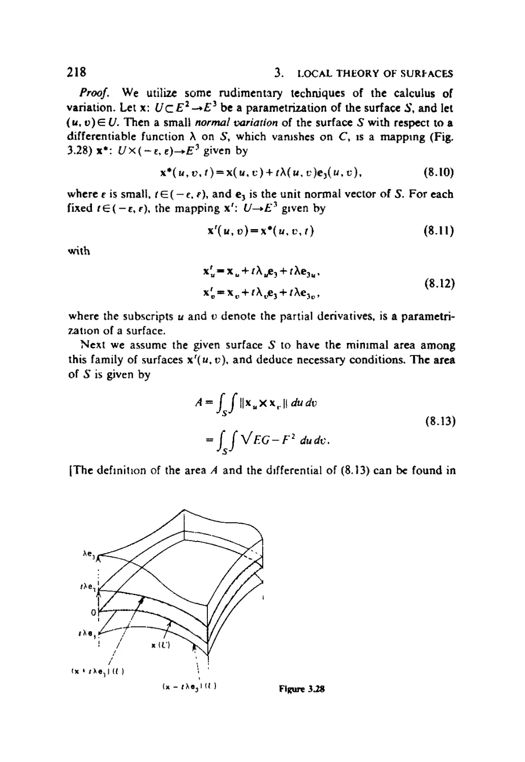
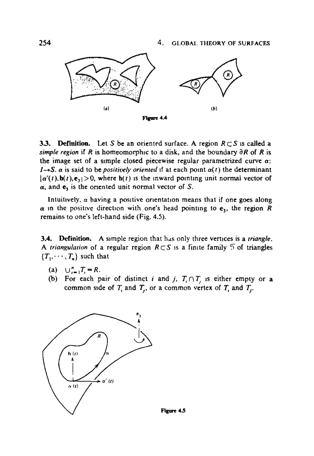
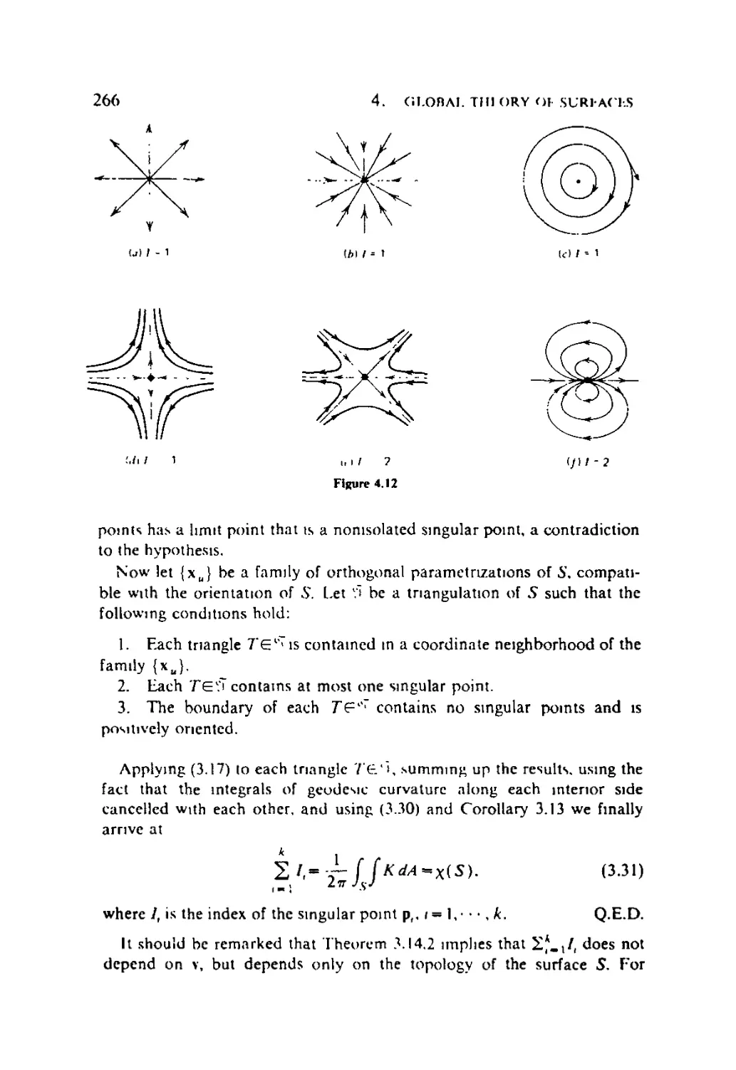
/


Текст
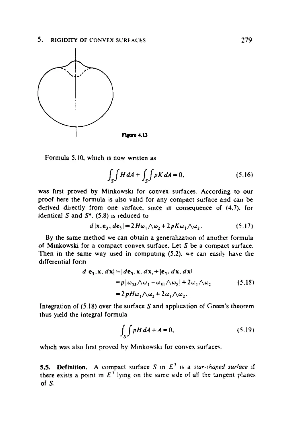
A First Course in
Differential Geometry
CHUAN-CHIH HSIUNG
Lehigh University
A W1LEY-1NTERSCIENCE PUBLICATION
JOHN WILEY & SONS, New York • Chichester • Brisbane • Torooto
Copyright « 1981 by John Wiley & Sons, Inc.
All rights reserved. Published simultaneously in Canada.
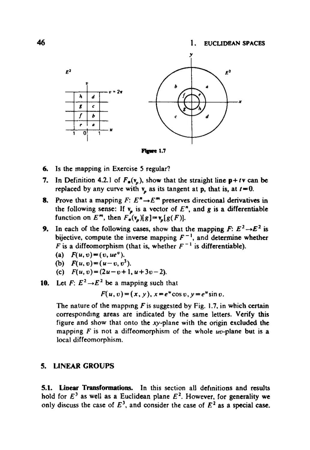
Reproduction or translation of any part of this work
beyond that permitted by Sections 107 or 108 of the
1976 United States Copyright Act without the permission
of the copyright owner is unlawful. Requests for
permission or further information should be addressed to
the Permissions Department. John Wiley & Sons. Inc.
Library of Congress Cataloging in Publication Data:
Hsiung. Chuan-Chih. 1916-
A first course in differential geometry.
(Pure and applied mathematics)
"A Wiley^Interscience publication "
Bibliography: p.
Includes index.
1. Geometry, Differential. I. Title.
QA641.H74 5163 6 80-22112
ISBN 0471-07953-7
Printed in the United States of America
10 9 8 7 6 5 4 3 2 t
To my wife Wenchin Yu
Preface
According to a definition stated by Felix Klein in 1872, we can use
geometric transformation groups to classify geometry. The study of proper-
ties of geometric figures (curves, surfaces, etc.) that are invariant under a
given geometric transformation group G is called the geometry belonging
to G. For instance, if G is the projective, affine. or Euclidean group, we
have the corresponding projective, affine, or Euclidean geometry.
The differential geometry of a geometric figure F belonging to a group G
is the study of the invariant properties of F under G in a neighborhood
of an element of F. In particular, the differential geometry of a curve is
concerned with the invariant properties of die curve in a neighborhood of
one of its points. In analytic geometry the tangent of a curve at a point is
customarily defined to be the limit of the secant through this point and a
neighboring point on the curve, as the second point approaches the first
along the curve. This definition illustrates the nature of differential
geometry in that it requires a knowledge of the curve only in a neighborhood
of the point and involves a limiting process (a property of this kind is said
to be local). These features of differential geometry show why it uses the
differential calculus so extensively. On the other hand, local properties of
geometric figures may be contrasted with global properties, which require
knowledge of entire figures.
The origins of differential geometry go back to the early days of
the differential calculus, when one of the fundamental problems was the
determination of the tangent to a curve. With the development of the
calculus, additional geometric applications were obtained. The principal
contributors in this early period were Leonhard Euler A707-1783),
Gaspard Monge A746-1818), Joseph Louis Lagrange A736-1813). and
Augustin Cauchy A789- 1857). A decisive step forward was taken by Karl
Friedrich Gauss A777-1855) with his development of the intrinsic
geometry on a surface. This idea of Gauss was generalized to n( > 3)-dimensional
space by Bernhard Riemann A826- 1866), thus giving rise to the geometry
that bears his name.
This book is designed to introduce differential geometry to beginning
graduate students as well as advanced undergraduate students (this intrc-
vii
viii
PREFACE
duction in the latter case is important for remedying the weakness of
geometry in the usual undergraduate curriculum). In the last couple of
decades differential geometry, along with other branches of mathematics,
has been highly developed. In this book we will study only the traditional
topics, namely, curves and surfaces in a three-dimensional Euclidean space
f3. Unlike most classical books on the subject, however, more attention is
paid here to the relationships between local and global properties, as
opposed to local properties only. Although we restrict our attention to
curves and surfaces in ?3, most global theorems for curves and surfaces in
this book can be extended to either higher dimensional spaces or more
general curves and surfaces or both. Moreover, geometric interpretations
are given along with analytic expressions. This will enable students to
make use of geometric intuition, which is a precious tool for studying
geometry and related problems; such a tool is seldom encountered in other
branches of mathematics.
We use vector analysis and exterior differential calculus. Except for
some tensor conventions to produce simplifications, we do not employ
tensor calculus, since there is no benefit in its use for our study in space
E\ There are four chapters whose contents are, briefly, as follows.
Chapter 1 contains, for the purpose of review and for later use, a
collection of fundamental material taken from point-set topology,
advanced calculus, and linear algebra. In keeping with this aim, all proofs of
theorems are self-contained and all theorems are expressed in a form
suitable for direct later application. Probably most students are familiar
with this material except for Section 6 on differential forms.
In Chapter 2 we first establish a general local theory of curves in ?3,
then give global theorems separately for plane and space curves, since
those for plane curves are not special cases of those for space curves. We
also prove one of the fundamental theorems in the local theory, the
uniqueness theorem for curves in ?3. A proof of this existence theorem is
given in Appendix 1.
Chapter 3 is devoted to a local theory of surfaces in E3. For this theory
we only state the fundamental theorem (Theorem 7.3), leaving the proofs
of the uniqueness and existence parts of the theorem to, respectively,
Chapter 4 (Section 4) and Appendix 2.
Chapter 4 begins with a discussion of orientation of surfaces and
surfaces of constant Gaussian curvature, and presents various global
theorems for surfaces.
Most sections end with a carefully selected set of exercises, some of
which supplement the text of the section: answers are given at the end of
the book. To allow the student to work independently of the hints that
accompany some of the exercises, each of these is starred and the hint
PREFACE
IX
together with the answer appear at the end of the book. Numbers in
brackets refer to the items listed in the Bibliography at the end of the
book.
Two enumeration systems are used to subdivide sections; in Chapters 1
(except Sections 4 and 7) and 2, triple numbers refer to an item (e.g^ a
theorem or definition), whereas in Chapters 3 and 4 such an item is
referred to by a double number. However, there should be no difficulty in
using the book for reference purposes, since the title of the item is always
written out (e.g., Corollary 5.1.6 of Chapter I or Lemma 1.5 of Chapter 3).
This book can be used for a full-year course if most sections of Chapter
1 are studied thoroughly.
For a one-semester course I suggest the use of the following sections:
Chapter 1: Sections 3.1, 3.2, 3.3, 6.
Chapter 2: Section 1.1 (omit 1.1.4-1.1.6), Section 1.2 (omit 1.2.6. 1.2.7),
Section 1.3 (omit 1.3.7-1.3.12), Sections 1.4 and 1.5 (omit 1.5.5): Section 2
(omit 2.3, 2.5, 2.6.4-2.6.6, 2.9-2.11, 2.14-2.23); Section 3 (omit 3.1.8-
3.1.14).
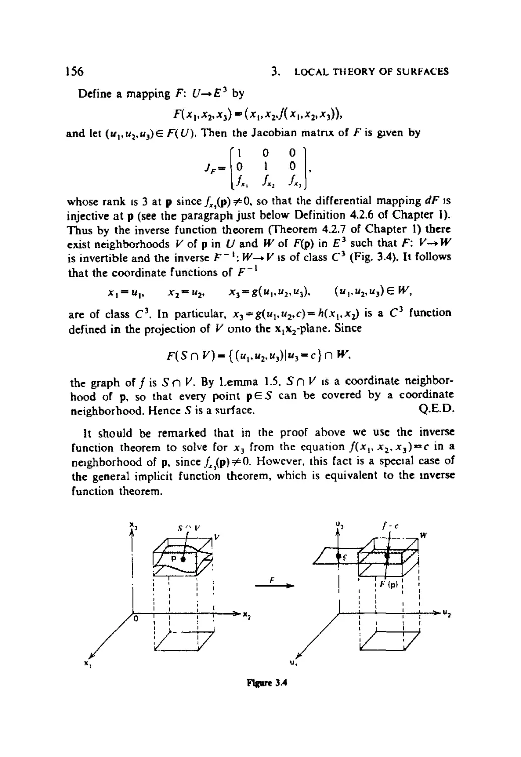
Chapter 3: Section 1 (omit the proof of 1.6, 1.7, 1.8, the proof of 1.10,
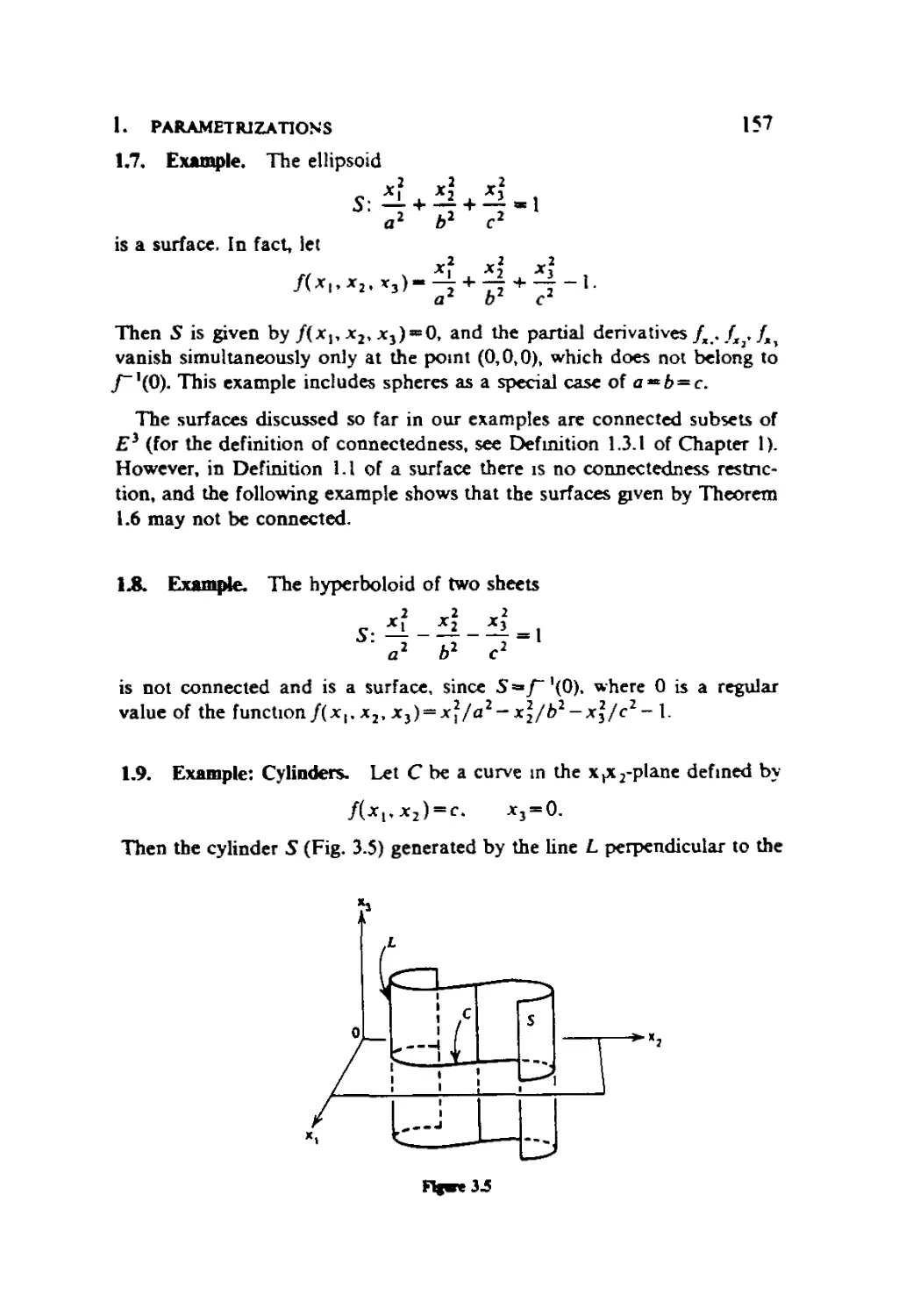
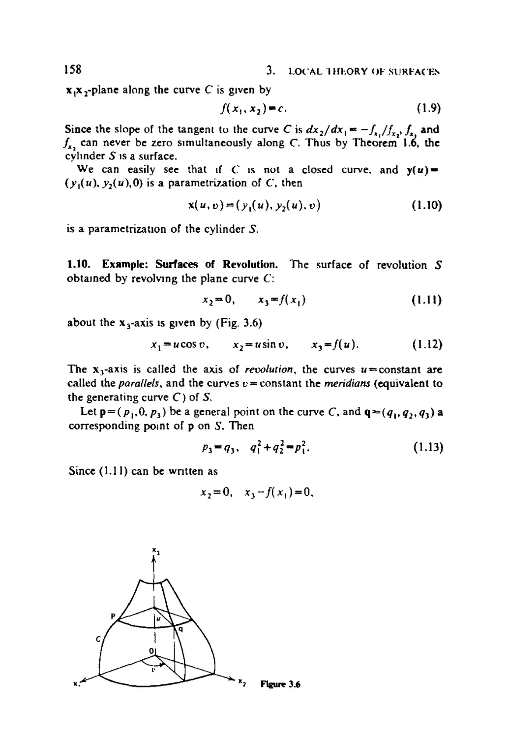
l.U-1.13, 1.15-1.18); Section 2 (omit the proof of 2.4); Sections 3-9;
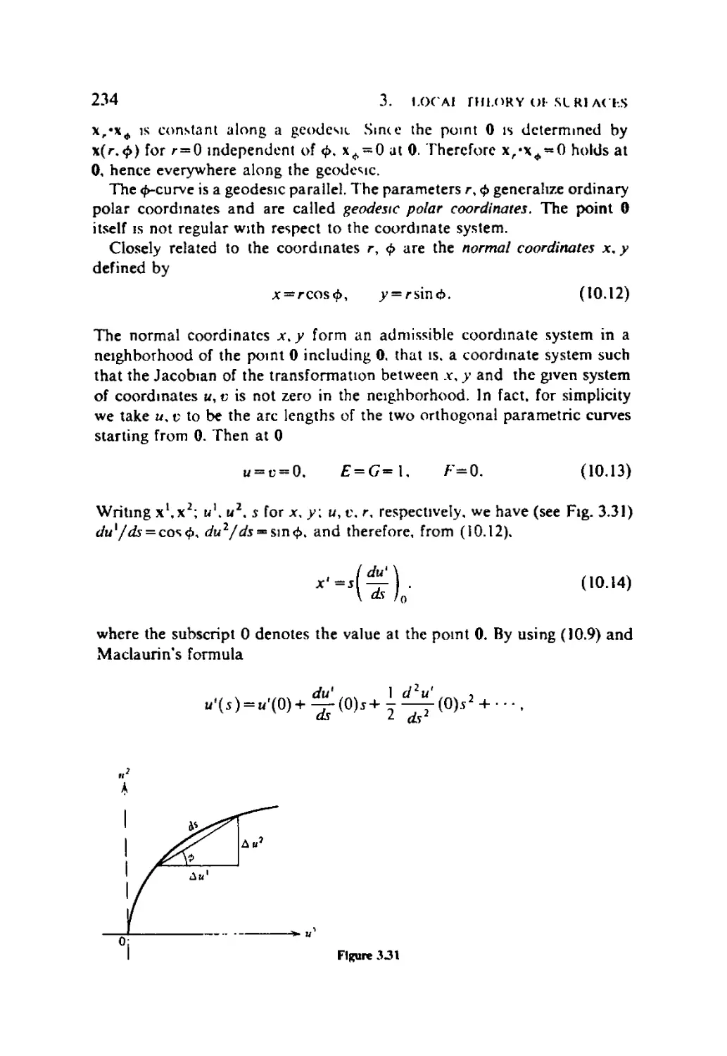
Section 10 (omit the material after 10.7).
Chapter 4: Section I (omit the proofs of 1.3 and 1.4); Section 3 (omit
3.14); Sections 4 and 5.
For a course lasting one quarter I suggest omission of the following
material from the one-semester outline above: Chapter 2: the second proof
of 2.6, 3.2; Chapter 3: the details of 1.3 and 1.4, the proof of 5.7. Section 6,
the proofs of 8.1 and 8.2; Chapter 4: Section 5.
I thank Donald M. Davis, Samuel L. Gulden, Theodore Hailperin,
Samir A. Khabbaz, A. Everett Pitcher, and Albert Wilansky for many
valuable discussions and suggestions in regard to various improvements of
the book; Helen Gasdaska for her patience and expert skill in typing the
manuscript; and the staff of John Wiley, in particular Beatrice Shube. for
their cooperation and help in publishing this book.
Chu*n-Chih Hsiung
Bethlehem, Pennsylvania
September, 1980
Contents
GENERAL NOTATION AND DEFINITIONS
CHAPTER 1. EUCLIDEAN SPACES
1. Point Sets, 1
1.1. Neighborhoods and Topologies, 1
1.2. Open and Closed Sets, and Continuous Mappings. 4
1.3. Connectedness, 7
1.4. Infimum and Supremum, and Sequences, 9
L5. Compactness, 11
2. Differentiation and Integration, 15
2.1. The Mean Value Theorems, 1?
2.2. Taylor's Formulas, 17
2.3. Maxima and Minima, 18
2.4. Lagrange Multipliers, 20
3. Vector 23
3.1. Vector Spaces, 23
3.2. Inner Product, 24
3.3. Vector Product, 25
3.4. Linear Combinations and Linear Independence;
Bases and Dimensions of Vector Spaces, 27
3.5. Tangent Vectors, 29
3.6. Directional Derivatives, 32
4. Mappings, 35
4.1. Linear Transformations and Dual Spaces. 35
4.2. Derivative Mappings. 40
5. Linear Groups, 46
5.1. Linear Transformations, 46
5.2. Translations and Affine Transformations, 52
xi
Xll
CON JLNIS
5.3. Isometrics or Rigid Motions, 54
5.4. Orientations. 59
6. Differential Forms, 64
6.1. 1-Forms. 64
6.2. Exterior Multiplication and Differentiation, 67
6.3. Structural Equations, 73
7. The Calculus of Variations, 75
CHAPTER 2. CURVES 78
1. General Local Theory, 78
1.1. Parametric Representations, 78
1.2. Arc Length. Vector Fields, and Knots. 82
1.3. The Frenet Formulas, 88
1.4. Local Canonical Form and Osculants, 100
1.5. Existence and Uniqueness Theorems. 105
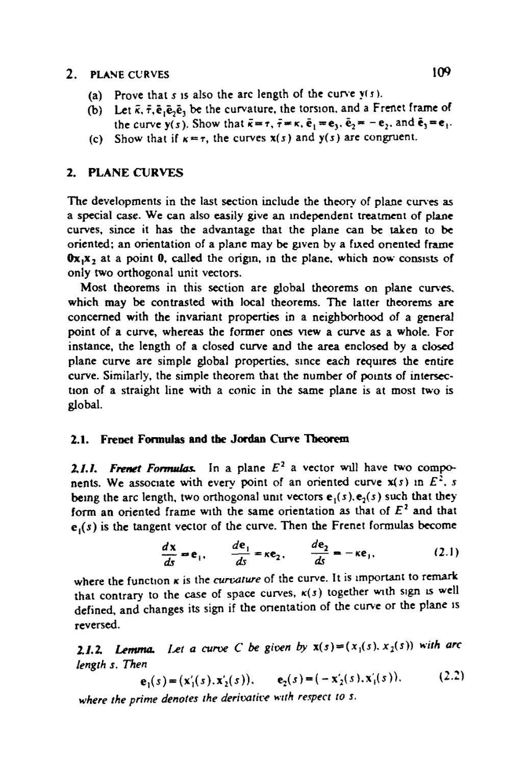
2. Plane Curves, 109
2.1. Frenet Formulas and the Jordan Curve Theorem, 109
2.2. Winding Number and Rotation Index, 110
2.3. Envelopes of Curves. 112
2.4. Convex Curves, 113
2.5. The isoperimetric Inequality. 118
2.6. The Four-Vertex Theorem, 123
2.7. The Measure of a Set of Lines. 126
2.8. More on Rotation Index. 130
3. Global Theorems for Space Curves, 139
3.1. Total Curvature, 139
3.2. Deformations, 147
CHAPTER 3. LOCAL THEORY OF SURFACES 151
1. Pararoeirizations, 151
2. Functions and Fundamental Forms 170
3. Form of a Surface in a Neighborhood of a Point, 182
4. Principal Curvatures Asymptotic Curves, and Conjugate
Directions, 188
5. Mappings of Surfaces 197
CONTENTS
XHl
6. Triply Orthogonal Systems and the Theorems of Dupin and
Liouville, 203
7. Fundamental Equations 207
8. Ruled Surfaces and Minimal Surfaces 214
9. Levi-Civita Parallelism, 224
10. Geodesies 229
CHAPTER 4. GLOBAL THEORY OF SURFACES 241
1. Orientation of Surfaces 241
2. Surfaces of Constant Gaussian Curvature. 246
3. The Gauss-Bonnet Formula, 252
4. Exterior Differential Forms and a Uniqueness Theorem
for Surfaces 267
5. Rigidity of Convex Surfaces and Minkowski's Formulas 275
6. Some Translation and Symmetry Theorems 280
7. Uniqueness Theorems for Minkowski's and Chiistoffers
Problems 285
8. Complete Surfaces 292
Appendix 1. Proof of Existence Theorem 15.1. Chapter 2 307
Appendix 2. Proof of the First Part of Theorem 7 J. Chapter 3 309
Bibliography 313
Answers and Hints to Exercises 316
Index
335
General Notation
and Definitions
NOTATION
Symbol
Usage
Meaning
€
<2
c
0
n
u
{ }
->
H»
I.!
(.)
DEFINITIONS
xE/4
xe>i
fic/f
0
f AnB
(AuB
{*!¦¦¦>
**
,4->fl
xv-*x2
[«.*]
(*.*)
x is an element of the set A
x is not an element of the set A
The set B is a subset of the set A
The empty set
Intersection of the sets A and B
Intersection of all the sets At
Union of the sets A and B
Union of all the sets A,
The set of all x such that • ¦ ¦
• ¦ ¦ implies
¦ ti ?tno only u—~^—^—
Function on the set A to the set B
Function assigning x3 to x
{x\a<x<b)
{x\a<x<b}
A function f on a set A to a set B is a rule that assigns to each element x
of A a unique element/(x) of B. The element/(x) is called the value of/at
x. or the image of x under/. The set A is called the domain off. the set B is
XVI GENERAL NOTATION AND DI-FINU'IONS
often called the range off, and the subset of B, denoted by f(A)> consisting
of all elements of the form/(x) is called the image of/.
If both /, and f2 are functions on A to B, then fx =/2 means that
/,(*)=/2(*)foraIlxe/f.
Let/: A-+B and g: B-*C be functions. Then the function g(f): A-*C,
whose value on each xtzA is the element g(f(x))E.C, is called the
composite function of/and g, denoted by go/.
If/: A-*B is a function, C is a subset of A, and D is a subset of B, the
restriction of/to C is the function/|C: C-*B defined by the same rule as/,
but applied only to elements of C, and the subset of A consisting of all
x?A such that/(x)eZ) is called the inverse image of D and is denoted by
A function/: A—*B is said to be one-to-one or infective if x^y implies
f(x)=?f(y)- An injective function is called an injection, f is said to be onto
or surjective if to each element 6GB there exists at least one element aSA
such that f(a) = h. A surjective function is called a surjection. A function
that is both injective and surjective is said to be bijecfive. A bijective
function is also called a bijection.
Note that under a bijective function/: A-+B, each element bGB is the
image of one and only one element aGA. We then have an inverse
function/ "l, defined throughout B, which assigns to each element bGB
the unique element aE.A such that b—f{a).
Let A be a nonnegative integer. A function on a Euclidean n-space E" to
the real line ?' is said to be of class Ck (respectively, C30) or a C*
(respectively. C*5) function if its partial derivatives of orders up to and
including k (respectively, of all orders) exist and are continuous. A C°
function means merely a continuous function.
The words "set," "space," and "collection" are synonymous, as are the
words "function" and "mapping."
A First Course in
Differential Geometry
1
Euclidean Spaces
This chapter contains, for a Euclidean space of three dimensions
(extension to higher dimensions is virtually automatic), the fundamental material
that is necessary for later developments of this book. Although most
students are probably familiar with a great part of the material, its
placement in one chapter makes it convenient for purposes of review and
also allows us to bring out more clearly relationships among certain
notions. Depending on the backgrounds of the students, certain sections
may be selected for more thorough study.
1. POINT SETS
1.1. Neighborhoods and Topologies. Let ?3 be a Euclidean three-
dimensional space. In the usual sense, in ?3 we lake a fixed nght-handed
rectangular trihedron OXjXjXj (see Fig. 1.1). that is. a point 0. called the
origin of ?3, and mutually orthogonal coordinate axes x,.x2.x3. whose
positive directions form a right-handed trihedron. Then relative to OxjXjXj a
point x in E3 has coordinates (x1,jc2,x3). More generally, we have the
following definition.
/././. Definition. A Euclidean n-dimensional space ?" is the set of all
ordered n- tuples x = (.x ].--•, x„) of real numbers. Such an n-tuple is a point
in E".
In accordance with our stated purpose, here and throughout this book
we limit our discussions to n= 1,2,3.
Let «„•¦•,«„ be real-valued functions on E" such that for each point
x=(*,,-••,*„),
u,(x) = .t,,---,i/),(x) = .x,.
1. taxi.iwan spachs
*. "fjure 1.1
These functions u,, • • ¦, un are called the natural coordinate functions of E\
The distance d{\,y) between two points x —(x,,- • ¦, xn) and y=
(y,,- • •, y„) in ?" is defined by the formula
<'2(x,y)= i(x,~y,J. «/(x.y)>0. A.1.1)
j- i
It is obvious that </(x,y) = 0 if and only if *, =>',. /= 1,- • •, n, that is, if and
only if x coincides with y. furthermore, we have d(\,y) — d(y,\) and the
triangle inequality for zE?"
tl(x.y)+d(y.z)>d(x.z). A.1.2)
LL2. Definition. An open spherical neighborhood of a point Pq in iT" is
the set of the form
{PE?-|rf(p.fc)<p}. A.1.3)
where p>0. More generally, a neighborhood of Pn is any set that contains a
spherical neighborhood of p^.
For n-3 it is convenient to use open spherical neighborhoods. However,
for n~2 a neighborhood of Pq is any set that contains some open disk
{jp(rf 3:d(p,Po)< p} about Pq, and for «= 1 it is an open interval
containing P«
We can easily obtain Lemma 1.1.3.
LI.3. LemmtL The neighborhoods of a point py in E" have the following
properties:
(a) p^ belongs to any neighborhood of p0.
(b) If U is a neighborhood of p<j, and V a set such that V3U, then V is
also a neighborhood of p0.
(c) // U and V are neighborhoods ofpy.so is Ur\V.
(d) // U is a neighborhood of pf,. there is a neighborhood V of pQ such that
VcU and V is a neighborhood of each of its points.
1. POINT SETS
3
1.1.4. Definition. In general, a topological space is a set S together with
an assignment to each element p0?S of a collection of open subsets of 5
(see Definition 1.2.1), to be called neighborhoods of p0, satisfying the four
properties listed in Lemma 1.1.3, and the collection of the neighborhoods
of all points of 5 is a topology for the space 5.
Thus a Euclidean space ?" and the unit sphere in ?3 with center at the
origin are both topological spaces.
1.1.5. Definition. Let S be a topological space, T a subset of S. and p a
point of T. Then a subset U of T is a neighborhood of p in T if U= Tn V,
where V is a neighborhood of/> in 5. The neighborhoods U in 7* so defined
have the four properties in Lemma 1.1.3. When T is made into a
topological space by defining neighborhoods in this way, it is a subspace of 5. and
all the neighborhoods form a relative topology of S for the space T.
In the remainder of this section, unless stated otherwise, all spaces are
supposed to be topological and all sets are to be in a general topological
space, although we shall be interested only in spaces E" for «= 1,2,3.
1.1.6. Definition. With respect to a subset T of a space S, each point p
has one of the following three properties:
(a) p is interior to 7* if p G T and T is a neighborhood of/?. The set of all
the points interior to T is the interior of 7.
(b) p is exterior to T if p ? T and there is a neighborhood of p that is
disjoint from T, (i.e., has no points in common with 7").
(c) p is a boundary point of T if p is neither interior nor exterior to T.
The set of all boundary points of T is the boundary of T and is denoted bv
dT.
From the definition above it follows that an interior point of 7 is
surrounded completely by points of T, that there are no points of 7 that
are arbitrarily close to an exterior point of T, and that a boundary point of
T may or may not belong to T.
The following is a frequently used method of obtaining new spaces from
given spaces.
Let S and 7" be nonempty spaces. The set 5x7", called the Cartesian
product of S and T, is defined to be the set of all ordered pairs (p.q) where
pES and qET. This set is made into a space as follows. If {p.q)ESx T.
then a neighborhood of (p,q) is any set containing a set of the form
UX V, where V is a neighborhood of p in S, and V is a neighborhood of q
in T. It is not hard to see that the neighborhood axioms a-d of Lemma
1.1.3 are satisfied.
4
1 . EUCLIDEAN SPACItS
1.1.7. Definition. SxT, made into a space as just described, is the
topological product of 5 and T.
Examples. 1. If S = 7"*= E\ then SxT is the plane with its usual
topology (i.e.. is E2).
2. If S=EZ and T=E\ then SxT=E\ In general, EmXE" =Em+«.
3. If S is an interval on E\ and 7" is a circle, then Sx T is a cylinder.
4. The torus is the topological product of a circle with itself.
Exercises
1. Prove Lemma 1.1.3.
2. I^t 5= {all {x, y) with x and y rational numbers}, (a) What is the
interior of S? (b) What is the boundary of 5?
1.2. Open and Closed Sets, and Continuous Mappings
1.2.L Definition. A subset T of a space S is open if every point of T is
interior to 7"; this is the same as saying that no boundary point of T
belongs to T. A subset T of a space 5 is closed if every point of S that is
not in T is in fact exterior to T\ this is the same as saying that every
boundary point of T is in T. The empty set, denoted by 0, is an open set
that contains no elements and is therefore a subset of every set.
The behavior of open and closed sets under the operations of union and
" intersection is of fundamental importance and is described by the
following theorem.
1.2.2. Theorem, (a) The union of any collection of open sets in a space S
is open.
<b) The intersection of a finite collection of open sets in S is open.
(c) The intersection of any collection of closed sets in S is closed.
(d) The union of a finite collection of closed sets in S is closed.
Proof, (a) Let {U,} be a collection of open sets in S, where / ranges
over some set of indices. Let U~ u U{ and take p in U. Then p&U; for
some /, and by Definition 1.2.1, U, is a neighborhood of/?. Since Ud Ut, V
is a neighborhood of p by Lemma 1.1.3(b). Thus V is a neighborhood of
each of its points and is therefore open by Definition 1.2.1.
(b) Let I/, and U2 be open sets in 5 and take p^Uxr\V2. Then by
Definition 1.2.1. t/, and U2 are neighborhoods of p. From l^mma 1.1.3(c)
I. POINT SETS
^
it thus follows that Vx n U2 is a neighborhood of p. Since p is arbitrary,
U} D U2 is open by Definition 12.1. Using mathematical induction, we can
extend this to a finite collection of open sets in S.
Parts (c) and (d) of Theorem 1.2.2 are obtained from parts (a) and fl>) by
considering the complementary sets.
Remark. The statement of Theorem 1.2.2b may not be true if "finite" is
replaced by "infinite." For example, if 5 is the real line E\ and Um is the
open interval (- 1/n, 1/n), then each UH is an open set, but the
intersection of all the U„ is the point 0, which is not open.
1.13. Definition. A point p is a limit (or cluster or accumulation) point of
a set T if every neighborhood of p contain^ a point of T distinct from p.
The closure of a subset Tof S, denoted by T, is the union of Tand the set
of its limit points.
Example. Consider the set
S«{pe?2|0<rf(p,0)<l}u {the point @.2)}.
where 0 is the point @.0). The boundary of S consists of the
circumference, where </(p,0) = 1. and the two points 0 and @,2). The intenor
of S is the set of points p with 0< J(p,0)< 1, and the closure of S is the set
consisting of the point @,2), together with the unit disk, the set of all
points p such that rf(p,0) < 1.
1.2.4. Definition. Let T be a subset of a space 5". The set of all points of
S that are not in T is the complement of 7" in 5, and is denoted by S-T.
The following lemma is an immediate consequence of Definitions 1.2.1
and 1.2.4.
1.2.5. Lemma. A subset Tof a space S is open (respectively, closed) if and
only if S~T is closed (respectively, open).
1.2.6. Theorem. Let T be any subset of a space S. Then T is closed if and
only if r«* T.
Proof. First suppose that T is closed. Then S-T is open. If S~T
contains a limit point/) of T, then every neighborhood N(p) of p contains
a point of 7; and N(p)ZS- T. This contradicts the fact that S- T is open.
Hence T» T.
Conversely, suppose that T— T. LetpSS~T. ThenpG.T, andp is not a
limit point of T. Thus p has a neighborhood that contains no point of T
6 I. EUCLIDEAN SPACES
and belongs to S-T. This shows that S-Tis open, and therefore that Tis
closed.
1.2.7. Definition. Let S and T be two spaces. A mapping/: S-»T is
continuous at a point p e S if for any neighborhood V of /(p) in T there is a
neighborhood U of p in 5 such that f(U)cV- / is continuous if it is
continuous at each point p in 5.
1.2.8. Definition. Let 5 and T be two spaces, and /: S->T be a bisection.
If both/and its inverse/"l are continuous, then /is a homeomorphismy and
S and 7" are homeomorphic.
Exercises
1. By constructing an example, show that the union of an infinite
collection of closed sets may not be closed.
*2. Show that (a) the interior of a set S is the largest (in the sense of
inclusion) open set contained in 5, and (b) the closure of a set S is the
smallest closed set that contains S.
*3. Let C be a closed set, and V an open set. Prove: (a) C- (/—{allp6C
with/>€?/} is closed, and (b) V—C is open.
4. Show that if p is a limit point of a set S in E", then every
neighborhood of p contains infinitely many points of S.
5. If S and T both are the real line, the usual definition of continuity is
that /: S~* T is continuous at x e S if for any e > 0 there is a 6 > 0 such
that \f(x')-f(x)\<e whenever x'?Sand |*'-xj<6\ Prove that this
is equivalent to Definition 1.2.7.
6. Let 5 and T be two spaces and /: S^T a mapping. Prove that/is
continuous if and only if the inverse image of any open set in 7* is
open in 5. Use this to show that the composition of continuous
mappings is continuous.
7. Let S be the union of two closed sets U and Vy and /: S-+T a
mapping. Suppose that the restriction of / to V and to V are
continuous mappings of V and V into T, respectively. Show that / is
continuous. Given an example to show that this does not hold if V
and V are not closed.
* Asterisks indicate exercises for which hints are provided at the end of the book.
1. POINT SETS
7
13. Connectedness
IJJ, Definition. A space $ is connected if it is not the union of two
nonempty disjoint open sets. A subset of a space is connected if it is a
connected space as a subspace with the relative topology. A space is
disconnected if it is not connected.
Examples. 1. The empty set is connected.
2. Let S«@, l)uB,3) on ?'. Then @,1) is open and also closed since
@,1)=[0, \]nS. Hence 5 is disconnected
We can easily prove the following two equivalent definitions of
connectedness.
1.S.Z Lemma. A space is connected if and only if it is not the union of r*o
nonempty disjoint closed sets,
1.3.3. Lemma. A space S is connected if and only if the only sets in S that
are both open and closed are S and the empty set.
Since connectedness is defined in terms of open sets, it is a topological
invariant, an invariant preserved by homeomorphisms. However it is also
preserved by continuous mappings, as indicated in Theorem 1.3.4.
1.3.4. Theorem. Every continuous image of a connected set is connected.
Proof. Suppose that S is any connected set, that/: S~+T is continuous
and surjective, and that Tis disconnected. If 7"** Uu V. where U and V are
nonempty disjoint open sets, then f~\U) &ndf~\V) are clearly disjoint
and nonempty, and are open by Exercise 6 of Section 1.2. Thus S =*/"*((/)
Uf~\V) is disconnected, contradicting the assumption. Hence T is
connected.
Example. Consider a continuous mapping of the unit interval of real
numbers x such that [0,1] is mapped onto the circumference of a circle,
that is, x is mapped onto the point (cos 2irx, sin2wjc) in E2. By Theorem
1.3.4, the circumference of a circle is connected.
In Theorem 1.3.5 we have one of the most important connected spaces.
1.3.5. Theorem. E1 is connected.
Proof. Let F be a closed proper subset of ?' so that Ex ±F*<3. Then
we can assume that xSE\ .vSF. vG/\ Furthermore, without loss of
generality we can assume that v<jc, since using inf instead of sup (see
8
1. EUCLIDEAN SPACES
Definition 1.4.1) we can have the case by a similar argument of y>x. Let
r»sup {t&F\t<x}. Then><2<jc. Since disclosed, every neighborhood
of z meets F so that zGF. Thus z < x. Since the open interval (z, jc) does
not intersect Ft it follows that z is not an interior point of F and so F is not
open. Hence by Lemma 1.3.3, E1 is connected.
1.3.6. Theorem. A subset of ?' is connected if and only if it is an interval
{open, closed, or half-open).
Proof. If a connected subset S of ?' is not an interval, then there exists
ae?l such that a&S and that A**{x\x>a}r\S is a nonempty subset of
S, so that A is open in 5. Since also A - {x\x > a) nS, A is closed in S. By
Lemma 1.3.3, S is disconnected, contradicting the assumption. Hence S is
an interval.
The proof that each interval S on E1 is connected is identical with the
proof of Theorem 1.3.5 except that now FcS, and x&S.
1.3.7. Theorem. If S and Tare connected spaces, then SxTis connected.
Proof. Suppose that SxT is not connected. Then by Definition 1.3.1,
SxT= Uu V, where U and V are nonempty disjoint open sets. Take (jc, y)
in U. The set Sx{y} is homeomorphic to S and so is connected. It follows
that Sx{v} is contained in V, for otherwise its intersections with {/and V
would form a decomposition into nonempty disjoint open sets. But then a
similar reasoning would show that for each x'ElS the slice {x'} X T would
be in U\ thus all SxT would be in V, and V would be empty. This
contradicts the assumption that V must be nonempty. Hence SxT is
connected. Q.E.D.
From Theorems 1.3.5, 1.3.6, and 1.3.7 we immediately have two
examples.
U.S. Examples. 1. The closed interval I = \a,b\ on E1, the closed
rectangle I2 = lxl, and, therefore by mathematical induction, the closed
rt-dimensional cube /" are connected. Similarly, ?' and En are connected.
2. A closed disk that is homeomorphic to I2 is connected. The surface
5 of a 2-sphere can be expressed as the union of two closed disks with
nonempty intersection. So by Exercise 5, below, this surface S2 is
connected. Similarly, the n-sphere is connected for any n.
1.3.9. Definition, If 7" is a connected subset of a set S and is not
contained in any other connected subset of S, then T is a component of 5.
In other words, components of 5 are maximal connected subsets of S.
1. POINT SETS
9
Exercises
1. Prove that the set A.1.3) is an open set, and discuss all the properties
described in Sections l.l- t.3 for this set of points.
2. Discuss ail the properties as in Exercise 1 for the set of points (x. y) in
E2 such that^2-/2<0.
3. Prove Lemmas 1.3.2 and 1.3.3.
4. Let A and B be connected sets in E2. Is A n B or A u B necessariiy
connected?
5. Let A and B be connected sets in a space 5, and suppose that An Bis
not empty. Show that A u B is connected.
1.4. Inflmum and Supremum, and Sequences
1.4.1. Definition. Let 5 be a set of real numbers. If M is a real number
such that x < M for each x SS, M is an upper bound of S. If A \s an upper
bound of S. and there is no upper bound of 5 smaller than A. then A is the
least upper bound or the supremum of 5, abbreviated lub 5 or sup S. On the
other hand, if m is a real number such that m <, x for each x65. then m is
a lower bound of S. If B is a lower bound of S and there is no lower bound
of S greater than 5, then B is the greatest lower bound or the infimum of S.
abbreviated gib S or inf S.
For the existence of a supremum and an infimum we have the following
axiom and theorem.
1.4.2. Axiom of Completeness. Any nonempty set of real numbers that has
an upper bound has a supremum.
1.4.3. Theorem. Any nonempty set S of real numbers that has a lower
bound has an infimum.
Proof of Theorem 1.4.3. The set 7", obtained by changing every element
of S to its negative, has as an upper bound the negative of any lower
bound of 5". By the axiom of completeness. T then has a supremum. whose
negative must be the infimum of S.
1.4.4. Definition. Let 5 be a subset of ?". and d(p,q) the distance
between two points p and q in 5. Then the diameter of S is
sup d(p,q)
S is bounded if its diameter is finite.
10
1. r-Ut'MDKAN'SI'ACfcS
From Definition 1.4.4 it follows that if a subset S" of E" is bounded, it
lies entirely within some sphere of radius r>0 with center at the origin
0-@.---.0)in E\
1.4.5. Definition. Let {pm} be a sequence of points in E". Then {pm} is
convergent to a point p in E", written
lim pm * p
m »oo
if and only if for every real number i >0 there is an integer M such that
whenever m>M. then d(pm,p)<c. A sequence of points in E" is convergent
if it is convergent to some point in E". A sequence is divergent if it is not
convergent.
Since this definition refers to the limit of a sequence, we cannot use it to
prove that a sequence is convergent unless we already know what the limit
is. Theorem 1.4.6 provides a way out of this inconvenience.
1.4.6. Theorem. A sequence \p„) of points in E" is comiergent if and only
H
lim d(p„,pm.) = 0,
that is, if and only if for every real number t >0 there exists an integer M such
that d(pm,pm)< t whenever m > M and m'> M.
1.4.7. Definition. The condition in Theorem 1.4.6 for the sequence {pm}
to be convergent is the Cauchy condition, and sequences that satisfy the
Cauchy condition are Cauchy sequences.
From Theorem 1.4.6 it follows that every Cauchy sequence is bounded;
therefore an unbounded sequence necessarily diverges.
1.4.8. Theorem. l*t {Cm} be a sequence of nonempty closed subsets of E"
such that Cm+i C.Cm for all m, and lim,, ,o0dm =0. where dm denotes the
diameter of Cm. Then nCrrt?:0.
Proof. Since lim „,_„«/„ -0, given t >0, there exists an integer M such
that dM <€. Let m>M,m'>M, and for each m choose a point pmECm.
Then pm 6Cw,pmGCw so that d(pm,pm.)<dM<t. Thus {pm} is a Cauchy
sequence, and therefore by Theorem 1.4.6 it is convergent, say pm^p. I^t
m be arbitrary. For m'>m, p„ ?Cm. Since C„ is closed and pm—»p, p€Cm
by Theorem 1.2.6. Hence pGCm, and the theorem is proved.
1. POINT SFTS i 1
Exercises
1. Show that the sup and inf of a set are uniquely determined whenever
they exist.
2. Let a sequence {x„) on ?' be defined as follows: x, = 1. x2 =- 2.
*„+i = }(•*„-1 +*„), n = 2,3.---. Show that d(xm,xn)< l/2v_t if m>
N, n > N, so that the Cauchy condition is fulfilled.
1.5. Compactness
1.5.1. Definition. A space is a Hausdarff space if for any two distinct
points p and q there are neighborhoods U of p and V of q such that
C/n y=0. Thus distinct points are separated by disjoint neighborhoods.
Example. Any Euclidean space is a Hausdorff space.
1.5.2. Definition. A covering of a space 5 is a collection of sets in 5
whose union is S. It is an open covering if all the sets of the collection are
open.
1.5.3. Definition. Given a covering of a space, a subcovenng is a covering
whose sets all belong to the given covering.
1.5.4. Definition. A compact space is a Hausdorff space with the property
that any open covering contains a finite covering, that is, a subcovenng
consisting of finitely many sets. A subset of a space is compact if it is a
compact subspace.
Example. The real line is not compact. For example, take the collection
of open intervals (n - 1, n+ I) for all integers n. This is an open covering of
the real line; but obviously no finite collection of these intervals can cover
the whole line. A similar argument shows that E* for each n is noncom-
pact. and in fact so is any unbounded subset of ?".
For a subset of E" to be compact, we have the following necessary and
sufficient condition.
1.5.5. Theorem. A subset S of E* is compact if and only if it is closed and
bounded.
Proof. The "if" part is the well-known Heine-Borel theorem. To prove
it, we assume that 5 is closed and bounded and that there is an open
12
1. EUCLIDEAN SPACES
covering {U,) of S. Then the new sets, V{, constructed as follows, are open
by Theorem 1.2.2(a): K, = C/,. V2 = U} U U2. V3 = Ux U V2 U C3 - ^2 U C/3,
and, in general. Vi4., = K, u VI+,. These sets ^. form an increasing sequence
K, c V2 c • • • c K C • • • and an open covering of S. From these open sets
Vn by Exercise 3(a) of Section 1.2 we have closed sets St^S— Vr Since S is
bounded, S, is also bounded. Thus we have a decreasing sequence of closed
bounded sets:
l^et df be the diameter of Sr Then we have a monotonic decreasing
sequence {d,} of positive numbers with 0 as its infimum, so that
lim ,_„<,</, "bO. Therefore by applying Theorem 1.4.8 to the sequence {S,}
we have at least a point pG n5,. This p must belong to 5 but not to any of
the sets V,. However, this cannot happen, since {Vt} is a covering of 5.
Thus one of the sets S, is empty, say Sr so that V4 contains 5, and the sets
UX.U2.-'' ,Uj form a finite covering of S. Hence S is compact.
To prove the "only if" part, we assume that S is compact and first show
that S is bounded. Let N(x0\ r) denote the open sphere in E* with center
at x0 and radius r. The collection of spheres N@; k), where &*= 1,2,3,- • •,
and 0 denotes the origin @.- • ¦ ,0) in E", is an open covering of S. By
compactness, a finite subcollection also covers S, hence 5 is bounded.
Now we prove that S is closed. Suppose the contrary. Then by Theorem
1.2,6 there is a limit point y of 5 such that y&S. If xGS, let rx = } <*(x,y).
Each rx is positive, since y?S and the collection {N(x\ rx)\x&S} is an
open covering of S. By compactness, a finite collection of these
neighborhoods covers S, say ScUa-i^x^;^), where rt=rXt. Let r denote the
smallest of the radii rj, r2,- • •, rp. Then it is easy to show that the
neighborhood N(y; r) has no point in common with any of the neighborhoods
N(xk;rk). In fact, if xGiV(y;r), then d{x,y)<r<,rk and
d(x>xk) = d(y~xk,y-x)>d(y.xk)-d(x,y)
~2rK -d(x,y)>rk.
so that x?N(xA; rk). Thus jV(v; r)r\S is empty, contradiction the fact that
y is a limit point of S. Hence S is closed. Q.E.D.
From the definition it is obvious that compactness is a topological
invariant. In fact it is preserved by any continuous mapping, as stated in
the following theorem.
1.5.6, Theorem. Let f: S-+T be a continuous mapping of a compact space S
onto a Hausdorff space T. Then T is compact.
1. POINT SETS
13
Proof. Let {Ut} be an open covering of T. Then the sets/" l(U,) form a
covering of S, which is open by Exercise 6 of Section 1.2. Since S is
compact, a finite subcollection of the sets /"'((/,). say
f~\V\)*f~\V2y-J-\Un), will cover S. Then UtM2r • • ,?/„ form a
finite subcovering of the given covering {U,} of 7". Since 7"is assumed to be
a Hausdorff space, it is compact.
1.5.7. Definition. Let/: S-»r be a function on a set S into a set T. Then
the graph of / is the set of all ordered pairs (x, y) with xSS and
.v»/(x)er, and is thus a special subset of Sx 7\ the Cartesian product of
S and T.
In particular, if 7" is ?J and S is a subset of ?l or ?2, then Sx T is a
subset of ?2 or ?3, and the graph of a function/: S^Tcan be
geometrically visualized as a curve in ?2 or ?3.
1.5.8. Definition. A function /: S-»?' on a subset 5 of ?" attains an
absolute maximum (respectively, minimum) at a point Po€S, and Pq is an
absolute-maximum (respectively, -minimum) point of /, if/(Po)>/(p)
(respectively, /(po) </(p)) for all /> G S.
By means of Theorems 1.5.5 and 1.5.6 we can easily deduce Theorem
1.5.9.
1.5.9. Theorem. Iff: S-*?' is a continuous function on a compact subset S
of ?", then f attains an absolute maximum and an absolute minimum
somewhere on S.
Proof. By Theorems 1.5.5 and 1.5.6, the continuous function / is
bounded on 5, that is. the image /(S) is a bounded set. Then by Axiom
1.4.2 and Theorem 1.4.3, there exist both the supremum M and the
infimum m for the values of /on S so that m </(p) < M for all peS, and M
cannot be decreased, nor m increased. If there is a point Dq in 5 such that
/(Po)~ M« then M is the maximum for/on 5, and it is attained there.
If there is no such point po with /(p,,) - M. then /(p) < M for all peS. In
this case, set
o(«)= ! . A.5.1)
Since the denominator of A.5.1) is never zero, g is continuous on 5 and
must therefore be bounded there. If we suppose that g(p) < A for all p€S,
then from A.5.1) we would have
/(p)<Af--j. for all pes.
IH
I. EUCLIDEAN SPACES
which however contradicts the fact that M is the supremum for the values
of /on S. Thus we conclude that this does not occur and there is a point
Po SS such that/(pb)«M. Similarly, we can show that there is a point in S
where /has the value m, and a minimum is attained. Q.E.D.
When S is the closed interval [a, b] on E\ we immediately obtain
Corollary 1.5.10 from Theorem 1.5-9.
1.5.10. Corollary, A continuous function /: [a, 6]—>El attains an absolute
maximum and an absolute minimum at some points of the closed interval
{a,b).
The three examples that follow show that if the interval is not closed,
Corollary 1.5-10 might not be true.
Examples. \. f(x)»*x, for0<x<10.
There is an absolute maximum at jc=10, but there is no absolute
minimum.
2. f(x)-x2t for -1<jc<2.
There is an absolute minimum at x = 0, but there is no absolute
maximum.
3. /(jc)-tan x, for- — <x<—.
There is neither an absolute maximum nor an absolute minimum.
1.5.11. Theorem. Let S be a connected set, and let f; S~*E* be a
continuous function. Let p,qf=El be any two image points of f, and suppose that
p<r<q. Then there is a point sGS such that f(s)=^r.
Proof. Suppose that/(j) is never r for any point s&S. Then we always
have either f(s)>r or/(j)<r. Let V be the subset {seS\f(s)>r} of S,
and V the subset {.se.S|/(s)<r}. These two sets V and V must cover 5.
Since/is continuous, by Exercise 6 of Section 1.2 the inverse image/"'(/)
of the open unbounded interval / consisting of the numbers x with x>r
(or with x<r) must be open relative to .V. Thus both U and V are open
relative to S. Moreover, since there is a point teS with/(r)=p, the set V
contains t and is therefore not empty; likewise, V is not empty. The
existence of two such sets contradicts the assumption that S was
connected. Hence somewhere in S,/must take the value r. Q.E.D.
In particular, when 5 is a closed interval [a. b]. /?*=inf f(S) and q**
sup/^X Theorem 1.5.11 becomes the following intermediate value
theorem of Bolzano.
1.5.12. Theorem. Iff: [a, b ]-*?*' is a continuous function, then f assumes
every value between its maximum and minimum.
2. DIFFERENTIATION AND INTEGRATION 15
Exercises
•I. Show that every infinite subset of a compact space has a limit point
2. If V is open in E* and Cc U is compact, show that there is a compact
set D such that Cc interior O and Z>c V.
3. Let AT be a compact subset of E" and /: Ar-*>5' be a continuous
function satisfying f(x)>0 for all xEX. Show that there exists e>0
such that f(x) > « for all xGX.
4. Investigate the possibility of absolute extrema of f(x)=x* + 256/x2
for 0<jc<4, and find any which exist
5. Consider the function 27/sinx + 64/cosjc, 0<x<tr/Z Why must
there be an absolute minimum in this open interval? Find where it
occurs and the corresponding value of the function.
6. Without drawing the graph, find the absolute maximum and
minimum of the function 2 sin x — I + 2 cos2 x.
2. DIFFERENTIATION AND INTEGRATION
In this section we list some fundamental formulas and theorems in
elementary calculus that we shall use later. We give here only proofs that cannot
be found in ordinary calculus books.
2.1. The Mean Value Theorems. This section contains four mean value
theorems of differential and integral calculus. The mean value theorem of
differential calculus is one of the most important theoretical results in the
subject. It expresses a geometric property of differentiable functions and
has many applications. The mean value theorems of integral calculus give
estimations of definite integrals.
2.1.1. Theorem (The mean value theorem of differential calcuhts). Suppose
that f: [a, b]-+E* is a continuous function and is differentiable in the interval
(a,b). If we put h**b-a> there is a point a + 8hE(a. b). 0<B<\. such that
f(a + h)=f(a)+hf(a + 0h). B.1.1)
where the prime denotes the derivative *ith respect to the argument.
2.1.2. Theorem (The first mean value theorem of integral calculus). Iff:
[a, b]-*E] is a continuous function, there is a point cG(a, b) such that
fbf(x)dx = (b-a)f(c). B.1.2)
16 1. EUCLIDEAN SPACES
Proof of Theorem 2.1.2. Pu tti ng F( x)« ///(/)dt and applying Theorem
2.1.1 to F(x) immediately give B.1.2).
2.1.3. Theorem {The generalized first mean value theorem of integral
calculus). Suppose that f,g: [a, &]-*?' are continuous functions and that g is
everywhere nonnegaiive (or nortpositive). Then there is a point c^(a> b) such
that
(bf(x)g(x)dx=f(c) Cg(x)dx. B.1.3)
It is obvious that when g(x) — 1 for all xE:[a, b] Theorem 2.1.3 becomes
Theorem 2.1.2.
Proof. We consider the case of g everywhere nonnegative and from this
case, by replacing g by — g, we can deduce the case of g everywhere
nonpositive. Denote the minimum and maximum values of/in [a, b] by m
and M, respectively. Then for every xG[a,b]
mg(x)<f{x)g(x)<Mg(x). B.1.4)
By the definition of a definite integral we know that if F: [a, b]-*Ex is a
continuous function and F>0 throughout [a,b], then
(bF(x)dx>0, B.1.5)
•'a
from which it follows that if G, H: [a, b\-^E] are continuous functions and
G>H throughout [a,b], then
fbG(x)dx>fbH(x)dx. B.1.6)
By integrating B.1.4) between a and b, and using B.1.6), we obtain
mfbg(x)dx<fhf(x)g{x)dx<Mfbg(x)dx. B.1.7)
Ja Ja Ja
For simplicity, denote f*g(x)dx by /. Since ?<x)>0 for all xE[a,b), by
B.1.5) we have />0. If /=»0, then B.1.7) implies that both sides of B.1.3)
are zero, so that B.1.3) is valid for any c. Now suppose that />0. Then
divide B.1.7) by /, so that
m<]1Jbf(x)g(x)dx<M.
Hence Theorem 1.5.12 gives our formula B.1.3) for some cE.(a,b).
2,1.4. Theorem (The second mean value theorem of integral calculus). Sup-
pose that f, g: \a, b]-*E] are functions of classes C° and Cl, respectively, and
2. DIFFERENTIATION AND INTEGRATION
17
that g is monotonic. Then (here exists a point f?[a, b] such that
[bf(x)g{x)dx-g{a)(ef(x)dx+g(b)(bf(x)dx. U.1.8)
Proof. We first notice that we can assume that g(b)=0. since replacing
g(x) by g(x)-g(b) changes both sides of B.1.8) by the same amount and
gives us a function that vanishes at x = b. Moreover, we can assume
g(a)>0; for if g(a)<0 we need only replace g(x) by -g(x). which
changes the sign of both sides of B.1.8). [The case g(a) = 0 is trivial: if
both g(a) and g(b) vanish, g(x) must be identically zero, and both sides of
B.1.8) are zero also.] Thus we need only prove that if g(x) is continuous
and monotonic decreasing and g(b) = 0, then
fbf(x)g(x)dx~g(a)ff(x)dx. B.1.9)
Now by putting F(x) = f*f(t)dt and applying the formula for
integration by parts to the left-hand side of B.1.9). we obtain
fbAx)g(x)dx = F(x)g(x)\ + fbF(x)[ -g(x)] dx. B.1.10)
The first term on the right-hand side of B.1.10) vanishes, since F(a) and
g(b) are zero. The expression -g'(.t) is even-where nonnegative. so that
by applying Theorem 2.1.3 we find that the integral on the nght-hand side
of B.1.10) has the value
F{c) I [ -g'(x)] dx for some cS[a,b).
Since F(c) = jcJ{x)dx and /*[ -g'(x)\dx=gia)-g{b)=g{a). B.1.10) is
just B.1.9), and our theorem is established.
Exercises
1. Use Theorem 2.1.1 to establish the following inequalities:
(a) sinAr<x, for x>0.
L
fb) -—-<ln(l+/i)<A, for *>-l,**0.
\+h
*2. If /'(x) = 0 for all x,a<x<b, show that /is constant there.
2.2. Taylor's Formulas. In this section we give a generalization of
Theorem 2.1.1 (the mean value theorem of differential calculus), together with a
further generalization to functions of two variables.
18
1. KUC LIDEAN St'ACfcS
2.2.1. Theorem. Let f: [atb]-*Ex be a function of class C, and let the
(n + \)st derivative /("+,) (x) of f exist for xE(ahb). If we put h = b-a.
there is a point a + 9h€(a,b), 0<0< 1, such that
B.2.1)
f{a + h)-f{a)+f'(a)h+-'-
+ _^~/j + („ + ]). h ¦
When a = 0, B.2.1) is called Maclaurin's formula.
2.2.2. Theorem. l*t D be a neighborhood of a point (a,b) in E2 and let f:
D-*El be a function of class C*1. Then there is a point (a + $h,b+9k)ED,
0<9<],such that
f(a + h.b + k)
where
-a + *„+i
y)
B.2.2)
B.2.3)
Exercises
1. Find the Taylor expansion for the function
f(x, y)=x* + lx2y2-xy + 2
at the point A, -2) through terms of degree 3.
23. Maxima and Minima
2.3.1. Definition. A function /: E"-v?l has a relative (or local)
maximum (respectively, minimum) at x0e?"\ and x0 is a relative (or local)
-maximum (respectively, -minimum) point of/, if there is a neighborhood V
about x0 in ?" such that/(x) </(x0) [respectively,/(x >/(x0)] for all x€ V.
The term cxtremum is used to refer to either maximum or minimum.
Necessary conditions for relative extremum are given in Theorem 2.3.2.
2. DIFFERENTIATION AND INTEGRATION 19
2.3.Z Theorem. At an interior point pGScE", if a function /: S—»?"' has
a relative extremum and is differentiable. that is, has first partial derivatives.
these derivatives vanish at p.
The converse of Theorem 2.3.2 is generally not true.
2.3.3. Definition. If a function/: 5 c ?"->?"' is differentiate at a point
peS and all the first partial derivatives of/are zero at p, then p is a critical
point off.
In terms of the critical points we have the following criterion for the
relative extrema of a function/: Sc E2->E\
2.3.4. Theorem. Suppose that a function /: S<zE2-+El is differentiable.
that is, has first partial derivatives, and that an interior point p of S is a
critical point off. l^et x,y be the natural coordinate functions of S. and fT. /„
and fxx, fxy, fyy denote, respectively, the first and second partial derivatives of
f(x.y). Suppose further that fx and fy are differentiable at p. and write
A=fxx(p), B=fxy(p), C=/„(p).
Then we have the following cases:
(a) If B2 — AC< 0 and A>0, then f has a relative minimum at p.
(b) /f B2-AC<0 and A <0, then f has a relative maximum at p.
(c) // B1 - A C> 0, then f has neither a relative maximum nor a relative
minimum at p, and p is called a saddle point.
(d) If B2-AC, no conclusion may be drawn, and any of the behaviors
of f described in parts (a)-(c) may occur.
A critical point p is said to be nondegenerate or degenerate according as
B2-AC*0or =0.
According to Corollary 1.5.10, a continuous function /: [a. b]-~?'
attains an absolute maximum and an absolute minimum at some points of
the interval \a, b}. If an absolute extremum occurs at an interior point of
the interval, then it is also a relative extremum, and therefore we have
/'{x) = 0 at the extremum point, provided /is differentiable there.
A function g: El-*El is periodic with period p if there is a constant
integer c>0 such that g(t)**g{t + c) for alt t, and p is the least such
number c. Now let a C1 function/: ?'-»?' be periodic with period b-a.
Then by Corollary 1.5.10, in the interval [a, b] the periodic function /has
an absolute maximum and an absolute minimum, which now are also a
relative maximum and a relative minimum, respectively. In particular, tf
the interval \a,b] is of length />0 with the two end points a and b
identified, between any two consecutive relative maxima (respectively.
20
J . h.UC U 1I.AN SPAC'fcS
minima) of /there is a relative minimum (respectively, maximum);
therefore the relative maxima and minima of / occur in pairs in the interval
\a, b\. To sum up, we hence obtain Theorem 2.3.5.
2.3.5. Theorem. Let f: /r,-»K1 be a periodic continuous C1 function with
period b-a. Then in the interval [a,b], every absolute exiremum off is also a
relative exiremum, and f has at least a relative maximum and a relative
minimum. In particular, if the interval [a, b] is of length />0 with the two end
points a and b identified, the relative maxima and minima of f occur in pairs
in the interval [a,b\.
2.3.6. Theorem (The chain rule). Let f: Sc?3->?1 be a function of class
C\ // jCj, x2. x7. and t are the natural coordinate functions of S and ?l,
respectively, and g: E] -*5 defined by g(t)'=(x,(/), x2(t). x*@) is <*
differentiate function, then fg{t) —f{xi(t),x2(t),x?i{t)) is differentiable, and
3
f(x{(t)x2@,X>(t))= 2/,.(¦*!.*2<*3K'<0,
where the prime denotes the derivative with respect to t, and fx the partial
derivative with respect to xr
Exercises
1. Find the critical points of the function f(x, y)=2x*-yi+ I2x2 + 21y
and determine the nature of each of them.
2. Show that all the critical points of the function f(x, y) = cos(xey) are
degenerate.
3. Find the critical points of the function /(x, y, z) - A - x2)y + (I — y2)z.
2.4. I ^grange Multipliers. The following theorem gives a very elegant
and useful method, known as the method of l^agrange multipliers, for
studying extremal problems for functions of several variables with
constraints. This method avoids either the impossibility or some complication
arising from direct elimination of variables, and permits the retention of
symmetry when the variables enter symmetrically at the outset of the
problem.
2.4.1. Theorem. Suppose that a real-valued function f(x, y) is
differentiable in a neighborhood N{a b) of a point (a. b) in E1. and that it has a relative
extremum at (a.b) subject to a constraint
*(x.y)-Q. B.4.1)
2. DIFFERENTIATION AND INTEGRATION 21
where $ is differentiable in N{a>ity and B.4.1) defines a differentiable function
y~g(x) B.4.2)
in a neighborhood of a such that g(a) = b. Then the point (a,b) is a cntical
point of F(x, y)»f(x, y)~\$(x, y) subject to no constraint, where A is a
constant, called a Lagrange multiplier.
Proof Since f(x, y) with B.4.2) has a relative extremum at (a, 6), by
Theorems 2.3.2 and 2.3.6 we obtain
0-f'(a,g(a))~fAa,b)+f,(a,b)g'(a). B.4.3)
From B.4.1), B.4.2) and Theorem 2.3.6 we also have
<l>x(a,b)+<t>y{a,b)g'(a)~Q. B.4.4)
Elimination of g'(a) from B.4.3) and B.4.4) gives
fx(atb)<t>y{a,b)-fy(a,bL>x(a.b) = 0. B.4.5)
On the other hand, by Definition 2.3.3 a critical point (jc, y) of F\x, y)
satisfies
/,(*.*)-**,(*, jO-o, /,<x,,v)-a^(jc.>-)-0.
or, by elimination of \,
U*,y)<>y(x>y)-fy(x<y)*Ax>y)=o. B.4.6)
From B.4.5) and B.4.6) it follows immediately that (a, b) is a cntical point
of F{x,y): hence our theorem is proved.
2.4.X Definition. A quadratic form f(x, y) in two variables x and v is a
homogeneous quadratic polynomial, that is. a function of two variables x
and y, which has the form
f(x,y)=ax2 + 2bxy + cyK B.4.7)
where a, b, and c are constants. The quadratic form f{x. y) is positive
(respectively, negative) definite if it satisfies
/(x,y)>0[respectively,/(x,y)<0]1 B.4.8)
for all (x,y)*@,0),
and it is positive (respectively, negative) semidefinite if it satisfies
/(jc,y)>0[ respectively,/(jc,>>KO], for all (x.y). B.4.9)
f(xQ,y0)^Q, for some (*0,y0)-*@,0).
By completing the square we obtain
and therefore we arrive at Lemma 2.4.3.
22 1. EUCLIDEAN SPACES
2.4.3. Lemma. The function f(xty) of B.4.7) is positive (respectively,
negative) definite if and only if it satisfies
ac-b2>0,a>0 (respectively, ac-b2<Q>a<0), B.4.10)
f(x, y) is positive (respectively, negative) semidefinite if and only if it satisfies
ac-b2 = 0, a>0 (respectively, a<0). B.4.11)
The following example illustrates that the method of Lagrange
multipliers in Theorem 2.4.1 is particularly useful when both/(x, y) and <f>(x, y)
are quadratic forms.
2.4.4. Example. Consider the quadratic formf(x, y) of B.4.7) and
<*>{x,y) = x2+y2-\. B.4.12)
From Theorem 2.3.5 it follows that every absolute extremum of f(x, y)
subject to <j>(x.y) = 0 is also a relative extremum, and such f(x,y) has an
absolute maximum and an absolute minimum. To find those extrema we
put, in accordance with Theorem 2.4.1,
F(x,y) = ax2 + 2bxy + cy2-\{x2+y2-\),
from which we have, for a relative extremum (x0, y0) of f(x,y) subject to
*(*,.>> ) = 0,
jF*{x0,yo)-axo+byo-\xo-0, B.4.13)
^Fy(xo>yo)-bxo+cyo-\yo=0, B.4.14)
together with
x2+y2 = \. B.4.15)
Multiplying B.4.13) by x0, and B.4.14) by.y0, and adding them together,
we obtain
ax2+2hxoy0+cy?=\(xl +y2).
or, by virtue of B.4.7) and B.4.15),
f(x0,y0) = \. B.4.16)
Thus the value of the Lagrange multiplier \ is in this case precisely the
extremum of the function f(x, y), which we are seeking.
We may now easily determine the value of A from B.4.13) and B.4.14).
To do so we rewrite these equations as
(a-\)x0 + by0 = Qt B.4.17)
I«0 + (o-a)>'0-0. B.4.18)
3. VECTORS
23
These are two linear homogeneous equations in the unknowns x0 and y0.
which by B.4.15) have a nontrivial solution (xQ, yQ)*@,O). This can
happen only if the determinant of the system is zero, that is, if
\2-(a + c)\+ac~b2-0. B.4.19)
Thus the required extrema of f(x,y) are the roots of B.4.19). To find the
corresponding extremum points we first eliminate a from B.4.13) and
B.4.14) to obtain
bx2 + (c-a)x0y0-by*-Q, B.4.20)
and then solve B.4.15) and B.4.20) simultaneously for x0 and/0, which are
here considered to be variables.
Exercises
1. Use the Lagrange multipliers to find the extrema and their respective
points of
(a) x2 + 4xy+y2 on x2+y2=l,
(b) x2+\2xy + 2y2 on 4x2+y2 = 25.
X VECTORS
3.1. Vector Spaces. Let ?3 be a three-dimensional Euclidean space and
0x,X2X3 a fixed right-handed rectangular trihedron in ?3 as introduced in
Section I.I. Then relative to (KjX^j. a point x in Ey has coordinates
(xvx2,x3).
3JJ. Definition. Two ordered pairs of points x = (jt,. jc2. *,), y =
{y\*yi*y*) anci x'~(*p*2.*j). if**(y\*yi\yy) are equivalent if the line
segments xy and xy are of the same length and are parallel in the same
sense. This relation, being reflexive, symmetric, and transitive, is clearly an
equivalence relation. Such an equivalence class of ordered pairs of points is
a vector, which can also be denoted by xy with respect to the
representative pair x,y. The components of the vector xy are^-x,. /-1.2.3. and two
vectors are equal if and only if they have the same components.
For any two vectors v,w in ?3 with the respective components c,,w-r. i*
1, 2, 3, and for any scalar (real number) c, we define the addition of v. w,
and the scalar multiplication of v by c, as follows:
( t>,, V2 . Cj ) + ( H', , H>2 , Wj ) = ( l>, + H', . V2 + *>2 . fj + Hj ). C.1.1)
r(tyc2.r3)«(ayctyct?3).
C.1.2)
24 1. EUCLIDEAN SPACES
3.1.2, Definition. The set of all vectors in ?3 with the addition and
scalar multiplication is a vector space (often called a linear space) over the
field R of real numbers, which is a set satisfying the following conditions:
The set is an Abelian group under addition C.1.3)
with @,0,0) as the identity,
fl(v + w) = d? + flw, (a + b)v = av + b\, a,bE:R C.1.4)
(distributive laws),
a(b\) = (ab)v, lv = v. C.1.5)
Using the origin 0 of our coordinate system OXjXjX-j, we can set up a 1:1
correspondence between every point x in ?3 and the vector Ox that will be
called the position vector of x. Notice that this correspondence is defined
only with reference to the point 0. By this correspondence we shall be able
to use the symbol for the position vector of a point also to denote the
point, and we thus see that ?3 itself is a vector space over /?.
3.2. Inner Product
3.2.1. Definition. The inner or scalar product vw of any two vectors v, w
with the respective components vt, wif i= 1,2,3, is a scalar defined by
3
v.w= ^ v,wr C.2.1)
/-I
From C.2.1) it follows that the inner product has the following
properties:
vw = wv,
vv>0, and vv = 0 if and only if v = 0\
(v, +v2)*w = v,'w + v2'w,
(cv)'W = v(cw) = c(vw), c = a scalar.
Write
|jv|i= + Vv^ S + Vrv~v , C.2.3)
and call it the norm (or length) of the vector v. A vector with unit norm is
called a unit vector. Thus (Fig. 1.2)
"¦x - y|| = the distance between two points C-2.4)
with position vectors x and y.
3. VECTORS
Flgore IJ
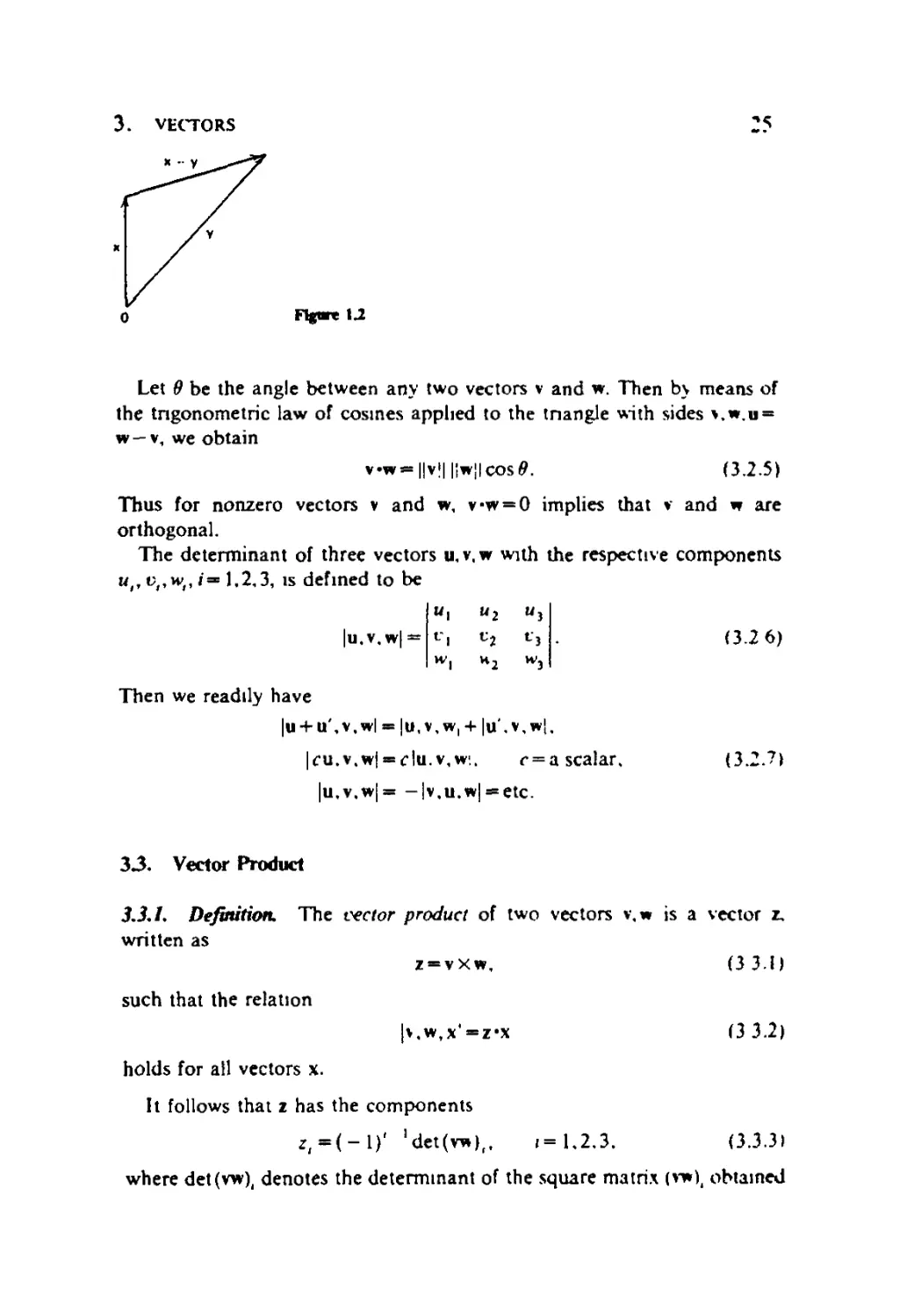
Let 9 be the angle between any two vectors v and w. Then by means of
the trigonometric law of cosines applied to the triangle with sides v.w.u =
w—v, we obtain
vw-||v!||iw!icos0. C.2.5)
Thus for nonzero vectors v and w, vw = 0 implies that v and w are
orthogonal.
The determinant of three vectors u,v,w with the respective components
u{, vt,w, /'= 1.2,3, is defined to be
|u.v,w| =
«, uz u3
r, v2 f3
W, H, K>,
C.26)
Then we readily have
|u-4-u',v,w| = |u,v,w, + |u',v,w|,
|fu.v.wj = f ju.v.w:. r = a scalar, C.2.?)
|u,v.w| = -|v.u.w! = etc.
3 J. Vector Product
3.3J. Definition. The vector product of two vectors v,w is a vector z,
written as
z = vxw, C.31)
such that the relation
|V.W,X;=Z'X C.3.2)
holds for all vectors x.
It follows that z has the components
r,-(-l)' ldet(vw)(, i= 1,2,3. C.3.3)
where det(vw), denotes the determinant of the square matrix (vw)( obtained
26 1. EUCLIDEAN SPACES
by deleting the ith column from the matrix
Thus the vector product has the following properties:
vXw+wXv = 0,
(v,+v2)Xw = v, Xw + v2 Xw, C.3.5)
(cv)xw**c(vX w), c = a scalar.
Geometrically, z is orthogonal to v and w. Moreover, if u is the unit vector
orthogonal to v and w such that
6 = |v,w,uj>0, C.3.6)
it follows from C.3.2) that z = Su; therefore for nonzero v and w, vXw = 0
implies that \ = cv/, where c is a scalar, which means that v and w are
parallel.
From C.2.6), C.3.2), and C.3.3) we easily obtain
w-ux v = u,vxw = vwxu = :u,v,w|, C.3.7)
Moreover, for a combination of the inner product and the vector product
we have the Lagrange identity:
(v!xv2)-(w1xw2) = (vl-w1)(v2.w2)-(v1.w2)(v2.wl). C.3.8)
In our later applications we shall consider vectors that are functions of
one or more variables, that is, whose components are functions of one or
more variables. In case the vectors are functions of one variable r, we have
that the following formulas hold, provided the derivatives in these
formulas exist;
d . . d\ dy*
— (v±w)=—- ±—-,
dt dt dt
d . . dc d\
T n =Tv + f"Ti c = a scalar
dty ' dt dt
?(.->-?—?. C.3.9)
d . . d\ dw
—- yXff = -Xw + VX ,
dt dt dt
d, [du ! ! d\ rfw:
-— U,V,W|= —r-,V,W! + U,—T.W. + ,U,V, —— ,
dt I dt 1 i dt i i dt 1
where, for example, dv(dt is also a vector defined as usual by
dv . Av v(/-fA/)-v(Q /, ,,m
— = hm r—- hm t C.3.10)
3. VECTORS
27
Similarly, we can discuss the partial derivatives of vectors that are
functions of two or three variables.
Exercises
1. Prove C.2.4).
2. Show that for vectors u,,u2,Vj,v2,
(u,xu2)-(vlxv2)=|u1xu2,v1,v2!.
3. Prove C.3.8).
4. Show that for vectors u,v.w.
(ux v) xw = (u-w)v- (vw)u.
5. Show that for vectors u,. u 2, v,, v2,
(u, xu2)x(v! xv2) = |u,.vl,v2|u2 -|u:,vl,v2|uI.
6. Show that for vectors u,, u 2, v,, v2. w,
|ulxu2.v1xv2,wj = |u],vl.v2|(u2-w)-|u2.v(.v;|(u,-w)
= |u,,u2.v2|(v1-w)-|u,.u2.vl|(>,-w).
*7. Show that the volume of the parallelepiped with sides u,v.w ts
±u*vxw.
3.4. Linear Combinations and Linear Independence: Bases and Dimensions
of Vector Spaces. Let v,.- ¦ • ,v( be vectors of a Euclidean space ?J. and
f[,- — ,c, scalars. Throughout this section the subscript / denotes a positive
integer.
3.4.1. Definition. An indicated sum of the form c 1vl + - ¦ • +c,t, is called
a linear combination of the vectors v,.- • • ,vr.
It is easily seen that the set of all vectors represented by linear
combinations of given vectors v,. • • • ,v, of ?° is a subspace of Ei, which is denoted
by fv,.- ¦ - .vj, and called the subspace generated (or spanned) by the vectors
v,,- • • ,v,. Geometrically, [v,] is the line containing the vector v,. and {v,.v,j
is the plane containing the two vectors v, and v2.
3.4.2. Definition. In ?3 vectors v,,--,v, are linearly independent if. for
all scalars c,, • • ¦ ,cr
rivi+'" *+r.v, — 0 implies c,= • • ¦ ^c^O. C.4.1)
28 1. EUCLIDEAN SPAC LS
Vectors that are not linearly independent are linearly dependent. If the
vectors v,,---,^ are linearly independent (respectively, dependent), we
may also say that the set (v,,- • ¦ ,v,} is linearly independent (respectively,
dependent).
From Definition 3.4.2 we can easily deduce the following results.
If one of the vectors v,,- ¦ ¦ ,v, is the zero vector, the vectors v,.- • • ,v, are
linearly dependent. Any subset of a linearly independent set is linearly
independent.
3.4.3. Theorem, Ix't the components of the vector v( be (vn,vl2yVl3). Then
the vectors v,, ¦ • <y,for 1 < i< 3 are linearly independent (respectively,
dependent ) if and only if (he rank of the matrix
is equal to (respectively, less than) i.
From Theorem 3.4.3 it follows that two vectors v,,v2 are linearly
dependent if and only if v,=cv2 with c a non/ero scalar, and three vectors are
linearly dependent if and only if one vector is a linear combination of the
other two. Thus we obtain the following geometric interpretation of linear
dependence.
3.4.4. Corollary. Two vectors are linearly dependent if and only if they are
parallel to each other, and three vectors are linearIv dependent if and only if
they are parallel to a plane.
3.4.5. Definition, The set {v,.- ¦ ¦,>¦} of vectors of a subspace S' of ?3 is
a basis of 5' if it is a linearly independent set that generates S\ and the
number / is the dimension of S'. We write i = dim S'. If ?,,-••,?, are
mutually orthogonal unit vectors, the basis {v,.- ¦ • ,v(} of 5"' is an orthonor-
mal basis.
We can easily prove the following two theorems.
3.4.6. Theorem. Ixn u^Uj.u, be vectors of Ex defined by
11,-0.0.0), u2 =@.1.0). u, =@.0,1). C.4.3)
Then the set {u^Uj.u,} is a basis of E\ which is called the natural basis
of E\
3.4.7. Theorem, If the set {v,, < • • , v(} of vectors is a basis of a subspace S'
of E3, then every vector of S' is uniquely expressible as a linear combination
of the vectors *,.••-,?,.
C.4.2)
3. VECTORS
29
Exercises
1. Prove Theorem 3.4.3.
2. Determine whether each of the following sets of vectors of ?J is
linearly independent or dependent:
(a) {(-1,2,1), C,1.-2)}.
(b) {A,3,2), B,1,0), @,5.4)},
(c) {A,0,-1). B,1,3), (-1,0,0), A,0.1)}.
3. Let v, and v2 be linearly independent vectors of ?\ and a. 6,c. d be
scalars. Prove that the vectors a\x+bv2 and fT, +dv2 are linearly
independent if and only if ad-bc^O.
4. Let v^Vj.Vj be linearly independent vectors of ?\ and atJ(i, j~ 1.2,3)
be scalars. Prove that the vectors Zj_,tflyV;, i— 1,2,3, are linearly
independent if and only if det (atJ)=^0.
5. Find a basis for ?3, that contains the vectors A,-1,0) and B, L3).
6. Find the dimension and a basis of the subspace [A,2,0), B,1,-1).
C,0, -2)] of E\
7. Prove Theorem 3.4.6.
8. Prove Theorem 3.4.7.
33, Tangent Vectors
33.1. Definition. A tangent vector of Ey at a point p. denoted by *f. is a
vector v with the initial point p, or vp is an ordered pair of points p and
p + v where p + v is considered as the position vector of a point (Fig. 1.3):
see Definition 3.1.1. p is the point of application of vp. For simplicity, we
may omit "tangent" for a tangent vector of ?3 at a point.
For example, if p —A.2,1) and v»B,3,3), then \p is a pa:r of points
A,2,1) and C,5,4).
It should be remarked that two tangent vectors vp and w^ are equal if and
only if v = w and p = q. Thus if p*q. then *,=?* V and vp.vtf are said to be
Figure 1J
f^
30
1. EUCLIDEAN SPACES
parallel. By defining
v, + w,-(v + w),, <•(»,)-(«),, C.5.1)
where c is a scalar, we see that the set 7J,(E3), consisting of all tangent
vectors of ?3 at a point p, is a vector space that is called the tangent space
of E3 at p. Moreover, at each p this tangent space 7J,(?3) is isomorphic to
?3, since the mapping /: E3-*7^,(?3) defined by /(v) = v , where v is
considered as the position vector of a point in ?3 with reference to an
origin 0, is indeed a linear isomorphism, a bijective mapping preserving the
addition and scalar multiplication (cf. Definition 5.1.1).
3.5.2. Definition. A vector field v on ?3 is a function that assigns to each
point p of ?3 a tangent vector v^ [or written as v(p)] of ?3 at p.
Let v and w be vector fields on ?\ Then by C.5.1) we can define v + w
to be the vector field on ?3 such that
(v+w)r = vp+w/, for all p. C.5.2)
Similarly, if # is a real-valued function on ?\ then by C.5.1) we can define
gv to be the vector field on ?3 such that
(gv),~*(p)v, for alt p. C.5.3)
3.5.3. Definition. Let u,.u2,u3 be the vector fields on E3 such that with
respect to a fixed right-handed rectangular trihedron OxjX2x3 in ?3
«,(p)-A<0,0),, MpWOJ.O),. u3(p) = @,0,l)„ C.5.4)
for each p of ?3. Then u,u2u3 is the natural frame field on ?3.
Thus u,{i— 1,2.3) is the unit vector field in the positive x, direction.
3.5.4. Lemma. If v is a vector field on E\ there are three uniquely
determined real-valued functions v^v2, t*j on E3 such that
v = r,u, + r2u2+r-,uv C.5.5)
The functions V\sVi,vi are called the huclidean coordinate functions of v or
the components of v with respect to the frame field u,u2u3.
Proof. By definition, v assigns to each point p a tangent vector \p at p,
whose components are functions of p. and therefore can be written as
vt(P^r:(p)«c?(P)- Thus
vpsa(vx{p).v7(p),v3(p))
-u1(p)(l.0,0)J, + »1(p)@,l,0)r + t-,(p)@,0.1),
^«--1(p)u1(p) + o2(p)u2(p) + t3(p)u3(p)
3. VECTORS 31
for each p. This shows that the vector fields y and c,u, +C2Ua + t3Uj have
the same (tangent vector) value at each point. Hence C.5.5) is proved.
The tangent-vector identity (ava2.ai)/,>*X*„xa,*l(p) appearing in this
proof will be used often.
A vector field v is differentiate if its Euclidean coordinate functions
c,, v2, t>3 are differentiable. From now on we shall assume all vector fields
to be differentiable.
From the paragraph preceding Definition 3.5.2, for each point p of ?3
there is a canonical isomorphism v-*^ of ?3 onto 7^(?3) at p. Using this
isomorphism, the inner product on ?3 itself may be transferred to each of
its tangent spaces.
3.5.5. Definition. The inner product of tangent vectors vp and w^ at the
same point p of ?3 is the number v^-wp*vw.
Evidently, this definition provides an inner product on each tangent
space Tp(E3) with the same properties as the original inner product on ?3.
In particular, each tangent vector vp of ?3 at p has norm (or length)
l!%,;l*"!ivll. and two tangent vectors vp and w^ of ?3 at p are orthogonal if
and only if vt-w|7 = 0.
3.5.6. Definition. A set e,(p).e2(p).c3(p) of three mutually orthogonal
unit vectors, tangent to ?3 at a point p, is a frame at p. Vector fields
e,,e2,e3 constitute a. frame field on ?3 if they do so at each pomt p of ?\
Thus e,e2c3 is a frame if and only if
e.-e,-^, forKi.^O, C.5.6)
where 8^ is the Kronecker delta @ if i^j. 1 if i=j). For example, at each
point p of ?3 the vectors u1(p).u2(p).u3(p) given by C.5.4) constitute a
frame at p.
Let €,-=(«,,, e^,*,})- Similar to C.2.6), define ? = (e,,e2.e3) to be the
matrix of the vectors e,.e2,e3 by
&=\e2X en eu\. C.5.7)
From C.3.7) it follows that
(elxe2)"e3=(e:xe3)*el=(e3Xel)*e2»dctt~, C.5.8)
where det & denotes the determinant of the matrix ?.
By Theorem 3.4.7 and Definitions 3.5.5 and 3.2.1 we obtain the
following useful result.
32 I . EUCLIDEAN SPACES
3,5.7. Lemma. I jet e,e2e3 be a frame field on Ey.
(a) // v is a vector field on ?\ then v = ^(,-)/e/, where the functions
f, =*v*e, are called the coordinate functions o/v with respect to eft-fi^
(b) Ify- 23„, fjtj and w « 2,3-. ig,e(, then v «w = 2f« i //?,¦ /« particular,
3 V*
1-1 /
Thus a given vector field v has a different set of coordinate functions
with respect to each choice of a frame field e,e2e3, and for a particular
problem one such choice may be more suitable than another.
Exercises
1. Let t-(-1,-2,1) and w~A,3, -2).
(a) At an arbitrary point p, express the tangent vector 2vp + 3v/p as a
linear combination of u,(p),u2(p).u,(p).
(b) If p = (l, - 1,2), express each of the tangent vectors \p% — 2vfp and
vp + w/J as a pair of points.
2. Let v, =u, -xfuj + u-,, v2-2u3, and v, = u, + u2.
(a) Prove that the vectors v,(p),v2(p),v3(p) are linearly independent at
each point p of ?5.
(b) Express the vector field jc,u, + .x2u2 + x3u3 as a linear combination
of v,,v2,v3.
3. Prove that the tangent vectors
ei = -L(i,2.1), e2=~^< -2.0,2), C3=J_(u-l,l)
V6 V"8 V3
constitute a frame. Express v = F,1, - 1) as a linear combination of
these vectors.
*4. If v and w are vector fields on liy that arc linearly independent at each
point, show that
V W
e,~----, e, . e,=e.xe,
jVJ |W| 3 12
is a frame field, where w = w-we2e2.
3.6. Directional Derivatives. Let /be a differentiable function on f3.
Then / -»/(p + /v) is an ordinary differentiable function on the real line
p+/v, which passes through a tangent vector \p of Ey at a point p, and the
3. VECTORS 33
derivative of this function / with respect to f at /»*0 is the initial rate of
change of/as p moves in the v direction. Thus we have Definition 3.6.1.
3.6.1. Definition. Let / be a differentiable real-valued function on ?\
and vp a tangent vector of ?3 at a point p. Then
v„[/] = |</<P + '*»l,-o C-6.1)
is the derivative of /with respect to vp.
It should be noted that this definition of derivative is the same as that of
the directional derivative given in elementary calculus but restricted to a
unit vector \p. However we shall still refer to v^[/] as a directional
derivative.
For example, suppose that
f=xtx2x3, p-(l,-4.2). t-(IJ.O). C.6.2)
where jc,,x2, x3 are the coordinate functions of ?3. Then p + rv=»fl -w. -4
+ f,2) and/(p+/v) = 2(I + t)(-4 + (). Thus by C.6.1) we have
^[/|-^2(l+/)(-4+Ol,-o-2B/-3)|,.0--6.
A computation of a general vp\f] in terms of the partial derivatives of/
at the point p is given in Lemma 3.6.2.
3.6.2. Lemma. If vp =(t1,f2. v3)p is a tangent vector of ?? ai a point p.
then
vp[/]=Jf|(p). C.6.3)
Proof. Let p—(/7l4 /?2. p3). Then
/(p + rv)=/(p, +/r,, p2 +tv2. py + tv3).
Since (d/dt)(pt +tv,)-v,t by putting xt **p, +tv, and using the chain rule
(Theorem 2.3.6) and C.6.1) we can immediately obtain C.6.3). Q.E.D.
Using C.6.3) we can also find vp[f] for the example above. From C.6.2)
it follows that
^-(p)=*2.v3(p)=-8.
dx3
Thus by C.6.3) we obtain v,[/]-!(-8)+ lB) + 0(-4) = -6.
Q.E.D.
34 1 . EUCLIDEAN SPACES
The main properties of this notion of derivative are given in the
following theorem.
3.6.3. Theorem. Ijet f and g be different iable functions on ?"¦*, vp and */p
tangent vectors at a point p, and a and b real numbers. Then
(a) (flv?+^){/] = av?[/] + ^[/],
0>) v,l*f+bg\-<"p[f] + bvp[g],
(c) »,lA]«v„[/]-*<p)+/(p)ir,[*].
Proof, Parts (a) and (b) follow readily from Lemma 3.6.2 and the sum
formula for partial derivatives. Similarly, we can also prove (c) by noticing
that
i^(P)-im<P)-,(P)+/(p)^(p))
-(i^^^PH/fPiji^fP)).
Parts (a) and (b) mean that vp[f] is linear in both v^ and/, and (c) is the
product formula for directional derivatives.
By the same method used in the last section, we can define the operation
v{/3 of a vector field v on a function /to be the real-valued function whose
value at each point p is v(p)[/], the derivative of / with respect to the
tangent vector v(p) at p. In particular, if u,u2u^ is the natural frame field
on ?3,
»,[/] = |?. '='-2,3. C.6.4)
In fact, since, for instance, u,(p) = (l,0,0)r by C.5.4). from C.6.3) it follows
immediately that u,(p)[/] = (d//9x,)(p) for each point p. hence that u,[/]
-3//3X,.
3.6.4. Corollary. If v and w are vector fields on ?3, and f.g,h are
real-valued different iable functions, then
(a) (f>+g»)lh}=fv\h}+gw[hl
(b) v[ af+ bg ] = a v[ / ] + bv( g ], for all real numbers a and b.
(c) v[/?] = vl/].g=/v[g].
Proof. By Theorem 3.6.3 we see that (a) and (b) are true at each point p
of F.y. Similarly, we can prove (c). In fact, the value of v(/g] at p is vp[fg),
which, by Theorem 3.6.3, is equal to
v/>[/j*«(p)+/(p)vp[g]-v[/|(p)v(p)+/(p)v[g](p)
-W/]-S+/-v[«])(p). Q.E.D.
4. MAPPINGS 35
By using C.6.4) we can easily compute \\f}. For example, if *=.t,a,-
jc2u2 + jc3u3 &ndf**xxxl + x2xl,
v[/]=^,u1[/]-x2u2[/]+x3u3[/]=-x1x22 + 2x2Ar}3.
Remark. ^For simplicity, if the point of application is not crucial, we shall
frequently omit the point of application p from the notation vp.
Exercises
1. Let vp be the tangent vector of ?3 for which v = { 1,2.2) and p =
B, - 1,1). Use both Definition 3.6.1 and Lemma 3.6.2 to compute die
directional derivative v,[/]. where f=xtxl+x2xl.
2. Let v=sjc3u,-X|U2+x2u3,/=x,x3,g = Jc]. Compute the following
functions: (a) v(/]; (b) v[/g]; (c) vtv[/]].
¦3. Prove the identity v = 2,\.,v(xtK, wh^re Xj.jc2,;c3 are the natural
coordinate functions.
4, If v[/]=w[/] for every function/on ?\ show that v=w.
4. MAPPINGS
In this section we discuss mappings of E" into ?"" for general n and
m,l<«,m<3. If /j=*3 and m=l, such a mapping is just a real-valued
function on ?3. If n= 1 and m = 3, such a mapping is a curve m ?3. If n=*2
and m = 3, such a mapping is a surface in ?\ The last two particular cases
are discussed in detail in later chapters.
4.1. Linear Transformations and Dual Spaces
4J.1. Definition. Given a mapping F: ?"-»?"\ let Jvbf2,- • •. fm denote
the real-valued functions on E" such that
W-(/,(p)./2(p)."-./JP>>
for every point pe?". Then these functions/,, /2,- ¦ -, fm are the Euclidean
coordinate functions of F. and we write
f-(/,./2-"-./,). H.l.D
The mapping ? is of class C*(fc > 1) if /,, /2,- • •. fm are of class C* in the
usual sense.
Note that the coordinate functions of F are the composite functions
ft =Xf(F), where *,, x2,- ¦ ¦, xm are the coordinate functions of ?m.
36 1 . EUCLIDEAN SPACES
Mappings may be described in many different ways. For example,
suppose that F: ?3->?3 is the mapping F~{xy,yz, z2). Then
WP)- (x(p)y{p)ty(pHPh z(PJ) ^r all p6E\
If p=(pt. p2- p3). then by the definition of the coordinate functions,
x{p)=pl. y(p)=p2* z(p)=pv
and therefore we obtain the following pointwise formula for F:
F{p^P2^Pi)^{p{p1,P1P^p\) for all p^Pi.py.
4J.2. Definition. A mapping F: En—*Em is a linear transformation of E"
into Em if, for all vectors x and y of E" and all scalars c and d*
F(cx+dy) = c(F(x)) + d(F{y)). D.1.2)
The kernel of a linear transformation F: ?"—>?"¦, denoted by ker ?, is the
set
ker?={x|Xe?\?(x) = 0}. D.1.3)
4.1.3. Examples of Mappings. 1. The mapping F: ?3-»?3 such that
F(x, y> z) = Bx,y- z, y + z),
where x. v. z are the coordinate functions of ?3. This is a linear
transformation of ?3 -»?\ Thus by a well-known theorem of linear algebra, F is
completely determined by its value on three (linearly independent) points,
say the unit points
u,=(l,0.0), u2@,l,0), u3@,0,l).
2. The mapping F: E2-*E2 such that
F( u, v) ~ {x, y). x = u2 +1-2. y = u 4- v,
where u, c and x. >> are the coordinate functions of the uc-plane and the
xy-plane, respectively.
It often helps to compute the image of a number of selected curves and
regions. For instance, the image curve of the horizontal line v—c in the
x>'-plane under F is given by the equation
x=*(y-cJ + c2.
Since x and >• are symmetric in u and v. points (a, b) and {b, a) in the
w-plane both have the same image. Thus the line c = u divides the
wt-plane into two half-planes, which are mapped by ?onto the same set in
the xy-plane. To determine this set, we first find the image of the line v-u
4. MAPPINGS 37
FlgveM
to be the parabola y2 = 2x. The image of any point (x, y) lies within this
parabola, for 2x-.y2 = (w-i>J>0. Conversely, it is easy to see that every
point (x, y) on or within this parabola is in turn the image of a point
(a, v); see Fig. 1.4. Accordingly, one may picture the effect of F
approximately as follows: first, fold the i/c-plane along the line c-«; then fit the
folded edge along the parabola,y2 = 2jt and flatten out the rest to cover the
inside of the parabola smoothly. (To permit the necessary distortion, think
of the w>plane as a sheet of rubber.)
3. The mapping F: ?2-*?2 such that
F{U>v) = (x,y).x = u2-c2.y2uc, D.1.4)
where «, v and x, y are the coordinate functions of the uc-plane and the
xy-plane respectively.
Let us first use polar coordinates r, / in the ut>plane so that
wrcost, c = rsinf, 0< f < 2ir.
By using some trigonometric identities, we can express D.1.4) as
F(rcos/,rsinO"('cos2/,r2sin2/), 0<r<2ir.
From this it follows that under F the image curve of the circle of radius r
and center at the origin counterclockwise once is the circle of radius r2 and
center at the origin counterclockwise twice (Fig. 1.5). Thus the effect of F
f\fmt\S
38 1. LUCLIDEAN SPACES
is to wrap the plane ?2 smoothly around itself, leaving the origin fhed,
since ?@,0)=@,0), and therefore F is surjective but not injective.
However, if we replace the utvplane by the open half-ptane D {all («, v)
with u>0}, then ?is injective in D. To see this let ?(u, t>) •?{/>,?). Then
luv — lpq, u2 -v2 =p2 -<72,
so that
0 = u2{u2 -v2 -p2 +q2) = {u2 +q2){u2 -p2).
Thus u2 =/?2. Since w>0 and/>>0, we have u=p and i> = <jr. Hence /"maps
D onto a subset D' in the xy-plane in an injective fashion. This mapping
has an inverse F ', which maps D' onto D. Solving D.1.4) we obtain
V2 V ' V2 y V '
The set D' is the set of points (x,y) for which x+ Vx2 +y2 >0, that is, all
points (x, y) except those of the form (c,0) with c<0.
4.1.4. Definition. Let A and B be two subspaces of E", Then
E*-A®B D.1.5)
means that E" =A+B= {x + y\xEA,yEB} and >lnfi = 0, D.1.5) is a
decomposition of En into a direct sum of the subspaces A and B. and each of
the sets A and 5 is the complement of the other in E".
From the definitions we can easily prove the following lemmas.
4.1.5. Lemma. Let F: ?" -»?"" be a linear transformation. Then ker F is a
subspace of E", F{ ?"*) is a subspace of Em, and F is a bijection if ker F=0.
The dimension of F(En) is called the rank of F, and the dimension of ker F is
called the nullity of F.
4.1.6. Lemma. Let F: E"~*Em be an injective but not surjective linear
transformation. Then there is a decomposition
Em=E,n®E"m-n D.1.6)
of Em into a direct sum of subspaces E'n and E"m " of dimensions n and
m — n, respectively, such that ?(?") = ?"* and F: ?*—>?'" is a bijection.
4.1.7. Lemma. Let F: E"~*Em be a surjective linear transformation. Then
there is a decomposition
E"=*E'm®E""-m D.1.7)
of E" into a direct sum of subspaces E'm and ?"" "" of dimensions m and
4. MAPPINGS 39
n-m; respectively, such that ?""""*ker F, and F\E'm'is a bijection onto
Em.
Lemma 4.1.8 follows immediately from Definition 4.1.2.
4.1.8. Lemma. Let V be a vector space over the field R of real numbers,
and let F, G be linear transformations of V into R. Define the sum F+- G and
the product cF of F by a scalar c as follows:
(/>G)(x) = F(x) + G(x), for all xEV. D.1.8)
(cF)(x) = F(cx) for all xGK,c6/l. D.1.9)
Then F+ G and cF are also linear transformations of V into R.
4.1.9. Lemma. If {v,, • • •, vB } is a basis of an n-dimensional vector space V
over /?, and //ct, • • ¦, c„ are n constants in R% there is one and only one linear
transformation F on V with F(Omc,, i- 1,- • •, n. This transformation F is
given by the formula
S^,)=2v, D-1.10)
»-1 .-I
where x»(*,,• ¦ • ,xn) is a variable vector of V.
Proof. By induction on n, D.1.10) follows directly from D.1.2) for any
linear transformation F with F\\) = cl. i* 1.- - -,«. Conversely, for any
basis {*,,¦¦*,?„} of V, each x has by Theorem 3.4.7 for V a unique
expression x — S^-i-Vr For any constants c,,- ¦ ¦ , c„ of R, D.1.10)
therefore defines a transformation of V into R. This transformation is linear,
since for any x and y = ^2"-]y,vl
F(ax + by) = F\ 2 (ar(+ty>, ] = 2 {axt+by,)ct
= a2 xtc, + b^dytc, = aF{x)^-bF{y).
4.1.10. Theorem. The set of all linear transformations of a vector space V
over the field R of real numbers with addition and scalar multiplication defined
by D.1.8) and D.1.9) is a vector space V* oxer R, which is called the dual
space of V.
The proof of Theorem 4.1.10 is only a routine verification of conditions
C.1.3), C.1.4), and C.1.5). and is left as an exercise.
40
1. EUCLIDEAN SPACES
4. ML Corollary. If a vector space V over R has a finite basis {v,, '-,%,},
then its dual space V* has a basis {?j, ¦ ¦ ¦, F„} called the dual basis to the
basis {v,,- • • ,v„} of V, consisting of the n linear transformations F{ defined by
Fj(X"~iXtyi)-xrj>= !,•••,«. The n linear transformations F, are uniquely
determined by the formulas
^('i)-*,y, /,y-l.---,«, D.1.11)
where 8fj is the Kronecker delta.
Proof. For n given scalars <:,,¦--,c„. the linear combination F=
2"-i<yF, is a linear transformation; by D.1.11), its value at any basis
vector v, is
It follows that the transformations ?,,¦ - •, Fn are linearly independent in
V*. for if f-2"-!^/) -0, then ?(v,) = 0 for each /, hence c, - • • • -c„ -0.
It also follows that the n linear transformations ?,.•¦-, ?„ span K", since
by Lemma 4,1,9 any linear transformation ? is determined by its value
F(v,) - e,-, hence ?« 2^-,c, ?,. Q.E.D.
Corollary 4.1.12 follows immediately from Corollary 4.1.11 and
Definition 3.4.5.
4.1.12. Corollary. The dual space V* of an n-dimensional vector space V
has the same dimension n as V.
4.2. Derivative Mappings. In ?\ let p be the position vector of a point,
and v a vector at p. Then
r^p + rv D.2.1)
is a curve in ?", and the tangent vector of the curve D,2.1) at r = 0, that is,
at p, is (rf/rfO(P+'v)l,-o~v- Moreover, a mapping F: ?"->?m maps the
curve D.2.1) in ?* to the curve
/-*?(p + /v) D.2.2)
in Em. Thus we can have a definition of a mapping.
4.2.1. Definition. For a mapping ?: ?*—>?m we define a mapping Fm
(which may also be denoted by df) such that for a vector v of ?" at a
point p
^(v)=-^?(p + rv)|,_0, D.2.3)
which is the tangent vector of the curve D.2.2) in ?"* at r=0, that is, at
4. MAPPINGS 41
F(p). This mapping F» (or dF) is the derivative mapping (or differential)
of F.
For example, let us compute the derivative mapping F« of the mapping
Fin Example 3 of Section 4.1.3. Suppose that p = (/?rp2). v = (r,.r:).
Then by D.2.3) we have
F*(v)=-^[F(/7,+fLv/>2 + /t:2)]U0
= Jt((pl + tv]J-{p2 + tv2)\2{p^tvx){p1 + tv2))\t.0
= {2(plvi-p2v2)t2(piV2+p2vl)) at F</>).
4.2.2. Theorem. I jet D.1.1) be a mapping of En into Em. If v is a vector of
E" at a point p, then
M*)-(»[/,].v[ /2].-¦¦.*[/,]) « F(p). D.2.4)
50 /fort F*(v) is determined by the derivatives v{ / ] of the coordinate functions
of F with respect to v.
Proof. For definiteness we set m = 3. By D.1.1) we have
F(p + /v)-(/1(p + /y),/:(p + rv),/3(p + fv)).
Thus D.2.4) for m = 3 follows immediately from D.2.3) and C.6.1) for
/-/,./2./3- ' Q-E-D.
Let 7^(?") be the set of all vectors in E" at a fixed point p. that is. the
tangent space of E" at p (see Definition 3.5.1). Then the derivative
mapping F* given by D,2.3) gives rise to a mapping
r.,:Tp(E-)-TFtpt(Em) D.2.5)
defined by
F*p(v) = F.(v) at Ftp). for vG7,(P).
F*, is called the derivative mapping of Fat p. In a corresponding situation
in elementary calculus, a differentiable function /: /?-»/?. where K is the
field of real numbers, has a derivative function /': R-*R. which at each
point / of R gives the derivative f\t) of / at t.
4.2.3. Corollary. At each point pGf" the derivative mapping D.2.5) of a
mapping F: ?"—»?'" is a linear transformation.
Proof. For v,we Tp(E"), and a.beR. we must show that
F,(av + 6w)-aF.<v) + &F,(w).
which follows immediately from Theorem 3.6.3a and Theorem 4.2.2.
Q.E.D.
42 1. EUCLIDEAN SPACES
The linearity of F+p is a generalization of the fact that the derivative
/'(/) of /: R-*R is the slope of the tangent line to the graph of / at t.
Indeed for each point p, F0p is the linear transformation that best
approximates the behavior of F near p. This idea could be fully developed
and used to prove Theorem 4.2.7.
Since the mapping D.2.5) is a linear transformation, it is reasonable to
compute its matrix with respect to its natural basis, defined in C.4.3):
U,(P), *,u,,(p) for Tp(E"),
«,(^(p)).--.um(f(p)) for Tn„{Em).
This matrix is called the Jacobian matrix of F at p and \e denoted by JF(p).
4.2.4. Corollary. For a mapping D.1.1) of E" into Em,
/%(u,(p))~ ? ^(pKCm 1 <;<n, D.2.6)
so that JF(p) = ((df,/dxJ)(p))i ^l<m,i<J<n, where *,,- • • ,x„are the coordinate
Junctions of E".
Proof. Substituting u;(p) for v in D.2.4) and using C.6.4) for /=
fi*'"*fm we obtain
^(p))-(|(p),-.^(p)) .
\ J J I F{P)
which is just D.2.6) in component form.
As usual, D.2.6) is abbreviated to
where uJ and df/dxj are evaluated at p, and u, is evaluated at F(p).
For Example 3 of Section 4.1.3, fl = u2~v2,f2~2uv; therefore JF at
p=(p,,p2)is
4.2.5. Tlteorem. l^et F\ En—*Em be a mapping, and v a vector of E" at a
point p. Set x(t) = p + tv% y(t)= F(\(t)). Then
F„(x'</))-y'@, D.2.7)
where the prime denotes the derivative with respect to t.
3m do
du dv
4. MAPPINGS
43
Proof. For definiteness we assume /n«3. By D.LI) we have
y@-^x@)-(/,(x@), /2(*@). AWO). DX8)
From D.1.1) and Theorem 4.9 it follows that
F.(x'(/))-(x'(/)[/t]^(r)[/2],x'(/)[/3]). DX9)
Suppose x-(jf,,x2, jc3). By considering/ —/(x)-/(jc,, x2, x3) and using
Lemma 3.6.2 and the chain rule (Theorem 2.3.6), we obtain
x'C)[j;]- i |j«<»^e>-^<o. («.io)
Substitution of D.2.10) in D.2.9) and use of D.2.8) thus give D.2.7).
4.Z6. Definition. A mapping ?: E " ->?m is regu/ar if for every point p of
?" the derivative mapping F+p is injective.
Since each /"^ is a linear transformation, by applying standard results
of linear algebra we have the following equivalent conditions:
(a) F+p is injective.
(b) If ?,(c)=0, then v=0, where vST^E").
(c) JF( p) has rank n (the dimension of the domain ?" of ?).
For example, the mapping F in Example 3 of Section 4.1.3 is not regular.
But the injective condition fails at only a single point, the origin @,0). In
fact, from the computation immediately preceding Theorem 4.2.5 it follows
that JF has rank 2 at p=*@,0), and rank 0 at @,0).
A differentiable mapping that has a differentiate inverse mapping is
called a diffeomorphism. A diffeomorphism is thus necessarily bijective, but
a differentiable bijective mapping may not be a diffeomorphism (Exercise
9 of Section 4.2).
The results of this section apply equally well to mappings defined only
on open sets of ?\ Thus we may speak of an injective or surjective
mapping or a diffeomorphism of one open set of ?" into another, such a
mapping being called a local injective or surjective mapping, or a local
diffeomorphism if about every point of ?" there is such an open set. For
example, consider the mapping F: ?*->?* such that
?(«,«) — (x,y), jf»MCOSc,^ = usint:.
The Jacobian JF of F is equal to x and is thus never zero in the right half
tw-plane Z)» {all (u, v) with u > 0}. However, F is not a diffeomorphism in
Dy since points (a, b) and (a. b + 2ir) of D always have the same image in
the xy-plane. The effect of the mapping may be seen from the set ScD,
shown together with its image F(S) in Fig. L6. We notice that although F
is not injective in S, two distinct points of S that have the same image must
44 1. EUCLIDEAN SPACES
v D y
Figure 1-6
be widely separated. Thus F is a local diffeomorphism in S (and in fact
in/>).
For local diffeomorphisms we have the following important theorem.
4.2.7. Theorem (Inverse Junction theorem). Let F: ?"-*?" be a different
tiable mapping such that F* p is injective at some point p. Then F is a local
diffeomorphism about p, that is, F maps any sufficiently small open set A
about p diffeomorphically onto an open set F( A).
Proof. See; for instance, T. M. Apostol [2, p. 144].
For local injective (respectively, surjective) differentiable mappings, we
have the following analogous theorem.
4.2.8. Theorem (on local injective or surjective mappings). Let U be an
open neighborhood of a point pG ?", and F: U->Em a differentiable mapping.
U
f*P-Tp{E")^TF(p){Em) D.2.11)
i*5 injective (respectively, surjective), there is a diffeomorphism G of a
neighborhood W of F(p)E?m onto a neighborhood G(W) of F(p)e?'n (respec-
tively, a diffeomorphism H of a neighborhood VofpE. E" onto a neighborhood
H(V) of pG E") such that G° F is locally about pE E" a linear injection into
Em (respectively, F° H is locally about pe?" a linear surjection onto ?"").
It is obvious that the converse of Theorem 4.2.8 holds.
Proof. We first consider the case in which the mapping D.2.11) is
injective. By identifying Tp(E") and TF{p)(Em) with E" and Em,
respectively, and applying Lemma 4.1.6, we obtain a decomposition D.1.6) of Em
4. MAPPINGS
45
such that F»p: En-+E'n is a bijection. Define a differentiabte mapping G:
?-«-?'-e?'""-"->?:m«?",©?',,"~" locally about F(p) by k-(u',iT)-»
F(iO+@,tt"), where we have identified the first ?'" with ?'. Obviously
G^^-F^+id] ?*"""" is_ bijective; therefore locally about F(p) there
exists the inverse mapping G~' denoted by G. Thus <7» ft"')**(m\0): that
is, G«F'\% locally about p a linear injection: ?"¦-*?'" <zE'*®E"m~~ — Em.
Now suppose the mapping D.2.11) to be surjective. Then by applying
Lemma 4.1.7, as above, we obtain a decomposition D.1.7) of E" such that
Fm: E'm-*Em is a bijection. Define a differentiabte mapping H: ?" —
?"»©r""w-»?"-?'"®?'""" locally about p by ««(m\u")-»
(F(u),«"), where we have identified the second E'm with ?"*. Since
H+f**F+p\E'm +'\d\E"m~m is bijective, locally about p there exists the
inverse mapping H _l denoted by H. Thus H(F{u\ y"), u")«(«',«"), and
F»/f(F<«',ii"),ii")*'!0«\ O; that is, F*// is locally about p the
projection E" «"?"" +?*"""*-*>?"•• and is therefore linear and surjective.
Exercises
1. For the mapping F given by D.1.4) find all points p, with sketches for
part d, such that
(a) F(p)«@,0). (b) F(p)«<3,-4).
(c) F(p)-p. (<i) FG>)-(*.n !<*<4,2<v<-.
•2. Under the mapping F given by D.1.4) find the image of each of the
following sets:
(a) The horizontal strip S: 1< v < 2.
(b) The half-disk 5: u2 + c2 < 1, c > 0.
(c) The wedge S: - u < v < u, u > 0.
In each case, show the set 5 and its image F\S) in a single sketch.
3. Prove Theorem 4.1.10.
4. (a) Show that the derivative mapping of the mapping Fin Example
1 of Section 4. ] .3 is given by
^.(^)-Bo,,c2 -c3, v2 +c3)^„.
(b) In general, if F: E"—*Em is a linear transformation, prove that
*W *<*>«*>•
5. Find F, for the mapping F(x,y,z)-(x,yco&z,ysinr): ?3-»?\
and compute F*(v,) if
(a) v-C,-2,l),p«@,0,0).
(b) v«C,-2,l),p = D,ir.|).
46
1. EUCLIDEAN SPACES
6. Is the mapping in Exercise 5 regular?
7. In Definition 4.2.1 of ?*(vp), show that the straight line p+fv can be
replaced by any curve with vp as its tangent at p, that is, at /—O.
8. Prove that a mapping F: E"^>Em preserves directional derivatives in
the following sense: If vp is a vector of ?", and g is a differentiate
function on Em, then Ft(vp)[g) = vp[g(F)].
9. In each of the following cases, show that the mapping F: E2—*E2 is
bijective, compute the inverse mapping F~\ and determine whether
F is a diffeomorphism (that is, whether F ~l is differentiate).
(a) F(m,«) — (», uev).
(b) ?(tM>)=(u-»,u3).
(c) F(w,t>) = Bii-t>+Uu+3t>-2).
10. Let F: E2—>E2 be a mapping such that
F(u,v) = (xty), x»eucost>,y~eusmo.
The nature of the mapping F is suggested by Fig. 1.7. in which certain
corresponding areas are indicated by the same letters. Verify this
figure and show that onto the jcy-plane with the origin excluded the
mapping F is not a diffeomorphism of the whole uc-plane but is a
local diffeomorphism.
5. LINEAR GROUPS
5.1. Linear Transformations. In this section all definitions and results
hold for ?3 as well as a Euclidean plane E2. However, for generality we
only discuss the case of ?\ and consider the case of ?2 as a special case.
5. LINEAR GROUPS
47
A mapping of ?3 into itself is a correspondence that associates with each
point x of ?3 a unique point y of ?3. By the correspondence mentioned in
Section 3.1, we consider x and y here also as the position vectors of the
respective points with reference to a fixed point 0 in ?\
5.LL Definition. A mapping F: ?3-*?3 is a linear transformation of E3
into itself if, for all vectors x and y and all scalars c and d,
F(cx+dy)-c{F(x)) + d(Hj))- E-1-1)
Definition 5.1.1 is a special case of Definition 42.
Let F and G be two linear transformations of ?3. Then by defining the
multiplication of F with G by
(G?)(x)«G(?(x)). E.1.2)
and introducing the identity mapping /:
/(x)«x, E.1.3)
we can show that F has a multiplicative inverse ?"' if and only if ? is
bijective. Thus that all the nonsingular (i.e.. bijective) linear transformations
of E3 form a multiplicative group, which is called the general linear group of
?3 and is denoted by GZ^. [A nonempty set G, on which there is defined a
binary operation "°*\ is called a group (with respect to this operation),
provided the following properties are satisfied: (i) if a, 6.c6G. then
(a°b)°c*ao(b°c); (ii) there exists an element eGG such that e*a~a°e
fa for every element a EG; (iii) if aGG, there exists an element xGG
such that aojc»jcoa«e.)
Let {x,,x2,x3} be a basis of ?3. Then we have, uniquely,
3
ft*,)- Z «ji«7. »-1,2,3. E.1.4)
? is nonsingular if and only if the matrix
E.1.5)
is nonsingular, that is, if and only if det A ^0. Let M be the set of all the
nonsingular 3x3 matrices with usual row-by-column multiplication. Then
the mapping F-*A defined by E.1.4) is an isomorphism of GL, onto Sf.
Now suppose {y,,y2,y3} to be another basis of ?3 so that
*y,)-2fl;,y,. '-1*2.3, E.1.6)
48 1. EUCLIDEAN SPACES
and denote the matrix (afj) by A*. Then (see Exercise 1 of Section 5.1)
there exists a unique linear transformation G of ?3 such that
<7(x,)-y„ i-1,2,3. E.1.7)
Furthermore, it can be shown that
A9-BAB~\ E.1.8)
where B~} is the inverse matrix of J? = Ff>) given by
3
GOO-Ji-SV/' '-1.2.3. E.1.9)
y-i
5.1.2. Definition. A linear transformation F: E3->?3 is an orthogonal
transformation if it preserves the inner product of any two vectors x and y,
that is, if
(E(x)).?(y) = x.y. E.1.10)
If F and G are orthogonal transformations of ?3, then for any two
vectors x and y of ?3
( F- \x)) -F- \y) = (F{F~ '(x))) •?( K '(y)) - x-y,
((FGKx))-(FC)(y)»(nC(x))).ftC(y))-(G(x)).G(y)»x.y,
showing that all the orthogonal transformations of E3 /orm a subgroup of the
linear group GL3, which is called the orthogonal group 03.
5.L3. Definition. A square matrix A of order 3 is orthogonal if
'AA=$, E.1.11)
where 'A is the transpose of A, and 9 is the identity matrix.
Equation 5.1.11 implies that A is nonsingular. It may therefore be
written as A ~'«'A and hence also as
A'A-$. E.1.12)
From E.1.11) or E.1.12) it follows that if A is an orthogonal matrix, then
(det/lJ=l or
det/l = ±l. E.1.13)
By definition 5.1.3 and direct multiplication of matrices we readily
obtain Theorem 5.1.4.
5. LINEAR GROUPS 49
J./.4 Theorem. The square matrix A given by E.1.5) is orthogonal if and
only if one of the following three equivalent conditions holds:
3
Z «,>««-%*¦ >.*-1.2,3, E.1.14)
/-i
3
2 «>,*«-*>*. J.*-1.2,3, E.1.15)
deiA+Qtaij-Aij, i, y= 1.2.3, E.1.16)
w/wre 6,* is a Kronecker delta, being 1 forj^k and Oforj?*k, and AtJ is the
cofactor of atj in det A.
5.1.5. Theorem. Let {x,,X2,x3} be an orthonormal basis of E3. A linear
transformation F: E3-+?3 given by E.1.4) is an orthogonal transformation if
and only if the matrix A=(atJ) is orthogonal.
Proof of Theorem 5.1.5. Suppose that F is orthogonal. Then by E.1.4)
and E.1.10) we have
(f^-fm J i ahJx\l %<>,>*) = 2 2<v».A.
3
- S0.^.*-*/**-^*- y.A-i.2.3.
i-1
which shows, due to Theorem 5.1.4, thai A is orthogonal. The converse of
this can be proved by reversing the argument.
5.1.6. Corollary. Let xl,x2 be an orthonormal basis of a plane E1. Then
the only orthogonal transformations of E1 are F and G given by
Fix,) = x ¦ cos 9 + x, sin 9,
11 E.1.17)
F(x2)= -x,sin#+x2cos0;
G(x,) = x,cos0+x,sin0.
11 E.1.18)
G(x2) = x,sin0-x2cos0.
where 9 is unique such that 0 < 0 < 2tt, so that F is a rotation of E2 through an
angle 9, and G is the rotation F followed by a reflection in x2. which maps
every point to its symmetric point with respect to x2 (two points in E2 are said
to be symmetric with respect to the x 2-axis if the x 2-axis is the perpendicular
bisector of the line segment joining the two points).
50
1. EUCLIDEAN SPACES
Proof. Let H be an orthogonal transformation of E1 given by
^(xl)-fl1xi + azx2. //(x2) = 6,x,+&2x2. E.1.19)
Then by the special case of Theorems 5.1.5 and 5.1.4 for ?2 we have
flf + aj-l, &j + 622-l, E.1.20)
a,6,+a2*>2«0. E.1.21)
By E.1.20) there is an angle B such that Q<0<2ir and cos0—av sin0~a2.
Then tan&=a2/al = ~b{/b2 by E.1.21), whence by E.1.20) again b2 =
±cos9,b}" ±sin0. The two choices of sign give exactly the two
transformations F and G. Q.E.D.
Now in E3 we consider a right-handed rectangular trihedron OxjXjXj
and a rotation /Mhat is an orthogonal transformation given by E.1.4) with
orthogonal matrix A —(a^) such that det A = + I. Then by E.1.14), A can
be expressed as
E.1.22)
cos a,
cosa2
cosa3
cos/3,
cos/?2
COS /J3
cosy,
cosy2
cosy3
and the columns of A are composed of the direction cosines of three
mutually orthogonal lines xf.x^Xj" through the origin 0, which
respectively pass through the image vectors, under F, of the unit vectors u, —
(l,0,0),u2 -@,1,0), u3 »@,0,1) on the coordinate axes x„ x2, x3.
It is well known that any rotation in E3 can be represented by three
independent parameters called the Euler angles (Fig. 1.8). We shall
determine the Euler angles for our rotation F, which takes the coordinate
v Figure \A
5. LINEAR GROUPS
51
axes x„x2,x3 onto three preassigned mutually orthogonal lines xf.x^.x;.
To this end, first let y be the line of intersection of the x,x2- and the
xfx$ -planes, and 4> the angle of the rotation A^ about x3, which takes the
Xj-axis onto y, so that
The rotation
about y through an angle 9 takes x} onto x*, and also x2 into the
xpi\ -plane. Finally, the rotation
cos? sin
<t> 0
-sin$ cos$ 0
0 0 1
1 0
0 cos0
0 -sin0
0
sin0
cos*
cos $ sin ^
— sin $ cos i^
0 0
about x* through an angle yp takes y onto xf, and x2 and x*. This shows
A=A+A,A + . E.1.23)
5.1.7. Theorem. An orthogonal transformation F of ?3 preserves the
distance between any two points, that 4s, F satisfies
d{F{x),F{y))=d{x.y), E.1.24)
where x,y are the position-oeetors of any iwo points.
Proof. From C.2.4), E.1.1), C.2.3). and Definition 5.1.2 we
immediately obtain
d(F(x,F(y))-\\F(x-y)\\ = \<x-yt\-d(x.y).
Exercises
1. If {xl,x2ix3Lii a basis of ?3, anc* zL,zX'?3-are *r*)*trar>" vectors of
?3, there exists exactly one linear "transformation F of ?J such that
F(x,) = z„ /= 1.2,3.
*2. Prove Theorem 5.1.4.
52
I, EUCLIDEAN SPACES
3. Test the following matrices for orthogonality, and find the inverses of
the orthogonal matrices:
[3 4 ]
<c)P 5 L
[5 5)
4. Find orthogonal 3x3 matrices with the following first rows:
\13' ' 13M3'3'3l'
5. If a rotation F has Euler angles <>, 0, tj<, find the Euler angles of F~ '¦
5.2. Translatioas and Afftne Transformations
5.2.1. Definition. A mapping F: ?3 ->?3 is a translation by a fixed vector
c if for every vector x
F(x)*=x + c. E.2.1)
It is easy to prove Lemma 5.2.2.
5.2.2. Lemma, (a) // F and G are translations of ?3, then FG=GF is
also a translation.
(b) The translation F given by E.2.1) has an inverse F~l that is the
translation by — c.
(c) Given any two points x and y of ?3, there exists a unique translation F
such that F(x) = y.
From Lemmas 5.2.2a and 5.2.2b it follows that all the translations F of
?3 given by E.2.1)/orm an Abelian group isomorphic to the additive groups of
the vectors co/?3,
A useful special case of Lemma 5.2.2c is that if ? is a translation such
that F(x)=x for some point x, then Fis the identity mapping /.
5.2*3. Theorem. A translation F of ?3 preserves the distance between any
two points, that is, E.1.24) holds for a translation.
Proof. Let F be given by E.2.1). Then
rf(F(x),F(y))«||F(x-y)||-||x + c-(y + c)[|-||x-yi|=f/(xty).
5.Z4. Definition. An affine transformation F of ?3 is a linear
transformation followed by a translation, that is, a mapping satisfying
F=HG, E.2.2)
(a)
1
2
V3
2
Vl
2
1
2
, (b)
1
2
VI
2
V
2
1
2
5. LINEAR GROUPS 53
where G is a linear transformation, and H is a translation of ?3.0 is called
the linear part of F, and H the translation part of F.
From E.2.1) and E.2.2) it follows that if H is a translation by a fixed
vector c, then for every vector x of ?3
F(x)-G(x)+c. E23)
The affine transformations F given by E2.3) include the linear
transformations (with c-0) and the translations (with C« /). If F is another affine
transformation of Ey given by
?(x)«G(x) + c, E2.4)
then
Fftx) = CC(x) + C(c) + c. E.2.5)
Furthermore, if G has an inverse G~\ then by solving E.2.3) for x we have
the inverse F~l of F:
F-\x)-G-l(x)-G-\c). E2.6)
Thus we obtain
5.25. Theorem. The nonsingular affine transformations of E3 form a group,
called the affine group A3> which contains as subgroups the general linear
group GLy and the group T of translations.
With respect to a right-handed trihedron Ox^^ in ?3, let A^{ai}) be
the matrix representing a linear transformation G so that
3
<?<*,)- 2 Vr i-U,3. E2.7)
Then for x-S3.,*^, we have
C(x)-2*iC(*,)-2B^.*,k-
i-i y-i\»-i /
Thus by putting G(x) = X3_,(G(x)),x, we obtain
3
(G00),-2«„V ¦'-1.2.3. E-2-8)
y-i
Let x***F(x)t x*«(x7,xj,xj), c=(c,,c2.c3), where *; and c,. i —1.2,3.
are the components of the respective vectors. Then in the component fonru
E.2.3) can be expressed as follows:
*:-2<V0 + '.. ''-1.2,3. E2.9)
54 1. EUCLIDEAN SPACES
Alternatively, using the column-vector conventions, in terms of matrix
multiplication we can write G(x)~Ax so that E.2.9) becomes
x*-/lx+c. E.2.10)
The product of the transformation E.2.10) by y* =*Bx* +d is
y*-(fl/l)x + flc + d, c,d: column matrices; E.2.11)
the formula is parallel to E.2.5). In E3, of special interest are the affine
transformations
x*«,4x+c, det^-1. E.2.12)
Since the product of two matrices of determinant I again has determinant
1, the affine transformations E.2.12) form a group, which is called the
unimodular affine group.
Exercises
1. Given the circle x]+x\** 1 in the x^j-plane, prove that every affine
transformation of the plane carries this circle to an ellipse or a circle.
2. Prove that the group of translations of ?3 is a normal subgroup of the
affine group of ?3.
53. Isometries or Rigid Motions
5.3J. Definition. A mapping F; ?3-»?3 is an isometry or a rigid motion
if it preserves the distance between any two points.
Lemma 5.3.2 follows from Theorems 5.1.7 and 5.2.3.
5.3.2. Lemma. Orthogonal transformations and translations of ?3„a«.
isometries of ?3.
5.3.3. Lemma. If F and F are isometries of ?\ the composite mapping FF
is also an isometry of ?3.
Proof of Lemma 5.3.3. I*et x and y be the position vectors of any two
points of ?3. Then
d((FF)(xUFF)(y)) = d(F{F{x)),F\F(y))) = d{F(x)tF(y)) = d{x.y).
5.3.4. Lemma. If F is an isometry of ?3 such that F@) = 0. then F is an
orthogonal transformation.
5, LINEAR GROUPS 55
Proof. Let x be the position vector of any point with reference to the
point 0. Then we have, in consequence o(_Q?A)t
||nx)l|^0^](x)l^lgCO). WW@.x)-llxH. E3.1)
Let y be the position vector, nf any nthcr point with reference to 0. Then
\]F(x) - F{yU - d( Fixl. ni))j?.dUai=aix^rJ,
which, together with C.2.3), implies
(F(x)-F{y)HF{x)'F(j))r{x-yHx-7),
or
|l/tx)|l2-2(f(x))^y) + ll^y)ll2-IWI2-2x-y+l|y||2. E32)
Thus from E.3.1) and E.3.2) we have
(/Xx)).fXy)-x-y. <533>
so that F preserves the inner product of any two vectors.
According to Definition 5.1.2 it remains to prove that F is a linear
transformation. Let u,H]ii3 be the unit natural frame with respect to a
right-handed rectangular trihedron Ox,*^ at the point 0 so that «,»
A,0,0), o2-@,1,0), u3-@,0,1). Then
j
x»(x,,x2,x3)» 2x.ii,.. EJ.4)
i-i
Since {u,,u2,u3) is an orthonormal basis, from E.3.3) it follows that
(F(u,), F(u2)f F{u3)} is also an orthonormal basis so that
3
*M-2*T».). E-3-5)
i-i
Taking the inner product of both sides of EJ.5) with fXny) and using the
orthonormality of the basis (F(u,), F(u2), ^(lij)}, we obtain
>—(tf(x)).F(U,), ,-1,2,3. E.3.6)
On the other hand, from E.3.5) and E.3.4) we have
<fW)-f<ii,)-*<ii,)-*y, >«1.2,3. EJ.7)
Substituting E.3.6) and E.3.7) in E.3.5) gives
3
F{x)'^lx,F(ul). E3.8)
¦-1
Using E.3.8) we hence obtain the linearity condition
F(ax + by)~aFX*) + t>F(y)- E3.9)
56 1. EUCLIDEAN SPACES
5.3.5. Theorem. If F is an isometry of ?3, there exist a unique translation
H and a unique orthogonal transformation G such that
F-//G, E.3.10)
where G is called the orthogonal part of F, and H the translation part of F.
Proof. Let H be the translation by /*@). By Lemma 5.2.2b, H~l is the
translation by ~f@), and by Lemma 5.3.2, H~ XF is an isometry.
Furthermore
(//-'F)@) = //-1(/;X0))»F@)-F@)-0.
Thus by Lemma 5.3.4, H~XF is an orthogonal transformation, say H~lF—
G, from which follows immediately E.3.10). _
To prove the required uniqueness, suppose ?« HG where H is a
translation and G an orthogonal transformation. Then
HG = HG, E.3.11)
so that G**H~XHG. Since^G and G are linear transformations^G^-GltO)
-0. It follows that //"'//-/.the identity mapping, so that H-H, which
together with E.3.11) implies G*~G. Q.E.D.
By Theorem 5.3.5 and Definition 5.2.4 we see that an isometry of E3_ts.a
special affine transformation, called an isometric (or a rigid) affine
transformation. Since the orthogonal transformations of E3 form a group, from
E.2.5) and E.2.6) it follows that the totality of isometries (or rigid affine
transformations) constitutes a subgroup of the affine group, called the
group of isometries or the Euclidean group of rigid motions of ?3, which is
the basis of Euclidean geometry.
The derivative mapping F9, given by Definition 4.8, of an isometry F;
?3->?3 is remarkably simple, as indicated in the following theorem.
5.3.6. Theorem. Let F be an isometry of E* with orthogonal part G. Then
*¦•<%)-«?*)*,> E-3.12)
for all tangent vectors vp of ?3 {for a pictorial explanation see Fig. 1.9).
Proof. Write ?= HG as in Theorem 5.2.4. Let H be a translation by a
vector c, so that F(p) = c+G(p). If yp is a trangent vector of ?3, then by
Definition 4.2.1, F*(vp) is the tangent to the curve t->F(p+tv) at r-0. But
5. LINEAR GROUPS 57
using the linearity of G we obtain
?(p + rv) = //C(p+/v)«//(C(p) + fG(»))
-c + G(p) + rG(T)-/tp) + '<?(»).
Hence ?¦(*„)« ^P + f^l.-o-^JUo-Gtoi*,,- Q-E-D.
We can express E.3.12) in terms of Euclidean coordinates as
fJS^, - 2 a.-.c.S,, E-3.13)
\j-\ f i.j-\
where <?»(olV) is the orthogonal part of the isometry F, and 6, is
evaluated at F(p) when u, is evaluated at p.
5.3.7. QargUaryL jfromggfa _g? ^3 preserve fhf inner prrAurtf of t^n^^t
vectorsJThat is, if v^ and wr are tangent vectors of E3 at the same point p„ and
F is an isometry, then •
f*(%)'f»(w,)-?,iy. [ E.3.14)
Proof. Let C be the orthogonal part of F. Then by Theorem 5.3.6 and
Definitions 5.1.2 and 3.5.5 we obtain
M*,)-F>r,) = (GiO*,)-<GwW>-(Gv).Gw
-vw«v,.w,. Q.E.D.
5.3.8. Remarks. 1. It should be safe to drop the point of application
from the notation, and write E.3.14) simply as ?,(*)•?,(!») = »•*.
2. In other words, Corollary 5.3.7 asserts that for each point p of E3
the derivative mapping F+p of an isometry F of ?3 at p is an orthogonal
transformation of tangent spaces (differing from G only by the canonical
isomorphism of ?3 mentioned in the paragraph just preceding Definition
3.5.5).
From Corollary 5.3.7 it follows automatically that isometrics also
preserve the concepts derived from the inner product such as norm and
orthogonality. Explicitly, if F is an isometry, then ||A"»(»)||"!l»|f. and if v
and w are orthogonal, so are /"»(v) and ?»(w). Thus frames (see Definition
3.5.6) are also preserved; that is, if e,e2ej is a frame at some point p of ?3.
and F is an isometry, then F«(ei)f •(e2)F,(e3) is a frame at F\p).
5.3.9. Theorem. Given any two frames on ?3t say ete^s3 at a point p and
f,f2f3 at a point q, there exbts a unique isometry F of E3 such that ?(p)*q
and F^e^t, fori* 1,2,3.
Proof. First we show that there is such an isometry. Let e, and f, for
i-l,2,3 be the points of ?3 canonicalJy corresponding to the vectors e,
58 1. EUCLIDEAN SPACES
and f,, respectively. Then there is a unique linear transformation G of ?3
such that G(ei)"ti for /«1,2,3 (see Exercise 1 of Section 5.1). It is easy to
verify that G is orthogonal. Let H be a translation by the point q—G(p).
Then the isometry F=HG carries the frame e^j to the frame f1f2f3- In
fact, first we have
/-(q)»tf(G(p))-C(p) + q-G(p)-q.
Then using Theorem 5.3.6 we obtain
F,fe)-(C«l)J^)-(fl)#Xrt-(f<)f-f<. for ,-1,2,3.
To prove the uniqueness, we notice that by Theorem 5.3.6 only G can be
the orthogonal part of the required isometry. The translation part is then
completely determined also, since it must carry G(p) to q. Hence the
isometry F= HG is uniquely determined. Q.E.D.
The isometry in Theorem 5.3.6 can be computed explicitly as follows.
Let ^f-(*,i'*;2»*/3) and ti=(fa>fi2>fa) for ,= l»2»3. Then by Theorem
5.1.4 the matrices S — (e0) and #= (/-,-) are orthogonal, and we claim that
the matrix of G in the theorem is '%&. It suffices to show that '^FS(e,)~f„
since this uniquely characterizes G. By using the column-vector convention
we have
*.r
el2
<I3,
-'*
T
0
0,
-
7„'
/.2
/»
that is, '^©(e,)-?,. Similarly, '??(?,-)-f, for i-2,3. Thus G-'SS. As
mentioned above, H must be a translation by q - C7(p).
Exercises
Throughout these exercises, G and G denote orthogonal transformations
(or their matrices), c,d,p,q and x*(x1, x2, x3) are vectors of ?3, and Ha is
a translation of E3 by a fixed vector a.
Prove that GHc = HC{e)G.
Given isometries F=HCG juid F-HdG, find the translation and
orthogonal parts of FF and FF.
3. Letc=B,3,-l)and
1
V2
0
1
V2
1
V2
0
1
V2
5. LINEAR GROUPS
59
If p-C,-2,5), find the coordinates of the point q for which (a)
q-//,<?(p);(b)q*(//rC)-!(p);(c)q-G//f(p).
4. In each case decide whether F is an isometry of ?5. If isometry exists,
find the translation and orthogonal parts.
(a) F(x) - - x. (b) Fix) - (x -c)c where |!c!| - I.
(c) ^x)-(x,-3tjc2-2.x, + l). (d) F(x)=(Xl,x2,2).
5. If H is a translation of ?3, then for every tangent vector v of ?3 show
that H0(v) is parallel to v.
6. Prove the general formulas^ FF )¦ = F. F and (F "l ), = (/*»)"' for the
special case where F and F are isometries of ?3.
7. (a) Let e,e2e3 be a frame at a point p, and let S=(el,e2,e3) given by
C.5.7). If F is the isometry that carries the natural frame up?*) at
the point 0 to this frame e,^, show that F=Hfi ~l.
(b) Let f^fj be a frame at a point q, and let ^-(f^fj.fj). Use
Exercise 6 to prove the result in the text that the isometry that
carries the frame eje^ to the frame fjfjfj has the orthogonal
part $"'S.
8. (a) Prove that an isometry F« HG carries the plane through a point p
orthogonal to the vector q to the plane through F(p) orthogonal to
<7<<J).
(b) If v is the plane through (J, - 1,0) orthogonal to @.1,0), find an
isometry F-HG such that F[v) is the plane through A,-2,1)
orthogonal to A,0, - 1).
9. Given c, = 5B,2,1). % - 3(-2,l,2), e,*^!.-2.2) at the point p~
@,1,0), and f.-O/V^Xl.O,!), f2 =@,1,0), f3-<l/V2 XU0,- 1) at
the point q=C, — 1,1), find the isometry F« HG that carries the frame
*ie& to me frame iit2ty
5.4. Orientations. In Section 1.1 we introduced a right-handed
rectangular trihedron in ?3. Similarly, we can define a left-handed rectangular
trihedron in ?3, so that we obtain an intuitive orientation of a trihedron in
?3. Replacing the trihedrons by frames gives the following definition of a
mathematical orientation.
5.4J. Definition. Let e,^ be a frame in ?3 at a point p. Then from
C.3.7) and Definition 3.5.6 it follows that
le,,e2,e3| = det?=±l, E.4.1)
where S is the matrix (e^e^e,) given by C.5.7). The frame e,e2eJ is
60 1. EUCLIDEAN SPACES
positively oriented (or, right-handed) or negatively oriented (ox, left-handed)
according as det & is + 1 or - 1,
The following results are obvious.
5.4.2. Remarks. 1. At each point p of ?3 the frame assigned by the
natural frame field u,u2u3 given by C.5.4) is positively oriented.
2. A frame e1e2e3 is positively oriented if and only if e, Xe2=e3.
3. For a positively oriented frame eje^, the vector products are
e, = e2Xe3=-e3Xe2,
e2""e3Xe1*e -e1xc3,
e3 = e1Xe2=-e2xe1. E.4.2)
For a negatively oriented frame e^e^, reverse the vectors in each of the
vector products above.
Next, we use E.1.13) to attach a sign to each isometry of ?3.
5.4.3. Definition. The sign of an isometry F of ?3 is the determinant of
the matrix of the orthogonal part G of F, and is denoted by
sgnF-detG. E.4.3)
The derivative mapping of an isometry carries a frame to a frame, and
the following lemma gives its effect on the orientation of a frame.
5.4.4. Lemma. If e,e2e3 is a frame at a point of ?3, and F is an isometry,
then
|f.(e,), MO> MOI = (sgn /r)ie1,e2,e3[. E.4.4)
Proof. Let e,5-^3,.,,^^. Then using E.3.13) we obtain
3
Me,)= 2 a,kejku,. E.4.5)
where G=(at/) is the orthogonal part of F. Thus the matrix of the frame
F.(e,)F,(OF,@ "
[ia.^y^iye^G'^ E.4.6)
where '& is the transpose of 6 = (e,y). From E.4.6) and E.4.1) it follows
5. LINEAR CROUPS
that
61
\F.(el),F.(e2),F0(ei)\-deHG%)-(<itiG)<itt&
HsgnFllepe^ejl,
where the last step follows from E.4.1 and E.4.3).
By using Definition 5.4.1 we readily obtain a corollary.
5.4.5. Corollary- Let F be an isometry of F3. // sgn F« +1, then F*
carries positively (respectively, negatively) oriented frames to positively
(respectively* negatively) oriented frames. On the other hand, if sgn F—— I.
positive goes to negative* and negative to positive.
5.4.6. Definition. An isometry F of E3 is orientation preserving (or a
proper motion) if sgn F«» + I, and is orientation reversing (or an improper
motion) if sgn F— — 1.
5.417. Examples. 1. Translations. All translations are orientation
preserving. In fact, from E.2.1) the orthogonal part of a translation F is just
the identity mapping /, so that sgn F=det /** + 1.
2. Rotations. Consider the orthogonal transformation F given by
E.1.17), which rotates ?3 clockwise through angle 9 around the x3-axis.
The matrix of F is
[ cos0 sin 9 0]
- sin 9 cos 9 0 *
10 0 l)
Thus sgn F=* det F= + 1 showing that F is orientation preserving.
3. Reflections. A reflection in a given plane, say x^j-plane, is a
mapping Fsuch that F(p)-(-p,,p2,p3) for all points 9-(pl.p2*Py) of
?3. Obviously, F is an orthogonal transformation with matrix
f-1 0 0}
0 10.
loot)
and is therefore an orientation-reversing isometry, as confirmed by the fact
that the mirror image of a right hand is a left hand.
5.4.8. Lemma. Let e^^ be a frame at a point of F3. //
3 3
»-2 «-*.«,. "= 2 *•««.¦ E4.7)
62 1. EUCLIDEAN SPACES
then the vector product of v and w is
vXw*S
E.4.8)
where S»|cl,e2,e3|= ± 1.
Proof. Equation 5.4.8 follows easily from E.4.7), C.3.5), E.4.2), and the
corresponding equations for a negatively oriented frame e^ej.
The effect of an isometry on the vector products is the content of the
following theorem.
$.4.9. Theorem. Let v and w be tangent vectors of E3 at a point p. If F is
an isometry of ?3, then
F,(vxw)-(«gn F)F#(v)xF,(w). E.4.9)
Proof. Write v = Z 3_, ©,u,(p) and w = 2 3_,w, u ^ (p), and let e, — Fm( u, (p)).
Since F, is linear, we have
3 3
i-1 i-I
By means of Lemma 5.4.8, a straightforward computation shows that
f,(»)xf,(w)-Wxw),
where
S-|el,e2,eJ|HF,(M1(p))f ^.Wp)). ^Wp))!-
Since u,u2u3 is positively oriented, by Lemma 5.4.4 we obtain
S=»(sgn F)|n1(p),u2(p).u3(p)|-sgn F\
hence E.4.9) is proved.
5.4.10. Theorem. Let u, v, and w be tangent vectors of ?3 at a point p. // F
is an isometry of ?3, then
|F,(u),?,(v),F,(w)| = (sgnF)|u,v,w|. E.4.10)
Proof. Using Corollary 5.3.7 and Theorem 5.4.9, and noticing that
ju,v,w| = u-vxw, we obtain E.4,10) immediately.
5. LINEAR GROUPS
Exercises
63
1. Let ?and ?be isometries of ?3. Prove that
sgn( FF ) = (sgn F )sgn ?« sgn( FF),
and deduce that sgn f « sgn (F~').
2. If ?0 is an orientation-reversing isometry of ?3, show that every
orientation-reversing isometry has a unique expression F0F, where F
is an orientation-preserving isometry.
Let v»C,l, -1) and w«(-3, -3,1) be tangent vectors of ?3 at a
point p. Show that
3.
is orthogonal, and verify the formula.
G.(vXw)-(sgnC)G.(»)x<;.(w).
*4. Prove that a rotation F (i.e., an orthogonal transformation F with del
?~ +1) does rotate ?3 around an axis. Explicitly, given a rotation ?.
show that there exist a number 9 and points ei.ej.ej with e,-e,»8,y
such that
Fie^ =elcos$+e7sin9t
F(*2)** -ejsinfl + e^cosfl,
?(e3)-e3.
*5. Let c be a point of ?3 such that ||c|j = 1. Prove that the formula
G(p)**cxp + p*e
for every point p of ?3 defines an orthogonal transformation.
Describe its general effect on ?3.
6. Prove that all orientation-preserving isometries of ?3 form a normal
subgroup of index 2 in the group of isometries of ?3.
7. Let ?, and F2 be two orientation-preserving isometries of ?3. Prove
that there is C°-family of orientation-preserving isometries Fit),
0<t< U of ?3 such that ?@)«=?, and ?(l)-?2.
64 1. EUCLIDEAN SPACES
6. DIFFERENTIAL FORMS
6.1. 1-Forms
6.1.1. Definition. A l-form $ on ?3 is a real-valued function on the set
T(E3) of all tangent vectors of ?3 such that 4> is linear at each point, that
is,
<Kav + />w)"»a<KY) + Mw) F.1.1)
for any numbers a, b and tangent vectors v,w at the same point of E3.
[Thus at each point p, <f>p is an element of the dual space of Tp(E*). In this
sense the notion of 1-form is dual to that of vector field.]
On ?3, let «f> and ^ be 1-forms, and/a real-valued function. Then $+$
and/<> are defined as follows:
(<J>+iJ/)(v)=4>(v) + tMv) for a11 tangent vectors v, F.1.2)
(/4»)(v,) =/(p)<>(v/») for a11 tangent vectors vp at a point p. F.1.3)
For a vector field v on ?3, at each point p of E3 the value of <J>(v) is the
number $(vp). If <Xv) is differentiable whenever v is, then <ft is said to be
differentiable. As with vector fields, all 1-forms will be assumed to be
differentiable. From the definitions it follows readily that <fr(v) is linear in
both $ and v, that is,
4>(/v + gw)-/</>(v)+g«Kw), F.1.4)
where w is a vector field, and /, g are functions.
In terms of directional derivatives, a most important way of assigning
1-forms to a function is given in Definition 6.1.2.
6.1.2. Definition. If /is a differentiable real-valued function on E3, the
differential df of / is the 1-form such that
df(vp) ¦ \[ f] for alt tangent vectors vp. F.1.6)
In fact, df is a 1-form, since by Definition 3.6.1 it is a real-valued
function on tangent vectors, and by Theorem 3.6.3a it is linear at each
point p.
6.1.3. Example, \-forms on E3. 1. The differentials dxvdx2,dx3 of
the natural coordinate functions x,,jc2,jc3. By Lemma 3.6.2, from F.1.6)
we obtain
*<(\>-v,[*(]- ? ^(p>- ? °a-°/- F-i-7>
7-1 °XJ J-\
6. DIFFERENTIAL FORMS
65
Thus the value ofdxt on an arbitrary tangent vector *, is the ith coordinate c,
of Us vector part, and does not depend on the point of application p.
2, The 1-form +w2j»i/d*,< Since dxt is a 1-form, from F.1.2) and
F.1.3) it follows that <#> is also a 1-fonn for any functions/s./2,/3. The
value of $ on an arbitrary tangent vector ip is
*<*,)-( ?/,<*,W« 2/<P)«fr,<»)- 2/<P>V F.1.8)
Example 1 shows that the 1-forms dxvdx2, dx3 are the analogues of the
tangent vectors of the natural coordinate functions xx,x2,xy for points.
Actually, dxx,dx2,dx3 are the duals of the natural unit vector fields
u,,u2,u3 since from F.1.7) we have (see Corollary 4.1.11)
dx,{Uj)=6ir F.1.9)
6.1,4. Lemma. Let x,, x 2, x3 be the natural coordinate functions for points
in ?3. Then dxy,dx2,dx^ constitute a basis of the dual space of the tangent
space 7T(?3), that is,
(a) dxu dx2, dx3 are linearly independent, and
(b) if $ is a \-form on E3, then
3
*-2/,*V F.U0)
where
/-¦<«i). F.1.U)
These functions f\,f2*h are called the Euclidean coordinate functions
of*.
Proof, (a) Suppose that there are numbers cx,c2,cy such that
2?«.iC,<toe,. Then 23_jCfrfxiAp)' for every tangent vector *p. and. in
particular, Zf_,c,dx,( «,) = (), for,/- 1,2,3. From F.1.9) it follows that c,«0
ioxj= 1,2,3. Thus rfx,, <ix2, dxy are linearly independent.
(b) Since by definition a I-form is a function on tangent vectors. ? and
*2?i~\ftdxt are equal if and only if they have the same value on every
tangent vector
3
V-2«i«.(P)- <6I12>
For a 1-form $, from F.1.12), F.1.1). and F.1.11) it follows readily that
¦(%)-¦( 2 «,Mp)|- 2 «>.¦(¦»)- 2 c,/f(p).
\»-i / i-i t-i
which is equal to B?., / <&, X*,) by F.1.8). Hence F.1.10) is established.
66 1. EUCLtDEAN SPACES
6.1.5. ¦ Corollary. Iffis a differentiable function on ?3, then
4T- 2 ?rdxt. F.1.13)
Proof. The value of the right-hand side of F.1.13) on an arbitrary
tangent vector vp given by F.1.12) is 2J„iC//3jc,)(p)©,, which is equal to
df(yp) by Lemma 3.6.2 and Definition 6.1.2.
Either Corollary 6.1.5 or Definition 6.1.2 gives immediately that for
differentiable functions / and g
Substituting fg and h(f) in turn for/in Corollary 6.1.5 and using the
chain rule (Theorem 2.3.6) for the latter case, we can easily obtain the
following two lemmas about the effect of d on products and compositions
of functions.
6.1.6. Lemma. Let fg be the product of differentiable functions f and g on
E\ Then
d{fg)=gdf+fdg. F.1.14)
6.1.7. Lemma. Let f: E3 -»El and h\ ?' ~*EX be differentiable functions,
so that the composite function h(f): ?3->E' is also differentiable. Then
d(h(f)) = h'{f)df, F.1.15)
where the prime denotes the ordinary derivative.
To compute df for a given function/we can also use F.1.14) and F.1.15)
rather than substitute in F.1.13). Then by means of F.1.6) we can obtain
all the directional derivatives of /. For example, suppose
¦ f=(l-y2)x + (z2+2)y.
From F.1.14) and F.1.15) it follows immediately that
df=(\-y2)dx + (-2xy + z2 +2)dy + 2yzdz.
Thus for v = (t>,,t>2,iK) and p —(/>|, p2,py) we obtain, in consequence of
F.1.8),
v[f]=df(vp) = (l-p})v]+{-2pip2+p2+2)v2+2p2PsV3.
Exercises
1. Let v=C,2, - 1) and p = @, - 5,2). Evaluate the following I -forms on
the tangent vector v: (a) z2dy; (b) ydx-zdy; (c) ydx+(\-
z2)dy-x2dz.
6. DIFFERENTIAL FORMS
67
2. If $-2?. »/<**, and v^Zj.ii^u,, show that the 1-form $ evaluated
on the vector field v is the function <Mv)~2?.,/t;J.
3. Evaluate the 1-form <t>**yzdx-xzdy on the vector fields:
(a) v—^u,+2a2+xu3.
(b) w«7(u,-u3)+2(u,-u2).
<c) (i/x)r+<i/»iv.
4. Express the following differentials in terms of df: (a) d(fi), and (b)
<*(V?), where/>0.
5. In each of the following cases, compute the differential of / and find
the directional derivative vp[/\ for v»»C,2, -1) and p«(l,5,2): (a)
f=xz2-y2z; (b)f**yex*; (c)/=sin(;cy) + cos<Jcz).
6. Which of the following are 1-forms? In each case $ is the function on
tangent vectors such that the value of $ on %*(f,.c2,Cj)^ for
P-</VP2>/>3) is (») ^-^ fl>) P2-P3: (c) Cift + ^jPi; (<*)
Vpljcf — jc| + jc|]; (e) 0; (f) (/*2J. In case $ is a 1-form, express it as
7. Prove Lemma 6.1.6 directly from Definition 6.1.2.
8. A 1-form $ is zero at a point p if $(%) = 0 for all tangent vectors v at
p. Use Lemma 3.6.2 to prove that p is a critical point (see Definition
2.3.3) of a function / if and only if df at p.
6.2. Exterior Multiplication and Differentiation. To study differential
forms of higher degrees on E3, we first have
6.2.L Definition. The exterior or wedge multiplication A on the
differentials dx{, dx2, dx3 of the natural coordinate functions xv x2, x3 of ?* is
associative, distributive, and anticommutative, that is, for all i, j, k= 1.Z3.
it satisfies
(dxlA<bj)Adxk-dxiA(dxJAdxk)t F.2.1)
(dxi + dXj)Adxk = dxiAdxk+dxJAdxk, F.2.2)
dxiAdXj=-dxJAdx,. F.2.3)
From F.2.3) we immediately have
dx,A«fr,-0. F.2.4)
We shall further restrict our definition by assuming
dxtAdXj^a for i+j. F.2.5)
Using F.2.3) and F.2.4) we can easily see that for k > 2
dx^A-'Adx,,
68 1. EUCLIDEAN SPACES
cannot be zero unless at least one index i} is repeated. Moreover, for any
permutation a of A,• ¦ •, k), k > 2, we have
dxi.oA" ' A**^,-*,<&„A- •' A<*xv F.2.6)
where ea is the sign of the permutation a, which is + 1 or — 1 depending on
whether a is even or odd.
To the exterior multiplication of differentials above we also adjoin
fAdx^dxt/\f"fdxt,
dx,/\{ jdxj) -fdXtAdxj, F.2.7)
where/is a real function on ?3.
Including 1-forms defined in Section 6.1, ap-form or a differential form
of degree /?, p *= 0,1,2,3, on ?3 is defined as follows.
6.2.2. Definition. Let/,/,,/2,/3 be differentiate functions on E*. On
?3, a 0-form is just an/, a \-form is an expression 23_,/,<?*,. (according to
Lemma 6.1.4), a 2-form is an expression f3dx]/\dx2+f2dx]/\dx3 +ftdx2A
dx3, and a 3~form is an expression fdx^/\dx2/\dxy A form is zero
(respectively, of class Cr) if all the coefficient functions of its expression
are zero (respectively, of class C).
Every p-form withp>3 on E* is zero, since in each term of its expression
some dxt must be repeated.
From the definition of a vanishing form we can easily prove Lemma
6.2.3.
6.2.3. Lemma. Two forms of the same degree with respect to the same
variables are equal if and only if all their corresponding coefficient functions
are equal.
Section 6.1 defined the sum of two 1-forms
3 3
to be
3
* + *= 2 (/+&¦)*,. F.2.9)
Similarly, we have definitions of the sums of two 2-forms and of two
3-forms.
6.2.4. Definition, The sum of two 2-forms
3 3
«2= 2 fjdXiAdxj, «2= 2 ljdxt/\dxj F.2.10)
6. DIFFERENTIAL FORMS 69
is
3
and the sum of two 3-forms
J-fdXiAdxtAdx,, Z?-fdxx/\dx2/\dX) F.2.12)
is
«3+w3 -(/+/)<&,/\dx2/\dx3. F.2.13)
By using Definition 6.2.1 and F.2.4) and F.2.7), we can easily compute
the exterior product of two forms, and in general we obtain Lemma 6.2.5.
6.2.5. Lemma. On ?3 the exterior product of a p-form and a q-form is a
(p + qyform, so that such a product a automaticoJfy zero whenever p + q>3.
6.2.6. Lemma. If $ and i/> are \-forms, then
¦A*--M*. F.2.14)
Proof of Lemma 6.2.6. Let $ and ^ be expressed by F.2.8). Then by
F.2.7) and Definition 6.2.1 we have
3 3
¦A*- 2 fitidxkt\dxr- 2 gjfdxjAdxi--+A+- FX15)
i,j-l i.j-l
Q.E.D.
The operator d of Definition 6.1.2 assigns a 1-fonn df to a O-fonn/of
class C1. We can generalize d to an operator, also denoted by dt which
assigns a (p+ l>form dup to a p-form u' of class C1 by simply applying d
to the coefficient functions of the expression of«'. More precisely we have
Definition 67.7.
6.2.7. Definition. The exterior derivatives of forms $ and w2 of class C1
expressed by F7.8) and F.2.10) are
3 3
rf*-2«A<k,. <*«2- 2 dfIJAdxt/\dx/. F7.16)
From Definition 6.2.7 it follows at once that the exterior derivative of
any form of degree greater than 3 is zero. By using Corollary 6.1.5 we can
easily obtain the exterior derivative of the 1-forra expressed by F.2.8):
F.2.17)
70 1. EUCLIDEAN SPACES
It is also easy to verify that the exterior differentiation is linear (this is true
for the particular case in Definition 6.1.2), that is,
diat+bM-adt+bdt, F.2.18)
where <fr and $ are arbitrary forms, and a and b are numbers.
The following theorem shows that the exterior differentiation does not
always satisfy the ordinary product formula.
6*2.8. Theorem. Let/ be a C1 Junction, <> and $ Uforms of class C1, and «
an arbitrary C1 form. Then
rf(*A*) -rf*A*-*Arf*. F-2.19)
rf(/«)-rf/A«+/rfw. F.2.20)
Proof. Let <f> and $ be expressed by F.2.8). Then by F.2.15), F.2.16),
and F.2.14) we obtain
3
rf(*A+)- 2 d{figj)AdxtAdXj
3
3 3
- 2 df^dx^jdxj- 2 f,dxtAdkj/\dXj
¦¦rf*A^-$A<ty.
The proof of F.2.20) will be left as an exercise.
6.2.9. Theorem (H. Pomcare). If $ b an arbitrary C2 form, then
d2*-0. F.2.21)
Proof. Since every />-form with />>3 on ?3 is zero, we need only
consider the cases of 4> a 0-form and $ a l-form. When $ is a 0-form/, by
F.1.13), F.2.4), and Definition 6.2.7 we obtain
Since /is of class C2, d2f/(Bxjdx,)- d2//C^K-«/) = 0 for all distinct i and
/; hence </2/-0.
6. DIFFERENTIAL FORMS 71
When 4> is a 1-form, let <t> be expressed by F.2.8). Then from F0.16) it
follows that
which is zero, since ^ is of class C2 for every i.
6.ZI0, Definition. A C1 form w is cfaverf if </u«0. A form « is exacr if
there is a C1 form «3 such that w**</u.
From Theorem 6.2.9 it follows that every exact form is closed.
Let v-(U|, Oj, 03) be a vector field of class C1 on ?3. Then we define dr
to be a vector field in the componentwise, that is,
dr"(do}tdo2,dc3). FJ.22)
By F.1.13) we thus obtain
where as in Section 3.3, dv/9*, for each i is a vector field defined by
Now we can define the following combined operator X of the vector
product x and the exterior product A* which is very useful as we shall see
in some of its important applications in Chapter 4.
6.11L Definition. Let v»(o„ 02,03) and w*(w,,h^,h'j) be two vector
fields of class C1 on E3. Then
vxw«yxw,
t*'w-!,(tx?K
F225)
From F.2.25) it follows that ixrfw is a vector field and at the same
time, is also a 1-form. Similarly, dvxdw is a vector field and also a 2-form.
72 1. EUCLIDEAN SPACES
Moreover, we can have
where w is another vector field of class C1 on ?3.
Exercises
1. Let <j>=*yzdx + dz and $**xdx-ydy. Find the standard expressions
for (a) $A$ and (b) <fy.
2. Let / and g be real C1 functions. Simplify the following forms: (a)
d{f-g)A(df+dg); (b) d(fdg/^df);(c) d(gfdf)+d(fdg).
3. Prove F.2.20).
4. Prove that the 1-form xdx+ydy+zdz is both closed and exact on
E\
5. Prove that the 2-form
Cy2z-3xz2)dy/\dz+x2ydzAdx+(z*-x2z)dxAdy
is exact on E3.
d. For any three 1 -forms $, «* 2 J _ i ftJ dxj, / -1,2,3, prove that
-Ml /l2 -M3
*iA^2A^3- /21 fu k'i\dxl/\dx1/\dx3.
\h\ hi hi}
7. Let/ and g be real Cl functions on E. Prove that
<*rA*"|g fg \du^dv<
and deduce that df/\dg——dg/\df, where the subscripts u and v
denote the partial derivatives with respect to u and v, respectively.
8. On f3 between the system of differential forms and the system of
vector analysis there are one-to-one correspondences A) and B)
defined as follows:
2 fidXi ++ 2 /«/ ++k dx,/\dx2 -f2 dx, A^3 +/i dx2Adx3.
t-] 1-j
In vector analysis of E3 the following operations are basic:
Gradient of a function /:
g«d/- 2 it,,.
6. DIFFERENTIAL FORMS 73
Curl of a vector field v«23.,J>i,:
-»(S-iiM*-*M*-«K
Divergence of a vector field v-Sf.i/u,:
diw= ?|?.
/-i *xi
Prove that all three operations may be expressed by exterior
derivatives as follows:
(a) 4f2grad/.
(b) If <^«-*v, then rf<> *-+ curl v.
<c) If w«-+y, then rfw»(div \)dxl/\dx2/\dxy
63. Stmctural Equations. Let e^^ be a positively oriented frame at a
point x on ?3. Then by Definition 3.5.6
e^-o^, 1,7-1,2.3. F.3.1)
Since, according to F.2.22), dx is a tangent vector of E3 at x, we have
3
t/x-X^e,, F3.2)
where w,,«2,u3 are 1-forms on ?3. Similarly,
3
rfe.-S'V5;. '-1.2,3, F.33)
where atJ are 1-forms on ?3.
Now consider a curve t-*x(t) in ?3. Then by the chain rule (Theorem
2.3.6) we can write the tangent vector of this curve at the point x as
dx 2, 9x dxt
Thus the vectors
P-.P-.P- F.3-5)
3x, 9x2 dx3
span the tangent space r,(?3) of ?3 at the point x, that is, the space that
contains the tangent vectors of all the curves in ?3 through x. Since Tx( ?3)
is isomorphic to ?3, tangent vectors F.3.5) are Unearly independent, so
74 1. EUCLIDEAN SPACES
that
#-2>iyV '-1.2.3. F.3.6)
oxi j-1
where (see Exercise 4 of Section 3.4)
det(a,v)*0. F.3.7)
On the other hand, replacing v by x in F.2.23) we have
dx- 2 I7*,. F.3.8)
Comparison of F.3.2) with F.3.8) and use of F.3.6) yield
3
«,~ 2 «,,<**,. /= 1,2,3. F.3.9)
y-i
Thus from F.3.9), F.3.7), Lemma 6.1.4, and Exercise 4 of Section 3.4 again
follows easily a lemma for «,.
6.3.1. Lemma. w,,w2,w3 defined by F.3.2) constitute a basis of the dual
space of the tangent space T(E3) at the point x.
Taking the exterior derivatives of both sides of F.3.1) we obtain
e,-rfe,+</e,-ej-0, 1,7-1,2,3. F.3.10)
Substituting F.3.3) in F.3.10) and using F.3.1) we have
«„+«,,-0, 1,7=1,2,3, F.3.11)
which imply
w.,-0, i-l,2,3. F.3.12)
Exterior differentiation of F.3.2) and use of F.2.20), F.3.3), and
Theorem 6.2.9 give
3 3 3
0 = 2 (<*e, A«, + c< dwi)= 2 c« duit + 2 e;w.y A«i •
i-l 1-1 Z.J-l
Since e,,e2,e3 are linearly independent, the equation above implies
3
rf«,-2«yA«,„ /—1.2.3. F.3.13)
y-i
Similarly, by exterior differentiation of F.3.3) we obtain
3
*««,- 2«i*A«*,. /.y-1.2.3. F.3.14)
*-i
7. THE CALCULUS OF VARIATIONS 75
We call F.3.13) and F.3.14) the structural equations for the forms «,.«,,.
where*,/-1,2,3.
Exercises
1. Prove F.3.14).
7. THE CALCULUS OF VARIATIONS
To study the Euler equations of the calculus of variations on plane curves,
consider the problem of finding a C1 curve a given by y*y(x) passing
through two points p—(x0, y0), q""(jc,,^,) such that the integral
/«/*'/(*, .v, ,')**, G.1)
where y'—dy/dx and /is a C2 function in all three variables x,y,y\
attains an extremal value. The equations
y-y+*>, {72)
where e is small and w is a Cl function of x such that
w—0 for x"»jc0,jc, G3)
defines a neighboring curve a of C passing through p and q. Let /(e) be the
integral G.1) corresponding to a, that is,
/(e)- p/(x,^+e«,/+ew')<k, G.4)
where v'—du/dx. Then on expanding/ in Taylor's series (Theorem 122)
we have
/(e)-/~e p(/,«+/y«V* + • • ¦, G.5)
where fy — df/dy',fy. — df/dy', and the unwritten terms are of degree >2
in e, and we call
SI-efX,Uy»+f,.»')dxt G.6)
the first variation of the integral /. Integrating the second term of the
integrand of G.6) by parts and making use of G3) we obtain
"-CU-&¦)•*¦ <7T)
The integral / is said to be stationary and a the corresponding extremal, if
the first variation 61 is zero for every C1 function « satisfying G 3).
74 I. EUCLIDEAN SPACES
that
Ir-SVi,, 1-1.2.3. F.3.6)
where (see Exercise 4 of Section 3.4)
det(a„)#0. F.3.7)
On the other hand, replacing v by x in F.2.23) we have
rfx- 2 jfdxr F-3.8)
Comparison of F.3.2) with F.3.8) and use of F.3.6) yield
3
«,« 2>y,dxy, /= 1,2,3. F.3.9)
7-1
Thus from F.3.9), F.3.7), Lemma 6.1.4, and F.xercise 4 of Section 3.4 again
follows easily a lemma for «,.
6L5.A Lemma. w1,co2,aj3 defined by F.3.2) constitute a basis of the dual
space of the tangent space T(E3) at the point x.
Taking the exterior derivatives of both sides of F.3.1) we obtain
e/rfe^+rfe^-O, i,j= 1,2,3. F.3.10)
Substituting F.3.3) in F.3.10) and using F.3.1) we have
«iy+«yi-0, 1,7-1.2,3. F.3.11)
which imply
w..-0, i-1,2.3. F.3.12)
Exterior differentiation of F.3.2) and use of F.2.20), F.3.3), and
Theorem 6.2.9 give
1 .1 3
0= 2 (dct/\u, +eld(*il)= 2e»^w, + X «;wiyAw,-
i-1 ,-1 ..y-1
Since e,,e2.e3 are linearly independent, the equation above implies
3
rfw,-- 2 «,A«,-,. i-1.2,3. F.3.13)
Similarly, by exterior differentiation of F.3.3) we obtain
3
^¦2h*A%, 1.7=1.2,3. F.3.14)
7. THE CALCULUS OF VARIATIONS 75
We call F.3.13) and F.3.14) the structural equations for the forms w,.«w.
where i\>= 1,2,3.
Exercises
1. Prove F.3.14).
7. THE CALCULUS OF VARIATIONS
To study the Euler equations of the calculus of variations on plane curves,
consider the problem of finding a C1 curve a given by y**y{x) passing
through two points Pm(x0,y0), q*(xuy^ such that the integral
I-flf{x,y^')dx, G.1)
where y'—dy/dx and / is a C2 function in all three variables x,y,y\
attains an extremal value. The equations
y-y+Ea, G2)
where t is small and «is a Cl function of x such that
w = 0 for Jt»x0,x, G.3)
defines a neighboring curve oof C passing through p and q. Let /(e) be the
integral G.1) corresponding to a, that is,
/(c) = fXtf(x,y+«*,/ + w')dx, G.4)
where v'^du/dx. Then on expanding/in Taylor's series (Theorem 122)
we have
/(e)-/-e fX\fy»+fy.»)dx+ ¦ • ¦, G.5)
vthtTcfy—df/By'tfy'^df/dy', and the unwritten terms are of degree >2
in e, and we call
8I-e[X\fyu>+fy.u')dx, G.6)
the first variation of the integral /. Integrating the second term of the
integrand of G.6) by parts and making use of G3) we obtain
"-•/.".'U-s*-)"*- <7J)
The integral / is said to be stationary and a the corresponding extremal, if
the first variation $1 is zero for every C function « satisfying G.3).
76 1. EUCLIDEAN SPACES
7.1. Lemma. If j^p(x)F(x)dx^O for continuous F(x) and all C1 (or
continuous) p(x) on the interval x0 <x <xu then F(x) — Qfor x€[x0, jc,J.
Proof. If there is a ?, x0 <?<*,, such that F(?)?*0, say F\?)>0. Then
by continuity there exists a whole interval ?0 <?<?,, in which F(?)>0.
Choose now
p(x) = Q. x<?0 or *>?,,
p(*)-U-«oJ(*.-*)J. i0<x<iv
Then clearly f*jp(x)F(x)dx>Q, which contradicts the assumption. Hence
no such 4 may exist. Q.E.D.
Theorem 7.2 follows immediately from G,7) and Lemma 7.1.
7.2. Theorem, a is an extremal curve of the integral G.1) // and only if it
satisfies
/,-?/,=<>. G.8)
which is called the Euler equation for the extremal a.
The Euler equations for surface functionals can be derived in the same
way. Moreover, Theorem 7,2 can be extended to piecewise Cl curves (see
Definition 1.2.2) as follows.
7.3. Theorem (G. Erdnumn). For integral A A) for a piecewise C1 curve a
given by y—y(x) passing through two points p = ( Jt0. y0), q = (x,, yt) with a
vertex r = (x2,y2) on the line x = x2 (see Fig. 1.10) to attain an extremal
value, the curve a must satisfy, in addition to the Euler equations for the two
arcs pr and rq,
/+J,-/-,-. G-9)
Figure 1.10
Integrating the second term of the integrand of the first integral of G.12)
and making use of G.3), we obtain
7. THE CALCULUS OF VARIATIONS 77
where
hy'fy(x2ty2.y^), f-y"fy(x2,y2,y'.),
y'+** \imy'(x2+&), y'- «¦ \imy'(x2 -8).
Proof. In this case, since we assume that the vertices of piecewise
neighboring curves of a still move along the line x>~x2f the integral G.4)
and therefore the integral G.5) split into two parts, respectively,
A0s" J f(x, y + eu, y' +eu')dx
G.11)
+ f f(x, y + ew, y' + ew')<fcc,
econd term of the integrand of the first
of G.3), we obtain
*° . G.13)
-«,/_„.-/ W(/r-)A.
where t^ =«(jc2). Substituting G.13) and a similar equation for the second
integral of G.12) in G.12), we have
From Lemma 7.1 and Theorem 7.2 for the arcs pr and nq it follows that
6/—0 gives the required conditions, and Theorem 7.3 is therefore proved.
Exercises
1. Complete the argument of the proof of Lemma 7.1 by considering the
cases $=jc0 and ? = x,.
2. Find extremals for the following integrals:
(a) C y\\+x1y')dx. (b) f*\y'2 + 2yy'-\6y2)dx.
(c) C\xy'+y'2)dx. (d) [*\y2+y'2-2ysinx)dx.
2
Curves
In this chapter we study curves in a Euclidean 3-space E3 and also in a
Euclidean plane E2 independently. We give local properties of the curves
first, then global properties.
1. GENERAL LOCAL THEORY
1.1. Parametric Representations. Let l = [a, b] be an interval on the real
line ?'. Throughout this chapter we shall assume this interval / to be in a
generalized sense, which allows a- - oo, b-* + oo, or both.
There are various notions of a curve in ?3. However, this chapter deals
only with the curves given by the following definition.
/././ Definition. A curve in ?3 is a differentiate mapping x: I->E2 of /
into ?3.
For each t El I we have
where x,, x2, x, are the Euclidean coordinate functions of x (by Definition
4.1.1, Chapter i), and / is called the parameter of the curve x. Thus x(/) can
be considered as the position vector of a moving point on the image set
x(/) of the curve x, which can also be expressed by f-*(Xj(/), x2(t), jc3(/)).
In the following we give several examples of curves that are used later. A
curve x: /-»?3 should be distinguished from its image set x(/). Two curves
may have the same image set as illustrated by item 6 of Examples 1.1.2.
I J.2. Examples. 1. Straight line. It is the simplest type of curve in ?3.
Explicitly the curve x: El-»?3 given by
x(/) = p + /q = (/7l + ^,,/>2 + /<?2,/>1 + r<?,), A.1.2)
78
79
where p=(pi>p2*P)) and q-'t?,,^,^), i* ** straight line through the
point p=x@) in the q direction.
2. Helix (Fig. 2.1). It is a curve x: El->E3 given by
x(/)«(acos/,asinf, bt)t a>0,b>0, A.1J)
rising at a constant rate on the cylinder x\ + x\»al, and is said to be right
winding. If b is negative instead of positive, the helix is said to be left
winding. The x,-axis is called the axis, and 2nb the pitch of the helix.
3. Curve with cusp (Fig. 2.2). The curve x: ?l-»?2 such that
X</)-(/2,/3). A.1.4)
Notice that x'@)=@,0). The origin @,0) is called a cusp.
4. The curve x: ?'->?2 such that
x@-(<3-3r-2,/2-/-2), teE*. A.1.5)
Elimination of / from A.1.5) gives xl"xf-3x]x2t which would not make
the sketch of the graph of the curve (Fig. 2.3) easier. Notice that x( - 1)~
xB)«@,0), so that the mapping x is not injective.
1. GENERAL VOCAL THEORY
v
ym:
Flpre2.1
80 2. curves
5. The mapping x:Ey-+E2 given by x(r)~(r,|/|), t&E\ is not a dif-
ferentiable curve, since |r | is not differentiate at r = 0 (Fig. 2.4).
6. Two curves
x@-(cos/,sin/,0), j
y(/)«(cos2/,sin2f,0), 0</<2tt,
have the same image set, namely, the unit circle xf+jcj-l, *3—0, and
both describe the motion of a point on the unit circle counterclockwise.
But the circle is traversed once in the first case and twice in the second.
1J.3. Definition. By C.3.10) of Chapter I and Definition l.l.l, for a
curve x: l-*E2 given by (l.l.l) we have
*'(<)-(*;(<WK(/)), (i.i.7)
where the prime denotes the derivative with respect to t. The vector A.1.7)
is called the tangent vector of the curve x at the point x(/); cf. D.10) of
Chapter 1.
Since a curve x can be considered as a motion of a moving particle x
that is located at the point x(/) at each "time" t, the tangent vector x'@
may also be called the velocity vector of x at t.
Given a curve x, we can construct many new curves that follow the same
path as x but move at different speeds.
/./.?. Definition. Let / and J be generalized intervals on the real line ?'.
Let x: 7-»?3 be a curve and let h: J~*I be a differentiable (real-valued)
function. Then the composite function
y = x(/,):y^?3 A.1.8)
is a curve called the reparametrization of x by h.
Let t?./,*?/, and
t-h{r). A.1.9)
To compute the coordinates of y we can simply substitute A.1.9) in the
coordinates *,{?), x2(r), x3(f) of x. For example, suppose x(r)~(r-1, r V7 ,
1. GENERAL LOCAL THEORY
81
V\ on/: 0</<9. If h(r) = r2 on J: 0<t<3, then
y(T) = x{Mr)) = x{T2) = (T2-l,r5,r).
Thus the curve x: I-*E3 has been repara me trued bv h to give the curve v:
Using the chain rule (Theorem 2.3.6, Chapter 1) and A.1.7). A.1.8). and
A.1.9), we immediately obtain the following relationship between the
tangent vector of a curve and the corresponding tangent vector of a
reparametrization.
/. 1.5. Lemma. Let y( t ), t e J. be the reparametrization of a curve x(/UG
/, by h so that A.1.9) holds. Then
y'{r)=^-(r)x{hir)). A.1.10)
AT
and ?(t)*0 if
dh
-r(r)^0 forall r&J. (I.!.11)
Moreover, under condition A.1.11) if h{r) and x(t) have continuous second
derivatives h"(r) and \"(t) in J and I, respectively, y(r) also has continuous
y"(T) in J.
The last part of Lemma 1.1.5 can be proved as follows. Condition
A.1.11) implies that h is a monotone function of t, so that / and J are in a
one-to-one correspondence. Thus the inverse function r = k(t} exists, and
k(t) would, as h(r), have a continuous second derivative. Hence from
A.1.10) it follows that y(-r) has continuous >"(t) in J.
By the chain rule and Lemma 3.6.2 of Chapter 1 we can obtain the
following lemma concerning the directional tangent of a function with
respect to a tangent vector of a curve.
1.1.6. Lemma. Let x be a curve in ?3. and f a differentiate function on
E\ Then
x'@[/] = ^(M. (.....2)
This lemma shows that the rate of change of / along the line through the
point x(t) in the direction x'(t) is the same as that along the curve x itself.
Exercises
1. Sketch the graphs of the following curves in E2 and express each curve
in terms of a parameter, (a) 2x,+3.t2s=5; (b) x2 =e*>; (c) 2.tf +
82
2. CURVES
x2 «*1; (d) The folium of Descartes xf + X3, «3x,x2l with slope / of a
line through the origin as the parameter.
2. Find a curve x(/) whose image set is the circle x} 4-xf «¦ 1, x3 =*0 such
that %(t) moves clockwise around the circle with x@)-@,1,0).
3. Let x(r) be a curve in E3 not passing through the origin. If x(r0) is the
point on the image set of x closest to the origin, and x'(to)?^0, show
that the position vector x(/0) is orthogonal to the vector xf(t0).
4. Find the (unique) curve x such that x@) = B,3,0) and x'(') =
(e',-2t,t2).
5. What is a curve x(r) whose second derivative x"@ is identically zero?
6. Let x: /->?3 be a curve with x'(/)^0 for all re/. Show that the norm
||x(/)jj [for the definition see C.2.3) of Chapter I] of the vector x(/) is a
nonzero constant if and only if x(t) is orthogonal to x'@ for all re/.
7. For a fixed t, the tangent line of a curve at x(t), where x'(t)^0, is the
straight line u-+x(t) + ux'(t). Find *e tangent lines of the helix x(r)=
B cosr, 2 sin /, /) at the points x@) and x(^ w).
8. Suppose that
x(r) = Bcos2/,sin2/,2sin/) for 0<t<±ir.
Find the coordinate functions of the curve y = x(/j), where h is the
function on J: 0<t<1 such that/i(T) = sin-,T.
9. Prove Lemma I.I.6.
1.2. Arc Length, Vector Fields, and Knots. If a curve x: /->?3 has a zero
tangent vector at a point x(/), then from A.1.7) we have x'(r)=0, and this
point is called a singular point of x. The point f = 0 in item 3 of Examples
1.1.2 is such a singular point.
1.2.1. Definition. A curve x: I-+E3 is regular if x'(t)^Q for all /?/.
Thus a regular curve has no singular points. On the other hand, we have
1.2.2. Definition. Let x: l~[a, 6]-+?3 be a mapping of / into ?3. x is a
piecewise (or sectionaliy) regular (smooth, i.e., Ch for some k> I) curve if
there exists a finite partition
9:a**0</,<--- <t„ = b
of [a, b] such that x is differentiable and regular (smooth) in each [/,, //+l]
for < = 0.1,- • •, n- 1. The points x(tt). i = 0, !.• * •, n, are the vertices of x,
and the image sets of x([/,, /l+,]) are the regular (smooth) arcs of x.
I. GENERAL LOCAL THEORY
83
Intuitively, the tangents of the two arcs x((f,_,,r,D and x(R.f,»iP
through the vertex x(/,) may be different. Thus a piecewisc regular (smooth)
curve fails to have a well-defined tangent line only at a finite numbcT of
vertices.
The curve in item 3 of Examples 1.1.2 is a piecewise regular curve.
Most of our discussions on curves are restricted to regular curves;
therefore from now on all curves are assumed to be regular unless stated
otherwise.
Let x: I**[a, fc]->?° be a curve. For every partition l? of [a.b]
mentioned above, we consider Z"_i!!«(/,)- *(',_ i) I = L(x. $), which is the sum
of the lengths of the straight segments x(r,)x(/)_,), i"= I,- •, n, or the
length of the polygon x(/0)x(/,)- ¦ ¦ x(tn) inscribed in x(/). Let -^ be the
norm of the partition <$ defined by
H^H-maxCr,-/,.,). i-l,-•-,/!.
Then
lim L(x.$)
is called the arc length, or shorter, the length of x( /), and x( /) is said to be
rectifiable, provided such a limit does exist and is finite.
i.2.3. Theorem. A curve x: /->?° with continuous derivative x\t) is
rectifiable, and its arc length from a fixed point tQ to a variable point t is given
by
s(t)=f'\\x'(t)\dt. A.2.1)
The proof of Theorem 1.2.3 can be found in calculus books, and is
therefore omitted here. Theorem 1.2.3 is also true for a piecewise regular
curve x: /—»?3 with continuous derivative x'(/) except at the vertices.
For a regular curve x: /-*?"\ since x'(t)=*0 for all r. from A.2.1) it
follows that s(t) is a differentiable function of t and
^-:|x'UV . A.2.2)
at
Thus if the original parameter t is the arc length s, then
|!x'(j);! = 1. A.2.3)
and A.2.1) gives that the arc length of the curve x from s = a to s-b with
a<b is just b-a.
1.2.4. Corollary, The arc lengths of a curve x and a regular
reparametncation of x are equal.
84 2. curves
Proof. Letx(/). a</<6. be a curve in A"\ and let x(/i(t)), <j<t</8, be
a regular reparametrization of x(/) so that A'(t)^0, / = /j(t). Then by
A.2.1) the length of the curve x(/i(t)) is
for dt/dT>0 (for dt/dr<0 we use A(a) = 6, h(p)=*a), the last integral
being the arc length of the curve x(/)-
Z.2.5. Corollary. The arc length of a curve x: l~*E* is invariant under
isometries of E*.
Proof. This corollary follows from the fact that the integrand |'.x'(f)|} of
A.2.1) is an inner product of vectors that is invariant under isometries of
E* (Corollary 5.3.7 of Chapter 1).
1.2.6. Theorem. There exists a reparametrization y of a curve x: I—>E3
such that y has unit tangent vectors.
Proof, fix a number t0 in /. and consider the arc-length function s(t)
given by A.2.1).
Since \'{t)^0 for all /, from A.2.2) it follows that ds/dt>0. By a
standard theorem of calculus, the function s has an inverse function
/ = /(.?). whose derivative di/ds at s = x(t) is the reciprocal of dsfdt at
t-t{s\ In particular, dt/ds>0.
Now let y be the reparametrization y(s) — x(t(s)) of x. Then by Lemma
1.1.5 we have
y*UH^E)x'(/E)).
which together with A.2.2) thus implies that
ly'COI'-f U)lix'('(-0):|-^(j)-^(j)-i.
1.2.7. Definition. A reparametrization \(s) of a curve x(/) by h so that
t = h(s) is orientation preserving if K > 0. that is. if h is monotone increasing,
and is orientation reversing if h' <.Q, that is. if h is monotone decreasing.
In the latter case of the definition above. x{t) and x(s) have the same
image set but are described in opposite directions. The reparametrization
above by the arc length s is always orientation preserving, since as/dt>0
for a curve x(/).
In Definition 3.5.2 of Chapter I we defined a vector field on E3. Now
we use a little variation to define a vector field on a curve x: /-»?3, and-
1. GENERAL LOCAL THEORY
85
then follow Definitions 3.5.6 and 5.4.1 of Chapter 1 to define oriented
frame fields on the curve x.
1.18. Definition. A vector field a on a curve x: /-»?' is a function that
assigns to each number / in / a vector a(r) of ?3 at the point x(r). A vector
field a on a curve x is a unit vector field if each vector a(r) is a unit vector.
We have already known such a vector field, namely, the vector field
formed by all the tangent vectors x'@ of the curve x. However, for a
general vector field a each vector ¦(/) need not be tangent to the curve x.
1.2.9, Definition. A set of three unit vector fields epe^.e^, on a curve x:
/-+?3 is a. frame field on the curve x, denoted by xe,c3e3, if e,(r).e2(f Xejd)
are mutually orthogonal at each point x(r). A frame field xe,e2e3 is
positively oriented (or, right-handed) or negatively oriented (or, left-handed)
depending on whether
|e,@.e2<0.e,(i)|- + lor-l A2.4)
at each point x(r).
The properties of vector fields on curves in ?3 are analogous to those of
vector fields on ?3. For example, if a is a vector field on a curve x: /-»?\
then for each / in / we can write (cf. Lemma 3.5.4 of Chapter 1)
3
a(/)-K(OW WO)*,,- I a,(<)u,(.t(r)h A.2.5)
i-i
where u/s are defined by C.5.4) of Chapter I, and the real-valued
functions a^, a2, ay on /are called the Euclidean coordinate functions of a.
The operations of addition, scalar multiplication, inner product, and
vector product of vector fields on the same curve are all defined m the
usual pointwise fashion (cf. Sections 3.1-3.3 of Chapter 1).
To differentiate a vector field a on a curve x: /-+?\ we simply
differentiate its Euclidean coordinate functions a^a^a^ given by A.2.5)
and thus obtain a new vector field on x: a' -^)^x{dajdt^yr
In ?3, corresponding to different properties of a mapping, we may have
different types of curve.
1.2.10. Definition. A mapping x: 7-»?3 is a curve of class C* if each of
the coordinate functions in the expression x(/)-(.v,(f). x:{t\ \yit\) has
continuous derivatives of orders up to and including k. A curve of class C°
is merely a continuous curve.
1.2.11. Definition. A curve x in ?3 is simple if x is injective. that is. if
x(/) = x(/,)only when r-/,. A curve x: [a./>]-*?3 is closed if x(a)=*x(M,
86
2. CURVES
and is closed of class Ck if it is closed and x'(a)«x'F),- •«,x(*)(a)«
x**^*). For a curve x: El-+E3 if there is a number p>0 such that
x(r+p)«*x(f) for all f, the curve x is periodicy and the least such number p
is the period of x.
A differentiable function that has arbitrarily small periods must be
constant (Exercise 8 of Section 1.2).
The curve in item 4 of Examples 1.1.2 is not simple, and the period of a
closed periodic curve x(s) with arc length s is the arc length of the curve.
1.2.12. Definition. A piecewise (or sectionally) regular or smooth curve
(see Definition 1.2.2) x: I=\a, ?]->?3 with vertices x(/,), i=»0,1,- - •, n and
a = /0</,< ¦ • • <t„ = b, is closed if x(a) = x(b).
The simplest example of a closed piecewise smooth curve is a rectilinear
polygon. It should be remarked that many interesting theorems in
differential geometry are valid for piecewise smooth curves.
1.2.13. Definition. A curve C in E3 is a knot if there is a homeomor-
phism of the unit circle
xf + x*=l, x3 = 0 A.2.6)
into ?3, whose image is C. Two knots C, and C2 are equivalent if there is a
bomeomorphism of E3 onto itself, which maps C, onto C2.
The simplest of the common knots are the overhand knot (often called
the cloverleaf knot or the trefoil) in Fig. 2.5 and the figure-eight knot (also
called the four-knot or Listing's knot) in Fig. 2,6.
It is obvious that the relation of knot equivalence is an equivalence
relation, that is, it is reflexive, symmetric, and transitive.
1.2.14. Definition. Equivalent knots are of the same type, and each
equivalence class of knots is a knot type. Those knots equivalent to the
circle (l .2.6) are trivial.
<8> (J)
Figure 2? Figure 2.6
1. GENERAL LOCAL THEORY 87
1.115. Theorem (for reference). Any knot that lies in a plane is necessarily
trivial.
This is a well-known and deep theorem of plane topology. For a proof
see A. H. Newman [42, p. 173].
1.2.16. Definition. A polygonal knot is the union of a finite number of
closed straight-line segments called edges, whose end points are the vertices
of the knot. A knot is tame if it is equivalent to a polygonal knot; otherwise
it is wild.
1.2.17. Theorem (for reference). If a knot in Ey parametrized by the arc
length is of class C1, it is tame.
For a proof see R. H. Crowell and R. H. Fox [18, Appendix 1].
Exercises
1. For the helix A.1.3), (a) express the coordinate functions in terms of
its arc length s; (b) find the unit tangent vector at a general point;
(c) find its arc length of one turn.
2. Show that all the tangent lines of the curve x@™^2r,3r2,3f3) make a
constant angle with the line x1 -0, x, =jc3.
3. Find the arc length of a complete arch of the cycloid
x( 0 = (a{ t - sin t), a{ 1 - cos t),0).
4. Let a be a vector field on the curve x(t)=*{e',e ~f, V2 r). In each of
the following cases, express a in the form 2)'_,a,«, given that:
(a) a(r) is the vector from the point x{t) to the origin of ?3;
(b) a(/)»x'(O-x"@;
(c) a(/) has unit norm and is orthogonal to both x'@ and x"(r).
5. Show that the curve given by
\(t\-t2h t<0
is of class C1 but not of class C2. Make a sketch of the curve and its
tangent vectors.
6. Use the following scheme to prove that in ?3 a straight line is the
shortest distance between two points. Let x: \a. 6)->?3 be a curve,
and set x(a) = p,xF)«q.
88
2. CURVES
(a) Let u be any fixed unit vector in ?3. Use C.2.5) of Chapter I to
show that
<q-p)'U-/*x'@-u*</V(')H<*.
(b) Use
liq-Pi:
to show that
\\x{b)-x(a)\\<jb\\xV)\\dt.
7. The following example shows that the arc length of a continuous
curve in a closed interval may be unbounded. Let x: [a, 6]->?2
be given by
(/,rsin-V for /#0,
[@.0), for r = 0.
(a) Sketch the graph of the curve x and, considering the point
t=*\/{n+\\ use Exercise 6 to show geometrically that the arc
length of the portion of the curve x corresponding to l/(«+1)<
t< \/n is at least 2/(n+{).
(b) Use part a to show that the arc length of the curve x in the
interval \/(N+ !)</<! is greater than 2S^_1l/(«+ ^),
therefore tends to infinity as N~*oo.
*8. Show that a differentiate function that has arbitrarily small periods
must be constant.
1.3. The Frenet Formulas. In this section we shall use the method of
frame fields (or moving frames) to derive the Frenet formulas for a curve
in ?3, which are fundamental in the study of differential geometry of
curves in ?3.
Let x: /~»?3 be a regular curve, and let xe,e2e3(r) be a positively
oriented frame field on the curve x. Suppose x to be of class C4, and
e,.e2.e3 of class C\ k> 1. (Although in most of our discussions in this
chapter the order of the class of the curve x need not be so high, for
simplicity we assume this order to cover all the cases.) Then from
Definition 1,2.9 we have
e,<o-.,<o-«„-(J: ;;;; u.3.0
|e,(»),e,(r).e,@|-l. 032)
I. GENERAL LOCAL THEORY
89
Since e,,e2,e3 are linearly independent, we can write
%- 2 «„(•*,. '" 1.2-3.
where
^(O-^'e,. fc/O-^-e,. i, y-1.2.3
Differentiating A.3.1) we obtain
Substitution of A.3.3) in the equation above gives
*„ + *„-0. d-3.5)
In other words, the functions qlf are skew symmetric in L J: therefore
fc.-0.i- 1,2,3.
For the theory of curves we take t to be the arc length s, and e, the unit
tangent vector. Then
/>,= 1, p2=P3 = 0. A.3.6)
and we shall write s for /. Notice that both e, and s are determined up to a
sign; geometrically they are determined by the orientation of the curve. We
shall say that the curve is oriented when a definite choice of e, and s has
been made.
The method of frame fields is to find a frame field xe^^ on the curve x
such that equations 1.3.3 take a form as simple as possible. This method is
quite commonly used in analytic geometry to reduce the equation of a
geometric figure such as a quadric surface to a canonical form by a proper
choice of the coordinate system. In differential geometry the figures under
consideration are more general; thus a frame field must be used.
To keep e, unchanged, the most general possible change of the frame
xeie2e3 *s given by
ej*ejcos* + ejsin0. A3?)
ey= -e|sin0 + e*cos0.
where 0 is a function of s; this is because there is a rotation in the
e2e3-plane (see Fig. 2.7). The frame xe,e*ej(j) satisfies a system of
differential equations of the same form as A.3.3), whose coefficients are
A.3.3)
A.3.4)
90 2. CURVES
Figure 2.7
denoted by the same symbols with asterisks. Then we find
<?f2-7i2cos0-fl3sintf,
from which it follows that
<?r22+<7f32=<7W3- A-3.9)
The quantity k(s)= Vi?22 + </,23 is therefore independent of the choice of
the vectors ej.ej, provided of course that e, remains the tangent vector.
We call k(s) the curvature of the curve at the point x(s).
In a neighborhood of the point x(s) suppose k( j)^0. Then 0(s) can be
so determined that
<712sin0 + </13cos0 = O,
that is, qf) =0. This defines 0(s) up to a multiple of v. and c* up to a sign.
Thus we have Theorem 1.3.1.
1.3.L Theorem. In a neighborhood of a point x{s) on a curve in ?3 with
arc length s and nonzero curvature there exist four frame fields
xe.e2e3, xe,(-e2)(-e3).
A.3.10)
x(-c,)e2(-e3), x(-c,)(-e2)e3,
for each of which e, is a unit tangent vector and cy'dex/ds — Q.
1.3.2. Definition. The frame fields A.3.10) are called Frenet frame fields.
With respect to a Frenet frame field, equations 1.3.3 become
dx det
c/e, de.
and are called the Frenet formulas for the curve x. k(s) and r(s)
A.3.11)
i are called
I. GENERAL LOCAL THEORY
91
the curvature and the torsion, and their reciprocals the radius of cwxature
and the radius of torsion of the curve at the point x(j), respectively. The
lines xe2.xe3 are called the principal normal and the binormal, and the
planes xe,^, xe^, and xete3, the osculating plane, the normal plane, and
the rectifying plane of the curve at the point x(s). respectively. Any line
through the point \(s) in the normal plane is called a normal line of the
curve at the point x(s).
It is clear that the principal normal, the binormal, the osculating plane,
the normal plane, and the rectifying plane are independent of the type of
Frenet frame selected from among the four possible choices. The same is
true of the torsion t(s), which is therefore an invariant of the curve under
orientation-preserving isometries. The curvature k is not so: only the
square of its value is determined by the curve. Among the four possible
Frenet frames we can determine a definite one by the following
conventions: (i) a choice of e,, which can be described geometrically by saving
that an orientation is given on the curve and (ii) a choice of e^ so as to
make k($ ) > 0. In fact, the second choice is an orientation of the curve in a
generalized sense.
The curvature of a curve has the following geometric interpretation.
13,3, Theorem. The curvature of a curve C at a point P is the limit of the
ratio of the angle between a tangent vector at P and a tangent vector at a
neighboring point Py of C, to the arc PPX, as the point Px approaches P along
C.
Proof. Let C be given by %{s) with arc length s, and let &B be the angle
between the unit tangent vectors e^i + Aj) ande^j) at the points x(j+Aj)
and x(s), respectively. Then from the isosceles triangle (Fig. 2.8) it follow*
immediately that .
||e1(j + Aj)-e,(j)||-2$iii5A*.
Thus
,. M ,. \** ,. l;eIE+A5)-e1E);; | <fet R
lim — » hm ¦— hm ; = H— «¦*.
a, -o &s 4tf_^) sin \ A0 a* -o ^ *l as il
/ ! v *
e, {$ ¦ Ai> b. (s) Figure 18
92 2. curves
Similarly we can have the following geometric interpretation of the
torsion of a curve.
1.3.4. Theorem. The torsion of a curve C at a point P is the limit of the
ratio of the angle between a binormal vector at P and a binormal vector at a
neighboring point Pt of C, to the arc PPt, as the point P^ approaches P along
C.
Identical vanishing of the curvature or torsion of a curve has the
following significance.
7.5.5. Lemma, A curve is a straight line if its k(s)~0. A curve lies in a
plane if its t(j) = 0.
Proof. In the first case, from the second equation of A.3.11) it follows
that e, is a constant vector. Integrating the first equation of A.3.11), we
obtain
x( j) = c,.^ + c, c = a constant vector,
which is the equation of a straight line [cf. A.1.2)].
In the second case, from the last equation of A.3.11) it follows that e3 is
a constant vector. Since e,*e3 =0, we have
d ,
— (x-e3)=e,-e3=0.
Hence x*e3 *=c = constant, and the curve lies in a plane.
1.3.6. Lemma. If all the tangents to a curve pass through a fixed point, the
curve is a straight line.
Proof. Let a be the fixed point, and \(s) the curve with arc length s
(Fig. 2.9). Then
x = a-cx\ A.3.12)
where the prime denotes the derivative with respect to r, and r is not zero.
Differentiation of A.3.12) with respect to s and use of the first two
equations of A.3.11) give
(l+c')x'"-«e2. A.3.13)
Taking the inner product of A.3.13) with e2, we thus obtain k-0, so that
the curve is a straight line by Lemma 1.3.5.
1.3.7. Definition. A curve C is called a Bertrand curve if there_exist
another curve C distinct from C, and a bijection /between C and C such
that C and C have the same principal normal at each pair of corresponding
1. GENERAL LOCAL THEORY
93
points under /, and then both C and C are called associated Bertrand
curves.
The existence of Bertrand curves is at once evident from the following
theorem.
1.3.8. Theorem. Every plane curve is a Bertrand curve.
Proof. The theorem is obvious for a straight line. Now let Q be the
locus of the centers of curvature of a nonrectilincar plane curve C given by
x(s) with arc length s. Then the center of curvature (for the definition see
Definition 1,4.2.5) of C at the point x(s) is
xo-x+^ej, A.3.14)
where jc and e? are, respectively, the curvature and the unit principal
normal vector of C at x(s). Differentiating A.3.14) with respect to s and
using the first and the third equations of A.3.11) with t-0, we obtain
where the prime denotes the derivative with respect to s. Thus the curve C
has the tangents of Q for principal normals, and the same is true of any
other orthogonal trajectory C of the tangents o^Q (for the case k'sO. see
Exercise 19 of Section 1.3). Hence C and C have the same principal
normals.
L3.9. Theorem. A curve C with nonzero curvature k and nonzero torsion r
is a Bertrand curve if and only if it satisfies the condition
aic + 6t»K A.3.16)
where a and b are constants.
Proof, Let the curve C be given by x(s) with arc length s. and let
6,EN3EN3E) be a Frenet frame of C at x{s). At first suppose that C is a
94
2. CURVES
Bertrand curve. Then the point of an associated Bertrand curve C of C
corresponding to x(s) is of the form
x(s)^x(s) + a(s)e1(s). A.3.17)
Differentiating A.3.17) with respect to s and using A.3.11) we obtain
dx
-r-=(l-aic)el+a'e2 + aTe3, A.3.18)
where the prime denotes the derivative with respect to s. Since dx/ds is
orthogonal to e^, o'»0 or a* const. Then differentiation of A.3.18) with
respect to s and use of the condition a'=*0 give
d2x
—- = -<ZK'e, + [A -a»c)ic-aT2]e2 + aT'e3. A.3.19)
ds
The vector d2x{s)/ds2 lies in the osculating plane of C and is therefore
a linear combination of the vectors dx/ds and e^ Thus the vector
-<nc'e,+aT'c3 is collinear with the vector dx/ds. From A.3.18) it follows
that when gk?" 1 we have, because of t?*=0,
and therefore A.3.16) by solving this differential equation.
Now let us discuss the excluded case aK~ 1 in which k= 1 /a™const, so
that C is of constant curvature and A,3.17) becomes A.3.14) with x0
replaced by x, which is the equation of the locus of the centers of curvature
of C. To show that the x in A.3.14) generates a_Bertrand curve C
associated with C, we shall find a Frenet frame of C. From A.3.18) we
readily obtain the tangent vector of C:
§4- <'•"<»
which is parallel to the binormal vector e3 of C, since we have assumed
t^O. Differentiation of A.3.20) with respect to s and use of A.3.11) give
dH _i_ _t^
ds2~*'* ^'
Thus
dx d2x t3 t3 ...
"*x^=-?e>xej-?e" {1-3-21)
which means that the binormal vector of C is parallel to the tangent vector
of C. Hence the corresponding rectifying planes of C^and C are parallel^so
that the corresponding principal normals of C and C are parallel, and C is
a Bertrand curve associated with C. Obviously, A.3.16) is also satisfied in
this case with a— \/k and 6 = 0.
1. GENERAL LOCAL THEORY 95
Now_for the converse, suppose that C satisfies A.3.16). and define a
curve C by
x-x + ae^. (IJ.22)
Differentiating A.3.22) with respect to s and using A.3.11) and A.3.16) we
obtain
dx
A.3.23)
which implies e2(s)— ^^(j). Hence C is a Bertrand curve.
1.3.10. Corollary. A curve C of constant curvature k is a Bertrand curve.
Furthermore, if the torsion of C is not constant, the associated curve of C is
the locus of the centers of curvature of C and has the same curvature tc as C.
Proof. If k is nonzero, then in the proof of Theorem 1J.9 we have
shown that C is a Bertrand curve with, as its associated curve, the locus of
the centers of curvature of C, and A.3.16) is reduced to a= 1/k, 6«0.
Furthermore, using Exercise 3 and A.3.21) and A.3.20), we obtain the
curvature of C:
- \\dx
ds
*tF.
and therefore a unit tangent vector e,
«i-
Form A.3.23) it follows that
rfe,
ds
_(*e,
Va
bK
" a/I
e,+ae3)
of C:
+t"h)
"Tb2'
-AT
«x?i|!||?!5ir3.iiH/Mr3
^ ds2 II <^ il k2 \ * I
Thus C is a curve of the curvature k. Since being associated in the sense of
Bertrand is asymmetric relation, C must be the locus of the centers of
curvature of C
1.3. IL Corollary. A circular helix C ( k = const and r — const) has tnfinitely
many associated Bertrand curves, all of which are circular helices *ith the
same axis and pitch as C.
Proof. By Corollary 1.3.10 a circular helix C is a Bertrand curve, so
that A.3.16) holds for C An associated curve of such a circular helix C is
given by A.3.17) with a(s) constant. Since, in general, condition A.3.16)
determines the constants a and b unless both k and t are constant, and
since in our case a can be chosen arbitrarily and b matched subsequently.
96 2. curves
C has infinitely many associated curves. Using Exercise lb it is easy to
check that all the associated curves are circular helices with the same axis
and pitch as C.
1.3.12. Corollary, If a curve C has more than one associated Bertrand
curve, it has infinitely many associated Bertrand curves, and this case occurs if
and only if C is a circular helix.
Proof. Suppose that a curve C has two distinct associated Bertrand
curves given by
xl(s) = x(s) + ale2(s), x2(s) = x(s)+a2e2(s),
where a, and a2 are two distinct constants. Then by Theorem 1.3.9 there
are two constants bx and b2 such that
l~a,K = 6|T, \~a2K=b2r. A.3.24)
By eliminating t from A.3.24) we obtain (a2b{-alb2)K=bx—b2, which
implies that a2bx f «,/>2, since bx^b7. Thus K = const. Similarly, r = const.
Using uniqueness theorem 1.5.2, we hence see that the circular helix is the
only such curve.
Exercises
1. For the helix A.1.3), find (cf. Exercise 1 of Section 1.2) (a) the
curvature and torsion (note that their ratio is constant); (b) the unit
principal normal and binormal vectors; (c) the equations of the
osculating, normal, and rectifying planes.
2. Find the curvature and torsion for each of the following curves:
(a) x(j) = (^cosj, f, -sin j, -{fcos-O.
(b) x@~Cr-/\3/2,3r + r3).
(c) x(/) = (l+/2,/./3).
3. Prove that for the curvature k and the torsion t of a curve x(r),
(a) ic«|;x'Xxl|V|r3-
(b) K2T=;x',x".x"'|!|x'|r6,
where the primes denote the derivative with respect to t.
4. Prove Theorem 1.3.4.
5. Consider the mapping
Ut.e ,/'\0), /<0.
*(/) = < @,0.0), / = 0,
{{t,0.e ,/,;), />0.
1. GENERAL LOCAL THEORY 97
(a) Prove that x(i) is regular for all /.
(b) Prove that for the curvature x(t) of the curve x</), k@)=0.
6. Prove that if all the tangents to a curve are parallel, the curve is a
straight line.
7. Prove that ail the normal planes of the curve x(f)«
(asin2/,asinrcosf,acos/) pass through the origin @.0.0).
8. Prove that if all the osculating planes of a curve pass through a fixed
point, the curve is a plane curve.
*9. Prove that if all the normal planes of a curve x(r) pass through a
fixed point a, the curve is spherical.
*10. Prove that the curve x@) = (-cos20, -2cos9,sin20) is spherical.
11. Prove that if all the principal normals of a curve pass through a
fixed point, the curve is either a circular arc or a whole circle.
12. A cylindrical helix is defined to be a curve that intersects a given
direction at a constant angle, and the direction is called the axis of
the helix. Prove that a necessary and sufficienccondition for a curve
to be a cylindrical helix is that the ratio of its curvature to its torsion
be constant.
•13. (a) Prove that the curve x(t) = {at.bt2,ty) with constants a and b is
a cylindrical helix if and only if 4b* -*9a2.
(b) What is the axis of the helix in this case?
14. Prove that the curve
x(s)-l-(sm9(s)ds. -fco%0(s)ds, -A a2~b2+c2.
is a cylindrical helix, and k/t = 6/o.
15. Prove that if the principal normals of a curve are all parallel to a
fixed plane, the curve is a cylindrical helix.
16. Find a function f(t) such that all the principal normals of the curve
x(t) = (xl,x2, xy) where jt,=<Jcosr, x2 = a%\x\ t, x3=/@ are parallel
to the x,x2-plane.
17. Prove that a nonplanar curve is a cylindrical helix if and only if its
tangent indicatrix (or binormal indicatrix) given b> Definition 3.1.2
(or a similar definition) is a plane curve, hence a circular arc or a
whole circle.
18. Prove that associated Bert rand curves intercept a constant distance
on their common principal normals.
98
2. CURVES
19. Prove that two concentric circles in the same plane are associated
Bertrand curves.
*20. Prove that the angle u between the tangents at corresponding points
of a Bertrand curve C and an associated Bertrand curve C is
constant.
*2i. Let C be a curve with nonzero curvatures k and nonzero torsion t.
Prove that if C is a Bertrand curve, it satisfies the condition
tfKsinu + tfTCOSw = sinw,
where a is a constant, and u> is the angle between the tangents at
corresponding points of C and an associated Bertrand curve C.
Conversely, prove that if C satisfies the condition above with
constant to, C is a Bertrand curve.
*22. Prove that the product of the torsions at corresponding points of two
associated Bertrand curves is constant and positive.
23. Prove that if a curve C is such that there exists another curve,
distinct from C, with the same binormals, the curve C is a plane
curve, and the two curves intercept a constant distance on their
common binormals.
*24. A curve C is called a Mannheim curt* if there exist another curve C,
distinct from C and a bijection / between C and C such _lhat the
principal normal at each point of C is the binormal of C at the
corresponding point under /. Prove that a curve C with nonzero
curvature k and nonzero torsion t is a Mannheim curve if and only
if it satisfies the condition
(l-tfK)K <IT2 = 0,
where a is a constant.
25. Let C and C be two_curves such that C intersects the tangents of C
orthogonally. Then C is called an involute of C\ and C an evotute of
C< Fig. 2.10).
In other words, an involute of a curve is an orthogonal trajectory of
Figure 2.10
GENERAL LOCAL THEORY
99
the tangents of the curve. Prove each of the following:
(a) An involute of a curve x(s) with arc length s is given by
x(s) = x(s) + (c~s)el(s).
where c is a constant, and e,(s) is the unit tangent vector of the
curve x(s).
(b) The tangent at a point of an involute of a curve C is orthogonaJ
to the rectifying plane at the corresponding point of C
(c) The distance between two involutes of a curve C. measured
along the tangents of C, is constant; and the tangents of the
two involutes at points on each tangent of C are parallel.
<d) If one end of a string of constant length / is fastened at the
point where 5 = 0 on a curve C, and if the string is held taut and
wound along C so as to remain tangent to C. the locus of the
other end of the string is an involute of C.
(e) An evolute of a curve x(s) with arc length s. nonzero curvature
k, and torsion t is given by
x{s) = x{s)+a(s)e2is)+b(s)e}is).
where e2{s). ey{s) are unit principal normal and binomial
vectors of x(s). respectively, and
1 a'-br __ b' +ar
k ' a b
the prime denoting the derivative with respect to 5.
(f) Any two involutes of a plane curve are associated Bertrand
curves.
26. Two curves are said to be parallel if between them there is a
bijection under which corresponding points are equally distant and
the tangents of the curves at corresponding points are parallel. By
Exercise 25c. two involutes of a curve C are parallel curves, for
which corresponding points are on a tangent of C.
*(a) Prove that the curves parallel to a nonrectlinear curve C are
the curves obtainable from C by a translation and the
orthogonal trajectories of the normal planes of C
(b) Find all curves parallel to the circle
x(j) = (/-cos-,rsin - ,k K
where r, k are constants, and s is the arc length of the circle.
100
2. CURVES
*27. Let C be a closed C3 curve given by A.3.3) with dx/dt^ei and t
replaced by the arc length s. Show that ~w fcq23ds, mod i, is
invariant under a rotation field given by A.3.7) along C. j~ /c*?23^
is called the fora/ rw/j/ number of the curve C [F. B. Fuller, 22]. For
an interesting application of this number to molecular biology see
F. H.C Crick [17].
1.4. Local Canonical Form and Osculants
1.4.1. Local Canonical Form. To study the properties of a curve C in a
neighborhood of a point O, we take a Frenet frame Oe®e%e® at O as the
coordinate frame with respect to which the equations of the curve will have
a simple form. Let s be the arc length of C. and for simplicity we assume
that 5 = 0 at O. Then the coordinates x{(s), x2(s), x3(s) of a point x(s) on
the curve with respect to Oe&e® are defined by
x(s) = x@) + xi{s)e°+x2(s)e*+x3(s)el (I.4.1)
It is obvious that the osculating, normal, and rectifying planes of the curve
C at the point O are given by jc3 =0. xx =0, and x2 =0, respectively.
By successive differentiation from A.3.11) we find
x' = elt x" = KC2, x'"=-«2e, H-K'ej+fcre3, A.4.2)
where the primes denote the derivatives with respect to s. Substitution of
A.4.2) in the Maclaurin's formula
x(s) = x(Q) + x'0s+ -xs7 + 37 x"'-*3 +<4)
gives immediately
*,<*)-*-^V+D).
*2(*)=^2 + ^V+D). d-4.3)
where the subscript 0 denotes the value at the point 0, and D) denotes
terms of degree > 4 in 5. The representation A.4.3) is called the local
canonical form of the curve C in a neighborhood of the point where 5=0.
Much information about the shape of a curve C in a neighborhood of a
point O could be acquired by studying the orthogonal projections of C
onto the e°e?-, e?e°-, and e°c°-planes. By eliminating s between equations
1. GENERAL LOCAL THEORY
101
A
7T\
F1fHv2.11
A.4.3), taken in pairs, with all terms after the first in the right-hand
member of each equation dropped, we can obtain an approximation to
these orthogonal projections, as indicated in Fig. 2.11.
1.4.X Osculants.
1.4.2.1. Definition. An osculant of order k of a curve C at a point O is the
limiting position of a geometric figure (such as a straight line, a plane, a
circle, or a sphere) through O and k neighboring points on C. as each of
these neighboring points independently approaches O along C In this
case, the osculant is said to have contact of order k with C at O.
The tangent of a curve at a point is an osculant of order 1. The
osculating plane of a curve C at a point O has the equation ,t3 -0 m our
coordinate system in Section 1.4.1. and is an osculant of order 2 by the
following theorem.
1.4.2.2 Theorem. The osculating plane of a curve C at a potnt O is the
limiting position of the plane through O and two neighboring points Ox. 02 on
C as each of Ov 02 independently approaches O along C.
102
2. CURVES
Proof. Let the equation of the plane in question be
a,*,+02*2+03X3=0, 0-4.4)
where ai,a1,ay are to be determined, since the plane passes through the
point O. Let s be the arc length of C, and let .*,, s2 be its values at 0,, 02,
respectively. Then by putting
.1
F{s)= ^a^Xs), A.4.5)
we have
F@) = 0, FE,)=0, F(s2) = 0.
By the mean value theorem (Theorem 2.1.1, Chapter 1) we obtain
F'@,.j,)=O, F'@2s2) = Q, O<0,.02<1.
Hence as slts7-*0, F'@) = 0. Without loss of generality we may assume
that $isl <82s2. Then application of the mean value theorem to F\92s2)
gives F"(ff) = 0, where 8lsi <a<92s2. Letting sl,s2-+0 we have F"@) = 0.
Substituting A.4.3) in A.4.5) and using the conditions /"@)=0, F'\0)=0
we thus obtain ai =a2 =0, which proves the lemma.
By omitting the direct applications of the mean value theorem we can
replace the proof above by the following simple equivalence.
Demanding that A.4.4) be satisfied by the power series A.4.3) for
X],x2,x3 identically in s as far as the terms in s2, we obtain aiaaa2a=0
again.
L4.2.3. Remark. From now on we shall use the simple method just
described to find the equation or equations of any osculant of a curve at a
point.
The osculating plane has also the following geometric interpretation.
1.4.2.4. Lemma. The osculating plane of a cun^ C at a point O where
kt^O is the only plane through the tangent of C at 0. which cuts the curve
into two parts.
Proof. A plane through the tangent of C at O has the equation
ax2 + bxy = 0,
where a and b are to be determined. Substituting A.4.3) in the left-hand
side of this equation we obtain
ax2(s) + bx3(s)~-aK0s2+ ~ k0(o + /)t0M3 +D),
which keeps the same sign for all sufficiently small positive and negative
values of 5 unless a = 0. Thus the proof is complete.
1. GENERAL LOCAL THEORY 103
The tangent and the osculating plane are the simplest geometric figures
among all the osculants of a curve at a point. In the following we shall
define more osculants of higher orders.
1.4.2,5, Definition, The osculating circle of a curve C at a point O is the
limiting position of the circle through O and two neighboring points (?,, 02
on C, as each of Ox,02 independently approaches O along C.
Clearly, the osculating circle lies in the osculating plane, and therefore
has equations of the form
*3«0, x] + x\ -2axxl ~2a2x2 — 0.
Let
F(s) = x>(s) + x22(s)~2alXl(s)-2a7x2(s).
Demanding that F(s)~Q be satisfied by the poweT series A.4.3) for
X|, x2, xy identically in s as far as the terms in j2, we can easily obtain
1
Hence the osculating circle of the curve C at O has radius l/*0 and its
center at the point
x@)+— e?, A.4.6)
which is on the principal normal e? and called the center of curvature of the
curve C at the point O.
1.4.16. Definition. The osculating sphere of a curve C at a point O is the
limiting position of a sphere through O and three neighboring points
Ov 02,03 on C, as each of 0,, 02,03 independently approaches O along C.
The equation of a sphere through O can be written as
xt+xl+xl-2atx} -2a2x2-2ayxi=0. A-4.7)
Demanding that A.4.7) be satisfied by A.4.3) identically in s as far as the
terms in s3, we obtain
c,«o, «:- —. fl3-:r(-) «
*o To v * 'o
Thus the center of the osculating sphere of C at O is the point
x(J)+^-*2+7(i)*3. d-4.8)
104
and the radius R is given by
Exercises
I. Use Theorem 1.4.2.2 and the method in Section J .4.2 to prove that
the equation of the osculating plane of a curve C at a point x(t) is
|X-x(r),x'.x"| = 0,
where the left-hand side is a determinant, X is the vector of the
natural coordinate functions on E3, and the primes denote the
derivatives with respect to the arc length s of C.
*2. Let C be the cubic parabola x(t) = (t, r2, r3). Show that:
(a) Through a point Q in space there pass three osculating planes of
C at three points P,, P2, P3. respectively.
(b) Q and Px, P2, Py are coplanar.
3. Let C be a curve given by \(s) with arc length s, c($) the center of
curvature of C at the point x{s), and K the locus of the center c(s) for
all s. Show that:
(a) The tangent of K at c{s) is orthogonal to the tangent of C at
Ms).
(b) If C is of constant curvature, then the tangent of K at c(s) is
orthogonal to the osculating plane of C at \(s), and K is also of
constant curvature.
Prove that the locus of the centers of curvature of a circular helix is a
circular helix (cf. Exercise 1 of Section 1.3).
Prove that a necessary and sufficient condition that a nonplanar
curve \(s) be a spherical curve is
i+[i(j)T-„.
where the prime denotes the derivative with respect to the arc length s
of the curve.
Prove that a curve \{s) with arc length s is a spherical curve if and
only if k>0 and there exists a differentiable function f(s) such that
/t-A A)',/' + t/k-0 (Y. C Wong, 62].
Prove that the only spherical curves of constant curvature are circles.
2. CURVES
A.4.9)
4.
5.
6.
7.
1. GENERAL LOCAL THEORY
105
1.5. Existence and Uniqueness Theorems. This section gives the
existence and uniqueness theorems for curves, which are fundamental in the
local theory of curves.
1.5.1. Existence Theorem. Given a C1 function k(s)>0 and a continuous
function t(s), s&I=>[a, b], there exists a C3 regular curve x: /-*EJ such that
s is the arc length, k(s) is the curvature, and t{s) is the torsion of the curve x.
Proof. See Appendix 1.
From Definition 1.3.2 of the Frenet frame fields and Corollary 5.4.5 of
Chapter 1, it follows that if an orientation-preserving isometry T carries a
curve C into another curve C\ the derivative mapping T, of T cames the
Frenet frame fields of C into those of C; hence C and C have the same
values of |k| and t at corresponding points, respectively. To this important
fact there is a converse.
1.5.2. Uniqueness Theorem. If there is a bijection between two curves such
that the two curves have the same values of s, k. and r at corresponding points,
respectively, the bijection is an orientation-preserving isometry, and in this
case the two curves are said to be congruent.
It may be useful to establish this theorem in the following more general
form.
1.5.3. Generalized Uniqueness Theorem. Let xextfi-^ /). r 6 / -[a. b\ be a
positively oriented frame field ( Definitions 3.5.6 and 5.4.1, Chapter 1)
satisfying the differential equations A.3.3), and yf ,f 2f 3< /) another such frame field
satisfying the differential equations
f -2>,o>M'>.
^ = 2>„a>f,e>. (-1.2.3.
Then there exists an orientation-preserving isometry whose derivative mapping
carries xe,e2e3(r) into yi^t^-^t) for all t.
Proof. Since the coefficients in A.3.3) and A.5.1) are invariant under
an orientation-preserving isometry, after performing such an isometry we
can assume that
xe1e2e,(r0) = >flf:f3(/o) A.5.2)
for a certain r0. It remains to prove that under this isometry xe,e^e,@ is
identical with yf,f2f3(r) for all t in the interval /. We suppose for the
moment that all indices /, j, I, m run from I to 3.
106 2. curves
Let (eA,e#2,el3) and (/,,. ftl, fty) be, respectively, the components of the
vectors e, and f, with respect to a fixed positively oriented frame in the
space E3. Written in terms of the components, the differential systems
A.3.3) and A.5.1) give
; /
Since the functions qtJ are skew symmetric in i and 7, using A.5.3) we
obtain
Hence n^ieimjil is a constant and is equal to its value for / = r0, that is,
SUO/,/@=IU'oU/('o)=2U'o)^('o)^w A-5-4)
For simplicity of notation, we introduce the matrices
Then A.5.4) can be written as
'FE-<\,
where 'F is the transpose of F, and 9 is the identity matrix. Thus 'Fis the
inverse of ?. Since by Theorem 5.1.4, Chapter 1. E is an orthogonal
matrix, from Definition 5.1.3. Chapter 1. it follows that 'F— 'For F~E. In
other words, e, =/,, which together with the first equations of A.3.3) and
A.5.1) gives
|(«-y)-o.
or, in consequence of A.5.2),
x-y-x(/0)-y(/0) = 0.
Hence we have proved that xeyc2ei(t) — yf]Uf^(t) for all values of r.
J.5.4. Remark. Generalized uniqueness theorem 1.5.3 is reduced to
uniqueness theorem 1.5.2 if the differential systems A.3.3) and A.5.1) are.
in particular, replaced by the Frenet formulas A.3.11) and simitar ones for
yf,f2f3(s), respectively.
In general, given the curvature k and the torsion t. it is very difficult to
solve the Frenet equations A.3.11) and to find the curve x(j). However, it
can (almost) be done in the case of a cylindrical helix.
1. GENERAL LOCAL THEORY 107
7.5.5. Example. Determine x(s) for a cylindrical helix with k>0 and
t**ck for some constant c.
For this purpose it will be useful to reparametrize x by a parameter t
given by
l(s)~ fSK(r)dr. A.5.5)
Note that this is an allowable change of parameter, since r' = K>0. where
the prime denotes the derivative with respect to 5, implies that t(s) is
injective, and that both t(s) and s(t) are differentiate. Substituting t = ck
in A.3.11) and using r' = * we have
<tej de2 de,
__,,, _r = _e,+fe), -S--^. A.5.6)
Thus
*\ ,
¦^---V ".5.7,
where a = c . Solving A.5.7) gives
e^acosaz + bsinar, A.5.8)
where a and b are constant vectors. Substituting A.5.8) in the first equation
of A.5.6) and integrating the resulting equation we obtain
ae,=asina/-bcosa/ + c, A.5.9)
where c is a constant vector. Hence by further integration.
x(j)= —I J As\nat{r)dr~ f bcosar(r)<i!r +*c + d). A.1
.10)
where d is a constant vector. However the integration constants s.b.cd are
not arbitrary.
Since ^ is a unit vector, we have e2m{de2/dt) = 0. which together with
A.5.8) implies
«(- lla'i2 + :|b!l2 )sin at cos at + or(a ¦ b)(cos2 at - sin2 at) = 0 A.5.11)
for every /. In particular, when / = 0. we have a*b = 0. Thus A.5.11)
becomes ~«(-||a'|2+|b|!2)sin2ar = 0 for every r, so that'a 2= b \
On the other hand, from A.5.8) we obtain
1 = !|e21|2 - |ja|| 2cos: at + lib'2sin2 at.
so that ||a]j = ||b:j= 1. Hence a and b are orthogonal unit sectors.
Similarly, e,'e2 =0 yields a*c-0 and then b*c = 0. Moreover. 1 = c, z
gives i|cj| = |c;. and so c= ±c(axb). On the other hand, from the second
108 2. CURVES
equation of A.5.6) it follows that
cc-cjxrej-cjx^+e,). A.5.12)
Substituting A.5.8) and A.5,9) in A.5.12) we can easily obtain
— (asina/ - bcos a/ + c)=»-[(ax c)cos a( + (b xc)sin a/ + c2(a xb)],
which gives that c = c(axb). Hence with respect to the orthonormal basis
{a,b,axb} we have
xE)=~( f sinat(r)dr,~ f cosaf(r)tfr, cs j + dP A.5.13)
where t{r) is given by A.5.5), and dt =x@).
/.5,6. Example. Using Theorem 1.5.2 we can give an analytic proof of
the second statement of Lemma 1.3.5.
By putting c=0 in Example 1.5.5, A.5.13) yields the curve
y(s) = ( j*sin t(r)dr,~ j*cost(r)dr.oY A.5.14)
where t(r) = Jotc{s)ds. This curve y(s) lies in the plane spaned by a and b
and is therefore a plane curve. Since y(s) has arc length 5, curvature k(s),
and torsion 0, by Theorem 1.5.2, x(s) is congruent to y(j), hence is a plane
curve.
Although this proof is not as simple as the original one, A.5.14) has
some applications; for instance, we can obtain a plane curve, expressed in
arc length, from its curvature by three integrations; see Exercise 1 below.
Exercises
1. Find a curve x(s) in arc length s with torsion t=t0 and curvature k(s)
given in each of the following:
(a) k(s ) =» constant >0.
(b) k(s)- , where m is constant.
s + m
@ K(.0=—^
2. Let x(s) be a curve with arc length j, curvature k >0, torsion t >0, and
a Frenet frame exe2ey Suppose that
y(s)= [ ejt)dt.
2. PLANE CURVES
109
(a) Prove that s is also the arc length of the curve y( s).
(b) Let k, neje^ be the curvature, the torsion, and a Frenet frame of
the curve y<s). Show that k»t, t^k. e,=ej, e^- -e2. ande3=e[.
(c) Show that if k«t, the curves x(s) and y(s) are congruent.
2. PLANE CURVES
The developments in the last section include the theory of plane curves as
a special case. We can also easily give an independent treatment of plane
curves, since it has the advantage that the plane can be taken to be
oriented; an orientation of a plane may be given by a fixed oriented frame
0x,x2 at a point 0, called the origin, in the plane, which now consists of
only two orthogonal unit vectors.
Most theorems in this section are global theorems on plane curves,
which may be contrasted with local theorems. The latter theorems are
concerned with the invariant properties in a neighborhood of a general
point of a curve, whereas the former ones view a curve as a whole. For
instance, the length of a closed curve and the area enclosed by a closed
plane curve are simple global properties, since each requires the entire
curve. Similarly, the simple theorem that the number of points of
intersection of a straight line with a conic in the same plane is at most two is
global.
2,1. Frenet Formulas and the Jordan Curve Theorem
2/./. Frenet Formulas. In a plane E2 a vector will have two
components. We associate with every point of an oriented curve xks) in f:. s
being the arc length, two orthogonal unit vectors e^s^e^is) such that they
form an oriented frame with the same orientation as that of ?2 and that
ej(s) is the tangent vector of the curve. Then the Frenet formulas become
dx det de2
-7-»e,. -r^Kej, ^-~-*ei» <2J)
ds ds ^ ds
where the function jc is the curvature of the curve. It is important to remark
that contrary to the case of space curves, k(j) together with sign is well
defined, and changes its sign if the orientation of the curve or the plane is
reversed.
2.LX Lemma. Ut a curve C be given by x(s)^(x^s\x2(s)) with arc
length s. Then
e,(j)-(x;(j).x'2(j)). esE)-(-x'2E).x'lE». B.2)
where the prime denotes the derivative with respect to s.
110 2. curves
Figure 2.12
Proof. The first equation of B.2) is obvious._and the second follows
immediately from (see Fig. 2.12): e2(coso,cos/3), cosa = x|, cos/J^Xj,
cosa = cos(a + ir/2), cos/? = cosa.
One of the most important global theorems for plane curves is without
doubt the Jordan curve theorem.
2.1.3. Jordan Curve Theorem. Let C be a simple closed curve in the plane
E2. Then E2 — C has exactly two connected components whose common
boundary is C.
One of the two components in the theorem is bounded and the other is
not. The bounded component is called the interior of C, and the other the
exterior of C. Whenever we speak of the area bounded by a simple closed
curve C, we mean the area of the interior of C.
2.2. Winding Number and Rotation Index. In the plane let 0 be a fixed
point, which we take as the origin of our fixed frame. Denote by Y the unit
circle with center at 0.
2.2.1. Definition. A simple closed curve is positively oriented if one goes
along the curve in the direction of increasing parameter, then the interior
of the curve remains to one's left-hand side. Tangents of a positively
oriented simple closed curve in the positive direction are positively oriented
tangents.
2.2.2. Definition, Let an oriented closed curve C be given by x(/)./e
[a,b], and p a point of the plane not on the curve. Then the mapping/:
C-»r, given by
/(*<,))«-i'lzJL ,€[«,*]•
.|x(r)-pi,
2. PLANE CURVES 111
Flfw* 2.13 F1c« 2.14
is defined to be the position mapping of the curve C relative to p. Intuitively
it is clear that when the point x(t) goes around the curve C once, its image
point /(x(/)) will go around V a number of times. This number is called the
winding number of the curve C relative to the point p.
Notice that the winding number remains unchanged if p moves along an
arc that does not meet the curve, and it is the same relative to points in the
same connected region. Furthermore, the winding number changes sign
when the orientation of the curve changes. By convention, the winding
number of a positively oriented simple closed curve is positive (see Figs.
2.13-2.15).
Similarly, we have a definition of the tangential mapping of a curve C
Z2.3. Definition. Let an oriented closed curve C of length L be given by
x(s) with arc length s. Then the mapping h: C^»T given by
A(x(j))-x'(j). 5G[0.Z.].
is defined to be the tangential mapping of the curve C. Clearly It is a
continuous mapping. Intuitively it is obvious that when the point x(i) goes
around the curve C once, its image point A(xE)) will go around T a
number of times. This number is called the rotation index of the curve C.
Like the winding number, the rotation index changes sign when the
orientation of the curve changes, and the rotation index of a positively
oriented simple closed curve is positive. The rotation indices of the curves
(S)
Figure 2.15
FtgweZ.16
112
Figure 2.17
Figure 2.18
in Figs. 2.13 to 2.15 are -1, 0, and 2. respectively, as indicated by the
tangential mappings of the curves in Figs. 2.16 to 2.18.
23. Envelopes of Curves
2.3.1. Definition. An envelope of a one-parameter family of curves is a
curve that has the following two properties: (i) at every one of its points it
is tangent to at least one curve of the family; (ii) it is tangent to every
curve of the family at at least one point.
2.3.2. Theorem. Let
/(x|(*2./)-0 B.3)
be the equation of a one-parameter family oj curves in the x ,x 2-plane, where t
is the parameter, and let an envelope C of this family be given by
x,-*@, *z = *@- B.4)
Assume further that f, 4>, and i? are continuously differentiate and that for
each value of t the curve B.3) and C have a common tangent at the point
(¦@. *H0)- Then the coordinates B.4) of each point of C satisfy B.3) and
/,(*„*„/)«<>, B.5)
where f, is the partial derivative off with respect to t.
Proof. Since B.3) and C have a common tangent at the point
(<>(/),i?(/)), this point certainly lies on B.3), for each /. Therefore
/(*<0.*<0.0-o B.6)
is an identity in /. Differentiating B.6) with respect to t and using the chain
rule (Theorem 2.3.6, Chapter 1), we obtain
+/f(*(r),*(r).0-0. " )
2. PLANE CURVES
113
where/j,/2 are the partial derivatives of/ with respect to xvx2.
respectively, and the prime denotes the derivative with respect to t.
On the other hand, the slope of a curve of the family B.3) is
B.8)
while the
slope
of the
dx2 __ fi(xy,x2,t)
dx\ f2(xl.x2.t)'
curve C defined by B.4) is
dx2^f(i)
dxx = <*,'({)'
B.9)
At the point where C is tangent to a curve of the family B.3) we then have
*'@ _ /,(<ft('U('M)
*'(') /2(*(').*@.»)
or
/i(*@.+@.0*'(')+/2(«(').^'),r)^'(')-0. (MO)
Combination of B.10) with B.7) thus gives B.5).
2.4. Convex Curves. In plane analytic geometry we have defined the
oriented distance from a point to a straight line. In the following we shall
use such oriented distance to define first a relationship between a straight
line and a curve, then an interesting class of curves.
2.4.1. Definition. In a plane ?2, points lie on one side of a straight line I if
the oriented distances from them to / are of the same sign, and a curve C
lies on one side of I if all points of C do so.
2.4.X Definition. A curve is convex if it lies on one side of each one of
its tangent lines.
Circles and ellipses are convex, and the curves in Figs. 2.13 to 2.15 are
not convex.
2.4.3. Definition. The diameter of a closed convex curve C is the greatest
distance between two points of C. The width of C in a direction is the
distance between two tangents of C parallel to the given direction. C is of
constant width if its width is independent of the direction.
A circle is of constant width, but there are curves of constant width that
are not circles, for instance, the curves in the following two examples and
Exercise 12 at the end of Section 2.
114
2. CURVES
.6.
Figure 2.19 Figure 2.2©
Examples. 1. (See Fig. 2.19.) ABC is an equilateral triangle with each of its
sides equal to /. The curve consisting of three circular arcs, each of which
has center at a vertex of A BC and radius /, is a piecewise differentiable
curve of constant width /.
2. (See Fig. 2.20.) From F.xample 1 we can construct a C1 curve of
arbitrary constant width, say, l + 2b. It is formed by six circular arcs, two
of which have center at each vertex of the triangle ABC and radii l + b and
b, respectively, as indicated by the thicker arcs for the vertex A.
2.4.4. length and Area of a Closed Convex Curve. Now let us consider a
positively oriented closed convex curve C, and take any point inside the
curve C to be the origin 0 of our fixed frame. If p is the oriented
perpendicular distance from 0 to the positively oriented tangent / at a point
x(.Xj,x2), and 9 is the angle between this perpendicular line and the
positive half of the xraxis (see Fig. 2.21). p is a single-valued function of B
and therefore is periodic with period 2ir, and the equation of the tangent
line / can be written in the form
Xicos0 + x2sin0=p@). B.11)
p
c
Figure 2.21
2. PLANE CURVES
115
The envelope of all the lines B.11) is the curve C. To determine the pomt x
of contact of the tangent B.11) with the curve C we differentiate B.11)
partially with respect to 6 so that we have
-xlsir\9 + x2cos9=p(9), (M2>
where the prime denotes the derivative with respect to 9. Solving B.11} and
B.12) for jc,, x2 and using Theorem 2.3.2. we have the parametric
representation of C:
x,=p@)cos0-/7'@)cos0,
B.13)
x2=p(9)sir\9+p'(9)cos9.
where 9 is the parameter. Thus if 9 and p{9) are given, we can determine a
unique point x(x,,x2) on the closed convex curve C, and the converse is
also true. Hence we call (B.p{9)) the polar tangential coordinates of the
point x on C.
Differentiation of B.13) with respect to 9 gives
*;- -[/>@)+/>"@I sin0.
B.14)
x'2=[p{9)+p" {9)] cos 9.
Let s he the arc length of the curve C. Then 5 is a monotone increasing
function of $ @< 9<2tr). Thus from Theorem 1.3.3 and equations 2.14 it
follows that the radius of curvature of C is
(>=^B=p(9)+p"{9)>0. O<0<2c. 12.15)
cl9
which can also be used to define a positively oriented convex curve C.
Let L be the length of C Then by B.15) we obtain
L=jds = j2'^d9^j2np(9)d9+[p(9)}20\ B.16)
Since p'(9) is also a periodic function of 9 with penod 2-r. we have
p'@)=p'B-jr) and therefore
L= CVp{9)d9. B.P)
Jo
a result known as Cauchy %s formula.
Let A be the area bounded by C. Then by approximating the shaded
area in Fig. 2.21 by using the area of the nearest mangle, we obtain, in
consequence of B.15),
A = \jp{9)ds=\j2Vp{9)[p{9)+p"{9V\d9. B.IS)
116
2. CURVES
But
f2"p@)p"@)d$=lp($)p'(e)]2o-f2"p'H8)M
Hence we have Blaschke's formula
A-\ [2W[p2@)~p'2(#)]d9. B.19)
2.4.5. Parallel Curves. For any positive number n, suppose that a length
n is measured off along each normal and in the exterior of a closed convex
curve C. The end points of these segments describe a parallel curve Cn of C
(for the definition of genera) parallel space curves, see Exercise 26 of
Section 1.3). Now we prove that C„ is also a closed convex curve. Let
@, p„{$)) be the polar tangential coordinates of the point on the curve C„
corresponding to a point with polar tangential coordinates (9tp(9)) on C.
Then
pH[9)-p{9) + n, B.20)
and by B.15) we obtain the radius of curvature of C„:
f>n = P + n. B.21)
From B.20), p„(8) is a periodic function of 9 with period 2iry and from
B.21), pB >0 since both p and n are positive. Hence, C„ is also a closed
convex curve.
Let L„ and An be, respectively, the length and the area of Cn. Then using
B.17), B.19), and B.20) we can easily obtain
?,„ = /.+ 2«ir, B.22)
A„=A+nL + n2Tr. B.23)
Equations 2.22 and 2.23 are called Steiner *s formulas for parallel curves of
a closed convex curve.
2.4.6. Theorem. The length (respectively, area) of a closed convex curve
lies between the lengths (respectively, areas) of the osculating circles of the
curve with the greatest and the least radii of curvature, respectively.
Proof. Let p, and p2 be. respectively, the greatest and least radii of
curvature of a closed convex curve C with length L and area A. Then by
B.15), B.16), and B.18) we obtain
lirpx> L>2vp2. B.24)
pxCVp(9)d9>2A>Pz(^p(9)dB. B.25)
•'o A>
2. PLANE CURVES 117
Since B.16) implies
[Up(9)d$ = C%(9)d8.
we have
277p,> [2*p(8)d9>2To2. {226)
Jo
Hence the combination of B.26) with B.25) gives
Trp]>A>TT&. B.27)
2.4.7. Theorem [A. Rosenthal and 0. Szasz, 47 ]. Among all closed convex
curves of a given diameter D, the curves of constant width D have the greatest
length.
Proof, Let C be a closed convex curve of length L given by the polar
tangential coordinates (9.p{9)) defined in Section 2.4.4. Since p{9) is a
periodic function with period 2ir, it can be represented by the Founer
series
P{9)=t<*o+ ^(ancosnB + bHsinn9), B.28)
2 n-t
where
*o-- {1Vp{0)d9. B.29)
Then using B.17) we readily see that
L = 7ra0. B.30)
On the other hand, B.29) can be written as
o0'-r[p(9)+p(9+ir)]d9.
IT Jn
ITJq
Since the width of C in any direction is not greater than D. we have (see
Fig. 2.22)
P(9)+p(B + t)<D.
Thus aQ<D and, in consequence of B.30).
L<ttD. B.31)
It is obvious that the equality in B.31) holds when and only when C is of
constant width D. Q.F..D.
Equation 2.31 implies Corollary 2.4.8.
118
p <e ¦*>—-j^\ 7 7 '
A / /C
\~^ Figure 2^2
Z4.8. Corollary [A. Barber, 3]. All closed convex curves of constant width
D have the same length trD.
2.5. The Isoperimetric Inequality
25./. Theorem. Among all simple closed curves of given length the circle
bounds the largest area. In other words, if A is the area bounded by a simple
closed curve C of length L, then
L2-4ttA>0, B.32)
where the equality holds when and only when C is a circle.
There are numerous geometric proofs of Theorem 2.5.1, varying in the
degree of elegance and in the differentiability or convexity assumption of
the curves. The first analytic proof was given by A Hurwitz [35] in 1902,
and a simple one by K. Schmidt [501 'n 1939.
Theorem 2.5.1 has been extended to curves on surfaces of variable
Gaussian curvature by A Huber [34] in 1954, to curves in even-dimensional
Euclidean spaces by I. J. Schoenberg [51] in 1954, and to curves on
surfaces in Euclidean spaces of any dimension by C. C. Hsiung [33] in
1961.
We shall give the proofs of Schmidt and Hurwitz.
Schmidt's Proof. We enclose C between two parallel lines /,,/2 such
that C lies between^, l2 and is tangent to them at points P, Q, respectively.
Construct a circle C that does not meet C but is tangent to_/,, l2 at points
P, Q respectively. Denote the radius and the center of C by r and 0,
respectively. Take 0 to be the origin of a coordinate frame Oxtx2 such that
2. PLANE CURVES
119
Q<s's0)
i / \
FigMtUD
the x,-axis is orthogonal to /, and /2. Let C be positively oriented and
given by x(j) = (x,(s). x2(s)) with arc length s such that s = 0 and s = s0
for /* and ?, respectively (Fig. 2.23) and
{Xi{Q),x2@)) = (xy(L).x2{L)).
Let the circle C be given by x(s) = (xl(s). x2(s)) such that
~+yJr2-xf(s) , 50<5<A.
B.33)
Denote /4 the area bounded by C\ In general, the area bounded by a closed
curve yE) = (>',E), >'2(s)) of length L with arc length 5 can be expressed b>
the line integrals
fl. fL I fl.
I yxyids=- yiy\ds=^\ {y^'2~y2y\)ds.
where the prime denotes the derivative with respect to s. For a proof of this
formula see, for instance, R. Courant A6, p. 273}. Application of this
120 2. CURVES
formula to our two curves C and C gives
A - f 'xxx'2ds,
A =*17T2- - { ic2JtJ<rtr = - I J2xj<?v.
Adding these two equations and using the inequality
(?«AV<i «??*?.
\»-i / i-i «-i
the equality holding if and only if ai/a2 = bx/b2, we obtain
A+nr1= \ (xlx'2-x2x\)ds< \ V{xxxi~^ix'\f &
Jo Jq t
<\Lyl{x\ + x\)(x? + x?)ds B.34)
Jo
+ xj ds-Lr.
Since the geometric mean of two positive numbers is less than or equal to
their arithmetic mean, and the equality holds if and only if the two
numbers are equal, it follows that
VA y/Vr* =UA+-nr2)<~Lr. B.35)
By squaring the inequality above and canceling r2, we thus obtain the
inequality B.32).
Suppose now that the equality sign in B.32) holds. Then the inequality
must hold everywhere in B.34) and B.35). The equality in B.35) implies
that A and nr1 have the same geometric and arithmetic mean, so that
A=-nr\ B.36)
Equations 2.36 and 2.32 with equality give
/.-2ir#\ B.37)
which shows that r is constant. The third equality in B.34) implies that
(*,x;-.Kj*iJ-(xf+*!)(jfi2 + jtf),
which gives (x,xj+x2x2J = 0 or
*&±*L.±r. B.38)
yjx'f + x'}
2. PLANE CURVES 12!
The second equality in B.34) shows that
xix'2~x2x\ >0.
But from B.38) we have
X\X2 — x2x\=* ±r(x2i + x\2)'= ±r.
Thus wc must take the positive sign on the right-hand side of B.38) so that
Xj=rx2, x2=-rx\. B.39)
Let e,,c, be. respectively, the unit tangent vectors of CC at the points
(xp x2), (x,, x2) related by B.39). Then
•¦-(?•$)¦ «¦-(?¦?)• <™
where s is the arc length of C. Since e, is a unit vector orthogonal to the
position vector of the point (x,, x2). we have
¦(-?•*)¦
which, together with B.39) and B.40), implies that e, =e, so that
dx. dx, dx, dx-.
-r1-—L. -+¦¦ -. B.41)
ds ds ds ds
From the first equation of B.41) we have ds^ds, and therefore from the
second we have x2=x2+a. where a is constant. Substituting the last
equation in the second equation of B.33) hence shows that the curve C is a
circle given by
x2+(x2-aJ = r2.
Hurwitz*s Proof. At first we prove Wirtinger's lemma.
2.5.2. Wirtinger's Lemma. Let f(t) be a continuous periodic function of
period lit with continuous derivative f'(t). If i f(t)dt = 0, then
CV[nt)Jdt>C"{fU)]1dt, B.42)
^0 ¦'0
where the equality holds if and only if
f(t)-acost + bs\nt, B.431
where a and b are constant.
122
2. CURVhS
To prove Lemma 2.5.2 let the Fourier series expansion of /(f) be
1 K
f(()--ra0+ 51 (a„cosrt/ + 6„sin/ir),
where
which is zero by our hypothesis. Since/'{/) is continuous, by term-by-term
differentiation we obtain its Fourier series:
/'(*) = 2 n(b„ca&nt-a„&\nni).
Thus from ParsevaPs formulas for/(/) and/'(/):
i r2*'
B-44)
it follows that
-'o •'o „-1
which is greater than or equal to zero, and is equal to zero if and only if
a„ =bn =0 for all n> I, that is, if and only if/(r) = a, cos / + />, sin /. Hence
the lemma is proved.
It should be remarked that the lemma is also true if the function/(r) has
a general period L instead of 2w, since from the theory of Fourier series
every equation in the proof above still holds for the general period L.
Now we can give Hurwitz's proof of Theorem 2.5.1. For this purpose, let
the simple closed curve C be given by x(.5) = (x,(j), x2{s)) with arc length 5
with respect to a coordinate frame 0x,x2. Since the proof depends entirely
on Wirtinger's lemma, from the foregoing remark we can assume without
loss of generality that L — l-n. We further assume that
f2*x,E)A-0.
¦'0
which means that the center of gravity of C lies on the x,-axis, and which
can always be achieved by a proper choice of the coordinate frame. The
length and the area of C are given by the integrals
-- f2v(x\2 + x'2)ds. A" [2"Xlx'2ds,
J0 J<i
2. PLANE CURVES 123
the prime denoting the derivative with respect to 5, from which *e obtain
2(ir-/4)- [7"{x[2-x;)ds+ f2 (x^x.fds.
By Wirtinger's lemma the first integral on the right-hand side of the
equation above is greater than or equal to zero, and the second integral is
clearly greater than or equal to zero. Hence
rr>A, B.45)
which is our isoperimetric inequality B.32) under the assumption that
From B.43) it follows that the equality in B.45) holds if and only if
.v, = acoss + bsins. *i = .x1.
that is, if and only if
x, = a cos s + b sin s, x2 = a sin s ~bcos s + c.
where c is constant. Hence C is a circle given by ** + (.*, -cJ-az + b2.
Q.F.D.
By squaring B.31) and using B.32) we obtain Corollary 2.5.3.
2.5.3. Corollary [ I~ BieberbacK 4]. For a closed convex curve C of area A
and diameter D,
A<.-tD\ B.46)
4
where the equality holds when and onh when C is a circle.
2.6. The Four-Vertex Theorem. A closed convex curve has at least four
vertices, each of which is defined to be a point where the curvature of the curve
has a relative extremum.
This theorem was first given by S. Mukhopadhyaya [41] in 1909. It is
also true for some nonconvex curves, but the proof is more difficult: for
simple closed nonconvex curves see S. B. Jackson [36] and L. Vietons E8].
We also remark that the theorem cannot be improved, since an ellipse with
unequal axes has exactly four vertices, which are its points of intersection
with the axes (see Fxercise 14 of Section 2).
Here we give two proofs, which were the work of G. Herglotz.
Proofs. From Theorem 2.3.5 of Chapter I we know that a closed curve
has at least two vertices corresponding, respectively, to a relative maximum
and a relative minimum of the curvature of the curve, and the number of
124
2. CURVES
vertices of the curve is even. In our two proofs we shall show that the
assumption of a closed convex curve with only two vertices will produce a
contradiction.
1. Let C be a closed curve given by x(f) —(x,(j), x2(s)) with arc length
5 and curvature k. Then substituting B.2) in the second equation of B.1)
we obtain
x['=—kx'2, x'2' = kx\, B.47)
where the primes denote the derivatives with respect to s. From B.47) it
follows that
Jc Jc
I xxK<h= I ( - x'2 + nx^)' ds — Q,
Jc Jc
I x2K'ds=* I (x\+KX2)'ds — 0.
Jc Jc
Hence for any constants a0, 0\,a2 we have
I {a0 + alxl + a2x2)K'ds — 0.
B.48)
Now suppose that C is convex with nonconstant curvature k and that k
attains a relative maximum and a relative minimum at points M and N,
respectively. I^t / be the straight line joining M and jV, and suppose that /
divides C into two parts C, and C2. Then each of these two parts lies on a
definite side of l. Otherwise, / will meet C at at least another point P
distinct from M and JV (Fig. 2.24). By convexity, among the three distinct
points M, N, P the tangent of C at the intermediate point, say N , must
coincide with /; therefore by convexity again / is tangent to C at the three
points M, N, P. But then the tangent of C at a point near N will have M
and P on distinct sides unless the whole segment MP of / belongs to C
(Fig. 2.25). This implies that k = 0 at M and N, hence that ksO on C, a
contradiction.
Figure 2.24
2. PLANE CURVES
125
Now let the equation of / be
a0+a]xl+a2x2**Q.
If C has no other vertices, then
*c* <0 along C,.
> 0 along C2.
Since the distances to / from all points of C, are of one sign, and those
from ail points of C2 are of the opposite sign, we may assume
ao+alx}+a2x2<0 for ail points of C,,
> 0 for all points of C2.
Thus the integrand in B.48) is always positive, contradicting the fact that
its integral is zero. Hence the theorem is proved.
2. Suppose that a closed convex curve C of length L and curvature k
has only two vertices M and A^ corresponding to a relative maximum and
a relative minimum of k, respectively. Then by the argument in proof 1,
the line MN does not meet C at any other point. Let C be given by
x(x!(i),x2{s)) with arc length s, and take MN to be on the x,-ajus with
5-0 and j = 50 for M and N, respectively. Then we can suppose
x2(s)<0, 0<s<so,
>0, s0<s<L.
From B.47) it follows that
fLKx'2ds=-x\\%-0. B.49)
Jo
The integral on the left-hand side of B.49) can be written as
fLKx'2ds= C\x'2ds + fLKx'2ds. B.50)
Jo Jo A0
Since k{s) is monotone in each of the intervals 0 < s <s0 and sQ < s < L. an
application of the second mean value theorem (Theorem 2.1.4. Chapter I)
to each term on the right-hand side of B.50) gives
(\x2ds-k@) f*'x2ds + K(s0) Cx\ds
Jo Jo J^
«x2U,)[k@)-ic(j0)]. 0<?,<v
f Kx'2ds = K(s0) ( 2x'2ds + K(L){ x'2ds
= X2(?2)[KE0)-«@)j. Sq<^<L.
126 2. curves
Adding the two equations above and using B.49) and B.50X we obtain
[*2Ui)-*2U2)][k@)-k(*o)]-0,
which is a contradiction, since
*2U,)-*2U2)<0, k@)-k(.so)>0.
Hence the theorem is proved.
2.7. The Measure of a Set of Lines. The measure M{S) of a set S of
points in a plane E2 can naturally be defined to be the area A(S) of 5,
which is invariant under all orientation-preserving isometries of E2 (for the
definition, see Definition 5.4.6, Chapter 1). Let the coordinates of a point
in E2 with respect to a fixed frame Ox,x2 be (xv x2). Then we define
M{S)~jjdXlAdx2, B.51)
where A denotes the exterior product (Section 6.2, Chapter 1).
Similarly, we can define a measure for a set of lines in E2. As was
defined in Section 2.6.4, the equation of a line / (Fig. 2.26) with respect to
the frame Ox,x2 can be written as
xlcos8 + x2s\n8=p. B.52)
Every line in E2 is determined completely by (p,8), so that (p,0) may be
considered to be the coordinates of the line. Thus we can replace the set of
all lines in E2 by the set
?-{(/>,0)<E?2|/>>O, O<0<2tt}, B.53)
and it is natural to define a measure of a subset § C ? to be
WL($) = jj^pAdO. B.54)
Figure IJ6
2. PLANE CURVES 127
Actually, up to a constant factor this is the only measure on L. which is
invariant under all orientation-preserving isoraetries of E2. In more detail
we have Theorem 2.7.1.
2.7.1. Theorem. Let f(p,9) be a continuous function on ?. For am set
See/f
<yL(%)-fff{p,9)dpAd9 B.55)
is invariant under all orientation-preserving isometries of E1, then /(p. 9) is
constant.
Proof. Consider a general differentiable mapping of ? onto ?:
p=p(pj). 9-9(pJ),
where p(p,9) and 9{p,§) are dif ferentiable functions of variables p,9.
Then by F.1.13) of Chapter 1 we have
^ 3 j- Zp - Jn 39 ^ d9 -
ap=—dp + -J-d9, d9~—ap+—d9y
9p d§ dp a*
and therefore
which implies that
ap/\d9~ ^P'$) ap/\d9~.
f(p,9)apAd0^f(p(pJ)f9{pJ))^V-apA^l B.56)
d(p,9)
where d(p,9)/d(p,9) is the Jacobian of the mapping defined by
HP,8) ,
On the other hand, a general orientation-preserving isometry of E2 is
given by
jr. »a +jc.cos^-jtjsin^.
B-57)
xl»b + xlsin^-?x2cos<f>,
where a, b and <fr are constants. Under this isometry, B.5.2) becomes
x,cos0 + Jt2sin0«/?.
dp
dp
d9
dp-
dp
60
d9
d§
128
2. CURVES
where
0=»0-$, p**p-aco$0-b$m$.
From the two equations above it follows easily that d(p,9)/d(p,9)** 1,
which reduces B.56) to
f{p,9)dpAde=f(p(pJ),e(pJ))dpAdd.
Thus
/ ff(p,9)dp/\d0= j jf(p{pJ),${pJ))dpAde. B.58)
But the assumption that B,55) is invariant under the isometry B.57) means
that
j ff(p,9)dpAd9= j jf(p,9)dpAdl B.59)
From B.58) and B.59) it follows that
jf/{p(p>e),0(pJ))dpAde=ffj(pJ)dpAdl B.60)
and for B.60) to be true for all S>, we must have
f(p(pJ),9{p,0))=f(pjy
Since for any pair of lines (/>,#) and (p,9) in ?2 there is an orientation-
preserving isometry Fsuch that F(p,9) = (p,9), we have
and/(/?,#)=const. Hence the theorem is proved.
2.7.2. Buffon's Needle Problem. Let the plane E2 be equipped with a
system of parallel lines such that every pair of consecutive lines has a
constant distance a. The well-known Buffon's needle problem is as follows.
If a needle of length L (here we suppose L<a) is thrown onto the plane,
what is the probability that the needle will intersect one of the parallel
lines? A solution to this problem can be deduced from the following more
general theorem.
2.7.3. Theorem (The Cauchy-Crofton formula). Let C be a regular curve of
length L. Then the measure of the set of lines (counted with the multiplicities,
each of which is the number of the common points of a line and C) which
intersect C is equal to 2L.
2. PLANE CURVES \Z9
Flg«re2J7
Proof. Let C be given by x(j)«(x,(j),x2(s)) with arc length j with
respect to a fixed frame 0x,x2. Suppose that a line / with coordinates (p. 9)
intersects C at a point P(x,.jc2), and let <#>, t be the angJes between the
tangent of C at P with / and the Xj-axis, respectively (Fig. 2.27). Then
jcJ^cost, jc2=sinT, B.61)
0«T+*±jir, B.62)
where the prime denotes the derivative with respect to 5. Using B.52).
B.61), and B.62), and noting that dB-r'as + d^, we can easily obtain
dp/\d9 = cos($±\ir)(k/\dt$>.
Let § be the set of lines that intersect C Since all measures are supposed to
be positive, we have the measure of S:
9MS)-J?frA^-/jT|sin*|*A</*
- Cds f*|sin$|</<>-2L.
2.7.4. Corollary. The measure of the set of lines that intersect a convex
curve C of length L is equal to L.
Proof. For each tangent of C the number of the points of intersection is
I, and <f> in Fig. 2.17 is zero, so that ds/\d$*Q. Thus each tangent is of
measure zero. Q.ED.
Corollary 2.7.4 means that for a closed convex curve C
ffdpWL,
130
2. ( uRVHS
where the left-hand side is (see Fig. 2.21)
C"d9 ['dp- B"dO[p]Z- [2np(9)d9.
Thus we obtain Cauchy's formula B.17).
Furthermore, since p(B) is periodic with period 277, from Cauchy's
formula B.17) it follows that f(?1'p{9 + ir)d0=L, the addition of which to
B.17) gives JQ*\p{9)+p{0 + TT)\d9=2L. Hence we obtain Corollary 2.4.8.
2.7.5. Corollary. The answer to Buff on's needle problem 2.7.2 is 2L/ira.
Proof. Let us put the needle on a circular disk of diameter a. Then we
throw the disk instead of the needle alone onto the plane. Except for a set
of measure zero, the disk always intersects one and only one line. Thus our
problem is entirely equivalent to that of comparing the measure of the lines
intersecting the disk with that intersecting the needle in the disk. By
Corollary 2.7.4 the first measure is equal to the length ira of the boundary
of the disk, whereas by Theorem 2.7.3 the second is 2/.. This means that in
the set of lines of measure ira, only those lines of measure 2L intersect the
needle. Hence the probability is IL/ira.
2.8. More on Rotation Index. We have presented an intuitive definition
for the rotation index of an oriented closed curve in Section 2.2, and shall
give a rigorous one in this section and prove an important theorem on
rotation index (or turning tangents) in the next section.
Let an oriented closed curve C of length L be given by \{s) with arc
length j, and let 0 be a fixed point. Choose a fixed direction through 0, say
Ox,, and denote by t(s) the angle from Ox, to the unit tangent vector ex(s)
of C at x(j), measured counterclockwise. We assume that 0 < tE)<2t7, so
that t(s) is uniquely determined. It should be remarked that t(s) is not
continuous, since in every neighborhood of s0 at which tE0)=0 there may
be values of t(s) differing from 2it by an arbitrarily small quantity (see
Fig. 2.28). There exists, however, a continuous function f(j) closely related
to t{s)% as given by the following lemma.
U
V
\ Figure 2.28
2. PLANE CURVES
131
2.8.1, l^mma. There exists a continuous function f (s) such that f (s) - r< 5)
is an integral multiple of It or, in notation, r{s)~r{s), mod 2r
Proof. Since a function continuous in a closed bounded set is
uniformly continuous, the tangential mapping h (Definition 2.2.3) of the curve
C is uniformly continuous. Therefore there exists a number <5>0 such that
for J5, — J2|<5, Hs^ and h{s2) he in the same half-plane. From our
conditions on f(s), it follows that if f(j,) is known. f(s2) is completely
determined. We then divide the interval 0 < s < L by the points sQ( =0) < j,
<"¦ <*m( — L) such that \s,-s,_ ,|<5, i= J,- • •, m. To define t(j). we
assign to t(s0) the value t($0). Then t{s) is determined in the subintenal
s0<s<su in particular, at j,. Using this f(jj) we can determine r{s) in the
second subinterval, and so on. The function fE) so defined clearly satisfies
the conditions of the lemma.
Since t(L)*t@), the difference f(Z.)-f@) is an integral multiple of 2tt.
say, yltt. We assert that the integer y is independent of the choice of the
function t(s). In fact, let f*(s) be a function satisfying the same
conditions. Then we have
f(i)-f(j)-„<j)-2ir,
where n(s) is an integer. Since n{s) is continuous in s, it must be a
constant. It follows that
f*U)-f*@)-f(L)-f@).
which shows that y is independent of the choice of t(j). We define y to be
the rotation index of C.
2.8.Z Theorem (Theorem on turning tangents). The rotation index of a
simple closed curve C is ± 1.
Proof. Consider the mapping 2, which maps an ordered pair of points
xE,),xE2),0<5| <s2 < L, of C to the end point of the unit vector through
0 parallel to the line segment joining \(st) to x($2). These ordered pairs of
points can be represented as a triangle A in the (j,.52>-plane defined by
0<st <s2 <L, (Fig. 2.29). The mapping ? of A into the unit circle T 15
continuous, and its restriction to the side j, ~s2 is the tangential
mapping h.
For a point pG A let r(p) be the angle between Ox, and 0?(p) such that
Q<T(p)<2n. Again this function need not be continuous. We shall.
however, show that there exists a continuous function t( p). p<S.±. such
that t(p) = t(p), mod 2tt,
In fact, let m be an interior point of A. We cover A by the radii through
m. By the arguments used in the proof of Lemma 2.8.1 (here we use each
Figure 2.29
radius for the curve and divide it into m parts, etc.), we can define a
function f(/7), pGA, such that r(p)-. t(/>), mod 2 it, and such that it
is continuous along every radius through m. It remains to prove that it is
continuous in A. For this purpose let pQ be a point of A. Since 2 is
continuous and the segment mpQ is a closed bounded (compact) set, by use
of the Heine-Borel covering theorem (Theorem 1.5.5, Chapter 1: every set
of open intervals covering a closed bounded set has a finite subset), we see
that there exists a number v = 'n(Pii)>0 such that for qQSmp0 and any
point <7GA for which the distance d(q.q0)<T}> the points ,{q) and Z(<?0)
are never antipodal. The latter condition is equivalent to the relation
r(q)-i(qo)^0, modir. B.63)
Suppose that m/2>e>0 be given. We choose a neighborhood t/of p0such
that V is contained in the tj-neighborhood of p0 and such that forpG V the
angle between 02( pQ) and 02( p) is less than €. This is possible because the
mapping 2 is continuous. The last condition can be expressed in the form
T(p)-T(p0)=*f' + 2*(/>)ir, !/i<f, B.64)
where k(p) is an integer. Let q0 be any point on the segment mp0. Draw
the segment qQq parallel to p0p with q on mp. The function r(q)-i(qQ) is
continuous in q along mp and is zero when q coincides with <?0. Since
d(q.q0)<-q, it follows from B.63) that \r(q)- f(</„)!<«. In particular, for
<7o=Po' \*(p)-f(Po)\<n. Combining this with B.64) we obtain k(p) = 0,
which shows that i(p) is differentiate.
Now let /J{0.0), fi((X L). D(U L) be the vertices of A (Fig. 2.29). The
rotation index y of C is defined by the line integral
2-rry = f d
dr.
J A
Since f(p) is defined in A,
/ rfT-f<p)i;.
JAt>
2. PLANE CURVES
133
which means that the line integral jADdr is independent of the path so that
f dr* [ dr+ f dr.
JAD JAB JBD
To evaluate the line integrals on the right-hand side we make use of a
suitable coordinate system. We can suppose x@) to be the lowest point of
the curve C, that is, the point whose x2-coordinate is a minimum, and wc
choose x{0) to be the origin 0. Then the tangent vector of C at xiO) is
horizontal and can be taken to be in the direction of Ox,, as otherwise we
reverse the orientation of C. Thus C lies in the upper half-plane bounded
by Ox,, and the line integral along AB is equal to the angle rotated b> OP
as PtC goes once along C. Since C lies in the upper plane, the vector trP
never points downward. It follows that the integral along AB is equal to rr.
On the other hand, the line integral along BD is the angle rotated by P0 as
P goes once along C. Since the vector PO never points upward, this integral
is also equal to w. Thus their sum is 2tt and the rotation index is + 1. Since
we may have reversed the orientation of C. the rotation index of C is zl\.
Hence our proof of the theorem is complete.
Theorem 2.8.2 was essentially known to Riemann. but the proof above
was given by H. Hopf [25].
The rotation index can also be defined by an integral formula. In fact
using the function i{s) in our lemma, we can express the components of
the unit tangent and normal vectors as follows:
e,~(cosf($),sinf(s)), ^ = { -sinf(j).cosfU)).
It follows from Frenet formulas A.3.11) that
dT(s) = del-e7=Kds. B.65)
From this we derive the following formula for the rotation index:
2tty= [nds. B.66)
Jc
This formula holds for closed curves that are not necessarily simple.
We have given the rotauon indices of some closed curves in Section 2.2.
2.8.3. Piecewise Smooth Curves (see Definition 1.112). The notion of
rotation index and the theorem on turning tangents can be extended to
closed piecewise smooth curves. We summari7e the results without proof as
follows. Let s„ ;"- 1,- • •, m, be the arc length of a closed oriented piecewise
smooth curve C\ measured from A0 to A,, so that sM= L is the length of C.
Since C is oriented, its tangential mapping h is defined at all points
134
2. CURVES
different from A(. At a vertex At there are two unit vectors, tangent
respectively to A,_^A, and A{A^X (we define Am+l =Ar), and their
corresponding points on V under h are denoted by h(A,)~ and h(A()+. Let <h
be the angle from h(A,)~ to A(i4,)+, with 0<4>,O, briefly the exterior
angle from the tangent of A,, ,/f, to the tangent of A,At+x. For each arc
At_}At we can define a continuous function f(j), which is one of the
determinations of the angle from Ox, to the tangent of C at x(s). Again the
difference fE.)-f(j/_1) is independent of the choice of this function. The
number y defined by the equation
2irY- 2 [f(j,)-f(V,)]+ 2*, B.67)
i-i t-i
is an integer, which will be called the rotation index of the curve C. The
theorem on turning tangents (Theorem 2.8.2) is again valid:
2.8.4. . Theorem. The rotation index of a simple closed piecewise smooth
curve is equal to ±\.
It is natural to expect that for a curve there is a relationship between the
convexity and the sign of the curvature, which is well defined for oriented
plane curves in an oriented plane. That this is so is confirmed by the
following theorem as an application of the theorem on turning tangents.
2.8.5. Theorem. A simple closed curve C is convex, if and only if it can be
so oriented that its curvature k > 0.
Let us first remark that the theorem is not true without the assumption
that the curve is simple. In fact, Fig. 2.30 gives a nonconvex curve with
K>0.
Proof of Theorem 2.8.5. Let r(s) be the function constructed in Lemma
2.8.1, so that from B.65) we have K = di/ds. The condition k>0 is
therefore equivalent to the assertion that t(s) is a monotone nondecreasing
function. We can assume that f@) = 0. From the theorem on turning
tangents it follows that the curve C can be so oriented that f(L) = 2ir.
Figure 2 JO
&
2. PLANE CUKVES
1?5
Suppose that f(j), 0<s<L, is monotone nondecreasing and that C is
not convex. Then there is a point A »x(j0) on C such that there are points
of C on both sides of the tangent / of C at A. Choose a positive side of /
and consider the oriented orthogonal distance p from a point x(jr) of C to
t. Since the curve C is closed and p is a continuous function in j, by
Weierstrass' theorem on continuous functions (CoroUars 1.5.10. Chapter I)
this distance/? attains a maximum and a minimum at points, say, M and .V
of C, respectively. Clearly, M and N are not on /. Since p«(x|j)-
Msoft'CiUo)' at M and N we have ^7/^-*e,E)*ej(j0) = 0, which means
that the tangents /,, t2 of C at M, N respectively are parallel to /.
Furthermore, among t and /,, t2 there are two tangents parallel in the same sense:
let the values of the parameter at the corresponding points of contact of
these two tangents be j, and s2 with si<s2. This happens only when
f(j)=fE]) for all Jj<j<j2, since t(s) is monotone nondecreasing. It
follows that the arc st < s < s2 of C is a line segment parallel to t. But this is
obviously impossible.
Next let C be convex. Then C can be in a half-plane as was shown m the
proof of Theorem 2.8.2. To prove that r(s) is monotone let us suppose
f(j,)»fE2X st<s2. Then the tangents of C at x(j,) and x(s2) are parallel
in the same sense; therefore there must exist a tangent of C parallel to
them in the opposite sense. From the convexity of C it follows that two of
the three tangents coincide.
We are thus led to the consideration of a line i tangent to C at two
distinct points A and B. We claim that the line segment AB must be a part
of C. In fact, suppose this is not the case and let D be a point of A B not on
C. Through D draw a line u orthogonal to / in the half-plane that contains
C. Then u intersects C at at least two points. Among these points of
intersection let F be farthest from t and 0 nearest, so that f =* G. Then G is
an interior point of the triangle ABF. The tangent to C at G must have
points of C on both sides, which contradicts the convexity of C
It follows that under the hypothesis of the last paragraph, the line
segment A B is a part of C, and the tangents of C at A and B are parallel in
the same sense. This proves that the segment that joins %(s{) to x(s2)
belongs to C implying that r(s) remains constant in the interval 5, <s < s2.
Hence the function f(s) is monotone, and our theorem is proved.
The first half of Theorem 2.8.5 can also be stated as follows.
2.8.6. Theorem. A closed curve with curvature k{s ) > 0 and rotation index
equal to 1 is convex.
136
Exercises
2. CURVES
1. Prove that a necessary and sufficient condition that a curve x@ be
plane is
|x',x",x'"S—0,
where the left-hand side is a determinant, and the primes denote the
derivatives with respect to /.
2. Determine/(/) so that the curve
x(/) = (acos/, asinf,/(f)), a = constt
shall be plane, and name the curve.
3. Find the winding numbers A, B, C. O, E, F, and G, relative to
various components and the rotation index / of each of the following
curves.
ie)
W
2. PLANE CURVES l?7
4. Prove geometrically that a convex curve has no self-intersections.
5. *(a) A set ScE2 is convex if given any two pomts p.qSS the line
segment joining p to q is contained in S. Prove that a closed
convex curve bounds a convex set.
(b) Converse of part a. Let C be a regular closed curve. Pro\e that
if C is the boundary of a convex region, then C is convex.
6. If a line / intersects a closed convex curve C. show that / either is
tangent to C or intersects C at exactly two points.
7. Prove B-40).
8. Is there any simple closed curve 5 inches long that bounds an area of
2 square inches?
*9. The convex hull H of a nonconvex simple closed curve C. defined to
be the boundary of the smallest convex set containing the interior of
C, is formed by the arcs of C and the line segments of the tangents to
C, which bridge the convex gaps (Fig. 2.31). H can be proved to be a
C1 closed convex curve. Use this to show that the tsopenmetnc
inequality B.28) can be restricted to convex curves.
10. Let C be a regular closed convex curve, and S the convex set
bounded by C. Let p0 E S. and p0 S C.
(a) Show that the line joining pQ to an arbitrary point qSC is not
tangent to C at q.
(b) From part a deduce that the rotation index of C is equal to the
winding number of C relative to p0.
(c) From part b obtain a simple proof for the fact that the rotation
index of a closed convex curve is ± 1.
11. If the tangents of a closed convex curve C at two points x and y are
parallel, then x and y are called opposite points. A convenient set of
formulas for C can be obtained by using
(*) y^x + Aei+jiej, x~x(j).
where s is the arc length, xe1e2 is a Frenet frame, and /i is the width of
FlgwZJl
138 2. curves
0 Figure 232
C at x, that is, the width of C in the direction of the tangent at x (Fig.
2.32). Denote the Frenet frame of C at y by yf ,f2. Then
f|--*i- f2 = "e2-
If C is of constant width fi, prove each of the following:
*{a) The chord xy is a double normal to C, that is, a normal to C at
both x and y (I.. Ruler).
*(b) The length of C is \iir (Corollary 2.4.8. Barber), or
I (ds + ds] ) = /jt7r,
where 5, is the arc length of y, and 0 is the angle between the
tangent of C at a point with the x,-axis.
(c) The sum of the radii of curvature of C at x and y is equal to the
constant jti.
*12. Any involute of a closed piecewise C2 curve with n cusps and no
parallel tangents is a curve of constant width with In vertices. Prove
this statement for n = 3 (see Fig. 2.33).
13. Show that there is at least one circumscribed square tangent to a
closed convex curve (A. l:mch. 1926).
14. Find the curvature of the ellipse with unequal axes:
x@) = (acos0,frsin0). 0e[O,2ir), a*b,
and show that the ellipse has exactly four vertices (a,0), (-0,0),
<0,H@,-&).
3. GLOBAL THEOREMS FOR SPACE Cl'RYF.S 139
Figure 233 Flgsrp 2J4
15. Show that the curve given by the equation
xf+x* = \
has eight vertices situated on the lines x, =0, x2 =0. r, ±xz =0.
16. Let C be a unit circle in a plane, let \\2 ** &c measure of the set of
lines in the plane, which intersect C, and let *:\, be the measure of
the set of those lines, each of which determines in C a chord of length
> V3 . Find the ratio 'flt,/^,. which intuitively is the probability
that a line that intersects C determines in C a chord longer than the
side of an equilateral triangle inscribed in C (Fig. 2.34).
3. GLOBAL THEOREMS FOR SPACE CURVES
This section gives several global theorems for general curves in space ?3.
Throughout this section all curves are assumed to be general space curves
unless stated otherwise.
\X Total Curvature
3.1.1. Definition. The total curvature of a closed curve C of length L is
defined by the integral
K= C'\K{s)\ds, C.1)
-'o
140 2. curves
where s and k(s) are the arc length and the curvature of the curve C,
respectively.
3.1.Z Definition. Let C be an oriented closed curve of length L given by
x(s) with arc length .r, and S the unit sphere with center at the origin 0 in
E\ Then the mapping/: C--*S given by
/(x(j))-e,(j), j€[0,/-],
where ej{5) is the unit tangent vector of C at the point x{s), is the
tangential mapping of the curve C, and the image T of C under / is the
tangent indicatrix of C.
We have defined the tangential mapping of a plane curve in Definition
2.2.2.
By the Frenet formulas A.3.11) we can easily see that a point of T is
singular (i.e., with either no tangent or a tangent of higher contact) if it is
the image under / of a point of zero curvature of C. Moreover, we have
3.1.3. temma. The total curvature of a closed curve C is equal to the
length of the tangent indicatnx T of C.
Concerning the total curvature we have the following theorem.
3.1.4. Theorem \W. FencheL, 20]. Let K be the total curvature of a closed
curve C. Then K>2it, where the equality holds if and only if C is a plane
convex curve.
The following proof was given independently by B. Segre [52] and by H.
Rutishauser and H. Samelson [48]. See also W. Fenchel [21]. The proof
depends on the following lemma.
3.1.5. Lemma. Let V be a closed rectifiable curve of length L on the unit
sphere S. If L<2tr, there exists a point mES such that the sperical distance
Tnx < L/4 for all points jcGT. If L = 2tt. but T is not the union of two great
semicircles, there exists a point tn^S such that Tnx <tt/2 for all x6F.
We use the notation ab to denote the spherical distance of two points
a, b on the unit sphere, that is, the shorter length of the great circular arc
between a and b. If ab<it, the midpoint m of a and b is the point on the
shortest great circular arc between a and b defined by the conditions
~am = bm-\ab. Let x be a point on S such that mx<lirr. Then
2mx <. ax + bx. In fact, let x' be the symmetry of x relative to m, that is, let
x' be the point on the great circle through m and x such that mx-x'm.
Since the theorems on the congruence of two triangles in a plane are also
3. GLOBAL THEOREMS FOR SPACE CURVES 141
true for two spherical triangles, the two spherical triangles Ibxm and
Aax'm are congruent, so that
x'a — xb, x'x « x'm + mx «2ffu\
from which it follows by the triangle inequality that
2 mx — x'x < x'a + ax «¦ 6x + ax, C.2)
as will be proved.
Proof of Lemma 3.1.5. To prove the first part of the lemma we take two
points a, b on T, which divide T into two equal parts. Then ab<ab (length
along r)™L/2<w. Denote the midpoint of a, b by m, and let x be a point
of r such that 2mx<tr. Such points x do exist, for instance, the point a.
Since the spherical distance is the shortest distance between two points on
a sphere (see Exercise 6, Section 10, Chapter 3), we have
ax <ox, bx <Q.
From C.2) it follows that
2mx <ax + bx = ab= —.
Hence the function f(x) = mx, x6l\ does not take values in the open
interval (L/4,ir/2) for all x. Since T is connected and/(x) is a continuous
function on I\ it is known (Theorem 1.3.4, Chapter 1) that the range of the
function/(x) is connected in the interval @,jr). But/(x) < L/4 for at least
one x, namely, x*a, hence we have/(x) = mx< L/4 for all x on T.
Suppose next that T is of length Its but is not the union of two great
semicircles. Again let a, b be two points on I\ which bisect T. Then a, b
can not be antipodal, and for any point x on T we have the strict
inequality
-r— /~S O*
ax + bx <ax + bx = v.
Again let m denote the midpoint of a, b. If/(x) = mx<ir/2 (such x exists:
e.g., x=a), then from C.2) we have
2mx < ax + bx <tt,
which means that/(x) cannot take the value v/2. Since the range of f(x)
is connected and/(a)<7r/2, we have/(xH/2 for all x&T. Hence the
second statement of the lemma is proved.
Proof of Theorem 3.1.4. Let the curve C be given by x(s) with arc length
s, take a fixed unit vector a, and put
g(j)-»-x(j).
g(s) is a continuous function on C, hence must have a maximum and a
142
2. CURVES
minimum. Since g'(s) exists, at such an extremum 50 we have
g'E0)-a-e,(Jo) = 0, C.3)
where e}(s) is the unit tangent vector of C at the point x(s). Equation 3.3
means that a, 2S a point on the unit sphere, has a spherical distance tr/2
from at least two points of the tangent indicatrix Y of C. Since a is
arbitrary, the tangent indicatrix Y is met by every great circle. By Lemma
3.1.5, the length of the tangent indicatrix Y is greater than or equal to 2wt
and is equal to 2tt when and only when Y is the union of two great
semicircles. In the former case, from Lemma 3.1.3 it follows that the total
curvature of C is greater than or equal to 2-n. In the latter case, C itself is
the union of two plane arcs, therefore must be a plane curve, since it has a
tangent everywhere. Moreover, suppose C be so oriented that its rotation
index
—- [ Kds>0.
2ttJ0
Then we have
fL(\K\-K)ds=2v- [LKds>0,
since the integrand on the left-hand side is continuous and nonnegative.
Thus the rotation index of C is either 0 or 1. For every vector in the plane,
parallel to it there is a tangent t of C such that C lies to the left of i. Then /
is parallel to the vector in the same sense, and at the point of contact of t
we have k(.y)>0, implying that fK>0Kds> 2tt. Since /Cj*| ds=2n, there is
no point of C with k<0, and therefore (cKds-2tr. By Theorem 2.23 we
conclude that C is convex. Hence Theorem 3.1.4 is completely proved.
3.1.6. Corollary. For a closed curve C if \k(s)\ < \/R, where s and k(s)
are the arc length and the curvature of (\ respectively, and R is a positive
constant. C has a length I, > 2ttR.
Proof. L = j?ds> /0''/?JKJ ds-Rj?-\K\ds > 2-rrR.
3.1.7. Remark. Theorem 3.14 holds also for piecewise smooth curves. As
the total curvature of such a curve C we define
A> r''|ic|ds+2>,.
•'o ,
where a, are the angles at the vertices of C. In other words, in this case the
tangent indicatrix of C consists of a number of arcs, each corresponding to
a smooth arc of C, and we join each pair of successive vertices by the
shortest great circular arc on the unit sphere. 'I"he length of the curve so
3. GLOBAL THEOREMS FOR SPACE CURVES
143
^^___^/ Figure 2J5
obtained is the total curvature of C. It can be proved that for a closed
piecewise smooth curve we have also K>2ir.
In the following we give another proof of Fenchel's theorem (Theorem
3.1.4) and a related theorem of Fary and Milnor on the total curvature of a
nontnvial knot. These are based on the following Crofton's theorem on the
measure of great circles that intersect an arc on the unit sphere.
3.1.8. Definition. Every oriented great circle on the unit sphere S
determines uniquely a pole, the end point of the unit vector normal to the
plane of the circle such that the pole remains to one's left side as one goes
along the circle (see Fig. 2.35). By the measure of a set of great circles on S
we mean the area of the domain of their poles.
3.1.9. Theorem (M. W. Crvfton). Let V be a smooth arc of length L on the
unit sphere 5, and let M be the measure of the oriented great circles of S
intersecting I\ each counted with a multiplicity which is the number of its
points of intersection with T. Then
M~4L. C.4)
Proof. Suppose that T is given by a unit vector e,(:s) with arc length s.
Locally (i.e., in a certain neighborhood of j), let e^s) and e^(s) be unit
vectors depending smoothly on s such that
e,-e, = $,,, Ki.;<3, C.5)
|e,,e2,e3|= + l. C.6)
Then by A.3.3) and A.3.5) we have
rfe,
— «a2e2 + a3e3.
de2
— = -fl2el+flle3, C.7)
de,
~ = -a3e,-a,e2.
144 2. CURVES
Since s is the arc length of F, from the first equation of C.7) it follows that
tff + aj-1, C.8)
so that we can put
a2 = cosr(s), a3 = sinT(.f). C.9)
If an oriented great circle on the unit sphere S intersects T at the point
e,(s), the pole of the great circle is of the form
y(s)"e2(s)cos9 + e2(s)sm9, P-W)
and vice versa. Thus (s,9) can serve as local coordinates in the domain D
of these poles. To find an expression for the element of area of this domain
D, we differentiate C.10) and, using C.7), obtain
dy = (-e2sin9 + e3cos9){d9 + a.ds)
C.11)
-zx{a2cos9 + a^smO) ds.
Since
dy = y9d9 + ysds,
where each subscript denotes the partial derivative with respect to it, we
have
yfl=-e2sin0 + e3cos0,
y3=al(-e2sin9 + e3cos9)~c^(a2cos9 + a3sin9).
On the other hand, the element of area dA of the domain O is [see (8.13),
Chapter 3]
dA~^{yRXysf d9ds. C.13)
Making use of E.4.2) of Chapter 1 and C.12), from C.13) we can easily
obtain
\dj4' = \a2cos0 + a3s\n9\d9ds=\cos(T-9)\d9ds, C.14)
where the absolute value on the left-hand side means that the area is
calculated in the measure-theoretic sense regardless of the orientation.
Now let y ¦"• be the oriented great circle with y as its pole, and let n(y i)
be the (arithmetic) number of common points of y l and T. Then
A/- f [n(yx)\dA\ = C'ds C"\cos{7 ~9)\d9. C.15)
JDJ J0 J0
3. GLOBAL THEOREMS FOR SPACE CURVES
145
But
( '\cos(t-0)\d9- f *~T|cos<>|^-4 for each fixed s. C.16)
since the absolute value of the area under the cosine curve over each
quadrant is 1. Substitution of C.16) in C.15) hence gives C.4).
3.1.10. Remark. By applying Theorem 3.1.9 to each subarc and adding
the results, we see that the theorem also holds for a piecewise smooth curve
F on the unit sphere. Actually, the theorem is true for any rectifiable arc
on the unit sphere, but the proof is much longer.
3J.ll. Another Proof of Theorem 3.1.4. Since the tangent indicatrix of a
closed curve satisfies the conditions of Theorem 3.1.9. Theorem 3.1.4
follows from Theorem 3.1.9 as an easy consequence. In fact, in the former
proof of Theorem 3.1.4 we have shown that the tangent indicatrix T of a
closed curve C of length L intersects every great circle of the unit sphere S
in at least two points, so that in this case every point of S belongs to the
domain D and n(y ± ) > 2. Since the area of the unit sphere S is 4s\ from
Theorem 3.1.9 we hence obtain the length of V:
K=jL\K{s)\ds=^j jn(y^)\dA\>2v. C.I7)
where 5 and k(s) are respectively the arc length and the curvature of the
curve C. Q.E.D.
Theorem 3.1.9 also leads to the following theorem, which gives a
necessary condition on the total curvature of a nontrivial knot.
3.1.11 Theorem [1. Fary and J. W. MUnor, 19, 39]. The total curvature of
a nontrivial knot is greater than or equal to 4rr.
Proof Let a nontrivial knot C be given by x(s) with arc length j. let y
be the pole of a great circle, denoted by yx, on the unit sphere 5
intersecting the tangent indicatrix T of C on S. and let n(y1) be the
number of common points of y -1 and T. From C.3) it follows that n{\ x ) is
the number of the relative maxima or minima of the height function \»\{s\
and is even by Theorem 2.3.5 of Chapter 1.
Suppose that the total curvature of C is less than 4r. Then there exists a
point yeS such that n(y l ) = 2, as otherwise n{\ x )>4 for all poles and
the right-hand side of the inequality C.17) becomes 4w. By a rotation if
necessary, we can assume y to be the point @,0,1), so that the coordinate
function x3(s) of a general point x(s)-(x,(s),x2(s). x,(j)) of C has only
146
2. 01RV1.S
one maximum M and one minimum m. These two points divide C into two
arcs, such that x3 increases on the one and decreases on the other. Since
every horizontal plane intersects each arc in at most one point, every
horizontal plane between the two extremal horizontal planes xy = M and
x3 = m intersects C in exactly two points. We join each pair of those points
by a line segment, and by all those line segments we form a surface
bounded by C, which is homeomorphic to a circular disk; see Fig. 2.36.
Thus C is a trivial knot, and this contradiction completes the proof.
K. Borsuk [6] has generalized Theorem 3.1.4 to curves in an n-dimen-
sional (n>3) Euclidean space ?". F. Brickell and C. C. Hsiung [7] have
jointly further generalized Borsuk's result to curves in an n-dimensional
nonelliptic space //", and have also generalized Theorem 3.1.12 to nontriv-
ial knots in a space //3.
3.1.15, Remark. After having studied the total curvature of a closed
curve O, we naturally would like to investigate the total torsion of G which
is defined to be the integral /C-Trfs, where s and t are the arc length and the
torsion of C, respectively. However for any real number r there is a closed
3. GLOB\L THEOREMS FOR SPACE CURVES
147
curve C such that its total torsion ts equal to r. To prove this, we need only
to consider curves made up of a circular helix with the ends joined b> a
plane curve as in Fig. 2.37, and to vary the pitch, the number of cotls. and
the right- or left-handedness of the helix.
On the other hand, we can have Geppert's theorem.
3.1.14. Theorem [ H. Geppert, 23). The total torsion of a closed curve on a
unit sphere is zero.
This theorem actually gives a sufficient condition for a nonplanar curve
to lie on a unit sphere; its proof requires some material in Chapter 3 and
is therefore omitted here. B. Segre [53] has studied the total absolute
torsion /c|t| ds of a closed curve C and has obtained some results on lower
bounds on the integral.
3.2. Deformations, We proved in Section 1.5 that a bijection between
two curves, under which the arc length s. the curvature k, and the torsion r
are preserved, can be established only by an orientation-preserving isome-
try. It is natural to study the mappings under which only s. k are preserved.
We shall call such a mapping a deformation of the curve. The most notable
result along this direction is the following theorem of A. Schur. It
formulates the geometric fact that if an arc is stretched, the distance between
its end points becomes longer. By the curvature of a curve in this section,
we shall always mean its absolute value.
3.2.1. Theorem (A. Schur). I jet C be a plane arc with curvature k(s) and
arc length s. which forms a convex curve with its chord A B. l.et C* be an arc
of the same length referred to the same parameter s such that its currature
k*{s)<.k{s). C.18)
// d, d* denote the lengths of the chords joining the end points of C. C*.
respectively, then d<d*, where the equality holds when and only when C and
C* are congruent.
Proof. Let T and V* be the tangent indicatrices of 0 and C*.
respectively. Let Pu P2 be two points on I\ and /**. P* their corresponding points
on T*. Denote the arc lengths of the arcs /», P2 and PfPf on T and F* by
f\P2> ^T^* an(i tneir spherical distances by PlP2,PfPf. respectively. Then
we have
~P^F2 <.PtP2. PjPj < P*P?.
The inequality C.18) implies (see Exercise 1)
PtP?<P^Pt. C.19)
148
2. CURVES
Since C is plane, T lies on a great circle, and we have
provided /*, /*2 < *r. Now let ? be the point on C at which the tangent of C
is parallel UMhe chord AB. Denote the image of Q on T by_/*0. Then the
condition P0P<ir is satisfied for any point P on I\ since P0P is equal to
the angle between the tangents of C at Q and the point corresponding to /*,
Let P?,P* be the points on T* corresponding to P0, P, respectively. Then
we have
~PJP*<T^P, C.20)
from which it follows that
cos ~PjP* > cos ~P~P, C.21)
since the cosine function is a monotone decreasing function of its
argument in the range between 0 and v.
Since C is convex, d is equal to the projection of C on its chord AB:
'cos J^Pds. C.22)
¦?¦
On the other hand, we have
dm> fLcos~pJP^ds, C.23)
since the integral on the right-hand side is equal to the projection of C*,
hence of the chord joining its end points, on the tangent of C* at the point
Q* corresponding to Q. Combining C.21), C.22), and C.23) we obtain
d*>d.
Suppose that d=d*. Then the inequalities C.20), C.21), and C.23) all
become equalities. Thus the chord joining the end points A*, B* of C*
must be parallel to the tangent of C* at Q*. Since the equality must hold in
C.20), we have
~PjP* = 1^P, C.24)
which implies that the images of A*Q* and B*Q* are on the unit circle, or
the arcs A*Q* and B*Q* are plane arcs. On the other hand, by using C.19)
we have
and therefore, in consequence of C.24),
pfp*~P^P.
Hence the arcs A*Q*,B*Q* have the same curvature as AQ, BQ at
corresponding points; therefore A*Q*> B*Q* are congruent to AQ, BQ%
respectively.
3. GLOBAL THEOREMS FOR SPACE CURVES
149
It remains to prove that the arcs A*Q*, B*Q* lie in the same plane.
Suppose the contrary. Then A*Q* and B*Q* must be tangent at Q* to the
line of intersection of the two distinct planes on which they he. Since this
line of intersection is parallel to A*B*. the only possibility is that it
contains A*, B*\ then the tangent to C at Q must also contain the end
points A, B, which contradicts the hypothesis that C together with the
chord AB is a convex curve. Hence C* is a plane arc and is congruent
to C.
Schur's theorem has many applications. One application is the
derivation of the following theorem of Schwarz, which discusses the lengths of
arcs joining two given points with curvature bounded from above by a
fixed constant.
3.2.2. Theorem (H. A. Schwarz). Let C be an arc of length L joining two
given points Ay B with curvature k<\/R such that R> \d, where R is a
positive constant and d is the length of the line segment A B, LetJ* be a circle
of radius R through A, B. Then either L< the shorter arc AB or L> the
longer arc A B on S.
Proof. We first remark that the assumption R > \d is necessary for the
existence of the circle &. To prove the theorem we can assume that
L<2itR, since otherwise there is nothing to prove. "Then we compare C
with an arc C" of the same length of S. Let d' be the length of the chord of
C". The conditions of Schur's theorem are satisfied, and we obtain d' < d.
Hence either L > the longer arc of S with the chord A B or L < the shorter
arc of S with the chord A$. Q.E.D.
In particular, we consider arcs joining A,B with curvature **-!//?,
R > d/2. Then the lengths of such arcs have no upper bound, as shown by
the example of a helix. They have d as a lower bound, but can be as close
to d as possible. This is therefore an example of a minimum problem with
no solution.
The discussion above leads to the minimum problem: determine the
shortest closed curve with curvature k< I//?. R being a given positive
constant. As a second application of Schur's theorem we have the
following solution of this problem.
3.2.3. Theorem. The shortest closed curve with curvature k<\/R. R being
a positive constant, is a circle of radius R.
This theorem is motivated by the physical problem of finding the
shortest piece of wire whose end points can be put together without
breaking the wire, that is, without increasing its curvature at any point
beyond \/R.
150
2. CURVES
Proof. By Corollary 3.1.6 the required curve has length L^lttR.
Moreover, by Fenchers theorem we have
2tt<.[\ds<.— [ ds=*—L = 2-n,
J0 K J0 R
where s is the arc length of the curve. Therefore k=* \/R; hence the curve
is a circle. We can also show that this curve is a circle of radius R by
comparing it with a circle of radius R and using Schur's theorem with
d*-d=0. Q.E.D.
Finally, we remark that Schur's theorem can be generalized to piecewise
smooth curves. We give here a statement of this generalization without
proof.
3.2.4, Theorem. Let C and C* be two piecewise smooth curves of the same
length such that C with its chord forms a convex plane curve. Referred to the
arc length s from one end point as parameter let k(s) be the curvature of C at
a regular point, and 8{(s) the angle between the oriented tangents at a vertex,
and denote the corresponding quantities for C* by the same notation with an
asterisk. Let d and d* be the distances between the end points of C and C*,
respectively. If k*(s)< k(s), 8*{s)<8,(s), then d*>d, where the equality
holds if and only if k*(s)**k(s), 9?(s)-e,U).
We remark that the last set of conditions in Theorem 3.2.4 does not
necessarily imply that C and C* are congruent. In fact, there are simple
rectilinear polygons in space that have equal sides and equal angles but are
not congruent.
Exercises
1. Show that a space (not plane) curve is a cylindrical helix if and only if
its tangent indicatrix or binormal indicatrix (which can be defined in
the same way as the tangent indicatrix) is a plane curve, hence a circle.
2. Prove Lemma 3.1.3.
3. Verify Fenchel's theorem for the ellispse given by
x(j) = Bcosf,sinr,0), 0</<2ir.
4. Let C be a curve on the unit sphere given by
x(;)-(cosj,sin5,0), 0<s<2tt.
Verify that Crofton's formula is true for C.
3
Local Theory of Surfaces
This chapter begins with the definition of a surface in a space ?3; then we
establish a general local theory of those surfaces, which is used throughout
the remainder of the book.
1. PARAMETRIZATIONS
There are various notions of a surface in ?3. However in this book unless
stated otherwise we deal only with the surfaces given by the following
definition: roughly speaking, our surfaces have no sharp points, edges, or
self-intersections.
1.1. Definition. A surface in ?3 is a subset Sc?3 such that for each
point peS there are a neighborhood V of p in ?3 and a mapping x:
U-* Vn S of an open set UcE2 onto Vn S c ?3 subject to the following
three conditions (Fig. 3.1):
x is of class C3 (see Definition 4.1.1 of Chapter 1). A.1)
x is a horneomorphism. A.2)
x is regular at each point q E U. A.3)
The mapping x is called a parametrization or a (local) coordinate system
at p or in a neighborhood of p, and the neighborhood I'n S of p in 5 a
coordinate neighborhood.
1.2. Remarks. 1. x of class C2 instead of class C3 in condition 1.1
above would suffice for many considerations of this book.
IM
3. LOCAL Til FOR Y OF SURFACES
2. By Definition 1.2.8 of Chapter 1, condition 1.2 means that x has a
continuous inverse x.
3. By Definition 4.2.6 of Chapter 1 and the paragraph just below it,
condition 1.3 means that for each qE.il, the differential mapping dx:
E2-*?3 is injective or equivalently that the Jacobian matrix Jx(q) of the
mapping x at each qEV has rank 2. This implies that at each qe U the
vector product
where (u,v)E U. Thus x is neither constant nor a function of u or v alone,
so that the surface S is neither a point nor a curve. Furthermore, the
vectors 3x/9« and 9x/9t? are linearly independent at each q.
1.3. Example. Show that the sphere
S2 = {(xvx2,xi)S E3\x2 + xl + xj = a2},
which consists of all points at distance a from the origin 0@,0,0), is a
surface.
First we find a parametrization in a neighborhood of the north pole
@,0, a). For each point (<7i.<?2» <?s) of the northern hemisphere S of S2
given by {(x,, x2, xi)ES2\x3>0) we take its orthogonal projection
(<7i,<?2,0) onto the x,x2-plane (see Fig. 3.2). By identifying this plane with
E2 we thus obtain an injection
xl: U={(xi,x2)EE2\x2 + xl<a2}^Sl
given by
x,(x1,x2) = (xl,x2> + ^72-(Jr2 + x2)), (x„x2)e(/. A.4)
Since x2 + x\<a2, the function /— + y<j2-(x2 + xl) has continuous
partial derivatives of all orders. Thus xl satisfies condition 1.1.
I. PARAMETRIZATIONS
153
!*¦.«,.«,'
Since x1 is an injection, and (x1)"' is the restriction to the set x'(C') of
the projection: D|,92>4j)-»Dit?2'U)< (x')~l is continuous and satisfies
condition 1.2.
To show that x1 is regular, we compute its Jacobian matrix
3x, 3x, 3/
3x, 3x, 3x,
9x, ax, 8/
3x-, 3x, 3x3
1 0
0 1
3x?
whose rank is obviously 2 at each point (x,, x,, x3)GS2. Hence x' is a
parametrization of S+.
Next we cover the whole sphere S1 with similar parametrizations as
follows. Define x2: ?/c?2->E3 by
x2(x1,x2)-(x1,x2.-^2-(xf + x2) ). A.5)
check that x2 is a parametrization, and observe that xl(U)\jx2(U) covers
S2 minus the equator
{(x1,x2,x3)€?Jix2 + x22-a2,x3-0).
Similarly, by using x,x3- and XjXj-planes we have the parametnzations:
x3(xl,x3)-(x,, + ^2-(x2 + x32) ,x3).
x4(xl,x3) = (x„-^2"(jc2 + x2) .x3).
x5(x2.x3)«(+Va2-(^I + ^) ^xy).
A.6)
x6(x„x3)-(-V^-(.x22 + xJ) ,x,.x3).
154
LOCAL TIILORY OF SURI-AC.ES
which, together with x' and x2, cover S2 completely, and show that S2 is a
surface.
1.4. Example. Let ?/- {(9,$)eE2\O<0<<rr, 0<<f><2*r}, and let x: ?/-»
?3 be given by
X(*,*)-(*P*2**3). A-7)
where
Xi = crsin0cos<J>, x2 = asin0sin^, x3=acos0, A.8)
a being constant; 9 is called the colatitude, <f» = longitude, the curves
<f> = constant the meridians, and the curves 9 = constant the parallels of
colatitude; the parallel 0 = 0 is also called the equator (Fig. 3.3). In the
following we shall prove that x is a parametrization of the sphere S2 with
center at the origin 0@,0,0) and radius a.
Clearly, x(?/)cS2. It is easy to see that condition 1.1 is satisfied. We
can also easily verify condition 1.3 by noticing the three Jacobian
determinants of the mapping x:
3(*i.*2)
3(*2»*3)
dxx 3jc,
!tf2sin20cos$,
= a2sin0cos0.
L
Figure 33
1. PARAMETRIZATIONS
155
whose simultaneous vanishing gives
a4(sm29co$29+ sin40cos2$ + sin40sin2$)-fl4sin20=O.
which does not hold in U,
Next, let (x,,jr2,af3)eS2- C, where C is the semicircle
C- {(x,,x2,x3N 52ix2 = 0, jc, >0}.
Then 9 is uniquely determined by 9 = cos~\x3/a), since O<0O. Using
this known 9 we find sin<> and cos$ from the first two equations of A.8)
and obtain $(Q<$<2it) uniquely. Thus x has an inverse x~l. Since S2 is a
surface, by Lemma 1.13 we see that x~' is continuous, and hence
condition 1.2 is verified. Q.E.D.
It should be remarked that x(?/)= S2-semicircle through the two poles
@,0,a) and @,0, -a) and that we can cover S2 by the coordinate
neighborhoods of two parametrizations of this type (see Exercise 10).
As is seen from Example 1.3 it is not a simple matter to show that a
given subset of E3 is a surface. Next we give a lemma and a theorem that
can be used to simplify such work in some cases. At first we extend
Example 1.3 to surfaces with only one parametnzation.
1.5. Lemma. ///: U-*El is a C3 function in an open set V of E2, then the
graph off, that is, the subset of E3 given by(xl,x2. f(xx, x2))for(xv x2)€ U
is a surface.
Proof. Using the argument of Example 1.3 with <?3 replaced by fiq^qj
we can readily see that the mapping x: U-^E3 given by
x{xl,x2) = {xl,x2,f[xl,x2))
is a parametrization of the graph of /, whose coordinate neighborhood
covers every point of the graph.
This parametrization x is called a Monge parametrization. and the
corresponding surface a simple surface, so that a general surface in E3 can
be constructed by gluing together simple surfaces.
1.6. Theorem. Let f: U<z?3—*El be a C3 function in an open subset U
of ?3, and let ce/( U), S=f~ \c). If every point of S is not a critical point
off (such c is called a regular value off), then S is a surface.
Proof. Let p=(*",,.r2,x5) be any point of S, and let (.*,. r,..t,)e (.'.
Then from the definition of a critical point (Definition 2.3.3 of Chapter 1).
at least one of the three partial derivatives fKlJXiJMl is not zero at p. say
/„(P)*0.
156
3. LOCAL THEORY OF SURFACES
Define a mapping F: C/-»?3 by
F(x1,x2,jc3)-(x1,x2,/(x„x2,^3)),
and let (uvu2tu3)? F(U). Then the Jacobian matrix of /'is given by
fl 0
Jf"\° 1
whose rank is 3 at p since /^(pJ^O, so that the differential mapping dF is
injective at p (see the paragraph just below Definition 4.2.6 of Chapter I).
Thus by the inverse function theorem (Theorem 4.2.7 of Chapter 1) there
exist neighborhoods V of p in V and W of F(p) in ?3 such that F: V-+W
is invertible and the inverse F~': H^-> K is of class C3 (Fig. 3.4). It follows
that the coordinate functions of ?-1
are of class C3. In particular, jc3 = g(ui,w2,c)=/i(jc1,x1) is a C3 function
defined in the projection of V onto the x,x2-plane. Since
F(SnV)={(u],u2,ui)\ui = c}nW,
the graph of / is S n K By Lemma 1.5, S n V is a coordinate
neighborhood of p, so that every point pES can be covered by a coordinate
neighborhood. Hence 5 is a surface. Q.E.D.
It should be remarked that in the proof above we use the inverse
function theorem to solve for x3 from the equation f(xv xltx3)*=c in a
neighborhood of p, since fx s(p) i= 0. However, this fact is a special case of
the general implicit function theorem, which is equivalent to the inverse
function theorem.
4&.
Figure 3.4
I. PARAMETRIZATIONS
157
1.7. Example. The ellipsoid
is a surface. In fact, let
a1 b2 >
.»3>-
r + -r-l-
Then 5 is given by /(x,, x2, x3)»0, and the partial derivatives/,./, . /
vanish simultaneously only at the point @,0,0), which does not belong to
/^'@). This example includes spheres as a special case of a^b — c.
The surfaces discussed so far in our examples are connected subsets of
?3 (for the definition of connectedness, see Definition 1.3.1 of Chapter I).
However, in Definition 1.1 of a surface theTe is no connectedness
restriction, and the following example shows that the surfaces given by Theorem
1.6 may not be connected.
1.8. Example. The hyperboloid of two sheets
x2 x2 x2
S- a* ft2 c> '
is not connected and is a surface, since S*=f\Q), where 0 is a regular
value of the function f{xl,x2, x-±) = x] / a1 - x\/ bl - x\/ c1 ~ I.
1.9. Example: Cylinders. Let C be a curve in the xlx2-plane defined by
/(x,,x2) = <\ x3 = 0.
Then the cylinder S (Fig. 3.5) generated by the line L perpendicular to the
Flf«T3-5
158
3. LOCAL 11IHORY OF SURFACES
x,x2-plane along the curve C is given by
/(x,,x2)-c.
A.9)
Since the slope of the tangent to the curve C is dx2/dxt «* -fx/fx>fK and
/ can never be zero simultaneously along C. Thus by Theorem 1.6, the
cylinder S is a surface.
We can easily see that if C is not a closed curve, and y(u) —
(_>>,(«), _y2(w),0) is a parametrization of C, then
x{u,v) = (yi{u),y2{u).v)
is a parametrization of the cylinder S.
A.10)
1.10. Example: Surfaces of Revolution. The surface of revolution 5
obtained by revolving the plane curve C:
*2~0, *3-/<*i) (I-")
about the xraxis is given by (Fig. 3.6)
x,=ucost\ x2=*«sino, x3=/(u). A-12)
The x3-axis is called the axis of revolution, the curves u** constant are
called the parallels, and the curves v = constant the meridians (equivalent to
the generating curve C) of S.
Let p~(pv0, p3) be a general point on the curve C, and q*s(?,,?2,<?3)a
corresponding point of p on S. Then
Pa = <73> qi + li-p]. A.13)
Since A.11) can be written as
x2 = 0, x3-/(jc,)-0.
*2 Figure 3.6
1. PARAMETRIZAT10NS 159
we define a function g in ?° by
g(xi,Xi>x>)-x>-f(Tfi[+7l). A.14)
Thus from A.13 ) it follows that S is given by
g(x,,x2,x3)=0.
Let _y — yx? + xf . Then using the chain rule (Theorem 2.3.6 of Chapter 1),
from A.14) we obtain the partial derivatives
**-—• *..- — • *"=1*
which show that g^, gx , and g^ cannot vanish simultaneously on S. Hence
S is a surface by Theorem 1.6.
Let
y(»)~(g(w),0,h(w)), a<w<b.g(w)>0. A.15)
be a parametrization of the curve C. Then the mapping
x(v,w)**(g(w)cosv.g(w)sinv,h(w)) A.16)
of the open set t/»{(u,wN?2|0<e<2ir. a<w<b} into the surface of
revolution S is a parametrization of 5. To show this we need to verify
conditions l.l, 1.2, and 1.3. Conditions 1.1 and 1.3 are straightforward. To
verify condition 1.2 we first see that x is injective. since A.15) is a
parametrization of the curve C, and A.16) gives
*,-*(»). *f + ^ = (g(n-)J.
where (x,, x2,x3)?S. Moreover, h> is a continuous function of x, and of
yxf+xl and is therefore a continuous function of (jc,, x2, x3). To prove
that x is continuous, it remains to prove that v is a continuous function
of (x,,x2,x3). For v?=v, since g(w)>0 by considering
sine x2/g(w) x2
tan — = -
we obtain
t;*=2tan_I
^^xj^xj
showing that if v^ir, v is a continuous function of (x,, xz, x,). Similarly, if
v is in a small interval about w, then
c~2cot'
-x, + yxf + x
Thus v is a continuous function of (x,,x2, x-,).
160 3. LOCAL THEORY OF SURFACES
The following lemma is a local converse of Theorem 1.6.
1.11. Lemma. Let ScE* be a surface and peS. Then there exists a
neighborhood Vofp in S such that V is the graph of a C3 function that takes
one of the following three forms: x3=/(x,, x2), x2 = g(x,, x3)t x,=A(x2,x3).
Proof. Let x: Uc.E2^S be a parametrization of 5 at p, and write
x(u,v) = (x](u,v\x2(u,v),x3(u,v)), where (u,v)?U. By condition 1.3,
one of the Jacobian determinants
d(*i,*2) 3(*2-*3) au,(*3)
d(u,v) ' 9(w,u) ' d{u,v)
is not zero at x~" ](j>) = <?- Suppose that
^fWo. A-17)
and consider the mapping 770 x: U~^E2, where it is the projection
Tr(x,,x2,x3)*=(x,, x2). Then ttox: (u,v)=*(xx(u.v), x2(u, u)), and by the
inverse function theorem and A.17) there exist neighborhoods Vx of q and
V2 of tf°x(q) such that tt°x: Vx-*V1 is a diffeomorphism of class C3, that
is, tf°x is of class C3 and has a C3 inverse (Fig. 3.7). Thus 7r|(x(Pr1)= V) is
injective and there is a C3 inverse (vx)'': V1-*VV Since x is a homeo-
morphism, K is a neighborhood of p in 5, and by composing the mapping
Gr°x)~l: (x,.x2)->(u(x,, x2), u(x,, x2)) with the function («, c)->x3(u, c),
we find that K is the graph of the C3 function x3=x3(u(x,, x2), e(x,,x2))
=/(x,, x2). Hence the first case is proved.
The other two cases, in which x2 = g(x,,x3) and x, =h(x2, x3), can be
treated similarly.
Figure 3.7
1. PARAMETRIZATION S
161
1.12. Example. The one-sheeted cone C given by
x3=+y/x} + xl , (.«,,.t2)€?2.
is not a surface. We cannot conclude this just from the fact that the natural
parametrization
(*r*2)->(x,,*2.+\/*? + .*2 )
is not of class C3; there could be other parametrizations satisfying
Definition l.l. However, this is not the case. In fact, if C were a surface then, by
Lemma 1.11, in a neighborhood of @,0.0NC the surface would be the
graph of a C3 function taking one of the three forms: x2 = h(xl. x3). x, =
g{x2,Xy). x3«/(X|, jc2). The first two forms can be discarded, since the
projections of C onto the x,x3- and XjXj-planes are not injective. In a
neighborhood of @,0,0) the last form would have to agree with
X)=+yxj+xj , which is not differentiate at @,0,0).
The following lemma reduces the conditions for a mapping to be a
parametrization of a given surface.
1.13. Lemma, l^t p be a point of a surface Sc?3. and x: V—»?' a
mapping of an open set U c ?2 satisfying conditions 1.1 and 1.3. // x is
injective, then x is continuous.
Proof. The first part of the proof is similar to the proof of Lemma 1.12.
Let x(u,c) = (jc,(u, c). x2(u, t),x3(u.r)). where (u.v)EL'. and let qSL.
By conditions 1.1 and 1.3 we may assume, interchanging the coordinate
axes of ?3 if necessary, that C(x,, x2)/B(u. c)Xq)^0. Let ?r: ?5~*?2 be
the projection tt{xx> x2. Xy)~(xt, x2). Using the inverse function theorem,
we obtain neighborhoods Vx of q in V and Vx of 7r°xfq) in ?2 such that
it ox: V^V2 is a diffeomorphism of class C1.
Now assume that x is injective. Then, restncted to x( \\).
x '-(iron)' ' <>ir.
(see Fig. 3.7). Thus x_l. as a composition of continuous mappings, is
continuous. Since q is arbitrary. x~' is continuous in x{i).
1.14. Example: Tori. The surface T obtained by revolving a ctrcle about
an axis in the plane of the circle but not intersecting the circle is a torus.
As a special case of the surfaces of revolution discussed in Example 1.10. a
torus is a surface.
162
3. LOCAL THEORY OF SURFACES
Figure 3 J
Let C be the circle in the x,x3-plane with radius r>0 and center
(rt,0,0). To revolve C about the x3-axis, we must assume R>r to keep C
from meeting the x3-axis. Let
y(u) — (R + rcos u, rsin u)
be the natural parametrization (Fig. 3.8) for C. Then we can easily obtain
the following parametrization (Fig. 3.9) for the torus T:
x(u,v) = ((/? + rcos w)cos t\ ( /? + rcosu)sinu, rsin w), A.18)
where Q<u<2v, §<c<2tt. The verification of condition 1.1 for this
mapping x is easy, and that of condition 1.3 is only a straightforward
computation. Since T is a surface, to verify condition 1.2 we need only, by
Lemma 1.13, show that x is injective. For this purpose we observe that
Figure 3.9
1. PARAMETRIZATIONS
163
sinu-x3/r, and also that if \dr? + x22 < /?, then ir/2<u<3r/2, and if
yxf+jtj >*, then either 0<u<w/2 or 3rr/2<u<2rr. Thus given
(*i,jc2,;c3), we can determine u,0<u<2v, uniquely. By knowing u.x,. x2
we find cost) and sine, and therefore determine i\ 0<c<2r. uniquely.
Hence x is injective.
It should be remarked that the torus T can be covered by the coordinate
neighborhoods of three parametrizations of the type A.18). (See Exercise
10 of Section 1.)
1.15. Example: Mobius Bands. Given a rectangle ABB 'A' with AA' = la-z
and AB~2b, where a and b are positive numbers, we obtain a cylinder (for
definition, see also Example 1.9) by gluing the opposite edges AB and A'B\
that is, by identifying A, B with A\ B\ respectively. On the other hand we
obtain a Mobius band by gluing, after one twist, the opposite edges AB
and A'B\ that is, by identifying A, B with B\ A', respectively (Fig. 3.10).
The construction of a Mobius band may be given geometrically as
follows (see Fig. 3.11). Let S] be a circle in the x,xrplane given by
xf + xf = a2, and let AB be an open segment in the x,xrplane given by
x, = a, -6<x3<&. Revolve the x1x3-plane about the x3-axis so that the
midpoint C of the segment AB moves along S\ and at the same time
rotate the segment AB about C in the x^-plane in such a way that when
the segment OC is rotated through an angle u, the segment AB is rotated
through an angle u/2. Thus when C moves along the circle Sl once. AB
returns to the initial position inverted, and describes a Mobius band M.
Geometrically it is obvious that M is a surface. We shall also show this fact
analytically as follows.
2bi .;¦.:¦,"... . •• ' ^i
* ~ B
Vot OS Wd
Figure 3.10
164 3. LOC AL'IME-ORY Of- SUKI-ACI*
Figure 3.11
Using Fig. 3.11 we can easily obtain a parametrization x: UtzE2^>M of
the Mobius band M given by
x{H,r) = ((a-f sin z ) cos u,l a-rsin - I sin u, t>cos — L A.19)
where 0<u<2tt and - b <v<b with M- AB\um.0as coordinate
neighborhood. It should also be noted that for this parametrization u is measured
counterclockwise from the positive xraxis.
Similarly, we can obtain another parametrization x(«, c)of M given by
(u,c) —I Ia-f5sinl ~ + — jsinu,
A-20)
where 0<u<2tt> - b<€<b, and H is measured counterclockwise from the
positive x2-axis, with M /4^iu_w/? as coordinate neighborhood. These
two coordinate neighborhoods cover the whole Mobius band M and can
be used to show that M is a surface.
It should be remarked that the intersection of these two coordinate
neighborhoods is not connected but consists of two connected
components:
W^[\{u.v)\^r<u<2my-b<v<b\,
1 2 * A.21)
W2-|x(m,u)|0<w<^, -b<v<b\.
1. PARAMETRIZATIONS
165
Furthermore, the change between the coordinates (u.c) and (u,v) is given
by
in W..
in Wz,
A.22)
A.23)
from which it follows that the Jacobian determinant
3(«,g)
a(«.f)'
1>0 in Wv
~\<0 in W2.
A.24)
In general, for changes of coordinates we have Lemma 1.16.
1.16. Lemma (Change of parameters). l*t p be a point of a surface S. and
let x: UcE2~*S, y: VcE2^>S be r*v paramethzations of S such thai
p ? x( U) n y( V) = W. Then the change of coordinates h = x "! * y: y~x{W)—
x~*(W)isa diffeomorphism of class C3 (Fig. 3.12).
Y \Mi
&
bp-
F1«wc3.12
166 3. LOCAL THEORY OF SURFACES
In other words, if x and y are given by
*(utv)~{x](u,v),x2(u,v),x3(u,v)), (u,t))et/,
y(jp,r)« (*,(*,/),x2(st /).x3(j, r)), (j,i)?K,
then the change of coordinates h can be given by
u-u(s,t), c-u(j,r), (j.Oey'^),
w and t> being of class C3, and has an inverse h-5 given by
s = s(u,v), t = t(u,v), (a,o)ex_l(HO,
5 and r being of class C3. Since
a(«,o) 3(j,i) ,
8(^,/) 3(m.c) '
the Jacobian determinants of both h and h"' are nonzero everywhere.
Proof of Ijemma 1.16. Since the composition of continuous mappings is
continuous (Exercise 6 of Section 1.2, Chapter 1), it follows that h^x"
y is a homeomorphism. Since we have not yet defined C3 functions on 5,
in the following we shall show, but not by the same argument as above,
that h is of class C3.
Let rGy-,{W) and set q = h(r). Since \(u,v) = (xi(u,v),x2{u,v),xi(u,v))
is a parametrization, we can assume, interchanging the coordinate axes of
E3 if necessary, that
^Wrt. A.25)
We extend x to a mapping t: Wx ?*'-->?3 defined by
t(u1vtw)-{xl{u,v),x2(u,v),x3{utv) + w).
A.26)
(w.o)Gt/.we?l.
Geometrically, f maps a vertical cylinder C over U into a vertical cylinder
over \(U) by mapping each section of C with height w into the surface
x(u,t>) + wc3, where e3 is the unit vector of the xraxis (Fig. 3.12).
It is clear that f is of class C3 and that the restriction f|(t/X @}) = x. The
Jacobian determinant of f at q is easily seen to be given by A.25). Thus by
applying the inverse function theorem we obtain a neighborhood M of x(q)
in ?3 such that f"' exists and is of class C3 in M.
By the continuity of y (see Definition 1..2.7 of Chapter I), there exists a
neighborhood N* of r in V such that y(N)cM. Since h\N = t~{ °y[A/ is a
composition of C3 mappings, by repeatedly applying the chain rule
(Theorem 2.3.6 of Chapter 1) we see that h is of class C3 at r. Because r is
arbitrary, h is of class C3 on y *{W).
1. PARAMETRIZATIONS 167
Similarly, we can show that h"l is of class C3. Hence h is a diffeomor-
phism of class C3. Q.E.D.
As in the case of curves, locally a surface is also often defined to be a
mapping into Ei, instead of a subset of ?3, as follows.
1.17. Definition. A parametrized surface x: (/c?2-»f3 is a C3 mapping
x of an open set UcE2 into if3, x is regular if the differential mapping
dxq\ E2-*Ey is injective for all qG U [i.e., if the vectors 3x/8u, dx/dt; are
linearly independent for all q»(u,oN(/]. A point pG U where dxp is not
injective is a singular point of x.
It should be noted that a parametrized surface, even when regular, may
have self-intersections in the image set of the surface.
The following lemma gives a relationship between parametrized surfaces
and our general surfaces.
1.18. Lemma. Let x: (/c?2-*? be a regular parametrized surface and
let q G U. Then there exists a neighborhood Vofq in E2 such that x{ V) c ?3
is a surface.
Proof. Let x be given by
x(m,c) = (*,(«. O, x2(u.r), *3(u,c)).
Then by regularity we can suppose A.25) to be true. Define a mapping f:
Ux.E*-*E* by A.26). Since the Jacobian determinant of f at q Is given by
A.25), applying the inverse function theorem we obtain neighborhoods H',
of q and W2 of f(q) such that f: WX-^W1 is a diffeomorphism. Set
V= WxnU. Then t\V=x\V, from which it follows that x{V) is diffeomor*
phic to V and is therefore a surface.
Exercises
1. Prove the equivalence of conditions 1.3 and 1.3'.
2. Show that the cylinder {xiyx2,xi)GE,\x2l+xl= 1} is a surface, and
find parametrizations whose coordinate neighborhoods cover it.
3. None of the following subset S of E3 are surfaces. Which points do
not satisfy at least one of the three conditions 1.1.1.2.1.3?
(a) Cone S: x]=x2+xl
(b) Closed disk 5: x2 + x$ < 1. x3 = 0.
(c) Folded plane 5: xix1^0,x] >0,x2>0.
168 3. LOCAL THEORY OF SURFACES
4. (a) Show that the set {(x,,x2,x3)e?3!x3 + 3(x2:+x32J = 2} is a
surface,
(b) For which values of c is the set {(x,,x2,x3)e?3jx3(x3+4)-
3x1x2=c) a surface?
5. Let U={(u,v)(EE2\u>Q, 0<v<2tt). Show that the subset x(C/)c
E3 given by
%(u,v)-(u cos v. u sin v,u + v)
is a simple surface.
6. In which of the following cases is the mapping x: ?2-»E3 a
parametrization? (a) x(u, v) = (u, c, uc); (b) x(u, u) = (u, u2, u3); (c) x(u, v)
= (u + w2, v, v2); (d) \(u, u)-(u,cos t\sint>).
7. Prove that A.10) is a parametrization of the cylinder S for a non-
closed curve C.
8. Find a parametrization of the surface obtained by devolving: (a) C:
x, = cosh x3.x2 = 0 about the x3-axis (catenoid Fig. 3.13); (b) C:
(x,-3J + x2 = 4, x3 = 0 about the x2-axis (torus); (c) C:x3=x2,
x2 = 0 about the x3-axis (paraboloid of revolution).
9. In each of the following show that x: UcE2-+Ei is a
parametrization of a surface 5 in E3, and that S is the surface as indicated:
(a) x(u,v) = (a sinu cosv,b sinw since cosu), where 0<u<?r,0<t>
<2u, the ellipsoid in Example 1.7.
(b) x(u,c) = (a cosh u,b sinh u since sinh u cosu), u>0,0<c<2ir,
the hyperboloid of two sheets in Example 1.8.
(c) x(n, u) = (au cose bu sin v, u2), «>0, 0<u<2tt, the elliptic
paraboloid
x = fl + fi
Figure 3.13
I. PARAMETR1ZATIONS 169
FTfsre3.W
(d) x(u.v) = a(u+v),b(u ~v)Auv). c/=?2-<0.0). the hyperbolic
paraboloid
10. Show that a torus can be covered by the coordinate neighborhoods of
three parametrizations of the type A.18).
11. Stereographic projection is a mapping it of the punctured sphere (i.e..
the unit sphere S2 minus a point n ) onto the plane f2. which maps a
point pES2-{n} to the point at which the line through n and p
intersects the plane E2 (Fig. 3.14). If we take E2 to be the x^-plane,
and n the north pole with coordinates @,0,2), then the sphere is given
by the equation
x2+jc2 + (x3-iJ=l.
(a) Show that it: 52-»?2 and tt ' :?2-*S2 are given, respectively,
by
2xj 2x2
2- x3 ' 2- x3 '
_ 4u _ 4r _ 2(u2+v2)
*'~ D° *2~ D' tj" D •
where p=(.x,,.v2,.t3), ^(p) = (u,r), and D — u2 + r2 + 4.
*(b) Show that the stereographic projection tr is a diffeomorphism.
(c) Show that using stereographic projection, we can co%er 5: by
two parametrizations.
*12. Let/0,/,: [a, b}^S be two curves on a surface S. Then a homotopy
(Fig. 3.15) of f0 into /, is a continuous mapping F: [a. 6]x/—5,
170
3. LOCAL THEORY Oh SURFACES
Figure 3.15
/ = [0,1], such that
^(r,0)=/o(r),F(M)=/,<r) for all te[a,b].
In case/0,/| are closed curves, the homotopy F satisfies the
additional condition
F(a,T)= F(b,T) for all t? [0,1].
Show that:
(a) Any closed curve in the plane El is homotopic to a constant
closed curve.
(b) The curve
/0: [0,2*]-^-E2-{@,0)}
/,sin/).rE[0,27r], is
/,: [0,27r]^pe5.
given by /0(r) = (cos /,sin/).rE[0,27r], is not homotopic to a
constant curve
2. FUNCTIONS AND FUNDAMENTAL FORMS
For studying the properties of a surface in a neighborhood of a point, we
first define C* functions of a surface at a point.
2.1. Definition. Let /: V(zS~*El be a function defined in an open
subset V of a surface S. Then / is of class C*. k> \,at p&V if, for some
parametnzation x: UcE2^>S with pGx(t/)c y, the composition /<>x:
UqE7-*E1 is of class Ck at x~l(p). /is of class Ck in V if it is so at all
points of V.
From Lemma 1.16 it follows immediately that Definition 2.1 for k<3
does not depend on the choice of the parametnzation x. In fact, if y:
2. FUNCTIONS AND FUNDAMENTAL FORMS 171
VcE2-*S is another parametrization with pGx(l'), and if h=*\'l »y. then
/ey=/ox°/» is also of class C3.
2X Remarks. 1. Let x: Uc E2-*S be a parametrization of a surface 5.
and / a function on S. Since U-*x(U) is diffeomorphic. we can identif>
x(U) with U so that a point (u, c) of U can also be considered as a point
of x(U) with coordinates (u, c). Using this identification we shall often
denote / and f°x by the same notation f(u,c), which is called the
expression of f in the coordinate system x.
2. Definition 2.1 can be easily extended to mappings between surfaces.
A continuous mapping/: Vx c 5", —>52 of an open set V} of a surface 5, to
a surface Sj is said to be of class C*.k>\, at p?^, if, for given
parametrization s
x,: l/,c?2-5„ x2: t/2c?2->52
with pSx,(?/|) and/(x1(i/l))cx2(l/2). the mapping
x-'./ox,:" {/,-{/,
is of class C* at q^x,^).
23. Definition. A curve (respectively. Ck.k>\, curve) a: /-*S on a
surface S is a differentiable (respectively. C*> function from a generalized
interval / (for the definition see Section 1.1 of Chapter 2) into S.
The following lemma will be useful in applications of this definition.
2.4. Lemma. Let x: U c E2^>S be a parametrization of a surface S. If a:
I—>S is a C3 curve whose image set lies in x(U). there exist unique C?
functions u, v on I such that
a(t) = x(u(t).v{t)) for all t. B.1)
or, in functional notation, a = x(u. t) (see Fig. 3.16).
Proof. By definition, the coordinate expression x ]a. /-*(.' is of class
C3; it is just a curve m E2 whose image set lies in the domain U of x. If
m, v are the Euclidean coordinate functions (for the definition see the
definition following A.2.5) of Chapter 2) of x~'<t, then
a=*xx~]ct=x(u.i).
172
3. LOCAL THfiORY Of SURFACES
Figure 3.16
These are the only such functions, for if a = x(u*.t;*), then
Q.E.D.
These functions
u = u{t), v=v(t) /?/ B.2)
are called the coordinate functions of the curve a with respect to the
parametrization x. For a general curve a we shall always assume that
m'2 + o'2^0. where the prime denotes the derivative with respect to r, since
otherwise the image set of a is just one point. To present an example of
coordinate functions, we consider the curve a given by
a{f)=*Bcos2r,sin2/,2sin/) for 0<r<
2'
B.3)
whose image set lies in the intersection of a cylinder C and the sphere S2
with radius 2 and center at the origin where C is constructed on the circle
in the x,xrp!ane with radius 1 and center at A,0.0), (Fig. 3.17). This curve
a lies in the part of the sphere .V2 that is covered by the coordinate
Figure 3.17
2. FUNCTIONS AND FUNDAMENTAL FORMS
173
neighborhood of the parametrization x given by A.7) and A.8). In fact,
from B.1) and B.3) and A.7) and A.8) it follows easily that the coordinate
functions of the curve a with respect to x are u(/) = *r/2-/. r(r)«f.
23. Definidon. Let p be a point of a surface S in ?\ A vector in ?? is a
tangent vector of 5 at p if it is tangent to some curve on 5 at p. A tangent
vector field on a surface 5 or on some region R of 5 is a function that
assigns to each point p of 5 or R a tangent vector of S at p.
2.6. Definition. Let ? be a tangent vector of a surface 5 at a point p, and
let/be a differentiable real-valued function on 5. The derivative vj/j of/
with respect to v is the common value of {d/dt) (fx)@) for ail curves x on
5, for which the initial tangent vector x'@) = (dx/dt)@) is v.
Directional derivatives on a surface have exactly the same properties as
those in the Euclidean case (Theorem 3.6.3 of Chapter 1).
2.7. Definition. Just as for ?3. a O-form f on a surface 5 is simply a
(differentiable) real-valued function on 5. a \-form $ on 5" is a real-valued
function on tangent vectors of 5, which is linear at each point (Definition
6.1.1 of Chapter 1), and a 2-form ^ on 5 is a real-valued function on all
ordered pairs of tangent vectors v,w of S such that ^(*.w) is bilinear in v.
w, and ^(v,w)« -^/(w,v).
2.8. Lemma. All tangent vectors of a surface S at a point p form a plane
that is called the tangent plane of S at p and is denoted by Tp{S).
Proof. Let x: UcE2~*S be a parametrization of the surface 5". and let
(m, c)G U and p = x(u0, v0). If the coordinate functions of any curve C on
S through p are given by B.2), then
u0-«(r0). c0-r(r0). f0€/. B.4)
By the chain rule, the tangent vector of the curve C at p is
(^)o = x>0.c0Mr0) + x>0,t-0)t-('o>- <2-«>
where the subscripts u, v denote the partial derivatives. Since by condition
1.3'. the vectors xu(u0,t'o) and xr(u0,r0) span a plane, from B.5) it
follows that all tangent vectors of S at p are in this plane, and the lemma is
proved. Q.E.D.
174 3. LOCAL niKORY OF SL'Rl'ACES
Let x: UcE2^S be a parametrization of a surface S. On U, lei m.i; be
the natural coordinate functions, and ut,u2 the natural unit vector fields so
that
rfu(u,)=l,rft/(u2) = 0; <fc(u,)«0,«Mu2)-l. B.6)
Then using Lemma 6.1.4 of Chapter 1 and part 1 of Remarks 2.2 we
readily see that if <J> is a 1-form on S, then
<}>=fxdu+f2dv, B.7)
where/, = ?(u,), /2 = <f>(u2). Moreover if, on S, t is a 2-form,/a function,
and if/ a 1-form given by
*-S,<fo+*2<*>. B-8)
then by Section 6.2 of Chapter 1 we have, for the 1-form <J> given by B.7),
T~gdu/\dt\ «*t(u,,u2). B.9)
*r\*={tei-Ji&x)du/\ dv- -tA*, B.10)
*-?*+i>- <2">
'¦-(!?-??)***¦ B12>
2.9. Definition. The line orthogonal to the tangent plane 7^E") of a
surface S at a point p is the normal to 5 at p. A normal vector field on S or
on a region R of S is a function that assigns to each point p of S or R a
normal vector of S at p.
The unit normal vector e3 of 5 at p is defined up to a sign, and is given,
in consequence of the Lagrange identity [C.3.8) of Chapter 1], by
B.13)
\/(xuxx,J yjx2uxl-~(\u^vJ
Let x: UcE2-*S be a parametrizalion of a surface S. and let (u, t>)€ V.
At a point x = x(u, c) on 5, define two tangent vectors e,,e2 such that: (i)
e((u. t). i=L2, are of class C2; and (ii) the determinant je,.e2,e3i>0.
Mere we do not assume c,,e2 to be orthogonal unit vectors, so that the
inner products
*(,-c,.c,, i.y-1.2, B.14)
are not necessarily the Kronecker deltas. Since e,,e2 are linearly
independent, any tangent vector of S at the point x can be expressed as their linear
2. FUNCTIONS AND FUNDAMENTAL FORMS \~?5
combination, and we can write
where the p's and ^'s are functions of u, v. For simplicity, we use the
differential notation
</x = x„du + xcdi;, B.16)
so that B.15) can be written in the condensed form
rfx-tfV,+0^2, B-17)
where
$l"pidu + qldt\ 92=p2du + q2dv B.18)
are, by B.7), linear differential forms or I-forms on S. Similarly, since
e3*rfe3«*0 for the unit normal vector e3, we can write
rfej^'e.+^V B.19)
where $\<p2 are I-forms.
From B.16) and B.19) it is natural to construct the following three inner
products:
2
II«-rfx-<fe3«- 2 g^'**- B.20)
v-i
Each of these products is a quadratic form in the sense of linear algebra,
that is, is not a 2-form defined by B.9), so that the multiplication between
the 0's and the <?'s is ordinary but not exterior. It is obvious that the first
form I is positive definite.
2.10. Definition. The quadratic forms I. II. and III given by {2.20) are
respectively the first, second, and third fundamental forms of the surface 5"
at the point x.
The vectors e,,e2 in the discussion above are arbitrary tangent vectors of
the surface S at the point x and can be specified in the following two
natural ways:
1. We choose
e,«x„, e: = x,. B.21)
176
3. LOCAL THEORY OF SURJ ACBS
This choice depends on the parameters u, t>. The corresponding trihedrons
xe1e2e3 are called the Gauss trihedrons. (Since e,,^ are not assumed to be
orthogonal unit vectors here, we use the term "trihedrons" instead of
"frames.") From B.16) and B.17) it follows that 01 =du and 02-<tft\ and I
becomes
1 - E du1 + 2 Fdu dv + G dv\ B.22)
where we have used the customary notation E, F,G for gn^^g^
respectively.
2. The vectors e,,^ are chosen to be orthogonal unit vectors, so that
e,-e,-«iy. /, y=K2, B.23)
where 5,, are the Kronecker deltas. The corresponding frames xe^^j are
called the Darboux frames; they are not completely determined by B.23).
Thus we see that in studying the differential geometry of a surface we
are naturally led to a number of quadratic forms, which have also simple
geometric interpretations,
2.11. Definition. The first form I is called the element of arc, for the arc
length of the curve B.2) on S is given by the formula
s=*j'^(dx/dtJ dt = jV\ , B.24)
which can also be written as
A2-1. B.25)
2.12. Definition. Suppose that a surface S admits a unit normal vector
field e3 (a necessary and sufficient condition for this is given in Theorem
1.2 of Chapter 4). The Gauss mapping g of the surface 5 is defined to be
the mapping #: 5" -*S7. where S2 is the unit sphere with center at a point 0
in A, which sends each point p of 5 to the end point of the unit vector
through 0 in the direction of the normal vector e3 of S at p.
By B.20) and Definition 2.12 we obtain immediately the following
geometric interpretation of the form III.
2.13. Lemma. The third fundamental form Hi of a surface S is the first
fundamental form of the image of S under the Gauss mapping g of S.
To get a geometric interpretation for the second fundamental form II of
a surface S, we study the relationship among the curvatures of curves on 5
at a point p. To do this we shall make use of a family of Gauss trihedrons.
2. FUNCTIONS AND FUNDAMENTAL FORMS
177
Let x: Vc?2~*S be a parametrization of the surface S. and let
(u,u)€ U. Let C be a curve on 5 through p = x(u,r) with arc length 5. and
let t,n be the unit tangent and principal normal vectors of C at p. The
curvature k of C at p is then given by dt/ds~ «n. If 8 denotes the angle
between the principal normal vector n and the surface normal e3. *e ha\e
the geometric interpretation of the second fundamental form II:
a , . dt rfe3 dx <*e3 II
which can be written as
a II Ldu + lMdudv + Ndv1 ty^
kcos$~~ = - B.26)
' Edu2 + 2Fdudv + Gdx2
The right-hand side of B.26) depends only on the point p and the vector t.
Suppose the curve C to be such that cos0#O; that is. its osculating
plane does not coincide with the tangent plane of the surface. For such
curves, B.26) implies Lemma 2.14.
2.14. Lemma. Curves on a surface S with the same tangent and osculaiing
plane at a point p have the same curvature at p.
Let kn be the curvature of the normal section, which is defined to be the
curve of intersection of S by the plane through t and ev kv is called the
normal curvature of S in the direction of t. From B.26) we have
kcos0 = kv. B.27)
since 0 = 0 for the normal section. Thus we have the following Meusnier's
theorem, which gives the law of change of the curvature as the osculating
plane rotates about t and can be stated geometrically as follows.
2.15. Theorem (J. B. Meusnier). The osculating circles of plane sections
through the same tangent lie on a sphere.
Proof. The proof follows readily from B.27) and Fig. 3.18.
For applications of the first and second fundamental forms to practical
problems, it is useful to have formulas for their coefficients. By B.161
B.20), and B.22) we can easily have
E=x*. F=xu«xr. C=xJ. B.28)
On the other hand, we have
e>*x =e,*x, =0.
178
3. 1 OCAL THHORY OF SURFACES
Figure 3.18
which give, by differentiation with respect to u and t;,
«3*xuu=-e3u-x„.
e3*Xu„~ _e3r*Xu= _e3u*Xt)'
e-,*x„ = ~e, *x .
B.29)
Substituting B.16) and dey-cyu du + e3(. t/t; in the second equation of B.20)
and using B.29), B.13), and B.28); we obtain
-eiu-x =c,*x„
' U * V ' UU i
VTg-f2
|xu,xt,,x„,
Feg'-f1
B.30)
^=-e3t,*xt, = e3-x,;i; =
,xw,x1..xtl|.j
Veg-'F2
where ju,v,w| denotes the determinant of the three vectors u,v,w in ?3 [as
C.2.6) in Chapter 1].
2.16, Examples, i. Let PcE3 be a plane passing though the point
Po=B(JC?'-1f2-x3>) anc* containing the orthogonal unit vectors w,=(al.a2,a3),
w2 = (/>,,62./>3), and let a coordinate system for P be given by
x(u.c)-Po+wtv, + uw2, (u,t)e?2.
Then x^w, and x,. = w2; therefore the first fundamental form at a general
point x(u, v) of P is
di2 = du2+dv2. B.31)
2. FUNCTIONS AND FUNDAMENTAL FORMS 179
2. Let S be the right cylinder over the circle xf + Xj* 1. .t3=0 given b>
the parametrization x: t/-»?3 where
?/={(u.c)e?2|0<«<2ff. -oc<c<x).
Then
xu = (-sinu,cosu.O). xr«@,0J).
and therefore the first fundamental form at the point x(u. v) of S is also
B.31).
3. The first fundamental form of the sphere given by A.8) is
?fc2=x<j2dff2 + fl2sin20rf*2. B.32)
and that of the surface of revolution given by A.12) is
<fc2=(l+/'2)<A/2 + u2*;2, B.33)
where f'=df/du.
Exercises
1. Prove that the definition in part 2 of Remarks 2.2 does not depend on
the choice of the parametrizations x, and x2.
2. A necessary and sufficient condition that two curves on a surface S
be orthogonal to each other at a point p of intersection is that the
directions dv/du, dvx/dux of the two curves at p satisfy the equation
Edu du] + F(dudvx +dut dv) + G du <fc, ~0,
where E, F, 6 are the coefficients of the first fundamental form of 5.
3. Show that on a surface 5 with parameters u and c the orthogonal
trajectories of the curves adu + bdv = 0 are given by
(Eb- Fa)du + ( Fb ~ Ga) dv = 0.
where E, F, G are the coefficients of the first fundamental form of S.
4. Prove that a necessary and sufficient condition that two one-parameter
families of curves on a surface with parameters u and v given by
adu2 + 2bdudv + cdt2 = 0 B.34)
be orthogonal is that
Ec-2Fb + Ga = 0.
180
3. LOCAL I HhORY OF SURFACfcS
5. Let 9 be the angle at the point {u,r) between the two directions
given by B.34), Show that
t . 2\/To~~V2 Vb~ac
tan^- r-7H .
Ec~ 2hb+Ga
6. Assume the parametric u~ and r-curves on a surface 5 to be
orthogonal. Show that the differential equation of the curves on S bisecting
the angles of the parametric curves is
Edu2-Gdv2 = 0.
7. Find the equation of the tangent plane of the elliptic paraboloid
x(u,v) = (au cosv,busmv,u\ m>0,0<c<2tt. at the point xCu^Dq).
*8. Show that (fxJixl,x2,x3),fXi(xi.x2,x3)Jlli(xl,x2,xl)) is a normal
vector of a surface given by f(x],x2.x3) — 0 at the point
(xx,x2,x\), where /^ = df/dxr
9. Find the equation of the tangent plane of a surface, which is the
graph of a differentiable function x3=f(xx,x2). at the point p =
(xvx2.xy).
10. Show that
(/,,i?c,-/«,«v^.^."^.^'.'^.^,~/',**.)
is a tangent vector at a point of the curve of intersection of two
surfaces given, respectively, by
f(xl,x2.xy)=0t z(X],x2.x,) = 0.
11. Find the equation of the normal plane at the point A,1,1) of the
curve
Avr2Jc3=L x\=xv
12. Show that if all normals to a connected surface pass through a fixed
point, the surface is contained in a sphere.
*13. Show that if all the normals of a connected surface intersect a given
straight line, the surface is a surface of revolution.
14. (a) Let/: 5-^E1 be a differentiable function on a surface S given
by
/(p) = ;ip~Poi'- p^s, po€s.
Show that peS is a critical point of/ if and only if the line
joining p to p0 is normal to S at p.
2. FUNCTIONS AND FUNDAMENTAL FORMS 181
(b) Let h: S-+E* be given by A(p)«p«v, where >€?J is a unit
vector. Show that p G S is a critical point of h vf and only tf v is
a normal vector of 5 at p.
•15. Let a surface S be given by/(x,, x2, .t3)»c where (x^.^^jief'
and c is constant. Show that the gradient vector field of /. grad
/™C//3xt,3//9x2,3//3x3), is a nonvanishing normal vector field
on S, and verify this geometrically for the sphere /(xt, jc2.x3) =
16. Let x: UaE2-*S be a parametrization of a surface 5, and let
(tt,c)G (A
(a) If x is the derivative mapping of x (see Definition 4.2A of
Chapter 1), show that
(U,)-^. x(U2) = xv.
where UX,U2 are the unit vector fields in the positive u.v
directions* respectively.
(b) If/is a differentiable function on 5, prove that
17. Prove B.7) and B.9) through B.12).
-.18. Find the first and second fundamental forms of the following
surfaces:
(a) The sphere given by A.8).
(b) The surface of revolution given by A.12).
(c) The torus given by
x,«=ucosu, x2>"=usint\ xy = yb2 -(u~ a) . a>b.
(d) The helicoid given by
x^ucosv, Xj^usinc. x3 = av+j{u), a= const.
19. For each of the following surfaces, describe the image of the Gauss
mapping on the unit sphere (use either normal):
(a) Cylinder: x?+x22 = r2.
(b) Plane: x, + x2 + x3 = 0.
(c) Sphere: (x, - lJ+xf+ U3 + 2J* 1.
(d) Cone: x^yxj+xl .
20. l>et g: T-*S2 be the Gauss mapping of the torus T (as in Example
1.14) derived from the outward unit normal. What are the image
182 3. LOCAL THEORY OF SURFACES
curves under g of the meridians and parallels of T2 (for the
definitions, see Example 1.10). What points of S2 are the image of exactly
two points of T1
21. Find the normal curvature of the curve x(/2, /) at / = 1 on the surface
x(w,u)=«(u,t;,K2 + v2).
3. FORM OF A SURFACE IN A NEIGHBORHOOD OF A POINT
Let x: UcE2-*S be a parametrization of a surface S, and let (w,o)e(/.
On S consider a point p at which for simplicity we assume that u=?>-=().
Then in a neighborhood of the point p we have the following Taylor's
expansion (by Theorem 2.2.2 of Chapter 1)
x(u,v) = x{Q,0) + x0uu + xovv+^{x°uuu2 + 2xouvuv + xovvv2) + C)t C.1)
where the subscripts u, v denote the partial derivatives, the superscript zero
denotes the value at p, and C) denotes the terms of degree > 3 in u and v.
Let d be an oriented distance of a neighboring point x(u, v) of p on S to
the tangent plane of S at p. Then by B.30) and C.1) we obtain
</=[x(u,e)-x@,0)]-e°
= {«uui + 2x0uvuv + x°t,vv2)-e^O) C.2)
= ^(L0u2 + 2MQuv+N0v2) + 0),
where the subscript zero denotes the value at p. Thus the form of S in the
neighborhood of p depends on the behavior of L0, M0, N0.
3.1. Definition. The point p is elliptic, hyperbolic, or parabolic according
to whether L0NQ-M?>Q, <0, or =0.
Since
Lou2 + 2M0uv+Nov2=L0L+^x^ + j-{L0V0-M2),
in a neighborhood of an elliptic point p the distance d is of the same sign
for all u and t\ so that the surface S lies wholly on one side of its tangent
plane at p.
Similarly, at a hyperbolic point p the surface 5 is of the form of a saddle,
that is, lies on both sides of its tangent plane at p. At a parabolic point p
3. FORM OF A SURFACE IN A NEIGHBORHOOD OF A POrST 183
with L0, M0, N0 not all zero, the surface S lies entirely on one side of its
tangent plane at p. In particular, a parabolic point p is called & planar pant
if L0—M0**tfQ**0. At such a planar point the form of the surface is not
defined by the process above because nothing can be said by using the sign
of the distance function d(u, c), which now is zero. However, we can have
Lemma 3.2.
3.2. Umnu. A surface having only planar points is a plane.
A proof of Lemma 3.2 is given in SecUon 7.
To further study the form of a surface 5 in a neighborhood of a point p.
we take a positively oriented frame (see Definition 5.4.1 of Chapter 1)
pefe^ej such that e° is the normal vector of 5 at p, and define the
coordinates x,, x2, x3 of a point x(u, c) on 5 relative to this frame by
x(ttte)-x@,0) = jcle° + x2e20 + jcje3°. C J)
Furthermore, we take *,, x2 to be the parameters u, v. Then from C-2) it
follows that d now is the .^-coordinate, and the equation of $ is
x3= -(L0xf + 2M0xxx2 + *'ox22) + C). C.4)
where C) denotes the terms of degree >3 in jcx and x2. By differentiating
C.3) with respect to x, and x2, respectively, and noticing that Cx5/3x,H
= Cx3/8x2H = 0, we obtain, at p.
(x„H-e?. (xrH = e2°, ?0-C0-I. F0-0. C.5)
A unit tangent vector t of 5 at p can be written as
( dx\ Qdu 0dv „ ,v
where s is the arc length of a curve on 5, to which t is tangent. If <? denotes
the angle that t makes with e°-axis. we have
cos$«t-e?=^. sin*-t-€2°=^. C.7)
as as
Then by B.26) the normal curvature in the direction t is given by the
formula
C.8)
= L0 cos ? + 2 M0cos <#> sin ? + /V0sin <J>.
This leads to the following geometric interpretation.
184 3. LOCAL THIiORY Or SURI AC»:S
33. Lemma. In the tangent plane of a surface S at a point p let us consider
the conies
Loxf + 2MQxlx2 + K0xl=±\, x3-0. C.9)
where the sign on the right-hand side of the first equation is so chosen that the
conies will be real. Then the absolute value of the radius of the normal
curvature of S at p in a direction is equal to the square of the length of the
position vector, with reference to p, of the conic C.9) in that direction.
Proof, Let the position vector, with reference to p, of the conic C.9) be
given by (*,, x2,0) with
Xi=rcos<>, x2 = rsin<f>, C.10)
so that r is the length of the vector. Then substitution of C.10) in C.8)
gives the required result immediately.
3.4. Definition. The conic C.9) is called the Dupin indicatrix of the
surface S at the point p. At a nonparabolic point p if the conic C.9) is not
a circle, the directions of the principal axes of C.9) are completely
determined and are called the principal directions of S at p.
The Dupin indicatrix is an ellipse at an elliptic point, a pair of conjugate
hyperbolas at a hyperbolic point, and a pair of straight lines at a non-
parabolic point. At a nonparabolic point p we can choose e°, e2 to be in
the directions of the principal axes of C.9). By this choice of e?. e°, C.9)
takes the normal form so that MQ — 0, and the normal curvatures in the
directions of e°, e%, for which «? = 0, it/2, are equal to L0, N0, respectively,
by C.8), which hence becomes
KN^) = ,cicosV4"K2s'n2<f>' C.11)
where k, and k2 are the normal curvatures in the principal directions.
3.5. Definition. Equation 3.11 is Euler's formula; k,, k2 are the principal
curvatures, and !/«], 1/k2 the radii of principal curvatures of the surface S
at the point p.
3.6. Definition. At a hyperbolic point p on a surface S, the Dupin
indicatrix has two asymptotes whose directions are called the asymptotic
directions of S at p. On a surface 5" a point at which the normal curvatures
of S are the same for all directions is called an umbilical point of S.
From B.26) it follows that the conditions for a point on a surface to be
an umbilical point are I./E-M/F-^/(J at the point. Thus an umbilical
3. FORM OF A SURFACE IN A NEIGHBORHOOD OF A POINT 185
point is either planar or elliptic. Furthermore, at an elliptic umbilical point
p, by taking e°, e° to be in the directions of the principal axes of the Dupm
indicatrix and noting that the normal curvature at p is the same for all
directions, we have Mo-0 and L0= N0; therefore by C.9) the Dupm
indicatrix at p is a circle.
The behavior of a surface S in a neighborhood of a point p can also be
described by studying the properties of the normal sections of 5" at p. which
are defined to be the curves of intersection of 5 by planes through the
normal of S at p.
3.7. Lemma. A normal section C of a surface S at a point p has p as a
point of inflexion only if the plane of C passes through an asymptotic direction
of S at p; otherwise the normal section C has a nonzero curvature at p.
Proof. Let the equation of the plane of the normal section C be
x2 = Xx}. C.12)
Substituting C.12) in C.4) we see that C is given by C.12) and
x,= X-{L0 + 2M0\ + N0\2)x\ + O). C.13)
where C) denotes the terms of degree > inA.ThusChaspasa point of
inflexion only if
/-0+2M0\+,V0,\:=*0. C.14)
which, together with C.12). implies that
L0xt+2Moxxx2 + Koxl = 0. C.15)
so that the plane C.12) of C passes through an asymptotic direction of S at
p, since those asymptotic directions are given by C.15) and t3 = 0.
On the other hand, if the plane C.12) of C does not pass through an
asymptotic direction of S at p, that is. if C.14) does not hold, then from
C.13) we can easily see that the curvature of C at p is nonzero.
3.8. Lemma. The locus of the centers of curvature of the normal sections of
a surface S a! a point p: (i) is a finite line segment lying on one side of the
normal e3 of S at p if p is elliptic, (ii) consists of r*o infinite line segments
on both sides of e3 // p is hyperbolic, (Hi) is an infinite line segment on one
side o/c3 if p is nonplanarparabolic (Fig. .*./9).
Proof. The normal curvature of S at p is a function of a direction in the
tangent plane of S at p. By Corollary 1.5.10 of Chapter 1. thts function
attains a maximum and a minimum. Since e3 is the principal normal of a
186 3. LOCAL THKORY OF SURi ACES
9
6
• P
6 9
• p
o
(Ml)
(ll} Figure 3.19
normal section C of S at p, the center of curvature of C at p is on e3; hence
the lemma follows immediately from Definition 1.4.2.5 of Chapter 2.
3.9. Examples of Points.
1. Elliptic points. Every point on an ellipsoid is elliptic.
2. Hyperbolic points. Every point on a hyperboloid of one sheet is
hyperbolic.
3. Umbilical points. Every point on a sphere is an umbilical point, and
on an ellipsoid with unequal axes there are four umbilical points (see
Exercise 3).
4. Parabolic points. The point @.0.0) on the surface
Xy**x\+ax\ C.16)
is a parabolic point.
5. Planar points. Every point of a plane is a planar point.
A "monkey saddle" {see Fig. 3.20) given by
xt=u. .*2=c. x^=u3 ~4v2u C.17)
has the point @,0,0) as a planar point. The surface has three hills and
three downward slopes; it is so named because a saddle for a monkey
needs two downward slopes for the legs and one for the tail.
3. FORM OF A SURFACE IN A NEIGHBORHOOD OF A POINT 187
F%n3J0
All types of points are illustrated on a torus such as the one given by
A.18). The outside points (obtained by rotating BCA) are elliptic; the
inside points (BDA) are hyperbolic; the circles obtained by rotating B and
A consist of only parabolic points (Fig. 321).
Exercises
Let C be the curve of intersection of two surfaces 5 and S. Show that
the curvature k of C at a point p is given by
jc2sinJ 9 — tcj, + <c? - ItCpKpCos 9,
where kn and kn areJhe normal curvatures at p, along the tangent
line to C, of 5 and 5, respectively, and 9 is the angle between the
normals of S and 5 at p.
Show that there are exactly two asymptotic directions of a surface S
at a hyperbolic point p, which are bisected by the principal directions
F1g«3Jl
188 3. LOCAL TMIiORY OF SUKtACES
at angle 9 such that
where *cx(p) and K2(p) are the principal curvatures of S at p.
3. Show that there are four umbilical points on the ellipsoid
x? x\ x\
_L + _?. + __i « 1, a>b>c>0.
a2 b2 c2
4. Find the umbilical points of the surface
.t1Jf2.v, = 8.
4. PRINCIPAL CURVATURES, ASYMPTOTIC CURVES, AND
CONJUGATE DIRECTIONS
Let x: UcF2—»S be a parametrization of a surface 5, and let («, v)EU.
The normal curvature of S at a fixed point is a function of a tangent
direction (or simply just direction) of S at the fixed point, ft is therefore
natural to study the directions for each of which the normal curvature
takes an extremum, and to study the values of these extrema.
Putting
, du , dv
«-¦?• *"*• «¦»
where .* is the arc length of a curve on S, from B.26) we obtain
kn = Lu'2 + 2Mu,v: + Si:'1, D.2)
?u'2 + 2FuV + GV2=J. D.3)
The problem is therefore to determine an extremum of kv(u\ c'), where u',
v' are related by D.3). According to l.agrange*s method of multipliers we
introduce a new variable \ and put
F{u\v)=I.u'2 + 2Mu'v' + Nv'2-A(Fu'2 + 2Fu'v + Gv'2- 1). D.4)
By Theorem 2.4.1 of Chapter 1, the condition for the extrema of ks with
the relation D.3) is the same as that for the extrema F(u\ v') without any
relation between «', r\ For an extremum of F we must have
Lu' + Mv'-\(Fu' + Fv') = 0.
Mu' + Nv'-\{Fu+Ch-') = Q. *4'5'
Therefore the values of u\ v' satisfying D.3) and D.5) determine the
4. PRINCIPAL CURVATURES AND ASYMPTOTIC CURVES 189
extrema of kn. Multiplying D.5) by u' and v\ respectively, and adding the
resulting equations we know that such a extremum of ks is equal to
ZV2 + 2A/uV + tfe'2-X(?V2 + 2FuV + Gc'2)»X.
Eliminating u\ x>' from D.5) gives
\L-XE A#-Xf|.0i {46)
which defines the two extrema of kn. Eliminating X from D.5), we obtain
\Ldu+Mdv Edu+Fdv |_q <^ -j^
which gives the directions where the extrema of k„ are attained.
4.1. Definition. The roots of D.6) are the principal curvatures, and the
roots of D.7) the principal directions of the surface 5 at a point p(u, c).
From C.11) it follows that «, and k2 are the extrema of the normal
curvature at the point p. so that Definition 4.1 of the principal curvatures
and principal directions is equivalent to Definition 3.5. Furthermore, by
the properties of the principal axes of a central conic we see that the two
principal directions of a surface at a nonparabolic point are real and
orthogonal to each other.
Equations 4.6 and 4.7 can also be written, respectively, as
(EG- F2)\2-{EN-2FM+GL)\ + LS- M2 = 0. D.8)
(EM-FL)du2 + {EK-GL)dudv + (FN-GM)dv2 = 0. D.9)
From D.8) the two elementary symmetric functions of the principal
curvatures K,, k2 have the expressions:
„ 1, ,1 EN-2FM + GL
D.10)
„ LN-M2
K^KlK1~ -.
EG-F2
4.2. Definition. H and K are, respectively, the mean curvature and the
Gaussian curvature of a surface 5 at a point p(u, v).
From Definition 3.1 and D.10) it follows that a point on a surface is
elliptic, hyperbolic, or parabolic according as K>0. <0, or =0 at the
point.
190 3. LOCAL THEORY OF SURFACES
43. I^miaa. The two principal curvatures k,, k2 can be expressed in terms
of //, K as follows:
KliK2^H±VH2~K . D.11)
Proof. Equation 4.11 can be proved by directly solving D.10)
simultaneously for k,, k2 and noting that
//2-A>-?(k,-k2J>0. D.12)
By D.11) or D.12) we immediately have Corollary 4,4.
4.4. Corollary. A point on a surface is an umbilical point if and only if at
the point
H2-K=Q. D.13)
A plane or sphere consists entirely of umbilical points. We shall prove
the converse of this result.
4.5. Theorem. A connected surface S consisting entirely of umbilical points
is contained in either a plane or a sphere.
Proof. Let p6S, and let x(«, v) be a parametrization of S at p such
that the coordinate neighborhood U is connected. The hypothesis implies
that the normal curvature at each point q€U is independent of the
direction, so that at q
L M N
Before we go on, we need the following elementary lemma.
4.6. Utnma. In Ey the two vectors
a=a1x„4-a2xl) + a3e3, b = 61xu + />2xp+ft3e3 D.15)
are equal if and only if
a»xM = b»x„, a-xv —b*x„, a«e3 —be3. D.16)
Proof. The "only if part is obvious. For the "if" part we first note that
the third equation of D.16) implies
*3~*3-
D.17)
4. PRINCIPAL CURVATURES ANT) ASYMPTOTIC CURVES 191
By means of B.28), from the first two equations of D.16) we then obtain
(flj-6,)?+(fla-6a)f-.0,
D.1$)
(«1-A1)f+(a2-6a)G-0.
Since ?G-F2>0, D.18) holds only if a, -ft,. a2«62, which together with
D.17) shows that ¦ « b. Q.E.D.
Now we continue with the proof of Theorem 4.5. By Lemma 4.6; B.30).
and B.28), we can easily show that D.14) implies that at q
Differentiating the first and second equations of D.19) with respect to c
and «, respectively, and subtracting one of the two resulting equations
from the other, we obtain at all q €. V
Pvxu-Pu*<,=Q- D~20)
Since x„ and x„ are linearly independent, D.20) holds only when p„=pr™0
for all q€ U. Since U is connected, p is constant in U.
Suppose first that p=0 at all qG U. Then from D.19), e3 is constant in U.
Integrating e^-dx^O gives e3'X«constant or axi+bx2 + cxi**d. where
x —(x,,x2,x3). Thus U is contained in a plane.
Next suppose that p#0 at all qe V. Then by D.19) we have at all qe V
which shows that the point z = x + — e, is fixed. Since
P
p p
U is contained in a sphere with center z and radius I/p. This completes the
proof of the theorem in the local sense, that is, for a neighborhood of a
point pes'.
To complete the proof we first notice that given any other point rGS.
due to the connectedness of S" there exists a continuous curve a: [0,1]—*S
with a@) = p, a(l) = r. For each point a(r)GS of this curve, there exists a
neighborhood U, in S contained in a plane or a sphere and such that
a~l(U() is an open interval of [0,1]. The union ua~\U(). /e[0,1). covers
the closed interval [0,1], so by the Heine-Borel theorem (Theorem 1.5.5 of
Chapter 1) the interval [0,1] is covered by finitely many elements of the
family {a~\Ut)}. Thus the curve a([0,1]) is covered by a finite number of
the neighborhoods Ur If one of these neighborhoods is contained in a
plane or sphere, all the other neighborhoods are in the same plane oi
192 3. LOCAL THEORY O* SURFACES
sphere. Since the point r is arbitrary, the whole S is contained in ihis plane
or sphere.
4.7. Definition, On a surface S a curve C is a line of curvature if the
tangent of C at every point p is a principal direction of S at p.
The lines of curvature are therefore defined by the differential equation
D.7) or D.9), From D.5) it follows that along a line of curvature
Ldu + Mdo-k(Edu + Fdv)-0,
D.21)
Mdu + Ndv-k(Fdu+Gdv)=0,
where k is the principal curvature in the direction of the line of curvature.
By using Lemma 4.6, the equation dey = e?iudu + eivdv, and B.16), B.28),
and B.30), from D.21), we can easily verify
de3 + kdx = 0, D.22)
since the inner products of the vector on the left-hand side of D.22) with
the vectors x„,x„,e3 are zero. Equation 4.22 is called the equation of
Rodriques.
4.8. Lemma. Necessary and sufficient conditions for the parametric curves
u^ const and Vsconst of a surface at a point x(u,u) to be the lines of
curvature at the point are
F=M = 0. D.23)
Proof. Assume that the parametric curves to be the lines of curvature.
Since the lines of curvature are orthogonal, F«« 0, and D.9) then becomes
EMdu2 + (EN-GL)dudv~G\fdv2-0.
For this equation to be dudv*=0 we have
EM = 0, GA/ = 0, EN-GL^O,
which imply immediately that A/ = 0.
Now suppose that F= A/«=0. Then D.9) becomes dudv—0, which means
that the parametric curves are the line of curvature.
4.9. Definition. On a surface S a curve C is an asymptotic curve if the
tangent of C at every point p is an aysmptotic direction of S at p.
From Lemma 3.7 and B.26) it follows that if C is an asymptotic curve of
a surface S, the normal curvature of S for the tangent to C at each point p
is zero; therefore at each p the second fundamental form II of S vanishes.
4. PRINCIPAL CURVATURES AND ASYMPTOTIC CURVES 193
that is,
Ldu2 + 2Mdudv + Kdv2-Q. D.M)
Hence D.24) is the differential equation of the asymptotic curves of the surface
S.
An asymptotic curve on a surface can be also defined in two other ways
as follows. By Lemma 3.7 we obtain Lemma 4.10.
4.10. Lemma. The tangent at each point p of an asymptotic curve of a
surface S has a contact of three points with S at p.
Furthermore, we have Lemma 4.11.
4.11. Lemma. // the osculating plane of a curve C on a surface S at each
point p coincides with the tangent plane of S at p, then C is an asymptotic
curve of S.
Proof. Let x(u, t;) be a parametrization of the surface S. and let
u=u(t), v = v{t) {425)
be the coordinate functions of the curve C with respect to this
parametrization x. Then from the unit tangent vector x' = xvu' + xrr' of C at a general
point p we obtain the principal normal vector of C at p:
x""x(M)u':+2x1M.ttV + xt(f,2 + xll«"+x(t'*. D.26)
where the primes denote the derivatives with respect to the arc length 5 of
C. By the assumption, at each point p the normal vector e3 of the surface S
is orthogonal to the osculating plane of C therefore to the principal
normal vector D.26). Thus
ej*x"=e3-xuuu'a + 2(e3*xHr)uV + e3-xt.ti:'2 = 0.
which together with B.30) implies D.24). Hence C is an asymptotic curve
of S. ' Q.E.D.
Since any plane through a straight line may be considered to be an
osculating plane of the line, and the osculating plane at a point of a plane
curve is the plane of the curve. Corollary 4.12 follows immediately from
Lemma 4.11.
4.12. Corollary. Every straight line on a surface is an asymptotic curve,
and every curve on a plane is an asymptotic curve.
194 3. LOCAL THEORY OF SURFACES
4.13. Definition. At a point on a surface two directions du:dv and
6m: 8v are conjugate to each other if they satisfy
Ldu&u + \f(du8v + dv8u) + Ndv5v = 0. D.27)
Using D.24), D.9), and the elementary relations between the roots and
coefficients of a quadratic equation, we can easily obtain Lemma 4.14.
4.14. Lemma. An asymptotic direction is self-conjugate, and at a non-
parabolic point the principal directions are conjugate.
4.15. Definition. A net of curves on a surface 5 is a pair of one-parameter
families of curves on S such that through each point p of S there passes
just one curve of each family, the two tangents of the curves at p being
distinct.
4.16. Definition. A conjugate net of curves on a surface S is a net of
curves such that the two tangents of the curves at each point are conjugate.
Exercises
* 1. Find the principal curvatures of a surface of revolution.
2. Show that there are no umbilical points of a surface with negative
Gaussian curvature K, and that umbilical points are planar if K<0.
3. Show that the sum of the normal curvatures of a surface S in two
orthogonal directions at a point p is always equal to 2 H, where H is
the mean curvature of S at p.
4. Show that
H(p)=^-B\N(<i>)d^,
ITT J0
where k/v(<J>) is the normal curvature, as in C.11).
5. Give an analytic proof as well as a geometric proof that the sphere
of radius a has Gaussian curvature K= \/a2 and mean curvature
H^\/a. For the analytic proof use the parametrization A.8) of the
sphere.
6. Let T be a torus with parametrization A.18). Show that the Gaussian
curvature of T is given by
Kss fosw
r( R + rcosu)
4. PRINCIPAL CURVATURES AND ASYMPTOTIC CURVES 195
Thus K has its maximum value l/r(/? + r) on the outer equator
(w-0) and its minimum value -\/r{R-r) on the inner equator
(u-w), and K*0 on the top and bottom circles (a* ±r/2).
7. Use part a of Exercise 3, Section 2 and part b of Exercise 2, Section
3, to show that the mean curvature H of a surface 5" vanishes at a
nonplanar point p if and only if there exist two orthogonal
asymptotic directions at p.
8. A tractrix is a plane curve with the following property: the segment
of its tangent between the point of contact p and some fixed straight
line in the plane (the asymptote of the tractrix) is of constant length
a. If the fixed line is taken to the xraxis, the tractrix (Fig. 322) is
given by (*,(/), x2(t)), where
x, =acosr + fl!ntan ¦=. x2=as\nt, 0</<t. D.28)
A pseudosphere (Fig. 3.23) is the surface of revolution obtained bv
revolving a tractrix about its asymptote. The pseudosphere with
respect to the tractrix D.28) is given by x(u. t)={.*,. x2..t3) where
jr, =flsin kcosc. x2 ^asinusint. x3 -afcosu + lntan -z ). D.29)
Show that the Gaussian curvature of the pseudosphere D.29) is
-\/a\
Figure 3.22 Flgwt 3.23
196 3. LOCAl THEORY OF SURFACES
9. Let a surface S be the graph of a differentiate function jc} •
/(Vj, x2), and write
/.,-p. /<2=<7< r */»,.,¦ J~?.*i' '«^
where the subscript letters denote partial derivatives.
(a) Prove that the principal curvatures of 5 are the roots of the
equation
{\+p2+q2)*\2 - [A + q2)r-2pqs + {\+p2)t]}j\ +p2 + q2 X
+ (r/-j2)=0.
(b) Prove that the Gaussian and mean curvatures of S are
K_ rt-s2 !i_{\+q2)r-2pqs + {\+p2)t
{\+p2+q2f 2(\+p2+q2f/2
10. Use tfxcrcise 9 to find the Gaussian curvature K and the mean
curvature H of the surface
2xy -6x2 --5jC|.x2 -dx\
at the origin @,0,0).
11. Prove Lemma 4.10.
12. Show that the lines of curvature of a surface of revolution are the
meridians and parallels.
13. Show that the lines of curvature on a real surface are real.
14. Prove that the lines of curvature on a surface are indeterminate if
and only if the surface is either a plane or a sphere.
15. Prove that all asymptotic curves of the surface
x(u, v) = i u,i.\ —— r2 J
are straight lines.
16. Show that at corresponding points the image under the Gauss
mapping of a surface (a) along a line of curvature C is parallel to C
and (b) along an asymptotic curve D is orthogonal to D.
17. Show that if the osculating plane of a line of curvature C of a
surface S, which is nowhere tangent to an asymptotic direction,
makes a constant angle with the tangent plane of S along C then C
is a plane curve.
*18. Let C be the curve of intersection of two surfaces 5, and S2, and let
0 be the angle between .V, and S2 at any point p on C. Suppose that
5. MAPPINGS OF SURFACES
197
C is a line of curvature of St. Show that 8 is constant if and only if C
is also a line of curvature of Sj (F. Joachimstahl).
19. Show that if a line of curvature C of a surface 5 is in a plane v or on
a sphere 2, along C the surface S makes a constant angle with v or
2.
*20. Show that if all lines of curvature of a surface are planar, the planes
of the lines of curvature of one family arc orthogonal to those of the
other family, and the planes of each family are parallel to each
other.
21. Can a line of curvature ever be an asymptotic curve?
22. Prove that the torsion of an asymptotic curve of a surface S at a
point pis equal to V-K, where Kis the Gaussian curvature of 5at
p (E. Beltrami-A. Enneper).
23. Prove that every net of curves in a plane is a conjugate net
24. Prove Lemma 4.14.
25. Prove that a necessary and sufficient condition that a net given by
the differential equation
be a conjugate net is
aV-2b\f + cL = 0.
*26. Show that at a n on planar umbilical point of a surface, any two
orthogonal directions are conjugate.
27. Show that the net of the lines of curvature on a surface is the only
orthogonal conjugate net on the surface.
5. MAPPINGS OF SURFACES
We discussed mappings and isometries for Euclidean spaces in Sections 4
and 5, respectively, of Chapter 1. Here we study isometries (or isometnc
mappings) and conformal mappings of surfaces.
5.1. Definition. An isometry /: S~*S of two surfaces S. S in E} is a
bijective differentiable mapping that preserves the first fundamental form:
when this is the case, the two surfaces 5", 5 are said to be isometric.
Lemma 5.2 follows immediately from Definition 2.11.
198
3. LOCAL THEORY OF SURFACES
5.2. Lemma, An isometry off: S-+S of two surfaces S, S in E3 preserves
the length of every curve on S.
S3. Definition. A mapping/: V—*S of a neighborhood V of a point p on
a surface S into a surface S is a local isometry at p if there exists a
neighborhood V of/(p)e.S_such that/: V-~*V is an isometry. If there exists
a local isometry of S into S at every point p G S, the surface S is said to be
locally isometric to S. Surfaces S and S are locally isometric if S is locally
isometric to 5, and S is locally isometric to 5.
It is obvious that if /: 5->5 is a diffeomorphism and a local isometry at
every point peS, then / is an isometry (globally). However two locally
isometric surfaces may not be (globally) isometric, as shown in the
following example.
5.4. Example. Let/be a mapping of the coordinate neighborhood of the
cylinder S in part 2 of Examples 2.16 into the plane P=x(E2) in part 1 of
Examples 2.16 defined by
/-X'X-':S-»/\
(the parametrization x of 5 in part 2 of Examples 2.16 is written as x here).
From Examples 2.16 it follows that 5" and P have the same first
fundamental form given by B.31) at each pair of corresponding points under /,
therefore that /is a local isometry, which cannot be extended to the entire
cylinder S because S is not even homeomerrprric to a plane. The latter can
be seen intuitively by noting that any simple closed curve in a plane can be
shrunk continuously into a point without leaving the plane, but a parallel
(i.e., a curve with v = const) of the cylinder does not have this property.
5.5. Example. A one-sheeted cone (minus the vertex and a generator) is
locally isometric to a plane. This can be seen geometrically by cutting the
cone along the generator and unrolling it onto a piece of a plane. In this
case the "unrolling" is a bending of the surface without stretching or
shrinking; therefore it is an isometry. This is also clear, perhaps even
clearer, from the inverse process of the unrolling: a piece of paper in the
form of a circular sector can be bent around a cone; the radius of the
sector becomes the length of the generator (Fig. 3.24).
5.6. Definition. A con formal mapping/: 5-»5of two surfaces 5, S in ?3
is a bijective differentiable mapping that preserves the angle between any
two intersecting curves on the surface S. A mapping /: V->S of a
5. MAPPINGS OF SURFACES
199
F1«wc3J4
neighborhood V of a point p on a surface S into another surface 5 is a
local conformal mapping at p if there exists a neighborhood V of /(p)eS
such that/: V~*V is a conformal mapping. If there exists a local conformal
mapping at each p G S, the surface S is locally conformal to the surface S.
5/7. Lemma. A mapping f\ S-+S of two surfaces S,Sb localfy_ conformal
at a point pG-S if and only if the first fundamental forms of 5,5" at p, /(p),
respectively, are proportional.
Proof. Let x(uyy) be a parametrization of the surface 5, and/x(u, c)**
x(w, o) be that of S. Let C,, C2 be two curves on the surface S intersecting
at a point p«x(u, v) given by the coordinate functions, respectively.
u-u(s), u-e(j); u-W|(j,), c-c^jj,). E.1)
where s, j, are the arc lengths of Ct,C2 respectively. Then the unit tangent
vectors of Cp C2 at p are, respectively.
du dv dut dc,
t«x,,-r+x—, t^x,,—-l-+xc—-1. E2)
" ds c ds dsx dst
From B.28) the angle between t,t, is therefore given by
cos0= —— [Edudui+F{dudvx+duxa\:) + Gdcdci\. E.3)
provided that the sign of sin 9 is properly chosen.
To prove the "only if" part, let 9 be the angle between the curves
corresponding to C,C under / at the corresponding point /(p)_on_ the
surface S. Then by replacing E, F, G in E.3). respectively, by ?. F. G. the
coefficients of the first fundamental form on 5, using
. „ VEG-F2 ... . ,.
sin0=* t—3 (dudv^-duxde).
asasy
200 3. LOCAL 1MHORY Oh MJRFACLS
and putting
? = X2?, F~\2F, G = X2t7, E.4)
where X2 is an arbitrary nonzero function of u, o, and the positive square
root is to be taken for X, we can easily verify that
cos §** cos 0, sin0«sin0. E.5)
Thus 9 = 9, and/is locally conformal at p.
To prove the "if" part, let us observe that if the mapping / preserves all
angles, it surely preserves right angles. Therefore from E.3), the conditions
of orthogonality,
Edudu,+ F(dudv\ + du,dv) + G dv dv, =0,
_ _ E-6>
Edudui+F{dudv] + duldv) + Gdvdv]=0,
must be equivalent for all directions dv/du, dc}/du{. Hence the conditions
of the form E.4) must be satisfied. Q.E.D.
It is easily seen that local con formality is an equivalence relation, so that
if a surface Sj is locally conformal to a surface $2, and 5^ is locally
conformal to a surface 53, then 5, is locally conformal to S3.
The most important property of conformal mappings is given by the
following theorem, which we shall not prove here.
5.8. Theorem. Any two surfaces are locally conformal.
The proof is based on the possibility of parametrizing a neighborhood of
any point of a surface such that the coefficients of the first fundamental
form are
?>X2(«,o)>0, F=0, C7 = X2(u,t;). E.7)
This possibility was proved by A. Korn, L. Lichtenstein, and S. S. Chern
[12}.
Such a coordinate system and such parameters u. v are said to be
isothermal. With an isothermal coordinate system, a surface is clearly
locally conformal to a plane, therefore to any other surface by composition
of mappings.
Exercises
1. Use the stereographic projection (cf. Exercise 11 of Section I) to
show that the sphere is locally conformal to a plane.
MAPPINGS OY SURFACES 201
2. Consider the sphere S2 given by A.8). Show that the mapping f:
S2-+?2 defined by
/(osintfcos<>,flsin^sin<).acostf) = (.tl.jt2).
where x, «<?, x2 = ln cot@/2), is conformal. Such a mapping/ is
called the Mercator projection. The following additional properties of
the Mercator projection are immediately evident The meridians of
longitude, $« const, become straight lines parallel to the x,-axis.
The loxodromes
0
4>cot a = In tan - +c (c = const).
which are the curves on S2 crossing the meridians of S2 at a
constant angle a, become the straight lines represented b>
x2 +*|COt a-c = 0.
These properties explain why the Mercator projection is so
extensively used in making maps of the earth's surface, particular!} for
use by mariners.
3. Let S1 be the sphere of radius a with center at the origin of ?? jcf.
A.8)]. Describe the effect of the following mappings f:S2-*S2 on the
meridians and parallels of S2:
(a) /(x)=-x; (b) /(*,, x2.x3) = (.*3..t,. x2):
(c)/(xp,2,x3) = (^i,^i.-,3).
4. Surfaces of each of the following pairs are congruent under a certain
mapping; find the mapping in each case:
(a) x2+(x2-2J+(x3+3J=4; (x, - IJ + x2 +x2 =4.
(b) x3=x,x2; x3 = -{x2 -x2).
(c) jcf+jcj-l; x,=0, 0<x2<2t.
5. Let/: UcE2-+E3 be given by
/(u, cK6^ sin a cose, u sin a sin i\ u cos a).
(u,t0el/={(u,tN?2; «>0), a = const*=0.
(a) Show that/is a local diffeomorphism of U onto a cone C (with
the vertex at the origin and 2a as the angle of the vertex) minus
the vertex.
(b) Is/a local isometry?
3. LOCAL THIiORY Oh SURFACES
Let/: ?2—>?2 be given by/(x,.y)-(u(x, y), v(x,y))> where u and o
are differentiate functions satisfying the Cauchy-Riemann
equations
ux=*vy, uy = -vx,
the subscript letters denoting the partial derivatives. Show that/is a
local conformal mapping from E2 -Q into E2, where QKt{(x,y)&
E2\u2x+u2y~0}.
A diffeomorphism /: S->5 of a surface S onto a surface S is said to
be area preserving if the area of any region R c S is equal to the area
of /(/?). Prove that if / is area preserving and conformal, / is an
isometry.
Let S2-{(xlmx2,Xy)eE*\x2 + x22+x32 = l} be the unit sphere, and
C={(x,,x2, x3)e/T2,x2 + x2 = 1} be the circumscribed cylinder.
Let
/: S2 - {@,0,1)U@,0, - \)}=M-*C
be a mapping defined as follows. For each pGAf, let q be the point
of intersection of the \3-anis and the straight line passing through p
and orthogonal to the x3-axis, and let / be the half-line starting from
q and containing p (Fig. 3.25). Then we define/(p) = Cn/. Show that
/is an area-preserving diffeomorphism.
Determine the function g(v) so that the conoid with parametrization
x(m, t>) = (ucosv, usinu, g(v)) shall be isometric to some surface of
revolution. [A conoid is a ruled surface (see Section 8) generated by
a straight line that moves along a given curve, and is orthogonal to
and intersects a fixed straight line / (Fig. 3.26).]
Figure 3 J5 Figure 326
6. TRIPLY ORTHOGONAL SYSTEMS 203
10. Prove that the surface of revolution
x(u, t)*(«cosc, usinclnu)
and the screw surface
y(u, t>) = (wcos t\ u since)
have the same Gaussian curvature K at each pair of corresponding
points (u,v), the formula for K being
1
but the two surfaces are not isometric.
11. Show that if a local isometry of two surfaces preserves the mean
curvature, it also preserves the principal curvatures.
*12. An inversion in a space ?3 is a mapping/: E} - {@.0,0)}-»?3
defined by
Show that an inversion (a) takes spheres into spheres, (b) is a
conformal mapping of two surfaces, (c) preserves the lines of
curvature of a surface, and (d) preserves the asymptotic curves of a
surface.
6. TRIPLY ORTHOGONAL SYSTEMS, AND THE THEOREMS OF
DUPIN AND LIOUV1LLE
A parametrization x of a surface is, as we know, a function of two
variables u, v. Now we generalize this notion of a surface b> taking the
parametrization x as a function of three variables u. i\ h\ and suppose that
it possesses continuous second partial derivatives in u. t.w with a Jacobian
\xu,xv,xw\=^Q in the domain D of the (u. i\H-)-space under consideration.
Then the variables w, v,w can be considered as local coordinates of a point
in the space, and each of the equations
u = const, i = const. w= const
defines a surface.
6.1. Definition. These three families of surfaces, of which there is a
member from each family through each point pGZ). form a triple system.
and a triple system is orthogonal if through p the three surfaces are
mutually orthogonal.
204 3. LOCAL THEORY Ol SUR1 At ES
Therefore the conditions for a triple system to be orthogonal are
x,/x».=0> x,/xM*0, x,/xo=0. F.1)
6.2. Example. Consider the coordinate surfaces of a spherical
coordinate system defined by the equations
.x, =rcos wcosd, x2 =rcoswsini;, x3=rsinu. F.2)
The three families of surfaces are (i) the spheres: r= constant, (ii) the cones
of revolution: u = constant, (iii) the planes: o = constant.
63. Theorem (C. Dupin). The surfaces of a triply orthogonal system
intersect each other in lines of curvature.
Proof. Differentiating F.1) partially with respect to u, v, w, respectively,
we obtain
xut>'xw + xwU'xv~^-
Xwu'Xv + Xvw*Xu=®>
or
X,h'Xu ~Xwu'Xv =^' X»-u*Xi +XiVXu ~0»
which give xt.w*xu =0. xwl/xt =0, and therefore xulj-xw=0. Thus
xcw-xu=0. x^-x^O, x„v*xw=0>
From the last equation above and F.1) it follows that xu,xt,xUB all are
orthogonal to xw, therefore lie on a plane. Thus ixu,xc,xut)| = 0. For a
surface vv = constant, this means that the coefficient M of the second
fundamental form of the surface vanishes if u, v are taken as the
parameters. Since the u- and ocurves are also orthogonal the coefficient F of the
first fundamental form of the surface also vanishes. Hence by Lemma 4.8,
the parametric w- and f-curves are the lines of curvature of the surface
w= constant. Since the same argument can be applied to the surfaces
m — constant and l = constant, the theorem is proved.
6.4. Example. A nontrival example of a triply orthogonal system is
given by the confocal quadrics. Limited to the central quadrics this system
is defined by the equation
_:«_ + _^l_ + ^l_ = k F.3)
t -«, t a2 t-a3
6. TRIPLY ORTHOGONAL SYSTEMS 205
where / is a parameter, and a{ >a2 >a3 >0. If (*,, x2, x3) are the
coordinates of a given point distinct from the origin, then F.3) is a cubic
equation in t, namely,
AO=('-«2)('-*3)*? + ('-«iX'-«s)*i
+ (t-ai)(t-a1)x*-(t-ai)(t-a2)(t-a2)-0.
Since
/(*,)= + ,/(a2)=-,/(a3)= + , tim 7F~Ft ---.
wx (t-ax){t-a2){t-ay)
by the fundamental property of continuous functions (if g{x) is a real
continuous function for xE[a, b) and if /(a) and/(ft) have opposite signs.
the equation g(x)=0 has at least one real root in [a, b J), FJ) has three
real roots r„ tv f3 satisfying
ti>a]>t2>a2>t3>a3. F.4)
Therefore through the given point there pass three quadrics of the family:
an ellipsoid corresponding to /,, a hyperboloid of one sheet corresponding
to /2, and a hyperboloid of two sheets corresponding to ry
The tangent plane of the quadric F.3) at a point p(ic,, x2. x?) is given by
the equation
.XiX, XjXf X-iX-i
-L-L + -i-1 + -^ = 1. F.5)
Let $ be the angle between the two tangent planes at p of the two quadncs
F.3) corresponding to t = tljJ where i,j = 1,2,3, and i*j. From F.5) for
t=t„tj it follows that cos0 is proportional to
*-i ('i-<0(',-0
F.6)
On the other hand, (*,, 3c2. Jc3) satisfy F.3) for t = tr tf. Subtracting one
of these two equations from the other shows immediately that F.6) is zero.
Thus the three quadrics F.3) corresponding to t**tvt2. ty are mutually
orthogonal at each point of intersection, hence form a tnply orthogonal
system. Furthermore, (tvt2,t}) can be taken as local coordinates of a
point in a domain not containing the origin and are called elliptic
coordinates. Since every central quadric can be "embedded" in a confocal family,
the following property of its lines of curvature is deduced immediately
from Theorem 6.3.
206
3. LOCAL THEORY OF SURFACES
63. Lemma. In general, the lines of curvature of a central quadric are
quartic curves (space curves of the fourth degree), which are the curves of
intersection of the quadric with its confocal quadrics.
Related to our present considerations is a theorem due to J. Uouville*
which is concerned with the conformal mappings of a three-space ?3 into
itself. In the plane the class of conformal mappings is defined by arbitrary
analytic functions and is rather extensive. The following theorem shows
that for ?3 the class is very restricted.
6.6. Theorem (J. Liouville). Every conformal mapping in E3 carries spheres
or planes into spheres or planes.
Proof. Let x«** rffw, v) define a sphere S. Then from D.19) we have
e3„ + pxH»«0, e3(;4-pxo = 0,
where e3 is the unit normal vector of 5, and p is a constant. Suppose that
the parametric u- and t>curves are orthogonal, and that
x(t*,i\w)«x(w,o) + we3<u,c). F.7)
Then
X„**„ + H«3u-A -Wp)XM,
xc = xu+we3lJ=(l ~wp)x0,
x„»e3.
In a domain of the (u, c,w)-space such that w=t 1/p, x(w, v,w) defines a
triply orthogonal system that contains the given sphere 5 as a member
corresponding to w~0. Geometrically the three families of surfaces are
two families of cones described by the normals to the given sphere S,
respectively, along the two families of the parametric curves with the
common vertex at the center of 5, and a family of concentric spheres
containing S.
Under a conformal mapping a triply orthogonal system goes to a triply
orthogonal system, and, by Theorem 6.3, S goes to a surface S' on which
the parametric curves are the lines of curvature. Since the parametric
curves are arbitrary orthogonal curves on S, it follows that any orthogonal
curves on S" are the lines of curvature. But this is possible only when every
point on S' is an umbilical point, that is, by Theorem 4.5 only when S' is a
sphere. Thus Theorem 6.6 is proved.
7. FUNDAMENTAL EQUATIONS 207
Exercises
1. Show that each of the following two systems of surfaces is triply
orthogonal:
(a) xf + xf + x|«u, x2«cx,, x2 + x$=wxy,
(b) x^ + xj + x^-ux,, xf + xf + x? = t;x2, x2 + xl + x2 = wxy.
7. FUNDAMENTAL EQUATIONS
In the theory of curves, the formulas of fundamental importance are the
Frenet formulas [A.3.11) of Chapter 2], which allow us to express the
derivatives of the vectors of a Frenet frame field as linear combinations of
these vectors themselves. The corresponding problem in the theory of
surfaces is to express x1M,.xBO,xcc,e3l),ejc as linear combinations of
xM,xc,e3, where x: UcE2^S is a parametrization of a surface S in ?\
(«, t>)ef7, and ej is the unit normal vector of 5. Unlike the theory of
curves, where the arc length is a natural parameter, it is in general not
possible to choose invariant parameters on a surface. Therefore the
coefficients of those linear combinations for a surface are not invariants, and
their properties are more complicated. Nevertheless, they still play an
important role in describing the geometrical properties of surfaces.
We first consider the partial derivatives of e^ Put
e3„=axu+6xc, e3c ~cx„ + dxv.
Taking the inner products of each of these two equations with xB.xr. we
get
-L = aE+bF, -M = cE+dF.
-M*~aF+bG, -N-cF+dG.
Solve these equations simultaneously for the coefficients a.b.c.d; the
result is
(FM-GL)xu+(FL-EM)xr
™-F> ' {1A)
(FN~GM)xy + (FM-EN)xc
*5o= EG-F2
which are called the Weingarten formulas.
Several consequences can be derived from G.1). At first, eyu-keyz if
and only if LN-M2 =0. Second, there is a linear relation among the three
208
3. LOCAL THf ORY OF SURF ACES
fundamental forms
ATI—2//IH-III — 0, G.2)
which can be obtained by direct computation and using G.1). However,
the computation can be simplified by choosing the parameters u and v
such that F=A/=0, since G.2) is independent of such choice.
It also follows from G.1) that the plane is the only surface consisting
entirely of planar points (Lemma 3.2). For the conditions Z.«M-»/V—0
imply that e3 is a constant vector, so that the surface is a plane (see the
proof of Theorem 4.5).
As another application of G.1) we shall study the surfaces on which the
Gaussian curvature K** LN- M2 vanishes identically. We suppose that the
neighborhood of our surface under consideration contains no planar point.
Then the differential equation D.24) of the asymptotic curves can be
written as (Vl du+Vti dvJ=0. the left-hand side of which is not
identically zero. By choosing these coincident asymptotic curves as the
w-curves, we have L-M = 0. From G.1) it follows that e3a = 0, so that e3 is
a function of v alone. Integrating the equation (x*e3)M = xu»ej3a0, we get
93(v)-x~p{vh G.3)
where p(v) is a function of v. Differentiation of G.3) with respect to v
gives
e>v-x=p'(v). G.4)
The vector e3u is orthogonal to e3, but is not zero. This implies that e3 and
e^ are linearly independent, so that along each M-curve, G.3) and G.4) are
the equations of the two distinct planes, that is, each u-curve is the line of
intersection of the two planes G.3) and G.4). Therefore the asymptotic
curves are straight lines. Since along each u-curve, e3 is constant and
orthogonal to the tangent plane of our surface, our surface thus has the
property that it is generated by a family of straight lines such that it has the
same tangent plane along each of these generators. Such a surface is called a
developable surface or simply a developable.
To find the formulas for xttu,xui.,x,.t.. we first notice that
Z.=xMW»e3, A/«xur*c3, /V=x1T'Cj,
given by B.30). Then we can write
x,,u-ri'iXy+ri2|X,. + f-e3.
*-t.-r,,2x11+rl22xl.+ Mej, G.5)
Xt>i>*sr2l2XU+I,222X,+<VeV
where the coefficients F's are to be determined.
7. FUNDAMENTAL EQUATIONS 209
To be able to write our formulas in a convenient form, we shall
introduce some new notation. We put
ul = w. u2 = v, e^x,,, e2aaxt- l7^
and make the convention that all Latin indices run from 1 to 2. Since the
symmetric matrix formed by the elements
S., = e,*e, G-7)
is nonsingular, we introduce the elements g'J of the inverse of the matrix
according to the equations
j
These quantities g'1 and gtJ can be used to introduce the processes of
raising or lowering indices. Associated with a quantity with a number of
indices, we can define quantities with indices raised or lowered. For
instance, from Aljk we define
A/k = 2*'^.«. A "k -2 g«g""Aimk.etc. G.9)
Then we have
At}k - Ig^A,', = 2 gjtgkmA'r, etc. G.10)
/ l.m
After these preparations let us proceed to the determination of the
coefficients in G.5). In our notation they are T/ k. which we can suppose
to be symmetric in i, k by introducing T2 ', with r2 J, - T,' 2. We
introduce the differential forms
<V" 2 r/*<***¦ Gn)
k
According to the rules above, the indices of u,' can be raised or lowered.
Thus we have
k k
By means of these differential forms w/ we can write G.5) as
de, ^w/e^+ui.'e,, G.1?)
/
where
u^^Ld^ + Mdu2. u2* = Mdux+Nduz. G.14)
210 3. LOCAL THEORY OF SURFACES
Differentiating G.7) and using G.13) and G.12) we obtain
But
and from G.11),
-«,, + «,-,. G.15)
k 3u*
wiy-2rv*<k*-
Substituting these two equations in G.15) we thus obtain
r„*+!>=-—¦ G.16)
' J duk
Since YtJ k is symmetric in i, k, the same is true of Yl/k:
r.,*=r*„. G.i7)
Equations 7.16 and 7.17 are sufficient to determine YiJk. In fact,
permuting G.16) cyclically in /, jt k we obtain
r +r -^l r +r =-^i
ou duJ
which together with G.16) give
' ' 2 \ au* Ou' 3w' /
F;rom Yljk we can determine F,J k as follows:
7.1. Definition. The functions Ytjk and T/ k first introduced by E. B.
Chnstoffel are the Christoffel symbols of the first and second kinds,
respectively, and G.5), G.18), and G.19) are the equations of Gauss,
it is important to notice that F,^ and Y,J k depend only on the first
fundamental form.
7. FUNDAMENTAL EQUATIONS 211
Written in terms of the notation of Gauss, the Christoffel symbols of the
second kind have the expressions:
f| _GEU-2FFU + FEC p2 _2EFU-EEC-FE,
11 „„ r.i. ' i 2(EG~F2)
^p .-. r2 EGy~FEc
r l -
*2 2
2{EG-F2
GEV-
2(?G-
2G?„-
^
-F*y
GGM-
)
FGK
- 2 EGr-2FFr + FG.
2{EG~F2) '2 2" 2(EG-F2)
From G.1) and G.5) it is possible to express higher partial derivatives of
x and e3 with respect to u, v as linear combinations of x„,xc and e3. Some
of these derivatives can be calculated in two different ways and are
independent of the order of differentiation. Thus we have
(*«)„-(*«)„» (x«)e-<0„. (esJ.-K,).-
By putting
*3«O-e3c-f3X- + ^3Xr + Y3<3'
where the order of differentiation is from the left to the right, all
coefficients on the right-hand side must then vanish. By a calculation, which we
shall not give here, we find that the conditions a, -¦/}, -0 can be written as
-Liv"^-(r1«1)B-(rl"l)fI+r1>1r/1-rIl1ra'2. G.20
-E
EG-F
+ r,22r122-r,2lr222.
A21)
Equation 7.22 is called the Gauss equation.
The conditions a2 = /?2 = 0 can be obtained from G.21) and G.22) by
interchanging 1,«, ?, L and 2, t>, G, N, respectively, and keeping F. M.
From each of the conditions a, =0, **«2 = j8j*0 we obtain the following
important theorem of Gauss.
7.2. Theorem. The Gaussian curvature of a surface depends only on the
first fundamental form of the surface.
212 3. 1.0( Al. TEIMORY O!- SUPIACtS
Furthermore, for the Gaussian curvature K we can have the following
formula, which is symmetric with respect to ?\ Fs G and u. v:
1
r
' 2W
Ev-Fu 3 Fc-Gu
3« W
\ G.23)
where W=V~EG- F2 .
The conditions y, =y1,= a.^ = P^ = Q give two other equations, which can
be written as
8L 3Af t
dv du
dM dN _
9r 9 m
and are known as the Mainardi-Codazzi equations. According to U. Study,
G.24) can also be written in the form:
-z.rl'2+M(r1Vrl',)-A'r1*1.
= ^V2 + M(iy2-r,'2)-MV2
G.24)
(EG-
--(?7V-
2FF+GE)(LV-MU)
¦2FM + GL)(EV- Fu)
E
F
G
E
F
G
E»
Fu
C'u
Ev
Fv
<\,
1 \
M\
N'
L
M
N
{F.G-2FF+GE){MV-NU)
(EN-2FM+GL)(FV-GU)
Finally, the condition y3 = 0 is identically satisfied.
A system of linear partial differential equations is said to be completely
integrable if its integrability conditions are satisfied. The system consisting
of G.5) and G.1). starting with the parametnzation x(u, v) of a surface S,
is such a system whose integrability conditions are G.22) and G.24).
The method we have used in developing the local theory of surfaces is
not the only method that could be used. Another method of defining a
surface gives the following fundamental theorem in the theory.
7.3. Theorem (O. Bonaet). Let E.F.G. and L.M,N be functions of
classes C2 and C\ respectively, defined in an open set VaE2 with E>0 and
G>0. Suppose that EG- F2 >0 and that the six functions satisfy the Gauss
and Mainardi-Codazzi equations G.22) and G.24). Then for every q? V there
exist a neighborhood UcV ofq and a C3 homeomorphism x: U-*x(U)cEy
such that the regular surface x(t/)c?3 has E, F,G and L, MyN as coeffi-
7. FUNDAMENTAL EQUATIONS 213
cients of the first and second fundamental forms. respectiteh. Furthermore, if
V is connected and
x*: t/-x*((/)c?3
is another C3 homeomorphism satisfying the same conditions, there exists an
orientation-preserving isometry (see Definition 5.4.6 of Chapter \) f in E' such
that x* ~/x.
Proof. A proof of the first part of the theorem is given in Appendix 2.
and a proof of the second part in Section 4 of Chapter 4.
1. Prove G.2).
2. Show that
a*"_3** r _r
du" du
*3. Show that
4. Show that in terms of the Riemann symbols of the second kind defined
by
OW OW m-1 m-1
G.21) and G.22) can be written as
R'm=g'2{LV-M2), i—1-2.
5. Show that in terms of the Riemann symbols of the first kind defined by
2
m-1
the Gaussian curvature K can be written as
?G-F2
214 3. LOCAL THEORY OF SURFACES
•6. Show that
*A.y*-TV,A*-rvrrt,+ 2 r,mA«k- 2 rrkrkmr G.25)
j, =i(i^ + J^_^_J^ G26)
*"* 2\3„«3M> a«A3w* du'du" 3u*3u>/
+ 2 ^(r.^r^-r^r,,,).
7. Show that Riemann symbols Rhijk satisfy the following identities:
Rhijk~ ~R,h,k*
Rhi)k~Rjkhi->
Rh,Jk + Rhjk,+ Rhk,j~®-
8. Show that /?' fc=0.
8. RULED SURFACES AND MINIMAL SURFACES
In this section we study surfaces satisfying certain simple analytic or
geometric conditions. In the last section we considered surfaces with zero
Gaussian curvature under the further restriction that there are no planar
points, and found that such a surface is generated by a family of straight
lines such that the tangent plane is the same along each of these
generators. These surfaces have been called developable surfaces, whereas a
surface generated by a family of straight lines without the other restriction
is called a ruled surface. A parametrization of a ruled surface is given by
xE,i)-y(*) + rz(.0. (8.1)
so that the surface is regarded as formed by the lines with direction vector
z(s) along the curve y(s). A line with direction vector z(s) and the curve
y(s) are known as a ruling and the directrix of the ruled surface,
respectively.
The condition that the tangent plane of the surface stay constant along
the generators is not a property of an arbitrary ruled surface. For example,
on the hyperboloid of one sheet there is twisting of the tangent planes as a
generator is traversed.
8. RULED SURFACES AND MINIMAL SURFACES
215
8.1. Theorem. The ruled surface (8.1) is developable if and onh if the
determinant
|y\z,z-!-0, (8.2)
where the prime denotes the derivative with respect to s.
Proof. To prove this, we want to find the analytic condition that the
ruled surface has the same tangent plane along each one of its generators.
Let us choose s to be the arc length of the curve y(s) so that y'2 = 1. and let
us assume that z2— I. Then from (8.1) we have the partial derivatives of x
with respect to s and t, respectively:
xJ=y' + /z', x,«z.
If the tangent plane of the surface is constant along each generator, the
tangent vectors x^x/fjXx^/j) for ail fl and t2, where xT(/t)»y' + ftr'.
i»U2, are coplanar, and therefore h^.x/^Lx^/j)!*!) for all tt and t2.
This is equivalent to (/, - t2)\z,y/,z'\ =*0. Thus if we choose r, &t2. we have
(8.2). Condition 8.2 implies that there exist functions a(s). fi(s), and yU),
not all zero, such that
av' + ^z + yr'-O. (8.3)
from which we can classify two possible cases of developable surfaces.
Case I: a = 0. This implies that Pz + yzJ = 0. If we take the inner
product of this equation with z, we have ? = -yz'-z^O. Since cr = 0 and
/?«0, we must have y^O, and condition 8.3 becomes z'-O, which gives
that z is constant. Thus all the generating lines are parallel to the same
direction z, and we obtain either a plane or a cylinder.
Case II: a^O. Dividing condition 8.3 by a, we have
y'-\(s)z + p(s)z.
We want to find the condition that these lines y' are tangent to some curve
on the surface. For this purpose we consider a curve C described by
y*=y+p(j)z and intersecting all the generating lines of direction vector z.
Since
-j— — AZ + /iZ+pZ + pz\
as
the tangent vector of the curve C at y* will be in the direction z only if
dy*/ds is a multiple of z. say equal to Jz. This implies that p = -p. and the
curve C is given by y* - y - pz.
We are now led to consider two subcases:
(i) \-p'=*Q. In this case we have dy* /ds=*0. so that the curve C is the
fixed point y* through which all the generating lines pass. Thus the surface
is a cone.
216
3. LOCAL 1 HLORY OF SURFACES
c ^A
\ Figwe3.27
(ii) X-fi'^O. In this case we have dy*/ds?=0, and the surface is the
tangent surface of the curve C (Fig. 3.27), by the foregoing remarks.
Now we must note that Cases I and II are not exhaustive. If a has only
isolated zeros, we can shrink our neighborhoods so that at any time we
only consider regions on which cr^O; but if a has a cluster of zeros, the
problem becomes difficult.
Since a surface with zero Gaussian curvature is a developable surface,
the proof of Theorem 8.1 is complete by the first part of the following
theorem.
8.2. Theorem. The plane, cylinder, cone, and tangent surfaces of curves all
have a metric with zero Gaussian curvature and are locally isometric to the
plane.
Proof. In the case of the cone and cylinder we can cut them along a
generator and unroll them onto the plane (cf. Example 5.5), and the
inverse of this mapping induces the metric of the plane on the cone and
cylinder, and has of course zero Gaussian curvature. The problem is thus
reduced to considering the tangent surface of a curve. We first show that
the surface generated by the tangent lines to a curve has zero Gaussian
curvature.
Let y(w) denote the position vector of a curve C. Then the surface S
generated by the tangent lines of the curve C is given by
x(u,v) = y(u) + vy'(u), (8.4)
where the prime denotes the derivative with respect to u. It suffices to show
that LN~ M2 = 0 where L, M, N are the coefficients of the second
fundamental form of the surface S, since up to a nonzero factor LN-M2 is
equal to the Gaussian curvature. From B.30) we must evaluate
c2/,-=|xu,x,.,xuul, c2A/ = jxM.x(.,xut,|. r2jV = |xH,xtttxrt.|,
where c?=0. Now xu-y' + vy'\ x(. -y\ xui>=y", and xt.v=0, which
implies that N-0. Thus it suffices to shown that M — 0, which is obviously
true, since c2A/ = |y' + ry",y',y"|.
8. RULED SURFACES AND MINIMAL SURFACES
217
Next, we shall show that the tangent surface of a curve is locally
isometric to the plane.
Let us choose the parameter u of the curve C to be the arc length so that
Y(uf = 1. Then y ~k2, k>0, where k is the curvature of the curve C
From (8.4) we thus obtain the first fundamental form of the surface S:
\=(]+v2K2)du2+2dudv + dv2. (8.5)
Now in the following we introduce a metric into a neighborhood on the
plane with the same first fundamental form as (8.5). A plane curve is
completely determined by its unit tangent and normal vectors t and n
satisfying the equations
— =»cn, -— = -Kt (8.6}
ds ds
with the initial conditions
t@) = to. d@) = iio (8.7)
for given /0 and nQ. In fact, since for a given k, (8.6) is a system of ordinary
linear homogeneous differential equations, there exists a local solution
tE),n(j) satisfying the given initial conditions (8.7). and once t{s)-
dy*(s)/ds is determined, y*(j) can be found by an integration. Hence
there exists a plane curve y*(s) that has the same curvature function k{s)
as that of the space curve y( u).
Now we look at the family of the tangent lines of this curve y*(s), which
can be given by
x»(j,r)-y*U) + ry*'(j). (8.8)
In a small neighborhood these tangent lines cover an open set I' of the
plane, and (8.8) is a parametrization of the set U. From (8.4). (8.5) and
(8.8) it follows immediately that the first fundamental form of I' is
r = (l+t2K2)d!2+2d*dt + dt2. (8.9)
Hence the surface 5 and the set V with metrics given by (8.5) and (8.9) are
locally isometric.
In the remainder of this section we consider the class of surfaces called
minimal surfaces, for each of which the mean curvature H vanishes
everywhere. The designation "minimal" is motivated by the following
theorem related to the classical problem of Plateau, which is to determine a
surface of minimal area bounded by a given closed curve m ?}.
83. Theorem. A necessary condition that a surface S *ith a boundary
curve C soh>e Plateau \f problem for C is that S be minimal.
218
LOCAL THEORY OF SURFACES
Proof. We utilize some rudimentary techniques of the calculus of
variation. Let x: UcE2-*E3 be a parametrization of the surface St and let
(u,o)e(/. Then a small normal variation of the surface 5 with respect to a
differentiable function A on 6', which vanishes on C, is a mapping (Fig.
3.28) x*: l/x(~e, e)—?3 given by
x*(u,v,t) = x(u,v) + tMu,v)e)(u,v),
(8.10)
where e is small, f G( -e, e), and c3 is the unit normal vector of S. For each
fixed re(-c,f), the mapping x': f/-»?3 given by
with
\'(U, V) = \*(U, L\ t)
x'u»»xu + /\lle3 + fAe3t<,
x'0-xe + /A1?3 + /Ae3c),
(8.11)
(8.12)
where the subscripts u and v denote the partial derivatives, is a
parametrization of a surface.
Next we assume the given surface S to have the minimal area among
this family of surfaces x'(u, u), and deduce necessary conditions. The area
of S is given by
xuX\,.\\dudv
= fjVEG-F2dudc.
(8.13)
[The definition of the area A and the differential of (8.13) can be found in
(x - t*e,l<< )
FlRiire3J8
8. RULED SURFACES AND MINIMAL SURFACES 219
most calculus books and are not given here.] By usmg the Wemgarten
equations G.1) we obtain, from (8.12),
x'„»xM + /Xje3+—t^-^[{FM-GL)xm + {FL-EM)xt],
EG~F (8.14)
x;«xc + fAce3+ t-^—[{FN-GM)\M + (FM-EX)xt\.
EG—F
Let E\ F\ G' be the coefficients of the first fundamental form of the
surface x'(u,v). Then from (8.14) and B.28) it follows that
E'=E-2tXL + (t2), (8.15)
where (/2) denotes the terms of degree > 2 in t. By interchanging u and c.
we obtain
G'-G-2/A^+(/2). (8.16)
Similarly,
F' = F-2tXM+(t2). (8.17)
From (8.15), (8.16), and (8.17) it thus follows that
E'G'-(F'J = EG-F2-2tX(EH+GL-2F\{) + (t2). (8.18)
Substitution of D.10) in (8.18) gives
ElG'-(F'J = (EG-F2){]-4t\H + (t2)).
which, by the binomial expansion for a square root, leads to
^E'G'-(F'J =y/EG-F2{\-2t\H + (t2)). (8.19)
Therefore the area of the surface x'(u, v) is
A'- f f^E'G'-iF'J dudv (8.20)
~A-2tj JxhVeG-F2 audv + (t2).
For the original surface S to have the minimal area, the derivative of the
area A' with respect to / must vanish for all X, which satisfies the boundary
condition. This means that
8A^2J JXHVEG^F1 duav = 0 (8.21)
for all A. SA is called the first variation of the area A. By an argument
analogous to that of Lemma 7.1 of Chapter 1, from (8.21) it follows that a
220 3. I.OCAI. THEORY OF SURI-ACES
necessary and sufficient condition is that
hVfg-f2 =0.
Since EG * F2 is strictly positive, wc must hnve //-(X and the theorem is
proved.
8.4. Remark. A minimal surface may be made experimentally by
dipping a simple closed curve made out of wire into some soap solution. The
resulting soap film bounded by the wire frame is a minimal surface.
However not all soap films are minimal surfaces according to our
definition of surfaces.
8.5. Example. The eatenoid given by
x(w,u) = (acoshecosu,acosht'sin«,fct:)>
(8.22)
0<U<2<77, -0C<i;<OO.
This is the surface of revolution generated by revolving the catenary
x,=fccosh (x3/a) about the x3-axis (cf. fig. 3.13). It is easy to verify that
the catenoid is a minimal surface.
A plane is trivially a minimal surface. Furthermore, we have Theorem
8.6.
8.6. Theorem. Catenoids are the only nonplanar surfaces of revolution that
are minimal.
Proof. A nonplanar surface of revolution with x3 as the axis of
revolution has a parametrization given by (see Example 1.10)
x(u,c) —(ucosc, usini;,/(u)), (8.23)
where f'(u) = df(u)/du=?Q. Therefore
xu = (cost),sin u,/'(«)), xt. = ( -wsin t\ ucoso.O).
from which we have ?= 1 +/'2, F=0, G=u2. By D.10) the condition for a
surface to be minimal is
EN + GL~2FM = 0. (8.24)
But since F—0, we need only to compute L and /V, for which we need the
second derivatives x„„ = @,0. /") and xt.,. = (-ucos v, -usint\0). Thus we
have
|xu,xt.,xuu| = u/", jxu,xr,x(>w| = u2/"«
8. RULED SURFACES AND MINIMAL SURFACES 221
and (8.24) becomes, in consequence of B.30),
(l+/'2)/' + u/"=0. (8.25)
Multiplying (8.25) by/' and putting/'2—^ we obtain
-4-T + —-0. (8.26)
y(\+y) u
Integration of (8.26) gives
yu*-a(\+y), (8.27)
where a is constant. Thus/'2-*a/(u2 —a) or
f'-ija/(u2-a) . (8.28)
By integrating (8.28) we obtain
/-Acosh-'f—V (8.29)
where b is constant. Substituting (8.29) in (8.23) and comparing the
resulting equation with (8.22), we see that our surface is a catenoid. Q.E.D.
Minimal surfaces have various interesting and important properties, two
of which are contained in Lemma 8.7 and Corollary 8.10.
8.7. Lemma. The Gauss mapping of a surface S is conformal if and only if
S is either a sphere or a minimal surface.
Proof. Let g: S-*S2 be the Gauss mapping (see Definition 2.12) of S
onto the unit sphere S2. At first suppose that S is a sphere. Without loss of
generality we may assume the center of S to be at the origin so that x — re3,
where x is the parametrization, r the radius, and Cj the unit normal vector
of S. Then dx-rde^, and therefore I«r2III; that is, the first and third
fundamental forms of S are proportional. Thus by Lemmas 2.13 and 5.7
the Gauss mapping g is conforma!.
Next we notice that since //«* ^(k, + k2) *Tom D^0). //-0 implies that
Kj — -k2 and therefore that K^k{k2 =* -k2 <0. Thus on a minimal surface
the Gaussian curvature K < 0, so that there are only hyperbolic or
parabolic points and no elliptic points. Now suppose that 5 is a minimal
surface. Then // = 0, and by the identity G.2): KI-2tf 11 +111*0 among
the three fundamental forms, we therefore have III- -/CI. which implies
that the Gauss mapping g is conformal. In this case the mapping g further
preserves the sense, since - K > 0.
Now, to prove the converse, we suppose that III = cl and //=^0, where c
is a nonzero constant. By the identity G.2) we then have 11/1 - j( K+c)/H.
222
3. LOCAL THEORY OF SURFACES
which shows that every point of the surface S is an umbilical point. Hence
by Theorem 4.5, S is a sphere.
8.8. Lemma. Let x — x(u,v) be a parametrization of a surface 5, and
assume x to be isothermal. Then
*«„+***-2A2H, (8.30)
where X2*«x2 »xJ, and H «= //e3 is called the mean curvature vector of S.
Proof. Since x is isothermal, we have E.7), that is,
x2-x2, x„-x„-0, (8.31)
and therefore H is reduced to
H=^. (8.32)
Differentiating (8.31) gives
Xit at* *X = — X *X
UU U UV tJ U VV*
which implies that
Similarly,
(xw + xcJ-xc»0.
Thus xUM+xvc is parallel to e3, and therefore can be written as
xBM + xot) = flC3. (8.33)
Taking the inner product of (8.33) with e3 and using B.30) and (8.32) we
obtain
a-L+N = 2\2H. (8.34)
Substitution of (8.34) in (8.33) gives (8.30) immediately.
8.9. Definition. The l/jplacian A/ of a C2 function /: UcE2-+El is
defined by
A/-|^ + ^, (u.v)eU. (8.35)
/ is harmonic in V if A/— 0.
From Lemma 8.8 and Definition 8.9 we obtain the following corollary
immediately.
8. RULED SURFACES AND MINIMAL SURFACES
223
8.10. Corollary. Let x(u, c)-(xj<k, c). x2(u, t), x^u. c)) be an
isothermal parametrization of a surface S. Then S is minimal if and onh if its
coordinate functions x,, x2, xy are harmonic.
Exercises
1. Prove that the element of area of the image of a surface 5 under the
Gauss mapping is KdA, where K and dA are, respectively, the
Gaussian curvature and the element of area of 5.
2. The surface
x, —w2+2uc, x2=*u + vy x3« w3+3k2c
is a ruled surface since the c-curves are straight lines. Check to see
whether this surface is developable.
3. Show that a curve C on a surface 5 is a line of curvature in case the
ruled surface of normals of S at points of C is a developable surface.
*4. Prove that each of the following surfaces is doubly ruled, that is, has
two families of rulings:
(a) Hyperboloid of one sheet: —*- + ~~ \ ««1.
a1 ft2 e*
(b) Saddle surface: x3 «&x,x2, for nonzero constant k.
x2 x\
(c) Hyperbolic paraboloid: x3 - — .
a1 b1
5. Show that each of the following surfaces is a minimum surface:
•fa) e"-^i (H. F. Scherk).
COSXy
u3 c3
(b) x(u,c)«(u-y+uc2,D-y+cu2,u2-c2), (u,c)e?2
(A. Enneper).
6. Determine the functions /(*,) and F(x2) so that the surface of the
type
*3-/(*l) + n*2)
may be a minimal surface.
¦7. Prove that the helicoid (Fig. 3.29)
x(u, v)*(vcosu,v$inu,au),
0<u<2ir, -oo<u<oo, a: constant,
is the only minimal surface, other than the plane, that is also a ruled
surface.
Figure 3 29
9. LEVI-OVITA PARALLELISM
Let x(w, v) be a parametrization of a surface S. To simplify our notation
we write m,|=u, u2 = v, and
x„,«x„ xu,u, = xu, \<ij<2,
and adopt the convention that subscripts denote differentiation only when
applied to vectors. From G.5) we have the differential forms
^-2*y^- 2 r^A'+S^e,*'. (9-1)
J-l J.k-l J-l
where bn**L, bntBMi b^^N,
Now we consider a tangent vector field v of the surface 5, which is a
function assigning a tangent vector to each point of S (see Definition 2.5).
Since any tangent vector of 5 at the point p( = x(w, v)) can be represented
as a linear combination of x, and x2, v is represented by
2
By (9.1) we obtain
2 f 2 2 1
d*m 2 D*'k+>*' 2 r^aki'+zs*.^^1- «9-3>
9.1. Definition. The cocariant differential Vt of a tangent vector t of a
surface 5 at a point p is the orthogonal projection of the differential rf»
from the normal e, of S at p onto the tangent plane of S at p.
Analytically, by just omitting the terms containing e, from (93), we have
(9.4)
2 [(vy)xi+yvXi],
or the relations
(9.5)
Vv=<tfv, mod e3,
(Vv)<3»0.
Since T,* depend only on the first fundamental form, the following funda-
mental theorem is obvious.
9.2. Theorem. The covariant differential Vv of a tangent vector v of a
surface S at a point p depends only on the first fundamental form of the surface
S.
93. Definition. A tangent vector field v of a surface S is parallel in the
sense of Levi-Civita along a curve ConSif V? = 0 along C.
Since Xj,x2 and dux,du2 are, respectively, linearly independent, it
follows from (9.4) that Vv —0 if and only if
7T7+2**r;y-o. i,;-i.2. (9.6)
Equations 9.6 form a system of four differential equations of the first order
in two independent variables ul,u2 and two dependent variables y\ y2.
Since the number of the equations is greater than the number of the
unknown functions, such a system (9.6) is said to be overdetermined and in
general we cannot get a solution on a surface, so we restrict our parallelism
along a curve on the surface.
226
3. LOCAL THEORY OI" SURFACES
Along a curve given by u' >=«'(/) on the surface S, from (9.5) it follows
that Vv-0 if and only if
f^i/'^-O, ,-,.2, ,,.7)
which form a system of two linear homogeneous equations in y' and
dy'/dt, j—1,2. By the existence and uniqueness theorems for ordinary
differential equations, equations 9.7 have unique solutionsy'(t), when the
initial valuesy'(t0) are given. Thus we have Theorem 9.4.
9.4. Theorem. On a surface S there exists a unique parallel tangent vector
field v(t) along a curve \(t) such that \(t0) is a given tangent vector; in other
words, every tangent vector v(/0) of the surface S at the point x(f0) can be
parallelly translated along a curve \{t) on S, and the vector v(/t) is called the
parallel translate ofv(tQ) along the curve \(t) at the point x(r,).
9.5. Example. If the surface x(u,v) is the Euclidean plane, then 1 =
ds2 =(du*J +(du2J and Tjk =0 for all i, j,k. Thus from (9.5) it follows
that Vv-0 if and only if <rfv' = 0 or the/ are constant, for all /. Hence the
Levi-Civita parallelism reduces to the usual one in the case of the Euclidean
plane.
9.6. Definition. A geometric property of a surface is intrinsic if it
depends only on the first fundamental form of the surface.
Geometrically, intrinsic properties of a surface are invariant under a
bending of the surface without stretching or shrinking. The simplest
example of such properties is the arc length of a curve on the surface. We
have also shown that the Gaussian curvature (Theorem 7.2) and the
covariant differentiation (Theorem 9.2) are intrinsic. It is possible to have
two distinct surfaces with the same first fundamental form — for instance, a
developable surface and a plane (Theorem 8.2). On the other hand, the
first fundamental form can be defined abstractly. As an example we
consider the upper half-plane {(x,y)',y>0}, for which the first
fundamental form is usually given by ds2~dx2 + dy2 but can also be defined by
ds2 — (dx2 + dy2)/y2. This introduces a new concept of the arc length on
the upper plane, and the half-plane with this new first fundamental form
has its Gaussian curvature equal to - 1 and is called the Poincare half-plane.
We discuss this half-plane further in Section 2 of Chapter 4.
9. LEVI-CIVITA PARALLELISM
9.7. Definition. A geometric property of a surface that does not
completely depend on the first fundamental form of the surface is extrinsic.
As an example, the second fundamental form of a surface is extrinsic: it
depends on the embedding of the surface in the Euclidean space, since it is
defined in terms of the normal vector of the surface.
The result that covariant differentiation is intrinsic gives the important
fact that any two surfaces with the same first fundamental form have the
same parallelism. Since the cone and the plane admit the same first
fundamental form, we can obtain the parallelism on the cone by unrolling
it onto the plane, translating parallelly in the Euclidean sense and then
rolling the plane back to the cone.
9.8. Lemma. The Levi-Cicita parallelism on a surface S preserves the
inner product of two tangent vector fields v and w on S and. in particular, the
angle 9 between v and w is constant if they are of constant lengths.
Proof. Since v *e3 = w *e3 - 0, we have
</(vw)=</vw + v</w=Vvw + vVw. (9.8)
If v and w are parallel along any curve C on S. then Vv=rw=0. and
therefore from (9.8) it follows that rf(vw) = 0, which means that v-w is
constant along the curve C. The particular case is obvious since in this case
vi* is equal to cos 8 except for a constant factor. Q.E.D.
Since EG- F2>Q, from (9.3) we can also write the condition of parallel
translation (9.7) in the form
^..x=0, 1*1.2. (9.9)
dt
Let 2, and Z2 be two surfaces tangent to each other along a curve C. so
that they have the same tangent plane and unit normal vector e3 at every
point of C. From (9.9) or from the definition that the Levi-Gvita
parallelism of a tangent vector field v along C is the orthogonal projection of the
derivative dv of v along C from the normal vector e3 onto the common
tangent plane, it follows that the parallelism is the same with respect to
both 2, and 22. To find a geometric realization of the parallelism along a
curve C on a surface S, we take the developable surface S^ enveloped b>
the tangent planes of 5 along C. Since S and Sq are tangent to each other
along C, the parallelism along C is the same with respect to them both.
Since Sq is isometric to the plane and ihe parallelism depends only on the
first fundamental form, we can unroll Sq onto the plane, perform the
parallel translation there, and roll the plane back to S0. This gives a
geometric interpretation of the Levi-Civita parallelism on a surface.
228 3. LOCAL THEORY OF SURr'ACES
9.9. Theorem. // the parallelism on a surface is independent of the path
chosen, the surface is developable.
Proof. Let p.q be two points on a surface S. and C a curve on S joining
p and q. When a tangent vector v of 5 at p is translated parallelly along C,
we obtain a vector w at q. If C is another curve on 5 joining p and q, then
the vector W obtained at q by translating v parallelly along C" will in
general be distinct from w. Now suppose that w = w' for any tangent vector
v, any two points p,q and all curves joining p and q (in a certain
neighborhood). Then for v given by (9.2), y' can be determined as
functions of u\ u2 such that (9.7) is satisfied for all curves ul — u\t). Under this
assumption we have
and therefore (9.6). since equations 9.10 hold for arbitrary functions uy(/).
By computing the second partial derivatives of y' from (9.6), and
comparing the resulting equations, we obtain
0, ay ay
du'du1 du'du*
*_,[ an7 a«' m_, j
which implies, since yk have arbitrary initial values,
t4~TT+ 2 (r^-r-r^o for an i.j.kj. (9.u)
dtr vu m-i
From G.22) it follows that the Gaussian curvature K of the surface S
vanishes. Hence 5 is a developable surface.
Remark. The converse of Theorem 9.9 is also true, since the surface is
then isometric to the plane on which the usual Euclidean parallelism is of
course independent of path.
Exercises
*1. Let C be a parallel of colatitude given by 0 = 0O (const) on a sphere S
with parametriz.ation A.8):
x@,?) = (asin0cos<>,asin0sin<|>,acos0).
Show that the parallel translate of the unit vector (dx/30)@o,O) along
10. GEODESICS 229
Cis
sin((co$0o)<M
*($)-[cos((cos0o )*)]*,
sin0o
where x, "«9x/90, x2 »3x/8$, and therefore deduce that r@)=TBir)
if and only if C is the equator of S.
10. GEODESICS
As another notion that can be introduced in the intrinsic geometry of
surfaces, which is the study of intrinsic properties of surfaces, we shall
define the geodesic curvature of a curve C on a surface 5 by using the
notion of parallelism. The curvature of a plane curve at a point p(s) can be
defined as ic*dt/ds, where s is the arc length, and t the angle which the
oriented tangent of C at p makes with a fixed direction (Theorem 1.3.3 of
Chapter 2). By generalizing this idea we have the following definition.
10.1. DeffaWoa Consider a family of unit tangent vectors y{s) of a
surface S, which are parallel along a curve C on S where s is the arc length
of C. Let t be the angle between y(s) and the unit tangent vector x'(*) of
C, where the prime denotes the derivative with respect to s. Then the rate
of change of t with respect to s
«.-f «'0..)
is called the geodesic curvature at a point p of C on S, and a curve on a
surface with zero geodesic curvature everywhere is a geodesic of the
surface.
10.2. Remarks. I. Let A9 be the angle between the tangent vector
x'(j+A$) and the parallel translate of the vector x'(j) along C at x(j+A5).
Since the angle between two tangent vectors of constant lengths remains
unchanged under a parallel translation, it follows that
k = lira ~, A0.2)
which shows that *c^ is independent of the choice of y<$).
2. Geometrically, the tangent vectors of a geodesic are parallel to
themselves along the geodesic. When the enveloping developable surface of
a geodesic is unrolled onto a plane, the geodesic goes to a straight line.
230
3. LOCAL THEORY OF SURFACES
We shall give some more properties of geodesic curvature and geodesies.
Let C be an oriented curve on a surface S with arc length s. From the
unit tangent vector x'(s) of C and the unit normal vector e3 of S we
construct a positively oriented frame xz,z2e3 (see Definition 1.2.9 of
Chapter 2) such that z,=x'. Therefore z2 is the unit vector in the tangent
plane of S, which is orthogonal to x' and satisfies lz,,z2,e3| =» +1. Let y,(j)
be a family of unit tangent vectors of 5 parallel along C, and y2(s) the
family of unit tangent vector of S such that xy1y2e3 is a positively oriented
frame at each point x(s). Then y, and y2 are obtained from zx,z2 by a
rotation about e3 (see Fig. 3.30), and we have
y, = z,cosf-z,sinf,
A0.3)
y2 = Z!sin / + z2cosr,
where t is the angle between x' and y,.
By taking s for /, y, for v, and y, for x, in (9.9). we obtain the condition
for y^j) to be parallel along C:
^•y2=0; A0.4)
the other condition {dyl/ds)'yl =0 holds automatically, since yx is a unit
vector. Making use of A0.3) and the relations zj - 1 for i = 1,2 and
z,*z2 =0, we can easily obtain
dy~\ di dz.
From A0.1), A0.4), and A0.5) we thus obtain the following formula for the
geodesic curvature:
dz\ \dz\ I \dx d7x I /f/wx
where we have used E.1.16) of Chapter 1 for the second equality.
Figure 3 JO
10. GEODESICS 231
Let n and k denote the unit principal normal and curvature of C,
respectively. Then we have, from the Frenet formula,
and therefore, from A0.6),
Kf«K(n-z2)-iccos(^ -9\-K%mB, A0.7)
where 0 is the angle between the principal normal n and the surface normal
Thus we have the following characterization of geodesies.
103. Theorem. A geodesic of a surface is either a straight line or a curve
whose osculating plane passes through the surface normal.
Proof. From A0.6) or A0.7) it follows immediately that k,=0 if either
K = Oor0 = O. Q.E.D,
Now we continue to consider a curve C with arc length s on a surface S
given by x(u\uz). The unit tangent vector of C at a point x(s) can be
written as
il = V ' —
du'
y-jj-. A0.8)
If the tangents of C are parallel along C, then C is a geodesic and v' satisfy
(9.7). Therefore substituting A0.8) in (9.7) with / replaced by s, we obtain
the following differential equations defining the geodesic C:
d2u' J, du} duk
ds2 ,.a_i & &
10.4. Lemma, On a surface S through a point and tangent to a direction
through the point, there passes exactly one geodesic.
Proof. Since A0.9) is a pair of ordinary differential equations of the
second order, by the existence and uniqueness theorems for such
differential equations, A0.9) has uniqueness solutions u\s),u2{s) when the initial
values u'(s0)t (du'/ds)(So), '•¦ 1,2, are given. Thus on S through a given
232
3. LOCAL THEORY OF SURFACES
point u'(s0) and tangent to a given direction (du'/ds)(sQ) there passes
exactly one geodesic. This geodesic is differentiable by the existence
theorem and is regular by l-emma 9.8, which implies that the parallelism
preserves the length of a tangent vector of s so that
holds all along the geodesic whenever it holds at the initial point u'(s0).
Q.E.D.
We shall define a system of parameters bearing a simple relationship to
geodesies. We take a curve C0 on a surface S given by x(u,v), and
construct geodesies of S through the points of C0 and orthogonal to C0.
Take these geodesies as u-curves and their orthogonal trajectories as
c-curves. We restrict our discussion to a neighborhood in which this
coordinate system is valid. Since the parametric curves are orthogonal we
have F=0. Denoting the arc length on u-curve by s we find, along
u-curves,
du = xu xJU = xuu Exu
X,~X"ds' yfg ' X" Ve E 2E2'
where the subscripts s and u denote partial derivatives. From G.20) we
have P,2, = ~\ EJG, therefore from A0.6) and G.5) we see that along
u-curves
k* ~ xM,xe,e3 = -— = - =0,
which implies that ? is a function of u alone. If we introduce a new
parameter J VE du and denote it again by u, the first fundamental form
of the surface S becomes
d^-du2+(;{u.v)dx?. A0.10)
10.5. Definition. The new u-curves above form a field of geodesies, and
the t>curves their geodesic parallels.
10.6. lierama. The geodesies of a field are cut by any two geodesic parallels
in arcs of the same length. Conversely, if any r»o v-cun-^s cut equal lengths on
their orthogonal trajectories, the trajectories are geodesies.
10. GEODESICS 233
Proof. From A0.10), the arc length on a u-curve is given by
s= I du*=ut — uQ.
Thus the first part of the lemma is proved.
Conversely, if any two t?*curve5 u«*u0 and m = m, cut equal lengths on
their orthogonal trajectories, then
is constant independent of u; therefore G<frz=»0. which means that the
trajectories are geodesic w-curves, since G?=0. Q.E.D.
The geodesies are curves of the shortest length in the following sense.
10.7. Lemma. A geodesic is the shortest curve between r*o points among
ail curves joining these two points and lying in a geodesic field,
Proof. Let po(u0,v0), P|(W|,U|) be two points, and v^l(u) any curve
joining p^,p, on a portion of the surface, where our coordinate system is
valid. Then the length between p^.p, along this curve is
j~ f J\+G(di:/duJ du> f rfu = «,-u0.
Hence the lemma is proved. Q.E.D.
Similar to the coordinate system above we can define the so-called
geodesic polar coordinates, which are convenient for the study of the
intrinsic geometry of a surface in a neighborhood of a point Through a
point 0 of S given by x(u, c) we construct the geodesies and their
orthogonal trajectories. By considerations analogous to the foregoing, we
see that the first fundamental form can be written as
dt2-dr2 + G(r,<>>)d$2t A0.11)
where r is the arc length along the geodesies through 0. and <> can be
chosen to be the angle the geodesic makes with a fixed direction at 0.
To prove A0.11) we must show that r = const is orthogonal to <i> — const,
or that xr*x4-0. To this end, consider
Since x,*x,- 1, we have x,»x^ = 0. But as xr is the unit tangent vector of
the geodesic, it may be considered as a vector of a parallel field of unit
vectors so that x,r-x* = 0, by (9.9). It therefore follows that (xr«x^),=0. or
234
3. LOCAL rWLORY O! SI Rl A< l-.S
x,*x* is constant along a geodesic. Since the point 0 is determined by
x(r.<f>) for r-0 independent of <>, x^O at 0. Therefore xr«x^«0 holds at
0, hence everywhere along the geodesic.
The <^-curve is a geodesic parallel. The parameters r, <J> generalize ordinary
polar coordinates and are called geodesic polar coordinates. The point 0
itself is not regular with respect to the coordinate system.
Closely related to the coordinates r, <f> are the normal coordinates x, y
defined by
x = rcos$, >> = rsin<i>. A0.12)
The normal coordinates xt y form an admissible coordinate system in a
neighborhood of the point 0 including 0, that is, a coordinate system such
that the Jacobian of the transformation between x, y and the given system
of coordinates u, v is not zero in the neighborhood. In fact, for simplicity
we take a, v to be the arc lengths of the two orthogonal parametric curves
starting from 0. Then at 0
u = u = 0. ?=C-1. F=0. A0.13)
Writing x',x2; u\ u2, s for jc, y; u, v, r, respectively, we have (see Fig. 3-31)
dux/ds — cos<?, du2/ds = sin<>. and therefore, from A0.12).
-m.
A0.14)
where the subscript 0 denotes the value at the point 0. By using A0.9) and
Maclaurin's formula
«'(S W<0)+ ^@M+ \ ^7«>M2 + ¦ - - .
HRure 33\
10. GEODK5KS 235
we obtain the relation between u' and x':
whose Jacobian at 0 is I. since x'@) = 0.
From A0.12) we can express r,? in terms of x, v:
A0.15)
r = \J.x2 + v2 , <> = tan^. A0.16)
" ' x
Since
,/„ xdx+ydy xdy~ydx
dr , d* = r2 •
the first fundamental form A0.11) becomes
ds2-gndx2 + 2gl2dxd>-+gnd>'2. A0.17)
where
r2 r rl \ rl I r1 r
from which we may write
*.-$(H- *.-$(?-)¦
so that
x\gu-\)=yHgn-\). A0-20)
Since A0.20) must be true for all jc, >\ we have
*„-I-<y2+---. g^-I=a*2+---. A0.21)
where a is a constant, and the dots denote terms of higher degrees in x and
y\ A0.23) is possible, since gn and ?a are regu'ar f°r r~0. Substitution of
A0.21) in A0.19) gives
A0.18)
A0.19)
-'¦••-S(H- «'--SE-)-
A0.22)
Thus when (G/r2- 1) is expanded in powers of r by Maclaunn's formula,
the first term must be ar2. Hence
— - -l=ar2+--, A0.23)
236 3. LOCAL THEORY OF SURE-ACHS
or
G = r2 + ar4 + •••, A0.24)
and A0.17) becomes
<h2~dx2 + dy2 + a(ydx-xdyf + • • •. A0.25)
Since the normal coordinates x and y are determined up to a rotation
about 0, the coefficients in A0.25), which are invariant under a rotation,
are intrinsic invariants of the surface. This is the case of a; the relation of
a to known invariants is easily found. In fact, with respect to the geodesic
polar coordinates r, <>, we have E=\, F=0, G=G(r,<f>), therefore, by
G.23).
X—L-^-^l^. (.0.26)
On the other hand, from A0.24) we obtain
A0.27)
Vg
bVg
Br
so that
Thus A0.26) becomes
Hence we have
= r(l
- = I +
Vg i.
/c=
+ ar2+...)l/2 = r+«,
3 , 9VC7
-cxr*+ ¦ ¦ • ,
2 Br2
-o ^L\ -
-o-0. Br l.-o-
3orr+---
r+(a/2)r3+ — '
/C0=limA:=-3a.
r -0
¦3+-.
3ar +
'1.
A0.28)
A0.29)
Using the element of arc in geodesic polar coordinates, we can derive
some simple geometric interpretation of the Gaussian curvature. Call the
curves r=const geodesic circles with center 0 and radius r. By A0.11),
A0.27), and A0.29) we obtain the perimeter of a geodesic circle of radius r:
A0.30)
= 2tjt- y *0rJ+ '
Hence
¦l™^. A0.31)
10. GEODESICS
237
Similarly, by (8.13) and A0.30) we obtain the area of a geodesic circle of
radius r:
A- C C VGd+dr- /"/.<*—irr2-~AT0r4+•••.
Jq J -w Jo 12
from which follows immediately
„ .. \2irr2~A
A0.32)
10J&. Definition. The geodesic torsion rg at a point p of a curve C on a
surface S is the torsion at p of the geodesic curve on 5, which passes
through p and is tangent to C.
To derive a formula for the geodesic torsion t^. let t, n and b be,
respectively, the unit tangent, principal normal, and binormal vectors of
the curve C at p, and let t„ be the unit vector orthogonal to both t and the
unit normal vector e3 of the surface S such that both frames tab and tt^
are positively oriented (Definition 1.2.9 of Chapter 2). Then
|t,n,b|=l, |MB.e,|=l. A0.33)
Since the vectors n,t„,b,e3 are coplanar, we have (sec Fig. 3.32)
b'e3=cos?=sin0. A0.34)
Differentiating A0.34) with respect to the arc length s of the curve C and
using a Frenet formula for C we obtain
-i-n*e3+b-e3-0'cos0, A0.35)
where t is the torsion of C at p, and the prime denotes the derivative with
respect to s. Since n*e3 =cos0, A0.35) is reduced to
@' + T)cos0 = b-€3. A0.36)
Fl«nre3J2
238 3, LOCAL THEORY OF SURFACES
Using E.1.16) of Chapter I, B.30), and the first equation of A0.33), and
noticing that \xu,xv,ei\=a(xuxxv)*€}l~VEG-F1 , we find
b-€3 = |t,n.e3|jxB,xt„e3|/ VeG-F2
Veg-f2
x'*xM x'-Xj, 0
* * n-«V
e','x„ e;-xr 0
A0.37)
« cosg I ?du+ Fdv Fdu + Gdv \
\TeG~F2 ^^du + Mdv Mdu + Ndv I'
Substituting A0.37) in A0.36) gives
_ {?M-FL)du2 + (EN-GL)dudv+(FN-GM)dv2
Ve~G~~F2 (Edu2 + 2Fdudv+Gdv2)
A0.38)
When 0 is either 0 or ir. from Theorem 10.3 the curve C is a geodesic, and
thus we have Lemma 10.9.
10.9. Lemma. The geodesic torsion at a point of a curve on a surface is
given by
- {EM-FL)du2+{ EN - GL)dudv + ( FN - GM)dv2
VEG^F2 (Edu2 + 2Fdudv + Gdv2)
If cos 0=0, then by Lemma 4.11 the curve C is an asymptotic curve. On
the other hand, the relation between the torsion and the geodesic torsion at
a point of a nonasymptotic curve on a surface is given by
t = V-0\ A0.40)
It should be noted that A0.40) is also valid for asymptotic curves (see
Exercise 11 below).
Lemma 10.10 follows immediately from D.9) and A0.39).
10.10. Lemma. // the geodesic torsion is zero at every point of a curve on a
surface, the curve is a line of curvature, and the converse is true, also.
10. GEODE5ICS
Exercises
239
*1. Prove that
K -K^+Kj,
where k, kn, and tcg are, respectively, the curvature, normal
curvature, and geodesic curvature at a point of a curve on a surface.
2. Show that the geodesic curvature at a point point p of an oriented
curve C on a surface S is the curvature of the orthogonal projection
of C onto the tangent plane of S at p.
3. To which of the three types— lines of curvature, asymptotic curves,
geodesies—do the following curves belong? (a) the top circle (w=
tt/2) on the torus with parametrization A.18); (b) the outer
equator («»0) of the torus; (c) the X|-axis on the surface; x3 =xlx2.
4. Consider the following three properties of curves on a surface:
(i) being an asymptotic curve, (ii) being a geodesic, and (iii) being a
straight line.
(a) Show that properties i and ii together imply property iii.
(b) Do properties i and iii together imply property ii?
(c) Do properties ii and iii together imply property l?
5. Consider the following three properties of curves on a surface:
(i) being a geodesic, (ii) being a line of curvature, and (iii) being a
plane curve.
(a) Prove that properties i and ii together imply property iii.
(b) Prove that properties i and iii together imply property u.
(c) Do properties ii and iii together imply property i?
*6. Use differential equations to show that (a) the geodesies of a plane
are straight lines, and (b) the great circles are geodesies of a sphere.
7. Show that the meridians (c = const) on a surface of revolution A.12)
are geodesies.
8. Find the equation in u and v of the geodesies of a surface whose first
fundamental form is
ds2~v(du2 + dv2), v>0.
9. Find the geodesies of a circular cylinder xf + xj^a2.
10. Prove that a necessary and sufficient condition that the torsion and
the geodesic torsion be equal at every point of a curve C on a
surface S is that the angle 9 between the principal normal of C and
the normal of S be constant along C
240
3. LOCAL THEORY OF SURFACES
Ml. Taking the asymptotic curves as parametric on a nondeveiopable
surface S, to that L =* 0, N = 0, M * 0« show by direct calculation that
the torsions t,, t2 of the u- and t>curves, respectively, at a point p of
S, are given by the formulas
M M
f\" n=r=-» t2 * + -
Veg-f2 V'eg-f2
Prove that A0,39) gives these results in this case.
4
Global Theory of Surfaces
Sections 2 and 3 of Chapter 2 presented some global theorems on curves.
Chapter 3 is a good basis for discussing some global theorems about
surfaces. As before, the theorems deal with the relations between local and
global (in general, topological) properties.
1. ORIENTATION OF SURFACES
In this section we discuss the orientability of a surface. Intuitively, since at
each point p of a surface 5 there is a tangent plane T/{S\ the choice of an
orientation of T^S) will induce an orientation of 5 in a neighborhood of p
(as indicated by the dashed arrows in Fig. 4.1). If it is possible to make
such a choice at each point p€5 so that in the intersection of any two
neighborhoods the orientations coincide, then 5" is said to be orientable:
otherwise, 5 is said to be nonorientable, Analytically, these ideas can be
expressed as follows.
Let x(u, o) be a parametrization of a neighborhood of a point p of a
surface S, and suppose that an orientation of the tangent plane Tfi 5) be
given by the orientation of the associated ordered basis {x^.x,.}. If p
belongs to the coordinate neighborhood of another parametrization x(u, t),
the new basis {x„,xc} is expressed in terms of the old one by
(I.I)
where u = u(u,v) and u«=i;(u, v) are the expressions of the change of
coordinates. Thus the bases {xM,x„} and {x^x^} determine the same
X,
X
9k
"9k
du
"9c
du
+ *.
9c
c3r
241
242
4. GLOBAL TIH-ORY OF SURFACI-.S
Figure 4.1
orientation of 7P(S) if and only if the Jacobian determinant
d( u.v)
a(s.f)
of the coordinate change is positive. Accordingly, we have Definition 1.1.
1.1. Definition. A surface .V is said to be orientable if it can be covered
by a family of coordinate neighborhoods such that if a point pES belongs
to two neighborhoods of the family, the change of coordinates has a
positive Jacobian determinant at p. The choice of such a family is called an
orientation of S. If such a choice is not possible, the surface is said to be
nonorientable.
1.2. Examples. 1. A surface that is the graph of a C3 function (cf.
Lemma 1.5 of Chapter 3) is an orientable surface. In fact, every surface
covered by one coordinate neighborhood is trivially orientable.
2. The sphere is an orientable surface. Instead of using a direct
calculation we can show this by a general argument. The sphere can be
covered by two coordinate neighborhoods (using stereographic projection;
see Exercise 11 of Section 1, Chapter 3) with parameters (u, v) and (u.v)
such that the intersection W of these two neighborhoods (the sphere minus
two points) is a connected set. Take any point p in W. Then we can assume
the Jacobian determinant of the coordinate change at p to be positive,
since otherwise we could make it so by interchanging u and v in the first
coordinate system. Since, in addition to this, the Jacobian determinant is
continuous and different from zero in W, from the connectedness of W it
follows (by Theorem 1.3.4 of Chapter 1) that the Jacobian determinant is
positive everywhere in W. Thus by Definition 1.1 the sphere is orientable.
1. ORIENTATION Of'SURFACES 243
By the same argument we further can obtain the more general result: A
surface covered by two coordinate neighborhoods with connected intersection is
orient able.
Since Definition 1.1. is more or less analytic, we shall prove the follow-
ing geometric criterion.
13. Theorem. A surface S C ?3 is orientable if and only if (here exists a
differentiabie unit normal vector field e3 on S.
Proof. If S is orientable. we can cover it by a family of coordinate
neighborhoods such that in the intersection of any two neighborhoods the
change of coordinates has a positive Jacobian determinant. At the points
p=x(w, v) of each neighborhood, define e3(p) = e3(u, r) by
e3(p)--rJ! <]2)
(cf. B.13) of Chapter 3). If p belongs to two neighborhoods with
parameters (u,v) and (u, v), then from A.1) it follows that
x-xxf = (x„xxc) {u,t\ A.3)
so that e3(w, v) and e3(u. v) coincide. Thus e3(p) is well defined. Moreover.
e3(u, o) is differentiate (cf. the definition of a differentiate vector field in
?3 on p. 31) since its coordinates in ?3 are differentiate functions of
(u,©) by A.2).
Conversely, let ej be a differentiable unit normal vector field on 5. and
consider a family of connected coordinate neighborhoods covering S. For
the points p«x(u, t>) of each coordinate neighborhood x{U). UcEz. take
the inner product
X X X
which is a continuous function on \(U). Since \(V) is connected, /is of
constant sign, and we can assume /= 1, for otherwise we could interchange
u and c in the parametrization. Thus we can have A.2) for all points
p = x(u, v) of each coordinate neighborhood x(U).
Continue this process for all coordinate neighborhoods, so that in the
intersection of any two of them, say x(u. v) and x(u. e), the Jacobian
determinant 9(«, t;)/9(u, c) must be positive: otherwise from A.2). A.3)
244
4. GLOBAL THEORY OF SURFACES
we would have
x.xx„ LXx-
^u=e'(p)=~H~^ = -e'(p)-
which is a contradiction. Hence by Definition 1.1, 5* is orientable. Q.E.D.
We have seen (Examples 1.2) that a surface that is the graph of a C3
function is orientable. Now we shall show that the inverse image of a
regular value (for the definition of a regular value see Theorem 1.6 of
Chapter 3) of a Ci function is also an orientable surface.
1.4. Lemma. If a surface S is given by 5=={(X|, x2, x3)e?3|/(xl, x2,x3)
~a), where f: UcE*-+E] is a C3 function, and a is a regular value off,
then S is orientable.
Proof. On S consider a curve (x,(/), x2(/), x3@) ^vith parameter /?/
passing through a given point p = (x,, .v2, x3)G5 for t~tQ so that xi(t0)=xi
for /= 1,2,3. Then we have
/(jc,(/M2(/).*3@) = *i E.4)
for all / G /. Differentiating A.4) with respect to t and using the chain rule
we obtain, at t = t0.
This shows that the tangent vector to the curve at / = /0 is orthogonal to the
vector {fx,fx,fx ) at p, which is a nonzero vector due to the regular value
a of/. Since the curve and the point p are arbitrary, we have a differentia-
ble unit normal vector field on 5":
e,(*„*2,x,)^-, -5--5).
where D=\jfx2 +f2+fx2 ¦ Hence by Theorem 1.3. S is orientable. Q.E.D.
Thus from Lemma 1.3, ellipsoids (Example 1.7. Chapter 3), hyperboloids
of two sheets (Example 1.8, Chapter 3) (in fact, all quadnc surfaces),
cylinders (Example 1.9. Chapter 3), and surfaces of revolution (Example
1.10, Chapter 3) are orientable. However, nonorientable surfaces do exist
in E3; the simplest case is the Mobius band M (Example 1.15, Chapter 3).
To show this, we suppose that there exists a differentiable unit normal
vector field e3 on M with a parametrization x(u. t:). Interchanging u and v
if necessary, we can assume that
e3(p)=ixuxxt.j'
1. ORIENTATION OF SURFACES 245
for any point p in the coordinate neighborhood of x(h, r>. Similarly, we
assume that
/ > *****
at all points of the coordinate neighborhood of another parametrization
x(w, c) of M. However, the intersection of the two coordinate
neighborhoods has two connected components Wx and W2, and from A.24) of
Chapter 3 the Jacobian determinant of the change of coordinates must be
- 1 in either Wx or W2. If p is a point of that component, then e3(p) =
-e3(p), which is a contradiction.
1.5. Remark. Orientation is definitely not a local property of a surface.
Locally, every surface is diffeomorphic to an open set of the plane, hence
orientable. Orientation is a global property in the sense that it involves the
whole surface.
Concerning the orientation we have the following global theorem.
1.6. Theorem. Every compact (Definition 1.5.4 of Chapter I) surface in
?3 is orientable.
Proof A proof has been given by H. Samel son [49].
Exercises
1. Let 5 be a regular surface covered by coordinate neighborhoods l',
and V2. Assume that K, n V2 has two connected components K',.»',.
and that the Jacobian of the change of coordinates is positive in W,
and negative in W2. Show that S is nonori en table,
2. Let 5^ be an orientable regular surface, and /: 5, -^ be a C?
mapping that is a local diffeomorphism of class C3 at every point
pes,. Prove that 5, is orientable.
3. Let / be a differentiate real-valued function on a connected surface
S- Show that (a) if df=0, then /is constant: (b) if f is never zero,
then either/>0 or/<0.
*4. Prove that a connected orientable surface has exactly two unit normal
vector fields, which are negatives of each other.
5. Let/: S1~*S2 be a C° differeomorphism of two regular surfaces,
(a) Show that 5", is orientable if and only if 5^ is orientable (thus
orientability is preserved by C° diffeomorphisms).
246
4. GLOBAJ. THEORY OF SURFACES
(b) Let 5, and S2 be orientable and oriented. Prove that the diffeo-
morphism / induces an orientation on i^. Use the antipodal
mapping of the sphere* to show that this orientation may be
distinct (cf. Exercise 4) from the initial one (thus orientation may
not be preserved by diffeomorphisms\ however, // Sx and 5^ are
connected\ a diffeomorphism either preserves or reverses the
orientation).
2. SURFACES OF CONSTANT GAUSSIAN CURVATURE
The surfaces of constant Gaussian curvature form an important class of
surfaces. From Definition 5.3 and Theorem 7.2 of Chapter 3 we know that
any two locally isometric surfaces have the same Gaussian curvature at
each pair of corresponding points. However the converse of this result is
not true in general, but is true for the special case in the following theorem.
2.1. Theorem (F. Minding). Two surfaces of the same constant Gaussian
curvature are locally isometric.
Proof. Let S" and 5 be two surfaces of the same constant Gaussian
curvature K, and let / be a mapping between two neighborhoods of two
arbitrary points O, O on 5, S such that each pair of corresponding points
has the same geodesic polar coordinates (r, <?) with respect to two arbitrary
tangent directions of 5, S at O, O, respectively. Then by A0.11) and A0.28)
of Chapter 3, the first fundamental forms of S, S at O, O are, respectively,
dsz^dr2jrGd4>1, ds2=dr1+Gd$2, B.1)
where
9G@. a) 3G~@,a)
G<0,40-G@. «)«<>. -—~= a '*• B-2)
or or
Furthermore, from A0.26) of Chapter 3 we have
1
™ K.-^jF. B.3)
VG 3r2 JZ ^
*Let S1-{(*,, x2, xJ)eE3\x1 +jrf+x? -1} be the unit sphere. Then the antipodal
mapping g: S2-*S2 defined by /(*,, Jt2,x3)«"(-X|. -x2, -Xj) ia a diffeomorphism, since
2. SURFACES OF CONSTANT GAUSSIAN CURVATURE
247
Thus VG and \G are solutions fo the differential equation
g-* B.4,
with a constant coefficient K.
Since K does not depend on r, B.4) can be treated as an ordinary
differential equation, and a solution of the equation is uniquel> determined
by the initial values of z and 9z/3r, which might also depend on ? as a
parameter. But by B.2), both VG and yjG satisfy the same initial
conditions. Thus we have_V7/ =yG everywhere, so that dsls*ds2. Hence
/ is a local isometry of 5,5. Q.ED.
From Theorem 2.1 and the well-known properties of the sphere
(Exercise 5 of Section 4, Chapter 3), plane (Theorem 8.2 of Chapter 3), and
pseudosphere (Exercise 8 of Section 4. Chapter 3) we have the following
two corollaries.
2.2. Corollary. A surface of positive constant Gaussian curvature K**a~l
is locally isometric to a sphere of radius a. A surface of zero Gaussian
curvature is locally isometric to a plane. A surface of negative constant
Gaussian curvature K** ~a~2 is locally isometric to the pseudosphere.
23. Corollary. Given two arbitrary points p and q of a surface S of
constant Gaussian curvature and t*-o arbitrary tangent directions of S at p and
q, respectively, there exists a local isometry of S into itself that takes p to q.
and the given direction at p to the given direction at q.
We have just discussed pieces of surfaces of constant Gaussian
curvature. For compact surfaces of constant Gaussian curvature we first have
Theorem 2.4.
2.4. Theorem (H. Liebmann). Let S be a compact connected surface of
constant Gaussian curvature K. Then S is a sphere of radius \/\ K .
Proof (D. Hilbert). First of all. the Gaussian curvature A' must be
positive. To show this, lei .v3 be the oriented distance from a point of the
surface S to an arbitrarily fixed horizontal plane in ?\ Stnce v, is a
continuous function over S that is compact, by Corollary 1.5.10 of Chapter
1 on S there is a point p at which x} is maximum, so that there are no
points on S that are on the other side of the tangent plane of 5 at p. Thus p
is not hyperbolic, and K>0t since K is constant throughout the whole
248
4. GLOBAL THKORY OF SURFACES
surface 5. However, K cannot be zero, since if it were. 5 would be
developable and not compact.
By Theorem 1.6 we assume that S is orientable and therefore two-sided
in the sense that at each point of S the unit outward (or inward) normal is
well defined. Using the family of outward normals of 5, we can completely
determine the second fundamental form (otherwise only up to a sign) and
also the principal curvatures of S. At each point of S there are two
principal curvatures which we denote by k,,k2- Let p be a point on 5 at
which the principal curvatures attain a maximum, and denote the
corresponding principal curvature by kv Since kxk2 = K= const, k2 attains a
minimum at p. If k, =k2 at p. the two principal curvatures must be equal at
every other point, so that the surface consists entirely of umbilical points
and is therefore a sphere by Theorem 4.5 of Chapter 3. Suppose that this is
not the case, so that k, > k2 at p. Then p is not an umbilical point, and by
continuity there is a neighborhood U of p on S free from umbilical points.
In U we can choose the lines of curvature as parametric curves, so that
F=*A/ = 0. Thus from D.6), G.23), and G.25) of Chapter 3 we obtain the
two principal curvatures, the Gauss equation, and the Mainardi-Codazzi
equations, respectively:
«,~|. «,-?: B.5)
K~ '
EV(L N\ EV/
„ GU(L N\ Gu/
iVeg
B.7)
Repeatedly differentiating B.5) and using B.7) give
*iu--?i{G*u-GuN)-J%(*i-*2)>
E
G
B.8)
B.9)
2. SURFACES Of- CONSTANT Ci At SSI AN Ct R\ ATVRE 249
Since at p. k, is a maximum and k2 is a mmimum. we have, at p.
ku«0. k2u.
Kitr<0. «2^>0. <2.10)
which together with B.8) and B.9) imply that at p
?r = 0, <7„ = 0.
?ct>0. C7BU>0. <2.U)
Substituting B.11) in B.6), we find that at p
which contradicts the fact that K>0. Hence Theorem 2.4 is proved.
2.5. Remarks. 1. Since the Gaussian curvature is an isometric
invariant, and a continuous image of a compact connected set is compact
and connected (Theorems 1.5.6 and 1.3.4 of Chapter 1). from Theorem 2A
we obtain the rigidity of the sphere in the following sense: if/: Z-»5 is an
isometry of a sphere S onto a surface S. then 5 is a sphere. Therefore we
can express Theorem 2.4 by saying that a sphere cannot he bent.
2. The compactness condition in Theorem 2.4 cannot be omitted* since
there are many nonspherical surfaces tn E} of constant (positive) Gaussian
curvature by Corollary 2.2. In other words, a sphere with a hole m it can
be bent.
3. From the proof of Theorem 2.4 it follows that a surface of constant
negative Gaussian curvature in ?3 cannot be compact.
In Section 8 we shall introduce complete surfaces, the class of which is
larger than that of compact surfaces. Concerning such surfaces of constant
negative Gaussian curvature we have the following theorem.
2.6. Theorem (D. Hilbert). There is no complete surface of constant
negative Gaussian curvature in a Euclidean space Ey.
Proof. The proof is omitted here, but can be found, for instance, in the
books of J. J. Stoker [55. pp. 265-271) and M. P. do Carmo [8. pp.
446-453].
Having obtained some information on surfaces of constant Gaussian
curvature from Theorems 2.1, 2.4, and 2.6, it is natural for us to investigate
the abstract surfaces of constant Gaussian curvature, in particular, those of
Gaussian curvature K= - 1. A notable example of such a surface is the
250
4. (il.OBAl. TIH-ORY OI: SURMCKS
Poincare half-plane, which can be defined as follows (we mentioned this
half-plane in the paragraph following Definition 9.6 of Chapter 3):
Take a system of coordinates u. t: defined on p. 232 so that the first
fundamental form is given by A0.10) on the same page. By substituting
?."= 1. F=0 in G.23) of Chapter 3 we obtain
«- -L^-- B-.3)
Then the condition that the Gaussian curvature AC be - I is
a-^=VG\ B.14)
from which we find
VC =A(v)e"+B{v)e \ B.15)
In particular, when fl(i:) = 0, A{v)-\, we have Ci^c2". and the first
fundamental form A0.10) of Chapter 3 becomes
ds2=du2+e2udt:2. B.16)
with respect to which, of course, K- - 1.
Putting
x = v, y = e \ B.17)
we obtain
*»_*!±*:. B.i8)
y
which is valid in the half-plane y >0. The half-plane y >0 with the first
fundamental form B.18) is called the Poincare half-plane.
Now let us determine the geodesies of the half-plane. Use E=G= \/y2,
F=0, w = x, v—y in G.20) of Chapter 3 to compute the Christoffel
symbols; the nonzero ones are
r.'.-J. r.'.-r,':--;. B.19)
Substituting B.19) and
dy_^dy_d± d2y = dv dj.^ f dx \2 dy_
da dx d^ ' ti%i dx ,/v* \ ds I jx2
in A0.9) of Chapter 3, we obtain the differential equation of the geodesies:
,g+(*)'+l-0. B,0,
2. SURFACES OF CONSTANT GAUSSIAN CCRN ATTJRF. 251
This differential equation can be integrated, giving
,'[.¦(?)']-...
where a is a constant. An integration of B.21) thus yields the equation of
the geodesies:
(x-x0J+y2~a2, B.22)
where x0 is another constant. Hence the geodesies of the Poincare half-plane
are the half-circle (in the Euclidean sense) *ith centers on the x-axis.
By the identity mapping the Poincare half-plane is mapped into the
Euclidean plane. This mapping is conformaL for the angle $ between t*o
tangent directions dx: dv and 8x: 8v is given by. in consequence of
E=G=\/y2, F-0.
E dx Sx + F( dx 8y + 8xdy) + G dy 8y
cosO=-
^Edx2 + 2Fdxy + Gdy2 \(E8x2 + 2F8x8y + G8y:
dx Sx +dy8v
B.23)
yjdx2 + dy2 yj8x2 + 8y2
which is the same formula as for the Huclidean plane.
Exercises
1- Let S be a surface of revolution given by A.12) of Chapter 3 with
constant Gaussian curvature K and the first fundamental form given
by B.33) of Chapter 3. Prove the following by using the geodesic
polar coordinates (ut, v) in terms of which the first fundamental form
ds2 = du2+Gck\
and K is expressed by
d2VG
du\
(a) For A>1/<j2>0.
«, . t
u»c,cos — +c,stn -
-+KVG =0.
„/[,-!(-,
"l\2l
¦ + c,cos — I
In particular, when r,=a and c2-0, S is a sphere.
252 4. GLOBAL THEORY OF SURFACES
(b) For K= -l/?2<0.
u = cieu</h + c2e "l/fc,
/r I ,li/2
.l-A(cie-./»-c2e "./*JI «fr,.
In particular, when c-,-6 and c2 = 0, S is a pseudosphere (see
Exercise 8 of Section 4, Chapter 3).
*2. A surface is called a Weingarten surface if its principal curvatures k,
and jc2 satisfy a linear relation
A,rfKl4-X2rfK2 = 0. B.24)
A Weingarten surface with relation B.24) is called a special Weingar-
ten surface if both A, and X2 are positive. Show that a compact
convex (Definition 5.1) special Weingarten surface 5 is a sphere
[Chern. 10], and deduce that a compact convex surface with its
Gaussian curvature K and mean curvature H satisfying
aK+2bH + c = 0. B.25)
where a, b<c are constant such that b2 - ac>0, is a sphere.
3. THE GAUSS-BONNET FORMULA
The Gauss-Bonnet formula yields one of the most important results in the
differential geometry of surfaces. The formula for a compact surface 5
expresses the integral of the Gaussian curvature of S as lit times the Euler
characteristic of 5. Since the Euler characteristic is a topological invariant,
the formula gives a relation between the differential invariant ds1 and a
topological property of the surface. This section presents the formula in its
most general form, that is. for a general region on a surface. The formula is
also valid on an abstract surface with a Riemann metric, that is, with an
element of arc, but we shall prove it only for surfaces in Euclidean space
t:\
3.1. Definition. Let «: [0, /]->S be an oriented simple closed piecewise
regular parametri/.ed curve on an oriented surface S: let a(/(), / = 0,1,- • •, k
and 0 = /0 < f ] < • • ¦ < tk < ik t J = /, be the vertices of a. and let the image
sets ftfl/,, t,+,]) be the arcs of a (see Definition 1.2.2 of Chapter 2). Let |0,!,
0 < 10, j < 7T, be the smallest angle from a'( r, - 0) to a'{ t, + 0). Then the angle
0,, ~ <7r<^<9T, with a sign to be chosen as follows is called the exterior
angle, and it 9, the interior angle, of a at the vertex «(/,-).
3. THE GAUSS- BONNET FORMULA
253
Ftgv«4J
If \St\?=7T, we define the sign of 0, to be that of the determinant
|o'(/, —0), «'(/,•+ 0),Cj|, where e3 is the oriented unit norma] vector of 5.
This means that if the vertex a(tt) is not a "cusp" (Fig. 4.2). the sign of 9, is
given by the orientation of S.
If i0,j = 7r, that is, if the vertex a(tt) is a cusp, we choose the sign of 9t to
be that of the determinant |a'(/(-*). a'(/, + f).e3| since by the regularity
condition of a there exists a number c'>0 such that the determinant does
not change sign for 0<e<V (Fig. 4.3).
Before we derive the Gauss-Bonnet formula, we need to review a few
notions from topology.
3.2. Definition. Let 5 be a surface. A region RcS. the union of a
connected open subset of S with its boundary* is said to be regular if it is
compact and its boundary is a finite union of noruntersectmg (simple).
closed piecewise regular curves.
The region in Fig. 4.4a is regular, but that in Fig. 4.4? is not. For
convenience, we shall consider a compact surface as a regular region with
empty boundary.
o„.
F1*bv4J
254
4. GLOBAL THEORY OF SURFACES
Figure 4.4
33. Definitioo. Let S be an oriented surface. A region RcS is called a
simple region if R is homeomorphic to a disk, and the boundary dR of R is
the image set of a simple closed piecewise regular parametrized curve a:
I-+S. a is said to be positively oriented if at each point a{t) the determinant
\a'{t)M0^2\>^> where h(f) is the inward pointing unit normal vector of
a, and e3 is the oriented unit normal vector of 5.
Intuitively, a having a positive orientation means that if one goes along
a in the positive direction with one's head pointing to e3, the region R
remains to one's left-hand side (Fig. 4.5).
3.4. Definition. A simple region that has only three vertices is a triangle.
A trianguiation of a regular region RcS is a finite family ^7 of triangles
{TV--,T„} such that
(a) ur_,7>K.
(b) For each pair of distinct i and /", T, n 7} is either empty or a
common side of T, and 7J, or a common vertex of T, and Tr
Figure 4.5
3. THE GAUSS-BOKNKT FORMULA 255
By way of clarifying condition (b), Fig. 4.6 shows three unallowable types
of intersection of triangles.
3.5. Definltioii. For a given triangulation ^ of a regular region RcS of
a surface S, let / be the number of triangles (faces), e the number of sides
(edges), and v the number of vertices. Then the number
v-e+f=x C-U
is the Euler characteristic of the triangulation.
The following theorems are given here without proofs; for more details
see, for instance, an exposition in L. V. Ahlfors and L. Sario [1. Chapter Ij.
3.6. Theorem. Every regular region of a surface admits a triangulation.
3.7. Theorem. Let S be an oriented surface, and {xa}.xa: C'cf2-» 5. a
family of parametrizations compatible with the orientation of 5, that is. for
each a, |xa„,x(Jto,e3|>0, where (u,v)EE2, xaM (respectively, xaK) is the
partial derivative of xa with respect to u (respectively, c), and e3 is the
oriented unit normal vector of S. Let RcS be a regular region of S. Then
there is a triangulation § of R such that every triangle T&5 is contained in
some neighborhood of the family {xa}. Furthermore, if the boundary of every
triangle of 5" is positively oriented, opposite orientations are induced on the
common side of every pair of adjacent triangles (Fig. 4 J).
256
4. GLOBAL THLORY OF SURFACES
3.8. Theorem. For a regular region RcS of a surface S, the Euler
characteristic is independent of the triangulation of R and can be therefore
denoted by x( #) for convenience.
Theorem 3.8 shows that the F.uler characteristic is a topological
invariant of the regular region R. Furthermore, it can be used to make a
topological classification of compact surfaces in E3 as in the following
theorem.
3.9. Theorem. Let SdEy be a compact connected surface. Then the Euler
characteristic x(S) of S takes one of (he values 2,0, - 2,- - •, — 2g,- • •, where
g is a positive integer. Furthermore, if S* c ?3 is another compact surface and
X(S)~X(S*)- lnen $ is homeomorphic to S*.
By a direct calculation, we obtain that the Euler characteristic of the
sphere is 2, that of the torus (sphere with one handle; see Fig. 4.8) is zero,
that of the double torus (sphere with two handles) is - 2, and, in general,
that of the g-torus (sphere with g handles) is -2(g—1). Thus from
Theorem 3.9 it follows that every compact connected surface ScE* is
homeomorphic to a sphere with g handles. The number
g=lB-x(S)) C.2)
is called the genus of S.
Now we can state and prove our main theorem.
3.10. Theorem (K. F. Gaass-O. Bonnet). Let RdS be a regular region of
an oriented surface S with a boundary dR formed by n closed, simple,
piecewise regular curves C,,- * ¦ ,C„. Suppose that each C, is positively
oriented, and let <>i,•'¦,<>, be the set of all interior angles of the curves
S;)t>prp Soherp wth hand'e Sphere with two handles
X - 2 x " 0 X -2
Figured
3. THE GAUSS-BONNET FORMULA
257
C,,--,C„. Then
n p
2 [ Kg(s)ds+ f [KdA=2rX{R)- 2 (--*!>• C.3)
where s and Kg(s) are, respectively, the arc length and the geodesic curvature
o/C,, and K and dA are, respectively, the Gaussian curvature and the element
of area [see (8.13) of Chapter 3] of R.
Proof. Let C be a curve on S, and denote, as usual, the oriented unit
normal vector of S by ej. Suppose that along C there is a unit tangent
vector field z{(s) of S such that the components of zx are functions of class
> 1 of the arc length s of C. Let yt{s) be a unit parallel tangent vector field
of S along C, and r the angle between y, and zv As in the case of geodesic
curvature (see part 1 of Remark 10.2, Chapter 3). dr/ds is then
independent of the choice of the vectors y^s) and is called the variation of the
vector field z,(s) along C. When z, is the field of the unit tangent vectors of
C its variation is the geodesic curvature of C
At first, we restrict our discussion to a coordinate neighborhood of an
orthogonal parametrization x: UcE2-+S of S, which is compatible with
the orientation of S. Let (u,v)EU, and let e5 be the unit tangent vectors of
the u-curves in the sense of increasing u. Denote the angle between e, and
z, by 6, and introduce the unit tangent vectors y^Zj.ej of 5 orthogonal to
the tangent vectors y,.zpe,, respectively, such that
|y1.y2>e3l = izp*2.eJ| = !e1.e;.e3!=l. C.4)
Then between the vectors y,,y2 and z,.z2 we have the relations
yx - c, cos( 9 - t ) + e2sin( $ - r),
y2= -e,sin@-T) + e2cos@-T).
By C.5) and e3 'e^O, in the same way as we derive A0.5) of Chapter 3. we
find that
</y, _ d^ d{B-r)
Since the vectors y, are parallel along C, from {9.9) of Chapter 3 it follows
that (dyx/ds)'f, = 0 for any two orthogonal tangent vectors f,(t=1.2).
Therefort(dyi/ds)'yx^0Ady]/ds)'y2.OTej'Fey/ds) + d9/ds-dT/tis
= 0. Hence we obtain the following formula for the variation v of the
vector field z,(s):
dr d9 ^de,
v——r ¦ T" + -j-'C-.. C.6)
ds ds ds
25^ 4. Cil.OHAl. THhORY OF Sl'RFACKS
or
l>ds^dO + c2-dc]. C.7)
Now we want to evaluate the total variation of a vector field along a
closed curve C:
f vds= j d0+ j v2'dQx. C.8)
For this purpose we need the following Green's theorem in the wi>plane:
lj?t R he a region of the uv-phine, hounded hy a closed simple piecewise
smooth curve C. If P(u. v) and Q{u,v) are C1 functions in R, then
//*¦«*-/./(?-?)**• C-9>
Since F=0 and c]=xu/\/E , e2 = \v/V(i . we have
Xr i ( Xuu Xu,^u "\ , / XU. XuEr \ !
Vg \\Ve i^/2I \Ve 2?3/2/ I
Vg [\Ve ^'v:> \y/-K 2?3/2/ \
and, in consequence of G.20) of Chapter 3,
F F E
r ' =^l r 2 = - —l- r ' ¦ .zs.
p 2 u_ r 2 = -
C-10)
C.11)
On the other hand, from E~\u*\u. F~xu'Xv — Q, G=xr*xt„ it follows
that Er—2xu'Xuv— ~2xuu*xr, Gu=2xU(.*xr, so that C.10) is reduced to
e2-</e,=y! (V,3 ,du + Tt2 2do). C.12)
If the closed curve C bounds a region R. applying C.9) to C.12) gives
fy| (r,V«+r,VO
C.13)
-I/[(#'-Hvrv,)j".
But by using G.22) of Chapter 3 and C.11), we can easily show
3. T! IE G AU SS -BONN JT I O R ML L A
259
Substituting C.12) through C.14) in C.8) we thus obtain
jvds^jdB-jJKdA, (?.!?>
where
dA = \rEG dudv
is the element of area of S.
Now let Rcx(U) be a simple region of S such that its boundary C is a
positively oriented curve a parametrized by the arc length .t. and let
a(s0),- - ¦ ,a(sk) and $0," - ,$k be. respectively, the vertices and the
interior angles of a. Let zt(j) be the unit tangent vector of the boundary a of R.
Then the left-hand side of C.15) becomes the integral of the geodesic
curvature xg{s) of a.
Let 6t: [s,, j/+,]-»?' be the differentiate functions that measure at each
jG^.j^,] the positive angle from \u to a\s). Then by using B.67) of
Chapter 2 and assuming sk^l = j0, we obtain
k k
(d8 = 2 [ffU+l)-fl(j()]-2r- 2 <*-*>¦ C-W
since the curve a is positively oriented so that its rotation index is +1.
Hence C.15) becomes
k s k
? f'^K.ds+ f [fCdA-lv- Sfir-*,). C.17)
,-o-\ JRJ ,-o
which is the Gauss-Bonnet formula for a region R lying in a coordinate
neighborhood of a surface.
Finally, let ReS be a regular region of an oriented surface 5. Then by
Theorem 3.7 there exists a triangulation 5 of R such that every mangle
Tj Cc5.j= I,- ¦ ¦. k> is contained in a coordinate neighborhood x,(t') of a
family of orthogonal parametrizations {x0}. compatible with the
orientation of S. Furthermore, if the boundary of every triangle of ^ts positively
oriented, oppositive orientations are induced on the common side of every
pair of adjacent triangles (Fig. 4.9).
By applying the local Gauss-Bonnet formula C.17) to every triangle of
5, adding up the resulting equations, and using the fact that the integrals
of geodesic curvature along each interior side cancel each other, we obtain
where /is the number of the triangles T; of ". <>,' are the intenor angles of
the triangles at the intenor vertices, (i.e.. at the vertices, not on the
260
4. GLOBAL THEORY OF SURFACES
Figured
boundary « of /?), and <>, are the interior angles of the boundary curves
In the first sum 2y(*r-<>,¦) on the right-hand side of C.18), each term
TT-ty is an exterior angle at an interior vertex of a triangle. Since each such
exterior angle (therefore each it) is associated with an interior side, that is,
with a side that is not on the boundary dR, and each interior side is on
exactly two triangles, the first part of the sum is equal to 2m?, where e is
the number of the interior sides. Since the sum of all the interior angles at
an interior vertex is 2tt, the second part of the sum is equal to -2ire.
where v is the number of the interior vertices. Since on the boundary BR
the number of vertices is equal to that of sides, x(K) = e--e+/, and by
substituting all the quantities above in C.18) we hence arrive at the
required formula C.3). Q.E.D.
If R is a simple region, its Euler characteristic is 1; therefore Theorem
3.10 becomes Corollary 3.11.
3.11. Corollary. // R is a simple region of 5. then C.3) becomes C.17).
Similarly from C.3) we obtain Corollary 3.12.
3.12. Coroilary. // the boundary dR of a region R has no vertex, then
X /""*'«„*+ f [KdA=2vX{R). C-19)
Since a compact surface may be considered as a regular region with
empty boundary. Corollary 3.13 follows immediately from Corollary 3.12.
3.13. Corollary. For a compact surface,
j JKdA=2TrX(S). C.20)
3. THE GAUSS- BONNET FORMULA
261
Corollary 3.13 is the result mentioned at the beginning of this section. It
shows that on the one hand x(S) is independent of the triangulation of 5
and, on the other hand, fsjKdA is a topological invariant.
3.14. Applications. Several applications of the Gauss-Bonnet theorem
(Theorem 3.10) include the following:
(a) A compact surface S of positive Gaussian curvature K is homeomor-
phic to a sphere.
Since K>0 by C.20) the Euler characteristic is positive, and by Theorem
3.9, S is homeomorphic to a sphere.
(b) Let S be an orientable surface of negative or zero Gaussian curvature.
Then two geodesies y} and y2 starting from a point pES cannot meet again at
a point q€E S to form the boundary of a simple region R of S.
Suppose the contrary. Then Corollary 3.11 and C.17) give
j JKdA=$x+$2,
where <>, and ^ are the interior angles of R. Thus we have a contradiction,
since XXOand^O for <=1,2.
When <f>, =^2 = 7r, y, and Y2 form a simple closed geodesic of S. Thus on
a surface of zero or negative Gaussian curvature there exists no simple closed
geodesic bounding a simple region of S.
(c) A surface S with negative Gaussian curvature and homeomorphic to a
cylinder has at most one simple closed geodesic.
At first we notice that there is a homeomorphism /1 of a cylinder
C=SJXL, where Sl = {(x,>0e?2|x2+.y2= 1} and Z, = @.3c). to a plane
tr minus a point peir. In fact, by taking p to be @,0), we can express
h: ?2-@.0)^C
by
M*''H(w)'')' /=\^^F-
To prove Application c we suppose that the surface 5 has a simple
closed geodesic C,. Since there is a homeomorphism / of 5 to a plane rr
minus a point p?7r, by Application b, f(C^) is the boundary of a simple
region of 17 containing p.
If S has another simple closed geodesic C2. then C, does not intersect
C2: if this were the case, the arcs of /(C,) and f(C2) between two
"consecutive" points r, and r2 of intersection would be the boundar> of a
simple region, contradicting Application b (see Fig. 4.10). By the argument
262 4. GLOBAL IUI-ORY OF SUR1;ACES
Figure 4.10
above,/(C2) is the boundary of a simple region R of m containing p, the
interior of which is homeomorphic to a cylinder. Thus x(^) = 0, since the
Gaussian curvature of a cylinder vanishes identically. On the other hand,
by the Gauss-Bonnet formula
[ (KdA=2mX{R) = 0,
which does not hold because K <0.
(d) On a compact surface S of positiv-e Gaussian curvature any two simple
closed geodesies C, and C2 intersect.
By Application a. 5 is homeomorphic to a sphere. If C| and C2 do not
intersect, then C, and C2 together form the boundary of a region /?. Since
a sphere minus a point is homeomorphic to a plane (see Exercise lib of
Section 1, Chapter 3), R is so and therefore x(^) = 0. By C.19) we have
UKdA=°-
which does not hold because K>Q.
(e) Let C be a closed space curve of length /. given by x(s) with arc
length 5, and S2 the unit sphere with center at the origin 0 in the space E3.
Then the mapping/: C->52 given by
/(x(.f))-n(.0. 56[0,jL],
where 11E) is the unit principal normal vector of C at the point x(s). is
called the principal normal mapping of C and the image T of C under/is
called the principal normal indicatrix of C. By the Frenet formula. A.3.11)
3. THE GAUSS BONN KT FORMULA
263
of Chapter 2, we have
d\ dn ,_ db
-.„. _-_-„ + *.—--«. C.21)
where >c and t are the curvature and torsion, and t and b the unit tangent
and binormal vectors of C at xE), respectively, such that the determinant
|t,n,b|** 1. Thus T has a nonzero tangent whenever
k2 + tVO. C.22)
As another application of the Gauss-Bonnet theorem we have Theorem
3.14.1.
3.14.1. Theorem (C G. J. Jacobi). If the principal normal indicatrix T of a
closed space curve C is regular and simple, then T divides the unit sphere S2
into two regions of equal areas.
Proof. Let 0 be the arc length of T. Then from C.21) we have
dn dn ds
~T = -r-r " -tcos$ + bsra«>. C.24)
da as da
where
jc=VkT+t2 cos<f>, t=Vk2 + t2 sin<S>. C.25)
Furthermore, differentiation of C.24) and use of C.25) and C.23) give
d2a d<t>
—-=(tsin<!> + bcos?)-r- -»• 0-26)
da2 da
Hence by A0.6) of Chapter 3 and C.24) and C.26), we can easily obtain
the geodesic curvature of T:
I dn d2n\ d$ .
i <*° da2 \ d°
Let R be one of the regions bounded by T on S2, and A its area. Since the
Gauss curvature of S2 is L and x(^)= 1- oy applying Corollary 3.11 to R
we have
2tt= [ dA+ (d$ = A>
jr Jr
which is one-half of the area of S2.
264
4. GLOBAL THEORY OF SURFACES
(f) Let T be a geodesic triangle (i.e., each side of T is a geodesic) with
interior angles <S>,,<>2,<>3 on an oriented surface S. "ITien xG*)-'; therefore
C.3) gives
3
f (KdA= 2>(-ff. C.28)
jtj ,_,
Thus r/*e 5u^j 0/ /fc<? interior angles, Z ?_]</>,. o/a geodesic triangle T on an
oriented surface S is greater than, equal to, or less than v depending on
whether K>Q, = 0, or <0. Furthermore, from Exercise 1 of Section 8,
Chapter 3, and C.28) it follows that 2?_i$, -w, called the excess of 7, is
equal to the area of the spherical image of T under the Gauss mapping
(Definition 2.12 of Chapter 3).
(g) A vector field v on a surface 5 is a function that assigns a vector
v(p)e?3 to each point pG5. Let p = x(u, v). Then v(p) can be written as
v(p) = (c,(u.u), r2(u, r), r3(M, r)). The vector field v is said to be of class
C". r>0, if the functions r,,r2,i^ are C functions for all u.t. pES is
called a singular point of a C vector field v of 5 if v(p) = 0. The singular
point p is said to be isolated if there exists a neighborhood V of p on S such
that v has no singular points in V other than p.
With each isolated singular point p of a C, r> 1, vector field v on an
oriented surface S we associate an integer, called the index of v, as follows.
Let x: UcE2^>S be an orthogonal parametrization of S at p = x@,0)
compatible with the orientation of S, and let a: [0, /]-»5 be a simple closed
piecewise regular parametrized curve C on S such that «{@,/))cx((/) is
the boundary of a simple region R containing p as its only singular point.
Let v = *(/)> <e[0, /], be the restriction of v along a, and let 0=$(t) be
some differentiable determination of the angle from x„ to v(r). Since the
curve C is closed, the vector v returns to the same position after a circuit
around C; hence / defined by
fdQ = f(^dt = 0(I)-Q@) = 2TTf C.29)
Jc J0 at
is an integer, which is called the index of the vector field v at the singular
point p.
To show that the index I is well defined, we first notice that it is
independent of the choice of the parametrization x, since from C.15) and
C.29) we have
Ivi-fyds+fJKdA, C.30)
where the right-hand side is independent of the choice of x.
3. THE GAUSS-BONNET FORMULA
265
Flgve4.ll
Next, we shall show that the index / does not depend on the choice of
the curve a. Let a0 and a, be the two curves as in the definition of /. and
first suppose that the image sets of a0 and a, do not intersect. Then there is
a homeomorphism of the region bounded by the image sets of a0 and a,
onto a region of the plane bounded by two concentric circles /?0 and /?,.
Since we can obtain a family of concentric circles /?, that depend
continuously on / and deform fi0 into fiv there is a family of curves a, that depend
continuously on t and deform aQ into a, (Fig. 4.11). Denote by It the index
of v with respect to the curve ar. Since the index is an integral. /, depends
continuously on r, /G@./j. Being an integer. /, is constant under this
deformation; hence /0 = /,.
If the image sets of a0 and a, intersect, we choose a curve so small that it
has no intersection with both ct0 and a,, and then apply the previous result.
It should be remarked that when p is not a singular point of v. We still
can define the index of v at p. but then it is zero. This follows because,
since / is independent of the choice of xu, we can choose x„ to be v so that
In Fig. 4.12 we give some examples of indices of vector fields in a plane
at an isolated singular point. The curves are the trajectories or the integral
curves of the vector fields and the singularities are called, respectively: (a)
a source or maximum. F) a sink or minimum, (c) a center, id) a simple
saddle point, (e) a monkey saddle, and (/) a dipole.
Concerning the indices of vector fields, we have the following important
theorem.
3.14.2. Theorem (H. Poincare). The sum of the indices of a C1 vector field
v with only isolated singular points on a compact surface S is equal to the
Euler characteristic of S.
Proof. At first we notice that the number of the singular points is finite.
Otherwise, by the Bolzano-Weiers trass theorem* the set of the singular
'Every infinite subset of a compact set A in E* hi* a least one limit point in A.
266
4. GLOBAL TIIIORY OF SUR1AC1 S
Y
<.») / - i
M
^r
Figure 4.12
points has a limit point that is a nonisolated singular point, a contradiction
to the hypothesis.
Now let {x0} be a family of orthogonal parametrizations of S.
compatible with the orientation of S. Let v'i be a triangulation of 5 such that the
following conditions hold:
1. Each triangle 7"el> is contained in a coordinate neighborhood of the
family {xu}.
2. Each TevT contains at most one singular point.
3. The boundary of each T^.K> contains no singular points and is
positively oriented.
Applying C.17) to each triangle 7'6'i, summing up the results, using the
fact that the integrals of geodesic curvature along each interior side
cancelled with each other, and using C.30) and Corollary 3.13 we finally
arrive at
I,',-
WK
dA^x(S). C.31)
where /, is the index of the singular point p,, /= !,• • •, k. Q.E.D.
It should be remarked that Theorem 3.14,2 implies that Xf — t/, does not
depend on v, but depends only on the topology of the surface S. For
4. EXTERIOR Dlf-PF-RfcNTIAL FORMS
26"
instance, on any surface homeomorphic to a sphere the sum of the indices
of any C1 vector field with isolated singular points must be equal to 2.
Therefore any such surface cannot have a C' vector field without singular
points.
Exercises
1. Prove C.14).
*2. Show that an orientable compact surface with positive Gaussian
curvature is simply connected (J. L. Synge).
3. Let 5 be a regular compact onentable surface that is not
homeomorphic to a sphere. Prove that there are points on 5 at which the
Gaussian curvature is positive, negative, and zero.
*4. Use the Gauss-Bonnet formula to find the Euler characteristic of the
torus with parametrizahon A.18) of Chapter 3.
*5. Find the Euler characteristic of the surface x\ +x\+x* — \.
6. Let T be the torus with parametnzatiun A.18) of Chapter 3. Pro\e
that the vector field on T obtained b\ parametrizing all its meridians
(c = const) by arc length and taking their tangent vectors is nonzero
everywhere and is differentiate.
7. Show that @.0) is an isolated singular point, and compute the index
at @,0) of the following vector fields \ = {a{t). b(t)) in the .xt.v,-plane
satisfying the differential equations dx^/dt — a, dx2/dt = b:
¦(a) v = (xl.x2).
(b) v«(x2,-.x,).
(c) v = (.Vj. ~.v2).
•(d) v = (xl-xl-2x]X2).
8. Prove that an orientable compact surface S in ?° has a differentiable
vector field without singular points if and only if 5 ts homeomorphic
to a torus.
4. EXTERIOR DIFFERENTIAL FORMS AND A UNIQUENESS
THEOREM FOR SURFACES
Section 6 of Chapter 1 introduced the exterior multiplication -V the
exterior differentiation d. and the mixed operation x on differential forms
in a space ?3, and obtained the structural equations for a positiveK
oriented frame at a point (Definition 5.4.1 of Chapter 1). In this section we
first express all these on a surface, then in Sections 5 through 7 we u*e
268
4. GLOBAL THEORY OP SURFACES
them to prove a uniqueness theorem and some global theorems for
surfaces.
Let S be a surface in F? so that on S the natural coordinate functions
x\*x2* *3 f°r P°mts 'n ^J are functions of two variables u, v. Then
dx,(u,v)=^-du+^dv, i—1,2,3. D.1)
By substituting D.1) in F.1.10), F.2.15), F.2.14), and F.2.16) of Chapter 1,
and using du/\dv= -dv/\du, we obtain
a ~ a{ u, v) du + b{ u, t;) dv.
D.2)
fl**c(u.v)du+f(u,v)dv,
aA0 = (af-bc)duAdc, D.3)
<*AP= -M«. D.4)
da~{by-av)duAdi\ D.5)
where a. /3 are two 1-forms on 5, and the subscripts u, v denote the partial
derivatives. From D.5) it follows that Green's formula C.9) becomes
\rjjda, D.6)
where R is a region of the no-plane, bounded by a closed simple piecewise
smooth curve C.
Let xe^e, be a positively oriented frame at a point x6?3, The space %
of all such frames has dimension 6, since it takes three coordinates to
specify the positive vector x, two more coordinates to specify the unit
vector e,. and one further coordinate to fix e2. and after e,,e2 the unit
vector e3 is completely determined.
Now on a surface S in ?3 we consider a two-parameter subfamily of the
family *t such that the vectors x,e,,e2, and e3 have components whose
Euclidean natural coordinates are C2 functions of two variables u,v in an
open set U<zE2. Then from Section 6.3 of Chapter 1 we have
3
d\- 2 «,¦*,«
'V D.7)
de,= 2 w//er '~ 1 -2,3,
7-1
4. EXTERIOR DIFFERENTIAL FORMS 269
and therefore the structural equations
3
rfu>, = ? u, A<v '-K2.3. D.8)
3
rfu,;s S^A%. i.y—1,2,3. D.9)
A-l
where u,,<«v, are 1-forms on the surface 5, and ut/ satisfy
w,y+u,,-0, 1,7-1,2,3, D.10)
which imply
Wj.-O. 1-1.2,3. D.11)
These structural equations are equivalent to the integrability conditions
G.21), G.22) and its similar equation, and G.24) of Chapter 3.
Now let x: UqE2-*S be a parametnzation of a surface S in E3. To
apply the theory of frame fields to the theory of surfaces S. we choose the
frames xe^e^w, v) such that x(u,v)E.S. and e3(u.v) is the unit normal
vector of the surface S. The latter condition involves a choice of one of the
two normal vectors, and means geometrically that the discussion applies to
an oriented surface. Quantities invariant under the change e3^-e3 are the
invariants of an unoriented surface.
By this choice, the vectors e, and e2 are tangent vectors of S at x. Since
dx**xudu+x1)dv is a linear combination of two tangent vectors, from
D.7) we have w3*0. Moreover, w, and w2 are linearly independent 1-forms
(Lemma 6.3.1 of Chapter 1). Put
ul3«flu1+ftci>2, td^^b'u, +CCJ2- D.12)
Then D.8) for i*=3 gives
0-td|AW|3+U2AW23- D.13)
Substituting D.12) in D.13) and observing that u, A^^O, we obtain
b = b'. D.14)
The first and second fundamental forms of the surface S have the
expressions
I-rfx2-«?+«*,
II--rfx«rfe,-«,«1j+«2ftJj D.15)
-awj +26u)laJ +cu>2.
Since the mean curvature H and the Gaussian curvature K of the surface 5
270
4. GLOBAL THEORY OF SURFACES
at the point x{u, v) are the two elementary symmetric functions of the
roots of the equation:
1 a -X h ! _q
I b c-a'i"
[cf. D.6) of Chapter 3], we have
H=\(a + c), K = ac-bz. D.16)
It should be noticed that if we change the direction of e3, then a, 6, and
c change sign. Hence when the orientation of the surface is reversed, H
changes its sign, while K is an invariant of the unoriented surface.
4.1. Lemma. // and K are in a sense the only invariants of the surface S
obtained algebraically from the two fundamental forms.
Proof. To make the statement of Lemma 4.1 precise, we study the
effect of a rotation of the tangent vectors e,.e2 yielding the new vectors:
c* =e|Cos A + e2sin A,
c*~ -e,sin A + e2cosA,
where the angle A = A(u, t;). Then with respect to the new frame xe*e*e3
we have equations of the same form as D.7) through D.12) and D.14),
expressed by the same letters, but each of which, except 4,x,e3, has an
asterisk. We also denote each new equation by the same numbers as those
of the corresponding old equation but with an asterisk. From D.7)*, D.7),
and D.17) it follows that
(a* = dx-e* =io,cosA + uJsin A,
w*=dx»e*= - «, sin A + u2cos A.
By introducing matrices
M-ss rj- -=(:;)¦ -ft)- ^
D.18) are thus reduced to the simplified form
w* = 7u>. D.20)
Moreover, from D.7)*, D.17). and D.10)* we have the differential forms
u)*3« - dey 'c* = «*,, w2*? = de} -e* = - «_?2 • D.21)
By introducing matrices
-(:;;)• Hi;;)- «*>
D.18)
4. EXTERIOR DIFFERENTIAL FORMS
271
and using DJ) for ere3, D.17), D.21). and D.19) we obtain
8' = T9. D.23)
Suppose that
M; !)¦ '-(;: *.")¦
Then use of D.22), D.24), D.19), D.12), D.14), D.12)*, and DJ4)* yields
$ = Au>. 8*=A*u*. D.25)
Equations 4.23. 4.25, and 4.20 imply that TS= TAu**A*T* or
A* = TA7~\ D.26)
which gives the change of the coefficients in II ansing from a change D.17)
of the frames.
With an indeterminate X we have, in consequence of D.26).
det(yf*-\/) = det(r(/1-X/)r ')=det(/< -A/).
Thus under a change of frames the equation detD - A/) = 0 is invariant,
so that the set of the two roots X,, X2 of the equation is unchanged. Hence
the two elementary symmetric functions j(A,+X2) and X(X2 of A, and A2
are the unique independent invariants of the surface S obtained
algebraically from the two fundamental forms I and II. (In general, a function of
two variables x,, x2 is a symmetric function of x,. Xj if it is unaltered when
x,, x2 are interchanged, and every symmetric function can be expressed in
terms of the elementary symmetric functions.) Since det(/l -X/) = Xi-
(a + c)\ + {ac-b2), the two elementary symmetric functions of the roots of
the equation de\{A -X/) = 0 are just H and A', and Lemma 4.1 is proved.
4.2. Lemma, to, A«2 is tne element oj area dA of the surface.
Proof. From D.18) it follows readily that
U>*A<J* ¦«U|A«2.
so that u, Aw2 is an invariant under the rotation D.17).
By means of D.7), the identity of Lagrange C.3.8) of Chapter I. and
B.13) and (8.13) of Chapter 3. we obtain
oixA^1ss(d\-el)A(dx'e2)
~ {(xudu + xtdv)-e, ] A[ (x„<*" + xr dx )«e2 ]
-L<X1,-ei)(xi-€2)-(xt-e,)<X1.-e2)]?/uAA- D-27>
• [(x.xx,,)^, xe2)!<AiA<fc=[(x„xx, )*ei]du/\dv
= \/fxT F2 du/\dv~dA.
272 4. CLORAL THEORY OF SURFACES
4.3. Another Proof of Theorem 7.2 of Chapter 3. We have the first
fundamental form l~u>] + w2 and the l-form a>,2 satisfying D.8):
rfa!,=w2Au>2i= -w2Awl2,
For given w, and w2,wl2 is uniquely determined by D.28); if there is
another solution of D.28) denoted by u',2, then
dinx ~ -u2 Aw'i2>2^ (/u2=ujAW|j. D.29)
From D.28) and D.29) it follows that «2 A(^i2 -wl2)=0, so that
w'l2-«l2"/«]' D'3°)
/being a function of u, v, since any l-form on the surface 5 is a linear
combination of w, and o>2 (see Exercise 2 of Section 4). Similarly,
^'\2 -«12"«w2' D-31)
where ^ is a function of u, u. Since oj, and w2 are linearly independent,
both D.30) and D.31) can hold when/=g~0. so that u]2 -w',2=0. Next
from D.9), D.12), D.14), and D.16) we have
S'WijAwu" -(a^i+boi2)A{ou)l+cu32)
D.32)
— -¦(ac — b )w, A*v%2 ~ — Ku) AW2.
which asserts that K depends only on /. Q.E.D.
With the method of frame fields so far developed we are in a position to
prove the following uniqueness theorem for surfaces, which is the second
part of Theorem 7.3 of Chapter 3.
4.4. Theorem. Let S and 5* be two surfaces, f: S^-S* a diffeomorphism,
1,1* and 11,11*, respectively, the corresponding first and second fundamental
forms of S, S* under f. Then f is an isometry (orientation preserving or
reversing) of ?3 if and only if I -1*, 11 = ± 11 *.
The "if part of the theorem is immediate, since I is invariant under an
isometry. and II up to a sign.
The "only if part of the theorem can be proved in the same way as the
corresponding theorem for curves (Theorem 1.5.3 of Chapter 2), with the
one new feature that there will be integrability conditions or, equivalently,
structural equations. We first prove Umma 4.5.
4.5. Lemma. I,et xe,e2ej(«, v) and x*e*e2e*(u, v) be two families of
frames depending on two parameters u, v. Let u>,, wt/. /', y'= 1,2.3, be defined
4. EXTERIOR DIFFERENTIAL FORMS 2^3
by D.7), and u*, w,* the corresponding forms defined by similar equations for
the second family of frames. If
«,««,*. u!t/"u*. D.33)
the two families of frames differ by an orientation-preserving isometry of E \
Proof of Ijemma 4.5. By applying an orientation-preserving isometry *e
may assume that for a fixed set of values (u0, c0) we have
xe|e2e3(u0.f0) = x'eteje^(u0,t0). D.34)
Let (en,el2,eti) and (e*.e*2.e*y). /= 1,2,3. be, respectively, the
components of the vectors e, and e* with respect to a given positively oriented
frame in the space. Then the second equation of D.7) and its
corresponding equation for the second family of frames x*e*e*e* can be written as
3 3
detJ{u.v)** 2 «,***,. de'iu.v)- 2 *„<:,.
A-l *-l
Since ulk~ — «*>*,, we have
d 2v;* = 2 <*w,* + 2 *„«./**«
\,-i / ../-I i./-i
3 H-35)
showing that X,3_i^,.e*fc is independent of u and r. Since Zj„,elt^4 = 5 ,
by interchanging rows and columns of the matrix (etJ) we have
3
2 <•/,*««,*¦ H36)
From D.34) through D.36) it thus follows that
3 3
2 *,,*,*- 2 *,/«(>'roKV^o-to)
'-1 '-' D.37)
3
= 2 e,J(u0,v0)elk(u0.v0)=5jk.
»-i
Subtracting D.37) from D.36) we obtain, for a fixed k.
3
2 *./*.*-*:*>-0. >-1-2,3. D.38)
i-1
which implies that e,k = e\ or e,=e,*, since deu>,y)*=0. Furthermore, from
274 4. GLOBAL THEORY OF SURFACES
the first equation of D.7) and Us corresponding equation we have
d{x~x*) = 2 <j((c,--c;)«0.
i-1
Thus x-x* is independent of u and t\ and
x-x*=x(u0.t-0)-x*(M0,p0)-0.
Hence the lemma is proved.
Proof of Theorem 4.4. Suppose the two surfaces S and 5* to have the
same parameters {u, v) so that each pair of corresponding points under the
diffeomorphism / has the same parameters. Without loss of generality we
can further suppose that the u-curves and r-curves are orthogonal to each
other on one surface; the same is then true on the other surface because it
js assumed that 1 = 1*. To the surface S attach the family of frames
xe^CjCu. r). such that x(u, v) is the position vector of the point with the
parameters w.o,e,(w, v) and e2(u.c) are the unit tangent vectors of
the u-, t>curves, respectively, and e3(u, v) is the unit normal vector of the
surface S satisfying |ei.e2,e3 = + 1. Similarly, we have a family of frames
x*e,e*e*(«, v) attached to the surface S*. From D.7) we see that o)p «* are
multiples of du, and w2.w2 are multiples of dv. But we have also
which is possible only when to,,o32 differ from a)*, to*, respectively, by at
most a sign. If w, and to* differ by a sign, we change the corresponding
tangent vector to its negative. It may then be necessary to change the sign
of e* to keep the frame e*e*e| positively oriented. Therefore in all cases it
is possible to choose the frames x*e*e*e*(a. v) such that
«;««,, w2*=w;. D.39)
To prove the theorem it suffices to show that by a reflection of a surface
if necessary, the conditions D.33) of Lemma 4.5 are fulfilled for our two
families of frames. Since c3,e* arc normal vectors of the surfaces S,S*,
respectively, we have co* =uK =0. Exterior differentiation of D.39) gives
du* =d(Jjl. du:* =doi2.
which become, in consequence of D.8) and its corresponding equation for
the second family of frames x*e*c*c*.
(W*2 -W,2)A«2 =0* <W*2 " W|2)A«i =0.
It follows that w*2 -u>12 is a multiple of both w, and as. and therefore that
w*2 -to,2 =0. since w, and a\ are linearly independent.
5. RIGIDITY OF CONVEX SlRf A< IS
If we have U* - ~ II. we apply a reflection in a plane (part 3 of
Examples 5.4.7. Chapter 1) to the .surface S* to get a surface S**. All the
frames attached to S* will be mapped into negatively oriented frames, and
we make them positively oriented by taking the negative of the unit normal
vector. The second fundamental form II** of the surface Sm* »ith
orientation reversed will then be equal to II. This show' that b> a reflection if
necessary we can suppose II* = II. which can be written explicitly as
a*u>?2 +26*u>*w* +r*w*: =flu>; +2/)w>>, +cvi. D.40)
Equation 4.40 is possible only when a* = a, b* ~h. c* =c or
w*3 = u>iv w2^ =u3lv
Thus the conditions D.33) of Lemma 4.5 are all fulfilled, and the proof of
the theorem is complete.
Exercises
1. Prove D.2). D.3). and D.5).
2. Prove D.12): that is. prove that any 1-form on the surface S is a linear
combination of u>^ and u;2.
*3. Let S be a surface given by D.7) and <j3 = 0. Show that for any
smooth closed curve C on 5. t— f w,,. mod 1. is invariant under a
It J C ^
rotation field given by D.17) along C.
5. RIGIDITY OF CONVEX SURFACES AND MINKOWSKI'S
FORMULAS
5.1. Definition. A surface in a Euclidean space ?"• is convex if its
Gaussian curvature is positive everywhere.
5.2. Theorem (S. Cohn-Vossen). An isometry f between r*o compact
convex surfaces in ?3 is either an isometry of Ey or an isometry of ?J and a
reflection in a plane. In other words, such an isometry f is aUays trivial.
Proof. Suppose that there is an isometry /between two compact convex
surfaces S.S*. Then by Theorem 4.4 it is sufficient to show that under the
isometry/the second fundamental forms II, II* of S, S* are equal. To this
end we use D.7) through D.9). D.12). and D.14) for 5: under / the
corresponding quantities and equations for S* are denoted, respectively.
276 4. GLOBAL rm-ORY OF SURFACES
by the same notation and numbers with an asterisk. Without loss of
generality we may assume that at corresponding points under/we have
D.39) and therefore
«?2-"l2- E-U
By means of F.2.19) of Chapter 1 we can have the exterior differential
of the determinant |x.w*3e, + w*3e2,e3| in the usual way:
rf|x,<*>*3e, +to*3e2,e3| = |^x.wnc] + w*3e2'e3!
+ x,</(u*3e,+uj3e2),e3| E.2)
+ |x, w*3e, + w*!e2, - de3 ¦.
To compute the right-hand side of E.2) we should first notice that each
determinant is the same as an ordinary one except that the product of any
two 1-forms that are scalar factors of the determinant is not ordinary but
exterior.
By using D.7). D.12)*, D.14)*, D.16)*, Lemma 4.2, and ieI,e2,c3i- 1, we
obtain
| dx, w*3e, + (jj2e2, e3; =, a> ,e, + u2e2, <o*3c, + u2*3e2, e31
= jaj(e1.w2*3e2.e3i + |u;2e2,w*3e1,e3!
= (J|Aw2j-w2A«ij
-(a*+c*)u,A«2-2//*<M.
Similarly, from D.7), D.9)*, and E.1) it follows that
|x,^ai*3c1+a)*1e2),e3i=0, E.4)
since
d{u*& + w*je2) = (rf«ot3)e, ~ w*3Arfe, +(cfw2*3)e2 -«VVe2.
Also, by D.7), D.12), D.12)*, D.14), D.14)*. D.16), D.16)*, and K=K\ we
have
\\,o)^e}+^3c2,-de3\=p(u*nAo>n-^yAoiii)^pJdA, E.5)
where
P = x-e3, E.6)
J = ac*+a*c-2bb* = 2K-\e!*~<! h*~b\. E.7)
\b* — b c*-c\
Here p is called the support function of the oriented surface S with
parametrization x(u, v) and is geometrically the oriented distance from the
origin 0 of E3 to the tangent plane of S at the point x(u,t).
Substitution of E.3) through E.5) in E.2) gives
d\x,w*3cl+^e2,Cj\^2H*dA+pJdA. E.8)
5. RIGIDITY OF CONVEX SURF AC ES 277
Integrating E.8) over the surface S and applying Green's formula D.t») we
thus obtain the integral formula
2J JH*dA + j JpJdA^O. E.9)
In particular, when S and S* are identical, J-2K and //• =//. and E.9)
therefore takes the form
2J JHdA+2J fpKdA=0. E.10)
Subtracting E.10) from E.9) we obtain
2J JH*dA-2J JHdA = J JBK~J)pd4
Js
_ f (\a*-a b*-b
~JsJ\b*
E.in
\pdA.
b c*-cf
To complete the proof we need the following lemma.
53. Lemma. Ijei
\x2 + 2nxy + i>y2. \*x1~ + 2\fxy + v*yl E.12)
be two positive definite quadratic forms with
E.13)
Then
~p v* - v
lM. :: :. :i<°. <*-»4>
where the equality holds when and only when the two forms are identical.
Proof of Lemma 5.3. At first we observe that \x2 + 2tixy + vy2 is
positive definite if and only if A>0, \»-\i2>0 (Lemma 2.4.3 of Chapter
1), which imply that v>0. Then the statement of the lemma remains
unchanged under a nonsingular linear transformation of the variables x. y.
In fact, if we consider a nonsingular linear transformation
x = a,* + 6,>\ y = a2x + b2y, (a,62-a2A,*0K
under which the two forms of E.12) become
XJc2 + 2jov + ry2. X*.x: + 2/I*.Kv + i'*.v2. E.15)
278 4. GLOBAL THEORY OF SURFACES
then
JX jiLh ^l* /*! j** M*L:a" a2;2|X* M* I
|X*-X M*-/i| |°i fl2J2!X*-X fi*-Mi
I jix* — /X v*-v\ l*i bz\'.fi-*-fi ¦'* — »' I "
Thus the statement of the lemma remains unchanged under any nonsingu-
lar linear transformation. Applying such a linear transformation when
necessary, we can therefore assume that /a*=ji. Then the left-hand side of
E.14) is reduced to
(X*-X)(,*-,)=-~(X*-AJ<0,
since E.13) becomes r*=Xf/X*, and v. X* are positive. Moreover, (X* —
X)(i'*-y) = 0 when and only when X*=X and v* = v. Hence the lemma is
proved.
Now we continue to prove Theorem 5.2. Let us choose the origin 0 to be
inside 5, so that we have p>0. Then by Lemma 5.3, the integrand on the
right-hand side of E.11) is nonpositive, and it follows that
IJHdA>IJH'dA-
Since the relation between S and S* is symmetric, we must also have
UH,dA< UHdA-
Hence
Isf"dA=IJ"'dA-
from which it follows that the determinant on the right-hand side of E.11)
vanishes. Therefore by Lemma 5.3 again, we obtain
a*=a, b*=b, c*=c,
which complete the proof of Theorem 5.2.
5.4. Remarks. 1. The proof of Theorem 5.2, is essentially due to G.
Herglotz [24].
2. Theorem 5.2 is certainly not true in general if we remove the
restriction that the surfaces be convex. Fig. 4.13 gives two C00 surfaces of
revolution, which are obviously isometric but not congruent (under an
isometry of Ei),
5. RIGIDITY OF CONVEX SURFACES
279
Figure 4.13
Formula 5.10, which is now written as
j JHdA + j JpKdA=0,
<5.!6>
was first proved by Minkowski for convex surfaces. According to our
proof here the formula is also valid for any compact surface and can be
derived directly from one surface, since in consequence of D.7), for
identical S and S\ E.8) is reduced to
d (x.e3, rfe31 = 2 Hu, Aw2 + IpKu^ A«2 ¦ E.17)
By the same method we can obtain a generalization of another formula
of Minkowski for a compact convex surface. Let S be a compact surface.
Then in the same way used in computing E.2), we can easiU have the
differential form
*/|e3,x. dx\=t\dey.x. dx,+ je,. dx. dx\
¦p|«32A«i -wjlA«2!+2c1:lA«2 E.1S>
— 2pH<?x/\u>2 + 2o), A «2 •
Integration of E.18) over the surface S and application of Green's theorem
thus yield the integral formula
u>
J pHdA+A=0.
which was also first proved by Minkowski for convex surfaces.
E.19)
5.5. Definition. A compact surface S in ?J is a star-shaped surface if
there exists a point in E} lying on the same side of all the tangent planes
of 5.
280
4. GLOBAL THEORY OF SURFACES
A compact convex surface S is a star-shaped surface, since every point
tnside 5 lies on the same side of all the tangent planes of S.
5.6. Theorem. A star-shaped surface of constant mean curvature is a
sphere. In particular, a compact convex surface of constant mean curvature is
a sphere.
Proof. When H is constant, from E.16) and E.19) we obtain
((H2-K)pdA=0. E.20)
/i<
Take the origin 0 to be the point lying on the same side of all tangent
planes of S so that we can assume that p > 0. Since
H2-K>0 E.21)
by D.12) of Chapter 3, E.20) holds when and only when H2-K=0, which
implies that every point of S is an umbilical point by Corollary 4.4 of
Chapter 3. Hence from Theorem 4.5 of Chapter 3 it follows that 5 is a
sphere.
Exercises
1. If a line / intersects a closed convex surface S, show that / either is
tangent to 5 or intersects 5 at exactly two points.
2. Prove E.4) and E.5).
*3. Show that for the mean curvature H of the torus T with the parame-
trization A.18) of Chapter 3
u
HdA>0.
*4. Prove that a star-shaped surface S of constant Gaussian curvature is
a sphere (this is a special case of Theorem 2.4). In particular, a
compact convex surface of constant Gaussian curvature is a sphere.
6. SOME TRANSLATION AND SYMMETRY THEOREMS
This section gives some translation and symmetry theorems on surfaces
that were obtained in a joint paper by H. Hopf and K. Voss [29].
6.1. Theorem. Let S, S* he two compact oriented surfaces of class C2 in
E*. Suppose that there is an orientation-preserving diffcomorphism f: S—>?•
6. SOME TRANSLATION AND SYMMETRY THEOREMS 281
such that the lines joining p and p* =/(p), for all p^S are parallel to a fixed
direction r in ?3, and such that S, S* hate the same mean curvature at each
pair of the corresponding points p,p* but have no cylindrical elements *hose
generators are parallel to r. Then f is a translation in ?3.
Proof. At first, let us suppose that 5 is an oriented surface of class C2
with a boundary C in ?3, and x: UcE2-*S a parametnzation of S. Let i
be the unit vector in the fixed direction r, and *.¦ a function of class C2 over
S. Then all the equations of Section 4 can be applied to S, and we shall use
the same symbols with an asterisk for the corresponding quantities for the
surface S* defined by the vector equation
x* = x + w, F.1)
where
w = ni. F.2)
By F.2.25) and F.2.26) of Chapter I. G.1) and D.10) of Chapter 3. and
D.27) we can easily obtain
dxxdx = 2(xuxxJduAdv = 2e3dA. F.3)
dxxde^ =(xk xe3l -xr xtiu)du/\d\ = -2e3//<?4. F.4)
where dA is the element of area of 5. Then from F.1) through f6.4) it
follows that
wxtfw = viixirfH-=(ixiVrfw = 0. F.5)
i/wx</w = d{hi) xd{ui) = (i x j)dv/\dv = 0. F.6)
2{e*dA*-eidA) = dx*Xdx*-dxxdx
= {dx + dvt)x(dx + dw)-dxxdx
= dxxdx + 2dxxdw + dv/xd™-dxxdx
= 2dxXdw,
2(e* dA* -eidA)-dx* xdx* ~dxxdx
= dxmxdx*--(dx* -d*)x(dx'-d*)
= dx*xdx* -dx*Xdx* + 2dx*xd*/-d*fXdw
= 2dx*xdw.
Comparison of the last two equations gives immediately
e*d4*-e3dA=dxXd» = dx*xd». F.7)
By taking the inner products of the vector w with both sides of F.7) we
obtain, by virtue of F.5),
282 4. GLOBAL TMLORY Ol- SCRl-ACIiS
Or
i»'cj^* = wc3<//l. F.8)
From F.1) and F.5) it follows that
je3*.w,i/w|=c3*'(wx^w) = 0, F.9)
ej.w, </x| = je*,w, d\*~dvn\
= :«*.*. «/x*|-'Cj*,w.</w -|cj.w,«/x*|. F.10)
By means of the relation d2\ = Q and equations F.4) and F.7), we have
c/je3,w, rfxj= - w(c/e3Xc/x)+c3*(dwxdx)
= 2H(we3)<//l+eil'(c?<?4* e3<W) F.11)
= 2//(w-e3)<M+C3-e*«M* dA.
Similarly, in consequence of F.10), F.7), F.8), and the equation analogous
to F.4) for the surface 5*, we obtain
rfje*,w, dx\ = d\e*,w, d\*\
= - w(<A:Jx</x*)+c?"(rfwX</x*)
= 2 //>-e,' ) dA* + c? *(et «M* e^/J)
= 2//*(w-e3) dA + dA' -e3-e? rf/l.
F.12)
Subtraction of F.11) from F.12) gives
rf|cj -e3,w, dx|
-2(//*-//)(we3)d^ + (l-e1-en(^+^*)-
F.13)
Integrating F.13) over the surface .V and applying Green's formula D.6) to
the left-hand side of the equation, we arrive at the integral formula
Me* -c3.w,</x|
F.14)
= j*J[2(//•-//)(w-c,)rf.4+{ I c}-e*)(dA+dA*)}.
In particular, when the surface S has empty boundary' C, the integral on
the left-hand side of F.14) vanishes; hence
2ff(fr-H)(*-^)dA+ff{] ii,-c;)(dA+dA*) = 0. F.15)
6. SOME TRANSLATION AND SYMM11RY UU-.ORE MS 28?
Since from the assumption of the theorem //• = // over S. the formula
F.15) becomes
f f(\ -ey-c;){dA+dA») = <).
Since / preserves the orientation. dA +cL4* >0. Furthermore, I -e3*e? >0
because e, and e* are unit vectors. Thus the integrand of F.16) is
nonnegative, and therefore F.16) holds when and only when 1 -e_,*e* =0.
which implies that
e3*=ej. f6.IT)
Now in the space F.y we choose the rectangular frame 0\,\a3 m such a
way that the x3-axis is along the fixed unit vector i. Since the surface 5 has
no cylindrical elements whose generators are parallel to i. the closed set M
of all points of the surface 5. at each of which the x3-component of the
unit normal vector e? of the surface 5 is zero, has no inner points;
therefore the open set S — M is everywhere dense over 5. Thus in
neighborhoods of any point of the set S-M and its corresponding point on ihe
surface S*, jc,, x2, x-, are regular parameters of the two surfaces 5. S* so
that S,S* can be represented, respective!), by the equations
/6.I8)
<6.l«N
Xy=XJ{Xi.X2).
xi=x$(x].x2) = xi(xi. Xj) + *-(xrx2).
Then the unit normal vectors ex.e* of 5. 5* are
= 1 /<**, 3x,
*3 / ; r i a-vi' *x*'
yjl + idxi/dxrf + Ox./Zx,J l
... ! (M ^l
yi + C.t;/3.tl>2+(a.x*/3-v:r v '
From F.17) through F.19) it follows immediately that in a neighborhood
of any point of the set S— M.
'Hx* dxj dx* dx}
3x, 3a, * dx2 dx2 '
and the function w is constant. Thus dw/O.v, and <3h7cU2 are zero in the
everywhere dense set S-M and therefore on the whole surface S b>
continuity. Hence the function h is constant on the whole surface S. and
the proof of the theorem is complete.
284
4. (i LORAL Tlll-ORY OY SURFACES
6.2. Remarks. 1. In Theorem 6.) we must require the condition that
neither the surface S nor the surface S* contains pieces of a cylinder whose
generators arc para]lei to the fixed direction r. This is because if the surface
S is a cylinder capped smoothly by almost-hemispheres at both ends, while
the surface S* is obtained from the surface S by elongating the cylindrical
portion of the surface 5, the surface S* is not obtainable from the surface
5" by a translation.
2. Theorem 6.1 is still true if the mean curvature is replaced by the
Gaussian curvature.
3. Theorem 6.1 was extended to hypersurfaces in a Euclidean n-space
E" for n>3 independently by C. C. Hsiung [31] and K. Voss E9).
Theorem 6.1 can be extended to surfaces with boundaries as follows.
63. Corollary. Let S, S* be compact oriented surfaces of class C2 with
boundaries C and C*. respectively, in space ?3. Suppose that there is a
diffeomorphism f: S—*S* with the same properties as those of the diffeomor-
phism f in Theorem 6.1.
(a) If the two boundaries C.C* are coincident, the two surfaces S, S* are
coincident.
(b) // the normals of the surfaces S,S* at every pair of corresponding
points, under f, on the boundaries C, C* are parallel, then f is a translation in
f:\
Proof. In both parts of this corollary, the integral over the boundary C
on the left-hand side of F.14) also vanishes, since over the boundary
C,w = 0 and e* =e3 in parts a and b. respectively. By the same argument as
that in the proof of Theorem 6.1, we see that / is a translation, which in
particular reduces to an identity in part a. Hence Corollary 6.3 is proved.
6.4. Definition. A compact surface S in ?3 is convex in a given direction
if no line in this direction intersects 5 at more than two points.
It is obvious that a compact surface 5 is convex in the usual sense if it is
convex in every direction in ?3.
An application of Theorem 6.1 gives the following symmetry theorem.
6.5. Theorem. Let a compact oriented surface S of class C2 in ?3 be
convex in a given direction r. // S has the same mean curvature at its points of
intersection with any line in the direction r, then the surface S has a plane of
symmetry orthogonal to the direction r.
7. Minkowski's and christofff.i/s problems
285
Proof. Let/be a mapping of the surface S onto itself such that the two
points of intersection of S with any line in the direction r are mapped into
each other. In particular, if a line in the direction r is tangent to S at a
point p, then/(p)** p. Let r be the reflection with respect to an arbitrary
plane orthogonal to the direction r. and p any point on 5. Then the
mapping r/"(p)»p* maps the surface S onto the surface S*-*rf(S)
generated by the point p*, and the two surfaces S, S* satisfy the conditions of
Theorem 6.1 so that r/=r is a translation. Therefore/=« ic a reflection
with respect to a plane orthogonal to the direction r, and hence Theorem
6.5 follows. Q.ED.
By noting that a compact surface 5" in ?3 must be a sphere if it has a
plane of symmetry orthogonal to every direction in ?3. we arrive readily
from THeorem 6.5 at the following known result (the particular case of
Theorem 5.6).
6.6. Corollary. A compact convex surface S of class C2 *ith constant mean
curvature in ?3 is a sphere.
7. UNIQUENESS THEOREMS FOR MINKOWSKI'S AND
CHRISTOFFELS PROBLEMS
In global differential geometry few problems have attracted as much
attention as those relating to the existence and uniqueness under certain
conditions on compact convex surfaces in space E3. Here uniqueness is to
be understood as uniqueness within isometries of ?3, possibly combined
with a reflection in a plane. The following are three of those classical
problems.
Weyl's problem [60]. It is the problem of the realization by a convex
surface in f3 of a differential geometric metric and positive Gaussian
curvature given on the unit sphere 2. In more detail, given a positive
definite quadratic form
ds2 = E(u,v)du2+2F(u.v)dudv + G(u.c)dv2
defined at every point (u,c) on 2 such that the Gaussian curvature K of
the form ds2 is positive every where, does there exist in ?J a compact
convex surface that may be diffeomorphic to II so that its first
fundamental form, in terms of the parameters u. c on ?, is ds21
Minkowski's problem [40]. Given a positive point function Kiey> defined
on the unit sphere 2 with unit inner normal vector e3. does there exist a
286
4. GLOBAL THKORY OF SURFACES
compact convex surface having A'(e^) as its Gaussian curvature at the
point where the unit inner vector is e3?
christohkl's PROBLEM [15]. The problem is the same as Minkowski's
except that the positive point function A"(e3) is replaced by the sum of the
principal radii of curvature (or equivalently the ratio of the mean curvature
to the Gaussian curvature).
The literature of these three problems is very long, so it is not given here.
This section gives uniqueness theorems for both Minkowski's and
Christoffers problems; the uniqueness theorem for Weyl's problem
appears in Section 5 as Theorem 5.2 of Cohn-Vossen. For the existence
theorems for Weyl's and Minkowski's problems, see Nirenberg D3).
First we have the following uniqueness theorem for Minkowski's
problem.
7.1. Theorem. Let S and S* be two compact oriented convex surfaces of
class C2 in ?°\ Suppose that there is a diffeomorphism /: S-+S* such that at
each pair of corresponding points, S and S* have the same unit inner normal
vector e3 and equal Gaussian curvatures K and A"*, respectively. Then f is a
translation in ?J.
Proof. As in the proof of Theorem 6.1, we first suppose that two
surfaces S and S* with boundaries C and C*, respectively, satisfy all the
other conditions of Theorem 7.1 so that all equations of Section 4 can be
applied to S, and for the corresponding quantities and equations for S*y
respectively, we shall use the same symbols and numbers with an asterisk.
Since under the given diffeomorphism/ the two surfaces S and S* have the
same unit normal vectors at corresponding points, e*=e3 and without loss
of generality we may assume that at corresponding points
ett*=ea. a=l,2. G.1)
Then equations D.7)* become
2
*x*-5>ft,. G-2)
</e3 = 2 w?„e„. G.3)
so that by comparing G.3) with the second equation of D.7) for j = 3, we
have
7. MINKOWSKI'S AND CHRISTOFFFX*S PROBLEMS 287
Since X>0, from D.16) the matrix
Hi J)
is nonsingular. Therefore we can write, by using D.12) and D.14),
i
"«*= 2 A«/^3> a-1.2, G.5)
?-i
where (A a^) is the inverse matrix of A and
*.*-**. «^-».2. G-6)
From D.16) and the definition of \ap it follows that
*.i*22-*.2X2I-(<*-6Tl = ^. G.7)
Since K* = ,K>0, we have G.5)*, G.6)*, A.7)* and, in consequence of
G.4) and G.5)*,
2
0-1
A?1AH~A*2A*laBA11A22-A12A21*' ^- G-9^
From D.27) and D.32) it follows that
which together with G.5), G.8), and G.9) implies
555 (ATlA22~A*2A 21 )W|3A3~ (A2IA12 ~A 22A1I )w13A3
~(A*IA22~A*2A2I ~ A*tAt2 + A22Au)^^
~[-A + 2(\u\n-\n\2i)]KdA=-AKdA+2dA.
where
. _ An -Aii A*2-Ai2 I
lA21~A21 A22~A22l
Using F.3). G.2), D.7), and G.11), we can easily obtain
d\x*,x.dx\=>xm-{dxxdx)-x*{dx*xdx)
G.11)
\o-l o-l ' {7
= 2x* *e3 <i4 - x *e3( u;* A": - *•>* Aw t)
= 2p*<?4+A/?K<?4-2p<zVi.
12)
288 4. GLOBAL THEORY OF SURFACES
where we have placed
p = x-e3, p»-x*«e,. G.13)
From G.10), G.10)*, and G.4) it follows that
K*dA* = KdA, G.14)
which together with the assumption that K* = K implies that dA*—dA.
Interchanging the roles of the two surfaces S and S* in G.12), we thus
obtain
d\x,x*,dx*l = 2pdA+Ap*KdA~2p*dA. G.15)
Addition of G.12) and G.15) gives immediately
d\x*,x,dx\+d\x,x*,dx*\ = A{p+p*)KdA. G.16)
Integrating G.16) over the surface S and applying Green's formula to the
left-hand side of the equation, we then arrive at the integral formula
j{\x\x,dx\ + \x,x*,dx*\) = fj\(p+p*)KdA. G.17)
In particular, when the boundary C is empty, the integral on the left-hand
side of G.17) vanishes; hence
j JA(p+p*)Kd4=0. G.18)
When necessary applying a translation in ?3 along the line joining any
two corresponding points x and x* of the two surfaces S and S*, we may
assume without loss of generality that the intersection D of the two
surfaces S and S* is nonempty. Then we can choose the origin 0 of the
fixed rectangular frame Ox1x2x3 in ?° to be in the region Z>, so that
p>0, p*>0. By using Lemma 5.3 and G.9) we thus see that the integrand
of G.18) is nonpositive; therefore G.18) holds when and only when
A-0, G.19)
which implies, by Lemma 5.3 again,
Kt-Ke* «.0-1.2. G.20)
Using G.20), G.5), and G.8) we obtain
">«-«.< o=l,2. G.21)
From G.21), D.7), and G.2) it follows that over the whole surface S
dx* = dx,
which implies that
x* = x + c, G.22)
where c is a constant vector. Hence the proof of the theorem is complete.
7. Minkowski's and christoffel's problems
289
This proof is due to S. S. Chern A3), and is a modification of Herglotz's
proof of Theorem 5.2.
By the proof of Theorem 7.1 we can readily extend Theorem 7.1 to
surfaces with boundaries as follows.
7.2. Corollary [C. C. Hsiung, 32]. Let S and S* be r*o compact onenied
convex surfaces of class C2 with boundaries C and C*. respect n*h\ in space
?3. Suppose that there is a diffeomorphism /: S-*fl* with the same properties
as those of the diffeomorphism f in Theorem 7.1. // / restricted to C is a
translation in ?3 carrying C onto C*, then f is a translation for the *hole
surface S.
Proof. From the assumption of/restricted to C it follows that along C.
d\* = d\z.x\d therefore |x*,x, rfxj + ix,x*. rfx*| = 0. So G.18) still holds, and
Theorem 7.2 is proved by the arguments in the remainder of the proof of
Theorem 7.1, except that D now is the intersection of the convex hulls of 5
and 5*. Q.E.D.
The uniqueness theorem for Christoffel's problem can be given as
follows.
73. Theorem. Let S and S* be two compact onenied convex surfaces of
class C2 in space ?3. Suppose that there is a diffeomorphism f: S-*S* such
that at each pair of corresponding points, S and 5* have the same unit inner
normal vector e3 and equal sums of the principal radii of curvature. Then f is a
translation in E .
Proof. As in the proof of Theorem 7.1, we first suppose that two
surfaces 5" and 5* with boundaries C and C\ respectively, satisfy al! the
other conditions of Theorem 7.3 so that all equations of Section 4 can be
applied to S, and for the corresponding quantities and equations for S* we
shall use the same symbols and numbers with an asterisk, respectively
Furthermore, we may assume G.1) at corresponding points under/so that
we have G.2) through G.7).
From D.7) it follows that
rfxx^e3 = e3(wlA^32-w2A^3i). G.23)
which compared with F.4) implies
2//<?4-u32Au1-«j,Awj. <7-24>
Using G.24), G.5), and w(y= -w,(, we thus obtain
2//d/f«<AM+A22)w„A«a. C7.25)
290 4' Ol-OBAI. THEORY OF SURFACES
From G.25) and G.10) it follows immediately that the sum of the principal
radii of curvature of the surface S at the point x is equal to
2^=An+A22. G.26)
By means of G.23), G.24), G.2), D.7), G.25). and G.11), we have the
differential form
d\x*,e^d\\^\*'(de3xd\)-e^(d\*xd\)
= -2(x*'e,)//(//l--(«tAw2-wjAW|)
= -p*(An+A22)W|3Aw23 <7-27)
-(A*1A22 A*2A21+A22Au)"»3Aw2V
where p* is given by G.13). Integrating G.27) over the surface S and
applying Green's formula to the left-hand side of the equation, we arrive at
the integral formula
J"jx*,e3.dx;=- j"J/?*(AM+A22)w13Aw23
C * G.28)
~ //(ATlA22-2*?2A2l +A*2All)^13Aw23-
From G.26) and G.26)* and the assumption that the sums of the
principal radii of curvature of S and S* at corresponding points under/
are equal, it follows readily that
ATt+A»~An+A22- 0-29)
Replacing S by S* in G.28) and using G.29) and G.4), we obtain
J"x*,e3.<*x*|=- jjy(An+A22K3Au23
G.30)
-|j2(Ar1A2J-Ar2A*2,)w.3A^3.
Subtracting G.30) from G.29) gives
j |x*.e3,^x-^x*j
-^/[2<ATiA52-\;2X'2l)-(A;1Xa-2A;2<?l+A5aAM)]«I3A«23. G.31)
In particular, when the boundary C is empty, the integral on the left-hand
7. MINKOWSKI'S AND CHRISTOfFKL*S PROBLEMS 291
side of G.31) vanishes, hence
JsJ G.32)
-(Af1A2i-2A*2X2l+A*2Xn)]W|3Aw23=0.
Subtracting G.32) from the equation obtained by interchanging 5 and S*
in G.32), we have
J / ^11^22 -^^iKsA^n
JsJ H33)
= J j(*uX12 -At2\5,)o;13Aw2J.
Thus the addition of G.32) to G.33) gives
//[(^ii -XM)(X*a -Xa)-(X;2 -Al2JJw,,A^-0. G.14)
On the other hand.
{Ar,-X|1)(M2-X22) = Y[(Xt1-Al!) + (A-22-A22)ji:
which is reduced, by means of G.29). to
(Ari-AM)(A*22-A22)=-^!(X;1-An-Anr + <A'22-A2:r-<0. G.35)
Moreover, from G.10) and the assumption K>0 we have
Wl3A^23 >0.
Thus the integrand of G.34) is nonpositive, and therefore G.34> holds, when
and only when G.20) does. By the same argument as that in the remainder
of the proof of Theorem 7.1. / is a translation in ?3 and Theorem 7.5 is
completely proved.
As we did for Theorem 7.1, we can extend Theorem 7.3 to surfaces with
boundaries as follows.
7.4. Corollary [C. C. Hsiung. 30]. Let S. S* be r*o compact oriented
convex surfaces of class C2 *ith boundaries C,C*. respectively, in E\
Suppose that there is a diffeomorphism f: S-*S* with the same properties as
those of the diffeomorphism f in Theorem 7.3. If f restricted to C is a
translation in Ei carrying C onto C*. then f is a translation for the *hole
surface S.
292
4. GLOBAL THEORY OF SURFACES
Proof. From the assumption of /restricted to C it follows that along C,
d\*=d\ and therefore !x*,c3,rfx-^x*|«0. So G.32) still holds, and
Theorem 7.4 is proved by the arguments in the remainder of the proof of
Theorem 7.3.
Exercises
1. Prove G.10) by computing de^ xrfe3 in two different ways.
8. COMPLETE SURFACES
In this section we study complete surfaces in space A3, which form a class
larger than that of compact surfaces in E3. We begin by continuing our
discussion of the intrinsic distance between two points on a surface S in ?3
(cf. Definition 9.6 of Chapter 3).
8.1. Definition. A continuous mapping a: [ayb]-+S of a closed interval
[a. b)zEx of the line ?"' into a surface 5 in /:3 is said to be a parametrized
piecewise Ck(k > 1) curve on S joining a{a) to a(b) if there exists a partition
of [a, b) by points a = tn</,<•••</„_, <t„ = b such that a is C* in
interval [/( ,, rj, /= 1,- ¦ ¦. n. The length /.(a) of « is defined to be
/*(«)= 2 P' |a'(/)i|rf/. (8.1)
,-] Ji, i
where the prime denotes the derivative with respect to / (cf. Definition
1.2.2 of Chapter 2 for a parametrized piecewise curve in A).
8.2. Lemma. Given two points p,qFS of a regular connected surface S,
there exists a parametrized piecewise Ck curve joining p and q.
Proof. Since S is connected, any two points of S can be joined by
arcwise connected paths, so that there exists a continuous curve a: [a, b)-+S
with a(a) = p,«(b) = q. Assume that /€?I a. b\. and let /, be an open interval
in [a,/?j containing f such that ail,) is contained in a coordinate
neighborhood of a(t). Then the union u/,, /G[a, />], covers [a, 6], and by
compactness a finite number of intervals /,,-•¦,/„ still covers [ayb\. Thus it is
possible to divide / by points «-r0<;, < • • • </w_, <tm=b such that each
subinterval [*,_,, r,] is contained in some Ir j= \,- ¦ • ,n. Hence a(f,_j, f,)
is contained in a coordinate neighborhood.
Since p = a(f0)and «(/,) lie in a same coordinate neighborhood x(L/)c5",
it is possible to join them by a C* curve, namely, the image by x of a C*
8. COMPLETE SURFACES
293
curve in UcE2 joining x"l(a('0)) and x" '(<*(/,)). By this process we joint
a(f,_,) and <*(*,), /«* 1»- • •, m, by a C* curve, and thus obtain a piecewise
C* curve joining p-ce(/0) and q»a(f„). Q.E.D.
Now let p,q€S be two points of a (regular) surface S. Denote by a, , a
parametrized piecewise C* curve on 5" joining p and q, and by L(ap q) the
length of ap r Then Lemma 8.2 shows that the set of all such curves ap 9 is
not empty. Thus we can have the following definition.
83. Definition. Tne (intrinsic) distance rf(p.q) between two points p.qe
S is
</(p,q) = infZ.<V,), (8.2)
where the infimum is taken over all piecewise C* curve joining p and q.
8.4. Lemma. The distance d(p,q) given by (8.2) defines a metric on a
surface S and the same topology as that of S.
Proof, d defines a metric if it has the following properties:
<*(p,q)>0. i*.3)
rf(p,q)-0 if and only if p = q. (8.4)
d(p,q) = d(q.p), (8-5)
d(p.q)+diq.r)>d(p.r). (8.6)
where p,q,r are arbitrary points of S. Now we verify these properties as
follows.
Equation 8.3 follows because the infimum of positive numbers is positive
or zero.
To prove (8.4) we first see that </(p.p) = 0 is obviously true, since a point
as a degenerate curve has zero length.
Now suppose that rf(p,q)«mf L(ap ^) = 0 and p*q. Let V be a
neighborhood of p on S with q & V, such that every point of V may be joined to
p by a unique geodesic of V (cf. Lemma 10.7 of Chapter 3). Let B,(p)c V
be the region, called a geodesic disk, bounded by a geodesic circle of radius
r, centered at p. and contained in V. By the definition of infimum. given
0<e<r, there exists a parametrized piecewise CA curve a: [a. b\—»S
joining p to q and with L(cr)<e. Since a(\a<b\) is connected and q??r.
there exists a point t0E\a, b] such that a(t0) belongs to the boundary of
Br(p). Thus L(a)>r>e> which contradicts the assumption L(a)<e. Hence
p=q, and property (8.4) is completely verified.
Equation 8.5 is immediate because ap q and a^ p are the same curve.
294
4. GLOBAL THEORY OF SURFACES
Equation 8.6 follows because the length of any piecewise curve joining p
and q is greater than or equal to rf(p,q).
Hence d defines a metric in S.
A basis for the open sets in the metric topology consists of the geodesic
disks 5,(p), r>0,peS, which are open sets in the usual topology.
Conversely, given a neighborhood U(p) of p on 5, there exists an r>0 with
B,(p)czU(p).
8.5. Corollary. , rf(p. r) - </(r. q)| < </(p, q).
Proof. From
rf(p,r)<rf(p,q) + rf(q.r), </(r,q) <</(r,p) + <i(p,q)
it follows that
-d(p,q)<</(p,r)-</(r,q)<rf(p,q).
8.6. Definition. A surface S is called a complete surface if every Cauchy
sequence of points of 5 (see Definition 1.4.7 of Chapter 1) converges on S.
8.7. Examples. 1. From Theorem 1.4.6 of Chapter 1 it follows that the
space Ey is complete. Moreover, any closed subset S of ?3 is complete. In
fact, any Cauchy sequence {p,} of points in S is also a Cauchy sequence of
points in ?\ which has a limit point p because of the completeness of ?3.
Since S is closed, pES; hence S is complete.
2. The Cartesian plane of pairs of real numbers (x, v) with the origin
@,0) removed is not complete. The distance function rf(p,q) is the Euclidean
distance function defined by
where (xp, yp). (xv, y ) are the rectangular coordinates of the points p and
q, respectively. The sequence of points {A/n.O)} is easily seen to be a
Cauchy sequence that does not converge on the plane, so this plane is not
complete.
3. Consider the paraboloid S given by
{(x,,x2,xj)e?5|.«3-jcf+.tj}.
Since every point not on 5 is exterior to S, S is closed. (In general, the set
{(x,, x2. x3N??,,|/(x1,x2) x3) = 0 and/is a continuous function} is closed,
since it is the inverse image/ '@) of zero under the continuous mapping
/: E3->?'.) Thus by the above part I, S is complete.
8. COMPLETE SURFACES
295
8A Theorem [R Hopf and W. RIdow, 28]. For a connected surface 5. the
following three properties are equivalent.
(a) Every Cauchy sequence of points of S is convergent.
(b) Every geodesic can be extended indefinitely in either direction, or else
it forms a closed curve.
(c) Every bounded set of points of S is relatively compact.
Proof. Condition c implies a, since every infinite subset of a compact
set has a limit point (see Exercise 1 of Section 1.5, Chapter 1).
Now we prove that condition a implies b. Let a be a geodesic of 5.
which cannot be extended indefinitely. If a is a closed curve, then
condition b is satisfied. If a is not a closed curve and if p(x) is some point on a.
there is some number L such that a can be extended for distances
(measured along a) less the L but cannot be extended for distances greater
than L. Consider now the sequence of points {x„} King on a at distances
from p along a given by A - \/n)L. Since
{x„} is a Cauchy sequence, which by condition a converges to some point
q on a whose distance from p is precisely L. If {x'„} is another Cauchy
sequence such that d(xvx\)-+L> then {x'„} tends to some limit point q\
Now the sequence x,,Xi,x2,x'2.x3.X3,- * *, is also a Cauchy sequence
tending to both q and q'. Thus q^q', and there exists a unique end point q
distant L from p along a. Consider now a coordinate neighborhood of S
that contains q. At q there is a uniquely determined direction t that is the
direction of the geodesic - a that starts at q. In this coordinate
neighborhood there is a unique geodesic at q that has the direction <-t) and this
gives a continuation of a beyond q, contrary to our assumption. It follows
that a must satisfy condition b, so we have proved that a implies b.
Since c implies a, we conclude that c implies b. Thus to complete the
proof of Theorem 8.8 it remains only to prove that b implies c.
Suppose now that the surface S has property b. Consider a point a of 5,
and geodesic arcs that start at a. We define the initial vector of a geodesic
arc starting at a to be the tangent vector of this arc at a, which has the
same sense and length as those of the geodesic arc. Since S has property b.
it follows that every tangent vector of 5 at a, whatever its length, is the
initial vector of a unique geodesic arc starting at a. This arc may eventually
cut itself or, if it forms part of a closed geodesic, may even cover part of
itself.
Let S(r) be the set of points x of 5 whose distance from a does not
exceed r (i.e., rf(x,a)<r], and let E(r) be the set of points x of S(r) that
296
4. GLOBAL THEORY OF SURFACES
can be joined to a by a geodesic arc whose length is actually equal to
</(x,a).
We first prove that the set ?(r) is compact. Let (xA), /i« 1,2,¦ • •, be a
sequence of points of E(r)y and let tA be the initial vector of a geodesic arc
of length d(atxh) joining a to xh. Then by Bolzano-Weierstrass theorem
the sequence of vectors {%„}, regarded as a sequence of points in a
Euclidean plane, admits at least one limit vector t. Moreover, this vector t
is the initial vector of a geodesic arc whose extremity belongs to E(r) and
is a limit point of the sequence {xk}. Thus E{r) is compact.
We next show
?@-5(r). (8.7)
It is obvious that (8.7) is true when r = 0. Furthermore, if it is true for
r=*R>0, it is surely true for r<R, Now we shall show the converse: that
is, if (8.7) is true for r< R, it is also true for r- R. Now every point of S(R)
is the limit of a sequence of points whose distance from a is less than R. By
assumption these points belong to E(r), and since E(r) is closed, it follows
that their limit belongs to E(r). Thus (8.7) is true for r=<R. To establish
(8.7) completely, it is necessary only to show that if (8.7) holds for r«#, it
also holds for r = R + s with arbitrary positive j.
We next show that to any point y of S such that d(a,y)>R, there is a
point x such that
«/(a,x)-/t, (8.8)
rf(a,y)«* + rf(y,x). (8.9)
From (8.2) it follows that we can join a to y by a curve a whose length is
less than d{a,y) + h~' for any integer. Let xA be the last point of this curve
a belonging to E(R)*=S(R) (see Fig. 4.14). Since d(a,xfc)-K, by (8.6) we
y
Figure 4.14
8. COMPLETE SURFACES 297
obtain
d{*.y)<d[*.xt,) + d{xh.y)-R + d{xh.y). (8.10)
d(xh.y)>d{*.y)-R. (g.tl)
Since the arc length of a from a to y is the sum of the arc lengths from a
to xh and from xh to y, we have
d(xh,y) <arc(xA,y) = arc(a,y) -arcCa.x,,}
<dia.y) + h '-arc<a,xA)
<d(*.y) + h l-R.
Now let A-*oo. Then {xh} will have at least one limit point x with the
property
d(x,y)<d{z.y)-F. (8.12)
Comparison of (8.11) with (8.12) gives (8.9) at this point x. Thus we have
proved the existence of a point x satisfying (8.8) and (8.9).
We have already seen in Chapter 3 that if two points x.y on the surface
S are not far apart, the point y is the extremity of a unique geodesic arc
with origin x and length rf(x.y). More precisely, we can have Lemma 8.9.
8.9. Lemma. On a surface S in space ?3, for ex4>ry point x € S there exists
a positive continuous function s(x) such that any r*o points y.z of Sx{5(x)) =
{yE:S\d(x,y)<s(x)} can be joined by a unique geodesic arc *ith length
d(ya).
Proof. For each xGS. let s(x) be the supremum of .* >0 such that any
two points y and z with d(x.y)<s and d{x>z)<,s can be joined by a
geodesic arc with length d(y.z). From the foregoing remark we know that
.s(x)>0. If s(x)*= oo for some point x, then sl\)~ oc for every point y of 5.
and any positive continuous function on 5 satisfies the condition of the
lemma. Now assume that s(x)<<x for every xeS". We shaJI prove the
continuity of s(x) by showing that jj(x)-5(y)i <d(x.y). Without loss of
generality, we may assume that s(x)>s(y). If d{x.y)>s(x). obviously
|*(x)-j(y)|<</(x,y). If d(x.y)<s(x), then S^s')** {z(ES\d{y.z)<s'} is
contained in S,(j(x)), where s'-s(x)~d(x.y). Hence *(y)>s(x)-^(x.y),
that is, U(x)-j(y)| < d{x,y), completing the proof of the lemma.
Now we come back to prove that condition b implies c for Theorem 8.8.
From Lemma 8.9 it follows that for each x e S. there exists a continuous
function 5(x)>0 such that if <y(x.y)<j(x). the point y is the extremity of
the unique geodesic arc of length d(x.y) joining x to y. Moreover, the
298
4. GLOBAL THEORY OF SURFACES
continuous function s(x) attains a positive minimum value on the compact
set ?(/?), and we take s to be this minimum.
If (8.7) is true for r=R, and if R<d(a.y)< R + s> there exists an
xe?{/?) such that d(*,x)**R and ^(x,y) = rf(a,y)- R <s. Thus there exist
a geodesic arc /? of length rf(a,x) joining a to x, and a geodesic y of length
d(x.y) joining x to y. The composite arc p formed by (.1 and y joins a to y,
and has <tf(a,y) as its length. Thus p is a geodesic arc, and y is joined to a by
a geodesic arc whose length is equal to rf(a,y). Hence ye?{/?+i), and the
range of validity of (8.7) is extended from ?(/?) to E(R+s). We have
incidentally proved that condition c implies that any two points of 5 can
be joined by a geodesic arc whose length is equal to the distance between
them.
Now it is evident that for a given bounded set M of points on S there is
some R such that M is contained in S( R) and therefore that M is relatively
compact since S{R\ — E{R)) is compact. Thus condition b implies c, and
the equivalence of the three conditions is established. Q.E.D.
We have also proved Theorem 8.10.
This proof is due to G. de Rham [46],
8.10. Theorem. On a complete surface S any two points p, q can be joined
by a geodesic arc with length d(p, q) that is shortest among the lengths of all
piecewise arcs between p and q.
Theorem 8.10 can be easily verified for the following three simple
complete surfaces (cf. part 3 of Example 8.7).
8.11. Examples. 1. In a plane, the geodesies arc straight lines, and any
two points p and q can be joined by a unique line segment with length
<*(p,q).
2. On a sphere, the geodesies are the great circles (Exercise 6 of Section
10, Chapter 3), and any two points p and q that are not antipodal points
(i.e., the end points of a diameter), can be joined by two great circular arcs,
of which only one has length ^(p,q). Moreover, between two antipodal
points p and q there are infinitely many great circular arcs with the same
length d(p,q).
3. On a circular cylinder, any two points p and q on the same generator
can be joined not only by means of the generator [with length d(p,q)] but
also by infinitely many circular helices of varying pitch, which wind
around the cylinder and all are geodesies (Exercise 9 of Section 10,
Chapter 3).
Since a compact surface evidently possesses property c of Theorem 8.8,
we have Theorem 8.12.
8. COMPLETE SURFACES
299
8.12. Theorem. All compact surfaces are complete.
Concerning the shortest arcs between two points on a surface, we
showed first in Lemma 10.7 of Chapter 3 that on a surface two points p
and q not too far apart (more precisely, lying in a geodesic field) can be
joined by a unique geodesic arc with length </(p,q), and then in Theorem
8.10 that on a complete surface any two points p and q can be joined by a
geodesic arc with length d(p,q); however the arc may not be unique, as we
have seen in part 3 of Example 8.11. For a general case we have Theorem
8.13.
8.13. Theorem. // there exists a shortest C2 piecenise arc a between two
points p and q on a surface S, the arc a is geodesic.
Proof. Let a be given by [a, fc]-»5 with a(a) = p and aF) = q, and
denote the segment of a from o(c) to a(d).a<c<d<b. by acd. Let aMj
with a < /, < /2 < b be any segment of a in a coordinate neighborhood of 5.
Then aMi is the shortest arc between a(/,) and a{t2\ since otherwise there
is an arc y between a(/,) and a(t2), which is shorter than at[, so that the
composite arc formed by the arcs acoV y, and a,ib is shorter than a.
contradicting the assumption of the theorem. Thus by applying the Heine-
Borel theorem to a covering of o, we need only to show that an> segment
of a in a coordinate neighborhood of S is geodesic.
Let the segment of a in the neighborhood of an orthogonal parametnza-
tion x(u, v) of 5* be taken as the curve u-0 from t = r0 to r,. With respect
to x(u, v), the first fundamental form of S is given by
ds2=?du2+Gdv2. tS.l?)
Let ft be any arc between a(v0) and a(vt) close to a and determined by
a small variation 5n= \/E Su along the curves c = const measured from a
(see Fig. 4.15). If ft is of equation u=*u(v), we take u so small that it can be
identified with Su. Since ft passes through a(vQ) and aft;,). u(v0)-u(cl) = 0
and the lengths of av Vi and ft are, respectively,
L=pVg~dvt L + 8L=ft}yjEu'2+Gl av.
where G=G@,v), G,=GEu,c), ?=?Fu.t). and u'=du/a\.
Since
( ?G(u.i)\
CEu,c)»C?@,u) + 6uG +•¦-. CB« r
\ OU /„-0
by neglecting all terms of order higher than Su (including {u'Y) we obtain
300 4. GLOBAL THEORY OF SURFACES
Figure 4.15
the first variation 8L of the length L:
C\,/2
VG(l+6u-~) -\'G \dv
= f\VG +Uu-—"~-VG )dv = f'~Su~^-u-dv (8.14)
¦r
5n aLv, ds=v G dv measured along a.
2GVK
Thus substituting in (8.! 4) the equation obtained by interchanging u and v
in the equation just before A0.10) of Chapter 3 we have
&L=-f,Kx&ndx, (8.15)
where *s is the geodesic curvature alonga(.nt,(u = 0).
A necessary- condition that /. be a minimum is that 8L = 0 for all Sn. By
Lemma 7.) of Chapter 1 this condition is fulfilled if and only if the
geodesic curvature kr vanishes along «,.0,v Hence by Definition 10.1 of
Chapter 3, a is a geodesic. Q.E.D.
Next we use the second variation of the length of an arc to find a
necessary condition for a shortest geodesic arc a between two points p and
q in a certain coordinate neighborhood of a surface $. To this end we
embed the arc o in a parametri/^ation x(w, r) of the surface S. In Chapter 3
it was shown that local coordinates u, v could be introduced in a
neighborhood of a such that u = 0 represents a and such that the curves v = const
are geodesies orthogonal to a. If t~ is chosen as the arc length along a. so
that v ranges over the interval 0<r< L, with /. the length of a, the first
fundamental form of A' is given by
ds2=du2+G{u.v)dv2. (8.16)
which is A0.10) of Chapter 3. Since « = 0 represents <r, we have
G@,f)-1. (8.17)
Since a is a geodesic, the geodesic curvature k^ vanishes on <*, so from the
8. COMPLETE SURFACES 301
equation obtained by interchanging u and c in the equation just before
A0.10) of Chapter 3, it follows that
C?w@,u)-0. (8.18)
Among all piecewise C1 arcs through p and q on the surface S. our
discussion is concerned only with those, called admissible arcs of the
geodesic arc o, lying in a neighborhood of a within whjch the geodesic
coordinate system for the form (8.16) is valid. For what follows it is useful
to consider a special class of such arcs, namely, arcs defined by u»rrj(c)
in the geodesic coordinate system, where 17(c) is a piecewise C2 function
defined for 0<v< L such that i)@)~ij(L) —0. and e is so small that the
arcs will lie close to a. The lengths L(e) of such arcs in the neighborhood
of a are given by
L{e)~ fV*V + G(nj(c).t>) dv, (8.19)
where rj'^drf/dv. Since a is assumed to be a shortest arc.
^1 -0.
at |,_0
which can be easily verified by means of (8.18) and
av. (8 JO)
rfL(e)l <¦' ">'2 + ?G„Wt:).t;)
dt
- f 2
C(m(c).f)
Here we obtain (8,20) by using (d/dE)j = f(d/de) for the integral in (8.19V
since its integrand has a continuous derivative. It is well known that a
further necessary condition L@) to furnish a minimum is
~\ >0.
dz2 Lo
Now let the integrand in (8.19) be simply written as f\e)— \'f(t) . Since
we have
/•(oho. «M\ =0,
dt l,_0
f*@,-l™ (8.2,)
Also/@) — G@, t;) = 1, and Maclaurin's expansion of /.(f).
^ Lo 2 rff2 \tm0
302 4. GLOBAL THEORY OF SURFACES
then takes the form
L(t)-L + f\ [ V2+ y <U0, t,)]e2<fc + ¦ • •, (8.22)
where the unwritten terms are of degree >3 in e. From A0.26) of Chapter
3 and (8.17) and (8.18), it follows that
GUU--2K for w-0, (8.23)
where K is the Gaussian curvature of the surface 5. Thus (8.22) can be
written as
L{E)-L^~jL[i],2-K{0,vW]eh+-'-. (8.24)
Clearly, if the length L of a is to furnish a minimum, the second variation
82L of the length /.,
S2L = [L[v'2-K{Q,vW]dc, (8.25)
¦'o
must be > 0 for all admissible arcs of a. This is therefore another necessary
condition that a should satisfy.
Since the minimizing arc a is assumed given in the present case by i) = 0t
from (8.25) it follows readily that 82L = 0 with respect to a. Thus the new
necessary condition on a will be satisfied if the integral 82L in (8.25) has
S2L — 0 as its minimum for tj = 0 within the class of admissible functions
introduced above. The idea of introducing an auxiliary minimum problem
based on the second variation is due to Jacobi. A necessary condition for
such a minimum is that a function tj(c) that vanishes at the two end points
should satisfy the corresponding Euler equation
^4+K@,c)tj=*0, (8.26)
dv2
which can be easily obtained by means of Theorem 7.2 of Chapter 1, and
is called the Jacobi equation.
8.14. Definition. A conjugate point p* on a geodesic arc a is an interior
point of the arc where a solution tj(c) of (8.26), which vanishes at/7(t>=0)
but not identically in t;, also vanishes at/>*(c = c*).
8.15. Example. Let a be a geodesic starting at any point p of a sphere S
of radius r. Then the Jacobi equation (8.26) becomes
? + J.,.o.
ds1 ri
8. COMPLETE SURFACES 303
where s is the arc length of a. The general solution of this equation is given
by
ij(j)~asin - +6cos -,
where a, b are arbitrary constants. The initial conditions tj@)»0, tj'@)« 1
then give rj(s)"rsin(s/r) whose first positive zero occurs at s = vr. Thus
the first conjugate point o/a@)*pon a is at the antipodal point (i.e.. -p) of
P-
Concerning the relationship between conjugate points and shortest
geodesic arcs we have
8.16. Theorem. For a geodesic arc a between any two points p,q on a
surface S to be shortest among all its admissible arcs, it is necessary and
sufficient that no conjugate point p* ^ q exist between p and q on a.
Proof. Here we prove only the "necessity part" of the theorem.
For this purpose we assume that on a geodesic arc joining p and q on 5,
which is shortest among all its admissible arcs, there is a conjugate point
p* lying between p and q. By Definition 8.14. we have a solution tj=«*>(c)
of the Jacobi equation (8.26) such that <fr(p) = 0. <Xp*) = 0. Of course.
ij = c^(o) for an arbitrary constant e is also such a solution.
Now define a function -fj by
from p to p*.
from p* to q.
The next step in the argument is to show that r\ is a "comer" solution (cf.
Theorem 7.3 of Chapter 1) of the problem of giving S2L an extremal value.
Since
where if *«<$>(»), it follows that
(*[$*-K@,v)ij2}dv = r*[j,'2-K@.vOJ]dv
p 9
Jp
because of (8.26). Thus rj satisfies the condition 52L = 0 and can be chosen
as near to the curve t? = 0 as we like, since t is arbitrary. Hence r\ =0 gives
82L its minimal value, and tj must be a "corner" solution of the problem of
finding a minimum of S2L. By Theorem 7.3 of Chapter 1. we have
tj'+ =tj'_ =0. But this is impossible, since there is no nontrivial solution of
(8.26), which vanishes simultaneously with its derivative. Hence the
"necessity part" of the theorem is proved.
¦(:
304 4. CH.OBAI. TIIKORY OF SURFAC'f-S
\\ o\ \3
^•^ ->-^ Ftgwe 4.16
8.17. Remark. It is easy to verify Theorem 8.17 for a sphere S. Consider
a great circle a on 5 through any two points p and q. I^et ax be the arc pp*q
on a, where p* is the antipodal point of p, and let a2 be the other arc
between p* and q on a (see Fig. 4.16). Point q lies between p and its first
conjugate point p* on at, and p* lies between p and q on a. It is true that a2
is shortest among all its admissible arcs between p and q (actually, in this
case, among all arcs between p and q on 5), but a, is not. Actually, if the
plane of a is rotated slightly about an axis through p and q, it will slice
from the sphere S an arc /?. which can be verified analytically to be strictly
shorter than a,.
As applications of Theorem 8.16 to special surfaces, we first have
Theorem 8.18.
8.18. Theorem. // the Gaussian curvature K of a connected surface S is
nonpositive, then there are no conjugate points on any geodesic on 5, and a
geodesic arc between any two points on S is always shortest among all its
admissible arcs.
Proof. Let a be a geodesic arc of length /. between any two points p
and q on 5. and use the same local coordinates u, v as before, so that a is
given by w*=0, p by u = 0. o = 0 and q by u = 0, v = L. Since K@,v)<0,
from the Euler equation (8.26) it follows that
7|^ = -/f@,t;)TJ>0,
dv2
so that
Thus the function r\dr)/dv is a nondecreasing function in the interval
[0. /.]. Since tj@) = tj(Z,) = 0, we have r^d-q/dv^O or d-q2/dv=0 in @, L\.
8. COMPI.FU: SURFAri-S 305
Thus 7j-const. and t] in [0, /.] due to tj@) = 0. Hence there are no
conjugate points on the geodesic arc a.
The second conclusion of the theorem follows readily from Theorem
8.16.
8.19. Remark. Since on a connected surface 5 of nonposiuve Gaussian
curvature K no two geodesies can meet more than one point (Apphcation
3.14b), any two points on 5 can be joined by a unique geodesic arc that is
shortest among all its admissible arcs.
8.20. Theorem (O. Bonnet). Lei the Gaussian curvature K of a complete
surface S satisfy the condition
K>±.
where k is a positive constant. Then S is compact, and the diameter p [see
Definition 1.4.4 of Chapter 1) of S satisfies the inequality
p<trk. (8.28)
Proof. Since 5" is complete, by Theorem 8.10 any two points p,q?S
can be joined by a geodesic arc a whose length L is equal to </(p.q>:
therefore the second variation 62L of L is nonnegative. On the other hand,
from (8.27) we have
n'2--^2>TT2-M0.th2,
which together with (8.25) implies that
r)'2-~v2)^>82L>0 (8.29)
for any admissible function 17(c), and in particular for
7?(c) = csiny (8.301
with small e, which is admissible because i)@) = r)(L) = 0. Substituting
(8.30) in (8.29) gives
From (8.31) it follows at once that L<*k. which means that d(p.q)<-?k
for any two points p.qES. Thus 5 is bounded and its diameter p<Tk.
306 4. GLOBAL THLORY OF SURFACLS
Moreover, since S is complete, from property c of Theorem 8.8 it follows
that S is compact.
8.21. Remarks. 1. The hypothesis K> 1 fk2 > 0 in Theorem 8.20
cannot be weakened to K>0. In fact, the paraboloid
has Gaussian curvature K > 0 and is complete (see part 3 of Example 8.7),
but it is not compact (see Theorem 1.5.5 of Chapter 1), since it is
unbonded. Furthermore, the Gaussian curvature K of the paraboloid tends
toward zero as the distance of the point (jcp Xj)??2 to the origin becomes
arbitrarily large.
2. The estimate of the diameter p>irk given in Theorem 8.20 is the
best possible, as shown by the example of the unit sphere for which K= 1
and q-tt.
Exercises
1. Let S be a complete surface, and F a nonempty closed subset of 5
such that the complement S-F is connected. Prove that S—F is a
noncompete regular surface.
*2. Show that the converse of Theorem 8.10 is false: give an example of a
surface S such that any two points on S can be joined by a geodesic
with the shortest length, but S is not complete.
3. Prove (8.26).
*4. Let a be a geodesic on the outer equator of a torus with parametriza-
tion A.18) of Chapter 3. Find s{ for the first conjugate point a(sx) of
a@) = p on a.
*5. Is the converse of Theorem 8.20 true? That is. if S is compact and has
diameter p<trk, is K> 1/A2?
APPENDIX I
Proof of Existence Theorem 1.5.1,
Chapter 2
The proof of Theorem 1.5. J (Chapter 2) depends on the following existence
and uniqueness theorem for systems of ordinary differential equations of
the first order.
A.l. Theorem. Consider a system of ordinary- differential equations of the
form
^=/(*;>v-¦•.>'„)• 1*1.¦••./!, (A.in
where the functions ft are of class Ck in some neighborhood o/(.x0,0.- • • .0N
RxE", R being the real line. Then there exist neighborhoods U of the origin
in E" and 1 ofx0 in R such that for any (yH,- • •, y„Q) 6 U and all x&I there
exists a unique Ck*] solution y,(x), i" I,- • •, n, of (A. 1.1) satisfying the
initial conditions
y,(xo)=y,o> i-l,¦•-,*. (A.1.2)
Proof of Existence Theorem 1.5.1, Chapter 2. Consider Frenet formulas
A.3.11) of Chapter 2, which can be written as
^-Sm^W*). i-1.---,9. (A.1.3)
where (yi,y2,yy) = ei.(y4<>V>,«) = e2'^7.>V>'9) = e3- and the functions
Hijis) are, within sign, either the curvature k(s), or the torsion r(sl or
zero. Then from Theorem A.l it follows that this system (A. 1.3) possesses a
unique solution of class C1, for which the initial values of the functions y,
are given. In other words, given a positively oriented frame ejejej
(Definitions 3.5.6 and 5.4.1 of Chapter 1) in ?3 and a value s0efcR. there exists
a unique family of trihedrons et(j)ej(.j)ej(j), sef. with elE0)=e°. / =
1,2,3.
307
308 appendix 1
Now we first show that for each s the trihedron ejCj^s^s) thus
obtained is also a positively oriented frame. For this purpose we use Frenet
formulas A.3.11) of Chapter 2 to obtain the first derivatives, with respect
to s, of the six functions of s
«Ve2' «Ve,, <V«v c,-e,, e2'c2, e3«e3,
namely,
<*<e,-e2)
-T(e,-e3)~K(el-e1) + K(e2'e2).
ds
<*(e,-e3)
ds
^(e2-e3)
ds
(A.l.4)
= ~T(e,-ej) + n(e2-e,),
" -K(e,*e3) -T(e2-e2)+T(e3-e3),
= 2K(el*e2),
= -2fc(e1-c2) + 2T(e2-e3),
ds =-2r(e2-e3).
U is easily seen that
ei«e2~0. C!*e3.^0, e2*e3=:0,
e,«e,sl, e2«c2=l, e3*e3=l
is a solution of the system (A.1.4) with initial conditions 0,0,0,1,1,1 for
s = s0. By the uniqueness part of Theorem A.l, the trihedron ej(j)e2(j)e3<.s)
is a frame for every s^l. Moreover* the frame e,E)c2{j)e3(j) for every
$<-/ is positively oriented, since the determinant je](S),e2E),e3{y)| is a
continuous function of s, and is equal to ± 1 and to + 1 for 5 = .?0.
From the family e,(.v)e2E)e3(j) we can obtain a curve \(s) by setting
x(s)= I e]{s)ds, sGl.
It is clear that x'(s)-ei(s). where the prime denotes the derivative with
respect to s, and that x"(.v) = kc2, so that .v and k are, respectively, the arc
length and the curvature of the curve \(s) at s. Moreover, since k and ^
are differentiate,
x'"E) = K'e2 + Ke2= -fc-2e,+/c'c2-+-KTe,. (A.1.5)
Since k is of class C], r is continuous, and the e, are differentiable (hence
continuous), x'"(s) is continuous, and the curve x(s) is of class C3. Finally,
from (A. 1.5) it follows that the torsion of the curve x(s) is t (cf. Exercise
3b, Section 1.3. Chapter 2). Hence \(s) is the required curve.
APPENDIX 2
Proof of the First Part of Theorem 73,
Chapter 3
As the proof given in Appendix 1 depends on Theorem A-l, the proof
given in this appendix depends on the following existence and uniqueness
theorem for systems of partial differential equations of the first order.
AX Theorem. Consider a system of partial differential equations of the
form
f?-tf<«V--.«-;/,•¦¦./•).
9m (A.2.1)
/c« !,••¦, n; a«« 1,* ¦ ¦, m,
where the functions f* are of class C2 and satisfy the integrability conditions
d2yk/du°du(i = d2yk/duf,du* or
du* fit 3*> *u* * 3«' ,T, Zx> 3«' ' (A22)
Jfe—1,- * ¦, n; a, /J— U- ¦ • ,m,
m some neighborhood of (uj,.' * * >«g\0,- *' ,0)e?'n x?". 7Vn there exist
neighborhoods U of the origin in E* and V of (mq. ¦ • ¦, u?) in Em such that
for any {y^,- * •, y?)€ ?/ aw/ ail (u\- • •, um)€~y there exists a unique
solutiony\u\- • •, u"), i¦» !,• • •, n, of(A.2A), satisfying
/(«o.---.«oWJ. '-U---,«- (A-2.3)
Proof of the First Part of Theorem 7.3, Chapter 3. Consider the system 5
of partial differential equations consisting of G.5) and G.1) of Chapter 3,
where the coefficients T/k are expressed by G.20) of Chapter 3 in terms of
C2 functions E, FyG and C' functions L, Af, N.
309
310 APPENDIX 2
System S defines a system of partial differential equations
^-/,W;>,.---,>'9).
(A.2.4)
where (/, y2,y3)-xH,(y4, y\ y6) = xc,{y\ y%, /9)-e3, and /', /*
1,- - - , 15, are linear combinations of y\- • ¦ , y9 with coefficients
0, r/k, ?, A/, N, or any one of
FM-GL FL-EM FN-GM FM-EN ,4^
._ ._ _ ^^ (A.2.5)
?G-?2 EG-F2 EG-F2 EG-F2
Then from Theorem A.2 it follows that the system S possesses a unique C2
solution x^.x^ej once the initial values for these solution vectors have
been prescribed at a point (u0, u0). Now we choose the initial values to be
x„("o>Uo) = x°> xo(tt0,t>0) = x°, e3(u0,u0)-ej,
such that
xM'Xw(u0,u0) = ?(u0,o0),
Xm'xw("o.«o)"^(uo^o). (A.2.6)
xo'Xc(u0,u0)^G(u0,u0);
^I^V"''^ (A.2.7)
llXcXXt:tl
Cj can be chosen in this way, since EG-F2>0 and (A.2.6) imply that x°
and x° are linearly independent.
With the given solution x„,xc,e3, we form a new system of partial
differential equations
x„-(/..V2..y3), *„-(A-K3./). (A.2.8)
which clearly satisfies the integrability conditions since xut>=xcu. From
Theorem A.2 again it follows that a unique solution x(u, t>) of (A.2.8)
results when its initial value x(u0.t;0) is prescribed. U should be remarked
that the solution x(u,o) is of class C\ Now let x: K-*?3 be a solution of
(A.2.8), defined in a neighborhood V of_(«0,o0), with x(u0, vQ)=\QE:E3.
We shall show that by contracting V and interchanging u and v, if
necessary, x(K) is the required surface.
We first show that the solution x^x^ej of (A.2.4) satisfies the following
equations:
x »x =?, x *x «?, x *x =<7,
(A.2.9)
xu*ei = xv'C}-\), c3,e1= I.
PROOF OF THE FIRST PART OF THEOREM 7.3, CHAPTER 3 31 1
To this end, by using G.5) and G.1) to express the partial derivatives of
x„»xu, x„*xc, xc*xc, xy*e3, xq*e3, e3*e3 (A.2.10)
as linear combinations of the same six quantities, we obtain a system of 12
partial differential equations:
— f,(M.c:x.-x1,,---.e,«e,).
3c
3(e3-e3)
dv
¦ = Fl(u,v; xu-xu,--
-*? l2(u,o;x/x,,-
-,e3-e3),
¦-^¦e,).
(A.2.11)
where F', i—!,¦••, 12, are linear combinations of the six quantities of
(A.2.10) with coefficients (except possibly for a factor 2) 0. T/k, L, M, iV, or
any of the four quantities of (A.2.5). System A.2.11 obviously satisfies the
integrability conditions, since xu,xv,e3 are of C2. Hence by Theorem A.2
again, a solution (A.2.10) of system A.2.11 is uniquely determined if their
initial values satisfy (A.2.6) and
xl/e3(uo,t>o) = xt?*e3(u0,t;o) = 0, e3-e3(u0.r0)~ 1. (A.2.12)
Since A.2.11 is obtained from (A.2.4), using G.5), G.1), and G20). we can
easily verify that (A.2.9) is a solution of (A.2.11) with initial conditions
(A.2.6) and (A.2.12). Hence the uniqueness part of Theorem A.2 shows
that the solution xu,x0,e3 of (A.2.4) satisfies (A.2.9).
From (A.2.9) it follows that
l|xwXxr||2 = x*x2o-(x1,-xcJ~?G-F2>0.
Thus if x: K-»?3 is given by
x{u,v) = (x]{u,v),x2(u,c),xy(u,v)), (u,v)GV.
one of the three components of x„Xxc, say the Jacobian determinant
d(xi,x2)/d(u>v), is not zero at (u0,v0). Therefore we may invert the
system formed by the first two component functions of x. in a neighbor'
hood t/c ^of (u0, t>0), so that we obtain a mapping F(xi% x2) = (v. c). By
restricting x to U, the mapping x: ?/-*¦? is injective. and its inverse
x~l = F°ir (where tt is the projection of ?3 on the x,x2-plane> is of class
C3, since x is of class C3. Therefore x: (/-*?} is a C3 homeomorphism
with x1#Axr?t0, hence is a regular surface.
From (A.2.9) it follows immediately that ?. F. G axe the coefficients of
the first fundamental form of the surface x(C') and that e, is a unit vector
3J2 APPENDIX 2
normal to the surface. Interchanging u and «, if necessary, we obtain
x„xx„
(A.2.13)
'iX„Xxw!|.
Finally, from (A.2.13) and G.5) we have
e3»xwl< = L, e3'xup = A/, e3»xuo-»Ar,
which show that L, M, N are the coefficients of the second fundamental
form of the surface x(u, v), and the proof of the first part of Theorem 7.3,
Chapter 3, is complete.
Bibliography
1. L. V. Ablfors and L. Sario. Riemann Surfaces, Princeton University Press, Princeton, NJ,
1960.
2. T. M. ApostoL Mathematical Analysis, Addison-Wesley, Reading. MA, 1957.
3. A. Barber, "Note sur le probleme de 1'aiguille et le jeu du joint couvert,** J. Math. Pur.
Appl., 5 A860): 273-286.
4. L. Bieberbach, "Liber eine Extremaleigenschaft des Kreises." Jahrfo Dtsch. Math.-
Verein.. 24A915): 247-250.
5. W. Blaschke, Voriejungen iiber Different ialgeometne. Vol. I, 4th ed. Sponger. Berlin.
1945.
6. K. Borsuk, "Sur la courbure totale des combes fcnnees,*" Ann. Soc. Polon. Math.. 20
A948): 251-265.
7. F. Brickel! and C. C Hsiung, "The total absolute curvature of closed curves in
Riemannian manifolds," J. Differ. Geom.. 9 A974): 177- 193.
8. M. P. do Carrno, Differentia! Geometry of Curves and Surfaces, Prentice-HalL Englewood
Cliffs, NJ, 1976.
9. E. C&rtan, Les Systemes Differentiels Exterieurs et leurs Applications Geometnaues.
Actuahtes Scienufiques et Industnelles. Hermann. Paris, 1945.
10. S. S. Chern, "Some new characterizations of F.ucbdean spheres,** Duke Math. J.. 12
A945): 279-290.
11. , Lecture notes on differential geometry. University of Chicago, 1954
(unpublished).
12. , "An elementary proof of the existence of isothermal parameters on a surface,**
Proc. Am. Math. Soc., 6 A955): 771-782.
13. , "A proof of the uniqueness of Minkowski's problem for convex surfaces," Am.
J. Math., 79 A957): 949 950.
14. , "Curves and surfaces in Euclidean space." Studies in Global Geometry and
Analysis, Studies tn Mathematics, Vol. 4, Mathematical Association of America, ]<*67,
pp. 16 56.
15. E. B. Christoffel. "Uber die Bestimmung der Gestalt etner krummen Oberflacbe durch
lokale Messungen auf Derselben.*' /. Reme Angc--. Math.. 64 A865): 193-209.
16. R. Courant, Differential and Integral Calculus. Vol. 1. Nordemaon. New York. 193?
17. F. H. C. Crick, "Linking numbers and nucleosomes,** Proc. Sat 1. Acad. Set. L'.S A.. 73
A976): 2639-2643.
18. R. H. Crowell and R. H. Fox, Introduction to Knot Theory. Gum. Boston, 1963.
19. I. Fary, "Sur la courbure totale d'une courbe gauche faisant un noeud," Bull Soc. Math.
Fr., 77A949): 128-138.
313
314
BIBLIOGRAPHY
20. W. Fenchel, "Uber Krumraung und Windung geschJossencr Raumkurven," Math. Ann.,
101 A929): 238-252.
21. , "On differential geometry of global space curves." Bull Am. Math. Soc., 57
A951): 44-54.
22. F. B. Fuller. "The writhing number of a space curve." Proc. Sail. Acad. Set. U.S.A., 68
A971): 815-819.
23. H. Geppert. "Sopra una caratterzione dclla spera," Ann. Mat. Pur. Appl. 20 A941):
59-66.
24. G. Herglotz, "Uber die Starrheit der Fjflachen," Abh. Math. Sent. Hansischen Univ.
{Hamburg). 15A943): 127-129.
25. H. Hopf. "Uber die Drehung der TaDgenten und Sehnen ebencr Kurven" Compositio
Math., 2 A935): 50-62.
26. .Selected topics in differential geometry in the large. New York University. 1955
(unpublished).
27. , Ixctures on differential geometry in the large, Stanford University, 1955
(unpublished).
28. H. Hopf and W. Rinow. "Uber den Begriff der Vollstandigen differentialgeometrischen
Flache," Comment. Math. Helv., 3 A931): 209-225.
29. H. Hopf and K. Voss, "Ein Satz aus der Flachcntheorie im Grossen," Arck. Math., 3
A952): 187-192.
30. C. C. Hsiung. "A theorem on surfaces with a closed boundary," Math. Z„ 64 A956):
41 46.
31. , "Some global theorems on hypersurfaces," Can. J. Math., 9 A957): 5-14.
32. , "A uniqueness theorem for Minkowski's problem for convex surfaces with
boundary," ///. J. Math.. 2 A958): 71-75.
33. . "Isoperimetnc inequalities for two-dimensional Riemannian manifolds with
boundary," Ann. Math., 73 A961): 213-220.
34. A. Huber. "On the isoperimetric inequality on surfaces of variable Gaussian curvature,"
Ann. Math., 60 A954): 237-247.
35. A. Hurwitz, "Sur quelques applications geometnques des series de Fourier." Ann. Ecole
Norm.. 19A902): 357-408.
36. S. B. Jackson. "Vertices of plane curves." Bull. Am. Math. Soc., 50 A944): 564-578.
37. W. Klingenberg. A Course in Differential Geometry, translated by D. Hoffman, Springer,
New York Heidelberg Berlin. 1978.
38. R- S. Millman and G. D. Parker, Element* of Differential Geometry. Prentice-Hall.
Englewood Cliffs, NJ. 1977.
39. J. W. Milnor. "On the total curvature of knots." Ann. Math., 52 A950): 248-257.
40. H. Minkowski, "Volumen und Oberflache," Math. Ann., 57 A903): 447-495.
41. S. Mukhopadhyaya. "New methods in the geometry of a plane arc," Bull. Calcutta
Math. Soc., 1 A909): 31-37.
42. A. H. Newman, Elements of the Topology of Plane Sets of Points, 2nd ed., Cambridge
University Press, Cambridge, 1951.
43. L. Nirenberg. "The Weyl and Minkowski problems in differential geometry in the
large." Comment. Pure Appl. Math., 6 A953): 337-394.
44 B. O'Neill. Elementary Differential Geometry, Academic Press. New York, 1966.
BIBLIOGRAPHY
315
45. A. V. Pogorelov, Differential Geometry, Noordboof, Grouingen, 1966.
46. G. de Rham, **Sur la reductibilite d'un espace de Riemann." Comment. Math. Heh^ 26
A952): 328-344.
47. A. Rosenthal and 0. Szasz, "Eine Extrcmalcigeiuchaft der Kurven konstaoter Breite.**
Jahrb. Dtsch. Math..Verein„ 25 A916): 278-282.
48. H. Rutisbauser and H. Samelson, "Sur la rayon d'unc sphere dont la surface concent
une courbe fcrmee," C. R. Acad. Sci. Paris. 227 A948): 755-757.
49. H. Samelson, "Orientabibty of hypersurfaces,"' Proc. Am. Math. Soc^ 22 A969): 301-302.
50. E. Schmidt, "Uber das isoperimetnscbe Problem in Raum von n Dimenstooen.** Math.
Z., 44 A939): 689-788.
51. I. J. Schoenberg, "An uoperimetnc inequality for closed curves convex in even-
dimensional Eucbdean spaces," Acta Math., 91 A954): 143- 164.
52. B. Segre. "Sui circoli geodeuci di una superficie a curvatura totale costante, cbe
contengono neU'interno una linea assegnata," Bolt. Unione Mat. Ital^ 13 A934): 279-283.
53 f "Sulla torsione integrale delle curve chiuse sghembe," Am Accad. Saz. Ltncet
Rend. CI. Sci. Fis. Mat. Natur., 3 A947): 422-426.
54. M. Spivak, A Comprehensive Introduction to Differential Geometry, Vols. I-V. Pubhsh or
Perish, Boston, 1970.
55. J. J. Stoker, Differential Geometry, Wiley-Interscience. New York, 1969.
56. D. J. Struik, Lectures on Classical Differential Geometry, 2nd ed-, Addison-Wesley,
Reading, MA. 1960.
57. J. A. Thorpe, Elementary Topics in Differential Geometry, Springer, New York-
Heidelberg-Berlin, 1979.
58. L. Vietoris, "Ein ernfacher Beweis des Viencbettelsatees der ebenen Kurven." Arch.
Math., 3 A952): 304-306.
59. K. Voss, "Einige differcntialgeometrische Kongruenzsatze fur geschkwsene Flachen und
Hyperflichen," Math. Ann., Ul A956): 180-218.
60. H. WeyK "Uber die Besummung einer geschlosseoen konvexen Flacbe durch ihr
Linienelement," Vieneljahnchr. Saturjorsch. Ges., Zurich. 61 A916): 40-72.
61. T. J. Willmore, An Introduction to Differential Geometry, Oxford University Press,
Oxford, 1959.
62. Y. C. Wong, "A global formulation of the condition for a curve to be in a sphere,"
Monatsh. Math^ 67 A963): 363-365.
Answers and Hints to Exercises
CHAPTER 1
Section 1.1
2. (a) Empty set. (b) The whole plane.
Section 1,2
1. The union of the closed disks (pe?2U(p,0)< 1 - l/rt,0=@,0)},2<n
<oc, is the open disk (p?/;2j rf(p,0) = 1}.
2- Hint: (a) Take the union of all open subsets of S. (b) Take the
intersection of all closed sets containing S.
3. Hint: Treat C as our universe and take the complement of U in C.
The set C - V is closed relative to C for any set C, closed or
not.
7. Example: Take t/ = [0,1). K = [l,2], r=?2, and assume that
\(x,3) for .tGK.
Section 13
1. Open, bounded, connected, and the boundary is the sphere (p?
2. Open, unbounded, disconnected, and the boundary consists of two
intersecting lines x-y^O and x+y = Q.
4. No. Draw some pictures.
Section 1.5
I. Hint: Assume the contrary and use Exercise 4 of Section 1.2 to
derive a contradiction.
316
CHAPTER 1 317
3. e-absolute minimum of/by Theorem 1.5.9.
4. Absolute minimum 48 V4 .
5. Since for 0<x<tr/2,/(x)>0, /@)- oo, and /(V2)«oo, there must
be an absolute minimum; it is 125 at the point x-arcsin |.
6. Absolute maximum: \\ absolute minimum: —3.
Section 2.1
1. (b) Hint: For h>0, 0<$<\ implies that l+0/i<l+/r and
therefore that 1/A+A)< 1/A+0A)<1. For -1<A<0. Q<$
< 1 implies that I > 1 +0/r > 1 +A >0 and therefore that
1/A+A)>1/A+M)>1.
2. Him: Use Theorem 2.1.1.
Section 2 J
1. f(x,y)~\l + 3(Kx-\)-\3(y + 2)
-M8(jc-lJ-25(;c-lX.y + 2) + 30> + 2J
+ 4(x- IK - \2(x- lJ0> + 2) + 6(;c- lXy + 2J + R(xy).
Section 2 J
1. Relative maximum at (-4,3), relative minimum at @.3), saddle points
at @,3) and (-4,-3).
3. @,1, J), @,-1,-^).
Section 2.4
1. (a) The maximum is 3 at (Vi /2, Vl /2) and (-V1/2.
-V2/2); the minimum is -1 at (V2/2.-V2/2) and
(-V2/2.V2/2).
(b) The maximum is 106^ at (|,4) and (-§, -4): the minimum is
-50 at B,-3) and (-2,3).
Section 33
6. Hint: Use Exercise 4.
7. Hint: Use the unit vector e - v x w/ ||v x w!'.
318
Section 3.4
ANSWERS AND HINTS TO EXERCISES
2. (a) Independent, (b) Dependent, (c) Dependent.
5. {A,1,3), A,-1,0), B,1,3)}.
6. Dimension is 2; {A,2,0), B,1, - 1)} is a basis.
Section 3.5
1. (a) u,(p) + 5u2(p)-4u3(p).
(b) yp =(A,-1,2), @,-3,3)), -2w„-(A,-1,2), (-1,-7,6)), t,+
w,-(A,-1,2), A,0,1)).
x.-jc, -x^+x1+(x\ + \)x, x3t+x7
2. (b) — -v,+ ¦ —— i-lv_ + -i ^v.
1 ' xf + 1 ' 2(xf + l)
xf + \
7V6 7V2
3. v
4. Hint: Use C.3.8).
4V3
Section 3.6
1. -11.
2. (a) Xj+Xjj:2. (b) jc|jt| — 3jk?jc3 +x,x*.
(c)
~x\ + 3x2x3.
3. Hint: Evaluate v —2j_,o,u( on xr
Section 4
1. (a) @,0). (b) B,-1), (-2,1). (c) @,0), (-;,?).(?,-I).
CHAPTER 1
319
2. LetF<«,t>) = (x,,v).
(a) The region bounded by the two parabolas y2=Mx+\) and
y2**\6(x + 4).
(b) The unit disk x1 +y2 < 1.
(c) The half-plane x > 0.
Hint: Begin by finding the images of the boundary curves of 5".
5. (a) C,-2,0). (b) C,-t,-2).
6. (a) No. (b) Yes.
9. Let F(u,v) = (x,y). (a) F~\x,y) = (ye ~x,x): F is a diffeomor-
phism. (b) F~"l(.x,.y) = (x+\(y , Vy ); F is not a diffeomorphism,
since F_1 is not differen liable when c = 0. (c) F~\x,y) = (Cx+y
- l)/7, (-x+2>> + 5)/7); Fis a diffeomorphism.
Section 5.1
2. Hint:
Usel,5.,
[I -
3. (a)
l
V3
2
[2 1]
« 2 3
15 5
4.
5
13
48
65
36
65
5. -*,-*,-*.
Section 53
2.
FF
FF
ai)Aik
^L
2
1
2
0
3
5
4
5
traj
~S,k to prove E.1.16).
• (b)
12 '
13
4
13
3
13
'
aslation pt
0(d)+2c
<7<c
) + 2d
^'ot an orthogonal matrix.
' 1
3
2
3
2
3
Lrt
2 2
3 3
2 1
3 3
1 2
3 3
orthogonal part
GG
GG
320
ANSWKKS ANJJ HUN 15 1U CAKKC15EJ.
3. (a)
2-V2
1
-1+4V2 j
(b)
7V2
2
-5
5V2
1 2
. (c)
V2 }
2
1
9V2
2
4. In (b) and (d) F is not an isometry.
translation part
(a)
(c)
identity
by(-3,-2,l)
8- (b)
orthogonal part
r -
1 0
01
0 -1 0
L 0 0 -1
0 0 r
0 1 0
j 0 0
*(p)-p+(^.-u), c«
V2
0
1
V2
1
V2
0
1
" Vl
/f<p)«p+Cf-2.1),
1
V2
_2
3
1
3 VI
I
3
4
3V2
1
V2
2
3
3V2
Section 5.4
4. Hint: At first use Theorem 5.1.4 to show that Fhas a characteristic
root + I, so there is a point p^O such that /r(p)-p.
5. Hint: For the first part of this exercise use the definition of an
orthogonal transformation and the identity C.3.8) of Lagrange.
CHAPTER 2
Section 6.1
321
1. (a) 8. (b) -19. (c) -21.
3. (a) y2z-xz2. (b) y2z + (x+y)z2. (c) yz~xz2/y+y2z/x.
4. (a) $f4df. (b) {f-^df.
5. (a) df=z2dx-2yzdy + Bxz-y2)dz, -7.
(b) df~yze" dx + e*'dy + xyex* dz, He2.
(c) df**(y cos xv-z sin xz)dx + x cos xydy-x sin xzdz, 17 cos 5-
5 sin 2.
6. (a) dx2~dxy (b) Not a l-form. (c) x2 </x, + xt dxy (d)
2xj<ixj-2x2rfx2 + 2x3dx3. (e) 0. (f) Not a l-form.
Section 62
1. (a) —y2zdx/\dy-xdx/\ dz+ydyf\dz. (b) -zdx/\dy~ydx/\dz.
2. (a) 2#A<fc. (b) 0. (c) (l-/)<//A4r-
Section 7
2. (a) ^-CjX-'+CV (b) ^ = C!SinDx-C2).
(c) y=--x2+cxx + C2. (d) ^C^+Cy-**- sinx
CHAPTER 2
Section 1.1
1. (a) X!=3/-5, x2 = -2f + 5.
(b) x, *»ln r, x2=/.
<c) X, ^sin t, x2 ^cos 2f.
(d) Xi._.iJE2.__.
2. x@ = {sin r,cos r). 0<r<2w.
4. x@~(*' + l.-'2+3,r3/3).
5. x@ = c,r+c2, a straight line.
7. u-*B,0,0) + u(a2,l), M-*(V2,V2,Jir) + i<(-V2,V2.1).
322
ANSWERS AND HINTS TO EXERCISES
8. y(T) = B(l -t2), 2tVi-t2 ,2t). 0<t< 1.
Section 1.2
1. (a) x(j) = (a cos-, asin-, — ).c*\/a2 + b1 .
\ C C C I
,v / a . s a s b\ ,,„
(b) —sin-,-cos-, - . (c) 2 re.
\ c c c c c)
3. 8a.
4. (a) -e'u, -e 'u2-N/2fu3.
(b) -2e_'u2 + V2uv
(c)
1 e2t V2c' \
he2' ' ]+e2' 7 \+e2' J
CHAPTER 2
5.
323
7. (a)
where/I = 1/<*+!). B-\/(n+lr\x-\/n.
8. Hint: Use mean value theorem 2.1.1, Chapter 1, and Exercise 2 of
Section 2.1, Chapter 1.
Section U
1. (a) K = a/c2.T = b/c\
-v / J • J ~\ (b . s b s a\
(b) - cos -, - sin -. 0 , - sin -. — cos -. - .
V c c t \ c c c c c I
(c) ?sin- x, -bcos- x, +ox, -ab- =*0.
c c l J c
asm - x, -acos- .v, -at, +p^ - =0,
c c ^ ' c
J . *
cos - jc, + sin - x-, - a - 0.
324 ANSWERS AND HINTS TO EXERCISES
2. (a) k=±1,t = 0.
(b)
(c)
I
2(l+9f2+9/4)'/2
(l+4,2-f9r4K/2' l+9/2+9/4'
9. Hint: Prove that (x-aJ»c2, where c is a positive constant; this
shows that the curve lies on a sphere with center at the point a
and radius c.
10. Hint: Prove that all the normal planes pass through the point
(-1,0,0).
13. (b) The line containing the vector A,01).
Hint: Use Exercise 12 and a calculation similar to that for Exercise
2c.
16. /(/)-c,/ + c2.
20. Hint: Differentiate e, =e,cosoj + e3sinto with respect to the arc
length s of C, and prove to to be constant.
21. Hint: For the first part, compare A.3.18) with the equation in the
hint of Exercise 20. For the second part, construct x = x + ac2
and prove ^ = ±c2.
22. Hint: First use A.3.18) and Exercise 21 to derive dsf ds = ai/sinw;
then obtain the equation therefrom by interchanging the roles
of the two curves or by applying the substitution
where c— ± 1.
24. Hint: For "if*" part, construct x = x + <ze2 and prove that both e, and
e2 are linear combination of e, and e3.
26. (a) Hint: Let C be given by \(s) with arc length s and Frenet
frame e,($)e2(.s)e3(.y). and write a parallel curve of C as
x^x + ae, + be2 +ce3.
(b) All circles in the plane xi=c for every constant c concentric
with the circle of intersection of the plane and the cylinder
27. Hint: Use A.3.3), A.3.7), and the equations similar to A.3.3) for the
frame xe^e^ to compute de2/ds in two ways; then obtain
q^ds^q^ds — dS by comparing the coefficients of the
corresponding terms of the two expressions.
CHAPTER 2
325
Section 1.4
2. Hint: Use Exercise 2c of Section 1.3. Let Pt be given by (t^tf.tf),
i—1,2,3. For b, prove that the three vectors QPt, i~ 1.2,3. are
related by
Section 1.5
I. (a) x(j)=I — A-cosos), sinar.Ol.
(b) x(s)~(xt(s),x2(s)tx3(s)) , where
x,(j)= -(.s + m)(sinln cosln + —,
Z \ m m I 2
*2E)™ ~~ ^(J + »»)Uuiln +cosln + —,
Z \ fn m I 2
X3E)«0.
(c) x(j)-(Vl+52 - 1, -ln(j+ Vl+J2 ),0).
Section 2
2. f(t)**A+ Bcos/ + Csinf; central conies.
3. (a) i4-0,tf-0,C«2,D=*0:/-l.
(b) i4-0,^--l,C«-2,-D-0,?-l,F-2,G-l; /-0.
(c) i*-l,jB-2,C-3.0-O;/-3.
(d) v<--2,5=-l,0-2, Z>~-2,?«0;/=-4.
(e) /<-i,JS--I,C-0,Z)-l;/-l.
@ y4--l,5«-2,C«0, ?>--2,?«-l; 7 = 0.
5. (a) Hint: Use the Jordan curve theorem (Theorem 2.1.3) and an
argument in Proof 1 of the four-vertex theorem (Theorem 2.6).
8. No. Use the isoperimetric inequality.
9. Hint: First observe that the area bounded by H is greater than or
equal to the area bounded by C and that the length of H is
smaller than or equal to the length of C. Then apply Section
2.6.5 to H.
II. (a) Hint: Differentiate (y-x)^ with respect to s.
(b) Hint: Differentiate (*) and use Theorem 1.3.3.
326 ANSWERS AND HINTS TO EXERCISES
12. Hint: First use Exercise 23d of Section 1.3 to show that the distance
between two opposite points Qy R is
QR**PQ + PR
= arc PB + DB + DB + DB + arc A B - arc A C + arc CP
- arc BC+ arc A B - arc A C + 2 DB.
13. Hint: Let D(9)=p(9)+p(9 + ir). Use B.42) to show that there is at
least one root of D(9)-D(9 + J 7r) = 0in the interval (K0O.
14. K{9) = ab(a2s\n29 + b2cos29)~y/2.
CHAPTER 3
Section 1
2. x(u,v) = (cost-,sine, u).
3. (a) The vertex @,0,0). (b) All points on the circle x2 +x 1 =
1,^3=0. (c) All points on the x3-axis.
4. (b) r*-4.
6. (a) Yes. (b) No. x is not one-to-one, (c) No. x is not one-
to-one. (d) Yes.
8. (a) x(u, u)=*(cosh w.usin u, ucost;).
(b) x(w,t>) = (C + 2cosu)cos t\2sin u,C + 2cosu)sini>).
(c) x(u.v)=*(uyv, u2+v2).
10. 0<u<2it, 0<k<2tt: 0<w,<;<tt/2; v/2<u.c<2ir,
0<M, V< \ IT, \ fT<U,V<2lT.
11. (b) Hint: Use the parametrization [from the parametrization A,8)
in Example 1.4]
x( u, t;) = (sin 9cos <J>,sin 9sin<?, 1 + cos9)
for S2 minus the south pole to show that
^¦(x„) = yu. T*(xf.) = y0.
where r(x) = y, are orthogonal and nonzero, hence
linearly independent.
12. (a) Hint: Let /0: \a. b]-+E2 be a closed curve, and let/t: [a,&l->p
e?2 be any constant closed curve at p. Then we have
the homotopy
«r.T)-r<|-T)/0(/)+T/,(/).
CHAPTER 3 327
(b) Hint: Let p-(x0, y0). Then the procedure in part a fails, since
for t satisfying tan t= -yQ/x0 we can find t such that
(l-T)(cos/,sin/) + T(x0,>0)»@,0).
Section 2
7. 2b0u0(cos o0)x1 +2aM0(sintH)Jt2 -abx3 -abu\ «0.
8. Hint: Obtain the equation fKidxl +fXj dx,2 +/x3dx3 *0 and interpret
it geometrically.
9« fXi(Xl,X2*X3Xxl-Xl)+fJ[2{xltX2,X3XX2-X2)-{x3-Xi)~0.
11. 2x,+x2-3x3«0.
13. Hint: Let v be the plane containing the given line r and passing
through any point p of the given surface S, and let ? be the
plane through p and orthogonal to r. Use Exercise 11 of
Section 1.3, Chapter 2, to show that the curve of intersection
of ? and S is a circle, so that every point pES has a
neighborhood contained in some surface of revolution with r
as axis.
15. Hint: Use Theorem 1.6 and the chain rule.
18. (a) E=~a, F~0,G=-asin20: L=~a, M-0, A^-asin2*.
(b) ?-l+/'2,F-0,G«u2;
uf\Q,u2f
where the primes denote the derivative with respect to u.
(C) E - , F-0. G»u2;
b2-(u-aJ
b2-{u~af b
(d) ?>1+/'2, F-af, C-u2 + a
uf\-o,u2f
L,M,N=
^(l+/'2)-»
19. (a) jcf+xJ-l.Xj-O.
(b) Vector (± 1/V3 . ± l/VJ, ±I/V3 ).
328
ANSWERS AND HINTS TO EXERCISES
(c) xj+jcf+xj = l.
(d) Plane x3-±l/V2.
20. The image curve of the meridian u = const is the great circle on the
plane x2-xx tano = 0, and that of the parallel u = const is the circle
of intersection of the unit sphere and the plane jc, == sin u. Points
x@, v) and x(w, v + ir) have the same image point (cosuvsmt>,0).
21. J.
Section 3
1. Hint: Let e3 and e3 be the unit normal vectors of S and S at p,
respectively. Compute ]| K^e3 - K^e, jj in two different ways, for
one of which use B.27), Exercise 4 of Section 3,3 of Chapter 1,
and the fact that e3 x e3 is along the tangent direction of C at p.
2. Hint: Use C.11).
, a2{a2-b2) , c2(b2~c2)
3. (jct, x2, x3), where x2 =0, xf = —, x] ~ -—.
a1 ~c al-cl
4. (±2, ±2, ±2).
Section 4
1. ?' and ^ for the surface A.12).
kVTTt1 i«i(i+/'2K/2
10. K= - 169/4, //=0.
18. Hint: Use D.22).
20. Hint: Apply Exercise 18 to two special surfaces.
21. It is true only on a plane.
26. Hint: Use Exercise 4 of Section 2 and Exercise 25.
Section 5
2. Hint: Use B.32).
3. (a) No effect on meridians, but a reflection with respect to the
x,x2-plane for parallels.
(b) For meridians: clockwise rotations through an angle w/2, first
about the x,-axis and then about the x3-axis. For parallels: a
clockwise rotation about the x,-axis through an angle ir/2.
CHAPTER 3
329
(c) For meridians: a rotation in the XfX2-plane through an angle
ir/4. For parallels: a reflection with respect to the x pi 2-plane.
4. (a) The translation taking the point @,2,-3) to the point A.0.0).
(b) A rotation about the x3-axis through an angle r/4.
(c) An isometry.
5. (b) No.
8. Hint: Use A.8) and (cos<j>,sin<>.0) for the parametrizations of M
and C, respectively.
9. g(c)=const, and the surface of revolution is a plane,
12. (a) Hint: Use ax2 + ?x + c = 0, b2 -4ac>0, for the vector
equation of a sphere.
(b) Hint: Let Edu2 + 2Fdudv+Gdv2 and E*du2 + 2F*dudv+
G*dv2 be, respectively, the first fundamental forms of a
surface S an* its image surface S*=f(S). Then ?• =
Ex'4, F* = Fx, G* = Gx~\
(c) Hint: Let Ldu2 + 2Mdudv + Ndv2 and L*du2 +2M*dudv +
N*dv2 be the second fundamental forms of S and S*.
respectively. Use Exercise 4 of Section 3.3. Chapter I.
and
L-c3-xulft A/ = e3*x„c, A^e^x^,
where e3 is the unit normal vector of S, to show that
L* L[x2/.+ 2?(x^3)],
A/*=--^[x2M + 2F(x-e3)].
N* L[x2N + 2G(x-e3)].
(d) Hint: This also follows readily from parts (b) and (c) and
Exercise 2 of Section 3.
Section 7
3. Hint: Use G.19), G.10), and G.16).
6. Hint: Use Exercise 3 for G.25), and G.25) and G.18) for G.26).
Section 8
2. The surface is developable.
->->u ANSWERS AND HINTS TO EXERCISES
4. (a) Hint: In the parametrization (8.1) for the hyperboloid, y(s) =
(a cos 5, 6 sin 5,0) is a parametrization of the ellipse
xf/a2 +xl/b2 = I, x, =0. and z(s) is either y(x)+ce3 or
-y'E) + ce3, where the prime denotes the derivative with
respect to 5, and e3 is the unit vector in the positive
direction of the x3-axis.
(b) Hint: In (8.1), take y(s) = E,0,0) and z(j) = @, 1, ks), which is a
vector along the line of intersection of the saddle surface
and the plane x, -5 at the point E,0,0). By interchanging
jc, and x2 we obtain another family of rulings.
(c) Hint: The plane x3 =0 intersects the paraboloid at two lines Lx:
x]/a + x2/b = 0, x3=0. and L2: xx/a-x2/b=0, x3=0.
Take Lx to be the curve yE) in (8.1) so that yE)=
E, -(b/a)s,0). Through L} we can determine a unique
plane such that the other line of intersection /,* of this
plane and the surface passes through the point
E. -(b/a)s,Q). Take z(s) to be the vector A, b/aAs/a1)
along L*. Similarly, by using L2 we can obtain another
family of rulings.
5. (a) Hint: Use Exercise 9 of Section 4.
6. /{*,)=-sec2(cx,+c,) + c3,
F(x2)= sec2(-cx2+c2) + o4.
where all c's are constant.
7. Hint: Suppose a minimal surface S is not a plane. Then by Exercise 7
of Section 4, Lemma 4.11, and Definition 1.3.7 of Chapter 2,
all the asymptotic curves orthogonal to each asymptotic
tangent, which lies entirely on S by Lemma 4.10, are Bertrand
curves and are therefore circular helices by Corollary 1.3.12 of
Chapter 2. Since the torsion of a circular helix is constant, we
can easily see that the whole surface 5 is part of a helicoid.
Section 9
1. Hint: Use (9.2) and v@) = x,</V0). v'@)»l, v2@> = 0. Then (9.7)
becomes
• •- v2sin 90cos 0O = 0, - — + v' cot 0Q=0,
and by solving these differential equations with the initial
conditions we can obtain the required result.
CHAPTER 4
Section 10
331
1. Hint: Use B.27) and A0.7).
3. (a) A line of curvature. (b) A line of curvature and a geodesic,
(c) A line of curvature, an asymptotic curve, and a geodesic.
4. (b) Yes. (c) Yes.
5. (c) No.
6. (b) Hint: A) Show that the differential equation of the geodesies
¦ on a sphere S with parametrization A.8) is
(*)$>" = -2<>'cot0-6'3sin0cos0.
where the*primes denote the derivative with respect to
the arc length along the geodesies.
B) Show that (*) is the equation of all great circles on
S by differentiating the equation
A sin 0cos <J> + Bsin 0sin <> + Ccos 9 = 0
of these circles twice with respect to 8 and eliminating
the arbitrary constants A, B.C.
8, («-c2J=4cf(u-cf), where c, and c2 are constant.
9. The generators of the cylinder, the circles of intersection of the
cylinder and the planes orthogonal to the generators of the cylinder,
and the helices on the cylinder.
11. Hint: Use Theorem 1.3.4 of Chapter 1, Lemma 4.11. and G.1) to
find t, and t2.
CHAPTER 4
Section 1
4. Hint: Use Exercise 3.
Section 2
2. Hint: Choose k,>k:2. Since k, is a monotonically nonincreasmg
function of k2, k2 has a minimum at the point p where *t has a
maximum. If there exist nonumbilical points on S. then p is not
an umbilical point. For otherwise. k1=k2 at p. and at a
nonumbilical point p* the principal curvatures k*. k* satisfy
k* <. k,, k* > k2, so that k* < k*. which contradicts the
assumption tcf >«?. Hence k,*=k2 at p. and 5 is a sphere by virtue of
332 ANSWI-RS AND HINTS TO EXERCISES
the argument at p in the proof of Theorem 2.4. For the second
part of the exercise, first notice that B.25) can be written as
and then differentiate the equation above.
Section 3
2. Hint: Use the Gauss-Bonnet formula.
4. 0.
Hint: Let S be the torus. Then use
rl-n
{ [KdA = Km f2""' [2""kVT6-~F2 dudv.
Exercise 18c of Section 2, Chapter 3, and Exercise 6 of Section
4, Chapter 3.
5. Hint: Show that the mapping x, ~x,, x2 =Xj, x3 -x, gives a homeo-
morphism of the sphere x] +x\ + x\ = 1 onto the surface xj +
7. (a) 1.
Hint: Restrict v to the unit circle y@~(cos/.sinO, f e[0,2ir).
The angle that v(r) makes with the xraxis is t. Thus
2w/ = 27r; hence 1~\.
(b) 1.
(c) -1.
(d) -2.
Hint: Restricting v to the circle y(/) = (cosr,sin t), re[0,2ir],
we obtain
v = (cos2/-sin2f, -2cos/sin/)
= (cos2/, -sin2f).
Thus/=-2.
Section 4
3. Hint; Use D.7)* and D.17) to compute c/e* in two ways; then obtain
u)*2=W|2+^A by comparing the coefficients of the
corresponding terms of the two expressions.
CHAPTER 4
Section 5
333
3. Hint: Cf. Exercise 4 of Section 3.
4. Hint: First, use the argument at the beginning of the proof of
Theorem 2.4 to show that #«c2, where c is a positive constant.
Then divide the proof into two cases according as //>0 or
H<0, and use E.21), E.16), and E.19) to show that for //>0,
-cA<.j (pKdA< -cA,
f (pKdA--cA = - f JHdA,
which implies that H2 - A>0. Similarly, for H<Q we have
cA<f (pKdA<cA.
Section 8
2. Hint: S: u2 +c2 < 1 with the Euclidean metric.
4. st=ir^r(R+r) .
Hint: Cf. Exercise 6 of Section 4, Chapter 3.
5. No.
Hint: Take S to be the torus with parametrization A.18), which has
diameter p**ir(R + r).
Index
Abelian group, 24
Accumulation point, 5
Admissible arc, 301
Affine group, 53
Affine transformation, 52
isometric, 56
Angle:
between curves on surface, 199
between vectors, 25
exterior, 252
interior, 252
of geodesic triangle, 264
Antipodal, point, 303
mapping, 246
Arc length, 83,84,88
of curve on surface, 176
reparametrization of curve by, 84
Area, element of, 271
Associated Bertrand curves, 93
Asymptotic curve, 192-193
of developable surface, 208
Asymptotic direction, 184
Axiom of completeness, 9
Axis'
of helix. 79
of revolution, 158
Basis, natural, 28
orthonormal, 28
of a space, 28
Beltrami-Enneper theorem. 197
Bertrand curve. 92-96, 97, 98
Binormal.91
vector, 92
Bolzano, intermediate value theorem of,
14
Bonnet's theorems, 212, 272, 305. 309
Boundary of set, 3
Boundary point of set, 3
Bounded set, 9
Buffon's needle problem. 128. 130
Cartesian product, 3
Catenary, 168,220
Catenoid. 168, 220
as minimal surface of revolution. 220
Cauchy, convergence condition. 10
sequence, 10
Cauchy-Crofton formula. 128
Cauchy-Riemann equations. 202
Cauchy's formula, 115
Center of curvature, 95. 103. 104. 185
Chain rule. 20
Ouistoffers problem, 286
uniqueness theorem for. 289
Christoffel symbols, 210
Circular helix, 95, 104 (Ex. A)
Closed form. 7]
Closed plane curve, 85. 86
diameter of 113,123
exterior of. 110
interior of, 110
Goted set, 4
Closure of set, 5
Ouster point. 5
Cohn-Vossen's theorem. 275
Compact space, U
Complement of set. 5. 38
Completely integrabte system. 212
Complete surface. 249. 294. 298. 299.
305
Component:
of *et, 8
of vector. 23
Cone, 161
local isometry of. to plane. 198
as ruled surface. 215
ConfocaJ quadrics. 204. 206
336 index
Conformal mapping, 198
Liouville's theorem for, 206
local, 199
of planes, 202
of Poincare half-plane to Euclidean
plane. 251
of spheres to planes, 200, 201
of surfaces, 200
Conjugate directions, 194
net, 194,197
Conjugate point, 302-305
Connected space, 7
Conoid, 202
Contact of order k with curve, 101
Continuous mapping, 6
Convergence of sequence, 10
Convex hull, 137,289
Convex set, 137
Convex surface, 275
of constant Gaussian curvature, 280
of constant mean curvature, 285
in direction, 284
Coordinate, neighborhood, 151
Coordinate functions:
of curve on surface, 172
of vector field on E3, 32
Coordinate system, 151
isothermal, 200,222
spherical, 204
Covariant differential, 225
Covering, 11
open, 11
finite, 11
sub-, 11
Critical point, 19, 180
Crofton's theorem, 143
Cubic parabola, 104
Curvature:
center of, see Center of curvature
ofcurve.90,91.96
Gaussian, 189, 196.211.270
intrinsic property of. 211. 272
of torus, 194
geodesic, 299
lines of, 192, 204,206
differential equation of, 189
mean, 189.196,270
normal, 177,183, 184
principal, 184, 189
radius or, 91.116
Curve:
asymptotic, see Asymptotic curve
Bert rand, see Bertrand curve
of class C*. 85
closed, 85,86
of constant width. 113,114, 138
continuous. 85
convex, 113, 134, 135,137
curvature of, 90,91,96
Mannheim, 98
oriented, 89
periodic, 86
piecewise (sectionaliy) regular (smooth),
82,86.133
plane, 92. 93. 136
rectifiable,83
regular, 82
reparametrization of, 80-81, 83
by arc length, 84
simple, 85
smooth, 82, 86
spherical, 104
on surface, 171-172
torsion of. 91, 92, 96
vertex of, 123, 138, 139
Cusp, 79
Cycloid, 87
Cylinder, 4, 157,244
first fundamental form of, 179
geodesies of, 239
local isometry of, to plane, 198
para metrication of, 158
as ruled surface, 215
Cylindrical helix, 97, 107
Darboux frame, 176
Decomposition of space, 38
Deformation of curve, 147
Derivative mapping, 41
Determinant of three vectors, 25
Developable surface. 208
Diameter:
of closed plane curve, 113, 123
of set. 9
Diffeomorphism, 43
area-preserving, 202
orientation-preserving ot exterior-
reversing, 245
INDEX 337
Differential:
form, see Form, differential
of function, 64
mapping, 41
Dimension of space, 28
Direction:
asymptotic, 184
principal, 184. 189
Directional derivative, 33, 173
Direct sum of spaces, 38
Disconnected space, 7
Distance:
inE3,2,24
on surface, 293-294
Divergence of sequence, 10
Dual basis, 40,65
Dual space, 39
Dupin:
indicatnx, 184
theorem, 204
Element:
of arc, 176
ofarea,218.271
Ellipsoid. 157,186,244
Empty set, 4
Enneper*s minimal surface, 223
Envelope:
of family of curves. 112
of family of tangent planes, 227
Equator, 154
Equivalent knots, 86
Erdmann's theorem, 76
Euclidean coordinate functions:
of form, 65
of mapping, 35
of vector field, 30.85
Euclidean group of rigid motions.
56
Euclidean space, 1
Euler angles, 50
Euler characteristic, 255. 256
Euler equation, 76
Euler's formula, 184
Evolute, 98
Exact form, 71
Existence and uniqueness theorem:
for system of ordinary differential
equations of first order, 307
for system of partial differential
equations of first order. 309
Existence theorem for curves. 105.
307
Exterior, of closed plane curve.
110
Exterior angle. 252
derivative, 69
Exterior differential form, 64, 267
Exterior multiplication. 67
Exterior point, 3
Exterior product. 69
Extremal curve of integral. 76
Extremum, 18
absolute. 20
relative (local). 18.20
Extrinsic property. 227
Fary-Milnor theorem, H5
Fenchel's theorem, 140
Field:
frame. 31
Frenet frame. 90
vector, see Vector field
Finite covering. 11
First fundamental form. 175.
176
coefficients of, 177
First variation:
of integral. 75
of length, 300
Folium of Descartes. 82
Form:
dosed. 71
onE3.64
exact. 71
exterior differential, 64. 267
fundamental. 175-178.269
structural equations for, 75. 269
on surface, 173. 174
Four-vertex theorem, 123
Frame, 31
Darboux. 176
moving. 88
positive!) or negative!) oriented. 60.
85
right-or left-handed oriented. 60.
85
Frenet formulas. 90.109
338 indux
Frenet frame field, 90
Function:
of class CM 70
continuous, 6
harmonic, 222
height, 145
Laplacian of, 222
periodic, 19
regular value of, 155, 244
Fundamental forms, 175-178, 269
relation among, 208
Fundamental theorem:
for curves, 105
for surfaces, 212, 272, 309
Gauss:
equations, 210, 211
mapping, 176
trihedron, 176
Gauss-Bonnet formula:
global, 257
local, 256
Gauss-Bonnet theorem. 256
applications of. 261-264
Gaussian curvature.s^r Curvature.Gaussian
Generalized uniqueness theorem for
curves, 105
Genera! linear group, 47
Genus of surface, 256
Geodesic circles, 236
Geodesic curvature, 229-231, 239
Geodesic disk, 293
Geodesic parallels, 232
Geodesic polar coordinates, 234
area of geodesic circle in, 237
first fundamental form in, 233
Gaussian curvature in, 236
perimeter of geodesic circle in, 236
Geodesies, 229
characterizations of, 231
of circular cylinder, 239
closed, 261. 262
differential equations of, 231
existence and uniqueness of, 231
field of, 2 32
of plane, 239
of Poincarc half-plane, 25 I
as shortest arcs;
in large, 298. 299
in small, 233, 304
of sphere, 239
Geodesic torsion, 237-238
of asymptotic curves, 240
Geodesic triangle, 264
excess of, 264
Gradient:
onE3,72
on surface, 181
Graph, 13
ofC3 function. 155,160
area of, 218
Gaussian curvature of, 196
mean curvature of, 196
principal curvature of, 196
tangent plane of, 180
Greatest lower bound, 9
Green's formula, 258, 268
Group, 47
Abelian, 24
affine,5 3
general linear, 47
of isometrics, 56
orthogonal, 48
Hausdorff space, 11
Height function, 145
Heine-Borel theorem ,11,132
Helicoid, 181
as ruled minimal surface, 223
Helix, 79, 87, 96
axis of, 79
circular, 95, 104
cylindrical, 97, 107
pitch of, 79
Hubert's theorem, 249
Homcomorphic spaces, 6
Homeomorphism, 6
Homotopy of curves, 169
Hopf-Rinow's theorem, 295
Hopf-Voss symmetry theorem. 284
Hopf-Voss translation theorem,
280
Hyperbolic paraboloid, 169. 223
Hyperboloid:
of one sheet, 223
of two sheets, 157, 244
Identity, Lagrange. 26
Index:
rotation, 111,131,134, 135, 136
of vector field, 264-267
Indicalrix:
binormal,9?
principal normal, 262, 263
tangent, 97, 140
Inequality, isoperimetric, 118
Infimum, 9
Inner product, 24. 3)
Integrability condition, 212. 269
Interior:
of closed plane curve, 110
of set, 3
Interior point, 3
Intermediate value theorem of Bolzano
14
Intrinsic property, 226
Inverse function theorem, 44
Inversion, 203
Involute, 98,138
Isometric affine transformation, 56
Isometry:
ofE3,54
local. 198,246
orientation-preserving. 61. 105, 127
orientation-reversing, 61
of surfaces, 197
Isoperimetric Inequality, 118
Isothermal coordinate system. 200,
222
Jacobian matrix, 42
Jacobi equation, 302
Jacobi theorem. 263
Joachimstahrs theorem, 196
Jordan curve theorem. 110
Kernel, 36
Knot, 86
clover leaf, 86
figure-eight, 86
four, 86
Listing's, 86
overhand, 86
polygonal, 87
tame, 87
trivial. 86
wild, 87
'SPf\ 339
Kronecker delta, 31
Lagrange identity, 26
Lagrange multiplier, 21
Least upper bound. 9
Left-handed oriented fTar^e fie5d. 60.
85
Length:
of curve, see Arc length
of vector. 24
Levi-Civita parallelism. 225
property of, 227
Liebmann's theorem. 247
Limit point. 5
Linear combination. 27
Linear dependence, 28
Linear independence. 27
Linear space. 24
Linear transformation, 36,47
kernel of, 36
nonsingular, 47
nullity of, 38
rank of. 38
LiouviUe's theorem. 206
Local canonical form of curve, 100
Lower bound, 9
Maclaunn's formula. 18. 100
Mainardi-Codazzi equations, 212
Mannheim curve. 98
Mapping:
antipodal, 2*6
area-preserving, 202
of class Ck. 35
conformal, 198
continuous. 6
derivative, 41
differential. 41
Gauss, 176
position. 111
principal normal, 262
tegulai.43
tangential. 111
Matrix-
Jacobian, 42
orthogonal. 48
Ma\tmunr
absolute. 13.20
relative (local). 18. 20
340 INDhX
Mean curvature, 189, 196, 270
vector, 222
Mean value theorem:
of differential calculus, 15
of integral calculus:
first. 15
generalized first, 16
second, 16
Measure of set of lines, 126
Mercator projection, 201
stereograph ic, 169,200
Meridian:
of sphere, 154
of surface of revolution, 158
Meusnier's theorem, 177
Minding's theorem. 246
Minimal surface, 217
Knneper's. 223
with isothermal parameters, 223
of revolution, 220
ruled, 223
Scherk*s, 223
as solution to variational problem.
217
Minimum:
absolute, 13, 20
relative (local), 18. 20
Minkowski's formulas, 277, 279
Minkowski's problem, 285
uniqueness theorem for, 286
Mobiusband, 163
nonorientability of, 244
parametrization of, 164
Monge parametrization, 155
Motion:
improper, 61
proper, 61
rigid, 54
Multiplication, exterior, 67
Multiplication wedge, 67
Natural basis, 28
Natural coordinate functions, 2
Natural frame field on E3, 30
Negatively oriented frame, 60, 85
Neighborhood, 2
open spherical, 2
Normal coordinates. 234
first fundamental form in, 236
Normal curvature, 177, 183, 184
Normal line to curve, 91
Normal plane to curve, 91
Normal principal, 91
Normal section, 177, 185
Normal vector field, 243. 245
Normal vector to surface. 174, 180
Norm of vector, 24
Nullity, 38
Open covering, 11
Open set. 4
Opposite points, 137
Orientable surface, 242-243
Orientation:
of frame, 59
of surface, 241 -245
Orientation-preserving (-reversing)
isometry,61, 105, 127
Oriented curve. 89. See also Positively
oriented
Orthogonal group. 48
Orthogonal matrix, 48
Orthogonal system of surfaces, 203
Orthogonal trajectory, 99
Orthogonal transformation. 48
Orthonormal basis, 28
Osculant of curve. 101
Osculating circle, 103
Osculating plane. 91,101-102,104
Osculating sphere, 103
Overdetermined system, 225
Paraboloid, 294, 306
Parallel curves. 99. 116
Steiner's formulas for, 116
Parallelism, Levi-Civita, 225
Parallels:
of colatitude, 154
geodesic, 232
Parallel translate, 226
existence and uniqueness of. 226
geometric interpretation of, 227
Parallel vector field along a curve, 225
differential equations for, 226
path-independence of, 228
Parameter of curve. 78
Parameters:
change of, for surfaces, 165
INDEX 34 J
isothermal, 200
Parametric representation of plane curve,
115
Parametrization of surface, 151
isothermal, 200, 222
Par sevaTs formulas, 122
Period, 19,86,88
Periodic function, 19
Piecewue regular (smooth) curve, 82
Plane:
first fundamental form of, 178
normal, 91
osculating, see Osculating plane
rectifying, 91
tangent, 173,180
Plateau's problem, 217
Poincare half-plane, 226, 250-251
Poincare theorems, 70, 265
Point:
accumulation, 5
antipodal, 303
of application, 29
conjugate, 302-305
critical, 19,180
elliptic, 182,185,186
hyperbolic, 182,185.186
limit, 5
parabolic, 182, 185,186
planar, 183,186
saddle, 19
umbilical, 184,186,190
Polar tangential coordinates, 115
Position:
mapping, 111
vector, 24
Positively oriented:
boundary of simple region, 254
frame, 60,85
simple closed curve. 110
tangent, 110
Principal:
curvature, 184,189
direction, 184,189
normal, 91
Product:
inner, 24,31
scalar, 24
vector, 25
Projection, Mercator, 201
stereographic, 169, 200
Pseudosphere, 195
Quadratic form. 21
Radius:
of curvature, 91
of torsion, 91
Rank of linear transformation, 38
Rectifiabte curve, 83
Rectifying plane, 91
Reflection, 49,61
Region:
regular, 253
simple, 254, 260
Regular curve, 82
Regular mapping, 43
Regular value of function,
155,244
Relative topology, 3
Reparametrization of curve, 80-81,
83
by arc length, 8*
orientation-preserving (-reversins).
84
Riemann symbols, 213. 214
Right-handed oriented frame. 60.
85
Rigid affine transformation. 56
Rigidity of sphere. 249
Rigid motion, 54
Rodriques, equation of, 192
Rotation, of E2,49,61
Rotation index. Ill, 131,134,135,
136
Ruled surface, 214
directrix of, 214
ruling of. 214
Saddle point. 19
Saddle surface. 223
Scalar product, 24
Schur's theorem for curves, 147
Screw surface, 203
Second fundamental form. 175. 177.
269
coefficients of, 178
Second variation of length, 302
Section, normal, 177,185
342 INDEX
SectionaUy regular (smooth) curve, 82
Sequence:
Cauchy, 10
convergent, 10
divergent, 10
Set.
bounded, 9
closed, 4
empty, 4
open, 4
Sign of tsometry, 60
Simple curve, 85
Simple region, 254,260
Simple surface, 155
Singular point of curve, 82
Space:
compact, 11
connected, 7
disconnected, 7
Hausdorff.il
linear, 24
Spaces, homeomorphJc. 6
Sphere:
first fundamental form of, 179
meridian of, 154
parametrizations of, 152-155,169
Stationary integral, 75
Steiner's formulas for parallel curves,
116
Stereographic projection, 169, 200
Straight line, 78, 92
length-minimizing property of, 87
Structural equations foT forms, 75,
269
Subcovering, 11
Subspace, 3
Supremum, 9
Surface:
complete, see Complete surface
of constant Gaussian curvature, 246-252
Hubert's theorem for, 249
Liebmann's theorem for, 247
Minding's theorem for, 246
convex, see Convex surface
developable, 208
equation of, 183
genus of, 256
minimal, see Minimal surface
Monge paiametrtzation of, 155
parametrization of, 151
by lines of curvature, 192
parametrized, 167
of revolution, 158, 244
axis of, 158
of constant Gaussian curvature, 251
meridian of, 158
minimal, 220
parallels of, 158
paiametrization of, 159
ruled, see Ruled surface
saddle, 223
screw, 203
simple, 155
star-shaped, 279
of constant Gaussian curvature, 280
of constant mean curvature, 280
Weingarten, 252
special, 252
Symbols:
Christoffel,210
Riemann.213,214
Tangent:
indicatrix.97,140
line of curve, 82
plane, 173,180
space, 30
surface, 216
local isometry of, to plane, 216
vector:
to curve, 80
toE3,29
to surface, 173
Tangential mapping, 111,140
Tangents, theorem on turning, 131
Taylor's formulas, 17
Third fundamental form, 175,176
Topological product, 4
Topological space, 3
Topology, 3
relative, 3
Torsion:
of curve, 91, 92, 96
geodesic, 237-238
of asymptotic curves, 240
radius of, 91
total, 146
Torus, 4,161
INDEX 343
Gaussian curvature of, 194
parametrization of, 162,181
Total curvature of curve, 139
Fary-Milnor theorem on, 145
Fenchers theorem on, 140
Total twist number of curve, 100
Tractrix, 195
Transformation:
affine,52
isometric, 56
linear, see Linear transformation
orthogonal, 48
Translation, 52,61
Trefoil, 86
Triangle, geodesic, 264
Triangle inequality, 2
Triangulation, 254-255
Trihedron:
Gauss, 176
right-handed rectangular, 1
Triply orthogonal system, 203-205
Dupin's theorem for, 204
Umbilical point, 184,186.190
Unimodular affuie group, 54
Uniqueness theorem for curves, 105
Unit vector, 24
Upper bound, 9
Variation:
fust:
of area, 219
of length, 300
second, of length, 302
of vector field, 257
Variations:
calculus of, 75
normal, of surfaces, 218
Vector, 23
curl of. 73
divergence of, 73
mean curvature, 222
product. 25
space, 24
tangent, to curve, 80
unit, 24
velocity. 80
Vector field, normal:
on curve, 85
onE3.30
on surface, 264
index of. 264-267
normal, 243. 245
singular point of, 264
tangent, 173
Vertex, of plane curve, see Curve,
vertex of
Vertices of piecewwe regular curve.
82
Wedge multiplication, 67
Weingarten formulas, 207
Weingarten surface, special. 252
Weyl's problem. 285
uniqueness theorem for. 275. 286
Width of closed curve:
constant, 113, 114, 138
in direction, 113
Winding number. 111,136
Wirtinger's lemma. 121